bank lending and asset prices in the euro area

Michael Frömmel and Torsten Schmidt

No. 42

RWIESSEN

RWI:

Dis

cuss

ion

Pape

rs

Rheinisch-Westfälisches Institutfür WirtschaftsforschungBoard of Directors:Prof. Dr. Christoph M. Schmidt, Ph.D. (President),Prof. Dr. Thomas K. BauerProf. Dr. Wim Kösters

Governing Board:Dr. Eberhard Heinke (Chairman);Dr. Dietmar Kuhnt, Dr. Henning Osthues-Albrecht, Reinhold Schulte

(Vice Chairmen);Prof. Dr.-Ing. Dieter Ameling, Manfred Breuer, Christoph Dänzer-Vanotti,Dr. Hans Georg Fabritius, Prof. Dr. Harald B. Giesel, Karl-Heinz Herlitschke,Dr. Thomas Köster, Tillmann Neinhaus, Dr. Gerd Willamowski

Advisory Board:Prof. David Card, Ph.D., Prof. Dr. Clemens Fuest, Prof. Dr. Walter Krämer,Prof. Dr. Michael Lechner, Prof. Dr. Till Requate, Prof. Nina Smith, Ph.D.,Prof. Dr. Harald Uhlig, Prof. Dr. Josef Zweimüller

Honorary Members of RWI EssenHeinrich Frommknecht, Prof. Dr. Paul Klemmer †

RWI : Discussion PapersNo. 42Published by Rheinisch-Westfälisches Institut für Wirtschaftsforschung,Hohenzollernstrasse 1/3, D-45128 Essen, Phone +49 (0) 201/81 49-0All rights reserved. Essen, Germany, 2006Editor: Prof. Dr. Christoph M. Schmidt, Ph.D.ISSN 1612-3565 – ISBN 3-936454-66-3

The working papers published in the Series constitute work in progresscirculated to stimulate discussion and critical comments. Views expressedrepresent exclusively the authors’ own opinions and do not necessarilyreflect those of the RWI Essen.

RWI : Discussion PapersNo. 42

Michael Frömmel and Torsten Schmidt

RWIESSEN

Bibliografische Information Der Deutschen BibliothekDie Deutsche Bibliothek verzeichnet diese Publikation in der DeutschenNationalbibliografie; detaillierte bibliografische Daten sind im Internetüber http://dnb.ddb.de abrufbar.

ISSN 1612-3565ISBN 3-936454-66-3

Michael Frömmel and Torsten Schmidt*

Bank Lending and Asset Pricesin the Euro Area

AbstractWe examine the dynamics of bank lending to the private sector for countriesof the Euro area by applying a Markov switching error correction model. Weidentify for Belgium, Germany, Ireland and Portugal stable, mean revertingregimes and unstable regimes with no tendency to return to the long termcredit demand equation, whereas for some other countries there is only weakevidence. Furthermore, for these as well as for other countries we detect in theless stable regimes a strong co-movement with the development of the stockmarket. We interpret this as evidence for constraints in bank lending. Incontrast, the banks’ capital seems to have only marginal impact on the lendingbehaviour.

JEL classification: C32, G21

Keywords: Credit demand, credit rationing, asset prices, credit channel

May 2006

* Michael Frömmel, University of Hannover; Torsten Schmidt, RWI Essen. All correspondenceto Torsten Schmidt, Rheinisch-Westfälisches Institut für Wirtschaftsforschung (RWI Essen),Hohenzollernstraße 1-3, 45128 Essen, Telefon: +49 201 / 81 49-287, Fax: +49 201 / 81 49-200. Email:[email protected].

1. Introduction

The strong decline in asset prices followed by an economic slowdown in majoreconomies beginning in 2001 has brought new attention to the real economiceffects of asset price bubbles once more (Bordo, Jeanne 2002; Borio, Lowe2002; Detken, Smets 2004). The major findings are, first, that it is important toconsider in which asset markets the bubble occurs: Real effects are partic-ularly severe if a bubble occurs in the real estate market, but also stock pricescan have substantial effects. Second, the consequences are the more severe themore private investment is involved. It is therefore important to understandthe propagation of an asset price shock to private investment. Third, as astylized fact asset price slumps and recessions are often accompanied by fi-nancial crises. In particular this last finding highlights the importance of fi-nancial factors for the transmission of asset price shocks.

For this reason the relation between asset prices and bank lending has oftenbeen analyzed for periods of severe economic and financial crisis. Popular ex-amples are the great depression 1929 in the United States (Bernanke 1983,1995; Eichengreen, Michener 2003), the collapse of real estate and stock pricesin Japan in 1990 (Kim, Moreno 1994; Brunner, Kamin 1998), or the East AsiaCrisis in 1997 (Stiglitz, Greenwald 2003; Carporale, Spagnolo 2003). These andother empirical studies of asset price bubbles provide details about how fi-nancial factors transmit asset price shocks to the real economy (Higgins, Osler1997). Private investment can be affected at least through two channels: Di-rectly by eroding private firms’ value of equity capital, which might be re-quired as collateral for a loan. Hence, firms lending opportunities shrink withsubsequent effects on investment. Second, and more indirectly, the drop inasset prices may affect the balance sheets of banks and therefore their lendingcapacities. In addition, a decline in asset prices may also recluce firms’ abilityto issue new shares. These arguments contrast with the view that a decline inasset prices reduces firms’ investment opportunities by lowering their profit-ability.

However, as specified by the literature asset price busts are not always accom-panied by a financial crisis (Bordo, Jeanne 2002). It is, however, also possiblethat a restriction in bank lending has dampening effects on economic activitybut do not lead to a real recession. Examples of such moderate real effects ofcredit lending are reported by the literature on the bank lending channel ofmonetary policy. Related empirical studies for the Euro Area find thatchanges in interest rates have effects on bank lending only in some countriesand with different magnitudes (Altunbas et al. 2002; Angeloni et al. 2003; deBondt 1999; Kakes and Sturm 2002). Countries therefore where the banklending channel seems to play some role are Belgium, France, Germany,Greece, Italy, the Netherlands and Portugal. In these countries the linkbetween bank lending and business investment may be important for the

4 Michael Frömmel and Torsten Schmidt

transmission of monetary policy (Angeloni et al. 2003). This result suggeststhat differences in the financial systems of Euro Area member countries alsomatter for other financial market shocks.

The aim of this paper therefore is to analyze the relation between asset pricesand bank lending before and after the stock market crash in 2000 in membercountries of the European monetary union. Our main hypothesis is that banklending is normally related to demand side factors such as GDP and interestrates, but during some shorter periods is determined by other factors. In a firststep, we therefore test for cointegration between these variables. This ap-proach is roughly in line with an empirical study for Germany (DeutscheBundesbank 2002). However, the recently established bank lending survey ofthe Eurosystem provides some evidence that bank lending at least in somecountries was quite restrictive during recent years (Deutsche Bundesbank2003). As suggested by the literature on asset price bubbles it is likely thatbank lending in the Euro Area was affected by the recent decline in assetprices. To test this hypothesis we estimate an error correction equation in-cluding the long-run credit demand determinants and changes in share pricesand banks’ equity capital as short-term determinants. To account for the possi-bility that bank lending is affected by these short-term factors only during rel-atively short phases we allow the coefficients of this error correction equationto switch between two states by estimation of a Markov regime switchingmodel. Using this approach it is possible to distinguish between a regime ofcredit market equilibrium determined by demand factors and a regime werebank lending is affected by asset prices or banks’ equity capital.

The outline of this paper is as follows: In section 2 we give a brief overview onempirical research on determinants of bank lending. In section 3 we estimateaggregated credit demand equations for a sample of European countries. In asecond step we investigate whether asset prices lead to a regime shift in deter-minants of credit demand during the asset price bust. In particular we testwhether the drop of asset prices is related to a slowdown or decline of banklending. Section 6 summarizes and concludes.

2. The link between asset prices and bank lending

Empirical studies on the determinants of bank lending find that measures ofeconomic activity, like GDP or industrial production, and interest rates in-fluence the outstanding credit volume. The relation between both variablesand loans are usually interpreted as credit demand (Barajas, Steiner 2002;Calza et al. 2003; Ghosh, Ghosh 1999; Pazarbasioglu 1997). A credit demandequation of this form can be derived under simplifying assumptions from aprivate firm balance sheet constraint (Friedman, Kuttner 1993: 211). The rea-soning behind the relation between GDP and loans is as follows: If a firmdecides to increase investment outlays over its net revenues it can do it by

Bank Lending and Asset Prices in the Euro Area 5

either raising equity capital or the demand for loans. In the second case, theeconomic activity indicator can be seen as a broad measure of firms’ in-vestment prospects and therefore in this case GDP is a proxy for creditdemand. Instead, a reduction of expected revenues also influences firms’access to bank loans. In addition, if interest rates – the price for loans – in-crease, this will reduce credit demand.

However, most of these empirical studies include variables which are relatedto credit supply and can be derived from a bank balance sheet (Friedman,Kuttner 1993: 214). Here we find two sets of variables: The first set indicatesbanks’ ability to lend. In this context the most important variables are equitycapital of banks and bank deposits. In addition, the portfolio approachsuggests that banks aim at holding assets in specific relations to each other.Thus, if the value of one asset changes substantially, the bank will adjust otherassets, too, to maintain these relations. Second, the theory of credit rationinghighlights the importance of banks’ willingness to lend and stresses the im-portance of non-price variables. These ideas are in line with the findings of em-pirical studies that interest rates are highly important for credit demand. Indi-cators of the banks’ willingness to lend are related measures for the riskinessof assets and assets which can be used as collateral (Jaffee, Stiglitz 1990).

Recently, the interaction of asset prices, bank lending and investment was an-alyzed in an extension of the Kiyotaki/Moore model (1997), in which bankcapital as well as firms’ net worth serve as collateral (Chen 2001). In thismodel, a reduction in return on investments reduces the net worth of firms aswell as banks and therefore constraints the sum of bank loans and investment.In addition, this reduction in investment lowers the prices of collateralizedassets and again erodes firms’ net worth and banks’ lending ability. This line ofargument highlights the interaction of asset prices and bank lending rein-forcing each other and therefore amplifying the initial shock. The model offersan explanation for the fact that depressions in asset markets are often accom-panied by banking crises. Nevertheless, it is not necessary to focus only on fi-nancial crises or economic recessions because the strong effect in the Kiyotakiand Moore model relies on some extreme assumptions. Under more generalspecifications collateral constraints may still amplify unexpected shocks in theeconomy but real effects are then much smaller (Cordoba, Ripoll 2004;Kocherlakota 2000). Hence, this model already provides some insights for theinvestigation of the phase after the asset price bust in 2000.

Moreover the approach can be extended by credit rationing, allowing creditmarket conditions to change over time. Azariadis/Smith (1998) allow creditmarket conditions to switch between a competitive market allocation andcredit rationing. Both regimes depend on private information about loan re-payment probabilities. In the following we use this model as a theoreticalbasing point. It provides a link between theoretical models of credit rationing


and empirical studies by allowing demand factors to determine the out-standing credit volume in the regime of credit market equilibrium. On theother hand in the credit rationing regime also supply factors may affect banklending. This model of switching credit market conditions depicts changes incredit growth over the business cycle but it is also possible to use it as a theo-retical basis for analyzing singular events.

Periods in which unusual events cause credit markets to be temporarily in adisequilibrium and restricted from the supply side are often called a creditcrunch or capital crunch. The ability or willingness of banks to lend is thenreduced: changes in the volume of credits are not in line with equilibrium de-terminants such as overall economic activity and interest rates. This definitionof a credit crunch is closely related to the regime switching model describedabove, emphasizing the supply side of the loan market. So it is not surprisingthat empirical studies of credit crunches try to detect changing determinantsof the outstanding credit volume (recent examples are Barajas, Steiner 2002;Ghosh, Ghosh 1999; Nehls, Schmidt 2004; Pazarbasioglu 1997). While creditdemand is usually assumed to be related to interest rates and economic ac-tivity, the main problem is to identify economic variables which only affectcredit supply and are related to the source of the credit crunch.

As mentioned above, a first source of a credit crunch can be a burst of an assetprice bubble. An often cited example is the banking crisis in Japan after theplunge of asset prices in the stock market and in the housing market in theearly nineties (Brunner, Kamin 1998; Kim, Moreno 1994). The case of Japanstresses the crucial role of property as collateral for loans. A significant re-lation between asset prices and bank lending was found for a number ofcountries (Hofmann 2004). However, the erosion of collateral was aggravatedby the fact that japanese banks were allowed to hold shares. This means thatthe stock valuations affect bank balance sheets and therefore their ability tolend. The reduction of outstanding credit in the Euro Area after the strongdecline in asset prices could be an indicator for a credit crunch at least in someEU countries like Germany (Nehls, Schmidt 2004). Moreover, these factorsare likely to play a role in Austria and Belgium, too.

A second trigger of a credit crunch is seen in major reforms of regulationstandards for the banking sector. The first Basle Accord for example may havecaused the credit crunch in the United States in the early nineties (Bernanke,Lown 1991). In this case the crunch occurred because banks had to improvetheir balance sheet positions and therefore had to reduce their lending activityfor fulfilling the demands by the new regulation. With regard to the im-portance of banks’ equity capital, some authors prefer to call this situation acapital crunch. As is stressed in the literature on the bank lending channel themagnitude of the effects of asset price changes on bank balance sheets depend


on the structure of the banking system. The more recent discussion of a reformof regulation standards (Basle II) starting in 2000 may have already forcedbanks to adjust their capital positions (Estrella 2004). Again, the discussionabout new capital standards might have led to a new credit crunch. This possi-bility is in particular important for Germany because it is often argued that theequity capital position of German banks is weak compared to internationalstandards of banks. But it is also likely that the preparation for the new capitalstandards has lead to adjustments in bank balance sheets in other countries.

In what follows we investigate whether we can identify periods during whichoutstanding bank credit in several European countries deviates from its longrun equilibrium. In addition, we study whether these deviations are related tofactors like asset prices or banks equity capital positions which are usuallyseen as supply side determinants of bank lending.

3. Data description

In this analysis we use quarterly data for the period 1993 to 2004. Creditvolume is measured by MFI lending to non-financial corporations which isdrawn from national central banks as well as equity capital of banks. Severalstructural breaks in these series are removed. Nominal GDP and ten year gov-ernment bond yield are from the EUROSTAT database, except for Portugalwhere we use data from the OECD database. The share price indices used arethose of Morgan Stanley. All variables except interest rates are in logarithms1.While the sample period covers the first quarter of 1993 till the fourth quarterof 2004 for most countries, due to reasons of data availability the series areshorter for Greece (1998:3), Ireland (1997:1), Italy (1998:2) and Portugal(1995:1). Furthermore, for Greece and Ireland no data on banks’ equities wereavailable to us.

4. The Long-Term Credit Equations

To get an error correction equation for credit demand we use the two step pro-cedure by Engle/Granger (1987). In a first step we estimate the long run creditdemand equation. We follow the literature, modeling the demand for loans asa function of economic activity, GDP, and financing costs, which are given bythe interest rate. The GDP is expected to have a positive impact on thedemand for loans. This textbook effect can be explained by the influence ofeconomic activity on income and profits, and therefore finally on an increasedlevel of investment and consumption (inter alia Kashyap et al.). The interestrate on the other hand reveals a negative impact on the demand of loans,as thedemand for loans depends on their price. Our analysis therefore starts with along-term credit demand equation of the form


1 Unit root tests for the used series can be found in the appendix.

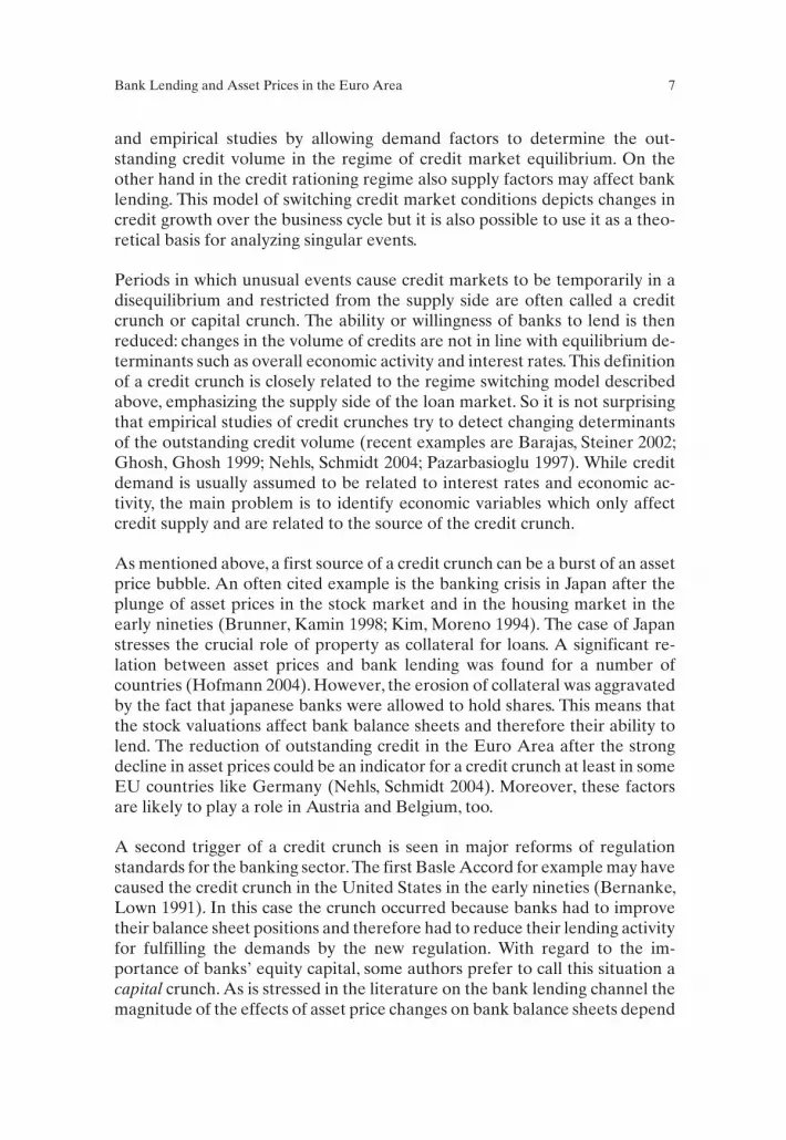
(1) k y it t t t= + ⋅ + ⋅ +ω α β ε

where kt is the log of the credit volume, yt the log of GDP, i t the long-term in-terest rate and ε t is an error term.

The estimation results for eq. 1 are shown in Table 1. All estimated coefficientsα for the impact of output on credit volume are significant and have the ex-pected sign. For most countries the size of α covers the range between 0.427(Finland) and 1.850 (Spain). For Portugal and Greece the elasticity of thecredit volume with respect to the output are higher and exceed 3.246 and4.320. All coefficients for the influence of the output, however, are in line withtheory, i.e. they have a significantly positive sign, and they are close to theresults of other empirical studies2.

Regarding the influence of interest rates the results are less convincing. Thecoefficients show the expected negative sign in 8 out of 11 cases, only four ofthem being significant. For three countries (France, Portugal and Spain) thecoefficient is positive, in the cases of Portugal and France even significant. This


Estimation of long-term credit equations

ω α βAustria –0.027

(0.163)1.090***(0.103)

–0.029***(0.010)

Belgium 5.137***(1.335)

0.570***(0.117)

–0.021*(0.012)

Finland 5.698***(0.951)

0.427***(0.088)

–0.001(0.010)

France 2.558**(1.119)

0.812***(0.085)

0.028***(0.009)

Germany –11.564***(2.113)

1.434***(0.158)

–0.047***(0.011)

Greece, from 1998:3 –31.932***(2.510)

4.320***(0.238)

–0.032**(0.015)

Ireland, from 1997:1 –5.279***(0.471)

1.654***(0.042)

–2.31E-05(0.014)

Italy, from 1998:2 –10.250***(0.484)

1.850***(0.038)

–0.001(0.005)

Netherland 0.826(0.741)

0.964***(0.060)

–0.009(0.011)

Portugal, from 1995:1 –22.703***(0.550)

3.246***(0.052)

0.015***(0.004)

Spain –1.949***(0.579)

1.781***(0.047)

0.004(0.004)

Significance is given in parentheses.Asterisks refer to level of significance:***:1 per cent,**:5 percent, *: 10 per cent.

Table 1

2 For instance Calza et al. (2003) find a coefficient for the whole Euro area of 1.457 for GDP,Bundesbank (2003) find for Germany, depending on the type of loans, between 1.14 and 1.67.Hofmann (2004) finds for various European countries values between 1.269 and 2.169.

observation, however, may be explained by the steadily declining real andnominal interest rates in the Euro area prior to and following the launch ofEMU and is in line with other recent studies (for instance Calza et al., 2003).We have also tried other specifications of the long term credit equation, in-cluding real variables and GMM estimators with various sets of instrumentvariables3. However, as the results do not substantially change, we rely on theOLS estimation as given in Table 1.

5. Analysis of Deviations from the Long-Term Credit Demand

Assuming that the credit equations from section 4 form a long run equi-librium, one may model the short term dynamic as an error correction model(ECM):

(2) [ ]∆ ∆k a b k y i c k ut t t t t t= + ⋅ − + ⋅ + ⋅ + ⋅ +− − − −1 1 1 1( )ω α β

= + ⋅ + ⋅ +− −a b c k ut t tε 1 1∆

where a,b and c are real numbers,and t is the residual from eq.1, that is the de-viation of credit volume from the long run equation. Furthermore, to takesome autocorrelation in the error terms into account, we add the laggedchange in credit volume ∆kt−1 to the equation. While it is common to assumethat the error correction coefficient b is always present and constant over time,we use a Markov switching error correction model (MS-ECM)4, in which thepresence or the speed of adjustment may differ depending on theunobservable regime s t . This state variable s t may take the values 1 and 2,therefore equation (2) emerges to:

(3) ∆∆∆k

a b c k u s

a b c kt

t t t t

t t

=+ ⋅ + ⋅ + =+ ⋅ + ⋅

− −

− −

1 1 1 1 1

2 2 1 2 1

1εε

,

+ =⎧⎨⎩ u st t, 2

where the state variable st follows a first order Markov process, characterizedby the transition probabilities:

(4)

p P s s

p P s s

q P s s

t t

t t

t t

= = =− = = =

= = =

−

−

−

( | )

( | )

( | )

1 1

1 1 2

2 2

1

1

1

1 2 11− = = =−q P s st t( | )

We refer to this model as the basic model. The specification of eq. (3) and (4)provides much flexibility to the estimation: As we do not place any prior as-


3 The estimation results are available from the authors on request.4 This model has been – for instance – applied for estimating bubbles in British house prices(Hall,Psaradakis,Sola 1997), for exchange rates in the European Monetary System (Bessec 2002).

sumption on the adjustment process to the long run equation, it may bepresent or not, or simply differ in speed between the states. Even regarding thenumber of regime switches we do not need the prerequisite that there is morethan one switch. The model is flexible enough to deal with a permanentchange5.


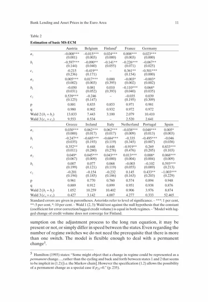
Estimation of basic MS-ECM

Austria Belgium Finland1 France Germany

a1 –0.008***(0.001)

–0.015***(0.003)

0.024***(0.000)

0.008***(0.003)

0.023***(0.000)

b1 –0.597***(0.144)

–0.090**(0.040)

–0.141**(0.055)

–0.226***(0.071)

–0.067**(0.025)

c1 -0.215(0.236)

–0.419**(0.171)

– 0.361**(0.154)

–0.501***(0.000)

a2 0.005***(0.002)

0.017***(0.003)

0.000(0.395)

–0.003*(0.002)

–0.003*(0.002)

b2 –0.050(0.031)

0.081(0.052)

0.010(0.393)

–0.110***(0.040)

0.068*(0.035)

c2 0.539***(0.125)

–0.246(0.147)

– –0.035(0.195)

0.039(0.309)

p 0.881 0.835 0.853 0.971 0.981q 0.980 0.902 0.932 0.972 0.972Wald 2 ( )b b1 2= 13.833 7.443 3.100 2.079 10.410Wald 3 ( )c c1 2= 9.553 0.534 – 2.520 2.641

Greece Ireland Italy Netherland Portugal Spain

a1 0.030***(0.000)

0.062***(0.017)

0.062***(0.017)

–0.038***(0.009)

0.048***(0.013)

0.005*(0.003)

b1 –0.247**(0.035)

–0.685***(0.193)

–0.684***(0.119)

–0.335(0.345)

–0.495***(0.007)

–0.046(0.038)

c1 0.352**(0.011)

0.448(0.280)

0.448(0.278)

–0.919**(0.476)

0.269(0.205)

0.833***(0.103)

a2 0.049*(0.067)

0.045***(0.009)

0.043***(0.000)

0.013***(0.004)

0.008*(0.004)

0.068***(0.009)

b2 0.007(0.199)

0.077(0.121)

0.068(0.119)

–0.003(0.055)

–0.102(0.089)

0.593***(0.213)

c2 –0.201(0.194)

–0.154(0.185)

–0.232(0.186)

0.145(0.163)

0.433**(0.203)

–1.003***(0.229)

p 0.961 0.770 0.760 0.574 0.894 0.948q 0.889 0.912 0.899 0.951 0.938 0.876Wald 2 ( )b b1 2= 1.052 10.259 10.402 0.906 3.976 8.874Wald 3 ( )c c1 2= 0.427 3.142 4.007 4.277 0.333 52.465

Standard errors are given in parentheses. Asterisks refer to level of significance. – ***: 1 per cent,**: 5 per cent, *: 10 per cent. – Wald 1 (2, 3): Wald test against the null hypothesis that the constant(coefficient for error correction/lagged credit volume) is equal in both regimes. – 1Model with lag-ged change of credit volume does not converge for Finland.

Table 2

5 Hamilton (1993) states: “Some might object that a change in regime could be represented as apermanent change…, rather than the cycling and back and forth between states 1 and 2 that seemsto be implicit in (1.2) [i.e. the Markov chain]. However the specification (1.2) allows the possibilityof a permanent change as a special case if p21=0.” (p. 235).

Estimation results of eq. (3) and (4) are presented in Table 2. In the estimationthe error correction coefficient b1 respectively b2 is of main interest. Mostcountries show one regime which is stabilizing, that is b1 (we regard to the sta-bilizing regime as regime 1 without any loss of generality) is significantlysmaller than zero. The only exceptions are the Netherlands and Spain, forwhich b1 is negative without being significant. The results, however, differ forb2 : For France it is significantly negative, too, indicating that both regimes arecharacterized by an adjustment to the equilibrium, with different speeds. ForSpain and Germany b2 takes a significantly positive value, whereas for the ma-jority of countries b2 does not significantly differ from zero at all. It istherefore informative to look at standard Wald tests against the null of b b1 2= .The results are given in the rows at the bottom of Table 2. Indeed, for allcountries but France we find significantly different values of b1 and b2 in bothregimes. Summing up so far, there is evidence that most countries of the Euroarea, France being the only exception, show a stable regime with mean re-version to the long-term credit equation and an unstable regime, which is at itsbest inconclusive. The differences between b1 and b2 are for these countriesstatistically significant.

It is now straightforward to introduce additional explanatory variables. Therationale is that the credit volume may react in different ways to other factorsdepending from whether we are in the stable (mean reversion to the long termrelationship) or in the unstable regime (no tendency to return). Therefore weextend equation (3) to equation (5)

(5) ∆∆Β ∆

ka b c C d shares e k u s

at

t t t t t t=+ ⋅ + ⋅ + ⋅ + ⋅ + =− −1 1 1 1 1 1 1ε ,

+ ⋅ + ⋅ + ⋅ + ⋅ + =⎧⎨⎩ − −b c C d shares e k u st t t t t t2 1 2 2 2 1 2ε ∆Β ∆ ,

which additionally takes into account the availability of banks’ capital and theinfluence of asset prices, representing the bank lending and the balance sheetchannel of transmission. Whilst the variable ∆BC is defined as the change inlogs of the bank capital, the variable shares measures the deviation of the re-spective national stock index from its long term trend6. This reflects ongoingunder- or overvaluation of companies, which may perpetually prevent banksfrom expanding their credit offers to companies.

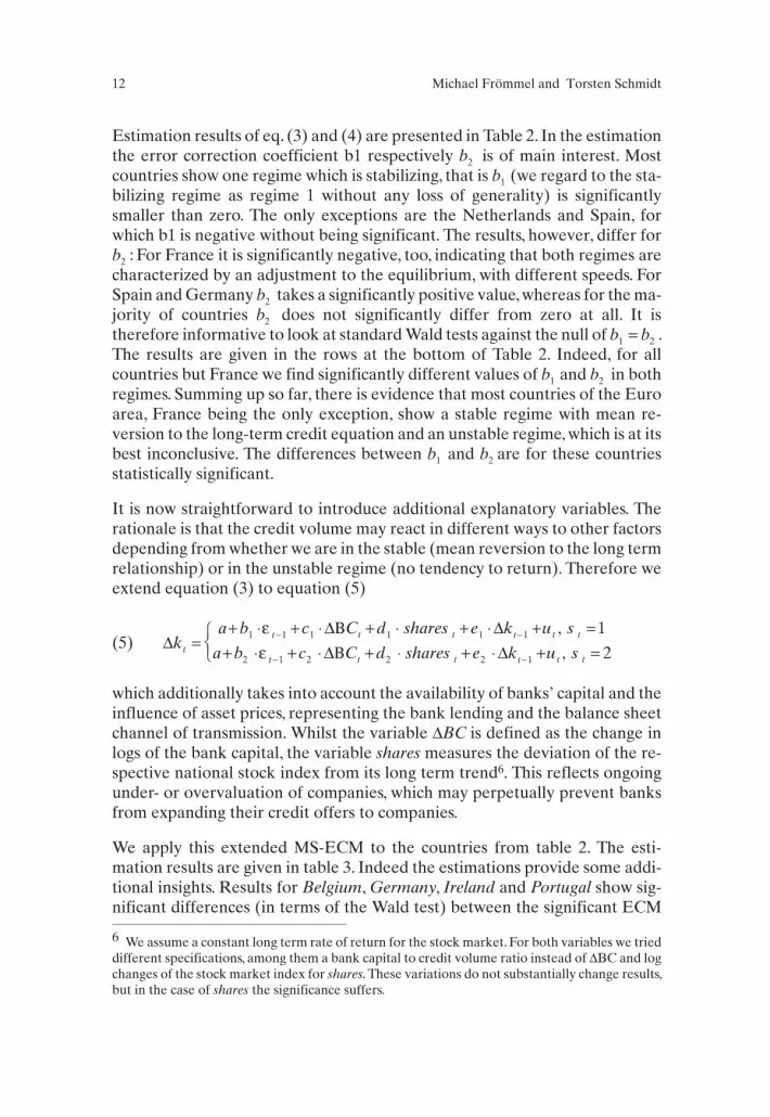
We apply this extended MS-ECM to the countries from table 2. The esti-mation results are given in table 3. Indeed the estimations provide some addi-tional insights. Results for Belgium, Germany, Ireland and Portugal show sig-nificant differences (in terms of the Wald test) between the significant ECM


6 We assume a constant long term rate of return for the stock market. For both variables we trieddifferent specifications, among them a bank capital to credit volume ratio instead of ∆BC and logchanges of the stock market index for shares. These variations do not substantially change results,but in the case of shares the significance suffers.


Estimation of the extended MS-ECM

Austria Belgium Finland France GermanyRegime 1:const. 0.005***

(0.002)0.009***(0.002)

0.015***(0.003)

0.001(0.002)

0.023***(0.001)

b1 (ECM) –0.032(0.031)

0.042(0.041)

0.032(0.047)

–0.237**(0.099)

0.331***(0.108)

c1 (∆BC) 0.079(0.057)

0.034*(0.017)

0.311(0.452)

0.462(0.299)

0.406(0.256)

d1 (Shares) 0.013(0.011)

0.069***(0.011)

0.051***(0.014)

0.016(0.013)

0.067***(0.017)

e1 (∆Kt-1) 0.437***(0.129)

–0.356**(0.154)

0.215(0.233)

–0.062*(0.033)

–2.120(1.706)

Regime 2:const. 0.005***

(0.002)0.009***(0.002)

0.015***(0.003)

0.001(0.002)

0.023***(0.001)

b2 (ECM) –1.111(1.496)

–0.329***(0.052)

-0.083(0.091)

–0.103***(0.034)

–0.188***(0.039)

c2 (∆BC) –0.648(2.168)

0.017(0.021)

–0.076**(0.029)

–0.042(0.057)

–0.340***(0.011)

d2 (Shares) –0.297(0.311)

0.014(0.010)

–0.007(0.005)

0.036***(0.011)

0.017***(0.005)

e2 (∆Kt-1) 0.275(1.037)

–0.324**(0.012)

0.156(0.149)

–0.029(0.233)

–0.260*(0.132)

p 0.980 0.805 0.974 0.952 0.961q 0.870 0.768 0.974 0.976 0.982Wald 2 ( )b b1 2= 0.520 32.668*** 1.143 1.564 19.003***Wald 3 ( )c c1 2= 0.112 0.427 0.728 2.937 6.605**Wald 3 ( )d d1 2= 0.994 15.055*** 14.257*** 1.172 8.683***Wald 3 ( )e e1 2= 0.024 0.029 0.045 0.018 1.196

Greece Irland Italien Netherland Portugal SpainRegime 1:const. 0.041***

(0.000)0.046***(0.008)

–0.001***(0.000)

0.010**(0.004)

0.022***(0.004)

0.023***(0.003)

b1 (ECM) –0.297**(0.038)

0.084(0.126)

–0.018(0.437)

–0.374**(0.170)

–0.660**(0.304)

0.045(0.185)

c1 (∆BC) – – –0.042(0.459)

0.004(0.107)

0.249*(0.145)

0.019(0.033)

d1 (Shares) 0.008(0.241)

0.017(0.017)

–0.067(1.257)

0.019(0.016)

0.011(0.019)

0.002(0.013)

e1 (∆Kt-1) 0.321***(0.000)

–0.223(0.222)

–0.001(0.485)

0.031(0.178)

–0.158(0.260)

0.354***(0.119)

Regime 2:const. 0.041***

(0.000)0.046***(0.008)

–0.001***(0.000)

0.010**(0.004)

0.022***(0.004)

0.023***(0.000)

b2 (ECM) –0.170***(0.003)

–0.578***(0.155)

–0.005(0.011)

–0.305**(0.135)

–0.001(0.066)

–0.163***(0.042)

c2 (∆BC) – – 0.011(0.008)

–0.047(0.105)

0.045(0.049)

–0.085***(0.025)

d2 (Shares) –0.006**(0.046)

0.083***(0.030)

–0.001*(0.000)

0.066***(0.021)

0.051***(0.009)

0.048***(0.008)

e2 (∆Kt-1) –0.097(0.180)

0.245(0.177)

1.045***(0.018)

0.086(0.195)

0.314**(0.128)

–0.219(0.140)

p 0.631 0.853 0.915 0.968 0.517 0.971q 0.783 0.722 0.999 0.962 0.903 0.978Wald 2 ( )b b1 2= 0.740 10.646*** 0.001 0.107 4.280** 1.172Wald 3 ( )c c1 2= – – 0.013 0.130 1.880 6.216**Wald 3 ( )d d1 2= 2.632* 2.970* 0.003 4.036** 3.356* 8.612***Wald 3 ( )e e1 2= 52.603*** 3.961** 4.647** 0.050 3.359* 18.243***

Standard errors given in parentheses. Asterisks refer to level of significance. – ***: 1 per cent,**: 5 per cent, *: 10 per cent.

Table 3

coefficient b1 of the stable regime and the respective coefficient b2 of the un-stable regime. Furthermore, for these countries there are significant dif-ferences in the influence of the stock market development between theregimes. For Belgium, Germany and Portugal there is a clear pattern: Duringunstable periods there is a strong positive influence of stock marketmovements on the credit volume. This means that deviations from thelong-term development of the credit volume go ahead with movements in thestock market: the credit volume tends to decline (increase) when shares pricesare below (above) average. During the stable regime, however, a similar be-havior for banks’ capital seems not to exist, except for Germany. In contrast tothese three countries (i.e. Belgium, Germany and Portugal) we find a relationin the opposite direction for Ireland: here the positive relation is in the stableregime, meaning that an increase in stock prices brings the credit volumecloser to the long term trend.

For Austria, Finland, Italy and Spain the results remain inconclusive. Althoughthere are different degrees of stability between the regimes, most coefficientsare not statistically significant and the Wald tests do not indicate significantdifferences between regimes.

France, Greece and the Netherlands finally, show two stable regimes with sig-nificantly negative ECM coefficients. The two regimes only differ in the speedof adjustment. However, France and the Netherlands show a higher influenceof shares prices in the unstable than in the stable regime (significantly dif-ferent only for the Netherlands). We interpret this as a slightly dampeningeffect of the stock market on the credit growth.

Summing up so far, we find evidence for the existence of a stable (tendency toreturn to the credit demand equation) and an unstable (no tendency to return)regime for Belgium, Germany, Ireland and Portugal. Except for Ireland themovement away from the demand equation shoes a positive relation to themovement of the stock market. For Germany we even find some evidence fora relation to the growth bank capital. Furthermore, we even find for Franceand the Netherlands, for which we can find no unstable regime, that the stockmarket development affects the speed of adjustment to the long termequation. For the other countries (Austria, Finland, Greece, Italy and Spain)the evidence is inconclusive.

6. Conclusions

This paper analyses the development of the credit volume in the countries ofthe Euro area. The analysis is based on the construction of a long-term creditdemand equation.The actual credit volume is then compared to this long-termtrend and deviations are analyzed in detail by applying a Markov switching


error corrction model to the deviations. We find for several Europeancountries (Belgium, Germany, Ireland, Portugal and Spain) strong evidencefor switching between a stable, mean reverting regime, and one unstable,bubble-like regime, which does not show a tendency to return to the long-rundemand equation. While France, Greek and the Netherlands show tworegimes with different speeds of adjustments only, the three remainingcountries Austria, Italy and Spain show only weak evidence of regimeswitches.

Furthermore, we find a positive relation between the credit volume and thedevelopment of the stock market in the unstable regime for Belgium,Germany and Portugal, as well as for Finland, France and the Netherlands inthe regime with lower adjustment speed, which is significantly higher than inthe other regime. A significant influence of the banks’ capital, however, is onlyvisible in the case of Germany.

From these results we conclude, that there are constraints, which may tempo-rarily dampen lending of banks to the private sector, and even drive away thecredit volume from the long term demand equation. Whether these con-straints lead to a real lack of credits, or only affect the adjustment speed, seemsto depend on country-specific characteristics. A crucial role is attributed to thedevelopment of stock markets and therefore our analysis is linked to the lit-erature on the credit channel. The results, however, do not clearly indicate,whether the impact of the asset price growth works via the supply side or thedemand side. In contrast, the availability of bank capital seems to play only aminor role in most countries, except of Germany. Our findings even affectmonetary policy, which needs to take into account the development of assetprices when conducting monetary policy, because there seems to be a sub-stantial, and between countries of the Euro area asymmetric effect on thetransmission mechanism.

ReferencesAltunbas, Y., O. Fazylov and Ph. Molyneux (2002), Evidence on the Bank Lending

Channel in Europe. Journal of Banking and Finance 26: 2093–2110.

Angeloni, Ignazio, Anil K. Kashyap, Benoit Mojon and Daniele Terlizzese (2003).Monetary policy transmission in the Euro Area: where do we stand?. Ignazio.Angeloni, Anil K. Kashyap and Benoit Mojon (eds.): Monetary policy transmissionin the Euro Area, Cambridge: Cambridge University Press.

Azariadis, C. and B.D. Smith (1998), Financial intermediation and regime switching inbusiness cycles. American Economic Review 88: 516–536.

Barajas, A. and R. Steiner (2002), Why don’t they lend? Credit Stagnation in LatinAmerica. IMF Staff Papers 49: 156–184.


Bernanke, B.S. (1983), Nonmonetary Effects of the Financial Crisis in the Propagationof the Great Depression. American Economic Review 73: 257–276.

Bernanke, B.S. (1995), The macroeconomics of the Great Depression: A ComparativeApproach. Journal of Money, Credit and Banking, 27, 1–28.

Bernanke, Ben S. and Carla S. Lown (1991). The Credit Crunch. Brookings Papers onEconomic Activity 1991 (2): 205–248.

Bessec, M. (2002), Mean Reversion versus Adjustment to PPP: The Two Regimes ofExchange Rate Dynamics under the EMS, 1979–1998. Economic Modelling 20:141–164.

Bordo, M. and O. Jeanne (2002), Boom-Busts in Asset Prices, Economic Instability andMonetary Policy. NBER Working Paper 8966. NBER, Cambridge, MA.

Borio, C. and Ph. Lowe (2002), Asset Prices, Financial and Monetary Stability: Ex-ploring the Nexus. BIS Working Paper 114. Bank for International Settlements,Basel.

Brunner, A.D. and St.B. Kamin (1998), Bank lending and economic activity in Japan:did “financial factors” contribute to the recent downturn? International Journal ofFinance and Economics 3: 73–89.

Calza, A., Ch. Gartner and J. Soucasaux Meneses e Sousa (2003), Modelling the De-mand for Loans to the Private Sector in the Euro Area. Applied Economics 35:107–117.

Carporale, G. and N. Spagnolo (2003), Asset Prices and Output Growth Volatility: TheEffects of Financial Crisis. Economics Letters 79: 69–74.

Chen, N.-K. (2001), Bank net worth, asset prices and economic activity. Journal of Mon-etary Economics 48: 415–436.

Cordoba, J-C. and M. Ripoll (2004), Credit Cycle Redux. International Economic Re-view 45: 1011–1046.

Davis, E.Ph. and H. Zhu (2004), Bank Lending and Commercial Property Cycles: SomeCross-Country Evidence. BIS Working Paper 150. Bank for International Settle-ments, Basel

De Bondt, G.J. (1999), Banks and monetary transmission in Europe: empirical evi-dence. Banca Nazionale del Lavoro Quarterly review 52: 149–168.

Detken, C. and F. Smets (2004), Asset price booms and monetary policy. ECB Discus-sion Paper 364. European Central Bank, Frankfurt a.M.

Deutsche Bundesbank (ed.) (2002), The Development of Bank Lending to the PrivateSector. Monthly Report 2002 (Oct.): 31–43.

Deutsche Bundesbank (ed.) (2003), German results of euro-area bank lending survey.Monthly Report 2003 (June): 67–76.

Eichengreen, B. and K. Mitchener (2003), The Great Depression as a credit boom gonewrong. BIS Working Paper 137. Bank for International Settlements, Basel.

Engle, R.F. and C. Granger (1987), Cointegration and Error Correction: Representa-tion, Estimation, and Testing. Econometrica 55: 251–276.


Estrella, A. (2004), The cyclical behavior of optimal bank capital, Journal of banking fi-nance 28: 1469–1498.

Friedman, B.M. and K.N. Kuttner (1993), Economic Activity and the Short-term CreditMarkets: An Analysis of Prices and Quantities, Brookings Papers on Economic Ac-tivity, 2, 193–283.

Ghosh, S.R. and A.R. Ghosh (1999), East Asia in the Aftermath: Was there a Crunch?IMF Working Paper 99/38. IMF, Washington, DC.

Hall, St., Z. Psaradakis and M. Sola (1997), Switching Error-Correction Models ofHouse Prices in the United-Kingdom. Economic Modelling 14: 517–527.

Hamilton, J.D. (1993). Estimation, Inference and Forecasting of Time Series Subject toChanges in Regime, in: Handbook of Statistics, Vol. 11, edited by G. S. Maddala, C. R.Rao and H. D. Vinod, Amsterdam: Elsevier, 231-259.

Higgins, M. and C. Osler (1997), Asset Market Hangovers and Economic Growth: TheOECD during 1984–93. Oxford Review of Economic Policy 13: 110–134.

Hofmann, B. (2004), The Determinants of Bank Credit in Industrialized Countries: DoProperty Prices Matter? International finance 7: 203–234.

Jaffee, D. and J.E. Stiglitz (1990), Credit Rationing. In B. Friedman and F. Hahn (eds.),Handbook of Monetary Economics, 2. Amsterdam: North-Holland, 838–888.

Kakes, J. and J.-E. Sturm (2002), Monetary Policy and Bank Lending: Evidence fromGerman Banking Groups. Journal of Banking and Finance 26: 2077–2092.

Kashyap, A.K., J.C. Stein and D.W. Wilcox (1993), Monetary Policy and Credit Condi-tions:Evidence from the Composition of External Finance.American Economic Re-view 83: 78–98.

Kim, S.B. and R. Moreno (1994), Stock Prices and Bank Lending Behavior in Japan.Federal Reserve Bank of San Fransisco Economic Review 1994: 31–42.

Kiyotaki, N. and J. Moore (1997), Credit cycles. Journal of political economy 105:211–248.

Kocherlakota, N.R. (2000), Creating Business Cycles Through Credit Constraints. Fed-eral Reserve Bank of Minneapolis Quarterly Review 24: 2–10.

Nehls, H. and T. Schmidt (2004), Credit Crunch in Germany? Kredit und Kapital 37:479–499.

Pazarbasioglu, C. (1997), A Credit Crunch? Finland in the Aftermath of the BankingCrisis. IMF Staff Papers 44: 315–327.

Stiglitz, J.E. and B.C. Greenwald (2003), Towards a New Paradigm in Monetary Eco-nomics. Cambridge: Cambridge University Press.

Zivot, E. and D.W.K. Andrews (1992), Further Evidence on the great Crash, the OilPrice Shock, and the Unit-Root Hypothesis. Journal of Business and Economic Sta-tistics 10: 251–270.



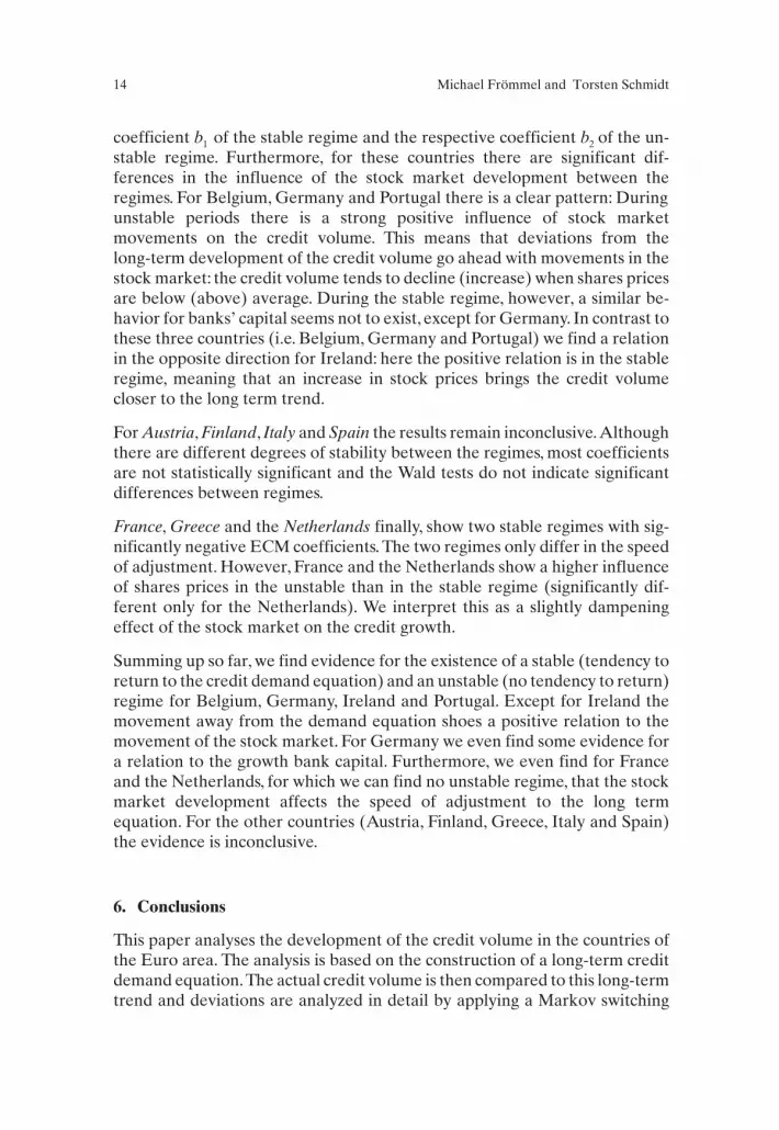
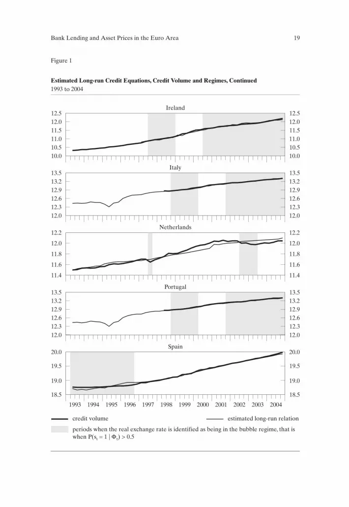
Estimated Long-run Credit Equations, Credit Volume and Regimes1993 to 2004

Austria

Belgium

France

Germany

Greece

credit volume

periods when the real exchange rate is identified as being in the bubble regime, that iswhen P(s = 1 | ) > 0.5t Φτ

estimated long-run relation

12.0

13.2

7.4 7.4

13.2

11.5

12.0 12.0

11.5

12.0

11.7

13.1

7.2 7.2

7.0 7.0

13.1

11.4

11.5 11.5

11.411.3

11.0 11.0

11.3

11.7

11.4

13.0

6.8 6.8

13.0

11.1

10.0 10.0

11.111.2

10.5 10,5

11.2

11.4

11.1

12.9

6.6 6.6

12.9

11.0

9.5 9.5

11.0

11.1

1993 1994 1995 1996 1997 1998 1999 2000 2001 2002 2003 2004

Figure 1


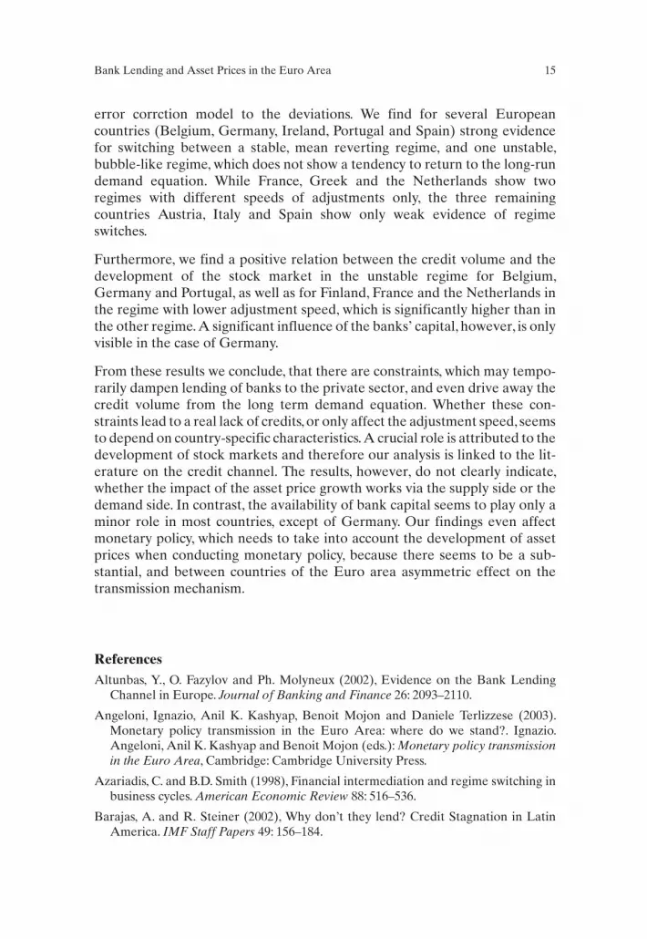
Estimated Long-run Credit Equations, Credit Volume and Regimes, Continued1993 to 2004

Ireland

Italy

Netherlands

Portugal

Spain

credit volume

periods when the real exchange rate is identified as being in the bubble regime, that iswhen P(s = 1 | ) > 0.5t Φτ

estimated long-run relation

12.5 12.5

12.2 12.2

13.5 13.5

13.5 13.5

20.0 20.0

12.0 12.011.5 11.5

12.0 12.0

11.8 11.8

13.2 13.212.9 12.912.6 12.6

13.2 13.212.9 12.9

10.5 10.511.0 11.0

11.6 11.6

12.3 12.3

12.3 12.3

19.0 19.0

12.6 12.6

19.5 19.5

10.0 10.0

11.4 11.4

12.0 12.0

12.0 12.0

18.5 18.5

1993 1994 1995 1996 1997 1998 1999 2000 2001 2002 2003 2004

Figure 1

Unit Root test results for time series used in the empirical analysis


ADF Unit Root tests

GDP Interest Rate Share prices Equity Capital

Level(c,t)

Change(c)

Level(c,t)

Change(c)

Level(c,t)

Change(c)

Level(c,t)

Change(c)

Austria –-2.63 –5.44*** –2.99 –4.57*** –1.20 –6.67*** –1.27 –4.03***Belgium –2.00 –4.38*** –2.89 –4.31*** –1.36 –7.65*** –1.25 –6.66***Finland –2.39 –4.58*** –2.25 –4.31*** –1.04 –6.70*** –1.74 –5.41***France –3.14 –9.45*** –3.37* –4.12*** –1.17 –6.73*** –1.47 –7.71***Germany –3.02 –6.33*** –3.22* –4.44*** –1.43 –6.96*** 0.34 –4.20***Ireland –0.08 –8.87*** –3.10 –4.95*** –1.53 –7.61*** n.a. n.a.Italy –2.00 –4.38*** –2.16 –3.68** –1.58 –6.66*** –3.75** –6.24***Netherland –1.31 –6.49*** –3.29* –4.45*** –1.00 –6.97*** –0.53 –6.07***Portugal n.a. n.a. –2.69 –4.28*** –1.46 –6.39*** –1.01 –4.53***Spain –5.30*** –7.05*** –2.85 –3.44** –1.36 –7.14*** –2.15 –6.81***

Lag selection by SIC. Lag length are not reported. – ***, **, * indicates significance at the 1, 5 and10 percent level using Mac Kinnon (1996) one-sided p-values. – c, t: a constant and a trend is in-cluded. – c: only a constant is included.

Table 4

ADF Unit Root Tests for Credits

Sample Level (c,t) Change (c)

Austria 93:1 – 04:4 1.26 –4.58***Belgium 93:1 – 04:4 0.03 –3.14**Finland 93:1 – 04:4 –2.13 –4.81***France 93:2 – 04:2 –2.55 –2.29*Germany 93:1 – 04:4 0.74 0.48Ireland 93:1 – 04:4 –2.13 –2.99**Italy 98:2 – 04:4 –0.89 –3.86***Netherlands 93:1 – 04:4 –0.95 –5.97***Portugal 93:1 – 04:4 –3.65** –2.43Spain 93:1 – 04:4 –4.92*** –3.46**

Table 5

Zivot Andrews Unit Root test for series with unknown break points for German creditModell A

stat. Break point–5.0985*** 2001:3

The ZA-test is performed using the GAUSS code provided by Junsoo Lee.Zivot Andrews (1992).

bank lending and asset prices in the euro area

Documents