Bank Capital, Borrower Power, and Loan Rates

Abstract

We test the predictions of several recent theories of how bank capital affects the rates

that banks charge their borrowers. Key to all these theories is the notion that the relative

bargaining power of a bank and its borrower are critical. We find that banks with low

capital are more sensitive to borrower cash flow than are banks with high capital: low-

capital banks charge relatively more for borrowers with low cash flow, but offer relatively

steeper discounts for borrowers with high cash flow. These effects are robust to controls

for business conditions and bank fixed effects. Our results suggest that low bank capital

generally toughens bank bargaining power, especially vis-a-vis low-cash-flow borrowers, but

weakens bank bargaining power vis-a-vis high-cash-flow borrowers. This is consistent with

Diamond and Rajan’s (2000) theory of bank capital. By contrast, although earlier work

has found that rates for borrowers with access to public debt markets are unaffected by

their bank’s capital level, once we control for economic conditions, lower bank capital leads

to higher spreads for these borrowers as well.

1

1 Introduction

The link between bank capital levels and lending behavior is critically important to policy

makers seeking to oversee the health of the banking system and its impact on the wider

economy. It is widely thought that, both in the early 1990s and in the subprime mortgage

crisis that began in 2007, low bank capital levels caused by large credit losses led to significant

cutbacks in bank lending—so-called “credit crunches”. A better understanding of this link can

help policy makers make better decisions for bank regulation and intervention.

Several recent theories suggest that a bank’s level of equity capital should affect the

bank’s lending behavior. Boot, Greenbaum, and Thakor (1993) predict that banks with low

capital are more likely to exploit borrowers, sacrificing reputational capital in order to preserve

financial capital. Combining this with the theories of Sharpe (1990) and Rajan (1992) on bank

information monopoly, this predicts that banks with low capital should charge higher rates

to borrowers that are more bank-dependent. By contrast, Diamond and Rajan (2000) predict

that banks with low capital are very focused on obtaining cash flow quickly; thus, compared to

banks with high capital, they may charge more to borrowers with low cash flow, but give big

discounts to borrowers with high cash flow. In this paper, we test these different theories on

a sample of loans to publicly-traded U.S. borrowers from 1987 to 2007. We find evidence that

supports Diamond and Rajan’s theory, but the evidence for Boot, Greenbaum, and Thakor

(1993) differs from previous findings.

Overall, we find a significantly negative relationship between a bank’s capital level and

the loan spread over LIBOR. This result is robust to the inclusion of firm-, loan-, and bank-

specific controls, and is potentially consistent with either theory. The size is economically

significant: when all controls are included, the impact of a 1% decrease in a bank’s capital/asset

ratio is a roughly 3 basis points increase in loan spread. Moreover, borrower cash flow has a

negative impact on lending rate, which one would expect since, all else equal, higher cash flow

should reduce credit risk.

We then conduct tests of Diamond and Rajan (2000). We find that although a bank’s

capital still has a negative impact on the spread it charges, the interaction of borrower cash

flow and bank capital level has a positive impact that can offset this. In other words, low-

capital banks give bigger discounts for higher cash flow than high-capital banks do, to the

extent that, if cash flow is sufficiently high, they charge lower all-in spreads than high-capital

2

banks. These results are robust to the inclusion of year dummies, a proxy for market credit

spreads, and the interaction of the credit spread proxy and borrower cash flow, so they do

not seem to be picking up business cycle effects that are independently correlated with bank

capital levels and with the link between borrower cash flow and lending spreads. Thus, our

findings are consistent with Diamond and Rajan’s predictions.

Turning to Boot, Greenbaum, and Thakor (1993), Sharpe (1990), and Rajan (1992),

we examine the links between bank capital, borrower bank-dependence, and loan spreads.

Consistent with earlier work, we find that banks with low capital charge higher spreads, but

this effect is concentrated on borrowers that are more likely to be bank-dependent; those with

access to public debt markets experience no net impact from their lending bank’s capital level.

However, once we include year dummies, the market credit spread, and the market credit

spread’s interaction with borrower market access, bank capital has an even more negative

impact on loan spreads, while the interaction between public debt market access and capital

loses significance and magnitude. In other words, once we correct for business cycle effects,

bank capital seems to matter for all borrowers, whether or not they have access to public debt

markets. These findings suggest that even firms with access to public debt markets may be

more bank-dependent than previous work suggests.

The upshot is that a bank’s capital level has a significant impact on the rates its

borrowers pay, even for our sample of borrowers with publicly-traded equity. Low capital

generally increases the rates a bank charges, but low-capital banks give significant discounts

to borrowers with high cash flow, consistent with Diamond and Rajan (2000). There is some

evidence that borrowers with access to public debt markets have less of an impact from their

bank’s capital level, but much of this lower impact is due to business cycle effects. Finally,

our results are robust to a number of considerations: including bank fixed effects, using bank

z-score instead of capital so as to take both bank risk and capital into account, controlling for

the endogeneity of public debt market access, and clustering errors both by firm and by bank.

Our work is related to two recent empirical papers on the importance of bank capital

for loan pricing. Hubbard, Kuttner, and Palia (2002) examine the pricing of U.S. bank loans

to publicly-traded firms during the period 1987 to 1992. They hypothesize that banks with low

capital will charge higher rates, but only for borrowers with high switching costs. Using various

proxies for borrower switching costs (largely based on Sharpe (1990) and Rajan (1992)), their

3

findings support this hypothesis. Steffen and Wahrenburg (2008) test a similar hypothesis

on a sample of U.K. loans to both public and private borrowers during the period 1996 to

2005. Like Hubbard, Kuttner, and Palia (2002), they find that banks with low capital charge

higher rates to borrowers with higher switching costs, but they find that this effect is limited to

economic downturns. They argue that this is consistent with banks needing financial capital

more in downturns, thus leading them to consume reputational capital by charging higher

spreads during these periods.1

Our paper differs from these earlier works in several important respects. First, our

sample is more recent than Hubbard, Kuttner, and Palia (2002) and in the U.S. rather than

the U.K, unlike Steffen and Wahrenburg (2008). Second, rather than relying on a dummy

variable for whether bank capital is low or not, we generally use the level of capital itself,

giving our tests more power. Third, we find that capital matters for all borrowers, once we

control for business conditions. Fourth, and most important, we assess several hypotheses

linked to the predictions of Diamond and Rajan (2000).

Our analysis of bank-dependent borrowers is also related to a recent literature which

attempts to investigate the importance of banks’ informational advantage vis-a-vis their bor-

rowers. Santos and Winton (2008) find that, controlling for risk, borrowers without public

debt market access pay higher rates than borrowers with such access, and this difference in-

creases during recessions, when banks are likely to have greater information monopoly rents

from bank-dependent borrowers. Schenone (2008) finds that borrowers pay higher rates before

their equity IPO than after their IPO; she argues that this effect is linked to bank informa-

tion monopolies. Similarly, Hale and Santos (2008) find that borrowers pay lower loan rates

after they undertake their bond IPO; they argue that this decline reflects a reduction in bank

information monopolies. In contrast to this literature, which focuses solely on the impact of

borrowers’ public market access on bank bargaining power, our paper also investigates how

bargaining power varies across banks depending on their capital level.

The rest of the paper is structured as follows. Section 2 discusses the relevant theories

and set out our empirical hypotheses. Section 3 discusses out data and empirical methodology.

Section 4 contains our main results, and section 5 discusses some robustness tests. Section 6

concludes our paper.

1We discuss both papers’ methodology in more detail in the next section.

4

2 Empirical Hypotheses

In assessing the impact of a bank’s capital level on its lending decisions, our first source of

predictions is Diamond and Rajan (2000). They model how a bank’s loan refinancing rate

varies with the bank’s capital level and the borrower’s cash flow situation. Compared to a

bank that has adequate capital relative to assets, a bank that has low capital may extract

more rents from borrowers whose cash position is relatively weak and will extract fewer rents

from borrowers whose cash position is relatively strong. The intuition is that a bank with low

capital is desperate to get cash to shore up its liquidity position vis-a-vis depositors and other

debt holders. If the borrower’s cash flow is also somewhat weak, the bank has a credible threat

to liquidate the borrower to get cash; this makes the borrower willing to pay more to avoid

liquidation. For borrowers with strong cash flows, however, the bank’s bargaining position is

weak; knowing the bank needs cash now, the borrower can extract weaker lending terms in

return for paying debts earlier. This leads to the following hypothesis.

Hypothesis 1: compared to adequately capitalized banks, banks with lower capital

charge higher rates for refinancing borrowers with weak cash flow and lower rates for borrowers

with strong cash flow.

Tests of Hypothesis 1 are subject to a possible critique, however: the correlation be-

tween bank capital levels and lending rates may be driven by some third variable that affects

both independently. For example, it may be the case that a borrower’s cash flow is more

important for loan pricing in recessions, when such cash is most useful in warding off default.

Also, banks suffer higher credit losses in recessions, reducing their capital. This would suggest

that, in recessions, bank lending rates are likely to be more strongly decreasing in borrower

cash flow, and bank capital levels are more likely to be low, leading to the correlation predicted

by Hypothesis 1. To test for this possibility, we need to control for the state of the economy.

Hypothesis 2: controlling for the state of the economy and its effect on the importance

of borrower cash flow for loan pricing, there is no link between bank capital level, borrower

cash flow, and refinancing rates for firms.

Another set of hypotheses arises from the literature on bank reputation and lend-

ing incentives. Boot, Greenbaum, and Thakor (1993) predict that banks with low financial

capital may sacrifice reputational capital by reneging on implicit guarantees. One such im-

plicit guarantee is the commitment to not exploit monopoly power over borrowers. Following

5

Sharpe (1990) and Rajan (1992), in a single-period setting, banks can extract rents from

bank-dependent borrowers through an informational hold-up mechanism: would-be competi-

tor banks face a Winner’s Curse in trying to win the business of these borrowers, and so they

bid less aggressively, allowing the incumbent bank to extract rents on average. Such rents are

increasing in the borrower’s risk of default. As noted by Santos and Winton (2008), this implies

that the Winner’s Curse should be greater in recessions; consistent with this, they find that

the relative spreads charged to firms that do not have access to public bond markets increase

in recessions, even after controlling for measures of borrower risk. In a multiperiod setting,

however, banks’ reputation concerns may offset their incentive to exploit such rents.

Combining Boot et al. (1993) with the theories of bank rent extraction just mentioned,

it follows that banks with lower financial capital should be more likely to sacrifice reputation

in order to save or augment their capital. This leads to our next hypothesis.

Hypothesis 3: banks with lower capital charge higher lending rates for refinancing

bank-dependent borrowers than do banks with adequate capital. For borrowers that are not

bank-dependent, bank capital level has no impact on lending rates.

Although they do not lay out a theoretical justification or set of predictions, Hubbard,

Kuttner, and Palia (2002) find results consistent with Hypothesis 3. In a sample of public U.S.

firms from 1987 to 1992, banks with capital/assets of less than 5.5% charge higher rates for

borrowers that are more likely to be bank-dependent (firms that have no debt rating, are in the

smallest tercile of Compustat firms by sales or market capitalization, or borrow at spreads over

the prime rate). By contrast, low-capital banks do not charge significantly different rates for

borrowers that are less likely to be bank-dependent. As discussed in the next section, our tests

differ from Hubbard, Kuttner, and Palia’s (2002) in that we examine the continuous impact of

capital rather than the impact of capital below a set cut-off.

Steffen and Wahrenburg (2008) outline Hypothesis 3 more clearly. Using a sample of

public and private U.K. firms from 1995-2005, they find that banks with weak Tier-1 capital

(less than 6.3% of assets) only charge higher rates to bank-dependent firms in recessions,

precisely when potential rents and incentives to conserve financial capital are likely to be

higher. Their tests differ from ours in that they use a dummy variable for low bank capital,

run separate regressions for bank-dependent and non-bank-dependent firms, and run separate

regressions for loans issued in expansions and loans issued in recessions.

6

Tests of Hypothesis 3 are subject to the same critique we mentioned above with regards

to the tests of Hypothesis 1: in a recession, bank capital levels tend to be lower, and bank-

dependent firms may be relatively riskier in ways that our controls do not fully capture, leading

to a spurious correlation between bank capital and bank-dependence. If controlling for the

state of the economy wipes out bank capital effects, this would argue for spurious correlation

opposed to the information rent/reputation model. We have

Hypothesis 4: controlling for the state of the economy, there is no link between bank

capital level, borrower bank-dependence, and the refinancing rates for firms.

In the next section, we describe the data we use and the methodology we adopt to test

these hypotheses.

3 Data, methodology and sample characterization

3.1 Data

The data for this project come from several data sources, including the Loan Pricing Cor-

poration’s Dealscan database (LPC), the Securities Data Corporation’s Domestic New Bond

Issuances database (SDC), the Center for Research on Securities Prices’s stock prices database

(CRSP), the Salomon Brother’s bond yields indices, Compustat, and from the Federal Re-

serve’s Bank Call Reports.

We use LPC’s Dealscan database of business loans to identify the firms that borrowed

from banks and when they did so. Most but not all of the loans in this database are syndicated.

It goes as far back as the beginning of the 1980s. In the first part of that decade the database

has a somewhat reduced number of entries but its comprehensiveness has increased steadily

over time. It is for this reason that we begin our sample in 1987. Our sample ends in June 2007.

We also use the Dealscan database to obtain information on: individual loans, including the

loan’s spread over Libor, maturity, seniority status, purpose and type; the borrower, including

its sector of activity, and its legal status (private or public firm); and finally, the lending

syndicate, including the identity and role of the banks in the loan syndicate.

We rely on SDC’s Domestic New Bond Issuances database to identify which firms in

our sample issued bonds prior to borrowing in the syndicated loan market. This database

contains information on the bonds issued in the United States by American nonfinancial firms

7

since 1970. We also rely on this database to identify some features of the bonds issued by the

firms in our sample, including their issuance date, their credit rating, and whether they were

publicly placed.

We use Compustat to get information on firms’ balance sheets. Even though LPC

contains loans from both privately-held firms and publicly-listed firms, given that Compustat

is dominated by publicly-held firms, we have to exclude loans to privately-held firms from our

sample.

We rely on the CRSP database to link companies and subsidiaries that are part of the

same firm, and to link companies over time that went through mergers, acquisitions or name

changes.2 We then use these links to merge the LPC, SDC and Compustat databases in order

to find out the financial condition of the firm at the time it borrowed from banks and if by

that date the firm had already issued bonds. We also use CRSP to determine our measure of

stock price volatility.

We use the Salomon Brother’s yield indices on new long-term industrial bonds to

control for changes in the cost of accessing the bond market. We consider the indices on yields

of triple-A and triple-B rated bonds because these go further back in time than the indices on

the investment-grade and below-grade bonds.

Finally, we use the Reports of Condition and Income compiled by the FDIC, the

Comptroller of the Currency, and the Federal Reserve System to obtain bank data, includ-

ing the bank’s capital-to-asset ratio, its size, profitability and risk, for the lead bank(s) in each

loan syndicate. Wherever possible we get bank data at the level of its bank holding company

using Y9C reports. If these reports are not available (because it is a stand-alone bank or a

small bank holding company) then we rely on Call Reports which have data at the bank level.

2The process we used to link LPC, SDC, and Compustat can be summarized as follows. The CRSP data

was first used to obtain CUSIPs for the companies in LPC where this information was missing through a name-

matching procedure. With a CUSIP, LPC could then be linked to both SDC and Compustat, which are CUSIP

based datasets. We proceed by using the PERMCO variable from CRSP to group companies across CUSIP,

since that variable tracks the same company across CUSIPs and ticker changes. We adopted a conservative

criteria and dropped companies that could not be reasonably linked.

8

3.2 Methodology

In order to test our hypotheses, we need to determine the impact of bank capital on loan

spreads, controlling for various borrowing firm, lending bank, and loan-specific characteristics.

We begin with the predictions that derive from Diamond and Rajan (2000). For Hypothesis

1, our basic model of loan credit spreads is as follows:

LOANSPREADf,l,b,t = c+ ζ · CAPITALb,t + δ · CASHFLOWf,t (1)

+ η · CAPITALb,t · CASHFLOWf,t

+I∑

i=1

ψiXi,l,t +J∑

j=1

νjYj,f,t +K∑

k=1

βk,tZk,b,t + εf,t. (2)

Here LOANSPREADf,l,b,t is the spread over Libor of loan l of firm f from bank b

at issue date t. According to Dealscan, our source of loan data, the all-in-drawn spread is

a measure of the overall cost of the loan, expressed as a spread over the benchmark London

interbank offering rate (LIBOR), because it takes into account both one-time and recurring fees

associated with the loan. CAPITALb,t is the ratio of bank b’s equity capital to total assets.

CASHFLOWf,t is one of several measures of firm f ’s cash flow, as described below. The Xi,l,t

represent loan-specific variables and the Yj,f,t represent various firm-specific variables, both

of which might be expected to affect the loan’s credit risk, and the Zk,b,t represent various

bank-specific variables which might affect the rate at which the bank is willing to lend.

Hypothesis 1 asserts that ζ is negative (lower-capital banks charge strictly higher rates

to low-cash-flow borrowers than higher-capital banks do), but η is positive (lower-capital banks

charge lower rates for high-cash-flow borrowers than higher-capital banks do). Although Dia-

mond and Rajan (2000) predict no relationship between borrower cash flow and lending rate

for high-capital banks, their model assumes a very simple structure. In a more continuous

model, higher cash flow means a lower probability of default, all else equal, and so we would

expect that δ is negative.

For Hypothesis 2, we return to Equation (1) and include controls for business con-

ditions. We examine whether inclusion of year dummies and a credit spread proxy (BBB-

AAA Y IELD, the spread between BBB and AAA bond yields) alters our results. We also

include the interaction between the BBB-AAA spread and the borrower’s cash flow to capture

9

the possibility that cash flow matters more in times when credit spreads are high. If Hypothesis

2 holds, then the impact of capital and of its interaction with cash flow should now be zero.

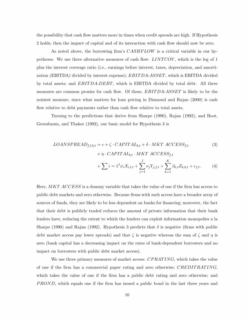
As noted above, the borrowing firm’s CASHFLOW is a critical variable in our hy-

potheses. We use three alternative measures of cash flow: LINTCOV , which is the log of 1

plus the interest coverage ratio (i.e., earnings before interest, taxes, depreciation, and amorti-

zation (EBITDA) divided by interest expense); EBITDA-ASSET , which is EBITDA divided

by total assets; and EBITDA-DEBT , which is EBITDA divided by total debt. All three

measures are common proxies for cash flow. Of these, EBITDA-ASSET is likely to be the

noisiest measure, since what matters for loan pricing in Diamond and Rajan (2000) is cash

flow relative to debt payments rather than cash flow relative to total assets.

Turning to the predictions that derive from Sharpe (1990), Rajan (1992), and Boot,

Greenbaum, and Thakor (1993), our basic model for Hypothesis 3 is

LOANSPREADf,l,b,t = c+ ζ · CAPITALb,t + δ ·MKT ACCESSf,t (3)

+ η · CAPITALb,t ·MKT ACCESSf,t

+∑

i = 1IψiXi,l,t +J∑

j=1

νjYj,f,t +K∑

k=1

βk,tZk,b,t + εf,t. (4)

Here, MKT ACCESS is a dummy variable that takes the value of one if the firm has access to

public debt markets and zero otherwise. Because firms with such access have a broader array of

sources of funds, they are likely to be less dependent on banks for financing; moreover, the fact

that their debt is publicly traded reduces the amount of private information that their bank

lenders have, reducing the extent to which the lenders can exploit information monopolies a la

Sharpe (1990) and Rajan (1992). Hypothesis 3 predicts that δ is negative (firms with public

debt market access pay lower spreads) and that ζ is negative whereas the sum of ζ and η is

zero (bank capital has a decreasing impact on the rates of bank-dependent borrowers and no

impact on borrowers with public debt market access).

We use three primary measures of market access: CPRATING, which takes the value

of one if the firm has a commercial paper rating and zero otherwise; CREDITRATING,

which takes the value of one if the firm has a public debt rating and zero otherwise; and

PBOND, which equals one if the firm has issued a public bond in the last three years and

10

zero otherwise. We also augment the last two of these measures by considering whether the

firm’s credit rating is above or below investment grade, since investment grade firms may have

easier access to funds; as noted before, Rajan (1992) implies that less risky borrowers face

lower information monopoly costs. In particular, we define IGRADE and BLGRADE as

dummy variables that take the value of one if the firm’s credit rating is investment grade or

below investment grade, respectively, and zero otherwise; we also define PBONDIGRADE

and PBONDBLGRADE as dummy variables that take the value of one if the firm issued

public bonds in the last three years and its most recent bond was rated investment grade or

below investment grade, respectively, and zero otherwise.

Following Santos and Winton (2008), we do not count privately-placed bonds as a

measure of public bond market access. We believe private placements are very different from

public issues, reaching a smaller set of investors and thus not increasing informed competition

as much as a public issue does.3 This is consistent with earlier work that considers private

placements to be closer to syndicated bank loans than to public bonds.

To test Hypothesis 4, we expand Equation (3) and include controls for business condi-

tions. As with Hypothesis 2 we examine whether inclusion of year dummies, the BBB-AAA

yield spread, and the interaction of BBB-AAA spread and the market access dummy alters our

results. Again, the interaction term is included to allow for the fact that market access may

matter more in times when market conditions are poor (credit spreads are high). If Hypothesis

4 holds, then the impacts of capital and of its interaction with cash flow should be zero.

As noted above, in testing our hypotheses we also include a number of firm-specific

controls, X, and loan-specific controls, Y, that may affect a firm’s risk. We begin by discussing

the firm-specific variables that we use. Several of these variables are proxies for the risk of the

firm. LAGE is the log of the firm’s age in years. To compute the firm age we proxy the firm’s

year of birth by the year of its equity IPO. Older firms are typically better established and so

less risky, so we expect this variable to have a negative effect on the loan spread. LSALES

is the log of the firm’s sales in hundreds of millions dollars, computed with the CPI deflator.

Larger firms are usually better diversified across customers, suppliers, and regions, so again

we expect this to have a negative effect on the loan spread.

3As a practical matter, there is far less information on private placements because the SEC filing rules on

public issues do not apply to private issues. This makes it hard to control for firms’ private placements.

11

We also include variables that proxy for the risk of the firm’s debt rather than that

of the overall business. PROFMARGIN is the firm’s profit margin (net income divided by

sales). More profitable firms have a greater cushion for servicing debt and so should pay lower

spreads on their loans. LEV ERAGE is the firm’s leverage ratio (debt over total assets); higher

leverage suggests a greater chance of default, so this should have a positive effect on spreads.

Another aspect of credit risk is losses to debt holders in the event of default. To capture

this, we include several variables that measure the size and quality of the asset base that debt

holders can draw on in default. TANGIBLES is the firm’s tangible assets — inventories plus

plant, property, and equipment — as a fraction of total assets. Tangible assets lose less of their

value in default than do intangible assets such as brand equity, so we expect this variable to

have a negative effect on spreads. ADV ERTISING is the firm’s advertising expense divided

by sales; this proxies for the firm’s brand equity, which is intangible, so we expect this to have

a positive effect on spreads. Similarly, R&D is the firm’s research and development expense

divided by sales; this proxies for intellectual capital, which is intangible, and so we also expect

this to have a positive effect on spreads.4 NWC is the firm’s net working capital (current

assets less current liabilities) divided by total debt; this measures the liquid asset base, which

is less likely to lose value in default, so we expect this to have a negative effect on spreads.5

MKTOBOOK is the firm’s market to book ratio, which proxies for the value the firm is

expected to gain by future growth. Although growth opportunities are vulnerable to financial

distress, we already have controls for the tangibility of book value assets. Thus, this variable

could have a negative effect on spreads if it represents additional value (over and above book

value) that debt holders can partially access in the event of default.

We complement this set of firm controls with two variables linked to the firm’s stock

market price. EXRET is the firm’s excess stock return (relative to the overall market) over the

last twelve months. To the extent a firm outperforms the market’s required return, it should

have more cushion against default and thus a lower spread. STOCKVOL is the standard

4Firms are required to report expenses with advertising only when they exceed a certain value. For this

reason, this variable is sometimes missing in Compustat. The same is true of expenses with research and

development. In either case, when the variable is missing we set it equal to zero. In Section 5 we discuss what

happens when we drop these variables from our models.

5For firms with no debt, this variable is set equal to the difference between current assets and current

liabilities.

12

deviation of the firm’s stock return over the past twelve months. Higher volatility indicates

greater risk, and thus a higher probability of default, so we expect this to have a positive

impact on spreads.

Lastly, we include dummy variables for the credit rating of the borrower and dummy

variables for single-digit SIC industry groups. Credit rating agencies claim that they have

access to private information on firms that is not captured by our public Compustat data.

Likewise, a given industry may face additional risk factors that are not captured by our controls,

so this dummy allows us to capture such risk at a very broad level.

We now discuss our loan-specific variables. We include dummy variables equal to one

if the loan has restrictions on paying dividends (DIV RESTRICT ), is senior (SENIOR),

is secured (SECURED), or has a guarantor (GUARANTOR). All else equal, any of these

features should make the loan safer, decreasing the spread, but it is well known that lenders are

more likely to require these features if they think the firm is riskier (see for example Berger and

Udell (1990)), so the relationship may be reversed. Loans with longer maturities (measured

by the log of maturity in years, LMATURITY ) may face greater credit risk, but they are

more likely to be granted to firms that are thought to be more creditworthy; again, the effect

on spread is ambiguous. Larger loans (measured by LAMOUNT , the log of loan amount in

hundreds of millions dollars) may represent more credit risk, raising the loan rate, but they

may also allow economies of scale in processing and monitoring the loan; again, the sign of

this variable’s effect on loan spreads is ambiguous.

Because the purpose of the loan is likely to affect its credit spread, we include dummy

variables for loans taken out for corporate purposes (CORPURPOSES), to repay existing

debt (DEBTREPAY ), and for working capital purposes (WORKCAPITAL). Similarly, we

include dummy variables to account for the type of the loan—whether it is a line of credit

(CREDITLINE) or a term loan (TERMLOAN).

Another loan control is RENEWAL, which is a dummy variable indicating whether

this loan is a renewal of an existing loan. If lenders renew a loan, this may indicate that the

firm is in relatively good shape, which could lead to more aggressive competition and thus a

negative effect on spread. Unfortunately, this variable is often missing from Dealscan, which

limits our ability to test for this effect.

We also control for the size of the loan syndicate by including the number of lead

13

arrangers in the syndicate, LEADBANKS. Syndicate arrangers do not compete to extend

the loan to the firm; instead, they act cooperatively, so this should not proxy for competition

per se. Multiple lead arrangers may lead to free rider problems in monitoring the borrower,

however, which would lead to higher spreads.

Finally, we include RELATIONSHIP , which is a dummy variable equal to one if

the firm borrowed from the same lead arranger in the three years prior to the current loan.

A relationship may give the firm the benefit of a lower spread, but it is also possible that it

indicates greater information monopoly, leading to higher spreads. Bharath, Dahiya, Saunders,

and Srinivasan (2008) find that the impact of a relationship on spreads is negative; however,

Santos and Winton (2008) find that this effect is reversed in recessions, when information

monopolies are likely to be stronger and maintaining relationships is likely to be less attractive

to lenders.

We also include bank-specific controls Z that may affect banks’ willingness or ability to

supply funds. LASSETS, the log of the bank’s total assets, controls for bank size. Arguably,

larger banks may be better-diversified or have better access to funding markets, leading to a

lower cost of funds and thus lower loan spreads relative to LIBOR. Similarly, a bank’s return

on assets (ROA) may proxy for improved bank financial position, again leading to a lower

loan spread. Conversely, indicators of bank risk such as the volatility of return on assets

(ROAV OL) or net loan chargeoffs as a fraction of assets (CHARGEOFFS) may mean that

the bank faces a higher cost of funds or is more willing to consume reputational capital in order

to build up financial capital; in either case, this would suggest a positive impact on spreads.6

Bank access to public debt markets would also reduce a bank’s cost of funds, leading

to a lower loan spread. A bank’s subordinated debt as a fraction of assets (SUBDEBT ) may

act as a substitute for bank equity capital, or subordinated debt may be an indicator of bank

access to public debt markets; in either case, the impact on loan spreads should be negative.

We include the bank’s holdings of cash and marketable securities as a fraction of total

assets (LIQUIDITY ) as a proxy for the bank’s cost of funds; banks with more liquid assets

should find it easier to fund loans on the margin, again leading to lower loan spreads. Finally,

we include LIBOR, the LIBOR rate in percent, as a proxy for overall bank cost of funds.

6We use the volatility of ROA rather than stock return because a large number of the banks in the sample

do not have publicly traded shares.

14

Table 1 presents the characteristics of our sample. There are 15,985 loans in our sample.

Considering firm controls, as is common in corporate samples, the age, size, market/book

ratio, and net working capital/debt are positively skewed, with mean values much greater

than median values. As an example, the median firm had sales of $760 million, whereas the

mean firm had sales of $3,783 million. By contrast, profit margin is negatively skewed, with

a median of 3.70% and a mean of 0.3%. Leverage has a median of 29.3%, the log of interest

coverage has a median of 1.92, and tangible assets as a fraction of total assets has a median of

70.3%. Only 18.9% of firms have a commercial paper rating, but 46.9% of firms have a credit

rating. 21.9% of firms issued a public bond in he last three years, and most of these issued

investment-grade bonds.

Turning to the loan controls, loan amount is positively skewed, with a median of $120

million and a mean of $324 million. The median maturity is 3.5 years. Large numbers of loans

are secured, senior, or have dividend restrictions, but the percentage with guarantors is small

(5.4%). 22.2% of loans are term loans, and 58.8% are credit lines. 41.1% of loans are from

lead arrangers that lent to the firm at least once in the last three years (RELATIONSHIP );

the median number of lead arrangers is 1, and the mean is only slightly higher (1.17).

Finally, considering bank controls, the mean and median bank capital ratio are 7.42%

and 7.48%, respectively, and the interquartile range is 2.22%. Banks are significantly larger

than their borrowers: the median bank has assets of $210 billion, whereas the mean bank has

assets of $340 billion. Return on assets has a median of 1.41% and a mean of 1.31%. By

contrast, the bank risk variables (net chargeoffs, return on asset volatility, and Z-score) are all

highly positively skewed, indicating that most banks have relatively low risk but a few have

very high risk. Less than 2% of banks have subordinated debt outstanding. Average liquidity

ratios are roughly 21%. Finally, the median LIBOR rate is 5.13% and the median BBB-AAA

spread is .84%.

4 Results

4.1 Basic Loan Spread Determinants

Our first set of regressions reported in Table 2 investigate the relationship between loan spreads

and our firm-, loan-, and bank-specific controls, including firm interest coverage and bank

15

capital. Throughout, our regressions results reflect robust standard errors clustered by firm.

Model 1 includes all of the firm- and loan-specific controls already mentioned along

with bank capital. Two points stand out: interest coverage has a significant negative impact

on spreads, as one would expect from risk-based loan pricing, and bank capital has a signif-

icant negative impact on spreads, consistent with the notion that banks with lower capital

charge higher rates due to liquidity concerns or to bolster financial capital at the expense of

reputational capital.

Most of the other firm controls have reasonable effects on spreads. Older and larger

firms have lower spreads, as do firms with more tangible assets or high recent excess stock

returns. Firms with higher leverage or stock volatility have higher spreads. These results

are generally consistent with those found in Santos and Winton (2008) and Hale and Santos

(2008).

Moving to the loan controls, larger loans do seem to be safer loans. Other loan features

seem to proxy for firm risk, as expected from the earlier literature: longer-term loans go to

safer firms, whereas secured loans or loans with guarantors tend to go to riskier firms. The

number of lead banks has a positive impact on loan spreads. This is consistent with the notion

that more lead arrangers means less monitoring due to free-rider problems.

In Model 2, we subdivide the credit rating dummy variable into dummies for the

individual ratings from AAA to CC (C is the omitted category). As one would expect, higher-

rated firms pay lower spreads, and vice versa; the exception is the CC-rating dummy, which

has a large negative impact on spreads. Given that only 0.3% of the sample is rated CC,

this may reflect an outlier. Bank capital’s negative impact becomes even larger and remains

significant. Other changes are that firm size, age, and tangible assets lose size and significance,

and other firm controls now have smaller though still significant effects. These changes are not

surprising, given that ratings encapsulate some public information about firm risk.

Model 3 adds more bank-specific controls. Most coefficients are relatively unchanged;

the coefficient on bank capital becomes slightly larger and remains highly significant. Of the

added bank controls, net chargeoffs are insignificant; bank size unexpectedly has a positive

impact, but this is barely significant. ROA and ROA volatility have the expected signs. AAA

banks charge significantly lower spreads, whereas lower-rated banks charge higher spreads that

generally increase as rating declines.

16

Model 4 adds liquidity, subordinated debt, and LIBOR as controls. Liquidity has

an unexpectedly positive impact on spreads. This may be because banks may hold more

liquidity in bad times and may charge higher rates in bad times, causing a spurious correlation.

Subordinated debt has the expected negative sign, but the coefficient is quite large. Finally,

LIBOR has a negative impact on spreads; this may be because LIBOR tends to be higher

during economic booms, when credit spreads are lower.

Model 5 adds the BBB-AAA spread and year dummies to control for time-varying busi-

ness conditions. Several loan control results change. Renewal loses significance, and the loan

purpose of repaying debt remains negative and significant but lower in magnitude. Seniority

now has a strongly negative impact.

Turning to the impact on bank controls, bank capital’s impact becomes stronger, sug-

gesting that business cycle effects actually obscure the importance of capital. Bank size now

has the expected negative and significant sign. ROA volatility, subordinated debt, liquidity,

and several rating dummies lose significance, suggesting that some of the earlier results are in

fact due to a correlation between these variables and business conditions.

Looking ahead to our formal hypothesis tests, we reemphasize that firm interest cov-

erage and bank capital have significant negative impacts in all of our base models. In the

interests of space, in what follows, we do not report the results for the various firm-, loan-, and

bank-specific controls unless they are part of the hypothesis being tested.

4.2 Bank capital and borrower cash flow

Table 3 investigates Hypothesis 1. Each of the three models uses a different firm cash flow

proxy: the log of 1 plus interest coverage, EBITDA over assets, and EBITDA over debt. In all

three cases, bank capital continues to have a strong negative impact, as does firm cash flow.

The interaction between bank capital and firm cash flow, however, is positive and significant, so

that banks with weaker capital give bigger discounts for higher borrower cash flow than banks

with stronger capital. This interaction effect is least significant for EBITDA/ASSETS, which

is not surprising, given our earlier comments on the noise in this proxy as a measure of cash

flow relative to debt payments.

Although this is consistent with Hypothesis 1, we can also look at the combined impact

of capital, cash flow, and their interaction. As an example, consider Model 1. A borrower with

17

LINTCOV equal to 0.5 that borrows from a bank with 5% capital/assets has a combined

impact of −39 basis points; for a bank with 10% capital/assets, the combined impact would be

−63 basis points. Thus, the low-capital bank charges a rate that is 24 basis points higher than

the high-capital bank. By contrast, if we consider a borrower with LINTCOV equal to 3.5,

the combined impact of capital, interest coverage, and their interaction would be −96 basis

points for the low-capital bank and −93 basis points for the high-capital bank. In this case,

the low-capital bank charges a rate that is 3 basis points lower than the high-capital bank.

Doing similar calculations for the other cash flow proxies shows that low-capital banks

always charge higher spreads for low-cash-flow borrowers than do high-capital banks. Borrower

cash flow must be very high before this is completely offset. These results are consistent with

Hypothesis 1.

Table 4 examines Hypothesis 1 in a different way. We take a subsample of loans from

banks with either very low (less than or equal to 5% of assets) or very high capital (greater

than or equal to 10% of assets). We then repeat the regressions of Table 3 with a dummy

variable (WELL-CAPITALIZED) that equals one if capital is above 10% in place of the

actual capital/assets ratio. It is immediately apparent that low-capital banks charge a higher

base spread than high-capital banks (the coefficient on the well-capitalized dummy is negative),

but this is strongly significant only for the interest coverage regression (Model 1) and is weakly

significant for cash flow/assets (Model 2). By contrast, the interaction of cash flow and the

well-capitalized dummy is always positive and significant (albeit weakly significant again for

cash flow to assets); moreover, its coefficient is larger relative to that on the well-capitalized

dummy than in the equivalent relationship in Table 3, suggesting that cash flow need not be as

high before a low-capital bank charges less than a high-capital bank. Again, this is consistent

with Hypothesis 1.

Table 5 examines Hypothesis 2. Models 1 through 3 correspond to the same models

in Table 3, but with year dummies, the BBB-AAA yield spread, and the interaction of the

BBB-AAA spread and borrower cash flow included. The BBB-AAA spread’s impact is positive

and highly significant in all three models, which is as expected — banks charge higher spreads

when market credit spreads are high. Its interaction with cash flow is negative and significant

(save for cash flow/assets in Model 2), which is also as expected — cash flow is more important

for loan pricing, hence has a bigger negative impact on spread, when credit spreads are high.

18

Nevertheless, in all three cases, the direct impact of bank capital is highly significant and

more negative than in Table 3, and the interaction of capital and cash flow is positive and

highly significant. Thus, Hypothesis 2 is rejected: controlling for economic conditions does not

eliminate the effects of bank capital, borrower cash flow, and their interaction on loan spreads.

Overall, our results suggest that the predictions of Diamond and Rajan (2000) hold:

relative to banks with high capital, banks with low capital charge higher rates for borrowers

with low cash flow, but this effect steadily declines with borrower cash flow, so that results

may be reversed for borrowers with very high cash flow.

4.3 Capital and borrower bank-dependence

We now turn to the question of how bank capital affects borrowers that either do or do not

have access to public debt markets. In Table 6, we examine Hypothesis 3, using our three

indicators for market access: whether the borrower has a commercial paper rating, whether

the borrower has a credit rating, and whether the borrower has issued a public bond at least

once in the last three years (Models 1, 2, and 4). As noted earlier, we also split up firms with

credit ratings into above and below investment grade (Model 3), and firms that have issued

public bonds into those whose most recent public bond was above or below investment grade

(Model 5). Finally, to avoid multicolinearity, in all models we drop the individual ratings

dummies from the firm controls.

The first thing to note is that, in Models 1, 2, and 4, the direct impact of bank capital

on loan spreads is negative and significant. The simple market access dummies have significant

negative impacts as well. The interaction of capital and market access, however, is positive and

significant, and its coefficient is roughly equal to the coefficient on capital alone in magnitude.

The implication is that, for firms that are bank dependent, less bank capital means a higher

loan spread, whereas for firms with public debt market access, the net impact of capital is

much smaller. At the bottom of the table, we report p-values for the hypothesis that this net

impact is equal to zero; as can be seen, we cannot reject this hypothesis in any of the cases.

These results are consistent with Hypothesis 3: bank capital only affects borrowers that are

bank dependent.

When we split borrowers with public debt market access into those that are above and

below investment grade, however, differences emerge. In both Models 3 and 5, bank capital

19

still has a significant negative impact on loan spreads, and this effect is almost completely offset

for investment-grade borrowers, but there is no significant offset for below-investment-grade

borrowers, even though they have access to public debt markets. Nevertheless, the interaction

between market access and bank capital still has a positive albeit insignificant impact for the

below-investment-grade borrowers, and we cannot reject the null hypothesis that the net impact

of bank capital is zero for these borrowers. Being an investment-grade borrower gives a much

lower loan spread than being a borrower without bond market access, whereas being a below-

investment-grade borrower has no significant impact on spread. These results suggest that,

among firms with access to public debt markets, investment-grade borrowers face sufficient

competition such that their bank’s capital ratio has no impact on the loan spread they pay,

whereas below-investment-grade borrowers are charged more by low-capital banks but not as

much more as borrowers without market access. This is consistent with Hypothesis 3 to the

extent that investment-grade borrowers are not dependent on banks and below-investment-

grade borrowers are somewhat dependent on banks.

In Table 7, we consider how these results are affected when we control for the state

of the economy. To that end we add year dummies, the BBB-AAA spread, and this spread’s

interaction with the relevant market access dummy to our model of loan spreads. Models 1

through 5 correspond to Models 1 through 5 of Table 6 with these additional controls. In all

cases, the BBB-AAA spread has a positive and significant impact on loan spreads, but this is

essentially offset for firms with access to the commercial paper market, investment grade firms,

and firms that have recently issued investment-grade public bonds.

Compared with Table 6, there is a major change in the results; now, the negative

impact of bank capital is still significant and somewhat larger than before, and the interaction

terms between bank capital and public debt market access are much smaller and insignificant.

Indeed, for Models 2 and 3 we can reject the hypothesis that the net impact of bank capital

for firms with market access is zero. Also, the impact of public debt market access is generally

still negative but smaller, and is only significant for firms with access to commercial paper and

firms with credit ratings that are investment grade.

These results run counter to Hypothesis 4, which predicts that business conditions are

wholly responsible for the correlation between bank capital and loan spreads. Instead, once

business conditions are controlled for with the credit spread and year dummies, bank capital’s

20

effect is stronger than before, and there is now a small and insignificant offset to this for having

public debt market access. One interpretation is that Hypothesis 3 is true, but that even firms

with public debt market access are more bank dependent than previously thought.

5 Robustness tests

In this section, we report the results of several robustness tests on our basic results.

5.1 Adding bank fixed effects

One concern is that our results may be driven by selection across firms and banks, with low-

capital banks attracting borrowers that are riskier in ways that our controls do not capture.

As a control for this, we rerun our regressions with bank fixed effects: Tables 8 and 9 add bank

fixed effects to the tests of Tables 5 and 7, respectively. Table 8 shows that Hypothesis 1 still

holds, and Hypothesis 2 is still rejected; indeed, coefficients are slightly larger than they were

in Table 5. Table 9 is consistent with Table 7: the direct impact of bank capital is negative

and significant, that of public debt market access is negative and sometimes significant, but

their interaction is small (relative to the impact of capital) and insignificant.

5.2 Substituting bank z-score for capital in our tests

Another concern is that the capital/assets ratio is a very crude measure of a bank’s capital

adequacy, because it does not incorporate the risk of the bank’s operations; a bank that has

capital/assets of 4% but invests mostly in T-bills may be less risky than a bank that has a

higher capital/assets ratio but invests mostly in risky loans. To control for this possibility,

Tables 10 and 11 substitute a bank’s z-score rather for its capital ratio. Z-score measures how

many standard deviations of ROA are needed to bring a bank’s capital ratio to zero; thus, it

indicates how thick or thin the bank’s capital cushion is relative to its earnings risk. In Table

10, results are roughly consistent with those for Table 5: the direct impact of bank z-score

is negative and significant, as is that for borrower cash flow (except for cash flow to debt),

but the interaction is positive and significant. Similarly, the results in Table 11 are roughly

consistent with those from Table 7: z-score has a negative direct impact, and the offset for

firms with market access is insignificant and smaller in magnitude.

21

5.3 Controlling for endogeneity of borrowers’ access to debt markets

Until now, we have been taking a firm’s access to public debt markets as exogenous. In reality,

as first noted by Faulkender and Petersen (2006), such access depends on firm characteristics,

making it endogenous. To correct for this, we follow the two-step procedure of Santos and

Winton (2008): first, we do a probit analysis of the determinants of bond market access,

including several instruments that are not part of our firm controls, then we use the predicted

value of bond market access in a second-stage regression that is analogous to those in Table

8. The instruments we use are whether a firm is included in the S&P 500, whether a firm’s

shares trade on the NYSE, whether a firm’s outstanding bond issues are large enough to merit

inclusion in Lehmann’s Corporate Bond Index, and whether the firm’s age is above the sample

median. As discussed in Faulkender and Petersen (2006) and Santos and Winton (2008), these

variables correlate with public debt market access but should not have a direct impact on

spreads over and above that induced by our other firm controls.

We report the second-stage results of this procedure in Table 12. Looking at Models 1

through 3, it is immediate that the results of Models 1, 2, and 4 of Table 6 still hold; indeed,

the coefficients are somewhat larger now. Thus, Hypothesis 3 holds so long as we do not control

for economic conditions. Models 4 through 6 control for economic conditions. In Models 4

and 5, the interaction terms are weaker, as in Table 7, but the interaction term in Model 6

is still significant and more than offsets the direct impact of capital. These results suggest

that Hypothesis 4 can be rejected, and Hypothesis 3 holds somewhat more fully than in Table

7; firms with public debt market access do face smaller capital effects even when economic

conditions are included, so long as the endogeneity of market access is taken into account.

5.4 Clustering simultaneously by firm and by bank

Throughout the paper standard errors are adjusted for clustering by firm. Since banks extend

multiple loans each year this could lead the error terms in our regression to be clustered by

bank as well as by firm. To address this issue, we follow Petersen (2006) and rerun our core

regressions with clustering by bank as well as by firm. The results of this test are reported in

Tables 13 and 14. Once again, our results continue to support Hypothesis 1, weakly support

Hypothesis 3, and reject Hypotheses 2 and 4: capital and cash flow matter, even with economic

conditions taken into account, but the impact of market access is muted.

22

5.5 Firm-bank selection

Given that bank capital typically has a strong negative impact on loan spreads (albeit offset for

borrowers with high cash flow), it is possible that some form of selection is driving the results.

In particular, it is possible that unobservably riskier borrowers seek out low-capital banks, or

that banks with low capital are those that have taken on riskier borrowers and suffered losses

as a result. Our use of bank fixed effects will correct for differences in average levels of capital

across banks, this will not correct for shifts in a given bank’s capital level over time.

Table 15 takes another look at possible selection, comparing borrowers at banks with

less than 5% capital/assets to borrowers at banks with greater than 10% capital/assets. We

see that, across these two extreme subsamples of banks, there are a number of significant

differences. Borrowers at the low-capital banks are younger, smaller, more highly levered,

have lower market/book ratios, lower interest coverage, and lower net working capital than

borrowers of high-capital banks. All of these go in the direction of higher risk for borrowers of

low-capital banks. On the other hand, these borrowers have higher tangible assets and similar

stock return volatility compared to borrowers of high-capital banks, and they have higher

values of the other other cash flow measures (cash flow/assets and cash flow/debt). Also, the

loans of the borrowers at low-capital banks are less likely to be secured or have a guarantor

(which tends to suggest lower risk, since riskier loans are more likely to be secured or have

guarantors), and are less likely to have dividend restrictions.

Turning to the bank characteristics, the low-capital banks are smaller, have lower ROA,

higher ROA volatility, higher chargeoffs, and lower z-scores than the high-capital banks, all of

which is consistent with the low-capital banks facing greater risk.

Overall, this comparison gives some grounds for thinking that low-capital banks have

riskier borrowers, though the evidence is not wholly one-sided. Of course, to the extent this

is observable, our previous results are still valid, but it is possible that borrowers are selecting

on the basis of unobservable risk characteristics as well. In future work, we intend to explicitly

model selection effects to see if these affect our findings.

23

6 Final remarks

Our paper examines the link between a bank’s capital level and the rate it charges its borrowers,

and how this link is affected by the borrower’s relative bargaining power. Our results strongly

support the predictions of Diamond and Rajan (2000): bank capital’s impact depends on the

cash flow position of the borrower, with low-cash-flow borrowers having little bargaining power,

and high-cash-flow borrowers having greater bargaining power, vis-a-vis low-capital banks. On

the other hand, we find that the impact of public bond market access on borrower bargaining

power is less firm: while it seems that such access undercuts the toughness of low-capital banks,

this result is significantly reduced once we control for business conditions. Overall, these results

tend to suggest that low-capital banks do charge higher rates for most borrowers, though this

can be overturned if the borrower has very high cash flow, and it may be somewhat offset for

firms with access to public debt markets.

These results are of more than academic interest. First of all, the impact of capital is

economically significant: a swing of 5% in capital/assets leads to an impact of roughly 15 basis

points in most specifications. Moreover, recall that all of these borrowers have publicly-traded

equity. To find that lower bank capital has significant effects on these borrowers suggests that

the effects on borrowers that are privately-held are even greater.7

7Again, Schenone’s (2008) work suggests that privately-held borrowers are subject to greater bank lock-in

effects than publicly-traded borrowers.

24

References

Boot, Arnoud, W.A., Stewart I. Greenbaum, and Anjan V. Thakor, 1993, Reputation andDiscretion in Financial Contracting, American Economic Review 83, 1165-1183.

Diamond, Douglas W., and Raghuram G. Rajan, 2000, A theory of bank capital, Journal ofFinance 55(6), 2431-2465.

Faulkender, Michael W., and Mitchell A. Petersen, 2006, Does the source of capital affectcapital structure? Review of Financial Studies 19(1), 45-79.

Hale, Galina B. and Joao A.C. Santos, 2008, Do banks price their informational monopoly?Forthcoming in the Journal of Financial Economics.

Hubbard, Robert G., Kenneth N. Kuttner, and Darius N. Palia, 2002, Are there bank effectsin borrowers’ costs of funds? Evidence from a matched sample of borrowers and banks,Journal of Business 75(4), 559-581.

Petersen, Mitchell A., 2006, Estimating standard errors in finance panel data sets: comparingapproaches, Working paper, Kellogg School of Management, Northwestern University.

Rajan, Raghuram G., 1992, Insiders and outsiders: The choice between informed and arm’slength debt, Journal of Finance 47(4), 1367-1400.

Santos, Joao A.C., and Andrew Winton, 2008, Bank Loans, Bonds, and Informational Monop-olies across the Business Cycle, Journal of Finance 63, 1315-1359.

Schenone, Carol, 2008, Lending Relationships and Information Rents: Do Banks Exploit TheirInformation Advantages? Working paper, University of Virginia.

Sharpe, Steven A., 1990, Asymmetric information, bank lending, and implicit contracts: Astylized model of customer relationships, Journal of Finance 45(4), 1069-1087.

Steffen, Sascha, and Mark Wahrenburg, 2008, Syndicated Loans, Lending Relationships, andthe Business Cycle. Working paper, Goethe University Frankfurt.

Stock, James H., and Mark W. Watson, 1989, New indexes of coincident and leading economicindicators, in Olivier J. Blanchard and Stanley Fischer, eds: NBER MacroeconomicsAnnual (Boston, MA.).

25

Table 1 Sample characterizationa

Variables Quartiles Mean Std deviatiobFirst Median Third

LOANSPREAD 65 150 250 170.775 124.383FIRM CONTROLS

AGE 7 14 35 21.101 16.981SALES 2.601 7.601 27.914 37.830 112.585LEVERAGE 0.166 0.293 0.417 0.306 0.207MKTOBOOK 1.139 1.445 1.992 1.785 1.307PROMARGIN 0.006 0.037 0.071 0.003 0.233LINTCOV 1.399 1.921 2.589 2.040 1.122NWC 0.060 0.461 1.362 7.100 82.852TANGIBLES 0.455 0.703 0.970 0.719 0.358R&D 0 0 0.015 0.021 0.055ADVERTISING 0 0 0.005 0.011 0.042STOCKVOL 18.745 26.541 38.434 31.632 20.028EXRET -0.574 0.369 1.404 0.449 2.430CPRATING 0.189CREDITRATING 0.469AAA 0.005AA 0.020A 0.104BBB 0.143BB 0.127B 0.064CCC 0.003CC 0.003PBOND 0.219PBONDIGRADE 0.137PBONDBGRADE 0.054EBITDA-ASSET 0.089 0.130 0.177 0.128 0.110EBITDA-DEBT 0.220 0.395 0.783 1.333 4.414

LOAN CONTROLSAMOUNT 0.250 1.200 3.500 3.235 6.404MATURITY 1.5 3.5 5 3.968 27.558RENEWAL 0.011SECURED 0.467SENIOR 0.958DIVRESTRICTION 0.470GUARANTOR 0.054CORPURPOSES 0.296DEBTREPAY 0.213WORKCAPITAL 0.184TERMLOAN 0.222CREDITLINE 0.588RELATIONSHIP 0.411LEADBANKS 1 1 1 1.174

BANK CONTROLSCAPITAL 6.219 7.416 8.438 7.479 1.593ASSETS 349.814 2104.87 6141.02 3400.46 3736.54ROA 0.877 1.412 1.798 1.307 0.858CHARGEOFFS 0.3575 0.741 1.266 1.235 1.975ROAVOL 0.584 0.932 1.267 1.227 1.356ZSCORE 5.104 8.181 12.994 11.088 8.868SUBDEBT 0.014 0.019 0.025 0.018 0.009LIQUIDITY 0.164 0.207 0.259 0.213 0.085AAA 0.012AA 0.164A 0.463BBB 0.023BB 0.001B 0.000LIBOR 2.794 5.130 5.700 4.472 2.009BBB-AAA 0.607 0.839 1.102 0.931 0.459

a Number of observations (loans) in the sample is 15985. LOANSPREAD: Loan spread over Libor at origination.AGE: Age of the borrower in years. SALES: Sales of the borrower in 100 million dollars. LEVERAGE: Debtover assets. MKTOBOOK: market to book value. PROFMARGIN: Net income over sales. LINTCOV: log of

26

interest coverage truncated at 0. NWC: Net working capital. TANGIBLES: Share of the borrower’s assets intangibles. R&D: Research and development expenses over sales. ADVERTISING: Advertising expenses oversales. STOCKVOL: Standard deviation of the borrower’s stock return. EXRET: Return on the borrower’sstock over the market return. AMOUNT: Loan amount in 100 million dollars. MATURITY: Maturity of theloan in years. RENEWAL: Dummy variable equal to 1 if the loan is a renewal. SECURED: Dummy variableequal to 1 if the loan is secured. SENIOR: Dummy variable equal to 1 if the loan is senior. DIVIDENDREST:Dummy variable equal to 1 is the borrower becomes subject to dividend restrictions. GUARANTOR: Dummyvariable equal to 1 if the borrower has a guarantor. CORPURPOSES: Dummy variable equal to 1 if theloan is for corporate purposes. DEBTREPAY: Dummy variable equal to 1 if the loan is to repay existing debt.WORKCAPITAL: Dummy variable equal to 1 if the loan is for working capital.. TERMLOAN: Dummy variableequal to 1 for term loans. CREDITLINE: Dummy variable equal to 1 for lines of credit. CAPITAL: Equitycapital over assets. ASSETS: Bank assets in 100 million dollars. ROAVOL: Standard deviation of the quarterlyROA computed over the last three years. CHARGEOFFS: Net charge offs over assets. ROA: net incomeover assets. ZSCORE: The ZSCORE of the bank computed with quarterly data over the previous three years.SUBDEBT: Subdebt over assets. LIQUIDITY: Cash plus securities over assets. CPRATING: Dummy variableequal to 1 if the borrower (bank) has a commercial paper rating. CREDITRATING: Dummy variable equal to1 if the borrower (bank) has a credit rating. LIBOR: Libor (3 month) at the time of the loan origination. BBB-AAA SLOPE: Slope of the bond yield curve computed as the difference between Salomon Brother’s yield indicesof triple-A and triple-B new industrial long-term-rated bonds. RELATIONSHIP: Dummy variable equal to 1 isthe firm borrowed from the lead bank at least once in the three years before to the current loan. LEADBANKS:Number of lead banks in the syndicate. EBITDA-ASSET: Ratio of EBITDA over assets. EBITDA-DEBT:Ratio of EBITDA over debt. BBB-AAA YIELD: Difference between the yield on triple B and triple A ratedbonds on the date of the loan issue. IGRADE: Dummy variable equal to 1 if the borrower is rated investmentgrade. BLGRADE: Dummy variable equal to 1 if the borrower is rated below grade. PBOND: Dummy variableequal to 1 if the borrower issued at least once in the public bond market in the three years prior to the loan.PBONDIGRADED: Dummy variable equal to 1 if the borrower issued at least once in the public bond marketin the three years prior to the loan and its most recent bond was rated investment grade. PBONGLGRADE:Dummy variable equal to 1 if the borrower issued at least once in the public bond market in the three yearsprior to the loan and its most recent bond was rated below grade.

27

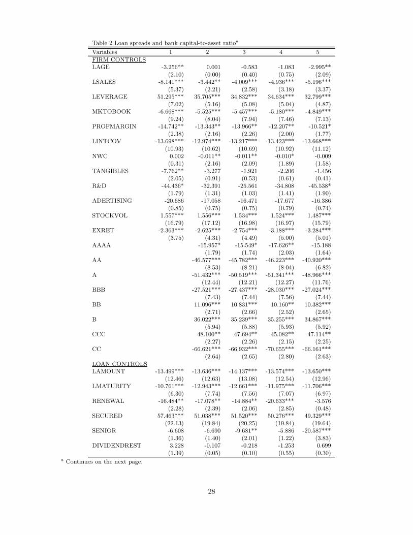
Table 2 Loan spreads and bank capital-to-asset ratioa

Variables 1 2 3 4 5

FIRM CONTROLSLAGE -3.256** 0.001 -0.583 -1.083 -2.995**

(2.10) (0.00) (0.40) (0.75) (2.09)LSALES -8.141*** -3.442** -4.009*** -4.936*** -5.196***

(5.37) (2.21) (2.58) (3.18) (3.37)LEVERAGE 51.295*** 35.705*** 34.832*** 34.634*** 32.799***

(7.02) (5.16) (5.08) (5.04) (4.87)MKTOBOOK -6.668*** -5.525*** -5.457*** -5.180*** -4.849***

(9.24) (8.04) (7.94) (7.46) (7.13)PROFMARGIN -14.742** -13.343** -13.966** -12.207** -10.521*

(2.38) (2.16) (2.26) (2.00) (1.77)LINTCOV -13.698*** -12.974*** -13.217*** -13.423*** -13.668***

(10.93) (10.62) (10.69) (10.92) (11.12)NWC 0.002 -0.011** -0.011** -0.010* -0.009

(0.31) (2.16) (2.09) (1.89) (1.58)TANGIBLES -7.762** -3.277 -1.921 -2.206 -1.456

(2.05) (0.91) (0.53) (0.61) (0.41)R&D -44.436* -32.391 -25.561 -34.808 -45.538*

(1.79) (1.31) (1.03) (1.41) (1.90)ADERTISING -20.686 -17.058 -16.471 -17.677 -16.386

(0.85) (0.75) (0.75) (0.79) (0.74)STOCKVOL 1.557*** 1.556*** 1.534*** 1.524*** 1.487***

(16.79) (17.12) (16.98) (16.97) (15.79)EXRET -2.363*** -2.625*** -2.754*** -3.188*** -3.284***

(3.75) (4.31) (4.49) (5.00) (5.01)AAAA -15.957* -15.549* -17.626** -15.188

(1.79) (1.74) (2.03) (1.64)AA -46.577*** -45.782*** -46.223*** -40.920***

(8.53) (8.21) (8.04) (6.82)A -51.432*** -50.519*** -51.341*** -48.966***

(12.44) (12.21) (12.27) (11.76)BBB -27.521*** -27.437*** -28.030*** -27.024***

(7.43) (7.44) (7.56) (7.44)BB 11.096*** 10.831*** 10.160** 10.382***

(2.71) (2.66) (2.52) (2.65)B 36.022*** 35.239*** 35.255*** 34.867***

(5.94) (5.88) (5.93) (5.92)CCC 48.100** 47.694** 45.082** 47.114**

(2.27) (2.26) (2.15) (2.25)CC -66.621*** -66.932*** -70.655*** -66.161***

(2.64) (2.65) (2.80) (2.63)LOAN CONTROLSLAMOUNT -13.499*** -13.636*** -14.137*** -13.574*** -13.650***

(12.46) (12.63) (13.08) (12.54) (12.96)LMATURITY -10.761*** -12.943*** -12.661*** -11.975*** -11.706***

(6.30) (7.74) (7.56) (7.07) (6.97)RENEWAL -16.484** -17.078** -14.884** -20.633*** -3.576

(2.28) (2.39) (2.06) (2.85) (0.48)SECURED 57.463*** 51.038*** 51.520*** 50.276*** 49.329***

(22.13) (19.84) (20.25) (19.84) (19.64)SENIOR -6.608 -6.690 -9.681** -5.886 -20.587***

(1.36) (1.40) (2.01) (1.22) (3.83)DIVIDENDREST 3.228 -0.107 -0.218 -1.253 0.699

(1.39) (0.05) (0.10) (0.55) (0.30)a Continues on the next page.

28

Table 2 Continued a

Variables 1 2 3 4 5

GUARANTOR 19.793*** 17.532*** 15.375*** 12.097** 7.169(3.94) (3.64) (3.16) (2.47) (1.48)

CORPURPOSES -2.765 -7.174*** -7.373*** -9.373*** -11.424***(1.04) (2.82) (2.90) (3.68) (4.45)

DEBTREPAY -23.782*** -25.819*** -24.263*** -22.402*** -16.946***(8.88) (9.76) (9.22) (8.37) (6.44)

WORKCAPITAL -10.598*** -14.379*** -15.414*** -18.613*** -23.521***(3.85) (5.29) (5.73) (7.02) (8.73)

TERMLOAN 64.556*** 57.128*** 56.517*** 56.559*** 55.478***(17.23) (15.53) (15.47) (15.50) (15.42)

CREDITLINE 16.889*** 12.655*** 12.694*** 13.204*** 13.446***(6.51) (4.94) (4.96) (5.16) (5.26)

LEADBANKS 13.804*** 13.024*** 11.089*** 7.818*** 1.907(4.74) (4.45) (3.77) (2.68) (0.62)

RELATIONSHIP -0.509 -0.039 0.117 0.643 0.699(0.28) (0.02) (0.07) (0.37) (0.40)

BANK CONTROLSCAPITAL -1.580** -1.782*** -1.875*** -2.161*** -2.726***

(2.47) (2.81) (2.83) (3.25) (3.74)LASSETS 1.114* 1.962*** -2.116**

(1.69) (2.62) (2.49)ROAVOL 1.707** 1.934** -0.091

(2.07) (2.27) (0.11)CHARGEOFFS -0.006 0.593 -0.180

(0.01) (1.07) (0.32)ROA -2.267** -2.854** -3.647***

(2.07) (2.53) (3.32)AAA -15.308*** -13.490** -7.368

(2.59) (2.24) (1.30)AA 11.419*** 8.874*** -2.598

(3.96) (3.05) (0.86)A 10.587*** 7.804*** -5.659**

(4.13) (2.95) (2.08)BBB 11.569* 9.233 -4.860

(1.81) (1.43) (0.74)BB 22.972 19.465 22.909

(1.32) (1.09) (1.25)B 83.784*** 83.595*** 95.160***

(5.99) (4.88) (4.99)LIQUIDITY 31.235** 9.521

(2.41) (0.74)SUBDEBT -404.819*** -93.488

(3.22) (0.73)LIBOR -4.398*** -4.075**

(7.26) (2.33)BUSINESS CONTROLSBBB-AAA SLOPE 14.723**

(2.56)YEAR DUMMIES IN

Constant 159.409*** 162.501*** 158.644*** 178.687*** 252.595***(9.07) (9.36) (8.89) (9.50) (5.12)

Observations 15985 15985 15985 15985 15985R-squared 0.55 0.57 0.57 0.58 0.59

a Models estimated with robust standard errors and clustered by firm to correct for correlation across observa-tions of a given firm. The dependent variable is LOANSPREAD: Loan spread over Libor at the time of the loanorigination. Included in the regressions but not shown in the table are also dummy variables for the issuer’ssector of activity as defined by SIC one-digit code. Robust t statistics in parentheses.

29

Table 3 Testing hypothesis 1: Borrowers’ cashflow and bank capitala

Variables 1 2 3

CAPITAL -5.829*** -3.622*** -2.723***

(4.24) (3.84) (3.87)

LINTCOV -27.655***

(6.35)

LINTCOV x CAPITAL 1.853***

(3.33)

EBITDA-ASSET -198.365***

(4.90)

EBITDA-ASSET x CAPITAL 9.203*

(1.74)

EBITDA-DEBT -2.659***

(3.21)

EBITDA-DEBT x CAPITAL 0.272***

(2.59)

FIRM CONTROLS IN IN IN

LOAN CONTROLS IN IN IN

BANK CONTROLS IN IN IN

BUSINESS CONTROLS IN IN IN

Constant 209.158*** 169.452*** 145.067***

(9.85) (8.44) (7.72)

Observations 15985 15985 15985

R-squared 0.58 0.58 0.57

a Models estimated with robust standard errors and clustered by firm to correct for correlation across observa-tions of a given firm. The dependent variable is LOANSPREAD: Loan spread over Libor at the time of the loanorigination. See Table 1 for the definitions of all controls included in the models. Included in the regressions butnot shown in the table are also dummy variables for the issuer’s sector of activity as defined by SIC one-digitcode. Robust t statistics in parentheses.

30

Table 4 Testing hypothesis 1: Comparing well– and under–capitalized banks’ loan pricinga

Variables 1 2 3

WELL-CAPITALIZEDb -37.661** -23.801* -13.805

(2.17) (1.66) (1.22)

LINTCOV -26.198***

(5.04)

LINTCOV x WELL-CAPITALIZEDb 15.715**

(2.55)

EBITDA-ASSET -174.671***

(3.50)

EBITDA-ASSET x WELL-CAPITALIZEDb 99.286*

(1.70)

EBITDA-DEBT -3.274***

(3.02)

EBITDA-DEBT x WELL-CAPITALIZEDb 3.971***

(3.01)

FIRM CONTROLS IN IN IN

LOAN CONTROLS IN IN IN

BANK CONTROLS IN IN IN

Constant 216.411*** 189.712*** 159.348***

(4.87) (4.50) (3.71)

Observations 1801 1801 1801

R-squared 0.57 0.56 0.56

a Models estimated on the sample of loans taken out from under and well capitalized banks. A bank is consideredundercapitalized if its capital-to-asset ratio is less or equal than 5%. A bank is considered well-capitalized if ithas a capital-to-asset ratio is higher or equal to 10%. Models estimated with robust standard errors and clusteredby firm to correct for correlation across observations of a given firm. The dependent variable is LOANSPREAD:Loan spread over Libor at the time of the loan origination. See Table 1 for the definitions of all controls includedin the models. Included in the regressions but not shown in the table are also dummy variables for the issuer’ssector of activity as defined by SIC one-digit code. Bank capital not included in BANK CONTROLS. Robustt statistics in parentheses.b Dummy variable equal to 1 for loans taken out from well capitalized banks.

31

Table 5 Testing hypothesis 2: Controlling for the state of the economya

Variables 1 2 3

CAPITAL -6.541*** -4.386*** -3.135***

(4.75) (4.37) (4.15)

LINTCOV -20.903***

(4.74)

LINTCOV x CAPITAL 1.847***

(3.45)

EBITDA-ASSET -216.297***

(5.28)

EBITDA-ASSET x CAPITAL 14.593***

(2.73)

EBITDA-DEBT -1.388

(1.58)

EBITDA-DEBT x CAPITAL 0.280***

(2.70)

BBB-AAA SLOPE 30.250*** 18.924*** 15.741***

(4.28) (2.89) (2.70)

LINTCOV x BBB-AAA -7.801***

(4.43)

EBITDA-ASSET x BBB-AAA -24.362

(1.11)

EBITDA-DEBT x BBB-AAA -1.481***

(4.35)

FIRM CONTROLS IN IN IN

LOAN CONTROLS IN IN IN

BANK CONTROLS IN IN IN

YEAR DUMMIES IN IN IN

Constant 273.677*** 238.332*** 214.760***

(5.49) (4.77) (4.26)

Observations 15985 15985 15985

R-squared 0.59 0.59 0.58

a Models estimated with robust standard errors and clustered by firm to correct for correlation across observa-tions of a given firm. The dependent variable is LOANSPREAD: Loan spread over Libor at the time of the loanorigination. See Table 1 for the definitions of all controls included in the models. Included in the regressions butnot shown in the table are also dummy variables for the issuer’s sector of activity as defined by SIC one-digitcode. We control for the state of the economy by adding the slope of the bond yield curve BBB−AAASLOPEand year dummies. Robust t statistics in parentheses.

32

Table 6 Testing hypothesis 3: Borrowers’ bank dependency and bank capitala

Variables 1 2 3 4 5

CAPITAL -2.469*** -2.894*** -2.799*** -2.340*** -2.251***

(3.42) (3.42) (3.31) (3.17) (3.15)

CPRATING -57.882***

(5.25)

CPRATING x CAPITAL 3.111**

(2.13)

CREDITRATING -19.165*

(1.88)

CREDITRATING x CAPITAL 2.475*

(1.88)

IGRADE -53.093***

(5.03)

BLGRADE 7.293

(0.50)

IGRADE x CAPITAL 2.542**

(1.99)

BLGRADE x CAPITAL 1.436

(0.73)

PBOND -19.161*

(1.68)

PBOND x CAPITAL 2.134

(1.43)

PBONDIGRADE -35.950***

(2.93)

PBONDBGRADE 2.159

(0.09)

PBONDIGRADE x CAPITAL 2.777*

(1.69)

PBONDBGRADE x CAPITAL 1.515

(0.44)

FIRM CONTROLSb IN IN IN IN IN

LOAN CONTROLS IN IN IN IN IN

BANK CONTROLS IN IN IN IN IN

Constant 179.348*** 184.994*** 187.177*** 179.656*** 178.041***

(9.21) (9.22) (9.41) (9.30) (9.21)

Observations 15985 15985 15985 15985 15985

R-squared 0.57 0.56 0.57 0.56 0.56

p value for H0:

CAP + CAP x MKT ACCESS = 0 (0.633) (0.692) (0.798) (0.881) (0.741)

(0.444) (0.827)

a Models estimated with robust standard errors and clustered by firm to correct for correlation across observa-tions of a given firm. The dependent variable is LOANSPREAD: Loan spread over Libor at the time of the loanorigination. See Table 1 for the definitions of all controls included in the models. Included in the regressions butnot shown in the table are also dummy variables for the issuer’s sector of activity as defined by SIC one-digitcode. Robust t statistics in parentheses.b FIRM CONTROLS do not include in this table our set of dummy variables for the firm credit rating.

33

Table 7 Testing hypothesis 4: Controlling for the state of the economya

Variables 1 2 3 4 5

CAPITAL -3.057*** -3.231*** -3.109*** -2.967*** -3.022***(3.98) (3.71) (3.56) (3.76) (3.91)

CPRATING -28.320**(2.41)

CPRATING x CAPITAL 1.915(1.35)

CREDITRATING -10.469(0.98)

CREDITRATING x CAPITAL 1.104(0.87)

IGRADE -30.155***(2.77)

BLGRADE -24.379(1.59)

IGRADE x CAPITAL 0.960(0.77)

BLGRADE x CAPITAL 1.650(0.90)

PBOND 5.314(0.44)

PBOND x CAPITAL 0.967(0.67)

PBONDIGRADE -12.140(0.94)

PBONDBGRADE -15.066(0.66)

PBONDIGRADE x CAPITAL 1.861(1.12)

PBONDBGRADE x CAPITAL 1.622(0.51)

BBB-AAA 18.545*** 13.202** 10.325* 17.602*** 15.117**(3.11) (2.09) (1.66) (2.92) (2.51)

MKT ACCESSb x BBB-AAA -18.885*** 2.350 -9.332** -16.198*** -15.065***(4.31) (2.12) (0.56) (3.49) (3.18)

33.694*** 19.900**(5.34) (2.24)

FIRM CONTROLS IN IN IN IN INLOAN CONTROLS IN IN IN IN INBANK CONTROLS IN IN IN IN INYEAR DUMMIES IN IN IN IN IN

Constant 252.380*** 258.136*** 266.661*** 254.303*** 257.395***(5.10) (5.19) (5.31) (5.15) (5.22)

Observations 15985 15985 15985 15985 15985R-squared 0.58 0.57 0.59 0.57 0.58

p value for H0:

CAP + CAP x MKT ACCESSb = 0 (0.407) (0.050) (0.045) (0.140) (0.474)(0.387) (0.656)

a Models estimated with robust standard errors and clustered by firm to correct for correlation across observa-tions of a given firm. The dependent variable is LOANSPREAD: Loan spread over Libor at the time of the loanorigination. See Table 1 for the definitions of all controls included in the models. Included in the regressions butnot shown in the table are also dummy variables for the issuer’s sector of activity as defined by SIC one-digitcode. We control for the state of the economy by adding the slope of the bond yield curve BBB−AAASLOPEand year dummies. Robust t statistics in parentheses.b MKTACCESS takes the variable(s) we use in each model reported in the table to control for borrowers’access to debt markets.

34

Table 8 Testing hypothesis 1: Adding bank fixed effectsa

Variables 1 2 3

CAPITAL -7.250*** -4.721*** -3.222***

(4.75) (4.10) (3.28)

LINTCOV -22.444***

(4.92)

LINTCOV x CAPITAL 2.151***

(3.82)

EBITDA-ASSET -240.560***

(5.65)

EBITDA-ASSET x CAPITAL 19.970***

(3.59)

EBITDA-DEBT -1.674*

(1.95)

EBITDA-DEBT x CAPITAL 0.321***

(3.08)

BBB-AAA 34.016*** 21.897*** 18.764***

(4.75) (3.33) (3.22)

LINTCOV x BBB-AAA -8.170***

(4.57)

EBITDA-ASSET x BBB-AAA -26.308

(1.23)

EBITDA-DEBT x BBB-AAA -1.429***

(4.28)

FIRM CONTROLS IN IN IN

LOAN CONTROLS IN IN IN

BANK CONTROLS IN IN IN

YEAR DUMMIES IN IN IN

Constant 245.006*** 207.199*** 181.586***

(6.53) (5.78) (5.10)

Observations 15985 15985 15985

R-squared 0.62 0.61 0.61

a Models estimated with robust standard errors, clustered by firm, and with bank fixed effects. The dependentvariable is LOANSPREAD: Loan spread over Libor at the time of the loan origination. See Table 1 for thedefinitions of all controls included in the models. Included in the regressions but not shown in the table arealso dummy variables for the issuer’s sector of activity as defined by SIC one-digit code. Robust t statistics inparentheses.

35

Table 9 Testing Hypothesis 3: Adding bank fixed effectsa

Variables 1 2 3 4 5

CAPITAL -2.701*** -3.006*** -3.273*** -2.637*** -2.727***(2.71) (2.72) (2.99) (2.61) (2.74)

CPRATING -24.849**(2.00)

CPRATING x CAPITAL 1.145(0.77)

CREDITRATING -14.108(1.21)

CREDITRATING x CAPITAL 1.260(0.91)

IGRADE -34.403***(2.82)

BLGRADE -27.896*(1.79)

IGRADE x CAPITAL 1.037(0.74)

BLGRADE x CAPITAL 2.024(1.09)

PBOND 8.340(0.65)

PBOND x CAPITAL 0.440(0.29)

PBONDIGRADE -7.194(0.52)

PBONDBGRADE -17.263(0.75)

PBONDIGRADE x CAPITAL 0.912(0.53)

PBONDBGRADE x CAPITAL 2.036(0.65)

BBB-AAA 21.175*** 15.673** 12.837** 20.129*** 17.642***(3.55) (2.47) (2.05) (3.35) (2.93)

MKT ACCESSb x BBB-AAA -17.574*** 2.893 -8.006* -15.231*** -13.376***(3.93) (0.66) (1.76) (3.30) (2.75)

32.823*** 19.584**(5.15) (2.20)

FIRM CONTROLS IN IN IN IN INLOAN CONTROLS IN IN IN IN INBANK CONTROLS IN IN IN IN INYEAR DUMMIES IN IN IN IN IN

Constant 231.921*** 230.495*** 237.590*** 231.067*** 233.419***(6.49) (6.33) (6.57) (6.46) (6.52)

Observations 15985 15985 15985 15985 15985R-squared 0.60 0.60 0.61 0.60 0.60

a Models estimated with robust standard errors, clustered by firm, and with bank fixed effects. The dependentvariable is LOANSPREAD: Loan spread over Libor at the time of the loan origination. See Table 1 for thedefinitions of all controls included in the models. Included in the regressions but not shown in the table arealso dummy variables for the issuer’s sector of activity as defined by SIC one-digit code. Robust t statistics inparentheses.b MKTACCESS takes the variable(s) we use in each model reported in the table to control for borrowers’access to debt markets.

36

Table 10 Testing hypothesis 1: Borrowers’ cashflow and banks’ ZSCOREa

Variables 1 2 3

ZSCORE -0.795*** -0.650*** -0.381***

(2.87) (3.01) (2.90)

LINTCOV -10.067***

(4.15)

LINTCOV x ZSCORE 0.225**

(2.07)

EBITDA-ASSET -160.025***

(5.48)

EBITDA-ASSET x ZSCORE 2.751**

(2.04)

EBITDA-DEBT 0.203

(0.49)

EBITDA-DEBT x ZSCORE 0.041**

(2.48)

BBB-AAA 27.706*** 15.494** 15.017***

(3.90) (2.37) (2.58)

LINTCOV x BBB-AAA -6.911***

(3.87)

EBITDA-ASSET x BBB-AAA -0.580

(0.03)

EBITDA-DEBT x BBB-AAA -1.417***

(4.07)

FIRM CONTROLS IN IN IN

LOAN CONTROLS IN IN IN

BANK CONTROLS IN IN IN

YEAR DUMMIES IN IN IN

Constant 228.353*** 209.906*** 191.936***

(4.59) (4.19) (3.79)

Observations 15985 15985 15985

R-squared 0.59 0.59 0.58

a Models estimated with robust standard errors and clustered by firm to correct for correlation across observa-tions of a given firm. The dependent variable is LOANSPREAD: Loan spread over Libor at the time of the loanorigination. See Table 1 for the definitions of all controls included in the models. Included in the regressions butnot shown in the table are also dummy variables for the issuer’s sector of activity as defined by SIC one-digitcode. Robust t statistics in parentheses.

37

Table 11 Borrowers’ bank dependency and banks’ ZSCOREa

Variables 1 2 3 4 5

ZSCORE -0.408*** -0.401*** -0.394*** -0.380*** -0.368***(2.99) (2.75) (2.69) (2.76) (2.76)

CPRATING -18.248***(2.91)

CPRATING x ZSCORE 0.261(1.28)

CREDITRATING -4.075(0.72)

CREDITRATING x ZSCORE 0.120(0.52)

IGRADE -26.593***(4.28)

BLGRADE -13.010*(1.73)

IGRADE x ZSCORE 0.229(1.22)

BLGRADE x ZSCORE 0.077(0.22)

PBOND 9.731(1.47)

PBOND x ZSCORE 0.174(0.77)

PBONDIGRADE -2.782(0.42)

PBONDBGRADE -3.199(0.32)

PBONDIGRADE x ZSCORE 0.278(1.10)

PBONDBGRADE x ZSCORE -0.106(0.23)

BBB-AAA 17.847*** 12.321* 9.511 16.891*** 14.442**(2.99) (1.95) (1.53) (2.80) (2.40)

MKT ACCESSb x BBB-AAA -17.843*** 3.058 -8.172* -15.279*** -13.851***(3.97) (0.72) (1.83) (3.24) (2.89)

34.023*** 20.859**(5.42) (2.34)

FIRM CONTROLS IN IN IN IN INLOAN CONTROLS IN IN IN IN INBANK CONTROLS IN IN IN IN INYEAR DUMMIES IN IN IN IN IN

Constant 230.122*** 235.247*** 245.026*** 232.856*** 235.210***(4.63) (4.72) (4.87) (4.70) (4.76)

Observations 15985 15985 15985 15985 15985R-squared 0.58 0.57 0.59 0.57 0.58

a Models estimated with robust standard errors and clustered by firm to correct for correlation across observa-tions of a given firm. The dependent variable is LOANSPREAD: Loan spread over Libor at the time of the loanorigination. See Table 1 for the definitions of all controls included in the models. Included in the regressions butnot shown in the table are also dummy variables for the issuer’s sector of activity as defined by SIC one-digitcode. Robust t statistics in parentheses.b MKTACCESS takes the variable(s) we use in each model reported in the table to control for borrowers’access to debt markets.

38

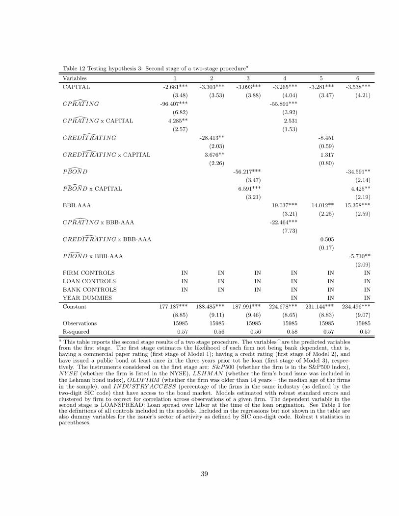
Table 12 Testing hypothesis 3: Second stage of a two-stage procedurea

Variables 1 2 3 4 5 6

CAPITAL -2.681*** -3.303*** -3.093*** -3.265*** -3.281*** -3.538***

(3.48) (3.53) (3.88) (4.04) (3.47) (4.21)

CPRATING -96.407*** -55.891***

(6.82) (3.92)

CPRATING x CAPITAL 4.285** 2.531

(2.57) (1.53)

CREDITRATING -28.413** -8.451

(2.03) (0.59)CREDITRATING x CAPITAL 3.676** 1.317

(2.26) (0.80)PBOND -56.217*** -34.591**

(3.47) (2.14)

PBOND x CAPITAL 6.591*** 4.425**

(3.21) (2.19)

BBB-AAA 19.037*** 14.012** 15.358***

(3.21) (2.25) (2.59)CPRATING x BBB-AAA -22.464***

(7.73)CREDITRATING x BBB-AAA 0.505

(0.17)PBOND x BBB-AAA -5.710**

(2.09)

FIRM CONTROLS IN IN IN IN IN IN

LOAN CONTROLS IN IN IN IN IN IN

BANK CONTROLS IN IN IN IN IN IN

YEAR DUMMIES IN IN IN

Constant 177.187*** 188.485*** 187.991*** 224.678*** 231.144*** 234.496***

(8.85) (9.11) (9.46) (8.65) (8.83) (9.07)

Observations 15985 15985 15985 15985 15985 15985

R-squared 0.57 0.56 0.56 0.58 0.57 0.57

a This table reports the second stage results of a two stage procedure. The variables · are the predicted variablesfrom the first stage. The first stage estimates the likelihood of each firm not being bank dependent, that is,having a commercial paper rating (first stage of Model 1); having a credit rating (first stage of Model 2), andhave issued a public bond at least once in the three years prior tot he loan (first stage of Model 3), respec-tively. The instruments considered on the first stage are: S&P500 (whether the firm is in the S&P500 index),NY SE (whether the firm is listed in the NYSE), LEHMAN (whether the firm’s bond issue was included inthe Lehman bond index), OLDFIRM (whether the firm was older than 14 years – the median age of the firmsin the sample), and INDUSTRY ACCESS (percentage of the firms in the same industry (as defined by thetwo-digit SIC code) that have access to the bond market. Models estimated with robust standard errors andclustered by firm to correct for correlation across observations of a given firm. The dependent variable in thesecond stage is LOANSPREAD: Loan spread over Libor at the time of the loan origination. See Table 1 forthe definitions of all controls included in the models. Included in the regressions but not shown in the table arealso dummy variables for the issuer’s sector of activity as defined by SIC one-digit code. Robust t statistics inparentheses.

39

Table 13 Testing hypothesis 1: Clustering by borrower and by banka

Variables 1 2 3

CAPITAL -6.541*** -4.386*** -3.135***

(4.15) (4.15) (3.19)

LINTCOV -20.903***

(3.81)

LINTCOV x CAPITAL 1.847***

(3.31)

EBITDA-ASSET -216.297***

(3.74)

EBITDA-ASSET x CAPITAL 14.593***

(2.87)

EBITDA-DEBT -1.388*

(1.78)

EBITDA-DEBT x CAPITAL 0.280***

(2.95)

BBB-AAA 30.250*** 18.924** 15.741***

(3.81) (2.46) (2.96)

LINTCOV x BBB-AAA -7.801***

(3.12)

EBITDA-ASSET x BBB-AAA -24.362

(0.76)

EBITDA-DEBT x BBB-AAA -1.481***

(4.51)

FIRM CONTROLS IN IN IN

LOAN CONTROLS IN IN IN

BANK CONTROLS IN IN IN

YEAR DUMMIES IN IN IN

Constant 273.677*** 238.332*** 214.760***

(5.49) (4.60) (4.24)

Observations 15985 15985 15985

R-squared 0.59 0.59 0.58

a Models estimated with robust standard errors, clustered by firm, and with bank fixed effects. The dependentvariable is LOANSPREAD: Loan spread over Libor at the time of the loan origination. See Table 1 for thedefinitions of all controls included in the models. Included in the regressions but not shown in the table arealso dummy variables for the issuer’s sector of activity as defined by SIC one-digit code. Robust t statistics inparentheses.

40

Table 14 Testing hypothesis 4: Clustering by borower and by banka

Variables 1 2 3 4 5

CAPITAL -3.057*** -3.231*** -3.109*** -2.967*** -3.022***(2.99) (3.50) (3.28) (3.07) (3.14)

CPRATING -28.320**(2.40)

CPRATING x CAPITAL 1.915(1.27)

CREDITRATING -10.469(0.92)

CREDITRATING x CAPITAL 1.104(0.83)

IGRADE -30.155**(2.23)

BLGRADE -24.379*(1.65)

IGRADE x CAPITAL 0.960(0.72)

BLGRADE x CAPITAL 1.650(0.84)

PBOND 5.314(0.48)

PBOND x CAPITAL 0.967(0.74)

PBONDIGRADE -12.141(0.95)

PBONDBGRADE -15.066(0.69)

PBONDIGRADE x CAPITAL 1.861(1.17)

PBONDBGRADE x CAPITAL 1.622(0.55)

BBB-AAA 18.545*** 13.202** 10.325* 17.602*** 15.117***(3.30) (2.42) (1.86) (3.08) (2.79)

MKT ACCESSb x BBB-AAA -18.885*** 2.350 -9.332* -16.198*** -15.065***(4.06) (0.63) (1.87) (4.04) (3.84)

33.694*** 19.900**(6.44) (2.21))

FIRM CONTROLS IN IN IN IN INLOAN CONTROLS IN IN IN IN INBANK CONTROLS IN IN IN IN INYEAR DUMMIES IN IN IN IN IN

Constant 252.380*** 258.136*** 266.661*** 254.303*** 257.3945***(5.09) (5.36) (5.47) (5.20) (5.42)

Observations 15985 15985 15985 15985 15985R-squared 0.58 0.57 0.59 0.57 0.58

a Models estimated with robust standard errors and clustered by firm to correct for correlation across observa-tions of a given firm. The dependent variable is LOANSPREAD: Loan spread over Libor at the time of the loanorigination. See Table 1 for the definitions of all controls included in the models. Included in the regressions butnot shown in the table are also dummy variables for the issuer’s sector of activity as defined by SIC one-digitcode. We control for the state of the economy by adding the slope of the bond yield curve BBB − AAA andyear dummies. Robust t statistics in parentheses.b MKTACCESS takes the variable(s) we use in each model reported in the table to control for borrowers’access to debt markets.

41

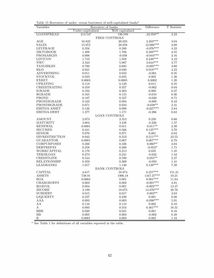
Table 15 Borrowers of under- versus borrowers of well-capitalized banksa

Variables Borrowers of banks: Difference T StatisticUnder-ca[pitalized Well capitalized

LOANSPREAD 213.547 190.589 -22.958** 2.23FIRM CONTROLS

AGE 16.822 20.025 3.203*** 3.04SALES 15.972 28.058 12.086*** 3.08LEVERAGE 0.356 0.280 -0.076*** 4.33MKTOBOOK 1.498 1.786 0.288*** 4.55PROMARGIN 0.006 -0.038 -0.044*** 3.16LINTCOV 1.710 1.958 0.248*** 3.10NWC 2.343 5.987 3.644*** 3.77TANGIBLES 0.780 0.685 -0.095*** 3.60R&D 0.021 0.040 0.018*** 4.23ADVERTISING 0.011 0.010 -0.001 0.35STOCKVOL 0.033 0.035 0.002 1.38EXRET 0.0003 0.0005 0.0002 1.20CPRATING 0.118 0.129 0.011 0.45CREDITRATING 0.359 0.357 -0.002 0.04IGRADE 0.194 0.203 0.009 0.27BGRADE 0.165 0.155 -0.010 0.36PBOND 0.187 0.167 -0.020 0.71PBONDIGRADE 0.103 0.094 -0.009 0.43PBONDBGRADE 0.071 0.033 -0.038** 2.31EBITDA-ASSET 0.126 0.099 -0.027*** 2.84EBITDA-DEBT 1.377 1.171 -0.206 0.62

LOAN CONTROLSAMOUNT 2.073 2.312 0.239 0.60MATURITY 3.664 3.438 -0.226 1.57RENEWAL 0.0001 0.011 0.011** 2.39SECURED 0.441 0.566 0.125*** 3.70SENIOR 0.970 0.971 0.001 0.04DIVRESTRICTION 0.042 0.553 0.511*** 23.55GUARANTOR 0.0001 0.067 0.067*** 6.78CORPURPOSES 0.266 0.326 0.060** 2.04DEBTREPAY 0.258 0.206 -0.052* 1.71WORKCAPITAL 0.178 0.213 0.035 1.45TERMLOAN 0.273 0.241 -0.032 1.44CREDITLINE 0.544 0.599 0.055** 2.27RELATIONSHIP 0.359 0.309 -0.050 1.41LEADBANKS 1.017 1.146 0.129*** 7.39

BANK CONTROLSCAPITAL 4.617 10.874 6.257*** 151.31ASSETS 738.91 1906.18 1167.27*** 10.21ROA 0.0004 0.001 0.001*** 11.64CHARGEOFFS 0.003 0.002 -0.001*** 4.81ROAVOL 0.004 0.001 -0.003*** 13.47ZSCORE 3.199 18.075 14.876*** 28.76SUBDEBT 0.015 0.017 0.002** 2.63LIQUIDITY 0.237 0.238 0.001 0.08AAA 0.093 0.003 -0.090*** 5.91AA 0.116 0.118 0.002 0.10A 0.093 0.554 0.461*** 16.31BBB 0.020 0.021 0.001 0.16BB 0.005 0.003 -0.002 0.49B 0.0001 0.003 0.002 1.34

a See Table 1 for definitions of all variables reported in the table.

42