averages of b-hadron, c-hadron, and tau-lepton properties
TRANSCRIPT
arX
iv:1
010.
1589
v3 [
hep-
ex]
6 S
ep 2
011
Averages of b-hadron, c-hadron, and τ -lepton Properties
Heavy Flavor Averaging Group (HFAG):
D. Asner1, Sw. Banerjee2, R. Bernhard3, S. Blyth4, A. Bozek5, C. Bozzi6,D. G. Cassel7, G. Cavoto8, G. Cibinetto6, J. Coleman9, W. Dungel10,
T. J. Gershon11, L. Gibbons7, B. Golob12, R. Harr13, K. Hayasaka14,H. Hayashii15, C.-J. Lin16, D. Lopes Pegna17, R. Louvot18, A. Lusiani19,
V. Luth20, B. Meadows21, S. Nishida22, D. Pedrini23, M. Purohit24,M. Rama25, M. Roney2, O. Schneider18, C. Schwanda10, A. J. Schwartz21,
B. Shwartz26, J. G. Smith27, R. Tesarek28, D. Tonelli28, K. Trabelsi22,P. Urquijo29, and R. Van Kooten30
1Pacific Northwest National Laboratory, USA2University of Victoria, Canada
3University of Zurich, Switzerland4National United University, Taiwan
5University of Krakow, Poland6INFN Ferrara, Italy
7Cornell University, USA8INFN Rome, Italy
9University of Liverpool, UK10Austrian Academy of Sciences, Austria
11University of Warwick, UK12University of Ljubljana, Slovenia13Wayne State University, USA
14Nagoya University, Japan15Nara Womana’s University, Japan
16Lawrence Berkeley National Laboratory, USA17Princeton University, USA
18Ecole Polytechnique Federale de Lausanne (EPFL), Switzerland19INFN Pisa, Italy
20SLAC National Accelerator Laboratory, USA21University of Cincinnati, USA
22KEK, Tsukuba, Japan23INFN Milano-Bicocca, Italy
24University of South Carolina, USA25INFN Frascati, Italy
26Budker Institute of Nuclear Physics, Russia27University of Colorado, USA
28Fermilab, USA29Syracuse University, USA30Indiana University, USA
6 September 2011(original version: 8 October 2010)
Abstract
This article reports world averages for measurements of b-hadron, c-hadron, and τlepton properties obtained by the Heavy Flavor Averaging Group (HFAG) using resultsavailable at least through the end of 2009. Some of the world averages presented use dataavailable through the spring of 2010. For the averaging, common input parameters usedin the various analyses are adjusted (rescaled) to common values, and known correlationsare taken into account. The averages include branching fractions, lifetimes, neutral mesonmixing parameters, CP violation parameters, and parameters of semileptonic decays.
2
Contents
1 Introduction 6
2 Methodology 7
3 b-hadron production fractions, lifetimes and mixing parameters 153.1 b-hadron production fractions . . . . . . . . . . . . . . . . . . . . . . . . . . . . 15
3.1.1 b-hadron production fractions in Υ (4S) decays . . . . . . . . . . . . . . . 153.1.2 b-hadron production fractions in Υ (5S) decays . . . . . . . . . . . . . . . 173.1.3 b-hadron production fractions at high energy . . . . . . . . . . . . . . . . 19
3.2 b-hadron lifetimes . . . . . . . . . . . . . . . . . . . . . . . . . . . . . . . . . . . 223.2.1 Lifetime measurements, uncertainties and correlations . . . . . . . . . . . 233.2.2 Inclusive b-hadron lifetimes . . . . . . . . . . . . . . . . . . . . . . . . . 243.2.3 B0 and B+ lifetimes and their ratio . . . . . . . . . . . . . . . . . . . . . 263.2.4 B0
s lifetime . . . . . . . . . . . . . . . . . . . . . . . . . . . . . . . . . . . 273.2.5 B+
c lifetime . . . . . . . . . . . . . . . . . . . . . . . . . . . . . . . . . . 313.2.6 Λ0
b and b-baryon lifetimes . . . . . . . . . . . . . . . . . . . . . . . . . . . 313.2.7 Summary and comparison with theoretical predictions . . . . . . . . . . 33
3.3 Neutral B-meson mixing . . . . . . . . . . . . . . . . . . . . . . . . . . . . . . . 343.3.1 B0 mixing parameters . . . . . . . . . . . . . . . . . . . . . . . . . . . . 353.3.2 B0
s mixing parameters . . . . . . . . . . . . . . . . . . . . . . . . . . . . 41
4 Measurements related to Unitarity Triangle angles 534.1 Introduction . . . . . . . . . . . . . . . . . . . . . . . . . . . . . . . . . . . . . 534.2 Notations . . . . . . . . . . . . . . . . . . . . . . . . . . . . . . . . . . . . . . . 55
4.2.1 CP asymmetries . . . . . . . . . . . . . . . . . . . . . . . . . . . . . . . 554.2.2 Time-dependent CP asymmetries in decays to CP eigenstates . . . . . . 554.2.3 Time-dependent CP asymmetries in decays to vector-vector final states . 564.2.4 Time-dependent asymmetries: self-conjugate multiparticle final states . 574.2.5 Time-dependent CP asymmetries in decays to non-CP eigenstates . . . . 604.2.6 Time-dependent CP asymmetries in the Bs System . . . . . . . . . . . . 654.2.7 Asymmetries in B → D(∗)K(∗) decays . . . . . . . . . . . . . . . . . . . 66
4.3 Common inputs and error treatment . . . . . . . . . . . . . . . . . . . . . . . . 684.4 Time-dependent asymmetries in b→ ccs transitions . . . . . . . . . . . . . . . 70
4.4.1 Time-dependent CP asymmetries in b→ ccs decays to CP eigenstates . 704.4.2 Time-dependent transversity analysis of B0 → J/ψK∗0 . . . . . . . . . . 714.4.3 Time-dependent CP asymmetries in B0 → D∗+D∗−K0
S decays . . . . . . 724.4.4 Time-dependent analysis of B0
s → J/ψφ . . . . . . . . . . . . . . . . . . 724.5 Time-dependent CP asymmetries in colour-suppressed b→ cud transitions . . . 744.6 Time-dependent CP asymmetries in charmless b→ qqs transitions . . . . . . . 76
4.6.1 Time-dependent CP asymmetries: b→ qqs decays to CP eigenstates . . 764.6.2 Time-dependent Dalitz plot analyses: B0 → K+K−K0 and B0 → π+π−K0
S79
4.6.3 Time-dependent analyses of B0 → φK0Sπ0 . . . . . . . . . . . . . . . . . 80
4.7 Time-dependent CP asymmetries in b → ccd transitions . . . . . . . . . . . . . 854.8 Time-dependent CP asymmetries in b → qqd transitions . . . . . . . . . . . . . 904.9 Time-dependent asymmetries in b→ sγ transitions . . . . . . . . . . . . . . . . 91
3
4.10 Time-dependent asymmetries in b→ dγ transitions . . . . . . . . . . . . . . . . 924.11 Time-dependent CP asymmetries in b → uud transitions . . . . . . . . . . . . . 944.12 Time-dependent CP asymmetries in b → cud/ucd transitions . . . . . . . . . . 1004.13 Time-dependent CP asymmetries in b → cus/ucs transitions . . . . . . . . . . . 1014.14 Rates and asymmetries in B∓ → D(∗)K(∗)∓ decays . . . . . . . . . . . . . . . . 103
4.14.1 D decays to CP eigenstates . . . . . . . . . . . . . . . . . . . . . . . . . 1034.14.2 D decays to suppressed final states . . . . . . . . . . . . . . . . . . . . . 1034.14.3 D decays to multiparticle self-conjugate final states . . . . . . . . . . . . 104
5 Semileptonic B decays 1105.1 Exclusive CKM-favored decays . . . . . . . . . . . . . . . . . . . . . . . . . . . . 110
5.1.1 B → Dℓ−νℓ . . . . . . . . . . . . . . . . . . . . . . . . . . . . . . . . . . 1105.1.2 B → D∗ℓ−νℓ . . . . . . . . . . . . . . . . . . . . . . . . . . . . . . . . . . 1125.1.3 B → D(∗)πℓ−νℓ . . . . . . . . . . . . . . . . . . . . . . . . . . . . . . . . 1165.1.4 B → D∗∗ℓ−νℓ . . . . . . . . . . . . . . . . . . . . . . . . . . . . . . . . . 116
5.2 Inclusive CKM-favored decays . . . . . . . . . . . . . . . . . . . . . . . . . . . . 1195.2.1 Inclusive Semileptonic Branching Fraction . . . . . . . . . . . . . . . . . 1195.2.2 Determination of |Vcb| . . . . . . . . . . . . . . . . . . . . . . . . . . . . 1205.2.3 Global Fit in the Kinetic Scheme . . . . . . . . . . . . . . . . . . . . . . 122
5.3 Exclusive CKM-suppressed decays . . . . . . . . . . . . . . . . . . . . . . . . . . 1235.4 Inclusive CKM-suppressed decays . . . . . . . . . . . . . . . . . . . . . . . . . . 125
5.4.1 BLNP . . . . . . . . . . . . . . . . . . . . . . . . . . . . . . . . . . . . . 1285.4.2 DGE . . . . . . . . . . . . . . . . . . . . . . . . . . . . . . . . . . . . . . 1295.4.3 GGOU . . . . . . . . . . . . . . . . . . . . . . . . . . . . . . . . . . . . . 1305.4.4 ADFR . . . . . . . . . . . . . . . . . . . . . . . . . . . . . . . . . . . . . 1325.4.5 BLL . . . . . . . . . . . . . . . . . . . . . . . . . . . . . . . . . . . . . . 1325.4.6 Summary . . . . . . . . . . . . . . . . . . . . . . . . . . . . . . . . . . . 133
6 B decays to charmed hadrons 135
7 B decays to charmless final states 1707.1 Mesonic charmless decays . . . . . . . . . . . . . . . . . . . . . . . . . . . . . . 1707.2 Radiative and leptonic decays . . . . . . . . . . . . . . . . . . . . . . . . . . . . 1777.3 B → Xsγ . . . . . . . . . . . . . . . . . . . . . . . . . . . . . . . . . . . . . . . 1787.4 Baryonic decays . . . . . . . . . . . . . . . . . . . . . . . . . . . . . . . . . . . . 1817.5 Bs decays . . . . . . . . . . . . . . . . . . . . . . . . . . . . . . . . . . . . . . . 1847.6 Charge asymmetries . . . . . . . . . . . . . . . . . . . . . . . . . . . . . . . . . 1847.7 Polarization measurements . . . . . . . . . . . . . . . . . . . . . . . . . . . . . . 189
8 D decays 1918.1 D0-D 0 Mixing and CP Violation . . . . . . . . . . . . . . . . . . . . . . . . . . 191
8.1.1 Introduction . . . . . . . . . . . . . . . . . . . . . . . . . . . . . . . . . . 1918.1.2 Input Observables . . . . . . . . . . . . . . . . . . . . . . . . . . . . . . . 1928.1.3 Fit results . . . . . . . . . . . . . . . . . . . . . . . . . . . . . . . . . . . 1938.1.4 Conclusions . . . . . . . . . . . . . . . . . . . . . . . . . . . . . . . . . . 195
8.2 Excited D(s) Mesons . . . . . . . . . . . . . . . . . . . . . . . . . . . . . . . . . 2018.3 Semileptonic Decays . . . . . . . . . . . . . . . . . . . . . . . . . . . . . . . . . 208
4
8.3.1 Introduction . . . . . . . . . . . . . . . . . . . . . . . . . . . . . . . . . . 2088.3.2 D→Pℓν Decays . . . . . . . . . . . . . . . . . . . . . . . . . . . . . . . 2088.3.3 Simple Pole . . . . . . . . . . . . . . . . . . . . . . . . . . . . . . . . . . 2088.3.4 z Expansion . . . . . . . . . . . . . . . . . . . . . . . . . . . . . . . . . . 2098.3.5 D→V ℓν Decays . . . . . . . . . . . . . . . . . . . . . . . . . . . . . . . 2118.3.6 S-Wave Component . . . . . . . . . . . . . . . . . . . . . . . . . . . . . . 2138.3.7 Model-independent Form Factor Measurement . . . . . . . . . . . . . . . 213
8.4 CP Asymmetries . . . . . . . . . . . . . . . . . . . . . . . . . . . . . . . . . . . 2178.5 T -violating Asymmetries . . . . . . . . . . . . . . . . . . . . . . . . . . . . . . . 2218.6 World Average for the D+
s Decay Constant fDs . . . . . . . . . . . . . . . . . . 2228.7 Two-body Hadronic D0 Decays and Final State Radiation . . . . . . . . . . . . 227
8.7.1 Branching Fraction Corrections . . . . . . . . . . . . . . . . . . . . . . . 2278.7.2 Average Branching Fractions . . . . . . . . . . . . . . . . . . . . . . . . . 230
9 τ lepton Properties 2359.1 Mass of the τ lepton . . . . . . . . . . . . . . . . . . . . . . . . . . . . . . . . . 2359.2 τ Branching Fractions: . . . . . . . . . . . . . . . . . . . . . . . . . . . . . . . . 2359.3 Tests of Lepton Universality . . . . . . . . . . . . . . . . . . . . . . . . . . . . . 2459.4 Measurement of |Vus| . . . . . . . . . . . . . . . . . . . . . . . . . . . . . . . . . 2509.5 Search for lepton flavor violation in τ decays . . . . . . . . . . . . . . . . . . . . 251
10 Summary 253
11 Acknowledgments 253
5
1 Introduction
Flavor dynamics is an important element in understanding the nature of particle physics. Theaccurate knowledge of properties of heavy flavor hadrons, especially b hadrons, plays an essen-tial role for determining the elements of the Cabibbo-Kobayashi-Maskawa (CKM) weak-mixingmatrix [1, 2]. Since the Belle and BABAR e+e− B factory experiments began collecting data,the size of available B meson samples has dramatically increased, and the accuracies of mea-surements have greatly improved. The CDF and DØ experiments at the Fermilab Tevatronhave also provided important results on B and D meson decays, most notably the discovery ofB0s -B
0s mixing, and confirmation of D0-D0 mixing.
The Heavy Flavor Averaging Group (HFAG) was formed in 2002 to continue the activities ofthe LEP Heavy Flavor Steering group [3]. This group was responsible for calculating averages ofmeasurements of b-flavor related quantities. HFAG has evolved since its inception and currentlyconsists of seven subgroups:
• the “B Lifetime and Oscillations” subgroup provides averages for b-hadron lifetimes, b-hadron fractions in Υ (4S) decay and pp collisions, and various parameters governingB0-B0 and B0
s -B0s mixing;
• the “Unitarity Triangle Parameters” subgroup provides averages for time-dependent CPasymmetry parameters and resulting determinations of the angles of the CKM unitaritytriangle;
• the “Semileptonic B Decays” subgroup provides averages for inclusive and exclusive B-decay branching fractions, and subsequent determinations of the CKM matrix elements|Vcb| and |Vub|;
• the “B to Charm Decays” subgroup provides averages of branching fractions for B decaysto final states involving open charm or charmonium mesons;
• the “Rare Decays” subgroup provides averages of branching fractions and CP asymmetriesfor charmless, radiative, leptonic, and baryonic B meson decays;
• the “Charm Physics” subgroup provides averages of branching fractions for D mesonhadronic and semileptonic decays, properties of excited D∗∗ and DsJ mesons, averagesof D0-D0 mixing and CP and T violation parameters, and an average value for the Ds
decay constant fDs.
• the “Tau Physics” subgroup provides documentation and averages for the τ lepton massand branching fractions, and documents upper limits for τ lepton-flavor-violating decays.
The “Lifetime and Oscillations” and “Semileptonic” subgroups continue the activities of theLEP working groups with some reorganization, i.e., merging four groups into two. The “Uni-tary Triangle,” “B to Charm Decays,” and “Rare Decays” subgroups were formed to provideaverages for new results obtained from the B factory experiments (and now also from the Fer-milab Tevatron experiments). The “Charm” and “Tau” subgroups were formed more recentlyin response to the wealth of new data concerning D and τ decays. All subgroups includerepresentatives from Belle and BABAR and, when relevant, CLEO, CDF, and DØ.
6
This article is an update of the “End of 2007” HFAG preprint [4]. Here we report worldaverages using results available at least through the end of 2009. Averages reported in Chap-ters 3 and 8 incorporate results available through the spring of 2010. In general, we use allpublicly available results that have written documentation. These include preliminary resultspresented at conferences or workshops. However, we do not use preliminary results that remainunpublished for an extended period of time, or for which no publication is planned. Closecontacts have been established between representatives from the experiments and members ofsubgroups that perform averaging to ensure that the data are prepared in a form suitable forcombinations.
In the case of obtaining a world average for which χ2/dof > 1, where dof is the numberof degrees of freedom in the average calculation, we do not scale the resulting error, as ispresently done by the Particle Data Group [5]. Rather, we examine the systematics of eachmeasurement to better understand them. Unless we find possible systematic discrepanciesbetween the measurements, we do not apply any additional correction to the calculated error.We provide the confidence level of the fit as an indicator for the consistency of the measurementsincluded in the average. In case some special treatment was necessary to calculate an average,or if an approximation used in the average calculation may not be good enough (e.g., assumingGaussian errors when the likelihood function indicates non-Gaussian behavior), we include awarning message.
Chapter 2 describes the methodology used for calculating averages. In the averaging proce-dure, common input parameters used in the various analyses are adjusted (rescaled) to commonvalues, and, where possible, known correlations are taken into account. Chapters 3–9 presentworld average values from each of the subgroups listed above. A brief summary of the averagespresented is given in Chapter 10. A complete listing of the averages and plots are also availableon the HFAG web site:
http://www.slac.stanford.edu/xorg/hfag and
http://belle.kek.jp/mirror/hfag (KEK mirror site).
2 Methodology
The general averaging problem that HFAG faces is to combine information provided by dif-ferent measurements of the same parameter to obtain our best estimate of the parameter’svalue and uncertainty. The methodology described here focuses on the problems of combiningmeasurements performed with different systematic assumptions and with potentially-correlatedsystematic uncertainties. Our methodology relies on the close involvement of the people per-forming the measurements in the averaging process.
Consider two hypothetical measurements of a parameter x, which might be summarized as
x = x1 ± δx1 ±∆x1,1 ±∆x2,1 . . .
x = x2 ± δx2 ±∆x1,2 ±∆x2,2 . . . ,
where the δxk are statistical uncertainties, and the ∆xi,k are contributions to the systematicuncertainty. One popular approach is to combine statistical and systematic uncertainties in
7
quadrature
x = x1 ± (δx1 ⊕∆x1,1 ⊕∆x2,1 ⊕ . . .)
x = x2 ± (δx2 ⊕∆x1,2 ⊕∆x2,2 ⊕ . . .)
and then perform a weighted average of x1 and x2, using their combined uncertainties, as ifthey were independent. This approach suffers from two potential problems that we attemptto address. First, the values of the xk may have been obtained using different systematicassumptions. For example, different values of the B0 lifetime may have been assumed inseparate measurements of the oscillation frequency ∆md. The second potential problem isthat some contributions of the systematic uncertainty may be correlated between experiments.For example, separate measurements of ∆md may both depend on an assumed Monte-Carlobranching fraction used to model a common background.
The problems mentioned above are related since, ideally, any quantity yi that xk dependson has a corresponding contribution ∆xi,k to the systematic error which reflects the uncertainty∆yi on yi itself. We assume that this is the case and use the values of yi and ∆yi assumedby each measurement explicitly in our averaging (we refer to these values as yi,k and ∆yi,kbelow). Furthermore, since we do not lump all the systematics together, we require that eachmeasurement used in an average have a consistent definition of the various contributions to thesystematic uncertainty. Different analyses often use different decompositions of their systematicuncertainties, so achieving consistent definitions for any potentially correlated contributionsrequires close coordination between HFAG and the experiments. In some cases, a group ofsystematic uncertainties must be lumped to obtain a coarser description that is consistentbetween measurements. Systematic uncertainties that are uncorrelated with any other sourcesof uncertainty appearing in an average are lumped with the statistical error, so that the onlysystematic uncertainties treated explicitly are those that are correlated with at least one othermeasurement via a consistently-defined external parameter yi. When asymmetric statisticalor systematic uncertainties are quoted, we symmetrize them since our combination methodimplicitly assumes parabolic likelihoods for each measurement.
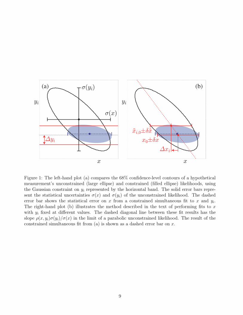
The fact that a measurement of x is sensitive to the value of yi indicates that, in principle,the data used to measure x could equally-well be used for a simultaneous measurement of x andyi, as illustrated by the large contour in Fig. 1(a) for a hypothetical measurement. However,we often have an external constraint ∆yi on the value of yi (represented by the horizontal bandin Fig. 1(a)) that is more precise than the constraint σ(yi) from our data alone. Ideally, insuch cases we would perform a simultaneous fit to x and yi, including the external constraint,obtaining the filled (x, y) contour and corresponding dashed one-dimensional estimate of xshown in Fig. 1(a). Throughout, we assume that the external constraint ∆yi on yi is Gaussian.
In practice, the added technical complexity of a constrained fit with extra free parametersis not justified by the small increase in sensitivity, as long as the external constraints ∆yi aresufficiently precise when compared with the sensitivities σ(yi) to each yi of the data alone.Instead, the usual procedure adopted by the experiments is to perform a baseline fit with all yifixed to nominal values yi,0, obtaining x = x0±δx. This baseline fit neglects the uncertainty dueto ∆yi, but this error can be mostly recovered by repeating the fit separately for each externalparameter yi with its value fixed at yi = yi,0 + ∆yi to obtain x = xi,0 ± δx, as illustrated inFig. 1(b). The absolute shift, |xi,0 − x0|, in the central value of x is what the experimentsusually quote as their systematic uncertainty ∆xi on x due to the unknown value of yi. Ourprocedure requires that we know not only the magnitude of this shift but also its sign. In the
8
x
yi
¾(x)
¾(yi)
¢yi
yi
x
x0§±x
xi,0§±x~ ~
¢xi
(a) (b)
Figure 1: The left-hand plot (a) compares the 68% confidence-level contours of a hypotheticalmeasurement’s unconstrained (large ellipse) and constrained (filled ellipse) likelihoods, usingthe Gaussian constraint on yi represented by the horizontal band. The solid error bars repre-sent the statistical uncertainties σ(x) and σ(yi) of the unconstrained likelihood. The dashederror bar shows the statistical error on x from a constrained simultaneous fit to x and yi.The right-hand plot (b) illustrates the method described in the text of performing fits to xwith yi fixed at different values. The dashed diagonal line between these fit results has theslope ρ(x, yi)σ(yi)/σ(x) in the limit of a parabolic unconstrained likelihood. The result of theconstrained simultaneous fit from (a) is shown as a dashed error bar on x.
9
limit that the unconstrained data is represented by a parabolic likelihood, the signed shift isgiven by
∆xi = ρ(x, yi)σ(x)
σ(yi)∆yi , (1)
where σ(x) and ρ(x, yi) are the statistical uncertainty on x and the correlation between x andyi in the unconstrained data. While our procedure is not equivalent to the constrained fit withextra parameters, it yields (in the limit of a parabolic unconstrained likelihood) a central valuex0 that agrees to O(∆yi/σ(yi))
2 and an uncertainty δx⊕∆xi that agrees to O(∆yi/σ(yi))4.
In order to combine two or more measurements that share systematics due to the sameexternal parameters yi, we would ideally perform a constrained simultaneous fit of all datasamples to obtain values of x and each yi, being careful to only apply the constraint on each yionce. This is not practical since we generally do not have sufficient information to reconstructthe unconstrained likelihoods corresponding to each measurement. Instead, we perform thetwo-step approximate procedure described below.
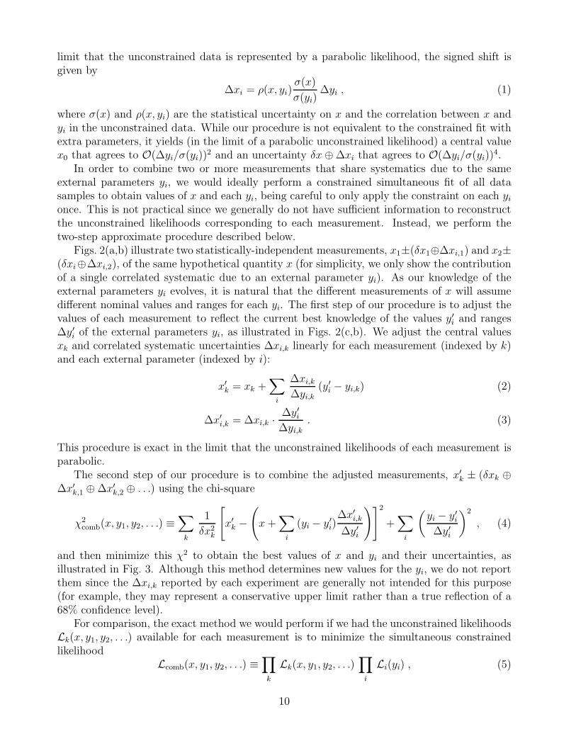
Figs. 2(a,b) illustrate two statistically-independent measurements, x1±(δx1⊕∆xi,1) and x2±(δxi⊕∆xi,2), of the same hypothetical quantity x (for simplicity, we only show the contributionof a single correlated systematic due to an external parameter yi). As our knowledge of theexternal parameters yi evolves, it is natural that the different measurements of x will assumedifferent nominal values and ranges for each yi. The first step of our procedure is to adjust thevalues of each measurement to reflect the current best knowledge of the values y′i and ranges∆y′i of the external parameters yi, as illustrated in Figs. 2(c,b). We adjust the central valuesxk and correlated systematic uncertainties ∆xi,k linearly for each measurement (indexed by k)and each external parameter (indexed by i):
x′k = xk +∑
i
∆xi,k∆yi,k
(y′i − yi,k) (2)
∆x′i,k = ∆xi,k ·∆y′i∆yi,k
. (3)
This procedure is exact in the limit that the unconstrained likelihoods of each measurement isparabolic.
The second step of our procedure is to combine the adjusted measurements, x′k ± (δxk ⊕∆x′k,1 ⊕∆x′k,2 ⊕ . . .) using the chi-square
χ2comb(x, y1, y2, . . .) ≡
∑
k
1
δx2k
[
x′k −(
x+∑
i
(yi − y′i)∆x′i,k∆y′i
)]2
+∑
i
(
yi − y′i∆y′i
)2
, (4)
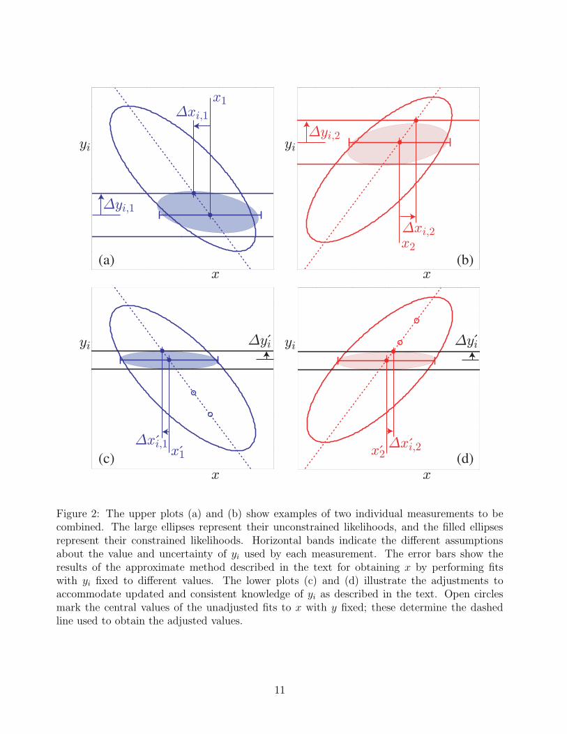
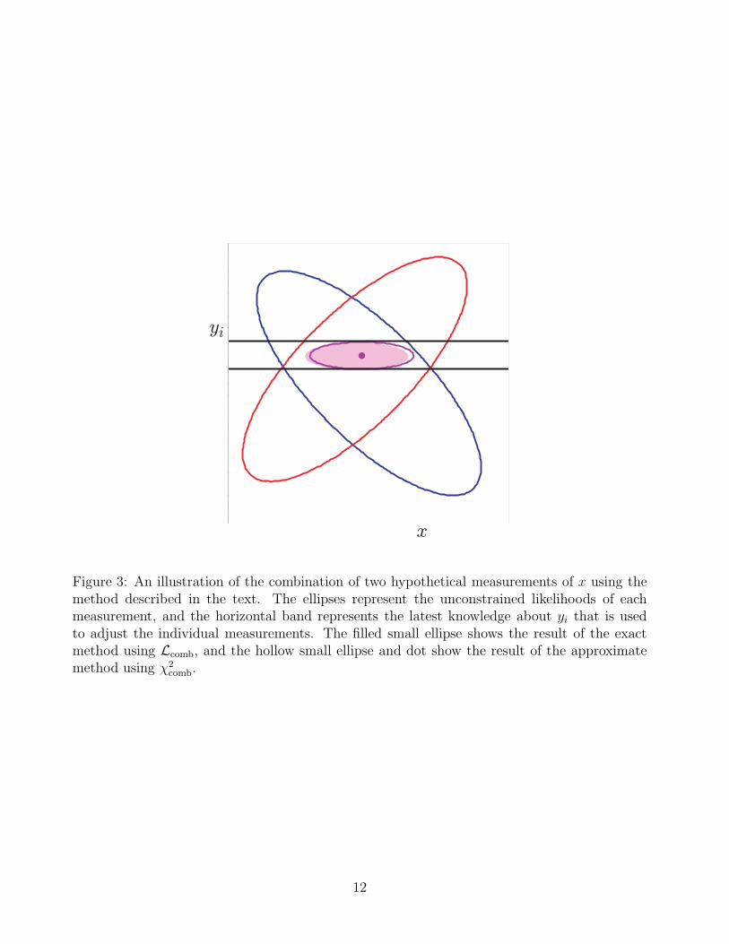
and then minimize this χ2 to obtain the best values of x and yi and their uncertainties, asillustrated in Fig. 3. Although this method determines new values for the yi, we do not reportthem since the ∆xi,k reported by each experiment are generally not intended for this purpose(for example, they may represent a conservative upper limit rather than a true reflection of a68% confidence level).
For comparison, the exact method we would perform if we had the unconstrained likelihoodsLk(x, y1, y2, . . .) available for each measurement is to minimize the simultaneous constrainedlikelihood
Lcomb(x, y1, y2, . . .) ≡∏
k
Lk(x, y1, y2, . . .)∏
i
Li(yi) , (5)
10
x
yi ¢yi
¢xi,1x1¶
¶
¶
x
yi
¢yi,1
¢xi,1
x1
x
yi ¢yi¶
¢xi,2¶x2¶
x
yi¢yi,2
¢xi,2x2
(a) (b)
(c) (d)
Figure 2: The upper plots (a) and (b) show examples of two individual measurements to becombined. The large ellipses represent their unconstrained likelihoods, and the filled ellipsesrepresent their constrained likelihoods. Horizontal bands indicate the different assumptionsabout the value and uncertainty of yi used by each measurement. The error bars show theresults of the approximate method described in the text for obtaining x by performing fitswith yi fixed to different values. The lower plots (c) and (d) illustrate the adjustments toaccommodate updated and consistent knowledge of yi as described in the text. Open circlesmark the central values of the unadjusted fits to x with y fixed; these determine the dashedline used to obtain the adjusted values.
11
x
yi
Figure 3: An illustration of the combination of two hypothetical measurements of x using themethod described in the text. The ellipses represent the unconstrained likelihoods of eachmeasurement, and the horizontal band represents the latest knowledge about yi that is usedto adjust the individual measurements. The filled small ellipse shows the result of the exactmethod using Lcomb, and the hollow small ellipse and dot show the result of the approximatemethod using χ2
comb.
12
with an independent Gaussian external constraint on each yi
Li(yi) ≡ exp
[
−1
2
(
yi − y′i∆y′i
)2]
. (6)
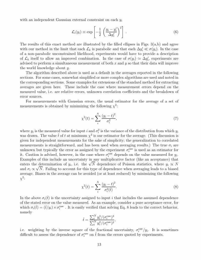
The results of this exact method are illustrated by the filled ellipses in Figs. 3(a,b) and agreewith our method in the limit that each Lk is parabolic and that each ∆y′i ≪ σ(yi). In the caseof a non-parabolic unconstrained likelihood, experiments would have to provide a descriptionof Lk itself to allow an improved combination. In the case of σ(yi) ≃ ∆y′i, experiments areadvised to perform a simultaneous measurement of both x and y so that their data will improvethe world knowledge about y.
The algorithm described above is used as a default in the averages reported in the followingsections. For some cases, somewhat simplified or more complex algorithms are used and noted inthe corresponding sections. Some examples for extensions of the standard method for extractingaverages are given here. These include the case where measurement errors depend on themeasured value, i.e. are relative errors, unknown correlation coefficients and the breakdown oferror sources.
For measurements with Gaussian errors, the usual estimator for the average of a set ofmeasurements is obtained by minimizing the following χ2:
χ2(t) =
N∑
i
(yi − t)2
σ2i
, (7)
where yi is the measured value for input i and σ2i is the variance of the distribution from which yi
was drawn. The value t of t at minimum χ2 is our estimator for the average. (This discussion isgiven for independent measurements for the sake of simplicity; the generalization to correlatedmeasurements is straightforward, and has been used when averaging results.) The true σi areunknown but typically the error as assigned by the experiment σraw
i is used as an estimator forit. Caution is advised, however, in the case where σraw
i depends on the value measured for yi.Examples of this include an uncertainty in any multiplicative factor (like an acceptance) thatenters the determination of yi, i.e. the
√N dependence of Poisson statistics, where yi ∝ N
and σi ∝√N . Failing to account for this type of dependence when averaging leads to a biased
average. Biases in the average can be avoided (or at least reduced) by minimizing the followingχ2:
χ2(t) =
N∑
i
(yi − t)2
σ2i (t)
. (8)
In the above σi(t) is the uncertainty assigned to input i that includes the assumed dependenceof the stated error on the value measured. As an example, consider a pure acceptance error, forwhich σi(t) = (t/yi)×σraw
i . It is easily verified that solving Eq. 8 leads to the correct behavior,namely
t =
∑Ni y
3i /(σ
rawi )2
∑Ni y
2i /(σ
rawi )2
,
i.e. weighting by the inverse square of the fractional uncertainty, σrawi /yi. It is sometimes
difficult to assess the dependence of σrawi on t from the errors quoted by experiments.
13
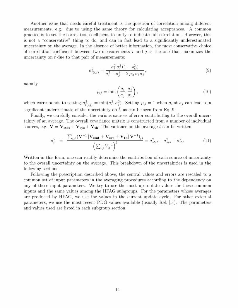
Another issue that needs careful treatment is the question of correlation among differentmeasurements, e.g. due to using the same theory for calculating acceptances. A commonpractice is to set the correlation coefficient to unity to indicate full correlation. However, thisis not a “conservative” thing to do, and can in fact lead to a significantly underestimateduncertainty on the average. In the absence of better information, the most conservative choiceof correlation coefficient between two measurements i and j is the one that maximizes theuncertainty on t due to that pair of measurements:
σ2t(i,j) =
σ2i σ
2j (1− ρ2ij)
σ2i + σ2
j − 2 ρij σi σj, (9)
namely
ρij = min
(
σiσj,σjσi
)
, (10)
which corresponds to setting σ2t(i,j)
= min(σ2i , σ
2j ). Setting ρij = 1 when σi 6= σj can lead to a
significant underestimate of the uncertainty on t, as can be seen from Eq. 9.Finally, we carefully consider the various sources of error contributing to the overall uncer-
tainty of an average. The overall covariance matrix is constructed from a number of individualsources, e.g. V = Vstat +Vsys +Vth. The variance on the average t can be written
σ2t =
∑
i,j (V−1 [Vstat +Vsys +Vth]V
−1)ij(
∑
i,j V−1ij
)2 = σ2stat + σ2
sys + σ2th. (11)
Written in this form, one can readily determine the contribution of each source of uncertaintyto the overall uncertainty on the average. This breakdown of the uncertainties is used in thefollowing sections.
Following the prescription described above, the central values and errors are rescaled to acommon set of input parameters in the averaging procedures according to the dependency onany of these input parameters. We try to use the most up-to-date values for these commoninputs and the same values among the HFAG subgroups. For the parameters whose averagesare produced by HFAG, we use the values in the current update cycle. For other externalparameters, we use the most recent PDG values available (usually Ref. [5]). The parametersand values used are listed in each subgroup section.
14
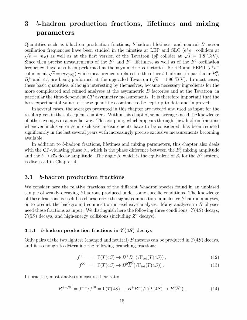
3 b-hadron production fractions, lifetimes and mixing
parameters
Quantities such as b-hadron production fractions, b-hadron lifetimes, and neutral B-mesonoscillation frequencies have been studied in the nineties at LEP and SLC (e+e− colliders at√s = mZ) as well as at the first version of the Tevatron (pp collider at
√s = 1.8 TeV).
Since then precise measurements of the B0 and B+ lifetimes, as well as of the B0 oscillationfrequency, have also been performed at the asymmetric B factories, KEKB and PEPII (e+e−
colliders at√s = mΥ (4S)) while measurements related to the other b-hadrons, in particular B0
s ,B+c and Λ0
b , are being performed at the upgraded Tevatron (√s = 1.96 TeV). In most cases,
these basic quantities, although interesting by themselves, became necessary ingredients for themore complicated and refined analyses at the asymmetric B factories and at the Tevatron, inparticular the time-dependent CP asymmetry measurements. It is therefore important that thebest experimental values of these quantities continue to be kept up-to-date and improved.
In several cases, the averages presented in this chapter are needed and used as input for theresults given in the subsequent chapters. Within this chapter, some averages need the knowledgeof other averages in a circular way. This coupling, which appears through the b-hadron fractionswhenever inclusive or semi-exclusive measurements have to be considered, has been reducedsignificantly in the last several years with increasingly precise exclusive measurements becomingavailable.
In addition to b-hadron fractions, lifetimes and mixing parameters, this chapter also dealswith the CP-violating phase βs, which is the phase difference between the B0
s mixing amplitudeand the b→ ccs decay amplitude. The angle β, which is the equivalent of βs for the B
0 system,is discussed in Chapter 4.
3.1 b-hadron production fractions
We consider here the relative fractions of the different b-hadron species found in an unbiasedsample of weakly-decaying b hadrons produced under some specific conditions. The knowledgeof these fractions is useful to characterize the signal composition in inclusive b-hadron analyses,or to predict the background composition in exclusive analyses. Many analyses in B physicsneed these fractions as input. We distinguish here the following three conditions: Υ (4S) decays,Υ (5S) decays, and high-energy collisions (including Z0 decays).
3.1.1 b-hadron production fractions in Υ (4S) decays
Only pairs of the two lightest (charged and neutral) B mesons can be produced in Υ (4S) decays,and it is enough to determine the following branching fractions:
f+− = Γ(Υ (4S) → B+B−)/Γtot(Υ (4S)) , (12)
f 00 = Γ(Υ (4S) → B0B0)/Γtot(Υ (4S)) . (13)
In practice, most analyses measure their ratio
R+−/00 = f+−/f 00 = Γ(Υ (4S) → B+B−)/Γ(Υ (4S) → B0B0) , (14)
15
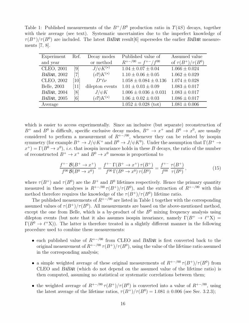
Table 1: Published measurements of the B+/B0 production ratio in Υ (4S) decays, togetherwith their average (see text). Systematic uncertainties due to the imperfect knowledge ofτ(B+)/τ(B0) are included. The latest BABAR result[6] supersedes the earlier BABAR measure-ments [7, 8].
Experiment Ref. Decay modes Published value of Assumed valueand year or method R+−/00 = f+−/f 00 of τ(B+)/τ(B0)
CLEO, 2001 [9] J/ψK(∗) 1.04± 0.07± 0.04 1.066± 0.024BABAR, 2002 [7] (cc)K(∗) 1.10± 0.06± 0.05 1.062± 0.029CLEO, 2002 [10] D∗ℓν 1.058± 0.084± 0.136 1.074± 0.028Belle, 2003 [11] dilepton events 1.01± 0.03± 0.09 1.083± 0.017BABAR, 2004 [8] J/ψK 1.006± 0.036± 0.031 1.083± 0.017BABAR, 2005 [6] (cc)K(∗) 1.06± 0.02± 0.03 1.086± 0.017Average 1.052± 0.028 (tot) 1.081± 0.006
which is easier to access experimentally. Since an inclusive (but separate) reconstruction ofB+ and B0 is difficult, specific exclusive decay modes, B+ → x+ and B0 → x0, are usuallyconsidered to perform a measurement of R+−/00, whenever they can be related by isospinsymmetry (for example B+ → J/ψK+ and B0 → J/ψK0). Under the assumption that Γ(B+ →x+) = Γ(B0 → x0), i.e. that isospin invariance holds in these B decays, the ratio of the numberof reconstructed B+ → x+ and B0 → x0 mesons is proportional to
f+− B(B+ → x+)
f 00 B(B0 → x0)=f+− Γ(B+ → x+) τ(B+)
f 00 Γ(B0 → x0) τ(B0)=f+−
f 00
τ(B+)
τ(B0), (15)
where τ(B+) and τ(B0) are the B+ and B0 lifetimes respectively. Hence the primary quantitymeasured in these analyses is R+−/00 τ(B+)/τ(B0), and the extraction of R+−/00 with thismethod therefore requires the knowledge of the τ(B+)/τ(B0) lifetime ratio.
The published measurements of R+−/00 are listed in Table 1 together with the correspondingassumed values of τ(B+)/τ(B0). All measurements are based on the above-mentioned method,except the one from Belle, which is a by-product of the B0 mixing frequency analysis usingdilepton events (but note that it also assumes isospin invariance, namely Γ(B+ → ℓ+X) =Γ(B0 → ℓ+X)). The latter is therefore treated in a slightly different manner in the followingprocedure used to combine these measurements:
• each published value of R+−/00 from CLEO and BABAR is first converted back to theoriginal measurement ofR+−/00 τ(B+)/τ(B0), using the value of the lifetime ratio assumedin the corresponding analysis;
• a simple weighted average of these original measurements of R+−/00 τ(B+)/τ(B0) fromCLEO and BABAR (which do not depend on the assumed value of the lifetime ratio) isthen computed, assuming no statistical or systematic correlations between them;
• the weighted average of R+−/00 τ(B+)/τ(B0) is converted into a value of R+−/00, usingthe latest average of the lifetime ratios, τ(B+)/τ(B0) = 1.081± 0.006 (see Sec. 3.2.3);
16
• the Belle measurement of R+−/00 is adjusted to the current values of τ(B0) = 1.518 ±0.007 ps and τ(B+)/τ(B0) = 1.081± 0.006 (see Sec. 3.2.3), using the quoted systematicuncertainties due to these parameters;
• the combined value of R+−/00 from CLEO and BABAR is averaged with the adjusted valueof R+−/00 from Belle, assuming a 100% correlation of the systematic uncertainty due tothe limited knowledge on τ(B+)/τ(B0); no other correlation is considered.
The resulting global average,
R+−/00 =f+−
f 00= 1.052± 0.028 , (16)
is consistent with an equal production of charged and neutral B mesons, although only at the1.9σ level.
On the other hand, the BABAR collaboration has performed a direct measurement of thef 00 fraction using a novel method, which does not rely on isospin symmetry nor requires theknowledge of τ(B+)/τ(B0). Its analysis, based on a comparison between the number of eventswhere a single B0 → D∗−ℓ+ν decay could be reconstructed and the number of events wheretwo such decays could be reconstructed, yields [12]
f 00 = 0.487± 0.010 (stat)± 0.008 (syst) . (17)
The two results of Eqs. (16) and (17) are of very different natures and completely indepen-dent of each other. Their product is equal to f+− = 0.512± 0.019, while another combinationof them gives f+−+f 00 = 0.999±0.030, compatible with unity. Assuming1 f+−+f 00 = 1, alsoconsistent with CLEO’s observation that the fraction of Υ (4S) decays to BB pairs is largerthan 0.96 at 95% CL [14], the results of Eqs. (16) and (17) can be averaged (first convertingEq. (16) into a value of f 00 = 1/(R+−/00 + 1)) to yield the following more precise estimates:
f 00 = 0.487± 0.006 , f+− = 1− f 00 = 0.513± 0.006 ,f+−
f 00= 1.052± 0.025 . (18)
The latter ratio differs from one by 2.1σ.
3.1.2 b-hadron production fractions in Υ (5S) decays
Hadronic events produced in e+e− collisions at the Υ (5S) energy can be classified into threecategories: light-quark (u, d, s, c) continuum events, bb continuum events, and Υ (5S) events.The latter two cannot be distinguished and will be called bb events in the following. These bbevents, which also include bbγ events because of possible initial-state radiation, can hadronizein different final states. We define f
Υ (5S)u,d as the fraction of bb events with a pair of non-strange
bottom mesons (final states BB, BB∗, B∗B, B∗B
∗, BBπ, BB
∗π, B∗Bπ, B∗B
∗π, and BBππ,
where B denotes a B0 or B+ meson and B denotes a B0or B− meson), f
Υ (5S)s as the fraction of
1A few non-BB decay modes of the Υ (4S) (Υ (1S)π+π−, Υ (2S)π+π−, Υ (1S)η) have been observed withbranching fractions of the order of 10−4 [13], corresponding to a partial width several times larger than that inthe e+e− channel. However, this can still be neglected and the assumption f+− + f00 = 1 remains valid in thepresent context of the determination of f+− and f00.
17
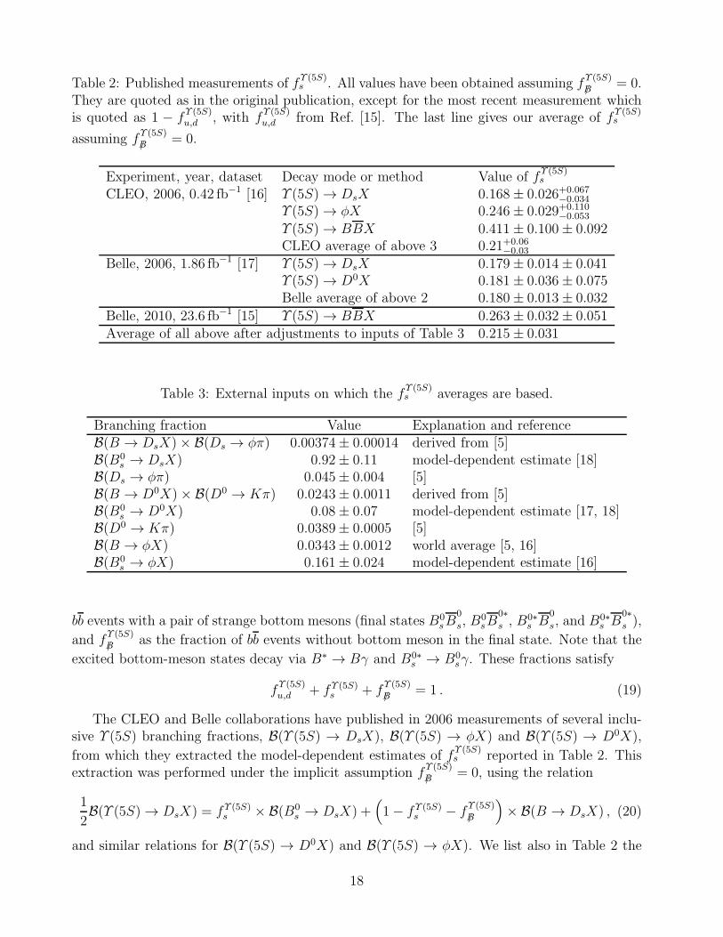
Table 2: Published measurements of fΥ (5S)s . All values have been obtained assuming f
Υ (5S)B/ = 0.
They are quoted as in the original publication, except for the most recent measurement whichis quoted as 1 − f
Υ (5S)u,d , with f
Υ (5S)u,d from Ref. [15]. The last line gives our average of f
Υ (5S)s
assuming fΥ (5S)B/ = 0.
Experiment, year, dataset Decay mode or method Value of fΥ (5S)s
CLEO, 2006, 0.42 fb−1 [16] Υ (5S) → DsX 0.168± 0.026+0.067−0.034
Υ (5S) → φX 0.246± 0.029+0.110−0.053
Υ (5S) → BBX 0.411± 0.100± 0.092CLEO average of above 3 0.21+0.06
−0.03
Belle, 2006, 1.86 fb−1 [17] Υ (5S) → DsX 0.179± 0.014± 0.041Υ (5S) → D0X 0.181± 0.036± 0.075Belle average of above 2 0.180± 0.013± 0.032
Belle, 2010, 23.6 fb−1 [15] Υ (5S) → BBX 0.263± 0.032± 0.051Average of all above after adjustments to inputs of Table 3 0.215± 0.031
Table 3: External inputs on which the fΥ (5S)s averages are based.
Branching fraction Value Explanation and referenceB(B → DsX)× B(Ds → φπ) 0.00374± 0.00014 derived from [5]B(B0
s → DsX) 0.92± 0.11 model-dependent estimate [18]B(Ds → φπ) 0.045± 0.004 [5]B(B → D0X)× B(D0 → Kπ) 0.0243± 0.0011 derived from [5]B(B0
s → D0X) 0.08± 0.07 model-dependent estimate [17, 18]B(D0 → Kπ) 0.0389± 0.0005 [5]B(B → φX) 0.0343± 0.0012 world average [5, 16]B(B0
s → φX) 0.161± 0.024 model-dependent estimate [16]
bb events with a pair of strange bottom mesons (final states B0sB
0
s, B0sB
0∗
s , B0∗s B
0
s, and B0∗s B
0∗
s ),
and fΥ (5S)B/ as the fraction of bb events without bottom meson in the final state. Note that the
excited bottom-meson states decay via B∗ → Bγ and B0∗s → B0
sγ. These fractions satisfy
fΥ (5S)u,d + fΥ (5S)s + f
Υ (5S)B/ = 1 . (19)
The CLEO and Belle collaborations have published in 2006 measurements of several inclu-sive Υ (5S) branching fractions, B(Υ (5S) → DsX), B(Υ (5S) → φX) and B(Υ (5S) → D0X),
from which they extracted the model-dependent estimates of fΥ (5S)s reported in Table 2. This
extraction was performed under the implicit assumption fΥ (5S)B/ = 0, using the relation
1
2B(Υ (5S) → DsX) = fΥ (5S)s × B(B0
s → DsX) +(
1− fΥ (5S)s − fΥ (5S)B/
)
× B(B → DsX) , (20)
and similar relations for B(Υ (5S) → D0X) and B(Υ (5S) → φX). We list also in Table 2 the
18
values of fΥ (5S)s derived from measurements of f
Υ (5S)u,d = B(Υ (5S) → BBX) [16, 15], as well as
our average value of fΥ (5S)s , all obtained under the assumption f
Υ (5S)B/ = 0.
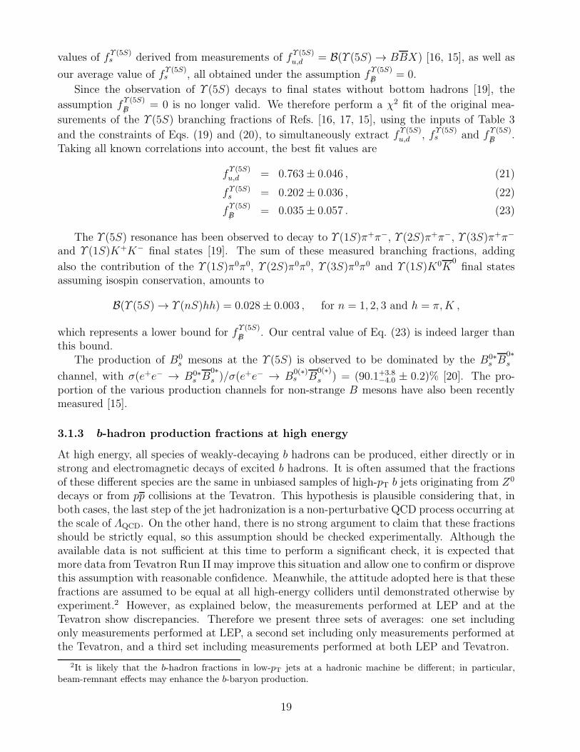
Since the observation of Υ (5S) decays to final states without bottom hadrons [19], the
assumption fΥ (5S)B/ = 0 is no longer valid. We therefore perform a χ2 fit of the original mea-
surements of the Υ (5S) branching fractions of Refs. [16, 17, 15], using the inputs of Table 3
and the constraints of Eqs. (19) and (20), to simultaneously extract fΥ (5S)u,d , f
Υ (5S)s and f
Υ (5S)B/ .
Taking all known correlations into account, the best fit values are
fΥ (5S)u,d = 0.763± 0.046 , (21)
fΥ (5S)s = 0.202± 0.036 , (22)
fΥ (5S)B/ = 0.035± 0.057 . (23)
The Υ (5S) resonance has been observed to decay to Υ (1S)π+π−, Υ (2S)π+π−, Υ (3S)π+π−
and Υ (1S)K+K− final states [19]. The sum of these measured branching fractions, adding
also the contribution of the Υ (1S)π0π0, Υ (2S)π0π0, Υ (3S)π0π0 and Υ (1S)K0K0final states
assuming isospin conservation, amounts to
B(Υ (5S) → Υ (nS)hh) = 0.028± 0.003 , for n = 1, 2, 3 and h = π,K ,
which represents a lower bound for fΥ (5S)B/ . Our central value of Eq. (23) is indeed larger than
this bound.The production of B0
s mesons at the Υ (5S) is observed to be dominated by the B0∗s B
0∗
s
channel, with σ(e+e− → B0∗s B
0∗
s )/σ(e+e− → B0(∗)s B
0(∗)
s ) = (90.1+3.8−4.0 ± 0.2)% [20]. The pro-
portion of the various production channels for non-strange B mesons have also been recentlymeasured [15].
3.1.3 b-hadron production fractions at high energy
At high energy, all species of weakly-decaying b hadrons can be produced, either directly or instrong and electromagnetic decays of excited b hadrons. It is often assumed that the fractionsof these different species are the same in unbiased samples of high-pT b jets originating from Z0
decays or from pp collisions at the Tevatron. This hypothesis is plausible considering that, inboth cases, the last step of the jet hadronization is a non-perturbative QCD process occurring atthe scale of ΛQCD. On the other hand, there is no strong argument to claim that these fractionsshould be strictly equal, so this assumption should be checked experimentally. Although theavailable data is not sufficient at this time to perform a significant check, it is expected thatmore data from Tevatron Run II may improve this situation and allow one to confirm or disprovethis assumption with reasonable confidence. Meanwhile, the attitude adopted here is that thesefractions are assumed to be equal at all high-energy colliders until demonstrated otherwise byexperiment.2 However, as explained below, the measurements performed at LEP and at theTevatron show discrepancies. Therefore we present three sets of averages: one set includingonly measurements performed at LEP, a second set including only measurements performed atthe Tevatron, and a third set including measurements performed at both LEP and Tevatron.
2It is likely that the b-hadron fractions in low-pT jets at a hadronic machine be different; in particular,beam-remnant effects may enhance the b-baryon production.
19
Contrary to what happens in the charm sector where the fractions of D+ and D0 aredifferent, the relative amount of B+ and B0 is not affected by the electromagnetic decays ofexcited B+∗
and B0∗ states and strong decays of excited B+∗∗and B0∗∗ states. Decays of the
type B0s∗∗ → B(∗)K also contribute to the B+ and B0 rates, but with the same magnitude if
mass effects can be neglected. We therefore assume equal production of B+ and B0. We alsoneglect the production of weakly-decaying states made of several heavy quarks (like B+
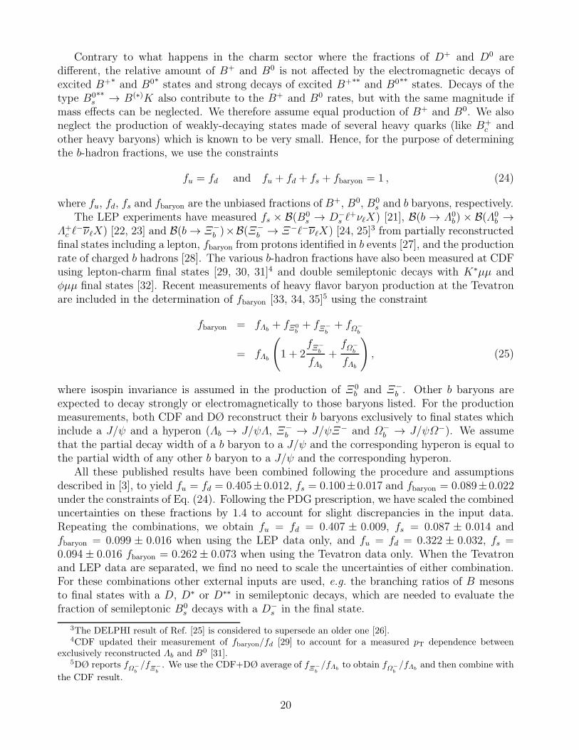
c andother heavy baryons) which is known to be very small. Hence, for the purpose of determiningthe b-hadron fractions, we use the constraints
fu = fd and fu + fd + fs + fbaryon = 1 , (24)
where fu, fd, fs and fbaryon are the unbiased fractions of B+, B0, B0s and b baryons, respectively.
The LEP experiments have measured fs × B(B0s → D−
s ℓ+νℓX) [21], B(b → Λ0
b) × B(Λ0b →
Λ+c ℓ
−νℓX) [22, 23] and B(b→ Ξ−b )×B(Ξ−
b → Ξ−ℓ−νℓX) [24, 25]3 from partially reconstructedfinal states including a lepton, fbaryon from protons identified in b events [27], and the productionrate of charged b hadrons [28]. The various b-hadron fractions have also been measured at CDFusing lepton-charm final states [29, 30, 31]4 and double semileptonic decays with K∗µµ andφµµ final states [32]. Recent measurements of heavy flavor baryon production at the Tevatronare included in the determination of fbaryon [33, 34, 35]5 using the constraint
fbaryon = fΛb + fΞ0b+ fΞ−
b+ fΩ−
b
= fΛb
(
1 + 2fΞ−
b
fΛb+fΩ−
b
fΛb
)
, (25)
where isospin invariance is assumed in the production of Ξ0b and Ξ−
b . Other b baryons areexpected to decay strongly or electromagnetically to those baryons listed. For the productionmeasurements, both CDF and DØ reconstruct their b baryons exclusively to final states whichinclude a J/ψ and a hyperon (Λb → J/ψΛ, Ξ−
b → J/ψΞ− and Ω−b → J/ψΩ−). We assume
that the partial decay width of a b baryon to a J/ψ and the corresponding hyperon is equal tothe partial width of any other b baryon to a J/ψ and the corresponding hyperon.
All these published results have been combined following the procedure and assumptionsdescribed in [3], to yield fu = fd = 0.405±0.012, fs = 0.100±0.017 and fbaryon = 0.089±0.022under the constraints of Eq. (24). Following the PDG prescription, we have scaled the combineduncertainties on these fractions by 1.4 to account for slight discrepancies in the input data.Repeating the combinations, we obtain fu = fd = 0.407 ± 0.009, fs = 0.087 ± 0.014 andfbaryon = 0.099 ± 0.016 when using the LEP data only, and fu = fd = 0.322 ± 0.032, fs =0.094± 0.016 fbaryon = 0.262± 0.073 when using the Tevatron data only. When the Tevatronand LEP data are separated, we find no need to scale the uncertainties of either combination.For these combinations other external inputs are used, e.g. the branching ratios of B mesonsto final states with a D, D∗ or D∗∗ in semileptonic decays, which are needed to evaluate thefraction of semileptonic B0
s decays with a D−s in the final state.
3The DELPHI result of Ref. [25] is considered to supersede an older one [26].4CDF updated their measurement of fbaryon/fd [29] to account for a measured pT dependence between
exclusively reconstructed Λb and B0 [31].5DØ reports fΩ−
b/fΞ−
b. We use the CDF+DØ average of fΞ−
b/fΛb
to obtain fΩ−b/fΛb
and then combine with
the CDF result.
20
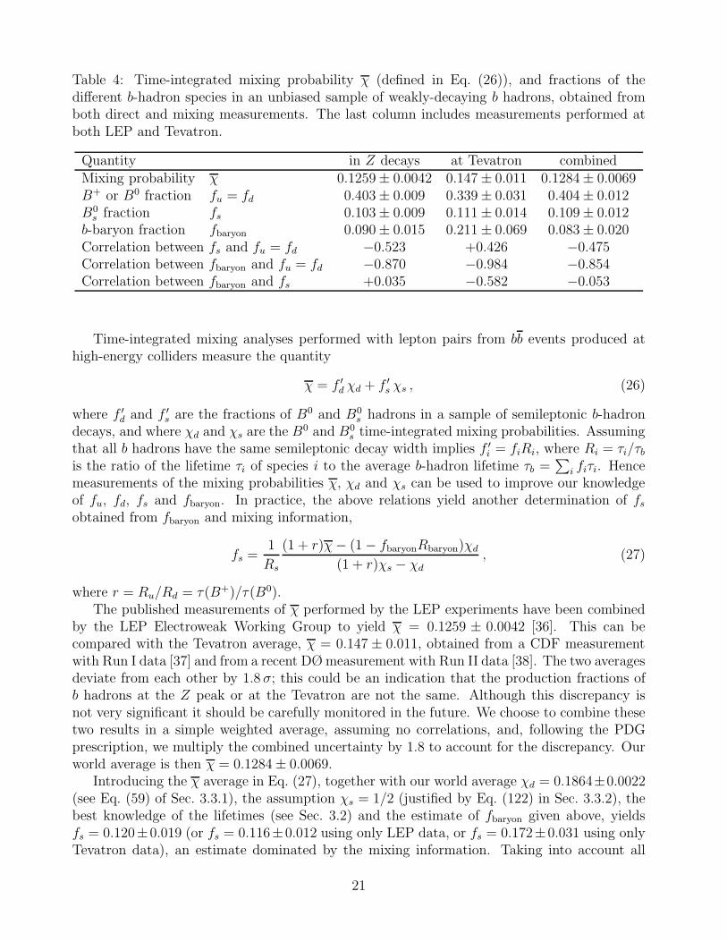
Table 4: Time-integrated mixing probability χ (defined in Eq. (26)), and fractions of thedifferent b-hadron species in an unbiased sample of weakly-decaying b hadrons, obtained fromboth direct and mixing measurements. The last column includes measurements performed atboth LEP and Tevatron.
Quantity in Z decays at Tevatron combinedMixing probability χ 0.1259± 0.0042 0.147± 0.011 0.1284± 0.0069B+ or B0 fraction fu = fd 0.403± 0.009 0.339± 0.031 0.404± 0.012B0s fraction fs 0.103± 0.009 0.111± 0.014 0.109± 0.012
b-baryon fraction fbaryon 0.090± 0.015 0.211± 0.069 0.083± 0.020Correlation between fs and fu = fd −0.523 +0.426 −0.475Correlation between fbaryon and fu = fd −0.870 −0.984 −0.854Correlation between fbaryon and fs +0.035 −0.582 −0.053
Time-integrated mixing analyses performed with lepton pairs from bb events produced athigh-energy colliders measure the quantity
χ = f ′d χd + f ′
s χs , (26)
where f ′d and f ′
s are the fractions of B0 and B0s hadrons in a sample of semileptonic b-hadron
decays, and where χd and χs are the B0 and B0
s time-integrated mixing probabilities. Assumingthat all b hadrons have the same semileptonic decay width implies f ′
i = fiRi, where Ri = τi/τbis the ratio of the lifetime τi of species i to the average b-hadron lifetime τb =
∑
i fiτi. Hencemeasurements of the mixing probabilities χ, χd and χs can be used to improve our knowledgeof fu, fd, fs and fbaryon. In practice, the above relations yield another determination of fsobtained from fbaryon and mixing information,
fs =1
Rs
(1 + r)χ− (1− fbaryonRbaryon)χd(1 + r)χs − χd
, (27)
where r = Ru/Rd = τ(B+)/τ(B0).The published measurements of χ performed by the LEP experiments have been combined
by the LEP Electroweak Working Group to yield χ = 0.1259 ± 0.0042 [36]. This can becompared with the Tevatron average, χ = 0.147 ± 0.011, obtained from a CDF measurementwith Run I data [37] and from a recent DØmeasurement with Run II data [38]. The two averagesdeviate from each other by 1.8 σ; this could be an indication that the production fractions ofb hadrons at the Z peak or at the Tevatron are not the same. Although this discrepancy isnot very significant it should be carefully monitored in the future. We choose to combine thesetwo results in a simple weighted average, assuming no correlations, and, following the PDGprescription, we multiply the combined uncertainty by 1.8 to account for the discrepancy. Ourworld average is then χ = 0.1284± 0.0069.
Introducing the χ average in Eq. (27), together with our world average χd = 0.1864±0.0022(see Eq. (59) of Sec. 3.3.1), the assumption χs = 1/2 (justified by Eq. (122) in Sec. 3.3.2), thebest knowledge of the lifetimes (see Sec. 3.2) and the estimate of fbaryon given above, yieldsfs = 0.120±0.019 (or fs = 0.116±0.012 using only LEP data, or fs = 0.172±0.031 using onlyTevatron data), an estimate dominated by the mixing information. Taking into account all
21
known correlations (including the one introduced by fbaryon), this result is then combined withthe set of fractions obtained from direct measurements (given above), to yield the improvedestimates of Table 4, still under the constraints of Eq. (24).6 As can be seen, our knowledge onthe mixing parameters substantially reduces the uncertainty on fs, and this even in the case ofthe world averages where a rather strong deweighting was introduced in the computation of χ.It should be noted that the results are correlated, as indicated in Table 4.
3.2 b-hadron lifetimes
In the spectator model the decay of b-flavored hadrons Hb is governed entirely by the flavorchanging b→ Wq transition (q = c, u). For this very reason, lifetimes of all b-flavored hadronsare the same in the spectator approximation regardless of the (spectator) quark content of theHb. In the early 1990’s experiments became sophisticated enough to start seeing the differencesof the lifetimes among various Hb species. The first theoretical calculations of the spectatorquark effects on Hb lifetime emerged only few years earlier.
Currently, most of such calculations are performed in the framework of the Heavy QuarkExpansion, HQE. In the HQE, under certain assumptions (most important of which is that ofquark-hadron duality), the decay rate of an Hb to an inclusive final state f is expressed as thesum of a series of expectation values of operators of increasing dimension, multiplied by thecorrespondingly higher powers of ΛQCD/mb:
ΓHb→f = |CKM |2∑
n
c(f)n
(ΛQCD
mb
)n
〈Hb|On|Hb〉, (28)
where |CKM |2 is the relevant combination of the CKM matrix elements. Coefficients c(f)n of
this expansion, known as Operator Product Expansion [39], can be calculated perturbatively.Hence, the HQE predicts ΓHb→f in the form of an expansion in both ΛQCD/mb and αs(mb). Theprecision of current experiments makes it mandatory to go to the next-to-leading order in QCD,i.e. to include correction of the order of αs(mb) to the c
(f)n ’s. All non-perturbative physics is
shifted into the expectation values 〈Hb|On|Hb〉 of operators On. These can be calculated usinglattice QCD or QCD sum rules, or can be related to other observables via the HQE [40]. Onemay reasonably expect that powers of ΛQCD/mb provide enough suppression that only the firstfew terms of the sum in Eq. (28) matter.
Theoretical predictions are usually made for the ratios of the lifetimes (with τ(B0) chosenas the common denominator) rather than for the individual lifetimes, for this allows severaluncertainties to cancel. The precision of the current HQE calculations (see Refs. [41, 42, 43] forthe latest updates) is in some instances already surpassed by the measurements, e.g. in the caseof τ(B+)/τ(B0). Also, HQE calculations are not assumption-free. More accurate predictionsare a matter of progress in the evaluation of the non-perturbative hadronic matrix elementsand verifying the assumptions that the calculations are based upon. However, the HQE, evenin its present shape, draws a number of important conclusions, which are in agreement withexperimental observations:
6The combined value of fbaryon is smaller than the results from either LEP or Tevatron separately. Thisseemingly surprising result arises from the smaller uncertainties on the other fractions and the application ofthe unitarity constraint of Eq. (24).
22
• The heavier the mass of the heavy quark the smaller is the variation in the lifetimes amongdifferent hadrons containing this quark, which is to say that as mb → ∞ we retrieve thespectator picture in which the lifetimes of all Hb’s are the same. This is well illustrated bythe fact that lifetimes are rather similar in the b sector, while they differ by large factorsin the c sector (mc < mb).
• The non-perturbative corrections arise only at the order of Λ2QCD/m
2b , which translates
into differences among Hb lifetimes of only a few percent.
• It is only the difference between meson and baryon lifetimes that appears at the Λ2QCD/m
2b
level. The splitting of the meson lifetimes occurs at the Λ3QCD/m
3b level, yet it is enhanced
by a phase space factor 16π2 with respect to the leading free b decay.
To ensure that certain sources of systematic uncertainty cancel, lifetime analyses are some-times designed to measure a ratio of lifetimes. However, because of the differences in decaytopologies, abundance (or lack thereof) of decays of a certain kind, etc., measurements of the in-dividual lifetimes are more common. In the following section we review the most common typesof the lifetime measurements. This discussion is followed by the presentation of the averagingof the various lifetime measurements, each with a brief description of its particularities.
3.2.1 Lifetime measurements, uncertainties and correlations
In most cases lifetime of an Hb is estimated from a flight distance and a βγ factor which is usedto convert the geometrical distance into the proper decay time. Methods of accessing lifetimeinformation can roughly be divided in the following five categories:
1. Inclusive (flavor-blind) measurements. These measurements are aimed at extract-ing the lifetime from a mixture of b-hadron decays, without distinguishing the decayingspecies. Often the knowledge of the mixture composition is limited, which makes thesemeasurements experiment-specific. Also, these measurements have to rely on Monte Carlofor estimating the βγ factor, because the decaying hadrons are not fully reconstructed.On the bright side, these usually are the largest statistics b-hadron lifetime measurementsthat are accessible to a given experiment, and can, therefore, serve as an important per-formance benchmark.
2. Measurements in semileptonic decays of a specific Hb. W from b → Wc pro-duces ℓνl pair (ℓ = e, µ) in about 21% of the cases. Electron or muon from such decays isusually a well-detected signature, which provides for clean and efficient trigger. c quarkfrom b→ Wc transition and the other quark(s) making up the decaying Hb combine intoa charm hadron, which is reconstructed in one or more exclusive decay channels. Know-ing what this charmed hadron is allows one to separate, at least statistically, different Hb
species. The advantage of these measurements is in statistics, which usually is superiorto that of the exclusively reconstructed Hb decays. Some of the main disadvantages arerelated to the difficulty of estimating lepton+charm sample composition and Monte Carloreliance for the βγ factor estimate.
3. Measurements in exclusively reconstructed hadronic decays. These have the ad-vantage of complete reconstruction of decaying Hb, which allows one to infer the decaying
23
species as well as to perform precise measurement of the βγ factor. Both lead to gener-ally smaller systematic uncertainties than in the above two categories. The downsides aresmaller branching ratios, larger combinatoric backgrounds, especially in Hb → Hcπ(ππ)and multi-body Hc decays, or in a hadron collider environment with non-trivial under-lying event. Hb → J/ψHs are relatively clean and easy to trigger on J/ψ → ℓ+ℓ−, buttheir branching fraction is only about 1%.
4. Measurements at asymmetric B factories.
In the Υ (4S) → BB decay, the B mesons (B+ or B0) are essentially at rest in the Υ (4S)frame. This makes direct lifetime measurements impossible in experiments at symmetriccolliders producing Υ (4S) at rest. At asymmetric B factories the Υ (4S) meson is boostedresulting in B and B moving nearly parallel to each other with the same boost. Thelifetime is inferred from the distance ∆z separating the B and B decay vertices along thebeam axis and from the Υ (4S) boost known from the beam energies. This boost is equalto βγ ≈ 0.55 (0.43) in the BABAR (Belle) experiment, resulting in an average B decaylength of approximately 250 (190) µm.
In order to determine the charge of the B mesons in each event, one of the them is fullyreconstructed in a semileptonic or hadronic decay mode. The other B is typically notfully reconstructed, only the position of its decay vertex is determined from the remainingtracks in the event. These measurements benefit from large statistics, but suffer from poorproper time resolution, comparable to the B lifetime itself. This resolution is dominatedby the uncertainty on the decay vertices, which is typically 50 (100) µm for a fully(partially) reconstructed B meson. With very large future statistics, the resolution andpurity could be improved (and hence the systematics reduced) by fully reconstructingboth B mesons in the event.
5. Direct measurement of lifetime ratios. This method has so far been only appliedin the measurement of τ(B+)/τ(B0). The ratio of the lifetimes is extracted from thedependence of the observed relative number of B+ and B0 candidates (both reconstructedin semileptonic decays) on the proper decay time.
In some of the latest analyses, measurements of two (e.g. τ(B+) and τ(B+)/τ(B0)) or three(e.g. τ(B+), τ(B+)/τ(B0), and ∆md) quantities are combined. This introduces correlationsamong measurements. Another source of correlations among the measurements are the sys-tematic effects, which could be common to an experiment or to an analysis technique acrossthe experiments. When calculating the averages, such correlations are taken into account pergeneral procedure, described in Ref. [44].
3.2.2 Inclusive b-hadron lifetimes
The inclusive b hadron lifetime is defined as τb =∑
i fiτi where τi are the individual specieslifetimes and fi are the fractions of the various species present in an unbiased sample of weakly-decaying b hadrons produced at a high-energy collider.7 This quantity is certainly less fun-damental than the lifetimes of the individual species, the latter being much more useful in
7In principle such a quantity could be slightly different in Z decays and at the Tevatron, in case the fractionsof b-hadron species are not exactly the same; see the discussion in Sec. 3.1.3.
24
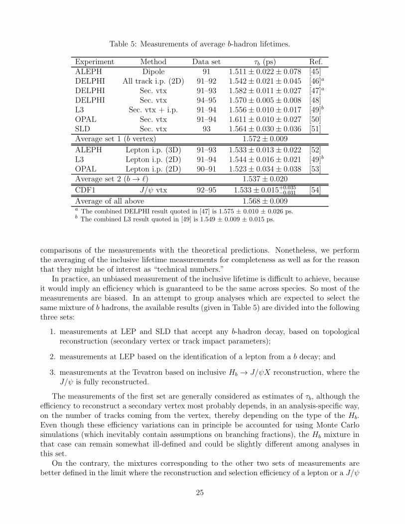
Table 5: Measurements of average b-hadron lifetimes.
Experiment Method Data set τb (ps) Ref.ALEPH Dipole 91 1.511± 0.022± 0.078 [45]DELPHI All track i.p. (2D) 91–92 1.542± 0.021± 0.045 [46]a
DELPHI Sec. vtx 91–93 1.582± 0.011± 0.027 [47]a
DELPHI Sec. vtx 94–95 1.570± 0.005± 0.008 [48]L3 Sec. vtx + i.p. 91–94 1.556± 0.010± 0.017 [49]b
OPAL Sec. vtx 91–94 1.611± 0.010± 0.027 [50]SLD Sec. vtx 93 1.564± 0.030± 0.036 [51]Average set 1 (b vertex) 1.572± 0.009
ALEPH Lepton i.p. (3D) 91–93 1.533± 0.013± 0.022 [52]L3 Lepton i.p. (2D) 91–94 1.544± 0.016± 0.021 [49]b
OPAL Lepton i.p. (2D) 90–91 1.523± 0.034± 0.038 [53]Average set 2 (b→ ℓ) 1.537± 0.020
CDF1 J/ψ vtx 92–95 1.533± 0.015+0.035−0.031 [54]
Average of all above 1.568± 0.009a The combined DELPHI result quoted in [47] is 1.575 ± 0.010 ± 0.026 ps.b The combined L3 result quoted in [49] is 1.549 ± 0.009 ± 0.015 ps.
comparisons of the measurements with the theoretical predictions. Nonetheless, we performthe averaging of the inclusive lifetime measurements for completeness as well as for the reasonthat they might be of interest as “technical numbers.”
In practice, an unbiased measurement of the inclusive lifetime is difficult to achieve, becauseit would imply an efficiency which is guaranteed to be the same across species. So most of themeasurements are biased. In an attempt to group analyses which are expected to select thesame mixture of b hadrons, the available results (given in Table 5) are divided into the followingthree sets:
1. measurements at LEP and SLD that accept any b-hadron decay, based on topologicalreconstruction (secondary vertex or track impact parameters);
2. measurements at LEP based on the identification of a lepton from a b decay; and
3. measurements at the Tevatron based on inclusive Hb → J/ψX reconstruction, where theJ/ψ is fully reconstructed.
The measurements of the first set are generally considered as estimates of τb, although theefficiency to reconstruct a secondary vertex most probably depends, in an analysis-specific way,on the number of tracks coming from the vertex, thereby depending on the type of the Hb.Even though these efficiency variations can in principle be accounted for using Monte Carlosimulations (which inevitably contain assumptions on branching fractions), the Hb mixture inthat case can remain somewhat ill-defined and could be slightly different among analyses inthis set.
On the contrary, the mixtures corresponding to the other two sets of measurements arebetter defined in the limit where the reconstruction and selection efficiency of a lepton or a J/ψ
25
from an Hb does not depend on the decaying hadron type. These mixtures are given by theproduction fractions and the inclusive branching fractions for each Hb species to give a leptonor a J/ψ. In particular, under the assumption that all b hadrons have the same semileptonicdecay width, the analyses of the second set should measure τ(b → ℓ) = (
∑
i fiτ2i )/(
∑
i fiτi)which is necessarily larger than τb if lifetime differences exist. Given the present knowledge onτi and fi, τ(b → ℓ)− τb is expected to be of the order of 0.01 ps.
Measurements by SLC and LEP experiments are subject to a number of common systematicuncertainties, such as those due to (lack of knowledge of) b and c fragmentation, b and c decaymodels, B(B → ℓ), B(B → c → ℓ), B(c → ℓ), τc, and Hb decay multiplicity. In the averaging,these systematic uncertainties are assumed to be 100% correlated. The averages for the setsdefined above (also given in Table 5) are
τ(b vertex) = 1.572± 0.009 ps , (29)
τ(b→ ℓ) = 1.537± 0.020 ps , (30)
τ(b → J/ψ) = 1.533+0.038−0.034 ps , (31)
whereas an average of all measurements, ignoring mixture differences, yields 1.568± 0.009 ps.
3.2.3 B0 and B+ lifetimes and their ratio
After a number of years of dominating these averages the LEP experiments yielded the sceneto the asymmetric B factories and the Tevatron experiments. The B factories have been verysuccessful in utilizing their potential – in only a few years of running, BABAR and, to a greaterextent, Belle, have struck a balance between the statistical and the systematic uncertainties,with both being close to (or even better than) the impressive 1%. In the meanwhile, CDFand DØ have emerged as significant contributors to the field as the Tevatron Run II dataflowed in. Both appear to enjoy relatively small systematic effects, and while current statisticaluncertainties of their measurements are factors of 2 to 4 larger than those of their B-factorycounterparts, both Tevatron experiments stand to increase their samples by almost an order ofmagnitude.
At present time we are in an interesting position of having three sets of measurements (fromLEP/SLC, B factories and the Tevatron) that originate from different environments, obtainedusing substantially different techniques and are precise enough for incisive comparison.
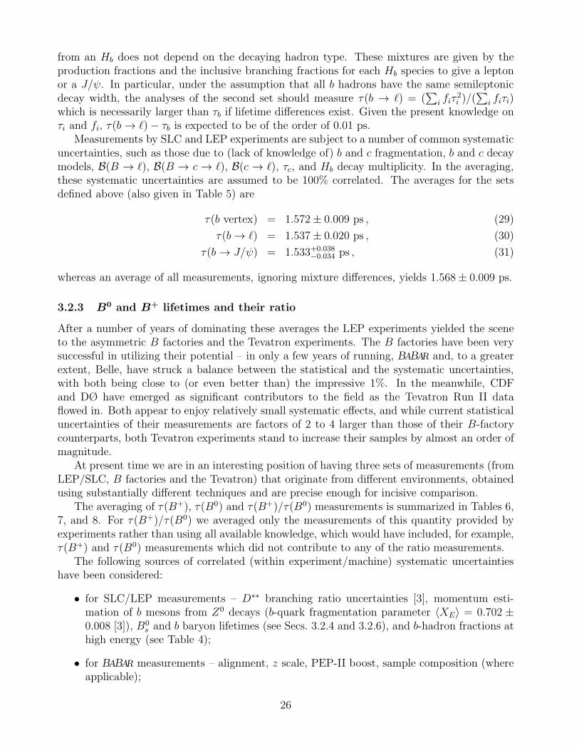
The averaging of τ(B+), τ(B0) and τ(B+)/τ(B0) measurements is summarized in Tables 6,7, and 8. For τ(B+)/τ(B0) we averaged only the measurements of this quantity provided byexperiments rather than using all available knowledge, which would have included, for example,τ(B+) and τ(B0) measurements which did not contribute to any of the ratio measurements.
The following sources of correlated (within experiment/machine) systematic uncertaintieshave been considered:
• for SLC/LEP measurements – D∗∗ branching ratio uncertainties [3], momentum esti-mation of b mesons from Z0 decays (b-quark fragmentation parameter 〈XE〉 = 0.702 ±0.008 [3]), B0
s and b baryon lifetimes (see Secs. 3.2.4 and 3.2.6), and b-hadron fractions athigh energy (see Table 4);
• for BABAR measurements – alignment, z scale, PEP-II boost, sample composition (whereapplicable);
26

Table 6: Measurements of the B0 lifetime.
Experiment Method Data set τ(B0) (ps) Ref.
ALEPH D(∗)ℓ 91–95 1.518± 0.053± 0.034 [55]ALEPH Exclusive 91–94 1.25+0.15
−0.13 ± 0.05 [56]ALEPH Partial rec. π+π− 91–94 1.49+0.17+0.08
−0.15−0.06 [56]DELPHI D(∗)ℓ 91–93 1.61+0.14
−0.13 ± 0.08 [57]DELPHI Charge sec. vtx 91–93 1.63± 0.14± 0.13 [58]DELPHI Inclusive D∗ℓ 91–93 1.532± 0.041± 0.040 [59]DELPHI Charge sec. vtx 94–95 1.531± 0.021± 0.031 [48]L3 Charge sec. vtx 94–95 1.52± 0.06± 0.04 [60]OPAL D(∗)ℓ 91–93 1.53± 0.12± 0.08 [61]OPAL Charge sec. vtx 93–95 1.523± 0.057± 0.053 [62]OPAL Inclusive D∗ℓ 91–00 1.541± 0.028± 0.023 [63]SLD Charge sec. vtx ℓ 93–95 1.56+0.14
−0.13 ± 0.10 [64]a
SLD Charge sec. vtx 93–95 1.66± 0.08± 0.08 [64]a
CDF1 D(∗)ℓ 92–95 1.474± 0.039+0.052−0.051 [65]
CDF1 Excl. J/ψK∗0 92–95 1.497± 0.073± 0.032 [66]CDF2 Incl. D(∗)ℓ 02–04 1.473± 0.036± 0.054 [67]p
CDF2 Excl. D−(3)π 02–04 1.511± 0.023± 0.013 [68]p
CDF2 Excl. J/ψKS, J/ψK∗0 02–09 1.507± 0.010± 0.008 [69]p
DØ Excl. J/ψK∗0 03–07 1.414± 0.018± 0.034 [70]DØ Excl. J/ψKS 02–06 1.501+0.078
−0.074 ± 0.050 [71]BABAR Exclusive 99–00 1.546± 0.032± 0.022 [72]BABAR Inclusive D∗ℓ 99–01 1.529± 0.012± 0.029 [73]BABAR Exclusive D∗ℓ 99–02 1.523+0.024
−0.023 ± 0.022 [74]BABAR Incl. D∗π, D∗ρ 99–01 1.533± 0.034± 0.038 [75]BABAR Inclusive D∗ℓ 99–04 1.504± 0.013+0.018
−0.013 [76]Belle Exclusive 00–03 1.534± 0.008± 0.010 [77]Average 1.518± 0.007a The combined SLD result quoted in [64] is 1.64 ± 0.08 ± 0.08 ps.p Preliminary.
• for DØ and CDF Run II measurements – alignment (separately within each experiment).
The resultant averages are:
τ(B0) = 1.518± 0.007 ps , (32)
τ(B+) = 1.641± 0.008 ps , (33)
τ(B+)/τ(B0) = 1.081± 0.006 . (34)
3.2.4 B0slifetime
Similar to the kaon system, neutral B mesons contain short- and long-lived components, sincethe light (L) and heavy (H) eigenstates, BL and BH, differ not only in their masses, but also in
27
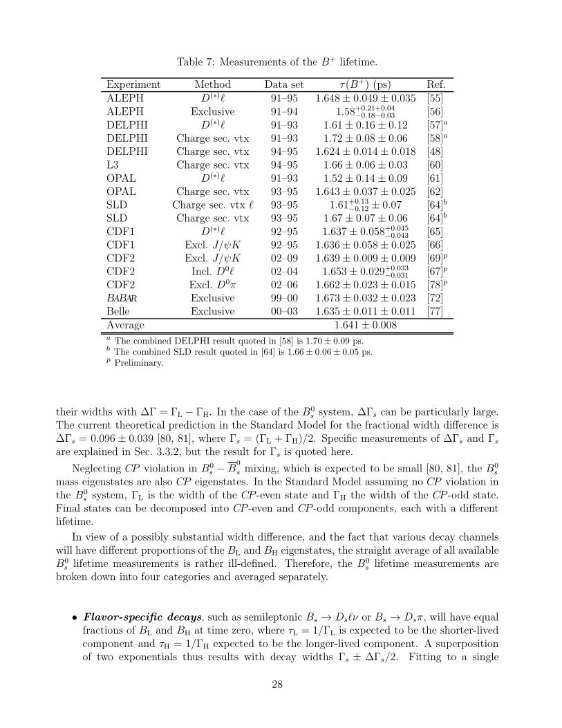
Table 7: Measurements of the B+ lifetime.
Experiment Method Data set τ(B+) (ps) Ref.
ALEPH D(∗)ℓ 91–95 1.648± 0.049± 0.035 [55]ALEPH Exclusive 91–94 1.58+0.21+0.04
−0.18−0.03 [56]DELPHI D(∗)ℓ 91–93 1.61± 0.16± 0.12 [57]a
DELPHI Charge sec. vtx 91–93 1.72± 0.08± 0.06 [58]a
DELPHI Charge sec. vtx 94–95 1.624± 0.014± 0.018 [48]L3 Charge sec. vtx 94–95 1.66± 0.06± 0.03 [60]OPAL D(∗)ℓ 91–93 1.52± 0.14± 0.09 [61]OPAL Charge sec. vtx 93–95 1.643± 0.037± 0.025 [62]SLD Charge sec. vtx ℓ 93–95 1.61+0.13
−0.12 ± 0.07 [64]b
SLD Charge sec. vtx 93–95 1.67± 0.07± 0.06 [64]b
CDF1 D(∗)ℓ 92–95 1.637± 0.058+0.045−0.043 [65]
CDF1 Excl. J/ψK 92–95 1.636± 0.058± 0.025 [66]CDF2 Excl. J/ψK 02–09 1.639± 0.009± 0.009 [69]p
CDF2 Incl. D0ℓ 02–04 1.653± 0.029+0.033−0.031 [67]p
CDF2 Excl. D0π 02–06 1.662± 0.023± 0.015 [78]p
BABAR Exclusive 99–00 1.673± 0.032± 0.023 [72]Belle Exclusive 00–03 1.635± 0.011± 0.011 [77]Average 1.641± 0.008a The combined DELPHI result quoted in [58] is 1.70± 0.09 ps.b The combined SLD result quoted in [64] is 1.66± 0.06± 0.05 ps.p Preliminary.
their widths with ∆Γ = ΓL − ΓH. In the case of the B0s system, ∆Γs can be particularly large.
The current theoretical prediction in the Standard Model for the fractional width difference is∆Γs = 0.096± 0.039 [80, 81], where Γs = (ΓL + ΓH)/2. Specific measurements of ∆Γs and Γsare explained in Sec. 3.3.2, but the result for Γs is quoted here.
Neglecting CP violation in B0s − B
0
s mixing, which is expected to be small [80, 81], the B0s
mass eigenstates are also CP eigenstates. In the Standard Model assuming no CP violation inthe B0
s system, ΓL is the width of the CP -even state and ΓH the width of the CP -odd state.Final states can be decomposed into CP -even and CP -odd components, each with a differentlifetime.
In view of a possibly substantial width difference, and the fact that various decay channelswill have different proportions of the BL and BH eigenstates, the straight average of all availableB0s lifetime measurements is rather ill-defined. Therefore, the B0
s lifetime measurements arebroken down into four categories and averaged separately.
• Flavor-specific decays, such as semileptonic Bs → Dsℓν or Bs → Dsπ, will have equalfractions of BL and BH at time zero, where τL = 1/ΓL is expected to be the shorter-livedcomponent and τH = 1/ΓH expected to be the longer-lived component. A superpositionof two exponentials thus results with decay widths Γs ± ∆Γs/2. Fitting to a single
28
Table 8: Measurements of the ratio τ(B+)/τ(B0).
Experiment Method Data set Ratio τ(B+)/τ(B0) Ref.
ALEPH D(∗)ℓ 91–95 1.085± 0.059± 0.018 [55]ALEPH Exclusive 91–94 1.27+0.23+0.03
−0.19−0.02 [56]DELPHI D(∗)ℓ 91–93 1.00+0.17
−0.15 ± 0.10 [57]DELPHI Charge sec. vtx 91–93 1.06+0.13
−0.11 ± 0.10 [58]DELPHI Charge sec. vtx 94–95 1.060± 0.021± 0.024 [48]L3 Charge sec. vtx 94–95 1.09± 0.07± 0.03 [60]OPAL D(∗)ℓ 91–93 0.99± 0.14+0.05
−0.04 [61]OPAL Charge sec. vtx 93–95 1.079± 0.064± 0.041 [62]SLD Charge sec. vtx ℓ 93–95 1.03+0.16
−0.14 ± 0.09 [64]a
SLD Charge sec. vtx 93–95 1.01+0.09−0.08 ± 0.05 [64]a
CDF1 D(∗)ℓ 92–95 1.110± 0.056+0.033−0.030 [65]
CDF1 Excl. J/ψK 92–95 1.093± 0.066± 0.028 [66]CDF2 Excl. J/ψK(∗) 02–09 1.088± 0.009± 0.004 [69]p
CDF2 Incl. Dℓ 02–04 1.123± 0.040+0.041−0.039 [67]p
CDF2 Excl. Dπ 02–04 1.10± 0.02± 0.01 [68]p
DØ D∗+µ D0µ ratio 02–04 1.080± 0.016± 0.014 [79]BABAR Exclusive 99–00 1.082± 0.026± 0.012 [72]Belle Exclusive 00–03 1.066± 0.008± 0.008 [77]Average 1.081± 0.006a The combined SLD result quoted in [64] is 1.01± 0.07± 0.06.p Preliminary.
exponential one obtains a measure of the flavor-specific lifetime [82]:
τ(B0s )fs =
1
Γs
1 +(
∆Γs2Γs
)2
1−(
∆Γs2Γs
)2 . (35)
As given in Table 9, the flavor-specific B0s lifetime world average is:
τ(B0s )fs = 1.455± 0.030 ps . (36)
This world average will be used later in Sec. 3.3.2 in combination with other measurementsto find τ(B0
s ) = 1/Γs and ∆Γs.
The following correlated systematic errors were considered: average B lifetime used inbackgrounds, B0
s decay multiplicity, and branching ratios used to determine backgrounds(e.g. B(B → DsD)). A knowledge of the multiplicity of B0
s decays is important formeasurements that partially reconstruct the final state such as B → DsX (where X is nota lepton). The boost deduced from Monte Carlo simulation depends on the multiplicityused. Since this is not well known, the multiplicity in the simulation is varied and thisrange of values observed is taken to be a systematic. Similarly not all the branching ratios
29
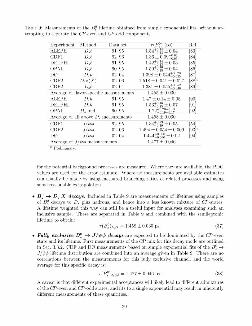
Table 9: Measurements of the B0s lifetime obtained from simple exponential fits, without at-
tempting to separate the CP -even and CP -odd components.
Experiment Method Data set τ(B0s ) (ps) Ref.
ALEPH Dsℓ 91–95 1.54+0.14−0.13 ± 0.04 [83]
CDF1 Dsℓ 92–96 1.36± 0.09+0.06−0.05 [84]
DELPHI Dsℓ 91–95 1.42+0.14−0.13 ± 0.03 [85]
OPAL Dsℓ 90–95 1.50+0.16−0.15 ± 0.04 [86]
DØ Dsµ 02–04 1.398± 0.044+0.028−0.025 [87]
CDF2 Dsπ(X) 02–06 1.518± 0.041± 0.027 [88]p
CDF2 Dsℓ 02–04 1.381± 0.055+0.052−0.046 [89]p
Average of flavor-specific measurements 1.455± 0.030ALEPH Dsh 91–95 1.47± 0.14± 0.08 [90]DELPHI Dsh 91–95 1.53+0.16
−0.15 ± 0.07 [91]OPAL Ds incl. 90–95 1.72+0.20+0.18
−0.19−0.17 [92]Average of all above Ds measurements 1.458± 0.030
CDF1 J/ψφ 92–95 1.34+0.23−0.19 ± 0.05 [54]
CDF2 J/ψφ 02–06 1.494± 0.054± 0.009 [93]p
DØ J/ψφ 02–04 1.444+0.098−0.090 ± 0.02 [94]
Average of J/ψφ measurements 1.477± 0.046p Preliminary.
for the potential background processes are measured. Where they are available, the PDGvalues are used for the error estimate. Where no measurements are available estimatescan usually be made by using measured branching ratios of related processes and usingsome reasonable extrapolation.
• B0s→ D+
sX decays. Included in Table 9 are measurements of lifetimes using samples
of B0s decays to Ds plus hadrons, and hence into a less known mixture of CP -states.
A lifetime weighted this way can still be a useful input for analyses examining such aninclusive sample. These are separated in Table 9 and combined with the semileptoniclifetime to obtain:
τ(B0s )DsX = 1.458± 0.030 ps . (37)
• Fully exclusive B0s→ J/ψφ decays are expected to be dominated by the CP -even
state and its lifetime. First measurements of the CP mix for this decay mode are outlinedin Sec. 3.3.2. CDF and DØ measurements based on simple exponential fits of the B0
s →J/ψφ lifetime distribution are combined into an average given in Table 9. There are nocorrelations between the measurements for this fully exclusive channel, and the worldaverage for this specific decay is:
τ(B0s )J/ψφ = 1.477± 0.046 ps . (38)
A caveat is that different experimental acceptances will likely lead to different admixturesof the CP -even and CP -odd states, and fits to a single exponential may result in inherentlydifferent measurements of these quantities.
30
• Decays to (almost) pure CP -even eigenstates, such as B0s → K+K− and B0
s →D
(∗)+s D
(∗)+s decays which are expected to be CP even to within 5%, and hence allow
the measurement of the lifetime of the “light” mass eigenstate τL = 1/ΓL. ALEPH
has measured 1.27 ± 0.33 ± 0.08 ps with B0s → D
(∗)+s D
(∗)+s decays [95], while CDF has
measured 1.53 ± 0.18 ± 0.02 ps with B0s → K+K− in Run II [96]. The average of these
two measurements is:
τL = 1/ΓL = τ(B0s → CP even) = 1.47± 0.16 ps . (39)
Finally, as will be shown in Sec. 3.3.2, measurements of ∆Γs, including separation intoCP -even and CP -odd components, give8
τ (B0s ) = 1/Γs = 1.506± 0.032 ps , (40)
and when combined with the flavor-specific lifetime measurements:
τ (B0s ) = 1/Γs = 1.477+0.021
−0.022 ps . (41)
3.2.5 B+c
lifetime
There are currently three measurements of the lifetime of the B+c meson from CDF [98, 99]
and DØ [100] using the semileptonic decay mode B+c → J/ψℓ and fitting simultaneously to
the mass and lifetime using the vertex formed with the leptons from the decay of the J/ψand the third lepton. Correction factors to estimate the boost due to the missing neutrino areused. In the analysis of the CDF Run I data [98], a mass value of 6.40 ± 0.39 ± 0.13 GeV/c2
is found by fitting to the tri-lepton invariant mass spectrum. In the CDF and DØ Run IIresults [99, 100], the B+
c mass is assumed to be 6285.7± 5.3± 1.2 MeV/c2, taken from a CDFresult [101]. These mass measurements are consistent within uncertainties, and also consistentwith the most recent precision determination from CDF of 6275.6 ± 2.9 ± 2.5 MeV/c2 [102].Correlated systematic errors include the impact of the uncertainty of the B+
c pT spectrum onthe correction factors, the level of feed-down from ψ(2S), MC modeling of the decay modelvarying from phase space to the ISGW model, and mass variations. Values of the B+
c lifetimeare given in Table 10 and the world average is determined to be:
τ(B+c ) = 0.461± 0.036 ps . (42)
3.2.6 Λ0band b-baryon lifetimes
The first measurements of b-baryon lifetimes originate from two classes of partially reconstructeddecays. In the first class, decays with an exclusively reconstructed Λ+
c baryon and a lepton ofopposite charge are used. These products are more likely to occur in the decay of Λ0
b baryons.In the second class, more inclusive final states with a baryon (p, p, Λ, or Λ) and a lepton havebeen used, and these final states can generally arise from any b baryon. With the large b-hadronsamples available at the Tevatron, the most precise measurements of b-baryons now come fromfully reconstructed exclusive decays.
8A recent CDF result, 1/Γs = 1.530± 0.025± 0.012 [97], has not yet been included in this average.
31
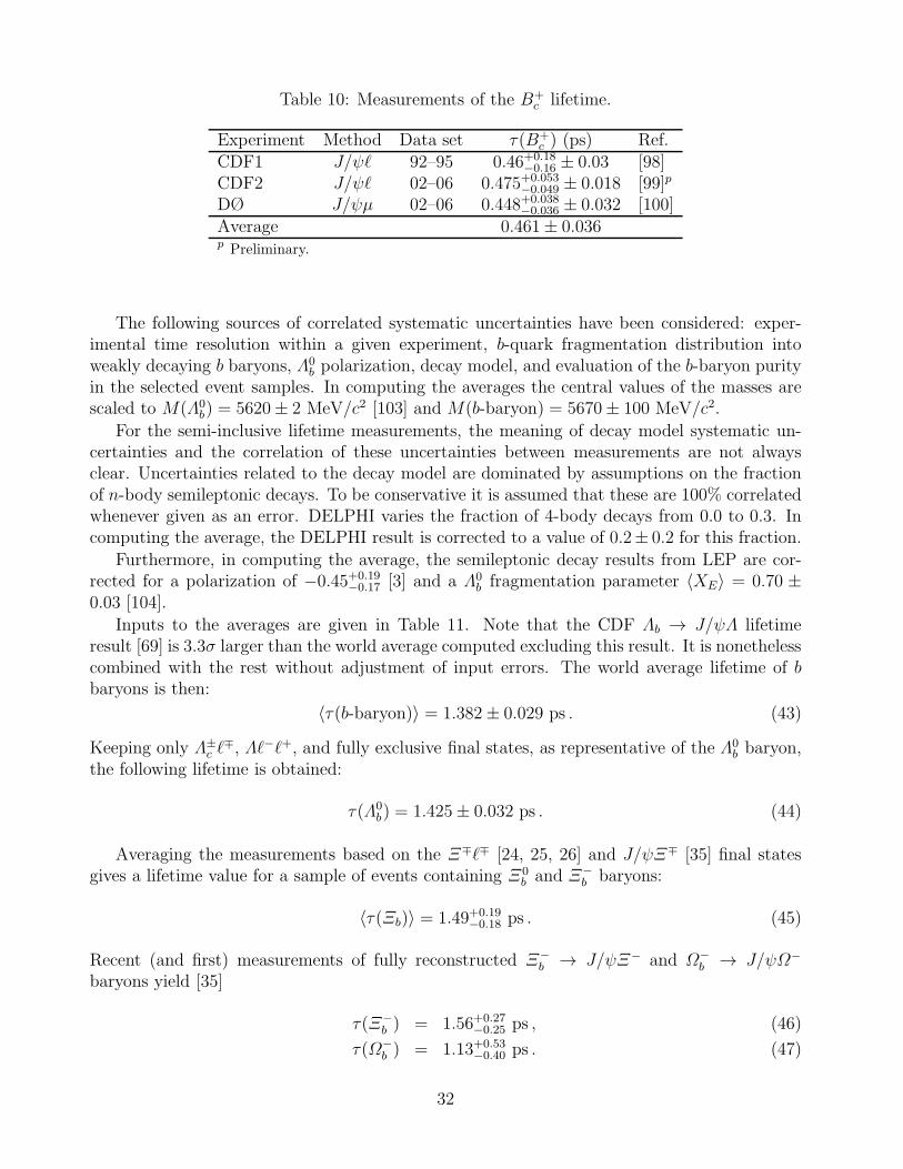
Table 10: Measurements of the B+c lifetime.
Experiment Method Data set τ(B+c ) (ps) Ref.
CDF1 J/ψℓ 92–95 0.46+0.18−0.16 ± 0.03 [98]
CDF2 J/ψℓ 02–06 0.475+0.053−0.049 ± 0.018 [99]p
DØ J/ψµ 02–06 0.448+0.038−0.036 ± 0.032 [100]
Average 0.461± 0.036p Preliminary.
The following sources of correlated systematic uncertainties have been considered: exper-imental time resolution within a given experiment, b-quark fragmentation distribution intoweakly decaying b baryons, Λ0
b polarization, decay model, and evaluation of the b-baryon purityin the selected event samples. In computing the averages the central values of the masses arescaled to M(Λ0
b) = 5620± 2 MeV/c2 [103] and M(b-baryon) = 5670± 100 MeV/c2.
For the semi-inclusive lifetime measurements, the meaning of decay model systematic un-certainties and the correlation of these uncertainties between measurements are not alwaysclear. Uncertainties related to the decay model are dominated by assumptions on the fractionof n-body semileptonic decays. To be conservative it is assumed that these are 100% correlatedwhenever given as an error. DELPHI varies the fraction of 4-body decays from 0.0 to 0.3. Incomputing the average, the DELPHI result is corrected to a value of 0.2± 0.2 for this fraction.
Furthermore, in computing the average, the semileptonic decay results from LEP are cor-rected for a polarization of −0.45+0.19
−0.17 [3] and a Λ0b fragmentation parameter 〈XE〉 = 0.70 ±
0.03 [104].
Inputs to the averages are given in Table 11. Note that the CDF Λb → J/ψΛ lifetimeresult [69] is 3.3σ larger than the world average computed excluding this result. It is nonethelesscombined with the rest without adjustment of input errors. The world average lifetime of bbaryons is then:
〈τ(b-baryon)〉 = 1.382± 0.029 ps . (43)
Keeping only Λ±c ℓ
∓, Λℓ−ℓ+, and fully exclusive final states, as representative of the Λ0b baryon,
the following lifetime is obtained:
τ(Λ0b) = 1.425± 0.032 ps . (44)
Averaging the measurements based on the Ξ∓ℓ∓ [24, 25, 26] and J/ψΞ∓ [35] final statesgives a lifetime value for a sample of events containing Ξ0
b and Ξ−b baryons:
〈τ(Ξb)〉 = 1.49+0.19−0.18 ps . (45)
Recent (and first) measurements of fully reconstructed Ξ−b → J/ψΞ− and Ω−
b → J/ψΩ−
baryons yield [35]
τ(Ξ−b ) = 1.56+0.27
−0.25 ps , (46)
τ(Ω−b ) = 1.13+0.53
−0.40 ps . (47)
32
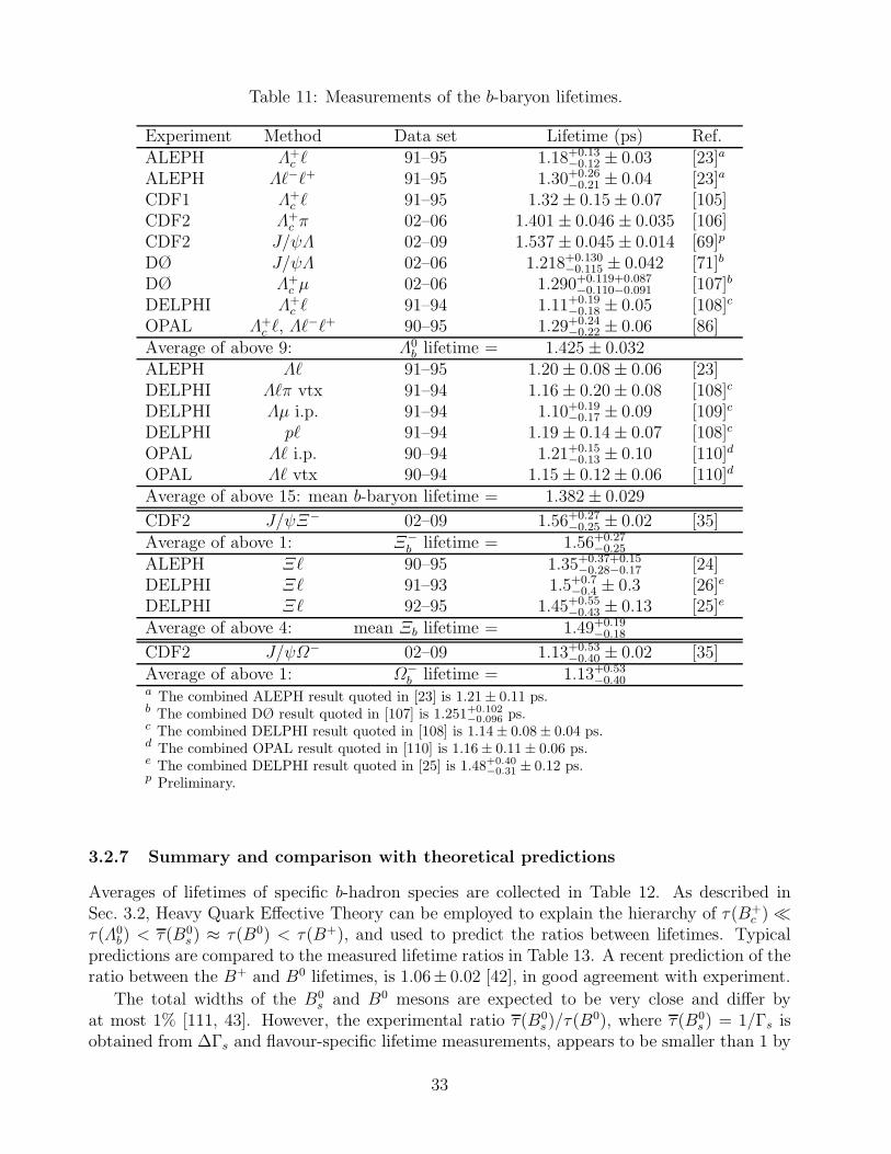
Table 11: Measurements of the b-baryon lifetimes.
Experiment Method Data set Lifetime (ps) Ref.ALEPH Λ+
c ℓ 91–95 1.18+0.13−0.12 ± 0.03 [23]a
ALEPH Λℓ−ℓ+ 91–95 1.30+0.26−0.21 ± 0.04 [23]a
CDF1 Λ+c ℓ 91–95 1.32± 0.15± 0.07 [105]
CDF2 Λ+c π 02–06 1.401± 0.046± 0.035 [106]
CDF2 J/ψΛ 02–09 1.537± 0.045± 0.014 [69]p
DØ J/ψΛ 02–06 1.218+0.130−0.115 ± 0.042 [71]b
DØ Λ+c µ 02–06 1.290+0.119+0.087
−0.110−0.091 [107]b
DELPHI Λ+c ℓ 91–94 1.11+0.19
−0.18 ± 0.05 [108]c
OPAL Λ+c ℓ, Λℓ
−ℓ+ 90–95 1.29+0.24−0.22 ± 0.06 [86]
Average of above 9: Λ0b lifetime = 1.425± 0.032
ALEPH Λℓ 91–95 1.20± 0.08± 0.06 [23]DELPHI Λℓπ vtx 91–94 1.16± 0.20± 0.08 [108]c
DELPHI Λµ i.p. 91–94 1.10+0.19−0.17 ± 0.09 [109]c
DELPHI pℓ 91–94 1.19± 0.14± 0.07 [108]c
OPAL Λℓ i.p. 90–94 1.21+0.15−0.13 ± 0.10 [110]d
OPAL Λℓ vtx 90–94 1.15± 0.12± 0.06 [110]d
Average of above 15: mean b-baryon lifetime = 1.382± 0.029
CDF2 J/ψΞ− 02–09 1.56+0.27−0.25 ± 0.02 [35]
Average of above 1: Ξ−b lifetime = 1.56+0.27
−0.25
ALEPH Ξℓ 90–95 1.35+0.37+0.15−0.28−0.17 [24]
DELPHI Ξℓ 91–93 1.5+0.7−0.4 ± 0.3 [26]e
DELPHI Ξℓ 92–95 1.45+0.55−0.43 ± 0.13 [25]e
Average of above 4: mean Ξb lifetime = 1.49+0.19−0.18
CDF2 J/ψΩ− 02–09 1.13+0.53−0.40 ± 0.02 [35]
Average of above 1: Ω−b lifetime = 1.13+0.53
−0.40a The combined ALEPH result quoted in [23] is 1.21± 0.11 ps.b The combined DØ result quoted in [107] is 1.251+0.102
−0.096 ps.c The combined DELPHI result quoted in [108] is 1.14± 0.08± 0.04 ps.d The combined OPAL result quoted in [110] is 1.16± 0.11± 0.06 ps.e The combined DELPHI result quoted in [25] is 1.48+0.40
−0.31 ± 0.12 ps.p Preliminary.
3.2.7 Summary and comparison with theoretical predictions
Averages of lifetimes of specific b-hadron species are collected in Table 12. As described inSec. 3.2, Heavy Quark Effective Theory can be employed to explain the hierarchy of τ(B+
c ) ≪τ(Λ0
b) < τ(B0s ) ≈ τ(B0) < τ(B+), and used to predict the ratios between lifetimes. Typical
predictions are compared to the measured lifetime ratios in Table 13. A recent prediction of theratio between the B+ and B0 lifetimes, is 1.06± 0.02 [42], in good agreement with experiment.
The total widths of the B0s and B0 mesons are expected to be very close and differ by
at most 1% [111, 43]. However, the experimental ratio τ(B0s )/τ(B
0), where τ(B0s ) = 1/Γs is
obtained from ∆Γs and flavour-specific lifetime measurements, appears to be smaller than 1 by
33
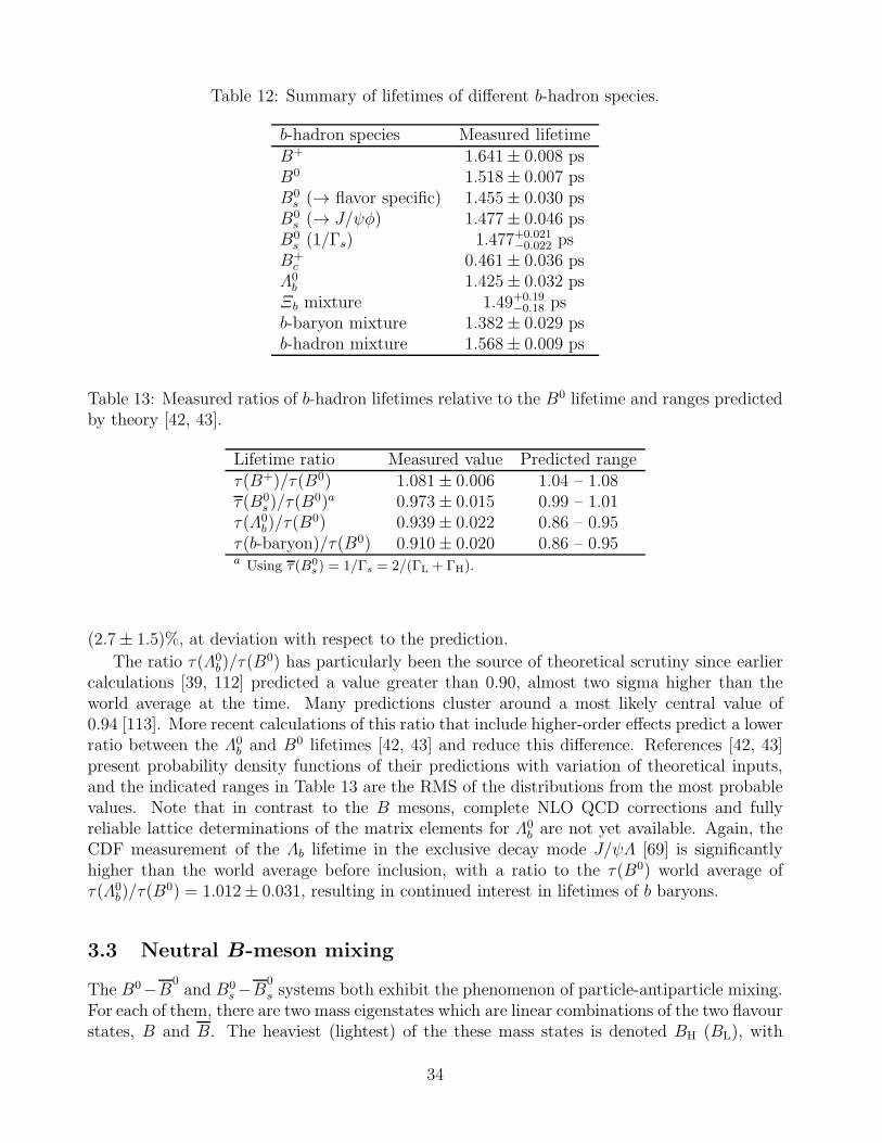
Table 12: Summary of lifetimes of different b-hadron species.
b-hadron species Measured lifetimeB+ 1.641± 0.008 psB0 1.518± 0.007 psB0s (→ flavor specific) 1.455± 0.030 ps
B0s (→ J/ψφ) 1.477± 0.046 ps
B0s (1/Γs) 1.477+0.021
−0.022 psB+c 0.461± 0.036 ps
Λ0b 1.425± 0.032 ps
Ξb mixture 1.49+0.19−0.18 ps
b-baryon mixture 1.382± 0.029 psb-hadron mixture 1.568± 0.009 ps
Table 13: Measured ratios of b-hadron lifetimes relative to the B0 lifetime and ranges predictedby theory [42, 43].
Lifetime ratio Measured value Predicted rangeτ(B+)/τ(B0) 1.081± 0.006 1.04 – 1.08τ(B0
s )/τ(B0)a 0.973± 0.015 0.99 – 1.01
τ(Λ0b)/τ(B
0) 0.939± 0.022 0.86 – 0.95τ(b-baryon)/τ(B0) 0.910± 0.020 0.86 – 0.95a Using τ (B0
s ) = 1/Γs = 2/(ΓL + ΓH).
(2.7± 1.5)%, at deviation with respect to the prediction.
The ratio τ(Λ0b)/τ(B
0) has particularly been the source of theoretical scrutiny since earliercalculations [39, 112] predicted a value greater than 0.90, almost two sigma higher than theworld average at the time. Many predictions cluster around a most likely central value of0.94 [113]. More recent calculations of this ratio that include higher-order effects predict a lowerratio between the Λ0
b and B0 lifetimes [42, 43] and reduce this difference. References [42, 43]present probability density functions of their predictions with variation of theoretical inputs,and the indicated ranges in Table 13 are the RMS of the distributions from the most probablevalues. Note that in contrast to the B mesons, complete NLO QCD corrections and fullyreliable lattice determinations of the matrix elements for Λ0
b are not yet available. Again, theCDF measurement of the Λb lifetime in the exclusive decay mode J/ψΛ [69] is significantlyhigher than the world average before inclusion, with a ratio to the τ(B0) world average ofτ(Λ0
b)/τ(B0) = 1.012± 0.031, resulting in continued interest in lifetimes of b baryons.
3.3 Neutral B-meson mixing
The B0−B0and B0
s−B0
s systems both exhibit the phenomenon of particle-antiparticle mixing.For each of them, there are two mass eigenstates which are linear combinations of the two flavourstates, B and B. The heaviest (lightest) of the these mass states is denoted BH (BL), with
34
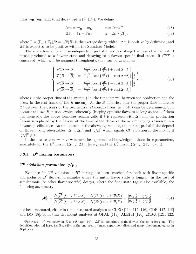
mass mH (mL) and total decay width ΓH (ΓL). We define
∆m = mH −mL , x = ∆m/Γ , (48)
∆Γ = ΓL − ΓH , y = ∆Γ/(2Γ) , (49)
where Γ = (ΓH+ΓL)/2 = 1/τ(B) is the average decay width. ∆m is positive by definition, and∆Γ is expected to be positive within the Standard Model.9
There are four different time-dependent probabilities describing the case of a neutral Bmeson produced as a flavour state and decaying to a flavour-specific final state. If CPT isconserved (which will be assumed throughout), they can be written as
P(B → B) = e−Γt
2
[
cosh(
∆Γ2t)
+ cos(∆mt)]
P(B → B) = e−Γt
2
[
cosh(
∆Γ2t)
− cos(∆mt)]
∣
∣
∣
qp
∣
∣
∣
2
P(B → B) = e−Γt
2
[
cosh(
∆Γ2t)
− cos(∆mt)]
∣
∣
∣
pq
∣
∣
∣
2
P(B → B) = e−Γt
2
[
cosh(
∆Γ2t)
+ cos(∆mt)]
, (50)
where t is the proper time of the system (i.e. the time interval between the production and thedecay in the rest frame of the B meson). At the B factories, only the proper-time difference∆t between the decays of the two neutral B mesons from the Υ (4S) can be determined, but,because the two B mesons evolve coherently (keeping opposite flavours as long as none of themhas decayed), the above formulae remain valid if t is replaced with ∆t and the productionflavour is replaced by the flavour at the time of the decay of the accompanying B meson in aflavour-specific state. As can be seen in the above expressions, the mixing probabilities dependon three mixing observables: ∆m, ∆Γ, and |q/p|2 which signals CP violation in the mixing if|q/p|2 6= 1.
In the next sections we review in turn the experimental knowledge on these three parameters,separately for the B0 meson (∆md, ∆Γd, |q/p|d) and the B0
s meson (∆ms, ∆Γs, |q/p|s).
3.3.1 B0 mixing parameters
CP violation parameter |q/p|d
Evidence for CP violation in B0 mixing has been searched for, both with flavor-specificand inclusive B0 decays, in samples where the initial flavor state is tagged. In the case ofsemileptonic (or other flavor-specific) decays, where the final state tag is also available, thefollowing asymmetry
AdSL =
N(B0(t) → ℓ+νℓX)−N(B0(t) → ℓ−νℓX)
N(B0(t) → ℓ+νℓX) +N(B0(t) → ℓ−νℓX)
=|p/q|2d − |q/p|2d|p/q|2d + |q/p|2d
(51)
has been measured, either in time-integrated analyses at CLEO [114, 115, 116], CDF [117, 118]and DØ [38], or in time-dependent analyses at OPAL [119], ALEPH [120], BABAR [121, 122,
9For reason of symmetry in Eqs. (48) and (49), ∆Γ is sometimes defined with the opposite sign. Thedefinition adopted here, i.e. Eq. (49), is the one used by most experimentalists and many phenomenologists inB physics.
35
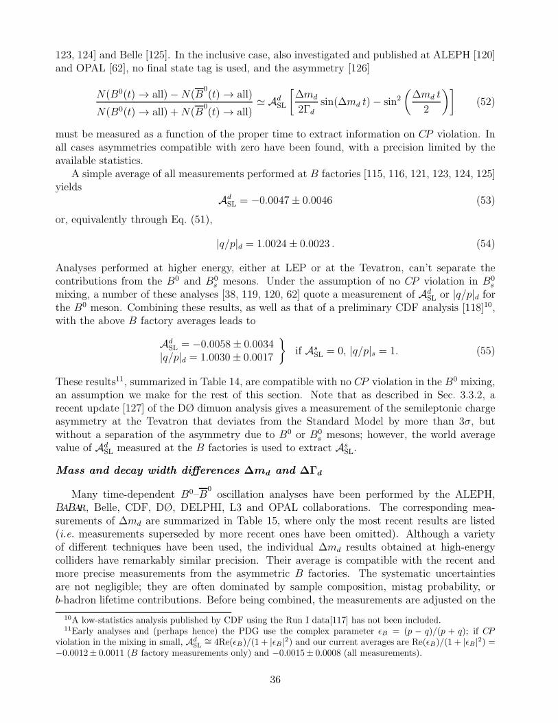
123, 124] and Belle [125]. In the inclusive case, also investigated and published at ALEPH [120]and OPAL [62], no final state tag is used, and the asymmetry [126]
N(B0(t) → all)−N(B0(t) → all)
N(B0(t) → all) +N(B0(t) → all)
≃ AdSL
[
∆md
2Γdsin(∆md t)− sin2
(
∆md t
2
)]
(52)
must be measured as a function of the proper time to extract information on CP violation. Inall cases asymmetries compatible with zero have been found, with a precision limited by theavailable statistics.
A simple average of all measurements performed at B factories [115, 116, 121, 123, 124, 125]yields
AdSL = −0.0047± 0.0046 (53)
or, equivalently through Eq. (51),
|q/p|d = 1.0024± 0.0023 . (54)
Analyses performed at higher energy, either at LEP or at the Tevatron, can’t separate thecontributions from the B0 and B0
s mesons. Under the assumption of no CP violation in B0s
mixing, a number of these analyses [38, 119, 120, 62] quote a measurement of AdSL or |q/p|d for
the B0 meson. Combining these results, as well as that of a preliminary CDF analysis [118]10,with the above B factory averages leads to
AdSL = −0.0058± 0.0034
|q/p|d = 1.0030± 0.0017
if AsSL = 0, |q/p|s = 1. (55)
These results11, summarized in Table 14, are compatible with no CP violation in the B0 mixing,an assumption we make for the rest of this section. Note that as described in Sec. 3.3.2, arecent update [127] of the DØ dimuon analysis gives a measurement of the semileptonic chargeasymmetry at the Tevatron that deviates from the Standard Model by more than 3σ, butwithout a separation of the asymmetry due to B0 or B0
s mesons; however, the world averagevalue of Ad
SL measured at the B factories is used to extract AsSL.
Mass and decay width differences ∆md and ∆Γd
Many time-dependent B0–B0oscillation analyses have been performed by the ALEPH,
BABAR, Belle, CDF, DØ, DELPHI, L3 and OPAL collaborations. The corresponding mea-surements of ∆md are summarized in Table 15, where only the most recent results are listed(i.e. measurements superseded by more recent ones have been omitted). Although a varietyof different techniques have been used, the individual ∆md results obtained at high-energycolliders have remarkably similar precision. Their average is compatible with the recent andmore precise measurements from the asymmetric B factories. The systematic uncertaintiesare not negligible; they are often dominated by sample composition, mistag probability, orb-hadron lifetime contributions. Before being combined, the measurements are adjusted on the
10A low-statistics analysis published by CDF using the Run I data[117] has not been included.11Early analyses and (perhaps hence) the PDG use the complex parameter ǫB = (p − q)/(p + q); if CP
violation in the mixing in small, AdSL
∼= 4Re(ǫB)/(1 + |ǫB|2) and our current averages are Re(ǫB)/(1 + |ǫB|2) =−0.0012± 0.0011 (B factory measurements only) and −0.0015± 0.0008 (all measurements).
36
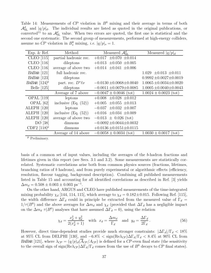
Table 14: Measurements of CP violation in B0 mixing and their average in terms of bothAd
SL and |q/p|d. The individual results are listed as quoted in the original publications, orconverted11 to an Ad
SL value. When two errors are quoted, the first one is statistical and thesecond one systematic. The second group of measurements, performed at high-energy colliders,assume no CP violation in B0
s mixing, i.e. |q/p|s = 1.
Exp. & Ref. Method Measured AdSL Measured |q/p|d
CLEO [115] partial hadronic rec. +0.017 ±0.070 ±0.014CLEO [116] dileptons +0.013 ±0.050 ±0.005CLEO [116] average of above two +0.014 ±0.041 ±0.006BABAR [121] full hadronic rec. 1.029 ±0.013 ±0.011BABAR [123] dileptons 0.9992±0.0027±0.0019BABAR [124]p part. rec. D∗ℓν −0.0130±0.0068±0.0040 1.0065±0.0034±0.0020
Belle [125] dileptons −0.0011±0.0079±0.0085 1.0005±0.0040±0.0043Average of 7 above −0.0047± 0.0046 (tot) 1.0024± 0.0023 (tot)
OPAL [119] leptons +0.008 ±0.028 ±0.012OPAL [62] inclusive (Eq. (52)) +0.005 ±0.055 ±0.013
ALEPH [120] leptons −0.037 ±0.032 ±0.007ALEPH [120] inclusive (Eq. (52)) +0.016 ±0.034 ±0.009ALEPH [120] average of above two −0.013 ± 0.026 (tot)
DØ [38] dimuons −0.0092±0.0044±0.0032CDF2 [118]p dimuons +0.0136±0.0151±0.0115
Average of 14 above −0.0058± 0.0034 (tot) 1.0030± 0.0017 (tot)p Preliminary.
basis of a common set of input values, including the averages of the b-hadron fractions andlifetimes given in this report (see Secs. 3.1 and 3.2). Some measurements are statistically cor-related. Systematic correlations arise both from common physics sources (fractions, lifetimes,branching ratios of b hadrons), and from purely experimental or algorithmic effects (efficiency,resolution, flavour tagging, background description). Combining all published measurementslisted in Table 15 and accounting for all identified correlations as described in Ref. [3] yields∆md = 0.508± 0.003± 0.003 ps−1.
On the other hand, ARGUS and CLEO have published measurements of the time-integratedmixing probability χd [144, 114, 115], which average to χd = 0.182±0.015. Following Ref. [115],the width difference ∆Γd could in principle be extracted from the measured value of Γd =1/τ(B0) and the above averages for ∆md and χd (provided that ∆Γd has a negligible impacton the ∆md τ(B
0) analyses that have assumed ∆Γd = 0), using the relation
χd =x2d + y2d2(x2d + 1)
with xd =∆md
Γdand yd =
∆Γd2Γd
. (56)
However, direct time-dependent studies provide much stronger constraints: |∆Γd|/Γd < 18%at 95% CL from DELPHI [130], and −6.8% < sign(ReλCP )∆Γd/Γd < 8.4% at 90% CL fromBABAR [121], where λCP = (q/p)d(ACP/ACP ) is defined for a CP -even final state (the sensitivityto the overall sign of sign(ReλCP )∆Γd/Γd comes from the use of B0 decays to CP final states).
37
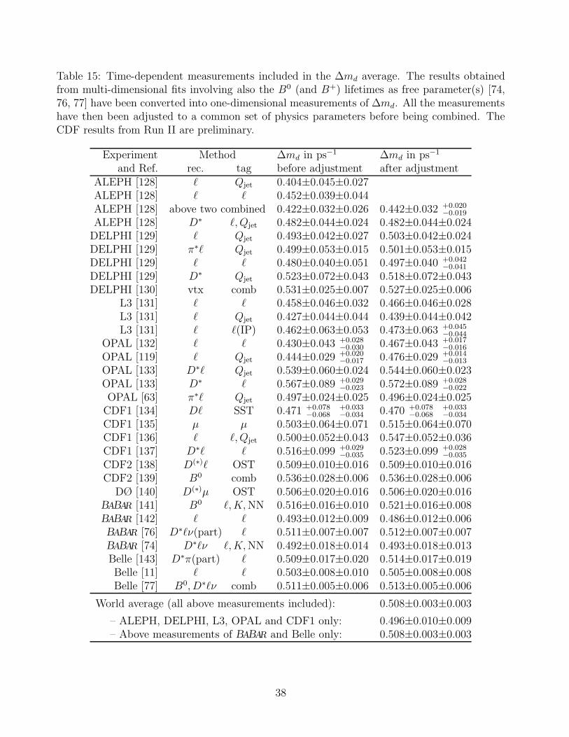
Table 15: Time-dependent measurements included in the ∆md average. The results obtainedfrom multi-dimensional fits involving also the B0 (and B+) lifetimes as free parameter(s) [74,76, 77] have been converted into one-dimensional measurements of ∆md. All the measurementshave then been adjusted to a common set of physics parameters before being combined. TheCDF results from Run II are preliminary.
Experiment Method ∆md in ps−1 ∆md in ps−1
and Ref. rec. tag before adjustment after adjustmentALEPH [128] ℓ Qjet 0.404±0.045±0.027ALEPH [128] ℓ ℓ 0.452±0.039±0.044ALEPH [128] above two combined 0.422±0.032±0.026 0.442±0.032 +0.020
−0.019
ALEPH [128] D∗ ℓ, Qjet 0.482±0.044±0.024 0.482±0.044±0.024DELPHI [129] ℓ Qjet 0.493±0.042±0.027 0.503±0.042±0.024DELPHI [129] π∗ℓ Qjet 0.499±0.053±0.015 0.501±0.053±0.015DELPHI [129] ℓ ℓ 0.480±0.040±0.051 0.497±0.040 +0.042
−0.041
DELPHI [129] D∗ Qjet 0.523±0.072±0.043 0.518±0.072±0.043DELPHI [130] vtx comb 0.531±0.025±0.007 0.527±0.025±0.006
L3 [131] ℓ ℓ 0.458±0.046±0.032 0.466±0.046±0.028L3 [131] ℓ Qjet 0.427±0.044±0.044 0.439±0.044±0.042L3 [131] ℓ ℓ(IP) 0.462±0.063±0.053 0.473±0.063 +0.045
−0.044
OPAL [132] ℓ ℓ 0.430±0.043 +0.028−0.030 0.467±0.043 +0.017
−0.016
OPAL [119] ℓ Qjet 0.444±0.029 +0.020−0.017 0.476±0.029 +0.014
−0.013
OPAL [133] D∗ℓ Qjet 0.539±0.060±0.024 0.544±0.060±0.023OPAL [133] D∗ ℓ 0.567±0.089 +0.029
−0.023 0.572±0.089 +0.028−0.022
OPAL [63] π∗ℓ Qjet 0.497±0.024±0.025 0.496±0.024±0.025CDF1 [134] Dℓ SST 0.471 +0.078
−0.068+0.033−0.034 0.470 +0.078
−0.068+0.033−0.034
CDF1 [135] µ µ 0.503±0.064±0.071 0.515±0.064±0.070CDF1 [136] ℓ ℓ, Qjet 0.500±0.052±0.043 0.547±0.052±0.036CDF1 [137] D∗ℓ ℓ 0.516±0.099 +0.029
−0.035 0.523±0.099 +0.028−0.035
CDF2 [138] D(∗)ℓ OST 0.509±0.010±0.016 0.509±0.010±0.016CDF2 [139] B0 comb 0.536±0.028±0.006 0.536±0.028±0.006
DØ [140] D(∗)µ OST 0.506±0.020±0.016 0.506±0.020±0.016BABAR [141] B0 ℓ,K,NN 0.516±0.016±0.010 0.521±0.016±0.008BABAR [142] ℓ ℓ 0.493±0.012±0.009 0.486±0.012±0.006BABAR [76] D∗ℓν(part) ℓ 0.511±0.007±0.007 0.512±0.007±0.007BABAR [74] D∗ℓν ℓ,K,NN 0.492±0.018±0.014 0.493±0.018±0.013Belle [143] D∗π(part) ℓ 0.509±0.017±0.020 0.514±0.017±0.019Belle [11] ℓ ℓ 0.503±0.008±0.010 0.505±0.008±0.008Belle [77] B0, D∗ℓν comb 0.511±0.005±0.006 0.513±0.005±0.006
World average (all above measurements included): 0.508±0.003±0.003
– ALEPH, DELPHI, L3, OPAL and CDF1 only: 0.496±0.010±0.009– Above measurements of BABAR and Belle only: 0.508±0.003±0.003
38
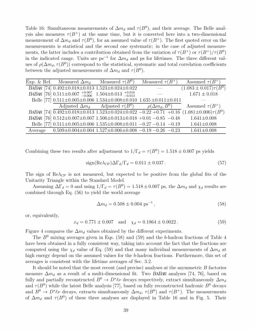
Table 16: Simultaneous measurements of ∆md and τ(B0), and their average. The Belle anal-ysis also measures τ(B+) at the same time, but it is converted here into a two-dimensionalmeasurement of ∆md and τ(B
0), for an assumed value of τ(B+). The first quoted error on themeasurements is statistical and the second one systematic; in the case of adjusted measure-ments, the latter includes a contribution obtained from the variation of τ(B+) or τ(B+)/τ(B0)in the indicated range. Units are ps−1 for ∆md and ps for lifetimes. The three different val-ues of ρ(∆md, τ(B
0)) correspond to the statistical, systematic and total correlation coefficientsbetween the adjusted measurements of ∆md and τ(B0).
Exp. & Ref. Measured ∆md Measured τ(B0) Measured τ(B+) Assumed τ(B+)BABAR [74] 0.492±0.018±0.013 1.523±0.024±0.022 — (1.083± 0.017)τ(B0)BABAR [76] 0.511±0.007 +0.007
−0.006 1.504±0.013 +0.018−0.013 — 1.671± 0.018
Belle [77] 0.511±0.005±0.006 1.534±0.008±0.010 1.635±0.011±0.011 —Adjusted ∆md Adjusted τ(B0) ρ(∆md, B
0) Assumed τ(B+)BABAR [74] 0.492±0.018±0.013 1.523±0.024±0.022 −0.22 +0.71 +0.16 (1.081±0.006)τ(B0)BABAR [76] 0.512±0.007±0.007 1.506±0.013±0.018 +0.01 −0.85 −0.48 1.641±0.008Belle [77] 0.511±0.005±0.006 1.535±0.008±0.011 −0.27 −0.14 −0.19 1.641±0.008
Average 0.509±0.004±0.004 1.527±0.006±0.008 −0.19 −0.26 −0.23 1.641±0.008
Combining these two results after adjustment to 1/Γd = τ(B0) = 1.518± 0.007 ps yields
sign(ReλCP )∆Γd/Γd = 0.011± 0.037 . (57)
The sign of ReλCP is not measured, but expected to be positive from the global fits of theUnitarity Triangle within the Standard Model.
Assuming ∆Γd = 0 and using 1/Γd = τ(B0) = 1.518±0.007 ps, the ∆md and χd results arecombined through Eq. (56) to yield the world average
∆md = 0.508± 0.004 ps−1 , (58)
or, equivalently,
xd = 0.771± 0.007 and χd = 0.1864± 0.0022 . (59)
Figure 4 compares the ∆md values obtained by the different experiments.The B0 mixing averages given in Eqs. (58) and (59) and the b-hadron fractions of Table 4
have been obtained in a fully consistent way, taking into account the fact that the fractions arecomputed using the χd value of Eq. (59) and that many individual measurements of ∆md athigh energy depend on the assumed values for the b-hadron fractions. Furthermore, this set ofaverages is consistent with the lifetime averages of Sec. 3.2.
It should be noted that the most recent (and precise) analyses at the asymmetric B factoriesmeasure ∆md as a result of a multi-dimensional fit. Two BABAR analyses [74, 76], based onfully and partially reconstructed B0 → D∗ℓν decays respectively, extract simultaneously ∆md
and τ(B0) while the latest Belle analysis [77], based on fully reconstructed hadronic B0 decaysand B0 → D∗ℓν decays, extracts simultaneously ∆md, τ(B
0) and τ(B+). The measurementsof ∆md and τ(B0) of these three analyses are displayed in Table 16 and in Fig. 5. Their
39
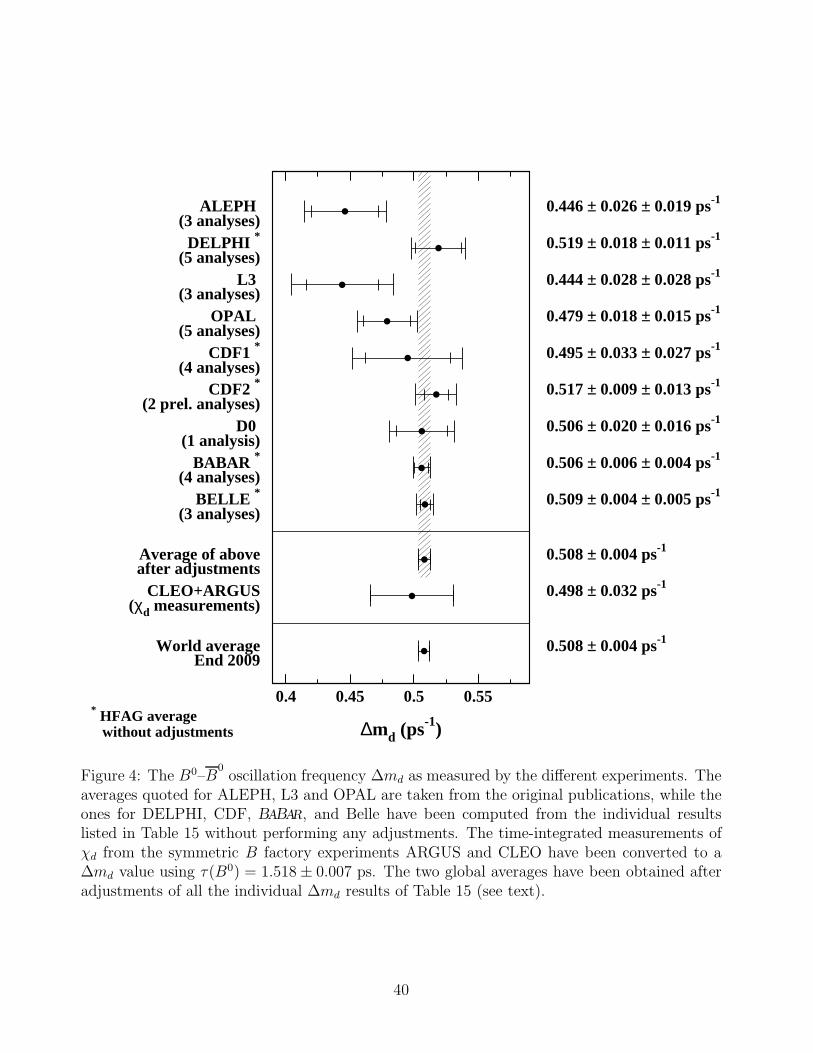
0.4 0.45 0.5 0.55
∆md (ps-1)
World averageEnd 2009
0.508 ± 0.004 ps-1
CLEO+ARGUS(χd measurements)
0.498 ± 0.032 ps-1
Average of aboveafter adjustments
0.508 ± 0.004 ps-1
BELLE *(3 analyses)
0.509 ± 0.004 ± 0.005 ps-1
BABAR *(4 analyses)
0.506 ± 0.006 ± 0.004 ps-1
D0 (1 analysis)
0.506 ± 0.020 ± 0.016 ps-1
CDF2 *(2 prel. analyses)
0.517 ± 0.009 ± 0.013 ps-1
CDF1 *(4 analyses)
0.495 ± 0.033 ± 0.027 ps-1
OPAL (5 analyses)
0.479 ± 0.018 ± 0.015 ps-1
L3 (3 analyses)
0.444 ± 0.028 ± 0.028 ps-1
DELPHI *(5 analyses)
0.519 ± 0.018 ± 0.011 ps-1
ALEPH (3 analyses)
0.446 ± 0.026 ± 0.019 ps-1
* HFAG average without adjustments
Figure 4: The B0–B0oscillation frequency ∆md as measured by the different experiments. The
averages quoted for ALEPH, L3 and OPAL are taken from the original publications, while theones for DELPHI, CDF, BABAR, and Belle have been computed from the individual resultslisted in Table 15 without performing any adjustments. The time-integrated measurements ofχd from the symmetric B factory experiments ARGUS and CLEO have been converted to a∆md value using τ(B0) = 1.518± 0.007 ps. The two global averages have been obtained afteradjustments of all the individual ∆md results of Table 15 (see text).
40
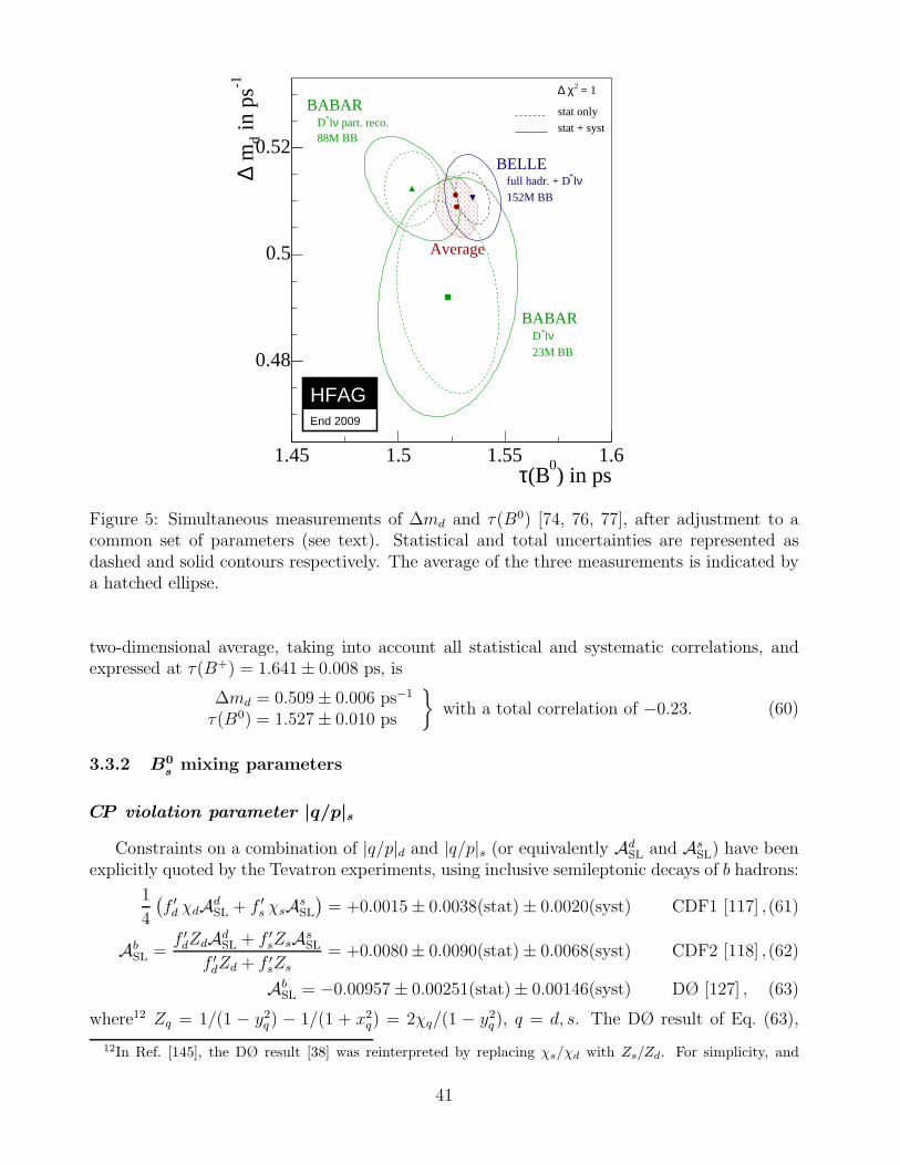
) in ps0
(Bτ1.45 1.5 1.55 1.6
-1 in
ps
d m∆
0.48
0.5
0.52
HFAGEnd 2009
BABARνl*D
23M BB
BABAR part. reco.νl*D
88M BB
BELLEνl*full hadr. + D
152M BB
Average
= 12χ ∆
stat only
stat + syst
Figure 5: Simultaneous measurements of ∆md and τ(B0) [74, 76, 77], after adjustment to acommon set of parameters (see text). Statistical and total uncertainties are represented asdashed and solid contours respectively. The average of the three measurements is indicated bya hatched ellipse.
two-dimensional average, taking into account all statistical and systematic correlations, andexpressed at τ(B+) = 1.641± 0.008 ps, is
∆md = 0.509± 0.006 ps−1
τ(B0) = 1.527± 0.010 ps
with a total correlation of −0.23. (60)
3.3.2 B0smixing parameters
CP violation parameter |q/p|s
Constraints on a combination of |q/p|d and |q/p|s (or equivalently AdSL and As
SL) have beenexplicitly quoted by the Tevatron experiments, using inclusive semileptonic decays of b hadrons:
1
4
(
f ′d χdAd
SL + f ′s χsAs
SL
)
= +0.0015± 0.0038(stat)± 0.0020(syst) CDF1 [117] ,(61)
AbSL =
f ′dZdAd
SL + f ′sZsAs
SL
f ′dZd + f ′
sZs= +0.0080± 0.0090(stat)± 0.0068(syst) CDF2 [118] ,(62)
AbSL = −0.00957± 0.00251(stat)± 0.00146(syst) DØ [127] , (63)
where12 Zq = 1/(1 − y2q ) − 1/(1 + x2q) = 2χq/(1 − y2q ), q = d, s. The DØ result of Eq. (63),
12In Ref. [145], the DØ result [38] was reinterpreted by replacing χs/χd with Zs/Zd. For simplicity, and
41
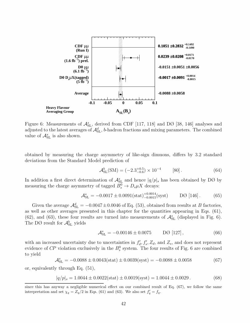
-0.1 -0.05 0 0.05 0.1
ASL(Bs)
Average -0.0088 ±0.0058
D0 DsµX(tagged)(5 fb−1)
-0.0017 ±0.0091 +0.0014-0.0017 ±0.0091 -0.0015
D0 µµ(6.1 fb−1)
-0.0151 ±0.0051 ±0.0056
CDF µµ(1.6 fb−1) prel.
0.0239 ±0.0208 +0.01710.0239 ±0.0208 -0.0170
CDF µµ(Run I)
0.1051 ±0.2832 +0.14920.1051 ±0.2832 -0.1490
Heavy FlavourAveraging Group
Figure 6: Measurements of AsSL, derived from CDF [117, 118] and DØ [38, 146] analyses and
adjusted to the latest averages ofAdSL, b-hadron fractions and mixing parameters. The combined
value of AsSL is also shown.
obtained by measuring the charge asymmetry of like-sign dimuons, differs by 3.2 standarddeviations from the Standard Model prediction of
AbSL(SM) = (−2.3+0.5
−0.6)× 10−4 [80] . (64)
In addition a first direct determination of AsSL and hence |q/p|s has been obtained by DØ by
measuring the charge asymmetry of tagged B0s → DsµX decays:
AsSL = −0.0017± 0.0091(stat)+0.0014
−0.0015(syst) DØ [146] . (65)
Given the average AdSL = −0.0047±0.0046 of Eq. (53), obtained from results at B factories,
as well as other averages presented in this chapter for the quantities appearing in Eqs. (61),(62), and (63), these four results are turned into measurements of As
SL (displayed in Fig. 6).The DØ result for Ab
SL yields
AsSL = −0.00146± 0.0075 DØ [127] , (66)
with an increased uncertainty due to uncertainties in f ′d, f
′s, Zd, and Zs, and does not represent
evidence of CP violation exclusively in the B0s system. The four results of Fig. 6 are combined
to yieldAs
SL = −0.0088± 0.0043(stat)± 0.0039(syst) = −0.0088± 0.0058 (67)
or, equivalently through Eq. (51),
|q/p|s = 1.0044± 0.0022(stat)± 0.0019(syst) = 1.0044± 0.0029 . (68)
since this has anyway a negligible numerical effect on our combined result of Eq. (67), we follow the sameinterpretation and set χq = Zq/2 in Eqs. (61) and (63). We also set f ′
q = fq.
42
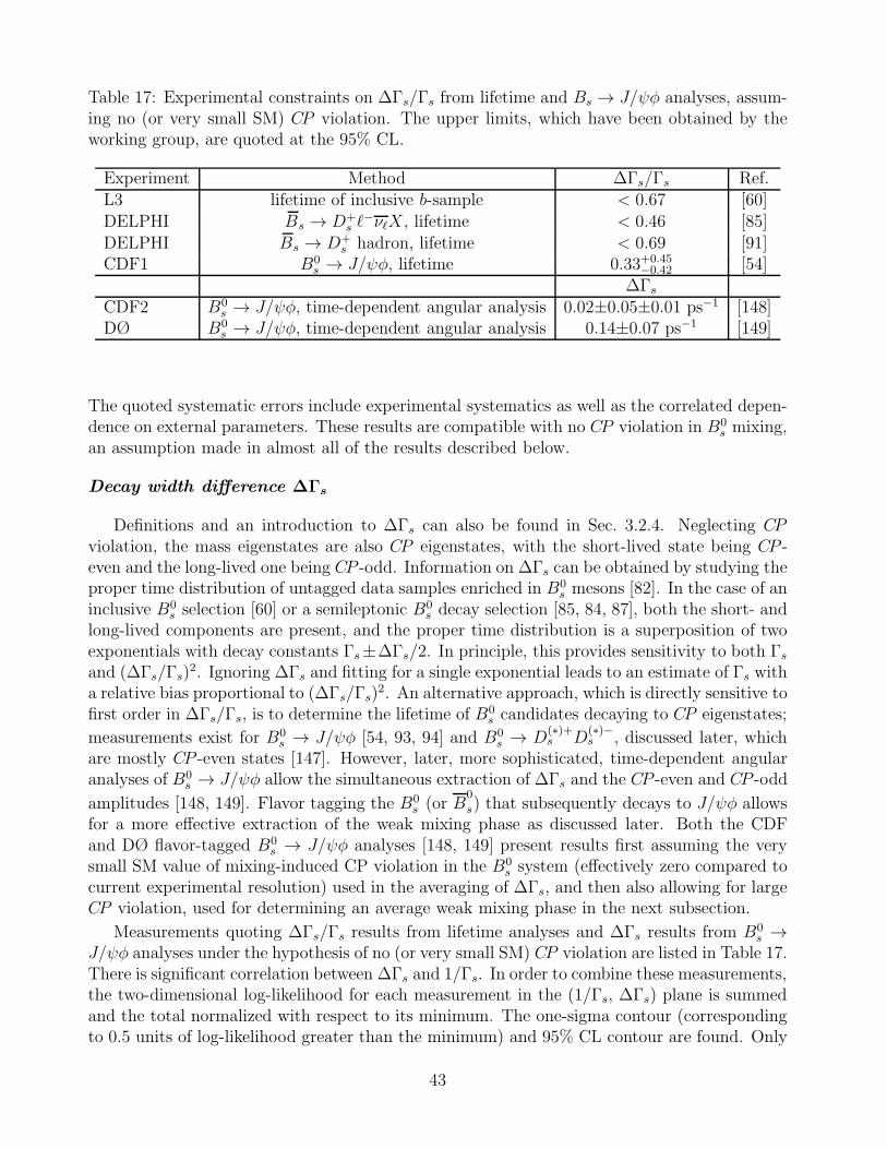
Table 17: Experimental constraints on ∆Γs/Γs from lifetime and Bs → J/ψφ analyses, assum-ing no (or very small SM) CP violation. The upper limits, which have been obtained by theworking group, are quoted at the 95% CL.
Experiment Method ∆Γs/Γs Ref.L3 lifetime of inclusive b-sample < 0.67 [60]DELPHI Bs → D+
s ℓ−νℓX , lifetime < 0.46 [85]
DELPHI Bs → D+s hadron, lifetime < 0.69 [91]
CDF1 B0s → J/ψφ, lifetime 0.33+0.45
−0.42 [54]∆Γs
CDF2 B0s → J/ψφ, time-dependent angular analysis 0.02±0.05±0.01 ps−1 [148]
DØ B0s → J/ψφ, time-dependent angular analysis 0.14±0.07 ps−1 [149]
The quoted systematic errors include experimental systematics as well as the correlated depen-dence on external parameters. These results are compatible with no CP violation in B0
s mixing,an assumption made in almost all of the results described below.
Decay width difference ∆Γs
Definitions and an introduction to ∆Γs can also be found in Sec. 3.2.4. Neglecting CPviolation, the mass eigenstates are also CP eigenstates, with the short-lived state being CP -even and the long-lived one being CP -odd. Information on ∆Γs can be obtained by studying theproper time distribution of untagged data samples enriched in B0
s mesons [82]. In the case of aninclusive B0
s selection [60] or a semileptonic B0s decay selection [85, 84, 87], both the short- and
long-lived components are present, and the proper time distribution is a superposition of twoexponentials with decay constants Γs±∆Γs/2. In principle, this provides sensitivity to both Γsand (∆Γs/Γs)
2. Ignoring ∆Γs and fitting for a single exponential leads to an estimate of Γs witha relative bias proportional to (∆Γs/Γs)
2. An alternative approach, which is directly sensitive tofirst order in ∆Γs/Γs, is to determine the lifetime of B0
s candidates decaying to CP eigenstates;
measurements exist for B0s → J/ψφ [54, 93, 94] and B0
s → D(∗)+s D
(∗)−s , discussed later, which
are mostly CP -even states [147]. However, later, more sophisticated, time-dependent angularanalyses of B0
s → J/ψφ allow the simultaneous extraction of ∆Γs and the CP -even and CP -odd
amplitudes [148, 149]. Flavor tagging the B0s (or B
0
s) that subsequently decays to J/ψφ allowsfor a more effective extraction of the weak mixing phase as discussed later. Both the CDFand DØ flavor-tagged B0
s → J/ψφ analyses [148, 149] present results first assuming the verysmall SM value of mixing-induced CP violation in the B0
s system (effectively zero compared tocurrent experimental resolution) used in the averaging of ∆Γs, and then also allowing for largeCP violation, used for determining an average weak mixing phase in the next subsection.
Measurements quoting ∆Γs/Γs results from lifetime analyses and ∆Γs results from B0s →
J/ψφ analyses under the hypothesis of no (or very small SM) CP violation are listed in Table 17.There is significant correlation between ∆Γs and 1/Γs. In order to combine these measurements,the two-dimensional log-likelihood for each measurement in the (1/Γs, ∆Γs) plane is summedand the total normalized with respect to its minimum. The one-sigma contour (correspondingto 0.5 units of log-likelihood greater than the minimum) and 95% CL contour are found. Only
43
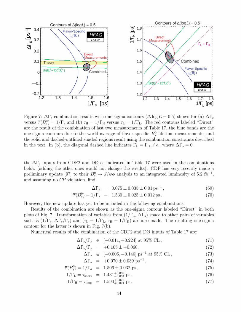
1.2 1.3 1.4
s
1.5 1.6
1/Γ [ps]
−0.2
0
0.1
—0.1
0.2
0.2
0.4
Direct
Theory
Measurements
[ps
]-1
s
∆Γ
Flavor-Specific τ (B )s
0fs
Combined
HFAG
End 09
Contours of ∆(logL) = 0.5
Br(B D D )*s s s0 ( ) *( )
1.31.2
1.3
1.2
1.4
1.6
1.5
1.8
1.7
1.4 1.5 1.7 1.81.6
L1/Γ [ps]
H1/
Γ [p
s]
LΓ = HΓ
DirectMeasurements
Flavor-Specific τ (B )s
0fs
Combined
HFAGEnd 09
Contours of ∆(logL) = 0.5
Br(B D D )*s s s0 ( ) *( )
Figure 7: ∆Γs combination results with one-sigma contours (∆ logL = 0.5) shown for (a) ∆Γsversus τ(B0
s ) = 1/Γs and (b) τH = 1/ΓH versus τL = 1/ΓL. The red contours labeled “Direct”are the result of the combination of last two measurements of Table 17, the blue bands are theone-sigma contours due to the world average of flavor-specific B0
s lifetime measurements, andthe solid and dashed-outlined shaded regions result using the combination constraints describedin the text. In (b), the diagonal dashed line indicates ΓL = ΓH, i.e., where ∆Γs = 0.
the ∆Γs inputs from CDF2 and DØ as indicated in Table 17 were used in the combinationsbelow (adding the other ones would not change the results). CDF has very recently made apreliminary update [97] to their B0
s → J/ψφ analysis to an integrated luminosity of 5.2 fb−1,and assuming no CP violation, find
∆Γs = 0.075± 0.035± 0.01 ps−1 , (69)
τ(B0s ) = 1/Γs = 1.530± 0.025± 0.012 ps . (70)
However, this new update has yet to be included in the following combinations.Results of the combination are shown as the one-sigma contour labeled “Direct” in both
plots of Fig. 7. Transformation of variables from (1/Γs, ∆Γs) space to other pairs of variablessuch as (1/Γs, ∆Γs/Γs) and (τL = 1/ΓL, τH = 1/ΓH) are also made. The resulting one-sigmacontour for the latter is shown in Fig. 7(b).
Numerical results of the combination of the CDF2 and DØ inputs of Table 17 are:
∆Γs/Γs ∈ [−0.011,+0.224] at 95% CL , (71)
∆Γs/Γs = +0.105±+0.060 , (72)
∆Γs ∈ [−0.006,+0.146] ps−1 at 95% CL , (73)
∆Γs = +0.070± 0.039 ps−1 , (74)
τ (B0s ) = 1/Γs = 1.506± 0.032 ps , (75)
1/ΓL = τshort = 1.431+0.038−0.037 ps , (76)
1/ΓH = τlong = 1.590+0.075+0.071 ps . (77)
44
Flavor-specific lifetime measurements are of an equal mix of CP -even and CP -odd statesat time zero, and if a single exponential function is used in the likelihood lifetime fit of such asample [82],
τ(B0s )fs =
1
Γs
1 +(
∆Γs2Γs
)2
1−(
∆Γs2Γs
)2 . (78)
Using the world average flavor-specific lifetime of Eq. (36) in Sec. 3.2.4 the one-sigma bluebands shown in Fig. 7 are obtained. Higher-order corrections were checked to be negligible inthe combination.
When the flavor-specific lifetime measurements are combined with the CDF2 and DØ mea-surements of Table 17, the solid-outline shaded regions of Fig. 7 are obtained, with numericalresults:
∆Γs/Γs ∈ [−0.028,+0.167] at 95% CL , (79)
∆Γs/Γs = +0.072+0.049−0.051 , (80)
∆Γs ∈ [−0.019,+0.112] ps−1 at 95% CL , (81)
∆Γs = +0.049+0.033−0.034 ps−1 , (82)
τ (B0s ) = 1/Γs = 1.477+0.021
−0.022 ps , (83)
1/ΓL = τshort = 1.425+0.037−0.035 ps , (84)
1/ΓH = τlong = 1.532± 0.049 ps . (85)
These results can be compared with the theoretical prediction of ∆Γs = 0.096± 0.039 ps−1 (or∆Γs = 0.088± 0.017 ps−1 if there is no new physics in ∆ms) [80, 81].
Measurements of B(B0s → D
(∗)+s D
(∗)−s ) can also be sensitive to ∆Γs. The decay B
0s → D+
s D−s
is into a final state that is purely CP even. Under various theoretical assumptions [147, 150],
the inclusive decay into this plus the excited states B0s → D
(∗)+s D
(∗)−s is also CP even to within
5%, and B0s → D
(∗)+s D
(∗)−s saturates ΓCP even
s . Under these assumptions, for no CP violation,we have:
∆Γs/Γs ≈2B(B0
s → D(∗)+s D
(∗)−s )
1− B(B0s → D
(∗)+s D
(∗)−s )
. (86)
However, there are concerns [151] that the assumptions needed for the above are overly restric-tive and that the inclusive branching ratio may be CP even to only 30%. In the application ofthe constraint as a Gaussian penalty function, the theoretical uncertainty is dealt with in twoways: the fraction of the CP -odd component of the decay [150] is taken to be a uniform distri-bution ranging from 0 to 0.05 and convoluted in the Gaussian, and the fractional uncertaintyon the average measured value is increased in quadrature by 30%.
Measurements for the branching fraction for this decay channel are shown in Table 18.Using their average value of 0.049± 0.014 with Eq. (86) yields
∆Γs/Γs = +0.103± 0.032 , (87)
consistent with the value given in Eq. (80).As described in Sec. 3.2.4 and Eq. (39), the average of the lifetime measurements with B0
s
→ K+K− and B0s → D
(∗)s D
(∗)s decays can be used to measure the lifetime of the CP -even (or
45
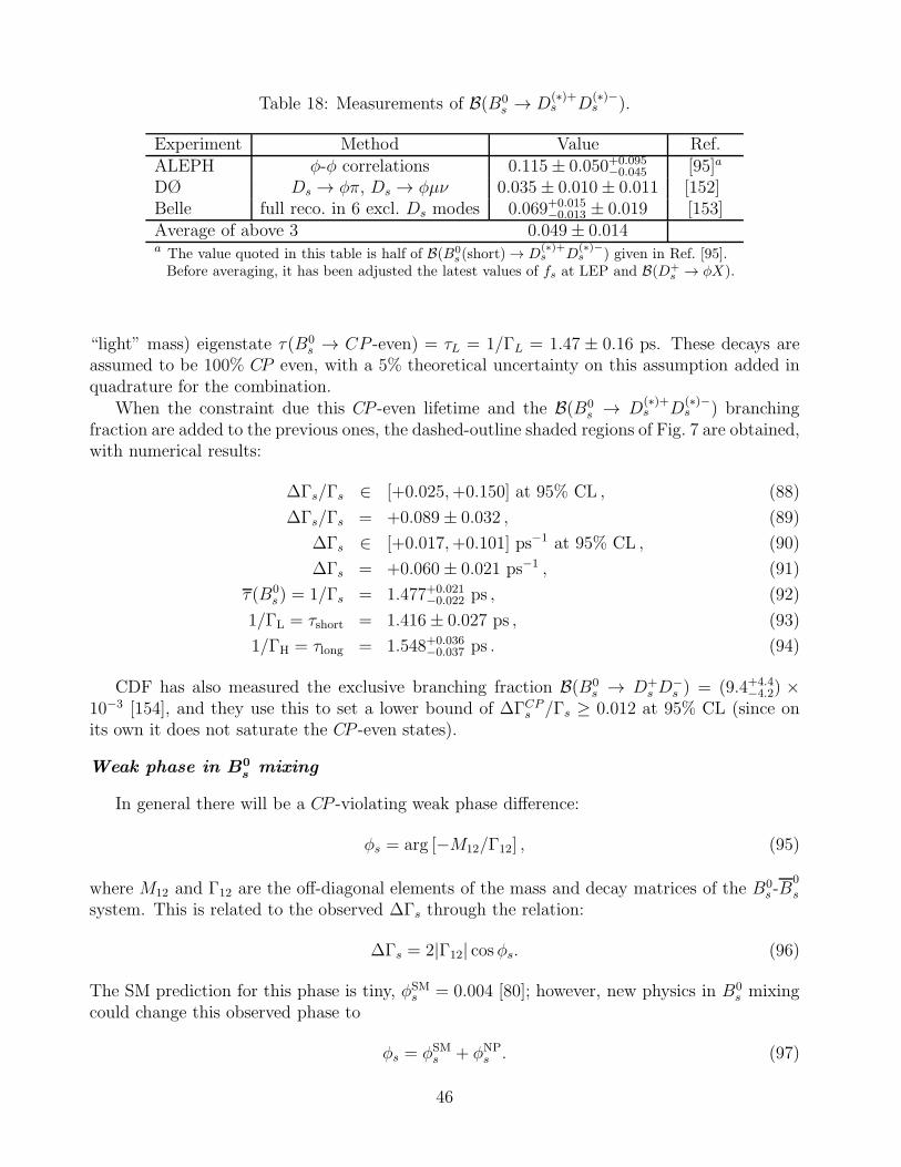
Table 18: Measurements of B(B0s → D
(∗)+s D
(∗)−s ).
Experiment Method Value Ref.ALEPH φ-φ correlations 0.115± 0.050+0.095
−0.045 [95]a
DØ Ds → φπ, Ds → φµν 0.035± 0.010± 0.011 [152]Belle full reco. in 6 excl. Ds modes 0.069+0.015
−0.013 ± 0.019 [153]Average of above 3 0.049± 0.014a The value quoted in this table is half of B(B0
s (short) → D(∗)+s D
(∗)−s ) given in Ref. [95].
Before averaging, it has been adjusted the latest values of fs at LEP and B(D+s → φX).
“light” mass) eigenstate τ(B0s → CP -even) = τL = 1/ΓL = 1.47 ± 0.16 ps. These decays are
assumed to be 100% CP even, with a 5% theoretical uncertainty on this assumption added inquadrature for the combination.
When the constraint due this CP -even lifetime and the B(B0s → D
(∗)+s D
(∗)−s ) branching
fraction are added to the previous ones, the dashed-outline shaded regions of Fig. 7 are obtained,with numerical results:
∆Γs/Γs ∈ [+0.025,+0.150] at 95% CL , (88)
∆Γs/Γs = +0.089± 0.032 , (89)
∆Γs ∈ [+0.017,+0.101] ps−1 at 95% CL , (90)
∆Γs = +0.060± 0.021 ps−1 , (91)
τ (B0s ) = 1/Γs = 1.477+0.021
−0.022 ps , (92)
1/ΓL = τshort = 1.416± 0.027 ps , (93)
1/ΓH = τlong = 1.548+0.036−0.037 ps . (94)
CDF has also measured the exclusive branching fraction B(B0s → D+
s D−s ) = (9.4+4.4
−4.2) ×10−3 [154], and they use this to set a lower bound of ∆ΓCPs /Γs ≥ 0.012 at 95% CL (since onits own it does not saturate the CP -even states).
Weak phase in B0smixing
In general there will be a CP -violating weak phase difference:
φs = arg [−M12/Γ12] , (95)
where M12 and Γ12 are the off-diagonal elements of the mass and decay matrices of the B0s -B
0
s
system. This is related to the observed ∆Γs through the relation:
∆Γs = 2|Γ12| cosφs. (96)
The SM prediction for this phase is tiny, φSMs = 0.004 [80]; however, new physics in B0
s mixingcould change this observed phase to
φs = φSMs + φNP
s . (97)
46
The relative phase between the B0s mixing amplitude and that of specific b → ccs quark
transitions such as for B0s or B
0
s → J/ψφ in the SM is [80, 155]:
2βSMs = 2 arg [− (VtsV∗tb) / (VcsV
∗cb)] = 0.037± 0.002 ≈ 0.04. (98)
This angle is analogous to the β angle in the usual CKM unitarity triangle aside from thenegative sign (resulting in a positive angle in the SM). The same additional contribution dueto new physics would show up in this observed phase [80], i.e.:
2βs = 2βSMs − φNP
s . (99)
The current experimental precision does not allow these small CP -violating phases φSMs and
βSMs to be resolved, and for large new physics effect, we can approximate φs ≈ −2βs ≈ φNP
s ,i.e., a significantly large observed phase would indicate new physics.
For non-zero |Γ12|, analysis of the time-dependent decay B0s → J/ψφ can measure the weak
phase. Including information on the B0s flavor at production time via flavor tagging improves
precision and also resolves the sign ambiguity on the weak phase angle for a given ∆Γs. BothCDF [148] and DØ [149] have performed such analyses and measure the same observed phase
that we denote φJ/ψφs = −2β
J/ψφs to reflect the different conventions of the experiments.
Under the assumption of non-zero φJ/ψφs , in addition to the result listed in Table 17, the
DØ collaboration [149] has also made simultaneous fits allowing φJ/ψφs to float while weakly
constraining the strong phases, δi to find:
∆Γs = +0.19± 0.07+0.02−0.01 ps−1 , (100)
τ (B0s ) = 1/Γs = 1.52± 0.06 ps , (101)
φJ/ψφs = −0.57+0.24+0.07−0.30−0.02 . (102)
If the SM value of φJ/ψφs = −0.04 is assumed, a probability of 6.6% to obtain a value of φ
J/ψφs
lower than −0.57 is found.The CDF analysis [148] reports confidence regions in the two-dimensional space of 2β
J/ψφs
and ∆Γs. They present a Feldman-Cousins confidence interval of 2βJ/ψφs where ∆Γs is treated
as a nuisance parameter:
2βJ/ψφs = −φJ/ψφs ∈ [0.56, 2.58] at 68% CL. (103)
Only a confidence range is quoted and a point estimate is not given since biases were observedin the analysis. Assuming the SM predictions for 2βs and ∆Γs, they find that the probabilityof a deviation as large as the level of the observed data is 7%. Note that CDF has very recentlymade a preliminary update [97] to their B0
s → J/ψφ analysis to an integrated luminosity of5.2 fb−1 indicating a best-fit confidence interval of:
2βJ/ψφs = −φJ/ψφs ∈ [0.04, 1.04] ∪ [2.16, 3.10] at 68% CL, (104)
where the probability of a larger deviation from the SM prediction is 44% or 0.8σ. However,this new result has not yet been used in the combinations below.
Given the consistency of these two measurements of the weak phase, as well as their de-viations from the SM, there is interest in combining the results and using in global fits, e.g.,
47
see Ref. [156]. To allow a combination on equal footing, the DØ collaboration has redone theirfits [157] allowing strong phase values, δi, to float as in the CDF analysis. Ensemble studiesto test confidence level coverage were performed by both collaborations and used to adjustlikelihood values to correspond to the usual Gaussian confidence levels. Two-dimensional like-lihoods were combined [158, 159] with the result shown in Fig. 8(a). After the combination,
consistency of the best fit values for φJ/ψφs = −2β
J/ψφs with SM predictions is at the level of
2.3σ, with numerical results for the two solutions given below. Despite possible biases in theCDF input, point estimates are still presented and the confidence level regions are straightprojections onto the ∆Γs or phase angle axes.
∆Γs = +0.150+0.055−0.056 ps−1 or − 0.150+0.056
−0.055 ps−1 , (105)
∈ [+0.060,+0.297] ∪ [−0.297,−0.060] ps−1 at 90% CL , (106)
φJ/ψφs = −2βJ/ψφs = −0.83+0.30−0.36 or − 2.31+0.36
−0.30 , (107)
∈ [−1.50,−0.32] ∪ [−2.82,−1.64] at 90% CL . (108)
A comparison between the above sum of the CDF and DØ likelihoods and the world averageB0s semileptonic asymmetry of Eq. (67) through [160]:
AsSL =
|Γ12s |
|M12s | sin φs =
∆Γs∆ms
tanφs (109)
is also made and shown in Fig. 8(a). Consistency between the two is observed, and the valueof As
SL is applied as a constraint resulting in the confidence level regions shown in Fig. 8(b)including the region delineated by new physics traced by the relation of Eq. (96). Numericalresults for the two solutions are:
∆Γs = +0.150+0.045−0.049 ps−1 or − 0.150+0.042
−0.049 ps−1 , (110)
∈ [+0.075,+0.228] ∪ [−0.220,−0.071] ps−1 at 90% CL , (111)
φJ/ψφs = −2βJ/ψφs = −0.82+0.16−0.21 or− 2.36+0.20
−0.14 , (112)
∈ [−1.20,−0.45] ∪ [−2.72,−1.99] at 90% CL . (113)
with a consistency of the best fit values with SM predictions of 2βs at the level of 2.8σ.
Finally, additional constraints are added due to the flavor-specific B0s lifetime world average
of Eq. (36) through Eq. (78), the CP -event lifetime of Eq. (39), and the world average of the
branching fraction B(B0s → D
(∗)+s D
(∗)−s ) through [150]:
2B(B0s → D(∗)+
s D(∗)−s ) ≃ ∆ΓCP
s
[
11−2xf
+ cosφs
2ΓL+
11−2xf
− cosφs
2ΓH
]
. (114)
Here xf is the fraction of the CP -odd component of the decay. To apply this as a constraint,we expand the above expression to second order,
2B(B0s → D(∗)+
s D(∗)−s ) ≃ ∆Γs
Γs cosφs
[
1
1− 2xf− ∆Γs cosφs
2Γs
]
, (115)
48
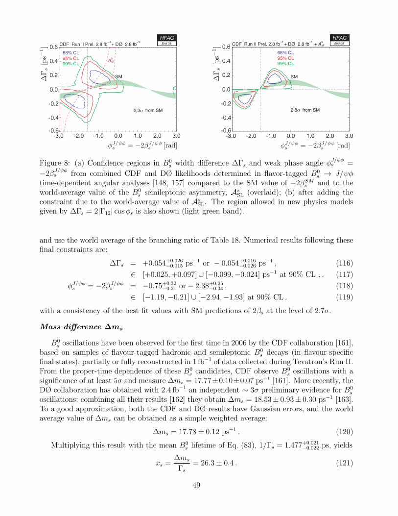
Figure 8: (a) Confidence regions in B0s width difference ∆Γs and weak phase angle φ
J/ψφs =
−2βJ/ψφs from combined CDF and DØ likelihoods determined in flavor-tagged B0
s → J/ψφtime-dependent angular analyses [148, 157] compared to the SM value of −2βSMs and to theworld-average value of the B0
s semileptonic asymmetry, AsSL (overlaid); (b) after adding the
constraint due to the world-average value of AsSL. The region allowed in new physics models
given by ∆Γs = 2|Γ12| cosφs is also shown (light green band).
and use the world average of the branching ratio of Table 18. Numerical results following thesefinal constraints are:
∆Γs = +0.054+0.026−0.015 ps−1 or − 0.054+0.016
−0.026 ps−1 , (116)
∈ [+0.025,+0.097] ∪ [−0.099,−0.024] ps−1 at 90% CL , , (117)
φJ/ψφs = −2βJ/ψφs = −0.75+0.32−0.21 or− 2.38+0.25
−0.34 , (118)
∈ [−1.19,−0.21] ∪ [−2.94,−1.93] at 90% CL . (119)
with a consistency of the best fit values with SM predictions of 2βs at the level of 2.7σ.
Mass difference ∆ms
B0s oscillations have been observed for the first time in 2006 by the CDF collaboration [161],
based on samples of flavour-tagged hadronic and semileptonic B0s decays (in flavour-specific
final states), partially or fully reconstructed in 1 fb−1 of data collected during Tevatron’s Run II.From the proper-time dependence of these B0
s candidates, CDF observe B0s oscillations with a
significance of at least 5σ and measure ∆ms = 17.77±0.10±0.07 ps−1 [161]. More recently, theDØ collaboration has obtained with 2.4 fb−1 an independent ∼ 3σ preliminary evidence for B0
s
oscillations; combining all their results [162] they obtain ∆ms = 18.53± 0.93± 0.30 ps−1 [163].To a good approximation, both the CDF and DØ results have Gaussian errors, and the worldaverage value of ∆ms can be obtained as a simple weighted average:
∆ms = 17.78± 0.12 ps−1 . (120)
Multiplying this result with the mean B0s lifetime of Eq. (83), 1/Γs = 1.477+0.021
−0.022 ps, yields
xs =∆ms
Γs= 26.3± 0.4 . (121)
49
With 2ys = ∆Γs/Γs = +0.072+0.049−0.051 (see Eq. (80)) and under the assumption of no CP violation
in B0s mixing, this corresponds to
χs =x2s + y2s2(x2s + 1)
= 0.49928± 0.00002 . (122)
The ratio of the B0 and B0s oscillation frequencies, obtained from Eqs. (58) and (120),
∆md
∆ms
= 0.0286± 0.0003 , (123)
can be used to extract the following ratio of CKM matrix elements,
∣
∣
∣
∣
VtdVts
∣
∣
∣
∣
= ξ
√
∆md
∆ms
m(B0s )
m(B0)= 0.2062± 0.0011+0.0080
−0.0060 , (124)
where the first quoted error is from experimental uncertainties (with the masses m(B0s ) and
m(B0) taken from [5]), and where the second quoted error is from theoretical uncertaintiesin the estimation of the SU(3) flavor-symmetry breaking factor ξ = 1.210+0.047
−0.035 obtained fromlattice QCD calculations [164].
B0s mesons were known to mix since many years. Indeed the time-integrated measurements
of χ (see Sec. 3.1.3), when compared to our knowledge of χd and the b-hadron fractions, in-dicated that B0
s mixing was large, with a value of χs close to its maximal possible value of1/2. However, the time dependence of this mixing could not be observed until recently, mainlybecause of lack of proper-time resolution to resolve the small period of the B0
s oscillations.The statistical significance S of a B0
s oscillation signal can be approximated as [165]
S ≈√
N
2fsig (1− 2w) exp
(
− (∆msσt)2 /2)
, (125)
where N is the number of selected and tagged B0s candidates, fsig is the fraction of B0
s signalin the selected and tagged sample, w is the total mistag probability, and σt is the resolutionon proper time. As can be seen, the quantity S decreases very quickly as ∆ms increases: thisdependence is controlled by σt, which is therefore the most critical parameter for ∆ms analyses.The method widely used for B0
s oscillation searches consists of measuring a B0s oscillation
amplitude A at several different test values of ∆ms, using a maximum likelihood fit based onthe functions of Eq. (50) where the cosine terms have been multiplied by A. One expects A = 1at the true value of ∆ms and A = 0 at a test value of ∆ms (far) below the true value. To agood approximation, the statistical uncertainty on A is Gaussian and equal to 1/S [165]. Inany analysis, a particular value of ∆ms can be excluded at 95% CL if A+1.645 σA < 1, whereσA is the total uncertainty on A. Because of the proper time resolution, the quantity σA(∆ms)is an increasing function of ∆ms (see Eq. (125) which merely models 1/σA(∆ms) in an analysislimited by the available statistics). Therefore, if the true value of ∆ms were infinitely large,one expects to be able to exclude all values of ∆ms up to ∆msens
s , where ∆msenss , called here
the sensitivity of the analysis, is defined by 1.645 σA(∆msenss ) = 1.
Figure 9 shows the measured B0s amplitude as a function of ∆ms, as obtained by CDF
(top) and DØ (middle) using Run II data. The recent DØ evidence of a B0s oscillation signal
is consistent with the 2006 observation by CDF. A large number of B0s oscillation searches,
50
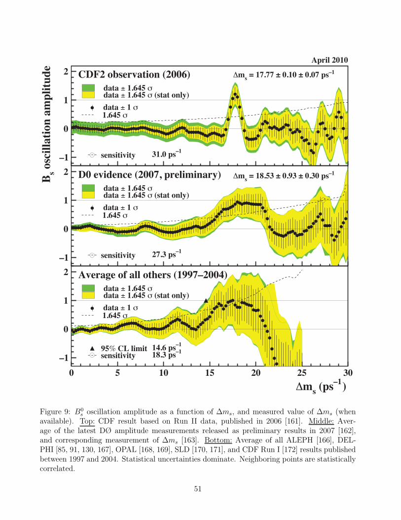
–1
0
1
2
–1
0
1
2
–1
0
1
2
0 5 10 15 20 25 30
Bs
osc
illa
tion
am
pli
tud
e
data ± 1 σ1.645 σ
sensitivity 31.0 ps–1
data ± 1.645 σdata ± 1.645 σ (stat only)
CDF2 observation (2006)
April 2010
data ± 1 σ1.645 σ
sensitivity 27.3 ps–1
data ± 1.645 σdata ± 1.645 σ (stat only)
D0 evidence (2007, preliminary)
Δms (ps
–1)
data ± 1 σ
95% CL limit 14.6 ps–1
1.645 σ
sensitivity 18.3 ps–1
data ± 1.645 σdata ± 1.645 σ (stat only)
Average of all others (1997–2004)
Δms = 17.77 ± 0.10 ± 0.07 ps–1
Δms = 18.53 ± 0.93 ± 0.30 ps–1
Figure 9: B0s oscillation amplitude as a function of ∆ms, and measured value of ∆ms (when
available). Top: CDF result based on Run II data, published in 2006 [161]. Middle: Aver-age of the latest DØ amplitude measurements released as preliminary results in 2007 [162],and corresponding measurement of ∆ms [163]. Bottom: Average of all ALEPH [166], DEL-PHI [85, 91, 130, 167], OPAL [168, 169], SLD [170, 171], and CDF Run I [172] results publishedbetween 1997 and 2004. Statistical uncertainties dominate. Neighboring points are statisticallycorrelated.
51
already based on the amplitude method, had been performed previously by ALEPH [166],CDF (Run I) [172], DELPHI [85, 91, 130, 167], OPAL [168, 169] and SLD [170, 171, 173] (weomit references to searches that have been superseded by more recent ones). All the resultspublished by these experiments (between 1997 and 2004) have been combined by averaging themeasured amplitudes A at each test value of ∆ms. The individual results have been adjustedto common physics inputs, and all known correlations have been accounted for; in the case ofthe inclusive (lepton) analyses, performed at LEP and SLC, the sensitivities (i.e. the statisticaluncertainties on A), which depend directly through Eq. (125) on the assumed fraction fsig ∼ fsof B0
s mesons in an unbiased sample of weakly-decaying b hadrons, have also been rescaled tothe LEP average fs = 0.103 ± 0.009. The resulting average amplitude spectrum, completelydominated by the e+e− → Z experiments, is displayed as the bottom plot of Fig. 9. Althoughno significant signal is seen, it is interesting to note the hint in the region 15–20 ps−1, consistentwith the recent results from the Tevatron.
52
4 Measurements related to Unitarity Triangle angles
The charge of the “CP (t) and Unitarity Triangle angles” group is to provide averages of mea-surements from time-dependent asymmetry analyses, and other quantities that are related tothe angles of the Unitarity Triangle (UT). In cases where considerable theoretical input isrequired to extract the fundamental quantities, no attempt is made to do so at this stage.However, straightforward interpretations of the averages are given, where possible.
In Sec. 4.1 a brief introduction to the relevant phenomenology is given. In Sec. 4.2 anattempt is made to clarify the various different notations in use. In Sec. 4.3 the commoninputs to which experimental results are rescaled in the averaging procedure are listed. Wealso briefly introduce the treatment of experimental errors. In the remainder of this section,the experimental results and their averages are given, divided into subsections based on theunderlying quark-level decays.
4.1 Introduction
The Standard Model Cabibbo-Kobayashi-Maskawa (CKM) quark mixing matrix V must beunitary. A 3×3 unitary matrix has four free parameters,13 and these are conventionally writtenby the product of three (complex) rotation matrices [174], where the rotations are characterizedby the Euler angles θ12, θ13 and θ23, which are the mixing angles between the generations, andone overall phase δ,
V =
Vud Vus VubVcd Vcs VcbVtd Vts Vtb
=
c12c13 s12c13 s13e−iδ
−s12c23 − c12s23s13eiδ c12c23 − s12s23s13e
iδ s23c13s12s23 − c12c23s13e
iδ −c12s23 − s12c23s13eiδ c23c13
(126)
where cij = cos θij , sij = sin θij for i < j = 1, 2, 3.Following the observation of a hierarchy between the different matrix elements, the Wolfen-
stein parameterization [175] is an expansion of V in terms of the four real parameters λ (theexpansion parameter), A, ρ and η. Defining to all orders in λ [176]
s12 ≡ λ,
s23 ≡ Aλ2, (127)
s13e−iδ ≡ Aλ3(ρ− iη),
and inserting these into the representation of Eq. (126), unitarity of the CKMmatrix is achievedto all orders. A Taylor expansion of V leads to the familiar approximation
V =
1− λ2/2 λ Aλ3(ρ− iη)−λ 1− λ2/2 Aλ2
Aλ3(1− ρ− iη) −Aλ2 1
+O(
λ4)
. (128)
At order λ5, the obtained CKM matrix in this extended Wolfenstein parametrization is:
V =
1− 12λ
2 − 18λ
4 λ Aλ3(ρ− iη)−λ+ 1
2A2λ5 [1− 2(ρ+ iη)] 1− 1
2λ2 − 1
8λ4(1 + 4A2) Aλ2
Aλ3[
1− (1− 12λ
2)(ρ+ iη)]
−Aλ2 + 12Aλ
4 [1− 2(ρ+ iη)] 1− 12A
2λ4
+O(
λ6)
. (129)
13 In the general case there are nine free parameters, but five of these are absorbed into unobservable quarkphases.
53
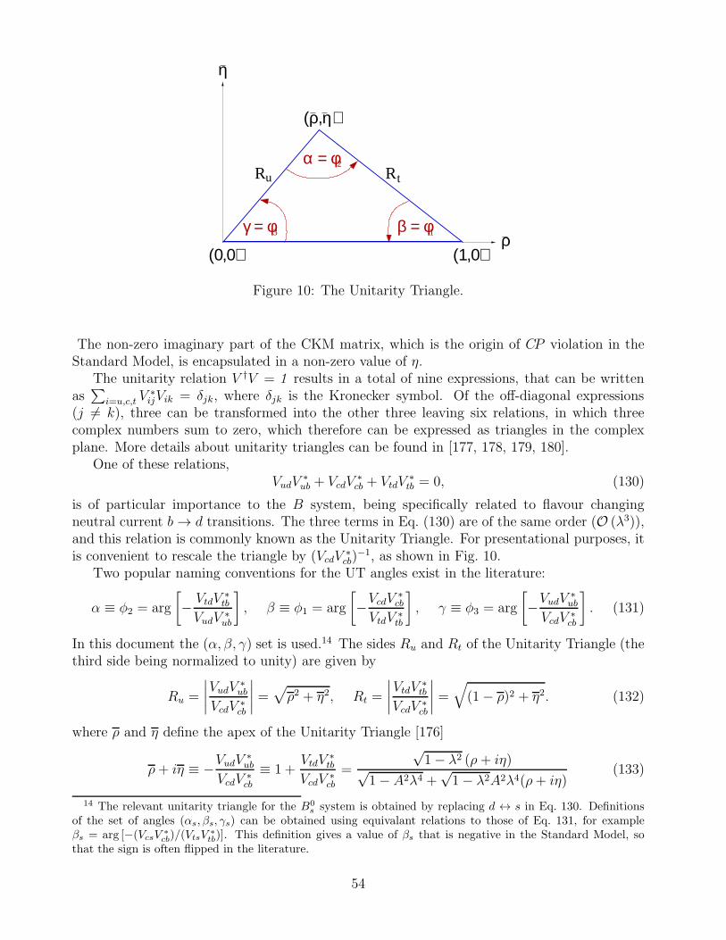
Rt
(ρ,η)
γ = φ
α = φ
β = φρ
η
Ru
(0,0) (1,0)
2
3 1
Figure 10: The Unitarity Triangle.
The non-zero imaginary part of the CKM matrix, which is the origin of CP violation in theStandard Model, is encapsulated in a non-zero value of η.
The unitarity relation V †V = 1 results in a total of nine expressions, that can be writtenas∑
i=u,c,t V∗ijVik = δjk, where δjk is the Kronecker symbol. Of the off-diagonal expressions
(j 6= k), three can be transformed into the other three leaving six relations, in which threecomplex numbers sum to zero, which therefore can be expressed as triangles in the complexplane. More details about unitarity triangles can be found in [177, 178, 179, 180].
One of these relations,VudV
∗ub + VcdV
∗cb + VtdV
∗tb = 0, (130)
is of particular importance to the B system, being specifically related to flavour changingneutral current b → d transitions. The three terms in Eq. (130) are of the same order (O (λ3)),and this relation is commonly known as the Unitarity Triangle. For presentational purposes, itis convenient to rescale the triangle by (VcdV
∗cb)
−1, as shown in Fig. 10.Two popular naming conventions for the UT angles exist in the literature:
α ≡ φ2 = arg
[
− VtdV∗tb
VudV ∗ub
]
, β ≡ φ1 = arg
[
−VcdV∗cb
VtdV ∗tb
]
, γ ≡ φ3 = arg
[
−VudV∗ub
VcdV ∗cb
]
. (131)
In this document the (α, β, γ) set is used.14 The sides Ru and Rt of the Unitarity Triangle (thethird side being normalized to unity) are given by
Ru =
∣
∣
∣
∣
VudV∗ub
VcdV ∗cb
∣
∣
∣
∣
=√
ρ2 + η2, Rt =
∣
∣
∣
∣
VtdV∗tb
VcdV ∗cb
∣
∣
∣
∣
=√
(1− ρ)2 + η2. (132)
where ρ and η define the apex of the Unitarity Triangle [176]
ρ+ iη ≡ −VudV∗ub
VcdV ∗cb
≡ 1 +VtdV
∗tb
VcdV ∗cb
=
√1− λ2 (ρ+ iη)√
1− A2λ4 +√1− λ2A2λ4(ρ+ iη)
(133)
14 The relevant unitarity triangle for the B0s system is obtained by replacing d ↔ s in Eq. 130. Definitions
of the set of angles (αs, βs, γs) can be obtained using equivalant relations to those of Eq. 131, for exampleβs = arg [−(VcsV
∗cb)/(VtsV
∗tb)]. This definition gives a value of βs that is negative in the Standard Model, so
that the sign is often flipped in the literature.
54
The exact relation between (ρ, η) and (ρ, η) is
ρ+ iη =
√1−A2λ4(ρ+ iη)√
1− λ2 [1− A2λ4(ρ+ iη)]. (134)
By expanding in powers of λ, several useful approximate expressions can be obtained, in-cluding
ρ = ρ(1− 1
2λ2) +O(λ4) , η = η(1− 1
2λ2) +O(λ4) , Vtd = Aλ3(1− ρ− iη) +O(λ6) . (135)
4.2 Notations
Several different notations for CP violation parameters are commonly used. This section reviewsthose found in the experimental literature, in the hope of reducing the potential for confusion,and to define the frame that is used for the averages.
In some cases, when B mesons decay into multibody final states via broad resonances (ρ,K∗, etc.), the experimental analyses ignore the effects of interference between the overlappingstructures. This is referred to as the quasi-two-body (Q2B) approximation in the following.
4.2.1 CP asymmetries
The CP asymmetry is defined as the difference between the rate involving a b quark and thatinvolving a b quark, divided by the sum. For example, the partial rate (or charge) asymmetryfor a charged B decay would be given as
Af ≡ Γ(B− → f)− Γ(B+ → f)
Γ(B− → f) + Γ(B+ → f). (136)
4.2.2 Time-dependent CP asymmetries in decays to CP eigenstates
If the amplitudes for B0 and B0 to decay to a final state f , which is a CP eigenstate witheigenvalue ηf , are given by Af and Af , respectively, then the decay distributions for neutral Bmesons, with known flavour at time ∆t = 0, are given by
ΓB0→f(∆t) =e−|∆t|/τ(B0)
4τ(B0)
[
1 +2 Im(λf)
1 + |λf |2sin(∆m∆t)− 1− |λf |2
1 + |λf |2cos(∆m∆t)
]
, (137)
ΓB0→f(∆t) =e−|∆t|/τ(B0)
4τ(B0)
[
1− 2 Im(λf)
1 + |λf |2sin(∆m∆t) +
1− |λf |21 + |λf |2
cos(∆m∆t)
]
. (138)
Here λf = qp
AfAf
contains terms related to B0–B0 mixing and to the decay amplitude (the
eigenstates of the effective Hamiltonian in the B0B0 system are |B±〉 = p |B0〉 ± q∣
∣B0⟩
). Thisformulation assumes CPT invariance, and neglects possible lifetime differences (between theeigenstates of the effective Hamiltonian; see Section 3.3 where the mass difference ∆m is alsodefined) in the neutral B meson system. The case where non-zero lifetime differences are takeninto account is discussed in Section 4.2.6. The time-dependent CP asymmetry, again defined as
55
the difference between the rate involving a b quark and that involving a b quark, is then givenby
Af (∆t) ≡ΓB0→f(∆t)− ΓB0→f(∆t)
ΓB0→f(∆t) + ΓB0→f(∆t)=
2 Im(λf)
1 + |λf |2sin(∆m∆t)− 1− |λf |2
1 + |λf |2cos(∆m∆t). (139)
While the coefficient of the sin(∆m∆t) term in Eq. (139) is everywhere15 denoted Sf :
Sf ≡ 2 Im(λf )
1 + |λf |2, (140)
different notations are in use for the coefficient of the cos(∆m∆t) term:
Cf ≡ −Af ≡ 1− |λf |2
1 + |λf |2. (141)
The C notation is used by the BABAR collaboration (see e.g. [181]), and also in this document.The A notation is used by the Belle collaboration (see e.g. [182]).
Neglecting effects due to CP violation in mixing (by taking |q/p| = 1), if the decay amplitudecontains terms with a single weak (i.e., CP violating) phase then |λf | = 1 and one finds Sf =−ηf sin(φmix+φdec), Cf = 0, where φmix = arg(q/p) and φdec = arg(Af/Af). Note that the B
0–B0 mixing phase φmix ≈ 2β in the Standard Model (in the usual phase convention) [183, 184].
If amplitudes with different weak phases contribute to the decay, no clean interpretation ofSf is possible. If the decay amplitudes have in addition different CP conserving strong phases,then |λf | 6= 1 and no clean interpretation is possible. The coefficient of the cosine term becomesnon-zero, indicating direct CP violation. The sign of Af as defined above is consistent withthat of Af in Eq. (136).
Frequently, we are interested in combining measurements governed by similar or identicalshort-distance physics, but with different final states (e.g., B0 → J/ψK0
Sand B0 → J/ψK0
L).
In this case, we remove the dependence on the CP eigenvalue of the final state by quoting−ηSf . In cases where the final state is not a CP eigenstate but has an effective CP content(see below), the reported −ηS is corrected by the effective CP .
4.2.3 Time-dependent CP asymmetries in decays to vector-vector final states
Consider B decays to states consisting of two spin-1 particles, such as J/ψK∗0(→ K0Sπ
0),D∗+D∗− and ρ+ρ−, which are eigenstates of charge conjugation but not of parity.16 In fact, forsuch a system, there are three possible final states; in the helicity basis these can be writtenh−1, h0, h+1. The h0 state is an eigenstate of parity, and hence of CP ; however, CP transformsh+1 ↔ h−1 (up to an unobservable phase). In the transversity basis, these states are transformedinto h‖ = (h+1+h−1)/2 and h⊥ = (h+1−h−1)/2. In this basis all three states are CP eigenstates,and h⊥ has the opposite CP to the others.
The amplitudes to these states are usually given by A0,⊥,‖ (here we use a normalizationsuch that |A0|2 + |A⊥|2 + |A‖|2 = 1). Then the effective CP of the vector-vector state is known
15 Occasionally one also finds Eq. (139) written as Af (∆t) = Amixf sin(∆m∆t) +Adir
f cos(∆m∆t), or similar.16 This is not true of all vector-vector final states, e.g., D∗±ρ∓ is clearly not an eigenstate of charge conju-
gation.
56
if |A⊥|2 is measured. An alternative strategy is to measure just the longitudinally polarizedcomponent, |A0|2 (sometimes denoted by flong), which allows a limit to be set on the effectiveCP since |A⊥|2 ≤ |A⊥|2+ |A‖|2 = 1−|A0|2. The most complete treatment for neutral B decaysto vector-vector final states is time-dependent angular analysis (also known as time-dependenttransversity analysis). In such an analysis, the interference between the CP -even and CP -oddstates provides additional sensitivity to the weak and strong phases involved.
In most analyses of time-dependent CP asymmetries in decays to vector-vector final statescarried out to date, an assumption has been made that each helicity (or transversity) amplitudehas the same weak phase. This is a good approximation for decays that are dominated byamplitudes with a single weak phase, such B0 → J/ψK∗0, and is a reasonable approximationin any mode for which only very limited statistics are available. However, for modes that havecontributions from amplitudes with different weak phases, the relative size of these contributionscan be different for each helicity (or transversity) amplitude, and therefore the time-dependentCP asymmetry parameters can also differ. The most generic analysis, suitable for modes withsufficient statistics, would allow for this effect; an intermediate analysis can allow differentparameters for the CP -even and CP -odd components. Such an analysis has been carried outby BABAR for the decay B0 → D∗+D∗− [185].
4.2.4 Time-dependent asymmetries: self-conjugate multiparticle final states
Amplitudes for neutral B decays into self-conjugate multiparticle final states such as π+π−π0,K+K−K0
S, π+π−K0
S, J/ψπ+π− or Dπ0 with D → K0
Sπ+π− may be written in terms of CP -even
and CP -odd amplitudes. As above, the interference between these terms provides additionalsensitivity to the weak and strong phases involved in the decay, and the time-dependence de-pends on both the sine and cosine of the weak phase difference. In order to perform unbinnedmaximum likelihood fits, and thereby extract as much information as possible from the distri-butions, it is necessary to select a model for the multiparticle decay, and therefore the resultsacquire some model dependence (binned, model independent methods are also possible, thoughare not as statistically powerful). The number of observables depends on the final state (and onthe model used); the key feature is that as long as there are regions where both CP -even andCP -odd amplitudes contribute, the interference terms will be sensitive to the cosine of the weakphase difference. Therefore, these measurements allow distinction between multiple solutionsfor, e.g., the four values of β from the measurement of sin(2β).
We now consider the various notations which have been used in experimental studies oftime-dependent asymmetries in decays to self-conjugate multiparticle final states.
B0 → D(∗)h0 with D → K0Sπ+π−
The states Dπ0, D∗π0, Dη, D∗η, Dω are collectively denoted D(∗)h0. When the D decaymodel is fixed, fits to the time-dependent decay distributions can be performed to extract theweak phase difference. However, it is experimentally advantageous to use the sine and cosine ofthis phase as fit parameters, since these behave as essentially independent parameters, with lowcorrelations and (potentially) rather different uncertainties. A parameter representing directCP violation in the B decay can also be floated. For consistency with other analyses, this couldbe chosen to be Cf , but could equally well be |λf |, or other possibilities.
Belle performed an analysis of these channels with sin(2φ1) and cos(2φ1) as free parame-ters [186]. BABAR have performed an analysis floating also |λf | [187] (and, of course, replacing
57
φ1 ⇔ β).
B0 → D∗+D∗−K0S
The hadronic structure of the B0 → D∗+D∗−K0S decay is not sufficiently well understood to
perform a full time-dependent Dalitz plot analysis. Instead, following Browder et al. [188],BABAR [189] divide the Dalitz plane in two: m(D∗+K0
S)2 > m(D∗−K0
S)2 (ηy = +1) and
m(D∗+K0S)
2 < m(D∗−K0S)
2 (ηy = −1); and then fit to a decay time distribution with asymmetrygiven by
Af (∆t) = ηyJcJ0
cos(∆m∆t)−[
2Js1J0
sin(2β) + ηy2Js2J0
cos(2β)
]
sin(∆m∆t) . (142)
A similar analysis has also been carried out by Belle [190]. The measured values are JcJ0,
2Js1J0
sin(2β) and 2Js2J0
cos(2β), where the parameters J0, Jc, Js1 and Js2 are the integrals over
the half Dalitz plane m(D∗+K0S)
2 < m(D∗−K0S)
2 of the functions |a|2+ |a|2, |a|2−|a|2, Re(aa∗)and Im(aa∗) respectively, where a and a are the decay amplitudes of B0 → D∗+D∗−K0
Sand
B0 → D∗+D∗−K0Srespectively. The parameter Js2 (and hence Js2/J0) is predicted to be positive;
with this assumption is it possible to determine the sign of cos(2β).
B0 → K+K−K0
Studies of B0 → K+K−K0 [191, 192, 193] and of the related decay B+ → K+K−K+ [194,195], show that the decay is dominated by components from the intermediate K+K− reso-nances φ(1020), f0(980), a poorly understood scalar structure that peaks near m(K+K−) ∼1550 MeV/c2 and is denoted X0(1550), as well as a large nonresonant contribution. There isalso a contribution from χc0.
The full time-dependent Dalitz plot analysis allows the complex amplitudes of each con-tributing term to be determined from data, including CP violation effects (i.e. allowing thecomplex amplitude for the B0 decay to be independent from that for B0 decay), although oneamplitude must be fixed to give a reference point. There are several choices for parametrizationof the complex amplitudes (e.g. real and imaginary part, or magnitude and phase). Similarly,there are various approaches to include CP violation effects. Note that positive definite parame-ters such as magnitudes are disfavoured in certain circumstances (they inevitably lead to biasesfor small values). In order to compare results between analyses, it is useful for each experimentto present results in terms of the parameters that can be measured in a Q2B analysis (such asAf , Sf , Cf , sin(2β
eff), cos(2βeff), etc.)In the BABAR analysis of B0 → K+K−K0 [191, 192], the complex amplitude for each
resonant contribution is written as
Af = cf(1 + bf )ei(φf+δf ) , Af = cf(1− bf )e
i(φf−δf ) , (143)
where bf and δf introduce CP violation in the magnitude and phase respectively. [The weak
phase in B0–B0mixing (2β) also appears in the full formula for the time-dependent decay
distribution.] The Q2B direct CP violation parameter is directly related to bf
Af =−2bf1 + b2f
≈ Cf , (144)
58
and the mixing-induced CP violation parameter can be used to obtain sin(2βeff)
− ηfSf ≈1− b2f1 + b2f
sin(2βefff ) , (145)
where the approximations are exact in the case that |q/p| = 1.BABAR [191, 192] present results for cf , φf , Af and βeff for each resonant contribution, as
well as averaged values of Af and βeff for the entire K+K−K0 Dalitz plot. Belle [193] presentresults for the resonant contributions only.
B0 → π+π−K0S
Studies of B0 → π+π−K0S [196, 197] and of the related decay B+ → π+π−K+ [194, 198,
199, 200] show that the decay is dominated by components from intermediate resonances in theKπ (K∗(892), K∗
0(1430)) and ππ (ρ(770), f0(980), f2(1270)) spectra, together with a poorlyunderstood scalar structure that peaks near m(ππ) ∼ 1300 MeV/c2 and is denoted fX(1300)(that could be identified as either the f0(1370) or f0(1500)), and a large nonresonant component.There is also a contribution from the χc0 state.
The full time-dependent Dalitz plot analysis allows the complex amplitudes of each con-tributing term to be determined from data, including CP violation effects. In the BABAR
analysis [196], the magnitude and phase of each component (for both B0 and B0 decays) aremeasured relative to B0 → f0(980)K
0S, using the following parameterisation
Af = |Af | ei arg(Af ) , Af =∣
∣Af∣
∣ ei arg(Af ) . (146)
In the Belle analysis [197], the B0 → K∗+π− amplitude is chosen as the reference, and theamplitudes are parameterised as
Af = af(1 + cf)ei(bf+df ) , Af = af(1− cf)e
i(bf−df ) . (147)
In both cases, the results are translated into quasi-two-body parameters such as 2βefff , Sf , Cf
for each CP eigenstate f , and direct CP asymmetries for each flavour-specific state. Relativephase differences between resonant terms are also extracted.
B0 → π+π−π0
The B0 → π+π−π0 decay is dominated by intermediate ρ resonances. Though it is possible,as above, to determine directly the complex amplitudes for each component, an alternativeapproach [201, 202], has been used by both BABAR [203] and Belle [204, 205]. The amplitudesfor B0 and B0 to π+π−π0 are written
A3π = f+A+ + f−A− + f0A0 , A3π = f+A+ + f−A− + f0A0 (148)
respectively. A+, A− and A0 represent the complex decay amplitudes for B0 → ρ+π−, B0 →ρ−π+ and B0 → ρ0π0 while A+, A− and A0 represent those for B0 → ρ+π−, B0 → ρ−π+
and B0 → ρ0π0 respectively. f+, f− and f0 incorporate kinematical and dynamical factors anddepend on the Dalitz plot coordinates. The full time-dependent decay distribution can thenbe written in terms of 27 free parameters, one for each coefficient of the form factor bilinears,as listed in Table 19. These parameters are often referred to as “the Us and Is”, and can be
59
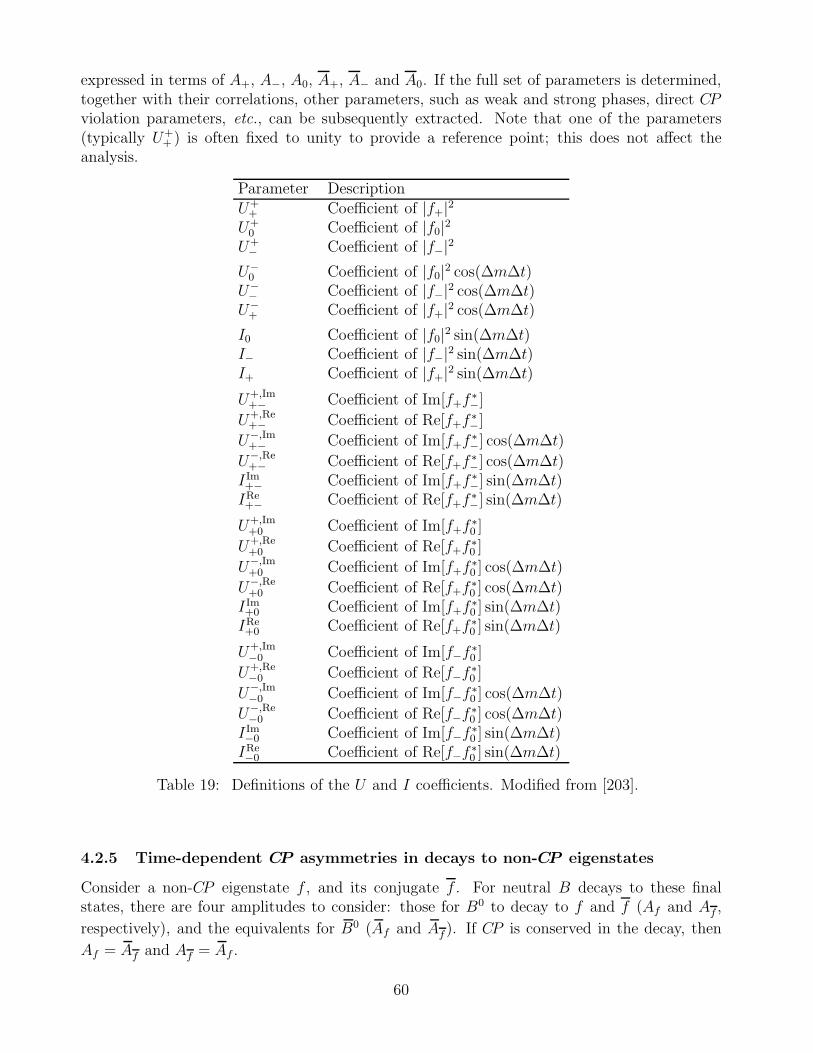
expressed in terms of A+, A−, A0, A+, A− and A0. If the full set of parameters is determined,together with their correlations, other parameters, such as weak and strong phases, direct CPviolation parameters, etc., can be subsequently extracted. Note that one of the parameters(typically U+
+ ) is often fixed to unity to provide a reference point; this does not affect theanalysis.
Parameter DescriptionU++ Coefficient of |f+|2
U+0 Coefficient of |f0|2
U+− Coefficient of |f−|2
U−0 Coefficient of |f0|2 cos(∆m∆t)
U−− Coefficient of |f−|2 cos(∆m∆t)
U−+ Coefficient of |f+|2 cos(∆m∆t)
I0 Coefficient of |f0|2 sin(∆m∆t)I− Coefficient of |f−|2 sin(∆m∆t)I+ Coefficient of |f+|2 sin(∆m∆t)
U+,Im+− Coefficient of Im[f+f
∗−]
U+,Re+− Coefficient of Re[f+f
∗−]
U−,Im+− Coefficient of Im[f+f
∗−] cos(∆m∆t)
U−,Re+− Coefficient of Re[f+f
∗−] cos(∆m∆t)
I Im+− Coefficient of Im[f+f∗−] sin(∆m∆t)
IRe+− Coefficient of Re[f+f
∗−] sin(∆m∆t)
U+,Im+0 Coefficient of Im[f+f
∗0 ]
U+,Re+0 Coefficient of Re[f+f
∗0 ]
U−,Im+0 Coefficient of Im[f+f
∗0 ] cos(∆m∆t)
U−,Re+0 Coefficient of Re[f+f
∗0 ] cos(∆m∆t)
I Im+0 Coefficient of Im[f+f∗0 ] sin(∆m∆t)
IRe+0 Coefficient of Re[f+f
∗0 ] sin(∆m∆t)
U+,Im−0 Coefficient of Im[f−f
∗0 ]
U+,Re−0 Coefficient of Re[f−f
∗0 ]
U−,Im−0 Coefficient of Im[f−f
∗0 ] cos(∆m∆t)
U−,Re−0 Coefficient of Re[f−f
∗0 ] cos(∆m∆t)
I Im−0 Coefficient of Im[f−f∗0 ] sin(∆m∆t)
IRe−0 Coefficient of Re[f−f
∗0 ] sin(∆m∆t)
Table 19: Definitions of the U and I coefficients. Modified from [203].
4.2.5 Time-dependent CP asymmetries in decays to non-CP eigenstates
Consider a non-CP eigenstate f , and its conjugate f . For neutral B decays to these finalstates, there are four amplitudes to consider: those for B0 to decay to f and f (Af and Af ,
respectively), and the equivalents for B0 (Af and Af ). If CP is conserved in the decay, then
Af = Af and Af = Af .
60
The time-dependent decay distributions can be written in many different ways. Here, we
follow Sec. 4.2.2 and define λf = qp
AfAf
and λf = qp
AfAf
. The time-dependent CP asymmetries
then follow Eq. (139):
Af(∆t) ≡ΓB0→f(∆t)− ΓB0→f(∆t)
ΓB0→f(∆t) + ΓB0→f(∆t)= Sf sin(∆m∆t)− Cf cos(∆m∆t), (149)
Af(∆t) ≡ΓB0→f(∆t)− ΓB0→f(∆t)
ΓB0→f(∆t) + ΓB0→f(∆t)= Sf sin(∆m∆t)− Cf cos(∆m∆t), (150)
with the definitions of the parameters Cf , Sf , Cf and Sf , following Eqs. (140) and (141).The time-dependent decay rates are given by
ΓB0→f(∆t) =e−|∆t|/τ(B0)
8τ(B0)(1 + 〈Aff〉) 1 + Sf sin(∆m∆t)− Cf cos(∆m∆t) , (151)
ΓB0→f(∆t) =e−|∆t|/τ(B0)
8τ(B0)(1 + 〈Aff〉) 1− Sf sin(∆m∆t) + Cf cos(∆m∆t) , (152)
ΓB0→f(∆t) =e−|∆t|/τ(B0)
8τ(B0)(1− 〈Aff〉)
1 + Sf sin(∆m∆t)− Cf cos(∆m∆t)
, (153)
ΓB0→f(∆t) =e−|∆t|/τ(B0)
8τ(B0)(1− 〈Aff〉)
1− Sf sin(∆m∆t) + Cf cos(∆m∆t)
, (154)
where the time-independent parameter 〈Aff〉 represents an overall asymmetry in the production
of the f and f final states,17
〈Aff〉 =
(
|Af |2 +∣
∣Af∣
∣
2)
−(
∣
∣Af∣
∣
2+∣
∣Af
∣
∣
2)
(
|Af |2 +∣
∣Af∣
∣
2)
+(
∣
∣Af∣
∣
2+∣
∣Af∣
∣
2) . (155)
Assuming |q/p| = 1, the parameters Cf and Cf can also be written in terms of the decayamplitudes as follows:
Cf =|Af |2 −
∣
∣Af
∣
∣
2
|Af |2 +∣
∣Af
∣
∣
2 and Cf =
∣
∣Af∣
∣
2 −∣
∣Af
∣
∣
2
∣
∣Af∣
∣
2+∣
∣Af
∣
∣
2 , (156)
giving asymmetries in the decay amplitudes of B0 and B0 to the final states f and f respectively.In this notation, the direct CP invariance conditions are 〈Aff〉 = 0 and Cf = −Cf . Note
that Cf and Cf are typically non-zero; e.g., for a flavour-specific final state, Af = Af = 0
(Af = Af = 0), they take the values Cf = −Cf = 1 (Cf = −Cf = −1).The coefficients of the sine terms contain information about the weak phase. In the case
that each decay amplitude contains only a single weak phase (i.e., no direct CP violation),these terms can be written
Sf =−2 |Af |
∣
∣Af
∣
∣ sin(φmix + φdec − δf )
|Af |2 +∣
∣Af∣
∣
2 and Sf =−2∣
∣Af∣
∣
∣
∣Af∣
∣ sin(φmix + φdec + δf)∣
∣Af∣
∣
2+∣
∣Af
∣
∣
2 ,
(157)
17 This parameter is often denoted Af (or ACP ), but here we avoid this notation to prevent confusion withthe time-dependent CP asymmetry.
61

where δf is the strong phase difference between the decay amplitudes. If there is no CPviolation, the condition Sf = −Sf holds. If decay amplitudes with different weak and strongphases contribute, no clean interpretation of Sf and Sf is possible.
Since two of the CP invariance conditions are Cf = −Cf and Sf = −Sf , there is motivationfor a rotation of the parameters:
Sff =Sf + Sf
2, ∆Sff =
Sf − Sf2
, Cff =Cf + Cf
2, ∆Cff =
Cf − Cf2
. (158)
With these parameters, the CP invariance conditions become Sff = 0 and Cff = 0. Theparameter ∆Cff gives a measure of the “flavour-specificity” of the decay: ∆Cff = ±1 corre-sponds to a completely flavour-specific decay, in which no interference between decays with andwithout mixing can occur, while ∆Cff = 0 results in maximum sensitivity to mixing-inducedCP violation. The parameter ∆Sff is related to the strong phase difference between the decay
amplitudes of B0 to f and to f . We note that the observables of Eq. (158) exhibit experi-mental correlations (typically of ∼ 20%, depending on the tagging purity, and other effects)between Sff and ∆Sff , and between Cff and ∆Cff . On the other hand, the final state specificobservables of Eq. (149) tend to have low correlations.
Alternatively, if we recall that the CP invariance conditions at the decay amplitude levelare Af = Af and Af = Af , we are led to consider the parameters [206]
Aff =
∣
∣Af
∣
∣
2 − |Af |2∣
∣Af∣
∣
2+ |Af |2
and Aff =
∣
∣Af
∣
∣
2 −∣
∣Af∣
∣
2
∣
∣Af∣
∣
2+∣
∣Af∣
∣
2. (159)
These are sometimes considered more physically intuitive parameters since they characterizedirect CP violation in decays with particular topologies. For example, in the case of B0 → ρ±π∓
(choosing f = ρ+π− and f = ρ−π+), Aff (also denoted A+−ρπ ) parameterizes direct CP violation
in decays in which the produced ρ meson does not contain the spectator quark, while Aff (alsodenoted A−+
ρπ ) parameterizes direct CP violation in decays in which it does. Note that wehave again followed the sign convention that the asymmetry is the difference between the rateinvolving a b quark and that involving a b quark, cf. Eq. (136). Of course, these parametersare not independent of the other sets of parameters given above, and can be written
Aff = −〈Aff〉+ Cff + 〈Aff〉∆Cff1 + ∆Cff + 〈Aff〉Cff
and Aff =−〈Aff〉+ Cff + 〈Aff〉∆Cff−1 + ∆Cff + 〈Aff〉Cff
. (160)
They usually exhibit strong correlations.We now consider the various notations which have been used in experimental studies of
time-dependent CP asymmetries in decays to non-CP eigenstates.
B0 → D∗±D∓
The above set of parameters (〈Aff〉, Cf , Sf , Cf , Sf ), has been used by both BABAR [185]
and Belle [207] in the D∗±D∓ system (f = D∗+D−, f = D∗−D+). However, slightly differentnames for the parameters are used: BABAR uses (A, C+−, S+−, C−+, S−+); Belle uses (A, C+,S+, C−, S−). In this document, we follow the notation used by BABAR.
B0 → ρ±π∓
62
In the ρ±π∓ system, the (〈Aff〉, Cff , Sff , ∆Cff , ∆Sff ) set of parameters has been usedoriginally by BABAR [208] and Belle [209], in the Q2B approximation; the exact names18 usedin this case are (Aρπ
CP , Cρπ, Sρπ,∆Cρπ,∆Sρπ), and these names are also used in this document.Since ρ±π∓ is reconstructed in the final state π+π−π0, the interference between the ρ reso-
nances can provide additional information about the phases (see Sec. 4.2.4). Both BABAR [203]and Belle [204, 205] have performed time-dependent Dalitz plot analyses, from which the weakphase α is directly extracted. In such an analysis, the measured Q2B parameters are alsonaturally corrected for interference effects. See Sec. 4.2.4.
B0 → D±π∓, D∗±π∓, D±ρ∓
Time-dependent CP analyses have also been performed for the final states D±π∓, D∗±π∓
and D±ρ∓. In these theoretically clean cases, no penguin contributions are possible, so thereis no direct CP violation. Furthermore, due to the smallness of the ratio of the magnitudesof the suppressed (b → u) and favoured (b → c) amplitudes (denoted Rf), to a very goodapproximation, Cf = −Cf = 1 (using f = D(∗)−h+, f = D(∗)+h− h = π, ρ), and the coefficientsof the sine terms are given by
Sf = −2Rf sin(φmix + φdec − δf ) and Sf = −2Rf sin(φmix + φdec + δf). (161)
Thus weak phase information can be cleanly obtained from measurements of Sf and Sf , al-though external information on at least one of Rf or δf is necessary. (Note that φmix + φdec =2β + γ for all the decay modes in question, while Rf and δf depend on the decay mode.)
Again, different notations have been used in the literature. BABAR [210, 211] defines thetime-dependent probability function by
f±(η,∆t) =e−|∆t|/τ
4τ[1∓ Sζ sin(∆m∆t) ∓ ηCζ cos(∆m∆t)] , (162)
where the upper (lower) sign corresponds to the tagging meson being a B0 (B0). [Note herethat a tagging B0 (B0) corresponds to −Sζ (+Sζ).] The parameters η and ζ take the values+1 and + (−1 and −) when the final state is, e.g., D−π+ (D+π−). However, in the fit, thesubstitutions Cζ = 1 and Sζ = a ∓ ηbi − ηci are made.19 [Note that, neglecting b terms,S+ = a − c and S− = a + c, so that a = (S+ + S−)/2, c = (S− − S+)/2, in analogy to theparameters of Eq. (158).] The subscript i denotes the tagging category. These are motivated bythe possibility of CP violation on the tag side [212], which is absent for semileptonic B decays(mostly lepton tags). The parameter a is not affected by tag side CP violation. The parameterb only depends on tag side CP violation parameters and is not directly useful for determiningUT angles. A clean interpretation of the c parameter is only possible for lepton-tagged events,so the BABAR measurements report c measured with those events only.
The parameters used by Belle in the analysis using partially reconstructed B decays [213],are similar to the Sζ parameters defined above. However, in the Belle convention, a tagging B0
corresponds to a + sign in front of the sine coefficient; furthermore the correspondence betweenthe super/subscript and the final state is opposite, so that S± (BABAR) = −S∓ (Belle). In thisanalysis, only lepton tags are used, so there is no effect from tag side CP violation. In the
18 BABAR has used the notations AρπCP [208] and Aρπ [203] in place of Aρπ
CP .19 The subscript i denotes tagging category.
63
Table 20: Conversion between the various notations used for CP violation parameters in theD±π∓, D∗±π∓ and D±ρ∓ systems. The bi terms used by BABAR have been neglected. Recallthat (α, β, γ) = (φ2, φ1, φ3).
BABAR Belle partial rec. Belle full rec.SD+π− −S− = −(a + ci) N/A 2RDπ sin(2φ1 + φ3 + δDπ)SD−π+ −S+ = −(a− ci) N/A 2RDπ sin(2φ1 + φ3 − δDπ)SD∗+π− −S− = −(a + ci) S+ −2RD∗π sin(2φ1 + φ3 + δD∗π)SD∗−π+ −S+ = −(a− ci) S− −2RD∗π sin(2φ1 + φ3 − δD∗π)SD+ρ− −S− = −(a + ci) N/A N/ASD−ρ+ −S+ = −(a− ci) N/A N/A
Table 21: Translations used to convert the parameters measured by Belle to the parametersused for averaging in this document. The angular momentum factor L is −1 for D∗π and +1for Dπ. Recall that (α, β, γ) = (φ2, φ1, φ3).
D∗π partial rec. D(∗)π full rec.a −(S+ + S−) 1
2(−1)L+1 (2RD(∗)π sin(2φ1 + φ3 + δD(∗)π) + 2RD(∗)π sin(2φ1 + φ3 − δD(∗)π))
c −(S+ − S−) 12(−1)L+1 (2RD(∗)π sin(2φ1 + φ3 + δD(∗)π)− 2RD(∗)π sin(2φ1 + φ3 − δD(∗)π))
Belle analysis using fully reconstructed B decays [214], this effect is measured and taken intoaccount using D∗lν decays; in neither Belle analysis are the a, b and c parameters used. In thelatter case, the measured parameters are 2RD(∗)π sin(2φ1 + φ3 ± δD(∗)π); the definition is suchthat S± (Belle) = −2RD∗π sin(2φ1 + φ3 ± δD∗π). However, the definition includes an angularmomentum factor (−1)L [215], and so for the results in the Dπ system, there is an additionalfactor of −1 in the conversion.
Explicitly, the conversion then reads as given in Table 20, where we have neglected the biterms used by BABAR (which are zero in the absence of tag side CP violation). For the averagesin this document, we use the a and c parameters, and give the explicit translations used inTable 21. It is to be fervently hoped that the experiments will converge on a common notationin future.
Time-dependent asymmetries in radiative B decays
As a special case of decays to non-CP eigenstates, let us consider radiative B decays. Here,the emitted photon has a distinct helicity, which is in principle observable, but in practice isnot usually measured. Thus the measured time-dependent decay rates are given by [216, 217]
ΓB0→Xγ(∆t) = ΓB0→XγL(∆t) + ΓB0→XγR
(∆t) (163)
=e−|∆t|/τ(B0)
4τ(B0)1 + (SL + SR) sin(∆m∆t)− (CL + CR) cos(∆m∆t) ,
ΓB0→Xγ(∆t) = ΓB0→XγL(∆t) + ΓB0→XγR(∆t) (164)
=e−|∆t|/τ(B0)
4τ(B0)1− (SL + SR) sin(∆m∆t) + (CL + CR) cos(∆m∆t) ,
64
where in place of the subscripts f and f we have used L and R to indicate the photon helicity.In order for interference between decays with and without B0-B0 mixing to occur, the X systemmust not be flavour-specific, e.g., in case of B0 → K∗0γ, the final state must beK0
Sπ0γ. The sign
of the sine term depends on the C eigenvalue of the X system. At leading order, the photonsfrom b → qγ (b → qγ) are predominantly left (right) polarized, with corrections of order ofmq/mb, thus interference effects are suppressed. Higher order effects can lead to corrections oforder ΛQCD/mb [218, 219], though explicit calculations indicate such corrections are small forexclusive final states [220, 221]. The predicted smallness of the S terms in the Standard Modelresults in sensitivity to new physics contributions.
4.2.6 Time-dependent CP asymmetries in the Bs System
A complete analysis of the time-dependent decay rates of neutral B mesons must also take intoaccount the lifetime difference between the eigenstates of the effective Hamiltonian, denotedby ∆Γ. This is particularly important in the Bs system, since non-negligible values of ∆Γs areexpected (see Section 3.3 for the latest experimental constraints). Neglecting CP violation inmixing, the relevant replacements for Eqs. 137 & 138 are [150]
ΓBs→f(∆t) = N e−|∆t|/τ(B0s)
4τ(B0s )
[
cosh(∆Γ∆t2
)+
2 Im(λf )
1+|λf |2sin(∆m∆t) − 1−|λf |
2
1+|λf |2cos(∆m∆t)− 2Re(λf )
1+|λf |2sinh(∆Γ∆t
2)]
,
(165)and
ΓB0s→f(∆t) = N e−|∆t|/τ(B0
s)
4τ(B0s )
[
cosh(∆Γ∆t2
)−2 Im(λf )
1+|λf |2sin(∆m∆t) +
1−|λf |2
1+|λf |2cos(∆m∆t) − 2Re(λf )
1+|λf |2sinh(∆Γ∆t
2)]
.
(166)To be consistent with our earlier notation,20 we write here the coefficient of the sinh term
as
A∆Γf = −2Re(λf)
1 + |λf |2. (167)
A complete, tagged, time-dependent analysis of CP asymmetries in Bs decays to a CP eigenstatef can thus obtain the parameters Sf , Cf and A∆Γ
f . Note that
(Sf)2 + (Cf )
2 +(
A∆Γf
)2= 1 . (168)
Since these parameters have sensitivity to both Im(λf) and Re(λf), alternative choices ofparametrization, including those directly involving CP violating phases (such as βs), are possi-ble. These can also be adopted for vector-vector final states.
The untagged time-dependent decay rate is given by
ΓBs→f(∆t) + ΓB0s→f(∆t) = N e−|∆t|/τ(B0
s )
2τ(B0s )
[
cosh
(
∆Γ∆t
2
)
− 2Re(λf)
1 + |λf |2sinh
(
∆Γ∆t
2
)
]
. (169)
20 As ever, alternative and conflicting notations appear in the literature. One popular alternative notationfor this parameter is A∆Γ. Particular care must be taken over the signs.
65
With the requirement∫ +∞
−∞ΓBs→f(∆t) + ΓB0
s→f(∆t)d(∆t) = 1, the normalization factor N is
fixed to 1 − (∆Γ2Γ
)2. Note that an untagged time-dependent analysis can probe λf , throughRe(λf), when ∆Γ 6= 0. The tagged analysis is, of course, more sensitive.
Other expressions can be similarly modified to take into account non-zero lifetime differ-ences. Note that when the final state contains a mixture of CP -even and CP -odd states (as, forexample, for vector-vector or multibody self-conjugate states), that Re(λf) contains terms pro-portional to both the sine and cosine of the weak phase difference, albeit with rather differentsensitivities.
4.2.7 Asymmetries in B → D(∗)K(∗) decays
CP asymmetries in B → D(∗)K(∗) decays are sensitive to γ. The neutral D(∗) meson producedis an admixture of D(∗)0 (produced by a b → c transition) and D(∗)0 (produced by a colour-suppressed b → u transition) states. If the final state is chosen so that both D(∗)0 and D(∗)0
can contribute, the two amplitudes interfere, and the resulting observables are sensitive to γ,the relative weak phase between the two B decay amplitudes [222]. Various methods have beenproposed to exploit this interference, including those where the neutralD meson is reconstructedas a CP eigenstate (GLW) [223, 224], in a suppressed final state (ADS) [225, 226], or in a self-conjugate three-body final state, such as K0
Sπ+π− (Dalitz) [227, 228]. It should be emphasised
that while each method differs in the choice of D decay, they are all sensitive to the sameparameters of the B decay, and can be considered as variations of the same technique.
Consider the case of B∓ → DK∓, with D decaying to a final state f , which is accessible toboth D0 and D0. We can write the decay rates for B− and B+ (Γ∓), the charge averaged rate(Γ = (Γ− + Γ+)/2) and the charge asymmetry (A = (Γ− − Γ+)/(Γ− + Γ+), see Eq. (136)) as
Γ∓ ∝ r2B + r2D + 2rBrD cos (δB + δD ∓ γ) , (170)
Γ ∝ r2B + r2D + 2rBrD cos (δB + δD) cos (γ) , (171)
A =2rBrD sin (δB + δD) sin (γ)
r2B + r2D + 2rBrD cos (δB + δD) cos (γ) ,(172)
where the ratio of B decay amplitudes21 is usually defined to be less than one,
rB =
∣
∣A(
B− → D0K−)∣
∣
|A (B− → D0K−)| , (173)
and the ratio of D decay amplitudes is correspondingly defined by
rD =|A (D0 → f)|∣
∣A(
D0 → f)∣
∣
. (174)
The strong phase differences between the B and D decay amplitudes are given by δB and δD,respectively. The values of rD and δD depend on the final state f : for the GLW analysis, rD = 1and δD is trivial (either zero or π), in the Dalitz plot analysis rD and δD vary across the Dalitz
21 Note that here we use the notation rB to denote the ratio of B decay amplitudes, whereas in Sec. 4.2.5we used, e.g., RDπ, for a rather similar quantity. The reason is that here we need to be concerned also with Ddecay amplitudes, and so it is convenient to use the subscript to denote the decaying particle. Hopefully, usingr in place of R will help reduce potential confusion.
66
plot, and depend on the D decay model used, for the ADS analysis, the values of rD and δDare not trivial.
Note that, for given values of rB and rD, the maximum size of A (at sin (δB + δD) = 1) is2rBrD sin (γ) / (r2B + r2D). Thus even for D decay modes with small rD, large asymmetries, andhence sensitivity to γ, may occur for B decay modes with similar values of rB. For this reason,the ADS analysis of the decay B∓ → Dπ∓ is also of interest.
In the GLW analysis, the measured quantities are the partial rate asymmetry, and thecharge averaged rate, which are measured both for CP -even and CP -odd D decays. The formeris defined as
RCP =2Γ (B− → DCPK
−)
Γ (B− → D0K−). (175)
It is experimentally convenient to measure RCP using a double ratio,
RCP =Γ (B− → DCPK
−) /Γ (B− → D0K−)
Γ (B− → DCPπ−) /Γ (B− → D0π−)(176)
that is normalized both to the rate for the favoured D0 → K−π+ decay, and to the equivalentquantities for B− → Dπ− decays (charge conjugate modes are implicitly included in Eq. (175)and (176)). In this way the constant of proportionality drops out of Eq. (171). Eq. (176) is exactin the limit that the contribution of the b → u decay amplitude to B− → Dπ− vanishes andwhen the flavour-specific rates Γ (B− → D0h−) (h = π,K) are determined using appropriatelyflavour-specific D decays. The direct CP asymmetry is defined as
ACP =Γ (B− → DCPK
−)− Γ (B+ → DCPK+)
Γ (B− → DCPK−) + Γ (B+ → DCPK+). (177)
For the ADS analysis, using a suppressed D → f decay, the measured quantities are againthe partial rate asymmetry, and the charge averaged rate. In this case it is sufficient to measurethe rate in a single ratio (normalized to the favoured D → f decay) since detection systematicscancel naturally; the observed quantity is then
RADS =Γ (B− → [f ]DK
−)
Γ(
B− →[
f]
DK−) , (178)
where inclusion of charge conjugate modes is implied. The direct CP asymmetry is defined as
RADS =Γ (B− → [f ]DK
−)− Γ (B+ → [f ]DK+)
Γ (B− → [f ]DK−) + Γ (B+ → [f ]DK
+). (179)
In the ADS analysis, there are an additional two unknowns (rD and δD) compared to the GLWcase. However, the value of rD can be measured using decays of D mesons of known flavour.
In the Dalitz plot analysis, once a model is assumed for the D decay, which gives the valuesof rD and δD across the Dalitz plot, it is possible to perform a simultaneous fit to the B+
and B− samples and directly extract γ, rB and δB. However, the uncertainties on the phasesdepend approximately inversely on rB. Furthermore, rB is positive definite (and small), andtherefore tends to be overestimated, which can lead to an underestimation of the uncertainty.Some statistical treatment is necessary to correct for this bias. An alternative approach is toextract from the data the “Cartesian” variables
(x±, y±) =(
Re(rBei(δB±γ)), Im(rBe
i(δB±γ)))
= (rB cos(δB ± γ), rB sin(δB ± γ)) . (180)
67
These are (a) approximately statistically uncorrelated and (b) almost Gaussian. The pairs ofvariables (x±, y±) can be extracted from independent fits of the B± data samples. Use of thesevariables makes the combination of results much simpler.
However, if the Dalitz plot is effectively dominated by one CP state, there will be ad-ditional sensitivity to γ in the numbers of events in the B± data samples. This can betaken into account in various ways. One possibility is to extract GLW-like variables in ad-dition to the (x±, y±) parameters. An alternative proceeds by defining z± = x± + iy± andx0 = −
∫
Re [f(s1, s2)f∗(s2, s1)] ds1ds2, where s1, s2 are the coordinates of invariant mass
squared that define the Dalitz plot and f is the complex amplitude for D decay as a func-tion of the Dalitz plot coordinates.22 The fitted parameters (ρ±, θ±) are then defined by
ρ±eiθ±
= z± − x0 . (181)
Note that the yields of B± decays are proportional to 1+(ρ±)2− (x0)2. This choice of variables
has been used by BABAR in the analysis of B∓ → DK∓ with D → π+π−π0 [232]; for this Ddecay, x0 = 0.850.
The relations between the measured quantities and the underlying parameters are summa-rized in Table 22. Note carefully that the hadronic factors rB and δB are different, in general,for each B decay mode.
Table 22: Summary of relations between measured and physical parameters in GLW, ADS andDalitz analyses of B → D(∗)K(∗).
GLW analysisRCP± 1 + r2B ± 2rB cos (δB) cos (γ)ACP± ±2rB sin (δB) sin (γ) /RCP±
ADS analysisRADS r2B + r2D + 2rBrD cos (δB + δD) cos (γ)AADS 2rBrD sin (δB + δD) sin (γ) /RADS
Dalitz analysis (D → K0Sπ+π−)
x± rB cos(δB ± γ)y± rB sin(δB ± γ)
Dalitz analysis (D → π+π−π0)ρ± |z± − x0|θ± tan−1(Im(z±)/(Re(z±)− x0))
4.3 Common inputs and error treatment
The common inputs used for rescaling are listed in Table 23. The B0 lifetime (τ(B0)) and mixingparameter (∆md) averages are provided by the HFAG Lifetimes and Oscillations subgroup(Sec. 3). The fraction of the perpendicularly polarized component (|A⊥|2) in B → J/ψK∗(892)decays, which determines the CP composition, is averaged from results by BABAR [233] andBelle [234]. See also HFAG B to Charm Decay Parameters subgroup (Sec. 6).
22 The x0 parameter is closely related to the ci parameters of the model dependent Dalitz plot analysis [227,229, 230], and the coherence factor of inclusive ADS-type analyses [231], integrated over the entire Dalitz plot.
68
At present, we only rescale to a common set of input parameters for modes with reasonablysmall statistical errors (b → ccs transitions). Correlated systematic errors are taken intoaccount in these modes as well. For all other modes, the effect of such a procedure is currentlynegligible.
Table 23: Common inputs used in calculating the averages.
τ(B0) (ps) 1.530± 0.008∆md (ps−1) 0.507± 0.004
|A⊥|2 (J/ψK∗) 0.219± 0.009
As explained in Sec. 1, we do not apply a rescaling factor on the error of an average that hasχ2/dof > 1 (unlike the procedure currently used by the PDG [5]). We provide a confidence levelof the fit so that one can know the consistency of the measurements included in the average,and attach comments in case some care needs to be taken in the interpretation. Note that, ingeneral, results obtained from data samples with low statistics will exhibit some non-Gaussianbehaviour. We average measurements with asymmetric errors using the PDG [5] prescription.In cases where several measurements are correlated (e.g. Sf and Cf in measurements of time-dependent CP violation in B decays to a particular CP eigenstate) we take these into account inthe averaging procedure if the uncertainties are sufficiently Gaussian. For measurements whereone error is given, it represents the total error, where statistical and systematic uncertaintieshave been added in quadrature. If two errors are given, the first is statistical and the secondsystematic. If more than two errors are given, the origin of the additional uncertainty will beexplained in the text.
69
4.4 Time-dependent asymmetries in b → ccs transitions
4.4.1 Time-dependent CP asymmetries in b → ccs decays to CP eigenstates
In the Standard Model, the time-dependent parameters for b → ccs transitions are predictedto be: Sb→ccs = −η sin(2β), Cb→ccs = 0 to very good accuracy. The averages for −ηSb→ccs andCb→ccs are provided in Table 24. The averages for −ηSb→ccs are shown in Fig. 11.
Both BABAR and Belle have used the η = −1 modes J/ψK0S, ψ(2S)K0
S, χc1K
0Sand ηcK
0S, as
well as J/ψK0L, which has η = +1 and J/ψK∗0(892), which is found to have η close to +1 based
on the measurement of |A⊥| (see Sec. 4.3). ALEPH, OPAL and CDF used only the J/ψK0S
final state. In the latest result from Belle [235], only J/ψK0Sand J/ψK0
Lare used, while results
from ψ(2S)K0Shave been presented separately [236]. BABAR have also determined the CP -
violation parameters of the B0 → χc0K0S decay from the time-dependent Dalitz plot analysis of
B0 → π+π−K0S(see subsection 4.6.2) [196]. A breakdown of results in each charmonium-kaon
final state is given in Table 25.
Table 24: Sb→ccs and Cb→ccs.
Experiment N(BB) −ηSb→ccs Cb→ccs
BABAR [237] 465M 0.687± 0.028± 0.012 0.024± 0.020± 0.016BABAR χc0K
0S
[196] 383M 0.690± 0.520± 0.040± 0.070 −0.290 +0.530−0.440 ± 0.030± 0.050
BABAR J/ψK0S (∗) [238] 88M 1.560± 0.420± 0.210 –
Belle J/ψK0 [235] 535M 0.642± 0.031± 0.017 −0.018± 0.021± 0.014Belle ψ(2S)K0
S[236] 657M 0.718± 0.090± 0.031 −0.039± 0.069± 0.0
B factory average 0.672± 0.023 0.004± 0.019Confidence level 0.30 0.51
ALEPH [239] – 0.84 +0.82−1.04 ± 0.16 –
OPAL [240] – 3.2 +1.8−2.0 ± 0.5 –
CDF [241] – 0.79 +0.41−0.44 –
Average 0.673± 0.023 0.004± 0.019
∗ This result uses ”hadronic and previously unused muonic decays of the J/ψ”. We neglect a small
possible correlation of this result with the main BABAR result [237] that could be caused by reprocessing
of the data.
It should be noted that, while the uncertainty in the average for −ηSb→ccs is still limited bystatistics, that for Cb→ccs is close to being dominated by systematics. This occurs due to thepossible effect of tag side interference on the Cb→ccs measurement, an effect which is correlatedbetween the different experiments. Understanding of this effect may continue to improve infuture, allowing the uncertainty to reduce.
From the average for −ηSb→ccs above, we obtain the following solutions for β (in [0, π]):
β = (21.1± 0.9) or β = (68.9± 0.9) (182)
In radians, these values are β = (0.368± 0.016), β = (1.203± 0.016).This result gives a precise constraint on the (ρ, η) plane, as shown in Fig. 11. The measure-
ment is in remarkable agreement with other constraints from CP conserving quantities, andwith CP violation in the kaon system, in the form of the parameter ǫK . Such comparisons havebeen performed by various phenomenological groups, such as CKMfitter [206] and UTFit [242].
70
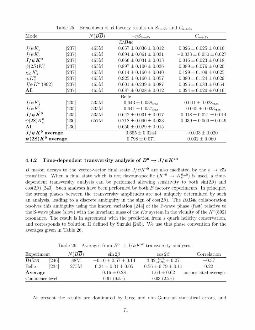
Table 25: Breakdown of B factory results on Sb→ccs and Cb→ccs.
Mode N(BB) −ηSb→ccs Cb→ccs
BABAR
J/ψK0S
[237] 465M 0.657± 0.036± 0.012 0.026± 0.025± 0.016J/ψK0
L [237] 465M 0.694± 0.061± 0.031 −0.033± 0.050± 0.027J/ψK0 [237] 465M 0.666± 0.031± 0.013 0.016± 0.023± 0.018ψ(2S)K0
S[237] 465M 0.897± 0.100± 0.036 0.089± 0.076± 0.020
χc1K0S [237] 465M 0.614± 0.160± 0.040 0.129± 0.109± 0.025
ηcK0S
[237] 465M 0.925± 0.160± 0.057 0.080± 0.124± 0.029J/ψK∗0(892) [237] 465M 0.601± 0.239± 0.087 0.025± 0.083± 0.054All [237] 465M 0.687± 0.028± 0.012 0.024± 0.020± 0.016
BelleJ/ψK0
S[235] 535M 0.643± 0.038stat 0.001± 0.028stat
J/ψK0L
[235] 535M 0.641± 0.057stat −0.045± 0.033statJ/ψK0 [235] 535M 0.642± 0.031± 0.017 −0.018± 0.021± 0.014ψ(2S)K0
S[236] 657M 0.718± 0.090± 0.033 −0.039± 0.069± 0.049
All [236] – 0.650± 0.029± 0.015 –J/ψK0 average 0.655± 0.0244 −0.003± 0.020ψ(2S)K0 average 0.798± 0.071 0.032± 0.060
4.4.2 Time-dependent transversity analysis of B0 → J/ψK∗0
B meson decays to the vector-vector final state J/ψK∗0 are also mediated by the b → ccstransition. When a final state which is not flavour-specific (K∗0 → K0
Sπ0) is used, a time-
dependent transversity analysis can be performed allowing sensitivity to both sin(2β) andcos(2β) [243]. Such analyses have been performed by both B factory experiments. In principle,the strong phases between the transversity amplitudes are not uniquely determined by suchan analysis, leading to a discrete ambiguity in the sign of cos(2β). The BABAR collaborationresolves this ambiguity using the known variation [244] of the P-wave phase (fast) relative tothe S-wave phase (slow) with the invariant mass of theKπ system in the vicinity of theK∗(892)resonance. The result is in agreement with the prediction from s quark helicity conservation,and corresponds to Solution II defined by Suzuki [245]. We use this phase convention for theaverages given in Table 26.
Table 26: Averages from B0 → J/ψK∗0 transversity analyses.
Experiment N(BB) sin 2β cos 2β CorrelationBABAR [246] 88M −0.10± 0.57± 0.14 3.32+0.76
−0.96 ± 0.27 −0.37Belle [234] 275M 0.24± 0.31± 0.05 0.56± 0.79± 0.11 0.22Average 0.16± 0.28 1.64± 0.62 uncorrelated averages
Confidence level 0.61 (0.5σ) 0.03 (2.2σ)
At present the results are dominated by large and non-Gaussian statistical errors, and
71
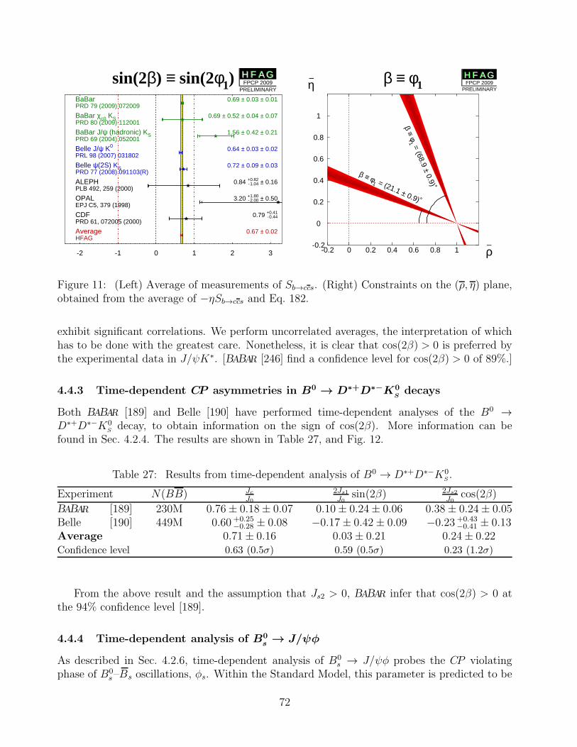
sin(2β) ≡ sin(2φ1)
-2 -1 0 1 2 3
BaBarPRD 79 (2009) 072009
0.69 ± 0.03 ± 0.01
BaBar χc0 KSPRD 80 (2009) 112001
0.69 ± 0.52 ± 0.04 ± 0.07
BaBar J/ψ (hadronic) KSPRD 69 (2004) 052001
1.56 ± 0.42 ± 0.21
Belle J/ψ K0
PRL 98 (2007) 0318020.64 ± 0.03 ± 0.02
Belle ψ(2S) KSPRD 77 (2008) 091103(R)
0.72 ± 0.09 ± 0.03
ALEPHPLB 492, 259 (2000)
0.84 +-01
.
.80
24 ± 0.16
OPALEPJ C5, 379 (1998)
3.20 +-12
.
.80
00 ± 0.50
CDFPRD 61, 072005 (2000)
0.79 +-00
.
.44
14
AverageHFAG
0.67 ± 0.02
H F A GH F A GFPCP 2009
PRELIMINARY
β ≡ φ1
ρ–
η–
-0.2 0 0.2 0.4 0.6 0.8 1-0.2
0
0.2
0.4
0.6
0.8
1
β ≡ φ1 = (21.1 ± 0.9)˚
β ≡ φ1 = (68.9 ± 0.9)˚
H F A GH F A GFPCP 2009
PRELIMINARY
Figure 11: (Left) Average of measurements of Sb→ccs. (Right) Constraints on the (ρ, η) plane,obtained from the average of −ηSb→ccs and Eq. 182.
exhibit significant correlations. We perform uncorrelated averages, the interpretation of whichhas to be done with the greatest care. Nonetheless, it is clear that cos(2β) > 0 is preferred bythe experimental data in J/ψK∗. [BABAR [246] find a confidence level for cos(2β) > 0 of 89%.]
4.4.3 Time-dependent CP asymmetries in B0 → D∗+D∗−K0Sdecays
Both BABAR [189] and Belle [190] have performed time-dependent analyses of the B0 →D∗+D∗−K0
Sdecay, to obtain information on the sign of cos(2β). More information can be
found in Sec. 4.2.4. The results are shown in Table 27, and Fig. 12.
Table 27: Results from time-dependent analysis of B0 → D∗+D∗−K0S.
Experiment N(BB) JcJ0
2Js1J0
sin(2β) 2Js2J0
cos(2β)
BABAR [189] 230M 0.76± 0.18± 0.07 0.10± 0.24± 0.06 0.38± 0.24± 0.05Belle [190] 449M 0.60 +0.25
−0.28 ± 0.08 −0.17± 0.42± 0.09 −0.23 +0.43−0.41 ± 0.13
Average 0.71± 0.16 0.03± 0.21 0.24± 0.22Confidence level 0.63 (0.5σ) 0.59 (0.5σ) 0.23 (1.2σ)
From the above result and the assumption that Js2 > 0, BABAR infer that cos(2β) > 0 atthe 94% confidence level [189].
4.4.4 Time-dependent analysis of B0s→ J/ψφ
As described in Sec. 4.2.6, time-dependent analysis of B0s → J/ψφ probes the CP violating
phase of B0s–Bs oscillations, φs. Within the Standard Model, this parameter is predicted to be
72
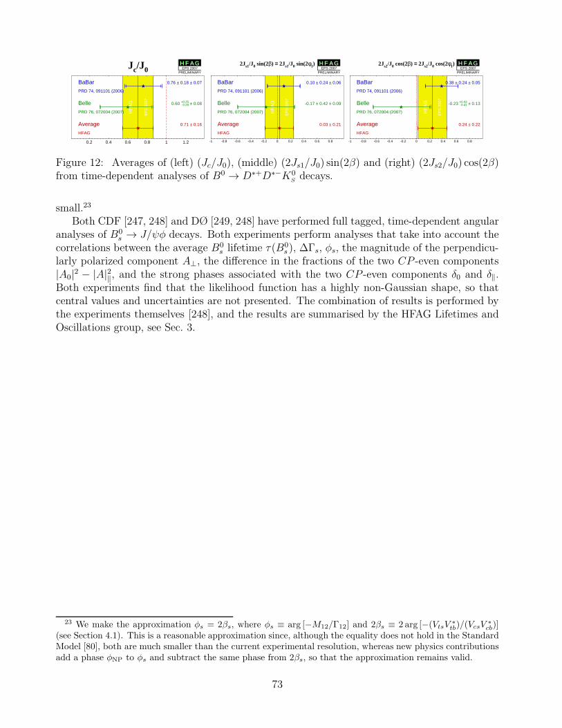
Jc/J0
HF
AG
EP
S 2
007
0.2 0.4 0.6 0.8 1 1.2
BaBar
PRD 74, 091101 (2006)
0.76 ± 0.18 ± 0.07
Belle
PRD 76, 072004 (2007)
0.60 +-00
.
.22
58 ± 0.08
Average
HFAG
0.71 ± 0.16
H F A GH F A GEPS 2007
PRELIMINARY
2Js1/J0 sin(2β) ≡ 2Js1/J0 sin(2φ1)
HF
AG
EP
S 2
007
-1 -0.8 -0.6 -0.4 -0.2 0 0.2 0.4 0.6 0.8
BaBar
PRD 74, 091101 (2006)
0.10 ± 0.24 ± 0.06
Belle
PRD 76, 072004 (2007)
-0.17 ± 0.42 ± 0.09
Average
HFAG
0.03 ± 0.21
H F A GH F A GEPS 2007
PRELIMINARY
2Js2/J0 cos(2β) ≡ 2Js2/J0 cos(2φ1)
HF
AG
EP
S 2
007
-1 -0.8 -0.6 -0.4 -0.2 0 0.2 0.4 0.6 0.8
BaBar
PRD 74, 091101 (2006)
0.38 ± 0.24 ± 0.05
Belle
PRD 76, 072004 (2007)
-0.23 +-00
.
.44
31 ± 0.13
Average
HFAG
0.24 ± 0.22
H F A GH F A GEPS 2007
PRELIMINARY
Figure 12: Averages of (left) (Jc/J0), (middle) (2Js1/J0) sin(2β) and (right) (2Js2/J0) cos(2β)from time-dependent analyses of B0 → D∗+D∗−K0
Sdecays.
small.23
Both CDF [247, 248] and DØ [249, 248] have performed full tagged, time-dependent angularanalyses of B0
s → J/ψφ decays. Both experiments perform analyses that take into account thecorrelations between the average B0
s lifetime τ(B0s ), ∆Γs, φs, the magnitude of the perpendicu-
larly polarized component A⊥, the difference in the fractions of the two CP -even components|A0|2 − |A|2‖, and the strong phases associated with the two CP -even components δ0 and δ‖.Both experiments find that the likelihood function has a highly non-Gaussian shape, so thatcentral values and uncertainties are not presented. The combination of results is performed bythe experiments themselves [248], and the results are summarised by the HFAG Lifetimes andOscillations group, see Sec. 3.
23 We make the approximation φs = 2βs, where φs ≡ arg [−M12/Γ12] and 2βs ≡ 2 arg [−(VtsV∗tb)/(VcsV
∗cb)]
(see Section 4.1). This is a reasonable approximation since, although the equality does not hold in the StandardModel [80], both are much smaller than the current experimental resolution, whereas new physics contributionsadd a phase φNP to φs and subtract the same phase from 2βs, so that the approximation remains valid.
73
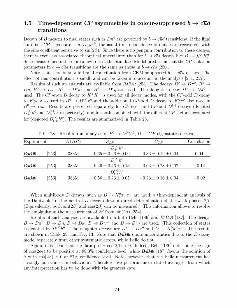
4.5 Time-dependent CP asymmetries in colour-suppressed b → cud
transitions
Decays of B mesons to final states such as Dπ0 are governed by b→ cud transitions. If the finalstate is a CP eigenstate, e.g. DCPπ
0, the usual time-dependence formulae are recovered, withthe sine coefficient sensitive to sin(2β). Since there is no penguin contribution to these decays,there is even less associated theoretical uncertainty than for b → ccs decays like B → J/ψK0
S .Such measurements therefore allow to test the Standard Model prediction that the CP violationparameters in b→ cud transitions are the same as those in b→ ccs [250].
Note that there is an additional contribution from CKM suppressed b → ucd decays. Theeffect of this contribution is small, and can be taken into account in the analysis [251, 252].
Results of such an analysis are available from BABAR [253]. The decays B0 → Dπ0, B0 →Dη, B0 → Dω, B0 → D∗π0 and B0 → D∗η are used. The daughter decay D∗ → Dπ0 isused. The CP -even D decay to K+K− is used for all decay modes, with the CP -odd D decayto K0
Sω also used in B0 → D(∗)π0 and the additional CP -odd D decay to K0Sπ
0 also used inB0 → Dω. Results are presented separately for CP -even and CP -odd D(∗) decays (denoted
D(∗)+ h0 andD
(∗)− h0 respectively), and for both combined, with the different CP factors accounted
for (denoted D(∗)CPh
0). The results are summarized in Table 28.
Table 28: Results from analyses of B0 → D(∗)h0, D → CP eigenstates decays.
Experiment N(BB) SCP CCP Correlation
D(∗)+ h0
BABAR [253] 383M −0.65± 0.26± 0.06 −0.33 ± 0.19± 0.04 0.04
D(∗)− h0
BABAR [253] 383M −0.46± 0.46± 0.13 −0.03 ± 0.28± 0.07 −0.14
D(∗)CPh
0
BABAR [253] 383M −0.56± 0.23± 0.05 −0.23 ± 0.16± 0.04 −0.02
When multibody D decays, such as D → K0Sπ+π− are used, a time-dependent analysis of
the Dalitz plot of the neutral D decay allows a direct determination of the weak phase: 2β.(Equivalently, both sin(2β) and cos(2β) can be measured.) This information allows to resolvethe ambiguity in the measurement of 2β from sin(2β) [254].
Results of such analyses are available from both Belle [186] and BABAR [187]. The decaysB → Dπ0, B → Dη, B → Dω, B → D∗π0 and B → D∗η are used. [This collection of statesis denoted by D(∗)h0.] The daughter decays are D∗ → Dπ0 and D → K0
Sπ+π−. The results
are shown in Table 29, and Fig. 13. Note that BABAR quote uncertainties due to the D decaymodel separately from other systematic errors, while Belle do not.
Again, it is clear that the data prefer cos(2β) > 0. Indeed, Belle [186] determine the signof cos(2φ1) to be positive at 98.3% confidence level, while BABAR [187] favour the solution ofβ with cos(2β) > 0 at 87% confidence level. Note, however, that the Belle measurement hasstrongly non-Gaussian behaviour. Therefore, we perform uncorrelated averages, from whichany interpretation has to be done with the greatest care.
74
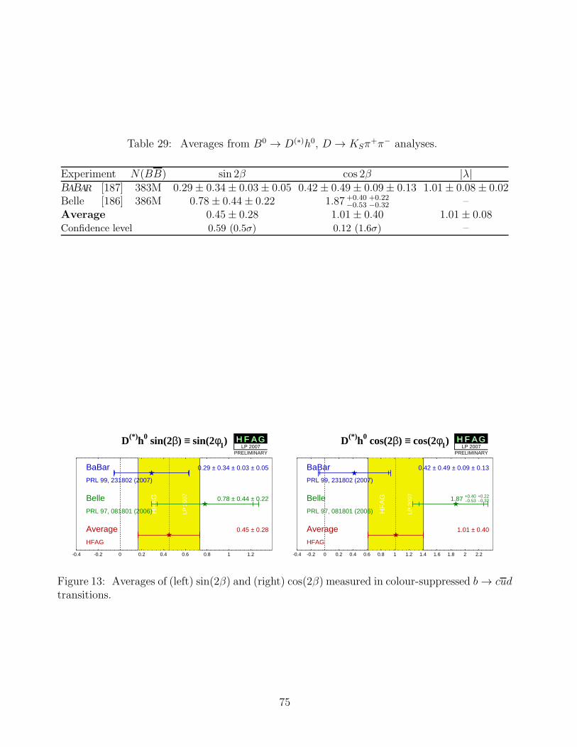
Table 29: Averages from B0 → D(∗)h0, D → KSπ+π− analyses.
Experiment N(BB) sin 2β cos 2β |λ|BABAR [187] 383M 0.29± 0.34± 0.03± 0.05 0.42± 0.49± 0.09± 0.13 1.01± 0.08± 0.02Belle [186] 386M 0.78± 0.44± 0.22 1.87 +0.40
−0.53+0.22−0.32 –
Average 0.45± 0.28 1.01± 0.40 1.01± 0.08Confidence level 0.59 (0.5σ) 0.12 (1.6σ) –
D(*)h0 sin(2β) ≡ sin(2φ1)
HF
AG
LP 2
007
-0.4 -0.2 0 0.2 0.4 0.6 0.8 1 1.2
BaBar
PRL 99, 231802 (2007)
0.29 ± 0.34 ± 0.03 ± 0.05
Belle
PRL 97, 081801 (2006)
0.78 ± 0.44 ± 0.22
Average
HFAG
0.45 ± 0.28
H F A GH F A GLP 2007
PRELIMINARY
D(*)h0 cos(2β) ≡ cos(2φ1)
HF
AG
LP 2
007
-0.4 -0.2 0 0.2 0.4 0.6 0.8 1 1.2 1.4 1.6 1.8 2 2.2
BaBar
PRL 99, 231802 (2007)
0.42 ± 0.49 ± 0.09 ± 0.13
Belle
PRL 97, 081801 (2006)
1.87 +-00
.
.45
03
+-00
.
.23
22
Average
HFAG
1.01 ± 0.40
H F A GH F A GLP 2007
PRELIMINARY
Figure 13: Averages of (left) sin(2β) and (right) cos(2β) measured in colour-suppressed b→ cudtransitions.
75
4.6 Time-dependent CP asymmetries in charmless b → qqs transi-
tions
The flavour changing neutral current b→ s penguin can be mediated by any up-type quark inthe loop, and hence the amplitude can be written as
Ab→s = FuVubV∗us + FcVcbV
∗cs + FtVtbV
∗ts
= (Fu − Fc)VubV∗us + (Ft − Fc)VtbV
∗ts
= O(λ4) + O(λ2)(183)
using the unitarity of the CKM matrix. Therefore, in the Standard Model, this amplitude isdominated by VtbV
∗ts, and to within a few degrees (δβ<∼ 2 for β ≈ 20) the time-dependent
parameters can be written24 Sb→qqs ≈ −η sin(2β), Cb→qqs ≈ 0, assuming b → s penguin contri-butions only (q = u, d, s).
Due to the large virtual mass scales occurring in the penguin loops, additional diagramsfrom physics beyond the Standard Model, with heavy particles in the loops, may contribute. Ingeneral, these contributions will affect the values of Sb→qqs and Cb→qqs. A discrepancy betweenthe values of Sb→ccs and Sb→qqs can therefore provide a clean indication of new physics [250,255, 256, 257].
However, there is an additional consideration to take into account. The above argumentassumes only the b → s penguin contributes to the b → qqs transition. For q = s this is agood assumption, which neglects only rescattering effects. However, for q = u there is a colour-suppressed b → u tree diagram (of order O(λ4)), which has a different weak (and possiblystrong) phase. In the case q = d, any light neutral meson that is formed from dd also hasa uu component, and so again there is “tree pollution”. The B0 decays to π0K0
S, ρ0 K0
Sand
ωK0Sbelong to this category. The mesons φ, f0 and η′ are expected to have predominant
ss parts, which reduces the relative size of the possible tree pollution. If the inclusive decayB0 → K+K−K0 (excluding φK0) is dominated by a nonresonant three-body transition, an OZI-rule suppressed tree-level diagram can occur through insertion of an ss pair. The correspondingpenguin-type transition proceeds via insertion of a uu pair, which is expected to be favoredover the ss insertion by fragmentation models. Neglecting rescattering, the final state K0K0K0
(reconstructed as K0SK
0SK
0S) has no tree pollution [258]. Various estimates, using different
theoretical approaches, of the values of ∆S = Sb→qqs − Sb→ccs exist in the literature [259, 260,261, 262, 263, 264, 265, 266, 267, 268, 269, 270, 271, 272]. In general, there is agreement thatthe modes φK0, η′K0 and K0K0K0 are the cleanest, with values of |∆S| at or below the fewpercent level (∆S is usually positive).
4.6.1 Time-dependent CP asymmetries: b → qqs decays to CP eigenstates
The averages for −ηSb→qqs and Cb→qqs can be found in Table 30, and are shown in Figs. 14, 15and 16. Results from both BABAR and Belle are averaged for the modes φK0, η′K0, f0K
0
and K+K−K0 (K0 indicates that both K0Sand K0
Lare used, although Belle use neither f0K
0L
24 The presence of a small (O(λ2)) weak phase in the dominant amplitude of the s penguin decays intro-duces a phase shift given by Sb→qqs = −η sin(2β) · (1 + ∆). Using the CKMfitter results for the Wolfensteinparameters [206], one finds: ∆ ≃ 0.033, which corresponds to a shift of 2β of +2.1 degrees. Nonperturbativecontributions can alter this result.
76
nor K+K−K0L), K0
SK0
SK0
S, π0K0
S,25 ρ0K0
Sand ωK0
S. BABAR also has presented results with
the final states π0π0K0S ,
26 f2K0S , fXK
0S , π
+π−K0S nonresonant and φK0
Sπ0. Results for f0K
0,K+K−K0, ρ0K0
S, f2K
0S, fXK
0Sand π+π−K0
Snonresonant are taken from time-dependent Dalitz
plot analyses of B0 → K+K−K0 and B0 → π+π−K0S (see subsection 4.6.2). The results
presented in Table 30 for f0K0 are for both experiments combinations of the results determined
in the K+K−K0 and π+π−K0Sfinal states.
Of these final states, φK0S , η
′K0S , π
0K0S , ρ
0K0S , ωK
0S and f0K
0L have CP eigenvalue η = −1,
while φK0L, η′K0
L, K0
SK0
SK0
S, f0K
0S, f2K
0S, fXK
0S,27 π0π0K0
Sand π+π−K0
Snonresonant have
η = +1.
The final state K+K−K0 (contributions from φK0 are implicitly excluded) is not a CPeigenstate. However, it can be treated as a quasi-two-body decay, with the CP compositiondetermined using either an isospin argument (used by Belle to determine a CP -even fraction of0.93±0.09±0.05 [277]) or a moments analysis (previously used by BABAR to find a CP -even frac-tions of 0.89± 0.08± 0.06 in K+K−K0
S[280]). Note that uncertainty in the CP composition of
the final state leads to a third source of uncertainty on the Belle results for −ηSK+K−K0. BABARresults for K+K−K0 are determined from the inclusive “high-mass” (mK+K− > 1.1 GeV/c2)region in their B0 → K+K−K0 time-dependent Dalitz plot analysis [192] (this approach au-tomatically corrects for the CP composition of the final state). Belle have also performed atime-dependent Dalitz plot analysis of B0 → K+K−K0 [193], but the results presented inTable 30 are from their previous analysis [277].
The final state φK0Sπ0 is also not a CP -eigenstate but its CP -composition can be determined
from an angular analysis. Since the angular parameters are common to the B0 → φK0Sπ
0 andB0 → φK+π− decays (because only Kπ resonance contribute), BABAR perform a simultaneousanalysis of the two final states [279] (see subsection 4.6.3).
It must be noted that Q2B parameters extracted from Dalitz plot analyses are constrainedto lie within the physical boundary (S2
CP + C2CP < 1) and consequenty the obtained errors
are highly non-Gaussian when the central value is close to the boundary. This is particularlyevident in the BABAR results for B0 → f0K
0 with f0 → π+π− [196]. These results must betreated with extreme caution.
As explained above, each of the modes listed in Table 30 has different uncertainties withinthe Standard Model, and so each may have a different value of −ηSb→qqs. Therefore, thereis no strong motivation to make a combined average over the different modes. We refer tosuch an average as a “naıve s-penguin average.” It is naıve not only because of the neglectof the theoretical uncertainty, but also since possible correlations of systematic effects betweendifferent modes are neglected. In spite of these caveats, there remains substantial interest in thevalue of this quantity, and therefore it is given here: 〈−ηSb→qqs〉 = 0.62± 0.04, with confidencelevel 0.18 (1.3σ). This value is in agreement with the average −ηSb→ccs given in Sec. 4.4.1. (Theaverage for Cb→qqs is 〈Cb→qqs〉 = −0.05± 0.03 with confidence level 0.78 (0.3σ).) We emphasiseagain that we do not advocate the use of these averages, and that the values should be treatedwith extreme caution, if at all.
From Table 30 it may be noted that the average for −ηSb→qqs in η′K0 (0.59± 0.07), is now
25 Belle [273] include the π0K0Lfinal state in order to improve the constraint on the direct CP violation
parameter; these events cannot be used for time-dependent analysis.26 We do not include a preliminary result from Belle [274], which remains unpublished after more than two
years.27 The fX is assumed to be spin even.
77
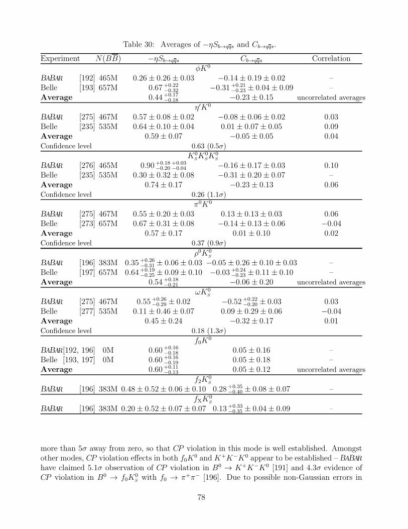
Table 30: Averages of −ηSb→qqs and Cb→qqs.
Experiment N(BB) −ηSb→qqs Cb→qqs CorrelationφK0
BABAR [192] 465M 0.26± 0.26± 0.03 −0.14± 0.19± 0.02 –Belle [193] 657M 0.67 +0.22
−0.32 −0.31 +0.21−0.23 ± 0.04± 0.09 –
Average 0.44 +0.17−0.18 −0.23± 0.15 uncorrelated averages
η′K0
BABAR [275] 467M 0.57± 0.08± 0.02 −0.08± 0.06± 0.02 0.03Belle [235] 535M 0.64± 0.10± 0.04 0.01± 0.07± 0.05 0.09Average 0.59± 0.07 −0.05± 0.05 0.04Confidence level 0.63 (0.5σ)
K0SK0
SK0
S
BABAR [276] 465M 0.90 +0.18−0.20
+0.03−0.04 −0.16± 0.17± 0.03 0.10
Belle [235] 535M 0.30± 0.32± 0.08 −0.31± 0.20± 0.07 –Average 0.74± 0.17 −0.23± 0.13 0.06Confidence level 0.26 (1.1σ)
π0K0
BABAR [275] 467M 0.55± 0.20± 0.03 0.13± 0.13± 0.03 0.06Belle [273] 657M 0.67± 0.31± 0.08 −0.14± 0.13± 0.06 −0.04Average 0.57± 0.17 0.01± 0.10 0.02Confidence level 0.37 (0.9σ)
ρ0K0S
BABAR [196] 383M 0.35 +0.26−0.31 ± 0.06± 0.03 −0.05± 0.26± 0.10± 0.03 –
Belle [197] 657M 0.64 +0.19−0.25 ± 0.09± 0.10 −0.03 +0.24
−0.23 ± 0.11± 0.10 –Average 0.54 +0.18
−0.21 −0.06± 0.20 uncorrelated averages
ωK0S
BABAR [275] 467M 0.55 +0.26−0.29 ± 0.02 −0.52 +0.22
−0.20 ± 0.03 0.03Belle [277] 535M 0.11± 0.46± 0.07 0.09± 0.29± 0.06 −0.04Average 0.45± 0.24 −0.32± 0.17 0.01Confidence level 0.18 (1.3σ)
f0K0
BABAR[192, 196] 0M 0.60 +0.16−0.18 0.05± 0.16 –
Belle [193, 197] 0M 0.60 +0.16−0.19 0.05± 0.18 –
Average 0.60 +0.11−0.13 0.05± 0.12 uncorrelated averages
f2K0S
BABAR [196] 383M 0.48± 0.52± 0.06± 0.10 0.28 +0.35−0.40 ± 0.08± 0.07 –
fXK0S
BABAR [196] 383M 0.20± 0.52± 0.07± 0.07 0.13 +0.33−0.35 ± 0.04± 0.09 –
more than 5σ away from zero, so that CP violation in this mode is well established. Amongstother modes, CP violation effects in both f0K
0 and K+K−K0 appear to be established – BABARhave claimed 5.1σ observation of CP violation in B0 → K+K−K0 [191] and 4.3σ evidence ofCP violation in B0 → f0K
0Swith f0 → π+π− [196]. Due to possible non-Gaussian errors in
78
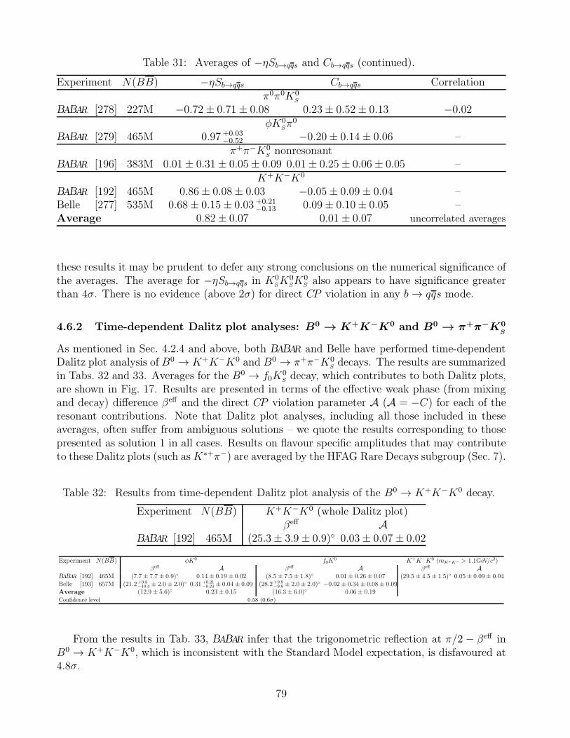
Table 31: Averages of −ηSb→qqs and Cb→qqs (continued).
Experiment N(BB) −ηSb→qqs Cb→qqs Correlationπ0π0K0
S
BABAR [278] 227M −0.72± 0.71± 0.08 0.23± 0.52± 0.13 −0.02φK0
Sπ0
BABAR [279] 465M 0.97 +0.03−0.52 −0.20± 0.14± 0.06 –π+π−K0
Snonresonant
BABAR [196] 383M 0.01± 0.31± 0.05± 0.09 0.01± 0.25± 0.06± 0.05 –K+K−K0
BABAR [192] 465M 0.86± 0.08± 0.03 −0.05± 0.09± 0.04 –Belle [277] 535M 0.68± 0.15± 0.03 +0.21
−0.13 0.09± 0.10± 0.05 –Average 0.82± 0.07 0.01± 0.07 uncorrelated averages
these results it may be prudent to defer any strong conclusions on the numerical significance ofthe averages. The average for −ηSb→qqs in K
0SK0
SK0
Salso appears to have significance greater
than 4σ. There is no evidence (above 2σ) for direct CP violation in any b→ qqs mode.
4.6.2 Time-dependent Dalitz plot analyses: B0 → K+K−K0 and B0 → π+π−K0S
As mentioned in Sec. 4.2.4 and above, both BABAR and Belle have performed time-dependentDalitz plot analysis of B0 → K+K−K0 and B0 → π+π−K0
Sdecays. The results are summarized
in Tabs. 32 and 33. Averages for the B0 → f0K0S decay, which contributes to both Dalitz plots,
are shown in Fig. 17. Results are presented in terms of the effective weak phase (from mixingand decay) difference βeff and the direct CP violation parameter A (A = −C) for each of theresonant contributions. Note that Dalitz plot analyses, including all those included in theseaverages, often suffer from ambiguous solutions – we quote the results corresponding to thosepresented as solution 1 in all cases. Results on flavour specific amplitudes that may contributeto these Dalitz plots (such asK∗+π−) are averaged by the HFAG Rare Decays subgroup (Sec. 7).
Table 32: Results from time-dependent Dalitz plot analysis of the B0 → K+K−K0 decay.
Experiment N(BB) K+K−K0 (whole Dalitz plot)βeff A
BABAR [192] 465M (25.3± 3.9± 0.9) 0.03± 0.07± 0.02
Experiment N(BB) φK0 f0K0 K+K−K0 (mK+K− > 1.1GeV/c2)
βeff A βeff A βeff ABABAR [192] 465M (7.7± 7.7± 0.9) 0.14± 0.19± 0.02 (8.5± 7.5± 1.8) 0.01± 0.26± 0.07 (29.5± 4.5± 1.5) 0.05± 0.09± 0.04Belle [193] 657M (21.2 +9.8
−10.4 ± 2.0± 2.0) 0.31 +0.21−0.23 ± 0.04± 0.09 (28.2 +9.9
−9.8 ± 2.0± 2.0) −0.02± 0.34± 0.08± 0.09Average (12.9± 5.6) 0.23± 0.15 (16.3± 6.0) 0.06± 0.19Confidence level 0.58 (0.6σ)
From the results in Tab. 33, BABAR infer that the trigonometric reflection at π/2 − βeff inB0 → K+K−K0, which is inconsistent with the Standard Model expectation, is disfavoured at4.8σ.
79
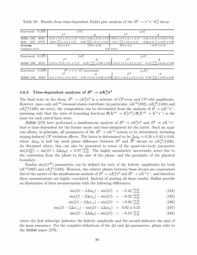
Table 33: Results from time-dependent Dalitz plot analysis of the B0 → π+π−K0S decay.
Experiment N(BB) ρ0K0S
f0K0S
βeff A βeff ABABAR [196] 383M (10.2± 8.9± 3.0± 1.9) 0.05± 0.26± 0.10± 0.03 (36.0± 9.8± 2.1± 2.1) −0.08± 0.19± 0.03± 0.04Belle [197] 657M (20.0 +8.6
−8.5 ± 3.2± 3.5) 0.03 +0.23−0.24 ± 0.11± 0.10 (12.7 +6.9
−6.5 ± 2.8± 3.3) −0.06± 0.17± 0.07± 0.09Average 16.4± 6.8 0.06± 0.20 20.6± 6.2 −0.07± 0.14Confidence level 0.39 (0.9σ)
Experiment N(BB) f2K0S
fXK0S
βeff A βeff ABABAR [196] 383M (14.9± 17.9± 3.1± 5.2) −0.28 +0.40
−0.35 ± 0.08± 0.07 (5.8± 15.2± 2.2± 2.3) −0.13 +0.35−0.33 ± 0.04± 0.09
Experiment N(BB) B0 → π+π−K0S nonresonant χc0K
0S
βeff A βeff ABABAR [196] 383M (0.4± 8.8± 1.9± 3.8) −0.01± 0.25± 0.06± 0.05 (23.2± 22.4± 2.3± 4.2) 0.29 +0.44
−0.53 ± 0.03± 0.05
4.6.3 Time-dependent analyses of B0 → φK0Sπ0
The final state in the decay B0 → φK0Sπ0 is a mixture of CP -even and CP -odd amplitudes.
However, since only φK∗0 resonant states contribute (in particular, φK∗0(892), φK∗00 (1430) and
φK∗02 (1430) are seen), the composition can be determined from the analysis of B → φK+π−,
assuming only that the ratio of branching fractions B(K∗0 → K0Sπ0)/B(K∗0 → K+π−) is the
same for each exited kaon state.BABAR [279] have performed a simultaneous analysis of B0 → φK0
Sπ0 and B0 → φK+π−
that is time-dependent for the former mode and time-integrated for the latter. Such an anal-ysis allows, in principle, all parameters of the B0 → φK∗0 system to be determined, includingmixing-induced CP violation effects. The latter is determined to be ∆φ00 = 0.28± 0.42± 0.04,where ∆φ00 is half the weak phase difference between B0 and B0 decays to φK∗0
0 (1430).As discussed above, this can also be presented in terms of the quasi-two-body parametersin(2βeff
00 ) = sin(2β + 2∆φ00) = 0.97 +0.03−0.52. The highly asymmetric uncertainty arises due to
the conversion from the phase to the sine of the phase, and the proximity of the physicalboundary.
Similar sin(2βeff) parameters can be defined for each of the helicity amplitudes for bothφK∗0(892) and φK∗0
2 (1430). However, the relative phases between these decays are constraineddue to the nature of the simultaneous analysis of B0 → φK0
Sπ0 and B0 → φK+π−, and therefore
these measurements are highly correlated. Instead of quoting all these results, BaBar providean illustration of their measurements with the following differences:
sin(2β − 2∆δ01)− sin(2β) = −0.42 +0.26−0.34 (184)
sin(2β − 2∆φ‖1)− sin(2β) = −0.32 +0.22−0.30 (185)
sin(2β − 2∆φ⊥1)− sin(2β) = −0.30 +0.23−0.32 (186)
sin(2β − 2∆φ⊥1)− sin(2β − 2∆φ‖1) = 0.02± 0.23 (187)
sin(2β − 2∆δ02)− sin(2β) = −0.10 +0.18−0.29 (188)
where the first subscript indicates the helicity amplitude and the second indicates the spin ofthe kaon resonance. For the complete definitions of the ∆δ and ∆φ parameters, please refer tothe BABAR paper [279].
80

Direct CP violation parameters for each of the contributing helicity amplitudes can also bemeasured. Again, these are determined from a simultaneous fit of B0 → φK0
Sπ0 and B0 →
φK+π−, with the precision being dominated by the statistics of the latter mode. Direct CPviolation measurements are tabulated by HFAG - Rare Decays (Sec. 7).
81
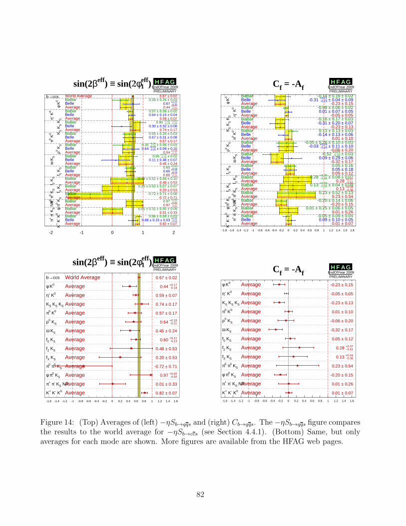
sin(2βeff) ≡ sin(2φe1ff)
HF
AG
End
OfY
ear
2009
HF
AG
End
OfY
ear
2009
HF
AG
End
OfY
ear
2009
HF
AG
End
OfY
ear
2009
HF
AG
End
OfY
ear
2009
HF
AG
End
OfY
ear
2009
HF
AG
End
OfY
ear
2009
HF
AG
End
OfY
ear
2009
HF
AG
End
OfY
ear
2009
HF
AG
End
OfY
ear
2009
HF
AG
End
OfY
ear
2009
HF
AG
End
OfY
ear
2009
HF
AG
End
OfY
ear
2009
HF
AG
End
OfY
ear
2009
b→ccs
φ K
0
η′ K
0
KS K
S K
S
π0 K0
ρ0 KS
ω K
S
f 0 K
S
f 2 K
S
f X K
S
π0 π0 K
S
φ π0 K
S
π+ π
- KS N
R
K+ K
- K0
-2 -1 0 1 2
World Average 0.67 ± 0.02BaBar 0.26 ± 0.26 ± 0.03Belle 0.67 +-
00
.
.23
22
Average 0.44 +-00
.
.11
78
BaBar 0.57 ± 0.08 ± 0.02Belle 0.64 ± 0.10 ± 0.04Average 0.59 ± 0.07BaBar 0.90 +-
00
.
.12
80
+-00
.
.00
34
Belle 0.30 ± 0.32 ± 0.08Average 0.74 ± 0.17BaBar 0.55 ± 0.20 ± 0.03Belle 0.67 ± 0.31 ± 0.08Average 0.57 ± 0.17BaBar 0.35 +-
00
.
.23
61 ± 0.06 ± 0.03
Belle 0.64 +-00
.
.12
95 ± 0.09 ± 0.10
Average 0.54 +-00
.
.12
81
BaBar 0.55 +-00
.
.22
69 ± 0.02
Belle 0.11 ± 0.46 ± 0.07Average 0.45 ± 0.24BaBar 0.60 +-
00
.
.11
68
Belle 0.60 +-00
.
.11
69
Average 0.60 +-00
.
.11
13
BaBar 0.48 ± 0.52 ± 0.06 ± 0.10Average 0.48 ± 0.53BaBar 0.20 ± 0.52 ± 0.07 ± 0.07Average 0.20 ± 0.53BaBar -0.72 ± 0.71 ± 0.08Average -0.72 ± 0.71BaBar 0.97 +-
00
.
.05
32
Average 0.97 +-00
.
.05
32
BaBar 0.01 ± 0.31 ± 0.05 ± 0.09Average 0.01 ± 0.33BaBar 0.86 ± 0.08 ± 0.03Belle 0.68 ± 0.15 ± 0.03 +-
00
.
.21
13
Average 0.82 ± 0.07
H F A GH F A GEndOfYear 2009PRELIMINARY
Cf = -Af
HF
AG
End
OfY
ear
2009
HF
AG
End
OfY
ear
2009
HF
AG
End
OfY
ear
2009
HF
AG
End
OfY
ear
2009
HF
AG
End
OfY
ear
2009
HF
AG
End
OfY
ear
2009
HF
AG
End
OfY
ear
2009
HF
AG
End
OfY
ear
2009
HF
AG
End
OfY
ear
2009
HF
AG
End
OfY
ear
2009
HF
AG
End
OfY
ear
2009
HF
AG
End
OfY
ear
2009
HF
AG
End
OfY
ear
2009
φ K
0
η′ K
0
KS K
S K
S
π0 K0
ρ0 KS
ω K
S
f 0 K
S
f 2 K
S
f X K
S
π0 π0 K
S
φ π0 K
S
π+ π
- KS N
R
K+ K
- K0
-1.8 -1.6 -1.4 -1.2 -1 -0.8 -0.6 -0.4 -0.2 0 0.2 0.4 0.6 0.8 1 1.2 1.4 1.6 1.8
BaBar -0.14 ± 0.19 ± 0.02Belle -0.31 +-
00
.
.22
13 ± 0.04 ± 0.09
Average -0.23 ± 0.15BaBar -0.08 ± 0.06 ± 0.02Belle 0.01 ± 0.07 ± 0.05Average -0.05 ± 0.05BaBar -0.16 ± 0.17 ± 0.03Belle -0.31 ± 0.20 ± 0.07Average -0.23 ± 0.13BaBar 0.13 ± 0.13 ± 0.03Belle -0.14 ± 0.13 ± 0.06Average 0.01 ± 0.10BaBar -0.05 ± 0.26 ± 0.10 ± 0.03Belle -0.03 +-
00
.
.22
43 ± 0.11 ± 0.10
Average -0.06 ± 0.20BaBar -0.52 +-
00
.
.22
20 ± 0.03
Belle 0.09 ± 0.29 ± 0.06Average -0.32 ± 0.17BaBar 0.05 ± 0.16Belle 0.05 ± 0.18Average 0.05 ± 0.12BaBar 0.28 +-
00
.
.34
50 ± 0.08 ± 0.07
Average 0.28 +-00
.
.34
71
BaBar 0.13 +-00
.
.33
35 ± 0.04 ± 0.09
Average 0.13 +-00
.
.33
46
BaBar 0.23 ± 0.52 ± 0.13Average 0.23 ± 0.54BaBar -0.20 ± 0.14 ± 0.06Average -0.20 ± 0.15BaBar 0.01 ± 0.25 ± 0.06 ± 0.05Average 0.01 ± 0.26BaBar -0.05 ± 0.09 ± 0.04Belle 0.09 ± 0.10 ± 0.05Average 0.01 ± 0.07
H F A GH F A GEndOfYear 2009PRELIMINARY
sin(2βeff) ≡ sin(2φe1ff)
b→ccs
φ K0
η′ K0
KS KS KS
π0 K0
ρ0 KS
ω KS
f0 KS
f2 KS
fX KS
π0 π0 KS
φ π0 KS
π+ π- KS NR
K+ K- K0
-1.6 -1.4 -1.2 -1 -0.8 -0.6 -0.4 -0.2 0 0.2 0.4 0.6 0.8 1 1.2 1.4 1.6
World Average 0.67 ± 0.02
Average 0.44 +-00
.
.11
78
Average 0.59 ± 0.07
Average 0.74 ± 0.17
Average 0.57 ± 0.17
Average 0.54 +-00
.
.12
81
Average 0.45 ± 0.24
Average 0.60 +-00
.
.11
13
Average 0.48 ± 0.53
Average 0.20 ± 0.53
Average -0.72 ± 0.71
Average 0.97 +-00
.
.05
32
Average 0.01 ± 0.33
Average 0.82 ± 0.07
H F A GH F A GEndOfYear 2009PRELIMINARY Cf = -Af
φ K0
η′ K0
KS KS KS
π0 K0
ρ0 KS
ω KS
f0 KS
f2 KS
fX KS
π0 π0 KS
φ π0 KS
π+ π- KS NR
K+ K- K0
-1.6 -1.4 -1.2 -1 -0.8 -0.6 -0.4 -0.2 0 0.2 0.4 0.6 0.8 1 1.2 1.4 1.6
Average -0.23 ± 0.15
Average -0.05 ± 0.05
Average -0.23 ± 0.13
Average 0.01 ± 0.10
Average -0.06 ± 0.20
Average -0.32 ± 0.17
Average 0.05 ± 0.12
Average 0.28 +-00
.
.34
71
Average 0.13 +-00
.
.33
46
Average 0.23 ± 0.54
Average -0.20 ± 0.15
Average 0.01 ± 0.26
Average 0.01 ± 0.07
H F A GH F A GEndOfYear 2009PRELIMINARY
Figure 14: (Top) Averages of (left) −ηSb→qqs and (right) Cb→qqs. The −ηSb→qqs figure comparesthe results to the world average for −ηSb→ccs (see Section 4.4.1). (Bottom) Same, but onlyaverages for each mode are shown. More figures are available from the HFAG web pages.
82
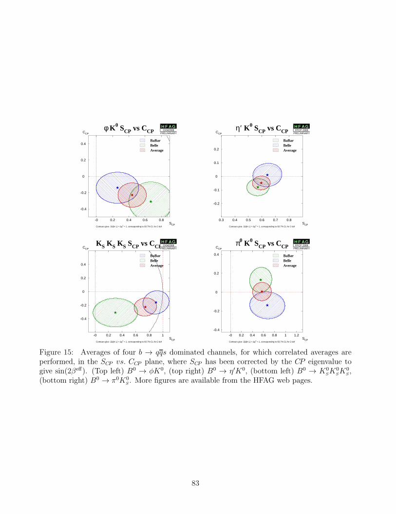
φ K0 SCP vs CCP
Contours give -2∆(ln L) = ∆χ2 = 1, corresponding to 60.7% CL for 2 dof
-0 0.2 0.4 0.6 0.8
-0.4
-0.2
0
0.2
0.4
SCP
CCP
BaBarBelleAverage
H F A GH F A GCKM2008
PRELIMINARY
η′ K0 SCP vs CCP
Contours give -2∆(ln L) = ∆χ2 = 1, corresponding to 60.7% CL for 2 dof
0.3 0.4 0.5 0.6 0.7 0.8
-0.2
-0.1
0
0.1
0.2
SCP
CCP
BaBarBelleAverage
H F A GH F A GFPCP 2009
PRELIMINARY
KS KS KS SCP vs CCP
Contours give -2∆(ln L) = ∆χ2 = 1, corresponding to 60.7% CL for 2 dof
-0 0.2 0.4 0.6 0.8 1
-0.4
-0.2
0
0.2
0.4
SCP
CCP
BaBarBelleAverage
H F A GH F A GCKM2008
PRELIMINARY
π0 K0 SCP vs CCP
Contours give -2∆(ln L) = ∆χ2 = 1, corresponding to 60.7% CL for 2 dof
-0 0.2 0.4 0.6 0.8 1 1.2
-0.4
-0.2
0
0.2
0.4
SCP
CCP
BaBarBelleAverage
H F A GH F A GFPCP 2009
PRELIMINARY
Figure 15: Averages of four b → qqs dominated channels, for which correlated averages areperformed, in the SCP vs. CCP plane, where SCP has been corrected by the CP eigenvalue togive sin(2βeff). (Top left) B0 → φK0, (top right) B0 → η′K0, (bottom left) B0 → K0
SK0
SK0
S,
(bottom right) B0 → π0K0S . More figures are available from the HFAG web pages.
83
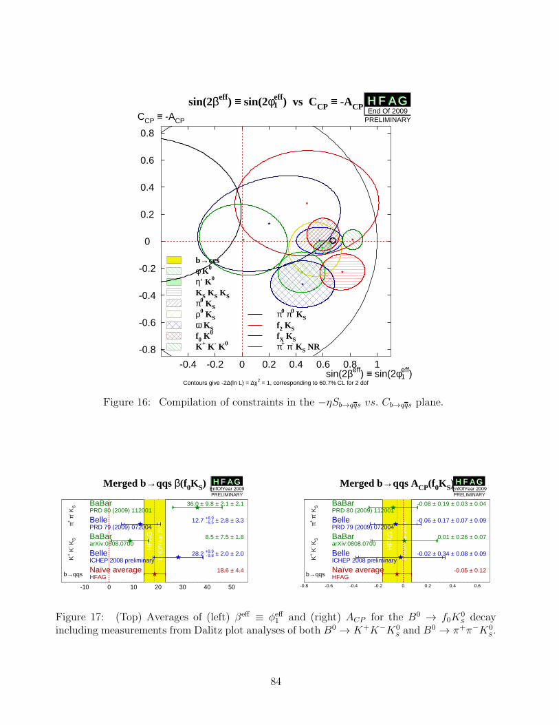
sin(2βeff) ≡ sin(2φe1ff) vs CCP ≡ -ACP
Contours give -2∆(ln L) = ∆χ2 = 1, corresponding to 60.7% CL for 2 dof
-0.4 -0.2 0 0.2 0.4 0.6 0.8 1
-0.8
-0.6
-0.4
-0.2
0
0.2
0.4
0.6
0.8
sin(2βeff) ≡ sin(2φe1
ff)
CCP ≡ -ACP
b→ccsφ K0
η′ K0
KS KS KSπ0 KSρ0 KSω KSf0 K
0f2 KSfX KS
π0 π0 KS
π+ π- KS NRK+ K- K0
H F A GH F A GEnd Of 2009
PRELIMINARY
Figure 16: Compilation of constraints in the −ηSb→qqs vs. Cb→qqs plane.
Merged b→qqs β(f0KS)
HF
AG
Enf
OfY
ear
2009π+
π- K
SK
+ K
- KS
b→qqs
-10 0 10 20 30 40 50
BaBarPRD 80 (2009) 112001
36.0 ± 9.8 ± 2.1 ± 2.1
BellePRD 79 (2009) 072004
12.7 +-66
.
.95 ± 2.8 ± 3.3
BaBararXiv:0808.0700
8.5 ± 7.5 ± 1.8
BelleICHEP 2008 preliminary
28.2 +-99
.
.98 ± 2.0 ± 2.0
Naïve averageHFAG
18.6 ± 4.4
H F A GH F A GEnfOfYear 2009PRELIMINARY
Merged b→qqs ACP(f0KS)
HF
AG
Enf
OfY
ear
2009π+
π- K
SK
+ K
- KS
b→qqs
-0.8 -0.6 -0.4 -0.2 0 0.2 0.4 0.6
BaBarPRD 80 (2009) 112001
-0.08 ± 0.19 ± 0.03 ± 0.04
BellePRD 79 (2009) 072004
-0.06 ± 0.17 ± 0.07 ± 0.09
BaBararXiv:0808.0700
0.01 ± 0.26 ± 0.07
BelleICHEP 2008 preliminary
-0.02 ± 0.34 ± 0.08 ± 0.09
Naïve averageHFAG
-0.05 ± 0.12
H F A GH F A GEnfOfYear 2009PRELIMINARY
Figure 17: (Top) Averages of (left) βeff ≡ φeff1 and (right) ACP for the B0 → f0K
0S decay
including measurements from Dalitz plot analyses of both B0 → K+K−K0Sand B0 → π+π−K0
S.
84
4.7 Time-dependent CP asymmetries in b → ccd transitions
The transition b → ccd can occur via either a b → c tree or a b → d penguin amplitude.Similarly to Eq. (183), the amplitude for the b→ d penguin can be written
Ab→d = FuVubV∗ud + FcVcbV
∗cd + FtVtbV
∗td
= (Fu − Fc)VubV∗ud + (Ft − Fc)VtbV
∗td
= O(λ3) + O(λ3).(189)
From this it can be seen that the b→ d penguin amplitude contains terms with different weakphases at the same order of CKM suppression.
In the above, we have followed Eq. (183) by eliminating the Fc term using unitarity. How-ever, we could equally well write
Ab→d = (Fu − Ft)VubV∗ud + (Fc − Ft)VcbV
∗cd,
= (Fc − Fu)VcbV∗cd + (Ft − Fu)VtbV
∗td.
(190)
Since the b→ ccd tree amplitude has the weak phase of VcbV∗cd, either of the above expressions
allow the penguin to be decomposed into parts with weak phases the same and different to thetree amplitude (the relative weak phase can be chosen to be either β or γ). However, if thetree amplitude dominates, there is little sensitivity to any phase other than that from B0–B0
mixing.The b → ccd transitions can be investigated with studies of various different final states.
Results are available from both BABAR and Belle using the final states J/ψπ0, D+D−, D∗+D∗−
and D∗±D∓, the averages of these results are given in Table 34. The results using the CPeigenstate (η = +1) modes J/ψπ0 and D+D− are shown in Fig. 18 and Fig. 19 respectively,with two-dimensional constraints shown in Fig. 20.
The vector-vector mode D∗+D∗− is found to be dominated by the CP -even longitudinallypolarized component; BABAR measures a CP -odd fraction of 0.158 ± 0.028 ± 0.006 [185] whileBelle measures a CP -odd fraction of 0.125±0.043±0.023 [281]. These values, listed as R⊥, areincluded in the averages which ensures the correlations to be taken into account.28 BABAR havealso performed an additional fit in which the CP -even and CP -odd components are allowedto have different CP violation parameters S and C. These results are included in Table 34.Results using D∗+D∗− are shown in Fig. 21.
For the non-CP eigenstate mode D∗±D∓BABAR uses fully reconstructed events while Belle
combines both fully and partially reconstructed samples. At present we perform uncorrelatedaverages of the parameters in the D∗±D∓ system.
In the absence of the penguin contribution (tree dominance), the time-dependent parameterswould be given by Sb→ccd = −η sin(2β), Cb→ccd = 0, S+− = sin(2β + δ), S−+ = sin(2β − δ),C+− = −C−+ and A = 0, where δ is the strong phase difference between the D∗+D− andD∗−D+ decay amplitudes. In the presence of the penguin contribution, there is no cleaninterpretation in terms of CKM parameters, however direct CP violation may be observed asany of Cb→ccd 6= 0, C+− 6= −C−+ or A+− 6= 0.
The averages for the b→ ccdmodes are shown in Figs. 22 and 23. Results are consistent withtree dominance, and with the Standard Model, though the Belle results in B0 → D+D− [284]
28 Note that the BABAR value given in Table 34 differs from that given above, since that in the table is notcorrected for efficiency.
85
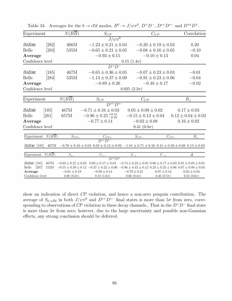
Table 34: Averages for the b→ ccd modes, B0 → J/ψπ0, D+D−, D∗+D∗− and D∗±D∓.
Experiment N(BB) SCP CCP CorrelationJ/ψπ0
BABAR [282] 466M −1.23± 0.21± 0.04 −0.20 ± 0.19± 0.03 0.20Belle [283] 535M −0.65± 0.21± 0.05 −0.08 ± 0.16± 0.05 −0.10Average −0.93± 0.15 −0.10± 0.13 0.04Confidence level 0.15 (1.4σ)
D+D−
BABAR [185] 467M −0.65± 0.36± 0.05 −0.07 ± 0.23± 0.03 −0.01Belle [284] 535M −1.13± 0.37± 0.09 −0.91 ± 0.23± 0.06 −0.04Average −0.89± 0.26 −0.48± 0.17 −0.02Confidence level 0.025 (2.2σ)
Experiment N(BB) SCP CCP R⊥
D∗+D∗−
BABAR [185] 467M −0.71± 0.16± 0.03 0.05± 0.09± 0.02 0.17± 0.03Belle [281] 657M −0.96± 0.25 +0.12
−0.16 −0.15± 0.13± 0.04 0.12± 0.04± 0.02Average −0.77± 0.14 −0.02± 0.08 0.16± 0.02Confidence level 0.41 (0.8σ)
Experiment N(BB) SCP+ CCP+ SCP− CCP− R⊥
D∗+D∗−
BABAR [185] 467M −0.76± 0.16± 0.04 0.02± 0.12± 0.02 −1.81± 0.71± 0.16 0.41± 0.50± 0.08 0.15± 0.03
Experiment N(BB) S+− C+− S−+ C−+ AD∗±D∓
BABAR [185] 467M −0.63± 0.21± 0.03 0.08± 0.17± 0.04 −0.74± 0.23± 0.05 0.00± 0.17± 0.03 0.01± 0.05± 0.01Belle [207] 152M −0.55± 0.39± 0.12 −0.37± 0.22± 0.06 −0.96± 0.43± 0.12 0.23± 0.25± 0.06 0.07± 0.08± 0.04Average −0.61 ± 0.19 −0.09± 0.14 −0.79± 0.21 0.07± 0.14 0.02± 0.04Confidence level 0.86 (0.2σ) 0.12 (1.6σ) 0.66 (0.4σ) 0.46 (0.7σ) 0.54 (0.6σ)
show an indication of direct CP violation, and hence a non-zero penguin contribution. Theaverage of Sb→ccd in both J/ψπ0 and D∗+D∗− final states is more than 5σ from zero, corre-sponding to observations of CP violation in these decay channels., That in the D+D− final stateis more than 3σ from zero; however, due to the large uncertainty and possible non-Gaussianeffects, any strong conclusion should be deferred.
86
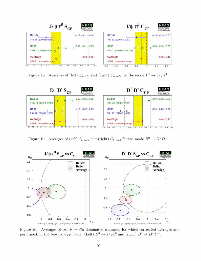
J/ψ π0 SCP
HF
AG
ICH
EP
200
8
-1.8 -1.6 -1.4 -1.2 -1 -0.8 -0.6 -0.4 -0.2 0 0.2
BaBar
PRL 101 (2008) 021801
-1.23 ± 0.21 ± 0.04
Belle
PRD 77 (2008) 071101(R)
-0.65 ± 0.21 ± 0.05
Average
HFAG correlated average
-0.93 ± 0.15
H F A GH F A GICHEP 2008
PRELIMINARY
J/ψ π0 CCP
HF
AG
ICH
EP
200
8
-0.8 -0.6 -0.4 -0.2 0 0.2 0.4
BaBar
PRL 101 (2008) 021801
-0.20 ± 0.19 ± 0.03
Belle
PRD 77 (2008) 071101(R)
-0.08 ± 0.16 ± 0.05
Average
HFAG correlated average
-0.10 ± 0.13
H F A GH F A GICHEP 2008
PRELIMINARY
Figure 18: Averages of (left) Sb→ccd and (right) Cb→ccd for the mode B0 → J/ψπ0.
D+ D- SCP
HF
AG
Win
ter
2009
-2.4 -2.2 -2 -1.8 -1.6 -1.4 -1.2 -1 -0.8 -0.6 -0.4 -0.2 0 0.2 0.4 0.6 0.8
BaBarPRD 79, 032002 (2009)
-0.65 ± 0.36 ± 0.05
BellePRL 98, 221802 (2007)
-1.13 ± 0.37 ± 0.09
AverageHFAG correlated average
-0.89 ± 0.26
H F A GH F A GWinter 2009
PRELIMINARY
D+ D- CCP
HF
AG
Win
ter
2009
-1.8 -1.6 -1.4 -1.2 -1 -0.8 -0.6 -0.4 -0.2 0 0.2 0.4 0.6 0.8
BaBarPRD 79, 032002 (2009)
-0.07 ± 0.23 ± 0.03
BellePRL 98, 221802 (2007)
-0.91 ± 0.23 ± 0.06
AverageHFAG correlated average
-0.48 ± 0.17
H F A GH F A GWinter 2009
PRELIMINARY
Figure 19: Averages of (left) Sb→ccd and (right) Cb→ccd for the mode B0 → D+D−.
J/ψ π0 SCP vs CCP
Contours give -2∆(ln L) = ∆χ2 = 1, corresponding to 60.7% CL for 2 dof
-1 -0.8 -0.6 -0.4 -0.2 0
-0.6
-0.4
-0.2
0
0.2
0.4
0.6
SCP
CCP
BaBarBelleAverage
H F A GH F A GICHEP 2008
PRELIMINARY
D+ D- SCP vs CCP
Contours give -2∆(ln L) = ∆χ2 = 1, corresponding to 60.7% CL for 2 dof
-1.6 -1.2 -0.8 -0.4 0 0.4 0.8
-0.8
-0.4
0
0.4
0.8
SCP
CCP
BaBarBelleAverage
H F A GH F A GWinter 2009
PRELIMINARY
Figure 20: Averages of two b → ccd dominated channels, for which correlated averages areperformed, in the SCP vs. CCP plane. (Left) B0 → J/ψπ0 and (right) B0 → D+D−.
87
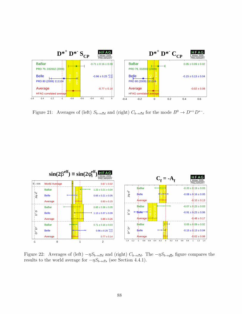
D*+ D*- SCP
HF
AG
Win
ter
2009
-1.6 -1.4 -1.2 -1 -0.8 -0.6 -0.4 -0.2 0
BaBarPRD 79, 032002 (2009)
-0.71 ± 0.16 ± 0.03
BellePRD 80 (2009) 111104
-0.96 ± 0.25 +-00
.
.11
26
AverageHFAG correlated average
-0.77 ± 0.14
H F A GH F A GWinter 2009
PRELIMINARY
D*+ D*- CCP
HF
AG
Win
ter
2009
-0.4 -0.2 0 0.2 0.4 0.6
BaBarPRD 79, 032002 (2009)
0.05 ± 0.09 ± 0.02
BellePRD 80 (2009) 111104
-0.15 ± 0.13 ± 0.04
AverageHFAG correlated average
-0.02 ± 0.08
H F A GH F A GWinter 2009
PRELIMINARY
Figure 21: Averages of (left) Sb→ccd and (right) Cb→ccd for the mode B0 → D∗+D∗−.
sin(2βeff) ≡ sin(2φe1ff)
HF
AG
Win
ter
2009
HF
AG
Win
ter
2009
HF
AG
Win
ter
2009
HF
AG
Win
ter
2009
b→ccs
J/ψ
π0
D+ D
-D
*+ D
*-
-1 0 1 2
World Average 0.67 ± 0.02
BaBar 1.23 ± 0.21 ± 0.04
Belle 0.65 ± 0.21 ± 0.05
Average 0.93 ± 0.15
BaBar 0.65 ± 0.36 ± 0.05
Belle 1.13 ± 0.37 ± 0.09
Average 0.89 ± 0.26
BaBar 0.71 ± 0.16 ± 0.03
Belle 0.96 ± 0.25 +-00
.
.11
62
Average 0.77 ± 0.14
H F A GH F A GWinter 2009
PRELIMINARY Cf = -Af
HF
AG
Win
ter
2009
HF
AG
Win
ter
2009
HF
AG
Win
ter
2009
J/ψ
π0
D+ D
-D
*+ D
*-
-1.4 -1.2 -1 -0.8 -0.6 -0.4 -0.2 0 0.2 0.4 0.6 0.8 1 1.2 1.4
BaBar -0.20 ± 0.19 ± 0.03
Belle -0.08 ± 0.16 ± 0.05
Average -0.10 ± 0.13
BaBar -0.07 ± 0.23 ± 0.03
Belle -0.91 ± 0.23 ± 0.06
Average -0.48 ± 0.17
BaBar 0.05 ± 0.09 ± 0.02
Belle -0.15 ± 0.13 ± 0.04
Average -0.02 ± 0.08
H F A GH F A GWinter 2009
PRELIMINARY
Figure 22: Averages of (left) −ηSb→ccd and (right) Cb→ccd. The −ηSb→qqs figure compares theresults to the world average for −ηSb→ccs (see Section 4.4.1).
88
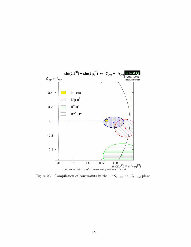
sin(2βeff) ≡ sin(2φe1ff) vs CCP ≡ -ACP
Contours give -2∆(ln L) = ∆χ2 = 1, corresponding to 60.7% CL for 2 dof
-0 0.2 0.4 0.6 0.8 1
-0.4
-0.2
0
0.2
0.4
sin(2βeff) ≡ sin(2φe1
ff)
CCP ≡ -ACP
b→ccs
J/ψ π0
D+ D-
D*+ D*-
H F A GH F A GICHEP 2008
PRELIMINARY
Figure 23: Compilation of constraints in the −ηSb→ccd vs. Cb→ccd plane.
89
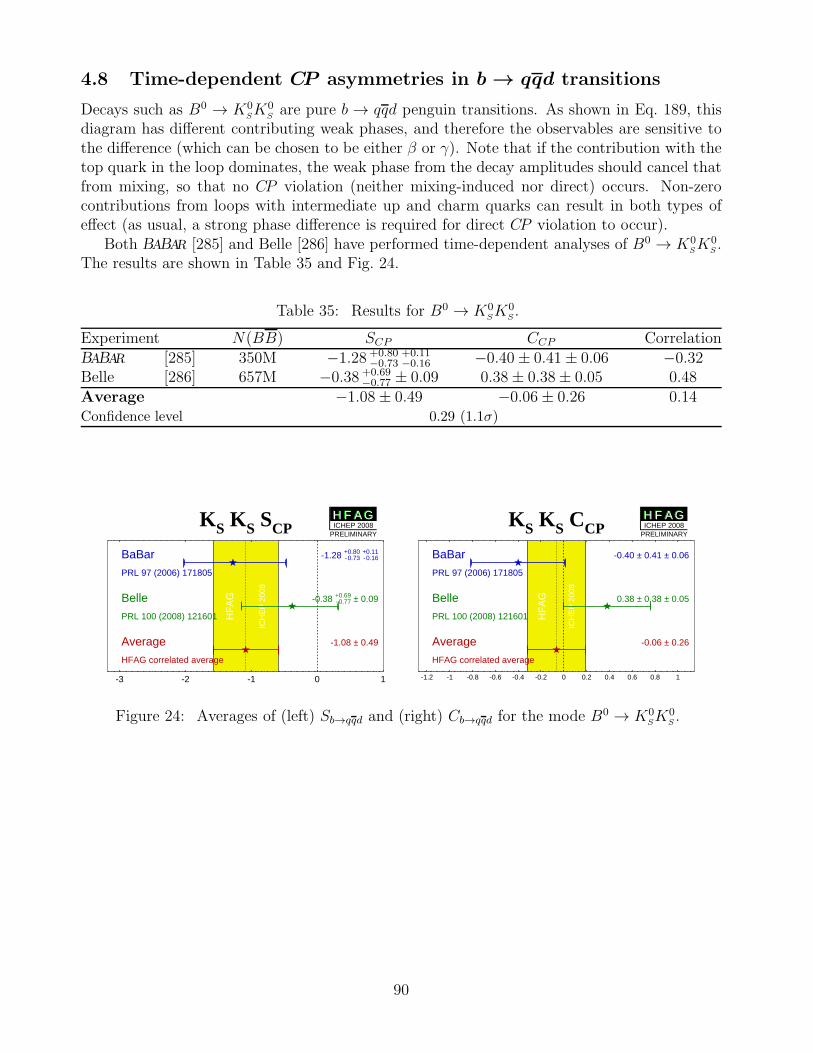
4.8 Time-dependent CP asymmetries in b → qqd transitions
Decays such as B0 → K0SK0
Sare pure b → qqd penguin transitions. As shown in Eq. 189, this
diagram has different contributing weak phases, and therefore the observables are sensitive tothe difference (which can be chosen to be either β or γ). Note that if the contribution with thetop quark in the loop dominates, the weak phase from the decay amplitudes should cancel thatfrom mixing, so that no CP violation (neither mixing-induced nor direct) occurs. Non-zerocontributions from loops with intermediate up and charm quarks can result in both types ofeffect (as usual, a strong phase difference is required for direct CP violation to occur).
Both BABAR [285] and Belle [286] have performed time-dependent analyses of B0 → K0SK
0S .
The results are shown in Table 35 and Fig. 24.
Table 35: Results for B0 → K0SK
0S .
Experiment N(BB) SCP CCP CorrelationBABAR [285] 350M −1.28 +0.80
−0.73+0.11−0.16 −0.40± 0.41± 0.06 −0.32
Belle [286] 657M −0.38 +0.69−0.77 ± 0.09 0.38± 0.38± 0.05 0.48
Average −1.08± 0.49 −0.06± 0.26 0.14Confidence level 0.29 (1.1σ)
KS KS SCP
HF
AG
ICH
EP
200
8
-3 -2 -1 0 1
BaBar
PRL 97 (2006) 171805
-1.28 +-00
.
.87
03
+-00
.
.11
16
Belle
PRL 100 (2008) 121601
-0.38 +-00
.
.67
97 ± 0.09
Average
HFAG correlated average
-1.08 ± 0.49
H F A GH F A GICHEP 2008
PRELIMINARY
KS KS CCPH
FA
G
ICH
EP
200
8
-1.2 -1 -0.8 -0.6 -0.4 -0.2 0 0.2 0.4 0.6 0.8 1
BaBar
PRL 97 (2006) 171805
-0.40 ± 0.41 ± 0.06
Belle
PRL 100 (2008) 121601
0.38 ± 0.38 ± 0.05
Average
HFAG correlated average
-0.06 ± 0.26
H F A GH F A GICHEP 2008
PRELIMINARY
Figure 24: Averages of (left) Sb→qqd and (right) Cb→qqd for the mode B0 → K0SK
0S .
90
4.9 Time-dependent asymmetries in b → sγ transitions
The radiative decays b → sγ produce photons which are highly polarized in the StandardModel. The decays B0 → Fγ and B0 → Fγ produce photons with opposite helicities, andsince the polarization is, in principle, observable, these final states cannot interfere. The finitemass of the s quark introduces small corrections to the limit of maximum polarization, but anylarge mixing induced CP violation would be a signal for new physics. Since a single weak phasedominates the b→ sγ transition in the Standard Model, the cosine term is also expected to besmall.
Atwood et al. [217] have shown that an inclusive analysis with respect to K0Sπ
0γ can beperformed, since the properties of the decay amplitudes are independent of the angular mo-mentum of the K0
Sπ0 system. However, if non-dipole operators contribute significantly to the
amplitudes, then the Standard Model mixing-induced CP violation could be larger than thenaıve expectation S ≃ −2(ms/mb) sin (2β) [218, 219]. In this case, the CP parameters mayvary over the K0
Sπ0γ Dalitz plot, for example as a function of the K0
Sπ0 invariant mass. Explicit
calculations indicate such corrections are small for exclusive final states [220, 221].With the above in mind, we quote two averages: one for K∗(892) candidates only, and the
other one for the inclusive K0Sπ
0γ decay (including the K∗(892)). If the Standard Model dipoleoperator is dominant, both should give the same quantities (the latter naturally with smallerstatistical error). If not, care needs to be taken in interpretation of the inclusive parameters,while the results on the K∗(892) resonance remain relatively clean. Results from BABAR [287]and Belle [288] are used for both averages; both experiments use the invariant mass range0.60 GeV/c2 < MK0
Sπ0 < 1.80 GeV/c2 in the inclusive analysis. In addition to the K0
Sπ0γ
decay, BABAR have presented results using K0Sηγ [289], and Belle have presented results using
K0Sργ [290].
Table 36: Averages for b→ sγ modes.
Experiment N(BB) SCP (b→ sγ) CCP (b→ sγ) CorrelationK∗(892)γ
BABAR [287] 467M −0.03± 0.29± 0.03 −0.14 ± 0.16± 0.03 0.05Belle [288] 535M −0.32 +0.36
−0.33 ± 0.05 0.20± 0.24± 0.05 0.08Average −0.16± 0.22 −0.04± 0.14 0.06Confidence level 0.40 (0.9σ)
K0Sπ
0γ (including K∗(892)γ)BABAR [287] 467M −0.17± 0.26± 0.03 −0.19 ± 0.14± 0.03 0.04Belle [288] 535M −0.10± 0.31± 0.07 0.20± 0.20± 0.06 0.08Average −0.15± 0.20 −0.07± 0.12 0.05Confidence level 0.30 (1.0σ)
K0Sηγ
BABAR [289] 465M −0.18 +0.49−0.46 ± 0.12 −0.32 +0.40
−0.39 ± 0.07 −0.17K0
Sρ0γ
Belle [290] 657M 0.11± 0.33 +0.05−0.09 −0.05 ± 0.18± 0.06 0.04
The results are shown in Table 36, and in Figs. 25 and 26. No significant CP violation resultsare seen; the results are consistent with the Standard Model and with other measurements in
91
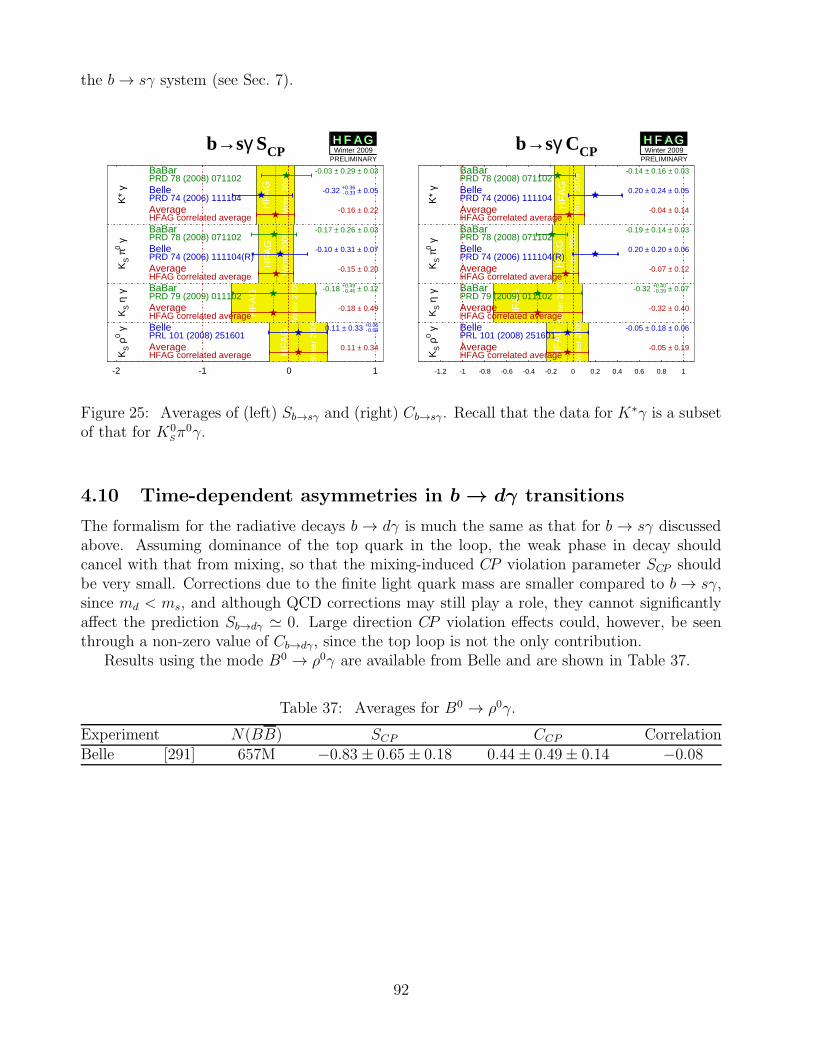
the b→ sγ system (see Sec. 7).
b→sγ SCP
HF
AG
Win
ter
2009
HF
AG
Win
ter
2009
HF
AG
Win
ter
2009
HF
AG
Win
ter
2009
K*
γK
S π
0 γK
S η
γK
S ρ
0 γ
-2 -1 0 1
BaBarPRD 78 (2008) 071102
-0.03 ± 0.29 ± 0.03
BellePRD 74 (2006) 111104
-0.32 +-00
.
.33
63 ± 0.05
AverageHFAG correlated average
-0.16 ± 0.22
BaBarPRD 78 (2008) 071102
-0.17 ± 0.26 ± 0.03
BellePRD 74 (2006) 111104(R)
-0.10 ± 0.31 ± 0.07
AverageHFAG correlated average
-0.15 ± 0.20
BaBarPRD 79 (2009) 011102
-0.18 +-00
.
.44
96 ± 0.12
AverageHFAG correlated average
-0.18 ± 0.49
BellePRL 101 (2008) 251601
0.11 ± 0.33 +-00
.
.00
59
AverageHFAG correlated average
0.11 ± 0.34
H F A GH F A GWinter 2009
PRELIMINARY
b→sγ CCP
HF
AG
Win
ter
2009
HF
AG
Win
ter
2009
HF
AG
Win
ter
2009
HF
AG
Win
ter
2009
K*
γK
S π
0 γK
S η
γK
S ρ
0 γ
-1.2 -1 -0.8 -0.6 -0.4 -0.2 0 0.2 0.4 0.6 0.8 1
BaBarPRD 78 (2008) 071102
-0.14 ± 0.16 ± 0.03
BellePRD 74 (2006) 111104
0.20 ± 0.24 ± 0.05
AverageHFAG correlated average
-0.04 ± 0.14
BaBarPRD 78 (2008) 071102
-0.19 ± 0.14 ± 0.03
BellePRD 74 (2006) 111104(R)
0.20 ± 0.20 ± 0.06
AverageHFAG correlated average
-0.07 ± 0.12
BaBarPRD 79 (2009) 011102
-0.32 +-00
.
.43
09 ± 0.07
AverageHFAG correlated average
-0.32 ± 0.40
BellePRL 101 (2008) 251601
-0.05 ± 0.18 ± 0.06
AverageHFAG correlated average
-0.05 ± 0.19
H F A GH F A GWinter 2009
PRELIMINARY
Figure 25: Averages of (left) Sb→sγ and (right) Cb→sγ. Recall that the data for K∗γ is a subsetof that for K0
Sπ0γ.
4.10 Time-dependent asymmetries in b → dγ transitions
The formalism for the radiative decays b → dγ is much the same as that for b → sγ discussedabove. Assuming dominance of the top quark in the loop, the weak phase in decay shouldcancel with that from mixing, so that the mixing-induced CP violation parameter SCP shouldbe very small. Corrections due to the finite light quark mass are smaller compared to b→ sγ,since md < ms, and although QCD corrections may still play a role, they cannot significantlyaffect the prediction Sb→dγ ≃ 0. Large direction CP violation effects could, however, be seenthrough a non-zero value of Cb→dγ, since the top loop is not the only contribution.
Results using the mode B0 → ρ0γ are available from Belle and are shown in Table 37.
Table 37: Averages for B0 → ρ0γ.
Experiment N(BB) SCP CCP CorrelationBelle [291] 657M −0.83 ± 0.65± 0.18 0.44± 0.49± 0.14 −0.08
92
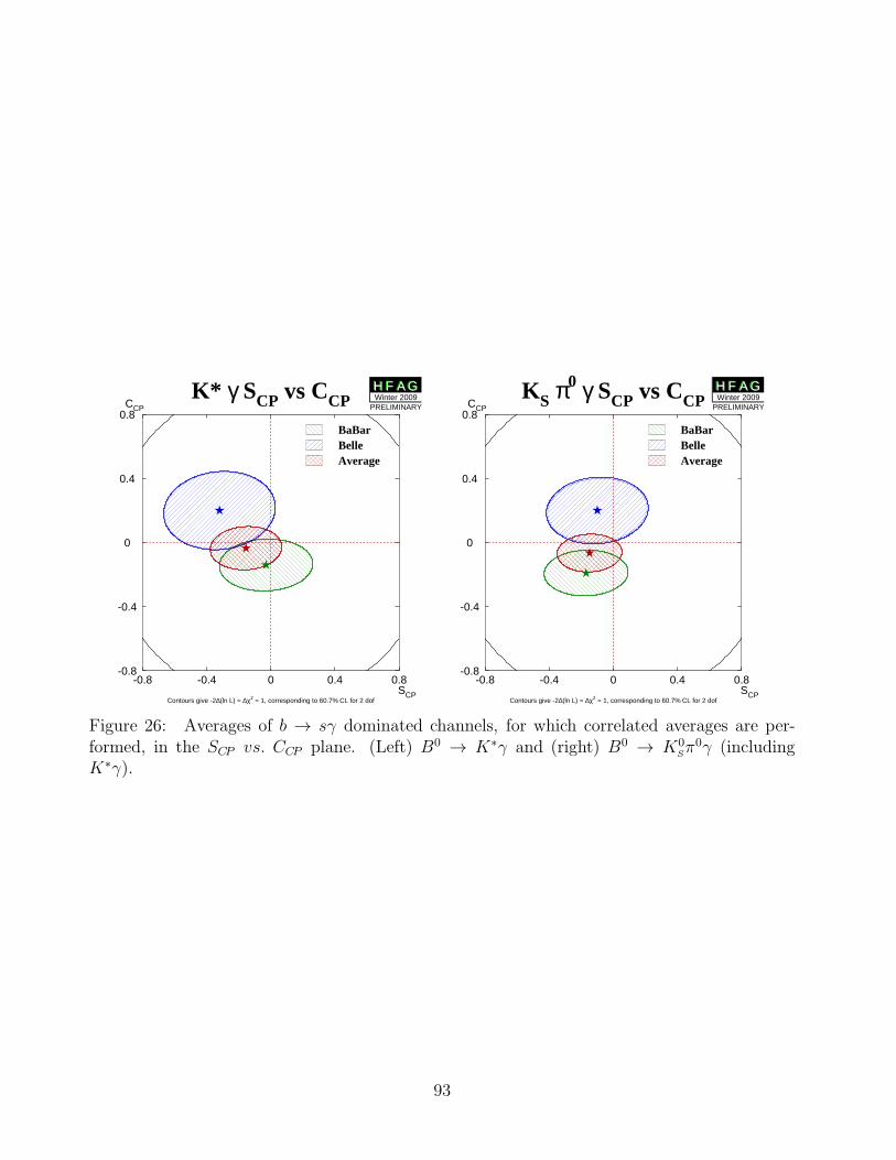
K* γ SCP vs CCP
Contours give -2∆(ln L) = ∆χ2 = 1, corresponding to 60.7% CL for 2 dof
-0.8 -0.4 0 0.4 0.8-0.8
-0.4
0
0.4
0.8
SCP
CCP
BaBarBelleAverage
H F A GH F A GWinter 2009
PRELIMINARY
KS π0 γ SCP vs CCP
Contours give -2∆(ln L) = ∆χ2 = 1, corresponding to 60.7% CL for 2 dof
-0.8 -0.4 0 0.4 0.8-0.8
-0.4
0
0.4
0.8
SCP
CCP
BaBarBelleAverage
H F A GH F A GWinter 2009
PRELIMINARY
Figure 26: Averages of b → sγ dominated channels, for which correlated averages are per-formed, in the SCP vs. CCP plane. (Left) B0 → K∗γ and (right) B0 → K0
Sπ0γ (including
K∗γ).
93
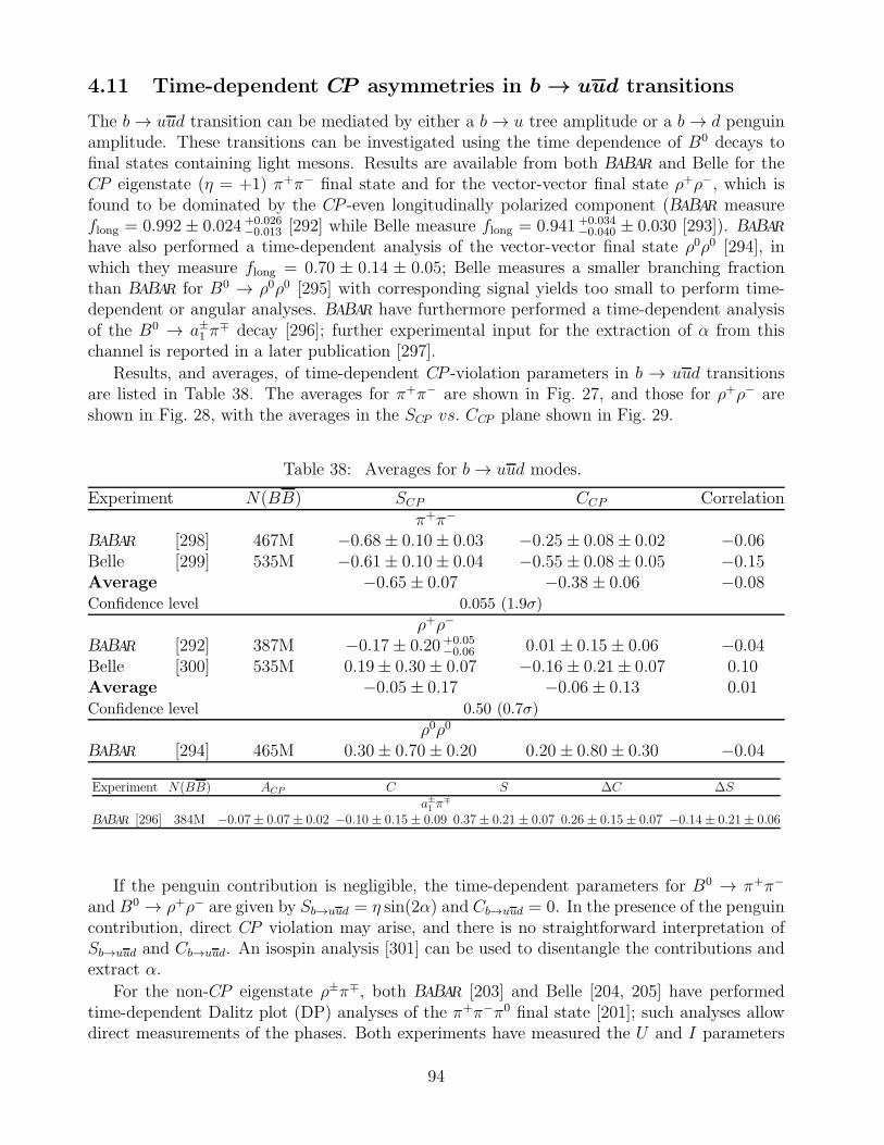
4.11 Time-dependent CP asymmetries in b → uud transitions
The b→ uud transition can be mediated by either a b→ u tree amplitude or a b → d penguinamplitude. These transitions can be investigated using the time dependence of B0 decays tofinal states containing light mesons. Results are available from both BABAR and Belle for theCP eigenstate (η = +1) π+π− final state and for the vector-vector final state ρ+ρ−, which isfound to be dominated by the CP -even longitudinally polarized component (BABAR measureflong = 0.992± 0.024 +0.026
−0.013 [292] while Belle measure flong = 0.941 +0.034−0.040 ± 0.030 [293]). BABAR
have also performed a time-dependent analysis of the vector-vector final state ρ0ρ0 [294], inwhich they measure flong = 0.70 ± 0.14 ± 0.05; Belle measures a smaller branching fractionthan BABAR for B0 → ρ0ρ0 [295] with corresponding signal yields too small to perform time-dependent or angular analyses. BABAR have furthermore performed a time-dependent analysisof the B0 → a±1 π
∓ decay [296]; further experimental input for the extraction of α from thischannel is reported in a later publication [297].
Results, and averages, of time-dependent CP -violation parameters in b → uud transitionsare listed in Table 38. The averages for π+π− are shown in Fig. 27, and those for ρ+ρ− areshown in Fig. 28, with the averages in the SCP vs. CCP plane shown in Fig. 29.
Table 38: Averages for b→ uud modes.
Experiment N(BB) SCP CCP Correlationπ+π−
BABAR [298] 467M −0.68± 0.10± 0.03 −0.25 ± 0.08± 0.02 −0.06Belle [299] 535M −0.61± 0.10± 0.04 −0.55 ± 0.08± 0.05 −0.15Average −0.65± 0.07 −0.38± 0.06 −0.08Confidence level 0.055 (1.9σ)
ρ+ρ−
BABAR [292] 387M −0.17± 0.20 +0.05−0.06 0.01± 0.15± 0.06 −0.04
Belle [300] 535M 0.19± 0.30± 0.07 −0.16 ± 0.21± 0.07 0.10Average −0.05± 0.17 −0.06± 0.13 0.01Confidence level 0.50 (0.7σ)
ρ0ρ0
BABAR [294] 465M 0.30± 0.70± 0.20 0.20± 0.80± 0.30 −0.04
Experiment N(BB) ACP C S ∆C ∆Sa±1 π
∓
BABAR [296] 384M −0.07± 0.07± 0.02 −0.10± 0.15± 0.09 0.37± 0.21± 0.07 0.26± 0.15± 0.07 −0.14± 0.21± 0.06
If the penguin contribution is negligible, the time-dependent parameters for B0 → π+π−
and B0 → ρ+ρ− are given by Sb→uud = η sin(2α) and Cb→uud = 0. In the presence of the penguincontribution, direct CP violation may arise, and there is no straightforward interpretation ofSb→uud and Cb→uud. An isospin analysis [301] can be used to disentangle the contributions andextract α.
For the non-CP eigenstate ρ±π∓, both BABAR [203] and Belle [204, 205] have performedtime-dependent Dalitz plot (DP) analyses of the π+π−π0 final state [201]; such analyses allowdirect measurements of the phases. Both experiments have measured the U and I parameters
94
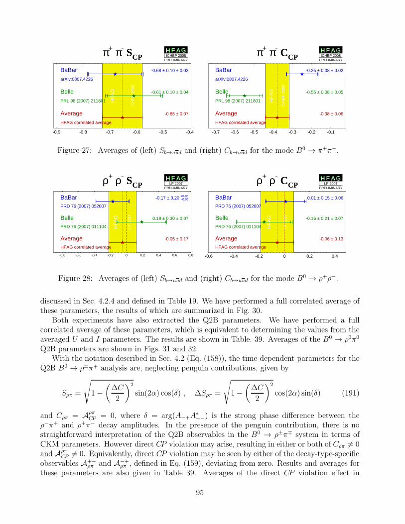
π+ π- SCP
HF
AG
ICH
EP
200
8-0.9 -0.8 -0.7 -0.6 -0.5 -0.4
BaBar
arXiv:0807.4226
-0.68 ± 0.10 ± 0.03
Belle
PRL 98 (2007) 211801
-0.61 ± 0.10 ± 0.04
Average
HFAG correlated average
-0.65 ± 0.07
H F A GH F A GICHEP 2008
PRELIMINARY
π+ π- CCP
HF
AG
ICH
EP
200
8
-0.7 -0.6 -0.5 -0.4 -0.3 -0.2 -0.1
BaBar
arXiv:0807.4226
-0.25 ± 0.08 ± 0.02
Belle
PRL 98 (2007) 211801
-0.55 ± 0.08 ± 0.05
Average
HFAG correlated average
-0.38 ± 0.06
H F A GH F A GICHEP 2008
PRELIMINARY
Figure 27: Averages of (left) Sb→uud and (right) Cb→uud for the mode B0 → π+π−.
ρ+ ρ- SCP
HF
AG
LP 2
007
-0.8 -0.6 -0.4 -0.2 0 0.2 0.4 0.6 0.8
BaBarPRD 76 (2007) 052007
-0.17 ± 0.20 +-00
.
.00
56
BellePRD 76 (2007) 011104
0.19 ± 0.30 ± 0.07
AverageHFAG correlated average
-0.05 ± 0.17
H F A GH F A GLP 2007
PRELIMINARY
ρ+ ρ- CCP
HF
AG
LP 2
007
-0.6 -0.4 -0.2 0 0.2 0.4
BaBarPRD 76 (2007) 052007
0.01 ± 0.15 ± 0.06
BellePRD 76 (2007) 011104
-0.16 ± 0.21 ± 0.07
AverageHFAG correlated average
-0.06 ± 0.13
H F A GH F A GLP 2007
PRELIMINARY
Figure 28: Averages of (left) Sb→uud and (right) Cb→uud for the mode B0 → ρ+ρ−.
discussed in Sec. 4.2.4 and defined in Table 19. We have performed a full correlated average ofthese parameters, the results of which are summarized in Fig. 30.
Both experiments have also extracted the Q2B parameters. We have performed a fullcorrelated average of these parameters, which is equivalent to determining the values from theaveraged U and I parameters. The results are shown in Table. 39. Averages of the B0 → ρ0π0
Q2B parameters are shown in Figs. 31 and 32.With the notation described in Sec. 4.2 (Eq. (158)), the time-dependent parameters for the
Q2B B0 → ρ±π∓ analysis are, neglecting penguin contributions, given by
Sρπ =
√
1−(
∆C
2
)2
sin(2α) cos(δ) , ∆Sρπ =
√
1−(
∆C
2
)2
cos(2α) sin(δ) (191)
and Cρπ = AρπCP = 0, where δ = arg(A−+A
∗+−) is the strong phase difference between the
ρ−π+ and ρ+π− decay amplitudes. In the presence of the penguin contribution, there is nostraightforward interpretation of the Q2B observables in the B0 → ρ±π∓ system in terms ofCKM parameters. However direct CP violation may arise, resulting in either or both of Cρπ 6= 0and Aρπ
CP 6= 0. Equivalently, direct CP violation may be seen by either of the decay-type-specificobservables A+−
ρπ and A−+ρπ , defined in Eq. (159), deviating from zero. Results and averages for
these parameters are also given in Table 39. Averages of the direct CP violation effect in
95
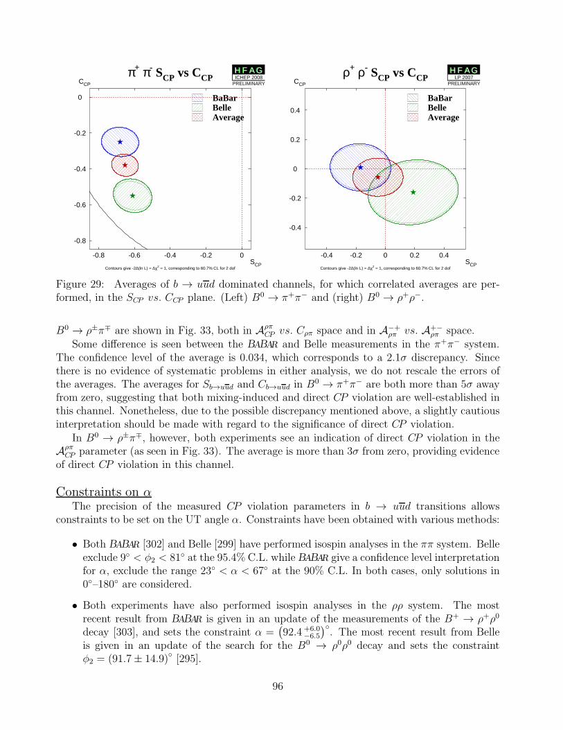
π+ π- SCP vs CCP
Contours give -2∆(ln L) = ∆χ2 = 1, corresponding to 60.7% CL for 2 dof
-0.8 -0.6 -0.4 -0.2 0
-0.8
-0.6
-0.4
-0.2
0
SCP
CCP
BaBarBelleAverage
H F A GH F A GICHEP 2008
PRELIMINARY
ρ+ ρ- SCP vs CCP
Contours give -2∆(ln L) = ∆χ2 = 1, corresponding to 60.7% CL for 2 dof
-0.4 -0.2 0 0.2 0.4
-0.4
-0.2
0
0.2
0.4
SCP
CCP
BaBarBelleAverage
H F A GH F A GLP 2007
PRELIMINARY
Figure 29: Averages of b → uud dominated channels, for which correlated averages are per-formed, in the SCP vs. CCP plane. (Left) B0 → π+π− and (right) B0 → ρ+ρ−.
B0 → ρ±π∓ are shown in Fig. 33, both in AρπCP vs. Cρπ space and in A−+
ρπ vs. A+−ρπ space.
Some difference is seen between the BABAR and Belle measurements in the π+π− system.The confidence level of the average is 0.034, which corresponds to a 2.1σ discrepancy. Sincethere is no evidence of systematic problems in either analysis, we do not rescale the errors ofthe averages. The averages for Sb→uud and Cb→uud in B
0 → π+π− are both more than 5σ awayfrom zero, suggesting that both mixing-induced and direct CP violation are well-established inthis channel. Nonetheless, due to the possible discrepancy mentioned above, a slightly cautiousinterpretation should be made with regard to the significance of direct CP violation.
In B0 → ρ±π∓, however, both experiments see an indication of direct CP violation in theAρπCP parameter (as seen in Fig. 33). The average is more than 3σ from zero, providing evidence
of direct CP violation in this channel.
Constraints on αThe precision of the measured CP violation parameters in b → uud transitions allows
constraints to be set on the UT angle α. Constraints have been obtained with various methods:
• Both BABAR [302] and Belle [299] have performed isospin analyses in the ππ system. Belleexclude 9 < φ2 < 81 at the 95.4% C.L. while BABAR give a confidence level interpretationfor α, exclude the range 23 < α < 67 at the 90% C.L. In both cases, only solutions in0–180 are considered.
• Both experiments have also performed isospin analyses in the ρρ system. The mostrecent result from BABAR is given in an update of the measurements of the B+ → ρ+ρ0
decay [303], and sets the constraint α =(
92.4 +6.0−6.5
). The most recent result from Belle
is given in an update of the search for the B0 → ρ0ρ0 decay and sets the constraintφ2 = (91.7± 14.9) [295].
96
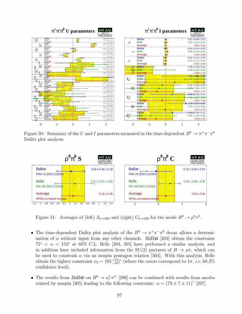
π+π-π0 U parameters
HF
AG
EP
S 0
7
HF
AG
EP
S 0
7
HF
AG
EP
S 0
7
HF
AG
EP
S 0
7
HF
AG
EP
S 0
7
HF
AG
EP
S 0
7
HF
AG
EP
S 0
7
HF
AG
EP
S 0
7
HF
AG
EP
S 0
7
HF
AG
EP
S 0
7
HF
AG
EP
S 0
7
HF
AG
EP
S 0
7
HF
AG
EP
S 0
7
HF
AG
EP
S 0
7H
FA
G
EP
S 0
7
HF
AG
EP
S 0
7
HF
AG
EP
S 0
7
U+ 0
U+ -
U- 0
U- -
U- +
U+ +
, -ImU
+ +, -R
e
U- +, -Im
U- +, -R
e
U+ +
, 0ImU
+ +, 0R
e
U- +, 0Im
U- +, 0R
e
U+ -, 0Im
U+ -, 0R
e
U- -, 0Im
U- -, 0R
e
-2 -1 0 1 2
BaBar 0.28 ± 0.07 ± 0.04Belle 0.29 ± 0.05 ± 0.04Average 0.26 ± 0.05BaBar 1.32 ± 0.12 ± 0.05Belle 1.27 ± 0.13 ± 0.09Average 1.19 ± 0.11BaBar -0.03 ± 0.11 ± 0.09Belle 0.15 ± 0.11 ± 0.08Average 0.03 ± 0.10BaBar -0.32 ± 0.14 ± 0.05Belle -0.62 ± 0.16 ± 0.08Average -0.44 ± 0.11BaBar 0.54 ± 0.15 ± 0.05Belle 0.23 ± 0.15 ± 0.07Average 0.37 ± 0.12BaBar -0.07 ± 0.71 ± 0.73Belle 1.18 ± 0.86 ± 0.34Average 0.52 ± 0.71BaBar 0.17 ± 0.49 ± 0.31Belle 0.49 ± 0.86 ± 0.52Average 0.05 ± 0.53BaBar -0.38 ± 1.06 ± 0.36Belle -2.32 ± 1.74 ± 0.91Average -0.56 ± 1.00BaBar 2.23 ± 1.00 ± 0.43Belle -1.18 ± 1.61 ± 0.72Average 1.12 ± 0.98BaBar -0.16 ± 0.57 ± 0.14Belle -0.57 ± 0.35 ± 0.51Average -0.50 ± 0.49BaBar -1.08 ± 0.48 ± 0.20Belle 0.29 ± 0.50 ± 0.35Average -0.57 ± 0.44BaBar -1.66 ± 0.94 ± 0.25Belle -0.41 ± 1.00 ± 0.47Average -1.30 ± 0.78BaBar -0.18 ± 0.88 ± 0.35Belle -2.37 ± 1.36 ± 0.60Average -0.96 ± 0.82BaBar -0.17 ± 0.50 ± 0.23Belle -1.34 ± 0.60 ± 0.47Average -0.74 ± 0.49BaBar -0.36 ± 0.38 ± 0.08Belle 0.25 ± 0.60 ± 0.33Average -0.21 ± 0.35BaBar 0.12 ± 0.75 ± 0.22Belle -0.02 ± 1.31 ± 0.83Average -0.10 ± 0.76BaBar -0.63 ± 0.72 ± 0.32Belle -0.53 ± 1.44 ± 0.65Average -0.49 ± 0.75
H F A GH F A GEPS 07
PRELIMINARY
π+π-π0 I parameters
HF
AG
EP
S 0
7H
FA
GE
PS
07
HF
AG
EP
S 0
7
HF
AG
EP
S 0
7
HF
AG
EP
S 0
7
HF
AG
EP
S 0
7
HF
AG
EP
S 0
7
HF
AG
EP
S 0
7
HF
AG
EP
S 0
7
I 0
I -
I +
II +m -
IR +e -
II +m 0
IR +e 0
II -m 0
IR -e 0
-2 -1 0 1 2
BaBar 0.01 ± 0.06 ± 0.01Belle 0.02 ± 0.10 ± 0.05Average 0.00 ± 0.05BaBar -0.01 ± 0.10 ± 0.02Belle 0.09 ± 0.10 ± 0.04Average 0.03 ± 0.08BaBar -0.02 ± 0.10 ± 0.03Belle -0.01 ± 0.11 ± 0.04Average -0.04 ± 0.08BaBar -1.99 ± 1.25 ± 0.34Belle -1.93 ± 2.39 ± 0.89Average -1.99 ± 1.19BaBar 1.90 ± 2.03 ± 0.65Belle 1.21 ± 2.59 ± 0.98Average 0.55 ± 1.80BaBar -0.21 ± 1.06 ± 0.25Belle -0.40 ± 1.86 ± 0.85Average -0.53 ± 1.01BaBar 0.41 ± 1.30 ± 0.41Belle 1.15 ± 2.26 ± 0.92Average -0.22 ± 1.35BaBar 1.23 ± 1.07 ± 0.29Belle -2.03 ± 1.62 ± 0.81Average -0.04 ± 1.05BaBar 0.41 ± 1.30 ± 0.21Belle -0.92 ± 1.34 ± 0.80Average -0.60 ± 1.01
H F A GH F A GEPS 07
PRELIMINARY
Figure 30: Summary of the U and I parameters measured in the time-dependent B0 → π+π−π0
Dalitz plot analysis.
ρ0π0 S
HF
AG
ICH
EP
200
8
-1.2 -1 -0.8 -0.6 -0.4 -0.2 0 0.2 0.4 0.6 0.8 1 1.2 1.4
BaBarPRD 76 (2007) 012004
0.04 ± 0.44 ± 0.18
BellePRL 98 (2007) 221602
0.17 ± 0.57 ± 0.35
AverageHFAG correlated average
0.12 ± 0.38
H F A GH F A GICHEP 2008
PRELIMINARY
ρ0π0 CH
FA
G
ICH
EP
200
8
-1 0 1 2
BaBarPRD 76 (2007) 012004
-0.10 ± 0.40 ± 0.53
BellePRL 98 (2007) 221602
0.49 ± 0.36 ± 0.28
AverageHFAG correlated average
0.30 ± 0.38
H F A GH F A GICHEP 2008
PRELIMINARY
Figure 31: Averages of (left) Sb→uud and (right) Cb→uud for the mode B0 → ρ0π0.
• The time-dependent Dalitz plot analysis of the B0 → π+π−π0 decay allows a determi-nation of α without input from any other channels. BABAR [203] obtain the constraint75 < α < 152 at 68% C.L. Belle [204, 205] have performed a similar analysis, andin addition have included information from the SU(2) partners of B → ρπ, which canbe used to constrain α via an isospin pentagon relation [304]. With this analysis, Belleobtain the tighter constraint φ2 = (83 +12
−23) (where the errors correspond to 1σ, i.e. 68.3%
confidence level).
• The results from BABAR on B0 → a±1 π∓ [296] can be combined with results from modes
related by isospin [305] leading to the following constraint: α = (79± 7± 11) [297].
97
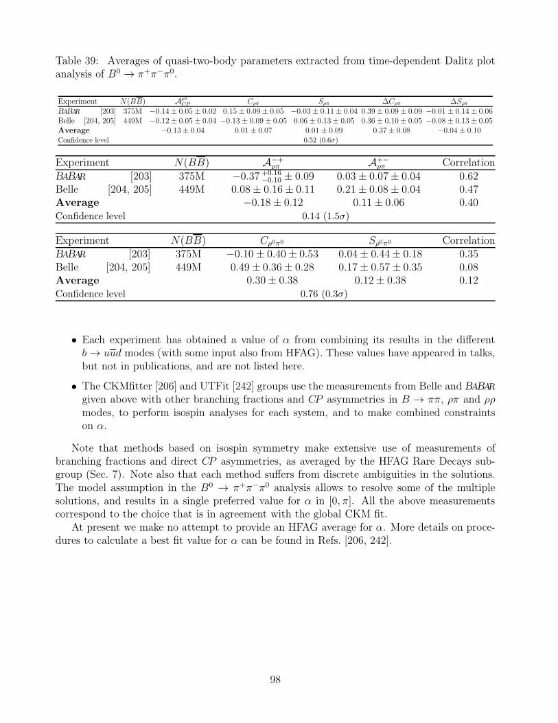
Table 39: Averages of quasi-two-body parameters extracted from time-dependent Dalitz plotanalysis of B0 → π+π−π0.
Experiment N(BB) AρπCP Cρπ Sρπ ∆Cρπ ∆Sρπ
BABAR [203] 375M −0.14± 0.05± 0.02 0.15± 0.09± 0.05 −0.03± 0.11± 0.04 0.39± 0.09± 0.09 −0.01± 0.14± 0.06Belle [204, 205] 449M −0.12± 0.05± 0.04 −0.13± 0.09± 0.05 0.06± 0.13± 0.05 0.36± 0.10± 0.05 −0.08± 0.13± 0.05Average −0.13± 0.04 0.01± 0.07 0.01± 0.09 0.37± 0.08 −0.04± 0.10Confidence level 0.52 (0.6σ)
Experiment N(BB) A−+ρπ A+−
ρπ Correlation
BABAR [203] 375M −0.37 +0.16−0.10 ± 0.09 0.03± 0.07± 0.04 0.62
Belle [204, 205] 449M 0.08± 0.16± 0.11 0.21± 0.08± 0.04 0.47Average −0.18± 0.12 0.11± 0.06 0.40Confidence level 0.14 (1.5σ)
Experiment N(BB) Cρ0π0 Sρ0π0 CorrelationBABAR [203] 375M −0.10± 0.40± 0.53 0.04± 0.44± 0.18 0.35Belle [204, 205] 449M 0.49± 0.36± 0.28 0.17± 0.57± 0.35 0.08Average 0.30± 0.38 0.12± 0.38 0.12Confidence level 0.76 (0.3σ)
• Each experiment has obtained a value of α from combining its results in the differentb → uud modes (with some input also from HFAG). These values have appeared in talks,but not in publications, and are not listed here.
• The CKMfitter [206] and UTFit [242] groups use the measurements from Belle and BABAR
given above with other branching fractions and CP asymmetries in B → ππ, ρπ and ρρmodes, to perform isospin analyses for each system, and to make combined constraintson α.
Note that methods based on isospin symmetry make extensive use of measurements ofbranching fractions and direct CP asymmetries, as averaged by the HFAG Rare Decays sub-group (Sec. 7). Note also that each method suffers from discrete ambiguities in the solutions.The model assumption in the B0 → π+π−π0 analysis allows to resolve some of the multiplesolutions, and results in a single preferred value for α in [0, π]. All the above measurementscorrespond to the choice that is in agreement with the global CKM fit.
At present we make no attempt to provide an HFAG average for α. More details on proce-dures to calculate a best fit value for α can be found in Refs. [206, 242].
98
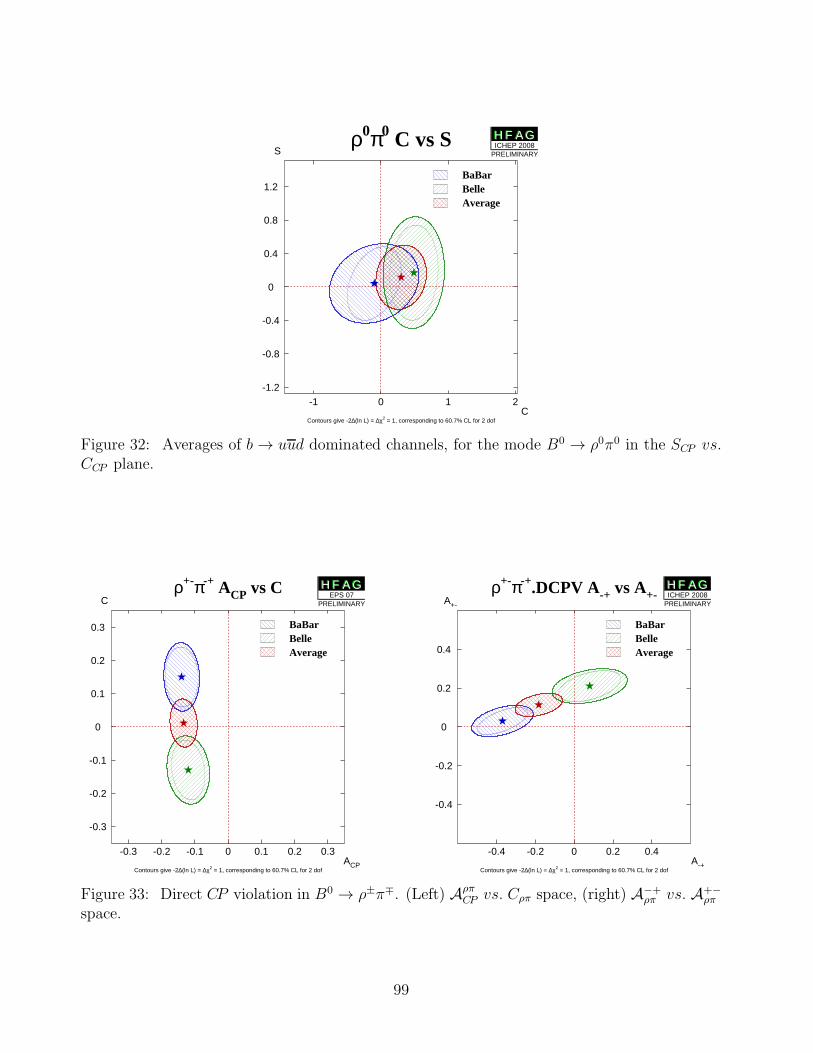
ρ0π0 C vs S
Contours give -2∆(ln L) = ∆χ2 = 1, corresponding to 60.7% CL for 2 dof
-1 0 1 2-1.2
-0.8
-0.4
0
0.4
0.8
1.2
C
S
BaBarBelleAverage
H F A GH F A GICHEP 2008
PRELIMINARY
Figure 32: Averages of b → uud dominated channels, for the mode B0 → ρ0π0 in the SCP vs.CCP plane.
ρ+-π-+ ACP vs C
Contours give -2∆(ln L) = ∆χ2 = 1, corresponding to 60.7% CL for 2 dof
-0.3 -0.2 -0.1 0 0.1 0.2 0.3
-0.3
-0.2
-0.1
0
0.1
0.2
0.3
ACP
C
BaBarBelleAverage
H F A GH F A GEPS 07
PRELIMINARY
ρ+-π-+.DCPV A-+ vs A+-
Contours give -2∆(ln L) = ∆χ2 = 1, corresponding to 60.7% CL for 2 dof
-0.4 -0.2 0 0.2 0.4
-0.4
-0.2
0
0.2
0.4
A-+
A+-
BaBarBelleAverage
H F A GH F A GICHEP 2008
PRELIMINARY
Figure 33: Direct CP violation in B0 → ρ±π∓. (Left) AρπCP vs. Cρπ space, (right) A−+
ρπ vs. A+−ρπ
space.
99
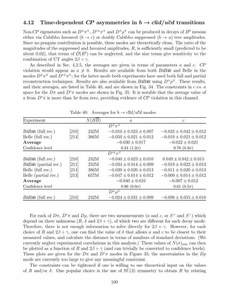
4.12 Time-dependent CP asymmetries in b → cud/ucd transitions
Non-CP eigenstates such as D±π∓, D∗±π∓ and D±ρ∓ can be produced in decays of B0 mesonseither via Cabibbo favoured (b → c) or doubly Cabibbo suppressed (b → u) tree amplitudes.Since no penguin contribution is possible, these modes are theoretically clean. The ratio of themagnitudes of the suppressed and favoured amplitudes, R, is sufficiently small (predicted to beabout 0.02), that terms of O(R2) can be neglected, and the sine terms give sensitivity to thecombination of UT angles 2β + γ.
As described in Sec. 4.2.5, the averages are given in terms of parameters a and c. CPviolation would appear as a 6= 0. Results are available from both BABAR and Belle in themodes D±π∓ and D∗±π∓; for the latter mode both experiments have used both full and partialreconstruction techniques. Results are also available from BABAR using D±ρ∓. These results,and their averages, are listed in Table 40, and are shown in Fig. 34. The constraints in c vs. aspace for the Dπ and D∗π modes are shown in Fig. 35. It is notable that the average value ofa from D∗π is more than 3σ from zero, providing evidence of CP violation in this channel.
Table 40: Averages for b→ cud/ucd modes.
Experiment N(BB) a cD±π∓
BABAR (full rec.) [210] 232M −0.010± 0.023± 0.007 −0.033± 0.042± 0.012Belle (full rec.) [214] 386M −0.050± 0.021± 0.012 −0.019± 0.021± 0.012Average −0.030± 0.017 −0.022± 0.021Confidence level 0.24 (1.2σ) 0.78 (0.3σ)
D∗±π∓
BABAR (full rec.) [210] 232M −0.040± 0.023± 0.010 0.049± 0.042± 0.015BABAR (partial rec.) [211] 232M −0.034± 0.014± 0.009 −0.019± 0.022± 0.013Belle (full rec.) [214] 386M −0.039± 0.020± 0.013 −0.011± 0.020± 0.013Belle (partial rec.) [213] 657M −0.047± 0.014± 0.012 −0.009± 0.014± 0.012Average −0.040± 0.010 −0.007± 0.012Confidence level 0.96 (0.0σ) 0.61 (0.5σ)
D±ρ∓
BABAR (full rec.) [210] 232M −0.024± 0.031± 0.009 −0.098± 0.055± 0.018
For each of Dπ, D∗π and Dρ, there are two measurements (a and c, or S+ and S−) whichdepend on three unknowns (R, δ and 2β + γ), of which two are different for each decay mode.Therefore, there is not enough information to solve directly for 2β + γ. However, for eachchoice of R and 2β + γ, one can find the value of δ that allows a and c to be closest to theirmeasured values, and calculate the distance in terms of numbers of standard deviations. (Wecurrently neglect experimental correlations in this analysis.) These values of N(σ)min can thenbe plotted as a function of R and 2β + γ (and can trivially be converted to confidence levels).These plots are given for the Dπ and D∗π modes in Figure 35; the uncertainties in the Dρmode are currently too large to give any meaningful constraint.
The constraints can be tightened if one is willing to use theoretical input on the valuesof R and/or δ. One popular choice is the use of SU(3) symmetry to obtain R by relating
100
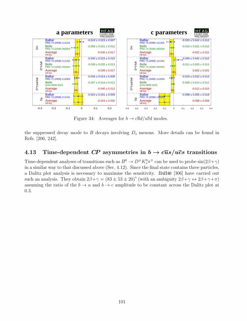
a parameters
HF
AG
ICH
EP
200
8
HF
AG
ICH
EP
200
8H
FA
GIC
HE
P 2
008
HF
AG
ICH
EP
200
8
Dπ
D*π
full
D*π
par
tial
Dρ
-0.3 -0.2 -0.1 0 0.1 0.2
BaBarPRD 73 (2006) 111101
-0.010 ± 0.023 ± 0.007
BellePRD 73 (2006) 092003
-0.050 ± 0.021 ± 0.012
AverageHFAG
-0.030 ± 0.017
BaBarPRD 73 (2006) 111101
-0.040 ± 0.023 ± 0.010
BellePRD 73 (2006) 092003
-0.039 ± 0.020 ± 0.013
AverageHFAG
-0.039 ± 0.017
BaBarPRD 71 (2005) 112003
-0.034 ± 0.014 ± 0.009
BellearXiv:0809.3203
-0.047 ± 0.014 ± 0.012
AverageHFAG
-0.040 ± 0.012
BaBarPRD 73 (2006) 111101
-0.024 ± 0.031 ± 0.009
AverageHFAG
-0.024 ± 0.032
H F A GH F A GICHEP 2008
PRELIMINARY
c parameters
HF
AG
ICH
EP
200
8H
FA
GIC
HE
P 2
008
HF
AG
ICH
EP
200
8
HF
AG
ICH
EP
200
8
Dπ
D*π
full
D*π
par
tial
Dρ
-0.5 -0.4 -0.3 -0.2 -0.1 0 0.1 0.2 0.3 0.4
BaBarPRD 73 (2006) 111101
-0.033 ± 0.042 ± 0.012
BellePRD 73 (2006) 092003
-0.019 ± 0.021 ± 0.012
AverageHFAG
-0.022 ± 0.021
BaBarPRD 73 (2006) 111101
0.049 ± 0.042 ± 0.015
BellePRD 73 (2006) 092003
-0.011 ± 0.020 ± 0.013
AverageHFAG
0.002 ± 0.021
BaBarPRD 71 (2005) 112003
-0.019 ± 0.022 ± 0.013
BellearXiv:0809.3203
-0.009 ± 0.014 ± 0.012
AverageHFAG
-0.012 ± 0.015
BaBarPRD 73 (2006) 111101
-0.098 ± 0.055 ± 0.018
AverageHFAG
-0.098 ± 0.058
H F A GH F A GICHEP 2008
PRELIMINARY
Figure 34: Averages for b→ cud/ucd modes.
the suppressed decay mode to B decays involving Ds mesons. More details can be found inRefs. [206, 242].
4.13 Time-dependent CP asymmetries in b → cus/ucs transitions
Time-dependent analyses of transitions such as B0 → D±K0Sπ
∓ can be used to probe sin(2β+γ)in a similar way to that discussed above (Sec. 4.12). Since the final state contains three particles,a Dalitz plot analysis is necessary to maximise the sensitivity. BABAR [306] have carried outsuch an analysis. They obtain 2β+γ = (83± 53± 20) (with an ambiguity 2β+γ ↔ 2β+γ+π)assuming the ratio of the b → u and b → c amplitude to be constant across the Dalitz plot at0.3.
101
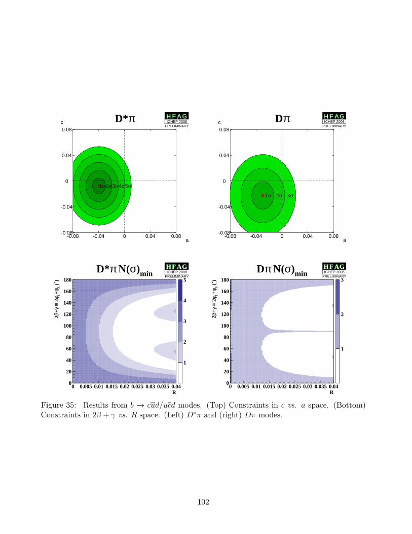
D*π
a
c
5σ4σ3σ2σ1σ
-0.08 -0.04 0 0.04 0.08-0.08
-0.04
0
0.04
0.08
H F A GH F A GICHEP 2008
PRELIMINARY
Dπ
a
c
3σ2σ1σ
-0.08 -0.04 0 0.04 0.08-0.08
-0.04
0
0.04
0.08
H F A GH F A GICHEP 2006
PRELIMINARY
D*π N(σ)min
0
20
40
60
80
100
120
140
160
180
0 0.005 0.01 0.015 0.02 0.025 0.03 0.035 0.04
1
2
3
4
5
R
2β+γ
≡ 2
φ 1+φ 3
(˚)
HF AGH F AGICHEP 2008
PRELIMINARY
Dπ N(σ)min
0
20
40
60
80
100
120
140
160
180
0 0.005 0.01 0.015 0.02 0.025 0.03 0.035 0.04
1
2
3
R
2β+γ
≡ 2
φ 1+φ 3
(˚)
HF AGH F AGICHEP 2006
PRELIMINARY
Figure 35: Results from b → cud/ucd modes. (Top) Constraints in c vs. a space. (Bottom)Constraints in 2β + γ vs. R space. (Left) D∗π and (right) Dπ modes.
102
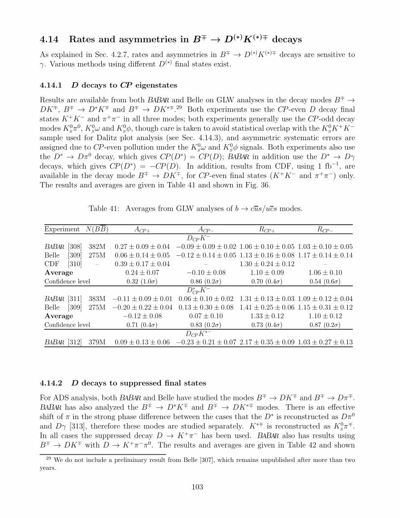
4.14 Rates and asymmetries in B∓ → D(∗)K(∗)∓ decays
As explained in Sec. 4.2.7, rates and asymmetries in B∓ → D(∗)K(∗)∓ decays are sensitive toγ. Various methods using different D(∗) final states exist.
4.14.1 D decays to CP eigenstates
Results are available from both BABAR and Belle on GLW analyses in the decay modes B∓ →DK∓, B∓ → D∗K∓ and B∓ → DK∗∓.29 Both experiments use the CP -even D decay finalstates K+K− and π+π− in all three modes; both experiments generally use the CP -odd decaymodesK0
Sπ0, K0
Sω andK0
Sφ, though care is taken to avoid statistical overlap with theK0
SK+K−
sample used for Dalitz plot analysis (see Sec. 4.14.3), and asymmetric systematic errors areassigned due to CP -even pollution under the K0
Sω and K0Sφ signals. Both experiments also use
the D∗ → Dπ0 decay, which gives CP (D∗) = CP (D); BABAR in addition use the D∗ → Dγdecays, which gives CP (D∗) = −CP (D). In addition, results from CDF, using 1 fb−1, areavailable in the decay mode B∓ → DK∓, for CP -even final states (K+K− and π+π−) only.The results and averages are given in Table 41 and shown in Fig. 36.
Table 41: Averages from GLW analyses of b → cus/ucs modes.
Experiment N(BB) ACP+ ACP− RCP+ RCP−
DCPK−
BABAR [308] 382M 0.27± 0.09± 0.04 −0.09± 0.09± 0.02 1.06± 0.10± 0.05 1.03± 0.10± 0.05Belle [309] 275M 0.06± 0.14± 0.05 −0.12± 0.14± 0.05 1.13± 0.16± 0.08 1.17± 0.14± 0.14CDF [310] – 0.39± 0.17± 0.04 – 1.30± 0.24± 0.12 –Average 0.24± 0.07 −0.10± 0.08 1.10± 0.09 1.06± 0.10Confidence level 0.32 (1.0σ) 0.86 (0.2σ) 0.70 (0.4σ) 0.54 (0.6σ)
D∗CPK
−
BABAR [311] 383M −0.11± 0.09± 0.01 0.06± 0.10± 0.02 1.31± 0.13± 0.03 1.09± 0.12± 0.04Belle [309] 275M −0.20± 0.22± 0.04 0.13± 0.30± 0.08 1.41± 0.25± 0.06 1.15± 0.31± 0.12Average −0.12± 0.08 0.07± 0.10 1.33± 0.12 1.10± 0.12Confidence level 0.71 (0.4σ) 0.83 (0.2σ) 0.73 (0.4σ) 0.87 (0.2σ)
DCPK∗−
BABAR [312] 379M 0.09± 0.13± 0.06 −0.23± 0.21± 0.07 2.17± 0.35± 0.09 1.03± 0.27± 0.13
4.14.2 D decays to suppressed final states
For ADS analysis, both BABAR and Belle have studied the modes B∓ → DK∓ and B∓ → Dπ∓.BABAR has also analyzed the B∓ → D∗K∓ and B∓ → DK∗∓ modes. There is an effectiveshift of π in the strong phase difference between the cases that the D∗ is reconstructed as Dπ0
and Dγ [313], therefore these modes are studied separately. K∗∓ is reconstructed as K0Sπ
∓.In all cases the suppressed decay D → K+π− has been used. BABAR also has results usingB∓ → DK∓ with D → K+π−π0. The results and averages are given in Table 42 and shown
29 We do not include a preliminary result from Belle [307], which remains unpublished after more than twoyears.
103
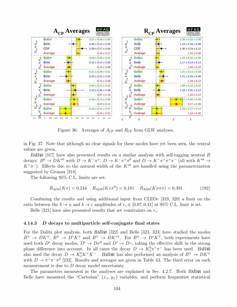
ACP Averages
HF
AG
Bea
uty
2009
HF
AG
Bea
uty
2009
HF
AG
Bea
uty
2009
HF
AG
Bea
uty
2009
HF
AG
Bea
uty
2009
HF
AG
Bea
uty
2009
DC
P K
AC
P+
DC
P K
AC
P-
D* C
P K
AC
P+
D* C
P K
AC
P-
DC
P K
* A
CP
+
DC
P K
* A
CP
-
-1.4 -1.2 -1 -0.8 -0.6 -0.4 -0.2 0 0.2 0.4 0.6 0.8 1 1.2 1.4
BaBar 0.27 ± 0.09 ± 0.04
Belle 0.06 ± 0.14 ± 0.05
CDF 0.39 ± 0.17 ± 0.04
Average 0.24 ± 0.07
BaBar -0.09 ± 0.09 ± 0.02
Belle -0.12 ± 0.14 ± 0.05
Average -0.10 ± 0.08
BaBar -0.11 ± 0.09 ± 0.01
Belle -0.20 ± 0.22 ± 0.04
Average -0.12 ± 0.08
BaBar 0.06 ± 0.10 ± 0.02
Belle 0.13 ± 0.30 ± 0.08
Average 0.07 ± 0.10
BaBar 0.09 ± 0.13 ± 0.06
Average 0.09 ± 0.14
BaBar -0.23 ± 0.21 ± 0.07
Average -0.23 ± 0.22
H F A GH F A GBeauty 2009
PRELIMINARY
RCP Averages
HF
AG
Bea
uty
2009
HF
AG
Bea
uty
2009
HF
AG
Bea
uty
2009
HF
AG
Bea
uty
2009
HF
AG
Bea
uty
2009
HF
AG
Bea
uty
2009
DC
P K
RC
P+
DC
P K
RC
P-
D* C
P K
RC
P+
D* C
P K
RC
P-
DC
P K
* R
CP
+
DC
P K
* R
CP
-
-1 0 1 2 3
BaBar 1.06 ± 0.10 ± 0.05
Belle 1.13 ± 0.16 ± 0.08
CDF 1.30 ± 0.24 ± 0.12
Average 1.10 ± 0.09
BaBar 1.03 ± 0.10 ± 0.05
Belle 1.17 ± 0.14 ± 0.14
Average 1.06 ± 0.10
BaBar 1.31 ± 0.13 ± 0.03
Belle 1.41 ± 0.25 ± 0.06
Average 1.33 ± 0.12
BaBar 1.09 ± 0.12 ± 0.04
Belle 1.15 ± 0.31 ± 0.12
Average 1.10 ± 0.12
BaBar 2.17 ± 0.35 ± 0.09
Average 2.17 ± 0.36
BaBar 1.03 ± 0.27 ± 0.13
Average 1.03 ± 0.30
H F A GH F A GBeauty 2009
PRELIMINARY
Figure 36: Averages of ACP and RCP from GLW analyses.
in Fig. 37. Note that although no clear signals for these modes have yet been seen, the centralvalues are given.
BABAR [317] have also presented results on a similar analysis with self-tagging neutral Bdecays: B0 → DK∗0 with D → K−π+, D → K−π+π0 and D → K−π+π+π− (all with K∗0 →K+π−). Effects due to the natural width of the K∗0 are handled using the parametrizationsuggested by Gronau [318].
The following 95% C.L. limits are set:
RADS(Kπ) < 0.244 RADS(Kππ0) < 0.181 RADS(Kπππ) < 0.391 . (192)
Combining the results and using additional input from CLEOc [319, 320] a limit on theratio between the b→ u and b → c amplitudes of rs ∈ [0.07, 0.41] at 95% C.L. limit is set.
Belle [321] have also presented results that set constraints on rs.
4.14.3 D decays to multiparticle self-conjugate final states
For the Dalitz plot analysis, both BABAR [322] and Belle [323, 324] have studied the modesB∓ → DK∓, B∓ → D∗K∓ and B∓ → DK∗∓. For B∓ → D∗K∓, both experiments haveused both D∗ decay modes, D∗ → Dπ0 and D∗ → Dγ, taking the effective shift in the strongphase difference into account. In all cases the decay D → K0
Sπ+π− has been used. BABAR
also used the decay D → K0SK+K− . BABAR has also performed an analysis of B∓ → DK∓
with D → π+π−π0 [232]. Results and averages are given in Table 43. The third error on eachmeasurement is due to D decay model uncertainty.
The parameters measured in the analyses are explained in Sec. 4.2.7. Both BABAR andBelle have measured the “Cartesian” (x±, y±) variables, and perform frequentist statistical
104
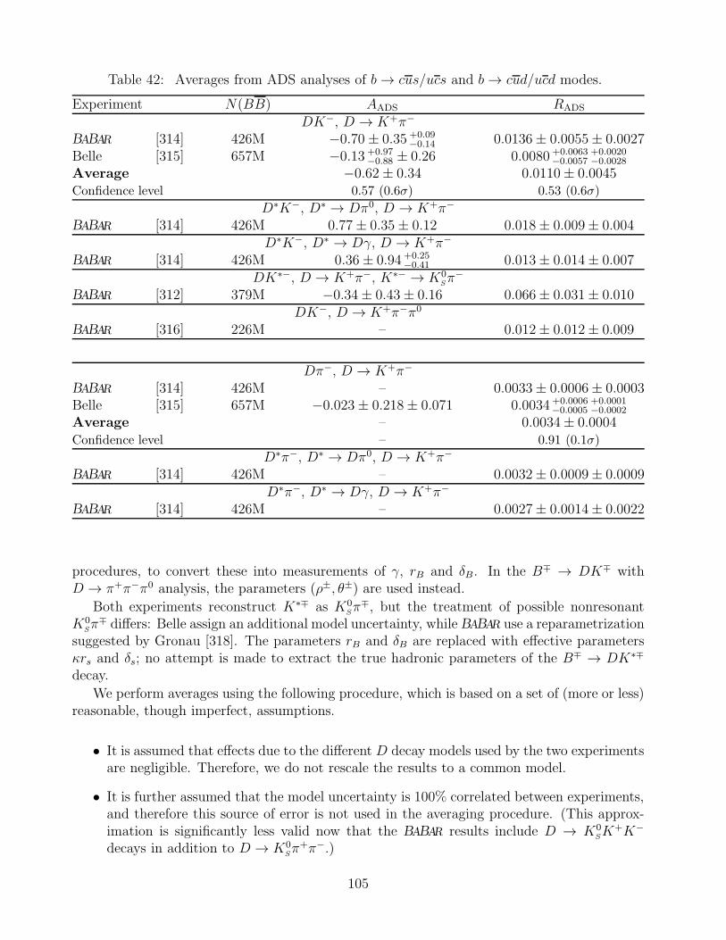
Table 42: Averages from ADS analyses of b→ cus/ucs and b→ cud/ucd modes.
Experiment N(BB) AADS RADS
DK−, D → K+π−
BABAR [314] 426M −0.70 ± 0.35 +0.09−0.14 0.0136± 0.0055± 0.0027
Belle [315] 657M −0.13 +0.97−0.88 ± 0.26 0.0080 +0.0063
−0.0057+0.0020−0.0028
Average −0.62± 0.34 0.0110± 0.0045Confidence level 0.57 (0.6σ) 0.53 (0.6σ)
D∗K−, D∗ → Dπ0, D → K+π−
BABAR [314] 426M 0.77± 0.35± 0.12 0.018± 0.009± 0.004D∗K−, D∗ → Dγ, D → K+π−
BABAR [314] 426M 0.36± 0.94 +0.25−0.41 0.013± 0.014± 0.007
DK∗−, D → K+π−, K∗− → K0Sπ−
BABAR [312] 379M −0.34± 0.43± 0.16 0.066± 0.031± 0.010DK−, D → K+π−π0
BABAR [316] 226M – 0.012± 0.012± 0.009
Dπ−, D → K+π−
BABAR [314] 426M – 0.0033± 0.0006± 0.0003Belle [315] 657M −0.023± 0.218± 0.071 0.0034 +0.0006
−0.0005+0.0001−0.0002
Average – 0.0034± 0.0004Confidence level – 0.91 (0.1σ)
D∗π−, D∗ → Dπ0, D → K+π−
BABAR [314] 426M – 0.0032± 0.0009± 0.0009D∗π−, D∗ → Dγ, D → K+π−
BABAR [314] 426M – 0.0027± 0.0014± 0.0022
procedures, to convert these into measurements of γ, rB and δB. In the B∓ → DK∓ withD → π+π−π0 analysis, the parameters (ρ±, θ±) are used instead.
Both experiments reconstruct K∗∓ as K0Sπ
∓, but the treatment of possible nonresonantK0
Sπ∓ differs: Belle assign an additional model uncertainty, while BABAR use a reparametrization
suggested by Gronau [318]. The parameters rB and δB are replaced with effective parametersκrs and δs; no attempt is made to extract the true hadronic parameters of the B∓ → DK∗∓
decay.
We perform averages using the following procedure, which is based on a set of (more or less)reasonable, though imperfect, assumptions.
• It is assumed that effects due to the different D decay models used by the two experimentsare negligible. Therefore, we do not rescale the results to a common model.
• It is further assumed that the model uncertainty is 100% correlated between experiments,and therefore this source of error is not used in the averaging procedure. (This approx-imation is significantly less valid now that the BABAR results include D → K0
SK+K−
decays in addition to D → K0Sπ+π−.)
105
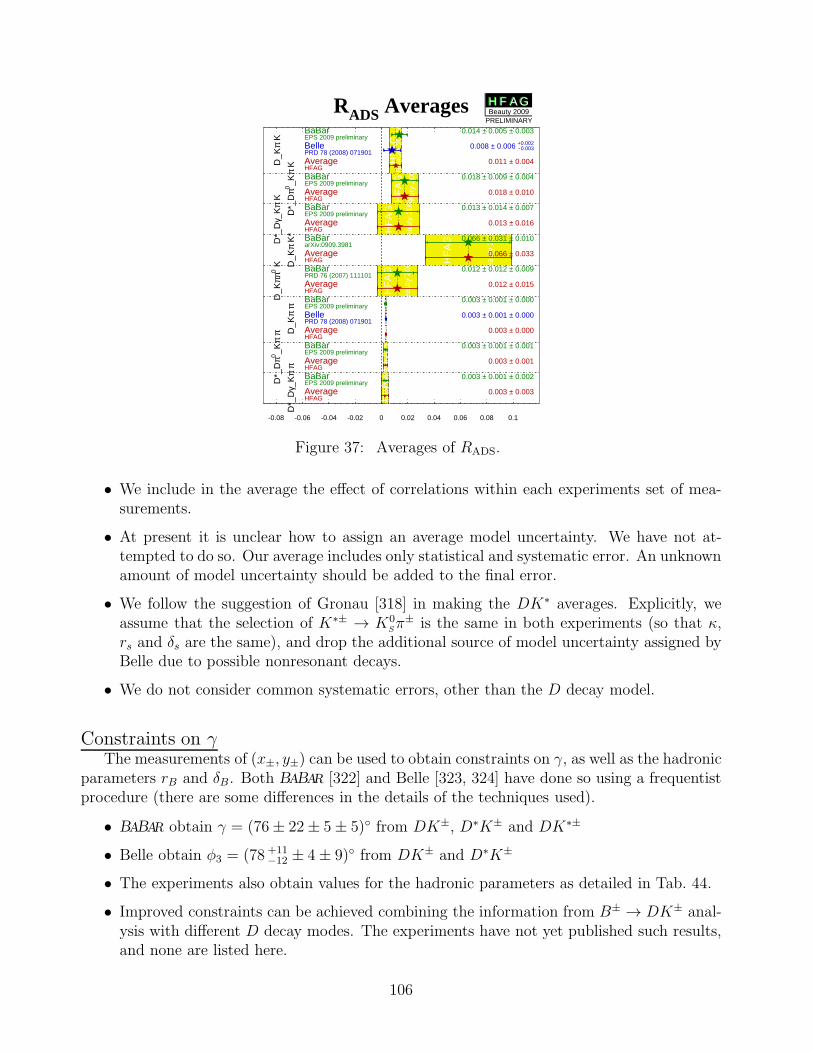
RADS Averages
HF
AG
Bea
uty
2009
HF
AG
Bea
uty
2009
HF
AG
Bea
uty
2009
HF
AG
Bea
uty
2009
HF
AG
Bea
uty
2009
HF
AG
Bea
uty
2009
HF
AG
Bea
uty
2009
HF
AG
Bea
uty
2009
D_K
π K
D*_
Dπ0 _K
π K
D*_
Dγ_
Kπ
K
D_K
π K
*
D_K
ππ0 K
D_K
π π
D*_
Dπ0 _K
π π
D*_
Dγ_
Kπ
π
-0.08 -0.06 -0.04 -0.02 0 0.02 0.04 0.06 0.08 0.1
BaBarEPS 2009 preliminary
0.014 ± 0.005 ± 0.003
BellePRD 78 (2008) 071901
0.008 ± 0.006 +-00
.
.00
00
23
AverageHFAG
0.011 ± 0.004
BaBarEPS 2009 preliminary
0.018 ± 0.009 ± 0.004
AverageHFAG
0.018 ± 0.010
BaBarEPS 2009 preliminary
0.013 ± 0.014 ± 0.007
AverageHFAG
0.013 ± 0.016
BaBararXiv:0909.3981
0.066 ± 0.031 ± 0.010
AverageHFAG
0.066 ± 0.033
BaBarPRD 76 (2007) 111101
0.012 ± 0.012 ± 0.009
AverageHFAG
0.012 ± 0.015
BaBarEPS 2009 preliminary
0.003 ± 0.001 ± 0.000
BellePRD 78 (2008) 071901
0.003 ± 0.001 ± 0.000
AverageHFAG
0.003 ± 0.000
BaBarEPS 2009 preliminary
0.003 ± 0.001 ± 0.001
AverageHFAG
0.003 ± 0.001
BaBarEPS 2009 preliminary
0.003 ± 0.001 ± 0.002
AverageHFAG
0.003 ± 0.003
H F A GH F A GBeauty 2009
PRELIMINARY
Figure 37: Averages of RADS.
• We include in the average the effect of correlations within each experiments set of mea-surements.
• At present it is unclear how to assign an average model uncertainty. We have not at-tempted to do so. Our average includes only statistical and systematic error. An unknownamount of model uncertainty should be added to the final error.
• We follow the suggestion of Gronau [318] in making the DK∗ averages. Explicitly, weassume that the selection of K∗± → K0
Sπ± is the same in both experiments (so that κ,
rs and δs are the same), and drop the additional source of model uncertainty assigned byBelle due to possible nonresonant decays.
• We do not consider common systematic errors, other than the D decay model.
Constraints on γThe measurements of (x±, y±) can be used to obtain constraints on γ, as well as the hadronic
parameters rB and δB. Both BABAR [322] and Belle [323, 324] have done so using a frequentistprocedure (there are some differences in the details of the techniques used).
• BABAR obtain γ = (76± 22± 5± 5) from DK±, D∗K± and DK∗±
• Belle obtain φ3 = (78 +11−12 ± 4± 9) from DK± and D∗K±
• The experiments also obtain values for the hadronic parameters as detailed in Tab. 44.
• Improved constraints can be achieved combining the information from B± → DK± anal-ysis with different D decay modes. The experiments have not yet published such results,and none are listed here.
106
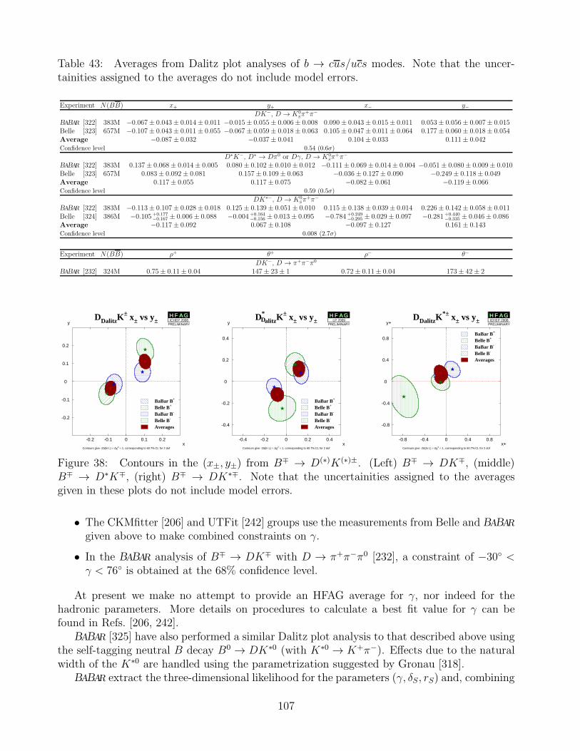
Table 43: Averages from Dalitz plot analyses of b → cus/ucs modes. Note that the uncer-tainities assigned to the averages do not include model errors.
Experiment N(BB) x+ y+ x− y−DK−, D → K0
Sπ+π−
BABAR [322] 383M −0.067± 0.043± 0.014± 0.011 −0.015± 0.055± 0.006± 0.008 0.090± 0.043± 0.015± 0.011 0.053± 0.056± 0.007± 0.015Belle [323] 657M −0.107± 0.043± 0.011± 0.055 −0.067± 0.059± 0.018± 0.063 0.105± 0.047± 0.011± 0.064 0.177± 0.060± 0.018± 0.054Average −0.087± 0.032 −0.037± 0.041 0.104± 0.033 0.111± 0.042Confidence level 0.54 (0.6σ)
D∗K−, D∗ → Dπ0 or Dγ, D → K0Sπ
+π−
BABAR [322] 383M 0.137± 0.068± 0.014± 0.005 0.080± 0.102± 0.010± 0.012 −0.111± 0.069± 0.014± 0.004 −0.051± 0.080± 0.009± 0.010Belle [323] 657M 0.083± 0.092± 0.081 0.157± 0.109± 0.063 −0.036± 0.127± 0.090 −0.249± 0.118± 0.049Average 0.117± 0.055 0.117± 0.075 −0.082± 0.061 −0.119± 0.066Confidence level 0.59 (0.5σ)
DK∗−, D → K0Sπ+π−
BABAR [322] 383M −0.113± 0.107± 0.028± 0.018 0.125± 0.139± 0.051± 0.010 0.115± 0.138± 0.039± 0.014 0.226± 0.142± 0.058± 0.011Belle [324] 386M −0.105 +0.177
−0.167 ± 0.006± 0.088 −0.004 +0.164−0.156 ± 0.013± 0.095 −0.784 +0.249
−0.295 ± 0.029± 0.097 −0.281 +0.440−0.335 ± 0.046± 0.086
Average −0.117± 0.092 0.067± 0.108 −0.097± 0.127 0.161± 0.143Confidence level 0.008 (2.7σ)
Experiment N(BB) ρ+ θ+ ρ− θ−
DK−, D → π+π−π0
BABAR [232] 324M 0.75± 0.11± 0.04 147± 23± 1 0.72± 0.11± 0.04 173± 42± 2
DDalitzK± x± vs y±
Contours give -2∆(ln L) = ∆χ2 = 1, corresponding to 60.7% CL for 2 dof
-0.2 -0.1 0 0.1 0.2
-0.2
-0.1
0
0.1
0.2
x
y
BaBar B+
Belle B+
BaBar B-
Belle B-
Averages
H F A GH F A GICHEP 2008
PRELIMINARY
D*DalitzK
± x± vs y±
Contours give -2∆(ln L) = ∆χ2 = 1, corresponding to 60.7% CL for 2 dof
-0.4 -0.2 0 0.2 0.4
-0.4
-0.2
0
0.2
0.4
x
y
BaBar B+
Belle B+
BaBar B-
Belle B-
Averages
H F A GH F A GLP 2009
PRELIMINARY
DDalitzK*± x± vs y±
Contours give -2∆(ln L) = ∆χ2 = 1, corresponding to 60.7% CL for 2 dof
-0.8 -0.4 0 0.4 0.8
-0.8
-0.4
0
0.4
0.8
x+
y+
BaBar B+
Belle B+
BaBar B-
Belle B-
Averages
H F A GH F A GICHEP 2008
PRELIMINARY
Figure 38: Contours in the (x±, y±) from B∓ → D(∗)K(∗)±. (Left) B∓ → DK∓, (middle)B∓ → D∗K∓, (right) B∓ → DK∗∓. Note that the uncertainities assigned to the averagesgiven in these plots do not include model errors.
• The CKMfitter [206] and UTFit [242] groups use the measurements from Belle and BABAR
given above to make combined constraints on γ.
• In the BABAR analysis of B∓ → DK∓ with D → π+π−π0 [232], a constraint of −30 <γ < 76 is obtained at the 68% confidence level.
At present we make no attempt to provide an HFAG average for γ, nor indeed for thehadronic parameters. More details on procedures to calculate a best fit value for γ can befound in Refs. [206, 242].
BABAR [325] have also performed a similar Dalitz plot analysis to that described above usingthe self-tagging neutral B decay B0 → DK∗0 (with K∗0 → K+π−). Effects due to the naturalwidth of the K∗0 are handled using the parametrization suggested by Gronau [318].
BABAR extract the three-dimensional likelihood for the parameters (γ, δS, rS) and, combining
107
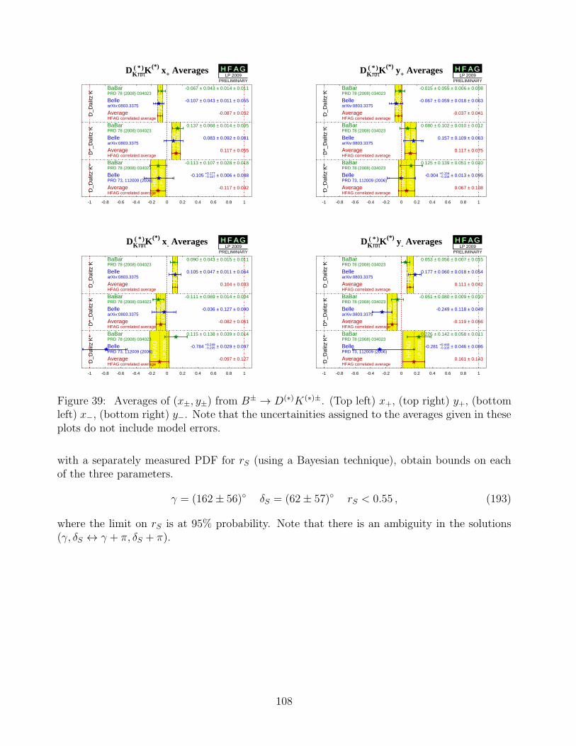
DK(π*π)K(*) x+ Averages
HF
AG
LP 2
009
HF
AG
LP 2
009
HF
AG
LP 2
009
D_D
alitz
KD
*_D
alitz
KD
_Dal
itz K
*
-1 -0.8 -0.6 -0.4 -0.2 0 0.2 0.4 0.6 0.8 1
BaBarPRD 78 (2008) 034023
-0.067 ± 0.043 ± 0.014 ± 0.011
BellearXiv:0803.3375
-0.107 ± 0.043 ± 0.011 ± 0.055
AverageHFAG correlated average
-0.087 ± 0.032
BaBarPRD 78 (2008) 034023
0.137 ± 0.068 ± 0.014 ± 0.005
BellearXiv:0803.3375
0.083 ± 0.092 ± 0.081
AverageHFAG correlated average
0.117 ± 0.055
BaBarPRD 78 (2008) 034023
-0.113 ± 0.107 ± 0.028 ± 0.018
BellePRD 73, 112009 (2006)
-0.105 +-00
.
.11
76
77 ± 0.006 ± 0.088
AverageHFAG correlated average
-0.117 ± 0.092
H F A GH F A GLP 2009
PRELIMINARY
DK(π*π)K(*) y+ Averages
HF
AG
LP 2
009
HF
AG
LP 2
009
HF
AG
LP 2
009
D_D
alitz
KD
*_D
alitz
KD
_Dal
itz K
*
-1 -0.8 -0.6 -0.4 -0.2 0 0.2 0.4 0.6 0.8 1
BaBarPRD 78 (2008) 034023
-0.015 ± 0.055 ± 0.006 ± 0.008
BellearXiv:0803.3375
-0.067 ± 0.059 ± 0.018 ± 0.063
AverageHFAG correlated average
-0.037 ± 0.041
BaBarPRD 78 (2008) 034023
0.080 ± 0.102 ± 0.010 ± 0.012
BellearXiv:0803.3375
0.157 ± 0.109 ± 0.063
AverageHFAG correlated average
0.117 ± 0.075
BaBarPRD 78 (2008) 034023
0.125 ± 0.139 ± 0.051 ± 0.010
BellePRD 73, 112009 (2006)
-0.004 +-00
.
.11
65
46 ± 0.013 ± 0.095
AverageHFAG correlated average
0.067 ± 0.108
H F A GH F A GLP 2009
PRELIMINARY
DK(π*π)K(*) x- Averages
HF
AG
LP 2
009
HF
AG
LP 2
009
HF
AG
LP 2
009
D_D
alitz
KD
*_D
alitz
KD
_Dal
itz K
*
-1 -0.8 -0.6 -0.4 -0.2 0 0.2 0.4 0.6 0.8 1
BaBarPRD 78 (2008) 034023
0.090 ± 0.043 ± 0.015 ± 0.011
BellearXiv:0803.3375
0.105 ± 0.047 ± 0.011 ± 0.064
AverageHFAG correlated average
0.104 ± 0.033
BaBarPRD 78 (2008) 034023
-0.111 ± 0.069 ± 0.014 ± 0.004
BellearXiv:0803.3375
-0.036 ± 0.127 ± 0.090
AverageHFAG correlated average
-0.082 ± 0.061
BaBarPRD 78 (2008) 034023
0.115 ± 0.138 ± 0.039 ± 0.014
BellePRD 73, 112009 (2006)
-0.784 +-00
.
.22
49
95 ± 0.029 ± 0.097
AverageHFAG correlated average
-0.097 ± 0.127
H F A GH F A GLP 2009
PRELIMINARY
DK(π*π)K(*) y- Averages
HF
AG
LP 2
009
HF
AG
LP 2
009
HF
AG
LP 2
009
D_D
alitz
KD
*_D
alitz
KD
_Dal
itz K
*
-1 -0.8 -0.6 -0.4 -0.2 0 0.2 0.4 0.6 0.8 1
BaBarPRD 78 (2008) 034023
0.053 ± 0.056 ± 0.007 ± 0.015
BellearXiv:0803.3375
0.177 ± 0.060 ± 0.018 ± 0.054
AverageHFAG correlated average
0.111 ± 0.042
BaBarPRD 78 (2008) 034023
-0.051 ± 0.080 ± 0.009 ± 0.010
BellearXiv:0803.3375
-0.249 ± 0.118 ± 0.049
AverageHFAG correlated average
-0.119 ± 0.066
BaBarPRD 78 (2008) 034023
0.226 ± 0.142 ± 0.058 ± 0.011
BellePRD 73, 112009 (2006)
-0.281 +-00
.
.43
43
05 ± 0.046 ± 0.086
AverageHFAG correlated average
0.161 ± 0.143
H F A GH F A GLP 2009
PRELIMINARY
Figure 39: Averages of (x±, y±) from B± → D(∗)K(∗)±. (Top left) x+, (top right) y+, (bottomleft) x−, (bottom right) y−. Note that the uncertainities assigned to the averages given in theseplots do not include model errors.
with a separately measured PDF for rS (using a Bayesian technique), obtain bounds on eachof the three parameters.
γ = (162± 56) δS = (62± 57) rS < 0.55 , (193)
where the limit on rS is at 95% probability. Note that there is an ambiguity in the solutions(γ, δS ↔ γ + π, δS + π).
108
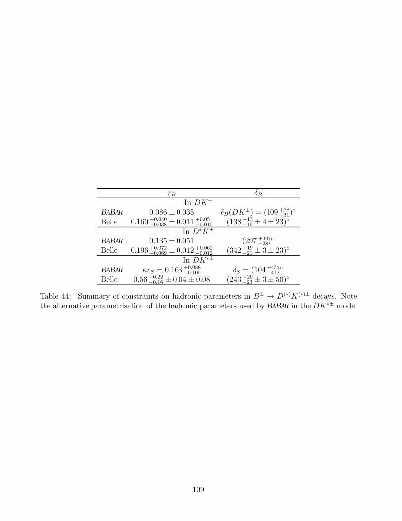
rB δBIn DK±
BABAR 0.086± 0.035 δB(DK±) = (109 +28
−31)
Belle 0.160 +0.040−0.038 ± 0.011 +0.05
−0.010 (138 +13−16 ± 4± 23)
In D∗K±
BABAR 0.135± 0.051 (297 +30−28)
Belle 0.196 +0.072−0.069 ± 0.012 +0.062
−0.012 (342 +19−21 ± 3± 23)
In DK∗±
BABAR κrS = 0.163 +0.088−0.105 δS = (104 +43
−41)
Belle 0.56 +0.22−0.16 ± 0.04± 0.08 (243 +20
−23 ± 3± 50)
Table 44: Summary of constraints on hadronic parameters in B± → D(∗)K(∗)± decays. Notethe alternative parametrisation of the hadronic parameters used by BABAR in the DK∗± mode.
109
5 Semileptonic B decays
Measurements of semileptonic B-meson decays are an important tool to study the magnitudeof the CKM matrix elements |Vcb| and |Vub|, the Heavy Quark parameters (e.g. b and c–quarkmasses), QCD form factors, QCD dynamics, new physics, etc.
In the following, we provide averages of exclusive and inclusive branching fractions, theproduct of |Vcb| and the form factor normalization F(1) and G(1) for B → D∗ℓ−νℓ and B →Dℓ−νℓ decays, respectively, and |Vub| as determined from inclusive and exclusive measurementsof B → Xuℓνℓ decays. We will compute Heavy Quark parameters and extract QCD formfactors for B → D∗ℓ−νℓ decays. Throughout this section, charge conjugate states are implicitlyincluded, unless otherwise indicated.
Brief descriptions of all parameters and analyses (published or preliminary) relevant for thedetermination of the combined results are given. The descriptions are based on the informationavailable on the web page at
http://www.slac.stanford.edu/xorg/hfag/semi/EndOfYear09
A description of the technique employed for calculating averages was presented in the previousupdate [4]. Asymmetric errors have been introduced in the current averages for B → Xuℓνdecays to take into account theoretical asymmetric errors.
5.1 Exclusive CKM-favored decays
Averages are provided for the branching fractions B(B → Dℓ−νℓ) and B(B → D∗ℓ−νℓ). Wethen provide averages for the inclusive branching fractions B(B → D(∗)πℓ−νℓ) and for Bsemileptonic decays into orbitally-excited P -wave charm mesons (D∗∗). As the D∗∗ branchingfraction is poorly known, we report the averages for the products B(B− → D∗∗(D(∗)π)ℓ−νℓ)×B(D∗∗ → D(∗)π). In addition, averages are provided for F(1)|Vcb| vs ρ2, where F(1) and ρ2 arethe normalization and slope of the form factor at zero recoil in B → D∗ℓ−νℓ decays, and forthe corresponding quantities G(1)|Vcb| vs ρ2 in B → Dℓ−νℓ decays.
5.1.1 B → Dℓ−νℓ
The average branching fraction B(B → Dℓ−νℓ) is determined by the combination of the re-
sults provided in Table 45 and 46, for B0 → D+ℓ−νℓ and B− → D0ℓ−νℓ, respectively. The
measurements included in the average are scaled to a consistent set of input parameters andtheir errors [326]. Therefore some of the (older) measurements are subject to considerableadjustments. The branching fractions are obtained from the integral over the measured differ-ential decay rates, apart for the BABAR results, for which the semileptonic B signal yields areextracted from a fit to the missing mass squared in a sample of fully reconstructed BB events.
Figure 40 illustrates the measurements and the resulting average.Recent measurement [332, 333] assume isospin conservation for the B → Dℓ−νℓ decays and
are averaged independently from the previous determinations of the B(B → Dℓ−νℓ) averagebranching fraction. Figure 41 and table 47 illustrates the measurements and the resultingaverage.
The average for G(1)|Vcb| is determined by the two-dimensional combination of the resultsprovided in Table 48. Figure 42 (a) provides a one-dimensional projection for illustrativepurposes, (b) illustrates the average G(1)|Vcb| and the measurements included in the average.
110
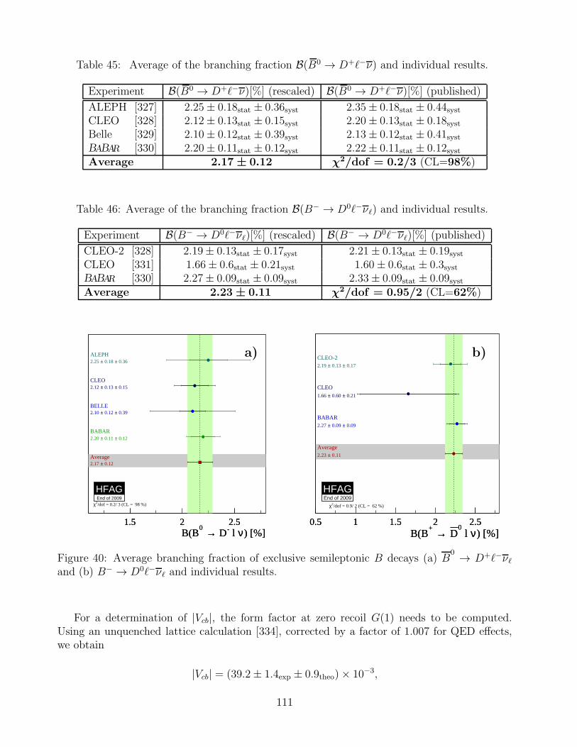
Table 45: Average of the branching fraction B(B0 → D+ℓ−ν) and individual results.
Experiment B(B0 → D+ℓ−ν)[%] (rescaled) B(B0 → D+ℓ−ν)[%] (published)
ALEPH [327] 2.25± 0.18stat ± 0.36syst 2.35± 0.18stat ± 0.44systCLEO [328] 2.12± 0.13stat ± 0.15syst 2.20± 0.13stat ± 0.18systBelle [329] 2.10± 0.12stat ± 0.39syst 2.13± 0.12stat ± 0.41systBABAR [330] 2.20± 0.11stat ± 0.12syst 2.22± 0.11stat ± 0.12systAverage 2.17 ± 0.12 χ2/dof = 0.2/3 (CL=98%)
Table 46: Average of the branching fraction B(B− → D0ℓ−νℓ) and individual results.
Experiment B(B− → D0ℓ−νℓ)[%] (rescaled) B(B− → D0ℓ−νℓ)[%] (published)
CLEO-2 [328] 2.19± 0.13stat ± 0.17syst 2.21± 0.13stat ± 0.19systCLEO [331] 1.66± 0.6stat ± 0.21syst 1.60± 0.6stat ± 0.3systBABAR [330] 2.27± 0.09stat ± 0.09syst 2.33± 0.09stat ± 0.09systAverage 2.23 ± 0.11 χ2/dof = 0.95/2 (CL=62%)
) [%]ν l - D→ 0B(B
1.5 2 2.5) [%]ν l - D→ 0
B(B1.5 2 2.5
ALEPH 0.36± 0.18 ±2.25
CLEO 0.15± 0.13 ±2.12
BELLE 0.39± 0.12 ±2.10
BABAR 0.12± 0.11 ±2.20
Average 0.12±2.17
HFAGEnd of 2009/dof = 0.2/ 3 (CL = 98 %)2χ
) [%]ν l 0
D → +B(B
0.5 1 1.5 2 2.5) [%]ν l
0D → +
B(B0.5 1 1.5 2 2.5
CLEO-2 0.17± 0.13 ±2.19
CLEO 0.21± 0.60 ±1.66
BABAR 0.09± 0.09 ±2.27
Average 0.11±2.23
HFAGEnd of 2009
/dof = 0.9/ 2 (CL = 62 %)2χ
a) b)
Figure 40: Average branching fraction of exclusive semileptonic B decays (a) B0 → D+ℓ−νℓ
and (b) B− → D0ℓ−νℓ and individual results.
For a determination of |Vcb|, the form factor at zero recoil G(1) needs to be computed.Using an unquenched lattice calculation [334], corrected by a factor of 1.007 for QED effects,we obtain
|Vcb| = (39.2± 1.4exp ± 0.9theo)× 10−3,
111
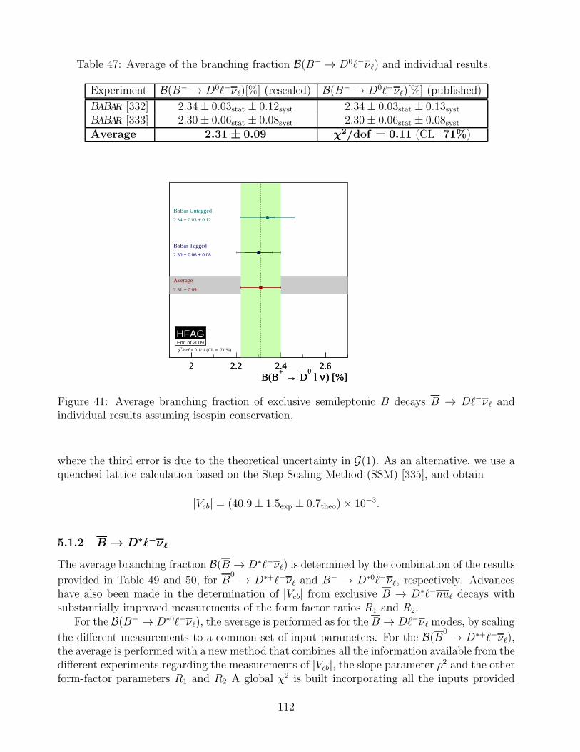
Table 47: Average of the branching fraction B(B− → D0ℓ−νℓ) and individual results.
Experiment B(B− → D0ℓ−νℓ)[%] (rescaled) B(B− → D0ℓ−νℓ)[%] (published)
BABAR [332] 2.34± 0.03stat ± 0.12syst 2.34± 0.03stat ± 0.13systBABAR [333] 2.30± 0.06stat ± 0.08syst 2.30± 0.06stat ± 0.08systAverage 2.31 ± 0.09 χ2/dof = 0.11 (CL=71%)
) [%]ν l 0
D → +B(B
2 2.2 2.4 2.6) [%]ν l
0D → +
B(B2 2.2 2.4 2.6
BaBar Untagged
0.12± 0.03 ±2.34
BaBar Tagged
0.08± 0.06 ±2.30
Average
0.09±2.31
HFAGEnd of 2009
/dof = 0.1/ 1 (CL = 71 %)2χ
Figure 41: Average branching fraction of exclusive semileptonic B decays B → Dℓ−νℓ andindividual results assuming isospin conservation.
where the third error is due to the theoretical uncertainty in G(1). As an alternative, we use aquenched lattice calculation based on the Step Scaling Method (SSM) [335], and obtain
|Vcb| = (40.9± 1.5exp ± 0.7theo)× 10−3.
5.1.2 B → D∗ℓ−νℓ
The average branching fraction B(B → D∗ℓ−νℓ) is determined by the combination of the results
provided in Table 49 and 50, for B0 → D∗+ℓ−νℓ and B
− → D∗0ℓ−νℓ, respectively. Advanceshave also been made in the determination of |Vcb| from exclusive B → D∗ℓ−nuℓ decays withsubstantially improved measurements of the form factor ratios R1 and R2.
For the B(B− → D∗0ℓ−νℓ), the average is performed as for the B → Dℓ−νℓ modes, by scaling
the different measurements to a common set of input parameters. For the B(B0 → D∗+ℓ−νℓ),the average is performed with a new method that combines all the information available from thedifferent experiments regarding the measurements of |Vcb|, the slope parameter ρ2 and the otherform-factor parameters R1 and R2 A global χ2 is built incorporating all the inputs provided
112
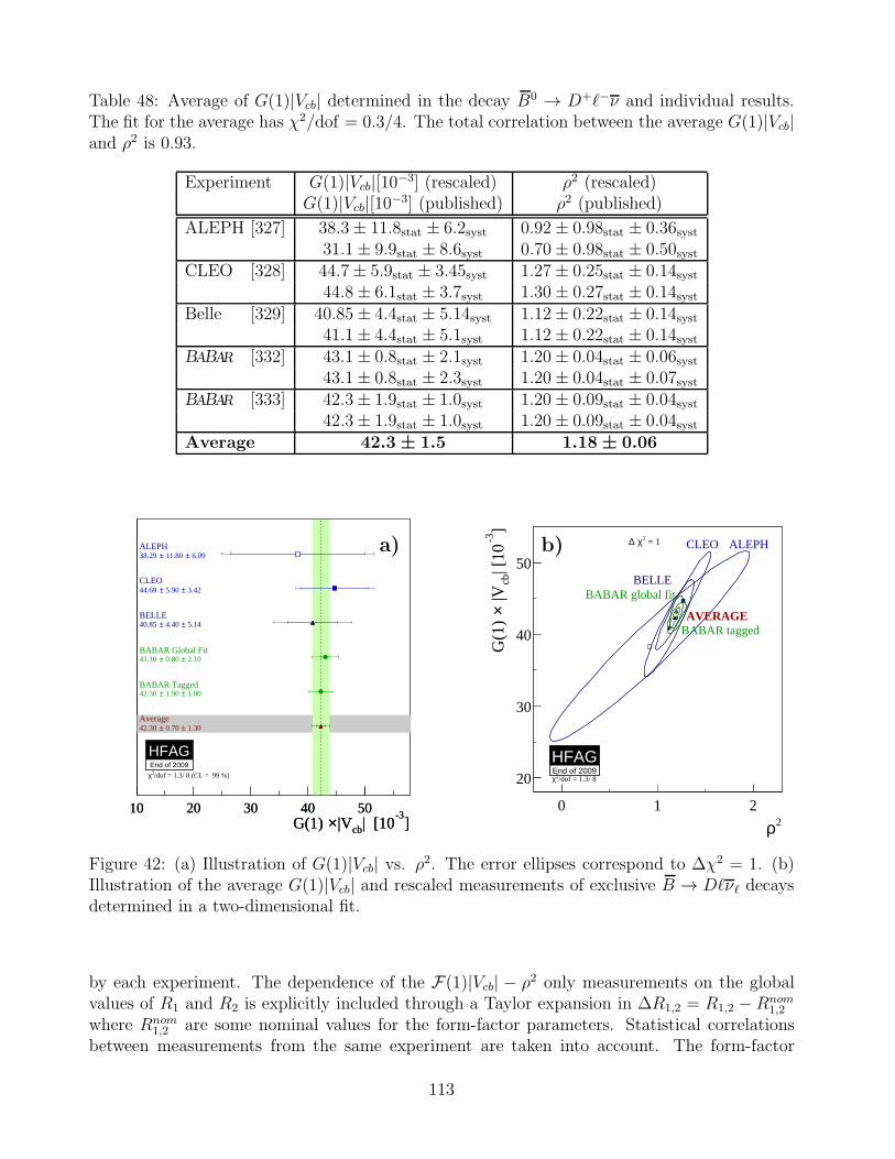
Table 48: Average of G(1)|Vcb| determined in the decay B0 → D+ℓ−ν and individual results.The fit for the average has χ2/dof = 0.3/4. The total correlation between the average G(1)|Vcb|and ρ2 is 0.93.
Experiment G(1)|Vcb|[10−3] (rescaled) ρ2 (rescaled)G(1)|Vcb|[10−3] (published) ρ2 (published)
ALEPH [327] 38.3± 11.8stat ± 6.2syst 0.92± 0.98stat ± 0.36syst31.1± 9.9stat ± 8.6syst 0.70± 0.98stat ± 0.50syst
CLEO [328] 44.7± 5.9stat ± 3.45syst 1.27± 0.25stat ± 0.14syst44.8± 6.1stat ± 3.7syst 1.30± 0.27stat ± 0.14syst
Belle [329] 40.85± 4.4stat ± 5.14syst 1.12± 0.22stat ± 0.14syst41.1± 4.4stat ± 5.1syst 1.12± 0.22stat ± 0.14syst
BABAR [332] 43.1± 0.8stat ± 2.1syst 1.20± 0.04stat ± 0.06syst43.1± 0.8stat ± 2.3syst 1.20± 0.04stat ± 0.07syst
BABAR [333] 42.3± 1.9stat ± 1.0syst 1.20± 0.09stat ± 0.04syst42.3± 1.9stat ± 1.0syst 1.20± 0.09stat ± 0.04syst
Average 42.3 ± 1.5 1.18 ± 0.06
2ρ0 1 2
]-3
| [10
cb |V×
G(1
)
20
30
40
50
HFAGEnd of 2009
ALEPHCLEO
BELLEBABAR global fit
BABAR taggedAVERAGE
= 12χ ∆
/dof = 1.3/ 82χ
]-3
| [10cb|V×G(1) 10 20 30 40 50
]-3
| [10cb|V×G(1) 10 20 30 40 50
ALEPH 6.09± 11.80 ±38.29
CLEO 3.42± 5.90 ±44.69
BELLE 5.14± 4.40 ±40.85
BABAR Global Fit 2.10± 0.80 ±43.10
BABAR Tagged 1.00± 1.90 ±42.30
Average 1.30± 0.70 ±42.30
HFAGEnd of 2009
/dof = 1.3/ 8 (CL = 99 %)2χ
a) b)
Figure 42: (a) Illustration of G(1)|Vcb| vs. ρ2. The error ellipses correspond to ∆χ2 = 1. (b)Illustration of the average G(1)|Vcb| and rescaled measurements of exclusive B → Dℓνℓ decaysdetermined in a two-dimensional fit.
by each experiment. The dependence of the F(1)|Vcb| − ρ2 only measurements on the globalvalues of R1 and R2 is explicitly included through a Taylor expansion in ∆R1,2 = R1,2 − Rnom
1,2
where Rnom1,2 are some nominal values for the form-factor parameters. Statistical correlations
between measurements from the same experiment are taken into account. The form-factor
113
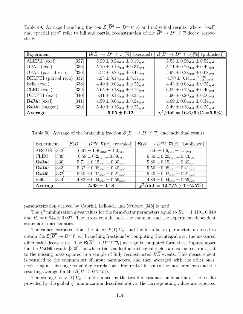
Table 49: Average branching fraction B(B0 → D∗+ℓ−ν) and individual results, where “excl”and “partial reco” refer to full and partial reconstruction of the B0 → D∗+ℓ−ν decay, respec-tively.
Experiment B(B0 → D∗+ℓ−ν)[%] (rescaled) B(B0 → D∗+ℓ−ν)[%] (published)
ALEPH (excl) [327] 5.29± 0.24stat ± 0.19syst 5.53± 0.26stat ± 0.52systOPAL (excl) [336] 5.10± 0.19stat ± 0.37syst 5.11± 0.20stat ± 0.49systOPAL (partial reco) [336] 5.52± 0.26stat ± 0.42syst 5.92± 0.28stat ± 0.68systDELPHI (partial reco) [337] 4.93± 0.15stat ± 0.17syst 4.70± 0.14stat
+0.36−0.31 syst
Belle (excl) [338] 4.40± 0.03stat ± 0.25syst 4.42± 0.03stat ± 0.25systCLEO (excl) [339] 5.65± 0.18stat ± 0.19syst 6.09± 0.19stat ± 0.40systDELPHI (excl) [340] 5.41± 0.18stat ± 0.33syst 5.90± 0.20stat ± 0.50systBABAR (excl) [341] 4.59± 0.04stat ± 0.24syst 4.69± 0.04stat ± 0.34systBABAR (tagged) [330] 5.40± 0.16stat ± 0.25syst 5.49± 0.16stat ± 0.25systAverage 5.05 ± 0.12 χ2/dof = 16.6/9 (CL=5.5%)
Table 50: Average of the branching fraction B(B− → D∗0ℓ−ν) and individual results.
Experiment B(B− → D∗0ℓ−ν)[%] (rescaled) B(B− → D∗0ℓ−ν)[%] (published)
ARGUS [342] 6.07± 1.40stat ± 1.0syst 6.6± 1.6stat ± 1.5systCLEO [339] 6.58± 0.2stat ± 0.39syst 6.50± 0.20stat ± 0.43systBABAR [330] 5.71± 0.15stat ± 0.30syst 5.80± 0.15stat ± 0.30systBABAR [343] 5.32± 0.08stat ± 0.40syst 5.56± 0.08stat ± 0.41systBABAR [332] 5.40± 0.02stat ± 0.21syst 5.40± 0.02stat ± 0.21systBelle [344] 4.83± 0.04stat ± 0.56syst 4.84± 0.04stat ± 0.56systAverage 5.63 ± 0.18 χ2/dof = 12.7/5 (CL=2.5%)
parametrization derived by Caprini, Lellouch and Neubert [345] is used.
The χ2 minimization gives values for the form-factor parameters equal to R1 = 1.410±0.049and R2 = 0.844± 0.027. The errors contain both the common and the experiment dependentsystematic uncertainties.
The values extracted from the fit for F(1)|Vcb| and the form-factor parameters are used to
obtain the B(B0 → D∗+ℓ−νℓ) branching fractions by computing the integral over the measured
differential decay rates. The B(B0 → D∗+ℓ−νℓ) average is computed form these inputs, apartfor the BABAR results [330], for which the semileptonic B signal yields are extracted from a fitto the missing mass squared in a sample of fully reconstructed BB events. This measurementis rescaled to the common set of input parameters, and then averaged with the other ones,neglecting at this stage remaining correlations. Figure 43 illustrates the measurements and theresulting average for the B(B → D∗ℓ−νℓ).
The average for F (1)|Vcb| is determined by the two-dimensional combination of the resultsprovided by the global χ2 minimization described above: the corresponding values are reported
114
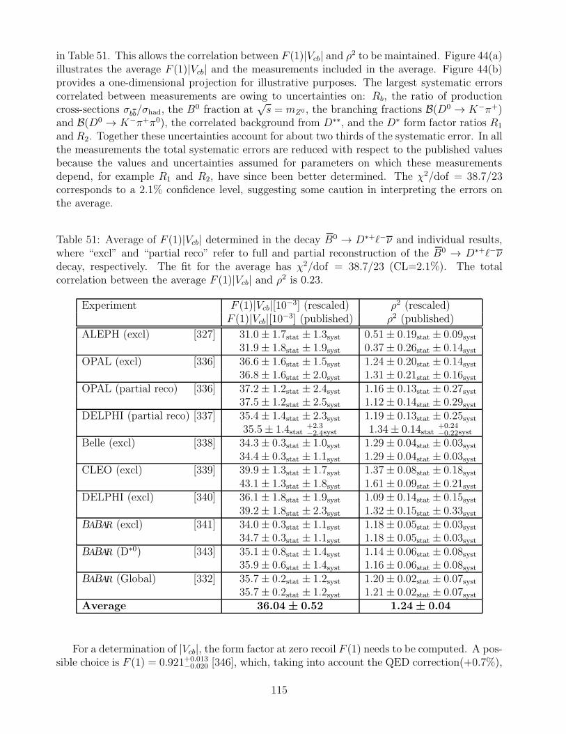
in Table 51. This allows the correlation between F (1)|Vcb| and ρ2 to be maintained. Figure 44(a)illustrates the average F (1)|Vcb| and the measurements included in the average. Figure 44(b)provides a one-dimensional projection for illustrative purposes. The largest systematic errorscorrelated between measurements are owing to uncertainties on: Rb, the ratio of productioncross-sections σbb/σhad, the B
0 fraction at√s = mZ0 , the branching fractions B(D0 → K−π+)
and B(D0 → K−π+π0), the correlated background from D∗∗, and the D∗ form factor ratios R1
and R2. Together these uncertainties account for about two thirds of the systematic error. In allthe measurements the total systematic errors are reduced with respect to the published valuesbecause the values and uncertainties assumed for parameters on which these measurementsdepend, for example R1 and R2, have since been better determined. The χ2/dof = 38.7/23corresponds to a 2.1% confidence level, suggesting some caution in interpreting the errors onthe average.
Table 51: Average of F (1)|Vcb| determined in the decay B0 → D∗+ℓ−ν and individual results,where “excl” and “partial reco” refer to full and partial reconstruction of the B0 → D∗+ℓ−νdecay, respectively. The fit for the average has χ2/dof = 38.7/23 (CL=2.1%). The totalcorrelation between the average F (1)|Vcb| and ρ2 is 0.23.
Experiment F (1)|Vcb|[10−3] (rescaled) ρ2 (rescaled)F (1)|Vcb|[10−3] (published) ρ2 (published)
ALEPH (excl) [327] 31.0± 1.7stat ± 1.3syst 0.51± 0.19stat ± 0.09syst31.9± 1.8stat ± 1.9syst 0.37± 0.26stat ± 0.14syst
OPAL (excl) [336] 36.6± 1.6stat ± 1.5syst 1.24± 0.20stat ± 0.14syst36.8± 1.6stat ± 2.0syst 1.31± 0.21stat ± 0.16syst
OPAL (partial reco) [336] 37.2± 1.2stat ± 2.4syst 1.16± 0.13stat ± 0.27syst37.5± 1.2stat ± 2.5syst 1.12± 0.14stat ± 0.29syst
DELPHI (partial reco) [337] 35.4± 1.4stat ± 2.3syst 1.19± 0.13stat ± 0.25syst35.5± 1.4stat
+2.3−2.4syst 1.34± 0.14stat
+0.24−0.22syst
Belle (excl) [338] 34.3± 0.3stat ± 1.0syst 1.29± 0.04stat ± 0.03syst34.4± 0.3stat ± 1.1syst 1.29± 0.04stat ± 0.03syst
CLEO (excl) [339] 39.9± 1.3stat ± 1.7syst 1.37± 0.08stat ± 0.18syst43.1± 1.3stat ± 1.8syst 1.61± 0.09stat ± 0.21syst
DELPHI (excl) [340] 36.1± 1.8stat ± 1.9syst 1.09± 0.14stat ± 0.15syst39.2± 1.8stat ± 2.3syst 1.32± 0.15stat ± 0.33syst
BABAR (excl) [341] 34.0± 0.3stat ± 1.1syst 1.18± 0.05stat ± 0.03syst34.7± 0.3stat ± 1.1syst 1.18± 0.05stat ± 0.03syst
BABAR (D∗0) [343] 35.1± 0.8stat ± 1.4syst 1.14± 0.06stat ± 0.08syst35.9± 0.6stat ± 1.4syst 1.16± 0.06stat ± 0.08syst
BABAR (Global) [332] 35.7± 0.2stat ± 1.2syst 1.20± 0.02stat ± 0.07syst35.7± 0.2stat ± 1.2syst 1.21± 0.02stat ± 0.07syst
Average 36.04 ± 0.52 1.24 ± 0.04
For a determination of |Vcb|, the form factor at zero recoil F (1) needs to be computed. A pos-sible choice is F (1) = 0.921+0.013
−0.020 [346], which, taking into account the QED correction(+0.7%),
115
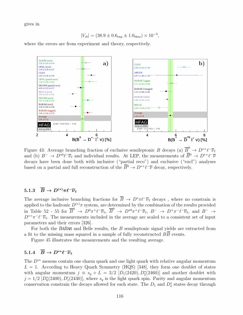
gives in
|Vcb| = (38.9± 0.6exp ± 1.0theo)× 10−3,
where the errors are from experiment and theory, respectively.
) [%]ν + l* - D→ 0B(B
2 4 6) [%]ν + l* - D→ 0
B(B2 4 6
ALEPH (excl) 0.19± 0.24 ±5.29
OPAL (excl) 0.37± 0.19 ±5.10
CLEO 0.19± 0.18 ±5.65
OPAL (partial reco) 0.42± 0.26 ±5.52
DELPHI (partial reco) 0.17± 0.15 ±4.93
BELLE (excl) 0.25± 0.03 ±4.40
DELPHI (excl) 0.33± 0.18 ±5.41
BABAR (excl) 0.30± 0.04 ±4.59
BABAR (tagged) 0.25± 0.16 ±5.40
Average 0.12±5.05
HFAGEnd of 2009
/dof = 16.6/ 9 (CL = 6 %)2χ
) [%]ν + l*0
D → +B(B
4 6 8) [%]ν + l
*0D → +
B(B4 6 8
CLEO 0.39± 0.20 ±6.58
ARGUS 1.10± 1.40 ±6.07
BABAR Tagged 0.30± 0.15 ±5.71
BABAR Untagged 0.40± 0.08 ±5.32
BABAR Global 0.21± 0.02 ±5.40
BELLE 0.56± 0.04 ±4.83
Average 0.18±5.63
HFAGEnd of 2009
/dof = 12.7/ 5 (CL = 3 %)2χ
a) b)
Figure 43: Average branching fraction of exclusive semileptonic B decays (a) B0 → D∗+ℓ−νℓ
and (b) B− → D∗0ℓ−νℓ and individual results. At LEP, the measurements of B0 → D∗+ℓ−νdecays have been done both with inclusive (“partial reco”) and exclusive (“excl”) analysesbased on a partial and full reconstruction of the B0 → D∗+ℓ−ν decay, respectively.
5.1.3 B → D(∗)πℓ−νℓ
The average inclusive branching fractions for B → D∗πℓ−νℓ decays , where no constrain isapplied to the hadronicD(∗)π system, are determined by the combination of the results provided
in Table 52 - 55 for B0 → D0π+ℓ−νℓ, B
0 → D∗0π+ℓ−νℓ, B− → D+π−ℓ−νℓ, and B− →
D∗+π−ℓ−νℓ. The measurements included in the average are scaled to a consistent set of inputparameters and their errors [326].
For both the BABAR and Belle results, the B semileptonic signal yields are extracted froma fit to the missing mass squared in a sample of fully reconstructed BB events.
Figure 45 illustrates the measurements and the resulting average.
5.1.4 B → D∗∗ℓ−νℓ
The D∗∗ mesons contain one charm quark and one light quark with relative angular momentumL = 1. According to Heavy Quark Symmetry (HQS) [348], they form one doublet of stateswith angular momentum j ≡ sq + L = 3/2 [D1(2420), D
∗2(2460)] and another doublet with
j = 1/2 [D∗0(2400), D
′1(2430)], where sq is the light quark spin. Parity and angular momentum
conservation constrain the decays allowed for each state. The D1 and D∗2 states decay through
116
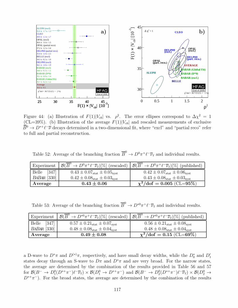
2ρ0 0.5 1 1.5 2
]-3
| [10
cb |V×
F(1
)
30
35
40
45
HFAGEnd of 2009
ALEPH
CLEO
OPAL(part. reco.)
OPAL(excl.)
DELPHI(part. reco.)
BELLE
DELPHI (excl.)
BABAR (excl.)
BABAR (D*0)
BABAR (Global Fit)
AVERAGE
= 12χ ∆
/dof = 38.7/23 (CL = 2 %)2χ
]-3
| [10cb |V×F(1) 25 30 35 40 45
]-3
| [10cb |V×F(1) 25 30 35 40 45
ALEPH (excl) 1.3± 1.7 ±31.0
CLEO 1.7± 1.3 ±39.9
OPAL (excl) 1.5± 1.6 ±36.6
OPAL (partial reco) 2.4± 1.2 ±37.2
DELPHI (partial reco) 2.3± 1.4 ±35.4
BELLE (excl) 1.0± 0.2 ±34.3
DELPHI (excl) 1.9± 1.8 ±36.1
BABAR (excl) 1.1± 0.3 ±34.0
BABAR (D*0) 1.4± 0.8 ±35.1
BABAR (Global Fit) 1.2± 0.2 ±35.7
Average 0.5±36.0
HFAGEnd of 2009
/dof = 38.7/23 (CL = 2 %)2χ
a) b)
Figure 44: (a) Illustration of F (1)|Vcb| vs. ρ2. The error ellipses correspond to ∆χ2 = 1(CL=39%). (b) Illustration of the average F (1)|Vcb| and rescaled measurements of exclusiveB0 → D∗+ℓ−ν decays determined in a two-dimensional fit, where “excl” and “partial reco” referto full and partial reconstruction.
Table 52: Average of the branching fraction B0 → D0π+ℓ−νℓ and individual results.
Experiment B(B0 → D0π+ℓ−νℓ)[%] (rescaled) B(B0 → D0π+ℓ−νℓ)[%] (published)
Belle [347] 0.43± 0.07stat ± 0.05syst 0.42± 0.07stat ± 0.06systBABAR [330] 0.42± 0.08stat ± 0.03syst 0.43± 0.08stat ± 0.03systAverage 0.43 ± 0.06 χ2/dof = 0.005 (CL=95%)
Table 53: Average of the branching fraction B0 → D∗0π+ℓ−νℓ and individual results.
Experiment B(B0 → D∗0π+ℓ−νℓ)[%] (rescaled) B(B0 → D∗0π+ℓ−νℓ)[%] (published)
Belle [347] 0.57± 0.21stat ± 0.07syst 0.56± 0.21stat ± 0.08systBABAR [330] 0.48± 0.08stat ± 0.04syst 0.48± 0.08stat ± 0.04systAverage 0.49 ± 0.08 χ2/dof = 0.15 (CL=69%)
a D-wave to D∗π and D(∗)π, respectively, and have small decay widths, while the D∗0 and D′
1
states decay through an S-wave to Dπ and D∗π and are very broad. For the narrow states,the average are determined by the combination of the results provided in Table 56 and 57for B(B− → D0
1(D∗+π−)ℓ−νℓ) × B(D0
1 → D∗+π−) and B(B− → D02(D
∗+π−)ℓ−νℓ) × B(D02 →
D∗+π−). For the broad states, the average are determined by the combination of the results
117
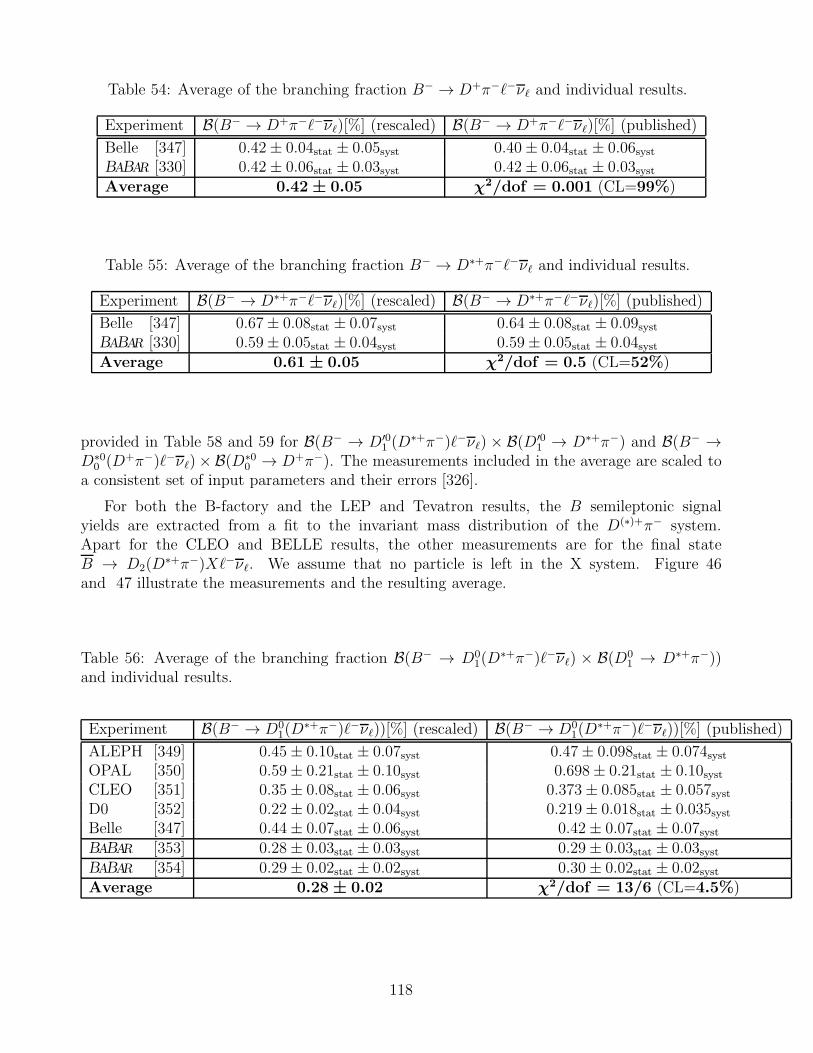
Table 54: Average of the branching fraction B− → D+π−ℓ−νℓ and individual results.
Experiment B(B− → D+π−ℓ−νℓ)[%] (rescaled) B(B− → D+π−ℓ−νℓ)[%] (published)
Belle [347] 0.42± 0.04stat ± 0.05syst 0.40± 0.04stat ± 0.06systBABAR [330] 0.42± 0.06stat ± 0.03syst 0.42± 0.06stat ± 0.03systAverage 0.42 ± 0.05 χ2/dof = 0.001 (CL=99%)
Table 55: Average of the branching fraction B− → D∗+π−ℓ−νℓ and individual results.
Experiment B(B− → D∗+π−ℓ−νℓ)[%] (rescaled) B(B− → D∗+π−ℓ−νℓ)[%] (published)
Belle [347] 0.67± 0.08stat ± 0.07syst 0.64± 0.08stat ± 0.09systBABAR [330] 0.59± 0.05stat ± 0.04syst 0.59± 0.05stat ± 0.04systAverage 0.61 ± 0.05 χ2/dof = 0.5 (CL=52%)
provided in Table 58 and 59 for B(B− → D′01 (D
∗+π−)ℓ−νℓ) × B(D′01 → D∗+π−) and B(B− →
D∗00 (D+π−)ℓ−νℓ)×B(D∗0
0 → D+π−). The measurements included in the average are scaled toa consistent set of input parameters and their errors [326].
For both the B-factory and the LEP and Tevatron results, the B semileptonic signalyields are extracted from a fit to the invariant mass distribution of the D(∗)+π− system.Apart for the CLEO and BELLE results, the other measurements are for the final stateB → D2(D
∗+π−)Xℓ−νℓ. We assume that no particle is left in the X system. Figure 46and 47 illustrate the measurements and the resulting average.
Table 56: Average of the branching fraction B(B− → D01(D
∗+π−)ℓ−νℓ) × B(D01 → D∗+π−))
and individual results.
Experiment B(B− → D01(D
∗+π−)ℓ−νℓ))[%] (rescaled) B(B− → D01(D
∗+π−)ℓ−νℓ))[%] (published)
ALEPH [349] 0.45± 0.10stat ± 0.07syst 0.47± 0.098stat ± 0.074systOPAL [350] 0.59± 0.21stat ± 0.10syst 0.698± 0.21stat ± 0.10systCLEO [351] 0.35± 0.08stat ± 0.06syst 0.373± 0.085stat ± 0.057systD0 [352] 0.22± 0.02stat ± 0.04syst 0.219± 0.018stat ± 0.035systBelle [347] 0.44± 0.07stat ± 0.06syst 0.42± 0.07stat ± 0.07systBABAR [353] 0.28± 0.03stat ± 0.03syst 0.29± 0.03stat ± 0.03systBABAR [354] 0.29± 0.02stat ± 0.02syst 0.30± 0.02stat ± 0.02systAverage 0.28 ± 0.02 χ2/dof = 13/6 (CL=4.5%)
118
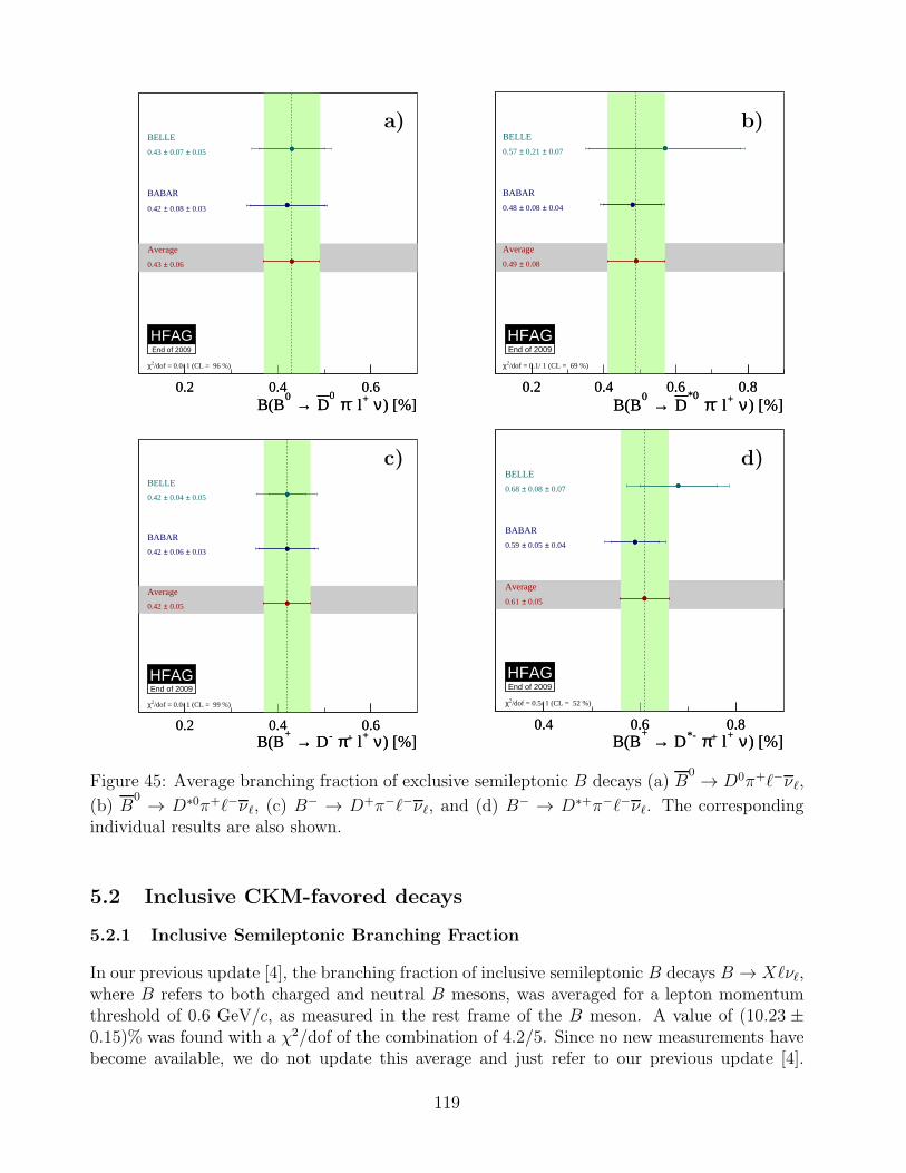
) [%]ν + l-π 0
D → 0B(B
0.2 0.4 0.6) [%]ν + l-π
0D → 0
B(B0.2 0.4 0.6
BELLE
0.05± 0.07 ±0.43
BABAR
0.03± 0.08 ±0.42
Average
0.06±0.43
HFAGEnd of 2009
/dof = 0.0/ 1 (CL = 96 %)2χ
) [%]ν + l-π *0
D → 0B(B
0.2 0.4 0.6 0.8) [%]ν + l-π
*0D → 0
B(B0.2 0.4 0.6 0.8
BELLE
0.07± 0.21 ±0.57
BABAR
0.04± 0.08 ±0.48
Average
0.08±0.49
HFAGEnd of 2009
/dof = 0.1/ 1 (CL = 69 %)2χ
a) b)
) [%]ν + l+π - D→ +B(B
0.2 0.4 0.6) [%]ν + l+π - D→ +
B(B0.2 0.4 0.6
BELLE
0.05± 0.04 ±0.42
BABAR
0.03± 0.06 ±0.42
Average
0.05±0.42
HFAGEnd of 2009
/dof = 0.0/ 1 (CL = 99 %)2χ
) [%]ν + l+π *- D→ +B(B
0.4 0.6 0.8) [%]ν + l+π *- D→ +
B(B0.4 0.6 0.8
BELLE
0.07± 0.08 ±0.68
BABAR
0.04± 0.05 ±0.59
Average
0.05±0.61
HFAGEnd of 2009
/dof = 0.5/ 1 (CL = 52 %)2χ
c) d)
Figure 45: Average branching fraction of exclusive semileptonic B decays (a) B0 → D0π+ℓ−νℓ,
(b) B0 → D∗0π+ℓ−νℓ, (c) B
− → D+π−ℓ−νℓ, and (d) B− → D∗+π−ℓ−νℓ. The correspondingindividual results are also shown.
5.2 Inclusive CKM-favored decays
5.2.1 Inclusive Semileptonic Branching Fraction
In our previous update [4], the branching fraction of inclusive semileptonic B decays B → Xℓνℓ,where B refers to both charged and neutral B mesons, was averaged for a lepton momentumthreshold of 0.6 GeV/c, as measured in the rest frame of the B meson. A value of (10.23 ±0.15)% was found with a χ2/dof of the combination of 4.2/5. Since no new measurements havebecome available, we do not update this average and just refer to our previous update [4].
119
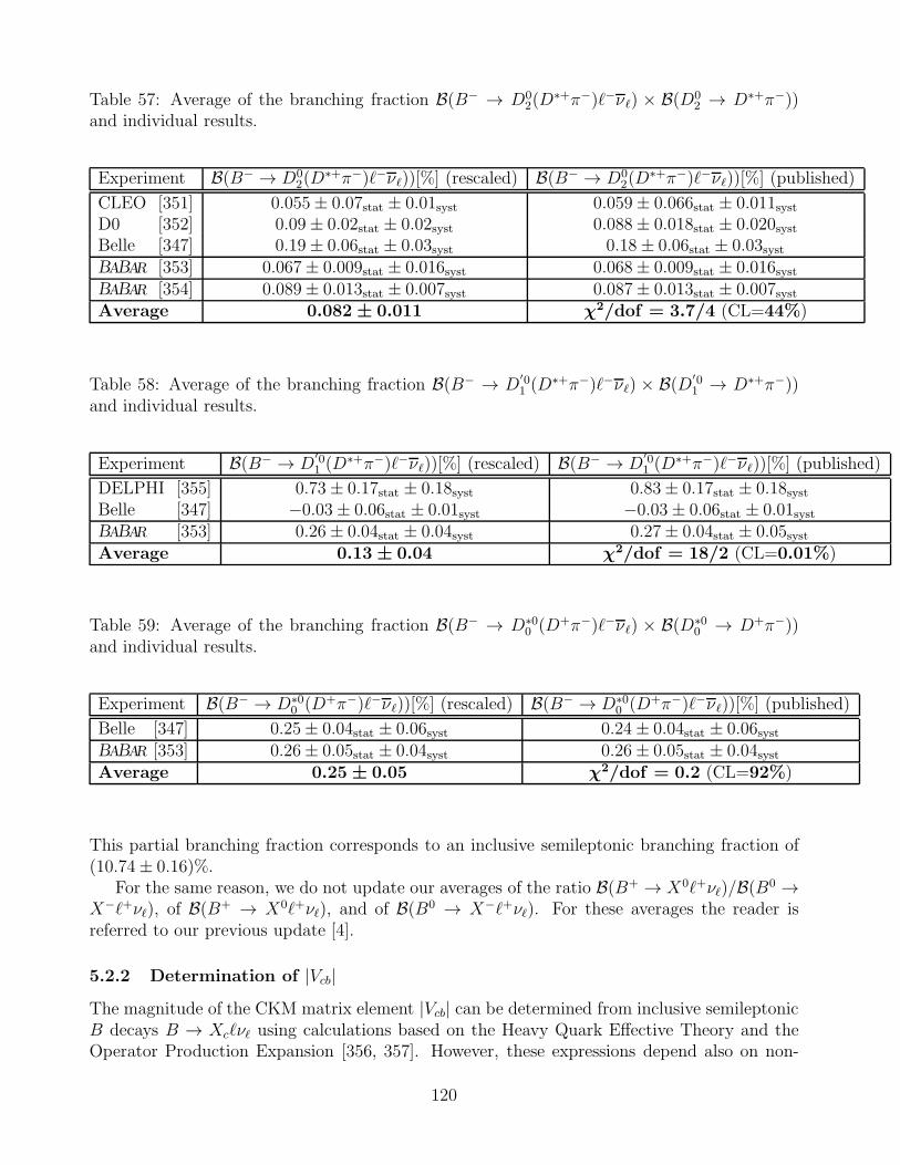
Table 57: Average of the branching fraction B(B− → D02(D
∗+π−)ℓ−νℓ) × B(D02 → D∗+π−))
and individual results.
Experiment B(B− → D02(D
∗+π−)ℓ−νℓ))[%] (rescaled) B(B− → D02(D
∗+π−)ℓ−νℓ))[%] (published)
CLEO [351] 0.055± 0.07stat ± 0.01syst 0.059± 0.066stat ± 0.011systD0 [352] 0.09± 0.02stat ± 0.02syst 0.088± 0.018stat ± 0.020systBelle [347] 0.19± 0.06stat ± 0.03syst 0.18± 0.06stat ± 0.03systBABAR [353] 0.067± 0.009stat ± 0.016syst 0.068± 0.009stat ± 0.016systBABAR [354] 0.089± 0.013stat ± 0.007syst 0.087± 0.013stat ± 0.007systAverage 0.082 ± 0.011 χ2/dof = 3.7/4 (CL=44%)
Table 58: Average of the branching fraction B(B− → D′01 (D
∗+π−)ℓ−νℓ) × B(D′01 → D∗+π−))
and individual results.
Experiment B(B− → D′01 (D
∗+π−)ℓ−νℓ))[%] (rescaled) B(B− → D′01 (D
∗+π−)ℓ−νℓ))[%] (published)
DELPHI [355] 0.73± 0.17stat ± 0.18syst 0.83± 0.17stat ± 0.18systBelle [347] −0.03± 0.06stat ± 0.01syst −0.03± 0.06stat ± 0.01systBABAR [353] 0.26± 0.04stat ± 0.04syst 0.27± 0.04stat ± 0.05systAverage 0.13 ± 0.04 χ2/dof = 18/2 (CL=0.01%)
Table 59: Average of the branching fraction B(B− → D∗00 (D+π−)ℓ−νℓ) × B(D∗0
0 → D+π−))and individual results.
Experiment B(B− → D∗00 (D+π−)ℓ−νℓ))[%] (rescaled) B(B− → D∗0
0 (D+π−)ℓ−νℓ))[%] (published)
Belle [347] 0.25± 0.04stat ± 0.06syst 0.24± 0.04stat ± 0.06systBABAR [353] 0.26± 0.05stat ± 0.04syst 0.26± 0.05stat ± 0.04systAverage 0.25 ± 0.05 χ2/dof = 0.2 (CL=92%)
This partial branching fraction corresponds to an inclusive semileptonic branching fraction of(10.74± 0.16)%.
For the same reason, we do not update our averages of the ratio B(B+ → X0ℓ+νℓ)/B(B0 →X−ℓ+νℓ), of B(B+ → X0ℓ+νℓ), and of B(B0 → X−ℓ+νℓ). For these averages the reader isreferred to our previous update [4].
5.2.2 Determination of |Vcb|The magnitude of the CKM matrix element |Vcb| can be determined from inclusive semileptonicB decays B → Xcℓνℓ using calculations based on the Heavy Quark Effective Theory and theOperator Production Expansion [356, 357]. However, these expressions depend also on non-
120
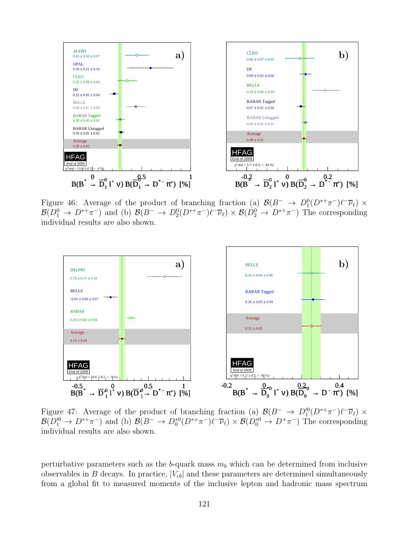
) [%]+π * - D→ 0
1D) B(ν + l0
1D → +B(B
0 0.5 1) [%]+π * - D→
0
1D) B(ν + l0
1D → +B(B
0 0.5 1
ALEPH 0.07± 0.10 ±0.45
OPAL 0.10± 0.21 ±0.59
CLEO 0.06± 0.08 ±0.35
D0 0.04± 0.02 ±0.22
BELLE 0.06± 0.07 ±0.44
BABAR Tagged 0.03± 0.03 ±0.28
BABAR Untagged 0.02± 0.02 ±0.29
Average 0.02±0.28
HFAGEnd of 2009
/dof = 13.0/ 6 (CL = 4 %)2χ
) [%]+π * - D→ 0
2D) B(ν + l0
2D → +B(B
-0.2 0 0.2) [%]+π * - D→
0
2D) B(ν + l0
2D → +B(B
-0.2 0 0.2
CLEO
0.01± 0.07 ±0.06
D0
0.02± 0.02 ±0.09
BELLE
0.03± 0.06 ±0.19
BABAR Tagged
0.02± 0.01 ±0.07
BABAR Untagged
0.01± 0.01 ±0.09
Average
0.01±0.08
HFAGEnd of 2009
/dof = 3.7/ 4 (CL = 44 %)2χ
a) b)
Figure 46: Average of the product of branching fraction (a) B(B− → D01(D
∗+π−)ℓ−νℓ) ×B(D0
1 → D∗+π−) and (b) B(B− → D02(D
∗+π−)ℓ−νℓ) × B(D02 → D∗+π−) The corresponding
individual results are also shown.
) [%]+π * - D→01’D) B(ν + l0
1’D → +B(B-0.5 0 0.5 1
) [%]+π * - D→01’D) B(ν + l0
1’D → +B(B-0.5 0 0.5 1
DELPHI
0.18± 0.17 ±0.73
BELLE
0.07± 0.06 ±-0.03
BABAR
0.04± 0.04 ±0.26
Average
0.04±0.13
HFAGEnd of 2009
/dof = 18.0/ 2 (CL = 0 %)2χ
) [%]+π - D→ *0
0D) B(ν + l*0
0D → +B(B
-0.2 0 0.2 0.4) [%]+π - D→
*0
0D) B(ν + l*0
0D → +B(B
-0.2 0 0.2 0.4
BELLE
0.06± 0.04 ±0.25
BABAR Tagged
0.04± 0.05 ±0.26
Average
0.05±0.25
HFAGEnd of 2009
/dof = 0.2/ 1 (CL = 92 %)2χ
a) b)
Figure 47: Average of the product of branching fraction (a) B(B− → D′01 (D
∗+π−)ℓ−νℓ) ×B(D′0
1 → D∗+π−) and (b) B(B− → D∗00 (D∗+π−)ℓ−νℓ) × B(D∗0
0 → D+π−) The correspondingindividual results are also shown.
perturbative parameters such as the b-quark mass mb which can be determined from inclusiveobservables in B decays. In practice, |Vcb| and these parameters are determined simultaneouslyfrom a global fit to measured moments of the inclusive lepton and hadronic mass spectrum
121
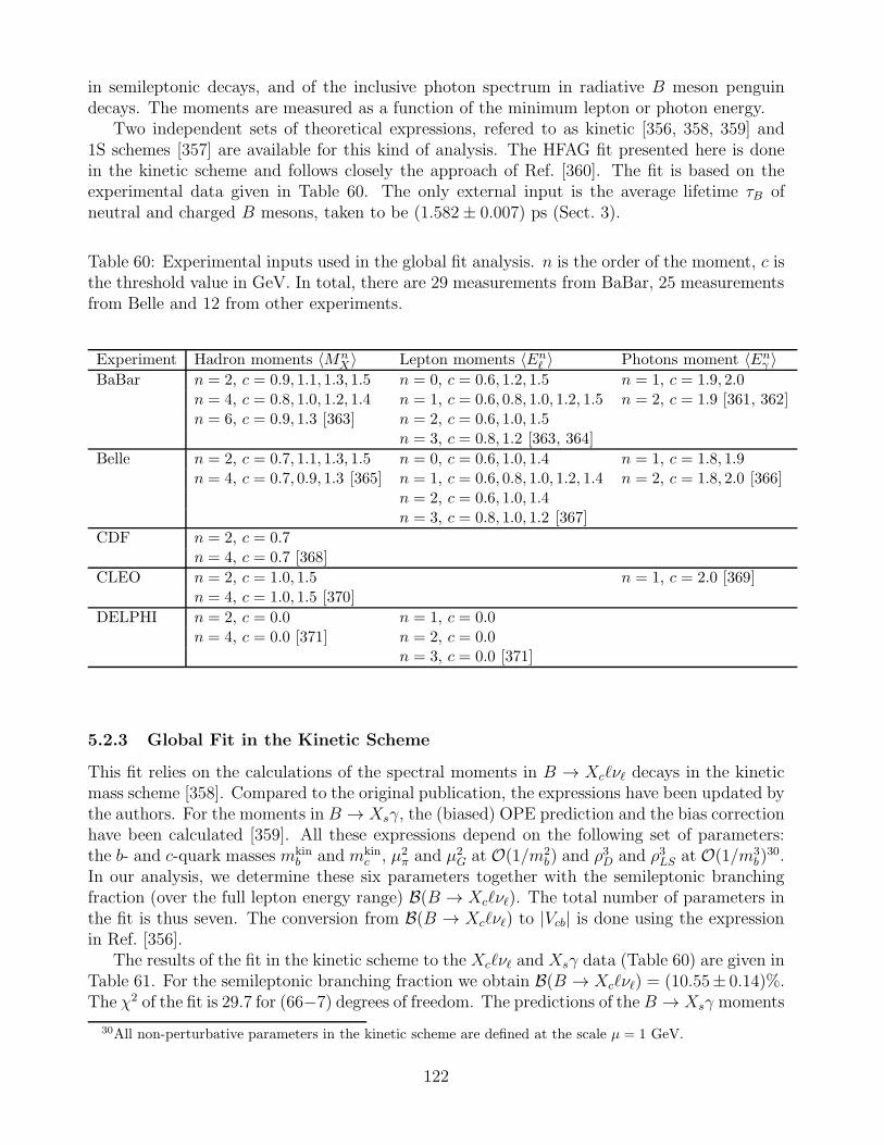
in semileptonic decays, and of the inclusive photon spectrum in radiative B meson penguindecays. The moments are measured as a function of the minimum lepton or photon energy.
Two independent sets of theoretical expressions, refered to as kinetic [356, 358, 359] and1S schemes [357] are available for this kind of analysis. The HFAG fit presented here is donein the kinetic scheme and follows closely the approach of Ref. [360]. The fit is based on theexperimental data given in Table 60. The only external input is the average lifetime τB ofneutral and charged B mesons, taken to be (1.582± 0.007) ps (Sect. 3).
Table 60: Experimental inputs used in the global fit analysis. n is the order of the moment, c isthe threshold value in GeV. In total, there are 29 measurements from BaBar, 25 measurementsfrom Belle and 12 from other experiments.
Experiment Hadron moments 〈MnX〉 Lepton moments 〈Enℓ 〉 Photons moment 〈Enγ 〉
BaBar n = 2, c = 0.9, 1.1, 1.3, 1.5 n = 0, c = 0.6, 1.2, 1.5 n = 1, c = 1.9, 2.0n = 4, c = 0.8, 1.0, 1.2, 1.4 n = 1, c = 0.6, 0.8, 1.0, 1.2, 1.5 n = 2, c = 1.9 [361, 362]n = 6, c = 0.9, 1.3 [363] n = 2, c = 0.6, 1.0, 1.5
n = 3, c = 0.8, 1.2 [363, 364]
Belle n = 2, c = 0.7, 1.1, 1.3, 1.5 n = 0, c = 0.6, 1.0, 1.4 n = 1, c = 1.8, 1.9n = 4, c = 0.7, 0.9, 1.3 [365] n = 1, c = 0.6, 0.8, 1.0, 1.2, 1.4 n = 2, c = 1.8, 2.0 [366]
n = 2, c = 0.6, 1.0, 1.4n = 3, c = 0.8, 1.0, 1.2 [367]
CDF n = 2, c = 0.7n = 4, c = 0.7 [368]
CLEO n = 2, c = 1.0, 1.5 n = 1, c = 2.0 [369]n = 4, c = 1.0, 1.5 [370]
DELPHI n = 2, c = 0.0 n = 1, c = 0.0n = 4, c = 0.0 [371] n = 2, c = 0.0
n = 3, c = 0.0 [371]
5.2.3 Global Fit in the Kinetic Scheme
This fit relies on the calculations of the spectral moments in B → Xcℓνℓ decays in the kineticmass scheme [358]. Compared to the original publication, the expressions have been updated bythe authors. For the moments in B → Xsγ, the (biased) OPE prediction and the bias correctionhave been calculated [359]. All these expressions depend on the following set of parameters:the b- and c-quark masses mkin
b and mkinc , µ2
π and µ2G at O(1/m2
b) and ρ3D and ρ3LS at O(1/m3
b)30.
In our analysis, we determine these six parameters together with the semileptonic branchingfraction (over the full lepton energy range) B(B → Xcℓνℓ). The total number of parameters inthe fit is thus seven. The conversion from B(B → Xcℓνℓ) to |Vcb| is done using the expressionin Ref. [356].
The results of the fit in the kinetic scheme to the Xcℓνℓ and Xsγ data (Table 60) are given inTable 61. For the semileptonic branching fraction we obtain B(B → Xcℓνℓ) = (10.55± 0.14)%.The χ2 of the fit is 29.7 for (66−7) degrees of freedom. The predictions of the B → Xsγ moments
30All non-perturbative parameters in the kinetic scheme are defined at the scale µ = 1 GeV.
122
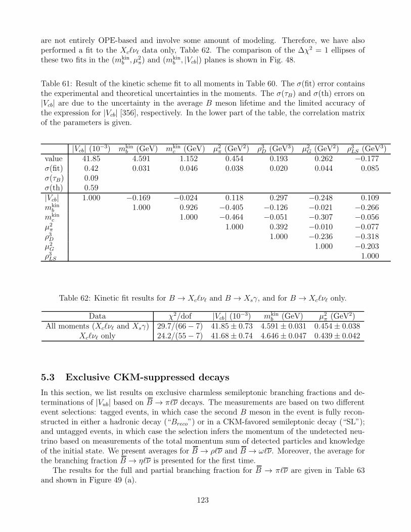
are not entirely OPE-based and involve some amount of modeling. Therefore, we have alsoperformed a fit to the Xcℓνℓ data only, Table 62. The comparison of the ∆χ2 = 1 ellipses ofthese two fits in the (mkin
b , µ2π) and (mkin
b , |Vcb|) planes is shown in Fig. 48.
Table 61: Result of the kinetic scheme fit to all moments in Table 60. The σ(fit) error containsthe experimental and theoretical uncertainties in the moments. The σ(τB) and σ(th) errors on|Vcb| are due to the uncertainty in the average B meson lifetime and the limited accuracy ofthe expression for |Vcb| [356], respectively. In the lower part of the table, the correlation matrixof the parameters is given.
|Vcb| (10−3) mkinb (GeV) mkin
c (GeV) µ2π (GeV2) ρ3D (GeV3) µ2
G (GeV2) ρ3LS (GeV3)value 41.85 4.591 1.152 0.454 0.193 0.262 −0.177σ(fit) 0.42 0.031 0.046 0.038 0.020 0.044 0.085σ(τB) 0.09σ(th) 0.59|Vcb| 1.000 −0.169 −0.024 0.118 0.297 −0.248 0.109mkinb 1.000 0.926 −0.405 −0.126 −0.021 −0.266
mkinc 1.000 −0.464 −0.051 −0.307 −0.056
µ2π 1.000 0.392 −0.010 −0.077ρ3D 1.000 −0.236 −0.318µ2G 1.000 −0.203ρ3LS 1.000
Table 62: Kinetic fit results for B → Xcℓνℓ and B → Xsγ, and for B → Xcℓνℓ only.
Data χ2/dof |Vcb| (10−3) mkinb (GeV) µ2
π (GeV2)All moments (Xcℓνℓ and Xsγ) 29.7/(66− 7) 41.85± 0.73 4.591± 0.031 0.454± 0.038
Xcℓνℓ only 24.2/(55− 7) 41.68± 0.74 4.646± 0.047 0.439± 0.042
5.3 Exclusive CKM-suppressed decays
In this section, we list results on exclusive charmless semileptonic branching fractions and de-terminations of |Vub| based on B → πℓν decays. The measurements are based on two differentevent selections: tagged events, in which case the second B meson in the event is fully recon-structed in either a hadronic decay (“Breco”) or in a CKM-favored semileptonic decay (“SL”);and untagged events, in which case the selection infers the momentum of the undetected neu-trino based on measurements of the total momentum sum of detected particles and knowledgeof the initial state. We present averages for B → ρℓν and B → ωℓν. Moreover, the average forthe branching fraction B → ηℓν is presented for the first time.
The results for the full and partial branching fraction for B → πℓν are given in Table 63and shown in Figure 49 (a).
123
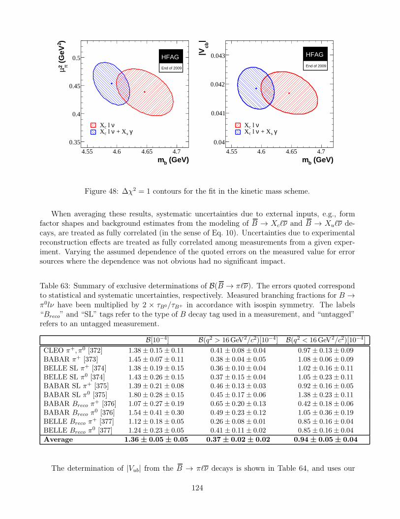
(GeV)bm4.55 4.6 4.65 4.7
)2 (
GeV
π2 µ
0.35
0.4
0.45
0.5 HFAG
End of 2009
ν l c Xγ s + Xν l c X
(GeV)bm4.55 4.6 4.65 4.7
|cb
|V
0.04
0.041
0.042
0.043
ν l c Xγ s + Xν l c X
HFAG
End of 2009
Figure 48: ∆χ2 = 1 contours for the fit in the kinetic mass scheme.
When averaging these results, systematic uncertainties due to external inputs, e.g., formfactor shapes and background estimates from the modeling of B → Xcℓν and B → Xuℓν de-cays, are treated as fully correlated (in the sense of Eq. 10). Uncertainties due to experimentalreconstruction effects are treated as fully correlated among measurements from a given exper-iment. Varying the assumed dependence of the quoted errors on the measured value for errorsources where the dependence was not obvious had no significant impact.
Table 63: Summary of exclusive determinations of B(B → πℓν). The errors quoted correspondto statistical and systematic uncertainties, respectively. Measured branching fractions for B →π0lν have been multiplied by 2 × τB0/τB+ in accordance with isospin symmetry. The labels“Breco” and “SL” tags refer to the type of B decay tag used in a measurement, and “untagged”refers to an untagged measurement.
B[10−4] B(q2 > 16GeV2/c2)[10−4] B(q2 < 16GeV2/c2)[10−4]
CLEO π+, π0 [372] 1.38 ± 0.15 ± 0.11 0.41 ± 0.08 ± 0.04 0.97 ± 0.13 ± 0.09BABAR π+ [373] 1.45 ± 0.07 ± 0.11 0.38 ± 0.04 ± 0.05 1.08 ± 0.06 ± 0.09BELLE SL π+ [374] 1.38 ± 0.19 ± 0.15 0.36 ± 0.10 ± 0.04 1.02 ± 0.16 ± 0.11BELLE SL π0 [374] 1.43 ± 0.26 ± 0.15 0.37 ± 0.15 ± 0.04 1.05 ± 0.23 ± 0.11BABAR SL π+ [375] 1.39 ± 0.21 ± 0.08 0.46 ± 0.13 ± 0.03 0.92 ± 0.16 ± 0.05BABAR SL π0 [375] 1.80 ± 0.28 ± 0.15 0.45 ± 0.17 ± 0.06 1.38 ± 0.23 ± 0.11BABAR Breco π
+ [376] 1.07 ± 0.27 ± 0.19 0.65 ± 0.20 ± 0.13 0.42 ± 0.18 ± 0.06BABAR Breco π
0 [376] 1.54 ± 0.41 ± 0.30 0.49 ± 0.23 ± 0.12 1.05 ± 0.36 ± 0.19BELLE Breco π
+ [377] 1.12 ± 0.18 ± 0.05 0.26 ± 0.08 ± 0.01 0.85 ± 0.16 ± 0.04BELLE Breco π
0 [377] 1.24 ± 0.23 ± 0.05 0.41 ± 0.11 ± 0.02 0.85 ± 0.16 ± 0.04
Average 1.36 ± 0.05 ± 0.05 0.37 ± 0.02 ± 0.02 0.94 ± 0.05 ± 0.04
The determination of |Vub| from the B → πℓν decays is shown in Table 64, and uses our
124
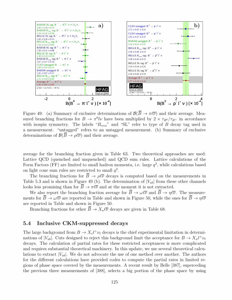
]-4
10× ) [ν + l-ρ → 0B(B
0 2 4]
-4 10× ) [ν + l-ρ → 0
B(B0 2 4
ν + l-ρ → 0CLEO untagged: B 0.52± 0.41 ±2.75
ν + l-ρ → 0CLEO untagged: B 0.37± 0.37 ±2.93
ν + l-ρ → 0BABAR untagged: B 0.57± 0.21 ±2.16
ν + l-ρ → 0 tag:: BrecoBELLE B 0.13± 0.46 ±2.56
ν + l0ρ → + tag:: BrecoBELLE B 0.15± 0.43 ±3.38
ν + l-ρ → 0BELLE SL tag: B 0.31± 0.54 ±2.24
ν + l0ρ → +BELLE SL tag: B 0.33± 0.43 ±2.54
ν + l-ρ → 0Average: B 0.16± 0.18 ±2.77
HFAGEnd of 2009/dof = 3.9/ 6 (CL = 69 %)2χ
]-4
10× ) [ν + l-π → 0B(B
-2 0 2]
-4 10× ) [ν + l-π → 0
B(B-2 0 2
+τ/0τ 2× ν + l0π → +BABAR SL tag: B 0.15± 0.28 ±1.80
+τ/0τ 2× ν + l0π → + tag: B recoBABAR B 0.30± 0.41 ±1.54
+τ/0τ 2× ν + l0π → +BELLE SL tag: B 0.15± 0.26 ±1.43
+τ/0τ 2× ν + l0π → + tag: B recoBELLE B 0.05± 0.23 ±1.24
ν + l-π → 0BABAR SL tag: B 0.08± 0.21 ±1.39
ν + l-π → 0BELLE SL tag: B 0.15± 0.19 ±1.38
ν + l-π → 0 tag: B recoBABAR B 0.19± 0.27 ±1.07
ν + lπ →CLEO untagged: B 0.11± 0.15 ±1.38
ν + lπ →BABAR untagged: B 0.11± 0.07 ±1.45
ν + l-π → 0 tag: B recoBELLE B 0.05± 0.18 ±1.12
ν + l-π → 0Average: B 0.05± 0.05 ±1.36
HFAGEnd of 2009
/dof = 5.4/ 9 (CL = 80 %)2χ
a) b)
Figure 49: (a) Summary of exclusive determinations of B(B → πℓν) and their average. Mea-sured branching fractions for B → π0lν have been multiplied by 2 × τB0/τB+ in accordancewith isospin symmetry. The labels “Breco” and “SL” refer to type of B decay tag used ina measurement. “untagged” refers to an untagged measurement. (b) Summary of exclusivedeterminations of B(B → ρℓν) and their average.
average for the branching fraction given in Table 63. Two theoretical approaches are used:Lattice QCD (quenched and unquenched) and QCD sum rules. Lattice calculations of theForm Factors (FF) are limited to small hadron momenta, i.e. large q2, while calculations basedon light cone sum rules are restricted to small q2.
The branching fractions for B → ρℓν decays is computed based on the measurements inTable 5.3 and is shown in Figure 49 (b). The determination of |Vub| from these other channelslooks less promising than for B → πℓν and at the moment it is not extracted.
We also report the branching fraction average for B → ωℓν and B → ηℓν. The measure-ments for B → ωℓν are reported in Table and shown in Figure 50, while the ones for B → ηℓνare reported in Table and shown in Figure 50.
Branching fractions for other B → Xuℓν decays are given in Table 68.
5.4 Inclusive CKM-suppressed decays
The large background from B → Xcℓ+νℓ decays is the chief experimental limitation in determi-
nations of |Vub|. Cuts designed to reject this background limit the acceptance for B → Xuℓ+νℓ
decays. The calculation of partial rates for these restricted acceptances is more complicatedand requires substantial theoretical machinery. In this update, we use several theoretical calcu-lations to extract |Vub|. We do not advocate the use of one method over another. The authorsfor the different calculations have provided codes to compute the partial rates in limited re-gions of phase space covered by the measurements. A recent result by Belle [387], supercedingthe previous three measurements of [388], selects a big portion of the phase space by using
125
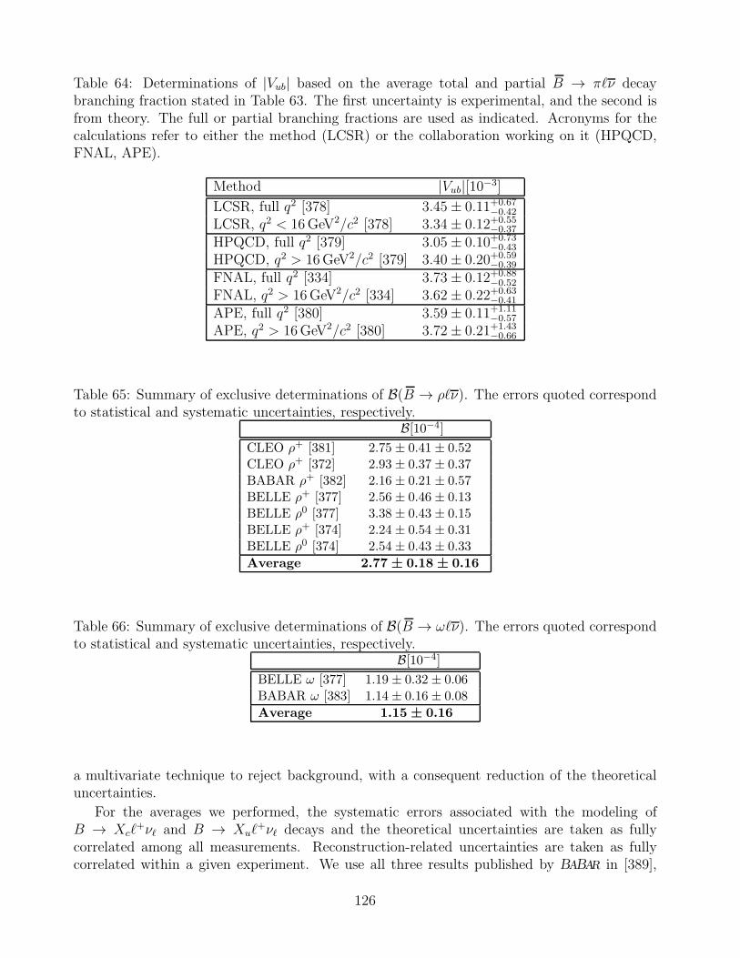
Table 64: Determinations of |Vub| based on the average total and partial B → πℓν decaybranching fraction stated in Table 63. The first uncertainty is experimental, and the second isfrom theory. The full or partial branching fractions are used as indicated. Acronyms for thecalculations refer to either the method (LCSR) or the collaboration working on it (HPQCD,FNAL, APE).
Method |Vub|[10−3]
LCSR, full q2 [378] 3.45± 0.11+0.67−0.42
LCSR, q2 < 16GeV2/c2 [378] 3.34± 0.12+0.55−0.37
HPQCD, full q2 [379] 3.05± 0.10+0.73−0.43
HPQCD, q2 > 16GeV2/c2 [379] 3.40± 0.20+0.59−0.39
FNAL, full q2 [334] 3.73± 0.12+0.88−0.52
FNAL, q2 > 16GeV2/c2 [334] 3.62± 0.22+0.63−0.41
APE, full q2 [380] 3.59± 0.11+1.11−0.57
APE, q2 > 16GeV2/c2 [380] 3.72± 0.21+1.43−0.66
Table 65: Summary of exclusive determinations of B(B → ρℓν). The errors quoted correspondto statistical and systematic uncertainties, respectively.
B[10−4]
CLEO ρ+ [381] 2.75 ± 0.41 ± 0.52CLEO ρ+ [372] 2.93 ± 0.37 ± 0.37BABAR ρ+ [382] 2.16 ± 0.21 ± 0.57BELLE ρ+ [377] 2.56 ± 0.46 ± 0.13BELLE ρ0 [377] 3.38 ± 0.43 ± 0.15BELLE ρ+ [374] 2.24 ± 0.54 ± 0.31BELLE ρ0 [374] 2.54 ± 0.43 ± 0.33
Average 2.77 ± 0.18 ± 0.16
Table 66: Summary of exclusive determinations of B(B → ωℓν). The errors quoted correspondto statistical and systematic uncertainties, respectively.
B[10−4]
BELLE ω [377] 1.19 ± 0.32 ± 0.06BABAR ω [383] 1.14 ± 0.16 ± 0.08
Average 1.15 ± 0.16
a multivariate technique to reject background, with a consequent reduction of the theoreticaluncertainties.
For the averages we performed, the systematic errors associated with the modeling ofB → Xcℓ
+νℓ and B → Xuℓ+νℓ decays and the theoretical uncertainties are taken as fully
correlated among all measurements. Reconstruction-related uncertainties are taken as fullycorrelated within a given experiment. We use all three results published by BABAR in [389],
126
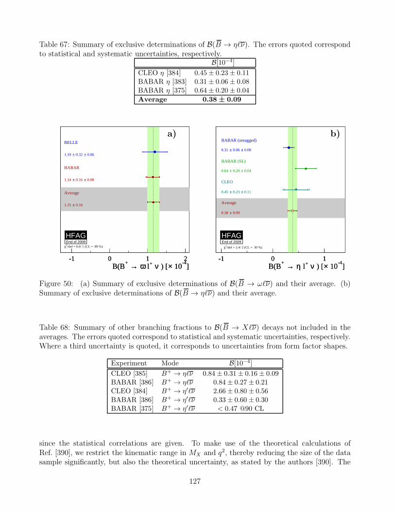
Table 67: Summary of exclusive determinations of B(B → ηℓν). The errors quoted correspondto statistical and systematic uncertainties, respectively.
B[10−4]
CLEO η [384] 0.45 ± 0.23 ± 0.11BABAR η [383] 0.31 ± 0.06 ± 0.08BABAR η [375] 0.64 ± 0.20 ± 0.04
Average 0.38 ± 0.09
]-4
10× ) [ν + lη → +B(B
-1 0 1]
-4 10× ) [ν + lη → +
B(B-1 0 1
BABAR (untagged)
0.08± 0.06 ±0.31
BABAR (SL)
0.04± 0.20 ±0.64
CLEO
0.11± 0.23 ±0.45
Average
0.09±0.38
HFAGEnd of 2009
/dof = 2.4/ 2 (CL = 30 %)2χ
]-4
10× ) [ν + lω → +B(B
-1 0 1 2]
-4 10× ) [ν + lω → +
B(B-1 0 1 2
BELLE
0.06± 0.32 ±1.19
BABAR
0.08± 0.16 ±1.14
Average
0.16±1.15
HFAGEnd of 2009/dof = 0.0/ 1 (CL = 89 %)2χ
a) b)
Figure 50: (a) Summary of exclusive determinations of B(B → ωℓν) and their average. (b)Summary of exclusive determinations of B(B → ηℓν) and their average.
Table 68: Summary of other branching fractions to B(B → Xℓν) decays not included in theaverages. The errors quoted correspond to statistical and systematic uncertainties, respectively.Where a third uncertainty is quoted, it corresponds to uncertainties from form factor shapes.
Experiment Mode B[10−4]
CLEO [385] B+ → ηℓν 0.84 ± 0.31± 0.16 ± 0.09BABAR [386] B+ → ηℓν 0.84 ± 0.27 ± 0.21CLEO [384] B+ → η′ℓν 2.66 ± 0.80 ± 0.56BABAR [386] B+ → η′ℓν 0.33 ± 0.60 ± 0.30BABAR [375] B+ → η′ℓν < 0.47 @90 CL
since the statistical correlations are given. To make use of the theoretical calculations ofRef. [390], we restrict the kinematic range in MX and q2, thereby reducing the size of the datasample significantly, but also the theoretical uncertainty, as stated by the authors [390]. The
127
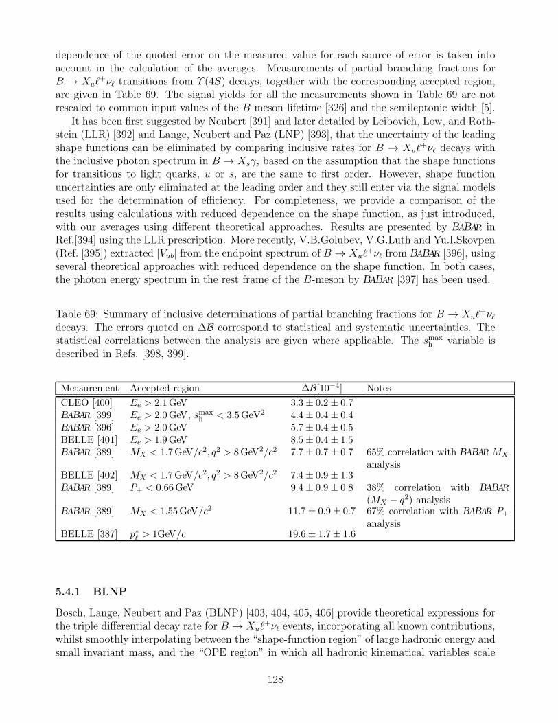
dependence of the quoted error on the measured value for each source of error is taken intoaccount in the calculation of the averages. Measurements of partial branching fractions forB → Xuℓ
+νℓ transitions from Υ (4S) decays, together with the corresponding accepted region,are given in Table 69. The signal yields for all the measurements shown in Table 69 are notrescaled to common input values of the B meson lifetime [326] and the semileptonic width [5].
It has been first suggested by Neubert [391] and later detailed by Leibovich, Low, and Roth-stein (LLR) [392] and Lange, Neubert and Paz (LNP) [393], that the uncertainty of the leadingshape functions can be eliminated by comparing inclusive rates for B → Xuℓ
+νℓ decays withthe inclusive photon spectrum in B → Xsγ, based on the assumption that the shape functionsfor transitions to light quarks, u or s, are the same to first order. However, shape functionuncertainties are only eliminated at the leading order and they still enter via the signal modelsused for the determination of efficiency. For completeness, we provide a comparison of theresults using calculations with reduced dependence on the shape function, as just introduced,with our averages using different theoretical approaches. Results are presented by BABAR inRef.[394] using the LLR prescription. More recently, V.B.Golubev, V.G.Luth and Yu.I.Skovpen(Ref. [395]) extracted |Vub| from the endpoint spectrum of B → Xuℓ
+νℓ from BABAR [396], usingseveral theoretical approaches with reduced dependence on the shape function. In both cases,the photon energy spectrum in the rest frame of the B-meson by BABAR [397] has been used.
Table 69: Summary of inclusive determinations of partial branching fractions for B → Xuℓ+νℓ
decays. The errors quoted on ∆B correspond to statistical and systematic uncertainties. Thestatistical correlations between the analysis are given where applicable. The smax
h variable isdescribed in Refs. [398, 399].
Measurement Accepted region ∆B[10−4] Notes
CLEO [400] Ee > 2.1GeV 3.3± 0.2 ± 0.7BABAR [399] Ee > 2.0GeV, smax
h < 3.5GeV2 4.4± 0.4 ± 0.4BABAR [396] Ee > 2.0GeV 5.7± 0.4 ± 0.5BELLE [401] Ee > 1.9GeV 8.5± 0.4 ± 1.5BABAR [389] MX < 1.7GeV/c2, q2 > 8GeV2/c2 7.7± 0.7 ± 0.7 65% correlation with BABAR MX
analysisBELLE [402] MX < 1.7GeV/c2, q2 > 8GeV2/c2 7.4± 0.9 ± 1.3BABAR [389] P+ < 0.66GeV 9.4± 0.9 ± 0.8 38% correlation with BABAR
(MX − q2) analysisBABAR [389] MX < 1.55GeV/c2 11.7 ± 0.9± 0.7 67% correlation with BABAR P+
analysisBELLE [387] p∗ℓ > 1GeV/c 19.6 ± 1.7± 1.6
5.4.1 BLNP
Bosch, Lange, Neubert and Paz (BLNP) [403, 404, 405, 406] provide theoretical expressions forthe triple differential decay rate for B → Xuℓ
+νℓ events, incorporating all known contributions,whilst smoothly interpolating between the “shape-function region” of large hadronic energy andsmall invariant mass, and the “OPE region” in which all hadronic kinematical variables scale
128
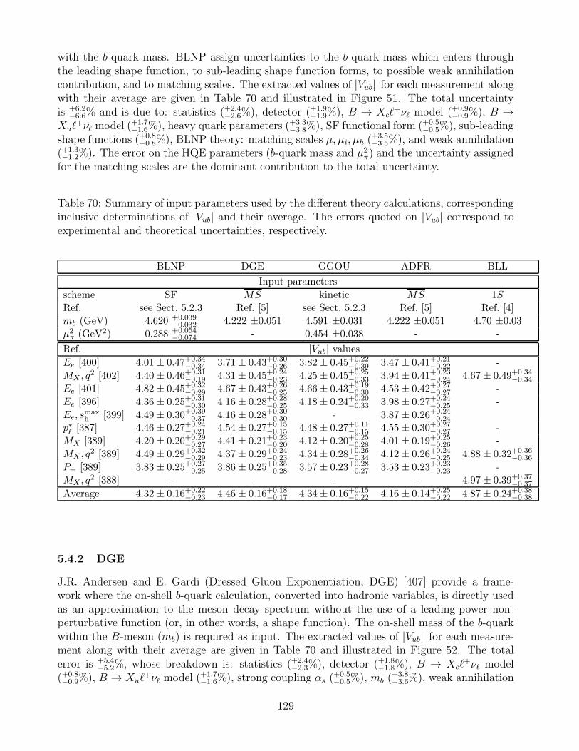
with the b-quark mass. BLNP assign uncertainties to the b-quark mass which enters throughthe leading shape function, to sub-leading shape function forms, to possible weak annihilationcontribution, and to matching scales. The extracted values of |Vub| for each measurement alongwith their average are given in Table 70 and illustrated in Figure 51. The total uncertaintyis +6.2
−6.6% and is due to: statistics (+2.4−2.6%), detector (+1.9
−1.9%), B → Xcℓ+νℓ model (+0.9
−0.9%), B →Xuℓ
+νℓ model (+1.7−1.6%), heavy quark parameters (+3.3
−3.8%), SF functional form (+0.5−0.5%), sub-leading
shape functions (+0.8−0.8%), BLNP theory: matching scales µ, µi, µh (
+3.5−3.5%), and weak annihilation
(+1.3−1.2%). The error on the HQE parameters (b-quark mass and µ2
π) and the uncertainty assignedfor the matching scales are the dominant contribution to the total uncertainty.
Table 70: Summary of input parameters used by the different theory calculations, correspondinginclusive determinations of |Vub| and their average. The errors quoted on |Vub| correspond toexperimental and theoretical uncertainties, respectively.
BLNP DGE GGOU ADFR BLL
Input parameters
scheme SF MS kinetic MS 1SRef. see Sect. 5.2.3 Ref. [5] see Sect. 5.2.3 Ref. [5] Ref. [4]
mb (GeV) 4.620 +0.039−0.032 4.222 ±0.051 4.591 ±0.031 4.222 ±0.051 4.70 ±0.03
µ2π (GeV2) 0.288 +0.054−0.074 - 0.454 ±0.038 - -
Ref. |Vub| valuesEe [400] 4.01± 0.47+0.34
−0.34 3.71 ± 0.43+0.30−0.26 3.82± 0.45+0.22
−0.39 3.47 ± 0.41+0.21−0.22 -
MX , q2 [402] 4.40± 0.46+0.31
−0.19 4.31 ± 0.45+0.24−0.23 4.25± 0.45+0.25
−0.33 3.94 ± 0.41+0.23−0.24 4.67 ± 0.49+0.34
−0.34
Ee [401] 4.82± 0.45+0.32−0.29 4.67 ± 0.43+0.26
−0.25 4.66± 0.43+0.19−0.30 4.53 ± 0.42+0.27
−0.27 -
Ee [396] 4.36± 0.25+0.31−0.30 4.16 ± 0.28+0.28
−0.25 4.18± 0.24+0.20−0.33 3.98 ± 0.27+0.24
−0.25 -
Ee, smaxh [399] 4.49± 0.30+0.39
−0.37 4.16 ± 0.28+0.30−0.30 - 3.87 ± 0.26+0.24
−0.24
p∗ℓ [387] 4.46± 0.27+0.24−0.21 4.54 ± 0.27+0.15
−0.15 4.48± 0.27+0.11−0.15 4.55 ± 0.30+0.27
−0.27 -
MX [389] 4.20± 0.20+0.29−0.27 4.41 ± 0.21+0.23
−0.20 4.12± 0.20+0.25−0.28 4.01 ± 0.19+0.25
−0.26 -
MX , q2 [389] 4.49± 0.29+0.32
−0.29 4.37 ± 0.29+0.24−0.23 4.34± 0.28+0.26
−0.34 4.12 ± 0.26+0.24−0.25 4.88 ± 0.32+0.36
−0.36
P+ [389] 3.83± 0.25+0.27−0.25 3.86 ± 0.25+0.35
−0.28 3.57± 0.23+0.28−0.27 3.53 ± 0.23+0.23
−0.23 -
MX , q2 [388] - - - - 4.97 ± 0.39+0.37
−0.37
Average 4.32± 0.16+0.22−0.23 4.46 ± 0.16+0.18
−0.17 4.34± 0.16+0.15−0.22 4.16 ± 0.14+0.25
−0.22 4.87 ± 0.24+0.38−0.38
5.4.2 DGE
J.R. Andersen and E. Gardi (Dressed Gluon Exponentiation, DGE) [407] provide a frame-work where the on-shell b-quark calculation, converted into hadronic variables, is directly usedas an approximation to the meson decay spectrum without the use of a leading-power non-perturbative function (or, in other words, a shape function). The on-shell mass of the b-quarkwithin the B-meson (mb) is required as input. The extracted values of |Vub| for each measure-ment along with their average are given in Table 70 and illustrated in Figure 52. The totalerror is +5.4
−5.2%, whose breakdown is: statistics (+2.4−2.3%), detector (+1.8
−1.8%), B → Xcℓ+νℓ model
(+0.8−0.9%), B → Xuℓ
+νℓ model (+1.7−1.6%), strong coupling αs (
+0.5−0.5%), mb (
+3.8−3.6%), weak annihilation
129
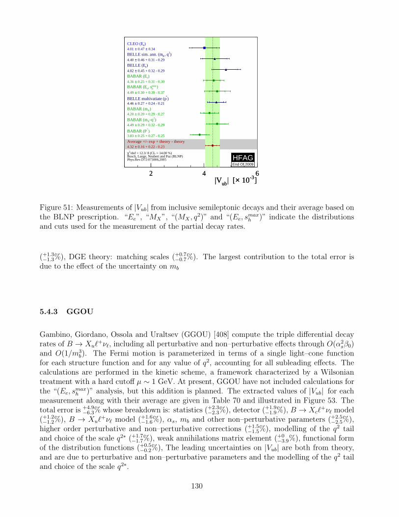
]-3 10×| [ub|V2 4 6
]-3 10×| [ub|V2 4 6
) eCLEO (E 0.34± 0.47 ±4.01
) 2, qXBELLE sim. ann. (m 0.46 + 0.31 - 0.29±4.40
) eBELLE (E 0.45 + 0.32 - 0.29±4.82
) eBABAR (E 0.25 + 0.31 - 0.30±4.36
) hmax, seBABAR (E
0.30 + 0.39 - 0.37±4.49
) *
BELLE multivatiate (p 0.27 + 0.24 - 0.21±4.46
) XBABAR (m 0.20 + 0.29 - 0.27±4.20
) 2-qXBABAR (m 0.29 + 0.32 - 0.29±4.49
) +
BABAR (P 0.25 + 0.27 - 0.25±3.83
Average +/- exp + theory - theory 0.16 + 0.22 - 0.23±4.32
HFAGEnd Of 2009
Bosch, Lange, Neubert and Paz (BLNP)Phys.Rev.D72:073006,2005
/dof = 12.3/ 8 (CL = 14.00 %)2χ
Figure 51: Measurements of |Vub| from inclusive semileptonic decays and their average based onthe BLNP prescription. “Ee”, “MX”, “(MX , q
2)” and “(Ee, smaxh )” indicate the distributions
and cuts used for the measurement of the partial decay rates.
(+1.3−1.3%), DGE theory: matching scales (+0.7
−0.7%). The largest contribution to the total error isdue to the effect of the uncertainty on mb
5.4.3 GGOU
Gambino, Giordano, Ossola and Uraltsev (GGOU) [408] compute the triple differential decayrates of B → Xuℓ
+νℓ, including all perturbative and non–perturbative effects through O(α2sβ0)
and O(1/m3b). The Fermi motion is parameterized in terms of a single light–cone function
for each structure function and for any value of q2, accounting for all subleading effects. Thecalculations are performed in the kinetic scheme, a framework characterized by a Wilsoniantreatment with a hard cutoff µ ∼ 1 GeV. At present, GGOU have not included calculations forthe “(Ee, s
maxh )” analysis, but this addition is planned. The extracted values of |Vub| for each
measurement along with their average are given in Table 70 and illustrated in Figure 53. Thetotal error is +4.9
−6.3% whose breakdown is: statistics (+2.3−2.3%), detector (+1.9
−1.9%), B → Xcℓ+νℓ model
(+1.2−1.2%), B → Xuℓ
+νℓ model (+1.6−1.6%), αs, mb and other non–perturbative parameters (+2.5
−2.5%),higher order perturbative and non–perturbative corrections (+1.5
−1.5%), modelling of the q2 tailand choice of the scale q2∗ (+1.7
−1.7%), weak annihilations matrix element (+0−3.9%), functional form
of the distribution functions (+0.5−0.2%), The leading uncertainties on |Vub| are both from theory,
and are due to perturbative and non–perturbative parameters and the modelling of the q2 tailand choice of the scale q2∗.
130
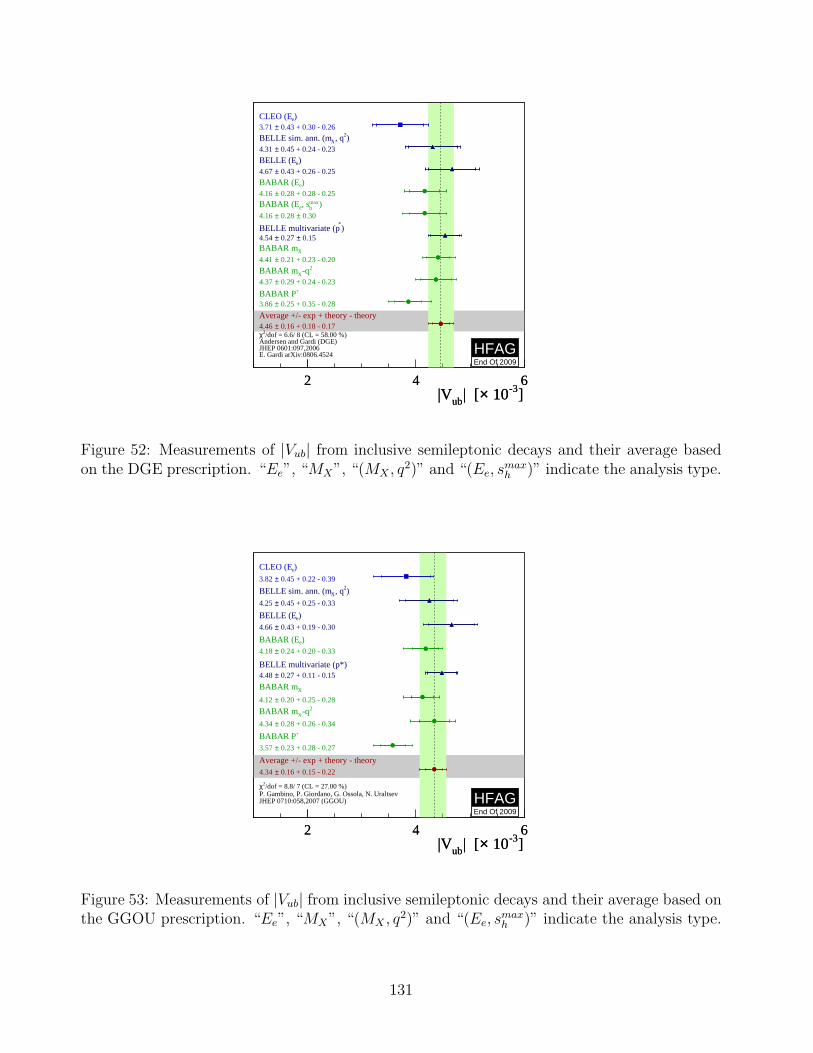
]-3 10×| [ub|V2 4 6
]-3 10×| [ub|V2 4 6
) eCLEO (E 0.43 + 0.30 - 0.26±3.71
) 2, qXBELLE sim. ann. (m 0.45 + 0.24 - 0.23±4.31
) eBELLE (E 0.43 + 0.26 - 0.25±4.67
) eBABAR (E 0.28 + 0.28 - 0.25±4.16
) hmax, seBABAR (E
0.30± 0.28 ±4.16
) *
BELLE multivariate (p 0.15± 0.27 ±4.54 XBABAR m
0.21 + 0.23 - 0.20±4.41
2-qXBABAR m 0.29 + 0.24 - 0.23±4.37
+BABAR P 0.25 + 0.35 - 0.28±3.86
Average +/- exp + theory - theory 0.16 + 0.18 - 0.17±4.46
HFAGEnd Of 2009
Andersen and Gardi (DGE)JHEP 0601:097,2006E. Gardi arXiv:0806.4524
/dof = 6.6/ 8 (CL = 58.00 %)2χ
Figure 52: Measurements of |Vub| from inclusive semileptonic decays and their average basedon the DGE prescription. “Ee”, “MX”, “(MX , q
2)” and “(Ee, smaxh )” indicate the analysis type.
]-3 10×| [ub|V2 4 6
]-3 10×| [ub|V2 4 6
) eCLEO (E 0.45 + 0.22 - 0.39±3.82
) 2, qXBELLE sim. ann. (m 0.45 + 0.25 - 0.33±4.25
) eBELLE (E 0.43 + 0.19 - 0.30±4.66
) eBABAR (E 0.24 + 0.20 - 0.33±4.18
BELLE multivariate (p*) 0.27 + 0.11 - 0.15±4.48
XBABAR m
0.20 + 0.25 - 0.28±4.12
2-qXBABAR m
0.28 + 0.26 - 0.34±4.34
+BABAR P 0.23 + 0.28 - 0.27±3.57
Average +/- exp + theory - theory 0.16 + 0.15 - 0.22±4.34
HFAGEnd Of 2009
P. Gambino, P. Giordano, G. Ossola, N. Uraltsev JHEP 0710:058,2007 (GGOU)
/dof = 8.8/ 7 (CL = 27.00 %)2χ
Figure 53: Measurements of |Vub| from inclusive semileptonic decays and their average based onthe GGOU prescription. “Ee”, “MX”, “(MX , q
2)” and “(Ee, smaxh )” indicate the analysis type.
131
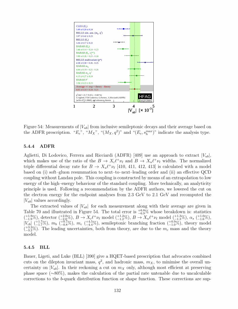
]-3 10×| [ub|V1 2 3 4 5
]-3 10×| [ub|V1 2 3 4 5
) eCLEO (E 0.24± 0.20 ±3.49
) 2, qXBELLE sim. ann. (m 0.23± 0.42 ±3.97
) eBELLE (E 0.22± 0.17 ±3.26
) eBABAR (E 0.14 + 0.24 - 0.23±3.46
) hmax, seBABAR (E
0.26 + 0.23 - 0.24±3.90
BELLE multivariate (p*) 0.30 + 0.26 - 0.25±4.58
XBABAR m 0.19 + 0.25 - 0.26±4.04
2-qXBABAR m 0.24± 0.27 ±4.15
+BABAR P 0.23± 0.23 ±3.56
Average +/- exp + theory - theory 0.14 + 0.24 - 0.21±4.05
HFAGEnd Of 2009
U.Aglietti, F.Di Lodovico, G.Ferrera , G.Ricciardi (ADFR)[arXiv:0711.0860], and references therein
/dof = 21.7/ 8 (CL = 0.60 %)2χ
Figure 54: Measurements of |Vub| from inclusive semileptonic decays and their average based onthe ADFR prescription. “Ee”, “MX”, “(MX , q
2)” and “(Ee, smaxh )” indicate the analysis type.
5.4.4 ADFR
Aglietti, Di Lodovico, Ferrera and Ricciardi (ADFR) [409] use an approach to extract |Vub|,which makes use of the ratio of the B → Xcℓ
+νℓ and B → Xuℓ+νℓ widths. The normalized
triple differential decay rate for B → Xuℓ+νℓ [410, 411, 412, 413] is calculated with a model
based on (i) soft–gluon resummation to next–to–next–leading order and (ii) an effective QCDcoupling without Landau pole. This coupling is constructed by means of an extrapolation to lowenergy of the high–energy behaviour of the standard coupling. More technically, an analyticityprinciple is used. Following a recommendation by the ADFR authors, we lowered the cut onthe electron energy for the endpoint analyses from 2.3 GeV to 2.1 GeV and recomputed the|Vub| values accordingly.
The extracted values of |Vub| for each measurement along with their average are given inTable 70 and illustrated in Figure 54. The total error is +6.8
−6.9% whose breakdown is: statistics(+1.9−1.9%), detector (+2.0
−2.0%), B → Xcℓ+νℓ model (+1.2
−1.2%), B → Xuℓ+νℓ model (+1.3
−1.3%), αs (+1.0−1.6%),
|Vcb| (+1.7−1.7%), mb (+0.7
−0.8%), mc (+4.5−4.4%), semileptonic branching fraction (+0.9
−1.0%), theory model(+3.2−3.2%). The leading uncertainties, both from theory, are due to the mc mass and the theorymodel.
5.4.5 BLL
Bauer, Ligeti, and Luke (BLL) [390] give a HQET-based prescription that advocates combinedcuts on the dilepton invariant mass, q2, and hadronic mass, mX , to minimise the overall un-certainty on |Vub|. In their reckoning a cut on mX only, although most efficient at preservingphase space (∼80%), makes the calculation of the partial rate untenable due to uncalculablecorrections to the b-quark distribution function or shape function. These corrections are sup-
132
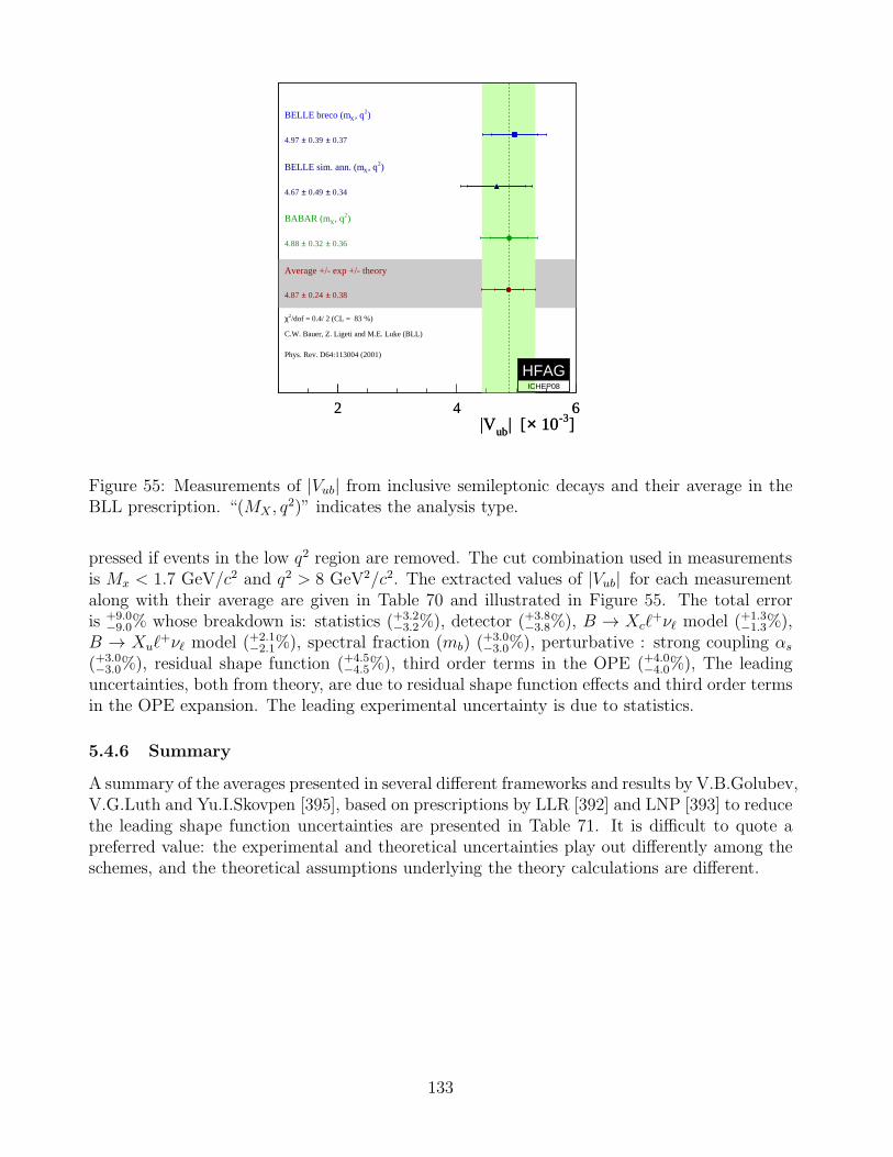
]-3 10×| [ub|V2 4 6
]-3 10×| [ub|V2 4 6
) 2, qXBELLE breco (m
0.37± 0.39 ±4.97
) 2, qXBELLE sim. ann. (m
0.34± 0.49 ±4.67
) 2, qXBABAR (m
0.36± 0.32 ±4.88
Average +/- exp +/- theory
0.38± 0.24 ±4.87
HFAGICHEP08
C.W. Bauer, Z. Ligeti and M.E. Luke (BLL)
Phys. Rev. D64:113004 (2001)
/dof = 0.4/ 2 (CL = 83 %)2χ
Figure 55: Measurements of |Vub| from inclusive semileptonic decays and their average in theBLL prescription. “(MX , q
2)” indicates the analysis type.
pressed if events in the low q2 region are removed. The cut combination used in measurementsis Mx < 1.7 GeV/c2 and q2 > 8 GeV2/c2. The extracted values of |Vub| for each measurementalong with their average are given in Table 70 and illustrated in Figure 55. The total erroris +9.0
−9.0% whose breakdown is: statistics (+3.2−3.2%), detector (+3.8
−3.8%), B → Xcℓ+νℓ model (+1.3
−1.3%),B → Xuℓ
+νℓ model (+2.1−2.1%), spectral fraction (mb) (
+3.0−3.0%), perturbative : strong coupling αs
(+3.0−3.0%), residual shape function (+4.5
−4.5%), third order terms in the OPE (+4.0−4.0%), The leading
uncertainties, both from theory, are due to residual shape function effects and third order termsin the OPE expansion. The leading experimental uncertainty is due to statistics.
5.4.6 Summary
A summary of the averages presented in several different frameworks and results by V.B.Golubev,V.G.Luth and Yu.I.Skovpen [395], based on prescriptions by LLR [392] and LNP [393] to reducethe leading shape function uncertainties are presented in Table 71. It is difficult to quote apreferred value: the experimental and theoretical uncertainties play out differently among theschemes, and the theoretical assumptions underlying the theory calculations are different.
133
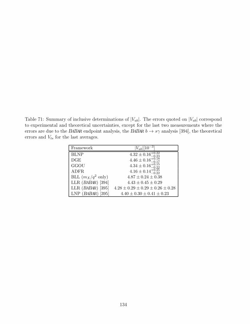
Table 71: Summary of inclusive determinations of |Vub|. The errors quoted on |Vub| correspondto experimental and theoretical uncertainties, except for the last two measurements where theerrors are due to the BABAR endpoint analysis, the BABAR b → sγ analysis [394], the theoreticalerrors and Vts for the last averages.
Framework |Vub|[10−3]
BLNP 4.32± 0.16+0.22−0.23
DGE 4.46± 0.16+0.18−0.17
GGOU 4.34± 0.16+0.15−0.22
ADFR 4.16± 0.14+0.25−0.22
BLL (mX/q2 only) 4.87 ± 0.24 ± 0.38
LLR (BABAR) [394] 4.43 ± 0.45 ± 0.29LLR (BABAR) [395] 4.28 ± 0.29 ± 0.29 ± 0.26 ± 0.28LNP (BABAR) [395] 4.40 ± 0.30 ± 0.41± 0.23
134
6 B decays to charmed hadrons
This section reports the updated contribution to the HFAG report from the “B → charm”group31. The mandate of the group is to compile measurements and perform averages of allavailable quantities related to B decays to charmed particles, excluding CP related quantities.To date the group has analyzed a total of 492 measurements reported in 148 papers, principallybranching fractions. The group aims to organize and present the copious information on Bdecays to charmed particles obtained from a combined sample of about two billion B mesonsfrom the BABAR, Belle and CDF Collaborations.
This huge sample of B mesons allows to measure decays to states with open or hiddencharm content with unprecedented precision. Branching fractions for rare B-meson decays ordecay chains of a few 10−7 are being measured with statistical uncertainties typically below30%, and new decay chains can be accessed with branching fractions down to 10−8. Resultsfor more common decay chains, with branching fractions around 10−4, are becoming precisionmeasurements, with uncertainties typically at the 3% level. Some decays have been observedfor the first time, for example B0 → J/ψη or B0 → Λ+
c pK−π+, with a branching fraction of
(9.6± 1.8)× 10−6 and (4.3± 1.4)× 10−5, respectively.The large sample of B mesons allows to greatly improve our understanding of recently
discovered new states with either hidden or open charm content, such as the X(3872), theY (3940),the Z(4430)−, the D∗−
sJ (2317) and D−sJ(2460) mesons. Measurements with many dif-
ferent final states for these particles are reported, allowing to shed more light on their nature.
The D0D∗0(2007) decay of the X(3872) has been observed for the first time, as well as the decay
into ψ(2S)γ. Using the branching fraction products B(B− → X(3872)K−)×B(X(3872) → f),a hierarchy can be established between the decay modes f : these branching fraction productsare found to be (1.67 ± 0.59) × 10−4, (0.12 ± 0.02) × 10−4, and (0.022 ± 0.005) × 10−4, for
D0D∗0(2007), J/ψπ+π− and J/ψγ, respectively. This is an important piece of information to
discriminate between various interpretations for the X(3872) state.The measurements are classified according to the decaying particle: Charged B, Neutral B
or Miscellaneous; the decay products and the type of quantity: branching fraction, productof branching fractions, ratio of branching fractions or other quantities. For the decay productclassification the below precedence order is used to ensure that each measurement appears inonly one category.
• new particles
• strange D mesons
• baryons
• J/ψ
• charmonium other than J/ψ
• multiple D, D∗ or D∗∗ mesons
• a single D∗ or D∗∗ meson
• a single D meson
• other particles
31The HFAG/BtoCharm group was formed in the spring of 2005; it performs its work using an XML databasebacked web application.
135
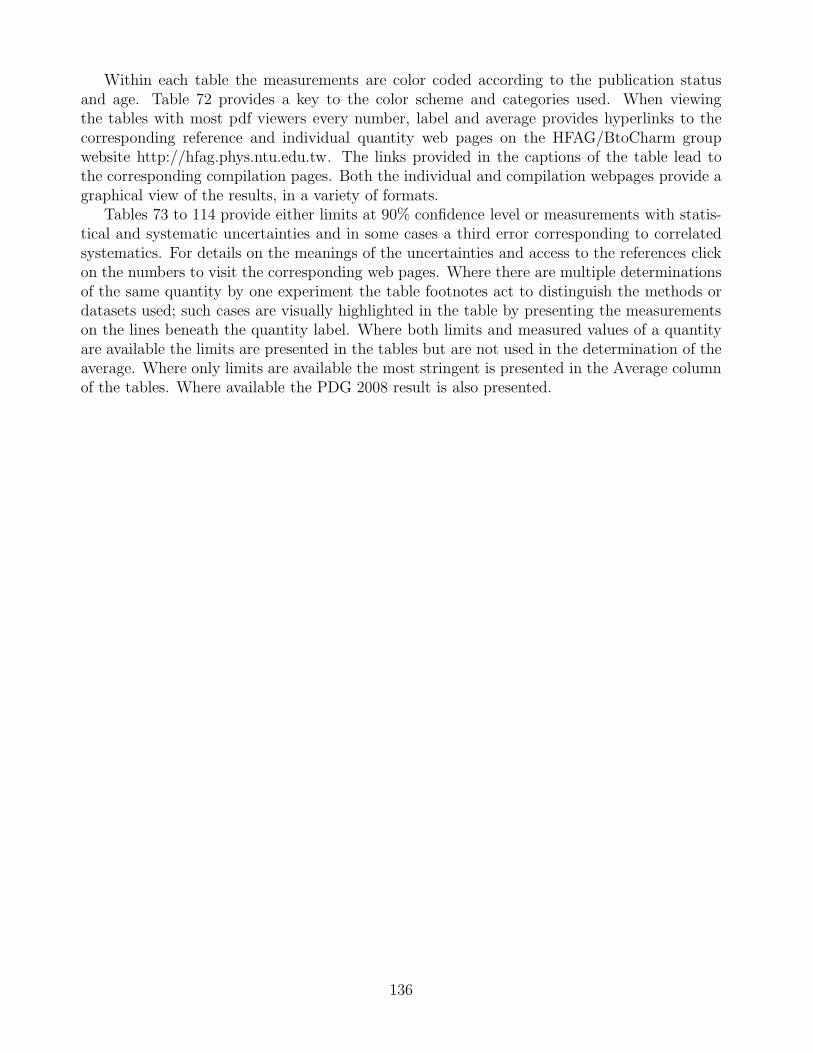
Within each table the measurements are color coded according to the publication statusand age. Table 72 provides a key to the color scheme and categories used. When viewingthe tables with most pdf viewers every number, label and average provides hyperlinks to thecorresponding reference and individual quantity web pages on the HFAG/BtoCharm groupwebsite http://hfag.phys.ntu.edu.tw. The links provided in the captions of the table lead tothe corresponding compilation pages. Both the individual and compilation webpages provide agraphical view of the results, in a variety of formats.
Tables 73 to 114 provide either limits at 90% confidence level or measurements with statis-tical and systematic uncertainties and in some cases a third error corresponding to correlatedsystematics. For details on the meanings of the uncertainties and access to the references clickon the numbers to visit the corresponding web pages. Where there are multiple determinationsof the same quantity by one experiment the table footnotes act to distinguish the methods ordatasets used; such cases are visually highlighted in the table by presenting the measurementson the lines beneath the quantity label. Where both limits and measured values of a quantityare available the limits are presented in the tables but are not used in the determination of theaverage. Where only limits are available the most stringent is presented in the Average columnof the tables. Where available the PDG 2008 result is also presented.
136

Table 72: Key to the colors used to classify the results presented in tables 73 to 114. When viewing these tables in a pdfviewer each number, label and average provides a hyperlink to the corresponding online version provided by the charm subgroupwebsite http://hfag.phys.ntu.edu.tw/b2charm/. Where an experiment has multiple determinations of a single quantity they aredistinguished by the table footnotes.
Class Definition
waiting Results without a preprint availablepubhot Results published during or after 2009prehot Preprint released during or after 2009pub Results published after or during 2008pre Preprint released after or during 2008pubold Results published before 2008preold Preprint released before 2008error Incomplete information to classifysuperceeded Results superceeded by more recent measurements from the same experimentinactive Results in the process of being entered into the databasenoquo Results without quotes
137
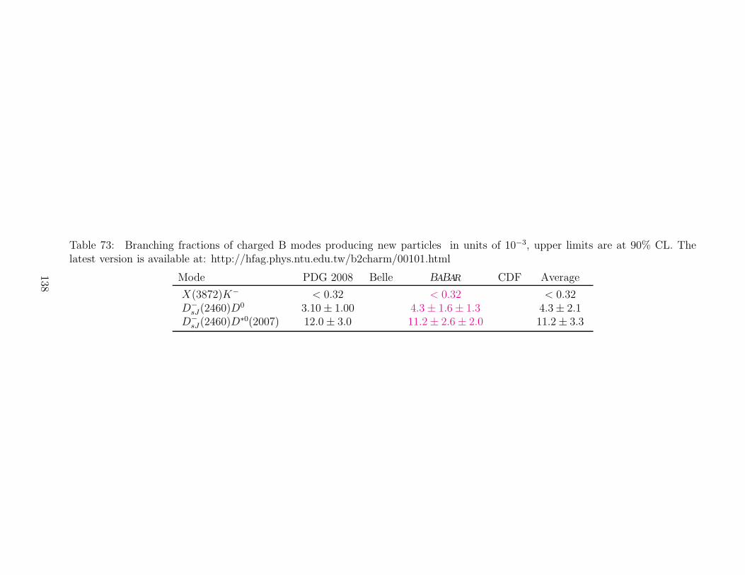
Table 73: Branching fractions of charged B modes producing new particles in units of 10−3, upper limits are at 90% CL. Thelatest version is available at: http://hfag.phys.ntu.edu.tw/b2charm/00101.html
Mode PDG 2008 Belle BABAR CDF Average
X(3872)K− < 0.32 < 0.32 < 0.32D−sJ(2460)D
0 3.10± 1.00 4.3± 1.6± 1.3 4.3± 2.1D−sJ(2460)D
∗0(2007) 12.0± 3.0 11.2± 2.6± 2.0 11.2± 3.3
138
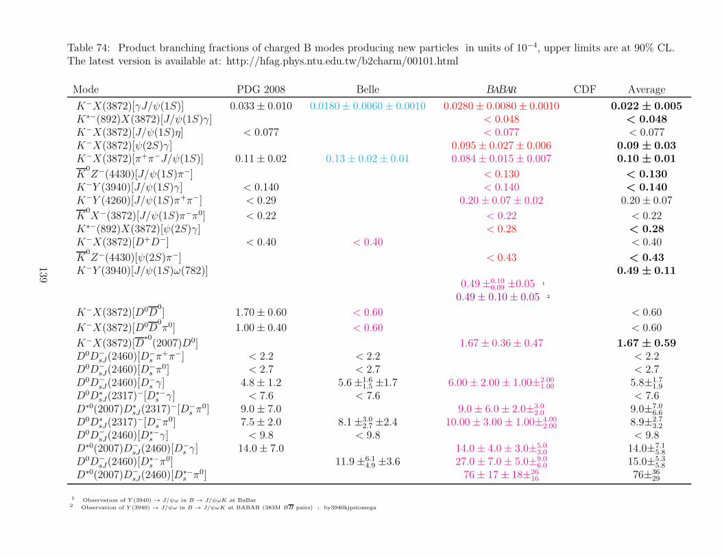
Table 74: Product branching fractions of charged B modes producing new particles in units of 10−4, upper limits are at 90% CL.The latest version is available at: http://hfag.phys.ntu.edu.tw/b2charm/00101.html
Mode PDG 2008 Belle BABAR CDF Average
K−X(3872)[γJ/ψ(1S)] 0.033± 0.010 0.0180± 0.0060± 0.0010 0.0280± 0.0080± 0.0010 0.022 ± 0.005K∗−(892)X(3872)[J/ψ(1S)γ] < 0.048 < 0.048K−X(3872)[J/ψ(1S)η] < 0.077 < 0.077 < 0.077K−X(3872)[ψ(2S)γ] 0.095± 0.027± 0.006 0.09 ± 0.03K−X(3872)[π+π−J/ψ(1S)] 0.11± 0.02 0.13± 0.02± 0.01 0.084± 0.015± 0.007 0.10 ± 0.01
K0Z−(4430)[J/ψ(1S)π−] < 0.130 < 0.130
K−Y (3940)[J/ψ(1S)γ] < 0.140 < 0.140 < 0.140K−Y (4260)[J/ψ(1S)π+π−] < 0.29 0.20± 0.07± 0.02 0.20± 0.07
K0X−(3872)[J/ψ(1S)π−π0] < 0.22 < 0.22 < 0.22
K∗−(892)X(3872)[ψ(2S)γ] < 0.28 < 0.28K−X(3872)[D+D−] < 0.40 < 0.40 < 0.40
K0Z−(4430)[ψ(2S)π−] < 0.43 < 0.43
K−Y (3940)[J/ψ(1S)ω(782)] 0.49 ± 0.110.49±0.10
0.09 ±0.05 1
0.49± 0.10± 0.05 2
K−X(3872)[D0D0] 1.70± 0.60 < 0.60 < 0.60
K−X(3872)[D0D0π0] 1.00± 0.40 < 0.60 < 0.60
K−X(3872)[D∗0(2007)D0] 1.67± 0.36± 0.47 1.67 ± 0.59
D0D−sJ(2460)[D
−s π
+π−] < 2.2 < 2.2 < 2.2D0D−
sJ(2460)[D−s π
0] < 2.7 < 2.7 < 2.7D0D−
sJ(2460)[D−s γ] 4.8± 1.2 5.6±1.6
1.5 ±1.7 6.00± 2.00± 1.00±2.001.00 5.8±1.7
1.9
D0D∗sJ(2317)
−[D∗−s γ] < 7.6 < 7.6 < 7.6
D∗0(2007)D∗sJ(2317)
−[D−s π
0] 9.0± 7.0 9.0± 6.0± 2.0±3.02.0 9.0±7.0
6.6
D0D∗sJ(2317)
−[D−s π
0] 7.5± 2.0 8.1±3.02.7 ±2.4 10.00± 3.00± 1.00±4.00
2.00 8.9±2.73.2
D0D−sJ(2460)[D
∗−s γ] < 9.8 < 9.8 < 9.8
D∗0(2007)D−sJ(2460)[D
−s γ] 14.0± 7.0 14.0± 4.0± 3.0±5.0
3.0 14.0±7.15.8
D0D−sJ(2460)[D
∗−s π0] 11.9±6.1
4.9 ±3.6 27.0± 7.0± 5.0±9.06.0 15.0±5.3
5.8
D∗0(2007)D−sJ(2460)[D
∗−s π0] 76± 17± 18±26
16 76±3629
1 Observation of Y (3940) → J/ψω in B → J/ψωK at BaBar2 Observation of Y (3940) → J/ψω in B → J/ψωK at BABAR (383M BB pairs) ; by3940kjpsiomega
139
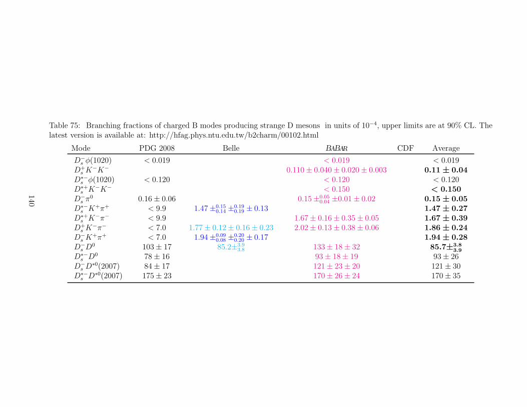
Table 75: Branching fractions of charged B modes producing strange D mesons in units of 10−4, upper limits are at 90% CL. Thelatest version is available at: http://hfag.phys.ntu.edu.tw/b2charm/00102.html
Mode PDG 2008 Belle BABAR CDF Average
D−s φ(1020) < 0.019 < 0.019 < 0.019
D+s K
−K− 0.110± 0.040± 0.020± 0.003 0.11 ± 0.04D∗−s φ(1020) < 0.120 < 0.120 < 0.120
D∗+s K−K− < 0.150 < 0.150
D−s π
0 0.16± 0.06 0.15±0.050.04 ±0.01± 0.02 0.15 ± 0.05
D∗−s K+π+ < 9.9 1.47±0.15
0.14 ±0.190.19 ± 0.13 1.47 ± 0.27
D∗+s K−π− < 9.9 1.67± 0.16± 0.35± 0.05 1.67 ± 0.39
D+s K
−π− < 7.0 1.77± 0.12± 0.16± 0.23 2.02± 0.13± 0.38± 0.06 1.86 ± 0.24D−s K
+π+ < 7.0 1.94±0.090.08 ±0.20
0.20 ± 0.17 1.94 ± 0.28D−s D
0 103± 17 85.2±3.93.8 133± 18± 32 85.7±3.8
3.9
D∗−s D0 78± 16 93± 18± 19 93± 26
D−s D
∗0(2007) 84± 17 121± 23± 20 121± 30D∗−s D∗0(2007) 175± 23 170± 26± 24 170± 35
140
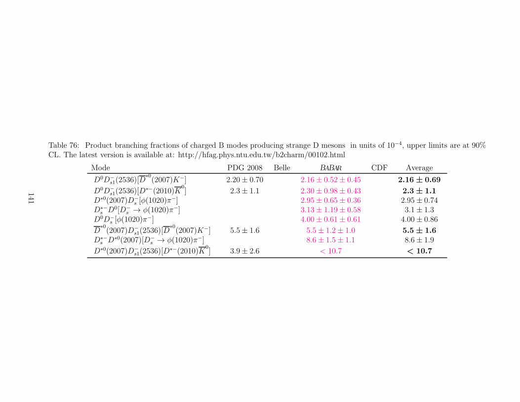
Table 76: Product branching fractions of charged B modes producing strange D mesons in units of 10−4, upper limits are at 90%CL. The latest version is available at: http://hfag.phys.ntu.edu.tw/b2charm/00102.html
Mode PDG 2008 Belle BABAR CDF Average
D0D−s1(2536)[D
∗0(2007)K−] 2.20± 0.70 2.16± 0.52± 0.45 2.16 ± 0.69
D0D−s1(2536)[D
∗−(2010)K0] 2.3± 1.1 2.30± 0.98± 0.43 2.3 ± 1.1
D∗0(2007)D−s [φ(1020)π
−] 2.95± 0.65± 0.36 2.95± 0.74D∗−s D0[D−
s → φ(1020)π−] 3.13± 1.19± 0.58 3.1± 1.3D0D−
s [φ(1020)π−] 4.00± 0.61± 0.61 4.00± 0.86
D∗0(2007)D−
s1(2536)[D∗0(2007)K−] 5.5± 1.6 5.5± 1.2± 1.0 5.5 ± 1.6
D∗−s D∗0(2007)[D−
s → φ(1020)π−] 8.6± 1.5± 1.1 8.6± 1.9
D∗0(2007)D−s1(2536)[D
∗−(2010)K0] 3.9± 2.6 < 10.7 < 10.7
141
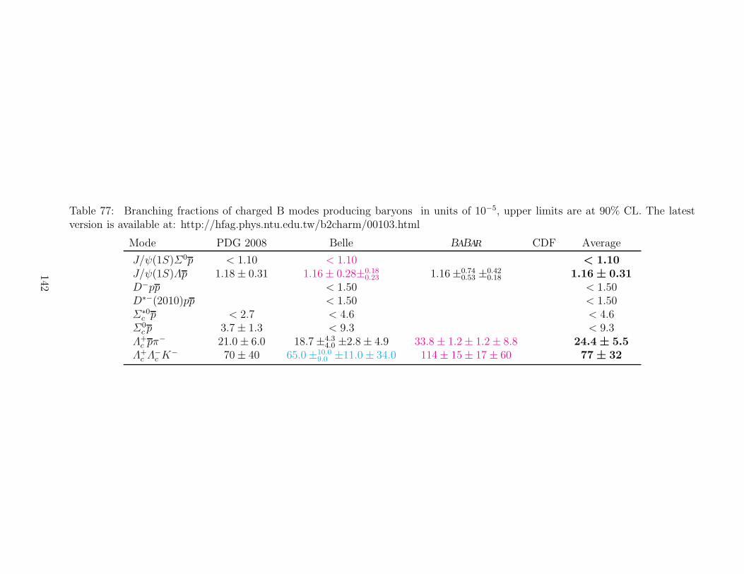
Table 77: Branching fractions of charged B modes producing baryons in units of 10−5, upper limits are at 90% CL. The latestversion is available at: http://hfag.phys.ntu.edu.tw/b2charm/00103.html
Mode PDG 2008 Belle BABAR CDF Average
J/ψ(1S)Σ0p < 1.10 < 1.10 < 1.10J/ψ(1S)Λp 1.18± 0.31 1.16± 0.28±0.18
0.23 1.16±0.740.53 ±0.42
0.18 1.16 ± 0.31D−pp < 1.50 < 1.50D∗−(2010)pp < 1.50 < 1.50Σ∗0c p < 2.7 < 4.6 < 4.6
Σ0c p 3.7± 1.3 < 9.3 < 9.3
Λ+c pπ
− 21.0± 6.0 18.7±4.34.0 ±2.8± 4.9 33.8± 1.2± 1.2± 8.8 24.4 ± 5.5
Λ+c Λ
−c K
− 70± 40 65.0±10.09.0 ±11.0± 34.0 114± 15± 17± 60 77 ± 32
142
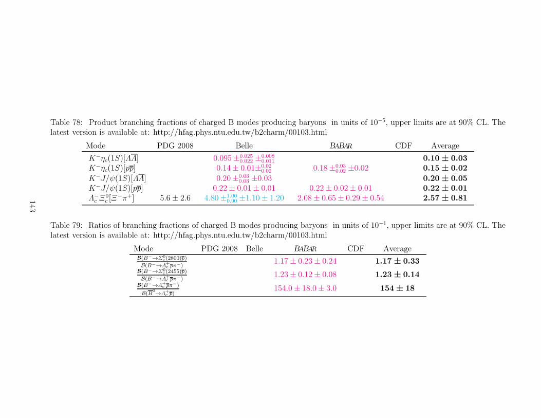
Table 78: Product branching fractions of charged B modes producing baryons in units of 10−5, upper limits are at 90% CL. Thelatest version is available at: http://hfag.phys.ntu.edu.tw/b2charm/00103.html
Mode PDG 2008 Belle BABAR CDF Average
K−ηc(1S)[ΛΛ] 0.095±0.0250.022 ±0.008
0.011 0.10 ± 0.03K−ηc(1S)[pp] 0.14± 0.01±0.02
0.02 0.18±0.030.02 ±0.02 0.15 ± 0.02
K−J/ψ(1S)[ΛΛ] 0.20±0.030.03 ±0.03 0.20 ± 0.05
K−J/ψ(1S)[pp] 0.22± 0.01± 0.01 0.22± 0.02± 0.01 0.22 ± 0.01Λ−c Ξ
0c [Ξ
−π+] 5.6± 2.6 4.80±1.000.90 ±1.10± 1.20 2.08± 0.65± 0.29± 0.54 2.57 ± 0.81
Table 79: Ratios of branching fractions of charged B modes producing baryons in units of 10−1, upper limits are at 90% CL. Thelatest version is available at: http://hfag.phys.ntu.edu.tw/b2charm/00103.html
Mode PDG 2008 Belle BABAR CDF AverageB(B−→Σ0
c (2800)p)
B(B−→Λ+c pπ−)
1.17± 0.23± 0.24 1.17 ± 0.33B(B−→Σ0
c (2455)p)
B(B−→Λ+c pπ−)
1.23± 0.12± 0.08 1.23 ± 0.14B(B−→Λ+
c pπ−)
B(B0→Λ+
c p)154.0± 18.0± 3.0 154 ± 18
143
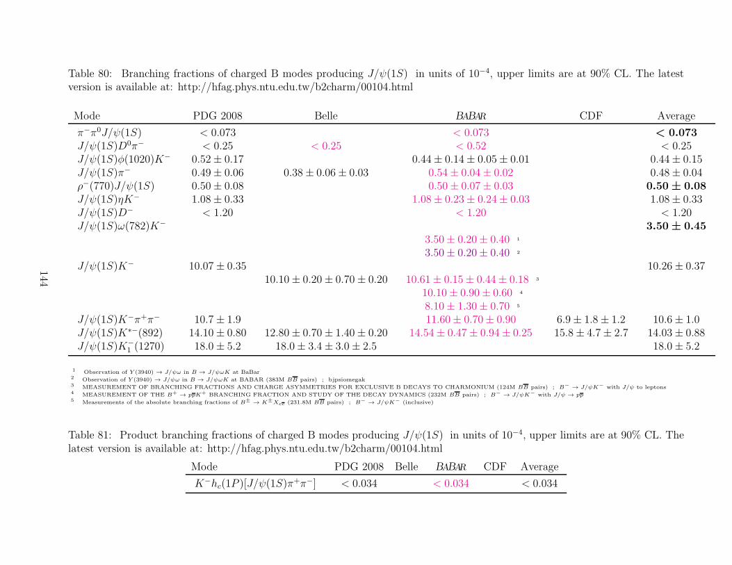
Table 80: Branching fractions of charged B modes producing J/ψ(1S) in units of 10−4, upper limits are at 90% CL. The latestversion is available at: http://hfag.phys.ntu.edu.tw/b2charm/00104.html
Mode PDG 2008 Belle BABAR CDF Average
π−π0J/ψ(1S) < 0.073 < 0.073 < 0.073J/ψ(1S)D0π− < 0.25 < 0.25 < 0.52 < 0.25J/ψ(1S)φ(1020)K− 0.52± 0.17 0.44± 0.14± 0.05± 0.01 0.44± 0.15J/ψ(1S)π− 0.49± 0.06 0.38± 0.06± 0.03 0.54± 0.04± 0.02 0.48± 0.04ρ−(770)J/ψ(1S) 0.50± 0.08 0.50± 0.07± 0.03 0.50 ± 0.08J/ψ(1S)ηK− 1.08± 0.33 1.08± 0.23± 0.24± 0.03 1.08± 0.33J/ψ(1S)D− < 1.20 < 1.20 < 1.20J/ψ(1S)ω(782)K− 3.50 ± 0.45
3.50± 0.20± 0.40 1
3.50± 0.20± 0.40 2
J/ψ(1S)K− 10.07± 0.35 10.26± 0.3710.10± 0.20± 0.70± 0.20 10.61± 0.15± 0.44± 0.18 3
10.10± 0.90± 0.60 4
8.10± 1.30± 0.70 5
J/ψ(1S)K−π+π− 10.7± 1.9 11.60± 0.70± 0.90 6.9± 1.8± 1.2 10.6± 1.0J/ψ(1S)K∗−(892) 14.10± 0.80 12.80± 0.70± 1.40± 0.20 14.54± 0.47± 0.94± 0.25 15.8± 4.7± 2.7 14.03± 0.88J/ψ(1S)K−
1 (1270) 18.0± 5.2 18.0± 3.4± 3.0± 2.5 18.0± 5.2
1 Observation of Y (3940) → J/ψω in B → J/ψωK at BaBar2 Observation of Y (3940) → J/ψω in B → J/ψωK at BABAR (383M BB pairs) ; bjpsiomegak3 MEASUREMENT OF BRANCHING FRACTIONS AND CHARGE ASYMMETRIES FOR EXCLUSIVE B DECAYS TO CHARMONIUM (124M BB pairs) ; B− → J/ψK− with J/ψ to leptons4 MEASUREMENT OF THE B+ → ppK+ BRANCHING FRACTION AND STUDY OF THE DECAY DYNAMICS (232M BB pairs) ; B− → J/ψK− with J/ψ → pp5 Measurements of the absolute branching fractions of B± → K±Xcc (231.8M BB pairs) ; B− → J/ψK− (inclusive)
Table 81: Product branching fractions of charged B modes producing J/ψ(1S) in units of 10−4, upper limits are at 90% CL. Thelatest version is available at: http://hfag.phys.ntu.edu.tw/b2charm/00104.html
Mode PDG 2008 Belle BABAR CDF Average
K−hc(1P )[J/ψ(1S)π+π−] < 0.034 < 0.034 < 0.034
144
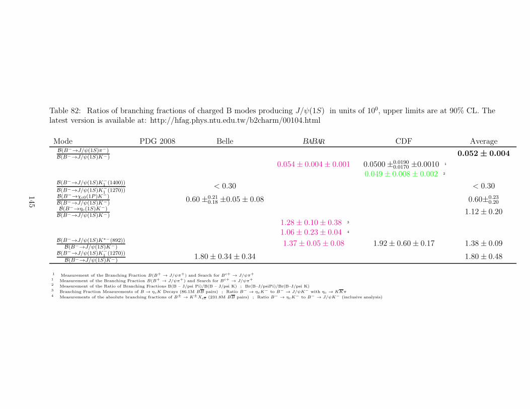
Table 82: Ratios of branching fractions of charged B modes producing J/ψ(1S) in units of 100, upper limits are at 90% CL. Thelatest version is available at: http://hfag.phys.ntu.edu.tw/b2charm/00104.html
Mode PDG 2008 Belle BABAR CDF AverageB(B−→J/ψ(1S)π−)B(B−→J/ψ(1S)K−)
0.052 ± 0.004
0.054± 0.004± 0.001 0.0500±0.01900.0170 ±0.0010 1
0.049± 0.008± 0.002 2
B(B−→J/ψ(1S)K−1 (1400))
B(B−→J/ψ(1S)K−1 (1270))
< 0.30 < 0.30B(B−→χc0(1P )K−)B(B−→J/ψ(1S)K−)
0.60±0.210.18 ±0.05± 0.08 0.60±0.23
0.20B(B−→ηc(1S)K−)B(B−→J/ψ(1S)K−)
1.12± 0.20
1.28± 0.10± 0.38 3
1.06± 0.23± 0.04 4
B(B−→J/ψ(1S)K∗−(892))B(B−→J/ψ(1S)K−)
1.37± 0.05± 0.08 1.92± 0.60± 0.17 1.38± 0.09B(B−→J/ψ(1S)K−
1 (1270))
B(B−→J/ψ(1S)K−)1.80± 0.34± 0.34 1.80± 0.48
1 Measurement of the Branching Fraction B(B+ → J/ψπ+) and Search for Bc+ → J/ψπ+
1 Measurement of the Branching Fraction B(B+ → J/ψπ+) and Search for Bc+ → J/ψπ+
2 Measurement of the Ratio of Branching Fractions B(B – J/psi Pi)/B(B – J/psi K) ; Br(B–J/psiPi)/Br(B–J/psi K)3 Branching Fraction Measurements of B → ηcK Decays (86.1M BB pairs) ; Ratio B− → ηcK
− to B− → J/ψK− with ηc → KKπ4 Measurements of the absolute branching fractions of B± → K±Xcc (231.8M BB pairs) ; Ratio B− → ηcK
− to B− → J/ψK− (inclusive analysis)
145
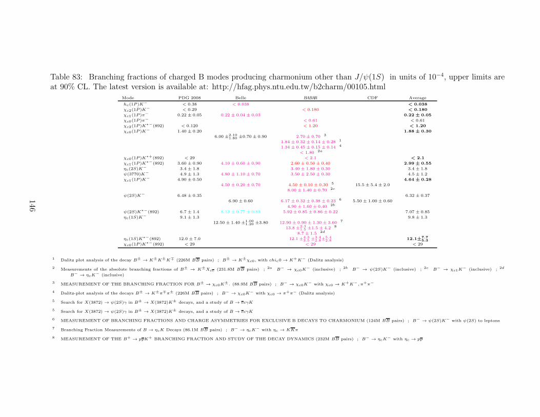
Table 83: Branching fractions of charged B modes producing charmonium other than J/ψ(1S) in units of 10−4, upper limits areat 90% CL. The latest version is available at: http://hfag.phys.ntu.edu.tw/b2charm/00105.html
Mode PDG 2008 Belle BABAR CDF Average
hc(1P )K− < 0.38 < 0.038 < 0.038
χc2(1P )K− < 0.29 < 0.180 < 0.180
χc1(1P )π− 0.22 ± 0.05 0.22 ± 0.04 ± 0.03 0.22 ± 0.05
χc0(1P )π− < 0.61 < 0.61
χc2(1P )K∗−(892) < 0.120 < 1.20 < 1.20
χc0(1P )K− 1.40 ± 0.20 1.88 ± 0.30
6.00 ±2.101.80 ±0.70 ± 0.90 2.70 ± 0.70 3
1.84 ± 0.32 ± 0.14 ± 0.28 1
1.34 ± 0.45 ± 0.15 ± 0.14 4
< 1.80 2a
χc0(1P )K∗+(892) < 29 < 2.1 < 2.1
χc1(1P )K∗−(892) 3.60 ± 0.90 4.10 ± 0.60 ± 0.90 2.60 ± 0.50 ± 0.40 2.99 ± 0.55
ηc(2S)K− 3.4 ± 1.8 3.40 ± 1.80 ± 0.30 3.4 ± 1.8
ψ(3770)K− 4.9 ± 1.3 4.80 ± 1.10 ± 0.70 3.50 ± 2.50 ± 0.30 4.5 ± 1.2
χc1(1P )K− 4.90 ± 0.50 4.64 ± 0.28
4.50 ± 0.20 ± 0.70 4.50 ± 0.10 ± 0.30 5 15.5 ± 5.4 ± 2.0
8.00 ± 1.40 ± 0.70 2c
ψ(2S)K− 6.48 ± 0.35 6.32 ± 0.37
6.90 ± 0.60 6.17 ± 0.32 ± 0.38 ± 0.23 6 5.50 ± 1.00 ± 0.60
4.90 ± 1.60 ± 0.40 2b
ψ(2S)K∗−(892) 6.7 ± 1.4 8.13 ± 0.77 ± 0.89 5.92 ± 0.85 ± 0.86 ± 0.22 7.07 ± 0.85
ηc(1S)K− 9.1 ± 1.3 9.8 ± 1.3
12.50 ± 1.40 ±1.001.20 ±3.80 12.90 ± 0.90 ± 1.30 ± 3.60 7
13.8 ±2.31.5 ±1.5 ± 4.2 8
8.7 ± 1.5 2d
ηc(1S)K∗−(892) 12.0 ± 7.0 12.1 ±4.3
3.5 ±3.42.8±
5.42.8 12.1±7.7
5.3
χc0(1P )K∗−(892) < 29 < 29 < 29
1 Dalitz plot analysis of the decay B± → K±K±K∓ (226M BB pairs) ; B± → K±χc0, with chic0 → K+K− (Dalitz analysis)
2 Measurements of the absolute branching fractions of B± → K±Xcc (231.8M BB pairs) ; 2a B− → χc0K− (inclusive) ; 2b B− → ψ(2S)K− (inclusive) ; 2c B− → χc1K
− (inclusive) ; 2d
B− → ηcK− (inclusive)
3 MEASUREMENT OF THE BRANCHING FRACTION FOR B± → χc0K±. (88.9M BB pairs) ; B− → χc0K
− with χc0 → K+K−, π+π−
4 Dalitz-plot analysis of the decays B± → K±π∓π± (226M BB pairs) ; B− → χc0K− with χc0 → π+π− (Dalitz analysis)
5 Search for X(3872) → ψ(2S)γ in B± → X(3872)K± decays, and a study of B → ccγK
5 Search for X(3872) → ψ(2S)γ in B± → X(3872)K± decays, and a study of B → ccγK
6 MEASUREMENT OF BRANCHING FRACTIONS AND CHARGE ASYMMETRIES FOR EXCLUSIVE B DECAYS TO CHARMONIUM (124M BB pairs) ; B− → ψ(2S)K− with ψ(2S) to leptons
7 Branching Fraction Measurements of B → ηcK Decays (86.1M BB pairs) ; B− → ηcK− with ηc → KKπ
8 MEASUREMENT OF THE B+ → ppK+ BRANCHING FRACTION AND STUDY OF THE DECAY DYNAMICS (232M BB pairs) ; B− → ηcK− with ηc → pp
146
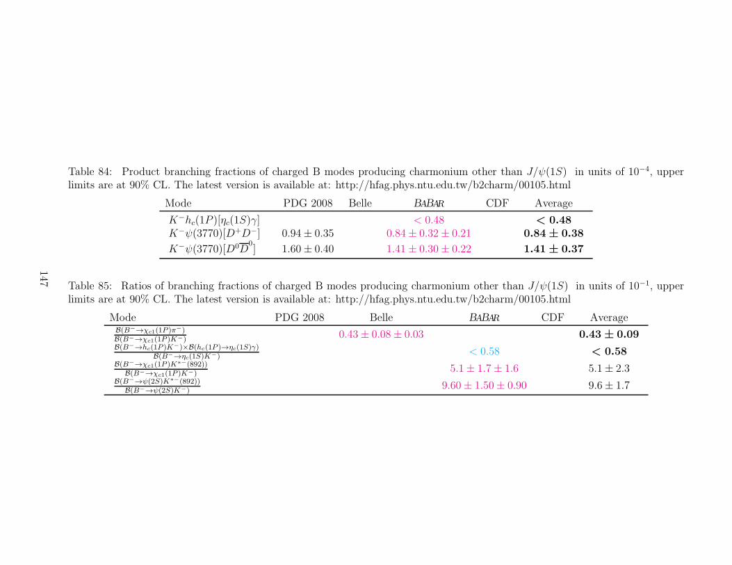
Table 84: Product branching fractions of charged B modes producing charmonium other than J/ψ(1S) in units of 10−4, upperlimits are at 90% CL. The latest version is available at: http://hfag.phys.ntu.edu.tw/b2charm/00105.html
Mode PDG 2008 Belle BABAR CDF Average
K−hc(1P )[ηc(1S)γ] < 0.48 < 0.48K−ψ(3770)[D+D−] 0.94± 0.35 0.84± 0.32± 0.21 0.84 ± 0.38
K−ψ(3770)[D0D0] 1.60± 0.40 1.41± 0.30± 0.22 1.41 ± 0.37
Table 85: Ratios of branching fractions of charged B modes producing charmonium other than J/ψ(1S) in units of 10−1, upperlimits are at 90% CL. The latest version is available at: http://hfag.phys.ntu.edu.tw/b2charm/00105.html
Mode PDG 2008 Belle BABAR CDF AverageB(B−→χc1(1P )π−)B(B−→χc1(1P )K−)
0.43± 0.08± 0.03 0.43 ± 0.09B(B−→hc(1P )K−)×B(hc(1P )→ηc(1S)γ)
B(B−→ηc(1S)K−)< 0.58 < 0.58
B(B−→χc1(1P )K∗−(892))B(B−→χc1(1P )K−)
5.1± 1.7± 1.6 5.1± 2.3B(B−→ψ(2S)K∗−(892))
B(B−→ψ(2S)K−)9.60± 1.50± 0.90 9.6± 1.7
147
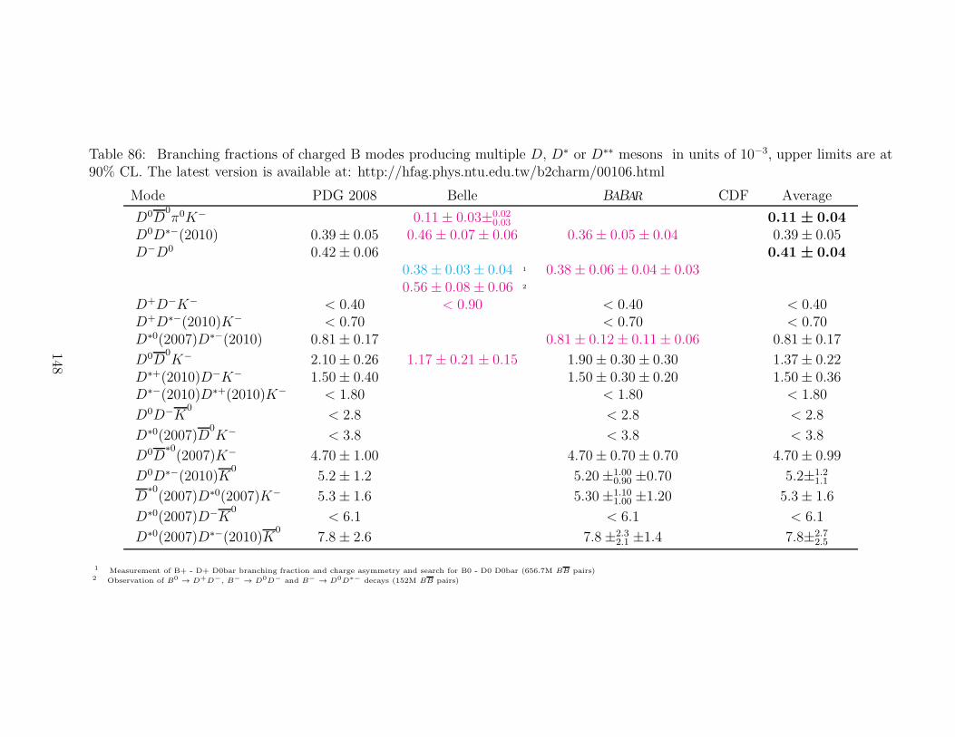
Table 86: Branching fractions of charged B modes producing multiple D, D∗ or D∗∗ mesons in units of 10−3, upper limits are at90% CL. The latest version is available at: http://hfag.phys.ntu.edu.tw/b2charm/00106.html
Mode PDG 2008 Belle BABAR CDF Average
D0D0π0K− 0.11± 0.03±0.02
0.03 0.11 ± 0.04D0D∗−(2010) 0.39± 0.05 0.46± 0.07± 0.06 0.36± 0.05± 0.04 0.39± 0.05D−D0 0.42± 0.06 0.41 ± 0.04
0.38± 0.03± 0.04 1 0.38± 0.06± 0.04± 0.030.56± 0.08± 0.06 2
D+D−K− < 0.40 < 0.90 < 0.40 < 0.40D+D∗−(2010)K− < 0.70 < 0.70 < 0.70D∗0(2007)D∗−(2010) 0.81± 0.17 0.81± 0.12± 0.11± 0.06 0.81± 0.17
D0D0K− 2.10± 0.26 1.17± 0.21± 0.15 1.90± 0.30± 0.30 1.37± 0.22
D∗+(2010)D−K− 1.50± 0.40 1.50± 0.30± 0.20 1.50± 0.36D∗−(2010)D∗+(2010)K− < 1.80 < 1.80 < 1.80
D0D−K0
< 2.8 < 2.8 < 2.8
D∗0(2007)D0K− < 3.8 < 3.8 < 3.8
D0D∗0(2007)K− 4.70± 1.00 4.70± 0.70± 0.70 4.70± 0.99
D0D∗−(2010)K0
5.2± 1.2 5.20±1.000.90 ±0.70 5.2±1.2
1.1
D∗0(2007)D∗0(2007)K− 5.3± 1.6 5.30±1.10
1.00 ±1.20 5.3± 1.6
D∗0(2007)D−K0
< 6.1 < 6.1 < 6.1
D∗0(2007)D∗−(2010)K0
7.8± 2.6 7.8±2.32.1 ±1.4 7.8±2.7
2.5
1 Measurement of B+ - D+ D0bar branching fraction and charge asymmetry and search for B0 - D0 D0bar (656.7M BB pairs)2 Observation of B0 → D+D−, B− → D0D− and B− → D0D∗− decays (152M BB pairs)
148
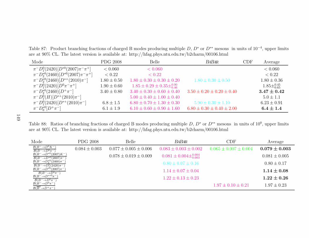
Table 87: Product branching fractions of charged B modes producing multiple D, D∗ or D∗∗ mesons in units of 10−4, upper limitsare at 90% CL. The latest version is available at: http://hfag.phys.ntu.edu.tw/b2charm/00106.html
Mode PDG 2008 Belle BABAR CDF Average
π−D01(2420)[D
∗0(2007)π−π+] < 0.060 < 0.060 < 0.060π−D∗0
2 (2460)[D∗0(2007)π−π+] < 0.22 < 0.22 < 0.22π−D∗0
2 (2460)[D∗+(2010)π−] 1.80± 0.50 1.80± 0.30± 0.30± 0.20 1.80± 0.30± 0.50 1.80± 0.36π−D0
1(2420)[D0π−π+] 1.90± 0.60 1.85± 0.29± 0.35±0.00
0.46 1.85±0.450.65
π−D∗02 (2460)[D+π−] 3.40± 0.80 3.40± 0.30± 0.60± 0.40 3.50± 0.20± 0.20± 0.40 3.47 ± 0.42
π−D01(H)[D∗+(2010)π−] 5.00± 0.40± 1.00± 0.40 5.0± 1.1
π−D01(2420)[D
∗+(2010)π−] 6.8± 1.5 6.80± 0.70± 1.30± 0.30 5.90± 0.30± 1.10 6.23± 0.91π−D∗0
0 [D+π−] 6.1± 1.9 6.10± 0.60± 0.90± 1.60 6.80± 0.30± 0.40± 2.00 6.4 ± 1.4
Table 88: Ratios of branching fractions of charged B modes producing multiple D, D∗ or D∗∗ mesons in units of 100, upper limitsare at 90% CL. The latest version is available at: http://hfag.phys.ntu.edu.tw/b2charm/00106.html
Mode PDG 2008 Belle BABAR CDF AverageB(B−→D0K−)B(B−→D0π−)
0.084± 0.003 0.077± 0.005± 0.006 0.083± 0.003± 0.002 0.065± 0.007± 0.004 0.079 ± 0.003B(B−→D∗0(2007)K−)B(B−→D∗0(2007)π−)
0.078± 0.019± 0.009 0.081± 0.004±0.0040.003 0.081± 0.005
B(B−→D∗02 (2460)π−)
B(B−→D01(2420)π
−)0.80± 0.07± 0.16 0.80± 0.17
B(B−→D∗0(2007)π−)B(B−→D0π−)
1.14± 0.07± 0.04 1.14 ± 0.08B(B−→D∗∗0π−)B(B−→D0π−)
1.22± 0.13± 0.23 1.22 ± 0.26B(B−→D0π−)
B(B0→D+π−)
1.97± 0.10± 0.21 1.97± 0.23
149
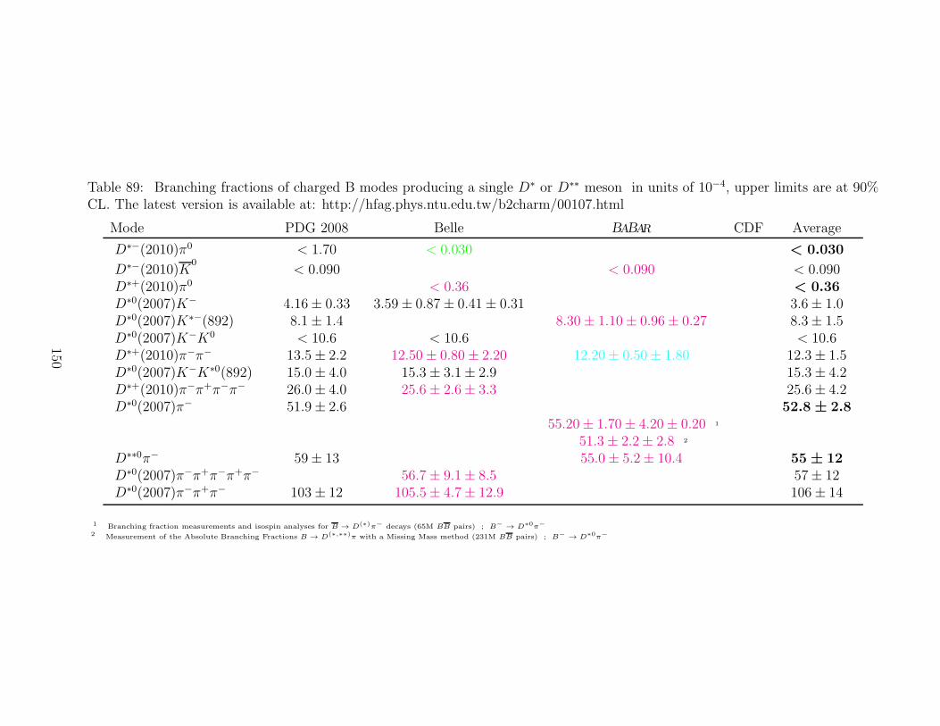
Table 89: Branching fractions of charged B modes producing a single D∗ or D∗∗ meson in units of 10−4, upper limits are at 90%CL. The latest version is available at: http://hfag.phys.ntu.edu.tw/b2charm/00107.html
Mode PDG 2008 Belle BABAR CDF Average
D∗−(2010)π0 < 1.70 < 0.030 < 0.030
D∗−(2010)K0
< 0.090 < 0.090 < 0.090D∗+(2010)π0 < 0.36 < 0.36D∗0(2007)K− 4.16± 0.33 3.59± 0.87± 0.41± 0.31 3.6± 1.0D∗0(2007)K∗−(892) 8.1± 1.4 8.30± 1.10± 0.96± 0.27 8.3± 1.5D∗0(2007)K−K0 < 10.6 < 10.6 < 10.6D∗+(2010)π−π− 13.5± 2.2 12.50± 0.80± 2.20 12.20± 0.50± 1.80 12.3± 1.5D∗0(2007)K−K∗0(892) 15.0± 4.0 15.3± 3.1± 2.9 15.3± 4.2D∗+(2010)π−π+π−π− 26.0± 4.0 25.6± 2.6± 3.3 25.6± 4.2D∗0(2007)π− 51.9± 2.6 52.8 ± 2.8
55.20± 1.70± 4.20± 0.20 1
51.3± 2.2± 2.8 2
D∗∗0π− 59± 13 55.0± 5.2± 10.4 55 ± 12D∗0(2007)π−π+π−π+π− 56.7± 9.1± 8.5 57± 12D∗0(2007)π−π+π− 103± 12 105.5± 4.7± 12.9 106± 14
1 Branching fraction measurements and isospin analyses for B → D(∗)π− decays (65M BB pairs) ; B− → D∗0π−
2 Measurement of the Absolute Branching Fractions B → D(∗,∗∗)π with a Missing Mass method (231M BB pairs) ; B− → D∗0π−
150
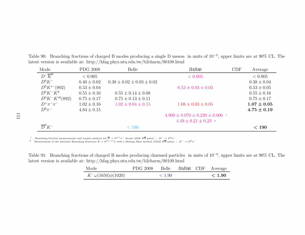
Table 90: Branching fractions of charged B modes producing a single D meson in units of 10−3, upper limits are at 90% CL. Thelatest version is available at: http://hfag.phys.ntu.edu.tw/b2charm/00108.html
Mode PDG 2008 Belle BABAR CDF Average
D−K0
< 0.005 < 0.005 < 0.005D0K− 0.40± 0.02 0.38± 0.02± 0.03± 0.02 0.38± 0.04D0K∗−(892) 0.53± 0.04 0.53± 0.03± 0.03 0.53± 0.05D0K−K0 0.55± 0.16 0.55± 0.14± 0.08 0.55± 0.16D0K−K∗0(892) 0.75± 0.17 0.75± 0.13± 0.11 0.75± 0.17D+π−π− 1.02± 0.16 1.02± 0.04± 0.15 1.08± 0.03± 0.05 1.07 ± 0.05D0π− 4.84± 0.15 4.75 ± 0.19
4.900± 0.070± 0.220± 0.006 1
4.49± 0.21± 0.23 2
D0K− < 190 < 190
1 Branching fraction measurements and isospin analyses for B → D(∗)π− decays (65M BB pairs) ; B− → D0π−
2 Measurement of the Absolute Branching Fractions B → D(∗,∗∗)π with a Missing Mass method (231M BB pairs) ; B− → D0π−
Table 91: Branching fractions of charged B modes producing charmed particles in units of 10−6, upper limits are at 90% CL. Thelatest version is available at: http://hfag.phys.ntu.edu.tw/b2charm/00109.html
Mode PDG 2008 Belle BABAR CDF Average
K−ω(1650)φ(1020) < 1.90 < 1.90
151
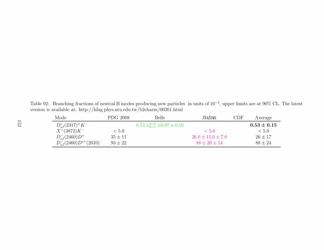
Table 92: Branching fractions of neutral B modes producing new particles in units of 10−4, upper limits are at 90% CL. The latestversion is available at: http://hfag.phys.ntu.edu.tw/b2charm/00201.html
Mode PDG 2008 Belle BABAR CDF Average
D∗sJ(2317)
+K− 0.53±0.130.14 ±0.07± 0.02 0.53 ± 0.15
X+(3872)K− < 5.0 < 5.0 < 5.0D−sJ(2460)D
+ 35± 11 26.0± 15.0± 7.0 26± 17D−sJ(2460)D
∗+(2010) 93± 22 88± 20± 14 88± 24
152
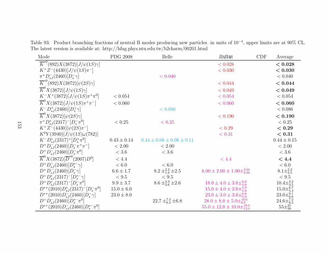
Table 93: Product branching fractions of neutral B modes producing new particles in units of 10−4, upper limits are at 90% CL.The latest version is available at: http://hfag.phys.ntu.edu.tw/b2charm/00201.html
Mode PDG 2008 Belle BABAR CDF Average
K∗0(892)X(3872)[J/ψ(1S)γ] < 0.028 < 0.028
K+Z−(4430)[J/ψ(1S)π−] < 0.030 < 0.030π+D−
sJ(2460)[D−s γ] < 0.040 < 0.040
K∗0(892)X(3872)[ψ(2S)γ] < 0.044 < 0.044
K0X(3872)[J/ψ(1S)γ] < 0.049 < 0.049
K−X+(3872)[J/ψ(1S)π+π0] < 0.054 < 0.054 < 0.054
K0X(3872)[J/ψ(1S)π+π−] < 0.060 < 0.060 < 0.060
K−D+sJ(2460)[D
+s γ] < 0.086 < 0.086
K0X(3872)[ψ(2S)γ] < 0.190 < 0.190
π+D∗sJ(2317)
−[D−s π
0] < 0.25 < 0.25 < 0.25K+Z−(4430)[ψ(2S)π−] < 0.29 < 0.29K0Y (3940)[J/ψ(1S)ω(782)] < 0.31 < 0.31K−D∗
sJ(2317)+[D+
s π0] 0.43± 0.14 0.44± 0.08± 0.06± 0.11 0.44± 0.15
D+D−sJ(2460)[D
−s π
+π−] < 2.00 < 2.00 < 2.00D+D−
sJ(2460)[D−s π
0] < 3.6 < 3.6 < 3.6
K0X(3872)[D
∗0(2007)D0] < 4.4 < 4.4 < 4.4
D+D−sJ(2460)[D
∗−s γ] < 6.0 < 6.0 < 6.0
D+D−sJ(2460)[D
−s γ] 6.6± 1.7 8.2±2.2
1.9 ±2.5 8.00± 2.00± 1.00±3.002.00 8.1±2.2
2.5
D+D∗sJ(2317)
−[D∗−s γ] < 9.5 < 9.5 < 9.5
D+D∗sJ(2317)
−[D−s π
0] 9.9± 3.7 8.6±3.32.6 ±2.6 18.0± 4.0± 3.0±6.0
4.0 10.4±3.23.5
D∗+(2010)D∗sJ(2317)
−[D−s π
0] 15.0± 6.0 15.0± 4.0± 2.0±5.03.0 15.0±6.7
5.4
D∗+(2010)D−sJ(2460)[D
−s γ] 23.0± 8.0 23.0± 3.0± 3.0±8.0
5.0 23.0±9.16.6
D+D−sJ(2460)[D
∗−s π0] 22.7±7.3
6.2 ±6.8 28.0± 8.0± 5.0±10.06.0 24.6±7.2
8.2
D∗+(2010)D−sJ(2460)[D
∗−s π0] 55.0± 12.0± 10.0±19.0
12.0 55±2520
153
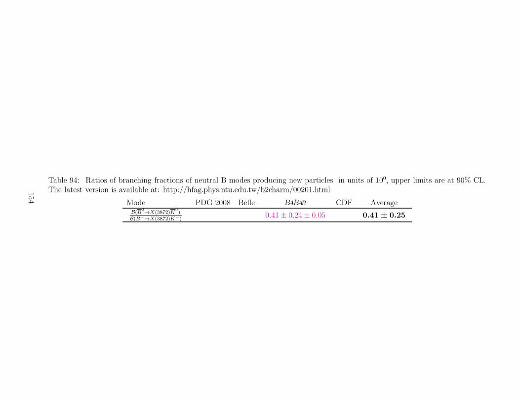
Table 94: Ratios of branching fractions of neutral B modes producing new particles in units of 100, upper limits are at 90% CL.The latest version is available at: http://hfag.phys.ntu.edu.tw/b2charm/00201.html
Mode PDG 2008 Belle BABAR CDF AverageB(B
0→X(3872)K
0)
B(B−→X(3872)K−)0.41± 0.24± 0.05 0.41 ± 0.25
154
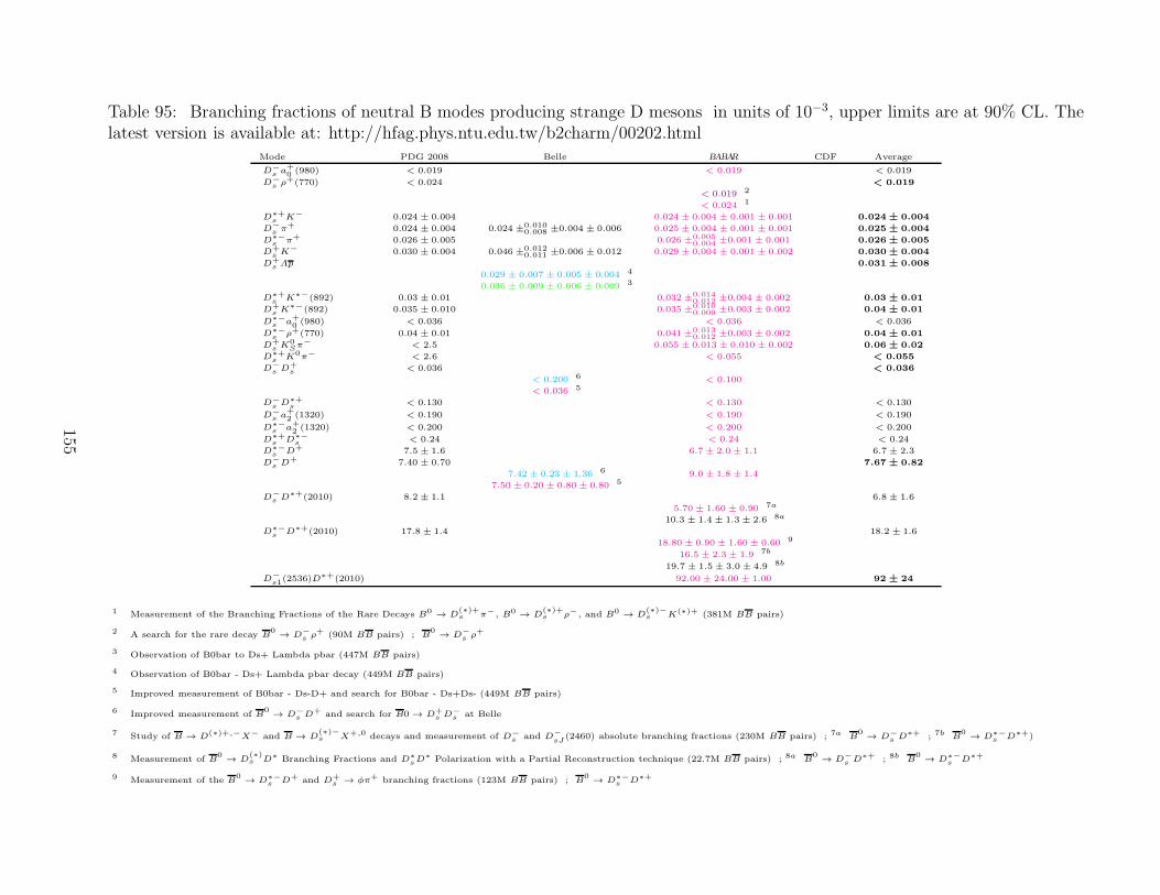
Table 95: Branching fractions of neutral B modes producing strange D mesons in units of 10−3, upper limits are at 90% CL. Thelatest version is available at: http://hfag.phys.ntu.edu.tw/b2charm/00202.html
Mode PDG 2008 Belle BABAR CDF Average
D−s a
+0 (980) < 0.019 < 0.019 < 0.019
D−s ρ
+(770) < 0.024 < 0.019
< 0.019 2
< 0.024 1
D∗+s K− 0.024 ± 0.004 0.024 ± 0.004 ± 0.001 ± 0.001 0.024 ± 0.004
D−s π
+ 0.024 ± 0.004 0.024 ±0.0100.008 ±0.004 ± 0.006 0.025 ± 0.004 ± 0.001 ± 0.001 0.025 ± 0.004
D∗−s π+ 0.026 ± 0.005 0.026 ±0.005
0.004 ±0.001 ± 0.001 0.026 ± 0.005
D+s K
− 0.030 ± 0.004 0.046 ±0.0120.011 ±0.006 ± 0.012 0.029 ± 0.004 ± 0.001 ± 0.002 0.030 ± 0.004
D+s Λp 0.031 ± 0.008
0.029 ± 0.007 ± 0.005 ± 0.004 4
0.036 ± 0.009 ± 0.006 ± 0.009 3
D∗+s K∗−(892) 0.03 ± 0.01 0.032 ±0.014
0.012 ±0.004 ± 0.002 0.03 ± 0.01
D+s K
∗−(892) 0.035 ± 0.010 0.035 ±0.0100.009 ±0.003 ± 0.002 0.04 ± 0.01
D∗−s a+0 (980) < 0.036 < 0.036 < 0.036
D∗−s ρ+(770) 0.04 ± 0.01 0.041 ±0.013
0.012 ±0.003 ± 0.002 0.04 ± 0.01
D+s K
0Sπ
− < 2.5 0.055 ± 0.013 ± 0.010 ± 0.002 0.06 ± 0.02
D∗+s K0π− < 2.6 < 0.055 < 0.055
D−s D
+s < 0.036 < 0.036
< 0.200 6 < 0.100
< 0.036 5
D−s D
∗+s < 0.130 < 0.130 < 0.130
D−s a
+2 (1320) < 0.190 < 0.190 < 0.190
D∗−s a+2 (1320) < 0.200 < 0.200 < 0.200
D∗+s D∗−
s < 0.24 < 0.24 < 0.24
D∗−s D+ 7.5 ± 1.6 6.7 ± 2.0 ± 1.1 6.7 ± 2.3
D−s D
+ 7.40 ± 0.70 7.67 ± 0.82
7.42 ± 0.23 ± 1.36 6 9.0 ± 1.8 ± 1.4
7.50 ± 0.20 ± 0.80 ± 0.80 5
D−s D
∗+(2010) 8.2 ± 1.1 6.8 ± 1.6
5.70 ± 1.60 ± 0.90 7a
10.3 ± 1.4 ± 1.3 ± 2.6 8a
D∗−s D∗+(2010) 17.8 ± 1.4 18.2 ± 1.6
18.80 ± 0.90 ± 1.60 ± 0.60 9
16.5 ± 2.3 ± 1.9 7b
19.7 ± 1.5 ± 3.0 ± 4.9 8b
D−s1(2536)D
∗+(2010) 92.00 ± 24.00 ± 1.00 92 ± 24
1 Measurement of the Branching Fractions of the Rare Decays B0 → D(∗)+s π−, B0 → D
(∗)+s ρ−, and B0 → D
(∗)−s K(∗)+ (381M BB pairs)
2 A search for the rare decay B0
→ D−s ρ
+ (90M BB pairs) ; B0
→ D−s ρ
+
3 Observation of B0bar to Ds+ Lambda pbar (447M BB pairs)
4 Observation of B0bar - Ds+ Lambda pbar decay (449M BB pairs)
5 Improved measurement of B0bar - Ds-D+ and search for B0bar - Ds+Ds- (449M BB pairs)
6 Improved measurement of B0
→ D−s D
+ and search for B0 → D+s D
−s at Belle
7 Study of B → D(∗)+,−X− and B → D(∗)−s X+,0 decays and measurement of D−
s and D−sJ
(2460) absolute branching fractions (230M BB pairs) ; 7a B0
→ D−s D
∗+ ; 7b B0
→ D∗−s D∗+)
8 Measurement of B0
→ D(∗)s D∗ Branching Fractions and D∗
sD∗ Polarization with a Partial Reconstruction technique (22.7M BB pairs) ; 8a B
0→ D−
s D∗+ ; 8b B
0→ D∗−
s D∗+
9 Measurement of the B0
→ D∗−s D+ and D+
s → φπ+ branching fractions (123M BB pairs) ; B0
→ D∗−s D∗+
155
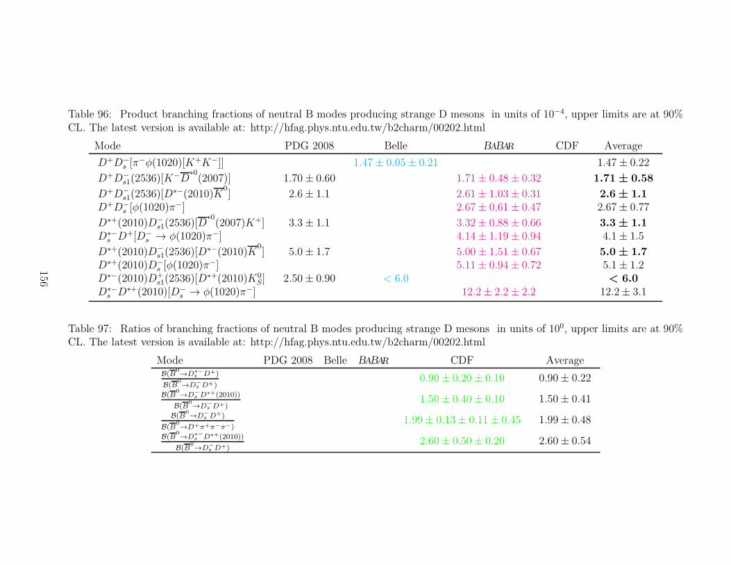
Table 96: Product branching fractions of neutral B modes producing strange D mesons in units of 10−4, upper limits are at 90%CL. The latest version is available at: http://hfag.phys.ntu.edu.tw/b2charm/00202.html
Mode PDG 2008 Belle BABAR CDF Average
D+D−s [π
−φ(1020)[K+K−]] 1.47± 0.05± 0.21 1.47± 0.22
D+D−s1(2536)[K
−D∗0(2007)] 1.70± 0.60 1.71± 0.48± 0.32 1.71 ± 0.58
D+D−s1(2536)[D
∗−(2010)K0] 2.6± 1.1 2.61± 1.03± 0.31 2.6 ± 1.1
D+D−s [φ(1020)π
−] 2.67± 0.61± 0.47 2.67± 0.77
D∗+(2010)D−s1(2536)[D
∗0(2007)K+] 3.3± 1.1 3.32± 0.88± 0.66 3.3 ± 1.1
D∗−s D+[D−
s → φ(1020)π−] 4.14± 1.19± 0.94 4.1± 1.5
D∗+(2010)D−s1(2536)[D
∗−(2010)K0] 5.0± 1.7 5.00± 1.51± 0.67 5.0 ± 1.7
D∗+(2010)D−s [φ(1020)π
−] 5.11± 0.94± 0.72 5.1± 1.2D∗−(2010)D+
s1(2536)[D∗+(2010)K0
S] 2.50± 0.90 < 6.0 < 6.0D∗−s D∗+(2010)[D−
s → φ(1020)π−] 12.2± 2.2± 2.2 12.2± 3.1
Table 97: Ratios of branching fractions of neutral B modes producing strange D mesons in units of 100, upper limits are at 90%CL. The latest version is available at: http://hfag.phys.ntu.edu.tw/b2charm/00202.html
Mode PDG 2008 Belle BABAR CDF AverageB(B
0→D∗−
s D+)
B(B0→D−
s D+)0.90± 0.20± 0.10 0.90± 0.22
B(B0→D−
s D∗+(2010))
B(B0→D−
s D+)1.50± 0.40± 0.10 1.50± 0.41
B(B0→D−
s D+)
B(B0→D+π+π−π−)
1.99± 0.13± 0.11± 0.45 1.99± 0.48
B(B0→D∗−
s D∗+(2010))
B(B0→D−
s D+)2.60± 0.50± 0.20 2.60± 0.54
156
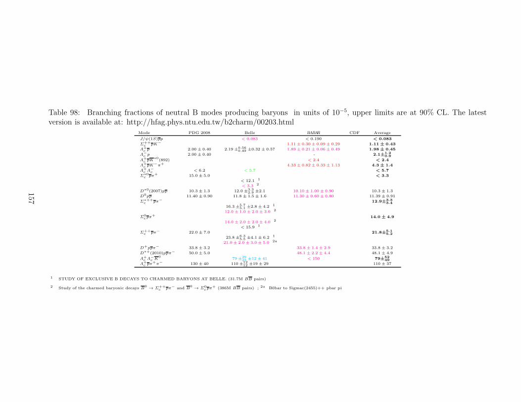
Table 98: Branching fractions of neutral B modes producing baryons in units of 10−5, upper limits are at 90% CL. The latestversion is available at: http://hfag.phys.ntu.edu.tw/b2charm/00203.html
Mode PDG 2008 Belle BABAR CDF Average
J/ψ(1S)pp < 0.083 < 0.190 < 0.083
Σ++c pK− 1.11 ± 0.30 ± 0.09 ± 0.29 1.11 ± 0.43
Λ+c p 2.00 ± 0.40 2.19 ±0.56
0.49 ±0.32 ± 0.57 1.89 ± 0.21 ± 0.06 ± 0.49 1.98 ± 0.45
Λ−c p 2.00 ± 0.40 - 2.1±1.2
0.9
Λ+c pK
∗0(892) < 2.4 < 2.4
Λ+c pK
−π+ 4.33 ± 0.82 ± 0.33 ± 1.13 4.3 ± 1.4
Λ+c Λ
−c < 6.2 < 5.7 < 5.7
Σ∗0c pπ+ 15.0 ± 5.0 < 3.3
< 12.1 1
< 3.3 2
D∗0(2007)pp 10.3 ± 1.3 12.0 ±3.32.9 ±2.1 10.10 ± 1.00 ± 0.90 10.3 ± 1.3
D0pp 11.40 ± 0.90 11.8 ± 1.5 ± 1.6 11.30 ± 0.60 ± 0.80 11.39 ± 0.91
Σ∗++c pπ−
12.9±3.3
3.4
16.3 ±5.75.1 ±2.8 ± 4.2 1
12.0 ± 1.0 ± 2.0 ± 3.0 2
Σ0cpπ
+14.0 ± 4.9
14.0 ± 2.0 ± 2.0 ± 4.0 2
< 15.9 1
Σ++c pπ− 22.0 ± 7.0 21.8±5.1
5.2
23.8 ±6.35.5 ±4.1 ± 6.2 1
21.0 ± 2.0 ± 3.0 ± 5.0 2a
D+ppπ− 33.8 ± 3.2 33.8 ± 1.4 ± 2.9 33.8 ± 3.2
D∗+(2010)ppπ− 50.0 ± 5.0 48.1 ± 2.2 ± 4.4 48.1 ± 4.9
Λ+c Λ
−c K
079 ±29
23 ±12 ± 41 < 150 79±52
49
Λ+c pπ
+π− 130 ± 40 110 ±1212 ±19 ± 29 110 ± 37
1 STUDY OF EXCLUSIVE B DECAYS TO CHARMED BARYONS AT BELLE. (31.7M BB pairs)
2 Study of the charmed baryonic decays B0
→ Σ++c pπ− and B
0→ Σ0
cpπ+ (386M BB pairs) ; 2a B0bar to Sigmac(2455)++ pbar pi
157
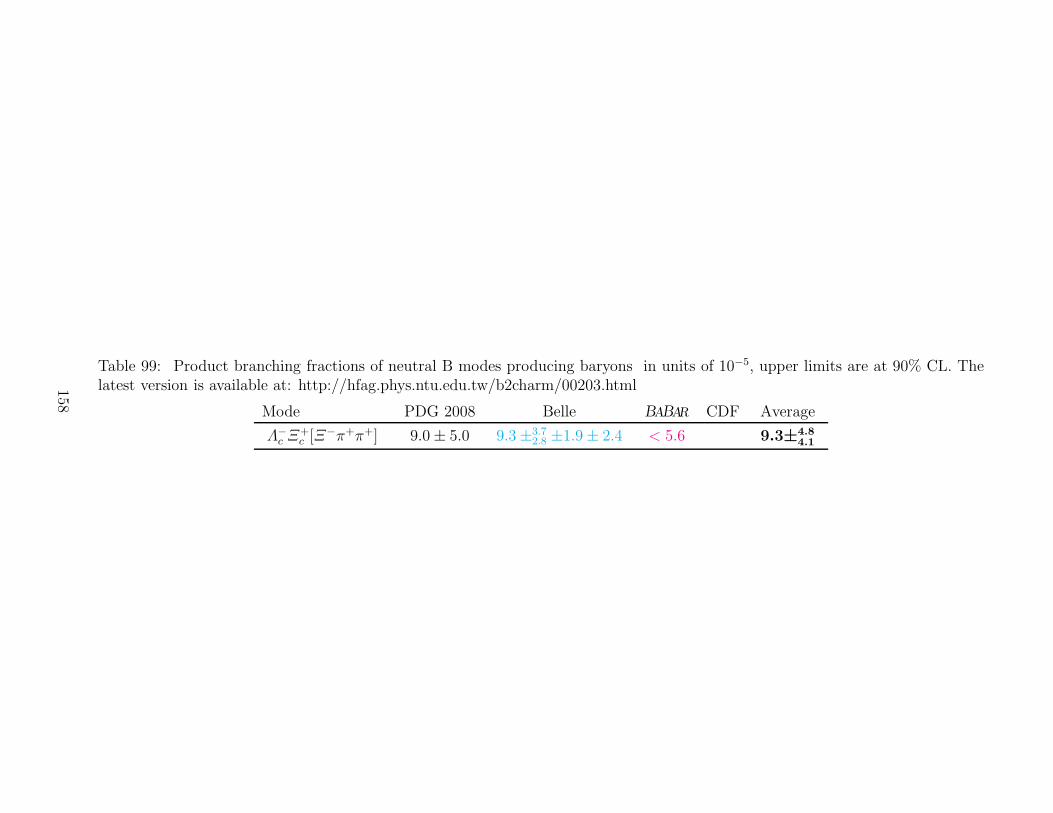
Table 99: Product branching fractions of neutral B modes producing baryons in units of 10−5, upper limits are at 90% CL. Thelatest version is available at: http://hfag.phys.ntu.edu.tw/b2charm/00203.html
Mode PDG 2008 Belle BABAR CDF Average
Λ−c Ξ
+c [Ξ
−π+π+] 9.0± 5.0 9.3±3.72.8 ±1.9± 2.4 < 5.6 9.3±4.8
4.1
158
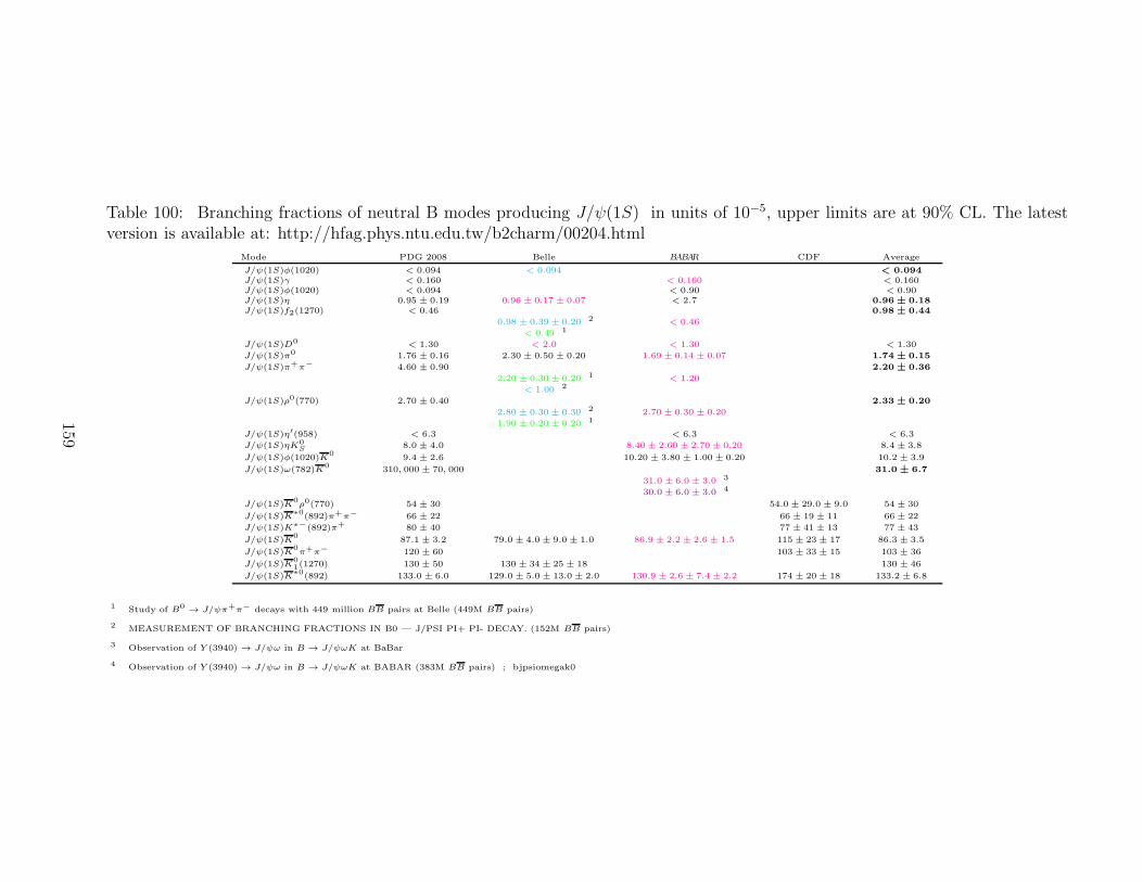
Table 100: Branching fractions of neutral B modes producing J/ψ(1S) in units of 10−5, upper limits are at 90% CL. The latestversion is available at: http://hfag.phys.ntu.edu.tw/b2charm/00204.html
Mode PDG 2008 Belle BABAR CDF Average
J/ψ(1S)φ(1020) < 0.094 < 0.094 < 0.094
J/ψ(1S)γ < 0.160 < 0.160 < 0.160J/ψ(1S)φ(1020) < 0.094 < 0.90 < 0.90J/ψ(1S)η 0.95 ± 0.19 0.96 ± 0.17 ± 0.07 < 2.7 0.96 ± 0.18
J/ψ(1S)f2(1270) < 0.46 0.98 ± 0.44
0.98 ± 0.39 ± 0.20 2 < 0.46
< 0.49 1
J/ψ(1S)D0 < 1.30 < 2.0 < 1.30 < 1.30
J/ψ(1S)π0 1.76 ± 0.16 2.30 ± 0.50 ± 0.20 1.69 ± 0.14 ± 0.07 1.74 ± 0.15
J/ψ(1S)π+π− 4.60 ± 0.90 2.20 ± 0.36
2.20 ± 0.30 ± 0.20 1 < 1.20
< 1.00 2
J/ψ(1S)ρ0(770) 2.70 ± 0.40 2.33 ± 0.20
2.80 ± 0.30 ± 0.30 2 2.70 ± 0.30 ± 0.20
1.90 ± 0.20 ± 0.20 1
J/ψ(1S)η′(958) < 6.3 < 6.3 < 6.3
J/ψ(1S)ηK0S 8.0 ± 4.0 8.40 ± 2.60 ± 2.70 ± 0.20 8.4 ± 3.8
J/ψ(1S)φ(1020)K0
9.4 ± 2.6 10.20 ± 3.80 ± 1.00 ± 0.20 10.2 ± 3.9
J/ψ(1S)ω(782)K0
310, 000 ± 70, 000 31.0 ± 6.7
31.0 ± 6.0 ± 3.0 3
30.0 ± 6.0 ± 3.0 4
J/ψ(1S)K0ρ0(770) 54 ± 30 54.0 ± 29.0 ± 9.0 54 ± 30
J/ψ(1S)K∗0
(892)π+π− 66 ± 22 66 ± 19 ± 11 66 ± 22
J/ψ(1S)K∗−(892)π+ 80 ± 40 77 ± 41 ± 13 77 ± 43
J/ψ(1S)K0
87.1 ± 3.2 79.0 ± 4.0 ± 9.0 ± 1.0 86.9 ± 2.2 ± 2.6 ± 1.5 115 ± 23 ± 17 86.3 ± 3.5
J/ψ(1S)K0π+π− 120 ± 60 103 ± 33 ± 15 103 ± 36
J/ψ(1S)K01(1270) 130 ± 50 130 ± 34 ± 25 ± 18 130 ± 46
J/ψ(1S)K∗0
(892) 133.0 ± 6.0 129.0 ± 5.0 ± 13.0 ± 2.0 130.9 ± 2.6 ± 7.4 ± 2.2 174 ± 20 ± 18 133.2 ± 6.8
1 Study of B0 → J/ψπ+π− decays with 449 million BB pairs at Belle (449M BB pairs)
2 MEASUREMENT OF BRANCHING FRACTIONS IN B0 — J/PSI PI+ PI- DECAY. (152M BB pairs)
3 Observation of Y (3940) → J/ψω in B → J/ψωK at BaBar
4 Observation of Y (3940) → J/ψω in B → J/ψωK at BABAR (383M BB pairs) ; bjpsiomegak0
159
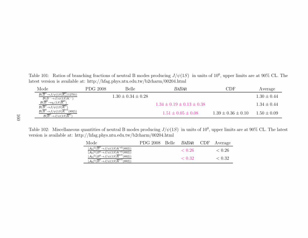
Table 101: Ratios of branching fractions of neutral B modes producing J/ψ(1S) in units of 100, upper limits are at 90% CL. Thelatest version is available at: http://hfag.phys.ntu.edu.tw/b2charm/00204.html
Mode PDG 2008 Belle BABAR CDF AverageB(B
0→J/ψ(1S)K
01(1270))
B(B−→J/ψ(1S)K−)1.30± 0.34± 0.28 1.30± 0.44
B(B0→ηc(1S)K
0)
B(B0→J/ψ(1S)K
0)
1.34± 0.19± 0.13± 0.38 1.34± 0.44
B(B0→J/ψ(1S)K
∗0(892))
B(B0→J/ψ(1S)K
0)
1.51± 0.05± 0.08 1.39± 0.36± 0.10 1.50± 0.09
Table 102: Miscellaneous quantities of neutral B modes producing J/ψ(1S) in units of 100, upper limits are at 90% CL. The latestversion is available at: http://hfag.phys.ntu.edu.tw/b2charm/00204.html
Mode PDG 2008 Belle BABAR CDF Average|A0|2(B
0→J/ψ(1S)K∗0(892))
|A0|2(B0→J/ψ(1S)K∗0(892))< 0.26 < 0.26
|A0|2(B0→J/ψ(1S)K∗0
(892))
|A0|2(B0→J/ψ(1S)K
∗0(892))
< 0.32 < 0.32
160
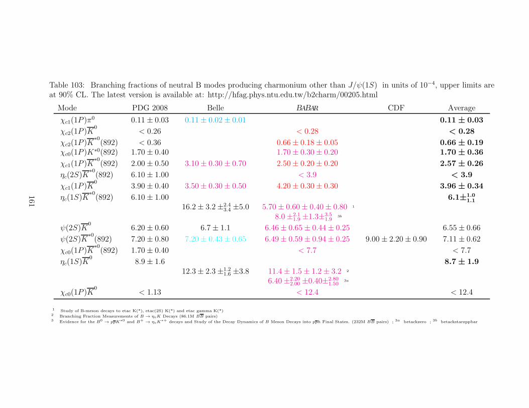
Table 103: Branching fractions of neutral B modes producing charmonium other than J/ψ(1S) in units of 10−4, upper limits areat 90% CL. The latest version is available at: http://hfag.phys.ntu.edu.tw/b2charm/00205.html
Mode PDG 2008 Belle BABAR CDF Average
χc1(1P )π0 0.11± 0.03 0.11± 0.02± 0.01 0.11 ± 0.03
χc2(1P )K0
< 0.26 < 0.28 < 0.28
χc2(1P )K∗0(892) < 0.36 0.66± 0.18± 0.05 0.66 ± 0.19
χc0(1P )K∗0(892) 1.70± 0.40 1.70± 0.30± 0.20 1.70 ± 0.36
χc1(1P )K∗0(892) 2.00± 0.50 3.10± 0.30± 0.70 2.50± 0.20± 0.20 2.57 ± 0.26
ηc(2S)K∗0(892) 6.10± 1.00 < 3.9 < 3.9
χc1(1P )K0
3.90± 0.40 3.50± 0.30± 0.50 4.20± 0.30± 0.30 3.96 ± 0.34
ηc(1S)K∗0(892) 6.10± 1.00 6.1±1.0
1.1
16.2± 3.2±2.43.4 ±5.0 5.70± 0.60± 0.40± 0.80 1
8.0±2.11.9 ±1.3±3.5
1.93b
ψ(2S)K0
6.20± 0.60 6.7± 1.1 6.46± 0.65± 0.44± 0.25 6.55± 0.66
ψ(2S)K∗0(892) 7.20± 0.80 7.20± 0.43± 0.65 6.49± 0.59± 0.94± 0.25 9.00± 2.20± 0.90 7.11± 0.62
χc0(1P )K∗0(892) 1.70± 0.40 < 7.7 < 7.7
ηc(1S)K0
8.9± 1.6 8.7 ± 1.912.3± 2.3±1.2
1.6 ±3.8 11.4± 1.5± 1.2± 3.2 2
6.40±2.202.00 ±0.40±2.80
1.503a
χc0(1P )K0
< 1.13 < 12.4 < 12.4
1 Study of B-meson decays to etac K(*), etac(2S) K(*) and etac gamma K(*)2 Branching Fraction Measurements of B → ηcK Decays (86.1M BB pairs)3 Evidence for the B0 → ppK∗0 and B+ → ηcK
∗+ decays and Study of the Decay Dynamics of B Meson Decays into pph Final States. (232M BB pairs) ; 3a betackzero ; 3b betackstarzppbar
161
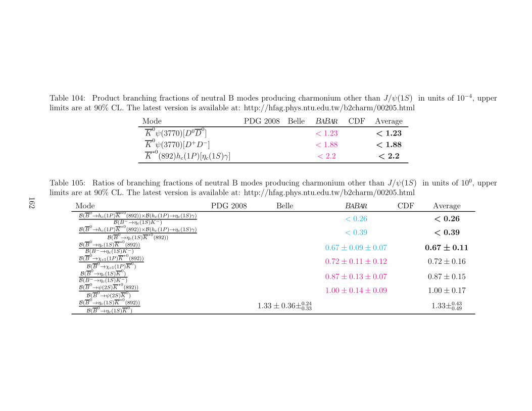
Table 104: Product branching fractions of neutral B modes producing charmonium other than J/ψ(1S) in units of 10−4, upperlimits are at 90% CL. The latest version is available at: http://hfag.phys.ntu.edu.tw/b2charm/00205.html
Mode PDG 2008 Belle BABAR CDF Average
K0ψ(3770)[D0D
0] < 1.23 < 1.23
K0ψ(3770)[D+D−] < 1.88 < 1.88
K∗0(892)hc(1P )[ηc(1S)γ] < 2.2 < 2.2
Table 105: Ratios of branching fractions of neutral B modes producing charmonium other than J/ψ(1S) in units of 100, upperlimits are at 90% CL. The latest version is available at: http://hfag.phys.ntu.edu.tw/b2charm/00205.html
Mode PDG 2008 Belle BABAR CDF AverageB(B
0→hc(1P )K
∗0(892))×B(hc(1P )→ηc(1S)γ)
B(B−→ηc(1S)K−)< 0.26 < 0.26
B(B0→hc(1P )K
∗0(892))×B(hc(1P )→ηc(1S)γ)
B(B0→ηc(1S)K
∗0(892))
< 0.39 < 0.39
B(B0→ηc(1S)K
∗0(892))
B(B−→ηc(1S)K−)0.67± 0.09± 0.07 0.67 ± 0.11
B(B0→χc1(1P )K
∗0(892))
B(B0→χc1(1P )K
0)
0.72± 0.11± 0.12 0.72± 0.16
B(B0→ηc(1S)K
0)
B(B−→ηc(1S)K−)0.87± 0.13± 0.07 0.87± 0.15
B(B0→ψ(2S)K
∗0(892))
B(B0→ψ(2S)K
0)
1.00± 0.14± 0.09 1.00± 0.17
B(B0→ηc(1S)K
∗0(892))
B(B0→ηc(1S)K
0)
1.33± 0.36±0.240.33 1.33±0.43
0.49
162
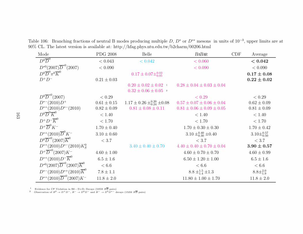
Table 106: Branching fractions of neutral B modes producing multiple D, D∗ or D∗∗ mesons in units of 10−3, upper limits are at90% CL. The latest version is available at: http://hfag.phys.ntu.edu.tw/b2charm/00206.html
Mode PDG 2008 Belle BABAR CDF Average
D0D0
< 0.043 < 0.042 < 0.060 < 0.042
D∗0(2007)D∗0(2007) < 0.090 < 0.090 < 0.090
D0D0π0K
00.17± 0.07±0.03
0.05 0.17 ± 0.08D+D− 0.21± 0.03 0.22 ± 0.02
0.20± 0.02± 0.02 1 0.28± 0.04± 0.03± 0.040.32± 0.06± 0.05 2
D0D∗0(2007) < 0.29 < 0.29 < 0.29
D∗−(2010)D+ 0.61± 0.15 1.17± 0.26±0.200.24 ±0.08 0.57± 0.07± 0.06± 0.04 0.62± 0.09
D∗+(2010)D∗−(2010) 0.82± 0.09 0.81± 0.08± 0.11 0.81± 0.06± 0.09± 0.05 0.81± 0.09
D0D0K
0< 1.40 < 1.40 < 1.40
D+D−K0
< 1.70 < 1.70 < 1.70
D+D0K− 1.70± 0.40 1.70± 0.30± 0.30 1.70± 0.42
D∗+(2010)D0K− 3.10± 0.60 3.10±0.40
0.30 ±0.40 3.10±0.570.50
D0D∗0(2007)K
0< 3.7 < 3.7 < 3.7
D∗+(2010)D∗−(2010)K0S 3.40± 0.40± 0.70 4.40± 0.40± 0.70± 0.04 3.90 ± 0.57
D+D∗0(2007)K− 4.60± 1.00 4.60± 0.70± 0.70 4.60± 0.99
D∗+(2010)D−K0
6.5± 1.6 6.50± 1.20± 1.00 6.5± 1.6
D∗0(2007)D∗0(2007)K
0< 6.6 < 6.6 < 6.6
D∗−(2010)D∗+(2010)K0
7.8± 1.1 8.8±1.51.4 ±1.3 8.8±2.0
1.9
D∗+(2010)D∗0(2007)K− 11.8± 2.0 11.80± 1.00± 1.70 11.8± 2.0
1 Evidence for CP Violation in B0 - D+D- Decays (535M BB pairs)2 Observation of B0 → D+D−, B− → D0D− and B− → D0D∗− decays (152M BB pairs)
163
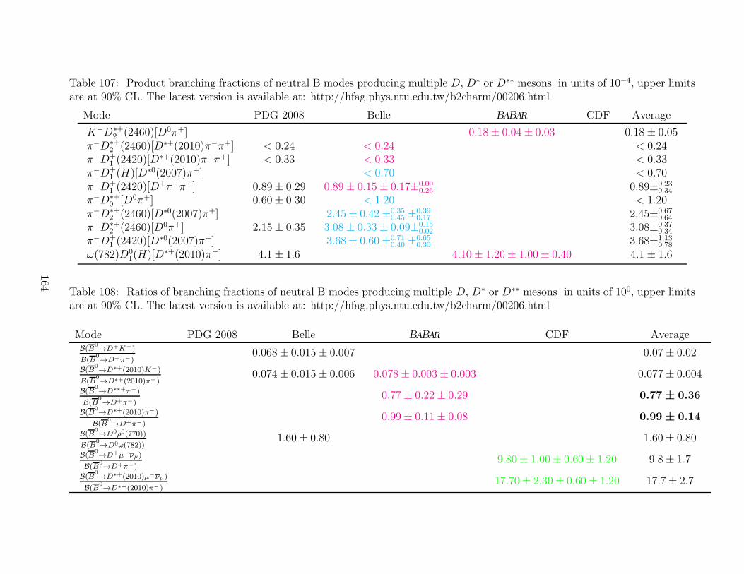
Table 107: Product branching fractions of neutral B modes producing multiple D, D∗ or D∗∗ mesons in units of 10−4, upper limitsare at 90% CL. The latest version is available at: http://hfag.phys.ntu.edu.tw/b2charm/00206.html
Mode PDG 2008 Belle BABAR CDF Average
K−D∗+2 (2460)[D0π+] 0.18± 0.04± 0.03 0.18± 0.05
π−D∗+2 (2460)[D∗+(2010)π−π+] < 0.24 < 0.24 < 0.24
π−D+1 (2420)[D
∗+(2010)π−π+] < 0.33 < 0.33 < 0.33π−D+
1 (H)[D∗0(2007)π+] < 0.70 < 0.70π−D+
1 (2420)[D+π−π+] 0.89± 0.29 0.89± 0.15± 0.17±0.00
0.26 0.89±0.230.34
π−D∗+0 [D0π+] 0.60± 0.30 < 1.20 < 1.20
π−D∗+2 (2460)[D∗0(2007)π+] 2.45± 0.42±0.35
0.45 ±0.390.17 2.45±0.67
0.64
π−D∗+2 (2460)[D0π+] 2.15± 0.35 3.08± 0.33± 0.09±0.15
0.02 3.08±0.370.34
π−D+1 (2420)[D
∗0(2007)π+] 3.68± 0.60±0.710.40 ±0.65
0.30 3.68±1.130.78
ω(782)D01(H)[D∗+(2010)π−] 4.1± 1.6 4.10± 1.20± 1.00± 0.40 4.1± 1.6
Table 108: Ratios of branching fractions of neutral B modes producing multiple D, D∗ or D∗∗ mesons in units of 100, upper limitsare at 90% CL. The latest version is available at: http://hfag.phys.ntu.edu.tw/b2charm/00206.html
Mode PDG 2008 Belle BABAR CDF AverageB(B
0→D+K−)
B(B0→D+π−)
0.068± 0.015± 0.007 0.07± 0.02
B(B0→D∗+(2010)K−)
B(B0→D∗+(2010)π−)
0.074± 0.015± 0.006 0.078± 0.003± 0.003 0.077± 0.004
B(B0→D∗∗+π−)
B(B0→D+π−)
0.77± 0.22± 0.29 0.77 ± 0.36
B(B0→D∗+(2010)π−)
B(B0→D+π−)
0.99± 0.11± 0.08 0.99 ± 0.14
B(B0→D0ρ0(770))
B(B0→D0ω(782))
1.60± 0.80 1.60± 0.80
B(B0→D+µ−νµ)
B(B0→D+π−)
9.80± 1.00± 0.60± 1.20 9.8± 1.7
B(B0→D∗+(2010)µ−νµ)
B(B0→D∗+(2010)π−)
17.70± 2.30± 0.60± 1.20 17.7± 2.7
164
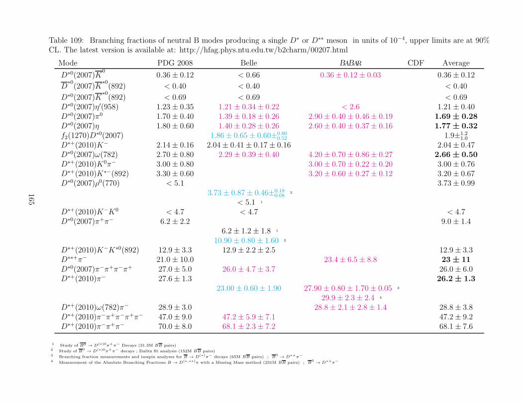
Table 109: Branching fractions of neutral B modes producing a single D∗ or D∗∗ meson in units of 10−4, upper limits are at 90%CL. The latest version is available at: http://hfag.phys.ntu.edu.tw/b2charm/00207.html
Mode PDG 2008 Belle BABAR CDF Average
D∗0(2007)K0
0.36± 0.12 < 0.66 0.36± 0.12± 0.03 0.36± 0.12
D∗0(2007)K
∗0(892) < 0.40 < 0.40 < 0.40
D∗0(2007)K∗0(892) < 0.69 < 0.69 < 0.69
D∗0(2007)η′(958) 1.23± 0.35 1.21± 0.34± 0.22 < 2.6 1.21± 0.40D∗0(2007)π0 1.70± 0.40 1.39± 0.18± 0.26 2.90± 0.40± 0.46± 0.19 1.69 ± 0.28D∗0(2007)η 1.80± 0.60 1.40± 0.28± 0.26 2.60± 0.40± 0.37± 0.16 1.77 ± 0.32f2(1270)D
∗0(2007) 1.86± 0.65± 0.60±0.800.52 1.9±1.2
1.0
D∗+(2010)K− 2.14± 0.16 2.04± 0.41± 0.17± 0.16 2.04± 0.47D∗0(2007)ω(782) 2.70± 0.80 2.29± 0.39± 0.40 4.20± 0.70± 0.86± 0.27 2.66 ± 0.50D∗+(2010)K0π− 3.00± 0.80 3.00± 0.70± 0.22± 0.20 3.00± 0.76D∗+(2010)K∗−(892) 3.30± 0.60 3.20± 0.60± 0.27± 0.12 3.20± 0.67D∗0(2007)ρ0(770) < 5.1 3.73± 0.99
3.73± 0.87± 0.46±0.180.08
2
< 5.1 1
D∗+(2010)K−K0 < 4.7 < 4.7 < 4.7D∗0(2007)π+π− 6.2± 2.2 9.0± 1.4
6.2± 1.2± 1.8 1
10.90± 0.80± 1.60 2
D∗+(2010)K−K∗0(892) 12.9± 3.3 12.9± 2.2± 2.5 12.9± 3.3D∗∗+π− 21.0± 10.0 23.4± 6.5± 8.8 23 ± 11D∗0(2007)π−π+π−π+ 27.0± 5.0 26.0± 4.7± 3.7 26.0± 6.0D∗+(2010)π− 27.6± 1.3 26.2 ± 1.3
23.00± 0.60± 1.90 27.90± 0.80± 1.70± 0.05 3
29.9± 2.3± 2.4 4
D∗+(2010)ω(782)π− 28.9± 3.0 28.8± 2.1± 2.8± 1.4 28.8± 3.8D∗+(2010)π−π+π−π+π− 47.0± 9.0 47.2± 5.9± 7.1 47.2± 9.2D∗+(2010)π−π+π− 70.0± 8.0 68.1± 2.3± 7.2 68.1± 7.6
1 Study of B0 → D(∗)0π+π− Decays (31.3M BB pairs)2 Study of B
0→ D(∗)0π+π− decays ; Dalitz fit analysis (152M BB pairs)
3 Branching fraction measurements and isospin analyses for B → D(∗)π− decays (65M BB pairs) ; B0
→ D∗+π−
4 Measurement of the Absolute Branching Fractions B → D(∗,∗∗)π with a Missing Mass method (231M BB pairs) ; B0
→ D∗+π−
165
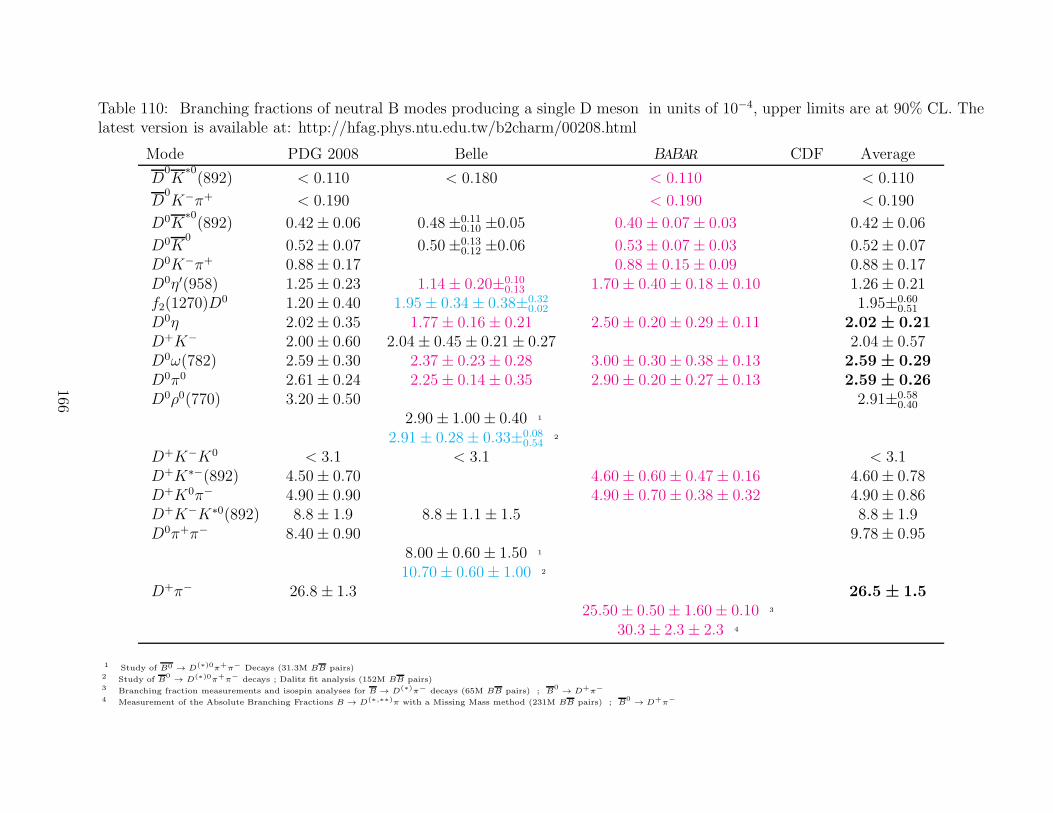
Table 110: Branching fractions of neutral B modes producing a single D meson in units of 10−4, upper limits are at 90% CL. Thelatest version is available at: http://hfag.phys.ntu.edu.tw/b2charm/00208.html
Mode PDG 2008 Belle BABAR CDF Average
D0K
∗0(892) < 0.110 < 0.180 < 0.110 < 0.110
D0K−π+ < 0.190 < 0.190 < 0.190
D0K∗0(892) 0.42± 0.06 0.48±0.11
0.10 ±0.05 0.40± 0.07± 0.03 0.42± 0.06
D0K0
0.52± 0.07 0.50±0.130.12 ±0.06 0.53± 0.07± 0.03 0.52± 0.07
D0K−π+ 0.88± 0.17 0.88± 0.15± 0.09 0.88± 0.17D0η′(958) 1.25± 0.23 1.14± 0.20±0.10
0.13 1.70± 0.40± 0.18± 0.10 1.26± 0.21f2(1270)D
0 1.20± 0.40 1.95± 0.34± 0.38±0.320.02 1.95±0.60
0.51
D0η 2.02± 0.35 1.77± 0.16± 0.21 2.50± 0.20± 0.29± 0.11 2.02 ± 0.21D+K− 2.00± 0.60 2.04± 0.45± 0.21± 0.27 2.04± 0.57D0ω(782) 2.59± 0.30 2.37± 0.23± 0.28 3.00± 0.30± 0.38± 0.13 2.59 ± 0.29D0π0 2.61± 0.24 2.25± 0.14± 0.35 2.90± 0.20± 0.27± 0.13 2.59 ± 0.26D0ρ0(770) 3.20± 0.50 2.91±0.58
0.40
2.90± 1.00± 0.40 1
2.91± 0.28± 0.33±0.080.54
2
D+K−K0 < 3.1 < 3.1 < 3.1D+K∗−(892) 4.50± 0.70 4.60± 0.60± 0.47± 0.16 4.60± 0.78D+K0π− 4.90± 0.90 4.90± 0.70± 0.38± 0.32 4.90± 0.86D+K−K∗0(892) 8.8± 1.9 8.8± 1.1± 1.5 8.8± 1.9D0π+π− 8.40± 0.90 9.78± 0.95
8.00± 0.60± 1.50 1
10.70± 0.60± 1.00 2
D+π− 26.8± 1.3 26.5 ± 1.525.50± 0.50± 1.60± 0.10 3
30.3± 2.3± 2.3 4
1 Study of B0 → D(∗)0π+π− Decays (31.3M BB pairs)2 Study of B
0→ D(∗)0π+π− decays ; Dalitz fit analysis (152M BB pairs)
3 Branching fraction measurements and isospin analyses for B → D(∗)π− decays (65M BB pairs) ; B0
→ D+π−
4 Measurement of the Absolute Branching Fractions B → D(∗,∗∗)π with a Missing Mass method (231M BB pairs) ; B0
→ D+π−
166
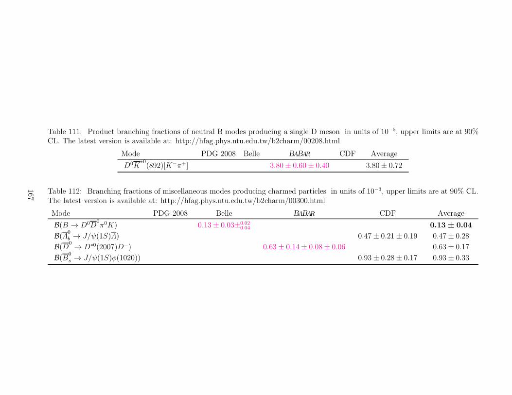
Table 111: Product branching fractions of neutral B modes producing a single D meson in units of 10−5, upper limits are at 90%CL. The latest version is available at: http://hfag.phys.ntu.edu.tw/b2charm/00208.html
Mode PDG 2008 Belle BABAR CDF Average
D0K∗0(892)[K−π+] 3.80± 0.60± 0.40 3.80± 0.72
Table 112: Branching fractions of miscellaneous modes producing charmed particles in units of 10−3, upper limits are at 90% CL.The latest version is available at: http://hfag.phys.ntu.edu.tw/b2charm/00300.html
Mode PDG 2008 Belle BABAR CDF Average
B(B → D0D0π0K) 0.13± 0.03±0.02
0.04 0.13 ± 0.04
B(Λ0
b → J/ψ(1S)Λ) 0.47± 0.21± 0.19 0.47± 0.28
B(D0 → D∗0(2007)D−) 0.63± 0.14± 0.08± 0.06 0.63± 0.17
B(B0
s → J/ψ(1S)φ(1020)) 0.93± 0.28± 0.17 0.93± 0.33
167
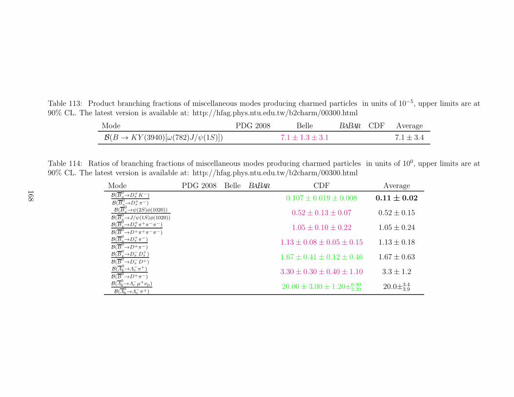
Table 113: Product branching fractions of miscellaneous modes producing charmed particles in units of 10−5, upper limits are at90% CL. The latest version is available at: http://hfag.phys.ntu.edu.tw/b2charm/00300.html
Mode PDG 2008 Belle BABAR CDF Average
B(B → KY (3940)[ω(782)J/ψ(1S)]) 7.1± 1.3± 3.1 7.1± 3.4
Table 114: Ratios of branching fractions of miscellaneous modes producing charmed particles in units of 100, upper limits are at90% CL. The latest version is available at: http://hfag.phys.ntu.edu.tw/b2charm/00300.html
Mode PDG 2008 Belle BABAR CDF AverageB(B
0s→D+
s K−)
B(B0s→D+
s π−)0.107± 0.019± 0.008 0.11 ± 0.02
B(B0s→ψ(2S)φ(1020))
B(B0s→J/ψ(1S)φ(1020))
0.52± 0.13± 0.07 0.52± 0.15
B(B0s→D+
s π+π−π−)
B(B0→D+π+π−π−)
1.05± 0.10± 0.22 1.05± 0.24
B(B0s→D+
s π−)
B(B0→D+π−)
1.13± 0.08± 0.05± 0.15 1.13± 0.18
B(B0s→D−
s D+s )
B(B0→D−
s D+)1.67± 0.41± 0.12± 0.46 1.67± 0.63
B(Λ0b→Λ−
c π+)
B(B0→D+π−)
3.30± 0.30± 0.40± 1.10 3.3± 1.2
B(Λ0b→Λ−
c µ+νµ)
B(Λ0b→Λ−
c π+)20.00± 3.00± 1.20±0.90
2.20 20.0±3.43.9
168
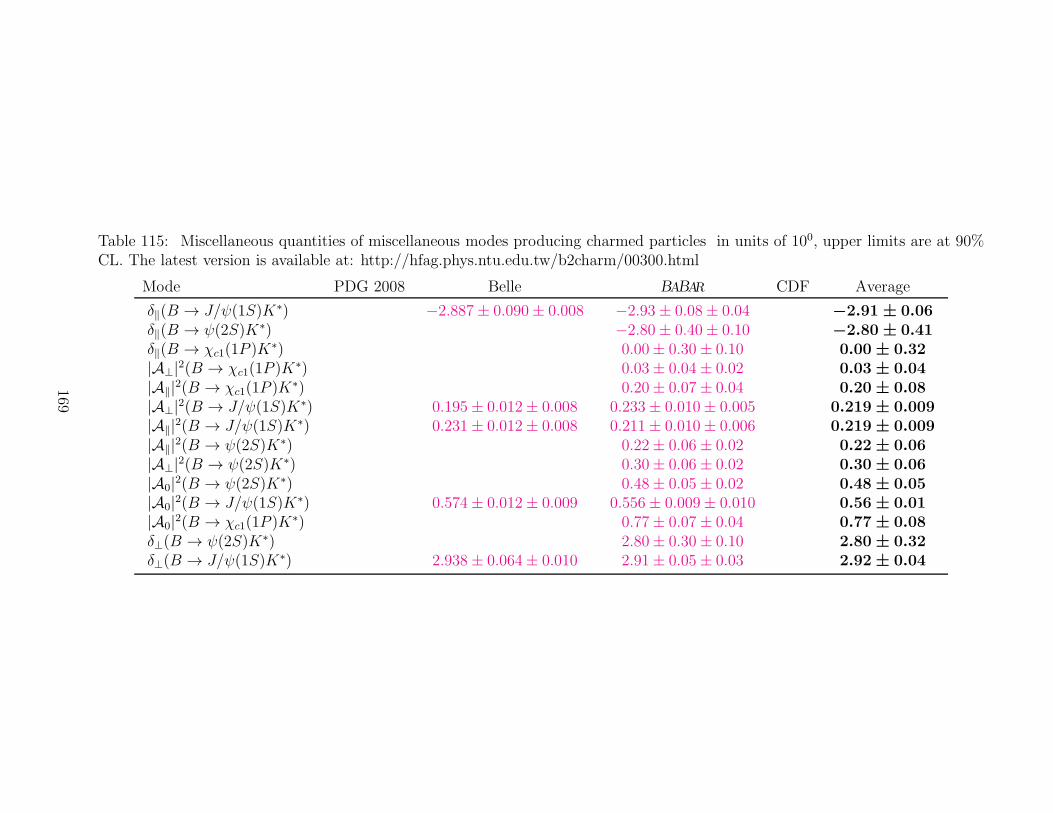
Table 115: Miscellaneous quantities of miscellaneous modes producing charmed particles in units of 100, upper limits are at 90%CL. The latest version is available at: http://hfag.phys.ntu.edu.tw/b2charm/00300.html
Mode PDG 2008 Belle BABAR CDF Average
δ‖(B → J/ψ(1S)K∗) −2.887± 0.090± 0.008 −2.93± 0.08± 0.04 −2.91 ± 0.06δ‖(B → ψ(2S)K∗) −2.80± 0.40± 0.10 −2.80 ± 0.41δ‖(B → χc1(1P )K
∗) 0.00± 0.30± 0.10 0.00 ± 0.32|A⊥|2(B → χc1(1P )K
∗) 0.03± 0.04± 0.02 0.03 ± 0.04|A‖|2(B → χc1(1P )K
∗) 0.20± 0.07± 0.04 0.20 ± 0.08|A⊥|2(B → J/ψ(1S)K∗) 0.195± 0.012± 0.008 0.233± 0.010± 0.005 0.219 ± 0.009|A‖|2(B → J/ψ(1S)K∗) 0.231± 0.012± 0.008 0.211± 0.010± 0.006 0.219 ± 0.009|A‖|2(B → ψ(2S)K∗) 0.22± 0.06± 0.02 0.22 ± 0.06|A⊥|2(B → ψ(2S)K∗) 0.30± 0.06± 0.02 0.30 ± 0.06|A0|2(B → ψ(2S)K∗) 0.48± 0.05± 0.02 0.48 ± 0.05|A0|2(B → J/ψ(1S)K∗) 0.574± 0.012± 0.009 0.556± 0.009± 0.010 0.56 ± 0.01|A0|2(B → χc1(1P )K
∗) 0.77± 0.07± 0.04 0.77 ± 0.08δ⊥(B → ψ(2S)K∗) 2.80± 0.30± 0.10 2.80 ± 0.32δ⊥(B → J/ψ(1S)K∗) 2.938± 0.064± 0.010 2.91± 0.05± 0.03 2.92 ± 0.04
169
7 B decays to charmless final states
The aim of this section is to provide the branching fractions and the partial rate asymmetries(ACP ) of charmless B decays. The asymmetry is defined as ACP =
NB−NBNB+NB
, where NB and
NB are respectively number of B0/B− and B0/B+ decaying into a specific final state. Fourdifferent B decay categories are considered: charmless mesonic, baryonic, radiative and lep-tonic. Measurements supported with written documents are accepted in the averages; writtendocuments could be journal papers, conference contributed papers, preprints or conference pro-ceedings. Results from ACP measurements obtained from time dependent analyses are listedand described in Sec. 4. Measurements of charmful baryonic B decays, which were included inour previous averages [4], are now shown in Section 7, which deals with B decays to charm.
So far all branching fractions assume equal production of charged and neutral B pairs.The best measurements to date show that this is still a good approximation (see Sec. 3). Forbranching fractions, we provide either averages or the most stringent 90% confidence levelupper limits. If one or more experiments have measurements with >4σ for a decay channel,all available central values for that channel are used in the averaging. We also give centralvalues and errors for cases where the significance of the average value is at least 3σ, even if nosingle measurement is above 4σ. Since a few decay modes are sensitive to the contribution ofnew physics and the current experimental upper limits are not far from the Standard Modelexpectation, we provide the combined upper limits or averages in these cases. Their upperlimits can be estimated assuming that the errors are Gaussian. For ACP we provide averagesin all cases.
Our averaging is performed by maximizing the likelihood, L =∏
i
Pi(x), where Pi is the
probability density function (PDF) of the ith measurement, and x is the branching fractionor ACP . The PDF is modeled by an asymmetric Gaussian function with the measured centralvalue as its mean and the quadratic sum of the statistical and systematic errors as the standarddeviations. The experimental uncertainties are considered to be uncorrelated with each otherwhen the averaging is performed. No error scaling is applied when the fit χ2 is greater than 1since we believe that tends to overestimate the errors except in cases of extreme disagreement(we have no such cases). One exception to consider the correlated systematic errors is theinclusive B → Xsγ mode, which is sensitive to physics beyond the Standard Model. In thisupdate, we have included new measurements from both Belle and BaBar to perform the average.The detail is described in Sec. 7.3.
At present, we have measurements of about 400 decay modes, reported in more than 200papers. Because the number of references is so large, we do not include them with the tablesshown here but the full set of references is available quickly from active gifs at the “Winter 2010”link on the rare web page: http://www.slac.stanford.edu/xorg/hfag/rare/index.html.Finally many new measurements involving scalar and tensor mesons are included for the firsttime.
7.1 Mesonic charmless decays
170
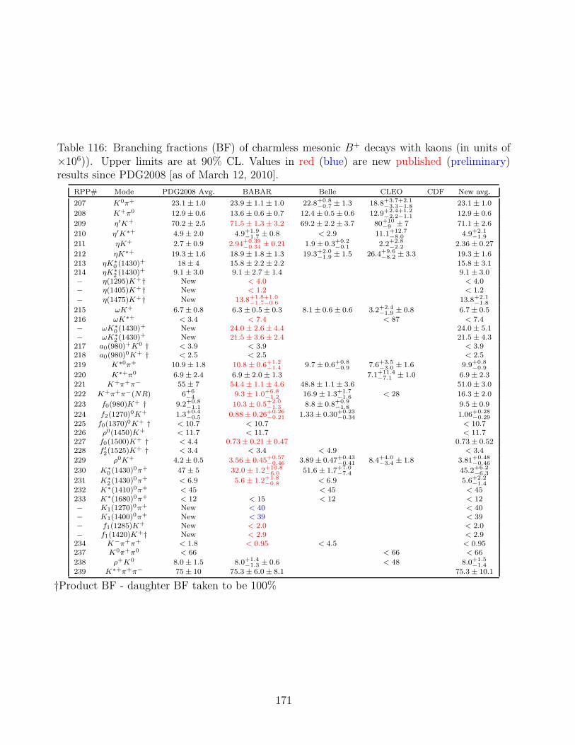
Table 116: Branching fractions (BF) of charmless mesonic B+ decays with kaons (in units of×106)). Upper limits are at 90% CL. Values in red (blue) are new published (preliminary)results since PDG2008 [as of March 12, 2010].
RPP# Mode PDG2008 Avg. BABAR Belle CLEO CDF New avg.
207 K0π+ 23.1± 1.0 23.9± 1.1± 1.0 22.8+0.8−0.7 ± 1.3 18.8+3.7+2.1
−3.3−1.8 23.1± 1.0
208 K+π0 12.9± 0.6 13.6± 0.6± 0.7 12.4± 0.5± 0.6 12.9+2.4+1.2−2.2−1.1 12.9± 0.6
209 η′K+ 70.2± 2.5 71.5± 1.3± 3.2 69.2± 2.2± 3.7 80+10−9 ± 7 71.1± 2.6
210 η′K∗+ 4.9± 2.0 4.9+1.9−1.7 ± 0.8 < 2.9 11.1+12.7
−8.0 4.9+2.1−1.9
211 ηK+ 2.7± 0.9 2.94+0.39−0.34 ± 0.21 1.9± 0.3+0.2
−0.1 2.2+2.8−2.2 2.36± 0.27
212 ηK∗+ 19.3± 1.6 18.9± 1.8± 1.3 19.3+2.0−1.9 ± 1.5 26.4+9.6
−8.2 ± 3.3 19.3± 1.6213 ηK∗
0 (1430)+ 18± 4 15.8± 2.2± 2.2 15.8± 3.1
214 ηK∗2 (1430)
+ 9.1± 3.0 9.1± 2.7± 1.4 9.1± 3.0− η(1295)K+† New < 4.0 < 4.0− η(1405)K+† New < 1.2 < 1.2
− η(1475)K+† New 13.8+1.8+1.0−1.7−0.6 13.8+2.1
−1.8
215 ωK+ 6.7± 0.8 6.3± 0.5± 0.3 8.1± 0.6± 0.6 3.2+2.4−1.9 ± 0.8 6.7± 0.5
216 ωK∗+ < 3.4 < 7.4 < 87 < 7.4− ωK∗
0 (1430)+ New 24.0± 2.6± 4.4 24.0± 5.1
− ωK∗2 (1430)
+ New 21.5± 3.6± 2.4 21.5± 4.3217 a0(980)+K0 † < 3.9 < 3.9 < 3.9218 a0(980)0K+ † < 2.5 < 2.5 < 2.5
219 K∗0π+ 10.9± 1.8 10.8± 0.6+1.2−1.4 9.7± 0.6+0.8
−0.9 7.6+3.5−3.0 ± 1.6 9.9+0.8
−0.9
220 K∗+π0 6.9± 2.4 6.9± 2.0± 1.3 7.1+11.4−7.1 ± 1.0 6.9± 2.3
221 K+π+π− 55± 7 54.4± 1.1± 4.6 48.8± 1.1± 3.6 51.0± 3.0
222 K+π+π−(NR) 6+6−4 9.3± 1.0+6.8
−1.2 16.9 ± 1.3+1.7−1.6 < 28 16.3± 2.0
223 f0(980)K+ † 9.2+0.8−1.1 10.3± 0.5+2.0
−1.3 8.8± 0.8+0.9−1.8 9.5± 0.9
224 f2(1270)0K+ 1.3+0.4−0.5 0.88± 0.26+0.26
−0.21 1.33± 0.30+0.23−0.34 1.06+0.28
−0.29225 f0(1370)0K+ † < 10.7 < 10.7 < 10.7226 ρ0(1450)K+ < 11.7 < 11.7 < 11.7227 f0(1500)K+ † < 4.4 0.73± 0.21± 0.47 0.73± 0.52228 f ′2(1525)K
+ † < 3.4 < 3.4 < 4.9 < 3.4
229 ρ0K+ 4.2± 0.5 3.56± 0.45+0.57−0.46 3.89± 0.47+0.43
−0.41 8.4+4.0−3.4 ± 1.8 3.81+0.48
−0.46
230 K∗0 (1430)
0π+ 47± 5 32.0± 1.2+10.8−6.0 51.6 ± 1.7+7.0
−7.4 45.2+6.2−6.3
231 K∗2 (1430)
0π+ < 6.9 5.6± 1.2+1.8−0.8 < 6.9 5.6+2.2
−1.4232 K∗(1410)0π+ < 45 < 45 < 45233 K∗(1680)0π+ < 12 < 15 < 12 < 12− K1(1270)0π+ New < 40 < 40− K1(1400)0π+ New < 39 < 39− f1(1285)K+ New < 2.0 < 2.0− f1(1420)K+† New < 2.9 < 2.9234 K−π+π+ < 1.8 < 0.95 < 4.5 < 0.95237 K0π+π0 < 66 < 66 < 66
238 ρ+K0 8.0± 1.5 8.0+1.4−1.3 ± 0.6 < 48 8.0+1.5
−1.4239 K∗+π+π− 75 ± 10 75.3± 6.0± 8.1 75.3± 10.1
†Product BF - daughter BF taken to be 100%
171
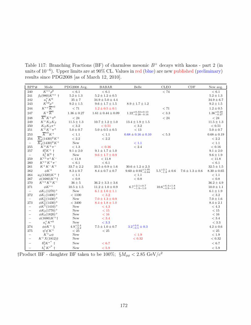
Table 117: Branching Fractions (BF) of charmless mesonic B+ decays with kaons - part 2 (inunits of 10−6). Upper limits are at 90% CL. Values in red (blue) are new published (preliminary)results since PDG2008 [as of March 12, 2010].
RPP# Mode PDG2008 Avg. BABAR Belle CLEO CDF New avg.
240 K∗+ρ0 < 6.1 < 6.1 < 74 < 6.1241 f0(980)K∗+ † 5.2± 1.3 5.2± 1.2± 0.5 5.2± 1.3
242 a+1 K0 35± 7 34.9± 5.0± 4.4 34.9± 6.7
243 K∗0ρ+ 9.2± 1.5 9.6± 1.7± 1.5 8.9± 1.7± 1.2 9.2± 1.5
244 K∗+K∗0
< 71 1.2± 0.5± 0.1 < 71 1.2± 0.5
247 K+K0
1.36± 0.27 1.61± 0.44± 0.09 1.22+0.33+0.13−0.28−0.16 < 3.3 1.36+0.29
−0.27
248 K0K+π0 < 24 < 24 < 24
249 K+KSKS 11.5± 1.3 10.7± 1.2± 1.0 13.4± 1.9± 1.5 11.5± 1.3250 KSKSπ
+ < 3.2 < 0.51 < 3.2 < 0.51251 K+K−π+ 5.0± 0.7 5.0± 0.5± 0.5 < 13 5.0± 0.7
253 K∗0K+ < 1.1 < 1.1 0.68 ± 0.16± 0.10 < 5.3 0.68± 0.19
254 K∗0(1430)
0K+ < 2.2 < 2.2 < 2.2
− K∗2(1430)
0K+ New < 1.1 < 1.1255 K+K+π− < 1.3 < 0.16 < 2.4 < 0.16257 b01K
+ † 9.1± 2.0 9.1± 1.7± 1.0 9.1± 2.0
− b+1 K0 † New 9.6± 1.7± 0.9 9.6± 1.9
259 K∗+π+K− < 11.8 < 11.8 < 11.8260 K∗+K+π− < 6.1 < 6.1 < 6.1261 K+K−K+ 33.7± 2.2 33.5± 0.9± 1.6 30.6± 1.2± 2.3 32.5± 1.5
262 φK+ 8.3± 0.7 8.4± 0.7± 0.7 9.60± 0.92+1.05−0.84 5.5+2.1
−1.8 ± 0.6 7.6± 1.3± 0.6 8.30± 0.65264 a2(1320)K+ † < 1.1 < 1.1 < 1.1267 φ(1680)K+† < 0.8 < 0.8 < 0.8270 K∗+K+K− 36± 5 36.2± 3.3± 3.6 36.2± 4.9
271 φK∗+ 10.5± 1.5 11.2± 1.0± 0.9 6.7+2.1+0.7−1.9−1.0 10.6+6.4+1.8
−4.9−1.6 10.0± 1.1− φK1(1270)+ New 6.1± 1.6± 1.1 6.1± 1.9272 φK1(1400)+ < 1100 < 3.2 < 3.2− φK∗
0 (1430)+ New 7.0± 1.3± 0.9 7.0± 1.6
273 φK∗2 (1430)
+ < 3400 8.4± 1.8± 1.0 8.4± 2.1− φK∗(1410)+ New < 4.3 < 4.3− φK2(1770)+ New < 15 < 15− φK2(1820)+ New < 16 < 16− φ(1680)K+† New < 3.4 < 3.4
− a+1 K∗0 New < 3.3 < 3.3
274 φφK+ § 4.9+2.4−2.2 7.5± 1.0± 0.7 3.2+0.6
−0.5 ± 0.3 4.2± 0.6
275 η′η′K+ < 25 < 25 < 25− K+ωφ New < 1.9 < 1.9− K+X(1812)† New < 0.32 < 0.32
− b01K∗+ † New < 6.7 < 6.7
− b+1 K∗0 † New < 5.9 < 5.9
†Product BF - daughter BF taken to be 100%; §Mφφ < 2.85 GeV/c2
172
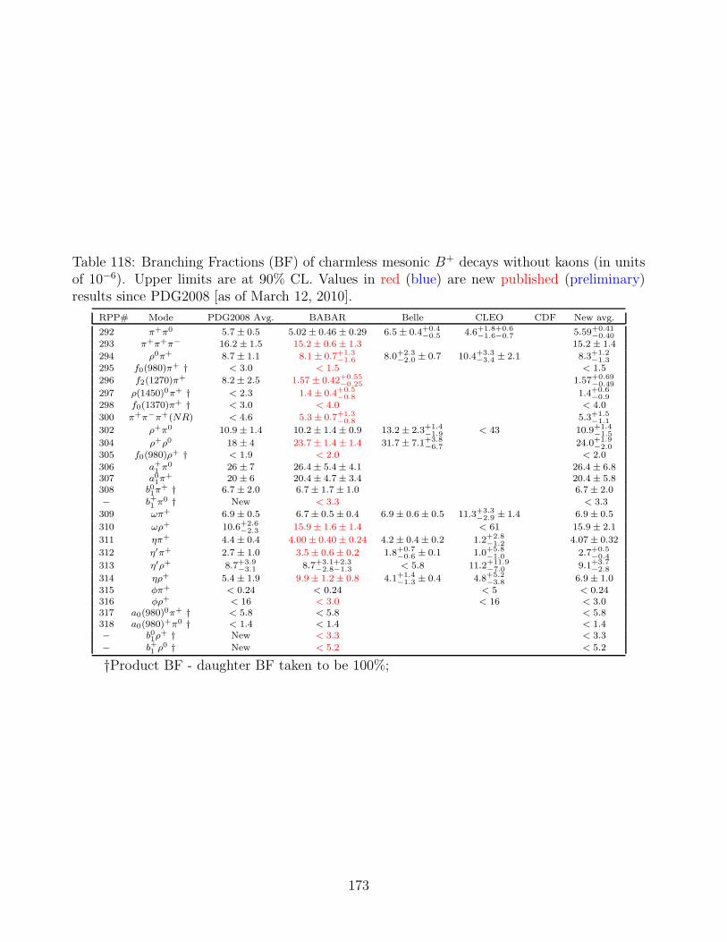
Table 118: Branching Fractions (BF) of charmless mesonic B+ decays without kaons (in unitsof 10−6). Upper limits are at 90% CL. Values in red (blue) are new published (preliminary)results since PDG2008 [as of March 12, 2010].
RPP# Mode PDG2008 Avg. BABAR Belle CLEO CDF New avg.
292 π+π0 5.7± 0.5 5.02± 0.46± 0.29 6.5± 0.4+0.4−0.5 4.6+1.8+0.6
−1.6−0.7 5.59+0.41−0.40
293 π+π+π− 16.2± 1.5 15.2± 0.6± 1.3 15.2± 1.4
294 ρ0π+ 8.7± 1.1 8.1± 0.7+1.3−1.6 8.0+2.3
−2.0 ± 0.7 10.4+3.3−3.4 ± 2.1 8.3+1.2
−1.3295 f0(980)π+ † < 3.0 < 1.5 < 1.5
296 f2(1270)π+ 8.2± 2.5 1.57± 0.42+0.55−0.25 1.57+0.69
−0.49
297 ρ(1450)0π+ † < 2.3 1.4± 0.4+0.5−0.8 1.4+0.6
−0.9298 f0(1370)π+ † < 3.0 < 4.0 < 4.0
300 π+π−π+(NR) < 4.6 5.3± 0.7+1.3−0.8 5.3+1.5
−1.1
302 ρ+π0 10.9± 1.4 10.2± 1.4± 0.9 13.2± 2.3+1.4−1.9 < 43 10.9+1.4
−1.5
304 ρ+ρ0 18 ± 4 23.7± 1.4± 1.4 31.7± 7.1+3.8−6.7 24.0+1.9
−2.0305 f0(980)ρ+ † < 1.9 < 2.0 < 2.0
306 a+1 π0 26 ± 7 26.4± 5.4± 4.1 26.4± 6.8
307 a01π+ 20 ± 6 20.4± 4.7± 3.4 20.4± 5.8
308 b01π+ † 6.7± 2.0 6.7± 1.7± 1.0 6.7± 2.0
− b+1 π0 † New < 3.3 < 3.3
309 ωπ+ 6.9± 0.5 6.7± 0.5± 0.4 6.9± 0.6± 0.5 11.3+3.3−2.9 ± 1.4 6.9± 0.5
310 ωρ+ 10.6+2.6−2.3 15.9± 1.6± 1.4 < 61 15.9± 2.1
311 ηπ+ 4.4± 0.4 4.00± 0.40± 0.24 4.2± 0.4± 0.2 1.2+2.8−1.2 4.07± 0.32
312 η′π+ 2.7± 1.0 3.5± 0.6± 0.2 1.8+0.7−0.6 ± 0.1 1.0+5.8
−1.0 2.7+0.5−0.4
313 η′ρ+ 8.7+3.9−3.1 8.7+3.1+2.3
−2.8−1.3 < 5.8 11.2+11.9−7.0 9.1+3.7
−2.8
314 ηρ+ 5.4± 1.9 9.9± 1.2± 0.8 4.1+1.4−1.3 ± 0.4 4.8+5.2
−3.8 6.9± 1.0315 φπ+ < 0.24 < 0.24 < 5 < 0.24316 φρ+ < 16 < 3.0 < 16 < 3.0317 a0(980)0π+ † < 5.8 < 5.8 < 5.8318 a0(980)+π0 † < 1.4 < 1.4 < 1.4− b01ρ
+ † New < 3.3 < 3.3
− b+1 ρ0 † New < 5.2 < 5.2
†Product BF - daughter BF taken to be 100%;
173
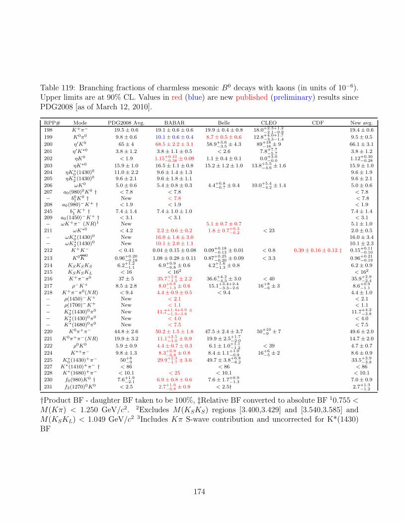
Table 119: Branching fractions of charmless mesonic B0 decays with kaons (in units of 10−6).Upper limits are at 90% CL. Values in red (blue) are new published (preliminary) results sincePDG2008 [as of March 12, 2010].
RPP# Mode PDG2008 Avg. BABAR Belle CLEO CDF New avg.
198 K+π− 19.5± 0.6 19.1± 0.6± 0.6 19.9± 0.4± 0.8 18.0+2.3+1.2−2.1−0.9 19.4 ± 0.6
199 K0π0 9.8± 0.6 10.1± 0.6± 0.4 8.7± 0.5± 0.6 12.8+4.0+1.7−3.3−1.4 9.5± 0.5
200 η′K0 65± 4 68.5± 2.2± 3.1 58.9+3.6−3.5 ± 4.3 89+18
−16 ± 9 66.1 ± 3.1
201 η′K∗0 3.8± 1.2 3.8± 1.1± 0.5 < 2.6 7.8+7.7−5.7 3.8± 1.2
202 ηK0 < 1.9 1.15+0.43−0.38 ± 0.09 1.1± 0.4± 0.1 0.0+3.0
−0.0 1.12+0.30−0.28
203 ηK∗0 15.9± 1.0 16.5± 1.1± 0.8 15.2± 1.2± 1.0 13.8+5.5−4.6 ± 1.6 15.9 ± 1.0
204 ηK∗0 (1430)
0 11.0± 2.2 9.6± 1.4± 1.3 9.6± 1.9205 ηK∗
2 (1430)0 9.6± 2.1 9.6± 1.8± 1.1 9.6± 2.1
206 ωK0 5.0± 0.6 5.4± 0.8± 0.3 4.4+0.8−0.7 ± 0.4 10.0+5.4
−4.2 ± 1.4 5.0± 0.6207 a0(980)0K0 † < 7.8 < 7.8 < 7.8− b01K
0 † New < 7.8 < 7.8208 a0(980)−K+ † < 1.9 < 1.9 < 1.9
245 b−1 K+ † 7.4± 1.4 7.4± 1.0± 1.0 7.4± 1.4
209 a0(1450)−K+ † < 3.1 < 3.1 < 3.1− ωK+π− (NR)1 New 5.1± 0.7± 0.7 5.1± 1.0
211 ωK∗0 < 4.2 2.2± 0.6± 0.2 1.8± 0.7+0.3−0.2 < 23 2.0± 0.5
− ωK∗0 (1430)
0 New 16.0± 1.6± 3.0 16.0 ± 3.4− ωK∗
2 (1430)0 New 10.1± 2.0± 1.1 10.1 ± 2.3
212 K+K− < 0.41 0.04± 0.15± 0.08 0.09+0.18−0.13 ± 0.01 < 0.8 0.39± 0.16± 0.12 ‡ 0.15+0.11
−0.10
213 K0K0
0.96+0.20−0.18 1.08± 0.28± 0.11 0.87+0.25
−0.20 ± 0.09 < 3.3 0.96+0.21−0.19
214 KSKSKS 6.2+1.2−1.1 6.9+0.9
−0.8 ± 0.6 4.2+1.6−1.3 ± 0.8 6.2± 0.9
215 KSKSKL < 16 < 162 < 162
216 K+π−π0 37± 5 35.7+2.6−1.5 ± 2.2 36.6+4.2
−4.3 ± 3.0 < 40 35.9+2.9−2.4
217 ρ−K+ 8.5± 2.8 8.0+0.8−1.3 ± 0.6 15.1+3.4+2.4
−3.3−2.6 16+8−6 ± 3 8.6+0.9
−1.1
218 K+π−π0(NR) < 9.4 4.4± 0.9± 0.5 < 9.4 4.4± 1.0− ρ(1450)−K+ New < 2.1 < 2.1− ρ(1700)−K+ New < 1.1 < 1.1
− K∗0 (1430)
0π0 New 11.7+1.4+4.0−1.3−3.6
3 11.7+4.2−3.8
− K∗2 (1430)
0π0 New < 4.0 < 4.0− K∗(1680)0π0 New < 7.5 < 7.5
220 K0π+π− 44.8± 2.6 50.2± 1.5± 1.8 47.5± 2.4± 3.7 50+10−9 ± 7 49.6 ± 2.0
221 K0π+π−(NR) 19.9± 3.2 11.1+2.5−1.0 ± 0.9 19.9 ± 2.5+1.7
−2.0 14.7 ± 2.0
222 ρ0K0 5.9± 0.9 4.4± 0.7± 0.3 6.1± 1.0+1.1−1.2 < 39 4.7± 0.7
224 K∗+π− 9.8± 1.3 8.3+0.9−0.8 ± 0.8 8.4± 1.1+1.0
−0.9 16+6−5 ± 2 8.6± 0.9
225 K∗0 (1430)
+π− 50+8−9 29.9+2.3
−1.7 ± 3.6 49.7 ± 3.8+6.8−8.2 33.5+3.9
−3.8227 K∗(1410)+π− † < 86 < 86 < 86228 K∗(1680)+π− < 10.1 < 25 < 10.1 < 10.1
230 f0(980)K0 † 7.6+1.9−2.1 6.9± 0.8± 0.6 7.6± 1.7+0.9
−1.3 7.0± 0.9
231 f2(1270)0K0 < 2.5 2.7+1.0−0.8 ± 0.9 < 2.5† 2.7+1.3
−1.2
†Product BF - daughter BF taken to be 100%, ‡Relative BF converted to absolute BF 10.755 <M(Kπ) < 1.250 GeV/c2. 2Excludes M(KSKS) regions [3.400,3.429] and [3.540,3.585] andM(KSKL) < 1.049 GeV/c2 3Includes Kπ S-wave contribution and uncorrected for K*(1430)BF
174
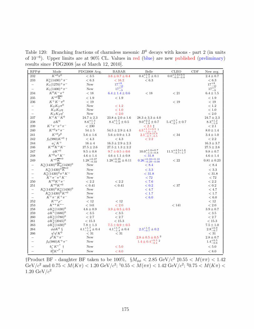
Table 120: Branching fractions of charmless mesonic B0 decays with kaons - part 2 (in unitsof 10−6). Upper limits are at 90% CL. Values in red (blue) are new published (preliminary)results since PDG2008 [as of March 12, 2010].
RPP# Mode PDG2008 Avg. BABAR Belle CLEO CDF New avg.
232 K∗0π0 < 3.5 3.6± 0.7± 0.4 0.4+1.9−1.7 ± 0.1 0.0+1.3+0.5
−0.0−0.0 2.4± 0.7
233 K∗2 (1430)
+π− < 6.3 < 16.2 < 6.3 < 6.3
− K1(1270)+π− New 17+8−11 17+8
−11
− K1(1400)+π− New 17+7−9 17+7
−9
234 K0K−π+ < 18 6.4± 1.4± 0.6 < 18 < 21 6.4± 1.5
235 K∗0K0
< 1.9 < 1.9 < 1.9236 K+K−π0 < 19 < 19 < 19− KSKSπ
0 New < 1.2 < 1.2− KSKSη New < 1.0 < 1.0− KSKSη
′ New < 2.0 < 2.0237 K+K−K0 24.7± 2.3 23.8± 2.0± 1.6 28.3± 3.3± 4.0 24.7± 2.3
238 φK0 8.6+1.3−1.1 8.4+1.5
−1.3 ± 0.5 9.0+2.2−1.8 ± 0.7 5.4+3.7
−2.7 ± 0.7 8.3+1.2−1.0
239 K+π−π+π− < 230 < 2.1 ‡ < 2.1
240 K∗0π+π− 54± 5 54.5± 2.9± 4.3 4.5+1.1+0.9−1.0−1.6
1 8.0± 1.4
241 K∗0ρ0 5.6± 1.6 5.6± 0.9± 1.3 2.1+0.8+0.9−0.7−0.5 < 34 3.4± 1.0
242 f0(980)K∗0 † < 4.3 < 4.3 < 2.2 < 2.2
244 a−1 K+ 16± 4 16.3± 2.9± 2.3 16.3± 3.7
246 K∗0K+K− 27.5± 2.6 27.5± 1.3± 2.2 27.5± 2.6
247 φK∗0 9.5± 0.8 9.7± 0.5± 0.6 10.0+1.6+0.7−1.5−0.8 11.5+4.5+1.8
−3.7−1.7 9.8± 0.7
248 K∗0π+K− 4.6± 1.4 4.6± 1.1± 0.8 < 31.8 4.6± 1.4
249 K∗0K∗0
1.28+0.37−0.32 1.28+0.35
−0.30 ± 0.11 0.26+0.33+0.10−0.29−0.08 < 22 0.81± 0.23
− K∗0 (1430)
0K∗0(1430)
0 New < 8.4 < 8.4
− K∗0 (1430)
0K∗0
New < 3.3 < 3.3− K∗
0 (1430)0π+K− New < 31.8 < 31.8
− K+π−π+K− New < 72 < 72250 K∗0K+π− < 2.2 < 2.2 < 7.6 < 2.2251 K∗0K∗0 < 0.41 < 0.41 < 0.2 < 37 < 0.2− K∗
0 (1430)0K∗
0 (1430)0 New < 4.7 < 4.7
− K∗0 (1430)
0K∗0 New < 1.7 < 1.7− K+π−K+π− New < 6.0 < 6.0252 K∗+ρ− < 12 < 12 < 12253 K∗+K∗− < 141 < 2.0 < 141 < 2.0258 φK∗
0 (1430)0 4.6± 0.9 3.9± 0.5± 0.5 3.9± 0.7
259 φK∗(1680)0 < 3.5 < 3.5 < 3.5260 φK∗
3 (1780)0 < 2.7 < 2.7 < 2.7
261 φK∗4 (2045)
0 < 15.3 < 15.3 < 15.3263 φK∗
2 (1430)0 7.8± 1.3 7.5± 0.9± 0.5 7.5± 1.0
264 φφK0 § 4.1+1.7−1.4 ± 0.4 4.1+1.7
−1.4 ± 0.4 2.3+1.0−0.7 ± 0.2 2.8+0.9
−0.7
266 η′η′K0 < 31 < 31 < 31− ρ0K+π− New 2.8± 0.5± 0.5 2 2.8± 0.7
− f0(980)K+π− New 1.4± 0.4+0.3−0.4
2 1.4+0.5−0.6
− b−1 K∗+ † New < 5.0 < 5.0
− b01K∗0 † New < 8.0 < 8.0
†Product BF - daughter BF taken to be 100%, §Mφφ < 2.85 GeV/c2 ‡0.55 < M(ππ) < 1.42GeV/c2 and 0.75 < M(Kπ) < 1.20 GeV/c2; 10.55 < M(ππ) < 1.42 GeV/c2; 20.75 < M(Kπ) <1.20 GeV/c2
175
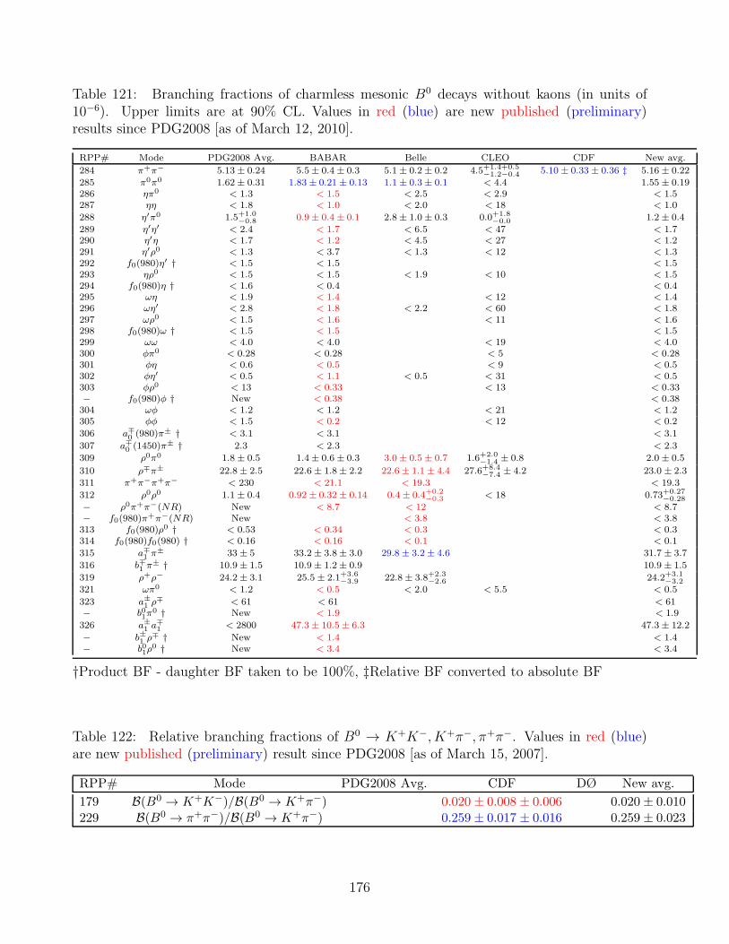
Table 121: Branching fractions of charmless mesonic B0 decays without kaons (in units of10−6). Upper limits are at 90% CL. Values in red (blue) are new published (preliminary)results since PDG2008 [as of March 12, 2010].
RPP# Mode PDG2008 Avg. BABAR Belle CLEO CDF New avg.
284 π+π− 5.13± 0.24 5.5± 0.4± 0.3 5.1± 0.2± 0.2 4.5+1.4+0.5−1.2−0.4 5.10 ± 0.33± 0.36 ‡ 5.16± 0.22
285 π0π0 1.62± 0.31 1.83± 0.21± 0.13 1.1± 0.3± 0.1 < 4.4 1.55± 0.19286 ηπ0 < 1.3 < 1.5 < 2.5 < 2.9 < 1.5287 ηη < 1.8 < 1.0 < 2.0 < 18 < 1.0
288 η′π0 1.5+1.0−0.8 0.9± 0.4± 0.1 2.8± 1.0± 0.3 0.0+1.8
−0.0 1.2± 0.4
289 η′η′ < 2.4 < 1.7 < 6.5 < 47 < 1.7290 η′η < 1.7 < 1.2 < 4.5 < 27 < 1.2291 η′ρ0 < 1.3 < 3.7 < 1.3 < 12 < 1.3292 f0(980)η′ † < 1.5 < 1.5 < 1.5293 ηρ0 < 1.5 < 1.5 < 1.9 < 10 < 1.5294 f0(980)η † < 1.6 < 0.4 < 0.4295 ωη < 1.9 < 1.4 < 12 < 1.4296 ωη′ < 2.8 < 1.8 < 2.2 < 60 < 1.8297 ωρ0 < 1.5 < 1.6 < 11 < 1.6298 f0(980)ω † < 1.5 < 1.5 < 1.5299 ωω < 4.0 < 4.0 < 19 < 4.0300 φπ0 < 0.28 < 0.28 < 5 < 0.28301 φη < 0.6 < 0.5 < 9 < 0.5302 φη′ < 0.5 < 1.1 < 0.5 < 31 < 0.5303 φρ0 < 13 < 0.33 < 13 < 0.33− f0(980)φ † New < 0.38 < 0.38304 ωφ < 1.2 < 1.2 < 21 < 1.2305 φφ < 1.5 < 0.2 < 12 < 0.2
306 a∓0 (980)π± † < 3.1 < 3.1 < 3.1
307 a∓0 (1450)π± † 2.3 < 2.3 < 2.3
309 ρ0π0 1.8± 0.5 1.4± 0.6± 0.3 3.0± 0.5± 0.7 1.6+2.0−1.4 ± 0.8 2.0± 0.5
310 ρ∓π± 22.8± 2.5 22.6± 1.8± 2.2 22.6± 1.1± 4.4 27.6+8.4−7.4 ± 4.2 23.0 ± 2.3
311 π+π−π+π− < 230 < 21.1 < 19.3 < 19.3
312 ρ0ρ0 1.1± 0.4 0.92± 0.32± 0.14 0.4± 0.4+0.2−0.3 < 18 0.73+0.27
−0.28
− ρ0π+π−(NR) New < 8.7 < 12 < 8.7− f0(980)π+π−(NR) New < 3.8 < 3.8313 f0(980)ρ0 † < 0.53 < 0.34 < 0.3 < 0.3314 f0(980)f0(980) † < 0.16 < 0.16 < 0.1 < 0.1
315 a∓1 π± 33 ± 5 33.2± 3.8± 3.0 29.8± 3.2± 4.6 31.7 ± 3.7
316 b∓1 π± † 10.9± 1.5 10.9± 1.2± 0.9 10.9 ± 1.5
319 ρ+ρ− 24.2± 3.1 25.5± 2.1+3.6−3.9 22.8± 3.8+2.3
−2.6 24.2+3.1−3.2
321 ωπ0 < 1.2 < 0.5 < 2.0 < 5.5 < 0.5
323 a±1 ρ∓ < 61 < 61 < 61
− b01π0 † New < 1.9 < 1.9
326 a±1 a∓1 < 2800 47.3± 10.5± 6.3 47.3± 12.2
− b±1 ρ∓ † New < 1.4 < 1.4
− b01ρ0 † New < 3.4 < 3.4
†Product BF - daughter BF taken to be 100%, ‡Relative BF converted to absolute BF
Table 122: Relative branching fractions of B0 → K+K−, K+π−, π+π−. Values in red (blue)are new published (preliminary) result since PDG2008 [as of March 15, 2007].
RPP# Mode PDG2008 Avg. CDF DØ New avg.
179 B(B0 → K+K−)/B(B0 → K+π−) 0.020 ± 0.008 ± 0.006 0.020 ± 0.010229 B(B0 → π+π−)/B(B0 → K+π−) 0.259 ± 0.017 ± 0.016 0.259 ± 0.023
176
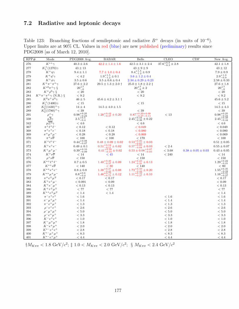
7.2 Radiative and leptonic decays
Table 123: Branching fractions of semileptonic and radiative B+ decays (in units of 10−6).Upper limits are at 90% CL. Values in red (blue) are new published (preliminary) results sincePDG2008 [as of March 12, 2010].
RPP# Mode PDG2008 Avg. BABAR Belle CLEO CDF New Avg.
276 K∗+γ 40.3± 2.6 42.2± 1.4± 1.6 42.5± 3.1± 2.4 37.6+8.9−8.3 ± 2.8 42.1 ± 1.8
277 K+1 (1270)γ 43± 13 43± 9± 9 43± 12
278 K+ηγ 9.4± 1.1 7.7± 1.0± 0.4 8.4+1.5−1.2 ± 0.9 7.9± 0.9
279 K+η′γ < 4.2 1.9+1.5−1.2 ± 0.1 3.6± 1.2± 0.4 2.9+1.0
−0.9280 K+φγ 3.5± 0.6 3.5± 0.6± 0.4 2.34± 0.29± 0.23 2.58± 0.33281 K+π−π+γ 27.6± 2.2 29.5± 1.3± 2.0 † 25.0± 1.8± 2.2 ‡ 27.6 ± 1.8
282 K∗0π+γ § 20+7−6 20+7
−6 ± 2 20+7−6
283 K+ρ0γ § < 20 < 20 < 20284 K+π−π+γ (N.R.) § < 9.2 < 9.2 < 9.2285 K0π+π0γ 46± 5 45.6± 4.2± 3.1 † 45.6 ± 5.2
286 K+1 (1400)γ < 15 < 15 < 15
287 K∗2 (1430)
+γ 14± 4 14.5± 4.0± 1.5 14.5 ± 4.3289 K∗
3 (1780)+γ < 39 < 39 < 39
291 ρ+γ 0.98+0.25−0.24 1.20+0.42
−0.37 ± 0.20 0.87+0.29+0.09−0.27−0.11 < 13 0.98+0.25
−0.24
338 pΛγ 2.5+0.5−0.4 2.45+0.44
−0.38 ± 0.22 2.45+0.49−0.44
342 pΣ0γ < 4.6 < 4.6 < 4.6367 π+ℓ+ℓ− < 0.12 < 0.12 < 0.049 < 0.049368 π+e+e− < 0.18 < 0.18 < 0.080 < 0.080369 π+µ+µ− < 0.28 < 0.28 < 0.069 < 0.069370 π+νν < 100 < 100 < 170 < 100
371 K+ℓ+ℓ− 0.44+0.08−0.07 0.48± 0.09± 0.02 0.53+0.06
−0.05 ± 0.03 0.51± 0.05
372 K+e+e− 0.49± 0.1 0.51+0.12−0.11 ± 0.02 0.57+0.09
−0.08 ± 0.03 < 2.4 0.55± 0.07
373 K+µ+µ− 0.39+0.10−0.09 0.41+0.16
−0.15 ± 0.02 0.53± 0.08+0.07−0.03 < 3.68 0.38± 0.05± 0.03 0.43± 0.05
374 K+νν < 14 < 45 < 14 < 240 < 14375 ρ+νν < 150 < 150 < 150
376 K∗+ℓ+ℓ− 0.7± 0.5 1.40+0.40−0.37 ± 0.09 1.24+0.23
−0.21 ± 0.13 1.29+0.22−0.21
377 K∗+νν < 140 < 80 < 140 < 80
378 K∗+e+e− 0.8± 0.8 1.38+0.47−0.42 ± 0.08 1.73+0.50
−0.42 ± 0.20 1.55+0.35−0.32
379 K∗+µ+µ− 0.8+0.6−0.4 1.46+0.79
−0.75 ± 0.12 1.11+0.32−0.27 ± 0.10 1.16+0.31
−0.27382 π+e±µ∓ < 0.17 < 0.17 < 0.17383 K+e+µ− < 0.091 < 0.09 < 0.09384 K+e−µ+ < 0.13 < 0.13 < 0.13386 K+τ±µ∓ < 77 < 77 < 77389 K∗+e±µ∓ < 1.4 < 1.4 < 1.4390 π−e+e+ < 1.6 < 1.6 < 1.6391 π−µ+µ+ < 1.4 < 1.4 < 1.4392 π−e+µ+ < 1.3 < 1.3 < 1.3393 ρ−e+e+ < 2.6 < 2.6 < 2.6394 ρ−µ+µ+ < 5.0 < 5.0 < 5.0395 ρ−e+µ+ < 3.3 < 3.3 < 3.3396 K−e+e+ < 1.0 < 1.0 < 1.0397 K−µ+µ+ < 1.8 < 1.8 < 1.8398 K−e+µ+ < 2.0 < 2.0 < 2.0399 K∗−e+e+ < 2.8 < 2.8 < 2.8400 K∗−µ+µ+ < 8.3 < 8.3 < 8.3401 K∗−e+µ+ < 4.4 < 4.4 < 4.4
†MKππ < 1.8 GeV/c2; ‡ 1.0 < MKππ < 2.0 GeV/c2; § MKππ < 2.4 GeV/c2
177
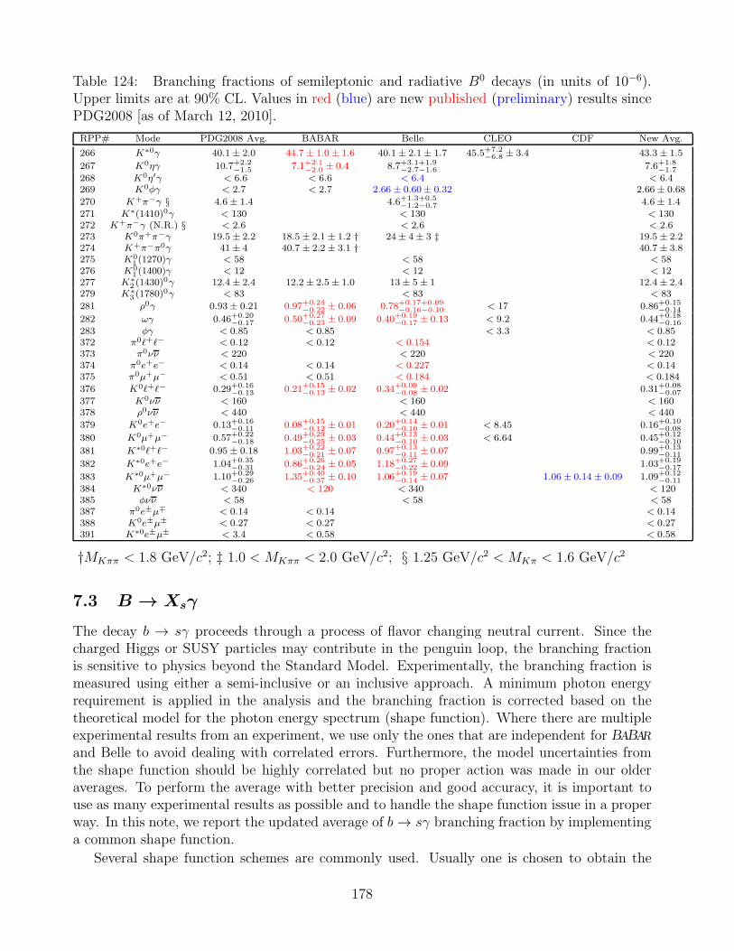
Table 124: Branching fractions of semileptonic and radiative B0 decays (in units of 10−6).Upper limits are at 90% CL. Values in red (blue) are new published (preliminary) results sincePDG2008 [as of March 12, 2010].
RPP# Mode PDG2008 Avg. BABAR Belle CLEO CDF New Avg.
266 K∗0γ 40.1± 2.0 44.7± 1.0± 1.6 40.1± 2.1± 1.7 45.5+7.2−6.8 ± 3.4 43.3± 1.5
267 K0ηγ 10.7+2.2−1.5 7.1+2.1
−2.0 ± 0.4 8.7+3.1+1.9−2.7−1.6 7.6+1.8
−1.7
268 K0η′γ < 6.6 < 6.6 < 6.4 < 6.4269 K0φγ < 2.7 < 2.7 2.66 ± 0.60± 0.32 2.66± 0.68
270 K+π−γ § 4.6± 1.4 4.6+1.3+0.5−1.2−0.7 4.6± 1.4
271 K∗(1410)0γ < 130 < 130 < 130272 K+π−γ (N.R.) § < 2.6 < 2.6 < 2.6273 K0π+π−γ 19.5± 2.2 18.5± 2.1± 1.2 † 24± 4± 3 ‡ 19.5± 2.2274 K+π−π0γ 41± 4 40.7± 2.2± 3.1 † 40.7± 3.8275 K0
1 (1270)γ < 58 < 58 < 58276 K0
1 (1400)γ < 12 < 12 < 12277 K∗
2 (1430)0γ 12.4± 2.4 12.2± 2.5± 1.0 13± 5± 1 12.4± 2.4
279 K∗3 (1780)
0γ < 83 < 83 < 83
281 ρ0γ 0.93± 0.21 0.97+0.24−0.22 ± 0.06 0.78+0.17+0.09
−0.16−0.10 < 17 0.86+0.15−0.14
282 ωγ 0.46+0.20−0.17 0.50+0.27
−0.23 ± 0.09 0.40+0.19−0.17 ± 0.13 < 9.2 0.44+0.18
−0.16283 φγ < 0.85 < 0.85 < 3.3 < 0.85372 π0ℓ+ℓ− < 0.12 < 0.12 < 0.154 < 0.12373 π0νν < 220 < 220 < 220374 π0e+e− < 0.14 < 0.14 < 0.227 < 0.14375 π0µ+µ− < 0.51 < 0.51 < 0.184 < 0.184
376 K0ℓ+ℓ− 0.29+0.16−0.13 0.21+0.15
−0.13 ± 0.02 0.34+0.09−0.08 ± 0.02 0.31+0.08
−0.07
377 K0νν < 160 < 160 < 160378 ρ0νν < 440 < 440 < 440
379 K0e+e− 0.13+0.16−0.11 0.08+0.15
−0.12 ± 0.01 0.20+0.14−0.10 ± 0.01 < 8.45 0.16+0.10
−0.08
380 K0µ+µ− 0.57+0.22−0.18 0.49+0.29
−0.25 ± 0.03 0.44+0.13−0.10 ± 0.03 < 6.64 0.45+0.12
−0.10
381 K∗0ℓ+ℓ− 0.95± 0.18 1.03+0.22−0.21 ± 0.07 0.97+0.13
−0.11 ± 0.07 0.99+0.13−0.11
382 K∗0e+e− 1.04+0.35−0.31 0.86+0.26
−0.24 ± 0.05 1.18+0.27−0.22 ± 0.09 1.03+0.19
−0.17
383 K∗0µ+µ− 1.10+0.29−0.26 1.35+0.40
−0.37 ± 0.10 1.06+0.19−0.14 ± 0.07 1.06 ± 0.14± 0.09 1.09+0.12
−0.11384 K∗0νν < 340 < 120 < 340 < 120385 φνν < 58 < 58 < 58387 π0e±µ∓ < 0.14 < 0.14 < 0.14388 K0e±µ± < 0.27 < 0.27 < 0.27391 K∗0e±µ± < 3.4 < 0.58 < 0.58
†MKππ < 1.8 GeV/c2; ‡ 1.0 < MKππ < 2.0 GeV/c2; § 1.25 GeV/c2 < MKπ < 1.6 GeV/c2
7.3 B → Xsγ
The decay b → sγ proceeds through a process of flavor changing neutral current. Since thecharged Higgs or SUSY particles may contribute in the penguin loop, the branching fractionis sensitive to physics beyond the Standard Model. Experimentally, the branching fraction ismeasured using either a semi-inclusive or an inclusive approach. A minimum photon energyrequirement is applied in the analysis and the branching fraction is corrected based on thetheoretical model for the photon energy spectrum (shape function). Where there are multipleexperimental results from an experiment, we use only the ones that are independent for BABARand Belle to avoid dealing with correlated errors. Furthermore, the model uncertainties fromthe shape function should be highly correlated but no proper action was made in our olderaverages. To perform the average with better precision and good accuracy, it is important touse as many experimental results as possible and to handle the shape function issue in a properway. In this note, we report the updated average of b→ sγ branching fraction by implementinga common shape function.
Several shape function schemes are commonly used. Usually one is chosen to obtain the
178
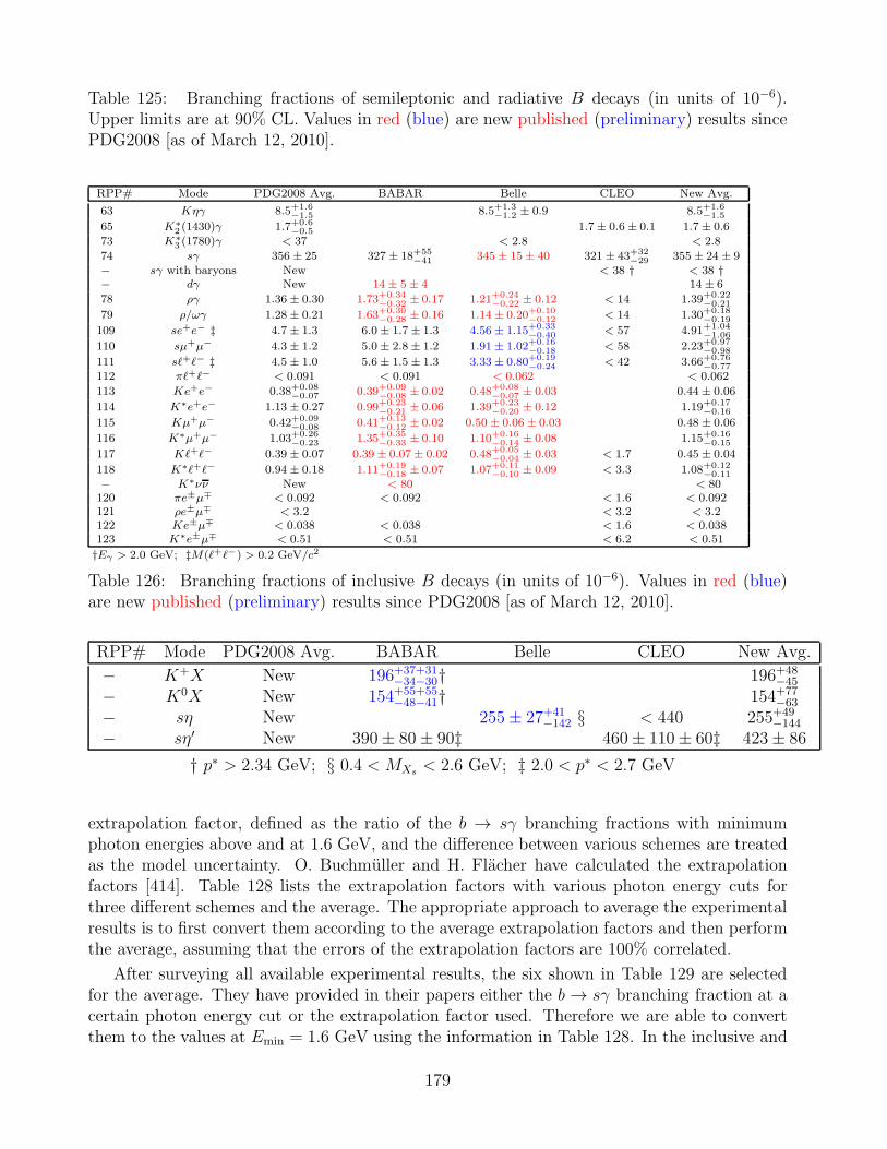
Table 125: Branching fractions of semileptonic and radiative B decays (in units of 10−6).Upper limits are at 90% CL. Values in red (blue) are new published (preliminary) results sincePDG2008 [as of March 12, 2010].
RPP# Mode PDG2008 Avg. BABAR Belle CLEO New Avg.
63 Kηγ 8.5+1.6−1.5 8.5+1.3
−1.2 ± 0.9 8.5+1.6−1.5
65 K∗2 (1430)γ 1.7+0.6
−0.5 1.7± 0.6± 0.1 1.7± 0.6
73 K∗3 (1780)γ < 37 < 2.8 < 2.8
74 sγ 356 ± 25 327 ± 18+55−41 345± 15± 40 321 ± 43+32
−29 355 ± 24 ± 9− sγ with baryons New < 38 † < 38 †− dγ New 14± 5± 4 14 ± 6
78 ργ 1.36± 0.30 1.73+0.34−0.32 ± 0.17 1.21+0.24
−0.22 ± 0.12 < 14 1.39+0.22−0.21
79 ρ/ωγ 1.28± 0.21 1.63+0.30−0.28 ± 0.16 1.14± 0.20+0.10
−0.12 < 14 1.30+0.18−0.19
109 se+e− ‡ 4.7± 1.3 6.0± 1.7± 1.3 4.56± 1.15+0.33−0.40 < 57 4.91+1.04
−1.06
110 sµ+µ− 4.3± 1.2 5.0± 2.8± 1.2 1.91± 1.02+0.16−0.18 < 58 2.23+0.97
−0.98
111 sℓ+ℓ− ‡ 4.5± 1.0 5.6± 1.5± 1.3 3.33± 0.80+0.19−0.24 < 42 3.66+0.76
−0.77112 πℓ+ℓ− < 0.091 < 0.091 < 0.062 < 0.062
113 Ke+e− 0.38+0.08−0.07 0.39+0.09
−0.08 ± 0.02 0.48+0.08−0.07 ± 0.03 0.44± 0.06
114 K∗e+e− 1.13± 0.27 0.99+0.23−0.21 ± 0.06 1.39+0.23
−0.20 ± 0.12 1.19+0.17−0.16
115 Kµ+µ− 0.42+0.09−0.08 0.41+0.13
−0.12 ± 0.02 0.50± 0.06± 0.03 0.48± 0.06
116 K∗µ+µ− 1.03+0.26−0.23 1.35+0.35
−0.33 ± 0.10 1.10+0.16−0.14 ± 0.08 1.15+0.16
−0.15
117 Kℓ+ℓ− 0.39± 0.07 0.39± 0.07± 0.02 0.48+0.05−0.04 ± 0.03 < 1.7 0.45± 0.04
118 K∗ℓ+ℓ− 0.94± 0.18 1.11+0.19−0.18 ± 0.07 1.07+0.11
−0.10 ± 0.09 < 3.3 1.08+0.12−0.11
− K∗νν New < 80 < 80120 πe±µ∓ < 0.092 < 0.092 < 1.6 < 0.092121 ρe±µ∓ < 3.2 < 3.2 < 3.2122 Ke±µ∓ < 0.038 < 0.038 < 1.6 < 0.038123 K∗e±µ∓ < 0.51 < 0.51 < 6.2 < 0.51
†Eγ > 2.0 GeV; ‡M(ℓ+ℓ−) > 0.2 GeV/c2
Table 126: Branching fractions of inclusive B decays (in units of 10−6). Values in red (blue)are new published (preliminary) results since PDG2008 [as of March 12, 2010].
RPP# Mode PDG2008 Avg. BABAR Belle CLEO New Avg.
− K+X New 196+37+31−34−30† 196+48
−45
− K0X New 154+55+55−48−41† 154+77
−63
− sη New 255± 27+41−142 § < 440 255+49
−144
− sη′ New 390± 80± 90‡ 460± 110± 60‡ 423± 86
† p∗ > 2.34 GeV; § 0.4 < MXs < 2.6 GeV; ‡ 2.0 < p∗ < 2.7 GeV
extrapolation factor, defined as the ratio of the b → sγ branching fractions with minimumphoton energies above and at 1.6 GeV, and the difference between various schemes are treatedas the model uncertainty. O. Buchmuller and H. Flacher have calculated the extrapolationfactors [414]. Table 128 lists the extrapolation factors with various photon energy cuts forthree different schemes and the average. The appropriate approach to average the experimentalresults is to first convert them according to the average extrapolation factors and then performthe average, assuming that the errors of the extrapolation factors are 100% correlated.
After surveying all available experimental results, the six shown in Table 129 are selectedfor the average. They have provided in their papers either the b → sγ branching fraction at acertain photon energy cut or the extrapolation factor used. Therefore we are able to convertthem to the values at Emin = 1.6 GeV using the information in Table 128. In the inclusive and
179
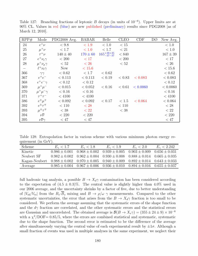
Table 127: Branching fractions of leptonic B decays (in units of 10−6). Upper limits are at90% CL. Values in red (blue) are new published (preliminary) results since PDG2008 [as ofMarch 12, 2010].
RPP# Mode PDG2008 Avg. BABAR Belle CLEO CDF DØ New Avg.
24 e+ν < 9.8 < 1.9 < 1.0 < 15 < 1.025 µ+ν < 1.7 < 1.0 < 1.7 < 21 < 1.026 τ+ν 140± 40 170± 60 165+38+35
−37−37 < 840 167± 3927 e+νeγ < 200 < 17 < 200 < 1728 µ+νµγ < 52 < 26 < 52 < 26− ℓ+νℓγ New < 15.6 < 15.6366 γγ < 0.62 < 1.7 < 0.62 < 0.62367 e+e− < 0.113 < 0.113 < 0.19 < 0.83 < 0.083 < 0.083368 e+e−γ < 0.12 < 0.12 < 0.12369 µ+µ− < 0.015 < 0.052 < 0.16 < 0.61 < 0.0060 < 0.0060370 µ+µ−γ < 0.16 < 0.16 < 0.16371 τ+τ− < 4100 < 4100 < 4100386 e±µ∓ < 0.092 < 0.092 < 0.17 < 1.5 < 0.064 < 0.064392 e±τ∓ < 110 < 28 < 110 < 28393 µ±τ∓ < 38 < 22 < 38 < 22394 νν < 220 < 220 < 220395 ννγ < 47 < 47 < 47
Table 128: Extrapolation factor in various scheme with various minimum photon energy re-quirement (in GeV).
Scheme Eγ < 1.7 Eγ < 1.8 Eγ < 1.9 Eγ < 2.0 Eγ < 2.242Kinetic 0.986± 0.001 0.968± 0.002 0.939± 0.005 0.903± 0.009 0.656± 0.031Neubert SF 0.982± 0.002 0.962± 0.004 0.930± 0.008 0.888± 0.014 0.665± 0.035Kagan-Neubert 0.988± 0.002 0.970± 0.005 0.940± 0.009 0.892± 0.014 0.643± 0.033Average 0.985± 0.004 0.967± 0.006 0.936± 0.010 0.894± 0.016 0.655± 0.037
full hadronic tag analysis, a possible B → Xdγ contamination has been considered accordingto the expectation of (4.5 ± 0.3)%. The central value is slightly higher than 4.0% used inour 2006 average, and the uncertainty shrinks by a factor of five, due to better understandingof |Vtd/Vts| from the Bs-Bs mixing and B → ρ/ω γ measurements. Compared to the othersystematic uncertainties, the error that arises from the B → Xdγ fraction is too small to beconsidered. We perform the average assuming that the systematic errors of the shape functionand the dγ fraction are correlated, and the other systematic errors and the statistical errorsare Gaussian and uncorrelated. The obtained average is B(B → Xsγ) = (355± 24± 9)× 10−6
with a χ2/DOF= 0.85/5, where the errors are combined statistical and systematic, systematicdue to the shape function. The second error is estimated to be the difference of the averageafter simultaneously varying the central value of each experimental result by ±1σ. Although asmall fraction of events was used in multiple analyses in the same experiment, we neglect their
180
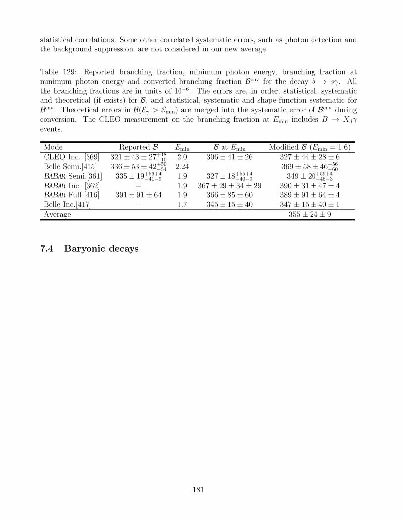
statistical correlations. Some other correlated systematic errors, such as photon detection andthe background suppression, are not considered in our new average.
Table 129: Reported branching fraction, minimum photon energy, branching fraction atminimum photon energy and converted branching fraction Bcnv for the decay b → sγ. Allthe branching fractions are in units of 10−6. The errors are, in order, statistical, systematicand theoretical (if exists) for B, and statistical, systematic and shape-function systematic forBcnv. Theoretical errors in B(Eγ > Emin) are merged into the systematic error of Bcnv duringconversion. The CLEO measurement on the branching fraction at Emin includes B → Xdγevents.
Mode Reported B Emin B at Emin Modified B (Emin = 1.6)CLEO Inc. [369] 321± 43± 27+18
−10 2.0 306± 41± 26 327± 44± 28± 6Belle Semi.[415] 336± 53± 42+50
−54 2.24 − 369± 58± 46+56−60
BABAR Semi.[361] 335± 19+56+4−41−9 1.9 327± 18+55+4
−40−9 349± 20+59+4−46−3
BABAR Inc. [362] − 1.9 367± 29± 34± 29 390± 31± 47± 4BABAR Full [416] 391± 91± 64 1.9 366± 85± 60 389± 91± 64± 4Belle Inc.[417] − 1.7 345± 15± 40 347± 15± 40± 1Average 355± 24± 9
7.4 Baryonic decays
181
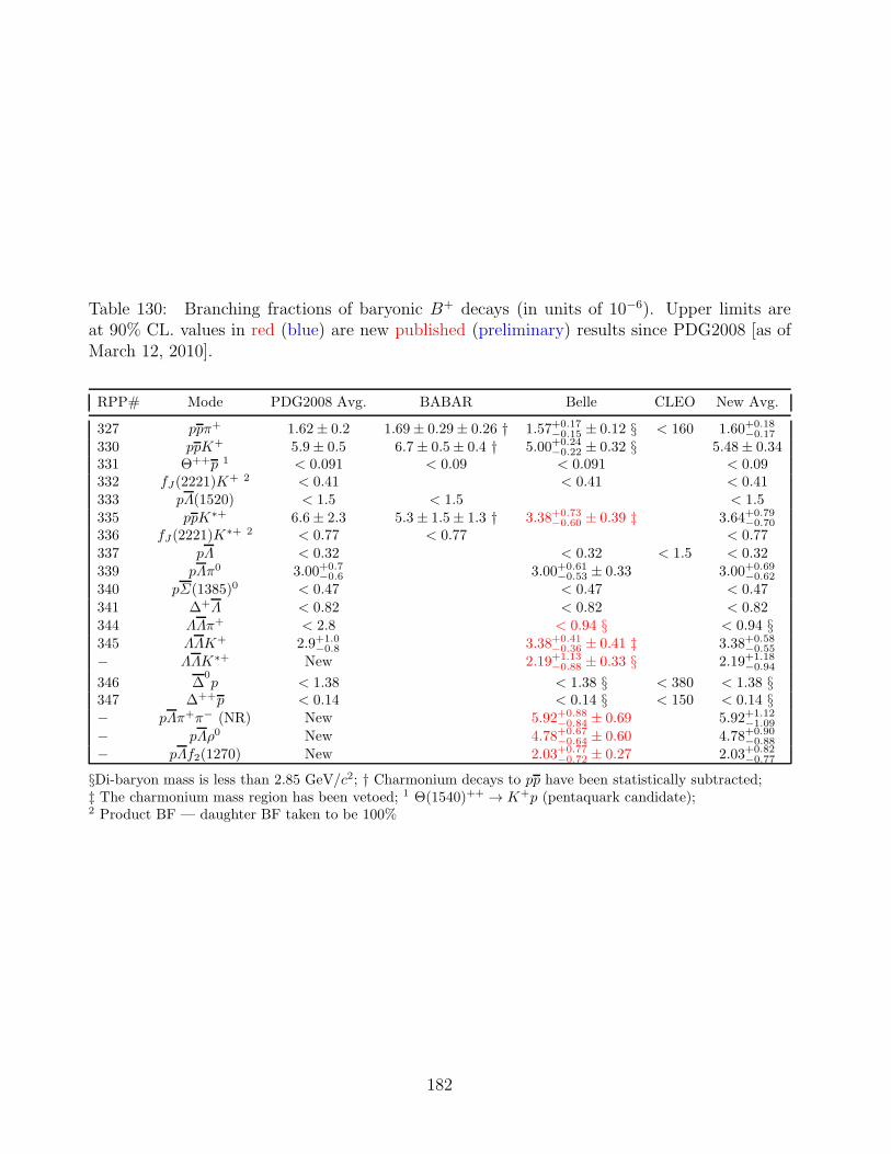
Table 130: Branching fractions of baryonic B+ decays (in units of 10−6). Upper limits areat 90% CL. values in red (blue) are new published (preliminary) results since PDG2008 [as ofMarch 12, 2010].
RPP# Mode PDG2008 Avg. BABAR Belle CLEO New Avg.
327 ppπ+ 1.62± 0.2 1.69± 0.29± 0.26 † 1.57+0.17−0.15 ± 0.12 § < 160 1.60+0.18
−0.17
330 ppK+ 5.9± 0.5 6.7± 0.5± 0.4 † 5.00+0.24−0.22 ± 0.32 § 5.48± 0.34
331 Θ++p 1 < 0.091 < 0.09 < 0.091 < 0.09332 fJ(2221)K
+ 2 < 0.41 < 0.41 < 0.41333 pΛ(1520) < 1.5 < 1.5 < 1.5335 ppK∗+ 6.6± 2.3 5.3± 1.5± 1.3 † 3.38+0.73
−0.60 ± 0.39 ‡ 3.64+0.79−0.70
336 fJ(2221)K∗+ 2 < 0.77 < 0.77 < 0.77
337 pΛ < 0.32 < 0.32 < 1.5 < 0.32339 pΛπ0 3.00+0.7
−0.6 3.00+0.61−0.53 ± 0.33 3.00+0.69
−0.62
340 pΣ(1385)0 < 0.47 < 0.47 < 0.47
341 ∆+Λ < 0.82 < 0.82 < 0.82344 ΛΛπ+ < 2.8 < 0.94 § < 0.94 §345 ΛΛK+ 2.9+1.0
−0.8 3.38+0.41−0.36 ± 0.41 ‡ 3.38+0.58
−0.55
− ΛΛK∗+ New 2.19+1.13−0.88 ± 0.33 § 2.19+1.18
−0.94
346 ∆0p < 1.38 < 1.38 § < 380 < 1.38 §
347 ∆++p < 0.14 < 0.14 § < 150 < 0.14 §− pΛπ+π− (NR) New 5.92+0.88
−0.84 ± 0.69 5.92+1.12−1.09
− pΛρ0 New 4.78+0.67−0.64 ± 0.60 4.78+0.90
−0.88
− pΛf2(1270) New 2.03+0.77−0.72 ± 0.27 2.03+0.82
−0.77
§Di-baryon mass is less than 2.85 GeV/c2; † Charmonium decays to pp have been statistically subtracted;‡ The charmonium mass region has been vetoed; 1 Θ(1540)++ → K+p (pentaquark candidate);2 Product BF — daughter BF taken to be 100%
182
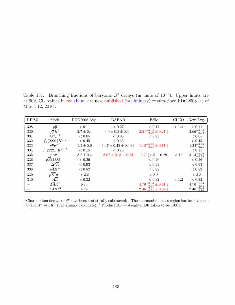
Table 131: Branching fractions of baryonic B0 decays (in units of 10−6). Upper limits areat 90% CL. values in red (blue) are new published (preliminary) results since PDG2008 [as ofMarch 12, 2010].
RPP# Mode PDG2008 Avg. BABAR Belle CLEO New Avg.
328 pp < 0.11 < 0.27 < 0.11 < 1.4 < 0.11330 ppK0 2.7± 0.4 3.0± 0.5± 0.3 † 2.51+0.35
−0.29 ± 0.21 ‡ 2.66+0.34−0.32
331 Θ+p 1 < 0.05 < 0.05 < 0.23 < 0.05332 fJ(2221)K
0 2 < 0.45 < 0.45 < 0.45333 ppK∗0 1.5± 0.6 1.47± 0.45± 0.40 † 1.18+0.29
−0.25 ± 0.11 ‡ 1.24+0.28−0.25
334 fJ(2221)K∗0 2 < 0.15 < 0.15 < 0.15
335 pΛπ− 3.2± 0.4 3.07± 0.31± 0.23 3.23+0.33−0.29 ± 0.29 < 13 3.14+0.29
−0.28
336 pΣ(1385)− < 0.26 < 0.26 < 0.26
337 ∆0Λ < 0.93 < 0.93 < 0.93338 pΛK− < 0.82 < 0.82 < 0.82
339 pΣ0π− < 3.8 < 3.8 < 3.8
340 ΛΛ < 0.32 < 0.32 < 1.2 < 0.32
− ΛΛK0 New 4.76+0.84−0.68 ± 0.61 ‡ 4.76+1.04
−0.91
− ΛΛK∗0 New 2.46+0.87−0.72 ± 0.34 ‡ 2.46+0.93
−0.80
† Charmonium decays to pp have been statistically subtracted; ‡ The charmonium mass region has been vetoed;1 Θ(1540)+ → pK0 (pentaquark candidate); 2 Product BF — daughter BF taken to be 100%.
183
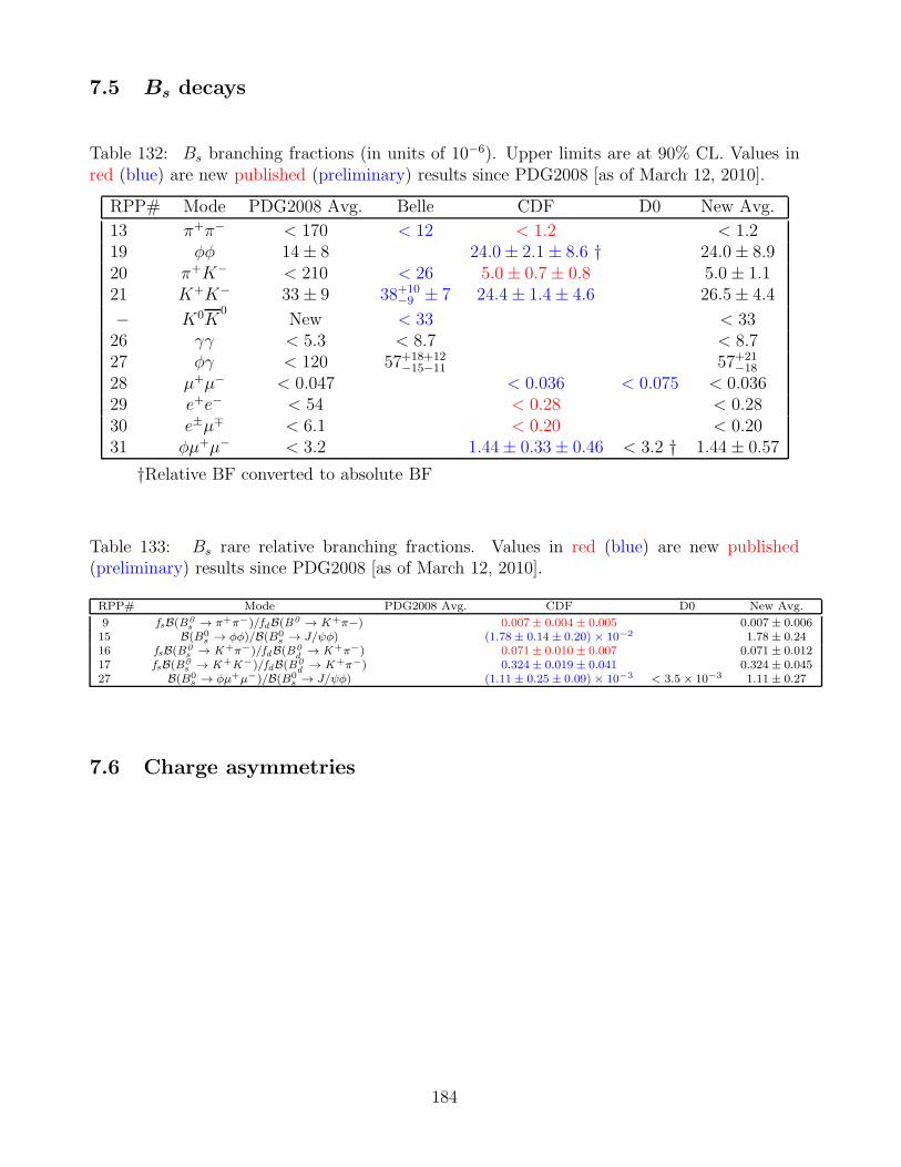
7.5 Bs decays
Table 132: Bs branching fractions (in units of 10−6). Upper limits are at 90% CL. Values inred (blue) are new published (preliminary) results since PDG2008 [as of March 12, 2010].
RPP# Mode PDG2008 Avg. Belle CDF D0 New Avg.
13 π+π− < 170 < 12 < 1.2 < 1.219 φφ 14± 8 24.0± 2.1± 8.6 † 24.0± 8.920 π+K− < 210 < 26 5.0± 0.7± 0.8 5.0± 1.121 K+K− 33± 9 38+10
−9 ± 7 24.4± 1.4± 4.6 26.5± 4.4
− K0K0
New < 33 < 3326 γγ < 5.3 < 8.7 < 8.727 φγ < 120 57+18+12
−15−11 57+21−18
28 µ+µ− < 0.047 < 0.036 < 0.075 < 0.03629 e+e− < 54 < 0.28 < 0.2830 e±µ∓ < 6.1 < 0.20 < 0.2031 φµ+µ− < 3.2 1.44± 0.33± 0.46 < 3.2 † 1.44± 0.57
†Relative BF converted to absolute BF
Table 133: Bs rare relative branching fractions. Values in red (blue) are new published(preliminary) results since PDG2008 [as of March 12, 2010].
RPP# Mode PDG2008 Avg. CDF D0 New Avg.
9 fsB(B0s → π+π−)/fdB(B
0 → K+π−) 0.007± 0.004± 0.005 0.007± 0.00615 B(B0
s → φφ)/B(B0s → J/ψφ) (1.78± 0.14± 0.20) × 10−2 1.78± 0.24
16 fsB(B0s → K+π−)/fdB(B
0
d→ K+π−) 0.071± 0.010± 0.007 0.071± 0.012
17 fsB(B0s → K+K−)/fdB(B
0
d→ K+π−) 0.324± 0.019± 0.041 0.324± 0.045
27 B(B0s → φµ+µ−)/B(B0
s → J/ψφ) (1.11± 0.25± 0.09) × 10−3 < 3.5× 10⁻³ 1.11± 0.27
7.6 Charge asymmetries
184
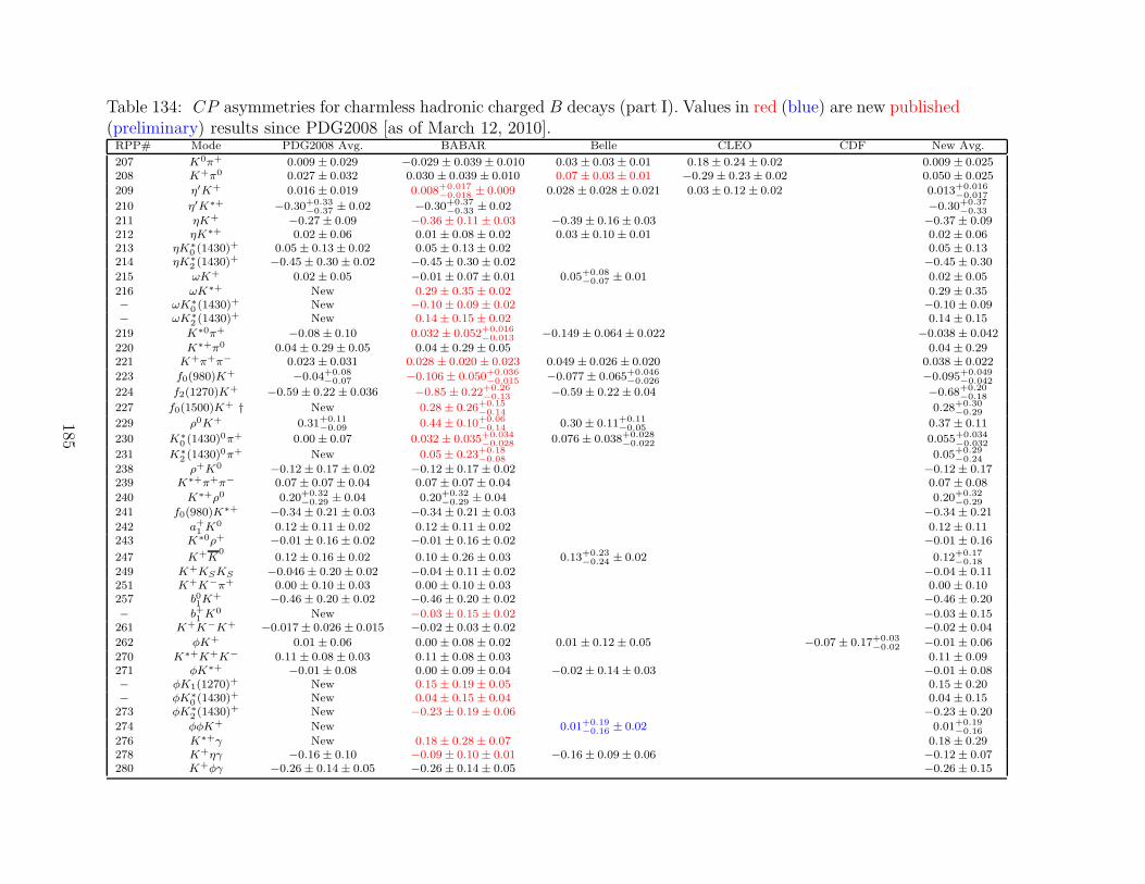
Table 134: CP asymmetries for charmless hadronic charged B decays (part I). Values in red (blue) are new published(preliminary) results since PDG2008 [as of March 12, 2010].RPP# Mode PDG2008 Avg. BABAR Belle CLEO CDF New Avg.
207 K0π+ 0.009 ± 0.029 −0.029± 0.039± 0.010 0.03 ± 0.03± 0.01 0.18± 0.24 ± 0.02 0.009 ± 0.025208 K+π0 0.027 ± 0.032 0.030 ± 0.039 ± 0.010 0.07 ± 0.03± 0.01 −0.29± 0.23± 0.02 0.050 ± 0.025
209 η′K+ 0.016 ± 0.019 0.008+0.017−0.018 ± 0.009 0.028 ± 0.028 ± 0.021 0.03± 0.12 ± 0.02 0.013+0.016
−0.017
210 η′K∗+ −0.30+0.33−0.37 ± 0.02 −0.30+0.37
−0.33 ± 0.02 −0.30+0.37−0.33
211 ηK+ −0.27± 0.09 −0.36± 0.11± 0.03 −0.39± 0.16± 0.03 −0.37± 0.09212 ηK∗+ 0.02± 0.06 0.01± 0.08± 0.02 0.03 ± 0.10± 0.01 0.02 ± 0.06213 ηK∗
0 (1430)+ 0.05± 0.13± 0.02 0.05± 0.13± 0.02 0.05 ± 0.13
214 ηK∗2 (1430)
+ −0.45± 0.30± 0.02 −0.45± 0.30± 0.02 −0.45± 0.30
215 ωK+ 0.02± 0.05 −0.01± 0.07± 0.01 0.05+0.08−0.07 ± 0.01 0.02 ± 0.05
216 ωK∗+ New 0.29± 0.35± 0.02 0.29 ± 0.35− ωK∗
0 (1430)+ New −0.10± 0.09± 0.02 −0.10± 0.09
− ωK∗2 (1430)
+ New 0.14± 0.15± 0.02 0.14 ± 0.15
219 K∗0π+ −0.08± 0.10 0.032 ± 0.052+0.016−0.013 −0.149± 0.064± 0.022 −0.038± 0.042
220 K∗+π0 0.04± 0.29± 0.05 0.04± 0.29± 0.05 0.04 ± 0.29221 K+π+π− 0.023 ± 0.031 0.028 ± 0.020 ± 0.023 0.049 ± 0.026 ± 0.020 0.038 ± 0.022
223 f0(980)K+ −0.04+0.08−0.07 −0.106± 0.050+0.036
−0.015 −0.077± 0.065+0.046−0.026 −0.095+0.049
−0.042
224 f2(1270)K+ −0.59± 0.22 ± 0.036 −0.85± 0.22+0.26−0.13 −0.59± 0.22± 0.04 −0.68+0.20
−0.18
227 f0(1500)K+ † New 0.28± 0.26+0.15−0.14 0.28+0.30
−0.29
229 ρ0K+ 0.31+0.11−0.09 0.44± 0.10+0.06
−0.14 0.30± 0.11+0.11−0.05 0.37 ± 0.11
230 K∗0 (1430)
0π+ 0.00± 0.07 0.032 ± 0.035+0.034−0.028 0.076± 0.038+0.028
−0.022 0.055+0.034−0.032
231 K∗2 (1430)
0π+ New 0.05± 0.23+0.18−0.08 0.05+0.29
−0.24
238 ρ+K0 −0.12± 0.17± 0.02 −0.12± 0.17± 0.02 −0.12± 0.17239 K∗+π+π− 0.07± 0.07± 0.04 0.07± 0.07± 0.04 0.07 ± 0.08
240 K∗+ρ0 0.20+0.32−0.29 ± 0.04 0.20+0.32
−0.29 ± 0.04 0.20+0.32−0.29
241 f0(980)K∗+ −0.34± 0.21± 0.03 −0.34± 0.21± 0.03 −0.34± 0.21
242 a+1 K0 0.12± 0.11± 0.02 0.12± 0.11± 0.02 0.12 ± 0.11
243 K∗0ρ+ −0.01± 0.16± 0.02 −0.01± 0.16± 0.02 −0.01± 0.16
247 K+K0
0.12± 0.16± 0.02 0.10± 0.26± 0.03 0.13+0.23−0.24 ± 0.02 0.12+0.17
−0.18249 K+KSKS −0.046± 0.20± 0.02 −0.04± 0.11± 0.02 −0.04± 0.11251 K+K−π+ 0.00± 0.10± 0.03 0.00± 0.10± 0.03 0.00 ± 0.10257 b01K
+ −0.46± 0.20± 0.02 −0.46± 0.20± 0.02 −0.46± 0.20
− b+1 K0 New −0.03± 0.15± 0.02 −0.03± 0.15
261 K+K−K+ −0.017± 0.026 ± 0.015 −0.02± 0.03± 0.02 −0.02± 0.04
262 φK+ 0.01± 0.06 0.00± 0.08± 0.02 0.01 ± 0.12± 0.05 −0.07± 0.17+0.03−0.02 −0.01± 0.06
270 K∗+K+K− 0.11± 0.08± 0.03 0.11± 0.08± 0.03 0.11 ± 0.09271 φK∗+ −0.01± 0.08 0.00± 0.09± 0.04 −0.02± 0.14± 0.03 −0.01± 0.08− φK1(1270)+ New 0.15± 0.19± 0.05 0.15 ± 0.20− φK∗
0 (1430)+ New 0.04± 0.15± 0.04 0.04 ± 0.15
273 φK∗2 (1430)
+ New −0.23± 0.19± 0.06 −0.23± 0.20
274 φφK+ New 0.01+0.19−0.16 ± 0.02 0.01+0.19
−0.16276 K∗+γ New 0.18± 0.28± 0.07 0.18 ± 0.29278 K+ηγ −0.16± 0.10 −0.09± 0.10± 0.01 −0.16± 0.09± 0.06 −0.12± 0.07280 K+φγ −0.26± 0.14± 0.05 −0.26± 0.14± 0.05 −0.26± 0.15
185
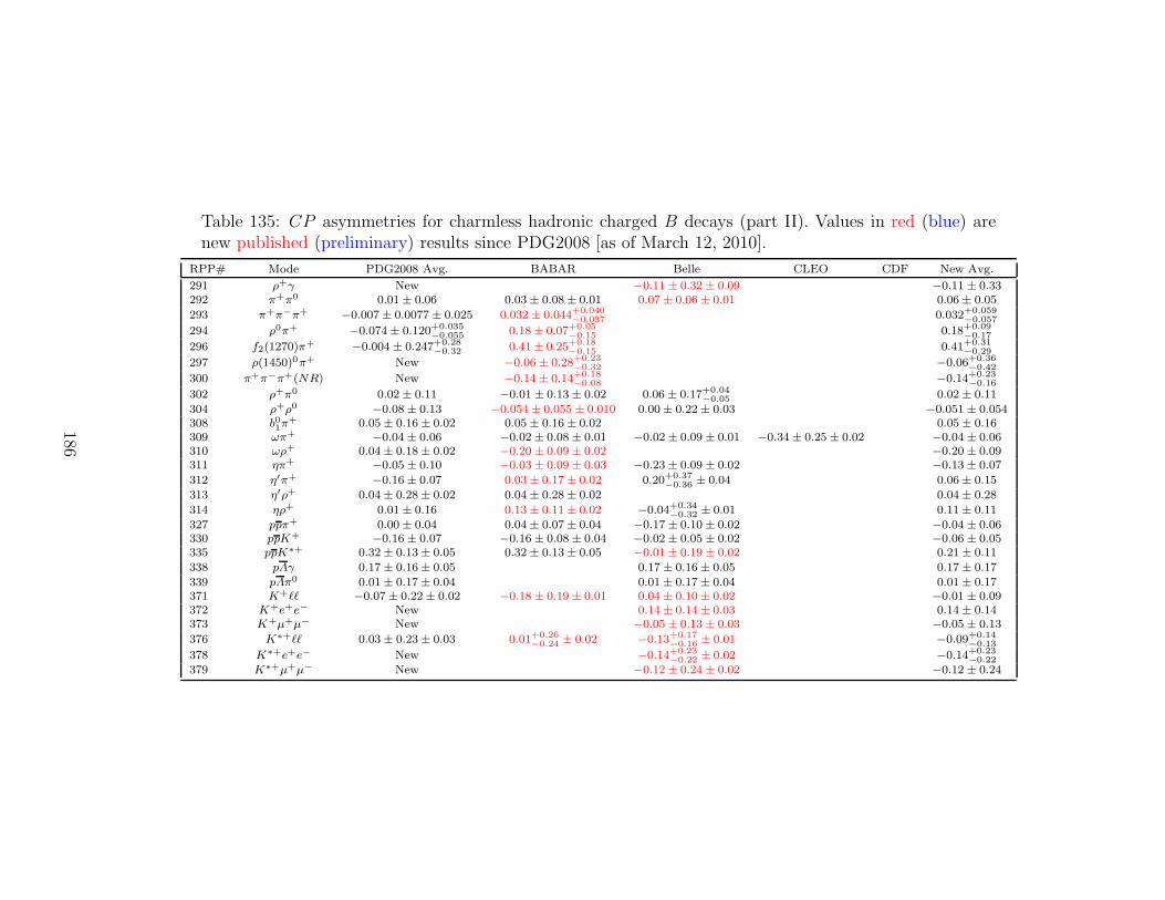
Table 135: CP asymmetries for charmless hadronic charged B decays (part II). Values in red (blue) arenew published (preliminary) results since PDG2008 [as of March 12, 2010].
RPP# Mode PDG2008 Avg. BABAR Belle CLEO CDF New Avg.
291 ρ+γ New −0.11± 0.32 ± 0.09 −0.11± 0.33292 π+π0 0.01± 0.06 0.03± 0.08± 0.01 0.07± 0.06± 0.01 0.06± 0.05
293 π+π−π+ −0.007± 0.0077 ± 0.025 0.032 ± 0.044+0.040−0.037 0.032+0.059
−0.057
294 ρ0π+ −0.074± 0.120+0.035−0.055 0.18± 0.07+0.05
−0.15 0.18+0.09−0.17
296 f2(1270)π+ −0.004± 0.247+0.28−0.32 0.41± 0.25+0.18
−0.15 0.41+0.31−0.29
297 ρ(1450)0π+ New −0.06± 0.28+0.23−0.32 −0.06+0.36
−0.42
300 π+π−π+(NR) New −0.14± 0.14+0.18−0.08 −0.14+0.23
−0.16
302 ρ+π0 0.02± 0.11 −0.01 ± 0.13± 0.02 0.06± 0.17+0.04−0.05 0.02± 0.11
304 ρ+ρ0 −0.08± 0.13 −0.054± 0.055 ± 0.010 0.00± 0.22± 0.03 −0.051± 0.054308 b01π
+ 0.05± 0.16± 0.02 0.05± 0.16± 0.02 0.05± 0.16309 ωπ+ −0.04± 0.06 −0.02 ± 0.08± 0.01 −0.02± 0.09 ± 0.01 −0.34± 0.25± 0.02 −0.04± 0.06310 ωρ+ 0.04± 0.18± 0.02 −0.20 ± 0.09± 0.02 −0.20± 0.09311 ηπ+ −0.05± 0.10 −0.03 ± 0.09± 0.03 −0.23± 0.09 ± 0.02 −0.13± 0.07
312 η′π+ −0.16± 0.07 0.03± 0.17± 0.02 0.20+0.37−0.36 ± 0.04 0.06± 0.15
313 η′ρ+ 0.04± 0.28± 0.02 0.04± 0.28± 0.02 0.04± 0.28
314 ηρ+ 0.01± 0.16 0.13± 0.11± 0.02 −0.04+0.34−0.32 ± 0.01 0.11± 0.11
327 ppπ+ 0.00± 0.04 0.04± 0.07± 0.04 −0.17± 0.10 ± 0.02 −0.04± 0.06330 ppK+ −0.16± 0.07 −0.16 ± 0.08± 0.04 −0.02± 0.05 ± 0.02 −0.06± 0.05335 ppK∗+ 0.32± 0.13± 0.05 0.32± 0.13± 0.05 −0.01± 0.19 ± 0.02 0.21± 0.11
338 pΛγ 0.17± 0.16± 0.05 0.17± 0.16± 0.05 0.17± 0.17
339 pΛπ0 0.01± 0.17± 0.04 0.01± 0.17± 0.04 0.01± 0.17371 K+ℓℓ −0.07± 0.22± 0.02 −0.18 ± 0.19± 0.01 0.04± 0.10± 0.02 −0.01± 0.09372 K+e+e− New 0.14± 0.14± 0.03 0.14± 0.14373 K+µ+µ− New −0.05± 0.13 ± 0.03 −0.05± 0.13
376 K∗+ℓℓ 0.03± 0.23± 0.03 0.01+0.26−0.24 ± 0.02 −0.13+0.17
−0.16 ± 0.01 −0.09+0.14−0.13
378 K∗+e+e− New −0.14+0.23−0.22 ± 0.02 −0.14+0.23
−0.22379 K∗+µ+µ− New −0.12± 0.24 ± 0.02 −0.12± 0.24
186
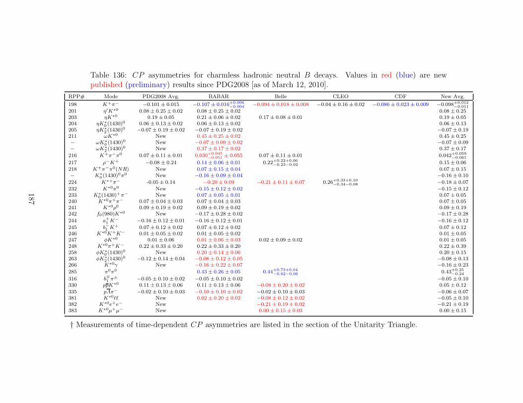
Table 136: CP asymmetries for charmless hadronic neutral B decays. Values in red (blue) are newpublished (preliminary) results since PDG2008 [as of March 12, 2010].
RPP# Mode PDG2008 Avg. BABAR Belle CLEO CDF New Avg.
198 K+π− −0.101± 0.015 −0.107 ± 0.016+0.006−0.004 −0.094± 0.018 ± 0.008 −0.04± 0.16 ± 0.02 −0.086± 0.023± 0.009 −0.098+0.012
−0.011201 η′K∗0 0.08± 0.25± 0.02 0.08± 0.25 ± 0.02 0.08± 0.25203 ηK∗0 0.19 ± 0.05 0.21± 0.06 ± 0.02 0.17± 0.08± 0.01 0.19± 0.05204 ηK∗
0 (1430)0 0.06± 0.13± 0.02 0.06± 0.13 ± 0.02 0.06± 0.13
205 ηK∗2 (1430)
0 −0.07± 0.19± 0.02 −0.07± 0.19± 0.02 −0.07± 0.19211 ωK∗0 New 0.45± 0.25 ± 0.02 0.45± 0.25− ωK∗
0 (1430)0 New −0.07± 0.09± 0.02 −0.07± 0.09
− ωK∗2 (1430)
0 New 0.37± 0.17 ± 0.02 0.37± 0.17
216 K+π−π0 0.07± 0.11± 0.01 0.030+0.045−0.051 ± 0.055 0.07± 0.11± 0.01 0.042+0.059
−0.061
217 ρ−K+ −0.08± 0.24 0.14± 0.06 ± 0.01 0.22+0.22+0.06−0.23−0.02 0.15± 0.06
218 K+π−π0(NR) New 0.07± 0.15 ± 0.04 0.07± 0.15− K∗
0 (1430)0π0 New −0.16± 0.09± 0.04 −0.16± 0.10
224 K∗+π− -0.05± 0.14 −0.20± 0.09 −0.21± 0.11± 0.07 0.26+0.33+0.10−0.34−0.08 −0.18± 0.07
232 K∗0π0 New −0.15± 0.12± 0.02 −0.15± 0.12233 K∗
0 (1430)+π− New 0.07± 0.05 ± 0.01 0.07± 0.05
240 K∗0π+π− 0.07± 0.04± 0.03 0.07± 0.04 ± 0.03 0.07± 0.05241 K∗0ρ0 0.09± 0.19± 0.02 0.09± 0.19 ± 0.02 0.09± 0.19242 f0(980)K∗0 New −0.17± 0.28± 0.02 −0.17± 0.28
244 a+1 K− −0.16± 0.12± 0.01 −0.16± 0.12± 0.01 −0.16± 0.12
245 b−1 K+ 0.07± 0.12± 0.02 0.07± 0.12 ± 0.02 0.07± 0.12
246 K∗0K+K− 0.01± 0.05± 0.02 0.01± 0.05 ± 0.02 0.01± 0.05247 φK∗0 0.01 ± 0.06 0.01± 0.06 ± 0.03 0.02± 0.09± 0.02 0.01± 0.05248 K∗0π+K− 0.22± 0.33± 0.20 0.22± 0.33 ± 0.20 0.22± 0.39258 φK∗
0 (1430)0 New 0.20± 0.14 ± 0.06 0.20± 0.15
263 φK∗2 (1430)
0 −0.12± 0.14± 0.04 −0.08± 0.12± 0.05 −0.08± 0.13266 K∗0γ New −0.16± 0.22± 0.07 −0.16± 0.23
285 π0π0 0.43± 0.26 ± 0.05 0.44+0.73+0.04−0.62−0.06 0.43+0.25
−0.24
316 b∓1 π± −0.05± 0.10± 0.02 −0.05± 0.10± 0.02 −0.05± 0.10
330 ppK∗0 0.11± 0.13± 0.06 0.11± 0.13 ± 0.06 −0.08± 0.20± 0.02 0.05± 0.12
335 pΛπ− −0.02± 0.10± 0.03 −0.10± 0.10± 0.02 −0.02± 0.10± 0.03 −0.06± 0.07381 K∗0ℓℓ New 0.02± 0.20 ± 0.02 −0.08± 0.12± 0.02 −0.05± 0.10382 K∗0e+e− New −0.21± 0.19± 0.02 −0.21± 0.19383 K∗0µ+µ− New 0.00± 0.15± 0.03 0.00± 0.15
† Measurements of time-dependent CP asymmetries are listed in the section of the Unitarity Triangle.
187
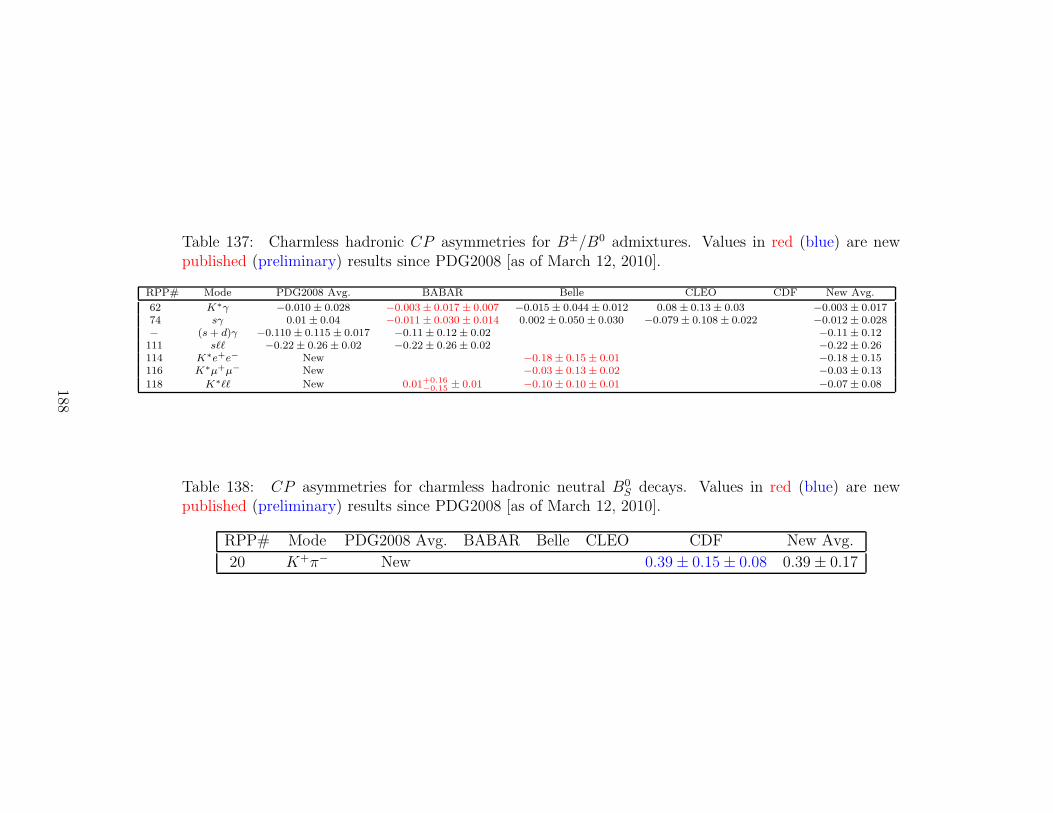
Table 137: Charmless hadronic CP asymmetries for B±/B0 admixtures. Values in red (blue) are newpublished (preliminary) results since PDG2008 [as of March 12, 2010].
RPP# Mode PDG2008 Avg. BABAR Belle CLEO CDF New Avg.
62 K∗γ −0.010± 0.028 −0.003± 0.017 ± 0.007 −0.015± 0.044± 0.012 0.08 ± 0.13± 0.03 −0.003± 0.01774 sγ 0.01± 0.04 −0.011± 0.030 ± 0.014 0.002 ± 0.050 ± 0.030 −0.079± 0.108± 0.022 −0.012± 0.028− (s+ d)γ −0.110 ± 0.115 ± 0.017 −0.11± 0.12± 0.02 −0.11± 0.12111 sℓℓ −0.22± 0.26± 0.02 −0.22± 0.26± 0.02 −0.22± 0.26114 K∗e+e− New −0.18± 0.15± 0.01 −0.18± 0.15116 K∗µ+µ− New −0.03± 0.13± 0.02 −0.03± 0.13
118 K∗ℓℓ New 0.01+0.16−0.15 ± 0.01 −0.10± 0.10± 0.01 −0.07± 0.08
Table 138: CP asymmetries for charmless hadronic neutral B0S decays. Values in red (blue) are new
published (preliminary) results since PDG2008 [as of March 12, 2010].
RPP# Mode PDG2008 Avg. BABAR Belle CLEO CDF New Avg.
20 K+π− New 0.39± 0.15± 0.08 0.39± 0.17
188
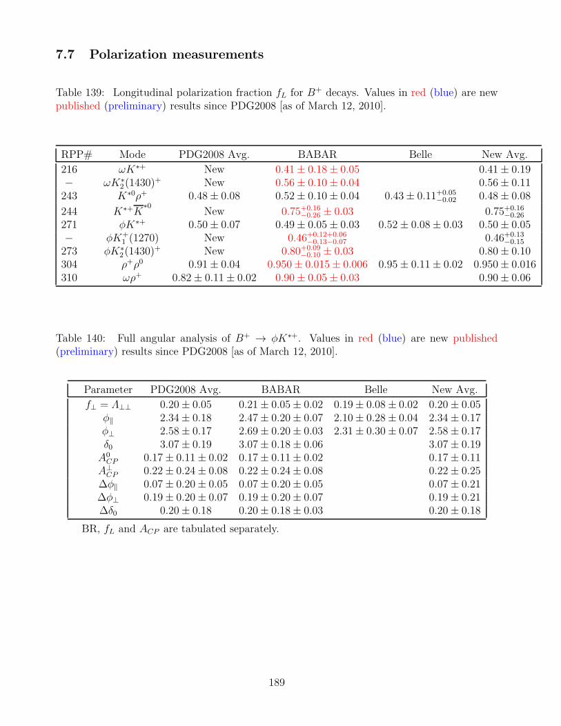
7.7 Polarization measurements
Table 139: Longitudinal polarization fraction fL for B+ decays. Values in red (blue) are newpublished (preliminary) results since PDG2008 [as of March 12, 2010].
RPP# Mode PDG2008 Avg. BABAR Belle New Avg.
216 ωK∗+ New 0.41± 0.18± 0.05 0.41± 0.19− ωK∗
2(1430)+ New 0.56± 0.10± 0.04 0.56± 0.11
243 K∗0ρ+ 0.48± 0.08 0.52± 0.10± 0.04 0.43± 0.11+0.05−0.02 0.48± 0.08
244 K∗+K∗0
New 0.75+0.16−0.26 ± 0.03 0.75+0.16
−0.26
271 φK∗+ 0.50± 0.07 0.49± 0.05± 0.03 0.52± 0.08± 0.03 0.50± 0.05− φK+
1 (1270) New 0.46+0.12+0.06−0.13−0.07 0.46+0.13
−0.15
273 φK∗2(1430)
+ New 0.80+0.09−0.10 ± 0.03 0.80± 0.10
304 ρ+ρ0 0.91± 0.04 0.950± 0.015± 0.006 0.95± 0.11± 0.02 0.950± 0.016310 ωρ+ 0.82± 0.11± 0.02 0.90± 0.05± 0.03 0.90± 0.06
Table 140: Full angular analysis of B+ → φK∗+. Values in red (blue) are new published(preliminary) results since PDG2008 [as of March 12, 2010].
Parameter PDG2008 Avg. BABAR Belle New Avg.
f⊥ = Λ⊥⊥ 0.20± 0.05 0.21± 0.05± 0.02 0.19± 0.08± 0.02 0.20± 0.05φ‖ 2.34± 0.18 2.47± 0.20± 0.07 2.10± 0.28± 0.04 2.34± 0.17φ⊥ 2.58± 0.17 2.69± 0.20± 0.03 2.31± 0.30± 0.07 2.58± 0.17δ0 3.07± 0.19 3.07± 0.18± 0.06 3.07± 0.19A0CP 0.17± 0.11± 0.02 0.17± 0.11± 0.02 0.17± 0.11
A⊥CP 0.22± 0.24± 0.08 0.22± 0.24± 0.08 0.22± 0.25
∆φ‖ 0.07± 0.20± 0.05 0.07± 0.20± 0.05 0.07± 0.21∆φ⊥ 0.19± 0.20± 0.07 0.19± 0.20± 0.07 0.19± 0.21∆δ0 0.20± 0.18 0.20± 0.18± 0.03 0.20± 0.18
BR, fL and ACP are tabulated separately.
189
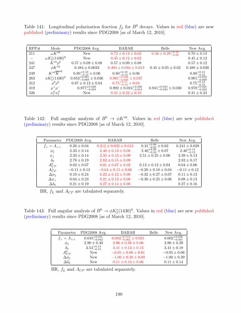
Table 141: Longitudinal polarization fraction fL for B0 decays. Values in red (blue) are newpublished (preliminary) results since PDG2008 [as of March 12, 2010].
RPP# Mode PDG2008 Avg. BABAR Belle New Avg.
211 ωK∗0 New 0.72± 0.14± 0.02 0.56± 0.29+0.18−0.08 0.70± 0.13
− ωK∗2 (1430)
0 New 0.45± 0.12± 0.02 0.45± 0.12241 K∗0ρ0 0.57± 0.09± 0.08 0.57± 0.09± 0.08 0.57± 0.12247 φK∗0 0.484± 0.0033 0.494± 0.034± 0.013 0.45± 0.05± 0.02 0.480± 0.030
249 K∗0K∗0
0.80+0.10−0.12 ± 0.06 0.80+0.10
−0.12 ± 0.06 0.80+0.12−0.13
263 φK∗2 (1430)
0 0.853+0.061−0.069 ± 0.036 0.901+0.046
−0.058 ± 0.037 0.901+0.059−0.069
312 ρ0ρ0 0.87± 0.13± 0.04 0.75+0.11−0.14 ± 0.04 0.75+0.12
−0.15
319 ρ+ρ− 0.977+0.028−0.024 0.992± 0.024+0.026
−0.013 0.941+0.034−0.040 ± 0.030 0.978+0.025
−0.022
326 a±1 a∓1 New 0.31± 0.22± 0.10 0.31± 0.24
Table 142: Full angular analysis of B0 → φK∗0. Values in red (blue) are new published(preliminary) results since PDG2008 [as of March 12, 2010].
Parameter PDG2008 Avg. BABAR Belle New Avg.
f⊥ = Λ⊥⊥ 0.26± 0.04 0.212± 0.032± 0.013 0.31+0.06−0.05 ± 0.02 0.241± 0.029
φ‖ 2.33± 0.14 2.40± 0.13± 0.08 2.40+0.28−0.24 ± 0.07 2.40+0.14
−0.13
φ⊥ 2.33± 0.14 2.35± 0.13± 0.09 2.51± 0.25± 0.06 2.39± 0.13δ0 2.78± 0.19 2.82± 0.15± 0.09 2.82± 0.17A0
CP 0.02± 0.07 0.01± 0.07± 0.02 0.13± 0.12± 0.04 0.04± 0.06A⊥
CP −0.11± 0.12 −0.04± 0.15± 0.06 −0.20± 0.18± 0.04 −0.11± 0.12∆φ‖ 0.10± 0.24 0.22± 0.12± 0.08 −0.32± 0.27± 0.07 0.11± 0.13∆φ⊥ 0.04± 0.23 0.21± 0.13± 0.08 −0.30± 0.25± 0.06 0.08± 0.13∆δ0 0.21± 0.19 0.27± 0.14± 0.08 0.27± 0.16
BR, fL and ACP are tabulated separately.
Table 143: Full angular analysis of B0 → φK∗2(1430)
0. Values in red (blue) are new published(preliminary) results since PDG2008 [as of March 12, 2010].
Parameter PDG2008 Avg. BABAR Belle New Avg.
f⊥ = Λ⊥⊥ 0.045+0.051−0.042 0.002+0.018
−0.002 ± 0.031 0.002+0.036−0.031
φ‖ 2.90± 0.40 3.96± 0.38± 0.06 3.96± 0.39δ0 3.54+0.13
−0.15 3.41± 0.13± 0.13 3.41± 0.18A0
CP New −0.05± 0.06± 0.01 −0.05± 0.06∆φ‖ New −1.00± 0.38± 0.09 −1.00± 0.39∆δ0 New 0.11± 0.13± 0.06 0.11± 0.14
BR, fL and ACP are tabulated separately.
190
8 D decays
8.1 D0-D 0 Mixing and CP Violation
8.1.1 Introduction
In 2007, Belle [418]and Babar [419] obtained the first evidence for D0-D 0 mixing, which hadbeen searched for for more than two decades without success. These results were later confirmedby CDF [420]. There are now numerous measurements of D0-D 0 mixing, with various levels ofsensitivity. All the results can be combined to yield world average (WA) values for the mixingparameters x ≡ (m1−m2)/Γ and y ≡ (Γ1−Γ2)/(2Γ), where m1, m2 and Γ1, Γ2 are the massesand decay widths for the mass eigenstates D1 ≡ p|D0〉 − q|D 0〉 and D2 ≡ p|D0〉 + q|D 0〉, andΓ = (Γ1 + Γ2)/2. Here we use the phase convention CP |D0〉 = −|D 0〉, CP |D 0〉 = −|D0〉; inthe absence of CP violation (CPV ), q/p=1, D1 is CP -even, and D2 is CP -odd.
The WA values are calculated by performing a global fit to more than two dozen measuredobservables. Assuming no CPV , the fit parameters are x, y, δ (the strong phase differencebetween amplitudes A(D 0→K+π−) and A(D0→K+π−)), a strong phase δKππ entering D0→K+π−π0 decays, and RD ≡
∣
∣A(D0→K+π−)/A(D 0→K+π−)∣
∣
2. To account for possible CPV ,
three additional parameters are added: |q/p|, φ ≡ Arg(q/p), and AD ≡ (R+D−R−
D)/(R+D+R−
D),where the + (−) superscript corresponds to D0 (D 0) decays.
The observables used are from measurements of D0→K+ℓ−ν, D0 →K+K−/π+π−, D0 →K+π−, D0→K+π−π0, D0→K0
S π+π−, and D0→K0
SK+K− decays; and from double-tagged
branching fractions measured at the ψ(3770) resonance. Correlations among observables are ac-counted for by using covariance matrices provided by the experimental collaborations. System-atic errors among different experiments are assumed uncorrelated as no significant correlationshave been identified. We have checked this method with a second method that adds togetherthree-dimensional log-likelihood functions for x, y, and δ obtained from several analyses; thiscombination accounts for non-Gaussian errors. When both methods are applied to the sameset of observables and data, equivalent results are obtained.
Mixing in heavy flavor systems such as those of B0 and B0s is governed by the short-distance
box diagram. In the D0 system, however, this diagram is doubly-Cabibbo-suppressed relativeto amplitudes dominating the decay width, and it is also GIM-suppressed. Thus the short-distance mixing rate is tiny, and D0-D 0 mixing is expected to be dominated by long-distanceprocesses. These are difficult to calculate reliably, and theoretical estimates for x and y rangeover two-three orders of magnitude [421, 422, 423, 424, 425].
With the exception of ψ(3770)→DD measurements, all methods identify the flavor of theD0 or D 0 when produced by reconstructing the decay D∗+→D0π+ or D∗−→D 0π−; the chargeof the pion (which has low momentum and is often referred to as the “soft” pion πs) identifies theD flavor. For signal decays, MD∗ −MD0 −Mπ+ ≡ Q ≈ 6 MeV, which is close to the threshold;thus analyses typically require that the reconstructed Q be small to suppress backgrounds.For time-dependent measurements, the D0 decay time is calculated as (d/p) ×MD0 , where dis the distance between the D∗ and D0 decay vertices and p is the D0 momentum. The D∗
vertex position is taken to be at the primary vertex for pp collider experiments [420], and atthe intersection of the D0 momentum vector with the beamspot profile for e+e− experiments.
191
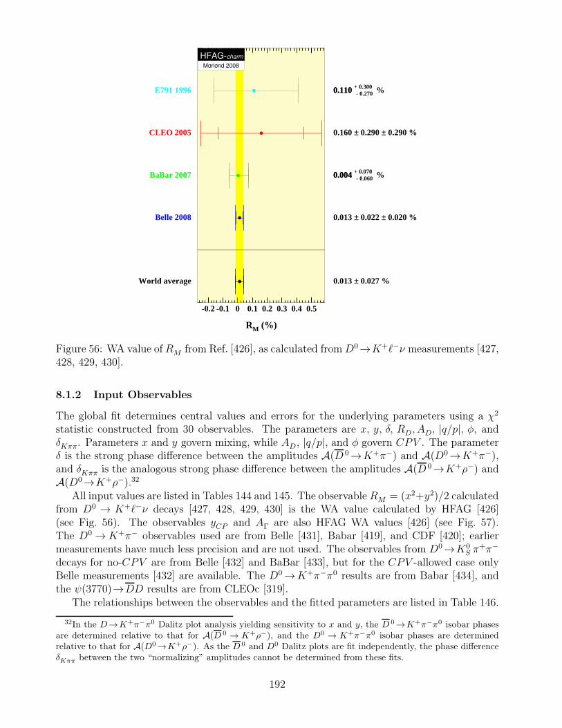
-0.2 -0.1 0 0.1 0.2 0.3 0.4 0.5
RM (%)
World average 0.013 ± 0.027 %
Belle 2008 0.013 ± 0.022 ± 0.020 %
BaBar 2007 0.004 + 0.070 % 0.004 - 0.060
CLEO 2005 0.160 ± 0.290 ± 0.290 %
E791 1996 0.110 + 0.300 % 0.110 - 0.270
Figure 56: WA value ofRM from Ref. [426], as calculated fromD0→K+ℓ−ν measurements [427,428, 429, 430].
8.1.2 Input Observables
The global fit determines central values and errors for the underlying parameters using a χ2
statistic constructed from 30 observables. The parameters are x, y, δ, RD, AD, |q/p|, φ, andδKππ. Parameters x and y govern mixing, while AD, |q/p|, and φ govern CPV . The parameterδ is the strong phase difference between the amplitudes A(D 0→K+π−) and A(D0→K+π−),and δKππ is the analogous strong phase difference between the amplitudes A(D 0→K+ρ−) andA(D0→K+ρ−).32
All input values are listed in Tables 144 and 145. The observable RM = (x2+y2)/2 calculatedfrom D0 → K+ℓ−ν decays [427, 428, 429, 430] is the WA value calculated by HFAG [426](see Fig. 56). The observables yCP and AΓ are also HFAG WA values [426] (see Fig. 57).The D0 →K+π− observables used are from Belle [431], Babar [419], and CDF [420]; earliermeasurements have much less precision and are not used. The observables from D0→K0
S π+π−
decays for no-CPV are from Belle [432] and BaBar [433], but for the CPV -allowed case onlyBelle measurements [432] are available. The D0→K+π−π0 results are from Babar [434], andthe ψ(3770)→DD results are from CLEOc [319].
The relationships between the observables and the fitted parameters are listed in Table 146.
32In the D→K+π−π0 Dalitz plot analysis yielding sensitivity to x and y, the D 0→K+π−π0 isobar phasesare determined relative to that for A(D 0 → K+ρ−), and the D0 → K+π−π0 isobar phases are determinedrelative to that for A(D0→K+ρ−). As the D 0 and D0 Dalitz plots are fit independently, the phase differenceδKππ between the two “normalizing” amplitudes cannot be determined from these fits.
192
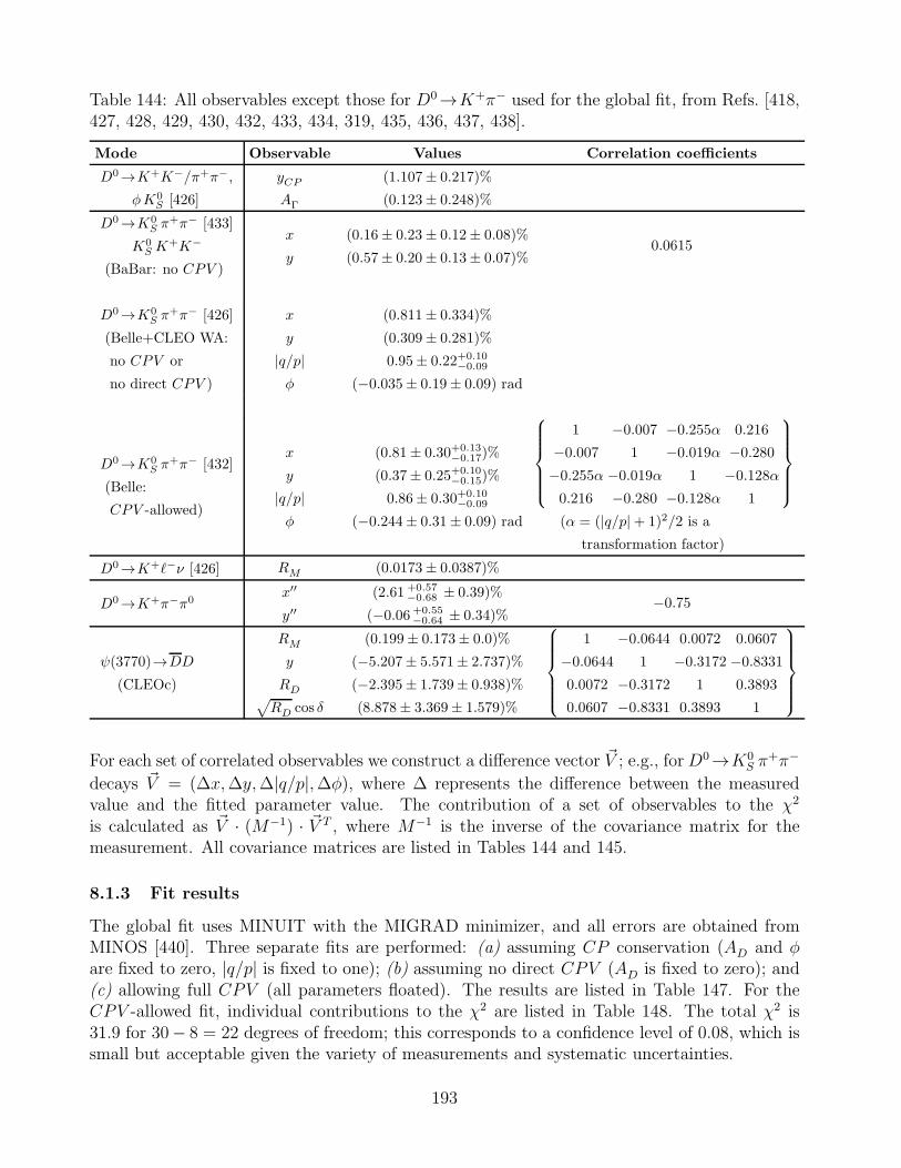
Table 144: All observables except those for D0→K+π− used for the global fit, from Refs. [418,427, 428, 429, 430, 432, 433, 434, 319, 435, 436, 437, 438].
Mode Observable Values Correlation coefficients
D0→K+K−/π+π−,
φK0S [426]
yCP
AΓ
(1.107± 0.217)%
(0.123± 0.248)%
D0→K0S π
+π− [433]
K0SK
+K−
(BaBar: no CPV )
x
y
(0.16± 0.23± 0.12± 0.08)%
(0.57± 0.20± 0.13± 0.07)%0.0615
D0→K0S π
+π− [426]
(Belle+CLEO WA:
no CPV or
no direct CPV )
x
y
|q/p|φ
(0.811± 0.334)%
(0.309± 0.281)%
0.95± 0.22+0.10−0.09
(−0.035± 0.19± 0.09) rad
D0→K0S π
+π− [432]
(Belle:
CPV -allowed)
x
y
|q/p|φ
(0.81± 0.30+0.13−0.17)%
(0.37± 0.25+0.10−0.15)%
0.86± 0.30+0.10−0.09
(−0.244± 0.31± 0.09) rad
1 −0.007 −0.255α 0.216
−0.007 1 −0.019α −0.280
−0.255α −0.019α 1 −0.128α
0.216 −0.280 −0.128α 1
(α = (|q/p|+ 1)2/2 is a
transformation factor)
D0→K+ℓ−ν [426] RM (0.0173± 0.0387)%
D0→K+π−π0x′′
y′′(2.61+0.57
−0.68 ± 0.39)%
(−0.06+0.55−0.64 ± 0.34)%
−0.75
ψ(3770)→DD
(CLEOc)
RM
y
RD√
RD cos δ
(0.199± 0.173± 0.0)%
(−5.207± 5.571± 2.737)%
(−2.395± 1.739± 0.938)%
(8.878± 3.369± 1.579)%
1 −0.0644 0.0072 0.0607
−0.0644 1 −0.3172 −0.8331
0.0072 −0.3172 1 0.3893
0.0607 −0.8331 0.3893 1
For each set of correlated observables we construct a difference vector ~V ; e.g., forD0→K0S π
+π−
decays ~V = (∆x,∆y,∆|q/p|,∆φ), where ∆ represents the difference between the measuredvalue and the fitted parameter value. The contribution of a set of observables to the χ2
is calculated as ~V · (M−1) · ~V T , where M−1 is the inverse of the covariance matrix for themeasurement. All covariance matrices are listed in Tables 144 and 145.
8.1.3 Fit results
The global fit uses MINUIT with the MIGRAD minimizer, and all errors are obtained fromMINOS [440]. Three separate fits are performed: (a) assuming CP conservation (AD and φare fixed to zero, |q/p| is fixed to one); (b) assuming no direct CPV (AD is fixed to zero); and(c) allowing full CPV (all parameters floated). The results are listed in Table 147. For theCPV -allowed fit, individual contributions to the χ2 are listed in Table 148. The total χ2 is31.9 for 30− 8 = 22 degrees of freedom; this corresponds to a confidence level of 0.08, which issmall but acceptable given the variety of measurements and systematic uncertainties.
193
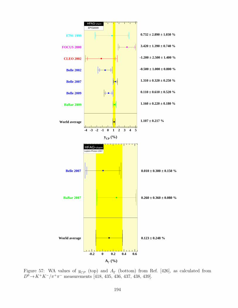
-4 -3 -2 -1 0 1 2 3 4 5
yCP (%)
World average 1.107 ± 0.217 %
BaBar 2009 1.160 ± 0.220 ± 0.180 %
Belle 2009 0.110 ± 0.610 ± 0.520 %
Belle 2007 1.310 ± 0.320 ± 0.250 %
Belle 2002 -0.500 ± 1.000 ± 0.800 %
CLEO 2002 -1.200 ± 2.500 ± 1.400 %
FOCUS 2000 3.420 ± 1.390 ± 0.740 %
E791 1999 0.732 ± 2.890 ± 1.030 %
HFAG-charm
EPS 2009
-0.2 0 0.2 0.4 0.6
AΓ (%)
World average 0.123 ± 0.248 %
BaBar 2007 0.260 ± 0.360 ± 0.080 %
Belle 2007 0.010 ± 0.300 ± 0.150 %
HFAG-charm Lepton-Photon 2007
Figure 57: WA values of yCP (top) and AΓ (bottom) from Ref. [426], as calculated fromD0→K+K−/π+π− measurements [418, 435, 436, 437, 438, 439].
194
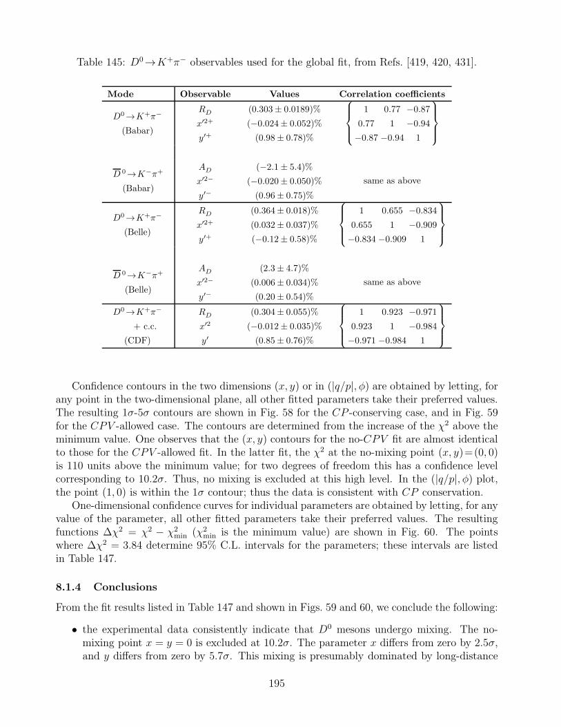
Table 145: D0→K+π− observables used for the global fit, from Refs. [419, 420, 431].
Mode Observable Values Correlation coefficients
D0→K+π−
(Babar)
RD
x′2+
y′+
(0.303± 0.0189)%
(−0.024± 0.052)%
(0.98± 0.78)%
1 0.77 −0.87
0.77 1 −0.94
−0.87 −0.94 1
D 0→K−π+
(Babar)
AD
x′2−
y′−
(−2.1± 5.4)%
(−0.020± 0.050)%
(0.96± 0.75)%
same as above
D0→K+π−
(Belle)
RD
x′2+
y′+
(0.364± 0.018)%
(0.032± 0.037)%
(−0.12± 0.58)%
1 0.655 −0.834
0.655 1 −0.909
−0.834 −0.909 1
D 0→K−π+
(Belle)
AD
x′2−
y′−
(2.3± 4.7)%
(0.006± 0.034)%
(0.20± 0.54)%
same as above
D0→K+π−
+ c.c.
(CDF)
RD
x′2
y′
(0.304± 0.055)%
(−0.012± 0.035)%
(0.85± 0.76)%
1 0.923 −0.971
0.923 1 −0.984
−0.971 −0.984 1
Confidence contours in the two dimensions (x, y) or in (|q/p|, φ) are obtained by letting, forany point in the two-dimensional plane, all other fitted parameters take their preferred values.The resulting 1σ-5σ contours are shown in Fig. 58 for the CP -conserving case, and in Fig. 59for the CPV -allowed case. The contours are determined from the increase of the χ2 above theminimum value. One observes that the (x, y) contours for the no-CPV fit are almost identicalto those for the CPV -allowed fit. In the latter fit, the χ2 at the no-mixing point (x, y)=(0, 0)is 110 units above the minimum value; for two degrees of freedom this has a confidence levelcorresponding to 10.2σ. Thus, no mixing is excluded at this high level. In the (|q/p|, φ) plot,the point (1, 0) is within the 1σ contour; thus the data is consistent with CP conservation.
One-dimensional confidence curves for individual parameters are obtained by letting, for anyvalue of the parameter, all other fitted parameters take their preferred values. The resultingfunctions ∆χ2 = χ2 − χ2
min (χ2min is the minimum value) are shown in Fig. 60. The points
where ∆χ2 = 3.84 determine 95% C.L. intervals for the parameters; these intervals are listedin Table 147.
8.1.4 Conclusions
From the fit results listed in Table 147 and shown in Figs. 59 and 60, we conclude the following:
• the experimental data consistently indicate that D0 mesons undergo mixing. The no-mixing point x = y = 0 is excluded at 10.2σ. The parameter x differs from zero by 2.5σ,and y differs from zero by 5.7σ. This mixing is presumably dominated by long-distance
195
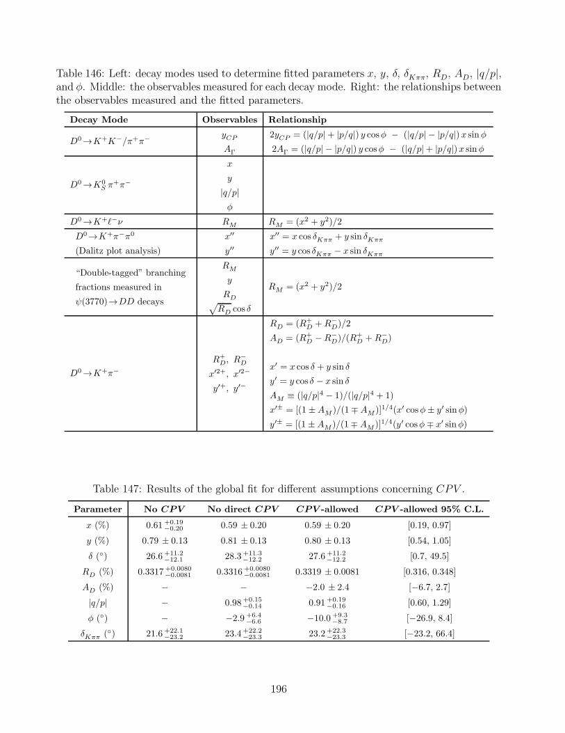
Table 146: Left: decay modes used to determine fitted parameters x, y, δ, δKππ, RD, AD, |q/p|,and φ. Middle: the observables measured for each decay mode. Right: the relationships betweenthe observables measured and the fitted parameters.
Decay Mode Observables Relationship
D0→K+K−/π+π− yCP
AΓ
2yCP = (|q/p|+ |p/q|) y cosφ − (|q/p| − |p/q|)x sinφ2AΓ = (|q/p| − |p/q|) y cosφ − (|q/p|+ |p/q|)x sinφ
D0→K0S π
+π−
x
y
|q/p|φ
D0→K+ℓ−ν RM RM = (x2 + y2)/2
D0→K+π−π0
(Dalitz plot analysis)
x′′
y′′x′′ = x cos δKππ + y sin δKππ
y′′ = y cos δKππ − x sin δKππ
“Double-tagged” branching
fractions measured in
ψ(3770)→DD decays
RM
y
RD√
RD cos δ
RM = (x2 + y2)/2
D0→K+π−
R+D, R
−D
x′2+, x′2−
y′+, y′−
RD = (R+D +R−
D)/2
AD = (R+D −R−
D)/(R+D +R−
D)
x′ = x cos δ + y sin δ
y′ = y cos δ − x sin δ
AM ≡ (|q/p|4 − 1)/(|q/p|4 + 1)
x′± = [(1 ±AM )/(1∓AM )]1/4(x′ cosφ± y′ sinφ)
y′± = [(1 ±AM )/(1∓AM )]1/4(y′ cosφ∓ x′ sinφ)
Table 147: Results of the global fit for different assumptions concerning CPV .
Parameter No CPV No direct CPV CPV -allowed CPV -allowed 95% C.L.
x (%)
y (%)
δ ()
RD (%)
AD (%)
|q/p|φ ()
δKππ ()
0.61+0.19−0.20
0.79 ± 0.13
26.6+11.2−12.1
0.3317+0.0080−0.0081
−−−
21.6+22.1−23.2
0.59 ± 0.20
0.81 ± 0.13
28.3+11.3−12.2
0.3316+0.0080−0.0081
−0.98+0.15
−0.14
−2.9+6.4−6.6
23.4+22.2−23.3
0.59 ± 0.20
0.80 ± 0.13
27.6+11.2−12.2
0.3319 ± 0.0081
−2.0 ± 2.4
0.91+0.19−0.16
−10.0+9.3−8.7
23.2+22.3−23.3
[0.19, 0.97]
[0.54, 1.05]
[0.7, 49.5]
[0.316, 0.348]
[−6.7, 2.7]
[0.60, 1.29]
[−26.9, 8.4]
[−23.2, 66.4]
196
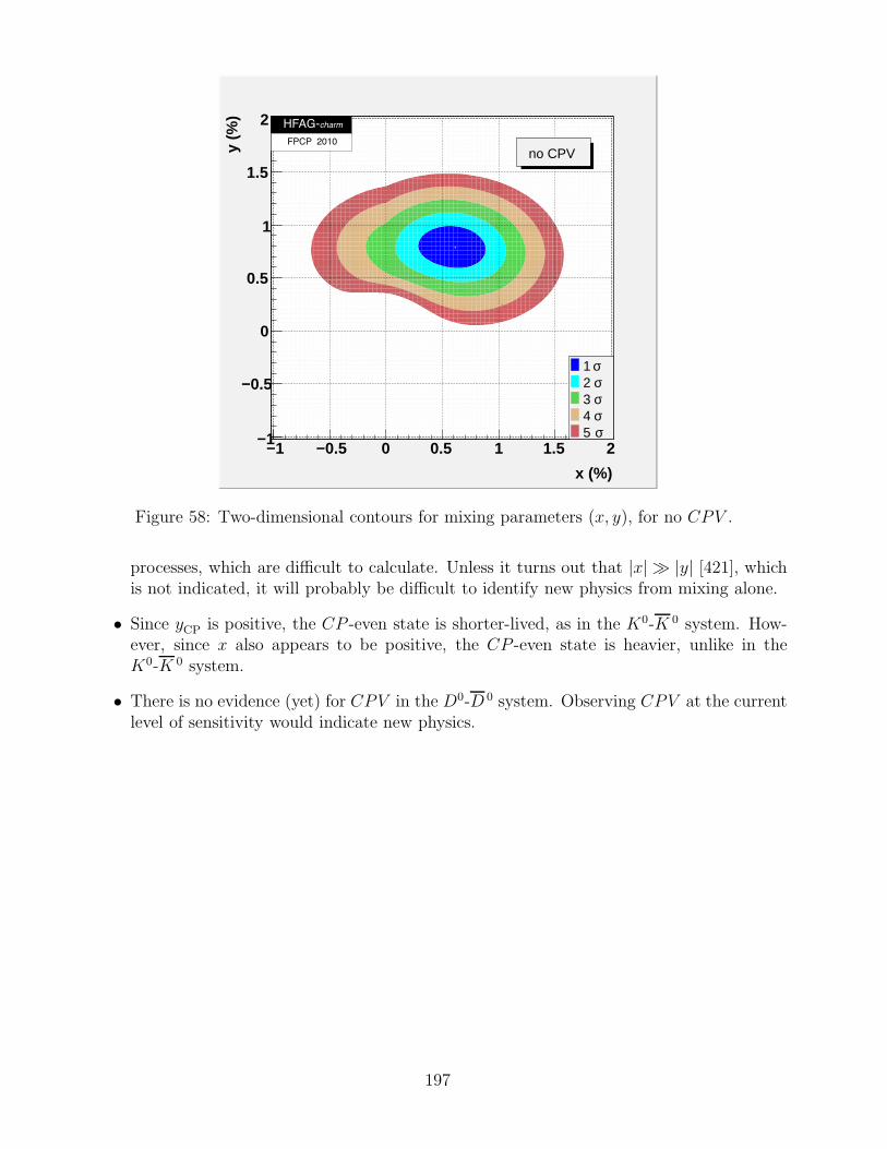
x (%)
−1 −0.5 0 0.5 1 1.5 2
y (%
)
−1
−0.5
0
0.5
1
1.5
2
no CPV
σ 1 σ 2 σ 3 σ 4 σ 5
HFAG-charm
FPCP 2010
Figure 58: Two-dimensional contours for mixing parameters (x, y), for no CPV .
processes, which are difficult to calculate. Unless it turns out that |x| ≫ |y| [421], whichis not indicated, it will probably be difficult to identify new physics from mixing alone.
• Since yCP is positive, the CP -even state is shorter-lived, as in the K0-K 0 system. How-ever, since x also appears to be positive, the CP -even state is heavier, unlike in theK0-K 0 system.
• There is no evidence (yet) for CPV in the D0-D 0 system. Observing CPV at the currentlevel of sensitivity would indicate new physics.
197
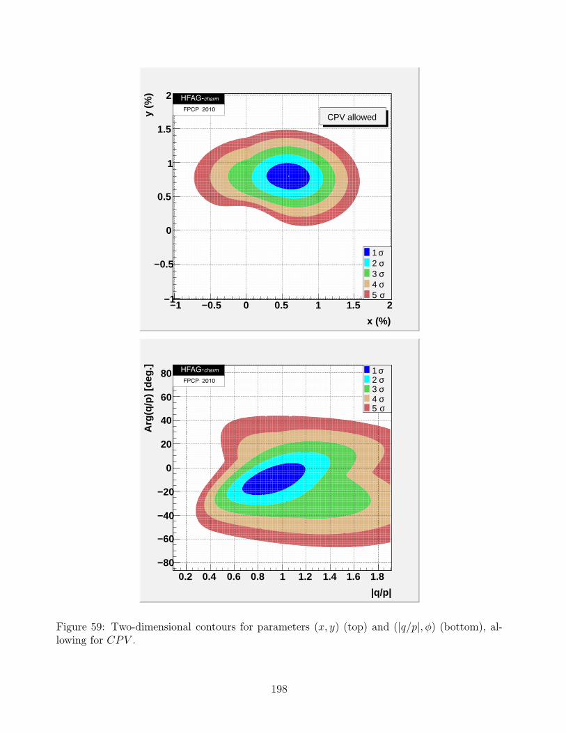
x (%)
−1 −0.5 0 0.5 1 1.5 2
y (%
)
−1
−0.5
0
0.5
1
1.5
2
CPV allowed
σ 1 σ 2 σ 3 σ 4 σ 5
HFAG-charm
FPCP 2010
|q/p|
0.2 0.4 0.6 0.8 1 1.2 1.4 1.6 1.8
Arg
(q/p
) [d
eg.]
−80
−60
−40
−20
0
20
40
60
80 σ 1 σ 2 σ 3 σ 4 σ 5
HFAG-charm
FPCP 2010
Figure 59: Two-dimensional contours for parameters (x, y) (top) and (|q/p|, φ) (bottom), al-lowing for CPV .
198
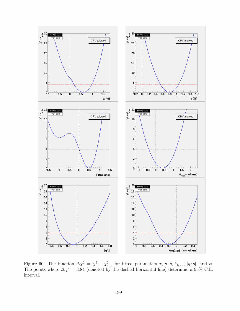
x (%)
−1 −0.5 0 0.5 1 1.5
min
2 χ −
2 χ
0
5
10
15
20
25
30
CPV allowedCPV allowed
HFAG-charm
FPCP 2010
y (%)
−0.2 0 0.2 0.4 0.6 0.8 1 1.2 1.4 1.6
min
2 χ −
2 χ
0
5
10
15
20
25
30
CPV allowed
HFAG-charm
FPCP 2010
(radians)δ
−1.5 −1 −0.5 0 0.5 1 1.5
min
2 χ −
2 χ
0
2
4
6
8
10
12
CPV allowed
HFAG-charm
FPCP 2010
(radians)ππKδ
−1 −0.5 0 0.5 1 1.5 2
min
2 χ −
2 χ
0
2
4
6
8
10
12
CPV allowed
HFAG-charm
FPCP 2010
|q/p|
0.4 0.6 0.8 1 1.2 1.4 1.6 1.8
min
2 χ −
2 χ
0
2
4
6
8
10
12
14
16
18
20 HFAG-charm
FPCP 2010
(radians)φArg(q/p) =
−1 −0.8 −0.6 −0.4 −0.2 0 0.2 0.4
min
2 χ −
2 χ
0
2
4
6
8
10
12
14
16
18
20 HFAG-charm
FPCP 2010
Figure 60: The function ∆χ2 = χ2 − χ2min for fitted parameters x, y, δ, δKππ, |q/p|, and φ.
The points where ∆χ2 = 3.84 (denoted by the dashed horizontal line) determine a 95% C.L.interval.
199
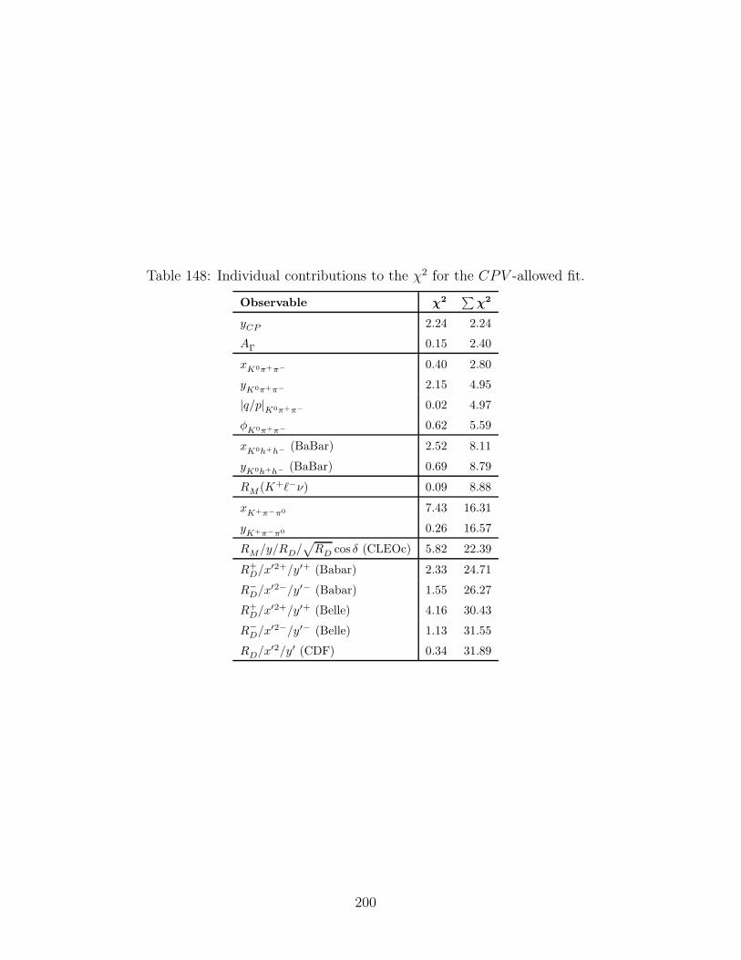
Table 148: Individual contributions to the χ2 for the CPV -allowed fit.
Observable χ2∑
χ2
yCP 2.24 2.24
AΓ 0.15 2.40
xK0π+π− 0.40 2.80
yK0π+π− 2.15 4.95
|q/p|K0π+π− 0.02 4.97
φK0π+π− 0.62 5.59
xK0h+h− (BaBar) 2.52 8.11
yK0h+h− (BaBar) 0.69 8.79
RM (K+ℓ−ν) 0.09 8.88
xK+π−π0 7.43 16.31
yK+π−π0 0.26 16.57
RM/y/RD/√
RD cos δ (CLEOc) 5.82 22.39
R+D/x
′2+/y′+ (Babar) 2.33 24.71
R−D/x
′2−/y′− (Babar) 1.55 26.27
R+D/x
′2+/y′+ (Belle) 4.16 30.43
R−D/x
′2−/y′− (Belle) 1.13 31.55
RD/x′2/y′ (CDF) 0.34 31.89
200
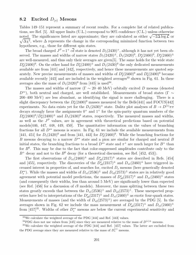
8.2 Excited D(s) Mesons
Tables 149–151 represent a summary of recent results. For a complete list of related publica-tions, see Ref. [5]. All upper limits (U.L.) correspond to 90% confidence (C.L.) unless otherwisenoted. The significances listed are approximate; they are calculated as either
√−2∆ logL or√
∆χ2, where ∆ represents the change in the corresponding minimized function between twohypotheses, e.g., those for different spin states.
The broad charged JP =1+ cd state is denoted D1(2430)+, although it has not yet been ob-
served. The masses and widths of narrow states D1(2420)±, D1(2420)
0, D∗2(2460)
0, D∗2(2460)
±
are well-measured, and thus only their averages are given[5]. The same holds for the wide stateD∗
0(2400)0. On the other hand for D∗
0(2400)± and D1(2430)
0 the only dedicated measurementsavailable are from [441] and [442], respectively, and hence these measurements are quoted sep-arately. New precise measurements of masses and widths of D∗
2(2460)0 and D∗
0(2400)0 became
available recently [443] and are included in the weighted averages33 shown in Fig. 61. In theseaverages also the mass of D1(2420)
0 from [445] is used34.
The masses and widths of narrow (Γ ∼ 20–40 MeV) orbitally excited D mesons (denotedD∗∗), both neutral and charged, are well established. Measurements of broad states (Γ ∼200–400 MeV) are less abundant, as identifying the signal is more challenging. There is aslight discrepancy between the D∗
0(2400)0 masses measured by the Belle[441] and FOCUS[442]
experiments. No data exists yet for the D1(2430)± state. Dalitz plot analyses of B → D(∗)ππ
decays strongly favor the assignments 0+ and 1+ for the spin-parity quantum numbers of theD∗
0(2400)0/D∗
0(2400)± and D1(2430)
0 states, respectively. The measured masses and widths,as well as the JP values, are in agreement with theoretical predictions based on potentialmodels[446, 447, 448, 449, 450]. The quantitative information on the values of branchingfractions for all D∗∗ mesons is scarce. In Fig. 61 we include the available measurements from[441, 451] for D1(2420)
0 and from [441, 443] for D∗2(2460)
0. While the branching fractions forB mesons decaying to a narrow D∗∗ state and a pion are similar for charged and neutral Binitial states, the branching fractions to a broad D∗∗ state and π+ are much larger for B+ thanfor B0. This may be due to the fact that color-suppressed amplitudes contribute only to theB+ decay and not to the B0 decay (for a theoretical discussion, see Ref. [452, 453]).
The first observations of Ds1(2460)± and D∗
s0(2317)± states are described in Refs. [454]
and [455], respectively. The discoveries of the D∗s0(2317)
± and Ds1(2460)± have triggered in-
creased interest in properties of, and searches for, excited Ds mesons (here generically denotedD∗∗s ). While the masses and widths of Ds1(2536)
± and Ds2(2573)± states are in relatively good
agreement with potential model predictions, the masses of D∗s0(2317)
± and Ds1(2460)± states
(and consequently their widths, less than around 5 MeV) are significantly lower than expected(see Ref. [456] for a discussion of cs models). Moreover, the mass splitting between these twostates greatly exceeds that between the Ds1(2536)
± and Ds2(2573)±. These unexpected prop-
erties have led to interpretations of the D∗s0(2317)
± and Ds1(2460)± as exotic four-quark states.
Measurements of masses (and the width of Ds2(2573)±) are averaged by the PDG [5]. In the
averages shown in Fig. 62 we include the mass measurement of D∗s0(2317)
± and Ds1(2460)±
from [457]35. Widths of other D∗∗s mesons are below the current experimental sensitivity and
33We calculate the weighted average of the PDG [444] and Ref. [443] values.34PDG does not use values from [445] since they are measured relative to the mass of D(∗)± mesons.35We calculate the weighted average of the PDG [444] and Ref. [457] values. The latter are excluded from
the PDG average since they are measured relative to the mass of D(∗)s mesons.
201
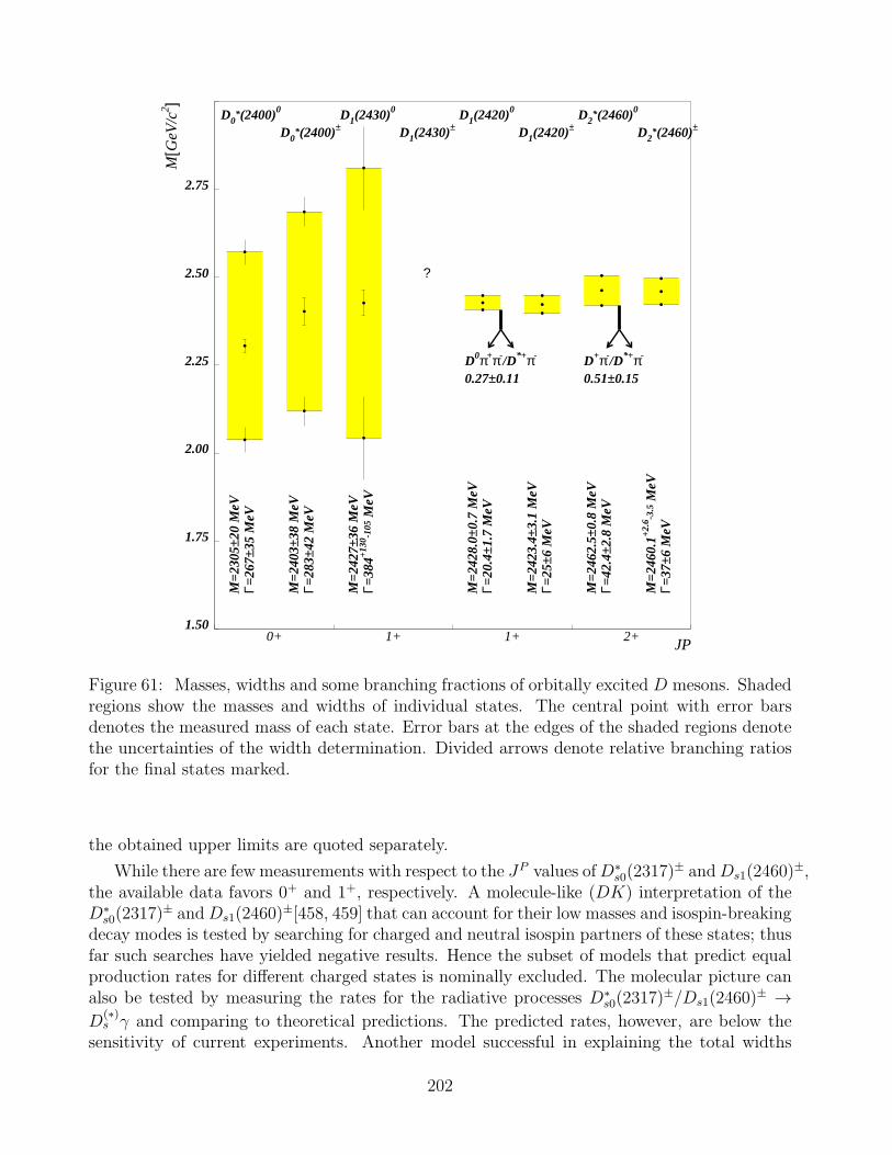
0+ 1+ 1+ 2+
D0*(2400)0
D0*(2400)±
D1(2430)0
D1(2430)±D1(2420)0
D1(2420)±D2
*(2460)0
D2*(2460)±
?
M=
2305
±20
MeV
Γ=26
7±35
MeV
M=
2403
±38
MeV
Γ=28
3±42
MeV
M=
2427
±36
MeV
Γ=38
4+13
0 -105
MeV
M=
2428
.0±0
.7 M
eVΓ=
20.4
±1.7
MeV
M=
2423
.4±3
.1 M
eVΓ=
25±6
MeV
M=
2462
.5±0
.8 M
eVΓ=
42.4
±2.8
MeV
M=
2460
.1+
2.6 -3
.5 M
eVΓ=
37±6
MeV
D0π+π-/D*+π-
0.27±0.11D+π-/D*+π-
0.51±0.15
1.50
1.75
2.00
2.25
2.50
2.75
JP
M[G
eV/c
2 ]
Figure 61: Masses, widths and some branching fractions of orbitally excited D mesons. Shadedregions show the masses and widths of individual states. The central point with error barsdenotes the measured mass of each state. Error bars at the edges of the shaded regions denotethe uncertainties of the width determination. Divided arrows denote relative branching ratiosfor the final states marked.
the obtained upper limits are quoted separately.
While there are few measurements with respect to the JP values ofD∗s0(2317)
± andDs1(2460)±,
the available data favors 0+ and 1+, respectively. A molecule-like (DK) interpretation of theD∗s0(2317)
± andDs1(2460)±[458, 459] that can account for their low masses and isospin-breaking
decay modes is tested by searching for charged and neutral isospin partners of these states; thusfar such searches have yielded negative results. Hence the subset of models that predict equalproduction rates for different charged states is nominally excluded. The molecular picture canalso be tested by measuring the rates for the radiative processes D∗
s0(2317)±/Ds1(2460)
± →D
(∗)s γ and comparing to theoretical predictions. The predicted rates, however, are below the
sensitivity of current experiments. Another model successful in explaining the total widths
202
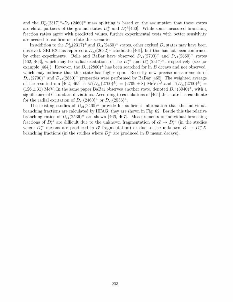
and the D∗s0(2317)
±-Ds1(2460)± mass splitting is based on the assumption that these states
are chiral partners of the ground states D+s and D∗±
s [460]. While some measured branchingfraction ratios agree with predicted values, further experimental tests with better sensitivityare needed to confirm or refute this scenario.
In addition to the D∗s0(2317)
± and Ds1(2460)± states, other excited Ds states may have been
observed. SELEX has reported a DsJ(2632)± candidate [461], but this has not been confirmed
by other experiments. Belle and BaBar have observed DsJ(2700)± and DsJ(2860)
± states[462, 463], which may be radial excitations of the D∗±
s and D∗s0(2317)
±, respectively (see forexample [464]). However, the DsJ(2860)
± has been searched for in B decays and not observed,which may indicate that this state has higher spin. Recently new precise measurements ofDsJ(2700)
± and DsJ(2860)± properties were performed by BaBar [465]. The weighted average
of the results from [462, 465] is M(Ds1(2700)±) = (2709 ± 8) MeV/c2 and Γ(Ds1(2700)
±) =(126± 31) MeV. In the same paper BaBar observes another state, denoted DsJ(3040)
±, with asignificance of 6 standard deviations. According to calculations of [464] this state is a candidatefor the radial excitation of Ds1(2460)
± or Ds1(2536)±.
The existing studies of Ds1(2460)± provide for sufficient information that the individual
branching fractions are calculated by HFAG; they are shown in Fig. 62. Beside this the relativebranching ratios of Ds1(2536)
± are shown [466, 467]. Measurements of individual branchingfractions of D∗∗
s are difficult due to the unknown fragmentation of cc → D∗∗s (in the studies
where D∗∗s mesons are produced in cc fragmentation) or due to the unknown B → D∗∗
s Xbranching fractions (in the studies where D∗∗
s are produced in B meson decays).
203
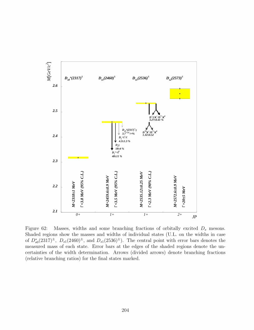
0+ 1+ 1+ 2+
Ds0*(2317)± Ds1(2460)± Ds1(2536)± Ds2(2573)±
M=
2318
±1 M
eV
Γ<3.
8 M
eV (
95%
C.L
.)
M=
2459
.6±0
.9 M
eV
Γ<3.
5 M
eV (
95%
C.L
.)
M=
2535
.12±
0.25
MeV
Γ<2.
3 M
eV (
90%
C.L
.)
M=
2572
.6±0
.9 M
eV
Γ=20
±5 M
eV
D+π-K+/D*+K0
3.27±0.41 %
D*0K+/D*+K0
1.32±0.52
Ds0*(2317)+γ
3.7+5.0-2.4%Ds
+π+π-
4.3±1.3 %Dsγ18±4 %
Ds*+π0
48±11 %
2.1
2.2
2.3
2.4
2.5
2.6
JP
M[G
eV/c
2 ]
Figure 62: Masses, widths and some branching fractions of orbitally excited Ds mesons.Shaded regions show the masses and widths of individual states (U.L. on the widths in caseof D∗
s0(2317)±, Ds1(2460)
±, and Ds1(2536)±). The central point with error bars denotes the
measured mass of each state. Error bars at the edges of the shaded regions denote the un-certainties of the width determination. Arrows (divided arrows) denote branching fractions(relative branching ratios) for the final states marked.
204
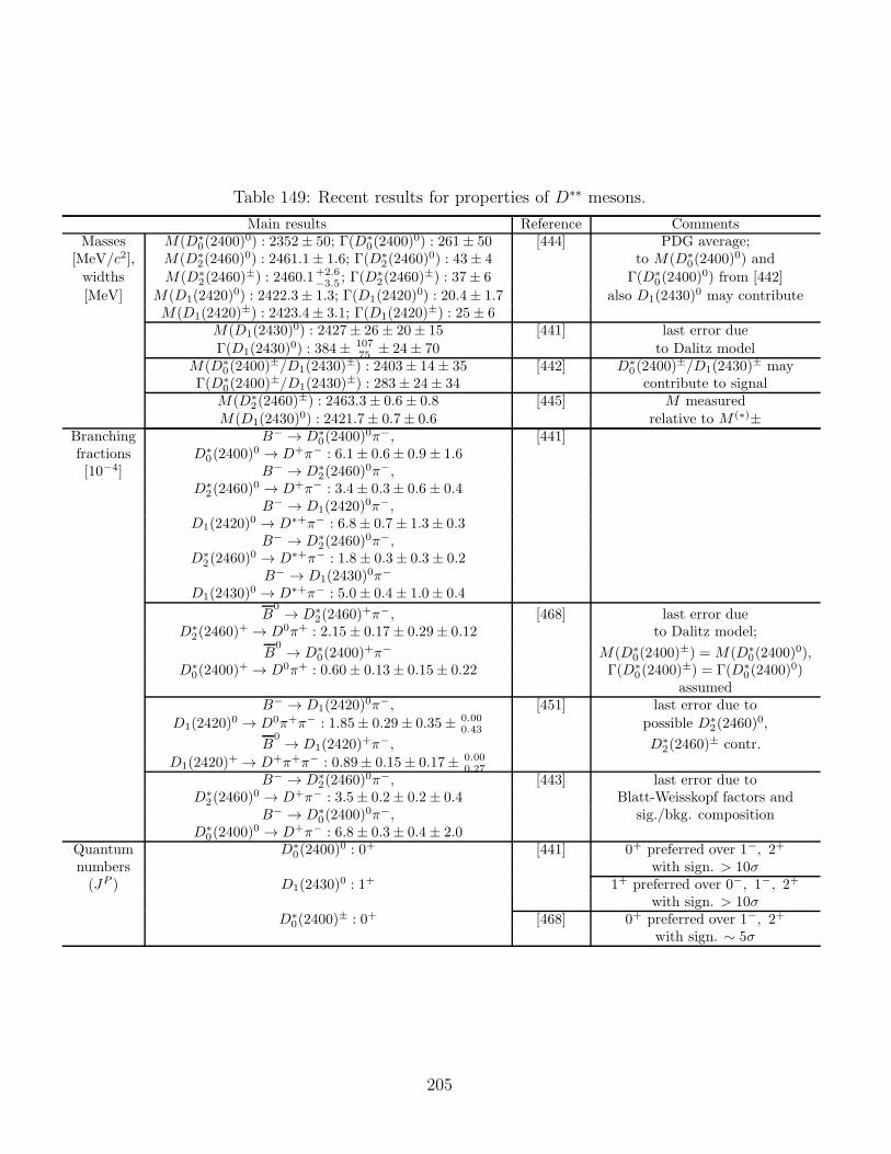
Table 149: Recent results for properties of D∗∗ mesons.
Main results Reference CommentsMasses M(D∗
0(2400)0) : 2352± 50; Γ(D∗
0(2400)0) : 261± 50 [444] PDG average;
[MeV/c2], M(D∗2(2460)
0) : 2461.1± 1.6; Γ(D∗2(2460)
0) : 43± 4 to M(D∗0(2400)
0) and
widths M(D∗2(2460)
±) : 2460.1+2.6−3.5 ; Γ(D
∗2(2460)
±) : 37± 6 Γ(D∗0(2400)
0) from [442]
[MeV] M(D1(2420)0) : 2422.3± 1.3; Γ(D1(2420)
0) : 20.4± 1.7 also D1(2430)0 may contribute
M(D1(2420)±) : 2423.4± 3.1; Γ(D1(2420)
±) : 25± 6M(D1(2430)
0) : 2427± 26± 20± 15 [441] last error due
Γ(D1(2430)0) : 384± 107
75 ± 24± 70 to Dalitz modelM(D∗
0(2400)±/D1(2430)
±) : 2403± 14± 35 [442] D∗0(2400)
±/D1(2430)± may
Γ(D∗0(2400)
±/D1(2430)±) : 283± 24± 34 contribute to signal
M(D∗2(2460)
±) : 2463.3± 0.6± 0.8 [445] M measuredM(D1(2430)
0) : 2421.7± 0.7± 0.6 relative to M (∗)±Branching B− → D∗
0(2400)0π−, [441]
fractions D∗0(2400)
0 → D+π− : 6.1± 0.6± 0.9± 1.6[10−4] B− → D∗
2(2460)0π−,
D∗2(2460)
0 → D+π− : 3.4± 0.3± 0.6± 0.4B− → D1(2420)
0π−,D1(2420)
0 → D∗+π− : 6.8± 0.7± 1.3± 0.3B− → D∗
2(2460)0π−,
D∗2(2460)
0 → D∗+π− : 1.8± 0.3± 0.3± 0.2B− → D1(2430)
0π−
D1(2430)0 → D∗+π− : 5.0± 0.4± 1.0± 0.4
B0 → D∗
2(2460)+π−, [468] last error due
D∗2(2460)
+ → D0π+ : 2.15± 0.17± 0.29± 0.12 to Dalitz model;
B0 → D∗
0(2400)+π− M(D∗
0(2400)±) =M(D∗
0(2400)0),
D∗0(2400)
+ → D0π+ : 0.60± 0.13± 0.15± 0.22 Γ(D∗0(2400)
±) = Γ(D∗0(2400)
0)assumed
B− → D1(2420)0π−, [451] last error due to
D1(2420)0 → D0π+π− : 1.85± 0.29± 0.35± 0.00
0.43 possible D∗2(2460)
0,
B0 → D1(2420)
+π−, D∗2(2460)
± contr.
D1(2420)+ → D+π+π− : 0.89± 0.15± 0.17± 0.00
0.27B− → D∗
2(2460)0π−, [443] last error due to
D∗2(2460)
0 → D+π− : 3.5± 0.2± 0.2± 0.4 Blatt-Weisskopf factors andB− → D∗
0(2400)0π−, sig./bkg. composition
D∗0(2400)
0 → D+π− : 6.8± 0.3± 0.4± 2.0Quantum D∗
0(2400)0 : 0+ [441] 0+ preferred over 1−, 2+
numbers with sign. > 10σ(JP ) D1(2430)
0 : 1+ 1+ preferred over 0−, 1−, 2+
with sign. > 10σD∗
0(2400)± : 0+ [468] 0+ preferred over 1−, 2+
with sign. ∼ 5σ
205
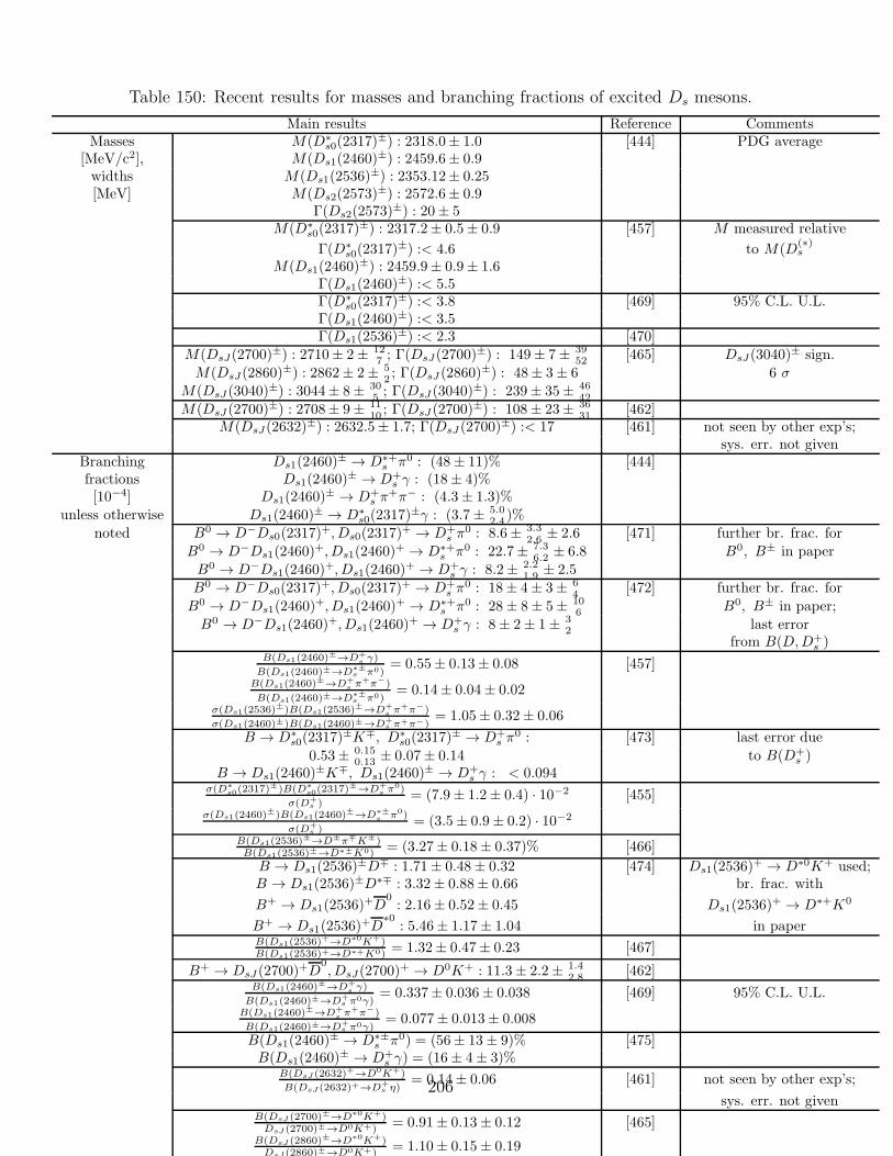
Table 150: Recent results for masses and branching fractions of excited Ds mesons.
Main results Reference CommentsMasses M(D∗
s0(2317)±) : 2318.0± 1.0 [444] PDG average
[MeV/c2], M(Ds1(2460)±) : 2459.6± 0.9
widths M(Ds1(2536)±) : 2353.12± 0.25
[MeV] M(Ds2(2573)±) : 2572.6± 0.9
Γ(Ds2(2573)±) : 20± 5
M(D∗s0(2317)
±) : 2317.2± 0.5± 0.9 [457] M measured relative
Γ(D∗s0(2317)
±) :< 4.6 to M(D(∗)s
M(Ds1(2460)±) : 2459.9± 0.9± 1.6
Γ(Ds1(2460)±) :< 5.5
Γ(D∗s0(2317)
±) :< 3.8 [469] 95% C.L. U.L.Γ(Ds1(2460)
±) :< 3.5Γ(Ds1(2536)
±) :< 2.3 [470]
M(DsJ(2700)±) : 2710± 2± 12
7 ; Γ(DsJ(2700)±) : 149± 7± 39
52 [465] DsJ(3040)± sign.
M(DsJ(2860)±) : 2862± 2± 5
2 ; Γ(DsJ (2860)±) : 48± 3± 6 6 σ
M(DsJ (3040)±) : 3044± 8± 30
5 ; Γ(DsJ (3040)±) : 239± 35± 46
42
M(DsJ (2700)±) : 2708± 9± 11
10 ; Γ(DsJ (2700)±) : 108± 23± 36
31 [462]M(DsJ(2632)
±) : 2632.5± 1.7; Γ(DsJ (2700)±) :< 17 [461] not seen by other exp’s;
sys. err. not givenBranching Ds1(2460)
± → D∗+s π0 : (48± 11)% [444]
fractions Ds1(2460)± → D+
s γ : (18± 4)%[10−4] Ds1(2460)
± → D+s π
+π− : (4.3± 1.3)%
unless otherwise Ds1(2460)± → D∗
s0(2317)±γ : (3.7± 5.0
2.4 )%
noted B0 → D−Ds0(2317)+, Ds0(2317)
+ → D+s π
0 : 8.6± 3.32.6 ± 2.6 [471] further br. frac. for
B0 → D−Ds1(2460)+, Ds1(2460)
+ → D∗+s π0 : 22.7± 7.3
6.2 ± 6.8 B0, B± in paper
B0 → D−Ds1(2460)+, Ds1(2460)
+ → D+s γ : 8.2± 2.2
1.9 ± 2.5
B0 → D−Ds0(2317)+, Ds0(2317)
+ → D+s π
0 : 18± 4± 3± 64 [472] further br. frac. for
B0 → D−Ds1(2460)+, Ds1(2460)
+ → D∗+s π0 : 28± 8± 5± 10
6 B0, B± in paper;
B0 → D−Ds1(2460)+, Ds1(2460)
+ → D+s γ : 8± 2± 1± 3
2 last errorfrom B(D,D+
s )B(Ds1(2460)
±→D+s γ)
B(Ds1(2460)±→D∗±s π0)
= 0.55± 0.13± 0.08 [457]
B(Ds1(2460)±→D+
s π+π−)
B(Ds1(2460)±→D∗±s π0)
= 0.14± 0.04± 0.02
σ(Ds1(2536)±)B(Ds1(2536)
±→D+s π+π−)
σ(Ds1(2460)±)B(Ds1(2460)±→D+s π+π−)
= 1.05± 0.32± 0.06
B → D∗s0(2317)
±K∓, D∗s0(2317)
± → D+s π
0 : [473] last error due
0.53± 0.150.13 ± 0.07± 0.14 to B(D+
s )B → Ds1(2460)
±K∓, Ds1(2460)± → D+
s γ : < 0.094σ(D∗
s0(2317)±)B(D∗
s0(2317)±→D+
s π0)
σ(D+s )
= (7.9± 1.2± 0.4) · 10−2 [455]
σ(Ds1(2460)±)B(Ds1(2460)
±→D∗±s π0)
σ(D+s )
= (3.5± 0.9± 0.2) · 10−2
B(Ds1(2536)±→D±π∓K±)
B(Ds1(2536)±→D∗±K0) = (3.27± 0.18± 0.37)% [466]
B → Ds1(2536)±D∓ : 1.71± 0.48± 0.32 [474] Ds1(2536)
+ → D∗0K+ used;B → Ds1(2536)
±D∗∓ : 3.32± 0.88± 0.66 br. frac. with
B+ → Ds1(2536)+D
0: 2.16± 0.52± 0.45 Ds1(2536)
+ → D∗+K0
B+ → Ds1(2536)+D
∗0: 5.46± 1.17± 1.04 in paper
B(Ds1(2536)+→D∗0K+)
B(Ds1(2536)+→D∗+K0) = 1.32± 0.47± 0.23 [467]
B+ → DsJ (2700)+D
0, DsJ(2700)
+ → D0K+ : 11.3± 2.2± 1.42.8 [462]
B(Ds1(2460)±→D+
s γ)
B(Ds1(2460)±→D+s π0γ)
= 0.337± 0.036± 0.038 [469] 95% C.L. U.L.
B(Ds1(2460)±→D+
s π+π−)
B(Ds1(2460)±→D+s π0γ)
= 0.077± 0.013± 0.008
B(Ds1(2460)± → D∗±
s π0) = (56± 13± 9)% [475]B(Ds1(2460)
± → D+s γ) = (16± 4± 3)%
B(DsJ (2632)+→D0K+)
B(DsJ (2632)+→D+s η)
= 0.14± 0.06 [461] not seen by other exp’s;
sys. err. not givenB(DsJ (2700)
±→D∗0K+)DsJ (2700)±→D0K+) = 0.91± 0.13± 0.12 [465]
B(DsJ (2860)±→D∗0K+)
DsJ (2860)±→D0K+) = 1.10± 0.15± 0.19
206
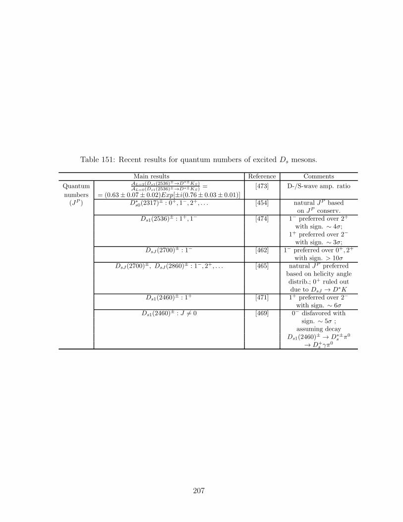
Table 151: Recent results for quantum numbers of excited Ds mesons.
Main results Reference Comments
Quantum AL=2(Ds1(2536)±→D∗±KS)
AL=0(Ds1(2536)±→D∗±KS)= [473] D-/S-wave amp. ratio
numbers = (0.63± 0.07± 0.02)Exp[±i(0.76± 0.03± 0.01)](JP ) D∗
s0(2317)± : 0+, 1−, 2+, . . . [454] natural JP based
on JP conserv.Ds1(2536)
± : 1+, 1− [474] 1− preferred over 2+
with sign. ∼ 4σ;1+ preferred over 2−
with sign. ∼ 3σ;DsJ (2700)
± : 1− [462] 1− preferred over 0+, 2+
with sign. > 10σDsJ(2700)
±, DsJ (2860)± : 1−, 2+, . . . [465] natural JP preferred
based on helicity angledistrib.; 0+ ruled outdue to DsJ → D∗K
Ds1(2460)± : 1+ [471] 1+ preferred over 2−
with sign. ∼ 6σDs1(2460)
± : J 6= 0 [469] 0− disfavored withsign. ∼ 5σ ;
assuming decayDs1(2460)
± → D∗±s π0
→ D+s γπ
0
207
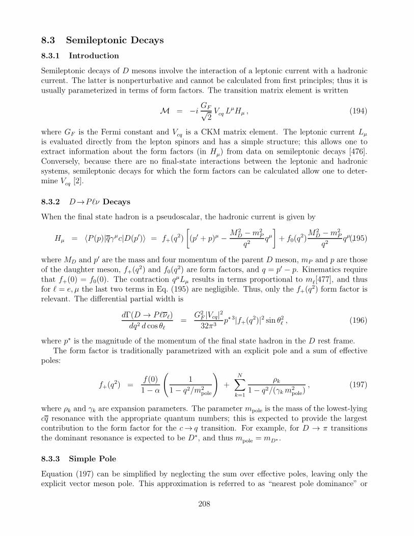
8.3 Semileptonic Decays
8.3.1 Introduction
Semileptonic decays of D mesons involve the interaction of a leptonic current with a hadroniccurrent. The latter is nonperturbative and cannot be calculated from first principles; thus it isusually parameterized in terms of form factors. The transition matrix element is written
M = −i GF√2Vcq L
µHµ , (194)
where GF is the Fermi constant and Vcq is a CKM matrix element. The leptonic current Lµis evaluated directly from the lepton spinors and has a simple structure; this allows one toextract information about the form factors (in Hµ) from data on semileptonic decays [476].Conversely, because there are no final-state interactions between the leptonic and hadronicsystems, semileptonic decays for which the form factors can be calculated allow one to deter-mine Vcq [2].
8.3.2 D→Pℓν Decays
When the final state hadron is a pseudoscalar, the hadronic current is given by
Hµ = 〈P (p)|qγµc|D(p′)〉 = f+(q2)
[
(p′ + p)µ − M2D −m2
P
q2qµ]
+ f0(q2)M2
D −m2P
q2qµ ,(195)
where MD and p′ are the mass and four momentum of the parent D meson, mP and p are thoseof the daughter meson, f+(q
2) and f0(q2) are form factors, and q = p′ − p. Kinematics require
that f+(0) = f0(0). The contraction qµLµ results in terms proportional to mℓ[477], and thusfor ℓ = e, µ the last two terms in Eq. (195) are negligible. Thus, only the f+(q
2) form factor isrelevant. The differential partial width is
dΓ(D → Pℓνℓ)
dq2 d cos θℓ=
G2F |Vcq|232π3
p∗ 3|f+(q2)|2 sin θ2ℓ , (196)
where p∗ is the magnitude of the momentum of the final state hadron in the D rest frame.The form factor is traditionally parametrized with an explicit pole and a sum of effective
poles:
f+(q2) =
f(0)
1− α
(
1
1− q2/m2pole
)
+N∑
k=1
ρk1− q2/(γkm2
pole), (197)
where ρk and γk are expansion parameters. The parameter mpole is the mass of the lowest-lyingcq resonance with the appropriate quantum numbers; this is expected to provide the largestcontribution to the form factor for the c→ q transition. For example, for D → π transitionsthe dominant resonance is expected to be D∗, and thus mpole = mD∗ .
8.3.3 Simple Pole
Equation (197) can be simplified by neglecting the sum over effective poles, leaving only theexplicit vector meson pole. This approximation is referred to as “nearest pole dominance” or
208
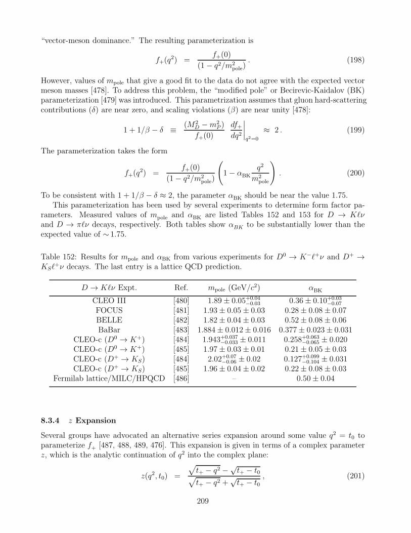
“vector-meson dominance.” The resulting parameterization is
f+(q2) =
f+(0)
(1− q2/m2pole)
. (198)
However, values of mpole that give a good fit to the data do not agree with the expected vectormeson masses [478]. To address this problem, the “modified pole” or Becirevic-Kaidalov (BK)parameterization [479] was introduced. This parametrization assumes that gluon hard-scatteringcontributions (δ) are near zero, and scaling violations (β) are near unity [478]:
1 + 1/β − δ ≡ (M2D −m2
P )
f+(0)
df+dq2
∣
∣
∣
∣
q2=0
≈ 2 . (199)
The parameterization takes the form
f+(q2) =
f+(0)
(1− q2/m2pole)
(
1− αBK
q2
m2pole
)
. (200)
To be consistent with 1 + 1/β − δ ≈ 2, the parameter αBK should be near the value 1.75.This parameterization has been used by several experiments to determine form factor pa-
rameters. Measured values of mpole and αBK are listed Tables 152 and 153 for D → Kℓνand D → πℓν decays, respectively. Both tables show αBK to be substantially lower than theexpected value of ∼ 1.75.
Table 152: Results for mpole and αBK from various experiments for D0 → K−ℓ+ν and D+ →KSℓ
+ν decays. The last entry is a lattice QCD prediction.
D → Kℓν Expt. Ref. mpole (GeV/c2) αBK
CLEO III [480] 1.89± 0.05+0.04−0.03 0.36± 0.10+0.03
−0.07
FOCUS [481] 1.93± 0.05± 0.03 0.28± 0.08± 0.07BELLE [482] 1.82± 0.04± 0.03 0.52± 0.08± 0.06BaBar [483] 1.884± 0.012± 0.016 0.377± 0.023± 0.031
CLEO-c (D0 → K+) [484] 1.943+0.037−0.033 ± 0.011 0.258+0.063
−0.065 ± 0.020CLEO-c (D0 → K+) [485] 1.97± 0.03± 0.01 0.21± 0.05± 0.03CLEO-c (D+ → KS) [484] 2.02+0.07
−0.06 ± 0.02 0.127+0.099−0.104 ± 0.031
CLEO-c (D+ → KS) [485] 1.96± 0.04± 0.02 0.22± 0.08± 0.03Fermilab lattice/MILC/HPQCD [486] – 0.50± 0.04
8.3.4 z Expansion
Several groups have advocated an alternative series expansion around some value q2 = t0 toparameterize f+ [487, 488, 489, 476]. This expansion is given in terms of a complex parameterz, which is the analytic continuation of q2 into the complex plane:
z(q2, t0) =
√
t+ − q2 −√t+ − t0
√
t+ − q2 +√t+ − t0
, (201)
209
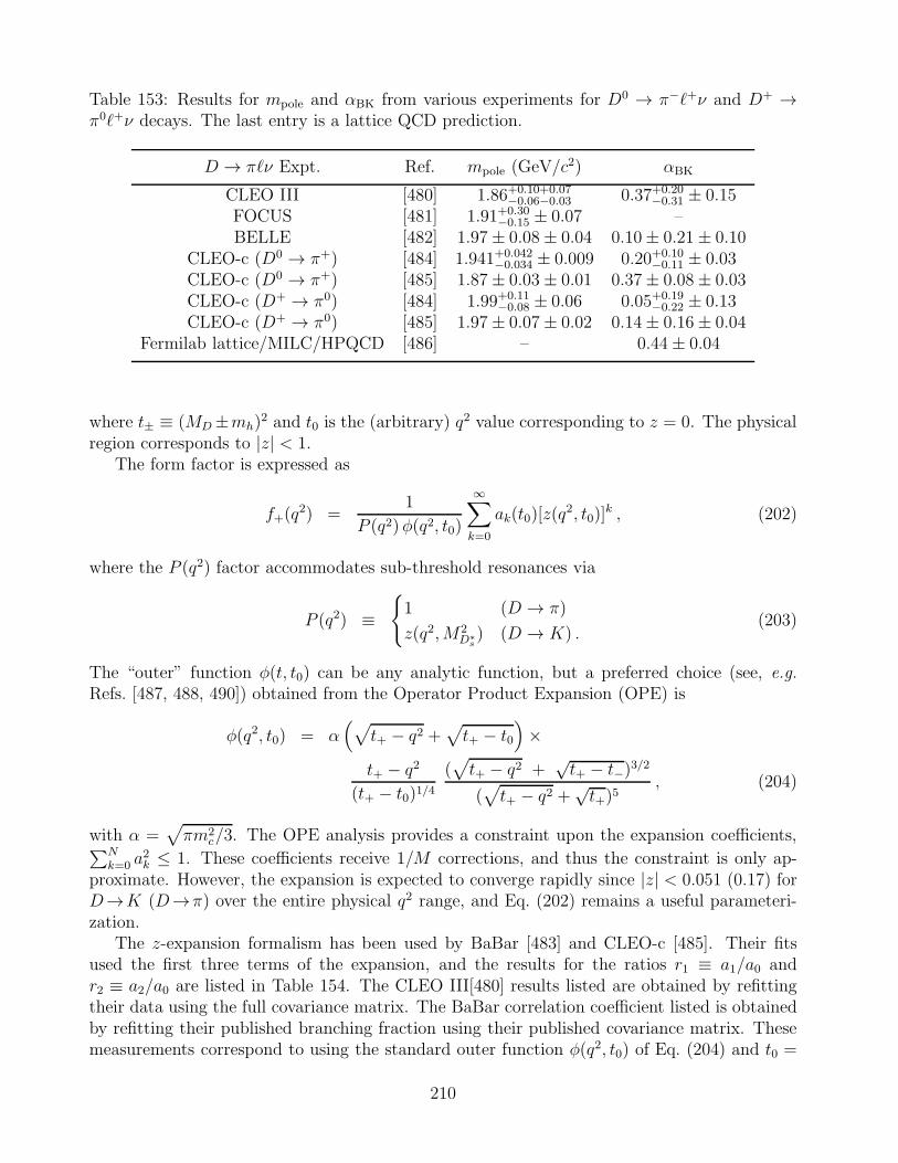
Table 153: Results for mpole and αBK from various experiments for D0 → π−ℓ+ν and D+ →π0ℓ+ν decays. The last entry is a lattice QCD prediction.
D → πℓν Expt. Ref. mpole (GeV/c2) αBK
CLEO III [480] 1.86+0.10+0.07−0.06−0.03 0.37+0.20
−0.31 ± 0.15FOCUS [481] 1.91+0.30
−0.15 ± 0.07 –BELLE [482] 1.97± 0.08± 0.04 0.10± 0.21± 0.10
CLEO-c (D0 → π+) [484] 1.941+0.042−0.034 ± 0.009 0.20+0.10
−0.11 ± 0.03CLEO-c (D0 → π+) [485] 1.87± 0.03± 0.01 0.37± 0.08± 0.03CLEO-c (D+ → π0) [484] 1.99+0.11
−0.08 ± 0.06 0.05+0.19−0.22 ± 0.13
CLEO-c (D+ → π0) [485] 1.97± 0.07± 0.02 0.14± 0.16± 0.04Fermilab lattice/MILC/HPQCD [486] – 0.44± 0.04
where t± ≡ (MD±mh)2 and t0 is the (arbitrary) q
2 value corresponding to z = 0. The physicalregion corresponds to |z| < 1.
The form factor is expressed as
f+(q2) =
1
P (q2)φ(q2, t0)
∞∑
k=0
ak(t0)[z(q2, t0)]
k , (202)
where the P (q2) factor accommodates sub-threshold resonances via
P (q2) ≡
1 (D → π)
z(q2,M2D∗s) (D → K) .
(203)
The “outer” function φ(t, t0) can be any analytic function, but a preferred choice (see, e.g.Refs. [487, 488, 490]) obtained from the Operator Product Expansion (OPE) is
φ(q2, t0) = α(
√
t+ − q2 +√
t+ − t0
)
×t+ − q2
(t+ − t0)1/4(√
t+ − q2 +√t+ − t−)
3/2
(√
t+ − q2 +√t+)5
, (204)
with α =√
πm2c/3. The OPE analysis provides a constraint upon the expansion coefficients,
∑Nk=0 a
2k ≤ 1. These coefficients receive 1/M corrections, and thus the constraint is only ap-
proximate. However, the expansion is expected to converge rapidly since |z| < 0.051 (0.17) forD→K (D→π) over the entire physical q2 range, and Eq. (202) remains a useful parameteri-zation.
The z-expansion formalism has been used by BaBar [483] and CLEO-c [485]. Their fitsused the first three terms of the expansion, and the results for the ratios r1 ≡ a1/a0 andr2 ≡ a2/a0 are listed in Table 154. The CLEO III[480] results listed are obtained by refittingtheir data using the full covariance matrix. The BaBar correlation coefficient listed is obtainedby refitting their published branching fraction using their published covariance matrix. Thesemeasurements correspond to using the standard outer function φ(q2, t0) of Eq. (204) and t0 =
210
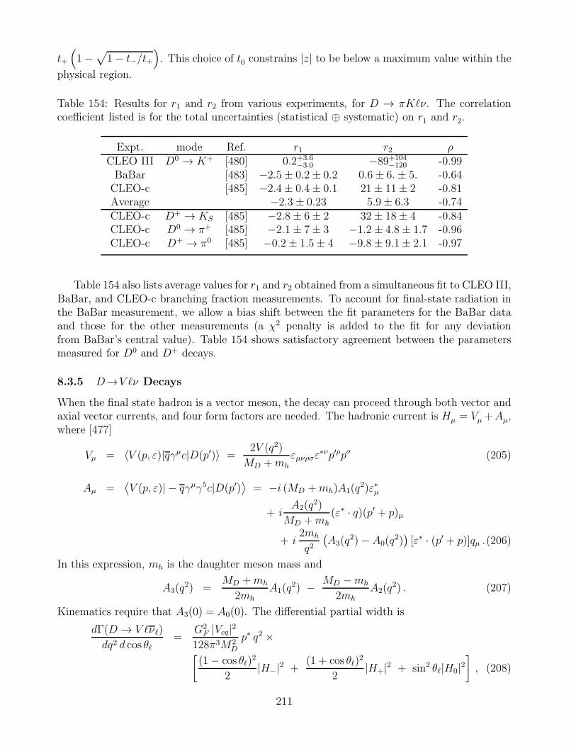
t+
(
1−√
1− t−/t+
)
. This choice of t0 constrains |z| to be below a maximum value within the
physical region.
Table 154: Results for r1 and r2 from various experiments, for D → πKℓν. The correlationcoefficient listed is for the total uncertainties (statistical ⊕ systematic) on r1 and r2.
Expt. mode Ref. r1 r2 ρCLEO III D0 → K+ [480] 0.2+3.6
−3.0 −89+104−120 -0.99
BaBar [483] −2.5± 0.2± 0.2 0.6± 6.± 5. -0.64CLEO-c [485] −2.4± 0.4± 0.1 21± 11± 2 -0.81Average −2.3± 0.23 5.9± 6.3 -0.74CLEO-c D+ → KS [485] −2.8± 6± 2 32± 18± 4 -0.84CLEO-c D0 → π+ [485] −2.1± 7± 3 −1.2 ± 4.8± 1.7 -0.96CLEO-c D+ → π0 [485] −0.2± 1.5± 4 −9.8 ± 9.1± 2.1 -0.97
Table 154 also lists average values for r1 and r2 obtained from a simultaneous fit to CLEO III,BaBar, and CLEO-c branching fraction measurements. To account for final-state radiation inthe BaBar measurement, we allow a bias shift between the fit parameters for the BaBar dataand those for the other measurements (a χ2 penalty is added to the fit for any deviationfrom BaBar’s central value). Table 154 shows satisfactory agreement between the parametersmeasured for D0 and D+ decays.
8.3.5 D→V ℓν Decays
When the final state hadron is a vector meson, the decay can proceed through both vector andaxial vector currents, and four form factors are needed. The hadronic current is Hµ = Vµ+Aµ,where [477]
Vµ = 〈V (p, ε)|qγµc|D(p′)〉 =2V (q2)
MD +mhεµνρσε
∗νp′ρpσ (205)
Aµ =⟨
V (p, ε)| − qγµγ5c|D(p′)⟩
= −i (MD +mh)A1(q2)ε∗µ
+ iA2(q
2)
MD +mh
(ε∗ · q)(p′ + p)µ
+ i2mh
q2(
A3(q2)− A0(q
2))
[ε∗ · (p′ + p)]qµ .(206)
In this expression, mh is the daughter meson mass and
A3(q2) =
MD +mh
2mhA1(q
2) − MD −mh
2mhA2(q
2) . (207)
Kinematics require that A3(0) = A0(0). The differential partial width is
dΓ(D → V ℓνℓ)
dq2 d cos θℓ=
G2F |Vcq|2
128π3M2D
p∗ q2 ×[
(1− cos θℓ)2
2|H−|2 +
(1 + cos θℓ)2
2|H+|2 + sin2 θℓ|H0|2
]
, (208)
211
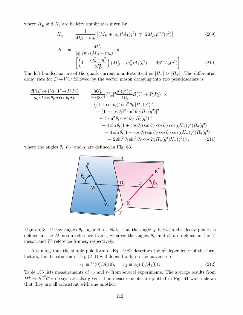
where H± and H0 are helicity amplitudes given by
H± =1
MD +mh
[
(MB +mh)2A1(q
2) ∓ 2MD p∗V (q2)
]
(209)
H0 =1
|q|M2
B
2mh(MD +mh)×
[(
1− m2h − q2
M2D
)
(M2D +m2
h)A1(q2) − 4p∗2A2(q
2)
]
. (210)
The left-handed nature of the quark current manifests itself as |H−| > |H+|. The differentialdecay rate for D→V ℓν followed by the vector meson decaying into two pseudoscalars is
dΓ(D→V ℓν, V →P1P2)
dq2d cos θV d cos θℓdχ=
3G2F
2048π4|Vcq|2
p∗(q2)q2
M2D
B(V → P1P2) ×
(1 + cos θℓ)2 sin2 θV |H+(q
2)|2+ (1− cos θℓ)
2 sin2 θV |H−(q2)|2
+ 4 sin2 θℓ cos2 θV |H0(q
2)|2+ 4 sin θℓ(1 + cos θℓ) sin θV cos θV cosχH+(q
2)H0(q2)
− 4 sin θℓ(1− cos θℓ) sin θV cos θV cosχH−(q2)H0(q
2)
− 2 sin2 θℓ sin2 θV cos 2χH+(q
2)H−(q2)
, (211)
where the angles θℓ, θV , and χ are defined in Fig. 63.
Figure 63: Decay angles θV , θℓ and χ. Note that the angle χ between the decay planes isdefined in the D-meson reference frame, whereas the angles θV and θℓ are defined in the Vmeson and W reference frames, respectively.
Assuming that the simple pole form of Eq. (198) describes the q2-dependence of the formfactors, the distribution of Eq. (211) will depend only on the parameters
rV ≡ V (0)/A1(0), r2 ≡ A2(0)/A1(0) . (212)
Table 155 lists measurements of rV and r2 from several experiments. The average results from
D+ →K∗0ℓ+ν decays are also given. The measurements are plotted in Fig. 64 which shows
that they are all consistent with one another.
212
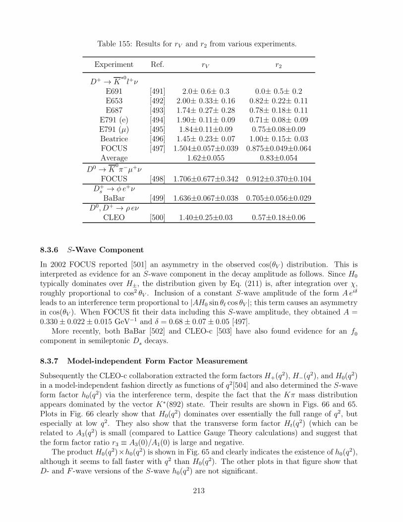
Table 155: Results for rV and r2 from various experiments.
Experiment Ref. rV r2
D+ → K∗0l+ν
E691 [491] 2.0± 0.6± 0.3 0.0± 0.5± 0.2E653 [492] 2.00± 0.33± 0.16 0.82± 0.22± 0.11E687 [493] 1.74± 0.27± 0.28 0.78± 0.18± 0.11
E791 (e) [494] 1.90± 0.11± 0.09 0.71± 0.08± 0.09E791 (µ) [495] 1.84±0.11±0.09 0.75±0.08±0.09Beatrice [496] 1.45± 0.23± 0.07 1.00± 0.15± 0.03FOCUS [497] 1.504±0.057±0.039 0.875±0.049±0.064Average 1.62±0.055 0.83±0.054
D0 → K0π−µ+ν
FOCUS [498] 1.706±0.677±0.342 0.912±0.370±0.104D+s → φ e+νBaBar [499] 1.636±0.067±0.038 0.705±0.056±0.029
D0, D+ → ρ eνCLEO [500] 1.40±0.25±0.03 0.57±0.18±0.06
8.3.6 S-Wave Component
In 2002 FOCUS reported [501] an asymmetry in the observed cos(θV ) distribution. This isinterpreted as evidence for an S-wave component in the decay amplitude as follows. Since H0
typically dominates over H±, the distribution given by Eq. (211) is, after integration over χ,roughly proportional to cos2 θV . Inclusion of a constant S-wave amplitude of the form Aeiδ
leads to an interference term proportional to |AH0 sin θℓ cos θV |; this term causes an asymmetryin cos(θV ). When FOCUS fit their data including this S-wave amplitude, they obtained A =0.330± 0.022± 0.015 GeV−1 and δ = 0.68± 0.07± 0.05 [497].
More recently, both BaBar [502] and CLEO-c [503] have also found evidence for an f0component in semileptonic Ds decays.
8.3.7 Model-independent Form Factor Measurement
Subsequently the CLEO-c collaboration extracted the form factors H+(q2), H−(q
2), and H0(q2)
in a model-independent fashion directly as functions of q2[504] and also determined the S-waveform factor h0(q
2) via the interference term, despite the fact that the Kπ mass distributionappears dominated by the vector K∗(892) state. Their results are shown in Figs. 66 and 65.Plots in Fig. 66 clearly show that H0(q
2) dominates over essentially the full range of q2, butespecially at low q2. They also show that the transverse form factor Ht(q
2) (which can berelated to A3(q
2) is small (compared to Lattice Gauge Theory calculations) and suggest thatthe form factor ratio r3 ≡ A3(0)/A1(0) is large and negative.
The product H0(q2)×h0(q2) is shown in Fig. 65 and clearly indicates the existence of h0(q
2),although it seems to fall faster with q2 than H0(q
2). The other plots in that figure show thatD- and F -wave versions of the S-wave h0(q
2) are not significant.
213
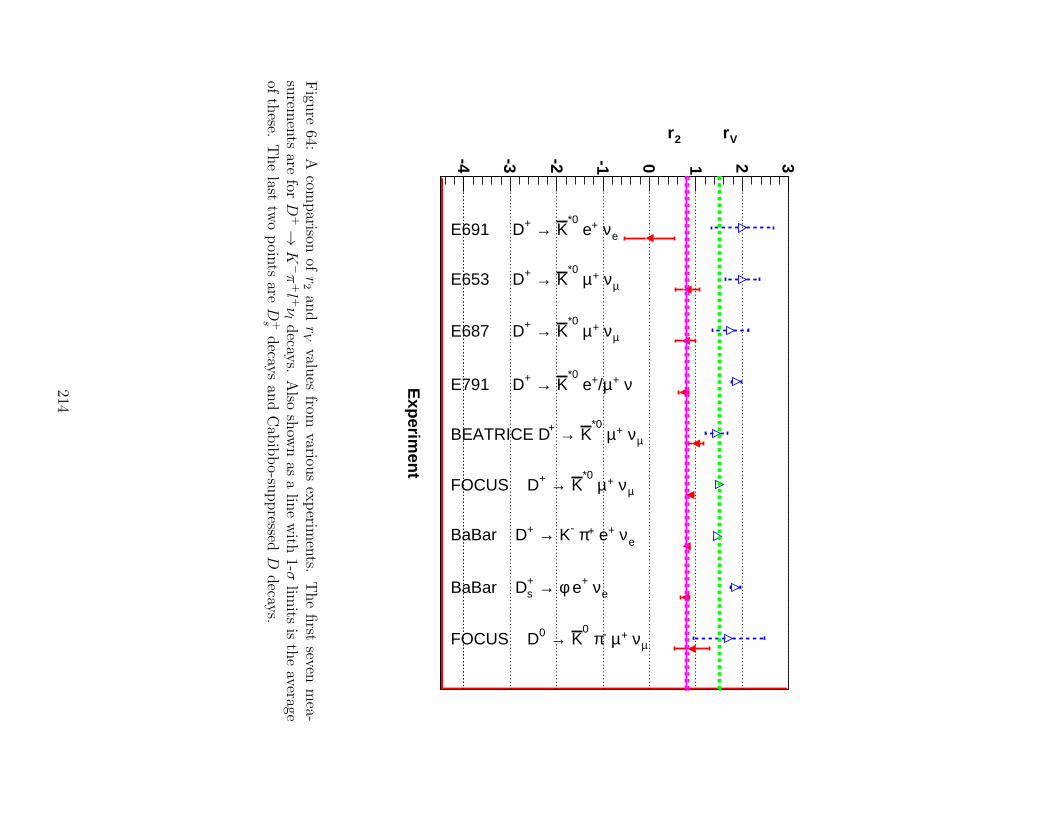
Experim
ent
V r2 r
-4 -3 -2 -1 0 1 2 3
eν + e*0
K → +E691 D
µν +µ *0
K → +E653 D
µν +µ *0
K → +E687 D
ν +µ/+ e*0
K → +E791 D
µν +µ *0
K → +BEATRICE D
µν +µ *0
K → +FOCUS D
eν + e+π - K→ +BaBar D
eν + eφ → s+BaBar D
µν +µ -π 0
K → 0FOCUS DE
xperiment
V r2 r
-4 -3 -2 -1 0 1 2 3
eν + e*0
K → +E691 D
µν +µ *0
K → +E653 D
µν +µ *0
K → +E687 D
ν +µ/+ e*0
K → +E791 D
µν +µ *0
K → +BEATRICE D
µν +µ *0
K → +FOCUS D
eν + e+π - K→ +BaBar D
eν + eφ → s+BaBar D
µν +µ -π 0
K → 0FOCUS D
Figu
re64:
Acom
parison
ofr2an
drVvalu
esfrom
variousexperim
ents.
Thefirst
sevenmea-
surem
ents
arefor
D+→
K−π+l +νldecay
s.Also
show
nas
alin
ewith
1-σlim
itsistheaverage
ofthese.
Thelast
twopoin
tsare
D+sdecay
san
dCab
ibbo-su
ppressed
Ddecay
s.
214
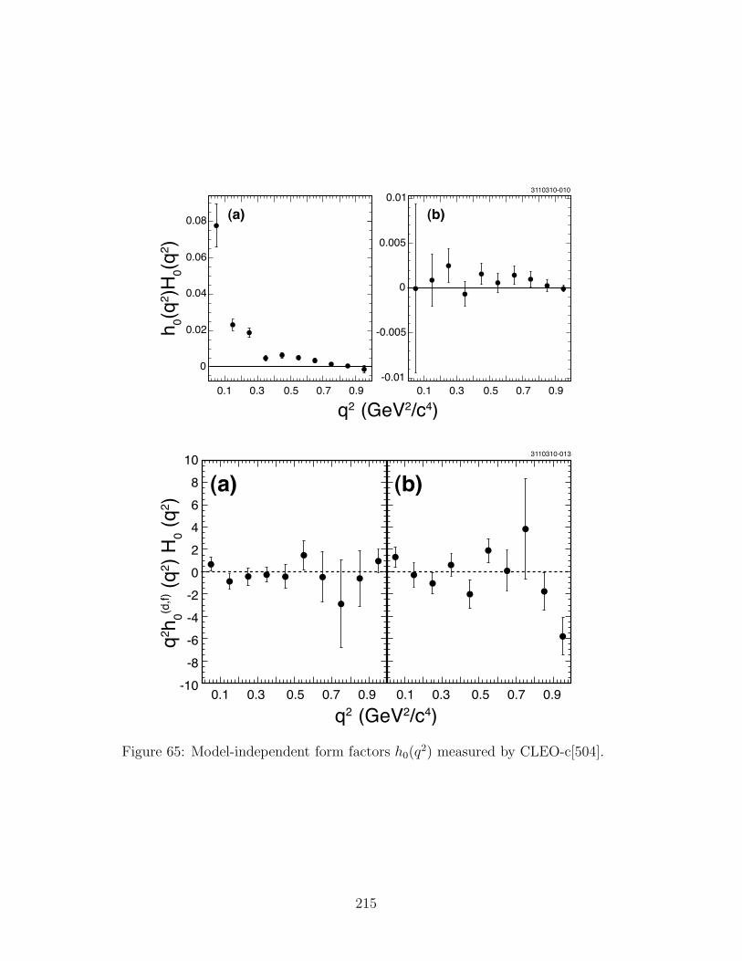
Figure 65: Model-independent form factors h0(q2) measured by CLEO-c[504].
215
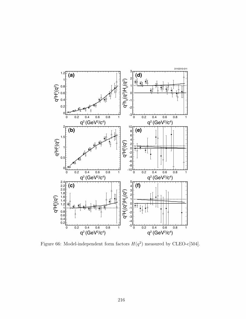
Figure 66: Model-independent form factors H(q2) measured by CLEO-c[504].
216
8.4 CP Asymmetries
CP violation occurs if the decay rate for a particle differs from that of its CP -conjugate[505].In general there are two classes of CP violation, termed indirect and direct [506]. Indirect CPviolation refers to ∆C = 2 processes and arises in D0 decays due to D0-D 0 mixing. It canoccur as an asymmetry in the mixing itself, or it can result from interference between a decayamplitude arising via mixing and a non-mixed amplitude. Direct CP violation refers to ∆C=1processes and occurs in both charged and neutral D decays. It results from interference betweentwo different decay amplitudes (e.g., a penguin and tree amplitude) that have different weak(CKM) and strong phases36. A difference in strong phases typically arises due to final-stateinteractions (FSI)[507]. A difference in weak phases arises from different CKM vertex couplings,as is often the case for spectator and penguin diagrams.
The CP asymmetry is defined as the difference between D and D partial widths divided bytheir sum:
ACP =Γ(D)− Γ(D)
Γ(D) + Γ(D). (213)
However, to take into account differences in production rates between D and D (which wouldaffect the number of respective decays observed), experiments usually normalize to a Cabibbo-favored mode. In this case there is the additional benefit that most corrections due to ineffi-ciencies cancel out, reducing systematic uncertainties. An implicit assumption is that there isno measurable CP violation in the Cabibbo-favored normalizing mode. The CP asymmetry iscalculated as
ACP =η(D)− η(D)
η(D) + η(D), (214)
where (considering, for example, D0 → K−K+)
η(D) =N(D0 → K−K+)
N(D0 → K−π+), (215)
η(D) =N(D 0 → K−K+)
N(D 0 → K+π−). (216)
In the case of D+ and D+s decays, ACP measures direct CP violation; in the case of D0 decays,
ACP measures direct and indirect CP violation combined. Values of ACP for D+, D0 and D+s
decays are listed in Tables 156, 157 and 158 respectively.
36The weak phase difference will have opposite signs for D→ f and D→ f decays, while the strong phasedifference will have the same sign. As a result, squaring the total amplitudes to obtain the decay rates givesinterference terms having opposite sign, i.e., non-identical decay rates.
217
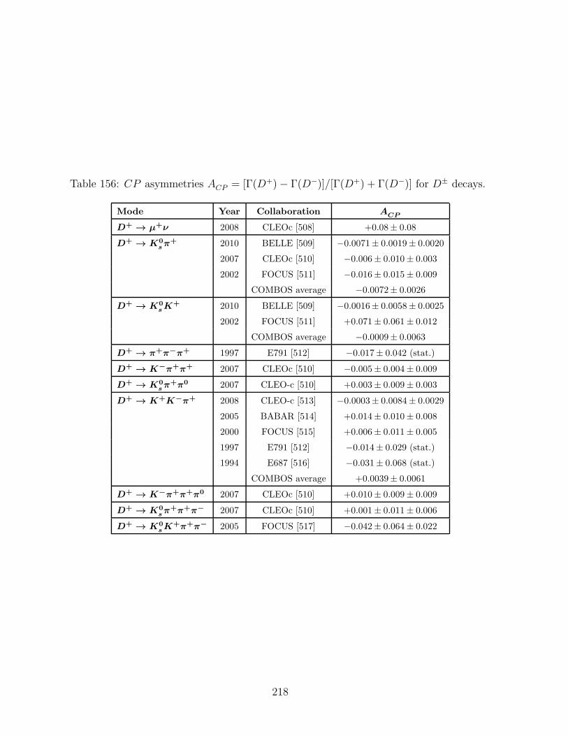
Table 156: CP asymmetries ACP = [Γ(D+)− Γ(D−)]/[Γ(D+) + Γ(D−)] for D± decays.
Mode Year Collaboration ACP
D+ → µ+ν 2008 CLEOc [508] +0.08± 0.08
D+ → K0sπ+ 2010 BELLE [509] −0.0071± 0.0019± 0.0020
2007 CLEOc [510] −0.006± 0.010± 0.003
2002 FOCUS [511] −0.016± 0.015± 0.009
COMBOS average −0.0072± 0.0026
D+ → K0sK+ 2010 BELLE [509] −0.0016± 0.0058± 0.0025
2002 FOCUS [511] +0.071± 0.061± 0.012
COMBOS average −0.0009± 0.0063
D+ → π+π−π+ 1997 E791 [512] −0.017± 0.042 (stat.)
D+ → K−π+π+ 2007 CLEOc [510] −0.005± 0.004± 0.009
D+ → K0sπ+π0 2007 CLEO-c [510] +0.003± 0.009± 0.003
D+ → K+K−π+ 2008 CLEO-c [513] −0.0003± 0.0084± 0.0029
2005 BABAR [514] +0.014± 0.010± 0.008
2000 FOCUS [515] +0.006± 0.011± 0.005
1997 E791 [512] −0.014± 0.029 (stat.)
1994 E687 [516] −0.031± 0.068 (stat.)
COMBOS average +0.0039± 0.0061
D+ → K−π+π+π0 2007 CLEOc [510] +0.010± 0.009± 0.009
D+ → K0sπ+π+π− 2007 CLEOc [510] +0.001± 0.011± 0.006
D+ → K0sK+π+π− 2005 FOCUS [517] −0.042± 0.064± 0.022
218
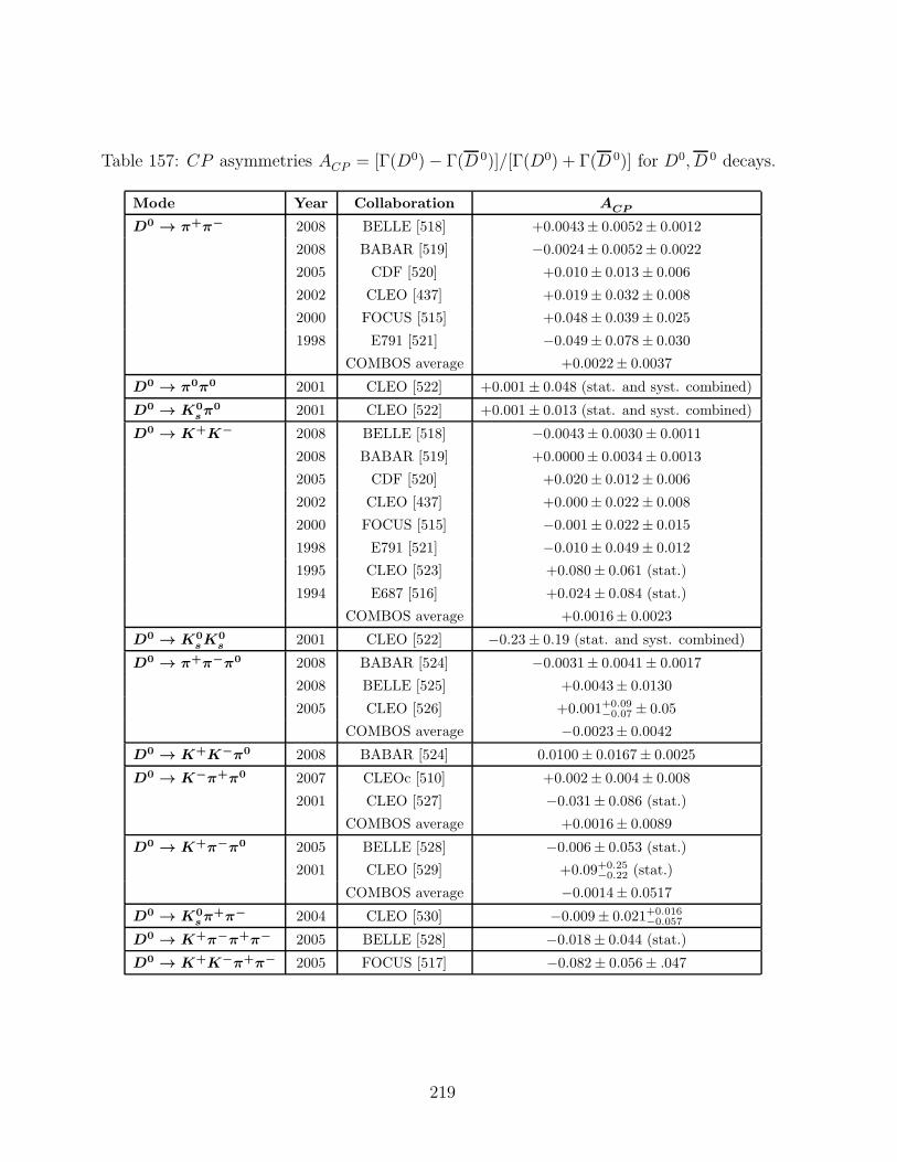
Table 157: CP asymmetries ACP = [Γ(D0)− Γ(D 0)]/[Γ(D0) + Γ(D 0)] for D0, D 0 decays.
Mode Year Collaboration ACP
D0 → π+π− 2008 BELLE [518] +0.0043± 0.0052± 0.0012
2008 BABAR [519] −0.0024± 0.0052± 0.0022
2005 CDF [520] +0.010± 0.013± 0.006
2002 CLEO [437] +0.019± 0.032± 0.008
2000 FOCUS [515] +0.048± 0.039± 0.025
1998 E791 [521] −0.049± 0.078± 0.030
COMBOS average +0.0022± 0.0037
D0 → π0π0 2001 CLEO [522] +0.001± 0.048 (stat. and syst. combined)
D0 → K0sπ0 2001 CLEO [522] +0.001± 0.013 (stat. and syst. combined)
D0 → K+K− 2008 BELLE [518] −0.0043± 0.0030± 0.0011
2008 BABAR [519] +0.0000± 0.0034± 0.0013
2005 CDF [520] +0.020± 0.012± 0.006
2002 CLEO [437] +0.000± 0.022± 0.008
2000 FOCUS [515] −0.001± 0.022± 0.015
1998 E791 [521] −0.010± 0.049± 0.012
1995 CLEO [523] +0.080± 0.061 (stat.)
1994 E687 [516] +0.024± 0.084 (stat.)
COMBOS average +0.0016± 0.0023
D0 → K0sK0
s2001 CLEO [522] −0.23± 0.19 (stat. and syst. combined)
D0 → π+π−π0 2008 BABAR [524] −0.0031± 0.0041± 0.0017
2008 BELLE [525] +0.0043± 0.0130
2005 CLEO [526] +0.001+0.09−0.07 ± 0.05
COMBOS average −0.0023± 0.0042
D0 → K+K−π0 2008 BABAR [524] 0.0100± 0.0167± 0.0025
D0 → K−π+π0 2007 CLEOc [510] +0.002± 0.004± 0.008
2001 CLEO [527] −0.031± 0.086 (stat.)
COMBOS average +0.0016± 0.0089
D0 → K+π−π0 2005 BELLE [528] −0.006± 0.053 (stat.)
2001 CLEO [529] +0.09+0.25−0.22 (stat.)
COMBOS average −0.0014± 0.0517
D0 → K0sπ+π− 2004 CLEO [530] −0.009± 0.021+0.016
−0.057
D0 → K+π−π+π− 2005 BELLE [528] −0.018± 0.044 (stat.)
D0 → K+K−π+π− 2005 FOCUS [517] −0.082± 0.056± .047
219
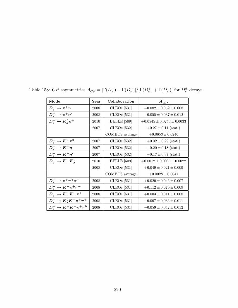
Table 158: CP asymmetries ACP = [Γ(D+s )− Γ(D−
s )]/[Γ(D+s ) + Γ(D−
s )] for D±s decays.
Mode Year Collaboration ACP
D+s
→ π+η 2008 CLEOc [531] −0.082± 0.052± 0.008
D+s
→ π+η′ 2008 CLEOc [531] −0.055± 0.037± 0.012
D+s
→ K0sπ+ 2010 BELLE [509] +0.0545± 0.0250± 0.0033
2007 CLEOc [532] +0.27± 0.11 (stat.)
COMBOS average +0.0653± 0.0246
D+s
→ K+π0 2007 CLEOc [532] +0.02± 0.29 (stat.)
D+s
→ K+η 2007 CLEOc [532] −0.20± 0.18 (stat.)
D+s
→ K+η′ 2007 CLEOc [532] −0.17± 0.37 (stat.)
D+s
→ K+K0s
2010 BELLE [509] +0.0012± 0.0036± 0.0022
2008 CLEOc [531] +0.049± 0.021± 0.009
COMBOS average +0.0028± 0.0041
D+s
→ π+π+π− 2008 CLEOc [531] +0.020± 0.046± 0.007
D+s
→ K+π+π− 2008 CLEOc [531] +0.112± 0.070± 0.009
D+s
→ K+K−π+ 2008 CLEOc [531] +0.003± 0.011± 0.008
D+s
→ K0sK−π+π+ 2008 CLEOc [531] −0.007± 0.036± 0.011
D+s
→ K+K−π+π0 2008 CLEOc [531] −0.059± 0.042± 0.012
220
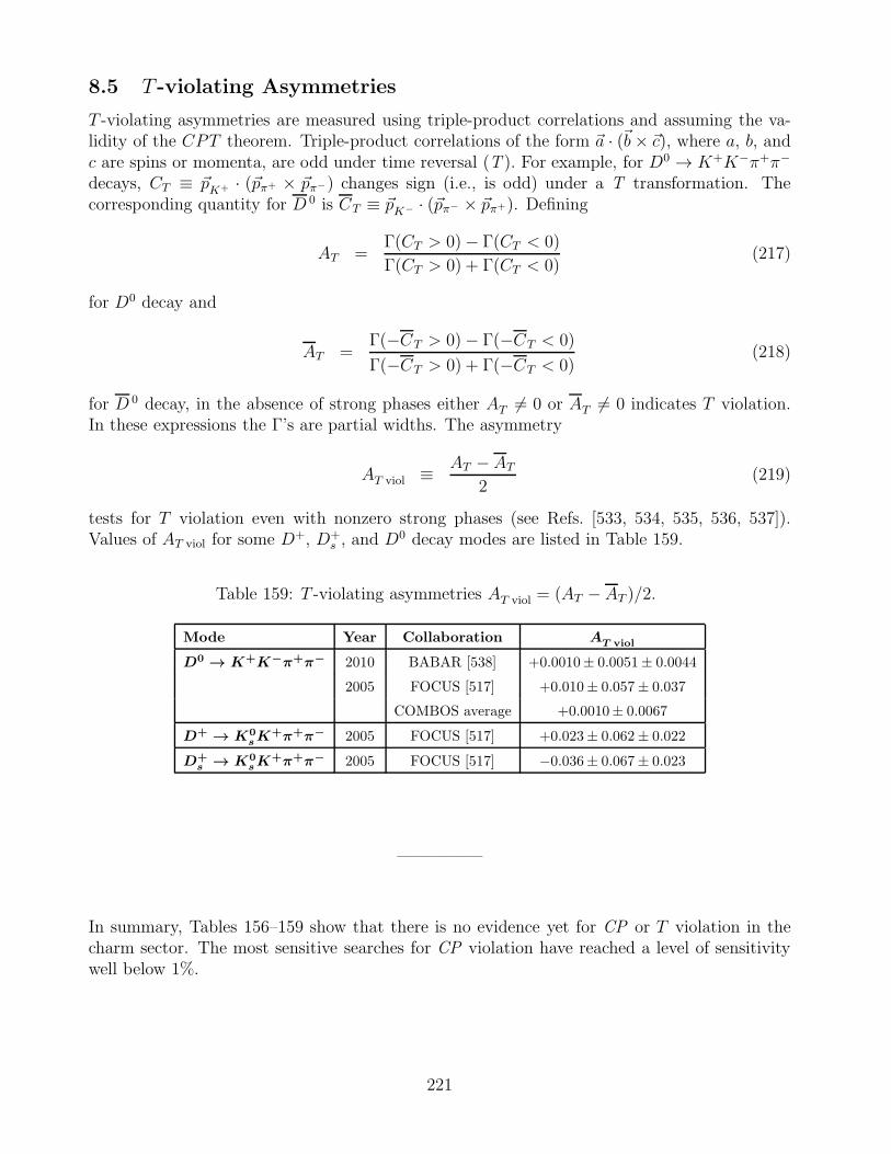
8.5 T -violating Asymmetries
T -violating asymmetries are measured using triple-product correlations and assuming the va-lidity of the CPT theorem. Triple-product correlations of the form ~a · (~b× ~c), where a, b, andc are spins or momenta, are odd under time reversal (T ). For example, for D0 → K+K−π+π−
decays, CT ≡ ~pK+ · (~pπ+ × ~pπ−) changes sign (i.e., is odd) under a T transformation. Thecorresponding quantity for D 0 is CT ≡ ~pK− · (~pπ− × ~pπ+). Defining
AT =Γ(CT > 0)− Γ(CT < 0)
Γ(CT > 0) + Γ(CT < 0)(217)
for D0 decay and
AT =Γ(−CT > 0)− Γ(−CT < 0)
Γ(−CT > 0) + Γ(−CT < 0)(218)
for D 0 decay, in the absence of strong phases either AT 6= 0 or AT 6= 0 indicates T violation.In these expressions the Γ’s are partial widths. The asymmetry
AT viol ≡ AT − AT2
(219)
tests for T violation even with nonzero strong phases (see Refs. [533, 534, 535, 536, 537]).Values of AT viol for some D+, D+
s , and D0 decay modes are listed in Table 159.
Table 159: T -violating asymmetries AT viol = (AT − AT )/2.
Mode Year Collaboration AT viol
D0 → K+K−π+π− 2010 BABAR [538] +0.0010± 0.0051± 0.0044
2005 FOCUS [517] +0.010± 0.057± 0.037
COMBOS average +0.0010± 0.0067
D+ → K0sK+π+π− 2005 FOCUS [517] +0.023± 0.062± 0.022
D+s
→ K0sK+π+π− 2005 FOCUS [517] −0.036± 0.067± 0.023
—————
In summary, Tables 156–159 show that there is no evidence yet for CP or T violation in thecharm sector. The most sensitive searches for CP violation have reached a level of sensitivitywell below 1%.
221
8.6 World Average for the D+s Decay Constant fDs
The Heavy Flavor Averaging Group has used Belle, BaBar, and CLEO measurements ofB(D+
s → µ+ν) and B(D+s → τ+ν) to calculate a world average (WA) value for the D+
s decayconstant fDs . The Belle results are from Ref. [539], the BaBar results are from Refs. [540, 541],and the CLEO results are from Refs. [542, 543, 544].
The value for fDs is calculated via
fDs =1
GF |Vcs|mℓ
(
1− m2ℓ
m2Ds
)
√
8π B(D+s →ℓ+ν)
mDsτDs
, (220)
where, for B(D+s →ℓ+ν), ℓ+ = µ+ or ℓ+ = τ+. The error on fDs is calculated as follows: values
for variables on the right-hand-side of Eq. (220) are sampled from Gaussian distributions havingmean values equal to the central values and standard deviations equal to their respective errors.The resulting values of fDs are plotted, and the r.m.s. of the distribution is taken as the ±1σerrors. The procedure is done separately for the WA values of B(D+
s →µ+ν) and B(D+s →τ+ν),
and for the BaBar value [540] of B(D+s →µ+ν).
The BaBar result is treated separately because the signal yield is normalized to D+s →φ π+
decays; thus the measurement is
Γ(D+s →µ+ν)
Γ(D+s →φπ+)
∣
∣
∣
Babar= 0.143 ± 0.018 (stat.) ± 0.006 (syst.) . (221)
To obtain B(D+s →µ+ν), one must multiply by B(D+
s →φπ+). However, for this analysis theφ is reconstructed via φ→K+K− with |MK+K− −Mφ| ≡ ∆MKK < 5.5 MeV [545]. For theBaBar measurements of B(D+
s →φπ+) [546, 475], a mass window ∆MKK < 15 MeV was used.Because the D+
s →φ π+ branching fraction depends on ∆MKK (see Table II of Ref. [531]), wedo not multiply together the BaBar results for Γ(D+
s →µ+ν)/Γ(D+s →φπ+) and B(D+
s →φπ+);instead we use the fact that CLEO has measured the branching fraction B(D+
s →K+K−π+)for ∆MKK = 5 MeV. To multiply the BaBar result for Γ(D+
s → µ+ν)/Γ(D+s → φπ+) by
the CLEO result for B(D+s → K+K−π+) requires dividing Eq. (221) by B(φ → K+K−) =
0.491 (as used in Ref. [540]) and subtracting in quadrature the 1.2% uncertainty in B(φ →K+K−) from the systematic error. In addition, for the result (221) BaBar subtracted offD+s → f0(980)(K
+K−)π+ background (48 events); as this process is included in the CLEOmeasurement, these events must be added back in to BaBar’s φπ+ yield. The BaBar resultthen becomes
Γ(D+s →µ+ν)
Γ(D+s →K+K−π+)
∣
∣
∣
∣
∆MKK=5.5 MeV
= 0.285 ± 0.035 (stat.) ± 0.011 (syst.) . (222)
Multiplying this by CLEO’s measurement [531]
B(D+s →K+K−π+)
∣
∣
∣
∆MKK=5 MeV= (1.69 ± 0.08 ± 0.06)% (223)
gives
B(D+s →µ+ν)
∣
∣
∣
BaBar adjusted=
(
4.81 ± 0.63 (stat.) ± 0.25 (syst.))
× 10−3 . (224)
222
In summary, three types of measurements are used to calculate the WA fDs:
1. the WA D+s → µ+ν branching fraction, which is calculated from Belle and CLEO mea-
surements (see Fig. 67);
2. the WA D+s → τ+ν branching fraction, which is calculated from CLEO and BaBar mea-
surements (see Fig. 68); and
3. the ratio Γ(D+s → µ+ν)/Γ(D+
s →K+K−π+) measured by BaBar, adjusted as describedabove [547].
The WA fDs value is obtained by averaging the three results, accounting for correlations suchas the values of |Vcs|, mDs
, and τDs in Eq. (220). The result is shown in Fig. 69. The WA valueis
fDs = 254.6 ± 5.9 MeV, (225)
where the statistical and systematic errors are combined. This value can be compared toresults from the two most precise lattice QCD calculations: it is 2.1σ higher than that fromthe HPQCD Collaboration (241 ±3 MeV [548]), and it is consistent with the less precise resultfrom the Fermilab/MILC Collaboration (249 ± 11 MeV [549]).
223
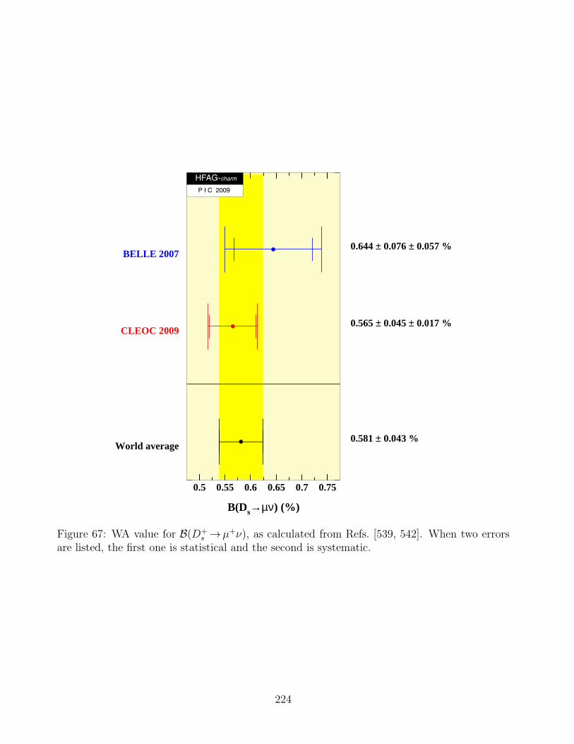
0.5 0.55 0.6 0.65 0.7 0.75
B(Ds→µν) (%)
World average 0.581 ± 0.043 %
CLEOC 2009 0.565 ± 0.045 ± 0.017 %
BELLE 2007 0.644 ± 0.076 ± 0.057 %
HFAG-charm
P I C 2009
Figure 67: WA value for B(D+s →µ+ν), as calculated from Refs. [539, 542]. When two errors
are listed, the first one is statistical and the second is systematic.
224
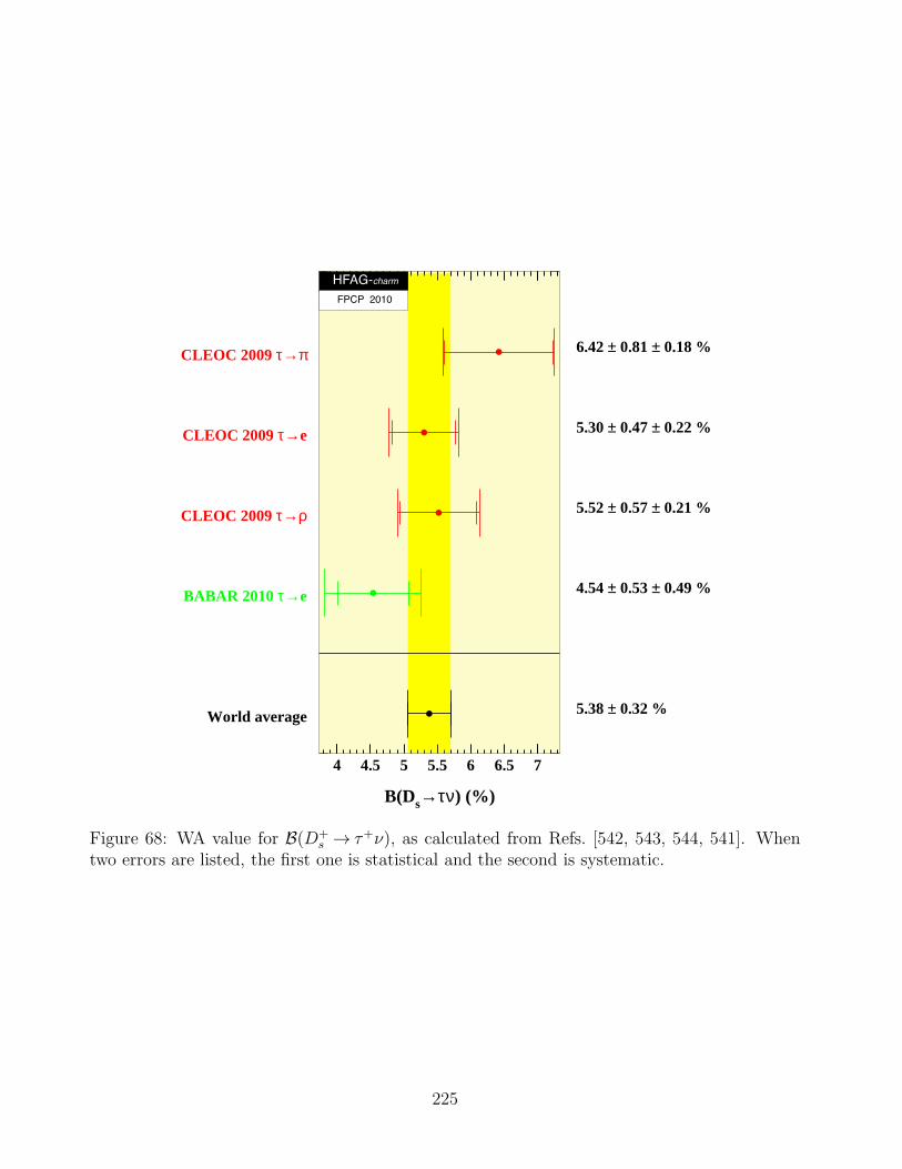
4 4.5 5 5.5 6 6.5 7
B(Ds→τν) (%)
World average 5.38 ± 0.32 %
BABAR 2010 τ→e 4.54 ± 0.53 ± 0.49 %
CLEOC 2009 τ→ρ 5.52 ± 0.57 ± 0.21 %
CLEOC 2009 τ→e 5.30 ± 0.47 ± 0.22 %
CLEOC 2009 τ→π 6.42 ± 0.81 ± 0.18 %
HFAG-charm
FPCP 2010
Figure 68: WA value for B(D+s → τ+ν), as calculated from Refs. [542, 543, 544, 541]. When
two errors are listed, the first one is statistical and the second is systematic.
225
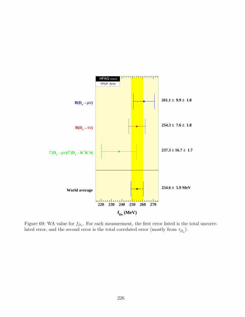
220 230 240 250 260 270
fDs (MeV)
World average254.6 ± 5.9 MeV
Γ(Ds→µν)/Γ(Ds→K+K-π)237.3 ± 16.7 ± 1.7
B(Ds→τν)254.3 ± 7.6 ± 1.8
B(Ds→µν)261.1 ± 9.9 ± 1.8
HFAG-charm
FPCP 2010
Figure 69: WA value for fDs. For each measurement, the first error listed is the total uncorre-lated error, and the second error is the total correlated error (mostly from τDs).
226
8.7 Two-body Hadronic D0 Decays and Final State Radiation
Branching fractions measurements for D0 → K−π+, D0 → π+π− and D0 → K+K− havereached sufficient precision to allow averages with O(1%) relative uncertainties. At these preci-sions, Final State Radiation (FSR) must be treated correctly and consistently across the inputmeasurements for the accuracy of the averages to match the precision. The sensitivity of mea-surements to FSR arises because of a tail in the distribution of radiated energy that extends tothe kinematic limit. The tail beyond Eγ ≈ 30 MeV causes typical selection variables like thehadronic invariant mass to shift outside the selection range dictated by experimental resolu-tion (see Fig. 70). While the differential rate for the tail is small, the integrated rate amountsto several percent of the total h+h−(nγ) rate because of the tail’s extent. The tail thereforetranslates directly into a several percent loss in experimental efficiency.
All measurements that include an FSR correction have a correction based on use of PHO-TOS [550, 551, 552, 553] within the experiment’s Monte Carlo simulation. PHOTOS itself,however, has evolved, over the period spanning the set of measurements. In particular, in-corporation of interference between radiation off of the two separate mesons has proceeded instages: it was first available for particle–antiparticle pairs in version 2.00 (1993), and extendedto any two body, all charged, final states in version 2.02 (1999). The effects of interference areclearly visible (Figure 70), and cause a roughly 30% increase in the integrated rate into the highenergy photon tail. To evaluate the FSR correction incorporated into a given measurement,we must therefore note whether any correction was made, the version of PHOTOS used incorrection, and whether the interference terms in PHOTOS were turned on.
8.7.1 Branching Fraction Corrections
Before averaging the measured branching fractions, the published results are updated, as nec-essary, to the FSR prediction of PHOTOS 2.15 with interference included. The correction willalways shift a branching fraction to a higher value: with no FSR correction or with no interfer-ence term in the correction, the experimental efficiency determination will be biased high, andtherefore the branching fraction will be biased low.
Most of the branching fraction analyses used the kinematic quantity sensitive to FSR inthe candidate selection criteria. For the analyses at the ψ(3770), the variable was ∆E, thedifference between the candidate D0 energy and the beam energy (e.g., EK + Eπ − Ebeam forD0 → K−π+). In the remainder of the analyses, the relevant quantity was the reconstructedhadronic two-body mass mh+h−. To correct we need only to evaluate the fraction of decaysthat FSR moves outside of the range accepted for the analysis.
The corrections were evaluated using an event generator (EvtGen [554]) that incorporatesPHOTOS to simulate the portions of the decay process most relevant to the correction. Wecompared corrections determined both with and without smearing to account for experimentalresolution. The differences were negligible, typically of order of a 1% of the correction itself.The immunity of the correction to resolution effects comes about because most of the longFSR-induced tail in, for example, the mh+h− distribution resides well away from the selectionboundaries. The smearing from resolution, on the other hand, mainly affects the distributionof events right at the boundary.
For measurements incorporating an FSR correction that did not include interference, weupdate by assessing the FSR-induced efficiency loss for both the PHOTOS version and config-uration used in the analysis and our nominal version 2.15 with interference. For measurements
227
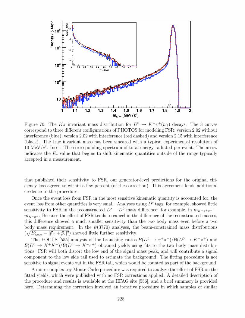
Figure 70: The Kπ invariant mass distribution for D0 → K−π+(nγ) decays. The 3 curvescorrespond to three different configurations of PHOTOS for modeling FSR: version 2.02 withoutinterference (blue), version 2.02 with interference (red dashed) and version 2.15 with interference(black). The true invariant mass has been smeared with a typical experimental resolution of10 MeV/c2. Inset: The corresponding spectrum of total energy radiated per event. The arrowindicates the Eγ value that begins to shift kinematic quantities outside of the range typicallyaccepted in a measurement.
that published their sensitivity to FSR, our generator-level predictions for the original effi-ciency loss agreed to within a few percent (of the correction). This agreement lends additionalcredence to the procedure.
Once the event loss from FSR in the most sensitive kinematic quantity is accounted for, theevent loss from other quantities is very small. Analyses using D∗ tags, for example, showed littlesensitivity to FSR in the reconstructed D∗ − D0 mass difference: for example, in mK−π+π+ −mK−π+ . Because the effect of FSR tends to cancel in the difference of the reconstructed masses,this difference showed a much smaller sensitivity than the two body mass even before a twobody mass requirement. In the ψ(3770) analyses, the beam-constrained mass distributions(√
E2beam − |~pK + ~pπ|2) showed little further sensitivity.
The FOCUS [555] analysis of the branching ratios B(D0 → π+π−)/B(D0 → K−π+) andB(D0 → K+K−)/B(D0 → K−π+) obtained yields using fits to the two body mass distribu-tions. FSR will both distort the low end of the signal mass peak, and will contribute a signalcomponent to the low side tail used to estimate the background. The fitting procedure is notsensitive to signal events out in the FSR tail, which would be counted as part of the background.
A more complex toy Monte Carlo procedure was required to analyze the effect of FSR on thefitted yields, which were published with no FSR corrections applied. A detailed description ofthe procedure and results is available at the HFAG site [556], and a brief summary is providedhere. Determining the correction involved an iterative procedure in which samples of similar
228
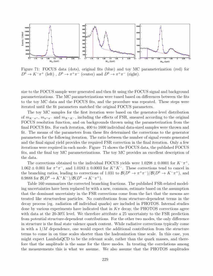
!"# !"#$ !"% !"%$ !"& !"&$ ' '"($ '"!(
'(((
)(((
*(((
%(((
!((((
!'(((
!)(((
!*(((
MKπ (GeV)
Events / 5
MeV
!"# !"#$ !"% !"%$ !"& !"&$ ' '"($ '"!
!((
'((
+((
)((
$((
*((
#((
%((
&((
Mππ (GeV)
!"# !"#$ !"% !"%$ !"& !"&$ ' '"($ '"!
$((
!(((
!$((
'(((
'$((
MKK (GeV)
Figure 71: FOCUS data (dots), original fits (blue) and toy MC parameterization (red) forD0 → K−π+ (left) , D0 → π+π− (center) and D0 → π+π− (right).
size to the FOCUS sample were generated and then fit using the FOCUS signal and backgroundparameterizations. The MC parameterizations were tuned based on differences between the fitsto the toy MC data and the FOCUS fits, and the procedure was repeated. These steps wereiterated until the fit parameters matched the original FOCUS parameters.
The toy MC samples for the first iteration were based on the generator-level distributionof mK−π+, mπ+π− and mK+K−, including the effects of FSR, smeared according to the originalFOCUS resolution function, and on backgrounds thrown using the parameterization from thefinal FOCUS fits. For each iteration, 400 to 1600 individual data-sized samples were thrown andfit. The means of the parameters from these fits determined the corrections to the generatorparameters for the following iteration. The ratio between the number of signal events generatedand the final signal yield provides the required FSR correction in the final iteration. Only a fewiterations were required in each mode. Figure 71 shows the FOCUS data, the published FOCUSfits, and the final toy MC parameterizations. The toy MC provides an excellent description ofthe data.
The corrections obtained to the individual FOCUS yields were 1.0298 ± 0.0001 for K−π+,1.062 ± 0.001 for π+π−, and 1.0183 ± 0.0003 for K+K−. These corrections tend to cancel inthe branching ratios, leading to corrections of 1.031 to B(D0 → π+π−)/B(D0 → K−π+), and0.9888 for B(D0 → K+K−)/B(D0 → K−π+).
Table 160 summarizes the corrected branching fractions. The published FSR-related model-ing uncertainties have been replaced by with a new, common, estimate based on the assumptionthat the dominant uncertainty in the FSR corrections come from the fact that the mesons aretreated like structureless particles. No contributions from structure-dependent terms in thedecay process (eg. radiation off individual quarks) are included in PHOTOS. Internal studiesdone by various experiments have indicated that in Kπ decay, the PHOTOS corrections agreewith data at the 20-30% level. We therefore attribute a 25 uncertainty to the FSR predictionfrom potential structure-dependent contributions. For the other two modes, the only differencein structure is the final state valence quark content. While radiative corrections typically comein with a 1/M dependence, one would expect the additional contribution from the structureterms to come in on time scales shorter than the hadronization time scale. In this case, youmight expect LambdaQCD to be the relevant scale, rather than the quark masses, and there-fore that the amplitude is the same for the three modes. In treating the correlations amongthe measurements this is what we assume. We also assume that the PHOTOS amplitudes
229
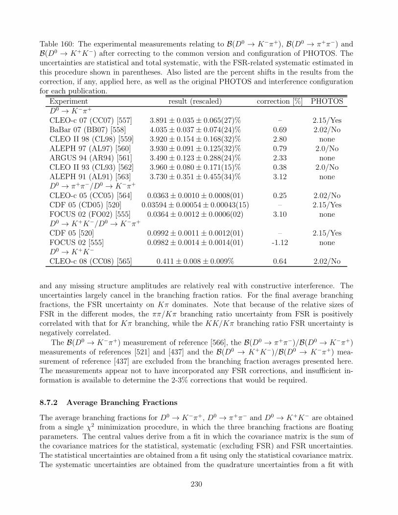
Table 160: The experimental measurements relating to B(D0 → K−π+), B(D0 → π+π−) andB(D0 → K+K−) after correcting to the common version and configuration of PHOTOS. Theuncertainties are statistical and total systematic, with the FSR-related systematic estimated inthis procedure shown in parentheses. Also listed are the percent shifts in the results from thecorrection, if any, applied here, as well as the original PHOTOS and interference configurationfor each publication.
Experiment result (rescaled) correction [%] PHOTOSD0 → K−π+
CLEO-c 07 (CC07) [557] 3.891± 0.035± 0.065(27)% – 2.15/YesBaBar 07 (BB07) [558] 4.035± 0.037± 0.074(24)% 0.69 2.02/NoCLEO II 98 (CL98) [559] 3.920± 0.154± 0.168(32)% 2.80 noneALEPH 97 (AL97) [560] 3.930± 0.091± 0.125(32)% 0.79 2.0/NoARGUS 94 (AR94) [561] 3.490± 0.123± 0.288(24)% 2.33 noneCLEO II 93 (CL93) [562] 3.960± 0.080± 0.171(15)% 0.38 2.0/NoALEPH 91 (AL91) [563] 3.730± 0.351± 0.455(34)% 3.12 noneD0 → π+π−/D0 → K−π+
CLEO-c 05 (CC05) [564] 0.0363± 0.0010± 0.0008(01) 0.25 2.02/NoCDF 05 (CD05) [520] 0.03594± 0.00054± 0.00043(15) – 2.15/YesFOCUS 02 (FO02) [555] 0.0364± 0.0012± 0.0006(02) 3.10 noneD0 → K+K−/D0 → K−π+
CDF 05 [520] 0.0992± 0.0011± 0.0012(01) – 2.15/YesFOCUS 02 [555] 0.0982± 0.0014± 0.0014(01) -1.12 noneD0 → K+K−
CLEO-c 08 (CC08) [565] 0.411± 0.008± 0.009% 0.64 2.02/No
and any missing structure amplitudes are relatively real with constructive interference. Theuncertainties largely cancel in the branching fraction ratios. For the final average branchingfractions, the FSR uncertainty on Kπ dominates. Note that because of the relative sizes ofFSR in the different modes, the ππ/Kπ branching ratio uncertainty from FSR is positivelycorrelated with that for Kπ branching, while the KK/Kπ branching ratio FSR uncertainty isnegatively correlated.
The B(D0 → K−π+) measurement of reference [566], the B(D0 → π+π−)/B(D0 → K−π+)measurements of references [521] and [437] and the B(D0 → K+K−)/B(D0 → K−π+) mea-surement of reference [437] are excluded from the branching fraction averages presented here.The measurements appear not to have incorporated any FSR corrections, and insufficient in-formation is available to determine the 2-3% corrections that would be required.
8.7.2 Average Branching Fractions
The average branching fractions for D0 → K−π+, D0 → π+π− and D0 → K+K− are obtainedfrom a single χ2 minimization procedure, in which the three branching fractions are floatingparameters. The central values derive from a fit in which the covariance matrix is the sum ofthe covariance matrices for the statistical, systematic (excluding FSR) and FSR uncertainties.The statistical uncertainties are obtained from a fit using only the statistical covariance matrix.The systematic uncertainties are obtained from the quadrature uncertainties from a fit with
230
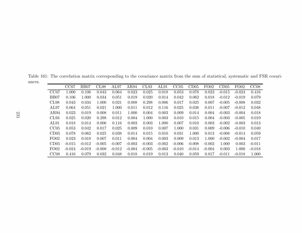
Table 161: The correlation matrix corresponding to the covariance matrix from the sum of statistical, systematic and FSR covari-ances.
CC07 BB07 CL98 AL97 AR94 CL93 AL91 CC05 CD05 FO02 CD05 FO02 CC08
CC07 1.000 0.106 0.043 0.064 0.023 0.025 0.018 0.053 0.078 0.023 -0.015 -0.024 0.416BB07 0.106 1.000 0.034 0.051 0.019 0.020 0.014 0.042 0.062 0.018 -0.012 -0.019 0.079CL98 0.043 0.034 1.000 0.021 0.008 0.298 0.006 0.017 0.025 0.007 -0.005 -0.008 0.032AL97 0.064 0.051 0.021 1.000 0.011 0.012 0.116 0.025 0.038 0.011 -0.007 -0.012 0.048AR94 0.023 0.019 0.008 0.011 1.000 0.004 0.003 0.009 0.014 0.004 -0.003 -0.004 0.018CL93 0.025 0.020 0.298 0.012 0.004 1.000 0.003 0.010 0.015 0.004 -0.003 -0.005 0.019AL91 0.018 0.014 0.006 0.116 0.003 0.003 1.000 0.007 0.010 0.003 -0.002 -0.003 0.013CC05 0.053 0.042 0.017 0.025 0.009 0.010 0.007 1.000 0.031 0.009 -0.006 -0.010 0.040CD05 0.078 0.062 0.025 0.038 0.014 0.015 0.010 0.031 1.000 0.013 -0.008 -0.014 0.059FO02 0.023 0.018 0.007 0.011 0.004 0.004 0.003 0.009 0.013 1.000 -0.002 -0.004 0.017CD05 -0.015 -0.012 -0.005 -0.007 -0.003 -0.003 -0.002 -0.006 -0.008 -0.002 1.000 0.003 -0.011FO02 -0.024 -0.019 -0.008 -0.012 -0.004 -0.005 -0.003 -0.010 -0.014 -0.004 0.003 1.000 -0.018CC08 0.416 0.079 0.032 0.048 0.018 0.019 0.013 0.040 0.059 0.017 -0.011 -0.018 1.000
231
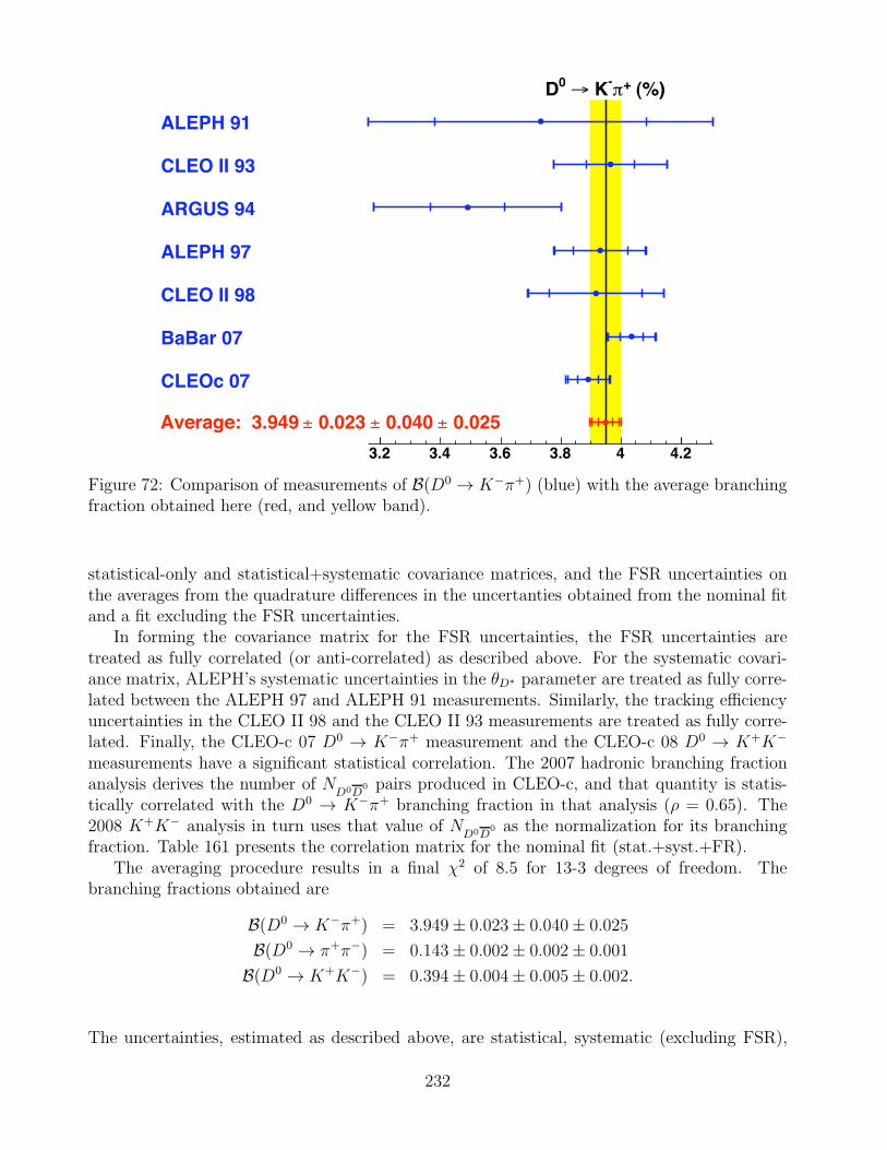
!"#"$%!!"#"&"!!!"#"$'!!()*+,-*.!!'#/&/!
!0123!4
!5""6
789:;!"<
=,=,+!"<
789:!>>!/?
(89@A!/<
(BCDE!/&
789:!>>!/'
(89@A!/F
'#$ '#& '#G '#? & &#$
Figure 72: Comparison of measurements of B(D0 → K−π+) (blue) with the average branchingfraction obtained here (red, and yellow band).
statistical-only and statistical+systematic covariance matrices, and the FSR uncertainties onthe averages from the quadrature differences in the uncertanties obtained from the nominal fitand a fit excluding the FSR uncertainties.
In forming the covariance matrix for the FSR uncertainties, the FSR uncertainties aretreated as fully correlated (or anti-correlated) as described above. For the systematic covari-ance matrix, ALEPH’s systematic uncertainties in the θD∗ parameter are treated as fully corre-lated between the ALEPH 97 and ALEPH 91 measurements. Similarly, the tracking efficiencyuncertainties in the CLEO II 98 and the CLEO II 93 measurements are treated as fully corre-lated. Finally, the CLEO-c 07 D0 → K−π+ measurement and the CLEO-c 08 D0 → K+K−
measurements have a significant statistical correlation. The 2007 hadronic branching fractionanalysis derives the number of N
D0D0 pairs produced in CLEO-c, and that quantity is statis-
tically correlated with the D0 → K−π+ branching fraction in that analysis (ρ = 0.65). The2008 K+K− analysis in turn uses that value of N
D0D0 as the normalization for its branching
fraction. Table 161 presents the correlation matrix for the nominal fit (stat.+syst.+FR).The averaging procedure results in a final χ2 of 8.5 for 13-3 degrees of freedom. The
branching fractions obtained are
B(D0 → K−π+) = 3.949± 0.023± 0.040± 0.025
B(D0 → π+π−) = 0.143± 0.002± 0.002± 0.001
B(D0 → K+K−) = 0.394± 0.004± 0.005± 0.002.
The uncertainties, estimated as described above, are statistical, systematic (excluding FSR),
232
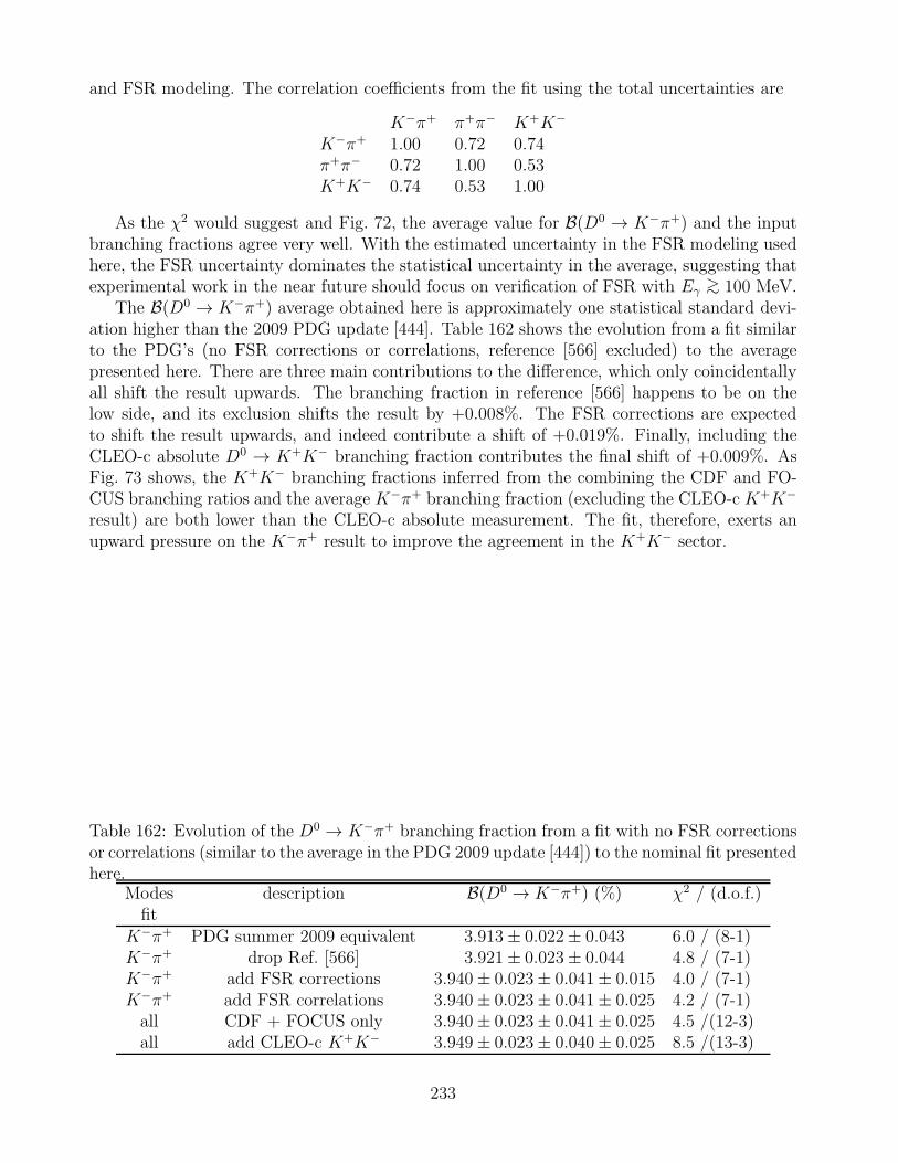
and FSR modeling. The correlation coefficients from the fit using the total uncertainties are
K−π+ π+π− K+K−
K−π+ 1.00 0.72 0.74π+π− 0.72 1.00 0.53K+K− 0.74 0.53 1.00
As the χ2 would suggest and Fig. 72, the average value for B(D0 → K−π+) and the inputbranching fractions agree very well. With the estimated uncertainty in the FSR modeling usedhere, the FSR uncertainty dominates the statistical uncertainty in the average, suggesting thatexperimental work in the near future should focus on verification of FSR with Eγ >∼ 100 MeV.
The B(D0 → K−π+) average obtained here is approximately one statistical standard devi-ation higher than the 2009 PDG update [444]. Table 162 shows the evolution from a fit similarto the PDG’s (no FSR corrections or correlations, reference [566] excluded) to the averagepresented here. There are three main contributions to the difference, which only coincidentallyall shift the result upwards. The branching fraction in reference [566] happens to be on thelow side, and its exclusion shifts the result by +0.008%. The FSR corrections are expectedto shift the result upwards, and indeed contribute a shift of +0.019%. Finally, including theCLEO-c absolute D0 → K+K− branching fraction contributes the final shift of +0.009%. AsFig. 73 shows, the K+K− branching fractions inferred from the combining the CDF and FO-CUS branching ratios and the average K−π+ branching fraction (excluding the CLEO-c K+K−
result) are both lower than the CLEO-c absolute measurement. The fit, therefore, exerts anupward pressure on the K−π+ result to improve the agreement in the K+K− sector.
Table 162: Evolution of the D0 → K−π+ branching fraction from a fit with no FSR correctionsor correlations (similar to the average in the PDG 2009 update [444]) to the nominal fit presentedhere.
Modes description B(D0 → K−π+) (%) χ2 / (d.o.f.)fit
K−π+ PDG summer 2009 equivalent 3.913± 0.022± 0.043 6.0 / (8-1)K−π+ drop Ref. [566] 3.921± 0.023± 0.044 4.8 / (7-1)K−π+ add FSR corrections 3.940± 0.023± 0.041± 0.015 4.0 / (7-1)K−π+ add FSR correlations 3.940± 0.023± 0.041± 0.025 4.2 / (7-1)all CDF + FOCUS only 3.940± 0.023± 0.041± 0.025 4.5 /(12-3)all add CLEO-c K+K− 3.949± 0.023± 0.040± 0.025 8.5 /(13-3)
233
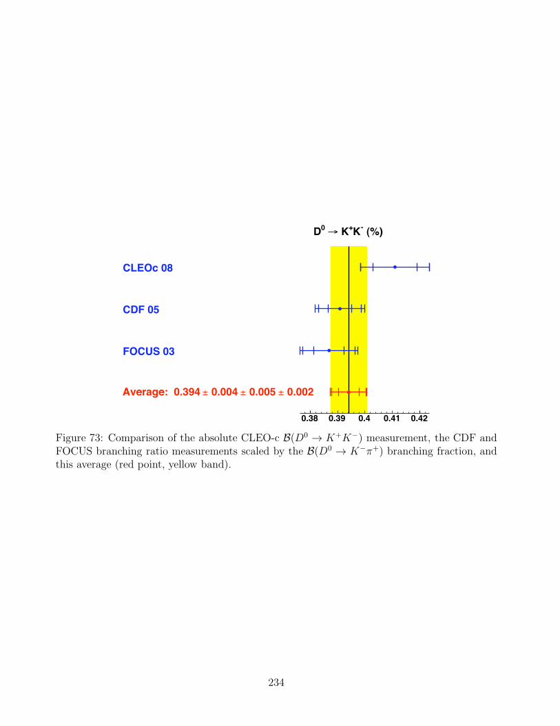
!"#""$!!"#""%!!!"#""&!!'()*+,)-!!"#./&!
!0123
45!4!"6
789:;!".!
967!"%
9<=8>!"?
"#.? "#./ "#& "#&@ "#&$
Figure 73: Comparison of the absolute CLEO-c B(D0 → K+K−) measurement, the CDF andFOCUS branching ratio measurements scaled by the B(D0 → K−π+) branching fraction, andthis average (red point, yellow band).
234
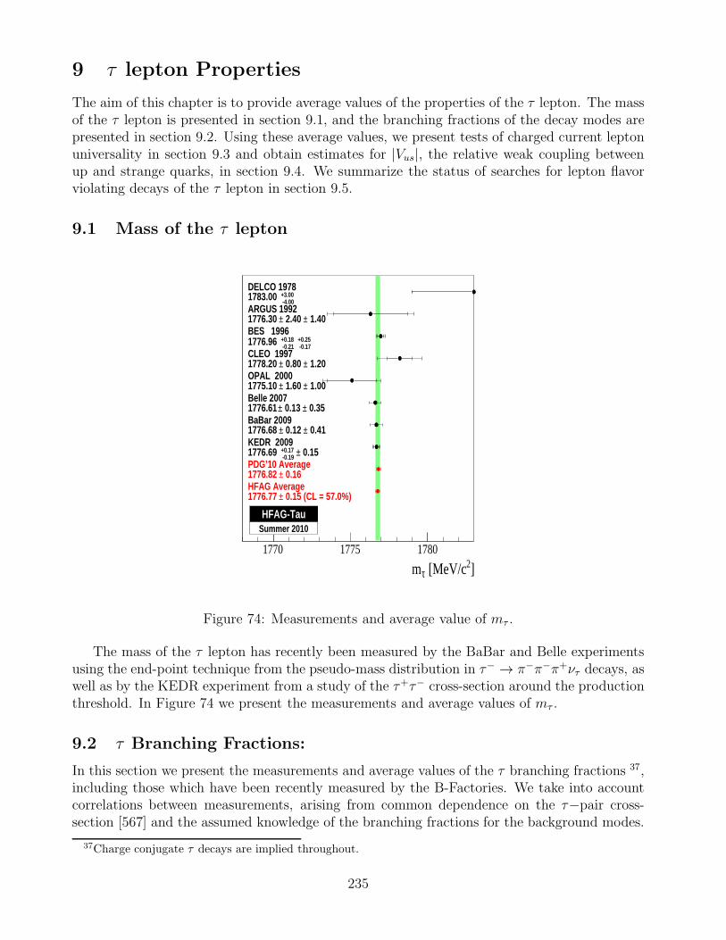
9 τ lepton Properties
The aim of this chapter is to provide average values of the properties of the τ lepton. The massof the τ lepton is presented in section 9.1, and the branching fractions of the decay modes arepresented in section 9.2. Using these average values, we present tests of charged current leptonuniversality in section 9.3 and obtain estimates for |Vus|, the relative weak coupling betweenup and strange quarks, in section 9.4. We summarize the status of searches for lepton flavorviolating decays of the τ lepton in section 9.5.
9.1 Mass of the τ lepton
]2 [MeV/cτm1770 1775 1780
HFAG Average 0.15 (CL = 57.0%)±1776.77
PDG’10 Average 0.16±1776.82
KEDR 2009 0.15± -0.19
+0.171776.69
BaBar 2009 0.41± 0.12 ±1776.68
Belle 2007 0.35± 0.13 ±1776.61
OPAL 2000 1.00± 1.60 ±1775.10
CLEO 1997 1.20± 0.80 ±1778.20
BES 1996 -0.17+0.25 -0.21
+0.181776.96
ARGUS 1992 1.40± 2.40 ±1776.30
DELCO 1978 -4.00+3.001783.00
HFAG-TauSummer 2010
Figure 74: Measurements and average value of mτ .
The mass of the τ lepton has recently been measured by the BaBar and Belle experimentsusing the end-point technique from the pseudo-mass distribution in τ− → π−π−π+ντ decays, aswell as by the KEDR experiment from a study of the τ+τ− cross-section around the productionthreshold. In Figure 74 we present the measurements and average values of mτ .
9.2 τ Branching Fractions:
In this section we present the measurements and average values of the τ branching fractions 37,including those which have been recently measured by the B-Factories. We take into accountcorrelations between measurements, arising from common dependence on the τ−pair cross-section [567] and the assumed knowledge of the branching fractions for the background modes.
37Charge conjugate τ decays are implied throughout.
235
For measurements from the same experiment, we treat the dependence on detector-specificsystematics as sources of correlated systematic uncertainties.
We report here results from single-quantity averages, which includes correlations betweenthe B-Factories, as well as the results from a global fit, which includes correlations between thedifferent branching fractions. We label results from the former as “HFAG Average”, and thelatter as “HFAG Fit” in the following figures.
For the “HFAG Fit”, we use 131 measurements from non-B-Factory experiments, whichincludes the set of 124 measurements used in the global fit performed by the PDG [5]. Themeasurements from non-B-Factories include 37 measurements from ALEPH, 2 measurementsfrom ARGUS, 1 measurement from CELLO, 36 measurements from CLEO, 6 measurementsfrom CLEO3, 14 measurements from DELPHI, 2 measurements from HRS, 11 measurementsfrom L3, 19 measurements from OPAL, and 3 measurements from TPC.
All of these measurements can be expressed as a linear function of the form(∑i αiPi)
(∑j βjPj)
of few
selected branching fractions (Pi), which are labelled as base modes. The base modes are chosensuch that they sum up to unity.
For the 124 measurements used in the PDG global fit, there are 31 base modes. Theseresults and their corresponding references are listed in Ref. [5]. We first augment this set with
4 additional base modes of B(τ− → K−π0ηντ ), B(τ− → K0π−ηντ ), B(τ− → K
0π−2π0ντ ) and
B(τ− → K0h−h−h+ντ ), because 2 of these modes (containing η) have been recently measured by
the B-Factories with significant precision. We also include 2 measurements from CLEO for themodes containing η, 2 measurements from ALEPH for the other modes, and 1 measurement
from OPAL of B(τ− → K0π− >= 1π0ντ ). We further include 1 measurement of B(τ− →
π−π−π+ηντ ) from CLEO, 1 measurement of B(τ− → K−ωντ) from CLEO3, and replace 1 basenode of B(τ− → h−ωντ ) with 2 base nodes containing measurements of B(τ− → π−ωντ ) andB(τ− → K−ωντ). This leads us to a global fit to a set of 131 measurements with 36 base nodes.
Finally we include the following 22 measurements from the B-Factories:
• 12 measurements from the BaBar collaboration:
B(τ− → µ−νµντ )/B(τ− → e−νeντ ) = (0.9796 ± 0.0016 ± 0.0036) [568],
B(τ− → π−ντ )/B(τ− → e−νeντ ) = (0.5945 ± 0.0014 ± 0.0061) [568],
B(τ− → K−ντ )/B(τ− → e−νeντ ) = (0.03882 ± 0.00032 ± 0.00057) [568],
B(τ− → K−π0ντ ) = (0.416 ± 0.003 ± 0.018)% [569]
B(τ− → K0π−ντ ) = (0.840 ± 0.004 ± 0.023)% [570]
B(τ− → K0π−π0ντ ) = (0.342 ± 0.006 ± 0.015)% [571]
B(τ− → π−π−π+ντ (ex. K0)) = (8.834 ± 0.007 ± 0.127)% [572]
B(τ− → K−π−π+ντ (ex. K0)) = (0.273 ± 0.002 ± 0.009)% [572]
B(τ− → K−π−K+ντ ) = (0.1346 ± 0.0010 ± 0.0036)% [572]
B(τ− → K−K−K+ντ ) = (1.58 ± 0.13 ± 0.12)× 10−5 [572]
B(τ− → 3h−2h+ντ (ex. K0)) = (8.56 ± 0.05 ± 0.42)× 10−4 [573]
B(τ− → 2π−π+ηντ (ex. K0)) = (1.60 ± 0.05 ± 0.11)× 10−4 [574]
236
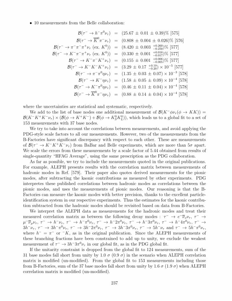
• 10 measurements from the Belle collaboration:
B(τ− → h−π0ντ ) = (25.67 ± 0.01 ± 0.39)% [575]
B(τ− → K0π−ντ ) = (0.808 ± 0.004 ± 0.026)% [576]
B(τ− → π−π−π+ντ (ex. K0)) = (8.420 ± 0.003 +0.260−0.250)% [577]
B(τ− → K−π−π+ντ (ex. K0)) = (0.330 ± 0.001 +0.016−0.017)% [577]
B(τ− → K−π−K+ντ ) = (0.155 ± 0.001 +0.006−0.005)% [577]
B(τ− → K−K−K+ντ ) = (3.29 ± 0.17 +0.19−0.20)× 10−5 [577]
B(τ− → π−π0ηντ ) = (1.35 ± 0.03 ± 0.07)× 10−3 [578]
B(τ− → K−ηντ ) = (1.58 ± 0.05 ± 0.09)× 10−4 [578]
B(τ− → K−π0ηντ ) = (0.46 ± 0.11 ± 0.04)× 10−4 [578]
B(τ− → K0π−ηντ ) = (0.88 ± 0.14 ± 0.04)× 10−4 [578]
where the uncertainties are statistical and systematic, respectively.We add to the list of base nodes one additional measurement of B(K−φντ (φ → KK)) =
B(K−K+K−ντ )× (B(φ → K+K−) + B(φ → K0SK
0L)), which leads us to a global fit to a set of
153 measurements with 37 base nodes.We try to take into account the correlations between measurements, and avoid applying the
PDG-style scale factors to all our measurements. However, two of the measurements from theB-Factories have significant discrepancy with respect to each other. These are measurementsof B(τ− → K−K+K−ντ ) from BaBar and Belle experiments, which are more than 5σ apart.We scale the errors from these measurements by a scale factor of 5.44 obtained from results ofsingle-quantity “HFAG Average”, using the same prescription as the PDG collaboration.
As far as possible, we try to include the measurements quoted in the original publications.For example, ALEPH presents results with the correlation matrix between measurements ofhadronic modes in Ref. [579]. Their paper also quotes derived measurements for the pionicmodes, after subtracting the kaonic contributions as measured by other experiments. PDGinterpretes these published correlations between hadronic modes as correlations between thepionic modes, and uses the measurements of pionic modes. Our reasoning is that the B-Factories can measure the kaonic modes with better precision, thanks to the excellent particle-identification system in our respective experiments. Thus the estimates for the kaonic contribu-tion subtracted from the hadronic modes should be revisited based on data from B-Factories.
We interpret the ALEPH data as measurements for the hadronic modes and treat theirmeasured correlation matrix as between the following decay modes : τ− → e−νeντ , τ
− →µ−νµντ , τ
− → h−ντ , τ− → h−π0ντ , τ
− → h−2π0ντ , τ− → h−3π0ντ , τ
− → h−4π0ντ , τ− →
3h−ντ , τ− → 3h−π0ντ , τ
− → 3h−2π0ντ , τ− → 3h−3π0ντ , τ
− → 5h−ντ and τ− → 5h−π0ντ ,where h− = π− or −K, as in the original publication. Since the ALEPH measurements ofthese branching fractions have been constrained to add up to unity, we exclude the weakestmeasurement of τ− → 3h−3π0ντ in our global fit, as in the PDG global fit.
If the unitarity constraint is dropped from the global fit to 124 measurements, sum of the31 base modes fall short from unity by 1.0 σ (0.9 σ) in the scenario when ALEPH correlationmatrix is modified (un-modified). From the global fit to 153 measurements including thosefrom B-Factories, sum of the 37 base modes fall short from unity by 1.6 σ (1.9 σ) when ALEPHcorrelation matrix is modified (un-modified).
237
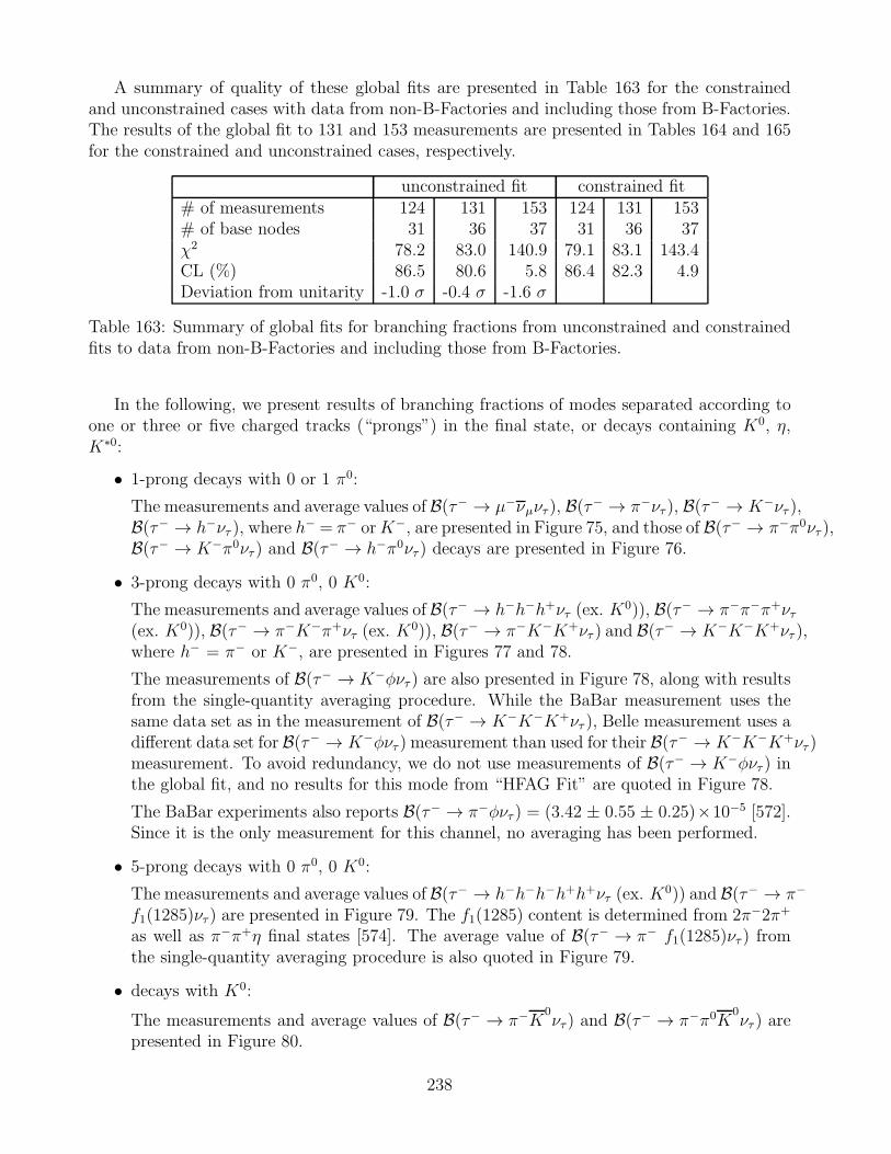
A summary of quality of these global fits are presented in Table 163 for the constrainedand unconstrained cases with data from non-B-Factories and including those from B-Factories.The results of the global fit to 131 and 153 measurements are presented in Tables 164 and 165for the constrained and unconstrained cases, respectively.
unconstrained fit constrained fit# of measurements 124 131 153 124 131 153# of base nodes 31 36 37 31 36 37χ2 78.2 83.0 140.9 79.1 83.1 143.4CL (%) 86.5 80.6 5.8 86.4 82.3 4.9Deviation from unitarity -1.0 σ -0.4 σ -1.6 σ
Table 163: Summary of global fits for branching fractions from unconstrained and constrainedfits to data from non-B-Factories and including those from B-Factories.
In the following, we present results of branching fractions of modes separated according toone or three or five charged tracks (“prongs”) in the final state, or decays containing K0, η,K∗0:
• 1-prong decays with 0 or 1 π0:
The measurements and average values of B(τ− → µ−νµντ ), B(τ− → π−ντ ), B(τ− → K−ντ ),B(τ− → h−ντ ), where h
− = π− orK−, are presented in Figure 75, and those of B(τ− → π−π0ντ ),B(τ− → K−π0ντ ) and B(τ− → h−π0ντ ) decays are presented in Figure 76.
• 3-prong decays with 0 π0, 0 K0:
The measurements and average values of B(τ− → h−h−h+ντ (ex. K0)), B(τ− → π−π−π+ντ
(ex. K0)), B(τ− → π−K−π+ντ (ex. K0)), B(τ− → π−K−K+ντ ) and B(τ− → K−K−K+ντ ),
where h− = π− or K−, are presented in Figures 77 and 78.
The measurements of B(τ− → K−φντ ) are also presented in Figure 78, along with resultsfrom the single-quantity averaging procedure. While the BaBar measurement uses thesame data set as in the measurement of B(τ− → K−K−K+ντ ), Belle measurement uses adifferent data set for B(τ− → K−φντ ) measurement than used for their B(τ− → K−K−K+ντ )measurement. To avoid redundancy, we do not use measurements of B(τ− → K−φντ ) inthe global fit, and no results for this mode from “HFAG Fit” are quoted in Figure 78.
The BaBar experiments also reports B(τ− → π−φντ ) = (3.42 ± 0.55 ± 0.25)×10−5 [572].Since it is the only measurement for this channel, no averaging has been performed.
• 5-prong decays with 0 π0, 0 K0:
The measurements and average values of B(τ− → h−h−h−h+h+ντ (ex. K0)) and B(τ− → π−
f1(1285)ντ) are presented in Figure 79. The f1(1285) content is determined from 2π−2π+
as well as π−π+η final states [574]. The average value of B(τ− → π− f1(1285)ντ ) fromthe single-quantity averaging procedure is also quoted in Figure 79.
• decays with K0:
The measurements and average values of B(τ− → π−K0ντ ) and B(τ− → π−π0K
0ντ ) are
presented in Figure 80.
238
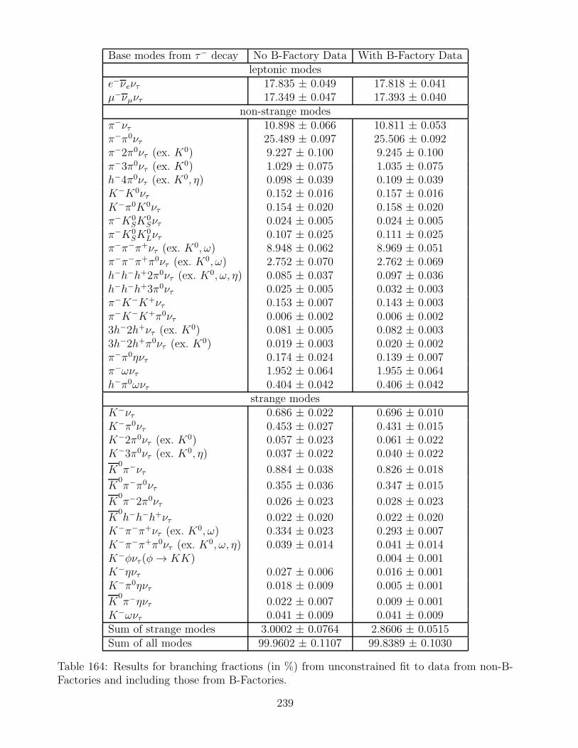
Base modes from τ− decay No B-Factory Data With B-Factory Dataleptonic modes
e−νeντ 17.835 ± 0.049 17.818 ± 0.041µ−νµντ 17.349 ± 0.047 17.393 ± 0.040
non-strange modesπ−ντ 10.898 ± 0.066 10.811 ± 0.053π−π0ντ 25.489 ± 0.097 25.506 ± 0.092π−2π0ντ (ex. K0) 9.227 ± 0.100 9.245 ± 0.100π−3π0ντ (ex. K0) 1.029 ± 0.075 1.035 ± 0.075h−4π0ντ (ex. K0, η) 0.098 ± 0.039 0.109 ± 0.039K−K0ντ 0.152 ± 0.016 0.157 ± 0.016K−π0K0ντ 0.154 ± 0.020 0.158 ± 0.020π−K0
SK0Sντ 0.024 ± 0.005 0.024 ± 0.005
π−K0SK
0Lντ 0.107 ± 0.025 0.111 ± 0.025
π−π−π+ντ (ex. K0, ω) 8.948 ± 0.062 8.969 ± 0.051π−π−π+π0ντ (ex. K0, ω) 2.752 ± 0.070 2.762 ± 0.069h−h−h+2π0ντ (ex. K0, ω, η) 0.085 ± 0.037 0.097 ± 0.036h−h−h+3π0ντ 0.025 ± 0.005 0.032 ± 0.003π−K−K+ντ 0.153 ± 0.007 0.143 ± 0.003π−K−K+π0ντ 0.006 ± 0.002 0.006 ± 0.0023h−2h+ντ (ex. K0) 0.081 ± 0.005 0.082 ± 0.0033h−2h+π0ντ (ex. K0) 0.019 ± 0.003 0.020 ± 0.002π−π0ηντ 0.174 ± 0.024 0.139 ± 0.007π−ωντ 1.952 ± 0.064 1.955 ± 0.064h−π0ωντ 0.404 ± 0.042 0.406 ± 0.042
strange modesK−ντ 0.686 ± 0.022 0.696 ± 0.010K−π0ντ 0.453 ± 0.027 0.431 ± 0.015K−2π0ντ (ex. K0) 0.057 ± 0.023 0.061 ± 0.022K−3π0ντ (ex. K0, η) 0.037 ± 0.022 0.040 ± 0.022
K0π−ντ 0.884 ± 0.038 0.826 ± 0.018
K0π−π0ντ 0.355 ± 0.036 0.347 ± 0.015
K0π−2π0ντ 0.026 ± 0.023 0.028 ± 0.023
K0h−h−h+ντ 0.022 ± 0.020 0.022 ± 0.020
K−π−π+ντ (ex. K0, ω) 0.334 ± 0.023 0.293 ± 0.007K−π−π+π0ντ (ex. K0, ω, η) 0.039 ± 0.014 0.041 ± 0.014K−φντ (φ→ KK) 0.004 ± 0.001K−ηντ 0.027 ± 0.006 0.016 ± 0.001K−π0ηντ 0.018 ± 0.009 0.005 ± 0.001
K0π−ηντ 0.022 ± 0.007 0.009 ± 0.001
K−ωντ 0.041 ± 0.009 0.041 ± 0.009Sum of strange modes 3.0002 ± 0.0764 2.8606 ± 0.0515Sum of all modes 99.9602 ± 0.1107 99.8389 ± 0.1030
Table 164: Results for branching fractions (in %) from unconstrained fit to data from non-B-Factories and including those from B-Factories.
239
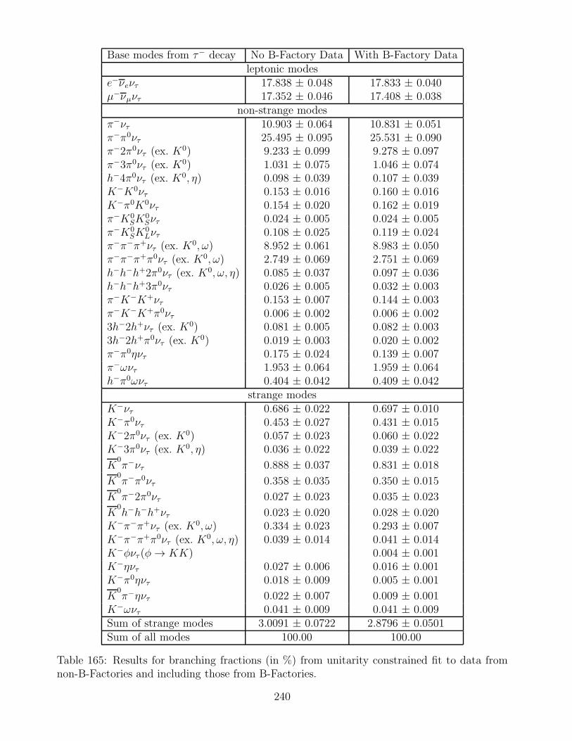
Base modes from τ− decay No B-Factory Data With B-Factory Dataleptonic modes
e−νeντ 17.838 ± 0.048 17.833 ± 0.040µ−νµντ 17.352 ± 0.046 17.408 ± 0.038
non-strange modesπ−ντ 10.903 ± 0.064 10.831 ± 0.051π−π0ντ 25.495 ± 0.095 25.531 ± 0.090π−2π0ντ (ex. K0) 9.233 ± 0.099 9.278 ± 0.097π−3π0ντ (ex. K0) 1.031 ± 0.075 1.046 ± 0.074h−4π0ντ (ex. K0, η) 0.098 ± 0.039 0.107 ± 0.039K−K0ντ 0.153 ± 0.016 0.160 ± 0.016K−π0K0ντ 0.154 ± 0.020 0.162 ± 0.019π−K0
SK0Sντ 0.024 ± 0.005 0.024 ± 0.005
π−K0SK
0Lντ 0.108 ± 0.025 0.119 ± 0.024
π−π−π+ντ (ex. K0, ω) 8.952 ± 0.061 8.983 ± 0.050π−π−π+π0ντ (ex. K0, ω) 2.749 ± 0.069 2.751 ± 0.069h−h−h+2π0ντ (ex. K0, ω, η) 0.085 ± 0.037 0.097 ± 0.036h−h−h+3π0ντ 0.026 ± 0.005 0.032 ± 0.003π−K−K+ντ 0.153 ± 0.007 0.144 ± 0.003π−K−K+π0ντ 0.006 ± 0.002 0.006 ± 0.0023h−2h+ντ (ex. K0) 0.081 ± 0.005 0.082 ± 0.0033h−2h+π0ντ (ex. K0) 0.019 ± 0.003 0.020 ± 0.002π−π0ηντ 0.175 ± 0.024 0.139 ± 0.007π−ωντ 1.953 ± 0.064 1.959 ± 0.064h−π0ωντ 0.404 ± 0.042 0.409 ± 0.042
strange modesK−ντ 0.686 ± 0.022 0.697 ± 0.010K−π0ντ 0.453 ± 0.027 0.431 ± 0.015K−2π0ντ (ex. K0) 0.057 ± 0.023 0.060 ± 0.022K−3π0ντ (ex. K0, η) 0.036 ± 0.022 0.039 ± 0.022
K0π−ντ 0.888 ± 0.037 0.831 ± 0.018
K0π−π0ντ 0.358 ± 0.035 0.350 ± 0.015
K0π−2π0ντ 0.027 ± 0.023 0.035 ± 0.023
K0h−h−h+ντ 0.023 ± 0.020 0.028 ± 0.020
K−π−π+ντ (ex. K0, ω) 0.334 ± 0.023 0.293 ± 0.007K−π−π+π0ντ (ex. K0, ω, η) 0.039 ± 0.014 0.041 ± 0.014K−φντ (φ→ KK) 0.004 ± 0.001K−ηντ 0.027 ± 0.006 0.016 ± 0.001K−π0ηντ 0.018 ± 0.009 0.005 ± 0.001
K0π−ηντ 0.022 ± 0.007 0.009 ± 0.001
K−ωντ 0.041 ± 0.009 0.041 ± 0.009Sum of strange modes 3.0091 ± 0.0722 2.8796 ± 0.0501Sum of all modes 100.00 100.00
Table 165: Results for branching fractions (in %) from unitarity constrained fit to data fromnon-B-Factories and including those from B-Factories.
240
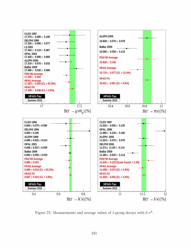
) [%]µνν-µ → -τB(17 17.5
HFAG Fit 0.038 (CL = 4.9%)±17.408
HFAG Average 0.043 (CL = 87.8%)±17.363
PDG’09 Average 0.050±17.330
BaBar 2009 0.080± 0.030 ±17.460
ALEPH 2005 0.032± 0.070 ±17.319
OPAL 2003 0.060± 0.090 ±17.340
L3 2001 0.067± 0.110 ±17.342
DELPHI 1999 0.077± 0.095 ±17.325
CLEO 1997 0.180± 0.080 ±17.370
HFAG-TauSummer 2010
) [%]ν-π → -τB(10.4 10.6 10.8 11
HFAG Fit
0.051 (CL = 4.9%)±10.831
HFAG Average
0.077 (CL = 12.4%)±10.719
PDG’09 Average
0.105±10.828
BaBar 2009
0.110± 0.030 ±10.590
ALEPH 2005
0.078± 0.070 ±10.828
HFAG-TauSummer 2010
) [%]ν- K→ -τB(0.4 0.6 0.8
HFAG Fit 0.010 (CL = 4.9%)±0.697
HFAG Average 0.010 (CL = 81.2%)±0.690
PDG’09 Average 0.023±0.685
BaBar 2009 0.010± 0.006 ±0.692
OPAL 2001 0.029± 0.027 ±0.658
ALEPH 1999 0.014± 0.025 ±0.696
DELPHI 1994 0.180±0.850
CLEO 1994 0.090± 0.070 ±0.660
HFAG-TauSummer 2010
) [%]ν- h→ -τB(11 11.5 12
HFAG Fit 0.052 (CL = 4.9%)±11.528
HFAG Average 0.073 (CL = 2.9%)±11.498
PDG’09 Average 0.120 (Scale Factor = 1.40)±11.630
BaBar 2009 0.114± 0.033 ±11.282
DELPHI 2006 0.114± 0.120 ±11.571
ALEPH 2005 0.078± 0.070 ±11.524
OPAL 1998 0.160± 0.130 ±11.980
CLEO 1997 0.120± 0.050 ±11.520
HFAG-TauSummer 2010
Figure 75: Measurements and average values of 1-prong decays with 0 π0.
241
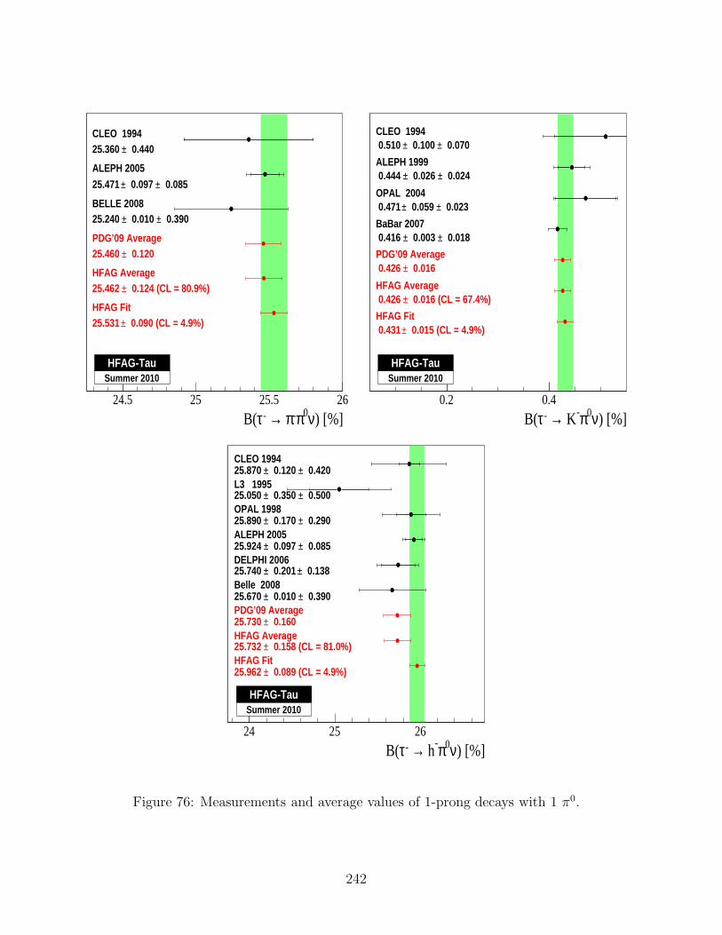
) [%]ν0π-π → -τB(24.5 25 25.5 26
HFAG Fit 0.090 (CL = 4.9%)±25.531
HFAG Average 0.124 (CL = 80.9%)±25.462
PDG’09 Average 0.120±25.460
BELLE 2008 0.390± 0.010 ±25.240
ALEPH 2005 0.085± 0.097 ±25.471
CLEO 1994 0.440±25.360
HFAG-TauSummer 2010
) [%]ν0π- K→ -τB(0.2 0.4
HFAG Fit 0.015 (CL = 4.9%)± 0.431
HFAG Average 0.016 (CL = 67.4%)± 0.426
PDG’09 Average 0.016± 0.426
BaBar 2007 0.018± 0.003 ± 0.416
OPAL 2004 0.023± 0.059 ± 0.471
ALEPH 1999 0.024± 0.026 ± 0.444
CLEO 1994 0.070± 0.100 ± 0.510
HFAG-TauSummer 2010
) [%]ν0π- h→ -τB(24 25 26
HFAG Fit 0.089 (CL = 4.9%)±25.962
HFAG Average 0.158 (CL = 81.0%)±25.732
PDG’09 Average 0.160±25.730
Belle 2008 0.390± 0.010 ±25.670
DELPHI 2006 0.138± 0.201 ±25.740
ALEPH 2005 0.085± 0.097 ±25.924
OPAL 1998 0.290± 0.170 ±25.890
L3 1995 0.500± 0.350 ±25.050
CLEO 1994 0.420± 0.120 ±25.870
HFAG-TauSummer 2010
Figure 76: Measurements and average values of 1-prong decays with 1 π0.
242
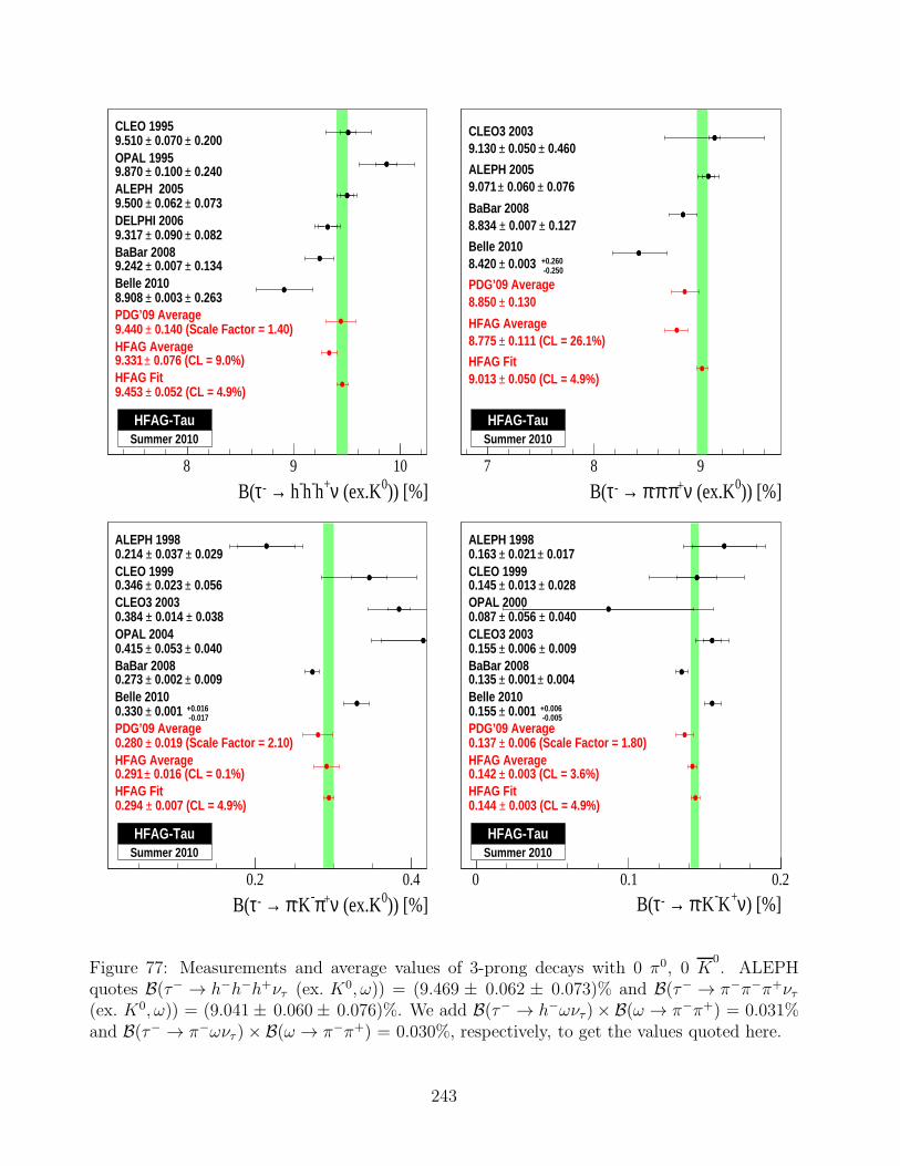
)) [%]0 (ex.Kν+h-h- h→ -τB(8 9 10
HFAG Fit 0.052 (CL = 4.9%)±9.453
HFAG Average 0.076 (CL = 9.0%)±9.331
PDG’09 Average 0.140 (Scale Factor = 1.40)±9.440
Belle 2010 0.263± 0.003 ±8.908
BaBar 2008 0.134± 0.007 ±9.242
DELPHI 2006 0.082± 0.090 ±9.317
ALEPH 2005 0.073± 0.062 ±9.500
OPAL 1995 0.240± 0.100 ±9.870
CLEO 1995 0.200± 0.070 ±9.510
HFAG-TauSummer 2010
)) [%]0 (ex.Kν+π-π-π → -τB(7 8 9
HFAG Fit 0.050 (CL = 4.9%)±9.013
HFAG Average 0.111 (CL = 26.1%)±8.775
PDG’09 Average 0.130±8.850
Belle 2010
-0.250+0.260 0.003 ±8.420
BaBar 2008 0.127± 0.007 ±8.834
ALEPH 2005 0.076± 0.060 ±9.071
CLEO3 2003 0.460± 0.050 ±9.130
HFAG-TauSummer 2010
)) [%]0 (ex.Kν+π-K-π → -τB(0.2 0.4
HFAG Fit 0.007 (CL = 4.9%)±0.294
HFAG Average 0.016 (CL = 0.1%)±0.291
PDG’09 Average 0.019 (Scale Factor = 2.10)±0.280
Belle 2010 -0.017+0.016 0.001 ±0.330
BaBar 2008 0.009± 0.002 ±0.273
OPAL 2004 0.040± 0.053 ±0.415
CLEO3 2003 0.038± 0.014 ±0.384
CLEO 1999 0.056± 0.023 ±0.346
ALEPH 1998 0.029± 0.037 ±0.214
HFAG-TauSummer 2010
) [%]ν+K-K-π → -τB(0 0.1 0.2
HFAG Fit 0.003 (CL = 4.9%)±0.144
HFAG Average 0.003 (CL = 3.6%)±0.142
PDG’09 Average 0.006 (Scale Factor = 1.80)±0.137
Belle 2010 -0.005+0.006 0.001 ±0.155
BaBar 2008 0.004± 0.001 ±0.135
CLEO3 2003 0.009± 0.006 ±0.155
OPAL 2000 0.040± 0.056 ±0.087
CLEO 1999 0.028± 0.013 ±0.145
ALEPH 1998 0.017± 0.021 ±0.163
HFAG-TauSummer 2010
Figure 77: Measurements and average values of 3-prong decays with 0 π0, 0 K0. ALEPH
quotes B(τ− → h−h−h+ντ (ex. K0, ω)) = (9.469 ± 0.062 ± 0.073)% and B(τ− → π−π−π+ντ(ex. K0, ω)) = (9.041± 0.060± 0.076)%. We add B(τ− → h−ωντ)× B(ω → π−π+) = 0.031%and B(τ− → π−ωντ )× B(ω → π−π+) = 0.030%, respectively, to get the values quoted here.
243
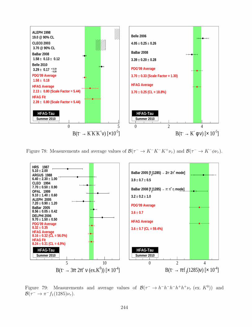
]-510×) [ν+K-K- K→ -τB(0 5
CLEO3 2003 3.70 @ 90% CL
ALEPH 199819.0 @ 90% CL
HFAG Fit 0.80 (Scale Factor = 5.44)± 2.39
HFAG Average 0.80 (Scale Factor = 5.44)± 2.13
PDG’09 Average 0.18± 1.58
Belle 2010
- 0.20+ 0.19 0.17 ± 3.29
BaBar 2008 0.12± 0.13 ± 1.58
HFAG-TauSummer 2010
]-5 10×) [ν φ - K→ -τB(0 2 4
HFAG Average
0.25 (CL = 18.8%)±3.70
PDG’09 Average
0.33 (Scale Factor = 1.30)±3.70
BaBar 2008
0.28± 0.20 ±3.39
Belle 2006
0.26± 0.25 ±4.05
HFAG-TauSummer 2010
Figure 78: Measurements and average values of B(τ− → K−K−K+ντ ) and B(τ− → K−φντ ).
]-4 10×)) [0 (ex.Kν +π 2-π 3→ -τB(5 10
HFAG Fit 0.31 (CL = 4.9%)±8.24
HFAG Average 0.32 (CL = 56.0%)±8.16
PDG’09 Average 0.35±8.32
DELPHI 2006 0.50± 1.50 ±9.70
BaBar 2005 0.42± 0.05 ±8.56
ALEPH 2005 1.20± 0.90 ±7.20
OPAL 1999 0.60± 1.40 ±9.10
CLEO 1994 0.90± 0.50 ±7.70
ARGUS 1988 1.00± 2.30 ±6.40
HRS 1987 2.00±5.10
HFAG-TauSummer 2010
]-4 10×) [ν(1285)1f-π → -τB(0 2 4
HFAG Average
0.7 (CL = 59.4%)±3.6
PDG’09 Average
0.7±3.6
mode]η +π -π →(1285) 1
BaBar 2008 [f
1.0± 0.2 ±3.2
mode]+π 2-π 2→(1285) 1
BaBar 2005 [f
0.5± 0.7 ±3.9
HFAG-TauSummer 2010
Figure 79: Measurements and average values of B(τ− → h−h−h−h+h+ντ (ex. K0)) andB(τ− → π−f1(1285)ντ).
244
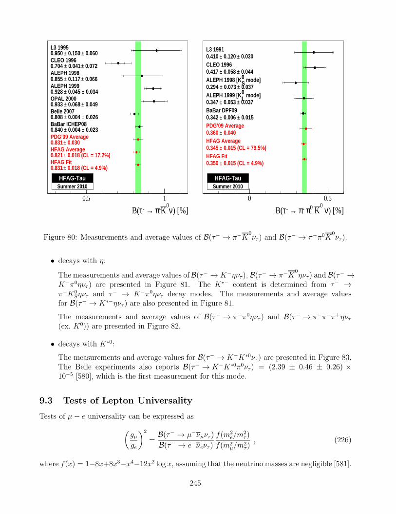
) [%]ν0
K-π → -τB(0.5 1
HFAG Fit 0.018 (CL = 4.9%)±0.831
HFAG Average 0.018 (CL = 17.2%)±0.821
PDG’09 Average 0.030±0.831
BaBar ICHEP08 0.023± 0.004 ±0.840
Belle 2007 0.026± 0.004 ±0.808
OPAL 2000 0.049± 0.068 ±0.933
ALEPH 1999 0.034± 0.045 ±0.928
ALEPH 1998 0.066± 0.117 ±0.855
CLEO 1996 0.072± 0.041 ±0.704
L3 1995 0.060± 0.150 ±0.950
HFAG-TauSummer 2010
) [%]ν 0
K 0π -π → -τB(0 0.5
HFAG Fit 0.015 (CL = 4.9%)±0.350
HFAG Average 0.015 (CL = 79.5%)±0.345
PDG’09 Average 0.040±0.360
BaBar DPF09 0.015± 0.006 ±0.342
mode]L0ALEPH 1999 [K
0.037± 0.053 ±0.347
mode]S0ALEPH 1998 [K
0.037± 0.073 ±0.294
CLEO 1996 0.044± 0.058 ±0.417
L3 1991 0.030± 0.120 ±0.410
HFAG-TauSummer 2010
Figure 80: Measurements and average values of B(τ− → π−K0ντ ) and B(τ− → π−π0K
0ντ ).
• decays with η:
The measurements and average values of B(τ− → K−ηντ ), B(τ− → π−K0ηντ ) and B(τ− →
K−π0ηντ ) are presented in Figure 81. The K∗− content is determined from τ− →π−K0
Sηντ and τ− → K−π0ηντ decay modes. The measurements and average valuesfor B(τ− → K∗−ηντ ) are also presented in Figure 81.
The measurements and average values of B(τ− → π−π0ηντ ) and B(τ− → π−π−π+ηντ(ex. K0)) are presented in Figure 82.
• decays with K∗0:
The measurements and average values for B(τ− → K−K∗0ντ ) are presented in Figure 83.The Belle experiments also reports B(τ− → K−K∗0π0ντ ) = (2.39 ± 0.46 ± 0.26) ×10−5 [580], which is the first measurement for this mode.
9.3 Tests of Lepton Universality
Tests of µ− e universality can be expressed as
(
gµge
)2
=B(τ− → µ−νµντ )
B(τ− → e−νeντ )
f(m2e/m
2τ )
f(m2µ/m
2τ ), (226)
where f(x) = 1−8x+8x3−x4−12x2 log x, assuming that the neutrino masses are negligible [581].
245
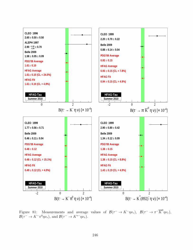
]-4 10×) [ν η - K→ -τB(0 2
HFAG Fit 0.10 (CL = 4.9%)±1.61
HFAG Average 0.10 (CL = 24.0%)±1.61
PDG’09 Average 0.10±1.61
Belle 2009 0.09± 0.05 ±1.58
ALEPH 1997 0.70± -1.20
+1.302.90
CLEO 1996 0.50± 0.50 ±2.60
HFAG-TauSummer 2010
]-4 10×) [ν η 0
K -π → -τB(-2 0 2
HFAG Fit
0.15 (CL = 4.9%)±0.94
HFAG Average
0.15 (CL = 7.8%)±0.93
PDG’09 Average
0.15±0.93
Belle 2009
0.04± 0.14 ±0.88
CLEO 1999
0.22± 0.70 ±2.20
HFAG-TauSummer 2010
]-4 10×) [ν η 0π - K→ -τB(-2 0 2
HFAG Fit
0.12 (CL = 4.9%)±0.49
HFAG Average
0.12 (CL = 15.1%)±0.48
PDG’09 Average
0.12±0.48
Belle 2009
0.04± 0.11 ±0.46
CLEO 1999
0.71± 0.56 ±1.77
HFAG-TauSummer 2010
]-4 10×) [ν η -(892)*
K→ -τB(0 2
HFAG Fit
0.19 (CL = 4.9%)±1.43
HFAG Average
0.15 (CL = 8.8%)±1.38
PDG’09 Average
0.15±1.38
Belle 2009
0.09± 0.12 ±1.34
CLEO 1999
0.42± 0.80 ±2.90
HFAG-TauSummer 2010
Figure 81: Measurements and average values of B(τ− → K−ηντ ), B(τ− → π−K0ηντ ),
B(τ− → K−π0ηντ ), and B(τ− → K∗−ηντ ).
246
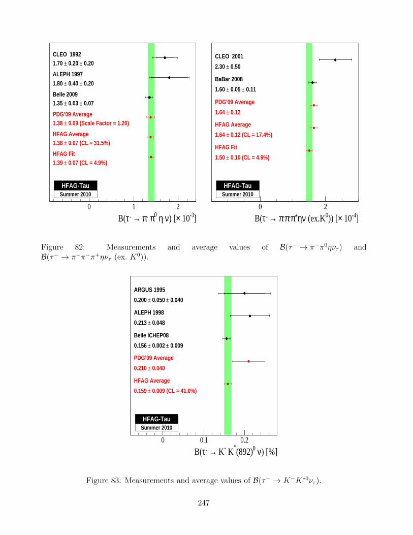
]-3 10×) [ν η 0π -π → -τB(0 1 2
HFAG Fit 0.07 (CL = 4.9%)±1.39
HFAG Average 0.07 (CL = 31.5%)±1.38
PDG’09 Average 0.09 (Scale Factor = 1.20)±1.38
Belle 2009 0.07± 0.03 ±1.35
ALEPH 1997 0.20± 0.40 ±1.80
CLEO 1992 0.20± 0.20 ±1.70
HFAG-TauSummer 2010
]-4 10×)) [0 (ex.Kνη+π-π-π → -τB(0 2
HFAG Fit
0.10 (CL = 4.9%)±1.50
HFAG Average
0.12 (CL = 17.4%)±1.64
PDG’09 Average
0.12±1.64
BaBar 2008
0.11± 0.05 ±1.60
CLEO 2001
0.50±2.30
HFAG-TauSummer 2010
Figure 82: Measurements and average values of B(τ− → π−π0ηντ ) andB(τ− → π−π−π+ηντ (ex. K0)).
) [%]ν 0(892)*
K- K→ -τB(0 0.1 0.2
HFAG Average
0.009 (CL = 41.0%)±0.159
PDG’09 Average
0.040±0.210
Belle ICHEP08
0.009± 0.002 ±0.156
ALEPH 1998
0.048±0.213
ARGUS 1995
0.040± 0.050 ±0.200
HFAG-TauSummer 2010
Figure 83: Measurements and average values of B(τ− → K−K∗0ντ ).
247
From the unitarity constrained fit, we obtain B(τ− → µ−νµντ )/B(τ− → e−νeντ ) = 0.9762 ±0.0028, which includes a correlation co-efficient of 18.33% between the branching fractions. This
yields a value of(
gµge
)
= 1.0019 ± 0.0014, which is consistent with the SM value.
These predictions from τ decays are more precise than the other determinations:
• We average the measurements of B(π → eνe(γ))/B(π → µνµ(γ)) = (1.2265± 0.0034 (stat)± 0.0044 (syst)) × 10−4 from TRIUMF [582] and = (1.2346 ± 0.0035 (stat) ± 0.0036(syst)) × 10−4 from PSI [583], to obtain a value of (1.2310 ± 0.0037)× 10−4. Comparingthis with the prediction of (1.2352 ± 0.0001) × 10−4 from recent theoretical calcula-
tions [584], we obtain a value of(
gµge
)
= 1.0017 ± 0.0015.
• The ratio B(K → eνe(γ))/B(K → µνµ(γ)) has recently been measured very precisely bythe KLOE [585] and the NA62 [586] collaborations. Using the new world average value of(2.487 ± 0.012)×10−5 from Ref. [587], and the predicted value of (2.477 ± 0.001)×10−5
from Ref. [584], we obtain(
gµge
)
= 0.9980 ± 0.0025.
• From the report of the FlaviaNet Working Group on Kaon Decays [588], we obtain(
gµge
)
= 1.0010 ± 0.0025 using measurements of B(K → πµν)/B(K → πeν).
• From the report of the LEP Electroweak Working Group [589], we obtain(
gµge
)
= 0.997 ±0.010 using measurements of B(W → µνµ)/B(W → eνe).
Tau-muon universality is tested with
(
gτgµ
)2
=B(τ → hντ )
B(h→ µνµ)
2mhm2µτh
(1 + δh)m3τττ
(
1−m2µ/m
2h
1−m2h/m
2τ
)2
, (227)
where h = π or K and the radiative corrections are δπ = (0.16 ± 0.14)% and δK = (0.90 ±0.22)% [590, 591, 592]. Using the world averaged mass and lifetime values and meson decay
rates [5] and our unitarity constrained fit, we determine(
gτgµ
)
= 0.9966 ± 0.0030 (0.9860 ±0.0073) from the pionic and kaonic branching fractions, where the correlation co-efficient be-
tween these values are 13.10%. Combining these results, we obtain(
gτgµ
)
= 0.9954 ± 0.0029,
which is 1.6 σ below the SM expectation.
We also test lepton universality between τ and µ (e), by comparing the averaged electronic(muonic) branching fractions of the τ lepton with the predicted branching fractions from mea-surements of the τ and µ lifetimes and their respective masses [5], using known electroweak and
radiative corrections [590]. This gives(
gτgµ
)
= 1.0011 ± 0.0021 and(
gτge
)
= 1.0030 ± 0.0021.
The correlation co-efficient between the determination of(
gτgµ
)
from electronic branching frac-
tion with the ones obtained from pionic and kaonic branching fractions are 48.16% and 21.82%,
respectively. Averaging these three values, we obtain(
gτgµ
)
= 1.0001 ± 0.0020, which is consis-
tent with the SM value. In Figure 84, we compare these above determinations with each otherand with the values obtained from W decays [589].
248
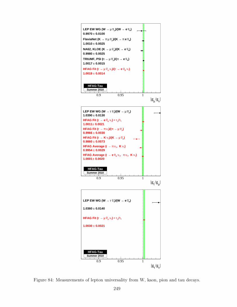
|e
/gµ
|g0.9 0.95 1
)τν eν e → τ)/(τν µν µ → τHFAG Fit ( 0.0014±1.0019
)eν e → π)/(µν µ → πTRIUMF, PSI ( 0.0015±1.0017
)eν e →)/(K µν µ →NA62, KLOE (K 0.0025±0.9980
)eν e π →)/(K µν µ π →FlaviaNet (K 0.0025±1.0010
)eν e →)/(W µν µ →LEP EW WG (W 0.0100±0.9970
HFAG-TauSummer 2010
|µ
/gτ
|g0.9 0.95 1
)τν, K τν π, τν eν e → τHFAG Average ( 0.0020±1.0001
)τν, K τν π → τHFAG Average ( 0.0029±0.9954
)µν µ →)/(K τν K → τHFAG Fit ( 0.0073±0.9860
) µν µ → π)/(τν π → τHFAG Fit ( 0.0030±0.9966
ττ/µτ ×) τν eν e → τHFAG Fit ( 0.0021±1.0011
)µν µ →)/(W τν τ →LEP EW WG (W 0.0130±1.0390
HFAG-TauSummer 2010
|e
/gτ|g0.9 0.95 1
ττ/µτ ×) τν µν µ → τHFAG Fit (
0.0021±1.0030
)eν e →)/(W τν τ →LEP EW WG (W
0.0140±1.0360
HFAG-TauSummer 2010
Figure 84: Measurements of lepton universality from W, kaon, pion and tau decays.
249
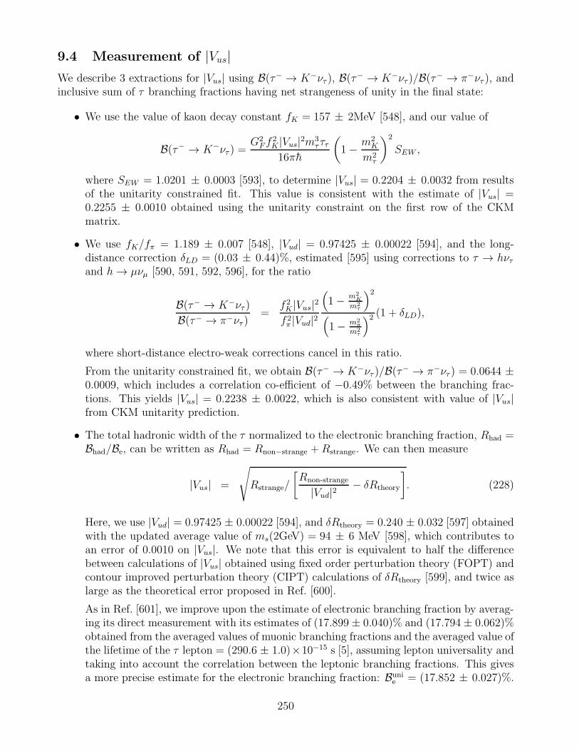
9.4 Measurement of |Vus|We describe 3 extractions for |Vus| using B(τ− → K−ντ ), B(τ− → K−ντ )/B(τ− → π−ντ ), andinclusive sum of τ branching fractions having net strangeness of unity in the final state:
• We use the value of kaon decay constant fK = 157 ± 2MeV [548], and our value of
B(τ− → K−ντ ) =G2Ff
2K |Vus|2m3
τ ττ16πh
(
1− m2K
m2τ
)2
SEW ,
where SEW = 1.0201 ± 0.0003 [593], to determine |Vus| = 0.2204 ± 0.0032 from resultsof the unitarity constrained fit. This value is consistent with the estimate of |Vus| =0.2255 ± 0.0010 obtained using the unitarity constraint on the first row of the CKMmatrix.
• We use fK/fπ = 1.189 ± 0.007 [548], |Vud| = 0.97425 ± 0.00022 [594], and the long-distance correction δLD = (0.03 ± 0.44)%, estimated [595] using corrections to τ → hντand h→ µνµ [590, 591, 592, 596], for the ratio
B(τ− → K−ντ )
B(τ− → π−ντ )=
f 2K |Vus|2f 2π |Vud|2
(
1− m2K
m2τ
)2
(
1− m2π
m2τ
)2 (1 + δLD),
where short-distance electro-weak corrections cancel in this ratio.
From the unitarity constrained fit, we obtain B(τ− → K−ντ )/B(τ− → π−ντ ) = 0.0644 ±0.0009, which includes a correlation co-efficient of −0.49% between the branching frac-tions. This yields |Vus| = 0.2238 ± 0.0022, which is also consistent with value of |Vus|from CKM unitarity prediction.
• The total hadronic width of the τ normalized to the electronic branching fraction, Rhad =Bhad/Be, can be written as Rhad = Rnon−strange +Rstrange. We can then measure
|Vus| =
√
Rstrange/
[
Rnon-strange
|Vud|2− δRtheory
]
. (228)
Here, we use |Vud| = 0.97425 ± 0.00022 [594], and δRtheory = 0.240 ± 0.032 [597] obtainedwith the updated average value of ms(2GeV) = 94 ± 6 MeV [598], which contributes toan error of 0.0010 on |Vus|. We note that this error is equivalent to half the differencebetween calculations of |Vus| obtained using fixed order perturbation theory (FOPT) andcontour improved perturbation theory (CIPT) calculations of δRtheory [599], and twice aslarge as the theoretical error proposed in Ref. [600].
As in Ref. [601], we improve upon the estimate of electronic branching fraction by averag-ing its direct measurement with its estimates of (17.899 ± 0.040)% and (17.794 ± 0.062)%obtained from the averaged values of muonic branching fractions and the averaged value ofthe lifetime of the τ lepton = (290.6 ± 1.0)×10−15 s [5], assuming lepton universality andtaking into account the correlation between the leptonic branching fractions. This givesa more precise estimate for the electronic branching fraction: Buni
e = (17.852 ± 0.027)%.
250
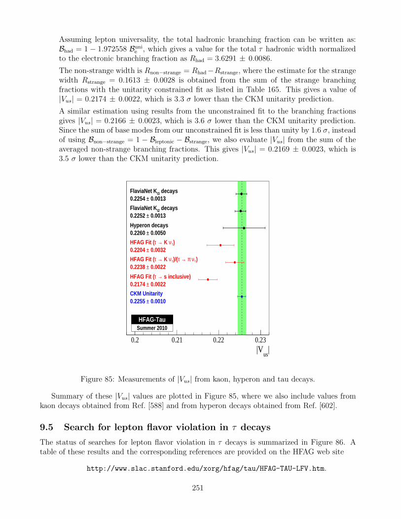
Assuming lepton universality, the total hadronic branching fraction can be written as:Bhad = 1 − 1.972558 Buni
e , which gives a value for the total τ hadronic width normalizedto the electronic branching fraction as Rhad = 3.6291 ± 0.0086.
The non-strange width is Rnon−strange = Rhad−Rstrange, where the estimate for the strangewidth Rstrange = 0.1613 ± 0.0028 is obtained from the sum of the strange branchingfractions with the unitarity constrained fit as listed in Table 165. This gives a value of|Vus| = 0.2174 ± 0.0022, which is 3.3 σ lower than the CKM unitarity prediction.
A similar estimation using results from the unconstrained fit to the branching fractionsgives |Vus| = 0.2166 ± 0.0023, which is 3.6 σ lower than the CKM unitarity prediction.Since the sum of base modes from our unconstrained fit is less than unity by 1.6 σ, insteadof using Bnon−strange = 1 − Bleptonic − Bstrange, we also evaluate |Vus| from the sum of theaveraged non-strange branching fractions. This gives |Vus| = 0.2169 ± 0.0023, which is3.5 σ lower than the CKM unitarity prediction.
|us
|V0.2 0.21 0.22 0.23
CKM Unitarity 0.0010±0.2255
s inclusive)→ τHFAG Fit ( 0.0022±0.2174
)τν π → τ)/(τν K → τHFAG Fit ( 0.0022±0.2238
)τν K → τHFAG Fit ( 0.0032±0.2204
Hyperon decays 0.0050±0.2260
decaysl2FlaviaNet K 0.0013±0.2252
decaysl3FlaviaNet K 0.0013±0.2254
HFAG-TauSummer 2010
Figure 85: Measurements of |Vus| from kaon, hyperon and tau decays.
Summary of these |Vus| values are plotted in Figure 85, where we also include values fromkaon decays obtained from Ref. [588] and from hyperon decays obtained from Ref. [602].
9.5 Search for lepton flavor violation in τ decays
The status of searches for lepton flavor violation in τ decays is summarized in Figure 86. Atable of these results and the corresponding references are provided on the HFAG web site
http://www.slac.stanford.edu/xorg/hfag/tau/HFAG-TAU-LFV.htm.
251
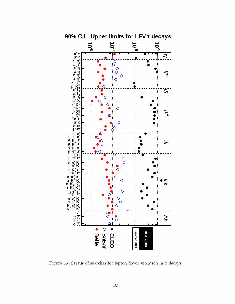
γ -eγ -µ0π -e 0π -µη -eη -µ’η -e’η -µ0S K-e0S K-µ0 f-e0 f-µ0ρ -e0ρ -µ
K*-e K*-µK* -eK* -µ
φ -eφ -µω -eω -µ
- e+ e-e - e+ e-µ-µ +µ -e-µ +µ -µ- e+µ -e-µ + e-µ-π +π -e-π +π -µ- K+π -e - K+π -µ-π + K-e-π + K-µ- K+ K-e - K+ K-µ
0S K0
S K-e0S K0
S K-µ-π + e-π -π +µ -π- K+ e-π - K+µ -π- K+ e-K - K+µ -K
Λ -πΛ -πΛ -KΛ -K
decaysτ90% C.L. Upper limits for LFV
-810
-710
-610
-510
γl0
lP0
lS0
lVlll
lhhh
Λ
CLE
OB
aBar
Belle
HF
AG
-Tau
Sum
mer 2010
Figure 86: Status of searches for lepton flavor violation in τ decays.
252
10 Summary
This article provides updated world averages for b-hadron properties at least through the endof 2009. Some results that appeared in the spring of 2010 are also included. A small selectionof highlights of the results described in Sections 3-9 is given in Tables 166 and 167.
Concerning lifetime and mixing averages, the most significant changes in the past two yearsare due to new results from the Tevatron experiments, mainly measurements of b-baryon life-times and searches for CP violation in B0
s mixing. While DØ has measured a like-sign dimuonasymmetry deviating by 3.2 σ from the SM, the latest results on the CP -violation phase inB0s → J/ψφ no longer show any hint of New Physics. On the other hand, averaging procedures
for the b-hadron production fractions have been improved: for the first time we obtain a setof fractions based on Tevatron measurements only, and we also extract the fraction of Υ (5S)decays to B0
s pairs taking into account decays without open-bottom mesons.The measurement of sin 2β ≡ sin 2φ1 from b → ccs transitions such as B0 → J/ψK0
S hasreached < 4% precision: sin 2β ≡ sin 2φ1 = 0.673±0.023. Measurements of the same parameterusing different quark-level processes provide a consistency test of the Standard Model and allowinsight into possible new physics. Recent improvements include the use of time-dependentDalitz plot analyses of B0 → K0
SK+K− and B0 → K0
Sπ+π− to obtain CP violation parameters
for φK0S , f0(980)K
0S and ρK0
S . All results among hadronic b → s penguin dominated decaysare currently consistent with the Standard Model expectations. Among measurements relatedto the Unitarity Triangle angle α ≡ φ2, updates of the parameters of the ρρ system now allowconstraints at the level of ≈ 6. Knowledge of the third angle γ ≡ φ3 also continues to improve.Notwithstanding the well-known statistical issues in extracting the value of the angle itself, theworld average values of the parameters in B → DK decays now show a significant direct CPviolation effect.
ConcerningD0-D 0 mixing, three experiments have now found evidence for this phenomenon:Belle, BABAR, and CDF. These measurements and others (made by Belle, BABAR, CLEO, FNALE791, FNAL E831) are combined to yield World Average (WA) values for mixing parametersx and y, and for CPV parameters |q/p| and φ. From this fit, the no-mixing point x=y=0 isexcluded at 10.2σ. The parameter x differs from zero by 2.5σ, and y differs from zero by 5.7σ.Mixing at this level is presumably dominated by long-distance processes, which are difficult tocalculate. Thus, it may be difficult to identify new physics from mixing alone. The WA valuefor the observable yCP is positive, which indicates that the CP -even state is shorter-lived as inthe K0-K 0 system. However, x also appears to be positive, which implies that the CP -evenstate is heavier; this is unlike in the K0-K 0 system. There is no evidence yet for CPV (eitherdirect or indirect) in the D0-D 0 system.
11 Acknowledgments
We are grateful for the strong support of the Belle, BABAR, CLEO, CDF, and DØ collaborations,without whom this compilation of results and world averages would not have been possible.The success of these experiments in turn would not have been possible without the excellentoperations of the KEKB, PEP-II, CESR, and Tevatron accelerators, and fruitful collaborationsbetween the accelerator groups and the experiments.
253
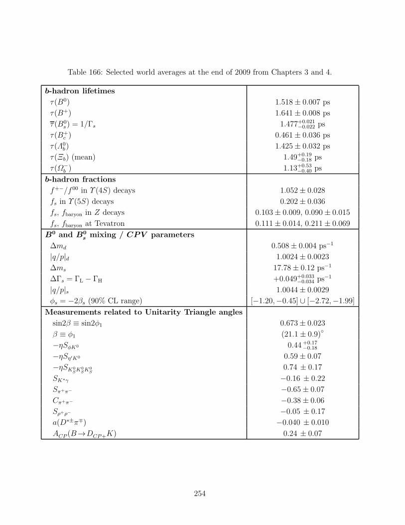
Table 166: Selected world averages at the end of 2009 from Chapters 3 and 4.
b-hadron lifetimes
τ(B0) 1.518± 0.007 ps
τ(B+) 1.641± 0.008 ps
τ (B0s ) = 1/Γs 1.477+0.021
−0.022 ps
τ(B+c ) 0.461± 0.036 ps
τ(Λ0b) 1.425± 0.032 ps
τ(Ξb) (mean) 1.49+0.19−0.18 ps
τ(Ω−b ) 1.13+0.53
−0.40 ps
b-hadron fractions
f+−/f 00 in Υ (4S) decays 1.052± 0.028
fs in Υ (5S) decays 0.202± 0.036
fs, fbaryon in Z decays 0.103± 0.009, 0.090± 0.015
fs, fbaryon at Tevatron 0.111± 0.014, 0.211± 0.069
B0 and B0smixing / CPV parameters
∆md 0.508± 0.004 ps−1
|q/p|d 1.0024± 0.0023
∆ms 17.78± 0.12 ps−1
∆Γs = ΓL − ΓH +0.049+0.033−0.034 ps−1
|q/p|s 1.0044± 0.0029
φs = −2βs (90% CL range) [−1.20,−0.45] ∪ [−2.72,−1.99]
Measurements related to Unitarity Triangle angles
sin2β ≡ sin2φ1 0.673± 0.023
β ≡ φ1 (21.1± 0.9)
−ηSφK0 0.44 +0.17−0.18
−ηSη′K0 0.59± 0.07
−ηSK0SK
0SK
0S
0.74 ± 0.17
SK∗γ −0.16 ± 0.22
Sπ+π− −0.65± 0.07
Cπ+π− −0.38± 0.06
Sρ+ρ− −0.05 ± 0.17
a(D∗±π∓) −0.040 ± 0.010
ACP (B→DCP+K) 0.24 ± 0.07
254
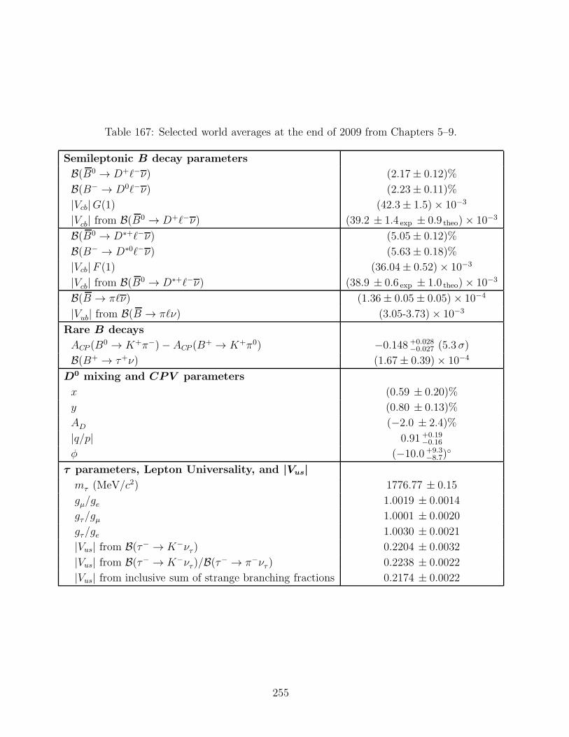
Table 167: Selected world averages at the end of 2009 from Chapters 5–9.
Semileptonic B decay parameters
B(B0 → D+ℓ−ν) (2.17± 0.12)%
B(B− → D0ℓ−ν) (2.23± 0.11)%
|Vcb|G(1) (42.3± 1.5)× 10−3
|Vcb| from B(B0 → D+ℓ−ν) (39.2 ± 1.4 exp ± 0.9 theo)× 10−3
B(B0 → D∗+ℓ−ν) (5.05± 0.12)%
B(B− → D∗0ℓ−ν) (5.63± 0.18)%
|Vcb|F (1) (36.04± 0.52)× 10−3
|Vcb| from B(B0 → D∗+ℓ−ν) (38.9 ± 0.6 exp ± 1.0 theo)× 10−3
B(B → πℓν) (1.36± 0.05± 0.05)× 10−4
|Vub| from B(B → πℓν) (3.05-3.73)× 10−3
Rare B decays
ACP (B0 → K+π−)− ACP (B
+ → K+π0) −0.148 +0.028−0.027 (5.3 σ)
B(B+ → τ+ν) (1.67± 0.39)× 10−4
D0 mixing and CPV parameters
x (0.59 ± 0.20)%
y (0.80 ± 0.13)%
AD (−2.0 ± 2.4)%
|q/p| 0.91 +0.19−0.16
φ (−10.0 +9.3−8.7)
τ parameters, Lepton Universality, and |Vus|
mτ (MeV/c2) 1776.77 ± 0.15
gµ/ge 1.0019 ± 0.0014
gτ/gµ 1.0001 ± 0.0020
gτ/ge 1.0030 ± 0.0021
|Vus| from B(τ− → K−ντ ) 0.2204 ± 0.0032
|Vus| from B(τ− → K−ντ )/B(τ− → π−ντ ) 0.2238 ± 0.0022
|Vus| from inclusive sum of strange branching fractions 0.2174 ± 0.0022
255
References
[1] N. Cabibbo, Phys. Rev. Lett. 10, 531–533 (1963).
[2] M. Kobayashi and T. Maskawa, Prog. Theor. Phys. 49, 652–657 (1973).
[3] D. Abbaneo et al., ALEPH, CDF, DELPHI, L3, OPAL, and SLD collaborations,arXiv:hep-ex/0009052 (2000), CERN-EP-2000-096; arXiv:hep-ex/0112028 (2001),CERN-EP-2001-050.
[4] E. Barberio et al. (Heavy Flavor Averaging Group) (2008),arXiv:0808.1297 [hep-ex].
[5] K. Nakamura et al. (Particle Data Group), J. Phys. G37, 075021 (2010).
[6] B. Aubert et al. (BABAR collaboration), Phys. Rev. Lett. 94, 141801 (2005),arXiv:hep-ex/0412062.
[7] B. Aubert et al. (BABAR collaboration), Phys. Rev. D65, 032001 (2002),arXiv:hep-ex/0107025.
[8] B. Aubert et al. (BABAR collaboration), Phys. Rev. D69, 071101 (2004),arXiv:hep-ex/0401028.
[9] J. P. Alexander et al. (CLEO collaboration), Phys. Rev. Lett. 86, 2737–2741 (2001),arXiv:hep-ex/0006002.
[10] S. B. Athar et al. (CLEO collaboration), Phys. Rev. D66, 052003 (2002),arXiv:hep-ex/0202033.
[11] N. C. Hastings et al. (Belle collaboration), Phys. Rev. D67, 052004 (2003),arXiv:hep-ex/0212033.
[12] B. Aubert et al. (BABAR collaboration), Phys. Rev. Lett. 95, 042001 (2005),arXiv:hep-ex/0504001.
[13] B. Aubert et al. (BABAR collaboration), Phys. Rev. Lett. 96, 232001 (2006),arXiv:hep-ex/0604031; A. Sokolov et al. (Belle collaboration),Phys. Rev. D75, 071103 (2007), arXiv:hep-ex/0611026; B. Aubert et al. (BABARcollaboration), Phys. Rev. D78, 112002 (2008), arXiv:0807.2014 [hep-ex].
[14] B. Barish et al. (CLEO collaboration), Phys. Rev. Lett. 76, 1570–1574 (1996).
[15] A. Drutskoy et al. (Belle collaboration), Phys. Rev. D81, 112003 (2010),arXiv:1003.5885 [hep-ex].
[16] G. S. Huang et al. (CLEO collaboration), Phys. Rev. D75, 012002 (2007),arXiv:hep-ex/0610035; this supersedes the results of Ref. [18].
[17] A. Drutskoy et al. (Belle collaboration), Phys. Rev. Lett. 98, 052001 (2007),arXiv:hep-ex/0608015.
256
[18] M. Artuso et al. (CLEO collaboration), Phys. Rev. Lett. 95, 261801 (2005),arXiv:hep-ex/0508047.
[19] K. F. Chen et al. (Belle collaboration), Phys. Rev. Lett. 100, 112001 (2008),arXiv:0710.2577 [hep-ex].
[20] R. Louvot et al. (Belle collaboration), Phys. Rev. Lett. 102, 021801 (2009),arXiv:0809.2526 [hep-ex].
[21] P. Abreu et al. (DELPHI collaboration), Phys. Lett. B289, 199–210 (1992); P. D.Acton et al. (OPAL collaboration), Phys. Lett. B295, 357–370 (1992); D. Buskulic etal. (ALEPH collaboration), Phys. Lett. B361, 221–233 (1995).
[22] P. Abreu et al. (DELPHI collaboration), Z. Phys. C68, 375–390 (1995).
[23] R. Barate et al. (ALEPH collaboration), Eur. Phys. J. C2, 197–211 (1998).
[24] D. Buskulic et al. (ALEPH collaboration), Phys. Lett. B384, 449–460 (1996).
[25] J. Abdallah et al. (DELPHI collaboration), Eur. Phys. J. C44, 299–309 (2005),arXiv:hep-ex/0510023.
[26] P. Abreu et al. (DELPHI collaboration), Z. Phys. C68, 541–554 (1995).
[27] R. Barate et al. (ALEPH collaboration), Eur. Phys. J. C5, 205–227 (1998).
[28] J. Abdallah et al. (DELPHI collaboration), Phys. Lett. B576, 29–42 (2003),arXiv:hep-ex/0311005.
[29] T. Affolder et al. (CDF collaboration), Phys. Rev. Lett. 84, 1663–1668 (2000),arXiv:hep-ex/9909011.
[30] T. Aaltonen et al. (CDF collaboration), Phys. Rev. D77, 072003 (2008),arXiv:0801.4375 [hep-ex].
[31] T. Aaltonen et al. (CDF collaboration), Phys. Rev. D79, 032001 (2009),arXiv:0810.3213 [hep-ex].
[32] F. Abe et al. (CDF collaboration), Phys. Rev. D60, 092005 (1999).
[33] V. M. Abazov et al. (DØ collaboration), Phys. Rev. Lett. 99, 052001 (2007),arXiv:0706.1690 [hep-ex].
[34] V. M. Abazov et al. (DØ collaboration), Phys. Rev. Lett. 101, 232002 (2008),arXiv:0808.4142 [hep-ex].
[35] T. Aaltonen et al. (CDF collaboration), Phys. Rev. D80, 072003 (2009),arXiv:0905.3123 [hep-ex].
257
[36] S. Schael et al., ALEPH, CDF, DELPHI, L3, OPAL, and SLD collaborations, LEPElectroweak Working Group, SLD Electroweak and Heavy Flavour Working Groups,Phys. Rept. 427, 257 (2006), arXiv:hep-ex/0509008; we use the average given inEq. 5.39 of this paper, obtained from a 10-parameter global fit of all electroweak datawhere the asymmetry measurements have been excluded.
[37] D. Acosta et al. (CDF collaboration), Phys. Rev. D69, 012002 (2004),arXiv:hep-ex/0309030; this supersedes the χ value of Ref. [117].
[38] V. M. Abazov et al. (DØ collaboration), Phys. Rev. D74, 092001 (2006),arXiv:hep-ex/0609014.
[39] M. A. Shifman and M. B. Voloshin, Sov. Phys. JETP 64, 698 (1986); J. Chay,H. Georgi, and B. Grinstein, Phys. Lett. B247, 399–405 (1990); I. I. Bigi, N. G.Uraltsev, and A. I. Vainshtein, Phys. Lett. B293, 430–436 (1992),arXiv:hep-ph/9207214; erratum Phys. Lett. B297, 477 (1992).
[40] I. I. Bigi, arXiv:hep-ph/9508408 (1995); G. Bellini, I. I. Bigi, and P. J. Dornan,Phys. Rept. 289, 1–155 (1997).
[41] M. Ciuchini, E. Franco, V. Lubicz, and F. Mescia, Nucl. Phys. B625, 211–238 (2002),arXiv:hep-ph/0110375; M. Beneke, G. Buchalla, C. Greub, A. Lenz, and U. Nierste,Nucl. Phys. B639, 389–407 (2002), arXiv:hep-ph/0202106; E. Franco, V. Lubicz,F. Mescia, and C. Tarantino, Nucl. Phys. B633, 212–236 (2002),arXiv:hep-ph/0203089.
[42] C. Tarantino, Eur. Phys. J. C33, s895–s899 (2004), arXiv:hep-ph/0310241;F. Gabbiani, A. I. Onishchenko, and A. A. Petrov, Phys. Rev. D68, 114006 (2003),arXiv:hep-ph/0303235.
[43] F. Gabbiani, A. I. Onishchenko, and A. A. Petrov, Phys. Rev. D70, 094031 (2004),arXiv:hep-ph/0407004.
[44] L. Di Ciaccio et al. (1996), internal note by former B lifetime working group,http://lepbosc.web.cern.ch/LEPBOSC/lifetimes/ps/final_blife.ps.
[45] D. Buskulic et al. (ALEPH collaboration), Phys. Lett. B314, 459–470 (1993).
[46] P. Abreu et al. (DELPHI collaboration), Z. Phys. C63, 3–16 (1994).
[47] P. Abreu et al. (DELPHI collaboration), Phys. Lett. B377, 195–204 (1996).
[48] J. Abdallah et al. (DELPHI collaboration), Eur. Phys. J. C33, 307–324 (2004),arXiv:hep-ex/0401025.
[49] M. Acciarri et al. (L3 collaboration), Phys. Lett. B416, 220–232 (1998).
[50] K. Ackerstaff et al. (OPAL collaboration), Z. Phys. C73, 397–408 (1997).
[51] K. Abe et al. (SLD collaboration), Phys. Rev. Lett. 75, 3624–3628 (1995),arXiv:hep-ex/9511005.
258
[52] D. Buskulic et al. (ALEPH collaboration), Phys. Lett. B369, 151–162 (1996).
[53] P. D. Acton et al. (OPAL collaboration), Z. Phys. C60, 217–228 (1993).
[54] F. Abe et al. (CDF collaboration), Phys. Rev. D57, 5382–5401 (1998).
[55] R. Barate et al. (ALEPH collaboration), Phys. Lett. B492, 275–287 (2000),arXiv:hep-ex/0008016.
[56] D. Buskulic et al. (ALEPH collaboration), Z. Phys. C71, 31–44 (1996).
[57] P. Abreu et al. (DELPHI collaboration), Z. Phys. C68, 13–24 (1995).
[58] W. Adam et al. (DELPHI collaboration), Z. Phys. C68, 363–374 (1995).
[59] P. Abreu et al. (DELPHI collaboration), Z. Phys. C74, 19–32 (1997).
[60] M. Acciarri et al. (L3 collaboration), Phys. Lett. B438, 417–429 (1998).
[61] R. Akers et al. (OPAL collaboration), Z. Phys. C67, 379–388 (1995).
[62] G. Abbiendi et al. (OPAL collaboration), Eur. Phys. J. C12, 609–626 (2000),arXiv:hep-ex/9901017.
[63] G. Abbiendi et al. (OPAL collaboration), Phys. Lett. B493, 266–280 (2000),arXiv:hep-ex/0010013.
[64] K. Abe et al. (SLD collaboration), Phys. Rev. Lett. 79, 590–596 (1997).
[65] F. Abe et al. (CDF collaboration), Phys. Rev. D58, 092002 (1998),arXiv:hep-ex/9806018.
[66] D. E. Acosta et al. (CDF collaboration), Phys. Rev. D65, 092009 (2002).
[67] CDF collaboration, CDF note 7514, 1 March 2005,http://www-cdf.fnal.gov/physics/new/bottom/050224.blessed-bsemi-life/.
[68] CDF collaboration, CDF note 7386, 23 March 2005,http://www-cdf.fnal.gov/physics/new/bottom/050303.blessed-bhadlife/.
[69] CDF collaboration, CDF note 10071, 23 February 2010,http://www-cdf.fnal.gov/physics/new/bottom/091217.blessed-JpsiX4.3/jpsix.html;these preliminary results replace the Λb → J/ψΛ and B0 → J/ψKS lifetimemeasurements of A. Abulencia et al. (CDF collaboration), Phys. Rev. Lett. 98, 122001(2007), arXiv:hep-ex/0609021; as well as the B0 → J/ψK∗0 lifetime measurement ofD. E. Acosta et al. (CDF collaboration), Phys. Rev. Lett. 94, 101803 (2005),arXiv:hep-ex/0412057.
[70] V. M. Abazov et al. (DØ collaboration), Phys. Rev. Lett. 102, 032001 (2009),arXiv:0810.0037 [hep-ex]; this replaces V. M. Abazov et al. (DØ collaboration),Phys. Rev. Lett. 95, 171801 (2005), arXiv:hep-ex/0507084.
259
[71] V. M. Abazov et al. (DØ collaboration), Phys. Rev. Lett. 99, 142001 (2007),arXiv:0704.3909 [hep-ex]; this replaces V. M. Abazov et al. (DØ collaboration),Phys. Rev. Lett. 94, 102001 (2005), arXiv:hep-ex/0410054.
[72] B. Aubert et al. (BABAR collaboration), Phys. Rev. Lett. 87, 201803 (2001),arXiv:hep-ex/0107019.
[73] B. Aubert et al. (BABAR collaboration), Phys. Rev. Lett. 89, 011802 (2002),arXiv:hep-ex/0202005; erratum Phys. Rev. Lett. 89, 169903 (2002).
[74] B. Aubert et al. (BABAR collaboration), Phys. Rev. D67, 072002 (2003),arXiv:hep-ex/0212017.
[75] B. Aubert et al. (BABAR collaboration), Phys. Rev. D67, 091101 (2003),arXiv:hep-ex/0212012.
[76] B. Aubert et al. (BABAR collaboration), Phys. Rev. D73, 012004 (2006),arXiv:hep-ex/0507054.
[77] K. Abe et al. (BELLE collaboration), Phys. Rev. D71, 072003 (2005),arXiv:hep-ex/0408111.
[78] CDF collaboration, CDF note 9370, 25 June 2008,http://www-cdf.fnal.gov/physics/new/bottom/080612.blessed-MCfree_Blifetime/.
[79] V. M. Abazov et al. (DØ collaboration), Phys. Rev. Lett. 94, 182001 (2005),arXiv:hep-ex/0410052.
[80] A. Lenz and U. Nierste, JHEP 06, 072 (2007), arXiv:hep-ph/0612167.
[81] M. Beneke, G. Buchalla, C. Greub, A. Lenz, and U. Nierste, Phys. Lett. B459, 631–640(1999), arXiv:hep-ph/9808385.
[82] K. Hartkorn and H. G. Moser, Eur. Phys. J. C8, 381–383 (1999).
[83] D. Buskulic et al. (ALEPH collaboration), Phys. Lett. B377, 205–221 (1996).
[84] F. Abe et al. (CDF collaboration), Phys. Rev. D59, 032004 (1999),arXiv:hep-ex/9808003.
[85] P. Abreu et al. (DELPHI collaboration), Eur. Phys. J. C16, 555 (2000),arXiv:hep-ex/0107077.
[86] K. Ackerstaff et al. (OPAL collaboration), Phys. Lett. B426, 161–179 (1998),arXiv:hep-ex/9802002.
[87] V. M. Abazov et al. (DØ collaboration), Phys. Rev. Lett. 97, 241801 (2006),arXiv:hep-ex/0604046.
260

[88] CDF collaboration, CDF note 9203 v2, 23 October 2008,http://www-cdf.fnal.gov/physics/new/bottom/080207.blessed-bs-lifetime/;we consider that these new results supersede the ones from the 3-year old CDF note7386 [68], although the lifetime analysis of one of the modes (Bs → Dsπππ) has notbeen updated.
[89] CDF collaboration, CDF note 7757, 13 August 2005,http://www-cdf.fnal.gov/physics/new/bottom/050707.blessed-bs-semi_life/.
[90] R. Barate et al. (ALEPH collaboration), Eur. Phys. J. C4, 367–385 (1998).
[91] P. Abreu et al. (DELPHI collaboration), Eur. Phys. J. C18, 229–252 (2000),arXiv:hep-ex/0105077.
[92] K. Ackerstaff et al. (OPAL collaboration), Eur. Phys. J. C2, 407–416 (1998),arXiv:hep-ex/9708023.
[93] CDF collaboration, CDF note 8524, 7 March 2007,http://www-cdf.fnal.gov/physics/new/bottom/061130.blessed-bh-lifetime_v2/;all these preliminary results are superseded by Ref. [69] except those on B0
s → J/ψφ.
[94] V. M. Abazov et al. (DØ collaboration), Phys. Rev. Lett. 94, 042001 (2005),arXiv:hep-ex/0409043.
[95] R. Barate et al. (ALEPH collaboration), Phys. Lett. B486, 286–299 (2000).
[96] D. Tonelli (for the CDF collaboration), arXiv:hep-ex/0605038 (2006).
[97] CDF collaboration, CDF note 10206, 18 July 2010,http://www-cdf.fnal.gov/physics/new/bottom/100513.blessed-BsJpsiPhi_5.2fb/.
[98] F. Abe et al. (CDF collaboration), Phys. Rev. Lett. 81, 2432–2437 (1998),arXiv:hep-ex/9805034.
[99] CDF collaboration, CDF note 9294, 28 April 2008,http://www-cdf.fnal.gov/physics/new/bottom/080327.blessed-BC_LT_SemiLeptonic/;this replaces A. Abulencia et al. (CDF collaboration), Phys. Rev. Lett. 97, 012002(2006), arXiv:hep-ex/0603027.
[100] V. M. Abazov et al. (DØ collaboration), Phys. Rev. Lett. 102, 092001 (2009),arXiv:0805.2614 [hep-ex].
[101] A. Abulencia et al. (CDF collaboration), Phys. Rev. Lett. 96, 082002 (2006),arXiv:hep-ex/0505076.
[102] T. Aaltonen et al. (CDF collaboration), Phys. Rev. Lett. 100, 182002 (2008),arXiv:0712.1506 [hep-ex].
[103] D. E. Acosta et al. (CDF collaboration), Phys. Rev. Lett. 96, 202001 (2006),arXiv:hep-ex/0508022.
261
[104] D. Buskulic et al. (ALEPH collaboration), Phys. Lett. B365, 437–447 (1996).
[105] F. Abe et al. (CDF collaboration), Phys. Rev. Lett. 77, 1439–1443 (1996).
[106] T. Aaltonen et al. (CDF collaboration), Phys. Rev. Lett. 104, 102002 (2010),arXiv:0912.3566 [hep-ex].
[107] V. M. Abazov et al. (DØ collaboration), Phys. Rev. Lett. 99, 182001 (2007),arXiv:0706.2358 [hep-ex].
[108] P. Abreu et al. (DELPHI collaboration), Eur. Phys. J. C10, 185–199 (1999).
[109] P. Abreu et al. (DELPHI collaboration), Z. Phys. C71, 199–210 (1996).
[110] R. Akers et al. (OPAL collaboration), Z. Phys. C69, 195–214 (1996).
[111] M. Beneke, G. Buchalla, and I. Dunietz, Phys. Rev. D54, 4419–4431 (1996),arXiv:hep-ph/9605259; Y.-Y. Keum and U. Nierste, Phys. Rev. D57, 4282–4289(1998), arXiv:hep-ph/9710512.
[112] M. B. Voloshin, Phys. Rept. 320, 275–285 (1999), arXiv:hep-ph/9901445;B. Guberina, B. Melic, and H. Stefancic, Phys. Lett. B469, 253–258 (1999),arXiv:hep-ph/9907468; M. Neubert and C. T. Sachrajda, Nucl. Phys. B483, 339–370(1997), arXiv:hep-ph/9603202.
[113] N. G. Uraltsev, Phys. Lett. B376, 303–308 (1996), arXiv:hep-ph/9602324; D. Pirjoland N. Uraltsev, Phys. Rev. D59, 034012 (1999), arXiv:hep-ph/9805488; P. Colangeloand F. De Fazio, Phys. Lett. B387, 371–378 (1996), arXiv:hep-ph/9604425;M. Di Pierro, C. T. Sachrajda, and C. Michael (UKQCD collaboration),Phys. Lett. B468, 143 (1999), arXiv:hep-lat/9906031.
[114] J. E. Bartelt et al. (CLEO collaboration), Phys. Rev. Lett. 71, 1680–1684 (1993).
[115] B. H. Behrens et al. (CLEO collaboration), Phys. Lett. B490, 36–44 (2000),arXiv:hep-ex/0005013.
[116] D. E. Jaffe et al. (CLEO collaboration), Phys. Rev. Lett. 86, 5000–5003 (2001),arXiv:hep-ex/0101006.
[117] F. Abe et al. (CDF collaboration), Phys. Rev. D55, 2546–2558 (1997).
[118] CDF collaboration, CDF note 9015, 16 October 2007,http://www-cdf.fnal.gov/physics/new/bottom/070816.blessed-acp-bsemil/.
[119] K. Ackerstaff et al. (OPAL collaboration), Z. Phys. C76, 401–415 (1997),arXiv:hep-ex/9707009.
[120] R. Barate et al. (ALEPH collaboration), Eur. Phys. J. C20, 431–443 (2001).
[121] B. Aubert et al. (BABAR collaboration), Phys. Rev. Lett. 92, 181801 (2004),arXiv:hep-ex/0311037; and Phys. Rev. D70, 012007 (2004), arXiv:hep-ex/0403002.
262
[122] B. Aubert et al. (BABAR collaboration), Phys. Rev. Lett. 88, 231801 (2002),arXiv:hep-ex/0202041.
[123] B. Aubert et al. (BABAR collaboration), Phys. Rev. Lett. 96, 251802 (2006),arXiv:hep-ex/0603053.
[124] B. Aubert et al. (BABAR collaboration) (2006), arXiv:hep-ex/0607091.
[125] E. Nakano et al. (Belle collaboration), Phys. Rev. D73, 112002 (2006),arXiv:hep-ex/0505017.
[126] M. Beneke, G. Buchalla, and I. Dunietz, Phys. Lett. B393, 132–142 (1997),arXiv:hep-ph/9609357; I. Dunietz, Eur. Phys. J. C7, 197–203 (1999),arXiv:hep-ph/9806521.
[127] V. M. Abazov et al. (DØ collaboration), Phys. Rev. D82, 032001 (2010),arXiv:1005.2757 [hep-ex]; V. M. Abazov et al. (DØ collaboration),Phys. Rev. Lett. 105, 081801 (2010), arXiv:1007.0395 [hep-ex].
[128] D. Buskulic et al. (ALEPH collaboration), Z. Phys. C75, 397–407 (1997).
[129] P. Abreu et al. (DELPHI collaboration), Z. Phys. C76, 579–598 (1997).
[130] J. Abdallah et al. (DELPHI collaboration), Eur. Phys. J. C28, 155 (2003),arXiv:hep-ex/0303032.
[131] M. Acciarri et al. (L3 collaboration), Eur. Phys. J. C5, 195–203 (1998).
[132] K. Ackerstaff et al. (OPAL collaboration), Z. Phys. C76, 417–423 (1997),arXiv:hep-ex/9707010.
[133] G. Alexander et al. (OPAL collaboration), Z. Phys. C72, 377–388 (1996).
[134] F. Abe et al. (CDF collaboration), Phys. Rev. Lett. 80, 2057–2062 (1998),arXiv:hep-ex/9712004; and Phys. Rev. D59, 032001 (1999), arXiv:hep-ex/9806026.
[135] F. Abe et al. (CDF collaboration), Phys. Rev. D60, 051101 (1999).
[136] F. Abe et al. (CDF collaboration), Phys. Rev. D60, 072003 (1999),arXiv:hep-ex/9903011.
[137] T. Affolder et al. (CDF collaboration), Phys. Rev. D60, 112004 (1999),arXiv:hep-ex/9907053.
[138] CDF collaboration, CDF note 8235, 26 April 2006,http://www-cdf.fnal.gov/physics/new/bottom/060406.blessed-semi_B0mix/.
[139] CDF collaboration, CDF note 7920, 15 November 2005,http://www-cdf.fnal.gov/physics/new/bottom/050804.hadr_B0mix/.
[140] V. M. Abazov et al. (DØ collaboration), Phys. Rev. D74, 112002 (2006),arXiv:hep-ex/0609034.
263
[141] B. Aubert et al. (BABAR collaboration), Phys. Rev. Lett. 88, 221802 (2002),arXiv:hep-ex/0112044; B. Aubert et al. (BABAR collaboration),Phys. Rev. D66, 032003 (2002), arXiv:hep-ex/0201020.
[142] B. Aubert et al. (BABAR collaboration), Phys. Rev. Lett. 88, 221803 (2002),arXiv:hep-ex/0112045.
[143] Y. Zheng et al. (Belle collaboration), Phys. Rev. D67, 092004 (2003),arXiv:hep-ex/0211065.
[144] H. Albrecht et al. (ARGUS collaboration), Z. Phys. C55, 357–364 (1992); H. Albrechtet al. (ARGUS collaboration), Phys. Lett. B324, 249–254 (1994).
[145] V. M. Abazov et al. (DØ collaboration), Phys. Rev. D76, 057101 (2007),arXiv:hep-ex/0702030.
[146] V. M. Abazov et al. (DØ collaboration), Phys. Rev. D82, 012003 (2010),arXiv:0904.3907 [hep-ex]; this replaces V. M. Abazov et al. (DØ collaboration),Phys. Rev. Lett. 98, 151801 (2007), arXiv:hep-ex/0701007.
[147] R. Aleksan, A. Le Yaouanc, L. Oliver, O. Pene, and J. C. Raynal,Phys. Lett. B316, 567–577 (1993).
[148] CDF collaboration, CDF note 9458, 7 August 2008,http://www-cdf.fnal.gov/physics/new/bottom/080724.blessed-tagged_BsJPsiPhi_update_prelim/;this replaces T. Aaltonen et al. (CDF collaboration), Phys. Rev. Lett. 100, 121803(2008), arXiv:0712.2348 [hep-ex]; as well as T. Aaltonen et al. (CDF collaboration),Phys. Rev. Lett. 100, 161802 (2008), arXiv:0712.2397 [hep-ex].
[149] V. M. Abazov et al. (DØ collaboration), Phys. Rev. Lett. 101, 241801 (2008),arXiv:0802.2255 [hep-ex]; this replaces V. M. Abazov et al. (DØ collaboration),Phys. Rev. Lett. 98, 121801 (2007), arXiv:hep-ex/0701012.
[150] I. Dunietz, R. Fleischer, and U. Nierste, Phys. Rev. D63, 114015 (2001),arXiv:hep-ph/0012219.
[151] U. Nierste, private communication, September 2006.
[152] V. M. Abazov et al. (DØ collaboration), Phys. Rev. Lett. 102, 091801 (2009),arXiv:0811.2173 [hep-ex]; this replaces V. M. Abazov et al. (DØ collaboration),Phys. Rev. Lett. 99, 241801 (2007), arXiv:hep-ex/0702049.
[153] S. Esen et al. (Belle collaboration), arXiv:1005.5177 [hep-ex] (2010), to appear inPhys. Rev. Lett.
[154] T. Aaltonen et al. (CDF collaboration), Phys. Rev. Lett. 100, 021803 (2008).
[155] As determined before direct experimental inputs of 2βJ/ψφs = −φJ/ψφs :, J. Charles et al.
(CKMfitter collaboration), Eur. Phys. J. C41, 1–131 (2005), arXiv:hep-ph/0406184,with updated results and plots available at , http://ckmfitter.in2p3.fr; M. Bona etal. (UTfit collaboration), JHEP 10, 081 (2006), arXiv:hep-ph/0606167.
264
[156] M. Bona et al. (UTfit collaboration), PMC Phys. A3, 6 (2009),arXiv:0803.0659 [hep-ph].
[157] DØ collaboration, additional online information with Ref. [149], likelihood scans for fitswith floating strong constraints δi available at ,http://www-d0.fnal.gov/Run2Physics/WWW/results/final/B/B08A/.
[158] CDF collaboration, CDF note 9787, 22 July 2009,http://www-cdf.fnal.gov/physics/new/bottom/090721.blessed-betas_combination2.8/.
[159] DØ collaboration, DØ note 5928-CONF, 22 July 2009,http://www-d0.fnal.gov/Run2Physics/WWW/results/prelim/B/B59/.
[160] M. Beneke, G. Buchalla, A. Lenz, and U. Nierste, Phys. Lett. B576, 173–183 (2003),arXiv:hep-ph/0307344.
[161] A. Abulencia et al. (CDF collaboration), Phys. Rev. Lett. 97, 242003 (2006),arXiv:hep-ex/0609040; this supersedes A. Abulencia et al. (CDF - Run IIcollaboration), Phys. Rev. Lett. 97, 062003 (2006), arXiv:hep-ex/0606027.
[162] DØ collaboration, DØ note 5474-CONF, 21 August 2007,http://www-d0.fnal.gov/Run2Physics/WWW/results/prelim/B/B51/; DØcollaboration, DØ note 5254-CONF, 24 October 2006,http://www-d0.fnal.gov/Run2Physics/WWW/results/prelim/B/B46/; these twonotes supersede any previous preliminary results from DØ and replace V. M. Abazov etal. (DØ collaboration), Phys. Rev. Lett. 97, 021802 (2006), arXiv:hep-ex/0603029.
[163] DØ collaboration, DØ note 5618-CONF v1.2, 2 May 2008,http://www-d0.fnal.gov/Run2Physics/WWW/results/prelim/B/B54/.
[164] M. Okamoto, PoS LAT2005, 013 (2006), arXiv:hep-lat/0510113; this estimate isobtained by combining the unquenched lattice QCD calculations from A. Gray et al.(HPQCD collaboration), Phys. Rev. Lett. 95, 212001 (2005), arXiv:hep-lat/0507015;and S. Aoki et al. (JLQCD collaboration), Phys. Rev. Lett. 91, 212001 (2003),arXiv:hep-ph/0307039.
[165] H. G. Moser and A. Roussarie, Nucl. Instrum. Meth. A384, 491–505 (1997).
[166] A. Heister et al. (ALEPH collaboration), Eur. Phys. J. C29, 143–170 (2003).
[167] J. Abdallah et al. (DELPHI collaboration), Eur. Phys. J. C35, 35–52 (2004),arXiv:hep-ex/0404013.
[168] G. Abbiendi et al. (OPAL collaboration), Eur. Phys. J. C11, 587–598 (1999),arXiv:hep-ex/9907061.
[169] G. Abbiendi et al. (OPAL collaboration), Eur. Phys. J. C19, 241–256 (2001),arXiv:hep-ex/0011052.
[170] K. Abe et al. (SLD collaboration), Phys. Rev. D67, 012006 (2003),arXiv:hep-ex/0209002.
265
[171] K. Abe et al. (SLD collaboration), Phys. Rev. D66, 032009 (2002),arXiv:hep-ex/0207048.
[172] F. Abe et al. (CDF collaboration), Phys. Rev. Lett. 82, 3576–3580 (1999).
[173] K. Abe et al. (SLD collaboration), arXiv:hep-ex/0012043 (2000).
[174] L.-L. Chau and W.-Y. Keung, Phys. Rev. Lett. 53, 1802 (1984).
[175] L. Wolfenstein, Phys. Rev. Lett. 51, 1945 (1983).
[176] A. J. Buras, M. E. Lautenbacher, and G. Ostermaier, Phys. Rev. D50, 3433–3446(1994), arXiv:hep-ph/9403384.
[177] C. Jarlskog, Phys. Rev. Lett. 55, 1039 (1985).
[178] C. Jarlskog, Phys. Lett. B615, 207–212 (2005), arXiv:hep-ph/0503199.
[179] J. D. Bjorken, P. F. Harrison, and W. G. Scott, Phys. Rev. D74, 073012 (2006),arXiv:hep-ph/0511201.
[180] P. F. Harrison, S. Dallison, and W. G. Scott, Phys. Lett. B680, 328–333 (2009),arXiv:0904.3077 [hep-ph].
[181] B. Aubert et al. (BABAR collaboration), Phys. Rev. Lett. 86, 2515–2522 (2001),arXiv:hep-ex/0102030.
[182] K. Abe et al. (Belle collaboration), Phys. Rev. Lett. 87, 091802 (2001),arXiv:hep-ex/0107061.
[183] A. B. Carter and A. I. Sanda, Phys. Rev. D23, 1567 (1981).
[184] I. I. Y. Bigi and A. I. Sanda, Nucl. Phys. B193, 85 (1981).
[185] B. Aubert et al. (BABAR collaboration), Phys. Rev. D79, 032002 (2009),arXiv:0808.1866 [hep-ex].
[186] P. Krokovny et al. (Belle collaboration), Phys. Rev. Lett. 97, 081801 (2006),arXiv:hep-ex/0605023.
[187] B. Aubert et al. (BABAR collaboration), Phys. Rev. Lett. 99, 231802 (2007),arXiv:0708.1544 [hep-ex].
[188] T. E. Browder, A. Datta, P. J. O’Donnell, and S. Pakvasa, Phys. Rev. D61, 054009(2000), arXiv:hep-ph/9905425.
[189] B. Aubert et al. (BABAR collaboration), Phys. Rev. D74, 091101 (2006),arXiv:hep-ex/0608016.
[190] J. Dalseno et al. (Belle collaboration), Phys. Rev. D76, 072004 (2007),arXiv:0706.2045 [hep-ex].
266
[191] B. Aubert et al. (BABAR collaboration), Phys. Rev. Lett. 99, 161802 (2007),arXiv:0706.3885 [hep-ex].
[192] B. Aubert et al. (BABAR collaboration), arXiv:0808.0700 [hep-ex] (2008).
[193] J. Dalseno, Belle collaboration, Preliminary results presented at ICHEP2008,http://www.hep.upenn.edu/ichep08/talks/misc/download_slides?Talk_id=163.
[194] A. Garmash et al. (Belle collaboration), Phys. Rev. D71, 092003 (2005),arXiv:hep-ex/0412066.
[195] B. Aubert et al. (BABAR collaboration), Phys. Rev. D74, 032003 (2006),arXiv:hep-ex/0605003.
[196] B. Aubert et al. (BABAR collaboration), Phys. Rev. D80, 112001 (2009),arXiv:0905.3615 [hep-ex].
[197] J. Dalseno et al. (Belle collaboration), Phys. Rev. D79, 072004 (2009),arXiv:0811.3665 [hep-ex].
[198] A. Garmash et al. (Belle collaboration), Phys. Rev. Lett. 96, 251803 (2006),arXiv:hep-ex/0512066.
[199] B. Aubert et al. (BABAR collaboration), Phys. Rev. D72, 072003 (2005),arXiv:hep-ex/0507004.
[200] B. Aubert et al. (BABAR collaboration), Phys. Rev. D78, 012004 (2008),arXiv:0803.4451 [hep-ex].
[201] A. E. Snyder and H. R. Quinn, Phys. Rev. D48, 2139–2144 (1993).
[202] H. R. Quinn and J. P. Silva, Phys. Rev. D62, 054002 (2000), arXiv:hep-ph/0001290.
[203] B. Aubert et al. (BABAR collaboration), Phys. Rev. D76, 012004 (2007),arXiv:hep-ex/0703008.
[204] A. Kusaka et al. (Belle collaboration), Phys. Rev. Lett. 98, 221602 (2007),arXiv:hep-ex/0701015.
[205] A. Kusaka et al. (Belle collaboration), Phys. Rev. D77, 072001 (2008),arXiv:0710.4974 [hep-ex].
[206] J. Charles et al., CKMfitter Group, Eur. Phys. J. C41, 1–131 (2005),arXiv:hep-ph/0406184, see also online updates, http://ckmfitter.in2p3.fr/.
[207] T. Aushev et al. (Belle collaboration), Phys. Rev. Lett. 93, 201802 (2004),arXiv:hep-ex/0408051.
[208] B. Aubert et al. (BABAR collaboration), Phys. Rev. Lett. 91, 201802 (2003),arXiv:hep-ex/0306030.
267
[209] C. C. Wang et al. (Belle collaboration), Phys. Rev. Lett. 94, 121801 (2005),arXiv:hep-ex/0408003.
[210] B. Aubert et al. (BABAR collaboration), Phys. Rev. D73, 111101 (2006),arXiv:hep-ex/0602049.
[211] B. Aubert et al. (BABAR collaboration), Phys. Rev. D71, 112003 (2005),arXiv:hep-ex/0504035.
[212] O. Long, M. Baak, R. N. Cahn, and D. Kirkby, Phys. Rev. D68, 034010 (2003),arXiv:hep-ex/0303030.
[213] I. Adachi et al. (Belle collaboration), arXiv:0809.3203 [hep-ex] (2008).
[214] F. J. Ronga et al. (Belle collaboration), Phys. Rev. D73, 092003 (2006),arXiv:hep-ex/0604013.
[215] R. Fleischer, Nucl. Phys. B671, 459–482 (2003), arXiv:hep-ph/0304027.
[216] D. Atwood, M. Gronau, and A. Soni, Phys. Rev. Lett. 79, 185–188 (1997),arXiv:hep-ph/9704272.
[217] D. Atwood, T. Gershon, M. Hazumi, and A. Soni, Phys. Rev. D71, 076003 (2005),arXiv:hep-ph/0410036.
[218] B. Grinstein, Y. Grossman, Z. Ligeti, and D. Pirjol, Phys. Rev. D71, 011504 (2005),arXiv:hep-ph/0412019.
[219] B. Grinstein and D. Pirjol, Phys. Rev. D73, 014013 (2006), arXiv:hep-ph/0510104.
[220] M. Matsumori and A. I. Sanda, Phys. Rev. D73, 114022 (2006),arXiv:hep-ph/0512175.
[221] P. Ball and R. Zwicky, Phys. Lett. B642, 478–486 (2006), arXiv:hep-ph/0609037.
[222] I. I. Y. Bigi and A. I. Sanda, Phys. Lett. B211, 213 (1988).
[223] M. Gronau and D. London., Phys. Lett. B253, 483–488 (1991).
[224] M. Gronau and D. Wyler, Phys. Lett. B265, 172–176 (1991).
[225] D. Atwood, I. Dunietz, and A. Soni, Phys. Rev. Lett. 78, 3257–3260 (1997),arXiv:hep-ph/9612433.
[226] D. Atwood, I. Dunietz, and A. Soni, Phys. Rev. D63, 036005 (2001),arXiv:hep-ph/0008090.
[227] A. Giri, Y. Grossman, A. Soffer, and J. Zupan, Phys. Rev. D68, 054018 (2003),arXiv:hep-ph/0303187.
[228] A. Poluektov et al. (Belle collaboration), Phys. Rev. D70, 072003 (2004),arXiv:hep-ex/0406067.
268
[229] A. Bondar and A. Poluektov, Eur. Phys. J. C47, 347–353 (2006),arXiv:hep-ph/0510246.
[230] A. Bondar and A. Poluektov, Eur. Phys. J. C55, 51 (2008),arXiv:0801.0840 [hep-ex].
[231] D. Atwood and A. Soni, Phys. Rev. D68, 033003 (2003), arXiv:hep-ph/0304085.
[232] B. Aubert et al. (BABAR collaboration), Phys. Rev. Lett. 99, 251801 (2007),arXiv:hep-ex/0703037.
[233] B. Aubert et al. (BABAR collaboration), Phys. Rev. D76, 031102 (2007),arXiv:0704.0522 [hep-ex].
[234] R. Itoh et al. (Belle collaboration), Phys. Rev. Lett. 95, 091601 (2005),arXiv:hep-ex/0504030.
[235] K. F. Chen et al. (Belle collaboration), Phys. Rev. Lett. 98, 031802 (2007),arXiv:hep-ex/0608039.
[236] H. Sahoo et al. (Belle collaboration), Phys. Rev. D77, 091103 (2008),arXiv:0708.2604 [hep-ex].
[237] B. Aubert et al. (BABAR collaboration), Phys. Rev. D79, 072009 (2009),arXiv:0902.1708 [hep-ex].
[238] B. Aubert et al. (BABAR collaboration), Phys. Rev. D69, 052001 (2004),arXiv:hep-ex/0309039.
[239] R. Barate et al. (ALEPH collaboration), Phys. Lett. B492, 259–274 (2000),arXiv:hep-ex/0009058.
[240] K. Ackerstaff et al. (OPAL collaboration), Eur. Phys. J. C5, 379–388 (1998),arXiv:hep-ex/9801022.
[241] A. A. Affolder et al. (CDF collaboration), Phys. Rev. D61, 072005 (2000),arXiv:hep-ex/9909003.
[242] M. Bona et al. (UTfit collaboration), JHEP 07, 028 (2005), arXiv:hep-ph/0501199,see also online updates, http://www.utfit.org/.
[243] I. Dunietz, H. R. Quinn, A. Snyder, W. Toki, and H. J. Lipkin,Phys. Rev. D43, 2193–2208 (1991).
[244] D. Aston et al., Nucl. Phys. B296, 493 (1988).
[245] M. Suzuki, Phys. Rev. D64, 117503 (2001), arXiv:hep-ph/0106354.
[246] B. Aubert et al. (BABAR collaboration), Phys. Rev. D71, 032005 (2005),arXiv:hep-ex/0411016.
269
[247] T. Aaltonen et al. (CDF collaboration), Phys. Rev. Lett. 100, 161802 (2008),arXiv:0712.2397 [hep-ex].
[248] CDF and D0 collaborations, CDF note 9787 and D0 note 5928, 2009,http://tevbwg.fnal.gov/results/Summer2009_betas/.
[249] V. M. Abazov et al. (D0 collaboration), Phys. Rev. Lett. 101, 241801 (2008),arXiv:0802.2255 [hep-ex].
[250] Y. Grossman and M. P. Worah, Phys. Lett. B395, 241–249 (1997),arXiv:hep-ph/9612269.
[251] R. Fleischer, Phys. Lett. B562, 234–244 (2003), arXiv:hep-ph/0301255.
[252] R. Fleischer, Nucl. Phys. B659, 321–355 (2003), arXiv:hep-ph/0301256.
[253] B. Aubert et al. (BABAR collaboration), Phys. Rev. Lett. 99, 081801 (2007),arXiv:hep-ex/0703019.
[254] A. Bondar, T. Gershon, and P. Krokovny, Phys. Lett. B624, 1–10 (2005),arXiv:hep-ph/0503174.
[255] R. Fleischer, Int. J. Mod. Phys. A12, 2459–2522 (1997), arXiv:hep-ph/9612446.
[256] D. London and A. Soni, Phys. Lett. B407, 61–65 (1997), arXiv:hep-ph/9704277.
[257] M. Ciuchini, E. Franco, G. Martinelli, A. Masiero, and L. Silvestrini,Phys. Rev. Lett. 79, 978–981 (1997), arXiv:hep-ph/9704274.
[258] T. Gershon and M. Hazumi, Phys. Lett. B596, 163–172 (2004),arXiv:hep-ph/0402097.
[259] Y. Grossman, Z. Ligeti, Y. Nir, and H. Quinn, Phys. Rev. D68, 015004 (2003),arXiv:hep-ph/0303171.
[260] M. Gronau and J. L. Rosner, Phys. Lett. B564, 90–96 (2003), arXiv:hep-ph/0304178.
[261] M. Gronau, Y. Grossman, and J. L. Rosner, Phys. Lett. B579, 331–339 (2004),arXiv:hep-ph/0310020.
[262] M. Gronau, J. L. Rosner, and J. Zupan, Phys. Lett. B596, 107–115 (2004),arXiv:hep-ph/0403287.
[263] H.-Y. Cheng, C.-K. Chua, and A. Soni, Phys. Rev. D72, 014006 (2005),arXiv:hep-ph/0502235.
[264] M. Gronau and J. L. Rosner, Phys. Rev. D71, 074019 (2005), arXiv:hep-ph/0503131.
[265] G. Buchalla, G. Hiller, Y. Nir, and G. Raz, JHEP 09, 074 (2005),arXiv:hep-ph/0503151.
[266] M. Beneke, Phys. Lett. B620, 143–150 (2005), arXiv:hep-ph/0505075.
270
[267] G. Engelhard, Y. Nir, and G. Raz, Phys. Rev. D72, 075013 (2005),arXiv:hep-ph/0505194.
[268] H.-Y. Cheng, C.-K. Chua, and A. Soni, Phys. Rev. D72, 094003 (2005),arXiv:hep-ph/0506268.
[269] G. Engelhard and G. Raz, Phys. Rev. D72, 114017 (2005), arXiv:hep-ph/0508046.
[270] M. Gronau, J. L. Rosner, and J. Zupan, Phys. Rev. D74, 093003 (2006),arXiv:hep-ph/0608085.
[271] L. Silvestrini, Ann. Rev. Nucl. Part. Sci. 57, 405–440 (2007),arXiv:0705.1624 [hep-ph].
[272] R. Dutta and S. Gardner, Phys. Rev. D78, 034021 (2008),arXiv:0805.1963 [hep-ph].
[273] M. Fujikawa et al. (Belle collaboration), Phys. Rev. D81, 011101 (2010),arXiv:0809.4366 [hep-ex].
[274] K. Abe et al. (Belle collaboration), arXiv:0708.1845 [hep-ex] (2007).
[275] B. Aubert et al. (BABAR collaboration), Phys. Rev. D79, 052003 (2009),arXiv:0809.1174 [hep-ex].
[276] M. Fujikawa, Belle collaboration, Preliminary results presented at CKM2008,http://agenda.infn.it/materialDisplay.py?contribId=34&sessionId=8&materialId=slides&confId=1066.
[277] K. Abe et al. (Belle collaboration), Phys. Rev. D76, 091103 (2007),arXiv:hep-ex/0609006.
[278] B. Aubert et al. (BABAR collaboration), Phys. Rev. D76, 071101 (2007),arXiv:hep-ex/0702010.
[279] B. Aubert et al. (BABAR collaboration), Phys. Rev. D78, 092008 (2008),arXiv:0808.3586 [hep-ex].
[280] B. Aubert et al. (BABAR collaboration), Phys. Rev. D71, 091102 (2005),arXiv:hep-ex/0502019.
[281] K. Vervink et al. (Belle collaboration), Phys. Rev. D80, 111104 (2009),arXiv:0901.4057 [hep-ex].
[282] B. Aubert et al. (BABAR collaboration), Phys. Rev. Lett. 101, 021801 (2008),arXiv:0804.0896 [hep-ex].
[283] S. E. Lee et al. (Belle collaboration), Phys. Rev. D77, 071101 (2008),arXiv:0708.0304 [hep-ex].
[284] S. Fratina et al. (Belle collaboration), Phys. Rev. Lett. 98, 221802 (2007),arXiv:hep-ex/0702031.
271
[285] B. Aubert et al. (BABAR collaboration), Phys. Rev. Lett. 97, 171805 (2006),arXiv:hep-ex/0608036.
[286] Y. Nakahama et al. (Belle collaboration), Phys. Rev. Lett. 100, 121601 (2008),arXiv:0712.4234 [hep-ex].
[287] B. Aubert et al. (BABAR collaboration), Phys. Rev. D78, 071102 (2008),arXiv:0807.3103 [hep-ex].
[288] Y. Ushiroda et al. (Belle collaboration), Phys. Rev. D74, 111104 (2006),arXiv:hep-ex/0608017.
[289] B. Aubert et al. (BABAR collaboration), Phys. Rev. D79, 011102 (2009),arXiv:0805.1317 [hep-ex].
[290] J. Li et al. (Belle collaboration), Phys. Rev. Lett. 101, 251601 (2008),arXiv:0806.1980 [hep-ex].
[291] Y. Ushiroda et al. (Belle collaboration), Phys. Rev. Lett. 100, 021602 (2008),arXiv:0709.2769 [hep-ex].
[292] B. Aubert et al. (BABAR collaboration), Phys. Rev. D76, 052007 (2007),arXiv:0705.2157 [hep-ex].
[293] A. Somov et al. (Belle collaboration), Phys. Rev. Lett. 96, 171801 (2006),arXiv:hep-ex/0601024.
[294] B. Aubert et al. (BABAR collaboration), Phys. Rev. D78, 071104 (2008),arXiv:0807.4977 [hep-ex].
[295] C. C. Chiang et al. (Belle collaboration), Phys. Rev. D78, 111102 (2008),arXiv:0808.2576 [hep-ex].
[296] B. Aubert et al. (BABAR collaboration), Phys. Rev. Lett. 98, 181803 (2007),arXiv:hep-ex/0612050.
[297] B. Aubert et al. (BABAR collaboration), Phys. Rev. D81, 052009 (2010),arXiv:0909.2171 [hep-ex].
[298] B. Aubert et al. (BABAR collaboration), arXiv:0807.4226 [hep-ex] (2008).
[299] H. Ishino et al. (Belle collaboration), Phys. Rev. Lett. 98, 211801 (2007),arXiv:hep-ex/0608035.
[300] A. Somov et al. (Belle collaboration), Phys. Rev. D76, 011104 (2007),arXiv:hep-ex/0702009.
[301] M. Gronau and D. London, Phys. Rev. Lett. 65, 3381–3384 (1990).
[302] B. Aubert et al. (BABAR collaboration), Phys. Rev. D76, 091102 (2007),arXiv:0707.2798 [hep-ex].
272
[303] B. Aubert et al. (BABAR collaboration), Phys. Rev. Lett. 102, 141802 (2009),arXiv:0901.3522 [hep-ex].
[304] H. J. Lipkin, Y. Nir, H. R. Quinn, and A. Snyder, Phys. Rev. D44, 1454–1460 (1991).
[305] M. Gronau and J. Zupan, Phys. Rev. D73, 057502 (2006), arXiv:hep-ph/0512148.
[306] B. Aubert et al. (BABAR collaboration), Phys. Rev. D77, 071102 (2008),arXiv:0712.3469 [hep-ex].
[307] K. Abe et al. (Belle collaboration), arXiv:hep-ex/0307074 (2003).
[308] B. Aubert et al. (BABAR collaboration), Phys. Rev. D77, 111102 (2008),arXiv:0802.4052 [hep-ex].
[309] K. Abe et al. (Belle collaboration), Phys. Rev. D73, 051106 (2006),arXiv:hep-ex/0601032.
[310] T. Aaltonen et al. (CDF collaboration), Phys. Rev. D81, 031105 (2010),arXiv:0911.0425 [hep-ex].
[311] B. Aubert et al. (BABAR collaboration), Phys. Rev. D78, 092002 (2008),arXiv:0807.2408 [hep-ex].
[312] B. Aubert et al. (BABAR collaboration), Phys. Rev. D80, 092001 (2009),arXiv:0909.3981 [hep-ex].
[313] A. Bondar and T. Gershon, Phys. Rev. D70, 091503 (2004), arXiv:hep-ph/0409281.
[314] N. Lopez March, BABAR collaboration, Preliminary results presented at EPS2009,http://indico.ifj.edu.pl/MaKaC/materialDisplay.py?contribId=863&sessionId=0&materialId=slides&confId=11.
[315] Y. Horii et al. (Belle collaboration), Phys. Rev. D78, 071901 (2008),arXiv:0804.2063 [hep-ex].
[316] B. Aubert et al. (BABAR collaboration), Phys. Rev. D76, 111101 (2007),arXiv:0708.0182 [hep-ex].
[317] B. Aubert et al. (BABAR collaboration), Phys. Rev. D80, 031102 (2009),arXiv:0904.2112 [hep-ex].
[318] M. Gronau, Phys. Lett. B557, 198–206 (2003), arXiv:hep-ph/0211282.
[319] D. M. Asner et al. (CLEO collaboration), Phys. Rev. D78, 012001 (2008),arXiv:0802.2268 [hep-ex].
[320] N. Lowrey et al. (CLEO collaboration), Phys. Rev. D80, 031105 (2009),arXiv:0903.4853 [hep-ex].
[321] P. Krokovny et al. (Belle collaboration), Phys. Rev. Lett. 90, 141802 (2003),arXiv:hep-ex/0212066.
273
[322] B. Aubert et al. (BABAR collaboration), Phys. Rev. D78, 034023 (2008),arXiv:0804.2089 [hep-ex].
[323] A. Poluektov et al. (Belle collaboration), arXiv:1003.3360 [hep-ex] (2010).
[324] A. Poluektov et al. (Belle collaboration), Phys. Rev. D73, 112009 (2006),arXiv:hep-ex/0604054.
[325] B. Aubert et al. (BABAR collaboration), Phys. Rev. D79, 072003 (2009),arXiv:0805.2001 [hep-ex].
[326] B semileptonic decays common input parameters,www.slac.stanford.edu/xorg/hfag/semi/EndOfYear09/common/common.param.
[327] D. Buskulic et al. (ALEPH collaboration), Phys. Lett. B395, 373–387 (1997).
[328] J. E. Bartelt et al. (CLEO collaboration), Phys. Rev. Lett. 82, 3746 (1999),arXiv:hep-ex/9811042.
[329] K. Abe et al. (Belle collaboration), Phys. Lett. B526, 258–268 (2002),arXiv:hep-ex/0111082.
[330] B. Aubert et al. (BABAR collaboration), Phys. Rev. Lett. 100, 151802 (2008),arXiv:0712.3503 [hep-ex].
[331] R. Fulton et al. (CLEO collaboration), Phys. Rev. D43, 651–663 (1991).
[332] B. Aubert et al. (BABAR collaboration), Phys. Rev. D79, 012002 (2009),arXiv:0809.0828 [hep-ex].
[333] B. Aubert et al. (BABAR collaboration), Phys. Rev. Lett. 104, 011802 (2010),arXiv:0904.4063 [hep-ex].
[334] M. Okamoto et al., Nucl. Phys. Proc. Suppl. 140, 461–463 (2005),arXiv:hep-lat/0409116.
[335] G. M. de Divitiis, E. Molinaro, R. Petronzio, and N. Tantalo, Phys. Lett. B655, 45–49(2007), arXiv:0707.0582 [hep-lat].
[336] G. Abbiendi et al. (OPAL collaboration), Phys. Lett. B482, 15–30 (2000),arXiv:hep-ex/0003013.
[337] P. Abreu et al. (DELPHI collaboration), Phys. Lett. B510, 55–74 (2001),arXiv:hep-ex/0104026.
[338] I. Adachi et al. (Belle collaboration) (2008), arXiv:0810.1657 [hep-ex].
[339] N. E. Adam et al. (CLEO collaboration), Phys. Rev. D67, 032001 (2003),arXiv:hep-ex/0210040.
[340] J. Abdallah et al. (DELPHI collaboration), Eur. Phys. J. C33, 213–232 (2004),arXiv:hep-ex/0401023.
274
[341] B. Aubert et al. (BABAR collaboration), Phys. Rev. D77, 032002 (2008),arXiv:0705.4008 [hep-ex].
[342] H. Albrecht et al. (ARGUS collaboration), Phys. Lett. B275, 195–201 (1992).
[343] B. Aubert et al. (BABAR collaboration), Phys. Rev. Lett. 100, 231803 (2008),arXiv:0712.3493 [hep-ex].
[344] I. Adachi et al. (Belle collaboration) (2009), arXiv:0910.3534 [hep-ex].
[345] I. Caprini, L. Lellouch, and M. Neubert, Nucl. Phys. B530, 153–181 (1998),arXiv:hep-ph/9712417.
[346] C. Bernard et al., Phys. Rev. D79, 014506 (2009), arXiv:0808.2519 [hep-lat].
[347] D. Liventsev et al. (Belle collaboration), Phys. Rev. D77, 091503 (2008),arXiv:0711.3252 [hep-ex].
[348] N. Isgur and M. B. Wise, Phys. Rev. Lett. 66, 1130–1133 (1991).
[349] D. Buskulic et al. (ALEPH collaboration), Z. Phys. C73, 601–612 (1997).
[350] G. Abbiendi et al. (OPAL collaboration), Eur. Phys. J. C30, 467–475 (2003),arXiv:hep-ex/0301018.
[351] A. Anastassov et al. (CLEO collaboration), Phys. Rev. Lett. 80, 4127–4131 (1998),arXiv:hep-ex/9708035.
[352] V. M. Abazov et al. (D0 collaboration), Phys. Rev. Lett. 95, 171803 (2005),arXiv:hep-ex/0507046.
[353] B. Aubert et al. (BABAR collaboration), Phys. Rev. Lett. 101, 261802 (2008),arXiv:0808.0528 [hep-ex].
[354] B. Aubert et al. (BABAR collaboration), Phys. Rev. Lett. 103, 051803 (2009),arXiv:0808.0333 [hep-ex].
[355] J. Abdallah et al. (DELPHI collaboration), Eur. Phys. J. C45, 35–59 (2006),arXiv:hep-ex/0510024.
[356] D. Benson, I. I. Bigi, T. Mannel, and N. Uraltsev, Nucl. Phys. B665, 367–401 (2003),arXiv:hep-ph/0302262.
[357] C. W. Bauer, Z. Ligeti, M. Luke, A. V. Manohar, and M. Trott,Phys. Rev. D70, 094017 (2004), arXiv:hep-ph/0408002.
[358] P. Gambino and N. Uraltsev, Eur. Phys. J. C34, 181–189 (2004),arXiv:hep-ph/0401063.
[359] D. Benson, I. I. Bigi, and N. Uraltsev, Nucl. Phys. B710, 371–401 (2005),arXiv:hep-ph/0410080.
275
[360] C. Schwanda et al. (Belle collaboration), Phys. Rev. D78, 032016 (2008),arXiv:0803.2158 [hep-ex].
[361] B. Aubert et al. (BABAR collaboration), Phys. Rev. D72, 052004 (2005),arXiv:hep-ex/0508004.
[362] B. Aubert et al. (BaBar collaboration), Phys. Rev. Lett. 97, 171803 (2006),arXiv:hep-ex/0607071.
[363] B. Aubert et al. (BABAR collaboration), Phys. Rev. D81, 032003 (2010),arXiv:0908.0415 [hep-ex].
[364] B. Aubert et al. (BABAR collaboration), Phys. Rev. D69, 111104 (2004),arXiv:hep-ex/0403030.
[365] C. Schwanda et al. (BELLE collaboration), Phys. Rev. D75, 032005 (2007),arXiv:hep-ex/0611044.
[366] A. Limosani et al. (Belle collaboration), Phys. Rev. Lett. 103, 241801 (2009),arXiv:0907.1384 [hep-ex].
[367] P. Urquijo et al. (Belle collaboration), Phys. Rev. D75, 032001 (2007),arXiv:hep-ex/0610012.
[368] D. E. Acosta et al. (CDF collaboration), Phys. Rev. D71, 051103 (2005),arXiv:hep-ex/0502003.
[369] S. Chen et al. (CLEO collaboration), Phys. Rev. Lett. 87, 251807 (2001),arXiv:hep-ex/0108032.
[370] S. E. Csorna et al. (CLEO collaboration), Phys. Rev. D70, 032002 (2004),arXiv:hep-ex/0403052.
[371] J. Abdallah et al. (DELPHI collaboration), Eur. Phys. J. C45, 35–59 (2006),arXiv:hep-ex/0510024.
[372] N. E. Adam et al. (CLEO collaboration), Phys. Rev. Lett. 99, 041802 (2007),arXiv:hep-ex/0703041.
[373] B. Aubert et al. (BABAR collaboration), Phys. Rev. Lett. 98, 091801 (2007),arXiv:hep-ex/0612020.
[374] T. Hokuue et al. (Belle collaboration), Phys. Lett. B648, 139–148 (2007),arXiv:hep-ex/0604024.
[375] B. Aubert et al. (BABAR collaboration), Phys. Rev. Lett. 101, 081801 (2008),arXiv:0805.2408 [hep-ex].
[376] B. Aubert et al. (BABAR collaboration), Phys. Rev. Lett. 97, 211801 (2006),arXiv:hep-ex/0607089.
[377] I. Adachi et al. (Belle collaboration) (2008), arXiv:0812.1414 [hep-ex].
276
[378] P. Ball and R. Zwicky, Phys. Rev. D71, 014015 (2005), arXiv:hep-ph/0406232.
[379] E. Dalgic et al., Phys. Rev. D73, 074502 (2006), arXiv:hep-lat/0601021.
[380] A. Abada et al., Nucl. Phys. B619, 565–587 (2001), arXiv:hep-lat/0011065.
[381] B. H. Behrens et al. (CLEO collaboration), Phys. Rev. D61, 052001 (2000),arXiv:hep-ex/9905056.
[382] B. Aubert et al. (BABAR collaboration), Phys. Rev. D72, 051102 (2005),arXiv:hep-ex/0507003.
[383] B. Aubert et al. (BABAR collaboration), Phys. Rev. D79, 052011 (2009),arXiv:0808.3524 [hep-ex].
[384] R. Gray et al. (CLEO collaboration), Phys. Rev. D76, 012007 (2007),arXiv:hep-ex/0703042.
[385] S. B. Athar et al. (CLEO collaboration), Phys. Rev. D68, 072003 (2003),arXiv:hep-ex/0304019.
[386] B. Aubert et al. (BABAR collaboration) (2006), arXiv:hep-ex/0607066.
[387] P. Urquijo et al. (Belle collaboration), Phys. Rev. Lett. 104, 021801 (2010),arXiv:0907.0379 [hep-ex].
[388] I. Bizjak et al. (Belle collaboration), Phys. Rev. Lett. 95, 241801 (2005),arXiv:hep-ex/0505088.
[389] B. Aubert et al. (BABAR collaboration), Phys. Rev. Lett. 100, 171802 (2008),arXiv:0708.3702 [hep-ex].
[390] C. W. Bauer, Z. Ligeti, and M. E. Luke, Phys. Rev. D64, 113004 (2001),arXiv:hep-ph/0107074.
[391] M. Neubert, Phys. Rev. D49, 4623–4633 (1994), arXiv:hep-ph/9312311.
[392] A. K. Leibovich, I. Low, and I. Z. Rothstein, Phys. Rev. D61, 053006 (2000),arXiv:hep-ph/9909404.
[393] B. O. Lange, M. Neubert, and G. Paz, JHEP 10, 084 (2005), arXiv:hep-ph/0508178.
[394] B. Aubert et al. (BABAR collaboration), Phys. Rev. Lett. 96, 221801 (2006),arXiv:hep-ex/0601046.
[395] V. B. Golubev, Y. I. Skovpen, and V. G. Luth, Phys. Rev. D76, 114003 (2007),arXiv:hep-ph/0702072.
[396] B. Aubert et al. (BABAR collaboration), Phys. Rev. D73, 012006 (2006),arXiv:hep-ex/0509040.
[397] B. Aubert et al. (BABAR collaboration), Phys. Rev. D72, 052004 (2005),arXiv:hep-ex/0508004.
277
[398] R. V. Kowalewski and S. Menke, Phys. Lett. B541, 29–34 (2002),arXiv:hep-ex/0205038.
[399] B. Aubert et al. (BABAR collaboration), Phys. Rev. Lett. 95, 111801 (2005),arXiv:hep-ex/0506036.
[400] A. Bornheim et al. (CLEO collaboration), Phys. Rev. Lett. 88, 231803 (2002),arXiv:hep-ex/0202019.
[401] A. Limosani et al. (Belle collaboration), Phys. Lett. B621, 28–40 (2005),arXiv:hep-ex/0504046.
[402] H. Kakuno et al. (BELLE collaboration), Phys. Rev. Lett. 92, 101801 (2004),arXiv:hep-ex/0311048.
[403] B. O. Lange, M. Neubert, and G. Paz, Phys. Rev. D72, 073006 (2005),arXiv:hep-ph/0504071.
[404] S. W. Bosch, B. O. Lange, M. Neubert, and G. Paz, Nucl. Phys. B699, 335–386 (2004),arXiv:hep-ph/0402094.
[405] S. W. Bosch, M. Neubert, and G. Paz, JHEP 11, 073 (2004), arXiv:hep-ph/0409115.
[406] M. Neubert, Eur. Phys. J. C44, 205–209 (2005), arXiv:hep-ph/0411027.
[407] J. R. Andersen and E. Gardi, JHEP 01, 097 (2006), arXiv:hep-ph/0509360.
[408] P. Gambino, P. Giordano, G. Ossola, and N. Uraltsev, JHEP 10, 058 (2007),arXiv:0707.2493 [hep-ph].
[409] U. Aglietti, F. Di Lodovico, G. Ferrera, and G. Ricciardi, Eur. Phys. J. C59, 831–840(2009), arXiv:0711.0860 [hep-ph].
[410] U. Aglietti, G. Ferrera, and G. Ricciardi, Nucl. Phys. B768, 85–115 (2007),arXiv:hep-ph/0608047.
[411] U. Aglietti, G. Ricciardi, and G. Ferrera, Phys. Rev. D74, 034004 (2006),arXiv:hep-ph/0507285.
[412] U. Aglietti, G. Ricciardi, and G. Ferrera, Phys. Rev. D74, 034005 (2006),arXiv:hep-ph/0509095.
[413] U. Aglietti, G. Ricciardi, and G. Ferrera, Phys. Rev. D74, 034006 (2006),arXiv:hep-ph/0509271.
[414] O. Buchmuller and H. Flacher, Phys. Rev. D73, 073008 (2006),arXiv:hep-ph/0507253.
[415] K. Abe et al. (Belle collaboration), Phys. Lett. B511, 151–158 (2001),arXiv:hep-ex/0103042.
278
[416] B. Aubert et al. (BABAR collaboration), Phys. Rev. D77, 051103 (2008),arXiv:0711.4889 [hep-ex].
[417] A. Limosani et al. (Belle collaboration), Phys. Rev. Lett. 103, 241801 (2009),arXiv:0907.1384 [hep-ex].
[418] M. Staric et al. (Belle collaboration), Phys. Rev. Lett. 98, 211803 (2007),arXiv:hep-ex/0703036.
[419] B. Aubert et al. (BABAR collaboration), Phys. Rev. Lett. 98, 211802 (2007),arXiv:hep-ex/0703020.
[420] T. Aaltonen et al. (CDF collaboration), Phys. Rev. Lett. 100, 121802 (2008),arXiv:0712.1567 [hep-ex].
[421] I. I. Y. Bigi and N. G. Uraltsev, Nucl. Phys. B592, 92–106 (2001),arXiv:hep-ph/0005089.
[422] A. A. Petrov (2003), arXiv:hep-ph/0311371.
[423] A. A. Petrov, Nucl. Phys. Proc. Suppl. 142, 333–339 (2005), arXiv:hep-ph/0409130.
[424] A. F. Falk, Y. Grossman, Z. Ligeti, Y. Nir, and A. A. Petrov, Phys. Rev. D69, 114021(2004), arXiv:hep-ph/0402204.
[425] M. Bobrowski, A. Lenz, J. Riedl, and J. Rohrwild, JHEP 03, 009 (2010),arXiv:1002.4794 [hep-ph].
[426] Charm physics results,http://www.slac.stanford.edu/xorg/hfag/charm/index.html.
[427] E. M. Aitala et al. (E791 collaboration), Phys. Rev. Lett. 77, 2384–2387 (1996),arXiv:hep-ex/9606016.
[428] C. Cawlfield et al. (CLEO collaboration), Phys. Rev. D71, 077101 (2005),arXiv:hep-ex/0502012.
[429] B. Aubert et al. (BABAR collaboration), Phys. Rev. D76, 014018 (2007),arXiv:0705.0704 [hep-ex].
[430] U. Bitenc et al. (BELLE collaboration), Phys. Rev. D77, 112003 (2008),arXiv:0802.2952 [hep-ex].
[431] L. M. Zhang et al. (BELLE collaboration), Phys. Rev. Lett. 96, 151801 (2006),arXiv:hep-ex/0601029.
[432] L. M. Zhang et al. (BELLE collaboration), Phys. Rev. Lett. 99, 131803 (2007),arXiv:0704.1000 [hep-ex].
[433] P. del Amo Sanchez et al. (BABAR collaboration) (2010), arXiv:1004.5053 [hep-ex].
279
[434] B. Aubert et al. (BABAR collaboration), Phys. Rev. Lett. 103, 211801 (2009),arXiv:0807.4544 [hep-ex].
[435] E. M. Aitala et al. (E791 collaboration), Phys. Rev. Lett. 83, 32–36 (1999),arXiv:hep-ex/9903012.
[436] J. M. Link et al. (FOCUS collaboration), Phys. Lett. B485, 62–70 (2000),arXiv:hep-ex/0004034.
[437] S. E. Csorna et al. (CLEO collaboration), Phys. Rev. D65, 092001 (2002),arXiv:hep-ex/0111024.
[438] B. Aubert et al. (BABAR collaboration), Phys. Rev. D78, 011105 (2008),arXiv:0712.2249 [hep-ex].
[439] A. Zupanc et al. (Belle collaboration), Phys. Rev. D80, 052006 (2009),arXiv:0905.4185 [hep-ex].
[440] MINUIT reference manual,http://wwwasdoc.web.cern.ch/wwwasdoc/minuit/minmain.html.
[441] K. Abe et al. (Belle collaboration), Phys. Rev. D69, 112002 (2004),arXiv:hep-ex/0307021.
[442] J. M. Link et al. (FOCUS collaboration), Phys. Lett. B586, 11–20 (2004),arXiv:hep-ex/0312060.
[443] B. Aubert et al. (BABAR collaboration), Phys. Rev. D79, 112004 (2009),arXiv:0901.1291 [hep-ex].
[444] C. Amsler et al. (Particle Data Group), Phys. Lett. B667, 1 (2008).
[445] A. Abulencia et al. (CDF collaboration), Phys. Rev. D73, 051104 (2006),arXiv:hep-ex/0512069.
[446] S. Godfrey and N. Isgur, Phys. Rev. D32, 189–231 (1985).
[447] J. L. Rosner, Comments Nucl. Part. Phys. 16, 109 (1986).
[448] S. Godfrey and R. Kokoski, Phys. Rev. D43, 1679–1687 (1991).
[449] N. Isgur and M. B. Wise, Phys. Rev. Lett. 66, 1130–1133 (1991).
[450] M. Di Pierro and E. Eichten, Phys. Rev. D64, 114004 (2001), arXiv:hep-ph/0104208.
[451] K. Abe et al. (Belle collaboration), Phys. Rev. Lett. 94, 221805 (2005),arXiv:hep-ex/0410091.
[452] P. Colangelo, F. De Fazio, and R. Ferrandes, Mod. Phys. Lett. A19, 2083–2102 (2004),arXiv:hep-ph/0407137.
[453] F. Jugeau, A. Le Yaouanc, L. Oliver, and J. C. Raynal, Phys. Rev. D72, 094010 (2005),arXiv:hep-ph/0504206.
280
[454] B. Aubert et al. (BABAR collaboration), Phys. Rev. Lett. 90, 242001 (2003),arXiv:hep-ex/0304021.
[455] D. Besson et al. (CLEO collaboration), Phys. Rev. D68, 032002 (2003),arXiv:hep-ex/0305100.
[456] R. N. Cahn and J. D. Jackson, Phys. Rev. D68, 037502 (2003),arXiv:hep-ph/0305012.
[457] K. Abe et al. (Belle collaboration), Phys. Rev. Lett. 92, 012002 (2004),arXiv:hep-ex/0307052.
[458] T. Barnes, F. E. Close, and H. J. Lipkin, Phys. Rev. D68, 054006 (2003),arXiv:hep-ph/0305025.
[459] H. J. Lipkin, Phys. Lett. B580, 50–53 (2004), arXiv:hep-ph/0306204.
[460] W. A. Bardeen, E. J. Eichten, and C. T. Hill, Phys. Rev. D68, 054024 (2003),arXiv:hep-ph/0305049.
[461] A. V. Evdokimov et al. (SELEX collaboration), Phys. Rev. Lett. 93, 242001 (2004),arXiv:hep-ex/0406045.
[462] J. Brodzicka et al. (Belle collaboration), Phys. Rev. Lett. 100, 092001 (2008),arXiv:0707.3491 [hep-ex].
[463] B. Aubert et al. (BABAR collaboration), Phys. Rev. Lett. 97, 222001 (2006),arXiv:hep-ex/0607082.
[464] T. Matsuki, T. Morii, and K. Sudoh, Eur. Phys. J. A31, 701–704 (2007),arXiv:hep-ph/0610186.
[465] B. Aubert et al. (BABAR collaboration), Phys. Rev. D80, 092003 (2009),arXiv:0908.0806 [hep-ex].
[466] V. Balagura et al. (Belle collaboration), Phys. Rev. D77, 032001 (2008),arXiv:0709.4184 [hep-ex].
[467] A. Heister et al. (ALEPH collaboration), Phys. Lett. B526, 34–49 (2002),arXiv:hep-ex/0112010.
[468] A. Kuzmin et al. (Belle collaboration), Phys. Rev. D76, 012006 (2007),arXiv:hep-ex/0611054.
[469] B. Aubert et al. (BABAR collaboration), Phys. Rev. D74, 032007 (2006),arXiv:hep-ex/0604030.
[470] J. P. Alexander et al. (CLEO collaboration), Phys. Lett. B303, 377–384 (1993).
[471] P. Krokovny et al. (Belle collaboration), Phys. Rev. Lett. 91, 262002 (2003),arXiv:hep-ex/0308019.
281
[472] B. Aubert et al. (BABAR collaboration), Phys. Rev. Lett. 93, 181801 (2004),arXiv:hep-ex/0408041.
[473] A. Drutskoy et al. (Belle collaboration), Phys. Rev. Lett. 94, 061802 (2005),arXiv:hep-ex/0409026.
[474] B. Aubert et al. (BABAR collaboration), Phys. Rev. D77, 011102 (2008),arXiv:0708.1565 [hep-ex].
[475] B. Aubert et al. (BABAR collaboration), Phys. Rev. D74, 031103 (2006),arXiv:hep-ex/0605036.
[476] T. Becher and R. J. Hill, Phys. Lett. B633, 61–69 (2006), arXiv:hep-ph/0509090.
[477] F. J. Gilman and R. L. Singleton, Phys. Rev. D41, 142 (1990).
[478] R. J. Hill (2006), arXiv:hep-ph/0606023.
[479] D. Becirevic and A. B. Kaidalov, Phys. Lett. B478, 417–423 (2000),arXiv:hep-ph/9904490.
[480] G. S. Huang et al. (CLEO collaboration), Phys. Rev. Lett. 94, 011802 (2005),arXiv:hep-ex/0407035.
[481] J. M. Link et al. (FOCUS collaboration), Phys. Lett. B607, 233–242 (2005),arXiv:hep-ex/0410037.
[482] L. Widhalm et al. (Belle collaboration), Phys. Rev. Lett. 97, 061804 (2006),arXiv:hep-ex/0604049.
[483] B. Aubert et al. (BABAR collaboration) (2006), arXiv:hep-ex/0607077.
[484] Y. Gao, CLEO collaboration, Preliminary results presented at ICHEP2006,http://ichep06.jinr.ru/reports/192_10s3_10p40_gao.pdf.
[485] S. Dobbs et al. (CLEO collaboration), Phys. Rev. D77, 112005 (2008),arXiv:0712.1020 [hep-ex].
[486] C. Aubin et al. (Fermilab Lattice collaboration), Phys. Rev. Lett. 94, 011601 (2005),arXiv:hep-ph/0408306.
[487] C. G. Boyd, B. Grinstein, and R. F. Lebed, Phys. Rev. Lett. 74, 4603–4606 (1995),arXiv:hep-ph/9412324.
[488] C. G. Boyd and M. J. Savage, Phys. Rev. D56, 303–311 (1997),arXiv:hep-ph/9702300.
[489] M. C. Arnesen, B. Grinstein, I. Z. Rothstein, and I. W. Stewart,Phys. Rev. Lett. 95, 071802 (2005), arXiv:hep-ph/0504209.
[490] C. Bourrely, B. Machet, and E. de Rafael, Nucl. Phys. B189, 157 (1981).
282
[491] J. C. Anjos et al., Phys. Rev. Lett. 65, 2630–2633 (1990).
[492] K. Kodama et al. (Fermilab E653 collaboration), Phys. Lett. B274, 246–252 (1992).
[493] P. L. Frabetti et al. (E687 collaboration), Phys. Lett. B307, 262–268 (1993).
[494] E. M. Aitala et al. (E791 collaboration), Phys. Rev. Lett. 80, 1393–1397 (1998),arXiv:hep-ph/9710216.
[495] E. M. Aitala et al. (E791 collaboration), Phys. Lett. B440, 435–441 (1998),arXiv:hep-ex/9809026.
[496] M. Adamovich et al. (BEATRICE collaboration), Eur. Phys. J. C6, 35–41 (1999).
[497] J. M. Link et al. (FOCUS collaboration), Phys. Lett. B544, 89–96 (2002),arXiv:hep-ex/0207049.
[498] J. M. Link et al. (FOCUS collaboration), Phys. Lett. B607, 67–77 (2005),arXiv:hep-ex/0410067.
[499] B. Aubert et al. (BABAR collaboration) (2006), arXiv:hep-ex/0607085.
[500] H. Mahlke (2007), arXiv:hep-ex/0702014.
[501] J. M. Link et al. (FOCUS collaboration), Phys. Lett. B535, 43–51 (2002),arXiv:hep-ex/0203031.
[502] B. Aubert et al. (BABAR collaboration), Phys. Rev. D78, 051101 (2008),arXiv:0807.1599 [hep-ex].
[503] K. M. Ecklund et al. (CLEO collaboration), Phys. Rev. D80, 052009 (2009),arXiv:0907.3201 [hep-ex].
[504] R. A. Briere et al. (CLEO collaboration), Phys. Rev. D81, 112001 (2010),arXiv:1004.1954 [hep-ex].
[505] I. I. Y. Bigi and A. I. Sanda, Camb. Monogr. Part. Phys. Nucl. Phys. Cosmol. 9, 1–382(2000).
[506] Y. Nir (1999), arXiv:hep-ph/9911321.
[507] F. Buccella, M. Lusignoli, G. Miele, A. Pugliese, and P. Santorelli,Phys. Rev. D51, 3478–3486 (1995), arXiv:hep-ph/9411286.
[508] B. I. Eisenstein et al. (CLEO collaboration), Phys. Rev. D78, 052003 (2008),arXiv:0806.2112 [hep-ex].
[509] B. R. Ko et al. (Belle collaboration), Phys. Rev. Lett. 104, 181602 (2010),arXiv:1001.3202 [hep-ex].
[510] S. Dobbs et al. (CLEO collaboration), Phys. Rev. D76, 112001 (2007),arXiv:0709.3783 [hep-ex].
283
[511] J. M. Link et al. (FOCUS collaboration), Phys. Rev. Lett. 88, 041602; 159903(E)(2002), arXiv:hep-ex/0109022.
[512] E. M. Aitala et al. (E791 collaboration), Phys. Lett. B403, 377–382 (1997),arXiv:hep-ex/9612005.
[513] P. Rubin et al. (CLEO collaboration), Phys. Rev. D78, 072003 (2008),arXiv:0807.4545 [hep-ex].
[514] B. Aubert et al. (BABAR collaboration), Phys. Rev. D71, 091101 (2005),arXiv:hep-ex/0501075.
[515] J. M. Link et al. (FOCUS collaboration), Phys. Lett. B491, 232–239 (2000),arXiv:hep-ex/0005037.
[516] P. L. Frabetti et al. (E687 collaboration), Phys. Rev. D50, 2953–2956 (1994).
[517] J. M. Link et al. (FOCUS collaboration), Phys. Lett. B622, 239–248 (2005),arXiv:hep-ex/0506012.
[518] M. Staric et al. (Belle collaboration), Phys. Lett. B670, 190–195 (2008),arXiv:0807.0148 [hep-ex].
[519] B. Aubert et al. (BaBar collaboration), Phys. Rev. Lett. 100, 061803 (2008),arXiv:0709.2715 [hep-ex].
[520] D. E. Acosta et al. (CDF collaboration), Phys. Rev. Lett. 94, 122001 (2005),arXiv:hep-ex/0504006.
[521] E. M. Aitala et al. (E791 collaboration), Phys. Lett. B421, 405–411 (1998),arXiv:hep-ex/9711003.
[522] G. Bonvicini et al. (CLEO collaboration), Phys. Rev. D63, 071101 (2001),arXiv:hep-ex/0012054.
[523] J. E. Bartelt et al. (CLEO collaboration), Phys. Rev. D52, 4860–4867 (1995).
[524] B. Aubert et al. (BABAR collaboration), Phys. Rev. D78, 051102 (2008),arXiv:0802.4035 [hep-ex].
[525] K. Arinstein (Belle collaboration), Phys. Lett. B662, 102–110 (2008),arXiv:0801.2439 [hep-ex].
[526] D. Cronin-Hennessy et al. (CLEO collaboration), Phys. Rev. D72, 031102 (2005),arXiv:hep-ex/0503052.
[527] S. Kopp et al. (CLEO collaboration), Phys. Rev. D63, 092001 (2001),arXiv:hep-ex/0011065.
[528] X. C. Tian et al. (Belle collaboration), Phys. Rev. Lett. 95, 231801 (2005),arXiv:hep-ex/0507071.
284
[529] G. Brandenburg et al. (CLEO collaboration), Phys. Rev. Lett. 87, 071802 (2001),arXiv:hep-ex/0105002.
[530] D. M. Asner et al. (CLEO collaboration), Phys. Rev. D70, 091101 (2004),arXiv:hep-ex/0311033.
[531] J. P. Alexander et al. (CLEO collaboration), Phys. Rev. Lett. 100, 161804 (2008),arXiv:0801.0680 [hep-ex].
[532] G. S. Adams et al. (CLEO collaboration), Phys. Rev. Lett. 99, 191805 (2007),arXiv:0708.0139 [hep-ex].
[533] E. Golowich and G. Valencia, Phys. Rev. D40, 112 (1989).
[534] I. I. Y. Bigi (2001), arXiv:hep-ph/0107102.
[535] W. Bensalem, A. Datta, and D. London, Phys. Rev. D66, 094004 (2002),arXiv:hep-ph/0208054.
[536] W. Bensalem and D. London, Phys. Rev. D64, 116003 (2001), arXiv:hep-ph/0005018.
[537] W. Bensalem, A. Datta, and D. London, Phys. Lett. B538, 309–320 (2002),arXiv:hep-ph/0205009.
[538] P. del Amo Sanchez et al. (BABAR collaboration) (2010), arXiv:1003.3397 [hep-ex].
[539] K. Abe et al. (Belle collaboration), Phys. Rev. Lett. 100, 241801 (2008),arXiv:0709.1340 [hep-ex].
[540] B. Aubert et al. (BABAR collaboration), Phys. Rev. Lett. 98, 141801 (2007),arXiv:hep-ex/0607094.
[541] J. P. Lees et al. (BABAR collaboration) (2010), arXiv:1003.3063 [hep-ex].
[542] J. P. Alexander et al. (CLEO collaboration), Phys. Rev. D79, 052001 (2009),arXiv:0901.1216 [hep-ex].
[543] P. U. E. Onyisi et al. (CLEO collaboration), Phys. Rev. D79, 052002 (2009),arXiv:0901.1147 [hep-ex].
[544] P. Naik et al. (CLEO collaboration), Phys. Rev. D80, 112004 (2009),arXiv:0910.3602 [hep-ex].
[545] J. Coleman (BaBar collaboration), private communication.
[546] B. Aubert et al. (BaBar collaboration), Phys. Rev. D71, 091104 (2005),arXiv:hep-ex/0502041.
[547] We do not use a less precise CLEO measurement of Γ(D+s →µ+ν)/Γ(D+
s →φπ+) [fromM. Chadha et al. (CLEO collaboration), Phys. Rev. D 58 032002 (1998)], as ∆MKK isnot documented.
285
[548] E. Follana, C. T. H. Davies, G. P. Lepage, and J. Shigemitsu (HPQCD collaboration),Phys. Rev. Lett. 100, 062002 (2008), arXiv:0706.1726 [hep-lat].
[549] C. Bernard et al., PoS LATTICE2008, 278 (2008), arXiv:0904.1895 [hep-lat].
[550] E. Barberio, B. van Eijk, and Z. Was, Comput. Phys. Commun. 66, 115–128 (1991).
[551] E. Barberio and Z. Was, Comput. Phys. Commun. 79, 291–308 (1994).
[552] P. Golonka and Z. Was, Eur. Phys. J. C45, 97–107 (2006), arXiv:hep-ph/0506026.
[553] P. Golonka and Z. Was, Eur. Phys. J. C50, 53–62 (2007), arXiv:hep-ph/0604232.
[554] A. Ryd et al., EVTGEN-V00-11-07.
[555] J. M. Link et al. (FOCUS collaboration), Phys. Lett. B555, 167–173 (2003),arXiv:hep-ex/0212058.
[556] D hadronic branching fractions and final state radiation,http://www.slac.stanford.edu/xorg/hfag/charm/hadronic/dhad_15sep09.html.
[557] S. Dobbs et al. (CLEO collaboration), Phys. Rev. D76, 112001 (2007),arXiv:0709.3783 [hep-ex].
[558] B. Aubert et al. (BABAR collaboration), Phys. Rev. Lett. 100, 051802 (2008),arXiv:0704.2080 [hep-ex].
[559] M. Artuso et al. (CLEO collaboration), Phys. Rev. Lett. 80, 3193–3197 (1998),arXiv:hep-ex/9712023.
[560] R. Barate et al. (ALEPH collaboration), Phys. Lett. B403, 367–376 (1997).
[561] H. Albrecht et al. (ARGUS collaboration), Phys. Lett. B340, 125–128 (1994).
[562] D. S. Akerib et al. (CLEO collaboration), Phys. Rev. Lett. 71, 3070–3074 (1993).
[563] D. Decamp et al. (ALEPH collaboration), Phys. Lett. B266, 218–230 (1991).
[564] P. Rubin et al. (CLEO collaboration), Phys. Rev. Lett. 96, 081802 (2006),arXiv:hep-ex/0512063.
[565] G. Bonvicini et al. (CLEO collaboration), Phys. Rev. D77, 091106 (2008),arXiv:0803.0793 [hep-ex].
[566] T. E. Coan et al. (CLEO collaboration), Phys. Rev. Lett. 80, 1150–1155 (1998),arXiv:hep-ex/9710028.
[567] S. Banerjee, B. Pietrzyk, J. M. Roney, and Z. Was, Phys. Rev. D77, 054012 (2008),arXiv:0706.3235 [hep-ph].
[568] B. Aubert et al. (BABAR collaboration), Phys. Rev. Lett. 105, 051602 (2010),arXiv:0912.0242 [hep-ex].
286
[569] B. Aubert et al. (BABAR collaboration), Phys. Rev. D76, 051104 (2007),arXiv:0707.2922 [hep-ex].
[570] B. Aubert et al. (BABAR collaboration), Nucl. Phys. Proc. Suppl. 189, 193–198(2009), arXiv:0808.1121 [hep-ex].
[571] S. Paramesvaran (BaBar collaboration) (2009), arXiv:0910.2884 [hep-ex].
[572] B. Aubert et al. (BABAR collaboration), Phys. Rev. Lett. 100, 011801 (2008),arXiv:0707.2981 [hep-ex].
[573] B. Aubert et al. (the BABAR collaboration), Phys. Rev. D72, 072001 (2005),arXiv:hep-ex/0505004.
[574] B. Aubert et al. (BaBar collaboration), Phys. Rev. D77, 112002 (2008),arXiv:0803.0772 [hep-ex].
[575] M. Fujikawa et al. (Belle collaboration), Phys. Rev. D78, 072006 (2008),arXiv:0805.3773 [hep-ex].
[576] D. Epifanov et al. (Belle collaboration), Phys. Lett. B654, 65–73 (2007),arXiv:0706.2231 [hep-ex].
[577] M. J. Lee et al. (Belle collaboration), Phys. Rev. D81, 113007 (2010),arXiv:1001.0083 [hep-ex].
[578] K. Inami et al. (Belle collaboration), Phys. Lett. B672, 209–218 (2009),arXiv:0811.0088 [hep-ex].
[579] S. Schael et al. (ALEPH collaboration), Phys. Rept. 421, 191–284 (2005),arXiv:hep-ex/0506072.
[580] I. Adachi et al. (Belle collaboration) (2008), arXiv:0808.1059 [hep-ex].
[581] Y.-S. Tsai, Phys. Rev. D4, 2821 (1971).
[582] D. I. Britton et al., Phys. Rev. Lett. 68, 3000–3003 (1992).
[583] G. Czapek et al., Phys. Rev. Lett. 70, 17–20 (1993).
[584] V. Cirigliano and I. Rosell, JHEP 10, 005 (2007), arXiv:0707.4464 [hep-ph].
[585] F. Ambrosino et al. (KLOE collaboration), Eur. Phys. J. C64, 627–636 (2009),arXiv:0907.3594 [hep-ex].
[586] E. Goudzovski (NA62 collaboration) (2010), arXiv:1008.1219 [hep-ex].
[587] E. Goudzovski Presented at BEACH, Perugia, Italy (June 2010),http://agenda.infn.it/getFile.py/access?contribId=145&sessionId=20&resId=0&materialId=slides&confId=1963.
[588] M. Antonelli et al. (2010), arXiv:1005.2323 [hep-ph].
[589] J. Alcaraz et al. (ALEPH collaboration) (2006), arXiv:hep-ex/0612034.
287
[590] W. J. Marciano and A. Sirlin, Phys. Rev. Lett. 71, 3629–3632 (1993).
[591] R. Decker and M. Finkemeier, Nucl. Phys. B438, 17–53 (1995),arXiv:hep-ph/9403385.
[592] R. Decker and M. Finkemeier, Phys. Lett. B334, 199–202 (1994).
[593] J. Erler, Rev. Mex. Fis. 50, 200–202 (2004), arXiv:hep-ph/0211345.
[594] J. C. Hardy and I. S. Towner, Phys. Rev. C79, 055502 (2009),arXiv:0812.1202 [nucl-ex].
[595] S. Banerjee (BaBar collaboration) (2008), arXiv:0811.1429 [hep-ex].
[596] W. J. Marciano, Phys. Rev. Lett. 93, 231803 (2004), arXiv:hep-ph/0402299.
[597] E. Gamiz, M. Jamin, A. Pich, J. Prades, and F. Schwab,Nucl. Phys. Proc. Suppl. 169, 85–89 (2007), arXiv:hep-ph/0612154.
[598] M. Jamin, J. A. Oller, and A. Pich, Phys. Rev. D74, 074009 (2006),arXiv:hep-ph/0605095.
[599] K. Maltman (2010), arXiv:1011.6391 [hep-ph].
[600] E. Gamiz, M. Jamin, A. Pich, J. Prades, and F. Schwab, PoS KAON, 008 (2008),arXiv:0709.0282 [hep-ph].
[601] M. Davier, A. Hocker, and Z. Zhang, Rev. Mod. Phys. 78, 1043–1109 (2006),arXiv:hep-ph/0507078.
[602] M. Jamin Presented at the Electroweak session of Rencontres de Moriond (March 2007),http://indico.in2p3.fr/getFile.py/access?contribId=38&sessionId=4&resId=0&materialId=slides&confId=151.
288