At What Price?Price Supports, Agricultural Productivity, and Misallocation

Nandita Krishnaswamy∗

January 22, 2018

Job Market Paper

Abstract

Agricultural price support policies are a popular way to alleviate the risk inherent in volatile prices,but, at the same time, may distort input allocation responses to agricultural productivity shocks acrossmultiple sectors. This could reduce productivity in the agricultural sector in developing countries. Iempirically test for misallocation in the Indian agricultural setting, with national price supports for riceand wheat. I first motivate the setting using a two-sector, two-factor general equilibrium model andderive comparative statics. I then use annual variation in the level of the national price supports forrice and wheat relative to market prices, together with exogenous changes in district-level agriculturalproductivity through weather shocks, in a differences-in-differences framework. I derive causal effects ofthe price supports on production patterns, labor allocation, wages, and output across sectors. I find thatrice area cultivated, rice area as a share of total area planted, rice yields, and rice production all increase,suggesting an increase in input intensity (inputs per unit area) dedicated to both staple crops. Wheatshows a similar increase in input intensity. The key input response is a reallocation of contract laborfrom the non-agricultural sector during peak cultivation periods, which results in an increase in wages inequilibrium in the non-agricultural sector (especially in response to price supports for the labor-intensivecrop, rice, of 23%). The reallocation of labor reduces agricultural productivity by 82% of a standarddeviation, and simultaneously reduces gross output in non-agricultural firms by 2.6% of a standard devi-ation. I also find that rice- and wheat-producing households do not smooth consumption more effectivelyin response to productivity shocks in the presence of price supports.

Keywords: Price Supports, India, Agricultural Production, Inputs, Labor AllocationJEL codes: J43, O12, O13, Q12, Q18

∗Columbia University, krishnaswamy.nandita@columbia.edu.

Emily Breza, Supreet Kaur, and Eric Verhoogen provided exceptional guidance at every stage of this project. I gratefully acknowledge

funding from the Center for Development Economics and Policy. I thank Douglas Almond, Sakai Ando, Belinda Archibong, Ashna

Arora, Cynthia Balloch, Iain Bamford, Michael Best, Varanya Chaubey, Anthony D’Agostino, Golvine de Rochambeau, Tong Geng,

Siddharth George, Francois Gerard, Siddharth Hari, Jonas Hjort, Adam Kapor, Pinar Keskin, Wojciech Kopczuk, Patrick McEwan,

Suresh Naidu, Hailey Nguyen, Suanna Oh, Kiki Pop-Eleches, Qiuying Qu, Laura Randall, Daniel Rappoport, Saravana Ravindran,

Debraj Ray, Bernard Salanie, Wolfram Schlenker, Yogita Shamdasani, Kartini Shastry, Jeff Shrader, Divya Singh, Rodrigo Soares,

Matthieu Teachout, Danna Thomas, Lin Tian, Martin Uribe, Akila Weerapana, Scott Weiner, Jing Zhou, Jon Zytnick, and numerous

seminar participants for valuable comments. Anthony D’Agostino, Rajeev Sati, and Dr. V. Parameswaran were instrumental in helping

me gather the necessary data. All errors are mine.

1 IntroductionAgricultural productivity in developing countries is low1, and the productivity gap across sectors is large2.Simultaneously, farmers are unable to completely smooth consumption in response to shocks3. In response,a number of countries have adopted price support policies for various crops, in an effort to help farmershedge against these risks4. However, prices on the open market, absent other frictions, are a mechanismfor allocating inputs efficiently within the agricultural sector, and across sectors. We lack causal estimatesof the effect of price supports on 1. distortions to farmers’ production and input decisions, 2. total factorproductivity in the agricultural sector, and 3. wages and output in the non-agricultural sector.

In this paper, I empirically study the extent to which price supports contribute to low agricultural pro-ductivity, and the productivity gap across sectors. I focus on the Public Distribution System in India, oneof the largest such programs in the world. I look at the implications of price supports for farmers’ cropchoices, agricultural input selections, and decisions about non-agricultural work. I also study the resultingequilibrium effect on wages and output in both sectors. To do this, I interact weather-driven variation acrossspace and time in local agricultural productivity (and therefore in local market prices) with changes in thelevel of the national-level price support in a differences-in-differences framework. I build a two-sector modelof allocation decisions for capital and labor across the agricultural and non-agricultural sectors, with andwithout price supports. The model describes the various channels through which prices mediate farmers’responses to agricultural productivity shocks and provides useful comparative statics.

There are two main reasons that India’s price support policies are an effective context for testing the impli-cations of such policies for farmers’ decision-making. First, national price supports for rice and wheat5 areannounced in June at the beginning of each agricultural season, and are therefore known to farmers beforeplanting. Second, there is variation between 1997 and 2012 - my time period of interest - in the extent towhich the policy has kept up with local market prices, which provides important variation in the salience ofthe program to farmers67.

First, I show that the support price is high in some years and low in others, relative to the entire predicteddistribution of market prices for rice and wheat. This provides variation across the years in the probabilitythat the price support will bind for a given district.

1Kuznets (1971), Gollin et al. (2002), Caselli (2005), Restuccia et al. (2008), Chanda & Dalgaard (2008), Vollrath (2009),Lagakos & Waugh (2010), Gollin et al. (2011), Herrendorf & Schoellman (2011)

2Gollin, Lagakos, and Waugh (2011) estimate this to be 3.63 in the case of India3Morduch 1995, Dercon 2002, Santangelo 20164Bangladesh, Brazil, Myanmar, Egypt, Indonesia, Mali, Pakistan, and Zambia, among other countries (World Bank Agri-

cultural Distortions Database). The FAO finds that 27% of the 81 developing countries surveyed had price supports in placeas of Jan 1, 2008.

5The Indian price supports are significant to farmers only for two staple crops, rice and wheat, in separate seasons. I discussthe implementation of these price supports in detail in section 2.

6There are two, more minor, benefits to studying the Indian price support policy: First, this is a long-standing policy, with asingle policy arm. The Indian government has provided price supports for staple crops since the 1970s, which reduces concernsthat farmers are wary of the government reversing course on the price supports it announces at the time of planting, or thatfarmers need time to learn about the logistics of the policy. Second, the policy has shown little variation in the way that it isadministered - eligibility criteria, key crops targeted, etc. - in the period I study.

7There are also advantages of assessing the impact of price supports in a developing country. Agricultural policies indeveloped countries (particularly in the US and across the EU), are often more nuanced than the Indian policy, and do nottherefore provide an appropriate context for studying the direct influence of price supports on agriculture. They often involvea combination of income supports and quotas, do not apply in a blanket way to all farmers, and do not directly address pricevolatility. I also expect the responses of farmers to be very different in a context in which land-holdings tend to be smallerand more heavily focused on staple crops, farming is more labor-intensive, and farmers have less access to instruments such asfutures contracts to address price volatility.

1

Second, each district’s level of early-season rainfall serves as an exogenous, pre-planting, district-level shockto agricultural productivity. I verify that these local productivity shocks significantly affect the wholesaleprices for rice and wheat that are eventually realized in the district; non-negative rainfall shocks (what Irefer to in the paper as “good rain”) lead to lower prices at harvest. So, it is clear that local market pricesadjust in response to productivity shocks. There are two different distortions that price supports create inthis environment; first, they allow farmers to sell output at a constant price (and not at the falling localmarket price) in response to positive productivity shocks, and second, in the case that they are set above adistrict’s local market price, they provide an income shock that increases the marginal return to investingin agriculture relative to the non-agricultural sector. I consider both distortions together in this paper.

Importantly, both the level of the price support and the local early-season productivity shock are known tofarmers before they make planting and input decisions.

To capture how responses to productivity shocks differ with and without price supports, I estimate thedifferential effect of “good rain”, and therefore higher productivity, on various production metrics in yearsin which support prices are high relative to years in which they are low. Having determined that there isa positive effect on agricultural output and yield, I consider the effect of the policy on various inputs toagriculture, including labor, to identify the channels through which the production measures are affected.Third, I consider the effect of this input reallocation across sectors on productivity in the agricultural sector,and output in the non-agricultural sector. Finally, I study the differential effect of agricultural productivityshocks on household income for staple-producing households in high- and low- price support years as a mea-sure of the income support provided by the policy.

There are four key results. First, the paper provides causal empirical evidence that price supports resultin increased input intensity (amounts of input used per unit area) in the agricultural sector. I find thatthe Indian price support policy increases area, area share, yield, and production of rice. The increase inarea and area share of rice suggest that farmers respond to the financial incentives of the price support byincreasing the intensity of rice production. The increases in raw yield of rice further suggest increases ininput intensity per hectare, beyond a simple reallocation of land towards a more input-intensive crop. I finda similar increase in yields and input intensity for wheat8. These production gains are restricted to districtsthat are relatively suitable for rice and wheat respectively.

The second key result is that these increases in area (for rice), yield and production (for both crops) co-incide with a reallocation of labor from the non-agricultural to the agricultural sector, particularly duringpeak cultivation periods (when the marginal returns to investing labor in production are highest). I confirmthat this reallocation is driven by contracted (short-term) employees rather than permanent employees ofnon-agricultural firms. For a sense of magnitude, among agricultural households, this is a decrease in daysengaged in non-agricultural labor of 35% for rice and 19% for wheat. I find no effect of price supports onlabor supply on the extensive margin, or other inputs. I turn to the model for the intuition behind theseresults. According to the two-sector, two-factor general equilibrium model I build, there are two competingeffects of higher productivity in the agricultural sector on labor use in the absence of price supports: first,that a lower relative price for agricultural goods (and the resulting income effect) leads to increased demandin the non-agricultural sector and a reallocation of inputs away from agriculture9, and second, that higher

8There is no change in total area cultivated in the Rabi season- the main wheat-producing season - in response to higherprice supports, nor in the area or area share dedicated to wheat. However, even as area remains constant, production and yieldboth see significant increases, suggesting a similar increase in input intensity as for rice.

9Similar reasoning has been developed in models by Murphy et al. 1989, Kongsamut et al. 2001, and Gollin et al. 2002.

2

relative productivity in agriculture puts upward pressure on wages and results in a reallocation of labor intoagriculture. Price supports partly negate the first channel, leaving the second to dominate.

Taken together, the results show crowding out effects in the non-agricultural sector as a result of the distor-tion in agricultural prices. I confirm this by analyzing output in the formal manufacturing sector, and findthat it falls by 8.5% in years in which price supports are high, in response to positive productivity shocks inagriculture. The paper therefore provides initial evidence on the ability of price support policies to slow thegrowth of the (more productive) non-agricultural sector in a transition economy10. In addition, the loss inmanufacturing output amounts to 0.83% of India’s GDP, which, when taken into account, effectively doublesthe implicit cost of these price supports.

More broadly, these results can be extended to intuit the effect of increasing agricultural market integration(and therefore a single price across districts, in the extreme case) in developing economies on the sectoralallocation of inputs. In a world without market integration, increased productivity in the agricultural sectorthrough a local rainfall shock reduces local market prices and strengthens the reallocation of inputs awayfrom agriculture. With market integration, prices are inelastic to local productivity shocks, and farmersbehave as they would when exposed to agricultural price supports.

Next, I ask whether the reallocation of labor into the non-agricultural sector can, in fact, reduce agriculturalproductivity. In accordance with the literature, I construct a Tornqvist-Theil index of agricultural TFP,aggregating across crops and across various inputs. I find a 0.82 standard deviation decrease in this measureof agricultural productivity in response to a positive agricultural productivity shock when price supports arehigh relative to when they are low. This is driven by the increase in labor use in the agricultural sector.This result, together with the crowding-out effects in the non-agricultural sector, suggests that not only doprice supports policies hinder growth in the non-agricultural sector - they also have a negative impact onproductivity within agriculture.

Finally, this paper also examines whether a price-support policy can provide income support in an environ-ment in which prices run counter to productivity shocks and serve as an automatic stabilizer for income.Agricultural price support policies pay out when prices are low but production is high. In the case of India’sprice support program, I find that price supports do not improve consumption-smoothing in response toproductivity shocks.

This paper contributes to the literature on the link between agricultural productivity and the growth ofthe non-agricultural sector (Bustos et al. 2012, Hornbeck & Keskin 2014, and many others). Studies basedin India conclude that the factor bias of the productivity shock drives the direction of the effect on thenon-agricultural sector11. Specifically, I examine the short-run effect of Hicks-neutral agricultural produc-tivity shocks, driven by rainfall12, on labor allocation and output in the non-agricultural sector, and thenask how these are affected by agricultural price supports. Studies on the effects of such rainfall shocks onthe non-agricultural sector have identified two channels through which the sectors are related: (1) wages

10The literature suggests that non-farm growth is key to increasing rural wages and reducing rates of poverty. In rural India,in particular, growth in the non-agricultural sector has been rapid, and has contributed more than double to rural growth thanthe use of agricultural technologies such as high-yielding varieties of seeds (Foster & Rosenzweig 2003).

11Studies on the Green Revolution in India have found a negative relationship (over the long term) between labor-augmentingtechnological progress and output and labor allocation to the manufacturing sector in India (Foster & Rosenzweig 2004, Moscona2017), while studies on short-term responses to rainfall shocks, assumed to be Hicks-neutral, have found the opposite (Emerick2016, Santangelo 2016).

12There is an expansive related literature on the effect of rainfall shocks on agricultural inputs, including labor (Jayachandran2006, Kaur 2017, and others), which suggests that rain is important for agricultural productivity.

3

and (2) relative prices and demand (Lee 2014, Emerick 2016, Santangelo 2016). These studies find thatthe latter channel is stronger in the case of India, leading to labor movements out of agriculture in periodsof good rainfall, which I confirm in this paper. In addition, as a contribution to this literature, this studyis the first to separately identify the contribution of the producer price channel to this effect. I find that,in the presence of worker mobility13, price supports simultaneously reduce wages for agricultural workersand increase the fraction of workers in agriculture, and reduce output and employment in the non-farm sector.

A second literature supports the idea that risk may have a significant impact on agricultural production.We know, for instance, that missing markets for insurance in many developing countries affect crop choice.Farmers continue to face shocks to output and prices, but lack access to financial instruments that couldhedge against risk. Small farmers do not typically enter into futures contracts, and index insurance (thathedges against weather shocks) remains rare (Cole et al. 2009, Binswanger-Mkhize 2011)14. Their decisionsabout what to plant are therefore distorted by risk. There are two types of empirical work within thisliterature. First, farmers without access to insurance products tend to use production decisions to hedgeagainst risk, even at the cost of expected income (Rosenzweig & Stark 1989, Fafchamps 1992, Morduch 1995,Dercon 1998, 2002, Dercon & Christiaensen 2011, Falco et al. 2014). Second, farmers diversify into morerisky crops and invest more in inputs following the provision of various types of insurance (Karlan et al.2014, Gehrke 2014, Cole et al. 2017), and large-scale government transfer programs (e.g. workfare programs,social transfers) (Bhargava 2015, Gehrke 2017)15.

I contribute to this literature by examining the production and the labor allocation responses to a specificpolicy-driven reduction in price volatility in the agricultural sector. There are two ways in which this paperdiffers from the insurance and agricultural production literature. First, there is little existing evidence ofthe price support policy’s effectiveness as an income support - this is because, unlike insurance, it pays outat times when lower prices might be offset by higher output. Second, experiments involving insurance tendto occur on a smaller scale. This price support policy covers all farmers in India, and my findings show thatthe aggregate effect (that cannot be studied through experiments) on labor allocation across sectors andnon-agricultural outupt is large.

A third strand of literature deals with the direct effects of price volatility on farmers. Allen & Atkin (2016)find, for example, find that farmers shift towards less risky crops in the presence of increased income volatil-ity (and decreased price volatility) in response to reduced trade costs16. This paper adds to this literatureby using clear policy variation to assess the effect of price supports that are meant solely to alleviate pricevolatility, but which are themselves focused on staple (less risky) crops. This is in contrast to examiningthe impact of reducing price volatility through trade, in which there is wide-ranging impact on outcomesranging from market access to input availability, rather than only on price volatility in a single sector.

A fourth strand of literature looks specifically at the effects of price supports in the agricultural sector, butdoes so by simulating an artificial price support as part of a structural model (Jonasson et al. 2014, Mariano& Giescke 2014). This paper adds to this literature by estimating the concrete effect of a particular pricesupport policy, rather than making the various requisite assumptions for a structural estimation.

13Prior work finds that, in the Indian context, there is a great deal of short-term movement of labor between sectors (Imbert& Papp 2015, Colmer 2017, and others). Workers are often engaged on a daily or weekly basis, and, even among those who areengaged primarily in agriculture, devote some time to non-agricultural activities.

14In the 2012-2013 agricultural cycle, 95% of rice- and wheat-producing households did not insure their staple crop.15In addition, these government policies have been shown to have labor market effects in similar contexts (Ardington et al.

2009, Basu et al. 2009, Azam 2012, Berg et al. 2013, Santangelo 2016), in particular by increasing non-agricultural wage rates.16In the form of expansions in the highway network

4

The paper proceeds as follows: Section 2 provides background on the agricultural sector and institutionaldetails about the timing of the policy that drive my empirical strategy. Section 3 provides a two-sectormodel of input allocation and derives useful comparative statics. Section 4 presents my empirical strategyand validates that early-season rainfall affects realized market prices in the harvest period, which impliesthat it influences farmers’ expectations of prices. Section 5 details how I aggregate information on prices,crops produced, area for each crop, production, yield, farmers’ expenditure at harvest, and rainfall into adistrict-level panel for the time period 1997-2012. Section 6 presents results and a discussion of the broaderimplications of my findings. Section 7 provides a numeric estimate of the effects of the price support onagricultural productivity. Section 8 presents various robustness checks to validate my results, and discussespotential confounds. Section 9 concludes.

2 Background and ContextPrice supports are especially relevant to farmers in the context of the Indian agricultural sector, becausefarmers tend to be small, price takers in their local wholesale market, and lack access to insurance to hedgeagainst the price risks that the policy protects against. I describe the agricultural sector in subsection 2.1.

I rely on two key factors about minimum support prices in my empirical strategy. First, they are announcedbefore planting and known to the farmer without uncertainty. Second, there is an element of randomnessin the level of the price support from the perspective of the farmer, because they are set at the nationallevel. Price supports are applicable only to two staple crops, rice and wheat, and I focus specifically on thesecrops in my analyses. I go on to describe the process of setting the minimum support price (MSP) and itsimplications in 2.2. I tie the implementation of the program into the farmer’s decision-making timeline in2.3.

2.1 Agriculture in IndiaIndian agriculture is characterized by small-holder farmers (1-2.5 acres) who typically plant 1-2 crops eachyear17. The Green Revolution of the 1960s resulted in large increases in the use of high-yielding varieties andcomplementary inputs like fertilizer, even among small farmers. However, levels of technology investmentremain low. Agricultural households commonly produce staples, and consume a significant proportion oftheir output18. They sell the rest of their produce either directly to wholesale markets (mandis) within theirdistricts, or to middlemen who aggregate produce and sell it in the market.

There is strong evidence that local markets (at the level of the district, for example) are not well-integrated,because of which the effects of local weather shocks on prices are not completely arbitraged across dis-tricts19.Transportation costs, the short shelf-life of most agricultural produce, and varied tastes for particularproduce across states all result in large amounts of price variation between states, and even across districtswithin the same state2021. Prices in the wholesale market are set using a system of first-price auctions andcan, in some cases, involve brokers who facilitate sales.

17 NSS rounds 55-68.18 NSS round 7019I quantify the impact of local shocks on local market prices in section 4.2.20Within-year within-state standard deviation in wholesale prices averages Rs. 143 per 100 kgs of rice and Rs. 108 per 100

kgs of wheat.21There are numerous regulatory barriers to inter-state movement of agricultural produce (Kohli & Smith 2003, Gulati 2012,

Allen 2013) that also contribute to this price dispersion.

5

2.2 Setting and Implementing Minimum Support Prices

Farmers and middlemen tend to transport their produce only to the nearest market, leading me to charac-terize them as price-takers from their own district’s wholesale market in this context 22.

Price supports were introduced well before the time period over which I conduct my analyses, so I do notanticipate a “learning period” in my data in which farmers discover and begin utilizing the program. TheIndian government has a long history of price support policies. Price supports for staple products began in1972, as production boomed and prices began to fall. I only analyze the effects of the price support after1997, when the consumption-side of the program underwent a major overhaul that included, for the firsttime, targeted subsidies.

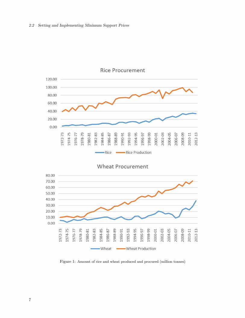
2.2 Setting and Implementing Minimum Support PricesSupport prices are announced at the beginning of each agricultural year, prior to planting, and paid at har-vest. In June each year, at the time of the early annual monsoon, the Committee for Agricultural Costs andPrices (CACP) of the Central government announces a slate of national Minimum Support Prices (MSPs)for up to 25 crops23. However, government procurement at the MSP is a viable alternative only in the case ofrice and wheat, which have both been procured at rates of higher than 15% since 199724 (Figure 1). As of the2011-2012 season, procurement of rice and wheat stands at 40.2% and 39.7% of total production respectively.

Support prices are set independently for the two main cultivation seasons in the country, the Winter Kharifseason (the main rice season25), and the Spring Rabi season (the main wheat season26), and paid out onlythe harvest period pertaining to that season27). The two seasons are distinct: either the rice support priceis in effect, or the wheat support price is in effect, and not both28. At baseline, we assume that farmersare aware of these prices before they make planting decisions (which occur 2-3 weeks after the main monsoon).

I consider the MSP-setting process to have elements of randomness from the perspective of the farmer, forfour reasons, and these in turn validate the parallel trends assumption in the differences-in-differences frame-work I use. First, the precise algorithm that is used to set prices is not public knowledge, and certainly notknown to the potential beneficiaries of the price supports 29. Second, in addition to the information observed

22Despite the lack of market integration described above, we can assume that there are at least some producers in any givendistrict that are able to transport and sell their produce in a neighboring district. To the extent that this small group of farmershas the alternative option of selling in another district at a higher price than in their own (or the MSP), they are less likely torespond to the policy, and will dampen the magnitude of the effect that I find.

23Data on Minimum Support Prices Recommended by CACP and Fixed by Government (Crop Year)24In theory, farmers can sell any of 25 crops to various government mandis during the harvest. In practice, however, the

price support policy focuses heavily on staples, particularly in the period between 1997-2012, the relevant period of studyfor this paper. In the case of pulses, for example, for which MSPs are regularly announced, under 1% of production isprocured (Bhattacharya 2016). For cotton, a key cash crop, the proportion of procurement stands at a low 7% (“Cottonprocurement at 2-2.5 million bales”, Nov 14th 2015, Business Standard, and data from the Cotton Corporation of Indiahttp://cotcorp.gov.in/statistics.aspx).

25Planting in June-July, harvesting in Dec-Jan26Planting in Nov-Dec, harvesting in Feb-Apr27For example, the MSP for rice applies only between January and March for the main rice harvest from the Kharif season,

while the MSP for wheat is effective in the Rabi season.28Apart from the fact that the rice MSPs are only paid for harvesting in the Kharif season and the wheat MSPs are only

paid for harvesting in the Rabi seasons, there are only 35 districts that cultivate both rice and wheat in the Rabi season (ofwhich only 4 are significant wheat producers) and only 7 districts that produce both rice and wheat in the Kharif season (ofwhich none are significant wheat producers). It is therefore unlikely that the support prices for rice and wheat intersect indecision-making within a season. However, farmers may certainly substitute production across seasons, since support prices areknown before the earlier of the two seasons (the Kharif season) begins. I show this mitigating effect in section 8.6.

29While State governments provide recommendations to the CACP, the committee takes into account a wide range of informa-tion, including cost surveys from around the country and monsoon forecasts. The CACP describes the following considerationsin setting these price supports ( Terms of Reference, CACP 2009):

6

2.2 Setting and Implementing Minimum Support Prices

Figure 1: Amount of rice and wheat produced and procured (million tonnes)

7

2.2 Setting and Implementing Minimum Support Prices

and taken into account by the national government, MSPs are set through a political process that introducessome randomness. There is a clear sense that political pressure sets ever-increasing MSPs30. Third, it isunlikely that there is meaningful district-specific information encoded into the national MSP announcementthat was previously unknown to farmers in that district that could directly influence production decisions.Fourth, I verify that price supports do not correlate with various other metrics that are observable to farmersthat may affect production: aggregate early-season rainfall (productivity) shocks31 and monsoon forecasts(Appendix Table A1.1).

The government serves as an alternative buyer for agricultural output at harvest, setting an effective (butnot legislated) price support. At harvest-time, State and Central governments set up mandis in which anyfarmer can sell their harvest directly to government officials at the previously-announced MSP. At the timeof the harvest, farmers observe realized prices in the wholesale market and make a decision about whetherto sell their crops at the government mandi or at the wholesale market, taking into account transportationcosts to both.

Since governments do not legislate a price floor, farmers often experience local market prices that are belowthe MSP in local wholesale markets in some years, but not in others. There are two main reasons I identifyfor continuing to observe prices below the MSP in some wholesale markets in some years: 1. Not all farmersare aware of the MSPs that have been set, and, as such, those producers do not consider the governmentprice support policy in their planting or selling decisions32 2. Even among those who are aware of the MSPwhile making their production decisions, some might find that the additional transport cost required to takeproduce to the government mandis is too high, and therefore remain non-compliers33. It is this population ofnon-compliers and those with imperfect information who participate in the local wholesale market, in whichI observe prices34.1. Cost of production, elicited through surveys,2. Demand and supply,3. Domestic and international price trends,4. Inter-crop price parity,5. Terms of trade between agriculture and non-agriculture, and6. Likely implications of MSP on consumers of that product.30MSPs have continued rising steeply in recent years and have never fallen in their entire history, even in periods in which

world prices for rice and wheat are falling. I assume, therefore, that individual districts have no influence in setting the nationalMSP, once state-time trends are accounted for. State governments or the Central government sometimes announce surprisebonuses to the MSP, which are unknown to the farmer at the time of planting (and therefore do not factor into plantingdecisions).

31Since the monsoon begins in the earliest states in late May and announcement of price supports is made in June, it ispossible that the aggregate of local-level rainfall shocks across the country is taken into account in setting the support pricein the Kharif season, but I show that this is not the case. To do this, I test whether early-season rainfall across the countryis predictive of the minimum support price (both in levels and first-differences) for rice and wheat, and find that it is not.Figure A1.1 indicates an increasing trend for real support prices over time for both rice and wheat, despite low (for example,2012) and high (e.g. 2008) early-season rainfall realizations. Figure A1.2 shows that changes in support prices also show noconsistent pattern in response to early-season rainfall. Second, even if there were such a pattern, it would not pose a threat toidentification. I rely on local-level variation in early-season rainfall around the national average by including year fixed-effectsin my specifications. This implies that changes in the national-level price support, even if based on some aggregate measure ofearly-season rainfall, are still random from the perspective of the individual farmer in a particular district. This does not posea problem in the Rabi season since the announcement of support prices takes place in June, while early season Rabi rainfallonly begins to be realized in September. Nevertheless, I present evidence that support prices do not depend on early-seasonrainfall realizations in both seasons.

32Data from the 70th round of the NSS suggests that only 32% of rice-producing households accurately know the currentMSP level for rice (39% for wheat). 12 % of rice-producing households and 16% of wheat-producing households reported salesto the government through the PDS system.

33Access to government mandis varies widely across districts and states, resulting in uneven access to price supports. I discussthis issue further in section 8.3.

34There are, of course, operational constraints to accessing government mandis that extend beyond distance. These include

8

2.3 The Farmer’s Timeline

The policy’s focus on rice and wheat is the result of the government’s overall goal to procure staples andredistribute it at a single subsidized price to low-income households through a network of close to 500,000ration stores across the country35. This paper focuses only on production responses to the support price,and assumes that the consumption side of the program does not vary systematically with production-sidefactors in the period of study36.

2.3 The Farmer’s TimelineI gather the details above into a timeline outlining the implementation of the policy for a representativestate (Figures 2 and 3).

There are three key takeaways from the timing of implementation. First, the MSP is known (withoutuncertainty) when planting decisions are being made, and can influence planting and input decisions. Second,early-season monsoon rain is observed before planting occurs, and shocks to early-season rain reflect shocksto agricultural productivity. Third, farmers may form expectations of yield and market price based onmonsoon rains, but these remain stochastic at the time of planting.

3 Two-Sector FrameworkIn this section, I present a two-sector model of allocation of capital and labor between agricultural and non-agricultural production. The model makes several simplifications to the context, but is used to provide usefulcomparative statics of farmers’ responses to productivity shocks arising from local-level rainfall variation,both with and without price supports.

I make the following simplifying assumptions in creating the framework. In Section 3.6, I discuss relaxingthese assumptions.

1. That each district behaves like a small closed economy.

2. That within the agricultural sector, a single crop is produced with a single price, and that the pricesupport (when I introduce it) applies to that one crop. This assumption allows me to focus on inter-sectoral labor shifts.

3. That realized prices are known with certainty immediately following the productivity shock - that is,that households observe early-season rainfall, and know the local market price for the agricultural goodprecisely.

4. That capital and labor are completely mobile across sectors.the operational hours of mandis, potential bribes that need to be paid for the produce to be accepted, and overcrowdedwarehouses - all of which narrow the complier population and dampen the effect of the policy on producers. I discuss theimplications of these in further detail in Section 8.

35Unlike the production-side price supports, which are available to all farmers, regardless of land-holding, the consumption-side subsidies are targeted toward poorer households. Rice and wheat are sold at a subsidized price (always below market retailprices) to people who hold Below-Poverty Line (BPL) cards (38% of the rural population), and at an even lower price to theultra-poor. Consumer prices through the program are set at the national level also.

36The resale of rice and wheat procured by the government through ration stores may directly affect farmers’ productionchoices, so I restrict my analyses to a time period (1997-2012) in which there are no major changes in administration andselection of beneficiaries by the government on the consumption side of the program. I discuss potential interactions betweenthe production and consumption sides of the program in greater detail in Section 8.

9

Figure 2: Timeline of events for the Kharif season.

Figure 3: Timeline of events for the Rabi season.

10

3.1 Household Utility Maximization

3.1 Household Utility MaximizationI begin with a version of the framework without price supports. A representative household h earns incomeI from renting a stock of capital, K, and labor L, at rates r and w respectively. In turn, the householdconsumes two goods, an agricultural good and a manufacturing good. It maximizes a standard CES utilityfunction37 subject to a budget constraint (without credit). That is, the household chooses qM and qA tomaximize:

Uh = [αqσ−1σ

A + (1− α)qσ−1σ

M ] σσ−1 s. t.

pAqA+ qM = I,

where pA is the price per unit of the agricultural output, and the price of the manufacturing good is nor-malized to 1.Household optimization then satisfies the following conditions:

Gαq−1σ

A

pA= G(1− α)q

−1σ

M38 (1)

and

qM = I − pAqA (2)

I combine equations 1 and 2 to derive the optimal quantity consumed of the manufacturing good:

qM = (1− α)σIασp1−σ

A + (1− α)σ(3)

39

37I also show that Cobb-Douglas Stone-Geary preferences, also common to the literature, provide an even more stark versionof the comparative statics derived here, due to stronger income effects arising from a subsistence constraint (derivation availableupon request). Prior literature (Restuccia et al. 2008, Herrendorf 2013, Lee 2014) suggests that C-D Stone-Geary preferencesbetter model the cross-country variation in responses to agricultural productivity shocks.

38Where G = [αqσ−1σ

A + (1 − α)qσ−1σ

M ]1

σ−1

39While we use equation 3 in deriving the general equilibrium in this model, an intuitive way to think about the equilibriumarises from examining quantity shares for the two goods:

qM

qA= (

1−αpMαpA

)σ (4)

The representative household consumes according to the (price-weighted) ratios of the importance of each good in the utilityfunction, downweighted by the substitutability between the goods. The higher the substitutability between the goods (higherσ), the closer the household gets to consuming only one good. If the goods are perfect complements, on the other hand, thegoods will be consumed exactly in a 1:1 ratio.

11

3.2 Producers’ Profit Maximization

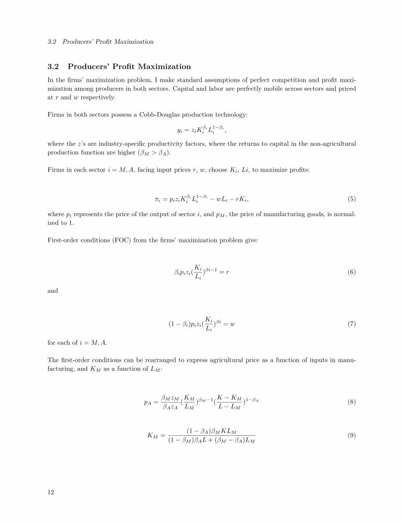
3.2 Producers’ Profit MaximizationIn the firms’ maximization problem, I make standard assumptions of perfect competition and profit maxi-mization among producers in both sectors. Capital and labor are perfectly mobile across sectors and pricedat r and w respectively.

Firms in both sectors possess a Cobb-Douglas production technology:

yi = ziKβii L

1−βii ,

where the z’s are industry-specific productivity factors, where the returns to capital in the non-agriculturalproduction function are higher (βM > βA).

Firms in each sector i = M,A, facing input prices r, w, choose Ki, Li, to maximize profits:

πi = piziKβii L

1−βii − wLi − rKi, (5)

where pi represents the price of the output of sector i, and pM , the price of manufacturing goods, is normal-ized to 1.

First-order conditions (FOC) from the firms’ maximization problem give:

βipizi(Ki

Li)βi−1 = r (6)

and

(1− βi)pizi(Ki

Li)βi = w (7)

for each of i = M,A.

The first-order conditions can be rearranged to express agricultural price as a function of inputs in manu-facturing, and KM as a function of LM :

pA = βMzMβAzA

(KM

LM)βM−1(K −KM

L− LM)1−βA (8)

KM = (1− βA)βMKLM(1− βM )βAL+ (βM − βA)LM

(9)

12

3.3 Equilibrium Without Price Supports

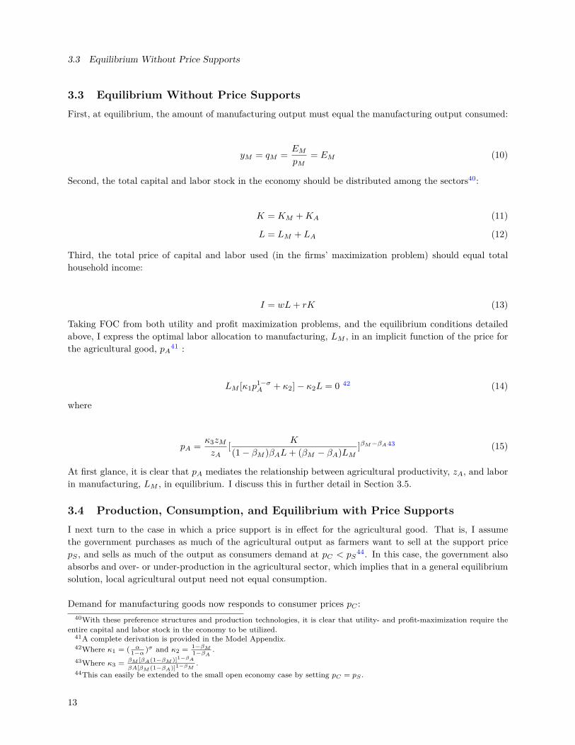
3.3 Equilibrium Without Price SupportsFirst, at equilibrium, the amount of manufacturing output must equal the manufacturing output consumed:

yM = qM = EMpM

= EM (10)

Second, the total capital and labor stock in the economy should be distributed among the sectors40:

K = KM +KA (11)

L = LM + LA (12)

Third, the total price of capital and labor used (in the firms’ maximization problem) should equal totalhousehold income:

I = wL+ rK (13)

Taking FOC from both utility and profit maximization problems, and the equilibrium conditions detailedabove, I express the optimal labor allocation to manufacturing, LM , in an implicit function of the price forthe agricultural good, pA41 :

LM [κ1p1−σA + κ2]− κ2L = 0 42 (14)

where

pA = κ3zMzA

[ K

(1− βM )βAL+ (βM − βA)LM]βM−βA43 (15)

At first glance, it is clear that pA mediates the relationship between agricultural productivity, zA, and laborin manufacturing, LM , in equilibrium. I discuss this in further detail in Section 3.5.

3.4 Production, Consumption, and Equilibrium with Price SupportsI next turn to the case in which a price support is in effect for the agricultural good. That is, I assumethe government purchases as much of the agricultural output as farmers want to sell at the support pricepS , and sells as much of the output as consumers demand at pC < pS

44. In this case, the government alsoabsorbs and over- or under-production in the agricultural sector, which implies that in a general equilibriumsolution, local agricultural output need not equal consumption.

Demand for manufacturing goods now responds to consumer prices pC :40With these preference structures and production technologies, it is clear that utility- and profit-maximization require the

entire capital and labor stock in the economy to be utilized.41A complete derivation is provided in the Model Appendix.42Where κ1 = ( α

1−α )σ and κ2 = 1−βM1−βA

.43Where κ3 = βM [βA(1−βM )]1−βA

βA[βM (1−βA)]1−βM.

44This can easily be extended to the small open economy case by setting pC = pS .

13

3.5 Comparative Statics

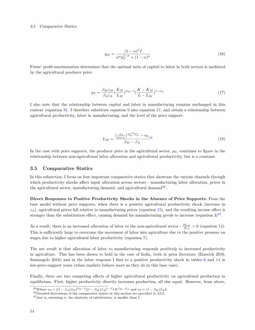
qM = (1− α)σIασp1−σ

C + (1− α)σ(16)

Firms’ profit-maximization determines that the optimal ratio of capital to labor in both sectors is mediatedby the agricultural producer price:

pS = βMzMβAzA

(KM

LM)βM−1(K −KM

L− LM)1−βA (17)

I also note that the relationship between capital and labor in manufacturing remains unchanged in thiscontext (equation 9). I therefore substitute equation 9 into equation 17, and obtain a relationship betweenagricultural productivity, labor in manufacturing, and the level of the price support:

LM =( κ4pSzA

)1

βM−βA − κ5

βM − βA45 (18)

In the case with price supports, the producer price in the agricultural sector, pS , continues to figure in therelationship between non-agricultural labor allocation and agricultural productivity, but is a constant.

3.5 Comparative StaticsIn this subsection, I focus on four important comparative statics that showcase the various channels throughwhich productivity shocks affect input allocation across sectors - manufacturing labor allocation, prices inthe agricultural sector, manufacturing demand, and agricultural demand46.

Direct Responses to Positive Productivity Shocks in the Absence of Price Supports: From thebase model without price supports, when there is a positive agricultural productivity shock (increase inzA), agricultural prices fall relative to manufacturing prices (equation 15), and the resulting income effect isstronger than the substitution effect, causing demand for manufacturing goods to increase (equation 3)47.

As a result, there is an increased allocation of labor to the non-agricultural sector - ∂LM∂zA> 0 (equation 14).

This is sufficiently large to overcome the movement of labor into agriculture due to the positive pressure onwages due to higher agricultural labor productivity (equation 7).

The net result is that allocation of labor to manufacturing responds positively to increased productivityin agriculture. This has been shown to hold in the case of India, both in prior literature (Emerick 2016,Santangelo 2016) and in the labor response I find to a positive productivity shock in tables 6 and 14 inlow-price-support years (when markets behave more as they do in this base case).

Finally, there are two competing effects of higher agricultural productivity on agricultural production inequilibrium. First, higher productivity directly increases production, all else equal. However, from above,

45Where κ4 = [(1 − βA)βM ]βM−1[(1 − βM )βA]1−βAKβM−βA and κ5 = (1 − βM )βAL.46Detailed derivations of the comparative statics in this section are provided in A3.2.47that is, assuming σ, the elasticity of substitution, is smaller than 1.

14

3.6 Assumptions

we know that the amount of labor dedicated to agriculture falls in response to relatively lower agriculturalprices and the resulting increase in manufacturing demand. The net effect of higher productivity on agricul-tural output without price supports depends on which channel dominates48.

I next move to the version of the model with price supports.

Responses to Positive Productivity Shocks with Price Supports: When there is a positive agri-cultural productivity shock, agricultural prices now do not fall relative to manufacturing prices. Therefore,one of the two channels shifting labor into agriculture is weakened, and the second dominates in equilibrium- ∂LM∂zA

< 0 (from equation 18). That is, price rigidities are sufficient to reverse the direction of the laborallocation response to positive productivity shocks.

In addition, equation 18 also shows that the level of the price support ps amplifies the effect of agriculturalproductivity shocks on equilibrium labor allocations. That, is, for a given positive productivity shock to zA,the resulting decrease in the labor allocated to manufacturing, LM , is larger when pS is higher:

∂LM∂pS∂zA

> 0 (19)

Finally, agricultural production increases unambiguously with zA in the presence of price supports; the shiftof labor away from manufacturing, coupled with increased productivity, leads to an increase in output - thereis therefore no labor channel mitigating the increase in output. Therefore, the presence of price supports(and the resulting increase in agricultural labor use), implies a bigger production boost in response to anagricultural productivity shock in this case relative to the base case without price supports.

3.6 AssumptionsThe framework outlined above is clearly a simplification of the Indian support price policy. The key differ-ences between the model and the execution of the policy are as follows:

First and most importantly, Indian districts do not exist entirely in either the regime with, or without pricesupports. If realized prices are sufficiently high, price supports do not bind and we can expect that thedistrict behaves according to the base case. If realized prices are low, then the district produces accordingto the binding support price. Adding a layer of complication to this is the fact that farmers do not know,at the time of planting, whether the price support will bind. Farmers in each district can only estimate aprobability that they will fall under one regime or another. Therefore, based on these probabilities, districtsfall on a continuum between the two models.

In light of this, we expect a decrease in the amount of labor allocated to the non-agricultural sector inhigh price-support years for two reasons. First, the probability that the price support will bind at harvestfor a given district is higher (therefore there is an increased chance of being in the price support case).Second, the level of the price support is higher relative to local prices, which we have shown to amplifythe non-agricultural labor response. Combined, both these effects suggest that the differential response of

48We know from equations 9 and 14 that KMLM

decreases in equilibrium with an increase in zA. By extension, KALA

= K−KML−LM

increases. Agricultural production is given by zA(KALA

)βALA, of which the first two terms increase in equilibrium in responseto an increase in zA, while the last term decreases.

15

non-agricultural labor allocation to an agricultural productivity shock in high- and low-price support yearswill be negative.

Second, capital and labor are not, in reality, perfectly mobile across sectors. Relaxing this assumption (inthe extreme, this would mean that there are separate labor stocks for agriculture and manufacturing) shouldimply that competition for labor in the agricultural sector in response to positive productivity shocks drivesup wages wA, and demand, prices, and wages in the manufacturing sector, qM and wM . There should besmaller labor movements between sectors, both in the base case and with price supports.

Third, not every farmer is a complier - either because of lack of knowledge of the government program, ordue to high transport costs to government depots. Because of this the general equilibrium effects will besignificantly weaker when taken to the data.

Fourth, the model assumes that the consumption price, pC , for agricultural goods, is exogenous. This closesoff manufacturing demand responses to agricultural prices in the price support case (since demand reliesentirely on pC , which is exogenously set). However, in the Indian Public Distribution System, only a smallselected fraction of the population can obtain (a quota of) rice at subsidized prices; the majority of con-sumers purchase rice on the open market. Open market rice prices, as I show in the next section, decreasein response to agricultural productivity shocks. We know from the model that income effects outweigh sub-stitution effects and manufacturing demand should increase as a result. This, when taken to the data, willdampen the negative manufacturing labor response to agricultural productivity shocks that I derived in themodel with price supports.

Fifth, farmers produce a wide variety of crops beyond the two for which price supports are significant,while the model assumes that agricultural output is a single crop. I show that in response to a positiveproductivity shock, farmers in fact substitute away from staples (perhaps due to utility from diet diversity,and the fulfillment of a caloric minimum intake), which the model cannot capture. This is negated in highprice-support years. We may also be concerned that subsitution among crops that are heterogeneous inlabor intensity entirely drives the labor market shifts I observe. However, I show increases in raw yield perhectare for staples, indicating an additional increase in input intensity for the crops under price supports -this means that the labor response does not arise simply from a shift to more labor-intensive crops that haveprice supports.

4 Empirical StrategyBroadly, identification stems from the interaction between local weather-related productivity shocks, andthe extent to which national price supports for rice and wheat keep up with local wholesale prices. Sincedistricts face different weather shocks in different periods, this provides exogenous variation in agriculturalproductivity and therefore prices at the district-year level49. To separately identify the differential effectof productivity shocks on production with and without price supports, I interact these with high and lowsupport prices in a differences-in-differences framework.

49Weather shocks can take two forms: rainfall and temperature. Previous work confirms that temperature and rainfall aresignificant predictors of crop yields (Lobell et al. 2007, Schlenker et al. 2009). However, I avoid using temperature shocksdue to their potential direct effect on workers’ productivity in the non-agricultural sector (West 2003; Chen 2003; Chan 2009),in favor of focusing on rainfall shocks. Previous work (Dercon 2004, Miguel et al. 2004, Jayachandran 2006, Kaur 2017) hasinterpreted rainfall shocks as exogenous shifters of TFP.

16

4.1 Differences-in-differences framework

4.1 Differences-in-differences frameworkI consider each district to be a distinct local market within which producers choose to sell either to themarket or to the government at harvest-time. I assume that producers have the ability to sell their produceto any wholesale market in their district50.

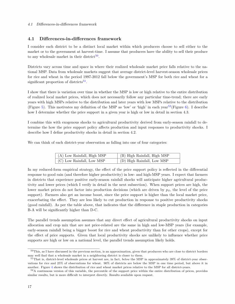
Districts vary across time and space in where their realized wholesale market price falls relative to the na-tional MSP. Data from wholesale markets suggest that average district-level harvest-season wholesale pricesfor rice and wheat in the period 1997-2012 fall below the government’s MSP for both rice and wheat for asignificant proportion of districts51.

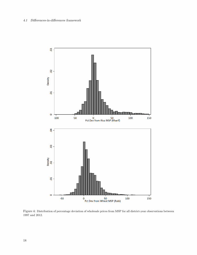
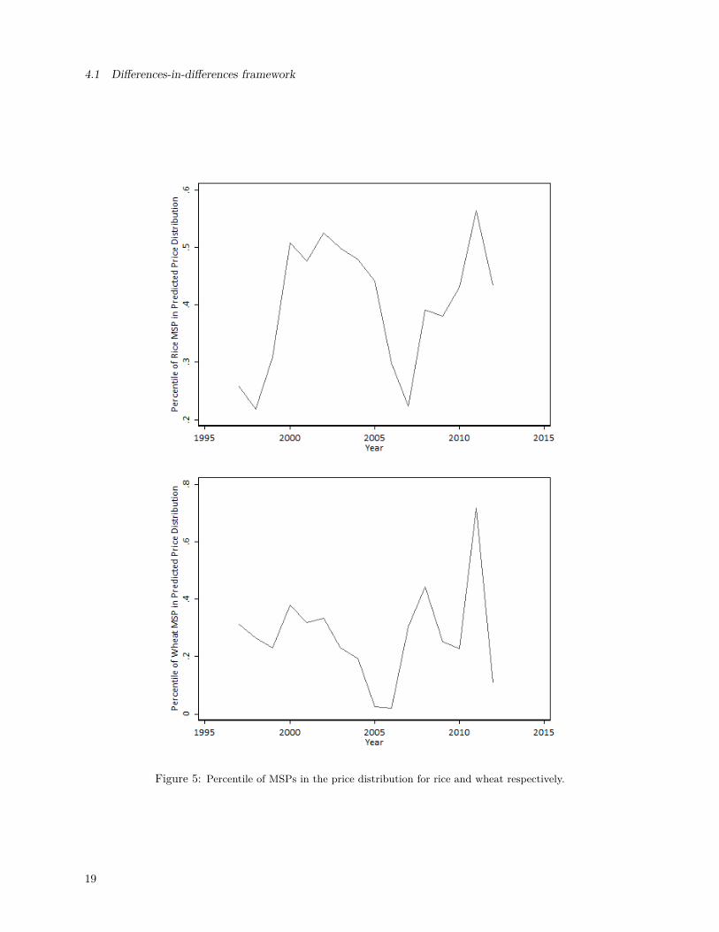
I show that there is variation over time in whether the MSP is low or high relative to the entire distributionof realized local market prices, which does not necessarily follow any particular time-trend; there are earlyyears with high MSPs relative to the distribution and later years with low MSPs relative to the distribution(Figure 5). This motivates my definition of the MSP as ‘low’ or ‘high’ in each year52(Figure 6). I describehow I determine whether the price support in a given year is high or low in detail in section 4.3.

I combine this with exogenous shocks to agricultural productivity derived from early-season rainfall to de-termine the how the price support policy affects production and input responses to productivity shocks. Idescribe how I define productivity shocks in detail in section 4.2.

We can think of each district-year observation as falling into one of four categories:

(A) Low Rainfall, High MSP (B) High Rainfall, High MSP(C) Low Rainfall, Low MSP (D) High Rainfall, Low MSP

In my reduced-form empirical strategy, the effect of the price support policy is reflected in the differentialresponse to good rain (and therefore higher productivity) in low- and high-MSP years. I expect that farmersin districts that experience positive early-season rainfall shocks will anticipate higher agricultural produc-tivity and lower prices (which I verify in detail in the next subsection). When support prices are high, thelower market prices do not factor into production decisions (which are driven by pS , the level of the pricesupport). Farmers also get an income boost, since the price support is higher than the local market price,exacerbating the effect. They are less likely to cut production in response to positive productivity shocks(good rainfall). As per the table above, that indicates that the difference in staple production in categoriesB-A will be significantly higher than D-C.

The parallel trends assumption assumes that any direct effect of agricultural productivity shocks on inputallocation and crop mix that are not price-related are the same in high and low-MSP years (for example,early-season rainfall being a bigger boost for rice and wheat productivity than for other crops), except forthe effect of price supports. Given that local productivity shocks are unlikely to influence whether pricesupports are high or low on a national level, the parallel trends assumption likely holds.

50This, as I have discussed in the previous section, is an approximation, given that producers who are close to district bordersmay well find that a wholesale market in a neighboring district is closer to them.

51That is, district-level wholesale prices at harvest are, in fact, below the MSP in approximately 39% of district-year obser-vations for rice and 25% of observations for wheat. 90% of districts are below the MSP in one time period, but above it inanother. Figure 4 shows the distribution of rice and wheat market prices relative to the MSP for all district-years.

52A continuous version of this variable, the percentile of the support price within the entire distribution of prices, providessimilar results, but is more difficult to interpret directly. Results available upon request.

17

4.1 Differences-in-differences framework

Figure 4: Distribution of percentage deviation of wholesale prices from MSP for all district-year observations between1997 and 2012.

18

4.1 Differences-in-differences framework

Figure 5: Percentile of MSPs in the price distribution for rice and wheat respectively.

19

4.1 Differences-in-differences framework

Figure 6: Illustration of variation in where MSP falls relative to the distribution of prices

There are three main challenges that drive my choice of empirical strategy. First, I cannot use a cross-sectional comparison of districts with high and low prices relative to the support price to independentlyidentify the effect of the price support policy. Districts in which realized wholesale market prices fall abovethe MSP are unobservably (to the econometrician) different from districts in which wholesale prices tend tobe low. I therefore use a district-time panel of planting decisions between 1997 and 2012 and include districtfixed-effects to compare the response of planting decisions to productivity shocks within the same districtin years in which the national MSPs for rice and wheat are more salient to the farmer’s decision-making(relatively higher) to years in which they are less so (relatively lower).

Second, using realized market prices at harvest to determine whether price supports are high or low in a givenyear results in reverse causality. Realized harvest wholesale market prices are, in equilibrium, determinedboth by planting decisions and market demand for each crop. They are also unknown to the farmer at thetime that planting decisions are made. I therefore use price trends for each district to create a (parametric)prediction model for market prices (Section 4.3)53. It is important that this prediction be informative beforeplanting decisions have been made. These predicted prices form the distribution of anticipated local marketprices that determines whether the MSP is high or low in a given year.

Third, a direct comparison between districts with low and high market prices might not estimate the trueeffect of the support price policy. There are both income and insurance mechanisms at work - people couldchange planting decisions simply because anticipated income is higher from staple production under theprogram, or they could respond to the security of having a guaranteed price for rice and wheat, even if theprobability of local market prices falling below the minimum support price is low54. Because of this, I chooseto define all districts in a given year as affected by either a ‘high’ MSP or a ‘low’ MSP, and calculate averageeffects across all districts (both below and above the support price). I do test that the effect of the programis greater for districts in the lowest 30 percentiles of the price distribution in each year55.

53Since each farmer is a price-taker, I abstract away from equilibrium effects in the prediction model.54This would be even more significant if the ability to sell on the local market were limited through informal quotas or limited

demand, leaving even farmers in high-price districts with no option other than to sell their remaining produce through thegovernment program, or let it rot for no return.

55These districts’ market prices typically always fall below the level of the price support in both low- and high-MSP years,and the model suggests that when the price support binds, the higher the level of the price support, the greater the responseof farmers in that district. The results are provided in Appendix Tables A2.1 and A2.2.

20

4.2 Positive Productivity Shocks: Early-season Rainfall

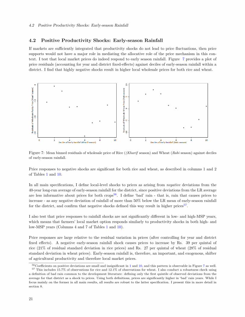
4.2 Positive Productivity Shocks: Early-season RainfallIf markets are sufficiently integrated that productivity shocks do not lead to price fluctuations, then pricesupports would not have a major role in mediating the allocative role of the price mechanism in this con-text. I test that local market prices do indeed respond to early season rainfall. Figure 7 provides a plot ofprice residuals (accounting for year and district fixed-effects) against deciles of early-season rainfall within adistrict. I find that highly negative shocks result in higher local wholesale prices for both rice and wheat.

Figure 7: Mean binned residuals of wholesale price of Rice ((Kharif season) and Wheat (Rabi season) against decilesof early-season rainfall.

Price responses to negative shocks are significant for both rice and wheat, as described in columns 1 and 2of Tables 1 and 10.

In all main specifications, I define local-level shocks to prices as arising from negative deviations from the40-year long-run average of early-season rainfall for the district, since positive deviations from the LR averageare less informative about prices for both crops56. I define ‘bad’ rain - that is, rain that causes prices toincrease - as any negative deviation of rainfall of more than 50% below the LR mean of early-season rainfallfor the district, and confirm that negative shocks defined this way result in higher prices57.

I also test that price responses to rainfall shocks are not significantly different in low- and high-MSP years,which means that farmers’ local market option responds similarly to productivity shocks in both high- andlow-MSP years (Columns 4 and 7 of Tables 1 and 10).

Price responses are large relative to the residual variation in prices (after controlling for year and districtfixed effects). A negative early-season rainfall shock causes prices to increase by Rs. 39 per quintal ofrice (21% of residual standard deviation in rice prices) and Rs. 27 per quintal of wheat (28% of residualstandard deviation in wheat prices). Early-season rainfall is, therefore, an important, and exogenous, shifterof agricultural productivity and therefore local market prices.

56Coefficients on positive deviations are small and insignificant in 1 and 10, and this pattern is observable in Figure 7 as well.57 This includes 15.7% of observations for rice and 12.1% of observations for wheat. I also conduct a robustness check using

a definition of bad rain common to the development literature: defining only the first quintile of observed deviations from theaverage for that district as a shock to prices. Using both definitions, prices are significantly higher in ‘bad’ rain years. While Ifocus mainly on the former in all main results, all results are robust to the latter specification. I present this in more detail insection 8.

21

4.3 High and Low Price Supports: The Farmer’s Prediction of Prices

4.3 High and Low Price Supports: The Farmer’s Prediction of PricesThere is an extensive literature that suggests that farmers adjust to information provided to them priorto the time of planting, based on anticipated profitability58. Here, I suggest that farmers use the infor-mation they have about productivity to make predictions about prices, and therefore about profitabilityof the their crop. I also assume that farmers’ expectations of market prices given early-season rainfall arerational based on their past observations. I make price predictions in a parametric way, assuming thatfarmers have knowledge of past rainfall and prices59, but limited recall. I use farmers’ price predictionsto classify support prices as high or low in a given year. A given district is 3.4pp, or 8.6% more likely tohave a binding realized market price in a ‘high’ MSP year relative to a ‘low’ MSP year (Column 3 of Table 1).

To do this, I define farmers’ information set in each time period, t, which includes mspt and early-seasonrainfall wt, and realized prices and early-season rainfall for the past α years. That is, they have observedthe relationship between early-season rainfall and realized prices for the past α years, and use the param-eters that define that relationship to predict this year’s market price based on this year’s early-season rainfall.

I then use only the data contained in these information sets to make a prediction about this year’s marketprices during the harvest period for rice and wheat. Specifically, I use a district-specific quadratic function ofearly-season rainfall60 , a district-specific time trend, a statextime trend, and district fixed effects, to predictmarket prices in t.

The empirical specification used in the prediction stage is as follows. I run the following specificationusing data from t− 1 to t− 5:

pmdst = β0 + β1dstEarlyRainfalldst + β2dstEarlyRainfall2dst

+ β3dsδtdst + ιds + εdst

where pmdst is the local price in a given district d in state s in a given agricultural year and season t. Thecoefficients on EarlyRainfalldst describe a district-specific quadratic function of the relationship betweenearly-season rainfall and local prices. I also include ιds, a district fixed effect. δt is a district-specific yeartrend, to account for districts being on different price trajectories over time. Xtst are state-time trends. Theerror εdst is clustered at the district level.

In creating the specification in this way, I allow for farmers to use other aspects of the prices and data theyhave observed over the past five years (time trends, district fixed effects that capture the average prices ofstaples in their district over the five-year period, etc.) in their predictions.

I use the coefficients from the prediction specification to predict prices in time t. Using the predicted prices,I then calculate the percentile of price support in the predicted price distribution. I use median of this valueto divide years into ‘high’ and ‘low’ MSP years.

58Rosenzweig & Udry 2013, Kala 201559and, in some specifications, past MSP60All rainfall terms are percent deviations from the 40-year long-run average of early-season rainfall taken from 1970 to 2015.

Early-season rainfall enters as a quadratic function to allow both positive and negative deviations from the long-run mean tohave an effect on prices.

22

4.4 The Farmer’s Decision Timeline

The effect of price supports on production outcomes is robust to various alternatives to this type of prediction.In two alternate specifications (presented in Tables A1.3 and A1.4 ), I a) exclude early-season rainfall fromthe prediction, and b) include the level of the MSP in the prediction (so farmers take into account responsesof harvest-season market prices to MSP announcements). I also run versions of the specification that varythe size of the information set, α, that the farmer considers in making his prediction (Table A1.5). I discussthese checks in detail in section 8.2.

4.4 The Farmer’s Decision TimelineTo make things more specific, the timeline of information and decision-making for the compliant farmerlooks as follows:

1. The farmer’s pre-planting information set I includes the realized wholesale market price in the districtand information about early season rainfall for the past five years, together with the standard deviationof realized market prices around the prediction. Given the lack of empirical work on farmer decision-making and the extent of information considered in making a decision about this season’s planting, thisis simply a benchmark model, and I will later examine robustness to varying the size of informationset.

2. Based on his information set, he creates a function that links early-season rainfall to realized wholesalemarket price within his district.

3. Before planting, the farmer observes the signal (early season rainfall), wdst in district d, in state s, intime t.

4. Based on the weather shock, and the prediction model, he knows ˆpsdst, the expected wholesale marketprice for the staple crop, and the distribution of potential yields for various crops, ˆYjdst.

5. These are all stochastic because of a second, multiplicative weather shock, ηdst, which is realized afterplanting and before the harvest, and affects the final distribution of the market price (but not plantingdecisions). The realized market price psdst = ˆpsdst∗ηdst, where η is centered around 1. That is, E[η] = 1.

6. At the same time, the government announces the national-level MSP for the year for the staple crop,mspt.

7. Given his price prediction and knowledge of the MSP, together with the standard deviation of realizedmarket prices around the predicted market price, the farmer knows the expected probability thatrealized market price will fall below the MSP. Since the realized market price psdst is stochastic evenafter the initial realization of the weather shock, the distribution of expected prices gives farmers aprobability, θ|wdst, that they will eventually sell their harvest at the mspt.

8. Farmers use these expected probabilities that the market price will fall below the MSP (in which casethey expect to sell their crop at the MSP), and predicted prices for rice and wheat, together withinformation encoded in early season rainfall about the year’s relative prices, costs, potential yields, andrevenues from various crops to select a portfolio of crops to plant.

9. Then, at harvest time, if the realized market price for the staple psdst is higher than the mspt, farmerssell their output at psdst. If it is lower, they sell their output at mspt.

23

4.5 Empirical Specifications

4.5 Empirical SpecificationsI implement the differences-in-differences strategy using the following empirical specification:

Ydst = β0 + β1GoodRainfalldst + β2GoodRainfall ∗HighMSP+

+ ιds + δt +Xtst + εdst

In this specification, Ydst are the outcomes of interest in district d in state s in agricultural year t (Juneto June). These include total area cultivated, area cultivated of staples, area share of staples and othercrops, yield, and production61. I include ιds, a district fixed-effect, to control for time-invariant districtheterogeneity, such as suitability of the district to grow staples, terrain, how urban or rural a particulardistrict is, average market prices in the district, and so on. δt is a year fixed-effect to isolate the effect ofhigh MSP from other changes in production from one year to the next. Xtst are state-time trends that aimto account for the potential influence of any particular state on support prices. Errors εdst are clustered atthe district level.

5 DataI rely on various sources of data at the district-,household-, and firm-level.

In combining data sources, I first deal with the issue of district boundaries changing and new districts beingcreated in the time period of interest. To do this, I aggregate split districts into their original parent districtprior to the split, weighting outcome variables by total land area of the split districts where appropriate62.My sample contains 469 districts after aggregation. I limit my analyses between the 1997-98 and the 2012-13agricultural seasons.

5.1 District-time Panel DataDistrict-time panel data comprise the main data in this paper. These types of data cover all sources ofvariation over time in prices and rainfall for the empirical analysis, as well as information on district-levelplanting patterns that change over time.

Data on cropping patterns are important for assessing the first-order responses to the price support policy.The government63 collects information on area planted and quantity produced for various crops for eachdistrict in each season in each year for all districts in India -these are known as the Area Production Yield(or APY) data64. I derive area cultivated and raw yields (output per unit area) for each crop in each district-season-year from this dataset. For further analysis on changes in cropping patterns, I classify crops into fourmain categories: other staple crops, pulses, cash crops, and spices.

61 I run specifications in levels rather than logs, to allow for switching into and away from producing staples. The data suggestthat this pattern is fairly common. Of the districts covered, 74 rice-producing districts and 97 wheat-producing districts reportzero production of the staple crop in the Kharif season for rice and in the Rabi season for wheat in at least one year, but notin all years.

62Districts that exchanged portions of their land area with each other (for example, by one district giving a block to anotherdistrict), are also aggregated.

63Directorate of Economics and Statistics of the Ministry of Agriculture and Farmers’ Welfare64 For a few states in a few years, missing APY data has to be supplemented with Land-Use Statistics Data instead, which

does not provide production data. Minor crops that comprise less than 1% of the cultivated area in a district are excluded fora few state-years in the LUS data, due to the sheer number of crops.

24

5.2 Repeated Cross-sectional Data

Rainfall data allow me to identify which districts face rainfall shocks that affect predicted market prices. Iobtain monthly precipitation data at 0.5° resolution65, which I aggregate to the district level66. I use totalprecipitation in the months of May and June for the Kharif season, and September, October, and Novemberfor the Rabi season, to define pre-planting shocks to agricultural productivity67.

I use wholesale price data aggregated to the district-level as a measure of local market prices. I use thesedata, together with rainfall data, to predict harvest-time market prices for each district and create a distri-bution of anticipated prices for all districts. Daily wholesale price data are sparse in India, particularly inthe period prior to 2005. I first compile all available price data for rice and wheat across markets in Indiareported by AGMARKNET (the number of markets and the number of districts covered varies over time,and currently stands at 3245 wholesale markets across the country)68. I average observed daily wholesaleprices over the harvest period for each season69. I convert prices into real terms using the World Bank’sGDP deflator.

Input data are gathered from three rounds of the Agricultural Census Inputs Survey, and cover variableinputs by crop - use of high-yielding varieties, fertilizers, and proportion of area irrigated for rice and wheat.

I eliminate all districts that report no rice or wheat production in the relevant seasons in years of my data.My final sample comprises 5,113 (91% of area under rice production) district-year observations for rice, and4,707 (94% of area under wheat production) district-year observations for wheat.

5.2 Repeated Cross-sectional DataHouseholds: The National Sample Survey (NSS) consumption/expenditure modules for rounds 55 to 68 arerepeated cross-sectional household surveys that are representative at the district-level. I focus on householdssurveyed during the Kharif and Rabi harvest months. The surveys provide detailed information on per-capita household consumption at harvest, an estimate of the number of crops produced by each householdduring the period of this study, and whether the household produces rice or wheat70.

In many analyses that use these data, I focus on households that consume rice (Kharif season) and wheat(Rabi season) out of home production, indicating that they are producers of staples71.

Individuals: The NSS employment survey rounds 60-68 also provide weekly information on labor supply and65 Climatic Research Unit of the University of East Anglia66I calculate measures of monthly rainfall (in mm) at the district-level by superimposing these data on India’s district

boundaries and calculating means across all 0.5° cells that fall within each district.67In order to define shocks to early-season rainfall more precisely, I calculate percent deviations of each district-year observa-

tions from the 40-year long-run district average of precipitation.68Given the low coverage provided by AGMARKNET data, I supplement their wholesale price data using price data, where

available, from the ICRISAT meso-level dataset, which covers all districts in 19 major states in India.69January through March for the Kharif season and March through June for the Rabi season. Wholesale prices rarely move

both above and below the price support in a single harvest period for a given district, and that there is little price-variation inmarkets during the season. This drives my decision to use mean wholesale prices for the entire harvest period for each districtto construct my measure of local market prices.

70The data distinguish between home production and production from external sources. If the household reports consumptionout of home produce of any crop, I assume that it produces that crop. This also includes products made from that crop - forexample, I assume that if a household consumes wheat flour from home production, that it produces wheat.

71Some households might, particularly in response to the price supports, exclusively sell their staple produce to the market,and consume staples purchased from PDS or on the open market, in which case they would not be included in my sample. Tothe extent that my analysis excludes such households, my estimates are a lower bound on the effects of the price support onharvest-season expenditure by staple producers.

25

5.3 District-level Snapshot

wages throughout the agricultural cycle. I am able to distinguish between agricultural and non-agriculturaltime-use. I also calculate average daily wages from these data.

I focus on non-urban households in the agricultural sector surveyed during cultivation periods in the agri-cultural cycle, when labor supply is likely to be most responsive to incentives in the form of price supports.The survey provides a rich set of household- and individual-level control variables.

Firms: The Annual Survey of Industries data are repeated cross sections between 2002 and 2009 that surveyall firms with above 100 employees, and a random sample of 1/3 of smaller firms, including both formal andinformal firms. These data are able to validate my results on how labor utilization and output by non-agricultural firms respond to agricultural price supports. These data contain detailed firm-level informationon characteristics, inputs, outputs, investment, capital, and employment.

I focus on non-urban firms. As a robustness check, I eliminate firms that use agricultural output as theirinputs.

5.3 District-level SnapshotCrop suitability measures72 use soil, topographic, and climatic data to estimate suitability distributions(created as an index with a maximum value of 100 and a minimum value of 0) for a variety of crops foreach 5 arc-minute grid cell. I obtain baseline suitability indices for 16 of the most prevalent crops in India,including rice and wheat. I aggregate suitability measures for each crop to the district-level73, and createabsolute and relative suitabiity measures74.

Districts vary widely in their innate suitability for growing rice and wheat, but are all incentivized to growstaples through the government’s national MSPs. These suitability indices can be considered a time-invariantbaseline characteristic for each district. It is therefore informative to understand how growing patterns andcrop yields in low-suitability districts change as a result of price supports, and how the gains from theprogram are distributed. The fact that low-suitability districts show no response to the program also servesas an additional test that the results derive directly from the program rather than some other randomunobserved variation.

6 Results and DiscussionThe set of results presented here are from the differences-in-differences framework. The preferred specifica-tion defines high and low support prices according to farmers’ price predictions based on a five-year recallof local market prices and productivity shocks.

The first coefficient provided in each table (on the indicator for “Good Rain”) describes the direct effect ofa positive productivity shock on the outcome. The second coefficient, on the interaction term between goodrainfall and high MSP, is our coefficient of interest. This estimates the differential production response togood rainfall (and therefore lower prices) in high MSP years relative to low MSP years. The last row ofevery table gives readers a sense of the magnitude of the effect: it shows the effect as a proportion of themean of the dependent variable. I refer mostly to these magnitudes in the rest of this section.

72From the Global Agro-Ecological Zones database collected and disseminated by International Institute for Applied SystemsAnalysis (IIASA) and the Food and Agriculture Organization of the United Nations (FAO)

73 I take an average of the Suitability Index across all 5-minute arc grid cells whose centroids lie within the district boundary.74Details are provided in the Data Appendix.

26

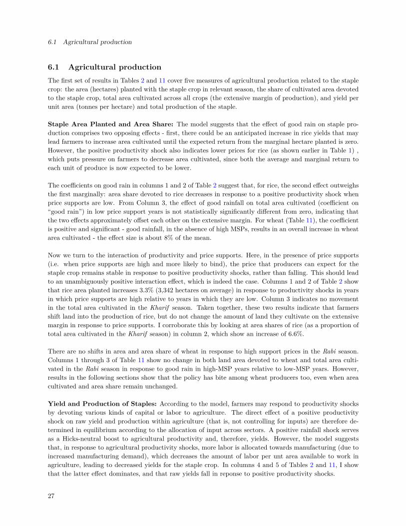
6.1 Agricultural production

6.1 Agricultural productionThe first set of results in Tables 2 and 11 cover five measures of agricultural production related to the staplecrop: the area (hectares) planted with the staple crop in relevant season, the share of cultivated area devotedto the staple crop, total area cultivated across all crops (the extensive margin of production), and yield perunit area (tonnes per hectare) and total production of the staple.

Staple Area Planted and Area Share: The model suggests that the effect of good rain on staple pro-duction comprises two opposing effects - first, there could be an anticipated increase in rice yields that maylead farmers to increase area cultivated until the expected return from the marginal hectare planted is zero.However, the positive productivity shock also indicates lower prices for rice (as shown earlier in Table 1) ,which puts pressure on farmers to decrease area cultivated, since both the average and marginal return toeach unit of produce is now expected to be lower.

The coefficients on good rain in columns 1 and 2 of Table 2 suggest that, for rice, the second effect outweighsthe first marginally: area share devoted to rice decreases in response to a positive productivity shock whenprice supports are low. From Column 3, the effect of good rainfall on total area cultivated (coefficient on“good rain”) in low price support years is not statistically significantly different from zero, indicating thatthe two effects approximately offset each other on the extensive margin. For wheat (Table 11), the coefficientis positive and significant - good rainfall, in the absence of high MSPs, results in an overall increase in wheatarea cultivated - the effect size is about 8% of the mean.

Now we turn to the interaction of productivity and price supports. Here, in the presence of price supports(i.e. when price supports are high and more likely to bind), the price that producers can expect for thestaple crop remains stable in response to positive productivity shocks, rather than falling. This should leadto an unambiguously positive interaction effect, which is indeed the case. Columns 1 and 2 of Table 2 showthat rice area planted increases 3.3% (3,342 hectares on average) in response to productivity shocks in yearsin which price supports are high relative to years in which they are low. Column 3 indicates no movementin the total area cultivated in the Kharif season. Taken together, these two results indicate that farmersshift land into the production of rice, but do not change the amount of land they cultivate on the extensivemargin in response to price supports. I corroborate this by looking at area shares of rice (as a proportion oftotal area cultivated in the Kharif season) in column 2, which show an increase of 6.6%.

There are no shifts in area and area share of wheat in response to high support prices in the Rabi season.Columns 1 through 3 of Table 11 show no change in both land area devoted to wheat and total area culti-vated in the Rabi season in response to good rain in high-MSP years relative to low-MSP years. However,results in the following sections show that the policy has bite among wheat producers too, even when areacultivated and area share remain unchanged.

Yield and Production of Staples: According to the model, farmers may respond to productivity shocksby devoting various kinds of capital or labor to agriculture. The direct effect of a positive productivityshock on raw yield and production within agriculture (that is, not controlling for inputs) are therefore de-termined in equilibrium according to the allocation of input across sectors. A positive rainfall shock servesas a Hicks-neutral boost to agricultural productivity and, therefore, yields. However, the model suggeststhat, in response to agricultural productivity shocks, more labor is allocated towards manufacturing (due toincreased manufacturing demand), which decreases the amount of labor per unt area available to work inagriculture, leading to decreased yields for the staple crop. In columns 4 and 5 of Tables 2 and 11, I showthat the latter effect dominates, and that raw yields fall in reponse to positive productivity shocks.

27

6.1 Agricultural production

I now consider the interactive effect of productivity shocks and high price supports on yield and productionof rice and wheat. According to the model, more labor is allocated to agriculture when price supports arebinding. This should have an unambiguously positive effect on yields and production, and therefore a pos-itive interaction effect between high price supports and positive shocks to agricultural productivity. I findan increase in raw yield of rice (production per hectare) of 7.2% when price supports are high (Column 4 ofTable 2). Given the expansion in the area planted with rice, which we expect to be less productive land onaverage, the increase in yields suggests a reallocation of inputs towards rice as in the model, which I verifyby looking at labor supply in agriculture in the next subsection. The expected return to investing in theseinputs is now higher (due to stability of producer prices in the face of positive productivity shocks whenprice supports are high).

Coupled with the increased area planted with rice, the amount of rice produced (Column 4 of Table 2) in-creases by 8.5% in response to good rainfall in a high-support year relative to a low-support year, on average.

Wheat production also increases between 9.7% (Column 5 of Table 11). This is driven by a significant (andlarge) increase in raw yields of wheat of between 8% (Column 4 of Table 11).

Crop Mix: My model abstracts away from the crop mix decision of the farmer by considering a singleagricultural output. However, Indian farmers often grow more than one crop, and the decision about howto allocate resources across crops is endogenous to the existence of price supports.

I find, in Table 3, that a positive productivity shock in low-suport years, leads to a shift in area share fromrice production in the Kharif season to risker, higher-return crops like pulses and oilseeds. I interpret thisas the direct effect of positive productivity shocks on crop choice. There are a number of potential micro-foundations for this result: 1. Farmers might consider rice to be a giffen good in production: after reachinga basic amount of production and satisfying a basic caloric requirement (which happens more easily whenthere is a positive production shock), they might want to consume a more diverse diet. Second, farmersmight be more willing to take on risk once their basic staple needs are met. Third, other crops may be moresensitive to early-season rainfall, both in productivity and prices.

I now move to the interactive effect of price supports and positive productivity shocks on crop mix responses.In the presence of high price supports, I find that, relative to low price-support years, there is a shift incrop mix towards the staple crop, rice. The overall effect on rice area shares in high price supports years(summing the direct and interaction terms in Column 2 of Table 2) is effectively zero: farmers do not shiftaway from rice in response to positive productivity shocks when price supports are high.

Crop Suitability and Responses to Price Supports: As described in section 5, I calculate a measureof relative crop suitability that is akin to a measure of marginal cost of cultivating a unit of land with eachof these staple crops relative to planting other crops. This is more suitable than a measure of absolute suit-ability given that landowners and making crop choices on the intensive (as well as extensive) margins. I usethese measures for two purposes; first, to discern whether there is heterogeneity in gains from the programbetween low- and highly-suitable districts. In a policy that prioritizes staple crops over others, my resultsshow that gains are distributed only among districts that are better able to switch into staple-production(Tables 4 and 12).

Second, I use this to verify that my estimates are driven by exposure to high price supports for rice and wheat

28

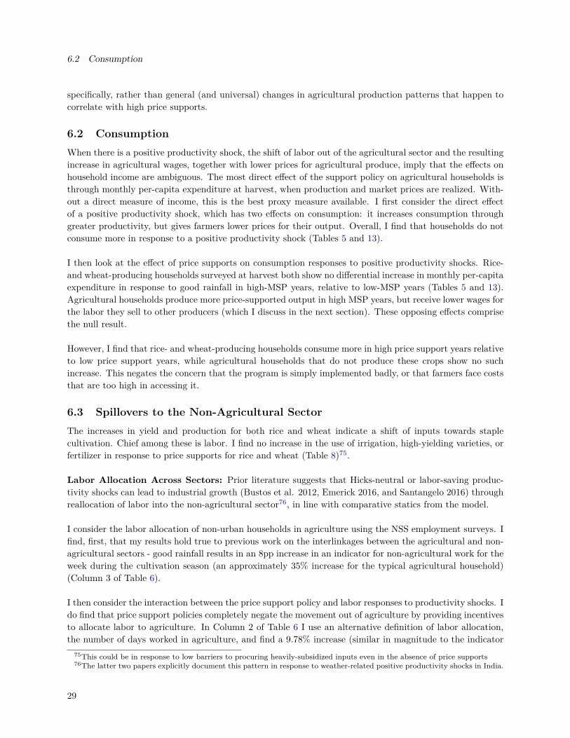
6.2 Consumption

specifically, rather than general (and universal) changes in agricultural production patterns that happen tocorrelate with high price supports.

6.2 ConsumptionWhen there is a positive productivity shock, the shift of labor out of the agricultural sector and the resultingincrease in agricultural wages, together with lower prices for agricultural produce, imply that the effects onhousehold income are ambiguous. The most direct effect of the support policy on agricultural households isthrough monthly per-capita expenditure at harvest, when production and market prices are realized. With-out a direct measure of income, this is the best proxy measure available. I first consider the direct effectof a positive productivity shock, which has two effects on consumption: it increases consumption throughgreater productivity, but gives farmers lower prices for their output. Overall, I find that households do notconsume more in response to a positive productivity shock (Tables 5 and 13).

I then look at the effect of price supports on consumption responses to positive productivity shocks. Rice-and wheat-producing households surveyed at harvest both show no differential increase in monthly per-capitaexpenditure in response to good rainfall in high-MSP years, relative to low-MSP years (Tables 5 and 13).Agricultural households produce more price-supported output in high MSP years, but receive lower wages forthe labor they sell to other producers (which I discuss in the next section). These opposing effects comprisethe null result.

However, I find that rice- and wheat-producing households consume more in high price support years relativeto low price support years, while agricultural households that do not produce these crops show no suchincrease. This negates the concern that the program is simply implemented badly, or that farmers face coststhat are too high in accessing it.

6.3 Spillovers to the Non-Agricultural SectorThe increases in yield and production for both rice and wheat indicate a shift of inputs towards staplecultivation. Chief among these is labor. I find no increase in the use of irrigation, high-yielding varieties, orfertilizer in response to price supports for rice and wheat (Table 8)75.

Labor Allocation Across Sectors: Prior literature suggests that Hicks-neutral or labor-saving produc-tivity shocks can lead to industrial growth (Bustos et al. 2012, Emerick 2016, and Santangelo 2016) throughreallocation of labor into the non-agricultural sector76, in line with comparative statics from the model.

I consider the labor allocation of non-urban households in agriculture using the NSS employment surveys. Ifind, first, that my results hold true to previous work on the interlinkages between the agricultural and non-agricultural sectors - good rainfall results in an 8pp increase in an indicator for non-agricultural work for theweek during the cultivation season (an approximately 35% increase for the typical agricultural household)(Column 3 of Table 6).

I then consider the interaction between the price support policy and labor responses to productivity shocks. Ido find that price support policies completely negate the movement out of agriculture by providing incentivesto allocate labor to agriculture. In Column 2 of Table 6 I use an alternative definition of labor allocation,the number of days worked in agriculture, and find a 9.78% increase (similar in magnitude to the indicator

75This could be in response to low barriers to procuring heavily-subsidized inputs even in the absence of price supports76The latter two papers explicitly document this pattern in response to weather-related positive productivity shocks in India.

29

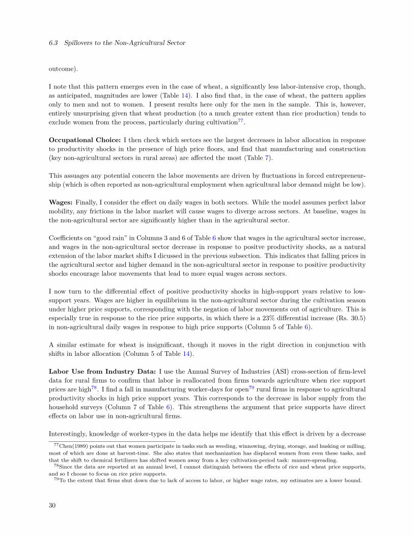
6.3 Spillovers to the Non-Agricultural Sector

outcome).

I note that this pattern emerges even in the case of wheat, a significantly less labor-intensive crop, though,as anticipated, magnitudes are lower (Table 14). I also find that, in the case of wheat, the pattern appliesonly to men and not to women. I present results here only for the men in the sample. This is, however,entirely unsurprising given that wheat production (to a much greater extent than rice production) tends toexclude women from the process, particularly during cultivation77.

Occupational Choice: I then check which sectors see the largest decreases in labor allocation in responseto productivity shocks in the presence of high price floors, and find that manufacturing and construction(key non-agricultural sectors in rural areas) are affected the most (Table 7).

This assuages any potential concern the labor movements are driven by fluctuations in forced entrepreneur-ship (which is often reported as non-agricultural employment when agricultural labor demand might be low).

Wages: Finally, I consider the effect on daily wages in both sectors. While the model assumes perfect labormobility, any frictions in the labor market will cause wages to diverge across sectors. At baseline, wages inthe non-agricultural sector are significantly higher than in the agricultural sector.

Coefficients on “good rain” in Columns 3 and 6 of Table 6 show that wages in the agricultural sector increase,and wages in the non-agricultural sector decrease in response to positve productivity shocks, as a naturalextension of the labor market shifts I dicussed in the previous subsection. This indicates that falling prices inthe agricultural sector and higher demand in the non-agricultural sector in response to positive productivityshocks encourage labor movements that lead to more equal wages across sectors.

I now turn to the differential effect of positive productivity shocks in high-support years relative to low-support years. Wages are higher in equilibrium in the non-agricultural sector during the cultivation seasonunder higher price supports, corresponding with the negation of labor movements out of agriculture. This isespecially true in response to the rice price supports, in which there is a 23% differential increase (Rs. 30.5)in non-agricultural daily wages in response to high price supports (Column 5 of Table 6).

A similar estimate for wheat is insignificant, though it moves in the right direction in conjunction withshifts in labor allocation (Column 5 of Table 14).

Labor Use from Industry Data: I use the Annual Survey of Industries (ASI) cross-section of firm-leveldata for rural firms to confirm that labor is reallocated from firms towards agriculture when rice supportprices are high78. I find a fall in manufacturing worker-days for open79 rural firms in response to agriculturalproductivity shocks in high price support years. This corresponds to the decrease in labor supply from thehousehold surveys (Column 7 of Table 6). This strengthens the argument that price supports have directeffects on labor use in non-agricultural firms.

Interestingly, knowledge of worker-types in the data helps me identify that this effect is driven by a decrease77Chen(1989) points out that women participate in tasks such as weeding, winnowing, drying, storage, and husking or milling,

most of which are done at harvest-time. She also states that mechanization has displaced women from even these tasks, andthat the shift to chemical fertilizers has shifted women away from a key cultivation-period task: manure-spreading.

78Since the data are reported at an annual level, I cannot distinguish between the effects of rice and wheat price supports,and so I choose to focus on rice price supports.

79To the extent that firms shut down due to lack of access to labor, or higher wage rates, my estimates are a lower bound.

30

in total worker-days of 17.8% for contract laborers, which is precisely the margin of adjustment for workerswho divide their time across sectors. There is no such effect for permanent employees of these firms (Columns8 and 9 of Table 6).

Output from Industry Data: Finally, I test the direct impact of price support policies on output in the non-agricultural sector using the ASI data. I find that gross output decreases by 2.6% of a standard deviationin high price support years in response to a positive agricultural productivity shock (Column 1 of Table 9).Value-added measures (Column 2) provide results of roughly similar magnitudes, though these estimates arenoisier.

These results suggest that the crowding out of labor from non-agricultural allocation in response to highprice supports has a concrete effect on production in the non-agricultural sector, at least in the short run.

7 Implications for Agricultural ProductivityBased on the results up to this point, I find that high price supports for rice and wheat crowd out labor allo-cation to, and output in the non-agricultural sector. However, the increase in labor usage in the agriculturalsector may, in fact, be productivity-enhancing in the agricultural sector. To examine this, I quantify theeffect of increasing labor usage in the agricultural sector on agricultural productivity (in the form of agri-cultural TFP). I use an aggregate agricultural TFP measure common to the literature, the Tornqvist-TheilIndex80:

ln( TFPtTFPt−1

) = 12

∑i

(Rit +Rit−1)ln( QitQit−1

)− 12

∑j

(Sjt + Sjt−1)ln( Xjt

Xjt−1)

Where Rit refers to the revenue share of output i in time t and Sjt refers to the cost share of input j in time t.

This index allows us to not only capture changes in quantities produced of various crops and quantitiesused of various inputs, but also any associated changes in input and output prices. These price changes areparticularly important since I have already shown that wages respond to the existence of high price supportsin accordance with the movement of labor.

I calculate this index for each district for each year in my data for which the NSS modules are available(from which I extract the district-level prices of 14 different crops81 that I use), and use the same differences-in-differences framework to examine the effect of the policy on agricultural productivity.

I find an increase in agricultural TFP in response to a positive agricultural productivity shock, as antici-pated (the coefficient on good rain in column 3 in Table 9). Turning to the interaction term, I find that theincreased use of labor in agriculture in response to the higher price support actually decreases agriculturalproductivity by 0.82 of a standard deviation, negating the positive productivity effect of the shock.

80Diewert 1976, Caves et al. 1982, Rosegrant & Evenson 1992, Murgai et al. 2001. This index provides an exact measureof technical change for linear homogeneous translog function that approximates - by a second-order Taylor polynomial - theCobb-Douglas production function that I use in the model.

81Details about the crops used and data sources for this analysis are given in the data appendix A4.2.

31

However, there are clear data limitations that deem my estimate a lower bound, the key of which is the lackof annual data on district-level input quantities and prices. Instead, I use input quantities for a single year,in which the price support for rice is low, for all inputs other than labor. I use input prices at the state,rather than district, level to calculate cost shares of various inputs (other than labor). Then, to the extentthat competition for inputs other than labor also increases simultaneously, pushing up their prices, or thatquantities used of these inputs increase when price supports are high, my estimates do not take that intoaccount, and are therefore a lower-bound estimate of the effect of price supports on agricultural productivity.

8 Potential Confounds and Robustness Checks

8.1 Defining High and Low Early-Season RainfallIn the main specifications, I define rainfall shocks in the two seasons to be a greater-than-50% negative devi-ation from the 40-year average of early-season rainfall. I also use one alternate specification of good rainfallcommon in previous literature (Jayachandran 2006; Kaur 2017) that provides a weaker price differentialbetween periods of ‘good’ and ‘bad’ rainfall82, and is therefore more conservative. I define the first quintileof observed deviations from the average for that district as a shock to rainfall and therefore prices.

I present results using this alternate specification in Table A1.2. I find that results all follow with similarmagnitudes as in my main rainfall specification, and remain significant.

8.2 Including Different Elements in the Farmer’s Information Set At PlantingI test the robustness of the production responses to including different amounts of information in the farmer’sinformation set at the time that planting decisions are made. Table A1.3 provides results for the five mainagricultural production outcomes from three prediction methods (based on varying the elements in thefarmer’s information set) for the main rice production (Kharif ) season. In the first column, support pricesand rainfall do not figure into price prediction (so farmers base their price expectations merely on district-specific time-trends in prices). The second allows predictions to take into account the district-specific effectof rainfall on prices, and is the preferred specification in the main tables of the paper. The third specificationaccounts for both minimum support prices and rainfall in making price predictions. I show that these keyeffects of the policy generally move in the same direction and are of the same approximate magnitude for allthree specifications. The same is true for wheat (Table A1.4).

I also test that the production results are robust to changing the number of years of information retained inthe farmer’s memory. I do this by testing a three-year and a seven-year recall period for rainfall and marketprices for the farmer, and find the same increase in input intensity aross specifications (Table A1.5).

8.3 International PricesIf farmers plant rice and wheat for export, prices for staples in international markets could affect plantingdecisions. This could affect my empirical strategy if high MSPs correlate with higher prices on the worldmarket. There are four reasons to think that this not the case. First, the trends in world prices andsupport prices (in real terms) do not coincide (Figure A1.3). Second, access to world markets should not

82The average price differential between periods of good and bad rainfall is Rs.26 per 100 kg for rice, and Rs.16 per 100 kgfor wheat, compared to the main definition of rainfall shocks, in which the differential was Rs. 39 per 100 kg for rice and Rs.26 per 100kg for wheat.

32

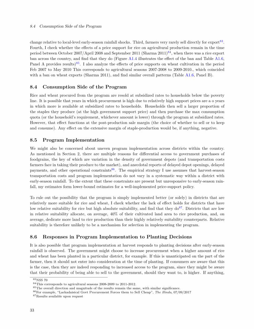
8.4 Consumption Side of the Program

change relative to local-level early-season rainfall shocks. Third, farmers very rarely sell directly for export83.Fourth, I check whether the effects of a price support for rice on agricultural production remain in the timeperiod between October 2007/April 2008 and September 2011 (Sharma 2011)84, when there was a rice exportban across the country, and find that they do (Figure A1.4 illustrates the effect of the ban and Table A1.6,Panel A provides results)85. I also analyze the effects of price supports on wheat cultivation in the periodFeb 2007 to May 2010 This corresponds to agricultural seasons 2007-2008 to 2009-2010., which coincidedwith a ban on wheat exports (Sharma 2011), and find similar overall patterns (Table A1.6, Panel B).

8.4 Consumption Side of the ProgramRice and wheat procured from the program are resold at subsidized rates to households below the povertyline. It is possible that years in which procurement is high due to relatively high support prices are a o yearsin which more is available at subsidized rates to households. Households then sell a larger proportion ofthe staples they produce (at the high government support price) and then purchase the max consumptionquota (or the household’s requirement, whichever amount is lower) through the program at subsidized rates.However, that effect functions at the post-production sale margin (the choice of whether to sell or to keepand consume). Any effect on the extensive margin of staple-production would be, if anything, negative.

8.5 Program ImplementationWe might also be concerned about uneven program implementation across districts within the country.As mentioned in Section 2, there are multiple reasons for differential access to government purchases offoodgrains, the key of which are variation in the density of government depots (and transportation costsfarmers face in taking their produce to the market), and anecdotal reports of delayed depot openings, delayedpayments, and other operational constraints86. The empirical strategy I use assumes that harvest-seasontransportation costs and program implementation do not vary in a systematic way within a district withearly-season rainfall. To the extent that these constraints are present but unresponsive to early-season rain-fall, my estimates form lower-bound estimates for a well-implemented price-support policy.

To rule out the possibility that the program is simply implemented better (or solely) in districts that arerelatively more suitable for rice and wheat, I check whether the lack of effect holds for districts that havelow relative suitability for rice but high absolute suitability, and find that they do87. Districts that are lowin relative suitability allocate, on average, 40% of their cultivated land area to rice production, and, onaverage, dedicate more land to rice production than their highly relatively suitability counterparts. Relativesuitability is therefore unlikely to be a mechanism for selection in implementing the program.

8.6 Responses in Program Implementation to Planting DecisionsIt is also possible that program implementation at harvest responds to planting decisions after early-seasonrainfall is observed. The government might choose to increase procurement when a higher amount of riceand wheat has been planted in a particular district, for example. If this is unanticipated on the part of thefarmer, then it should not enter into consideration at the time of planting. If consumers are aware that thisis the case, then they are indeed responding to increased access to the program, since they might be awarethat their probability of being able to sell to the government, should they want to, is higher. If anything,

83NSS 7084This corresponds to agricultural seasons 2008-2009 to 2011-2012.85The overall direction and magnitude of the results remain the same, with similar significance.86For example, “Lackadaisical Govt Procurement Forces them to Sell Cheap”, The Hindu, 07/09/201787Results available upon request

33

8.7 Spillover Effects of Rice Cultivation on Wheat Cultivation

this overcomes the access constraints mentioned in the paragraph above, getting us closer to an accurateestimate of the effect of a well-implemented program on farmer decision-making.

8.7 Spillover Effects of Rice Cultivation on Wheat CultivationRice cultivation begins in June, immediately after the southwest monsoon, while wheat cultivation occursprimarily in the Rabi season, which occurs from October through April. Given the staggered timing of riceand wheat production, there is a concern that rice production (and the resulting increase in income dueto high rice support prices) drives the increase in wheat yields. To understand the effect of wheat supportprices on farmers separately from the effects of rice support prices, I focus on the effect of wheat supportprices on production in four subsamples of my data:

1. Years in which rice price supports are low relative to the rice price distribution - that is, the percentileof the support price relative to the price distribution is lower than the median across all years

2. Districts that plant over half their cultivated area with wheat in the Rabi season, but less than half oftheir cultivated area with rice in the Kharif season

3. The intersection of subsamples 1 and 2

4. Top-ten wheat-producing states, excluding Rajasthan and Madhya Pradesh

I present results in Table A1.7. I find results that are entirely consistent with my basic results with regardto area cultivated with wheat (no effect), total area cultivated (no effect), and significant increases in wheatyield, and in wheat production. This indicates that the influence of support price policies on wheat produc-tion are not driven by spillover responses in the Rabi season from the rice-intensive Kharif season.

Finally, I check if high rice support prices mitigate, rather than drive, the increases in wheat yields andproduction, and find that they do. In the final four columns of Table A1.7, I present results from a falsificationtest: I consider districts that devote more than half their Kharif season area share to rice, and less thanhalf their Rabi season area share to wheat - these are districts that might rely relatively heavily on rice pricesupports and not on wheat price supports. I find no effect of high wheat support prices on production inthose districts, suggesting that rice price supports can, in some instances, dampen the effects of the wheatpricing policy.

8.8 Individual States’ Influence on ResultsI exclude Rajasthan and Madhya Pradesh from all wheat specifications, even though they are significantcontributors to wheat production in India. This is because they are states that have also had a long historyof significant state-level bonuses to the national-level support price policy (Rs. 100-150 above the MSP inthe years in my sample). I verify that patterns of response to the policy are unique for these two particularstates, but hold entirely well across the board when they are excluded (Appendix Table A2.4). Given theinfluence of the state government on production patterns in these two states, I achieve a more characteristicestimate of the policy response by using the other 31 states alone.

I test that results are not driven by state-level policies or trends that encourage particular patterns ofproduction, with the exception of Rajasthan and Madhya Pradesh for wheat. Since rainfall is also likely tobe serially correlated within a state, it is particularly important that these state policies do not respond toearly-season rainfall or rainfall predictions for the state and, in turn, influence my results. I therefore createleave-one-out estimators for each state for both rice and wheat cultivation, which are presented in Appendix

34

Tables A2.3 and A2.4. I find that my main results remain consistent in sign and magnitude and, in the vastmajority of specifications, significant, across the state-level jackknife specifications.

9 ConclusionThis paper provides empirical evidence on producer responses to agricultural price supports, which candistort gains to farmers. I find that farmers respond in significant ways to price supports for two staples,rice and wheat, in the Indian Public Distribution System. Producers switch farmland into rice production,increasing output by 8% in response to good rainfall shocks in high-price-support years relative to years inwhich the price support is lower relative to the distribution of market prices. Wheat farmers, in contrast,do not change patterns of land cultivated, but similarly increase yield and total production significantly.

The production results, taken together, suggest that farmers are using more inputs per unit area cultivatedfor the two supported staple crops. Importantly, I find that the key source of increased agricultural yield isa reallocation of labor from the non-agricultural sector (particularly by contracted, rather than permanent,workers), resulting in a decrease in output of 8.5% in rural manufacturing and an increase in wages in thenon-agricultural sector. This has, in line with other work by Gollin et al. (2013), Matsuyama (1992), Fosterand Rosenzweig (2004, 2008), the potential to crowd-out growth driven by a more productive non-agriculturalsector in favor of availing of these government incentives for agricultural production. The magnitudes ofthese effects are large: a measure of contract labor worker-days in manufacturing decreases by 17.8%, andgross output falls by 2.6% of a standard deviation. In addition, when the loss in manufacturing output istaken into account, the implicit cost of the price support program doubles.

Simultaneously, the increased use of less-efficient quantities of labor in the agricultural sector results in adecrease in agricultural productivity of 0.82 standard deviations. Agricultural price supports therefore hin-der the growth of the non-agricultural sector, while reducing productivity in the agricultural sector they aremeant to support.

Finally, from a policy perspective, price supports can, and do, place heavy administrative burdens on gov-ernments. At the same time, countries like India continue to battle high rates of malnutrition, stunting,and seasonal hunger. Recent estimates suggest that up to 10% of rice sold through the Public DistributionSystem rots and goes to waste. It is plausible that open market sales of rice (perhaps coupled with heavyconsumer subsidies), lead to lower production but more effective distribution of food to poor households.

Future work can consider the specific labor market implications and broader welfare effects of price supportsrelative to direct lump-sum payments to farmers, or payments to farmers when agricultural productivityis low (insurance). Future work will also consider how to balance price policy and procurement across theentire spectrum of crops for which the government announces support prices to prevent wastage while stilloffering farmers income support when necessary.

35

REFERENCES

References[1] Cally Ardington, Anne Case, and Victoria Hosegood. Labor supply responses to large social transfers:

Longitudinal evidence from South Africa. American Economic Journal: Applied Economics, 1(1):22–48,2009.

[2] David Atkin. Trade, tastes, and nutrition in India. American Economic Review, 103(5):1629–1663,2013.

[3] Mehtabul Azam. The impact of Indian job guarantee scheme on labor market outcomes: Evidence froma natural experiment. Unpublished Manuscript, 2011.

[4] Arnab K Basu. Impact of rural employment guarantee schemes on seasonal labor markets: Optimumcompensation and workers’ welfare. Journal of Economic Inequality, pages 1–34, 2013.

[5] Erlend Berg, Sambit Bhattacharyya, Rajasekhar Durgam, and Manjula Ramachandra. Can rural publicworks affect agricultural wages? evidence from India. 2012.

[6] Ernst R. Berndt and Laurits R. Christensen. The translog function and the substitution of equipment,structures, and labor in U.S. manufacturing 1929-68. Journal of Econometrics, 1(1):81 – 113, 1973.

[7] Anil K Bhargava. The impact of India’s rural employment guarantee on demand for agricultural tech-nology. Unpublished Manuscript, 2014.

[8] Hans P. Binswanger-Mkhize. Is there too much hype about index-based agricultural insurance? TheJournal of Development Studies, 48(2):187–200, 2012.

[9] Jonathan Brooks, Paris Mateusz Filipski, Erik Jonasson, and Edward Taylor. Modeling the welfareimplications of agricultural policies in developing countries. 2012.

[10] Robin Burgess and Dave Donaldson. Railroads and the demise of famine in colonial India. UnpublishedManuscript, 2017.

[11] Paula Bustos, Bruno Caprettini, and Jacopo Ponticelli. Agricultural productivity and structural trans-formation: Evidence from Brazil. American Economic Review, 2016.

[12] Francesco Caselli. Chapter 9: Accounting for cross-country income differences. volume 1 of Handbookof Economic Growth, pages 679 – 741. Elsevier, 2005.

[13] Douglas W Caves, Laurits R Christensen, and W Erwin Diewert. The economic theory of index numbersand the measurement of input, output, and productivity. Econometrica: Journal of the EconometricSociety, pages 1393–1414, 1982.

[14] Areendam Chanda and Carl-Johan Dalgaard. Dual economies and international total factor productivitydifferences: Channelling the impact from institutions, trade, and geography. Economica, 75(300):629–661, 2008.

[15] Shawn Cole, Xavier Giné, Jeremy Tobacman, Petia Topalova, Robert Townsend, and James Vickery.Barriers to household risk management: Evidence from India. American Economic Journal: AppliedEconomics, 5(1):104–135, 2013.

[16] Shawn Cole, Xavier Giné, and James Vickery. How does risk management influence production deci-sions? Evidence from a field experiment. The Review of Financial Studies, 30(6):1935–1970, 2017.

36

REFERENCES

[17] Jonathan Colmer. Weather, labour reallocation, and industrial production: Evidence from India. Work.Pap., London Sch. Econ., London, 2016.

[18] Mulat Demeke, Guendalina Pangrazio, Materne Maetz, et al. Country responses to the food securitycrisis: Nature and preliminary implications of the policies pursued, 2009.

[19] Stefan Dercon. Income risk, coping strategies, and safety nets. The World Bank Research Observer,17(2):141–166, 2002.

[20] Stefan Dercon, Tessa Bold, and César Calvo. Social Protection for the Poor and Poorest: Concepts,Policies and Politics, chapter Insurance for the Poor?, pages 47–63. Springer, 2016.

[21] Stefan Dercon and Luc Christiaensen. Consumption risk, technology adoption and poverty traps: Evi-dence from Ethiopia. Journal of Development Economics, 96(2):159–173, 2011.

[22] W Erwin Diewert. Exact and superlative index numbers. Journal of Econometrics, 4(2):115–145, 1976.

[23] Jean Drèze, Reetika Khera, et al. Rural poverty and the Public Distribution System. Economic andPolitical Weekly, 47(45-46), 2013.

[24] Kyle Emerick. Agricultural productivity and the sectoral reallocation of labor in rural india. UnpublishedManuscript, 2016.

[25] Benjamin Faber. Trade integration, market size, and industrialization: Evidence from China’s NationalTrunk Highway System. Review of Economic Studies, 81(3):1046–1070, 2014.

[26] Salvatore Di Falco, Felice Adinolfi, Martina Bozzola, and Fabian Capitanio. Crop insurance as a strategyfor adapting to climate change. Journal of Agricultural Economics, 65(2):485–504, 2014.

[27] Andrew D Foster and Mark R Rosenzweig. Agricultural development, industrialization and rural in-equality. Unpublished Manuscript, 2003.

[28] Andrew D Foster and Mark R Rosenzweig. Agricultural productivity growth, rural economic diversity,and economic reforms: India, 1970–2000. Economic Development and Cultural Change, 52(3):509–542,2004.

[29] Esther Gehrke. An employment guarantee as risk insurance? Assessing the effects of the NREGS onagricultural production decisions. The World Bank Economic Review, 2014.

[30] Poykayil Simon George. Government intervention in foodgrain markets: Procurement and public distri-bution of foodgrains in India. Indian Institute of Management, Centre for Management in Agriculture,CMA Monographs, 100, January 1983.

[31] Xavier Giné, Robert Townsend, and James Vickery. Patterns of rainfall insurance participation in ruralIndia. World Bank Economic Review, pages 1–28, 2009.

[32] Douglas Gollin, David Lagakos, and Michael EWaugh. The agricultural productivity gap. The QuarterlyJournal of Economics, 129(2):939–993, 2013.

[33] Douglas Gollin, Stephen Parente, and Richard Rogerson. The role of agriculture in development.American Economic Review, 92(2):160–164, 2002.

[34] Berthold Herrendorf, Richard Rogerson, and Ákos Valentinyi. Two perspectives on preferences andstructural transformation. American Economic Review, 103(7):2752–89, December 2013.

37

REFERENCES

[35] Berthold Herrendorf and Todd Schoellman. Why is measured productivity so low in agriculture? Reviewof Economic Dynamics, 18(4):1003–1022, 2015.

[36] Richard Hornbeck and Pinar Keskin. The historically evolving impact of the Ogallala Aquifer: Agri-cultural adaptation to groundwater and drought. American Economic Journal: Applied Economics,6(1):190–219, January 2014.

[37] Hanan G Jacoby. Food prices, wages, and welfare in rural India. Economic Inquiry, 54(1):159–176,2016.

[38] Seema Jayachandran. Selling labor low: Wage responses to productivity shocks in developing countries.Journal of Political Economy, 114(3):538–575, 2006.

[39] Katrina Jessoe, Dale T. Manning, and J. Edward Taylor. Climate change and labour allocation in ruralMexico: Evidence from annual fluctuations in weather. The Economic Journal, pages n/a–n/a, 2017.

[40] Bharat Jha, Shikha; Ramaswami. The percolation of public expenditure: Food subsidies and the poorin india and the philippines. In Barry ; Panagariya Arvind Shah, Shekar; Bosworth, editor, India PolicyForum 2011-12, chapter India Policy Forum 2011-12, pages 95–138. 2012.

[41] Raghbendra; K. V. Bhanu Murthy; Anurag Sharma Jha. Market integration in wholesale rice marketsin India. ASARC Working Papers 2005-03 2005., March 2005. ASARC Working Papers 2005-03 2005.

[42] Maria Christina Jolejole-Foreman, Mindy Mallory, and Kathy Baylis. Impact of wheat and rice exportban on Indian market integration. 2013 Annual Meeting, August 4-6, 2013, Washington, D.C. 150595,Agricultural and Applied Economics Association, 2013.

[43] Erik Jonasson, Mateusz Filipski, Jonathan Brooks, and J Edward Taylor. Modeling the welfare impactsof agricultural policies in developing countries. Journal of Policy Modeling, 36(1):63–82, 2014.

[44] Namrata Kala. Ambiguity aversion and learning in a changing world: The potential effects of climatechange from Indian agriculture. PhD thesis, Ph. D. Dissertation, Yale University, 2015.

[45] Dean Karlan, Robert Osei, Isaac Osei-Akoto, and Christopher Udry. Agricultural decisions after relaxingcredit and risk constraints. The Quarterly Journal of Economics, 129(2):597–652, 2014.

[46] Anjini Kochar. Can targeted food programs improve nutrition? an empirical analysis of india’s publicdistribution system. Economic Development and Cultural Change, 54(1):203–235, 2005.

[47] Marisol Kohli, Renu;Smith. Developing Agricultural Trade: New Roles for Government in PoorCountries, chapter Country Studies of the Changing Role of Government in Agricultural Trade: In-dia, pages 33–48. Springer, 2002.

[48] Piyabha Kongsamut, Sergio Rebelo, and Danyang Xie. Beyond balanced growth. The Review ofEconomic Studies, 68(4):869–882, 2001.

[49] Marta Kozicka, Regine Weber, and Matthias Kalkuhl. Public distribution system in India - leakage,self-selection and targeting errors. 2016.

[50] Hyojung Lee. Industrial output fluctuations in developing countries: General equilibrium consequencesof agricultural productivity shocks. Unpublished Manuscript, 2014.

[51] Marc Jim M Mariano and James A Giesecke. The macroeconomic and food security implications ofprice interventions in the Philippine rice market. Economic Modelling, 37:350–361, 2014.

38

REFERENCES

[52] Jonathan Morduch. Income smoothing and consumption smoothing. The Journal of EconomicPerspectives, 9(3):103–114, 1995.

[53] Jacob Moscona. The impact of India’s green revolution: An empirical investigation of modern agricul-tural development. Unpublished Manuscript, 2017.

[54] Rinku Murgai, Mubarik Ali, and Derek Byerlee. Productivity growth and sustainability in post-greenrevolution agriculture: The case of the Indian and Pakistan Punjabs. The World Bank ResearchObserver, 16(2):199–218, 2001.

[55] Kevin M. Murphy, Andrei Shleifer, and Robert W. Vishny. Income distribution, market size andindustrialization. The Quarterly Journal of Economics, 104(3):537–564, 1989.

[56] National Sample Survey Office. Key indicators of situation of agricultural households in India. Technicalreport, Ministry of Statistics and Programme Implementation, Government of India, 2013.

[57] Diego Restuccia and Richard Rogerson. Misallocation and productivity. Review of Economic Dynamics,16:1–10, 2013.

[58] Diego Restuccia, Dennis Tao Yang, and Xiaodong Zhu. Agriculture and aggregate productivity: Aquantitative cross-country analysis. Journal of Monetary Economics, 55(2):234 – 250, 2008.

[59] Mark W. Rosegrant and Robert E. Evenson. Agricultural productivity and sources of growth in SouthAsia. American Journal of Agricultural Economics, 74(3):757–761, 1992.

[60] Mark Rosenzweig and Christopher R Udry. Forecasting profitability. Technical report, National Bureauof Economic Research, 2013.

[61] Gabriella Santangelo. Firms and farms:The impact of agricultural productivity on the local indianeconomy. Unpublished Manuscript, 2016.

[62] Maurice Schiff and Alberto Valdés. Agriculture and the macroeconomy, with emphasis on developingcountries. In Agriculture and its External Linkages, volume 2 of Handbook of Agricultural Economics,chapter 27, pages 1421 – 1454. Elsevier, 2002.

[63] Rahul Sharma. Food export restrictions: Review of the 2007-2010 experience and considerations fordisciplining restrictive measures. FAO Commodity And Trade Policy Research Working Paper No. 32.,May 2011.

[64] Ashutosh Kumar Tripathi. Agricultural Prices and Production in Post-reform India. Routledge, 2014.

[65] Dietrich Vollrath. How important are dual economy effects for aggregate productivity? Journal ofDevelopment Economics, 88(2):325 – 334, 2009.

[66] Gerdis Wischnath and Halvard Buhaug. Rice or riots: On food production and conflict severity acrossIndia. Political Geography, 43:6–15, 2014.

[67] Laura Zimmermann. Labor market impacts of a large-scale public works program: Evidence from theIndian Employment Guarantee Scheme. IZA Discussion Paper No. 6858, 2012.

39

10 Tables

40

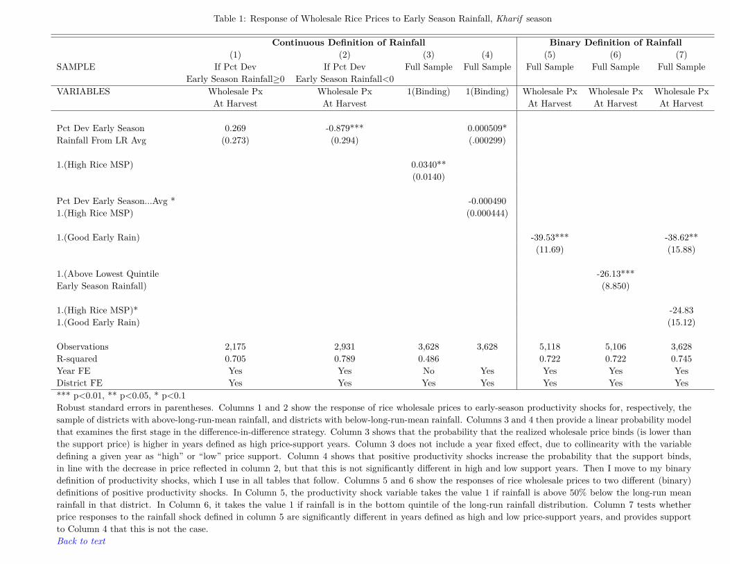
Table 1: Response of Wholesale Rice Prices to Early Season Rainfall, Kharif season

Continuous Definition of Rainfall Binary Definition of Rainfall(1) (2) (3) (4) (5) (6) (7)

SAMPLE If Pct Dev If Pct Dev Full Sample Full Sample Full Sample Full Sample Full SampleEarly Season Rainfall≥0 Early Season Rainfall<0

VARIABLES Wholesale Px Wholesale Px 1(Binding) 1(Binding) Wholesale Px Wholesale Px Wholesale PxAt Harvest At Harvest At Harvest At Harvest At Harvest

Pct Dev Early Season 0.269 -0.879*** 0.000509*Rainfall From LR Avg (0.273) (0.294) (.000299)

1.(High Rice MSP) 0.0340**(0.0140)

Pct Dev Early Season...Avg * -0.0004901.(High Rice MSP) (0.000444)

1.(Good Early Rain) -39.53*** -38.62**(11.69) (15.88)

1.(Above Lowest Quintile -26.13***Early Season Rainfall) (8.850)

1.(High Rice MSP)* -24.831.(Good Early Rain) (15.12)

Observations 2,175 2,931 3,628 3,628 5,118 5,106 3,628R-squared 0.705 0.789 0.486 0.722 0.722 0.745Year FE Yes Yes No Yes Yes Yes YesDistrict FE Yes Yes Yes Yes Yes Yes Yes*** p<0.01, ** p<0.05, * p<0.1Robust standard errors in parentheses. Columns 1 and 2 show the response of rice wholesale prices to early-season productivity shocks for, respectively, thesample of districts with above-long-run-mean rainfall, and districts with below-long-run-mean rainfall. Columns 3 and 4 then provide a linear probability modelthat examines the first stage in the difference-in-difference strategy. Column 3 shows that the probability that the realized wholesale price binds (is lower thanthe support price) is higher in years defined as high price-support years. Column 3 does not include a year fixed effect, due to collinearity with the variabledefining a given year as “high” or “low” price support. Column 4 shows that positive productivity shocks increase the probability that the support binds,in line with the decrease in price reflected in column 2, but that this is not significantly different in high and low support years. Then I move to my binarydefinition of productivity shocks, which I use in all tables that follow. Columns 5 and 6 show the responses of rice wholesale prices to two different (binary)definitions of positive productivity shocks. In Column 5, the productivity shock variable takes the value 1 if rainfall is above 50% below the long-run meanrainfall in that district. In Column 6, it takes the value 1 if rainfall is in the bottom quintile of the long-run rainfall distribution. Column 7 tests whetherprice responses to the rainfall shock defined in column 5 are significantly different in years defined as high and low price-support years, and provides supportto Column 4 that this is not the case.Back to text

41

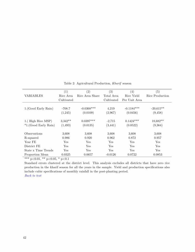
Table 2: Agricultural Production, Kharif season

(1) (2) (3) (4) (5)VARIABLES Rice Area Rice Area Share Total Area Rice Yield Rice Production

Cultivated Cultivated Per Unit Area

1.(Good Early Rain) -708.7 -0.0368*** 4,219 -0.1184*** -20,615**(1,245) (0.0109) (2,967) (0.0456) (9,458)

1.( High Rice MSP) 3,342** 0.0397*** -2,715 0.1424*** 18,682***1.(Good Early Rain) (1,493) (0.0135) (3,441) (0.0522) (9,364)

Observations 3,608 3,608 3,608 3,608 3,608R-squared 0.986 0.920 0.962 0.872 0.957Year FE Yes Yes Yes Yes YesDistrict FE Yes Yes Yes Yes YesState x Time Trends Yes Yes Yes Yes YesProportion Mean 0.0325 0.0657 -0.0126 0.0722 0.0853*** p<0.01, ** p<0.05, * p<0.1Standard errors clustered at the district level. This analysis excludes all districts that have zero riceproduction in the kharif season for all the years in the sample. Yield and production specifications alsoinclude cubic specifications of monthly rainfall in the post-planting period.Back to text

42

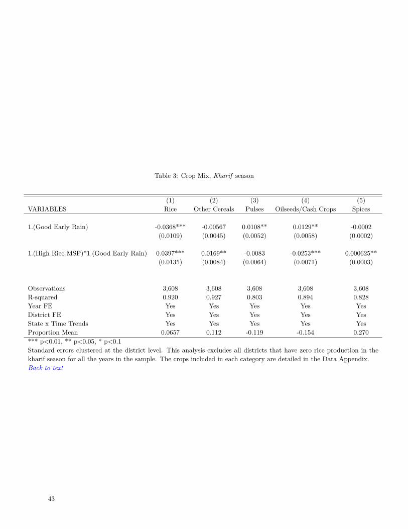
Table 3: Crop Mix, Kharif season

(1) (2) (3) (4) (5)VARIABLES Rice Other Cereals Pulses Oilseeds/Cash Crops Spices

1.(Good Early Rain) -0.0368*** -0.00567 0.0108** 0.0129** -0.0002(0.0109) (0.0045) (0.0052) (0.0058) (0.0002)

1.(High Rice MSP)*1.(Good Early Rain) 0.0397*** 0.0169** -0.0083 -0.0253*** 0.000625**(0.0135) (0.0084) (0.0064) (0.0071) (0.0003)

Observations 3,608 3,608 3,608 3,608 3,608R-squared 0.920 0.927 0.803 0.894 0.828Year FE Yes Yes Yes Yes YesDistrict FE Yes Yes Yes Yes YesState x Time Trends Yes Yes Yes Yes YesProportion Mean 0.0657 0.112 -0.119 -0.154 0.270*** p<0.01, ** p<0.05, * p<0.1Standard errors clustered at the district level. This analysis excludes all districts that have zero rice production in thekharif season for all the years in the sample. The crops included in each category are detailed in the Data Appendix.Back to text

43

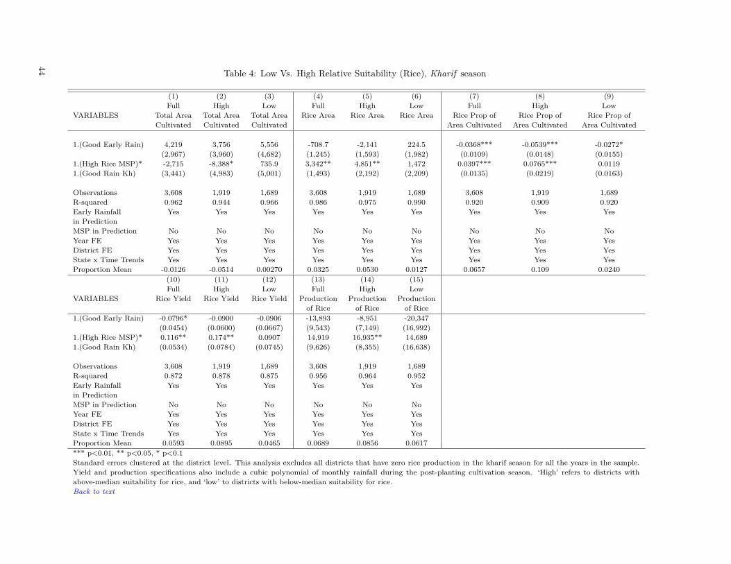
Table 4: Low Vs. High Relative Suitability (Rice), Kharif season

(1) (2) (3) (4) (5) (6) (7) (8) (9)Full High Low Full High Low Full High Low

VARIABLES Total Area Total Area Total Area Rice Area Rice Area Rice Area Rice Prop of Rice Prop of Rice Prop ofCultivated Cultivated Cultivated Area Cultivated Area Cultivated Area Cultivated

1.(Good Early Rain) 4,219 3,756 5,556 -708.7 -2,141 224.5 -0.0368*** -0.0539*** -0.0272*(2,967) (3,960) (4,682) (1,245) (1,593) (1,982) (0.0109) (0.0148) (0.0155)

1.(High Rice MSP)* -2,715 -8,388* 735.9 3,342** 4,851** 1,472 0.0397*** 0.0765*** 0.01191.(Good Rain Kh) (3,441) (4,983) (5,001) (1,493) (2,192) (2,209) (0.0135) (0.0219) (0.0163)

Observations 3,608 1,919 1,689 3,608 1,919 1,689 3,608 1,919 1,689R-squared 0.962 0.944 0.966 0.986 0.975 0.990 0.920 0.909 0.920Early Rainfall Yes Yes Yes Yes Yes Yes Yes Yes Yesin PredictionMSP in Prediction No No No No No No No No NoYear FE Yes Yes Yes Yes Yes Yes Yes Yes YesDistrict FE Yes Yes Yes Yes Yes Yes Yes Yes YesState x Time Trends Yes Yes Yes Yes Yes Yes Yes Yes YesProportion Mean -0.0126 -0.0514 0.00270 0.0325 0.0530 0.0127 0.0657 0.109 0.0240

(10) (11) (12) (13) (14) (15)Full High Low Full High Low

VARIABLES Rice Yield Rice Yield Rice Yield Production Production Productionof Rice of Rice of Rice

1.(Good Early Rain) -0.0796* -0.0900 -0.0906 -13,893 -8,951 -20,347(0.0454) (0.0600) (0.0667) (9,543) (7,149) (16,992)

1.(High Rice MSP)* 0.116** 0.174** 0.0907 14,919 16,935** 14,6891.(Good Rain Kh) (0.0534) (0.0784) (0.0745) (9,626) (8,355) (16,638)

Observations 3,608 1,919 1,689 3,608 1,919 1,689R-squared 0.872 0.878 0.875 0.956 0.964 0.952Early Rainfall Yes Yes Yes Yes Yes Yesin PredictionMSP in Prediction No No No No No NoYear FE Yes Yes Yes Yes Yes YesDistrict FE Yes Yes Yes Yes Yes YesState x Time Trends Yes Yes Yes Yes Yes YesProportion Mean 0.0593 0.0895 0.0465 0.0689 0.0856 0.0617*** p<0.01, ** p<0.05, * p<0.1Standard errors clustered at the district level. This analysis excludes all districts that have zero rice production in the kharif season for all the years in the sample.Yield and production specifications also include a cubic polynomial of monthly rainfall during the post-planting cultivation season. ‘High’ refers to districts withabove-median suitability for rice, and ‘low’ to districts with below-median suitability for rice.Back to text

44

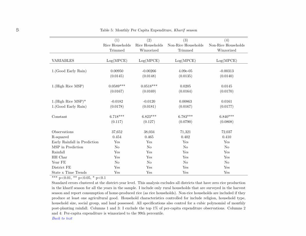
Table 5: Monthly Per Capita Expenditure, Kharif season

(1) (2) (3) (4)Rice Households Rice Households Non-Rice Households Non-Rice Households

Trimmed Winzorized Trimmed Winzorized

VARIABLES Log(MPCE) Log(MPCE) Log(MPCE) Log(MPCE)

1.(Good Early Rain) 0.00950 -0.00266 4.09e-05 -0.00313(0.0145) (0.0148) (0.0135) (0.0140)

1.(High Rice MSP) 0.0589*** 0.0518*** 0.0205 0.0145(0.0167) (0.0169) (0.0164) (0.0170)

1.(High Rice MSP)* -0.0182 -0.0120 0.00863 0.01611.(Good Early Rain) (0.0178) (0.0181) (0.0167) (0.0177)

Constant 6.718*** 6.823*** 6.783*** 6.840***(0.117) (0.127) (0.0790) (0.0808)

Observations 37,652 38,034 71,321 72,037R-squared 0.454 0.465 0.402 0.410Early Rainfall in Prediction Yes Yes Yes YesMSP in Prediction No No No NoRainfall Yes Yes Yes YesHH Char Yes Yes Yes YesYear FE No No No NoDistrict FE Yes Yes Yes YesState x Time Trends Yes Yes Yes Yes*** p<0.01, ** p<0.05, * p<0.1Standard errors clustered at the district-year level. This analysis excludes all districts that have zero rice productionin the kharif season for all the years in the sample. I include only rural households that are surveyed in the harvestseason and report consumption of home-produced rice (as rice households). Non-rice households are included if theyproduce at least one agricultural good. Household characteristics controlled for include religion, household type,household size, social group, and land possessed. All specifications also control for a cubic polynomial of monthlypost-planting rainfall. Columns 1 and 3: I exclude the top 1% of per-capita expenditure observations. Columns 2and 4: Per-capita expenditure is winzorized to the 99th percentile.Back to text

45

Table 6: Labor Market Responses to Price Supports, Kharif season

Agriculture Non-Agriculture Non-AgricultureASI Data

(1) (2) (3) (4) (5) (6) (7) (8) (9)VARIABLES 1.(Main Activity Agri Days Agri 1.(Main Activity Non-Agri NonAgri Total Contract Non-Contract

Agri) (of past week) Wage Non-Agri) Days Wage Days Days Days(of past week)

1.(Good Early Rain) -0.0641** -0.448** 10.34** 0.0783*** 0.548*** -25.07** 1,331 1,481 503.9(0.0273) (0.191) (4.88) (0.0248) (0.173) (12.51) (1,870) (2,413) (1,226)

1.(High Rice MSP)* 0.0735** 0.512** -9.91** -0.0800*** -0.561*** 30.56** -4,560** -5,617** -1,6091.(Good Early Rain) (0.0294) (0.205) (4.91) (0.0265) (0.185) (13.90) (2,155) (2,738) (1,205)

Observations 72,614 72,619 16,261 72,614 72,619 13,867 98,774 36,791 88,713R-squared 0.251 0.250 0.514 0.228 0.228 0.442 0.191 0.166 0.188Early Rainfall Yes Yes Yes Yes Yes Yes Yes Yes Yesin PredictionMSP in Prediction No No No No No No No No NoYear FE Yes Yes Yes Yes Yes Yes Yes Yes YesDistrict FE Yes Yes Yes Yes Yes Yes Yes Yes YesState x Time Trends Yes Yes Yes Yes Yes Yes Yes Yes YesProportion Mean 0.0982 0.0978 -0.206 -0.357 -0.358 0.230 -0.0940 -0.178 -0.0525*** p<0.01, ** p<0.05, * p<0.1Standard errors clustered at the district level. This analysis excludes all districts that have zero rice production in the kharif season for all the years in thesample. Columns 1-6 consider labor market outcomes from the NSS household survey of employment. I include only agricultural households in the ruralsample that are surveyed in the kharif cultivation season, and individuals who have indicated they have worked or searched for work in the past week.Standard individual and household controls - household size, household type, land possessed, social group, age, sex, education, religion and marital status-are included in all specifications. I also include cubic polynomials of monthly rainfall throughout the cultivation period. Wage regressions are restrictedto individuals with non-zero wages. Columns 7-9 consider labor use in firms (both formal and informal) in the Annual Survey of Industries data. Column(7) considers total manufacturing days, while columns (8) and (9) consider permanent and contracted workers separately. The ASI analysis includes onlyopen firms operating in the rural sector. It also includes a vector of firm-level controls, including industry, ownership, age, age squared, organization type,and number of plants.Back to text

46

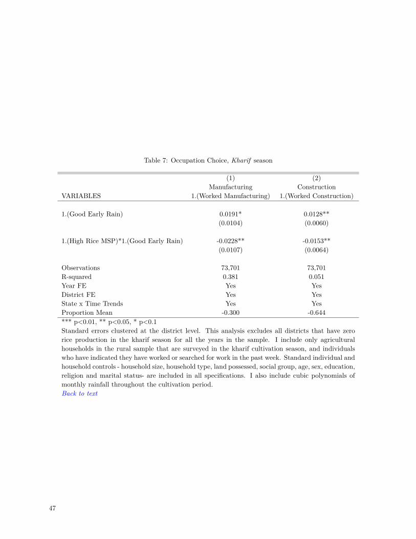
Table 7: Occupation Choice, Kharif season

(1) (2)Manufacturing Construction

VARIABLES 1.(Worked Manufacturing) 1.(Worked Construction)

1.(Good Early Rain) 0.0191* 0.0128**(0.0104) (0.0060)

1.(High Rice MSP)*1.(Good Early Rain) -0.0228** -0.0153**(0.0107) (0.0064)

Observations 73,701 73,701R-squared 0.381 0.051Year FE Yes YesDistrict FE Yes YesState x Time Trends Yes YesProportion Mean -0.300 -0.644*** p<0.01, ** p<0.05, * p<0.1Standard errors clustered at the district level. This analysis excludes all districts that have zerorice production in the kharif season for all the years in the sample. I include only agriculturalhouseholds in the rural sample that are surveyed in the kharif cultivation season, and individualswho have indicated they have worked or searched for work in the past week. Standard individual andhousehold controls - household size, household type, land possessed, social group, age, sex, education,religion and marital status- are included in all specifications. I also include cubic polynomials ofmonthly rainfall throughout the cultivation period.Back to text

47

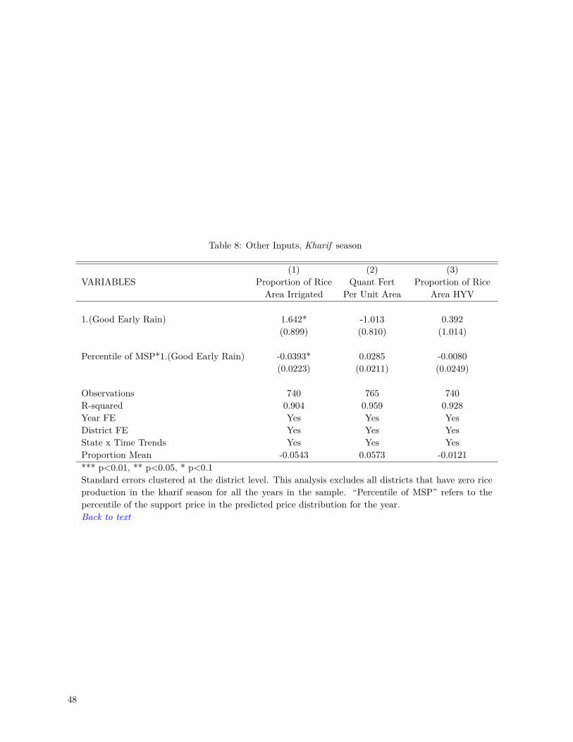
Table 8: Other Inputs, Kharif season

(1) (2) (3)VARIABLES Proportion of Rice Quant Fert Proportion of Rice

Area Irrigated Per Unit Area Area HYV

1.(Good Early Rain) 1.642* -1.013 0.392(0.899) (0.810) (1.014)

Percentile of MSP*1.(Good Early Rain) -0.0393* 0.0285 -0.0080(0.0223) (0.0211) (0.0249)

Observations 740 765 740R-squared 0.904 0.959 0.928Year FE Yes Yes YesDistrict FE Yes Yes YesState x Time Trends Yes Yes YesProportion Mean -0.0543 0.0573 -0.0121*** p<0.01, ** p<0.05, * p<0.1Standard errors clustered at the district level. This analysis excludes all districts that have zero riceproduction in the kharif season for all the years in the sample. “Percentile of MSP” refers to thepercentile of the support price in the predicted price distribution for the year.Back to text

48

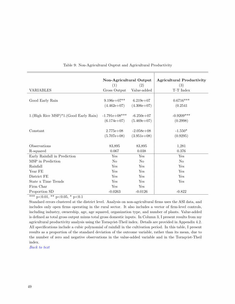
Table 9: Non-Agricultural Ouptut and Agricultural Productivity

Non-Agricultural Output Agricultural Productivity(1) (2) (3)

VARIABLES Gross Output Value-added T-T Index

Good Early Rain 9.196e+07** 6.219e+07 0.6716***(4.462e+07) (4.306e+07) (0.2541

1.(High Rice MSP)*1.(Good Early Rain) -1.791e+08*** -6.250e+07 -0.9209***(6.174e+07) (5.469e+07) (0.2998)

Constant 2.775e+08 -2.058e+08 -1.550*(5.707e+08) (3.951e+08) (0.9295)

Observations 83,895 83,895 1,281R-squared 0.067 0.038 0.376Early Rainfall in Prediction Yes Yes YesMSP in Prediction No No NoRainfall Yes Yes YesYear FE Yes Yes YesDistrict FE Yes Yes YesState x Time Trends Yes Yes YesFirm Char Yes YesProportion SD -0.0263 -0.0126 -0.822*** p<0.01, ** p<0.05, * p<0.1Standard errors clustered at the district level. Analysis on non-agricultural firms uses the ASI data, andincludes only open firms operating in the rural sector. It also includes a vector of firm-level controls,including industry, ownership, age, age squared, organization type, and number of plants. Value-addedis defined as total gross output minus total gross domestic inputs. In Column 3, I present results from myagricultural productivity analysis using the Tornqvist-Theil index. Details are provided in Appendix 4.2.All specifications include a cubic polynomial of rainfall in the cultivation period. In this table, I presentresults as a proportion of the standard deviation of the outcome variable, rather than its mean, due tothe number of zero and negative observations in the value-added variable and in the Tornqvist-Theilindex.Back to text

49

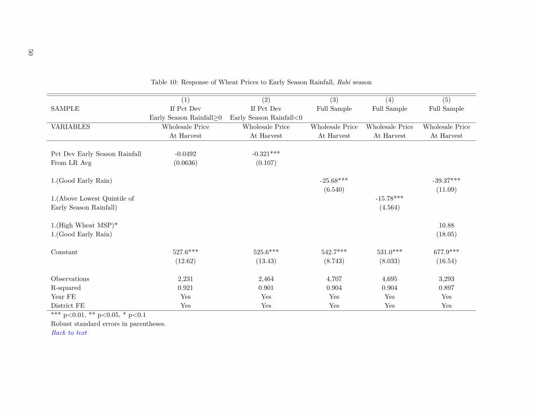
Table 10: Response of Wheat Prices to Early Season Rainfall, Rabi season

(1) (2) (3) (4) (5)SAMPLE If Pct Dev If Pct Dev Full Sample Full Sample Full Sample

Early Season Rainfall≥0 Early Season Rainfall<0VARIABLES Wholesale Price Wholesale Price Wholesale Price Wholesale Price Wholesale Price

At Harvest At Harvest At Harvest At Harvest At Harvest

Pct Dev Early Season Rainfall -0.0492 -0.321***From LR Avg (0.0636) (0.107)

1.(Good Early Rain) -25.68*** -39.37***(6.540) (11.09)

1.(Above Lowest Quintile of -15.78***Early Season Rainfall) (4.564)

1.(High Wheat MSP)* 10.881.(Good Early Rain) (18.05)

Constant 527.6*** 525.6*** 542.7*** 531.0*** 677.9***(12.62) (13.43) (8.743) (8.033) (16.54)

Observations 2,231 2,464 4,707 4,695 3,293R-squared 0.921 0.901 0.904 0.904 0.897Year FE Yes Yes Yes Yes YesDistrict FE Yes Yes Yes Yes Yes*** p<0.01, ** p<0.05, * p<0.1Robust standard errors in parentheses.Back to text

50

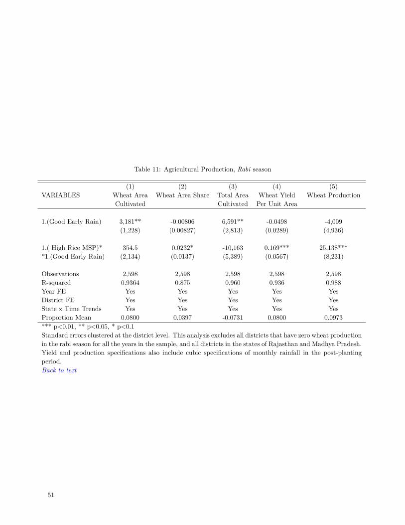
Table 11: Agricultural Production, Rabi season

(1) (2) (3) (4) (5)VARIABLES Wheat Area Wheat Area Share Total Area Wheat Yield Wheat Production

Cultivated Cultivated Per Unit Area

1.(Good Early Rain) 3,181** -0.00806 6,591** -0.0498 -4,009(1,228) (0.00827) (2,813) (0.0289) (4,936)

1.( High Rice MSP)* 354.5 0.0232* -10,163 0.169*** 25,138****1.(Good Early Rain) (2,134) (0.0137) (5,389) (0.0567) (8,231)

Observations 2,598 2,598 2,598 2,598 2,598R-squared 0.9364 0.875 0.960 0.936 0.988Year FE Yes Yes Yes Yes YesDistrict FE Yes Yes Yes Yes YesState x Time Trends Yes Yes Yes Yes YesProportion Mean 0.0800 0.0397 -0.0731 0.0800 0.0973*** p<0.01, ** p<0.05, * p<0.1Standard errors clustered at the district level. This analysis excludes all districts that have zero wheat productionin the rabi season for all the years in the sample, and all districts in the states of Rajasthan and Madhya Pradesh.Yield and production specifications also include cubic specifications of monthly rainfall in the post-plantingperiod.Back to text

51

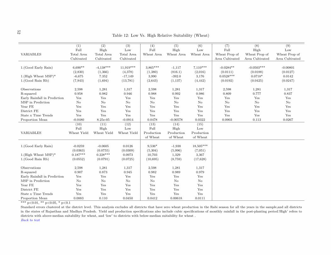
Table 12: Low Vs. High Relative Suitability (Wheat)

(1) (2) (3) (4) (5) (6) (7) (8) (9)Full High Low Full High Low Full High Low

VARIABLES Total Area Total Area Total Area Wheat Area Wheat Area Wheat Area Wheat Prop of Wheat Prop of Wheat Prop ofCultivated Cultivated Cultivated Area Cultivated Area Cultivated Area Cultivated

1.(Good Early Rain) 6,690** -4,138*** 11,919*** 3,865*** -1,117 7,110*** -0.0284** -0.0503*** -0.00801(2,830) (1,366) (4,378) (1,380) (816.1) (2,016) (0.0111) (0.0188) (0.0127)

1.(High Wheat MSP)* -6,675 7.352 -17,149 3,990 -392.0 3,176 0.0528*** 0.0718* 0.01421.(Good Rain Rb) (7,943) (1,694) (13,781) (2,643) (1,137) (4,442) (0.0192) (0.0425) (0.0247)

Observations 2,598 1,281 1,317 2,598 1,281 1,317 2,598 1,281 1,317R-squared 0.958 0.982 0.946 0.988 0.992 0.986 0.809 0.777 0.837Early Rainfall in Prediction Yes Yes Yes Yes Yes Yes Yes Yes YesMSP in Prediction No No No No No No No No NoYear FE Yes Yes Yes Yes Yes Yes Yes Yes YesDistrict FE Yes Yes Yes Yes Yes Yes Yes Yes YesState x Time Trends Yes Yes Yes Yes Yes Yes Yes Yes YesProportion Mean -0.0480 8.25e-05 -0.0914 0.0478 -0.00578 0.0322 0.0903 0.113 0.0267

(10) (11) (12) (13) (14) (15)Full High Low Full High Low

VARIABLES Wheat Yield Wheat Yield Wheat Yield Production Production Productionof Wheat of Wheat of Wheat

1.(Good Early Rain) -0.0259 -0.0605 0.0126 9,536* -1,938 18,505***(0.0363) (0.0755) (0.0309) (5,304) (5,996) (7,051)

1.(High Wheat MSP)* 0.187*** 0.228*** 0.0973 10,703 1,329 3,3671.(Good Rain Rb) (0.0552) (0.0791) (0.0725) (10,695) (8,759) (17,628)

Observations 2,598 1,281 1,317 2,598 1,281 1,317R-squared 0.907 0.873 0.945 0.982 0.989 0.979Early Rainfall in Prediction Yes Yes Yes Yes Yes YesMSP in Prediction No No No No No NoYear FE Yes Yes Yes Yes Yes YesDistrict FE Yes Yes Yes Yes Yes YesState x Time Trends Yes Yes Yes Yes Yes YesProportion Mean 0.0883 0.110 0.0450 0.0412 0.00618 0.0111*** p<0.01, ** p<0.05, * p<0.1Standard errors clustered at the district level. This analysis excludes all districts that have zero wheat production in the Rabi season for all the years in the sample,and all districtsin the states of Rajasthan and Madhya Pradesh. Yield and production specifications also include cubic specifications of monthly rainfall in the post-planting period.‘High’ refers todistricts with above-median suitability for wheat, and ‘low’ to districts with below-median suitability for wheat .Back to text

52

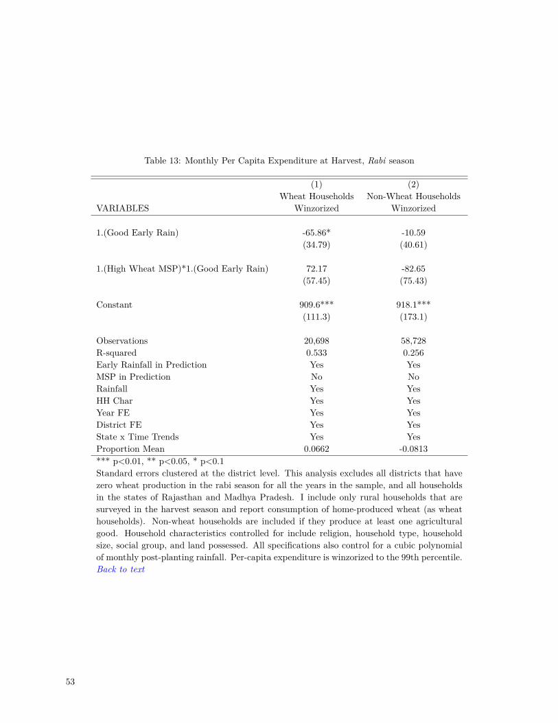
Table 13: Monthly Per Capita Expenditure at Harvest, Rabi season

(1) (2)Wheat Households Non-Wheat Households

VARIABLES Winzorized Winzorized

1.(Good Early Rain) -65.86* -10.59(34.79) (40.61)

1.(High Wheat MSP)*1.(Good Early Rain) 72.17 -82.65(57.45) (75.43)

Constant 909.6*** 918.1***(111.3) (173.1)

Observations 20,698 58,728R-squared 0.533 0.256Early Rainfall in Prediction Yes YesMSP in Prediction No NoRainfall Yes YesHH Char Yes YesYear FE Yes YesDistrict FE Yes YesState x Time Trends Yes YesProportion Mean 0.0662 -0.0813*** p<0.01, ** p<0.05, * p<0.1Standard errors clustered at the district level. This analysis excludes all districts that havezero wheat production in the rabi season for all the years in the sample, and all householdsin the states of Rajasthan and Madhya Pradesh. I include only rural households that aresurveyed in the harvest season and report consumption of home-produced wheat (as wheathouseholds). Non-wheat households are included if they produce at least one agriculturalgood. Household characteristics controlled for include religion, household type, householdsize, social group, and land possessed. All specifications also control for a cubic polynomialof monthly post-planting rainfall. Per-capita expenditure is winzorized to the 99th percentile.Back to text

53

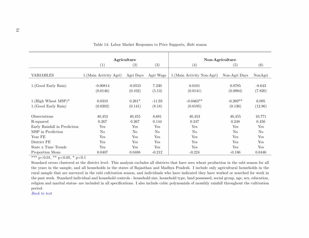
Table 14: Labor Market Responses to Price Supports, Rabi season

Agriculture Non-Agriculture(1) (2) (3) (4) (5) (6)

VARIABLES 1.(Main Activity Agri) Agri Days Agri Wage 1.(Main Activity Non-Agri) Non-Agri Days NonAgri

1.(Good Early Rain) -0.00814 -0.0555 7.230 0.0101 0.0785 -8.643(0.0146) (0.102) (5.13) (0.0141) (0.0984) (7.820)

1.(High Wheat MSP)* 0.0310 0.261* -11.93 -0.0463** -0.269** 6.0951.(Good Early Rain) (0.0202) (0.141) (8.18) (0.0195) (0.136) (12.86)

Observations 40,453 40,455 8,681 40,453 40,455 10,771R-squared 0.267 0.267 0.144 0.247 0.248 0.456Early Rainfall in Prediction Yes Yes Yes Yes Yes YesMSP in Prediction No No No No No NoYear FE Yes Yes Yes Yes Yes YesDistrict FE Yes Yes Yes Yes Yes YesState x Time Trends Yes Yes Yes Yes Yes YesProportion Mean 0.0407 0.0488 -0.212 -0.224 -0.186 0.0446*** p<0.01, ** p<0.05, * p<0.1Standard errors clustered at the district level. This analysis excludes all districts that have zero wheat production in the rabi season for allthe years in the sample, and all households in the states of Rajasthan and Madhya Pradesh. I include only agricultural households in therural sample that are surveyed in the rabi cultivation season, and individuals who have indicated they have worked or searched for work inthe past week. Standard individual and household controls - household size, household type, land possessed, social group, age, sex, education,religion and marital status- are included in all specifications. I also include cubic polynomials of monthly rainfall throughout the cultivationperiod.Back to text

54

A1 Robustness Checks

Figure A1.1: MSPs for rice (Kharif season) and wheat (Rabi season) plotted against early-season rainfall across thecountry between 1997 and 2012.Note: Early-season rainfall is weighted by area cultivated in that season in a given district. Year t refers tothe planting season t,t+1. For example, 2012 refers to the 2012-2013 season.

Figure A1.2: Change in MSPs for rice (Kharif season) and wheat (Rabi season) plotted against early-seasonrainfall across the country between 1997 and 2012.Note: Early-season rainfall is weighted by area cultivated in that season in a given district. Year t refers tothe planting season t,t+1. For example, 2012 refers to the 2012-2013 season.

[Regression Tests of Aggregate Rainfall and Price Supports: Table A1.1]

55

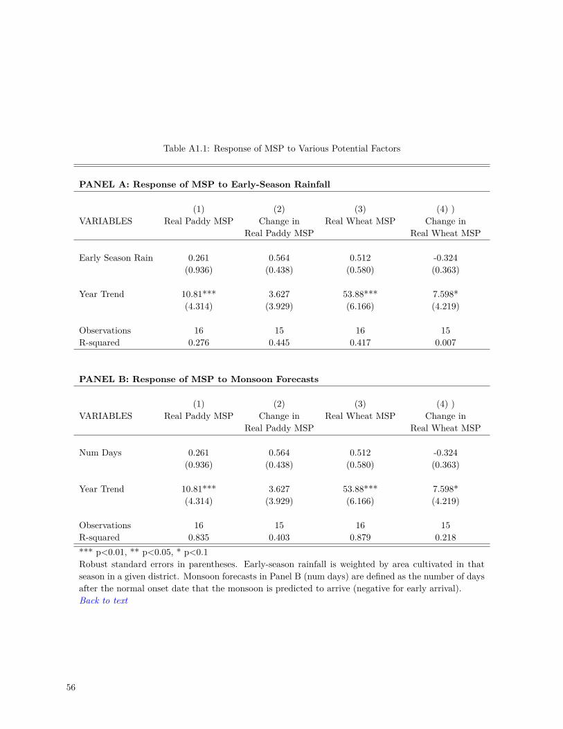
Table A1.1: Response of MSP to Various Potential Factors

PANEL A: Response of MSP to Early-Season Rainfall

(1) (2) (3) (4) )VARIABLES Real Paddy MSP Change in Real Wheat MSP Change in

Real Paddy MSP Real Wheat MSP

Early Season Rain 0.261 0.564 0.512 -0.324(0.936) (0.438) (0.580) (0.363)

Year Trend 10.81*** 3.627 53.88*** 7.598*(4.314) (3.929) (6.166) (4.219)

Observations 16 15 16 15R-squared 0.276 0.445 0.417 0.007

PANEL B: Response of MSP to Monsoon Forecasts

(1) (2) (3) (4) )VARIABLES Real Paddy MSP Change in Real Wheat MSP Change in

Real Paddy MSP Real Wheat MSP

Num Days 0.261 0.564 0.512 -0.324(0.936) (0.438) (0.580) (0.363)

Year Trend 10.81*** 3.627 53.88*** 7.598*(4.314) (3.929) (6.166) (4.219)

Observations 16 15 16 15R-squared 0.835 0.403 0.879 0.218*** p<0.01, ** p<0.05, * p<0.1Robust standard errors in parentheses. Early-season rainfall is weighted by area cultivated in thatseason in a given district. Monsoon forecasts in Panel B (num days) are defined as the number of daysafter the normal onset date that the monsoon is predicted to arrive (negative for early arrival).Back to text

56

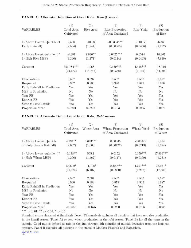
Table A1.2: Staple Production Response to Alternate Definition of Good Rain

PANEL A: Alternate Definition of Good Rain, Kharif season

(1) (2) (3) (4) (5)VARIABLES Total Area Rice Area Rice Proportion Rice Yield Production

Cultivated of Area Cultivated of Rice

1.(Above Lowest Quintile of 2,588 -400.8 -0.0304*** -0.0117 -6,336Early Rainfall) (2,564) (1,244) (0.00883) (0.0406) (7,702)

1.(Above lowest quintile...)* -4,387 2,636** 0.0425*** 0.0574 10,2671.(High Rice MSP) (3,246) (1,271) (0.0114) (0.0465) (7,840)

Constant 351,784*** 1,068 0.139*** 1.448*** -78,719(24,173) (14,747) (0.0338) (0.199) (54,006)

Observations 3,597 3,597 3,597 3,597 3,597R-squared 0.962 0.986 0.920 0.871 0.956Early Rainfall in Prediction Yes Yes Yes Yes YesMSP in Prediction No No No No NoYear FE Yes Yes Yes Yes YesDistrict FE Yes Yes Yes Yes YesState x Time Trends Yes Yes Yes Yes YesProportion Mean -0.0204 0.0257 0.0703 0.0295 0.0475

PANEL B: Alternate Definition of Good Rain, Rabi season

(1) (2) (3) (4) (5)VARIABLES Total Area Wheat Area Wheat Proportion Wheat Yield Production

Cultivated of Area Cultivated of Wheat

1.(Above Lowest Quintile 4,394** 3,643*** 0.00843 -0.00377 5,534of Early Season Rainfall) (2,007) (1,063) (0.00727) (0.0213) (3,394)

1.(Above lowest quintile...)* -9,138** 565.1 0.0152 0.150*** 17,909***1.(High Wheat MSP) (4,296) (1,562) (0.0117) (0.0369) (5,231)

Constant 58,602* -11,108* -0.300*** 1.227*** 33,031*(31,325) (6,107) (0.0860) (0.292) (17,889)

Observations 2,587 2,587 2,587 2,587 2,587R-squared 0.960 0.989 0.875 0.935 0.987Early Rainfall in Prediction Yes Yes Yes Yes YesMSP in Prediction No No No No NoYear FE Yes Yes Yes Yes YesDistrict FE Yes Yes Yes Yes YesState x Time Trends Yes Yes Yes Yes YesProportion Mean -0.0656 0.00675 0.0260 0.0706 0.0688*** p<0.01, ** p<0.05, * p<0.1Standard errors clustered at the district level. This analysis excludes all districts that have zero rice productionin the kharif season (Panel A) or zero wheat production in the rabi season (Panel B) for all the years in thesample. Good rain is defined as rain in the 2nd through 5th quintiles of rainfall deviation from the long-runaverage. Panel B excludes all districts in the states of Madhya Pradesh and Rajasthan.Back to text57

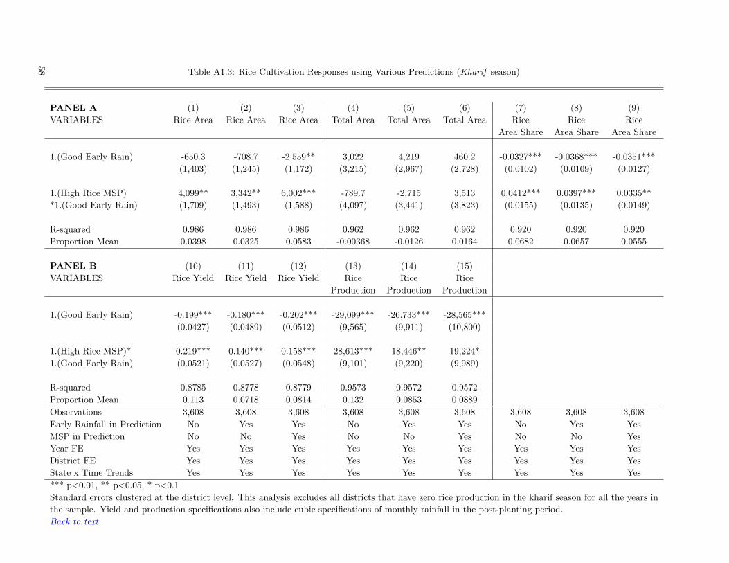
Table A1.3: Rice Cultivation Responses using Various Predictions (Kharif season)

PANEL A (1) (2) (3) (4) (5) (6) (7) (8) (9)VARIABLES Rice Area Rice Area Rice Area Total Area Total Area Total Area Rice Rice Rice

Area Share Area Share Area Share

1.(Good Early Rain) -650.3 -708.7 -2,559** 3,022 4,219 460.2 -0.0327*** -0.0368*** -0.0351***(1,403) (1,245) (1,172) (3,215) (2,967) (2,728) (0.0102) (0.0109) (0.0127)

1.(High Rice MSP) 4,099** 3,342** 6,002*** -789.7 -2,715 3,513 0.0412*** 0.0397*** 0.0335***1.(Good Early Rain) (1,709) (1,493) (1,588) (4,097) (3,441) (3,823) (0.0155) (0.0135) (0.0149)

R-squared 0.986 0.986 0.986 0.962 0.962 0.962 0.920 0.920 0.920Proportion Mean 0.0398 0.0325 0.0583 -0.00368 -0.0126 0.0164 0.0682 0.0657 0.0555

PANEL B (10) (11) (12) (13) (14) (15)VARIABLES Rice Yield Rice Yield Rice Yield Rice Rice Rice

Production Production Production

1.(Good Early Rain) -0.199*** -0.180*** -0.202*** -29,099*** -26,733*** -28,565***(0.0427) (0.0489) (0.0512) (9,565) (9,911) (10,800)

1.(High Rice MSP)* 0.219*** 0.140*** 0.158*** 28,613*** 18,446** 19,224*1.(Good Early Rain) (0.0521) (0.0527) (0.0548) (9,101) (9,220) (9,989)

R-squared 0.8785 0.8778 0.8779 0.9573 0.9572 0.9572Proportion Mean 0.113 0.0718 0.0814 0.132 0.0853 0.0889Observations 3,608 3,608 3,608 3,608 3,608 3,608 3,608 3,608 3,608Early Rainfall in Prediction No Yes Yes No Yes Yes No Yes YesMSP in Prediction No No Yes No No Yes No No YesYear FE Yes Yes Yes Yes Yes Yes Yes Yes YesDistrict FE Yes Yes Yes Yes Yes Yes Yes Yes YesState x Time Trends Yes Yes Yes Yes Yes Yes Yes Yes Yes*** p<0.01, ** p<0.05, * p<0.1Standard errors clustered at the district level. This analysis excludes all districts that have zero rice production in the kharif season for all the years inthe sample. Yield and production specifications also include cubic specifications of monthly rainfall in the post-planting period.Back to text

58

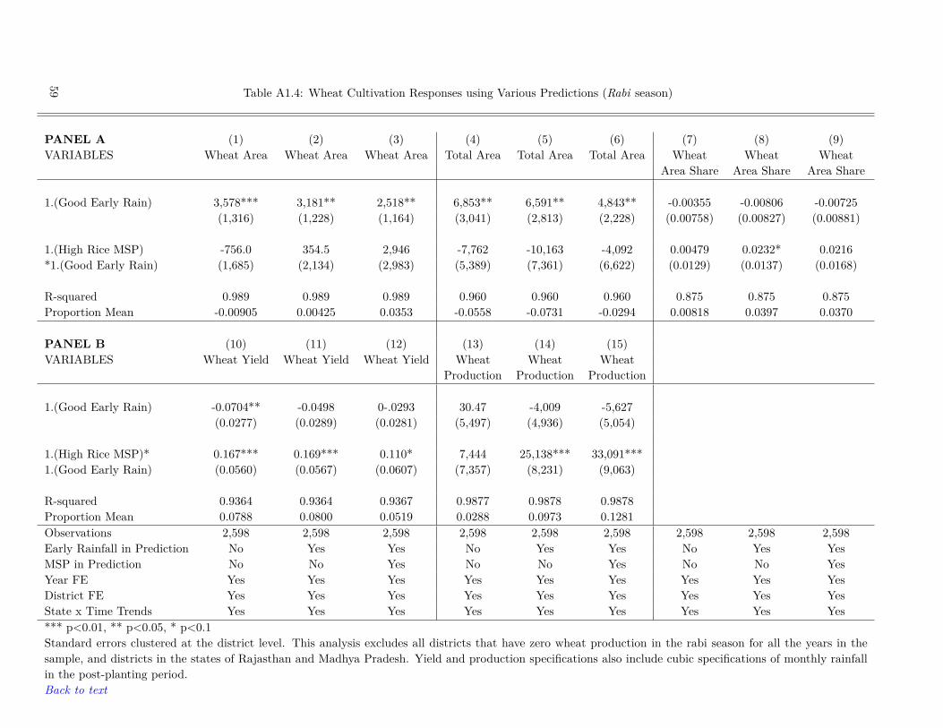
Table A1.4: Wheat Cultivation Responses using Various Predictions (Rabi season)

PANEL A (1) (2) (3) (4) (5) (6) (7) (8) (9)VARIABLES Wheat Area Wheat Area Wheat Area Total Area Total Area Total Area Wheat Wheat Wheat

Area Share Area Share Area Share

1.(Good Early Rain) 3,578*** 3,181** 2,518** 6,853** 6,591** 4,843** -0.00355 -0.00806 -0.00725(1,316) (1,228) (1,164) (3,041) (2,813) (2,228) (0.00758) (0.00827) (0.00881)

1.(High Rice MSP) -756.0 354.5 2,946 -7,762 -10,163 -4,092 0.00479 0.0232* 0.0216*1.(Good Early Rain) (1,685) (2,134) (2,983) (5,389) (7,361) (6,622) (0.0129) (0.0137) (0.0168)

R-squared 0.989 0.989 0.989 0.960 0.960 0.960 0.875 0.875 0.875Proportion Mean -0.00905 0.00425 0.0353 -0.0558 -0.0731 -0.0294 0.00818 0.0397 0.0370

PANEL B (10) (11) (12) (13) (14) (15)VARIABLES Wheat Yield Wheat Yield Wheat Yield Wheat Wheat Wheat

Production Production Production

1.(Good Early Rain) -0.0704** -0.0498 0-.0293 30.47 -4,009 -5,627(0.0277) (0.0289) (0.0281) (5,497) (4,936) (5,054)

1.(High Rice MSP)* 0.167*** 0.169*** 0.110* 7,444 25,138*** 33,091***1.(Good Early Rain) (0.0560) (0.0567) (0.0607) (7,357) (8,231) (9,063)

R-squared 0.9364 0.9364 0.9367 0.9877 0.9878 0.9878Proportion Mean 0.0788 0.0800 0.0519 0.0288 0.0973 0.1281Observations 2,598 2,598 2,598 2,598 2,598 2,598 2,598 2,598 2,598Early Rainfall in Prediction No Yes Yes No Yes Yes No Yes YesMSP in Prediction No No Yes No No Yes No No YesYear FE Yes Yes Yes Yes Yes Yes Yes Yes YesDistrict FE Yes Yes Yes Yes Yes Yes Yes Yes YesState x Time Trends Yes Yes Yes Yes Yes Yes Yes Yes Yes*** p<0.01, ** p<0.05, * p<0.1Standard errors clustered at the district level. This analysis excludes all districts that have zero wheat production in the rabi season for all the years in thesample, and districts in the states of Rajasthan and Madhya Pradesh. Yield and production specifications also include cubic specifications of monthly rainfallin the post-planting period.Back to text

59

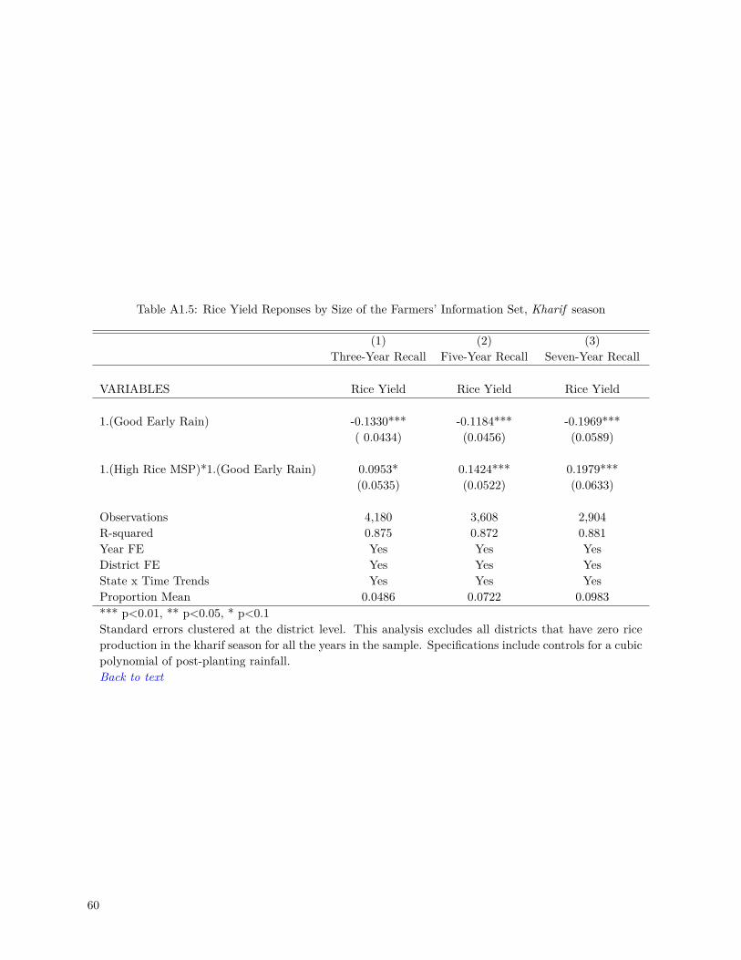
Table A1.5: Rice Yield Reponses by Size of the Farmers’ Information Set, Kharif season

(1) (2) (3)Three-Year Recall Five-Year Recall Seven-Year Recall

VARIABLES Rice Yield Rice Yield Rice Yield

1.(Good Early Rain) -0.1330*** -0.1184*** -0.1969***( 0.0434) (0.0456) (0.0589)

1.(High Rice MSP)*1.(Good Early Rain) 0.0953* 0.1424*** 0.1979***(0.0535) (0.0522) (0.0633)

Observations 4,180 3,608 2,904R-squared 0.875 0.872 0.881Year FE Yes Yes YesDistrict FE Yes Yes YesState x Time Trends Yes Yes YesProportion Mean 0.0486 0.0722 0.0983*** p<0.01, ** p<0.05, * p<0.1Standard errors clustered at the district level. This analysis excludes all districts that have zero riceproduction in the kharif season for all the years in the sample. Specifications include controls for a cubicpolynomial of post-planting rainfall.Back to text

60

Figure A1.3: Variation over time in real MSP, weighted mean real price, and real export price of common rice fromIndia

Figure A1.4: Amount of common rice exported from India

Back to text

61

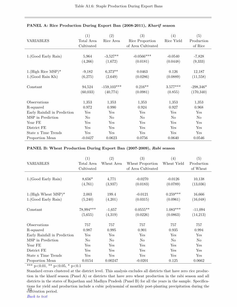
Table A1.6: Staple Production During Export Bans

PANEL A: Rice Production During Export Ban (2008-2011), Kharif season

(1) (2) (3) (4) (5)VARIABLES Total Area Rice Area Rice Proportion Rice Yield Production

Cultivated of Area Cultivated of Rice

1.(Good Early Rain) 5,964 -3,527** -0.0566*** -0.0540 -7,828(4,266) (1,672) (0.0181) (0.0448) (9,333)

1.(High Rice MSP)* -9,182 6,373** 0.0463 0.126 12,1871.(Good Rain Kh) (6,275) (2,649) (0.0286) (0.0889) (11,558)

Constant 94,524 -159,103*** 0.216** 3.577*** -298,346*(60,033) (40,774) (0.0981) (0.855) (170,340)

Observations 1,353 1,353 1,353 1,353 1,353R-squared 0.972 0.990 0.924 0.927 0.968Early Rainfall in Prediction Yes Yes Yes Yes YesMSP in Prediction No No No No NoYear FE Yes Yes Yes Yes YesDistrict FE Yes Yes Yes Yes YesState x Time Trends Yes Yes Yes Yes YesProportion Mean -0.0427 0.0623 0.0756 0.0640 0.0546

PANEL B: Wheat Production During Export Ban (2007-2009), Rabi season

(1) (2) (3) (4) (5)VARIABLES Total Area Wheat Area Wheat Proportion Wheat Yield Production

Cultivated of Area Cultivated of Wheat

1.(Good Early Rain) 8,656* 4,771 -0.0270 -0.0126 10,138(4,761) (3,937) (0.0183) (0.0789) (13,036)

1.(High Wheat MSP)* 2,003 199.4 -0.0121 0.259*** 16,6661.(Good Early Rain) (5,240) (4,201) (0.0315) (0.0961) (16,048)

Constant 78,994*** -1,657 0.0555** 1.083*** -11,094(5,655) (4,319) (0.0226) (0.0863) (14,213)

Observations 757 757 757 757 757R-squared 0.987 0.995 0.901 0.935 0.994Early Rainfall in Prediction Yes Yes Yes Yes YesMSP in Prediction No No No No NoYear FE Yes Yes Yes Yes YesDistrict FE Yes Yes Yes Yes YesState x Time Trends Yes Yes Yes Yes YesProportion Mean 0.0154 0.00247 -0.0201 0.125 0.0662*** p<0.01, ** p<0.05, * p<0.1Standard errors clustered at the district level. This analysis excludes all districts that have zero rice produc-tion in the kharif season (Panel A) or districts that have zero wheat production in the rabi season and alldistricts in the states of Rajasthan and Madhya Pradesh (Panel B) for all the years in the sample. Specifica-tions for yield and production include a cubic polynomial of monthly post-planting precipitation during thecultivation period.Back to text

62

Table A1.7: Tests on Various Subsamples of Wheat-Producing Districts

(1) (2) (3) (4) (5) (6) (7) (8) (9) (10) (11) (12)Test1a Test1b Test1c Test1d Test2a Test2b Test2c Test2d Test3a Test3b Test3c Test3d

VARIABLES WheatArea

TotalArea

WheatYield

Production WheatArea

TotalArea

WheatYield

Production WheatArea

TotalArea

WheatYield

Production

Cultivated of Wheat Cultivated of Wheat Cultivated Wheat

1.(Good Early Rain) 576.2 1,021 -0.0793** -8,774* 6,143** 2,290 -0.138*** 5,743 1,392 -1,127 -0.133* -18,195(994.6) (2,465) (0.0323) (4,687) (2,509) (3,042) (0.0499) (8,616) (3,455) (5,322) (0.0778) (16,531)

1.(High Wheat MSP)* 3,148 7,036 0.240*** 34,140*** -614.3 -1,425 0.361*** 23,097 81.64 -4,269 0.307** 31,5691.(Good Rain Rb) (2,708) (6,801) (0.0548) (11,590) (3,274) (4,488) (0.0996) (14,248) (4,905) (7,975) (0.122) (25,225)

Observations 1,403 1,403 1,403 1,403 522 522 522 522 279 279 279 279R-squared 0.990 0.977 0.942 0.987 0.986 0.987 0.954 0.981 0.990 0.992 0.964 0.985Early Rainfall in Prediction Yes Yes Yes Yes Yes Yes Yes Yes Yes Yes Yes YesMSP in Prediction No No No No No No No No No No No NoYear FE Yes Yes Yes Yes Yes Yes Yes Yes Yes Yes Yes YesDistrict FE Yes Yes Yes Yes Yes Yes Yes Yes Yes Yes Yes YesState x Time Trends Yes Yes Yes Yes Yes Yes Yes Yes Yes Yes Yes Yes

(13) (14) (15) (16) (17) (18) (19) (20)Test4a Test4b Test4c Test4d Test5a Test5b Test5c Test5d

VARIABLES WheatArea

TotalArea

WheatYield

Production WheatArea

TotalArea

WheatYield

Production

Cultivated of Wheat Cultivated of Wheat

1.(Good Early Rain) 3,986*** 8,629** -0.0201 5,147 -388.7 -5,729 0.0637 -1,202(1,497) (3,460) (0.0253) (5,204) (2,003) (3,569) (0.0741) (9,699)

1.(High Wheat MSP)* 964.3 -10,677 0.225*** 26,157*** -1,053 -1,593 -0.00319 10,8481.(Good Rain Rb) (2,529) (8,792) (0.0519) (9,827) (4,102) (5,554) (0.132) (19,304)

Observations 1,773 1,773 1,773 1,773 658 658 658 658R-squared 0.987 0.943 0.929 0.985 0.997 0.991 0.954 0.994Early Rainfall in Prediction Yes Yes Yes Yes Yes Yes Yes YesMSP in Prediction No No No No No No No NoYear FE Yes Yes Yes Yes Yes Yes Yes YesDistrict FE Yes Yes Yes Yes Yes Yes Yes YesState x Time Trends Yes Yes Yes Yes Yes Yes Yes Yes*** p<0.01, ** p<0.05, * p<0.1Standard errors clustered at the district level. This analysis excludes all districts that have zero wheat production in the rabi season for all the years in the sample. Test 1: Restrictingto years in which the rice price floor is low. Test 2: Restricting to districts in which the proportion of area cultivated with rice is less than 50% in the Kharif season and proportionof area cultivated with wheat in the rabi season is more than 50%. Test 3: Identical to test 2, but restricted to years in which the rice price floor is low. Test 4: Restricted to top 8wheat producing states, excluding Madhya Pradesh and Rajasthan. Test 5: A falsification test that restricts analysis to years in which the paddy support price is high and to districtsin which the proportion of area cultivated with rice in the Kharif season is greater than 50%. For test 5 alone, we observe no significant effect on wheat cultivation from the wheatsupport price, presumably due to a spillover effect from the Kharif season.Back to text

63

A2 Additional Tables

64

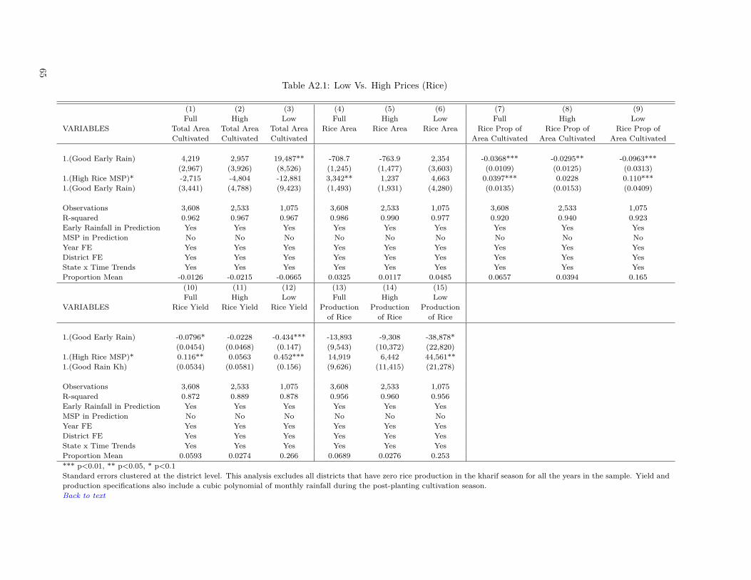
Table A2.1: Low Vs. High Prices (Rice)

(1) (2) (3) (4) (5) (6) (7) (8) (9)Full High Low Full High Low Full High Low

VARIABLES Total Area Total Area Total Area Rice Area Rice Area Rice Area Rice Prop of Rice Prop of Rice Prop ofCultivated Cultivated Cultivated Area Cultivated Area Cultivated Area Cultivated

1.(Good Early Rain) 4,219 2,957 19,487** -708.7 -763.9 2,354 -0.0368*** -0.0295** -0.0963***(2,967) (3,926) (8,526) (1,245) (1,477) (3,603) (0.0109) (0.0125) (0.0313)

1.(High Rice MSP)* -2,715 -4,804 -12,881 3,342** 1,237 4,663 0.0397*** 0.0228 0.110***1.(Good Early Rain) (3,441) (4,788) (9,423) (1,493) (1,931) (4,280) (0.0135) (0.0153) (0.0409)

Observations 3,608 2,533 1,075 3,608 2,533 1,075 3,608 2,533 1,075R-squared 0.962 0.967 0.967 0.986 0.990 0.977 0.920 0.940 0.923Early Rainfall in Prediction Yes Yes Yes Yes Yes Yes Yes Yes YesMSP in Prediction No No No No No No No No NoYear FE Yes Yes Yes Yes Yes Yes Yes Yes YesDistrict FE Yes Yes Yes Yes Yes Yes Yes Yes YesState x Time Trends Yes Yes Yes Yes Yes Yes Yes Yes YesProportion Mean -0.0126 -0.0215 -0.0665 0.0325 0.0117 0.0485 0.0657 0.0394 0.165

(10) (11) (12) (13) (14) (15)Full High Low Full High Low

VARIABLES Rice Yield Rice Yield Rice Yield Production Production Productionof Rice of Rice of Rice

1.(Good Early Rain) -0.0796* -0.0228 -0.434*** -13,893 -9,308 -38,878*(0.0454) (0.0468) (0.147) (9,543) (10,372) (22,820)

1.(High Rice MSP)* 0.116** 0.0563 0.452*** 14,919 6,442 44,561**1.(Good Rain Kh) (0.0534) (0.0581) (0.156) (9,626) (11,415) (21,278)

Observations 3,608 2,533 1,075 3,608 2,533 1,075R-squared 0.872 0.889 0.878 0.956 0.960 0.956Early Rainfall in Prediction Yes Yes Yes Yes Yes YesMSP in Prediction No No No No No NoYear FE Yes Yes Yes Yes Yes YesDistrict FE Yes Yes Yes Yes Yes YesState x Time Trends Yes Yes Yes Yes Yes YesProportion Mean 0.0593 0.0274 0.266 0.0689 0.0276 0.253*** p<0.01, ** p<0.05, * p<0.1Standard errors clustered at the district level. This analysis excludes all districts that have zero rice production in the kharif season for all the years in the sample. Yield andproduction specifications also include a cubic polynomial of monthly rainfall during the post-planting cultivation season.Back to text

65

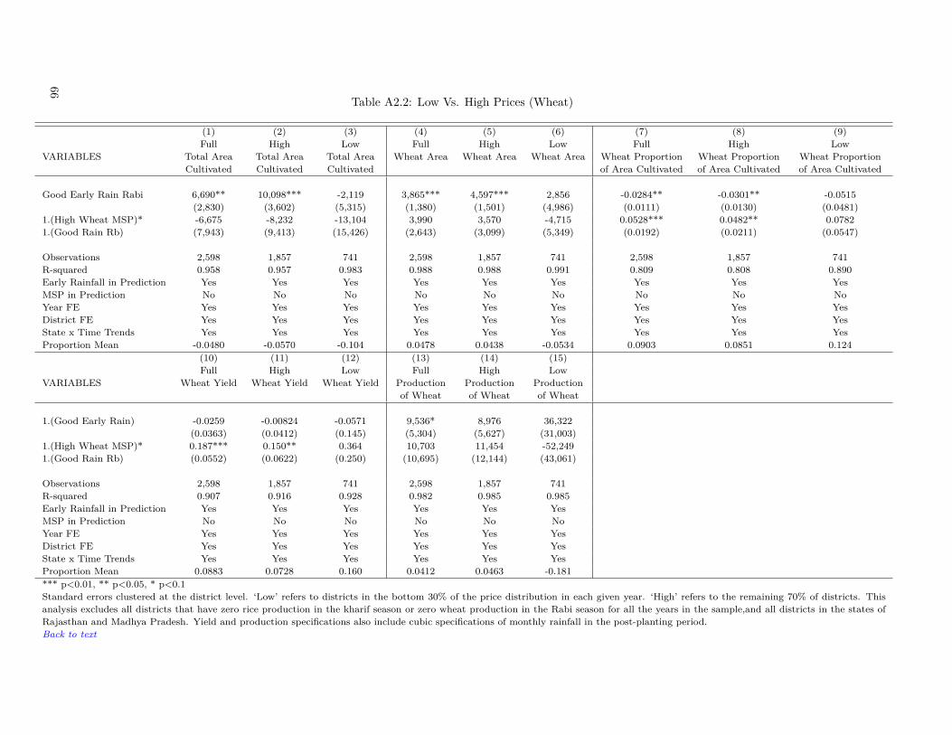
Table A2.2: Low Vs. High Prices (Wheat)

(1) (2) (3) (4) (5) (6) (7) (8) (9)Full High Low Full High Low Full High Low

VARIABLES Total Area Total Area Total Area Wheat Area Wheat Area Wheat Area Wheat Proportion Wheat Proportion Wheat ProportionCultivated Cultivated Cultivated of Area Cultivated of Area Cultivated of Area Cultivated

Good Early Rain Rabi 6,690** 10,098*** -2,119 3,865*** 4,597*** 2,856 -0.0284** -0.0301** -0.0515(2,830) (3,602) (5,315) (1,380) (1,501) (4,986) (0.0111) (0.0130) (0.0481)

1.(High Wheat MSP)* -6,675 -8,232 -13,104 3,990 3,570 -4,715 0.0528*** 0.0482** 0.07821.(Good Rain Rb) (7,943) (9,413) (15,426) (2,643) (3,099) (5,349) (0.0192) (0.0211) (0.0547)

Observations 2,598 1,857 741 2,598 1,857 741 2,598 1,857 741R-squared 0.958 0.957 0.983 0.988 0.988 0.991 0.809 0.808 0.890Early Rainfall in Prediction Yes Yes Yes Yes Yes Yes Yes Yes YesMSP in Prediction No No No No No No No No NoYear FE Yes Yes Yes Yes Yes Yes Yes Yes YesDistrict FE Yes Yes Yes Yes Yes Yes Yes Yes YesState x Time Trends Yes Yes Yes Yes Yes Yes Yes Yes YesProportion Mean -0.0480 -0.0570 -0.104 0.0478 0.0438 -0.0534 0.0903 0.0851 0.124

(10) (11) (12) (13) (14) (15)Full High Low Full High Low

VARIABLES Wheat Yield Wheat Yield Wheat Yield Production Production Productionof Wheat of Wheat of Wheat

1.(Good Early Rain) -0.0259 -0.00824 -0.0571 9,536* 8,976 36,322(0.0363) (0.0412) (0.145) (5,304) (5,627) (31,003)

1.(High Wheat MSP)* 0.187*** 0.150** 0.364 10,703 11,454 -52,2491.(Good Rain Rb) (0.0552) (0.0622) (0.250) (10,695) (12,144) (43,061)

Observations 2,598 1,857 741 2,598 1,857 741R-squared 0.907 0.916 0.928 0.982 0.985 0.985Early Rainfall in Prediction Yes Yes Yes Yes Yes YesMSP in Prediction No No No No No NoYear FE Yes Yes Yes Yes Yes YesDistrict FE Yes Yes Yes Yes Yes YesState x Time Trends Yes Yes Yes Yes Yes YesProportion Mean 0.0883 0.0728 0.160 0.0412 0.0463 -0.181*** p<0.01, ** p<0.05, * p<0.1Standard errors clustered at the district level. ‘Low’ refers to districts in the bottom 30% of the price distribution in each given year. ‘High’ refers to the remaining 70% of districts. Thisanalysis excludes all districts that have zero rice production in the kharif season or zero wheat production in the Rabi season for all the years in the sample,and all districts in the states ofRajasthan and Madhya Pradesh. Yield and production specifications also include cubic specifications of monthly rainfall in the post-planting period.Back to text

66

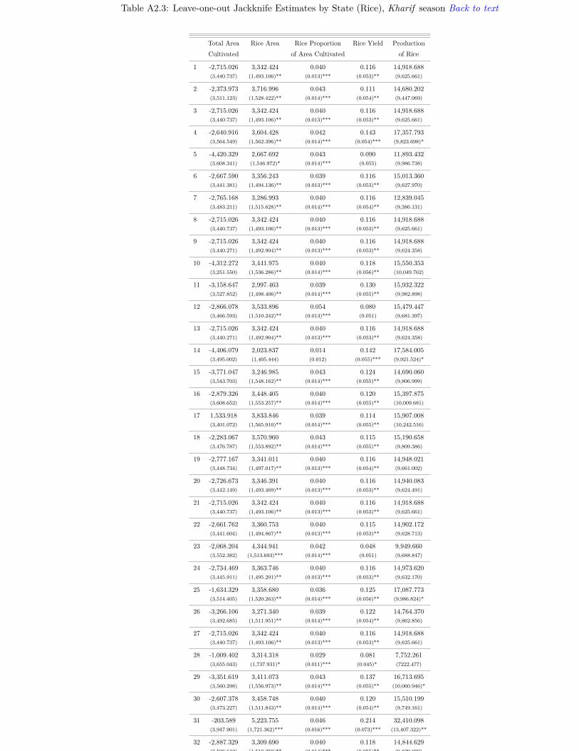
Table A2.3: Leave-one-out Jackknife Estimates by State (Rice), Kharif season Back to text

Total Area Rice Area Rice Proportion Rice Yield ProductionCultivated of Area Cultivated of Rice

1 -2,715.026 3,342.424 0.040 0.116 14,918.688(3,440.737) (1,493.106)** (0.013)*** (0.053)** (9,625.661)

2 -2,373.973 3,716.996 0.043 0.111 14,680.202(3,511.123) (1,528.422)** (0.014)*** (0.054)** (9,447.069)

3 -2,715.026 3,342.424 0.040 0.116 14,918.688(3,440.737) (1,493.106)** (0.013)*** (0.053)** (9,625.661)

4 -2,640.916 3,604.428 0.042 0.143 17,357.793(3,564.549) (1,562.396)** (0.014)*** (0.054)*** (9,823.698)*

5 -4,420.329 2,667.692 0.043 0.090 11,893.432(3,608.341) (1,546.972)* (0.014)*** (0.055) (9,986.738)

6 -2,667.590 3,356.243 0.039 0.116 15,013.360(3,441.381) (1,494.136)** (0.013)*** (0.053)** (9,627.970)

7 -2,765.168 3,286.993 0.040 0.116 12,839.045(3,483.211) (1,515.628)** (0.014)*** (0.054)** (9,386.131)

8 -2,715.026 3,342.424 0.040 0.116 14,918.688(3,440.737) (1,493.106)** (0.013)*** (0.053)** (9,625.661)

9 -2,715.026 3,342.424 0.040 0.116 14,918.688(3,440.271) (1,492.904)** (0.013)*** (0.053)** (9,624.358)

10 -4,312.272 3,441.975 0.040 0.118 15,550.353(3,251.550) (1,536.286)** (0.014)*** (0.056)** (10,049.762)

11 -3,158.647 2,997.463 0.039 0.130 15,932.322(3,527.852) (1,498.406)** (0.014)*** (0.055)** (9,982.898)

12 -2,866.078 3,533.896 0.054 0.080 15,479.447(3,466.593) (1,510.242)** (0.013)*** (0.051) (9,681.397)

13 -2,715.026 3,342.424 0.040 0.116 14,918.688(3,440.271) (1,492.904)** (0.013)*** (0.053)** (9,624.358)

14 -4,406.079 2,023.837 0.014 0.142 17,584.005(3,495.002) (1,405.444) (0.012) (0.055)*** (9,921.524)*

15 -3,771.047 3,246.985 0.043 0.124 14,690.060(3,543.703) (1,548.162)** (0.014)*** (0.055)** (9,806.999)

16 -2,879.326 3,448.405 0.040 0.120 15,397.875(3,608.652) (1,553.257)** (0.014)*** (0.055)** (10,009.681)

17 1,533.918 3,833.846 0.039 0.114 15,907.008(3,401.072) (1,565.910)** (0.014)*** (0.055)** (10,242.516)

18 -2,283.067 3,570.960 0.043 0.115 15,190.658(3,476.787) (1,553.892)** (0.014)*** (0.055)** (9,809.386)

19 -2,777.167 3,341.011 0.040 0.116 14,948.021(3,448.734) (1,497.017)** (0.013)*** (0.054)** (9,661.002)

20 -2,726.673 3,346.391 0.040 0.116 14,940.083(3,442.149) (1,493.469)** (0.013)*** (0.053)** (9,624.491)

21 -2,715.026 3,342.424 0.040 0.116 14,918.688(3,440.737) (1,493.106)** (0.013)*** (0.053)** (9,625.661)

22 -2,661.762 3,360.753 0.040 0.115 14,902.172(3,441.604) (1,494.867)** (0.013)*** (0.053)** (9,628.713)

23 -2,068.204 4,344.941 0.042 0.048 9,949.660(3,552.382) (1,513.693)*** (0.014)*** (0.051) (9,688.847)

24 -2,734.469 3,363.746 0.040 0.116 14,973.620(3,445.911) (1,495.201)** (0.013)*** (0.053)** (9,632.170)

25 -1,634.329 3,358.680 0.036 0.125 17,087.773(3,514.405) (1,520.263)** (0.014)*** (0.056)** (9,986.824)*

26 -3,266.106 3,271.340 0.039 0.122 14,764.370(3,492.685) (1,511.951)** (0.014)*** (0.054)** (9,862.856)

27 -2,715.026 3,342.424 0.040 0.116 14,918.688(3,440.737) (1,493.106)** (0.013)*** (0.053)** (9,625.661)

28 -1,009.402 3,314.318 0.029 0.081 7,752.261(3,655.043) (1,737.931)* (0.011)*** (0.045)* (7222.477)

29 -3,351.619 3,411.073 0.043 0.137 16,713.695(3,560.298) (1,556.973)** (0.014)*** (0.055)** (10,060.946)*

30 -2,607.378 3,458.748 0.040 0.120 15,510.199(3,473.227) (1,511.843)** (0.014)*** (0.054)** (9,749.161)

31 -203.589 5,223.755 0.046 0.214 32,410.098(3,947.901) (1,721.362)*** (0.016)*** (0.073)*** (13,407.322)**

32 -2,887.329 3,309.690 0.040 0.118 14,844.629(3,506.642) (1,510.259)** (0.014)*** (0.055)** (9,829.899)

33 -4,165.939 2,176.149 0.042 0.128 12,561.164(3,540.985) (1,412.450) (0.014)*** (0.055)** (9,798.029)67

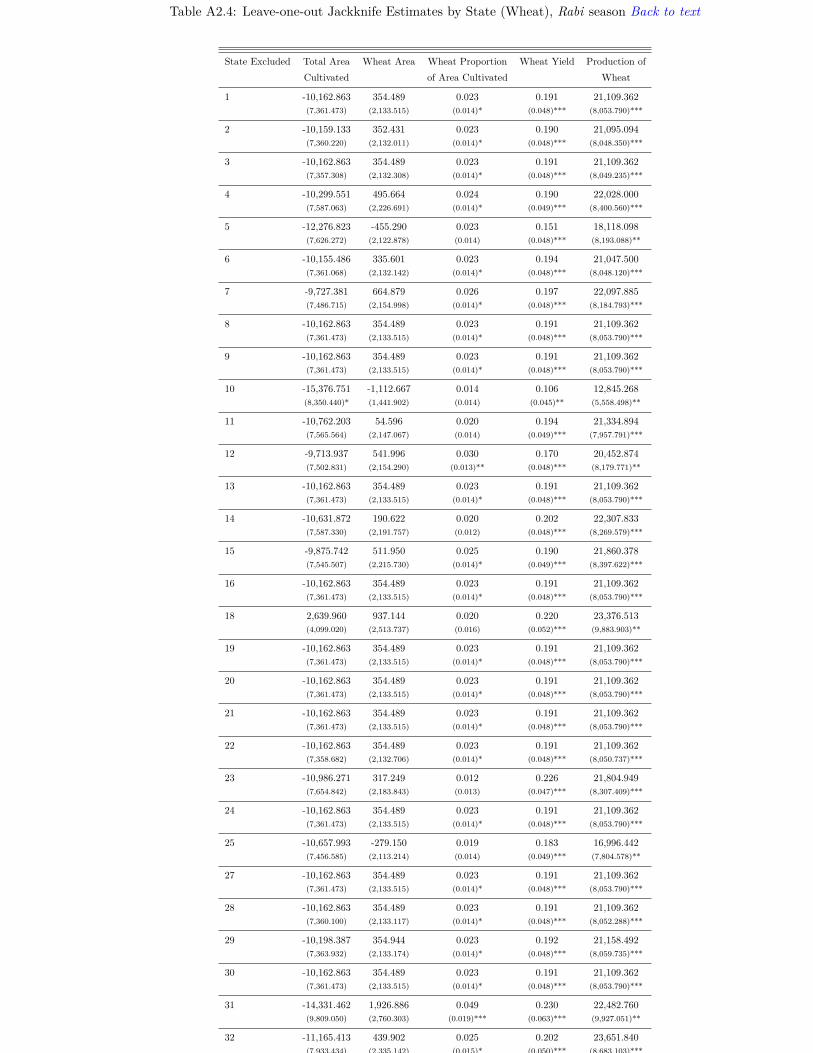
Table A2.4: Leave-one-out Jackknife Estimates by State (Wheat), Rabi season Back to text

State Excluded Total Area Wheat Area Wheat Proportion Wheat Yield Production ofCultivated of Area Cultivated Wheat

1 -10,162.863 354.489 0.023 0.191 21,109.362(7,361.473) (2,133.515) (0.014)* (0.048)*** (8,053.790)***

2 -10,159.133 352.431 0.023 0.190 21,095.094(7,360.220) (2,132.011) (0.014)* (0.048)*** (8,048.350)***

3 -10,162.863 354.489 0.023 0.191 21,109.362(7,357.308) (2,132.308) (0.014)* (0.048)*** (8,049.235)***

4 -10,299.551 495.664 0.024 0.190 22,028.000(7,587.063) (2,226.691) (0.014)* (0.049)*** (8,400.560)***

5 -12,276.823 -455.290 0.023 0.151 18,118.098(7,626.272) (2,122.878) (0.014) (0.048)*** (8,193.088)**

6 -10,155.486 335.601 0.023 0.194 21,047.500(7,361.068) (2,132.142) (0.014)* (0.048)*** (8,048.120)***

7 -9,727.381 664.879 0.026 0.197 22,097.885(7,486.715) (2,154.998) (0.014)* (0.048)*** (8,184.793)***

8 -10,162.863 354.489 0.023 0.191 21,109.362(7,361.473) (2,133.515) (0.014)* (0.048)*** (8,053.790)***

9 -10,162.863 354.489 0.023 0.191 21,109.362(7,361.473) (2,133.515) (0.014)* (0.048)*** (8,053.790)***

10 -15,376.751 -1,112.667 0.014 0.106 12,845.268(8,350.440)* (1,441.902) (0.014) (0.045)** (5,558.498)**

11 -10,762.203 54.596 0.020 0.194 21,334.894(7,565.564) (2,147.067) (0.014) (0.049)*** (7,957.791)***

12 -9,713.937 541.996 0.030 0.170 20,452.874(7,502.831) (2,154.290) (0.013)** (0.048)*** (8,179.771)**

13 -10,162.863 354.489 0.023 0.191 21,109.362(7,361.473) (2,133.515) (0.014)* (0.048)*** (8,053.790)***

14 -10,631.872 190.622 0.020 0.202 22,307.833(7,587.330) (2,191.757) (0.012) (0.048)*** (8,269.579)***

15 -9,875.742 511.950 0.025 0.190 21,860.378(7,545.507) (2,215.730) (0.014)* (0.049)*** (8,397.622)***

16 -10,162.863 354.489 0.023 0.191 21,109.362(7,361.473) (2,133.515) (0.014)* (0.048)*** (8,053.790)***

18 2,639.960 937.144 0.020 0.220 23,376.513(4,099.020) (2,513.737) (0.016) (0.052)*** (9,883.903)**

19 -10,162.863 354.489 0.023 0.191 21,109.362(7,361.473) (2,133.515) (0.014)* (0.048)*** (8,053.790)***

20 -10,162.863 354.489 0.023 0.191 21,109.362(7,361.473) (2,133.515) (0.014)* (0.048)*** (8,053.790)***

21 -10,162.863 354.489 0.023 0.191 21,109.362(7,361.473) (2,133.515) (0.014)* (0.048)*** (8,053.790)***

22 -10,162.863 354.489 0.023 0.191 21,109.362(7,358.682) (2,132.706) (0.014)* (0.048)*** (8,050.737)***

23 -10,986.271 317.249 0.012 0.226 21,804.949(7,654.842) (2,183.843) (0.013) (0.047)*** (8,307.409)***

24 -10,162.863 354.489 0.023 0.191 21,109.362(7,361.473) (2,133.515) (0.014)* (0.048)*** (8,053.790)***

25 -10,657.993 -279.150 0.019 0.183 16,996.442(7,456.585) (2,113.214) (0.014) (0.049)*** (7,804.578)**

27 -10,162.863 354.489 0.023 0.191 21,109.362(7,361.473) (2,133.515) (0.014)* (0.048)*** (8,053.790)***

28 -10,162.863 354.489 0.023 0.191 21,109.362(7,360.100) (2,133.117) (0.014)* (0.048)*** (8,052.288)***

29 -10,198.387 354.944 0.023 0.192 21,158.492(7,363.932) (2,133.174) (0.014)* (0.048)*** (8,059.735)***

30 -10,162.863 354.489 0.023 0.191 21,109.362(7,361.473) (2,133.515) (0.014)* (0.048)*** (8,053.790)***

31 -14,331.462 1,926.886 0.049 0.230 22,482.760(9,809.050) (2,760.303) (0.019)*** (0.063)*** (9,927.051)**

32 -11,165.413 439.902 0.025 0.202 23,651.840(7,933.434) (2,335.142) (0.015)* (0.050)*** (8,683.103)***

33 -10,916.277 519.454 0.026 0.190 22,644.611(7,953.558) (2,316.098) (0.015)* (0.052)*** (8,733.157)**68

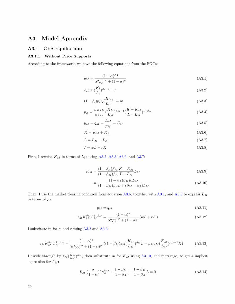
A3 Model Appendix

A3.1 CES EquilibriumA3.1.1 Without Price Supports

According to the framework, we have the following equations from the FOCs:

qM = (1− α)σIασp1−σ

A + (1− α)σ(A3.1)

βipizi(Ki

Li)βi−1 = r (A3.2)

(1− βi)pizi(Ki

Li)βi = w (A3.3)

pA = βMzMβAzA

(KM

LM)βM−1(K −KM

L− LM)1−βA (A3.4)

yM = qM = EMpM

= EM (A3.5)

K = KM +KA (A3.6)

L = LM + LA (A3.7)

I = wL+ rK (A3.8)

First, I rewrite KM in terms of LM using A3.2, A3.3, A3.6, and A3.7:

KM = (1− βA)βM(1− βM )βA

K −KM

L− LMLM (A3.9)

= (1− βA)βMKLM(1− βM )βAL+ (βM − βA)LM

(A3.10)

Then, I use the market clearing condition from equation A3.5, together with A3.1, and A3.8 to express LMin terms of pA.

yM = qM (A3.11)

zMKβMM L1−βM

M = (1− α)σ

ασp1−σA + (1− α)σ

(wL+ rK) (A3.12)

I substitute in for w and r using A3.2 and A3.3:

zMKβMM L1−βM

M = [ (1− α)σ

ασp1−σA + (1− α)σ

]((1− βM )zM (KM

LM)βML+ βMzM (KM

LM)βM−1K) (A3.13)

I divide through by zM (KMLM )βM , then substitute in for KM using A3.10, and rearrange, to get a implicitexpression for LM :

LM [( α

1− α )σp1−σA + 1− βM

1− βA]− 1− βM

1− βAL = 0 (A3.14)

69

A3.2 CES Comparative Statics

Finally, I use equation A3.4 and substitute in for KM using A3.10, to obtain an expression for pA in termsof LM and constants:

pA = βMzMβAzA

(KM

LM)βM−1(K −KM

L− LM)1−βA (A3.15)

=βM [βA(1−βM )]1−βA

βA[βM (1−βA)]1−βM zM

zA[ K

(1− βM )βAL+ (βM − βA)LM]βM−βA (A3.16)

A3.1.2 With Price Supports

When price supports are set at the level pS in the agricultural sector, with a consumer price for agriculturalgoods set at pC , I start with a modified set of first-order conditions. I rewrite A3.4 as follows:

pS = βMzMβAzA

(KM

LM)βM−1(K −KM

L− LM)1−βA (A3.17)

Then, I substitute for KM using A3.10, and rearrange to get:

pS = βMzMβAzA

[(1− βA)βM ]βM−1KβM−βA [(1− βM )βA]1−βA

[(1− βM )βAL+ (βM − βA)LM ]βM−βA(A3.18)

Rewriting in terms of LM ,

LM =( [(1−βA)βM ]βM−1[(1−βM )βA]1−βAKβM−βA

pSzA)

1βM−βA − (1− βM )βAL

βM − βA(A3.19)

A3.2 CES Comparative StaticsNow, I derive various relevant comparative statics for the two different cases.

A3.2.1 Without Price Supports

Labor in ManufacturingI substitute A3.16 into A3.14 to get:

LM [κ1(κ3zMzA

)1−σ( K

(1− βM )βAL+ (βM − βA)LM)(βM−βA)(1−σ) + κ2]− κ2L = 0 (A3.20)

(A3.21)

As long as σ < 1, an increase in zA decreases the left-hand side of the equation. The effective size of theexponent on LM is positive, so it is clear that LM must increase in response to an increase in zA to keep thesystem in equilibrium.

∂LM∂zA

> 0

Relative Price of Agricultural GoodsFrom A3.16, and since ∂LM

∂zA> 0, an increase in zA results in a decrease in pA.

∂pA∂zA

< 0

70

A3.2 CES Comparative Statics

Production in ManufacturingFrom A3.1, it is clear that qM increases as pA falls, which happens in response to an increase in zA. Therefore,

∂qM∂zA

> 0

Labor in AgricultureWith a given total stock of labor, L,

∂LA∂zA

= −∂LM∂zA

< 0

Production in AgricultureAgricultural production is influenced by two different pressures: 1. The posiive effect of increased agriculturalproductivity zA, and 2. The resulting decrease in capital and labor allocated to agriculture in equilibrium.

Overall, using equations A3.1 and the budget constraint from the household problem, we have:

qA = Iασ

pσA(ασp(1−σ)A + (1− α)σ)

(A3.22)

Since we know agricultural prices fall with a positive productivity shock,∂qA∂zA

> 0

However, I should note that the amount of rice produced in response to a positive productivity shock actuallyfalls in my empirical analysis, due to substitution with other crops, which the model cannot capture.

A3.2.2 With Price Supports

I now turn to the version of the model with price supports. The equilibrium is defined in equation 18:

LM =( κ4pSzA

)1

βM−βA − κ5

βM − βALabor in Manufacturing

∂LM∂zA

= −1(βM − βA)2 (κ4

pS)

1βM−βA ( 1

zA)

1−βM+βAβM−βA

1z2A

< 0 (A3.23)

Production in ManufacturingFrom A3.10, KM decreases when LM falls, which happens in response to an increase in zA. Therefore, overallmanufacturing production, qM , falls.

∂qM∂zA

< 0 (A3.24)

Labor in AgricultureWith a given total stock of labor, L

∂LA∂zA

= −∂LM∂zA

> 0

71

A3.2 CES Comparative Statics

Production in AgricultureWith a given stock of capital and labor, and equations A3.23 and A3.10, we know that KA and LA bothincrease in response to a positive productivity shock zA. Therefore,

∂qA∂zA

> 0 (A3.25)

Size of the effect relative to the level of the price supportThe effect of the level of the price support on the size of the labor and production effects can be determinedfrom equation A3.19.

∂LM∂zA∂pS

= κ1

βM−βA4

1(βM − βA)3 ( 1

pSzA)

1−βM+βAβM−βA

1z2A

1p2S

> 0 (A3.26)

This suggests that the negative effect of the productivity shock on labor allocated to manufacturing is largerwhen price supports are higher.

72

A4 Data Appendix

A4.1 Crops by Category

Category CropsOther Cereals Bajra, Barley, Jowar, Maize, Ragi, Wheat, Small Millets,

Others

Pulses Arhar/Tur, Beans, Blackgram, Cowpeas, Gram, Horseg-ram, Khesari, Masoor, Moth, Greengram, Urad, Otherpulses

Cash Crops and Oilseeds Arecanut, Cashewnut, Castorseed, Cotton, Coconut,Groundnut, Guarseed, Hemp, Jute, Linseed, Mesta,Nigerseed, Safflower, Sesamum, Sugarcane, Soybeans,Sunflower, Tobacco

Spices Black pepper, Cardamom, Coriander, Dry Chillies, DryGinger, Garlic, Ginger, Turmeric

A4.2 Crops Used in the Productivity CalculationJowar, bajra, maize, barley, small millets, ragi, gram, arhar/tur, moong, masoor, urad, peas, groundnut,cotton.

Data Type Data Source NotesOutputDistrict-level Production of Vari-ous Crops

APY data

District-level crop prices District-level averages of pricesfaced by households in that districtfor each crop in the NSS consump-tion/expenditure data

Rounds 60-68, Schedule 1.0. Soy-bean is not reported in NSS rounds66 and 68. Cotton is not reportedin NSS round 68. Revenue sharesare adjusted accordingly. Wherea crop’s prices are not availablefor a particular district, I replacethe missing data with the state-average price for the crop.

InputsLand use in agriculture APY dataQuantities and price of labor NSS Employment/Unemployment

SurveysRounds 60-68, Schedule 10. Toobtain correct labor cost share es-timates, I aggregate up the NSSdata using the multipliers pro-vided.

73

A4.3 Absolute and Relative Suitability

Data Type Data Source NotesFertilizer Use (N, P, and K) Agricultural Input Survey 2006-07 The survey does not provide

season-wise input use, so, to theextent that the cost shares of otherinputs are high relative to labor,the effect of the labor-use increasein high MSP years is understated,resulting in a lower-bound esti-mate of the fall in agricultural pro-ductivity.

Use of agricultural machinery Agricultural Input Survey 2006-07Use of irrigation Agricultural Input Survey 2006-07Use of high-yielding varieties Agricultural Input Survey 2006-07Prices of non-labor inputs Cost of Cultivation Survey 2006-07 Prices are aggregated to the state-

level.

A4.3 Absolute and Relative SuitabilityAbsolute suitability for rice and wheat is simply the value of the Suitability Index for the district. Relativesuitability is arguably a more important measure, since a district that is absolutely bad for staple produc-tion could still do relatively better by planting staples than by planting other crops (that have absolutelyworse letterpaper suitability measures). It also captures the district’s comparative (rather than absolute)advantage, a key determinant of potential gains from trade.

To calculate the relative suitability of crops, I weight the absolute suitability levels by the average share ofthe country’s land area used in the production of that crop in the main growing season (to avoid placing toohigh a weight on the suitability of a district to grow more minor crops). I then calculate an overall index ofsuitability for the district:

I then calculate the relative suitability of the staple crops by taking:

with an analogous measure for relative wheat suitability. I then run analyses separately for low- and high-suitability districts (dividing the sample by the median of the relative suitability measure).

74