asymmetric trading costs prior to earnings announcements
TRANSCRIPT
DOI: 10.1111/1475-679X.12189Journal of Accounting Research
Vol. No. November 2017Printed in U.S.A.
Asymmetric Trading Costs Priorto Earnings Announcements:
Implications for Price Discoveryand Returns
T R A V I S L . J O H N S O N∗ A N D E R I C C . S O†
Received 29 May 2015; accepted 15 June 2017
ABSTRACT
We show that the cost of trading on negative news, relative to positive news,increases before earnings announcements. Our evidence suggests that thisasymmetry is due to financial intermediaries reducing their exposure to an-nouncement risks by providing liquidity asymmetrically. This asymmetry cre-ates a predictable upward bias in prices that increases preannouncement, andsubsequently reverses, confounding short-window announcement returns asmeasures of earnings news and risk premia. These findings provide an alter-native explanation for asymmetric return reactions to firms’ earnings news,and help explain puzzling prior evidence that announcement risk premiaprecede the actual announcements. Our study informs methods for researchcentering on earnings announcements and offers a possible explanation for
∗McCombs School of Business, The University of Texas at Austin; †Sloan School of Man-agement, Massachusetts Institute of Technology.
Accepted by Christian Leuz. We thank two anonymous referees, Audra Boone, ZhiDa, Emmanuel De George, Amit Goyal (WFA discussant), Nick Guest, Terry Hender-shott, S.P. Kothari, Charles Lee, Russ Lundholm (Stanford discussant), Paul Tetlock, Ro-drigo Verdi, Frank Zhang (Illinois discussant), and seminar participants at the 2014Citi Quant Research Conference, Cornell University, London Business School, MIT,NASDAQ Economic Research, Stanford University Summer Camp, The University ofTexas at Austin, University of Illinois, and the 2015 Western Finance Association Meet-ing for helpful suggestions. An online appendix to this paper can be downloaded athttp://research.chicagobooth.edu/arc/journal-of-accounting-research/online-supplements.
1
Copyright C©, University of Chicago on behalf of the Accounting Research Center, 2017
2 T. L. JOHNSON AND E. C. SO
patterns in returns around anticipated periods of heightened inventory risks,including alternative firm-level, industry-level, and macroeconomic informa-tion events.
JEL codes: E44; G12; G14; G21; M40; M41
Keywords: earnings announcements; liquidity provision; transaction costs;announcement returns; risk premia; bad news; asymmetric reaction
1. Introduction
A vast literature spanning accounting, finance, and economics studies stockreturns around firms’ earnings announcements. Researchers use stock re-turns around earnings announcements to understand revisions in investorexpectations about firm value, risk premia driven by the release of earningsnews, and determinants of the equity market reaction to earnings news,such as the credibility of financial reporting. Similarly, liquidity and tradingvolumes around earnings announcements are commonly used to gauge theextent of attention or disagreement among investors, information asymme-try, and the news conveyed to investors.
This study provides both theoretical and empirical evidence that re-turns, liquidity, and trading volume around earnings announcements areasymmetrically influenced by frictions in the financial intermediary sec-tor, which is composed of investment banks, broker-dealers, and market-making firms, among others. Intermediaries provide liquidity by serving asthe trade counterparty in response to imbalanced demand between buy-ers and sellers. In doing so, they are forced to take temporary positionsin the security, referred to as inventory, and thus expose themselves toprice fluctuations (inventory risk). Due to this exposure, the compensationthat intermediaries demand varies with their inventory positions as well asthe security’s risk profile. We show that these factors create asymmetries intrading costs and, in turn, price discovery surrounding earnings announce-ments by altering investors’ incentives to trade.
Our central hypothesis stems from prior evidence that intermediaries arepositively exposed to the market and hold positive average inventory posi-tions, indicating that they are likely exposed to increased risks associatedwith earnings announcements.1 As a result of this exposure, we predictthat intermediaries demand greater compensation for providing liquidityto sell orders, which would exacerbate their exposure, relative to buy or-ders, which would shield them from announcement risks by helping them
1 For example, Brunnermeier and Pedersen [2009] report that broker-dealer firms havemedian market betas above one. Adrian and Shin [2010] show that financial intermediaries’leverage is highly procyclical and argues that this is because they expand their positions inresponse to market booms. Similarly, studies using proprietary data on market makers’ inven-tory positions show that they tend to hold positive inventories (Madhavan and Smidt [1993],Comerton-Forde et al. [2010]).
ASYMMETRIC TRADING COSTS PRIOR TO EARNINGS ANNOUNCEMENTS 3
reduce net exposure before the announcement (referred to as “gettingflat” in the industry). This asymmetry acts like an endogenous short-salecost by discouraging selling, which in turn causes an upward bias in prean-nouncement price discovery and returns that reverses postannouncement.We refer to this hypothesis about the causes and effects of asymmetric trad-ing costs (ATCs) as the ATC hypothesis. We formalize the ATC hypothesisby developing a model of trading before an information event involving afinancial intermediary with positive exposure to the announcing firm’s eq-uity. Our model predicts the following chain of events: the intermediary setsasymmetric prices for liquidity to reduce its inventory before the announce-ment, causing a positive bias in preannouncement price discovery, whichleads to an upward bias in preannouncement returns that corrects oncethe news is released. The upward bias may initially seem counterintuitivebecause, for most agents, the desire to sell would lead to the opposite—adecrease in average prices before announcements. However, when liquid-ity providers in our model seek to reduce their inventories, they use theirpricing power to induce buy demands and ensure that average prices areabove fundamental value.
Our first set of empirical results supports the cornerstone of the ATC hy-pothesis, that intermediaries provide liquidity asymmetrically before earn-ings announcements. Using short-term return reversals as a proxy for thecompensation intermediaries demand for this, as in Campbell, Grossman,and Wang [1993], we show that reversals become increasingly asymmetricbefore announcements. Reversals associated with net selling pressure (i.e.,recent losers) increase several days before announcements and peak atmore than three times normal levels immediately before announcements,whereas no discernible trend exists for buying pressure. These results areconsistent with our model’s prediction that intermediaries demand greatercompensation for providing liquidity to sellers, relative to buyers, and thusthat traders incur higher relative costs of impounding negative news intopreannouncement prices.
A natural question is whether the magnitude of an intermediary-basedstory could explain the magnitude of our findings. We estimate that theasymmetry in liquidity provision in our sample peaks at 54 basis points(bp) on day t − 1, which is based on the spread in return reversal mag-nitudes across quintiles of prior day net buying/selling pressure. A basis ofcomparison for this estimate is the returns of unconditional return-reversalstrategies, which peak in our sample at around 100 bp before earnings an-nouncements. Another reasonable benchmark of comparison is the typicalmagnitude of price pressures due to specialist inventory positions, whichHendershott and Menkveld [2014] estimate is 49 bp, with a half-life of0.92 days. These comparisons suggest that our results are not only econom-ically meaningful but also comport with plausibility bounds established byresearch.
Our second set of empirical results provide support for our model’s pre-diction that investors respond to ATCs by trading more aggressively on
4 T. L. JOHNSON AND E. C. SO
positive signals before announcements. Specifically, preannouncement ab-normal order imbalances (AOIs) are strongly positive for good news andinsignificantly negative or even slightly positive for bad news, a stark illus-tration that traders with negative news are deterred from trading before theannouncement.
In related tests, we show that preannouncement prices incorporatemore good than bad news and that prices adjust following the announce-ment. Similarly, we also show that preannouncement abnormal tradingvolume positively predicts firms’ earnings news. These results suggest ATCsincentivize investors to more actively trade on positive signals before an-nouncements and that this asymmetry reverses afterward. This asymmetryattenuates after the announcement because the arrival of news reduces theincentives for liquidity providers to get flat.
The third main empirical pattern we find is that firms’ average returnsare positive beginning an entire week before their earnings announcementsbut become insignificant on announcement dates (t) and significantlynegative following the announcements (t+1). This pattern supports ourmodel’s prediction that preannouncement price discovery asymmetricallyreflects good news, causing an upward bias in preannouncement prices.
The market frictions we highlight yield an important insight for re-search using earnings announcement returns as measures of risk premia. Inour sample, the average three-day market-adjusted return centered on an-nouncement dates is 17 bp (consistent with Cohen et al. [2007]), whereasthe average announcement month return is more than three times larger at55 bp (consistent with Barber et al. [2013]), despite both intending to cap-ture risk premia associated with earnings news. Our model helps explainthis discrepancy by showing that, on average, earnings announcement re-turns reflect two offsetting forces. The first is a positive risk premium drivenby the release of earnings news.2 The second is a negative correction of thepreannouncement upward bias in prices as inventory risks subside and trad-ing costs revert to normal levels. These offsetting effects cause abnormal re-turns to be zero or negative following announcements, despite the positiverisk premium. Our paper thus helps explain the timing mismatch betweenthe realization of risk premia (i.e., abnormal returns) and the realizationof the underlying risk (i.e., the earnings announcement) documented byBarber et al. [2013]. Absent the ATC hypothesis, this mismatch is puzzlingbecause standard asset pricing models predict that risks and risk premiaoccur at the same time.
We next empirically validate the central cross-sectional implications ofour model, that the preannouncement asymmetries in trading costs, or-der imbalances, and returns are all concentrated among high uncertainty
2 Barber et al. [2013] argue that earnings announcement premia reflect compensation foridiosyncratic risks, whereas Savor and Wilson [2016] argue that it stems from exposure tomacroeconomic risk.
ASYMMETRIC TRADING COSTS PRIOR TO EARNINGS ANNOUNCEMENTS 5
stocks because these pose greater inventory risk. We also show that uncer-tainty proxies have a significantly positive relation with firms’ preannounce-ment returns but that the sign of this relation flips and becomes signifi-cantly negative on and following earnings announcements. The changingsign of the uncertainty-return relation supports our model’s prediction thatthe upward bias in preannouncement prices and its subsequent reversal aremore pronounced when intermediaries face greater inventory risk.
To provide assurance that frictions in the intermediary sector are driv-ing our results, we also address a variety of alternative explanations. Onepossibility is that our results are driven by asymmetric disclosure, wherebyfirms are more likely to disclose good news before announcements thanbad news. This could explain our evidence that good news is reflected inpreannouncement returns, whereas bad news is only reflected on or afterthe announcement. Another alternative hypothesis is that short-sale costs,rather than asymmetric liquidity provision (ALP), make negative news moreexpensive to impound into preannouncement prices.
We discuss these and other alternative hypothesis in detail and show that,although each can explain some of our findings, each also makes predic-tions contradicted by other parts of our findings. Explaining all of our find-ings with a single story is important because a key result in our paper isthat preannouncement asymmetries in liquidity provision, AOIs, and re-turns are strongly correlated in both time series and cross-sectional tests.These correlations indicate that our broader results likely stem from a dis-tinct underlying driver and thus are difficult to reconcile with the variety ofpartial alternative explanations.
We also provide evidence distinguishing our ATC hypothesis from alter-natives by linking our findings to changes in the financial intermediarysector. Specifically, we follow Adrian and Shin [2010] by using time serieschanges in aggregate repurchase agreement (repo) behavior to captureintermediaries’ preferences to expand versus contract their net positionsand thus their willingness to provide liquidity to buyers versus sellers. Weshow that our main findings are more pronounced when intermediariesare shrinking their balance sheets, suggesting that our findings stem fromtheir risk- and inventory-management practices.
Because our model’s predictions depend on liquidity providers antici-pating the arrival of news, we also use unanticipated nonearnings 8-K fil-ing dates as a placebo test. Our ATC hypothesis predicts no asymmetries intrading costs, price discovery, or returns before nonearnings 8-K announce-ments, while some alternatives (e.g., asymmetric disclosure) predict thoseasymmetries before nonearnings 8-K announcements. Consistent with theATC hypothesis, we find no significant changes in these variables beforenonearnings 8-Ks.
To summarize, other hypotheses are difficult to reconcile with ALP andthe upward bias in market prices that rise preannouncement and reverseafterward, as well as the link between our findings and both uncertainty andthe financial intermediary sector. However, behavioral biases or omitted
6 T. L. JOHNSON AND E. C. SO
frictions may be correlated with those variables as well. We therefore viewour main results as being consistent with frictions in the intermediary sectorplaying an important role and providing a potential (but not exclusive)explanation for the patterns we document.
A central contribution of our paper is in providing a liquidity-provision-based explanation for daily return patterns around earnings announce-ments, one of the most significant information events for a firm. Prior re-search uses the asymmetric reaction to earnings announcements to inferasymmetric leakage of news to the market, where insiders opportunisticallyleak upcoming news when that news is good but withhold it when it is bad.Our findings point to an important alternative possibility. Specifically, liq-uidity providers’ aversion to inventory risk would lead to these systematicreturn patterns, even in the absence of any asymmetric news leakage, thatis, even when the market’s ability to anticipate good and bad news at theupcoming announcement is the same.
Our paper also provides a unified framework that links several pervasivelystudied market outcomes. These outcomes include market prices, returns,trading volumes, order flows, and liquidity—the central constructs of inter-est in virtually all capital market studies. As a result, our paper provides aconceptual basis and empirical support for understanding several resultsthat likely appear puzzling when viewed outside of our framework. Ourmodel and results therefore may influence the way that researchers under-stand market outcomes across a variety of settings, particularly outcomesoccurring around anticipated periods of heightened inventory risks, includ-ing alternative firm-level (e.g., anticipated earnings guidance), industry-level (e.g., trade association meetings), and macroeconomic informationevents (e.g., Federal Open Market Committee (FOMC) meetings). Forexample, our ATC hypothesis offers a new explanation for the evidencein Lucca and Moench [2015] that market returns are significantly posi-tive immediately before scheduled FOMC meetings. Like the pre-earnings-announcement return premium discussed above, this pattern is difficult toexplain in a frictionless model but can be seen as a natural consequence ofALP before information events.
The rest of the paper is organized as follows. Section 2 provides a modelof liquidity provision. Section 3 discusses our main findings. Section 4 con-tains additional analyses. Section 5 distinguishes between our hypothesisand alternatives. Section 6 discusses implications for future research, andSection 7 concludes.
2. Model
Our model conveys the intuition for the ATC hypothesis that we advanceand test. We hypothesize that frictions in the intermediary sector causeATCs before information events, causing a positive bias in preannounce-ment price discovery, which leads to an upward bias in preannounce-ment returns that corrects when the news is released. The key frictions
ASYMMETRIC TRADING COSTS PRIOR TO EARNINGS ANNOUNCEMENTS 7
intermediaries face in the model are an exogenous preference for holdingpositive positions and an aversion to inventory risk. The former is consis-tent with the evidence in Brunnermeier and Pedersen [2009] and Adrianand Shin [2010] that broker-dealers’ assets are procyclical as well as the ev-idence in Comerton-Forde et al. [2010] that market makers hold positiveinventories 94% of the time, perhaps because it is costly to locate or bor-row shares when providing liquidity to buyers. The latter idea is supportedby the link between short-term reversals and liquidity provision in Chor-dia, Roll, and Subrahmanyam [2002] and Nagel [2012], perhaps becauseintermediaries employ trader-specific risk budgets for agency reasons.
We rely on a broader definition of “intermediary,” based on Nagel[2012]. It includes all traders who act as liquidity providers, which is tosay they often have orders on both sides of the market and their goalis to profit by temporarily holding shares as they pass from a seller to abuyer. We contrast this sort of intermediary with traders or investors whoaim to build a directional position to profit from price movements orhedge risks, which requires demanding liquidity. By this broad definition,intermediaries will mechanically always play an important role in provid-ing liquidity, even as market microstructure evolves with technology andregulation.
Recent microstructure literature provides evidence that there is a speedhierarchy in liquidity provision, with high-frequency traders (HFTs) actingas intraday intermediaries and lower frequency traders absorbing inven-tory when HFTs reach their risk-bearing capacity. For example, Menkveld[2013] shows that HFTs trade a stock hundreds of times per day, are mostlyon the passive (i.e., nonmarketable) side of the order, and typically holdzero inventory overnight. However, as Nagel [2012] points out, unlessintraday order imbalances exactly cancel out, someone must provideovernight inventory and will demand compensation in the form of priceconcessions measurable using daily data. These overnight intermediariesare likely algorithmic traders, quantitative hedge funds, and proprietarytrading groups within investment banks. Our model abstracts away fromthis type of intermediary classification and instead models the behavior ofa single intermediary.
2.1 ASSUMPTIONS
We study an asset with payoff v = v−1 + v0 at t = 0, where v−1 = {−1, 1}corresponds to a normal period information release and v0 = {−σ, σ },σ > 1, corresponds to a high-volatility information release, such as an earn-ings announcement. We model two trading periods to illustrate that inter-mediaries behaving optimally will carry an undesirably high inventory fromnormal periods into the preannouncement period.
The positive innovations v−1 = 1 and v0 = σ have probabilities z−1 andz0, respectively. However, these innovations are exposed to priced risk,meaning agents value them using risk-neutral probabilities y−1 and y0

8 T. L. JOHNSON AND E. C. SO
instead of z−1 and z0.3 We assume that the asset has a positive risk premium,so investors price assets using risk-neutral probabilities that underestimatethe probability of the good state: y−1 < z−1 and y0 < z0. For analytic conve-nience, we assume that the risk-neutral probabilities are y−1 = y0 = 1
2 andthe risk-free rate is 0.
There are three types of agents in the model: an intermediary M, in-formed traders It , and uninformed traders Ut . To avoid the complexity asso-ciated with dynamic trading strategies, we assume that the traders at t = −1are different from those at t = −2 and that all traders hold their positionsuntil t = 0. The timeline in the model is as follows:
Prior to t = −2, M chooses initial position Q−2 and ask and bid prices a−2, b−2.t = −2, I−2 and U−2 purchase quantities of shares xI,−2 and xU ,−2, respectively.Prior to t = −1, v−1 is revealed, M chooses ask and bid prices a−1, b−1.t = −1, I−1 and U−1 purchase quantities of shares xI,−1 and xU ,−1, respectively.t = 0, v0 is revealed, all positions are liquidated for v−1 + v0.
As in Hendershott and Menkveld [2014], all trades clear through theintermediary exclusively and at the bid or ask price for any quantity thetrader chooses. Therefore each trader pays the ask price for any sharesbought and receives the bid price for any shares sold.
The t = −2 informed trader, I−2, receives a private signal about therealization of v−1 but not v0. The signal takes one of two values, s−2 ={g, b}, where P(v−1 = 1 | s−2 = g) = P(v−1 = −1 | s−2 = b) = p > 1
2 . In-formed traders have mean-variance preferences, where both moments areunder the risk-neutral measure,4 and therefore I−2’s demand satisfies:
xI,−2(s−2; a−2, b−2) = arg maxx
Ey (x (v − p (x)) | s−2)
− γT Vary (x (v − p (x)) | s−2) , (1)
where γT is the traders’ risk aversion, and the price function p (x) equalsthe ask a−2 for positive x (i.e., buying) and the bid b−2 for negative x (i.e.,selling).
The t = −1 informed trader I−1 observes the public announcement ofv−1 and receives a private signal about the realization of v0. The signaltakes one of two values, s−1 = {g, b}, and has the same precision as s−2,meaning P(v0 = σ | s−1 = g) = P(v0 = −σ | s−1 = b) = p > 1
2 . I−1 also hasmean-variance preferences and chooses demand xI,−1(s−1; a−1, b−1) usingan optimization similar to equation (1).
3 We write Ey and E
z for expectations under the risk-neutral measure and physical measure,respectively.
4 We use the risk-neutral measure to adjust for priced systematic risk and mean-variancepreferences to adjust for the additional idiosyncratic risk traders are exposed to by takingconcentrated positions.
ASYMMETRIC TRADING COSTS PRIOR TO EARNINGS ANNOUNCEMENTS 9
The uninformed traders in our model are not the usual price-insensitivenoise traders. The crux of our story is that the intermediary uses ATCs toattract buyers for the undesired inventory, which necessitates price-sensitivetraders. Furthermore, in the presence of a price-insensitive uninformedtrader, the intermediary would set enormous bid-ask spreads to profit fromuninformed order flow and avoid the informed trader. We therefore modeluninformed traders as mean-variance agents who behave as if they are in-formed. Their signals at times t = −2 and t = −1 are u−2 and u−1, respec-tively. The uninformed traders believe that these signals inform them aboutv−1 and v0, even though in reality they are uninformative. Therefore, unin-formed trader demand functions are identical to informed trader demandfunctions but with false signals u−2 and u−1 in place of s−2 and s−1.
The intermediary has mean-variance preferences, where both momentsare under the risk-neutral measure, and chooses Q−2, a−2, b−2, a−1, andb−1 to maximize its expected utility. The intermediary chooses Q−2, a−2,and b−2 prior to trade at t = −2 while anticipating how these choices willaffect inventory and liquidity provision in period t = −1. In the model, weassume that M can costlessly choose whatever Q−2 it wants. In reality, theintermediary anticipates the earnings announcement well in advance andshifts prices to induce order flow that pushes the inventory toward Q−2,making Q−2 the average initial inventory. Before t = −1, it chooses a−1 andb−1 that are optimal, given the net inventory carried forward after the initialround of trading Q−1 = Q−2 − xI,−2 − xU ,−2 as well as the realization of v−1.
We make two unorthodox assumptions in our model: that the interme-diary is a monopolist who chooses bid and ask prices and that the interme-diary must be willing to trade any desired quantity at these prices. A moretypical approach (e.g., Grossman and Miller [1988], Nagel [2012]) is tomodel a competitive intermediary sector that is nevertheless averse to id-iosyncratic risk and to allow prices to be set using market clearing. In thissetting, there is no asymmetry in liquidity provision and therefore no up-ward pressure on prices. To allow intermediaries to provide liquidity asym-metrically, we instead adopt the assumption from Amihud and Mendelson[1980], Hendershott and Menkveld [2014], and elsewhere that intermedi-aries have market power.5 In this case, it is intractable to allow prices to bean arbitrary continuous function of order flow, and so we follow Hender-shott and Menkveld [2014] and focus on a discrete pricing mechanism withunlimited quantities at a single bid and ask price.6
Expected profits for the intermediary come from trading at advanta-geous prices: selling at a > v and buying at b < v, where v is the conditional
5 While at odds with the continuous limit order book structure that allows anyone to com-pete with liquidity providers, this assumption is consistent with evidence that intermediaries’inventories affect prices, implying that the sector as a whole must have some degree of marketpower (Hendershott and Seasholes [2007], Nagel [2012]).
6 Our model’s qualitative predictions are identical if the intermediary chooses amongpiecewise-linear pricing schedules.
10 T. L. JOHNSON AND E. C. SO
risk-neutral expected value of v. The intermediary also considers two costsassociated with inventory levels Q−1 and Q0 = Q−1 − xI,−1 − xU ,−1. The firstis inventory risk, which affects Q0 disproportionately because v0 is morevolatile than v−1. The second is a linear benefit (cost) ρ to holding positive(negative) inventory positions. The linear functional form, as opposed toa linear cost for negative inventories without a benefit for positive invento-ries, is analytically convenient but also proxies for the fact that positive in-ventories today are beneficial because they reduce the probability of futurenegative inventories. All together, the intermediary’s objective function is:
U (Q2 , a−2, b−2, a−1, b−1)
=
Expected trading profit︷ ︸︸ ︷E
y
(t=−1∑t=−2
xI,t (p (xI,t ; at , bt ) − vt ) + xU ,t (p (xU ,t ; at , bt ) − vt )
)
− γM(E
y (Q 2−1
)+ σ 2E
y (Q 20
))︸ ︷︷ ︸Inventory risk
+ ρ(E
y (Q−1)+ E
y (Q0))︸ ︷︷ ︸
Cost of negative inventory
. (2)
2.2 RESULTS AND EMPIRICAL PREDICTIONS
This section presents our equilibrium results and corresponding empiri-cal predictions. We provide a detailed solution of the model and prove ourequilibrium results in the appendix. We assume throughout that the inter-mediary (1) has a benefit of positive inventory positions (ρ > 0) and (2)is risk averse (γM > 0). We also assume announcement news creates morevolatility than normal news (σ 2 > 1).
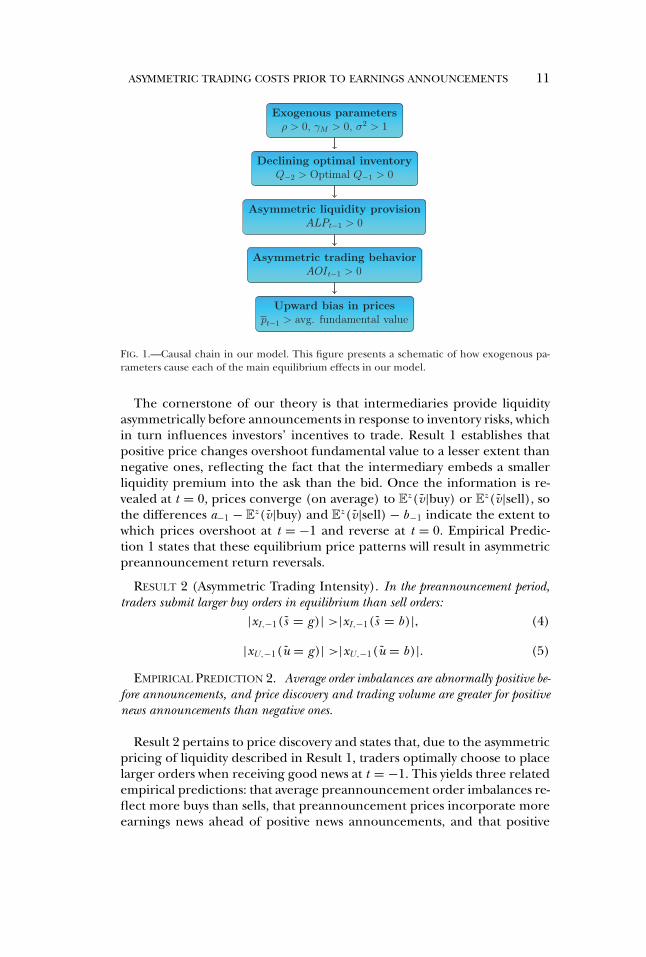
Our results are driven by the decrease in the intermediary’s optimalinventory before announcements. The intermediary’s choice of initialinventory Q−2 is determined by the tradeoff between a preference forpositive positions and the risk associated with nonzero inventory. In thepreannouncement period t = −1, however, the tradeoff changes becauseinventory risk rises, making the optimal target inventory for t = −1 lessthan Q−2. To reduce inventory toward this optimal target, the intermediaryprovides liquidity asymmetrically, giving rise to the following equilibriumresults. This progression is illustrated by figure 1.
RESULT 1 (Asymmetric Liquidity Provision). In the preannouncement period,negative price changes overshoot the information revealed by the trade more thanpositive ones:
Ez (v|sell) − E
z(b−1) > Ez(a−1) − E
z (v|buy). (3)
EMPIRICAL PREDICTION 1. The compensation intermediaries demand for pro-viding liquidity, as measured by return reversals, is higher for seller-initiated thanbuyer-initiated trades.
ASYMMETRIC TRADING COSTS PRIOR TO EARNINGS ANNOUNCEMENTS 11
FIG. 1.—Causal chain in our model. This figure presents a schematic of how exogenous pa-rameters cause each of the main equilibrium effects in our model.
The cornerstone of our theory is that intermediaries provide liquidityasymmetrically before announcements in response to inventory risks, whichin turn influences investors’ incentives to trade. Result 1 establishes thatpositive price changes overshoot fundamental value to a lesser extent thannegative ones, reflecting the fact that the intermediary embeds a smallerliquidity premium into the ask than the bid. Once the information is re-vealed at t = 0, prices converge (on average) to E
z(v|buy) or Ez(v|sell), so
the differences a−1 − Ez(v|buy) and E
z(v|sell) − b−1 indicate the extent towhich prices overshoot at t = −1 and reverse at t = 0. Empirical Predic-tion 1 states that these equilibrium price patterns will result in asymmetricpreannouncement return reversals.
RESULT 2 (Asymmetric Trading Intensity). In the preannouncement period,traders submit larger buy orders in equilibrium than sell orders:
|xI,−1(s = g)| >|xI,−1(s = b)|, (4)
|xU ,−1(u = g)| >|xU ,−1(u = b)|. (5)
EMPIRICAL PREDICTION 2. Average order imbalances are abnormally positive be-fore announcements, and price discovery and trading volume are greater for positivenews announcements than negative ones.
Result 2 pertains to price discovery and states that, due to the asymmetricpricing of liquidity described in Result 1, traders optimally choose to placelarger orders when receiving good news at t = −1. This yields three relatedempirical predictions: that average preannouncement order imbalances re-flect more buys than sells, that preannouncement prices incorporate moreearnings news ahead of positive news announcements, and that positive
12 T. L. JOHNSON AND E. C. SO
news announcements have greater preannouncement trading volume thannegative ones.
To study the implications of ATCs for returns before and after announce-ments, we first compute the average prices and returns in a “frictionlessbenchmark,” wherein there is no information asymmetry and the assettrades at its risk-neutral expected value in each period. In this case, ex-pected returns (price changes) are:
Ez (p −1 − p −2) = E
z (v−1) = 2(
z −1 − 12
), (6)
Ez (p 0 − p −1) = E
z (v0) = 2(
z0 − 12
)σ. (7)
Expected returns are driven by the risk associated with the news in eachperiod, 1 and σ , and the difference between physical and risk-neutral prob-abilities (zt and yt = 1
2 ).
RESULT 3 (Abnormal Returns Around Announcements). Expected returnscomputed using average prices under the physical measure satisfy:
Ez (p −1 − p −2) = 2
(z−1 − 1
2
)︸ ︷︷ ︸Normal risk prem.
+ ρ(σ 2 − 1)
(2p (1 − p ) + γM
γT
8p (1 − p )(1 + σ 2) + 2 γMγT
)︸ ︷︷ ︸
Upward bias
,
(8)
Ez (p 0 − p −1) = 2
(z0 − 1
2
)σ︸ ︷︷ ︸
Announcement risk prem.
− ρ(σ 2 − 1)
(2p (1 − p ) + γM
γT
8p (1 − p )(1 + σ 2) + 2 γMγT
)︸ ︷︷ ︸
Reversal of bias
.
(9)
EMPIRICAL PREDICTION 3. Average returns are abnormally positive before an-nouncements and less positive or even negative following the announcement. Ab-normal preannouncement returns that reverse reflect an upward bias resulting fromATCs, while longer window announcement returns reflect an announcement riskpremium.
Equation (8) quantifies two sources of preannouncement abnormal re-turns: a risk premium 2(z−1 − 1
2 ), which occurs in the frictionless bench-mark as well, and an upward bias caused by the ATCs. The upward biasis proportional to the benefit of positive inventory ρ multiplied by the in-crease in variance at the announcement (σ 2 − 1), both of which are posi-tive by assumption.

ASYMMETRIC TRADING COSTS PRIOR TO EARNINGS ANNOUNCEMENTS 13
It may be initially puzzling that the intermediary’s desire to reduce inven-tory, which leads to lower both ask and bid prices, results in higher averagetransaction prices. However, the equilibrium response of traders describedin Result 2 has an indirect effect on average prices: traders with positive sig-nals use larger quantities, meaning many more trades happen at a−1 thanb−1. This indirect effect outweighs the direct effect of lower average a−1 andb−1, because the intermediary is a net seller on average and uses its marketpower to capture positive expected trading profits while still reducing theirinventory risk.
Similarly, equation (9) quantifies the two sources of excess returns onthe announcement date: a risk premium 2(z0 − 1
2 )σ , which is likely largerthan the normal period premium 2(z−1 − 1
2 ), and a reversal of the upwardbias in preannouncement prices. Comparing equations (8) and (9) yieldstwo important insights. First, even if there is an abnormally large risk pre-mium at the announcement, returns measured in a narrow window aroundthe announcement will be confounded by the reversal of the preannounce-ment bias and therefore will understate the risk premium. Second, long-window cumulative returns surrounding the announcement represent therisk premium, while the portion of preannouncement returns that reversepostannouncement reflects the upward bias.
RESULT 4 (Comparative Statics). Averages of ALP, preannouncement returns,and postannouncement reversals are all increasing in the intermediary’s inventoryQ−1, risk aversion γM , cost of negative positions ρ, and the announcement risk σ .
EMPIRICAL PREDICTION 4. Averages of preannouncement ALP, preannounce-ment returns, and postannouncement reversals are all greater when intermediarieshave larger positive inventory positions, less risk-bearing capacity, higher costs of lo-cating and borrowing shares, and/or the earnings announcement risk is higher.
Our final result shows comparative statics for Results 1 through 3. Whenthe intermediary has a larger inventory, has greater risk aversion, or facesgreater announcement risks, all else equal it will be more aggressive in re-ducing inventory by asymmetrically providing liquidity, thereby increasingthe temporary bias in preannouncement prices p −1.
3. Empirical Tests
3.1 SAMPLE SELECTION
We construct the main data set used in our analyses from three sources.We obtain price and return data from CRSP, firm fundamentals from Com-pustat, and analysts’ forecasts of earnings from IBES. We eliminate firmsthat have been in the CRSP database for less than six months to ensurethat there are sufficient data to calculate historical return volatility and mo-mentum. We also require that firms have coverage in the IBES database tocalculate analyst-based earnings surprises and eliminate firms with prices
14 T. L. JOHNSON AND E. C. SO
below $1 to mitigate the influence of bid-ask bounce on our calculation ofreturn reversals, as noted in Roll [1984].
Our main analyses examine changes in liquidity and equity prices sur-rounding the date of firms’ quarterly earnings announcements.7 Becausewe expect liquidity provision to significantly change once the news is an-nounced, it is important to correctly identify the announcement date tocleanly test our hypotheses. To do so, we follow the procedure from Della-Vigna and Pollet [2009] that compares Compustat and IBES announce-ment dates and assigns the earlier date as being correct.8 We eliminate ob-servations where the Compustat and IBES announcement dates are morethan two trading days apart and also use the IBES time stamp to deter-mine whether the announcement occurred after the market close. Whenit does, we adjust the announcement date one trading day forward. Usingthis approach, our final sample consists of 215,754 quarterly earnings an-nouncements from 1993 to 2012.
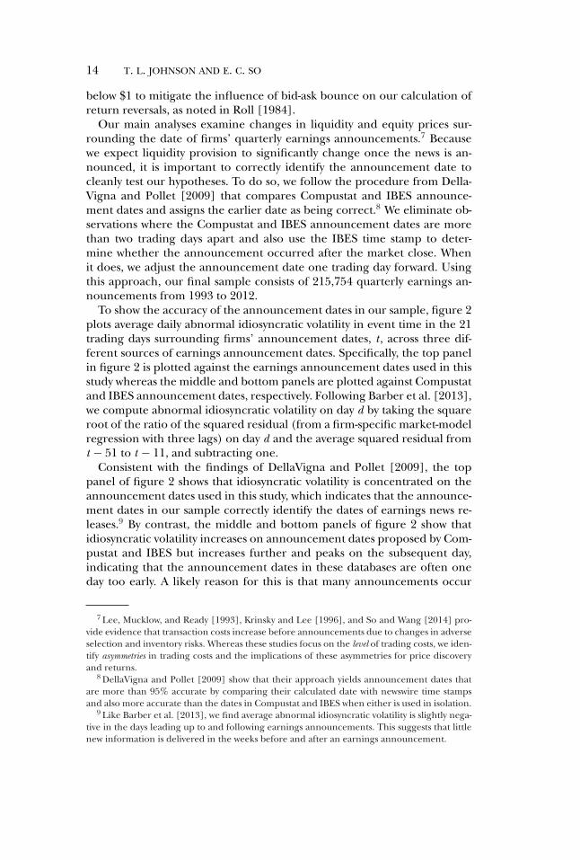
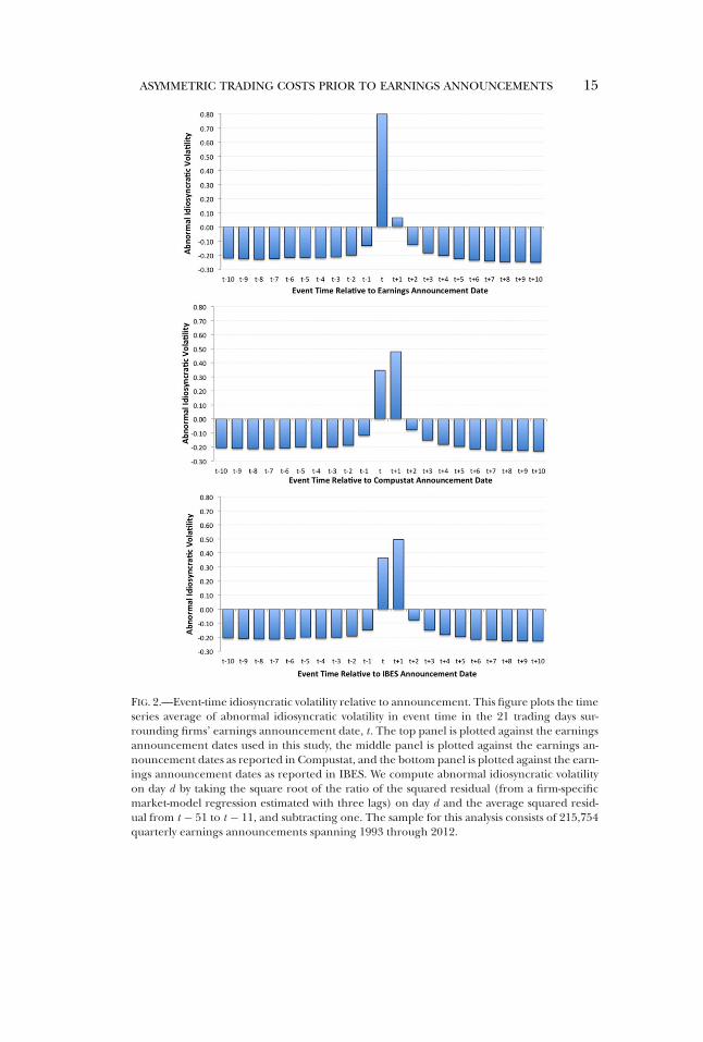
To show the accuracy of the announcement dates in our sample, figure 2plots average daily abnormal idiosyncratic volatility in event time in the 21trading days surrounding firms’ announcement dates, t , across three dif-ferent sources of earnings announcement dates. Specifically, the top panelin figure 2 is plotted against the earnings announcement dates used in thisstudy whereas the middle and bottom panels are plotted against Compustatand IBES announcement dates, respectively. Following Barber et al. [2013],we compute abnormal idiosyncratic volatility on day d by taking the squareroot of the ratio of the squared residual (from a firm-specific market-modelregression with three lags) on day d and the average squared residual fromt − 51 to t − 11, and subtracting one.
Consistent with the findings of DellaVigna and Pollet [2009], the toppanel of figure 2 shows that idiosyncratic volatility is concentrated on theannouncement dates used in this study, which indicates that the announce-ment dates in our sample correctly identify the dates of earnings news re-leases.9 By contrast, the middle and bottom panels of figure 2 show thatidiosyncratic volatility increases on announcement dates proposed by Com-pustat and IBES but increases further and peaks on the subsequent day,indicating that the announcement dates in these databases are often oneday too early. A likely reason for this is that many announcements occur
7 Lee, Mucklow, and Ready [1993], Krinsky and Lee [1996], and So and Wang [2014] pro-vide evidence that transaction costs increase before announcements due to changes in adverseselection and inventory risks. Whereas these studies focus on the level of trading costs, we iden-tify asymmetries in trading costs and the implications of these asymmetries for price discoveryand returns.
8 DellaVigna and Pollet [2009] show that their approach yields announcement dates thatare more than 95% accurate by comparing their calculated date with newswire time stampsand also more accurate than the dates in Compustat and IBES when either is used in isolation.
9 Like Barber et al. [2013], we find average abnormal idiosyncratic volatility is slightly nega-tive in the days leading up to and following earnings announcements. This suggests that littlenew information is delivered in the weeks before and after an earnings announcement.
ASYMMETRIC TRADING COSTS PRIOR TO EARNINGS ANNOUNCEMENTS 15
FIG. 2.—Event-time idiosyncratic volatility relative to announcement. This figure plots the timeseries average of abnormal idiosyncratic volatility in event time in the 21 trading days sur-rounding firms’ earnings announcement date, t . The top panel is plotted against the earningsannouncement dates used in this study, the middle panel is plotted against the earnings an-nouncement dates as reported in Compustat, and the bottom panel is plotted against the earn-ings announcement dates as reported in IBES. We compute abnormal idiosyncratic volatilityon day d by taking the square root of the ratio of the squared residual (from a firm-specificmarket-model regression estimated with three lags) on day d and the average squared resid-ual from t − 51 to t − 11, and subtracting one. The sample for this analysis consists of 215,754quarterly earnings announcements spanning 1993 through 2012.
16 T. L. JOHNSON AND E. C. SO
after markets close, meaning an announcement made today is commonlyreflected in tomorrow’s close-to-close return.
The findings in figure 2 help explain why we find no excess returns onannouncement dates, whereas prior research finds significant excess re-turns on Compustat announcement dates (e.g., Ball and Kothari [1991]and Frazzini and Lamont [2007]). By using Compustat dates that are fre-quently one day too early, these studies record the return one day beforethe actual announcement, which is abnormally positive, as the announce-ment date return.
3.2 ASYMMETRIC TRADING COSTS
Our first analyses test Empirical Prediction 1, which states that interme-diaries set asymmetric prices for providing liquidity before earnings an-nouncements. Because intermediaries in our model demand compensa-tion for providing liquidity in the form of transitory price concessions, weuse short-term return reversals as a proxy for the expected returns interme-diaries demand for providing liquidity, although, in the online appendix,we also find similar results using alternative proxies for transaction costs.
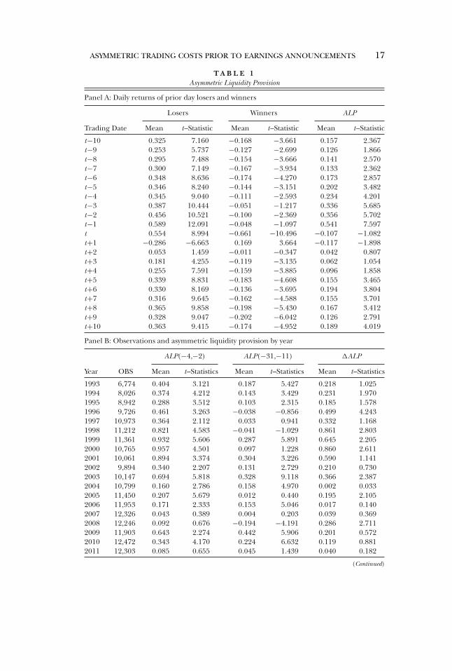
Panel A of table 1 contains average daily returns for firms within the low-est quintile of returns over the prior day (“losers”) and firms within thehighest quintile of returns over the prior day (“winners”), in event timefor the 21 trading days surrounding firms’ announcement dates. Averagedaily returns of firms in the lowest quintile are generally positive and sig-nificant, consistent with intermediaries receiving compensation for provid-ing liquidity in periods of net selling by setting prices below fundamentalvalue. Similarly, the average daily return for firms in the highest quintile aregenerally negative and significant. Consistent with the findings of Avramov,Chordia, and Goyal [2006], losers exhibit greater reversals than winnersthroughout the event window, suggesting that intermediaries are generallymore averse to providing liquidity to sellers and thus demand asymmetriclevels of compensation.
The final column of panel A presents average levels of ALP defined as thedifference between returns earned from a long position in prior day losersand returns earned from a short position in prior day winners. ALP cap-tures differences in reversal magnitudes across losers and winners, and thushigher values of ALP indicate that intermediaries demand greater compen-sation for providing liquidity to sellers relative to buyers. The average levelof ALP increases beginning several days before the announcement, consis-tent with intermediaries often taking multiple days to unwind net positions(Madhavan and Smidt [1993]) and thus being averse to taking on addi-tional inventory before high volatility events because doing so increasestheir risk exposure.
Panel A of table 1 also shows that ALP steadily increases until t − 1,reflecting the contrast between the rapid ascension of reversals associ-ated with the loser portfolio and the flatter trend in reversals associatedwith the winner portfolio. These results suggest that intermediaries are
ASYMMETRIC TRADING COSTS PRIOR TO EARNINGS ANNOUNCEMENTS 17
T A B L E 1Asymmetric Liquidity Provision
Panel A: Daily returns of prior day losers and winners
Losers Winners ALP
Trading Date Mean t–Statistic Mean t–Statistic Mean t–Statistic
t−10 0.325 7.160 −0.168 −3.661 0.157 2.367t−9 0.253 5.737 −0.127 −2.699 0.126 1.866t−8 0.295 7.488 −0.154 −3.666 0.141 2.570t−7 0.300 7.149 −0.167 −3.934 0.133 2.362t−6 0.348 8.636 −0.174 −4.270 0.173 2.857t−5 0.346 8.240 −0.144 −3.151 0.202 3.482t−4 0.345 9.040 −0.111 −2.593 0.234 4.201t−3 0.387 10.444 −0.051 −1.217 0.336 5.685t−2 0.456 10.521 −0.100 −2.369 0.356 5.702t−1 0.589 12.091 −0.048 −1.097 0.541 7.597t 0.554 8.994 −0.661 −10.496 −0.107 −1.082t+1 −0.286 −6.663 0.169 3.664 −0.117 −1.898t+2 0.053 1.459 −0.011 −0.347 0.042 0.807t+3 0.181 4.255 −0.119 −3.135 0.062 1.054t+4 0.255 7.591 −0.159 −3.885 0.096 1.858t+5 0.339 8.831 −0.183 −4.608 0.155 3.465t+6 0.330 8.169 −0.136 −3.695 0.194 3.804t+7 0.316 9.645 −0.162 −4.588 0.155 3.701t+8 0.365 9.858 −0.198 −5.430 0.167 3.412t+9 0.328 9.047 −0.202 −6.042 0.126 2.791t+10 0.363 9.415 −0.174 −4.952 0.189 4.019
Panel B: Observations and asymmetric liquidity provision by year
ALP(−4,−2) ALP(−31,−11) �ALP
Year OBS Mean t–Statistics Mean t–Statistics Mean t–Statistics
1993 6,774 0.404 3.121 0.187 5.427 0.218 1.0251994 8,026 0.374 4.212 0.143 3.429 0.231 1.9701995 8,942 0.288 3.512 0.103 2.315 0.185 1.5781996 9,726 0.461 3.263 −0.038 −0.856 0.499 4.2431997 10,973 0.364 2.112 0.033 0.941 0.332 1.1681998 11,212 0.821 4.583 −0.041 −1.029 0.861 2.8031999 11,361 0.932 5.606 0.287 5.891 0.645 2.2052000 10,765 0.957 4.501 0.097 1.228 0.860 2.6112001 10,061 0.894 3.374 0.304 3.226 0.590 1.1412002 9,894 0.340 2.207 0.131 2.729 0.210 0.7302003 10,147 0.694 5.818 0.328 9.118 0.366 2.3872004 10,799 0.160 2.786 0.158 4.970 0.002 0.0332005 11,450 0.207 5.679 0.012 0.440 0.195 2.1052006 11,953 0.171 2.333 0.153 5.046 0.017 0.1402007 12,326 0.043 0.389 0.004 0.203 0.039 0.3692008 12,246 0.092 0.676 −0.194 −4.191 0.286 2.7112009 11,903 0.643 2.274 0.442 5.906 0.201 0.5722010 12,472 0.343 4.170 0.224 6.632 0.119 0.8812011 12,303 0.085 0.655 0.045 1.439 0.040 0.182
(Continued)
18 T. L. JOHNSON AND E. C. SO
T A B L E 1—Continued
Panel B: Observations and asymmetric liquidity provision by year
ALP(−4,−2) ALP(−31,−11) �ALP
Year OBS Mean t–Statistics Mean t–Statistics Mean t–Statistics
2012 12,421 −0.054 −0.766 0.045 1.178 −0.098 −1.282All 215,754 0.411 7.200 0.121 3.413 0.290 5.345
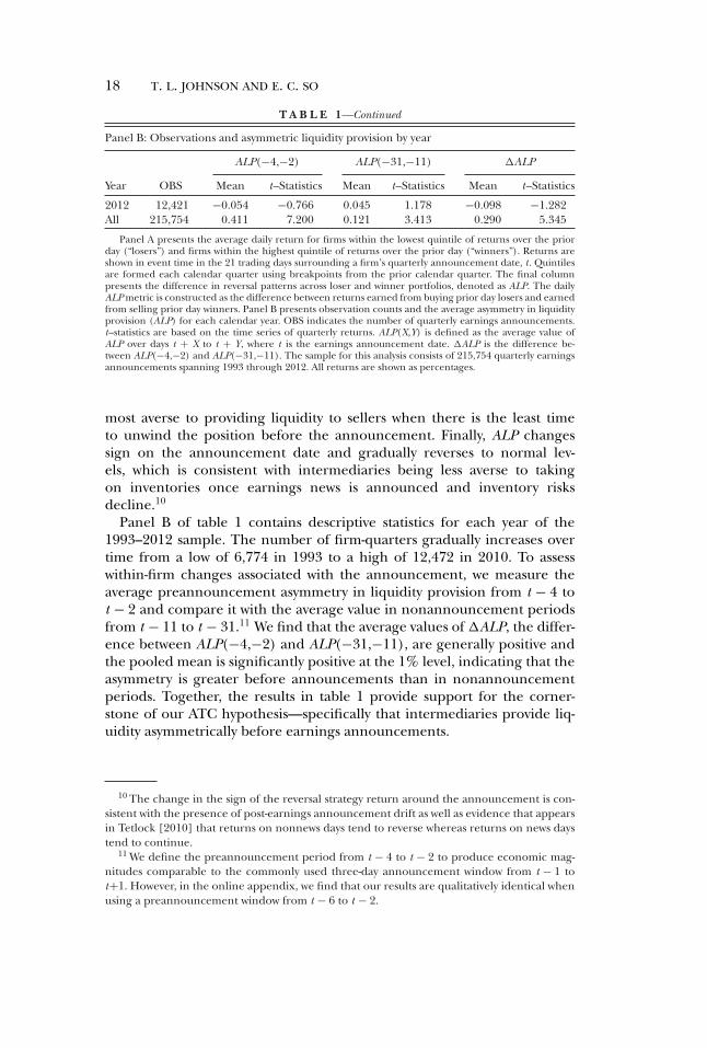
Panel A presents the average daily return for firms within the lowest quintile of returns over the priorday (“losers”) and firms within the highest quintile of returns over the prior day (“winners”). Returns areshown in event time in the 21 trading days surrounding a firm’s quarterly announcement date, t . Quintilesare formed each calendar quarter using breakpoints from the prior calendar quarter. The final columnpresents the difference in reversal patterns across loser and winner portfolios, denoted as ALP. The dailyALP metric is constructed as the difference between returns earned from buying prior day losers and earnedfrom selling prior day winners. Panel B presents observation counts and the average asymmetry in liquidityprovision (ALP) for each calendar year. OBS indicates the number of quarterly earnings announcements.t–statistics are based on the time series of quarterly returns. ALP(X,Y) is defined as the average value ofALP over days t + X to t + Y, where t is the earnings announcement date. �ALP is the difference be-tween ALP(−4,−2) and ALP(−31,−11). The sample for this analysis consists of 215,754 quarterly earningsannouncements spanning 1993 through 2012. All returns are shown as percentages.
most averse to providing liquidity to sellers when there is the least timeto unwind the position before the announcement. Finally, ALP changessign on the announcement date and gradually reverses to normal lev-els, which is consistent with intermediaries being less averse to takingon inventories once earnings news is announced and inventory risksdecline.10
Panel B of table 1 contains descriptive statistics for each year of the1993–2012 sample. The number of firm-quarters gradually increases overtime from a low of 6,774 in 1993 to a high of 12,472 in 2010. To assesswithin-firm changes associated with the announcement, we measure theaverage preannouncement asymmetry in liquidity provision from t − 4 tot − 2 and compare it with the average value in nonannouncement periodsfrom t − 11 to t − 31.11 We find that the average values of �ALP, the differ-ence between ALP(−4,−2) and ALP(−31,−11), are generally positive andthe pooled mean is significantly positive at the 1% level, indicating that theasymmetry is greater before announcements than in nonannouncementperiods. Together, the results in table 1 provide support for the corner-stone of our ATC hypothesis—specifically that intermediaries provide liq-uidity asymmetrically before earnings announcements.
10 The change in the sign of the reversal strategy return around the announcement is con-sistent with the presence of post-earnings announcement drift as well as evidence that appearsin Tetlock [2010] that returns on nonnews days tend to reverse whereas returns on news daystend to continue.
11 We define the preannouncement period from t − 4 to t − 2 to produce economic mag-nitudes comparable to the commonly used three-day announcement window from t − 1 tot+1. However, in the online appendix, we find that our results are qualitatively identical whenusing a preannouncement window from t − 6 to t − 2.
ASYMMETRIC TRADING COSTS PRIOR TO EARNINGS ANNOUNCEMENTS 19
3.3 IMPLICATIONS OF ASYMMETRIC TRADING COSTS
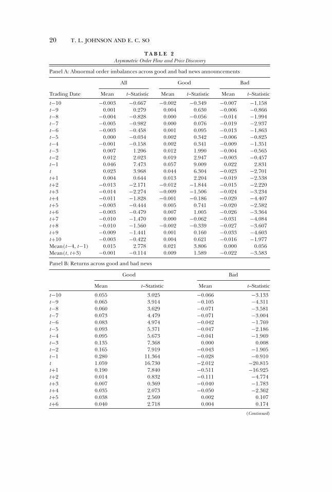
Tables 2 and 3 present three tests of Empirical Prediction 2, which statesthat traders respond to asymmetric liquidity costs by trading more aggres-sively on good news than bad news. We begin by showing pooled averagesof AOIs for all earnings announcements in the “All” column of panel A intable 2. Average order imbalances tend to be positive leading up to the an-nouncement and peak on day t − 1, indicating that investors tend to benet buyers before earnings announcements. By contrast, average order im-balances flip sign and become negative following the announcement, indi-cating that investors become net sellers once the news is announced andinventory risks decline.
A second implication of Empirical Prediction 2 is that informed tradersplace larger orders when they receive positive signals. To establish thispattern empirically, panel A of table 2 contains daily AOIs around an-nouncements in which firms report “good” news, defined as earningsat or above the consensus earnings forecast, and those where firms re-port “bad” news, defined as earnings below the consensus. Panel A showsthat there is a large spike in directional trading before good news an-nouncements and no spike for bad news. In fact, AOIs are positive theday before bad news announcements. Panel A of table 2 also showsthat postannouncement order imbalances follow the opposite pattern:negative news tends to be followed by a longer trend of net selling,whereas no such trend exists for positive news. These patterns are con-sistent with the idea that investors are deterred from expressing negativenews before earnings announcements and instead trade on negative newsafterward.
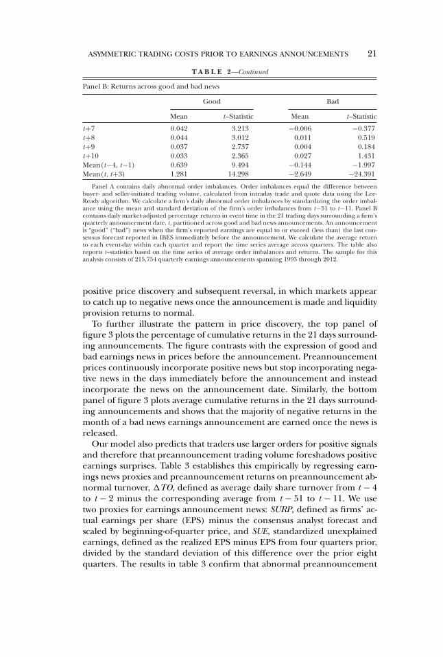
In panel B of table 2, we test the third implication of Empirical Pre-diction 2, that asymmetric order flow results in biased price discoverybefore earnings announcements. We show that, for good news announce-ments, average returns are consistently positive leading up to the announce-ment. They then increase as the announcement approaches and remainstatistically significant throughout.12 By contrast, for bad news announce-ments, average returns are slightly negative several days before the an-nouncement but attenuate over time, becoming statistically insignificantin the days immediately before the announcement.
Starting on the announcement day, the pattern in price discovery im-mediately reverses, with prices strongly incorporating negative news but re-acting less to good news, which preannouncement prices already reflectedto a greater degree. Panel B of table 2 also provides average returns inthe four trading days before the announcement and the four trading dayson and after it. These tests illustrate the preannouncement bias toward
12 We do not estimate ALP in good and bad news subsamples because our model predictsthat ALP is determined by intermediary inventory and preferences and is not affected by thesign of earnings news.
20 T. L. JOHNSON AND E. C. SO
T A B L E 2Asymmetric Order Flow and Price Discovery
Panel A: Abnormal order imbalances across good and bad news announcements
All Good Bad
Trading Date Mean t–Statistic Mean t–Statistic Mean t–Statistic
t−10 −0.003 −0.667 −0.002 −0.349 −0.007 −1.158t−9 0.001 0.279 0.004 0.630 −0.006 −0.866t−8 −0.004 −0.828 0.000 −0.056 −0.014 −1.994t−7 −0.005 −0.982 0.000 0.076 −0.019 −2.937t−6 −0.003 −0.458 0.001 0.095 −0.013 −1.863t−5 0.000 −0.034 0.002 0.342 −0.006 −0.825t−4 −0.001 −0.158 0.002 0.341 −0.009 −1.351t−3 0.007 1.206 0.012 1.990 −0.004 −0.565t−2 0.012 2.023 0.019 2.947 −0.003 −0.457t−1 0.046 7.473 0.057 9.009 0.022 2.831t 0.023 3.968 0.044 6.304 −0.023 −2.701t+1 0.004 0.644 0.013 2.204 −0.019 −2.538t+2 −0.013 −2.171 −0.012 −1.844 −0.015 −2.220t+3 −0.014 −2.274 −0.009 −1.506 −0.024 −3.234t+4 −0.011 −1.828 −0.001 −0.186 −0.029 −4.407t+5 −0.003 −0.444 0.005 0.741 −0.020 −2.582t+6 −0.003 −0.479 0.007 1.005 −0.026 −3.364t+7 −0.010 −1.470 0.000 −0.062 −0.031 −4.084t+8 −0.010 −1.560 −0.002 −0.339 −0.027 −3.607t+9 −0.009 −1.441 0.001 0.160 −0.033 −4.603t+10 −0.003 −0.422 0.004 0.621 −0.016 −1.977Mean(t−4, t−1) 0.015 2.778 0.021 3.806 0.000 0.056Mean(t, t+3) −0.001 −0.114 0.009 1.589 −0.022 −3.583
Panel B: Returns across good and bad news
Good Bad
Mean t–Statistic Mean t–Statistic
t−10 0.055 3.025 −0.066 −3.133t−9 0.065 3.914 −0.105 −4.311t−8 0.060 3.629 −0.071 −3.581t−7 0.073 4.479 −0.071 −3.004t−6 0.083 4.974 −0.042 −1.769t−5 0.093 5.371 −0.047 −2.186t−4 0.095 5.673 −0.041 −1.969t−3 0.135 7.368 0.000 0.008t−2 0.165 7.919 −0.043 −1.905t−1 0.280 11.364 −0.028 −0.910t 1.059 16.730 −2.012 −20.815t+1 0.190 7.840 −0.511 −16.925t+2 0.014 0.832 −0.111 −4.774t+3 0.007 0.369 −0.040 −1.783t+4 0.035 2.073 −0.050 −2.362t+5 0.038 2.569 0.002 0.107t+6 0.040 2.718 0.004 0.174
(Continued)
ASYMMETRIC TRADING COSTS PRIOR TO EARNINGS ANNOUNCEMENTS 21
T A B L E 2—Continued
Panel B: Returns across good and bad news
Good Bad
Mean t–Statistic Mean t–Statistic
t+7 0.042 3.213 −0.006 −0.377t+8 0.044 3.012 0.011 0.519t+9 0.037 2.737 0.004 0.184t+10 0.033 2.365 0.027 1.431Mean(t−4, t−1) 0.639 9.494 −0.144 −1.997Mean(t, t+3) 1.281 14.298 −2.649 −24.391
Panel A contains daily abnormal order imbalances. Order imbalances equal the difference betweenbuyer- and seller-initiated trading volume, calculated from intraday trade and quote data using the Lee-Ready algorithm. We calculate a firm’s daily abnormal order imbalances by standardizing the order imbal-ance using the mean and standard deviation of the firm’s order imbalances from t−51 to t−11. Panel Bcontains daily market-adjusted percentage returns in event time in the 21 trading days surrounding a firm’squarterly announcement date, t , partitioned across good and bad news announcements. An announcementis “good” (“bad”) news when the firm’s reported earnings are equal to or exceed (less than) the last con-sensus forecast reported in IBES immediately before the announcement. We calculate the average returnto each event-day within each quarter and report the time series average across quarters. The table alsoreports t–statistics based on the time series of average order imbalances and returns. The sample for thisanalysis consists of 215,754 quarterly earnings announcements spanning 1993 through 2012.
positive price discovery and subsequent reversal, in which markets appearto catch up to negative news once the announcement is made and liquidityprovision returns to normal.
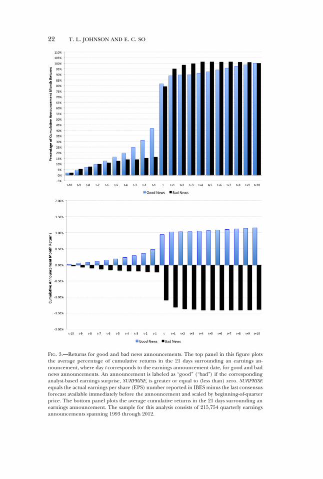
To further illustrate the pattern in price discovery, the top panel offigure 3 plots the percentage of cumulative returns in the 21 days surround-ing announcements. The figure contrasts with the expression of good andbad earnings news in prices before the announcement. Preannouncementprices continuously incorporate positive news but stop incorporating nega-tive news in the days immediately before the announcement and insteadincorporate the news on the announcement date. Similarly, the bottompanel of figure 3 plots average cumulative returns in the 21 days surround-ing announcements and shows that the majority of negative returns in themonth of a bad news earnings announcement are earned once the news isreleased.
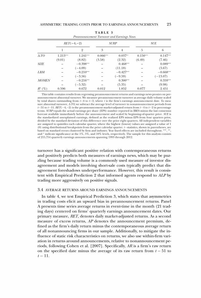
Our model also predicts that traders use larger orders for positive signalsand therefore that preannouncement trading volume foreshadows positiveearnings surprises. Table 3 establishes this empirically by regressing earn-ings news proxies and preannouncement returns on preannouncement ab-normal turnover, �TO, defined as average daily share turnover from t − 4to t − 2 minus the corresponding average from t − 51 to t − 11. We usetwo proxies for earnings announcement news: SURP, defined as firms’ ac-tual earnings per share (EPS) minus the consensus analyst forecast andscaled by beginning-of-quarter price, and SUE, standardized unexplainedearnings, defined as the realized EPS minus EPS from four quarters prior,divided by the standard deviation of this difference over the prior eightquarters. The results in table 3 confirm that abnormal preannouncement
22 T. L. JOHNSON AND E. C. SO
FIG. 3.—Returns for good and bad news announcements. The top panel in this figure plotsthe average percentage of cumulative returns in the 21 days surrounding an earnings an-nouncement, where day t corresponds to the earnings announcement date, for good and badnews announcements. An announcement is labeled as “good” (“bad”) if the correspondinganalyst-based earnings surprise, SURPRISE, is greater or equal to (less than) zero. SURPRISEequals the actual earnings per share (EPS) number reported in IBES minus the last consensusforecast available immediately before the announcement and scaled by beginning-of-quarterprice. The bottom panel plots the average cumulative returns in the 21 days surrounding anearnings announcement. The sample for this analysis consists of 215,754 quarterly earningsannouncements spanning 1993 through 2012.
ASYMMETRIC TRADING COSTS PRIOR TO EARNINGS ANNOUNCEMENTS 23
T A B L E 3Preannouncement Turnover and Earnings News
RET(−4,−2) SURP SUE
1 2 3 4 5 6
�TO 1.213∗∗∗ 1.241∗∗∗ 0.066∗∗∗ 0.037∗∗ 0.150∗∗∗ 0.147∗∗∗
(9.01) (8.82) (3.58) (2.32) (6.49) (7.46)SIZE – −0.398∗∗∗ – 0.468∗∗∗ – 0.089∗∗∗
– (−4.09) – (11.18) – (3.67)LBM – −0.210∗∗∗ – −0.427∗∗∗ – −0.668∗∗∗
– (−3.56) – (−9.59) – (−13.07)MOMEN – −0.216∗∗∗ – 0.300∗∗∗ – 0.359∗∗∗
– (−5.32) – (5.35) – (9.98)R2 (%) 0.596 0.672 0.012 1.852 0.077 2.451
This table contains results from regressing preannouncement returns and earnings news proxies on pre-announcement abnormal turnover. We measure preannouncement turnover as average daily volume scaledby total shares outstanding from t−4 to t−2, where t is the firm’s earnings announcement date. To mea-sure abnormal turnover, �TO, we subtract the average level of turnover in nonannouncement periods fromt−51 to t−11. RET(−4,−2) is the preannouncement market-adjusted return from t−4 to t−2 in percentageterms. SURP equals the actual earnings per share (EPS) number reported in IBES minus the last consensusforecast available immediately before the announcement and scaled by beginning-of-quarter price. SUE isthe standardized unexplained earnings, defined as the realized EPS minus EPS from four quarters prior,divided by the standard deviation of this difference over the prior eight quarters. All independent variablesare assigned to quintiles each calendar quarter, where the highest (lowest) values are assigned a value of 1(0) using distributional breakpoints from the prior calendar quarter. t−statistics, shown in parentheses, arebased on standard errors clustered by firm and industry. Year fixed effects are included throughout. ∗∗∗, ∗∗,and ∗ indicate significance at the 1%, 5%, and 10% levels, respectively. The sample for this analysis consistsof 215,754 quarterly earnings announcements spanning 1993 through 2012.
turnover has a significant positive relation with contemporaneous returnsand positively predicts both measures of earnings news, which may be puz-zling because trading volume is a commonly used measure of investor dis-agreement and models involving short-sale costs typically predict that dis-agreement foreshadows underperformance. However, this result is consis-tent with Empirical Prediction 2 that informed agents respond to ALP bytrading more aggressively on positive signals.
3.4 AVERAGE RETURNS AROUND EARNINGS ANNOUNCEMENTS
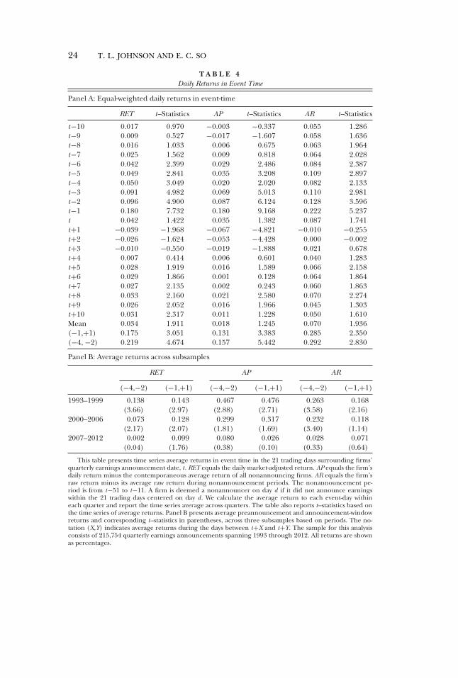
In table 4, we test Empirical Prediction 3, which states that asymmetriesin trading costs elicit an upward bias in preannouncement returns. PanelA presents time series average returns in event-time in the month (21 trad-ing days) centered on firms’ quarterly earnings announcement dates. Ourprimary measure, RET, denotes daily market-adjusted returns. As a secondmeasure of excess returns, AP denotes the announcement premium, de-fined as the firm’s daily return minus the contemporaneous average returnof all nonannouncing firms in our sample. Additionally, to mitigate the in-fluence of static risk characteristics on returns, we also use within-firm vari-ation in returns around announcements, relative to nonannouncement pe-riods, following Cohen et al. [2007]. Specifically, AR is a firm’s raw returnon the specified date minus the average of its raw return from t − 51 tot − 11.
24 T. L. JOHNSON AND E. C. SO
T A B L E 4Daily Returns in Event Time
Panel A: Equal-weighted daily returns in event-time
RET t–Statistics AP t–Statistics AR t–Statistics
t−10 0.017 0.970 −0.003 −0.337 0.055 1.286t−9 0.009 0.527 −0.017 −1.607 0.058 1.636t−8 0.016 1.033 0.006 0.675 0.063 1.964t−7 0.025 1.562 0.009 0.818 0.064 2.028t−6 0.042 2.399 0.029 2.486 0.084 2.387t−5 0.049 2.841 0.035 3.208 0.109 2.897t−4 0.050 3.049 0.020 2.020 0.082 2.133t−3 0.091 4.982 0.069 5.013 0.110 2.981t−2 0.096 4.900 0.087 6.124 0.128 3.596t−1 0.180 7.732 0.180 9.168 0.222 5.237t 0.042 1.422 0.035 1.382 0.087 1.741t+1 −0.039 −1.968 −0.067 −4.821 −0.010 −0.255t+2 −0.026 −1.624 −0.053 −4.428 0.000 −0.002t+3 −0.010 −0.550 −0.019 −1.888 0.021 0.678t+4 0.007 0.414 0.006 0.601 0.040 1.283t+5 0.028 1.919 0.016 1.589 0.066 2.158t+6 0.029 1.866 0.001 0.128 0.064 1.864t+7 0.027 2.135 0.002 0.243 0.060 1.863t+8 0.033 2.160 0.021 2.580 0.070 2.274t+9 0.026 2.052 0.016 1.966 0.045 1.303t+10 0.031 2.317 0.011 1.228 0.050 1.610Mean 0.034 1.911 0.018 1.245 0.070 1.936(−1,+1) 0.175 3.051 0.131 3.383 0.285 2.350(−4,−2) 0.219 4.674 0.157 5.442 0.292 2.830
Panel B: Average returns across subsamples
RET AP AR
(−4,−2) (−1,+1) (−4,−2) (−1,+1) (−4,−2) (−1,+1)
1993–1999 0.138 0.143 0.467 0.476 0.263 0.168(3.66) (2.97) (2.88) (2.71) (3.58) (2.16)
2000–2006 0.073 0.128 0.299 0.317 0.232 0.118(2.17) (2.07) (1.81) (1.69) (3.40) (1.14)
2007–2012 0.002 0.099 0.080 0.026 0.028 0.071(0.04) (1.76) (0.38) (0.10) (0.33) (0.64)
This table presents time series average returns in event time in the 21 trading days surrounding firms’quarterly earnings announcement date, t . RET equals the daily market-adjusted return. AP equals the firm’sdaily return minus the contemporaneous average return of all nonannouncing firms. AR equals the firm’sraw return minus its average raw return during nonannouncement periods. The nonannouncement pe-riod is from t−51 to t−11. A firm is deemed a nonannouncer on day d if it did not announce earningswithin the 21 trading days centered on day d. We calculate the average return to each event-day withineach quarter and report the time series average across quarters. The table also reports t–statistics based onthe time series of average returns. Panel B presents average preannouncement and announcement-windowreturns and corresponding t–statistics in parentheses, across three subsamples based on periods. The no-tation (X,Y) indicates average returns during the days between t+X and t+Y. The sample for this analysisconsists of 215,754 quarterly earnings announcements spanning 1993 through 2012. All returns are shownas percentages.
ASYMMETRIC TRADING COSTS PRIOR TO EARNINGS ANNOUNCEMENTS 25
Panel A of table 4 presents one of our main results. Specifically, the tableshows that, on average, firms begin earning significantly positive returns anentire week before their earnings announcements starting on t − 6. Prean-nouncement returns grow in magnitude and significance when approach-ing the announcement, peaking on day t − 1.
The evidence in table 4 is generally consistent with the findings of Bar-ber et al. [2013] that the bulk of the monthly earnings AP is earned beforeannouncements. However, our evidence also contrasts with the finding ofBarber et al. [2013] that the largest abnormal return occurs on the an-nouncement date, t . To our knowledge, by precisely measuring the earn-ings announcement date, our study is the first to show that returns are onlyreliably positive before, but not during, the arrival of earnings news.13
As shown in section 2, in the presence of an announcement risk premiumbut no market frictions, prices should be low preannouncement, rise dur-ing the announcement in proportion to the realization of priced risk, andstabilize postannouncement. By contrast, our evidence shows that pricespredictably increase preannouncement, do not significantly change duringthe announcement, and decrease postannouncement. Our model and em-pirical results help to reconcile these findings by highlighting the influenceof ATCs.
The bottom rows of table 4 quantify the relative magnitudes of prean-nouncement returns from t − 4 to t − 2 and announcement returns fromt − 1 to t + 1. Across all three return metrics, the mean and t -statistic ofreturns from t − 4 to t − 2 are just as large, if not larger, than those corre-sponding to t − 1 to t + 1. Table 4 also shows that cumulative returns fromt − 1 to t + 1 are only significantly positive because of large positive returnsthe day immediately before the announcement on t − 1, rather than thereturns on the announcement day t .
Additionally, the cumulative returns from t − 10 to t+10 highlight thepuzzling discrepancy between the estimated magnitudes of short- andlonger window announcement risk premia. Specifically, consistent with themagnitudes shown by prior research, the average three-day market-adjustedannouncement return is approximately 17 bp, whereas average announce-ment month return is approximately three times as large at 55 bp, despiteboth measures intending to capture risk premia associated with earningsnews. Our paper helps to explain this discrepancy by identifying marketfrictions that elicit a downward bias in short-window announcement returnsbecause, while the returns reflect risk premia, they also reflect a reversal ofthe upward bias in preannouncement prices.
Thus our return-based results help solve the puzzle from Barber et al.[2013] that a significant portion of the monthly earnings AP is earned
13 Similarly, whereas So and Wang [2014] and Levi and Zhang [2015] show that announce-ment returns are positive, conditional upon extreme negative preannouncement returns, ourunconditional tests show that average announcement day returns are insignificantly differentfrom zero.
26 T. L. JOHNSON AND E. C. SO
before announcement dates. We show that, even in the presence of a riskpremium associated with an information event, researchers are likely toobserve abnormal returns beforehand due to predictable asymmetries intrading costs.
The evidence of significant preannouncement returns in table 4 is un-likely to be driven by an idiosyncratic risk premium, considering the ev-idence in figure 2 that idiosyncratic volatility is concentrated on the an-nouncement date. In standard asset pricing models, risk premia should beearned at the same time as the realization of the priced risk. However, weshow that excess returns precede idiosyncratic volatility at the announce-ment by an entire week and provide a friction-based explanation for thisphenomenon.
More generally, positive preannouncement returns are unlikely to purelyreflect compensation for an unspecified form of risk, for example causedby peer firms announcing their earnings, because of the postannounce-ment reversal. Excess returns due to risk premia do not reverse because, ifthey did, they would not compensate long-term investors for bearing therisk. Instead, the postannouncement reversal of preannouncement excessreturns is consistent with a friction-based, transitory bias in preannounce-ment prices. Due to this upward bias, prices must adjust further in responseto the release of negative earnings news, suggesting that evidence of anasymmetric reaction to negative news announcements shown in prior re-search is at least partially driven by greater preannouncement costs of sell-ing rather than selective disclosures.
Our ATC hypothesis predicts that preannouncement biases vary with howintermediaries provide liquidity, which is likely influenced by the contin-ued evolution of market microstructure and changes to the compositionand market power of liquidity providers, as discussed in section 2. To illu-minate this issue, panel B of table 4 reports average preannouncement-and announcement-window returns across three subsamples partitionedby time. The results show both measures of returns decrease over time,particularly the preannouncement return, consistent with changes in thefinancial intermediary sector gradually alleviating the frictions that lead topredictable upward biases in preannouncement prices.
4. Additional Analyses
4.1 CROSS-SECTIONAL IMPLICATIONS
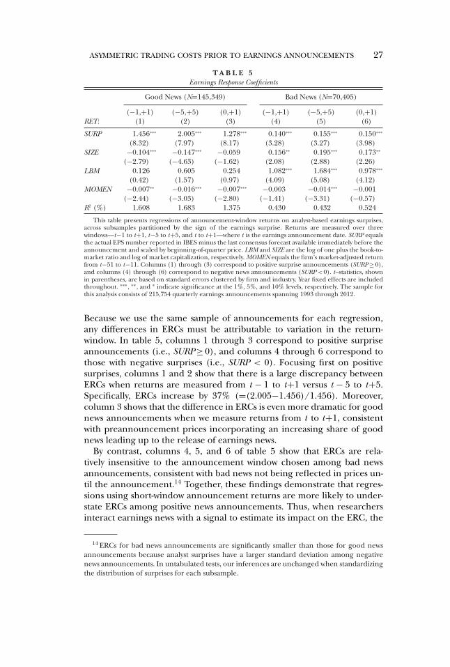
Our model predicts that market prices incorporate more good newsbefore announcements and less during, and vice versa for bad news. To-gether, these predictions suggest that estimated earnings response coeffi-cients (ERCs) are more likely to be sensitive to the chosen return windowfor announcements with positive earnings surprises. To test this predictionempirically, we estimate ERCs using the same sample but three differentannouncement windows from t − 1 to t+1, t − 5 to t+5, and t to t+1.
ASYMMETRIC TRADING COSTS PRIOR TO EARNINGS ANNOUNCEMENTS 27
T A B L E 5Earnings Response Coefficients
Good News (N=145,349) Bad News (N=70,405)
(−1,+1) (−5,+5) (0,+1) (−1,+1) (−5,+5) (0,+1)RET: (1) (2) (3) (4) (5) (6)
SURP 1.456∗∗∗ 2.005∗∗∗ 1.278∗∗∗ 0.140∗∗∗ 0.155∗∗∗ 0.150∗∗∗
(8.32) (7.97) (8.17) (3.28) (3.27) (3.98)SIZE −0.104∗∗∗ −0.147∗∗∗ −0.059 0.156∗∗ 0.195∗∗∗ 0.173∗∗
(−2.79) (−4.63) (−1.62) (2.08) (2.88) (2.26)LBM 0.126 0.605 0.254 1.082∗∗∗ 1.684∗∗∗ 0.978∗∗∗
(0.42) (1.57) (0.97) (4.09) (5.08) (4.12)MOMEN −0.007∗∗ −0.016∗∗∗ −0.007∗∗∗ −0.003 −0.014∗∗∗ −0.001
(−2.44) (−3.03) (−2.80) (−1.41) (−3.31) (−0.57)R2 (%) 1.608 1.683 1.375 0.430 0.432 0.524
This table presents regressions of announcement-window returns on analyst-based earnings surprises,across subsamples partitioned by the sign of the earnings surprise. Returns are measured over threewindows—t−1 to t+1, t−5 to t+5, and t to t+1—where t is the earnings announcement date. SURP equalsthe actual EPS number reported in IBES minus the last consensus forecast available immediately before theannouncement and scaled by beginning-of-quarter price. LBM and SIZE are the log of one plus the book-to-market ratio and log of market capitalization, respectively. MOMEN equals the firm’s market-adjusted returnfrom t−51 to t−11. Columns (1) through (3) correspond to positive surprise announcements (SURP ≥ 0),and columns (4) through (6) correspond to negative news announcements (SURP < 0). t–statistics, shownin parentheses, are based on standard errors clustered by firm and industry. Year fixed effects are includedthroughout. ∗∗∗, ∗∗, and ∗ indicate significance at the 1%, 5%, and 10% levels, respectively. The sample forthis analysis consists of 215,754 quarterly earnings announcements spanning 1993 through 2012.
Because we use the same sample of announcements for each regression,any differences in ERCs must be attributable to variation in the return-window. In table 5, columns 1 through 3 correspond to positive surpriseannouncements (i.e., SURP ≥ 0), and columns 4 through 6 correspond tothose with negative surprises (i.e., SURP < 0). Focusing first on positivesurprises, columns 1 and 2 show that there is a large discrepancy betweenERCs when returns are measured from t − 1 to t+1 versus t − 5 to t+5.Specifically, ERCs increase by 37% (=(2.005−1.456)/1.456). Moreover,column 3 shows that the difference in ERCs is even more dramatic for goodnews announcements when we measure returns from t to t+1, consistentwith preannouncement prices incorporating an increasing share of goodnews leading up to the release of earnings news.
By contrast, columns 4, 5, and 6 of table 5 show that ERCs are rela-tively insensitive to the announcement window chosen among bad newsannouncements, consistent with bad news not being reflected in prices un-til the announcement.14 Together, these findings demonstrate that regres-sions using short-window announcement returns are more likely to under-state ERCs among positive news announcements. Thus, when researchersinteract earnings news with a signal to estimate its impact on the ERC, the
14 ERCs for bad news announcements are significantly smaller than those for good newsannouncements because analyst surprises have a larger standard deviation among negativenews announcements. In untabulated tests, our inferences are unchanged when standardizingthe distribution of surprises for each subsample.
28 T. L. JOHNSON AND E. C. SO
estimates are potentially confounded by any correlation between the signaland the nature of the firm’s earnings news.
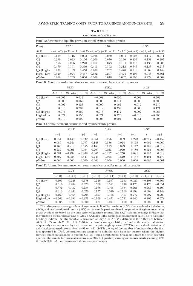
Our next cross-sectional tests explore Empirical Prediction 4, whichstates that the extent to which intermediaries provide liquidity asymmet-rically increases with σ , the volatility associated with the announcement.We test this prediction in panel A of table 6 using three proxies for uncer-tainty: EVOL, the firm’s earnings volatility, defined as the standard deviationof quarterly earnings scaled by total assets over the prior eight quarters;VLTY, the firm’s return volatility, defined as the standard deviation of dailymarket-adjusted returns from t − 51 to t − 11; and AGE, the log of the num-ber of months since the firm first appeared in CRSP. We expect that highervalues of EVOL and VLTY and lower values of AGE indicate greater uncer-tainty about firms’ earnings and thus higher ALP. Consistent with changesin ALP stemming from inventory risks, panel A of table 6 shows that the pre-announcement increase in ALP is pronounced among higher uncertaintystocks across all three proxies.
Our model also predicts that the preannouncement upward bias in orderflow and returns, as well as the subsequent reversal, are pronounced amonghigher uncertainty stocks, due to greater asymmetries in preannouncementtrading costs. Consistent with our prediction, panel B of table 6 shows thatpreannouncement AOIs and returns are strongest among high uncertaintystocks.
Although panels A and B of table 6 show the link between uncertaintyand preannouncement returns, we also predict a sharp reversal in the linkbetween uncertainty and returns once earnings news is announced and in-ventory risks decline. Consistent with this prediction, panel C of table 6shows that the uncertainty-return relation is strongly positive on day t − 1,where uncertainty proxies have the most robust positive relation with pre-announcement returns. However, panel C also shows that the sign of theuncertainty-return relation flips on day t , becoming significantly negativeon and following the announcement.
The knife-edge change in returns shown in table 6 provides clear evi-dence of a predictable upward bias in preannouncement prices that re-verses postannouncement. Moreover, the preannouncement bias and sub-sequent reversal are economically large, with the day t − 1 difference acrossvolatility quintiles in average returns annualizing to 127.6% and the day tdifference annualizing to −79.8%.
Panel D of table 6 illustrates an important implication of our findings.Specifically, we study three common definitions of announcement-windowreturns and show that the choice over alternative windows significantly im-pacts the size and significance of the relation between uncertainty prox-ies and announcement returns. For example, using the earnings volatilityproxy, we show that measuring returns from t − 1 to t results in an insignifi-cant spread in announcement returns across high and low uncertainty firms(17 bp, p-value = 0.12), whereas the uncertainty spread jumps more thanfourfold to 71 bp and becomes highly statistically significant (p-value =
ASYMMETRIC TRADING COSTS PRIOR TO EARNINGS ANNOUNCEMENTS 29
T A B L E 6Cross-Sectional Implications
Panel A: Asymmetric liquidity provision sorted by uncertainty proxies
Proxy: VLTY EVOL AGE
ALP: (−4,−2) (−31,−11) �ALP (−4,−2) (−31,−11) �ALP (−4,−2) (−31,−11) �ALP
Q1 (Low) 0.119 0.116 0.003 0.026 0.030 −0.004 0.623 0.112 0.511Q2 0.259 0.093 0.166 0.200 0.070 0.130 0.435 0.138 0.297Q3 0.356 0.086 0.270 0.267 0.073 0.194 0.342 0.136 0.206Q4 0.470 0.101 0.369 0.413 0.102 0.312 0.346 0.133 0.213Q5 (High) 0.639 0.189 0.450 0.708 0.237 0.470 0.218 0.069 0.149High−Low 0.520 0.074 0.447 0.682 0.207 0.474 −0.405 −0.043 −0.361p-Value 0.000 0.269 0.000 0.000 0.018 0.002 0.000 0.424 0.002
Panel B: Abnormal order imbalances and returns sorted by uncertainty proxies
VLTY EVOL AGE
AOI(−4,−2) RET(−4,−2) AOI(−4,−2) RET(−4,−2) AOI(−4,−2) RET(−4, −2)
Q1 (Low) −0.007 0.019 −0.008 0.036 0.009 0.369Q2 0.000 0.062 0.000 0.141 0.009 0.309Q3 0.002 0.123 0.009 0.162 0.012 0.210Q4 0.010 0.289 0.012 0.332 0.003 0.171Q5 (High) 0.014 0.569 0.013 0.412 −0.007 0.066High−Low 0.021 0.550 0.021 0.376 −0.016 −0.303p-Value 0.019 0.000 0.006 0.001 0.051 0.003
Panel C: Announcement returns sorted by uncertainty proxies
VLTY EVOL AGE
t−1 t t+1 t−1 t t+1 t−1 t t+1
Q1 (Low) 0.054 0.140 0.032 0.061 0.176 0.069 0.278 −0.217 −0.152Q2 0.080 0.245 0.077 0.148 0.186 0.024 0.195 0.002 −0.060Q3 0.160 0.219 0.055 0.168 0.113 0.029 0.172 0.108 −0.012Q4 0.237 0.091 −0.084 0.209 −0.053 −0.070 0.180 0.124 0.006Q5 (High) 0.381 −0.492 −0.308 0.307 −0.217 −0.250 0.091 0.185 0.018High−Low 0.327 −0.633 −0.341 0.246 −0.393 −0.319 −0.187 0.401 0.170p-Value 0.000 0.000 0.000 0.000 0.000 0.000 0.000 0.000 0.001
Panel D: Alternative announcement return metrics sorted by uncertainty proxies
VLTY EVOL AGE
(−1,0) (−1,+1) (0,+1) (−1,0) (−1,+1) (0,+1) (−1,0) (−1,+1) (0,+1)
Q1 (Low) 0.193 0.228 0.178 0.226 0.297 0.253 0.026 −0.108 −0.366Q2 0.316 0.402 0.329 0.320 0.351 0.210 0.173 0.123 −0.051Q3 0.372 0.437 0.285 0.266 0.305 0.154 0.261 0.262 0.109Q4 0.313 0.242 0.020 0.137 0.080 −0.108 0.292 0.302 0.148Q5 (High) −0.169 −0.463 −0.793 0.057 −0.173 −0.457 0.272 0.297 0.209High−Low −0.362 −0.692 −0.971 −0.169 −0.471 −0.711 0.246 0.405 0.574p-Value 0.003 0.000 0.000 0.121 0.001 0.000 0.010 0.002 0.000
This table presents average values of asymmetry in liquidity provision (ALP), abnormal order imbalances(AOI), and market-adjusted returns (RET) across sample partitions based on quintiles of a given uncertaintyproxy. p -values are based on the time series of quarterly returns. The (X,Y) column headings indicate thatthe variable is measured over days t+X to t+Y, where t is the earnings announcement date. The t+X columnheadings indicate that the variable is measured on day t+X. �ALP is defined as the difference betweenALP(−4, −2) and ALP(−31, −11). EVOL is the firm’s earnings volatility, defined as the standard deviationof quarterly earnings scaled by total assets over the prior eight quarters. VLTY is the standard deviation ofdaily market-adjusted returns from t−51 to t−11. AGE is the log of the number of months since the firmfirst appeared in CRSP. Observations are assigned to quintiles each calendar quarter, where the highest(lowest) values are assigned to quintile Q5 (Q1) using distributional breakpoints from the prior calendarquarter. The sample for this analysis consists of 215,754 quarterly earnings announcements spanning 1993through 2012. ALP and returns are shown as a percentages.
30 T. L. JOHNSON AND E. C. SO
0.00) when announcement-window returns are measured from t to t+1.The striking contrast in these estimates reflects our knife-edge results,where uncertainty proxies relate positively to preannouncement returns(t − 1) but negatively to postannouncement returns (t+1).15
4.2 INTERNAL VALIDITY: TIME SERIES AND CROSS-SECTIONAL TESTS
In this section, we further validate our hypothesis that asymmetries inpreannouncement trading costs, order imbalances, and returns are alldriven by the inventory management decisions of intermediaries. To doso, we first show that these three patterns are correlated across quarters intime series tests and across firms in cross-sectional tests, indicating that ourfindings stem from the same underlying phenomenon. Next, we show thatour effects are stronger when financial intermediaries are contracting theirbalance sheets, consistent with our hypothesis.
For our time series tests, we calculate three pairwise correlations amongthe quarterly average values of ALP, AOI, and RET, denoted as ρ(ALP, AOI),ρ(ALP, RET), and ρ(AOI, RET), for each event-day from t − 10 to t+10.Panel A of table 7 shows that the time series correlations between ALP,AOI, and RET are positive and economically large, with the average cor-relation exceeding 50%. Moreover, the bottom two rows of panel A showthat these correlations tend to be stronger in the preannouncement periodfrom t − 4 to t − 2, relative to the pooled 21-day event-window, consistentwith preannouncement inventory risks being a central driver of the linkbetween ALP, AOI, and RET.
In panel B of table 7, we also show that ALP, AOI, and RET tend tobe concentrated among the same types of firms. Specifically, we computewithin-quarter averages of ALP, AOI, and RET for decile portfolios sortedby each of our uncertainty proxies and then calculate correlations in thecross-section of these portfolios.16 We calculate these correlations withineach quarter and present time series average correlations as well as corre-sponding t -statistics in a fashion similar to Fama-MacBeth tests.
Panel B shows that the preannouncement patterns in returns, AOI, andALP are all concentrated among the same types of firms within a given quar-ter, which generates positive cross-portfolio correlations across all threemetrics.17 An important caveat to these results is that they do not establishcausality in support of our ATC hypothesis. Instead, they are consistent with
15 Similarly, table 6 shows that, on average, high uncertainty firms underperform low un-certainty firms during their announcements. Such a conclusion would be puzzling becauseinvestors appear to earn lower returns when investing in higher risk stocks and vice versa.However, our results indicate that this is likely the reversal of an upward bias in preannounce-ment prices concentrated among high uncertainty firms.
16 We rely on portfolios for these tests, rather than individual firms, because we need multi-ple firms to implement the ALP estimates used throughout our main analyses.
17 In the online appendix, we find similarly positive cross-sectional correlations when calcu-lating firm-specific versions of our main outcome variables.
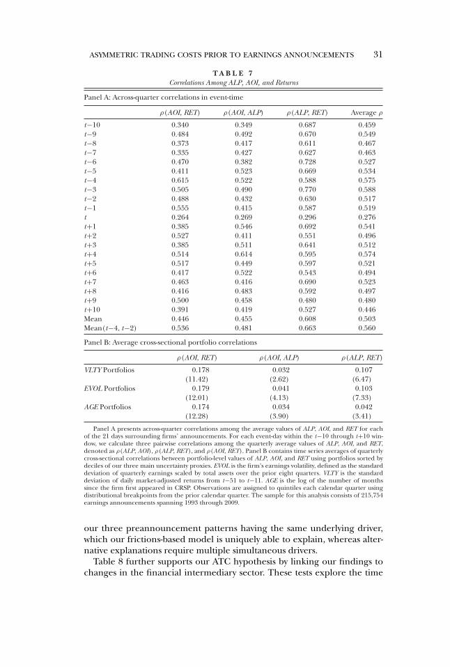
ASYMMETRIC TRADING COSTS PRIOR TO EARNINGS ANNOUNCEMENTS 31
T A B L E 7Correlations Among ALP, AOI, and Returns
Panel A: Across-quarter correlations in event-time
ρ(AOI, RET) ρ(AOI, ALP) ρ(ALP, RET) Average ρ
t−10 0.340 0.349 0.687 0.459t−9 0.484 0.492 0.670 0.549t−8 0.373 0.417 0.611 0.467t−7 0.335 0.427 0.627 0.463t−6 0.470 0.382 0.728 0.527t−5 0.411 0.523 0.669 0.534t−4 0.615 0.522 0.588 0.575t−3 0.505 0.490 0.770 0.588t−2 0.488 0.432 0.630 0.517t−1 0.555 0.415 0.587 0.519t 0.264 0.269 0.296 0.276t+1 0.385 0.546 0.692 0.541t+2 0.527 0.411 0.551 0.496t+3 0.385 0.511 0.641 0.512t+4 0.514 0.614 0.595 0.574t+5 0.517 0.449 0.597 0.521t+6 0.417 0.522 0.543 0.494t+7 0.463 0.416 0.690 0.523t+8 0.416 0.483 0.592 0.497t+9 0.500 0.458 0.480 0.480t+10 0.391 0.419 0.527 0.446Mean 0.446 0.455 0.608 0.503Mean(t−4, t−2) 0.536 0.481 0.663 0.560
Panel B: Average cross-sectional portfolio correlations
ρ(AOI, RET) ρ(AOI, ALP) ρ(ALP, RET)
VLTY Portfolios 0.178 0.032 0.107(11.42) (2.62) (6.47)
EVOL Portfolios 0.179 0.041 0.103(12.01) (4.13) (7.33)
AGE Portfolios 0.174 0.034 0.042(12.28) (3.90) (3.41)
Panel A presents across-quarter correlations among the average values of ALP, AOI, and RET for eachof the 21 days surrounding firms’ announcements. For each event-day within the t−10 through t+10 win-dow, we calculate three pairwise correlations among the quarterly average values of ALP, AOI, and RET,denoted as ρ(ALP, AOI), ρ(ALP, RET), and ρ(AOI, RET). Panel B contains time series averages of quarterlycross-sectional correlations between portfolio-level values of ALP, AOI, and RET using portfolios sorted bydeciles of our three main uncertainty proxies. EVOL is the firm’s earnings volatility, defined as the standarddeviation of quarterly earnings scaled by total assets over the prior eight quarters. VLTY is the standarddeviation of daily market-adjusted returns from t−51 to t−11. AGE is the log of the number of monthssince the firm first appeared in CRSP. Observations are assigned to quintiles each calendar quarter usingdistributional breakpoints from the prior calendar quarter. The sample for this analysis consists of 215,754earnings announcements spanning 1993 through 2009.
our three preannouncement patterns having the same underlying driver,which our frictions-based model is uniquely able to explain, whereas alter-native explanations require multiple simultaneous drivers.
Table 8 further supports our ATC hypothesis by linking our findings tochanges in the financial intermediary sector. These tests explore the time
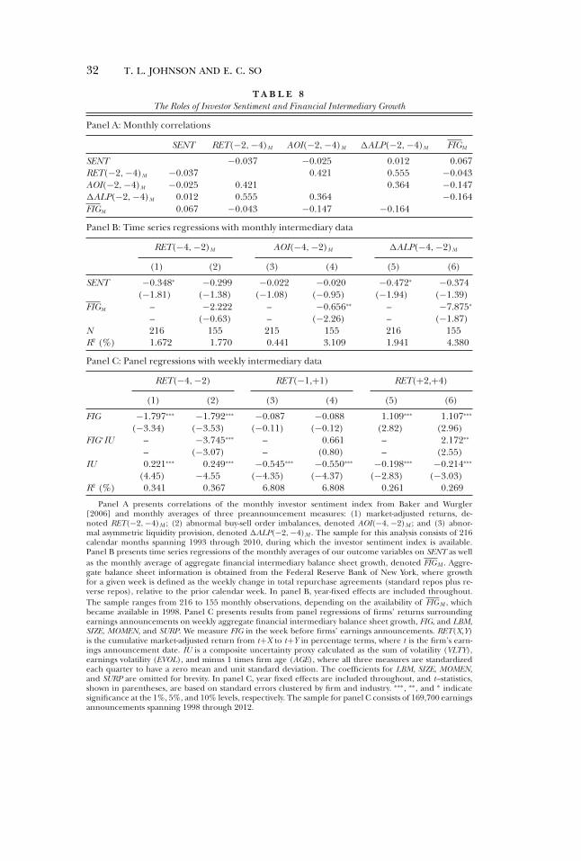
32 T. L. JOHNSON AND E. C. SO
T A B L E 8The Roles of Investor Sentiment and Financial Intermediary Growth
Panel A: Monthly correlations
SENT RET(−2,−4)M AOI(−2,−4)M �ALP(−2,−4)M FIGM
SENT −0.037 −0.025 0.012 0.067RET(−2,−4)M −0.037 0.421 0.555 −0.043AOI(−2,−4)M −0.025 0.421 0.364 −0.147�ALP(−2,−4)M 0.012 0.555 0.364 −0.164FIGM 0.067 −0.043 −0.147 −0.164
Panel B: Time series regressions with monthly intermediary data
RET(−4,−2)M AOI(−4,−2)M �ALP(−4,−2)M
(1) (2) (3) (4) (5) (6)
SENT −0.348∗ −0.299 −0.022 −0.020 −0.472∗ −0.374(−1.81) (−1.38) (−1.08) (−0.95) (−1.94) (−1.39)
FIGM – −2.222 – −0.656∗∗ – −7.875∗
– (−0.63) – (−2.26) – (−1.87)N 216 155 215 155 216 155R2 (%) 1.672 1.770 0.441 3.109 1.941 4.380
Panel C: Panel regressions with weekly intermediary data
RET(−4,−2) RET(−1,+1) RET(+2,+4)
(1) (2) (3) (4) (5) (6)
FIG −1.797∗∗∗ −1.792∗∗∗ −0.087 −0.088 1.109∗∗∗ 1.107∗∗∗
(−3.34) (−3.53) (−0.11) (−0.12) (2.82) (2.96)FIG∗IU – −3.745∗∗∗ – 0.661 – 2.172∗∗
– (−3.07) – (0.80) – (2.55)IU 0.221∗∗∗ 0.249∗∗∗ −0.545∗∗∗ −0.550∗∗∗ −0.198∗∗∗ −0.214∗∗∗
(4.45) −4.55 (−4.35) (−4.37) (−2.83) (−3.03)R2 (%) 0.341 0.367 6.808 6.808 0.261 0.269
Panel A presents correlations of the monthly investor sentiment index from Baker and Wurgler[2006] and monthly averages of three preannouncement measures: (1) market-adjusted returns, de-noted RET(−2,−4)M ; (2) abnormal buy-sell order imbalances, denoted AOI(−4, −2)M ; and (3) abnor-mal asymmetric liquidity provision, denoted �ALP(−2, −4)M . The sample for this analysis consists of 216calendar months spanning 1993 through 2010, during which the investor sentiment index is available.Panel B presents time series regressions of the monthly averages of our outcome variables on SENT as wellas the monthly average of aggregate financial intermediary balance sheet growth, denoted FIGM . Aggre-gate balance sheet information is obtained from the Federal Reserve Bank of New York, where growthfor a given week is defined as the weekly change in total repurchase agreements (standard repos plus re-verse repos), relative to the prior calendar week. In panel B, year-fixed effects are included throughout.The sample ranges from 216 to 155 monthly observations, depending on the availability of FIGM , whichbecame available in 1998. Panel C presents results from panel regressions of firms’ returns surroundingearnings announcements on weekly aggregate financial intermediary balance sheet growth, FIG, and LBM,SIZE, MOMEN, and SURP. We measure FIG in the week before firms’ earnings announcements. RET(X,Y)is the cumulative market-adjusted return from t+X to t+Y in percentage terms, where t is the firm’s earn-ings announcement date. IU is a composite uncertainty proxy calculated as the sum of volatility (VLTY),earnings volatility (EVOL), and minus 1 times firm age (AGE), where all three measures are standardizedeach quarter to have a zero mean and unit standard deviation. The coefficients for LBM, SIZE, MOMEN,and SURP are omitted for brevity. In panel C, year fixed effects are included throughout, and t–statistics,shown in parentheses, are based on standard errors clustered by firm and industry. ∗∗∗, ∗∗, and ∗ indicatesignificance at the 1%, 5%, and 10% levels, respectively. The sample for panel C consists of 169,700 earningsannouncements spanning 1998 through 2012.
ASYMMETRIC TRADING COSTS PRIOR TO EARNINGS ANNOUNCEMENTS 33
series implications of Empirical Prediction 4 that our findings should bemost pronounced when intermediaries prefer to reduce their net positions.Adrian and Shin [2010] use weekly aggregate repurchase agreement trans-actions to measure adjustments to the scale of financial intermediaries’ bal-ance sheets. We use the average of this measure over each calendar month,denoted as FIGM . We adopt this measure, assuming it is correlated with in-termediaries’ willingness to provide liquidity to buyers, which would reducetheir net balance sheet position, versus sellers, which would have the oppo-site effect. The negative correlations between FIGM and AOI, ALP, and RETin panel A indicate that the asymmetries we study are stronger when inter-mediaries are contracting their balance sheets and are therefore less willingto take on new inventory positions, as we predict.
Panel B of table 8 provides complimentary evidence using time seriesregressions, with fixed effects, of our main outcome variables on investorsentiment and intermediary balance-sheet growth. The regression evidenceis consistent with panel A, where sentiment relates insignificantly or nega-tively to RET, AOI, and �ALP. FIGM , by contrast, relates negatively to allthree outcome variables and significantly so for AOI and �ALP.
Finally, in panel C of table 8, we extend the monthly time series analy-sis in panels A and B by examining the link between returns surroundingfirms’ announcements and weekly changes in the intermediary sector. Thesetests combine both time series and cross-sectional implications within apanel data setting. We measure weekly aggregate intermediary balance-sheet growth in the week before firms’ earnings announcements, denotedFIG, and predict that it relates negatively to the preannouncement upwardbias in prices and positively to the subsequent reversal. These tests also in-clude a composite uncertainty proxy, IU, calculated as the sum of the threeuncertainty proxies from table 6 (VLTY, EVOL, and −1∗AGE), where allthree measures are standardized each quarter.
Columns 1, 3, and 5 of panel C corroborate our central hypotheses byshowing that both the preannouncement upward bias in returns and thesubsequent reversal are most pronounced when intermediaries are scal-ing down their balance sheet positions. The symmetry in results across pre-versus postannouncement returns is consistent with intermediaries induc-ing a short-term upward bias in preannouncement prices that subsequentlyreverses.
Finally, columns 2, 4, and 6 combine our cross-sectional and time se-ries tests by interacting FIG with uncertainty proxies. Using an interactionterm between FIG and our uncertainty proxy, IU, we confirm our predictionthat the relation between intermediary balance sheet growth and returns ismore pronounced among high uncertainty stocks because their announce-ments engender greater risks.
4.3 EXTERNAL VALIDITY: EXTENSION TO FRIDAY EFFECTS
In the online appendix, we provide a validity test in a seemingly unrelatedsetting—and contribute directly to the literature—by demonstrating how
34 T. L. JOHNSON AND E. C. SO
our theory can help explain well-known Friday effects in prior research.The main intuition for our analysis of Friday effects is that weekends, likeearnings announcements, pose heightened inventory risks because marketsare closed longer and prices move more, compared to typical overnightperiods (French [1980]). Given this mechanism, our theory predicts thatintermediaries’ risk and inventory management concerns influence marketoutcomes in much the same way as earnings announcements.
Echoing our earnings announcement results, we show in the onlineappendix that ALP, AOIs, and average returns, respectively, all increasethroughout the week and reverse at the beginning of the subsequent week.We also show that these predictable patterns are concentrated among highvolatility firms and are positively correlated in the cross-section. These find-ings suggest that the intraweek patterns we document stem from the riskand inventory management practices of intermediaries.
The evidence on intraweek patterns contributes to the literature by pro-viding a novel explanation for the well-documented Friday effect that stockreturns are abnormally positive on Fridays (e.g., French [1980], Lakon-ishok and Levi [1982], Keim and Stambaugh [1984]). Prior literature hasargued that the effects stem from investor behavior, whereas we argue thatit derives, at least in part, from intermediaries’ inventory management de-cisions throughout the week.
5. Alternative Hypotheses
As noted in section 1, there are multiple alternative explanations forour findings. The first is that they stem from firms selectively disclos-ing positive earnings news before their announcements, as suggested byRoychowdhury and Sletten [2012]. Under this explanation, firms are morelikely to withhold bad news and disclose good news, resulting in an upwardbias in preannouncement price discovery. While this would explain the ob-served return patterns conditional on the sign of earnings news, in a fullyrational pricing model, selective disclosure alone would not cause averagepreannouncement returns to be unconditionally positive because rationalinvestors should interpret the lack of preannouncement disclosure as badnews and adjust prices accordingly. If investors do not rationally interpretno news as bad news or underreact specifically to bad news, selective dis-closure could also explain the unconditional return pattern we documentempirically (a possibility raised by Giglio and Shue [2014]).
A selective disclosure story, whether it features rational or irrational in-vestors, does not explain our evidence of ALP. Any public disclosures willbe available to both intermediaries and investors and thus will not cre-ate asymmetric private information. As a result, without the frictions wedescribe, intermediaries have no reason to asymmetrically provide liquid-ity. Furthermore, alternative hypotheses based on asymmetric disclosuredo not explain why order imbalances are positive, even before bad news
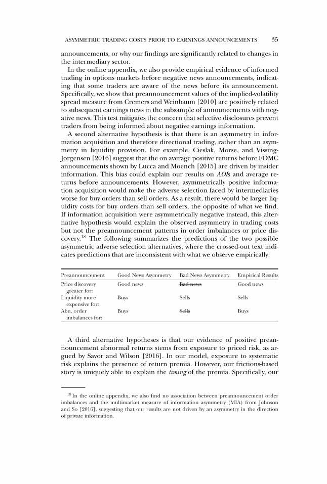
ASYMMETRIC TRADING COSTS PRIOR TO EARNINGS ANNOUNCEMENTS 35
announcements, or why our findings are significantly related to changes inthe intermediary sector.
In the online appendix, we also provide empirical evidence of informedtrading in options markets before negative news announcements, indicat-ing that some traders are aware of the news before its announcement.Specifically, we show that preannouncement values of the implied-volatilityspread measure from Cremers and Weinbaum [2010] are positively relatedto subsequent earnings news in the subsample of announcements with neg-ative news. This test mitigates the concern that selective disclosures preventtraders from being informed about negative earnings information.
A second alternative hypothesis is that there is an asymmetry in infor-mation acquisition and therefore directional trading, rather than an asym-metry in liquidity provision. For example, Cieslak, Morse, and Vissing-Jorgensen [2016] suggest that the on average positive returns before FOMCannouncements shown by Lucca and Moench [2015] are driven by insiderinformation. This bias could explain our results on AOIs and average re-turns before announcements. However, asymmetrically positive informa-tion acquisition would make the adverse selection faced by intermediariesworse for buy orders than sell orders. As a result, there would be larger liq-uidity costs for buy orders than sell orders, the opposite of what we find.If information acquisition were asymmetrically negative instead, this alter-native hypothesis would explain the observed asymmetry in trading costsbut not the preannouncement patterns in order imbalances or price dis-covery.18 The following summarizes the predictions of the two possibleasymmetric adverse selection alternatives, where the crossed-out text indi-cates predictions that are inconsistent with what we observe empirically:
Preannouncement Good News Asymmetry Bad News Asymmetry Empirical Results
Price discoverygreater for:
Good news Bad news Good news
Liquidity moreexpensive for:
Buys Sells Sells
Abn. orderimbalances for:
Buys Sells Buys
A third alternative hypotheses is that our evidence of positive prean-nouncement abnormal returns stems from exposure to priced risk, as ar-gued by Savor and Wilson [2016]. In our model, exposure to systematicrisk explains the presence of return premia. However, our frictions-basedstory is uniquely able to explain the timing of the premia. Specifically, our
18 In the online appendix, we also find no association between preannouncement orderimbalances and the multimarket measure of information asymmetry (MIA) from Johnsonand So [2016], suggesting that our results are not driven by an asymmetry in the directionof private information.
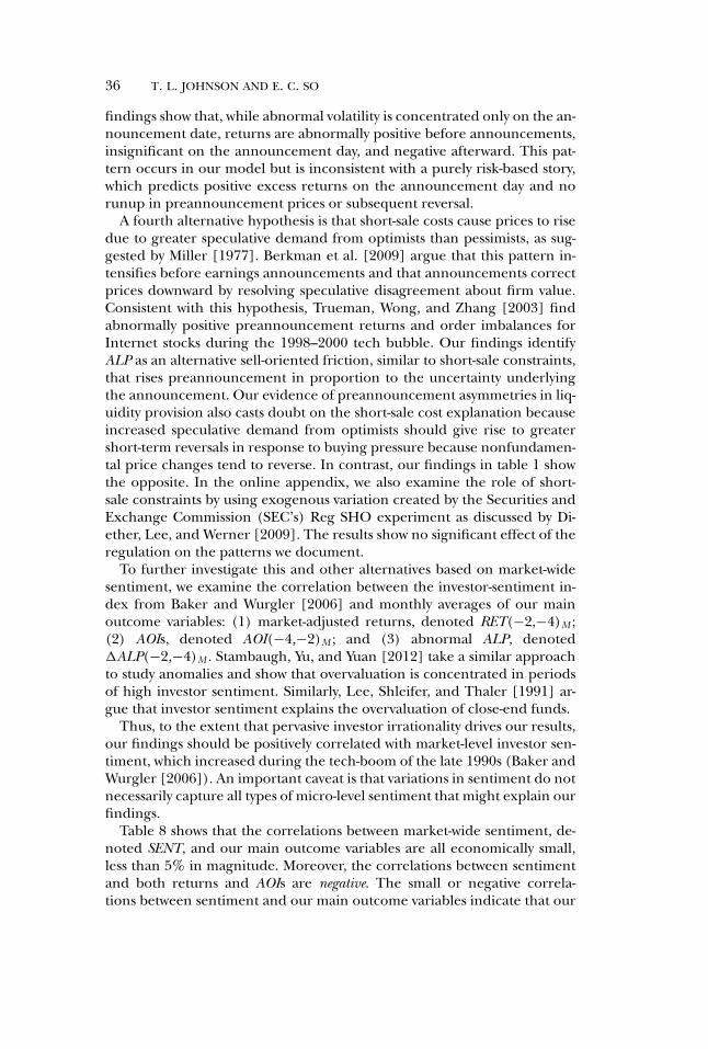
36 T. L. JOHNSON AND E. C. SO
findings show that, while abnormal volatility is concentrated only on the an-nouncement date, returns are abnormally positive before announcements,insignificant on the announcement day, and negative afterward. This pat-tern occurs in our model but is inconsistent with a purely risk-based story,which predicts positive excess returns on the announcement day and norunup in preannouncement prices or subsequent reversal.
A fourth alternative hypothesis is that short-sale costs cause prices to risedue to greater speculative demand from optimists than pessimists, as sug-gested by Miller [1977]. Berkman et al. [2009] argue that this pattern in-tensifies before earnings announcements and that announcements correctprices downward by resolving speculative disagreement about firm value.Consistent with this hypothesis, Trueman, Wong, and Zhang [2003] findabnormally positive preannouncement returns and order imbalances forInternet stocks during the 1998–2000 tech bubble. Our findings identifyALP as an alternative sell-oriented friction, similar to short-sale constraints,that rises preannouncement in proportion to the uncertainty underlyingthe announcement. Our evidence of preannouncement asymmetries in liq-uidity provision also casts doubt on the short-sale cost explanation becauseincreased speculative demand from optimists should give rise to greatershort-term reversals in response to buying pressure because nonfundamen-tal price changes tend to reverse. In contrast, our findings in table 1 showthe opposite. In the online appendix, we also examine the role of short-sale constraints by using exogenous variation created by the Securities andExchange Commission (SEC’s) Reg SHO experiment as discussed by Di-ether, Lee, and Werner [2009]. The results show no significant effect of theregulation on the patterns we document.
To further investigate this and other alternatives based on market-widesentiment, we examine the correlation between the investor-sentiment in-dex from Baker and Wurgler [2006] and monthly averages of our mainoutcome variables: (1) market-adjusted returns, denoted RET(−2,−4)M ;(2) AOIs, denoted AOI(−4,−2)M ; and (3) abnormal ALP, denoted�ALP(−2,−4)M . Stambaugh, Yu, and Yuan [2012] take a similar approachto study anomalies and show that overvaluation is concentrated in periodsof high investor sentiment. Similarly, Lee, Shleifer, and Thaler [1991] ar-gue that investor sentiment explains the overvaluation of close-end funds.
Thus, to the extent that pervasive investor irrationality drives our results,our findings should be positively correlated with market-level investor sen-timent, which increased during the tech-boom of the late 1990s (Baker andWurgler [2006]). An important caveat is that variations in sentiment do notnecessarily capture all types of micro-level sentiment that might explain ourfindings.
Table 8 shows that the correlations between market-wide sentiment, de-noted SENT, and our main outcome variables are all economically small,less than 5% in magnitude. Moreover, the correlations between sentimentand both returns and AOIs are negative. The small or negative correla-tions between sentiment and our main outcome variables indicate that our
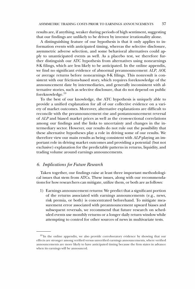
ASYMMETRIC TRADING COSTS PRIOR TO EARNINGS ANNOUNCEMENTS 37
results are, if anything, weaker during periods of high sentiment, suggestingthat our findings are unlikely to be driven by investor irrationality alone.
A distinguishing feature of our hypothesis is that it only applies to in-formation events with anticipated timing, whereas the selective disclosure,asymmetric adverse selection, and some behavioral alternatives could ap-ply to unanticipated events as well. As a placebo test, we therefore fur-ther distinguish our ATC hypothesis from alternatives using nonearnings8-K filings, which are less likely to be anticipated. In the online appendix,we find no significant evidence of abnormal preannouncement ALP, AOI,or average returns before nonearnings 8-K filings. This nonresult is con-sistent with our frictions-based story, which requires foreknowledge of theannouncement date by intermediaries, and generally inconsistent with al-ternative stories, such as selective disclosure, that do not depend on publicforeknowledge.19
To the best of our knowledge, the ATC hypothesis is uniquely able toprovide a unified explanation for all of our collective evidence on a vari-ety of market outcomes. Moreover, alternative explanations are difficult toreconcile with the preannouncement rise and postannouncement reversalof ALP and biased market prices as well as the cross-sectional correlationsamong our findings and the links to uncertainty and changes in the in-termediary sector. However, our results do not rule out the possibility thatthese alternative hypotheses play a role in driving some of our results. Wetherefore view our main results as being consistent with ALP playing an im-portant role in driving market outcomes and providing a potential (but notexclusive) explanation for the predictable patterns in returns, liquidity, andtrading volume around earnings announcements.
6. Implications for Future Research
Taken together, our findings raise at least three important methodologi-cal issues that stem from ATCs. These issues, along with our recommenda-tions for how researchers can mitigate, utilize them, or both are as follows:
1) Earnings announcement returns: We predict that a significant portionof the returns associated with earnings announcements (e.g., news,risk premia, or both) is concentrated beforehand. To mitigate mea-surement error associated with preannouncement upward biases andsubsequent reversals, we recommend that future research on sched-uled events use monthly returns or a longer daily return window whileattempting to control for other sources of news in multivariate tests.
19 In the online appendix, we also provide corroboratory evidence by showing that oureffects are stronger among verified versus unverified earnings announcements, where verifiedannouncements are more likely to have anticipated timing because the firm states in advancewhen its earnings will be announced.
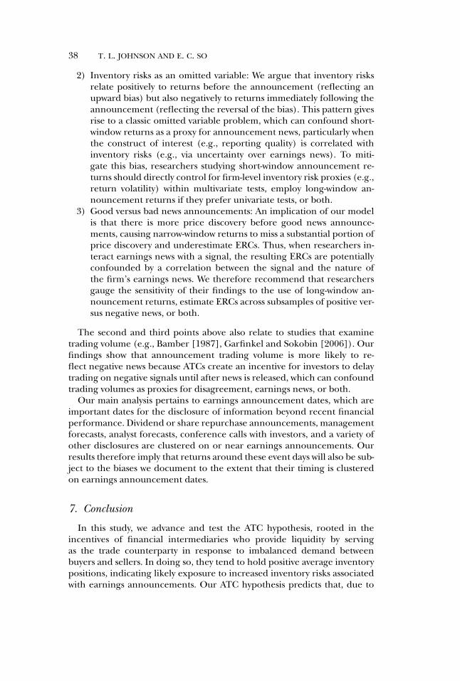
38 T. L. JOHNSON AND E. C. SO
2) Inventory risks as an omitted variable: We argue that inventory risksrelate positively to returns before the announcement (reflecting anupward bias) but also negatively to returns immediately following theannouncement (reflecting the reversal of the bias). This pattern givesrise to a classic omitted variable problem, which can confound short-window returns as a proxy for announcement news, particularly whenthe construct of interest (e.g., reporting quality) is correlated withinventory risks (e.g., via uncertainty over earnings news). To miti-gate this bias, researchers studying short-window announcement re-turns should directly control for firm-level inventory risk proxies (e.g.,return volatility) within multivariate tests, employ long-window an-nouncement returns if they prefer univariate tests, or both.
3) Good versus bad news announcements: An implication of our modelis that there is more price discovery before good news announce-ments, causing narrow-window returns to miss a substantial portion ofprice discovery and underestimate ERCs. Thus, when researchers in-teract earnings news with a signal, the resulting ERCs are potentiallyconfounded by a correlation between the signal and the nature ofthe firm’s earnings news. We therefore recommend that researchersgauge the sensitivity of their findings to the use of long-window an-nouncement returns, estimate ERCs across subsamples of positive ver-sus negative news, or both.
The second and third points above also relate to studies that examinetrading volume (e.g., Bamber [1987], Garfinkel and Sokobin [2006]). Ourfindings show that announcement trading volume is more likely to re-flect negative news because ATCs create an incentive for investors to delaytrading on negative signals until after news is released, which can confoundtrading volumes as proxies for disagreement, earnings news, or both.
Our main analysis pertains to earnings announcement dates, which areimportant dates for the disclosure of information beyond recent financialperformance. Dividend or share repurchase announcements, managementforecasts, analyst forecasts, conference calls with investors, and a variety ofother disclosures are clustered on or near earnings announcements. Ourresults therefore imply that returns around these event days will also be sub-ject to the biases we document to the extent that their timing is clusteredon earnings announcement dates.
7. Conclusion
In this study, we advance and test the ATC hypothesis, rooted in theincentives of financial intermediaries who provide liquidity by servingas the trade counterparty in response to imbalanced demand betweenbuyers and sellers. In doing so, they tend to hold positive average inventorypositions, indicating likely exposure to increased inventory risks associatedwith earnings announcements. Our ATC hypothesis predicts that, due to
ASYMMETRIC TRADING COSTS PRIOR TO EARNINGS ANNOUNCEMENTS 39
this exposure, intermediaries reduce their exposure to announcementrisks by providing liquidity asymmetrically, which increases the cost oftrading on negative news before earnings announcements.
Our model and empirical findings provide support for our hypothesis.Specifically, we show that ATCs create a predictable upward bias in pricesthat increases preannouncement and subsequently reverses, confoundingshort-window announcement returns as measures of earnings news andrisk premia. More broadly, we provide a unified framework that links sev-eral pervasively studied market outcomes. These outcomes include marketprices, returns, trading volumes, order flows, and liquidity, which mattercentrally in virtually all capital market research.
An important contribution of our paper is that it provides a liquidity-provision-based explanation for daily return patterns around the earningsannouncement, one of the most significant information events for a firm. Anatural reason that one would observe systematically positive returns lead-ing up to good news at earnings announcements while not observing a sim-ilar pattern for bad news is that there is asymmetric news leakage to themarket. This raises the possibility that insiders opportunistically leak infor-mation about an upcoming public news event when the news is good butwithhold news when it is bad. Our findings point to an important alter-native possibility. Specifically, liquidity providers’ aversion to inventory riskcould lead to these systematic return patterns even in the absence of anyasymmetric news leakage.
Our paper also provides a conceptual basis and empirical support for un-derstanding several results that likely appear puzzling when viewed outsideof our framework. An example of our paper’s conceptual contribution isin explaining why earnings announcement risk premia occur before theactual announcement (Barber et al. [2013]). In the absence of our frame-work, this separation is puzzling because standard asset pricing models pre-dict that risks and risk premia should occur at the same time. Our resultsindicate that this pattern arises due to ATCs. As a result, our model andevidence have the potential to influence the way that researchers under-stand market outcomes across a variety of settings, particularly those thatstudy market outcomes in close proximity to firm-level, industry-level, andmacroeconomic information events.
APPENDIX
Model Solution and ProofsA.1 DETAILED MODEL SOLUTION
We solve the model by working backward, beginning with the tradinggame at t = −1. The intermediary has initial inventory Q−1 that is deter-mined by its choice of Q−2 and the trading game at t = −2, but at t =−1, inventory is no longer a choice variable. Given realization v−1 = v−1,the two possible asset values are {v−1 − σ, v−1 + σ }. The intermediary’s

40 T. L. JOHNSON AND E. C. SO
problem in the subgame is therefore:
a−1, b−1 = arg maxa,b
U(a, b | Q−1, v−1
). (A.1)
U(a, b | Q−1, v−1
)
=Expected trading profit︷ ︸︸ ︷
Ey (xI,−1(p (xI,−1; a, b) − v−1) + xU ,−1(p (xU ,−1; a, b) − v−1)
)− γMσ 2
Ey (Q−1 − xI,−1 − xU ,−1
)2︸ ︷︷ ︸Inventory risk
+ρ Ey (Q−1 − xI,−1 − xU ,−1
)︸ ︷︷ ︸Cost of negative inventory
.
(A.2)
Our assumptions imply that the informed trader’s demand function att = −1 satisfies:
xI,−1(s−1; a−1, b−1) = arg maxx
Ey (x (v − p (x)) | s−1)
− γT Vary (x (v − p (x)) | s−1) , (A.3)
where
p (x) ={
a−1 if x ≥ 0b−1 if x < 0
. (A.4)
This implies:
xI,−1(s−1; a−1, b−1) =⎧⎨⎩
v−1+(2p −1)σ−a−18γT p (1−p )σ 2 if s−1 = g
v−1−(2p −1)σ−b−18γT p (1−p )σ 2 if s−1 = b .
(A.5)
Similarly, for uninformed traders, we have:
xU ,−1(u−1; a−1, b−1) =⎧⎨⎩
v−1+(2p −1)σ−a−18γT p (1−p )σ 2 if u−1 = g
v−1−(2p −1)σ−b−18γT p (1−p )σ 2 if u−1 = b .
(A.6)
We substitute demand functions from (A.5) and (A.6) into each of thethree components of intermediary utility, relying on the following nota-tion:
A0,d ≡ (2p −1)8γT p (1−p )σ.
(A.7)
A1,d ≡ 18γT p (1−p )σ 2.
(A.8)
α ≡ a − v−1. (A.9)
β ≡ b − v−1. (A.10)
ASYMMETRIC TRADING COSTS PRIOR TO EARNINGS ANNOUNCEMENTS 41
The expected trading profit term satisfies:
Ey (trading profit
) = Ey [xi (s−1)(p (xi (s−1; a, b)) − v)
+ xu(u−1; a, b)(p (xu(u−1)) − v)]
= 14
[2(A0,d − A1,dα)(α − σ(2p − 1))
+ 2(A0,d − A1,dα)α + 2(−A0,d − A1,dβ)β
+ 2(−A0,d − A1,dβ)(β − σ(1 − 2p ))]
= −A0,dσ(2p − 1) + 32
A0,d(α − β) − A1,d(α2 + β2).
(A.11)
The expected inventory risk term satisfies:
σ 2E
y((
Q−1 − xI,−1 − xU ,−1)2)
= σ 2
4[(Q−1 − 2A0,d + 2A1,dα)2 + 2(Q−1
+ A1,d(α + β))2 + (Q−1 + 2A0,d
+ 2A1,dβ)2] = A0,v + A1,vα + B1,vβ
+ A2,v(α2 + β2) + C2,vαβ, (A.12)
where
A0,v ≡ σ 2(2A2
0,d + Q 2−1
). (A.13)
A1,v ≡ 2σ 2A1,d(Q−1 − A0,d). (A.14)
B1,v ≡ 2σ 2A1,d(Q−1 + A0,d). (A.15)
A2,v ≡ 32σ 2A2
1,d . (A.16)
C2,v ≡ σ 2A21,d . (A.17)
Finally, the expected cost of negative inventory term satisfies:
ρ Ey (Q−1 − xI,−1 − xU ,−1
) = ρ(Q−1 + A1,d (α + β)
). (A.18)
Putting the pieces together, the marker maker’s full objective functionsatisfies:
U(a, b | Q−1
) = A0,m + A1,mα + B1,mβ + A2,m(α2 + β2) + C2,mαβ, (A.19)
where
A0,m ≡ −A0,dσ(2p − 1) − γMσ 2(2A2
0,d + Q 2−1
)+ ρQ−1. (A.20)
A1,m ≡ 32 A0,d − 2γMσ 2A1,d(Q−1 − A0,d) + ρA1,d . (A.21)

42 T. L. JOHNSON AND E. C. SO
B1,m ≡ − 32 A0,d − 2γMσ 2A1,d(Q−1 + A0,d) + ρA1,d. (A.22)
A2,m ≡ −A1,d − 32γMσ 2A2
1,d. (A.23)
C2,m ≡ −γMσ 2A21,d . (A.24)
We solve the first-order conditions with respect to a and b and find thefollowing prices:
a−1 = M−1 + 12 S−1, (A.25)
b−1 = M−1 − 12 S−1, (A.26)
where
M−1 ≡ v−1 − 4p (1−p )γM
4p (1−p )+ γMγT
σ 2(
Q−1 − ρ
2γM σ 2
), (A.27)
S−1 ≡ 12p (1−p )+2 γMγT
8p (1−p )+ γMγT
(2p − 1)σ. (A.28)
Substituting a−1 and b−1 from (A.25) and (A.26) into the intermediary’sutility function in equation (A.1), we have the following subgame expectedutility as a function of Q−1:
U−1(Q−1) = C − 4p (1 − p )γMσ 2
4p (1 − p ) + γMγT
(Q−1 − ρ
2γMσ 2
)2
, (A.29)
where C is a constant that does not depend on inventory Q−1. Note thatexpected subgame utility is maximized when excess inventory Q−1 − ρ
2γM σ 2
is zero, leading to the interpretation of ρ
2γM σ 2 as the target or optimal inven-tory for the announcement period.
Using the subgame equilibrium characterization, we solve for the inter-mediary’s t = −2 optimal choice of Q−2, a−2, and b−2:
U (Q−2, a−2, b−2)
=Expected trading profit︷ ︸︸ ︷
Ey (xI,−2(p (xI,−2; a−2, b−2) − v−2) + xU ,−1(p (xU ,−2; a−2, b−2) − v−2)
)− γM E
y (Q−2 − xI,−2 − xU ,−2)2︸ ︷︷ ︸
Inventory risk
+ρ Ey (Q−2 − xI,−2 − xU ,−2
)︸ ︷︷ ︸Cost of negative inventory
+ C − 4p (1 − p )γMσ 2
4p (1 − p ) + γMγT
Ey(
Q−2 − xI,−2 − xU ,−2 − ρ
2γMσ 2
)2
︸ ︷︷ ︸Expected t=−2 utility
. (A.30)

ASYMMETRIC TRADING COSTS PRIOR TO EARNINGS ANNOUNCEMENTS 43
Solving first-order conditions with respect to Q−2, a−2, and b−2 using a pro-cess similar to the one used for t = −1 yields the following solution:
Q−2 = ρ
2γM
(8p (1 − p ) + γM
γT
4p (1 − p )(1 + σ 2) + γMγT
). (A.31)
a−2 = 12
S−2. (A.32)
b−2 = −12
S−2. (A.33)
S−2 ≡ 3(4p (1−p )+σ 2)+2 γMγT
K
2(4p (1−p )+σ 2)+ γMγT
K(2p − 1). (A.34)
K ≡ 4p (1−p )(1+σ 2)+ γMγT
4p (1−p )+ γMγT
. (A.35)
A.2 PROOFS OF EQUILIBRIUM RESULTS
RESULT A.1 (Asymmetric Liquidity Provision). In the preannouncement pe-riod, negative price changes overshoot the information revealed by the trade more thanpositive ones:
Ez (v|sell) − E
z(b−1) > Ez(a−1) − E
z (v|buy). (A.36)
Proof. Equations (A.27) and (A.28) imply that:
Ez (a−1 + b−1 − 2v−1) = 2E
z (M−1 − v−1)
= − 8p (1 − p )γM
4p (1 − p ) + γMγT
σ 2(
Ez(Q−1) − ρ
2γMσ 2
).
(A.37)
Since liquidity provision at t = −2 is symmetric, we have that:
Ez(Q−1) = Q−2 = ρ
2γM
(8p (1 − p ) + γM
γT
4p (1 − p )(1 + σ 2) + γMγT
)>
ρ
2γMσ 2. (A.38)
In words, before the preannouncement trading period, expected marketmarket inventory is above the optimal Q0, which necessitates ALP:
Ez(Q−1) >
ρ
2γMσ 2⇒ E
z (a−1 + b−1 − 2v−1) < 0 (A.39)
⇒ Ez (a−1 − v−1) < E
z (v−1 − b−1) .

44 T. L. JOHNSON AND E. C. SO
Furthermore, since:
Ez(v|buy) = v−1 + 1
2(2p − 1)σ + 2
(z0 − 1
2
)σ, (A.40)
Ez(v|sell) = v−1 − 1
2(2p − 1)σ + 2
(z0 − 1
2
)σ, (A.41)
we have:
Ez(a−1) − E
z (v|buy) = E
z(a−1 − v−1 − 1
2 (2p − 1)σ − 2(z0 − 1
2
)σ)
(A.42)
< Ez(v−1 − b−1 − 1
2 (2p − 1)σ + 2(z0 − 1
2
)σ)
(A.43)
= Ez (v|sell) − E
z(b−1). (A.44)
�
RESULT A.2 (Asymmetric Trading Intensity). In the preannouncement pe-riod, traders submit larger buy orders in equilibrium than sell orders:
|xI,−1(s = g)| >|xI,−1(s = b)|. (A.45)
|xU ,−1(u = g)| >|xU ,−1(u = b)|. (A.46)
Proof. Follows from Result A.1 and the demand functions in equations(A.5) and (A.6). �
RESULT A.3 (Abnormal Returns Around Announcements). Expected re-turns computed using average prices under the physical measure satisfy:
Ez (p −1 − p −2) = 2
(z−1 − 1
2
)︸ ︷︷ ︸Normal risk prem.
+ ρ(σ 2 − 1)
(2p (1 − p ) + γM
γT
8p (1 − p )(1 + σ 2) + 2 γMγT
)︸ ︷︷ ︸
Upward bias
(A.47)
Ez (p 0 − p −1) = 2
(z0 − 1
2
)σ︸ ︷︷ ︸
Announcement risk prem.
− ρ(σ 2 − 1)
(2p (1 − p ) + γM
γT
8p (1 − p )(1 + σ 2) + 2 γMγT
)︸ ︷︷ ︸
Reversal of bias
(A.48)
ASYMMETRIC TRADING COSTS PRIOR TO EARNINGS ANNOUNCEMENTS 45
Proof. Since liquidity provision is symmetric at t = −2, the average pricep −2 equals the frictionless benchmark E y (v) = 0.
For a given inventory Q−1, we define the average price at t = −1, p (Q−1),as the average across the four different demand combinations of thevolume-weighted average price given that demand combination.20 This av-erage satisfies:
p (Q−1) = Ez(vwap) = M−1 + S−1
v−1 − M−1
4(2p − 1)σ − S−1.(A.49)
We can therefore substitute equations (A.27) and (A.28) into (A.49) andsimplify to:
p (Q−1) = v−1 +2p (1 − p ) + γM
γT
4p (1 − p ) + γMγT
(Q−1 − ρ
2γMσ 2
)γMσ 2. (A.50)
We now take the expectation over possible Q−1 and use equation (A.38)for E
z(Q−1). Since Ez(Q−1) >
ρ
2γM σ 2 , average excess inventory is positive,resulting in ALP and, as a consequence, an upward bias in prices:
p −1 ≡ Ez(p (Q−1)
) = 2(z−1 − 1
2
)+ ρ(σ 2 − 1)(
2p (1−p )+ γMγT
8p (1−p )(1+σ 2)+2 γMγT
). (A.51)
The asset liquidates at t = 0 for v, making the average price p 0 equal thefrictionless benchmark 2(z−1 − 1
2 ) + 2(z0 − 12 )σ . Combining the equations
for p −2, p −1, and p 0 yields the expected returns in (A.47) and (A.48). �
RESULT A.4 (Comparative Statics). Average asymmetry in liquidity provision,preannouncement returns, and postannouncement reversals are all increasing in theintermediary’s inventory Q−1, risk aversion γM , cost of negative positions ρ, and theannouncement risk σ .
Proof. From equation (A.50), it is clear that the average preannounce-ment price conditional on Q−1 is increasing in Q−1. Furthermore, aftersome algebra, the average preannouncement price in equation (A.51) isincreasing in γM , ρ, and σ . Finally, the asymmetry in liquidity provision, asmeasured by the difference:
Ez (v−1 − b−1) − E
z (a−1 − v−1) = −2Ez (M−1 − v−1) (A.52)
= 8p (1−p )γM
4p (1−p )+ γMγT
σ 2(E
z(Q−1) − ρ
2γM σ 2
)(A.53)
= 4p (1−p )γM
4p (1−p )(1+σ 2)+ γMγT
ρ(σ 2 − 1), (A.54)
is also an increasing function of γM , ρ, and σ. �
20 Other possible average prices in this setting exhibit the pattern in Result A.3 even morestrongly.

46 T. L. JOHNSON AND E. C. SO
REFERENCES
ADRIAN, T., AND H. SHIN. “Liquidity and Leverage.” Journal of Financial Intermediation 19 (2010):418–37.
AMIHUD, Y., AND H. MENDELSON. “Dealership Market: Market-Making with Inventory.” Journalof Financial Economics 8 (1980): 31–53.
AVRAMOV, D.; T. CHORDIA; AND A. GOYAL. “Liquidity and Autocorrelations in Individual StockReturns.” The Journal of Finance 61 (2006): 2365–94.
BAKER, M., AND J. WURGLER. “Investor Sentiment and the Cross-Section of Stock Returns.” TheJournal of Finance 61 (2006): 1645–80.
BALL, R., AND S. KOTHARI. “Security Returns Around Earnings Announcements.” AccountingReview 66 (1991): 718–38.
BAMBER, L.S. “Unexpected Earnings, Firm Size, and Trading Volume Around Quarterly Earn-ings Announcements.” Accounting Review 66 (1987): 510–32.
BARBER, B. M.; E.T. DE GEORGE; R. LEHAVY; AND B. TRUEMAN. “The Earnings AnnouncementPremium Around the Globe.” Journal of Financial Economics 108 (2013): 118–38.
BERKMAN, H.; V. DIMITROV; P. C. JAIN; P.D. KOCH; AND S. TICE. “Sell on the News: Differences ofOpinion, Short-Sales Constraints, and Returns Around Earnings Announcements.” Journalof Financial Economics 92 (2009): 376–99.
BRUNNERMEIER, M.K., AND L.H. PEDERSEN. “Market Liquidity and Funding Liquidity.” Reviewof Financial Studies 22 (2009): 2201–38.
CAMPBELL, J.Y.; S.J. GROSSMAN; AND J. WANG. “Trading Volume and Serial Correlation in StockReturns.” The Quarterly Journal of Economics 108 (1993): 905–39.
CHORDIA, T.; R. ROLL; AND A. SUBRAHMANYAM. “Order Imbalance, Liquidity, and Market Re-turns.” Journal of Financial Economics 65 (2002): 111–30.
CIESLAK, A.; A. MORSE; AND A. VISSING-JORGENSEN. “Stock Returns over the FOMC Cycle.”2016. SSRN Working paper 2687614.
COHEN, D.; A. DEY; T. LYS; AND S. SUNDER. “Earnings Announcement Premia and the Limitsto Arbitrage.” Journal of Accounting and Economics 43 (2007): 153–80.
COMERTON-FORDE, C.; T. HENDERSHOTT; C. JONES; P. MOULTON; AND M. SEASHOLES. “TimeVariation in Liquidity: The Role of Market-Maker Inventories and Revenues.” Journal of Fi-nance 65 (2010): 295–331.
CREMERS, M., AND D. WEINBAUM. “Deviations from Put-Call Parity and Stock Return Pre-dictability.” Journal of Financial and Quantitative Analysis 45 (2010): 335–67.
DELLAVIGNA, S., AND J.M. POLLET. “Investor Inattention and Friday Earnings Announce-ments.” Journal of Finance 64 (2009): 709–49.
DIETHER, K.B.; K.H. LEE; AND I.M. WERNER. “It’s Sho Time! Short-Sale Price Tests and MarketQuality.” The Journal of Finance 64 (2009): 37–73.
FRAZZINI, A., AND O. LAMONT. “The Earnings Announcement Premium and Trading Volume.”Working paper, Harvard University, 2007.
FRENCH, K.R. “Stock Returns and the Weekend Effect.” Journal of Financial Economics 8 (1980):55–69.
GARFINKEL, J.A., AND J. SOKOBIN. “Volume, Opinion Divergence, and Returns: A Studyof Post–Earnings Announcement Drift.” Journal of Accounting Research 44 (2006):85–112.
GIGLIO, S., AND K. SHUE. “No News Is News: Do Markets Underreact to Nothing?” Review ofFinancial Studies 27 (2014): 3389–440.
GROSSMAN, S., AND M. MILLER. “Liquidity and Market Structure.” Journal of Finance 43 (1988):617–33.
HENDERSHOTT, T., AND A.J. MENKVELD. “Price Pressures.” Journal of Financial Economics 114(2014): 405–23.
HENDERSHOTT, T., AND M.S. SEASHOLES. “Market Maker Inventories and Stock Prices.” Ameri-can Economic Review 97 (2007): 210–14.
JOHNSON, T.L., AND E.C. SO. “A Simple Multimarket Measure of Information Asymmetry.”Management Science (2016): Forthcoming.

ASYMMETRIC TRADING COSTS PRIOR TO EARNINGS ANNOUNCEMENTS 47
KEIM, D.B., AND R.F. STAMBAUGH. “A Further Investigation of the Weekend Effect in StockReturns.” The Journal of Finance 39 (1984): 819–35.
KRINSKY, I., AND J. LEE. “Earnings Announcements and the Components of the Bid-AskSpread.” Journal of Finance 51 (1996): 1523–35.
LAKONISHOK, J., AND M. LEVI. “Weekend Effects on Stock Returns: A Note.” The Journal ofFinance 37 (1982): 883–89.
LEE, C.; B. MUCKLOW; AND M. READY. “Spreads, Depths, and the Impact of Earnings Informa-tion: An Intraday Analysis.” Review of Financial Studies 6 (1993): 345–74.
LEE, C.; A. SHLEIFER; AND R.H. THALER. “Investor Sentiment and the Closed-End Fund Puzzle.”The Journal of Finance 46 (1991): 75–109.
LEVI, S., AND X. ZHANG. “Asymmetric Decrease in Liquidity Trading Before Earnings An-nouncements and the Announcement Return Premium.” Journal of Financial Economics 118(2015): 383–98.
LUCCA, D.O., AND E. MOENCH. “The Pre FOMC Announcement Drift.” The Journal of Finance70 (2015): 329–71.
MADHAVAN, A., AND S. SMIDT. “An Analysis of Changes in Specialist Inventories and Quota-tions.” Journal of Finance 48 (1993): 1595–628.
MENKVELD, A. “High Frequency Trading and the New-Market Makers.” Journal of FinancialMarkets 16 (2013): 712–40.
MILLER, E.M. “Risk, Uncertainty, and Divergence of Opinion.” The Journal of Finance 32 (1977):1151–68.
NAGEL, S. “Evaporating Liquidity.” Review of Financial Studies 25 (2012): 2005–39.ROLL, R. “A Simple Implicit Measure of the Effective Bid-Ask Spread in an Efficient Market.”
Journal of Finance 39 (1984): 1127–39.ROYCHOWDHURY, S., AND E. SLETTEN. “Voluntary Disclosure Incentives and Earnings Informa-
tiveness.” The Accounting Review 87 (2012): 1679–708.SAVOR, P., AND M. WILSON. “Earnings Announcements and Systematic Risk.” The Journal of
Finance 71 (2016): 83–138.SO, E.C., AND S. WANG. “News-Driven Return Reversals: Liquidity Provision Ahead of Earnings
Announcements.” Journal of Financial Economics 114 (2014): 20–35.STAMBAUGH, R.F.; J. YU; AND Y. YUAN. “The Short of It: Investor Sentiment and Anomalies.”
Journal of Financial Economics 104 (2012): 288–302.TETLOCK, P.C. “Does Public Financial News Resolve Asymmetric Information?” Review of Finan-
cial Studies 23 (2010): 3520–57.TRUEMAN, B.; M. WONG; AND X.J. ZHANG. “Anomalous Stock Returns Around Internet Firms’
Earnings Announcements.” Journal of Accounting and Economics 34 (2003), 249–71.