Assessing substitution and complementary effects

amongst crime typologies1

Detotto Claudio°; Pulina Manuela*

° Centre for North South Economic Research (CRENoS) and Department of Economics (DEIR), University of

Sassari, Via Torre Tonda, 34, 07100 Sassari, Italy, Tel. +39-(0)79/2017302, FAX +39-(0)79/2017312. E-mail:

cdetotto@uniss.it

* Corresponding author. Ph.D. at Southampton University (UK). Centre for North South Economic Research

(CRENoS) and Department of Economics (DEIR), University of Sassari, Via Torre Tonda, 34, 07100 Sassari,

Italy, Tel. +39-(0)79/388381, FAX +39-(0)79/2017312. E-mail: mpulina@uniss.it

Abstract. This paper aims at assessing how offenders allocate their effort amongst several crime typologies.

Specifically, complementary and substitution effects are tested amongst number of recorded crimes.

Furthermore, the extent to which crime is detrimental for economic growth is also tested. The case study is Italy

and the time span under analysis is from 1981:1 up to 2004:4. A Vector Autoregressive Correction Mechanism

(VECM) is employed after having assessed the integration and cointegration status of the variables under

investigation. The main findings are that a bi-directional complementary effect exists between drug related

crimes and receiving, whereas a bi-directional substitution effect is detected between robberies, extortions and

kidnapping and homicides and falsity, respectively. Furthermore, economic growth produces a positive effect on

the growth of homicides, receiving and drug related crimes; while, the growth in robberies, extortion and

kidnapping and falsity have a crowding-out effect on economic growth.

Keywords: Crime; substitution and complementary effect; economic growth; crowding-out effect.

JEL Codes: K14, C32, E24

1Acknowledgements. The authors acknowledge the financial support provided by the Italian Ministry for

University and Scientific Research (PRIN Project 2006 “The cost of crime: analysis measurement and

applications”). Manuela Pulina acknowledges the financial support provided by the Fondazione del Banco di

Sardegna (SECS-P/01 – Economia Politica). The views expressed here are those of the authors.

I. Introduction

Since Becker (1968), the standard economic model of crime has primarily been concerned

with the criminal’s choice between legal and illegal activities. In this framework, the criminal

is a rational agent that maximises his/her utility given his/her budget constraint. In the real

world, however, the criminal does not have to choose only the optimal allocation of effort

between legal or illegal activities, but he/she could allocate his/her effort between several

crime offences. A general crime model has to assume that payoffs and sanctions in one crime

may affect the level of activity in other crimes. Hence, the relationships between the different

“submarkets of crime” (Jantzen, 2008) have to be taken into account in order to explain

criminals’ behaviour.

In the Nineties, crime economic research has started to focus on the relationship existing

amongst different types of crime. For example, Enders and Sandler (1993), within the

terrorism economics literature, find that threats and hoaxes are complementary with

skyjackings, hostagings and assassinations. Koskela and Virén (1997) show that an increase

in punishment or arrest rates makes criminals switch from less to more profitable criminal

activities. The present paper, stemming from this strand of research, aims to test for either a

complementary or substitution relationship amongst several types of crimes. The crime

typologies considered are: number of recorded voluntary committed homicides, robberies,

extortions and kidnapping, receiving, falsity and drug related crimes. The analysis is also

underpinned by an economics framework by including the real per capita Gross Domestic

Product (GDP) as an additional variable. This investigation fits into the current debate testing

both the effects that economic growth produces on criminal activity but also highlights

possible crowding-out effects running from illegal activity to legal economic activity. Via a

Vector Error Correction Mechanism (VECM), it is possible to explore multiple economic

correlations both in the short and long run. A set of dummy variables are also included in

order to capture the impact of important policy measures such pardons and amnesties on

crime rates that took place in Italy during the period under investigation.

To this aim, quarterly Italian data over the period first quarter 1981 – fourth quarter 2004

are employed. Italy can be considered as an interesting case study for several reasons. Firstly,

an unprecedented increase in total crime offences has been observed over last 25 years,

passing from 39.3 per 1,000 inhabitants in the year 1979 to 50.7 in 2004 (+35.7%). If the time

span from 1993 up to 2007 is considered, the number of total crime offences increased by

29.8%, in contrast with many Western countries, such as USA (-20.4%), Canada (-15.8%),

the UK (-10.9%), France (-7.5%) and Germany (-6.9%) (Eurostat, 2009). From this point of

view, this study makes an important contribution to explore the causes of this large increase

by considering the relationship between the different types of crime, and between crime and

economic growth.

Secondly, the Italian crime pattern is characterized by a prevalence of property crimes

(73.4% of total crime offences) which are better explained by economic motivations. The

total thefts account for the 53.8% of the total crimes in Italy (2001), well above, for example,

what is observed in the UK, 41.49% (Bolton, 2001), that is one of the countries with the

highest crime rate in Europe (Eurostat, 2009). Furthermore, certain types of crime, such as

robbery, extortion, receiving, falsity, are committed mostly by organized crime gangs. Hence,

this study allows one to investigate the allocation of the organized crime criminal effort.

A promising field of research has developed around the estimation of the social cost of

crime. It is well known that crime generates significant negative externalities, causing,

tangible and intangible, direct and indirect costs for the community. A recent paper by Detotto

and Vannini (2009) gauges the social cost of crime in Italy by analysing a subset of offences,

such as street crimes, robbery, fraud and homicide. Their findings show that in the year 2006,

the estimated total social cost was about € 40 billions, that represented 2.6% of Italian GDP. It

is evident that in Italy the criminal activity has a significant impact on legal activities, and its

estimate has important policy implications.

The rest of this paper is organised as follows. Section 2 presents a literature review on

crime economics related to time series analysis. Section 3 describes the economic model

adopted and the data used. Section 4 explains the methodology and the results are presented.

Section 5 gives an account on the findings from the Granger causality test. The last section

presents the main conclusions of this study.

II. Literature review

This section is aimed at giving an account on crime economic literature related to the time

series analysis. Masih and Masih (1996) estimate the relationship between different crime

types and their socioeconomic determinants within a multivariate cointegrated system for the

Australian case (1960-1993). Within a Granger test framework, the authors establish the

direction of the temporal causation between the variables showing the criminal activity

positively responds to urbanization and bad economic conditions, but they fail to find a crime

impact on the socioeconomic variables under study.

Using an Australian dataset (1964-2001), Narayan and Smyth (2004), within an ARDL

model, examine the relationship amongst unemployment, real wage and seven different crime

categories that are homicide, motor vehicle theft, fraud, break and enter, robbery, stealing,

serious assault. They found that, in the short run, robbery and stealing Granger cause real

income, while robbery and motor vehicle theft Granger cause unemployment. In the long run,

income is Granger caused by unemployment, homicide and motor vehicle, whereas fraud is

Granger caused by real income and unemployment.

Habibullah and Baharon (2009), applying an ARDL model to the Malaysian case (1973-

2003), analyse the relationship between real gross national product and different crime

offences. The results indicate that, in all cases, the long run causal effect runs from economic

variables to crime rates and not vice versa.

Chen (2009) implements a VAR model to examine the long-run and causal relationships

among unemployment, income and crime in Taiwan (1976-2005). The results indicate the

presence of long-run relationships amongst unemployment, income and theft and amongst

unemployment, income and economic fraud. Moreover, Chen shows the presence of a long-

run level equilibrium relationship among unemployment, income and total crime. The

Granger causality tests depict a neutral relationship among unemployment, income and all

crime categories used

A common theme in the aforementioned studies is the investigation of crime in the

context of separate and independent submarkets. They specify a different econometric model

for each type of crime without considering possible relationships that may exist amongst

various illegal activities. First attempts at closing this gap can be seen with the use of cross-

section techniques (Holtmann and Yap, 1978; Hakim et al., 1984; Cameron, 1987). In

general, these studies find the presence of positive cross effect of imprisonment and arrest

rates among several property crimes. Koskela and Virén (1997), for example, propose a

theoretical choice model of crime switching that analyses the occupational behaviour of a

representative rational agent between one legal and two criminal activities. These authors test

the model within a cointegration and error correction framework using annual data from

Finland for robberies and vehicle thefts for the time spam between 1951 and 1992. The

findings show the presence of substitution between the two types of crime: namely, an

increase in punishment or arrest rates makes criminals switch from less to more profitable

activities.

Jantzen (2008) employs a Johansen’s cointegration method to estimate the long run

equilibrium relationship existing between several crime types, namely murder, assault,

robbery, burglary, larceny and vehicle theft. Augmented Granger causality tests are also

conducted to identify the direction of causality between the variables. The results indicate the

existence of a long run equilibrium relationship between property crimes. Besides, they are

Granger caused by violent crimes such as murder and assault.

An interesting case study relates to the analysis of the substitution effect stemming from

the economics of terrorism. By implementing a VAR model, Enders and Sandler (1993) study

the behaviour of rational terrorists to measure the relationships between various terrorism

attack modes, namely skyjackings, incidents involving a hostage, assassinations, threats and

hoaxes and all other incident types. A set of dummy variables are included in order to capture

the effect of exogenous policy interventions, such as the installation of metal detectors in

airports or the retaliatory raid on Libya. The authors find that threats and hoaxes events are

complementary with skyjackings, hostagings and assassinations. Moreover, they show the

impact effects of policy intervention on each terrorism series.

From this literature review it emerges that the relationship between crime and economic

variables, such as GDP and unemployment, has been extensively studied, especially within a

time series framework. On the whole, ARDL models have been employed given the use of

low frequency data due to the availability of relatively short-span dataset. Furthermore, a

great focus on the investigation of the temporal relationship between legal and illegal activity

has been given via the standard Granger causality test. Overall, the rather mixed evidence

emerges on the type of temporal causality existing between the analysed variables, depending

on the econometric approach and country analysed.

However, scarce attention has been given to the investigation on what extent offenders,

regarded as rational individuals, allocate their efforts between legal and illegal activities, as

well as amongst different types of crimes. To date, only a few studies exist on these specific

economic issues. The present study, stemming from this latter strand of research, as provided

in the literature review, can be regarded as novel. Possible substitution and complementary

effects amongst several types of offences will be investigated within a multivariate framework

and a quarterly frequency.

III. Data description

In this paper six crime typologies are employed: number of recorded attempted or committed

intentional homicides (H), number of recorded robberies, extortions and kidnapping (R), the

number of receiving - or dealings with stolen property (e.g. archaeological goods) - (RE),

number of recorded falsity - such as fraud using altered or false documentation - (F), and

finally the number of recorded drug crimes (DR); all these variables are defined per 100

thousands inhabitants. Table 1 provides detailed definitions of the crime variables used in this

study. As a further variable, the per capita real GDP is also employed. Quarterly Italian data

from ISTAT (Italian National Institute of Statistics) over the time span 1981:1 up to 2004:4

are collected.

The empirical analysis has a twofold aim: firstly, to assess for either a substitution or

complementary relationship amongst the different crime typologies and, secondly, to pick up

possible crowding-out effects between crime and economic growth. The variables under

study have been transformed into a natural logarithmic specification (L), assuming the

existence of a non-linear relationship. A graphical representation of the moving trend

proposed by Hodrick and Prescott (calculated using Eviews 4.0) helps identifying the general

trend of each series, as shown in Figure 1. An upwards trend characterises receiving (LRE)

and falsity (LF), though the latter shows a reverse pattern at the end of the Nineties. LR and

LDR depict an upwards trend until the beginnings of the Nineties and thereafter show a more

stable path of growth. Finally, homicides are characterised by a cyclical pattern with a peak

reached in the second half of the Eighties and a recrudescent of this crime occurred in the year

2000.

IV. VECM and empirical results

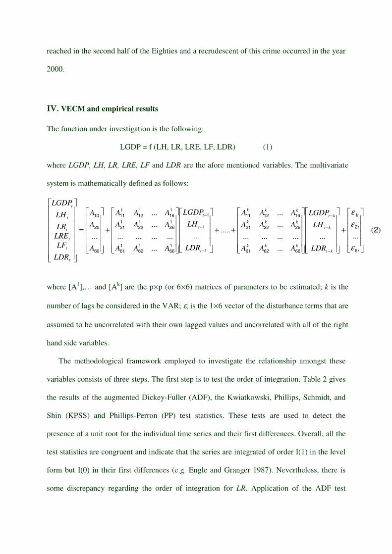
The function under investigation is the following:

LGDP = f (LH, LR, LRE, LF, LDR) (1)

where LGDP, LH, LR, LRE, LF and LDR are the afore mentioned variables. The multivariate

system is mathematically defined as follows:

)(......

...

............

...

...

........

...

............

...

...

...2

6

2

1

666261

262221

161211

1

1

1

1

66

1

62

1

61

1

26

1

22

1

21

1

16

1

12

1

11

60

20

10

+

++

+

=

−

−

−

−

−

−

t

t

t

kt

kt

kt

kkk

kkk

kkk

t

t

t

t

t

t

t

t

t

LDR

LH

LGDP

AAA

AAA

AAA

LDR

LH

LGDP

AAA

AAA

AAA

A

A

A

LDR

LF

LRE

LR

LH

LGDP

ε

ε

ε

where [A1],… and [A

k] are the pµp (or 6µ6) matrices of parameters to be estimated; k is the

number of lags be considered in the VAR; εt is the 1µ6 vector of the disturbance terms that are

assumed to be uncorrelated with their own lagged values and uncorrelated with all of the right

hand side variables.

The methodological framework employed to investigate the relationship amongst these

variables consists of three steps. The first step is to test the order of integration. Table 2 gives

the results of the augmented Dickey-Fuller (ADF), the Kwiatkowski, Phillips, Schmidt, and

Shin (KPSS) and Phillips-Perron (PP) test statistics. These tests are used to detect the

presence of a unit root for the individual time series and their first differences. Overall, all the

test statistics are congruent and indicate that the series are integrated of order I(1) in the level

form but I(0) in their first differences (e.g. Engle and Granger 1987). Nevertheless, there is

some discrepancy regarding the order of integration for LR. Application of the ADF test

yields the unit root is rejected when applied to its first difference but there is no evidence

when the test is applied to its level. KPSS suggests the series is I(1). Hence, overall there is

ground to treat LR as stationary in its first difference.

Given the unit root results, the second step is to use the Vector Autoregressive (VAR)

approach that Johansen (1988) and Johansen and Juselius (1990) implemented to investigate

the existence of a common long run equilibrium amongst I(1) variables. The joint F-test and

the Akaike (AIC), Schwartz (SC) and Hannan-Quinn (HQ) Information Criteria are used to

select the number of lags required in the unrestricted VAR to ensure that residuals are white-

noise (i.e. the vector autocorrelation test in this case is F(180,197)=1.0352 [0.4054]). Thus,

the chosen lag length is four accordingly (Garratt et al., 2003). The cointegration test results

are presented in Table 3. Though, the null hypothesis of no cointegration fails to be rejected

by the maximum likelihood (Max) statistic, at least a single significant cointegrating vector is

identified using the trace statistic. Hence, one concludes that all variables are cointegrated,

and causally related in each model. The calculated cointegrating vector (ECT), that is the

residual from the long run equation, is then incorporated in its first lag in the error correction

specification.

The third step of the analysis is to estimate an unrestricted vector error correction model

(VECM) where the long run and short run information are simultaneously included:

ttititt DMYYDY ε++Γ+Π= ∑−

=

−− K1p

1i1 (3)

where: Yt = (LGDPt, …. ,LDRt) is a vector of all the endogenous variables defined above,

expressed in their first difference (D) being I(1); Π is the long run part of the model, that

contains the cointegrating relations (β) and the loading coefficients (α); Γ is the matrix of the

short run parameters to be estimated; DM contains all deterministic variables that is constants,

linear trend and specified other dummy variables; εt is the vector of the disturbance terms that

are assumed to be uncorrelated with their own lagged values and uncorrelated with all of the

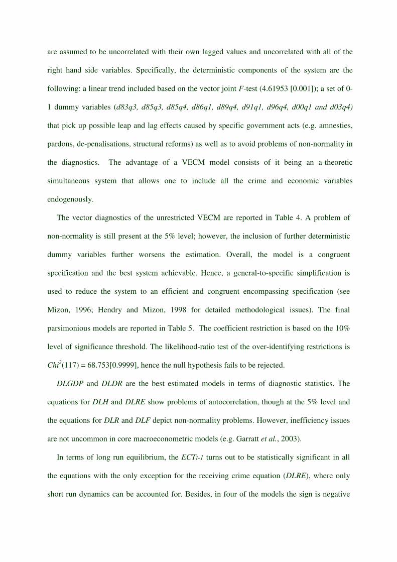
right hand side variables. Specifically, the deterministic components of the system are the

following: a linear trend included based on the vector joint F-test (4.61953 [0.001]); a set of 0-

1 dummy variables (d83q3, d85q3, d85q4, d86q1, d89q4, d91q1, d96q4, d00q1 and d03q4)

that pick up possible leap and lag effects caused by specific government acts (e.g. amnesties,

pardons, de-penalisations, structural reforms) as well as to avoid problems of non-normality in

the diagnostics. The advantage of a VECM model consists of it being an a-theoretic

simultaneous system that allows one to include all the crime and economic variables

endogenously.

The vector diagnostics of the unrestricted VECM are reported in Table 4. A problem of

non-normality is still present at the 5% level; however, the inclusion of further deterministic

dummy variables further worsens the estimation. Overall, the model is a congruent

specification and the best system achievable. Hence, a general-to-specific simplification is

used to reduce the system to an efficient and congruent encompassing specification (see

Mizon, 1996; Hendry and Mizon, 1998 for detailed methodological issues). The final

parsimonious models are reported in Table 5. The coefficient restriction is based on the 10%

level of significance threshold. The likelihood-ratio test of the over-identifying restrictions is

Chi2(117) = 68.753[0.9999], hence the null hypothesis fails to be rejected.

DLGDP and DLDR are the best estimated models in terms of diagnostic statistics. The

equations for DLH and DLRE show problems of autocorrelation, though at the 5% level and

the equations for DLR and DLF depict non-normality problems. However, inefficiency issues

are not uncommon in core macroeconometric models (e.g. Garratt et al., 2003).

In terms of long run equilibrium, the ECTt-1 turns out to be statistically significant in all

the equations with the only exception for the receiving crime equation (DLRE), where only

short run dynamics can be accounted for. Besides, in four of the models the sign is negative

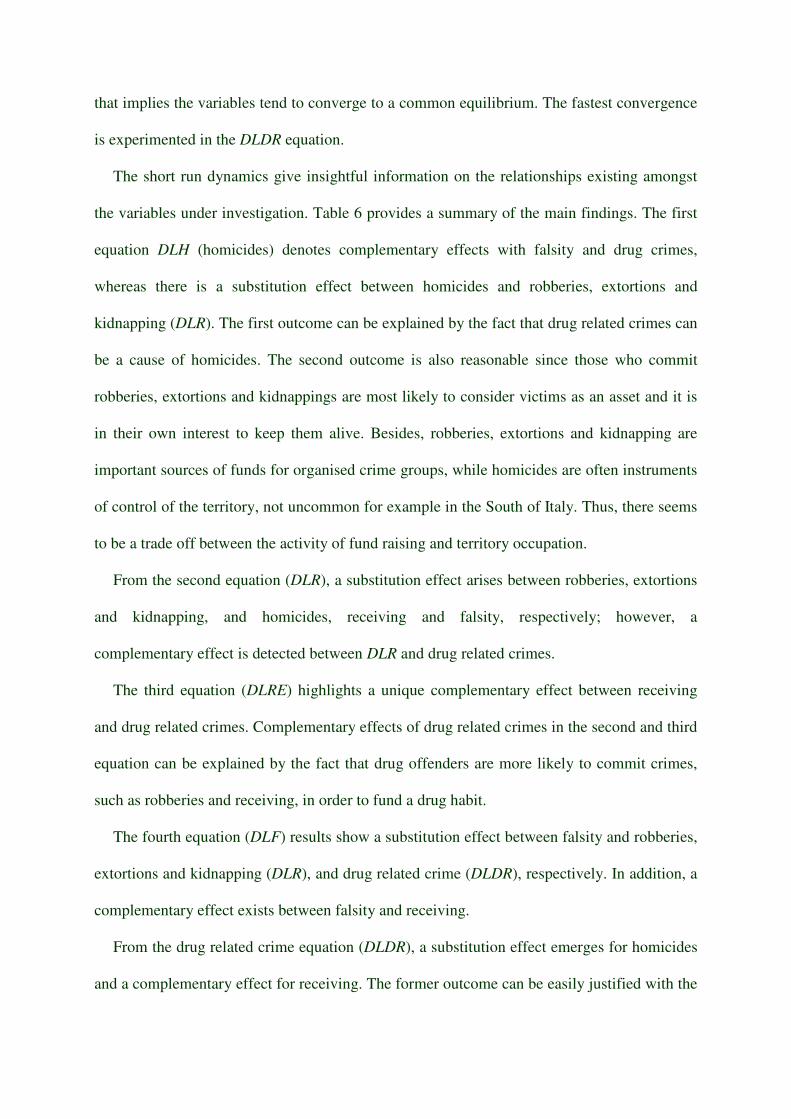
that implies the variables tend to converge to a common equilibrium. The fastest convergence

is experimented in the DLDR equation.

The short run dynamics give insightful information on the relationships existing amongst

the variables under investigation. Table 6 provides a summary of the main findings. The first

equation DLH (homicides) denotes complementary effects with falsity and drug crimes,

whereas there is a substitution effect between homicides and robberies, extortions and

kidnapping (DLR). The first outcome can be explained by the fact that drug related crimes can

be a cause of homicides. The second outcome is also reasonable since those who commit

robberies, extortions and kidnappings are most likely to consider victims as an asset and it is

in their own interest to keep them alive. Besides, robberies, extortions and kidnapping are

important sources of funds for organised crime groups, while homicides are often instruments

of control of the territory, not uncommon for example in the South of Italy. Thus, there seems

to be a trade off between the activity of fund raising and territory occupation.

From the second equation (DLR), a substitution effect arises between robberies, extortions

and kidnapping, and homicides, receiving and falsity, respectively; however, a

complementary effect is detected between DLR and drug related crimes.

The third equation (DLRE) highlights a unique complementary effect between receiving

and drug related crimes. Complementary effects of drug related crimes in the second and third

equation can be explained by the fact that drug offenders are more likely to commit crimes,

such as robberies and receiving, in order to fund a drug habit.

The fourth equation (DLF) results show a substitution effect between falsity and robberies,

extortions and kidnapping (DLR), and drug related crime (DLDR), respectively. In addition, a

complementary effect exists between falsity and receiving.

From the drug related crime equation (DLDR), a substitution effect emerges for homicides

and a complementary effect for receiving. The former outcome can be easily justified with the

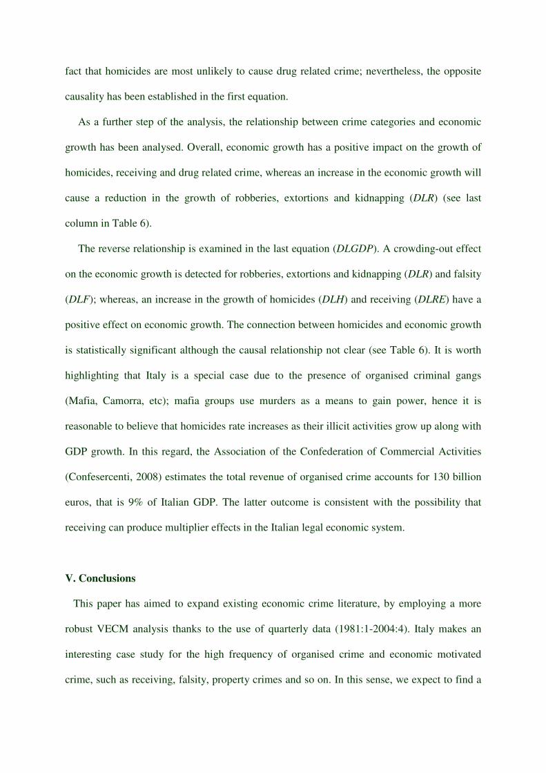
fact that homicides are most unlikely to cause drug related crime; nevertheless, the opposite

causality has been established in the first equation.

As a further step of the analysis, the relationship between crime categories and economic

growth has been analysed. Overall, economic growth has a positive impact on the growth of

homicides, receiving and drug related crime, whereas an increase in the economic growth will

cause a reduction in the growth of robberies, extortions and kidnapping (DLR) (see last

column in Table 6).

The reverse relationship is examined in the last equation (DLGDP). A crowding-out effect

on the economic growth is detected for robberies, extortions and kidnapping (DLR) and falsity

(DLF); whereas, an increase in the growth of homicides (DLH) and receiving (DLRE) have a

positive effect on economic growth. The connection between homicides and economic growth

is statistically significant although the causal relationship not clear (see Table 6). It is worth

highlighting that Italy is a special case due to the presence of organised criminal gangs

(Mafia, Camorra, etc); mafia groups use murders as a means to gain power, hence it is

reasonable to believe that homicides rate increases as their illicit activities grow up along with

GDP growth. In this regard, the Association of the Confederation of Commercial Activities

(Confesercenti, 2008) estimates the total revenue of organised crime accounts for 130 billion

euros, that is 9% of Italian GDP. The latter outcome is consistent with the possibility that

receiving can produce multiplier effects in the Italian legal economic system.

V. Conclusions

This paper has aimed to expand existing economic crime literature, by employing a more

robust VECM analysis thanks to the use of quarterly data (1981:1-2004:4). Italy makes an

interesting case study for the high frequency of organised crime and economic motivated

crime, such as receiving, falsity, property crimes and so on. In this sense, we expect to find a

rational behaviour among crime agents. The objective of this study has been firstly to

examine how criminals allocate their effort amongst different crime typologies, secondly to

what extent crime affects economic growth, as well as economic growth affects criminal

activity.

The pre-modelling results have shown that a long run unique common equilibrium exists

amongst the criminal variables (i.e. number of recorded homicides; robberies, extortions and

kidnapping; receiving; falsity; and drug related crimes) and GDP. On this basis, the VECM

model has highlighted the following findings: firstly, economic growth produces a positive

effect on the growth of homicides, receiving and drug related crimes, conversely, a negative

effect on robberies, extortions and kidnapping; secondly, the growth in robberies, extortions

and kidnapping and falsity has a crowding-out effect on economic growth, while homicides

and receiving produce a positive effect on legal activities.

The VECM has also shown how offenders allocate their effort amongst the crime typologies

analysed. Specifically, with regard to the short run dynamics, a bi-directional complementary

effect has been detected between drug related crimes and receiving. Whereas, a bi-directional

trade off effect has been highlighted between robberies, extortions and kidnapping, and

homicides and falsity, respectively.

Further findings have shown that growth in drug related crimes increase growth in

homicides but a trade off effect has also been highlighted when treating homicides as the

dependent variable.

Although, Italian data have been employed in this study, the findings should be of interest

and replicated for other countries. Economic issues, such as crowding-out effects of illegal

activity and offenders’ allocation of their effort in criminal submarkets, have been so far

under-researched despite its substantial importance to government interventions. This paper

helps to shed new light on these topics.

References

Becker, G.S. (1968) Crime and punishment: an economic approach, Journal of Political

Economy, 76, 169-217.

Bolton, P. (2001) Social Indicators, House of Commons Library, Research Paper 01/83.

Cameron, S. (1987) Substitution between offence categories in the supply of property crime:

Some new evidence, International Journal of Social Economics, 14, 48-60.

Chen, S.W. (2009) Investigating causality among unemployment, income and crime in

Taiwan: evidence from the bounds test approach, Journal of Chinese Economics and

Business Studies, 7, 115-125.

Confesercenti (2008) SOS Impresa. XI Rapporto, Roma, Confesercenti.

Detotto, C., Vannini, M. (2009) “Counting the cost of crime in Italy.” Workshop on Applied

analyses of crime: Implications for cost-effective criminal justice policies,

PortoConteRicerche, Italy, 26 October 2009.

Enders, W., Sandler, T. (1993) The effectiveness of antiterrorism policies: A vector-

autoregression-intervention analysis, American Political Science Review, 7, 829-844.

Engle, R.F. and Granger, C.W.J. (1987) Cointegration and error correction: Representation,

estimation and testing, Econometrica, 55, 251-276.

Garratt, A., Lee, K., Pesaran H. and Shin Y. (2003) A long run structural macroeconometric

model of the UK, The Economic Journal, 133, 412-455.

Habibullah, M.S., Baharom, A.H. (2009) Crime and economic conditions in Malaysia,

International Journal of Social Economics, 36, 1071-1081

Hakim, S., Spiegel, U., Weinblatt, J. (1984) Substitution, size effects, and the composition of

property crime, Social Science Quarterly, 65, 719-734

Hendry, D.F., Mizon, G.E. (1998) Exogeneity, causality, and co-breaking in economic policy

analysis of a small econometric model of money in the UK, Empirical Economics, 23,

267-294.

Holtmann, A.G., Yap L. (1978) Does punishment pay?, Public Finance, 33, 90-97.

Jantzen, R. (2008) Dynamics of New York City crime, The 66th International Atlantic

Economic Conference (IAES), Montréal, Canada.

Johansen, S. (1988) Statistical Analysis of Cointegration Vectors, Journal of Economic

Dynamics and Control, 12, 231-254.

Johansen, S. (1995) Likelihood Based Inference in Cointegrated Vector Autoregressive

Models, Oxford, Oxford University Press.

Koskela, E., Viren, M. (1997) An occupational choice model of crime switching, Applied

Economics, 1997, 29, 655- 660

Masih, A.M.M., Masih, R., (1996) Temporal causality and the dynamics of different

categories of crime and their socioeconomic determinants: evidence from Australia,

Applied Economics, 28, 1093-1104.

Mizon, G.E. (1996), Progressive Modelling of Macroeconomic Time Series - The LSE

Methodology, Ch. 4 in Hoover, K.D. (ed) Macroeconometrics, California, Kluwer

Academic Publishers.

Narayan, P.K., Smyth, R. (2004) Crime rates, male youth unemployment and real income in

Australia: evidence from Granger causality tests, Applied Economics, 36, 2079-2095.

Pindyck, R.S., and Rubinfeld, D.L. (1991) Econometric Models and Economic Forecasts,

Singapore, International Editions.

Figure 1 Graphs of LH, LR, LRE, LF, LDR, LGDP and Hodrick-Prescott trend

Table 1 List of crime variables (Number of recorder crimes per 100,000 inhabitants)

Name Definition Code

Homicide Voluntary committed homicide H

Robberies, extortions and kidnapping

Robberies, extortions and kidnapping R

Receiving A receiving offence is committed when a person who intentionally handles, receives, retains or disposes of stolen goods, knowing or having reasonable grounds to believe they have been stolen

RE

Falsity A falsity offence regards counterfeit of credit cards and currency, false seals (e.g. brand counterfeit, falsification of stamps or passports of the State) and falsifying documents (e.g. alteration of official documents and certificates)

F

Drug Offence of possession, production and trade of drugs DR

-1.2

-1.1

-1.0

-0.9

-0.8

-0.7

-0.6

-0.5

-0.4

1985 1990 1995 2000

LH HPLH

2.2

2.4

2.6

2.8

3.0

3.2

3.4

3.6

1985 1990 1995 2000

LR HPLR

1.0

1.5

2.0

2.5

3.0

3.5

4.0

4.5

1985 1990 1995 2000

LRE HPLRE

2.8

3.2

3.6

4.0

4.4

4.8

1985 1990 1995 2000

LF HPLF

1.6

2.0

2.4

2.8

3.2

3.6

4.0

1985 1990 1995 2000

LDR HPLDR

8.1

8.2

8.3

8.4

8.5

8.6

1985 1990 1995 2000

LGDP HPLGDP

Table 2 Unit roots test on dependent and explanatory variables (sample: 1981:1- 2004:4)

Variables Status ADF lags KPSS lags PP Lags

LGDP c,t - I(1) -1.96 4 0.23*** 7 -1.68 5

DLGDP c,t - I(0) -4.39*** 3 0.07 5 -6.72*** 4

LH c - I(1) -1.34 7 0.63** 7 -2.29 11

DLH c - I(0) -4.38*** 7 0.20 22 -10.26*** 24

LR c,t - I(0) or I(1) -3.05** 2 0.26*** 6 -3.88** 4

DLR c - I(0) -9.82*** 1 0.19 2 -14.40 2

LRE c,t - I(1) -1.07 6 0.20** 7 -1.05 3

DLRE c - I(0) -3.66*** 5 0.11 3 -9.88*** 3

LF c - I(1) -1.13 0 1.15** 7 -1.06 2

DLF c - I(0) -10.90*** 0 0.11 2 -10.90*** 1

LDR c,t - I(1) -1.12 3 0.25*** 7 -2.77 3

DLDR c - I(0) -8.33*** 2 0.23 49 -15.58*** 27

Notes: (1) *** and ** indicate statistical significance at the 1% and 5% levels, respectively. (2) D denotes the first-difference

operator. (3) Number of lags set in the ADF test is set upon AIC criterion, whereas KPSS and PP test upon Newey-West

bandwidth. (4) A constant and trend (c,t) are included upon a trend coefficient statistically significant.

Table 3 Johansen cointegration trace test

Lgdp lh lr lre lf ldr - Sample: 1981:1 – 2004:4 - 4 lags - constant

H0:rank<= Trace 95% 99% Max 95% 99%

0 111.61*** 94.15 103.18 38.47 39.37 45.1

1 73.14** 68.52 76.07 29.55 33.46 38.77

2 43.59 47.21 54.46 15.77 27.07 32.24

3 27.81 29.68 35.65 15.09 20.97 25.52

4 12.72 15.41 20.04 8.09 14.07 18.63

5 4.63** 3.76 6.65 4.63** 3.76 6.65 Notes: (1) **, *** denote that a test statistics at the 5% and 1 % levels of significance, respectively. (2) four lags and an

unrestricted constant are added; equivalent results are obtained when including both the constant and the trend in the

cointegrating space.

Table 4 Unrectricted VECM, vector diagnostic statistics

tests distribution statistics p-value

Vector autocorrelation F(180, 126) 0.96841 0.5812

Vector Normality Chi^2(12) 25.005** 0.0148

Vector heteroscedasticity Chi^2(12) 1225.1 0.8661 Notes: (1) ** indicate significance at the 5% level

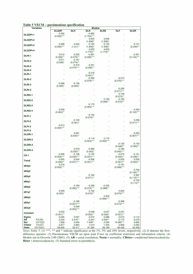
Table 5 VECM – parsimonious specification Variables Models

DLGDP DLH DLR DLRE DLF DLDR

DLGDPt-1 0.392

(0.092)*** -

-4.893 (1.754)***

- - -

DLGDPt-2 - - 3.645

(1.838)* 3.646

(1.838)* - -

DLGDPt-3 0.268

(0.095)*** 2.423

(1.21)** -3.124

(1.846)* -3.124

(1.846)* -

5.131 (2.240)**

DLGDPt-4 - - 4.653

(1.770)** 4.653

(1.770)** -

DLHt-1 0.012

(0.006)** 0.200

(0.075)** -0.281

(0.095)*** - -

-0.401 (0.143)***

DLHt-2 0.011

(0.006)* 0.167

(0.074)** - - - -

DLHt-3 - -0.474

(0.074)*** 0.241

(0.092)** - - -

DLHt-4 - - - - - -

DLRt-1 - - -0.218

(0.081)** - - -

DLRt-2 -- - -0.269

(0.079)*** -

-0.273 (0.076)***

-

DLRt-3 -0.008

(0.005)* -0.106

(0.060)* - - - -

DLRt-4 - - - - -0.259

(0.071)*** -

DLREt-1 - - - - 0.149

(0.073)** -

DLREt-2 - - - 0.183

(0.089)** -0.160

(0.072)** -

DLREt-3 - - -0.173

(0.063)*** - - -

DLREt-4 0.009

(0.004)** - - -

0.303 (0.102)***

DLFt-1 - - -0.154

(0.075)** - - -

DLFt-2 - 0.100

(0.061)* - - -

0.259 (0.071)***

DLFt-3 -0.013

(0.005)*** - - - - -

DLFt-4 - - - - -

DLDRt-1 - 0.091

(0.035)** - - -

-0.253 (0.067)***

DLDRt-2 - - 0.119

(0.044)*** 0.170

(0.059)*** - -

DLDRt-3 - - - -0.125

(0.048)** -0.143

(0.065)**

DLDRt-4 0.079

(0.035)** -0.080

(0.043)* -

0.185 (0.045)***

-

Cit-1 -0.006

(0.002)*** -0.128

(0.030)*** 0.154

(0.037)*** -

-0.074 (0.032)**

-0.141 (0.056)**

Trend 0.000

(0.000)** 0.004

(0.001)*** -0.006

(0.001)*** -

0.002 (0.001)**

0.005 (0.002)**

d83q3 0.018

(0.005)*** - - -

-0.191 (0.069)***

-

d85q3 - - - - - 0.702

(0.100)***

d85q4 - - -0.184

(0.071)** - -

0.387 (0.115)***

d86q1 - - - - - -0.752

(0.112)**

d89q4 - 0.169

(0.060)*** 0.308

(0.073)*** -0.235

(0.088)** - -

d91q1 0.009

(0.005)* -

0.162 (0.070)**

0.262

(0.070)*** -

d96q4 - - - 0.403

(0.089)*** - -

d00q1 - 0.186

(0.057)*** - -

-0.398 (0.072)***

-

d03q4 - 0.349

(0.053)*** - - - -

Constant 0.003

(0.001)** -

0.048 (0.023)**

0.047 (0.026)*

0.047 (0.021)**

-

Sigma 0.005 0.057 0.072 0.086 0.073 0.110 AR F(5,50) 2.234 2.416** 2.201 2.534** 2.173 2.279 Nor Chi^2(2) 1.658 0.946 7.429** 0.290 16.965*** 0.685 CHeter F(4,67) 0.877 0.884 1.010 1.404 0.858 0.263 Heter Chi^2(61) 66.605 52.417 47.364 58.769 69.436 50.458

Notes Table 5: (1) ***, ** and * indicate significance at the 1%, 5% and 10% levels, respectively. (2) D denotes the first-

difference operator. (3) Parsimonious VECM set upon joint F-test on coefficient restriction and information criteria. (4)

Models run in Givewin 2.00 (2001). (5) AR = serial correlation; Norm = normality; CHeter= conditional heteroscedasticity;

Heter = heteroscedasticity. (5) Standard errors in parenthesis.

Table 6 Substitution/complementary effects and crowding-out effects on economic growth

Effects based upon the first significant lag at least at the 10%

Variables DLH DLR DLRE DLF DLDR DLGDP

DLH - S* C* C** Pos**

DLR S*** - S*** S** C*** Neg***

DLRE - C*** Pos*

DLF S*** C** - S**

DLDR S*** C*** - Pos**

DLGDP Pos** Neg* Pos** Neg*** -

Notes: Effects based upon the first significant lag at least at the 10% (see Pindyck, and Rubinfeld, 1991); related coefficients

statistically significant at the 10% (*), 5%(**) and 1%(***) respectively.