margins of multinational labor substitution
TRANSCRIPT

IZA DP No. 2131
Margins of Multinational Labor Substitution
Marc-Andreas MuendlerSascha O. Becker
DI
SC
US
SI
ON
PA
PE
R S
ER
IE
S
Forschungsinstitutzur Zukunft der ArbeitInstitute for the Studyof Labor
May 2006

Margins of
Multinational Labor Substitution
Marc-Andreas Muendler University of California, San Diego
and CESifo
Sascha O. Becker University of Munich, CESifo
and IZA Bonn
Discussion Paper No. 2131 May 2006
IZA
P.O. Box 7240 53072 Bonn
Germany
Phone: +49-228-3894-0 Fax: +49-228-3894-180
Email: [email protected]
Any opinions expressed here are those of the author(s) and not those of the institute. Research disseminated by IZA may include views on policy, but the institute itself takes no institutional policy positions. The Institute for the Study of Labor (IZA) in Bonn is a local and virtual international research center and a place of communication between science, politics and business. IZA is an independent nonprofit company supported by Deutsche Post World Net. The center is associated with the University of Bonn and offers a stimulating research environment through its research networks, research support, and visitors and doctoral programs. IZA engages in (i) original and internationally competitive research in all fields of labor economics, (ii) development of policy concepts, and (iii) dissemination of research results and concepts to the interested public. IZA Discussion Papers often represent preliminary work and are circulated to encourage discussion. Citation of such a paper should account for its provisional character. A revised version may be available directly from the author.

IZA Discussion Paper No. 2131 May 2006
ABSTRACT
Margins of Multinational Labor Substitution*
Multinational labor demand responds to wage differentials at the extensive margin, when a multinational enterprise (MNE) expands into foreign locations, and at the intensive margin, when an MNE operates existing affiliates across locations. We derive conditions for parametric and nonparametric identification of an MNE model to infer elasticities of labor substitution at both margins, controlling for location selectivity. Prior studies have rarely found foreign wages or operations to affect employment. Our strategy detects salient adjustments at the extensive margin for German MNEs. With every percentage increase in German wages, German MNEs allocate 2,000 manufacturing jobs to Eastern Europe at the extensive margin and 4,000 jobs overall. JEL Classification: F21, F23, C14, C24, J23 Keywords: multinational enterprise, location choice, sample selectivity, labor demand,
translog cost function, nonparametric estimation Corresponding author: Marc-Andreas Muendler Department of Economics, 0508 University of California, San Diego (UCSD) 9500 Gilman Drive La Jolla, CA 92093-0508 USA Email: [email protected]
* We thank Gordon Hanson, Xiaohong Chen, Peter Egger, Sebastian Kessing and Hal White as well as participants at various seminars and conferences for insightful suggestions. We thank Steve Redding for sharing code to compute market access statistics. Jennifer Poole, Robert Jäckle, Nadine Gröpl, and Daniel Klein provided excellent research assistance. Simone Hofer from ubs kindly shared the bank’s international wage data. We gratefully acknowledge financial support from the VolkswagenStiftung under its grant initiative Global Structures and Their Governance and administrative and financial support from the Ifo Institute. Becker also gratefully acknowledges financial support from the Fritz-Thyssen-Stiftung.

1 Introduction
Multinational enterprises (MNEs) are important mediators of world trade. Sur-prisingly, however, the operation of MNEs has rarely been found to affect factordemands across locations (e.g. Slaughter (2000) for U.S., Konings (2004) for Eu-ropean MNEs). We quantify the effect of permanent wage differentials on MNEemployment at two critical margins. An MNE’s labor demand responds to inter-national wage differentials at the extensive margin, when the MNE expands into aforeign market, and at the intensive margin, when the MNE operates existing affil-iates and chooses employment. Our paper thus offers an integration of two strandsof the empirical literature—one on MNEs’ location choices (Devereux and Griffith1998, Head and Mayer 2004) and one on MNE operations across existing locations(Slaughter 2000, Head and Ries 2002, Hanson, Mataloni, and Slaughter 2005)—intoa unified estimation framework.
The MNE’s two-stage decision, to first expand (extensive margin) and then op-erate (intensive margin), has a well-defined econometric counterpart in sample selec-tion. Aside from the economic interpretation of the extensive margin, labor demandor cost function estimates at the intensive margin are subject to selectivity bias un-less corrected. Using comprehensive data on German manufacturing MNEs and theirmajority-owned foreign manufacturing affiliates, we find that an MNE’s propensityto select a foreign location is a salient predictor of its labor demand across locationsand that permanent wage differentials have a strong impact on multinational laborsubstitution both at the extensive and the intensive margin.
A methodological contribution of our paper is to extend the univariate sampleselection case to one of multiple selections. We derive conditions under which thecommon Heckman (1979) selection correction can be applied location by location tocorrect outcome estimation, in our case a seemingly unrelated equation system ofthe MNE’s cost function. We also prove identification of a nonparametric selectionmodel, which extends single-equation models (such as those in Das, Newey, andVella (2003)) to the multivariate case. The nonparametric estimator is simple toimplement in a two-stage approach and is applicable to the estimation of multivariatedemand systems in general (for a recent parametric approach to multivariate demandsee e.g. Yen (2005)).
To quantify the extensive margin, we base our parametric and non-parametricestimators of location selection on MNE-wide profit maximization. Existing firm-level studies on the expansion of MNEs do not find low wages or low per-capitaincomes to be significant predictors of location choice (e.g. Devereux and Griffith(1998) for U.S., Head and Mayer (2004) for Japanese, Buch, Kleinert, Lipponer,and Toubal (2005) for German MNEs).1 Multinomial logit estimation turns wages
1Carr, Markusen, and Maskus (2001) find evidence in aggregate data that relatively abundanthigh-skilled labor is a significant predictor of foreign direct investment (FDI) of U.S. MNEs (andBlonigen, Davies, and Head (2003) find that larger skill differentials predict less foreign MNE
2

into significant predictors of location choice in Disdier and Mayer (2004) for FrenchMNEs, and in Becker, Ekholm, Jackle, and Muendler (2005) for Swedish MNEsand the same German MNEs as in this paper. But multinomial logit estimationrests on the assumption that independent agents within the MNE decide on distinctinvestment projects; that is incompatible with MNE-wide profit maximization. De-vereux and Griffith (1998) estimate multinomial logit choice and, to be consistentwith MNE-wide optimization, restrict their sample to MNEs who invest in only onelocation abroad; they do not find wages to be significant predictors of U.S. MNEs’location choices. In contrast, when we condition on an MNEs’ past presence and itsinteraction with wages, we find wage variables to be statistically significant predic-tors of location choices in probit and in non-parametric selection regressions. Whenweighted with the impact of location selection on employment, wage differentialsacross locations are substantial predictors of labor substitution within MNEs at theextensive margin.
At the intensive margin, the world’s ten largest MNEs in 2000 produce almostone percent of world GDP, and the one hundred largest MNEs are responsible formore than four percent of world GDP.2 Despite this apparent importance of MNEsfor international transactions, Slaughter (2000) reports that, in a sample of U.S.MNEs, operations in low-wage locations have no detectable impact on MNE em-ployment in the home market. In contrast, Feenstra and Hanson (1999) attributedabout a third of U.S. relative wage changes to outsourcing (within MNEs or acrossfirms). Similar to Slaughter (2000), Konings (2004) and Barba Navaretti and Castel-lani (2004) find no evidence for the hypothesis that operations of European MNEsin low-wage locations have an impact on home-market labor demand. Braconier andEkholm (2000) and Marin (forthcoming) estimate wage elasticities of labor demandand intermediate imports from Central and Eastern Europe for Western EuropeanMNEs, and report no significant effect of foreign relative wages. Brainard and Riker(2001), however, do find that foreign affiliate employment substitutes modestly forU.S. parent employment but less so than for employment across foreign locations.3
Hanson, Mataloni, and Slaughter (2005) shift focus from factor demands to inter-mediate input uses and, as an exception to most prior firm-level evidence, reportthat affiliates of U.S. MNEs process significantly more intra-firm imports the lowerare low-skilled wages. The result challenges the view that relative abundance inlow-skilled labor fails to attract MNEs. We revisit their result in the context ofmultinational labor substitution and extend the estimation framework to incorpo-rate location choice. When controlling for the propensity to select a foreign location,wages are statistically significant and economically salient predictors of MNEs’ labordemands at the intensive margin.
activity).2UNCTAD press release TAD/INF/PR/47 (12/08/02).3At the aggregate level, Brainard (1997) does not find relative abundance of low-skilled labor
to explain MNE sales patterns across locations.
3

Our findings point to large sunk entry and exit costs so that MNE expansions (orwithdrawals) are infrequent but, when undertaken, they have a sizeable impact onlabor demand. We find cross-wage elasticities at the extensive margin to be strictlypositive. So, home and foreign employment are substitutes within MNEs not only atthe intensive but also at the extensive margin. Elasticities at the extensive marginare about half the size of elasticities at the intensive margin in locations close tohome. For overseas developing country wages, however, elasticities are significantlydifferent from zero only at the extensive margin. Bootstraps reject equality betweenthe intensive and the total elasticity of substitution for most locations, corroboratingthe importance of the extensive margin. Elasticity point estimates at both marginsare robust across different samples and wage data, specifications, and parametricand nonparametric estimation techniques.
We evaluate the counterfactual question how many jobs MNEs would reallocatein response to shrinking wage differentials. A one-percent drop in German wagesrelative to the sample-mean level would reduce MNE employment in Central andEastern Europe (CEE) by around 4,000 jobs, for instance. Similarly, a one-percentincrease in CEE wages would bring 730 jobs to Germany. These are sizeable figures.Wages in CEE are, on average, about 10 percent of the German level in 2000. Ifthe estimated elasticities of substitution were constant at all levels of wages, anincrease in CEE wages of 450% to cut the wage gap to Germany in half wouldbring 330,000 (= 730 · 450) counterfactual manufacturing jobs to Germany—abouta quarter of the estimated home employment at German manufacturing MNEs.4 Ofcourse, elasticities of substitution are not constant at all levels of wages so that thecounterfactual prediction is crude. We nevertheless view the magnitude as indicativeof the potential importance of multinational labor substitution.
This paper has five more sections. Section 2 elaborates a model of the expansionand operation of MNEs, and Section 3 derives identification conditions for its estima-tion under location selectivity. Section 4 presents the data and discusses descriptivestatistics on location choice. Estimation results on multinational labor substitutionare presented in Section 5, and interpreted in counterfactual evaluations. Section 6concludes.
2 Multinational Expansion and Operation
Let observed employment y`j of MNE j at time t in location ` obey
y`jt = x`
jtβ` + ε`jt
4If international wage gaps shrink at a similar rate as per capita GDP converges to steady stateand Germany is close to its steady state, the CEE-German wage gap would take around 35 yearsto contract to half its present size (Barro and Sala i Martin 1992).
4

if MNE j is present at `. Else, y`jt = 0. In the translog case, the vector x`
jt
of employment predictors includes additively separable transformations of outputs,inputs and factor prices (we discuss regressor construction below), including theprevailing wage differentials between locations at time t. ε`jt is a disturbance term.So, the conditional expectation of MNE j’s observed employment in location ` is
y`jt ≡ E
[y`
jt
∣∣x`jt,djt, zj,t−τ
]= x`
jtβ` + E
[ε`jt |djt, zj,t−τ
], (1)
where the vector djt of presence indicators dkjt reflects MNE j’s observed pattern of
locations k = 1, . . . , L at time t (dkjt = 1 if firm j is present in location k and dk
jt = 0otherwise) and contains d`
jt = 1. The information set zj,t−τ at moment t− τ affectslabor demand through the resulting choice of presence in location `.
We define the extensive margin of labor demand to be the expected labor demandyext
` in location `, predicted by a firm j’s current choices of presence around the worldand its past information set zj,t−τ ,
yext,`jt ≡ E
[ε`jt | d1
jt, . . . , d`jt = 1, . . . , dL
jt; zj,t−τ
], (2)
where the optimal binary choices (d1jt, . . . , d
`jt, . . . , d
Ljt) are functions of MNE j’s
information set at the moment of location choice t− τ , and τ is the time it takes anMNE to implement location choices (two to four years, say). The information setzj,t−τ at moment t−τ predicts presence in location k with dk
jt = 1(H(zj,t−τ )+ηkj,t−τ >
0), where H(·) is an unknown function and ηkj,t−τ is a disturbance to the MNE’s
presence. Most important, zj,t−τ includes the then prevailing wage differentialsbetween locations.
Labor demand at the intensive margin is accordingly defined as
yint,`jt ≡ y`
jt − yext,`jt = x`
jtβ`. (3)
The labor demand effect at the extensive margin yext,`jt = E[ε`jt |djt] is an addi-
tive component of conditional labor demand E[y`jt |x`
jt,djt, zj,t−τ ]. Economically, anMNE’s mere presence at a location typically raises the labor demand predictionfor that location.5 Statistically, the extensive margin needs to be included in theregression to correct for selectivity.
MNE j produces a vector of location-specific outputs qjt = (q1jt, . . . , q
Ljt)
′ at Llocations. We consider MNEs to be price takers in input market, whereas theymay have market power in output markets. (We estimate a cost function, so anypricing behavior in the sales market is consistent with our approach.) On the inputside, we focus on employment. We view MNEs as wage takers in the local markets,competing with labor demand from non-tradeable goods sectors and incumbent
5To be precise, this is true if high home wages raise the probability of presence at a foreignlocation ` and the presence likelihood is positively correlated with labor demand at that foreignlocation `. Both conditions are satisfied in our MNE sample.
5

firms. Similarly, we consider demand for capital goods and intermediate inputsfrom non-MNEs as sufficiently large so that the remaining demand of MNEs forthose goods has a negligible price impact.
Final goods prices are world-market prices that differentiated products from loca-tions ` = 1, . . . , L can fetch, given product characteristics. Final goods are producedwith labor and capital. After controlling for location choice in the formation of theMNE, we consider installed capital kjt = (k1
jt, . . . , kLjt)
′ to be a quasi-fixed factor inan MNE’s short-run cost function Cjt (but put to use at locations k = 1, . . . , L todifferent degrees). We consider labor at locations k = 1, . . . , L to be immobile acrossnational borders and its factor prices wt = (w1
t , . . . , wLt )′ as specific to L locations.
2.1 Location choice
Define γ`N as the fixed FDI entry costs at location ` and γ`
X as the fixed FDI exitcosts from location `.6 Then, fixed costs of changing presence at location ` in t,anticipated at t− τ , become
G`(d`jt, d
`j,t−τ ) = γ`
N d`jt(1−d`
j,t−τ ) + γ`X (1−d`
jt)d`j,t−τ ,
where d`jt is the indicator for MNE j’s current FDI presence at location `, and d`
j,t−τ
for its past presence. We restrict the long-term fixed cost components γ`N and γ`
X
to be time invariant in our four-year MNE panel data (but control for time-varyingcountry and MNE characteristics in selection estimation). The decision-relevantfixed cost difference F `
j,t−τ ≡ G`(1, d`j,t−τ )−G`(0, d`
j,t−τ ) between presence at location` and absence from ` at time t is
F `j,t−τ = γ`
N − (γ`X + γ`
N) d`j,t−τ , (4)
where (γ`X + γ`
N) is sometimes called the hysteresis band and reflects the sunk costeffect that induces firms to continue operations at location ` (Dixit 1989).7
To select locations (τ years prior to production and sales), MNE j maximizesexpected profits Ej,t−τ [p(qi6=j,t,qjt)
′ · qjt − Cjt(qjt;kjt,w)]. This implies that MNEj’s rule for FDI presence at location ` can be written as
d`jt = 1
(Ej,t−τ [p
`q`,∗jt ] + Ej,t−τ [Cjt(q
`jt =0; ·)− Cjt(q
`,∗jt ; ·)]− F `
j,t−τ +η`j,t−τ > 0
)= 1
(h(z0
j,t−τ )− γ`N + (γ`
X +γ`N) d`
j,t−τ + η`j,t−τ > 0
)= 1
(H(zj,t−τ ) + η`
j,t−τ > 0)
(5)
6For simplicity, the fixed costs of reentry into a given location after a period of absence areassumed to be equal to the costs at first entry γ`
N .7Probit estimation with firm-fixed effects is known for problematic performance in panel data
with a short time horizon (Heckman 1981). We therefore do not attempt to estimate MNE-specificsunk costs of presence F `
j,t−τ at location `. We distinguish between entry and exit sunk costcomponents to account for MNE-specific differences in F `
j,t−τ , similar to Roberts and Tybout’s(1997) model of sunk costs in exporting status.
6

(see Appendix A for a derivation). The unknown function h(z0j,t−τ ) captures both
expected revenues from producing the profit-maximizing quantity q`,∗jt at location `
and expected cost savings from producing at ` (see first line). Sunk costs of presenceat location ` have an observable component F `
j,t−τ by (4) and a disturbance η`j,t−τ .
The disturbance η`j,t−τ is known to the MNE but not to the researcher. To simplify
notation, we write H(zj,t−τ ) ≡ h(z0j,t−τ ) − γ`
N + (γ`X +γ`
N) d`j,t−τ and include past
presence in any location in the information set zj,t−τ .Equation (5) is the selection equation: the empirical rule of presence in locations
` = 1, . . . , L. We estimate the rule both parametrically (with a probit regressionand H(zj,t−τ ) = zj,t−τγ
`) and nonparametrically.
2.2 Multiproduct cost function
To obtain theoretically well-defined estimates of elasticities of labor substitutionacross locations, we opt for a flexible parametric specification of the MNE’s multi-product cost function. We first augment the cost function with parametric correc-tions for location selectivity. We then proceed to a model with a parametric costfunction part and a nonparametric correction for selectivity.
We use a short-run multiproduct translog cost function to estimate labor de-mand, and extend it to control for location selectivity.8 A short-run cost function,given MNE j’s location choice, treats MNE j’s vector of capital stocks kjt as quasi-fixed factors. We prefer a short-run over a long-run cost function because we alreadycontrol for the installation of foreign affiliates through location selectivity (5) andbecause the inclusion of capital stock variables captures otherwise unobservable(firm-specific) user costs of capital across locations.
Applying Shepard’s (1953) lemma to the short-run multiproduct translog costfunction yields location-specific wage bill shares s`
jt ≡ w`ty
`jt/Cjt (the wage bill at
location ` in the MNE’s total wage bill) as functions of (qjt;kjt,w). We multiply thewage bill shares s`
jt with observation-specific scalars Cjt/w`t to arrive at our outcome
equation (labor demand at `)
y`jt = x`
jt β` + ε`jt (6)
with
x`jtβ
` = α`Cjt
w`t
+L∑
m=1
(µ`m ln
[(qm
jt )Cjt/w`
t
]+ κ`m ln
[(km
jt )Cjt/w`
t
]+ δ`m ln
[(wm
t )Cjt/w`t
])8We follow Brown and Christensen’s (1981, eq. 10.21) short-run version of Christensen, Jorgen-
son, and Lau (1973) and extend the framework to multiple products. A main alternative would beHall’s (1973) generalization of Diewert’s (1971) Leontief cost function to the multiproduct case. Wefavor the translog cost function because its dimensionality requirements are considerably leanerand permit higher-order approximations to the nonparametric correction for selectivity. Kohli(1978) took the translog specification to the empirical trade literature.
7

(see Appendix B), where ε`jt is a disturbance.Compared to translog regression equations in wage bill shares s`
jt, the transfor-mation with observation-specific scalars Cjt/w
`t to an equivalent regression of y`
jt onx`
jt has three important advantages. First, there is no constant term among theregressors x`
jt so that lacking identification of the constant in a nonparametric se-lection correction is no concern. Second, wages are regressors only and do not enterthe dependent variable. Third, labor demand is not bounded above so that, condi-tional on x`
jt, the labor demand disturbance satisfies the assumption of a one-sidedtruncation for (parametric and nonparametric) selectivity correction.
Stacking locations with zero output and factor use. Most MNEs produce insome but not in all locations. For cases of zero output or input, however, equation (6)is not well defined. Especially zero turnover and zero capital stocks require attentionbecause they are MNE-specific, but absence from a location also suggests droppingwage regressors when no employment occurs.
One possible treatment is estimation of separate equation systems for every singlepresence pattern in the data. The resulting estimators are hard to interpret, however,and plagued by dimensionality: potential presence in up to L− 1 locations outsidethe home location implies that there are up to 2L−1 − 1 regional presence patternsfor an MNE.9 In the German sample in 2000, for instance, only 57 out of 1,770MNEs are omnipresent in all four world locations while every single one of the 15possible regional presence pattern occurs. So, there would be 15 sets of estimates.
We choose to stack observations of all MNEs in the sample. Stacking observationsimproves efficiency, collapses the up to 2L−1−1 sets of estimates into one consistentlyestimated (L−1)-equation system, and provides a single L× L matrix of estimatesfor wage elasticities of regional labor demands. Stacking is permissible under threeconditions: (i) all MNEs face identical sunk cost F `
j,t−τ for presence at location` conditional on their prior presence and information set (so that presence is notcorrelated with inputs); (ii) MNEs face an identical short-run cost function Cjt(·) =C(·) in all locations of presence, conditional on their characteristics (so that onecommon parameter vector is justified); and (iii) the disturbances ε`jt are uncorrelatedacross observations.
We set all missing location variables for an absent MNE j to zero—that is logemployment, turnover, capital stock and wages are zero at location m from whereMNE j is absent. This is equivalent to interacting the translog cost function coef-ficients with presence indicators: µ`m = 0 when no output is produced at locationm, and κ`m = δ`m = 0 when MNE j employs no factors at location m. Stackingcan induce correlations between the transformed regressors and the error ε`jt in (6).
9MNEs are present in their home location by sample definition, so only 2L−1 patterns areobservable in principle. Firms that only operate domestically without any foreign affiliate are notMNEs by definition so that the single presence pattern with the only presence at the home locationmust be subtracted.
8

To remove this source of potential bias, we include the set of absence indicators(1−djt) (with nuisance parameters β`
d) among the regressors in the outcome equa-tion: y`
jt = x`jtβ
` = x0`jt β
` + (1−djt) β`d. The set of absence indicators (1−djt) also
offsets the zero output prediction at the sample mean.
3 Estimation under Location Selectivity
The selection equation (5) for location ` is
d`jt = 1
(H(zj,t−τ ) + η`
j,t−τ > 0)
and, conditional on MNE j’s selection of location `, expectations of the outcome (6)are
E[y`
jt |x`jt,djt, zj,t−τ
]= x`
jtβ` + E
[ε`jt | d1
jt, . . . , d`jt = 1, . . . , dL
jt; zj,t−τ
],
where disturbances ε`jt and η`j,t−τ are uncorrelated across observations (of MNEs i
and j, and between periods t and t+1). The timing of η`j,t−τ is not important and
the η`j,t−τ realization could be simultaneous with ε`jt. Natural exclusion restrictions
on covariates that do not enter the cost function identify location selection.In this section, we discuss cross-regional distributional assumptions on (ε`jt, η
`j,t−τ )
and permissible estimation techniques under those conditions. For a parametriccost function specification (with well-defined elasticities of substitution), a para-metric approach to selectivity appears natural to start with. We present sets ofnecessary and sufficient distributional assumptions for univariate Heckman (1979)corrections location by location, to which we refer as parametric selectivity correc-tion. Empirical evidence on the necessary assumptions is favorable in our sample.For multivariate selectivity, an extension of the Heckman (1979) estimator has acomplicated form (conditional moments of multivariate normal distributions haveno known closed form for multiple truncations, see Kotz, Balakrishnan, and Johnson(2000)). Simulated maximum-likelihood would be a viable technique but requiresjoint multivariate normality.
To be free of distributional restrictions, we extend the parametric approach toa nonparametric multivariate selection model (similar to one in Das, Newey, andVella (2003)) and account for cross-location correlations between labor demandchoices at the extensive and intensive margins. We derive identification from com-mon sufficient assumptions. The nonparametric procedure allows for unknown dis-turbance distributions, and for unknown functional forms of E
[ε`jt |djt, zj,t−τ
]and
1(H(zj,t−τ ) + ηkj,t−τ > 0).
3.1 Parametric selectivity correction
Consider Heckman (1979) selectivity corrections location by location. There aretwo alternative sets of assumptions that allow for such a parametric correction,
9
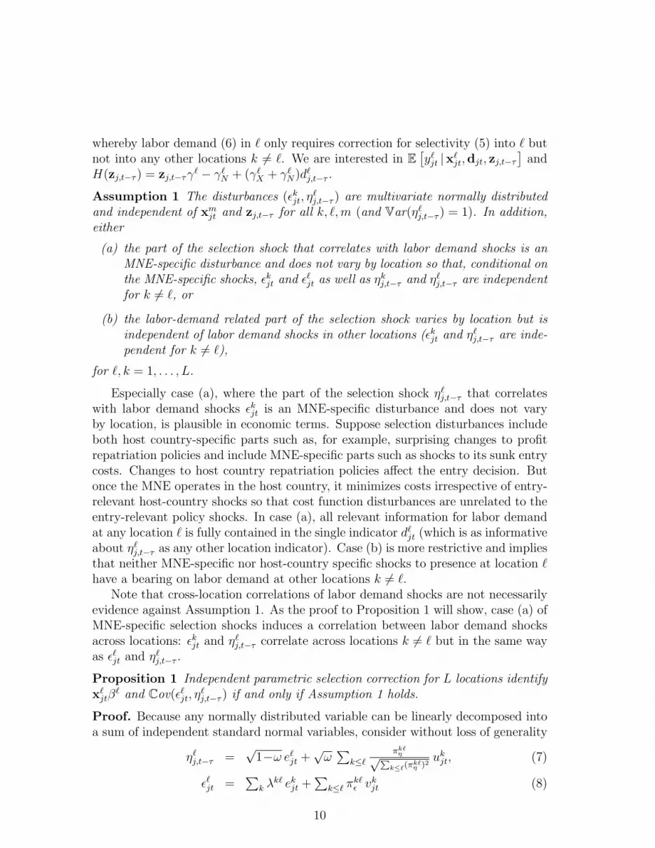
whereby labor demand (6) in ` only requires correction for selectivity (5) into ` butnot into any other locations k 6= `. We are interested in E
[y`
jt |x`jt,djt, zj,t−τ
]and
H(zj,t−τ ) = zj,t−τγ` − γ`
N + (γ`X + γ`
N)d`j,t−τ .
Assumption 1 The disturbances (εkjt, η`j,t−τ ) are multivariate normally distributed
and independent of xmjt and zj,t−τ for all k, `,m (and Var(η`
j,t−τ ) = 1). In addition,either
(a) the part of the selection shock that correlates with labor demand shocks is anMNE-specific disturbance and does not vary by location so that, conditional onthe MNE-specific shocks, εkjt and ε`jt as well as ηk
j,t−τ and η`j,t−τ are independent
for k 6= `, or
(b) the labor-demand related part of the selection shock varies by location but isindependent of labor demand shocks in other locations (εkjt and η`
j,t−τ are inde-pendent for k 6= `),
for `, k = 1, . . . , L.
Especially case (a), where the part of the selection shock η`j,t−τ that correlates
with labor demand shocks εkjt is an MNE-specific disturbance and does not varyby location, is plausible in economic terms. Suppose selection disturbances includeboth host country-specific parts such as, for example, surprising changes to profitrepatriation policies and include MNE-specific parts such as shocks to its sunk entrycosts. Changes to host country repatriation policies affect the entry decision. Butonce the MNE operates in the host country, it minimizes costs irrespective of entry-relevant host-country shocks so that cost function disturbances are unrelated to theentry-relevant policy shocks. In case (a), all relevant information for labor demandat any location ` is fully contained in the single indicator d`
jt (which is as informativeabout η`
j,t−τ as any other location indicator). Case (b) is more restrictive and impliesthat neither MNE-specific nor host-country specific shocks to presence at location `have a bearing on labor demand at other locations k 6= `.
Note that cross-location correlations of labor demand shocks are not necessarilyevidence against Assumption 1. As the proof to Proposition 1 will show, case (a) ofMNE-specific selection shocks induces a correlation between labor demand shocksacross locations: εkjt and η`
j,t−τ correlate across locations k 6= ` but in the same wayas ε`jt and η`
j,t−τ .
Proposition 1 Independent parametric selection correction for L locations identifyx`
jtβ` and Cov(ε`jt, η
`j,t−τ ) if and only if Assumption 1 holds.
Proof. Because any normally distributed variable can be linearly decomposed intoa sum of independent standard normal variables, consider without loss of generality
η`j,t−τ =
√1−ω e`
jt +√ω∑
k≤`
πk`η√P
k≤`(πk`η )2
ukjt, (7)
ε`jt =∑
k λk` ek
jt +∑
k≤` πk`ε vk
jt (8)
10

for independent standard normal variables ekjt, u
kjt, v
kjt (k = 1, . . . , L), where ω ∈ [0, 1]
is a weight to satisfy (σ`η)
2 = σ``η = 1, and πk`
η , πk`ε , λk` are parameters. To prove
sufficiency, let πk`η = πk`
ε = 0 for k 6= `.First consider (a) MNE-specific selection shocks η`
j,t−τ whose labor demand re-lated part does not vary over locations. Concretely, set ek
jt = ejt for all locations k,and denote λ·` ≡
∑k λ
k`. Then the variances and covariances of the selection shocks(7) are σ``
η = 1 and σk`η = 1−ω. The variances and covariances of the labor demand
shocks (8) are σ``ε = (λ·`)2 + (π``
ε )2 and σk`ε = (λ·`)2. And the covariances between
the selection shock in location k and the demand shock in location ` are σk`ηε = λ·`.
Second, consider (b) location-varying selection shocks η`j,t−τ that are independent
of labor demand shocks in other locations. Concretely, set λk` = 0 for k 6= `,and denote λ·` ≡ λ`` for comparability. Then the selection shock variances andcovariances are σ``
η = 1 and σk`η = 0. The variances and covariances of the labor
demand shocks are σ``ε = (λ·`)2 + (π``
ε )2 and σk`ε = 0. The covariances between the
selection shock in location k and the demand shock in location ` are σ``ηε =
√1−ω λ·`
and σk`ηε = 0 for k 6= `.
In both cases, the marginal likelihood function becomes
g(y`jt|x`
jt, zj,t−τ ) =φ((y`
jt − x`jtβ
`)/σ`ε
)σ`
ε Φ(zj,t−τγ`)· Φ
(ρ``
ηε(y`jt − x`
jtβ`) + zj,t−τγ
`
σ`ε (1− ρ``
ηε)1/2
), (9)
after concentrating out u`jt and v`
jt, where σ`ε =
√σ``
ε and ρ``ηε = σ``
ηε/σ`ε, and φ(·) and
Φ(·) are the standard normal density and distribution functions. This is precisely thelikelihood function for independent Heckman (1979) correction location by location.
For necessity, observe that parameters πk`η 6= 0 or πk`
ε 6= 0 for any k 6= ` causecross-equation correlations and do not permit concentrating out u`
jt and v`jt to arrive
at (9). Similarly, λk` 6= 0 for any k 6= ` precludes concentrating out e`jt to arrive
at (9).
Estimation. Extending the parametric two-stage procedure to L locations, wefirst estimate equations (5) with probit regressions by location. Second, we estimateoutcome (6) at location ` by including the predicted selectivity hazard (inverse of theMills ratio) Λ`
jt from the first stage among the regressors (we also include absenceindicators (1−djt) among the regressors to prevent stacking bias). The coefficienton the predicted selectivity hazard equals β`
Λ ≡ ρ``εησ
`ε. We implement the second-
stage estimation of (6) for L−1 locations (excluding home) by iterating Zellner’s(1962) seemingly unrelated regression (SUR) over the estimated disturbance covari-ance matrix until the estimates converge. This is equivalent to maximum-likelihoodestimation (Dhrymes 1971) and makes estimation invariant to the deleted locationequation L (Barten 1969). Through constraints, we impose linear homogeneity infactor prices and symmetry of wage coefficients (see appendix B). We treat induced
11

heteroskedasticity following Heckman (1979) (resulting in differing standard errorson symmetric coefficients). After estimation, we test whether either of the two pos-sible sets of distributional assumptions are satisfied. We will find implications of set(b) violated but fail to find evidence against (a).
Tests. Implications of Assumption 1 are testable. In case (a) of MNE-specificselection shocks and for any ω < 1, Assumption 1 implies that σk`
η is the same forany pair of locations k 6= `. Note that we have no evidence on σk`
ηε for k 6= ` fromlocation-by-location estimation. We obtain estimates of σk`
η from multivariate probitestimation instead and use a χ2-test for their equality.
Under the additional assumption that ω = 0, there is a further test to querycase (a), whether selection shocks are purely MNE-specific. Probit (maximumlikelihood) estimation of selection in the Heckman procedure does not predict thedisturbances ηjt. A testable implication of an MNE-specific selection shock, how-ever, is that, if an MNE is neither present in all locations nor absent from alllocations, the choices of presence and absence must be consistent with a location-independent MNE-specific selection shock for all locations. Concretely, an MNEobservation contradicts the assumption of a location-independent selection shock ifzj,t−τγ
k − F kj,t−τ > zj,t−τγ
` − F `j,t−τ for locations k of absence and locations ` of
presence because ηjt can be subtracted from both sides of the inequalities. Thisimplication is testable for the predicted values, which are normally distributed con-ditional on zj,t−τ and dj,t−τ by normality of ηjt.
For (b) location-variant selection shocks, the set of assumptions implies thatσk`
ε = 0. So, a regression of ε`jt on ε1jt, . . . , ε`−1jt , ε`+1
jt , . . . , εLjt must have zero coeffi-cients. We test this implication.
Both sets (a) and (b) of assumptions imply that εkjt is independent of dkjt for all k
because εkjt and η`j,t−τ are independent. We include absence indicators (1−djt) among
the regressors in the outcome equation, however, so this is not a useful implicationin our context.
3.2 Nonparametric selectivity correction
In the nonparametric version of the multivariate binary choice model (5) and (6),
d`jt = 1
(H(zj,t−τ ) + η`
j,t−τ > 0), (` = 1, . . . , L)
E[y`
jt |x`jt,djt, zj,t−τ
]= x`
jtβ` + E
[ε`jt
∣∣∣ d`jt = 1,dk 6=`
jt ; zj,t−τ
],
no distributional assumptions are placed on η`j,t−τ or εjt and H(·) is an unknown
function.We augment the nonparametric sample selection model in Das, Newey, and Vella
(2003) to remain identified under multivariate binary selection (similar in spirit to aselection model with endogeneity in Das, Newey, and Vella (2003)). Suppose ηk
j,t−τ
12

and ε`jt are correlated. Suppose also that zj,t−τ and x`jt are correlated (e.g. wages
in the past and present, as our data show). Because dkjt is a function of ηk
j,t−τ , itcorrelates with ε`jt; because dk
jt is a function of zj,t−τ , it correlates with x`jt. So, if the
labor demand equation does not condition on dkjt, the identifying restriction that x`
jt
and y`jt are uncorrelated will be violated.
Define the propensity score (the expected probability of selection conditional onzj,t−τ ) as p`
jt ≡ E[d`jt | zj,t−τ ] = 1−G(−H(zj,t−τ )), where G(·) is the cumulative
distribution function of η`j,t−τ . Then, assuming G(·) is one-to-one and changing
variables with u`jt = 1−G(η`
j,t−τ ), labor demand at the extensive margin becomes
E[ε`jt | d`jt = 1,dk 6=`
jt , zj,t−τ ] = E[ε`jt | η`j,t−τ > −H(·);dk 6=`
jt , zj,t−τ ]
= E[ε`jt |u`jt < p`
jt;dk 6=`jt ]
=
∫ ∫ p`jt
0
ε`jt f(ε`jt, u`jt|d
k 6=`jt ) dε`jtdu
`jt /p
`jt
= m`(p`
jt,dk 6=`jt
).
So, the conditional labor demand disturbance for location ` depends only on thepropensity score for that location and the pattern of presence elsewhere. Observedlabor demand then satisfies
E[y`
jt |x`jt,djt, zj,t−τ
]= x`
jtβ` +m`
(p`
jt,dk 6=`jt
).
To establish identification, consider deviations from the truth ∆ξ`(x`jt) ≡ x`
jt(β`−
β`) and ∆m`(p`jt,d
k 6=`jt ) ≡ m`(p`
jt,dk 6=`jt )−m`(p`
jt,dk 6=`jt ), where hats denote estimates
of the true (not hatted) functions. Assumption 2 states sufficient conditions foridentification.
Assumption 2
(i) E[ε`jt | d`jt = 1,dk 6=`
jt , zj,t−τ ] = m`(p`jt,d
k 6=`jt ),
(ii) Pr(∆ξ`(x`jt)+∆m`(p`
jt,dk 6=`jt )=0|d`
jt =1) = 1 implies that ∆ξ`(x`jt) is constant,
(iii) ∇zj,t−τp`
jt 6= 0 with probability one,
for ` = 1, . . . , L.
Part (i) requires, as in the parametric case, that the conditional expectation ofthe labor demand disturbance at location ` is only a function of the propensity scoreof presence at ` and observed presence elsewhere. So, in the regression of observedlabor demand y`
jt on x`jtβ
` and m`(p`jt,d
k 6=`jt ), x`
jtβ` is a separate additive component.
This specification extends nonparametric selectivity correction in Das, Newey, andVella (2003) to the multivariate case.
13

Part (ii) is the same identification condition as in Das, Newey, and Vella (2003)and implies that p`
jt (which enters m`(p`jt,d
k 6=`jt )) depends on variables in zj,t−τ
that are not in x`jtβ
`. Otherwise, a regression of y`jt on x`
jtβ` leaves ∆ξ`(x`
jt) =
m`(p`jt,d
k 6=`jt ) and ∆m`(p`
jt,dk 6=`jt ) = −m`(p`
jt,dk 6=`jt ) indeterminate—a violation of (ii).
In our context, the exclusion restriction arises naturally because the MNE choosesx`
jt in response to information after t− τ , whereas the decision of presence is basedon zj,t−τ . In addition, parent-firm characteristics and competitor-level host-countrycharacteristics are predictors of presence but not related to the labor-cost specificpart of the cost function other than through wages themselves. The rank condi-tion (iii) requires that the information set zj,t−τ predicts the propensity score.
Assumption 2 allows us to relax the earlier identifying assumption that (εkjt, η`j,t−τ )
is independent of xmjt and zj,t−τ for all k, `,m. Assumption 2 only requires that, con-
ditional on the propensity score p`jt, ε
`jt is uncorrelated with all functions of x`
jt
and zj,t−τ . Moreover, the nonparametric estimator xmjt allows for conditional het-
eroskedasticity of unknown form (and thus presents a nonparametric alternativeto Chen and Khan’s (2003) three-step estimator). Also note that we need no as-sumption on the cross-equation correlation of η`
j,t−τ if we include dk 6=`jt . This makes
nonparametric analysis a powerful tool for multivariate binary selection estimation.
Proposition 2 If Assumption 2 holds and if m`(p`jt,d
k 6=`jt ) and p`
jt(zj,t−τ ) are contin-uously differentiable and have continuous distribution functions almost everywhere,then x`
jtβ` and m`(p`
jt,dk 6=`jt ) are identified up to additive constants.
Proof. In any observationally equivalent model it must be the case that the observedoutcome satisfies E[y`
jt |x`jt,djt, zj,t−τ ] = x`
jtβ` + m`(p`
jt,dk 6=`jt ) for some x`
jtβ` and
m`(p`jt,d
k 6=`jt ). Equivalently, deviations from the truth ∆ξ`(x`
jt)+∆m`(p`jt,d
k 6=`jt ) = 0.
This identity must be differentiable with respect to x`jt and zj,t−τ by continuous
differentiability of m`(p`jt,d
k 6=`jt ) and p`
jt(zj,t−τ ). So,
∇x`jt∆ξ`(x`
jt) = 0,
(∂∆m`(p`jt,d
k 6=`jt )/∂p`
jt) · ∇zj,t−τp`
jt = 0.
The first equation implies that ∆ξ`(x`jt) = x`
jt(β` − β`) = c1 for a constant c1
and x`jtβ
` is identified up to this constant. By ∇zj,t−τp`
jt 6= 0, the second equation
implies that ∆m`(p`jt,d
k 6=`jt ) = m`(p`
jt,dk 6=`jt ) − m`(p`
jt,dk 6=`jt ) = c2 for a constant c2
and m`(p`jt,d
k 6=`jt ) is identified up to that constant.
Note that lacking identification of additive constants is not a problem in ourcontext. The transformed cost function regressors x`
jtβ` in equation (6) do not
include a constant term. To assess the labor demand effect of permanent wagedifferentials at the extensive margin, we will evaluate ∇p`
jtm`(p`
jt,dk 6=`jt ) · ∇zj,t−τ
p`jt (a
scalar), for which the constant does not matter.
14

Conversely, if we want to include the propensity scores pk 6=`jt in the second-stage
regression, instead of the presence indicators dk 6=`jt , we can only do so if η`
j,t−τ and
εkjt are uncorrelated across locations (k 6= `). This is a drawback of identificationunder Assumption 2.
Suppose we are interested in a broader definition of the extensive margin,
yext,`jt ≡ E
[ε`jt | d`
jt = 1; zj,t−τ
],
which does not condition on the observed location pattern outside `. This defini-tion allows us to investigate the impact of a permanent wage differential (in zj,t−τ )through its effect on the entire grid of an MNE’s potential locations. Formally,we can now evaluate ∇pjt
m`(pjt) · ∇zj,t−τpjt (a matrix), where pjt is the vector
of propensity scores. Under the restriction that η`j,t−τ and εkjt are not correlated
across locations (k 6= `), dkjt is not correlated with εkjt because ε`jt must be uncorre-
lated with all functions of zj,t−τ . Then we can relax item (i) in Assumption 2 toE[ε`jt | d`
jt = 1, zj,t−τ ] = m`(pjt).
Assumption 3
(i) E[ε`jt | d`jt = 1, zj,t−τ ] = m`(pjt) and Cov(ε`jt, η
kj,t−τ ) = 0 for k 6= `,
(ii) Pr(∆ξ`(x`jt)+∆m`(p`
jt,dk 6=`jt )=0|d`
jt =1) = 1 implies that ∆ξ`(x`jt) is constant,
(iii) ∇zj,t−τp`
jt 6= 0 with probability one,
for ` = 1, . . . , L.
Proposition 3 follows as a corollary to Proposition 2 (replace the scalar derivative∂∆m`(p`
jt,dk 6=`jt )/∂p`
jt with the vector ∇pjt∆m`(pjt), and ∇zj,t−τ
p`jt with ∇zj,t−τ
pjt).
Proposition 3 If Assumption 3 holds and if m`(pjt) and p`jt(zj,t−τ ) are continu-
ously differentiable and have continuous distribution functions almost everywhere,then x`
jtβ` and m`(pjt) are identified up to additive constants.
Das, Newey, and Vella (2003) establish convergence rates and asymptotic nor-mality of similar estimators on the basis of smoothness properties of p`
jt(zj,t−τ ) andm`(pjt) (and a generalization of x`
jtβ` to a function of x`
jt) for splines and powerseries. We use power series to approximate p`
jt(zj,t−τ ) and m`(pjt). Power seriesare root-n asymptotic normal and can estimate smooth functionals of unknown pa-rameters (Newey 1997). Most important for our application, the first derivative ofthe power series estimator is a smooth functional and hence also root-n asymptoticnormal.
15

Estimation. We first estimate equations (5) with individual linear regressions bylocation. We use a third-order polynomial in wages and two additional predictors,alongside otherwise linear predictors (to break the curse of dimensionality). Second,we include the predicted propensity scores p`
jt from the first stage on the second
stage (6). Under Assumption 2 we approximate m`(p`jt,d
k 6=`jt ) with a third-order
polynomial in p`jt, interacted with dk 6=`
jt (we continue to include absence indicators
(1−djt) without interactions to both approximate m`(·) and remove potential stack-ing bias). Under Assumption 3 we approximate m`(p`
jt) with a third-order polyno-mial in pjt (and include absence indicators (1−djt) among the regressors to removepotential stacking bias). We implement the second-stage estimation of (6) for L−1locations (excluding home) by iterating SUR over the estimated disturbance covari-ance matrix until the estimates converge. Through constraints, we impose linearhomogeneity in factor prices and symmetry of wage coefficients (see appendix B).
3.3 Wage Elasticities of Labor Demand
We use elasticities of substitution to quantify the responses of multinational labordemand y`
jt to permanent wage changes. The (constant-output) cross-price elastic-ity of substitution between factors ` and k is defined as ε`k ≡ ∂ ln y`
jt/∂ lnwk andbecomes
εT`k =
ψ`k + s`sk
s`(k 6= `) and εT
`` =ψ`` + s`(s` − 1)
s`(10)
for a short-run translog cost function function, where s` = w`y`/C is the wage billshare of the workforce at ` (the wage bill at location ` in the MNE’s total wagebill) and ψ`k ≡ ∂s`
jt/∂ lnwk is the marginal change of the wage bill share at ` inresponse to a log wage change at k. These elasticities can be calculated both foreach individual MNE-j observation and in the aggregate using sample means. Wewill report elasticity estimates from cost function coefficients and observed meanwage bill shares.
A permanent change of the wage level wk in location k is reflected in both vectorsof regressors x`
jt (with wkt ) and zj,t−τ (with wk
t−τ ). So, the response of the wage billshare s`
jt to a permanent change in lnwkt is
ψ`k = δ`k + ∂E[ε`jt | ·, wk
t−τ
]/∂wk
t−τ ≡ ψint`k + ψext
`k . (11)
The first term in (11) captures the labor demand response at the intensive marginψint
`k ≡ ∂s`jt/∂w
kt . The second term in (11) is a measure of the labor demand response
to a permanent change in wk at the extensive margin ψext`k ≡ ∂s`
jt/∂wkt−τ .
By (6), the labor demand response at the intensive margin is ψint`k = δ`k under
any of the Assumptions 1 through 3. The labor demand response at the extensive
16

margin, however, depends on the identifying assumption:
ψext`k =
γ`
wkβ`Λ ∆`
jt · w`tw
kt /Cjt Assumption 1,
(∂m`(p`jt,d
k 6=`jt )/∂p`
jt) · (∂p`jt/∂w
kt−τ ) · w`
twkt /Cjt Assumption 2,
∇pjtm`(pjt) · ∇wk
t−τpjt · w`
twkt /Cjt Assumption 3.
(12)
We multiply by present wages wkt because estimation on the first stage uses wk
t asregressors, not their logs. We divide by Cjt/w
`t to convert estimates from labor
demand equation (6) back into their wage bill share equivalents because we alsouse ψint
`k = δ`k at the intensive margin. Under Heckman (1979) correction (Assump-tion 1), γ`
wk is the wage coefficient in the selection equation, β`Λ ≡ ρ``
εησ`ε is the
coefficient on the selectivity hazard in the outcome equation, and ∆`jt is the first
derivative of the selectivity hazard Λ`jt (the inverse of the Mills ratio) with respect
to its scalar argument, ∆`j(zj,t−τγ
`) ≡ Λ`j(zj,t−τγ
`)[Λ`j(zj,t−τγ
`) − zj,t−τγ`]. Because
∆`j(·) ∈ (0, 1), the sign of the log wage effect on the wage bill at the extensive margin
is the sign of the product γ`wkβ
`Λ (the coefficients on the two stages of estimation).
Under polynomial series estimation, the derivatives of m`(·) and p`jt are the marginal
effects on the third-order polynomials, evaluated at the sample mean.10
We run 200 bootstraps on the two-stage procedure to find standard errors forour elasticity estimates. Bootstrapping is advantageous because it does not requiretreatment of insignificant wage coefficients from the first-sage regressions in ourquantification of the extensive margin. Moreover, Eakin, McMillen, and Buono(1990) show in simulations that analytic confidence intervals for elasticity estimatesunder normality assumptions can widely differ from bootstrapped confidence intervalestimates.
4 Data and Descriptive Statistics
Our main data source is a confidential three-dimensional panel (parent-affiliate-yearobservations) of German MNEs at Deutsche Bundesbank (BuBa). We retain man-ufacturing parents and majority-owned manufacturing affiliates only. We transformthe data to parent-location-year observations and combine the data with comple-mentary information on wages and host-country characteristics from various sources.
Firm-level data. Information on foreign affiliates’ turnover, employment andfixed assets stems from BuBa’s midi database (MIcro database Direct Investment,formerly direk). midi contains outward FDI information from a legally mandated
10If w`t is a strictly location-specific variable, equation (12) does not apply to k = ` since w`
t dropsfrom a binary probit likelihood function. By our variable construction, w`
t is MNE j’s competitors’mean factor price exposure. It is thus also MNE-specific.
17

Table 1: Employment at German MNEs in 2000
HOM CEE DEV OIN WEU(1) (2) (3) (4) (5)
Employment 1,423,086a 245,721 332,622 319,221 394,579Estimation sample employment 962,726 125,199 184,560 139,240 191,854Mean employment per sample MNE 1,629.0 387.6 407.4 736.7 282.6
Sources: midi and ustan 1996 to 2001, manufacturing MNEs and their majority-owned foreignmanufacturing affiliates. Locations: HOM (Germany), CEE (Central and Eastern Europe), DEV(Developing countries), OIN (Overseas Industrialized countries), WEU (Western Europe).
aPredicted German employment at in- and out-of-sample MNEs, based on linear employmentregressions to account for incomplete midi-ustan matches.
annual survey, which covers the universe of German firms and households with for-eign corporate holdings above minimum ownership shares and capital stock thresh-olds (Lipponer 2003). Individually identified outward FDI data are available for theyears 1996-2001 and provide two-digit NACE 1.1 sector classifications for the parentand affiliates. We restrict our sample to majority-owned foreign affiliates becauseestimation of a multilocation cost function suggests the use of observations of parentfirms with full managerial control and because majority ownership is insensitive toa change in the notification threshold in midi 1999. Assets and capital structure ofevery majority-owned foreign firm are reported in midi, including in years with zeroturnover. Turnover does not distinguish within-MNE shipments from final sales butis nevertheless a proxy to affiliate production for cost function estimation.
Balance sheet and income statement information for German parent firms comesfrom BuBa’s ustan database, which records this information for German firms thatdraw a bill of exchange (for a documentation in English see Deutsche Bundesbank(1998)). The bill of exchange is a common form of payment among firms of all sizesthroughout the sample period 1996-2001 (though losing some popularity thereafter),and ustan is considered the most comprehensive source of balance sheet data forcompanies of all sizes outside the financial sector in Germany. The midi and ustandata were linked by parent name and address in previous work (Becker, Ekholm,Jackle, and Muendler 2005), resulting in the loss of some observations from theuniverse.11
To obtain interpretable results, we lump host countries into four aggregate lo-cations : CEE (Central and Eastern Europe), DEV (Developing countries), OIN(Overseas Industrialized countries), and WEU (Western Europe); see table 15 inthe Appendix for definitions. As Table 1 shows, the four aggregate foreign locations
11Our conservative string matching routine filtered out potential duplicates from time-varyingfirm identifiers in ustan. In manual treatments, only doubtlessly identifiable parent pairs frommidi and ustan were kept. At the expense of reduced sample size, this caution guarantees theformation of time-consistent parent pairs.
18

Table 2: Location Counts by MNE
L in 2000 TotalL in 1996 1 2 3 4 5 (100%)
1 0.0% 83.5% 12.2% 2.6% 1.6% 794
2 83.7% 12.5% 3.2% 0.6% 68734.7% 54.7% 8.2% 2.1% 0.4% 1,052
3 23.7% 55.8% 15.8% 4.7% 19028.0% 17.1% 40.2% 11.4% 3.4% 264
4 11.1% 25.0% 45.8% 18.1% 7224.2% 8.4% 19.0% 34.7% 13.7% 95
5 7.4% 3.7% 22.2% 66.7% 2735.7% 4.8% 2.4% 14.3% 42.9% 42
Total 630 211 91 44 976477 1,293 308 112 57 2,247
Source: midi population 1996 and 2000 (not matched to ustan), manufacturing MNEs and theirmajority-owned foreign manufacturing affiliates. Locations: Home (Germany), CEE (Central andEastern Europe), DEV (Developing countries), OIN (Overseas Industrialized countries), WEU(Western Europe); see table 15 for definitions.
host similarly large manufacturing workforces for German manufacturing MNEs:between 250,000 and 400,000 employees. Aggregation into four foreign locationsbeyond home reduces the estimated cross-wage labor demand elasticity matrix tofive columns and rows (with 25 elasticity estimates). Except for possibly DEV,which spans Latin America and the Asia-Pacific region (except Japan, Australiaand New Zealand), aggregate locations are fairly homogeneous. Among the low-wage locations we focus on CEE, where most expansions happen. Among the 2,247midi MNEs with foreign presence either in 1996 or 2000, CEE was the region whereMNEs opened most new affiliates, 18.2 percent more in 2000 than in 1996, followedby DEV with 12.6 percent, OIN with 3.2 percent and WEU with 2.0 percent.
midi and ustan matches are incomplete so that we do not observe parent em-ployment for every German MNE. For comparisons, we predict total parent employ-ment for the full sample of German manufacturing MNEs from a linear regression ofparent employment on foreign employments and estimate that German manufactur-ing MNEs with majority-owned foreign manufacturing affiliates employ about 1.4million German workers. Conditional on MNE presence, the largest employmentper sample MNE occurs in OIN and the smallest employment in WEU.
Table 2 shows changes to the presence patterns of German MNEs between 1996and 2000. Adjustments are infrequent. Among firms who remain MNEs in both
19

Table 3: MNE Counts of Changing Affiliate Numbers
CEE DEV OIN WEU MNE TotalN2000 −N1996 (1) (2) (3) (4) (5)
≤ −3 2 3 2 15 22−2 3 11 3 14 31−1 6 17 11 64 98
0 186 131 145 397 859
+1 25 32 20 72 149+2 11 11 4 16 42+3 2 6 4 10 22
≥ +4 7 11 4 14 36
MNE Total 242 222 193 602 1,259
N2000 1.49 2.38 1.56 1.96N1996 1.41 2.28 1.50 2.01
Sources: midi population 1996 and 2000 (not matched to ustan). MNEs with regional presence ofat least one affiliate in 1996; manufacturing MNEs and their majority-owned foreign manufacturingaffiliates. Locations: Home (Germany), CEE (Central and Eastern Europe), DEV (Developingcountries), OIN (Overseas Industrialized countries), WEU (Western Europe). Median number ofaffiliates by MNE, location and year: 1.
years, more than four in five with a presence in only one location abroad in 1996keep exactly one foreign location (large numbers in row 2; large numbers sum to 100percent for location counts 2 through 5). More than half of all MNEs who are presentin only one foreign location in 1996 have a presence in only one foreign location in2000 (small numbers in row 2; small numbers sum to 100 percent for location counts1 through 5). In general, entries along the diagonal exhibit the highest frequencyin every row and every column. Regional expansions are gradual: the frequenciesabove the diagonal decrease monotonically in every row. Regional exits, however, arenot gradual: MNEs who exit most frequently abandon all foreign locations at once;frequencies in the first column dominate frequencies below the diagonal in everyrow (small numbers in column 1). There is a large number of complete withdrawalsbetween 1996 and 2000 (477 out of 2,247 MNEs). Note that the midi data coverthe universe of German firms with FDI above minimum thresholds, and sampleattrition is mitigated by the legal obligation to report and Deutsche Bundesbank’scommitment to follow up on missing questionnaires.
German MNEs typically pursue a single-affiliate strategy of foreign expansions:the median number of affiliates of a German MNE per location is one. Table 3 showsthat, once an MNE has established its presence in a given location with at least oneaffiliate, the number of affiliates hardly changes: 859 out of 1,259 observations of
20

MNEs in given locations exhibit no change to the number of affiliates between 1996and 2000; 247 out of 1,259 observations of MNEs in their locations increase ordecrease the number of affiliates by one. A small remainder of 153 manufacturingparents chooses to change the number of affiliates by more. (The MNE total inTable 3 is smaller than that in Table 2 because we condition on presence in alocation.) Together, the infrequent changes to foreign presence in Tables 2 and 3suggest that MNEs face potentially large sunk costs of foreign presence.
Changes to the number of host countries within locations are even more infre-quent than changes to the number of affiliates: an analysis of host country changessimilar to Table 3 shows that 947 out of 1,259 observations of MNEs in given loca-tions exhibit no change in the number of selected host countries within the location.Infrequent net changes to the number of affiliates and countries could, in principle,conceal gross changes such as changes to the country composition within a loca-tion or exit and reentry with a different affiliate. Yet only small fractions of MNEswho maintain a constant number of affiliates within a location change countries inthe location. In both CEE and WEU 4.2 percent of MNEs with constant affiliatenumbers between 1996 and 2000 change country, and 7.2 percent of the MNEs withconstant affiliate numbers in DEV change country, but none do so in OIN. Simi-larly small fractions are associated with changing affiliate IDs, suggesting that thefew gross changes beyond net changes are mostly country changes and not reentrieswith different affiliates. Motivated by these findings, we define the extensive margin(selection into a location) as the presence of an MNE in an aggregate location withat least one affiliate. We do not distinguish the few country changes within aggre-gate locations for selection estimation, but our labor demand (outcome) estimationaccounts for varying country-level exposures.
We deflate parent variables with the German CPI and deflate affiliate variableswith country-level CPIs (from the IMF’s International Financial Statistics). CPIdeflation factors are re-based to unity at year end 1998. We transform foreigncurrency values to their EUR equivalents in December 1998 in order to removenominal exchange rate fluctuations. December 1998 is the mid point in time for our1996-2001 sample. Introduction of the euro in early 1999 makes December 1998 anatural reference date. See Appendix C for details on currency conversion.
Complementary data. Wage information is not reported in midi. We obtainmanufacturing wages by country and sector for 1996 through 2001 from the unidoIndustrial Statistics Database at the 3-digit ISIC level (dividing sectoral wage billsby employment). To mitigate possible workforce composition effects in our la-bor demand regression on wages, we use medians over sectors by foreign country.Though German wages are available from ustan, we also take the German wagesfrom unido for comparability; we use sector wages for location selection estimation(where workforce composition behind labor cost measures is not an econometricconcern) and Germany-wide sector medians for translog estimation. We conduct ro-
21

Table 4: Sample Means of Variables
HOM CEE DEV OIN WEU(t: 1998-2001, t− τ : 1996-99) (1) (2) (3) (4) (5)
Indic.: Presence in t 1 .379 .323 .299 .702Indic.: Presence in t− τ 1 .351 .296 .281 .706
MNE-wide regressors (Labor demand estimation)Wage bill share (t) .791 .067 .049 .170 .191ln Fixed assets (t) 17.264 14.886 15.108 15.804 15.282ln Turnover (t) 18.450 15.931 16.505 17.277 17.073ln Wage (t) 10.360 8.286 8.657 10.316 10.098
Competitor-average regressors (Selection estimation)ln sample-mean Wage (t− τ) 10.428 8.278 8.708 10.348 10.076Comp.s’ hosts’ ln Market access (t− τ) 11.234 10.525 12.637 12.826 11.552Comp.s’ hosts’ skill share < Home (t− τ) 20.151 18.958 22.358 22.565 20.715Comp.s’ hosts’ skill share ≥ Home (t− τ) 42.100 39.052 48.083 49.629 43.382Comp.s’ hosts’ distance (t− τ) 31.669 29.505 35.930 36.562 32.620Comp.s’ hosts’ ln Cons. p.c. (t− τ) 30.444 28.614 34.007 34.534 31.243
Parent-firm regressors (Selection estimation)Indic.: Headquarters West Germany (t− τ) .973 .964 .974 .969 .974ln Count of host countries (t− τ) 1.138 1.327 1.638 1.478 1.263ln Employment (t− τ) 6.342 6.452 7.214 6.880 6.474ln Equity (t− τ) 16.662 16.852 17.837 17.588 16.941ln Liability (t− τ) 17.728 17.927 18.716 18.373 17.891ln Capital-labor ratio (t− τ) 10.835 11.004 11.070 11.104 10.936
Parent observations 1,640 612 457 489 1,095
Sources: midi and ustan 1996 to 2001, censored (second-stage) estimation sample of 1,640 MNEs.Averages of MNE variables are conditional on presence. Locations: HOM (Germany), CEE (Cen-tral and Eastern Europe), DEV (Developing countries), OIN (Overseas Industrialized countries),WEU (Western Europe).
bustness checks using oww wage data by occupation (Occupational Wages aroundthe World, Freeman and Oostendorp 2001) between 1983 and 1999 and using ubswage data for 1994, 1997, 2000 and 2003. We also obtain sector-specific Germanwages from the original data that underly the oww information for Germany. Wedeflate and currency-convert the wages in accordance with all other variables, andtransform them into annual wages. Appendix D provides further details on wagevariable construction.
National accounts information for host-country regressors comes from the WorldBank’s World Development Indicators and the IMF’s International Financial Statis-tics. We use cepii bilateral trade and geographic data (www.cepii.fr) to computemarket access to a host country as in Redding and Venables (2004), see Appendix E.To condition selection estimation on skill endowments beyond labor costs, we in-
22

clude the host country’s percentage of high-school or higher educated residents in1999 from Barro and Lee (2001) and interact the variable with an indicator whetherthe percentage exceeds that in Germany (19.5%).12
Table 4 shows means of variables by location in the censored panel (of MNEswith presence in at least one foreign location for labor demand estimation). Inour main specifications, we consider multinational labor demand during the years1998-2001 (called t) for a sample of 1,640 MNEs and infer their location selectiontwo years prior to production (t − τ) from an uncensored sample of 3,392 MNEs.For robustness checks, we also use a single cross-section of 322 MNEs in 2000 andtheir location selection in 1996. The frequency of MNE presence abroad increasedby two to four percentage points between 1996-99 and 1998-2001 in all locationsbut WEU (Western European countries) where it slightly fell in the censored panel.German MNEs spend the bulk of their wage bill (79 percent) at home. From GermanMNEs, CEE receives labor expenditures beyond the remaining developing worldcombined. (Note that shares do not add to unity across columns because averages areconditional on presence, omitting absent MNEs). A similar cross-location patternarises for turnover and capital stocks.
Substantial wage disparities persist across locations. Between Germany andCEE, for instance, MNE wages differ by 2.1 log points, or a factor of around 800percent (exp{10.360 − 8.286} = 8.0 for 1998-2001). This MNE-level difference issmaller, however, than the country-population weighted wage gap of about 1,000percent (1/.099) in the raw unido wage data in 2000. The smaller conditionaldifferential could reflect MNE selection into relative high-wage countries within thelow-wage region CEE.
Choice-specific variables (host country attributes) are not identified in binomialchoice models such as probit for parametric selection correction. We estimate ourmodel also in an MNE cross-section where we have no time-varying host countryattributes. We therefore transform host country attributes to competitor-averagesby MNE, and use competitor-average transformations in all procedures for compa-rability. We group MNEs into eight manufacturing sectors13 and calculate meanhost-country attributes over all competitor observations by location and sector. Wetake the total of competitors’ foreign employments as host-country weights withinthe location. The wage at t − τ in CEE, for example, is the average wage paidat competitor’s affiliates in CEE. In Table 4, we only take means over MNEs withpresence in a given location so that the table reports CEE wages of the competitors
12For estimation of location selection, we also experimented with German import and exportdata from 2000 as controls for trade in the MNE’s home sector. The import and export datawere at the two-digit product level (matching NACE 1.1 two-digit sector codes) and by countryof destination or origin (Fachserie 7, Reihe 7 from destatis.de/genesis) but did not prove to besignificant predictors of location selection.
13The sectors are: food; textiles and leather; wood, pulp and paper; chemicals, rubber, plasticand energy producing materials; mineral and metal products; machinery and equipment; transportequipment; manufactures not elsewhere classified.
23

of a German MNE with FDI in CEE.14 German MNEs in CEE, compared to anyother location, face competitors in host countries that offer the least market access,that have the smallest skill endowments, that are geographically the closest and thatexhibit the smallest per-capita consumption. The CEE wages paid by competitorsof MNEs in CEE are below those paid by competitors in DEV. MNEs in OIN facecompetitors with the strongest host-country market access and host-country skillendowments.
Parent-level covariates are suggestive of selectivity effects at their means. Parentswith headquarters in East Germany (including West Berlin) are slightly more likelyto expand to CEE and OIN than the average German MNE. For all other parent-firm regressors, regional conditional means (columns 2 to 5) exceed the unconditionalmean (column 1), and regional means tend to be the lower the higher the frequencyof MNE presence. Conditional on their presence abroad, MNEs exhibit larger homeworkforces, larger parent-firm equity or debt, and higher parent-firm capital-laborratios.
5 Estimation
A permanent wage differential between an MNE’s home and a foreign location di-rectly affects employment at the intensive margin through labor reallocation acrossexisting affiliates. A permanent wage differential indirectly affects labor demand atthe extensive margin by altering the likelihood of presence, which in turn changesconditional expectations of labor demand. We estimate both margins.
The effect of home wages on employment is identifiable at both margins fromsector variation in a cross-section of German MNEs because individual wage-takingfirms face bargained earnings schedules from sectoral agreements between unions andemployers’ associations (with one-year to two-year terms).15 Time variation of homewages provides additional identification. Similarly, both time variation and variationacross locations identify employment effects of foreign wages at the intensive margin.Identification of foreign wages at the extensive margin is more limited, however.Because binomial choice models (of presence or absence) cannot identify coefficientsof choice-specific variables (host country attributes), foreign wage changes at theextensive margin are mainly identified over time. We obtain additional variation byconsidering competitor-average foreign wages which vary by MNE. To clear wagevariables of workforce composition effects, we use country-wide sector medians forforeign wages. For German wages, we use sector medians in outcome (translog)estimation but sector wages in location selection estimation (where composition
14We use the wage level at t−τ as a regressor in selection estimation, not its log. For comparisonsto the the log wage at t, we report the log of the sample-mean wage at t− τ in Table 4.
15The use of sector home wages and location selectivity controls removes potential firm-levelbargaining effects behind labor demand coefficients on home wages. Foreign affiliates of GermanMNEs are few and small, with arguably no impact on foreign wage levels.
24

Table 5: Sunk-cost Coefficients in Short Probit Regression
CEE DEV OIN WEU(1) (2) (3) (4)
FDI in CEE (t− τ) 2.112 -.181 -.131 -.290(.060)∗∗∗ (.067)∗∗∗ (.071)∗ (.058)∗∗∗
FDI in DEV (t− τ) -.169 2.200 .124 -.156(.069)∗∗ (.063)∗∗∗ (.070)∗ (.061)∗∗
FDI in OIN (t− τ) -.149 .146 2.274 -.140(.071)∗∗ (.069)∗∗ (.066)∗∗∗ (.063)∗∗
FDI in WEU (t− τ) -.461 -.220 -.310 1.760(.056)∗∗∗ (.059)∗∗∗ (.062)∗∗∗ (.051)∗∗∗
Const. -.872 -1.241 -1.319 -.707(.044)∗∗∗ (.049)∗∗∗ (.050)∗∗∗ (.042)∗∗∗
Obs. 3,392 3,392 3,392 3,392
Sources: midi 1996 to 2001, pooled sample of manufacturing MNEs and their majority-ownedforeign manufacturing affiliates with two-year selection lags (τ = 2). Standard errors in parenthe-ses: ∗ significance at ten, ∗∗ five, ∗∗∗ one percent. Locations: Home (Germany), CEE (Centraland Eastern Europe), DEV (Developing countries), OIN (Overseas Industrialized countries), WEU(Western Europe).
effects in wages are not a concern). Estimation at the intensive margin conditionson a firm’s MNE status.
5.1 Location choice
We estimate binomial choices of presence in up to four foreign locations—CEE,DEV, OIN and WEU—with probit regressions for parametric selectivity correction(Assumption 1) and with series estimators of selection propensities for nonparamet-ric correction (Assumptions 2 or 3).
Probit estimation. To have a first idea of sunk costs in location choice, Table 5shows probit probability estimates from a short regression of MNE presence on pastpresence indicators across locations and a constant. Past presence between 1996 and1999 at a given location is a highly significant predictor of MNE presence two yearslater in that location (and continues to be highly significant in a long regression).MNE presence indicators elsewhere serve as rudimentary controls. We consider thisregression a reduced-form version of the empirical presence rule (5); long regressionsthat underpin location selection with additional economic regressions will corrobo-rate the sunk cost implication that past presence predicts about 70 percent of thepropensity of future presence.
25

Table 6: Sunk Entry and Exit Costs in Probability Terms
CEE DEV OIN WEU(1) (2) (3) (4)
Sunk entry cost: γN .872∗∗∗ 1.241∗∗∗ 1.319∗∗∗ .707∗∗∗(.044) (.049) (.050) (.042)
Sunk exit cost: γX 1.240∗∗∗ .959∗∗∗ .954∗∗∗ 1.053∗∗∗(.291) (.225) (.224) (.247)
Hysteresis band: (γN + γX) 2.112∗∗∗ 2.200∗∗∗ 2.274∗∗∗ 1.760∗∗∗(.060) (.063) (.066) (.051)
Marginal effect of hysteresis band .704∗∗∗ .710∗∗∗ .714∗∗∗ .621∗∗∗(.015) (.016) (.017) (.014)
Sources: midi 1996 to 2001, 3,392 pooled observations of manufacturing MNEs and their majority-owned foreign manufacturing affiliates with two-year selection lags. Estimates are probit coeffi-cients from Table 5. Significance levels from χ2 tests. Standard errors in parentheses: ∗ significanceat ten, ∗∗ five, ∗∗∗ one percent. Locations: Home (Germany), CEE (Central and Eastern Europe),DEV (Developing countries), OIN (Overseas Industrialized countries), WEU (Western Europe).
The reduced-form estimates provide a summary view of sunk costs in probabilityterms. Recall that the sunk cost part of location selection (5) can be representedwith
F `j,t−τ = γ`
N − (γ`X + γ`
N) d`j,t−τ ,
where γN are sunk entry costs, γ`X sunk exit costs, and (γ`
X + γ`N) is also called
the hysteresis band. Table 6 shows the decomposition result, based on estimates ofcoefficients along the diagonal and the constant in Table 5. For the entry and exitcost decomposition involves the estimate of the constant, entry and exit costs cannotbe expressed in marginal probability terms of their own. A marginal probabilitymeasure can be inferred for their sum, the hysteresis band.
Past presence increases the likelihood of future presence in a given location bymore than seventy percent in all but WEU, where the marginal effect predicts a morethan sixty percent increase. Long probit regressions confirm these magnitudes. Thetotal, however, hides the differential impact of entry and exit costs. Entry cost arethe largest in the distant low-income and high-income locations DEV and OIN, anddominate exit costs there. Conversely, entry costs are the lowest in the nearby low-income and high-income locations CEE and WEU, and significantly smaller thanexit costs. Among the exit costs are the opportunity costs of absence. GermanMNEs are considerably less reluctant to leave distant locations DEV and OIN thanthey abandon the neighboring locations CEE or WEU.
Indicators for past FDI presence may not exclusively capture sunk costs but alsofirm heterogeneity. In long regressions, we look into the black box behind rule (5) and
26

Table 7: Marginal Effects in Long Probit RegressionsCEE DEV OIN WEU
Predictors (t− τ) (1) (2) (3) (4)
FDI in CEE .619 .184 .472 -.361(.234)∗∗∗ (.270) (.299) (.293)
FDI in DEV -.001 .800 -.094 -.054(.109) (.111)∗∗∗ (.070) (.149)
FDI in OIN -.259 -.485 -.083 -.179(.476) (.326) (.442) (1.035)
FDI in WEU .314 .108 .009 .983(.203) (.297) (.298) (.019)∗∗∗
Home sector wage .0004 .001 .006 .019(.004) (.004) (.003)∗ (.007)∗∗
Competitors’ wages CEE -.050 -.023 .001 -.099(.055) (.045) (.039) (.060)∗
Competitors’ wages OIN -.001 -.002 -.028 .025(.015) (.016) (.015)∗ (.020)
FDI in loc. × Home sector wage -.0007 -.005 -.015 -.020(.005) (.004) (.004)∗∗∗ (.008)∗∗∗
FDI in CEE × Comp.s’ wages CEE .054 -.060 -.093 .090(.066) (.057) (.050)∗ (.083)
FDI in OIN × Comp.s’ wages OIN .010 .029 .035 .005(.027) (.026) (.019)∗ (.034)
ln Count of host countries .036 .086 .031 .128(.040) (.035)∗∗ (.028) (.053)∗∗
ln Employment .116 .057 .064 .153(.026)∗∗∗ (.023)∗∗ (.021)∗∗∗ (.031)∗∗∗
ln Liability -.089 -.047 -.052 -.166(.022)∗∗∗ (.019)∗∗ (.017)∗∗∗ (.026)∗∗∗
ln Capital-labor ratio .085 .023 .034 .072(.022)∗∗∗ (.019) (.017)∗ (.026)∗∗∗
Obs. 2,413 2,413 2,413 2,413Pseudo R2 .559 .523 .555 .457
Sources: midi and ustan 1996 to 2001 (unido wages), pooled sample of manufacturing MNEsand their majority-owned foreign manufacturing affiliates with two-year selection lags (τ = 2).Standard errors in parentheses: ∗ significance at ten, ∗∗ five, ∗∗∗ one percent. Further regressors(not significantly different from zero at five percent level in any location): Competitors’ wagesDEV and WEU and their interactions with FDI presence in DEV and WEU, Competitors’ hostsln Market access, Indic. of Headquarters West Germany, ln Equity, Parent profits/equity, Com-petitors’ hosts skill shares, Competitors’ hosts distance, Competitors’ hosts ln Consumption percapita. Without wage-presence interactions, past presence has a marginal effect of .779 (standarderror .022) in CEE, .671 (.027) in DEV, .713 (.026) in OIN, and .747 (.020) in WEU. Locations:CEE (Central and Eastern Europe), DEV (Developing countries), OIN (Overseas Industrializedcountries), WEU (Western Europe).
27

include firm-level predictors as well as competitor-average host country attributes.Table 7 presents the marginal effects for the full list of covariates.16 Among thefirm-level predictors, we include interactions between past presence indicators andwages to capture the co-determining effect of wage differentials and an MNE’s pastpresence at a location.
In the long regressions of Table 7, past presence elsewhere (off the diagonal) losespredictive power. But past presence for the region itself continues to be a statisticallysignificant and salient predictor of presence (except for CEE because of the wageinteraction). When leaving interactions between wages and past presence out for acomparison, past presence at the same location has a highly statistically significantprobability effect of .779 (standard error .022) in CEE, .671 (.027) in DEV, .713(.026) in OIN, and .747 (.020) in WEU—similar to the marginal effects in the shortregression (last row in Table 6). These probability effects of past presence confirmthe importance of the hysteresis band. The MNE’s number of host countries in thepast also significantly raises the likelihood of presence. German MNEs with largehome employment, low parent debt, and a high capital-labor ratio at the parent firmare significantly more likely to be present at most or all foreign locations within twoyears.
Time and, by construction, competitor variation identifies wage effects. Thehome wage has the expected positive sign in all regressions and is a significant pre-dictor for presence in OIN and WEU, both by itself and in its interaction with pastpresence. The negative coefficients on the home wage interaction with past pres-ence suggest that wage differentials matter less for the location decision of MNEsthat already own an affiliate in the region. With German wages partly controllingfor the wage differential between the foreign location and the home sector, severalforeign wages are statistically insignificant predictors of location choice. Insignifi-cant coefficients of host wages are common in the literature on location choice (e.g.Devereux and Griffith (1998) for U.S., Head and Mayer (2004) for Japanese, andBuch, Kleinert, Lipponer, and Toubal (2005) for German MNEs). For estimationof the cross-elasticity of labor demand at the extensive margin, however, only thecoefficient on the German wage matters (because the extensive margin is only de-fined for foreign labor demand). Bootstraps over both estimation stages will showeven for the statistically weak wage prediction of location selection into CEE that,weighted with the strong labor demand effects of CEE selection, home wage levelssignificantly affect the elasticities of labor substitution at the extensive margin.
Further covariates (not reported) include competitors’ wages in OIN and WEUand their interactions with past presence in DEEV and WEU, competitors’ hosts’
16For continuous variables, marginal effects are γ`∗ = ∂Φ(·)/∂zj,t−τ = φ(·)γ`; for indicator vari-ables, marginal effects are the differences in Φ(·) between setting the indicator to 1 or 0 (evaluatedat the sample mean zj,t−τ , and the variance-covariance matrix estimator being transformed withthe delta method). Sample size drops from 3,392 to 2,414 mainly because of missing informationfrom parent balance sheets.
28

market access, competitors’ hosts’ skill shares, competitors’ hosts’ distance, competi-tors’ hosts’ per-capita consumption, an indicator of parents’ headquarters in WestGermany, equity, and parent profits/equity. None of those covariates is significantat the five-percent level in any location. To tentatively control for an outside marginof arm’s length trade between independent firms, we also included a set of sectorand location specific import and export measures but found the trade variables notto be significant predictors of location choice; here we leave them out.
Nonparametric propensity score approximations. We estimate the propen-sity score of location choice with a third-order polynomial in wages, market access,and the count of an MNE’s past host countries, alongside the same linear predic-tors as for probit estimation. The predicted propensity scores are .338 for CEE,.291 for DEV, .262 for OIN and .617 for WEU—slightly under-predicting the ac-tual frequencies of presence in Table 4 but reflecting the relative frequencies acrosslocations.
Table 8 reports coefficient estimates by location. Marginal effects are close tothose in the probit regressions. Estimates of the hysteresis band along the diagonalof past presence indicators continue to have a magnitude similar to probit estimation.When leaving interactions between wages and past presence out, past presence at thesame location has a highly statistically significant probability effect of .759 (standarderror .018) in CEE, .668 (.020) in DEV, .711 (.017) in OIN, and .707 (.024) in WEU—again close to the marginal effects in the short regression (last row in Table 6).Inclusion of wage interactions with past presence shifts much predictive power tothe interaction terms in DEV and all predictive power to the interaction terms inOIN. In WEU, the wage-presence interaction countervails the high marginal effectsof past presence.
We present F -tests of joint significance of individual wages for p values at orbelow the .1 threshold. Similar to probit estimation, polynomial terms that involvehome wages predict location choice more successfully than most foreign wages (ex-cept OIN wages). Home wages are the important predictors for cross-elasticities oflabor substitution at the extensive margin. Using unido wages, series terms involv-ing the home sector wage predict selection into DEV and OIN at the five percentsignificance level.
Significant parent-level covariates from probit remain significant predictors undernonparametric estimation, excepting the host country count variable. Similarly,insignificant parent-level covariates remain insignificant.
5.2 Translog estimation with selectivity correction
We proceed to estimation of the short-run translog cost function and include pre-dicted selection hazards from probit estimation as regressors in the equation system(parametric selectivity correction, Assumption 1). Alternatively, we include pre-
29

Table 8: Marginal Effects in Nonparametric Probability ModelCEE DEV OIN WEU
Predictors (t− τ) (1) (2) (3) (4)
FDI in CEE .644 .108 .193 -.207(.145)∗∗∗ (.149) (.138) (.184)
FDI in DEV -.070 .383 -.065 -.007(.088) (.116)∗∗∗ (.083) (.107)
FDI in OIN .016 .060 .068 .075(.553) (.568) (.550) (.687)
FDI in WEU .174 -.122 -.057 1.082(.222) (.215) (.201) (.258)∗∗∗
FDIa in loc. × Home sector wage .001 .006 -.010 -.004(.003) (.004)∗ (.003)∗∗∗ (.004)
FDI in OIN × Comp.s’ wages OIN -.001 -.002 .031 -.003(.018) (.018) (.017)∗ (.022)
Series terms of wages: p-values from F testsHome sector wage terms .041 .021Competitors’ CEE wage termsCompetitors’ DEV wage termsCompetitors’ OIN wage terms .012 .052Competitors’ WEU wage terms
ln Employment .064 .039 .049 .090(.014)∗∗∗ (.014)∗∗∗ (.013)∗∗∗ (.017)∗∗∗
ln Liability -.046 -.028 -.036 -.094(.011)∗∗∗ (.012)∗∗ (.011)∗∗∗ (.014)∗∗∗
ln Capital-labor ratio .046 .020 .028 .045(.011)∗∗∗ (.012)∗ (.011)∗∗∗ (.014)∗∗∗
Obs. 2,413 2,413 2,413 2,413R2 .666 .618 .633 .556
Sources: midi and ustan 1996 to 2001 (unido wages), pooled sample of manufacturing MNEsand their majority-owned foreign manufacturing affiliates with two-year selection lags (τ = 2).Standard errors in parentheses: ∗ significance at ten, ∗∗ five, ∗∗∗ one percent. Further regressors(not significantly different from zero at five percent level in any location): Interactions of com-petitors’ wages in CEE/DEV/WEU with FDI presence in CEE/DEV/WEU, Competitors’ hostsln Market access, ln Count of host countries, Indic. of Headquarters West Germany, ln Equity,Parent profits/equity, Competitors’ hosts skill shares, Competitors’ hosts distance, Competitors’hosts ln Cons. p.c. Without wage-presence interactions, past presence has a marginal effect of .759(standard error .018) in CEE, .668 (.020) in DEV, .711 (.017) in OIN, and .707 (.024) in WEU.Locations: CEE (Central and Eastern Europe), DEV (Developing countries), OIN (Overseas In-dustrialized countries), WEU (Western Europe).
aFDI presence in regression location.
30

dicted propensity scores from nonparametric selection estimation (Assumptions 2or 3).
Translog cost function estimation. Table 9 presents estimates of translog costfunction equations for 1,640 stacked MNE observations between 1998 and 2001.(We lose observations mainly because of missing wage information at affiliate lo-cations.) Coefficient estimates are from iterated seemingly unrelated regressions oftransformed wage bill shares on their translog predictors for four out of five loca-tions, excluding home. For the regression, wage bill shares and covariates are scaledby observation-specific cost-wage ratios to remove upper truncation. Beyond thereported wage coefficients, the equations include the full sets of turnover and fixedasset regressors, the scaled equivalent of the constant, and indicators of absencefrom all other locations. All but two wage coefficients in Table 9 are significantlydifferent from zero at the one percent level, and all coefficients but one are significantat the five percent level in each, parametric and nonparametric, regression. Mostcoefficients on output and fixed assets (not reported) are similarly highly significant.
Equation estimates in the upper panel of Table 9 include the predicted selectivityhazards (inverses of Mills ratios) by location (Assumption 1). Selectivity hazardsare statistically different from zero at the one percent level in all equations exceptDEV (significance at ten-percent level). The lower panel presents estimates fromnonparametric selectivity correction (Assumption 2), using third-order polynomialsin the location’s propensity score interacted with indicators for presence at all otherlocations. χ2 tests on the series terms overwhelmingly reject their joint equality tozero. The translog cost function regressors predict the bulk of labor demand vari-ation across locations, with R2 regression fits ranging between .92 and .97 for allequations. Regression fits are similar under parametric and nonparametric selectiv-ity correction. Overall, we consider the significance of selectivity correction termsstrong evidence for the importance of the extensive margin.
Tests for parametric selectivity correction. We test whether Assumption 1for parametric selection correction is satisfied in our context. There are two cases:(a) the part of the selection shock that correlates with labor demand shocks is anMNE-specific disturbance and does not vary by location, and (b) the labor-demandrelated part of the selection shock varies by location but is independent of labordemand shocks in other locations. We test the two cases in turn. Tests fail to rejectcase (a), but they do reject case (b). We consider the assumptions of case (a) botheconomically plausible and statistically acceptable.
Consider (a) MNE-specific selection shocks whose labor demand related partdoes not vary by location. This case implies that the covariance between selectiondisturbances is the same for any pair of locations k 6= `. We obtain estimates ofthose covariances from multivariate probit estimation of simultaneous selection intothe four foreign locations. In the cross section of MNEs in 2000 with multivariate
31

Table 9: Translog Cost Parameter Estimates
Labor cost shares in: CEE DEV OIN WEU(transformed) (1) (2) (3) (4)
Parametric Selectivity Correction (Assumption 1)ln Wages
HOM .020 -.002 .078 .183(.001)∗∗∗ (.0008)∗∗ (.004)∗∗∗ (.005)∗∗∗
CEE -.008 -.001 -.003 -.008(.0008)∗∗∗ (.0002)∗∗∗ (.0004)∗∗∗ (.0005)∗∗∗
DEV -.001 .001 -.002 .004(.0003)∗∗∗ (.0008) (.0004)∗∗∗ (.0006)∗∗∗
OIN -.003 -.002 -.112 .039(.00007)∗∗∗ (.00007)∗∗∗ (.003)∗∗∗ (.001)∗∗∗
WEU -.008 .004 .039 -.219(.0001)∗∗∗ (.0001)∗∗∗ (.001)∗∗∗ (.004)∗∗∗
Selectivity hazard 81.487 32.872 33.468 92.618(15.830)∗∗∗ (17.751)∗ (12.462)∗∗∗ (16.618)∗∗∗
R2 .945 .950 .966 .932
Nonparametric Selectivity Correction (Assumption 2)ln Wages
HOM .023 .0003 .075 .149(.001)∗∗∗ (.001) (.005)∗∗∗ (.006)∗∗∗
CEE -.008 -.003 -.003 -.009(.0008)∗∗∗ (.0004)∗∗∗ (.0005)∗∗∗ (.0006)∗∗∗
DEV -.003 .002 -.002 .003(.0004)∗∗∗ (.0009)∗∗ (.0005)∗∗∗ (.0007)∗∗∗
OIN -.003 -.002 -.109 .040(.0005)∗∗∗ (.0005)∗∗∗ (.005)∗∗∗ (.002)∗∗∗
WEU -.009 .003 .040 -.183(.0006)∗∗∗ (.0007)∗∗∗ (.002)∗∗∗ (.006)∗∗∗
Series termsχ2 tests (p-value) 517.4 (.000) 376.0 (.000) 117.8 (.000) 198.9 (.000)
R2 .954 .955 .965 .926
Sources: midi and ustan 1996 to 2001 (unido wages). Stacked observations of 1,640 MNEs.Further regressors: ln Turnover, ln Fixed assets, Absence indicators, Transformed constant (inparametric selectivity regression). Standard errors in parentheses: ∗ significance at ten, ∗∗ five,∗∗∗ one percent. Standard errors corrected for first-stage estimation of selectivity hazards (hencenot symmetric on restricted coefficients). Locations: HOM (omitted), CEE (Central and EasternEurope), DEV (Developing countries), OIN (Overseas Industrialized countries), WEU (WesternEurope).
32

probit regressors from 1996, we fail to reject the joint equality of six correlationcoefficients between the four equations with a χ2 test statistic of 4.63 (p value .592).Under a restriction on the selection disturbance, another implication of case (a) isthat, if an MNE is neither present in all locations nor absent from all locations,the choices of presence and absence must be consistent with a location-independentMNE-specific selection shock for all locations. We calculate the regression predictionfor all MNEs that are not omnipresent, pick the maximum probit prediction amongall locations of absence and the minimum probit prediction among all locations ofpresence thus stacking the cards of the test against case (a). Although 191 out of1,941 observations show the wrong pattern, a one-sided t-test of the null hypothesisthat absence and presence predictions are reversed is rejected overwhelmingly witha t statistic of 77.4 (zero p value).
Second, consider (b) location-varying selection shocks that are independent oflabor demand shocks in other locations. This assumption implies that labor demandresiduals from one location must have no correlation with labor demand residualsfrom any other location. We reject this hypothesis for three out of six pairs of thefour location residuals with p values below .01, for two pairs with p values below .1,but fail to reject zero correlation in one remaining case (CEE-OIN).
While case (b) is rejected, there is no evidence against case (a) where selectiondisturbances correlate with labor demand shocks only through an MNE-specificshock but not through location-specific shocks. Note that cross-location correla-tions of labor demand errors are not evidence against case (a) because MNE-specificselection shocks themselves induce a correlation between the labor demand distur-bances across locations. As discussed before, case (a) is plausible in economic terms.Suppose selection disturbances include both host country-specific parts such as, forexample, surprising changes to profit repatriation policies and include MNE-specificparts. Changes to host country repatriation policies affect the entry decision. Butonce the MNE operates in the host country, it minimizes costs irrespective of entry-relevant host-country shocks so that cost function disturbances are unrelated tothe entry-relevant policy shocks. Given supportive test results and the economicplausibility of case (a), we regard estimation under parametric selectivity correction(Assumption 1) a relevant benchmark.
Elasticities of multinational labor substitution. Table 10 shows own-wageand cross-wage substitution elasticities for permanent wage changes by one percentin different locations, separately for the extensive and the intensive margins. Thereis no well-defined extensive margin for selection into the home location (Germany)in a sample of MNEs, which are observable to the statistician only when active in thehome location. The standard errors are from 200 bootstraps over the two estimationsteps of parametric selectivity corrected translog estimates (Assumption 1). Onemargin at a time is set to zero to isolate the effect at the other margin. Cross-priceelasticities are affine transformations of translog coefficients (equation (10)). While
33

Table 10: Cross-wage Elasticities under Parametric Selectivity
Wage change (by 1%) inEmployment HOM CEE DEV OIN WEUchange (%) in (1) (2) (3) (4) (5)
HOM intensive -.574∗∗∗ .051∗∗∗ .011 .150∗∗∗ .361∗∗∗
CEE intensive only 1.596∗∗∗ -1.295∗∗∗ -.039 -.081 -.181extensive only .795∗∗∗ -1.250∗∗∗ .071 .155 -.097
DEV intensive only .651 -.071 -.912∗∗∗ -.116 .448∗∗extensive only .772∗∗∗ -.250 -.982∗∗∗ .324 .656
OIN intensive only 2.328∗∗∗ -.040 -.031 -3.160∗∗∗ .903∗∗∗extensive only .960∗∗∗ -.288 .032 -2.597∗ .365
WEUintensive only 2.214∗∗∗ -.036∗ .048∗∗ .358∗∗∗ -2.584∗∗∗extensive only 1.016∗∗∗ -.341 .128 1.137∗ -.951∗∗∗
Sources: midi and ustan 1996 to 2001 (unido wages). Elasticities at the extensive and intensivemargins from 1,640 stacked MNE observations. Underlying labor demand estimates from para-metric selectivity-corrected ISUR estimates (Assumption 1, Table 9). Standard errors from 200bootstraps: ∗∗ significance at five, ∗∗∗ one percent. Locations: HOM (Germany), CEE (Centraland Eastern Europe), DEV (Developing countries), OIN (Overseas Industrialized countries), WEU(Western Europe).
log wage effects on wage bill shares are additive in translog estimation at the intensiveand the extensive margin (equation (6)), cross-wage substitution elasticities are not.
Own-wage elasticities along the diagonal—for both the intensive and the ex-tensive margins—are uniformly negative, and significantly negative, as productiontheory requires. While this might be expected for estimates at the intensive mar-gin, it is a reassuring finding for estimates at the extensive margin. Note that weimpose linear homogeneity in factor prices and symmetry of wage coefficients atthe intensive margin through constraints on the translog regression, but we do notrestrict estimates at the extensive margin because those constraints are not welldefined at the observation level—neither under parametric nor nonparametric se-lectivity correction. The own-wage elasticity of substitution is considerably largerin most foreign locations than at home, suggesting that MNE employment abroadresponds more sensitively to labor costs there than home employment responds tohome wages.
Cross-wage elasticities in the first row (foreign wage effects on home employment)and in the first column (home wage effects on foreign employment) are significantlypositive for eleven out of thirteen estimates at the intensive and the extensive mar-gins. A one-percent reduction in the wage in CEE, for instance, is associated with a.05 percent drop in home employment at German MNE parents. In contrast, a one-percent increase in the German sector wage is associated with a 1.6 percent boost
34

to MNE employment in CEE at the intensive margin and a .8 percent boost at theextensive margin. So, home and CEE employment are substitutes within MNEs.The large difference in cross-wage effects is consistent with two main facts. First,employment at German MNE parents is larger in levels than at their CEE affiliatesso that a smaller percentage wage drop in Germany means a larger reduction inemployment in absolute terms. Second, CEE workers tend to be less productivethan German workers, which is reflected in the translog cost function coefficients.
The extensive margin is a noticeable component of adjustment, beyond its crucialrole in correcting cost function estimates for location selectivity bias. Elasticitiesat the extensive margin are strictly positive. So, home and foreign employment aresubstitutes within MNEs not only at the intensive but also at the extensive margin.Although the CEE and DEV home wage effects on selection were not statisticallydifferent from zero on the first stage with probit (Table 7), the strong significanceof the selection effect on labor demand on the second stage in CEE (selectivityhazard coefficient in Table 9) turns home wage effects into significant predictorsof employment substitution at the extensive margin. Beyond the marginal wagecoefficients from two-step estimation, observed wage bill shares provide informationfor elasticity estimation and thus contribute to the significance of elasticity estimates.
Elasticities at the extensive margin are smaller in magnitude than at the intensivemargin in the geographically close locations CEE and WEU, and in OIN. In DEV,however, the extensive margin dominates the insignificant elasticity at the intensivemargin and we find a .8 percent increase in DEV employment in response to aone-percent home wage increase—similar in magnitude to that in CEE. In CEE, aone-percent increase in the German home wage is also associated with a .8 percentincrease in MNE employment at the extensive margin, if no adjustment occurs atthe intensive margin.
We also add the intensive and extensive wage effects on wage bills and computethe total home wage elasticities of foreign labor demand. We find highly signifi-cant estimates for the total elasticities at three locations: .61 in CEE, 2.51 in OINand 2.45 in WEU (significantly different from zero at the one-percent level). Our200 bootstraps allow us to test whether the elasticities at the intensive margin aresignificantly different from the total elasticities. We reject their equality for DEV,OIN and WEU (with t statistics between 2.1 and 16.6) on unido wages and rejecttheir equality for all locations (t statistics between 4.1 and 21.4) on oww wages,corroborating the importance of the extensive margin.
Cross-wage estimates beyond the first row and column are for the most partnot statistically different from zero. Notable exceptions at the intensive margin aresignificant pairs of positive cross-wage effects involving WEU: on the one hand ofOIN on WEU (.36) and vice versa (.90), and on the other hand of DEV on WEU(.05) and vice versa (.45). The significantly positive and mutually consistent effectssuggest that MNE employment is a substitute at the intensive margin between OINand WEU and between DEV and WEU. The substitution effect is also corroborated
35

Table 11: Foreign-Wage Elasticities of Home Employment
Wage change (1%) inHome employment HOM CEE DEV OIN WEU Obs.change (%) (1) (2) (3) (4) (5) (6)
StackingAss. 1, unido 98-01 -.574 .051 .011 .150 .361 1,640
(.062)∗∗∗ (.007)∗∗∗ (.008) (.028)∗∗∗ (.037)∗∗∗
Ass. 1, unido 00 -.631 .062 .034 .202 .332 322(.115)∗∗∗ (.026)∗∗ (.021) (.071)∗∗∗ (.078)∗∗∗
Ass. 1, oww 98-01 -.477 .051 -.002 .209 .219 1,458(.053)∗∗∗ (.010)∗∗∗ (.005) (.030)∗∗∗ (.037)∗∗∗
Ass. 1, ubs 98-01 -.434 .013 .008 .078 .336 1,614(.056)∗∗∗ (.006)∗∗ (.011) (.031)∗∗ (.038)∗∗∗
Ass. 2, unido 98-01 -.533 .055 .014 .146 .319 1,640(.048)∗∗∗ (.006)∗∗∗ (.006)∗∗ (.026)∗∗∗ (.032)∗∗∗
Ass. 3, unido 98-01 -.525 .053 .015 .144 .313 1,640(.051)∗∗∗ (.007)∗∗∗ (.007)∗∗ (.024)∗∗∗ (.035)∗∗∗
Omnipresent MNEsAss. 1, unido 98-01 -1.354 .090 -.021 .526 .758 93
(.209)∗∗∗ (.104) (.048) (.135)∗∗∗ (.143)∗∗∗
Sources: midi and ustan 1996 to 2001 (unido wages). Elasticities of wage effects on homeemployment (first row of elasticity matrix) at the intensive margin. Standard errors from 200bootstraps: ∗∗ significance at five, ∗∗∗ one percent. Locations: HOM (Germany), CEE (Centraland Eastern Europe), DEV (Developing countries), OIN (Overseas Industrialized countries), WEU(Western Europe).
by a positive cross-wage elasticity between OIN and WEU (1.14) at the extensivemargin.
5.3 Specification comparisons
To assess the robustness of our estimates, we compare several further specificationsand report the first rows of the cross-wage elasticity matrices (foreign wage effectson home employment) in Table 11, and the first columns separately by intensive andextensive margin in Tables 12 and 13 (home wage effects on foreign employment).
Foreign-wage elasticities of home employment are robust across specifications(Table 11). Estimates on our benchmark sample (first row) with unido wages andMNEs between 1998 and 2001 under Assumption 1 conform closely to several otherspecifications. The similarity between the 1998-2001 MNE sample and the singlecross section of MNEs in 2000 (with location choice in 1996) in the second row isconsistent with the view that cross sectional and not time series variation is the
36

Table 12: Home-Wage Elasticities at the Intensive Margin
Home wage change (1%), by regression specificationStacking Omnipr.
unido unido ubs oww unido unido unido98-01 00 98-01 98-01 98-01 98-01 98-01
Emplmt. Ass. 1 Ass. 1 Ass. 1 Ass. 1 Ass. 2 Ass. 3 Ass. 1chg. (%) (1) (2) (3) (4) (5) (6) (7)
CEE 1.596 1.810 1.366 .603 1.707 1.648 3.535(.218)∗∗∗ (.748)∗∗ (.247)∗∗∗ (.272)∗∗ (.215)∗∗∗ (.226)∗∗∗ (4.062)
DEV .651 1.534 -.147 .322 .807 .880 -.444(.466) (1.004) (.480) (.430) (.323)∗∗ (.397)∗∗ (1.072)
OIN 2.328 2.573 3.540 .979 2.255 2.235 1.938(.432)∗∗∗ (.888)∗∗∗ (.516)∗∗∗ (.399)∗∗ (.376)∗∗∗ (.363)∗∗∗ (.482)∗∗∗
WEU 2.214 1.860 2.087 1.826 1.951 1.915 2.851(.224)∗∗∗ (.407)∗∗∗ (.353)∗∗∗ (.197)∗∗∗ (.191)∗∗∗ (.205)∗∗∗ (.494)∗∗∗
Obs. 1,640 322 1,458 1,614 1,640 1,640 93
Sources: midi and ustan 1996 to 2001 (unido wages). Elasticities of home wage effects on foreignemployment (first column of elasticity matrix) at the intensive margin. Standard errors from 200bootstraps: ∗∗ significance at five, ∗∗∗ one percent. Locations: HOM (Germany), CEE (Centraland Eastern Europe), DEV (Developing countries), OIN (Overseas Industrialized countries), WEU(Western Europe).
main source of identification at the intensive margin. oww and ubs wage data inthe third and fourth row result in smaller estimation samples and perhaps introduceattenuation bias for some coefficients (the ubs wage data are particularly sketchyfor CEE). Coefficient estimates are nevertheless similar across wage data. Non-parametric estimation does not yield statistically different estimates, neither underAssumption 2 nor 3, excepting DEV. The sample of 93 omnipresent MNEs between1996 and 2001 is small but results in significant outcome estimates on the secondstage (we predict selectivity hazards from first-stage regressions on the full sample);the magnitude of coefficient estimates, when significant, is considerably larger thanfor the stacked samples, suggesting that foreign employment at omnipresent MNEsresponds more elastically to home wages. Estimates for DEV are not significantexcept for nonparametric specifications. This is consistent with the assertion thathigher order series terms in the outcome regression help remove bias that parametricselectivity correction cannot prevent with a single selectivity hazard.
Home-wage elasticities of foreign employment at the intensive margin (Table 12)are robust too. Estimates on our benchmark sample (now in the first column)conform closely to several other specifications. In fact, the comments on the rows ofTable 11 above apply also to the columns of Table 12, except only that the coefficientestimates for the sample of omnipresent MNEs now closely resemble those from other
37

Table 13: Home-Wage Elasticities at the Extensive Margin
Home wage change (1%), by regression specificationStacking Omnipr.
unido unido ubs oww unido unido unido98-01 00 98-01 98-01 98-01 98-01 98-01
Emplmt. Ass. 1 Ass. 1 Ass. 1 Ass. 1 Ass. 2 Ass. 3 Ass. 1chg. (%) (1) (2) (3) (4) (5) (6) (7)
CEE .795 .838 .395 .524 .869 -.040 .643(.201)∗∗∗ (.232)∗∗∗ (.380) (.197)∗∗∗ (3.282) (9.586) (.300)∗∗
DEV .772 .572 .975 .626 -9.719 3.941 .592(.162)∗∗∗ (.252)∗∗ (.298)∗∗∗ (.892) (8.133) (17.680) (.503)
OIN .960 1.116 1.431 1.160 .833 -4.249 .345(.340)∗∗∗ (.392)∗∗∗ (.845)∗ (.625)∗ (3.669) (7.373) (.331)
WEU 1.016 1.183 1.561 1.808 1.527 -2.457 .719(.171)∗∗∗ (.301)∗∗∗ (.372)∗∗∗ (.504)∗∗∗ (1.999) (3.141) (.096)∗∗∗
Obs. 1,640 322 1,458 1,614 1,640 1,640 93
Sources: midi and ustan 1996 to 2001 (unido wages). Elasticities of home wage effects on foreignemployment (first column of elasticity matrix) at the extensive margin. Standard errors from200 bootstraps: ∗∗ significance at five, ∗∗∗ one percent. Locations: CEE (Central and EasternEurope), DEV (Developing countries), OIN (Overseas Industrialized countries), WEU (WesternEurope).
specifications.At the extensive margin, home-wage elasticities of foreign employment (Table 13)
are (highly) significant in the parametric specifications (columns 1 through 4), forall wage data and in the year 2000 cross section (with unido wages). Coefficientmagnitudes vary slightly more across specifications than they do at the intensivemargin. Nonparametric estimates of elasticities at the extensive margin are samplemeans of the first derivatives of our third-order polynomial series expansions. Wecompute the elasticities after dropping outlier predictions, for which the first-stageprobability model results in propensity scores outside the zero-one range. Nonpara-metric estimates for the extensive margin (columns 5 and 6 of Table 13) are notstatistically different from zero but similar in magnitude when plausible (column 5,excepting DEV). Although the inclusion of nonparametric series terms in translogestimation yields more precise estimates of intensive margin coefficients (Tables 11and 12) by approximating disturbance components beyond the parametric selec-tivity hazard, the series terms do not seem to provide a precise estimate of theextensive margin itself.We nevertheless view the similarity between parametric andplausible nonparametric estimates as an indication that our parametric benchmarkestimates of the extensive margin are reasonable. Point estimates for omnipresentMNEs (column 7) are smaller than in the benchmark specification, arguably because
38

Table 14: Counterfactual Employment Effects of a One-percent Re-duction in the Home-Foreign Wage Gap
Permanent wage gap reductionby one percent between Home and
Employment effect CEE DEV OIN WEUat the intensive margin on (1) (2) (3) (4)
Homea 728 161 2,141 5,143(101)∗∗∗ (118) (401)∗∗∗ (526)∗∗∗
Foreignb extensive margin -1,954 -2,567 -3,066 -4,010(493)∗∗∗ (537)∗∗∗ (1084)∗∗∗ (674)∗∗∗
Foreignb total -3,951 -2,128 -7,999 -9,656(734)∗∗∗ (1698) (1933)∗∗∗ (1162)∗∗∗
Sources: Own calculations based on selectivity corrected translog estimates for 1,640 Germanmanufacturing MNEs and their majority-owned foreign manufacturing affiliates in midi and ustanbetween 1996 and 2001 (unido wages). Point estimates from parametric selectivity correction(Assumption 1, Table 10) multiplied by employment in 2000 (Table 1). Standard errors from 200bootstraps: ∗∗ significance at five, ∗∗∗ one percent. Home (Germany), CEE (Central and EasternEurope), DEV (Developing countries), OIN (Overseas Industrialized countries), WEU (WesternEurope).
aGap reducing foreign wage increases (by one percent).bGap reducing home wage reduction (by one percent).
this selected sample expands to foreign locations more frequently.Taken together, our results confirm the statistical plausibility of the benchmark
estimates from parametric selectivity correction (Assumption 1). Several tests forthe validity of Assumption 1 fail to reject the identifying hypothesis that selectionshocks correlate with labor demand shocks only through an MNE-specific error butnot through location-specific errors. Nonparametric estimation yields very similarand highly significant elasticity estimates at the intensive margin. At the extensivemargin, the benchmark estimates from parametric selectivity correction are highlysignificant but nonparametric estimates fail to attain significance. In short, thebenchmark estimates from parametric selectivity correction are statistically robust.We now turn to the economic implications of our estimates for multinational laborsubstitution.
5.4 Counterfactual Evaluation
Our hypothetical experiment is a permanent change in the wage differential betweenhome and foreign locations. How much larger would parent employment be if thewage gap to foreign locations narrowed? How much smaller would affiliate employ-ment be? Counterfactual predictions in Table 14 give answers to these questions.
39

We use the home-wage elasticities of foreign labor demand and the foreign-wageelasticities of home labor demand from our selectivity corrected translog benchmarkestimates for the 1998-2001 MNE sample (Table 10). These estimates reflect theemployment responses at the mean MNE (the mean MNE in the stacked samplehas propensities of presence abroad as in the first row of Table 4). We multiplythe elasticity estimates with the workforce totals in Table 1 and obtain the impliedemployment changes from one-percent increases in wages by margin.
A one percent smaller wage gap between Germany and locations in CEE, forinstance, is associated with around 700 more jobs at German parents and 4,000less jobs at affiliates in CEE. CEE affiliates tend to have smaller work forces and,arguably, lower labor productivity than German establishments so that employmentin CEE is more sensitive to home wage changes than home employment responds toforeign wages. The labor substitution effects of one-percent wage changes betweenhome locations and CEE are smaller than the effects relative to OIN or WEU. Inabsolute magnitude, however, a closing of the HOM-CEE wag gap by half at constantelasticities results in larger employment effects than a reduction of the HOM-OINor HOM-WEU wage gaps by half. Using country populations as weights for locationmean unido wages, CEE wages are, on average, 9.9 percent of the German levelin 2000 (population-weighted mean oww wages in CEE are 9.8 percent). If theestimated elasticities of substitution are constant at all levels of wages, an increase inCEE wages by 450%(= ((1−.099)/2)/.099) to reduce the wage gap vis a vis Germanyby half would bring 330,000 (= 730 ·450) counterfactual manufacturing jobs (with astandard error of 45,000 jobs) to Germany—around a quarter of the estimated homeemployment at German manufacturing MNEs (Table 1). If international wage gapsshrink at a similar rate as per capita GDP converges to steady state and Germanyis close to its steady state, the CEE-German wage gap would take around 35 yearsto contract to half its present size (Barro and Sala i Martin 1992). The unidowage level in WEU is 78.6 (96.1) percent of that in Germany so that an increase inWEU wages by 14% (2%) to cut the gap in about half would attract 70,000 (4,000)counterfactual manufacturing jobs to the German plants of German manufacturingMNEs.
Elasticities of labor substitution are local properties of the MNE’s cost function,however, and the assumption of a constant elasticity of substitution at all wagelevels is coarse. The rough calculations are merely intended to put an economicmeaning to the abstract elasticity figures. In our view, the magnitude of our calcu-lations for constant elasticities nonetheless underscores the potential importance ofjob substitution within MNEs for labor market outcomes.
40

6 Conclusion
While the public discourse over outsourcing seems to have settled on the idea thatmultinational enterprises (MNEs) substitute jobs at home for foreign employment,economic studies on MNE labor demand across locations have found weak or noevidence of job substitution. We integrate two distinct branches of the literature—one on predictions of MNEs’ location choices, and one on labor substitutabilityacross established MNE locations—into a single econometric model that correctscost function estimation for location selectivity. In our framework, multinationallabor demand responds to wage differentials across locations both at the extensivemargin, when an MNE expands into foreign locations, and at the intensive margin,when an MNE reallocates jobs across existing foreign affiliates. We derive condi-tions for common Heckman (1979) selectivity corrections, location by location, andfor nonparametric identification. Cost function estimation, however, conditions onMNE output. The empirical exercise thus leaves aside the counterfactual questionhow the market share and size of an MNE would differ if its access to foreign lo-cations were limited in spite of global product market competition. This matter ispart of our ongoing research.
Empirical evidence on German manufacturing MNEs shows that firms changemultinational presence only infrequently and hardly alter their number of affiliateswithin regions. These infrequent changes to multinational presence at the extensivemargin give rise to rare but salient labor demand effects in response to permanentwage differentials across locations. With every percentage increase in Central andEastern European wages, German manufacturing MNEs are found to allocate 700MNE jobs to Germany. With every percentage increase in German wages, GermanMNEs allocate 2,000 jobs to Central and Eastern Europe at the extensive marginand 4,000 jobs in total. Given the sizeable wage differential between Germany andCentral and Eastern Europe (requiring a 450 percent increase in Eastern Europeanwages in 2000 to reduce the gap by half), we conclude that international wagedifferentials have a salient impact on multinational labor substitution.
41
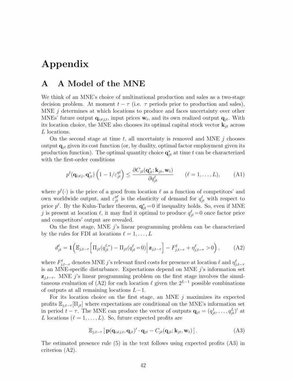
Appendix
A A Model of the MNE
We think of an MNE’s choice of multinational production and sales as a two-stagedecision problem. At moment t − τ (i.e. τ periods prior to production and sales),MNE j determines at which locations to produce and faces uncertainty over otherMNEs’ future output qi6=j,t, input prices wt, and its own realized output qjt. Withits location choice, the MNE also chooses its optimal capital stock vector kjt acrossL locations.
On the second stage at time t, all uncertainty is removed and MNE j choosesoutput qjt given its cost function (or, by duality, optimal factor employment given itsproduction function). The optimal quantity choice q∗
jt at time t can be characterizedwith the first-order conditions
p`(qi6=j,q∗jt)(1− 1/εq`
jt
)≤∂Cjt(q
∗jt;kjt,wt)
∂q`jt
(` = 1, . . . , L), (A1)
where p`(·) is the price of a good from location ` as a function of competitors’ andown worldwide output, and εq`
jt is the elasticity of demand for q`jt with respect to
price p`. By the Kuhn-Tucker theorem, q∗jt =0 if inequality holds. So, even if MNE
j is present at location `, it may find it optimal to produce q`jt =0 once factor price
and competitors’ output are revealed.On the first stage, MNE j’s linear programming problem can be characterized
by the rules for FDI at locations ` = 1, . . . , L
d`jt = 1
(Ej,t−τ
[Πjt(q
`,∗jt )− Πjt(q
`jt =0)
∣∣∣ zj,t−τ
]− F `
j,t−τ + η`j,t−τ >0
), (A2)
where F `j,t−τ denotes MNE j’s relevant fixed costs for presence at location ` and η`
j,t−τ
is an MNE-specific disturbance. Expectations depend on MNE j’s information setzj,t−τ . MNE j’s linear programming problem on the first stage involves the simul-taneous evaluation of (A2) for each location ` given the 2L−1 possible combinationsof outputs at all remaining locations L−1.
For its location choice on the first stage, an MNE j maximizes its expectedprofits Ej,t−τ [Πjt] where expectations are conditional on the MNE’s information setin period t− τ . The MNE can produce the vector of outputs qjt = (q1
jt, . . . , qLjt)
′ atL locations (` = 1, . . . , L). So, future expected profits are
Ej,t−τ [p(qi6=j,t,qjt)′ · qjt − Cjt(qjt;kjt,wt) ] . (A3)
The estimated presence rule (5) in the text follows using expected profits (A3) incriterion (A2).
42

B Multiproduct translog cost function
Consider the short-run multiproduct translog function with quasi-fixed capital:17
lnCjt = ϕ+L∑
m=1
ϕ0m ln qm
jt +L∑
`=1
α` lnw`t +
L∑m=1
L∑`=1
µ`m ln qmjt lnw`
t
+1
2
L∑m=1
L∑`=1
ϕ1`m ln qm
jt ln q`jt +
1
2
L∑m=1
L∑`=1
δ`m lnwmt lnw`
t
+L∑
m=1
ζ0m ln km
jt +L∑
m=1
L∑`=1
ζ11`m ln km
jt ln q`jt (B1)
+L∑
m=1
L∑`=1
κ`m ln kmjt lnw`
t +1
2
L∑m=1
L∑`=1
ζ1`m ln km
jt ln k`jt.
By Shepard’s (1953) lemma, MNE j’s demand for employment y`jt is equal to
∂Cjt/∂w`t so that the wage bill share s`
jt ≡ w`ty
`jt/Cjt at location ` becomes
s`jt =
∂Cjt/∂w`t
Cjt/w`t
= α` +L∑
m=1
(µ`m ln qm
jt + κ`m ln kmjt + δ`m lnwm
t
)for ` = 1, . . . , L. We transform these L equations into L simultaneous labor de-mand functions by multiplying the dependent variable and all regressors with theobservation-specific scalars Cjt/w
`t and obtain y`
jt = ∂Cjt/∂w`t = s`
jtCjt/w`t as in
equation (6).With L locations, there are L(L−1)/2 symmetry restrictions δk` = δ`k for any k, `.
Linear homogeneity in factor prices requires that∑L
`=1 α` = 1 and that∑L
`=1 µ`m =∑L`=1 κ`m =
∑L`=1 δ`m =
∑L`=1 δm` = 0 for all m. We impose those restrictions on
estimation but do not constrain estimates of factor price coefficients at the extensivemargin. We do not impose any returns-to-scale restrictions.
C Currency conversion and deflation
We convert all economic data of foreign affiliates into euro (EUR) and deflate them.In BuBa’s original midi data, all information on foreign affiliates is reported inGerman currency using the exchange rate at the closing date of the foreign affiliate’sbalance sheet. We apply the following deflation and currency conversion method toall financial variables. Deutschmark (DEM) figures are converted into euro figures at
17Slaughter (2000) adds ln(k/q) terms to a version of (B1). Given the additive logarithmic struc-ture, this is equivalent to an affine transformation of the parameter pairs (αk, ζk) and (µk,`, κk,`)because ln(k/q) = ln k − ln q.
43

the rate 1/1.95583 (the conversion rate at inception of the euro in 1999). (i) We usethe market exchange rate on the end-of-month day closest to an affiliate’s balancesheet closing date to convert the DEM or EUR figures into local currency for everyaffiliate. This reverses the conversion applied to the questionnaires at the date ofreporting. (ii) A CPI factor for every country deflates the foreign-currency financialfigures to the December-1998 real value in local currency. (iii) For each country,the average of all end-of-month exchange rates vis-a-vis the DEM or EUR betweenJanuary 1996 and December 2001 is used as a proxy for purchasing power parityof foreign consumption baskets relative to the DEM or EUR. All deflated local-currency figures are converted back to DEM or EUR using this purchasing-powerproxy.
We use the foreign countries’ CPIs (Consumer Price Indices from the IMF’sInternational Financial Statistics) to deflate the figures. Whenever a country’s CPIis not available from IFS but the main currency used in that country is issued in someother country, we use the CPI of the currency-issuing country. The CPI deflationfactors for all countries are rebased to unity at year-end 1998. For the ubs wagedata, we first translate U.S. dollars into Euros and then proceeded as detailed above.Parent-level and sector-level domestic variables are transformed into December 1998Euros using the German CPI.
D Wages
We base our estimation on sectoral manufacturing wages by country between 1996and 2001 from the unido Industrial Statistics Database at the 3-digit ISIC level,Rev. 2 (UNIDO 2005). The unido measure of annual sectoral wage bills includes allpayments to workers at establishments in the reference sector and year (wages andsalaries, remuneration for time not worked, bonuses and gratuities, allowances, andpayments in kind; but excludes contributions to social security, pensions, insurance,severance and termination pay). We divide the sectoral wage bill by the sectoralnumber of workers and employees. We deflate the wages with the country-level CPI(standardized to unity in December 1998) and convert the foreign currency to EURat the December 1998 exchange rate. To mitigate possible workforce compositioneffects in our labor demand regression on wages, we use the sector median wage bycountry (and lose sectoral wage variation also for Germany) in the outcome esti-mation. We use sectoral unido wages for Germany in selection estimation becauseworkforce composition behind labor cost measures is not an econometric concernfor location choice. The unido data cover 109 countries and result in the largestoverlap with midi observations on German MNEs for estimation.
For robustness checks, we use oww monthly average wage rates of male workersat the country level for 161 occupations in 155 countries between 1983 and 1999.Missing observations, however, reduce the overlap with midi data on German MNEs
44

below the overlap that unido data provide. We follow Freeman and Oostendorp’s(2001) recommendation and pick the base calibration with lexicographic weightingfor the aggregate wages by country. We deflate the wages with the country-levelCPI (standardized to unity in December 1998) and convert the foreign currencyto EUR at the December 1998 exchange rate. We fill missing values, by countryand occupation group, with information from the latest preceding year that haswage information available and reuse oww wages from 1999 in 2000 and 2001. Tomitigate workforce composition effects, we take country medians over 161 owwoccupation groups for foreign wages. We multiply the resulting monthly medianoccupation wage by twelve to approximate annual earnings for cost function esti-mation. Complementing foreign oww wages, we use the German annual earningssurvey (table 62321 from destatis.de/genesis) and obtain sectoral monthly wages,broken down into three blue-collar and four white-collar occupation groups by sec-tor (two-digit NACE 1.1). We compute median wages over these seven occupationgroups by sector, deflate them with the German CPI (standardized to unity in De-cember 1998), and multiply them by twelve to arrive at annual earnings for costfunction estimation. Occupational wage information from the German annual earn-ings survey enters the ILO database, on which oww wages are based, so that theseforeign and domestic wages are compatible.
For additional robustness checks, we also use ubs wage data collected by theSwiss commercial bank for metropolitan areas around the world in 1994, 1997, 2000and 2003 (UBS 2003). We linearly interpolate ubs wages between survey yearsto cover our sample period 1996-2001. ubs carried out surveys in approximately70 cities during the second quarter of 1994, 1997 and 2000, and during the firstquarter of 2003. Questionnaires request detailed information on wage components,wage deductions and working hours across thirteen occupations. ubs converts wagefigures into U.S. dollars and smoothes the effect of day-to-day currency fluctuationsby using the average daily spot rate during the quarter of the ubs survey. Weconvert ubs wages into EUR at the average USD/EUR exchange rate during thesurvey quarter and deflate figures with the German CPI (standardized to unity inDecember 1998). We use the machinist wage as the most closely comparable wageto median oww and German wages. We take ubs wages also for Germany (and losesectoral variation).
Whenever foreign price deflators are missing or period-average exchange rateinformation is incomplete for purchasing-power parity oriented wage conversion, weuse current exchange rates and the German price deflator.
E Market access
We construct market access measures following Redding and Venables (2004). Weobtain bilateral trade data for 1996 through 2001 and geographic information on
45

Table 15: Location Definitions
Locations Countries
WEU Western European countries(EU 15 plus Norway and Switzerland)
OIN Overseas Industrialized countriesincluding Australia, Canada, Japan, New Zealand, USAas well as Iceland and Greenland
CEE Central and Eastern European countriesincluding accession countries and candidates for EUmembership
DEV Developing countriesincluding Turkey, Russia and Central Asian economiesas well as dominions of Western European countries andthe USA
country pairs from cepii (www.cepii.fr). After filling in missing imports to B fromA with exports information from country A to B, we drop all exports informationand set exports from A to B equal to B’s imports from A. We adopt this proce-dure because we consider imports, whenever available, more reliably measured thanexports.
Our regression specification for an unbalanced panel of country pairs by year is
lnXij = αixi + βjmj + δ ln dij + µ bij + εij,
where Xij denotes country i’s aggregate exports in USD (+1) to country j, xi anexporter country dummy, mj an importer country dummy, dij the geographicaldistance between country i and j, and bij a dummy variable indicating a commonborder. We compute market access Ai to country i as
Ai = exp{βimi}(.67√areai/π
)δ/2
+∑
j 6=i exp{βj mj} (dij)δ exp{µ bij}.
This is measure MA(3) in Redding and Venables (2004).
46

References
Barba Navaretti, G., and D. Castellani (2004): “Investments Abroad andPerformance at Home: Evidence from Italian Multinationals,” CEPR DiscussionPaper, 4284.
Barro, R. J., and J. W. Lee (2001): “International Data on Educational At-tainment: Updates and Implications,” Oxford Economic Papers, 53(3), 541–63.
Barro, R. J., and X. Sala i Martin (1992): “Convergence,” Journal of PoliticalEconomy, 100(2), 223–51.
Barten, A. P. (1969): “Maximum Likelihood Estimation of a Complete Systemof Demand Equations,” European Economic Review, 1(1), 7–73.
Becker, S. O., K. Ekholm, R. Jackle, and M.-A. Muendler (2005): “Lo-cation Choice and Employment Decisions: A Comparison of German and SwedishMultinationals,” Review of World Economics, 141(4), 693–731.
Blonigen, B. A., R. B. Davies, and K. Head (2003): “Estimating theKnowledge-Capital Model of the Multinational Enterprise: Comment,” Ameri-can Economic Review, 93(3), 980–94.
Braconier, H., and K. Ekholm (2000): “Swedish Multinationals and Competi-tion from High- and Low-Wage Locations,” Review of International Economics,8(3), 448–61.
Brainard, S. L. (1997): “An Empirical Assessment of the Proximity-Concentration Trade-off between Multinational Sales and Trade,” American Eco-nomic Review, 87(4), 520–44.
Brainard, S. L., and D. A. Riker (2001): “Are US Multinationals ExportingUS Jobs?,” in Globalization and labour markets, ed. by D. Greenaway, and D. R.Nelson, vol. 2, pp. 410–26. Elgar, Cheltenham, UK and Northampton, MA.
Brown, R. S., and L. R. Christensen (1981): “Estimates of Elasticities ofSubstitution in a Model of Partial Static Equilibrium: An Application to U.S.Agriculture, 1947-1974,” in Modeling and measuring natural resource substitution,ed. by E. R. Berndt, and B. C. Field, chap. 10, pp. 209–29. MIT Press, Cambridge,Massachusetts.
Buch, C. M., J. Kleinert, A. Lipponer, and F. Toubal (2005): “Determi-nants and Effects of Foreign Direct Investment: Evidence from German Firm-Level Data,” Economic Policy, 41, 51–98.
47

Carr, D. L., J. R. Markusen, and K. E. Maskus (2001): “Estimating theKnowledge-Capital Model of the Multinational Enterprise,” American EconomicReview, 91(3), 693–708.
Chen, S., and S. Khan (2003): “Semiparametric Estimation of a HeteroskedasticSample Selection Model,” Econometric Theory, 19(6), 1040–64.
Christensen, L. R., D. W. Jorgenson, and L. J. Lau (1973): “TranscendentalLogarithmic Production Frontiers,” Review of Economics and Statistics, 55(1),28–45.
Das, M., W. K. Newey, and F. Vella (2003): “Nonparametric Estimation ofSample Selection Models,” Review of Economic Studies, 70(1), 33–58.
Deutsche Bundesbank (1998): “The Methodological Basis of the DeutscheBundesbank’s Corporate Balance Sheet Statistics,” Monthly Report, 1998(10),49–64.
Devereux, M. P., and R. Griffith (1998): “Taxes and the Location of Produc-tion: Evidence from a Panel of US Multinationals,” Journal of Public Economics,68(3), 335–67.
Dhrymes, P. J. (1971): “Equivalence of Iterative Aitken and Maximum LikelihoodEstimators for a System of Regression Equations,” Australian Economic Papers,10(16), 20–24.
Diewert, W. E. (1971): “An Application of the Shephard Duality Theorem: AGeneralized Leontief Production Function,” Journal of Political Economy, 79(3),481–507.
Disdier, A. C., and T. Mayer (2004): “How Different Is Eastern Europe? Struc-ture and Determinants of Location Choices by French Firms in Eastern and West-ern Europe,” Journal of Comparative Economics, 32(2), 280–96.
Dixit, A. K. (1989): “Entry and Exit Decisions under Uncertainty,” Journal ofPolitical Economy, 97(3), 620–38.
Eakin, B. K., D. P. McMillen, and M. J. Buono (1990): “ConstructingConfidence Intervals Using the Bootstrap: An Application to a Multi-ProductCost Function,” Review of Economics and Statistics, 72(2), 339–44.
Feenstra, R. C., and G. H. Hanson (1999): “The Impact of Outsourcing andHigh-Technology Capital on Wages: Estimates for the United States, 1979-1990,”Quarterly Journal of Economics, 114(3), 907–40.
48

Freeman, R. B., and R. H. Oostendorp (2001): “The Occupational Wagesaround the World Data File,” International Labour Review, 140(4), 379–401.
Hall, R. E. (1973): “The Specification of Technology with Several Kinds of Out-put,” Journal of Political Economy, 81(4), 878–92.
Hanson, G. H., R. J. Mataloni, and M. J. Slaughter (2005): “Vertical Pro-duction Networks in Multinational Firms,” Review of Economics and Statistics,87(4), 664–78.
Head, K., and T. Mayer (2004): “Market Potential and the Location of JapaneseInvestment in the European Union,” Review of Economics and Statistics, 86(4),959–72.
Head, K., and J. Ries (2002): “Offshore Production and Skill Upgrading byJapanese Manufacturing Firms,” Journal of International Economics, 58(1), 81–105.
Heckman, J. J. (1979): “Sample Selection Bias as a Specification Error,” Econo-metrica, 47(1), 153–61.
(1981): “The Incidental Parameters Problem and the Problem of InitialConditions in Estimating a Discrete Time-Discrete Data Stochastic Process,” inThe structural analysis of discrete data, ed. by C. Manski, and D. F. McFadden,pp. 179–95. MIT Press, Cambridge, MA.
Kohli, U. R. (1978): “A Gross National Product Function and the Derived De-mand for Imports and Supply of Exports,” Canadian Journal of Economics, 11(2),167–82.
Konings, J. (2004): “The Employment Effects of Foreign Direct Investment,” EIBPapers, 9(1), 86–108.
Kotz, S., N. Balakrishnan, and N. L. Johnson (2000): Continuous Multi-variate Distributions, vol. 1 of Wiley Series in Probability and Statistics. Wiley,New York, 2nd edn.
Lipponer, A. (2003): “A “New” Micro Database for German FDI,” in ForeignDirect Investment in the Real and Financial Sector of Industrial Countries, ed.by H. Herrmann, and R. Lipsey, pp. 215–44. Springer, Berlin.
Marin, D. (forthcoming): “A New Division of Labor in Europe: Offshoring andOutsourcing into Eastern Europe,” Journal of the European Economic Associa-tion.
49

Newey, W. K. (1997): “Convergence Rates and Asymptotic Normality for SeriesEstimators,” Journal of Econometrics, 79(1), 147–68.
Redding, S., and A. J. Venables (2004): “Economic Geography and Interna-tional Inequality,” Journal of International Economics, 62(1), 53–82.
Roberts, M. J., and J. R. Tybout (1997): “The Decision to Export in Colombia:An Empirical Model of Entry with Sunk Costs,” American Economic Review,87(4), 545–64.
Shepard, R. W. (1953): Cost and production functions. Princeton UniversityPress, Princeton.
Slaughter, M. J. (2000): “Production Transfer within Multinational Enterprisesand American Wages,” Journal of International Economics, 50(2), 449–72.
UBS (2003): “Prices and Earnings: A Comparison of Purchasing Power Aroundthe World,” ubs.com Zurich.
UNIDO (2005): “INDSTAT3 2005 ISIC Rev.2 User’s Guide,” unido.org/doc/3531Vienna.
Yen, S. T. (2005): “A Multivariate Sample-Selection Model: Estimating Cigaretteand Alcohol Demands with Zero Observations,” American Journal of AgriculturalEconomics, 87(2), 453–66.
Zellner, A. (1962): “An Efficient Method for Estimating Seemingly UnrelatedRegressions and Tests for Aggregation Bias,” Journal of the American StatisticalAssociation, 57(298), 348–68.
50