artificial life, adaptive behavior, agents and ant colony
TRANSCRIPT
ART IF IC IAL L IFE , ADAPT IVEBEHAV IOR, AGENTS AND ANTCOLONY OPT IMIZAT IONKar th ik Ba lak r i shnan andVasant Honavar, cha i r s

Coverage and Generalization in an Arti�cial Immune System
Justin Balthrop
Computer Science Dept.
University of New Mexico
Albuquerque, NM 87131
Fernando Esponda
Computer Science Dept.
University of New Mexico
Albuquerque, NM 87131
Stephanie Forrest
Computer Science Dept.
University of New Mexico
Albuquerque, NM 87131
Matthew Glickman
Computer Science Dept.
University of New Mexico
Albuquerque, NM 87131
Abstract
LISYS is an arti�cial immune system frame-
work which is specialized for the problem of
network intrusion detection. LISYS learns to
detect abnormal packets by observing normal
network traÆc. Because LISYS sees only a
partial sample of normal traÆc, it must gen-
eralize from its observations in order to char-
acterize normal behavior correctly. A vari-
ation of the r-contiguous bits matching rule
is introduced, and its e�ect on coverage and
generalization is studied. The e�ect of rep-
resentation diversity on coverage and gener-
alization is also explored by studying permu-
tations in the order of bits in the representa-
tion.
1 Introduction
The natural immune system uses a variety of evolu-
tionary and adaptive mechanisms to protect organisms
from foreign pathogens and misbehaving cells in the
body. Arti�cial immune systems (AISs) seek to cap-
ture some aspects of the natural immune system in
a computational framework, either for the purpose of
modeling the natural immune system or for solving
engineering problems. In either form, the fundamen-
tal problem solved by most AISs can be thought of as
learning to discriminate between \self" (the normally
occurring patterns in the system being protected, e.g.,
the body) and \non-self" (foreign pathogens, such as
bacteria or viruses, or components of self that are
no longer functioning normally). Almost any set of
patterns that can be expressed as strings of symbols
can be placed into this framework, for example, the
set of normally occurring TCP connections in a local
area network (LAN) and the set of TCP connections
observed during a network attack [Hofmeyr, 1999,
Kim and Bentley, 2001]. This is the example on which
we will focus in this paper.
We are interested in the question of representation|
how well a set of AIS detectors covers the set of nor-
mally occurring patterns (or conversely, how well it
can detect the set of abnormal patterns). Because AIS
detectors are typically generated on-line in a uctuat-
ing environment, they are highly unlikely to be ex-
posed to every possible normal pattern during train-
ing. Consequently, it is important for detectors to gen-
eralize from the set of observed normal patterns to the
set of expected normal patterns. The generalization
properties of the AIS a�ect both false positives (mis-
takenly identifying normal patterns as abnormal) and
false negatives (mistakenly identifying abnormal pat-
terns as legitimate). These are known as Type I and
Type II errors respectively in the statistical decision
theory literature.
There are several components of the AIS that a�ect
how well it represents its environment and how well it
generalizes. The �rst of these is the mapping from the
domain to detectors, or what information is presented
to the AIS. Here we will use the 49-bit compressed
representation of TCP SYN packets, introduced by
Hofmeyr [Hofmeyr, 1999, Hofmeyr and Forrest, 1999,
Hofmeyr and Forrest, 2000]. In this representation
each detector is a 49-bit string. Detectors are matched
against the compressed 49-bit SYN packets (see Fig-
ure 1) using a partial matching rule which scores how
closely they match. Choosing an appropriate map-
ping for a given problem in the AIS context has all
the same complications as choosing a representation
for a genetic algorithms problem. Some representa-
tions are clearly better than others, but it is diÆcult
to formalize criteria by which one can choose a good
one in a particular instance. The 49-bit representation
chosen by Hofmeyr works surprisingly well, although
it contains a minimal amount of information and the
information is arranged in an arbitrary ordering.
3ARTIFICIAL LIFE, ADAPTIVE BEHAVIOR, AGENTS AND ANT COLONY OPTIMIZATION
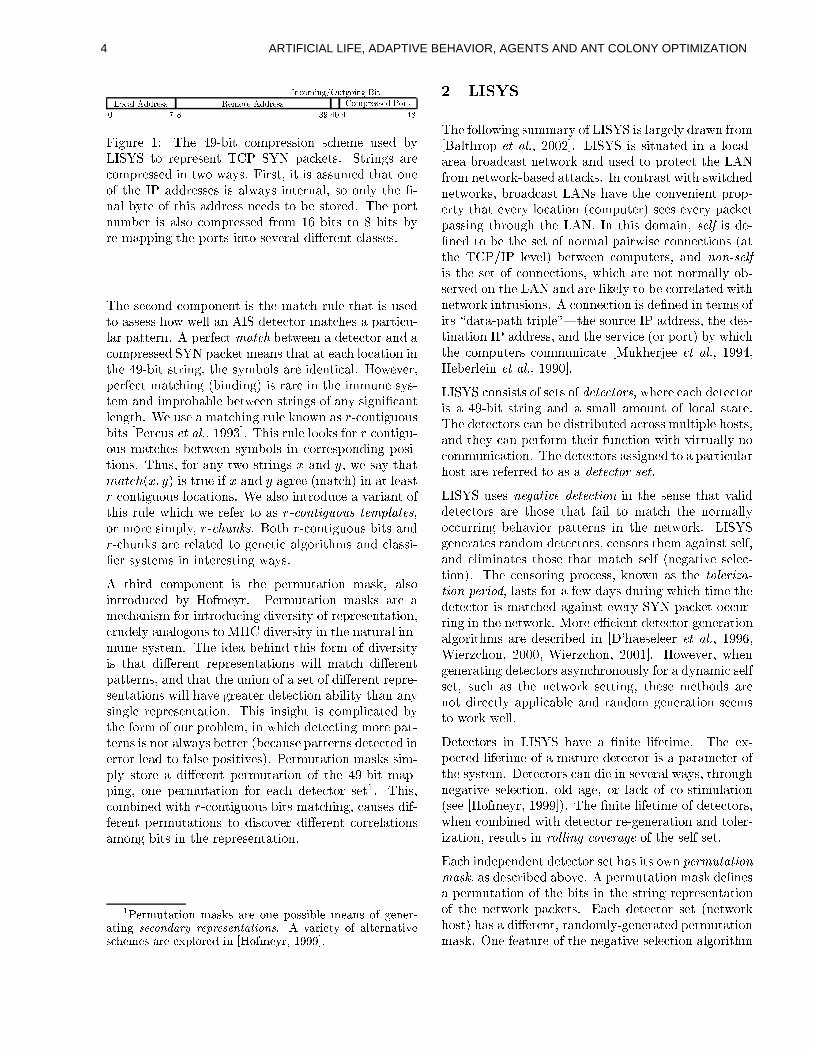
Local Address Remote Address Compressed Port
0 7 8 39 40 41 48
Incoming/Outgoing Bit
Figure 1: The 49-bit compression scheme used by
LISYS to represent TCP SYN packets. Strings are
compressed in two ways. First, it is assumed that one
of the IP addresses is always internal, so only the �-
nal byte of this address needs to be stored. The port
number is also compressed from 16 bits to 8 bits by
re-mapping the ports into several di�erent classes.
The second component is the match rule that is used
to assess how well an AIS detector matches a particu-
lar pattern. A perfect match between a detector and a
compressed SYN packet means that at each location in
the 49-bit string, the symbols are identical. However,
perfect matching (binding) is rare in the immune sys-
tem and improbable between strings of any signi�cant
length. We use a matching rule known as r-contiguous
bits [Percus et al., 1993]. This rule looks for r contigu-
ous matches between symbols in corresponding posi-
tions. Thus, for any two strings x and y, we say that
match(x; y) is true if x and y agree (match) in at least
r contiguous locations. We also introduce a variant of
this rule which we refer to as r-contiguous templates,
or more simply, r-chunks. Both r-contiguous bits and
r-chunks are related to genetic algorithms and classi-
�er systems in interesting ways.
A third component is the permutation mask, also
introduced by Hofmeyr. Permutation masks are a
mechanism for introducing diversity of representation,
crudely analogous to MHC diversity in the natural im-
mune system. The idea behind this form of diversity
is that di�erent representations will match di�erent
patterns, and that the union of a set of di�erent repre-
sentations will have greater detection ability than any
single representation. This insight is complicated by
the form of our problem, in which detecting more pat-
terns is not always better (because patterns detected in
error lead to false positives). Permutation masks sim-
ply store a di�erent permutation of the 49-bit map-
ping, one permutation for each detector set1. This,
combined with r-contiguous bits matching, causes dif-
ferent permutations to discover di�erent correlations
among bits in the representation.
1Permutation masks are one possible means of gener-ating secondary representations. A variety of alternativeschemes are explored in [Hofmeyr, 1999].
2 LISYS
The following summary of LISYS is largely drawn from[Balthrop et al., 2002]. LISYS is situated in a local-
area broadcast network and used to protect the LAN
from network-based attacks. In contrast with switched
networks, broadcast LANs have the convenient prop-
erty that every location (computer) sees every packet
passing through the LAN. In this domain, self is de-
�ned to be the set of normal pairwise connections (at
the TCP/IP level) between computers, and non-self
is the set of connections, which are not normally ob-
served on the LAN and are likely to be correlated with
network intrusions. A connection is de�ned in terms of
its \data-path triple"|the source IP address, the des-
tination IP address, and the service (or port) by which
the computers communicate [Mukherjee et al., 1994,
Heberlein et al., 1990].
LISYS consists of sets of detectors, where each detector
is a 49-bit string and a small amount of local state.
The detectors can be distributed across multiple hosts,
and they can perform their function with virtually no
communication. The detectors assigned to a particular
host are referred to as a detector set.
LISYS uses negative detection in the sense that valid
detectors are those that fail to match the normally
occurring behavior patterns in the network. LISYS
generates random detectors, censors them against self,
and eliminates those that match self (negative selec-
tion). The censoring process, known as the toleriza-
tion period, lasts for a few days during which time the
detector is matched against every SYN packet occur-
ring in the network. More eÆcient detector generation
algorithms are described in [D'haeseleer et al., 1996,
Wierzchon, 2000, Wierzchon, 2001]. However, when
generating detectors asynchronously for a dynamic self
set, such as the network setting, these methods are
not directly applicable and random generation seems
to work well.
Detectors in LISYS have a �nite lifetime. The ex-
pected lifetime of a mature detector is a parameter of
the system. Detectors can die in several ways, through
negative selection, old age, or lack of co-stimulation
(see [Hofmeyr, 1999]). The �nite lifetime of detectors,
when combined with detector re-generation and toler-
ization, results in rolling coverage of the self set.
Each independent detector set has its own permutation
mask, as described above. A permutation mask de�nes
a permutation of the bits in the string representation
of the network packets. Each detector set (network
host) has a di�erent, randomly-generated permutation
mask. One feature of the negative-selection algorithm
4 ARTIFICIAL LIFE, ADAPTIVE BEHAVIOR, AGENTS AND ANT COLONY OPTIMIZATION
as originally implemented is that it can result in unde-
tectable patterns called holes [D'haeseleer et al., 1996,
D'haeseleer, 1996], or put more positively generaliza-
tions [Esponda and Forrest, 2002]. Holes can exist for
any symmetric, �xed-probability matching rule, but
permutation masks e�ectively change the match rule
and thus the distribution of holes. Using a di�erent
permutation on each host allows us to control how
much the system generalizes in the vicinity of self, and
thus gives us more control over the undetectable holes[Esponda and Forrest, 2002].
The original LISYS system uses several other mecha-
nisms, such as activation thresholds, sensitivity levels,
and co-stimulation to reduce false positives, and mem-
ory detectors to increase true positives. For details
on the full system, the reader is referred to [Hofmeyr,
1999, Hofmeyr and Forrest, 2000].2
3 Data Set
The experiments reported in this paper use the data
set described in [Balthrop et al., 2002]. Our data col-
lection strategy was to control the data set as much as
possible while still collecting data in a realistic context.
The data set was collected from an internal restricted
network of computers in a small university research
group. The six internal computers in this network
connected to the Internet through a single Linux ma-
chine that acted as a �rewall, router and masquerading
server for the internal machines. The internal network
was set up as a broadcast network, so we were able to
monitor the traÆc of all the computers easily.
This scenario provided a data set that satis�ed both
objectives. The internal restricted network was much
more controlled than the external university or depart-
mental networks. In this environment, we can under-
stand all of the connections that occur, and we can
be relatively certain that there were no attacks during
the normal training periods. Moreover, this environ-
ment is realistic. Many corporations have intranets
in which activity is somewhat restricted and external
connections must pass through a �rewall. This en-
vironment could also model the increasingly common
home network that connects to the Internet through
a cable or DSL modem and has a single external IP
address. Attacks are a reality in environments such as
these, and the attack scenarios corresponded to plau-
sible occurrences in this class of environment.
2The programs used to generate the results in this paperare available from http://www.cs.unm.edu/�immsec. Theprograms are part of LISYS and are found in the LisysSimdirectory of that package.
The normal network data in our data set consist of two
weeks of data collected in November, 2001. In these
data, there are a total of 22,329 TCP SYN packets,
and roughly 55% of this is web traÆc. Thus, there
was an average of approximately 1600 packets per day
during the normal period. Because the network data
being produced is dependent on a small number of
users, two weeks seemed to be the shortest period of
time that could possibly give a reasonable character-
ization of self. Attack data were generated over the
course of two days near the end of the collection pe-
riod. The attacks took place about one week after the
normal period ended, and consisted of 76,179 TCP
SYN packets.
In [Hofmeyr, 1999], network connections to web servers
are removed from the data by �ltering out all con-
nections to port 80. Instead of completely removing
web connections, the data set simulates the behavior
of a proxy server. All outgoing connections to port 80
(http) or port 443 (https) are re-mapped to port 3128
on the proxy machine. This is very close to what the
traÆc would have been like if we were using the web
proxy cache SQUID.
All of the attacks, with the exception of the denial-
of-service attack, were performed using a laptop con-
nected to the internal network. The �rewall machine
was con�gured as a DHCP server, so the laptop was
able to acquire a dynamic IP address because it had
a physical connection to the internal network. We
used the free security scanner Nessus to perform the
attacks. A total of eight attacks were run, includ-
ing denial of service (from an internal computer to an
external computer), a �rewall attack against the �re-
wall/gateway machine, an ftp attack against an inter-
nal machine, an ssh probe against several internal ma-
chines, an attack probing for certain services, a TCP
SYN scan, an nmap tcp connect() scan against several
internal computers, and a full nmap port scan.
4 r-Chunks Matching
In this section we introduce a variant of the r-
contiguous bits matching rule, which we refer to as
\r-chunks." We will show in section 7 that r-chunks
matching performs better than full-length r-contiguous
bits matching for our data set. However, r-chunks
matching also has the virtue of being more amenable
to mathematical analysis than full-length matching[Esponda and Forrest, 2002]. r-Chunks matching is
reminiscent of the f1; 0;#g matching rule for classi-
�er systems [Holland et al., 1986], with the additional
restrictions that all detectors have a constant number
of de�ned bits (the r parameter) and that all the de-
5ARTIFICIAL LIFE, ADAPTIVE BEHAVIOR, AGENTS AND ANT COLONY OPTIMIZATION
�ned bits are located in contiguous positions. Match-
ing with both r-chunks and full-length detectors is re-
lated to the crossover operator in genetic algorithms[Holland, 1975].
In r-chunks detectors, only r contiguous positions of
the detector are speci�ed (known as the window of the
detector); the remaining bit positions can be thought
of as \don't cares." Alternatively, an r-chunks detec-
tor can be thought of as a string of r bits together
with a speci�cation of the window to which it refers.
An r-chunks detector d is said to match a string x if all
the bits of d are equal to the r bits of x in the window
speci�ed by d.
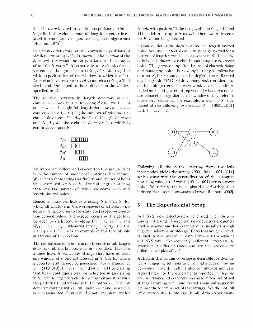
The relation between full-length detectors and r-
chunks is shown in the following �gure for l = 4
and r = 2. A single full-length detector can be de-
composed into l � r + 1 (the number of windows) r-
chunks detectors. Let dfl be the full-length detector
and dc1; dc2; dc3 the r-chunks detectors into which it
can be decomposed:
dfl: 1 0 1 1
dc1: 1 0
dc2: 0 1
dc3: 1 1
An important di�erence between the two match rules
is in the number of undetectable strings they induce.
We refer to these strings as \holes" and the set of holes
for a given self set S as H . For full-length matching
there are two sources of holes: crossover holes and
length-limited holes.
Hence, a crossover hole is a string h not in S, for
which all windows in h are crossovers of adjacent win-
dows in S, according to the restricted crossover opera-
tion de�ned below. A crossover occurs in this context
between two adjacent windows Wi = vi::vi+r�1 and
Wi+1 = ui+1::ui+r whenever bits vj = uj 8j : i+ 1 �j � i+ r� 1. There is an example of this type of hole
at the end of this section.
The second source of holes arises because in full-length
detectors, all the bit positions are speci�ed. This can
induce holes h which are strings that have at least
one window of r bits not present in S, but for which
a detector still cannot be generated. For instance, let
S = f110; 010g, l = 3, r = 2 and let h = 011 be a string
that has r contiguous bits not exhibited in any string
in S. A full-length detector for hmust either start with
the pattern 01 and/or end with the pattern 11 but any
detector starting with 01 will match self and hence can
not be generated. Similarly, if a potential detector for
h ends with pattern 11 the two possible strings 011 and
111 match a string in S as well, therefore a detector
for h cannot be generated.
r-Chunks detection does not induce length-limited
holes, because a detector can always be generated for a
pattern of length r which is not present in S. Thus, the
only holes induced by r-chunks matching are crossover
holes. This greatly simpli�es the task of characterizing
and managing holes. For example, the generalization
of a set S, for r-chunks, can be depicted as a directed
acyclic graph (DAG) with as many nodes as there are
distinct bit patterns for each window (each node la-
belled as the bit pattern it represents) where two nodes
are connected together if the windows they refer to
crossover. Consider, for example, a self set S com-
prised of the following two strings S = f0001; 1011gwith l = 4, r = 2:
����00 ��
��00 ��
��01
ccc
����01ccc
����10 ��
��11#
##
�����
Following all the paths, starting from the left-
most nodes, yields the strings f0001; 0011; 1001; 1011gwhich constitute the generalization of the r-chunks
matching rule, out of which f0011; 1001g are crossoverholes. We refer to the holes plus the self strings that
induced them as the crossover-closure [Helman, 2002].
5 The Experimental Setup
In LISYS, new detectors are generated when the sys-
tem is initialized. Thereafter, new detectors are gener-
ated whenever another detector dies, usually through
negative selection or old-age. Detectors are generated,
trained, tested, and killed asynchronously throughout
a LISYS run. Consequently, di�erent detectors are
tolerized at di�erent times and are thus exposed to
di�erent samples of self.
Although this rolling coverage is desirable for dynam-
ically changing self sets and to make evasion by an
adversary more diÆcult, it also complicates analysis.
Accordingly, for the experiments reported in this pa-
per, we trained all detectors on the identical set of self
strings (training set), and tested them subsequently
against the identical set of test strings. We did not kill
o� detectors due to old age. In all of the experiments
6 ARTIFICIAL LIFE, ADAPTIVE BEHAVIOR, AGENTS AND ANT COLONY OPTIMIZATION
the initial tolerization period was set to 15,000 packets,
corresponding to approximately 8 days. Among these
15,000 initial packets, there were 131 unique strings to
which the immature detectors were exposed.
6 The E�ect of Permutation Masks
The goal of the �rst experiment was to assess how
di�erent permutations a�ect the performance of the
system. Because performance is measured in terms
of true and false positives, this experiment also tests
the e�ect of permutations on the system's ability to
generalize (because low false positive rates correspond
to good generalization).
100 sets of detectors were tolerized using the 131
unique strings derived from the �rst 15,000 packets
in the data-set (the training set), and each detector
set was assigned a random permutation mask. Each
detector set had exactly 5,000 mature detectors at the
end of the tolerization period and an r-value of 10.
These numbers were chosen on the basis of previous
experiments [Balthrop et al., 2002] which showed that
5,000 detectors provide maximal coverage (i.e. adding
more detectors does not improve subsequent match-
ing) for this data set and r threshold.3 Each set of
detectors was then run against the remaining 7,329
normal packets, as well as against the simulated at-
tack data. In these data (the test sets), there are a
total of 476 unique 49-bit strings. Of these 476, 50
also occur in the training set and are thus undetectable
(because any detectors which would match them are
eliminated during negative selection). This leaves 426
potentially detectable strings, of which 26 come from
the normal test set and 400 are from the attack test
set. The maximal possible coverage by a detector set
is thus 426 unique matches.
An ideal detector set would achieve zero false positives
on the normal test data and a high number of true
positives on the attack data. Thus, a perfect detector
set would match the 400 unique attack strings, and
fail to match the 26 unique normal strings in the test
set, thus generalizing from the self observed during
training. Note that because network attacks rarely,
if ever, produce only a single anomalous packet, we
3The use of 5,000 detectors to protect 131 unique stringsis clearly a somewhat arti�cial situation. This arises fromthe small size of our data set and the decision to providemaximal coverage of non-self. In general, once the num-ber of self strings increases above a certain threshold, thenumber of detectors needed to cover non-self through nega-tive detection becomes less than that required for positivedetection (see [Esponda and Forrest, 2002] for the exacttradeo�). And, for most applications, complete coverageof non-self is an overly strict requirement.
0 5 10 15 20 25
False Positives
0
100
200
300
400
Tru
e Po
sitiv
es
permutationsunpermuted
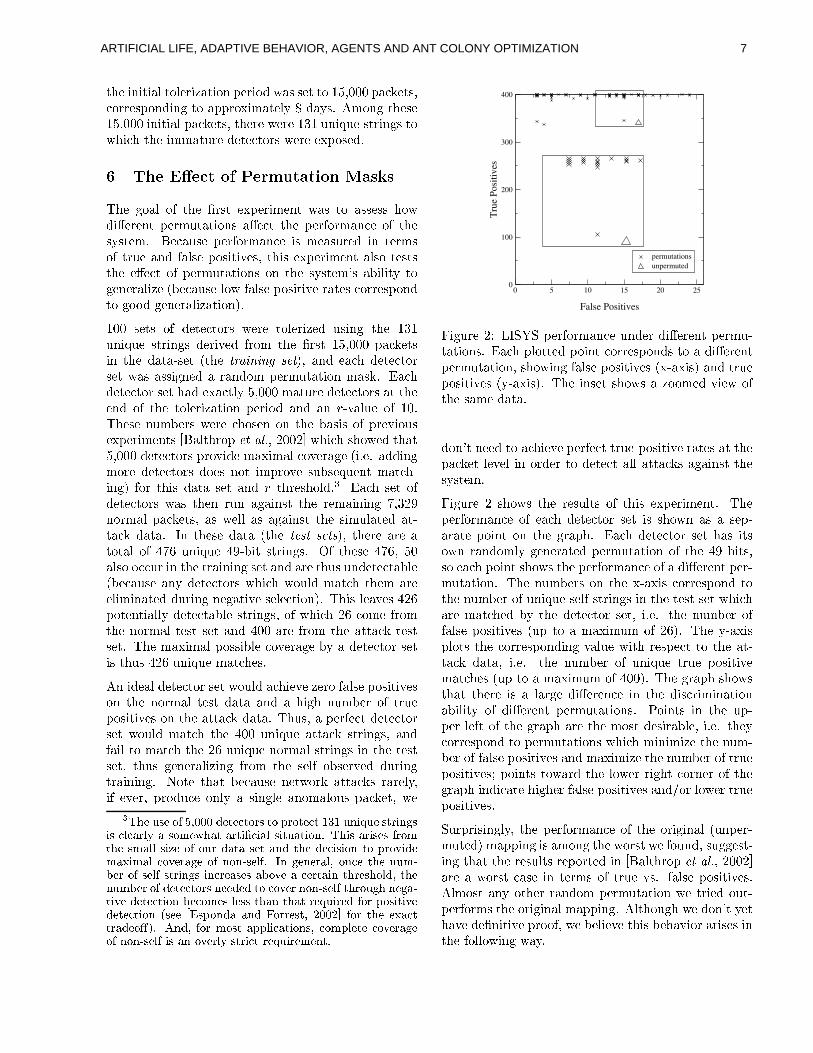
Figure 2: LISYS performance under di�erent permu-
tations. Each plotted point corresponds to a di�erent
permutation, showing false positives (x-axis) and true
positives (y-axis). The inset shows a zoomed view of
the same data.
don't need to achieve perfect true-positive rates at the
packet level in order to detect all attacks against the
system.
Figure 2 shows the results of this experiment. The
performance of each detector set is shown as a sep-
arate point on the graph. Each detector set has its
own randomly generated permutation of the 49 bits,
so each point shows the performance of a di�erent per-
mutation. The numbers on the x-axis correspond to
the number of unique self-strings in the test set which
are matched by the detector set, i.e. the number of
false positives (up to a maximum of 26). The y-axis
plots the corresponding value with respect to the at-
tack data, i.e. the number of unique true positive
matches (up to a maximum of 400). The graph shows
that there is a large di�erence in the discrimination
ability of di�erent permutations. Points in the up-
per left of the graph are the most desirable, i.e. they
correspond to permutations which minimize the num-
ber of false positives and maximize the number of true
positives; points toward the lower right corner of the
graph indicate higher false positives and/or lower true
positives.
Surprisingly, the performance of the original (unper-
muted) mapping is among the worst we found, suggest-
ing that the results reported in [Balthrop et al., 2002]
are a worst case in terms of true vs. false positives.
Almost any other random permutation we tried out-
performs the original mapping. Although we don't yet
have de�nitive proof, we believe this behavior arises in
the following way.
7ARTIFICIAL LIFE, ADAPTIVE BEHAVIOR, AGENTS AND ANT COLONY OPTIMIZATION
The LISYS design assumes that there are certain pre-
dictive bit-patterns that exhibit regularity in self, and
that these can be the basis of distinguishing self from
non-self. As it turns out, there are also deceptive bit-
patterns which exhibit regularity in the training set
(observed self), but the regularity does not generalize
to the rest of self (the normal part of the test set).
These patterns tend to cause false positives when self
strings that do not �t the predicted regularity occur.
We believe that the identity permutation is bad be-
cause the predictive bits are at the ends of the string,
while the deceptive region is in the middle. Under
such an arrangement, it is diÆcult to �nd a window
that covers many predictive bit positions without also
including deceptive ones. It is highly likely that a
random permutation will break up the deceptive re-
gion, and bring the predictive bits closer to the middle,
where they will appear in more windows.
7 r-Chunks vs. Full-Length Detectors
In this section we compare the performance of r-
chunks matching to that of r-contiguous bits match-
ing with full-length detectors on our data set. The
essential di�erence between full-length detectors and
r-chunks lies in the holes which they induce, as dis-
cussed earlier. Holes are desirable to the extent that
they prevent false positives (strings which are close to
self and represent legitimate but novel behavior of the
network)4; holes are undesirable to the extent which
they lead to false negatives (a failure to match strings
which correspond to attempted intrusions). Although
both representations are subject to crossover holes,
full-length detectors are additionally subject to length-
limited holes. Therefore, we are interested in knowing
if in practice length-limited holes generalize over true
positives or false positives.
For this experiment, we generated one set of r-chunks
detectors for each value of r, ranging from 1 to 12. Be-
cause there are only 2r � (l� r +1) possible r-chunks
detectors, we generated all of them, and then elim-
inated through negative selection any detector that
matched a string in the training set. Full-length de-
tectors were generated according the the procedure de-
scribed in Section 5.
The results of this experiment are shown in Figure
3. As in the initial permutation-mask experiment,
the number of false positives is plotted on the x-axis
and the number of true positives on the y-axis. There
are two sets of points, each connected by lines. One
4This is the sense in which holes can be thought of asgeneralizations.
0 5 10 15 20 25
False Positives
0
100
200
300
400
Tru
e Po
sitiv
es
r-chunk detectorsfull length detectors
Figure 3: LISYS performance under di�erent r-values.
For r-chunks we plotted r =1..12 and for full length
detectors we plotted r =8, 10 and 12 (the points for
r-chunks and those for full-length detectors are each
connected via a line to indicate the ordering in terms
of r). Each point shows false positives (x-axis) and
true positives (y-axis).
set indicates the results obtained with r-chunks for
values of r ranging from 1 to 12. The second set,
shows the results of using full-length detectors for
r = 8; 10; and 12.
Section 4 tells us that for any self set, a given value of r
will always achieve equivalent-or-greater overall cover-
age (i.e. a greater sum-total of true and false positives)
when using r-chunks than with using full-length detec-
tors. This follows from the fact that there are no holes
induced by r-chunks which are not also induced using
full-length detectors. The experiment shows whether
or not this additional coverage is helpful. Figure 3
shows that for this data set r-chunks outperforms full-
length detectors. The greater coverage achieved by
r-chunks more often results in the detection of true
positives than false positives. In fact, for any value of
r shown using full-length detectors, there exists some
value of r for which r-chunks achieve a higher rate of
true positives while incurring an equal or lesser num-
ber of false positives.
Another property of r-chunks illustrated by the graph
is that for a given value of r, equivalent-or-greater
overall coverage will always be achieved using r + 1
rather than r. This is because any string detected us-
ing r can be detected using r+1. For this reason, as we
increase r, while the number of true and/or false pos-
itives may increase or remain constant, neither value
can decrease.
8 ARTIFICIAL LIFE, ADAPTIVE BEHAVIOR, AGENTS AND ANT COLONY OPTIMIZATION
A surprising result is how well r-chunks performs as r
becomes low (e.g. even for r = 1). An explanation for
this phenomenon is discussed below. This is surprising
in part because of the diÆculty reported by Kim and
Bentley [2001] in �nding detectors using r-contiguous
bits and negative selection, a result explained in part
by their choice of a low value for r [Balthrop et al.,
2002].
7.1 r-Chunks and the Magic Bit
We were interested in how r-chunks could perform so
well, especially for r = 1. A closer examination of the
data revealed that the DHCP (Dynamic Host Con�gu-
ration Protocol) con�guration on the internal network
was set up in such a way that dynamic IP addresses
were always assigned with the �nal byte in the range
128-254, while static IP addresses were always in the
range of 1-127 for the same byte. This is not an un-
usual DHCP con�guration. As it happened, however,
no hosts connected to the network using DHCP during
the normal data collection period. When we ran the
attacks, the attacking laptop did use DHCP to con-
nect to the network, and the majority of the attacks
were launched from this laptop (the Denial-of-Service
attack is the only one that wasn't).
As a consequence, the majority of our attack data had
the �rst bit of the 49-bit string (the internal IP is at
the start of the string) set to one, while none of the
normal data had this bit set. In other words, there
was a single \magic bit" that identi�ed approximately
84% of the attack SYN packets. r-chunks was able to
detect this magic bit and take advantage of it. Thus,
even the smallest possible window r = 1 could take
advantage of the magic bit, and because r + 1 can
detect everything that r can detect, all of the other r
values can use the magic bit as well.
Although artifacts such as these are not unlikely oc-
currences in real data, we were curious to see what the
results would be without the presence of a magic bit.
Would r-chunks (and full-length detectors) still per-
form well? To answer this question we eliminated the
magic bit from our data by systematically changing
the internal address of the computer from which the
attacks originated to look like the address of another
internal computer. This scenario is also realistic, be-
cause the attacks could as easily have originated from
an internal computer as from a malicious laptop, and
such an internal attack might be more diÆcult to de-
tect.
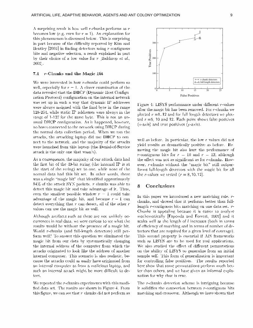
We repeated the r-chunks experiments with this modi-
�ed data set. The results are shown in Figure 4. From
this �gure, we can see that r-chunks did not perform as
0 5 10 15 20 25
False Positives
0
100
200
300
Tru
e Po
sitiv
es
r-chunk detectorsfull length detectors
Figure 4: LISYS performance under di�erent r-values
after the magic bit has been removed. For r-chunks we
plotted r =1..12 and for full length detectors we plot-
ted r =8, 10 and 12. Each point shows false positives
(x-axis) and true positives (y-axis).
well as before. In particular, the low r-values did not
yield results as dramatically positive as before. Re-
moving the magic bit also hurt the performance of
r-contiguous bits for r = 10 and r = 12, although
the e�ect was not as signi�cant as for r-chunks. How-
ever, r-chunks without the \magic bit" still outper-
forms full-length detectors with the magic bit for all
the r-values we tested (r = 8; 10; 12).
8 Conclusions
In this paper we introduced a new matching rule, r-
chunks, and showed that it performs better than full-
length r-contiguous bits matching on one data set. r-
Chunks is appealing because it is easier to analyze
mathematically [Esponda and Forrest, 2002] and it
scales well as the length of l increases (both in terms
of eÆciency of matching and in terms of number of de-
tectors that are required for a given level of coverage).
This second property is essential if AIS frameworks
such as LISYS are to be used for real applications.
We also studied the e�ect of di�erent permutations
on the ability of LISYS to generalize from an initial
sample self. This form of generalization is important
for controlling false positives. The results reported
here show that some permutations perform much bet-
ter than others, and we have given an informal expla-
nation for why that is true.
The r-chunks detection scheme is intriguing because
it solidi�es the connection between r-contiguous bits
matching and crossover. Although we have shown that
9ARTIFICIAL LIFE, ADAPTIVE BEHAVIOR, AGENTS AND ANT COLONY OPTIMIZATION
the crossover-closure is a good generalization for this
data set, we still don't know whether it will carry over
to related problems. However, the connection is tanta-
lizing, and one that we plan to explore in future work.
It is important to emphasize that the results presented
here are empirical and are based on one small data
set. An important avenue for further work is to con-
duct experiments on other applications and to develop
a mathematical understanding of the properties of this
system. A second caveat concerns the simpli�ed ver-
sion of LISYS used to conduct these experiments. In
the future, it will be important to con�rm how well
permutations and r-chunks perform in the context of
the complete LISYS system.
Acknowledgments
The authors gratefully acknowledge the support of
the National Science Foundation (grants IRI-9711199,
CDA-9503064, and ANIR-9986555), the OÆce of
Naval Research (grant N00014-99-1-0417), Defense
Advanced Projects Agency (grant AGR F30602-00-2-
0584), the Intel Corporation, and the Santa Fe Insti-
tute.
References
[Balthrop et al., 2002] J. Balthrop, S. Forrest, and
M. Glickman. Revisiting lisys: Parameters and nor-
mal behavior. In CEC-2002: Proceedings of the
Congress on Evolutionary Computing, 2002.
[D'haeseleer et al., 1996] P. D'haeseleer, S. Forrest,
and P. Helman. An immunological approach to
change detection: algorithms, analysis and impli-
cations. In Proceedings of the 1996 IEEE Sym-
posium on Computer Security and Privacy. IEEE
Press, 1996.
[D'haeseleer, 1996] P. D'haeseleer. An immunologi-
cal approach to change detection: theoretical re-
sults. In Proceedings of the 9th IEEE Computer Se-
curity Foundations Workshop. IEEE Computer So-
ciety Press, 1996.
[Esponda and Forrest, 2002] F. Esponda and S. For-
rest. De�ning self: Positive and negative detec-
tion. Technical Report TR-CS-2002-03, University
of New Mexico, 2002.
[Heberlein et al., 1990] L. T. Heberlein, G. V. Dias,
K. N. Levitte, B. Mukherjee, J. Wood, and D. Wol-
ber. A network security monitor. In Proceedings of
the IEEE Symposium on Security and Privacy. IEE
Press, 1990.
[Helman, 2002] Paul Helman, 2002. Personal commu-
nication.
[Hofmeyr and Forrest, 1999] S. Hofmeyr and S. For-
rest. Immunity by design: An arti�cial immune sys-
tem. In Proceedings of the Genetic and Evolutionary
Computation Conference (GECCO), pages 1289{
1296, San Francisco, CA, 1999. Morgan-Kaufmann.
[Hofmeyr and Forrest, 2000] S. Hofmeyr and S. For-
rest. Architecture for an arti�cial immune system.
Evolutionary Computation Journal, 8(4):443{473,
2000.
[Hofmeyr, 1999] S. Hofmeyr. An immunological model
of distributed detection and its application to com-
puter security. PhD thesis, University of New Mex-
ico, Albuquerque, NM, 1999.
[Holland et al., 1986] J.H. Holland, K.J. Holyoak,
R.E. Nisbett, and P. Thagard. Induction: Processes
of Inference, Learning, and Discovery. MIT Press,
1986.
[Holland, 1975] John H. Holland. Adaptation in Natu-
ral and Arti�cial Systems. The University of Michi-
gan Press, Ann Arbor, MI, 1975.
[Kim and Bentley, 2001] J. Kim and P. J. Bentley. An
evaluation of negative selection in an arti�cial im-
mune system for network intrusion detection. In
GECCO-2001: Proceedings of the Genetic and Evo-
lutionary Computation Conference, 2001.
[Mukherjee et al., 1994] B. Mukherjee, L. T. Heber-
lein, and K. N. Levitt. Network intrusion detection.
IEEE Network, pages 26{41, 1994.
[Percus et al., 1993] J. K. Percus, O. Percus, and
A. S. Perelson. Predicting the size of the anti-
body combining region from consideration of eÆ-
cient self/non-self discrimination. Proceedings of the
National Academy of Science, 90:1691{1695, 1993.
[Wierzchon, 2000] S. T. Wierzchon. Discriminative
power of the receptors activated by k-contiguous
bits rule. Journal of Computer Science and Tech-
nology, 1(3):1{13, 2000.
[Wierzchon, 2001] S. T. Wierzchon. Deriving concise
description of non-self patterns in an arti�cial im-
mune system. In S. T. Wierzchon, L. C. Jain,
and J. Kacprzyk, editors, New Learning Paradigm
in Soft Computing, pages 438{458, Heidelberg New
York, 2001. Physica-Verlag.
10 ARTIFICIAL LIFE, ADAPTIVE BEHAVIOR, AGENTS AND ANT COLONY OPTIMIZATION
A Racing Algorithm for Configuring Metaheuristics
Mauro Birattari †
IRIDIAUniversite Libre de Bruxelles
Brussels, Belgium
Thomas Stutzle, Luis Paquete, and Klaus VarrentrappIntellektik/Informatik
Technische Universitat DarmstadtDarmstadt, Germany
Abstract
This paper describes a racing procedure for find-ing, in a limited amount of time, a configurationof a metaheuristic that performs as good as pos-sible on a given instance class of a combinatorialoptimization problem. Taking inspiration frommethods proposed in the machine learning litera-ture for model selection through cross-validation,we propose a procedure that empirically evalu-ates a set of candidate configurations by discard-ing bad ones as soon as statistically sufficient ev-idence is gathered against them. We empiricallyevaluate our procedure using as an example theconfiguration of an ant colony optimization algo-rithm applied to the traveling salesman problem.The experimental results show that our procedureis able to quickly reduce the number of candi-dates, and allows to focus on the most promisingones.
1 INTRODUCTION
A metaheuristic is a general algorithmic template whosecomponents need to be instantiated and properly tuned inorder to yield a fully functioning algorithm. The instan-tiation of such an algorithmic template requires to chooseamong a set of different possible components and to assignspecific values to all free parameters. We will refer to suchan instantiation as aconfiguration. Accordingly, we callconfiguration problemthe problem of selecting the optimalconfiguration.
Practitioners typically configure their metaheuristics in aniterative process on the basis of some runs of different con-figurations that are felt as promising. Usually, such a pro-cess is heavily based on personal experience and is guided
†This research was carried out while MB was with Intellek-tik, Technische Universitat Darmstadt.
by a mixture of rules of thumb. Most often this leads totedious and time consuming experiments. In addition, itis very rare that a configuration is selected on the basis ofsome well defined statistical procedure.
The aim of this work is to define an automatic hands-offprocedure for finding a good configuration through sta-tistically guided experimental evaluations, while minimiz-ing the number of experiments. The solution we pro-pose is inspired by a class of methods proposed for solv-ing the model selection problem in memory-based super-vised learning (Maron and Moore, 1994; Moore and Lee,1994). Following the terminology introduced by Maronand Moore (1994), we callracing method for selectiona method that finds a good configuration (model) froma given finite pool of alternatives through a sequence ofsteps.1 As the computation proceeds, if sufficient evidenceis gathered that some candidate is inferior to at least anotherone, such a candidate is dropped from the pool and the pro-cedure is iterated over the remaining ones. The eliminationof inferior candidates, speeds up the procedure and allowsa more reliable evaluation of the promising ones.
Two are the main contributions of this paper. First, we givea formal definition of the metaheuristic configuration prob-lem. Second, we show that a metaheuristic can be tunedefficiently and effectively by a racing procedure. Our re-sults confirm the general validity of the racing algorithmsand extend their area of applicability. On a more technicallevel, left aside the specific application to metaheuristics,we give some contribution to the general class of racingalgorithms. In particular, our method adopts blocking de-sign (Dean and Voss, 1999) in a nonparametric setting. Insome sense, therefore, the method fills the gap between Ho-effding race (Maron and Moore, 1994) and BRACE (Mooreand Lee, 1994): similarly to Hoeffding race it features anonparametric test, and similarly to BRACE it considers a
1Several metaheuristics involve continuous parameters. Thiswould actually lead to an infinite set of candidate configurations.In practice, typically only a finite set of possible parameter valuesare considered by discretizing the range of continuous parameters.
11ARTIFICIAL LIFE, ADAPTIVE BEHAVIOR, AGENTS AND ANT COLONY OPTIMIZATION
blocking design.
The rest of the paper is structured as follows. Section 2gives a formal definition of the problem of configuring ametaheuristic. Section 3 describes the general ideas behindracing algorithms and introduces F-Race, a racing methodspecifically designed for matching the peculiar characteris-tics of the metaheuristic configuration problem. Section 4proposes some background information onMAX–MIN-Ant-System and on the traveling salesman problem (TSP),which are respectively the metaheuristic and the problemconsidered in this paper. In particular, the section gives adescription of the sub class of TSP instances, and of thecandidate configurations ofMAX–MIN-Ant-System thatwe consider in our experimental evaluation. Section 5 pro-poses some experimental results, and Section 6 concludesthe paper.
2 CONFIGURING A METAHEURISTIC
This section introduces and defines the general problemof configuring a metaheuristic. Before proposing a formaldefinition, it is worth outlining briefly, with the help of anexample, the type of problem setting to which our proce-dure applies. Namely, our methodology is meant to be ap-plied to repetitive problems, that is, problems where manysimilar instances appear over time.
2.1 An Example: Delivering Pizza
The example we propose is admittedly simplistic and doesnot cover all possible aspects of the configuration problem;still it has the merit of highlighting those elements that areessential for the discussion that follows.
Let us consider the followingpizza delivery problem. Or-ders are collected for a (fixed) time period of, say, 30 min-utes. At the end of the time period, a pizza delivery boyhas some limited amount of time for scheduling a reason-ably short tour that visits all the customers that have calledin the last 30 minutes. Then the boy leaves and deliversthe pizzas following a chosen route. The time available forscheduling may be constant or may be expressed as a func-tion of some characteristic of the instance itself, for exam-ple the size which in the pizza delivery problem might bemeasured by the number of customers to visit.
In such a setting, every 30 minutes a new instance of anoptimization problem is given, and a solution as good aspossible has to be found in a limited amount of time. Itis very likely that every instance will be different from allprevious ones in the location of the customers that needto be visited. Further, a certain variability in the instancesize, that is the number of customers to be served, is to beexpected, too.
The occurrence of different instances can be convenientlyrepresented as the result of random experiments governedby some unknown probability measure, sayPI , defined onthe class of the possible instances. In the example discussedhere, it is reasonable to assume that different experimentsare independent and all governed by the same probabilitymeasure. In Section 2.3, we will briefly discuss how to pos-sibly tackle situations in which such assumptions appearunreasonable.
Now, our pizza delivery boy loves metaheuristics and usesone to find a shortest possible tour visiting all the cus-tomers. Being such a metaheuristic a general algorithmictemplate, different configurations are possible (see Sec-tion 4.2 for a more detailed example). In our setting, theproblem that the delivery boy has to solve is to find theconfiguration that is expected to yield the best solution tothe instances that hetypically faces. The concept oftypi-cal instance, used here informally, has to be understood inrelation to the probability measurePI , and will receive aclear mathematical meaning presently.
SincePI is unknown, the only information that can be usedfor finding the best configuration must be extracted from asample of previously seen instances. By adopting the ter-minology used in machine learning, we will use the ex-pressiontraining instancesto denote the available previousinstances. On the basis of such training instances, we willlook for the configuration that is expected to have the bestperformance over thewholeclass of possible instances.
The fact of extending results obtained on a usually smalltraining set to a possibly infinite set of instances is agenuinegeneralization, as intended in supervised learn-ing (Mitchell, 1997). In the context of metaheuristics con-figuration, generalization is fully justified by the assump-tion that the same probability measurePI governs the se-lection of all the instances: both those used for training andthose that will be solved afterwards. The training instancesare in this sense representative of the whole set of instances.
2.2 The Formal Statement
In order to give a formal definition of the general problemof configuring a metaheuristic, we consider the followingobjects:
• Θ is the finite set of candidate configurations.
• I is the possibly infinite set of instances.
• PI is a probability measure over the setI of instances:With some abuse of notation, we indicate withPI(i)the probability that the instancei is selected for beingsolved.2
2Since a probability measure is associated to (sub)sets and not
12 ARTIFICIAL LIFE, ADAPTIVE BEHAVIOR, AGENTS AND ANT COLONY OPTIMIZATION
• t : I → < is a function associating to every instancethe computation time that is allocated to it.
• c(θ, i) = c(θ, i, t(i)) is a random variable represent-ing the cost of the best solution found by running con-figurationθ on instancei for t(i) seconds.3
• C ⊂ < is the range ofc, that is, the possible valuesfor the cost of the best solution found in a run of aconfigurationθ ∈ Theta on an instancei ∈ I.
• PC is a probability measure over the setC: With thenotation4 PC(c|θ, i), we indicate the probability thatc is the cost of the best solution found by running fort(i) seconds configurationθ on instancei.
• C(θ) = C(θ|Θ, I, PI , PC , t) is the criterion that needsto be optimized with respect toθ. In the most generalcase it measures in some sense the desirability ofθ.
On the basis of these concepts, the problem of configuringa metaheuristic can be formally described by the 6-tuple〈Θ, I, PI , PC , t, C〉. The solution of this problem is theconfigurationθ∗ such that:
θ∗ = arg minθC(θ). (1)
As far as the criterionC is concerned, different alternativesare possible. In this paper, we consider the optimizationof the expected value of the costc(θ, i). Such a criterionis adopted in many different applications and, besides be-ing quite natural, it is often very convenient from both thetheoretical and the practical point of view. Formally:
C(θ) = EI,C
[c(θ, i)
]=∫I
∫C
c(θ, i) dPC(c|θ, i) dPI(i),
(2)where the expectation is considered with respect to bothPI andPC , and the integration is taken in the Lebesguesense (Billingsley, 1986).
The measuresPI andPC are usually not explicitly avail-able and the analytical solution of the integrals in Equa-tion 2, one for each configurationθ, is not possible. Inorder to overcome such a limitation, the integrals definedin Equation 2 will be estimated in a Monte Carlo fashionon the basis of a training set of instances, as it will be ex-plained in Section 3.
to single elements, the correct notation should bePI({i}). Ournotational abuse consists therefore in using the same symboliboth for the elementi ∈ I, and for the singleton{i} ⊂ I.
3In the following, for the sake of a lighter notation, the depen-dency ofc on t will be often implicit.
4The same remark as in Note 2 applies here.
2.3 Further Considerations and Possible Extensions
The formal configuration problem, as described in Sec-tion 2.2, assumes that, as far as a given instance is con-cerned, no information on the performance of the variouscandidate configurations can be obtained prior to their ac-tual execution on the instance itself. In this sense, the in-stances area priori indistinguishable.
In many practical situations, it is knowna priori that var-ious types of instances with different characteristics mayarise. In such a situation all possible prior knowledgeshould be used to cluster the instances into homogeneousclasses and to find, for each class, the most suitable config-uration.
The case mentioned in Section 2.1, in which it is not rea-sonable to accept that all instances are extracted indepen-dently and according to the same probability measure, canpossibly be handled in a similar way. Often, some temporalcorrelation is observed among instances. In other words,temporal patterns can be observed on previous instancesthat bringa priori information on the characteristics of thecurrent instance. This phenomenon can be handled by as-suming that the instances are generated by a process akinto a time-series. Also in this case, different configurationproblems should be formulated: Each class of instances tobe treated separately would be composed by instances thatfollow in time a given pattern and that are therefore sup-posed to share similar characteristics. The aim is again tomatch the hypothesis ofa priori indistinguishability of in-stances within each of the different configuration problemsin which the original one is reformulated.
3 A RACING ALGORITHM
Before giving a definition of a racing algorithm for solv-ing the problem given in Equation 1, it is convenient todescribe a somewhat naivebrute-forceapproach for high-lighting some of the difficulties associated with the config-uration problem.
A brute-force approach to the problem defined in Equa-tion 1 consists in estimating the quantities defined in Equa-tion 2 by means of asufficiently largenumber of runs ofeach candidate on asufficiently largeset of training in-stances. The candidate configuration with the smallest es-timated quantity is then selected.
However, such abrute-forceapproach presents some draw-backs: First, the size of the training set must be definedprior to any computation. A criterion is missing to avoidconsidering, on the one hand, too few instances, whichcould prevent from obtaining reliable estimates, and on theother hand, too many instances, which would then requirea great deal of useless computation. Second, no criterion
13ARTIFICIAL LIFE, ADAPTIVE BEHAVIOR, AGENTS AND ANT COLONY OPTIMIZATION
Θ
i
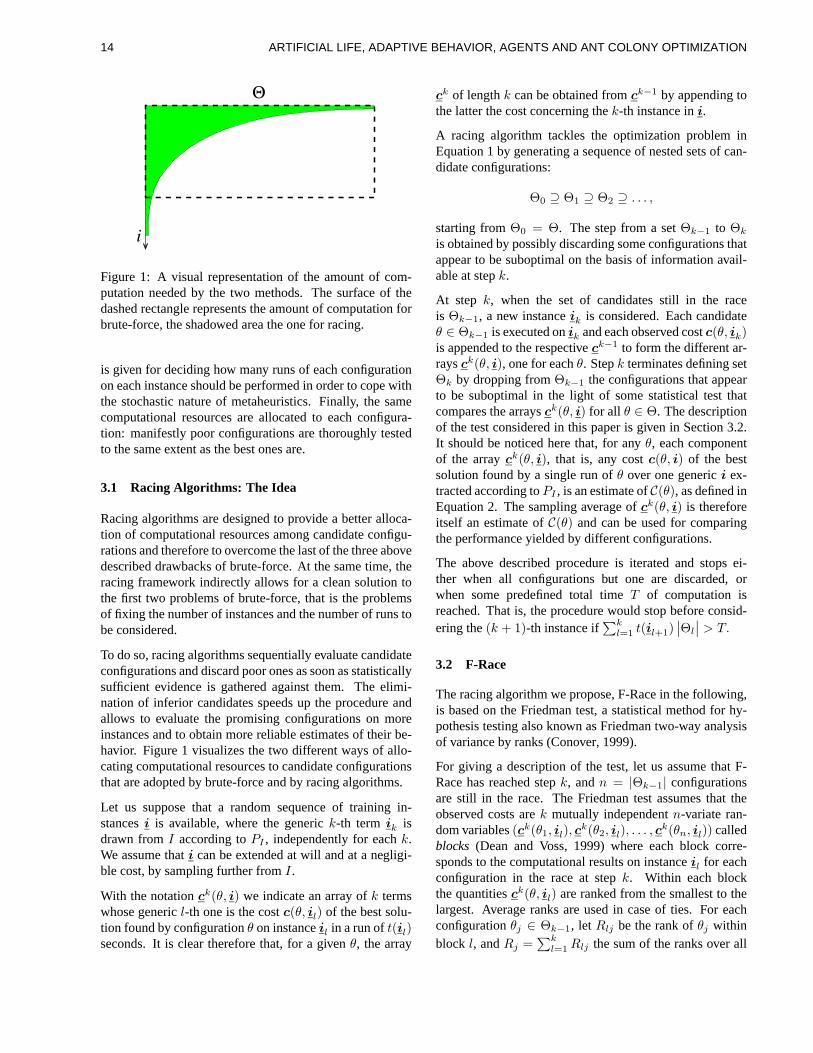
Figure 1: A visual representation of the amount of com-putation needed by the two methods. The surface of thedashed rectangle represents the amount of computation forbrute-force, the shadowed area the one for racing.
is given for deciding how many runs of each configurationon each instance should be performed in order to cope withthe stochastic nature of metaheuristics. Finally, the samecomputational resources are allocated to each configura-tion: manifestly poor configurations are thoroughly testedto the same extent as the best ones are.
3.1 Racing Algorithms: The Idea
Racing algorithms are designed to provide a better alloca-tion of computational resources among candidate configu-rations and therefore to overcome the last of the three abovedescribed drawbacks of brute-force. At the same time, theracing framework indirectly allows for a clean solution tothe first two problems of brute-force, that is the problemsof fixing the number of instances and the number of runs tobe considered.
To do so, racing algorithms sequentially evaluate candidateconfigurations and discard poor ones as soon as statisticallysufficient evidence is gathered against them. The elimi-nation of inferior candidates speeds up the procedure andallows to evaluate the promising configurations on moreinstances and to obtain more reliable estimates of their be-havior. Figure 1 visualizes the two different ways of allo-cating computational resources to candidate configurationsthat are adopted by brute-force and by racing algorithms.
Let us suppose that a random sequence of training in-stancesi is available, where the generick-th term ik isdrawn fromI according toPI , independently for eachk.We assume thati can be extended at will and at a negligi-ble cost, by sampling further fromI.
With the notationck(θ, i) we indicate an array ofk termswhose genericl-th one is the costc(θ, il) of the best solu-tion found by configurationθ on instanceil in a run oft(il)seconds. It is clear therefore that, for a givenθ, the array
ck of lengthk can be obtained fromck−1 by appending tothe latter the cost concerning thek-th instance ini.
A racing algorithm tackles the optimization problem inEquation 1 by generating a sequence of nested sets of can-didate configurations:
Θ0 ⊇ Θ1 ⊇ Θ2 ⊇ . . . ,
starting fromΘ0 = Θ. The step from a setΘk−1 to Θk
is obtained by possibly discarding some configurations thatappear to be suboptimal on the basis of information avail-able at stepk.
At step k, when the set of candidates still in the raceis Θk−1, a new instanceik is considered. Each candidateθ ∈ Θk−1 is executed onik and each observed costc(θ, ik)is appended to the respectiveck−1 to form the different ar-raysck(θ, i), one for eachθ. Stepk terminates defining setΘk by dropping fromΘk−1 the configurations that appearto be suboptimal in the light of some statistical test thatcompares the arraysck(θ, i) for all θ ∈ Θ. The descriptionof the test considered in this paper is given in Section 3.2.It should be noticed here that, for anyθ, each componentof the arrayck(θ, i), that is, any costc(θ, i) of the bestsolution found by a single run ofθ over one generici ex-tracted according toPI , is an estimate ofC(θ), as defined inEquation 2. The sampling average ofck(θ, i) is thereforeitself an estimate ofC(θ) and can be used for comparingthe performance yielded by different configurations.
The above described procedure is iterated and stops ei-ther when all configurations but one are discarded, orwhen some predefined total timeT of computation isreached. That is, the procedure would stop before consid-ering the(k + 1)-th instance if
∑kl=1 t(il+1)
∣∣Θl
∣∣ > T.
3.2 F-Race
The racing algorithm we propose, F-Race in the following,is based on the Friedman test, a statistical method for hy-pothesis testing also known as Friedman two-way analysisof variance by ranks (Conover, 1999).
For giving a description of the test, let us assume that F-Race has reached stepk, andn = |Θk−1| configurationsare still in the race. The Friedman test assumes that theobserved costs arek mutually independentn-variate ran-dom variables(ck(θ1, il), c
k(θ2, il), . . . , ck(θn, il)) called
blocks (Dean and Voss, 1999) where each block corre-sponds to the computational results on instanceil for eachconfiguration in the race at stepk. Within each blockthe quantitiesck(θ, il) are ranked from the smallest to thelargest. Average ranks are used in case of ties. For eachconfigurationθj ∈ Θk−1, letRlj be the rank ofθj withinblock l, andRj =
∑kl=1Rlj the sum of the ranks over all
14 ARTIFICIAL LIFE, ADAPTIVE BEHAVIOR, AGENTS AND ANT COLONY OPTIMIZATION
instancesil, with 1 ≤ l ≤ k. The Friedman test considersthe following statistic (Conover, 1999):
T =
(n− 1)n∑j=1
(Rj −
k(n+ 1)2
)2
k∑l=1
n∑j=1
R2lj −
kn(n+ 1)2
4
.
Under the null hypothesis that all possible rankings of thecandidates within each block are equally likely,T is ap-proximativelyχ2 distributed withn−1 degrees of freedom.If the observedT exceeds the1− α quantile of such a dis-tribution, the null is rejected, at the approximate levelα, infavor of the hypothesis that at least one candidate tends toyield a better performance than at least one other.
If the null is rejected, we are justified in performing pair-wise comparisons between individual candidates. Candi-datesθj andθh are considered different if
|Rj −Rh|√2k(1− T
k(n−1) )(∑k
l=1∑nj=1R
2lj−
kn(n+1)24
)(k−1)(n−1)
> t1−α/2,
wheret1−α/2 is the 1 − α/2 quantile of the Student’stdistribution (Conover, 1999).
In F-Race, if at stepk the null of the aggregate comparisonis not rejected, all candidates inΘk−1 pass toΘk. On theother hand, if the null is rejected, pairwise comparisons areexecuted between the best candidate and each other one.All candidates that result significatively worse than the bestare discarded and will not appear inΘk.
3.3 Discussion on the Role of Ranking in F-Race
In F-Race, ranking plays an important two-fold role. Thefirst one is connected with the nonparametric nature of atest based on ranking. The main merit of nonparametricanalysis is that it does not require to formulate hypothe-ses on the distribution of the observations. Discussionson the relative pros and cons of the parametric and non-parametric approaches can be found in most textbooks onstatistics (Larson, 1982). For an organic presentation of thetopic, we refer the reader, for example, to Conover (1999).Here we limit ourselves to mention some widely acceptedfacts about parametric and nonparametric hypothesis test-ing: When the hypotheses they formulate are met, para-metric tests have a higher power than nonparametric onesand usually require much less computation. Further, whena large amount of data is available the hypotheses for theapplication of parametric tests tend to be met in virtue ofthe central limit theorem. Finally, it is well known that thet-test, the classical parametric test that is of interest here,is robust against departure from some of its hypotheses,
namely the normality of data: When the hypothesis of nor-mality is not strictly met t-testgracefullylooses power.
For what concerns the metaheuristics configuration prob-lem, we are in a situation in which these arguments looksuspicious. First, since we wish to reduce as soon as possi-ble the number of candidates, we deal with very small sam-ples and it is exactly on these small samples, for which thecentral limit theorem cannot be advocated, that we wish tohave the maximum power. Second, the computational costsare not really relevant since in any case they are negligiblecompared to the computational cost of executing configura-tions of the metaheuristic in order to enlarge the availablesamples. Section 5 shows that the doubts expressed herefind some evidential support in our experiments.
A second role played by ranking in F-Race is to imple-ment in a natural way a blocking design (Dean and Voss,1999). The variation in the observed costsc is due to dif-ferent sources: Metaheuristics are intrinsically stochasticalgorithms, the instances might be very different one fromthe other, and finally some configurations perform betterthan others. This last source of variation is the one thatis of interest in the configuration problem while the oth-ers might be considered as disturbing elements. Blockingis an effective way for normalizing the costs observed ondifferent instances. By focusing only on the ranking ofthe different configurations within each instance, blockingeliminates the risks that the variation due to the differenceamong instances washes out the variation due to the differ-ence among configurations.
The work proposed in this paper was openly and largely in-spired by some algorithms proposed in the machine learn-ing community (Maron and Moore, 1994; Moore and Lee,1994) but it is precisely in the adoption of a statistical testbased on ranking that it diverges from previously publishedworks. Maron and Moore (1994) proposed Hoeffding Racethat adopts a nonparametric approach but does not considerblocking. In a following paper, Moore and Lee (1994) de-scribe BRACE that adopts blocking but discards the non-parametric setting in favor of a Bayesian approach. Otherrelevant work was proposed by Gratch et al. (1993) and byChien et al. (1995) who consider blocking in a parametricsetting.
This paper, to the best of our knowledge, is the first workin which blocking is considered in a nonparametric set-ting. Further, in all the above mentioned works blockingwas always implemented through multiple pairwise pairedcomparisons (Hsu, 1996), and only in the more recentone (Chien et al., 1995) correction for multiple tests is con-sidered. F-Race is the first racing algorithm to implementblocking through ranking and to adopt an aggregate testover all candidates, to be performed prior to any pairwisetest.
15ARTIFICIAL LIFE, ADAPTIVE BEHAVIOR, AGENTS AND ANT COLONY OPTIMIZATION
4 MAX–MIN-ANT-SYSTEM FOR TSP
In this paper we illustrate F-Race by using as an examplethe configuration ofMAX–MIN-Ant-System (MMAS)(Stutzle and Hoos, 1997; Stutzle and Hoos, 2000), a par-ticular Ant Colony Optimization algorithm (Dorigo and DiCaro, 1999; Dorigo and Stutzle, 2002), over a class of in-stances of the Traveling Salesman Problem (TSP).
4.1 A Class of TSP Instances
Given a complete graphG = (N,A, d) with N being theset ofn = |N | nodes,A being the set of arcs fully connect-ing the nodes, andd being the weight function that assignseach arc(i, j) ∈ A a lengthdij , the Traveling SalesmanProblem (TSP) is the problem of finding a shortest closedtour visiting each node ofG once. We assume the TSPis symmetric, that is, we havedij = dji for every pair ofnodesi andj.
The TSP is extensively studied in literature and that servesas a standard benchmark problem (Johnson and McGeoch,1997; Lawler et al., 1985; Reinelt, 1994). For our studywe randomly generate Euclidean TSP instances with a ran-dom distribution of city coordinates and a random num-ber of cities. Euclidean TSPs were chosen because suchinstances are used in a large number of experimental re-searches on the TSP (Johnson and McGeoch, 1997; John-son et al., 2001). In our case, city locations are randomlychosen according to a uniform distribution in a square ofdimension10.000×10.000, and the resulting distances arerounded to the nearest integer. The number of cities in eachinstance is chosen as an integer randomly sampled accord-ing to a uniform distribution in the interval[300, 500]. Wegenerated a total number of 400 such instances for our ex-periments reported in Section 5.
4.2 MAX–MIN-Ant-System
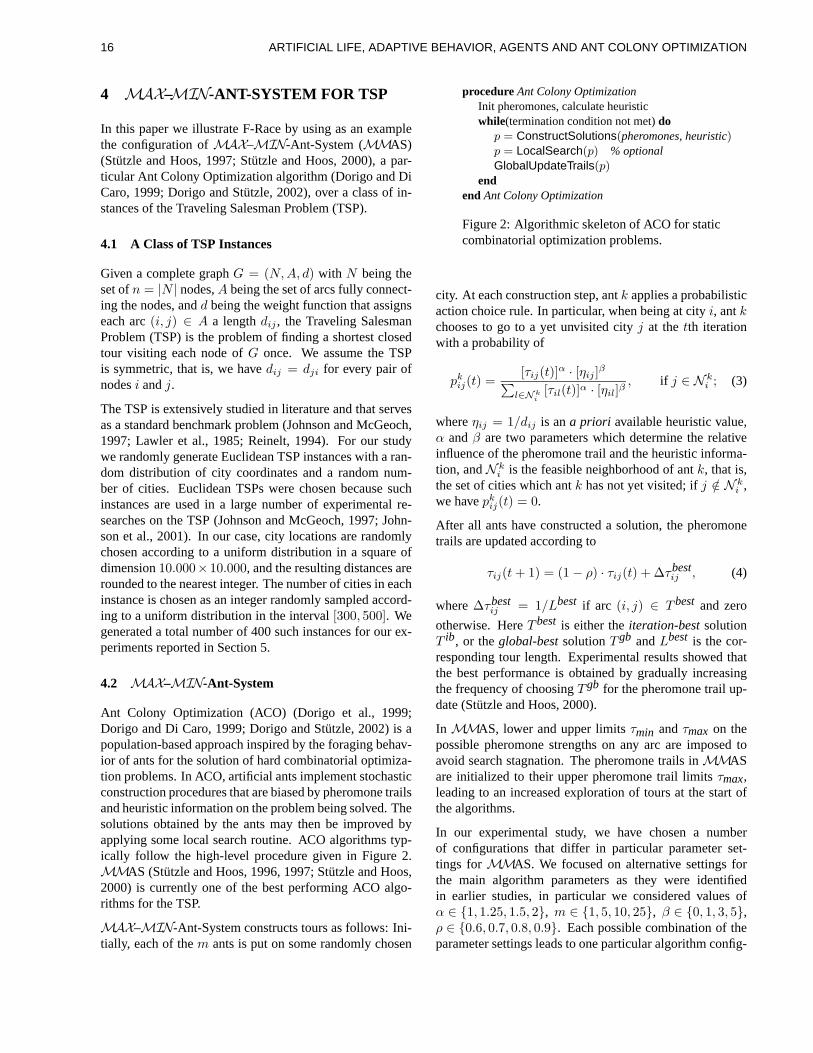
Ant Colony Optimization (ACO) (Dorigo et al., 1999;Dorigo and Di Caro, 1999; Dorigo and Stutzle, 2002) is apopulation-based approach inspired by the foraging behav-ior of ants for the solution of hard combinatorial optimiza-tion problems. In ACO, artificial ants implement stochasticconstruction procedures that are biased by pheromone trailsand heuristic information on the problem being solved. Thesolutions obtained by the ants may then be improved byapplying some local search routine. ACO algorithms typ-ically follow the high-level procedure given in Figure 2.MMAS (Stutzle and Hoos, 1996, 1997; Stutzle and Hoos,2000) is currently one of the best performing ACO algo-rithms for the TSP.
MAX–MIN-Ant-System constructs tours as follows: Ini-tially, each of them ants is put on some randomly chosen
procedureAnt Colony OptimizationInit pheromones, calculate heuristicwhile(termination condition not met)dop = ConstructSolutions(pheromones, heuristic)p = LocalSearch(p) % optionalGlobalUpdateTrails(p)
endendAnt Colony Optimization
Figure 2: Algorithmic skeleton of ACO for staticcombinatorial optimization problems.
city. At each construction step, antk applies a probabilisticaction choice rule. In particular, when being at cityi, antkchooses to go to a yet unvisited cityj at thetth iterationwith a probability of
pkij(t) =[τij(t)]α · [ηij ]β∑l∈Nki
[τil(t)]α · [ηil]β, if j ∈ N k
i ; (3)
whereηij = 1/dij is ana priori available heuristic value,α andβ are two parameters which determine the relativeinfluence of the pheromone trail and the heuristic informa-tion, andN k
i is the feasible neighborhood of antk, that is,the set of cities which antk has not yet visited; ifj /∈ N k
i ,we havepkij(t) = 0.
After all ants have constructed a solution, the pheromonetrails are updated according to
τij(t+ 1) = (1− ρ) · τij(t) + ∆τbestij , (4)
where∆τbestij = 1/Lbest if arc (i, j) ∈ Tbest and zero
otherwise. HereTbest is either theiteration-bestsolutionT ib, or theglobal-bestsolutionTgb andLbest is the cor-responding tour length. Experimental results showed thatthe best performance is obtained by gradually increasingthe frequency of choosingTgb for the pheromone trail up-date (Stutzle and Hoos, 2000).
In MMAS, lower and upper limitsτmin andτmax on thepossible pheromone strengths on any arc are imposed toavoid search stagnation. The pheromone trails inMMASare initialized to their upper pheromone trail limitsτmax,leading to an increased exploration of tours at the start ofthe algorithms.
In our experimental study, we have chosen a numberof configurations that differ in particular parameter set-tings forMMAS. We focused on alternative settings forthe main algorithm parameters as they were identifiedin earlier studies, in particular we considered values ofα ∈ {1, 1.25, 1.5, 2}, m ∈ {1, 5, 10, 25}, β ∈ {0, 1, 3, 5},ρ ∈ {0.6, 0.7, 0.8, 0.9}. Each possible combination of theparameter settings leads to one particular algorithm config-
16 ARTIFICIAL LIFE, ADAPTIVE BEHAVIOR, AGENTS AND ANT COLONY OPTIMIZATION
uration, leading to a total number of4×4×4×4 = 256 con-figurations. In our experiments each solution is improvedby a 2.5-opt local search procedure (Bentley, 1992).
5 EXPERIMENTAL RESULTS
In this section we propose a Monte Carlo evaluation ofF-Race based on a resampling technique (Good, 2001).
For comparison, we consider two other instances of racingalgorithms both based on a paired t-test. They are thereforeparametric, and they adopt a blocking design. We referto them astn-Raceand tb-Race. The first does not adoptany correction for multiple-tests, while the second adoptsthe Bonferroni correction and is thereforenot unlike themethod described by Chien et al. (1995).
The goal is to select anas good as possibleconfigura-tion out of the 256 configurations of theMAX–MIN-Ant-System described in Section 4.2.
Each configuration was executed once on each of the 400instances for10s on a CPU Athlon 1.4GHz with 512 MBof RAM, for a total time of about 12 days to allow in afollowing phase the application of the resampling analysis.The costs of the best solution found in each of these exper-iments were stored in a two-dimensional400 × 256 array.In the following, when saying that werun configurationjover instancei, we will simply mean that we execute thepseudo-experimentthat consists in reading the value in po-sition (i, j) from the array of the results.
From the 400 instances, we extract 1000 pseudo-sampleseach of which is obtained by re-ordering randomly the orig-inal instances. Each pseudo-sample is used for apseudo-trial , that is, for simulating a run of a racing algorithm: Oneafter the other the instances are considered and, on the ba-sis of the results of pseudo-experiments, configurations areprogressively discarded. Each algorithm stops after execut-ing 5 × 256 pseudo-experiments.5 Upon time expiration,the best candidate in the pseudo-trial is selected and it istested on 10 instances that werenot used during the selec-tion itself. The results obtained on these previously unseeninstances are recorded and are used for comparing the threeracing methods. To summarize, after 1000 pseudo-trials avector of 10 × 1000 components is obtained for each ofF-Race, tn-Race, and tb-Race. It is important to note thatthe three algorithms face the same pseudo-samples and thatthe candidates selected in each pseudo-trial by each algo-rithm are tested on the same unseen instances. The generici-th components of the three10×1000 vectors refers there-fore to the results obtained by the champions of the three
5In such a time, by definition, brute-force would be able totest the 256 candidates on only 5 instances. The5× 256 pseudo-experiments simulate 3.5 hours of actual computation on the com-puter used for producing the results proposed here.
races respectively, where the three races were conducted onthe basis of the same pseudo-sample: We are therefore jus-tified in using paired statistical tests when comparing thethree races among them.
On the basis of a paired Wilcoxon test we can state thatF-Race is significatively better, at a significance level of5%, than both tn-Race and tb-Race.6
Some insight on this result can be obtained from the fol-lowing observation. By early dropping the less interestingcandidates, F-Race is able to perform more experiments onthe more promising candidates. On the 1000 pseudo-trialsconsidered, at the moment in which the computation timewas up and a decision among the surviving candidate hadto be taken, the set of survivors was on average composedby 7.9 candidates and such survivors had been tested on av-erage on77.9 instances. In the case of tn-Race, the averagesize of the set of survivors upon expiration of computationtime was31.1, while the number of instances seen by suchsurvivors was on average18.2. For tb-Race the numbersare253.8 and5, respectively. In this sense, F-Race provedto be the bravest of the three, while tb-Race appeared tobe extremely conservative and on average it dropped onlyslightly more than2 candidates before the time limit.
On the basis of our Monte Carlo evaluation, some strongerstatement can be pronounced on the quality of the resultsobtained by F-Race. We have shown above that the perfor-mance of F-Race was good in arelativesense: F-Race pro-duced better results than its competitors. We state now that,in a precise sense to be defined presently, the performanceof F-Race wasabsolutelygood. We compare F-Race withCheat, a brute-force method that, rather unfairly, uses ineach pseudo-trial the same number of instances used by F-Race and on these instances runs all the candidate config-urations. In doing so, Cheat allows itself an enormouslylarge amount of computation time. In our experiments,Cheat has performed on average about19950 experimentsper trial which is equivalent to about55 hours of computa-tion against the3.5 hour available to F-Race. The selectionoperated by Cheat is theoptimumthat can be obtained fromthe fixed set of training instances, and considering only onerun of each configuration on each instance. F-Race can beseen as an approximation of Cheat: The set of experimentperformed by F-Race is aproper subsetof the experimentsperformed by Cheat.
Now, in the statistical analysis of the results obtained byour Monte Carlo experiments, we were not able to rejectthe null that F-Race and Cheat produce equivalent results.Also in this case, we have worked at the significance levelof 5%: neither Wilcoxon test nor t-test were able to showsignificance.
6The same conclusion can be drawn on the basis of a pairedt-test.
17ARTIFICIAL LIFE, ADAPTIVE BEHAVIOR, AGENTS AND ANT COLONY OPTIMIZATION
6 CONCLUSIONS
The paper has given a formal definition of the problem ofconfiguring a metaheuristic and has presented F-Race, analgorithm belonging to the class of racing algorithms pro-posed in the machine learning community for solving themodel selection problem (Maron and Moore, 1994).
In giving a formal definition of the configuration problem,we have stressed the important role played by the probabil-ity measure defined on the class of the instances. Withoutsuch a concept, it is impossible to give a meaning to thegeneralization process that is implicit when a configurationis selected on the basis of its performance on a limited setof instances.
F-Race, the algorithm we propose in this paper, is the spe-cialization of the generic class of racing algorithms to theconfiguration of metaheuristics. The adoption of the Fried-man test, which is nonparametric and two-way, matchesindeed the specificities of the configuration problem. Asshown by the experimental results proposed in Section 5,F-Race obtains better results than its competitors that adopta parametric approach. This better performance can be in-deed explained by the ability of discarding inferior candi-dates earlier and faster than the competitors. Still, we donot feel like using these results for claiming a generalpre-sumedsuperiority of F-Race against its fellow racing algo-rithms. Rather, we wish to stress the appeal of the racingidea in itself, and we want to interpret our results as an evi-dence that this idea is extremely promising for configuringmetaheuristics and should be further investigated.
Acknowledgments
This work was supported by the “Metaheuristics Network”,a Research Training Network funded by the Improving Hu-man Potential programme of the CEC, grant HPRN-CT-1999-00106. The information provided is the sole respon-sibility of the authors and does not reflect the Community’sopinion. The Community is not responsible for any use thatmight be made of data appearing in this publication.
ReferencesBentley, J. L. (1992). Fast algorithms for geometric traveling
salesman problems.ORSA Journal on Computing, 4(4):387–411.
Billingsley, P. (1986).Probability and Measure. John Wiley &Sons, New York, NY, USA, second edition.
Chien, S., Gratch, J., and Burl, M. (1995). On the efficient allo-cation of resources for hypothesis evaluation: A statistical ap-proach.Pattern Analysis and Machine Intelligence, 17(7):652–665.
Conover, W. J. (1999).Practical Nonparametric Statistics. JohnWiley & Sons, New York, NY, USA, third edition.
Dean, A. and Voss, D. (1999).Design and Analysis of Experi-ments. Springer Verlag, New York, NY, USA.
Dorigo, M. and Di Caro, G. (1999). The Ant Colony Optimizationmeta-heuristic. In Corne, D., Dorigo, M., and Glover, F., ed-itors, New Ideas in Optimization, pages 11–32. McGraw Hill,London, UK.
Dorigo, M., Di Caro, G., and Gambardella, L. M. (1999). Antalgorithms for discrete optimization.Artificial Life, 5(2):137–172.
Dorigo, M. and Stutzle, T. (2002). The ant colony optimiza-tion metaheuristic: Algorithms, applications and advances. InMetaheuristics Handbook. Kluwer Academic Publishers. Inpress.
Good, P. I. (2001).Resampling Methods. Birkhauser, Boston,MA, USA, second edition.
Gratch, J., Chien, S., and DeJong, G. (1993). Learning searchcontrol knowledge for deep space network scheduling. InIn-ternational Conference on Machine Learning, pages 135–142.
Hsu, J. (1996).Multiple Comparisons. Chapman & Hall/CRC,Boca Raton, Fl, USA.
Johnson, D. S. and McGeoch, L. A. (1997). The travelling sales-man problem: A case study in local optimization. In Aarts, E.H. L. and Lenstra, J. K., editors,Local Search in CombinatorialOptimization, pages 215–310. John Wiley & Sons, Chichester,UK.
Johnson, D. S., McGeoch, L. A., Rego, C., and Glover,F. (2001). 8th DIMACS implementation challenge.http://www.research.att.com/ ˜ dsj/chtsp/ .
Larson, H. (1982).Introduction to Probability Theory and Statis-tical Inference. John Wiley & Sons, New York, NY, USA.
Lawler, E. L., Lenstra, J. K., Kan, A. H. G. R., and Shmoys, D. B.(1985).The Travelling Salesman Problem. John Wiley & Sons,Chichester, UK.
Maron, O. and Moore, A. W. (1994). Hoeffding races: Accel-erating model selection search for classification and functionapproximation. In Cowan, J. D., Tesauro, G., and Alspector, J.,editors,Advances in Neural Information Processing Systems,volume 6, pages 59–66. Morgan Kaufmann Publishers, Inc.
Mitchell, T. M. (1997). Machine Learning. McGraw-Hill, NewYork, NY, USA.
Moore, A. W. and Lee, M. S. (1994). Efficient algorithms for min-imizing cross validation error. InInternational Conference onMachine Learning, pages 190–198. Morgan Kaufmann Pub-lishers, Inc.
Reinelt, G. (1994).The Traveling Salesman: Computational So-lutions for TSP Applications, volume 840 ofLecture Notes inComputer Science. Springer Verlag, Berlin, Germany.
Stutzle, T. and Hoos, H. (1996). Improving the Ant-System: Adetailed report on theMAX–MIN Ant System. TechnicalReport AIDA–96–12, FG Intellektik, TU Darmstadt, Germany.
Stutzle, T. and Hoos, H. H. (1997). TheMAX–MIN Ant Sys-tem and local search for the traveling salesman problem. InBack, T., Michalewicz, Z., and Yao, X., editors,Proceedingsof the 1997 IEEE International Conference on EvolutionaryComputation (ICEC’97), pages 309–314. IEEE Press, Piscat-away, NJ, USA.
Stutzle, T. and Hoos, H. H. (2000).MAX–MIN Ant System.Future Generation Computer Systems, 16(8):889–914.
18 ARTIFICIAL LIFE, ADAPTIVE BEHAVIOR, AGENTS AND ANT COLONY OPTIMIZATION
Dynamic Search with Charged Swarms
T.M.Blackwell
Department of Computer Science University College London
Gower Street, London, UK
P. J. Bentley
Department of Computer Science University College London
Gower Street, London, UK
Abstract
Two novel particle swarm optimization (PSO) algorithms are used to track and optimize a 3- dimensional parabolic benchmark function where the optimum location changes randomly and with high severity. The new algorithms are based on an analogy of electrostatic energy with charged particles. For comparison, the same experiment is performed with a conventional PSO algorithm. It is found that the best strategy for this particular problem involves a combination of neutral and charged particles.
1 INTRODUCTION
Particle Swarm Optimization (PSO) is a population based evolutionary technique applied to optimization problems. It differs from other population approaches such as genetic algorithms, by the inclusion of a solution (or particle) velocity, which moves the position of the solution in the space of all possible solutions, rather than relying on recombination of existing solutions. Linear spring forces govern the dynamics of the population (or swarm); each particle is attracted to its previous best position, and to the global best position attained by the swarm, where fitness is quantified by the value of a function at that position. These swarms have proven to be very successful in finding global optima in various static contexts such as the optimization of certain benchmark functions (Eberhart and Shi 2001a).
The real world is rarely static, however, and many systems will require frequent re-optimization due to system and/or environmental change. The problem of re-scheduling system resources is an important example of this. One important and implicit constraint is the requirement to balance the desired error of the solution with the need to be prepared to respond rapidly to change. For example, to achieve a low error will require a large number of iterations/generations, and will leave the evolutionary population well adapted to that situation. But
system and environment change may occur on short time-scales and may be large enough to leave the population ill-adapted to the new problem, so that a solution considered good enough may be hard to find within this time-scale.
This work addresses these issues with the use of two novel swarm algorithms. These algorithms are tested and compared with the conventional PSO algorithm for an extreme search problem wherein the optimum location (solution) is randomized within a box representing the entire dynamic range.
2 BACKGROUND
Eberhart and Shi (2001b) have applied the conventional PSO algorithm to some dynamic search and optimization problems. In their experiments, they use a time-scale of 100 iterations, and choose as a benchmark the (3-dimensional) parabolic function and the sphere function in 10-dimensions. The optimum location of these functions was moved along a line by increments of 0.2% and 1% of the dynamic range, with each change occurring at 100 iterations. It was found that, under these conditions, the PSO algorithm performed at least as well as other evolutionary techniques (Angeline 1997, Bäck 1998).
One drawback noted by Eberhart and Shi is the lack of a strategy for dealing with a wide variety of change. One possibility is to randomize the swarm when a change is detected. In their work (2001b), the particle positions are retained, but the personal and global best positions are calculated with respect to the new optimum location. Another possibility would be to randomize the swarm when a change is detected. In general, a good strategy is needed that can account for chaotic rather than linear change, and for change that is commensurate with the entire range of the dynamic variables, and not just limited to one per cent of this range.
This work investigates the capabilities of two novel swarm algorithms to overcome an extreme problem of this type. The two new algorithms were originated by the authors in quite a different context: the problem of artificial improvised music (Blackwell and Bentley
19ARTIFICIAL LIFE, ADAPTIVE BEHAVIOR, AGENTS AND ANT COLONY OPTIMIZATION
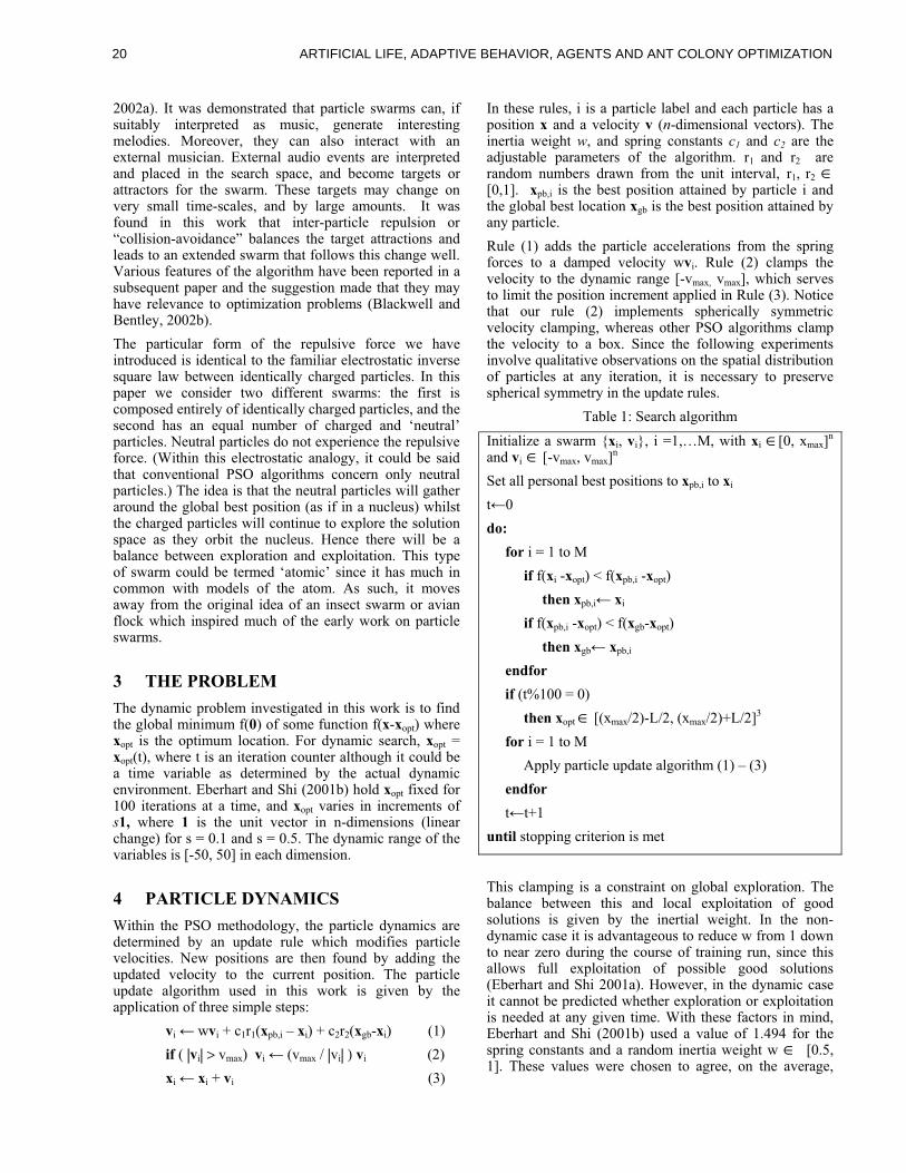
2002a). It was demonstrated that particle swarms can, if suitably interpreted as music, generate interesting melodies. Moreover, they can also interact with an external musician. External audio events are interpreted and placed in the search space, and become targets or attractors for the swarm. These targets may change on very small time-scales, and by large amounts. It was found in this work that inter-particle repulsion or “collision-avoidance” balances the target attractions and leads to an extended swarm that follows this change well. Various features of the algorithm have been reported in a subsequent paper and the suggestion made that they may have relevance to optimization problems (Blackwell and Bentley, 2002b).
The particular form of the repulsive force we have introduced is identical to the familiar electrostatic inverse square law between identically charged particles. In this paper we consider two different swarms: the first is composed entirely of identically charged particles, and the second has an equal number of charged and ‘neutral’ particles. Neutral particles do not experience the repulsive force. (Within this electrostatic analogy, it could be said that conventional PSO algorithms concern only neutral particles.) The idea is that the neutral particles will gather around the global best position (as if in a nucleus) whilst the charged particles will continue to explore the solution space as they orbit the nucleus. Hence there will be a balance between exploration and exploitation. This type of swarm could be termed ‘atomic’ since it has much in common with models of the atom. As such, it moves away from the original idea of an insect swarm or avian flock which inspired much of the early work on particle swarms.
3 THE PROBLEM
The dynamic problem investigated in this work is to find the global minimum f(0) of some function f(x-xopt) where xopt is the optimum location. For dynamic search, xopt = xopt(t), where t is an iteration counter although it could be a time variable as determined by the actual dynamic environment. Eberhart and Shi (2001b) hold xopt fixed for 100 iterations at a time, and xopt varies in increments of s1, where 1 is the unit vector in n-dimensions (linear change) for s = 0.1 and s = 0.5. The dynamic range of the variables is [-50, 50] in each dimension.
4 PARTICLE DYNAMICS
Within the PSO methodology, the particle dynamics are determined by an update rule which modifies particle velocities. New positions are then found by adding the updated velocity to the current position. The particle update algorithm used in this work is given by the application of three simple steps:
vi wvi + c1r1(xpb,i – xi) + c2r2(xgb-xi) (1)
if ( |vi| > vmax) vi (vmax / |vi| ) vi (2)
xi xi + vi (3)
In these rules, i is a particle label and each particle has a position x and a velocity v (n-dimensional vectors). The inertia weight w, and spring constants c1 and c2 are the adjustable parameters of the algorithm. r1 and r2 are random numbers drawn from the unit interval, r1, r2 ∈ [0,1]. xpb,i is the best position attained by particle i and the global best location xgb is the best position attained by any particle.
Rule (1) adds the particle accelerations from the spring forces to a damped velocity wvi. Rule (2) clamps the velocity to the dynamic range [-vmax, vmax], which serves to limit the position increment applied in Rule (3). Notice that our rule (2) implements spherically symmetric velocity clamping, whereas other PSO algorithms clamp the velocity to a box. Since the following experiments involve qualitative observations on the spatial distribution of particles at any iteration, it is necessary to preserve spherical symmetry in the update rules.
Table 1: Search algorithm
Initialize a swarm {xi, vi}, i =1,…M, with xi ∈[0, xmax]n
and vi ∈ [-vmax, vmax]n
Set all personal best positions to xpb,i to xi
t 0
do:
for i = 1 to M
if f(xi -xopt) < f(xpb,i -xopt)
then xpb,i xi
if f(xpb,i -xopt) < f(xgb-xopt)
then xgb xpb,i
endfor
if (t%100 = 0)
then xopt ∈ [(xmax/2)-L/2, (xmax/2)+L/2]3
for i = 1 to M
Apply particle update algorithm (1) – (3)
endfor
t t+1
until stopping criterion is met
This clamping is a constraint on global exploration. The balance between this and local exploitation of good solutions is given by the inertial weight. In the non-dynamic case it is advantageous to reduce w from 1 down to near zero during the course of training run, since this allows full exploitation of possible good solutions (Eberhart and Shi 2001a). However, in the dynamic case it cannot be predicted whether exploration or exploitation is needed at any given time. With these factors in mind, Eberhart and Shi (2001b) used a value of 1.494 for the spring constants and a random inertia weight w ∈ [0.5, 1]. These values were chosen to agree, on the average,
20 ARTIFICIAL LIFE, ADAPTIVE BEHAVIOR, AGENTS AND ANT COLONY OPTIMIZATION
with Clerc’s analysis for convergence (Clerc 1999), and to provide a balance between exploration and exploitation.
The PSO algorithm for the dynamic problem investigated here is given in table 1.
In order to introduce the notion of charge – and hence collision avoidance – all that needs to be done is to modify the rule for particle accelerations, rule (1). The grounds for this extension, and a full description of the effects of the various parameters on particle motion, are given in (Blackwell, 2001) and (Blackwell and Bentley, 2002b). In those studies, an additional acceleration towards the swarm centre was also implemented, but this is not used here.
The necessary amendment to the particle update algorithm is an extra particle acceleration ai given by
prp,r
QQijcoreij
ij3
ji
i
ij
<<=≠
ra (4)
where rij = xi – xj , rij = | xi – xj| and each particle has a
charge of magnitude Qi. Neutral particles are assigned a
charge Qi = 0 and so will not contribute to the sum in (4).
A charged particle i will have Qi > 0 and will experience
the repulsive effects from all other charged particles j i.
Repulsion is only experienced for separations within the
shell pcore < rij < p. The lower cut-off pcore is a safeguard
against the singularity of the inverse square law. The
upper cut off p is a tunable parameter allowing the
domain of influence of the repulsion to be controlled.
The charged particle update algorithm, which replaces the
particle update algorithm within the search algorithm
(Table 1), is given by replacing rule (1) with:
vi wvi + c1r1(xpb,i – xi) + c2r2(xgb-xi) + ai (1')
It is worth noting that since the particles are updated in turn (i.e. from i = 1 to i = M), contributions to ai can involve non-updated particle positions (j > i) as well as updated positions (j < i). This was found to give better avoidance in earlier experiments.
5 EXPERIMENTS
The experiments were conducted on the parabolic function in n = 3 dimensions, f(x-xopt) = (x-xopt) • (x-xopt).
The task is made dynamic by placing xopt in a cube of side L and then randomly re-positioning it to another point in this cube every 100 iterations. The severity s therefore varies randomly from zero up to ( 3)L. With L set to 2vmax, this gives a severity of up to 2 3 times the dynamic range. The parameter xmax solely determines the initial distribution of the particle velocities and positions and plays no part in subsequent updates after the first jump in xopt. The values of the spatial parameters set out in Table 2.
Table 2: Spatial parameters
L xmax vmax M
64 128 32 20
The values of the electrostatic parameters pcore, p and Q are set out in Table 3.
Table 3: Electrostatic parameters
pcore p Q
1 3xmax 16
The values of the PSO parameters w, c1 and c2 are those used by Eberhart and Shi (2001b). The inertia weight w varies randomly between 0.5 and 1.0, so that the mean 0.75 is close to the Clerc constriction factor 0.729 (Clerc 1999). The spring constants c1 and c2 are set to 1.494, also in accordance with Clerc’s analysis.
In all these experiments, 50 optimum jumps are made, (or 5000 iterations of the system). In addition to the numerical data produced by these experiments, a three dimensional animation was set up which enabled a qualitative assessment of the three swarms.
For comparison, four experiments were performed:
I Neutral swarm.
The first experiment uses the conventional PSO algorithm, which is implemented by setting the charge on all 20 particles to zero (i.e. each particle is neutral).
II Charged swarm.
In the second experiment, all 20 particles carry the same charge, Q. In other words, all particles experience repulsive forces from the other particles.
III Atomic swarm.
The third experiment evaluates the atomic swarm, where 10 particles have charge Q and the remaining half are neutral.
IV Neutral swarm, one optimum jump.
The fourth experiment is identical to Experiment 1 except that just 200 iterations were allowed. The positions and velocities of the particles were saved to file for analysis of individual particle motion.
21ARTIFICIAL LIFE, ADAPTIVE BEHAVIOR, AGENTS AND ANT COLONY OPTIMIZATION
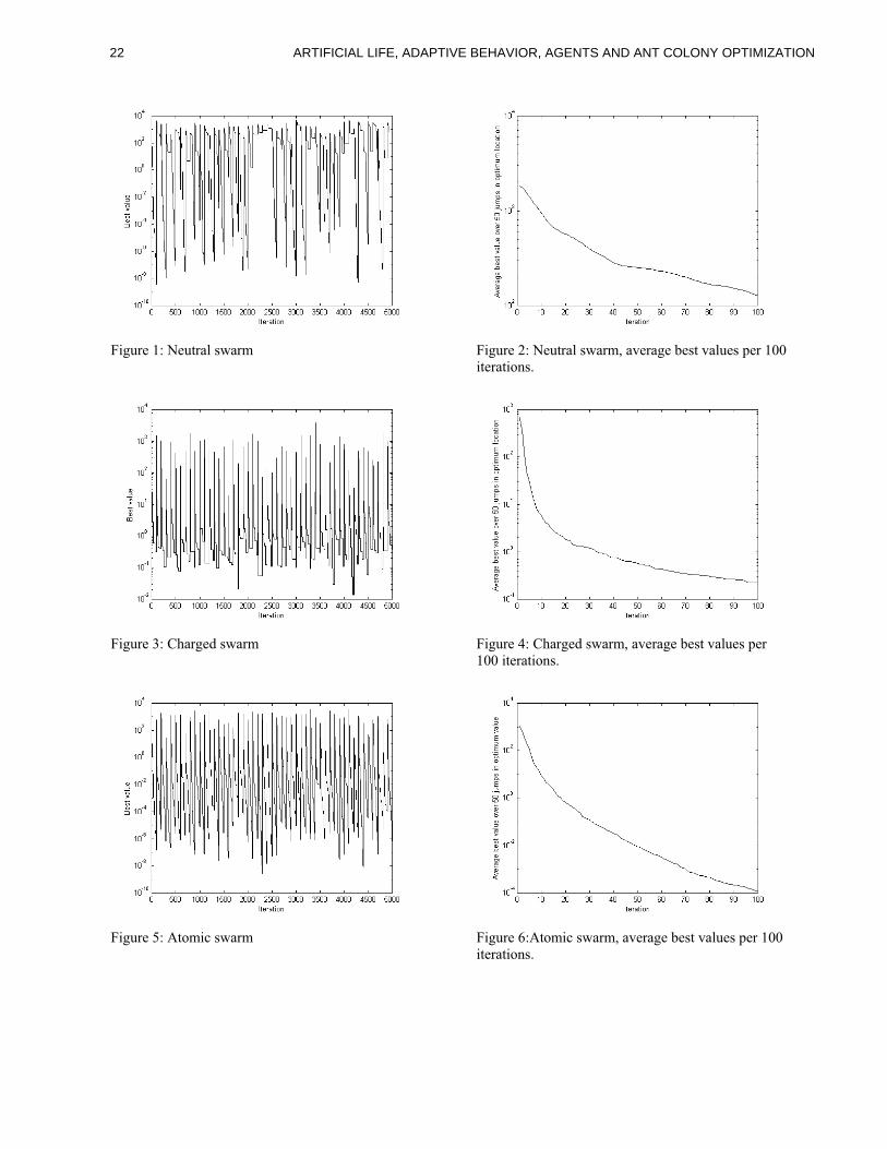
Figure 1: Neutral swarm
Figure 3: Charged swarm
Figure 5: Atomic swarm
Figure 2: Neutral swarm, average best values per 100
iterations.
Figure 4: Charged swarm, average best values per
100 iterations.
Figure 6:Atomic swarm, average best values per 100
iterations.
22 ARTIFICIAL LIFE, ADAPTIVE BEHAVIOR, AGENTS AND ANT COLONY OPTIMIZATION

6 RESULTS
The results for the experiments on the neutral, charged and atomic swarms are shown in Figures 1 to 6. In each case, two graphs have been prepared, plotted as a function of iteration number t: the best value found by the swarm, f(xgb - xopt), and the average best value over the 50 problem optimum jumps (i.e., average best per 100 iterations, from optimum jump to the iteration before the next optimum jump).
6.1 EXPERIMENT I: NEUTRAL SWARM
The best value attained after 100 iterations, i.e. just before the first optimum jump, is of the order of 10-8. This is at least two orders of magnitude lower than the best value obtained in the first 100 iterations of an equivalent experiment (Eberhart and Shi 2001b figure 1, p98), although comparable to the best values obtained in subsequent optimum positions. The discrepancy is presumably due to initial conditions, although the spherically symmetric clamping rule may play a part.
However, the results depart significantly at the first optimum jump, due to the increased severity. The remarkable feature of Figure 1 is the small spikes at the optimum jump followed by a leveling of the graph for some tens of iterations, after a short fall. This plateau in best values sometimes then drops before the next optimum jump, but often does not. For example, there is a run from t = 2100 to 2500 where the initial short fall is not improved upon. The plot of the averages over the 50 optimum jumps shows an average best of 125 at 100 iterations. The slope at this point is -3.2, indicating only a slow improvement (3% per iteration) with increasing iteration.
The 3D animations showed a very unusual feature. For the first 100 iterations, the particles were clumped very closely around the optimum. At the optimum jump, however, the particles moved along a line in the general direction of the new optimum, and then began to oscillate along this line about a point close, but not adjacent to the new optimum. After some tens of iterations the oscillations would cease and the particles would begin to swarm towards the new optimum, although they might not reach it before the next jump. This behavior was repeated invariably at each optimum jump, and in repeats of this experiment.
6.2 EXPERIMENT II: CHARGED SWARM
Figure 3 shows the best values over the 5000 iterations. By comparison with Figure 1, the spikes are now long, showing an improved best value by a factor of 103 after just a few iterations at each jump. The leveling out now occurs at a much smaller best value, a feature illustrated in Figure 4 which shows the average best values. In Figure 4, the lowest average best value obtained is 0.226, and the slope at this point is -2.10x10⁻³ showing an improvement of 1% per iteration at this point.
The animations revealed typical swarming behavior: at each optimum jump the swarm moved towards the new optimum, with irregular motion about the swarm centre. After a few iterations the swarm centre was coincident with the optimum and the particle motion continued to be chaotic and spherically symmetric about this point, with particles amplitudes of some tens of units. These pictures agreed with previous swarm experiments (Blackwell and Bentley, 2001b).
6.3 EXPERIMENT III: ATOMIC SWARM.
Once more, the plot of best values, Figure 5, shows spikes at each optimum jump, but the spikes drop to a much lower best value, in the range 10-4 to 10-8 in 49 of the 50 jumps. The figure does not show the plateaus that are a feature of Figures 1 and 3. The plot of average best values, Figure 6, shows a much improved average best at 100 iterations of 1.12x10⁻⁴, with a slope of -1.21 x 10⁻⁵ or 11% of the best value per iteration at this point. The average global best just before the next optimum jump is at least 6 orders of magnitude better than the neutral swarm and about 2000 times better than the charged swarm.
In order to distinguish charged from neutral particles for the purposes of the animation, the particles were colored red (charged) and blue (neutral). At each optimum jump, the animations displayed the particles moving in an irregular swarming motion towards the optimum, followed by a long period where the blue neutral particles clumped around the optimum, moving ever slower with very small amplitude, surrounded with a ‘cloud’ of charged red particles, moving much like the charged swarm described in II. The picture was very reminiscent of representations of an atomic nucleus surrounded by an electron cloud.
6.4 EXPERIMENT IV: NEUTRAL SWARM, ONE
OPTIMUM JUMP.
A further experiment was conducted on the neutral swarm to give greater insight on the linear non-swarming behavior of the particles just after the optimum jump, as observed in the animation. Just two hundred iterations were completed, allowing a single optimum jump to occur.
At t =100, the 20 particles were clumped very tightly around xo, and moving slowly. Between t = 100 and t = 120, all the particles followed a very similar trajectory. For this reason, some results for just a single particle, particle 0, will be presented. Table 4 shows x, y and z components of the optimum location, global best location and position and velocity of particle 0 at iteration 99, just before the effects of the optimum jump have influenced the particle dynamics.
23ARTIFICIAL LIFE, ADAPTIVE BEHAVIOR, AGENTS AND ANT COLONY OPTIMIZATION
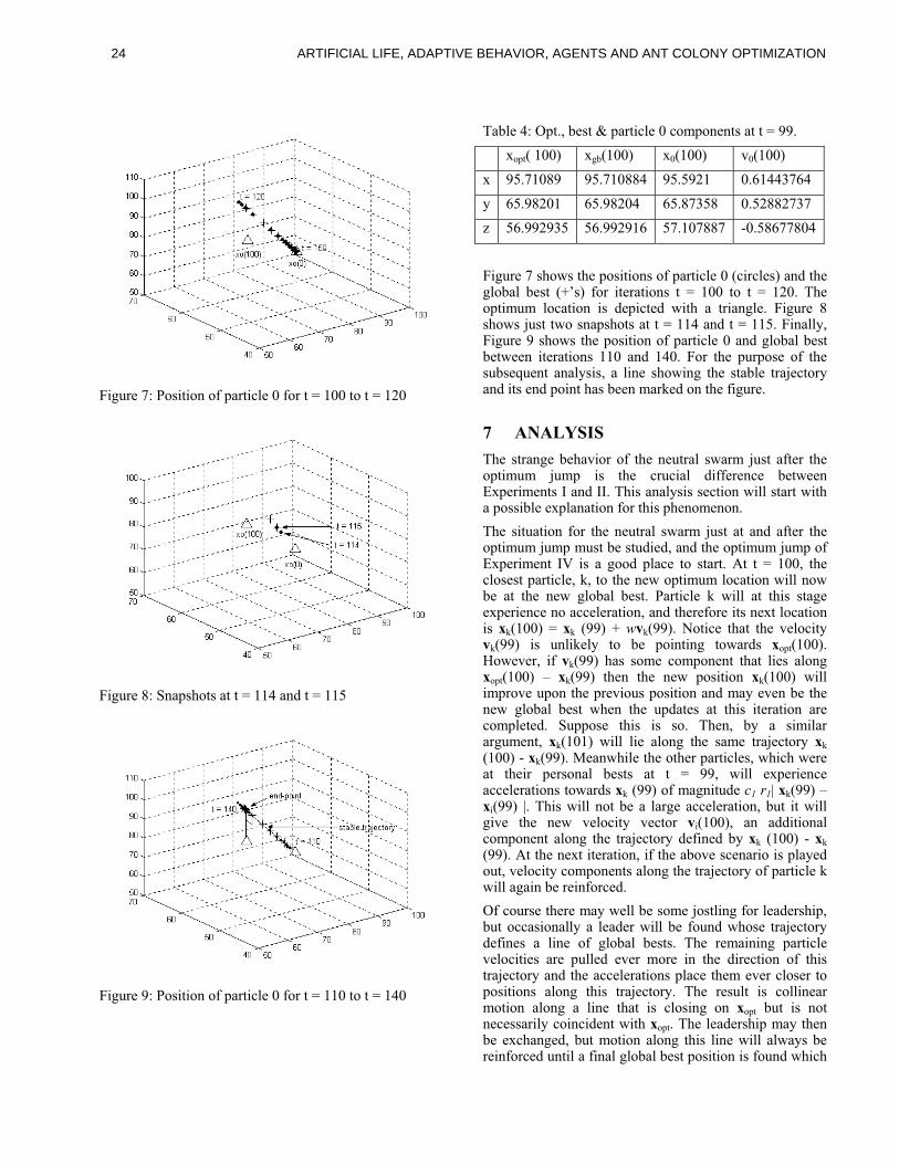
Figure 7: Position of particle 0 for t = 100 to t = 120
Figure 8: Snapshots at t = 114 and t = 115
Figure 9: Position of particle 0 for t = 110 to t = 140
Table 4: Opt., best & particle 0 components at t = 99.
xopt( 100) xgb(100) x0(100) v0(100)
x 95.71089 95.710884 95.5921 0.61443764
y 65.98201 65.98204 65.87358 0.52882737
z 56.992935 56.992916 57.107887 -0.58677804
Figure 7 shows the positions of particle 0 (circles) and the global best (+’s) for iterations t = 100 to t = 120. The optimum location is depicted with a triangle. Figure 8 shows just two snapshots at t = 114 and t = 115. Finally, Figure 9 shows the position of particle 0 and global best between iterations 110 and 140. For the purpose of the subsequent analysis, a line showing the stable trajectory and its end point has been marked on the figure.
7 ANALYSIS
The strange behavior of the neutral swarm just after the optimum jump is the crucial difference between Experiments I and II. This analysis section will start with a possible explanation for this phenomenon.
The situation for the neutral swarm just at and after the optimum jump must be studied, and the optimum jump of Experiment IV is a good place to start. At t = 100, the closest particle, k, to the new optimum location will now be at the new global best. Particle k will at this stage experience no acceleration, and therefore its next location is xk(100) = xk (99) + wvk(99). Notice that the velocity vk(99) is unlikely to be pointing towards xopt(100). However, if vk(99) has some component that lies along xopt(100) – xk(99) then the new position xk(100) will improve upon the previous position and may even be the new global best when the updates at this iteration are completed. Suppose this is so. Then, by a similar argument, xk(101) will lie along the same trajectory xk (100) - xk(99). Meanwhile the other particles, which were at their personal bests at t = 99, will experience accelerations towards xk (99) of magnitude c1 r1| xk(99) – xi(99) |. This will not be a large acceleration, but it will give the new velocity vector vi(100), an additional component along the trajectory defined by xk (100) - xk (99). At the next iteration, if the above scenario is played out, velocity components along the trajectory of particle k will again be reinforced.
Of course there may well be some jostling for leadership, but occasionally a leader will be found whose trajectory defines a line of global bests. The remaining particle velocities are pulled ever more in the direction of this trajectory and the accelerations place them ever closer to positions along this trajectory. The result is collinear motion along a line that is closing on xopt but is not necessarily coincident with xopt. The leadership may then be exchanged, but motion along this line will always be reinforced until a final global best position is found which
24 ARTIFICIAL LIFE, ADAPTIVE BEHAVIOR, AGENTS AND ANT COLONY OPTIMIZATION
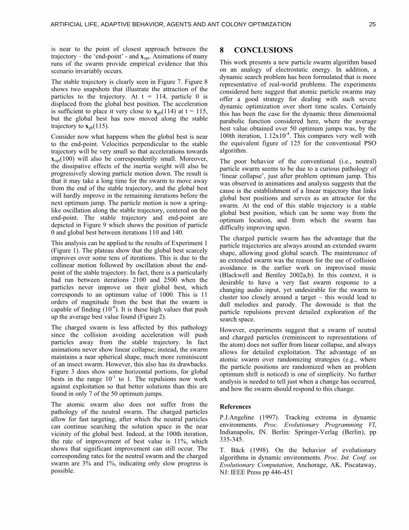
is near to the point of closest approach between the trajectory – the ‘end-point’ - and xopt. Animations of many runs of the swarm provide empirical evidence that this scenario invariably occurs.
The stable trajectory is clearly seen in Figure 7. Figure 8 shows two snapshots that illustrate the attraction of the particles to the trajectory. At t = 114, particle 0 is displaced from the global best position. The acceleration is sufficient to place it very close to xgb(114) at t = 115, but the global best has now moved along the stable trajectory to xgb(115).
Consider now what happens when the global best is near to the end-point. Velocities perpendicular to the stable trajectory will be very small so that accelerations towards xopt(100) will also be correspondently small. Moreover, the dissipative effects of the inertia weight will also be progressively slowing particle motion down. The result is that it may take a long time for the swarm to move away from the end of the stable trajectory, and the global best will hardly improve in the remaining iterations before the next optimum jump. The particle motion is now a spring-like oscillation along the stable trajectory, centered on the end-point. The stable trajectory and end-point are depicted in Figure 9 which shows the position of particle 0 and global best between iterations 110 and 140.
This analysis can be applied to the results of Experiment 1 (Figure 1). The plateau show that the global best scarcely improves over some tens of iterations. This is due to the collinear motion followed by oscillation about the end-point of the stable trajectory. In fact, there is a particularly bad run between iterations 2100 and 2500 when the particles never improve on their global best, which corresponds to an optimum value of 1000. This is 11 orders of magnitude from the best that the swarm is capable of finding (10-8). It is these high values that push up the average best value found (Figure 2).
The charged swarm is less affected by this pathology since the collision avoiding acceleration will push particles away from the stable trajectory. In fact animations never show linear collapse; instead, the swarm maintains a near spherical shape, much more reminiscent of an insect swarm. However, this also has its drawbacks. Figure 3 does show some horizontal portions, for global bests in the range 10-1 to 1. The repulsions now work against exploitation so that better solutions than this are found in only 7 of the 50 optimum jumps.
The atomic swarm also does not suffer from the pathology of the neutral swarm. The charged particles allow for fast targeting, after which the neutral particles can continue searching the solution space in the near vicinity of the global best. Indeed, at the 100th iteration, the rate of improvement of best value is 11%, which shows that significant improvement can still occur. The corresponding rates for the neutral swarm and the charged swarm are 3% and 1%, indicating only slow progress is possible.
8 CONCLUSIONS
This work presents a new particle swarm algorithm based on an analogy of electrostatic energy. In addition, a dynamic search problem has been formulated that is more representative of real-world problems. The experiments considered here suggest that atomic particle swarms may offer a good strategy for dealing with such severe dynamic optimization over short time scales. Certainly this has been the case for the dynamic three dimensional parabolic function considered here, where the average best value obtained over 50 optimum jumps was, by the 100th iteration, 1.12x10⁻⁴. This compares very well with the equivalent figure of 125 for the conventional PSO algorithm.
The poor behavior of the conventional (i.e., neutral) particle swarm seems to be due to a curious pathology of ‘linear collapse’, just after problem optimum jump. This was observed in animations and analysis suggests that the cause is the establishment of a linear trajectory that links global best positions and serves as an attractor for the swarm. At the end of this stable trajectory is a stable global best position, which can be some way from the optimum location, and from which the swarm has difficulty improving upon.
The charged particle swarm has the advantage that the particle trajectories are always around an extended swarm shape, allowing good global search. The maintenance of an extended swarm was the reason for the use of collision avoidance in the earlier work on improvised music (Blackwell and Bentley 2002a,b). In this context, it is desirable to have a very fast swarm response to a changing audio input, yet undesirable for the swarm to cluster too closely around a target – this would lead to dull melodies and parody. The downside is that the particle repulsions prevent detailed exploration of the search space.
However, experiments suggest that a swarm of neutral and charged particles (reminiscent to representations of the atom) does not suffer from linear collapse, and always allows for detailed exploitation. The advantage of an atomic swarm over randomizing strategies (e.g., where the particle positions are randomized when an problem optimum shift is noticed) is one of simplicity. No further analysis is needed to tell just when a change has occurred, and how the swarm should respond to this change.
References
P.J.Angeline (1997). Tracking extrema in dynamic environments. Proc. Evolutionary Programming VI, Indianapolis, IN. Berlin: Springer-Verlag (Berlin), pp 335-345.
T. Bäck (1998). On the behavior of evolutionary algorithms in dynamic environments. Proc. Int. Conf. on Evolutionary Computation, Anchorage, AK. Piscataway, NJ: IEEE Press pp 446-451
25ARTIFICIAL LIFE, ADAPTIVE BEHAVIOR, AGENTS AND ANT COLONY OPTIMIZATION

Blackwell, T. (2001) “Making Music with Swarms,” MSc thesis, University College London.
Blackwell, T. and Bentley, P. J. (2002a) Improvised Music with Swarms, Proc CEC 2002 (to be published).
Blackwell, T. and Bentley, P. J. (2002b) Don’t push me! Collision-Avoiding Swarms, Proc CEC 2002 (to be published).
M.Clerc (1999). The swarm and the queen: towards a deterministic and adaptive particle swarm optimization. Proc CEC 1999. Washington, DC, pp 1951 – 1957.
R.C.Eberhart and Y.Shi (2001a). Particle swarm optimization: Developments, applications and resources. Proc CEC 2001. Piscataway, NJ, pp 81-86.
R.C.Eberhart and Y.Shi (2001b). Tracking and optimizing dynamic systems with particle swarms. Proc CEC 2001. Piscataway, NJ, pp 94-100.
26 ARTIFICIAL LIFE, ADAPTIVE BEHAVIOR, AGENTS AND ANT COLONY OPTIMIZATION
Ant Colony Optimization for the Edge-Weighted k-Cardinality TreeProblem
Christian BlumIRIDIA
Universit�e Libre de BruxellesBrussels, Belgium
e-mail: [email protected]: (32) 2 650 3168, fax: (32) 2 650 2715
Abstract
In this paper we deal with an NP -hardcombinatorial optimization problem, the k-cardinality tree problem in edge-weightedgraphs. This problem has several applica-tions in practice, which justify the need foreÆcient methods to obtain good solutions.Metaheuristic applications have already beenshown to be successful in tackling the k-cardinality tree problem in the past. Inthis paper we propose an ACO algorithm forthe edge-weighted k-cardinality tree problembased on the Hyper-Cube Framework for AntColony Optimization. We investigate theusefulness of a higher order pheromone rep-resentation in contrast to the standard �rstorder pheromone representation and compareour algorithms to a multi{start local searchand a heuristic developed to tackle the prob-lem.
1 Introduction
The k-cardinality tree problem is a combinatorial op-timization problem which generalizes the well knownminimum weight spanning tree problem. It consists in�nding in a node- or edge-weighted graphG = (V;E) asubtree with exactly k edges, such that the sum of theweights is minimal. Due to various applications, e.g.in oil-�eld leasing [23], facility layout [18], quorum-castrouting [9] and telecommunications [21] it has gainedconsiderable interest in recent years. In this paper wewill deal with the k-cardinality tree problem in edge-weighted graphs. The problem can be formally de�nedas follows. Let G = (V;E) be a graph with a weightfunction w : E ! IN on the edges. We denote by Tkthe set of all k-cardinality trees in G. Then the edge-weighted problem (G;w; k) is to �nd a k-cardinalitytree Tk 2 Tk which minimizes
w(Tk) =P
e2E(Tk)w(e): (1)
Several authors have proved independently that theedge-weighted k-cardinality tree problem (1) is NP -hard, see [17, 26]. In [26] it has been shown that itis still NP -hard if w(e) 2 f1; 2; 3g for all edges e andG = Kn, but polynomially solvable if there are onlytwo distinct weights. Several authors have consideredspecial types of graphs. One of the results is that theproblem is polynomially solvable if G is a tree (see[25]). The edge-weighted problem is NP -complete forplanar graphs and for points in the plane, when edgeweights correspond to distances between the points(see [26]). In the same paper polynomial algorithms fordecomposable graphs and graphs with bounded tree-width have been given. There is also a polynomialalgorithm for the case when all points lie on the bound-ary of a convex region. In [14], the authors have fo-cused on properties of the distance matrix. They haveassumed that G = Kn and have proved several results(both NP -completeness and polynomial time solvabil-ity) on the complexity of the problem with graded dis-tance matrices.Concerning methodology, both exact and heuristic al-gorithms have been developed, with a general focus onapproximation algorithms. We �rst note that integerprogramming formulations have been presented in [17]and later in [20]. Based on detailed studies of the as-sociated polyhedron in the former paper a Branch andCut algorithm has been developed and implementedin [19]. The code and also implementations of most ofthe heuristics in [16] are documented in [15]. A Branchand Bound method is described in [9]. The heuris-tics mentioned are based on greedy and dual greedystrategies and also make use of dynamic programmingapproaches. Other constructive heuristics have beenpresented in [9].More recently, authors successfully applied meta-heuristic methods to the k-cardinality tree problem(see Tab. 1 for an overview). Metaheuristics1 in-clude but are not restricted to Simulated Annealing(SA), Evolutionary Computation (EC) with its mostfamous representative the Genetic Algorithm (GA),
1See [5] for an overview on metaheuristics.
27ARTIFICIAL LIFE, ADAPTIVE BEHAVIOR, AGENTS AND ANT COLONY OPTIMIZATION
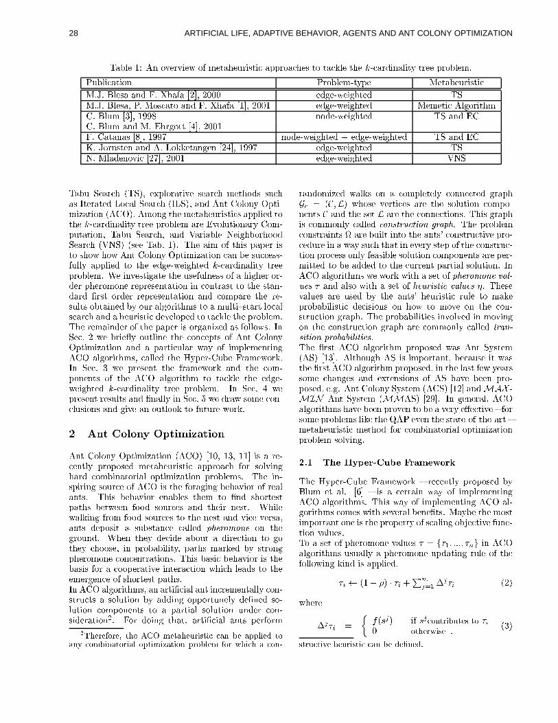
Table 1: An overview of metaheuristic approaches to tackle the k-cardinality tree problem.
Publication Problem-type Metaheuristic
M.J. Blesa and F. Xhafa [2], 2000 edge-weighted TSM.J. Blesa, P. Moscato and F. Xhafa [1], 2001 edge-weighted Memetic AlgorithmC. Blum [3], 1998 node-weighted TS and ECC. Blum and M. Ehrgott [4], 2001F. Catanas [8], 1997 node-weighted + edge-weighted TS and ECK. Jornsten and A. Lokketangen [24], 1997 edge-weighted TSN. Mladenovic [27], 2001 edge-weighted VNS
Tabu Search (TS), explorative search methods suchas Iterated Local Search (ILS), and Ant Colony Opti-mization (ACO). Among the metaheuristics applied tothe k-cardinality tree problem are Evolutionary Com-putation, Tabu Search, and Variable NeighborhoodSearch (VNS) (see Tab. 1). The aim of this paper isto show how Ant Colony Optimization can be success-fully applied to the edge-weighted k-cardinality treeproblem. We investigate the usefulness of a higher or-der pheromone representation in contrast to the stan-dard �rst order representation and compare the re-sults obtained by our algorithms to a multi{start localsearch and a heuristic developed to tackle the problem.The remainder of the paper is organized as follows. InSec. 2 we brie y outline the concepts of Ant ColonyOptimization and a particular way of implementingACO algorithms, called the Hyper-Cube Framework.In Sec. 3 we present the framework and the com-ponents of the ACO algorithm to tackle the edge-weighted k-cardinality tree problem. In Sec. 4 wepresent results and �nally in Sec. 5 we draw some con-clusions and give an outlook to future work.
2 Ant Colony Optimization
Ant Colony Optimization (ACO) [10, 13, 11] is a re-cently proposed metaheuristic approach for solvinghard combinatorial optimization problems. The in-spiring source of ACO is the foraging behavior of realants. This behavior enables them to �nd shortestpaths between food sources and their nest. Whilewalking from food sources to the nest and vice versa,ants deposit a substance called pheromone on theground. When they decide about a direction to gothey choose, in probability, paths marked by strongpheromone concentrations. This basic behavior is thebasis for a cooperative interaction which leads to theemergence of shortest paths.In ACO algorithms, an arti�cial ant incrementally con-structs a solution by adding opportunely de�ned so-lution components to a partial solution under con-sideration2. For doing that, arti�cial ants perform
2Therefore, the ACO metaheuristic can be applied toany combinatorial optimization problem for which a con-
randomized walks on a completely connected graphGc = (C;L) whose vertices are the solution compo-nents C and the set L are the connections. This graphis commonly called construction graph. The problemconstraints are built into the ants' constructive pro-cedure in a way such that in every step of the construc-tion process only feasible solution components are per-mitted to be added to the current partial solution. InACO algorithms we work with a set of pheromone val-
ues � and also with a set of heuristic values �. Thesevalues are used by the ants' heuristic rule to makeprobabilistic decisions on how to move on the con-struction graph. The probabilities involved in movingon the construction graph are commonly called tran-
sition probabilities.The �rst ACO algorithm proposed was Ant System(AS) [13]. Although AS is important, because it wasthe �rst ACO algorithm proposed, in the last few yearssome changes and extensions of AS have been pro-posed, e.g. Ant Colony System (ACS) [12] andMAX -MIN Ant System (MMAS) [29]. In general, ACOalgorithms have been proven to be a very e�ective { forsome problems like the QAP even the state-of-the-art {metaheuristic method for combinatorial optimizationproblem solving.
2.1 The Hyper-Cube Framework
The Hyper-Cube Framework { recently proposed byBlum et al. [6] { is a certain way of implementingACO algorithms. This way of implementing ACO al-gorithms comes with several bene�ts. Maybe the mostimportant one is the property of scaling objective func-tion values.To a set of pheromone values � = f�1; :::; �ng in ACOalgorithms usually a pheromone updating rule of thefollowing kind is applied.
�i (1� �) � �i +Pns
j=1�j�i (2)
where
�j�i =
�f(sj) if sjcontributes to �i0 otherwise :
(3)
structive heuristic can be de�ned.
28 ARTIFICIAL LIFE, ADAPTIVE BEHAVIOR, AGENTS AND ANT COLONY OPTIMIZATION
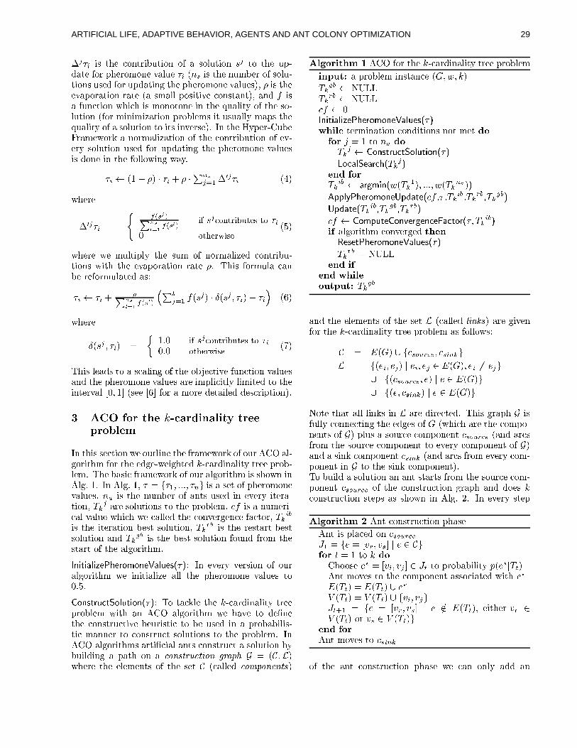
�j�i is the contribution of a solution sj to the up-date for pheromone value �i (ns is the number of solu-tions used for updating the pheromone values), � is theevaporation rate (a small positive constant), and f isa function which is monotone in the quality of the so-lution (for minimization problems it usually maps thequality of a solution to its inverse). In the Hyper-CubeFramework a normalization of the contribution of ev-ery solution used for updating the pheromone valuesis done in the following way.
�i (1� �) � �i + � �Pns
j=1�0j�i (4)
where
�0j�i =
(f(sj)Pns
l=1f(sl)
if sjcontributes to �i
0 otherwise(5)
where we multiply the sum of normalized contribu-tions with the evaporation rate �. This formula canbe reformulated as:
�i �i +�P
ns
l=1f(sl)
�Pk
j=1 f(sj) � Æ(sj ; �i)� �i
�(6)
where
Æ(sj ; �i) =
�1:0 if sjcontributes to �i0:0 otherwise
(7)
This leads to a scaling of the objective function valuesand the pheromone values are implicitly limited to theinterval [0; 1] (see [6] for a more detailed description).
3 ACO for the k-cardinality treeproblem
In this section we outline the framework of our ACO al-gorithm for the edge-weighted k-cardinality tree prob-lem. The basic framework of our algorithm is shown inAlg. 1. In Alg. 1, � = f�1; :::; �ng is a set of pheromonevalues, na is the number of ants used in every itera-tion, Tk
j are solutions to the problem, cf is a numeri-cal value which we called the convergence factor, Tk
ib
is the iteration best solution, Tkrb is the restart best
solution and Tkgb is the best solution found from the
start of the algorithm.
InitializePheromoneValues(�): In every version of ouralgorithm we initialize all the pheromone values to0:5.
ConstructSolution(�): To tackle the k-cardinality treeproblem with an ACO algorithm we have to de�nethe constructive heuristic to be used in a probabilis-tic manner to construct solutions to the problem. InACO algorithms arti�cial ants construct a solution bybuilding a path on a construction graph G = (C;L)where the elements of the set C (called components)
Algorithm 1 ACO for the k-cardinality tree problem
input: a problem instance (G;w; k)
Tkgb NULL
Tkrb NULL
cf 0InitializePheromoneValues(�)while termination conditions not met dofor j = 1 to na doTk
j ConstructSolution(�)
LocalSearch(Tkj)
end forTk
ib argmin(w(Tk1); :::; w(Tk
na))
ApplyPheromoneUpdate(cf ,� ,Tkib,Tk
rb,Tkgb)
Update(Tkib,Tk
gb,Tkrb)
cf ComputeConvergenceFactor(�; Tkib)
if algorithm converged thenResetPheromoneValues(�)
Tkrb = NULL
end ifend whileoutput: Tk
gb
and the elements of the set L (called links) are givenfor the k-cardinality tree problem as follows:
C = E(G) [ fcsource; csinkgL = f(ei; ej) j ei; ej 2 E(G); ei 6= ejg
[ f(csource; e) j e 2 E(G)g[ f(e; csink) j e 2 E(G)g
Note that all links in L are directed. This graph G isfully connecting the edges of G (which are the compo-nents of G) plus a source component csource (and arcsfrom the source component to every component of G)and a sink component csink (and arcs from every com-ponent in G to the sink component).To build a solution an ant starts from the source com-ponent csource of the construction graph and does kconstruction steps as shown in Alg. 2. In every step
Algorithm 2 Ant construction phase
Ant is placed on csourceJ1 = fe = [vr; vs] j e 2 Cgfor t = 1 to k doChoose e? = [vi; vj ] 2 Jt to probability p(e?jTt)Ant moves to the component associated with e?
E(Tt) = E(Tt) [ e?V (Tt) = V (Tt) [ fvi; vjgJt+1 = fe = [vr; vs] j e =2 E(Tt); either vr 2V (Tt) or vs 2 V (Tt)g
end forAnt moves to csink
of the ant construction phase we can only add an
29ARTIFICIAL LIFE, ADAPTIVE BEHAVIOR, AGENTS AND ANT COLONY OPTIMIZATION
edge e = [vi; vj ] to the partial k-cardinality tree Tt(t 2 f1; k�1g) if exactly one of the two nodes incidentwith this edge (vi, or vj) is already in the node setV (Tt) of Tt. The generation of the transition prob-abilities p(ejTt) for all e 2 Jt is dependent on thepheromone representation to be explained in the fol-lowing.There are a number of design decisions to be madewhen developing an ACO algorithm to tackle a com-binatorial optimization problem. One of the most cru-cial decisions is the choice of a pheromone model. Forthe TSP for example it is a fairly obvious choice toput a pheromone value on every link between a pair ofcities. For other combinatorial optimization problemsthe choice is not as obvious as for the TSP (see [28]for MAX-SAT, or [7] for FOP Shop scheduling). Oftenthis problem can be stated as the problem of assigningpheromone values to the decision variables themselves(�rst order pheromone values) or to subsets of decisionvariables (higher order pheromone values). In the fol-lowing we present two di�erent pheromone representa-tions (models) for the edge-weighted k-cardinality treeproblem.
1) Pheromone values on decision variables: This�rst pheromone model (called PH1storder further on)is the most simple choice of a pheromone represen-tation for the edge-weighted k-cardinality tree prob-lem. To every edge ei 2 E(G)3 we have associateda pheromone value �ei . Therefore, if jE(G)j = m wehave m pheromone values. The probabilities p(eijTt)for the edges in set Jt of the ant construction phaseto be chosen by the ant (called transition probabili-ties) are determined as follows. If t = 1 the transitionprobabilities are
p(eijT1) =( �eiP
el2J1�el
: if ei 2 J10 : otherwise
(8)
where J1 is the set of operations allowed to be sched-uled next (see Alg. 2). As a good edge (an edge with alow weight) is not necessarily a good starting point forbuilding a low weight k-cardinality tree, we decidednot to use any heuristic information in this formula.This is di�erent for the next k � 1 construction steps.For t > 1 the transition probabilities are
p(eijTt) =
8<:
�ei �1
w(ei)Pel2Jt
�el �1
w(el)
: if ei 2 Jt0 : otherwise
(9)
This means that for the second and consecutive stepsthe distribution given by the pheromone values is in- uenced by the weights of the edges. Low edge weightsresult in a higher probability to be chosen by the ants
3We consider the edges of graph G to be the decisionvariables of the problem.
and the other way around. With this pheromone repre-sentation the algorithm tries to learn for every edge thedesirability of having it in a solution. This pheromonemodel doesn't take into account any dependencies be-tween decision variables.
2) Pheromone values on pairs of decision vari-ables: This pheromone model (called PH2ndorder fur-ther on) takes into account dependencies between deci-sion variables. To every pair < ei; ej > (where ei 6= ej)of edges in E(G) we have associated a pheromone value�<ei;ej> (where �<ei;ej> and �<ej ;ei> are the same).We also use the pheromone values of the pheromonemodel PH1storder for the �rst construction step (whent = 1). Therefore, in this model we have m+(m2�m)pheromone values. If t = 1 the transition probabilitiesp(eijT1) are generated as shown in equation (8). Ift > 1 the transition probabilities p(eijTt; t) are gener-ated as follows:8>><>>:
�Pej2E(Tt)
�<ej;ei>
�� 1
w(ei)Pel2Jt
�Pej2E(Tt)
�<ej;el>
�� 1
w(el)
: if ei 2 Jt
0 : otherwise
(10)where Jt is as described above. With this pheromonerepresentation the algorithm tries to learn for everypair of edges the desirability of having them together ina solution. As we have pheromones on pairs of edges,this pheromone model takes into account all �rst orderdependencies between decision variables.
LocalSearch(Tkj): The most important ingredient of
a local search method is the neighborhood function.Let Tk be a k-cardinality tree. The neighborhoodNSwap(Tk) of a k-cardinality tree Tk consists of allk-cardinality trees which can be generated from Tk bycutting o� one of the leaf edges e from Tk and addingone edge from the neighborhood of Tk n e. This neigh-borhood function has the advantage to be easy to com-pute, but it is probably coming with the disadvantageof quite a few low quality local minima. However wedecided to use this simple neighborhood function ina steepest descent local search (best improvement) inorder not to spend a too high percentage of the com-putation time on the local search.
ApplyPheromoneUpdate(cf ,� ,Tkib,Tk
rb,Tkgb): For up-
dating the pheromone values we are using a so-calledonline delayed pheromone update rule. We always use3 di�erent solutions for updating the pheromone val-ues4, the best solution found in the current iterationTk
ib, the restart best solution Tkrb and the best solu-
tion found since the start of the algorithm Tkgb. In
contrast to the usual updating rule of the Hyper-CubeFramework as shown in equation (6), in our updatingrule the in uence of each on of these 3 solutions is de-pendent one the state of convergence of the algorithm
4Note that a similar scheme was used in [29].
30 ARTIFICIAL LIFE, ADAPTIVE BEHAVIOR, AGENTS AND ANT COLONY OPTIMIZATION
(given by the convergence factor cf) rather than bythe quality of the solutions themselves. First we com-pute an update value �e for every edge e 2 E(G) inthe following way.
�e �ibÆ(Tkib; e)+�rbÆ(Tk
rb; e)+�gbÆ(Tkgb; e) (11)
where �ib is the in uence weight of Tkib, �rb the in u-
ence weight of Tkrb, �gb the in uence weight of Tk
gb
and �ib+�rb+�gb = 1:0. The Æ-function is de�ned asfollows.
Æ(Tk; ei) =
�1:0 if ei 2 E(Tk)0:0 otherwise
(12)
To the pheromone values �ei of pheromone modelPH1storder we then apply the following update rule.
�ei �ei + � � (�ei � �ei) (13)
To the pheromone values �<ei;ej> of the pheromonemodel PH2ndorder we apply basically the samepheromone update rule. We compute for every or-dered pair of edges < ei; ej > the value �<ei;ej> byusing in equation (11) the following Æ-function.
Æ(Tk; �<ei;ej>) =
�1:0 if ei; ej 2 E(Tk)0:0 otherwise
(14)
Then for updating the pheromone values we use thefollowing rule.
�<ei;ej> �<ei;ej> + � ���<ei;ej> � �<ei;ej>
�(15)
Depending on the convergence factor cf the in uenceof every one of these 3 solutions on the pheromoneupdate is determined. The convergence factor cf is avalue providing an estimate about the state of conver-gence of the system. The convergence factor is com-puted in the following way.
cf =
Pe2E(G)
Æ(Tkib;e)�(1:0��e)
k(16)
where we use the Æ-function de�ned in equation (12).As by using the Hyper-Cube Framework for updatingthe pheromone values, the pheromone values can onlyassume values between 0:0 and 1:0 (see [6]) it obviouslyholds that cf also only can assume values between 0:0and 1:0. It is also clear that if cf is close to 0:0 thesystem is in a state where the probability to producesolution Tk
ib is close to 1 and therefore the probabil-ity to produce a solution di�erent to Tk
ib is close to0. This is what we informally call the state of conver-gence for our system.From experience gathered with the algorithm we chosethe schedule of settings for values �,�ib, �rb and �gbas shown in Tab. 2. In the following we give an inter-pretation of the choice of parameters shown in Tab. 2.
At the beginning of the search process the evapora-tion rate (which is in the Hyper-Cube Framework moreappropriately called learning rate) is set to the value0:15, because at the beginning of the search there is noneed to be very careful. The algorithm should ratherdrift around in the search space to get a kind of globalperspective. Also the in uence of the best solutionfound in an iteration is quite high, which also sup-ports the algorithm drifting through the search space.Once the algorithm starts converging (cf falls below0:3) we decrease the learning rate (in order to performa more careful search) and increase the in uence of thebest solution found since the restart of the algorithm.Once the algorithm is near to the state of convergenceonly the restart best solution is used to update thepheromone values and we decrease the learning rateeven more in the hope to �nd a better solution nearthe restart best solution. Before the algorithm is com-pletely converged we use the best solution found sincethe start of the algorithm to update the pheromonevalues. This action basically results in a shift of theprobability distribution given by the pheromone val-ues toward the best solution found. The reason behindthat is the hope to �nd a better solution in-betweentwo good solutions which are the restart best and theoverall best solution in this case. This idea is verysimilar to ideas we can �nd in Path Relinking [22] forexample.
Update(Tkib,Tk
rb,Tkgb): In this procedure we replace
the old solution Tkrb with Tk
ib if w(Tkib) < w(Tk
rb).
We do the same for Tkgb.
ComputeConvergenceFactor(�; Tkib): The convergence
factor cf is re-computed in every iteration accordingto equation (16).
ResetPheromoneValues(�): In this procedure we resetall pheromone values �e to the start value 0:5.
4 Test results
We chose three di�erent problem instances for a pre-liminary testing of our algorithms. Two of them arecomplete grid graphs5 with 10 rows and 10 columnswhich sums up to 100 nodes and 180 edges. Thesegraphs are called 10x10 1.gg and 10x10 2.gg in the fol-lowing. The weights of the nodes were randomly gen-erated using a uniform distribution on the integers be-tween 1 and 100. There are two motivations for choos-ing grid graphs for testing our algorithms. Problemsin practice are often modeled as grid graphs (e.g., theoil-�eld leasing problem in [23]). Also, it was observedin earlier publications (see [3]) that the problem is con-siderably harder to solve in grid graphs compared tounstructured graphs. Additionally we chose one of the
5No edges or nodes are missing in the grid.
31ARTIFICIAL LIFE, ADAPTIVE BEHAVIOR, AGENTS AND ANT COLONY OPTIMIZATION
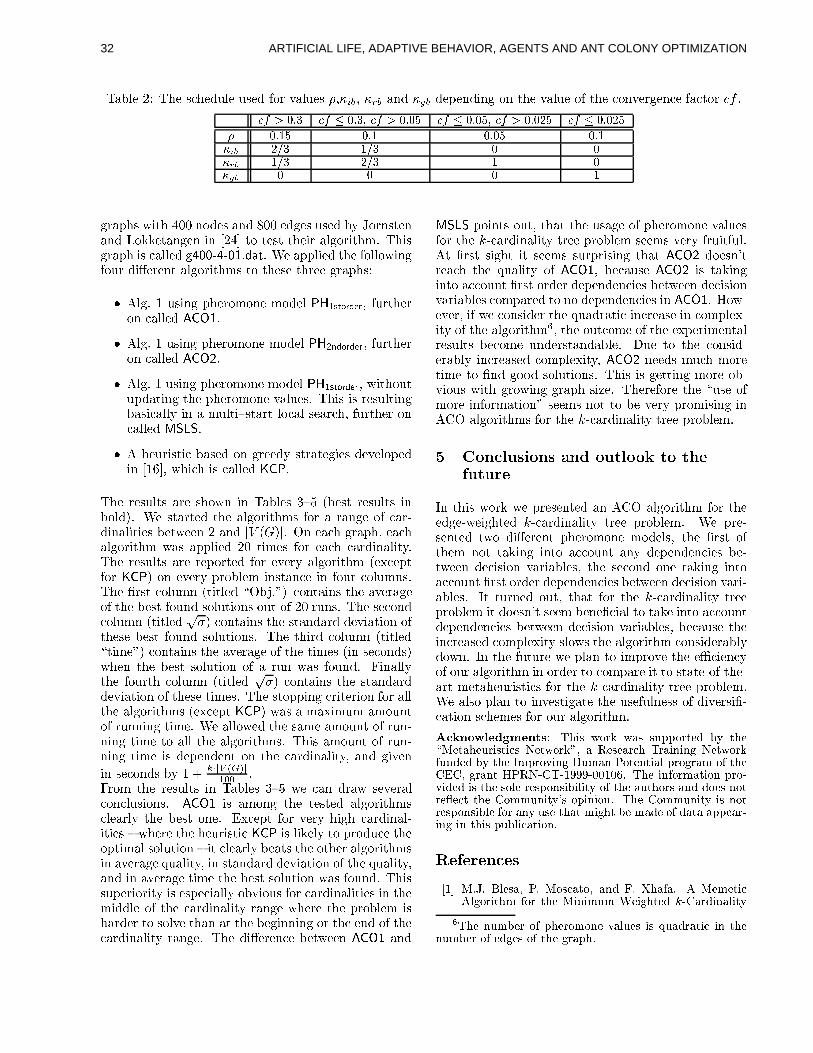
Table 2: The schedule used for values �,�ib, �rb and �gb depending on the value of the convergence factor cf .
cf > 0:3 cf � 0:3, cf > 0:05 cf � 0:05, cf > 0:025 cf � 0:025
� 0:15 0:1 0:05 0:1�ib 2=3 1=3 0 0�rb 1=3 2=3 1 0�gb 0 0 0 1
graphs with 400 nodes and 800 edges used by Jornstenand Lokketangen in [24] to test their algorithm. Thisgraph is called g400-4-01.dat. We applied the followingfour di�erent algorithms to these three graphs:
� Alg. 1 using pheromone model PH1storder, furtheron called ACO1.
� Alg. 1 using pheromone model PH2ndorder, furtheron called ACO2.
� Alg. 1 using pheromone model PH1storder, withoutupdating the pheromone values. This is resultingbasically in a multi{start local search, further oncalled MSLS.
� A heuristic based on greedy strategies developedin [16], which is called KCP.
The results are shown in Tables 3{5 (best results inbold). We started the algorithms for a range of car-dinalities between 2 and jV (G)j. On each graph, eachalgorithm was applied 20 times for each cardinality.The results are reported for every algorithm (exceptfor KCP) on every problem instance in four columns.The �rst column (titled \Obj.") contains the averageof the best found solutions out of 20 runs. The secondcolumn (titled
p�) contains the standard deviation of
these best found solutions. The third column (titled\time") contains the average of the times (in seconds)when the best solution of a run was found. Finallythe fourth column (titled
p�) contains the standard
deviation of these times. The stopping criterion for allthe algorithms (except KCP) was a maximum amountof running time. We allowed the same amount of run-ning time to all the algorithms. This amount of run-ning time is dependent on the cardinality, and given
in seconds by 1 +k�jV (G)j
100 .From the results in Tables 3{5 we can draw severalconclusions. ACO1 is among the tested algorithmsclearly the best one. Except for very high cardinal-ities { where the heuristic KCP is likely to produce theoptimal solution { it clearly beats the other algorithmsin average quality, in standard deviation of the quality,and in average time the best solution was found. Thissuperiority is especially obvious for cardinalities in themiddle of the cardinality range where the problem isharder to solve than at the beginning or the end of thecardinality range. The di�erence between ACO1 and
MSLS points out, that the usage of pheromone valuesfor the k-cardinality tree problem seems very fruitful.At �rst sight it seems surprising that ACO2 doesn'treach the quality of ACO1, because ACO2 is takinginto account �rst order dependencies between decisionvariables compared to no dependencies in ACO1. How-ever, if we consider the quadratic increase in complex-ity of the algorithm6, the outcome of the experimentalresults become understandable. Due to the consid-erably increased complexity, ACO2 needs much moretime to �nd good solutions. This is getting more ob-vious with growing graph size. Therefore the \use ofmore information" seems not to be very promising inACO algorithms for the k-cardinality tree problem.
5 Conclusions and outlook to thefuture
In this work we presented an ACO algorithm for theedge-weighted k-cardinality tree problem. We pre-sented two di�erent pheromone models, the �rst ofthem not taking into account any dependencies be-tween decision variables, the second one taking intoaccount �rst order dependencies between decision vari-ables. It turned out, that for the k-cardinality treeproblem it doesn't seem bene�cial to take into accountdependencies between decision variables, because theincreased complexity slows the algorithm considerablydown. In the future we plan to improve the eÆciencyof our algorithm in order to compare it to state-of-the-art metaheuristics for the k-cardinality tree problem.We also plan to investigate the usefulness of diversi�-cation schemes for our algorithm.
Acknowledgments: This work was supported by the\Metaheuristics Network", a Research Training Networkfunded by the Improving Human Potential program of theCEC, grant HPRN-CT-1999-00106. The information pro-vided is the sole responsibility of the authors and does notre ect the Community's opinion. The Community is notresponsible for any use that might be made of data appear-ing in this publication.
References
[1] M.J. Blesa, P. Moscato, and F. Xhafa. A MemeticAlgorithm for the Minimum Weighted k-Cardinality
6The number of pheromone values is quadratic in thenumber of edges of the graph.
32 ARTIFICIAL LIFE, ADAPTIVE BEHAVIOR, AGENTS AND ANT COLONY OPTIMIZATION
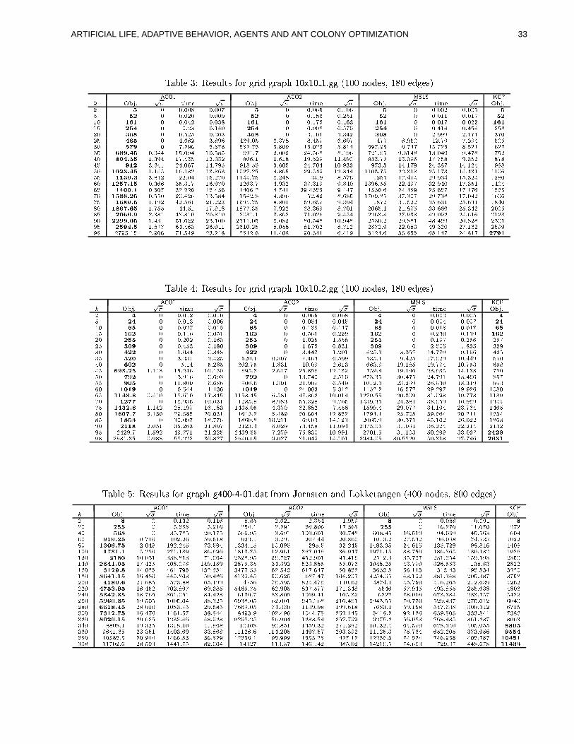
Table 3: Results for grid graph 10x10 1.gg (100 nodes, 180 edges)
ACO1 ACO2 MSLS KCP
k Obj.p� time
p� Obj.
p� time
p� Obj.
p� time
p� Obj.
2 5 0 0.008 0.007 5 0 0.065 0.106 5 0 0.002 0.005 5
5 52 0 0.020 0.009 52 0 0.186 0.251 52 0 0.011 0.017 52
10 161 0 0.042 0.038 161 0 0.175 0.163 161 0 0.017 0.022 161
15 254 0 0.23 0.140 254 0 0.998 0.579 254 0 0.414 0.454 25820 368 0 0.525 0.363 368 0 3.101 3.342 368 0 2.999 2.171 370
25 465 0 4.662 3.896 469.05 6.378 8.457 6.607 477 6.950 12.79 7.294 50530 579 0 7.296 5.378 582.75 3.809 15.023 8.814 597.95 6.747 15.725 8.521 62735 689.45 0.944 15.094 10.585 691.7 2.002 24.568 8.196 721.65 9.3148 13.049 9.478 75240 804.55 1.394 17.435 12.332 806.1 1.618 19.529 11.490 853.75 13.396 17.758 9.352 87845 912 3.641 24.067 14.795 918.55 3.605 24.704 10.933 973.3 14.179 24.387 14.124 98850 1023.45 1.145 16.132 13.863 1027.25 4.865 29.549 12.344 1103.75 22.318 25.173 14.431 110655 1139.3 3.812 22.04 15.270 1144.75 6.248 34.9 8.576 1253 17.474 29.934 15.324 1280
60 1257.15 0.366 35.317 16.970 1263.7 4.932 37.319 9.840 1396.55 22.497 32.940 17.351 140465 1400.1 0.307 32.226 15.456 1406.2 4.741 39.4555 9.147 1556.6 24.489 25.657 17.176 156570 1538.25 0.550 29.426 13.584 1542.8 4.396 52.42 8.685 1709.85 37.307 29.738 17.042 169675 1689.5 1.192 42.561 21.223 1694.75 8.801 59.657 9.304 1872 31.522 35.631 25.631 1840
80 1867.65 1.755 44.51 17.818 1877.35 7.922 68.369 8.701 2065.1 21.875 33.666 25.342 200585 2066.9 2.381 48.310 20.819 2081.1 7.362 71.026 9.454 2263.4 27.933 42.992 24.616 212890 2299.05 1.431 51.622 23.100 2311.05 6.082 80.548 10.948 2530.2 29.881 48.499 20.828 230195 2594.5 1.877 64.463 26.011 2610.25 8.058 81.702 8.712 2872.9 22.083 49.320 27.162 259998 2795.15 2.906 71.549 23.218 2812.6 11.408 90.541 6.419 3124.6 35.858 68.147 24.817 2791
Table 4: Results for grid graph 10x10 2.gg (100 nodes, 180 edges)
ACO1 ACO2 MSLS KCP
k Obj.p� time
p� Obj.
p� time
p� Obj.
p� time
p� Obj.
2 4 0 0.012 0.010 4 0 0.065 0.068 4 0 0.003 0.005 4
5 24 0 0.013 0.006 24 0 0.054 0.045 24 0 0.004 0.007 24
10 65 0 0.027 0.015 65 0 0.138 0.147 65 0 0.018 0.017 65
15 162 0 0.116 0.051 162 0 0.561 0.229 162 0 0.230 0.139 162
20 255 0 0.202 0.163 255 0 1.025 1.558 255 0 0.197 0.256 257
25 309 0 0.453 0.180 309 0 1.675 0.831 309 0 2.505 1.835 32930 422 0 1.034 0.348 422 0 3.447 1.201 425.3 3.357 14.779 9.166 425
35 520 0 3.331 3.425 520.1 0.307 7.463 6.599 535.1 9.425 17.029 10.449 57040 602 0 5.14 5.285 602.75 1.831 10.09 2.613 663.9 19.185 19.774 10.753 65845 693.25 1.118 15.246 10.150 695.3 2.617 25.856 12.139 759.4 19.146 23.635 14.133 780
50 792 0 3.916 0.693 792 0 13.740 2.510 873.35 30.475 24.791 13.466 85755 905 0 11.800 6.686 906.6 1.391 21.907 6.549 1012.3 23.299 26.930 18.319 97360 1019 0 6.544 1.136 1019 0 24.003 5.312 1152.2 16.577 29.297 19.926 1080
65 1148.8 0.410 18.610 17.345 1153.45 6.581 47.362 10.014 1279.55 20.309 31.098 19.773 118970 1277 0 16.936 10.631 1285.8 8.983 55.328 9.765 1439.35 24.381 38.059 16.969 1344
75 1432.6 1.142 28.197 16.183 1435.05 4.370 62.882 7.456 1599.4 29.077 34.194 23.764 1465
80 1607.7 3.130 29.585 20.031 1615.2 8.489 60.664 12.852 1794.1 25.708 39.664 20.211 163485 1853 0 30.097 18.776 1860.8 10.211 69.03 14.123 2065.9 30.371 45.102 26.022 1863
90 2118 2.051 35.263 21.807 2123.4 6.029 73.458 11.994 2375.05 31.091 36.224 22.214 213295 2429.7 1.592 49.771 21.225 2439.55 7.279 75.830 10.991 2701.5 31.103 50.298 33.037 2429
98 2631.35 0.988 58.222 30.827 2640.65 9.027 81.049 14.101 2934.05 30.5829 50.318 27.746 2631
Table 5: Results for graph g400-4-01.dat from Jornsten and Lokketangen (400 nodes, 800 edges)
ACO1 ACO2 MSLS KCP
k Obj.p� time
p� Obj.
p� time
p� Obj.
p� time
p� Obj.
2 8 0 0.132 0.116 8.85 2.621 2.354 1.959 8 0 0.088 0.091 8
20 253 0 5.388 5.916 254.1 2.291 36.806 17.368 253 0 16.270 11.070 272
40 563 0 35.785 20.175 566.95 3.691 100.601 30.748 608.45 16.519 94.069 45.563 60460 919.25 0.716 102.26 59.518 923.1 3.291 207.44 20.860 1013.2 27.532 96.098 74.733 102280 1306.75 2.048 192.245 73.594 1334.15 10.095 295.5 32.245 1483.35 24.615 135.729 98.816 1408
100 1731.1 5.280 271.189 86.696 1817.75 12.961 367.046 36.947 1971.15 33.750 186.865 130.132 1926
120 2180 10.031 338.813 71.064 2328.95 26.727 452.901 41.416 2512.3 35.797 231.954 159.193 2350140 2641.05 17.425 408.078 149.159 2875.35 34.392 523.885 55.076 3048.25 43.770 326.553 138.83 2822
160 3129.8 14.028 461.798 132.681 3477.55 62.543 617.647 80.852 3653.8 56.113 313.43 195.834 3220180 3641.15 16.480 445.803 50.486 4139.45 50.625 687.47 104.207 4254.95 43.192 381.348 205.387 3758200 4180.6 21.685 573.88 65.199 4756 76.595 824.476 110.62 4874.1 45.750 416.265 212.639 4262
220 4753.95 16.452 702.897 69.385 5465.75 62.905 837.577 171.348 5546 57.945 493.855 255.638 4806240 5342.85 18.765 861.051 84.423 6176.7 83.805 1009.41 105.39 6227 78.016 673.384 233.757 5429260 5960.35 19.505 1005.04 38.325 6938.05 62.001 945.168 216.461 6943.55 70.770 529.437 275.012 6040280 6618.45 28.010 1083.75 29.585 7669.05 74.339 1139.98 199.618 7683.1 59.158 547.638 309.312 6715300 7312.75 16.476 1161.57 38.844 8493.9 102.496 1044.78 252.145 8418.2 92.126 659.805 333.841 7386
320 8029.15 20.625 1232.46 48.928 9298.25 56.904 1283.54 257.799 9275.2 56.083 768.435 361.237 8063340 8808.1 19.325 1318.16 41.868 10168 90.851 1359.32 271.292 10132.4 64.570 678.346 405.055 8805
360 9641.65 23.351 1403.69 33.868 11126.6 114.205 1497.57 293.392 11125.3 75.764 652.205 373.956 9554
380 10585.5 20.914 1466.83 36.829 12336.1 95.999 1555.28 427.12 12256.3 74.524 746.958 405.787 10451
398 11702.6 28.593 1441.75 82.004 14327 113.37 1461.42 385.02 14216.5 74.663 729.97 448.678 11433
33ARTIFICIAL LIFE, ADAPTIVE BEHAVIOR, AGENTS AND ANT COLONY OPTIMIZATION
Tree Subgraph Problem. In Proceedings of the Meta-heuristics International Conference MIC'2001, vol-ume 1, pages 85{90, Porto, Portugal, July 2001.
[2] M.J. Blesa and F. Xhafa. A C++ Implementationof Tabu Search for k-Cardinality Tree Problem basedon Generic Programming and Component Reuse. Inc/o tranSIT GmbH, editor, Net.ObjectDsays 2000Tagungsband, pages 648{652, Erfurt, Germany, 2000.Net.ObjectDays-Forum.
[3] C. Blum. Optimality criteria and local search meth-ods for node-weighted k-cardinality tree and subgraphproblems. Master's thesis, Department of Mathemat-ics, University of Kaiserslautern, Germany, 1998. InGerman.
[4] C. Blum and M. Ehrgott. Local search algorithmsfor the k-cardinality tree problem. Technical Re-port TR/IRIDIA/2001-12, IRIDIA, Universit�e Librede Bruxelles, Belgium, 2001. submitted to DiscreteApplied Mathematics.
[5] C. Blum and A. Roli. Metaheuristics in combinatorialoptimization: Overview and conceptual comparison.Technical Report TR/IRIDIA/2001-13, IRIDIA, Uni-versit�e Libre de Bruxelles, Belgium, 2001.
[6] C. Blum, A. Roli, and M. Dorigo. HC-ACO: Thehyper-cube framework for ant colony optimization. InProceedings of Metaheuristics International Confer-ence MIC'2001, pages 399{403, Porto, Portugal, July2001.
[7] C. Blum and M. Sampels. Ant Colony Optimizationfor FOP Shop scheduling: a case study on di�erentpheromone representations. Accepted for presentationat the Congress on Evolutionary Computation, CEC2002, May 2002.
[8] F. Catanas. Heuristics for the p-minimal spanning treeproblem. Technical report, Centre for QuantitativeFinance, Imperial College, London, UK, 1997.
[9] S.Y. Cheung and A. Kumar. EÆcient quorumcastrouting algorithms. In Proceedings of INFOCOM'94,Los Alamitos, USA, 1994. IEEE Society Press.
[10] M. Dorigo. Optimization, Learning and Natural Al-gorithms (in Italian). PhD thesis, DEI, Politecnico diMilano,Italy, 1992. pp. 140.
[11] M. Dorigo, G. Di Caro, and L. M. Gambardella. Antalgorithms for discrete optimization. Arti�cial Life,5(2):137{172, 1999.
[12] M. Dorigo and L. M. Gambardella. Ant Colony Sys-tem: A cooperative learning approach to the travelingsalesman problem. IEEE Transactions on Evolution-ary Computation, 1(1):53{66, 1997.
[13] M. Dorigo, V. Maniezzo, and A. Colorni. Ant System:Optimization by a colony of cooperating agents. IEEETransactions on Systems, Man and Cybernetics - PartB, 26(1):29{41, 1996.
[14] T. Dudas, B. Klinz, and G.J. Woeginger. The compu-tational complexity of the k-minimum spanning treeproblem in graded matrices. Computers and Mathe-matics with Applications, 36:61{67, 1998.
[15] M. Ehrgott and J. Freitag. K TREE /K SUBGRAPH: A program package for minimalweighted k-cardinality-trees and -subgraphs. Euro-pean Journal of Operational Research, 1(93):214{225,1996. code available at http://www.mathematik.uni-kl.de/~wwwwi/WWWWI/ORSEP/contents.html.
[16] M. Ehrgott, J. Freitag, H.W. Hamacher, and F. Maf-�oli. Heuristics for the k-cardinality tree and sub-graph problem. Asia Paci�c Journal of OperationalResearch, 14(1):87{114, 1997.
[17] M. Fischetti, H.W. Hamacher, K. Joernsten, andF. MaÆoli. Weighted k-cardinality trees: Complexityand polyhedral structure. Networks, 24:11{21, 1994.
[18] L.R. Foulds and H.W. Hamacher. A new integerprogramming approach to (restricted) facilities layoutproblems allowing exible facility shapes. TechnicalReport 1992-3, University of Waikato, Department ofManagement Science, 1992.
[19] J. Freitag. Minimal k-cardinality trees. Master's the-sis, Department of Mathematics, University of Kaiser-slautern, Germany, 1993. in german.
[20] N. Garg. A 3-approximation for the minimum treespanning k vertices. In Proceedings of the 37th AnnualIEEE Symposium on Foundations of Computer Sci-ence, pages 302{309, Los Alamitos, USA, 1996. IEEESociety Press.
[21] N. Garg and D. Hochbaum. An O(log k) approxima-tion algorithm for the k minimum spanning tree prob-lem in the plane. Algorithmica, 18:111{121, 1997.
[22] F. Glover, M. Laguna, and R. Marti. Fundamentalsof scatter search and path relinking. Control and Cy-bernetics, 29(3):653{684, 2000.
[23] H.W. Hamacher and K. Joernsten. Optimal relin-quishment according to the Norwegian petrol law: Acombinatorial optimization approach. Technical Re-port No. 7/93, Norwegian School of Economics andBusiness Administration, Bergen, Norway, 1993.
[24] K. Joernsten and A. L�kketangen. Tabu search forweighted k-cardinality trees. Asia Paci�c Journal ofOperational Research, 14(2):9{26, 1997.
[25] F. MaÆoli. Finding a best subtree of a tree. TechnicalReport 91.041, Politecnico di Milano, Dipartimento diElettronica, Italy, 1991.
[26] M.V. Marathe, R. Ravi, S.S. Ravi, D.J. Rosenkrantz,and R. Sundaram. Spanning trees { short or small.SIAM Journal on Discrete Mathematics, 9(2):178{200, 1996.
[27] N. Mladenovic. Variable neighborhood search forthe k-cardinality tree problem. In Proceedings of theMetaheuristics International Conference MIC'2001,2001.
[28] A. Roli, C. Blum, and M. Dorigo. ACO for maximalconstraint satisfaction problems. In Proceedings ofMetaheuristics International Conference MIC'2001,pages 187{191, Porto, Portugal, July 2001.
[29] T. St�utzle and H. H. Hoos. MAX -MIN ant system.Future Generation Computer Systems, 16(8):889{914,2000.
34 ARTIFICIAL LIFE, ADAPTIVE BEHAVIOR, AGENTS AND ANT COLONY OPTIMIZATION
On a Particularity in Model-Based Search
Christian Blum�, Michael Sampels
IRIDIAUniversit�e Libre de Bruxelles
Brussels, Belgiume-mail: fcblum,[email protected]
tel: (32) 2 650 3168, fax: (32) 2 650 2715
Mark Zlochin
Department of Computer ScienceTechnion { Israel Institute of Technology,
Haifa, Israele-mail: [email protected]
tel: (972) 4 829 4948
Abstract
Giving positive feedback to good solutionsis a common base technique in model-basedsearch algorithms, such as Ant Colony Op-timization, Estimation of Distribution Algo-rithms, or Neural Networks. In particular,the reinforcement of components of good so-lutions by positive feedback is known as asuccessful technique in tackling hard combi-natorial optimization problems. We show bya simple model-based search algorithm forthe node-weighted k-cardinality tree prob-lem that this strategy doesn't guaranteesteadily increasing performance of the algo-rithm in general. It is rather possible that forsome \problem"-"probabilistic model" com-binations the average performance of the sys-tem is decreasing and even the average proba-bility of sampling good solutions is decreasingover time. The result is proven analyticallyand the consequences are studied in some em-pirical case studies.
1 Introduction
Model-based search (MBS) [10] algorithms are increas-ingly popular methods for solving combinatorial opti-mization problems. In MBS algorithms, such as AntColony Optimization (ACO) [2] or Estimation of Dis-tribution Algorithms (EDAs)1 [7, 8], candidate solu-tions are generated using a parametrized probabilisticmodel that is updated using the previously seen solu-tions in such a way that the search will concentrate inthe regions of the search space containing high qual-ity solutions. In particular, reinforcment of solutioncomponents depending on the solution quality is an
�Corresponding author1EDAs are covering several algorithms emerging from
the �eld of Evolutionary Computation.
important factor in the development of heuristics totackle hard combinatorial optimization problems. Itis assumed that good solutions don't occur sporadi-cally, but consist of good solution components. Tolearn which components contribute to good solutionscan help to assemble them to better solutions. In gen-eral, a model-based search approach attempts to solvean optimization problem by repeating the followingtwo steps:
� Candidate solutions are constructed using someparametrized probabilistic model, that is, aparametrized probability distribution over the so-lution space.
� The candidate solutions are used to modify themodel in a way that is deemed to bias future sam-pling toward low cost solutions.
Often it is implicitly assumed that the average per-formace of model-based algorithms is increasing overtime. However, during empirical investigations of anAnt Colony Optimization Algorithm for the GroupShop scheduling problem2 we observed that for someof the probabiltistic models chosen the performanceof the system was decreasing over time. This trig-gered us to explore \problem"-"probabilistic model"combinations where the expected performance of amodel-based search algorithm decreases over time. Asa test case we chose the node-weighted k-cardinalitytree problem, an NP -hard combinatorial optimizationproblem.
The paper is organized as follows. In Sec. 2 we brie ypresent the node-weighted k-cardinality tree problem.In Sec. 3 we outline a simple model-based search al-gorithm for the k-cardinality tree problem. Section 4contains the analytical analysis of the system for a
2Group Shop scheduling is a general formulation ofscheduling problems covering Job Shop scheduling andOpen Shop scheduling
35ARTIFICIAL LIFE, ADAPTIVE BEHAVIOR, AGENTS AND ANT COLONY OPTIMIZATION
small problem instance. Section 5 deals with empiri-cal results and Sec. 6 �nally o�ers conclusions and anoutlook to the future.
2 The node-weighted k-cardinalitytree problem
The k-cardinality tree problem is a combinatorial op-timization problem that generalizes the well{knownminimum weight spanning tree problem. It consistsin �nding in a node- or edge-weighted graph a subtreewith exactly k edges, such that the sum of the weightsis minimal. Due to various applications, such as oil-�eld leasing [6], facility layout [4], quorum-cast routing[1] and telecommunications [5], it has gained consid-erable interest in recent years. In this paper we dealwith the k-cardinality tree problem in node-weightedgraphs. The problem can be formally de�ned as fol-lows. Let G = (V;E) be a graph (where jV j = n andjEj = m) with a weight function w : V ! IN on thenodes. We denote the set of all k-cardinality trees inG by Tk. Then the node-weighted problem (G;w; k) isto �nd a k-cardinality tree Tk 2 Tk that minimizes
w(Tk) =P
v2V (Tk)w(v): (1)
The general problem is NP -hard, and in [9] NP -completeness results have been obtained for grid andsplit graphs.
3 A simple MBS algorithm for thek-cardinality tree problem
In this section we brie y outline a simple model-basedsearch algorithm based on positive feedback for thek-cardinality tree problem. It is constructed in astraight-forward manner and it is representative forthe class of model-based algorithms. The pseudo-codefor this algorithm is shown in Alg. 1. In Alg. 1, T i
k
Algorithm 1 A model-based algorithm for the node-weighted k-cardinality tree problem
input: A problem instance (G;w; k)InitializeModelParameters(�)while termination conditions not met dofor i = 1; :::; ns doT ik ConstructSolution(�)
end for
ApplyModelParameterUpdate(� ,T 1k ,...,T
nsk )
end while
output: A k-cardinality tree T bestk
denotes the ith solution constructed in the current it-eration, ns � 1 is the total number of solutions con-structed in every iteration, and � = f�v1 ; :::; �vng is
a set of model parameters. After initialization of themodel parameters, in every step of the algorithm nssolutions are constructed using the current values ofthe model parameters. These solutions are then usedto update the model parameters which are de�ned asfollows: To every node v 2 V (G) we have associated amodel parameter �v . The components of Alg. 1 are tobe explained in more detail in the following.
InitializeModelParameters(�): At the beginning of thealgorithm, the model parameters �v are all initializedto the same small numerical value c > 0.
ConstructSolution(�): In order to construct solutionsto the problem we have to formalize how to use themodel parameter values to construct solutions3. Forconstructing a solution, k + 1 construction steps aredone as shown in Alg. 2. In every step of the construc-
Algorithm 2 Solution construction
V (T0) ; and E(T0) ;J0 V (G)Choose v? 2 J0 with probability p(v? j T0)fSee eqn.(2)gV (T0) V (T0) [ v
?
for t = 1 to k do
Jt fv 2 V (G) n V (Tt�1) j 9 e[vr; v] 2E(G) with vr 2 V (Tt�1)gChoose v? 2 Jt with probability p(v? j Tt)Find an edge e connecting v? with TtE(Tt) E(Tt�1) [ fegV (Tt) V (Tt�1) [ fv
?gend for
tion phase, we can only add a node v to the partialk-cardinality tree Tt (t 2 f1; :::; k � 1g) if there is anedge e 2 E(G) that connects one of the nodes in Ttwith v. The probabilities p(vi j Tt) for all vi 2 Jt arethen de�ned in the following way.
p(vi j Tt) =
( �viPv2Jt
�vif vi 2 Jt
0 otherwise(2)
where Jt is the set of nodes allowed to be added nextto the partial k-cardinality tree Tt (see Alg. 2).
ApplyModelParameterUpdate(� ,T 1k ,. . . ,T
nsk ): Once
all solutions of an iteration are constructed, a rule up-dating the model parameters is applied. For the setof model parameters f�v1 ; :::; �vng this update rule isde�ned as:
�vi (1� �) � �vi +1ns�Pns
j=1�� jvi (3)
3We have to de�ne a method of using the model tosample the search space.
36 ARTIFICIAL LIFE, ADAPTIVE BEHAVIOR, AGENTS AND ANT COLONY OPTIMIZATION
where
�� jvi =
(1
w(Tj
k)
if vi 2 Tj
0 otherwise :(4)
In (4), T j is the jth solution produced in the cur-rent iteration, w(T j) is the quality of solution T j and0 < � < 1 is a parameter supporting the intensi�cationof the search (a similar parameter in ACO algorithmsis called evaporation rate). This update rule is simi-lar to update rules used in Ant Colony Optimizationand some other population-based methods from the�eld of Evolutionary Computation. It should lead toan increase of model parameter values associated withsolution components which have been found in betterquality solutions compared with other solution com-ponents, hence increasing the expected performanc ofthe algorithm over time. In the following section wewill prove that this expectation is not always met inpractice.
4 A counterexample: Decreasingaverage performance of a MBSalgorithm over time
In this section we choose a small problem instanceof the k-cardinality tree problem and we show thatthe expected performance of Alg. 1 is decreasing.The problem instance under consideration is shownin Fig. 1. It shows an undirected graph G = (V;E)formally de�ned as follows.
V (G) = fv1; v2; v3; v4g (5)
E(G) = fev1;v2 ; ev2;v3 ; ev3;v4g (6)
w(vi) = wi > 0; for i = 1; :::; 4 (7)
For the weights we choose
w2; w3 > w1; w4; (8)
and for the sake of simplicity we choose
w1 = w4and w2 = w3 : (9)
In graph G we want to solve the 1-cardinality treeproblem with the model-based search algorithm out-lined in the last section. In G we can �nd 3 di�erent1-cardinality trees:
T a with V (T a) = fv1; v2g; E(Ta) = fev1;v2g
) w(T a) = w1 + w2
T b with V (T b) = fv2; v3g; E(Tb) = fev2;v3g
) w(T b) = w2 + w3
T c with V (T c) = fv3; v4g; E(Tc) = fev3;v4g
) w(T c) = w3 + w4
Because of (8) and (9) it holds that
w(T a) = w(T c) < w(T b): (10)
Therefore T a and T c are both optimal solutions ofthis problem instance and T b is the worst solution.With model parameter values �v1(t); :::; �v4 (t) at dis-crete time steps t = 0; 1; :::, the probabilities pa(t),pb(t) and pc(t) to construct solutions T a, T b and T c
are the following:
pa(t) =�v1 (t)P4
i=1�vi (t)
+�v2 (t)P4
i=1�vi (t)
��v1 (t)
�v1 (t)+�v3 (t)(11)
pb(t) =�v2 (t)P4
i=1�vi (t)
��v3 (t)
�v1 (t)+�v3 (t)
+�v3 (t)P4
i=1�vi (t)
��v2 (t)
�v2 (t)+�v4 (t)(12)
pc(t) =�v4 (t)P4
i=1�vi (t)
+�v3 (t)P4
i=1�vi (t)
��v4 (t)
�v4 (t)+�v2 (t)(13)
We use the notation pvi for the probability of node vito be found in a solution constructed. These probabil-ities are obviously the following ones.
pv1(t) = pa(t) (14)
pv2(t) = pa(t) + pb(t) (15)
pv3(t) = pb(t) + pc(t) (16)
pv4(t) = pc(t) (17)
Let us now examine the evolution of the model param-eter values over time.
Evolution of �v1 over time: After every construc-tion step there are two possibilities. Either v1 is apart of the constructed solution, or it is not. Then theexpected value of �v1 at time t+ 1 is the following.
E(�v1(t+ 1)) =�(1� �) � �v1(t) +
1w1+w2
�� pv1(t)
Æ ��Æ ��Æ ��Æ ��
w1 w2 w3 w4
v1 v2 v3 v4
Figure 1: The problem instance consists of four nodesv1, v2, v3 and v4, connected by three edges. The nodeweights of the nodes vi are indicated by wi.
37ARTIFICIAL LIFE, ADAPTIVE BEHAVIOR, AGENTS AND ANT COLONY OPTIMIZATION
+ (1� �) � �v1(t) � (1� pv1(t))
= �v1(t)pv1(t)� ��v1(t)pv1(t)
+ 1w1+w2
pv1(t) + �v1(t)� �v1(t)pv1(t)
� ��v1(t) + ��v1(t)pv1(t)
= �v1(t) +�
1w1+w2
� pv1(t)� ��v1(t)�
As pv1(t) = pa(t) we get
E(�v1 (t+ 1)) = �v1(t) +�
1w1+w2
� pa(t)� ��v1(t)�(18)
Evolution of �v2 over time: After every construc-tion step there is { as above for �v1 { the possibilitythat v2 is a part of the solution constructed. But thereare also two di�erent solutions v2 can be part of. Inthe following pa+b will stand for pa + pb, w1+2 willstand for w1 + w2, and w2+3 will stand for w2 + w3.
E(�v2 (t+ 1)) =�(1� �) � �v2(t) +
pa(t)
pa+b(t)1
w1+2+
pb(t)
pa+b(t)1
w2+3
�� pv2(t)
+ (1� �) � �v2(t) � (1� pv2(t))
As pv2 = pa+b we get
E(�v2(t+ 1)) = (1� �) � �v2(t) � pa+b(t) +pa(t)
w1+2
+pb(t)
w2+3+ (1� �) �v2(t) (1� pa+b(t))
= �v2(t)pa+b(t)� ��v2(t)pa+b(t)
+pa(t)
w1+2+
pb(t)
w2+3+ �v2(t)
� �v2(t)pa+b(t)� ��v2(t)
+ ��v2(t)pa+b(t) :
Therefore we get
E(�v2 (t+ 1)) = �v2(t) +�pa(t)
w1+2+
pb(t)
w2+3� ��v2(t)
�:
(19)For the evolution of �v3and �v4 the computations arethe same as for �v2 and �v1 respectively. Consequently
E(�v3(t+ 1)) = �v3(t) +�pc(t)
w3+4+
pb(t)
w2+3� ��v3(t)
�(20)
and
E(�v4(t+ 1)) = �v4(t) +�
1w3+4
� pc(t)� ��v4(t)�
:
(21)It is common practice in Genetic Algorithm researchto analyse the bahaviour of the algorithm with in�nitepopulation size. Therefore, in the following we con-sider the limit case of ns !1. In this case the law oflarge number says that the actual value of �vi(t) con-verges in probability to the expected value. Therefore
we use �vi(t) instead of E(�vi(t)) in the following.The algorithm at time t = 0 starts with �v1(0) =�v2(0) = �v3(0) = �v4(0) = c > 0. With (9), (11)and (13) it follows that pa(0) = pc(0). With (18) and(21) it follows that �v1(1) = �v4(1) and with (19) and(20) it follows that �v2(1) = �v3(1). In turn this implieswith (9) that pa(1) = pc(1). By induction it followsthat for t � 0
�v1(t) = �v4(t) and �v2(t) = �v3(t) (22)
pa(t) = pc(t) : (23)
This means that the evolution of �v1(t) is equal to theevolution of �v4 (t), the evolution of �v2(t) is equal tothe evolution of �v3(t) and the probability to producetree T a is equal to the probability to produce tree T c.This allows us to simplify equations (11), (12) and(13) expressing everything in terms of �v1(t) and �v2(t).Substituting �v3(t) by �v2(t) and �v4(t) by �v1(t) inequations (11), (12) and (13) results in
pa(t) = pc(t) =�v1 (t)
2(�v1 (t)+�v2 (t))��1 +
�v2 (t)
�v1 (t)+�v2 (t)
�(24)
pb(t) =�v2 (t)
�v1 (t)+�v2 (t)�
�v2 (t)
�v1 (t)+�v2 (t): (25)
Theorem 1 In the settings described above the fol-lowing holds. The probability pb(t) to produce T b (theworst 1-cardinality tree to be found in graph G as de-�ned in equations (5){(9)) is increasing from the �rststep of Alg. 1 onward as long as
1w2+3
pb(t) � �v1 >1
w1+2� pa(t) (�v2 � �v1) : (26)
Proof: In the following we will write �v1+v2(t) for�v1(t) + �v2(t). Then
pb(t+ 1) > pb(t),�
�v2 (t)+�pa(t)
w1+2+
pb(t)
w2+3���v2 (t)
��v1+v2 (t)+
�2pa(t)
w1+2+
pb(t)
w2+3��(�v1+v2 (t))
��2
>��v2 (t)
�v1+v2 (t)
�2, (taking the square root)�
�v2(t) +�pa(t)
w1+2+
pb(t)
w2+3� ��v2(t)
��� (�v1+v2(t))
>
�v2(t) ���v1+v2(t) +
�2pa(t)
w1+2+
pb(t)
w2+3� �(�v1+v2(t))
��,
�v2(t)�v1(t) + (�v2(t))2+
pa(t)
w1+2�v1 (t) +
pa(t)
w1+2�v2(t)
+pb(t)
w2+3�v1(t) +
pb(t)
w2+3�v2(t)� ��v2(t)�v1(t)� � (�v2 (t))
2
>
�v2(t)�v1 (t) + (�v2(t))2+
2pa(t)
w1+2�v2(t) +
pb(t)
w2+3�v2 (t)
���v2(t)�v1 (t)� � (�v2(t))2
,1
w2+3pb(t) � �v1 >
1w1+2
� pa(t) (�v2 � �v1) :
38 ARTIFICIAL LIFE, ADAPTIVE BEHAVIOR, AGENTS AND ANT COLONY OPTIMIZATION
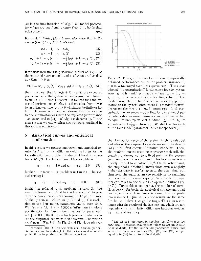
As in the �rst iteration of Alg. 1 all model parame-ter values are equal and greater than 0, it holds thatpb(1) > pb(0). qed
Remark 1 With (22) it is now also clear that in thecase pb(t+ 1) > pb(t) it holds that
pa(t+ 1) < pa(t); (27)
pc(t+ 1) < pc(t); (28)
pa(t+ 1)� pa(t) = � 12(pb(t+ 1)� pb(t)) ; (29)
pc(t+ 1)� pc(t) = � 12(pb(t+ 1)� pb(t)) :(30)
If we now measure the performance P(t) of Alg. 1 asthe expected average quality of a solution produced atany time t � 0 as
P(t) = w1+2 � pa(t) +w2+3 � pb(t) +w3+4 � pc(t); (31)
then it is clear that for pb(t+ 1) > pb(t) the expectedperformance of the system is decreasing from time t
to time t+1. Using Theorem 1 it follows that the ex-pected performance of Alg. 1 is decreasing from t = 0to an unknown time tstop > 0 which may be �nite or in-�nite. To summarize, we have shown that it is possibleto �nd circumstances where the expected performance{ as formalized in (31) { of Alg. 1 is decreasing. In thenext section we will con�rm the outcomes outlined inthis section empirically.
5 Analytical curves and empiricalcon�rmation
In this section we present analytical and empirical re-sults for Alg. 1 on two di�erent weight settings for thek-cardinality tree problem instance de�ned in equa-tions (5){(9). The �rst setting of the weights is
w1 = w4 = 1:0 and w2 = w3 = 2:0 (32)
further on referred to as problem instance 1. The sec-ond setting is
w1 = w4 = 1:0 and w2 = w3 = 100:0 (33)
further on referred to as problem instance 2. Weused the formulas derived in the last section4 to pro-duce the analytical curves showing (i) the performanceof the system as de�ned in (31), and (ii) the evolu-tion of the four model parameter values over time.We also run Alg. 1 with 10000 solution constructionsper iteration for four di�erent values for parameter� 2 f0:5; 0:1; 0:05; 0:01g on both problem instances tosee the empirical behavior of the system. The resultsare shown in Fig. 3{5. In Fig. 3 and Fig. 4, we observe
4Formulas (18){(21) for the evolution of model param-eter values, and formulas (11){(13) for the evolution of theprobabilities to produce the di�erent solutions.
3
3.1
3.2
3.3
3.4
3.5
3.6
0 200 400 600 800 1000 1200 1400 1600
aver
age
solu
tion
qual
ity
iteration
perturbation of parameter rho, rho = 0.05
no perturbation0.1% perturbation
1% perturbation10% perturbation
Figure 2: This graph shows four di�erent empiricallyobtained performance curves for problem instance 1,� = 0:05 (averaged over 100 experiments). The curvelabeled \no perturbation" is the curve for the systemstarting with model parameter values �v1 = �v2 =�v3 = �v4 = c, where c is the starting value for themodel parameters. The other curves show the perfor-mance of the system when there is a random pertur-bation on the starting model parameters. 0:1% per-turbation for example means that for every model pa-rameter value we were tossing a coin: this means thatto equal probability we either added 1
1000� c to �vi or
we subtracted 11000� c from �vi . We did that for each
of the four model parameter values independently.
that the performance of the system in the analyticaland also in the empirical case decreases quite drasti-cally in the �rst couple of hundred iterations. Then,the analytic curves seem to converge (with still de-creasing performance) to a �xed point of the system(not being one of the solutions). This �xed point is im-plicitly de�ned by equation (26)5. On the other hand,the empirically obtained curves show even a slightlyhigher decrease in performance at the beginning, butthen near the equilibrium the sensitivity to samplingerrors seems to increase rapidly. As a result, the sys-tem converges to one of the two optimal solutions (Taor Tb). For problem instance 2, the number of itera-tions needed for both, the analytical and the empiricalcurves, to reach there limits is lower than for prob-lem instance 1. Qualitatively the results are the samefor the two di�erent weight settings. This is in accor-dance with the results of the last section, which are notdependent on the relative di�erence between weightsw1 = w4 and w2 = w3.
5This claim is supported by the fact that if we take theanalytically obtained convergence values (exact up to fourdecimal digits) for the four model parameter values andsubstitute them in equations (24), (25) and (26) we getequality in (26) for up to decimal digits.
39ARTIFICIAL LIFE, ADAPTIVE BEHAVIOR, AGENTS AND ANT COLONY OPTIMIZATION
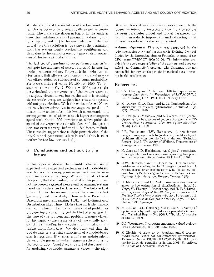
We also compared the evolution of the four model pa-rameter values over time, analytically as well as empir-ically. The graphs are shown in Fig. 5. In the analyticcase, the evolution of model parameter values �v1 and�v4 (resp. �v2 and �v3) is the same whereas in the em-pirical case the evolution is the same at the beginning,until the system nearly reaches the equilibrium andthen, due to the sampling error, begins to drift towardone of the two optimal solutions.
The last set of experiments we performed was to in-vestigate the in uence of perturbations of the startingmodel parameter values. To perturb the model param-eter values (initially set to a constant c), a value 1
x� c
was either added or substracted to equal probability.For x we considered values 10, 100 and 1000. The re-sults are shown in Fig. 2. With x = 1000 (just a slightperturbation) the convergence of the system seems tobe slightly slowed down, but at the end it is reachingthe state of convergence slightly faster than the systemwithout perturbation. With the choice of x = 100, wenotice a bigger advantage in convergence speed in allphases. The choice of x = 10 (which corresponds to astrong perturbation) shows a much higher convergencespeed until about 1000 iterations at which point thespeed of convergence gets really slow and the systemdoes not even converge before the 1500 iteration limit.These results suggest that a slight perturbation of theinitial model parameter values is useful (but it mustneither be too low nor too high).
6 Conclusions and outlook to thefuture
In this paper we showed that { unlike what is usuallyexpected { the expected performance of model-basedsearch algorithms using positive feedback can decreaseover time in certain settings. We want to make clear atthis point, that the results presented in this paper havenot uncovered a general weak point of learning systemsbased on positive feedback as such. We believe thatit is rather in the nature of algorithms such as AntSystem [3] and related algorithms such as PopulationBased Incremental Learning (PBIL) and Estimation ofDistribution algorithms (EDAs) that such phenomenacan occur when applied to a certain kind of problem orproblem instances with a certain kind of structure. Inthe case of the problem and problem instance chosenin this paper we have a structure of two equally goodsolutions competing in the system and a bad solutiontaking pro�t from that. We also point out that theupdate rule is a crucial component of a model-basedsearch algorithm. If we chose a di�erent update rule inthe example presented { for instance a rule only usingthe best solution found since the start of the algorithmfor updating the model parameter values { the algo-
rithm wouldn't show a decreasing performance. In thefuture we intend to investigate into the interactionsbetween parameter model and model parameter up-date rule in order to improve the understanding aboutphenomena related to the one presented.
Acknowledgments: This work was supported by the
\Metaheuristics Network", a Research Training Network
funded by the Improving Human Potential program of the
CEC, grant HPRN-CT-1999-00106. The information pro-
vided is the sole responsibility of the authors and does not
re ect the Community's opinion. The Community is not
responsible for any use that might be made of data appear-
ing in this publication.
References
[1] S.Y. Cheung and A. Kumar. EÆcient quorumcastrouting algorithms. In Proceedings of INFOCOM'94,Los Alamitos, USA, 1994. IEEE Society Press.
[2] M. Dorigo, G. Di Caro, and L. M. Gambardella. Antalgorithms for discrete optimization. Arti�cial Life,5(2):137{172, 1999.
[3] M. Dorigo, V. Maniezzo, and A. Colorni. Ant System:Optimization by a colony of cooperating agents. IEEETransactions on Systems, Man and Cybernetics{PartB, 26(1):29{41, 1996.
[4] L.R. Foulds and H.W. Hamacher. A new integerprogramming approach to (restricted) facilities layoutproblems allowing exible facility shapes. TechnicalReport 1992-3, University of Waikato, Department ofManagement Science, 1992.
[5] N. Garg and D. Hochbaum. An O(log k) approxima-tion algorithm for the k minimum spanning tree prob-lem in the plane. Algorithmica, 18:111{121, 1997.
[6] H.W. Hamacher and K. Joernsten. Optimal relin-quishment according to the Norwegian petrol law: Acombinatorial optimization approach. Technical Re-port No. 7/93, Norwegian School of Economics andBusiness Administration, Bergen, Norway, 1993.
[7] H. M�uhlenbein and G. Paa�. From recombination ofgenes to the estimation of distributions. In H.-M.Voigt, W. Ebeling, I. Rechenberg, and H.-P. Schwefel,editors, Proceedings of the 4th Conference on ParallelProblem Solving from Nature { PPSN IV, volume 1411of Lecture Notes in Computer Science, pages 178{187,Berlin, 1996. Springer.
[8] M. Pelikan, D.E. Goldberg, and F. Lobo. A survey ofoptimization by building and using probabilistic mod-els. Technical Report No. 99018, IlliGAL, Universityof Illinois, 1999.
[9] G.J. Woeginger. Computing maximum valued regions.Acta Cybernetica, 4(10):303{315, 1992.
[10] M. Zlochin, M. Birattari, N. Meuleau, and M. Dorigo.Model-based search for combinatorial optimization.Technical Report TR/IRIDIA/2001-15, IRIDIA, Uni-versit�e Libre de Bruxelles, Belgium, 2001. Submittedto Annals of Operations Research.
40 ARTIFICIAL LIFE, ADAPTIVE BEHAVIOR, AGENTS AND ANT COLONY OPTIMIZATION
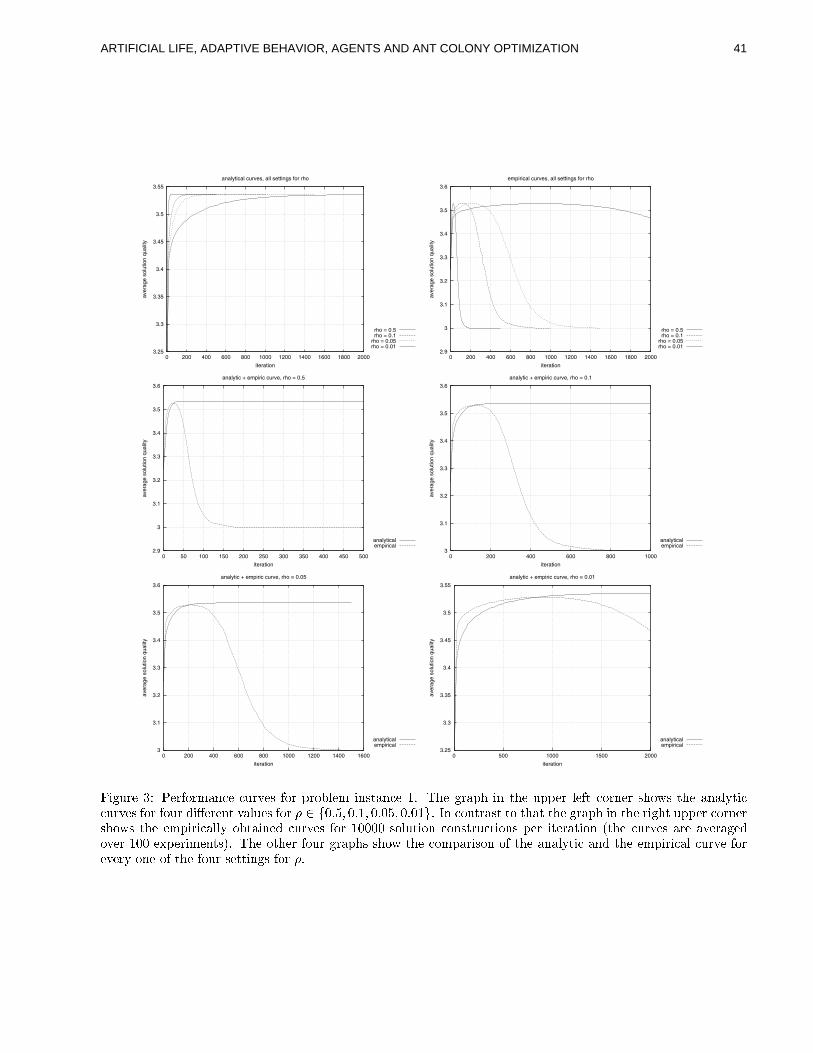
3.25
3.3
3.35
3.4
3.45
3.5
3.55
0 200 400 600 800 1000 1200 1400 1600 1800 2000
aver
age
solu
tion
qual
ity
iteration
analytical curves, all settings for rho
rho = 0.5rho = 0.1
rho = 0.05rho = 0.01
2.9
3
3.1
3.2
3.3
3.4
3.5
3.6
0 200 400 600 800 1000 1200 1400 1600 1800 2000
aver
age
solu
tion
qual
ity
iteration
empirical curves, all settings for rho
rho = 0.5rho = 0.1
rho = 0.05rho = 0.01
2.9
3
3.1
3.2
3.3
3.4
3.5
3.6
0 50 100 150 200 250 300 350 400 450 500
aver
age
solu
tion
qual
ity
iteration
analytic + empiric curve, rho = 0.5
analyticalempirical
3
3.1
3.2
3.3
3.4
3.5
3.6
0 200 400 600 800 1000
aver
age
solu
tion
qual
ity
iteration
analytic + empiric curve, rho = 0.1
analyticalempirical
3
3.1
3.2
3.3
3.4
3.5
3.6
0 200 400 600 800 1000 1200 1400 1600
aver
age
solu
tion
qual
ity
iteration
analytic + empiric curve, rho = 0.05
analyticalempirical
3.25
3.3
3.35
3.4
3.45
3.5
3.55
0 500 1000 1500 2000
aver
age
solu
tion
qual
ity
iteration
analytic + empiric curve, rho = 0.01
analyticalempirical
Figure 3: Performance curves for problem instance 1. The graph in the upper left corner shows the analyticcurves for four di�erent values for � 2 f0:5; 0:1; 0:05; 0:01g. In contrast to that the graph in the right upper cornershows the empirically obtained curves for 10000 solution constructions per iteration (the curves are averagedover 100 experiments). The other four graphs show the comparison of the analytic and the empirical curve forevery one of the four settings for �.
41ARTIFICIAL LIFE, ADAPTIVE BEHAVIOR, AGENTS AND ANT COLONY OPTIMIZATION
124
126
128
130
132
134
136
138
140
0 200 400 600 800 1000 1200 1400 1600 1800 2000
aver
age
solu
tion
qual
ity
iteration
analytical curves, all settings for rho
rho = 0.5rho = 0.1
rho = 0.05rho = 0.01
100
105
110
115
120
125
130
135
140
0 200 400 600 800 1000 1200 1400 1600 1800 2000
aver
age
solu
tion
qual
ity
iteration
empirical curves, all settings for rho
rho = 0.5rho = 0.1
rho = 0.05rho = 0.01
Figure 4: Performance curves for problem instance 2 (higher weights on v2 and v3). The graph on the left showsthe analytic curves for four di�erent values for � 2 f0:5; 0:1; 0:05; 0:01g. In contrast, the graph on the right showsthe empirically obtained curves for 10000 solution constructions per iteration (the curves are averaged over 100experiments).
0
0.5
1
1.5
2
2.5
3
3.5
4
4.5
0 200 400 600 800 1000 1200 1400 1600
mod
el p
aram
eter
val
ue
iteration
evolution of model parameter values, analytic, rho = 0.05
\tau_{1}\tau_{2}\tau_{3}\tau_{4}
0
1
2
3
4
5
6
7
0 200 400 600 800 1000 1200 1400 1600
mod
el p
aram
eter
val
ue
iteration
evolution of model parameter values, empiric, rho = 0.05
\tau_{1}\tau_{2}\tau_{3}\tau_{4}
0
1
2
3
4
5
6
7
0 200 400 600 800 1000 1200 1400 1600
mod
el p
aram
eter
val
ue
iteration
evolution of model parameter values, empiric, rho = 0.05
\tau_{1}\tau_{2}\tau_{3}\tau_{4}
Figure 5: The three graphs show the evolution of the four model parameter values exemplary for problem instance1, � = 0:05. The top graph shows the analytic curves (there are just two curves visible, because the curves for�v1 and �v4 (�v2 and �v3 respectively) are exactly the same). In contrast, the two lower graphs show the evolutionof model parameter values empirically obtained. In the graph on the left the system is converging to solutionTa, and in the graph on the right to the solution Tc.
42 ARTIFICIAL LIFE, ADAPTIVE BEHAVIOR, AGENTS AND ANT COLONY OPTIMIZATION
An Ant System Algorithm for Graph Bisection
Thang N. BuiDept. of Computer Science
Penn State HarrisburgMiddletown, PA 17057
Lisa C. StriteDept. of Computer Science
Penn State HarrisburgMiddletown, PA 17057
Abstract
This paper gives an algorithm for the graphbisection problem using the Ant System (AS)technique. The ant algorithm given in thispaper differs from the usual ant algorithmsin that the individual ant in the system doesnot construct a solution to the problem nora component of the solution directly. Ratherthe collective behavior of the two species ofants in the system induces a solution to theproblem. The algorithm also incorporates lo-cal optimization algorithms to speed up theconvergence rate and to improve the qualityof the solutions. The results achieved by thisalgorithm on several classes of graphs equalthe best known results for the majority ofgraphs tested, and are very close to the bestknown results for the remainder.
1 Introduction
Let G = (V,E) be a graph on n vertices, where nis even. A bisection of G is a partition of the vertexset V into two disjoint sets A,B of equal size, i.e.,A∪B = V,A∩B = ∅, and |A| = |B|. Such a bisectionis denoted by (A,B). The cut size of a bisection (A,B)is the number of edges that have one endpoint in A andthe other endpoint in B. The graph bisection problemis the problem of finding a bisection of minimum cutsize for a given graph. The graph bisection problem iswell-known to be NP-hard [13]. It arises in a wide va-riety of problems including VLSI placement and rout-ing, sparse matrix computation, and processor alloca-tion [6][7][16]. Since the problem is NP-hard, effortshave been concentrated on designing efficient approx-imation algorithms and heuristics for solving it. Inthis paper we use ideas from Ant System (AS) [11] todesign an algorithm for the graph bisection problem.
Our algorithm incorporates several AS features as wellas local optimization techniques and graph preprocess-ing. The algorithm was tested on five classes of graphsranging in size from 500 to 5,252 vertices with averagedegrees from 2 to 36. The results were compared withthe best known results for each graph as well as re-sults from several other heuristic algorithms. For themajority of graphs tested, the algorithm produced thebest known results. For the remaining graphs the re-sults produced by the algorithm are very close to thebest known solutions. A major advantage of this al-gorithm compared to other existing algorithms for thegraph bisection problem is that our algorithm is veryamenable to parallelization.
The rest of the paper is organized as follows. In Sec-tion 2 we provide some background information on thegraph bisection problem and AS. We describe our algo-rithm in Section 3. The performance of the algorithmson the test graphs is described in Section 4 and con-clusions are given Section 5.
2 Preliminaries
2.1 The Graph Bisection Problem
As mentioned above the graph bisection problem isNP-hard and thus we do not expect to have a polyno-mial time algorithm for solving it. For special types ofgraphs there are polynomial time algorithms for solv-ing it exactly, e.g., k-outerplanar graphs, for fixed k,or planar graphs whose optimal bisection is of sizeO(log n) [8]. However, the complexity of the problemon planar graphs remains an open question.
One approach to NP-hard problems is to find efficientapproximation algorithms. Currently, the best knownpolynomial time approximation algorithm for bisectinggraphs can find a solution that is within O(
√n log n) of
the optimal [12]. It has been shown that it is NP-hard
43ARTIFICIAL LIFE, ADAPTIVE BEHAVIOR, AGENTS AND ANT COLONY OPTIMIZATION
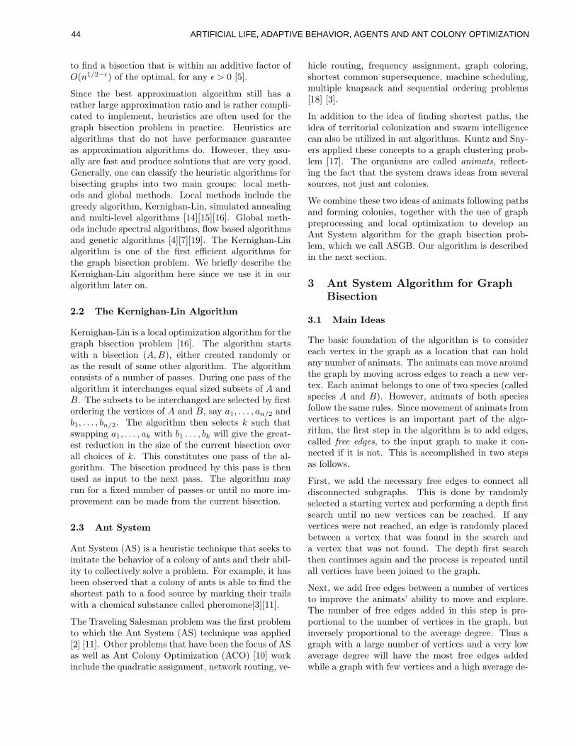
to find a bisection that is within an additive factor ofO(n1/2−ε) of the optimal, for any ε > 0 [5].
Since the best approximation algorithm still has arather large approximation ratio and is rather compli-cated to implement, heuristics are often used for thegraph bisection problem in practice. Heuristics arealgorithms that do not have performance guaranteeas approximation algorithms do. However, they usu-ally are fast and produce solutions that are very good.Generally, one can classify the heuristic algorithms forbisecting graphs into two main groups: local meth-ods and global methods. Local methods include thegreedy algorithm, Kernighan-Lin, simulated annealingand multi-level algorithms [14][15][16]. Global meth-ods include spectral algorithms, flow based algorithmsand genetic algorithms [4][7][19]. The Kernighan-Linalgorithm is one of the first efficient algorithms forthe graph bisection problem. We briefly describe theKernighan-Lin algorithm here since we use it in ouralgorithm later on.
2.2 The Kernighan-Lin Algorithm
Kernighan-Lin is a local optimization algorithm for thegraph bisection problem [16]. The algorithm startswith a bisection (A,B), either created randomly oras the result of some other algorithm. The algorithmconsists of a number of passes. During one pass of thealgorithm it interchanges equal sized subsets of A andB. The subsets to be interchanged are selected by firstordering the vertices of A and B, say a1, . . . , an/2 andb1, . . . , bn/2. The algorithm then selects k such thatswapping a1, . . . , ak with b1 . . . , bk will give the great-est reduction in the size of the current bisection overall choices of k. This constitutes one pass of the al-gorithm. The bisection produced by this pass is thenused as input to the next pass. The algorithm mayrun for a fixed number of passes or until no more im-provement can be made from the current bisection.
2.3 Ant System
Ant System (AS) is a heuristic technique that seeks toimitate the behavior of a colony of ants and their abil-ity to collectively solve a problem. For example, it hasbeen observed that a colony of ants is able to find theshortest path to a food source by marking their trailswith a chemical substance called pheromone[3][11].
The Traveling Salesman problem was the first problemto which the Ant System (AS) technique was applied[2] [11]. Other problems that have been the focus of ASas well as Ant Colony Optimization (ACO) [10] workinclude the quadratic assignment, network routing, ve-
hicle routing, frequency assignment, graph coloring,shortest common supersequence, machine scheduling,multiple knapsack and sequential ordering problems[18] [3].
In addition to the idea of finding shortest paths, theidea of territorial colonization and swarm intelligencecan also be utilized in ant algorithms. Kuntz and Sny-ers applied these concepts to a graph clustering prob-lem [17]. The organisms are called animats, reflect-ing the fact that the system draws ideas from severalsources, not just ant colonies.
We combine these two ideas of animats following pathsand forming colonies, together with the use of graphpreprocessing and local optimization to develop anAnt System algorithm for the graph bisection prob-lem, which we call ASGB. Our algorithm is describedin the next section.
3 Ant System Algorithm for GraphBisection
3.1 Main Ideas
The basic foundation of the algorithm is to considereach vertex in the graph as a location that can holdany number of animats. The animats can move aroundthe graph by moving across edges to reach a new ver-tex. Each animat belongs to one of two species (calledspecies A and B). However, animats of both speciesfollow the same rules. Since movement of animats fromvertices to vertices is an important part of the algo-rithm, the first step in the algorithm is to add edges,called free edges, to the input graph to make it con-nected if it is not. This is accomplished in two stepsas follows.
First, we add the necessary free edges to connect alldisconnected subgraphs. This is done by randomlyselected a starting vertex and performing a depth firstsearch until no new vertices can be reached. If anyvertices were not reached, an edge is randomly placedbetween a vertex that was found in the search anda vertex that was not found. The depth first searchthen continues again and the process is repeated untilall vertices have been joined to the graph.
Next, we add free edges between a number of verticesto improve the animats’ ability to move and explore.The number of free edges added in this step is pro-portional to the number of vertices in the graph, butinversely proportional to the average degree. Thus agraph with a large number of vertices and a very lowaverage degree will have the most free edges addedwhile a graph with few vertices and a high average de-
44 ARTIFICIAL LIFE, ADAPTIVE BEHAVIOR, AGENTS AND ANT COLONY OPTIMIZATION
gree will have the least free edges added. To select thelocations of the free edges, a pool of possible pairs ofvertices are randomly selected. The number of pairsin the pool is τ times the number of pairs that willactually be chosen. The distance between each pair isdetermined, in terms of the minimum number of stepsneeded to move from one vertex to the other, up to acertain maximum distance. Then pairs of vertices areselected randomly from the pool but in proportion tothe distance between them. In other words, a pair ofvertices that is furthest apart has the greatest chanceof being selected.
Once the free edges are added, the animats considerthem in the same manner as regular edges in selectingmoves. However, when the cut size of a partition iscalculated, the free edges are ignored.
The algorithm now starts by distributing α animatson the graph. (Note that the values of all parametersused in the description of the algorithm are given inTable 1.) Their species and location are chosen ran-domly. At any point throughout the algorithm, theconfiguration of animats on the graph constitutes apartition of the graph in the following way. Each ver-tex is considered to be colonized by one species. Ata given time, it is said to be colonized by whicheverspecies that has the greater number of animats on it.Ties are broken in a random order by assigning thevertex to the species that results in a lower cut size.The set of all vertices colonized by each species, calledcolony, makes up one half of the partition. This par-tition is not necessarily a bisection, since one colonymay contain more vertices than the other. Thus, othertechniques are used at certain points in the algorithmto ensure that the final solution is a bisection.
In addition, each vertex can hold pheromone. Thetwo species produce separate types of pheromone, soeach vertex has an amount of A pheromone and Bpheromone.
The idea of the algorithm is for each species of animatsto form a colony consisting of a set of vertices that arehighly connected to each other but highly disconnectedfrom the other colony. The result should be two sets ofvertices that are highly connected amongst themselves,but have few edges going between the two sets.
The ASGB algorithm is divided up into σ sets eachcomprised of γ iterations. In each iteration a percent-age of animats are activated. When an animat is acti-vated, it adds an amount of pheromone to the vertexit is currently at based on conditions at the vertex. Itthen may die with a certain probability or it may re-produce with a certain probability and then moves to
a new vertex. In each iteration, these activations areperformed in parallel. After each iteration, the graphis updated with the new information.
After each set, the configuration of the graph is forcedinto a bisection using a greedy algorithm and a localoptimization algorithm is run to help speed up the con-vergence rate. During each set, the parameters, whichinclude probabilities for activation, death, reproduc-tion and birth are varied. The parameters are variedin such a way that at the beginning of the set, thecolonies change a great deal and by the end of the setthe colonies have converged to a stable configuration.The next set begins at the state where the previousset ended. However, if the animats follow their usualrules immediately, they will not be able to move awayfrom the local optimum that has been reached. So,for all but the initial set, a jolt is performed for a cer-tain number of the first iterations to help move theconfiguration, or distribution of animats on the ver-tices, away from the local optimal solution to whichit had converged. The jolt allows animats to selectmoves randomly instead of following the normal rulesfor movement. The length of the jolt is changed duringthe algorithm. The first jolt lasts for ν iterations andfor subsequent jolts the length decreases linearly untilthe last set where there is no jolt. The idea is thatwith each successive set, the bisection should comecloser to the optimal bisection, and thus shorter andshorter jolts are needed.
After σ sets have been completed, the solution is thebest bisection that has been achieved. This is usuallythe bisection found by the last set; however, occasion-ally the best bisection is found earlier.
In the following subsections we will describe in detailwhat occurs in one iteration, what occurs when ananimat is activated and what occurs between sets. Thefull ASGB algorithm is given in Figure 1.
3.2 Iteration
An iteration of the algorithm consists of a percentageof the animats being activated and then performingthe necessary operations in parallel. The probabilityof an animat being activated changes during the set.At the beginning of the set, more animats are acti-vated during each iteration. By the end of the set,only a small percentage of the animats are activatedin each iteration. The actual probability of activationis a sigmoid-like function. The function starts at amaximum of πamax and ends at πamin.
After the activations of animats have been completed,ε percent of the pheromone on each vertex is evap-
45ARTIFICIAL LIFE, ADAPTIVE BEHAVIOR, AGENTS AND ANT COLONY OPTIMIZATION
Figure 1: An Ant System algorithm for graph bisec-tion
Preprocess the graph to make it connectedRandomly add α animats to graphFor set=1 to σ
For time=1 to γFor each animat do (in parallel):
Activate animat with probability a(time)If activated
Add p(animat, time) pheromone tothe animat’s location
Die with probability πdIf not dead
If animat meets reproduction criteriaThen reproduce with probability πr
If time is in a jolt periodThen select move randomly
Else select move based on pheromoneand connectivity
EndifEndif
Endfor animatEvaporate ε percent of the pheromone from
each vertexEndfor timeConvert configuration to a bisection with
a greedy algorithmRun Kernighan-Lin local optimizationReduce total number of animatsEqualize number of animats in each species
Endfor setReturn best bisection found
orated. This prevents pheromone from building uptoo much and highly populated vertices from beingoveremphasized, which in turn prevents the algorithmfrom converging prematurely.
3.3 Activation of an Animat
When an animat is activated, it deposits pheromoneon its current vertex, dies with a certain probability orreproduces with a certain probability, and then movesto another vertex. These operations are performed bythe animat by using local information to make deci-sions.
3.3.1 Pheromone
The purpose of pheromone is to allow the algorithmto retain a “memory” of good configurations that havebeen found in the past. The formula for the amountof pheromone to be deposited is:
p(a, i) =acolatotal
· iγ
Table 1: Parameter valuesParam. Value Descriptionγ 1000 Number of iterations per setσ 10 Number of setsν 50 Maximum jolt lengthα 10000 Initial number of animatsπamax 0.8 Maximum activation probabilityπamin 0.2 Minimum activation probabilityπd 0.035 Death probabilityβinit 4 Expected number of animats born
in first iterationβfinal 2 Expected number of animats born
in final iterationβrange 50% Percentage range from average
number of animats bornπr 0.01 Reproduction probabilityη 10 Max number of offspring per ani-
matµ 5 Number of moves needed before an-
imat can reproduceψstay 20% Percentage of offspring that stay on
old location when not colonized byanimat’s species
ωpmin 0 Minimum pheromone weightωpmax 1 Maximum pheromone weightωcmin 250 Minimum connection weightωcmax 500 Maximum connection weightπmin 0.1 Minimum probability for moving to
a vertexρ 0.9 Reduction factor for returning to
previous locationψswap 75% Percentage of vertices needed for
swapψmaj 90% Percentage of animats needed for
majorityε 0.2 Evaporation rateλ 1000 Pheromone limitτ 50 Free edge factor
where a is the animat, i is the iteration number, acol isthe number of vertices adjacent to the animat’s currentlocation which are colonized by the animat’s species,and atotal is the total number of vertices adjacent tothe animat’s current location. The idea here is foran animat to deposit more pheromone at a vertex ifthat vertex is highly connected to vertices colonizedby its own species. Also, less pheromone is used inearly iterations to allow for more exploration and morepheromone is used later on to emphasize exploitation.Even though the number of neighbors of a seems torelate more directly to the cut size, the amount ofpheromone deposited is made proportional to the frac-tion acol/atotal, to prevent the amount of pheromoneat any vertex from growing out of control, even withevaporation.
There is also a limit to the amount of pheromone ofeach species that can be stored on a vertex. The limit
46 ARTIFICIAL LIFE, ADAPTIVE BEHAVIOR, AGENTS AND ANT COLONY OPTIMIZATION
for a vertex is the product of the degree of that ver-tex and the pheromone limit parameter (λ). This al-lows densely connected vertices to accumulate morepheromone. The more highly connected a vertex is,the more essential it is that it is colonized by the rightspecies. This is because a mistake on a highly con-nected vertex will mean a much greater cut size.
3.3.2 Death
Next, the animat may be selected to die. The an-imat die with probability πd, which is fixed through-out the algorithm. However, the activation probabilitychanges throughout the set, so that early in the set,more animats are activated, and therefore more ani-mats die early in the set. The purpose of this is tohave shorter life spans in the beginning, which allowsmore turnover and change in the configuration. Laterin the set, the animats live longer and thus there isless change and the solution is able to converge.
3.3.3 Reproduction
If the animat is not selected for death, the algorithmproceeds to the reproduction step. The animat is se-lected for reproduction with fixed probability πr. How-ever, the number of new animats that are produceddepends on time. In the first iteration of a set, the av-erage number of animats born is βinit and it decreaseslinearly over time to βfinal in the last iteration. Thechanging birth rate serves to allow more change in ear-lier iterations, in which animats live for shorter lengthsof time. In later iterations, fewer animats are born, butthey live longer. The actual number of animats born isselected uniformly at random over a range centered onthe average birth rate for the iteration. The numberof animats born can be up to βrange more or less thanthe specified average.
If the vertex on which the parent is located is colonizedby its own species, the offspring animats are all placedon that vertex. However, if the vertex is colonized bythe opposite species, only ψstay percent of the offspringanimats are placed there. The remaining new animatswill be placed on the vertex to which the parent animatmoves in the next step. The rationale is that if theparent animat is already in its own colony but moves toanother vertex, it should leave its offspring behind tohelp maintain the majority on that vertex. However,if the parent’s species is not in majority, it should takemost of its children to the new vertex in which it istrying to create a colony. The parent leaves some ofits offspring behind however, so that some of its speciesremain at the vertex (in case that vertex really should
be part of their colony).
There are two other constraints on reproduction.First, there is a limit to how many offspring an an-imat can produce during its lifetime (η). This valueis fixed throughout the algorithm and is the same foreach animat. Once the limit is reached, the animatcan no longer reproduce. This serves to prevent onespecies from taking over the graph and forcing theother species into extinction.
To prevent a species from overemphasizing a vertexthrough reproduction, the animats are not allowed toreproduce until they have made a set minimum num-ber of moves (µ). This ensures that the graph is ex-plored and that new configurations are created by thereproduction and movement rather than being inhib-ited by these operations.
3.3.4 Movement
An animat can move to any vertex which is connectedto its current location by an edge. There are two fac-tors used to select a move from the set of possiblemoves. For each vertex to which the animat couldmove, the connectivity to other vertices is examined.The animat should move to a vertex that is highly con-nected to other vertices colonized by its own species.This factor gives an indication of the current configura-tion of the graph. In addition, the animat should learnfrom the past and take into account the pheromonethat other animats have deposited. Throughout thecourse of a set, these two factors are weighted differ-ently. Initially, the pheromone is weighted at ωpminwith the weight increasing linearly to ωpmax. Con-versely, the connectivity is weighted at ωcmax to be-gin and decreases linearly to ωcmin. In this way, theconfiguration of the colonies changes greatly in earlyiterations and over time learning is incorporated intothe algorithm. These basic factors drive the animatsto create colonies of highly connected vertices whichare highly disconnected from the vertices colonized bythe opposing species.
These factors are the basis of move selection. Theprobability of moving to an adjacent vertex is propor-tional to the two combined factors. Specifically, thefactors are combined as follows to create a “probabil-ity” of moving to a specific vertex v:
pr(v) = cvc + pvp + πmin
where vc is the number of vertices adjacent to v thatare colonized by the animat’s own species, c is theconnectivity weight and ωcmin ≤ c ≤ ωcmax, vp isthe amount of pheromone of the animat’s species on
47ARTIFICIAL LIFE, ADAPTIVE BEHAVIOR, AGENTS AND ANT COLONY OPTIMIZATION
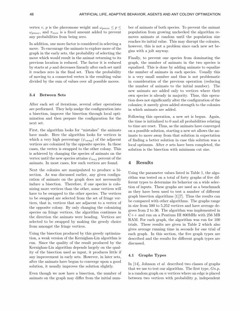
vertex v, p is the pheromone weight and ωpmin ≤ p ≤ωpmax, and πmin is a fixed amount added to preventany probabilities from being zero.
In addition, one more factor is considered in selecting amove. To encourage the animats to explore more of thegraph in the early sets, the probability of selecting themove which would result in the animat returning to itsprevious location is reduced. The factor it is reducedby starts at ρ and decreases linearly after each set untilit reaches zero in the final set. Then the probabilityof moving to a connected vertex is the resulting valuedivided by the sum of values over all possible moves.
3.4 Between Sets
After each set of iterations, several other operationsare performed. They help nudge the configuration intoa bisection, improve the bisection through local opti-mization and then prepare the configuration for thenext set.
First, the algorithm looks for “mistakes” the animatshave made. Here the algorithm looks for vertices inwhich a very high percentage (ψswap) of the adjacentvertices are colonized by the opposite species. In thesecases, the vertex is swapped to the other colony. Thisis achieved by changing the species of animats on thevertex until the new species attains ψmaj percent of theanimats. In most cases, few such vertices are found.
Next the colonies are manipulated to produce a bi-section. As was discussed earlier, any given configu-ration of animats on the graph does not necessarilyinduce a bisection. Therefore, if one species is colo-nizing more vertices than the other, some vertices willhave to be swapped to the other species. The verticesto be swapped are selected from the set of fringe ver-tices, that is, vertices that are adjacent to a vertex ofthe opposite colony. By only changing the colonizingspecies on fringe vertices, the algorithm continues inthe direction the animats were heading. Vertices areselected to be swapped by making the greedy choicefrom amongst the fringe vertices.
Using the bisection produced by this greedy optimiza-tion, a weak version of the Kernighan-Lin algorithm isrun. Since the quality of the result produced by theKernighan-Lin algorithm depends largely on the qual-ity of the bisection used as input, it produces little ifany improvement in early sets. However, in later sets,after the animats have begun to converge upon a goodsolution, it usually improves the solution slightly.
Even though we now have a bisection, the number ofanimats on the graph may differ from the initial num-
ber of animats of both species. To prevent the animatpopulation from growing unchecked the algorithm re-moves animats at random until the population sizereaches its initial value. This may disrupt the colonies,however, this is not a problem since each new set be-gins with a jolt anyway.
Finally, to prevent one species from dominating thegraph, the number of animats in the two species isequalized. This is done by adding animats to equalizethe number of animats in each species. Usually thisis a very small number and thus is not problematicin consideration of the previous operation (reducingthe number of animats to the initial number). Thenew animats are added only to vertices where theirown species is already in majority. Thus, this opera-tion does not significantly alter the configuration of thecolonies; it merely gives added strength to the coloniesin which animats are added.
Following this operation, a new set is begun. Again,the time is initialized to 0 and all probabilities relatingto time are reset. Thus, as the animats have convergedon a possible solution, starting a new set allows the an-imats to move away from that solution in expectationof finding a better solution in case this solution was alocal optimum. After σ sets have been completed, thesolution is the bisection with minimum cut size.
4 Results
Using the parameter values listed in Table 1, the algo-rithm was tested on a total of forty graphs of five dif-ferent types to determine its behavior on a wide selec-tion of inputs. These graphs are used as a benchmarkas they have been used to test a number of differentgraph bisection algorithms [1][7]. Thus the results canbe compared with other algorithms. The graphs rangein size from 500 to 5,252 vertices and have average de-grees from 2 to 36. The algorithm was implemented inC++ and run on a Pentium III 800MHz with 256 MBRAM. For each graph, the algorithm was run for 100trials. These results are given in Table 2 which alsogives average running time in seconds for one trial ofeach graph. In this section, the five graph types aredescribed and the results for different graph types arediscussed.
4.1 Graphs Types
In [14], Johnson et al. described two classes of graphsthat we use to test our algorithm. The first type, Gn.p,is a random graph on n vertices where an edge is placedbetween two vertices with probability p, independent
48 ARTIFICIAL LIFE, ADAPTIVE BEHAVIOR, AGENTS AND ANT COLONY OPTIMIZATION
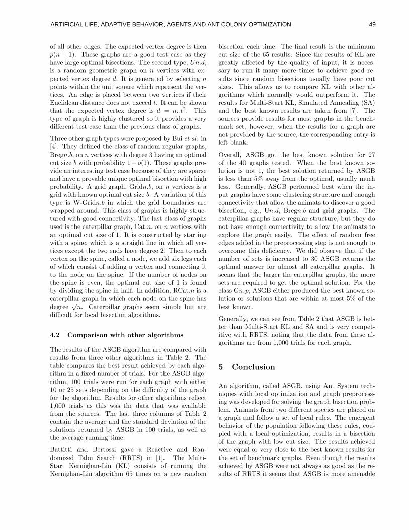
of all other edges. The expected vertex degree is thenp(n − 1). These graphs are a good test case as theyhave large optimal bisections. The second type, Un.d,is a random geometric graph on n vertices with ex-pected vertex degree d. It is generated by selecting npoints within the unit square which represent the ver-tices. An edge is placed between two vertices if theirEuclidean distance does not exceed t. It can be shownthat the expected vertex degree is d = nπt2. Thistype of graph is highly clustered so it provides a verydifferent test case than the previous class of graphs.
Three other graph types were proposed by Bui et al. in[4]. They defined the class of random regular graphs,Bregn.b, on n vertices with degree 3 having an optimalcut size b with probability 1− o(1). These graphs pro-vide an interesting test case because of they are sparseand have a provable unique optimal bisection with highprobability. A grid graph, Gridn.b, on n vertices is agrid with known optimal cut size b. A variation of thistype is W-Gridn.b in which the grid boundaries arewrapped around. This class of graphs is highly struc-tured with good connectivity. The last class of graphsused is the caterpillar graph, Cat.n, on n vertices withan optimal cut size of 1. It is constructed by startingwith a spine, which is a straight line in which all ver-tices except the two ends have degree 2. Then to eachvertex on the spine, called a node, we add six legs eachof which consist of adding a vertex and connecting itto the node on the spine. If the number of nodes onthe spine is even, the optimal cut size of 1 is foundby dividing the spine in half. In addition, RCat.n is acaterpillar graph in which each node on the spine hasdegree
√n. Caterpillar graphs seem simple but are
difficult for local bisection algorithms.
4.2 Comparison with other algorithms
The results of the ASGB algorithm are compared withresults from three other algorithms in Table 2. Thetable compares the best result achieved by each algo-rithm in a fixed number of trials. For the ASGB algo-rithm, 100 trials were run for each graph with either10 or 25 sets depending on the difficulty of the graphfor the algorithm. Results for other algorithms reflect1,000 trials as this was the data that was availablefrom the sources. The last three columns of Table 2contain the average and the standard deviation of thesolutions returned by ASGB in 100 trials, as well asthe average running time.
Battitti and Bertossi gave a Reactive and Ran-domized Tabu Search (RRTS) in [1]. The Multi-Start Kernighan-Lin (KL) consists of running theKernighan-Lin algorithm 65 times on a new random
bisection each time. The final result is the minimumcut size of the 65 results. Since the results of KL aregreatly affected by the quality of input, it is neces-sary to run it many more times to achieve good re-sults since random bisections usually have poor cutsizes. This allows us to compare KL with other al-gorithms which normally would outperform it. Theresults for Multi-Start KL, Simulated Annealing (SA)and the best known results are taken from [7]. Thesources provide results for most graphs in the bench-mark set, however, when the results for a graph arenot provided by the source, the corresponding entry isleft blank.
Overall, ASGB got the best known solution for 27of the 40 graphs tested. When the best known so-lution is not 1, the best solution returned by ASGBis less than 5% away from the optimal, usually muchless. Generally, ASGB performed best when the in-put graphs have some clustering structure and enoughconnectivity that allow the animats to discover a goodbisection, e.g., Un.d, Bregn.b and grid graphs. Thecaterpillar graphs have regular structure, but they donot have enough connectivity to allow the animats toexplore the graph easily. The effect of random freeedges added in the preprocessing step is not enough toovercome this deficiency. We did observe that if thenumber of sets is increased to 30 ASGB returns theoptimal answer for almost all caterpillar graphs. Itseems that the larger the caterpillar graphs, the moresets are required to get the optimal solution. For theclass Gn.p, ASGB either produced the best known so-lution or solutions that are within at most 5% of thebest known.
Generally, we can see from Table 2 that ASGB is bet-ter than Multi-Start KL and SA and is very compet-itive with RRTS, noting that the data from these al-gorithms are from 1,000 trials for each graph.
5 Conclusion
An algorithm, called ASGB, using Ant System tech-niques with local optimization and graph preprocess-ing was developed for solving the graph bisection prob-lem. Animats from two different species are placed ona graph and follow a set of local rules. The emergentbehavior of the population following these rules, cou-pled with a local optimization, results in a bisectionof the graph with low cut size. The results achievedwere equal or very close to the best known results forthe set of benchmark graphs. Even though the resultsachieved by ASGB were not always as good as the re-sults of RRTS it seems that ASGB is more amenable
49ARTIFICIAL LIFE, ADAPTIVE BEHAVIOR, AGENTS AND ANT COLONY OPTIMIZATION
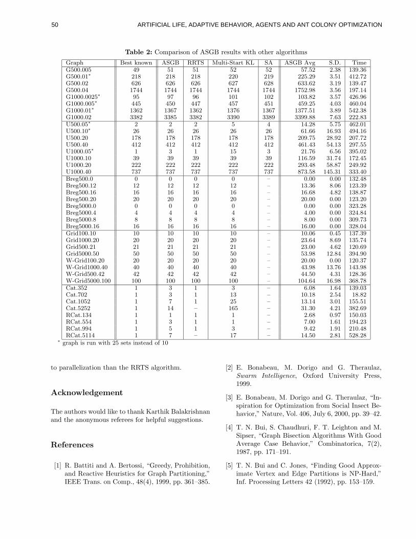
Table 2: Comparison of ASGB results with other algorithms
Graph Best known ASGB RRTS Multi-Start KL SA ASGB Avg S.D. TimeG500.005 49 51 51 52 52 57.52 2.38 139.36G500.01∗ 218 218 218 220 219 225.29 3.51 412.72G500.02 626 626 626 627 628 633.62 3.19 139.47G500.04 1744 1744 1744 1744 1744 1752.98 3.56 197.14G1000.0025∗ 95 97 96 101 102 103.82 3.57 426.96G1000.005∗ 445 450 447 457 451 459.25 4.03 460.04G1000.01∗ 1362 1367 1362 1376 1367 1377.51 3.89 542.38G1000.02 3382 3385 3382 3390 3389 3399.88 7.63 222.83U500.05∗ 2 2 2 5 4 14.28 5.75 462.01U500.10∗ 26 26 26 26 26 61.66 16.93 494.16U500.20 178 178 178 178 178 209.75 28.92 207.72U500.40 412 412 412 412 412 461.43 54.13 297.55U1000.05∗ 1 3 1 15 3 21.76 6.56 395.02U1000.10 39 39 39 39 39 116.59 31.74 172.45U1000.20 222 222 222 222 222 293.48 58.87 249.92U1000.40 737 737 737 737 737 873.58 145.31 333.40Breg500.0 0 0 0 0 – 0.00 0.00 132.48Breg500.12 12 12 12 12 – 13.36 8.06 123.39Breg500.16 16 16 16 16 – 16.68 4.82 138.87Breg500.20 20 20 20 20 – 20.00 0.00 123.20Breg5000.0 0 0 0 0 – 0.00 0.00 323.28Breg5000.4 4 4 4 4 – 4.00 0.00 324.84Breg5000.8 8 8 8 8 – 8.00 0.00 309.73Breg5000.16 16 16 16 16 – 16.00 0.00 328.04Grid100.10 10 10 10 10 – 10.06 0.45 137.39Grid1000.20 20 20 20 20 – 23.64 8.69 135.74Grid500.21 21 21 21 21 – 23.00 4.62 120.69Grid5000.50 50 50 50 50 – 53.98 12.84 394.90W-Grid100.20 20 20 20 20 – 20.00 0.00 120.37W-Grid1000.40 40 40 40 40 – 43.98 13.76 143.98W-Grid500.42 42 42 42 42 – 44.50 4.31 128.36W-Grid5000.100 100 100 100 100 – 104.64 16.98 368.78Cat.352 1 3 1 3 – 6.08 1.64 139.03Cat.702 1 3 1 13 – 10.18 2.54 18.82Cat.1052 1 7 1 25 – 13.14 3.01 155.51Cat.5252 1 14 – 165 – 31.30 4.21 382.69RCat.134 1 1 1 1 – 2.68 0.97 150.03RCat.554 1 3 1 1 – 7.00 1.61 194.23RCat.994 1 5 1 3 – 9.42 1.91 210.48RCat.5114 1 7 – 17 – 14.50 2.81 528.28
∗ graph is run with 25 sets instead of 10
to parallelization than the RRTS algorithm.
Acknowledgement
The authors would like to thank Karthik Balakrishnanand the anonymous referees for helpful suggestions.
References
[1] R. Battiti and A. Bertossi, “Greedy, Prohibition,and Reactive Heuristics for Graph Partitioning,”IEEE Trans. on Comp., 48(4), 1999, pp. 361–385.
[2] E. Bonabeau, M. Dorigo and G. Theraulaz,Swarm Intelligence, Oxford University Press,1999.
[3] E. Bonabeau, M. Dorigo and G. Theraulaz, “In-spiration for Optimization from Social Insect Be-havior,” Nature, Vol. 406, July 6, 2000, pp. 39–42.
[4] T. N. Bui, S. Chaudhuri, F. T. Leighton and M.Sipser, “Graph Bisection Algorithms With GoodAverage Case Behavior,” Combinatorica, 7(2),1987, pp. 171–191.
[5] T. N. Bui and C. Jones, “Finding Good Approx-imate Vertex and Edge Partitions is NP-Hard,”Inf. Processing Letters 42 (1992), pp. 153–159.
50 ARTIFICIAL LIFE, ADAPTIVE BEHAVIOR, AGENTS AND ANT COLONY OPTIMIZATION
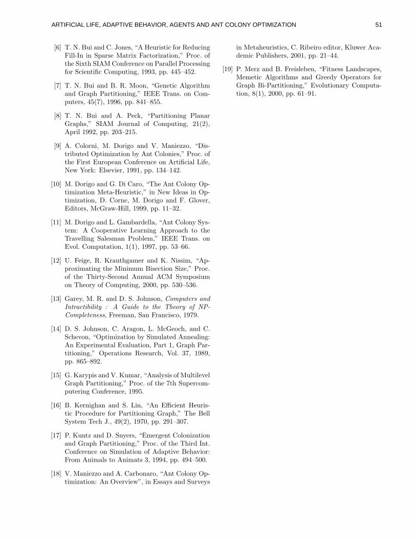
[6] T. N. Bui and C. Jones, “A Heuristic for ReducingFill-In in Sparse Matrix Factorization,” Proc. ofthe Sixth SIAM Conference on Parallel Processingfor Scientific Computing, 1993, pp. 445–452.
[7] T. N. Bui and B. R. Moon, “Genetic Algorithmand Graph Partitioning,” IEEE Trans. on Com-puters, 45(7), 1996, pp. 841–855.
[8] T. N. Bui and A. Peck, “Partitioning PlanarGraphs,” SIAM Journal of Computing, 21(2),April 1992, pp. 203–215.
[9] A. Colorni, M. Dorigo and V. Maniezzo, “Dis-tributed Optimization by Ant Colonies,” Proc. ofthe First European Conference on Artificial Life,New York: Elsevier, 1991, pp. 134–142.
[10] M. Dorigo and G. Di Caro, “The Ant Colony Op-timization Meta-Heuristic,” in New Ideas in Op-timization, D. Corne, M. Dorigo and F. Glover,Editors, McGraw-Hill, 1999, pp. 11–32.
[11] M. Dorigo and L. Gambardella, “Ant Colony Sys-tem: A Cooperative Learning Approach to theTravelling Salesman Problem,” IEEE Trans. onEvol. Computation, 1(1), 1997, pp. 53–66.
[12] U. Feige, R. Krauthgamer and K. Nissim, “Ap-proximating the Minimum Bisection Size,” Proc.of the Thirty-Second Annual ACM Symposiumon Theory of Computing, 2000, pp. 530–536.
[13] Garey, M. R. and D. S. Johnson, Computers andIntractibility : A Guide to the Theory of NP-Completeness, Freeman, San Francisco, 1979.
[14] D. S. Johnson, C. Aragon, L. McGeoch, and C.Schevon, “Optimization by Simulated Annealing:An Experimental Evaluation, Part 1, Graph Par-titioning,” Operations Research, Vol. 37, 1989,pp. 865–892.
[15] G. Karypis and V. Kumar, “Analysis of MultilevelGraph Partitioning,” Proc. of the 7th Supercom-putering Conference, 1995.
[16] B. Kernighan and S. Lin, “An Efficient Heuris-tic Procedure for Partitioning Graph,” The BellSystem Tech J., 49(2), 1970, pp. 291–307.
[17] P. Kuntz and D. Snyers, “Emergent Colonizationand Graph Partitioning,” Proc. of the Third Int.Conference on Simulation of Adaptive Behavior:From Animals to Animats 3, 1994, pp. 494–500.
[18] V. Maniezzo and A. Carbonaro, “Ant Colony Op-timization: An Overview”, in Essays and Surveys
in Metaheuristics, C. Ribeiro editor, Kluwer Aca-demic Publishers, 2001, pp. 21–44.
[19] P. Merz and B. Freisleben, “Fitness Landscapes,Memetic Algorithms and Greedy Operators forGraph Bi-Partitioning,” Evolutionary Computa-tion, 8(1), 2000, pp. 61–91.
51ARTIFICIAL LIFE, ADAPTIVE BEHAVIOR, AGENTS AND ANT COLONY OPTIMIZATION
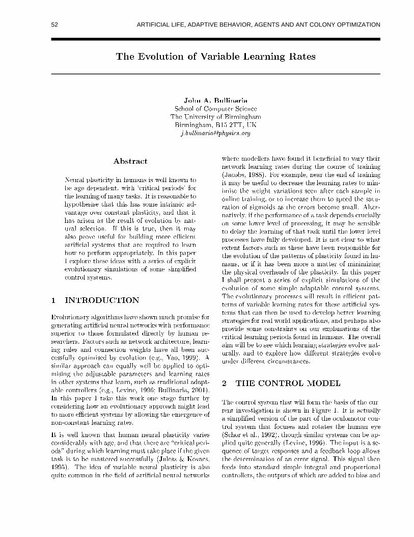
The Evolution of Variable Learning Rates
John A. Bullinaria
School of Computer ScienceThe University of BirminghamBirmingham, B15 2TT, [email protected]
Abstract
Neural plasticity in humans is well known tobe age dependent, with `critical periods' forthe learning of many tasks. It is reasonable tohypothesise that this has some intrinsic ad-vantage over constant plasticity, and that ithas arisen as the result of evolution by nat-ural selection. If this is true, then it mayalso prove useful for building more eÆcientarti�cial systems that are required to learnhow to perform appropriately. In this paperI explore these ideas with a series of explicitevolutionary simulations of some simpli�edcontrol systems.
1 INTRODUCTION
Evolutionary algorithms have shown much promise forgenerating arti�cial neural networks with performancesuperior to those formulated directly by human re-searchers. Factors such as network architecture, learn-
ing rules and connection weights have all been suc-cessfully optimised by evolution (e.g., Yao, 1999). Asimilar approach can equally well be applied to opti-mising the adjustable parameters and learning ratesin other systems that learn, such as traditional adapt-able controllers (e.g., Levine, 1996; Bullinaria, 2001).In this paper I take this work one stage further byconsidering how an evolutionary approach might leadto more eÆcient systems by allowing the emergence ofnon-constant learning rates.
It is well known that human neural plasticity variesconsiderably with age, and that there are \critical peri-ods" during which learning must take place if the giventask is to be mastered successfully (Julesz & Kovacs,1995). The idea of variable neural plasticity is alsoquite common in the �eld of arti�cial neural networks
where modellers have found it bene�cial to vary theirnetwork learning rates during the course of training(Jacobs, 1988). For example, near the end of trainingit may be useful to decrease the learning rates to min-imise the weight variations seen after each sample inonline training, or to increase them to speed the satu-ration of sigmoids as the errors become small. Alter-natively, if the performance of a task depends cruciallyon some lower level of processing, it may be sensibleto delay the learning of that task until the lower levelprocesses have fully developed. It is not clear to whatextent factors such as these have been responsible forthe evolution of the patterns of plasticity found in hu-mans, or if it has been more a matter of minimizingthe physical overheads of the plasticity. In this paperI shall present a series of explicit simulations of theevolution of some simple adaptable control systems.The evolutionary processes will result in eÆcient pat-terns of variable learning rates for these arti�cial sys-tems that can then be used to develop better learningstrategies for real world applications, and perhaps alsoprovide some constraints on our explanations of thecritical learning periods found in humans. The overallaim will be to see which learning strategies evolve nat-urally, and to explore how di�erent strategies evolveunder di�erent circumstances.
2 THE CONTROL MODEL
The control system that will form the basis of the cur-rent investigation is shown in Figure 1. It is actuallya simpli�ed version of the part of the oculomotor con-trol system that focuses and rotates the human eye(Schor et al., 1992), though similar systems can be ap-plied quite generally (Levine, 1996). The input is a se-quence of target responses and a feedback loop allowsthe determination of an error signal. This signal thenfeeds into standard simple integral and proportionalcontrollers, the outputs of which are added to bias and
52 ARTIFICIAL LIFE, ADAPTIVE BEHAVIOR, AGENTS AND ANT COLONY OPTIMIZATION
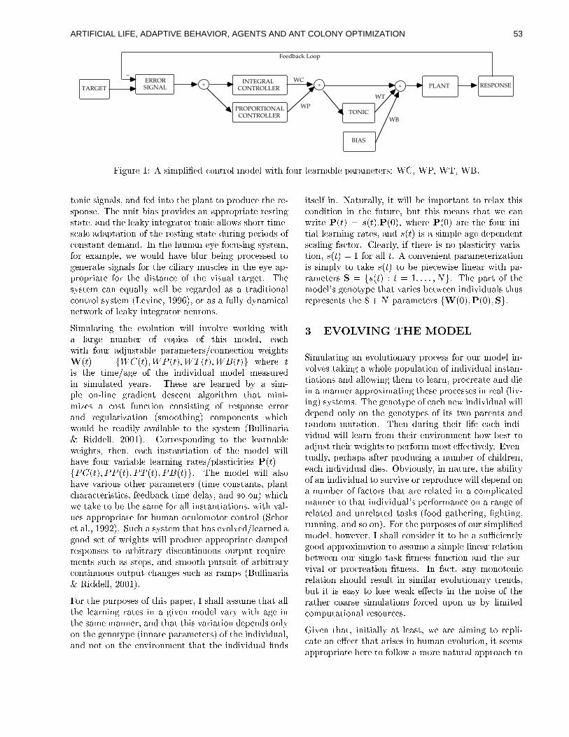
TARGET RESPONSE ERRORSIGNAL
INTEGRALCONTROLLER
_
PROPORTIONAL CONTROLLER
+ PLANT+
Feedback Loop
WC
WP
BIAS
+
WB
WT
TONIC
Figure 1: A simpli�ed control model with four learnable parameters: WC, WP, WT, WB.
tonic signals, and fed into the plant to produce the re-sponse. The unit bias provides an appropriate restingstate, and the leaky integrator tonic allows short time-scale adaptation of the resting state during periods ofconstant demand. In the human eye focusing system,for example, we would have blur being processed togenerate signals for the ciliary muscles in the eye ap-propriate for the distance of the visual target. Thesystem can equally well be regarded as a traditionalcontrol system (Levine, 1996), or as a fully dynamicalnetwork of leaky integrator neurons.
Simulating the evolution will involve working witha large number of copies of this model, eachwith four adjustable parameters/connection weightsW(t) = fWC(t);WP (t);WT (t);WB(t)g where t
is the time/age of the individual model measuredin simulated years. These are learned by a sim-ple on-line gradient descent algorithm that mini-mizes a cost function consisting of response errorand regularization (smoothing) components whichwould be readily available to the system (Bullinaria& Riddell, 2001). Corresponding to the learnableweights, then, each instantiation of the model willhave four variable learning rates/plasticities P(t) =fPC(t); PP (t); PT (t); PB(t)g. The model will alsohave various other parameters (time constants, plantcharacteristics, feedback time delay, and so on) whichwe take to be the same for all instantiations, with val-ues appropriate for human oculomotor control (Schoret al., 1992). Such a system that has evolved/learned agood set of weights will produce appropriate dampedresponses to arbitrary discontinuous output require-ments such as steps, and smooth pursuit of arbitrarycontinuous output changes such as ramps (Bullinaria& Riddell, 2001).
For the purposes of this paper, I shall assume that allthe learning rates in a given model vary with age inthe same manner, and that this variation depends onlyon the genotype (innate parameters) of the individual,and not on the environment that the individual �nds
itself in. Naturally, it will be important to relax thiscondition in the future, but this means that we canwrite P(t) = s(t):P(0), where P(0) are the four ini-tial learning rates, and s(t) is a simple age dependentscaling factor. Clearly, if there is no plasticity varia-tion, s(t) = 1 for all t. A convenient parameterizationis simply to take s(t) to be piecewise linear with pa-rameters S = fs(t) : t = 1; : : : ; Ng. The part of themodel's genotype that varies between individuals thusrepresents the 8 +N parameters fW(0);P(0);Sg.
3 EVOLVING THE MODEL
Simulating an evolutionary process for our model in-volves taking a whole population of individual instan-tiations and allowing them to learn, procreate and diein a manner approximating these processes in real (liv-ing) systems. The genotype of each new individual willdepend only on the genotypes of its two parents andrandom mutation. Then during their life each indi-vidual will learn from their environment how best toadjust their weights to perform most e�ectively. Even-tually, perhaps after producing a number of children,each individual dies. Obviously, in nature, the abilityof an individual to survive or reproduce will depend ona number of factors that are related in a complicatedmanner to that individual's performance on a range ofrelated and unrelated tasks (food gathering, �ghting,running, and so on). For the purposes of our simpli�edmodel, however, I shall consider it to be a suÆcientlygood approximation to assume a simple linear relationbetween our single task �tness function and the sur-vival or procreation �tness. In fact, any monotonicrelation should result in similar evolutionary trends,but it is easy to lose weak e�ects in the noise of therather coarse simulations forced upon us by limitedcomputational resources.
Given that, initially at least, we are aiming to repli-cate an e�ect that arises in human evolution, it seemsappropriate here to follow a more natural approach to
53ARTIFICIAL LIFE, ADAPTIVE BEHAVIOR, AGENTS AND ANT COLONY OPTIMIZATION
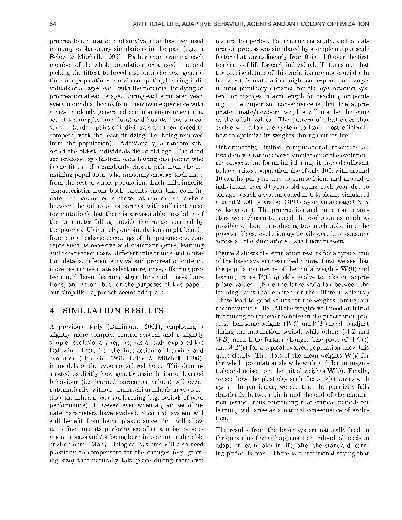
procreation, mutation and survival than has been usedin many evolutionary simulations in the past (e.g. inBelew & Mitchell, 1996). Rather than training each
member of the whole population for a �xed time andpicking the �ttest to breed and form the next genera-tion, our populations contain competing learning indi-viduals of all ages, each with the potential for dying orprocreation at each stage. During each simulated year,
every individual learns from their own experience witha new randomly generated common environment (i.e.set of training/testing data) and has its �tness mea-sured. Random pairs of individuals are then forced tocompete, with the least �t dying (i.e. being removedfrom the population). Additionally, a random sub-set of the oldest individuals die of old age. The deadare replaced by children, each having one parent whois the �ttest of a randomly chosen pair from the re-maining population, who randomly chooses their matefrom the rest of whole population. Each child inheritscharacteristics from both parents such that each in-nate free parameter is chosen at random somewherebetween the values of its parents, with suÆcient noise(or mutation) that there is a reasonable possibility ofthe parameter falling outside the range spanned bythe parents. Ultimately, our simulations might bene�t
from more realistic encodings of the parameters, con-cepts such as recessive and dominant genes, learningand procreation costs, di�erent inheritance and muta-tion details, di�erent survival and procreation criteria,more restrictive mate selection regimes, o�spring pro-tection, di�erent learning algorithms and �tness func-tions, and so on, but for the purposes of this paper,our simpli�ed approach seems adequate.
4 SIMULATION RESULTS
A previous study (Bullinaria, 2001), employing aslightly more complex control system and a slightlysimpler evolutionary regime, has already explored theBaldwin E�ect, i.e. the interaction of learning andevolution (Baldwin, 1896; Belew & Mitchell, 1996),in models of the type considered here. This demon-strated explicitly how genetic assimilation of learnedbehaviour (i.e. learned parameter values) will occurautomatically, without Lamarckian inheritance, to re-duce the inherent costs of learning (e.g. periods of poorperformance). However, even when a good set of in-nate parameters have evolved, a control system willstill bene�t from being plastic since that will allowit to �ne tune its performance after a noisy procre-ation process and/or being born into an unpredictableenvironment. Many biological systems will also needplasticity to compensate for the changes (e.g. grow-ing size) that naturally take place during their own
maturation period. For the current study, such a mat-uration process was simulated by a simple output scalefactor that varies linearly from 0.5 to 1.0 over the �rst
ten years of life for each individual. (It turns out thatthe precise details of this variation are not crucial.) Inhumans this maturation might correspond to changesin inter-pupilliary distance for the eye rotation sys-tem, or changes in arm length for reaching or point-
ing. The important consequence is that the appro-priate innate/newborn weights will not be the sameas the adult values. The pattern of plasticities thatevolve will allow the system to learn most eÆcientlyhow to optimize its weights throughout its life.
Unfortunately, limited computational resources al-lowed only a rather coarse simulation of the evolution-ary process, but for an initial study it proved suÆcientto have a �xed population size of only 100, with around10 deaths per year due to competition, and around 4individuals over 30 years old dying each year due toold age. (Such a system coded in C typically simulatedaround 20,000 years per CPU day on an average UNIXworkstation.) The procreation and mutation param-eters were chosen to speed the evolution as much aspossible without introducing too much noise into the
process. These evolutionary details were kept constantacross all the simulations I shall now present.
Figure 2 shows the simulation results for a typical runof the basic system described above. First we see thatthe population means of the initial weights W(0) andlearning rates P(0) quickly evolve to take on appro-priate values. (Note the large variation between thelearning rates that emerge for the di�erent weights.)These lead to good values for the weights throughoutthe individuals' life. All the weights will need an initial�ne tuning to remove the noise in the procreation pro-cess, then some weights (WC andWP ) need to adjustduring the maturation period, while others (WT andWB) need little further change. The plots of WC(t)and WT (t) for a typical evolved population show thisquite clearly. The plots of the mean weights W(t) forthe whole population show how they di�er in magni-tude and noise from the initial weights W(0). Finally,we see how the plasticity scale factor s(t) varies withage t. In particular, we see that the plasticity fallsdrastically between birth and the end of the matura-tion period, thus con�rming that critical periods forlearning will arise as a natural consequence of evolu-tion.
The results from the basic system naturally lead tothe question of what happens if an individual needs toadapt or learn later in life, after the standard learn-ing period is over. There is a traditional saying that
54 ARTIFICIAL LIFE, ADAPTIVE BEHAVIOR, AGENTS AND ANT COLONY OPTIMIZATION
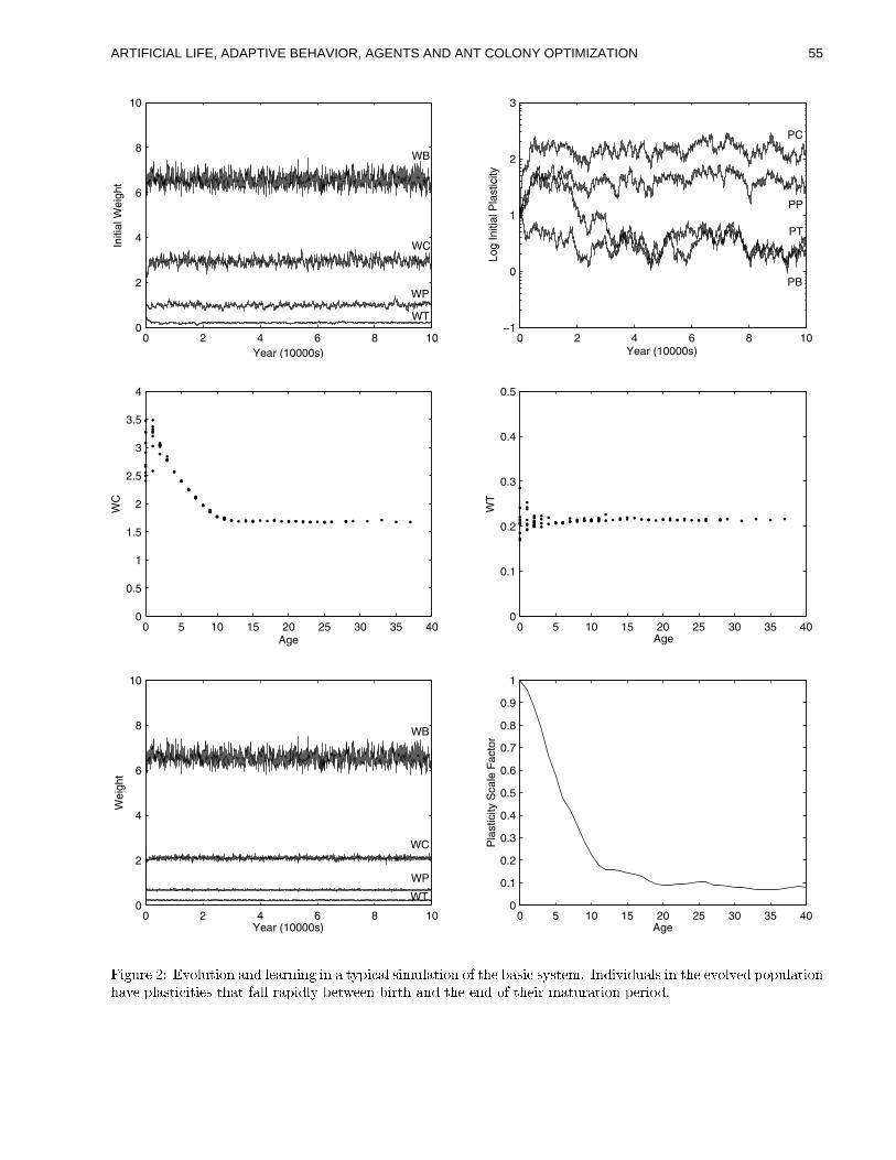
0 2 4 6 8 100
2
4
6
8
10
Year (10000s)
Initi
al W
eigh
t
WB
WC
WP
WT
0 2 4 6 8 10−1
0
1
2
3
Year (10000s)
Log
Initi
al P
last
icity
PT
PB
PC
PP
0 5 10 15 20 25 30 35 400
0.5
1
1.5
2
2.5
3
3.5
4
Age
WC
0 5 10 15 20 25 30 35 400
0.1
0.2
0.3
0.4
0.5
Age
WT
0 2 4 6 8 100
2
4
6
8
10
Year (10000s)
Wei
ght
WB
WC
WP
WT
0 5 10 15 20 25 30 35 400
0.1
0.2
0.3
0.4
0.5
0.6
0.7
0.8
0.9
1
Age
Pla
stic
ity S
cale
Fac
tor
Figure 2: Evolution and learning in a typical simulation of the basic system. Individuals in the evolved populationhave plasticities that fall rapidly between birth and the end of their maturation period.
55ARTIFICIAL LIFE, ADAPTIVE BEHAVIOR, AGENTS AND ANT COLONY OPTIMIZATION
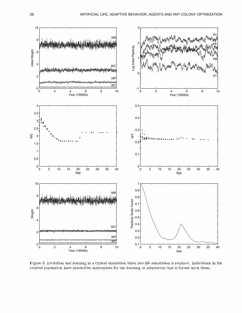
0 2 4 6 8 100
2
4
6
8
10
Year (10000s)
Initi
al W
eigh
t
WB
WC
WP
WT
0 2 4 6 8 10−1
0
1
2
3
Year (10000s)
Log
Initi
al P
last
icity
PC
PP
PB
PT
0 5 10 15 20 25 30 35 400
0.5
1
1.5
2
2.5
3
3.5
4
Age
WC
0 5 10 15 20 25 30 35 400
0.1
0.2
0.3
0.4
0.5
Age
WT
0 2 4 6 8 100
2
4
6
8
10
Year (10000s)
Wei
ght
WB
WC
WP
WT
0 5 10 15 20 25 30 35 400.1
0.2
0.3
0.4
0.5
0.6
0.7
0.8
0.9
1
Age
Pla
stic
ity S
cale
Fac
tor
Figure 3: Evolution and learning in a typical simulation when late life adaptation is required. Individuals in theevolved population have plasticities appropriate for the learning or adaptation that is forced upon them.
56 ARTIFICIAL LIFE, ADAPTIVE BEHAVIOR, AGENTS AND ANT COLONY OPTIMIZATION
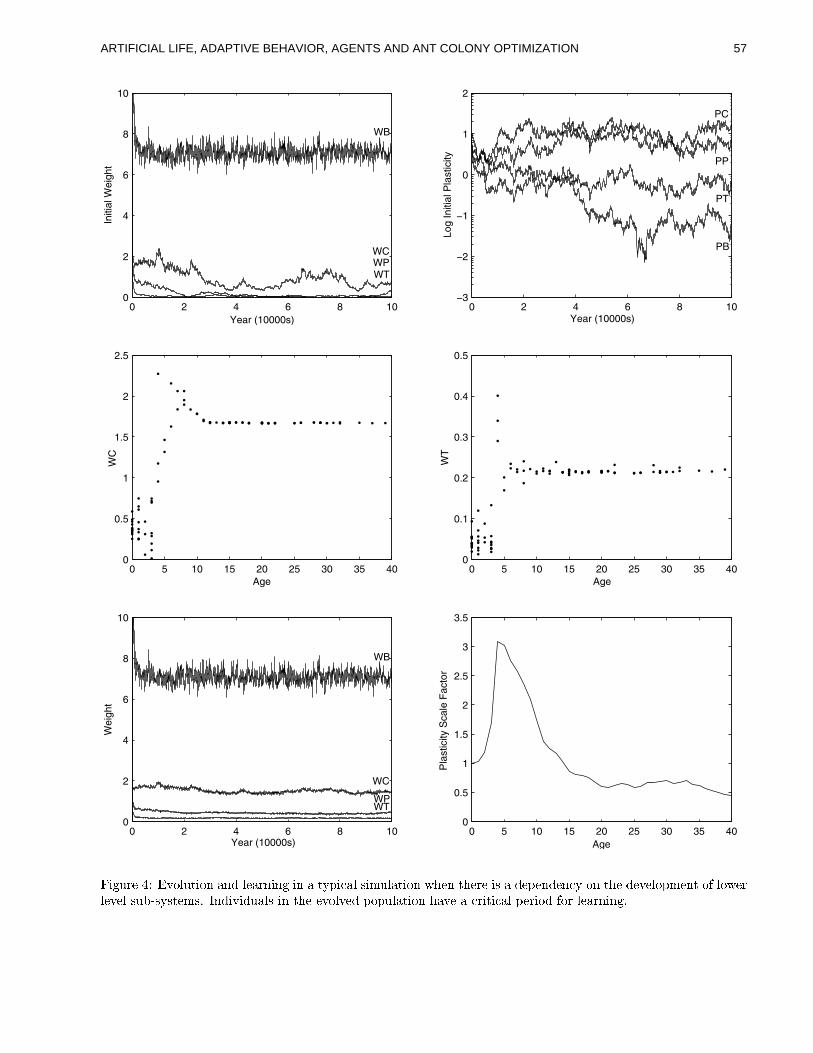
0 2 4 6 8 100
2
4
6
8
10
Year (10000s)
Initi
al W
eigh
t
WB
WT WP WC
0 2 4 6 8 10−3
−2
−1
0
1
2
Year (10000s)
Log
Initi
al P
last
icity
PC
PP
PT
PB
0 5 10 15 20 25 30 35 400
0.5
1
1.5
2
2.5
Age
WC
0 5 10 15 20 25 30 35 400
0.1
0.2
0.3
0.4
0.5
Age
WT
0 2 4 6 8 100
2
4
6
8
10
Year (10000s)
Wei
ght
WB
WC
WP WT
0 5 10 15 20 25 30 35 400
0.5
1
1.5
2
2.5
3
3.5
Age
Pla
stic
ity S
cale
Fac
tor
Figure 4: Evolution and learning in a typical simulation when there is a dependency on the development of lowerlevel sub-systems. Individuals in the evolved population have a critical period for learning.
57ARTIFICIAL LIFE, ADAPTIVE BEHAVIOR, AGENTS AND ANT COLONY OPTIMIZATION
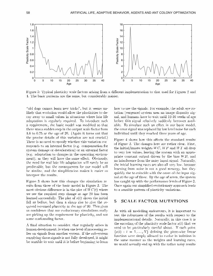
0 5 10 15 20 25 30 35 400
0.2
0.4
0.6
0.8
1
1.2
1.4
1.6
1.8
Age
Pla
stic
ity S
cale
Fac
tor
0 5 10 15 20 25 30 35 400
2
4
6
8
10
12
14
16
18
Age
Pla
stic
ity S
cale
Fac
tor
Figure 5: Typical plasticity scale factors arising from a di�erent implementation to that used for Figures 2 and4. The basic patterns are the same, but considerably noisier.
\old dogs cannot learn new tricks", but it seems un-likely that evolution would allow the plasticities to de-cay away to small values in situations where late lifeadaptation is regularly required. To introduce sucha requirement, the basic model was modi�ed so thatthere was a sudden step in the output scale factor from1.0 to 0.75 at the age of 20. (Again it turns out thatthe precise details of this variation are not crucial.)There is no need to specify whether this variation cor-responds to an internal factor (e.g. compensation forsystem damage or deterioration) or an external factor(e.g. adaptation to changes in the operating environ-ment), as they will have the same e�ect. Obviously,the need for real late life adaptation will rarely be sopredictable, but the consequences for our model willbe similar, and the simpli�cation makes it easier tointerpret the results.
Figure 3 shows how this changes the simulation re-sults from those of the basic model in Figure 2. Themost obvious di�erence is in the plot of WC(t) wherewe see the required step change at age 20 has beenlearned successfully. The plot of s(t) shows the initialfall as before, but then a sharp rise to give the re-quired increased plasticity at the age of 20. This givesus con�dence that our evolutionary simulations reallyare picking up the requirement for plasticity, and notsome confounding factor.
A �nal situation to consider, that regularly arises inhuman development, is when one level of processing re-
lies on signals from another system. If the sub-systemsupplying those signals is not fully developed, it mightbe sensible to wait until it is before beginning to learn
how to use the signals. For example, the adult eye ro-tation (vergence) system uses an image disparity sig-nal, and humans have to wait until 12-16 weeks of agebefore this signal relatively suddenly becomes avail-able. To simulate such an e�ect in our basic model,the error signal was replaced by low level noise for eachindividual until they reached three years of age.
Figure 4 shows how this a�ects the standard resultsof Figure 2. The changes here are rather clear. First,the initial/innate weights WC, WP and WT all dropto very low values, leaving the system with an appro-priate constant output driven by the bias WB, andno interference from the noisy input signal. Naturally,the initial learning rates are also all very low, becauselearning from noise is not a good strategy, but theyquickly rise to coincide with the onset of the input sig-nal at the age of three. By the age of seven, the system
has caught up with the performance levels of Figure 2.Once again our simpli�ed evolutionary approach leadsto a sensible pattern of plasticity variations.
5 SCALE FACTOR MUTATIONS
As with all modelling endeavours, it is important totest the robustness of the results with respect to theimplementational details. Naturally, in this case it isthe encoding of the plasticity scale factor s(t) that weneed to be particularly careful about. If each pointfs(t) : t = 1; : : : ; Ng de�ning the piece-wise linearfunction were simply allowed to evolve in isolation inthe same manner as the weights and learning rates,we would actually end up with the rather noisy results
58 ARTIFICIAL LIFE, ADAPTIVE BEHAVIOR, AGENTS AND ANT COLONY OPTIMIZATION
shown in Figure 5.
The individual performance advantages that would
keep the curves smooth, and reduce any unnecessaryplasticity, are rather weak and get lost in the noise ofour coarse simulations. This is particularly apparentafter the age of about 10. The weakness is partly dueto the error signals being relatively low after the mat-uration period is complete, and partly because it will
be relatively unimportant if the �tness starts decreas-ing again after a number of children have already beenproduced, or if the majority of individuals normallydie before reaching that age.
Fortunately, we can compensate for these limitationsby variations of the plasticity scale factor mutations.First, we can prevent unnecessary plasticity (whichwill surely have an intrinsic cost in real systems) byallowing mutations which set random points s(n) tozero. Then, it is unlikely in real systems to be eÆcientto have s(t) varying wildly with age, so it is reasonableto encourage smoothness of s(t) by allowing mutationswhich swap the values of random adjacent points s(n)and s(n+1). It was these simple variations that turnedthe noisy and ineÆcient results of Figure 5 into thesmooth and eÆcient results of Figures 2, 3 and 4.
6 CONCLUSIONS
By simulating evolving populations of simple adapt-able control systems we have seen that there is a natu-ral propensity for the evolution of plasticities that varysensibly with age, quite independently of any physicaloverheads of the plasticity. This is consistent with thewell known \critical periods" of human brain devel-opment (Julesz & Kovacs, 1995). It is reasonable toexpect that such an evolutionary approach will alsobe a pro�table strategy for obtaining improved per-
formance in adaptable systems for real world applica-tions.
There are two competing e�ects at play. In order tosurvive in competition with �tter adults and/or a hos-tile environment, a newborn needs to adapt as quicklyas possible to its environment. It also needs to adapteÆciently to its own maturation. Large plasticitieswill be bene�cial for both. In adults, however, largeplasticities can lead to an unstable learning system,in which unusual/extreme experiences can potentiallyresult in a large shift of the systems' parameters witha serious reduction in overall �tness. Lower learn-ing rates in this situation will allow smoother optimalparameter estimation and more consistently good re-sponses in a varied environment. In this paper it hasbeen demonstrated how a process of evolution by nat-
ural selection can result in a population of individualsystems that deal with these con icting requirementsby having plasticities that vary appropriately with age
under normal maturation, when late life adaptationis required, and when there is a dependence on theprior development of other sub-systems. We have alsoseen how appropriate changes to the implementationaldetails (e.g. the plasticity scale factor mutations) can
lead to vastly superior results.
In complex systems, such as the human brain, we canexpect each of the various sub-systems to evolve appro-priately for its own requirements, so there may well beno single global behaviour. The next stage of this workwill be to develop and test larger scale and more re-alistic simulations of speci�c human sub-systems, andto explore explicitly how these ideas could be appliedto the formulation of more eÆcient arti�cial adaptablesystems for particular real world engineering applica-tions.
References
Baldwin, J.M. (1896). A New Factor in Evolution.The American Naturalist, 30, 441-451.
Belew, R.K. & Mitchell, M. (Eds) (1996). Adaptive
Individuals in Evolving Populations. Reading, MA:Addison-Wesley.
Bullinaria, J.A. (2001). Exploring the Baldwin Ef-fect in Evolving Adaptable Control Systems. In: R.F.French & J.P. Sougne (Eds), Connectionist Models of
Learning, Development and Evolution, 231-242. Lon-don: Springer.
Bullinaria, J.A. & Riddell, P.M. (2001). Neural Net-work Control Systems that Learn to Perform Appro-priately. International Journal of Neural Systems, 11,79-88.
Jacobs, R.A. (1988). Increased Rates Of ConvergenceThrough Learning Rate Adaptation. Neural Networks,1, 295-307.
Julesz, B. & Kovacs, I. (Eds) (1995). Maturational
Windows and Adult Cortical Plasticity. Reading, MA:Addison-Wesley.
Levine, W.S. (1996). The Control Handbook. London:CRC Press.
Schor, C.M., Alexander, J., Cormack, L. & Stevenson,S. (1992). Negative Feedback Control Model of Prox-imal Convergence and Accommodation. Ophthalmic
and Physiological Optics, 12, 307-318.
Yao, X. (1999). Evolving Arti�cial Neural Networks.Proceedings of the IEEE, 87, 1423-1447.
59ARTIFICIAL LIFE, ADAPTIVE BEHAVIOR, AGENTS AND ANT COLONY OPTIMIZATION
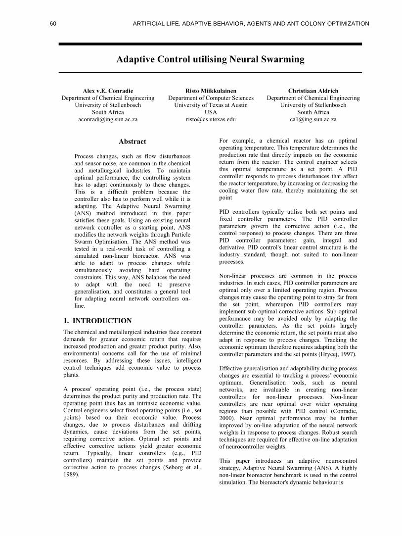
Adaptive Control utilising Neural Swarming
Alex v.E. Conradie
Department of Chemical Engineering University of Stellenbosch
South Africa [email protected]
Risto Miikkulainen
Department of Computer Sciences University of Texas at Austin
Christiaan Aldrich
Department of Chemical Engineering University of Stellenbosch
South Africa [email protected]
Abstract
Process changes, such as flow disturbances and sensor noise, are common in the chemical and metallurgical industries. To maintain optimal performance, the controlling system has to adapt continuously to these changes. This is a difficult problem because the controller also has to perform well while it is adapting. The Adaptive Neural Swarming (ANS) method introduced in this paper satisfies these goals. Using an existing neural network controller as a starting point, ANS modifies the network weights through Particle Swarm Optimisation. The ANS method was tested in a real-world task of controlling a simulated non-linear bioreactor. ANS was able to adapt to process changes while simultaneously avoiding hard operating constraints. This way, ANS balances the need to adapt with the need to preserve generalisation, and constitutes a general tool for adapting neural network controllers on-line.
1. INTRODUCTION The chemical and metallurgical industries face constant demands for greater economic return that requires increased production and greater product purity. Also, environmental concerns call for the use of minimal resources. By addressing these issues, intelligent control techniques add economic value to process plants. A process' operating point (i.e., the process state) determines the product purity and production rate. The operating point thus has an intrinsic economic value. Control engineers select fixed operating points (i.e., set points) based on their economic value. Process changes, due to process disturbances and drifting dynamics, cause deviations from the set points, requiring corrective action. Optimal set points and effective corrective actions yield greater economic return. Typically, linear controllers (e.g., PID controllers) maintain the set points and provide corrective action to process changes (Seborg et al., 1989).
For example, a chemical reactor has an optimal operating temperature. This temperature determines the production rate that directly impacts on the economic return from the reactor. The control engineer selects this optimal temperature as a set point. A PID controller responds to process disturbances that affect the reactor temperature, by increasing or decreasing the cooling water flow rate, thereby maintaining the set point PID controllers typically utilise both set points and fixed controller parameters. The PID controller parameters govern the corrective action (i.e., the control response) to process changes. There are three PID controller parameters: gain, integral and derivative. PID control's linear control structure is the industry standard, though not suited to non-linear processes. Non-linear processes are common in the process industries. In such cases, PID controller parameters are optimal only over a limited operating region. Process changes may cause the operating point to stray far from the set point, whereupon PID controllers may implement sub-optimal corrective actions. Sub-optimal performance may be avoided only by adapting the controller parameters. As the set points largely determine the economic return, the set points must also adapt in response to process changes. Tracking the economic optimum therefore requires adapting both the controller parameters and the set points (Hrycej, 1997). Effective generalisation and adaptability during process changes are essential to tracking a process' economic optimum. Generalisation tools, such as neural networks, are invaluable in creating non-linear controllers for non-linear processes. Non-linear controllers are near optimal over wider operating regions than possible with PID control (Conradie, 2000). Near optimal performance may be further improved by on-line adaptation of the neural network weights in response to process changes. Robust search techniques are required for effective on-line adaptation of neurocontroller weights. This paper introduces an adaptive neurocontrol strategy, Adaptive Neural Swarming (ANS). A highly non-linear bioreactor benchmark is used in the control simulation. The bioreactor's dynamic behaviour is
60 ARTIFICIAL LIFE, ADAPTIVE BEHAVIOR, AGENTS AND ANT COLONY OPTIMIZATION
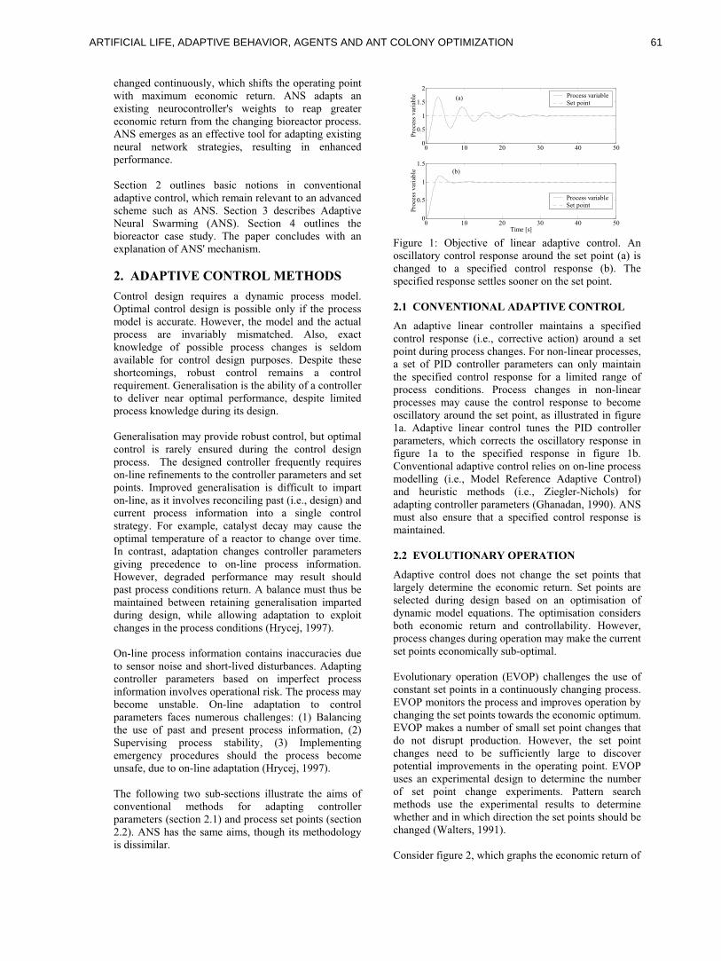
changed continuously, which shifts the operating point with maximum economic return. ANS adapts an existing neurocontroller's weights to reap greater economic return from the changing bioreactor process. ANS emerges as an effective tool for adapting existing neural network strategies, resulting in enhanced performance. Section 2 outlines basic notions in conventional adaptive control, which remain relevant to an advanced scheme such as ANS. Section 3 describes Adaptive Neural Swarming (ANS). Section 4 outlines the bioreactor case study. The paper concludes with an explanation of ANS' mechanism.
2. ADAPTIVE CONTROL METHODS Control design requires a dynamic process model. Optimal control design is possible only if the process model is accurate. However, the model and the actual process are invariably mismatched. Also, exact knowledge of possible process changes is seldom available for control design purposes. Despite these shortcomings, robust control remains a control requirement. Generalisation is the ability of a controller to deliver near optimal performance, despite limited process knowledge during its design. Generalisation may provide robust control, but optimal control is rarely ensured during the control design process. The designed controller frequently requires on-line refinements to the controller parameters and set points. Improved generalisation is difficult to impart on-line, as it involves reconciling past (i.e., design) and current process information into a single control strategy. For example, catalyst decay may cause the optimal temperature of a reactor to change over time. In contrast, adaptation changes controller parameters giving precedence to on-line process information. However, degraded performance may result should past process conditions return. A balance must thus be maintained between retaining generalisation imparted during design, while allowing adaptation to exploit changes in the process conditions (Hrycej, 1997). On-line process information contains inaccuracies due to sensor noise and short-lived disturbances. Adapting controller parameters based on imperfect process information involves operational risk. The process may become unstable. On-line adaptation to control parameters faces numerous challenges: (1) Balancing the use of past and present process information, (2) Supervising process stability, (3) Implementing emergency procedures should the process become unsafe, due to on-line adaptation (Hrycej, 1997). The following two sub-sections illustrate the aims of conventional methods for adapting controller parameters (section 2.1) and process set points (section 2.2). ANS has the same aims, though its methodology is dissimilar.
0 10 20 30 40 500
0.5
1
1.5
2
Pro
cess
var
iab
le Process variableSet point
0 10 20 30 40 500
0.5
1
1.5
Time [s]
Pro
cess
var
iab
le
Process variableSet point
(a)
(b)
Figure 1: Objective of linear adaptive control. An oscillatory control response around the set point (a) is changed to a specified control response (b). The specified response settles sooner on the set point.
2.1 CONVENTIONAL ADAPTIVE CONTROL An adaptive linear controller maintains a specified control response (i.e., corrective action) around a set point during process changes. For non-linear processes, a set of PID controller parameters can only maintain the specified control response for a limited range of process conditions. Process changes in non-linear processes may cause the control response to become oscillatory around the set point, as illustrated in figure 1a. Adaptive linear control tunes the PID controller parameters, which corrects the oscillatory response in figure 1a to the specified response in figure 1b. Conventional adaptive control relies on on-line process modelling (i.e., Model Reference Adaptive Control) and heuristic methods (i.e., Ziegler-Nichols) for adapting controller parameters (Ghanadan, 1990). ANS must also ensure that a specified control response is maintained. 2.2 EVOLUTIONARY OPERATION Adaptive control does not change the set points that largely determine the economic return. Set points are selected during design based on an optimisation of dynamic model equations. The optimisation considers both economic return and controllability. However, process changes during operation may make the current set points economically sub-optimal. Evolutionary operation (EVOP) challenges the use of constant set points in a continuously changing process. EVOP monitors the process and improves operation by changing the set points towards the economic optimum. EVOP makes a number of small set point changes that do not disrupt production. However, the set point changes need to be sufficiently large to discover potential improvements in the operating point. EVOP uses an experimental design to determine the number of set point change experiments. Pattern search methods use the experimental results to determine whether and in which direction the set points should be changed (Walters, 1991). Consider figure 2, which graphs the economic return of
61ARTIFICIAL LIFE, ADAPTIVE BEHAVIOR, AGENTS AND ANT COLONY OPTIMIZATION
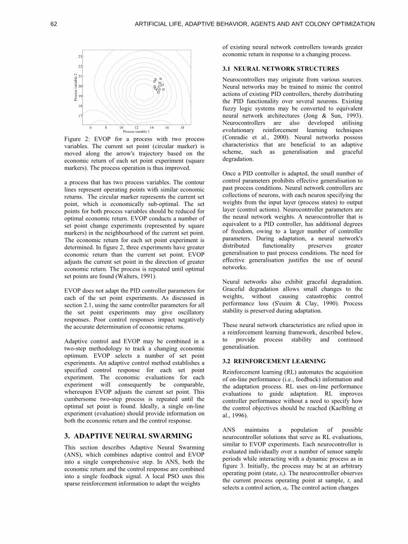
6 8 10 12 14 16 18
17
18
19
20
21
22
23
Process variable 1
Pro
cess
var
iab
le 2
Figure 2: EVOP for a process with two process variables. The current set point (circular marker) is moved along the arrow's trajectory based on the economic return of each set point experiment (square markers). The process operation is thus improved. a process that has two process variables. The contour lines represent operating points with similar economic returns. The circular marker represents the current set point, which is economically sub-optimal. The set points for both process variables should be reduced for optimal economic return. EVOP conducts a number of set point change experiments (represented by square markers) in the neighbourhood of the current set point. The economic return for each set point experiment is determined. In figure 2, three experiments have greater economic return than the current set point. EVOP adjusts the current set point in the direction of greater economic return. The process is repeated until optimal set points are found (Walters, 1991). EVOP does not adapt the PID controller parameters for each of the set point experiments. As discussed in section 2.1, using the same controller parameters for all the set point experiments may give oscillatory responses. Poor control responses impact negatively the accurate determination of economic returns. Adaptive control and EVOP may be combined in a two-step methodology to track a changing economic optimum. EVOP selects a number of set point experiments. An adaptive control method establishes a specified control response for each set point experiment. The economic evaluations for each experiment will consequently be comparable, whereupon EVOP adjusts the current set point. This cumbersome two-step process is repeated until the optimal set point is found. Ideally, a single on-line experiment (evaluation) should provide information on both the economic return and the control response.
3. ADAPTIVE NEURAL SWARMING This section describes Adaptive Neural Swarming (ANS), which combines adaptive control and EVOP into a single comprehensive step. In ANS, both the economic return and the control response are combined into a single feedback signal. A local PSO uses this sparse reinforcement information to adapt the weights
of existing neural network controllers towards greater economic return in response to a changing process. 3.1 NEURAL NETWORK STRUCTURES Neurocontrollers may originate from various sources. Neural networks may be trained to mimic the control actions of existing PID controllers, thereby distributing the PID functionality over several neurons. Existing fuzzy logic systems may be converted to equivalent neural network architectures (Jong & Sun, 1993). Neurocontrollers are also developed utilising evolutionary reinforcement learning techniques (Conradie et al., 2000). Neural networks possess characteristics that are beneficial to an adaptive scheme, such as generalisation and graceful degradation. Once a PID controller is adapted, the small number of control parameters prohibits effective generalisation to past process conditions. Neural network controllers are collections of neurons, with each neuron specifying the weights from the input layer (process states) to output layer (control actions). Neurocontroller parameters are the neural network weights. A neurocontroller that is equivalent to a PID controller, has additional degrees of freedom, owing to a larger number of controller parameters. During adaptation, a neural network's distributed functionality preserves greater generalisation to past process conditions. The need for effective generalisation justifies the use of neural networks. Neural networks also exhibit graceful degradation. Graceful degradation allows small changes to the weights, without causing catastrophic control performance loss (S'euim & Clay, 1990). Process stability is preserved during adaptation. These neural network characteristics are relied upon in a reinforcement learning framework, described below, to provide process stability and continued generalisation. 3.2 REINFORCEMENT LEARNING Reinforcement learning (RL) automates the acquisition of on-line performance (i.e., feedback) information and the adaptation process. RL uses on-line performance evaluations to guide adaptation. RL improves controller performance without a need to specify how the control objectives should be reached (Kaelbling et al., 1996). ANS maintains a population of possible neurocontroller solutions that serve as RL evaluations, similar to EVOP experiments. Each neurocontroller is evaluated individually over a number of sensor sample periods while interacting with a dynamic process as in figure 3. Initially, the process may be at an arbitrary operating point (state, st). The neurocontroller observes the current process operating point at sample, t, and selects a control action, at. The control action changes
62 ARTIFICIAL LIFE, ADAPTIVE BEHAVIOR, AGENTS AND ANT COLONY OPTIMIZATION
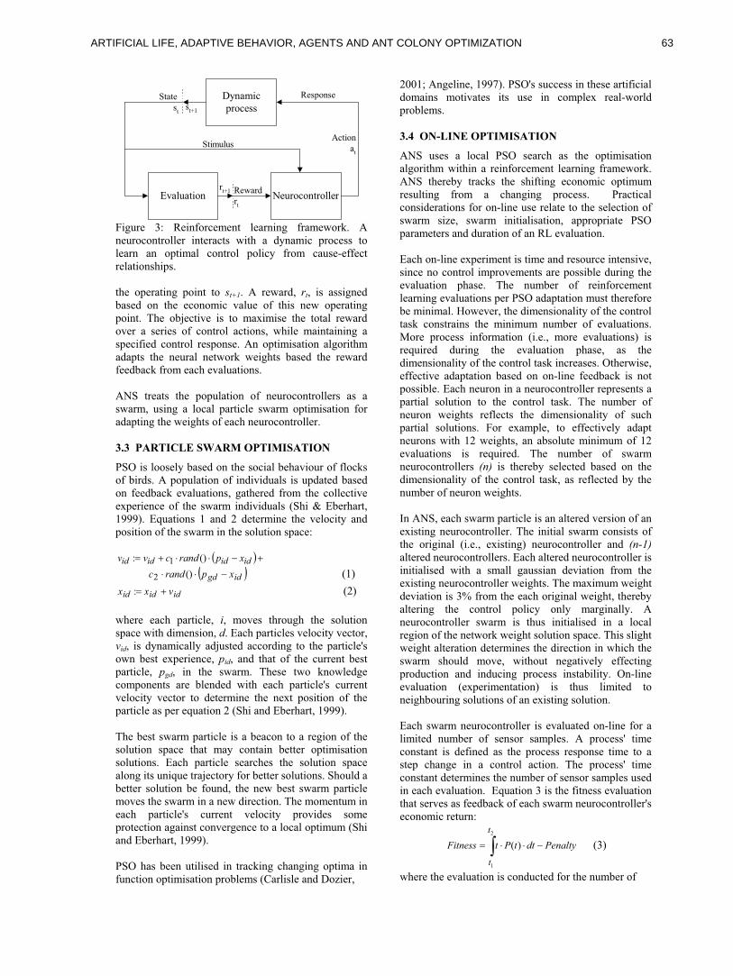
Dynamic
process
NeurocontrollerReward
rt
rt+1
st+1
State
st
Action
at
Evaluation
Stimulus
Response
Figure 3: Reinforcement learning framework. A neurocontroller interacts with a dynamic process to learn an optimal control policy from cause-effect relationships. the operating point to st+1. A reward, rt, is assigned based on the economic value of this new operating point. The objective is to maximise the total reward over a series of control actions, while maintaining a specified control response. An optimisation algorithm adapts the neural network weights based the reward feedback from each evaluations. ANS treats the population of neurocontrollers as a swarm, using a local particle swarm optimisation for adapting the weights of each neurocontroller.
3.3 PARTICLE SWARM OPTIMISATION PSO is loosely based on the social behaviour of flocks of birds. A population of individuals is updated based on feedback evaluations, gathered from the collective experience of the swarm individuals (Shi & Eberhart, 1999). Equations 1 and 2 determine the velocity and position of the swarm in the solution space:
idididid xprandcvv (): 1
idgd xprandc ()2 (1)
ididid vxx : (2)
where each particle, i, moves through the solution space with dimension, d. Each particles velocity vector, vid, is dynamically adjusted according to the particle's own best experience, pid, and that of the current best particle, pgd, in the swarm. These two knowledge components are blended with each particle's current velocity vector to determine the next position of the particle as per equation 2 (Shi and Eberhart, 1999). The best swarm particle is a beacon to a region of the solution space that may contain better optimisation solutions. Each particle searches the solution space along its unique trajectory for better solutions. Should a better solution be found, the new best swarm particle moves the swarm in a new direction. The momentum in each particle's current velocity provides some protection against convergence to a local optimum (Shi and Eberhart, 1999). PSO has been utilised in tracking changing optima in function optimisation problems (Carlisle and Dozier,
2001; Angeline, 1997). PSO's success in these artificial domains motivates its use in complex real-world problems. 3.4 ON-LINE OPTIMISATION ANS uses a local PSO search as the optimisation algorithm within a reinforcement learning framework. ANS thereby tracks the shifting economic optimum resulting from a changing process. Practical considerations for on-line use relate to the selection of swarm size, swarm initialisation, appropriate PSO parameters and duration of an RL evaluation. Each on-line experiment is time and resource intensive, since no control improvements are possible during the evaluation phase. The number of reinforcement learning evaluations per PSO adaptation must therefore be minimal. However, the dimensionality of the control task constrains the minimum number of evaluations. More process information (i.e., more evaluations) is required during the evaluation phase, as the dimensionality of the control task increases. Otherwise, effective adaptation based on on-line feedback is not possible. Each neuron in a neurocontroller represents a partial solution to the control task. The number of neuron weights reflects the dimensionality of such partial solutions. For example, to effectively adapt neurons with 12 weights, an absolute minimum of 12 evaluations is required. The number of swarm neurocontrollers (n) is thereby selected based on the dimensionality of the control task, as reflected by the number of neuron weights. In ANS, each swarm particle is an altered version of an existing neurocontroller. The initial swarm consists of the original (i.e., existing) neurocontroller and (n-1) altered neurocontrollers. Each altered neurocontroller is initialised with a small gaussian deviation from the existing neurocontroller weights. The maximum weight deviation is 3% from the each original weight, thereby altering the control policy only marginally. A neurocontroller swarm is thus initialised in a local region of the network weight solution space. This slight weight alteration determines the direction in which the swarm should move, without negatively effecting production and inducing process instability. On-line evaluation (experimentation) is thus limited to neighbouring solutions of an existing solution. Each swarm neurocontroller is evaluated on-line for a limited number of sensor samples. A process' time constant is defined as the process response time to a step change in a control action. The process' time constant determines the number of sensor samples used in each evaluation. Equation 3 is the fitness evaluation that serves as feedback of each swarm neurocontroller's economic return:
PenaltydttPtFitness
t
t
2
1
)( (3)
where the evaluation is conducted for the number of
63ARTIFICIAL LIFE, ADAPTIVE BEHAVIOR, AGENTS AND ANT COLONY OPTIMIZATION
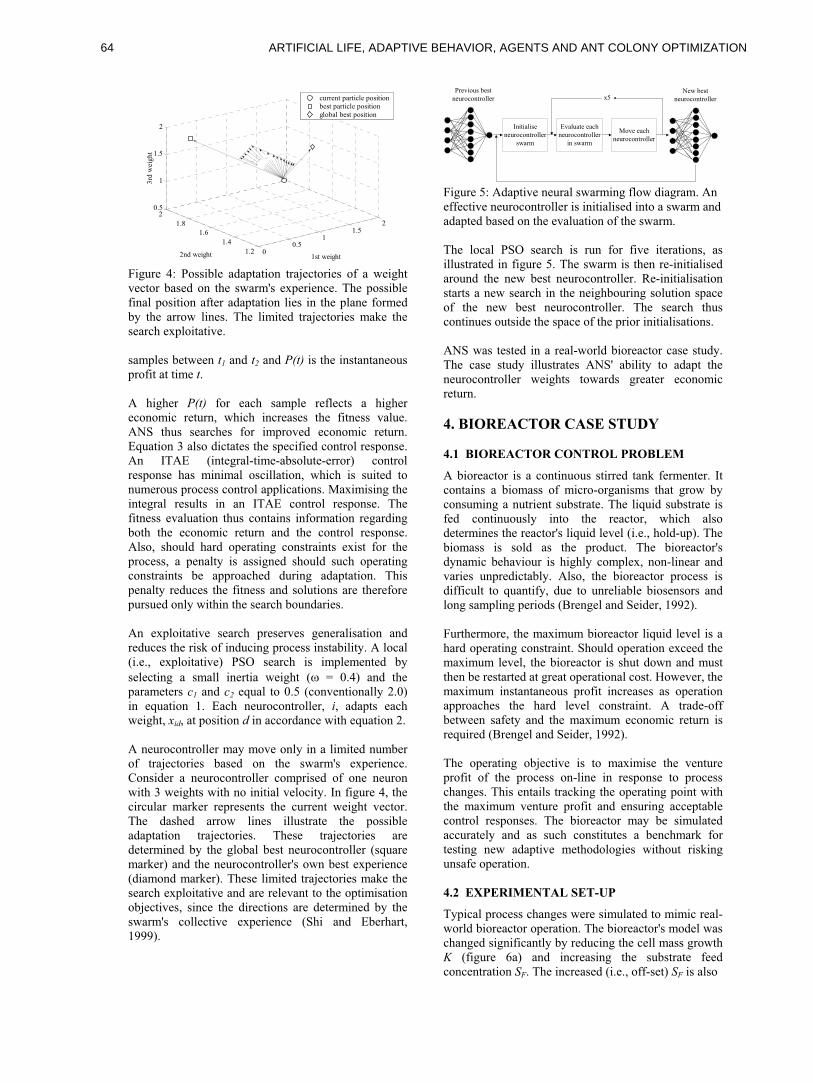
00.5
11.5
2
1.2
1.4
1.6
1.8
20.5
1
1.5
2
1st weight2nd weight
3rd
wei
gh
t
current particle positionbest particle position global best position
Figure 4: Possible adaptation trajectories of a weight vector based on the swarm's experience. The possible final position after adaptation lies in the plane formed by the arrow lines. The limited trajectories make the search exploitative. samples between t1 and t2 and P(t) is the instantaneous profit at time t. A higher P(t) for each sample reflects a higher economic return, which increases the fitness value. ANS thus searches for improved economic return. Equation 3 also dictates the specified control response. An ITAE (integral-time-absolute-error) control response has minimal oscillation, which is suited to numerous process control applications. Maximising the integral results in an ITAE control response. The fitness evaluation thus contains information regarding both the economic return and the control response. Also, should hard operating constraints exist for the process, a penalty is assigned should such operating constraints be approached during adaptation. This penalty reduces the fitness and solutions are therefore pursued only within the search boundaries. An exploitative search preserves generalisation and reduces the risk of inducing process instability. A local (i.e., exploitative) PSO search is implemented by
selecting a small inertia weight ( = 0.4) and the parameters c1 and c2 equal to 0.5 (conventionally 2.0) in equation 1. Each neurocontroller, i, adapts each weight, xid, at position d in accordance with equation 2. A neurocontroller may move only in a limited number of trajectories based on the swarm's experience. Consider a neurocontroller comprised of one neuron with 3 weights with no initial velocity. In figure 4, the circular marker represents the current weight vector. The dashed arrow lines illustrate the possible adaptation trajectories. These trajectories are determined by the global best neurocontroller (square marker) and the neurocontroller's own best experience (diamond marker). These limited trajectories make the search exploitative and are relevant to the optimisation objectives, since the directions are determined by the swarm's collective experience (Shi and Eberhart, 1999).
Initialise
neurocontroller
swarm
Evaluate each
neurocontroller
in swarm
Move each
neurocontroller
x5New best
neurocontroller
Previous best
neurocontroller
Figure 5: Adaptive neural swarming flow diagram. An effective neurocontroller is initialised into a swarm and adapted based on the evaluation of the swarm. The local PSO search is run for five iterations, as illustrated in figure 5. The swarm is then re-initialised around the new best neurocontroller. Re-initialisation starts a new search in the neighbouring solution space of the new best neurocontroller. The search thus continues outside the space of the prior initialisations. ANS was tested in a real-world bioreactor case study. The case study illustrates ANS' ability to adapt the neurocontroller weights towards greater economic return.
4. BIOREACTOR CASE STUDY 4.1 BIOREACTOR CONTROL PROBLEM A bioreactor is a continuous stirred tank fermenter. It contains a biomass of micro-organisms that grow by consuming a nutrient substrate. The liquid substrate is fed continuously into the reactor, which also determines the reactor's liquid level (i.e., hold-up). The biomass is sold as the product. The bioreactor's dynamic behaviour is highly complex, non-linear and varies unpredictably. Also, the bioreactor process is difficult to quantify, due to unreliable biosensors and long sampling periods (Brengel and Seider, 1992). Furthermore, the maximum bioreactor liquid level is a hard operating constraint. Should operation exceed the maximum level, the bioreactor is shut down and must then be restarted at great operational cost. However, the maximum instantaneous profit increases as operation approaches the hard level constraint. A trade-off between safety and the maximum economic return is required (Brengel and Seider, 1992). The operating objective is to maximise the venture profit of the process on-line in response to process changes. This entails tracking the operating point with the maximum venture profit and ensuring acceptable control responses. The bioreactor may be simulated accurately and as such constitutes a benchmark for testing new adaptive methodologies without risking unsafe operation. 4.2 EXPERIMENTAL SET-UP Typical process changes were simulated to mimic real-world bioreactor operation. The bioreactor's model was changed significantly by reducing the cell mass growth K (figure 6a) and increasing the substrate feed concentration SF. The increased (i.e., off-set) SF is also
64 ARTIFICIAL LIFE, ADAPTIVE BEHAVIOR, AGENTS AND ANT COLONY OPTIMIZATION
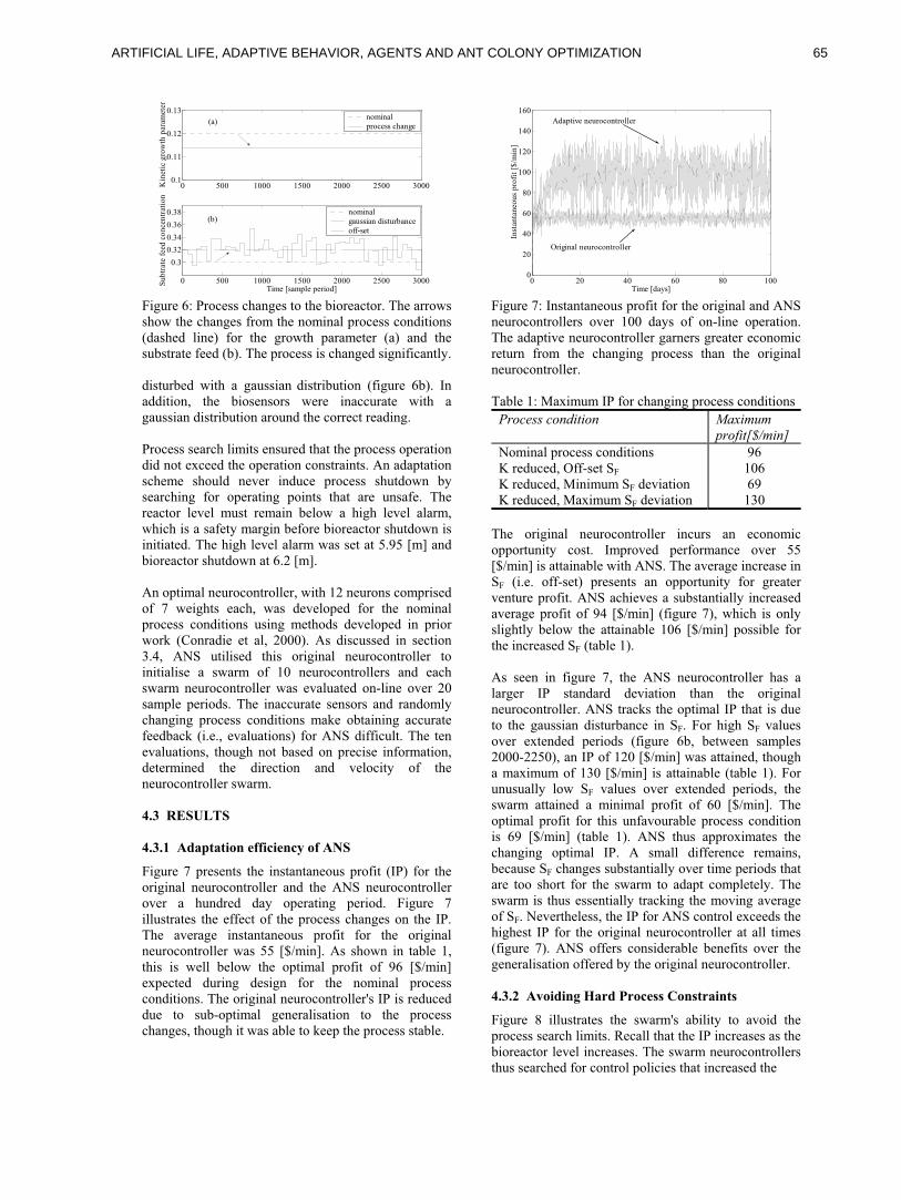
0 500 1000 1500 2000 2500 30000.1
0.11
0.12
0.13
Kin
etic
gro
wth
par
amet
er
nominal process change
0 500 1000 1500 2000 2500 3000
0.3
0.32
0.34
0.36
0.38
Time [sample period]
Su
btr
ate
feed
co
nce
ntr
atio
n
nominal gaussian disturbanceoff-set
(a)
(b)
Figure 6: Process changes to the bioreactor. The arrows show the changes from the nominal process conditions (dashed line) for the growth parameter (a) and the substrate feed (b). The process is changed significantly. disturbed with a gaussian distribution (figure 6b). In addition, the biosensors were inaccurate with a gaussian distribution around the correct reading. Process search limits ensured that the process operation did not exceed the operation constraints. An adaptation scheme should never induce process shutdown by searching for operating points that are unsafe. The reactor level must remain below a high level alarm, which is a safety margin before bioreactor shutdown is initiated. The high level alarm was set at 5.95 [m] and bioreactor shutdown at 6.2 [m]. An optimal neurocontroller, with 12 neurons comprised of 7 weights each, was developed for the nominal process conditions using methods developed in prior work (Conradie et al, 2000). As discussed in section 3.4, ANS utilised this original neurocontroller to initialise a swarm of 10 neurocontrollers and each swarm neurocontroller was evaluated on-line over 20 sample periods. The inaccurate sensors and randomly changing process conditions make obtaining accurate feedback (i.e., evaluations) for ANS difficult. The ten evaluations, though not based on precise information, determined the direction and velocity of the neurocontroller swarm. 4.3 RESULTS
4.3.1 Adaptation efficiency of ANS Figure 7 presents the instantaneous profit (IP) for the original neurocontroller and the ANS neurocontroller over a hundred day operating period. Figure 7 illustrates the effect of the process changes on the IP. The average instantaneous profit for the original neurocontroller was 55 [$/min]. As shown in table 1, this is well below the optimal profit of 96 [$/min] expected during design for the nominal process conditions. The original neurocontroller's IP is reduced due to sub-optimal generalisation to the process changes, though it was able to keep the process stable.
0 20 40 60 80 1000
20
40
60
80
100
120
140
160
Time [days]
Inst
anta
neo
us
pro
fit
[$/m
in]
Original neurocontroller
Adaptive neurocontroller
Figure 7: Instantaneous profit for the original and ANS neurocontrollers over 100 days of on-line operation. The adaptive neurocontroller garners greater economic return from the changing process than the original neurocontroller. Table 1: Maximum IP for changing process conditions
Process condition Maximum
profit[$/min]
Nominal process conditions K reduced, Off-set SF
K reduced, Minimum SF deviation K reduced, Maximum SF deviation
96 106 69
130
The original neurocontroller incurs an economic opportunity cost. Improved performance over 55 [$/min] is attainable with ANS. The average increase in SF (i.e. off-set) presents an opportunity for greater venture profit. ANS achieves a substantially increased average profit of 94 [$/min] (figure 7), which is only slightly below the attainable 106 [$/min] possible for the increased SF (table 1). As seen in figure 7, the ANS neurocontroller has a larger IP standard deviation than the original neurocontroller. ANS tracks the optimal IP that is due to the gaussian disturbance in SF. For high SF values over extended periods (figure 6b, between samples 2000-2250), an IP of 120 [$/min] was attained, though a maximum of 130 [$/min] is attainable (table 1). For unusually low SF values over extended periods, the swarm attained a minimal profit of 60 [$/min]. The optimal profit for this unfavourable process condition is 69 [$/min] (table 1). ANS thus approximates the changing optimal IP. A small difference remains, because SF changes substantially over time periods that are too short for the swarm to adapt completely. The swarm is thus essentially tracking the moving average of SF. Nevertheless, the IP for ANS control exceeds the highest IP for the original neurocontroller at all times (figure 7). ANS offers considerable benefits over the generalisation offered by the original neurocontroller. 4.3.2 Avoiding Hard Process Constraints Figure 8 illustrates the swarm's ability to avoid the process search limits. Recall that the IP increases as the bioreactor level increases. The swarm neurocontrollers thus searched for control policies that increased the
65ARTIFICIAL LIFE, ADAPTIVE BEHAVIOR, AGENTS AND ANT COLONY OPTIMIZATION
0 1000 2000 3000 4000 50002.5
3
3.5
4
4.5
5
5.5
6
6.5
Time [Sample periods]
Bio
reac
tor
lev
el [
m]
Level Trend line High level alarm
Figure 8: Avoiding the hard level constraint. The trend line (solid) illustrates the swarm moving away from high level alarm set at 5.95 [m]. Process shutdown is thereby avoided. bioreactor level. Consequently, the swarm moved towards the high level alarm during on-line operation. The high level alarm of 5.95 [m] should never be exceeded; preserving the safety margin before bioreactor shutdown. A neurocontroller's fitness was penalised severely for exceeding the high level alarm. Such a penalised fitness was always lower than the fitness of a neurocontrol policy that remained within the search boundaries. Neurocontrollers, with a penalised fitness, no longer guided the swarm and the swarm moved away from the high level alarm. In Figure 8 at 3000 sample periods, the trend line indicates a move away from the high level alarm. Shutdown at a reactor level of 6.2 [m] was thus safely avoided in ANS' on-line search.
4.3.3 Neuron Weight Adaptations Each neuron in a neurocontroller has a particular functionality that is a partial solution to the control task. A neuron's weight vector determines its functionality. The changes to a neuron's weight vector during adaptation, provides insight into how its functionality changed in response to the changing process conditions. Principal component analysis allows visualisation of neuron weight vectors and therefore neuron functionality. Figure 9 is a principal component plot of the weight vector of each neuron in the swarm's current best neurocontroller. After each adaptation, all the neuron weight vectors for the best swarm neurocontroller were plotted in figure 9 as circular markers. The markers thus represent the history of adapted neuron functionalities. In figure 9, the clusters indicate the different neuron functionalities that solve the control task. A cluster that is distributed over a larger region of the neuron weight space, had undergone a greater degree of on-line adaptation to its functionality. The extent of each neuron's adaptation is determined by the reigning process changes.
-10
-5
0
5
-5
0
5-5
0
5
Principal Component 1Principal Component 2
Pri
nci
pal
Co
mp
on
ent
3
Figure 9: Principle component analysis of neuron functionality (85% variance explained). Circular markers represent neuron weight vectors. Each cluster represents the change in neuron functionality due to adaptation. The extent of each neuron's adaptation is determined by the reigning process changes.
5. DISCUSSION AND FUTURE WORK ANS' exploitative search preserves the existing neurocontroller's generalisation. For the bioreactor, adaptation failure (i.e., shutdown) never occurs during extensive implementation. Also, instability is never induced in the control response. The bounded nature of each neuron cluster in figure 9 provides insight into how ANS preserves generalisation. Each neurocontroller retains memory of its best position (eq. 1) during the five iterations between initialisations. As the fitness landscape changes, the fitness value of a neurocontroller's best position is no longer valid. A neurocontroller's best position rather serves as an example of where previous good solutions have been found. Memory of past neurocontroller positions biases the search in the direction of good past solutions. This memory function preserves generalisation by considering both past and current process information in the search. Re-initialisation, which clears the swarm's memory, limits prolonged bias to past solutions. Without limiting memory of past solutions, a drifting optimum would be difficult to track.
ANS' search for optimal control policies in a changing process works as follows. Process changes affect each neuron's functionality differently. Some neurons consequently no longer contribute to optimal economic return. The functionality of such a neuron needs to be updated, while retaining information in its weight structure that is still valid. Consider a neuron weight that is optimal once adapted to a fixed value, despite continued process changes. Such fixed weights correspond to process conditions that remain constant (e.g., fixed growth parameter). As described in section 3.4, the possible directions for adaptation are limited to the positional experiences of all the swarm neurocontrollers. In ANS, the swarm neurocontrollers align along such a fixed weight, preventing (as per eq. 1) the swarm from moving along that particular weight dimension. After several ANS
66 ARTIFICIAL LIFE, ADAPTIVE BEHAVIOR, AGENTS AND ANT COLONY OPTIMIZATION
-10
-5
0
5
-5
0
5-5
0
5
Principal Component 1Principal Component 2
Pri
nci
pal
Co
mp
on
ent
3
Figure 10: Arrow lines indicate the trajectories of neuron functionalities in response to common (re-occurring) process changes such as SF. ANS implicitly takes advantage of common process changes, which facilitates effective adaptation. iterations, only weights still relevant to improving the IP are implicitly changed. Re-occurring process changes (e.g., SF) govern which specific neuron weights are continuously changed to track the economic return. The dimensionality of the search is thus somewhat reduced. Figure 10 is a copy of figure 9, except that adaptation trajectories are emphasised by drawing arrow lines through the clusters. Each neuron functionality (cluster) moves along a fixed trajectory in response to re-occurring process changes. ANS establishes these trajectories implicitly and exploits this swarm knowledge for greater economic return. Future work will explicitly identify neuron functionalities that require adaptation. Such explicit knowledge may be used to further speed adaptation using fewer on-line evaluations. As ANS is a robust means for adapting neurocontrollers, it will be tested in other complex domains such as robotics and gaming.
6. CONCLUSIONS Although neurocontrollers generalise their control actions in a changing process, such generalisation (though robust) may be economically sub-optimal. Adaptive Neural Swarming augments neurocontroller weights on-line, thereby garnering greater economic return from the changing process. ANS balances the need to adapt with the need to preserve generalisation. ANS also effectively avoids hard operating constraints during its on-line search. ANS implicitly identifies re-occurring process changes and uses this knowledge to speed adaptation. ANS is therefore a robust general tool for adapting of neural network controllers on-line. The greater economic return for the bioreactor case study suggests that the process industries would benefit significantly by implementing Adaptive Neural Swarming.
Acknowledgements This work was supported in part by the South African Foundation for Research and Development, the Harry-Crossley Scholarship Fund, the National Science
Foundation under grant IIS-0083776 and by the Texas Higher Education Coordinating Board under grant ARP-003658-476-2001. References Angeline, P.J., (1997). Tracking Extrema in Dynamic
Evironments. Proceedings of the 6th Int. Conference on Evolutionary Programming, Vol. 1213: 335-345. Brengel, D.D., and Seider, W.D., (1992). Coordinated design and control optimization of nonlinear processes. Computers and Chemical Engineering 16(9): 861-886. Carlisle, A., and Dozier, G., (2000). Adapting Particle
Swarm Optimization to Dynamic Environments.
Proceedings ICAI 2000, Las Vegas, Vol. I: 429:434. Conradie, A.v.E, (2000), Neurocontroller development
for nonlinear processes utilising evolutionary reinforcement learning. M.S.c. thesis, Univeristy of Stellenbosch, South Africa. Conradie, A., Nieuwoudt, I., and Aldrich, C., (2000). Nonlinear neurocontroller development with evolutionary reinforcement learning. 9th National Meeting of SAIChe, Secunda, South Africa. Ghanadan, R., (1990). Adaptive PID control of
nonlinear systems, M.Sc. thesis, University of Maryland, USA. Hrycej, T., (1997). Neurocontrol: Towards an
industrial control methodology. John Wiley & Sons (New York): 223-242. Jang, J.S.R., and Sun, C.T., (1993). Functional equivalence between radial basis function networks
and fuzzy inference systems. IEEE Transactions on Neural Networks, 4(1): 156-159. Kaelbling, L.P., Littman, M.L., and Moore, A.W., (1996). Reinforcement Learning: A Survey. Journal of Artificial Intelligence Research, 4: 237-285. Seborg, D.E., Edgar, T.F., and Mellicamp, D.A., (1989). Process Dynamics and Control. John Wiley & Sons (New York). S'equim, C.H., and Clay, R.D., (1990). Fault tolerance
in artificial neural networks. Int'l Joint Conference Neural Networks (San Diego), vol. 1: 703-708. Shi, Y., and Eberhart, R.C., (1999). Empirical study of particle swarm optimization. Proceedings of the 1999 Congress on Evolutionary Computation. IEEE Service Center (Piscataway, NJ): 1945-1950 . Walters, F.H., (1991). Sequential simplex optimization.
CRC Press (Florida): 55-60.
67ARTIFICIAL LIFE, ADAPTIVE BEHAVIOR, AGENTS AND ANT COLONY OPTIMIZATION
Particle Swarm Optimization Applied to the Atomic Cluster Optimization Problem
R.J.W. Hodgson
Physics Department University of Ottawa
Ottawa, Ontario, Canada K1N 6N5 [email protected]
Abstract The Particle Swarm Optimization method has proven quite successful in treating a variety of applied problems. Here we further test its capabilities by studying its behavior when applied to a challenging problem, namely the search for energy conformations of atomic clusters. In its simplest form this is known as the Lennard-Jones Problem. Results are compared with those achieved using simple Genetic Algorithms.
1 INTRODUCTION The problem of minimizing the potential energy function of clusters of atoms is generally known as the molecular conformation problem. Cluster sizes can range from a few atoms up to several hundred atoms. Physical and chemical characteristics vary with size. The determination of the global minima or ground states of these energy functions is of particular interest to researchers in chemistry, biology, physics and optimization methods. One particular class of these problems in molecular conformation is that where the interaction potential is the pure Lennard-Jones potential function. This turns out to be a very difficult problem to solve since the number of local minima has been estimated to increase exponentially with the number of atoms N (Tsai and Jordan, 1993; Stillinger, 1999). Studies have shown that at N = 13 there are 988 local minima, and for N = 98 the number grows to the order of 1040. In spite of this formidable hurdle, success has been found in locating what are believed to be the global minima (ground states) for systems with N as large as 250 (Hartke, 1993 and 2001). While Genetic Algorithms (GA) have played an important role in treating this problem (Barron et al. 1999; Deaven and Ho, 1995; Zeiri, 1995), the generic GA has not proven to be very successful beyond small numbers of atoms, requiring a large number of generations in order to locate the global minima. In place of it, modifications to
the GA operations of crossover, and mutation have had to be made in order to bring about more rapidly converging sequences. These variations have been based on physical insight into the problem (Hartke, 2001) incorporating crossover and mutation procedures based on the physical geometry of the clusters. In addition, improvements have been achieved by incorporating local search algorithms into the GA as well (Deaven et al., 1996; Doye et al., 1999; Neisse & Mayne, 1996; Radcliffe and Surry, 1995; Wales and Doye, 1997). These investigations have shown that the problem can be treated using problem-specific GAs. Here we investigate and compare the success of the Particle Swarm Optimization (PSO) method with a fairly generic GA when applied to the Lennard-Jones problem. There has already been some discussion of the similarities and differences between the PSO method and genetic algorithms (Eberhart and Shi, 1998; Angeline, 1998). The PSO method has proven to be successful in a variety of applications (Kennedy and Eberhart, 2001). Our objective is to see how well it can handle quite a challenging function in order to better understand its capabilities. Certainly the success achieved using special treatments tailored to the cluster problem will not be achieved using a simple approach such as the PSO. However, it’s ability to seek out the global minimum in a function with a large number of local minima will be severely tested. If it can accomplish this test as well if not better than simple generic genetic algorithms, then it should merit recognition as a valuable tool for treating other global optimization problems.
2 THE LENNARD-JONES PROBLEM The Lennard-Jones problem is concerned with determining the lowest-energy configuration of a cluster of neutral atoms interacting via the Lennard-Jones potential. The function to be minimized is the total energy (in reduced units) of the Lennard-Jones cluster as computed from ( )
112 6
1 1
N N
ij iji j i
r r−
− −
= = +
−∑ ∑
68 ARTIFICIAL LIFE, ADAPTIVE BEHAVIOR, AGENTS AND ANT COLONY OPTIMIZATION
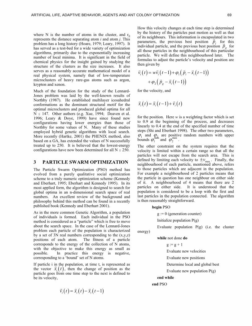
where N is the number of atoms in the cluster, and rij represents the distance separating atom i and atom j. This problem has a long history (Hoare, 1979; Leary, 1997). It has served as a test-bed for a wide variety of optimization algorithms, primarily due to the exponentially increasing number of local minima. It is significant in the field of chemical physics for the insight gained by studying the structure of the clusters as the size increases. It also serves as a reasonably accurate mathematical model of a real physical system, namely that of low-temperature microclusters of heavy rare-gas atoms such as argon, krypton and xenon. Much of the foundation for the study of the Lennard-Jones problem was laid by the well-known results of Northby (1987). He established multilayer icosahedral conformations as the dominant structural motif for the optimal microclusters and produced global optima for all N # 147. Other authors (e.g. Xue, 1994; Deaven et al. 1996; Leary & Doye, 1999) have since found new configurations having lower energies than those of Northby for some values of N. Many of these studies employed hybrid genetic algorithms with local search. More recently (Hartke, 2001) the PHENIX method, also based on a GA, has extended the values of N successfully treated up to 250. It is believed that the lowest-energy configurations have now been determined for all N # 250.
3 PARTICLE SWARM OPTIMIZATION The Particle Swarm Optimization (PSO) method has evolved from a purely qualitative social optimization scheme to a truly numeric optimization scheme (Kennedy and Eberhart, 1995; Eberhart and Kennedy 1995). In its most applied form, the algorithm is designed to search for global optima in an n-dimensional search space of real numbers. An excellent review of the background and philosophy behind this method can be found in a recently published book (Kennedy and Eberhart 2001). As in the more common Genetic Algorithm, a population of individuals is formed. Each individual in the PSO method is considered as a “particle” which is free to move about the search space. In the case of the Lennard-Jones problem each particle of the population is characterized by a set of 3N real numbers corresponding to the (x,y,z) positions of each atom. The fitness of a particle corresponds to the energy of the collection of N atoms, with the objective to make this energy as small as possible. In practice this energy is negative, corresponding to a ‘bound’ set of N atoms. If particle i in the population, at time t, is represented as the vector ( )ix t , then the change of position as the particle goes from one time step to the next is defined to be its velocity, ( ) ( ) ( )1i i iv t x t x t= − −
How this velocity changes at each time step is determined by the history of the particles past motion as well as that of its neighbours. This information is encapsulated in two parameters, the previous best position ip for this individual particle, and the previous best position gp for all those particles in the neighbourhood of this particular particle. We will define this neighbourhood later. The formulas to adjust the particle’s velocity and position are then given by ( ) ( ) ( )( )
( )( )1
2
1 1
1i i i i
g i
v t wv t p x t
p x t
ϕ
ϕ
= − + − −
+ − −
for the velocity, and
( ) ( ) ( )1i i ix t x t v t= − + for the position. Here w is a weighting factor which is set to 0.9 at the beginning of the process, and decreases linearly to 0.4 at the end of the specified number of time steps (Shi and Eberhart 1998). The other two parameters,
1ϕ and 2ϕ are positive random numbers with upper bounds max
1ϕ and max2ϕ .
The other constraint on the system requires that the velocity is limited within a certain range so that all the particles will not escape from the search area. This is defined by limiting each velocity to maxv± . Finally, the neighbourhood of each particle, mentioned above, refers to those particles which are adjacent in the population. For example a neighbourhood of 2 particles means that the particle in question has one neighbour on either side of it. A neighbourhood of 4 means that there are 2 particles on either side. It is understood that the population is considered to be a loop with the first and last particles in the population connected. The algorithm is then reasonably straightforward. begin PSO g := 0 (generation counter) Initialize population P(g)
Evaluate population P(g) (i.e. the cluster energy) while not done do g := g + 1 Evaluate new velocities Evaluate new positions Determine local and global best Evaluate new population P(g) end while end PSO
69ARTIFICIAL LIFE, ADAPTIVE BEHAVIOR, AGENTS AND ANT COLONY OPTIMIZATION
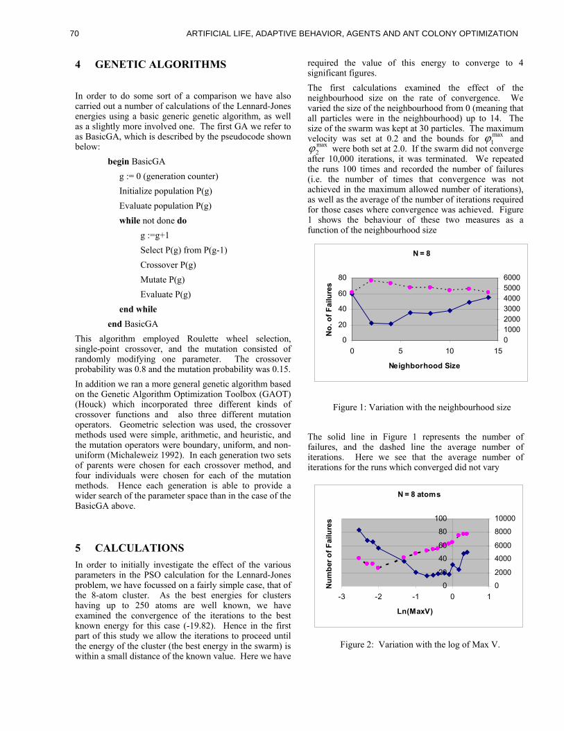
4 GENETIC ALGORITHMS In order to do some sort of a comparison we have also carried out a number of calculations of the Lennard-Jones energies using a basic generic genetic algorithm, as well as a slightly more involved one. The first GA we refer to as BasicGA, which is described by the pseudocode shown below:
begin BasicGA g := 0 (generation counter) Initialize population P(g) Evaluate population P(g) while not done do g :=g+1 Select P(g) from P(g-1) Crossover P(g) Mutate P(g) Evaluate P(g) end while end BasicGA This algorithm employed Roulette wheel selection, single-point crossover, and the mutation consisted of randomly modifying one parameter. The crossover probability was 0.8 and the mutation probability was 0.15. In addition we ran a more general genetic algorithm based on the Genetic Algorithm Optimization Toolbox (GAOT) (Houck) which incorporated three different kinds of crossover functions and also three different mutation operators. Geometric selection was used, the crossover methods used were simple, arithmetic, and heuristic, and the mutation operators were boundary, uniform, and non-uniform (Michaleweiz 1992). In each generation two sets of parents were chosen for each crossover method, and four individuals were chosen for each of the mutation methods. Hence each generation is able to provide a wider search of the parameter space than in the case of the BasicGA above.
5 CALCULATIONS In order to initially investigate the effect of the various parameters in the PSO calculation for the Lennard-Jones problem, we have focussed on a fairly simple case, that of the 8-atom cluster. As the best energies for clusters having up to 250 atoms are well known, we have examined the convergence of the iterations to the best known energy for this case (-19.82). Hence in the first part of this study we allow the iterations to proceed until the energy of the cluster (the best energy in the swarm) is within a small distance of the known value. Here we have
required the value of this energy to converge to 4 significant figures. The first calculations examined the effect of the neighbourhood size on the rate of convergence. We varied the size of the neighbourhood from 0 (meaning that all particles were in the neighbourhood) up to 14. The size of the swarm was kept at 30 particles. The maximum velocity was set at 0.2 and the bounds for max
1ϕ and max2ϕ were both set at 2.0. If the swarm did not converge
after 10,000 iterations, it was terminated. We repeated the runs 100 times and recorded the number of failures (i.e. the number of times that convergence was not achieved in the maximum allowed number of iterations), as well as the average of the number of iterations required for those cases where convergence was achieved. Figure 1 shows the behaviour of these two measures as a function of the neighbourhood size Figure 1: Variation with the neighbourhood size The solid line in Figure 1 represents the number of failures, and the dashed line the average number of iterations. Here we see that the average number of iterations for the runs which converged did not vary
Figure 2: Variation with the log of Max V.
N = 8
0
20
40
60
80
0 5 10 15
Neighborhood Size
No.
of F
ailu
res
0100020003000400050006000
N = 8 atoms
0
20
40
60
80
100
-3 -2 -1 0 1
Ln(MaxV)
Num
ber o
f Fai
lure
s
0
2000
4000
6000
8000
10000
70 ARTIFICIAL LIFE, ADAPTIVE BEHAVIOR, AGENTS AND ANT COLONY OPTIMIZATION
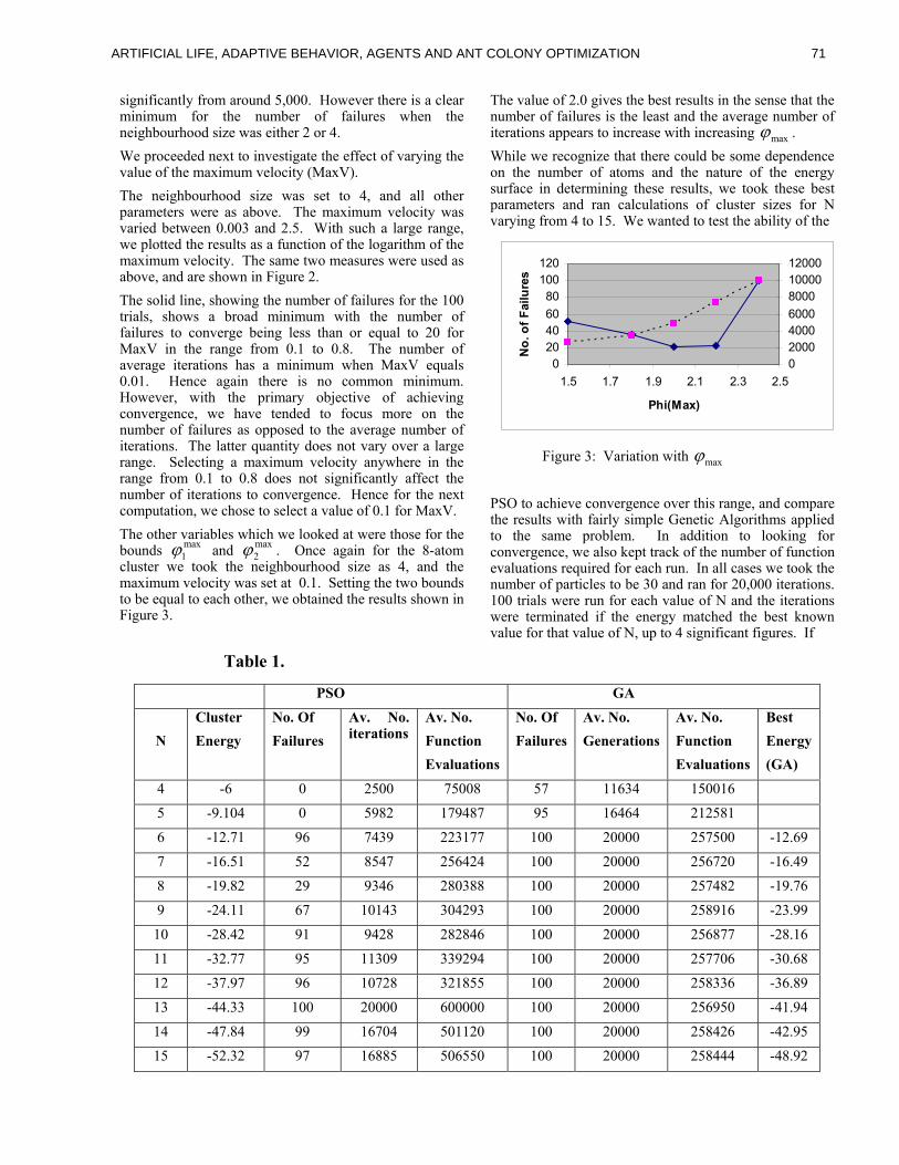
significantly from around 5,000. However there is a clear minimum for the number of failures when the neighbourhood size was either 2 or 4. We proceeded next to investigate the effect of varying the value of the maximum velocity (MaxV). The neighbourhood size was set to 4, and all other parameters were as above. The maximum velocity was varied between 0.003 and 2.5. With such a large range, we plotted the results as a function of the logarithm of the maximum velocity. The same two measures were used as above, and are shown in Figure 2. The solid line, showing the number of failures for the 100 trials, shows a broad minimum with the number of failures to converge being less than or equal to 20 for MaxV in the range from 0.1 to 0.8. The number of average iterations has a minimum when MaxV equals 0.01. Hence again there is no common minimum. However, with the primary objective of achieving convergence, we have tended to focus more on the number of failures as opposed to the average number of iterations. The latter quantity does not vary over a large range. Selecting a maximum velocity anywhere in the range from 0.1 to 0.8 does not significantly affect the number of iterations to convergence. Hence for the next computation, we chose to select a value of 0.1 for MaxV. The other variables which we looked at were those for the bounds max
1ϕ and max2ϕ . Once again for the 8-atom
cluster we took the neighbourhood size as 4, and the maximum velocity was set at 0.1. Setting the two bounds to be equal to each other, we obtained the results shown in Figure 3.
Table 1.
The value of 2.0 gives the best results in the sense that the number of failures is the least and the average number of iterations appears to increase with increasing maxϕ . While we recognize that there could be some dependence on the number of atoms and the nature of the energy surface in determining these results, we took these best parameters and ran calculations of cluster sizes for N varying from 4 to 15. We wanted to test the ability of the Figure 3: Variation with maxϕ PSO to achieve convergence over this range, and compare the results with fairly simple Genetic Algorithms applied to the same problem. In addition to looking for convergence, we also kept track of the number of function evaluations required for each run. In all cases we took the number of particles to be 30 and ran for 20,000 iterations. 100 trials were run for each value of N and the iterations were terminated if the energy matched the best known value for that value of N, up to 4 significant figures. If
PSO GA
N Cluster Energy
No. Of Failures
Av. No. iterations
Av. No. Function Evaluations
No. Of Failures
Av. No. Generations
Av. No. Function Evaluations
Best Energy(GA)
4 -6 0 2500 75008 57 11634 150016 5 -9.104 0 5982 179487 95 16464 212581 6 -12.71 96 7439 223177 100 20000 257500 -12.69
7 -16.51 52 8547 256424 100 20000 256720 -16.49
8 -19.82 29 9346 280388 100 20000 257482 -19.76
9 -24.11 67 10143 304293 100 20000 258916 -23.99
10 -28.42 91 9428 282846 100 20000 256877 -28.16
11 -32.77 95 11309 339294 100 20000 257706 -30.68
12 -37.97 96 10728 321855 100 20000 258336 -36.89
13 -44.33 100 20000 600000 100 20000 256950 -41.94
14 -47.84 99 16704 501120 100 20000 258426 -42.95
15 -52.32 97 16885 506550 100 20000 258444 -48.92
020406080100120
1.5 1.7 1.9 2.1 2.3 2.5
Phi(Max)
No.
of F
ailu
res
020004000600080001000012000
71ARTIFICIAL LIFE, ADAPTIVE BEHAVIOR, AGENTS AND ANT COLONY OPTIMIZATION
the run did not converge to this limit under the 20,000 iteration limit, then the run was counted as a failure. Table 1 provides a summary of these results for N = 4 to 15. The second column is the known lowest energy for each of these cluster sizes (Leary, 1997). The next three columns show the PSO results: the number of failures to converge out of the 100 total trials; the average number of iterations required for those trials which did converge; and the average number of function evaluations used in the converged runs. The number of failures to converge is also graphed in Figure 4 as a function of N. Here two plots are shown, the solid line shows runs which were terminated after 10,000 iterations if convergence was not achieved, whereas the dashed line shows the same results for 20,000 iterations. It can be seen that there is not a great deal of difference between these two results. Fig. 4. Failures vs N Table 1 also shows the results of runs using the modified GA. The basic GA was not successful in the sense that after 500,000 generations, convergence could not be achieved even for N = 4 atoms. Limiting the runs to 20,000 generations and using a population size of 30, the modified GA did find the known energies for N=4 and N=5, but was unsuccessful in 100 trials for the other values of N. The best energies achieved are shown in the table, and for the smaller values of N are relatively close to the known energies, indicating that allowing the GA to continue would likely achieve convergence. The PSO method was able to achieve convergence in at least one of the trials for all values of N studied here, except for N = 13. In many cases only a few of the trials converged, seeming to indicate that the particle “swarm” could not get close enough to the fixed point in the set number of iterations.
6 SUMMARY AND CONCLUSIONS The Particle Swarm Optimization method has been applied to a variety of areas since its introduction only a few years ago. As far as we are aware this is the first time
that it has been applied to the energy conformation problem for atomic clusters. There has also been some other work on comparing the PSO with genetic algorithms (Eberhart and Shi 1998; Angeline 1998). Genetic algorithms incorporate selection, crossover and mutation schemes in order to search the parameter space. In the PSO there is no specific selection process, however each individual carries with it a copy of its personal best value, which serves a somewhat similar role to that of a parent. The offspring of an individual is a function of this best value. The PSO is the only evolutionary algorithm that does not incorporate selection of the fittest. The role of the crossover function in the GA is to select information from parents (usually two) to create offspring. In the PSO the influence on one particle by the others comes only in the value of the best position of the particles in the defined neighbourhood. Mutations are an important aspect of the GA process in that they help to break out of the genetic sequence generated by the parents and offspring. However a common limitation of the GA is that as the population converges, the average fitness value becomes high so that mutations will usually result in a low-fitness chromosome which will be rejected by the selection process. The result is that the process may converge to a local optimum instead of finding the global one. There are variations which try to circumvent this, including the incorporation of local optimization methods. Particle swarm uses a highly directional mutation operation as each individual’s velocity vector is modified using a vector whose direction lies between the personal best and the neighbourhood best. As a consequence the PSO may have difficulties when the average local gradients point away from the global optima or are constantly changing. Our calculations here have shown that the PSO is indeed an effective optimization method. Significantly better results have been found for the location of the global optimum energy value for a cluster of atoms interacting via the Lennard-Jones potential than for the case of a relatively generic GA. The potential energy surfaces for these problems are known to contain large numbers of local minima, often very close to the global minima for certain values of N. Hence it is not unexpected to find that many of the runs converge to one of these local minima. The use of a low value of the maximum velocity in our calculations undoubtedly resulted in slow convergence in most cases, however it was somewhat necessary in the sense that the parameter values for the sizes of clusters studied here are in the range [-1, 1]. Small variations in these parameter values can shift the energy significantly, so that it is important to search over a relatively fine mesh. The runs with the genetic algorithms quickly converged to a limit, and then tended to stay near that value for most of the subsequent generations. Here it would help to have
0
20
40
60
80
100
120
3 8 13 18
Number of Atoms
Num
ber o
f Fai
lure
s
72 ARTIFICIAL LIFE, ADAPTIVE BEHAVIOR, AGENTS AND ANT COLONY OPTIMIZATION
more flexible mutation and selection schemes to prevent this from happening. Future work will focus on studying possible variations to the PSO which can help improve the success rate for this type of problem.
Acknowledgments This investigation was supported in part by the National Science and Engineering Research Council of Canada (NSERC).
References Angeline, P.J. “Particle Swarm - Evolutionary Optimization Versus Particle Swarm Optimization: Philosophy and Performance Differences”, Lecture Notes in Computer Science 1447 (1998) 601-610. Barron, C., Gomez, S., Romero, D. and Saaverdra, A. “A genetic algorithm for Lennard-Jones atomic clusters”, App. Math. Letts. 12 (1999) 85-90. Deaven, D.M. and Ho, K.M. “Molecular Geometry Optimization with a Genetic Algorithm”, Phys. Rev. Letts. 75 (1995) 288-291. Deaven, D.M., Tit, N., Morris, J.R. and Ho, K.M. “Structural optimization of Lennard-Jones clusters by a genetic algorithm”, Chem. Phys. Letts. 256 (1996) 195-200. Doye, J.P.K., Miller, M.A. and Wales, D.J., “The double-funnel energy landscape of the 38-atom Lennard-Jones cluster”, J. Chem. Phys. 110 (1999) 6896-6906. Eberhart, R.C. and Kennedy, J. “A new optimizer using particle swarm theory”, Proc. Sixth Int. Symp. on Micro Machine and Human Science (Nagoya, Japan) (1995) 39-43. Eberhat, R.C. and Shi, Y. “Comparison between Genetic Algorithms and Particle Swarm Optimization”, Lecture Notes in Computer Science 1447 (1998) 611-618. Hartke, B. “Global Geometry optimization of clusters using genetic algorithms”, J. Phys. Chem. 97 (1993) 9973-9976 Hartke, B. “Global geometry optimization of atomic and molecular clusters by genetic algorithms”, Proc. Of the Genetic and Evolutionary Computation Coference (GECCO) 2001, 1284-1291. Hoare, M. “ Structure and dynamics of simple microclusters”, Adv. Chem. Phys. 40 (1979) 49-135. Hoare, M.R. and Pal, P. Adv. Physics 20 (1971) 161. Houck, C.R., Joines, J.A. and Kay, M.G. Genetic Algorithm Optimization Toolbox (GAOT) for Matlab. http://www.ie.ncsu.edu/mirage/GAToolBox/gaot/ Kennedy, J. “The particle swarm: social adaptation of knowledge”, Proc. 1997 IEEE Int. Conf. on Evolutionary Computation, 303-308.
Kennedy, J. and Eberhart, R.C. “Particle swarm optimization”, Proc. 1995 IEEE Int. Conf. on Neural Networks (Perth, Australia) 1942-1948. Kennedy, J. and Eberhart, R.C. “Swarm Intelligence”, Morgan Kaufmann, 2001. Leary, R.H. “Global Optima of Lennard-Jones Clusters”, J. Global Optim. 11 (1997) 35-53 Leary, R.H. and Doye, J.P.K. “Tetrahedral global minimum for the 98-atom Lennard-Jones cluster”, Phys. Rev. E 60 (1999) R6320-22. Michalewicz, Z. (1992) “Genetic Algorithms + Data Structures = Evolution Programs” Springer-Verlag,. Niesse, J.A. and Mayne, H.R. “Global geometry optimization of atomic clusters using modified genetic algorithm in space-fixed coordinates”, J. Chem. Phys. 105 (1996) 4700-4706. Northby, J.A., “Structure and binding of Lennard-Jones clusters: 13 # N # 147", J. Chem. Phys. 87 (1987) 6166-6177. Peterson, C., Sommelius, O. and Soderberg, B. “Variational appraoch for minimizing Lennard-Jones energies”, Phys. Rev. E 53 (1996) 1725-1731. Radcliffe, N.J. and Surry, P.D., “Formal Memetic Algorithms”, Evolutionary Computing. AISB Workshop. Selected Papers. Springer-Verlag. 1994, pp.1-16. Berlin, Germany. Shi, Y. and Eberhart, R.C. “Particle Swarm - Parameter Selection in Particle Swarm Optimization”, Lecture Notes in Computer Science 1447 (1998) 591-600. Stillinger, F.H., Phys. Rev. E 59, 48 (1999). Tsai, C.J. and Jordan, K.D., J. Phys. Chem. 97, 11 227 (1993). Wales, D.J. and Doye, J.P.K. “Global optimization by Basin-Hopping and the Lowest Energy Structures of Lennard-Jones Clusters up to 110 Atoms”, J. Phys. Chem. A 101 (1997) 5111-5116. Wille, L. and Vennik, J., “Computational Complexity of the ground-state determination of atomic clusters”, J. Phys A 18 (1985) L419-L422. Wolf, M.D. and Landman, U. “Genetic Algorithms for Structural Cluster Optimization”, J. Phys. Chem. A 102 (1998) 6129-6137. Xue, G. “Improvement on the Northby Algorithm for Molecular Conformation: Better Solutions”, J. Global Optim. 4 (1994) 425-440. Zeiri, Y., “Prediction of the lowest energy structure of clusters using a genetic algorithm”, Phys. Rev. E 51, R2769 (1995).
73ARTIFICIAL LIFE, ADAPTIVE BEHAVIOR, AGENTS AND ANT COLONY OPTIMIZATION
Option Valuation with Generalized Ant Programming
Christian Keber
University of Vienna
Department of Business Administration
Bruenner Strasse 72, A-1210
Matthias G. Schuster
University of Vienna
Department of Business Administration
Bruenner Strasse 72, A-1210
Abstract
For the valuation of American put options ex-
act pricing formulas haven't as yet been de-
rived We therefore determine analytical ap-
proximations for pricing such options by in-
troducing the Generalized Ant Programming
(GAP) approach applicable to all problems
in which the search space of feasible solu-
tions consists of computer programs. GAP is
a new method inspired by Genetic Program-
ming as well as by Ant Algorithms. Applying
our GAP-approximations for the valuation of
American put options on non-dividend pay-
ing stocks to experimental data as well as
huge validation data sets we can show that
our formulas deliver accurate results and out-
perform other formulas presented in the lit-
erature.
1 INTRODUCTION
In their seminal papers Black and Scholes (1973) and
Merton (1973) derived an analytical solution for the
valuation of European call options on stocks paying no
dividends during the time to expiration. Merton ad-
ditionally showed that premature exercising of Amer-
ican call options on this type of stocks is never op-
timal and that the valuation can also be made using
the Black/Scholes{Merton method. If in the case of an
American call option, dividends are paid, and these are
known with certainty, its value can be obtained using
the analytically exact pricing model of Roll (1977).
In comparison to American call options, premature ex-
ercise of American put options on non-dividend paying
stocks may produce bene�ts, if the stock price falls
below a certain, permanently variable critical value
(killing price). As a result of this di�erence between
the premature exercising of American call options and
of American put options, ascertaining the optimal time
for premature exercising, or the killing price, is a part
of the problem to be solved, for which there was pre-
viously no exact model. Thus, the valuation of Amer-
ican put options is based on numerical procedures or
analytical approximations. The best-known numeri-
cal procedures are the lattice approach of Cox, Ross,
and Rubinstein (1979) and the �nite di�erence method
of Brennan and Schwartz (1977). However, getting
accurate results by using numerical procedures nor-
mally requires long calculation time. A simple analyt-
ical approximation for the valuation of American put
options on non-dividend paying stocks was presented
by Johnson (1983). This simple analytical approxima-
tion, however, is not very accurate, so that many more
ambitious analytical approximations have been devel-
oped. The best-known of these come from MacMillan
(1986) and Geske and Johnson (1984).
MacMillan's analytical approximation for the valua-
tion of American put options consists of raising the
value of a suitable European put option by the value
of the approximately calculated premature exercising
of the option. This method forms the basis for analyt-
ical approximations used to evaluate a range of other
American options, such as index options, currency op-
tions, and options on futures (see, e.g., Barone-Adesi
and Whaley (1987)). Geske and Johnson's analyti-
cal approximation assumes that premature exercise is
possible only at particular, discrete points in time. Ac-
cordingly, for each of these moments an option value is
calculated, and, based on this, the value of the Amer-
ican put option is ascertained using the polynomial
extrapolation method. This method treats American
put options both with and without dividends. The
MacMillan method, however, deals only with put op-
tions on stocks paying no dividend during the maturity
of the options, although it was extended by Barone-
Adesi and Whaley (1988) as well as Fischer (1993) to
ARTIFICIAL LIFE, ADAPTIVE BEHAVIOR, AGENTS AND ANT COLONY OPTIMIZATION74
include the dividend paying case. It is characteristic
of most approximations for the valuation of Ameri-
can put options found in the literature that they ap-
proximate either the stochastic stock price process, or
the partial di�erential equation (with the appropri-
ate boundaries) which implicitly describes the option
price. In contrast, Geske and Johnson (1984) as well
as Kim (1990) formulate a valuation equation which
represents an exact solution of the partial di�erential
equation, and then solve it either by analytical approx-
imation or by numerical techniques.
During the last few decades an increasing number of
researchers of various disciplines has been impressed
by the problem-solving power of nature. They devel-
oped optimization algorithms and heuristics based on
the imitation and simulation of admirable natural phe-
nomena. For example, Arti�cial Neural Networks im-
itate the principle of human brains and Evolutionary
Algorithms make use of the Darwinian principle of the
survival{of{the{�ttest. Both methodologies are used
to solve problems which are normally not amenable to
traditional solution techniques and have been applied
to option pricing problems. For instance, Hutchinson,
Lo, and Poggio (1994) employ an arti�cial neural net-
work for the valuation of European options whereas
Chen, Lee, and Yeh (1999), Chidambaran, Lee, and
Trigueros (2000), and Keber (2000) use Genetic Pro-
gramming to solve option pricing problems.
A further example and one of the most recent develop-
ments of nature-based solution techniques is the Ant
Colony Optimization meta-heuristic. Ant Algorithms
originally introduced by Dorigo and colleagues (Dorigo
(1992) and Dorigo, Maniezzo, and Colorni (1991)) as
a multi-agent approach to diÆcult combinatorial op-
timization problems like the travelling salesman prob-
lem (TSP) are inspired by the foraging behaviour of
real ant colonies, in particular, how ants can �nd short-
est paths between two points. Real ant colonies are
capable of solving such problems using collective be-
haviour and indirect communication via a chemical
substance called pheromone deposited on the ground.
It is hardly surprising that for the �rst time ant al-
gorithms have been applied to the travelling salesman
problem because the analogy between the real ants'
problem and the TSP is obvious. In the meantime,
ant-based algorithms have been applied successfully to
a broad �eld of combinatorial optimization problems
(see, e.g., Dorigo, Caro, and Gambardella (1999)).
In this contribution we develop the Generalized Ant
Programming (GAP) approach as a new variant of ant
algorithms and apply the proposed method to the op-
tion valuation problem. GAP enables computers to
solve problems without being explicitly programmed.
It is applicable to all problems in which the search
space of feasible solutions consists of computer pro-
grams. GAP works by using arti�cial ants to automat-
ically generate computer programs. As an acid test for
GAP we derive analytical approximations for the valu-
ation of American put options on non-dividend paying
stocks. We focus on this problem for several reasons.
Firstly, analytical exact solutions for pricing American
puts have not as yet been derived. Secondly, testing
new techniques should not be based on simple prob-
lems because any assessment of the proposed method
would be open to criticism. Furthermore, our results
have to be compared with other approximations pre-
sented in the literature. This can be easily done by
using the most frequently quoted approximations men-
tioned above. Using experimental data as well as huge
validation data sets we can show that the GAP based
formulas for the valuation of American put options on
non-dividend paying stocks deliver accurate approxi-
mation results and outperform other approximations
presented in the literature.
In the second section we focus on the concept of the
Generalized Ant Programming approach. The third
section presents the GAP-approximations for the valu-
ation of American put options on non-dividend paying
stocks. In the fourth section we show the experimental
results. The contribution concludes with a summary.
2 GENERALIZED ANT
PROGRAMMING
2.1 INTRODUCTION
The Generalized Ant Programming (GAP) approach
is a new method inspired by the Genetic Program-
ming approach introduced by Koza (1992) as well
as by Ant Algorithms originally presented by Dorigo
(1992) as a multi-agent approach to diÆcult combi-
natorial optimization problems like TSP. GAP is an
approach designed to generate computer programs by
simulating the behaviour of real ant colonies. When
travelling real ants deposit pheromone on the ground
which in uence the choices they make. Ants tend to
choose steps marked by strong pheromone concentra-
tions. Pheromone trails can be seen as \public in-
formation" which is modi�ed by ants to re ect their
experience while solving a problem, e.g., to �nd short-
est paths between the nest and food sources. The
quantity of pheromone left by an ant depends on the
amount of food found. Within a given interval of time,
shorter paths can be travelled more often, which causes
a stronger pheromone concentration. In return, this
ARTIFICIAL LIFE, ADAPTIVE BEHAVIOR, AGENTS AND ANT COLONY OPTIMIZATION 75
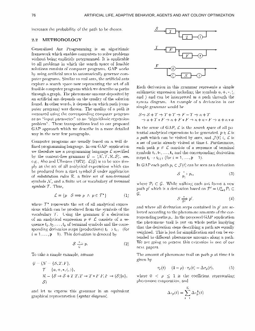
increases the probability of the path to be chosen.
2.2 METHODOLOGY
Generalized Ant Programming is an algorithmic
framework which enables computers to solve problems
without being explicitly programmed. It is applicable
to all problems in which the search space of feasible
solutions consists of computer programs. GAP works
by using arti�cial ants to automatically generate com-
puter programs. Similar to real ants, the arti�cial ants
explore a search space now representing the set of all
feasible computer programs which we describe as paths
through a graph. The pheromone amount deposited by
an arti�cial ant depends on the quality of the solution
found. In other words, it depends on which path (com-
puter program) was chosen. The quality of a path is
measured using the corresponding computer program
as an \input parameter" to an \algorithmic regression
problem". These transpositions lead to our proposed
GAP approach which we describe in a more detailed
way in the next few paragraphs.
Computer programs are usually based on a well de-
�ned programming language. In our GAP{application
we therefore use a programming language L speci�ed
by the context-free grammar G = (N ; T ;R;S), see,e.g., Aho and Ullmann (1972). L(G) is to be seen sim-
ply as the set of all analytical expressions which can
be produced from a start symbol S under application
of substitution rules R, a �nite set of non-terminal
symbols N , and a �nite set or vocabulary of terminal
symbols T . Thus,
L = fp j S =) p ^ p 2 T �g (1)
where T � represents the set of all analytical expres-
sions which can be produced from the symbols of the
vocabulary T . Using the grammar G a derivation
of an analytical expression p 2 L consists of a se-
quence t1; t2; : : : ; tp of terminal symbols and the corre-
sponding derivation steps (productions) ti ! ti+1 (for
i = 1; : : : ; p� 1). This derivation is denoted by
S �
=)G
p: (2)
To take a simple example, assume
G = (N = fS; T; Fg;T = fa;+; �; (; )g;R = fS ! S + T jT; T ! T � F jF; F ! (S)jag;S)
and let us express this grammar in an equivalent
graphical representation (syntax diagram).
S -T
-
Tj+
6
T -F
-
Fj�6
F - ja
-
j( S j)-6
Each derivation in this grammar represents a simple
arithmetic expression including the symbols a;+; �; (;and ) and can be interpreted as a path through the
syntax diagram. An example of a derivation in our
simple grammar would be
S) S + T ) T + T ) F + T ) a+ T
) a+ T � F ) a+ F � F ) a+ a � F ) a+ a � aIn the sense of GAP, L is the search space of all po-
tential analytical expressions to be generated, p 2 L is
a path which can be visited by ants, and J (t) � L is
a set of paths already visited at time t. Furthermore,
each path p 2 L consists of a sequence of terminal
symbols t1; t2; : : : ; tp and the corresponding derivation
steps ti ! ti+1 (for i = 1; : : : ; p� 1).
In GAP each path pi 2 J (t) can be seen as a derivation
S �
=)Pi
pi; (3)
where Pi � G. While walking each ant forms a new
path p0 which is a derivation based on P 0 = [ni=1Pi �
G,S �
=)P0
p0; (4)
and where all derivation steps contained in p0 are se-
lected according to the pheromone amounts of the cor-
responding paths pi. In the proposed GAP-application
the pheromone trail is put on whole paths implying
that the derivation steps describing a path are equally
weighted. This is just for simpli�cation and can be ex-
tended to di�erent pheromone amounts along a path.
We are going to present this extension in one of our
next papers.
The amount of pheromone trail on path p at time t is
given by
�p(t) = (1� �) � �p(t) + ��p(t); (5)
where 0 < � � 1 is the coeÆcient representing
pheromone evaporation, and
��p(t) =
KXk=1
��kp (t)
ARTIFICIAL LIFE, ADAPTIVE BEHAVIOR, AGENTS AND ANT COLONY OPTIMIZATION76
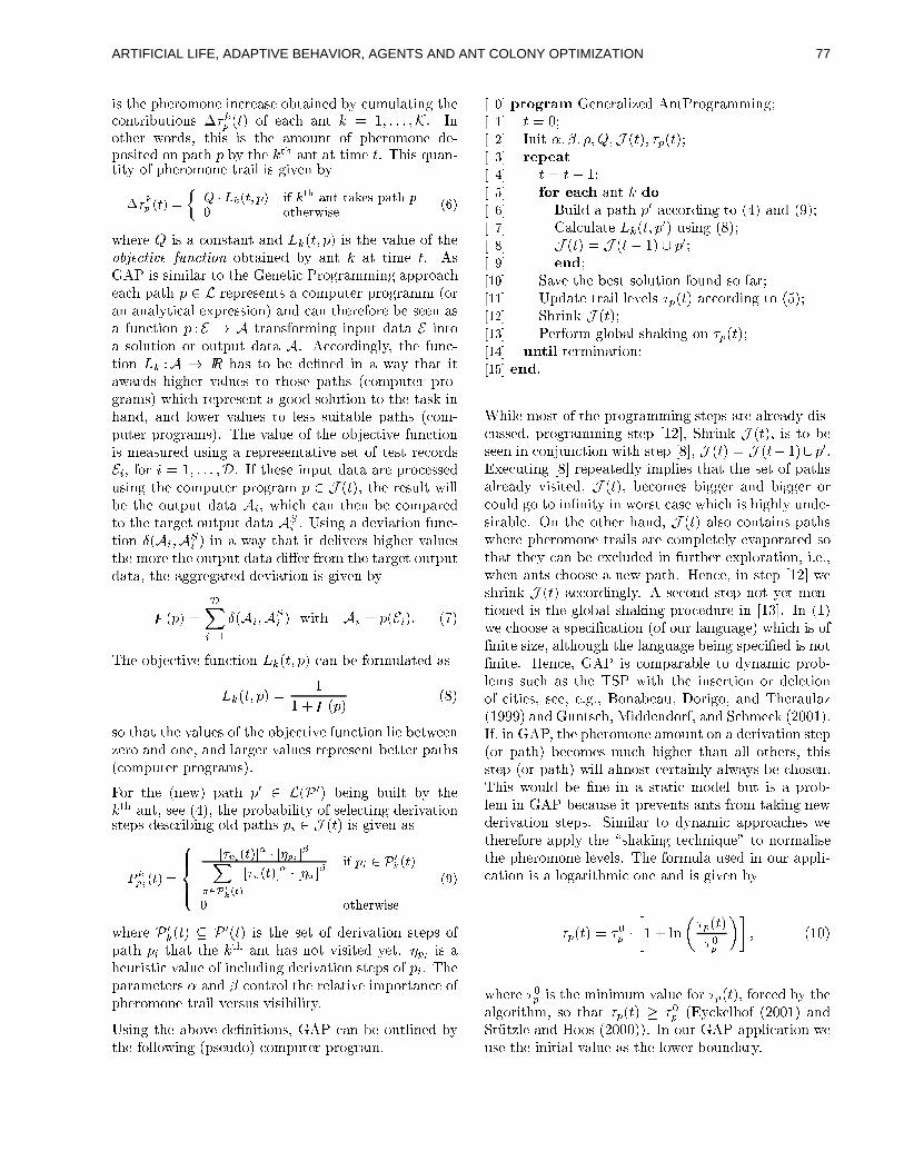
is the pheromone increase obtained by cumulating thecontributions ��
kp (t) of each ant k = 1; : : : ;K. In
other words, this is the amount of pheromone de-posited on path p by the kth ant at time t. This quan-tity of pheromone trail is given by
��kp (t) =
�Q � Lk(t; p) if kth ant takes path p
0 otherwise(6)
where Q is a constant and Lk(t; p) is the value of the
objective function obtained by ant k at time t. As
GAP is similar to the Genetic Programming approach
each path p 2 L represents a computer programm (or
an analytical expression) and can therefore be seen as
a function p : E ! A transforming input data E into
a solution or output data A. Accordingly, the func-
tion Lk :A ! IIR has to be de�ned in a way that it
awards higher values to those paths (computer pro-
grams) which represent a good solution to the task in
hand, and lower values to less suitable paths (com-
puter programs). The value of the objective function
is measured using a representative set of test records
Ei, for i = 1; : : : ;D. If these input data are processed
using the computer program p 2 J (t), the result will
be the output data Ai, which can then be compared
to the target output data ASi . Using a deviation func-
tion Æ(Ai;ASi ) in a way that it delivers higher values
the more the output data di�er from the target output
data, the aggregated deviation is given by
z(p) =
DXi=1
Æ(Ai;ASi ) with Ai = p(Ei): (7)
The objective function Lk(t; p) can be formulated as
Lk(t; p) =1
1 +z(p)(8)
so that the values of the objective function lie between
zero and one, and larger values represent better paths
(computer programs).
For the (new) path p0 2 L(P 0) being built by the
kth ant, see (4), the probability of selecting derivationsteps describing old paths pi 2 J (t) is given as
Pkpi(t) =
8>><>>:
[�pi(t)]� � [�pi ]
�X�2P0
k(t)
[��(t)]� � [�� ]�
if pi 2 P 0k(t)
0 otherwise
(9)
where P 0
k(t) � P 0(t) is the set of derivation steps of
path pi that the kth ant has not visited yet. �pi is a
heuristic value of including derivation steps of pi. The
parameters � and � control the relative importance of
pheromone trail versus visibility.
Using the above de�nitions, GAP can be outlined by
the following (pseudo) computer program.
[ 0] program Generalized AntProgramming;
[ 1] t = 0;
[ 2] Init �; �; �;Q;J (t); �p(t);
[ 3] repeat
[ 4] t = t+ 1;
[ 5] for each ant k do
[ 6] Build a path p0 according to (4) and (9);
[ 7] Calculate Lk(t; p0) using (8);
[ 8] J (t) = J (t� 1) [ p0;
[ 9] end;
[10] Save the best solution found so far;
[11] Update trail levels �p(t) according to (5);
[12] Shrink J (t);
[13] Perform global shaking on �p(t);
[14] until termination;
[15] end.
While most of the programming steps are already dis-
cussed, programming step [12], Shrink J (t), is to be
seen in conjunction with step [8], J (t) = J (t�1)[p0.Executing [8] repeatedly implies that the set of paths
already visited, J (t), becomes bigger and bigger or
could go to in�nity in worst case which is highly unde-
sirable. On the other hand, J (t) also contains paths
where pheromone trails are completely evaporated so
that they can be excluded in further exploration, i.e.,
when ants choose a new path. Hence, in step [12] we
shrink J (t) accordingly. A second step not yet men-
tioned is the global shaking procedure in [13]. In (1)
we choose a speci�cation (of our language) which is of
�nite size, although the language being speci�ed is not
�nite. Hence, GAP is comparable to dynamic prob-
lems such as the TSP with the insertion or deletion
of cities, see, e.g., Bonabeau, Dorigo, and Theraulaz
(1999) and Guntsch, Middendorf, and Schmeck (2001).
If, in GAP, the pheromone amount on a derivation step
(or path) becomes much higher than all others, this
step (or path) will almost certainly always be chosen.
This would be �ne in a static model but is a prob-
lem in GAP because it prevents ants from taking new
derivation steps. Similar to dynamic approaches we
therefore apply the \shaking technique" to normalise
the pheromone levels. The formula used in our appli-
cation is a logarithmic one and is given by
�p(t) = �0p ��1 + ln
��p(t)
�0p
��; (10)
where �0p is the minimum value for �p(t), forced by the
algorithm, so that �p(t) � �0p (Eyckelhof (2001) and
St�utzle and Hoos (2000)). In our GAP-application we
use the initial value as the lower boundary.
ARTIFICIAL LIFE, ADAPTIVE BEHAVIOR, AGENTS AND ANT COLONY OPTIMIZATION 77
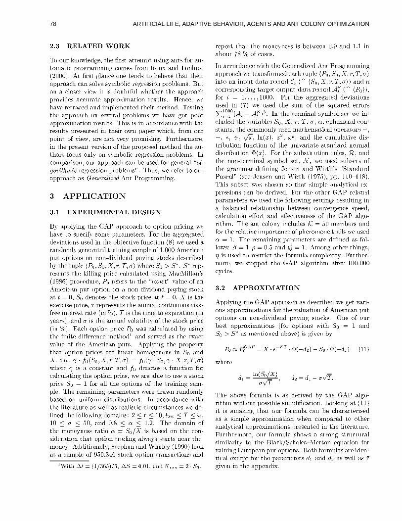
2.3 RELATED WORK
To our knowledge, the �rst attempt using ants for au-
tomatic programming comes from Roux and Fonlupt
(2000). At �rst glance one tends to believe that their
approach can solve symbolic regression problems. But
on a closer view it is doubtful whether the approach
provides accurate approximation results. Hence, we
have retraced and implemented their method. Testing
the approach on several problems we have got poor
approximation results. This is in accordance with the
results presented in their own paper which, from our
point of view, are not very promising. Furthermore,
in the present version of the proposed method the au-
thors focus only on symbolic regression problems. In
comparison, our approach can be used for general \al-
gorithmic regression problems". Thus, we refer to our
approach as Generalized Ant Programming.
3 APPLICATION
3.1 EXPERIMENTAL DESIGN
By applying the GAP approach to option pricing we
have to specify some parameters. For the aggregated
deviations used in the objective function (8) we used a
randomly generated training sample of 1,000 American
put options on non-dividend paying stocks described
by the tuple hP0; S0; X; r; T; �i where S0 > S�. S� rep-
resents the killing price calculated using MacMillan's
(1986) procedure, P0 refers to the \exact" value of an
American put option on a non-dividend paying stock
at t = 0, S0 denotes the stock price at t = 0, X is the
exercise price, r represents the annual continuous risk-
free interest rate (in %), T is the time to expiration (in
years), and � is the annual volatility of the stock price
(in %). Each option price P0 was calculated by using
the �nite di�erence method1 and served as the exact
value of the American puts. Applying the property
that option prices are linear homogenous in S0 and
X , i.e., � f0(S0; X; r; T; �) = f0( � S0; � X; r; T; �)
where is a constant and f0 denotes a function for
calculating the option price, we are able to use a stock
price S0 = 1 for all the options of the training sam-
ple. The remaining parameters were drawn randomly
based on uniform distributions. In accordance with
the literature as well as realistic circumstances we de-
�ned the following domains: 2 � r � 10, 1=360 � T � 1=4,
10 � � � 50, and 0:8 � � � 1:2. The domain of
the moneyness ratio � = S0=X is based on the con-
sideration that option trading always starts near-the-
money. Additionally, Stephan and Whaley (1990) look
at a sample of 950,346 stock option transactions and
1With �t = (1=365)=5, �S = 0:01, and Smax = 2 � S0.
report that the moneyness is between 0.9 and 1.1 in
about 78 % of cases.
In accordance with the Generalized Ant Programming
approach we transformed each tuple hP0; S0; X; r; T; �iinto an input data record Ei (b= hS0; X; r; T; �i) and a
corresponding target output data record ASi (b= hP0i),
for i = 1; : : : ; 1000. For the aggregated deviations
used in (7) we used the sum of the squared errorsP1000
i=1 (Ai � ASi )
2. In the terminal symbol set we in-
cluded the variables S0, X , r, T , �, �, ephemeral con-
stants, the commonly used mathematical operators +,
�, �, �, px, ln(x), x2, xy , and the cumulative dis-
tribution function of the univariate standard normal
distribution �(x). For the substitution rules, R, andthe non-terminal symbol set, N , we used subsets of
the grammar de�ning Jensen and Wirth's \Standard
Pascal" (see Jensen and Wirth (1975), pp. 110{118).
This subset was chosen so that simple analytical ex-
pressions can be derived. For the other GAP related
parameters we used the following settings resulting in
a balanced relationship between convergence speed,
calculation e�ort and e�ectiveness of the GAP algo-
rithm. The ant colony includes K = 50 members and
for the relative importance of pheromone trails we used
� = 1. The remaining parameters are de�ned as fol-
lows: � = 1; � = 0:5 and Q = 1. Among other things,
� is used to restrict the formula complexity. Further-
more, we stopped the GAP algorithm after 100,000
cycles.
3.2 APPROXIMATION
Applying the GAP approach as described we get vari-
ous approximations for the valuation of American put
options on non-dividend paying stocks. One of our
best approximations (for options with S0 = 1 and
S0 > S� as mentioned above) is given by
P0 � PGAP0 = X � e��r�T � �(�d2)� S0 � �(�d1) (11)
where
d1 =ln(S0=X)
�pT
; d2 = d1 � �
pT :
The above formula is as derived by the GAP algo-
rithm without possible simpli�cation. Looking at (11)
it is amazing that our formula can be characterised
as a simple approximation when compared to other
analytical approximations presented in the literature.
Furthermore, our formula shows a strong structural
similarity to the Black/Scholes{Merton equation for
valuing European put options. Both formulas are iden-
tical except for the parameters d1 and d2 as well as �r
given in the appendix.
ARTIFICIAL LIFE, ADAPTIVE BEHAVIOR, AGENTS AND ANT COLONY OPTIMIZATION78
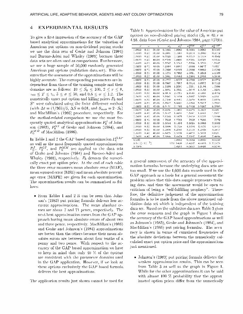
4 EXPERIMENTAL RESULTS
To give a �rst impression of the accuracy of the GAP
based analytical approximations for the valuation of
American put options on non-dividend paying stocks
we use the data sets of Geske and Johnson (1984)
and Barone-Adesi and Whaley (1988) because these
data sets are often used as comparisons. Furthermore,
we use a huge sample of 50,000 randomly generated
American put options (validation data set). This en-
sures that the assessment of the approximations will be
highly accurate. The corresponding parameters are in-
dependent from those of the training sample and their
domains are as follows: 10 � S0 � 100, 2 � r � 8,1=360 � T � 1=4, 5 � � � 50, and 0:8 � � � 1:2. The
numerically exact put option and killing prices P0 and
S� were calculated using the �nite di�erence method
(with �t = (1=365)=5, �S = 0:01, and Smax = 2 � S0)and MacMillan's (1986) procedure, respectively. For
the method-related comparison we use the most fre-
quently quoted analytical approximations P J0 of John-
son (1983), PGJ0 of Geske and Johnson (1984), and
PMM0 of MacMillan (1986).
In Table 1 and 2 the GAP based approximation PGAP0
as well as the most frequently quoted approximations
PJ0 , P
GJ0 , and P
MM0 are applied to the data sets
of Geske and Johnson (1984) and Barone-Adesi and
Whaley (1988), respectively. P0 denotes the numeri-
cally exact put option price. At the end of each table
the three error measures mean absolute error (MAE),
mean squared error (MSE) and mean absolute percent-
age error (MAPE) are given for each approximation.
The approximation results can be summarised as fol-
lows:
� From Tables 1 and 2 it can be seen that John-
son's (1983) put pricing formula delivers less ac-
curate approximations. The mean absolute er-
rors are about 7 and 71 pence, respectively. The
next best approximation comes from the GAP ap-
proach having mean absolute errors of about two
and three pence, respectively. MacMillan's (1986)
and Geske and Johnson's (1984) approximations
are better than the others because their mean ab-
solute errors are between about four tenths of a
penny and two pence. With respect to the ac-
curacy of the GAP based approximation we have
to keep in mind that only 40 % of the options
are consistent with the parameter domains used
in the GAP application. However, if we look at
these options exclusively the GAP based formula
delivers the best approximations.
The application results just shown cannot be used for
Table 1: Approximations for the value of American put
options on non-dividend paying stocks (S0 = 40; r =
4:88, data from (Geske and Johnson 1984, page 1519)).
T � X P0 PJ0
PMM0
PGJ0
PGAP0
0.0833 0.20 35.00 0.0063 0.0062 0.0065 0.0062 0.0063
0.3333 0.20 35.00 0.2001 0.1969 0.2044 0.2000 0.2042
0.5833 0.20 35.00 0.4323 0.4205 0.4415 0.4318 0.4582
0.0833 0.20 40.00 0.8509 0.8406 0.8503 0.8521 0.8533
0.3333 0.20 40.00 1.5787 1.5262 1.5768 1.5759 1.5937
0.5833 0.20 40.00 1.9894 1.8916 1.9888 1.9827 2.0551
0.0833 0.20 45.00 5.0000 4.8403 5.0000 4.9969 5.0000
0.3333 0.20 45.00 5.0875 4.7882 5.0661 5.1053 5.1069
0.5833 0.20 45.00 5.2661 4.8584 5.2364 5.2893 5.3536
0.0833 0.30 35.00 0.0777 0.0777 0.0780 0.0772 0.0773
0.3333 0.30 35.00 0.6967 0.7056 0.7014 0.6972 0.7012
0.5833 0.30 35.00 1.2188 1.2390 1.2281 1.2198 1.2506
0.0833 0.30 40.00 1.3081 1.3047 1.3078 1.3103 1.3104
0.3333 0.30 40.00 2.4810 2.4757 2.4783 2.4801 2.4952
0.5833 0.30 40.00 3.1681 3.1634 3.1667 3.1628 3.2331
0.0833 0.30 45.00 5.0590 4.9910 5.0470 5.0631 5.0578
0.3333 0.30 45.00 5.7042 5.6090 5.6794 5.7017 5.7232
0.5833 0.30 45.00 6.2421 6.1265 6.2150 6.2367 6.3292
0.0833 0.40 35.00 0.2466 0.2499 0.2472 0.2461 0.2461
0.3333 0.40 35.00 1.3447 1.3886 1.3491 1.3461 1.3421
0.5833 0.40 35.00 2.1533 2.2475 2.1619 2.1553 2.1698
0.0833 0.40 40.00 1.7659 1.7763 1.7659 1.7688 1.7670
0.3333 0.40 40.00 3.3854 3.4494 3.3825 3.3863 3.3902
0.5833 0.40 40.00 4.3506 4.4728 4.3494 4.3475 4.3943
0.0833 0.40 45.00 5.2856 5.2706 5.2735 5.2848 5.2847
0.3333 0.40 45.00 6.5078 6.5535 6.4875 6.5015 6.5211
0.5833 0.40 45.00 7.3808 7.4874 7.3597 7.3695 7.4498
MAE 0.0692 0.0082 0.0040 0.0210
MSE (�10�5) 1351.8420 15.4237 4.4433 117.0473
MAPE 0.0217 0.0045 0.0025 0.0096
a general assessment of the accuracy of the approxi-
mation formulas because the underlying data sets are
too small. If we use the 1,000 data records used in the
GAP approach as a basis for a general assessment the
problem arises that this data sample represents train-
ing data, and thus the assessment would be open to
criticism of being a \self-ful�lling prophecy". There-
fore, the de�nitive judgement of the approximation
formulas is to be made from the above mentioned val-
idation data set which is independent of the training
data set. Based on the validation data set Table 3 gives
the error measures and the graph in Figure 1 shows
the accuracy of the GAP based approximations as well
as Johnson's (1983), Geske and Johnson's (1984), and
MacMillan's (1986) put pricing formulas. The accu-
racy is shown in terms of cumulated frequencies of
the absolute deviations between the numerically cal-
culated exact put option price and the approximations
just mentioned.
� Johnson's (1983) put pricing formula delivers the
weakest approximation results. This can be seen
from Table 3 as well as the graph in Figure 1.
While for the other approximations it can be said
with almost 100 % probability that the approx-
imated option prices di�er from the numerically
ARTIFICIAL LIFE, ADAPTIVE BEHAVIOR, AGENTS AND ANT COLONY OPTIMIZATION 79
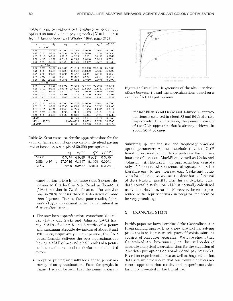
Table 2: Approximations for the value of American put
options on non-dividend paying stocks (X = 100, data
from (Barone-Adesi and Whaley 1988, page 315)).
T � S0 P0 PJ0
PMM0
PGJ0
PGAP0
r = 8:00
0.25 0.20 80.00 20.0000 18.0909 20.0000 20.0012 20.0000
0.25 0.20 90.00 10.0353 9.0470 10.0130 10.0730 10.0456
0.25 0.20 100.00 3.2217 3.0378 3.2201 3.2115 3.2262
0.25 0.20 110.00 0.6642 0.6406 0.6810 0.6647 0.6725
0.25 0.20 120.00 0.0888 0.0865 0.0967 0.0879 0.0863
r = 12:00
0.25 0.20 80.00 20.0000 17.1344 20.0000 20.0112 20.0000
0.25 0.20 90.00 10.0000 8.2620 10.0000 9.9811 10.0000
0.25 0.20 100.00 2.9225 2.6265 2.9251 2.9110 2.9050
0.25 0.20 110.00 0.5541 0.5189 0.5781 0.5541 0.5549
0.25 0.20 120.00 0.0685 0.0654 0.0789 0.0676 0.0609
r = 8:00
0.25 0.40 80.00 20.3196 19.7588 20.2478 20.3699 20.3078
0.25 0.40 90.00 12.5635 12.4222 12.5142 12.5511 12.5769
0.25 0.40 100.00 7.1049 7.1204 7.0999 7.1018 7.1162
0.25 0.40 110.00 3.6968 3.7476 3.7120 3.7017 3.7002
0.25 0.40 120.00 1.7885 1.8310 1.8068 1.7892 1.7824
r = 8:00
0.50 0.20 80.00 20.0000 16.6555 20.0000 19.9402 20.0000
0.50 0.20 90.00 10.2890 8.8392 10.2348 10.3712 10.4406
0.50 0.20 100.00 4.1885 3.7889 4.1933 4.1519 4.3474
0.50 0.20 110.00 1.4095 1.3140 1.4459 1.4121 1.5142
0.50 0.20 120.00 0.3969 0.3768 0.4244 0.3961 0.4239
MAE 0.7083 0.0184 0.0173 0.0256
MSE (�10�4) 14886.3928 7.3752 8.2725 29.2733
MAPE 0.0721 0.0218 0.0034 0.0177
Table 3: Error measures for the approximations for the
value of American put options on non-dividend paying
stocks based on a sample of 50,000 put options.
PJ0 P
MM0 P
GJ0 P
GAP0
MAE 0.0674 0.0059 0.0031 0.0025MSE (�10�3) 27.0546 0.1197 0.1008 0.0201MAX 1.8806 0.0827 1.2102 0.0584
exact option prices by no more than 5 pence, de-
viation to this level is only found in Johnson's
(1983) solution in 72 % of cases. Put another
way, in 28 % of cases there is a deviation of more
than 5 pence. Due to these poor results, John-
son's (1983) approximation is not considered in
further discussions.
� The next best approximations come fromMacMil-
lan (1986) and Geske and Johnson (1984) hav-
ing MAEs of about 6 and 3 tenths of a penny
and maximum absolute deviations of about 8 and
120 pence, respectively. In comparison, the GAP
based formula delivers the best approximations
having a MAE of two and a half tenths of a penny
and a maximum absolute deviation of about 6
pence.
� In option pricing we usally look at the penny ac-
curacy of an approximation. From the graphs in
Figure 1 it can be seen that the penny accuracy
Figure 1: Cumulated frequencies of the absolute devi-
ations between P0 and the approximations based on a
sample of 50,000 put options.
of MacMillan's and Geske and Johnson's, approx-
imations is achieved in about 83 and 94 % of cases,
respectively. In comparison, the penny accuracy
of the GAP approximation is already achieved in
about 96 % of cases.
Summing up, for realistic and frequently observed
option parameters we can conclude that the GAP
based approximation clearly outperforms the approx-
imations of Johnson, MacMillan as well as Geske and
Johnson. Additionally, our approximation consists
only of fundamental mathematical operations and is
therefore easy to use whereas, e.g., Geske and John-
son's formula requires at least the distribution function
of the trivariate, possibly also the multivariate, stan-
dard normal distribution which is normally calculated
using numerical integration. Moreover, the results pre-
sented so far represent work in progress and seem to
be very promising.
5 CONCLUSION
In this paper we have introduced the Generalized Ant
Programming approach as a new method for solving
problems in which the search space of feasible solutions
consists of computer programs. We have shown that
Generalized Ant Programming can be used to derive
accurate analytical approximations for the valuation of
American put options on non-dividend paying stocks.
Based on experimental data as well as huge validation
data sets we have shown that our formula delivers ac-
curate approximation results and outperforms other
formulas presented in the literature.
ARTIFICIAL LIFE, ADAPTIVE BEHAVIOR, AGENTS AND ANT COLONY OPTIMIZATION80
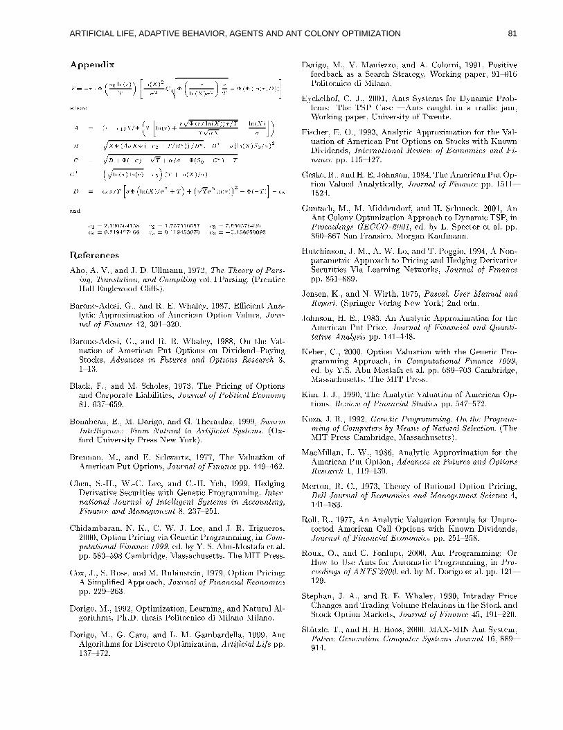
Appendix
�r = �r � ��c6 ln(r)
T
�24 ln(X)2
�2C
vuut�
r
ln(X)�2
!r
T� � (� (ln(r)D))
35
where
A = (r � c1)X=�
T
"ln(r) +
rp� (r= ln(X)) r=T
Tp�X
�ln(X)
�
#!
B =
qX�(A�X� (�c2 + T=B�)) =B�; B
�= �(ln(X)S0=�)
2
C =
qB + �(��)�
pT + �=� + �(S0 + C�)� T
C�
=
�qln(�) ln(r)� c3
�(T + ln(X)=�)
D = c4�=T
���
�ln(X)=�
2+ T
�+
�pT�
2ln(r)
�2 � �(�T )
�� c5
and
c1 = 2:190564158 c2 = 1:757516557 c3 = 7:556576426c4 = 0:219427468 c5 = 0:119453070 c6 = �0:158050093
References
Aho, A. V., and J. D. Ullmann, 1972, The Theory of Pars-ing, Translation, and Compiling vol. I Parsing. (PrenticeHall Englewood Cli�s).
Barone-Adesi, G., and R. E. Whaley, 1987, EÆcient Ana-lytic Approximation of American Option Values, Jour-nal of Finance 42, 301{320.
Barone-Adesi, G., and R. E. Whaley, 1988, On the Val-uation of American Put Options on Dividend{PayingStocks, Advances in Futures and Options Research 3,1{13.
Black, F., and M. Scholes, 1973, The Pricing of Optionsand Corporate Liabilities, Journal of Political Economy81, 637{659.
Bonabeau, E., M. Dorigo, and G. Theraulaz, 1999, SwarmIntelligence: From Natural to Arti�cial Systems. (Ox-ford University Press New York).
Brennan, M., and E. Schwartz, 1977, The Valuation ofAmerican Put Options, Journal of Finance pp. 449{462.
Chen, S.-H., W.-C. Lee, and C.-H. Yeh, 1999, HedgingDerivative Securities with Genetic Programming, Inter-national Journal of Intelligent Systems in Accounting,Finance and Management 8, 237{251.
Chidambaran, N. K., C. W. J. Lee, and J. R. Trigueros,2000, Option Pricing via Genetic Programming, in Com-putational Finance 1999, ed. by Y. S. Abu-Mostafa et al.pp. 583{598 Cambridge, Massachusetts. The MIT Press.
Cox, J., S. Ross, and M. Rubinstein, 1979, Option Pricing:A Simpli�ed Approach, Journal of Financial Economicspp. 229{263.
Dorigo, M., 1992, Optimization, Learning, and Natural Al-gorithms, Ph.D. thesis Politecnico di Milano Milano.
Dorigo, M., G. Caro, and L. M. Gambardella, 1999, AntAlgorithms for Discrete Optimization, Arti�cial Life pp.137{172.
Dorigo, M., V. Maniezzo, and A. Colorni, 1991, Positivefeedback as a Search Strategy, Working paper, 91{016Politecnico di Milano.
Eyckelhof, C. J., 2001, Ants Systems for Dynamic Prob-lems: The TSP Case { Ants caught in a traÆc jam,Working paper, University of Twente.
Fischer, E. O., 1993, Analytic Approximation for the Val-uation of American Put Options on Stocks with KnownDividends, International Review of Economics and Fi-nance pp. 115{127.
Geske, R., and H. E. Johnson, 1984, The American Put Op-tion Valued Analytically, Journal of Finance pp. 1511{1524.
Guntsch, M., M. Middendorf, and H. Schmeck, 2001, AnAnt Colony Optimization Approach to Dynamic TSP, inProceedings GECCO{2001, ed. by L. Spector et al. pp.860{867 San Fransico. Morgan Kaufmann.
Hutchinson, J. M., A. W. Lo, and T. Poggio, 1994, A Non-parametric Approach to Pricing and Hedging DerivativeSecurities Via Learning Networks, Journal of Financepp. 851{889.
Jensen, K., and N. Wirth, 1975, Pascal, User Manual andReport. (Springer Verlag New York) 2nd edn.
Johnson, H. E., 1983, An Analytic Approximation for theAmerican Put Price, Journal of Financial and Quanti-tative Analysis pp. 141{148.
Keber, C., 2000, Option Valuation with the Genetic Pro-gramming Approach, in Computational Finance 1999,ed. by Y.S. Abu-Mostafa et al. pp. 689{703 Cambridge,Massachusetts. The MIT Press.
Kim, I. J., 1990, The Analytic Valuation of American Op-tions, Review of Financial Studies pp. 547{572.
Koza, J. R., 1992, Genetic Programming. On the Program-ming of Computers by Means of Natural Selection. (TheMIT Press Cambridge, Massachusetts).
MacMillan, L. W., 1986, Analytic Approximation for theAmerican Put Option, Advances in Futures and OptionsResearch 1, 119{139.
Merton, R. C., 1973, Theory of Rational Option Pricing,Bell Journal of Economics and Management Science 4,141{183.
Roll, R., 1977, An Analytic Valuation Formula for Unpro-tected American Call Options with Known Dividends,Journal of Financial Economics pp. 251{258.
Roux, O., and C. Fonlupt, 2000, Ant Programming: OrHow to Use Ants for Automatic Programming, in Pro-ceedings of ANTS'2000, ed. by M. Dorigo et al. pp. 121{129.
Stephan, J. A., and R. E. Whaley, 1990, Intraday PriceChanges and Trading Volume Relations in the Stock andStock Option Markets, Journal of Finance 45, 191{220.
St�utzle, T., and H. H. Hoos, 2000, MAX-MIN Ant System,Future Generation Computer Systems Journal 16, 889{914.
ARTIFICIAL LIFE, ADAPTIVE BEHAVIOR, AGENTS AND ANT COLONY OPTIMIZATION 81
Effects of Agent Representation on the Behavior of a Non-ReciprocalCooperation Game
Nicole P. LeahyGraduate Program in Bioinformatics and Computational Biology
Iowa State UniversityAmes, IA 50011
Abstract
Game theoretic models are often used to simulatephenomena observed in the natural world. It isgenerally assumed that the implementation (orrepresentation) of the agents within a game hasno significant effect on the outcome ofsimulations. To test this assumption the effect ofchanging the representation of agents in the non-reciprocal cooperation game studied by Riolo etal. (2001) was used. In addition to theimplementation used by Riolo et al. (2001),agents were also represented as higher dimensionreal vectors, integer values, at bit-strings. It wasfound that the method of agent implementationused has a highly significant effect on thecooperation rate and general behavior of thesimulation.
1 INTRODUCTIONBiologists and social scientists have long been interestedin the evolution of cooperation (e.g. Roy, 2000; Sigmundand Nowak, 1999; Mouston et al., 2000; Hemesath,1994). It is not understood how selfishly actingindividuals could evolve cooperative behavior (Axelrod,1984). Scientists studying this phenomenon often usetheoretical games to investigate the origin of cooperation.It is often tacitly assumed that agent representation hasonly minor effects on the long-term behavior and resultsof the model. The purpose of this paper is to present theresults of a study in which the method of representing theagent in the model published by Riolo, et al. (2001) wasaltered.In Riolo et al. (2001)’s game individuals (agents) learnedto cooperate despite the cost of assisting another agentand without reciprocity. In brief, this game was designedso that an agent assisted another agent if identificationtags were sufficiently similar. The agents had no memoryof previous encounters and were unlikely to play otheragents more than once (a substantial departure from theusual iterated game used to study the evolution of
cooperation). Riolo et al. (2001) reported agents to assistother agents at a rate of 73.6%, after evolution. A moredetailed description of the Riolo et al. (2001) simulation isprovided in the Experimental Design section.Agents in Riolo et al. (2001) consisted of two realnumbers: the first served as an identity tag and the otherdetermining the altruistic behavior. This study used threealternate implementations of the agents: multi-dimensionalreal vectors, integer value, and bit-strings. Using a multi-dimensional vector representation expands the tag space(the number of possible tags). The real numberrepresentation of computers is a fine-grained approachsince tags may vary by very small amounts. When usinginteger value tags with a maximum value, the differencebetween agents becomes more pronounced. As the size ofthe maximum allowable integer increases, the resultsshould approach those of the single dimensional realvector case. Using bit-strings examines the effect of bothhigher dimensionality and the granularity of theenvironment.
2 EXPERIMENTAL DESIGNThe experiments in this paper were conducted in the samemanner as described in Riolo et al. (2001). Specifically,each simulation used a population of 100 agents whichwere evolved for 30,000 generations. Each agent had atag (τ), tolerance threshold (T), and a score. Everygeneration, each agent played three agents selected atrandom with replacement. For each place the first agent(agent A) determines if it will assist the other agent (agentB). If the distance between tags of agent A and agent Bwas lower than the threshold of agent A, the score ofagent A was lowered by 0.1, and the score of agent Bincreased by 1.0. This represents a costly contribution byagent A to agent B.The next generation was determined with tournamentselection of size two, where the population was randomlyshuffled and two agents were select without replacementuntil there were no remaining agents. if the agents in eachpair had equal scores, each was copied to the nextgeneration. If one agent had a higher score, that agentwas copied twice to the next generation and the agent withthe lower score was not copied. Each copy was then
ARTIFICIAL LIFE, ADAPTIVE BEHAVIOR, AGENTS AND ANT COLONY OPTIMIZATION82
subjected to mutation. Mutation of the tag occured at afrequency of 0.1, and was performed by generating a newtag uniformly at random in the tag space. At the samefrequency, the tolerance threshold mutated by arepresentation-dependent function with a distributiondesigned to leave the simulation as close as possible to theoriginal study (Gaussian with mean zero and a standarddeviation of 0.01). If the new T<0, then it was set to 0.
2.1 MULTI-DIMENSION REPRESENTATION
An agent tag in Riolo et al. (2001) was represented as areal number, τ ∈ [0,1], with tag distance calculated as theabsolute value of the difference between two tags.Similarly, the agent tolerance was initialized as a realnumber, T ∈ [0,1]. To examine the effect of a larger tagspace on the behavior of the game, tags were representedas real vectors, τ ∈ [0,1]n, where n is the dimension of thetag space. The tolerance was represented as a single realvariable with T ∈ [0,1]. The distance between the tags oftwo agents, A and B, is the Euclidean distance,
( )∑=
−=n
iBA iiD
BA1
2)()( ττττ
Player A assists player B if ATDBA
≤ττ .
The mutation of T was the same as in Riolo et al. (2001)except that the standard deviation (σ ) of the mutationdistribution was adjusted so that the ratio of thehypervolume of the hypersphere of radius σ (Vσ) to thehypervolume of the tag space (Vt) was constant acrossdimensions (Table 1). This was done in order to insurethat the tolerance mutation was equivalent to theat used inRiolo et al. (2001). Runs were performed for n = 1, 2, 3,4, 5, where n is the number of dimensions of the tagspace. 30 replicates were run for each tag space. Notethat the case where n=1 is identical to the setup for Rioloet al. (2001).
Table 1: σ for Higher Dimensions
n σσσσ Vσσσσ:Vt
1 0.01 0.022 0.079788456 0.023 0.16838903 0.024 0.25231352 0.025 0.32805473 0.02
2.2 INTEGER REPRESENTATION
Using real values for τ and T is a relatively fine-grainedenvironment since it is extremely unlikely that any twoagents will have the same τ. In Riolo et al. (2001), T mostfrequently changed by small values relative to the tagspace, creating a fine distinction between agents with anapproximately continuous tag space. By employinginteger representation of the tag space and tollerance, thesimulation becomes more discrete. Both τ and T wereinitialized as τ, T ∈ [0,1,2,...,I], where I is the maximuminteger. Constraining the tag space and randomly selectingnew tags may result in duplication of the tags of otheragents, especially at low values for I. The mutation of T
was performed by adding ∑=
=∆I
ii
1δ , for
[ ]1,0,1 +−∈iδ , δi ∈ [-1, 0, +1], with p(-1) = p(+1) =0.1, and p(0) = 0.8. Experiments were run for I=10, 100,1000, and 10,000.
2.3 BIT-STRING REPRESENTATIONImplementing the tag and tolerance as bit strings bothincreases the tag space by using larger strings andconstrains the tag space, reducing the values of eachdimension to one of two states. The distance between twoagents was measured as the Hamming distance. The valueof T was implemented as the weight of the tolerancebinary string. Mutation of the tolerance was performed asbit flips determined by a Poisson distribution with theexpected probability of each bit-flip set equal to 0.01.Since it is not possible for T < 0, there were no boundaryeffects as there were in the other two representations.Experiments were performed for string lengths, L of 10,20, 30, 40, 50, 60, 70, 80, 90, and 100 bits. The bit-stringfor the tag and tolerance were of equal length in allsimulations.
3 RESULTSAn interesting difference between the results of theseexperiments and those reported by Riolo et al. (2001) wasthe presence of failed states. A failed state is anoccurrence of donation rates less that 10% for at least onegeneration. The value of 10% was selected fromexamination of the reproduction of the results of Riolo, etal. (2001). In only one replicate did a population fall to adonation rate of 10% or lower one without persisting in afailed state for multiple generations. The comparisons ofa typical run from Riolo et al. (2001) compared to a failedstate are shown in Figures 1 and 2. The donation rate isthe proportion of plays per generation that result in oneagent assisting another. A cooperative state is defined asan occurrence of donation rates greater than 10%.Significance levels were calculated using ANOVA andstudent-t tests.
ARTIFICIAL LIFE, ADAPTIVE BEHAVIOR, AGENTS AND ANT COLONY OPTIMIZATION 83
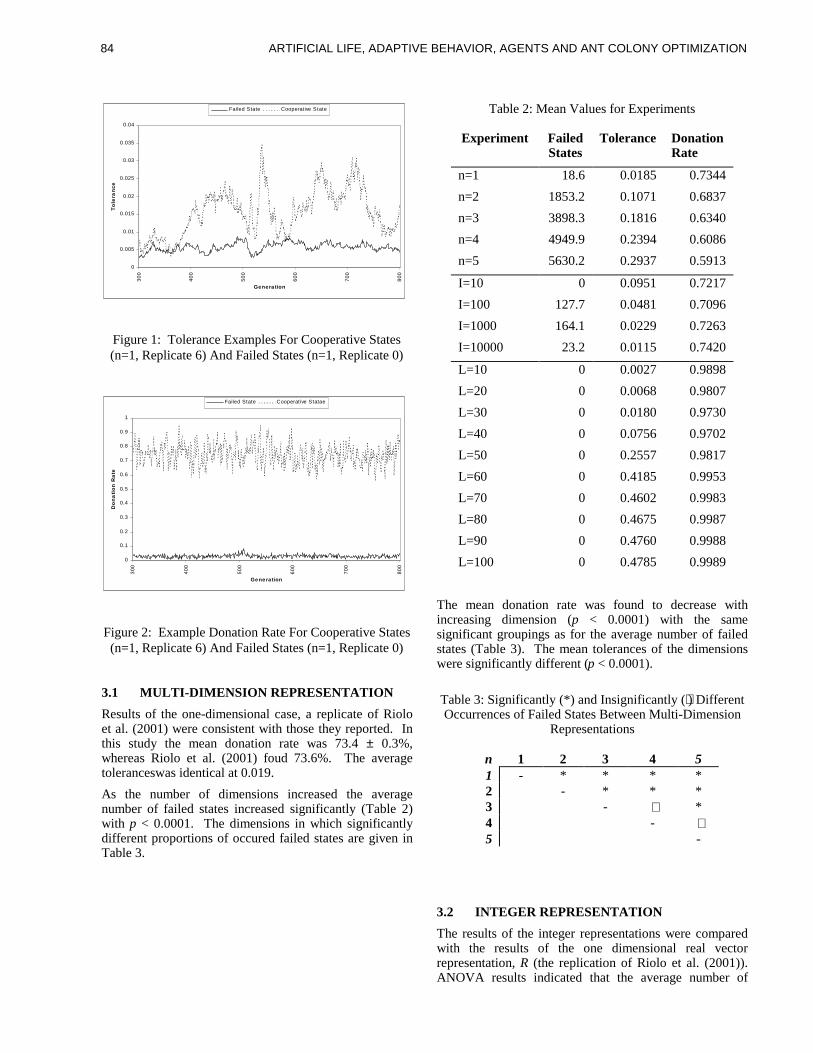
0
0.005
0.01
0.015
0.02
0.025
0.03
0.035
0.04
300
400
500
600
700
800
Genera tion
Tole
ranc
eFailed State Cooperative State
Figure 1: Tolerance Examples For Cooperative States(n=1, Replicate 6) And Failed States (n=1, Replicate 0)
0
0.1
0.2
0.3
0.4
0.5
0.6
0.7
0.8
0.9
1
300
400
500
600
700
800
Ge ne ration
Don
atio
n R
ate
Failed State Cooperative Statae
Figure 2: Example Donation Rate For Cooperative States(n=1, Replicate 6) And Failed States (n=1, Replicate 0)
3.1 MULTI-DIMENSION REPRESENTATIONResults of the one-dimensional case, a replicate of Rioloet al. (2001) were consistent with those they reported. Inthis study the mean donation rate was 73.4 ± 0.3%,whereas Riolo et al. (2001) foud 73.6%. The averagetoleranceswas identical at 0.019.As the number of dimensions increased the averagenumber of failed states increased significantly (Table 2)with p < 0.0001. The dimensions in which significantlydifferent proportions of occured failed states are given inTable 3.
Table 2: Mean Values for Experiments
Experiment FailedStates
Tolerance DonationRate
n=1 18.6 0.0185 0.7344n=2 1853.2 0.1071 0.6837n=3 3898.3 0.1816 0.6340n=4 4949.9 0.2394 0.6086n=5 5630.2 0.2937 0.5913
I=10 0 0.0951 0.7217I=100 127.7 0.0481 0.7096I=1000 164.1 0.0229 0.7263I=10000 23.2 0.0115 0.7420
L=10 0 0.0027 0.9898L=20 0 0.0068 0.9807L=30 0 0.0180 0.9730L=40 0 0.0756 0.9702L=50 0 0.2557 0.9817L=60 0 0.4185 0.9953L=70 0 0.4602 0.9983L=80 0 0.4675 0.9987L=90 0 0.4760 0.9988L=100 0 0.4785 0.9989
The mean donation rate was found to decrease withincreasing dimension (p < 0.0001) with the samesignificant groupings as for the average number of failedstates (Table 3). The mean tolerances of the dimensionswere significantly different (p < 0.0001).
Table 3: Significantly (*) and Insignificantly (⋅) DifferentOccurrences of Failed States Between Multi-Dimension
Representations
n 1 2 3 4 51 - * * * *2 - * * *3 - ⋅ *4 - ⋅5 -
3.2 INTEGER REPRESENTATIONThe results of the integer representations were comparedwith the results of the one dimensional real vectorrepresentation, R (the replication of Riolo et al. (2001)).ANOVA results indicated that the average number of
ARTIFICIAL LIFE, ADAPTIVE BEHAVIOR, AGENTS AND ANT COLONY OPTIMIZATION84
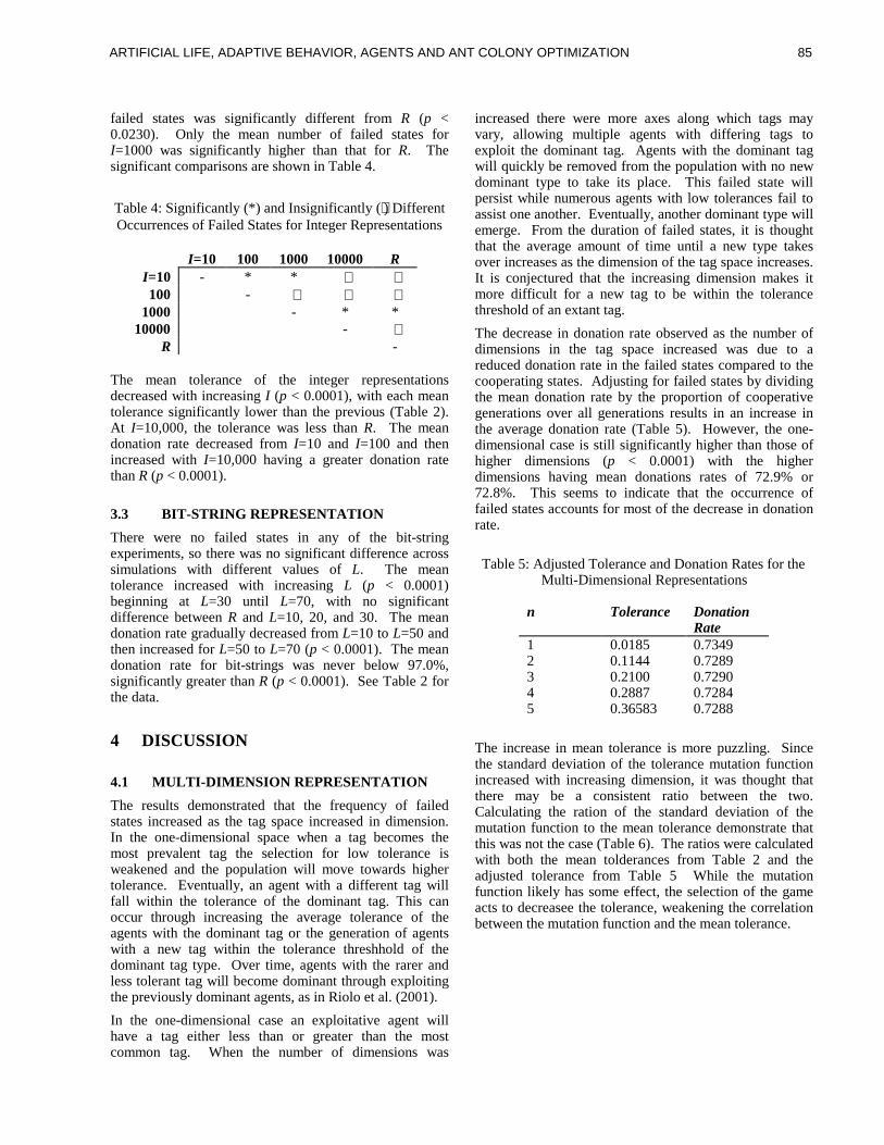
failed states was significantly different from R (p <0.0230). Only the mean number of failed states forI=1000 was significantly higher than that for R. Thesignificant comparisons are shown in Table 4.
Table 4: Significantly (*) and Insignificantly (⋅) DifferentOccurrences of Failed States for Integer Representations
I=10 100 1000 10000 RI=10 - * * ⋅ ⋅100 - ⋅ ⋅ ⋅
1000 - * *10000 - ⋅
R -
The mean tolerance of the integer representationsdecreased with increasing I (p < 0.0001), with each meantolerance significantly lower than the previous (Table 2).At I=10,000, the tolerance was less than R. The meandonation rate decreased from I=10 and I=100 and thenincreased with I=10,000 having a greater donation ratethan R (p < 0.0001).
3.3 BIT-STRING REPRESENTATIONThere were no failed states in any of the bit-stringexperiments, so there was no significant difference acrosssimulations with different values of L. The meantolerance increased with increasing L (p < 0.0001)beginning at L=30 until L=70, with no significantdifference between R and L=10, 20, and 30. The meandonation rate gradually decreased from L=10 to L=50 andthen increased for L=50 to L=70 (p < 0.0001). The meandonation rate for bit-strings was never below 97.0%,significantly greater than R (p < 0.0001). See Table 2 forthe data.
4 DISCUSSION
4.1 MULTI-DIMENSION REPRESENTATIONThe results demonstrated that the frequency of failedstates increased as the tag space increased in dimension.In the one-dimensional space when a tag becomes themost prevalent tag the selection for low tolerance isweakened and the population will move towards highertolerance. Eventually, an agent with a different tag willfall within the tolerance of the dominant tag. This canoccur through increasing the average tolerance of theagents with the dominant tag or the generation of agentswith a new tag within the tolerance threshhold of thedominant tag type. Over time, agents with the rarer andless tolerant tag will become dominant through exploitingthe previously dominant agents, as in Riolo et al. (2001).In the one-dimensional case an exploitative agent willhave a tag either less than or greater than the mostcommon tag. When the number of dimensions was
increased there were more axes along which tags mayvary, allowing multiple agents with differing tags toexploit the dominant tag. Agents with the dominant tagwill quickly be removed from the population with no newdominant type to take its place. This failed state willpersist while numerous agents with low tolerances fail toassist one another. Eventually, another dominant type willemerge. From the duration of failed states, it is thoughtthat the average amount of time until a new type takesover increases as the dimension of the tag space increases.It is conjectured that the increasing dimension makes itmore difficult for a new tag to be within the tolerancethreshold of an extant tag.The decrease in donation rate observed as the number ofdimensions in the tag space increased was due to areduced donation rate in the failed states compared to thecooperating states. Adjusting for failed states by dividingthe mean donation rate by the proportion of cooperativegenerations over all generations results in an increase inthe average donation rate (Table 5). However, the one-dimensional case is still significantly higher than those ofhigher dimensions (p < 0.0001) with the higherdimensions having mean donations rates of 72.9% or72.8%. This seems to indicate that the occurrence offailed states accounts for most of the decrease in donationrate.
Table 5: Adjusted Tolerance and Donation Rates for theMulti-Dimensional Representations
n Tolerance DonationRate
1 0.0185 0.73492 0.1144 0.72893 0.2100 0.72904 0.2887 0.72845 0.36583 0.7288
The increase in mean tolerance is more puzzling. Sincethe standard deviation of the tolerance mutation functionincreased with increasing dimension, it was thought thatthere may be a consistent ratio between the two.Calculating the ration of the standard deviation of themutation function to the mean tolerance demonstrate thatthis was not the case (Table 6). The ratios were calculatedwith both the mean tolderances from Table 2 and theadjusted tolerance from Table 5 While the mutationfunction likely has some effect, the selection of the gameacts to decreasee the tolerance, weakening the correlationbetween the mutation function and the mean tolerance.
ARTIFICIAL LIFE, ADAPTIVE BEHAVIOR, AGENTS AND ANT COLONY OPTIMIZATION 85
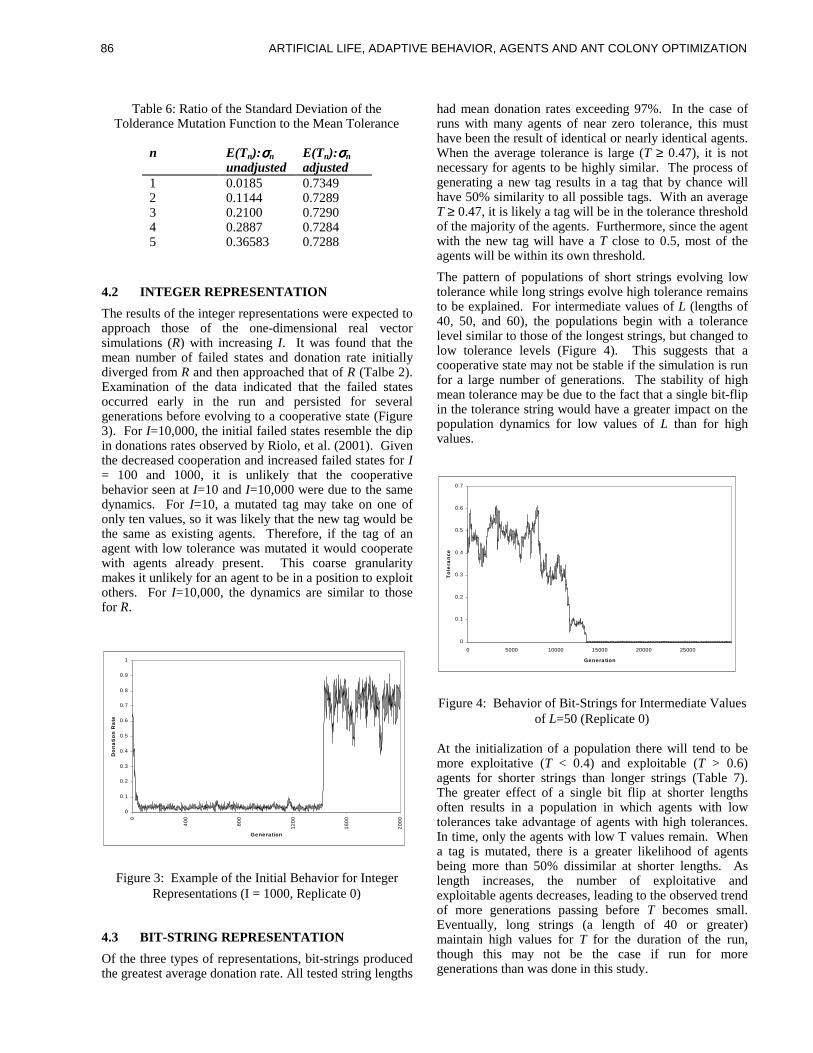
Table 6: Ratio of the Standard Deviation of theTolderance Mutation Function to the Mean Tolerance
n E(Tn):σσσσn E(Tn):σσσσnunadjusted adjusted
1 0.0185 0.73492 0.1144 0.72893 0.2100 0.72904 0.2887 0.72845 0.36583 0.7288
4.2 INTEGER REPRESENTATIONThe results of the integer representations were expected toapproach those of the one-dimensional real vectorsimulations (R) with increasing I. It was found that themean number of failed states and donation rate initiallydiverged from R and then approached that of R (Talbe 2).Examination of the data indicated that the failed statesoccurred early in the run and persisted for severalgenerations before evolving to a cooperative state (Figure3). For I=10,000, the initial failed states resemble the dipin donations rates observed by Riolo, et al. (2001). Giventhe decreased cooperation and increased failed states for I= 100 and 1000, it is unlikely that the cooperativebehavior seen at I=10 and I=10,000 were due to the samedynamics. For I=10, a mutated tag may take on one ofonly ten values, so it was likely that the new tag would bethe same as existing agents. Therefore, if the tag of anagent with low tolerance was mutated it would cooperatewith agents already present. This coarse granularitymakes it unlikely for an agent to be in a position to exploitothers. For I=10,000, the dynamics are similar to thosefor R.
0
0.1
0.2
0.3
0.4
0.5
0.6
0.7
0.8
0.9
1
0
400
800
1200
1600
2000
Ge ne ration
Don
atio
n R
ate
Figure 3: Example of the Initial Behavior for IntegerRepresentations (I = 1000, Replicate 0)
4.3 BIT-STRING REPRESENTATIONOf the three types of representations, bit-strings producedthe greatest average donation rate. All tested string lengths
had mean donation rates exceeding 97%. In the case ofruns with many agents of near zero tolerance, this musthave been the result of identical or nearly identical agents.When the average tolerance is large (T ≥ 0.47), it is notnecessary for agents to be highly similar. The process ofgenerating a new tag results in a tag that by chance willhave 50% similarity to all possible tags. With an averageT ≥ 0.47, it is likely a tag will be in the tolerance thresholdof the majority of the agents. Furthermore, since the agentwith the new tag will have a T close to 0.5, most of theagents will be within its own threshold.The pattern of populations of short strings evolving lowtolerance while long strings evolve high tolerance remainsto be explained. For intermediate values of L (lengths of40, 50, and 60), the populations begin with a tolerancelevel similar to those of the longest strings, but changed tolow tolerance levels (Figure 4). This suggests that acooperative state may not be stable if the simulation is runfor a large number of generations. The stability of highmean tolerance may be due to the fact that a single bit-flipin the tolerance string would have a greater impact on thepopulation dynamics for low values of L than for highvalues.
0
0.1
0.2
0.3
0.4
0.5
0.6
0.7
0 5000 10000 15000 20000 25000
Genera tion
Tole
ranc
e
Figure 4: Behavior of Bit-Strings for Intermediate Valuesof L=50 (Replicate 0)
At the initialization of a population there will tend to bemore exploitative (T < 0.4) and exploitable (T > 0.6)agents for shorter strings than longer strings (Table 7).The greater effect of a single bit flip at shorter lengthsoften results in a population in which agents with lowtolerances take advantage of agents with high tolerances.In time, only the agents with low T values remain. Whena tag is mutated, there is a greater likelihood of agentsbeing more than 50% dissimilar at shorter lengths. Aslength increases, the number of exploitative andexploitable agents decreases, leading to the observed trendof more generations passing before T becomes small.Eventually, long strings (a length of 40 or greater)maintain high values for T for the duration of the run,though this may not be the case if run for moregenerations than was done in this study.
ARTIFICIAL LIFE, ADAPTIVE BEHAVIOR, AGENTS AND ANT COLONY OPTIMIZATION86
Table 7. Expected Proportion of Exploitable andExploitative Agents at Initialization of Bit-String
Populations
L Proportion10 0.36320 0.26330 0.20040 0.15450 0.11960 0.09270 0.07280 0.05790 0.045100 0.035
5 CONCLUSIONSThe results of the experiments described in this paperdemonstrate that altering the representation of the agentsin the Riolo et al. (2001) simulation has significant effectson the outcome. In the literature, when game theoreticmodels of the evolution of cooperation are examined, onlythe rules of the game rather than the digital representationof the agents are modified. The results described abovecaution that generic statements of a game should not bemade from a single implementation. Furthermore, sincethe outcome of this game is partially dependent upon therepresentation used, it would not be prudent to presentdata as a model for the natural world unless it is eitherconfirmed by multiple representations or shown that thechosen representation is a reasonable approximation, suchas fitting the model to data from the natural world. Withthe variety of models used to simulate aspects of thenature, it would be of interest to test the effect of agentrepresentation on the behavior of other game theoreticmodels.
5 ACKNOWLEDGEMENTSI would like to thank Dan Ashlock (Department ofMathematics, Iowa State University) for introducing me togame theoretic models of cooperation and his advice onthis project.
6 REFERENCESAxelrod, R. (1984). The Evolution of Cooperation. BasicBooks, New York.Hemesath, M. (1994). Cooperate or defect? Russian andAmerican students in a prisoner’s dilemma. ComparativeEconomic Studies 176:83-93.Mouston, J.M., J. Kinnie, B. Luop, C. Terry, and S.S. Ho(2000). Competitiveness and conflict behavior insimulation of social dilemma. Psychological Reports86:1219-1225.
Nowak, M.A., and K. Sigmund (1998). Evolution ofindirect reciprocity by image scoring. Nature 393:573-577.Riolo, Rick L., Michael D. Cohen, and Robert Axelrod(2001). Evolution of cooperation without reciprocity.Nature 414:441-443.Roy, D. (2000). Learning and the theory of games.Journal of Theoretical Biology 204:409-414.Sigmund, K., and M.A. Nowak (1999). Evolutionarygame theory. Current Biology 9:R503-R505.
ARTIFICIAL LIFE, ADAPTIVE BEHAVIOR, AGENTS AND ANT COLONY OPTIMIZATION 87
AAAA , Ali fe, Adaptive Behavior, Agents, and Ant Colony Optimization
Intelligent Packets for Dynamic Network Routing Using Distributed Genetic Algorithm
Suihong Liang
A. Nur Zincir-Heywood
[email protected] Faculty of Computer Science
6050 University Avenue, Hali fax, NS, Canada, B3H 1W5
Malcolm I. Heywood
[email protected] +1 902 4942951
Abstract
A distributed GA is designed for the packet switched network routing problem under minimal information. The requirements of such a problem mean that agents are required to possess more intelli gence than was previously the case. To this end a distributed GA approach is developed and benchmarked against the AntNet algorithm under the same information constraints.
1 GENERAL FORMATTING INSTRUCTIONS
Network information systems and telecommunication in general rely on a combination of routing strategies and protocols to ensure that information sent by a user is actually received at the desired remote location. In addition, the distributed nature of the problem means that multiple users can make requests simultaneously. This results in delayed response times, lost information or other reductions to the quality of service objectives on which users judge network service. Routing is the process used to determine how a packet travels from source to destination. Protocols are used to implement handshaking activities such as error checking and receiver acknowledgements. In this work, we are interested in the routing problem on computer networks.
The routing problem has several properties, which make it particularly challenging. The problem is distributed in nature; hence a solution that assumes access to any form of global information is not desirable. The problem is also dynamic; hence a solution that is suff icient for presently experienced network conditions may well be ineff icient under other loads experienced by the network. Moreover, the traff ic experienced by networks is subject to widely varying load conditions, making ‘ typical’ network conditions unrepresentative.
Traditionally, routing strategies are implemented through the information contained in routing tables available at
each node in the network (Forouzan, 2001). That is, a table details the next ‘hop’ a packet takes based on the overall destination of the packet. This should not be taken to imply that a routing table consists of an exhaustive list of all destinations – a form of global information. Instead, the table consists of specific entries for the neighboring nodes and then a series of default paths for packets with any other destination – such as OSPF or BGP4 (Halabi, 1997). Application of a classical optimization technique to such a problem might take the form of first assessing the overall pattern of network traff ic, and then defining the contents of each routing table such that congestion is minimized. This approach does not generally work in practice as it simply costs too much to collect the information centrally on a regular basis, where regular updating is necessary in order to satisfy the dynamic nature of network utili zation. We, therefore, see the generic objectives of a routing strategy to be both dynamically reconfigurable and be based on locally available information, whilst also satisfying the user quality of service objectives (i.e. a global objective).
Several approaches have been proposed for addressing these objectives including: active networking (Tennenhouse et. al.,1997), social insect metaphors (Di Caro, Dorigo, 1998), (Heusse et al., 1998) cognitive packet networks (Gelenbe et. al.,1999), and what might be loosely called other ‘adaptive’ techniques (Corne et. al., 2000). The latter typically involve using evolutionary or neural techniques to produce a ‘ routing controller’ as opposed to a ‘ routing table’ at each node, where the controller may require knowledge of the global connectivity to ensure a valid route. The global information assumption may be avoided by framing the problem as a reinforcement-learning context (Boyan, Littman, 1994). However, the Q-learning method, on which this is based, results in single path solutions for each destination. Both the social insect metaphor and the cognitive packet approach provide a methodology for routing, without such constraints; by utili zing probabili stic routing tables and letting the packets themselves investigate and report network topology and performance.
ARTIFICIAL LIFE, ADAPTIVE BEHAVIOR, AGENTS AND ANT COLONY OPTIMIZATION88
AAAA , Ali fe, Adaptive Behavior, Agents, and Ant Colony Optimization
All methods as currently implemented, however, suffer from one drawback or another. Cognitive packet networks and active networking algorithms attempt to provide routing programs at the packet level, hence achieving scalable run time eff iciency becomes an issue. To date, implementations of ‘ adaptive’ techniques and social insect metaphors have relied, at some point, on the availabilit y of global information (Liang, et al., 2002).
The purpose of this work is to investigate the application of a genetic algorithm (GA) to build on lessons learnt from the social insect metaphor. This represents a major departure from previous works attempting to utili ze GAs to solve the dynamic routing problem e.g. (Corne D.W., et al. 2000). In particular, a distributed GA is defined in which populations associated with each node of the network are required to co-evolve to solve the problem as a whole. Moreover, the GA interaction with the environment drives the features measured by the routing tables, as opposed to the tables predefining the features for measurement (a form of a priori information). Section 2 introduces the ‘ant’ based social insect metaphor against which the proposed approach is compared. Section 3 introduces the proposed GA-agent scheme. Section 4 summarizes the network on which experiments are performed. Results are presented in section 5 and conclusions drawn in section 6.
2 ROUTING USING A SOCIAL INSECT METAPHORE
As indicated above, active networking (Tennenhouse et. al.,1997) and cognitive packet (Gelenbe et. al.,1999) based approaches emphasize a per packet mechanism for routing. The aforementioned ‘adaptive’ techniques (Corne et. al., 2000) tend to emphasize adding ‘ intelli gence’ to the routers leaving the packets unchanged. A social insect metaphor provides a middle ground in which the concepts of a routing table and data packet still exist, but in addition, intelli gent packets – ants – are introduced that interact to keep the contents of the routing tables up to date. To do so, the operation of ant packets is modeled on observations made regarding the manner in which worker ants use chemical trails as a method of indirect stigmergic communication. Specifically, ants are only capable of simple stochastic decisions influenced by the availabilit y of previously laid stigmergic trails. The chemical denoting a stigmergic trail i s subject to decay over time, and reinforcement proportional to the number of ants taking the same path. Trail building is naturally a bi-directional process, ants need to reach the food (destination) and make a successful return path, in order to significantly reinforce a stigmergic trail (Forward only routing has also been demonstrated (Heusse et al., 1998)). Moreover, the faster the route, then the earlier the trail i s reinforced. An ant on encountering multiple stigmergic trails will probabili stically choose the route with greatest stigmergic reinforcement. Naturally, this will correspond to the ‘f astest’ route to the food (destination). The probabili stic nature of the decision, however, means that
ants are still able to investigate routes with a lower stigmergic trial.
This approach has proved to be a flexible framework for solving a range of problems including the traveling sales man problem (Dorigo et al., 1996) and the quadratic assignment problem (Maniezzo et al., 1999). The work reported here follows the ‘AntNet’ algorithm of Di Caro and Dorigo (Di Caro, Dorigo, 1998), and is informally summarized as follows,
• Each node in the network retains a record of packet destinations as seen on data packets passing through that node. This is used to periodically, but asynchronously, launch ‘f orward’ ants with destinations stochastically sampled from the collected set of destinations;
• Once launched, a forward ant uses the routing table information to make probabili stic decisions regarding the next hop to take at each node. While moving, each forward ant collects time stamp and node identifier information where this is later used to update the routing tables along the path followed;
• If a forward ant re-encounters a node previously visited before reaching the destination, it is kill ed;
• On successfully reaching the destination node, total trip time is estimated and the forward ant converted into a backward ant;
• The backward ant returns to the source using exactly the same route as recorded by the forward ant. Instead of using the data packet queues, however, the backward ant uses a priority queue;
• At each node visited by the backward ant the corresponding routing table entries are updated to reflect the relative performance of the path;
• When the backward ant reaches the source, it ‘dies’ .
Although providing for a robust ant routing algorithm under simulation conditions, an assumption is made, which inadvertently implies the use of global information - knowledge of the number of nodes in the network (Di Caro, Dorigo, 1998). The definition of routing tables is, such that it is assumed that every node has a unique location in the routing table, see Table 1, or a total of L (number of neighboring nodes) by K (number of nodes in the entire network) entries. In practice, this is never the case. To do so would assume that it is first feasible, and secondly, should the network configuration ever change, then all nodes should be updated with the new configuration information. Moreover, as forward ants propagate across the network, the amount of information they need to ‘carry’ also increases (node identifier and time stamp).
ARTIFICIAL LIFE, ADAPTIVE BEHAVIOR, AGENTS AND ANT COLONY OPTIMIZATION 89
AAAA , Ali fe, Adaptive Behavior, Agents, and Ant Colony Optimization
î
−+−−
+
=
)()( infinfsup
infsup21 ItII
IIc
t
Wcr
antant
best
Table-1 Original Routing Table at any Network Node k on the NTTnet
All Network Nodes (Possible Destinations)
P1,1 P1,2 ------ P1,55
P2,1 P2,2 ------ P2,55
------ ------ ------ ------
Out
goin
g L
inks
(E
ach
no
de h
as
L ne
igh
bor
ing
link
s)
PL,1 PL,2 ------ PL,55
In order to avoid the use of global information, the authors modify the information provided at the routing tables such that the routing tables only detail the neighboring nodes, see Table 2, or a total of 2 by L entries. Such a limitation, therefore, places greater emphasis on the learning capacity of the ant. This is particularly significant during step (2) of the ant forward pass (section 2.1). Tables 1 and 2 ill ustrate the difference in available information for a node in the commonly used Japanese benchmark backbone (NTTNet) routing problem.
Table-2 Proposed Routing Table at any Network Node on the NTTnet
Neighbor Node
If used for other nodes
P1,1 P1,d , d � �
P2,2 P2,d ,d � �
------ ------
Out
goin
g L
inks
(E
ach
node
has
L
nei
ghb
orin
g lin
ks)
PL,L PL,d , d � �
The following section summarizes the AntNet algorithm.
2.1 ANTNET ALGORITHM
It is assumed that routing tables, Tk, exist at each node, k, in which a routing decision is made. Tables consist of ‘ n’ rows, one row for each neighboring node/link. As far as a normal data packet is concerned, if the destination, d, from current node, k, is a neighbor then the routing is still a stochastic decision. In all other cases, a route is selected based on the neighbor node probabiliti es.
1. New forward ants, Fsd, are created periodically, but independently of the other nodes, from source, s, to destination node, d, in proportion to the destination frequency of passing data packets. Forward ants travel the network using the same priority structures as data packets, hence are subject to the same delay profiles.
2. Next link in the forward ant route is selected stochastically, p’ (j), in proportion to the routing table probabiliti es and length of the corresponding output queue.
where p(j) is the probabilit y of selecting node j as the next hop; α weights the significance given to local queue length verses global routing information, p(j); l j is proportional to the inverse of queue length at destination ‘ j’ normalized to the unit interval; and Nk is the number of links from node k.
3. On visiting a node different from the destination, a forward ant checks for a buffer with the same identifier as itself. If such a buffer exists, the ant must be entering a cycle and dies. If this is not the case, then the ant saves the previously visited node identifier and time stamp at which the ant was serviced by the current node in a buffer with the forward ant’s identifier. The total number of buffers at a node is managed by attaching “an age” to buffer space and allowing backward ants to free the corresponding buffer space.
4. When the current node is the destination, k = d, then the forward ant is converted into a backward ant, Bds. The information recorded at the forward ant buffer is then used to retrace the route followed by the forward ant.
5. At each node visited by the backward ant, routing table probabiliti es are updated using the following rule,
IF (node was in the path of the ant) THEN p(i) = p(i) + r { 1 – p(i)} ELSE p(i) = p(i) – r P(i) where r ∈ (0, 1] is the reinforcement factor central to expressing path quality (length), congestion and underlying network dynamics.
As indicated above, the reinforcement factor should be a factor of trip time and local statistical model of the node neighborhood. To this end (Di Caro, Dorigo, 1998) recommend the following relationship,
where Wbest is the best case trip time to destination d over a suitable temporal horizon, W; tant is the actual trip time taken by the ant; I inf = Wbest; Isup = µkd + { σkd / [W (1 – γ)]0.5} .
The estimates for mean, µkd, and variant, σkd, of the trip time are also made iteratively, using the trip time information, okd. Thus,
µkd = µkd + η(okd – µkd)
(σkd)2 = (σkd)
2 + η { (okd – µd)2 – (σkd)
2}
Trip time information is now updated incrementally based on the recorded trip duration between current node, k, and ultimate destination, d. This means that it is no longer
( )1||1
)()('
−++
=k
j
N
ljpjp
αα
ARTIFICIAL LIFE, ADAPTIVE BEHAVIOR, AGENTS AND ANT COLONY OPTIMIZATION90
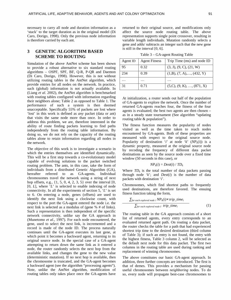
AAAA , Ali fe, Adaptive Behavior, Agents, and Ant Colony Optimization
necessary to carry all node and duration information as a ‘stack’ to the target duration as in the original model (Di Caro, Dorigo, 1998). Only the previous node information is therefore carried by each ant.
3 GENETIC ALGORITHM BASED SCHEME TO ROUTING
Simulation of the above AntNet scheme has been shown to provide a robust alternative to six standard routing algorithms – OSPF, SPF, BF, Q-R, P-QR and Daemon (Di Caro, Dorigo, 1998). However, this is not without utili zing routing tables in the AntNet algorithm, which provide entries for all nodes on the network. In practice, such (global) information is not actually available. In (Liang et al. 2002), the AntNet algorithm is benchmarked with routing tables configured with information regarding their neighbors alone; Table 2 as opposed to Table 1. The performance of such a system is then deemed unacceptable. Specifically 55% of packets are lost where ‘ lost’ in this work is defined as any packet (data or ant) that visits the same node more than once. In order to address this problem, we are, therefore interested in the abilit y of route finding packets learning to find paths independently from the routing table information. By doing so, we do not rely on the capacity of the routing tables alone to retain information regarding all nodes in the network.
The objective of this work is to investigate a scenario in which the entries themselves are identified dynamically. This will be a first step towards a co-evolutionary model capable of evolving solutions to the packet switched routing problem. The ants, in this case, take the form of individuals from a distributed Genetic Algorithm (GA), hereafter referred to as GA-agents. Individual chromosomes travel the network using a string of next hop offsets, e.g., { 1, 5, 0, 4, 2, 3, 5} over the interval [0, [0, L], where ‘L’ is selected to enable indexing of node connectivity. In all the experiments of section 5, ‘L’ is set to 6. On entering a node, genes (offsets) are used to identify the next link using a clockwise count, with respect to the port the GA-agent entered the node i.e. the next link is selected as a modulus of (gene % # of links). Such a representation is then independent of the specific network connectivity, unlike say the GA approach in (Munetomo et al., 1997). For each node encountered, the gene, used to select the next link, is incremented and a record is made of the node ID. The process naturally continues until the GA-agent executes its last gene, at which point it becomes a backward agent, returning to its original source node. In the special case of a GA-agent attempting to return down the same link as it entered a node, the router randomly selects the next hop from the available links, and changes the gene to the new value (deterministic mutation). If no next hop is available, then the chromosome is truncated, and the GA-agent becomes a backward agent (see the algorithm “processing agents“). Note, unlike the AntNet algorithm, modification of routing tables only takes place once the GA-agents have
returned to their original source, and modifications only affect the source node routing table. The above representation supports single point crossover, resulting in variable length individuals. Mutation randomly selects a gene and adds/ subtracts an integer such that the new gene is still i n the interval [0, 6].
Table 3 – GA-agent Routing Table
Agent ID Agent Fitness Trip Time (ms) and node ID
95 0.32 (3, J), (9, C), (21, W)
234 0.39 (1,B), (7, A),…, (432, Y)
… … …
31 0.71 (5,C), (9, K), …, (871, X)
At initialization, a router sends out half of the population of GA-agents to explore the network. Once the number of returned GA-agents reaches four, the fitness of the four agents is evaluated; the best two agents are then chosen – as in a steady state tournament (See algorithm “updating routing table & population” ).
The fitness function measures the popularity of nodes visited as well as the time taken to reach nodes encountered by GA-agents. Both of these properties are measured with respect to the original source node. Popularity of destination ‘ i’ at node ‘k’ (NPk(i)) is a dynamic property, measured at the original source node by recoding the frequency of different data packet destinations as seen by the source node over a fixed time window (50 seconds in this case), or
NPk(i) = Dest(i) / TDk
Where TDk is the total number of data packets passing through node ‘k’ ; and Dest(i) is the number of data packets with destination ‘ i’ .
Chromosomes, which find shortest paths to frequently used destinations, are therefore favored. The ensuing fitness function taking the form,
∑for each explored node i NPk(i)× trip_timei
∑for each explored node I trip_timei
(1)
The routing table in the GA approach consists of a short list of returned agents, every entry corresponds to an evaluated returned agent path. On routing a data packet, the router checks the table for a path that had experienced shortest trip time to the desired destination (third column of Table 3); if such an entry is not found, the entry with the highest fitness, Table 3 column 2, will be selected as the default next node for this data packet. The first two columns in the routing table are used during ranking and replacement of winning chromosomes.
The above constitutes our basic GA-agent approach. In addition, three further concepts are introduced. The first is that of demes. This provides a mechanism for passing useful chromosomes between neighboring nodes. To do so, every node will propagate best-case chromosomes to
ARTIFICIAL LIFE, ADAPTIVE BEHAVIOR, AGENTS AND ANT COLONY OPTIMIZATION 91
AAAA , Ali fe, Adaptive Behavior, Agents, and Ant Colony Optimization
neighboring nodes every 500 or 700ms (tunable parameter, see “propagate freq” in section 5). Secondly, in order to avoid stagnation in the routing tables, an incremental penalty is applied to each entry of the routing table (see the algorithm “updating routing table & population“). The motivation for such an aging mechanism is to ensure that routing tables remain sensitive to the dynamic nature of the environment (e.g., changes to network topology, network node/link failure, network congestion). Such a mechanism is introduced during updates to routing tables: making every routing table entry a bit smaller in fitness, and a bit longer in trip time, or
fitness agent in routing table = original fitness × c2;
trip_time every node of every entry = original_trip_time / c2;
where c2 is a constant ∈ (0.0, 1.0) (2)
Finally, when initializing the populations of chromosomes at each node, nodes with a higher connectivity naturally represent a larger search problem. Thus, the number of chromosomes per population is initialized in proportion to the square of the number of neighbors.
The algorithm is outlined as follows: (c1, c2, and c3 are constants.)
init
initialize first generation of agents; #agents = #links2 × c1; string of offsets of an agent - { 3, 1, 4, 5, 2, …} clear routing table; clear flow pattern stats; send out half population of individuals;
processing agents
if (case of backward agent) then if (agent arrives at the source)
then if (agent timeout) then (kill agent);
else (put into “back” list); end if
else if (next hop is down) then (kill agent); else (forward to the link) end if
end if else agent records the trip time info;
retrieve offset from the next unused gene position; if (corresponding link is available and no loop caused)
then (send the agent to the link); else (randomly [each available link has equal probabilit y] select an available link [without entering a loop]); end if
if (no such link found) then (convert the agent into a
backward agent)
else (set the offset to the new value); (send agent to the link); end if
end if
updating routing table & population (once 4 agents return to the same source, i.e. steady state tournament)
update the performance table by aging mechanism: fitness of agent = original fitness × c2; trip time to every node of every entry = original trip time / c2; use the fitness function to evaluate the fitness of backward agents; select the best two agents as parents; put/update the fitness of parent agents in the routing table; delete the entries of the worst two agents in the routing table; use standard crossover and mutation on the parents to generate two children; put the children into the population; delete the worst two agents from the population; if (current time > last clear time + c3) then (clear flow statistics) randomly launch 4 agents from the population to explore the network;
routing data packets
if (routing table is empty) then (randomly choose a link to forward) else (search the routing table for the shortest trip time to the desired destination)
if (no entry found for the desired destination) then (choose fittest entry); end if
end if if (no route is found) then (discard the packet) end if
3.1 DATA STRUCTURES
Every agent consists of a string of next hop offsets, and time stamp records. Every router consists of an incoming buffer, a processing buffer (stores a packet at a time), and an outgoing buffer for each neighboring router. For the GA approach, every router has a population of chromosomes, a routing table, a flow pattern statistics table, and a fitness table. The number of chromosomes per population is in direct proportion to the square of number of neighbors. The routing table, which is updated whenever four chromosomes return, consists of current fittest individuals, c.f (1). The flow pattern estimates the popularity of data packets passing through the node, c.f. (2). The fitness table stores the fitness of every chromosome, currently a member of the routing table.
ARTIFICIAL LIFE, ADAPTIVE BEHAVIOR, AGENTS AND ANT COLONY OPTIMIZATION92
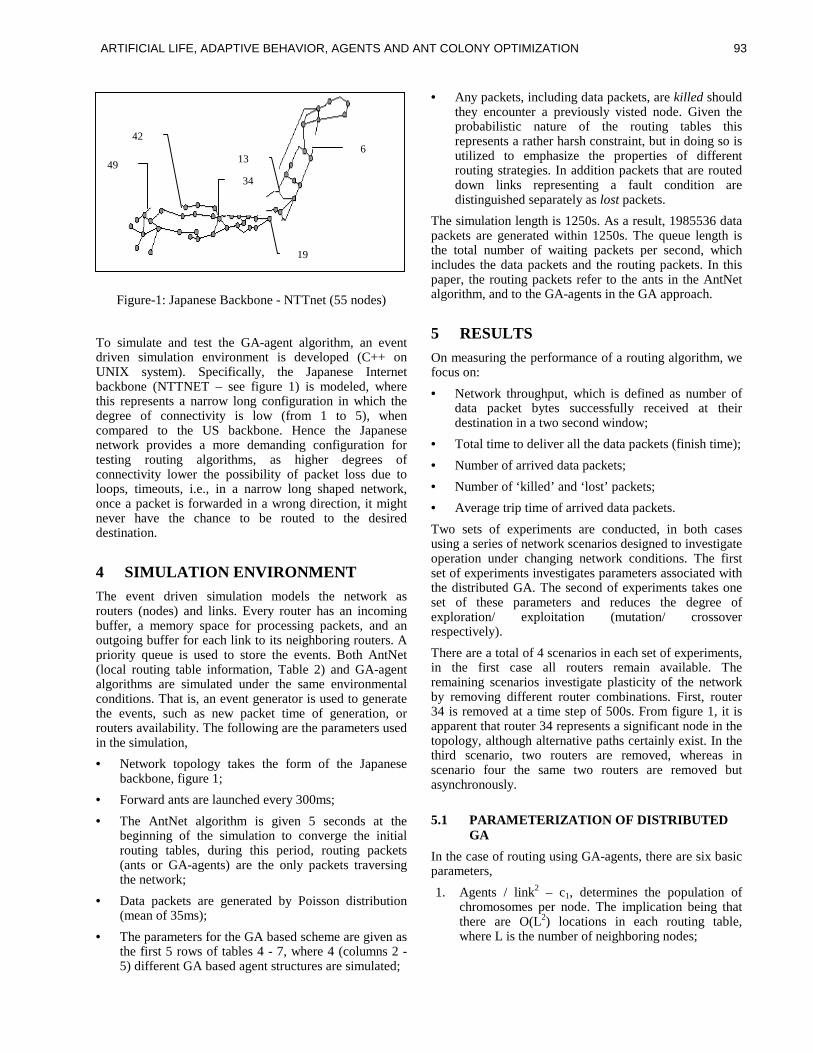
AAAA , Ali fe, Adaptive Behavior, Agents, and Ant Colony Optimization
Figure-1: Japanese Backbone - NTTnet (55 nodes)
To simulate and test the GA-agent algorithm, an event driven simulation environment is developed (C++ on UNIX system). Specifically, the Japanese Internet backbone (NTTNET – see figure 1) is modeled, where this represents a narrow long configuration in which the degree of connectivity is low (from 1 to 5), when compared to the US backbone. Hence the Japanese network provides a more demanding configuration for testing routing algorithms, as higher degrees of connectivity lower the possibilit y of packet loss due to loops, timeouts, i.e., in a narrow long shaped network, once a packet is forwarded in a wrong direction, it might never have the chance to be routed to the desired destination.
4 SIMULATION ENVIRONMENT
The event driven simulation models the network as routers (nodes) and links. Every router has an incoming buffer, a memory space for processing packets, and an outgoing buffer for each link to its neighboring routers. A priority queue is used to store the events. Both AntNet (local routing table information, Table 2) and GA-agent algorithms are simulated under the same environmental conditions. That is, an event generator is used to generate the events, such as new packet time of generation, or routers availabilit y. The following are the parameters used in the simulation,
• Network topology takes the form of the Japanese backbone, figure 1;
• Forward ants are launched every 300ms;
• The AntNet algorithm is given 5 seconds at the beginning of the simulation to converge the initial routing tables, during this period, routing packets (ants or GA-agents) are the only packets traversing the network;
• Data packets are generated by Poisson distribution (mean of 35ms);
• The parameters for the GA based scheme are given as the first 5 rows of tables 4 - 7, where 4 (columns 2 - 5) different GA based agent structures are simulated;
• Any packets, including data packets, are kill ed should they encounter a previously visted node. Given the probabili stic nature of the routing tables this represents a rather harsh constraint, but in doing so is utili zed to emphasize the properties of different routing strategies. In addition packets that are routed down links representing a fault condition are distinguished separately as lost packets.
The simulation length is 1250s. As a result, 1985536 data packets are generated within 1250s. The queue length is the total number of waiting packets per second, which includes the data packets and the routing packets. In this paper, the routing packets refer to the ants in the AntNet algorithm, and to the GA-agents in the GA approach.
5 RESULTS
On measuring the performance of a routing algorithm, we focus on:
• Network throughput, which is defined as number of data packet bytes successfully received at their destination in a two second window;
• Total time to deliver all the data packets (finish time);
• Number of arrived data packets;
• Number of ‘ kill ed’ and ‘ lost’ packets;
• Average trip time of arrived data packets.
Two sets of experiments are conducted, in both cases using a series of network scenarios designed to investigate operation under changing network conditions. The first set of experiments investigates parameters associated with the distributed GA. The second of experiments takes one set of these parameters and reduces the degree of exploration/ exploitation (mutation/ crossover respectively).
There are a total of 4 scenarios in each set of experiments, in the first case all routers remain available. The remaining scenarios investigate plasticity of the network by removing different router combinations. First, router 34 is removed at a time step of 500s. From figure 1, it is apparent that router 34 represents a significant node in the topology, although alternative paths certainly exist. In the third scenario, two routers are removed, whereas in scenario four the same two routers are removed but asynchronously.
5.1 PARAMETERIZATION OF DISTRIBUTED GA
In the case of routing using GA-agents, there are six basic parameters,
1. Agents / link2 – c1, determines the population of chromosomes per node. The implication being that there are O(L2) locations in each routing table, where L is the number of neighboring nodes;
6 13
19
34
42
49
ARTIFICIAL LIFE, ADAPTIVE BEHAVIOR, AGENTS AND ANT COLONY OPTIMIZATION 93

AAAA , Ali fe, Adaptive Behavior, Agents, and Ant Colony Optimization
2. Aging – c2, rate by which fitness of individuals currently populating the routing tables decay;
3. Propagate ratio – the number of chromosomes exchanged between populations, expressed as a % of node population size;
4. Propagate freq – rate of exchange of chromosomes between populations;
5. Flow clear freq – c3, time interval over which data packet destination statistics are collected;
6. Crossover and Mutation – the results in this section utili ze maximum crossover and mutation rates in order to encourage continuous investigation of alternative routes. Section 5.2 considers the case of a more classical section of crossover and mutation thresholds.
These are initially selected to enable quali fication of the sensitivity to population size, rate of aging etc. and remain the same across all experiments; Tables 4 to 7, columns 2 - 5. Table 8 summarizes the same information for the AntNet algorithm under a ‘ local’ routing table configuration. Thus, Local AntNet utili zes tables of length O(L), significantly less than the GA-agent case.
Table 4 – No Network Failure.
# Agents / link2 32 32 40 48
Aging 0.8 0.9 0.9 0.9
Propagate ratio 5% 3% 3% 2%
Propagate freq 500ms 500ms 700ms 700ms
Flow clear freq 50s 50s 50s 50s
Finish time (s) 1,252 1,253 1,252 1,267
Arrived Packets (AP) (×1000)
1,619 1,585 1,583 1,560
Avg. trip time for AP (ms)
742 905 678 1,236
# kill ed packets 366,533 400,351 402,517 385,750
# lost packets 0 0 0 0
# Agents (×103) 1,690 1,028 801 475
Table 5 – Router 34 is Down at 500s.
# Agents / link2 32 32 40 48
Aging 0.8 0.9 0.9 0.9
Propagate ratio 5% 3% 3% 2%
Propagate freq 500ms 500ms 700ms 700ms
Flow clear freq 50s 50s 50s 50s
Finish time (s) 1,417 1,307 1,444 1,494
Arrived Packets (AP) (×1000)
1,346 1,298 1,333 1,373
Avg. trip time for AP (ms)
2,014 2,613 3,156 2,668
# kill ed packets 617,064 665,188 630,479 590,732
# lost packets 21,922 21,922 21,923 21,918
# Agents (×103) 1,801 1,087 966 552
Table 6 – Routers 49 & 13 are Down at 500s.
# Agents / link2 32 32 40 48
Aging 0.8 0.9 0.9 0.9
Propagate ratio 5% 3% 3% 2%
Propagate freq 500ms 500ms 700ms 700ms
Flow clear freq 50s 50s 50s 50s
Finish time (s) 1,254 1,445 1,258 1,520
Arrived packets (AP) (×1000)
1,317 1,369 1,402 1,504
Avg. trip time for AP (ms)
947 1,301 850 1,759
# kill ed packets 623,539 571,390 539,747 438,378
# lost packets 44,466 44,882 43,658 43,496
# Agents (×103) 1,543 973 754 514
Table 7 – Router 13 is down at 300s, Router 49 is down at 500s, and both are up at 800s.
# Agents / link2 32 32 40 48
Aging 0.8 0.9 0.9 0.9
Propagate ratio 5% 3% 3% 2%
Propagate freq 500ms 500ms 700ms 700ms
Flow clear freq 50s 50s 50s 50s
Finish time (s) 1,535 1,261 1,496 1,437
Arrived packets (AP) (×103)
1,410 1,334 1,441 1,458
Avg. trip time for AP (ms)
2088 1202 470 2018
# kill ed packets 551,218 627,596 520,989 503,873
# lost packets 23,953 23,426 23,401 23,085
# Agents (×103) 1,447 1,043 896 648
Performance is quali fied in terms of two basic parameters, time taken for all packets to be received (or lost) and the number of packets successfully received. Naturally, the former should be minimized and the latter maximized. In the case of experiment 1 – no network failures – the time for all packets to be accounted for is essentially the same,
ARTIFICIAL LIFE, ADAPTIVE BEHAVIOR, AGENTS AND ANT COLONY OPTIMIZATION94

AAAA , Ali fe, Adaptive Behavior, Agents, and Ant Colony Optimization
irrespective of parameter or algorithm. An immediate difference is recognized, however, in the number of arrived packets. The AntNet algorithm can only successfully route 55% of those in the GA-agent approach. This observation is repeated across all the remaining scenarios. Moreover, in terms of ‘ kill ed’ packets this means that less than 50% of the packets in the local version of the AntNet algorithm revisit sites previously encountered.
Table 8 – AntNet with Local Information Only
No network failure
Finish time (s) 1,267
Arrived packets (AP) 903 (×103)
Avg. trip time of AP (ms) 398
# kill ed packets 1,082,652
# lost packets 0
# of Ants 218 (×103)
Router 34 down at 500s
Finish time (s) 1,369
Arrived packets (AP) 813 (×103)
Avg. trip time of AP (ms) 2,899
# kill ed packets 1,138,860
# lost packets 32,763
# of Ants 219 (×103)
Routers 49 & 13 down at 500s
Finish time (s) 1,300
Arrived packets (AP) 827 (×103)
Avg. trip time of AP (ms) 1,617
# kill ed packets 1,114,729
# lost packets 43,682
# of Ants 219 (×103)
Routers 13 down at 300s, Router 49 down at 500s, both up at 800s
Finish time (s) 1,272
Arrived packets (AP) 863 (×103)
Avg. trip time of AP (ms) 1,254
# kill ed packets 1,099,283
# lost packets 23,209
# of Ants 219 (×103)
In terms of specific parameter settings, the GA-agent approach appears to consistently route the most packets successfully when the number of agents per link is highest
and propagation ratio least. (Investigation of GA-agents without demes, however, performs very badly.) It is also noticed that although a maximum allowable length of 30 genes per individual is permitted, chromosomes never reach this limit. Instead a preference of chromosome lengths of 10 or less genes is found for nodes with a low level of connectivity and 15 to 25 for individuals with a connectivity of 3 or more.
5.2 PARAMETERIZATION OF CROSSOVER AND MUTATION
As a final experiment, one instance of the distributed parameter set is investigated under a classical crossover and mutation rate of 90% crossover and 10% mutation. As identified in section 5.1, lower agent per link counts result in less packets being delivered. Table 9 reports the case of 32 agents/ link, an aging factor of 0.9, a propagation ration of 3% and a frequency of 500ms (column 3 in tables 4 to 7).
On comparison with the same parameterization under 100% crossover and mutation, the number of ‘ kill ed’ or ‘ lost’ packets decreases by 33% to 8%, and the trip time improves in each scenario other than no network failure. Moreover, the case of 90% crossover and 10% mutation betters all combined ‘kill ed-lost’ packet counts of any of the distributed GA parameters investigated in section 5.1. The implication being that more data packets are routed to the destination without either encountering a faulty link or a previously visited node. The principle penalty, however, appears to be an increase in the number of GA-agents introduced. Future work will naturally investigate whether this trend holds for other distributed GA parameterizations (the case of 48 agents per link appears to utili ze less GA-agents).
Table 9 – GA-agent with Crossover of 90%, Mutation 10%
No network failure
Finish time (s) 1,252
Arrived packets (AP) 1,693 (×103)
Avg. trip time of AP (ms) 1,171
# kill ed packets 292,723
# lost packets 0
# of Agents 961 (×103)
Router 34 down at 500s
Finish time (s) 1,507
Arrived packets (AP) 1,401 (×103)
Avg. trip time of AP (ms) 356
# kill ed packets 562,751
# lost packets 21,924
# of Agents 1,170 (×103)
ARTIFICIAL LIFE, ADAPTIVE BEHAVIOR, AGENTS AND ANT COLONY OPTIMIZATION 95
AAAA , Ali fe, Adaptive Behavior, Agents, and Ant Colony Optimization
Routers 49 & 13 down at 500s
Finish time (s) 1,252
Arrived packets (AP) 1,417 (×103)
Avg. trip time of AP (ms) 861
# kill ed packets 523,673
# lost packets 44,658
# of Agents 1,025 (×103)
Routers 13 down at 300s, Router 49 down at 500s, both up at 800s
Finish time (s) 1,252
Arrived packets (AP) 1,555 (×103)
Avg. trip time of AP (ms) 1,012
# lost packets 406,840
# kill ed packets 23,861
# of Ants 1,083 (×103)
6 CONCLUSIONS
As indicated in the introduction, network routing problems force an interesting set of constraints, which present a suitable test-bed for problem solving using co-evolutionary techniques. In this work, we emphasize the case in which routing table features, as well as content, are evolved. Thus, we are not privy to a priori knowledge regarding the number of nodes in the network. The AntNet algorithm (Di Caro et al., 1998) does not perform eff iciently and the GA representation cannot make use of global knowledge of network connectivity, as has been the case in the past (Munetomo et al., 1997). Such an environment implies that packets responsible for updating network connectivity requires more autonomy than were previously acknowledged to solve packet switched routing problems. As a first attempt at addressing these problems directly, we utili ze a representation that is independent of specific network connectivity patterns and distributed in its operation (multi -population model with chromosomes physically traveling the network). Such a system improves on the AntNet algorithm when constrained to a ‘ local’ table representation, Table 2 (see (Liang et al., 2002) for a detailed discussion of AntNet under ‘ local’ and ‘global’ routing table constraints), or be it whilst utilizing larger routing tables. The principle drawback for the GA-agent is the search eff iciency of the ensuing routing table where a search as opposed to an indexing process is now necessary. Future work will expand the interaction between chromosomes to facilit ate a more co-evolutionary approach to the development of routing policies and develop a better organization to the routing table structure. Moreover, the relationship between routing table size and performance requires further investigation.
Acknowledgments
A. Nur Zincir-Heywood and Malcolm I. Heywood gratefully acknowledge the support of the Individual Research Grants from the Natural Sciences and Engineering Research Council of Canada.
References
Boyan J.A., Littman M.L., “Packet Routing in Dynamically Routing Networks: A Reinforcement Learning Approach,” Advances in Neural Information Processing Systems, Volume 6, pp 671-678, 1994.
Corne D.W., Oates M.J., Smith G.D., Telecommunications Optimization: Heuristic and Adaptive Techniques. John Wiley & Sons, isbn 0-471-98855-3, 2000.
Di Caro G., Dorigo M., “AntNet: Distributed Stigmergetic Control for Communications Networks,” Journal of Artificial Intelli gence Research, 9, pp 317-365, 1998.
Dorigo M., Maniezzo V., Colorni A., “Ant System: Optimization by a Colony of Cooperating Agents,” IEEE Transactions on Systems, Man and Cybernetics – B, 26(1) pp 29-41, Feb 1996.
Forouzan B. A., “Data Communications and Networking” , Mc-Graw Hill , ISBN 0-07-232204-7, 2001.
Gelenbe E., Xu Z., Seref E., “Cognitive Packet Networks,” Proceeding of 11th IEEE International Conference on Tools with Artificial Intelli gence, pp 47-54, 1999.
Halabi B., Internet Routing Architectures, Cisco Press, ISBN 1-56205-652-2, 1997.
Heusse M., Snyers D., Guerin S., Kuntz P., “Adaptive Agent-driven Routing and Load Balancing in Communication Networks,” Advances in Complex Systems, 1, pp 237-254, 1998.
Liang S., Zincir-Heywood A.N., Heywood M.I., “The Effect of Routing under Local Information using a Social Insect Metaphor,” IEEE International Congress on Evolutionary Computation, May 2002.
Maniezzo V., Colorni A., “The Ant System Applied to the Quadratic Assignment Problem,” IEEE Transactions on Knowledge and Data Engineering, 11(5), pp 769-778, Sept/ Oct 1999.
Munetomo M., Takai Y., Sato Y., “An Adaptive Network Routing Algorithm Employing Path Genetic Operators,” Proceedings of the 7th International Conference on Genetic Algorithms, pp 643-649, 1997.
Tennenhouse D., Smith J., Sincoskie W., Wetherall D., Minden G., “A Survey of Active Network Research,” IEEE Communications Magazine, 35(1), pp 80-86, Jan 1997.
ARTIFICIAL LIFE, ADAPTIVE BEHAVIOR, AGENTS AND ANT COLONY OPTIMIZATION96
Agent Support for Genetic Search in an Immunological Model ofSparse Distributed Memory
Keith E. Mathias and Jason S. ByasseeTRW Systems
16201 E. Centretech Pkwy.Aurora, CO 80011
keith.mathias, [email protected]
Abstract
This research focuses on agent migrationstrategies and communication behaviors ina sparse distributed memory implementationbased on the human immune system. Evalua-tion of various agent strategy/behavior com-binations is measured in the context of ge-netic search performance at multiple, in-dependent system nodes. Results indicatethat agent behaviors which promote andenhance information exchange between dis-tributed nodes yield the best performance.
1 Introduction
Our research involves a sparse distributed memory(SDM) where the theoretical memory capacity far out-weighs the physical memory space (i.e., the ratio ofmemory cells to items represented is 1 to n, wheren >> 1). This model is based in part on the humanimmune system, wherein memory persists in the formof a relatively modest population of antibodies (107
to 108) with a high affinity to a much greater number(1012 to 1016) of possible antigen strains [5]. An effec-tive SDM must develop and maintain a sufficient (withrespect to quality) population of memory cells so thatassociative recall is not only feasible, but efficient.
The memory cell population in this SDM is sparselydistributed in representation space and physically dis-tributed in the execution environment. In this system,mobile software agents circulate a limited number ofmemory cells between system nodes (Figure 1). Dis-tributed, independent genetic search is leveraged inorder to develop a system-wide memory cell popula-tion. Emergent behavior at the system level is a resultof interactions between simultaneous and independentgenetic searches, as well as, local feedback decisions.
Significant work has been performed with respect toagent strategies and enhanced distributed communi-cation performance [3, 4]. This research differs in thatwe seek to examine the impact of mobile agents withrespect to their migration strategies and communica-tion behaviors to improve genetic search performance.Improved genetic search performance in turn, resultsin a more efficient SDM.
Figure 1: Agent Circulation of Antibodies.
2 Sparse Distributed Memory
This investigation is influenced by previous work thatincorporates genetic algorithms in an immune systemmodel to explore pattern recognition [2]. We havemodeled the problem space using Hamming space (i.e.,bit strings). In training the SDM, the objective is todynamically develop “immunity” to patterns that arerepeatedly re-introduced from a fixed library of pat-terns. Immunity is achieved by evolving a memorycell population that generalizes to adequately repre-sent a much larger set of random bit string patterns.The random set of bit string patterns that must bematched is known here as the antigen library. Thesystem population of memory cells, known as anti-bodies, consists of a small (relative to the size of theantigen library) collection of bit string patterns. Anti-body evolution (i.e., system level learning) is a result
ARTIFICIAL LIFE, ADAPTIVE BEHAVIOR, AGENTS AND ANT COLONY OPTIMIZATION 97
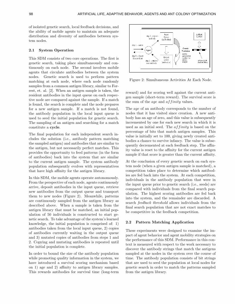
of isolated genetic search, local feedback decisions, andthe ability of mobile agents to maintain an adequatedistribution and diversity of antibodies between sys-tem nodes.
2.1 System Operation
This SDM consists of two core operations. The first isgenetic search, taking place simultaneously and con-tinuously on each node. The second involves mobileagents that circulate antibodies between the systemnodes. Genetic search is used to perform patternmatching at each node, where each node randomlysamples from a common antigen library, similar to For-rest, et. al. [2]. When an antigen sample is taken, theresident antibodies in the input queue on each respec-tive node are compared against the sample. If a matchis found, the search is complete and the node preparesfor a new antigen sample. If a match is not found,the antibody population in the local input queue isused to seed the initial population for genetic search.The sampling of an antigen and searching for a matchconstitute a cycle.
The final population for each independent search in-cludes the solution (i.e., antibody pattern matchingthe sampled antigen) and antibodies that are similar tothe antigen, but not necessarily perfect matches. Thisprovides the opportunity to feed patterns (in the formof antibodies) back into the system that are similarto the current antigen sample. The system antibodypopulation subsequently evolves with representativesthat have high affinity for the antigen library.
In this SDM, the mobile agents operate autonomously.From the perspective of each node, agents continuouslyarrive, deposit antibodies in the input queue, retrievenew antibodies from the output queue and transportthem to new nodes (Figure 2). Meanwhile, patternsare continuously sampled from the antigen library asdescribed above. When a sample is taken from theantigen library that must be matched, an initial pop-ulation of 50 individuals is constructed to start ge-netic search. To take advantage of the system’s learnedknowledge, the initial population is comprised of: 1)antibodies taken from the local input queue, 2) copiesof antibodies currently waiting in the output queueand 3) mutated copies of antibodies from steps 1 and2. Copying and mutating antibodies is repeated untilthe initial population is complete.
In order to bound the size of the antibody populationwhile promoting quality information in the system, wehave introduced a survival scoring mechanism basedon 1) age and 2) affinity to antigen library samples.This rewards antibodies for survival time (long-term
Figure 2: Simultaneous Activities At Each Node.
reward) and for scoring well against the current anti-gen sample (short-term reward). The survival score isthe sum of the age and affinity values.
The age of an antibody corresponds to the number ofnodes that it has visited since creation. A new anti-body has an age of zero, and this value is subsequentlyincremented by one for each new search in which it isused as an initial seed. The affinity is based on thepercentage of bits that match antigen samples. Thisvalue is initially set to 100, giving newly created anti-bodies a chance to survive infancy. The value is subse-quently decremented at each feedback step. The affin-ity value is reset to the affinity for the current antigensample if that score is greater than the current affinity.
At the conclusion of every genetic search on each sys-tem node (when a given antigen sample is matched), acompetition takes place to determine which antibod-ies are fed back into the system. At each competition,individuals in the antibody population that were inthe input queue prior to genetic search (i.e., seeds) arecompared with individuals from the final search pop-ulation. The highest scoring antibodies are fed backinto the system, and the remainder are discarded. Asearch feedback threshold allows individuals from thefinal search population that are not exact matches tobe competitive in the feedback competition.
2.2 Pattern Matching Application
These experiments were designed to examine the im-pact of agent behavior and agent mobility strategies onthe performance of this SDM. Performance in this con-text is measured with respect to the work necessary todiscover the antibody strings that match the antigenssampled at the nodes in the system over the course oftime. The antibody population consists of bit stringsthat are used to seed the population at local nodes forgenetic search in order to match the patterns sampledfrom the antigen library.
ARTIFICIAL LIFE, ADAPTIVE BEHAVIOR, AGENTS AND ANT COLONY OPTIMIZATION98
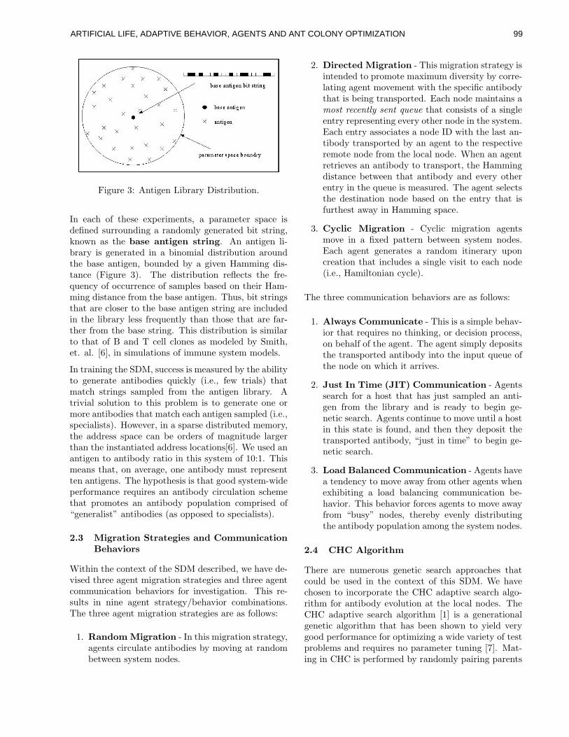
Figure 3: Antigen Library Distribution.
In each of these experiments, a parameter space isdefined surrounding a randomly generated bit string,known as the base antigen string. An antigen li-brary is generated in a binomial distribution aroundthe base antigen, bounded by a given Hamming dis-tance (Figure 3). The distribution reflects the fre-quency of occurrence of samples based on their Ham-ming distance from the base antigen. Thus, bit stringsthat are closer to the base antigen string are includedin the library less frequently than those that are far-ther from the base string. This distribution is similarto that of B and T cell clones as modeled by Smith,et. al. [6], in simulations of immune system models.
In training the SDM, success is measured by the abilityto generate antibodies quickly (i.e., few trials) thatmatch strings sampled from the antigen library. Atrivial solution to this problem is to generate one ormore antibodies that match each antigen sampled (i.e.,specialists). However, in a sparse distributed memory,the address space can be orders of magnitude largerthan the instantiated address locations[6]. We used anantigen to antibody ratio in this system of 10:1. Thismeans that, on average, one antibody must representten antigens. The hypothesis is that good system-wideperformance requires an antibody circulation schemethat promotes an antibody population comprised of“generalist” antibodies (as opposed to specialists).
2.3 Migration Strategies and CommunicationBehaviors
Within the context of the SDM described, we have de-vised three agent migration strategies and three agentcommunication behaviors for investigation. This re-sults in nine agent strategy/behavior combinations.The three agent migration strategies are as follows:
1. RandomMigration - In this migration strategy,agents circulate antibodies by moving at randombetween system nodes.
2. Directed Migration - This migration strategy isintended to promote maximum diversity by corre-lating agent movement with the specific antibodythat is being transported. Each node maintains amost recently sent queue that consists of a singleentry representing every other node in the system.Each entry associates a node ID with the last an-tibody transported by an agent to the respectiveremote node from the local node. When an agentretrieves an antibody to transport, the Hammingdistance between that antibody and every otherentry in the queue is measured. The agent selectsthe destination node based on the entry that isfurthest away in Hamming space.
3. Cyclic Migration - Cyclic migration agentsmove in a fixed pattern between system nodes.Each agent generates a random itinerary uponcreation that includes a single visit to each node(i.e., Hamiltonian cycle).
The three communication behaviors are as follows:
1. Always Communicate - This is a simple behav-ior that requires no thinking, or decision process,on behalf of the agent. The agent simply depositsthe transported antibody into the input queue ofthe node on which it arrives.
2. Just In Time (JIT) Communication - Agentssearch for a host that has just sampled an anti-gen from the library and is ready to begin ge-netic search. Agents continue to move until a hostin this state is found, and then they deposit thetransported antibody, “just in time” to begin ge-netic search.
3. Load Balanced Communication - Agents havea tendency to move away from other agents whenexhibiting a load balancing communication be-havior. This behavior forces agents to move awayfrom “busy” nodes, thereby evenly distributingthe antibody population among the system nodes.
2.4 CHC Algorithm
There are numerous genetic search approaches thatcould be used in the context of this SDM. We havechosen to incorporate the CHC adaptive search algo-rithm for antibody evolution at the local nodes. TheCHC adaptive search algorithm [1] is a generationalgenetic algorithm that has been shown to yield verygood performance for optimizing a wide variety of testproblems and requires no parameter tuning [7]. Mat-ing in CHC is performed by randomly pairing parents
ARTIFICIAL LIFE, ADAPTIVE BEHAVIOR, AGENTS AND ANT COLONY OPTIMIZATION 99
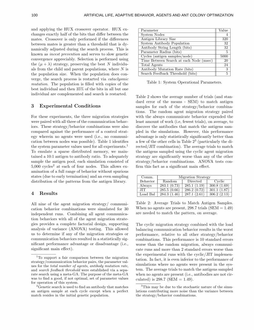
and applying the HUX crossover operator. HUX ex-changes exactly half of the bits that differ between themates. Crossover is only performed if the differencesbetween mates is greater than a threshold that is dy-namically adjusted during the search process. This isknown as incest prevention and serves to slow geneticconvergence appreciably. Selection is performed usingthe (µ + λ) strategy, preserving the best N individu-als from the child and parent populations, where N isthe population size. When the population does con-verge, the search process is restarted via cataclysmicmutation. The population is filled with copies of thebest individual and then 35% of the bits in all but oneindividual are complemented and search is restarted.
3 Experimental Conditions
For these experiments, the three migration strategieswere paired with all three of the communication behav-iors. These strategy/behavior combinations were alsocompared against the performance of a control strat-egy wherein no agents were used (i.e., no communi-cation between nodes was possible). Table 1 identifiesthe system parameter values used for all experiments.1
To emulate a sparse distributed memory, we main-tained a 10:1 antigen to antibody ratio. To adequatelysample the antigen pool, each simulation consisted of5,000 cycles2 at each of four nodes. This allows ex-amination of a full range of behavior without spuriousstates (due to early termination) and an even samplingdistribution of the patterns from the antigen library.
4 Results
All nine of the agent migration strategy/ communi-cation behavior combinations were simulated for 30independent runs. Combining all agent communica-tion behaviors with all of the agent migration strate-gies provides a complete factorial design, supportinganalysis of variance (ANOVA) testing. This allowedus to determine if any of the migration strategies orcommunication behaviors resulted in a statistically sig-nificant performance advantage or disadvantage (i.e.,significant main effect).
1To support a fair comparison between the migrationstrategy/communication behavior pairs, the parameter val-ues for the total number of agents, antibody mutation rate,and search feedback threshold were established via a sepa-rate search using a meta-GA. The purpose of the meta-GAwas to find a good, if not optimal, set of parameter valuesfor operation of this system.
2Genetic search is used to find an antibody that matchesan antigen sample at each cycle except when a perfectmatch resides in the initial genetic population.
Parameter ValueSystem Nodes 4Antigen Library Size 320System Antibody Population 32Antibody String Length (bits) 32Parameter Radius (bits) 5Cycles (antigen samples/node) 5000Time Between Search at each Node (msec) 20Total Agents 24Antibody Mutation Rate (bits) 3Search Feedback Threshold (bits) 5
Table 1: System Operational Parameters.
Table 2 shows the average number of trials (and stan-dard error of the means - SEM) to match antigensamples for each of the strategy/behavior combina-tions. The random agent migration strategy pairedwith the always communicate behavior expended theleast amount of work (i.e, fewest trials), on average, todiscover the antibodies that match the antigens sam-pled in the simulations. However, this performanceadvantage is only statistically significantly better thana few of the other cells in Table 23 (particularly the di-rected/JIT combination). The average trials to matchthe antigens sampled using the cyclic agent migrationstrategy are significantly worse than any of the otherstrategy/behavior combinations. ANOVA tests con-firm this fact as a significant main effect.
Comm. Migration StrategyBehavior Random Directed CyclicAlways 283.1 (0.73) 285.1 (1.19) 300.8 (1.69)JIT 285.5 (0.66) 286.2 (0.72) 301.1 (1.87)Load Bal 284.3 (1.46) 287.1 (2.61) 306.2 (2.13)
Table 2: Average Trials to Match Antigen Samples.When no agents are present, 298.7 trials (SEM = 1.49)are needed to match the pattern, on average.
The cyclic migration strategy combined with the loadbalancing communication behavior results in the worstperformance, relative to all other strategy/behaviorcombinations. This performance is 10 standard errorsworse than the random migration, always communi-cate runs and more than 2 standard errors worse thanthe experimental runs with the cyclic/JIT implemen-tation. In fact, it is even inferior to the performance ofsimulations where no agents were present in the sys-tem. The average trials to match the antigens sampledwhen no agents are present (i.e., antibodies are not cir-culated) is 298.7 (SEM = 1.49).
3This may be due to the stochastic nature of the simu-lations contributing more noise than the variance betweenthe strategy/behavior combinations.
ARTIFICIAL LIFE, ADAPTIVE BEHAVIOR, AGENTS AND ANT COLONY OPTIMIZATION100
It is important to note that the system learns and per-forms significantly better than genetic search on anequivalent problem when a random initial populationis used. For example, on average, CHC solves a 32-bitone-max4 problem in 504 trials (SEM = 9.12), whenbeginning with a random initial population.
4.1 An Emergent Behavior
Although the goal of genetic search at each local nodeis to match antigen library samples, the search effortscombined with the local survival decisions result in aglobally emergent behavior. The communication of in-formation via agents consistently resulted in an inter-esting phenomenon, notably the discovery and propa-gation of the string pattern used to create the antigenlibrary (i.e., the base antigen string). Table 3 showsthe average percentage of the system’s final antibodypopulation occupied by copies of strings matching thebase antigen for each respective strategy/behavior ex-periment. This is referred to as the saturation rate.
Comm. Migration StrategyBehavior Random Directed CyclicAlways 100.0% (0.00) 100.0% (0.00) 89.7% (1.04)
JIT 100.0% (0.00) 100.0% (0.00) 89.1% (1.35)Load Bal 96.1% (0.74) 97.2% (0.68) 82.9% (3.40)
Table 3: Antibody Population Saturation Rate. Whenno agents are present, the average saturation rate is91.1% (SEM = 0.50).
ANOVA testing confirms the trends evident by vi-sual inspection as significant. First, the load-balancingcommunication behavior does not allow the base anti-gen to saturate the system, regardless of the agentmigration strategy employed. The cyclic agent migra-tion strategy also prevents the base antigen string fromsaturating the antibody population. This seems obvi-ous in hindsight as the cyclic migration strategy is themost restrictive of the migration strategies. Visita-tion by a given agent is not equally likely at all nodesat each time step for this migration strategy. Thisrestriction is so severe in fact, that the results werecomparable to runs where no agents were present inthe system. While simulations using no agents did dis-cover this base antigen string, the simulations yieldedan average saturation rate of 91.1% (SEM = 0.50).
The discovery of antibodies that match the base anti-gen string cannot be a result of searches in which thebase antigen is sampled from the antigen library. An-
4A one-max problem is equivalent to finding a match-ing bit-string using an evaluation score that reports thenumber (or percentage) of bits matching another pattern.
tibodies fed back to the system must meet or exceeda feedback threshold of five bits.
In searching for strings to match samples from the anti-gen library, each node contributes strings to the sys-tem antibody competition that have a large numberof bits in common with the base antigen. This mayor may not be sufficient for a given antibody to sur-vive the feedback competition and be propagated toother nodes. However, those strings that are close tothe base antigen string in Hamming distance will alsolikely score well against other antigens, if kept in thesystem antibody population. This causes the systemantibody population to accumulate alleles in commonwith the base antigen string. When the antibody pop-ulation is viewed as a probability vector that repre-sents the percentage of 0- or 1-bits at each locus overthe strings in the antibody population, this vector willapproximate the base antigen string more accuratelyover time.
Eventually, an antibody matching the base antigen isa by-product of a search for another antigen librarysample. Antibody copies of the base antigen stringwill likely perform well in the feedback competitionsat each node, and chances of survival in the systemwill be better than average. After surviving in the an-tibody population for several cycles, the age weightingguarantees future survival.
The base string is very rarely useful in exactly match-ing any string in the antigen library (a 1 in 320 chance),yet this string serves as a good seed string for the ge-netic search. The discovery of the base string may ormay not be an optimal system-wide strategy for learn-ing how best to reduce the number of trials requiredto evolve an antibody that matches an antigen sam-ple. For example, the discovery of four antibodies thatdivide the antigen library into equally sized attractionbasins, based on Hamming distance, might work aswell as, or better than, a single generalist. Regardless,the discovery of the base string is an interesting exam-ple of local behavior that facilitates emergent globalbehavior.
The best performances shown in Table 2 generally cor-respond with complete saturation (Table 3), yet thereis not a perfect correlation. For example, the load bal-ancing/random migration implementation performsquite well, but does not exhibit complete saturation.Therefore, saturation of the antibody population withthe base antigen must not be the only factor in obtain-ing good performance.
ARTIFICIAL LIFE, ADAPTIVE BEHAVIOR, AGENTS AND ANT COLONY OPTIMIZATION 101
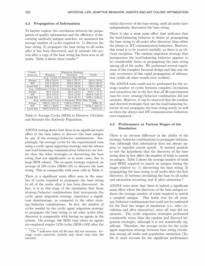
4.2 Propagation of Information
To further explore the correlation between the propa-gation of quality information and the efficiency of dis-covering antibody/antigen matches, we measured theaverage number of cycles required to: 1) discover thebase string, 2) propagate the base string to all nodesafter it has been discovered, and 3) saturate the sys-tem after a copy of the base string has been seen at allnodes. Table 4 shows these results.5
Comm. Migration StrategyBehavior Random Directed Cyclic
Avg. Cycles to Discover Base StringAlways 138.4 (24.5) 234.4 (51.7) 123.4 (19.9)
JIT 147.2 (23.6) 153.0 (26.6) 182.3 (35.7)Load Bal 195.4 (37.2) 153.6 (32.4) 123.5 (20.9)Avg. Additional Cycles to Circulate Base String to All NodesAlways 36.4 (12.4) 60.4 (22.1) 818.7 ( 77.7)
JIT 35.6 (12.4) 58.8 (17.8) 1018.9 (135.1)Load Bal 19.4 ( 4.3) 89.4 (31.5) 1278.1 (130.3)
Avg. Additional Cycles to Saturate With Base StringAlways 1083.9 (154.4) 1106.6 (178.0) *3906 (0)
JIT 865.1 ( 86.8) 973.2 (107.4) *3798.5 (831.5)Load Bal *2944.5(410.3) *2943.4 (378.5) *2013 (0)
Table 4: Average Cycles (SEM) to Discover, Circulateand Saturate the Antibody Population.
ANOVA testing shows that there is no significant maineffect in the time taken to discover the base antigenby any of the strategy/behavior combinations. Sur-prisingly, the average cycles for the experimental runsusing a cyclic agent migration strategy and the alwaysand load-balancing communication behaviors are bet-ter than the other strategies at discovering the basestring (but not significantly so in most cases, due tolarge SEM values). The no agent strategy required, anaverage of 163 cycles (SEM=19) to discover the basestring. This is comparable with most cells in Table 4.
There is a significant main effect seen in the num-ber of cycles required to propagate the base stringto all of the nodes after it has been discovered. Infact, it is at this stage of the simulation that thosestrategy/behavior combinations that incorporate thecyclic agent migration strategy experience a signifi-cant disadvantage, as compared to the other strat-egy/behavior combinations. In fact, the number ofcycles needed by the cyclic agent migration strategyto propagate the base string to all other nodes afterdiscovery is comparable with having no agents in thesystem. On average, the SDM runs where no agentsare employed require 1158 cycles (SEM=102) after the
5The * indicates that all 30 runs did not saturate. Av-erage cycles reported, include only those runs that didsaturate.
initial discovery of the base string, until all nodes haveindependently discovered the base string.
There is also a weak main effect that indicates thatthe load-balancing behavior is slower at propagatingthe base string to all nodes after discovery than eitherthe always or JIT communication behaviors. However,this trend is to be treated carefully, as there is an ob-vious exception. The random migration strategy thatincorporates the load-balancing behavior appears tobe considerably faster at propagating the base stringamong all of the nodes. We performed several repeti-tions of the complete factorial design and this was theonly occurrence of this rapid propagation of informa-tion (while all other trends were verified).
The ANOVA tests could not be performed for the av-erage number of cycles between complete circulationand saturation due to the fact that all 30 experimentalruns for every strategy/behavior combination did notsaturate. However, it can be observed that the randomand directed strategies that use the load-balancing be-havior do not propagate the base string nearly as wellas when the always and JIT communication behaviorswere employed.
4.3 Performance at Various Stages of theSimulation
There is an obvious difference in the ability of thestrategy/behavior combinations to propagate informa-tion (although that information does not always ap-pear to expedite search speed). It seemed prudentto test the hypothesis that the discovery of the basestring does in fact affect the number of trials to matchan antigen. Table 5 shows the average number of trials(and SEM) required to match an antigen during thestages relative to: 1) discovering the base string, 2)propagating the base string to all nodes after the firstdiscovery, 3) between circulating the base to all nodesand saturation occurring, and 4) after saturation.5
ANOVA tests show that there is indeed a significantmain effect where the discovery of the base antigen re-duces the average number of trials required to matcha sampled antigen. This holds true for all strat-egy/behavior combinations but could not be confirmedfor the final two stages of simulation (i.e., after cir-culation and after saturation), since all runs did notsaturate. The cyclic migration strategies performedconsistently worse than the random and directed mi-gration strategies, although it is not statistically sig-nificant. Therefore, the average cycles for the cyclicagent migration strategy between base string circula-tion among all nodes and population saturation (Ta-ble 4) must account for the significant performance
ARTIFICIAL LIFE, ADAPTIVE BEHAVIOR, AGENTS AND ANT COLONY OPTIMIZATION102
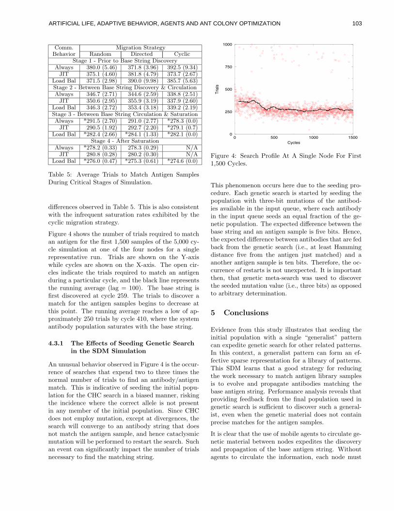
Comm. Migration StrategyBehavior Random Directed Cyclic
Stage 1 - Prior to Base String DiscoveryAlways 380.0 (5.46) 371.8 (3.96) 392.5 (9.34)
JIT 375.1 (4.60) 381.8 (4.79) 373.7 (2.67)Load Bal 371.5 (2.98) 390.0 (9.98) 385.7 (5.63)Stage 2 - Between Base String Discovery & CirculationAlways 346.7 (2.71) 344.6 (2.59) 338.8 (2.51)
JIT 350.6 (2.95) 355.9 (3.19) 337.9 (2.60)Load Bal 346.3 (2.72) 353.4 (3.18) 339.2 (2.19)Stage 3 - Between Base String Circulation & SaturationAlways *291.5 (2.70) 291.0 (2.77) *278.3 (0.0)
JIT 290.5 (1.92) 292.7 (2.20) *279.1 (0.7)Load Bal *282.4 (2.66) *284.1 (1.33) *282.1 (0.0)
Stage 4 - After SaturationAlways *278.2 (0.33) 278.3 (0.29) N/A
JIT 280.8 (0.28) 280.2 (0.30) N/ALoad Bal *276.0 (0.47) *275.3 (0.61) *274.6 (0.0)
Table 5: Average Trials to Match Antigen SamplesDuring Critical Stages of Simulation.
differences observed in Table 5. This is also consistentwith the infrequent saturation rates exhibited by thecyclic migration strategy.
Figure 4 shows the number of trials required to matchan antigen for the first 1,500 samples of the 5,000 cy-cle simulation at one of the four nodes for a singlerepresentative run. Trials are shown on the Y-axiswhile cycles are shown on the X-axis. The open cir-cles indicate the trials required to match an antigenduring a particular cycle, and the black line representsthe running average (lag = 100). The base string isfirst discovered at cycle 259. The trials to discover amatch for the antigen samples begins to decrease atthis point. The running average reaches a low of ap-proximately 250 trials by cycle 410, where the systemantibody population saturates with the base string.
4.3.1 The Effects of Seeding Genetic Searchin the SDM Simulation
An unusual behavior observed in Figure 4 is the occur-rence of searches that expend two to three times thenormal number of trials to find an antibody/antigenmatch. This is indicative of seeding the initial popu-lation for the CHC search in a biased manner, riskingthe incidence where the correct allele is not presentin any member of the initial population. Since CHCdoes not employ mutation, except at divergences, thesearch will converge to an antibody string that doesnot match the antigen sample, and hence cataclysmicmutation will be performed to restart the search. Suchan event can significantly impact the number of trialsnecessary to find the matching string.
0 500 1000 1500Cycles
0
250
500
750
1000
Tria
ls
Figure 4: Search Profile At A Single Node For First1,500 Cycles.
This phenomenon occurs here due to the seeding pro-cedure. Each genetic search is started by seeding thepopulation with three-bit mutations of the antibod-ies available in the input queue, where each antibodyin the input queue seeds an equal fraction of the ge-netic population. The expected difference between thebase string and an antigen sample is five bits. Hence,the expected difference between antibodies that are fedback from the genetic search (i.e., at least Hammingdistance five from the antigen just matched) and aanother antigen sample is ten bits. Therefore, the oc-currence of restarts is not unexpected. It is importantthen, that genetic meta-search was used to discoverthe seeded mutation value (i.e., three bits) as opposedto arbitrary determination.
5 Conclusions
Evidence from this study illustrates that seeding theinitial population with a single “generalist” patterncan expedite genetic search for other related patterns.In this context, a generalist pattern can form an ef-fective sparse representation for a library of patterns.This SDM learns that a good strategy for reducingthe work necessary to match antigen library samplesis to evolve and propagate antibodies matching thebase antigen string. Performance analysis reveals thatproviding feedback from the final population used ingenetic search is sufficient to discover such a general-ist, even when the genetic material does not containprecise matches for the antigen samples.
It is clear that the use of mobile agents to circulate ge-netic material between nodes expedites the discoveryand propagation of the base antigen string. Withoutagents to circulate the information, each node must
ARTIFICIAL LIFE, ADAPTIVE BEHAVIOR, AGENTS AND ANT COLONY OPTIMIZATION 103
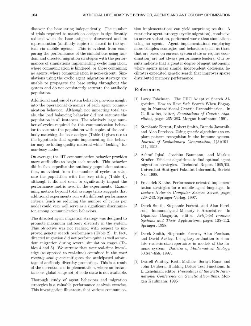
discover the base string independently. The numberof trials required to match an antigen is significantlyreduced when the base antigen is discovered and itsrepresentation (antibody copies) is shared in the sys-tem via mobile agents. This is evident from com-paring the performances of the simulations using ran-dom and directed migration strategies with the perfor-mances of simulations implementing cyclic migration,where communication is hindered, or those containingno agents, where communication is non-existent. Sim-ulations using the cyclic agent migration strategy areunable to propagate the base string throughout thesystem and do not consistently saturate the antibodypopulation.
Additional analysis of system behavior provides insightinto the operational dynamics of each agent commu-nication behavior. Although not impacting total tri-als, the load balancing behavior did not saturate thepopulation in all instances. The relatively large num-ber of cycles required for this communication behav-ior to saturate the population with copies of the anti-body matching the base antigen (Table 4) gives rise tothe hypothesis that agents implementing this behav-ior may be hiding quality material while “looking” fornon-busy nodes.
On average, the JIT communication behavior providesmore antibodies to begin each search. This behaviordid in fact expedite the antibody population satura-tion, as evident from the number of cycles to satu-rate the population with the base string (Table 4),although it did not seem to significantly impact theperformance metric used in the experiments. Exam-ining metrics beyond total average trials suggests thatadditional experiments run with different performancecriteria (such as reducing the number of cycles pernode) could very well serve as a significant discrimina-tor among communication behaviors.
The directed agent migration strategy was designed topromote maximum antibody diversity in the system.This objective was not realized with respect to im-proved genetic search performance (Table 2). In fact,directed migration did not perform quite as well as ran-dom migration during several simulation stages (Ta-bles 4 and 5). We surmise that near real-time knowl-edge (as opposed to real-time) contained in the mostrecently sent queue mitigates the anticipated advan-tage of antibody diversity promotion. This is a resultof the decentralized implementation, where an instan-taneous global snapshot of node state is not available.
Thorough study of agent behaviors and migrationstrategies is a valuable performance analysis exercise.This investigation illustrates that various communica-
tion implementations can yield surprising results. Arestrictive agent strategy (cyclic migration), conduciveto uneven visitation, performed worse than simulationsusing no agents. Agent implementations employingmore complex strategies and behaviors (such as thosethat are based on current system state or require coor-dination) are not always performance leaders. Our re-sults indicate that a greater degree of agent autonomy,where agents make simple, independent decisions, fa-cilitates expedited genetic search that improves sparsedistributed memory performance.
References
[1] Larry Eshelman. The CHC Adaptive Search Al-gorithm. How to Have Safe Search When Engag-ing in Nontraditional Genetic Recombination. InG. Rawlins, editor, Foundations of Genetic Algo-rithms, pages 265–283. Morgan Kaufmann, 1991.
[2] Stephanie Forrest, Robert Smith, Brenda Javornik,and Alan Perelson. Using genetic algorithms to ex-plore pattern recognition in the immune system.Journal of Evolutionary Computation, 1(3):191–211, 1993.
[3] Ashraf Iqbal, Joachim Baumann, and MarkusStraßer. Efficient algorithms to find optimal agentmigration strategies. Technical Report 1985/05,Universitat Stuttgart Fakultat Informatik, BerichtNr., 1998.
[4] Frederick Knabe. Performance oriented implemen-tation strategies for a mobile agent language. InLecture Notes in Computer Science Series, pages229–243. Springer-Verlag, 1997.
[5] Derek Smith, Stephanie Forrest, and Alan Perel-son. Immunological Memory is Associative. InDipankar Dasgupta, editor, Artificial ImmuneSystems and Their Applications, pages 105–112.Springer, 1998.
[6] Derek Smith, Stephanie Forrest, Alan Perelson,and David Ackley. Using lazy evaluation to simu-late realistic-size repertoires in models of the im-mune system. Bulletin of Mathematical Biology,60:647–658, 1997.
[7] Darrell Whitley, Keith Mathias, Soraya Rana, andJohn Dzubera. Building Better Test Functions. InL. Eshelman, editor, Proceedings of the Sixth Inter-national Conference on Genetic Algorithms. Mor-gan Kaufmann, 1995.
ARTIFICIAL LIFE, ADAPTIVE BEHAVIOR, AGENTS AND ANT COLONY OPTIMIZATION104
Studies on the Dynamics of Ant Colony Optimization Algorithms
Daniel Merkle
Institute AIFB
University of Karlsruhe
D-76128 Karlsruhe, Germany
Martin Middendorf
Computer Science Group
Catholic University of Eichst�att-Ingolstadt
D-85072 Eichst�att, Germany
Abstract
A deterministic model for Ant Colony Opti-
mization (ACO) algorithms is proposed and
used to study the dynamics of ACO. The
model is based on the average expected be-
haviour of ants. The behaviour of ACO algo-
rithms and the model are analysed for certain
types of permutation problems. It is shown
numerically that decisions of the ants are in-
uenced in an intriguing way by the proper-
ties of the pheromone matrix. This explains
why ACO algorithms show a complex dy-
namic behaviour. Simulations are done to
compare the behaviour of the ACO model
with the ACO algorithm. The results show
that the model describes essential features of
the dynamics of ACO algorithms.
1 INTRODUCTION
Ant Colony Optimization (ACO) has been applied suc-
cessfully to several optimization problems (ACO was
proposed in [1, 2]). Since ACO algorithms are based on
sequences of random decisions of arti�cial ants which
are usually not independent it is diÆcult to analyze the
behaviour of ACO algorithms theoretically. Except
from convergence proofs for types of ACO algorithms
with a strong elite principle [3, 4, 12] not much the-
oretical work has been done. Usually ant algorithms
have been tested on benchmark problems or real world
problems. In this paper we propose and analyze a de-
terministic model for ACO algorithms and use it to
derive exact results on optimization problems with a
simple structure. The analytical results are comple-
mented with empirical tests to compare computations
done with the ACO model with test runs of the ACO
algorithm.
Modelling has been done in the �eld of genetic algo-
rithms (GAs) by several authors in order to better
understand GAs behaviour. One line of modelling is
to use an in�nite population which is often easier to
handle than a �nite population since many proper-
ties of an in�nite population do not uctuate due to
few random events [13, 14]. Another method is to
characterize the population by few parameters (e.g.,
mean and variance of the �tness distribution of the
population) which capture important aspects of the
population instead of dealing with a concrete popula-
tion (e.g., [9{11]). Mostly in these studies, GAs are
modelled on problems which are simple but have some
characteristic features of more complicated and real-
world problems (e.g., \Royal Road" functions [8]).
The approach used in this paper is to de�ne a deter-
ministic model for ACO that is based on the expected
decisions of the ants. In the model the pheromone
update in every iteration is done by adding for each
pheromone value the expected update of a random
generation of ants.
In Section 2, we describe the permutation problems
that are used in this paper. The ACO algorithm is
described in Section 3 and the ACO model is de�ned
in Section 4. In Section 5, we discuss how to apply
the model to permutation problems. A �xed point
analysis of pheromone matrices is done in Section 6.
In Section 7, we analyze the dynamic behaviour of
the ACO model. Simulation results are described in
Section 8 and conclusions are given in Section 9.
2 PERMUTATION PROBLEMS
Although the general approach of our ACOmodel does
not depend on a speci�c type of optimzation problems
we give a more elaborated description only for permu-
tation problems. They are also used as test problems.
In particular, we use the following type of permutation
ARTIFICIAL LIFE, ADAPTIVE BEHAVIOR, AGENTS AND ANT COLONY OPTIMIZATION 105
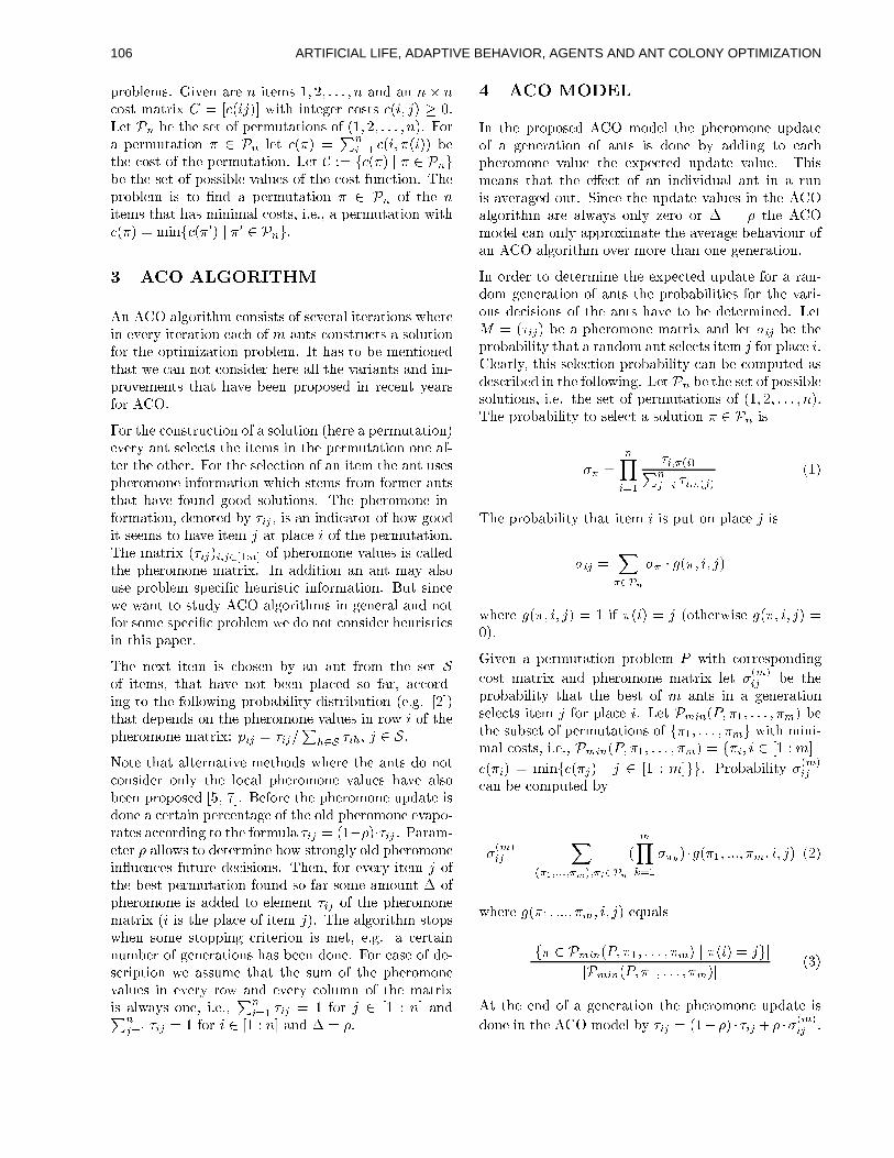
problems. Given are n items 1; 2; : : : ; n and an n � n
cost matrix C = [c(ij)] with integer costs c(i; j) � 0.
Let Pn be the set of permutations of (1; 2; : : : ; n). For
a permutation � 2 Pn let c(�) =P
n
i=1c(i; �(i)) be
the cost of the permutation. Let C := fc(�) j � 2 Png
be the set of possible values of the cost function. The
problem is to �nd a permutation � 2 Pn of the n
items that has minimal costs, i.e., a permutation with
c(�) = minfc(�0) j �0 2 Png.
3 ACO ALGORITHM
An ACO algorithm consists of several iterations where
in every iteration each of m ants constructs a solution
for the optimization problem. It has to be mentioned
that we can not consider here all the variants and im-
provements that have been proposed in recent years
for ACO.
For the construction of a solution (here a permutation)
every ant selects the items in the permutation one af-
ter the other. For the selection of an item the ant uses
pheromone information which stems from former ants
that have found good solutions. The pheromone in-
formation, denoted by �ij , is an indicator of how good
it seems to have item j at place i of the permutation.
The matrix (�ij)i;j2[1:n] of pheromone values is called
the pheromone matrix. In addition an ant may also
use problem speci�c heuristic information. But since
we want to study ACO algorithms in general and not
for some speci�c problem we do not consider heuristics
in this paper.
The next item is chosen by an ant from the set S
of items, that have not been placed so far, accord-
ing to the following probability distribution (e.g. [2])
that depends on the pheromone values in row i of the
pheromone matrix: pij = �ij=P
h2S�ih, j 2 S.
Note that alternative methods where the ants do not
consider only the local pheromone values have also
been proposed [5, 7]. Before the pheromone update is
done a certain percentage of the old pheromone evapo-
rates according to the formula �ij = (1��)��ij . Param-
eter � allows to determine how strongly old pheromone
in uences future decisions. Then, for every item j of
the best permutation found so far some amount � of
pheromone is added to element �ij of the pheromone
matrix (i is the place of item j). The algorithm stops
when some stopping criterion is met, e.g. a certain
number of generations has been done. For ease of de-
scription we assume that the sum of the pheromone
values in every row and every column of the matrix
is always one, i.e.,P
n
i=1�ij = 1 for j 2 [1 : n] andP
n
j=1�ij = 1 for i 2 [1 : n] and � = �.
4 ACO MODEL
In the proposed ACO model the pheromone update
of a generation of ants is done by adding to each
pheromone value the expected update value. This
means that the e�ect of an individual ant in a run
is averaged out. Since the update values in the ACO
algorithm are always only zero or � = � the ACO
model can only approximate the average behaviour of
an ACO algorithm over more than one generation.
In order to determine the expected update for a ran-
dom generation of ants the probabilities for the vari-
ous decisions of the ants have to be determined. Let
M = (�ij) be a pheromone matrix and let �ij be the
probability that a random ant selects item j for place i.
Clearly, this selection probability can be computed as
described in the following. Let Pn be the set of possible
solutions, i.e. the set of permutations of (1; 2; : : : ; n).
The probability to select a solution � 2 Pn is
�� =
nYi=1
�i;�(i)Pn
j=i�i;�(j)
(1)
The probability that item i is put on place j is
�ij =X�2Pn
�� � g(�; i; j)
where g(�; i; j) = 1 if �(i) = j (otherwise g(�; i; j) =
0).
Given a permutation problem P with corresponding
cost matrix and pheromone matrix let �(m)
ijbe the
probability that the best of m ants in a generation
selects item j for place i. Let Pmin(P; �1; : : : ; �m) be
the subset of permutations of f�1; : : : ; �mg with mini-
mal costs, i.e., Pmin(P; �1; : : : ; �m) = f�i; i 2 [1 : m] j
c(�i) = minfc(�j) j j 2 [1 : m]gg. Probability �(m)
ij
can be computed by
�(m)
ij=
X(�1;:::;�m);�i2Pn
(
mYk=1
��k ) �g(�1; :::; �m; i; j) (2)
where g(�1; :::; �m; i; j) equals
jf� 2 Pmin(P; �1; : : : ; �m) j �(i) = jgj
jPmin(P; �1; : : : ; �m)j(3)
At the end of a generation the pheromone update is
done in the ACO model by �ij = (1��) � �ij +� ��(m)
ij.
ARTIFICIAL LIFE, ADAPTIVE BEHAVIOR, AGENTS AND ANT COLONY OPTIMIZATION106
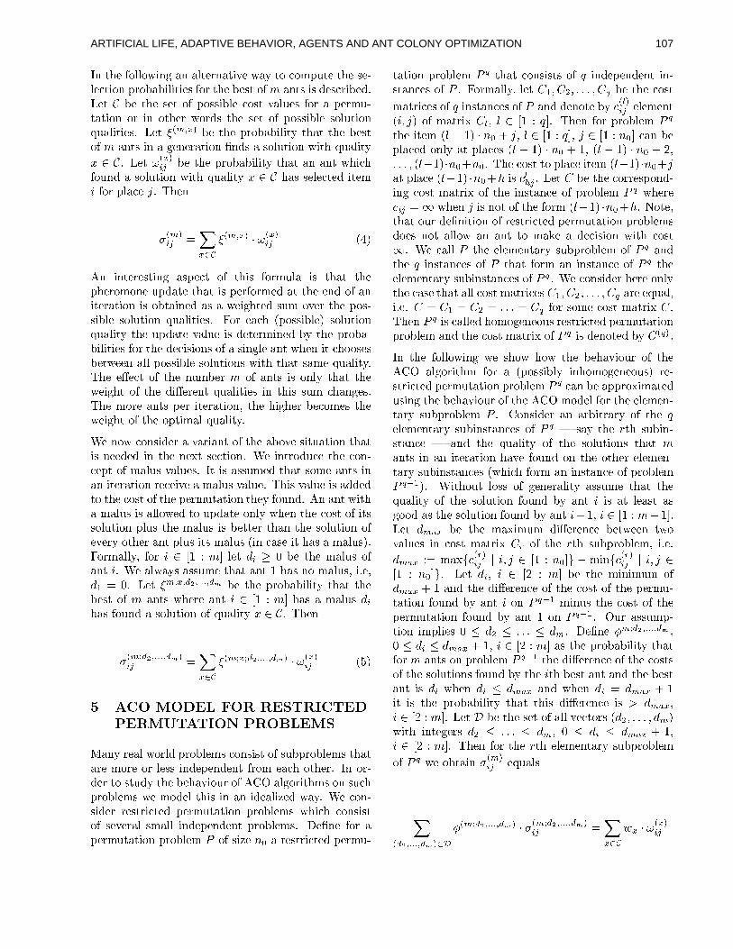
In the following an alternative way to compute the se-
lection probabilities for the best ofm ants is described.
Let C be the set of possible cost values for a permu-
tation or in other words the set of possible solution
qualities. Let �(m;x) be the probability that the best
of m ants in a generation �nds a solution with quality
x 2 C. Let !(x)
ijbe the probability that an ant which
found a solution with quality x 2 C has selected item
i for place j. Then
�(m)
ij=Xx2C
�(m;x)
� !(x)
ij(4)
An interesting aspect of this formula is that the
pheromone update that is performed at the end of an
iteration is obtained as a weighted sum over the pos-
sible solution qualities. For each (possible) solution
quality the update value is determined by the proba-
bilities for the decisions of a single ant when it chooses
between all possible solutions with that same quality.
The e�ect of the number m of ants is only that the
weight of the di�erent qualities in this sum changes.
The more ants per iteration, the higher becomes the
weight of the optimal quality.
We now consider a variant of the above situation that
is needed in the next section. We introduce the con-
cept of malus values. It is assumed that some ants in
an iteration receive a malus value. This value is added
to the cost of the permutation they found. An ant with
a malus is allowed to update only when the cost of its
solution plus the malus is better than the solution of
every other ant plus its malus (in case it has a malus).
Formally, for i 2 [1 : m] let di � 0 be the malus of
ant i. We always assume that ant 1 has no malus, i.e,
d1 = 0. Let �m;x;d2;:::;dm be the probability that the
best of m ants where ant i 2 [1 : m] has a malus dihas found a solution of quality x 2 C. Then
�(m;d2;:::;dm)
ij=Xx2C
�(m;x;d2;:::;dm)
� !(x)
ij(5)
5 ACO MODEL FOR RESTRICTED
PERMUTATION PROBLEMS
Many real world problems consist of subproblems that
are more or less independent from each other. In or-
der to study the behaviour of ACO algorithms on such
problems we model this in an idealized way. We con-
sider restricted permutation problems which consist
of several small independent problems. De�ne for a
permutation problem P of size n0 a restricted permu-
tation problem Pq that consists of q independent in-
stances of P . Formally, let C1; C2; : : : ; Cq be the cost
matrices of q instances of P and denote by c(l)
ijelement
(i; j) of matrix Cl, l 2 [1 : q]. Then for problem Pq
the item (l � 1) � n0 + j, l 2 [1 : q], j 2 [1 : n0] can be
placed only at places (l � 1) � n0 + 1, (l � 1) � n0 + 2,
: : : ; (l�1)�n0+n0. The cost to place item (l�1)�n0+j
at place (l�1) �n0+h is clhj. Let C be the correspond-
ing cost matrix of the instance of problem Pq where
cij =1 when j is not of the form (l�1) �n0+h. Note,
that our de�nition of restricted permutation problems
does not allow an ant to make a decision with cost
1. We call P the elementary subproblem of P q and
the q instances of P that form an instance of P q the
elementary subinstances of P q . We consider here only
the case that all cost matrices C1; C2; : : : ; Cq are equal,
i.e. C = C1 = C2 = : : : = Cq for some cost matrix C.
Then P q is called homogeneous restricted permutation
problem and the cost matrix of P q is denoted by C(q).
In the following we show how the behaviour of the
ACO algorithm for a (possibly inhomogeneous) re-
stricted permutation problem Pq can be approximated
using the behaviour of the ACO model for the elemen-
tary subproblem P . Consider an arbitrary of the q
elementary subinstances of P q | say the rth subin-
stance | and the quality of the solutions that m
ants in an iteration have found on the other elemen-
tary subinstances (which form an instance of problem
Pq�1). Without loss of generality assume that the
quality of the solution found by ant i is at least as
good as the solution found by ant i+1, i 2 [1 : m�1].
Let dmax be the maximum di�erence between two
values in cost matrix Cr of the rth subproblem, i.e.
dmax := maxfc(r)
ijj i; j 2 [1 : n0]g � minfc
(r)
ijj i; j 2
[1 : n0]g. Let di, i 2 [2 : m] be the minimum of
dmax + 1 and the di�erence of the cost of the permu-
tation found by ant i on Pq�1 minus the cost of the
permutation found by ant 1 on Pq�1. Our assump-
tion implies 0 � d2 � : : : � dm. De�ne �m;d2;:::;dm ,
0 � di � dmax + 1, i 2 [2 : m] as the probability that
for m ants on problem Pq�1 the di�erence of the costs
of the solutions found by the ith best ant and the best
ant is di when di � dmax and when di = dmax + 1
it is the probability that this di�erence is > dmax,
i 2 [2 : m]. Let D be the set of all vectors (d2; : : : ; dm)
with integers d2 � : : : � dm, 0 � di � dmax + 1,
i 2 [2 : m]. Then for the rth elementary subproblem
of P q we obtain �(m)
ijequals
X(d2;:::;dm)2D
�(m;d2;:::;dm)
� �(m;d2;:::;dm)
ij=Xx2C
wx � !(x)
ij
ARTIFICIAL LIFE, ADAPTIVE BEHAVIOR, AGENTS AND ANT COLONY OPTIMIZATION 107
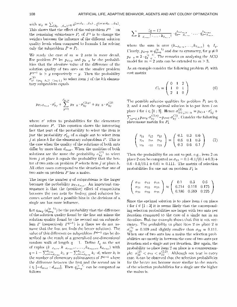
with wx =P
(d2;:::;dm)2D�(m;d2;:::;dm) � �(m;x;d2;:::;dm).
This shows that the e�ect of the subproblem Pq�1 on
the remaining subinstance Pr of P q is to change the
weights between the in uence of the di�erent solution
quality levels when compared to formula 4 for solving
only the subproblem P = Pr.
We study the case of m = 2 ants in more detail.
For problem Pq let pd>y and pd=y be the probabil-
ities that the absolute value of the di�erence of the
solution quality of two ants on the smaller problem
Pq�1 is > y respectively = y. Then the probability
�(2)
(l�1)n0+h;(l�1)n0+jto select item j of the lth elemen-
tary subproblem equals
pd>dmax� �
0
hj+
dmaxXy=1
pd=y � �0(2;y)
hj+ pd=0 � �
0(2)
hj
where �0 refers to probabilities for the elementary
subinstance P . This equation shows the interesting
fact that part of the probability to select the item is
just the probability �0
hjof a single ant to select item
j at place h for the elementary subproblem P . This is
the case when the quality of the solutions of both ants
di�er by more than dmax. When the qualities of both
solutions are the same the probability �0(2)
hjto select
item j at place h equals the probability that the bet-
ter of two ants on problem P selects item j at place h.
All other cases correspond to the situation that one of
two ants on problem P has a malus.
The larger the number q of subproblems is the larger
becomes the probability pd>dmax. An important con-
sequence is that the (positive) e�ect of competition
between the two ants for �nding good solutions be-
comes weaker and a possible bias in the decisions of a
single ant has more in uence.
Let qd=y (q(q�1)
d=y) be the probability that the di�erence
of the solution quality found by the �rst ant minus the
solution quality found by the second ant on subprob-
lem P (respectively Pq�1) is y (here we do not as-
sume that the �rst ant �nds the better solution). The
value of this di�erence on subproblem Pq�1 can be de-
scribed as the result of a generalized one-dimensional
random walk of length q � 1. De�ne Iy as the set
of tuples (k�dmax; k�dmax+1; : : : ; kdmax�1
; kdmax) with
q� 1 =P
dmax
i=�dmax
ki, y =P
dmax
i=�dmax
ki � di where ki is
the number of elementary subinstances of P q�1 where
the di�erence between the �rst and the second ant is
i 2 [�dmax : dmax]. Then q(q�1)
d=ycan be computed as
follows
X (q � 1)!
k�dmax! � : : : � kdmax
!� q
k�dmax
d=�dmax
� : : : � qkdmax
d=dmax
where the sum is over (k�dmax; : : : ; kdmax
) 2 Iy.
Clearly, pd=0 = q(q�1)
d=0and due to symmetry, for y 6= 0
pd=y = 2 � q(q�1)
d=y. The remarks on analysing the ACO
model for m = 2 ants can be extended to m � 3.
As an example consider the following problem P1 with
cost matrix
C1 =
0@
0 1 2
1 0 1
2 1 0
1A (6)
The possible solution qualities for problem P1 are 0,
2, and 4 and the optimal solution is to put item i on
place i for i 2 [1 : 3]. Hence �(2)
3i+j;3i+h= pd>4 � �
0
hj+P
y=2;4pd=y��
0(2;y)
hj+pd=0��
0(2)
hj. Consider the following
pheromone matrix for P1
0@
�11 �12 �13
�21 �22 �23
�31 �32 �33
1A =
0@
0:1 0:3 0:6
0:6 0:1 0:3
0:3 0:6 0:1
1A (7)
Then the probability for an ant to put, e.g., item 2 on
place 2 can be computed as �22 = 0:1 �0:1=(0:1+0:3)+
0:6 � 0:1=(0:1 + 0:6) � 0:111. The matrix of selection
probabilities for one ant on problem P1 is
0@
�11 �12 �13
�21 �22 �23
�31 �32 �33
1A �
0@
0:1 0:3 0:6
0:714 0:111 0:175
0:186 0:589 0:225
1A
Since the optimal solution is to place item i on place
i for i 2 [1 : 3] it is seems likely that the correspond-
ing selection probabilities are larger with two ants per
iteration compared to the case of a single ant in an
iteration. But our example shows that this is not nec-
essary. The probability to place item 2 on place 2 is
�(2)
22= 0:109 and slightly smaller than �22 = 0:111.
When one of two ants has a malus the selection prob-
abilities are mostly in between the case of two ants per
iteration and a single ant per iteration. But again, the
probability to place item 2 on place is a counterexam-
ple: �(2)
22< �22 < �
(2;2)
22. Although not true in every
case, it can be observed that the selection probabilities
for the better ant become more similar to the matrix
of the selection probabilities for a single ant the higher
the malus is.
ARTIFICIAL LIFE, ADAPTIVE BEHAVIOR, AGENTS AND ANT COLONY OPTIMIZATION108
Figure 1: Direction of the vector �eld for changes of
pheromone vectors (�21; �22; �23) for the ACO model
with a single ant and �11 = �12 = �13 = 1=3; possible
pheromone vectors lay in the white area; distance from
right (bottom,left ) line: �21 (�22,�23)
6 FIXED POINTS
Since the pheromone values of an ACO algorithm re-
ect the frequencies of decisions that resulted in good
solutions it is desirable that the selection probabili-
ties used by an ant are equal to their corresponding
pheromone values. As observed in [6] this might often
not be the case since the decisions of an ant are not in-
dependent. We say that there is a selection bias when
the probability of a random ant to choose an item is
di�erent from the corresponding pheromone value. A
pheromone matrix where the probability of a random
ant to choose an item is the same as the corresponding
pheromone value, i.e., �ij = �ij , for all i; j, is called
�xed point matrix. A �xed point matrix can change
in the ACO model only for m � 2 ants. The ques-
tion arises which matrices are �xed point matrices for
a permutation problem.
As an example consider a permutation problem of size
n = 3 where the pheromone matrix (�ij)i;j2[1:3] is de-
�ned by the values �11; �12; �21; �22. Clearly, the se-
lection probabilities for the items in the �rst row are
always equal to their corresponding pheromone values.
It remains to determine the probability of choosing the
�rst and the second item in the second row. The se-
lection probabilities for these items are
�21 :=�12 �21
1� �22+
(1� �11 � �12 ) �21
�21 + �22
�22 :=�11 �22
1� �21+
(1� �11 � �12 ) �22
�21 + �22
The solutions of �21 � �21 = 0 and �22 � �22 = 0 show
1st row
Figure 2: ACOmodel for Pq
1, q = 2; 4; 8; 16; 32; 64; 128,
m = 2; change of pheromone values �11; �12; �13 (�rst
row of corresponding �xed point matrix is identical):
starting point at (�11; �12; �13) = (0:1; 0:3; 0:6)
that the �xed points depend only on the pheromone
values in the �rst row of the pheromone matrix:
1. �21 = 0, �22 = (�11 + �12 � 1)=(�11 � 1)
2. �21 = (�11 + �12 � 1)=(�12 � 1), �22 = 0
3. �21 = (�11)=(�11 + �12), �22 = (�12)=(�11 + �12)
4. �21 = 1� 2 � �11, �22 = 1� 2 � �12
Analysing the eigenvalues of the Jacobian matrix of
[�21 � �21; �22 � �22] the stability of the �xed points
was determined. For every pair of possible values �11and �12 exactly one of the �xed points is stable and
attracting in the range of possible pheromone values.
The cases (1), (2), and (3) are symmetric: for �11 > 0:5
the �xed point (1) is stable, for �12 > 0:5 the �xed
point (2) is stable, and for 1� �11� �12 > 0:5 the �xed
point (3) is stable. In every other case the �xed point
(4) is stable. Thus, there exists always exactly one
stable �xed point matrix. Some of the three unstable
�xed points might lay outside of the allowed parameter
range �21; �22; �23 2 (0; 1), �21 + �22 + �23 = 1.
The directions of the vector �eld for changes of
pheromone vector (�21; �22; �23) when (�11; �12; �13) =
(1=3; 1=3; 1=3) are shown in Figure 1. In this case
the vector �eld is symmetric with respect to rotations
of 60 degree around the �xed point (�21; �22; �23) =
(1=3; 1=3; 1=3). It is interesting to observe that in some
areas of the vector �eld there are points (�21; �22; �23)
with a value �2i > 1=3 for i 2 [1 : 3] that becomes even
larger. This shows that the e�ects of the selection bias
can be complex even for small problems.
ARTIFICIAL LIFE, ADAPTIVE BEHAVIOR, AGENTS AND ANT COLONY OPTIMIZATION 109
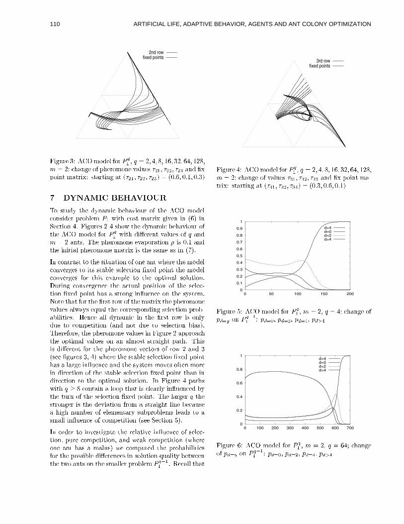
2nd rowfixed points
Figure 3: ACOmodel for Pq
1, q = 2; 4; 8; 16; 32; 64; 128,
m = 2; change of pheromone values �21; �22; �23 and �x
point matrix: starting at (�21; �22; �23) = (0:6; 0:1; 0:3)
7 DYNAMIC BEHAVIOUR
To study the dynamic behaviour of the ACO model
consider problem P1 with cost matrix given in (6) in
Section 4. Figures 2-4 show the dynamic behaviour of
the ACO model for Pq
1with di�erent values of q and
m = 2 ants. The pheromone evaporation � is 0:1 and
the initial pheromone matrix is the same as in (7).
In contrast to the situation of one ant where the model
converges to its stable selection �xed point the model
converges for this example to the optimal solution.
During convergence the actual position of the selec-
tion �xed point has a strong in uence on the system.
Note that for the �rst row of the matrix the pheromone
values always equal the corresponding selection prob-
abilities. Hence all dynamic in the �rst row is only
due to competition (and not due to selection bias).
Therefore, the pheromone values in Figure 2 approach
the optimal values on an almost straight path. This
is di�erent for the pheromone vectors of row 2 and 3
(see �gures 3, 4) where the stable selection �xed point
has a large in uence and the system moves often more
in direction of the stable selection �xed point than in
direction to the optimal solution. In Figure 4 paths
with q � 8 contain a loop that is clearly in uenced by
the turn of the selection �xed point. The larger q the
stronger is the deviation from a straight line because
a high number of elementary subproblems leads to a
small in uence of competition (see Section 5).
In order to investigate the relative in uence of selec-
tion, pure competition, and weak competition (where
one ant has a malus) we computed the probabilities
for the possible di�erences in solution quality between
the two ants on the smaller problem Pq�1
1. Recall that
3rd rowfixed points
Figure 4: ACOmodel for P q
1, q = 2; 4; 8; 16; 32; 64; 128,
m = 2; change of values �31; �32; �33 and �x point ma-
trix: starting at (�31; �32; �33) = (0:3; 0:6; 0:1)
0
0.1
0.2
0.3
0.4
0.5
0.6
0.7
0.8
0.9
1
0 50 100 150 200
d>4d=0d=2d=4
Figure 5: ACO model for Pq
1, m = 2, q = 4; change of
pd=y on Pq�1
1: pd=0, pd=2, pd=4, pd>4
0
0.2
0.4
0.6
0.8
1
0 100 200 300 400 500 600 700
d>4d=0d=2d=4
Figure 6: ACO model for Pq
1, m = 2, q = 64; change
of pd=y on Pq�1
1: pd=0, pd=2, pd=4, pd>4
ARTIFICIAL LIFE, ADAPTIVE BEHAVIOR, AGENTS AND ANT COLONY OPTIMIZATION110
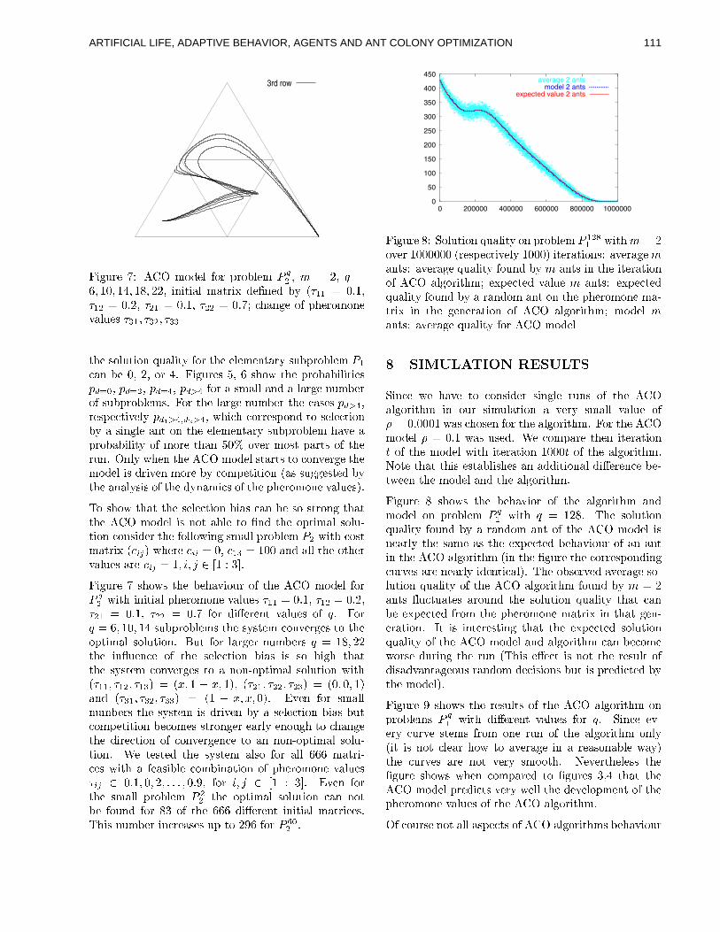
3rd row
Figure 7: ACO model for problem Pq
2, m = 2, q =
6; 10; 14; 18; 22, initial matrix de�ned by (�11 = 0:1,
�12 = 0:2, �21 = 0:1, �22 = 0:7; change of pheromone
values �31; �32; �33
the solution quality for the elementary subproblem P1
can be 0, 2, or 4. Figures 5, 6 show the probabilities
pd=0, pd=2, pd=4, pd>4 for a small and a large number
of subproblems. For the large number the cases pd>4,
respectively pd1>4;d2>4, which correspond to selection
by a single ant on the elementary subproblem have a
probability of more than 50% over most parts of the
run. Only when the ACO model starts to converge the
model is driven more by competition (as suggested by
the analysis of the dynamics of the pheromone values).
To show that the selection bias can be so strong that
the ACO model is not able to �nd the optimal solu-
tion consider the following small problem P2 with cost
matrix (cij) where cii = 0, c13 = 100 and all the other
values are cij = 1; i; j 2 [1 : 3].
Figure 7 shows the behaviour of the ACO model for
Pq
2with initial pheromone values �11 = 0:1, �12 = 0:2,
�21 = 0:1, �22 = 0:7 for di�erent values of q. For
q = 6; 10; 14 subproblems the system converges to the
optimal solution. But for larger numbers q = 18; 22
the in uence of the selection bias is so high that
the system converges to a non-optimal solution with
(�11; �12; �13) = (x; 1 � x; 1), (�21; �22; �23) = (0; 0; 1)
and (�31; �32; �33) = (1 � x; x; 0). Even for small
numbers the system is driven by a selection bias but
competition becomes stronger early enough to change
the direction of convergence to an non-optimal solu-
tion. We tested the system also for all 666 matri-
ces with a feasible combination of pheromone values
�ij 2 0:1; 0; 2; : : : ; 0:9, for i; j 2 [1 : 3]. Even for
the small problem P2
2the optimal solution can not
be found for 83 of the 666 di�erent initial matrices.
This number increases up to 296 for P 60
2.
0
50
100
150
200
250
300
350
400
450
0 200000 400000 600000 800000 1000000
average 2 antsmodel 2 ants
expected value 2 ants
Figure 8: Solution quality on problem P128
1withm = 2
over 1000000 (respectively 1000) iterations: averagem
ants: average quality found by m ants in the iteration
of ACO algorithm; expected value m ants: expected
quality found by a random ant on the pheromone ma-
trix in the generation of ACO algorithm; model m
ants: average quality for ACO model
8 SIMULATION RESULTS
Since we have to consider single runs of the ACO
algorithm in our simulation a very small value of
� = 0:0001 was chosen for the algorithm. For the ACO
model � = 0:1 was used. We compare then iteration
t of the model with iteration 1000t of the algorithm.
Note that this establishes an additional di�erence be-
tween the model and the algorithm.
Figure 8 shows the behavior of the algorithm and
model on problem Pq
1with q = 128. The solution
quality found by a random ant of the ACO model is
nearly the same as the expected behaviour of an ant
in the ACO algorithm (in the �gure the corresponding
curves are nearly identical). The observed average so-
lution quality of the ACO algorithm found by m = 2
ants uctuates around the solution quality that can
be expected from the pheromone matrix in that gen-
eration. It is interesting that the expected solution
quality of the ACO model and algorithm can become
worse during the run (This e�ect is not the result of
disadvantageous random decisions but is predicted by
the model).
Figure 9 shows the results of the ACO algorithm on
problems Pq
1with di�erent values for q. Since ev-
ery curve stems from one run of the algorithm only
(it is not clear how to average in a reasonable way)
the curves are not very smooth. Nevertheless the
�gure shows when compared to �gures 3,4 that the
ACO model predicts very well the development of the
pheromone values of the ACO algorithm.
Of course not all aspects of ACO algorithms behaviour
ARTIFICIAL LIFE, ADAPTIVE BEHAVIOR, AGENTS AND ANT COLONY OPTIMIZATION 111
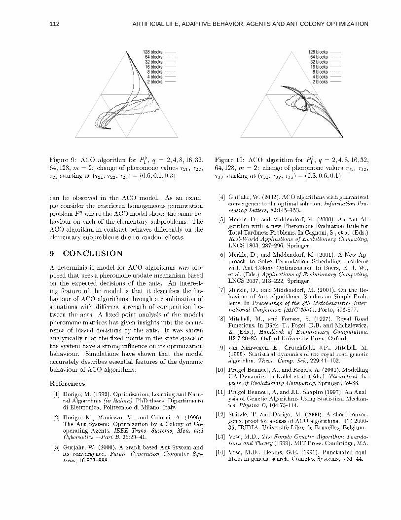
128 blocks64 blocks32 blocks16 blocks8 blocks4 blocks2 blocks
Figure 9: ACO algorithm for Pq
1, q = 2; 4; 8; 16; 32;
64; 128, m = 2: change of pheromone values �21, �22,
�23 starting at (�21, �22, �23) = (0:6; 0:1; 0:3)
can be observed in the ACO model. As an exam-
ple consider the restricted homogeneous permutation
problem Pq where the ACO model shows the same be-
haviour on each of the elementary subproblems. The
ACO algorithm in contrast behaves di�erently on the
elementary subproblems due to random e�ects.
9 CONCLUSION
A deterministic model for ACO algorithms was pro-
posed that uses a pheromone update mechanism based
on the expected decisions of the ants. An interest-
ing feature of the model is that it describes the be-
haviour of ACO algorithms through a combination of
situations with di�erent strength of competition be-
tween the ants. A �xed point analysis of the models
pheromone matrices has given insights into the occur-
rence of biased decisions by the ants. It was shown
analytically that the �xed points in the state space of
the system have a strong in uence on its optimization
behaviour. Simulations have shown that the model
accurately describes essential features of the dynamic
behaviour of ACO algorithms.
References
[1] Dorigo, M. (1992). Optimization, Learning and Natu-ral Algorithms (in Italian). PhD thesis, Dipartimentodi Elettronica, Politecnico di Milano, Italy.
[2] Dorigo, M., Maniezzo, V., and Colorni, A. (1996).The Ant System: Optimization by a Colony of Co-operating Agents. IEEE Trans. Systems, Man, andCybernetics { Part B, 26:29{41.
[3] Gutjahr, W. (2000). A graph-based Ant System andits convergence, Future Generation Computer Sys-tems, 16:873{888.
128 blocks64 blocks32 blocks16 blocks8 blocks4 blocks2 blocks
Figure 10: ACO algorithm for Pq
1, q = 2; 4; 8; 16; 32;
64; 128, m = 2: change of pheromone values �31, �32,
�33 starting at (�31, �32, �33) = (0:3; 0:6; 0:1)
[4] Gutjahr, W. (2002). ACO algorithms with guaranteedconvergence to the optimal solution. Information Pro-cessing Letters, 82:145{153.
[5] Merkle, D., and Middendorf, M. (2000). An Ant Al-gorithm with a new Pheromone Evaluation Rule forTotal Tardiness Problems. In Cagnoni, S., et al. (Eds.)Real-World Applications of Evolutionary Computing,LNCS 1803, 287{296, Springer.
[6] Merkle, D., and Middendorf, M. (2001). A New Ap-proach to Solve Permutation Scheduling Problemswith Ant Colony Optimization. In Boers, E. J. W.,et al. (Eds.) Applications of Evolutionary Computing,LNCS 2037, 213{222, Springer.
[7] Merkle, D., and Middendorf, M. (2001). On the Be-haviour of Ant Algorithms: Studies on Simple Prob-lems. In Proceedings of the 4th Metaheuristics Inter-national Conference (MIC`2001), Porto, 573-577.
[8] Mitchell, M., and Forrest, S. (1997). Royal RoadFunctions. In B�ack, T., Fogel, D.B. and Michalewicz,Z. (Eds.), Handbook of Evolutionary Computation.B2.7:20{25, Oxford University Press, Oxford.
[9] van Nimwegen, E., Crutch�eld, J.P., Mitchell, M.(1999). Statistical dynamics of the royal road geneticalgorithm. Theor. Comp. Sci., 229:41{102.
[10] Pr�ugel-Bennett, A., and Rogers, A. (2001). ModellingGA Dynamics. In Kallel et al. (Eds.), Theoretical As-pects of Evolutionary Computing, Springer, 59-86.
[11] Pr�ugel-Bennett, A, and J.L. Shapiro (1997). An Anal-ysis of Genetic Algorithms Using Statistical Mechan-ics. Physica D, 104:75-114.
[12] St�utzle, T. and Dorigo, M. (2000). A short conver-gence proof for a class of ACO algorithms. TR 2000-35, IRIDIA, Universit�e Libre de Bruxelles, Belgium.
[13] Vose, M.D., The Simple Genetic Algorithm: Founda-tions and Theory (1999). MIT Press, Cambridge, MA.
[14] Vose, M.D., Liepins, G.E. (1991). Punctuated equi-libria in genetic search. Complex Systems, 5:31{44.
ARTIFICIAL LIFE, ADAPTIVE BEHAVIOR, AGENTS AND ANT COLONY OPTIMIZATION112
Continual Coevolution through Complexification
Kenneth O. StanleyDepartment of Computer Sciences
University of Texas at AustinAustin, TX 78712
Risto MiikkulainenDepartment of Computer Sciences
University of Texas at AustinAustin, TX 78712
Abstract
In competitive coevolution, the goal is to es-tablish an “arms race” that will lead to increas-ingly sophisticated strategies. However, in prac-tice, the process often leads to idiosyncrasiesrather than continual improvement. Applyingthe NEAT method for evolving neural networksto a competitive simulated robot duel domain,we will demonstrate that (1) as evolution pro-gresses the networks become more complex, (2)complexification elaborates on existing strate-gies, and (3) if NEAT is allowed to complexify,it finds dramatically more sophisticated strate-gies than when it is limited to fixed-topology net-works. The results suggest that in order to real-ize the full potential of competitive coevolution,genomes must be allowed to complexify as wellas optimize over the course of evolution.
1 INTRODUCTION
In competitive coevolution, two or more populations of in-dividuals evolve simultaneously in an environment wherean increased fitness in one population leads to a decreasedfitness for another. Ideally, competing populations willcontinually outdo one another, leading to an ”arms race” ofincreasing sophistication (Dawkins and Krebs 1979; VanValin 1973). In practice, evolution tends to find the sim-plest solutions that can win, meaning that strategies canswitch back and forth between different idiosyncratic yetuninteresting variations (Darwen 1996; Floreano and Nolfi1997; Rosin and Belew 1997). Several methods have beendeveloped to encourage the arms race (Angeline and Pol-lack 1994; Rosin and Belew 1997). For example, a ”hall offame” can be used to ensure that current strategies remaincompetitive against strategies from the past. Although suchtechniques improve the performance of competitive coevo-
lution, they do not directly encourage continual coevolu-tion, i.e. creating new solutions that maintain existing ca-pabilities. Much time is wasted evaluating solutions thatare deficient in this way.
The problem is that in general genomes have a fixed setof genes mapping to a fixed phenotypic structure. Once agood strategy is found, the entire representational space ofthe genome is used to encode it. Thus, the only way toimprove it is to alter the strategy, thereby sacrificing someof the functionality learned over previous generations.
In this paper, we propose a novel solution to this prob-lem. The idea is to complexify or add structure to the dom-inant strategy, so that it does not merely become different,but rather more elaborate. This idea is implemented in amethod for evolving increasingly complex neural networks,called NeuroEvolution of Augmenting Topologies (NEAT;Stanley and Miikkulainen 2001, 2002b,c). NEAT begins byevolving networks without any hidden nodes. Over manygenerations, new hidden nodes and connections are added,resulting in the complexification of the solution space. Thisway, more complex strategies elaborate on simpler strate-gies, focusing search on solutions that are likely to maintainexisting capabilities.
NEAT was tested in a competitive robot control domainwith and without complexification. The main results werethat (1) evolution did complexify when possible, (2) com-plexification led to elaboration, and (3) significantly moresophisticated and successful strategies were evolved withcomplexification than without. These results imply thatcomplexification allows coevolution to continually elabo-rate on successful strategies, resulting in an arms race thatachieves a significantly higher level of sophistication thanis otherwise possible.
We begin by describing the NEAT neuroevolution method,followed by a description of the robot duel domain and adiscussion of the results.
113ARTIFICIAL LIFE, ADAPTIVE BEHAVIOR, AGENTS AND ANT COLONY OPTIMIZATION
2 NEUROEVOLUTION OFAUGMENTING TOPOLOGIES (NEAT)
The NEAT method of evolving artificial neural networkscombines the usual search for appropriate network weightswith complexification of the network structure. This ap-proach is highly effective: NEAT outperforms other neu-roevolution (NE) methods, e.g. on the benchmark doublepole balancing task by a factor of five (Stanley and Miik-kulainen 2001, 2002b,c). The NEAT method consists of so-lutions to three fundamental challenges in evolving neuralnetwork topology: (1) What kind of genetic representationwould allow disparate topologies to crossover in a mean-ingful way? (2) How can topological innovation that needsa few generations to optimize be protected so that it doesnot disappear from the population prematurely? (3) Howcan topologies be minimized throughout evolution so themost efficient solutions will be discovered? In this section,we explain how NEAT addresses each challenge.1
2.1 GENETIC ENCODING
Evolving structure requires a flexible genetic encoding. Inorder to allow structures to complexify, their representa-tions must be dynamic and expandable. Each genome inNEAT includes a list of connection genes, each of whichrefers to two node genes being connected. Each connec-tion gene specifies the in-node, the out-node, the weight ofthe connection, whether or not the connection gene is ex-pressed (an enable bit), and an innovation number, whichallows finding corresponding genes during crossover.
Mutation in NEAT can change both connection weights andnetwork structures. Connection weights mutate as in anyNE system, with each connection either perturbed or not.Structural mutations, which form the basis of complexifi-cation, occur in two ways (figure 1). In the add connectionmutation, a single new connection gene is added connect-ing two previously unconnected nodes. In the add nodemutation an existing connection is split and the new nodeplaced where the old connection used to be. The old con-nection is disabled and two new connections are added tothe genome. This method of adding nodes was chosen inorder to integrate new nodes immediately into the network.Through mutation, genomes of varying sizes are created,sometimes with completely different connections specifiedat the same positions.
In order to perform crossover, the system must be able totell which genes match up between any individuals in thepopulation. The key observation is that two genes that havethe same historical origin represent the same structure (al-
1A more comprehensive description of the NEAT method isgiven in Stanley and Miikkulainen (2001, 2002c).
1 2 3
4
5
1 2 3
4
5
1 2 3
4
5
1 2 3
4 6
5
1−>4
1−>4
1−>4
1−>4
2−>4
2−>4
2−>4
2−>4
2−>5
2−>5
2−>5
2−>5
3−>5
3−>5
3−>5
3−>5
4−>5
4−>5
4−>5
4−>5
3−>4
3−>6 6−>5
DIS
DIS
DIS
DIS DIS
1
1
1
1
3
3
3
3
4
4
4
4
5
5
5
5
6
6
6
6
7
8 9
Mutate Add Connection
Mutate Add Node
Figure 1: The two types of structural mutation in NEAT.Both types, adding a connection and adding a node, are illus-trated with the genes above their phenotypes. The top number ineach genome is the innovation number of that gene. The bottomtwo numbers denote the two nodes connected by that gene. Theweight of the connection, also encoded in the gene, is not shown.The symbol DIS means that the gene is disabled, and therefore notexpressed in the network. The figure shows how connection genesare appended to the genome when a new connection is added tothe network and when a new node is added. Assuming the de-picted mutations occurred one after the other, the genes would beassigned increasing innovation numbers as the figure illustrates,thereby allowing NEAT to keep an implicit history of the originof every gene in the population.
though possibly with different weights), since they wereboth derived from the same ancestral gene from some pointin the past. Thus, all a system needs to do to know whichgenes line up with which is to keep track of the historicalorigin of every gene in the system.
Tracking the historical origins requires very little compu-tation. Whenever a new gene appears (through structuralmutation), a global innovation number is incremented andassigned to that gene. The innovation numbers thus rep-resent a chronology of every gene in the system. As anexample, let us say the two mutations in figure 1 occurredone after another in the system. The new connection genecreated in the first mutation is assigned the number
�, and
the two new connection genes added during the new nodemutation are assigned the numbers � and � . In the future,whenever these genomes crossover, the offspring will in-herit the same innovation numbers on each gene; innova-tion numbers are never changed. Thus, the historical originof every gene in the system is known throughout evolution.
Through innovation numbers, the system now knows ex-actly which genes match up with which. Genes that do notmatch are either disjoint or excess, depending on whetherthey occur within or outside the range of the other parent’sinnovation numbers. When crossing over, the genes in both
114 ARTIFICIAL LIFE, ADAPTIVE BEHAVIOR, AGENTS AND ANT COLONY OPTIMIZATION
genomes with the same innovation numbers are lined up.Genes that do not match are inherited from the more fit par-ent, or if they are equally fit, from both parents randomly.
Historical markings allow NEAT to perform crossoverwithout the need for expensive topological analysis.Genomes of different organizations and sizes stay compat-ible throughout evolution, and the problem of competingconventions (Radcliffe 1993) is essentially avoided. Suchcompatibility is essential in order to complexify structure.
2.2 PROTECTING INNOVATION THROUGHSPECIATION
Adding new structure to a network usually initially reducesfitness. However, NEAT speciates the population, so thatindividuals compete primarily within their own niches in-stead of with the population at large. This way, topologicalinnovations are protected and have time to optimize theirstructure before they have to compete with other niches inthe population.
Historical markings make it possible for the system to di-vide the population into species based on topological simi-larity. We can measure the distance � between two networkencodings as a simple linear combination of the number ofexcess ( � ) and disjoint ( � ) genes, as well as the averageweight differences of matching genes ( � ):
���� ��
�� �� ���� ��� (1)
The coefficients , � , and � adjust the importance of thethree factors, and the factor
�, the number of genes in the
larger genome, normalizes for genome size. Genomes aretested one at a time; if a genome’s distance to a randomlychosen member of the species is less than ��� , a compatibil-ity threshold, it is placed into this species. Each genome isplaced into the first species where this condition is satisfied,so that no genome is in more than one species.
As the reproduction mechanism for NEAT, we use explicitfitness sharing (Goldberg and Richardson 1987), where or-ganisms in the same species must share the fitness of theirniche, preventing any one species from taking over the pop-ulation.
2.3 MINIMIZING DIMENSIONALITY THROUGHCOMPLEXIFICATION
Unlike other systems that evolve network topologies andweights (Angeline et al. 1993; Gruau et al. 1996; Yao 1999;Zhang and Muhlenbein 1993), NEAT begins with a uni-form population of simple networks with no hidden nodes.Speciation protects new innovations, allowing topologicaldiversity to be gradually introduced over evolution.
Figure 2: The Robot Duel Domain. The robots begin on op-posite sides of the board facing away from each other as shownby the lines pointing away from their centers. The concentriccircles around each robot represent the separate rings of oppo-nent sensors and food sensors available to each robot. Eachring contains five sensors, which appear larger or smaller de-pending on their activations. From this initial position, nei-ther robot has a positional advantage. The robots lose energywhen they move around, yet they can gain energy by consum-ing food (shown as black dots). The food is placed in a hor-izontally symmetrical pattern around the middle of the board.The objective is to attain a higher level of energy than the op-ponent, and then collide with it. Because of the complex inter-action between foraging, pursuit, and evasion behaviors, the do-main allows for a broad range of strategies of varying sophistica-tion. Animated demos of the robot duel domain are available atwww.cs.utexas.edu/users/nn/pages/research/neatdemo.html.
New structure is introduced incrementally as structural mu-tations occur, and only those structures survive that arefound to be useful through fitness evaluations. This way,NEAT searches through a minimal number of weight di-mensions, significantly reducing the number of generationsnecessary to find a solution, and ensuring that networks be-come no more complex than necessary. In other words,NEAT searches for the optimal topology by complexifyingwhen necessary.
3 THE ROBOT DUEL DOMAIN
To demonstrate the effect of complexification on competi-tive coevolution, a domain is needed where it is possible todevelop increasingly sophisticated strategies and where thesophistication can be readily measured. A balance betweenthe potential complexity of evolved strategies and their an-alyzability is difficult to strike. Pursuit and evasion taskshave been utilized for this purpose in the past (Gomez andMiikkulainen 1997; Jim and Giles 2000; Miller and Cliff1994; Reggia et al. 2001), and can serve as a benchmarkdomain for competitive coevolution as well. While past ex-periments evolved either a predator or a prey, an interestingcoevolution task can be established if the agents are insteadequal and engaged in a duel. To win, an agent must de-
115ARTIFICIAL LIFE, ADAPTIVE BEHAVIOR, AGENTS AND ANT COLONY OPTIMIZATION
velop a strategy that outwits that of its opponent, utilizingstructure in the environment.
In the robot duel domain, two simulated robots try to over-power each other (figure 2). The two robots begin on op-posite sides of a rectangular room facing away from eachother. As the robots move, they lose energy in proportionto the amount of force they apply to their wheels. Althoughthe robots never run out of energy (they are given enoughto survive the entire competition), the robot with higherenergy can win by colliding with its competitor. In addi-tion, each robot has a sensor indicating the difference inenergy between itself and the other robot. To keep their en-ergies high, the robots can consume food items, arrangedin a symmetrical pattern in the room.
The robot duel task supports a broad range of sophisticatedstrategies that are easy to observe and interpret without ex-pert knowledge. The competitors must become proficientat foraging, prey capture, and escaping predators. In addi-tion, they must be able to quickly switch from one behaviorto another. The task is well-suited to competitive coevolu-tion because naive strategies such as forage-then-attack canbe complexified into more sophisticated strategies such asluring the opponent to waste its energy before attacking.
The simulated robots are similar to Kheperas (Mondadaet al. 1993). Each has two wheels controlled by separatemotors. Five rangefinder sensors can sense food and an-other five can sense the other robot. Finally, each robot hasan energy-difference sensor, and a single wall sensor.
The robots are controlled with neural networks evolvedwith NEAT. The networks receive all of the robot sensorsas inputs, as well as a constant bias that NEAT can use tochange the activation thresholds of neurons. They producethree motor outputs: Two to encode rotation either right orleft, and a third to indicate forward motion power.
This complex robot-control domain allows competitive co-evolution to evolve increasingly sophisticated and complexstrategies, and can be used to benchmark coevolution meth-ods.
4 EXPERIMENTS
In order to demonstrate how complexification contributesto continual coevolution, we ran four evolution trials withfull NEAT and three trials with complexification turned off.The methodology is described below.
4.1 COMPETITIVE COEVOLUTION SETUP
In each evolution trial, 2 populations, each containing 256genomes, were evolved simultaneously. In each generation,each population is evaluated against an intelligently chosen
sample of networks from the other population. The popu-lation currently being evaluated is called the host popula-tion, and the population from which opponents are chosenis called the parasite population (Rosin and Belew 1997).The parasites are chosen for their quality and diversity,making host/parasite evolution more efficient and more re-liable than random or round robin tournament.
A single fitness evaluation included two competitions, onefor the east and one for the west starting position. That way,networks needed to implement general strategies for win-ning, independent of their starting positions. Host networksreceived a single fitness point for each win, and no pointsfor losing. If a competition lasted 750 time steps with nowinner, the host received 0 points.
In selecting the parasites for fitness evaluation, good usecan be made of the speciation and fitness sharing that al-ready occur in NEAT. Each host was evaluated against thechampions of four species with the highest fitness. Theyare good opponents because they are the best of the bestspecies, and they are guaranteed to be diverse because theircompatibility must be outside the threshold ��� (section 2.2).Another eight opponents were chosen randomly from aHall of Fame (Rosin and Belew 1997) that contained pop-ulation champions from all generations. Together, specia-tion, fitness sharing, and Hall of Fame comprise a state ofthe art competitive coevolution methodology. However, asour experimental results will show, complexification is themost important ingredient in establishing continual coevo-lution.
4.2 MONITORING PROGRESS INCOMPETITIVE COEVOLUTION
In order to track progress in coevolution, we need to beable to tell whether one strategy is better than another. Be-cause the board configurations can vary during the game,networks were compared on 144 different food configura-tions from each side of the board, giving 288 total compar-isons. The food configurations included the same 9 sym-metrical food positions used during training, plus an addi-tional 2 food items, which were placed in one of 12 dif-ferent positions on the east and west halves of the board.Some starting food positions give an initial advantage toone robot or another, depending on how close they are tothe robots’ starting positions. We say that network � is su-perior to network � if � wins more comparisons than � outof the 288 total comparisons.
Given this definition of superiority, progress can be tracked.The obvious way to do it is to compare each network to oth-ers throughout evolution, finding out whether later strate-gies can beat more opponents than earlier strategies. Forexample, Floreano and Nolfi (1997) used a measure called
116 ARTIFICIAL LIFE, ADAPTIVE BEHAVIOR, AGENTS AND ANT COLONY OPTIMIZATION
20
40
60
80
100
120
140
0 50 100 150 200 250 300 350 400 450 500
Ave
rage
Con
nect
ions
in H
ighe
st D
omin
ant
Generation
Complexification of Connections
0
2
4
6
8
10
12
0 50 100 150 200 250 300 350 400 450 500
Ave
rage
Nod
es in
Hig
hest
Dom
inan
t
Generation
Complexification of Nodes
Figure 3: Complexification of connections and nodes over generations. The graphs depict the average number of connections andthe average number of hidden nodes in the highest dominant network in each generation. Averages are taken over four complexifyingruns. A hash mark appears every generation in which a new dominant strategy emerged in at least one of the four runs. The graphs showthat as dominance increases, so does complexity level on average. The differences in complexity between the average final dominantand first dominant strategies are statistically significant for both connections and nodes (������� �� ).master tournament, in which the champion of each genera-tion is compared to all other generation champions. Unfor-tunately, such methods are impractical in a time-intensivedomain such as the robot duel competition. Moreover, themaster tournament only shows how often each championwins against other champions. In order to track strategicinnovation, we need to identify dominant strategies, i.e.those that defeat all previous dominant strategies. Thisway, we can make sure that evolution proceeds by devel-oping a progression of strictly more powerful strategies,instead of e.g. switching between alternative ones.
To meet this goal, we developed the dominance tourna-ment method of tracking progress in competitive coevo-lution (Stanley and Miikkulainen 2002a). Let a genera-tion champion be the winner of a 288 game comparisonbetween the two population champions of a single genera-tion. Let !#" be the $ th dominant strategy to appear in theevolution. Then dominance is defined recursively:
% The first dominant strategy ! is the generation cham-pion of the first generation;
% dominant strategy !�" , where $'&)( , is a generationchampion such that for all *�+,$ , !�" is superior to(wins the 288 game comparison with) !.- .
This strict definition of dominance prohibits circularities.For example, !0/ must be superior to strategies ! through! � , ! � superior to both ! and ! � , and ! � superior to ! .The entire process of deriving a dominance hierarchy froma population is a dominance tournament, where competi-tors play all previous dominant strategies until they eitherlose a 288 game comparison, or win every comparisonto previous dominant strategies, thereby becoming a new
dominant strategy. Dominance tournaments require signif-icantly fewer comparisons than the master tournament.
The question tested in the experiments is: Does the com-plexification of networks help attain high levels of domi-nance?
5 RESULTS
Each of the seven evolution trials lasted 500 generations,and took between 5 and 10 days on a 1GHz PIII proces-sor, depending on the progress of evolution and sizes ofthe networks involved. The NEAT algorithm itself usedless than 1% of this computation: the rest of the time wasspent in evaluating networks in the robot duel task. Evolu-tion of fully-connected topologies took about 90% longerthan structure-growing NEAT because larger networks takelonger to evaluate.
We define complexity as the number of nodes and connec-tions in a network: The more nodes and connections thereare in the network, the more complex behavior it can poten-tially implement. The results were analyzed to answer threequestions: (1) As evolution progresses does it also contin-ually complexify? (2) How is complexification utilized tocreate more sophisticated strategies? (3) Does complexi-fication allow better strategies to be discovered than doesevolving fixed-topology networks?
5.1 EVOLUTION OF COMPLEXITY
NEAT was run four times, each time from a different seed,to verify consistency of results. The highest levels of dom-inance achieved were 17, 14, 17, and 16, averaging at 16.
117ARTIFICIAL LIFE, ADAPTIVE BEHAVIOR, AGENTS AND ANT COLONY OPTIMIZATION
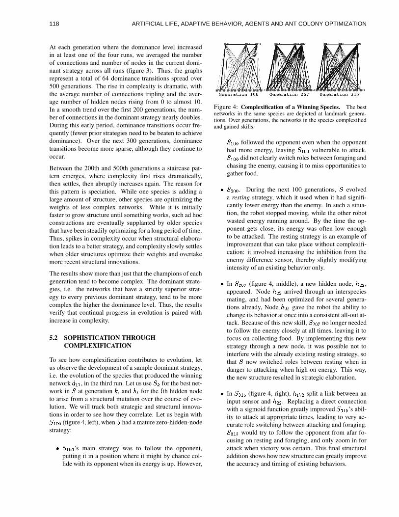
At each generation where the dominance level increasedin at least one of the four runs, we averaged the numberof connections and number of nodes in the current domi-nant strategy across all runs (figure 3). Thus, the graphsrepresent a total of 64 dominance transitions spread over500 generations. The rise in complexity is dramatic, withthe average number of connections tripling and the aver-age number of hidden nodes rising from 0 to almost 10.In a smooth trend over the first 200 generations, the num-ber of connections in the dominant strategy nearly doubles.During this early period, dominance transitions occur fre-quently (fewer prior strategies need to be beaten to achievedominance). Over the next 300 generations, dominancetransitions become more sparse, although they continue tooccur.
Between the 200th and 500th generations a staircase pat-tern emerges, where complexity first rises dramatically,then settles, then abruptly increases again. The reason forthis pattern is speciation. While one species is adding alarge amount of structure, other species are optimizing theweights of less complex networks. While it is initiallyfaster to grow structure until something works, such ad hocconstructions are eventually supplanted by older speciesthat have been steadily optimizing for a long period of time.Thus, spikes in complexity occur when structural elabora-tion leads to a better strategy, and complexity slowly settleswhen older structures optimize their weights and overtakemore recent structural innovations.
The results show more than just that the champions of eachgeneration tend to become complex. The dominant strate-gies, i.e. the networks that have a strictly superior strat-egy to every previous dominant strategy, tend to be morecomplex the higher the dominance level. Thus, the resultsverify that continual progress in evolution is paired withincrease in complexity.
5.2 SOPHISTICATION THROUGHCOMPLEXIFICATION
To see how complexification contributes to evolution, letus observe the development of a sample dominant strategy,i.e. the evolution of the species that produced the winningnetwork ! 21 , in the third run. Let us use 354 for the best net-work in 3 at generation 6 , and 798 for the : th hidden nodeto arise from a structural mutation over the course of evo-lution. We will track both strategic and structural innova-tions in order to see how they correlate. Let us begin with3 <;=; (figure 4, left), when 3 had a mature zero-hidden-nodestrategy:
% 3 <;>; ’s main strategy was to follow the opponent,putting it in a position where it might by chance col-lide with its opponent when its energy is up. However,
Figure 4: Complexification of a Winning Species. The bestnetworks in the same species are depicted at landmark genera-tions. Over generations, the networks in the species complexifiedand gained skills.
?5@<A>Afollowed the opponent even when the opponent
had more energy, leaving?B@CA>A
vulnerable to attack.?5@<A>Adid not clearly switch roles between foraging and
chasing the enemy, causing it to miss opportunities togather food.
D ?FE=A>A. During the next 100 generations,
?evolved
a resting strategy, which it used when it had signifi-cantly lower energy than the enemy. In such a situa-tion, the robot stopped moving, while the other robotwasted energy running around. By the time the op-ponent gets close, its energy was often low enoughto be attacked. The resting strategy is an example ofimprovement that can take place without complexifi-cation: it involved increasing the inhibition from theenemy difference sensor, thereby slightly modifyingintensity of an existing behavior only.
D In?FE>G=H
(figure 4, middle), a new hidden node, I E=E ,appeared. Node I E=E arrived through an interspeciesmating, and had been optimized for several genera-tions already, Node I E>E gave the robot the ability tochange its behavior at once into a consistent all-out at-tack. Because of this new skill,
?JE>G=Hno longer needed
to follow the enemy closely at all times, leaving it tofocus on collecting food. By implementing this newstrategy through a new node, it was possible not tointerfere with the already existing resting strategy, sothat
?now switched roles between resting when in
danger to attacking when high on energy. This way,the new structure resulted in strategic elaboration.
D In?FK @2L
(figure 4, right), I @2H=E split a link between aninput sensor and I E>E . Replacing a direct connectionwith a sigmoid function greatly improved
? K @2L’s abil-
ity to attack at appropriate times, leading to very ac-curate role switching between attacking and foraging.? K @2L
would try to follow the opponent from afar fo-cusing on resting and foraging, and only zoom in forattack when victory was certain. This final structuraladdition shows how new structure can greatly improvethe accuracy and timing of existing behaviors.
118 ARTIFICIAL LIFE, ADAPTIVE BEHAVIOR, AGENTS AND ANT COLONY OPTIMIZATION
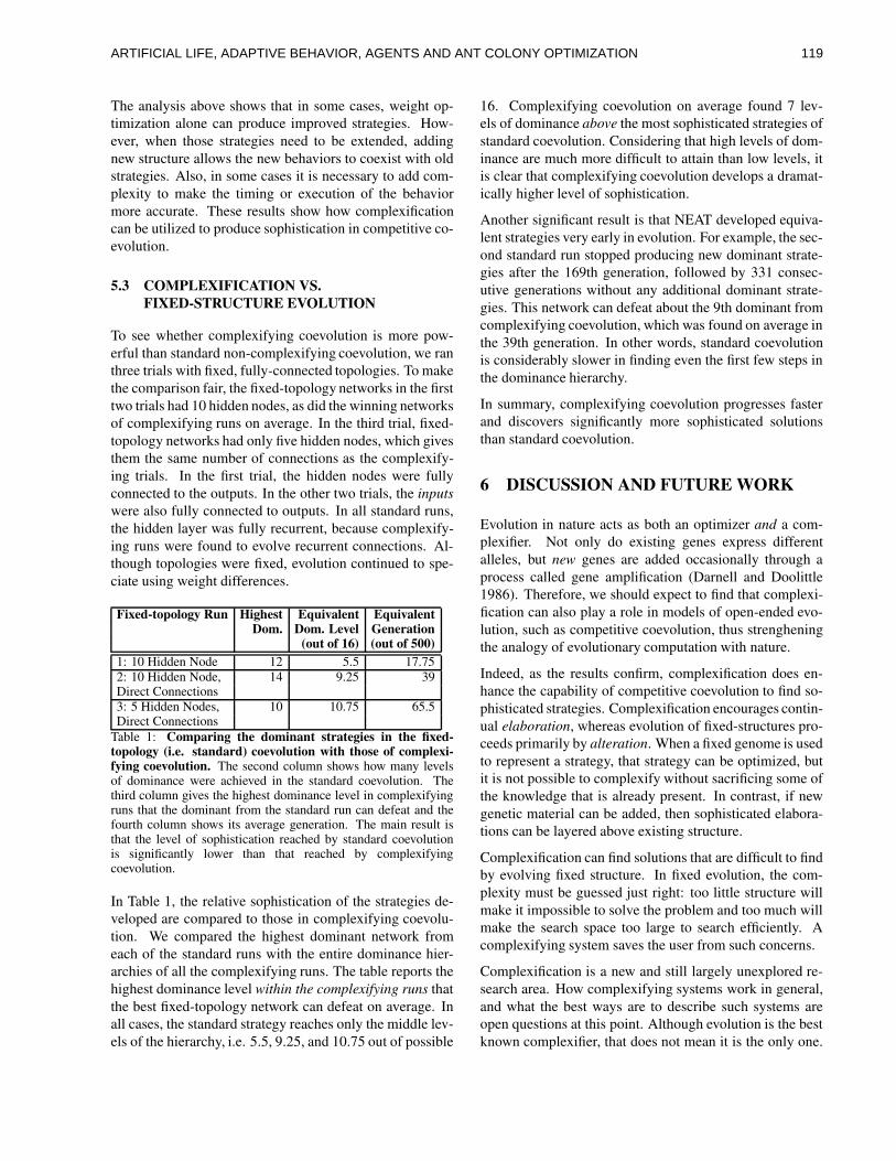
The analysis above shows that in some cases, weight op-timization alone can produce improved strategies. How-ever, when those strategies need to be extended, addingnew structure allows the new behaviors to coexist with oldstrategies. Also, in some cases it is necessary to add com-plexity to make the timing or execution of the behaviormore accurate. These results show how complexificationcan be utilized to produce sophistication in competitive co-evolution.
5.3 COMPLEXIFICATION VS.FIXED-STRUCTURE EVOLUTION
To see whether complexifying coevolution is more pow-erful than standard non-complexifying coevolution, we ranthree trials with fixed, fully-connected topologies. To makethe comparison fair, the fixed-topology networks in the firsttwo trials had 10 hidden nodes, as did the winning networksof complexifying runs on average. In the third trial, fixed-topology networks had only five hidden nodes, which givesthem the same number of connections as the complexify-ing trials. In the first trial, the hidden nodes were fullyconnected to the outputs. In the other two trials, the inputswere also fully connected to outputs. In all standard runs,the hidden layer was fully recurrent, because complexify-ing runs were found to evolve recurrent connections. Al-though topologies were fixed, evolution continued to spe-ciate using weight differences.
Fixed-topology Run Highest Equivalent EquivalentDom. Dom. Level Generation
(out of 16) (out of 500)1: 10 Hidden Node 12 5.5 17.752: 10 Hidden Node, 14 9.25 39Direct Connections3: 5 Hidden Nodes, 10 10.75 65.5Direct Connections
Table 1: Comparing the dominant strategies in the fixed-topology (i.e. standard) coevolution with those of complexi-fying coevolution. The second column shows how many levelsof dominance were achieved in the standard coevolution. Thethird column gives the highest dominance level in complexifyingruns that the dominant from the standard run can defeat and thefourth column shows its average generation. The main result isthat the level of sophistication reached by standard coevolutionis significantly lower than that reached by complexifyingcoevolution.
In Table 1, the relative sophistication of the strategies de-veloped are compared to those in complexifying coevolu-tion. We compared the highest dominant network fromeach of the standard runs with the entire dominance hier-archies of all the complexifying runs. The table reports thehighest dominance level within the complexifying runs thatthe best fixed-topology network can defeat on average. Inall cases, the standard strategy reaches only the middle lev-els of the hierarchy, i.e. 5.5, 9.25, and 10.75 out of possible
16. Complexifying coevolution on average found 7 lev-els of dominance above the most sophisticated strategies ofstandard coevolution. Considering that high levels of dom-inance are much more difficult to attain than low levels, itis clear that complexifying coevolution develops a dramat-ically higher level of sophistication.
Another significant result is that NEAT developed equiva-lent strategies very early in evolution. For example, the sec-ond standard run stopped producing new dominant strate-gies after the 169th generation, followed by 331 consec-utive generations without any additional dominant strate-gies. This network can defeat about the 9th dominant fromcomplexifying coevolution, which was found on average inthe 39th generation. In other words, standard coevolutionis considerably slower in finding even the first few steps inthe dominance hierarchy.
In summary, complexifying coevolution progresses fasterand discovers significantly more sophisticated solutionsthan standard coevolution.
6 DISCUSSION AND FUTURE WORK
Evolution in nature acts as both an optimizer and a com-plexifier. Not only do existing genes express differentalleles, but new genes are added occasionally through aprocess called gene amplification (Darnell and Doolittle1986). Therefore, we should expect to find that complexi-fication can also play a role in models of open-ended evo-lution, such as competitive coevolution, thus strengheningthe analogy of evolutionary computation with nature.
Indeed, as the results confirm, complexification does en-hance the capability of competitive coevolution to find so-phisticated strategies. Complexification encourages contin-ual elaboration, whereas evolution of fixed-structures pro-ceeds primarily by alteration. When a fixed genome is usedto represent a strategy, that strategy can be optimized, butit is not possible to complexify without sacrificing some ofthe knowledge that is already present. In contrast, if newgenetic material can be added, then sophisticated elabora-tions can be layered above existing structure.
Complexification can find solutions that are difficult to findby evolving fixed structure. In fixed evolution, the com-plexity must be guessed just right: too little structure willmake it impossible to solve the problem and too much willmake the search space too large to search efficiently. Acomplexifying system saves the user from such concerns.
Complexification is a new and still largely unexplored re-search area. How complexifying systems work in general,and what the best ways are to describe such systems areopen questions at this point. Although evolution is the bestknown complexifier, that does not mean it is the only one.
119ARTIFICIAL LIFE, ADAPTIVE BEHAVIOR, AGENTS AND ANT COLONY OPTIMIZATION
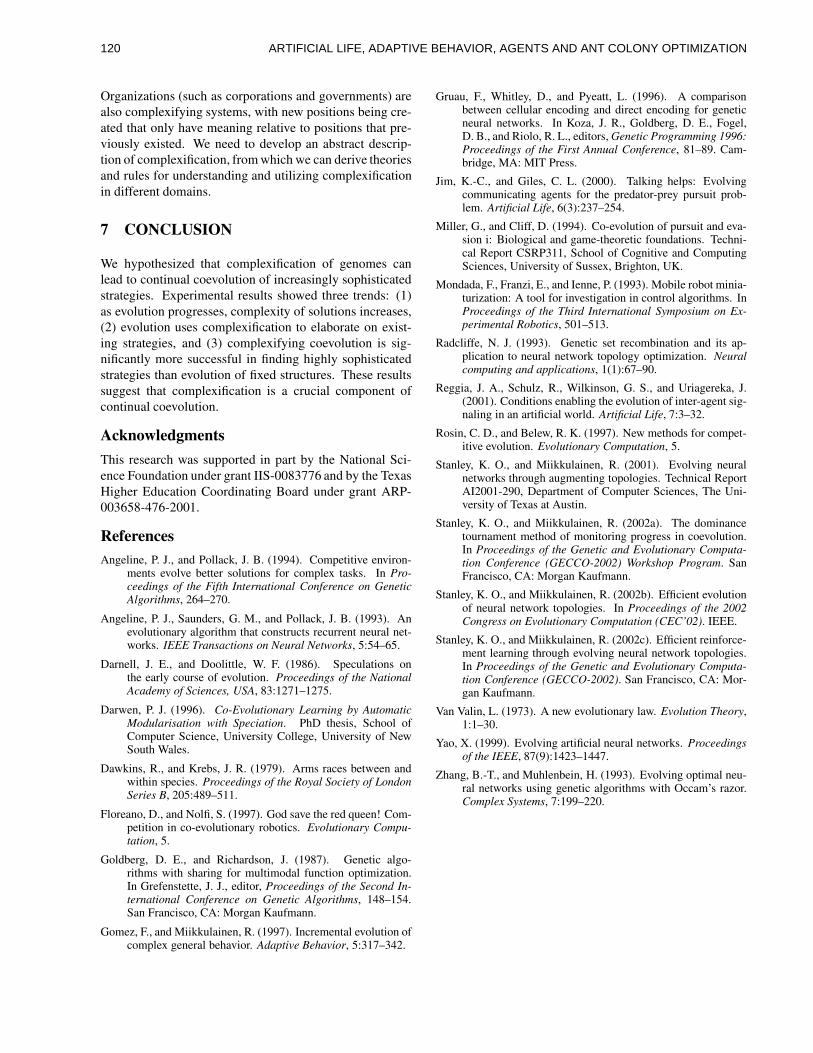
Organizations (such as corporations and governments) arealso complexifying systems, with new positions being cre-ated that only have meaning relative to positions that pre-viously existed. We need to develop an abstract descrip-tion of complexification, from which we can derive theoriesand rules for understanding and utilizing complexificationin different domains.
7 CONCLUSION
We hypothesized that complexification of genomes canlead to continual coevolution of increasingly sophisticatedstrategies. Experimental results showed three trends: (1)as evolution progresses, complexity of solutions increases,(2) evolution uses complexification to elaborate on exist-ing strategies, and (3) complexifying coevolution is sig-nificantly more successful in finding highly sophisticatedstrategies than evolution of fixed structures. These resultssuggest that complexification is a crucial component ofcontinual coevolution.
Acknowledgments
This research was supported in part by the National Sci-ence Foundation under grant IIS-0083776 and by the TexasHigher Education Coordinating Board under grant ARP-003658-476-2001.
ReferencesAngeline, P. J., and Pollack, J. B. (1994). Competitive environ-
ments evolve better solutions for complex tasks. In Pro-ceedings of the Fifth International Conference on GeneticAlgorithms, 264–270.
Angeline, P. J., Saunders, G. M., and Pollack, J. B. (1993). Anevolutionary algorithm that constructs recurrent neural net-works. IEEE Transactions on Neural Networks, 5:54–65.
Darnell, J. E., and Doolittle, W. F. (1986). Speculations onthe early course of evolution. Proceedings of the NationalAcademy of Sciences, USA, 83:1271–1275.
Darwen, P. J. (1996). Co-Evolutionary Learning by AutomaticModularisation with Speciation. PhD thesis, School ofComputer Science, University College, University of NewSouth Wales.
Dawkins, R., and Krebs, J. R. (1979). Arms races between andwithin species. Proceedings of the Royal Society of LondonSeries B, 205:489–511.
Floreano, D., and Nolfi, S. (1997). God save the red queen! Com-petition in co-evolutionary robotics. Evolutionary Compu-tation, 5.
Goldberg, D. E., and Richardson, J. (1987). Genetic algo-rithms with sharing for multimodal function optimization.In Grefenstette, J. J., editor, Proceedings of the Second In-ternational Conference on Genetic Algorithms, 148–154.San Francisco, CA: Morgan Kaufmann.
Gomez, F., and Miikkulainen, R. (1997). Incremental evolution ofcomplex general behavior. Adaptive Behavior, 5:317–342.
Gruau, F., Whitley, D., and Pyeatt, L. (1996). A comparisonbetween cellular encoding and direct encoding for geneticneural networks. In Koza, J. R., Goldberg, D. E., Fogel,D. B., and Riolo, R. L., editors, Genetic Programming 1996:Proceedings of the First Annual Conference, 81–89. Cam-bridge, MA: MIT Press.
Jim, K.-C., and Giles, C. L. (2000). Talking helps: Evolvingcommunicating agents for the predator-prey pursuit prob-lem. Artificial Life, 6(3):237–254.
Miller, G., and Cliff, D. (1994). Co-evolution of pursuit and eva-sion i: Biological and game-theoretic foundations. Techni-cal Report CSRP311, School of Cognitive and ComputingSciences, University of Sussex, Brighton, UK.
Mondada, F., Franzi, E., and Ienne, P. (1993). Mobile robot minia-turization: A tool for investigation in control algorithms. InProceedings of the Third International Symposium on Ex-perimental Robotics, 501–513.
Radcliffe, N. J. (1993). Genetic set recombination and its ap-plication to neural network topology optimization. Neuralcomputing and applications, 1(1):67–90.
Reggia, J. A., Schulz, R., Wilkinson, G. S., and Uriagereka, J.(2001). Conditions enabling the evolution of inter-agent sig-naling in an artificial world. Artificial Life, 7:3–32.
Rosin, C. D., and Belew, R. K. (1997). New methods for compet-itive evolution. Evolutionary Computation, 5.
Stanley, K. O., and Miikkulainen, R. (2001). Evolving neuralnetworks through augmenting topologies. Technical ReportAI2001-290, Department of Computer Sciences, The Uni-versity of Texas at Austin.
Stanley, K. O., and Miikkulainen, R. (2002a). The dominancetournament method of monitoring progress in coevolution.In Proceedings of the Genetic and Evolutionary Computa-tion Conference (GECCO-2002) Workshop Program. SanFrancisco, CA: Morgan Kaufmann.
Stanley, K. O., and Miikkulainen, R. (2002b). Efficient evolutionof neural network topologies. In Proceedings of the 2002Congress on Evolutionary Computation (CEC’02). IEEE.
Stanley, K. O., and Miikkulainen, R. (2002c). Efficient reinforce-ment learning through evolving neural network topologies.In Proceedings of the Genetic and Evolutionary Computa-tion Conference (GECCO-2002). San Francisco, CA: Mor-gan Kaufmann.
Van Valin, L. (1973). A new evolutionary law. Evolution Theory,1:1–30.
Yao, X. (1999). Evolving artificial neural networks. Proceedingsof the IEEE, 87(9):1423–1447.
Zhang, B.-T., and Muhlenbein, H. (1993). Evolving optimal neu-ral networks using genetic algorithms with Occam’s razor.Complex Systems, 7:199–220.
120 ARTIFICIAL LIFE, ADAPTIVE BEHAVIOR, AGENTS AND ANT COLONY OPTIMIZATION
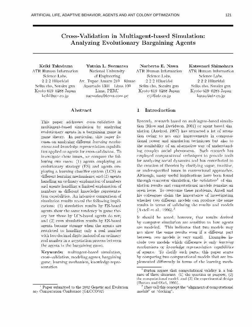
����������� ����������������������� ��������������� ����!"�����#� $%��&'�"�����(�����*)+,������- ./�����1032��������(����������-546�����������"�����7+,���#�8���
9":<;>=?;A@CBD=<BFEBDGHBIKJ/LNMPODQSRUTWVXTDY[Z]\^QSRU_^`aZ]T
bDc `ad�T c dfe(RUgDhjikUlmkUlmk M#`anoRU\^`qpFR]`
b d�`qnoR l csr Zut b ZU\^RUnvO lmw ODTx�y ZU_zZ8{u|s}U~]� kU�U�S� RU�FR]T
n�d�`anv`X��RU_^\ji c Zui �^�
�f����BF=<B����C���:vGHBF������ R]_^`aZUTDRU�(�PTD`a�Ud�\^h^`a_ yZ]Y��KT w `aTDd�d�\^`aT w
IP��iJOF�DR c IPQSRU\^O k |s� l L#`qQSR cIP�DRU\^_^R]pFZ�|s�U�u| l e�`qQSR�|s�]�
e(`aQSRut��K�KLC�h�ODd�QSRU_^h^O��_^d�\^\^Rui c ZUQ�i �ud
�����j��:<�j�������C�"B� �BIKJ/LNMPODQSRUTWVXTDY[Z]\^QSRU_^`aZ]T
bDc `ad�T c dfe(RUgDhjikUlmkUlmk M#`anoRU\^`qpFR]`
b d�`qnoR l csr Zut b ZU\^RUnvO lmw ODTx�y ZU_zZ8{u|s}U~]� kU�U�S� RU�FR]T
d�` �^`¡�ARU_^\ji c Zui �z�
9�BD�����¢��u�j;A�£;>G¤��£BF�jBIKJ/LNMPODQSRUTWVXTDY[Z]\^QSRU_^`aZ]T
bDc `ad�T c dfe(RUgDhjikUlmkUlmk M#`anoRU\^`qpFR]`
b d�`qnoR l csr Zut b ZU\^RUnvO lmw ODTx�y ZU_zZ8{u|s}U~]� kU�U�S� RU�FR]TnoRU_zh�O���RU_^\ji c Zui �^�
¥§¦#¨<©<ªD«¬?©
J r `qh®�DRU�ud�\®RUpDpD\^d�h^h^d�h°¯²±´³�µ¶µ¶·¡¸²¹�º¼»¾½�¹�¿m»[³�ÀÁ`qTQ�OD�a_^`qR w d�T<_ l gDRUh�d�pÂh^`aQ�OF�qRU_^`qZUT°g y RUTDRU� yvà `qT wd���Z]�aOD_^`aZUTDRU\ y R w d�Tv_^hf`qTÄRÅgDRU\ w RU`qTF`aT wÆw R]QSd%`qTw RUQSdÄ_ r d�Z]\ y iÇVXTÈ�FRU\^_z` c OF�qRU\jt#_ r `ah"�FRU��d�\�Y¾Z lc OFh^d�h�ZUT�RUTFR]� y<à `aT w pF`qÉud�\^d�T<_Sº¼Ê¶¹�±sÀF»¾ÀoˤÌ�ʶ¯²Í�¹�·ÀF»[µ�Ì%µ�R]TFp�βÀF³�ÏCºÐʶ½ÑË�Ê�±´ÊzÒÓ±´Ê²µ¶Ê²ÀF¿m¹�¿m»¾³�À c RU�DRUgD`a�a` l_^`ad�hÔRU�D�D�a`ad�pS_^Z�R w d�T<_^hÔY¾ZU\ c \^ZUh^h l �oRU�q`apDRU_^`qZUTi�JZ`aT<�Ud�h�_z` w RU_zd�_ r d�h^d%`qh�h^ODd�hotÓÕ�d c ZUQS�DRU\^d%_ r d�Y[Z]� l�aZjÕ/`aT w _XÕ�Z c RUh^d�hoÖØ×^|UÙ�R w d�Tv_^h"d�QS�D�aZ y `aT w RUTd���Z]�aOD_^`aZUTDRU\ y h^_^\^R]_^d w y ×[� b Ù%RUTDp3R w d�T<_^hWd�Q l�F�qZ y `aT w R8�qd�R]\^TF`qT w c �aR]h�h^`aÚDd�\�h y h�_zd�QÛ×¾eCÜ b Ù�RUhpF`qÉud�\^d�T<_(�ad�RU\^TD`aT w QSd csr RUTD`ah^QShoݲRUTDpÅ× k Ù�R w d�T<_^hr R]TFpD�a`qT w RUT%ZU\^pF`qTFR]\ y d�Þv�F�qRUTDRU_^`aZ]T Z]YFT<ODQ�gud�\^hRUTDpÆR w d�T<_^h r RUTDpD�a`aT w R��q`aQS`a_zd�pÆd�Þv�F�qRUTFR]_^`aZUT"Z]YT<ODQ�gud�\^hWRUh"pD`aÉud�\^d�T<_Ån<TDZjÕ/�ad�p w dÄ\^d��D\^d�h^d�T<_^R l_^`aZ]T c RU�FR]gF`q�a`a_^`qd�hji�IPTÅ`aT<_^d�TDh^`a�Ud c ZUQS�DRU\^`ah^ZUTWZ]Yh^`aQ�OD�aRU_z`aZUTW\^d�h�OD�a_zhP\^d���d�RU�?_ r d�Y¾ZU�a�aZjÕ/`aT w `aQS�D�a` lc RU_^`aZUTDhjÖ�×z|UÙ#h^`aQ�OD�aR]_^`aZUTß\^d�h^OF�q_^h%g y � b l gFRUh^d�pR w d�T<_^hCh r ZjÕà_ r d�h^RUQSdP_^d�TFpDd�T c y `qT w R]QSdf_ r d lZU\ y gDOF_�_ r ZUh^dWg y eAÜ b l gFRUh^d�pßR w d�T<_zh%pDZ�TDZU_jÝRUTDpß× k Ù�d���d�Táh^`aQ�OF�qRU_^`qZUTÄ\^d�h�OD�a_^h#g y � b l gFRUh^d�pR w d�T<_^h�gud c ZUQSdWh^_^\^RUT w dÅÕ r d�Tâ_ r dÅR w d�Tv_^h8RU\^d\^d�h�_^\^` c _zd�pã_^Z r R]TFpD�a`qT w Z]TF� y R3\^d�RU� T<ODQ�gud�\Õ/`a_ r _´Õ�Z/pDd c `qQSRU��pD` w `a_zh�`qTFh^_^d�RUp�ZUY<RUTfZU\^pD`aTDRU\ y\^d�RU��T<ODQ�g�d�\`aT%R�TDd w ZU_^`qRU_^`qZUT%�F\^Z c d�h�hKgud�_´Õ�d�d�T_ r d�R w d�T<_^hC`aTÆ_ r d�gFR]\ w RU`aTD`aT w%w RUQSdvi9�:<ä? ��u�jE��²å Q�OD�a_^`qR w d�T<_ l gDRUh�d�pæh^`aQ�OF�qRU_^`aZ]Ttc \^ZUh�h l �oRU�q`apDRU_^`aZ]TtjQSZvpDd��q`aT w R w d�T<_^hjt²gDRU\ w RU`qTF`aT ww RUQSdvt��qd�RU\^TD`aT w QSd csr RUTD`ah^Q�tvn<TDZoÕ/�qd�p w dP\^d��D\^d lh^d�T<_zRU_^`aZUT
ç#è�ézê<ë¶ì�í´î�ï�ðfñÐòXòXë¶ó�ò¡ô�ò¡õvëföz÷²÷�ö�øë¶ù�ë¶òXñ¼ú#ézùvó�û�ü²ô²ý¼î�òXñÐô²ùvþézìXÿ��uô²ðfê�îvòÑé^ò¡ñ¼ô²ù��uô²ù��aë¶ìXë¶ù�ú¶ë��¡øû������ ÷�ö �
� ��� ©vª������#¬?©���� �
L�d c d�T<_^� y tD\^d�h^d�RU\ csr gDRUh^d�páZUTáQ�OD�a_z`aR w d�T<_ l gDRUh^d�p�h^`aQ�OF�qR l_^`qZUTà×���ZUh^h/R]TFp���Ro�v`apDh^h�ZUT�t k �U��|oÙCZU\�R w d�Tv_ l gFRUh^d�p¤h^`aQ lOD�aRU_^`qZUTN×[I#Þ<d��a\^Zvpt�|s}U}��jÙ r R]h%RU_^_^\^R c _^d�pâR��qZU_�ZUYPRU_z_^d�T l_^`qZUTãZjÕ/`aT w _zZ TDZU_*Z]TF� y `aQS�D\^Zj��d�QSd�T<_^hH`aT c ZUQS�DOD_^R l_^`qZUTFR]���uZjÕAd�\�R]TFp h^`aQ�OD�aRU_z`aZUTÈ_^d csr TD`! <ODd�h�gFOD_�RU�qh�Z _^Z_ r dWRo�oR]`a�aRUgD`a�q`¼_ y ZUYPR]TØRU�a_^d�\^TDRU_^`a�UdÆÕAR y ZUYPOFTDpDd�\^h^_^R]TFp l`aT w c ZUQS�F�qd�Þ h^Z c `qRU�%� r d�TFZ]QSd�TDRui b O csr \^d�h�d�RU\ csr r RUhd�QS�F�qZ y d�p c ZUQS�DOD_^RU_^`qZUTFR]�P_zd c¶r TD`! vOFd�hÅ_^Zâ�D\^Zo�v`apDd�_^ZvZU�ahY¾ZU\�RUTDRU� yvà `qT w h^Z c `aR]��p y TDRUQS` c h�RUTDp r R]h c ZUT<_z\^`agDOF_^d�p�_^Z_ r d c \^d�RU_z`aZUTÄZ]YK_ r d�Z]\^`ad�h�g y c �aR]\^`aY y `aT w �oR w OFdvt�`qT<_^OF`q_^`a�UdvtZU\8OFTDpDd�\ l h^�ud c `qÚFd�pâ`ah^h^OFd�h8`aT c ZUT<�Ud�T<_^`qZUTFR]��R]�F�D\^ZUR csr d�hoiIP�q_ r ZUO w r t�QSR]T y ODh�d�Y¾OF�K`qQS�F�a` c RU_^`aZUTDh r Rj�Ud%gud�d�THY¾ZUODTFp_ r \^ZUO w r�c ZUQS�FOD_^d�\�h^`aQ�OD�aR]_^`aZUT�tF_ r d�¸²¹�ºÐ»[½�¹�¿m»¾³�À�"WZUYKh^`aQ lOD�aRU_^`qZUTá\^d�h^OF�q_^hfRUTFp c ZUQS�FOD_^RU_z`aZUTDRU�QSZvpDd��ah�\^d�QSRU`aTDhPRUTZU�ud�Tâ`qh�h^ODdviÆJZ"Zo�Ud�\ c ZUQSd8_ r d�h^dÆ�D\^ZUgD�ad�QShot�IPÞv_^d��a��RUTDpr `ah c Z]�a�ad�R w ODd�h c �aRU`qQ°_ r dÄ`qQS�uZU\^_^RUT c d¤ZUYf`aT<�Ud�h^_^` w R]_^`aT wÕ r d�_ r d�\Å_XÕAZÄpF`qÉud�\^d�T<_ÅQSZvpFd��ah c RUT �D\^ZvpFO c dá_ r d�h^RUQSd\^d�h�OD�a_zh%`aT*_^d�\^QSh�ZUY/�oRU�q`apDRU_^`aT w _ r dÅ\^d�h^OF�q_^h%RUTDp*QSZvpDd��ah×[I#Þ<_^d��a��d�_CR]�Xiat?|s}U}U{DÙ^i #VX_ h r ZUOF�qp gud3TDZU_^d�p�t r ZjÕAd��Ud�\jt"_ r RU_ \^d�h^OF�q_^h pFd�\^`a�Ud�pg y c ZUQS�DOD_^d�\Wh^`aQ�OD�aR]_^`aZUT§RU\^d�h^d�TDh^`a_^`a�Udá_^Z r ZjÕ R w d�T<_^hRU\^dHQSZvpDd��qd�p�i®J r `qh�`aTDpD` c RU_^d�h�_ r RU_�_XÕAZßQSZ<pDd��ahÄQSR yTDZU_�h r ZjÕ _ r dßh�RUQSdØ\^d�h^OF�q_^hHd��Ud�T�`qYWRÈpF`qÉÓd�\^d�T<_��DRU\^_gud�_XÕAd�d�T _XÕAZNQSZ<pDd��ahß`qhß�Ud�\ y h^Q8R]�a�Xi �KÞvRUQS�D�ad�hß`qT lc �aODpFdß_´Õ�ZÈQSZ<pDd��ah¤Õ r ` csr pF`qÉud�\^d�T c dØ`ah*ZUTD� y ºÐʶ¹�±sÀF»[ÀoËÌ�ʶ¯²Í�¹�ÀF»[µ�Ì%µÅZ]\ βÀF³�ÏCºÐʶ½ÑË�Êß±zÊ´ÒÓ±zÊ�µ¶Ê²ÀF¿m¹�¿m»[³�À�¯¶¹ÑÒ�¹%$�»[ºÐ»[¿m»[Ê�µZUY%R w d�T<_^hji JZ c �aR]\^`aY y h^O csr �FRU\^_zhotf_ r `qhá�FR]�ud�\Äh^_^RU\^_^hg y c ZUQS�FR]\^`aT w _´Õ�Z c ZUQS�DOF_^R]_^`aZUTDRU�(QSZvpFd��ah�_ r RU_/RU\^d�`aQ l�D�ad�QSd�T<_zd�pØpD`aÉud�\^d�T<_^� y `aTØ_^d�\^QSh�ZUYP_ r dÅ�qd�R]\^TF`qT w QSd c¶r l&(' î�ìXòXô²ùÈézì*)²î�ë¶í ò¡õ?ézò�ú¶ô²ðfê�î�ò�ézòXñ¼ô²ùÓézýCüvézý¼ñÐóvñÐò ÿHñ¼í�éSï?ézýÐþ
ézù�ú¶ëSô �Ôò¡õvìXë¶ëSë¶ýÐë¶ðfë¶ù]òXí,+-�*. �KòXõ�ë0/]î�ë¶íXòXñ¼ô²ùáô²ì�êvî�ìXê<ôjíXë213�Xö �òXõ�ë�ú¶ô²ðfê�î�ò�ézòXñ¼ô²ùÓézý�ðfôoóvë¶ý41Dézù�ó5�*6 ��òXõ�ë�ë87oê�ë¶ìXñ¼ð�ë¶ù]ò�ézý<ó�ë¶í´ñ9)²ù� ' î�ìXòXô²ù�ézù�ó5ï�ë¶ý41�. : : ;2�*<=?> õ�ë¶ÿAú]ézýÐýoòXõ�ñ¼íuú¶ô²ù�ú¶ë¶ê�òuò¡õvëA@zé^ýÐñB)²ù�ðfë¶ù]òFô �Uú¶ô²ð�êvî�ò�ézòXñÐô²ùÓé^ýðfôoó�ë¶ý¼í*C�ô²ìD@¾óvôoúFEoñ¼ù%) CG<
121ARTIFICIAL LIFE, ADAPTIVE BEHAVIOR, AGENTS AND ANT COLONY OPTIMIZATION
RUTD`ah^QSh�R]TFpàn<TDZoÕ/�qd�p w d¤\^d��D\^d�h^d�T<_^RU_z`aZUT c RU�FR]gF`q�a`a_^`qd�h"ZUYR w d�T<_^hji H M#d�\^dvtÆÕAd c R]�a��_ r `qhØ_ y �udÈZUYá`aT<�Ud�h^_^` w R]_^`aZUT¯²±´³�µ¶µ�·X¸²¹�ºÐ»[½�¹�¿m»¾³�ÀDt I®Õ r ` csr QSd�RUTDhØ_zZÇ�oR]�a`apDRU_^d _ r d§\^d lh^OF�q_^h�RUTFpHQSZvpFd��ah�R w RU`qTFh^_�pD`aÉud�\^d�T<_�`qQS�F�ad�QSd�T<_^RU_z`aZUT*ZUYR w d�T<_^hji � ZU_^d�_ r RU_/_ r `ahPpD`aÉud�\^h�Y[\^Z]Q _ r d�ODh^OFR]�(QSd�R]TF`qT wZUY c \^ZUh^h l �oRU�a`qpFR]_^`aZUTH_ r RU_ csr d c n<h�_ r dÅ\^d�h^OF�q_^h�Z]Y�R�h^`aT w �ad�ad�RU\^TD`aT w RU� w ZU\^`a_ r Q ZU\%RÄh�`qT w �qdÅn<TDZjÕ/�ad�p w dW\^d��F\^d�h^d�Tv_^R l_^`qZUTNZUT�Rß\^d�h^d�\^�Ud�pNh�d�_áZ]YSpDRU_^R�i I#h�R c Z]T c \^d�_^d¤pDZ lQSRU`aT�tÕAdÅd�QS�F�qZ y R�gDRU\ w RU`qTF`aT wáw RUQSd�×���OF_ r ZvZut k �U�U�DÙY¾ZU\�_ r `ah c ZUQS�DRU\^`ah^ZUT�t�gud c RUODh�dW_ r `ah w RUQSdÅ`ahSZUTDd8ZUY�_ r dY¾OFTDpDRUQSd�T<_zRU�Ód�ÞvRUQS�F�qd�hARUTDpÆgud c RUODh�d#\^R]_^`aZUTDRU�Ógud r Rj�<`qZU\^hZUYKR w d�Tv_^h r Rj��d�RU�a\^d�RUp y gud�d�T�RUTDRU� yvà d�p�`aT w RUQSd�_ r d�Z]\ y×FJ�h�g�ZU\^TDdfRUTFp"L�ODgF`aTDh^_^d�`aT�t�|¶}U}�KDÙ^iJ r `ah �DRU�ud�\S`ah ZU\ w RUTD` à d�p RUh8Y[ZU�q�aZjÕ/hoi b d c _^`aZ]T k h^_^RU\^_^hg y d�Þ<�D�aR]`aTF`qT w _ r d�gFRU\ w RU`aTD`aT w%w RUQSdvi�I c ZUT c \^d�_zd�`qQS�F�ad lQSd�T<_^RU_^`qZUT�ZUY<R w d�T<_^h`ah�pFd�h c \^`agud�p�`aT b d c _z`aZUT���i b d c _^`aZ]T�K�D\^d�h^d�T<_^h c ZUQS�DOD_^d�\�h^`aQ�OF�qRU_^`aZ]TFh�R]TFp b d c _^`aZ]T-L�pD`ah c ODh^h�d�h_ r d c \^ZUh^h l �jRU�a`qpFRU_z`aZUT�ZUYF\^d�h�OD�a_zhKRUTDp%QSZvpFd��ahjiNM`aTDRU�a� y t²ZUOD\c ZUT c �qOFh^`aZUTDh/RU\^d�QSRUpDd�`qT b d c _^`aZUTÆ{ui
O P «�ª�QÔ«R� � � � QSQÔ«RTSU
I°gDRU\ w RU`qTF`aT w3w RUQSd ×���OF_ r ZvZut k �U�U�DÙWÕAR]h*h^_^ODpF`qd�p `aT_ r d c Z]T<_^d�Þ<_�Z]Y w RUQSdf_ r d�ZU\ y ×FJ�h�g�ZU\^TDdfRUTFp"L�ODgF`aTDh^_^d�`aT�t|s}U}2KuÙ^i�J r `ah�h^_^ODp y RUpDpF\^d�h^h�d�p�_ r d�h^`a_^ODRU_^`qZUTÄÕ r d�\^d%_XÕAZZU\8QSZU\^d��D�aR y d�\^h�×¾ZU\8R w d�T<_^hjÙf_^\ y _zZ�\^d�R csr RHQ�OF_zOFR]�a� ygud�TDd�Ú c `aRU�R w \^d�d�QSd�Tv_P_ r \�Z]O w r TDd w ZU_^`qRU_^`qZUTFhjtFRUTDpá`qT<��d�h l_^` w RU_^d�p Õ r d�TWRUTDp8Õ r RU_Ôn<`qTFpDhCZUY?ZUÉud�\^hCZUY?RUT `qTFpD`a�v`apDOFR]��D�aR y d�\ c RUT�gud�R c�c d��D_^d�p�g y Z]_ r d�\��F�qR y d�\^hjiJZÅOFTDpDd�\^h^_^R]TFpÄ_ r d�gDRU\ w RU`qTF`aT wÆw R]QSd<t?�ad�_?V h w `a�Ud�RUT�d�Þ lRUQS�D�advi VXT L�ODgF`aTDh^_^d�`aTWV hWÕ�ZU\^nN×¾L#ODgD`aTDh�_zd�`qTt?|s} �Uk Ùzt r d`a�q�aODh�_z\^RU_^d�páRÅ_ y �F` c R]��h^`a_zOFR]_^`aZUT�OFh^`aT w _ r d�Y[ZU�q�aZjÕ/`aT w h c d lTDRU\^`aZuÖ?_´Õ�Z��F�qR y d�\^hjt(X " R]TFpYX # t r Rj�Ud�_^Z�\^d�R csr RUT%R w \^d�d lQSd�T<_?ZUT�_ r d��FRU\^_z`a_^`qZUTfZ]Y�R5Z �D`ad,[ui\MuZU\?_ r `ah?�FOD\^�uZUh^dvt�_ r d yRU�q_^d�\^TDRU_zd/ZUÉud�\^hKpFd�h c \^`qgF`qT w �uZUh^h^`agD�ad�pD`a�v`ah^`aZUTDhZUYu_ r d/�D`advth^O csr RUh]Z^X " \^d c d�`a�Ud�h`_HRUTDpaX # \^d c d�`a�Ud�h8|`bc_HRU_P_z`aQSdd [ut(Õ r d�\^de_ `qh�R]T y �oRU�qOFd `aT¤_ r dÅ`qT<_^d�\^�oRU��f ��gU|ih¡iDj r d�TR"�D�aR y d�\P\^d c d�`q��d�h�RUT�ZUÉud�\jt?_ r d8�D�aR y d�\�pDd c `qpFd�h�Õ r d�_ r d�\_^Z�R c�c d��D_/`q_CZU\/TFZU_²iVXY�_ r d��F�qR y d�\AR c�c d��D_^hC_ r d�ZUÉud�\jt�_ r dTDd w ZU_^`aR]_^`aZUT"�D\^Z c d�h^hCd�TDpDhot�RUTDpÆd�R csr �F�qR y d�\�\^d c d�`a�Ud�hC_ r dh r R]\^dCZUYu_ r d/�D`ad�pDd�_zd�\^QS`qTFd�p%g y _ r d c ZUT c �aODpDd�p c ZUT<_^\^R c _jiJ�_ r d�\^Õ/`ah^dvt<_ r df\^d c d�`a�<`qT w �F�qR y d�\AQSRUnUd�h/R c ZUODT<_^d�\ l Z]ÉÓd�\jtRUTDp R]�a��ZUYu_ r d#RUguZj�UdCh^_^d��Fh�RU\^d/\^d��ud�RU_^d�p OFTv_^`a�FR�h^ZU�aOD_^`qZUT`ahK\^d�R csr d�pSZ]\K_ r d#�F\^Z c d�h�hK`ahKRUguZU\^_^d�pSpDODdP_zZ�h^ZUQSd�d�Þ<_^d�\ lTDRU�K\^d�RUh^ZUTà×^Ê k ËGk t?_ r dST<OFQ�gud�\�ZUYATDd w ZU_^`aR]_^`aZUT��D\^Z c d�h^h^d�h`ah�ÚDTF`q_^d Z]\�ZUTDd ZUYA_ r dÅ�D�aR y d�\^hf�qd�Rj�Ud�h�_ r dÅ�F\^Z c d�h^hjÙ^iÅVXT_ r d c RUh^d�_ r RU_/_ r d�TDd w ZU_^`qRU_^`aZUT"�D\^Z c d�h^h#`qh�RUguZU\^_^d�p�t<guZU_ rlnm ô²íXí�ú¶ý ézíXí´ñ9ovë¶íKòXõ�ë/üvézýÐñ¼óÓézòXñ¼ô²ù�ñ¼íXíXî�ë¶íPézí��p.?�uêvìXë¶ó�ñÐú¶òXñ¼ô²ù�í,1
�Xö �(é�)²ë¶ù]òCézù�ó�ðfë¶úzõ?ézù�ñÐí´ð ó�ë¶í´ñ9)²ù�íq1<ézù�ó�ìXë¶íXîvýÐòXñ¼ù%)Cô²îvòXê�î�òXí/ézíó�ë¶í´ú�ì´ñÐê�òXñ¼ô²ù�ír� m ô²í´í,1Föz÷²÷G.2�*<ts<ìXô²ð òXõ�ñ¼íÔü]ñÐë8uÔê�ô²ñÐù]ò,1�ô²îvìv�aôoú¶î�íñ¼íKìXë¶ýmézòXë¶ó%òXôfò¡õvëCíXë¶ú¶ô²ùvó%ê<ô²ñ¼ù]ò�ñÐùSõ�ñÐíKú¶ýmézí´íXñBo�ú]ézòXñÐô²ùt<w ��ézìXý¼ë¶ÿ�ézýÐí´ôÔú¶ýmézñ¼ðfí�òXõ�ëí�ézðfëê�ô²ñÐù]òÓî�í´ñÐù%)�òXõ�ëòXë¶ìXðyx{z}|?~�~��� |{�?�i���i�?���!�?�?���!|?�0�*�ÔézìXý¼ë¶ÿWézù�ó�ø/ézíXí´ë¶ì,1n. : : :��*<
�D�aR y d�\^h c RUTWTFZ8�qZUT w d�\A\^d c d�`a�UdfR]T y h r RU\^d�ZUY�_ r d��D`adviMPd�\^dvt�ÕAd c ZUTDh�`qpFd�\%_ r dÅÚFTD`a_^d l r ZU\^` à ZUTØh^`a_zOFR]_^`aZUT�t�Õ r d�\^d_ r d QSR]Þ<`aQ�OFQ�T<ODQ�gud�\àZ]Yáh^_^d��Dh ×������ �����(�ÓÙ¤`qT _ r dw RUQSd�`ahCÚDÞ<d�pWR]TFpÆR]�a�Ó�F�qR y d�\^hAn<TDZjÕ _ r `ahA`aTDY[Z]\^Q8R]_^`aZUTWRUhc ZUQSQSZUTHnvTFZjÕ/�ad�p w dÄ× b _��R r �Xt(|¶}�� k Ù^i�VXTH_ r d c RUh�d Õ r d�\^d���(� �(������� |Ä×[RU�qh�Z�nvTFZjÕ/TØRUh _ r d��<º¼¿m»[Ì�¹�¿4��Ì Ë<¹�Ì%Ê�ÙztR w d�T<_�X " c RUTÅQSR]n�d�_ r d#ZUTD� y ZUÉud�\�RUTDpÆ_ r d�TcX # c RUTÅR c lc d��D_fZU\f\^d�Y[ODh^d `q_ji�VXYrX # \^d�Y¾ODh�d�h�_ r d�ZUÉud�\jt?guZU_ r R w d�T<_^h\^d c d�`a�Ud�TDZU_ r `aT w i b `qT c dÄRH\^RU_^`qZUTFR]�fR w d�Tv_Æ`qhWgDRUh^d�p ZUT_ r d�TDZU_^`qZUTWZUY�Z RUT y _ r `aT w `qh#g�d�_z_^d�\#_ r RUT"TDZU_ r `aT w [utvR8\^R l_^`qZUTFR]�`X " _^d�TFpDh�_zZ"nUd�d���QSZ]h�_fZUYK_ r dS�F`qdS_^Z r d�\^h^d��aY�g yZUÉud�\^`aT w Z]TF� y R8QS`aTD`aQ�ODQ h r RU\^d�_^Z�X # i b `aT c d�_ r d�\^d�RU\^dTDZ"Y¾OF\^_ r d�\Ph�_zd��Dh�_^ZÅgud8�D�aR y d�pá`aT¤_ r d w RUQSdvt?RÆ\^R]_^`aZUTDRU�X # `qTFd��v`a_^RUgD� y R c�c d��F_^h _ r d"_z`aT y ZUÉud�\ji�� y RU�D�F� y `qT w RgDR c n<Õ�RU\^p�`qTFpDO c _^`qZUTá\^d�RUh�Z]TF`qT w _^ZÅ_ r d�h^`a_^ODRU_^`qZUTÄRUguZj�Udvt`a_�`qh#��ZUh^h�`qgF�qd�_^ZÅ�ud�\^Y[ZU\^Q h^`aQ�OD�aR]_^`aZUT�Y[Z]\������ �(�����5� |UiMuZU\_ r d#h^RUQSd�\^d�RUh^ZUT%ZUY�_ r dCOF�q_^`aQSRU_zOFQ w RUQSd<tU_ r d/R w d�T<_Õ r Z c RUT§QSRUnUdÄ_ r d��qRUh^_WZ]ÉÓd�\W`qhWgud�_^_zd�\W�uZ]h�`q_^`aZUTDd�p _^Z\^d c d�`a�UdÅ_ r dW�aRU\ w d�\%h r RU\^dÆg y ZUÉud�\^`aT w R�QS`aTD`aQ�OFQæZUÉud�\× b _��R r �Xt�|s}�� k Ù^iKVXTá_ r `qh c RUh^d<t�_ r d��qRUh�_/ZUÉud�\C`qh w \^R]T<_^d�pW_^Z_ r d�R w d�T<__ r RU_pDZvd�hTDZU_QSRUnUd�_ r d/ÚD\^h^_�ZUÉud�\�`qY������ �(�����`ahKd��Ud�T�tog�d c RUODh^d#d�R csr R w d�T<_`qh�RU�q�aZjÕAd�p8_^Z�QSRUnUdCRU_KQSZUh^_���(� �(������� k ZUÉud�\^hji�JAT _ r d#ZU_ r d�\ r R]TFp�tU_ r d��aRUh^_KZUÉud�\�`qhw \^RUT<_zd�pÆ_^Z�_ r dfh^RUQSdfR w d�T<_A_ r RU_/QSRUnUd�hA_ r dfÚD\^h^_�ZUÉud�\C`aY���(� �(����� `qh#ZvpDpiIPY¾_^d�\â_ r `qh*h^d�h^h^`aZUT�tSÕAd ODh^dà_ r dß_^d�\^QSh�Z �FR y ZUÉR[NRUTDpZ R w d�T<_�[%`aTDh�_zd�R]pWZUY�_ r d�_^d�\^QSh�Z h r RU\^dq[%RUTDp Z �F�qR y d�\F[�Y¾ZU\_ r d�`a\/Õ/`qpFdfQSd�RUTD`aT w h#`qTW_ r d�gFR]\ w RU`aTD`aT w w RUQSd<i
¡ ¢ ����U¤£�� � Q «RQ�U � ©v¨
JZ�`aQS�D�ad�QSd�T<_ÔR w d�T<_zhA`qT _ r d#Y[\^RUQSd�ÕAZ]\^nSZ]Y�_ r d#gDRU\ w RU`qT l`aT wSw RUQSd<t<_ r `qh�h^d c _^`qZUTÆh^_^RU\^_^h�g y QSZvpDd��q`aT w R8gDRUh^` c �DRU\^_ZUY�R w d�T<_zh#RUTFpÅ_ r d�T"QSZ<pDd��a`aT w _ r d��FRU\^_zh/ZUYZUOD\�Y¾Z c ODhji
¥ ��¦ § �?E:�¨>;>¢ª©���«PB���BF��;�¬�BF�j�MuZU\ÔRfgDRUh^` c �DRU\^_�ZUYuQSZ<pDd��a`aT w R w d�T<_^hjtoÕAd/`aQS�D�ad�QSd�T<_Ô_ r dY¾ZU�a�aZjÕ/`aT w c Z]Q8��ZUTDd�T<_zh�ZUY�R w d�Tv_^h#RUhPh r ZjÕ/T�`qTYM` w OD\^dW|Ui� ZU_zdf_ r RU_/d�R csr R w d�Tv_ r RUh/_ r d�h�RUQSdfRU\ csr `a_zd c _^OD\^dvi
® §�:<G¤���oä �¯ ����oBD��:�©u;[:<�ÈG¤:<G¤���oä h^_^ZU\^d�h�Ràh�d�_"ZUY h^_^\^R]_^d w `ad�h×[_ r d�T<OFQ�gud�\(ZUY<h�_z\^RU_^d w `ad�h�`qhN°8`qT�_ r `qh�Ú w OF\^dvÙ^t�Õ r ` csrc ZUTFh^`ah^_KZUY�ÚDÞ<d�p T<ODQ�gud�\^hCZUY?�FRU`q\^hKZUY�ZUÉud�\^h�×FJ�Ù?RUTDp_ r \^d�h r ZU�apDh¤×[J�Ù^tKRUTDp _ r dÄÕ�ZU\^_ r ZUY�_ r d�h^_^\^R]_^d w `ad�h×[Õ�Ù^i�J r d�h^dfh^_^\^RU_^d w `qd�h#RU\^dfh^`aQS`a�qRU\C_^Z8_ r ZUh^d�OFh^d�pÆ`aT×FJ��a`a�Ud�\jt?|s}U}]{FÙ^i�J r d/ZUÉud�\�R]TFp%_ r \^d�h r ZU�qp �oRU�qOFd�hKRU\^dd�T c ZvpFd�pÅg y²± ZURU_z`aT w �uZ]`aT<_CT<ODQ�gud�\^hK`aT _ r df`qT<_^d�\^�oRU�f �ng]|ih¡tjÕ r `a�ad#_ r d�ÕAZU\^_ r �oRU�qOFd�hKRU\^d c RU� c OD�aRU_^d�pÅRUhARj� ld�\^R w d�h�ZUYKR c vOF`q\^d�pá�FR y ZUÉuhji#VXTÄ_ r `ah�QSZvpDd��XtuR w d�T<_^h`aTDpFd��ud�TDpFd�T<_^� y h^_^Z]\^dCpF`qÉud�\^d�T<_h^_^\^R]_^d w `ad�hot]Õ r ` c¶r RU\^d`aTD`a_^`qRU�a� y w d�TFd�\^RU_^d�p�RU_A\^RUTFpDZUQ�i
122 ARTIFICIAL LIFE, ADAPTIVE BEHAVIOR, AGENTS AND ANT COLONY OPTIMIZATION
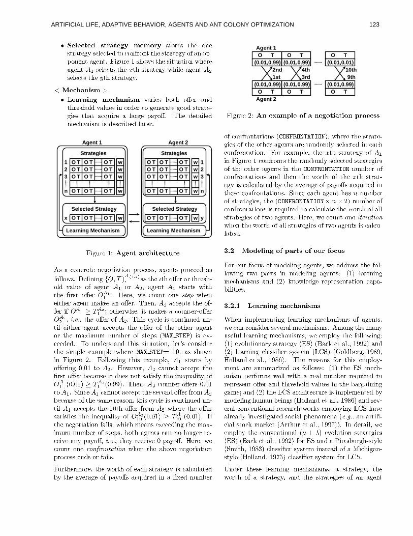
¯ �:�¨>:(¬���:<E �����oBD��:�©uä G¤:<G¤�u�jä h^_^ZU\^d�h _ r d ZUTDdh^_^\^RU_^d w y h^d��qd c _^d�pf_^Z c ZUTDY[\^ZUTv_�_ r dÔh^_^\^R]_^d w y ZUY�R]T�ZU� l�uZUTDd�T<_�R w d�T<_ji¤M` w OF\^dS|Ch r ZjÕ/hÔ_ r d#h^`a_^ODRU_z`aZUTÅÕ r d�\^dR w d�T<_³X " h^d��qd c _^hP_ r d³_Ó_ r h�_z\^RU_^d w y Õ r `q�ad�R w d�T<_³X #h^d��qd c _^h�_ r d�´v_ r h^_^\^R]_^d w y i
® §�:(¬o£BF¢�;>��G �¯ ��:<BD�j¢;>¢ª© G¤:(¬o£BD¢;>��G �oR]\^`ad�h3guZU_ r ZUÉud�\NRUTDp_ r \^d�h r ZU�ap �jRU�aODd�hC`qTÅZ]\^pFd�\C_^Z w d�TDd�\^R]_^d w ZvZvpÅh^_^\^RU_zd lw `ad�há_ r RU_�R c <OD`a\^dâRà�aRU\ w d¤�DR y ZUÉ�i,J r dâpDd�_^RU`a�qd�pQSd c¶r RUTD`ah^Q `qhCpFd�h c \^`agud�p��qRU_^d�\ji
Agent 1
Strategies
Learning Mechanism
O T O T O TO T O T O TO T O T O T
O T O T O T
1 www
w
23
O T O T O T wx
Agent 2
Strategies
Learning Mechanism
O T O T O TO T O T O TO T O T O T
O T O T O T
1www
w
23
O T O T O T w y
Selected Strategy Selected Strategy
n n
M` w OD\^d |UÖ¶µ ©u:v¢��8BD�?¬]£;[��:(¬U����j:
IPh�R c ZUT c \^d�_^d TDd w ZU_^`qRU_^`qZUT*�D\^Z c d�h^hjtR w d�T<_^h��F\^Z c d�d�p*RUhY¾ZU�a�aZjÕ/hji\�fd�ÚDTD`aT we·2¸ gF¹0º »¤¼i½p¾ ¿*ÀÁ RUh�_ r d�´_ r ZUÉud�\�ZU\�_ r \^d�h r lZU�qp �oR]�aODdHZUY�R w d�T<_�X " ZU\�X # t�R w d�T<_�X " h�_zRU\^_^h�Õ/`q_ r_ r dÄÚF\^h^_"ZUÉud�\ ¸ » ½" i6MPd�\^dvt�Õ�d c ZUODT<_WZUTFdàµ�¿mÊzÒâÕ r d�Td�`a_ r d�\�R w d�T<_#QSRUnUd�h/RUT�Z]ÉÓd�\jiÔJ r d�T�t¤X # R c�c d��D_^h�_ r d�ZUY lY¾d�\�`aY ¸ » ½"Äà ¹ » ¿" ÝÓZU_ r d�\^Õ/`ah^dvt�`a_�QSR]n�d�hPR c Z]OFT<_^d�\ l ZUÉud�\¸ » ¿# t»Åk[Ê k tF_ r d%Z]ÉÓd�\�ZUY�X # i�J r `qh c y c �qd�`qh c ZUT<_^`qT<OFd�p�ODT l_^`q��d�`a_ r d�\ÆR w d�T<_ÅR c�c d��D_^hW_ r dÄZUÉud�\ÆZUY�_ r dÄZU_ r d�\WR w d�T<_ZU\Æ_ r d�QSR]Þ<`aQ�OFQ T<ODQ�gud�\ÅZUYfh^_^d��Dh�×����(� ���(���ÓÙ�`ahÆd�Þ lc d�d�pDd�pi§JZHOFTDpDd�\^h^_^R]TFp§_ r `ah h^`a_^ODRU_z`aZUT�tC�qd�_ V h c ZUTDh�`qpFd�\_ r dÄh^`aQS�F�qd�d�Þ<RUQS�D�adÄÕ r d�\^dÆ����� ���(���t�Á|s�ut/RUhÆh r ZjÕ/T`aTyM` w OD\^d k iÇM�ZU�a�aZjÕ/`aT w _ r `ahád�Þ<R]QS�F�advteX " h^_^RU\^_zhág yZUÉud�\^`aT w �nÈ ��|Å_^ZÉX # i¤MPZjÕ�d��Ud�\jt�X # c RUTDTDZU_%R c�c d��F_�_ r dÚD\^h�_/ZUÉud�\Pgud c RUODh^d�`a_�pDZvd�h�TFZU_#h�RU_z`ah^Y y _ r d�`aTDd, <ODRU�a`a_ y ZUY¸ » ½" ×[�nÈ ��|UÙ Ã ¹ » ¿" ×[�nÈ }U}uÙ^i�J r d�T�t¤X # c Z]OFT<_^d�\ l ZUÉud�\^hP�nÈ �u|_^ZAX " i b `aT c d`X " c RUTFTDZU_(R c�c d��D_(_ r dÔh^d c Z]TFp�ZUÉud�\�Y[\^ZUQSX #gud c RUODh�d#ZUYu_ r d#h^RUQSd�\^d�RUh^ZUT�to_ r `ah c y c �ad�`ah c ZUT<_^`aT<ODd�pSODT l_^`q��X " R c�c d��D_^h�_ r dá|s�]_ r ZUÉud�\�Y¾\^ZUQÊX # Õ r d�\^d%_ r d�ZUÉud�\h^RU_^`ah^ÚDd�h�_ r dÅ`aTDdq vOFR]�a`a_ y ZUY ¸ » ¿"�Ë ×¾�nÈ �u|]Ù Ã ¹ » ½"�Ë ×[�nÈ ��|UÙ^iWVXY_ r d#TDd w ZU_^`aR]_^`aZUTÅY[RU`q�ahjtUÕ r ` csr QSd�RUTDhAd�Þ c d�d�pF`aT w _ r d#QSR]Þ l`aQ�OFQ T<ODQ�gud�\#ZUYKh^_^d��DhotDguZU_ r R w d�T<_^h c RUTÄTDZÅ�aZUT w d�\�\^d lc d�`q�Ud�RUT y �FR y ZUÉ�tÔ»Åk[Ê k tÓ_ r d y \^d c d�`a�Ud%�Å�FR y ZUÉ�i#MPd�\^d<tuÕAdc ZUODT<_8Z]TFd⯶³�À^Ìj±´³�ÀF¿m¹�¿m»¾³�ÀáÕ r d�T§_ r d"R]guZo�Ud�TDd w ZU_^`qRU_^`aZUT�D\^Z c d�h^h#d�TFpDhCZ]\�Y¾RU`a�ahjiMuOD\^_ r d�\^QSZ]\^d<tF_ r d�ÕAZU\^_ r ZUY�d�R csr h^_^\^RU_^d w y `ah c RU� c OF�qRU_^d�pg y _ r d8Rj�Ud�\^R w d8ZUYA�FR y ZUÉuh�R c vOF`q\�d�p¤`qT¤R"ÚDÞ<d�p¤T<ODQ�gud�\
Agent 1
Agent 2
(0.01,0.99) (0.01,0.99)
(0.01,0.01)T
(0.01,0.99) (0.01,0.99)
(0.01,0.99)
O TO TO
TO TO TO
1st2nd
3rd4th
9th10th
M` w OD\^d k Ö3µ ¢ß:(Í?BFGÆW¨>:á��«/B�¢�:(©��u��;>BF��;>��¢Î��o�t¬�:<���
ZUY c ZUTFY¾\^ZUT<_^R]_^`aZUTDh8×�Ï�Ð�Ñ�Ò(Ó�Ð�Ñ(�����¤Ô,Ð�ÑÓÙ^tFÕ r d�\^d�_ r d�h^_^\^RU_zd lw `qd�h/ZUY�_ r d�ZU_ r d�\#R w d�Tv_^h/RU\^d�\^RUTFpDZUQS� y h^d��ad c _zd�p"`qTWd�R csrc ZUTDY[\^ZUT<_zRU_^`aZ]Ti�MuZU\8d�Þ<RUQS�D�advtÔ_ r d�_Ó_ r h^_^\^RU_zd w y ZUY0X "`aT�M` w OD\^dÅ| c ZUTFY¾\^ZUT<_^hC_ r df\^R]TFpDZUQS� y h^d��ad c _^d�p�h^_^\^R]_^d w `ad�hZUYA_ r d�ZU_ r d�\�R w d�Tv_^hf`qT¤_ r dDÏ�Ð�Ñ(Ò�Ó�Ð�Ñ(�����¤Ô,Ð�Ñ"T<ODQ�gud�\�ZUYc ZUTDY[\^ZUT<_zRU_^`aZ]TFh RUTDp§_ r d�TØ_ r d�ÕAZ]\^_ r Z]Y�_ r d-_Ó_ r h^_^\^RU_ ld w y `ah c R]� c OF�qRU_^d�p"g y _ r d�Rj��d�\^R w d#ZUY��DR y ZUÉuhAR c <OD`a\^d�pW`aT_ r d�h�d c ZUTFY¾\^ZUT<_^R]_^`aZUTDhji b `aT c d%d�R csr R w d�T<_ r RUh�°ßT<ODQ�gud�\ZUY�h^_^\^RU_zd w `qd�hot�_ r d8×�Ï�Ð�Ñ(Ò�Ó�Ð(Ñ������¤Ô,Ð�Ñ�Õ²°ÉÕ k ÙT<OFQ�gud�\/ZUYc ZUTDY[\^ZUT<_zRU_^`aZ]TFhC`qh�\^d, <OD`a\^d�pÆ_zZ c RU� c OD�aR]_^dP_ r dfÕ�ZU\^_ r ZUY?RU�a�h^_^\^RU_^d w `qd�h#ZUY�_´Õ�Z8R w d�T<_zhoiÔMPd�\^dvt�Õ�d c ZUODT<_#ZUTDd"»¾¿mʲ±´¹�¿ »¾³�ÀÕ r d�T _ r d#Õ�ZU\^_ r Z]Y�RU�q��h�_z\^RU_^d w `ad�hKZ]Y�_XÕAZ�R w d�T<_zhA`qh c RU� c O l�aR]_^d�p�i
¥ ��Ö § �?E:�¨>;>¢ª©���«�BD�o���8��«�����D«¡�\¬����MuZU\#ZUOF\fY¾Z c ODhfZUYQSZvpFd��a`qT w R w d�Tv_^hjtuÕAd�RUpDpF\^d�h^hf_ r d�Y[ZU� l�aZjÕ/`aT w _XÕAZÈ�FR]\^_^hH`qTãQSZvpDd��q`aT w R w d�T<_^hjÖ ×^|UÙW�ad�RU\^TD`aT wQSd csr R]TF`qh�QShÅRUTFp�× k Ù�n<TDZjÕ/�ad�p w d�\^d��D\^d�h�d�T<_^R]_^`aZUT c RU�FR lgD`a�a`q_^`ad�hji
¥ ��Ö���¦ ��:<BF�j¢�;>¢ª©�G¤:(¬]£�BF¢�;>�²G¤�j r d�Tà`qQS�F�ad�QSd�T<_^`qT w �ad�RU\^TD`aT w QSd csr RUTD`ah^QShÆZUY�R w d�Tv_^hjtÕAd c RUT c Z]TFh^`apDd�\h^d��Ud�\^R]�<QSd csr RUTD`ah^QShoi�IPQSZ]T w _ r d�QSRUT yODh�d�Y¾OF���ad�RU\^TD`aT w QSd csr R]TF`qh�QShjtFÕAd�d�QS�F�qZ y _ r d�Y¾ZU�a�qZoÕ/`qT w Ö×^|UÙ�d��UZU�qOF_z`aZUTDRU\ y h^_^\^RU_^d w y ×[� b Ù�×Å�CR c nÆd�_CRU�¡iat?|s}U} k ÙRUTDp× k ÙC�ad�RU\^TD`aT w c �aRUh^h^`aÚDd�\�h y h^_^d�Q°×[eAÜ b Ù�×F×AZU�apDgud�\ w t�|s} � }FtMPZU�q�aRUTDp"d�_CR]�Xiat?|s} � {DÙ^i J r dH\^d�RUh^ZUTDh�Y¾ZU\�_ r `ahád�QS�D�aZ y lQSd�T<_ÅRU\^d�h^ODQSQSRU\^` à d�pàR]hÆY[ZU�q�aZjÕ/hoÖ ×^|UÙ�_ r d�� b QSd c¶r lRUTD`ah^Q �ud�\^Y¾ZU\^QSh8ÕAd��a��Õ/`a_ r RH\^d�RU�CT<ODQ�gud�\S\^dq vOF`q\^d�pâ_^Z\^d��F\^d�h^d�Tv_#ZUÉud�\#R]TFp"_ r \^d�h r ZU�ap"�oRU�qOFd�h�`qT�_ r d�gFR]\ w RU`aTD`aT ww RUQSdvÝoRUTDpÄ× k Ù�_ r d#eCÜ b RU\ csr `a_^d c _^OF\^dA`ahK`aQS�D�ad�QSd�T<_^d�p%g yQSZvpFd��a`qT w r ODQSRUT�gud�`qT w hK×[M#ZU�a�aR]TFp"d�_�RU�Xiat?|s} � {FÙ�RUTDp�h^d�� ld�\^RU� c Z]T<��d�T<_^`qZUTDRU��\^d�h^d�R]\ c¶r ÕAZU\^nvh/d�QS�D�aZ y `qT w eAÜ b"r Rj�UdRU�q\�d�RUp y `qT<��d�h^_^` w RU_^d�p"h^Z c `qRU�?� r d�TFZUQSd�TDR�×�Ê k ËGk¾t�RUTÆRU\^_^`qÚ lc `aRU��h^_^Z c nÆQSRU\^nUd�_S×[I#\^_ r OD\�d�_CRU�¡iat�|¶}U}��jÙ^Ù^i�VXT�pDd�_zRU`a�XtDÕAdd�QS�F�qZ y _ r d c ZUT<�Ud�T<_^`aZ]TFRU�P×ÙØÛÚÎÜ?Ù�d��UZU�aOD_^`aZUTâh^_^\^R]_^d w `ad�h×[� b ÙK×��CR c n d�_#R]�Xiat?|s}U} k ÙY¾ZU\�� b RUTFp8R��K`a_z_^h^gFOD\ w r l h^_ y �qd× b QS`a_ r t�|s} � �FÙ c �aRUh^h�`qÚFd�\�h y h^_^d�Q `qTFh^_^d�RUpWZUYR²��` csr ` w RUT lh^_ y �ad ×[M#ZU�a�qRUTFp�t?|s}��8LFÙ c �aRUh^h�`qÚFd�\�h y h^_^d�Q Y[Z]\CeCÜ b i�PTDpDd�\ _ r d�h^d �qd�RU\^TD`aT w QSd csr RUTD`ah^QShot"RÇh^_^\^RU_^d w y t"_ r dÕAZ]\^_ r ZUY�R h^_^\^RU_zd w y t/R]TFp3_ r d¤h�_z\^RU_^d w `ad�h"ZUY�RUT3R w d�T<_
123ARTIFICIAL LIFE, ADAPTIVE BEHAVIOR, AGENTS AND ANT COLONY OPTIMIZATION
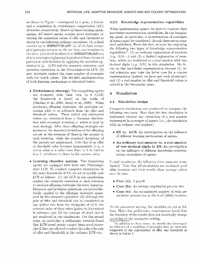
RUhfh r ZjÕ/TÄ`aTÝM` w OF\^d�| c Z]\�\^d�h^�uZUTDp¤_^ZWR w d�TDd<t�R"ÚD_^TDd�h^hjtRUTDp RH�uZU�DOF�qRU_^`aZ]T§`aTØd���Z]�aOD_^`aZUTDRU\ y c ZUQS�DOF_zRU_^`aZ]T�×¾��Ü/Ù�a`q_^d�\^RU_^OD\^d<to\^d�h^�ud c _z`a�Ud�� y iN�CRUh^d�p8ZUT%_ r d�h^d#�ad�RU\^TF`qT w QSd c¶r lRUTD`ah^QShjtA��Ü l gDRUh^d�p R w d�Tv_^hÅR c <OD`a\^d w ZvZvpàh^_^\^RU_^d w `qd�hÅg y�oRU\ y `aT w _ r dfT<ODQSd�\^` c RU�(�oRU�qOFd�h�Z]Y�ZUÉud�\CR]TFp"_ r \^d�h r ZU�ap"RUhh r ZjÕ/T�g y _ r d/Y¾ZU�a�qZoÕ/`qT w ZU\^pD`aTDRU\ y �D\^Z c d�pDOF\^dvÖK×^|]Ù?RfÚDÞ<d�pT<ODQ�gud�\%×ÙØ*ZU\rÞ��(Ñ���Ó(���\Ô,Ð(Ñ Þ(���vÕ¤°�ÙKZUY_ r d�gud�h^_Ph^_^\^RU_zd lw `qd�h�×>Ò�¹�±´Ê²ÀF¿mµ�Ù�\^d�QSRU`qTFh/`aTW_ r d�h�d�_AY¾\^ZUQ Z]TFdf`a_zd�\^RU_z`aZUTÆ_^Z_ r dÔTDd�Þ<_jÝF× k ÙvR#ÚFÞvd�p�T<ODQ�g�d�\�×�ÜPZU\ªÞ(��Ñ���Ó(���\ÔqÐ�Ñ Þ(���vÕ¤°AÙZUY<TFd�Õ¤h^_^\^R]_^d w `ad�hC×�³pßfµmÒu±s»[ÀoË<ÙD`ah��D\^ZvpFO c d�p�Y¾\^ZUQN_ r d�h�d�_�ZUY�DRU\^d�T<_^h�R]_Kd�R csr `q_^d�\^RU_^`aZ]TSg y RU�D�F� y `qT w _ r dCQ�OD_^RU_^`qZUT%ZU� ld�\^RU_^`aZ]T `qT�×ÙØ0Ú�Ü?Ù l � b RUTDp%_ r d c \^ZUh�h^Zj�Ud�\jtoQ�OD_^RU_z`aZUT�tjRUTDp`aT<�Ud�\^h^`aZUT�ZU��d�\^R]_^`aZUTDh�`qT¤_ r d8�K`q_^_^h^gDOF\ w r l h^_ y �adSeAÜ b ÝÔ×[��ÙTDd�Õ h^_^\^RU_^d w `ad�h�\^d��D�aR c dS_ r dSh^RUQSd T<ODQ�gud�\�Z]YCh^_^\^R]_^d w `ad�hÕ/`a_ r �qZoÕãÕAZ]\^_ r �oR]�aODd�hjiSJ r d8pFd�_^R]`a�ad�p�`qQS�F�ad�QSd�T<_^RU_z`aZUTZUY�guZ]_ r �ad�RU\^TD`aT w QSd csr R]TF`qh�QShA`qh�pFd�h c \^`qgud�p�gud��aZjÕ�i
¯ ��àÓ��¨>����;>��¢BD�jäÄ�²���jBF��:�©�ä�å J/ÕAZfgDRU\ w RU`qTF`qT w R w d�T<_^hRU\^d d, <OD`a�D�ud�p Õ/`q_ r _ r d�`q\°ZjÕ/T ×ÙØáÚâÜ?Ù l � b Ý_ r d5Y¾\^RUQSd�Õ�ZU\^n `ah7gDRUh^d�p ZUT _ r d5ÕAZU\^nvh ZUY×F×Ad�\^pF`qT w d�_CRU�¡iat k �U�U�Dt��A\^R w _#d�_CRU�¡iat k �U�U�DÙ^iãj r d�T�F\^ZvpDO c `qT w ZUÉuh^�D\^`aT w h�_z\^RU_^d w `ad�hjt�_ r d"Q�OF_zRU_^`aZ]TØZU� ld�\^RU_^`aZUT R]pFpDh8_^ZHZU\Æh^ODgF_z\^R c _^h8Y¾\^ZUQ'_ r d"Z]ÉÓd�\ RUTDp_ r \^d�h r ZU�ap3�oRU�qOFd�hji,J r d�h�dHRUpDpFd�pNRUTDp3h^OFgD_^\^R c _^d�p�oRU�qOFd�hÆRU\^d c RU� c OF�qRU_^d�pÈY[\^ZUQ'Ry×CR]OFh^h^`aRUT§pD`ah^_^\^`agDO l_^`aZ]TÄÕ/`a_ r h^_^RUTDpFR]\^pÄpDd��v`aRU_z`aZUT�ä(tÓÕ r ` csr `ahPnUd��D_�g yd�R csr h�_z\^RU_^d w y iIPY¾_^d�\C_ r d�h^d�ZUÉuh^�F\^`qT w h^_^\^R]_^d w `ad�hPRU\^d�F\^ZvpDO c d�p�tj_ r d/h^_^RUTDpDRU\^p�pDd��<`aR]_^`aZUTDhZUYu_ r dAZ]ÉÓh^�D\^`aT wRU\^d�h^d�_PR]hP_ r d%Rj�Ud�\^R w d�h#ZUYK_ r ZUh^d�`aTá_ r d��DRU\^d�T<_^hPRU_d�R csr `q_^d�\�R]_^`aZUT�tAÕ r `a�qd�_ r d�h^_^RUTDpFR]\^pàpDd��<`qRU_^`aZUTDhÅZUY_ r d��DRU\^d�T<_^hPRU\^d�QSRU`aT<_zRU`aTDd�p�i � Z]_^d�_ r RU_/`aY�RUT"ZUÉud�\ZU\�_ r \^d�h r Z]�ap��oR]�aODd�gud c ZUQSd�h�`aTDRU�D�F\^Z]�F\^`qRU_^dÆ×^Ê k ËGk t<RQS`aT<ODh��oRU�qOFd#Z]\CR��oRU�qOFd#QSZ]\^d�_ r RUTá|UÙzt<`q_�`qhC\^d�h�d�_K_^Z�8ZU\�|UtDÕ r ` csr d���d�\A`qh c �aZ]h�d�\�_^Z�_ r d c OD\^\^d�T<_A�oRU�aODdvi
¯ ��:<BD�j¢;>¢ª©å¬%¨>BF����;�æ:v� ��ä�����:vGHå J/Õ�Z gFR]\ w RU`aTD`aT wR w d�T<_^hSRU\^d"d, <OD`a�D�ud�pßÕ/`q_ r _ r d�`q\8ZjÕ/T§�K`q_^_^h^gDOF\ w r lh^_ y �ad�eCÜ b i�JZ c ZUTFpDO c _ c Z]Q8�DOD_^d�\ h�`qQ�OD�aRU_^`qZUTDhÅ`aT_ r dfh^RUQSdPY¾\^RUQSd�ÕAZU\^n%ZUY�� b t�ÕAd#h^d�_AZU\AQSZvpD`aY y d�R csreAÜ b RUh%Y¾ZU�a�aZjÕ/hjÖá×^|UÙ#_ r dWeAÜ b `aT*ZUOD\%h^`aQ�OD�aR]_^`aZUTDhRU�D�F�q`ad�h�_ r d c \^ZUh^h�Zj�Ud�\�ZU�ud�\^RU_z`aZUT*R]_Sd�R csr `a_zd�\^RU_z`aZUT_^Z��F\^ZvpDO c dKZUÉuh^�F\^`qT w h^_^\^RU_zd w `qd�h�_ r d�d��Ud�\ y `q_^d�\^RU_^`aZ]Ti�áOD_^R]_^`aZUTSR]TFp8`aT<�Ud�\^h�`qZUT8ZU�ud�\^RU_^`qZUTFhÔRU\^d/�F\^Z]gFRUgD`a�q`ah l_^` c RU�q� y R]�F�D�a`qd�p§_^Z¤_ r d�ZUÉuh^�F\^`qT w h^_^\^R]_^d w `ad�h w d�TDd�\ lRU_^d�pWg y _ r d c \^ZUh^h^Zo�Ud�\CZU�ud�\^RU_^`qZUTÝ?× k ÙRU�q_ r Z]O w r _ r d�FR]`a\�ZUY/ZUÉud�\�RUTDpØ_ r \^d�h r ZU�ap c R]Tâgud c Z]TFh^`apDd�\^d�p*RUhZUTDdH» ̲·X¿mÍ�ʲÀ�\^OD�adÅY[\^ZUQÛ_ r dÅ�<`qd�Õ/��ZU`aT<_SZUY�eAÜ b t(_ r dh^d��qd c _^d�pÆZU\^pDd�\CZUY�_ r d�h^df\^OF�qd�h�×[�DRU`q\^hoÙ�`ahCpDd�_^d�\^QS`aTFd�p`aTØRUpF�jRUT c dvÝRUTFp3×[�uÙ#_ r d c ZUT c d��D_8Z]Y%½�³�ÀGç ¿�¯¶¹�±´Ê�`qhTFZ]_Pd�Q8�D�aZ y d�pá`aTáZUOD\Ph^`aQ�OD�aRU_z`aZUTDhoi�MuZU\P_ r d�h^d c ZUTDp�uZU`qT<_jt<`aTÆ�FRU\^_z` c OF�qRU\jt<R8�D\^d��a`aQS`qTFR]\ y \^d�h^d�R]\ c¶r Y¾ZUODTFp_ r RU_PeAÜ b l gFRUh^d�p�R w d�T<_^h c RUTFTDZU_#�ad�RU\^T w ZvZvp�h^_^\^RU_zd lw `ad�h`aYF_ r d y RU\^dARU�q�aZjÕAd�p%_^Z#h^d��ad c __ r dC\^OF�qd�h/×¾_ r d��FR]`a\ZUY�ZUÉud�\#R]TFp"_ r \^d�h r ZU�ap�Ù(`aT�_ r d�ZU\^pD`aTDRU\ y eCÜ b ÕAR y i
¥ ��Ö���Ö 9�¢�D e¨>:<EW©u:"�j:(��o:v��:<¢���BD��;>��¢ã¬�BnBD�;�¨>;[��;>:v�j r d�TW`aQS�D�ad�QSd�T<_z`aT w R w d�T<_^hjt�ÕAd r Rj�Ud�_^Z c ZUTFh^`apDd�\�_ r d�`a\n<TDZjÕ/�ad�p w d�\^d��F\^d�h^d�Tv_^RU_^`qZUT c RU�DRUgF`q�a`a_z`ad�hoi�VXTÆ_ r d�gDRU\ w RU`qT l`aT w w RUQSdvtu`qTÄ�DRU\^_^` c OD�aRU\jt�R8\^d��D\^d�h^d�T<_^RU_^`qZUTáZUYKh^_^\^R]_^d w `ad�hZUY<R w d�T<_^h(Q�OFh^_?gud c ZUTDh�`qpFd�\^d�p�tj_ r ZUO w r _ r d�\^dKRU\^dÔTDZ/h^_^RUT lpDRU\^p w OD`apDd��a`aTDd�hoiNMu\^Z]Q _ r `qh�Y¾R c _jtUÕ�d/h^_^RU\^_�g y d�QS�D�aZ y `qT w_ r d�Y¾ZU�a�qZoÕ/`qT w _´Õ�ZH_ y ��d�hÆZUYfn<TDZoÕ/�qd�p w d�\^d��D\^d�h^d�T<_^RU_^`qZUTc RU�DRUgF`q�a`a_z`ad�hoÖ è�×^|UÙ(R]T�ZU\^pD`aTDRU\ y d�Þv�F�qRUTFR]_^`aZUT"Z]Y�T<OFQ�gud�\^h×�Ê k ËGk¾t�ui �u|2é2éqé ÙCRUTDpN× k ÙCR��a`aQS`q_^d�p*d�Þ<�D�aR]TFRU_z`aZUTâZUY�T<ODQ lgud�\^hjt(Õ r ` c¶r RU\^d8\^d�h^_^\^` c _^d�pH_^Z�RW\^d�RU��T<ODQ�g�d�\�Õ/`a_ r _XÕAZpDd c `aQSR]�ApF` w `a_^hÆ×�Êqk ËGk t(�ui �u|UÙ#`qT¤_ r `ah%h^`aQ�OD�aR]_^`aZUT�i�j¤d Y[Z lc OFh�ZUT�_ r `ah�nvTFZjÕ/�ad�p w d \^d��F\^d�h^d�T<_zRU_^`aZ]T*gud c R]OFh^dá×z|UÙ/h^Z lc `aRU�/h c `ad�T<_^`qh�_zh8QSR y _^RUnUd"_ r d"�qRU_^_^d�\ c RUh^d�Y¾ZU\SR c ZUT c `ah^d\^d��F\^d�h^d�Tv_^RU_^`qZUTâ×[VXTDpDd�d�p�t�ÕAd r Ro�Ud�QSd�_/h^O csr h^`a_^ODRU_z`aZUTDhoÙzÝRUTDp*× k ÙR8\^d�RU�T<ODQ�gud�\C`aT�ZUÉud�\#R]TFp"_ r \^d�h r ZU�ap"�oRU�qOFd�h�`qhc \^`a_^` c R]�?`aT�_ r d�gFR]\ w RU`aTD`aT w w RUQSd<i
ê ë ��T���£´«©(��� �
ì ��¦ ��;>GÄ�ª¨>BD��;>��¢ßE:v�²;�©u¢ÜZUQS�DOD_^d�\�h^`aQ�OF�qRU_^`qZUTFh�RU\^d c ZUTFpDO c _zd�p¤_zZ c ZUQS�FR]\^d _ r dY¾ZU�a�aZjÕ/`aT w _´Õ�Z c RUh�d�hji � ZU_^d8_ r RU_�_ r d8ÚD\^h�_fh^`aQ�OD�aRU_z`aZUTÄ`qh�ud�\^Y¾ZU\^QSd�p Õ/`a_ r ZUOD_ÆRUT y \^d�h^_^\^` c _z`aZUTàZUY�Râ\^d�RU��T<ODQ�gud�\\^d��F\^d�h^d�Tv_^d�p `qTSh^_^\^RU_^d w `qd�hÔZUY�R w d�Tv_^hP×�»Åk[Ê k t]_ r d#h^`aQ�OF�qRU_^`aZ]TÕ/`a_ r RUTÆZU\^pD`aTDRU\ y \^d�RU�ÓT<ODQ�gud�\jÙ^i
¯ �P�íà?�²�ß�¶îS�å IPTÄ`aT<�Ud�h�_^` w RU_^`qZUT�ZUT�_ r dS`aT ± ODd�T c dZUY�pD`aÉud�\^d�T<_/�qd�R]\^TF`qT w QSd c¶r RUTD`ah^QSh/ZUYR w d�T<_^hji
¯ µ ¢Ä���oE�;>¢BD�oäá�j:vBn¨�¢��GÄ��:v��à?����BÅ�j:<B�¨�¢��GÄ��:<���«P�s ��HE�:(¬�;>G¤Bn¨AE�;�©�;>��� ;>¢§����å IPTW`aT<�Ud�h^_^` w R]_^`aZUTZUT�_ r d8`qT ± OFd�T c dSZUYApD`aÉud�\^d�Tv_fn<TDZoÕC�ad�p w d%\^d��D\^d�h�d�T l_^RU_z`aZUT c RU�DRUgF`q�a`a_z`ad�h�ZUYR w d�T<_^hji
VXT8d�R csr h^`aQ�OF�qRU_^`aZ]Tt]_ r d#Y¾ZU�a�qZoÕ/`qT w _ r \^d�d c RUh^d�hARU\^d/`qT<��d�h l_^` w RU_^d�p�i � Z]_^d%_ r RU_�RU�a��h�`qQ�OD�aRU_^`qZUTDh�RU\^d c ZUTDpFO c d�pÄOFT<_z`a�LU�U�]�H`q_^d�\�R]_^`aZUT RUTFp _ r d�`a\S\^d�h^OD�a_^h8h r ZjÕ Ro�Ud�\^R w d"�oRU�qOFd�hZj��d�\�|¶�S\^ODTDhoi
¯ îSBF��:ÛïXBnð�å I �DR y Z]ɯ îSBF��:ÛïX�ªð�å IPTWRo�Ud�\^R w dfTDd w ZU_^`aR]_^`aZUTÅ�F\^Z c d�h^h�h�` à d¯ îSBF��:íï*¬%ð�å IPT¤R c�c ODQ�OD�aRU_zd�p*T<OFQ�gud�\�ZUY�d�R csr TDd lw ZU_^`qRU_^`qZUTW�F\^Z c d�h�hCh^` à d�RU_A_ r d#ÚDTFRU�K×�L]�U�U�uÙ�`a_zd�\^RU_z`aZUT
IPh#_ r d��DRU\^RUQSd�_^d�\#h^d�_^_^`qT w tF_ r d��oRU\^`qRUgD�ad�h#RU\^d%h^d�_�R]hPY[ZU� l�aZjÕ/hji � ZU_^d�_ r RU_#�F\^d��a`qQS`aTDRU\ y d�Þ<R]QS`aTFR]_^`aZUTDhPY[ZUODTDpÄ_ r RU__ r d/_zd�TDpDd�T c y Z]YÓ_ r dC\^d�h�OD�a_^hÔpFZvd�h�TDZU_KpD\^RUh^_^` c RU�q� y csr RUT w dR c�c ZU\^pF`qT w _^ZS_ r df�DRU\^RUQSd�_^d�\�h^d�_^_z`aT w iñ�ò ùáézó�óvñÐòXñ¼ô²ù òXô�ò¡õvë¶íXë�ñ¼íXíXîvë¶í,1(uëPí´õ�ô²î�ý¼ó�ézý¼íXô%ñÐù]ü²ë¶í´òXñ9)�ézòXë
ézù8ñÐù%óvî�ë¶ù�ú¶ë#ô �KéCðfôoó�ë¶ý¼ñÐù�)�ô �(í´ò¡ì�é^ò¡ë8)²ñ¼ë¶í�òXõÓézòfézìXëCú¶î�ìXìXë¶ù]òXý¼ÿú¶ô²ðfê<ôjíXë¶ó ô ��òXõ�ë�ú¶ô²ð#ï�ñ¼ùÓézòXñ¼ô²ù ô �fô ô�ë¶ì¤ézù�óßò¡õvìXë¶íXõ�ô²ý¼ó�ézííXõvô{uÔù�ñ¼ùes�ñ9)²î�ìXë³. <
124 ARTIFICIAL LIFE, ADAPTIVE BEHAVIOR, AGENTS AND ANT COLONY OPTIMIZATION
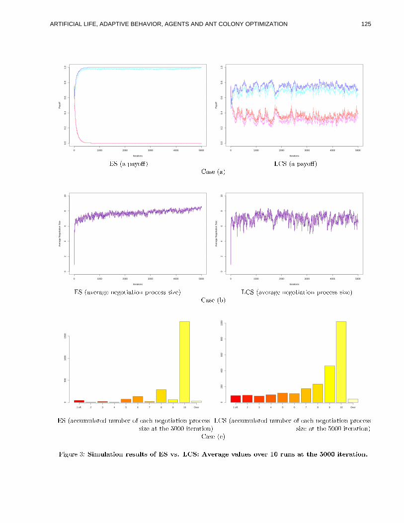
0 1000 2000 3000 4000 5000
0.0
0.2
0.4
0.6
0.8
1.0
Iterations
Pay
off
0 1000 2000 3000 4000 5000
0.0
0.2
0.4
0.6
0.8
1.0
Iterations
Pay
off
� b ×[RS�FR y ZUÉ�Ù eCÜ b ×¾R8�DR y ZUÉ�ÙÜRUh^dÆ×[RuÙ
0 1000 2000 3000 4000 5000
02
46
810
Iterations
Ave
rage
Neg
otia
tion
Siz
e
0 1000 2000 3000 4000 5000
02
46
810
Iterations
Ave
rage
Neg
otia
tion
Siz
e
� b ×[Rj�Ud�\^R w dfTDd w ZU_^`aR]_^`aZUT"�D\^Z c d�h^h#h^` à dvÙ eAÜ b ×[Rj�Ud�\^R w dfTDd w ZU_^`qRU_^`aZUT"�D\^Z c d�h^h#h^` à dvÙÜRUh^dÆ×[g�Ù
1 off. 2 3 4 5 6 7 8 9 10 Over
050
010
0015
00
1 off. 2 3 4 5 6 7 8 9 10 Over
020
040
060
080
010
00
� b ×[R c�c ODQ�OD�aRU_^d�pWT<ODQ�g�d�\CZUYd�R csr TDd w ZU_^`qRU_^`qZUT"�F\^Z c d�h^hßeAÜ b ×[R c�c ODQ�OD�aRU_^d�pWT<ODQ�g�d�\#Z]Y�d�R csr TDd w ZU_^`qRU_^`qZUT"�F\^Z c d�h^hh^` Ã d�RU_A_ r d�L]�U�U�S`a_^d�\^RU_^`qZUTÙ h^` Ã d�R]_�_ r drLU�U�U�S`a_^d�\^RU_z`aZUT�Ù
ÜRUh^dÆ× c Ù
M` w OD\^d��uÖ �;[G��W¨>BF��;>��¢à�j:<���ª¨[���%��«P�P�aà����8�¶îS��å µ àu:<�jBn©�:�à<Bn¨>��:<�8��àu:v�²¦�õH�j�¢��SBD�8��£�:�ö�õ�õ�õ¤;[��:v�oBD��;>��¢�
125ARTIFICIAL LIFE, ADAPTIVE BEHAVIOR, AGENTS AND ANT COLONY OPTIMIZATION
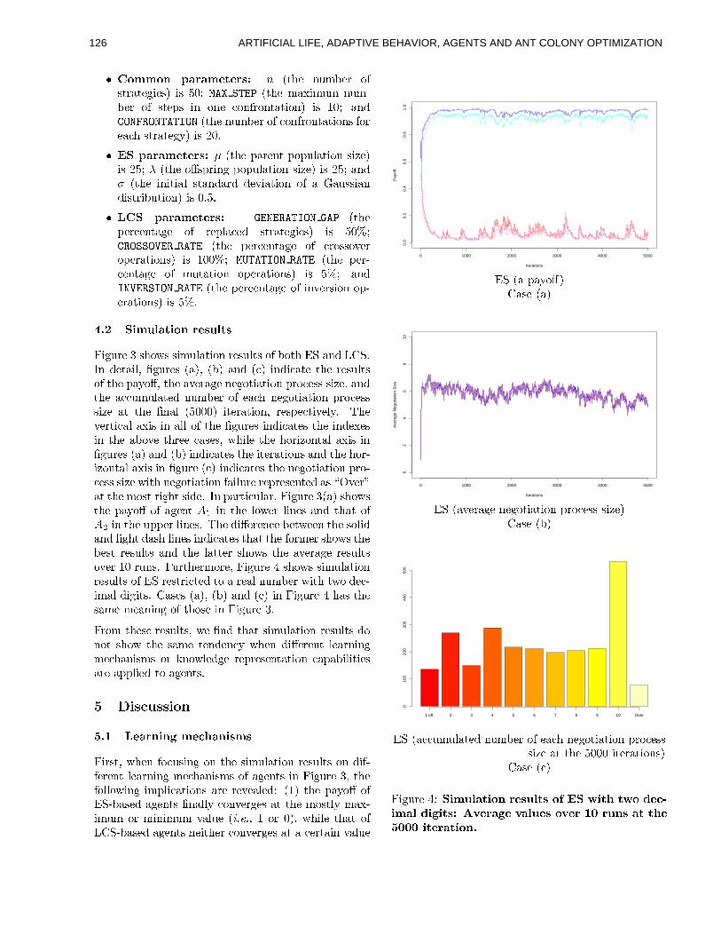
¯ îS��GHG¤��¢ BF�jBDGH:v��:v�o��å ° ×[_ r d,T<ODQ�g�d�\ ZUYh^_^\^RU_^d w `ad�hjÙ�`ah÷L]�uÝv�(��� �(�����ß×[_ r dWQSR]Þ<`aQ�OFQæT<ODQ lgud�\ßZUY�h�_zd��Dhâ`aT ZUTFd c ZUTFY¾\^ZUT<_^R]_^`aZUT�Ù"`ah |¶�uÝ�RUTDpÏ(Ð�Ñ�Ò�Ó(Ð�Ñ��(���\ÔqÐ�Ñ ×[_ r dCT<ODQ�g�d�\�ZUY c Z]TFY¾\^ZUT<_^RU_z`aZUTDhY¾ZU\d�R csr h�_z\^RU_^d w y Ù`ah k �ui
¯ �P� BF�jBDGH:v��:v�o��å Ø ×¾_ r d��FR]\^d�T<_���ZU�FOD�aR]_^`aZUTáh^` à dvÙ`ah k LuÝNܤ×[_ r d�ZUÉuh��D\^`aT w �uZ]�FOD�aRU_z`aZUTáh^` à dvÙ`qh k LuÝDRUTDpä ×[_ r dÄ`qTF`q_^`aRU��h^_^R]TFpDRU\^p§pFd��v`aRU_^`qZUTÈZUY�Ry×CR]OFh^h^`aRUTpF`qh�_z\^`agDOF_z`aZUT�Ù`ahC�nÈ Lui
¯ �¶îS� �BF�jBFG¤:<��:<�j��å Þ(��Ñ��(Ó����¤Ô,Ð�Ñ Þ��(� ×[_ r d�ud�\ c d�T<_zR w d Z]Y7\^d��F�qR c d�p h^_^\^RU_zd w `qd�hoÙ7`qhøLU��ùSÝÏ(Ó�Ð����(Ð�ú��(Ó Ó��(��� ×¾_ r d,�ud�\ c d�T<_zR w d ZUY c \^ZUh^h�Zj�Ud�\ZU�ud�\^RU_^`qZUTDhoÙ�`qh3|¶�U��ùSÝ���û��(���\ÔqÐ�Ñ Ó����(� ×¾_ r dà�ud�\ lc d�T<_zR w d Z]Y Q�OD_^RU_z`aZUT ZU�ud�\^RU_^`qZUTDhoÙN`qhSL�ùSÝÇRUTDpÔqÑ�ú���Ó(�\Ô,Ð(Ñ Ó��(���¤×[_ r d��ud�\ c d�T<_zR w d�Z]Y�`qT<��d�\^h^`aZUT"ZU� ld�\^RU_^`aZUTDhjÙ�`ah`L�ùSi
ì ��Ö ��;>GÄ�ª¨>BD��;>��¢ß�j:<���ª¨>���M` w OD\^dA�fh r ZjÕ/hh�`qQ�OD�aRU_^`qZUT�\^d�h�OD�a_zhKZUYFg�ZU_ r � b RUTDp�eAÜ b iVXTHpDd�_zRU`a�Xt?Ú w OF\^d�hÅ×¾RuÙ^t�×[g�ÙCRUTDp§× c ÙA`aTDpF` c R]_^d _ r d8\^d�h^OF�q_^hZUYu_ r d/�DR y Z]É�to_ r d#Ro�Ud�\^R w d/TFd w Z]_^`aRU_z`aZUT%�D\^Z c d�h^h�h^` à d<tjRUTDp_ r dÅR c�c OFQ�OF�qRU_^d�pâT<ODQ�gud�\�ZUY/d�R csr TDd w ZU_^`qRU_^`qZUT*�D\^Z c d�h^hh^` à dÄRU_"_ r dÄÚFTDRU� ×�LU�]�U�uÙ�`a_^d�\^RU_^`qZUTt/\^d�h^�ud c _^`a�Ud�� y i6J r d�Ud�\^_^` c RU�R]Þ<`ah#`qT�RU�a�ZUY_ r d�Ú w OF\^d�hP`aTDpF` c RU_zd�h#_ r d�`qTFpDd�Þ<d�h`aT�_ r d8RUguZj�UdS_ r \^d�d c RUh�d�hjt�Õ r `a�qd8_ r d r ZU\^` à Z]T<_^RU�KR]Þ<`ah�`aTÚ w OF\^d�h#×¾RuÙDRUTDp�×[g�ÙF`aTDpF` c RU_zd�h_ r dA`q_^d�\^RU_^`aZ]TFh�RUTDp%_ r d r ZU\ l` à ZUT<_zRU�ÓR]Þ<`ah�`qTWÚ w OF\^d%× c Ù(`aTDpF` c R]_^d�hA_ r d#TDd w ZU_^`aR]_^`aZUTÅ�F\^Z lc d�h^hh^` à dÔÕ/`q_ r TDd w ZU_^`aR]_^`aZUT�Y[R]`a�aOD\^dK\^d��D\^d�h^d�T<_^d�p�R]h�ZiJA�Ud�\F[RU_�_ r d�QSZUh^_�\^` w r _�h�`qpFdvi�VXT��DRU\^_^` c OD�aRU\jt?M` w OD\^dK�u×[R�Ùuh r ZjÕ/h_ r d8�DR y Z]ÉâZ]Y�R w d�T<_÷X " `aT¤_ r dS�aZjÕAd�\��a`aTDd�h�RUTDp*_ r RU_�ZUYX # `aT�_ r d/OD�F��d�\�a`aTDd�hoi�J r d�pF`qÉud�\^d�T c dAgud�_´Õ�d�d�T�_ r d/h^ZU�a`qpRUTDp��q` w r _?pFR]h r �a`aTDd�h`qTFpD` c RU_^d�h(_ r RU_?_ r dAY¾ZU\^QSd�\�h r ZoÕ/h(_ r dgud�h^_%\^d�h�OD�a_^h%R]TFpH_ r d"�qRU_^_^d�\�h r ZjÕ/h%_ r dÅRj�Ud�\^R w dÆ\^d�h^OF�q_^hZj��d�\f|s�%\^OFTDhjiRMuOD\^_ r d�\^QSZU\^d<t%M` w OD\^drK�h r ZjÕ/h/h^`aQ�OF�qRU_^`aZ]T\^d�h�OD�a_zhKZUY?� b \^d�h^_^\^` c _^d�p8_^Z�R�\^d�RU�FT<ODQ�gud�\ÔÕ/`q_ r _XÕAZ�pFd c l`aQSRU�?pD` w `q_^hjiCÜRUh^d�h�×[R�Ù^t(×[g�ÙRUTDp¤× c Ù`aT�M` w OD\^düK r R]h�_ r dh^RUQSd�QSd�RUTD`aT w ZUY�_ r ZUh^d�`aT5M` w OD\^d��uiMu\^ZUQ _ r d�h�d�\^d�h^OD�a_^hjtFÕAdfÚDTDp�_ r RU_/h�`qQ�OD�aRU_^`qZUT�\^d�h^OF�q_^h/pFZTDZU_%h r ZjÕ _ r dÅh^RUQSd�_zd�TDpDd�T c y Õ r d�TßpD`aÉud�\^d�Tv_%�ad�RU\^TD`aT wQSd csr R]TF`qh�QSh8ZU\%n<TDZjÕ/�ad�p w d�\^d��D\^d�h�d�T<_^R]_^`aZUT c RU�DRUgD`a�a`q_^`ad�hRU\^dfR]�F�D�a`qd�p�_^Z�R w d�T<_^hji
ý þ �´¨<¬\�P¨<¨(��� �
ö���¦ ��:vBF�j¢;[¢ª©�GH:�¬]£�BF¢;>��G¤�M`a\^h^_jtFÕ r d�TÄY¾Z c ODh^`aT w ZUT�_ r d�h^`aQ�OD�aRU_z`aZUTÄ\^d�h^OF�q_^hPZUTápD`aY lY¾d�\^d�T<_P�qd�R]\^TF`qT w QSd csr RUTD`ah^QShPZUYKR w d�Tv_^h#`aT�M` w OD\^d��utD_ r dY¾ZU�a�aZjÕ/`aT w `aQS�D�a` c RU_z`aZUTDh%RU\^d8\^d��Ud�R]�ad�pÖÅ×^|UÙC_ r dÅ�FR y ZUÉßZUY� b l gFRUh^d�páR w d�T<_zh#ÚFTDRU�a� y c ZUT<�Ud�\ w d�hPR]_P_ r d�QSZUh^_^� y QSR]Þ l`aQ�OFQ®ZU\�QS`qTF`qQ�ODQ®�oRU�qOFd�×^»�k¾Ê k¾tC|SZU\%�uÙ^t�Õ r `q�adÅ_ r RU_%ZUYeAÜ b l gDRUh^d�pÆR w d�T<_^h�TDd�`q_ r d�\ c ZUT<�Ud�\ w d�h�RU_AR c d�\^_^RU`qTW�oR]�aODd
0 1000 2000 3000 4000 5000
0.0
0.2
0.4
0.6
0.8
1.0
Iterations
Pay
off
� b ×[R8�DR y ZUÉ�ÙÜRUh^dÆ×[RuÙ
0 1000 2000 3000 4000 5000
02
46
810
Iterations
Ave
rage
Neg
otia
tion
Siz
e
� b ×[Ro�Ud�\^R w d�TFd w ZU_z`aRU_^`qZUT"�F\^Z c d�h�h�h^` à d<ÙÜRUh^dÆ×[g�Ù
1 off. 2 3 4 5 6 7 8 9 10 Over
010
020
030
040
050
0
� b ×[R c�c ODQ�OD�aRU_zd�pWT<ODQ�g�d�\CZUY�d�R csr TFd w ZU_z`aRU_^`qZUT"�F\^Z c d�h�hh^` Ã d�RU_�_ r drLU�U�U�S`a_zd�\^RU_z`aZUTDhjÙ
ÜRUh^dÆ× c Ù
M` w OD\^d�KuÖ �;[G��W¨>BF��;>��¢H�j:v�²�W¨>������«A�P�â %;>��£*�Ñ ��"E�:(¬{ÿ;>G¤Bn¨ÔE�;�©�;>����å µ àu:v�oB�©u:-à<Bn¨>�:v�%�GàÓ:v�e¦�õ��j�¢���BF����£�:ö�õ�õ�õ�;>��:v�jBF��;>��¢��
126 ARTIFICIAL LIFE, ADAPTIVE BEHAVIOR, AGENTS AND ANT COLONY OPTIMIZATION
TDZU\ c �aZUh^d�_^ZS_ r d�QSRUÞ<`qQ�ODQ ZU\PQS`qTF`qQ�ODQ �oRU�qOFdvÝ�× k Ù_ r dRj��d�\^R w dfTDd w ZU_^`qRU_^`qZUTáh^` à d�ZUY�� b l gDRUh^d�p"R w d�T<_^h#`qT c \^d�RUh^d�hjtÕ r `a�adÅ_ r RU_�ZUY�eAÜ b l gDRUh^d�pâR w d�Tv_^h�pFZvd�h8TDZU_�gFOD_�h�`qQS�F� yZUh c `a�a�qRU_^d�hoÝ�RUTFp ×[�uÙ�R]�a_ r ZUO w r _ r d8R c�c ODQ�OD�aRU_^d�p¤T<ODQ�gud�\ZUY_ r dÆ|s�U_ r TDd w ZU_^`aR]_^`aZUT��F\^Z c d�h�h�h^` à d�RU_/_ r d0LU�U�U�S`a_^d�\^R l_^`qZUTÄ`qh r ` w r g�ZU_ r `qTÄ� b l gDRUh^d�p�RUTDpáeAÜ b l gFRUh^d�pÄR w d�Tv_^hjt_ r dÅR c�c OFQ�OF�qRU_^d�pâT<ODQ�gud�\�Z]Y�RUTDZU_ r d�\�TFd w ZU_z`aRU_^`qZUTH�F\^Z lc d�h^h�h^` à d�ZUY?� b l gDRUh^d�pÆR w d�T<_^h�`ahKQSZUh^_^� y c �aZUh^d�_^Z��utUÕ r `a�ad_ r RU_/ZUY�eAÜ b l gDRUh^d�p�R w d�T<_^h/`qh�TFZU_²iJ r d8\^d�RUh�Z]TFh�Y¾ZU\�_ r d8RUg�Zo�UdS\^d�h^OF�q_^h�RU\^d8h^ODQSQSRU\^` à d�pHRUhY¾ZU�a�aZjÕ/hjÖ�×z|UÙ_ r d�h^_^RUTDpFRU\^p�pDd��<`aR]_^`aZUTWZUYR�×CR]OFh^h^`aRUT�pD`ah l_^\^`qgFOD_^`aZ]T `qTã� b pFd c \^d�R]h�d�h¤RUh�_ r dâ`a_^d�\^RU_^`qZUTFh�gud c ZUQSd�aR]\ w d<tvÕ r `q�ad�_ r d c \^ZUh^h^Zo�Ud�\jt<Q�OD_^RU_z`aZUT"RUTDp"`aT<�Ud�\^h�`qZUTÆZU� ld�\^RU_^`aZ]TFh�`aTWeAÜ b RU\^d c ZUTDh�_zRUT<_^� y �ud�\^Y¾ZU\^QSd�p�i b `aT c dfQSZUh^_ZUYF_ r d�h^dÔZU�ud�\^RU_^`qZUTFhÕAZ]\^nfRUh�R#pF`q��d�\ w d�T<_�ZU\d�Þv�F�qZU\^d�p�Y¾R c l_^ZU\jt²_ r dÔpFd c \^d�RUh�dAZ]YFh^O csr `aT ± ODd�T c dKQSRUnUd�h�h^`aQ�OD�aRU_z`aZUT�\^d lh^OF�q_^h c Z]T<��d�\ w dvÝ�× k ÙÓ_ r d#ZUÉud�\KRUTDp _ r \^d�h r ZU�qpS�oR]�aODd�hK`qT RU�a�ZUÉuh^�F\^`qT w RU\^d8QSZvpD`aÚDd�pÄRU_fd���d�\ y `a_zd�\^RU_z`aZUT�`aT¤� b tFÕ r `a�ad_ r d y RU\^d8QSZvpF`qÚFd�p*ZUTF� y g y R"Q�OF_^R]_^`aZUTHZ]�ud�\^RU_^`aZUT�d�Þ<d lc OF_zd�pâ`qTßR��qZoÕ6�F\^Z]gFRUgD`a�q`a_ y `aT*eAÜ b iªMuOF\^_ r d�\^QSZU\^dvt�� bQSZvpF`qÚFd�h h^O csr �oRU�aODd�h �a`qn�dW`aTßR w \^RUpF`qd�Tv_ h^d�RU\ csr t�Õ r `a�adeAÜ b QSZvpF`qÚFd�h�_ r d�Q \^RUTDpDZUQS� y iMPd�\^dvtKÕAd c ZUTFh^`apDd�\ _ r RU_ w RUQSd�_ r d�ZU\ y �D\^Zo�Ud�hÅ_ r RU_8\^R l_^`qZUTFR]�fR w d�Tv_^hÝX " R]TFpSX # \^d c d�`q��dÄ_ r dÄQSRUÞ<`qQ�ODQÂRUTDpQS`aTD`aQ�OFQ �FR y ZUÉuhPRU_f_ r d8ÚDTFRU�TDd w ZU_^`qRU_^`qZUT��F\^Z c d�h�hjt�\^d lh^�ud c _z`a�Ud�� y i#J r `ahf`ah�g�d c RUODh^d5X " `qTÄZ]OF\fh^`aQ�OD�aR]_^`aZUTDh r RUh_^ZÅR c�c d��F_�RUT y h^QSRU�a�ZUÉud�\��D\^ZU�uZUh^d�pág y X # R]_P_ r d�|¶�U_ rTDd w ZU_^`aR]_^`aZUT��F\^Z c d�h�hjÝDZU_ r d�\^Õ/`ah^dvt¤X " c RUTDTFZ]_/\^d c d�`a�Ud�RUT y�DR y ZUÉ�t�»Åk[Ê k t�`a_�\^d c d�`q��d�h��"�DR y ZUÉ�i0jHd%_ r d�\^d�Y¾ZU\^d8d�Þ<��d c __ r d�Y¾ZU�a�qZoÕ/`qT w h^`aQ�OF�qRU_^`aZ]Tà\^d�h�OD�a_zhoÖâ×z|UÙ��ad�RU\^TF`qT w R w d�T<_^hc RUTHR c vOF`q\^d8_ r d8QSRUÞv`aQ�ODQ RUTFpHQS`aTD`aQ�OFQ �FR y ZUÉuhjÝA× k Ù_ r dWRo�Ud�\^R w dÆTDd w ZU_^`qRU_^`qZUTØh^` à dW`aT c \�d�RUh^d�h�`aYPR w d�T<_^h��ad�RU\^Th^_^\^RU_^d w `qd�h/RU�D�F\^Z]�F\^`qRU_^d�� y Ý�RUTDpâ×¾�uÙ(�ad�RU\^TD`aT w R w d�Tv_^h c ZUQ l�D�ad�_^d�_ r d�`a\#TDd w ZU_^`qRU_^`aZUT��D\^Z c d�h^h�RU_�_ r d�ÚDTFRU�(ZUÉud�\#ZUY�X #RUTDp _ r d#R c�c d��F_zRUT c d�ZUYvX " i(VXTÅRUTDRU� yvà `qT w _ r d#h^`aQ�OF�qRU_^`aZ]T\^d�h�OD�a_zh�R c�c ZU\^pD`aT w _^ZW_ r d8RUguZj�Ud�_ r \^d�d8RUh^h�ODQS�D_^`aZUTDhjtÓÕAdc RUT c Z]TFh^`apDd�\�_ r RU_P_ r d�� b l gFRUh^d�p"R w d�T<_^h#h r ZjÕÈ_ r d�h^RUQSd_^d�TDpFd�T c y `aT w RUQSdÅ_ r d�Z]\ y gDOD_�_ r RU_�eAÜ b l gFRUh^d�p*R w d�T<_^hc RUTDTFZU_²iªMu\^Z]QÇ_ r `ah/RUTFR]� y h^`ahjt�ÕAd c RUT"ÚD\^h^_ c ZUT c �aODpFd�_ r RU_h^`aQ�OD�aR]_^`aZUT \^d�h^OD�a_^h/RU\^dfh^d�TFh^`a_z`a�Ud#_^ZS_ r d#�ad�RU\^TD`aT w QSd csr R lTD`ah^QSh�RU�F�D�a`qd�pÆ_^Z8R w d�T<_zhoi
ö���Ö 9"¢�D ÷¨>:vEª©�:"�j:(�j:v��:<¢���BD��;>��¢a¬�Bn�BF�;�¨[;>��;>:v�� d�Þ<_²tuÕ r d�T�Y¾Z c ODh^`aT w ZUT�_ r d%h^`aQ�OF�qRU_^`qZUT�\^d�h^OF�q_^hPZUTápD`aY lY¾d�\^d�T<_PnvTFZjÕ/�ad�p w d�\^d��D\^d�h�d�T<_^R]_^`aZUT c RU�DRUgD`a�a`q_^`ad�hPZUYÔR w d�T<_^h`aTÉM` w OD\^dÆ�§×[_ r dWTDZU\^QSRU� c RUh^d�d�QS�D�aZ y `aT w R]TØZU\^pF`qTFR]\ y\^d�RU��T<ODQ�g�d�\jÙ�RUTFpyM` w OD\^d�K�×[_ r dÄ\^d�h^_^\^` c _^d�p c RUh^dád�Q l�D�aZ y `aT w R�\^d�RU��T<ODQ�gud�\SÕ/`a_ r _XÕAZÄpFd c `aQSRU�/pD` w `a_zhoÙztK_ r dY¾ZU�a�aZjÕ/`aT w `aQS�D�a` c RU_z`aZUTDh%RU\^d8\^d��Ud�R]�ad�pÖÅ×^|UÙC_ r d8�DR y ZUÉ*`aT_ r d�TDZU\^QSRU� c RUh�dfÚFTDRU�a� y c ZUT<�Ud�\ w d�hPR]_�_ r d�QSZUh^_^� y QSRUÞv` lQ�ODQ ZU\QS`aTD`aQ�ODQ �jRU�aODd�×^»�k¾Ê k¾tF|/Z]\��uÙztUÕ r `q�ad/_ r RU_`aTS_ r d\^d�h�_z\^` c _^d�p c RUh�d%pFZvd�h�TDZU_ c Z]Q8�D�ad�_^d�� y c ZUT<�Ud�\ w dvÝ�× k Ù�_ r d
Rj��d�\^R w d�TDd w ZU_^`aR]_^`aZUT�h^` à d�`qTÄ_ r d�TDZU\^QSRU� c RUh^dS`qT c \^d�RUh^d�hjtÕ r `a�ad#_ r RU_Ô`aT _ r d#\^d�h^_^\^` c _^d�p c R]h�d�pDd c \^d�RUh^d�hoÝURUTDpÄ×[��Ù?_ r dR c�c OFQ�OF�qRU_^d�pHT<ODQ�g�d�\�ZUYAd�R csr TFd w Z]_^`aRU_z`aZUTH�F\^Z c d�h�h�h^` à dd�Þ c d��F_�_ r d%ÚDTDRU�C×�»Åk[Êqk¾tF_ r dÆ|¶�U_ r ÙÔ�F\^Z c d�h^h�`aTá_ r d�TFZ]\^QSRU�c RUh^dS`ah�QSZ]h�_z� y c �aZUh^d8_zZ"�utÓÕ r `q�ad8_ r RU_f`qT¤_ r d8\^d�h^_^\^` c _^d�pc RUh^d�`ah�TDZU_jiJZ#h^d�d�n�_ r dC\^d�RUh�Z]TFh�Y¾ZU\�_ r dAR]guZo�UdCpD`aÉud�\^d�T<_\^d�h�OD�a_zhot²�ad�_?V hQSZj��d�ZUOF\AY¾Z c ODhAZ]TÆ_^Z�_ r d8|s�U_ r Z]ÉÓd�\K`aT5M` w OD\^d k t�Õ r d�\^d_ r d��oR]�aODd�h/ZUY�Z]ÉÓd�\�RUTDpá_ r \^d�h r ZU�ap"RU\^d�h^d�_ r d�\^d�R]h��nÈ �u| kRUTDpØ�nÈ �u|U|Ut\^d�h���d c _^`q�Ud�� y iHVXTØ_ r `qh c RUh^dvtÔ_ r dWR w d�T<_�Õ r Z\^d c d�`a�Ud�h�_ r d�ZUÉud�\#Y¾\^ZUQ _ r d�ZU�D�uZUTDd�T<_#R w d�T<_ c RUTDTFZU_#R c lc d��D_�`a_�Õ r d�Tâd�QS�D�aZ y `aT w RUT�ZU\^pD`aTDRU\ y \^d�RU��T<ODQ�g�d�\�gud lc RUODh�dP_ r d�`aTDdq vOFR]�a`a_ y ZUY ¸ ×[�nÈ �u| k Ù Ã ¹%×[�nÈ �u|U|UÙ(pDd�h c \^`agud�p`aT b d c _z`aZUT¤�uiq| `ah�TFZU_�h^RU_^`ah^ÚDd�p�iÅVXT c ZUT<_z\^RUh�_²t(_ r dÅh^RUQSdR w d�T<_�R c�c d��D_^hÅ_ r dWZUÉud�\SÕ r d�Tßd�QS�D�aZ y `aT w RÄ\^d�RU��T<ODQ lgud�\�Õ/`q_ r _´Õ�ZÅpFd c `aQSRU��pD` w `a_^hfg�d c RUODh^d%_ r d�`qTFd, <ODRU�a`q_ y ZUY¸ ×[�nÈ �u|UÙ Ã ¹%×¾�nÈ �u|]Ù`qh�h�RU_z`ah^ÚFd�p�iJ r dfh^RUQSdfh�_zZU\ y c R]T"gud_^ZU�qp¤Y[Z]\�Z]_ r d�\�h^_^d��Fh�Õ r d�\^dSg�ZU_ r _ r d8Z]ÉÓd�\�RUTDp�_ r \^d�h r lZU�qpâ�oRU�qOFd�h%RU\^d c �aZ]h�dÅ_^ZÄd�R csr Z]_ r d�\ji���ODdÆ_^ZÄ_ r `ah�Y¾R c _²tR w d�T<_^h r Rj��d�RØ�uZ]h�h^`agD`a�q`a_ y ZUY�R c�c d��F_z`aT w ZUÉud�\^hÆ`aT§d�R csrTDd w ZU_^`aR]_^`aZUTH�D\^Z c d�h^hoi-MuZU\�_ r `ah�\^d�RUh^ZUT�t�R w d�T<_zh%Õ/`q_ r \^d lh^_^\^` c _^d�pânvTFZjÕ/�ad�p w d \^d��F\^d�h^d�T<_zRU_^`aZ]T c RU�DRUgD`a�a`q_^`ad�h c RUTFTDZU_�ad�RU\^T w ZvZvpSh�_z\^RU_^d w `ad�hKR]�F�D\^ZU�D\^`aRU_^d�� y RUTDp%_ r ODh�_ r d y QSR yR c�c d��D_�OFTvÕ/`a�a�q`aT w ×�»Åk[Ê k t]h^QSRU�a�¡Ù?ZUÉud�\^hK`aT d�R csr TDd w ZU_^`qRU_^`aZUT�D\^Z c d�h^h�h^` à dvi�J r `qh�`aT c \^d�R]h�d�h�_ r d8R c�c OFQ�OF�qRU_^d�pÄT<ODQ�gud�\ZUY/d�R csr TDd w ZU_^`qRU_^`aZUTH�D\^Z c d�h^h�h^` à dÅd�Þ c d��F_�_ r dÅÚFTDRU�P×[_ r d|s�U_ r Ù��F\^Z c d�h�h�`qTÝM` w OD\^deKu× c ÙK`aT c Z]Q8�DRU\^`qh�Z]TÄÕ/`q_ r _ r RU_`aT�M` w OD\^d���× c Ù^iJ r `ah�ÚDTDpF`aT w `qTFpD` c RU_^d�hf_ r RU_#h^`aQ�OD�aRU_z`aZUTÄ\^d�h^OF�q_^h c R]T�gud lc ZUQSdÆh^_^\^RUT w dÅÕ r d�T*R w d�T<_^h�RU\^d8\^d�h�_z\^` c _^d�pØ_zZ r R]TFpD�a`qT wZUTD� y R8\^d�RU��T<ODQ�g�d�\#Õ/`q_ r _´Õ�Z8pDd c `qQSRU��pD` w `a_zh/`aTDh�_zd�R]p�ZUYRUT�Z]\^pF`qTFRU\ y \^d�RU��T<ODQ�gud�\jiKÜZUTFh^`qpFd�\^`aT w _ r d�Y[R c _(_ r RU_�_ r d�D\^d��v`aZUODhfh^d c _z`aZUTá`qTFpD` c RU_^d�hf_ r RU_f� b l gDRUh^d�p�R w d�T<_^h�h r ZjÕ_ r d�h^RUQSd�_^d�TFpDd�T c y `aT w RUQSd�_ r d�ZU\ y tDÕAd c RUTÄh�d c ZUTDpFRU\ yc ZUT c �qOFpDd�_ r RU_8h�`qQ�OD�aRU_^`qZUTß\^d�h�OD�a_^h8RU\^d�h^d�TDh^`a_^`q�UdW_^ZH_ r dn<TDZjÕ/�ad�p w dÅ\^d��D\^d�h^d�T<_^RU_z`aZUT c RU�DRUgD`a�a`q_^`ad�h�Z]Y�R w d�T<_^hjt�d��Ud�Td�QS�F�qZ y `aT w _ r d�h^RUQSd�QSd csr RUTD`ah^Q�i
ö�� ¥ �P����:<¢���;[Bn¨¶«¡B�¬������j�²«¡���ÅG¤�?E�:(¨>;>¢W©HBn©�:v¢(���Mu\^ZUQÈ_ r dRUguZj��d�R]TFRU� y h^`ahjt�guZU_ r ×^|]Ù<�qd�R]\^TF`qT w QSd csr RUTD`ah^QShRUTDpß× k Ù�n<TDZoÕ/�qd�p w d�\^d��F\^d�h^d�T<_zRU_^`aZ]T c R]�FRUgD`a�q`a_^`qd�hPR]\^d%`aQ l�uZU\^_zRUT<_fY¾R c _^ZU\^h�Y¾ZU\ c \^ZUh^h l �oRU�a`qpFR]_^`aT w h^`aQ�OD�aRU_z`aZUTÄ\^d�h^OF�q_^hRUTDp c ZUQS�DOF_^R]_^`aZUTDRU��QSZvpFd��ahjiÄJ r `qhS`aTDpD` c RU_^d�h8_ r RU_%`q_�`qhTDd c d�h^h�RU\ y _^Z�`qT<��d�h^_^` w RU_^d�h^O csr Y¾R c _zZU\^hAg�d�Y¾ZU\^d#`qT<��d�h^_^` w RU_ l`aT w h^Z c `qRU�K� r d�TDZUQSd�TDR�RU\^`ah^`aT w Y¾\^ZUQ �ad�RU\^TD`aT w R w d�T<_�`qT l_^d�\^R c _^`aZ]Ti
� � � � ¬t£��P¨(��� �
J r `ahS�DRU�ud�\ RUpFpD\^d�h�h^d�p c \^ZUh^h l �oRU�q`apDRU_^`qZUTØ`qTßQ�OF�q_^`aR w d�T<_ lgDRUh^d�p�h^`aQ�OD�aRU_z`aZUTÄg y RUTFR]� y<à `aT w d��UZU�aOD_^`qZUTDRU\ y R w d�T<_^h�`aTR"gDRU\ w RU`qTF`qT w"w RUQSdvi%VXTH�DRU\^_^` c OD�aRU\jtÓ_ r `ah��DRU�ud�\�Y[Z c OFh^d�p
127ARTIFICIAL LIFE, ADAPTIVE BEHAVIOR, AGENTS AND ANT COLONY OPTIMIZATION
ZUT�R]TFRU� y<à `aT w pF`qÉÓd�\^d�T<_(�ad�RU\^TF`qT w QSd csr RUTD`ah^QSh�RUTDp�n<TDZjÕ/� ld�p w dÅ\^d��F\^d�h^d�T<_zRU_^`aZ]T c RU�DRUgD`a�a`q_^`ad�h�RU�D�D�a`ad�p¤_^Z�R w d�Tv_^h�Y¾ZU\c \^ZUh^h l �oRU�q`apDRU_^`qZUTi�JZ�`aT<�Ud�h�_z` w RU_zd�_ r d�`qQS�uZU\^_^RUT c d�ZUY�_ r dRUguZj�UdC`ah^h^OFd�hjtjÕAd c ZUQS�DRU\^d�pS_ r dAY¾ZU�a�qZoÕ/`qT w _XÕAZ c RUh�d�hjÖ�×^|]ÙR w d�T<_^hSd�Q8�D�aZ y `qT w RUTØd���Z]�aOD_^`aZUTDRU\ y h�_z\^RU_^d w y ×[� b ÙPRUTDpR w d�T<_^hWd�QS�F�qZ y `aT w Râ�ad�RU\^TF`qT w c �qRUh^h�`qÚFd�\�h y h^_^d�Q ×¾eCÜ b ÙRUh/pF`qÉÓd�\^d�T<_#�ad�RU\^TF`qT w QSd csr R]TF`qh�QShjÝ�RUTDp*× k Ù�R w d�T<_^h r RUT lpD�a`aT w RUT�ZU\^pD`aTDRU\ y d�Þv�F�qRUTFR]_^`aZUT�ZUYKT<ODQ�g�d�\^hPRUTDp�R w d�T<_^hr RUTFpD�a`qT w R��q`aQS`a_zd�pØd�Þv�F�qRUTFR]_^`aZUT Z]Y�T<ODQ�gud�\^hSRUh8pF`qÉud�\ ld�T<_nvTFZjÕ/�ad�p w d�\^d��D\^d�h^d�T<_^RU_z`aZUT c RU�DRUgD`a�a`q_^`ad�hji(J r \^ZUO w r RUT`aT<_zd�TDh^`a�Ud c ZUQS�DRU\^`ah^ZUT¤ZUYÔ_ r dÅRUguZj��d%h�`qQ�OD�aRU_^`qZUTÄ\^d�h�OD�a_zhotÕAd8Y¾ZUODTFp�_ r RU_�guZU_ r �qd�RU\^TD`aT w QSd csr RUTD`ah^QSh�RUTDp�n<TDZjÕ/� ld�p w d�\^d��D\^d�h�d�T<_^R]_^`aZUT c RU�FR]gF`q�a`a_^`qd�h#RU\^d�`aQS�uZU\^_zRUT<_fY¾R c _^ZU\^hY¾ZU\ c \^ZUh^h l �oRU�q`apDRU_^`qT w h�`qQ�OD�aRU_^`qZUTà\^d�h^OF�q_^hÆRUTDp c ZUQS�DOD_^R l_^`qZUTFR]�(QSZvpFd��ahjiMPZjÕAd��Ud�\jt#_ r dÄ\^d�h^OD�a_^h"ZUgD_^RU`qTFd�p3`aTN_ r `qh��DRU�ud�\WpDZ TDZU_c Zo�Ud�\�RU�a�Y¾R c _^ZU\^h#Y[Z]\ c \^ZUh�h l �oRU�q`apDRU_^`aZ]Tt�RUTDpá_ r OFh#Y¾OD\^_ r d�\c RU\^d�Y[OD�W <ODRU�a`qÚ c RU_^`qZUTFh�R]TFpS�^ODh^_^`aÚ c R]_^`aZUTDhPh�O csr RUhPd�Þ<��d�\ l`aQSd�T<_^hP`qTÄZ]_ r d�\�pDZUQSRU`qTFhPR]\^d%TDd�d�pDd�pá_^Z w d�TDd�\^R]�a` à d�ZUOD\\^d�h�OD�a_zhoi b O csr `aQS�uZ]\^_^RUT<_8pD`a\^d c _^`aZ]TFhSQ�ODh^_%gud��DOD\�h^ODd�p`aTá_ r d8TDd�RU\�Y[OD_^OD\^dvt?gFOD_f_ r d�Y¾ZU�a�qZoÕ/`qT w `qQS�F�q` c RU_^`qZUTFh�RU\^d�uZU_zd�T<_z`aRU�q� y h^O w]w d�h^_^d�p�Y[\^Z]QN_ r d c OD\^\^d�Tv_\^d�h�OD�a_zhoÖ�×^|UÙDh^`aQ lOD�aRU_^`qZUT \^d�h^OF�q_^hKg y � b l gFRUh^d�p R w d�Tv_^hÔh r ZjÕà_ r dCh�RUQSdP_zd�T lpDd�T c y `qT w RUQSd�_ r d�ZU\ y gFOD_#_ r ZUh^d�g y eAÜ b l gDRUh^d�p�R w d�T<_^hpDZ�TFZU_²ÝÔRUTDpN× k Ù/d��Ud�THh^`aQ�OD�aR]_^`aZUT*\^d�h^OD�a_^h%g y � b l gDRUh^d�pR w d�T<_^h#g�d c ZUQSd�h^_^\^RUT w d�Õ r d�T�_ r d�R w d�T<_^h#R]\^d�\^d�h^_^\^` c _^d�p_^Z r RUTDpD�a`aT w ZUTD� y R8\^d�RU�(T<ODQ�g�d�\CÕ/`a_ r _XÕAZ�pFd c `aQSRU�(pF` wUl`a_zhK`aTDh�_zd�RUpSZUY?RUT Z]\^pF`qTFRU\ y \^d�RU�FT<ODQ�gud�\�`aTSR�TDd w ZU_^`qRU_^`aZUT�D\^Z c d�h^h#gud�_XÕAd�d�TWR w d�T<_^hC`aT�_ r d�gFR]\ w RU`aTD`aT w w RUQSd<iMuOD_^OD\^d \^d�h�d�RU\ csr Õ/`a�a��`aT c �aODpFd8_ r dÅY[ZU�q�aZjÕ/`aT w Ö�×^|UÙ�QSRUT yh^`aQ�OD�aR]_^`aZUTDh�`qTÅZ]_ r d�\KpFZUQSR]`aTDhK_^Z w d�TFd�\^RU�q` à d#ZUOD\K\^d�h�OD�a_zhoÝ× k Ù�R c Z]Q8�DRU\^`qh�Z]TSÕ/`a_ r ZU_ r d�\��ad�RU\^TF`qT w QSd c¶r RUTD`ah^QShh^O csrRUh\^d�`aTFY¾ZU\ c d�QSd�T<_(�ad�RU\^TD`aT w ZU\�ZU_ r d�\ÔnvTFZjÕ/�ad�p w dK\^d��D\^d�h�d�T l_^RU_z`aZUTDh�h^O csr RUh%pD`ah c \^d�_^d T<OFQ�gud�\^hoÝ#×[�uÙ#R��oRU�q`apDRU_^`aZ]TØZUY\^d�h�OD�a_zh RUTDp QSZvpFd��ahSÕ/`q_ r QSZU\^d"_ r RUT _´Õ�ZÄR w d�T<_^hjÝARUTDp×�KuÙ�RUTØ`aT<�Ud�h�_z` w RU_z`aZUTâZUTØ_ r d"`qT ± ODd�T c dÆZUYP_ r d"pD`ah c ZUODT<_Y¾R c _zZU\�`qTW� b l RUTFp"eAÜ b l gDRUh^d�pWR w d�T<_^hji
¥§¬�� � ����£�UN� Q3U¤TSU � ©<¨
J r d%\^d�h^d�R]\ c¶r \^d��uZU\^_^d�p r d�\^d%ÕARUhPh^OD�F�uZ]\^_^d�p�`qTÄ�DRU\^_�g yR c ZUT<_^\^R c _(Õ/`a_ r _ r d/Jd��ad c ZUQSQ�ODTD` c RU_^`qZUTFh(I#pF�jRUT c d�QSd�T<_J�\ w RUTD` à RU_^`aZ]T�ZUY � RU�DRUT�d�T<_^`a_^�qd�p�t�Z L�d�h�d�RU\ csr Z]T�MPODQSRUTÜZUQSQ�OFTD` c RU_^`qZUT�i [
� U��8U�ª�U � ¬\U�¨ ìXò¡õ]î�ì,1� < ' <�ë¶ò ézý4<3�*. : : � �*< @ íXíXë¶òÆèDìXñÐú¶ñ¼ù%)���ù�ó�ë¶ì�û�ù�þóvô )²ë¶ù�ô²î�í�ûW7oê�ë¶ú¶ò�ézò¡ñ¼ô²ù�íñÐù�ézù ìXòXñ9o�ú¶ñ ézý��ÑòXô]ú�E m é^ì*E²ë¶ò,1 C�ñ¼ù < ' < ìXòXõoîvì�ë¶ò/ézý}<n�qû�ó�íq<9�*1����?���Nx�|?�%| ��� �?~��?���W�i|?���i�!���� | ��� � �! �" � ~���� �$#%# 1 ó�ó�ñ¼íXô²ùvþ&Wë¶íXý¼ë¶ÿ21jê�êt<n. ;(' ) )G< 7oë¶ý¼ìXôoót1+*3< m <ª�*. : : � �*<,���?� � | �+� ���! {�!� � |.- � |{| � �iz}�?���!|?��/0 �i�{�%���21R�?~����43e|i�?�{� ~�|.- � | ��� �i���!���!|?�a�?��� � |?�Ù� �65�|?z}�?�Å�Ù|?�%1
èDìXñ¼ù�ú¶ë¶òXô²ù7�Aù�ñÐüjë¶ìXíXñ¼òmÿÆèDìXë¶íXíq< 7oòXë¶ý¼ý418*3<�ë¶òPézý}<��p.?: : 9 �*<v@ ý¼ñ9)²ùvñÐù%):�ÑñÐðPî�ý ézò¡ñ¼ô²ù m ôoó�ë¶ý¼í,+ �ÔézíXë;�ÑòXî�ó�ÿ�ézù�ó<*?ë¶íXî�ý¼òXí,1 C � | �+��= �Å�?���!|?���?���?���,3e�?�>�?� � �?�Å�!�x��?�@?WzA�i�?���CB��?�Å�Ù|?�D���?��|?z ��E � 3F?G�IH 1!J(ô²ý}<%. 1LK�ôG<(. 1�ê�êt<%.²ö 6('.()�. <'NMézúFEn1 > <vë¶ò�ézý}<N�*. : :²ö?�p<¶@¾û�ü²ô²ý¼î�òXñ¼ô²ùÓézìXÿáè�ìXô )jì�ézð�ðfñ¼ù%)�ézù�óû�ü²ô²ý¼î�òXñ¼ô²ùO�ÑòXì�ézòXë8)²ñ¼ë¶í,+P�ÑñÐðfñ¼ýmézì´ñÐòXñ¼ë¶í%ézù�óOQ�ñ9ô�ë¶ìXë¶ù�ú¶ë¶íq1 CR���?�S ��� 0 �%� = �?���N�{|?� = �Å�!|?���?z �:T z}|!�iz}� �r� �!��� � |?�L-*�iz}�{��x��i1�ê�êt<. ..'�ö²ö <üvézù ' ì�é�)²ò,1UQ�<VQ�< ' <²ë¶òPézý}<n�¡ö^÷²÷²÷G�*<ª@¾ûN/]î�ñ¼ýÐñ¼ï�ìXñ¼î�ðW��ë¶ýÐë¶ú¶òXñ¼ô²ùñ¼ù ýÐòXë¶ìXùÓézòXñ¼ù%)²þFªô<ë¶ìXí ' ézì*)�ézñ¼ù�ñÐù�) m ô]ó�ë¶ý¼í,+ > õvë�û�ü²ô²ý¼î�òXñÐô²ùvþézì´ÿÆ�uô²ðfê�îvò¡ñ¼ù%) ê�ê�ìXô�ézú^õt1 CR���?�YX?�&� # ���Å�{z����?���!|?���?� � |?���-��iz}�i��x��D|.-��&�?�:"�|ixi�!�{� � -*|?z � | �+��= �Å�?���!|?���?�+�Nx�|?��| � �!xi~e|?�� | ����= ���!�����!�Z�Nx�|?�%| � �!xi~¶�?���<[\�Ù�%���%x�� E � ��[�\ ]6]^Hq<' î�ìXòXô²ùt1_*3< m <jézù�óe�ï�ë¶ý41 ' <?�*. : : ;?�p<�@ > õ�ë�JAézýÐñ¼ó�ñ¼òmÿ�ô ���Óô²ðfþêvî�ò�ézòXñÐô²ùÓézý m ô]ó�ë¶í/ñ¼ùÝì*)�ézù�ña`]ézòXñÐô²ùb�Ñú¶ñ¼ë¶ù�ú¶ë2+�s<ìXô²ð m ô]ó�ë¶ý*?ë]ézý¼ñÐí´ð òXô*èDî�ìXê�ô²íXë8ô �CòXõ�ë m ô]ó�ë¶ý}1 C � | �+��= �Å�?���!|?���?���?�%�3÷�?�>�?� � �?���!x��?��?NzA�{�?�%�cB��?���!|?�b�8����|?z �:E � 3d?e�fH 1IJ(ô²ý4<n. 1fKAôG<. 1jê�ê\<�; �('V� . <�ÔézìXý¼ë¶ÿ21hg�< m <Uézù�ó8ø/ézí´íXë¶ì,1hiv<��*. : : : �*<�@��uôjð�ê�îvò�ézò¡ñ¼ô²ùÓézýuézù�óì*)�ézù�ña`]ézòXñ¼ô²ù > õvë¶ô²ìXÿ21 C�ñÐù;Æë¶ñ¼íXíq1jø�<��qû�ót<B�*1_3 = � ���!�6�i�{���j" � ~����� � ~Gkl3÷|i�?�izF� 0 �6� z}|i�?xh����|7m¶�Ù~���zF�C5 = �Å��� 0 z���� n\xi�Ù�?� # ���Å�{�!� �Ù��{�i��x���k?1 > õ�ë m ò}> èDìXë¶íXíq1oê�ê\<Fö : :('G6 6z÷G<øë¶ìXó�ñ¼ù%)G1�û�<�oA<ë¶òáézý}< �Xöz÷²÷²÷��p<0@ m î�ý¼ò¡ñ¼þ ò íXí´î�ëDK�ë8)²ô²òXñ ézòXñÐô²ùèDìXô]ú¶ë¶íXíXë¶íuï]ÿ�û�ü²ô²ýÐîvò¡ñ¼ô²ùÓézìXÿp�Ññ¼ð#îvýmézòXñ¼ô²ùt+VJAézýÐñ¼óÓézòXñÐôjù�ézùvó<�Ñô²þú¶ñ ézý²ûW7oòXë¶ù�í´ñÐô²ù�íq1 C �Nq #%r � �i����z}�@-*|?z�3e�?�>�?� � �?���!x{~N�?��� � | � ���= �Å�{zG"�xi�Ù�i��x��{1_K�ôG<��Ñû�K$*Ó÷j÷�ö()G<øô²ýÐóvï<ë¶ì*)G1sQ�<�û�<��p.?: t : �*<puW�{�%�{�Å�!x 0 � �{|?zF�!�&� � ~÷�!�4"����?z}xh� r? � ��� � �CB��?���!|?� r �?�%�l3÷�?x!�?�!����v(���?zF���!���i1 ó�ó�ñ¼íXô²ù�þ>Wë¶íXýÐë¶ÿ�<oAô²ýÐý ézù�ót1@w?<joA<\�*. : � ;?�p< 0 �?� � ���?�Å�!|?�Y�!��x3�?� = z}�?�N�?��� 0 zF�Å� n\�x{�!�?��" � ~���� � ~�1f��ù�ñ¼ü²ë¶ìXí´ñÐò ÿ�ô � m ñ¼úzõ�ñB)�ézù"èDìXë¶íXí,<oAô²ýÐý ézù�ót1�w?<yoA<jë¶òPézý}<n�p.?: t 9 �*< # ��� = x{�Å�!|?��1 > õvë m ò4> èDìXë¶íXíq<m ô²íXíq1z�%<#ézù�ó{QCé¡ü]ñ¼ó�íXí´ô²ùt1�è�<��Xöz÷²÷G. �*<�3 = � ���!� 0 �i�i�����&1R�?~��p�"�� ��= ���?�Å�!|?��1Uiuë¶ú¶òXî�ìXëpK�ô²òXë¶í#ñ¼ù ìXòXñBo�ú¶ñ ézý ò ù]òXë¶ýÐý¼ñ9)jë¶ù�ú¶ë218J(ô²ý4<. :6� : 1���ê�ìXñÐù�)²ë¶ìXþ&J(ë¶ìXý é�)G<m ô²íXíq1@���Xöz÷²÷G. �*<¶@¾û(óvñÐòXô²ìXñ ézý ò ù]òXìXôoóvî�ú¶òXñÐô²ùt+ m ë¶í´íXÿF�Ñÿoí´òXë¶ð�í' > õ�ë > ézì*)²ë¶ò]�aô²ì m î�ý¼ò¡ñ )²ë¶ù]ò ' ézíXë¶ó|�Ññ¼ð#î�ý ézòXñÐôjù%C§ñ¼ù� m ô²íXí#ézù�óFQCé¡ü]ñÐóvíXíXô²ù\1Föz÷²÷G.2�p1²ê�êt<n.('G.()�<m î�òXõ�ô]ôG1 <��Xöz÷²÷²÷G�*<0@ KAô²ù�þ > ë¶úzõvù�ñÐú]ézý ò ùoòXìXô]ó�î�ú¶òXñ¼ô²ùâòXô' ézì*)�ézñ¼ù�ñÐù�) > õvë¶ô²ìXÿ21 C q |?zF� �7�Nx�|?�%| � �!xi~�1jêvêt<n.()G;('G. 9 9 <ý¼ñÐüjë�ìq1�w�<�*3<ª�*. : : 9 �*< @�ù ìXòXñ9o�ú¶ñ ézý )²ë¶ù]ò¡ír� ô²ì,K�ë8)²ô²òXñ ézþòXñ¼ô²ùÆñÐùWû(ý¼ë¶ú¶òXìXô²ù�ñ¼ú²�Óô²ðfð�ë¶ìXú¶ë21 CáèDõt<aQ�< > õ�ë¶í´ñÐíq1U��ù�ñ¼ü²ë¶ìXí´ñÐò ÿô ��èvë¶ù�ù�í´ÿoý¼üvézù�ñ é <íXï�ô²ìXù�ë21 m <�w�<?ézù�ób*?î�ï�ñ¼ù�íXòXë¶ñ¼ùt1 <¤�*. : :()G�*< 0 � | = zF~��0�!�uª� � �P���?��|?z � 1 m ò4> èDìXë¶íXíq<*?î�ïvñÐù�í´òXë¶ñÐùt1 <%�p.?: t²ö �*<n@zè<ë¶ì*�aë¶ú¶ò(ûN/]î�ñ¼ýÐñ¼ï�ìXñ¼î�ð ñÐùSé ' ézì*)�é^ñÐù�þñ¼ù%) m ô]ó�ë¶ýBCG1U�Nx�|?��| � �i��zF�!x��?1fJ(ô²ý}<n;z÷G1fK�ôG<�. 1]ê�ê\<n: �('G.z÷G: <��ð�ñ¼òXõt1��%<2s3<��*. : t 6 �*<ª@Ås?ý¼ë87]ñÐï�ý¼ëGi�ë]ézì´ù�ñÐù%)�ô �KèDìXô²ï�ýÐë¶ðW��ô²ýÐü]þñ¼ù%)loAë�îvìXñÐí´òXñÐú¶íAòXõ�ìXôjî%)²õ óÓézê�òXñ¼ü²ë<�Ñë]ézì´úzõt1 Cb���?�l}?�&� # �%���izF����?���!|?���?��~�|?�!��� � |?�h-��iz}�i��x��²|?� 0 zF�Å� n\x{�!�?� # �%���i�Ù� �C�{�i��x�� E&# ~��� 0 # \ }6�.H 1oê�êt<_)�öjö(' )�ö ; <��ò6�ézõ�ý}1 ò <n�p.?: �²ö �*<U1ª�?zA�{�?�!���!���P���?��|?z � 1jû�ú¶ô²ù�ô²ðfñÐú¶í�*?ë¶í´ë]ézìXúzõò ù�íXòXñ¼ò¡îvòXë�ézòÔòXõ�ël��ò¡ô]ú�E]õ�ô²ý¼ð��Ñú^õ�ôoôjý�ô �?û�ú¶ô²ù�ô²ðfñÐú¶íq<
128 ARTIFICIAL LIFE, ADAPTIVE BEHAVIOR, AGENTS AND ANT COLONY OPTIMIZATION