are agronomic models useful for studying farmers' fertilisation practices?

AGRICULTURALSYSTEMS

www.elsevier.com/locate/agsy

Agricultural Systems 83 (2005) 297–314

Are agronomic models useful forstudying farmers’ fertilisation practices?

Thomas Nesme a,*, St�ephane Bellon b, Franc�oise Lescourret a,Rachid Senoussi c, Robert Habib a

a Unit�e Plantes et Syst�emes de culture Horticoles, INRA, Domaine Saint Paul, Site Agroparc,

84914 Avignon Cedex 9, Franceb Unit�e d’Ecod�eveloppement, INRA, Domaine Saint Paul, Site Agroparc, 84914 Avignon Cedex 9, France

c Unit�e de Biom�etrie, INRA, Domaine Saint Paul, Site Agroparc, 84914 Avignon Cedex 9, France

Received 18 September 2003; received in revised form 27 April 2004; accepted 3 May 2004

Abstract

Nitrogen fertilisation is a source of potential groundwater pollution and is a key issue in the

current debate about the environmental impacts of agricultural production. It is also a key el-

ement in the management of cropping systems by farmers. Therefore, cropping system design

entails the understanding and evaluation of farmers’ fertilisation practices. Biophysical models

describing the soil–plant system can serve this purpose. A comparison between model outputs

and farmers’ practices was made of a set of 128 apple (Malus domestica Borkh.) plots from 31

members of a farmers’ co-operative in south-eastern France. Farmers’ fertilisation practices

were compared with theoretical practices generated by a series of soil–plant system models

of increasing complexity, each model giving the amount of nitrogen that should be applied

to the plot according to the knowledge included in the model. The model that reproduced

farmers’ fertilisation practices most closely was the most complex, taking all plant require-

ments, soil organic matter and residue mineralisation, denitrification and irrigation supply into

account. A Monte Carlo method showed that the differences between farmers’ practices and

model outputs were not random. Spatial analysis showed a strong spatial organisation of these

differences, mainly due to three farms. This congruence between farmers’ practices and model

outputs suggests the existence of some indicators that depict the N nutrition status of the or-

chard as a basis for rules indicating how much nitrogen should be applied. The spatial analysis

suggests the existence of farmer and neighbourhood effects, which need to be explained. Mod-

els appear to be useful tools to study farmers’ practices by removing biophysical effects (soil,

* Corresponding author. Tel.: +33-4-32-72-24-56; fax: +33-4-32-72-24-32.

E-mail address: [email protected] (T. Nesme).

0308-521X/$ - see front matter � 2004 Elsevier Ltd. All rights reserved.

doi:10.1016/j.agsy.2004.05.001

mail to: [email protected]

298 T. Nesme et al. = Agricultural Systems 83 (2005) 297–314

variety, etc.). This raises new questions concerning agricultural research at the interface be-

tween the biophysical and social sciences.

� 2004 Elsevier Ltd. All rights reserved.

Keywords: Biophysical model; Farmers’ fertilisation practice; Nitrogen; Orchard; Spatial analysis

1. Introduction

Nitrogen fertilisation has an important effect on crop growth (Visser, 1983) butmay also be a source of groundwater pollution (Weinbaum et al., 1992; Bellon

et al., 2001). Potential groundwater pollution depends on the topography of each

rural catchments and the spatial distribution of crops and agricultural practices

(Beaujouan et al., 2001). Nitrogen fertilisation practices used by farmers are also a

key issue in the current environmental debate about agricultural production (Sansa-

vini, 1997; Reganold et al., 2001). Therefore, they are a key element in the manage-

ment of cropping systems. To satisfy the need for agricultural sustainability and the

demands of society, most cropping systems must evolve towards more environmen-tally friendly practices (Meynard et al., 2001).

In a context where N fertilisation and other cropping practices are supposed to

change on the basis of technical recommendations and public policies or regulations,

extension services need to find the best way to move from existing practices to new

ones. For agronomic research, this prerequisite for change entails a deeper under-

standing of current farmers’ practices and their determinants (Landais and Deffon-

taines, 1988; Meynard et al., 2002; Papy, 1998). Indeed, to find a common ground

farmers and advisers need to refer to the same indicators and determinants.Studies of cropping practices mainly concern annual crops. Most focus on the ef-

fects of a single technical operation on crop performance or its impact on environ-

ment. Other agronomic studies consider practices as being interrelated, supported by

specific concepts such as the crop management sequence (Sebillotte, 1978, 1990) or as

being related to work organisation (Aubry et al., 1998; Dounias et al., 2002; Sebil-

lotte and Soler, 1988) or as being included in an innovative process (Fujisaka,

1993, 1997). Finally, the social sciences also take farmers’ practices into consider-

ation, in fields such as anthropology, sociology and geography (Marqui�e and Cellier,1983; Soulard, 1999). To our knowledge, studies of farmers’ practices have never

been carried out in relation to fruit tree cropping systems.

In this paper, rather than studying decision-making processes per se (as done by

Cerf (1994, 1998), for instance), we compared fertilisation practices assumed to be

based on relatively informal practical knowledge with practices based on scientifi-

cally documented knowledge formalised in an agronomic model. In crop manage-

ment, informal practical knowledge mostly relates to field observations, which are

objects that farmers use to implement their decisions (Geertz, 1983).Agronomic models, such as those used in this study, are essentially biophysical

models integrating soil, plant and climate processes. They rarely include interactions

T. Nesme et al. = Agricultural Systems 83 (2005) 297–314 299

with a decision model that could simulate farmer decision-making. Agronomic

knowledge represented by the model depends on the number of processes taken into

account and the way in which these processes are described.

We used apple tree N fertilisation as a case study, because we had observed a wide

variation in the N fertiliser applied in apple orchards located in a production regionin south-eastern France. This region is identified as a vulnerable zone according to

the European Nitrates Directive (91/676/CEE). N fertilisation did not appear to fol-

low unique or logical pathways (Nesme et al., 2003). Agronomist knowledge was

represented by a biophysical N balance model whose output was the yearly N

amount to be applied. This method is still largely an agronomists’ tool, as shown

by Cerf and Meynard (1989): in wheat production, for which the N balance method

was first developed, few farmers use N balance models. A fortiori, in apple produc-

tion, to which the method has never been applied, farmers do not use N balance orother formalised scientific knowledge. Instead, their fertilisation decisions are based

on empirical knowledge and crop observations.

In the present paper, we set out to analyse to what extent agronomic models may

be useful to study farmers’ cultural practices with regard to the total N fertiliser ap-

plied. We focussed on the spatial distribution of practices among different plots and

farmers.

2. Materials and methods

2.1. N balance models

A series of five static agronomic models of nitrogen balance of increasing com-

plexity was developed from the current literature. The modelled system was the

amount of mineral nitrogen in the soil, limited by a depth of 60 cm and 1 m on each

side of the tree row, corresponding to the assumed efficient root system distribution(Atkinson, 1980). Since the distance between tree rows was usually around 4 m, the

soil portion considered was nearly half of the total plot soil. The general modelling

concept was the one proposed by R�emy and H�ebert (1977), quantifying N flows cor-

responding to each major soil N process between an entrance and an exit date. The

first model is elementary. It uses soil and atmospheric contributions for N supply,

and fruit uptake for N utilisation. Each of the last four models integrated one addi-

tional biophysical process compared with the previous model, as shown in Table 1.

The period of model application was from April 15th to November 15th, corre-sponding to the growing season in the study area. Each model was built on the as-

sumption that nitrate leaching were zero and that initial and final mineral soil N

amount were equal. No organic fertilisation was applied by farmers so that volatil-

isation flows could be assumed to be zero. Organic matter dynamics were modelled

according to the bi-compartmental model of H�enin and Dupuis (1945), modified and

validated (Boiffin et al., 1986; Mary and Gu�erif, 1994), presented in Fig. 1. The soil

organic matter mineralisation rate (k2 in Fig. 1) was computed monthly with Eq. (1)

(R�emy and Marin Lafl�eche, 1974; Boiffin et al., 1986)

Fig. 1. Representation of the H�enin and Dupuis model (1945). Words in italics indicate biophysical pro-

cesses and values in italics between parentheses indicate their annual rates.

Table 1

Biophysical processes described by each of the five N balance models, according to the type of flow

Model number Utilisation of the N pool Supply to the N pool

1 Fruit uptake Soil organic matter mineralisation+

atmospheric deposition

2 Same as Model 1 Same as Model 1+ crop residue mineralisation

3 Same as Model 2 + leaves, prun-

ing wood and reserve increase in

perennial parts uptake

Same as Model 2

4 Same as Model 3+denitrification Same as Model 3

5 Same as Model 4 Same as Model 4+N from irrigation water


k2 ¼1200

ðclayþ 200Þ � ð0:3� limestone þ 200Þ � eln 2ðT�10Þ=10 ð1Þ

where clay, limestone and T represent soil surface clay and limestone content (g/kg)

and mean monthly air temperature (�C) from the local meteorological station overthe 1972–1999 period, respectively. The coefficient k2 was then multiplied by the soil

organic N amount, taking soil bulk density and stone content into account, in order

to compute mineral N delivered by soil organic matter mineralisation. Leaf miner-

alisation was modelled on the assumption that a small adult tree of 10 years of age

on a dwarfing rootstock in an orchard of 1,500 trees/ha is covered with 12 m2 of

leaves (Palmer, 1987). Based on a leaf surface density of 13 mg/cm2 at the end of the

season (Lauri, com. pers.), the total dry weight of leaves was estimated to be 2400 kg/

ha, which represents 26.4 kg N/ha, assuming a value of 1.1% N content in the dry


weight of leaves at leaf fall (Sanchez et al., 1995). Because of wind action, we as-

sumed that only 50% of the total leaves stayed on the plot, the rest being blown

away. For pruning wood mineralisation, we estimated a total dry weight return of

2000 kg/ha, with 0.5% of N content in the dry weight (Trocme and Gras, 1964).

Isohumic coefficients for crop residues (k1 in Fig. 1) were 0.1 and 0.3 for leaves andpruning wood, respectively (Spring et al., 1993; Lin�eres and Djackovitch, 1993). N

atmospheric depositions were estimated to be 15 kg N/ha/yr (ONF, 1999), and only

half was considered to enter the studied system because the modelled system soil

surface was half the total plot surface. N was also supplied by irrigation water (all

orchards were irrigated) and the N supplied was estimated on the basis of the total

irrigation water supply, the irrigation system and the N content of irrigation water

(DIREN, 1998), depending on the source of water (river or ground water). Plant

uptake was estimated with reference to the N in leaves, pruning wood, fruits and Nreserve increase in perennial parts, depending on the model (Table 1). Because of the

low density of the tree root system (Atkinson and Wilson, 1980), we assumed that

plants could not reach all the soil mineral N. Therefore, we assumed that tree roots

could only reach 70% of the soil mineral N, corresponding to a long-term N use

coefficient of 0.7 (R�emy and H�ebert, 1977). Fruit N off take was computed using the

expected yield given by farmers, multiplied by the fruit N content, depending on the

variety. Denitrification was estimated on a monthly basis by the validated model

proposed by H�enault (1993)

denit ¼ DPR� Fw � Ft � FNO3ð2Þ

where denit represents the amount of nitrate denitrified per hectare and unit of time,

DPR is the denitrification potential rate (in kg NO3 per hectare and unit of time) and

Fw, Ft, and FNO3are coefficients between 0 and 1, that take account of the effects of

soil moisture, air temperature and soil nitrate content, respectively. Fw was computed

on the assumption that all soils were at field capacity as all of the orchards were

irrigated. FNO3was estimated by taking mean N fertilisation and seasonal plant

uptake into account.The output of the N balance model is the amount of N fertiliser that should be

applied to the plot so that the total N supplied was equal to the total N used, the

lower limit of N fertiliser use being zero (since negative fertilisation cannot exist).

This output was calculated so that N leaching and N soil enrichment were zero.

2.2. Study area and data collection

The series of models was applied to each of 128 mature apple plots of three vari-eties (Golden, Granny and Gala), owned by 31 growers grouped into a producer or-

ganisation and for the year 1999. The 1999 climate was fairly normal: no spring frost,

no hot summer temperatures, a water deficit somewhat lower than the observed

mean between 1972 and 2000 (486 mm vs 524 mm), and average rainfall (673 mm

vs 656 mm). This set of plots represents more than 90% of the adult orchards of

the producer organisation for these three varieties, and it illustrates a large part of

the variability encountered in French apple orchards (Chazoule and Desplobins,


1999; Nesme et al., 2003). All trees were trained with a central axis and long pruning

principles (Lauri and Lespinasse, 1999). Plot age varied from 4 to 40 years. The study

area is located in south-eastern France, between Nımes and Montpellier (43.66�N,

4.11�E). It covers a large area of the Or pond catchment area (‘‘�etang de l’Or’’), clas-

sified as a vulnerable zone by the ‘‘Nitrate Directive’’. The climate is Mediterraneanand the distribution of soils is quite diversified. Apple trees are located mainly on

four types of soils resulting from the following: alluvial deposits (fluviosol, according

to the classification of Baize and Girard, 1995), which may or may not be character-

ised by hydromorphy; brown calcareous soils (brunisol); red Mediterranean soils

(fersialsol); marsh hydromorphic soils (reducti-redoxisol). These soils typically corre-

spond to the location of apple tree production in France. Characteristics of the crop-

ping systems (variety, expected yield, irrigation system, bore-hole zone and water

amount) were collected by interviewing farmers or using data recorded by farmers,organised into a database (Habib et al., 2001). Informal discussions about global

cropping objectives and N fertilisation were also held with the farmers and the co-

operative extension officer. Discussions with the extension officer were also used to

evaluate the technical level of the farmers. Soil model inputs (soil organic C and

N, particle size distribution, limestone, stone content) were measured on 42 plots.

These variables were extrapolated using the soil map (Arnal, 1984) for the 86 other

plots. Farmers’ fertilisation practices were collected using data recorded by farmers.

These were used to compute the amount of N provided to the studied system, de-pending on the way fertilisers were applied (broadcast or point-placed).

2.3. Model comparison and selection

The amount of N supplied by the farmers and the model outputs were compared

and the squared difference was computed and summed over the 128 plots for each of

the five models. The bootstrap method (MathSoft, 1999) was used to calculate a con-

fidence interval for the sum of squared differences and, therefore, to test the statisti-cal significance of the differences between models: for each model, 1000 vectors of

128 items were drawn with replacement from the initial vector of squared differences.

The sum was computed for each drawn set of data, yielding a bootstrap distribution

for the sum of squared differences. Distribution summaries comprised the mean of

the 1000 sums, considered as an unbiased estimator of the initial sum of squared dif-

ferences according to the law of large numbers, and the standard error of that mean.

The normality of the bootstrap distribution was checked with a Quantile–Quantile

plot (Venables and Ripley, 1999), which compares a set of data with the quantileof a cumulative normal distribution function. Variance homogeneity was checked

with a non-parametric test of multiple comparison (Sprent and Ley, 1992). A classi-

cal analysis of variance, followed by multiple comparison Tukey tests, were then per-

formed to compare the sum of squared differences among the models.

To test whether the observed sum of squared differences of each model was ran-

dom, a Monte Carlo method was used (Manly, 1991). This method, regardless of the

probability distribution of the squared differences, makes it possible to compute

the significance level of a test statistic by randomly reordering squared differences.


The fertilisation practices were randomly uniformly assigned to the plots, indepen-

dent of soil type, and the squared differences with predictions by each of the models

were computed and summed. This operation was carried out 999 times and, for each

model, the initial sum of squared differences was compared with the 999 randomly

obtained sums of squared differences. The number of randomly obtained sums ofsquared differences greater than the initial sum of squared differences divided by

1000 corresponds to the significance level of the test.

The model that minimised the sum of squared differences was selected and then

used for the spatial analysis.

2.4. Spatial analysis

For the spatial analysis, the target variable was the difference between model out-put and farmer practice, referred to as the model discrepancy.

A spatial analysis was undertaken and a correlogram calculated to identify the ex-

istence of spatial correlation in the discrepancies (Upton and Fingleton, 1985). In the

correlogram, the Euclidean distance, referred to as the geographic distance hereafter,

was computed for each pair of plots. Geographic distances were grouped into classes

and the covariance of discrepancies per pair of plots for each class was computed as

qðdÞ ¼ 1

kd

Xi;j

ðVi� �V ÞðVj� �V Þ ð3Þ

where kd is the number of plot pairs in each class, Vi is the model discrepancy of plot

i, �V is the mean of Vi in the class and d is the mean geographic distance within the

class. For n classes of distances, the following vector was obtained

q1 ¼ q1ðd1Þ; q1ðd2Þ; . . . ; q1ðdnÞð Þ; ð4Þ
where 1, 2 and n represent the class identifiers. Observed values of discrepancies were
then redistributed randomly 999 times to the plots and the same calculations were

made, leading to the following matrix:

q1ðd1Þ q1ðd2Þ . . . q1ðdnÞq2ðd1Þ q2ðd2Þ . . . q2ðdnÞ. . . . . . . . . . . .

q1000ðd1Þ q1000ðd2Þ . . . q1000ðdnÞ

0BB@

1CCA ð5Þ

The average per column of the matrix given in Eq. (5) was the vector

q ¼ ðqðd1Þ; qðd2Þ; . . . ; qðdnÞÞ ð6Þ
The statistic used for the test was
TiðdmÞ ¼Xdmj¼0

qiðdjÞ�

� qðdjÞ�2

ð7Þ

where dm is the maximum geographic distance on which the test was applied. dm maybe lower than the observed maximum geographic distance in order to avoid the tail


of the distribution of geographic distance for cases where classes contain very few

pairs of plots. A vector (T1ðdmÞ; T2ðdmÞ; . . . T1000ðdmÞ) was obtained, making the

comparison of T1 with the 999 randomly simulated values of T possible in order to

determine whether the observed discrepancies were random. The limit value of the

type I error risk (risk of rejecting the null hypothesis, i.e. no spatial correlation, whenit is true) was given by the number of values of T greater than T1 divided by 1000.

2.5. Model sensitivity analysis

A sensitivity analysis of the models to a variation of 10% of soil characteristics

(clay, limestone, organic N and stone content) was performed. The effects of varia-

tion were observed on the classification of models according to the sum of squared

differences between model output and farmers’ practices. The same analysis was per-formed on model parameters such as N content, isohumic coefficient of senescent

leaves and pruning wood, senescent leaf surface density, and the portion of leaves

blown away. To test the models’ behaviour under different climatic conditions, the

sensitivity of the models was studied by replacing the mean monthly air temperatures

over the 1972–1999 period with observed monthly air temperatures corresponding to

10 different years (from 1990 to 1999). The impact of variations of 10% of soil water

content around field capacity was also analysed. The observed variables were the

classification of the models according to the sum of squared discrepancies and theresult of the spatial analysis on model discrepancies.

All the statistical analyses were conducted with S-plus software (MathSoft, 1999).

3. Results and interpretation

3.1. Quantification of model terms

The values of each model term are presented in Tables 2 and 3, showing constant

and variable terms, respectively. For constant terms, pruning wood mineralisation

appeared as an N immobilisation, because of the high wood C/N ratio. For variable

terms, according to standard deviation, fruit N uptake and humus mineralisation ap-

peared to be relatively constant compared with denitrification and N supply by irri-

Table 2

Values for constant model terms (kg N/ha/yr)

Variable N flow (kg N/ha/yr)

Leaf uptake )27Pruning wood uptake )10Reserve increase in perennial parts uptake )40Atmospheric deposition +7.5

Leaf mineralisation +7

Pruning wood mineralisation )18

Table 3

Mean, standard deviation (std. dev.), minimum (min.) and maximum (max.) for variable model terms (kg

N/ha/yr)

Variable Mean Std. dev. Min. Max.

Fruit uptake )33 7.7 )50 )11Denitrification )9 13 )88 0

Humus mineralisation 45 11 23 85

N from irrigation water 14 23 1 87


gation water, which seemed to be variable. Mean total crop uptake (N in fruits,

leaves, pruning wood and reserve increase in perennial parts) was estimated at 110

kg N/ha/yr, whereas mean residues and soil organic matter mineralisation was 34

kg N/ha/yr.

By comparison, the mean N amount applied by farmers to the soil was 103 kg N/

ha/yr, with a standard deviation of 54 kg N/ha/yr and a minimum and maximum of 0

and 182 kg N/ha/yr, respectively.

3.2. Comparison of models and model selection based on differences between model

output and fertilisation practice

The sum of the squared differences between model output and N amount supplied

by farmers is given in Table 4. The hierarchy of model numbers according to this

criterion was similar when only the 42 plots on which soil characteristics had been

measured were considered (data not shown). The model discrepancy was high be-

tween the outputs of the first two models and fertilisation practices, based on thesum of squared differences (Table 4). The representation of N dynamics included

in these models (plant requirement limited to fruit N uptake, atmospheric deposi-

tion, humus mineralisation, plus residue mineralisation for Model 2) was too simple

to account for farmers’ practices. For both, model outputs were often zero because

of insufficient consideration of plant uptake. Therefore, for subsequent comparison

between model output and practices, the first two models were not considered. Sum-

maries of the bootstrap distribution of the sum of squared differences are depicted in

Fig. 2 for the last three models. Significant differences appeared between these mod-els (P < 0:05). On average, Model 5 clearly appeared to be the closest to farmers’ fer-

tilisation practices. Comparing model outputs with random fertilisation practices

Table 4

Observed sums of squared differences (kg2 N/ha2/yr2) between model output and farmers’ fertilisation

practices, according to model number

Model number Observed sum of squared differences

1 1,558,616

2 1,511,098

3 389,250

4 340,841

5 291,294

250

300

350

400

450

500

Sum

of s

quar

ed d

iffer

ence

s (x

1000

)

M3 M4 M5

Model number

a

b

c

Fig. 2. Box plots representing the estimated sum of squared differences (kg2 N/ha2/yr2) by bootstrap sam-

pling according to the model number. The horizontal white line, the extremities of the box, the square

brackets and the horizontal black lines represent the mean, the upper and lower quartile, the upper and

lower extreme (excluding outliers) and the outliers of the variable, respectively. Values exceeding 1.5 times

the inter-quartile range are considered outliers. Different letters located in front of the mean indicate sig-

nificant differences at the P ¼ 0:05 level with a Tukey test.


with the Monte Carlo method gave the results presented in Fig. 3. For Model 3, 134

of 999 random sums of squared differences were lower than the observed sum of

squared differences, so that the distance between model output and farmers’ fertili-

sation practices could not be considered as being significantly different from random

values (P > 0:05). This means that Model 3 is not relevant for our purposes. On thecontrary, for Models 4 and 5, no random sum of squared differences was found to be

smaller than the observed sum of squared differences. This means that the smallest

distance between model output and farmers’ practices was on average calculated

when both were related to the same plot. Model 5 was chosen for further analysis

because it was able to decrease the sum of squared differences from 43% compared

with Model 4 in plots characterised by high N supply with irrigation water (more

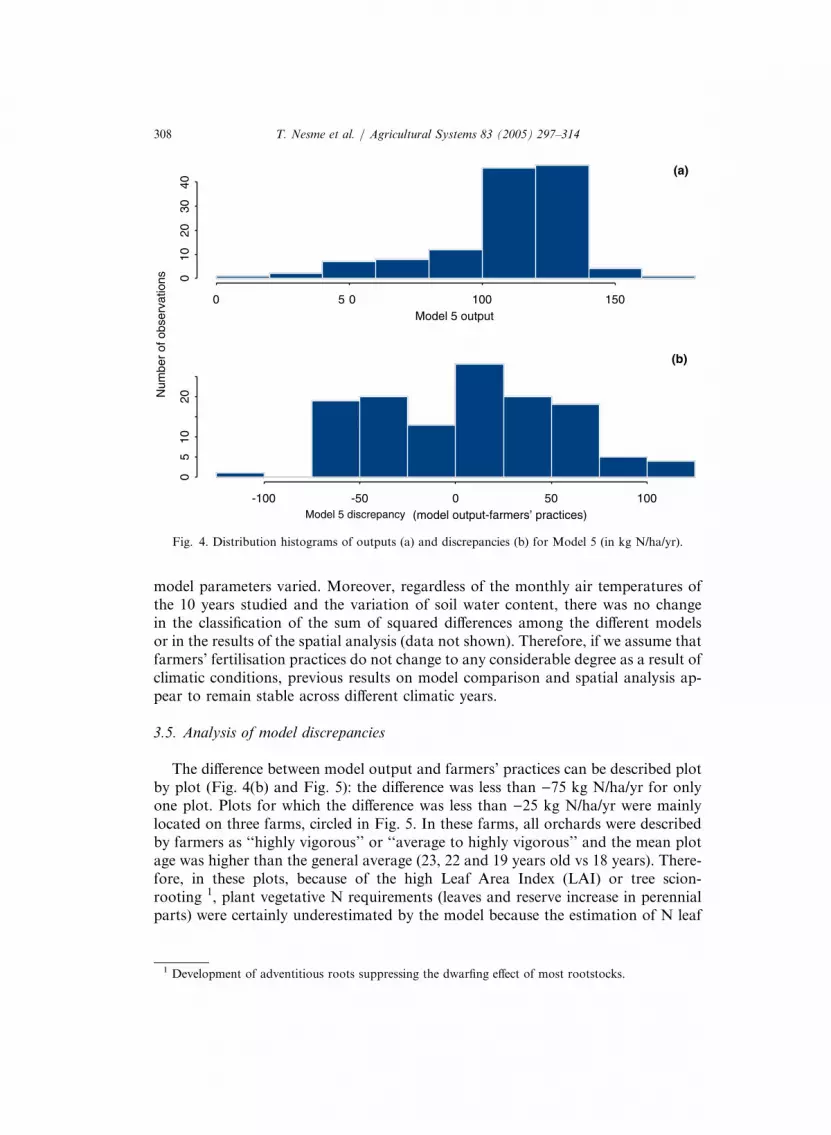
than 15 kg N/ha/yr). Distribution histograms of Model 5 output and discrepancies

are given in Fig. 4. Model 5 output ranged from 1 to 166 kg N/ha/yr, with a meanat 109 kg N/ha/yr. Most values of Model 5 output lay between 100 and 140 kg N/ha/

yr, which is the standard range of recommended fertilisation (Soing, 1999). Model 5

discrepancy was more variable, ranging from )110 to +103 kg N/ha/yr, with mean

and standard deviation at 6 and 47 kg N/ha/yr, respectively. Most values of Model

5 discrepancy lay between )75 and +75 kg N/ha/yr.

3.3. Spatial analysis

The spatial distribution of Model 5 discrepancy is presented in Fig. 5. The corre-

logram showed a strong spatial organisation of model discrepancies (P < 0:001)

300 350 400 450 500 550

010

025

0

Sum of squared differences for Model 3 (x1000)

Pop

ulat

ion

size

300 350 400 450 500 550

010

025

0


Pop

ulat

ion

size

300 350 400 450 500 550

010

025

0


Pop

ulat

ion

size

Fig. 3. Frequency histograms of the sum of squared differences (kg2 N/ha2/yr2) obtained from randomly

distributed fertilisation practices (Monte Carlo method). The arrows indicate the observed sum of squared

differences (i.e. obtained with the observed fertilisation practice distribution).


when the analysis was conducted with 10 classes of 1.5 km width with a maximum

statistic distance dm of either 9 or 15 km. The three groups of plots with values be-

tween )75 and )25 kg N/ha/yr located in the south of the area seemed to be respon-

sible of the spatial organisation of model discrepancy. They correspond to three

farms and are circled in Fig. 5. Indeed, when all these plots were removed from

the dataset, the spatial organisation disappeared, whereas when the plots of any of

the three farms were removed, the spatial organisation was not altered. Model 5 dis-

crepancies were particularly homogeneous within and among the three farms. Fortwo farms, this was because of similar N fertilisation on all plots and homogeneous

cropping systems and soil conditions (all plots were situated on reducti-redoxisol for

one farm and on hydromorphic fluviosol for the other) leading to homogeneous

model outputs. On the other hand, for the third farm (located in the south–west

of the area), soil, cropping systems and fertilisation practices varied but led to rather

homogeneous model discrepancies.

3.4. Model sensitivity analysis

The classification of models according to the sum of squared differences between

model output and farmers’ practices did not change when soil characteristics and

0 5 0 100 150

010

2030

40

Model 5 output

-100 -50 0 50 100

05

1020

Model 5 deviation (model output-farmers’ practices)

(a)

(b)

Num

ber

of o

bser

vatio

ns

Model 5 discrepancy

Fig. 4. Distribution histograms of outputs (a) and discrepancies (b) for Model 5 (in kg N/ha/yr).


model parameters varied. Moreover, regardless of the monthly air temperatures of

the 10 years studied and the variation of soil water content, there was no changein the classification of the sum of squared differences among the different models

or in the results of the spatial analysis (data not shown). Therefore, if we assume that

farmers’ fertilisation practices do not change to any considerable degree as a result of

climatic conditions, previous results on model comparison and spatial analysis ap-

pear to remain stable across different climatic years.

3.5. Analysis of model discrepancies

The difference between model output and farmers’ practices can be described plot

by plot (Fig. 4(b) and Fig. 5): the difference was less than )75 kg N/ha/yr for only

one plot. Plots for which the difference was less than )25 kg N/ha/yr were mainly

located on three farms, circled in Fig. 5. In these farms, all orchards were described

by farmers as ‘‘highly vigorous’’ or ‘‘average to highly vigorous’’ and the mean plot

age was higher than the general average (23, 22 and 19 years old vs 18 years). There-

fore, in these plots, because of the high Leaf Area Index (LAI) or tree scion-

rooting 1, plant vegetative N requirements (leaves and reserve increase in perennialparts) were certainly underestimated by the model because the estimation of N leaf

1 Development of adventitious roots suppressing the dwarfing effect of most rootstocks.

Fig. 5. Spatial representation of classes of differences between Model 5 output and farmers’ fertilisa-

tion practices (one symbol per plot, in kg N/ha/yr). The three big circles encompass the plots of three

farms.


uptake was based on small, young trees (see Section 2.1). Thus, the corresponding

model output should have been greater. It is possible that the farmers’ fertilisation

levels were high in these plots because the overall objective of the N fertilisation

might have been to satisfy plant N demand and to suit tree vigour. To determine

their fertilisation level, farmers may use indicators based on crop observation (Gras

et al., 1989), which are integrative variables reflecting the N status of the crop. Ac-

cording to informal discussions with farmers, orchard vigour seems to be the most

commonly used indicator. Plots for which the difference was greater than )25 andless than +25 kg N/ha/yr were owned mainly by farmers whose technical level was

considered to be good by the co-operative extension officer. Plots for which the dif-

ference was greater than 25 and less than 75 kg N/ha/yr were mainly young orchards.

In these plots, plant N requirement might have been overestimated by the model be-

cause of low N leaf or crop uptake. Thus, model output should probably have been

lower. Finally, plots for which the difference was greater than 75 kg N/ha/yr were

either young plots or plots that did not receive any fertilisation. Indeed, for three

of the nine plots, no fertilisation was applied by farmers to reduce production costs.In those cases and for the studied year, production was apparently not indicative of

crop N requirement for farmers.


4. Discussion

4.1. Model accuracy

The equations describing all soil N processes (except plant uptake) used in thisstudy have been widely applied and validated (Jeuffroy and Recous, 1999; Mey-

nard et al., 1981; R�emy, 1981). Moreover, equations related to crop residue min-

eralisation, soil organic matter mineralisation and denitrification have been

adapted and integrated into the Stics N dynamics and balance model (Brisson

et al., 1998), recently validated for annual crops (Brisson et al., 2002). Model

5, which was the best of the five models used here to account for farmers’ fertil-

isation practices, accurately represents state-of-the-art N balance modelling. How-

ever, some improvements could be made, particularly related to orchard Nuptake estimation. Indeed, we can assume that N reserve increase in perennial

parts may vary between trees, depending on age, tree shape and vigour, root-

stock, variety, cropping conditions, etc. Leaf mass may also vary considerably be-

tween plots, depending on age, tree shape and vigour and pruning practices.

Unfortunately, to our knowledge, there is no available method to estimate whole

tree N requirements that take these plot characteristics into account. We were

therefore, unable to take this variability into consideration. Such a method would

also be useful to estimate crop residues such as leaves and pruning wood andthus to quantify residue mineralisation.

4.2. Comparison of model outputs and fertilisation practices: interpretation of farmers’

indicators

The more complex the model, the better the agreement between farmers’ fertilisa-

tion practices and model output, in general. This result suggests that both the farmer

and the agronomic model take similar account of the initial state of the soil, plantuptake and bio-physical processes (mineralisation, atmospheric deposition, denitrifi-

cation and N supply by irrigation). However, farmers, when interviewed, do not ex-

plicitly refer to these states and processes but instead emphasize the role of tree

growth rate and tree vigour to determine the amount of N fertiliser that they use.

Tree growth rate and tree vigour are recognised as being sensitive to plant N status

(Huett, 1996; Weinbaum et al., 1992) and strongly dependant on the timing of N fer-

tilisation (Lobit et al., 2001). Vigour is a widely used indicator for horticultural crop

management by farmers (Navarrete et al., 1997). Farmers make an integrative obser-vation of this variable: as a function of time (both within and between seasons) and

as a function of space (on the whole tree and the whole plot). Because of its N sen-

sitivity, vigour may reflect the balance between plant requirement and soil N supply.

It may be the reason why farmer practices and recommendations by agronomists

were not significantly different, in general. However, there is a need to define pre-

cisely what apple tree vigour consists of and how it can be measured. It may never-

theless be difficult to summarise such a complex criterion by means of a single plant

variable (Navarrete et al., 1997). There is also a need to evaluate the N sensitivity of


tree vigour to know whether it can be used by agriculture extension services as a rel-

evant decision-support tool.

4.3. Individual and collective comparison of model discrepancy

The spatial analysis showed strong spatial correlation which seemed to be due to

close values of Model 5 discrepancy within and among the three farms located in the

south of the study area. Within-farm homogeneity suggests the existence of an over-

all fertilisation pattern for each farmer. A new study could be undertaken to deter-

mine whether this farm model discrepancy was due to biophysical processes that was

not included in the model, to farm characteristics or to farmer effects. Questions are

also raised about the way a farmer may adapt the N fertilisation to different soils,

plant uptake, orchard vigour or varieties. Does the farmer have some reference plotsor trees that are used specifically to make fertilisation decisions (Aubry, 1995)? The

analysis of model discrepancy could be the basis for an interview with the farmer

about fertilisation management.

Spatial homogeneity of Model 5 discrepancies between farms located in the south

of the area means that the plots belonging to these farms were managed with the

same fertilisation pattern by different farmers. Other studies are necessary to identify

the reasons for such similar patterns. This phenomenon may be due to the local in-

fluence of an extension officer or the existence of social relationships between farmersexchanging technical knowledge among themselves. Indeed, farmers who are inte-

grated into a historical and social context may share of their common elements of

knowledge and decision making (Darr�e, 1999).

4.4. Different perspectives on model discrepancy

The differences between model outputs and farmers’ practices can be used in two

ways. First, it is an indicator of the farmer’s fertilisation pattern: it corresponds to

the amount of N (positive or negative) that the farmer judges necessary to apply

to the orchard when estimated soil flows and plant requirements are removed. This

raises various questions requiring further investigation: does the farmer want to re-

duce (positive discrepancy) or increase (negative discrepancy) tree vigour? Does heconsider N fertilisation to be a key practice for tree management? Sebillotte (1990)

proposed to define a cropping system as a group of plots treated in a homogeneous

way, characterised by the nature of the crop and the crop management applied. We

think model discrepancy may help to identify plots treated in a homogeneous way

for N fertilisation. Therefore, it could be used to help identify farmers’ cropping sys-

tems not only on the basis of fertilisation practices but also on the basis of fertilisa-

tion patterns. Second, model discrepancy can be understood as the estimation of

environmental risk for nitrogen: if it is negative, the plot is over-fertilised and thesurplus may contribute to tree storage, N leaching, soil mineral N enrichment or

N atmospheric emission. When coupled with a water flow simulation model, and

taking spatial distribution of practices into account, model discrepancy could form


the basis of an estimate of the global environmental risk in a small agricultural re-

gion (Beaujouan et al., 2001).

5. Conclusion

This study has demonstrated that agronomic models can be helpful in analysing

farmers’ fertilisation practices and formulating questions about key elements that de-

termine the practices, decision rules and indicators used by farmers. Comparison of

model outputs with farmers’ practices can contribute to the identification of plots on

which the farmer makes decisions, and sets priorities. This raises questions concern-

ing agricultural research at the interface between the biophysical and social sciences

related to sources of knowledge and local social influences.This study has also identified some issues concerning the design and use of agro-

nomic models. If models are a way of formalising agronomic knowledge and identi-

fying gaps in knowledge, they also appear to be a way of studying farmers’ practices.

This is one step towards the integration of actual farmers’ practices and biophysical

modelling.

Acknowledgements

We thank Georges Fandos for his help with data collection and the farmers who

responded to the survey. This work was funded by the nationwide INRA programme

on Integrated Fruit Production ‘‘Action Transversale 67, Production Fruiti�ere In-

t�egr�ee’’. We also thank two anonymous reviewers for their comments, which greatly

improved the manuscript.

References

Arnal, H., 1984. Carte p�edologique de France �a 1/100 000. Feuille de Montpellier (M-22). Notice

explicative. INRA, Orl�eans.

Atkinson, D., 1980. The distribution and effectiveness of the roots of tree crops. Hortic. Rev., 424–490.

Atkinson, D., Wilson, S.A., 1980. The growth and distribution of fruit tree roots: some consequences for

nutrient uptake. Acta Hort. 92, 137–151.

Aubry, C., 1995. Gestion de la sole d’une culture dans l’exploitation agricole. Cas du bl�e d’hiver en grande

culture dans la r�egion picarde. Ph.D. Thesis, Institut National Agronomique Paris-Grignon, Paris, p.

271.

Aubry, C., Papy, F., Capillon, A., 1998. Modelling decision-making processes for annual crop

management. Agr. Syst. 56, 45–65.

Baize, D., Girard, M.-C., 1995. R�ef�erentiel p�edologique. INRA, Paris.

Beaujouan, V., Durand, P., Ruiz, L., 2001. Modelling the effect of the spatial distribution of agricultural

practices on nitrogen fluxes in rural catchments. Ecol. Model. 137, 93–105.

Bellon, S., Lescourret, F., Calmet, J.P., 2001. Characterisation of apple orchard management systems in a

French Mediterranean Vulnerable Zone. Agronomie 21, 200–213.

Boiffin, J., K�eli Zagbahi, J., Sebillotte, M., 1986. Syst�emes de culture et statut organique des sols dans le

Noyonnais: application du mod�ele de H�enin-Dupuis. Agronomie 6, 437–446.


Brisson, N., Mary, B., Ripoche, D., Jeuffroy, M.-H., Ruget, F., Nicoullaud, B., Gate, P., Devienne-Baret,

F., Antonioletti, R., Durr, C., Richard, G., Beaudoin, N., Recous, S., Tayot, X., Pl�enet, D., Cellier, P.,

Machet, J.-M., Meynard, J.-M., Del�ecolle, R., 1998. STICS: a generic model for the simulation of

crops and their water and nitrogen balances. 1: theory and parametrization applied to wheat and corn.

Agronomie 18, 311–346.

Brisson, N., Ruget, F., Gate, P., Lorgeou, J., Nicoullaud, B., Tayot, X., Pl�enet, D., Jeuffroy, M.-H.,

Bouthier, A., Ripoche, D., Mary, B., Justes, E., 2002. STICS: a generic model for simulating crops and

their water and nitrogen balances. 2: model validation for wheat and maize. Agronomie 22, 69–92.

Cerf, M., 1994. Essai d’analyse psychologique des connaissances techniques et pratiques des agriculteurs:

application au raisonnement de l’implantation des betteraves sucri�eres. Ph.D. Thesis, University of

Paris VII, Paris, p. 274.

Cerf, M., Meynard, J.-M., 1989. Sur l’origine du hiatus entre les conseils techniques et les pratiques des

agriculteurs, r�esultats d’une enquete sur la fertilisation. In: Dodd, V.A., Grace, P.M. (Eds.),

Agricultural Engineering. Balkema, pp. 2925–2934.

Cerf, M., Papy, F., Angevin, F., 1998. Are farmers expert at identifying workable days for tillage?

Agronomie 18, 45–59.

Chazoule, C., Desplobins, G., 1999. Codification des techniques et relance des vari�et�es: le cas Cripps Pink

cov – Pink Lady. In: Domestiquer le v�eg�etal. INRA, Paris.

Darr�e, J.-P., 1999. La production de connaissance pour l’action. MSH/INRA, Paris.

DIREN. 1998. Nappe villafranchienne de Mauguio Lunel. Etude diagnostic de la pollution azot�ee.Rapport de synth�ese (1995–1997), Diren, Montpellier, p. 31+ annexes.

Dounias, I., Aubry, C., Capillon, A., 2002. Decision-making processes for crop management on African

farms. Modelling from a case study of cotton crops in northern Cameroon. Agr. Syst. 73, 233–260.

Fujisaka, S., 1993. Were farmers wrong in rejecting a recommendation. The case of nitrogen at

transplanting for irrigated rice. Agr. Syst. 43, 271–286.

Fujisaka, S., 1997. Research: help or hindrance to good farmers in high risk systems? Agr. Syst. 54, 137–

152.

Geertz, C., 1983. Local Knowledge. Further Essays in Interpretive Anthropology. Harper Collins, New

York.

Gras, R., Benoit, M., Deffontaines, J.P., Duru, M., Lafarge, M., Langlet, A., Osty, P.L., 1989. Le fait

technique en agronomie: activit�e agricole, concepts et m�ethodes d’�etude. L’Harmattan, Paris.

Habib, R., Nesme, T., Pl�enet, D., Lescourret, F., 2001. Data modelling for database design in apple

production monitoring systems for a producer organization. Acta Hort. 566, 477–482.

H�enault, C., 1993. Quantification de la d�enitrification dans les sols, �a l’�echelle de la parcelle cultiv�ee, �a

l’aide d’un mod�ele pr�evisionnel. Ph.D. Thesis, ENSA-M, Montpellier, p. 108.

H�enin, S., Dupuis, M., 1945. Essai de bilan de la mati�ere organique des sols. Ann. Agron. 15, 161–172.

Huett, D.O., 1996. Prospects for manipulating the vegetative-reproductive balance in horticultural crops

through nitrogen nutrition: a review. Aust. J. Agr. Res. 47, 47–66.

Jeuffroy, M.-H., Recous, S., 1999. Azodyn: a simple model simulating the date of nitrogen deficiency for

decision support in wheat fertilization. Eur. J. Agron. 10, 129–144.

Landais, E., Deffontaines, J.P., 1988. Les pratiques des agriculteurs: point de vue sur un courant nouveau

de la recherche agronomique. Etudes Rurales 109, 125–138.

Lauri, P.-E., Lespinasse, J.-M., 1999. Apple tree training in France: current concepts and practical

implications. Fruits 54, 441–449.

Lin�eres, M., Djackovitch, J., 1993. Caract�erisation de la stabilit�e biologique des apports organiques par

l’analyse biochimique. In: Decroux, J., Ignazi, J. (Eds.), Mati�eres organiques et agriculture, 4�emes

journ�ees de l’analyse de terre et 5�eme forum de la fertilisation raisonn�ee. Gemas-Comifer, Paris, pp.

159–168.

Lobit, P., Soing, P., G�enard, M., Habib, R., 2001. Effects of timing of nitrogen fertilization on shoot

development in peach (Prunus persica) trees. Tree Physiol. 20, 35–42.

Manly, B.F.J., 1991. Randomization and Monte Carlo Methods in Biology. Chapman & Hall, London.

Marqui�e, J.C., Cellier, J.M., 1983. Modifications du comportement d’exploration visuelle au cours du

temps dans une tache agricole. Le Travail humain 46, 121–134.


Mary, B., Gu�erif, J., 1994. Int�erets et limites des mod�eles de pr�evision de l’�evolution des mati�eres

organiques dans le sol. Cahiers Agr. 3, 247–257.

MathSoft, 1999. S-Plus 2000. Guide to statistics. MathSoft, Seattle.

Meynard, J.-M., Boiffin, J., Caneill, J., Sebillotte, M., 1981. Elaboration du rendement et fertilisation

azot�ee du bl�e d’hiver en Champagne Crayeuse. 2: Types de r�eponse �a la fumure azot�ee et application de

la m�ethode du bilan pr�evisionnel. Agronomie 1, 795–806.

Meynard, J.-M., Cerf, M., Guichard, L., Jeuffroy, M.-H., Makowski, D., 2002. Which decision support

tools for the environmental management of nitrogen? Agronomie 22, 817–829.

Meynard, J.-M., Dor�e, T., Habib, R., 2001. L’�evaluation et la conception de syst�emes de culture pour une

agriculture durable. CR Acad. Agr. Fr. 87, 223–236.

Navarrete, M., Jeannequin, B., Sebillotte, M., 1997. Vigour of greenhouse tomato plants (Lycopersicon

esculentum Mill.): analysis of the criteria used by growers and search for objective criteria. J. Hortic.

Sci. 72, 821–829.

Nesme, T., Lescourret, F., Bellon, S., Pl�enet, D., Habib, R., 2003. Relevance of orchard design issuing

from growers’ planting choices to study fruit tree cropping systems. Agronomie 23, 651–660.

ONF, 1999. Le flash RENECOFOR. Office National des Forets, Fontainebleau, p. 4.

Palmer, J.W., 1987. The measurement of leaf area in apple trees. J. Hortic. Sci. 62, 5–10.

Papy, F., 1998. Savoir pratique sur les syst�emes techniques et aide �a la d�ecision. Points de vue

d’agronomes. In: Biarn�es, A. (Ed.), La conduite du champ cultiv�e. Ortsom �editions, Paris, pp. 245–259.

Reganold, J.P., Glover, J.D., Andrews, P.K., Hinman, H.R., 2001. Sustainability of three apple

production systems. Nature 410, 926–929.

R�emy, J.C., 1981. Etat actuel et perspectives de la mise en oeuvre des techniques de pr�evision de la fumure

azot�ee. CR Acad. Agr. Fr. 10, 859–874.

R�emy, J.C., H�ebert, J., 1977. Le devenir des engrais azot�es dans le sol. CR Acad. Agr. Fr, 700–714.

R�emy, J.C., Marin Lafl�eche, A., 1974. L’analyse de terre: r�ealisation d’un programme d’interpr�etation

automatique. Ann. Agron. 20, 607–632.

Sanchez, E.E., Khemira, H., Sugar, D., Righetti, T.L., 1995. Nitrogen management in orchards. In:

Bacon, P.E. (Ed.), Nitrogen Fertilization in the Environment. Dekker, Sydney, pp. 327–380.

Sansavini, S., 1997. Integrated fruit production in Europe: research and strategies for a sustainable

industry. Sci. Hortic. 68, 25–36.

Sebillotte, M., 1978. Itin�eraires techniques et �evolution de la pens�ee agronomique. CR Acad. Agr. Fr. 64,

906–914.

Sebillotte, M., 1990. Syst�emes de culture, un concept op�eratoire pour les agronomes. In: Combe, L.,

Picard, D. (Eds.), Un point sur...sles syst�emes de culture. INRA, Versailles, pp. 165–196.

Sebillotte, M., Soler, L.-G., 1988. Le concept de mod�ele g�en�eral et la compr�ehension du comportement de

l’agriculteur. CR Acad. Agr. Fr. 74, 59–70.

Soing, P., 1999. Fertilisation des vergers, environnement et qualit�e. Ctifl, Paris.

Soulard, C.T., 1999. Les agriculteurs et la pollution des eaux. Proposition d’une g�eographie des pratiques.

Ph.D. Thesis, University of Paris I Panth�eon-Sorbonne, Paris, p. 359.Sprent, P., Ley, J.P., 1992. Pratique des statistiques non param�etriques. INRA, Paris.

Spring, J.L., Chapuis, P., Ev�equoz, C., Girardet, G., Ryser, J.P., Schmid, C., Terrettaz, R., Thentz, M.,

Vanetti, R., 1993. La fertilisation des arbres fruitiers, kiwis et des arbustes �a baies. Rev. Suisse Vitic.

Arboric. Hortic. 25, 189–199.

Trocme, S., Gras, R., 1964. Sol et fertilisation en arboriculture fruiti�ere. Perrin, GM, Paris.

Upton, G.J.G., Fingleton, B., 1985. Spatial Data Analysis by Example. Wiley, Suffolk.

Venables, W.N., Ripley, B.D., 1999. Modern Applied Statistics with S-Plus. Springer, New York.

Visser, J., 1983. Effect of the Ground Water Regime and Nitrogen Fertilizer on the Yield and Quality of

Apples. Ministerie van verkeer en waterstaat, Lelystad.

Weinbaum, S.A., Johnson, R.S., DeJong, T.M., 1992. Causes and consequences of overfertilization in

orchards. HortTechnology 2, 112–121.

are agronomic models useful for studying farmers' fertilisation practices?

Documents