World Applied Sciences Journal 35 (11): 2401-2413, 2017ISSN 1818-4952© IDOSI Publications, 2017DOI: 10.5829/idosi.wasj.2017.2401.2413

Corresponding Author: R.O. Aja, Department of Mathematic, College of Physical and Applied Sciences,Michael Okpara University of Agriculture, Umudike, Nigeria.

2401

Application of Project Evaluation, Review Technique and Critical Path Method (PERT-CPM) Model in Monitoring Building Construction

R.O. Aja and W.I.E. Chukwu1 2

Department of Mathematic, College of Physical and Applied Sciences,1

Michael Okpara University of Agriculture, Umudike, NigeriaDepartment of Industrial Mathematics and Applied Statistics,2

Faculty of Physical Sciences, Ebonyi State University, Abakaliki, Nigeria

Abstract: The need to control large-scale projects cannot be over emphasized, especially in constructioncompanies that face numerous challenges. A tool for monitoring and controlling projects is the ProjectEvaluation and Review Technique -Critical Path Method (PERT-CPM). In this paper, PERT-CPM model wasapplied in monitoring the construction of a five bed-rooms duplex building. Activities of the building projectconsidered in this study were translated to a network diagram. Critical activities were identified. The activitytimes were observed to have been Weibully distributed. Tchebyshev’s inequality method was used to calculatethe lower and upper bound estimates in days for critical activities of the project. The overall time for thecompletion of the Building was obtained. The probability of completing the project in a given time wasobtained. The PERT-CPM method applied in this study reduced the actual time the company spent in executingthe entire project by 97 days and this has a serious implication on the profit margin for the Company.

Key words: Critical path Method Project Evaluation and Review Technique Building constructionMonitoring Weibull distribution Tchebyshev’s inequality

INTRODUCTION scheduling and coordination of numerous interrelated

Residential and non-residential buildings are completion of large building projects made up of smallerstructures, which serve as shelters for man, his properties tasks some of which can be started straight away whileand activities. So, building projects must be properly some need to await the completion of other activities orplanned, designed and erected to obtain desired can be done in parallel before they eventually commencesatisfaction from the environment. Such building project as observed by [2]. The task of planning, scheduling (orinvolves a single non-representative scheme typically organizing) and control are considered to be basicundertaken to accomplish a premeditated result within a managerial functions and CPM-PERT has been rightfullytime bound and financial plan. However, because of the accorded due importance in the literature of Operationsindividuality of each project, its outcome can never be Research and Quantitative Analysis for handling thepredicted with an absolute confidence as observed by [1]. planning, scheduling and control of building

The management of large-scale project of projects.Hence, the goal of CPM-PERT and relatedconstructing a five bed room building project poses techniques is to facilitate the management, coordinationnumerous challenges. These challenges have led to and control of the various activities involved in a projectwidespread use of project management techniques such so that the project itself may be completed successfullyas Critical Path Method (CPM) and PERT (Project because PERT-CPM can answer the following importantEvaluation and Review Technique). These project questions: How long will the entire project take to bemanagement techniques provide managers with a completed? What are the risks involved? Which are thesystematic quantitative framework for planning, critical activities or tasks in the project which could delay

activities associated with the successful on-time

World Appl. Sci. J., 35 (11): 2401-2413, 2017

2402

the entire project if they were not completed on time? Is activity takes in the completion of the entire project. PERTthe project on schedule, behind schedule or ahead ofschedule? If the project has to be finished earlier thanplanned, what is the best way to do this at the least cost?The questions posed above are answered by CPM-PERTby structuring the activities of the building constructionwork into a network and examining the time requirementsand precedence relationships associated with theactivities as observed in [3].

It is pertinent to observe that PERT-CPM provided afocus around which managers could brain-storm and puttheir ideas together. It has been demonstrated that it is agreat communication medium by which thinkers andplanners at one level could communicate their ideas, theirdoubts and fears to another level and so it is mostimportantly a useful tool for evaluating the performanceof individuals and teams in a project. There are manyvariations of CPM-PERT which have been useful inplanning costing, scheduling manpower and machinetime. [4], studied project planning and scheduling usingPERT and CPM techniques with linear programming. Heinvestigated the trade-off between the cost and minimumexpected time that will be required to complete a buildingproject and observed that the use of CPM-PERT reducedthe time for the building construction from 79 days to 40days which is very substantial but this increased the costof the building project.

When the activity times in the projects aredeterministic and known, Critical Path Method (CPM), amathematically ordered network for planning andscheduling project has been demonstrated to be a usefultool in managing such projects in an efficient manner tomeet the challenge of meeting dead-lines in projectexecution. It has been used extensively in projectmanagement because of its simplicity and for easyidentification of critical activities in the system. CPM isalso applied in computation of project duration byidentifying sequence of activities that must not bedelayed in execution of the project if the dead-lines mustbe met. The critical path is obtained by computing earlystart and finish times using a forward-pass algorithm whilelate start and finish time are computed using a backwardpass algorithm.

However, there are many cases where the activitytimes may not be presented in a precise manner, suchproblems have been demonstrated by researchers to besolved using the Project Evaluation and ReviewTechnique which is based on the probability theory.Project Evaluation and Review Technique (PERT)emphasizes the relationship between the time each

is a technique involving three estimates. These estimatesare identified as Optimistic, most likely and Pessimisticand are made for each activity of the overall project. Theoptimistic time estimate is the minimum time the activitywill take by assuming that everything surrounding theexecution of the project goes right the first time. Thereverse is the pessimistic estimate, or maximum timeestimate for completing the activity. The third is the mostlikely estimate or the normal or realistic time an activityrequires. PERT was developed in 1958 by a research teamto help measure and control the progress of the U.S.ANavy’s Polaris Fleet Ballistic Missile Program [5]. PERTwas introduced to complement CPM by incorporating aprobabilistic concept for modeling activity durationsthrough estimating the uncertainty in a project networkand by computing the probability to complete the projectwithin a specified time.

In real life practice PERT-CPM has been frequentlyused for planning, managing and controlling projects inareas such as research projects, road construction,building construction, software development, productdevelopment, construction and plant maintenance,various engineering practices among others. Thetechniques have exceptionally wide applications and theirapplications have contributed significantly to betterplanning, control and general organization of manyprojects. Construction companies which always have anumber of construction works awarded to them oncontract by the public sector or private and individualsface lots of challenges like varying cost of materials,mechanical breakdown, power failure, strike, water failureetc. Because of these challenges mentioned above, thisstudy applied Tchebyshev’s approach to obtain the lowerbound and upper bound probability of completing criticalactivities of the project under consideration becauseproject schedules change on a regular basis. PERT-CPMallows continuous monitoring of the schedule andthereby helps project managers track the critical activitiesin their projects. The time taken to execute these criticalactivities guide in determining the length of time the non-critical activities can be delayed within the total floatperiod so that the duration of the construction target willstill be met. The trend in recent years has been to mergethe two methods- PERT and CPM into what is called thePERT-CPM approach.

This study therefore applied PERT-CPM approach toidentify the critical activities that could delay completionof a building construction, duration of the entire projectactivities and the probability of meeting specifieddeadlines in the construction of five bed-room duplex.

2a+ß

2a+ß

2a+ß

( ) 2 2 43 6

m mE T or+ + + +

= =

2

26

i ii

− =

2 2c i=∑ 2

c i= ∑

World Appl. Sci. J., 35 (11): 2401-2413, 2017

2403

MATERIAL AND METHODS is assumed to enclose every possible estimates of the

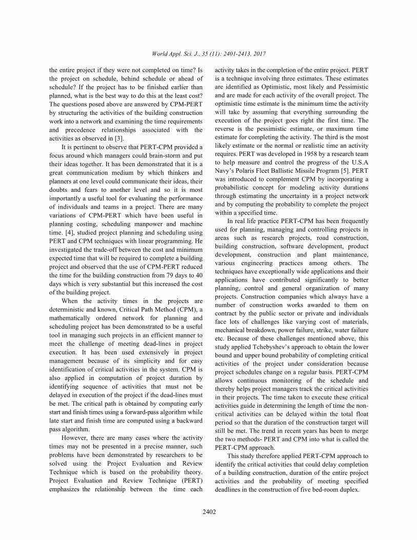
Study Location and Data Description: In order to estimate must lie somewhere in the range ( , ). Thatschedule the activities in the network we require an is, the most likely time (m) estimate may coincide withestimate of how much time each activity should take whenit is done in the normal way. These estimates as providedby the project manager of Fenlands Associates Limited,a construction company based in Port-hercourt Nigeria.Table 1 shows the break down description of activitiesinvolved and the respective precedence relationship ofthe activities for the construction process of a 5-bed roomduplex at No. 6, King Perekule Road, GRA Phase 1 Port-Harcourt, Rivers State Nigeria The construction activitybegins with activity 1 and ends with activity 65. Thenetwork analysis technique applied in analyzing the dataare the critical path method (CPM) and project evaluationreview technique (PERT). Traditionally Beta distributionis applied in using PERT in analyzing network problem butin this work we observed that Weibull distribution whichdoes not require approximation of the mean and variancedoes better than the Beta distribution. Since the Weibullprobability distribution can usually accommodate longerright tail probability than the Beta probability distribution.Furthermore, since Weibull probability distribution iscontinuous, has a finite endpoint, defined mode betweenits endpoints and it is capable of describing both skewedand symmetric activity time distribution as observed in[6]. In view of this, the Weilbull Distribution functionoffers an accurate and more realistic description ofdistribution phenomena.

Fig. 1: An Example of Weibull Distribution

The three estimates of time required are:

1. Optimistic time denoted by 2. Pessimistic time denoted by 3. Most likely time denoted by m

According to [7], the range specified by theoptimistic time ( ) and pessimistic time ( ) estimates

duration of the activity. The most likely time (m)

the midpoint . Hence, we assume that the

duration of each activity follows a Weibulldistribution with its uni-modal point occurring at mand its end points at and .

4. In Weibull distribution, the midpoint is

assumed to weigh half as much as the most likelypoint (m). Thus, the expected or mean {E(T) or µ}time of an activity, that is also the weighted averageof the time estimates, is computed as the arithmeticmean of and 2m. That is, expected time to

complete an activity is approximated

. With uncertain

activity time, variance can be used to describedispersion (variation) in the activity timevalues. The calculations are based on theanalogy to the normal distribution where 99% ofarea under the normal curve is within ±3 from themean or fall within the range approximately 6standard deviation in length, therefore the interval( , ) is assumed to enclose about 6 standarddeviations of a symmetric distribution. Thus if i

denotes the standard deviation of the duration ofactivity i, then

5. So, the variance of the activity time is

6. If we assume that the deviation of the activities areindependent random variables, then the variance ofthe total critical path’s duration is the sum of thevariances on the critical path. Suppose is thec

standard deviation of the critical path, thenand where i is an element on

the critical path.

Upper Bound and Lower Bound of a Set of Real Numbers:The understanding of upper bound and lower bound of aset of real numbers is needed since its application isinevitable in this section.

World Appl. Sci. J., 35 (11): 2401-2413, 2017

2404

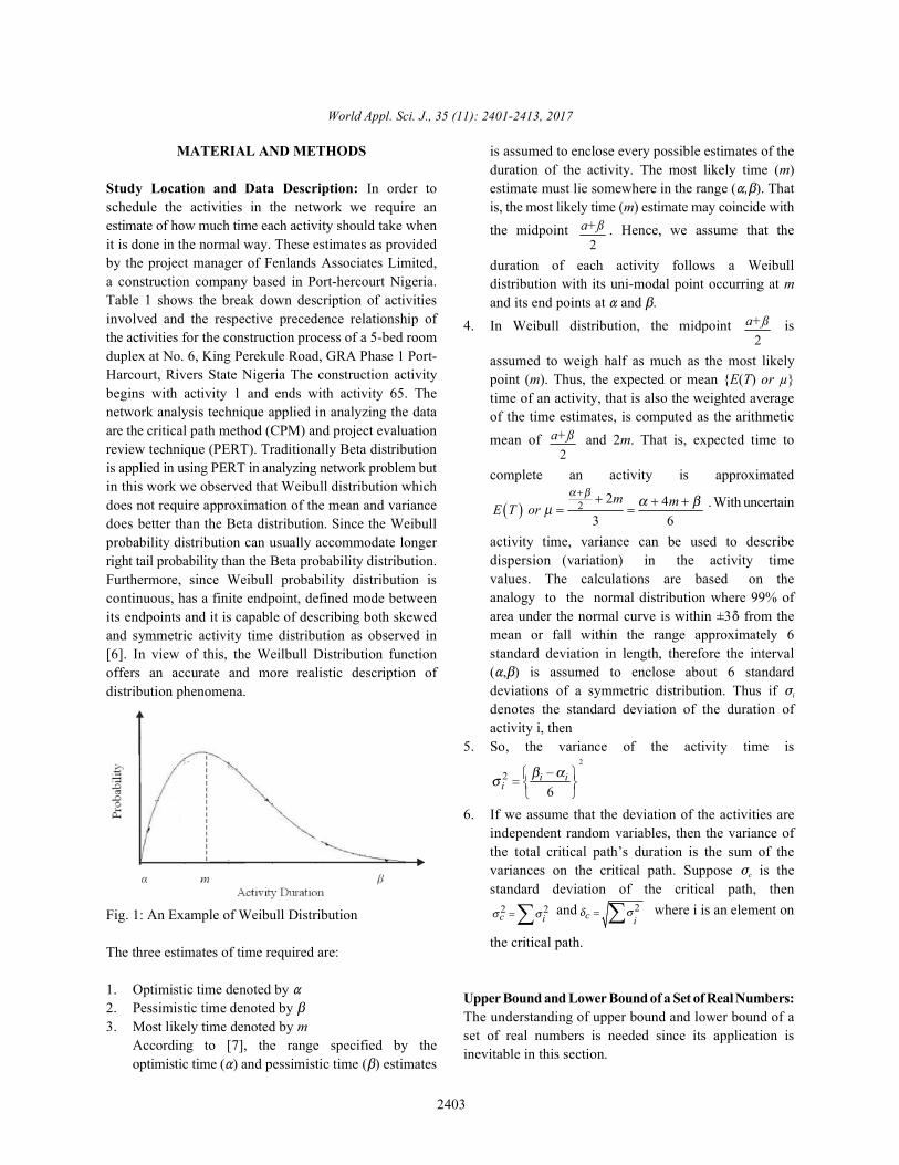
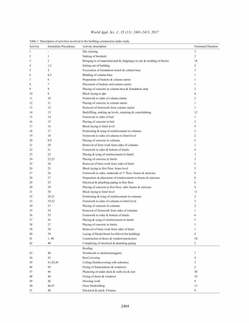
Table 1: Description of activities involved in the building construction under study

Activity Immediate Precedence Activity description Estimated Duration

1 - Site clearing 32 1 Sinking of borehole 23 2 Bringing in of materials(sand & chippings) to site & molding of blocks 184 1,3 Setting out of building 25 4 Excavation of foundation trench & column base 36 4,5 Blinding of column base 17 6 Preparation of baskets & column starter 18 7 Placement of baskets and column starter 19 8 Placing of concrete in column base & foundation strip 210 8 Block laying to dpc 411 10 Formwork to sides of column starter 212 11 Placing of concrete in column starter 113 12 Removal of formwork from column starter 114 13 Backfilling, making up levels, ramming & consolidating 1215 14 Formwork to sides of bed 116 15 Placing of concrete in bed 217 16 Block laying to lintel level 918 17 Positioning & tying of reinforcement in columns 219 18 Formwork to sides of columns to lintel level 220 8,9 Placing of concrete in columns 221 20 Removal of form work from sides of columns 122 21 Formwork to sides & bottom of lintels 423 22 Placing & tying of reinforcement in lintels 324 22,23 Placing of concrete in lintels 325 24 Removal of form work from sides of lintel 226 25 Block laying to first floor, beam level 527 26 Formwork to sides, underside of 1 floor, beams & staircase 9st

28 27 Preparation & placement of reinforcement in beams & staircase 829 25 Electrical & plumbing piping in first floor 630 29 Placing of concrete in first floor, slab, beams & staircase 431 30 Block laying to lintel level 1132 28,31 Positioning & tying of reinforcement in columns 233 19,32 Formwork to sides of columns to lintel level 334 33 Placing of concrete in columns 235 34 Removal of formwork from sides of columns 136 35 Formwork to sides & bottom of lintels 437 36 Placing & tying of reinforcement in lintels 338 37 Placing of concrete in lintels 339 38 Removal of form work from sides of lintel 140 39 Laying of blocks/beam level(level the building) 441 1, 40 Construction of doors & windows/protectors 1042 40 Completing of electrical & plumbing piping 2

Roofing43 40 Woodwork or skeleton(noggins) 744 43 Roof covering 445 41,42,44 Ceiling finish(covering with asbestos) 346 45 Fixing of frames(doors & windows) 247 46 Plastering of under deck & walls (in & out) 3048 46 Fixing of doors & windows 1049 46 Dressing work 850 46,47 Floor finish/tilling 1351 48 Electrical & mech. Fixtures 9

{ ( )}{ ( ) } E u xP u x cc

≥ ≤

World Appl. Sci. J., 35 (11): 2401-2413, 2017

2405

Table 1: Continued

Activity Immediate Precedence Activity description Estimated Duration

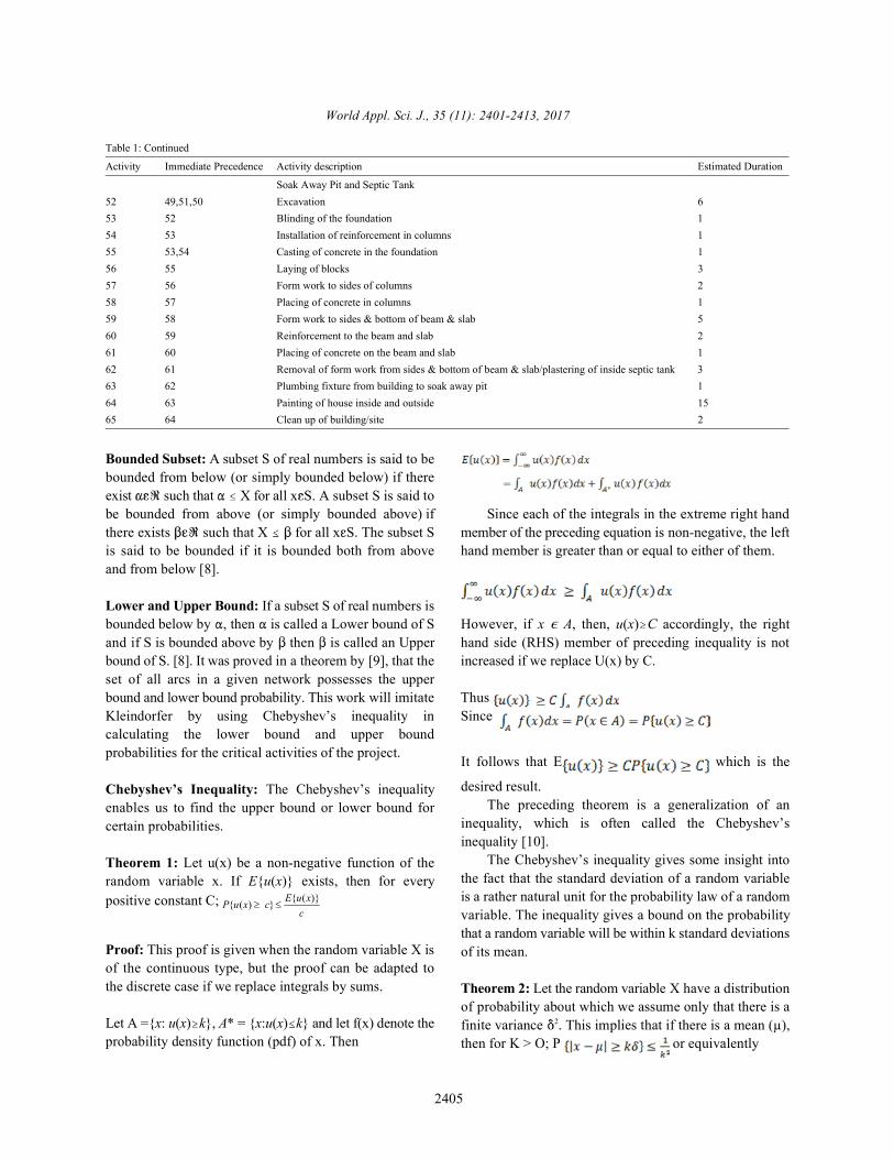
Soak Away Pit and Septic Tank 52 49,51,50 Excavation 653 52 Blinding of the foundation 154 53 Installation of reinforcement in columns 155 53,54 Casting of concrete in the foundation 156 55 Laying of blocks 357 56 Form work to sides of columns 258 57 Placing of concrete in columns 159 58 Form work to sides & bottom of beam & slab 560 59 Reinforcement to the beam and slab 261 60 Placing of concrete on the beam and slab 162 61 Removal of form work from sides & bottom of beam & slab/plastering of inside septic tank 363 62 Plumbing fixture from building to soak away pit 164 63 Painting of house inside and outside 1565 64 Clean up of building/site 2

Bounded Subset: A subset S of real numbers is said to bebounded from below (or simply bounded below) if thereexist such that X for all x S. A subset S is said tobe bounded from above (or simply bounded above) if Since each of the integrals in the extreme right handthere exists such that X for all x S. The subset S member of the preceding equation is non-negative, the leftis said to be bounded if it is bounded both from above hand member is greater than or equal to either of them. and from below [8].

Lower and Upper Bound: If a subset S of real numbers isbounded below by , then is called a Lower bound of S However, if x A, then, u(x) C accordingly, the rightand if S is bounded above by then is called an Upper hand side (RHS) member of preceding inequality is notbound of S. [8]. It was proved in a theorem by [9], that the increased if we replace U(x) by C.set of all arcs in a given network possesses the upperbound and lower bound probability. This work will imitate ThusKleindorfer by using Chebyshev’s inequality in Sincecalculating the lower bound and upper boundprobabilities for the critical activities of the project.

Chebyshev’s Inequality: The Chebyshev’s inequalityenables us to find the upper bound or lower bound forcertain probabilities.

Theorem 1: Let u(x) be a non-negative function of therandom variable x. If E{u(x)} exists, then for everypositive constant C;

Proof: This proof is given when the random variable X isof the continuous type, but the proof can be adapted tothe discrete case if we replace integrals by sums.

Let A ={x: u(x) k}, A* = {x:u(x) k} and let f(x) denote theprobability density function (pdf) of x. Then

It follows that E which is the

desired result.The preceding theorem is a generalization of an

inequality, which is often called the Chebyshev’sinequality [10].

The Chebyshev’s inequality gives some insight intothe fact that the standard deviation of a random variableis a rather natural unit for the probability law of a randomvariable. The inequality gives a bound on the probabilitythat a random variable will be within k standard deviationsof its mean.

Theorem 2: Let the random variable X have a distributionof probability about which we assume only that there is afinite variance . This implies that if there is a mean (µ),2

then for K > O; P or equivalently

( )1

expx xf x− = −

( ) ( )exp /R x x = −

11mod 1 for 1M e

= = − >

011mean x

= = + Γ +

22 2 2 11 1

= Γ + − Γ +

( ) 4 or 6mE T + +

=6

i ii−

=

World Appl. Sci. J., 35 (11): 2401-2413, 2017

2406

P time is computed with the formula Lt = minimum (LT + t ).

Proof: From theorem 1, let u(x) = (x – µ) and C = k2 2 2

Replacing them, we now have

P

Since the numerator of the RHS of the inequality is This2

implies that which is our desired result [10].2

The Weibull probability density function, reliability,mode, variance and mean formula are given in equations(1) -(5) from [11].

(1)

(2)

(3)

(4)

(5)

where is the shape parameter, is the scale parameter, is the gamma function and x shifts the mean on the x-0

axis. The addition of a threshold value does not changethe basic shape of the distribution, only its location onthe x-axis is affected..

Data presentation: Table 1 shows the break downdescription of activities involved and the respectiveprecedence relationship of the activities for theconstruction process of a 5-bed room duplex at No. 6,King Perekule Road, GRA Phase 1 Port-Harcourt, RiversState Nigeria. The construction activity starts withactivity 1 and ends with activity 65 as shown in Table 1:The Earliest Occurrence Time and Latest Occurrence Timefor All the Activities of the Project are shown in Table 2.These earliest occurrence time and latest occurrence timeof each activity was computed using the forward pass andbackward pass procedure. The forward pass is obtainedwith the formula ET = Muximum (ET + t ) while the Latestj i jj

j i jj

The optimistic estimate ( ), most likely estimate (m) andpessimistic estimate ( ) of the building were determined tosee the estimates as they effect the constructionactivities. The expected time (mean) µ and the standarddeviation for each activity was calculated using thefollowing formulas and

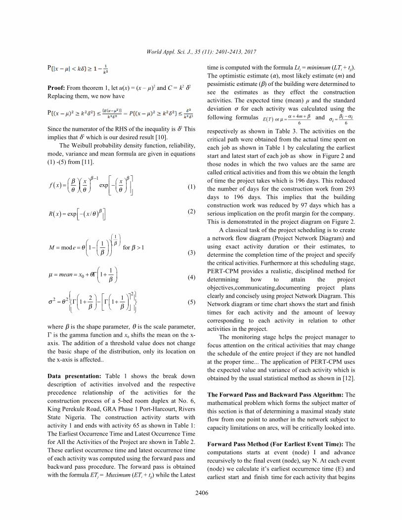
respectively as shown in Table 3. The activities on thecritical path were obtained from the actual time spent oneach job as shown in Table 1 by calculating the earlieststart and latest start of each job as show in Figure 2 andthose nodes in which the two values are the same arecalled critical activities and from this we obtain the lengthof time the project takes which is 196 days. This reducedthe number of days for the construction work from 293days to 196 days. This implies that the buildingconstruction work was reduced by 97 days which has aserious implication on the profit margin for the company.This is demonstrated in the project diagram on Figure 2.

A classical task of the project scheduling is to createa network flow diagram (Project Network Diagram) andusing exact activity duration or their estimates, todetermine the completion time of the project and specifythe critical activities. Furthermore at this scheduling stage,PERT-CPM provides a realistic, disciplined method fordetermining how to attain the projectobjectives,communicating,documenting project plansclearly and concisely using project Network Diagram. ThisNetwork diagram or time chart shows the start and finishtimes for each activity and the amount of leewaycorresponding to each activity in relation to otheractivities in the project.

The monitoring stage helps the project manager tofocus attention on the critical activities that may changethe schedule of the entire project if they are not handledat the proper time... The application of PERT-CPM usesthe expected value and variance of each activity which isobtained by the usual statistical method as shown in [12].

The Forward Pass and Backward Pass Algorithm: Themathematical problem which forms the subject matter ofthis section is that of determining a maximal steady stateflow from one point to another in the network subject tocapacity limitations on arcs, will be critically looked into.

Forward Pass Method (For Earliest Event Time): Thecomputations starts at event (node) I and advancerecursively to the final event (node), say N. At each event(node) we calculate it’s earliest occurrence time (E) andearliest start and finish time for each activity that begins

85,85

36

82,82

37 38

88, 88

39

89, 89107, 107

41

43

45

44

42

103, 107

104, 104

95, 107

40

3

23,23

2

5, ,5

0,0

3,3

25,25

5

6

7

28, 28

29,29

30,30

18

0

31,31 9

20

33,33

35,35

21

36,36

22

40,40

23

43,43

24

46,46

16

54,62

10

35,43

11

37,45

12

38,46

13

39,47

14

51,59

15

52,60

69,72

29

26

17

3031

32

27 2833

1819

34 35

54,,57

58,61

72,72

77,7778,78

75,7553,53

62,62

70,70

63,71 65,7367,75

25 48,48

0

4

1 41 0

1

12 1 2

9

2

5

6

9 8

2

411 0

3

2 2

0

21

4

3 3 1 4

0

10

2

74

3

0

0

2

1

100, 100

93, 93

1 17 , 1 5 8

1 19 ,1 49

5 0

4 6 5 2

4 85 1

4 9

53

5 4

5 5

5 7

1 09 ,1 09

1 39 ,1 39

1 52 ,1 52

1 5 8 , 15 8

1 28 ,1 58

1 5 9 , 1 5 9

1 6 1 , 1 6 1

1 60 ,1 60

16 6, 16 6

4 7

194, 1 94

6 36 0 6 1 6 2

1 7 5 , 1 75

17 8, 17 8 17 9, 1 7 9

6 46 5

1 9 6 , 1 9 6

5 9

1 7 2 , 1 7 2 1 7 4 , 17 4

5 8

1 6 7 , 16 7

5 6

1 6 4 , 16 43 0

0

109

8 0

0

6

13

1

03

2

1

52

1 3

1 5 2

World Appl. Sci. J., 35 (11): 2401-2413, 2017

2407

Fig. 2: Project Network Diagram showing Earliest Occurrence Time and Latest Occurrence Time for All the Activities ofthe Project.

Fig. 2: Continues: Project Network Diagram showing Earliest Occurrence Time and Latest Occurrence Time for All theActivities of the Project.

World Appl. Sci. J., 35 (11): 2401-2413, 2017

2408

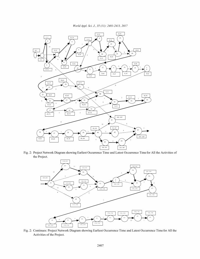
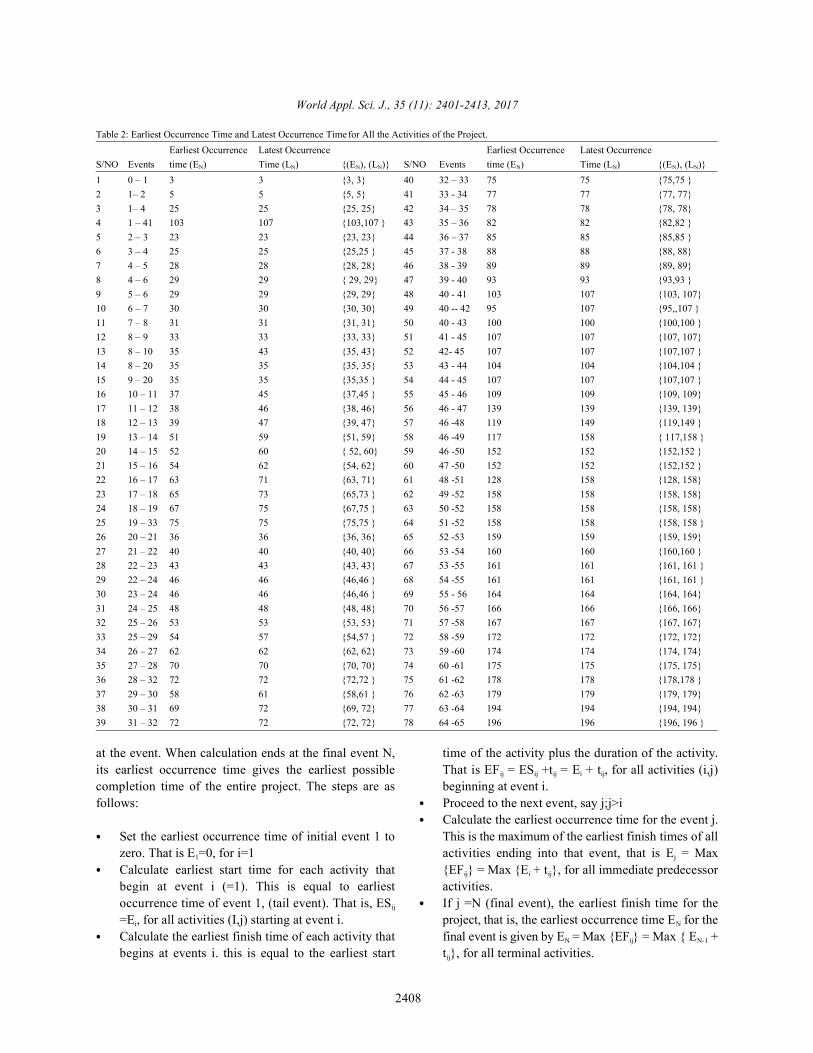
Table 2: Earliest Occurrence Time and Latest Occurrence Timefor All the Activities of the Project.Earliest Occurrence Latest Occurrence Earliest Occurrence Latest Occurrence

S/NO Events time (E ) Time (L ) {(E ), (L )} S/NO Events time (E ) Time (L ) {(E ), (L )}N N N N N N N N

1 0 – 1 3 3 {3, 3} 40 32 – 33 75 75 {75,75 }2 1– 2 5 5 {5, 5} 41 33 - 34 77 77 {77, 77}3 1– 4 25 25 {25, 25} 42 34 – 35 78 78 {78, 78}4 1 – 41 103 107 {103,107 } 43 35 – 36 82 82 {82,82 }5 2 – 3 23 23 {23, 23} 44 36 – 37 85 85 {85,85 }6 3 – 4 25 25 {25,25 } 45 37 - 38 88 88 {88, 88}7 4 – 5 28 28 {28, 28} 46 38 - 39 89 89 {89, 89}8 4 – 6 29 29 { 29, 29} 47 39 - 40 93 93 {93,93 }9 5 – 6 29 29 {29, 29} 48 40 - 41 103 107 {103, 107}10 6 – 7 30 30 {30, 30} 49 40 -- 42 95 107 {95,,107 }11 7 – 8 31 31 {31, 31} 50 40 - 43 100 100 {100,100 }12 8 – 9 33 33 {33, 33} 51 41 - 45 107 107 {107, 107}13 8 – 10 35 43 {35, 43} 52 42- 45 107 107 {107,107 }14 8 – 20 35 35 {35, 35} 53 43 - 44 104 104 {104,104 }15 9 – 20 35 35 {35,35 } 54 44 - 45 107 107 {107,107 }16 10 – 11 37 45 {37,45 } 55 45 - 46 109 109 {109, 109}17 11 – 12 38 46 {38, 46} 56 46 - 47 139 139 {139, 139}18 12 – 13 39 47 {39, 47} 57 46 -48 119 149 {119,149 }19 13 – 14 51 59 {51, 59} 58 46 -49 117 158 { 117,158 }20 14 – 15 52 60 { 52, 60} 59 46 -50 152 152 {152,152 }21 15 – 16 54 62 {54, 62} 60 47 -50 152 152 {152,152 }22 16 – 17 63 71 {63, 71} 61 48 -51 128 158 {128, 158}23 17 – 18 65 73 {65,73 } 62 49 -52 158 158 {158, 158}24 18 – 19 67 75 {67,75 } 63 50 -52 158 158 {158, 158}25 19 – 33 75 75 {75,75 } 64 51 -52 158 158 {158, 158 }26 20 – 21 36 36 {36, 36} 65 52 -53 159 159 {159, 159}27 21 – 22 40 40 {40, 40} 66 53 -54 160 160 {160,160 }28 22 – 23 43 43 {43, 43} 67 53 -55 161 161 {161, 161 }29 22 – 24 46 46 {46,46 } 68 54 -55 161 161 {161, 161 }30 23 – 24 46 46 {46,46 } 69 55 - 56 164 164 {164, 164}31 24 – 25 48 48 {48, 48} 70 56 -57 166 166 {166, 166}32 25 – 26 53 53 {53, 53} 71 57 -58 167 167 {167, 167}33 25 – 29 54 57 {54,57 } 72 58 -59 172 172 {172, 172}34 26 – 27 62 62 {62, 62} 73 59 -60 174 174 {174, 174}35 27 – 28 70 70 {70, 70} 74 60 -61 175 175 {175, 175}36 28 – 32 72 72 {72,72 } 75 61 -62 178 178 {178,178 }37 29 – 30 58 61 {58,61 } 76 62 -63 179 179 {179, 179}38 30 – 31 69 72 {69, 72} 77 63 -64 194 194 {194, 194}39 31 – 32 72 72 {72, 72} 78 64 -65 196 196 {196, 196 }

at the event. When calculation ends at the final event N, time of the activity plus the duration of the activity.its earliest occurrence time gives the earliest possible That is EF = ES +t = E + t , for all activities (i,j)completion time of the entire project. The steps are as beginning at event i. follows: Proceed to the next event, say j;j>i

Set the earliest occurrence time of initial event 1 to This is the maximum of the earliest finish times of allzero. That is E =0, for i=1 activities ending into that event, that is E = Max1

Calculate earliest start time for each activity that {EF } = Max {E + t }, for all immediate predecessorbegin at event i (=1). This is equal to earliest activities.occurrence time of event 1, (tail event). That is, ES If j =N (final event), the earliest finish time for theij

=E , for all activities (I,j) starting at event i. project, that is, the earliest occurrence time E for thei

Calculate the earliest finish time of each activity that final event is given by E = Max {EF } = Max { E +begins at events i. this is equal to the earliest start t }, for all terminal activities.

ij ij ij i ij

Calculate the earliest occurrence time for the event j.

j

ij i ij

N

N ij N-1

ij

46m+ +

( )6−

=

46m+ + ( )

6−

=

World Appl. Sci. J., 35 (11): 2401-2413, 2017

2409

Table 3: Project activity, Optimistic estimate ( ), Most likely estimate (m), Pessimistic estimate ( ), Expected time E(T) = µ= and Standard

Deviation

Activity Optimistic Most Likely Pessimistic Expected time Standard

S/N (I-j) time ( ) time (m) Time ( ) E(T) =µ Deviation

1 0 - 1 2 3 4 3.00 0.332 1 - 2 1 2 4 2.17 0.503 1 - 4 0 0 0 0.00 0.004 1 – 41 0 0 0 0.00 0.005 2 – 3 16 18 20 18.00 0.676 3 – 4 1 2 3.5 2.08 0.427 4 – 5 1.5 3 4.5 3.00 0.508 4 – 6 0 0 0 0.00 0.009 5 – 6 0.2 1 1.8 1.00 0.2710 6 – 7 0.5 1 2 1.08 0.2511 7 – 8 0.5 1 2.5 1.17 0.3312 8 – 9 1.5 2 3.5 2.17 0.3313 8 – 10 2 4 5 3.83 0.5014 8 – 20 0 0 0 0.00 0.0015 9 – 20 1 2 3.5 2.08 0.4216 10 – 11 1 2 4 2.17 0.5017 11 – 12 0.8 1 1.2 1.00 0.0718 12 – 13 0.2 1 1.8 1.00 0.2719 13 – 14 10 12 14 12.00 0.6720 14 – 15 .8 1 1.5 1.05 0.1221 15 – 16 1 2 3 2.00 0.3322 16 – 17 4 9 11 8.50 1.1723 17 – 18 1.4 2 2.6 2.00 0.2024 18 – 19 1 2 3 2.00 0.3325 19 – 33 0 0 0 0.00 0.0026 20 – 21 0.5 1 2.5 1.17 0.3327 21 – 22 3 4 5 4.00 0.3328 22 – 23 2 3 4 3.00 0.3329 22 – 24 0 0 0 0.00 0.0030 23 – 24 2.5 3 4 3.08 0.2531 24 – 25 1.5 2 4 2.25 0.4232 25 – 26 4 5 7 5.17 0.5033 25 – 29 3 6 8 5.83 0.8334 26 – 27 7 9 11 9.00 0.6735 27 – 28 6.5 8 10 8.08 0.5836 28 – 32 1 2 3 2.00 0.3337 29 – 30 3 4 5 4.00 0.3338 30 – 31 9 11 13 11.00 0.6739 31 – 32 0 0 0 0.00 0.0040 32 – 33 1.5 3 4.5 3.00 0.5041 33 - 34 1.5 2 3.5 2.17 0.3342 34 – 35 0.5 1 1.8 1.05 0.2243 35 – 36 5 4 7 4.67 0.3344 36 – 37 1 3 5 3.00 0.6745 37 – 38 2 3 4 3.00 0.3346 38 – 39 0.5 1 2.5 1.17 0.3347 39 – 40 2.5 4 5.5 4.00 0.5048 40 – 41 9 10 11 10.00 0.3349 40 – 42 1 2 3 2.00 0.33

46m+ + ( )

6−

=

World Appl. Sci. J., 35 (11): 2401-2413, 2017

2410

Table 3: Continued Activity Optimistic Most Likely Pessimistic Expected time Standard

S/N (I-j) time ( ) time (m) Time ( ) E(T) =µ Deviation

50 40 – 43 4 7 10 7.00 1.0051 41 – 45 0 0 0 0.00 0.0052 42 – 45 0 0 0 0.00 0.0053 43 – 44 3 4 5 4.00 0.3354 44 – 45 2 3 4 3.00 0.3355 45 – 46 1.5 2 3.5 2.17 0.3356 46 – 47 29 30 31 30.00 0.3357 46 – 48 9 10 11 10.00 0.3358 46 – 49 7 8 9 8.00 0.3359 46 – 50 0 0 0 0.00 0.0060 47 – 50 11.5 13 14.5 13.00 0.5061 48 – 51 7.5 9 10.5 9.00 0.5062 49 – 52 0 0 0 0.00 0.0063 50 – 52 4 6 10 6.33 1.0064 51 – 52 0 0 0 0.00 0.0065 52 – 53 1.5 1 2 1.25 0.0866 53 – 54 0.5 1 1.5 1.00 0.1767 53 – 55 0 0 0 0.00 0.0068 54 – 55 0.5 1 1.5 1.00 0.1769 55 – 56 2.5 3 4 3.08 0.2570 56 – 57 1.5 2 4 2.25 0.4271 57-58 0.5 1 1.5 1.00 0.1772 58-59 4 5 7 5.17 0.5073 59-60 1.5 2 3 2.08 0.2574 60-61 0.5 1 2 1.08 0.2575 61-62 2 3 5 3.17 0.5076 62-63 0.5 1 2 1.08 0.2577 63-64 14 15 16 15.00 0.3378 64-65 1 2 3 2.00 0.33

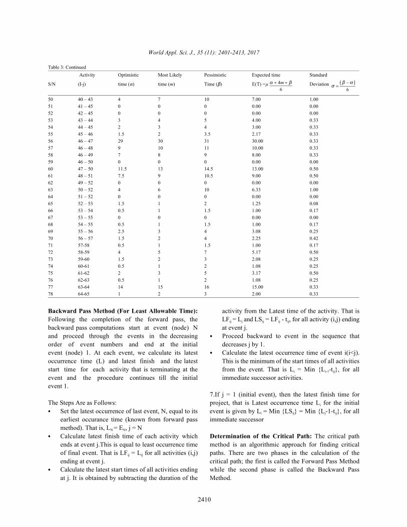
Backward Pass Method (For Least Allowable Time): activity from the Latest time of the activity. That isFollowing the completion of the forward pass, the LF = L and LS = LF - t , for all activity (i,j) endingbackward pass computations start at event (node) N at event j. and proceed through the events in the decreasing Proceed backward to event in the sequence thatorder of event numbers and end at the initial decreases j by 1. event (node) 1. At each event, we calculate its latest Calculate the latest occurrence time of event i(i<j).occurrence time (L) and latest finish and the latest This is the minimum of the start times of all activitiesstart time for each activity that is terminating at the from the event. That is L = Min {L -t }, for allevent and the procedure continues till the initial immediate successor activities.event 1.

The Steps Are as Follows: project, that is Latest occurrence time L for the initialSet the latest occurrence of last event, N, equal to its event is given by L = Min {LS } = Min {L -1-t }, for allearliest occurance time (known from forward pass immediate successormethod). That is, L = E , j = NN N

Calculate latest finish time of each activity which Determination of the Critical Path: The critical pathends at event j.This is equal to least occurrence time method is an algorithmic approach for finding criticalof final event. That is LF = L for all activities (i,j) paths. There are two phases in the calculation of theij ij

ending at event j. critical path; the first is called the Forward Pass MethodCalculate the latest start times of all activities ending while the second phase is called the Backward Passat j. It is obtained by subtracting the duration of the Method.

ij j ij ij ij

i i-1 ij

7.If j = 1 (initial event), then the latest finish time fori

i ij j ij

World Appl. Sci. J., 35 (11): 2401-2413, 2017

2411

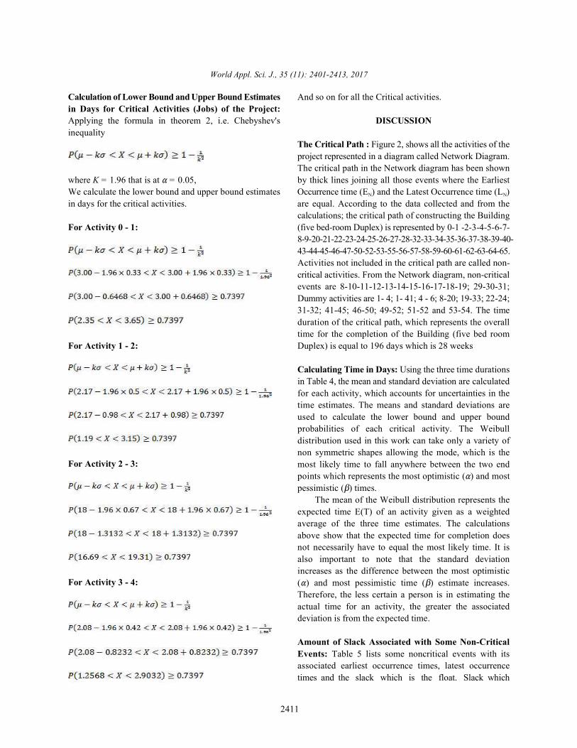
Calculation of Lower Bound and Upper Bound Estimates And so on for all the Critical activities.in Days for Critical Activities (Jobs) of the Project:Applying the formula in theorem 2, i.e. Chebyshev's DISCUSSIONinequality

project represented in a diagram called Network Diagram.

where K = 1.96 that is at = 0.05, by thick lines joining all those events where the EarliestWe calculate the lower bound and upper bound estimates Occurrence time (E ) and the Latest Occurrence time (L )in days for the critical activities. are equal. According to the data collected and from the

For Activity 0 - 1: (five bed-room Duplex) is represented by 0-1 -2-3-4-5-6-7-

43-44-45-46-47-50-52-53-55-56-57-58-59-60-61-62-63-64-65.

critical activities. From the Network diagram, non-critical

Dummy activities are 1- 4; 1- 41; 4 - 6; 8-20; 19-33; 22-24;

duration of the critical path, which represents the overall

For Activity 1 - 2: Duplex) is equal to 196 days which is 28 weeks

Calculating Time in Days: Using the three time durations

for each activity, which accounts for uncertainties in the

used to calculate the lower bound and upper bound

For Activity 2 - 3:

For Activity 3 - 4:

The Critical Path : Figure 2, shows all the activities of the

The critical path in the Network diagram has been shown

N N

calculations; the critical path of constructing the Building

8-9-20-21-22-23-24-25-26-27-28-32-33-34-35-36-37-38-39-40-

Activities not included in the critical path are called non-

events are 8-10-11-12-13-14-15-16-17-18-19; 29-30-31;

31-32; 41-45; 46-50; 49-52; 51-52 and 53-54. The time

time for the completion of the Building (five bed room

in Table 4, the mean and standard deviation are calculated

time estimates. The means and standard deviations are

probabilities of each critical activity. The Weibulldistribution used in this work can take only a variety ofnon symmetric shapes allowing the mode, which is themost likely time to fall anywhere between the two endpoints which represents the most optimistic ( ) and mostpessimistic ( ) times.

The mean of the Weibull distribution represents theexpected time E(T) of an activity given as a weightedaverage of the three time estimates. The calculationsabove show that the expected time for completion doesnot necessarily have to equal the most likely time. It isalso important to note that the standard deviationincreases as the difference between the most optimistic( ) and most pessimistic time ( ) estimate increases.Therefore, the less certain a person is in estimating theactual time for an activity, the greater the associateddeviation is from the expected time.

Amount of Slack Associated with Some Non-CriticalEvents: Table 5 lists some noncritical events with itsassociated earliest occurrence times, latest occurrencetimes and the slack which is the float. Slack which

World Appl. Sci. J., 35 (11): 2401-2413, 2017

2412

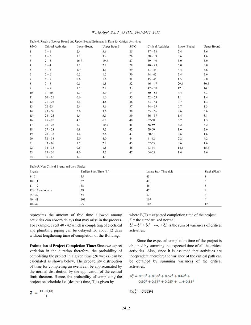
Table 4: Result of Lower Bound and Upper Bound Estimates in Days for Critical Activities

S/NO Critical Activities Lower Bound Upper Bound S/NO Critical Activities Lower Bound Upper Bound

1 0 – 1 2.4 3.6 25 37 – 38 2.4 3.62 1 – 2 1.1 3.2 26 38 – 39 0.6 1.63 2 – 3 16.7 19.3 27 39 – 40 3.0 5.04 3 – 4 1.3 2.9 28 40 – 43 5.0 9.05 4 – 5 1.9 4.1 29 43 - 44 3.4 4.66 5 – 6 0.5 1.5 30 44 - 45 2.4 3.67 6 – 7 0.6 1.6 31 45 - 46 1.5 2.88 7 – 8 0.5 1.8 32 46 – 47 29.4 30.69 8 – 9 1.5 2.8 33 47 – 50 12.0 14.010 9 – 20 1.3 2.9 34 50 – 52 4.4 8.311 20 – 21 0.6 1.6 35 52 – 53 1.1 1.412 21 – 22 3.4 4.6 36 53 – 54 0.7 1.313 22 -23 2.4 3.6 37 54 – 55 0.7 1.314 23 - 24 2.6 3.6 38 55 – 56 2.6 3.615 24 – 25 1.4 3.1 39 56 – 57 1.4 3.116 25 – 26 4.2 6.2 40 57-58 0.7 1.317 26 – 27 7.7 10.3 41 58-59 4.2 6.218 27 – 28 6.9 9.2 42 59-60 1.6 2.619 28 – 32 1.4 2.6 43 60-61 0.6 1.620 32 – 33 2.0 4.0 44 61-62 2.2 4.221 33 - 34 1.5 2.8 45 62-63 0.6 1.622 34 – 35 0.6 1.5 46 63-64 14.4 15.623 35 – 36 4.0 5.3 47 64-65 1.4 2.624 36 - 37 1.7 4.3

Table 5: Non-Critical Events and their Slacks

Events Earliest Start Time (Ei) Latest Start Time (Li) Slack (Float)

8-10 35 43 810 - 11 37 42 511 - 12 38 46 812 - 13 and others 39 47 825 - 29 54 57 340 - 41 103 107 440 - 42 95 107 12

represents the amount of free time allowed among where E(T) = expected completion time of the projectactivities can absorb delays that may arise in the process. Z = the standardized normalFor example, event 40 - 42 which is completing of electrical = + + ---, + is the sum of variances of criticaland plumbing piping can be delayed for about 12 days activities.without lengthening time of completion of the Building.

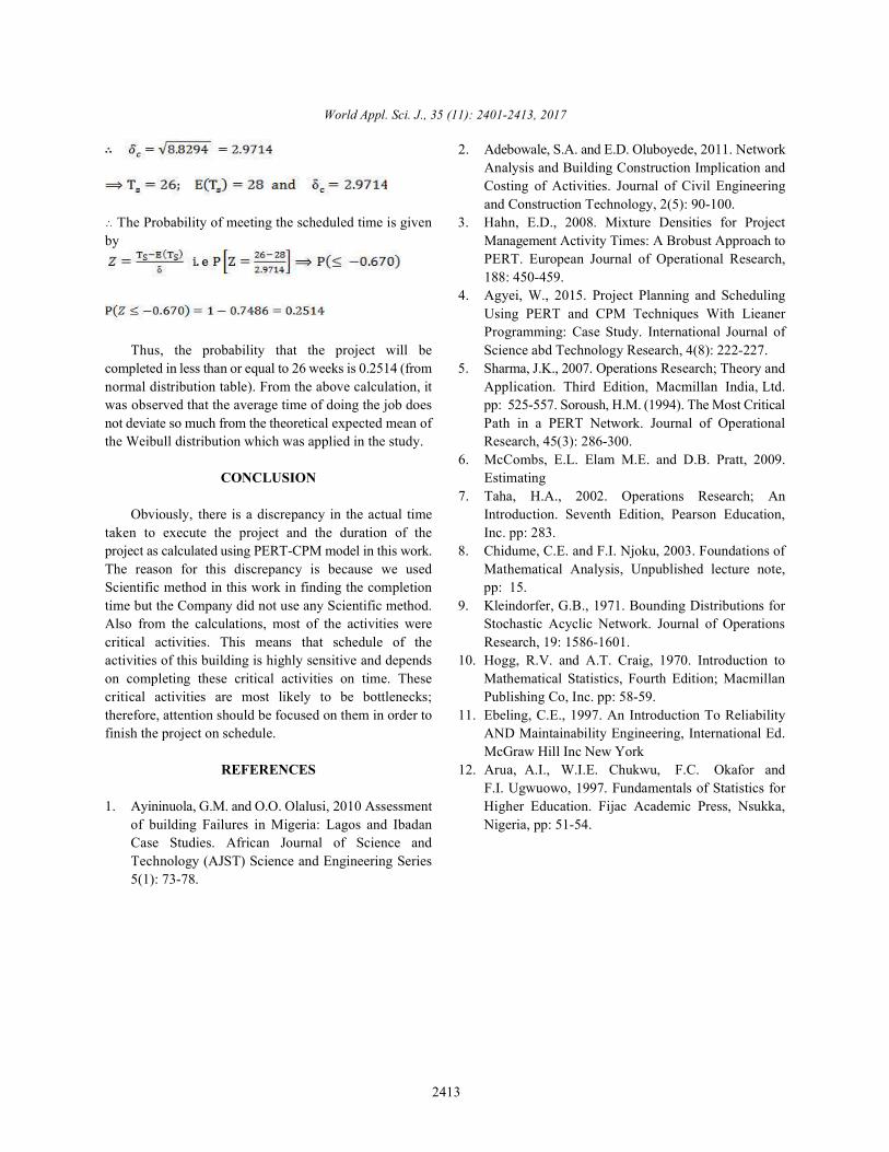
Estimation of Project Completion Time: Since we expect obtained by summing the expected time of all the criticalvariation in the duration therefore, the probability of activities. Also, since it is assumed that activities arecompleting the project in a given time (26 weeks) can be independent, therefore the variance of the critical path cancalculated as shown below. The probability distribution be obtained by summing variances of the criticalof time for completing an event can be approximated by activities.the normal distribution by the application of the centrallimit theorem. Hence, the probability of completing theproject on schedule i.e. (desired) time, T is given bys

c 1 2 n2 2 2 2

Since the expected completion time of the project is

World Appl. Sci. J., 35 (11): 2401-2413, 2017

2413

2. Adebowale, S.A. and E.D. Oluboyede, 2011. Network

Costing of Activities. Journal of Civil Engineering

The Probability of meeting the scheduled time is given 3. Hahn, E.D., 2008. Mixture Densities for Projectby Management Activity Times: A Brobust Approach to

PERT. European Journal of Operational Research,

Using PERT and CPM Techniques With Lieaner

Thus, the probability that the project will be Science abd Technology Research, 4(8): 222-227.completed in less than or equal to 26 weeks is 0.2514 (from 5. Sharma, J.K., 2007. Operations Research; Theory andnormal distribution table). From the above calculation, it Application. Third Edition, Macmillan India, Ltd.was observed that the average time of doing the job does pp: 525-557. Soroush, H.M. (1994). The Most Criticalnot deviate so much from the theoretical expected mean of Path in a PERT Network. Journal of Operationalthe Weibull distribution which was applied in the study. Research, 45(3): 286-300.

CONCLUSION Estimating

Obviously, there is a discrepancy in the actual time Introduction. Seventh Edition, Pearson Education,taken to execute the project and the duration of the Inc. pp: 283.project as calculated using PERT-CPM model in this work. 8. Chidume, C.E. and F.I. Njoku, 2003. Foundations ofThe reason for this discrepancy is because we used Mathematical Analysis, Unpublished lecture note,Scientific method in this work in finding the completion pp: 15. time but the Company did not use any Scientific method. 9. Kleindorfer, G.B., 1971. Bounding Distributions forAlso from the calculations, most of the activities were Stochastic Acyclic Network. Journal of Operationscritical activities. This means that schedule of the Research, 19: 1586-1601.activities of this building is highly sensitive and depends 10. Hogg, R.V. and A.T. Craig, 1970. Introduction toon completing these critical activities on time. These Mathematical Statistics, Fourth Edition; Macmillancritical activities are most likely to be bottlenecks; Publishing Co, Inc. pp: 58-59.therefore, attention should be focused on them in order to 11. Ebeling, C.E., 1997. An Introduction To Reliabilityfinish the project on schedule. AND Maintainability Engineering, International Ed.

REFERENCES 12. Arua, A.I., W.I.E. Chukwu, F.C. Okafor and

1. Ayininuola, G.M. and O.O. Olalusi, 2010 Assessment Higher Education. Fijac Academic Press, Nsukka,of building Failures in Migeria: Lagos and Ibadan Nigeria, pp: 51-54.Case Studies. African Journal of Science andTechnology (AJST) Science and Engineering Series5(1): 73-78.

Analysis and Building Construction Implication and

and Construction Technology, 2(5): 90-100.

188: 450-459.4. Agyei, W., 2015. Project Planning and Scheduling

Programming: Case Study. International Journal of

6. McCombs, E.L. Elam M.E. and D.B. Pratt, 2009.

7. Taha, H.A., 2002. Operations Research; An

McGraw Hill Inc New York

F.I. Ugwuowo, 1997. Fundamentals of Statistics for