Application of TOPNET in the distributed model

intercomparison project

Christina Bandaragodaa,*, David G. Tarbotona, Ross Woodsb

aUtah Water Research Laboratory, Department of Civil and Environmental Engineering, Utah State University, Logan, UT 84322, USAbNational Institute of Water and Atmospheric Research, Christchurch, New Zealand

Received 11 August 2003; revised 12 November 2003; accepted 29 March 2004

Abstract

This paper describes the application of a networked version of TOPMODEL, TOPNET, as part of the Distributed Model

Intercomparison Project (DMIP). The model implementation is based on a topographically derived river network with spatially

distributed sub-basins draining to each network reach. The river network is mapped from the US National Elevation Dataset

Digital Elevation Model (DEM) using procedures that objectively estimate drainage density from geomorphic principles.

Rainfall inputs are derived from NEXRAD (radar) for each sub-basin. For each sub-basin, the wetness index distribution is

derived from the DEM. The initial model parameters for each sub-basin are estimated using look up tables based on soils

(STATSGO) and vegetation (1-km AVHRR). These initial model parameters provide the spatially distributed pattern of

parameters at the scale of each sub-basin. Calibration uses a multiplier for each parameter to adjust the parameters while

retaining the relative spatial pattern obtained from the soils and vegetation data. Parameter multipliers were calibrated using the

shuffled complex evolution algorithm [J. Optim. Theory Appl. 61 (1993)] with the objective to minimize the mean square error

between observed and modeled hourly streamflows. We describe the model and calibrated results submitted for all basins for

the time periods involved in the DMIP study. We were encouraged by the relatively good performance of the model, especially

in comparison to streamflow from smaller interior watersheds not used in calibration and simulated as ungaged basins. The

limited resources used to achieve these results show some of the potential for distributed models to be useful operationally.

q 2004 Elsevier B.V. All rights reserved.

Keywords: Distributed; Rainfall runoff; NEXRAD; Hydrologic modeling; Ungaged basins

1. Introduction

We have applied a distributed version of TOPMO-

DEL (Beven and Kirkby, 1979; Beven et al., 1995a)

with a DEM-based system for delimiting channels,

model components, and estimation of model

parameters, to the Distributed Model Intercomparison

Project (DMIP) watersheds. The implementation

of TOPMODEL used is modified from the

original (Beven and Kirkby, 1979; Beven et al.,

1995a) by the addition of a potential evapotranspira-

tion component, a canopy storage component to

model interception, and the inclusion of a soil zone

component that provides infiltration excess runoff

generation capability through a Green-Ampt like

parameterization.

Journal of Hydrology 298 (2004) 178–201

www.elsevier.com/locate/jhydrol

0022-1694/$ - see front matter q 2004 Elsevier B.V. All rights reserved.

doi:10.1016/j.jhydrol.2004.03.038

* Corresponding author.

E-mail address: cmay@cc.usu.edu (C. Bandaragoda).

To parameterize the model using physical data, we

used the soil texture from each of the 11 soil depth

grid layers derived from Pennsylvania State Univer-

sity STATSGO data (Soil Survey Staff, 1994a,b)

provided on the DMIP website (Smith, 2002), and soil

hydraulic properties derived from texture using

relationships provided by Clapp and Hornberger

(1978). We also used 1 km resolution Advanced

Very High Resolution Radiometer (AVHRR) veg-

etation data processed through the NASA Land Data

Assimilation Systems (LDAS) program with an

International Geosphere-Biosphere Program (IGBP)

classification system (Eidenshink and Faundeen,

1994). There are a total of nine parameters that were

derived from this soils and vegetation information.

We used a GIS to spatially average the parameter

values for each sub-basin model element.

The calibration procedure used is designed to

retain the spatial pattern provided by estimating

parameters from the GIS data, while still allowing

an adjustment of parameters to match observed stream

flow. Parameters are adjusted through a set of

multipliers that scale the parameters while maintain-

ing the relative differences between model elements

indicated from the GIS information. There is one

multiplier for each parameter that is the same across

all sub-basins. Sub-grid variability within sub-basins

is not explicitly represented apart from the spatial

distribution of soil moisture that is parameterized by

distribution of the TOPMODEL wetness index.

The DMIP dataset provides a unique opportunity to

explore questions of location-specific radar data

quality, and model performance over calibration and

validation periods for different watersheds using

different models. The results for our model are

presented with an overview of model performance

and acceptability in some watersheds, and recommen-

dations for TOPNET model improvement in others.

We address the following questions related to the

use of distributed hydrologic models. Can radar

rainfall data be used for flood forecasting? Can

distributed models simulate flow at uncalibrated

interior locations? How applicable is a TOPMODEL

representation to the DMIP watersheds? Can flows be

predicted well with little or no calibration?

We found that lack of information on the uncer-

tainty in radar rainfall inputs limits the useful

interpretation of the statistical measures used to assess

forecast performance. Distributed models have an

advantage over lumped models in the ability to

disaggregate the source of streamflow to ungaged

locations upstream of the calibration location. We

found that the exponential discharge–storage response

function of TOPMODEL, used to model the saturated

zone, limited the ability of the model to match

streamflow recessions in both high flow and low flow

periods. The small difference between calibrated and

uncalibrated results for TOPNET showed that, in some

basins, flows can be predicted well with little or no

calibration. Calibration reduced the mean square

errors, improving measures such as the Nash–Sutcliffe

efficiency. Matching peak flows was emphasized by

this approach but this was at a cost of introducing bias

and poorer representation of low flows.

The following sections of this paper include a

description of our model and the methods used in the

DMIP experiment. Results of the DMIP experiment

are given, followed by conclusions on the model

performance.

2. Model description

TOPNET was developed by combining TOPMO-

DEL (Beven and Kirkby, 1979; Beven et al., 1995a),

which is most suited to small watersheds, with a

kinematic wave channel routing algorithm (Goring,

1994) so as to have a modeling system that can be

applied over large watersheds using smaller sub-

basins within the large watershed as model elements.

A key contribution of TOPMODEL is the parameter-

ization of the soil moisture deficit (depth to water

table) using a topographic index to model the

dynamics of variable source areas contributing to

saturation excess runoff. Beven et al. (1995a) indicate

that “TOPMODEL is not a hydrological modeling

package. It is rather a set of conceptual tools that can

be used to reproduce the hydrological behavior of

catchments in a distributed or semi-distributed way, in

particular the dynamics of surface or sub-surface

contributing areas.”

The model we developed and applied here,

TOPNET, uses TOPMODEL concepts for the rep-

resentation of sub-surface storage controlling the

dynamics of the saturated contributing area and

baseflow recession. To form a complete model we

C. Bandaragoda et al. / Journal of Hydrology 298 (2004) 178–201 179

added potential evapotranspiration, interception and

soil zone components. The physical processes rep-

resented in each sub-basin are shown in Fig. 1.

Kinematic wave routing moves the sub-basin inputs

through the stream channel network. A GIS based

parameterization program, TOPSETUP, has been

developed to facilitate the transformation of spatial

datasets into modeling parameters and the calculation

of weights associated with point precipitation measure-

ments to provide sub-basin aggregate precipitation.

In addition to streamflow, TOPNET diagnostic

output for each model element consists of time series

of model state variables for each sub-basin: mean

water table depth, soil zone storage, and canopy

storage. Diagnostic output also includes information

for each sub-basin on: infiltration excess runoff,

saturation excess runoff, base flow, drainage from

the soil to the saturated zone (recharge), percent

saturated area, potential evapotranspiration, and

actual evapotranspiration.

2.1. Potential evapotranspiration component

In TOPNET, potential evapotranspiration is

calculated using the Priestley – Taylor equation

(Priestley and Taylor, 1972). This was chosen because

it can be used with minimal input requirements of air

temperature, dew point, date and time. Famiglietti

et al. (1992) and Famiglietti and Wood (1994a,b) used

more complete surface energy balance equations with

TOPMODEL in developing the TOPLATS soil

vegetation atmosphere transfer scheme (SVATS).

Famiglietti’s work focused on estimating evaporation

fluxes as inputs to atmospheric models. We opted for a

simpler approach here because the focus is on

modeling runoff and because much of the data

required to run a more complex SVATS model,

such as wind and aerodynamic roughness is uncertain

and difficult to estimate from the available data.

The available energy used in the Priestley–Taylor

equation is calculated based on top of the atmosphere

solar radiation forcing following procedures given in

the Handbook of Hydrology (Shuttleworth, 1993)

with atmospheric transmissivity estimated from the

diurnal temperature range (Bristow and Campbell,

1984). Temperature and dew point for each sub-basin

are estimated from nearby measurements using a

lapse rate and the elevation difference between the

mean sub-basin elevation and measurement elevation.

In the calculation of potential evapotranspiration,

Fig. 1. Schematic of the physical processes represented by the TOPNET modeling system.

C. Bandaragoda et al. / Journal of Hydrology 298 (2004) 178–201180

albedo and lapse rate are treated as parameters with

albedo determined from land cover data.

2.2. Canopy interception component

The canopy interception component is a new and

much simpler approach than standard interception

models (e g. Rutter et al., 1972). It was developed

based on the work of Ibbitt (1971) and requires only

two parameters: canopy interception capacity, CC,

and interception evaporation adjustment factor, Cr:

Driving inputs to the canopy interception component

are hourly precipitation and potential evapotran-

spiration. These are determined from the GIS land

cover data. The state variable quantifying the

amount of water held in interception storage, Si; is

used in a function f ðSiÞ to quantify the proportion of

precipitation that is throughfall (Ibbitt, 1971). The

remainder Pð1 2 f ðSiÞÞ; where P is precipitation

rate, is added to interception storage. The same

function f ðSiÞ is used to quantify the exposure of

water held in interception storage to potential

evapotranspiration. Physically, f ðSiÞ could express

the fraction of leaf area that is wet, relative to its

maximum. Higher rates of evaporation from inter-

ception than transpiration under the same conditions,

have been suggested by Stewart (1977) and Ding-

man (2002). Here we represent this effect using a

factor Cr quantifying the increase in evaporation

losses from interception relative to the potential

evapotranspiration rate (Ibbitt, 1971; Stewart, 1977).

The evaporation outflux from the interception store

is written as ECrf ðSiÞ where E is the potential

evapotranspiration rate. The rate of change for

interception storage is therefore given by

dSi

dt¼ Pð1 2 f ðSiÞÞ2 ECrf ðSiÞ ð1Þ

f ðSiÞ; the function giving throughfall as a function of

interception storage, Si; and canopy interception

capacity, CC, is given by:

f ðSiÞ ¼Si

CC2 2

Si

CC

� �ð2Þ

Analytic integrals of Eq. (1) using (2) are used to

solve for Si at the end of each time step to obtain

the cumulative throughfall and cumulative evapor-

ation of intercepted water. Cr applies only to

intercepted water, not soil water available for

transpiration. Unsatisfied potential evapotranspira-

tion demand is calculated as potential evapotran-

spiration minus cumulative evaporation of

intercepted water divided by the interception

enhancement factor Cr:

2.3. Soil component

Throughfall, T ; and unsatisfied potential evapotran-

spiration, Ep; from the interception component serve as

the forcing for the soil component, which represents the

upper layer of soil to the depth below which roots can no

longer extract water. Beven et al. (1995a) indicate that

two formulations that have been adopted in past

TOPMODEL applications have assumed that the

unsaturated flows are essentially vertical and have

been expressed in terms of drainage flux from the

unsaturated zone. Neither of the formulations pre-

sented by Beven et al. (1995a) limit the infiltration

capacity, possibly due to the historical association of

TOPMODEL with the saturation excess rather than the

infiltration excess runoff generation mechanism. We

felt it important to accommodate both saturation and

infiltration excess runoff generation mechanisms and

therefore developed our own soil component that

combines gravity drainage and Green-Ampt infiltration

excess concepts to control the generation of surface

runoff by infiltration excess as well as the drainage to

the saturated zone and evapotranspiration.

Parameters describing the soil store processes are

depth ðdÞ; saturated hydraulic conductivity ðKÞ;

Green-Ampt wetting front suction ðcfÞ; pore discon-

nectedness index soil drainage parameter ðcÞ; drain-

able porosity ðDu1Þ; and plant available porosity

ðDu2Þ: The soil parameters are estimated based on soil

texture from GIS soils data using relationships from

Clapp and Hornberger (1978).

The state variable Sr quantifies the depth of water

held in the soil zone for each model element and is

calculated according to

dSr

dt¼ I 2 Es 2 R ð3Þ

where I is the infiltration rate; Es; soil evaporation

rate; R is the drainage rate or recharge to the saturated

zone store from the soil store. The infiltration rate, I; is

limited to be less than the infiltration capacity, Ic;

C. Bandaragoda et al. / Journal of Hydrology 298 (2004) 178–201 181

modeled with a Green-Ampt formulation where we

use the soil zone storage as infiltrated depth for the

purposes of calculating Ic:

Unsatisfied evapotranspiration demand is given

first call upon available surface water so the forcing to

the soil zone is T 2 Ep: When this quantity is negative

it represents evaporative demand on the soil com-

ponent. When this quantity is positive it represents net

surface water input that may infiltrate or become

infiltration or saturation excess surface runoff.

Soil evapotranspiration is assumed to be at the

potential rate when the soil moisture content is in

excess of field capacity, but between field capacity

and permanent wilting point, evapotranspiration is

assumed to reduce linearly to zero as wilting point is

approached. Soil evaporation is modeled as

Es ¼ min 1;Sr

dDu2

� �ðEp 2 TÞ

for Ep . T and 0 otherwise

ð4Þ

where Ep 2 T is the unsatisfied potential evapotran-

spiration demand.

We assume the soil zone is comprised of two parts,

the drainable part in excess of field capacity,

characterized by Du1; and the plant available

moisture, characterized by Du2: Drainage is estimated

as gravity drainage and is modeled to only occur when

the moisture content is greater than field capacity. The

relative drainable saturation, Srd; is defined as

Srd ¼maxð0; Sr 2 dDu2Þ

dDu1

ð5Þ

The drainage from the soil store and recharge to the

saturated zone occurs at a rate (m/h) given by

R ¼ KScrd ð6Þ

This is based upon a Brooks and Corey (1966)

parameterization of the unsaturated hydraulic con-

ductivity controlling the rate of drainage.

For locations with large wetness index values, the

water table evaluated in the saturated zone component

below may upwell into and influence the soil moisture

content of the soil zone. This occurs when depth to the

water table, z; is less than depth of the soil zone, d: We

model the supplementary moisture in the soil zone in

these cases by assuming uniform soil moisture deficit

from the surface to the water table and saturated

conditions from the water table to the root zone. Thus,

the shallow water table ðz , dÞ increases the soil

storage to

S0r ¼ Sr þ ðdue 2 SrÞ

d 2 z

d

� �ð7Þ

The soil component described here was

developed independently of TOPMODEL, which we

used to develop the saturated zone described in

Section 2.4.

2.4. Saturated zone component

The saturated zone component is constructed

using the classical TOPMODEL assumptions of

(1) saturated hydraulic conductivity decreasing

exponentially with depth and (2) saturated lateral

flow driven by topographic gradients at (3) steady

state (Beven and Kirkby, 1979; Beven et al., 1995a).

With these assumptions the local depth to the water

table, z; is the following function of the wetness

index lnða=tan bÞ

z ¼ �z þ ðl2 lnða=tanbÞÞ=f ð8Þ

where l is the spatial average of lnða=tanbÞ and �z the

spatial average of the depth to the water table

quantifying the basin average soil moisture deficit

and serving as a state variable for the saturated zone

component. The parameter f quantifies the assumed

decrease of hydraulic conductivity with depth. A

histogram of wetness index values over each sub-

basin is used to record the proportion of each sub-

basin falling within each wetness index class.

Locations, or wetness index classes, where z is less

than 0 as calculated using Eq. (8) are interpreted to

be saturated and represent the variable source area

where surface water input ðT 2 EpÞ becomes satur-

ation excess runoff.

The saturated zone state equation is

dðDu1�zÞ

dt¼ 2ris þ T0 e2l e2f �z ð9Þ

where ris is the recharge, R, to the saturated zone

averaged across wetness index classes, recognizing

that for classes where the water table impacts the soil

zone, Sr, and hence R, are impacted by z through

Eq. (7). The last term in this equation represents the

per unit area baseflow, Qb; draining the saturated zone

C. Bandaragoda et al. / Journal of Hydrology 298 (2004) 178–201182

derived using the exponential decrease in hydraulic

conductivity with depth assumed by TOPMODEL,

with T0 being transmissivity

Qb ¼ T0 e2l e2f �z ð10Þ

In solving the model we do not save a state variable

either for the saturated zone or soil zone for each

wetness index class. Rather we only save state

variables �z and Sr for each sub-basin. At each time

step, Eq. (8) gives the depth to the water table for a

specific wetness index class within a sub-basin, and

Eq. (7) gives the modification of Sr for wetness index

classes impacted by a shallow water table. This

approach is different from the Beven version of

TOPMODEL (Beven et al., 1995b) where a separate

soil zone is modeled for each wetness index class. We

felt that keeping track of state variables at scales

smaller than the basic sub-basin model element

introduces unnecessary complexity and is unwar-

ranted. If smaller spatial resolution is required to

provide more explicit resolution of spatial variability,

then smaller sub-basins can be delineated.

2.5. Routing component

There are three sources of runoff from each sub-

basin; (1) saturation excess runoff from excess

precipitation on variable source saturated areas as

determined from the topographic wetness index, (2)

infiltration excess runoff as determined from the

Green-Ampt parameterization based upon soil zone

storage and (3) base flow representing saturated zone

drainage according to Eq. (10). This runoff is delayed

in reaching the outlet due to the time taken by within

sub-basin travel, as well as travel in the stream

network to the overall watershed outlet. Within sub-

basin travel is modeled assuming a constant hillslope

velocity, V ; which is a calibrated input parameter. A

histogram of the down slope flow distances from each

grid cell in each sub-basin to the first stream

encountered is derived from the GIS and used to

perform this routing.

Once in the stream, a kinematic wave routing

algorithm (Goring, 1994) is used to route flow through

the network. Sub-basin inputs to the channel network

are assumed to occur at the head of first order streams

and at the midpoint of internal stream reaches. Fig. 2

gives an example of the sub-basins used to model flow

in the Illinois River at Tahlequah. The inset on Fig. 2

gives the schematic channel network with sub-basin

inputs used to route flow for the portion of this

network draining to the interior gage at Savoy. The

parameters used in the kinematic wave channel

network routing are Manning’s roughness parameter

n; as well as width, slope and length for each channel

segment. Slope and length are determined from the

GIS based upon the Digital Elevation Model (DEM).

Channel width is determined as a power function of

contributing area (Leopold and Maddock, 1953) fit to

data from New Zealand rivers.

2.6. Precipitation interpolation

TOPNET is configured to derive aggregated sub-

basin precipitation inputs as a weighted sum of point

precipitation measurements. The weights associated

with each gauge for each sub-basin are calculated as

part of the preprocessing by TOPSETUP using linear

interpolation based upon Delauney triangles. In the

DMIP application, the center points of NEXRAD

radar grid cells were used as precipitation gage

locations. With this input, TOPSETUP determines

the set of weights used to estimate sub-basin

precipitation in terms of individual NEXRAD radar

grid cells.

3. The DMIP experiment

Results were submitted to the National Weather

Service (NWS) for the period June 1, 1993–July 31,

2001 with May 1, 2000–July 31, 2001 serving as a

validation period. Our group submitted both cali-

brated and uncalibrated results for all five basins, all

interior locations within each of the five basins

(Reed et al., 2003), and over the entire calibration

and validation period requested by the NWS. The

difference between calibrated and uncalibrated

simulations showed how simulations improved

with calibration specific to a particular basin. With

calibration using streamflow measurements at basin

outlets, model predictions reported at interior

locations can test the ability of distributed models

to predict flow at ungaged locations. With model

calculations performed at an hourly time step,

C. Bandaragoda et al. / Journal of Hydrology 298 (2004) 178–201 183

results can be analyzed in terms of usefulness and

acceptability for multiple uses, including flood

forecasting.

3.1. Spatial configuration

To delineate streams and sub-basins we used the

30 m resolution National Elevation Dataset DEM

(USGS, 2003) for this region. Software developed

by Tarboton (2002) was used to filter the DEM,

remove pits and calculate the single (D8) flow

direction and contributing drainage area associated

with each grid cell. The curvature based drainage

network delineation method described by Tarboton

and Ames (2001) was used to delineate streams.

This method delineates the highest resolution stream

network statistically consistent with empirical geo-

morphologic laws, specifically the constant drop

property (Broscoe, 1959) which is related to

Horton’s slope and length laws and the power law

relationship between stream slope and drainage area

(Flint, 1974). The average drainage density that

resulted was 0.4 km21 for the DMIP watersheds.

The resulting channel network was visually checked

against digital raster graph images of USGS

1:24,000 topographic maps.

The DMIP stream gage and ungaged simulation

point locations were all found to lie on third or higher

order streams. To reduce the number of model

elements involved we generalized the delineated

stream network by eliminating all first and second

order streams. The DEM flow direction grid was

Fig. 2. Model element distribution for the watershed of the Illinois River at Tahlequah. Channel routing of flow from sub-watersheds through the

channel system is displayed for the interior gage at Savoy.

C. Bandaragoda et al. / Journal of Hydrology 298 (2004) 178–201184

then used to delineate the sub-basin draining

directly to each third or higher order stream reach.

These sub-basins are shown in Fig. 3 and were used as

model elements in TOPNET. The average size of the

model elements was 90 km2.

The D1 multiple flow direction algorithm

(Tarboton, 1997) was used to calculate flow

direction, slope ðtan bÞ and specific catchment

area, a; for each grid cell in the DEM. This method

provides a better estimate of contributing area on

hillsides (Tarboton, 1997). The distribution of

wetness index, lnða=tan bÞ; within each sub-basin

was represented using a histogram that recorded the

fraction of the sub-basin within each wetness index

class. Fig. 4 shows the wetness index and wetness

index histograms for a portion of the Blue River

watershed.

3.2. Temporal inputs

Climate inputs included precipitation at each

NEXRAD Stage III radar grid location Radar data

was modeled as point rainfall measurements at the

center of each 4 £ 4 km2 radar grid cell. Hourly data

for air temperature and dew point temperature at each

basin gage location, provided by NCDC Cooperate

Observer Stations, were adjusted from the gage

elevation to the basin average elevation of each sub-

basin using lapse rates.

Fig. 3. DMIP river basins are located in the south central United States and range in size from 800 to 2500 km2. Interior gaged locations were

modeled as ‘ungaged’ for the experiment. The Illinois at Tahlquah basin includes the Illinois at Watts basin. The Illinois at Watts streamgage

location was used once as an interior ‘ungaged’ location for modeling Illinois at Tahlequah, and secondly for the calibration of Illinois at Watts.

C. Bandaragoda et al. / Journal of Hydrology 298 (2004) 178–201 185

3.3. Parameter estimation and calibration

Parameters are time invariant and describe the

unchanging properties of the sub-basins or model

elements. The parameters of TOPNET are related to

physical properties of the sub-basin, including soils,

topography, land cover and channel geometry. These

are calculated from spatial GIS data and may be

spatially uniform, spatially variable and calibrated, or

uncalibrated. Table 1 lists the TOPNET model

parameters. The third column of Table 1 summarizes

how each parameter was estimated in the DMIP

experiment. Parameters f ; K0; V ; Cr, and n; were

calibrated for the August 2002 DMIP submission.

Sub-basin model elements have their own distinct

model parameters and state variables derived from

the soil and vegetation data. The pattern of the

spatial variability between sub-basins is maintained

during calibration by using multipliers for each

parameter that are the same across all sub-basins to

scale the Geographic Information System (GIS)

derived sub-basin parameters for each sub-basin by

the same factor. The calibration procedure uses

multipliers, rather than individual sub-basin par-

ameters as its calibration variables. One multiplier

value for each parameter applied uniformly to the

entire watershed limits the degrees of freedom, and

is a parsimonious way to maintain spatial variation

Fig. 4. TOPMODEL wetness index for the upper portion of the Blue watershed. A histogram represents the distribution of wetness index within

each sub-basin.

C. Bandaragoda et al. / Journal of Hydrology 298 (2004) 178–201186

between sub-basins based on GIS-derived parameter

values.

To prepare TOPNET model input, soils and land

cover data were interpolated to the 30 m DEM grid

scale. The mapping from soil texture classes and land

cover types to model parameters is through a set of

value attribute lookup tables, which associate a model

parameter value with each 30 m grid cell. Spatial

averages of the 30 m grid cell parameter values over

the sub-basins that represent model elements are used

to obtain the sub-basin parameter values.

Parameters obtained from soil data were derived

using soil texture for each of the 11 standard soil depth

grid layers from the Pennsylvania (Penn) State

University gridding of the NRCS STATSGO data-

base. Fig. 5 shows the derivation of distributed soil

based parameters from the soil database. Soil texture

from 11 depth based grid layers was associated with

each soil class identified using a map unit identifier.

The texture of each layer was used to obtain soil

parameter values based on the soil hydraulic proper-

ties given by Clapp and Hornberger (1978) for each

layer. A depth-weighted average was used to calculate

the soil class parameter values for drainable porosity,

plant available porosity, and wetting front suction.

Linear regression of lnðKÞ versus depth z was used to

fit the assumed exponential function describing

decrease of hydraulic conductivity with depth and

estimate saturated hydraulic conductivity at the sur-

face, K0 and sensitivity parameter f ; for each soil

class. This regression did not always work because in

some soil profiles, hydraulic conductivity increased

with depth, or was constant. A lower bound value of

f ¼ 0:667 m21 was used in these cases corresponding

to a soil depth length scale of 1.5 m.

Parameter values for lapse rate, soil zone drainage

sensitivity, and hydraulic geometry were left at the

default values set in TOPNET, given in Table 1.

Parameter values for land cover are given in Table 2.

The model was run for an initialization period of 24

days before the DMIP comparison period beginning

June 1, 1993, to account for lack of prior knowledge

of the initial state variables.

This is the first application that uses this procedure

for estimating parameters from STATSGO soil and

NASA LDAS vegetation data with TOPNET. There is

a scale difference between the sub-basin K0 and f

parameters and the point scale parameters inferred

from GIS soil texture data. Because of this scale

difference, we did not have good default parameters to

use in a truly uncalibrated model run and general

multiplier values for f and K0 were developed to

produce quasi-uncalibrated, or not formally calibrated

simulations. Saturated store sensitivity, f ; is related to

streamflow recessions. An average f was obtained by

analysis of recessions in the DMIP basins and divided

by the average f from the soil data to obtain the

default f multiplier for the uncalibrated model runs.

Conceptually, the multiplier value relates the average

soil f to the average recession f : We had hoped to

develop an empirical relationship between soil f and

recession f using values from each gaged basin, but

Table 1

TOPNET model parameters

Sub-basin Name Estimation

f (m21) Saturated store

sensitivity

From soils (multiplier

calibrated)

K0 (m/h) Surface saturated

hydraulic conductivity

From soils (multiplier

calibrated)

Du1 Drainable porosity From soils

Du2 Plant available porosity From soils

d (m) Depth of soil zone Depth ¼ 1=f from soils

C Soil zone drainage

sensitivity

1

cf (m) Wetting front suction From soils

V (m/h) Overland flow velocity 360 (multiplier

calibrated)

CC (m) Canopy capacity From vegetation

Cr Intercepted evaporation

enhancement

From vegetation

(multiplier calibrated)

a Albedo From vegetation

Lapse (8C/m) Lapse rate 0.0065

Channel

parameters

n Mannings n 0.024 (multiplier

calibrated)

a Hydraulic geometry

constant

0.00011

b Hydraulic geometry

exponent

0.518

State

variables

Initialization

�z (m) Average depth to

water table

Saturated zone drainage

matches initial

observed flow

SR (m) Soil zone storage 0.02

CV (m) Canopy storage 0.0005

C. Bandaragoda et al. / Journal of Hydrology 298 (2004) 178–201 187

were unsuccessful. The default multiplier value for

surface saturated hydraulic conductivity, K0; was

selected by trial and error so that, on average, peak

flows were of the correct order of magnitude for the

DMIP basins. The multiplier values used for uncali-

brated model simulations were: (1) saturated store

sensitivity, f : 6.67, and (2) surface saturated hydraulic

conductivity, K0 : 1000. The multipliers for other

parameters were held at one for uncalibrated model

simulations.

Although the official calibration period for the

DMIP experiment was June 1993–May 1999 with a

validation period to July 2001, we used a shortened

calibration period and calibrated to observed stream

flow at the gaged basins for the time period of October

1998–May 1999. We hoped that calibrating to the end

of the dataset up to the validation period would avoid

incorporating the bias noted in the rainfall prior to

1997 (Seo et al., 1997).

We used the Shuffled Complex Evolution (SCE)

algorithm (Duan et al., 1993) implemented in

NLFIT (Kuczera, 1983a,b; Kuczera, 1994) to

calibrate five selected parameters, (1) saturated

store sensitivity, f ; (2) surface saturated hydraulic

conductivity, K0 (3) canopy capacity, CC, (4)

Manning’s n; and (5) overland flow velocity, V :

NLFIT is a software package that allows the user to

choose parameters for optimization and runs the

model for a range of parameter values chosen by

Table 2

Vegetation parameter values derived from land cover data from

NASA LDAS vegetation database with IGBP classification of 1-km

AVHRR imagery

Veg

class

CC (m) CR Albedo Description

0 0 1 0.23 Unclassified

1 0.003 3 0.14 Evergreen needleleaf forest

2 0.003 3 0.14 Evergreen broadleaf forest

3 0.003 3 0.14 Deciduous needleleaf forest

4 0.003 3 0.14 Deciduous broadleaf forest

5 0.003 3 0.14 Mixed forest

6 0.002 2 0.2 Closed shrublands

7 0.0015 1.5 0.2 Open shrublands

8 0.0015 1.5 0.2 Woody savannah

9 0.0015 1.5 0.2 Savannahs

10 0.001 1 0.26 Grasslands

11 0.001 1 0.1 Permanent wetlands

12 0.001 1 0.26 Croplands

13 0.001 1 0.3 Urban/developed

14 0.0015 1.5 0.2 Natural vegetation

Fig. 5. Derivation of distributed soil based parameters from Penn State soil texture layers derived from STATSGO.

C. Bandaragoda et al. / Journal of Hydrology 298 (2004) 178–201188

the SCE algorithm using a global probabilistic

search. We used this method to search for multiplier

values for each of the calibrated parameters. The

unique GIS-derived parameters for each sub-basin

were uniformly scaled up or down using the

multiplier value derived for the entire watershed.

The objective function used in calibration was the

mean square error between modeled and observed

hourly streamflow. Lack of time and resources

limited experiments with different objective func-

tions. The remaining 10 parameters were left

uncalibrated due to the model being less sensitive

to these parameters and to keep the calibration

parsimonious recognizing concerns regarding over-

parameterization of distributed models.

4. Results and analysis

The model was calibrated using streamflow, once

for each of the five DMIP experiment gaged flow

locations. The calibration for each DMIP basin used

only the downstream gaged location and reserved the

interior gaged locations for validation. The number of

function evaluations for the search algorithm to

minimize the mean square error was as low as 916

for the Elk Basin and as high as 2668 for the Blue

Basin.

Results are separated by calibration and validation

periods in order to compare the model performance of

the two periods, as well as to compare the model

performance of calibrated and uncalibrated simu-

lations. The values for calibrated parameter multi-

pliers are given in Table 3 for the five parameters that

we calibrated for each DMIP basin, with the

corresponding number of function evaluations and

the mean square error for our shortened calibration

period. We were able to obtain convergence in all

cases, an indication of the robustness of the SCE

algorithm. This limited study leaves open future

exploration of alternative calibration objectives,

improvements in parameter estimation schemes,

exploration of non-uniqueness of parameter values

and uncertainty in model predictions due to multiple

behavioral parameter sets.

4.1. Flow prediction

Statistical analyses of the simulations at the

calibration streamflow gages are presented in Table 4

for the calibration period and in Table 5 for the

validation period. Tables 6 and 7 give statistics at the

internal locations not used in calibration. Statistical

measures included: modeled average flow, hourly root

mean square, mean absolute error, absolute maximum

error, Nash–Sutcliffe efficiency measure (NSC),

percent bias, and peak difference. Equations for

statistical measures are available in (Gupta et al.,

1998). Measured average flows are included to

provide a reference scale for the results.

Fig. 6 gives a hydrograph comparison for the

Illinois River at Tahlequah in 1997. Rainfall is shown

as basin average daily totals from NEXRAD data, and

hydrograph plots include observed streamflow, simu-

lated streamflow with calibration and simulated

streamflow without calibration. This figure is typical

of many of the hydrograph comparisons obtained and

illustrates some of the challenges faced in this

modeling experiment. In some cases, the uncalibrated

flows matched peaks better than the calibrated flows;

see dates 2/20, 6/1, 7/100 and 8/12 in Fig. 6. Looking at

intermediate model outputs (not shown here) reveals

Table 3

Calibrated parameter multipliers and number of function evaluations to converge to the corresponding mean square error using the period

October, 1998–May, 1999

f K V Cr n No. of function

evaluations

Mean sq. error

(mm/h)2

Baron 2.9 411.9 3.2 0.8 5.0 1657 0.0023

Blue 1.7 79.9 2.4 1.1 2.4 2668 0.0017

Elk 1.6 187.6 1.8 0.8 3.6 916 0.0020

Tahl 1.8 102.7 1.8 1.0 2.8 1551 0.0011

Watt 1.5 134.3 3.3 0.9 4.4 2536 0.0015

C. Bandaragoda et al. / Journal of Hydrology 298 (2004) 178–201 189

Table 4

Calibrated and uncalibrated results during the June 1, 1993–May 31, 1999 calibration period at streamflow gages used for calibration

Calibration period: June 1, 1993–May 31, 1999

Illinois at Tahlequah Illinois at Watts Baron Fork at Eldon Blue River Elk River

(m3/s) Calibrated Unclb Calibrated Unclb Calibrated Unclb Calibrated Unclb Calibrated Unclb

Measured ave flow 30.38 30.38 20.92 20.92 11.78 11.78 9.83 9.83 28.89 28.89

Modeled ave flow 35.49 32.74 24.60 22.34 13.19 12.23 15.21 13.74 38.80 35.33

Hourly RMS 25.11 32.91 20.11 29.72 14.73 18.82 17.24 21.93 38.65 56.74

Mean abs. error 12.99 15.03 10.15 12.09 5.29 5.82 9.31 8.90 20.35 19.76

Abs. max error 358.65 399.12 331.90 404.38 811.03 712.24 310.71 357.47 1398.59 1075.51

NSC 0.71 0.51 0.68 0.31 0.71 0.53 0.53 0.25 0.53 20.02

%Bias 248.59 7.72 256.44 8.33 268.58 22.28 2238.50 2118.24 2135.08 227.83

Peak difference 168.12 3.38 191.57 108.04 103.12 164.14 298.27 2117.54 1381.22 285.72

Table 5

Calibrated and uncalibrated results during the June 1, 1999–July 31, 2000 validation period at streamflow gages used for calibration

Validation period: June 1, 1999–July 31, 2000

Illinois at Tahlequah Illinois at Watts Baron Fork at Eldon Blue River Elk River

(m3/s) Calibrated Unclb Calibrated Unclb Calibrated Unclb Calibrated Unclb Calibrated Unclb

Measured ave flow 30.91 30.91 19.63 19.63 9.59 9.59 2.25 2.25 19.05 19.05

Modeled ave flow 38.25 34.30 24.69 21.57 10.53 9.34 9.04 6.60 36.89 31.69

Hourly RMS 34.73 34.11 26.79 32.75 17.94 26.22 9.83 11.32 28.46 44.62

Mean abs. error 15.63 12.79 10.81 10.59 4.33 4.72 6.83 4.73 20.15 15.65

Abs. max error 416.95 666.95 459.10 421.72 828.58 944.58 171.59 169.35 391.99 488.90

NSC 0.81 0.81 0.78 0.67 0.84 0.67 213.64 218.44 0.59 20.02

%Bias 257.56 10.52 255.39 15.94 256.26 14.59 2381.56 2172.77 2199.08 231.57

Peak difference 181.69 2299.57 195.47 13.66 547.44 823.33 2135.42 2133.16 251.36 2226.43

Table 6

Calibrated and uncalibrated results during the June 1, 1993–May 31, 1999 calibration period at interior locations modeled as ‘ungaged’

Calibrated at Tahlequah Calibrated at Eldon

Illinois at Watts Flint Creek Peacheater Creek

(m3/s) Calibrated Unclb Calibrated Unclb Calibrated Unclb

Measured ave flow 20.92 20.92 3.28 3.28 0.70 0.70

Modeled ave flow 23.97 22.10 3.88 3.57 1.03 0.96

Hourly RMS 20.90 30.26 4.25 5.61 1.25 1.93

Mean abs. error 9.55 12.34 1.71 2.04 0.50 0.53

Abs. max error 395.39 415.29 231.66 249.85 37.68 57.21

NSC 0.66 0.28 0.51 0.15 0.26 20.75

%Bias 241.69 8.76 244.73 8.02 249.58 239.31

Peak difference 240.23 165.38 203.54 173.77 5.70 210.42

C. Bandaragoda et al. / Journal of Hydrology 298 (2004) 178–201190

that the baseflow from the uncalibrated model tends to

better match the observed streamflow. The difference

between model and observed baseflow after calibration

is a significant contributor to the bias reported in

Tables 4–7. There are also peaks in the simulated

streamflow due to what appear to be significant basin

average daily rainfall totals in excess of 20 mm, where

little or no observed streamflow peak occurs. These

may be due to the radar overestimating the rainfall

input, or to snow, which had not been incorporated into

TOPNET at the time of these model simulations, or due

to limitations in the models ability to represent

antecedent conditions and discern whether or not the

basin is primed to respond to rainfall.

The values for the Nash–Sutcliffe efficiency

reported in Tables 4 and 5 (parent basins) and

Tables 6 and 7 (interior locations) are different

from the values in Table 9 of Reed et al. (2003)

since our statistical measures are reported for the

calibration and validation periods separately. Using

Fig. 6. Hydrograph for the Illinois River at Tahlequah for flows from January, 1997 to August, 1997.

Table 7

Calibrated and uncalibrated results during the June 1, 1999–July 31, 2000 validation period at interior locations modeled as ‘ungaged’

Calibrated at Tahlequah

Illinois at Watts Flint Creek Peacheater Creek

(m3/s) Calibrated Unclb Calibrated Unclb Calibrated Unclb

Measured ave flow 19.63 19.63 3.86 3.86 0.61 0.61

Modeled ave flow 24.38 21.78 4.55 4.14 0.91 0.81

Hourly RMS 28.33 35.01 12.76 14.60 1.54 2.41

Mean abs. error 10.46 11.13 2.40 2.92 0.42 0.45

Abs. max error 457.69 413.40 459.65 478.14 63.51 71.97

NSC 0.75 0.62 0.45 0.28 0.80 0.50

%Bias 240.53 13.87 246.42 7.97 248.70 231.54

Peak difference 257.61 96.85 429.57 410.78 59.76 63.95

C. Bandaragoda et al. / Journal of Hydrology 298 (2004) 178–201 191

the Nash–Sutcliffe efficiency, where a value of 1

represents a perfect fit and values less than 0.7 are

generally considered unacceptable, one can see that

many of our simulations would be deemed unaccep-

table. One can also see that both our calibrated and

uncalibrated model simulations are better in the

validation period than over the calibration period,

with the exception of the Blue River. The improved

model performance in the validation period is possibly

due to the fact that we calibrated our models only to the

portion of the streamflow record immediately before the

validation period that is more similar to the validation

period than the entire calibration period. There is also

variability in model performance measures due to the

differences in precipitation and streamflow patterns

between calibration and validation periods.

In Tables 4 and 5, there is a notable difference in

the relatively better performance at Illinois at

Tahlequah, Illinois at Watts, and the Baron Fork at

Eldon compared to the poor performance at the Elk

River watershed and Blue River, Oklahoma. Looking

at the Nash–Sutcliffe efficiency and bias results, one

can see that the Nash–Sutcliffe efficiency is improved

by calibration. This is expected with the use of mean-

square error as an objective during calibration. This

improvement in mean square error comes at a cost,

however, in terms of increased bias associated with

the calibrated flows. The statistical improvement does

not therefore necessarily reflect an improvement in

terms of simulated hydrographs. This was evident

in Fig. 6 where, although the calibration resulted in

better fitting of some high peak flows which dominate

the mean square error differences, calibration resulted

in an overall increase in modeled flows and decreased

the quality of model performance during average and

low flow periods.

The percent bias, calculated for the entire exper-

imental period (calibration and validation periods), is

presented in Figs. 7 and 8, where the calibration

(Fig. 7) created a model that fits the high spring flows,

but that causes over-prediction during the rest of the

year, during lower flow periods. The uncalibrated

results (Fig. 8) show the tendency of the model to

over-predict streamflow in the first three months of the

water year, and then to under-predict during the

higher flow periods.

4.2. Using distributed models to simulate flow

at uncalibrated interior locations

There are three DMIP interior locations that were

modeled as ‘ungaged’ but have measured streamflow

to use for testing model results. The comparison of

model performance in the additional five ungaged

locations are presented using the coefficient of

variation to compare with the models in Reed et al.

(2003). Tables 6 and 7 present the statistical results for

the interior locations with measured streamflow not

available for calibration. Using the Nash–Sutcliffe

coefficient as a measure, the calibrated model did well

modeling the high flows at Peacheater Creek,

especially during the validation period. This result is

encouraging since the June flood event was greater than

100 times the average low flows in the creek (Fig. 9a).

However, the effect of calibration on the peak flows can

be seen when a log scale is used, Fig. 9b and c. Fig. 9c

Fig. 7. Percent bias of calibrated results by month for selected DMIP watersheds.

C. Bandaragoda et al. / Journal of Hydrology 298 (2004) 178–201192

shows the streamflow for this period in the Baron Fork

at Eldon. This is the streamflow location used in

calibration. High flows dominate the mean square error

objective and Nash–Sutcliffe efficiency measure. The

high flows in Fig. 9c are well matched, suggesting that

the physical processes involved in the generation of

high flows have been sufficiently captured by the model

to carry over into an out of sample validation period.

This matching of high flows also carries over to the

interior Peacheater Creek location.

Fig. 8. Percent bias of uncalibrated results by month for selected DMIP watersheds.

Fig. 9. (a) Peacheater Creek calibrated streamflow results, (b) Peacheater Creek calibrated log streamflow results, and (c) Baron Fork at Eldon

log streamflow results for the 1999–2000 validation period.

C. Bandaragoda et al. / Journal of Hydrology 298 (2004) 178–201 193

The low flow recessions are not modeled well,

either at Baron Fork (Fig. 9c) or Peacheater Creek

(Fig. 9b). TOPMODEL has a single function that

models baseflow recession, Eq. (10). The calibration

has resulted in the adjustment of the sensitivity

parameter f to match high flow recessions rather

than low flow recessions. Jakeman and Hornberger

(1993) identified the need for rainfall runoff models to

include both a quick flow and slow flow response. In

TOPMODEL, as it is functioning in the sub-surface

storage component of TOPNET, the response is being

controlled by the single exponential discharge–

storage function that is unable to represent both high

and low flow recessions. Furthermore, the recessions

in Fig. 9b and c on the log scale appear close to linear

suggesting that linear discharge–storage, rather than

exponential discharge–storage functions may be

better for this watershed. These results indicate that

if the full range of streamflow is to be simulated

successfully a more flexible parameterization of the

discharge–storage function is required, perhaps

along the lines of Lamb and Beven (1997) or

Duan and Miller (1997). Using validation periods

and interior locations for testing model performance

of distributed models has helped us test our model

assumptions and their impact on simulation of

streamflow. The DMIP intercomparison experiment

has proven to be a valuable and important frame-

work for assessment of model performance before

operational or other model applications are

implemented.

4.3. Using radar rainfall for distributed modeling

The propagation of radar-rainfall estimation errors

through runoff predictions should be estimated.

Unfortunately, because all available rain gage data

was used in the generation of NEXRAD Stage III

data, there is no independent data to assess the

accuracy of this data (Seo et al., 1997; Young et al.,

2000). Examples of limitations are well documented

in the literature (Smith et al., 1996; Young et al.,

2000). Lack of information on the uncertainty in radar

rainfall inputs does limit the interpretation of model

performance based on statistical measures, especially

over time-scales longer than the single event.

4.4. Diagnosis of TOPNET using DMIP results

One of the benefits of distributed hydrologic

modeling is the spatial variation of intermediate

calculations and model results. Participation in the

DMIP experiment has provided a good way to test the

strengths and weaknesses of TOPNET and point

towards directions for model improvements. In

Figs. 10–14, we use November–December data

from 1994 for the Baron Fork at Eldon as an

example of how we perform model diagnosis using

Fig. 10. Calibrated and uncalibrated simulated streamflow for Baron Fork at Eldon, November 1994.

C. Bandaragoda et al. / Journal of Hydrology 298 (2004) 178–201194

Fig. 11. Calibrated (—) and uncalibrated (- - -) watershed averaged model components for Baron Fork at Eldon, at the beginning of the water

year 10/25/1994–12/20/1994.

C. Bandaragoda et al. / Journal of Hydrology 298 (2004) 178–201 195

the different modeled responses captured by cali-

brated and uncalibrated results. This time period is

presented since the temporal shift in bias with over-

prediction in the early part of the water year was of

special interest. We wanted to check whether this bias

is a function of radar input bias, model structure, or

soil parameterization.

In Fig. 10, the hydrograph for the time period

shows that the calibrated result fits the peak event in

the beginning of November, and the uncalibrated

result over-estimates the peak flow. Fig. 10 also shows

that the calibrated result over-predicts the low flows

while the uncalibrated flow fits the low flows and

recessions better. An investigation of how the model

is partitioning the flows can be conducted by checking

the basin averaged model component results

during the time period. Fig. 11 shows the averages

of sub-basin outputs for some TOPNET diagnostic

variables, this is an aggregate view of model response.

The calibrated and uncalibrated models have different

basin averaged flow, baseflow, saturation excess

runoff, depth to the water table, �z; and soil zone

storage. Canopy storage, evapotranspiration, and

infiltration excess were also investigated but these

results are not shown because the calibrated and

uncalibrated modeling of these components was not

significantly different.

Fig. 12 shows the streamflow originating from each

individual sub-basin, indicating that the difference in

modeled response can be traced to specific sub-basins.

Fig. 12. Calibrated (—) and uncalibrated (- - -) direct streamflow by sub-watershed for Baron Fork at Eldon, at the beginning of the water year

10/25/1994–12/20/1994.

C. Bandaragoda et al. / Journal of Hydrology 298 (2004) 178–201196

Sub-basin one does not contribute to the difference in

flow between calibrated and uncalibrated simulations

while all the other sub-basins do, to a varying degree.

The parameters to which basin response is most

sensitive are K0 and f : These are reported in Table 8

for each sub-basin within the Baron Fork at Eldon

watershed. This table also presents the calibration and

default (uncalibrated) multipliers that were used to

obtain these parameters from those derived directly

from the soils data. Most notable is that overall the f

parameter is larger for the uncalibrated than for the

calibrated simulations.

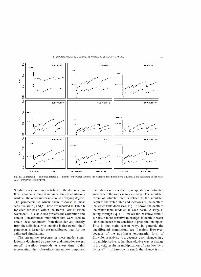
The streamflow response in these model simu-

lations is dominated by baseflow and saturation excess

runoff. Baseflow responds at short time scales

representing the sub-surface streamflow response.

Saturation excess is due to precipitation on saturated

areas where the wetness index is large. The simulated

extent of saturated area is related to the simulated

depth to the water table and increases as the depth to

the water table decreases. Fig. 13 shows the depth to

the water table modeled in each basin. A large f ;

acting through Eq. (10), makes the baseflow from a

sub-basin more sensitive to changes in depth to water

table and hence more sensitive to precipitation inputs.

This is the main reason why, in general, the

uncalibrated simulations are flashier. However,

because of the non-linear exponential form of

Eq. (10), sensitivity to �z depends upon changes in �z

in a multiplicative, rather than additive way. A change

in �z by D�z results in multiplication of baseflow by a

factor e2fD�z: If baseflow is small, the change is still

Fig. 13. Calibrated (—) and uncalibrated (- - -) depth to the water table by sub-watershed for Baron Fork at Eldon, at the beginning of the water

year 10/25/1994–12/20/1994.

C. Bandaragoda et al. / Journal of Hydrology 298 (2004) 178–201 197

small in absolute terms. If, however, baseflow is large,

the change is large.

The specific degree to which a sub-basin is more

or less flashy in uncalibrated versus calibrated

simulations depends upon the juxtaposition of

precipitation, antecedent precipitation and basin

parameters. Fig. 14 shows the sub-basin rainfall in

each sub-basin with the three-day storm totals

associated with the 11/6/94 and 12/9/94 events, as

well as the prior three-month antecedent precipi-

tation. Sub-basin one has the smallest rainfall totals

for this two-month period. Initial depth to water

table is largest with the result that increases in soil

moisture do not significantly increase the saturated

area. The baseflow response from sub-basin one in

both simulations is relatively minor due to the

sensitivity multiplier being applied to a small

Table 8

Baron Fork at Eldon f and K0 sub-basin parameters

Calibrated Uncalibrated

Multipliers 2.9 411.9 6.7 1000

Sub-basin f (m21) K0 (m/h) f (m21) K0 (m/h)

1 3.76 12.4 8.69 30.0

2 3.80 12.4 8.78 30.2

3 4.02 12.4 9.29 30.0

4 4.57 12.9 10.57 31.4

5 7.93 22.8 18.31 55.4

6 6.72 20.4 15.53 49.6

7 3.73 12.4 8.63 30.0

8 4.19 12.3 9.68 29.8

9 4.14 12.4 9.57 30.2

Fig. 14. Radar rain sub-watershed averages for Baron Fork at Eldon, at the beginning of the water year 10/25/1994–12/20/1994.

C. Bandaragoda et al. / Journal of Hydrology 298 (2004) 178–201198

number. Sub-basins five and six have different soils

that result in them having different f and K0

parameters. The larger values of f should imply

large sensitivity, but the large sensitivity results in

the saturated zone adjusting rapidly to accommodate

inputs. As soon as �z decreases due to water entering

the saturated zone, the baseflow increases modulat-

ing the reduction in �z: This effect limits the range

over which �z varies for these sub-basins, as

indicated in Fig. 13. The f values for sub-basins

five and six are sufficiently large that this behavior

is similar for both calibrated and uncalibrated

simulations. In the remaining sub-basins, the depth

to water table is such that streamflow is quite

sensitive to decreases in �z: The sub-basins with the

largest precipitation inputs (two, three and seven)

that follow the largest antecedent precipitation

inputs are most sensitive and exhibit the largest

differences between calibrated and uncalibrated

results.

We do not know, for these watersheds, how much

of this model behavior is representative of reality. We

also do not know whether the rainfall inputs are

sufficiently resolved at the scale of sub-basins to

meaningfully drive differences in sub-basin response.

Distributed modeling studies like this stimulate

questions and hypotheses that can be pursued further

in the ongoing effort to better understand and model

the hydrologic response of watersheds. We have

confirmed that for TOPNET, with TOPMODEL

controlling sub-surface flow, the parameter f is highly

sensitive and its derivation from GIS soils information

and careful calibration of the multiplier value is

important for accurate streamflow simulations.

4.5. Model run-time

Computer and time resources remain a limiting

factor to the operational use of distributed models.

Our computer system for the work was an AMD

athlon XP 1900 þ with 512 MB RAM, 1.4 GHz, and

Windows 2000 platform. Run-time for one seven-year

model run of 63,000 hourly timestep was 4–9 min for

a range of 9–21 model elements. Time for parameter

calibration by the SCE algorithm incorporated in the

NLFIT software for five parameters took between 6

and 9 h. See Table 9 for computer run times required

to model each of the DMIP basins.

5. Discussion and conclusion

For both calibration and validation periods, we

found that for our model calibrated flows using the

mean square error objective function improved the

matching of the peak streamflows, at the cost of over-

predicting the low flows and introducing bias into the

cumulative water balance, shown in the different

results for calibrated and uncalibrated simulations.

Statistics based on the square of the error term are

highly sensitive to differences between model and

measured flow during peak flood flows. Overall, the

model performed as well, or better in some cases, in

the validation period as in the calibration period. Lack

of information on the uncertainty in radar rainfall

inputs limited the interpretation of statistical perform-

ance measures used in DMIP to verify the quality of

flood simulations. Similarly, this lack of information

would limit the useful interpretation of statistical

performance measures used to verify the quality of

flood forecasts in applications beyond the scope of

this project.

The use of distributed models to simulate flow at

ungaged interior locations was highlighted with the

model results in Peacheater Creek at Christie,

Oklahoma. Our model simulations with calibration

were as good at interior locations, especially during

the validation period, as in the larger scale basins.

Understanding the reasons for the difference in

relative performance in larger basins and in interior

locations compared to the distributed Sacramento

models will help us improve our model simulations

for all basin scales. Comparative studies between the

model structures for simulating the sub-surface

(TOPMODEL versus Sacramento), treatment of

Table 9

Model run time and calibration time for each of the DMIP basins

Basin Model

elements

Run-time

minutes/model run

Parameter

calibration (h)

Baron 9 4 6

Blue 9 7 6

Elk 16 6 8

Tahl 21 9 9

Watt 15 7 7

C. Bandaragoda et al. / Journal of Hydrology 298 (2004) 178–201 199

radar rain sub-basin averaging, and soil parameteriza-

tion should be conducted.

The exponential functional form of baseflow

discharge–storage response limits the capability of

our model to match recessions in both low and high

flow scenarios and a single value per sub-basin for the

f parameter may not be appropriate. If the full range

of streamflow is to be simulated successfully a more

flexible parameterization of the discharge–storage

function is required, perhaps including separate quick

flow and slow flow functionality (Jakeman and

Hornberger, 1993) or development of a generalized

discharge–storage function from actual recession

curve analysis (Lamb and Beven, 1997), or by

generalizing the discharge–storage function (Duan

and Miller, 1997).

The small difference between calibrated and

uncalibrated results for TOPNET showed that, in

some basins, flows could be predicted well with

little or no calibration. Interior gages were modeled

comparatively as well as calibrated gages and show

the benefit of distributed models for simulating

uncalibrated interior monitoring point locations. In

future work we intend to investigate model element

scale questions and sensitivity to the spatial data

resolution of soil and vegetation data. We would

like to increase the number of model elements to see

if smaller element size improves model perform-

ance. Since the submission of DMIP results in

August 2000, we have added an impervious

area parameter to the model structure and will be

testing this functionality in urban and disturbed

watersheds.

Acknowledgements

We would like to thank Richard Ibbitt for his

suggestions and review. This work was supported by

the Utah Water Research Laboratory and by a visiting

scientist award from the National Institute of Water and

Atmospheric Research, Christchurch, New Zealand.

References

Beven, K.J., Kirkby, M.J., 1979. A physically based variable

contributing area model of basin hydrology. Hydrological

Sciences Bulletin 24(1), 43–69.

Beven, K., Lamb, R., Quinn, P., Romanowicz, R., Freer, J., 1995a.

Topmodel. In: Singh, V.P., (Ed.), Computer Models of

Watershed Hydrology, 18. Water Resources Publications,

Highlands Ranch, CO, (Chapter 18); pp. 627–668.

Beven, K., Quinn, P., Romanowicz, R., Freer, J., Fisher, J., Lamb,

R., 1995b. Topmodel and Gridatb, a Users Guide to the

Distribution Versions (95.02), CRES Technical Report TR110,

Centre for Research on Environmental Systems and Statistics,

Institute of Environmental and Biological Sciences, Lancaster

University, Lancaster.

Bristow, K.L., Campbell, G.S., 1984. On the relationship between

incoming solar radiation and the daily maximum and

minimum temperature. Agricultural and Forest Meteorology

31, 159–166.

Brooks, R.H., Corey, A.T., 1966. Properties of porous media

affecting fluid flow. Journal of Irrigation and Drainage ASCE

92(IR2), 61–88.

Broscoe, A.J., 1959. Quantitative analysis of longitudinal stream

profiles of small watersheds. Office of Naval Research, Project

NR 389-042. Technical Report No. 18, Department of Geology,

Columbia University, New York.

Clapp, R.B., Hornberger, G.M., 1978. Empirical equations for some

soil hydraulic properties. Water Resources Research 14,

601–604.

Dingman, S.L., 2002. Physical Hydrology, second ed., Prentice

Hall, Englewood Cliffs, NJ, 646 pp.

Duan, J., Miller, N.L., 1997. A generalized power function for the

subsurface transmissivity profile in TOPMODEL. Water

Resources Research 33, 2559–2562.

Duan, Q., Gupta, V.K., Sorooshian, S., 1993. A shuffled complex

evolution approach for effective and efficient global minimiz-

ation. Journal of Optimization Theory and Its Applications

76(3), 501–521.

Eidenshink, J.C., Faundeen, J.L., 1994. The 1-Km avhrr global land

data set: first stages in implementation. International Journal of

Remote Sensing 15, 3443–3462.

Famiglietti, J.S., Wood, E.F., 1994a. Application of multiscale

water and energy balance models on a Tallgras Prairie. Water

Resources Research 30(11), 3079–3093.

Famiglietti, J.S., Wood, E.F., 1994b. Mutiscale modeling of

spatially variable water and energy balances. Water Resources

Research 30(11), 3061–3078.

Famiglietti, J.S., Wood, E.F., Sivapalan, M., Thongs, D.J., 1992. A

catchment scale water balance model for fife. Journal of

Geophysical Research 97(D17), 18997–19007.

Flint, J.J., 1974. Stream gradient as a function of order, magnitude

and discharge. Water Resources Research 10(5), 969–973.

Goring, D.G., 1994. Kinematic shocks and monoclinal waves in the

Waimakariri, a steep, braided, gravel-bed river, Proceedings of

the International Symposium on Waves: Physical and Numeri-

cal Modelling, University of British Columbia, Vancouver,

Canada, 21–24 August, 1994, pp. 336–345.

Gupta, H.V., Sorooshian, S., Yapo, P.O., 1998. Toward improved

calibration of hydrologic models: multiple and noncommensur-

able measures of information. Water Resources Research 24(4),

751–763.

C. Bandaragoda et al. / Journal of Hydrology 298 (2004) 178–201200

Ibbitt, R., 1971. Development of a conceptual model of intercep-

tion, Unpublished Hydrological Research Progress Report No.

5, Ministry of Works, New Zealand.

Jakeman, A.J., Hornberger, G.M., 1993. How much complexity is

warranted in a rainfall-runoff model. Water Resources Research

29(8), 2637–2649.

Kuczera, G., 1983a. Improved parameter inference in catchment

models. 1. Evaluating parameters. Water Resources Research

19(5), 1151–1162.

Kuczera, G., 1983b. Improved parameter inference in catchment

models. 2. Combining different kinds of hydrologic data and

testing their compatibility. Water Resources Research 19(5),

1162–1172.

Kuczera, G., 1994. Nlfit, a Bayesian Nonlinear Regression Program

Suite, Version 1.00g, Department of Civil Engineering and

Surveying, University of Newcastle, New South Wales.

Lamb, R., Beven, K., 1997. Using interactive recession curve

analysis to specify a general catchment storage model.

Hydrology and Earth Systems Science 1, 101–113.

Leopold, L.B., Maddock, T., 1953. The hydraulic geometry of

stream channels and some physiographic implications. US

Geological Survey Professional Paper, No. 252.

Priestley, C.H.B., Taylor, R.J., 1972. On the assessment of surface

heat flux and evaporation using large-scale parameters. Monthly

Weather Review 100(2), 81–92.

Reed, S., Koren, V., Smith, M., Zhang, Z., Moreda, F., Seo, D.-J.,

2004. Overall distributed model intercomparison project results,

Journal of Hydrology 298(1–4), 27–60.

Rutter, A.J., Kershaw, K.A., Robins, P.C., Morton, A.J., 1972. A

predictive model of rainfall interception in forests. 1. Derivation

of the model from observations in a plantation of Corsican Pine.

Agricultural Meteorology 9, 367–384.

Seo, D.J., Fulton, R.A., Breidenbach, J.P., 1997. Final Report for

Interagency MOU among the Nexrad Program, WSR-88D OSF

and NWS/OH/HRL, NWS/OH/HRL, Silver Spring, MD.

Shuttleworth, W.J., 1993. Evaporation. In: Maidment, D.R., (Ed.),

Handbook of Hydrology, McGraw-Hill, New York, (Chapter 4).

Smith, M., 2002. Distributed model intercomparison project

(Dmip). National Weather Service. Retrieved October, 2001

from the World Wide Web: http://www.nws.noaa.gov/oh/hrl/

dmip/.

Smith, J.A., Seo, D.J., Baeck, M.L., Hudlow, M.D., 1996. An

intercomparison study of nexrad precipitation estimates. Water

Resources Research 32, 2035–2045.

Soil Survey Staff, 1994a. State Soil Geographic Database (Statsgo)

Collection for the Conterminous United States, USDA-NRCS,

National Soil Survey Center, Lincoln, NE, CD-ROM.

Soil Survey Staff, 1994b. State Soil Geographic Database (Statsgo)

Data Users Guide Miscellaneous Publication 1492, USDA

Natural Resources Conservation Service, US Government

Printing Office, Washington, DC, p. 88.

Stewart, J.B., 1977. Evaporation from the wet canopy of a pine

forest. Water Resources Research 13(6), 915–921.

Tarboton, D.G., 1997. A new method for the determination of flow

directions and contributing areas in grid digital elevation

models. Water Resources Research 33(2), 309–319.

Tarboton, D.G., 2002. Terrain Analysis Using Digital Elevation

Models (Taudem), Utah Water Research Laboratory, Utah State

University, http://www.engineering.usu.edu/dtarb.

Tarboton, D.G., Ames, D.P., 2001. Advances in the mapping of flow

networks from digital elevation data, World Water and

Environmental Resources Congress, Orlando, FL, May 20–

24, 2001, ASCE.

USGS, 2003. The National Map Seamless Data Distribution Server,

EROS Data Center, http://seamless.usgs.gov/.

Young, C.B., Bradley, A.A., Krajewski, W.F., Kruger, A., 2000.

Evaluating nexrad multisensor precipitation estimates for

operational hydrologic forecasting. Journal of Hydrometeorol-

ogy 1, 241–254.

C. Bandaragoda et al. / Journal of Hydrology 298 (2004) 178–201 201