ARTICLE IN PRESS

0098-3004/$ - se

doi:10.1016/j.ca

$Code avail�Correspond

fax: +1505 665

E-mail addr

Computers & Geosciences 32 (2006) 1139–1155

www.elsevier.com/locate/cageo

Application of parallel computing to stochastic parameterestimation in environmental models$

Jasper A. Vrugta,�, Breanndan O Nuallainb, Bruce A. Robinsona, Willem Boutenc,Stefan C. Dekkerd, Peter M.A. Slootb

aEarth and Environmental Sciences Division, Los Alamos National Laboratory, Mail Stop T003, Los Alamos, NM 87545, USAbFaculty of Sciences, Section Computational Science, University of Amsterdam, Kruislaan 403, 1098 SJ Amsterdam, The Netherlands

cFaculty of Sciences, Computational Bio- and Physical Geography, University of Amsterdam, Nieuwe Achtergracht 166, 1018 WV

Amsterdam, The NetherlandsdDepartment of Environmental Sciences, Faculty of Geosciences, Utrecht University, P.O. Box 80.115, 3508 TC Utrecht, The Netherlands

Received 2 May 2005; received in revised form 25 October 2005; accepted 25 October 2005

Abstract

Parameter estimation or model calibration is a common problem in many areas of process modeling, both in on-line

applications such as real-time flood forecasting, and in off-line applications such as the modeling of reaction kinetics and

phase equilibrium. The goal is to determine values of model parameters that provide the best fit to measured data,

generally based on some type of least-squares or maximum likelihood criterion. Usually, this requires the solution of a

non-linear and frequently non-convex optimization problem. In this paper we describe a user-friendly, computationally

efficient parallel implementation of the Shuffled Complex Evolution Metropolis (SCEM-UA) global optimization

algorithm for stochastic estimation of parameters in environmental models. Our parallel implementation takes better

advantage of the computational power of a distributed computer system. Three case studies of increasing complexity

demonstrate that parallel parameter estimation results in a considerable time savings when compared with traditional

sequential optimization runs. The proposed method therefore provides an ideal means to solve complex optimization

problems.

r 2005 Elsevier Ltd. All rights reserved.

Keywords: Optimization; Model; Hydrology; Bird migration; Octave; Message passing interface

1. Introduction and scope

The field of earth sciences is experiencing rapidchanges as a result of the growing understanding of

e front matter r 2005 Elsevier Ltd. All rights reserved

geo.2005.10.015

able from vrugt@lanl.gov

ing author. Tel.: +1505 667 0404;

8737.

ess: vrugt@lanl.gov (J.A. Vrugt).

environmental physics, along with recent advancesin measurement technologies, and dramatic in-creases in computing power. More complex, spa-tially explicit computer models are now possible,allowing for a more realistic representation ofsystems of interest. The increasing complexity ofthese models has, however, resulted in a largernumber of parameters that must be estimated.While the values of some of these parameters might

.

ARTICLE IN PRESS

1Eaton, J.W., 1998. Web: http://www.octave.org/, University

of Wisconsin, Department of Chemical Engineering, Madison,

WI 53719.2Fernandez Baldomero, J., 2004. LAM/MPI parallel comput-

ing under GNU Octave, http://atc.ugr.es/javier-bin/mpitb3Fernandez Baldomero, J., Anguita, M., Mota, S., Canaz,

Ortigosa, E., Rojas, F.J., 2004. MPI toolbox for Octave,

VecPar’04, Valencia, Spain, http://atc.ugr.es/�javier/investigacion/

papers/VecPar04.pdf

J.A. Vrugt et al. / Computers & Geosciences 32 (2006) 1139–11551140

be estimated directly from knowledge of the under-lying system, most represent effective propertiesthat cannot, in practice, be measured via directionobservation. Therefore, it is common practice toestimate values for model parameters by calibratingthe model against a historical record of input–out-put data. The successful application of these modelsdepends critically on how well the model iscalibrated.

Because of the time-consuming nature of manualtrial-and-error model calibration, there has been agreat deal of research into the development ofautomatic methods for parameter estimation(Levenberg, 1944; Marquardt, 1963; Nelder andMead, 1965; Kirkpatrick et al., 1983; Glover, 1986;Goldberg, 1989; Duan et al., 1993; Bahren et al.,1997; Zitzler and Thiele, 1999; among many others).Automatic parameter estimation methods seek totake advantage of the speed and power of digitalcomputers while being objective and relatively easyto implement. Over the years, many studies havedemonstrated that population-based global-searchapproaches have desirable properties that allowthem to overcome many of the difficulties related tothe shape of the response surface (the objectivefunction mapped out in the parameter space). Thesemethods have therefore become standard forsolving complex non-convex optimization pro-blems. However, application of global optimizationmethods to high-dimensional parameter estimationproblems requires the solution of a large number ofdeterministic model runs. The computationalburden of these models often hampers the useof advanced global optimization algorithms forcalibrating parameters in complex environmentalmodels.

Fortunately, during the past decade there hasbeen considerable progress in the development ofdistributed computer systems using the power ofmultiple processors to efficiently solve complex,high-dimensional computational problems (Byrdet al., 1993; Coleman et al., 1993a,b; More andWu, 1995). Parallel computing offers the possibilityof solving computationally challenging optimizationproblems in less time than is possible using ordinaryserial computing (Abramson, 1991; Goldberg et al.,1995; Alba and Troya, 1999; Herrera et al., 1998;Alba et al., 2004; Eklund, 2004; de Toro Negroet al., 2004; amongst various others). Despite theseprospects, parallel computing has not entered intowidespread use in the field due to difficulties withimplementation and barriers posed by technical

jargon. This is unfortunate, as many optimizationproblems in earth science are ‘‘embarrassinglyparallel’’ and thus are ideally suited for solutionon distributed computer systems.

In this paper we describe a parallel computingimplementation of the Shuffled Complex EvolutionMetropolis (SCEM-UA) global optimization algo-rithm for computationally efficient stochastic esti-mation of parameters in environmental models. Ourimplementation uses the recently developed MPITBtoolbox for GNU Octave (Eaton, 19981; FernandezBaldomero, 20042; Fernandez Baldomero et al.,20043), which is designed to take advantage of thecomputational power of a distributed computersystem. The implementation of parallelization in theSCEM-UA algorithm is done in a user-friendly way,such that the software can be easily adapted withoutin-depth knowledge of parallel computing. Thefeatures and capability of the parallel SCEM-UAimplementation are illustrated using a diverse set ofmodeling case studies of increasing complexity: (1) asynthetic 20-dimensional benchmark problem; (2)the calibration of the conceptual Sacramento SoilMoisture Accounting (SAC-SMA) model, and (3)the prediction of flight routes of migratory birds.

The remainder of this paper is organized asfollows. Section 2 presents a short introduction onparameter estimation in environmental models. InSections 3 and 4 we describe the SCEM-UAalgorithm and its parallel implementation on adistributed computer system, briefly describe theMPITB toolbox for GNU Octave for paralleliza-tion, and discuss the MPI (Message Passing Inter-face, 1997) implementation used to distribute tasksbetween different computers. In Section 5, weillustrate the power and applicability of parallelSCEM-UA parameter optimization using three casestudies of increasing complexity. There we focus onthe relationship between the computational timeneeded for parameter estimation and number ofnodes used. Finally, in Section 6 we summarize theresults and conclusions.

ARTICLE IN PRESSJ.A. Vrugt et al. / Computers & Geosciences 32 (2006) 1139–1155 1141

2. Parameter estimation

Consider an environmental system F for which amodel f is to be calibrated. Assume that themathematical structure of the model is essentiallypredetermined and fixed, and that realistic upperand lower bounds on each of the p modelparameters can be specified a priori. Let ~Y ¼f ~y1; . . . ; ~ytg denote the vector of measurement dataavailable at time steps 1,y,t and let Y ðyÞ ¼fy1ðyÞ; . . . ; ytðyÞg represent the corresponding vectorof model output predictions using the model e withparameter values y. The difference between themodel-simulated output and measured data can berepresented by the residual vector, E:

EðyÞ ¼ G½Y ðyÞ� � G½ ~Y � ¼ fe1ðyÞ; . . . ; etðyÞg, (1)

where the function G( � ) allows for various user-selected linear or non-linear transformations. Theaim of model calibration is to determine aset of model parameters y such that the measure E

is in some sense forced to be as close to zero aspossible. The formulation of a criterion thatmathematically measures the ‘‘size’’ of EðyÞ istypically based on assumptions regarding thedistribution of the measurement errors presentedin the data.

The classical approach to estimating the para-meters in Eq. (1) is to ignore input data uncertaintyand to assume that the predictive model e is acorrect representation of the underlying physicaldata-generating system (F). In line with classicalstatistical estimation theory, the residuals in Eq. (1)are then assumed to be mutually independent(uncorrelated) and Gaussian-distributed with aconstant variance. Under these circumstances, thetraditional ‘‘best’’ parameter set in Eq. (1) can befound by minimizing the following additive simpleleast-squares (SLS) objective function with respectto y:

FSLSðyÞ ¼Xt

i¼1

eiðyÞ2. (2)

For cases where the residuals in Eq. (1) arecorrelated a covariance structure of the residuals(or measurement noise) can be included in thedefinition of Eq. (2) so that the error terms becomeuncorrelated. Many algorithms have been devel-oped to solve the non-linear SLS optimizationproblem stated in Eq. (2). These algorithms includelocal search methodologies, which seek to improve

the objective function using an iterative searchstarting from a single arbitrary initial point inparameter space; and global search methods, inwhich multiple, concurrent searches are conductedfrom different starting points within parameterspace.

3. The SCEM-UA algorithm

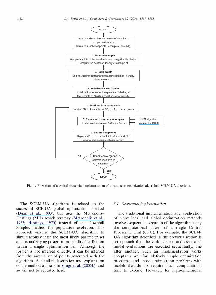
The SCEM-UA algorithm is a general-purpose,global optimization algorithm that provides anefficient estimate of the most likely parameter setand its underlying posterior probability distributionwithin a single optimization run (see Vrugt et al.,2003b). A condensed description of the method isgiven below and is illustrated in Fig. 1.

1.

Generate sample: Sample s parameter combina-tions fy1; . . . ; ysg randomly from the prior dis-tribution and compute the posterior density ofeach of these points using a slightly modifiedimplementation of Eq. (2) as presented in Boxand Tiao (1973).

2.

Rank points: Sort the s points in order ofdecreasing posterior density and store them inarray D[1:s,1:n+1], where n denotes the numberof parameters.

3.

Initialize Markov Chains: Initialize the startinglocations of k sequences using the first k elementsof D;Sk ¼ D½k; 1 : nþ 1�.

4.

Partition into complexes: Partition the s pointsof D into k complexes fC1; . . . ;Ckg, each contain-ing m points. The first complex contains everykðj � 1Þ þ 1 point of D, the second complex everykðj � 1Þ þ 2 of D, and so on, where j ¼ 1; . . . ;m.

5.

Evolve each sequence/complex: Evolve each se-quence and complex using the Sequence Evolu-tion Metropolis algorithm, described in detail inVrugt et al. (2003b).

6.

Shuffle complexes: Unpack all complexes C backinto D, and rank the points in order of decreasingposterior density.

7.

Check convergence: If convergence criteria aresatisfied, stop; otherwise return to step 4.

The algorithm is an approximate Markov ChainMonte Carlo (MCMC) sampler, which generates k

sequences of parameter sets fyð1Þ; yð2Þ; . . . ; yðNÞgthat converges to the stationary posterior dis-tribution for a large enough number of simula-tions N.

ARTICLE IN PRESS

START

Input: n = dimension,k = numberof complexes

s = population size

Compute number of points in complex (m = s /k).

1. GeneratesampleSample s points in the feasible space usingprior distribution

Compute the posterior density at each point.

2. Rank pointsSort de s points inorder of decreasing posterior density.

Store them in D.

3. Initialize Markov ChainsInitialize k independent sequences S starting at

the k points of D with highest posterior density.

4. Partition into complexesPartition D into k complexes Cq, q = 1,…,k of m points.

5. Evolve each sequence/complexEvolve each sequence k,Sq, q = 1,…,k

SEM algorithm

(Vrugt et al., 2003a)

6. Shuffle complexesReplace Cq, q= 1,...,k back into D and sort D in

order of decreasing posterior density.

7. Check convergenceConvergence criteria

satisfied?

STOP

No

Yes

Fig. 1. Flowchart of a typical sequential implementation of a parameter optimization algorithm: SCEM-UA algorithm.

J.A. Vrugt et al. / Computers & Geosciences 32 (2006) 1139–11551142

The SCEM-UA algorithm is related to thesuccessful SCE-UA global optimization method(Duan et al., 1993), but uses the Metropolis–Hastings (MH) search strategy (Metropolis et al.,1953; Hastings, 1970) instead of the DownhillSimplex method for population evolution. Thisapproach enables the SCEM-UA algorithm tosimultaneously infer the most likely parameter setand its underlying posterior probability distributionwithin a single optimization run. Although theformer is not inferred directly, it can be inferredfrom the sample set of points generated with thealgorithm. A detailed description and explanationof the method appears in Vrugt et al. (2003b), andso will not be repeated here.

3.1. Sequential implementation

The traditional implementation and applicationof many local and global optimization methodsinvolves sequential execution of the algorithm usingthe computational power of a single CentralProcessing Unit (CPU). For example, the SCEM-UA algorithm described in the previous section isset up such that the various steps and associatedmodel evaluations are executed sequentially, oneafter another. Such an implementation worksacceptably well for relatively simple optimizationproblems, and those optimization problems withmodels that do not require much computationaltime to execute. However, for high-dimensional

ARTICLE IN PRESSJ.A. Vrugt et al. / Computers & Geosciences 32 (2006) 1139–1155 1143

optimization problems involving complex spatiallydistributed models, such as are frequently used inthe field of earth science, this sequential implemen-tation needs to be revisited (Abramson, 1991;Goldberg et al., 1995; Alba and Troya, 1999;Herrera et al., 1998; Vrugt et al., 2001; Alba et al.,2004; Eklund, 2004; de Toro Negro et al., 2004;Vrugt et al., 2004; amongst various others).

Most computational time required for calibratingparameters in complex environmental models isspent running the model code and generating thedesired output. Thus, there should be large compu-tational efficiency gains from parallelizing thealgorithm so that independent model simulationsare run on different nodes in a distributed computersystem.

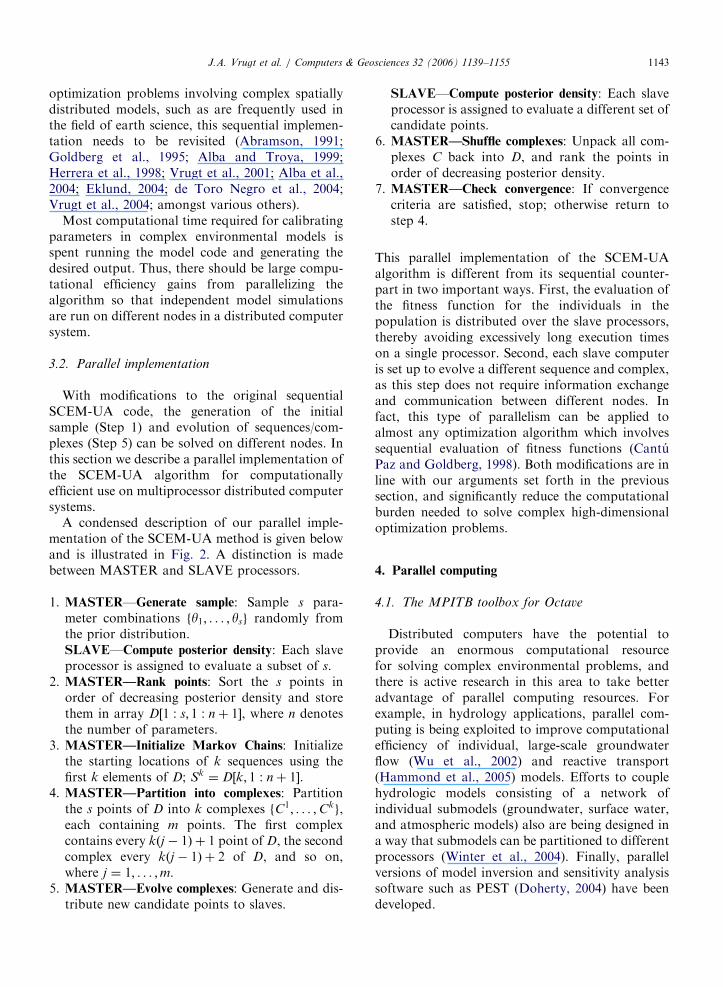
3.2. Parallel implementation

With modifications to the original sequentialSCEM-UA code, the generation of the initialsample (Step 1) and evolution of sequences/com-plexes (Step 5) can be solved on different nodes. Inthis section we describe a parallel implementation ofthe SCEM-UA algorithm for computationallyefficient use on multiprocessor distributed computersystems.

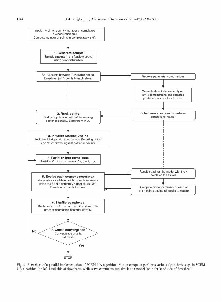
A condensed description of our parallel imple-mentation of the SCEM-UA method is given belowand is illustrated in Fig. 2. A distinction is madebetween MASTER and SLAVE processors.

1.

MASTER—Generate sample: Sample s para-meter combinations fy1; . . . ; ysg randomly fromthe prior distribution.SLAVE—Compute posterior density: Each slaveprocessor is assigned to evaluate a subset of s.

2.

MASTER—Rank points: Sort the s points inorder of decreasing posterior density and storethem in array D½1 : s; 1 : nþ 1�, where n denotesthe number of parameters.

3.

MASTER—Initialize Markov Chains: Initializethe starting locations of k sequences using thefirst k elements of D; Sk ¼ D½k; 1 : nþ 1�.

4.

MASTER—Partition into complexes: Partitionthe s points of D into k complexes fC1; . . . ;Ckg,each containing m points. The first complexcontains every kðj � 1Þ þ 1 point of D, the secondcomplex every kðj � 1Þ þ 2 of D, and so on,where j ¼ 1; . . . ;m.

5.

MASTER—Evolve complexes: Generate and dis-tribute new candidate points to slaves.

SLAVE—Compute posterior density: Each slaveprocessor is assigned to evaluate a different set ofcandidate points.

6.

MASTER—Shuffle complexes: Unpack all com-plexes C back into D, and rank the points inorder of decreasing posterior density.

7.

MASTER—Check convergence: If convergencecriteria are satisfied, stop; otherwise return tostep 4.

This parallel implementation of the SCEM-UAalgorithm is different from its sequential counter-part in two important ways. First, the evaluation ofthe fitness function for the individuals in thepopulation is distributed over the slave processors,thereby avoiding excessively long execution timeson a single processor. Second, each slave computeris set up to evolve a different sequence and complex,as this step does not require information exchangeand communication between different nodes. Infact, this type of parallelism can be applied toalmost any optimization algorithm which involvessequential evaluation of fitness functions (CantuPaz and Goldberg, 1998). Both modifications are inline with our arguments set forth in the previoussection, and significantly reduce the computationalburden needed to solve complex high-dimensionaloptimization problems.

4. Parallel computing

4.1. The MPITB toolbox for Octave

Distributed computers have the potential toprovide an enormous computational resourcefor solving complex environmental problems, andthere is active research in this area to take betteradvantage of parallel computing resources. Forexample, in hydrology applications, parallel com-puting is being exploited to improve computationalefficiency of individual, large-scale groundwaterflow (Wu et al., 2002) and reactive transport(Hammond et al., 2005) models. Efforts to couplehydrologic models consisting of a network ofindividual submodels (groundwater, surface water,and atmospheric models) also are being designed ina way that submodels can be partitioned to differentprocessors (Winter et al., 2004). Finally, parallelversions of model inversion and sensitivity analysissoftware such as PEST (Doherty, 2004) have beendeveloped.

ARTICLE IN PRESS

Input: n = dimension, k = number of complexess = population size

Compute number of points in complex (m = s /k).

Split s points between T available nodes.Broadcast (s /T) points to each slave.

Receive parameter combinations

On each slave independently run(s /T) combinations and computeposterior density of each point.

Collect results and send s posteriordensities to master

No

Yes

STOP

Receive and run the model with the kpoints on the slaves

Compute posterior density of each ofthe k points and send results to master

1. Generate sampleSample s points in the feasible space

using prior distribution.

2. Rank pointsSort de s points in order of decreasing

posterior density. Store them in D.

3. Initialize Markov ChainsInitialize k independent sequences S starting at the

k points of D with highest posterior density.

4. Partition into complexesPartition D into k complexes Cq, q = 1,…,k.

5. Evolve each sequence/complexGenerate k candidate points in each sequenceusing the SEM algorithm(Vrugt et al., 2003a).

Broadcast k points to slave.

6. Shuffle complexesReplace Cq, q= 1,...,k back into D and sort D in

order of decreasing posterior density.

7. Check convergenceConvergence criteria

satisfied?

Fig. 2. Flowchart of a parallel implementation of SCEM-UA algorithm. Master computer performs various algorithmic steps in SCEM-

UA algorithm (on left-hand side of flowsheet), while slave computers run simulation model (on right-hand side of flowsheet).

J.A. Vrugt et al. / Computers & Geosciences 32 (2006) 1139–11551144

ARTICLE IN PRESSJ.A. Vrugt et al. / Computers & Geosciences 32 (2006) 1139–1155 1145

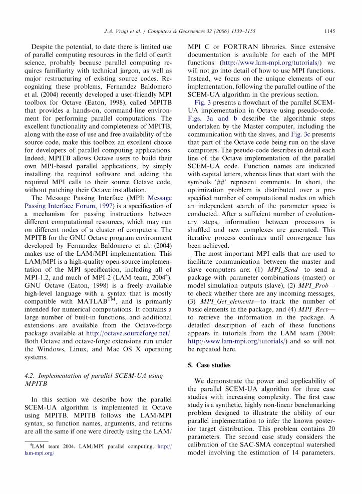
Despite the potential, to date there is limited useof parallel computing resources in the field of earthscience, probably because parallel computing re-quires familiarity with technical jargon, as well asmajor restructuring of existing source codes. Re-cognizing these problems, Fernandez Baldomeroet al. (2004) recently developed a user-friendly MPItoolbox for Octave (Eaton, 1998), called MPITBthat provides a hands-on, command-line environ-ment for performing parallel computations. Theexcellent functionality and completeness of MPITB,along with the ease of use and free availability of thesource code, make this toolbox an excellent choicefor developers of parallel computing applications.Indeed, MPITB allows Octave users to build theirown MPI-based parallel applications, by simplyinstalling the required software and adding therequired MPI calls to their source Octave code,without patching their Octave installation.

The Message Passing Interface (MPI: MessagePassing Interface Forum, 1997) is a specification ofa mechanism for passing instructions betweendifferent computational resources, which may runon different nodes of a cluster of computers. TheMPITB for the GNU Octave program environmentdeveloped by Fernandez Baldomero et al. (2004)makes use of the LAM/MPI implementation. ThisLAM/MPI is a high-quality open-source implemen-tation of the MPI specification, including all ofMPI-1.2, and much of MPI-2 (LAM team, 20044).GNU Octave (Eaton, 1998) is a freely availablehigh-level language with a syntax that is mostlycompatible with MATLABTM, and is primarilyintended for numerical computations. It contains alarge number of built-in functions, and additionalextensions are available from the Octave-forgepackage available at http://octave.sourceforge.net/.Both Octave and octave-forge extensions run underthe Windows, Linux, and Mac OS X operatingsystems.

4.2. Implementation of parallel SCEM-UA using

MPITB

In this section we describe how the parallelSCEM-UA algorithm is implemented in Octaveusing MPITB. MPITB follows the LAM/MPIsyntax, so function names, arguments, and returnsare all the same if one were directly using the LAM/

4LAM team 2004. LAM/MPI parallel computing, http://

lam-mpi.org/

MPI C or FORTRAN libraries. Since extensivedocumentation is available for each of the MPIfunctions (http://www.lam-mpi.org/tutorials/) wewill not go into detail of how to use MPI functions.Instead, we focus on the unique elements of ourimplementation, following the parallel outline of theSCEM-UA algorithm in the previous section.

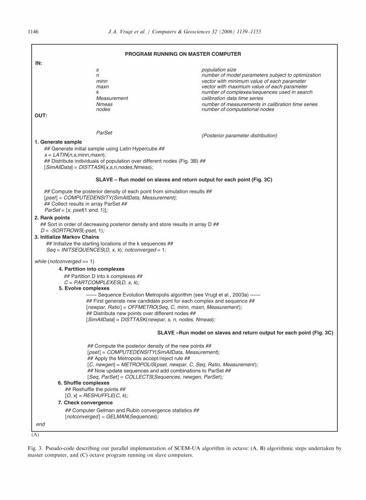
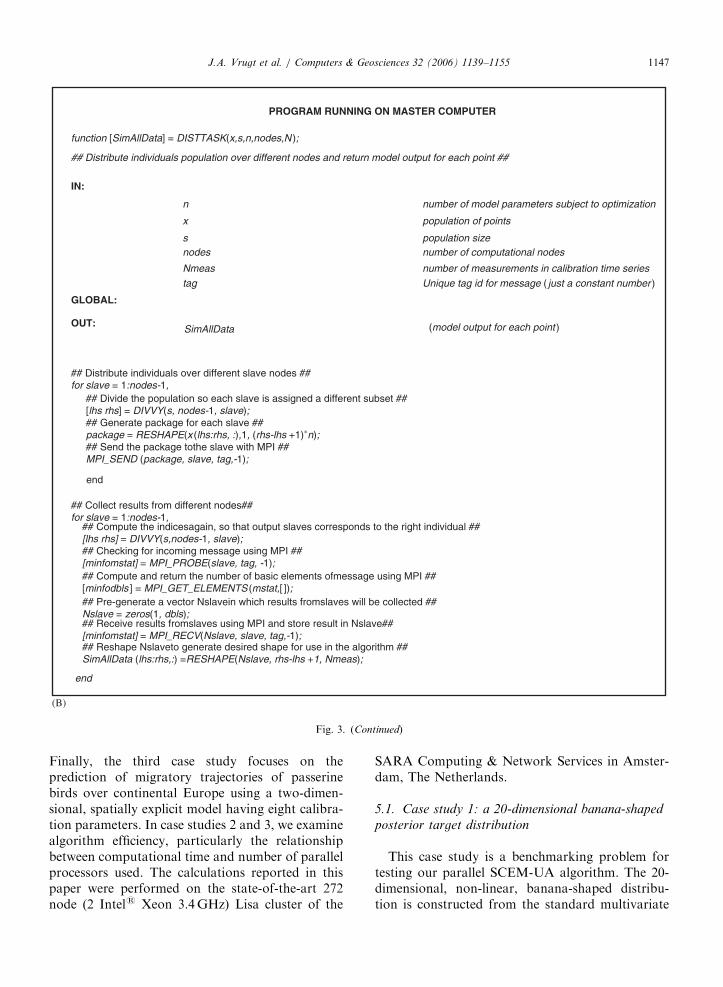
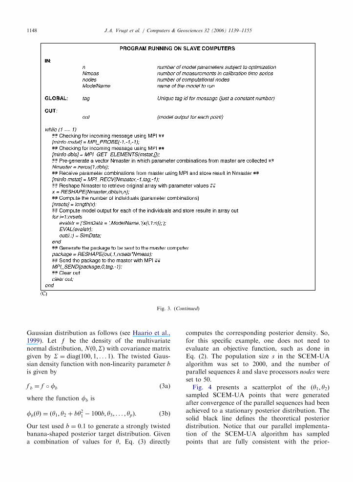
Fig. 3 presents a flowchart of the parallel SCEM-UA implementation in Octave using pseudo-code.Figs. 3a and b describe the algorithmic stepsundertaken by the Master computer, including thecommunication with the slaves, and Fig. 3c presentsthat part of the Octave code being run on the slavecomputers. The pseudo-code describes in detail eachline of the Octave implementation of the parallelSCEM-UA code. Function names are indicatedwith capital letters, whereas lines that start with thesymbols ‘##’ represent comments. In short, theoptimization problem is distributed over a pre-specified number of computational nodes on whichan independent search of the parameter space isconducted. After a sufficient number of evolution-ary steps, information between processors isshuffled and new complexes are generated. Thisiterative process continues until convergence hasbeen achieved.

The most important MPI calls that are used tofacilitate communication between the master andslave computers are: (1) MPI_Send—to send apackage with parameter combinations (master) ormodel simulation outputs (slave), (2) MPI_Prob—to check whether there are any incoming messages,(3) MPI_Get_elements—to track the number ofbasic elements in the package, and (4) MPI_Recv—to retrieve the information in the package. Adetailed description of each of these functionsappears in tutorials from the LAM team (2004:http://www.lam-mpi.org/tutorials/) and so will notbe repeated here.

5. Case studies

We demonstrate the power and applicability ofthe parallel SCEM-UA algorithm for three casestudies with increasing complexity. The first casestudy is a synthetic, highly non-linear benchmarkingproblem designed to illustrate the ability of ourparallel implementation to infer the known poster-ior target distribution. This problem contains 20parameters. The second case study considers thecalibration of the SAC-SMA conceptual watershedmodel involving the estimation of 14 parameters.

ARTICLE IN PRESS

PROGRAM RUNNING ON MASTER COMPUTER

OUT:

1. Generate sample## Generate initial sample using Latin Hypercube ##x = LATIN(n,s,minn,maxn);## Distribute individuals of population over different nodes (Fig. 3B) ##[SimAllData] = DISTTASK(x,s,n,nodes,Nmeas);

SLAVE – Run model on slaves and return output for each point (Fig. 3C)

## Compute the posterior density of each point from simulation results ##[pset ] = COMPUTEDENSITY(SimAllData, Measurement);## Collect results in array ParSet ##ParSet = [x, pset(1:end, 1)];

2. Rank points## Sort in order of decreasing posterior density and store results in array D ##D = -SORTROWS(-pset, 1);

3. Initialize Markov Chains## Initialize the starting locations of the k sequences ##Seq = INITSEQUENCES(D, x, k); notconverged = 1;

4. Partition into complexes## Partition D into k complexes ##C = PARTCOMPLEXES(D, x, k);

5. Evolve complexes------ Sequence Evolution Metropolis algorithm (see Vrugt et al., 2003a) ------## First generate new candidate point for each complex and sequence ##[newpar, Ratio ] = OFFMETRO(Seq, C, minn, maxn, Measurement );## Distribute new points over different nodes ##[SimAllData] = DISTTASK(newpar, s, n, nodes, Nmeas);

SLAVE –Run model on slaves and return output for each point (Fig. 3C)

## Compute the posterior density of the new points ##[pset ] = COMPUTEDENSITY(SimAllData, Measurement);## Apply the Metropolis accept /reject rule ##[C, newgen] = METROPOLIS(pset, newpar, C, Seq, Ratio, Measurement );## Now update sequences and add combinations to ParSet ##[Seq, ParSet ] = COLLECTS(Sequences, newgen, ParSet );

6. Shuffle complexes## Reshuffle the points ##[D, x] = RESHUFFLE(C, k);

7. Check convergence

## Computer Gelman and Rubin convergence statistics ##[notconverged ] = GELMAN(Sequences);

while (notconverged == 1)

ParSet

IN:snminnmaxnkMeasurementNmeasnodes

population sizenumber of model parameters subject to optimization vector with minimum value of each parametervector with maximum value of each parameternumber of complexes/sequences used in searchcalibration data time seriesnumber of measurements in calibration time seriesnumber of computational nodes

(Posterior parameter distribution)

end

(A)

Fig. 3. Pseudo-code describing our parallel implementation of SCEM-UA algorithm in octave: (A, B) algorithmic steps undertaken by

master computer, and (C) octave program running on slave computers.

J.A. Vrugt et al. / Computers & Geosciences 32 (2006) 1139–11551146

ARTICLE IN PRESS

PROGRAM RUNNING ON MASTER COMPUTER

## Distribute individuals population over different nodes and return model output for each point ##

IN:

GLOBAL:

OUT:

## Distribute individuals over different slave nodes ##for slave = 1:nodes-1,

## Divide the population so each slave is assigned a different subset ##[lhs rhs] = DIVVY(s, nodes-1, slave);## Generate package for each slave ##package = RESHAPE(x (lhs:rhs, :),1, (rhs-lhs +1)∗n);## Send the package tothe slave with MPI ##MPI_SEND (package, slave, tag,-1);

## Collect results from different nodes##for slave = 1:nodes-1,

## Compute the indicesagain, so that output slaves corresponds to the right individual ##[lhs rhs] = DIVVY(s,nodes-1, slave);## Checking for incoming message using MPI ##[minfomstat] = MPI_PROBE(slave, tag, -1);## Compute and return the number of basic elements ofmessage using MPI ##[minfodbls ] = MPI_GET_ELEMENTS (mstat,[ ]);## Pre-generate a vector Nslavein which results fromslaves will be collected ##Nslave = zeros(1, dbls);## Receive results fromslaves using MPI and store result in Nslave##[minfomstat] = MPI_RECV(Nslave, slave, tag,-1);## Reshape Nslaveto generate desired shape for use in the algorithm ##SimAllData (lhs:rhs,:) =RESHAPE(Nslave, rhs-lhs +1, Nmeas);

function [SimAllData] = DISTTASK(x,s,n,nodes,N );

n

x

snodes

Nmeas

tag

SimAllData

number of model parameters subject to optimization

population of points

population sizenumber of computational nodes

number of measurements in calibration time series

Unique tag id for message ( just a constant number )

(model output for each point )

end

end

(B)

Fig. 3. (Continued)

J.A. Vrugt et al. / Computers & Geosciences 32 (2006) 1139–1155 1147

Finally, the third case study focuses on theprediction of migratory trajectories of passerinebirds over continental Europe using a two-dimen-sional, spatially explicit model having eight calibra-tion parameters. In case studies 2 and 3, we examinealgorithm efficiency, particularly the relationshipbetween computational time and number of parallelprocessors used. The calculations reported in thispaper were performed on the state-of-the-art 272node (2 Intels Xeon 3.4GHz) Lisa cluster of the

SARA Computing & Network Services in Amster-dam, The Netherlands.

5.1. Case study 1: a 20-dimensional banana-shaped

posterior target distribution

This case study is a benchmarking problem fortesting our parallel SCEM-UA algorithm. The 20-dimensional, non-linear, banana-shaped distribu-tion is constructed from the standard multivariate

ARTICLE IN PRESS

Fig. 3. (Continued)

J.A. Vrugt et al. / Computers & Geosciences 32 (2006) 1139–11551148

Gaussian distribution as follows (see Haario et al.,1999). Let e be the density of the multivariatenormal distribution, Nð0;SÞ with covariance matrixgiven by S ¼ diagð100; 1; . . . 1Þ. The twisted Gaus-sian density function with non-linearity parameter b

is given by

f b ¼ f � fb (3a)

where the function fb is

fbðyÞ ¼ ðy1; y2 þ by21 � 100b; y3; . . . ; ypÞ. (3b)

Our test used b ¼ 0:1 to generate a strongly twistedbanana-shaped posterior target distribution. Givena combination of values for y, Eq. (3) directly

computes the corresponding posterior density. So,for this specific example, one does not need toevaluate an objective function, such as done inEq. (2). The population size s in the SCEM-UAalgorithm was set to 2000, and the number ofparallel sequences k and slave processors nodes wereset to 50.

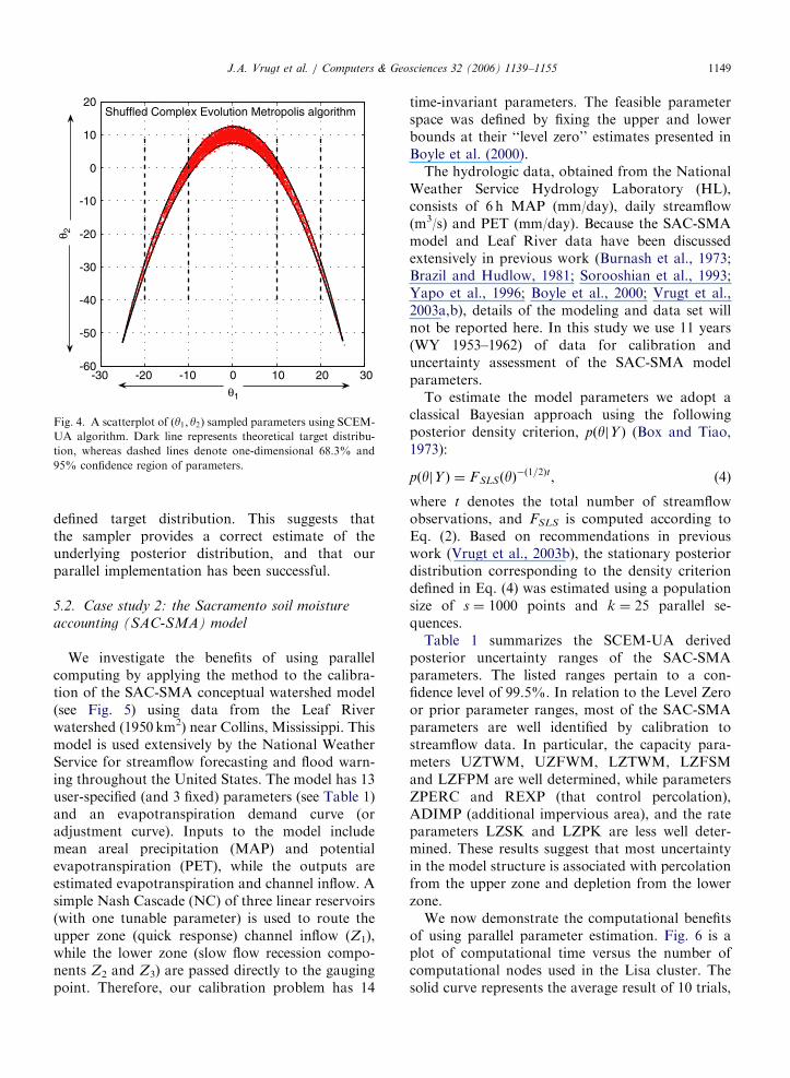
Fig. 4 presents a scatterplot of the ðy1; y2Þsampled SCEM-UA points that were generatedafter convergence of the parallel sequences had beenachieved to a stationary posterior distribution. Thesolid black line defines the theoretical posteriordistribution. Notice that our parallel implementa-tion of the SCEM-UA algorithm has sampledpoints that are fully consistent with the prior-

ARTICLE IN PRESS

-30 -20 -10 0 10 20 30-60

-50

-40

-30

-20

-10

0

10

20Shuffled Complex Evolution Metropolis algorithm

θ 2

θ1

Fig. 4. A scatterplot of (y1; y2) sampled parameters using SCEM-

UA algorithm. Dark line represents theoretical target distribu-

tion, whereas dashed lines denote one-dimensional 68.3% and

95% confidence region of parameters.

J.A. Vrugt et al. / Computers & Geosciences 32 (2006) 1139–1155 1149

defined target distribution. This suggests thatthe sampler provides a correct estimate of theunderlying posterior distribution, and that ourparallel implementation has been successful.

5.2. Case study 2: the Sacramento soil moisture

accounting (SAC-SMA) model

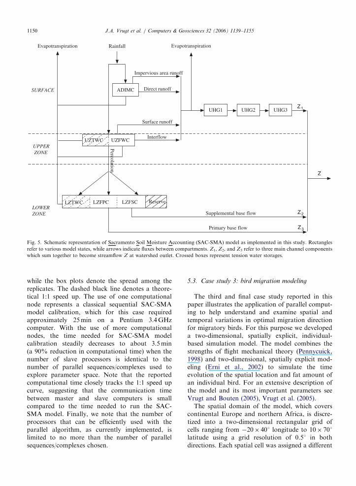
We investigate the benefits of using parallelcomputing by applying the method to the calibra-tion of the SAC-SMA conceptual watershed model(see Fig. 5) using data from the Leaf Riverwatershed (1950 km2) near Collins, Mississippi. Thismodel is used extensively by the National WeatherService for streamflow forecasting and flood warn-ing throughout the United States. The model has 13user-specified (and 3 fixed) parameters (see Table 1)and an evapotranspiration demand curve (oradjustment curve). Inputs to the model includemean areal precipitation (MAP) and potentialevapotranspiration (PET), while the outputs areestimated evapotranspiration and channel inflow. Asimple Nash Cascade (NC) of three linear reservoirs(with one tunable parameter) is used to route theupper zone (quick response) channel inflow (Z1),while the lower zone (slow flow recession compo-nents Z2 and Z3) are passed directly to the gaugingpoint. Therefore, our calibration problem has 14

time-invariant parameters. The feasible parameterspace was defined by fixing the upper and lowerbounds at their ‘‘level zero’’ estimates presented inBoyle et al. (2000).

The hydrologic data, obtained from the NationalWeather Service Hydrology Laboratory (HL),consists of 6 h MAP (mm/day), daily streamflow(m3/s) and PET (mm/day). Because the SAC-SMAmodel and Leaf River data have been discussedextensively in previous work (Burnash et al., 1973;Brazil and Hudlow, 1981; Sorooshian et al., 1993;Yapo et al., 1996; Boyle et al., 2000; Vrugt et al.,2003a,b), details of the modeling and data set willnot be reported here. In this study we use 11 years(WY 1953–1962) of data for calibration anduncertainty assessment of the SAC-SMA modelparameters.

To estimate the model parameters we adopt aclassical Bayesian approach using the followingposterior density criterion, pðyjY Þ (Box and Tiao,1973):

pðyjY Þ ¼ FSLSðyÞ�ð1=2Þt, (4)

where t denotes the total number of streamflowobservations, and FSLS is computed according toEq. (2). Based on recommendations in previouswork (Vrugt et al., 2003b), the stationary posteriordistribution corresponding to the density criteriondefined in Eq. (4) was estimated using a populationsize of s ¼ 1000 points and k ¼ 25 parallel se-quences.

Table 1 summarizes the SCEM-UA derivedposterior uncertainty ranges of the SAC-SMAparameters. The listed ranges pertain to a con-fidence level of 99.5%. In relation to the Level Zeroor prior parameter ranges, most of the SAC-SMAparameters are well identified by calibration tostreamflow data. In particular, the capacity para-meters UZTWM, UZFWM, LZTWM, LZFSMand LZFPM are well determined, while parametersZPERC and REXP (that control percolation),ADIMP (additional impervious area), and the rateparameters LZSK and LZPK are less well deter-mined. These results suggest that most uncertaintyin the model structure is associated with percolationfrom the upper zone and depletion from the lowerzone.

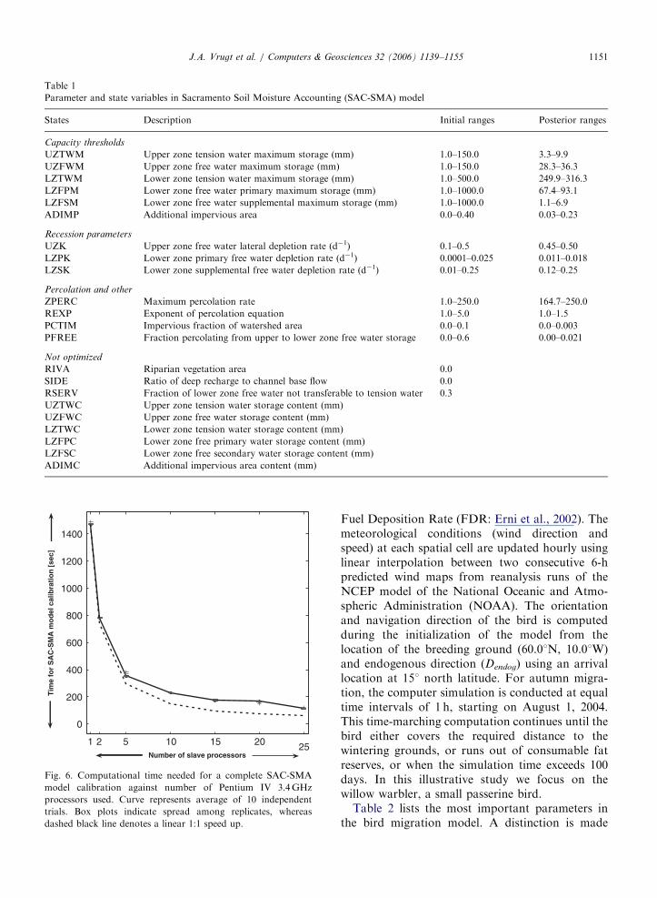
We now demonstrate the computational benefitsof using parallel parameter estimation. Fig. 6 is aplot of computational time versus the number ofcomputational nodes used in the Lisa cluster. Thesolid curve represents the average result of 10 trials,

ARTICLE IN PRESS

Evapotranspiration

SURFACE

UPPER ZONE

LOWERZONE

Direct runoff

Surface runoff

Interflow

Supplemental base flow

Primary base flow

Reserve

ADIMC

Rainfall

UZFWCUZTWC

Impervious area runoff

LZFSCLZFPCLZTWC

UHG1 UHG2 UHG3

Evapotranspiration

Z1

Z2

Z3

Z

PercolationFig. 5. Schematic representation of Sacramento Soil Moisture Accounting (SAC-SMA) model as implemented in this study. Rectangles

refer to various model states, while arrows indicate fluxes between compartments. Z1, Z2, and Z3 refer to three main channel components

which sum together to become streamflow Z at watershed outlet. Crossed boxes represent tension water storages.

J.A. Vrugt et al. / Computers & Geosciences 32 (2006) 1139–11551150

while the box plots denote the spread among thereplicates. The dashed black line denotes a theore-tical 1:1 speed up. The use of one computationalnode represents a classical sequential SAC-SMAmodel calibration, which for this case requiredapproximately 25min on a Pentium 3.4GHzcomputer. With the use of more computationalnodes, the time needed for SAC-SMA modelcalibration steadily decreases to about 3.5min(a 90% reduction in computational time) when thenumber of slave processors is identical to thenumber of parallel sequences/complexes used toexplore parameter space. Note that the reportedcomputational time closely tracks the 1:1 speed upcurve, suggesting that the communication timebetween master and slave computers is smallcompared to the time needed to run the SAC-SMA model. Finally, we note that the number ofprocessors that can be efficiently used with theparallel algorithm, as currently implemented, islimited to no more than the number of parallelsequences/complexes chosen.

5.3. Case study 3: bird migration modeling

The third and final case study reported in thispaper illustrates the application of parallel comput-ing to help understand and examine spatial andtemporal variations in optimal migration directionfor migratory birds. For this purpose we developeda two-dimensional, spatially explicit, individual-based simulation model. The model combines thestrengths of flight mechanical theory (Pennycuick,1998) and two-dimensional, spatially explicit mod-eling (Erni et al., 2002) to simulate the timeevolution of the spatial location and fat amount ofan individual bird. For an extensive description ofthe model and its most important parameters seeVrugt and Bouten (2005), Vrugt et al. (2005).

The spatial domain of the model, which coverscontinental Europe and northern Africa, is discre-tized into a two-dimensional rectangular grid ofcells ranging from �20� 401 longitude to 10� 701latitude using a grid resolution of 0.51 in bothdirections. Each spatial cell was assigned a different

ARTICLE IN PRESS

Table 1

Parameter and state variables in Sacramento Soil Moisture Accounting (SAC-SMA) model

States Description Initial ranges Posterior ranges

Capacity thresholds

UZTWM Upper zone tension water maximum storage (mm) 1.0–150.0 3.3–9.9

UZFWM Upper zone free water maximum storage (mm) 1.0–150.0 28.3–36.3

LZTWM Lower zone tension water maximum storage (mm) 1.0–500.0 249.9–316.3

LZFPM Lower zone free water primary maximum storage (mm) 1.0–1000.0 67.4–93.1

LZFSM Lower zone free water supplemental maximum storage (mm) 1.0–1000.0 1.1–6.9

ADIMP Additional impervious area 0.0–0.40 0.03–0.23

Recession parameters

UZK Upper zone free water lateral depletion rate (d�1) 0.1–0.5 0.45–0.50

LZPK Lower zone primary free water depletion rate (d�1) 0.0001–0.025 0.011–0.018

LZSK Lower zone supplemental free water depletion rate (d�1) 0.01–0.25 0.12–0.25

Percolation and other

ZPERC Maximum percolation rate 1.0–250.0 164.7–250.0

REXP Exponent of percolation equation 1.0–5.0 1.0–1.5

PCTIM Impervious fraction of watershed area 0.0–0.1 0.0–0.003

PFREE Fraction percolating from upper to lower zone free water storage 0.0–0.6 0.00–0.021

Not optimized

RIVA Riparian vegetation area 0.0

SIDE Ratio of deep recharge to channel base flow 0.0

RSERV Fraction of lower zone free water not transferable to tension water 0.3

UZTWC Upper zone tension water storage content (mm)

UZFWC Upper zone free water storage content (mm)

LZTWC Lower zone tension water storage content (mm)

LZFPC Lower zone free primary water storage content (mm)

LZFSC Lower zone free secondary water storage content (mm)

ADIMC Additional impervious area content (mm)

1 2 5 10 15 20 25

0

200

400

600

800

1000

1200

1400

Tim

e fo

r S

AC

-SM

A m

od

el c

alib

rati

on

[se

c]

Number of slave processors

Fig. 6. Computational time needed for a complete SAC-SMA

model calibration against number of Pentium IV 3.4GHz

processors used. Curve represents average of 10 independent

trials. Box plots indicate spread among replicates, whereas

dashed black line denotes a linear 1:1 speed up.

J.A. Vrugt et al. / Computers & Geosciences 32 (2006) 1139–1155 1151

Fuel Deposition Rate (FDR: Erni et al., 2002). Themeteorological conditions (wind direction andspeed) at each spatial cell are updated hourly usinglinear interpolation between two consecutive 6-hpredicted wind maps from reanalysis runs of theNCEP model of the National Oceanic and Atmo-spheric Administration (NOAA). The orientationand navigation direction of the bird is computedduring the initialization of the model from thelocation of the breeding ground (60.01N, 10.01W)and endogenous direction (Dendog) using an arrivallocation at 151 north latitude. For autumn migra-tion, the computer simulation is conducted at equaltime intervals of 1 h, starting on August 1, 2004.This time-marching computation continues until thebird either covers the required distance to thewintering grounds, or runs out of consumable fatreserves, or when the simulation time exceeds 100days. In this illustrative study we focus on thewillow warbler, a small passerine bird.

Table 2 lists the most important parameters inthe bird migration model. A distinction is made

ARTICLE IN PRESSJ.A. Vrugt et al. / Computers & Geosciences 32 (2006) 1139–11551152

between default values and parameters subject tooptimization. The uncertainty ranges of the calibra-tion parameters correspond to those of the willowwarbler. The total set of parameters in Table 2defines how the willow warbler reacts to its fatreserve and spatially and temporally varying envir-onmental conditions. Each parameter combinationtherefore results in a different simulated flight routetrajectory.

To implement and test our parallel SCEM-UAalgorithm, we must specify a life-history objectivethat the willow warbler is trying to satisfy, afterwhich the algorithm can be used to estimate theparameters in Table 2. Most optimality models thathave been developed in the avian migrationliterature consider flight time to be the mainobjective. In light of these considerations, we seekto identify all parameter combinations that result ina migration time close to the observed migrationtime of the willow warbler. Extensive ringingrecoveries (Hedenstrom and Pettersson, 1987) haveestablished this to be approximately 60 days. Toconduct the parameter search with the SCEM-UAalgorithm, we used a population size of 500 points,in combination with 10 parallel sequences. Theresults of our analysis are presented in Figs. 7 and 8and discussed.

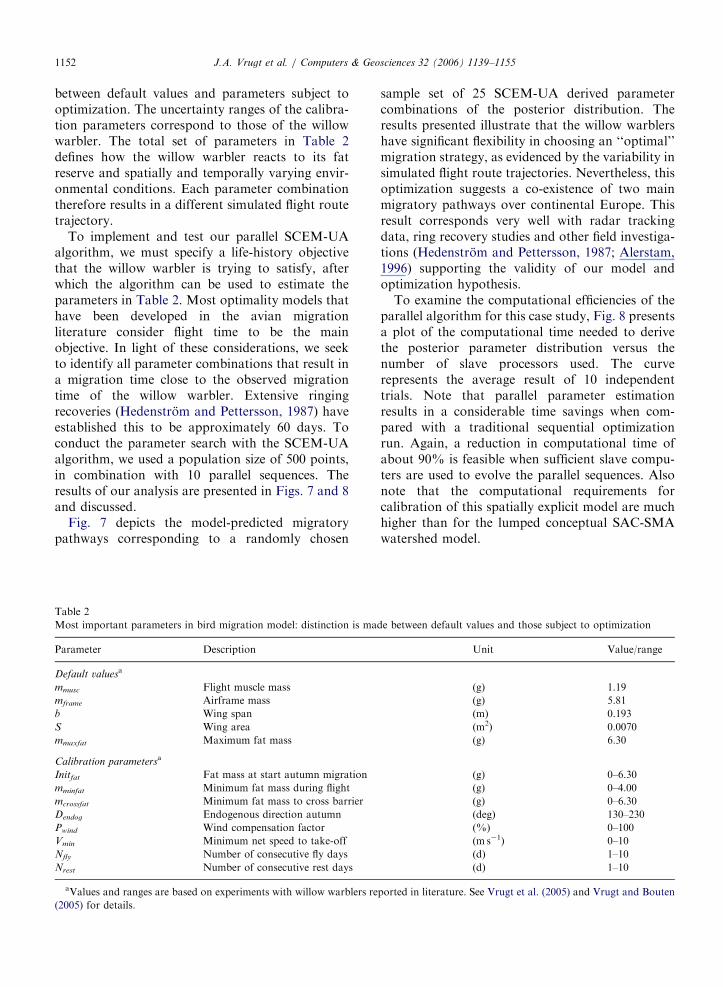
Fig. 7 depicts the model-predicted migratorypathways corresponding to a randomly chosen

Table 2

Most important parameters in bird migration model: distinction is ma

Parameter Description

Default valuesa

mmusc Flight muscle mass

mframe Airframe mass

b Wing span

S Wing area

mmaxfat Maximum fat mass

Calibration parametersa

Initfat Fat mass at start autumn migration

mminfat Minimum fat mass during flight

mcrossfat Minimum fat mass to cross barrier

Dendog Endogenous direction autumn

Pwind Wind compensation factor

Vmin Minimum net speed to take-off

Nfly Number of consecutive fly days

Nrest Number of consecutive rest days

aValues and ranges are based on experiments with willow warblers re

(2005) for details.

sample set of 25 SCEM-UA derived parametercombinations of the posterior distribution. Theresults presented illustrate that the willow warblershave significant flexibility in choosing an ‘‘optimal’’migration strategy, as evidenced by the variability insimulated flight route trajectories. Nevertheless, thisoptimization suggests a co-existence of two mainmigratory pathways over continental Europe. Thisresult corresponds very well with radar trackingdata, ring recovery studies and other field investiga-tions (Hedenstrom and Pettersson, 1987; Alerstam,1996) supporting the validity of our model andoptimization hypothesis.

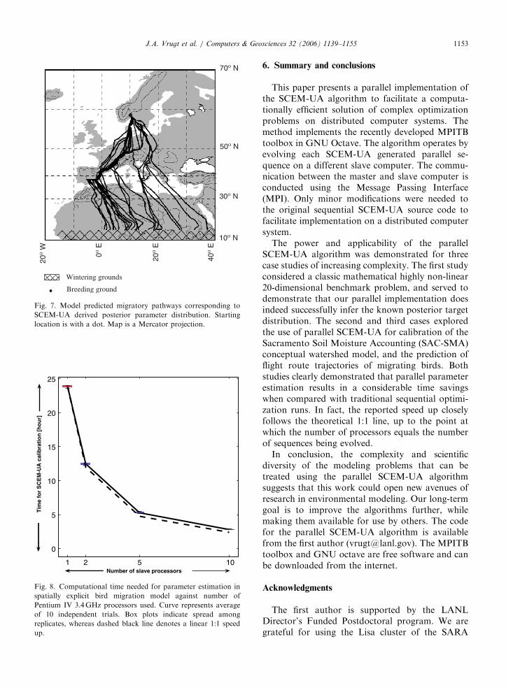
To examine the computational efficiencies of theparallel algorithm for this case study, Fig. 8 presentsa plot of the computational time needed to derivethe posterior parameter distribution versus thenumber of slave processors used. The curverepresents the average result of 10 independenttrials. Note that parallel parameter estimationresults in a considerable time savings when com-pared with a traditional sequential optimizationrun. Again, a reduction in computational time ofabout 90% is feasible when sufficient slave compu-ters are used to evolve the parallel sequences. Alsonote that the computational requirements forcalibration of this spatially explicit model are muchhigher than for the lumped conceptual SAC-SMAwatershed model.

de between default values and those subject to optimization

Unit Value/range

(g) 1.19

(g) 5.81

(m) 0.193

(m2) 0.0070

(g) 6.30

(g) 0–6.30

(g) 0–4.00

(g) 0–6.30

(deg) 130–230

(%) 0–100

(m s�1) 0–10

(d) 1–10

(d) 1–10

ported in literature. See Vrugt et al. (2005) and Vrugt and Bouten

ARTICLE IN PRESS

Wintering grounds

70ο N

50ο N

30ο N

10ο N

20ο

W

0ο E

20ο

E

40ο

E

Breeding ground

Fig. 7. Model predicted migratory pathways corresponding to

SCEM-UA derived posterior parameter distribution. Starting

location is with a dot. Map is a Mercator projection.

1 2 5 10

0

5

10

15

20

25

Tim

e fo

r S

CE

M-U

A c

alib

rati

on

[h

ou

r]

Number of slave processors

Fig. 8. Computational time needed for parameter estimation in

spatially explicit bird migration model against number of

Pentium IV 3.4GHz processors used. Curve represents average

of 10 independent trials. Box plots indicate spread among

replicates, whereas dashed black line denotes a linear 1:1 speed

up.

J.A. Vrugt et al. / Computers & Geosciences 32 (2006) 1139–1155 1153

6. Summary and conclusions

This paper presents a parallel implementation ofthe SCEM-UA algorithm to facilitate a computa-tionally efficient solution of complex optimizationproblems on distributed computer systems. Themethod implements the recently developed MPITBtoolbox in GNU Octave. The algorithm operates byevolving each SCEM-UA generated parallel se-quence on a different slave computer. The commu-nication between the master and slave computer isconducted using the Message Passing Interface(MPI). Only minor modifications were needed tothe original sequential SCEM-UA source code tofacilitate implementation on a distributed computersystem.

The power and applicability of the parallelSCEM-UA algorithm was demonstrated for threecase studies of increasing complexity. The first studyconsidered a classic mathematical highly non-linear20-dimensional benchmark problem, and served todemonstrate that our parallel implementation doesindeed successfully infer the known posterior targetdistribution. The second and third cases exploredthe use of parallel SCEM-UA for calibration of theSacramento Soil Moisture Accounting (SAC-SMA)conceptual watershed model, and the prediction offlight route trajectories of migrating birds. Bothstudies clearly demonstrated that parallel parameterestimation results in a considerable time savingswhen compared with traditional sequential optimi-zation runs. In fact, the reported speed up closelyfollows the theoretical 1:1 line, up to the point atwhich the number of processors equals the numberof sequences being evolved.

In conclusion, the complexity and scientificdiversity of the modeling problems that can betreated using the parallel SCEM-UA algorithmsuggests that this work could open new avenues ofresearch in environmental modeling. Our long-termgoal is to improve the algorithms further, whilemaking them available for use by others. The codefor the parallel SCEM-UA algorithm is availablefrom the first author (vrugt@lanl.gov). The MPITBtoolbox and GNU octave are free software and canbe downloaded from the internet.

Acknowledgments

The first author is supported by the LANLDirector’s Funded Postdoctoral program. We aregrateful for using the Lisa cluster of the SARA

ARTICLE IN PRESSJ.A. Vrugt et al. / Computers & Geosciences 32 (2006) 1139–11551154

Computing & Network Services in Amsterdam, TheNetherlands.

References

Abramson, D.A., 1991. Constructing school timetables using

simulated annealing: sequential and parallel algorithms.

Management Science 37 (1), 98–113.

Alba, E., Troya, J.M., 1999. A survey of parallel distributed

genetic algorithms. Complexity 4, 31–52.

Alba, E., Luna, F., Nebro, A.J., Troya, J.M., 2004. Parallel

heterogeneous genetic algorithms for continuous optimiza-

tion. Parallel Computing 30, 699–719.

Alerstam, T., 1996. The geographical scale factor in orientation

of migrating birds. Journal of Experimental Biology 199,

9–19.

Bahren, J., Protopopescu, V., Reister, D., 1997. TRUST: a

deterministic algorithm for global optimization. Science 276,

1094–1097.

Box, G.E.P., Tiao, G.C., 1973. Bayesian Inference in Statistical

Analyses. Addison-Wesley, Longman, Reading, MA

585pp.

Boyle, D.P., Gupta, H.V., Sorooshian, S., 2000. Towards

improved calibration of hydrologic models: combining the

strengths of manual and automatic methods. Water Re-

sources Research 36 (12), 3663–3674.

Brazil, L.E., Hudlow, M.D., 1981. Calibration procedures used

with the National Weather Service forecast system. In:

Haimes, Y.Y., Kindler, J. (Eds.), Water and Related Land

Resources. Pergamon, New York, pp. 457–466.

Burnash, R.J.C., Ferral, R.L., McGuire, R.A., 1973. A general-

ized streamflow simulation system: conceptual models for

digital computers. National Weather Service, NOAA, and the

State of California Department Of Water Resources Techni-

cal Report, Joint Federal-State River Forecast Center,

Sacramento, CA, 68pp.

Byrd, R.H., Eskow, E., Schnabel, R.B., Smith, S.L., 1993.

Parallel global optimization: numerical methods, dynamic

scheduling methods, and application to nonlinear con-

figuration. In: Ford, B., Fincham, A. (Eds.), Parallel

Computation. Oxford University Press, New York, NY,

pp. 187–207.

Cantu Paz, E., Goldberg, D.E., 1998. A survey of parallel genetic

algorithms. Calculateurs Paralleles, Reseaux et Systemes

Repartis 10 (2), 141–171.

Coleman, T.F., Shalloway, D., Wu, Z., 1993a. A parallel build-up

algorithm for global energy minimization of molecular

clusters using effective energy simulated annealing. Journal

of Global optimization 4, 171–185.

Coleman, T.F., Shalloway, D., Wu, Z., 1993b. Isotropic effective

energy simulated annealing searches for low energy molecular

cluster states. Computational Optimization and Applications

2, 145–170.

de Toro Negro, F., Ortega, J., Ros, E., Mota, S., Paechter, B.,

Martın, J.M., 2004. PSFGA: parallel processing and evolu-

tionary computation for multiobjective optimization. Parallel

Computing 30, 721–739.

Doherty, J., 2004. PEST Model-independent Parameter Estima-

tion, User Manual: fifth ed. Watermark Numerical Comput-

ing Inc.

Duan, Q.Y., Gupta, V.K., Sorooshian, S., 1993. Shuffled

Complex Evolution approach for effective and efficient global

minimization. Journal of Optimization Theory and Applica-

tions 76 (3), 501–521.

Eklund, S.E., 2004. A massively parallel architecture for distri-

buted genetic algorithms. Parallel Computing 30, 647–676.

Erni, B., Liechti, F., Bruderer, B., 2002. Stopover strategies in

passerine bird migration: a simulation study. Journal of

Theoretical Biology 219, 479–493.

Glover, F., 1986. Future paths for integer programming and links

to artificial intelligence. Computers and Operations Research

5, 533–549.

Goldberg, D.E., 1989. Genetic Algorithms in Search, Optimiza-

tion, and Machine learning. Addison-Wesley, Reading, MA,

pp. 1–403.

Goldberg, D.E., Kargupta, H., Horn, J., Cantu-Paz, E., 1995.

Critical deme size for serial and parallel genetic algorithms.

Technical Report 95002, GA Laboratory, University of

Illinois, Urbana-Campaign, IL.

Haario, H., Saksman, E., Tamminen, J., 1999. Adaptive proposal

distribution for random walk Metropolis algorithm. Compu-

tational Statistics 14 (3), 375–395.

Hammond, G.E., Valocchi, A.J., Lichtner, P.C., 2005. Applica-

tion of Jacobian-free Newton–Krylov with physics-based

preconditioning to biogeochemical transport. Advances in

Water Resources 28, 359–376.

Hastings, W.K., 1970. Monte-Carlo sampling methods using

Markov Chains and their applications. Biometrika 57,

97–109.

Hedenstrom, A., Pettersson, J., 1987. Migration routes and

wintering areas of willow warblers Phylloscopus trochilus

ringed in Fennoscandia. Ornis Fennica 64, 137–143.

Herrera, F., Lozano, M., Moraga, C., 1998. Hybrid distributed

real-coded genetic algorithms. In: Eiben, A.E., Back, T.,

Schoenauer, M., Schwefel, H.P. (Eds.), Parallel Problem

Solving from Nature (V). pp. 879–888.

Kirkpatrick, S., Gelatt, C.D., Vecchi, M.P., 1983. Optimization

by simulated annealing. Science 220, 671–680.

Levenberg, K., 1944. A method for the solution of certain

problems in least squares. Quaternary Applied Mathematics

2, 164–168.

Marquardt, D., 1963. An algorithm for least-squares estimation

of nonlinear parameters. SIAM Journal on Applied Mathe-

matics 11, 431–441.

Message Passing Interface Forum, 1997. MPI-2: Extensions to

the Message-passing Interface. University of Tennessee,

Knoxville, TN.

Metropolis, N., Rosenbluth, A.W., Rosenbluth, M.N., Teller,

A.H., Teller, E., 1953. Equations of state calculations by fast

computing machines. Journal of Chemical Physics 21,

1087–1091.

More, J.J., Wu, Z., 1995. e-optimal solutions to distance

geometry problems via global continuation. In: Pardalos,

P.M., Shalloway, D., Xue, G. (Eds.), Global Minimization

of Nonconvex Energy Functions: Molecular Confirmation

and Protein Folding. American Mathematical Society,

pp. 151–168.

Nelder, J.A., Mead, R., 1965. A Simplex method for function

minimization. Computer Journal 7, 308–313.

Pennycuick, C.J., 1998. Computer simulation of fat and muscle

burn in long-distance bird migration. Journal of Theoretical

Biology 191, 47–61.

ARTICLE IN PRESSJ.A. Vrugt et al. / Computers & Geosciences 32 (2006) 1139–1155 1155

Sorooshian, S., Duan, Q., Gupta, V.K., 1993. Calibration of

rainfall-runoff models: Application of global optimization to

the Sacramento Soil Moisture Accounting model. Water

Resources Research 29, 1185–1993.

Vrugt, J.A., Bouten, W., 2005. Differential flight patterns of

migratory birds explained by Pareto optimization of flight

time and energy use. To be submitted.

Vrugt, J.A., van Wijk, M.T., Hopmans, J.W., Simunek, J., 2001.

One-, two-, and three-dimensional root water uptake func-

tions for transient modeling. Water Resources Research 37

(10).

Vrugt, J.A., Gupta, H.V., Bastidas, L.A., Bouten, W., Sor-

ooshian, S., 2003a. Effective and efficient algorithm for multi-

objective optimization of hydrologic models. Water Re-

sources Research 39 (8), 1214.

Vrugt, J.A., Gupta, H.V., Bouten, W., Sorooshian, S., 2003b.

A Shuffled Complex Evolution Metropolis algorithm

for optimization and uncertainty assessment of hydrologic

model parameters. Water Resources Research 39 (8),

1201.

Vrugt, J.A., Schoups, G., Hopmans, J.W., Young, C., Wallender,

W.W., Harter, T., Bouten, W., 2004. Inverse modeling of

large-scale spatially distributed vadose zone properties using

global optimization. Water Resources Research 40, W06503.

Vrugt, J.A., van Belle, J., Bouten W., 2005. Multi-criteria

optimization of animal behavior: Pareto front analysis of

flight time and energy-use in long-distance bird migration.

Journal of Theoretical Biology, in review.

Winter, C.L., Springer, E.P., Costigan, K., Fasel, P., Mniszewski,

S., Zyvoloski, G., 2004. Virtual watersheds: simulating the

water balance of the Rio Grande basin. Computing in Science

and Engineering 6 (3), 18–26.

Wu, Y.S., Zhang, K., Ding, C., Pruess, K., Elmroth, E.,

Bodvarsson, G.S., 2002. An efficient parallel-computing

method for modeling nonisothermal multiphase flow and

multicomponent transport in porous and fractured media.

Advances in Water Resources 25, 243–261.

Yapo, P., Gupta, H.V., Sorooshian, S., 1996. Automatic

calibration of conceptual rainfall-runoff models: sensitivity

to calibration data. Journal of Hydrology 181, 23–48.

Zitzler, E., Thiele, L., 1999. Multiobjective evolutionary algo-

rithms: a comparative case study and the strength Pareto

approach. IEEE Transactions on Evolutionary Computation

3 (4), 257–271.