application of interval iterations to the entrainment problem in respiratory physiology
TRANSCRIPT

November 2009, published 2, doi: 10.1098/rsta.2009.0177367 2009 Phil. Trans. R. Soc. A
Jacques Demongeot and Jules Waku entrainment problem in respiratory physiologyApplication of interval iterations to the
Referencesl.html#ref-list-1http://rsta.royalsocietypublishing.org/content/367/1908/4717.ful
This article cites 26 articles, 1 of which can be accessed free
Subject collections
(13 articles)bioinformatics � collectionsArticles on similar topics can be found in the following
Email alerting service herein the box at the top right-hand corner of the article or click Receive free email alerts when new articles cite this article - sign up
http://rsta.royalsocietypublishing.org/subscriptions go to: Phil. Trans. R. Soc. ATo subscribe to
on March 13, 2014rsta.royalsocietypublishing.orgDownloaded from on March 13, 2014rsta.royalsocietypublishing.orgDownloaded from
Phil. Trans. R. Soc. A (2009) 367, 4717–4739doi:10.1098/rsta.2009.0177
Application of interval iterations to theentrainment problem in respiratory physiology
BY JACQUES DEMONGEOT* AND JULES WAKU
TIMC-IMAG Laboratory, University J. Fourier of Grenoble,38706 La Tronche, France
We present here some theoretical and numerical results about interval iterations.We consider first an application of the interval iterations theory to the problem ofentrainment in respiratory physiology for which the classical point iterations theory fails.Then, after a brief review of some of the main aspects of point iterations, we explainwhat is meant by the term ‘interval iterations’. It consists essentially in replacing in thepoint iterations the function to iterate by a set-valued map. We present both theoreticaland numerical aspects of this new type of iterations and we observe the dynamicalbehaviours encountered, such as fixed intervals and interval limit cycles. The comparisonbetween point and interval iterations is carried out with respect to a parameter ε, whichdetermines the thickness of a neighbourhood around the function to iterate. We willfinally focus our attention on the Verhulst and Ricker functions largely used in populationdynamics, which exhibit various asymptotic behaviours.
Keywords: interval iterations; respiratory entrainment; set-valued map; invariant domain;intervals limit cycles; population dynamics
1. Introduction
It is well known (May 1976; May & Oster 1976; Demongeot et al. 1997;Murray 2002) that a first-order difference equation (e.g. the logistic one-dimensional equation for a single species) allows the description of complexdynamical behaviours in population growth modelling in many contexts andseveral disciplines, such as in biology, economy and social sciences (Schafferet al. 1986; Demongeot & Leitner 1996; Demongeot et al. 1997; Stenseth et al.1997; Demongeot & Waku 2005). The case of n-dimensional flows (system ofdifference equations for n species) will not be treated in the following, but couldbe considered as a natural generalization of the techniques here proposed. Letthe basic equation be
xt+1 = f (xt). (1.1)
The variable xt can be referred to as the ‘population’ at time t; f is usuallya nonlinear function, containing one or more adjustable parameters, which tunethe nonlinear behaviour of the considered system. Population here means people,*Author for correspondence ([email protected]).
One contribution of 17 to a Theme Issue ‘From biological and clinical experiments to mathematicalmodels’.
This journal is © 2009 The Royal Society4717
on March 13, 2014rsta.royalsocietypublishing.orgDownloaded from

4718 J. Demongeot and J. Waku
animals, insects, bacteria or any self-reproducing organisms that grow over timeand fluctuate erratically. So equation (1.1) can model, for example, the growthof a population from one generation to another. xt can be considered as thepopulation size at time t (demography), the fraction of population infected attime t (epidemiology), the number of bits of information that can be rememberedafter a lapse of time t (telecommunications), the number of people to have hearda piece of information/rumour after time t (sociology), the phase of a periodicsignal in physiology, etc. Depending on the domains of application, parametershave different significance. For example, when xt is a population size, one ofthe parameters can be the growth rate and another the maximum number ofindividuals in the area of study.
The function f can also represent the relationship between xt+1 and xt , adiscrete variable linked to a dynamical system trajectory or to a time seriesof empirical observations (e.g. a Poincaré map or an empirical phase responsecurve), and equation (1.1) can exhibit complex dynamical behaviours includingfixed points, cycles of points of arbitrary 2m order and chaos when f is as afunction of the first argument a non-invertible, uni-modal map. These complexdynamical behaviours appear, in general, when f is continuous and uni-modal,from a stable point, through a sequence of bifurcations, into stable cycles of period2, 22, 23, 24, . . . , 2n , . . . and finally into a regime of chaos. This regime ischaracterized by the rapid loss of predictive power owing to the property thattrajectories arising from nearby initial conditions diverge exponentially fast atthe average. We can note that the sequence of bifurcations follows Sarkovskii’sω-order (Holmgren 1996) (respectively, Cosnard’s (1983) c-order) for uni-modal(respectively, multi-modal) maps. When the empirical data used for identifyingthe function f come from a noisy experimental process, we propose in the followingto replace f by a set-valued map whose graph (Aubin & Frankowska 1990; Chenet al. 2005) is bounded by the graphs of the functions (1 − ε)f and (1 + ε)f . Thepoint iterations dynamics of f is then replaced by a new process called intervaliterations, which just corresponds to the iterations of this set-valued map. Thepresent paper is devoted to new results concerning the bifurcations observed forthe interval iterations process of some set-valued maps defined from C 1 uni-modalmaps f on [0,1], applied in respiratory physiology and population dynamics.
2. Physiological motivation
Respiratory rhythm is controlled by bulbar centres that are characterized by anautonomous periodic free run and a particular ability to be forced by peripheralstimulations such as stretch receptor excitations at the end of each lung inflation(Pham Dinh et al. 1983). Let us denote the central respiratory variable by R,which is equal to 1 during central inspiration (corresponding to the phrenicnerve activity), and 0 during central expiration (corresponding to the phrenicsilence). Let P denote the peripheral respiratory variable, which is equal to 1when the lungs are inflated (by an external pump with period T ) and 0 whenthey are deflated. Respiratory regulatory properties imply that the delay xi+1(modulo T ) between the end of the (i + 1)th central inspiration and that of the(i + 1)th peripheral inflation depends only on the previous delay xi . Figure 1shows the placement of the R signal (black bars) on the P signal. In figure 2, the
Phil. Trans. R. Soc. A (2009)
on March 13, 2014rsta.royalsocietypublishing.orgDownloaded from

Application of interval iterations 4719
t
R0
1
TI TE
P
t0
1
I I I
T T
ti+1ti
T T
first respiratory cycleinspiration expiration
Figure 1. Relationships between respiratory variable R indicating the phases of inspiration withbold black bars (respectively expiration without bars) when R equals 1 (respectively, 0) and pumpvariable P indicating the phases of lung inflation (respectively, deflation) by an external pump whenP equals 1 (respectively, 0). tiT denotes the delay between the ith inspiration and the ith inflation.
I
1 s
I = T/2
2
1–2 3
(a) (b)
(c)
1–1
2
2
1–1 4
6
2–1
3–2
264
5 3
1
2,34
5
0 s 1 s 2 s 3 s 4 s 5 sT
Figure 2. (a) Parametric space (I , T ), with indications of the experiments reported in figure 4(black points 1–5) and of the observed p/q entrainment; (c) experimental recording of the Ractivity keeping only the bold black bars of figure 1 (displayed modulo T ) showing an empirical4/3 entrainment; theoretical landscape showing (b) Arnold’s tongues in qualitative agreement with(a) experimental tongues, but quantitative discrepancies (e.g. a width of the harmonic 1/1 regionlarger in the theoretical than in the empirical case).
curve giving xi+1 as function f (xi) of xi is called the respiratory phase responsecurve. Forcing the respiratory centres to have p inspirations during q pumpcycles is called the p/q entrainment that corresponds to the existence of a cycleof order p for iterations of f and to the occurrence of (p–q) changes between
Phil. Trans. R. Soc. A (2009)
on March 13, 2014rsta.royalsocietypublishing.orgDownloaded from

4720 J. Demongeot and J. Waku
1
0 0 0
1 2 3
tT1 tTl tTi
tTl+1tTl+1
(a) (b) (c)
Figure 3. (a) Point iterations with a fixed point in parametric circumstances (1), (b) experimentalrespiratory phase response curve (2), and (c) point iterations showing a chaotic behaviour (3).
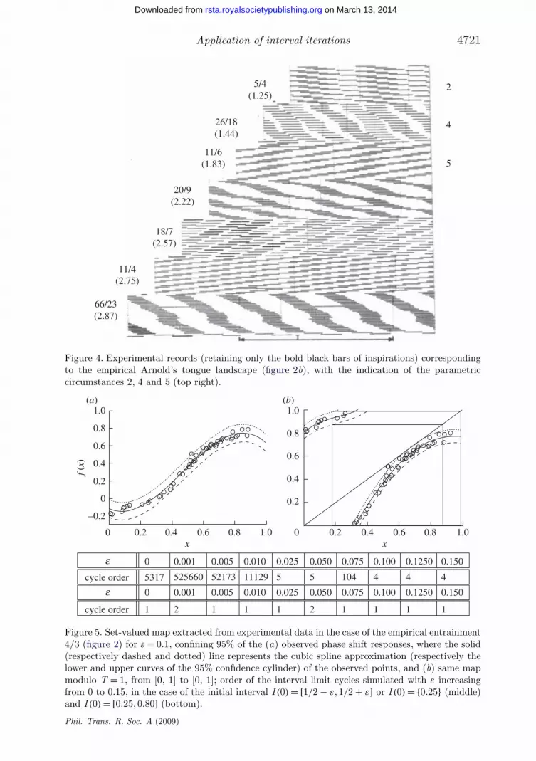
the upper and the lower parts of the graph of f during this cycle. The intervaliterations of the set-valued map centred on the central cubic function (the widthof this map surrounding f corresponding to the contour lines of the empiricaldistribution containing 95% of the experimental points) gives the followingresults: a regularization occurs from ε = 0.056 to 0.2, with a 4/3 (followed bya 6/5, for ε > 0.2) entrainment (figure 5). The experimental phase response curvein figure 2 has been built from the data recorded in rabbits (Demongeot et al.1987). We see in the table in figure 5 a dramatic change concerning the orderof the observed entrainments: if we start from the initial point 0.25 or a shortrange interval [0.5 − ε, 0.5 − ε], then we get a complex dynamics similar to thatobserved in point iterations; but when the length of the initial interval increases,then we observe a simplification of the cycles which tends to be a fixed interval ora cycle of two intervals, which is compatible with experimental observations wherecycle order is systematically smaller than that predicted by point iterations. Inpractice, when the a priori knowledge on the noise is slight, we start with a largeinitial interval and hence we get a reduced number of bifurcations.
In Demongeot et al. (1997), we called ‘chaos’ (Hoppensteadt 1993) what weobserved to be a unique fixed interval corresponding to the closure of the setof the chaotic point iterations values (ε = 0) (figure 3). The threshold εc fromwhich bifurcations to high-order cycles disappear is εc = 0.025 in figure 5. Thetheoretical bifurcation Arnold’s tongues landscape (figure 2b) fits qualitativelyexperimental data (Demongeot et al. 1987) and interval iterations regularizepoint iterations, replacing high-order cycles by their nearest sufficiently largebifurcation tongue (figure 4). The main interest of the interval iterations is togive, starting from different initial intervals, the same result on the entrainmentfraction p/q, with the same uncertainty ε = 0.1 as on the experimental curve. Thisqualitative fit allows us to avoid at this step the model refutation, which couldbe the case, by examining only point iterations corresponding to a behaviour atthe edge of chaos (figure 5).
Figure 6 shows the estimates of the empirical distribution of the datadeviations with respect to the central interpolated curve (a cubic spline) givenin figure 2: this distribution is not normal and has a skewness (Fisher γ1
Phil. Trans. R. Soc. A (2009)
on March 13, 2014rsta.royalsocietypublishing.orgDownloaded from
Application of interval iterations 4721
5/4(1.25)
2
4
5
26/18(1.44)
11/6(1.83)
20/9(2.22)
18/7(2.57)
11/4(2.75)
66/23(2.87)
Figure 4. Experimental records (retaining only the bold black bars of inspirations) correspondingto the empirical Arnold’s tongue landscape (figure 2b), with the indication of the parametriccircumstances 2, 4 and 5 (top right).
1.0(a) (b)
0.8
0.6
0.4
0.2
0
1.0
0.8
0.6
0.4
0.2
0 0.2 0.4 0.6 0.8 1.0
–0.2
0
0 0.001 0.005 0.010 0.025 0.050 0.075 0.100 0.1250 0.150
0
5317cycle order
cycle order
525660 52173 11129 5 5 4 4 4104
1 2 1 1 1 2 1 1 1 1
0.001 0.005 0.010 0.025 0.050 0.075 0.100 0.1250 0.150
0.2 0.4 0.6 0.8 1.0
f (x)
x x
e
e
Figure 5. Set-valued map extracted from experimental data in the case of the empirical entrainment4/3 (figure 2) for ε = 0.1, confining 95% of the (a) observed phase shift responses, where the solid(respectively dashed and dotted) line represents the cubic spline approximation (respectively thelower and upper curves of the 95% confidence cylinder) of the observed points, and (b) same mapmodulo T = 1, from [0, 1] to [0, 1]; order of the interval limit cycles simulated with ε increasingfrom 0 to 0.15, in the case of the initial interval I (0) = [1/2 − ε, 1/2 + ε] or I (0) = {0.25} (middle)and I (0) = [0.25, 0.80] (bottom).
Phil. Trans. R. Soc. A (2009)
on March 13, 2014rsta.royalsocietypublishing.orgDownloaded from

4722 J. Demongeot and J. Waku
0
–0.10 –0.05 0.05 0.100
value
–0.10 –0.05 0.05 0.100
value
2
468
1012
14(a) (b)
dens
ity
Figure 6. (a) Gaussian and (b) triangular kernel estimates fitting the distribution of empiricaldeviations to the central cubic spline of figure 5, equal to: −0.05 −0.05 0 0.02 0.03 0.04 0.05 0 0 0−0.02 −0.03 −0.02 −0.08 −0.04 −0.04 0.01 −0.02 0 −0.01 0 0 0 0 0.05 0.04 0.1 0 0 0.01 0.02 0.020.02 0.03 0 −0.01 0 0 −0.02 −0.05 0.05 −0.03 −0.03 −0.02 0.05 0.05 −0.02.
parameter of skewness equals 0.31) and a kurtosis (Fisher γ2 parameter ofkurtosis equals 0.6) incompatible with the Gaussian hypothesis (p = 0.4 for boththe skewness and the kurtosis test of normality). This strong evidence againstnormality prevents the use of the additive noised point iterations approaches(Homburg & Young 2006). We can make explicit other arguments againstthis approach.
Proposition 2.1. Let us consider the iterations on I = [0, 1] by f of a randomvariable X0 valued in I , with a noisy innovation at each time step: Xt = (1 +Yt−1)f (Xt−1), where f is the logistic function f (x) = rx(1 − x), Y0 is a randomvariable independent of X0 with mean 0 and variance ε2 (e.g. a variable uniformon [−√
3ε,√
3ε]), and Yt−1 has the same density function as Y0 and is independentof the Xs’s for times s < t and of the Ys’s for s < t − 1. When converging to anequilibrium measure, the probability distribution of Xt has its variance V (Xt) oforder O(r2t).
Proof. It is possible to prove the concentration towards an equilibrium measurefor the associated dynamics in the space of probability distributions (Tong 1983;Wu & Shao 2004). Yt−1f (xt − 1) can be considered as an additive random noise.If X and Y are independent, Z = (1 + Y )f (X ) has a variance V (Z ) verifying
ε2E(f 2(X )) ≤ (1 + ε2)E(f 2(X )) − E2(f (X )) = V (Z) = (1 + ε2)V (f (X ))
+ ε2E2(f (X )) ≤ (1 + ε2)E(f 2(X )) ≤ (1 + ε2)m2,
where E denotes the expectation and m = supx∈I f (x). If f is the logistic functionf (x) = rx(1 − x), we have more precisely
V (f (X )) = E(f 2(X )) − E2(f (X )) = r2[E(X 2(1 − X )2) − E2(X (1 − X ))]= r2[E(X 2) − 2E(X 3) + E(X 4) − E2(X ) + 2E(X )E(X 2) − E2(X 2)],
Phil. Trans. R. Soc. A (2009)
on March 13, 2014rsta.royalsocietypublishing.orgDownloaded from

Application of interval iterations 4723
and, from Jensen’s inequality −E(X 3) ≤ −E3(X ), we getV (f (X )) ≤ r2[V (X ) + 2E(X )V (X ) + V (X 2)]
≤ 2r2V (X )(1 + E(X )) (2.1)
and
(2.2)r2ε2E(X 2(1 − X )2) ≤ V (Z) = E((1 + Y )2f (X )2) − E2((1 + Y )f (X ))
= ε2E(f (X )2) − E2(f (X ))
= ε2V (f (X )) + (ε2 − 1)E2(f (X )) ≤ 2ε2r2V (X )(1 + E(X ))
≤ 4ε2r2. (2.3)
�Because the upper and the lower bounds of V (xt) are of the order O(r2t),
the variance of xt is not controlled in the additive noise scheme, if r > 1.The ignorance about the exact distribution of deviations to f pushes us tochoose a uniform random variable for X0 and Y0 and for the Yt ’s on theiterated intervals I (t)’s, especially in the vicinity of the point iteration case (εsmall). We will in the following denote by Fε(I ) the image of the interval Iby a set-valued map whose graph is a neighbourhood Vε(f ) of the graph of f(Aubin & Frankowska 1990)
Fε(I ) = [inf{y; x ∈ I , (x , y) ∈ Vε(f )}, sup{y; x ∈ I , (x , y) ∈ Vε(f )}].By choosing interval iterations, we do not manage the uncertainty as in Markov
iterations of an initial probability distribution on I by a deterministic transferfunction f leading to a stationary distribution (Dobbs 2007), but neverthelessthe interval iteration we propose deals with an absence of knowledge on f comingfrom an empirical intrinsic—but unknown and non-classical—noise. Comparablestudies have been done in set-valued iterations theory (Nadler 1969; Smajdor1985; Przytycki 1987) giving general conditions of convergence to attractors(De Farias & van Roy 2000; Graczyk et al. 2004; Kleptsyn & Nalskii 2004;Cheban & Mammana 2005; Desheng & Kloeden 2005; Kloeden & Valero 2005;Kamran 2007), but never solving the precise problem of their bifurcations incomparison with point iterations as reference when the uncertainty on f vanishes.Another type of iterations consists of adding a noise to the second member ofequation (1.1): Xt+1 = f (Xt) + W (t), where {W (t)}t≥0 is a uniform or Gaussianrandom process (Demongeot et al. 1987; Chan & Tong 1994). The successionof the ‘images’ of an interval in such a dynamics has analogies with intervaliteration, but the initial uniform probability distribution is replaced by a non-uniform one since the first iteration, except if X0 is uniform and if W (t) dependson Xt and is uniform on the interval [(1 − ε)f (Xt), (1 + ε)f (Xt)]. For example,near a stable fixed point β/(1 − α) of f , we can linearize f as f (x) ≈ αx + β andthe local random iterations are
Xt = (1 + Yt−1)f (Xt−1) ≈ (1 + Yt−1)(αXt−1 + β),with Yt−1 uniform on [−√
3ε,√
3ε] and independent of the Xs’s for s < t andthe Ys’s for s < t − 1. In this case, Xt has the same asymptotic distributionas the random variable β/(1 − α) + Z , where Z = β
∑i∈N αiYi , i.e. a circular
distribution on [−√3εβ/(1 − α),
√3εβ/(1 − α)] (Lévy 1939).
Phil. Trans. R. Soc. A (2009)
on March 13, 2014rsta.royalsocietypublishing.orgDownloaded from

4724 J. Demongeot and J. Waku
3. Point iterations: basic definitions
To study the dynamics of a discrete system or to solve equations numerically, weconsider an initial point and successively see what it becomes after a time interval.The sequence of the so-obtained points gives the dynamical behaviour of theinitial point during iterations. When we consider a continuous univariate functionf defined on a bounded interval I = [a, b] into itself, we denote the iterates of f bythe notation f ◦0(x) = x ; f ◦1(x) = f (x), . . . , f ◦n(x) = f (f ◦(n−1)(x)), for n = 2, 3, . . . .Then we say that x∗ is a fixed point of period m or order m if and only if
(i)f ◦m(x∗) = x∗ and (ii)f ◦j(x∗) = x∗ for j ≤ m.
The orbit of a point y iterated by the map f is the set of points W (y) ={f ◦j(y), ∀j = 0, 1, 2, . . .}. The local behaviour of a fixed point x∗ of f is determinedby its multipliers defined by
λ(x∗) = df (x)
dx|x=x∗ .
The study of the behaviour of a discrete dynamical system consists ofcharacterizing the multipliers of its fixed points and of its limit cycles. Thenwe have the classification
|λ(x∗)| < 1 ⇒ x∗ is an attracting equilibrium or stable fixed point;|λ(x∗)| = 0 ⇔ x∗ is a super-stable fixed point;|λ(x∗)| = 1 ⇔ x∗ is a neutral fixed point; and|λ(x∗)| > 1 ⇒ x∗ is a repulsive equilibrium or unstable fixed point.
To be more precise, if x∗ is stable, any small perturbation from its equilibriumdecays to zero, monotonically if 0 < λ(x∗) < 1, or with decreasing oscillationsif −1 < λ(x∗) < 0. On the other hand, if x∗ is unstable, any perturbation ismonotonically amplified if λ(x∗) > 1, or by growing oscillations if λ(x∗) < −1.Bifurcations occur when |λ(x∗)| passes through 1. So with λ(x∗) = −1, we have apitchfork bifurcation, while with λ(x∗) = 1, we have a fold bifurcation.
Let x0, x1, x2, . . . , xm−1 be the elements of an m-cycle C of f , i.e. C = (x0,x1, x2, . . . , xm−1) verifies
∀i = 1, . . . , m − 1, f (xi−1) = xi and f (xm−1) = x0,
then all these points are fixed points of period m of f . We can easily check, thanksto a chain of differentiations of f , that they have the same cycle multiplier thatis defined by
λ(m)(C ) = f ′(x0)f ′(x1), . . . , f ′(xm−1) = Πi=1,...,m−1f ′(xi) (3.1)
with f ′(xi) = df (x)/dx taken at x = xi . For such a periodic orbit, we have thesame classification as for fixed points replacing the point multiplier by λ(m)(C ):C is stable if |λ(m)(C )| < 1; if |λ(m)(C )| = +1, the cycle C is called neutral; if|λ(m)(C )| > 1, C becomes unstable and is in general replaced by a new stable cycleof period 2k+1, with m = 2k ; the maximum of stability, called super-stability, isobserved for the cycle C such as λ(m)(C ) = 0.
Phil. Trans. R. Soc. A (2009)
on March 13, 2014rsta.royalsocietypublishing.orgDownloaded from
Application of interval iterations 4725
4. Interval iterations
Interval iterations can be considered as the natural generalization of pointiterations. In this new iterations type, the entity to iterate is a compactinterval with non-empty interior instead of a point. If we denote the upper(respectively, lower) boundary of the function f to iterate by f ε = (1 + ε)f(respectively, fε = (1 − ε)f ), then after the (i + 1)th iteration, we obtain fromthe interval I (i) another interval I (i + 1) defined by I (i + 1) = [inf fε(I (i)),sup f ε(I (i))]. If I (0) = [x0, x1] ⊂ I = [a, b], then I (1) = [inf fε(I (0)), sup f ε(I (0))],which means that I (1) = [infx∈I (0) fε(x), supx∈I (0) f ε(x)]. We can also define theinterval iterations process by considering the set-valued application Sε from I tothe set of subsets of I , denoted P(I ), defined by
∀x ∈ I , Sε(x) = [fε(x), f ε(x)] and I (i + 1) = ∪x∈I (i)Sε(x).
By allowing a sufficient regularity (usually C 1) to the map f on the interval I ,we can consider two possible situations,
(i) if x0 = x1, then I (0) = {x0}, I (1) = [fε(x0), f ε(x0)] = [(1 − ε)f (x0),(1 + ε)f (x0)], and
(ii) if x0 = x1, the existence of I (1) follows from the fact that I (0) = [x0, x1] isa compact interval and that fε (respectively, f ε) are continuous functions.
It has been already shown (Demongeot & Waku 2005) that the notions offixed points and cycles of points can be generalized into those of fixed intervalsand cycles of intervals. We will study hereafter the stability of this new type ofiterations. For point iterations simulations, we begin the process with an initialpoint x0 and successively compare the point xi with xi+1 as i increases untiltwo consecutive points coincide under a fixed stop criterion, when the iterationconverges. The new approach adopted here involves, instead iterating points,iterating intervals. If the map under consideration is f , then a neighbourhoodcentred on this function can be defined by the neighbourhood Vε(f ) defined usingfive different methods,
(i) Vε(f ) = {(x , y) ∈ I 2/y ∈ Sε(x)} (ε-vertical neighbourhood),(ii) Vε(f ) = {(x , y) ∈ I 2/ supz∈f −1(y) d(x , z) ≤ ε} (ε-vertical neighbourhood),(iii) Vε(f ) = ∪B((x , f (x)), ε(x)) ∩ I 2, with B((x , f (x)), ε(x)) the open ball
centred in (x , f (x)) with radius ε(x) (orthogonal tubular neighbourhood),(iv) Vε(f ) = {(x , y) ∈ I 2/ ∃ ρ ∈ [r − ε, r + ε] and y = fρ(x)}, where ρ is a
parameter (2ε-diameter parametric neighbourhood), and(v) Vε(f ) = the subset of I 2 delimited by the contour line of a probability
distribution g on I 2 containing (1 − ε)per cent of the mass of g, whoseprojection of its set of maxima (crest line) is f (supposed to be anapplication). Given a set of data, g could be replaced by a smoothestimation of the presence probability distribution of the experimentalpoints. If the marginal repartition function Gx of y (considered as arandom variable) is continuous for any x ∈ I , then we can take Vε(f ) ={(x , y) ∈ I 2/y ∈ [hx(ε/2), Hx(1 − ε/2)]}, where we denote, if Gx is notinvertible: hx(ξ) = infz{z ; Gx(z) = ξ} and Hx(ξ) = supz{z ; Gx(z) = ξ}. Allthe definitions above account for the existence of a certain uncertainty
Phil. Trans. R. Soc. A (2009)
on March 13, 2014rsta.royalsocietypublishing.orgDownloaded from
4726 J. Demongeot and J. Waku
about the knowledge of f , whose empirical observations are supposed tolie in Vε(f ). The first (respectively, second) definition of Vε(f ) expressesthis uncertainty as a statistical regression with x (respectively, y) asa control variable. The third definition is used if uncertainty is x-dependent, and the fourth when uncertainty lies on the parameter of thefunction, if the variation coefficient of the data (the ratio between standarddeviation and mean) remains constant. The fifth definition corresponds toa neighbourhood in the observation space of the experimental data. Wewill in the following use definition (1.1).
5. Dynamical properties
Lemma 5.1. (After Demongeot et al. (1997).) Let f be a C 1 uni-modal map ofthe interval [0, 1] and I an invariant interval for the interval iterations process inwhich f has its unique maximum f (xc) at xc, then I = Fε(I ) ⊃ [fε(f ε(xc)), f ε(xc)].
Proof. (i) By definition, sup(f ε(I )) = f ε(xc), hence (figure 1): sup I =sup(f ε(I )) = f ε(xc). (ii) We also have: inf(I ) ≤ fε(f ε(xc)), because f ε(xc) ∈ f ε(I ) ⊂ Iand ∀x ∈ I , inf(I ) ≤ fε(x). �
Theorem 5.2. Let f be a C 1 uni-modal map of the interval [0, 1] (i.e. f(x)increases from 0 to f (xc), where xc is the location of the maximum of f , thendecreases to 0). If I denotes the stable fixed interval, supposed to be unique, ofthe interval iterations process of the set-valued map defined by ∀x ∈ [0, 1], Sε(x) =[fε(x), f ε(x)], then I contains the stable fixed points x∗
ε and x∗ε
of, respectively, fεand f ε, supposed to exist and to be unique. We have
(i) if x∗ε < x∗ε
< xc, then I = [x∗ε , x∗ε ];
(ii) if x∗ε < xc < x∗ε
, then I = [inf(x∗ε , fε(f ε(xc))), f ε(xc)]; and
(iii) if xc ≤ x∗ε < x∗ε
, then there exists,— either an interval [x1, x2], for which x1 > xc, fε(x2) = x1, f ε(x1) = x2 and
x1 (respectively, x2) is a stable fixed point of fεof ε (respectively, f εofε),with fε(f ε(xc)) > xc, then I = [x1, x2],
— or an interval [x1, x2] with the same characteristics as above, but withfε(f ε(xc)) ≤ xc, then we have a cycle of intervals,
I1 = [fε(f ε(xc)), x2], I2 = [x1, f ε(xc)] if we start from I (0) = [xc, xc],— or an interval [x1, x2] with the same characteristics as above, but with
x1 ≤ xc, thenI1 = [fε(f ε(xc)), f ε(xc)],
— or, more generally, a sequence of 2m points in [0, 1], x1, . . . , x2m asextremities of 2m−1 intervals constituting a limit cycle of order 2m−1.The order of apparition of these intervals in interval iterations will bedescribed in propositions 5.4 and 5.5.
Proof. (i) If x∗ε and x∗ε
are less than xc, they are stable fixed points of,respectively, fε and f ε and the result comes from the fact that fε and f ε are
Phil. Trans. R. Soc. A (2009)
on March 13, 2014rsta.royalsocietypublishing.orgDownloaded from

Application of interval iterations 4727
f e = f (1 + e)
f
f e = f (1 – e)
0.4 0.5 0.6 0.7 0.8x1 x2
Figure 7. Existence of an interval [x1, x2], for which x1 > xc , fε(x2) = x1, f ε(x1) = x2 and x1(respectively, x2) is a stable fixed point of fεof ε (respectively, f εofε).
1.0
0.8
0.6
0.4
0.2
0
I0
I2I1
0.2 0.4 0.6 0.8 1.0
Figure 8. The first three steps of logistic interval iterations for k = 2, r = 2.7, ε = 0.15 and I0 = {1/2}.
increasing between 0 and xc; if we start from I (0) = [x∗ε , x∗
ε ], then the iteratedintervals I (i) converge to [x∗
ε , x∗ε ] because
— f εok(x∗ε ) ≤ x∗ε
and f okε (x∗ε
) ≥ x∗ε , ∀k ≥ 2;
— f εok(x∗ε ) and f ok
ε (x∗ε) converge, respectively, to x∗ε and x∗ε when k tends
to infinity; and— / ⊃ ∪kεN ([x∗
ε , f εok(x∗ε )] ∪ [f ok
ε (x∗ε), x∗ε]).(ii) The result comes from the fact that f ε(xc) is the maximum value of f ε on
[0,1] and from lemma 5.1.(iii) The results come from the fact that x1 (respectively, x2) is a stable
fixed point of fεof ε (respectively, f εofε), and from lemma 5.1 (figures 7and 8). �
Phil. Trans. R. Soc. A (2009)
on March 13, 2014rsta.royalsocietypublishing.orgDownloaded from

4728 J. Demongeot and J. Waku
0 10
(a)
(c) (d ) (e)
(b)
1
10 x1
xc xcx1 x1x2 x2
x2xc xcx3
x3 x4
x3xcx
?
10 x
?
1x
?
f ε
x = f εrof εlofεlofε
r(x) x = f εrof εlofεrofε
l(x)x = f εlof εrofεrofε
l(x)
fε
f ε
fε
f ε
fε
f ε
fε
f ε
fε
Figure 9. (a) p = 0 and (b) p = 1, possible case, (c−e) and three impossible cases.
Definition 5.3. Let f be a C 1 uni-model map of the interval [0,1] on itself andlet xc be the point at which f has its maximum value. Let f εl and f εr (respectively,f lε and f r
ε ) be the functions equal to f ε (respectively, fε) on [0, xc[ for f εl and f lε , on
[xc, 1] for f εr and f rε and to identity Id[0,1] elsewhere. We call functional w-order
the partial order defined on [0.1][0,1] by the following sequences:
w0(f ) = w̄0(f ) = Id[0,1] ≺ w1(f ) = f rε of εlof εr ≺ w̄1(f ) = f εrof l
ε of rε ≺ · · ·
≺ wnf = wn−1(f ) of rε o w̄n−1(f ) of εl o w̄n−1(f ) o f εr o wn−1(f )
≺ w̄nf = w̄n−1(f ) of εro wn−1(f ) of lε o wn−1(f ) o f r
ε o w̄n−1(f ).
Proposition 5.4. Let f be C 1 uni-modal map of [0, 1] on itself and x in [xc, 1]belonging to a limit cycle of order 2k for the interval iterations of f . Then, if ε issufficiently small, x verifies
(i) if k = 2p, then x = f εlow̄p(f )(x), and(ii) if k = 2p + 1, then x = f εrowp(f )of r
ε o w̄p(f )(x).
Proof. Let the case p = 0: the only possible configuration corresponding toan invariant interval [x1, x2] is given in figure 9a and we have: x = f εrowo(f )of r
ε o w0(f )(x). In case p = 1, the point x1 (respectively, x2) has bifurcated in twopoints, x1 and x2 (respectively, x3 and x4), and the only possibleconfiguration corresponding to the limit cycle of intervals ([x1, x2], [x3, x4])is given in figure 9b and we have x4 = f εlof εrof l
ε of rε (x4) = f εlo w̄1(f )(x4). The
other possible configurations are x4 = f εrof εlof lε of r
ε (x4), x4 = f εlof εrof rε of l
ε (x4) andx4 = f εrof εlof l
ε (x4) (figure 9c–e), all incompatible with the dynamics. Indeed,
Phil. Trans. R. Soc. A (2009)
on March 13, 2014rsta.royalsocietypublishing.orgDownloaded from
Application of interval iterations 4729
x4 needs to be the ancestor of x1, because f rε (x4) is the rightmost among the
iterated extremities of intervals, and x1 (respectively, x3) needs to be the ancestorof x3 (respectively, x2) for the same kind of argument. The case where p is anyinteger strictly more than 1 is proved by using an induction based on the fact thatthe case p is obtained from the case p − 1 from a doubling period bifurcation. Itis true when ε = 0, because it comes from the point iterations dynamics of thefunctions f C 1 uni-modal map of the interval [0,1] on itself, with f (0) = f (1) = 0(Collet & Eckmann 1980), and it remains true for ε sufficiently small by using anargument of continuity; for large ε, we use simulations in the case of the logisticfunction f (x) = rx(1 − x). �
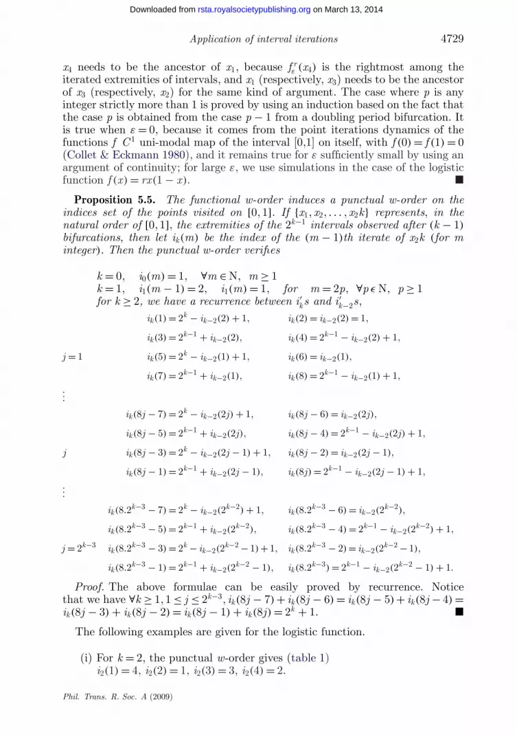
Proposition 5.5. The functional w-order induces a punctual w-order on theindices set of the points visited on [0, 1]. If {x1, x2, . . . , x2k} represents, in thenatural order of [0, 1], the extremities of the 2k−1 intervals observed after (k − 1)bifurcations, then let ik(m) be the index of the (m − 1)th iterate of x2k (for minteger). Then the punctual w-order verifies
k = 0, i0(m) = 1, ∀m ∈ N, m ≥ 1k = 1, i1(m − 1) = 2, i1(m) = 1, for m = 2p, ∀p ε N, p ≥ 1for k ≥ 2, we have a recurrence between i′ks and i′k−2s,
ik (1) = 2k − ik−2(2) + 1, ik (2) = ik−2(2) = 1,
ik (3) = 2k−1 + ik−2(2), ik (4) = 2k−1 − ik−2(2) + 1,
j = 1 ik (5) = 2k − ik−2(1) + 1, ik (6) = ik−2(1),
ik (7) = 2k−1 + ik−2(1), ik (8) = 2k−1 − ik−2(1) + 1,...
ik (8j − 7) = 2k − ik−2(2j) + 1, ik (8j − 6) = ik−2(2j),
ik (8j − 5) = 2k−1 + ik−2(2j), ik (8j − 4) = 2k−1 − ik−2(2j) + 1,
j ik (8j − 3) = 2k − ik−2(2j − 1) + 1, ik (8j − 2) = ik−2(2j − 1),
ik (8j − 1) = 2k−1 + ik−2(2j − 1), ik (8j) = 2k−1 − ik−2(2j − 1) + 1,...
ik (8.2k−3 − 7) = 2k − ik−2(2k−2) + 1, ik (8.2k−3 − 6) = ik−2(2k−2),
ik (8.2k−3 − 5) = 2k−1 + ik−2(2k−2), ik (8.2k−3 − 4) = 2k−1 − ik−2(2k−2) + 1,
j = 2k−3 ik (8.2k−3 − 3) = 2k − ik−2(2k−2 − 1) + 1, ik (8.2k−3 − 2) = ik−2(2k−2 − 1),
ik (8.2k−3 − 1) = 2k−1 + ik−2(2k−2 − 1), ik (8.2k−3) = 2k−1 − ik−2(2k−2 − 1) + 1.
Proof. The above formulae can be easily proved by recurrence. Noticethat we have ∀k ≥ 1, 1 ≤ j ≤ 2k−3, ik(8j − 7) + ik(8j − 6) = ik(8j − 5) + ik(8j − 4) =ik(8j − 3) + ik(8j − 2) = ik(8j − 1) + ik(8j) = 2k + 1. �
The following examples are given for the logistic function.
(i) For k = 2, the punctual w-order gives (table 1)i2(1) = 4, i2(2) = 1, i2(3) = 3, i2(4) = 2.
Phil. Trans. R. Soc. A (2009)
on March 13, 2014rsta.royalsocietypublishing.orgDownloaded from
4730 J. Demongeot and J. Waku
0 2 4 6 8 10 12 14 16
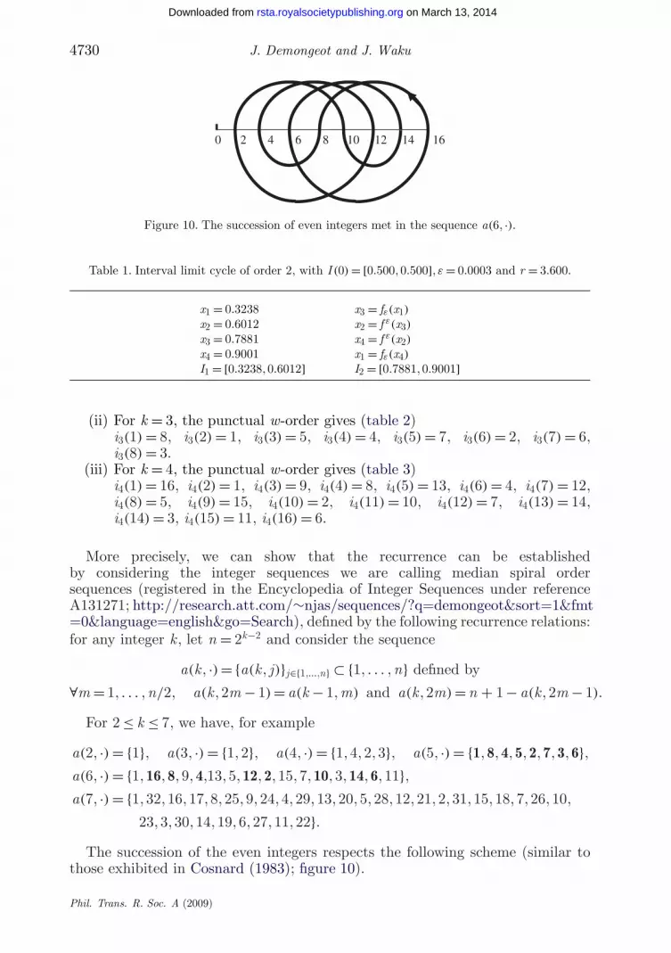
Figure 10. The succession of even integers met in the sequence a(6, ·).
Table 1. Interval limit cycle of order 2, with I (0) = [0.500, 0.500], ε = 0.0003 and r = 3.600.
x1 = 0.3238 x3 = fε(x1)
x2 = 0.6012 x2 = f ε(x3)
x3 = 0.7881 x4 = f ε(x2)
x4 = 0.9001 x1 = fε(x4)
I1 = [0.3238, 0.6012] I2 = [0.7881, 0.9001]
(ii) For k = 3, the punctual w-order gives (table 2)i3(1) = 8, i3(2) = 1, i3(3) = 5, i3(4) = 4, i3(5) = 7, i3(6) = 2, i3(7) = 6,i3(8) = 3.
(iii) For k = 4, the punctual w-order gives (table 3)i4(1) = 16, i4(2) = 1, i4(3) = 9, i4(4) = 8, i4(5) = 13, i4(6) = 4, i4(7) = 12,i4(8) = 5, i4(9) = 15, i4(10) = 2, i4(11) = 10, i4(12) = 7, i4(13) = 14,i4(14) = 3, i4(15) = 11, i4(16) = 6.
More precisely, we can show that the recurrence can be establishedby considering the integer sequences we are calling median spiral ordersequences (registered in the Encyclopedia of Integer Sequences under referenceA131271; http://research.att.com/∼njas/sequences/?q=demongeot&sort=1&fmt=0&language=english&go=Search), defined by the following recurrence relations:for any integer k, let n = 2k−2 and consider the sequence
a(k, ·) = {a(k, j)}j∈{1,...,n} ⊂ {1, . . . , n} defined by
∀m = 1, . . . , n/2, a(k, 2m − 1) = a(k − 1, m) and a(k, 2m) = n + 1 − a(k, 2m − 1).
For 2 ≤ k ≤ 7, we have, for example
a(2, ·) = {1}, a(3, ·) = {1, 2}, a(4, ·) = {1, 4, 2, 3}, a(5, ·) = {1, 8, 4, 5, 2, 7, 3, 6},a(6, ·) = {1, 16, 8, 9, 4,13, 5, 12, 2, 15, 7, 10, 3, 14, 6, 11},a(7, ·) = {1, 32, 16, 17, 8, 25, 9, 24, 4, 29, 13, 20, 5, 28, 12, 21, 2, 31, 15, 18, 7, 26, 10,
23, 3, 30, 14, 19, 6, 27, 11, 22}.The succession of the even integers respects the following scheme (similar to
those exhibited in Cosnard (1983); figure 10).
Phil. Trans. R. Soc. A (2009)
on March 13, 2014rsta.royalsocietypublishing.orgDownloaded from
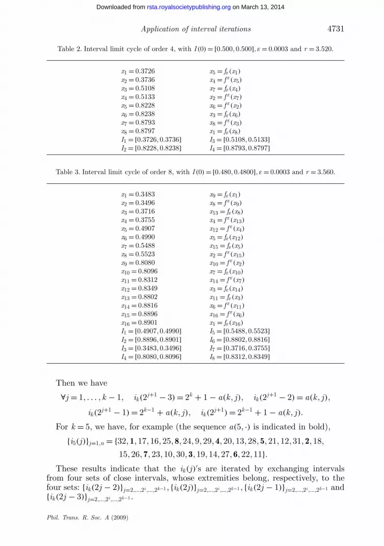
Application of interval iterations 4731
Table 2. Interval limit cycle of order 4, with I (0) = [0.500, 0.500], ε = 0.0003 and r = 3.520.
x1 = 0.3726 x5 = fε(x1)
x2 = 0.3736 x4 = f ε(x5)
x3 = 0.5108 x7 = fε(x4)
x4 = 0.5133 x2 = f ε(x7)
x5 = 0.8228 x6 = f ε(x2)
x6 = 0.8238 x3 = fε(x6)
x7 = 0.8793 x8 = f ε(x3)
x8 = 0.8797 x1 = fε(x8)
I1 = [0.3726, 0.3736] I3 = [0.5108, 0.5133]I2 = [0.8228, 0.8238] I4 = [0.8793, 0.8797]
Table 3. Interval limit cycle of order 8, with I (0) = [0.480, 0.4800], ε = 0.0003 and r = 3.560.
x1 = 0.3483 x9 = fε(x1)
x2 = 0.3496 x8 = f ε(x9)
x3 = 0.3716 x13 = fε(x8)
x4 = 0.3755 x4 = f ε(x13)
x5 = 0.4907 x12 = f ε(x4)
x6 = 0.4990 x5 = fε(x12)
x7 = 0.5488 x15 = fε(x5)
x8 = 0.5523 x2 = f ε(x15)
x9 = 0.8080 x10 = f ε(x2)
x10 = 0.8096 x7 = fε(x10)
x11 = 0.8312 x14 = f ε(x7)
x12 = 0.8349 x3 = fε(x14)
x13 = 0.8802 x11 = fε(x3)
x14 = 0.8816 x6 = f ε(x11)
x15 = 0.8896 x16 = f ε(x6)
x16 = 0.8901 x1 = fε(x16)
I1 = [0.4907, 0.4990] I5 = [0.5488, 0.5523]I2 = [0.8896, 0.8901] I6 = [0.8802, 0.8816]I3 = [0.3483, 0.3496] I7 = [0.3716, 0.3755]I4 = [0.8080, 0.8096] I8 = [0.8312, 0.8349]
Then we have
∀j = 1, . . . , k − 1, ik(2j+1 − 3) = 2k + 1 − a(k, j), ik(2j+1 − 2) = a(k, j),
ik(2j+1 − 1) = 2k−1 + a(k, j), ik(2j+1) = 2k−1 + 1 − a(k, j).
For k = 5, we have, for example (the sequence a(5, ·) is indicated in bold),
{i5(j)}j=1,n = {32, 1, 17, 16, 25, 8, 24, 9, 29, 4, 20, 13, 28, 5, 21, 12, 31, 2, 18,
15, 26, 7, 23, 10, 30, 3, 19, 14, 27, 6, 22, 11}.These results indicate that the ik(j)′s are iterated by exchanging intervals
from four sets of close intervals, whose extremities belong, respectively, to thefour sets: {ik(2j − 2)}j=2,...,2i ,...,2k−1 , {ik(2j)}j=2,...,2i ,...,2k−1 , {ik(2j − 1)}j=2,...,2i ,...,2k−1 and{ik(2j − 3)}j=2,...,2i ,...,2k−1 .
Phil. Trans. R. Soc. A (2009)
on March 13, 2014rsta.royalsocietypublishing.orgDownloaded from

4732 J. Demongeot and J. Waku
1.0
0.8f e fe
f
0.6
0.4
0.2
0 0.2 0.4 0.6 0.8 1.0
Figure 11. Example of a set-valued map built with an ε-vertical neighbourhood around f , wheref is the logistic function f (x) = rx(1 − x).
We leave the reader to check the consistency of the recurrent formulae ofproposition 5.5 with the examples given in tables 1–3. We can make more precisethe relationship between x1 and x2, respectively fixed points of fεof ε and fεof ε,verifying
x2 > x1 > xc, fε(x2) = x1 and f ε(x1) = x2,
as in case iii(a) of theorem 5.2, because if ∃ τ > 0/∀y ∈ [x1 − τ , x2 + τ ], −1 <f ′(y) < 0, then f is locally invertible, and there exists η given by Rolle’stheorem, such as 0 < η < x2 − x1 and x1 = x2 − e/f ′(x2 − η), where e = f (x2) −f (x1) = x1 − x2 + ε(f (x1) + f (x2)). The interval [x1, x2] is then a stable fixedinterval for the interval iterations dynamics. More generally, for proving theexistence of fixed intervals for f ◦m (m = 1 in the previous example), wecan use numerous fixed set theorems proven for the set-valued mappings(figure 11) (Nadler 1969; Smajdor 1985; Przytycki 1987; De Farias & vanRoy 2000; Reich & Zaslavski 2002; Graczyk et al. 2004; Kleptsyn & Nalskii2004; Cheban & Mammana 2005; Desheng & Kloeden 2005; Kloeden &Valero 2005; Kamran 2007; Wlodarczyk et al. 2007). These theorems involvein general a local Lipschitzian property of the set-valued mapping, for anadapted metric.
Proposition 5.6. Let us consider the case of the set-valued logistic mappingf (x) = rx(1 − x) and use as set distance the Hausdorff metric H. Then, if we startfrom I (0) = [x , y], with 1/2 < x < x∗ < y < 1, where x∗ = f (x∗), there exists a stablefixed interval I ∗ to which converge the iterates I (t) = f (I (t − 1))of I (0).
Proof. We have I (1) = [(1 − ε)ry(1 − y), (1 + ε)rx(1 − x)], I (2) = [(1 − ε2)r2
x(1 − x)(1 − (1 + ε)rx(1 − x)), (1 − ε2)r2y(1 − y)(1 − (1 − ε)ry(1 − y))], and by
Phil. Trans. R. Soc. A (2009)
on March 13, 2014rsta.royalsocietypublishing.orgDownloaded from

Application of interval iterations 4733
I1 = [0.4907,0.4990] I2 = [0.8896,0.8901] I3 = [0.3483,0.3496]
I8 = [0.8312,0.8349] I4 = [0.8080,0.8096]
I7 = [0.3716,0.3755] I6 = [0.8802,0.8816] I5 = [0.5488,0.5523]
Figure 12. Graphical example of the limit cycle of order 8 corresponding to table 3.
Table 4. Limit cycle orders of interval iterations starting with the interval I (0) = [0.25, 0.25].
ε
r 0 0.001 0.005 0.010 0.025 0.050 0.075 0.100 0.1250 0.150
2.50 cycle order 1 1 1 1 1 1 1 1 1 13.10 cycle order 2 2 2 2 1 1 1 1 1 13.20 cycle order 2 2 2 2 2 1 1 1 1 13.30 cycle order 2 2 2 2 2 2 1 1 1 13.40 cycle order 2 2 2 2 2 2 2 1 1 13.50 cycle order 4 4 2 2 2 2 2 1 1 13.60 cycle order 752 2 2 2 2 1 1 1 1 13.70 cycle order 1458 1 1 1 1 1 1 1 1 13.80 cycle order 3625 1 1 1 1 1 1 1 1 1
supposing that y − x∗ > x∗ − x and ε is sufficiently small, we have
H (I (i), I (i + 1)) − H (I (i + 1), I (i + 2)) = (f ε(x) − y) − (fε(y) − fεof ε(x))
= (β − α) + (fε(β) − fε(α)),
where α = y and β = f ε(x); but fε is a local Lipschitzian contraction, if 2 < r < 3,because
f ′ε (x
∗ε ) = (1 − ε)(2 − r).
Then the set-valued application is a set-valued contraction mapping and theexistence of a stable fixed interval has been proved in Nadler (1969). �
We can obtain the results of tables 1–3 and figure 12 by using either intervaliteration simulations or Newton iterations or continued fractions method (Lange1986) which gives with a controlled accuracy the roots of polynomials. Forexample, in the logistic case, if ε = 0.0003 and r = 2.8, the fixed point of thefunction f (x) = rx(1 − x) is equal to 0.6428571429 and the invariant intervalis [0.6418799286, 0.6438345399]. By looking at simulated dynamical behaviours(tables 4–6), we observed (table 4), for ε and I (0) small, the same first doublingbifurcations as for point iterations. When ε increases, I (0) remaining narrow,then we observe progressively only one doubling bifurcation (table 5) and when εis small but I (0) wide, we observe always the fixed interval: I = [fε(f ε(xc)), f ε(xc)]because fε(f ε(xc)) < xc and x∗
ε > xc (table 6 and case iii(c) of theorem 5.2).
Phil. Trans. R. Soc. A (2009)
on March 13, 2014rsta.royalsocietypublishing.orgDownloaded from
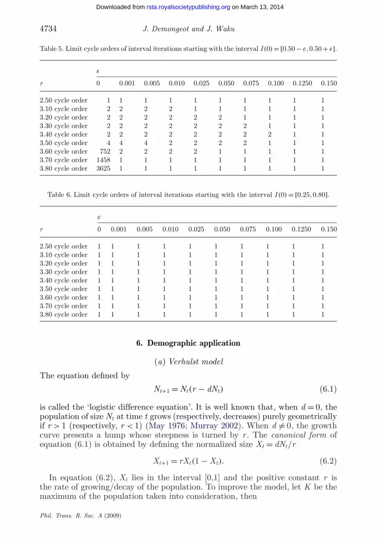
4734 J. Demongeot and J. Waku
Table 5. Limit cycle orders of interval iterations starting with the interval I (0) = [0.50 − ε, 0.50 + ε].
ε
r 0 0.001 0.005 0.010 0.025 0.050 0.075 0.100 0.1250 0.150
2.50 cycle order 1 1 1 1 1 1 1 1 1 13.10 cycle order 2 2 2 2 1 1 1 1 1 13.20 cycle order 2 2 2 2 2 2 1 1 1 13.30 cycle order 2 2 2 2 2 2 2 1 1 13.40 cycle order 2 2 2 2 2 2 2 2 1 13.50 cycle order 4 4 4 2 2 2 2 1 1 13.60 cycle order 752 2 2 2 2 1 1 1 1 13.70 cycle order 1458 1 1 1 1 1 1 1 1 13.80 cycle order 3625 1 1 1 1 1 1 1 1 1
Table 6. Limit cycle orders of interval iterations starting with the interval I (0) = [0.25, 0.80].
ε
r 0 0.001 0.005 0.010 0.025 0.050 0.075 0.100 0.1250 0.150
2.50 cycle order 1 1 1 1 1 1 1 1 1 13.10 cycle order 1 1 1 1 1 1 1 1 1 13.20 cycle order 1 1 1 1 1 1 1 1 1 13.30 cycle order 1 1 1 1 1 1 1 1 1 13.40 cycle order 1 1 1 1 1 1 1 1 1 13.50 cycle order 1 1 1 1 1 1 1 1 1 13.60 cycle order 1 1 1 1 1 1 1 1 1 13.70 cycle order 1 1 1 1 1 1 1 1 1 13.80 cycle order 1 1 1 1 1 1 1 1 1 1
6. Demographic application
(a) Verhulst model
The equation defined by
Nt+1 = Nt(r − dNt) (6.1)
is called the ‘logistic difference equation’. It is well known that, when d = 0, thepopulation of size Nt at time t grows (respectively, decreases) purely geometricallyif r > 1 (respectively, r < 1) (May 1976; Murray 2002). When d = 0, the growthcurve presents a hump whose steepness is turned by r . The canonical form ofequation (6.1) is obtained by defining the normalized size Xt = dNt/r
Xt+1 = rXt(1 − Xt). (6.2)
In equation (6.2), Xt lies in the interval [0,1] and the positive constant r isthe rate of growing/decay of the population. To improve the model, let K be themaximum of the population taken into consideration, then
Phil. Trans. R. Soc. A (2009)
on March 13, 2014rsta.royalsocietypublishing.orgDownloaded from
Application of interval iterations 4735
1.0(b)
(a)
0.8
0.6
0.4
0.2
0 0.2 0.4 0.6 0.8 1.0
x: normalized size of population
f(x)
: uni
mod
al f
unct
ion
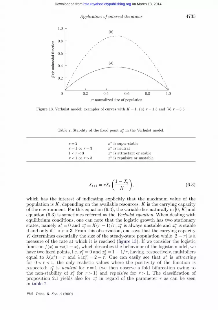
Figure 13. Verhulst model: examples of curves with K = 1. (a) r = 1.5 and (b) r = 3.5.
Table 7. Stability of the fixed point x∗2 in the Verhulst model.
r = 2 x∗ is super-stabler = 1 or r = 3 x∗ is neutral1 < r < 3 x∗ is attractant or stabler < 1 or r > 3 x∗ is repulsive or unstable
Xt+1 = rXt
(1 − Xt
K
), (6.3)
which has the interest of indicating explicitly that the maximum value of thepopulation is K , depending on the available resources. K is the carrying capacityof the environment. For this equation (6.3), the variable lies naturally in [0, K ] andequation (6.3) is sometimes referred as the Verhulst equation. When dealing withequilibrium conditions, one can note that the logistic growth has two stationarystates, namely x∗
1 = 0 and x∗2 = K (r − 1)/r ; x∗
1 is always unstable and x∗2 is stable
if and only if 1 < r < 3. From this observation, one says that the carrying capacityK determines essentially the size of the steady-state population while |2 − r | is ameasure of the rate at which it is reached (figure 13). If we consider the logisticfunction f (x) = rx(1 − x), which describes the behaviour of the logistic model, wehave two fixed points, i.e. x∗
1 = 0 and x∗2 = 1 − 1/r , having, respectively, multipliers
equal to λ(x∗1 ) = r and λ(x∗
2 ) = 2 − r . One can easily see that x∗1 is attracting
for 0 < r < 1, the only realistic values where the positivity of the function isrespected; x∗
1 is neutral for r = 1 (we then observe a fold bifurcation owing tothe non-stability of x∗
1 for r > 1) and repulsive for r > 1. The classification ofproposition 2.1 yields also for x∗
2 in regard of the parameter r as can be seenin table 7.
Phil. Trans. R. Soc. A (2009)
on March 13, 2014rsta.royalsocietypublishing.orgDownloaded from

4736 J. Demongeot and J. Waku
1.4(a) (b) 100
80
60
40
20
0
1.2
1.0
0.8
0.6
0.4
0.2
0 0.2 0.4 0.6 0.8 1.8 1.2 1.4x
f (x)
f (x)
0.2 0.4 0.6 0.8 1.0x
Figure 14. Examples of Ricker curves with K = 1. (a) r = 1.5 and (b) r = 3.5.
We can see that f is defined onto the interval [0,1]. So the region where thestudy of this function really has an interest is the one with values of r between 0and 4. This is simply obtained by considering that the value of the function at itsmaximum has to be in the interval of definition of the function. Detailed studiesin the unstable fixed points region defined by r are interesting because it is wherethe unpredictable dynamical behaviour is encountered. The interval generallyconsidered as the invariant region of this map is [xL, xU ] = [r2(4 − r)/16, r/4],because the critical point is xc = 1/2 (see also Demongeot & Waku 2005). Byconsidering interval variations, we observe in tables 4 and 5 that if I (0) isa singleton or a narrow interval for r larger than 3 and ε = 0.001, then theinvariant interval becomes a cycle of order 2 of intervals and after r = 3.5 acycle of order 4 of intervals. The cascade of doubling bifurcations we alwaysobserve dramatically changes for ε > 0.01 (only one bifurcation is observed) andfor ε > 0.1 (no more bifurcations are observed). If I (0) becomes sufficiently widewe cannot obtain any cycle and there is always a unique stable interval equal to[fε(f ε(xc)), f ε(xc)].
(b) Ricker model
The equation defined by
Nt+1 = Nt exp[r
(1 − Nt
K
)](6.4)
represents the ‘Ricker model’ for the growth of a single species in ecologyliterature (May & Oster 1976; Reich & Zaslavski 2002). Ricker introducedequation (6.4) to describe fish populations from the Pacific coast of Canada. Thisequation has also been used to describe epidemic systems. The Ricker model(figure 14) is considered to be biologically and ecologically more realistic than
Phil. Trans. R. Soc. A (2009)
on March 13, 2014rsta.royalsocietypublishing.orgDownloaded from

Application of interval iterations 4737
Table 8. Stability of the fixed point x∗2 .
r = 1 x∗ is super-stable0 < r < 2 x∗ is attractant or stabler = 2 x∗ is Lyapunov stabler > 2 x∗ is repulsive or instable
the logistic model. If K = 1, f (x) = x exp[r(1 − x)], which describes the behaviourof the Ricker model related to equation (6.4). We observe two fixed points,x∗
1 = 0 whose multiplier is λ(x∗1) = exp(r) and x∗2 = 1, with λ(x∗
2 ) = 1 − r . Asin §7a, we can summarize the dynamical behaviour of the second fixed pointin table 8. As the critical point is xc = 1/r , the general invariant region of thismap is [exp(2r − 1 − er−1)/r , exp(r − 1)/r]. By considering interval iterations,we observe the same qualitative features as for the logistic model, i.e. the samecascade of doubling period bifurcations starting at r = 2, for ε < 0.01 as for ε = 0,plus a systematic fixed interval for ε more than 0.1 (table 6). We can finallyremark that some uni-modal growth curves in population dynamics show pitfallsin upper and lower bounds of the population size; in these cases, the precisecorresponding interval iterations must be obtained (Demongeot & Waku 2005).
7. Conclusion
After a physiological example justifying the introduction of interval iterationsand a brief review about point iterations, we defined interval iterations byusing instead of function f a couple of functions fε = (1 − ε)f and f ε = (1 + ε)fcorresponding to the lower and upper bounds of a set-valued mapping of width2εf containing f . The interval iterations have the advantage that they can bereduced to the classical point iterations when ε tends to 0 and so can be consideredas their natural extension. In this paper, we have carried out some calculationson interval iterations showing essentially that, when the parameter ε is small,the bifurcations of point iterations are respected. When ε takes large values,depending on the shape of f , a stable fixed interval is quickly reached after a fewiterations. The main interest of interval iterations is to better take into accountthe uncertainty about the function f to iterate, owing to multiple errors aboutthe exact location of experimental points. Then the truly observed bifurcationsin experiments are more comparable to those observed during simulated intervaliterations of the set-valued mapping and then the qualitative fit with empiricaldata becomes, in general, better.
References
Aubin, J. & Frankowska, H. 1990 Set-valued analysis. Berlin, Germany: Birkhauser.Chan, K. S. & Tong, H. 1994 A note on noisy chaos. J. R. Stat. Soc. 56, 301–311.Cheban, D. & Mammana, C. 2005 Relation between different types of global attractors of
set-valued nonautonomous dynamical systems. Set-Valued Anal. 13, 291–321. (doi:10.1007/s11228-004-0046-x)
Phil. Trans. R. Soc. A (2009)
on March 13, 2014rsta.royalsocietypublishing.orgDownloaded from

4738 J. Demongeot and J. Waku
Chen, G., Huang, X. & Yang, X. 2005 Vector optimization. Set-valued and variational analysis.Berlin, Germay: Springer Verlag.
Collet, P. & Eckmann, J. P. 1980 Iterated maps on the interval as dynamical systems. Berlin,Germany: Birkhauser.
Cosnard, M. 1983 Contributions à l’étude du comportement itératif des transformationsunidimensionnelles. Grenoble, France: Thèse Université J. Fourier.
De Farias, D. P. & van Roy, B. 2000 On the existence of fixed points for approximate valueiteration and temporal-difference learning. J. Optimiz. Theory Appl. 105, 589–608. (doi:10.1023/A:1004641123405)
Demongeot, J. & Leitner, F. 1996 Compact set valued flows I: applications in medical imaging.C. R. Acad. Sci. II B 323, 747–754.
Demongeot, J. & Waku, J. 2005 Counter-examples about lower and upper bounded populationgrowth. Math. Popul. Stud. 12, 199–209. (doi:10.1080/08898480500301785)
Demongeot, J., Jacob, C. & Cinquin, P. 1987 Periodicity and chaos in biological systems: new toolsfor the study of attractors. Life Sci. Ser. Plenum 138, 255–266.
Demongeot, J., Kulesa, P. & Murray, J. D. 1997 Compact set valued flows II: applications inbiological modelling. C. R. Acad. Sci. Paris, Série II b 324, 107–115. (doi:10.1016/s1251-8069(99)80014-1)
Desheng, L. & Kloeden, P. E. 2005 Equi-attraction and continuous dependence of strongattractors of set-valued dynamical systems on parameters. Set-Valued Anal. 13, 405–416.(doi:10.1007/s11228-005-2971-8)
Dobbs, N. 2007 Visible measures of maximal entropy in dimension one. Bull. Lond. Math. Soc. 39,366–376. (doi:10.1112/blms/bdm005)
Graczyk, J., Sands, D. & Swiatek, G. 2004 Metric attractors for smooth unimodal maps. Ann.Math. 159, 725–740. (doi:10.4007/annals.2004.159.725)
Holmgren, R. A. 1996 A first course in discrete dynamical systems. Berlin, Germany: SpringerVerlag.
Homburg, A. J. & Young, T. 2006 Hard bifurcations in dynamical systems with bounded randomperturbations. Regul. Chaotic Dyn. 11, 247–258. (doi:10.1070/RD2006v011n02ABEH000348)
Hoppensteadt, F. C. 1993 Analysis and simulation of chaotic systems. Berlin, Germany: SpringerVerlag.
Kamran, T. 2007 Multi-valued f -weakly Picard mappings. Nonlinear Anal. 67, 2289–2296.(doi:10.1016/j.na.2006.09.010)
Kleptsyn, V. A. & Nalskii, M. B. 2004 Contraction of orbits in random dynamical systems on thecircle. Funct. Anal. Appl. 38, 36–54. (doi:10.1007/s10688-005-0005-9)
Kloeden, P. E. & Valero, J. 2005 Attractors of weakly asymptotically compact set-valued dynamicalsystems. Set-Valued Anal. 13, 381–404. (doi:10.1007/s11228-004-0047-9)
Lange, L. 1986 Continued fraction applications to zero location. Lect. Notes Math. 1199, 220–262.Lévy, P. 1939 L’addition des variables aléatoires définies sur une circonférence. Bull. Soc. Math.
Fr. 67, 1–41.May, R. M. 1976 Simple mathematical models with very complicated dynamics. Nature 261,
459–467. (doi:10.1038/261459a0)May, R. M. & Oster, G. F. 1976 Bifurcations and dynamic complexity in simple ecological models.
Am. Nat. 110, 573–599. (doi:10.1086/283092)Murray, J. D. 2002 Mathematical biology, 3rd edn. New York, NY: Springer-Verlag.Nadler, S. B. 1969 Multi-valued contraction mappings. Pac. J. Math. 30, 475–488.Pham Dinh, T., Demongeot, J., Baconnier, P. & Benchetrit, G. 1983 Simulation of a biological
oscillator: the respiratory rhythm. J. Theor. Biol. 103, 113–132. (doi:10.1016/0022-5193(83)90202-3)
Przytycki, F. 1987 Chaos after bifurcation of a Morse–Smale diffeomorphism through a one-cyclesaddle–node and iterations of multivalued mappings of an interval and a circle. Bull. Braz.Math. Soc. 18, 29–79. (doi:10.1007/BF02584831)
Reich, S. & Zaslavski, A. J. 2002 Generic existence of fixed points for set-valued mappings.Set-Valued Anal. 10, 287–296. (doi:10.1023/A:1020602030873)
Phil. Trans. R. Soc. A (2009)
on March 13, 2014rsta.royalsocietypublishing.orgDownloaded from

Application of interval iterations 4739
Schaffer, W. M., Eller S. & Kot, M. M. 1986 Effects of noise on some dynamical models in ecology.J. Math. Biol. 24, 479–523. (doi:10.1007/BF00275681)
Smajdor, A. 1985 Iterations of multi-valued functions. Katowice, Poland: Prace NaukoweUniwersytetu Slaskiego.
Stenseth, N. C., Falck, W., Bjornstad, O. N. & Krebs, C. J. 1997 Population regulation in SnowshoeHare and Canadian Lynx: asymmetric food web configurations between Hare and Lynx. Proc.Natl Acad. Sci. USA 94, 5147–5152. (doi:10.1073/pnas.94.10.5147)
Tong, H. 1983 Threshold models in non-linear time series analysis. New York, NY: Springer-Verlag.Wlodarczyk, K., Plebaniak, R. & Obczynski, C. 2007 Endpoints of set-valued dynamical systems
of asymptotic contractions of Meir–Keeler type and strict contractions in uniform spaces.Nonlinear Anal. 67, 1668–1679. (doi:10.1016/j.na.2006.07.039)
Wu, W. B. & Shao, X. 2004 Limit theorems for iterated random functions. J. Appl. Probab. 41,425–436. (doi:10.1239/jap/1082999076)
Phil. Trans. R. Soc. A (2009)
on March 13, 2014rsta.royalsocietypublishing.orgDownloaded from