analysis of thermal and compute performance of data
TRANSCRIPT
Analysis of Thermal and Compute Performance of Data
Centre Servers
Daniel Simon Burdett
Submitted in accordance with the requirements for the degree of
Doctor of Philosophy
The University of Leeds
School of Mechanical Engineering
January 2018

i
The candidate confirms that the work submitted is their own and that appropriate
credit has been given where reference has been made to the work of others.
This copy has been supplied on the understanding that it is copyright material and
that no quotation from the thesis may be published without proper acknowledgement.
The right of Daniel Simon Burdett to be identified as Author of this work has been
asserted by them in accordance with the Copyright, Designs and Patents Act 1988.
© 2017 The University of Leeds and Daniel Simon Burdett

ii
Acknowledgements
This body of work would not be possible without the continued support from my
supervisor Dr Jon Summers. It has been a real privilege working closely with you, and
I have appreciated every moment of your valuable time you have spared me; not only
for this thesis but throughout my time at the university before it too.
I would also like to thank Dr Yaser Al-Anii and Mustafa Khadim for the enjoyment of
working alongside one-another and the lessons we have shared.
I am also particularly grateful to aql for their continued support for this research, and
to Dr Adam Beaumont for sharing his time and wisdom with me repeatedly.
My network of supporting friends within Leeds cannot go unmentioned as I am always
grateful to them for being there for me, especially Nina, Pixie, Roan, Emma, Ash,
John, Sean, Ruth, and Morgan - all of whom have had to put up with my work-talk for
nearly four years now! Without their friendship, assistance, and insight this thesis
would likely go unfinished.
I am lucky enough to have wonderful parents, whose love I am always very grateful
for. Their unwavering support in every aspect of my life is often needed and always
appreciated.
And finally, I would like to thank Char for supporting me in this and every endeavour,
for helping me through any problem with unwavering patience and love, for knowing
what to say to make anything work, for always making me smile and laugh when it is
(and isn't) needed, and most importantly for being mine.
And also for bringing me Han, to keep me on my toes while I write.
iii
Abstract
Data centres are an increasingly large contributing factor to the consumption of
electricity globally, and any improvements to their effectiveness are important in
minimising their effect on the environment. This study aims to achieve this by looking
at ways of understanding and more effectively utilising IT in data centre spaces. This
was achieved through the testing of a range of ways of creating virtual load, and
employing them on servers in a controlled thermal environment.
A Generic Server Wind-tunnel was designed and built which afforded control of
thermal environment and six different servers were tested within, yielding results on
performance and thermal effect. Further testing was also conducted on a High
Performance Computing server with a view to understanding the effect of internal
temperature on performance. Transfer functions were created for each of the six
servers, predicting behaviour reliability for five output functions and validating the
developed methodology to an appropriate accuracy. The trends seen and the
methodology presented should allowed data centre managers better insight into the
behaviour of their servers.
iv
Contents
Acknowledgements.............................................................................. ii
Abstract ............................................................................................ iii
List of Figures ................................................................................... viii
List of Tables .................................................................................... xv
1 Introduction............................................................................... 1
1.1 What is Energy Efficiency? ........................................................ 3
1.2 Research Aim .......................................................................... 4
1.3 Thesis outline .......................................................................... 5
2 Review of Literature and Theory ................................................... 6
2.1 What is a data centre? ............................................................. 6
2.2 Background ............................................................................ 8
2.3 Growth of Data Centres ............................................................ 9
2.4 Energy flow through a data centre ........................................... 11
2.4.1 Power Systems ................................................................ 11
2.4.2 Power Density and Heat Load ............................................ 14
2.4.3 Cooling Infrastructure ....................................................... 18
2.5 Why is Cooling Important? ...................................................... 23
2.6 Energy Efficiency ................................................................... 26
2.7 Metrics for Data Centres ......................................................... 27
2.8 Compute Efficiency Metrics and Benchmarking ........................... 34
2.8.1 Bits per kiloWatt hour ....................................................... 36
2.8.2 Weighted CPU Utilization - SPECpower ................................ 37
v
2.8.3 LINPACK ......................................................................... 40
2.9 Summary ............................................................................. 42
3 Evolution of Computational Loading ............................................ 43
3.1 Theory ................................................................................. 43
3.2 Laboratory Set-up ................................................................. 44
3.3 SPECpower ........................................................................... 46
3.3.1 Results ........................................................................... 48
3.3.2 Discussion ...................................................................... 50
3.4 Static HTTP ........................................................................... 53
3.4.1 Results & Discussion......................................................... 55
3.5 Zabbix Server ....................................................................... 58
3.6 Stress .................................................................................. 59
3.7 Dynamic HTTP ....................................................................... 60
3.7.1 Results & Discussion......................................................... 62
3.8 LINPACK .............................................................................. 65
3.9 Summary ............................................................................. 66
4 Immersed Liquid-Cooled High Performance Computer Testing ......... 67
4.1 Temperature Observations ...................................................... 69
4.1.1 Room and GPU Temperature ............................................. 69
4.1.2 Power and Temperature .................................................... 71
4.1.3 Temperature, Power, and Performance ............................... 71
4.1.4 Limitations ...................................................................... 75
4.2 Summary ............................................................................. 76
vi
5 Generic Server Wind Tunnel ....................................................... 77
5.1 The Generic Server Wind-tunnel Design and Setup ..................... 80
5.2 Post-Processing Scripts........................................................... 86
5.3 Results ................................................................................. 88
6 GSWT Case Study Results and Analysis ....................................... 91
6.1 SunFire V20z ........................................................................ 91
6.1.1 Transfer Function Equations .............................................. 94
6.2 ARM .................................................................................. 101
6.2.1 Transfer Function Equations ............................................ 105
6.3 Intel .................................................................................. 110
6.3.1 Transfer Function Equations ............................................ 112
6.4 PowerEdge R720 ................................................................. 116
6.4.1 Transfer Function Equations ............................................ 116
6.5 PowerEdge R620 - 1 ............................................................ 122
6.5.1 Transfer Function Equations ............................................ 123
6.6 PowerEdge R620 - 2 ............................................................ 128
6.6.1 Transfer Function Equations ............................................ 129
6.7 Comparing Results ............................................................... 131
6.7.1 Performance ................................................................. 131
6.7.2 Energy Efficiency ........................................................... 136
6.7.3 Power Consumption ....................................................... 139
6.7.4 Downstream Temperature ............................................... 141
6.7.5 Delta-T ......................................................................... 145
vii
6.8 Summary ........................................................................... 146
7 Conclusions and Recommendations ........................................... 148
7.1 Future Work ....................................................................... 151
Bibliography ................................................................................... 155
Appendix A - Static HTTP Scripts ....................................................... 172
Appendix B - Dynamic HTTP Scripts ................................................... 178
Appendix C - GSWT Scripts .............................................................. 181
viii
List of Figures
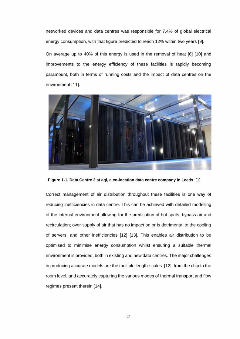
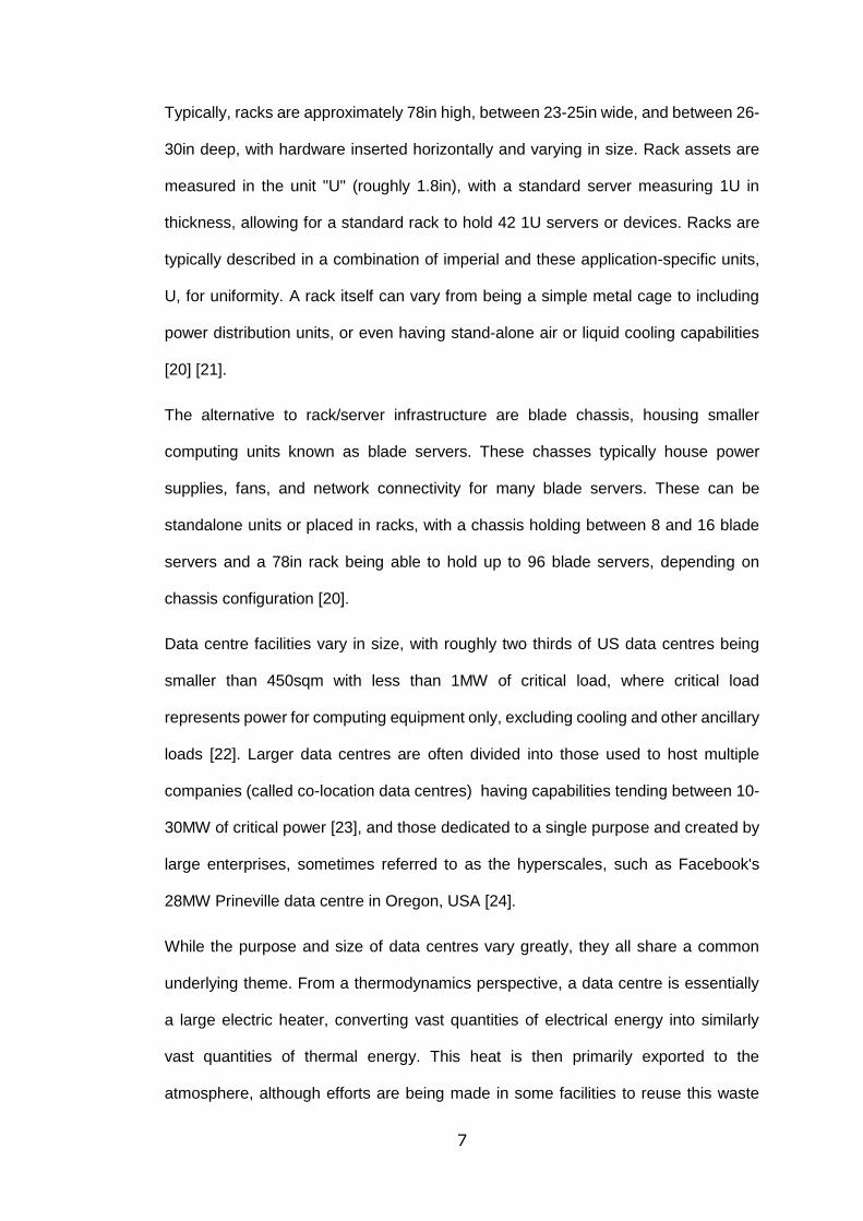
Figure 1-1. Data Centre 3 at aql, a co-location data centre company in Leeds [1] ... 2
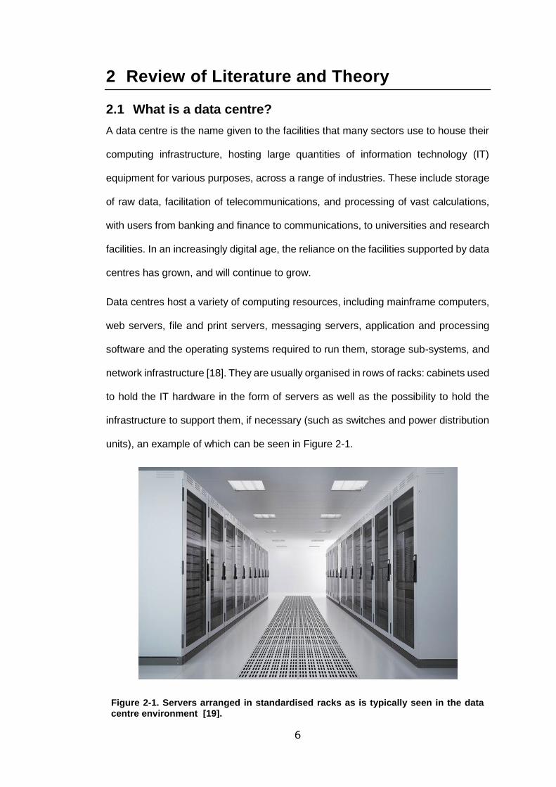
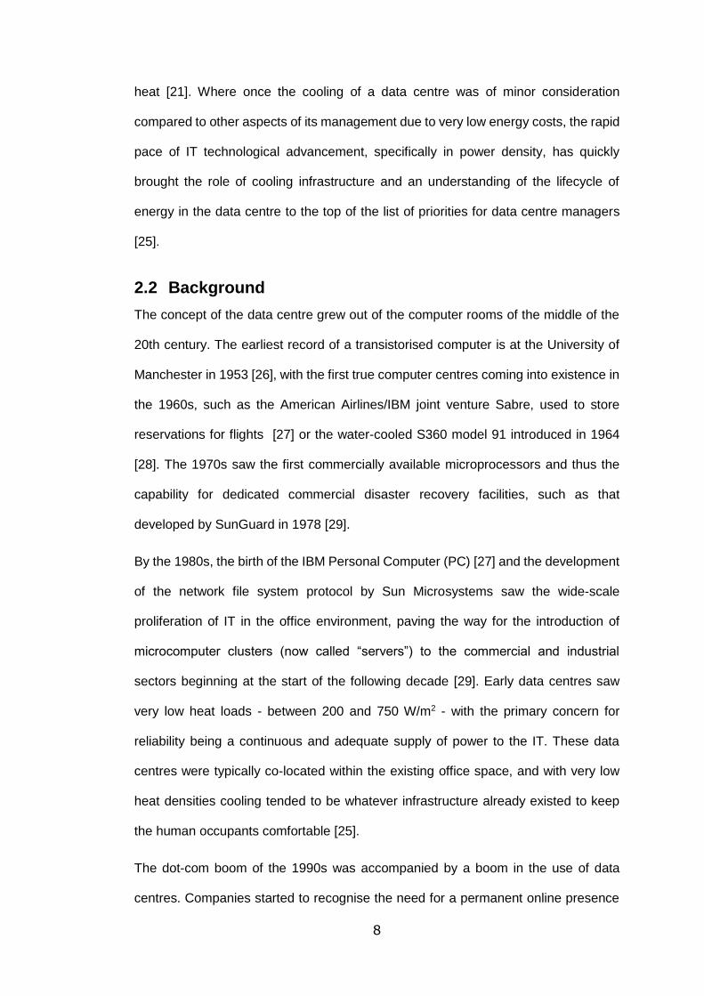
Figure 2-1. Servers arranged in standardised racks as is typically seen in the data
centre environment [19]. ......................................................................................... 6
Figure 2-2. The flow of energy through a typical data centre from the input of electrical
energy to the expulsion of thermal energy ............................................................. 12
Figure 2-3. Historical and Predicted Trends in ICT Equipment for the Years 1992 -
2010 [47] .............................................................................................................. 15
Figure 2-4. An air-cooled data centre, showing the CRAC, plenum, and hot and cold
aisles [61]. ............................................................................................................ 20
Figure 2-5. A representation of hot aisle containment, showing hot air returning to the
CRAC unit without remixing [70] ............................................................................ 21
Figure 2-6. Percentage increase in power consumption for increase in temperature
for a range of servers tested by Muroya et al. [77] ................................................. 25
Figure 2-7. Temperature-dependant CPU current leakage analysis performed by
Zapater, Marina et al on two processors in a server [78] ........................................ 25
Figure 2-8. PUE values for observed data centres by Energy Star for 2010 [91] ... 30
Figure 2-9. The difference between reported values of PUE and realistic values, for a
given data centre [93] ........................................................................................... 31
Figure 2-10. Workload state diagram for SPECpower_ssj2008 [103] ..................... 39
Figure 2-11. Published results for the Top10 Green500 Supercomputers show
significant improvements in energy efficiency over the last 9 years [105] ............... 41
ix
Figure 3-1. The ARM server is comprised of 12 daughter boards (left) containing four
nodes each. These fit side by side in the chassis (right), giving a total of 48 nodes for
the system. ............................................................................................................ 45
Figure 3-2. Shows a CAD model of the original flow box attached to the outlet of the
3 1/2U ARM server, with 12 holes in the top for insertion of sensor equipment ...... 46
Figure 3-3. The architecture of a SPEC_ssj2008 benchmark test, showing linkage
between Control and Collect System, System Under Test, and power analyzer [113]
.............................................................................................................................. 47
Figure 3-4. Load vs Power (left) and Operations vs Load (right) for ARM 48 node
benchmarking run. ................................................................................................. 49
Figure 3-5. Load vs Power (left) and Operations vs Load (right) for x86 4 node
benchmarking run. ................................................................................................. 49
Figure 3-6. Node locations for the ARM server, showing 48 nodes across 12 daughter
boards after the 5thand 8th board locations were swapped. .................................... 51
Figure 3-7. Temperature and power by ARM node location at 100% loading, showing
temperature gradient from front to back and hot spots towards the left of the chassis.
.............................................................................................................................. 52
Figure 3-8. Temperature and power by ARM node location at idle, with lower
temperature and power figures than 100% but still exhibiting heat gradient and
hotspots. ................................................................................................................ 52
Figure 3-9. SPECpower results for the ARM (left) and x86 (right) servers showing the
comparison in Performance to Power Ratio for the two tests ................................. 53
Figure 3-10. Comparison results between the ARM and x86 servers for 10 minute
tests period, with the former shown in red and the latter shown in green. .............. 56
x
Figure 3-11. Power usage against time for the x86 Server, where the time increases
as the number of concurrent users does. ............................................................... 57
Figure 3-12. The Zabbix server collates data from many sources to one easy to
access location. The metric seen here is for network traffic - in, out, and total - for
both the x86 and ARM servers across a period of 2 hours. .................................... 58
Figure 3-13. Richfaces PhotoAlbum hosts a fully useable photo album on each
Apache web server. The front-end accesses a MySQL database of pictures, installed
on each node. ........................................................................................................ 60
Figure 3-14. ‘Monuments and just buildings’ is the first of five different albums created
in the application that the program can randomly request pictures from. ................ 61
Figure 3-15. Comparison of CPU loading against number of Concurrent users for
ARM Server Node 1 ............................................................................................... 63
Figure 3-16. Dynamic HTTP results for a range of concurrent users from 25 to 600
showing bytes per second per Watt of electrical power into the server, for tests of ten
minutes in duration ................................................................................................ 64
Figure 3-17. Partial results for the ARM server showing a similar trend to Figure 3-16
for a range of users from 50 to 600 at intervals of 50, with each test lasting 2 minutes.
.............................................................................................................................. 64
Figure 4-1. The data centre laboratory showing the control computer in the cold aisle
and the liquid-cooled server under test in the hot aisle, being heated by load banks
situated in the four racks. ....................................................................................... 68
Figure 4-2: Steady relationship between Room temperature and GPU internal
temperature, across a range of roughly 1200 results from each of the nearly 60 tests
of 20 iterations each. ............................................................................................. 70
xi
Figure 4-3: Relationship between temperature and power consumption for the server,
showing an increase in the former leading to an increase in the latter. Room
temperature is in red and displayed on the primary y-axis and GPU temperature is in
blue and displayed on the secondary y-axis. .......................................................... 71
Figure 4-4. As Room temperature increases, there is both an increase in power
consumption and a drop in the number of floating point operations performed
simultaneously. ...................................................................................................... 72
Figure 4-5. As GPU temperature increases performance gradually and then
significantly decreases. .......................................................................................... 73
Figure 4-6. The relationship between Room temperature and performance follows the
same trend, although shows that minor fluctuations in room temperature can
potentially have less detrimental effect. ................................................................. 74
Figure 4-7. This translates to a drop in overall power efficiency, measured in floating
point operations performed per Watt consumed. ................................................... 75
Figure 5-1. The first iteration of the GSWT design with a vertically sliding lid which
attempted to accommodate servers of many sizes. ............................................... 78
Figure 5-2. The final design had moving geometry placed internally to accommodate
different servers while being more air-tight. ............................................................ 79
Figure 5-3. The GSWT with the server access panel removed, and before any flow or
heating components have been installed. .............................................................. 80
Figure 5-4. Diagram of the averaging-pitot tube from Furness Controls, showing
internal design to achieve differnetial pressure [120] ............................................. 81
Figure 5-5. The GSWT housing the ARM server used in the heat map testing, with
aluminium recirculation ducting and fan installed, being controlled manually by a 24V
power supply. ........................................................................................................ 83
xii
Figure 5-6. Modified Cosmetic office-water cooler, used for cooling upstream air in
the GSWT .............................................................................................................. 84
Figure 5-7. Scatter plot showing an example transfer function for power at 75%
utilisation varying upstream temperature and flow rate for the Sunfire V20z server
plotted against the experimental data used to determine it .................................... 90
Figure 6-1. A surface plot demonstrating the relationship between input factors
upstream temperature and flow rate on operations performed per second per watt for
a loading of 75%, across the normalised range of -0.1 to 0.15 and -1 to 0 respectively.
These correlate to inlet temperatures of between 23°C and 28°C and flow rates of up
to 0.75m3/s, and show that an increase in temperature, or decrease in flow rate both
lead to a drop in energy effficiency for the server. .................................................. 96
Figure 6-2. Surface plot of load and flow rate against downstream temperature for a
fixed input temperature of 28°C. ............................................................................ 98
Figure 6-3. A surface plot of load and flow rate against change in temperature for a
fixed upstream temperature of 28°C ...................................................................... 99
Figure 6-4. Operations per second per watt against normalised upstream temperature
and flow rate for a load of 100%. ......................................................................... 100
Figure 6-5. Performance and energy efficiency for the SunFire server with upstream
temperature 25.5°C and flow rate 0.75m3/s ......................................................... 101
Figure 6-6. Surface plot of 100% load for the ARM server, showing variations with
upstream temperature and flow rate .................................................................... 106
Figure 6-7. Pure performance and energy efficiency for the ARM server across loads
0 to 100% at upstream temperature 20°C and flow rate 1.125m3/s ...................... 107
Figure 6-8. Surface plot of upstream temperature and flow rate versus energy
efficiency for a 50% load. ..................................................................................... 108
xiii
Figure 6-9. Energy and efficiency and performance at two different thermal conditions
for the ARM server ............................................................................................... 109
Figure 6-10. Surface plot of operations per second per watt for the Intel server ... 113
Figure 6-11. Operations per second per watt for 50% CPU load .......................... 114
Figure 6-12. CPU% load versus operations per second per watt for the Intel server at
two different thermal conditions, with upstream temperatures of 22°C and 35°C . 115
Figure 6-13. Surface plot of operations per second against upstream temperature and
flow rate for the R720 server ................................................................................ 119
Figure 6-14. Power consumption as a factor of upstream temperature and flow rate.
The surface plot has to be displayed with non-standard axis due to the gradient of the
surface. ................................................................................................................ 122
Figure 6-15. Operations per second per watt against upstream temperature and flow
rate for a load of 50% for the first R620 server. .................................................... 125
Figure 6-16. Operations per second per watt at a load of 60%............................. 126
Figure 6-17. Two points of inflection on the surface of operations per second per watt
for the R620 - 1 .................................................................................................... 127
Figure 6-18. Downstream temperature against load and flow rate for an inlet
temperature of 25°C ............................................................................................ 128
Figure 6-19. Operations per second per watt compared with upstream temperature
and flow rate for a load of 50% ............................................................................ 130
Figure 6-20 Operations per second per watt compared with upstream temperature
and flow rate for a load of 62.5% ......................................................................... 131
Figure 6-21. The number of operations performed per second for each of the six
servers at an inlet temperature of 18°C and a flow rate of 0.375m3/s ................... 133
xiv
Figure 6-22 Operations per second for the ARM server at different temperatures and
flow rates ............................................................................................................. 134
Figure 6-23. Operations per second at 18°C and 0.375m3/s against server age .. 135
Figure 6-24. Operations per second per watt for the six servers at 18°C and
0.375m3/s ............................................................................................................ 137
Figure 6-25. Operations per second per watt for the six servers at 27°C and
0.375m3/s ............................................................................................................ 138
Figure 6-26. Power consumption for all six servers at 18°C and a flow rate of
0.375m3/s ............................................................................................................ 140
Figure 6-27. Downstream temperature data for an upstream temperature of 27°C and
flow rate of 0.375m3/s .......................................................................................... 143
Figure 7-1. A flowchart depicting the flow of control and recorded information through
the GSWT, from hardware and computational load to the web front-end. ............ 153
xv
List of Tables
Table 2-1. Summary of "typical" data centre thermal loads and temperature limits
established by Khosrow et al. in 2014 [21] ............................................................ 17
Table 2-2. Heat load of servers/blade servers as reviewed by Khosrow et al in 2014
[21] ........................................................................................................................ 18
Table 2-3. ASHRAE 2015 temperature and humidity recommendations for data
centres [82] ............................................................................................................ 26
Table 2-4. Proxies for computational efficiency suggested by the Green Grid [100]36
Table 6-1. Showing the difference for the SunFire V20z from regression one to
regression four for the output variable operations per second, showing those factors
eliminated and those found to be relevant or chosen to be included. Blue values of P
denote a high likelihood of importance, and red values denote definite importance.
.............................................................................................................................. 93
Table 6-2. Accuracy, R2, and Standard Errors for each output for the SunFire server.
.............................................................................................................................. 94
Table 6-3. Test conditions and range of results for the ARM server ..................... 103
Table 6-4. Showing the difference for the ARM server from regression one to
regression four for the output variable operations per second, showing those factors
eliminated and those found to be relevant or chosen to be included. Blue values of P
denote a high likelihood of importance, and red values denote definite importance.
............................................................................................................................ 104
Table 6-5. shows average percentage difference, R2 and standard error values for
the transfer functions for each of the five output variables for the ARM server ..... 106
Table 6-6. Range of inputs and results for the Intel server ................................... 110
Table 6-7. Regression of input factors for Intel operations per second. ................ 111
xvi
Table 6-8. Accuracy, R2 and Standard Error for calculated values from the Intel
transfer equations ................................................................................................ 112
Table 6-9. Input and output range and results for the PowerEdge R720 .............. 116
Table 6-10. Original transfer function data for the R720, showing poor accuracy
before data range review ..................................................................................... 118
Table 6-11. Accuracy, R2 and Standard Error for revised transfer functions, showing
more reliability ..................................................................................................... 119
Table 6-12. Analysis data from the fifth regression of input factors for operations per
second transfer function, showing high VIFs for upstream temperature and flow rate
............................................................................................................................ 120
Table 6-13. Regression analysis data for downstream temperature equation for the
R720. ................................................................................................................... 121
Table 6-14. The range of data for the first PowerEdge R620 ............................... 123
Table 6-15. Accuracies for the PowerEdge R620 - 1 ........................................... 124
Table 6-16. The range of data for the PowerEdge R620 - 2 ................................. 128
Table 6-17. Accuracy, R2 and standard error for the second R620 server ........... 129
Table 6-18. Transfer Functions for operations per second across the six servers. 132
Table 6-19. Operations per second for the six servers, at extremes of the
recommended envelope temperatures and flow rates .......................................... 134
Table 6-20. Transfer Functions for operations per second per watt for the six tested
servers. ................................................................................................................ 136
Table 6-21. Transfer Functions for power consumption for the six tested servers. 139
Table 6-22. Transfer Functions for downstream temperature for the six tested servers.
............................................................................................................................ 141

xvii
Table 6-23. Accuracy data for downstream temperature on the six servers ......... 142
Table 6-24. Accuracy data for delta-T functions for the six servers ...................... 145
1
1 Introduction
A data centre is a facility that entities use to house their computing infrastructure,
hosting large quantities of information technology (IT) equipment for a range of
purposes, across a range of industries. These include the storage of raw data, the
facilitation of telecommunications, or the processing of vast calculations, such as High
Performance Computing (HPC), Artificial Intelligence (AI), Machine Learning to name
a few, with a range of users from banking and finance, to communications, to
universities and research facilities, or even companies whose sole business is the
management and use of data centres. Figure 1-1 shows an example of one of these
facilities at aql in Leeds; a co-location data centre company with an appetite for
energy efficiency and exploring the possibilities of heat transportation, and the group
responsible for supporting this project [1]. Co-location facilities are data centres in
which other businesses can rent space for servers [2].
The computing infrastructure within these facilities is usually laid out in rows of 2m tall
racks, and the quantity and density of these datacom systems results in a distributed
and complicated dynamic generation of heat throughout the facility. This heat needs
to be transported away from the servers and rejected to the outside environment,
usually by means of air cooling.
These facilities have evolved at a staggering pace over a period of only a few
decades, both technologically and in size. Data centres consumed 0.12% of the US
energy consumption in the year 2000 [3]. However, only ten years later, in 2010, that
figure had grown to over 2% [4]. When viewed on a global scale, it was reported that
data centres were responsible for 1.1-1.5% of worldwide electricity consumption in
2011 [5] [6]. Some studies suggesting that the ICT sector is responsible for about 2%
of global CO2 emissions in the manufacturing of ICT equipment is included [5] [7]
[8]. Greenpeace, 2015, estimated that the collective electrical energy consumption of
2
networked devices and data centres was responsible for 7.4% of global electrical
energy consumption, with that figure predicted to reach 12% within two years [9].
On average up to 40% of this energy is used in the removal of heat [6] [10] and
improvements to the energy efficiency of these facilities is rapidly becoming
paramount, both in terms of running costs and the impact of data centres on the
environment [11].
Figure 1-1. Data Centre 3 at aql, a co-location data centre company in Leeds [1]
Correct management of air distribution throughout these facilities is one way of
reducing inefficiencies in data centre. This can be achieved with detailed modelling
of the internal environment allowing for the predication of hot spots, bypass air and
recirculation; over-supply of air that has no impact on or is detrimental to the cooling
of servers, and other inefficiencies [12] [13]. This enables air distribution to be
optimised to minimise energy consumption whilst ensuring a suitable thermal
environment is provided, both in existing and new data centres. The major challenges
in producing accurate models are the multiple length-scales [12], from the chip to the
room level, and accurately capturing the various modes of thermal transport and flow
regimes present therein [14].

3
An alternative to modelling a data centre as a whole is to consider the behaviour of
the servers themselves. By understanding the optimal working conditions of the
hardware employed in the data centre, achieving energy or cost savings by pushing
up utilisation, or optimising the environment to suit requirements [15]. Utilisation of
existing hardware is rarely maximised, with some data centres seeing as low as 10%
of server capabilities actually utilised [16]. Data centre behaviour as a whole can be
reported using industry standard metrics [17], but there exists a need for more detail
in properly capturing such a complex problem.
However it is achieved, the proper management of this heat, from creation to
expulsion, combined with the appropriate utilisation of hardware is the ultimate goal
for energy efficient data centre management, and the implementation, understanding,
optimisation of such a data centre configuration is paramount for such a rapidly
growing industry.
1.1 What is Energy Efficiency?
Energy is a basic building block of modern existence, and can neither be created nor
destroyed but only transformed. This transformation, in its many forms, drives our
existence - especially in this increasingly technologically reliant age. Stored chemical
energy in coal or gas is burnt to create thermal energy, which in turn is transformed
to kinetic energy to drive turbines and generators, and then to electrical energy. Every
one of these steps involves energy loss. For example, heat energy lost to the
atmosphere, or sound energy created in place of electricity, and the degree to which
these losses are minimised gauges the energy efficiency of the process. Efficiency is
defined, very simplistically, as the ratio of what you get against what you pay for. The
energy efficiency of a power station can be determined by weighing how much stored
or potential chemical energy was input against how much electrical energy it provides.
When considering a data centre, determining the energy efficiency becomes difficult.
The desired output varies depending on who you ask; the cooling technician may be

4
interesting in the ratio of electrical energy into the data centre against heat expelled
by the chillers, but the data centre manager is interested in how many servers the
data centre has reliably supported for that electricity cost, whilst the end user may
only be interested in how quickly their calculations ran or how many web-pages were
able to be accessed.
Therefore, does efficiency better describe the heat expelled from the data centre or
the operations performed by the servers per second, when compared with power
cost? What efficiency measures take into account the role of finance, the cost of
added redundancies or greater cooling infrastructure? Each data centre will have its
own priorities in terms of efficiency, and within each data centre there will be
personnel who have their own priorities - be that computational efficiency, energy
efficiency, financial efficiency, or something else entirely, and this project sets out to
provide a methodology for understanding or observing each.
1.2 Research Aim
This research aims to develop a methodology for quickly and robustly ascertaining
the performance of a data centre server with a view to maximising one or multiple
forms of efficiency for a data centre. Primarily this will be to best ascertain the Central
Processing Unit (CPU) loading, inlet temperature, and flow rate of cooling air through
the server to provide the most amount of computational work for the least power
consumed by the unit, to best improve the energy efficiency of the data centre as a
whole. Alternatively, the methodology can be employed to maximise the change in
temperature, or delta-T, across a server, to best meet contractual obligations and
improve the efficiency of larger cooling infrastructure, or even to find the lowest overall
power consumption of the employed hardware.

5
1.3 Thesis outline
The thesis is divided into seven main chapters, including this first brief introduction.
Chapter 2 provides a review of literature relating to data centres, considering the
growth of the industry and the impact of this growth, and the flow of energy through a
data centre. This looks at the components that comprise a data centre and the
importance of cooling infrastructure for maintaining a working thermal envelope, as
well as a consideration of methods for understanding how efficiently or effectively a
data centre is performing. Chapter 3 takes lessons learnt from these methods and
presents an experimental analysis of creating virtual loads within two different data
centre servers, with a view to understanding their energy efficiency. Chapter 4 is then
another experimental body of work employing one of these methods to determine the
effect changes in thermal environment can have on server performance and energy
efficiency. Lessons learnt in these two chapters are carried forward to the
development of an experimental rig, called the Generic Server Wind-tunnel (GSWT),
detailed in Chapter 5. This explores the design of the GSWT and the methodology of
utilising it to consider the relationship between thermal environment and energy
efficiency, with Chapter 6 demonstrating six case studies to validate and analysis this
developed methodology. Chapter 7 summarises the findings of each of these bodies
of work and considers recommendations for future work.
6
2 Review of Literature and Theory
2.1 What is a data centre?
A data centre is the name given to the facilities that many sectors use to house their
computing infrastructure, hosting large quantities of information technology (IT)
equipment for various purposes, across a range of industries. These include storage
of raw data, facilitation of telecommunications, and processing of vast calculations,
with users from banking and finance to communications, to universities and research
facilities. In an increasingly digital age, the reliance on the facilities supported by data
centres has grown, and will continue to grow.
Data centres host a variety of computing resources, including mainframe computers,
web servers, file and print servers, messaging servers, application and processing
software and the operating systems required to run them, storage sub-systems, and
network infrastructure [18]. They are usually organised in rows of racks: cabinets used
to hold the IT hardware in the form of servers as well as the possibility to hold the
infrastructure to support them, if necessary (such as switches and power distribution
units), an example of which can be seen in Figure 2-1.
Figure 2-1. Servers arranged in standardised racks as is typically seen in the data centre environment [19].
7
Typically, racks are approximately 78in high, between 23-25in wide, and between 26-
30in deep, with hardware inserted horizontally and varying in size. Rack assets are
measured in the unit "U" (roughly 1.8in), with a standard server measuring 1U in
thickness, allowing for a standard rack to hold 42 1U servers or devices. Racks are
typically described in a combination of imperial and these application-specific units,
U, for uniformity. A rack itself can vary from being a simple metal cage to including
power distribution units, or even having stand-alone air or liquid cooling capabilities
[20] [21].
The alternative to rack/server infrastructure are blade chassis, housing smaller
computing units known as blade servers. These chasses typically house power
supplies, fans, and network connectivity for many blade servers. These can be
standalone units or placed in racks, with a chassis holding between 8 and 16 blade
servers and a 78in rack being able to hold up to 96 blade servers, depending on
chassis configuration [20].
Data centre facilities vary in size, with roughly two thirds of US data centres being
smaller than 450sqm with less than 1MW of critical load, where critical load
represents power for computing equipment only, excluding cooling and other ancillary
loads [22]. Larger data centres are often divided into those used to host multiple
companies (called co-location data centres) having capabilities tending between 10-
30MW of critical power [23], and those dedicated to a single purpose and created by
large enterprises, sometimes referred to as the hyperscales, such as Facebook's
28MW Prineville data centre in Oregon, USA [24].
While the purpose and size of data centres vary greatly, they all share a common
underlying theme. From a thermodynamics perspective, a data centre is essentially
a large electric heater, converting vast quantities of electrical energy into similarly
vast quantities of thermal energy. This heat is then primarily exported to the
atmosphere, although efforts are being made in some facilities to reuse this waste
8
heat [21]. Where once the cooling of a data centre was of minor consideration
compared to other aspects of its management due to very low energy costs, the rapid
pace of IT technological advancement, specifically in power density, has quickly
brought the role of cooling infrastructure and an understanding of the lifecycle of
energy in the data centre to the top of the list of priorities for data centre managers
[25].
2.2 Background
The concept of the data centre grew out of the computer rooms of the middle of the
20th century. The earliest record of a transistorised computer is at the University of
Manchester in 1953 [26], with the first true computer centres coming into existence in
the 1960s, such as the American Airlines/IBM joint venture Sabre, used to store
reservations for flights [27] or the water-cooled S360 model 91 introduced in 1964
[28]. The 1970s saw the first commercially available microprocessors and thus the
capability for dedicated commercial disaster recovery facilities, such as that
developed by SunGuard in 1978 [29].
By the 1980s, the birth of the IBM Personal Computer (PC) [27] and the development
of the network file system protocol by Sun Microsystems saw the wide-scale
proliferation of IT in the office environment, paving the way for the introduction of
microcomputer clusters (now called “servers”) to the commercial and industrial
sectors beginning at the start of the following decade [29]. Early data centres saw
very low heat loads - between 200 and 750 W/m2 - with the primary concern for
reliability being a continuous and adequate supply of power to the IT. These data
centres were typically co-located within the existing office space, and with very low
heat densities cooling tended to be whatever infrastructure already existed to keep
the human occupants comfortable [25].
The dot-com boom of the 1990s was accompanied by a boom in the use of data
centres. Companies started to recognise the need for a permanent online presence
9
with a fast internet connection, leading to the introduction of the facilities housing
hundreds and thousands of dedicated servers that we see today [27] [29]. The
increase in both hardware demand and heat load saw increasingly greater
requirements for cooling, resulting in the implementation of large chillers and other
cooling units. This increased cooling infrastructure was often noisy and cumbersome,
rendering the environment uninhabitable by human workers and creating demand for
dedicated IT spaces [25].
This trend has continued unabated in the years since, with an increasing reliance on
data centres and digital infrastructure in our professional and personal lives. More
recently, the advent of the “Internet of Things” has seen the demand for data centre
increase even further, with support needed for an ever-growing number of household
or everyday internet-capable objects connected by expanding wireless or mobile
networks [30].
2.3 Growth of Data Centres
In 1965, Gordon Moore, working from data trends for the years 1958 to 1965,
theorised that every subsequent year would see a doubling in the transistor density
on microprocessors in ICT hardware [31], with this figure being amended to every two
years by 1975 [32]. This trend, referred to as 'Moore's Law', has generally been
proved to be true, and it is these advances that have driven growth in the use of, and
electrical consumption of, both data centres and the ICT industry as a whole. Attempts
to better characterise and even predict these trends have had varying (and
sometimes conflicting) degrees of success.
A report in Forbes magazine in 1999 suggested that up to 8% of the electrical
consumption of the US at the time was due to ICT technology, going on to predict that
this number would rise to 30-50% by 2020 [33] - although this report was criticised by
the Lawrence Berkeley National Laboratory (LBNL) the following year for over-
estimating these figures [34].

10
Mitchell-Jackson et al reported in 2002 that data centres had consumed 0.12% of the
US energy consumption for the year 2000[1], although this figure seems very
conservative when considering that an Environmental Protection Agency report on
data centre efficiency from 2008 had stated that the data centre power consumption
for the year 2006 was 61TWh or roughly 1.5% total energy consumption for the
country, having supposedly doubled from their known figures for the year 2000 [35].
In 2012, an article by The New York Times on the growth of the internet reported that
this figure had grown to over 2% [4], although a report on historical data centre energy
consumption trends for 2000-2014 published by LBNL in 2016 put this figure closer
to 1.8%. This report also stated that the rate of growth had considerably decreased,
demonstrated in five-year intervals. For the years 2000-2005, data centre energy
consumption grew by 90%, dropping to 24% for the years 2005-2010, and dropping
further still to just 4% growth across the years 2010-2014 [36].
The reasons suggested for this decrease in growth rate are varied including, but not
limited to, a greater virtualisation of machines resulting in higher utilisation of existing
hardware, and a general implementation of energy efficiency improvements across
data centres as a whole. Jonathan Koomey, speaking in 2017, found that energy
efficiency improvements in new hardware were such that a case study data centre
considered in the writing of the LBNL report found 32% of its hardware to be an older
variety, responsible for consuming 60% of the total energy consumption for the data
centre while only providing 4% of the performance [37].
The same report suggested that 'best practice' or 'hyperscale shift' approaches to
data centre management be adopted, including the aggregation of smaller inefficient
data centres into larger ones that may benefit from economies of scale, or widespread
adoption of the most efficient equipment and practices. It also suggested that there
could be scope for even lowering data centre energy consumption as a percentage
of total energy consumption for the US over previous years.
11
When looked at on a global scale, these same trends of growth generally continue. It
was reported by the Uptime Institute in 2013 that data centres were responsible for
1.1-1.5% of worldwide electricity consumption in 2011, [5] with a 2014 article by W.
Van Heddeghem et al putting this figure at 3.9% for ICT in 2007 and 4.6% in 2012,
with data centre servers themselves consuming 270TWh of power in 2012 or 1.3% of
global energy consumption for that year as detailed by the International Energy
Agency [38].
This progression has given rise to a need for a clearer understanding of the energy
flows and efficiency losses seen in data centres. The research is being undertaken,
and in some cases lessons learned are being adopted, but the pursuit of a better
understanding of the trends clearly still needs to continue.
2.4 Energy flow through a data centre
2.4.1 Power Systems
When looking at data centres from the perspective of an engineer, as opposed to a
computer scientist, perhaps the most important thing to consider is the role and
lifecycle of energy through the facility.
All data centres are comprised of three basics aspects: power systems, such as the
Uninterruptable Power Supply (UPS) or Power Distribution Units (PDUs); ICT which
is comprised of servers in standardised racks; and cooling infrastructure. In the case
of legacy data centres cooling is usually achieved by air, with infrastructure made up
of Computer Room Air Coolers (CRACs) or Computer Room Air Handlers (CRAHs)
units and external chiller units. CRACs are essentially large air conditioning units, with
refrigerant loops to cool air, while CRAHs move air into the room that has already
been chilled externally [13] [39]. Some more modern data centres are now using liquid
cooling instead, with air being replaced as the medium of transporting heat away from
IT equipment due to the far greater heat capacity of liquids compared to air [13].

12
Figure 2-2. The flow of energy through a typical data centre from the input of electrical energy to the expulsion of thermal energy
When looked at from an energy perspective, a very clear lifecycle for energy emerges,
as seen in Figure 2-2 and as described by Barroso et al. [23]. Electrical energy enters
the data centre from a utility substation, which transforms high voltage (110kV or
greater) to medium voltage (less than 50kV). This medium voltage is then used to
distribute power to the data centres primary distribution centres, known as
substations, which step the voltage down further from medium to low (typically below
1000V) [23].
These substations transmit power into the data centre where it enters the
uninterruptible power supply (UPS). The UPS can take the form of a switchgear and
either battery or flywheel attached to a motor/generator. This provides a store of
energy, either electrical or mechanical, to bridge the 10-15s gap when mains power
fails and before generator power can take over. As well as this, the UPS conditions
the power from the substation, smoothing voltage fluctuations with AC-DC and DC-
AC conversion steps [23].
UPS power is then routed to power distribution units (PDUs). These PDUs take a
large input feed and distribute it to smaller circuits that provide power to the actual
servers. Typically, a large data centre may actually use several levels of PDUs, with
larger ones distributing power to smaller rack level PDUs, which then provide power
to the individual servers in the rack. [23]
13
There is some geographical variation as to these final power steps. In North America,
the PDU is typically delivered 480V 3-phase power whereas in the EU this is usually
400V 3-phase. This means US servers require an additional transformation step to
deliver the desired 110V output for their servers, whereas in the EU 230V input can
be delivered to servers without the need for another step [23].
Finally, the power is stepped down and converted from AC to DC one final time, in
the Power Supply Unit (PSU) for the server. This provides between 5-12V of power
at 20-100A to the motherboard, where voltage regulators distribute the power among
the processors and peripherals based on server architecture [20].
Each transformation or distribution step results in a loss of power and thus efficiency,
with some steps showing efficiencies of 85–95% or worse [20], with the rest converted
to heat [23]. Cumulatively, this translates to between only 75% [40] and 50% [20] of
the power coming into the data centre which is not required for ancillary functions
such as lighting and cooling, actually being consumed usefully, depending on load.
Research has been conducted on improving the efficiency of both the transformative
steps and the UPS, and improving these attributes further is outside the scope of this
thesis [41] [42].
Once delivered to a server, power is used by a range of components, including
processors, fan, DRAM (dynamic random-access memory), networking and hard
drives. When considered from both a computational and thermodynamic perspective,
the processor is usually considered to be the most important part of the computer as
this is where the 'useful' work is performed, and has historically been considered the
largest consumer of power in the server. While this may not be entirely accurate, 25-
40% of total server power is typically due to CPU power consumption [17]. Whilst this
is where the useful "work" of the data centre is conducted, it is also the greatest
source of heat, due to electrical impedance in the increasingly densely populated
14
circuits. These components are also highly sensitive to the thermal environment and
require constant cooling; otherwise they exceed their thermal envelope.
An important attribute to consider when looking at a data centre is that of power
density. Designers have been increasingly boosting the computing power per square
metre of facilities to improve overall space efficiencies, both on the component and
system scale. At the component level, this means advances in processor capability
and reductions in die size, whilst at the server scale this can be seen in the packing
of more components into the same space and the improvement of interconnect
latency between them. For instance, during the 1990s the smallest server was the 1U
machine, whereas the creation of blade servers has led to two servers of similar
power being able to occupy the same space [40]. Combining the advances in
processor and server technology, following the trajectory outlined in by Moore's Law
[31] [32] has resulted in a massive increase in power density within a short space of
time, and with it massive advances in cooling requirements. To really put the pace of
these advancements into perspective, it is necessary to quantify them.
2.4.2 Power Density and Heat Load
A significant amount of work has been undertaken logging power densities and trends
of rack power in data centres during the last two decades. Karlsson et al. [7] cite a
growth of rack power consumption from 1kW to 12kW over the 10 years from 1995,
supported by Patel who stated that the greatest rack power in 2003 to be 10kW [43].
A study from the Uptime Institute suggested that the average rack density in 2012 to
be 8.4kW, with the greatest at the time being 24kW [5]. Another paper from the 2011
suggested an even greater maximum rack power usage of 30kW [13].
When considering this in terms of power density, a number of studies conducted on
the energy consumption and efficiency of data centres have estimated that
consumption is between 15 and 40 times more power per square foot than
15
commercial office space [41] [44]. A study on 14 data centres by the LBNL in 2005
found power density averaged between 120 and 940 W/m2 [45] whereas only 50–
100 W/m2 was consumed in a typical commercial office space. [46]
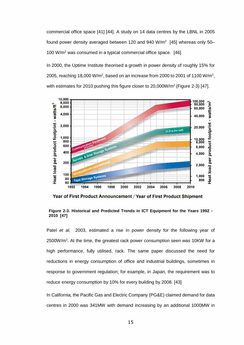
In 2000, the Uptime Institute theorised a growth in power density of roughly 15% for
2005, reaching 18,000 W/m2, based on an increase from 2000 to 2001 of 1100 W/m2,
with estimates for 2010 pushing this figure closer to 20,000W/m2 (Figure 2-3) [47].
Figure 2-3. Historical and Predicted Trends in ICT Equipment for the Years 1992 - 2010 [47]
Patel et al, 2003, estimated a rise in power density for the following year of
2500W/m2. At the time, the greatest rack power consumption seen was 10KW for a
high performance, fully utilised, rack. The same paper discussed the need for
reductions in energy consumption of office and industrial buildings, sometimes in
response to government regulation; for example, in Japan, the requirement was to
reduce energy consumption by 10% for every building by 2008. [43]
In California, the Pacific Gas and Electric Company (PG&E) claimed demand for data
centres in 2000 was 341MW with demand increasing by an additional 1000MW in

16
2003; the equivalent of building three new power plants [46]. The same paper
discussed the development of what was, at the time, the world’s largest data centre,
with a projected energy consumption of 180MW by 2005. The authors stated that
power densities at the time averaged between 1080W/m2 and 3230W/m2 [48].
A paper from 2000 by Mitchell-Jackson et al [49] discussed forecasts for data centre
growth, and the reliability of projected and provided figures. The authors raised an
excellent point that comparisons of power density in literature rarely specify whether
it is the power density of a rack in the data centre or the average power density across
the entire data centre. If it is the former, extrapolating the figure to the size of the data
centre will provide very misleading results for comparison [49].
A further point raised is that of determining the power density figures. The provided
densities often rely upon nameplate power for equipment, whereas in practice the
power draw may, and probably will, differ from this quite significantly. Not only this,
but as most data centres now operate on a high level of redundancy in their power
system infrastructure, taking into account the nameplate power usage of both a power
supply and its backup may also lead to misleading figures for day to day usage [49].
At the time, this would have resulted in an overestimation of cooling requirements for
data centres, leading to a much higher cooling capability, and thus greater power
loading, than necessary. Whether the same is true nearly 15 years later is debatable,
as the pace at which power densities increase is so great that what cooling
infrastructure may seem redundant today, may be a necessity tomorrow.
Aside from using the power consumption figures for racks to establish power
requirements for a data centre, they are also used to determine the capabilities of
cooling infrastructure required. In most areas of the industry it is assumed that 100%
of the electrical energy going into a server will be directly transformed into thermal
energy, which will then need to be transported away from the racks to ensure safe
and efficient running conditions within the equipment’s thermal envelope.
17
Mitchell-Jackson et al found that when trying to quantify power requirements for data
centres, there was much confusion as to what should be included in power estimates,
with most studies excluding cooling requirements entirely [3]. This has staggering
implications for the reliability of aggregate power consumption figures if the IT
infrastructure of a data centre is only responsible for between 40% and 55% of power
usage [50] [51] [52].
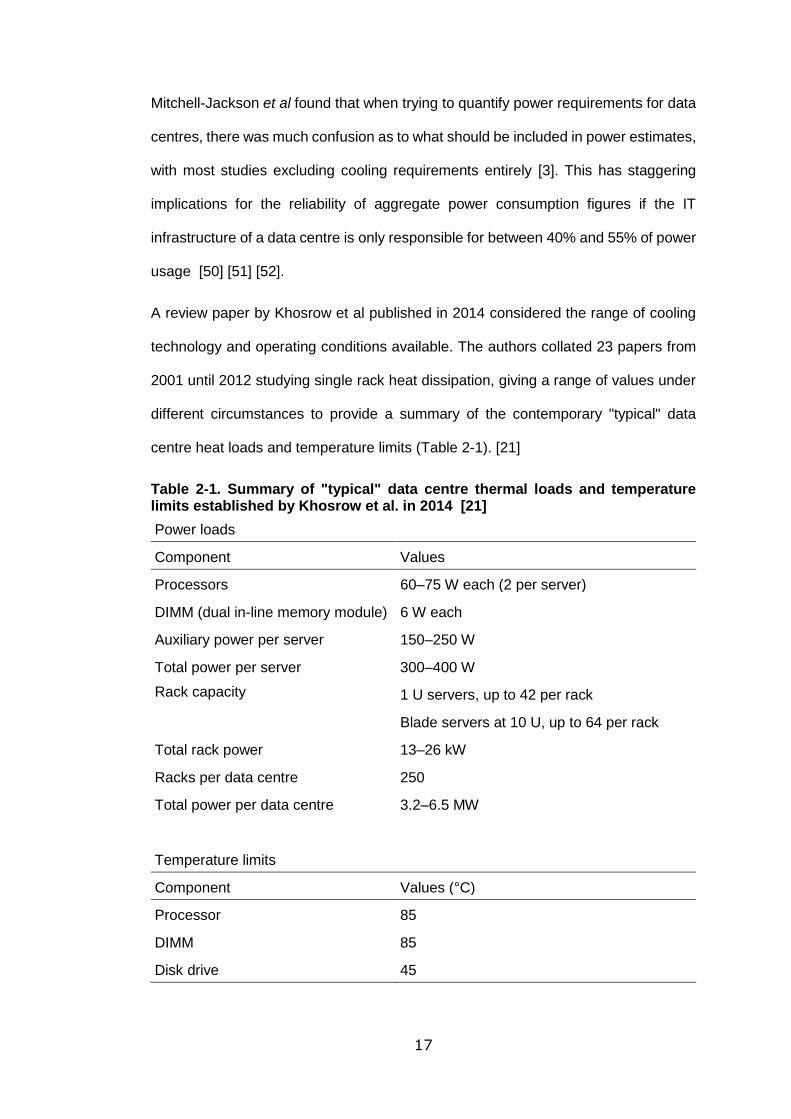
A review paper by Khosrow et al published in 2014 considered the range of cooling
technology and operating conditions available. The authors collated 23 papers from
2001 until 2012 studying single rack heat dissipation, giving a range of values under
different circumstances to provide a summary of the contemporary "typical" data
centre heat loads and temperature limits (Table 2-1). [21]
Table 2-1. Summary of "typical" data centre thermal loads and temperature limits established by Khosrow et al. in 2014 [21]
Power loads
Component Values
Processors 60–75 W each (2 per server)
DIMM (dual in-line memory module) 6 W each
Auxiliary power per server 150–250 W
Total power per server 300–400 W
Rack capacity 1 U servers, up to 42 per rack
Blade servers at 10 U, up to 64 per rack
Total rack power 13–26 kW
Racks per data centre 250
Total power per data centre 3.2–6.5 MW
Temperature limits
Component Values (°C)
Processor 85
DIMM 85
Disk drive 45
18
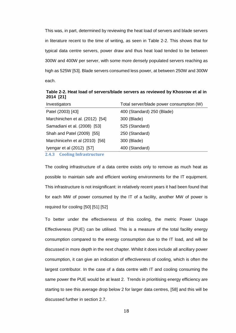
This was, in part, determined by reviewing the heat load of servers and blade servers
in literature recent to the time of writing, as seen in Table 2-2. This shows that for
typical data centre servers, power draw and thus heat load tended to be between
300W and 400W per server, with some more densely populated servers reaching as
high as 525W [53]. Blade servers consumed less power, at between 250W and 300W
each.
Table 2-2. Heat load of servers/blade servers as reviewed by Khosrow et al in 2014 [21]
Investigators Total server/blade power consumption (W)
Patel (2003) [43] 400 (Standard) 250 (Blade)
Marchinichen et al. (2012) [54] 300 (Blade)
Samadiani et al. (2008) [53] 525 (Standard)
Shah and Patel (2009) [55] 250 (Standard)
Marchinicehn et al (2010) [56] 300 (Blade)
Iyengar et al (2012) [57] 400 (Standard)
2.4.3 Cooling Infrastructure
The cooling infrastructure of a data centre exists only to remove as much heat as
possible to maintain safe and efficient working environments for the IT equipment.
This infrastructure is not insignificant: in relatively recent years it had been found that
for each MW of power consumed by the IT of a facility, another MW of power is
required for cooling [50] [51] [52]
To better under the effectiveness of this cooling, the metric Power Usage
Effectiveness (PUE) can be utilised. This is a measure of the total facility energy
consumption compared to the energy consumption due to the IT load, and will be
discussed in more depth in the next chapter. Whilst it does include all ancillary power
consumption, it can give an indication of effectiveness of cooling, which is often the
largest contributor. In the case of a data centre with IT and cooling consuming the
same power the PUE would be at least 2. Trends in prioritising energy efficiency are
starting to see this average drop below 2 for larger data centres, [58] and this will be
discussed further in section 2.7.

19
When looked at in general terms, the cooling systems for data centres are a series of
fluid loops, sometimes open but usually closed. An open system, such as free-
cooling, exports a medium warmed by the IT and replaces it with a cooler incoming
medium. The simplest example of free-cooling a data centre would be to open the
windows, although this would only work efficiently where the outside temperature was
lower, and carries other risks such as introducing contaminants that could damage
delicate hardware [23].
A closed-loop system re-circulates the same cooling medium repeatedly, transferring
heat to a higher loop through a heat exchanger. This heat is then usually rejected to
the environment, although in some cases it may be reused where there is a demand,
and the infrastructure to satisfy the demand [21].
There are two main methods for cooling a data centre with a closed loop system: air-
cooling and liquid-cooling. The former is more prolific, perhaps due to simplicity and
cost, although if done correctly the latter holds the capability to be more effective [59].
In air-cooled data centres, racks are usually arranged in cold and hot aisles and
placed on a raised floor. Computer room air conditioning units (or CRACs) provide a
feed of cool air to the underfloor, with perforated tiles in the plenum providing control
of the airflow into the cold aisles from underneath. This air then passes through the
racks, heating up, before rising and returning to the CRAC units from above (Figure
2-4). There are a variety of CRAC types, such as direct expansion or water cooling,
but all contain a heat exchanger and an air mover [23] [60].

20
Figure 2-4. An air-cooled data centre, showing the CRAC, plenum, and hot and cold aisles [61].
Considerable research has been done to understand the exact airflow patterns and
distribution throughout an air-cooled data centre, including investigating leakage of
(over-)pressurised cold air through aisle containment [62], the effect of perforated
plenum floor tiles [63] [64] [65] [66], and the effect of ceiling height and topology on
air stratification and flow impedance [60]. The importance of understanding this is due
to the narrow thermal envelopes of some of the more sensitive equipment.
An important example of this is airflow recirculation. This occurs when cold air is
supplied to a rack through a plenum at the wrong rate resulting in mixing of cold air
and hot air above the rack. This can lead to permeation of hot air into the cold aisle,
with those servers highest in the racks seeing inlet temperatures as high as 40°C,
well above the American Society of Heating, Refrigeration, and Air-conditioning
Engineers (ASHRAE) recommended inlet temperatures [67], resulting in losses in
load capacity as well as the possibility of hardware failures [60]. These
recommendations will be discussed in more detail in 2.5.
This has led to a significant rise in containment between hot and cold aisles, where
physical barriers are used to minimise or prevent the possibility of recirculation or
mixing, with Shrivastava et al reporting in 2012 that 80% of data centres had, or
planned to have, a containment system in place [68]. Schneider Electric reported in
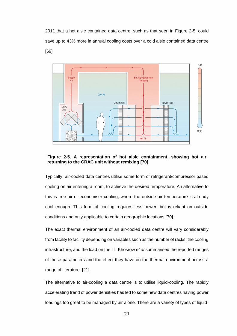
21
2011 that a hot aisle contained data centre, such as that seen in Figure 2-5, could
save up to 43% more in annual cooling costs over a cold aisle contained data centre
[69]
Figure 2-5. A representation of hot aisle containment, showing hot air returning to the CRAC unit without remixing [70]
Typically, air-cooled data centres utilise some form of refrigerant/compressor based
cooling on air entering a room, to achieve the desired temperature. An alternative to
this is free-air or economiser cooling, where the outside air temperature is already
cool enough. This form of cooling requires less power, but is reliant on outside
conditions and only applicable to certain geographic locations [70].
The exact thermal environment of an air-cooled data centre will vary considerably
from facility to facility depending on variables such as the number of racks, the cooling
infrastructure, and the load on the IT. Khosrow et al summarised the reported ranges
of these parameters and the effect they have on the thermal environment across a
range of literature [21].
The alternative to air-cooling a data centre is to utilise liquid-cooling. The rapidly
accelerating trend of power densities has led to some new data centres having power
loadings too great to be managed by air alone. There are a variety of types of liquid-
22
cooling available to data centres, ranging from bringing a liquid-loop and heat
exchanger into the rack through to fully immersing servers in dialectic liquid. The latter
is referred to as "direct liquid-cooling". [71]
Greenberg et al. [41] points out that despite the increased initial infrastructure costs
associated with liquid cooling, it can lead to considerable savings due to less energy
being consumed in cooling. There are some that suggest the move from air- to liquid-
cooled data centres is a question of when, not if, due to the trend of increasingly high-
density heat loads across not only High Performance Computing (HPC) hardware,
but across wider server trends, and that greater heat capacity and use of control
liquids will become more necessary [72].
In 2012, IBM constructed an experimental liquid-cooled data centre to determine the
potential for savings. They found that the cooling energy requirement dropped from
between 30% and 50% of data centre energy overhead when using CRACs to only
3.5% [50] [51] [57]. Not only does this translate to a saving in energy consumption,
but it can also lead to an increase in performance. A study undertaken in 2009, by
Ellsworth and Lyana, compared the efficiency of air- and liquid-cooled systems and
found that the latter could lead to an increase in processor performance of 33% [73].
This advantage is due, in part, to the far greater heat capacity of the medium, as well
as the greater control with placement (i.e. proximity to the heat sources), contact, and
flow that liquid allows.
Liquid-cooling also provides a much higher quality waste heat than air, lending itself
to the application of heat reuse schemes [21, 74]. Reusing the heat created by data
centres has been suggested for years, usually finding practical limitations due to the
usefulness of the grade of heat produced. A paper published in 2016 suggested that
matching a 3.5MW data centre to district heating schemes in London could see
savings in CO2e exported to the atmosphere, and a saving of nearly £1million per
year that would otherwise have been spent on heating [74].
23
Despite these advantages, the majority of data centres still operate with air-cooling,
and thus an understanding of both is necessary to provide a well-rounded and
informed view of data centre thermal management.
2.5 Why is Cooling Important?
Cooling in data centres is required to ensure cool air reaches the server inlets. This
is important for two reasons;
• to maintain the safe working envelope for internal components
• to minimise the energy consumed by the servers
Considering the former, it is known that the processor in particular is sensitive to high
temperatures. CPUs are essentially very dense collections of transistors - with this
density increasing at a bi-yearly rate, as outlined by Moore's Law [32]. These
transistors very rapidly switch on and off to provide binary signals. Where this was
once a physical switch, with a path for electrons to flow from source to sink when
switched to on, and a barrier or absence of path when switched to off, this has been
replaced by more advanced Metal Oxide Semiconductor Field-Effect Transistor
(MOSFET). For a MOSFET transistor to register as 'on' it must be supplied with a
voltage greater than a certain minimum known as the 'threshold voltage' [75].
As temperature increases the threshold voltage required for electrons to form a path
decreases too, meaning transistors fail to switch off as effectively. This can lead to an
increasing number of errors within the processor as temperature increases. This is
known as 'subthreshold leakage' and is a phenomenon seen more frequently as
transistor sizes, and thus the size of the gap between source and sink, decreases
[75].
The latter reason for maintaining inlet temperatures lies in the behaviour of server
fans when presented with sub-optimal conditions. Manufacturers create algorithms
for server fans that respond to internal temperature probes and react to maintain a
24
safe working environment for the components. While they are small components,
servers tend to include multiple fans and when they are relied upon to drive flow
through a server their power consumption rapidly accumulates. A study by Vogel et
al from 2010 found that server fans could be responsible for up to 15% of overall
server power consumption [76].
Due to the nature of fan behaviour and the scaling of power consumption with size, a
smaller fan would have to run at twice the RPM of a larger fan to create the same flow
rate, but would have to consume eight times as much power to do so. For this reason,
it is preferential to have the flow through the server driven by a large dedicated fan in
a CRAC than many more small server fans.
This means that most data centres have an ideal temperature envelope for operating,
such that increasing the temperature of the room minimises the work done by, and
power consumed by, the other data centre cooling infrastructure until the point at
which server fans are required to overcompensate and greatly increase power
consumption of the servers. This finding can be seen in the work of Muroya et al in
their 2010 paper analysing the effect of higher working temperatures on power
consumption for data centres, shown in Figure 2-6. A rise in inlet temperature to a
rack of servers led to a rise in power consumption for three of the five servers tested,
with variation attributed to position in the rack. [77].
25
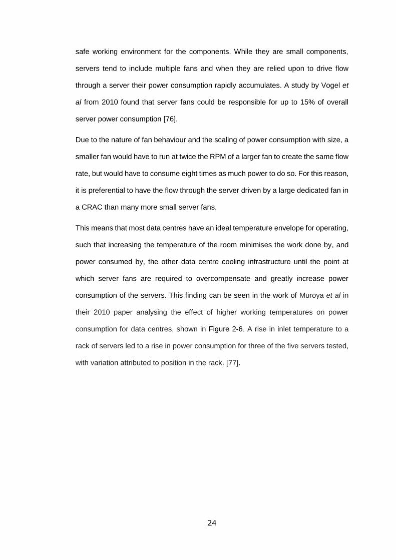
Figure 2-6. Percentage increase in power consumption for increase in temperature for a range of servers tested by Muroya et al. [77]
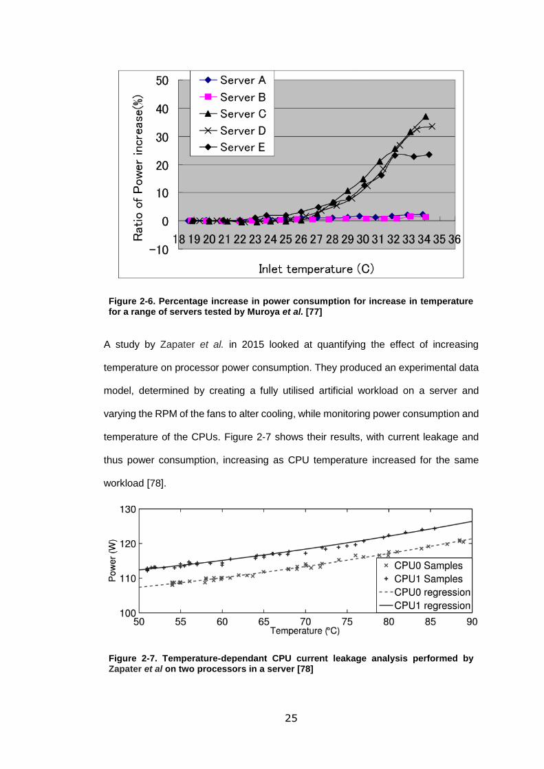
A study by Zapater et al. in 2015 looked at quantifying the effect of increasing
temperature on processor power consumption. They produced an experimental data
model, determined by creating a fully utilised artificial workload on a server and
varying the RPM of the fans to alter cooling, while monitoring power consumption and
temperature of the CPUs. Figure 2-7 shows their results, with current leakage and
thus power consumption, increasing as CPU temperature increased for the same
workload [78].
Figure 2-7. Temperature-dependant CPU current leakage analysis performed by Zapater et al on two processors in a server [78]
26
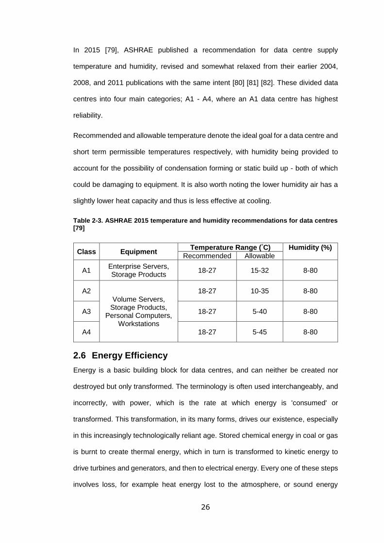
In 2015 [79], ASHRAE published a recommendation for data centre supply
temperature and humidity, revised and somewhat relaxed from their earlier 2004,
2008, and 2011 publications with the same intent [80] [81] [82]. These divided data
centres into four main categories; A1 - A4, where an A1 data centre has highest
reliability.
Recommended and allowable temperature denote the ideal goal for a data centre and
short term permissible temperatures respectively, with humidity being provided to
account for the possibility of condensation forming or static build up - both of which
could be damaging to equipment. It is also worth noting the lower humidity air has a
slightly lower heat capacity and thus is less effective at cooling.
Table 2-3. ASHRAE 2015 temperature and humidity recommendations for data centres [79]
Class Equipment Temperature Range (°C) Humidity (%)
Recommended Allowable
A1 Enterprise Servers, Storage Products
18-27 15-32 8-80
A2 Volume Servers,
Storage Products, Personal Computers,
Workstations
18-27 10-35 8-80
A3 18-27 5-40 8-80
A4 18-27 5-45 8-80
2.6 Energy Efficiency
Energy is a basic building block for data centres, and can neither be created nor
destroyed but only transformed. The terminology is often used interchangeably, and
incorrectly, with power, which is the rate at which energy is 'consumed' or
transformed. This transformation, in its many forms, drives our existence, especially
in this increasingly technologically reliant age. Stored chemical energy in coal or gas
is burnt to create thermal energy, which in turn is transformed to kinetic energy to
drive turbines and generators, and then to electrical energy. Every one of these steps
involves loss, for example heat energy lost to the atmosphere, or sound energy

27
created in place of electricity, and the degree to which these losses are minimised
gauges the energy efficiency of the process. Efficiency is defined, very simplistically,
as the ratio of what you get against what you pay for:
𝐸𝑛𝑒𝑟𝑔𝑦 𝐸𝑓𝑓𝑖𝑐𝑖𝑒𝑛𝑐𝑦 = 𝑈𝑠𝑒𝑓𝑢𝑙 𝑜𝑢𝑡𝑝𝑢𝑡 𝑜𝑓 𝑎 𝑝𝑟𝑜𝑐𝑒𝑠𝑠
𝐸𝑛𝑒𝑟𝑔𝑦 𝑖𝑛𝑝𝑢𝑡 𝑖𝑛𝑡𝑜 𝑎 𝑝𝑟𝑜𝑐𝑒𝑠𝑠 [83]
The energy efficiency of a power station can be determined by weighing how much
stored or potential chemical energy was input against how much electrical energy it
provides to the grid. This could consider the thermal losses at generation, or the
transmission losses to resistance in the cables between the generator and substation.
When considering a data centre, determining the energy efficiency becomes difficult.
Does efficiency better describe the heat expelled from the data centre or the
operations performed by the servers per second, when compared with power cost?
Which efficiencies takes into account the role of finance, the cost of added
redundancies or greater cooling infrastructure? Each data centre will have its own
priorities in terms of efficiency, and in each data centre there will be personnel who
have their own priorities; be those computational efficiency, energy efficiency,
financial efficiency, or something else entirely, and this project sets out to provide a
methodology for understanding or observing each.
2.7 Metrics for Data Centres
The data centre can be considered as a single system, and any system requires
constant surveillance to ensure proper running. When monitoring a data centre, the
data centre manager has a range of tools at their disposal. Monitoring an existing
data centre allows for informed decision-making on a range of issues such as [84];
• capacity planning - when expanding or introducing new equipment to a data
centre, it is important to understand how effectively existing infrastructure is
performing and what effect new equipment will have on the efficiency of the
data centre as a whole.
28
• device placement - it is also important to understand where best to place
new equipment in a room, for example to avoiding amplifying existing hot-
spots.
• equipment maintenance - by utilising a Condition-Based Maintenance
system, where equipment is continually monitored for early warning signs of
impending faults or failures, maintenance cost and loss of service can be
minimised or avoided.
• capacity utilisation - it is rare for a data centre to have a perfectly steady-
state load, transiently, and as such, proper monitoring of utilisation of
infrastructure such as cooling, power, or even IT, best informs the decision-
making regarding expansion and the introduction of redundant systems to
avoid potential loss of service.
• energy efficiency - to improve, or even understand, the energy efficiency of
a data centre it is imperative to monitor some key attributes, such as power
consumption of the rooms, temperature into and out of the room, cooling
utilisation, and if possible, useful work done. It is this particular goal of
monitoring data centres that is the focus of this study.
The term "metric" is given to those procedures developed for monitoring with a view
to improving various aspects of a system, in this case the data centre, and which can
be employed to better aid decision-making on the previously mentioned issues.
Selecting a metric for a data centre and then measuring it over a period of time,
highlights to the operator trends that can be seen in the data centre and theoretically
offers the best path for improvement of that particular attribute.
A simple example of this could be monitoring the outside ambient air, the inlet of a
cooling system to best determine those days of the year a compressor may be
switched off to save power. Furthermore, the monitoring of this particular attribute
may lead the operator to predict upcoming cooling system behaviour based on

29
historic data, perhaps bringing online an extra CRAC unit in the event of a period of
hot weather to prevent over-utilisation and loss of service.
There are many types of metrics available to the data centre operator, monitoring
varying attributes and of differing usefulness. The most well-known of these is the
'PUE' or Power Usage Effectiveness, defined as
𝑃𝑈𝐸 =𝑇𝑜𝑡𝑎𝑙 𝑑𝑎𝑡𝑎 𝑐𝑒𝑛𝑡𝑟𝑒 𝑒𝑛𝑒𝑟𝑔𝑦
𝑇𝑜𝑡𝑎𝑙 𝐼𝑇 𝑒𝑛𝑒𝑟𝑔𝑦
This affords an insight into the ratio of power consumed by the IT performing 'useful'
work against how much power is consumed by the data centre infrastructure
supporting it, including energy used for cooling, lost in power conversion and
distribution, and required for support systems such as lighting or security monitoring.
Originally devised to simply aid planning, this metric was proposed by Belady and
Melone in 2006 [85] and popularised by the Green Grid in 2007 in a white paper
entitled "Green Grid Metrics: Describing Data Center Power Efficiency" [86] and has
since been widely adopted by the community at large, seeing use by organisations
such as ASHRAE and the Environmental Protection Agency [87]. Their report details
how a facility should measure PUE, measuring power consumption at the interface of
substation and facility to properly capture total data centre energy consumption, as
well as only recording power delivered directly to IT equipment, excluding losses in
transmission or conversion at the PDU level. Most recently an ISO standard for PUE
has been published, explaining how to measure different categories of the metric [88].
A study by the Uptime Institute undertaken in 2013 found the average PUE value for
the data centres considered to be 1.65 [89], an improvement on their reported value
of 1.8 from 2011 [90], and a further improvement on their previously reported value
of 2.5 in 2007 [89]. In 2010, Energy Star conducted a survey of PUE in over 100 data
centres, and found the average to be 1.91 with a range of 1.25 to 3.75 (Figure 2-8)
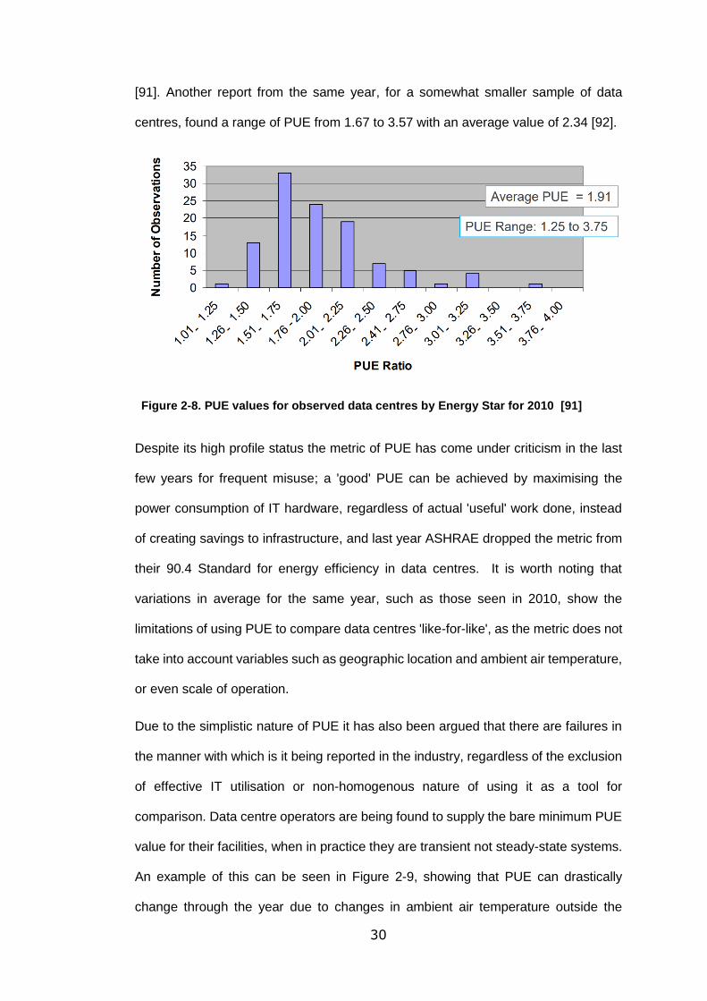
30
[91]. Another report from the same year, for a somewhat smaller sample of data
centres, found a range of PUE from 1.67 to 3.57 with an average value of 2.34 [92].
Figure 2-8. PUE values for observed data centres by Energy Star for 2010 [91]
Despite its high profile status the metric of PUE has come under criticism in the last
few years for frequent misuse; a 'good' PUE can be achieved by maximising the
power consumption of IT hardware, regardless of actual 'useful' work done, instead
of creating savings to infrastructure, and last year ASHRAE dropped the metric from
their 90.4 Standard for energy efficiency in data centres. It is worth noting that
variations in average for the same year, such as those seen in 2010, show the
limitations of using PUE to compare data centres 'like-for-like', as the metric does not
take into account variables such as geographic location and ambient air temperature,
or even scale of operation.
Due to the simplistic nature of PUE it has also been argued that there are failures in
the manner with which is it being reported in the industry, regardless of the exclusion
of effective IT utilisation or non-homogenous nature of using it as a tool for
comparison. Data centre operators are being found to supply the bare minimum PUE
value for their facilities, when in practice they are transient not steady-state systems.
An example of this can be seen in Figure 2-9, showing that PUE can drastically
change through the year due to changes in ambient air temperature outside the

31
facility, and the knock-on effect this has on the power consumption and efficiency of
cooling infrastructure [93].
Figure 2-9. The difference between reported values of PUE and realistic values, for a given data centre [93]
Nonetheless, it should be noted that while PUE is not the metric for energy efficiency
that the industry has distorted it to represent, and while it was never designed to be
comparable from one data centre to another, the ability to rank the efficiency of data
centres against each other relatively simply has led to legitimate improvements in
energy efficiency through such simple innovations as reassessing cooling
requirements [58].
An offshoot of PUE is pPUE or Partial Power Usage Effectiveness, which allows for
those systems where infrastructure may be fractured, such as a small in-house data
centre in an office complex, where the cooling is part of the general cooling
infrastructure of the building as whole.
The counterpart to PUE, and created at the same time, is DCiE or Data Centre
Infrastructure Efficiency [86], which is literally the inverse of PUE;
𝐷𝐶𝑖𝐸 = 1
𝑃𝑈𝐸

32
As a measure of energy efficiency, DCiE has the advantage of tending toward 100%
as improvements are made, as opposed to PUE which has a theoretical minimum
limit of 1, but as PUE became more widely used DCiE fell out of use.
In a follow-up paper from 2010, the Green Grid proposed a modified version of PUE
known as ERE or Energy Reuse Effectiveness which takes into account any reuse of
heat [94];
𝐸𝑅𝐸 = 𝑇𝑜𝑡𝑎𝑙 𝑑𝑎𝑡𝑎 𝑐𝑒𝑛𝑡𝑟𝑒 𝑒𝑛𝑒𝑟𝑔𝑦 − 𝑇𝑜𝑡𝑎𝑙 𝑟𝑒𝑢𝑠𝑒𝑑 𝑒𝑛𝑒𝑟𝑔𝑦
𝑇𝑜𝑡𝑎𝑙 𝐼𝑇 𝑒𝑛𝑒𝑟𝑔𝑦
This allows data centres that adopt the practice of waste heat reuse to measure the
effectiveness of this practice. The theoretical limit of this metric would be 0 for a data
centre that managed to somehow reuse all energy used throughout the data centre,
although practically the number would tend closer to 1 for real data centres, with a
facility reusing no waste energy having ERE and PUE equal.
An interesting metric proposed by the Uptime Institute in collaboration with the
McKinsey and Company in 2008 is that of CADE or Corporate Average Data Center
Efficiency [95]. This metric is a product of infrastructure to IT utilisation but goes a
step further, taking into account the effectiveness or efficiency of utilisation as well;
𝐶𝐴𝐷𝐸 = 𝐼𝑛𝑓𝑟𝑎𝑠𝑡𝑟𝑢𝑐𝑡𝑢𝑟𝑒 𝑢𝑡𝑖𝑙𝑖𝑠𝑎𝑡𝑖𝑜𝑛 × 𝐼𝑛𝑓𝑟𝑎𝑠𝑡𝑟𝑢𝑐𝑢𝑡𝑟𝑒 𝑒𝑛𝑒𝑟𝑔𝑦 𝑒𝑓𝑓𝑖𝑐𝑖𝑒𝑛𝑐𝑦
× 𝐼𝑇 𝑢𝑡𝑖𝑙𝑖𝑠𝑎𝑡𝑖𝑜𝑛 𝑥 𝐼𝑇 𝑒𝑛𝑒𝑟𝑔𝑦 𝑒𝑓𝑓𝑖𝑐𝑖𝑒𝑛𝑐𝑦
To give this metric context a simple example is provided by Patterson in their chapter
on Energy Efficiency Metrics in the book ‘Energy Efficient Thermal Management of
Data Centres’ [17].
Supposing a data centre has 427kW of IT equipment requiring power and cooling
infrastructure. Ideally, infrastructure utilisation would match IT load in a ratio of 1:1,
but in this example, the available power system provides 700kW of power, while
cooling comes in units of 150kW, meaning four would be needed to provide 600kW
33
in order to cover the IT load of 427kW. This gives an infrastructure utilisation of 0.71.
This informs the first part of the equation, infrastructure utilisation, with infrastructure
energy efficiency being given by the previously mentioned metrics such as PUE or
DCiE.
The third term in the equation is IT utilisation. It was originally suggested that
processor utilisation should be used to quantify this, and this is the attribute that has
been used to determine IT utilisation in this thesis. However, this is far from perfect,
as no two servers are the same and where processor utilisation may represent the
bottleneck or weak link for many, it is possible that other aspects of the server such
as quantity of memory, storage viability, or network performance may be the limiting
factor for others. For the purpose of this thesis, attempts have been made to hold
these attributes constant throughout testing, but for future work the full range of
parameters would need to be properly understood to fully express IT utilisation.
When looking at actual data centre utilisation, it is typically surprisingly low. Writing in
2016, Walker suggests this figure for the average utilisation to be about 6-15% for
non-virtualised servers, with cloud computing pushing this number closer to 30% [96].
A report written in 2015 by Amazon correlates this, suggesting that in data centres
monitored non-virtualised utilisation rarely exceed 20%, with some virtualised
environments in their data centres pushing this figure as high as 60% [97].
The fourth and final component of CADE is IT energy efficiency and at the time of the
metrics inception, this metric was left undefined and for future development. Metrics
for IT energy efficiency have since been proposed and will be discussed, and it is the
adaptation and use of these that are explored in this work.
Taken together, the theoretically ideal value for CADE is 100%, the same as DCiE,
but in practice this metric sees far lower values. Patterson suggests a metric for
fulfilling the fourth component of the CADE equation as itEUE;
34
𝑖𝑡𝐸𝑈𝐸 =𝑇𝑜𝑡𝑎𝑙 𝑒𝑛𝑒𝑟𝑔𝑦 𝑖𝑛𝑡𝑜 𝑡ℎ𝑒 𝐼𝑇 𝑒𝑞𝑢𝑖𝑝𝑚𝑒𝑛𝑡
𝑇𝑜𝑡𝑎𝑙 𝑒𝑛𝑒𝑟𝑔𝑦 𝑖𝑛𝑡𝑜 𝑡ℎ𝑒 𝑐𝑜𝑚𝑝𝑢𝑡𝑒 𝑐𝑜𝑚𝑝𝑜𝑛𝑒𝑛𝑡𝑠
Where the metric represents the ratio of power consumed by compute infrastructure,
such as internal fans, power supplies, voltage regulators, with the power consumed
by the components involved in the useful compute, such as CPU, memory, and
storage. They go on to state that while this metric could theoretically be helpful,
complications arise in monitoring and calculating it under anything other than
laboratory conditions, due to the large variability in configurations across different
servers, as well as the variable power consumptions for different loads for different
components, and the relationship with the environmental conditions such as inlet
temperature. [17]
2.8 Compute Efficiency Metrics and Benchmarking
Data centres exist to do useful work on IT hardware, yet the metric currently used
most commonly by the industry, the PUE, only considers the amount of power
consumed by IT, using this figure to represent useful work done. A more thorough
metric for energy efficiency is required. In practice, this is far from simple.
The first challenge is defining the "useful work" of a data centre, which will not only
vary from data centre to data centre, depending on their intended purpose, but may
also vary within the same data centre on a day to day, or rack to rack basis, with some
servers performing transactional requests such as hosting and processing a search
engine, while others may be performing computationally taxing tasks such as
computational fluid dynamics simulations.
One solution would be to adopt a very specific IT energy efficiency metric for a data
centre. In the two examples above, the useful work for the search engine may be
considered as information packets transmitted back and forth from the data centre,
while high performance computing (HPC) may look at operations performed per

35
second. Both are metrics that have been considered, and to a degree, duplicated for
this thesis and can be seen in Chapter 3.
The Green Grid has proposed a number of metrics or proxies for considering compute
efficiency of a data centre, starting with a white paper from 2008 outlining a metric
called DCeP or Data Centre Energy Productivity, where
𝐷𝐶𝑒𝑃 =𝑈𝑠𝑒𝑓𝑢𝑙 𝑊𝑜𝑟𝑘 𝑃𝑟𝑜𝑑𝑢𝑐𝑒𝑑
𝑇𝑜𝑡𝑎𝑙 𝐷𝑎𝑡𝑎 𝐶𝑒𝑛𝑡𝑒𝑟 𝐸𝑛𝑒𝑟𝑔𝑦 𝐶𝑜𝑛𝑠𝑢𝑚𝑒𝑑 𝑃𝑟𝑜𝑑𝑢𝑐𝑖𝑛𝑔 𝑡ℎ𝑖𝑠 𝑊𝑜𝑟𝑘 [86]
This was followed in 2009 by a paper recognising the difficulty of implementing DCeP,
for the same reasons as previously mentioned, in which the Green Grid proposed a
number of proxies for compute efficiency instead, shown in Table 2-4 [98]. These
followed much the same selection criteria as standard metrics, considering attributes
such as ease of use, accuracy, cost, invasiveness, objectivity, and whether they
would interrupt the daily operation of the data centre they were being used on.
Of the eight proxies proposed, seven can be considered 'energy proxies' and one a
'power proxy' - that is to say energy or power are used as the denominator. They
state the former to be useful for judging the energy efficiency of the data centre,
providing information on CO2 footprint or electrical consumption, whereas the latter is
typically considered for capacity planning and not necessarily relevant here.

36
Table 2-4. Proxies for computational efficiency suggested by the Green Grid [98]
1 Useful Work Self-assessment and Reporting
2 DCeP subset by productivity link
3 DCeP subset by sample workload
4 Bits per KiloWatt hour
5 Weighted CPU utilization – SPECint_rate
6 Weighted CPU utilization – SPECpower
7 Compute units per second trend curve
The two proxies of particular interest to this thesis are #4 - Bits per KiloWatt hour and
#6 Weighted CPU utilisation, which will be discussed in more depth in sections 2.8.1
and 2.8.2.
2.8.1 Bits per kiloWatt hour
The Green Grid report summarised the metric of bits per kiloWatt hour as a measure
of productivity of a data centre, dividing the total bit volume of every outbound router
on the network, by the total data centre energy consumption, measured in Mb/kWh.
This can be seen in the equation below
𝑏𝑘𝑤ℎ = ∑ 𝑏𝑖
𝑘𝑖=1
𝐸𝐷𝐶
where:
𝑘 - the total number of outbound routers
𝑏𝑖 - the total number of bits coming out of the ith router during assessment
𝐸𝐷𝐶 - the total energy consumed by the data centre during assesment [98] [66]
The advantage of this proxy metric is that it is very non-invasive. Data for 𝑏𝑖 would be
collected from traffic statistics for all outbound routers during the assessment window,
with a minimum of additional setup being required and theoretically no impact on
operations. It is also fairly intutitive to understand, allowing a data centre operator to
37
see the effect of changes to either the numerator or the denominator of the equation
with relative ease.
A reduction of the number of idle servers employed or consolidation of workload to
fewer servers would hopefully result in the same or greater bit rate for less overall
energy consumption. The same could be true for improvements to the overall
infrastructure of the data centre, with performance remaining constant and power
consumption of utlitilies, such as cooling, decreasing.
Conversely, the growth of a partially filled data centre should also see an
improvement in bits per kiloWatt hour if adequate planning has gone into its design.
Infrastructure may stay the same, but the bits coming and going should increase as
more servers are introduced.
2.8.2 Weighted CPU Utilization - SPECpower
This metric utilises the SPEC_ssj2008 benchmarks, correlating published results on
server performance with direct CPU utilisation measurements, to establish an
estimate for computational efficiency of a server, or group of servers [99]. This is then
used to calculate efficiency figures for the data centre as a whole by considering the
population mix and performance of different servers. This benchmark was released
in late 2007, and it is worth noting, that at their time of writing in 2009, Green Grid
believed there to be more benchmarks in development by the Standard Performance
Evaluation Corporation (SPEC); in practice there has not been and SPEC_ssj2008 is
still widely used today [98] [100].
SPEC_ssj2008 creates Java-based simulated workloads in a virtual environment
modelling a series of 'warehouses' on the System Under Test (SUT) [101]. This load
is executed by a 'driver' scheduling work for each 'warehouse' using Java's
ScheduledExecutorService [102], in practice executing six 6 different transactions of
38
the following approximate frequency, with randomly generated input data for each
transaction;
• New Order (30.3%) – a new order is inserted into the system
• Payment (30.3%) – record a customer payment
• Order Status (3.0%) – request the status of an existing order
• Delivery (3.0%) – process orders for delivery
• Stock Level (3.0%) – find recently ordered items with low stock levels
• Customer Report (30.3%) – create a report of recent activity for a
customer.
The number of these operations successfully performed per second is used to
determine performance, with simultaneous request operations being throttled by the
requested CPU loading, calculated based on the number of operations performed at
initial calibration stages.
For a benchmark result to be submitted to SPECpower, it must follow their prescribed
testing regime. This comprises of three calibrations steps, followed by ten load steps
decreasing from 100% to 10% in 10% decrements, and ending with an idle step. Total
testing time is roughly 75 minutes, with default load duration each of 240 seconds,
with 30 seconds of 'ramp up' and 'ramp down' time before and after each load, and
between 5 and 10 seconds over interval time between, as seen in Figure 2-10 [103].
The proxy discussed in the Green Grid paper is calculated by identifying the average
CPU utilisation for each server in the data centre and then multiplying this figure by
published SPECpower 100 percent load level results for that server.
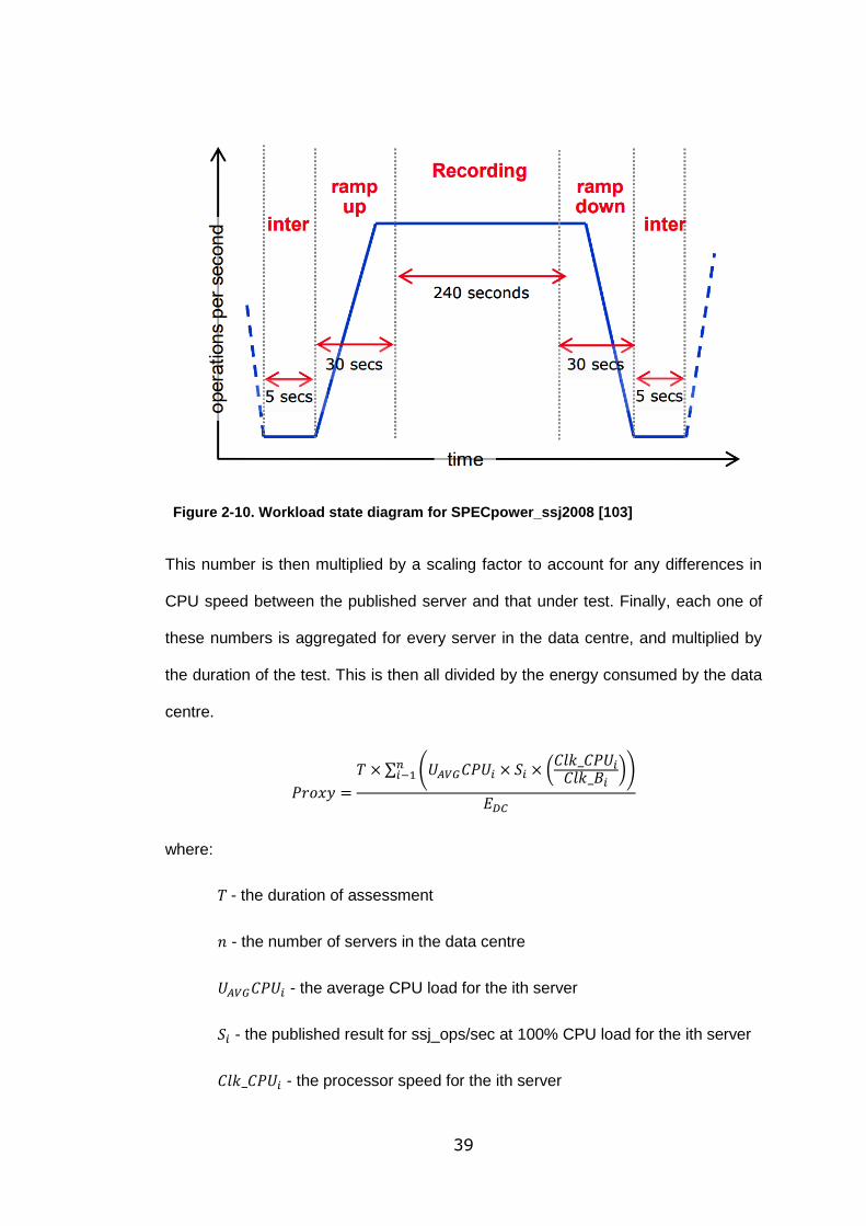
39
Figure 2-10. Workload state diagram for SPECpower_ssj2008 [103]
This number is then multiplied by a scaling factor to account for any differences in
CPU speed between the published server and that under test. Finally, each one of
these numbers is aggregated for every server in the data centre, and multiplied by
the duration of the test. This is then all divided by the energy consumed by the data
centre.
𝑃𝑟𝑜𝑥𝑦 =
𝑇 × ∑ (𝑈𝐴𝑉𝐺𝐶𝑃𝑈𝑖 × 𝑆𝑖 × (𝐶𝑙𝑘_𝐶𝑃𝑈𝑖
𝐶𝑙𝑘_𝐵𝑖))𝑛
𝑖−1
𝐸𝐷𝐶
where:
𝑇 - the duration of assessment
𝑛 - the number of servers in the data centre
𝑈𝐴𝑉𝐺𝐶𝑃𝑈𝑖 - the average CPU load for the ith server
𝑆𝑖 - the published result for ssj_ops/sec at 100% CPU load for the ith server
𝐶𝑙𝑘_𝐶𝑃𝑈𝑖 - the processor speed for the ith server
40
𝐶𝑙𝑘_𝐵𝑖 - the processor speed of the server used in the published results
𝐸𝐷𝐶 - the total energy consumed during the data centre during assesment
[98] [66]
The advantage of this proxy is that it provides a metric for computational efficiency
without the need for any additional software to be installed - provided the data centre
operator is monitoring CPU utilisation. Tools for querying this figure are widely
available. The downside is that it fully relies upon a third party to have conducted the
full SPECpower benchmark on a server of the same make and model as the operator
is using, and to have published these results with SPECpower.
2.8.3 LINPACK
A sub-system of data centres that require special consideration are those that contain
High-Performance Computers (HPC), and for these a well-established benchmark is
that of LINPACK. This was developed by the Top500 organisation to determine and
catalogue the capabilities of the most powerful supercomputers in the world, with the
organisation publishing a ranking of benchmark results twice a year [104], with results
submitted by interested parties in a similar manner to published SPECpower results.
LINPACK works by timing how long it takes for the HPC to solve a dense system of
linear equations, inverting an extremely large matrix, with the size of the problem
scaling to the capabilities of the system under test. Top500 claim this to be indicative
of overall performance of an HPC, as the problem is quite similar to the kind of
calculations HPCs tend to be employed on [104]. Some argue that this particular form
of artificial load fails to adequately capture the true performance of an HPC and that
application specific benchmarks should be employed to truly gauge the potential of
the machine [17].
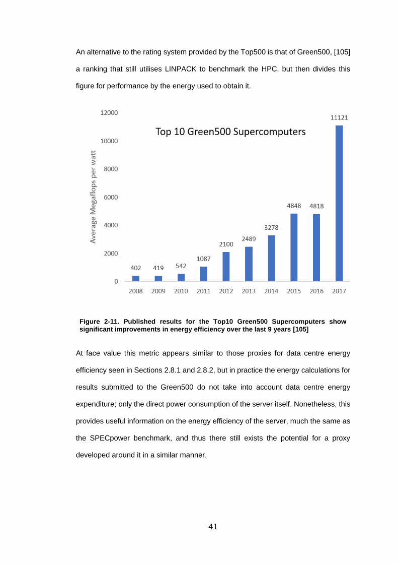
41
An alternative to the rating system provided by the Top500 is that of Green500, [105]
a ranking that still utilises LINPACK to benchmark the HPC, but then divides this
figure for performance by the energy used to obtain it.
Figure 2-11. Published results for the Top10 Green500 Supercomputers show significant improvements in energy efficiency over the last 9 years [105]
At face value this metric appears similar to those proxies for data centre energy
efficiency seen in Sections 2.8.1 and 2.8.2, but in practice the energy calculations for
results submitted to the Green500 do not take into account data centre energy
expenditure; only the direct power consumption of the server itself. Nonetheless, this
provides useful information on the energy efficiency of the server, much the same as
the SPECpower benchmark, and thus there still exists the potential for a proxy
developed around it in a similar manner.
42
2.9 Summary
The literature considered in Chapter 2 has shown that data centres are a continually
growing industry and that this growth has an impact on both global energy
consumption and environmental impact. While the rate at which this impact develops
has slowed in recent years due to the adoption of better practices, there is still great
scope for improvement. One such area of improvement is in better understanding and
even quantifying the utilisation of IT hardware within the data centre itself. Current
widely adopted industry metrics for gauging data centre effectiveness do so without
significant consideration for what hardware is actually doing and whether it is being
appropriately utilised.
Furthermore, while a great deal of research exists into the importance of adequate
cooling on maintaining the working thermal envelope for a data centre and the
mechanisms that can achieve it, there exists little research specifically into the actual
effect of these variations on IT performance. Current regulations on thermal envelope
within the data centre exist to protect delicate hardware from failure, with little
consideration given to the effect of changes in temperature on performance and
power consumption before this point. The work presented in the following chapters
aims to develop a methodology to characterise IT utilisation, both on its own and as
a function of thermal environment with a view to satisfying these limitations in
literature.
43
3 Evolution of Computational Loading
The aim of the research was to develop a robust methodology for testing a data centre
server with a view to informing, and even improving, efficiency on the whole room or
data centre scale. This initially required exploration of the options and development
of a method for computationally loading of servers to simulate the loads in use in a
data centre. Once this was complete, this methodology could be expanded to include
variations in thermal environment and the effect these might have on server
performance.
3.1 Theory
No single benchmark of computational efficiency can represent all applications of
servers in data centres, even those that can stress or emulate stress on multiple
components in a server. This is a concern mirrored in the difficulties quantifying the
efficiency of IT utilisation which are discussed in section 2.7. Efforts have been made
to consider the variations in different kinds of benchmark in this body of work, with a
view to best capturing the energy efficiency of servers.
Computational loading research was performed on two servers of roughly equal age
and power draw, but of competing server and processor architectures; ARM [106]
and Intel x86 [107]. Whilst intended to develop the computational loading
methodology, the effect on internal thermal environment for the servers, particularly
the ARM server, was also considered while running a range of benchmarks on each
system. These ranged from application specific testing, developed in house and
considering each system as a web-server, to commercially available loading tools
such as SPECpower2008 [99] and StressLinux [108]. The two different architectures
occupy different positions on the performance curve typically seen across a range of
data centres; the Intel providing more raw computing power and the ARM providing
greater energy efficiency. It was important to establish that any computational loading

44
methodology would not be limited to one specific chipset and thus exclude large
swathes of data centre hardware for testing.
3.2 Laboratory Set-up
The two servers were set up in a laboratory space, utilised for the duration of this
project, in the Energy Building at the University of Leeds. The space was
approximately 4m by 5m and approximately 3m high, and for the purpose of this set
of tests the servers were mounted in one of two racks placed together in the room,
with at least one meter clearance all around.
The two servers were mounted in the same rack and plugged into the same
networked PDU. The ARM server was an engineering sample from Avantek, utilising
Calxeda daughter cards each with 4 ARM processors, designated by the company
as CX00003 and created in 2013 [109]. It was located in the top half of the rack and
the Intel server was located at the bottom half with the network switch mounted
equidistant between them. A gap of 10U was allowed above and below each server
for them to be considered thermally independent of surrounding equipment. The
laboratory space was shared with a second Cool-IT rack, containing 30 servers,
including the network head-node, used as the Control and Collect System (CCS) for
the SPECpower and web-application testing as well as a Zabbix server for data-
logging [110]. The servers contained in this rack were water-cooled, somewhat
mitigating the impact of their heat generation on the overall laboratory conditions.
The ARM Chassis was comprised of 48 separate nodes on 12 daughter cards, each
containing four ARMv7 processors and acting as independent servers, all within the
same housing and utilising the same backplane. Each node contained 4GB of RAM
and was installed with Ubuntu running linux kernel 3.5.0_42_Highbank operating
system. It ran a single 1000W PSU (power supply unit) with redundant PSUs being
an available option. The PSU was not hot-swappable meaning the server had to be
stopped and shutdown to remove it and had no markings that could be seen stating
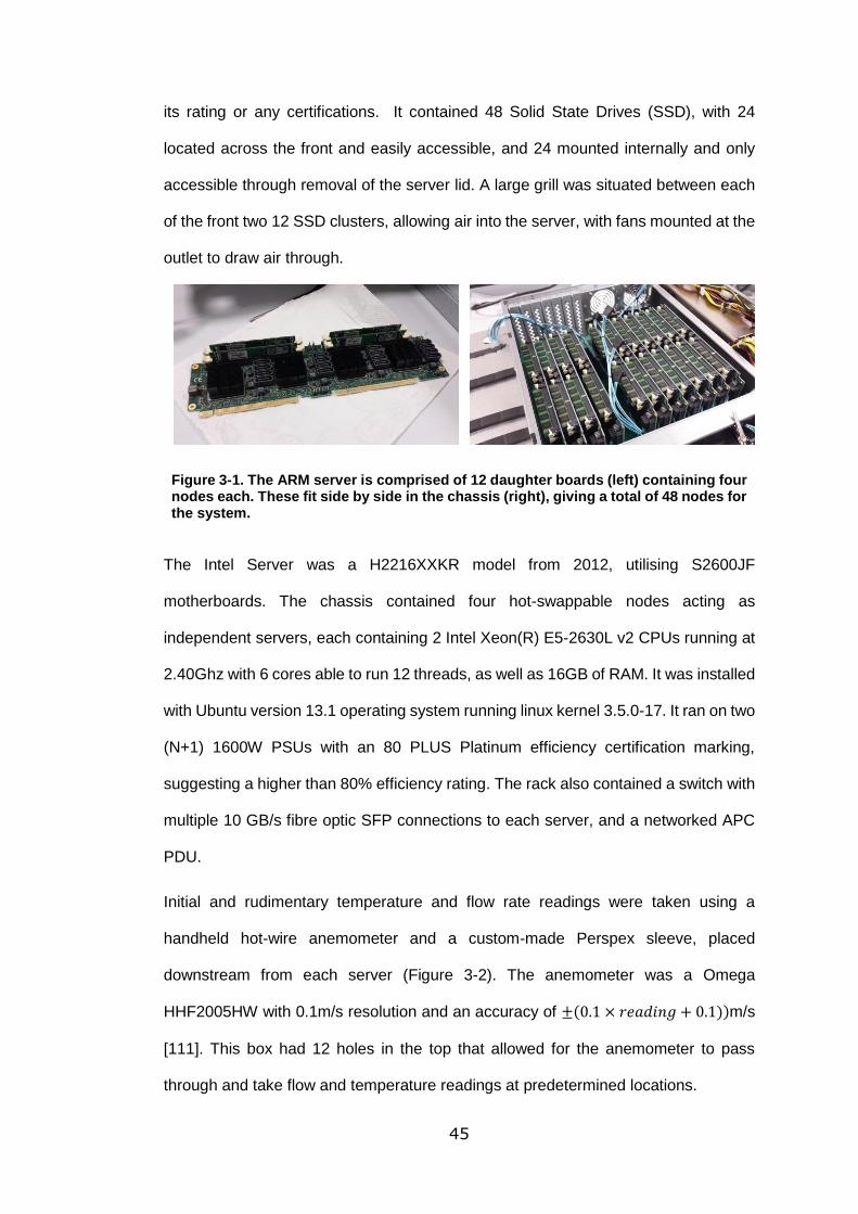
45
its rating or any certifications. It contained 48 Solid State Drives (SSD), with 24
located across the front and easily accessible, and 24 mounted internally and only
accessible through removal of the server lid. A large grill was situated between each
of the front two 12 SSD clusters, allowing air into the server, with fans mounted at the
outlet to draw air through.
Figure 3-1. The ARM server is comprised of 12 daughter boards (left) containing four nodes each. These fit side by side in the chassis (right), giving a total of 48 nodes for the system.
The Intel Server was a H2216XXKR model from 2012, utilising S2600JF
motherboards. The chassis contained four hot-swappable nodes acting as
independent servers, each containing 2 Intel Xeon(R) E5-2630L v2 CPUs running at
2.40Ghz with 6 cores able to run 12 threads, as well as 16GB of RAM. It was installed
with Ubuntu version 13.1 operating system running linux kernel 3.5.0-17. It ran on two
(N+1) 1600W PSUs with an 80 PLUS Platinum efficiency certification marking,
suggesting a higher than 80% efficiency rating. The rack also contained a switch with
multiple 10 GB/s fibre optic SFP connections to each server, and a networked APC
PDU.
Initial and rudimentary temperature and flow rate readings were taken using a
handheld hot-wire anemometer and a custom-made Perspex sleeve, placed
downstream from each server (Figure 3-2). The anemometer was a Omega
HHF2005HW with 0.1m/s resolution and an accuracy of ±(0.1 × 𝑟𝑒𝑎𝑑𝑖𝑛𝑔 + 0.1))m/s
[111]. This box had 12 holes in the top that allowed for the anemometer to pass
through and take flow and temperature readings at predetermined locations.
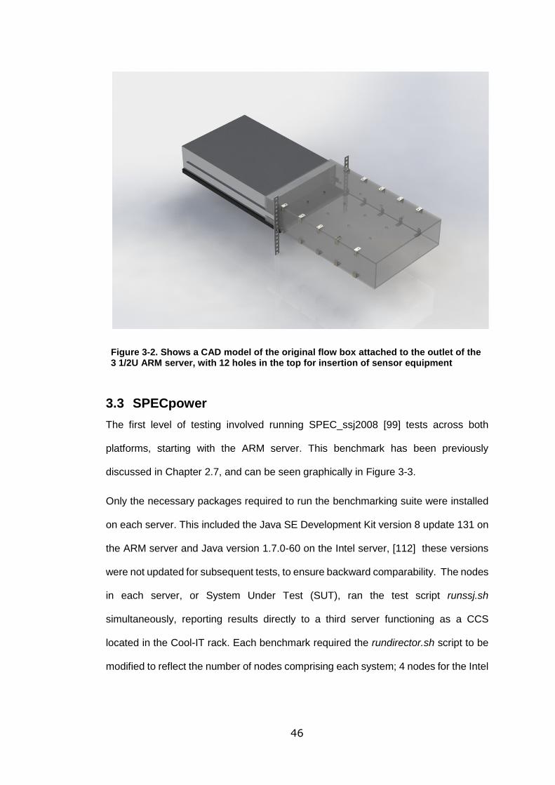
46
Figure 3-2. Shows a CAD model of the original flow box attached to the outlet of the 3 1/2U ARM server, with 12 holes in the top for insertion of sensor equipment
3.3 SPECpower
The first level of testing involved running SPEC_ssj2008 [99] tests across both
platforms, starting with the ARM server. This benchmark has been previously
discussed in Chapter 2.7, and can be seen graphically in Figure 3-3.
Only the necessary packages required to run the benchmarking suite were installed
on each server. This included the Java SE Development Kit version 8 update 131 on
the ARM server and Java version 1.7.0-60 on the Intel server, [112] these versions
were not updated for subsequent tests, to ensure backward comparability. The nodes
in each server, or System Under Test (SUT), ran the test script runssj.sh
simultaneously, reporting results directly to a third server functioning as a CCS
located in the Cool-IT rack. Each benchmark required the rundirector.sh script to be
modified to reflect the number of nodes comprising each system; 4 nodes for the Intel
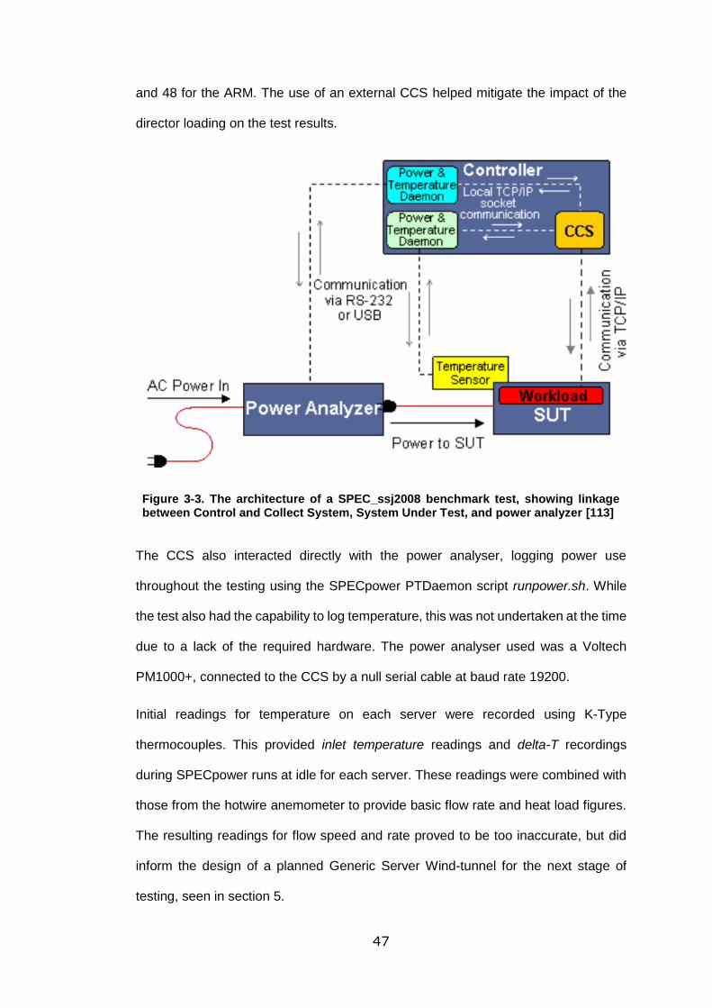
47
and 48 for the ARM. The use of an external CCS helped mitigate the impact of the
director loading on the test results.
Figure 3-3. The architecture of a SPEC_ssj2008 benchmark test, showing linkage between Control and Collect System, System Under Test, and power analyzer [113]
The CCS also interacted directly with the power analyser, logging power use
throughout the testing using the SPECpower PTDaemon script runpower.sh. While
the test also had the capability to log temperature, this was not undertaken at the time
due to a lack of the required hardware. The power analyser used was a Voltech
PM1000+, connected to the CCS by a null serial cable at baud rate 19200.
Initial readings for temperature on each server were recorded using K-Type
thermocouples. This provided inlet temperature readings and delta-T recordings
during SPECpower runs at idle for each server. These readings were combined with
those from the hotwire anemometer to provide basic flow rate and heat load figures.
The resulting readings for flow speed and rate proved to be too inaccurate, but did
inform the design of a planned Generic Server Wind-tunnel for the next stage of
testing, seen in section 5.
48
Internal monitoring on the ARM server was achieved through the development of shell
scripts to poll the IPMI for each node repeatedly throughout the duration of each test.
The IPMItool provided temperatures at four locations for each node, two on the CPU
and two elsewhere on the daughter board, as well as CPU power usage. The power
and the average of these temperatures were written to text files for post-processing,
which included matching the timestamps reported by the IPMItool [114] and
SPECpower to determine the heat and power maps for each load.
The first iteration of internal mapping required each node to be polled concurrently.
This created a lag between the 0th and 47th node in each sample of approximately 70
seconds. To remove these differences a second script was developed that controlled
slave scripts to poll a fraction of the nodes concurrently, providing slightly more
accurate internal results. This would later be replaced by a simultaneously polling
script, not used for the duration of these initial computational tests.
3.3.1 Results
The first full benchmark of the ARM chassis took place at 15:40 on 11/08/14, lasting
75 minutes. A full run consisted of three calibrations followed by stress tests ranging
from 100% load to idle of 240 seconds each. The voltage stayed consistent at
approximately 240V through the test, with the power analyser reporting an uncertainty
of 0.5%.
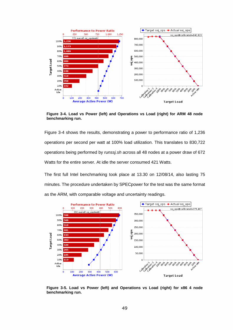
49
Figure 3-4. Load vs Power (left) and Operations vs Load (right) for ARM 48 node benchmarking run.
Figure 3-4 shows the results, demonstrating a power to performance ratio of 1,236
operations per second per watt at 100% load utilization. This translates to 830,722
operations being performed by runssj.sh across all 48 nodes at a power draw of 672
Watts for the entire server. At idle the server consumed 421 Watts.
The first full Intel benchmarking took place at 13.30 on 12/08/14, also lasting 75
minutes. The procedure undertaken by SPECpower for the test was the same format
as the ARM, with comparable voltage and uncertainty readings.
Figure 3-5. Load vs Power (left) and Operations vs Load (right) for x86 4 node benchmarking run.
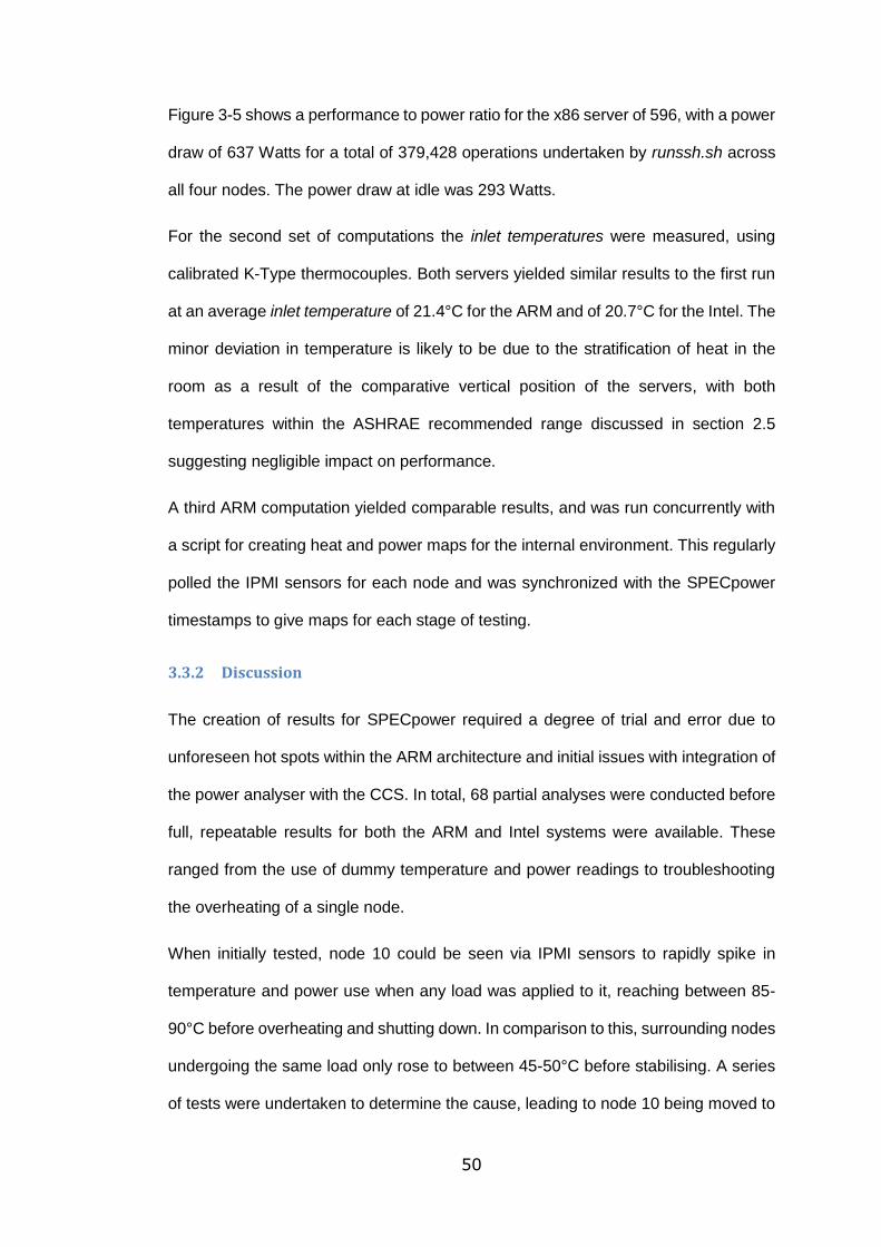
50
Figure 3-5 shows a performance to power ratio for the x86 server of 596, with a power
draw of 637 Watts for a total of 379,428 operations undertaken by runssh.sh across
all four nodes. The power draw at idle was 293 Watts.
For the second set of computations the inlet temperatures were measured, using
calibrated K-Type thermocouples. Both servers yielded similar results to the first run
at an average inlet temperature of 21.4°C for the ARM and of 20.7°C for the Intel. The
minor deviation in temperature is likely to be due to the stratification of heat in the
room as a result of the comparative vertical position of the servers, with both
temperatures within the ASHRAE recommended range discussed in section 2.5
suggesting negligible impact on performance.
A third ARM computation yielded comparable results, and was run concurrently with
a script for creating heat and power maps for the internal environment. This regularly
polled the IPMI sensors for each node and was synchronized with the SPECpower
timestamps to give maps for each stage of testing.
3.3.2 Discussion
The creation of results for SPECpower required a degree of trial and error due to
unforeseen hot spots within the ARM architecture and initial issues with integration of
the power analyser with the CCS. In total, 68 partial analyses were conducted before
full, repeatable results for both the ARM and Intel systems were available. These
ranged from the use of dummy temperature and power readings to troubleshooting
the overheating of a single node.
When initially tested, node 10 could be seen via IPMI sensors to rapidly spike in
temperature and power use when any load was applied to it, reaching between 85-
90°C before overheating and shutting down. In comparison to this, surrounding nodes
undergoing the same load only rose to between 45-50°C before stabilising. A series
of tests were undertaken to determine the cause, leading to node 10 being moved to
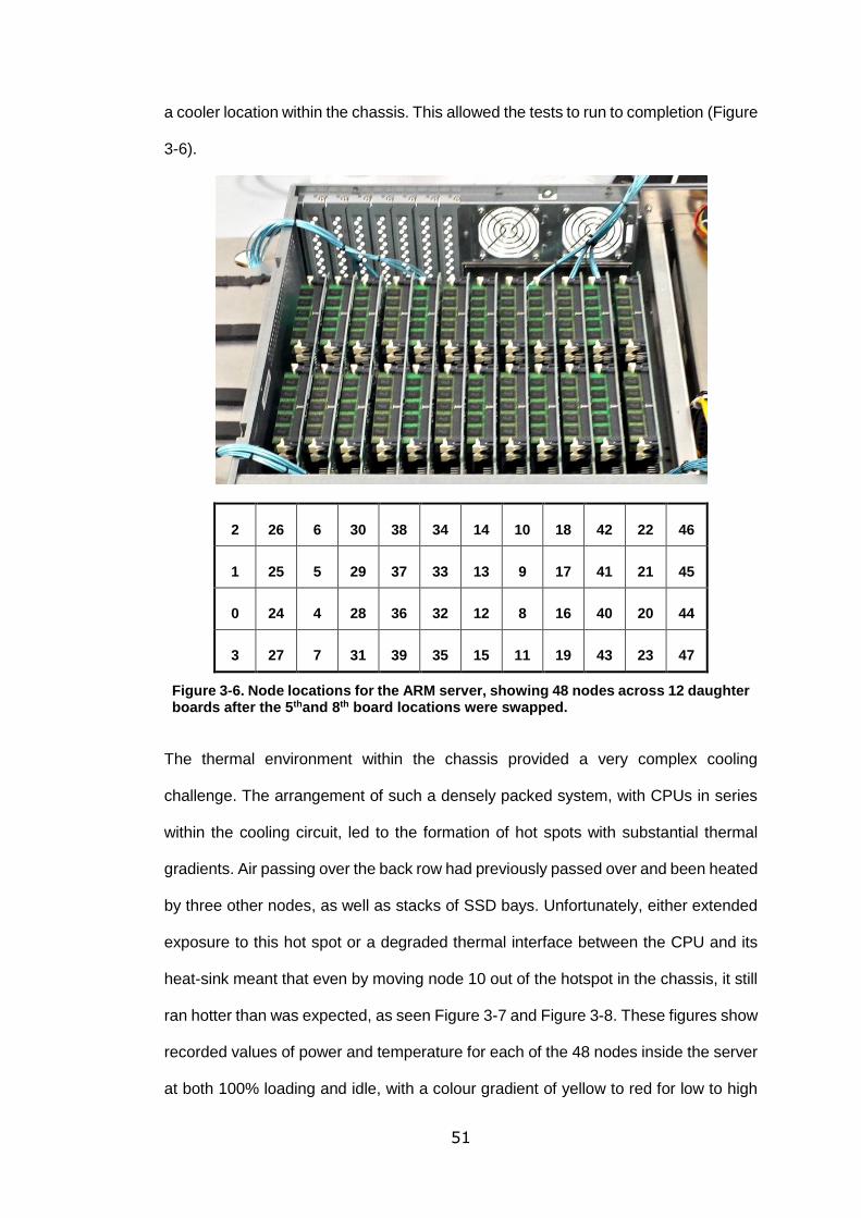
51
a cooler location within the chassis. This allowed the tests to run to completion (Figure
3-6).
2 26 6 30 38 34 14 10 18 42 22 46
1 25 5 29 37 33 13 9 17 41 21 45
0 24 4 28 36 32 12 8 16 40 20 44
3 27 7 31 39 35 15 11 19 43 23 47
Figure 3-6. Node locations for the ARM server, showing 48 nodes across 12 daughter boards after the 5thand 8th board locations were swapped.
The thermal environment within the chassis provided a very complex cooling
challenge. The arrangement of such a densely packed system, with CPUs in series
within the cooling circuit, led to the formation of hot spots with substantial thermal
gradients. Air passing over the back row had previously passed over and been heated
by three other nodes, as well as stacks of SSD bays. Unfortunately, either extended
exposure to this hot spot or a degraded thermal interface between the CPU and its
heat-sink meant that even by moving node 10 out of the hotspot in the chassis, it still
ran hotter than was expected, as seen Figure 3-7 and Figure 3-8. These figures show
recorded values of power and temperature for each of the 48 nodes inside the server
at both 100% loading and idle, with a colour gradient of yellow to red for low to high
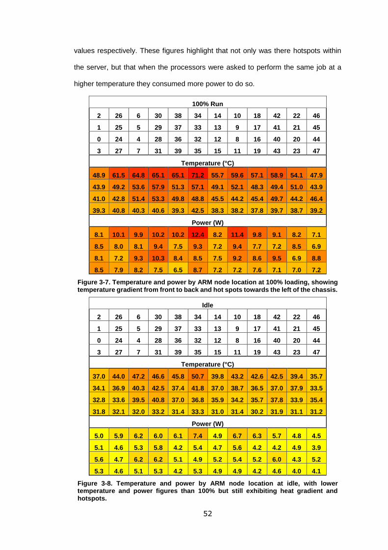
52
values respectively. These figures highlight that not only was there hotspots within
the server, but that when the processors were asked to perform the same job at a
higher temperature they consumed more power to do so.
100% Run
2 26 6 30 38 34 14 10 18 42 22 46
1 25 5 29 37 33 13 9 17 41 21 45
0 24 4 28 36 32 12 8 16 40 20 44
3 27 7 31 39 35 15 11 19 43 23 47
Temperature (°C)
48.9 61.5 64.8 65.1 65.1 71.2 55.7 59.6 57.1 58.9 54.1 47.9
43.9 49.2 53.6 57.9 51.3 57.1 49.1 52.1 48.3 49.4 51.0 43.9
41.0 42.8 51.4 53.3 49.8 48.8 45.5 44.2 45.4 49.7 44.2 46.4
39.3 40.8 40.3 40.6 39.3 42.5 38.3 38.2 37.8 39.7 38.7 39.2
Power (W)
8.1 10.1 9.9 10.2 10.2 12.4 8.2 11.4 9.8 9.1 8.2 7.1
8.5 8.0 8.1 9.4 7.5 9.3 7.2 9.4 7.7 7.2 8.5 6.9
8.1 7.2 9.3 10.3 8.4 8.5 7.5 9.2 8.6 9.5 6.9 8.8
8.5 7.9 8.2 7.5 6.5 8.7 7.2 7.2 7.6 7.1 7.0 7.2
Figure 3-7. Temperature and power by ARM node location at 100% loading, showing temperature gradient from front to back and hot spots towards the left of the chassis.
Idle
2 26 6 30 38 34 14 10 18 42 22 46
1 25 5 29 37 33 13 9 17 41 21 45
0 24 4 28 36 32 12 8 16 40 20 44
3 27 7 31 39 35 15 11 19 43 23 47
Temperature (°C)
37.0 44.0 47.2 46.6 45.8 50.7 39.8 43.2 42.6 42.5 39.4 35.7
34.1 36.9 40.3 42.5 37.4 41.8 37.0 38.7 36.5 37.0 37.9 33.5
32.8 33.6 39.5 40.8 37.0 36.8 35.9 34.2 35.7 37.8 33.9 35.4
31.8 32.1 32.0 33.2 31.4 33.3 31.0 31.4 30.2 31.9 31.1 31.2
Power (W)
5.0 5.9 6.2 6.0 6.1 7.4 4.9 6.7 6.3 5.7 4.8 4.5
5.1 4.6 5.3 5.8 4.2 5.4 4.7 5.6 4.2 4.2 4.9 3.9
5.6 4.7 6.2 6.2 5.1 4.9 5.2 5.4 5.2 6.0 4.3 5.2
5.3 4.6 5.1 5.3 4.2 5.3 4.9 4.9 4.2 4.6 4.0 4.1
Figure 3-8. Temperature and power by ARM node location at idle, with lower temperature and power figures than 100% but still exhibiting heat gradient and hotspots.
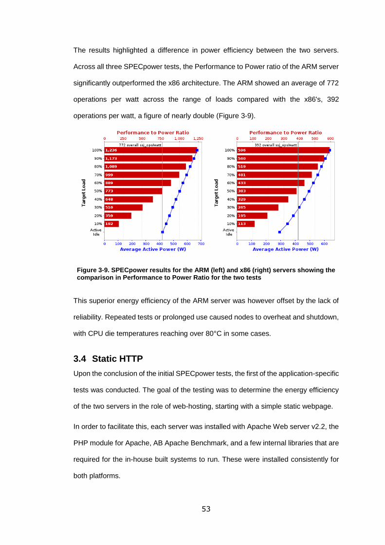
53
The results highlighted a difference in power efficiency between the two servers.
Across all three SPECpower tests, the Performance to Power ratio of the ARM server
significantly outperformed the x86 architecture. The ARM showed an average of 772
operations per watt across the range of loads compared with the x86's, 392
operations per watt, a figure of nearly double (Figure 3-9).
Figure 3-9. SPECpower results for the ARM (left) and x86 (right) servers showing the comparison in Performance to Power Ratio for the two tests
This superior energy efficiency of the ARM server was however offset by the lack of
reliability. Repeated tests or prolonged use caused nodes to overheat and shutdown,
with CPU die temperatures reaching over 80°C in some cases.
3.4 Static HTTP
Upon the conclusion of the initial SPECpower tests, the first of the application-specific
tests was conducted. The goal of the testing was to determine the energy efficiency
of the two servers in the role of web-hosting, starting with a simple static webpage.
In order to facilitate this, each server was installed with Apache Web server v2.2, the
PHP module for Apache, AB Apache Benchmark, and a few internal libraries that are
required for the in-house built systems to run. These were installed consistently for
both platforms.

54
Each system acted as the tester for the other system; x86 providing the load for the
ARM and vice versa. This asymmetry was far from ideal, but without the presence of
another server at the time, was the only option. The headnode in the Cool-IT rack
acted as the controller for the duration of the tests, run by four main scripts developed
specifically for the task.
Initially the headnode also created the loading for each test, but the 1Gbps connection
speed between the Cool-IT rack and testing rack provided insufficient bandwidth for
the tests to be fully realised. Instead, the headnode distributed the loading scripts to
the test server not under benchmark and initiated the test there. The connection
speed between each test server was a maximum of 20Gbps, eliminating potential
network bottlenecks.
These scripts (see Appendix A) consisted of a head, body, and two output scripts.
The user initiated the head3.sh script, which prompted for parameters such as server
under test, test duration, number of users, and range of users. This then created the
working directories for the test across the headnode and loading nodes, before
initiating the body3.sh. The body3.sh script then determined which server was to be
tested and wrote and distributed testing scripts accordingly, which initiated AB
Apache Benchmark for the duration and concurrency level of each test.
The concurrency level was a measure of the number of virtual users simultaneously
accessing the website. The Apache server creates threads to handle each user, with
a maximum number of simultaneous threads set to default at 150 per node, although
this figure was adjustable.
When the Intel server loaded the ARM, 12 scripts were distributed to each of the four
Intel nodes, providing testing for all 48 ARM nodes. These were synchronised to start
together and on completion report the results of the benchmark to the relevant
directory on the headnode. This waited for the directory to contain 48 results files
before initiating the output scripts which trimmed and merged the important aspects
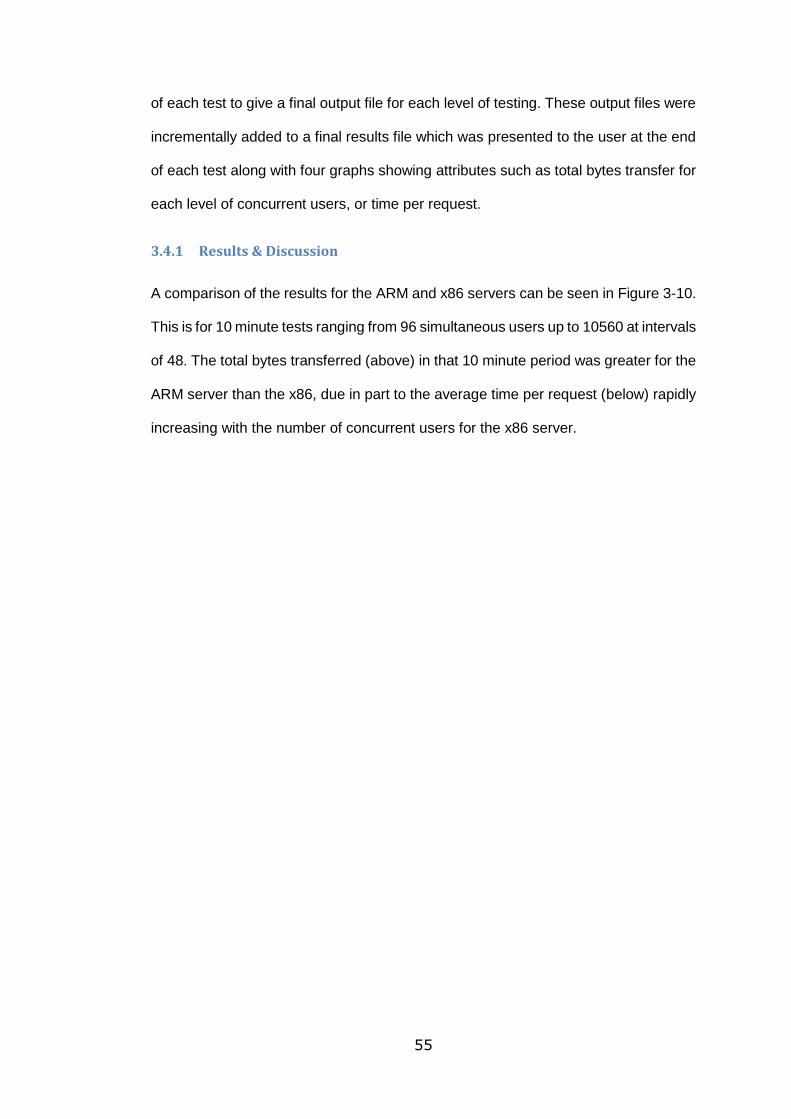
55
of each test to give a final output file for each level of testing. These output files were
incrementally added to a final results file which was presented to the user at the end
of each test along with four graphs showing attributes such as total bytes transfer for
each level of concurrent users, or time per request.
3.4.1 Results & Discussion
A comparison of the results for the ARM and x86 servers can be seen in Figure 3-10.
This is for 10 minute tests ranging from 96 simultaneous users up to 10560 at intervals
of 48. The total bytes transferred (above) in that 10 minute period was greater for the
ARM server than the x86, due in part to the average time per request (below) rapidly
increasing with the number of concurrent users for the x86 server.
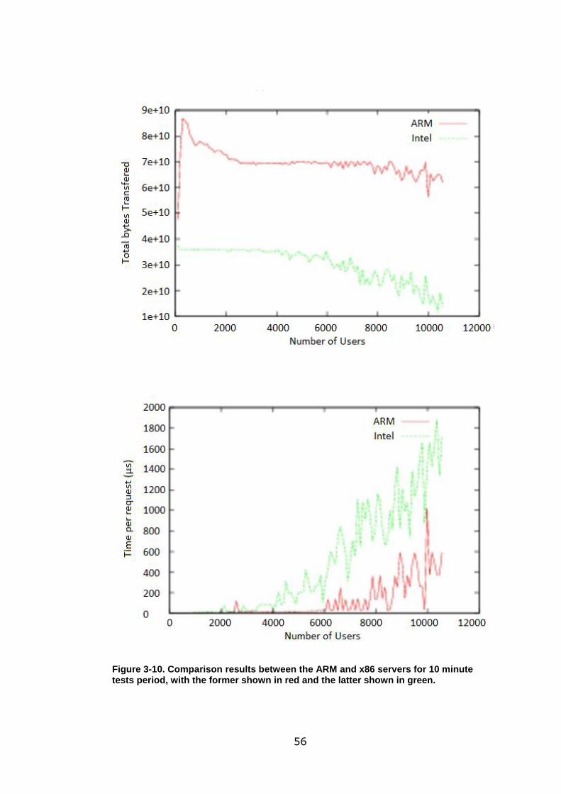
56
Figure 3-10. Comparison results between the ARM and x86 servers for 10 minute tests period, with the former shown in red and the latter shown in green.
57
The static HTTP test had a number of limitations; the testing created more load on
the server doing the loading than that which was under test due to the page being
accessed being only 11.5kB in size and comprising only text. This suggested the
testing loaded the periphery aspects of the servers, such as backplane and network
capability, more than the CPU load-carrying capabilities (Figure 3-10 and Figure
3-11). The drop of power usage with more attempted work done seen in Figure 3-11
suggests a bottleneck of resource within the server, skewing the value of the data.
This shows a trend of less power being consumed for more users being served, which
matches with the drop in Total bytes transferred seen in Figure 3-10.
Figure 3-11. Power usage against time for the x86 Server, where the time increases as the number of concurrent users does.
The fact that each test had to be created by the other system would also suggest the
introduction of immeasurable network interferences present during testing, although
efforts were made to minimise this; despite the ARM server having 12 times more
nodes than the x86, the workload was created and divided such that the total work
done by each server was the same, with each x86 node loading 12 ARM nodes for
one direction of testing, and 12 ARM nodes loading each x86 node for the other.
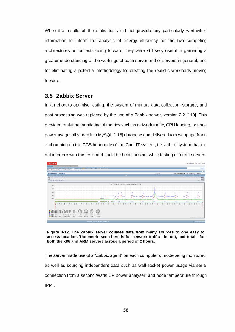
58
While the results of the static tests did not provide any particularly worthwhile
information to inform the analysis of energy efficiency for the two competing
architectures or for tests going forward, they were still very useful in garnering a
greater understanding of the workings of each server and of servers in general, and
for eliminating a potential methodology for creating the realistic workloads moving
forward.
3.5 Zabbix Server
In an effort to optimise testing, the system of manual data collection, storage, and
post-processing was replaced by the use of a Zabbix server, version 2.2 [110]. This
provided real-time monitoring of metrics such as network traffic, CPU loading, or node
power usage, all stored in a MySQL [115] database and delivered to a webpage front-
end running on the CCS headnode of the Cool-IT system, i.e. a third system that did
not interfere with the tests and could be held constant while testing different servers.
Figure 3-12. The Zabbix server collates data from many sources to one easy to access location. The metric seen here is for network traffic - in, out, and total - for both the x86 and ARM servers across a period of 2 hours.
The server made use of a “Zabbix agent” on each computer or node being monitored,
as well as sourcing independent data such as wall-socket power usage via serial
connection from a second Watts UP power analyser, and node temperature through
IPMI.
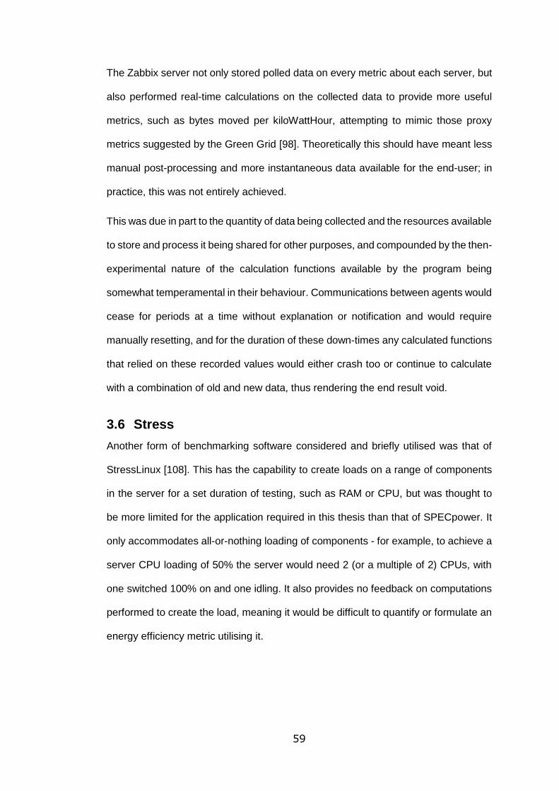
59
The Zabbix server not only stored polled data on every metric about each server, but
also performed real-time calculations on the collected data to provide more useful
metrics, such as bytes moved per kiloWattHour, attempting to mimic those proxy
metrics suggested by the Green Grid [98]. Theoretically this should have meant less
manual post-processing and more instantaneous data available for the end-user; in
practice, this was not entirely achieved.
This was due in part to the quantity of data being collected and the resources available
to store and process it being shared for other purposes, and compounded by the then-
experimental nature of the calculation functions available by the program being
somewhat temperamental in their behaviour. Communications between agents would
cease for periods at a time without explanation or notification and would require
manually resetting, and for the duration of these down-times any calculated functions
that relied on these recorded values would either crash too or continue to calculate
with a combination of old and new data, thus rendering the end result void.
3.6 Stress
Another form of benchmarking software considered and briefly utilised was that of
StressLinux [108]. This has the capability to create loads on a range of components
in the server for a set duration of testing, such as RAM or CPU, but was thought to
be more limited for the application required in this thesis than that of SPECpower. It
only accommodates all-or-nothing loading of components - for example, to achieve a
server CPU loading of 50% the server would need 2 (or a multiple of 2) CPUs, with
one switched 100% on and one idling. It also provides no feedback on computations
performed to create the load, meaning it would be difficult to quantify or formulate an
energy efficiency metric utilising it.
60
3.7 Dynamic HTTP
After SPECpower and static HTTP testing, the next step in the benchmarking process
was Dynamic HTTP testing. Whilst static testing only requested and transferred the
same basic webpage repeatedly, dynamic testing placed greater and more realistic
workload on the server under test by having each webpage transaction perform work
on accessing the website.
This was achieved by utilising a pre-existing dynamic webpage application called
Richfaces PhotoAlbum [116], which uses a JBoss container and MySQL database to
create a functional and interactive photo album website on each node (Figure 3-13).
While the application already existed, it had never been utilised on an ARM
architecture before. This meant the code had to be compiled from source, followed
by considerable troubleshooting to integrate all aspects of the software together
successfully.
Figure 3-13. Richfaces PhotoAlbum hosts a fully useable photo album on each Apache web server. The front-end accesses a MySQL database of pictures, installed on each node.
The software JMeter [117] was used to invoke the load in place of AB Apache,
allowing more flexibility in the work provided by the benchmark. Whereas AB Apache
would access a certain webpage as many times and for as long as requested, JMeter

61
could be programmed to perform certain workload plans on initiation. In the case of
the PhotoAlbum application, the testing plan called for JMeter to simulate users
following links on the website front page.
The test plan was pre-programmed with roughly 100 possible routes it could follow
and would randomly select this with a pre-specified number of users until a request
to stop was sent. This usually resulted in requests to access photos from the photo
album, requiring the webpage to do work accessing and presenting the file from the
MySQL database (Figure 3-14).
Figure 3-14. ‘Monuments and just buildings’ is the first of five different albums created in the application that the program can randomly request pictures from.
While the route that the virtual user could take was randomised, each photo was of
the same size, meaning a steady load was created on each server based upon the
number of concurrent users specified.
An individual test could be initiated manually by the user, but for batch processing a
modified version of the static HTTP testing scripts was used (see Appendix 0). The
modified shell script would create and distribute the work-plan to the nodes, with each
plan varying based on user inputs for attributes such as duration, concurrency level,
and testing interval, as well as starting and initialising each server for testing. These
62
tests were run for a user-specified input before being stopped, with the script building
in a few minutes tolerance before starting the next test to allow processes to finish.
Whilst the static test collated results to present a final output file and a series of
graphs, the Zabbix server provided most of this functionality. Every test had a
background output file which was used to check the integrating of each run providing,
for example, figures for the number of user requests which failed, but the functionality
for simple calculations was built into the Zabbix server, giving post-processed graphs
in real-time.
3.7.1 Results & Discussion
Initial testing was conducted on a single ARM node to determine the behaviour of the
CPU load for an increase in concurrent users. Whilst the static testing very rarely saw
a CPU usage above 30% regardless of the range of users due to the minimal work
actually done by the server under test, there existed a significant relationship between
CPU loading and concurrent users for the dynamic tests.
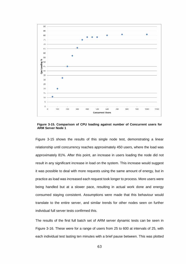
63
Figure 3-15. Comparison of CPU loading against number of Concurrent users for ARM Server Node 1
Figure 3-15 shows the results of this single node test, demonstrating a linear
relationship until concurrency reaches approximately 450 users, where the load was
approximately 81%. After this point, an increase in users loading the node did not
result in any significant increase in load on the system. This increase would suggest
it was possible to deal with more requests using the same amount of energy, but in
practice as load was increased each request took longer to process. More users were
being handled but at a slower pace, resulting in actual work done and energy
consumed staying consistent. Assumptions were made that this behaviour would
translate to the entire server, and similar trends for other nodes seen on further
individual full server tests confirmed this.
The results of the first full batch set of ARM server dynamic tests can be seen in
Figure 3-16. These were for a range of users from 25 to 600 at intervals of 25, with
each individual test lasting ten minutes with a brief pause between. This was plotted
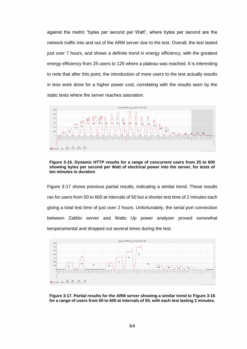
64
against the metric “bytes per second per Watt”, where bytes per second are the
network traffic into and out of the ARM server due to the test. Overall, the test lasted
just over 7 hours, and shows a definite trend in energy efficiency, with the greatest
energy efficiency from 25 users to 125 where a plateau was reached. It is interesting
to note that after this point, the introduction of more users to the test actually results
in less work done for a higher power cost, correlating with the results seen by the
static tests where the server reaches saturation.
Figure 3-16. Dynamic HTTP results for a range of concurrent users from 25 to 600 showing bytes per second per Watt of electrical power into the server, for tests of ten minutes in duration
Figure 3-17 shows previous partial results, indicating a similar trend. These results
ran for users from 50 to 600 at intervals of 50 but a shorter test time of 2 minutes each
giving a total test time of just over 2 hours. Unfortunately, the serial port connection
between Zabbix server and Watts Up power analyser proved somewhat
temperamental and dropped out several times during the test.
Figure 3-17. Partial results for the ARM server showing a similar trend to Figure 3-16 for a range of users from 50 to 600 at intervals of 50, with each test lasting 2 minutes.
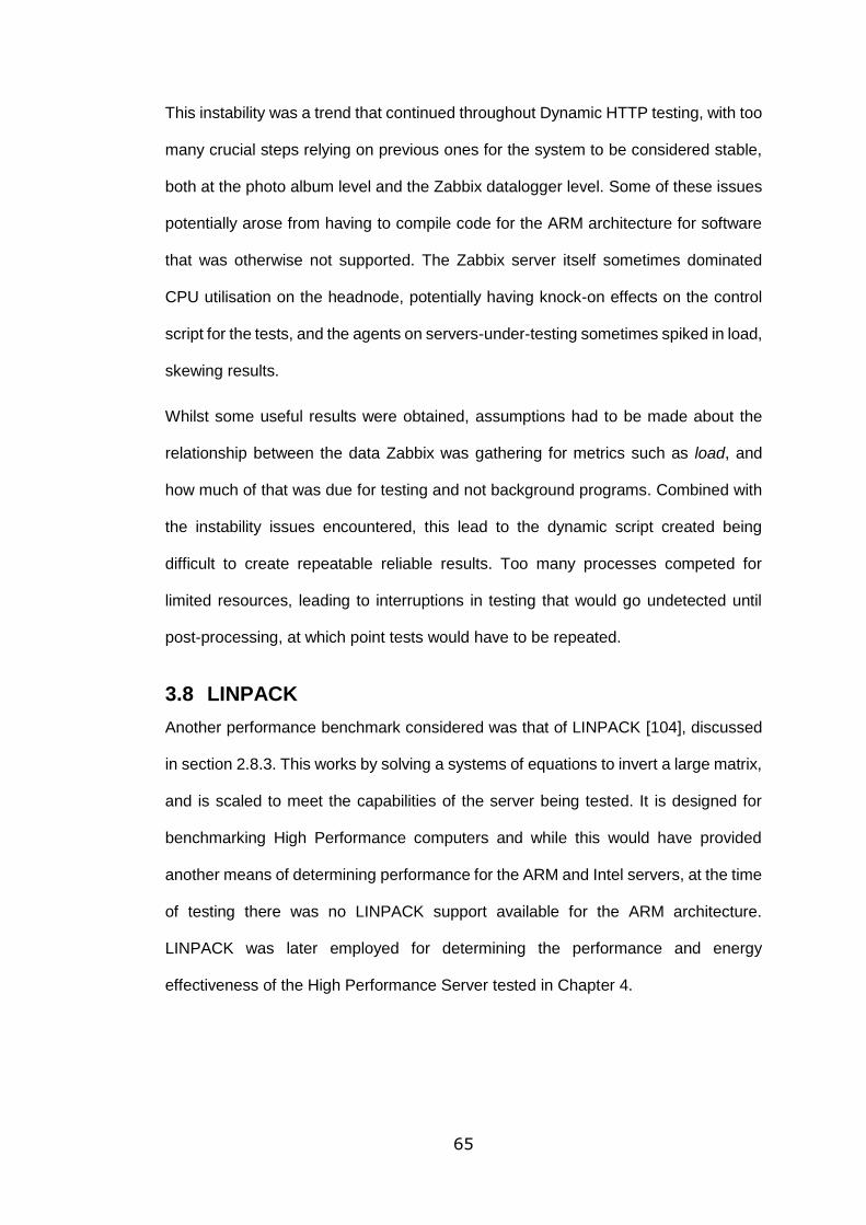
65
This instability was a trend that continued throughout Dynamic HTTP testing, with too
many crucial steps relying on previous ones for the system to be considered stable,
both at the photo album level and the Zabbix datalogger level. Some of these issues
potentially arose from having to compile code for the ARM architecture for software
that was otherwise not supported. The Zabbix server itself sometimes dominated
CPU utilisation on the headnode, potentially having knock-on effects on the control
script for the tests, and the agents on servers-under-testing sometimes spiked in load,
skewing results.
Whilst some useful results were obtained, assumptions had to be made about the
relationship between the data Zabbix was gathering for metrics such as load, and
how much of that was due for testing and not background programs. Combined with
the instability issues encountered, this lead to the dynamic script created being
difficult to create repeatable reliable results. Too many processes competed for
limited resources, leading to interruptions in testing that would go undetected until
post-processing, at which point tests would have to be repeated.
3.8 LINPACK
Another performance benchmark considered was that of LINPACK [104], discussed
in section 2.8.3. This works by solving a systems of equations to invert a large matrix,
and is scaled to meet the capabilities of the server being tested. It is designed for
benchmarking High Performance computers and while this would have provided
another means of determining performance for the ARM and Intel servers, at the time
of testing there was no LINPACK support available for the ARM architecture.
LINPACK was later employed for determining the performance and energy
effectiveness of the High Performance Server tested in Chapter 4.
66
3.9 Summary
Ultimately the most reliable computational loading system tested was that of the
SPECpower2008 benchmark. This was especially true once time had been dedicated
to further understanding the underlying scripting of the benchmark, allowing for
modifications to better reflect the type of testing desired. It allowed repeated and
consistent loading, with variation in duration and utilisation as necessary, and
reported power consumption and operations per second performed. This satisfied the
goal of determining the IT utilisation efficiency of a server, laying the ground-work for
understanding the effect temperature would have on this attribute in later work.
It is still worth noting the difficulty of defining the 'useful work' of a server, as discussed
within section 2.8. The benchmarks considered look at two specific forms of
determining performance; the operations performed per second and the amount of
information the server is providing a user with. While the latter is useful for
understanding the performance and efficiency of a web server this is still a specific
application. Looking at the underlying performance of the server itself, as provided by
SPECpower, seems to be more useful for determining a comparative server
performance when considering how broad the applications of data centre servers can
be.
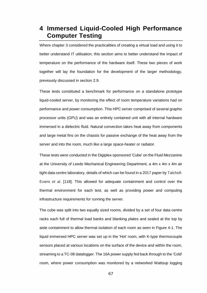
67
4 Immersed Liquid-Cooled High Performance Computer Testing
Where chapter 3 considered the practicalities of creating a virtual load and using it to
better understand IT utilisation, this section aims to better understand the impact of
temperature on the performance of the hardware itself. These two pieces of work
together will lay the foundation for the development of the larger methodology,
previously discussed in section 2.9.
These tests constituted a benchmark for performance on a standalone prototype
liquid-cooled server, by monitoring the effect of room temperature variations had on
performance and power consumption. This HPC server comprised of several graphic
processor units (GPU) and was an entirely contained unit with all internal hardware
immersed in a dielectric fluid. Natural convection takes heat away from components
and large metal fins on the chassis for passive exchange of the heat away from the
server and into the room, much like a large space-heater or radiator.
These tests were conducted in the Digiplex-sponsored 'Cube' on the Fluid Mezzanine
at the University of Leeds Mechanical Engineering Department, a 4m x 4m x 4m air
tight data centre laboratory, details of which can be found in a 2017 paper by Tatchell-
Evans et al. [118]. This allowed for adequate containment and control over the
thermal environment for each test, as well as providing power and computing
infrastructure requirements for running the server.
The cube was split into two equally sized rooms, divided by a set of four data centre
racks each full of thermal load banks and blanking plates and sealed at the top by
aisle containment to allow thermal isolation of each room as seen in Figure 4-1. The
liquid immersed HPC server was set up in the 'Hot' room, with K-type thermocouple
sensors placed at various locations on the surface of the device and within the room,
streaming to a TC-08 datalogger. The 16A power supply fed back through to the 'Cold'
room, where power consumption was monitored by a networked Wattsup logging
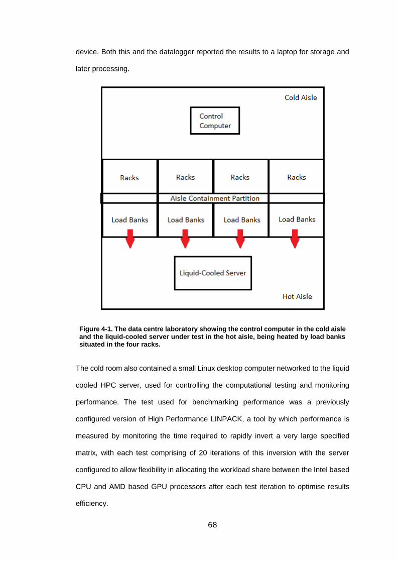
68
device. Both this and the datalogger reported the results to a laptop for storage and
later processing.
Figure 4-1. The data centre laboratory showing the control computer in the cold aisle and the liquid-cooled server under test in the hot aisle, being heated by load banks situated in the four racks.
The cold room also contained a small Linux desktop computer networked to the liquid
cooled HPC server, used for controlling the computational testing and monitoring
performance. The test used for benchmarking performance was a previously
configured version of High Performance LINPACK, a tool by which performance is
measured by monitoring the time required to rapidly invert a very large specified
matrix, with each test comprising of 20 iterations of this inversion with the server
configured to allow flexibility in allocating the workload share between the Intel based
CPU and AMD based GPU processors after each test iteration to optimise results
efficiency.
69
Initial testing occurred across a two-day time span, during which at least 6 tests of
nearly 3 hours each were run to completion, with room temperatures ranging from
22°C - 35°C. These initial tests provided important information on the relationship
between room temperature, GPU internal temperature, and power consumption, and
allowed basic monitoring of computational performance. Preliminary results showed
an increase in temperature yielded a slight drop in performance and increase in power
consumption, although the testing setup was inadequate to accurately quantify this
yet. This was due to a lag of logging capabilities for attributes monitored, with only
instantaneous data available at the time. At the conclusion of the two days of testing,
the server was returned to the manufacturer and the results were processed and
lessons learned.
The second round of testing was more comprehensive, with scripts written to log,
store, and calculate any variables identified as important from the preliminary testing
were conducted. This included, but wasn't limited to; GPU temperatures, start and
stop times for each test, average and final computational performance of each test,
average and maximum power consumptions, power efficiency, and temperatures
throughout the ‘Hot’ room.
Nearly 60 tests of equal duration ran to completion across approximately 10 days,
with average room temperatures ranging from 21°C - 40°C, and some temperatures
peaking as high as 50°C. These tests were further post-processed by extracting
values of performance, temperature, and power consumption for the duration of each
individual iteration of each test, providing nearly 1200 total results for comparison.
4.1 Temperature Observations
4.1.1 Room and GPU Temperature
The relationship between average room temperature and average internal GPU
temperature can be seen in Figure 4-2, showing a relatively steady relationship with
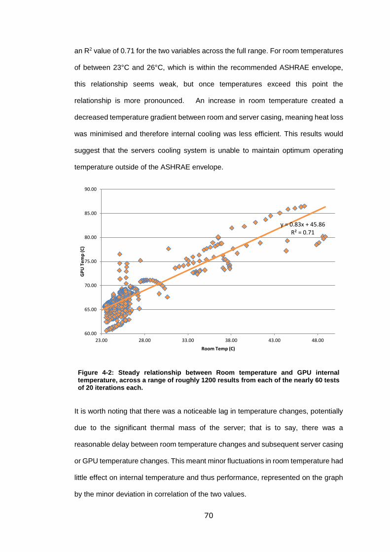
70
an R2 value of 0.71 for the two variables across the full range. For room temperatures
of between 23°C and 26°C, which is within the recommended ASHRAE envelope,
this relationship seems weak, but once temperatures exceed this point the
relationship is more pronounced. An increase in room temperature created a
decreased temperature gradient between room and server casing, meaning heat loss
was minimised and therefore internal cooling was less efficient. This results would
suggest that the servers cooling system is unable to maintain optimum operating
temperature outside of the ASHRAE envelope.
Figure 4-2: Steady relationship between Room temperature and GPU internal temperature, across a range of roughly 1200 results from each of the nearly 60 tests of 20 iterations each.
It is worth noting that there was a noticeable lag in temperature changes, potentially
due to the significant thermal mass of the server; that is to say, there was a
reasonable delay between room temperature changes and subsequent server casing
or GPU temperature changes. This meant minor fluctuations in room temperature had
little effect on internal temperature and thus performance, represented on the graph
by the minor deviation in correlation of the two values.
y = 0.83x + 45.86R² = 0.71
60.00
65.00
70.00
75.00
80.00
85.00
90.00
23.00 28.00 33.00 38.00 43.00 48.00
GP
U T
em
p (
C)
Room Temp (C)
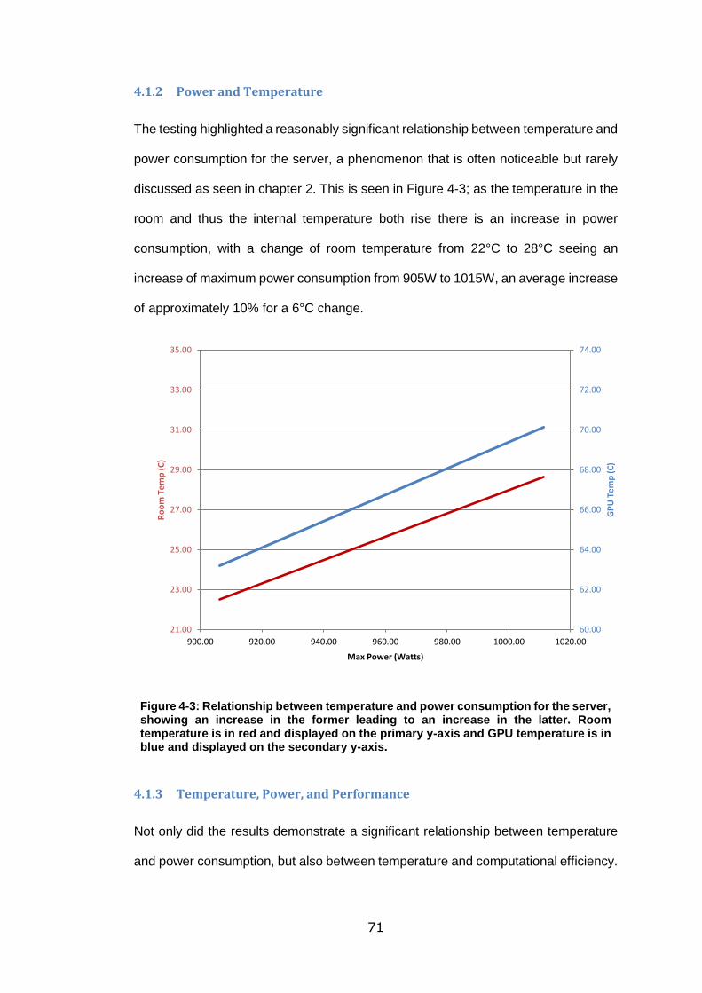
71
4.1.2 Power and Temperature
The testing highlighted a reasonably significant relationship between temperature and
power consumption for the server, a phenomenon that is often noticeable but rarely
discussed as seen in chapter 2. This is seen in Figure 4-3; as the temperature in the
room and thus the internal temperature both rise there is an increase in power
consumption, with a change of room temperature from 22°C to 28°C seeing an
increase of maximum power consumption from 905W to 1015W, an average increase
of approximately 10% for a 6°C change.
Figure 4-3: Relationship between temperature and power consumption for the server, showing an increase in the former leading to an increase in the latter. Room temperature is in red and displayed on the primary y-axis and GPU temperature is in blue and displayed on the secondary y-axis.
4.1.3 Temperature, Power, and Performance
Not only did the results demonstrate a significant relationship between temperature
and power consumption, but also between temperature and computational efficiency.
60.00
62.00
64.00
66.00
68.00
70.00
72.00
74.00
21.00
23.00
25.00
27.00
29.00
31.00
33.00
35.00
900.00 920.00 940.00 960.00 980.00 1000.00 1020.00
GP
U T
em
p (
C)
Ro
om
Te
mp
(C
)
Max Power (Watts)
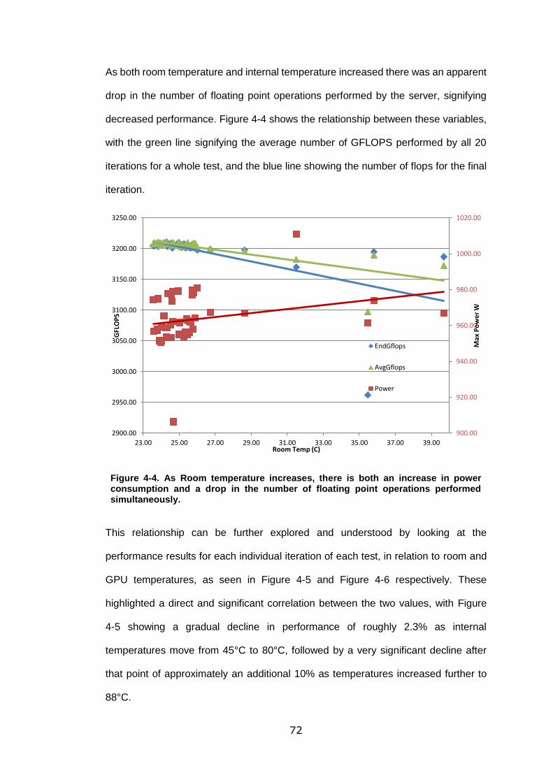
72
As both room temperature and internal temperature increased there was an apparent
drop in the number of floating point operations performed by the server, signifying
decreased performance. Figure 4-4 shows the relationship between these variables,
with the green line signifying the average number of GFLOPS performed by all 20
iterations for a whole test, and the blue line showing the number of flops for the final
iteration.
Figure 4-4. As Room temperature increases, there is both an increase in power consumption and a drop in the number of floating point operations performed simultaneously.
This relationship can be further explored and understood by looking at the
performance results for each individual iteration of each test, in relation to room and
GPU temperatures, as seen in Figure 4-5 and Figure 4-6 respectively. These
highlighted a direct and significant correlation between the two values, with Figure
4-5 showing a gradual decline in performance of roughly 2.3% as internal
temperatures move from 45°C to 80°C, followed by a very significant decline after
that point of approximately an additional 10% as temperatures increased further to
88°C.
900.00
920.00
940.00
960.00
980.00
1000.00
1020.00
2900.00
2950.00
3000.00
3050.00
3100.00
3150.00
3200.00
3250.00
23.00 25.00 27.00 29.00 31.00 33.00 35.00 37.00 39.00
Max
Po
we
r W
GFL
OP
S
Room Temp (C)
EndGflops
AvgGflops
Power
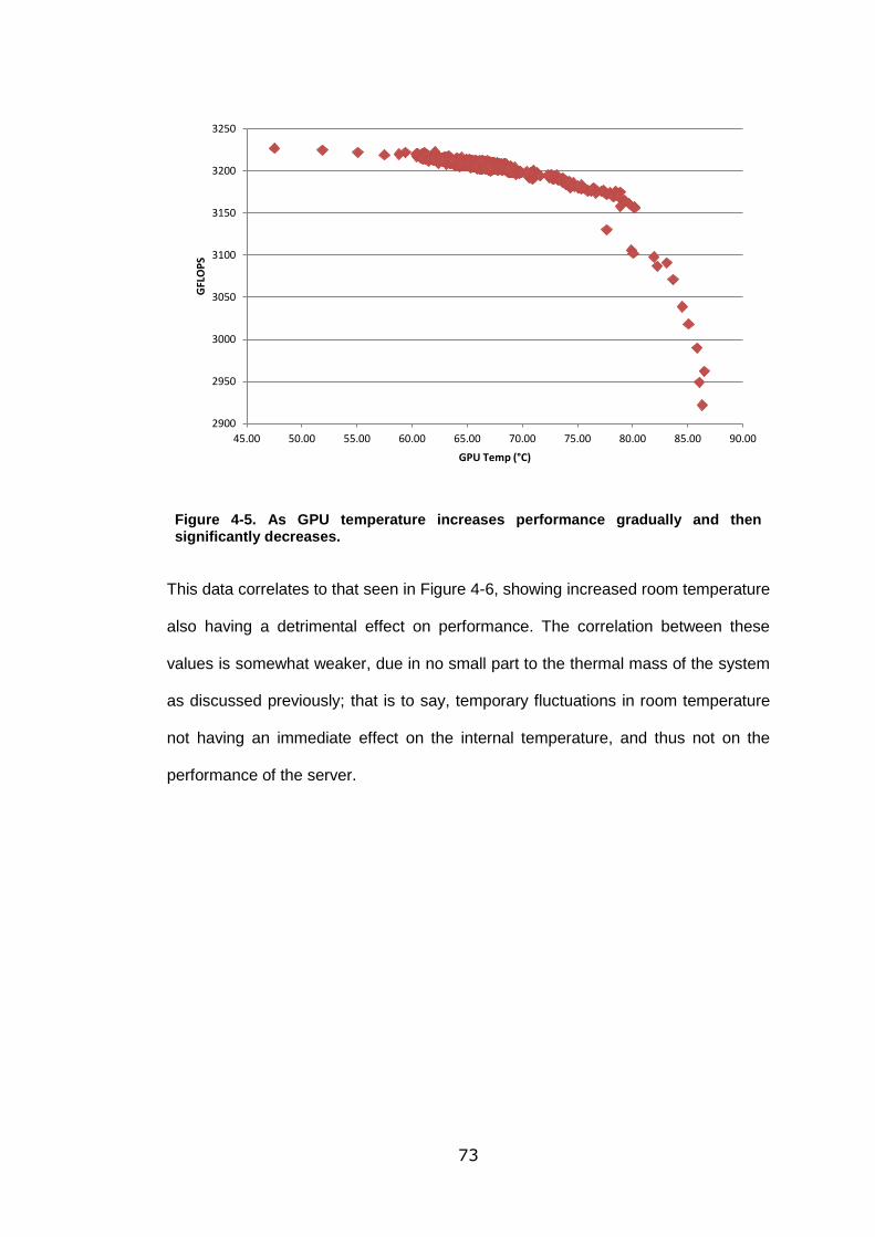
73
Figure 4-5. As GPU temperature increases performance gradually and then significantly decreases.
This data correlates to that seen in Figure 4-6, showing increased room temperature
also having a detrimental effect on performance. The correlation between these
values is somewhat weaker, due in no small part to the thermal mass of the system
as discussed previously; that is to say, temporary fluctuations in room temperature
not having an immediate effect on the internal temperature, and thus not on the
performance of the server.
2900
2950
3000
3050
3100
3150
3200
3250
45.00 50.00 55.00 60.00 65.00 70.00 75.00 80.00 85.00 90.00
GFL
OP
S
GPU Temp (°C)
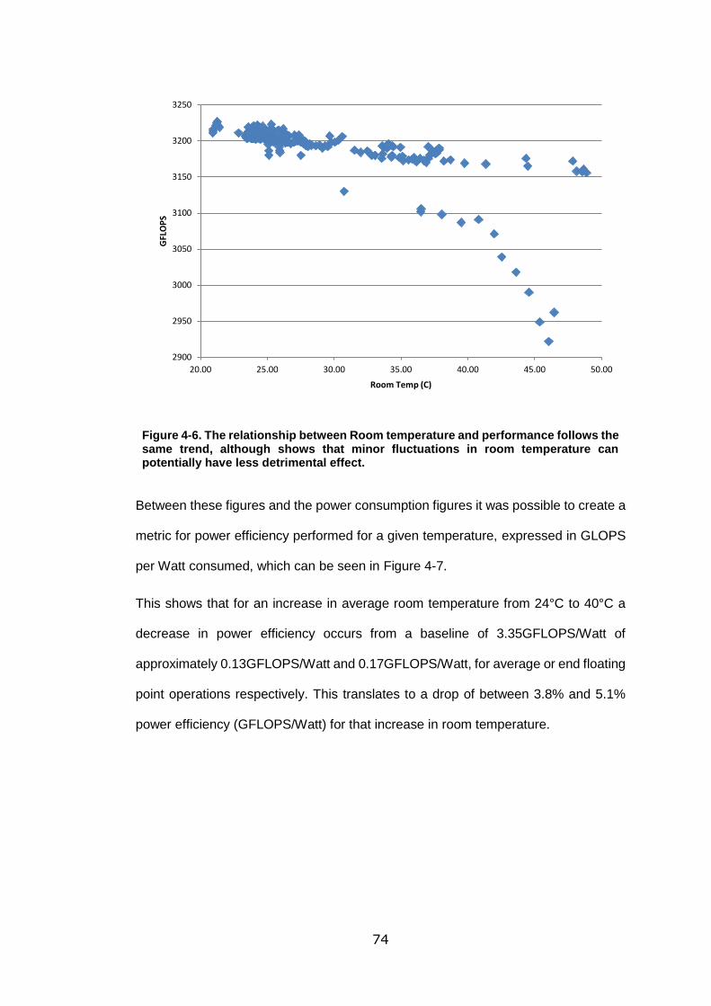
74
Figure 4-6. The relationship between Room temperature and performance follows the same trend, although shows that minor fluctuations in room temperature can potentially have less detrimental effect.
Between these figures and the power consumption figures it was possible to create a
metric for power efficiency performed for a given temperature, expressed in GLOPS
per Watt consumed, which can be seen in Figure 4-7.
This shows that for an increase in average room temperature from 24°C to 40°C a
decrease in power efficiency occurs from a baseline of 3.35GFLOPS/Watt of
approximately 0.13GFLOPS/Watt and 0.17GFLOPS/Watt, for average or end floating
point operations respectively. This translates to a drop of between 3.8% and 5.1%
power efficiency (GFLOPS/Watt) for that increase in room temperature.
2900
2950
3000
3050
3100
3150
3200
3250
20.00 25.00 30.00 35.00 40.00 45.00 50.00
GFL
OP
S
Room Temp (C)
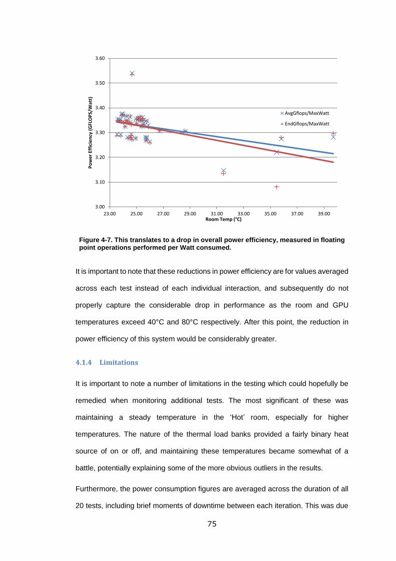
75
Figure 4-7. This translates to a drop in overall power efficiency, measured in floating point operations performed per Watt consumed.
It is important to note that these reductions in power efficiency are for values averaged
across each test instead of each individual interaction, and subsequently do not
properly capture the considerable drop in performance as the room and GPU
temperatures exceed 40°C and 80°C respectively. After this point, the reduction in
power efficiency of this system would be considerably greater.
4.1.4 Limitations
It is important to note a number of limitations in the testing which could hopefully be
remedied when monitoring additional tests. The most significant of these was
maintaining a steady temperature in the ‘Hot’ room, especially for higher
temperatures. The nature of the thermal load banks provided a fairly binary heat
source of on or off, and maintaining these temperatures became somewhat of a
battle, potentially explaining some of the more obvious outliers in the results.
Furthermore, the power consumption figures are averaged across the duration of all
20 tests, including brief moments of downtime between each iteration. This was due
3.00
3.10
3.20
3.30
3.40
3.50
3.60
23.00 25.00 27.00 29.00 31.00 33.00 35.00 37.00 39.00
Po
we
r Ef
fici
en
cy (
GFL
OP
S/W
att)
Room Temp (°C)
AvgGflops/MaxWatt
EndGflops/MaxWatt
76
to the result reporting being undertaken by High Performance LINPACK; no report
was written, only monitoring reported to the terminal and piped by the user to logs.
Sandwiching this piping between timestamps provided beginning and end points for
the tests, but since the High Performance LINPACK was compiled code this meant
no timestamps for each iteration was available and thus gave no ability to link each
to power or temperature precisely; only as an average.
The timestamp for each iteration was inferred from this piped terminal output and
provided enough information to divide the internal and external thermal log data into
the relevant sections, but proved unable to properly capture the much lower resolution
power consumption data at this level, proving the need for averaging across each test
for that particular metric. In future testing, it would be beneficial to record power
readings at a higher resolution, closer to that of other variables.
4.2 Summary
The work outlined in this chapter has shown a pronounced relationship between
computational performance and thermal environment for this server, with relatively
minor drops in performance for temperature gains within the ASHRAE envelope
followed by a considerable performance drop-off once this envelope is exceeded.
While the server used to establish these findings is somewhat non-uniform, being a
liquid-immersed High Performance Computer, the results should nonetheless
translate to any data centre server to some degree. This work highlights the
importance of controlling both workload and thermal environment carefully in
understanding the full performance of a server. To this end, a much more controlled
thermal environment and a variety of different servers is required to better understand
this causality relationship.

77
5 Generic Server Wind Tunnel
With the computational methodology providing a better understanding of creating
virtual loads and the energy efficiency of the work done by each server, and the tests
conducted on the immersed liquid-cooled server providing an insist into the effect of
changes in temperature in both the performance and efficiency of a server the next
step in properly understanding the behaviour of the servers and the flow of energy
through them called for full control of the thermodynamic environment in which to test
servers. A Generic Server Wind Tunnel (GSWT) was developed and went through
many iterations, starting with Figure 5-1, before settling on the design shown in Figure
5-2.
Development of the GSWT also constituted development of a methodology to
incorporate the work done in chapters 3 and 4, combining virtual load and the
quantification of energy efficiency of a server with control of thermal environment.
Chapter 6 will see this methodology employed on a number of server case studies.
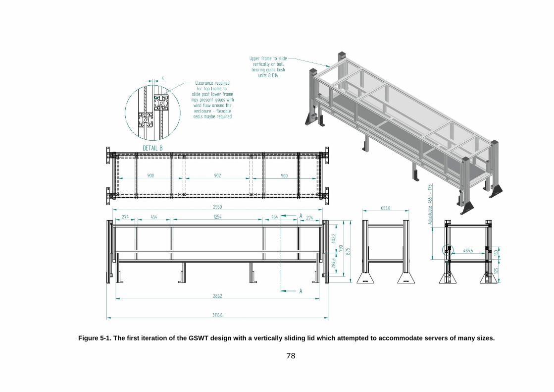
78
Figure 5-1. The first iteration of the GSWT design with a vertically sliding lid which attempted to accommodate servers of many sizes.
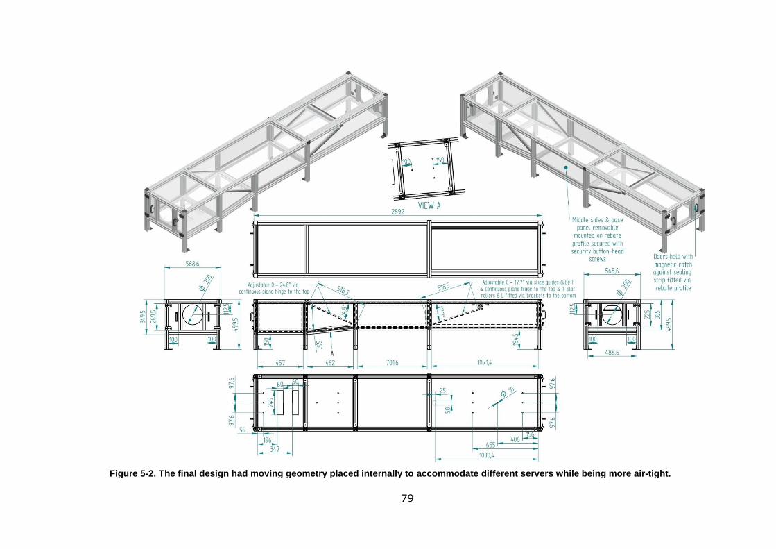
79
Figure 5-2. The final design had moving geometry placed internally to accommodate different servers while being more air-tight.
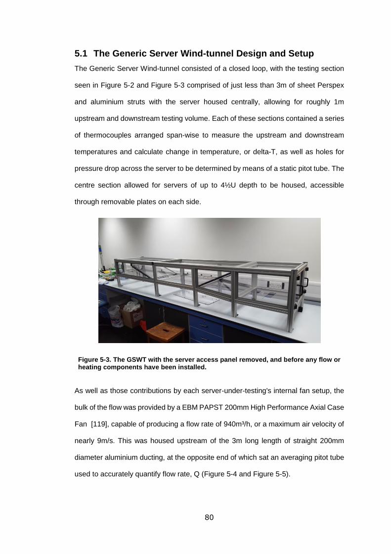
80
5.1 The Generic Server Wind-tunnel Design and Setup
The Generic Server Wind-tunnel consisted of a closed loop, with the testing section
seen in Figure 5-2 and Figure 5-3 comprised of just less than 3m of sheet Perspex
and aluminium struts with the server housed centrally, allowing for roughly 1m
upstream and downstream testing volume. Each of these sections contained a series
of thermocouples arranged span-wise to measure the upstream and downstream
temperatures and calculate change in temperature, or delta-T, as well as holes for
pressure drop across the server to be determined by means of a static pitot tube. The
centre section allowed for servers of up to 4½U depth to be housed, accessible
through removable plates on each side.
Figure 5-3. The GSWT with the server access panel removed, and before any flow or heating components have been installed.
As well as those contributions by each server-under-testing's internal fan setup, the
bulk of the flow was provided by a EBM PAPST 200mm High Performance Axial Case
Fan [119], capable of producing a flow rate of 940m³/h, or a maximum air velocity of
nearly 9m/s. This was housed upstream of the 3m long length of straight 200mm
diameter aluminium ducting, at the opposite end of which sat an averaging pitot tube
used to accurately quantify flow rate, Q (Figure 5-4 and Figure 5-5).

81
Figure 5-4. Diagram of the averaging-pitot tube from Furness Controls, showing internal design to achieve differnetial pressure [120]
The flow rate was calculated by the averaging pitot tube by using the equation below.
𝑣 = √𝐷𝑃
𝐾×
𝑇
𝑃×
1
𝐷𝑟× 574.09287
where:
𝑣 - the average velocity of the air in m/s
𝐷𝑃 - the differential pressure in Pascals
𝐾 - K factor of the pitot tube as supplied by the manufacturer; 1.8 [120]
𝑃 - the static pressure in Pa; assumed to be the standard 101325Pa SI at sea
level [121]
𝑇 - the air temperature in Kelvin
𝐷𝑟 - relative density of air compared with air at @20°C; assumed to be 1
6mm
200mm
Upstream Manometer
Downstream Manometer

82
This provided an average velocity in air, which was then converted to a flow rate by
𝑄 = 𝜋𝑟2 × 𝑣
where:
𝑟 - the radius of the ducting the pitot tube is located in; 0.1m
𝑣 - the average velocity of the air in m/s
The differential pressure was converted to Pascal by a pressure transducer that
provided a value of 0-50mV based on the range of 0-200Pa. This mV range was then
converted to a range of 0-2V to be used as an input channel by the datalogger. This
voltage transformation step was then taken into account in the calculation of velocity.
The pitot tube was calibrated by recording values for differential pressure when there
was no air movement and subtracting it from future readings.
The fan was powered by a 24V nominal power supply and controlled by a separate
0-10V signal. For the purposes of the tests in this thesis, this control voltage was
managed manually; future work could have this action performed by a digital to
analogue PCI card. By interfacing the flow rate data provided by the averaging pitot
tube with the outputs to the fan speed provided by the PCI card in the control system;
this would allow for more accurate control of the flow rate through each server under
testing.
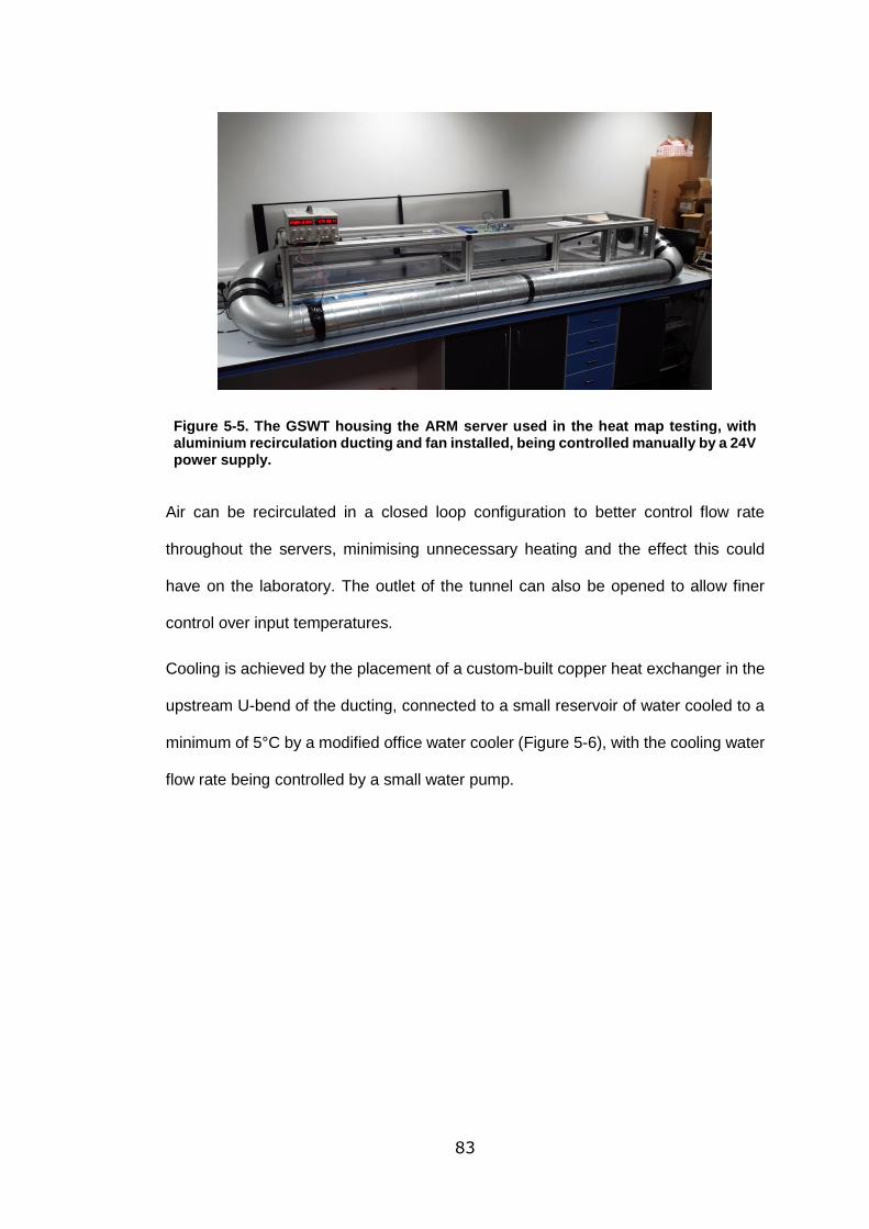
83
Figure 5-5. The GSWT housing the ARM server used in the heat map testing, with aluminium recirculation ducting and fan installed, being controlled manually by a 24V power supply.
Air can be recirculated in a closed loop configuration to better control flow rate
throughout the servers, minimising unnecessary heating and the effect this could
have on the laboratory. The outlet of the tunnel can also be opened to allow finer
control over input temperatures.
Cooling is achieved by the placement of a custom-built copper heat exchanger in the
upstream U-bend of the ducting, connected to a small reservoir of water cooled to a
minimum of 5°C by a modified office water cooler (Figure 5-6), with the cooling water
flow rate being controlled by a small water pump.
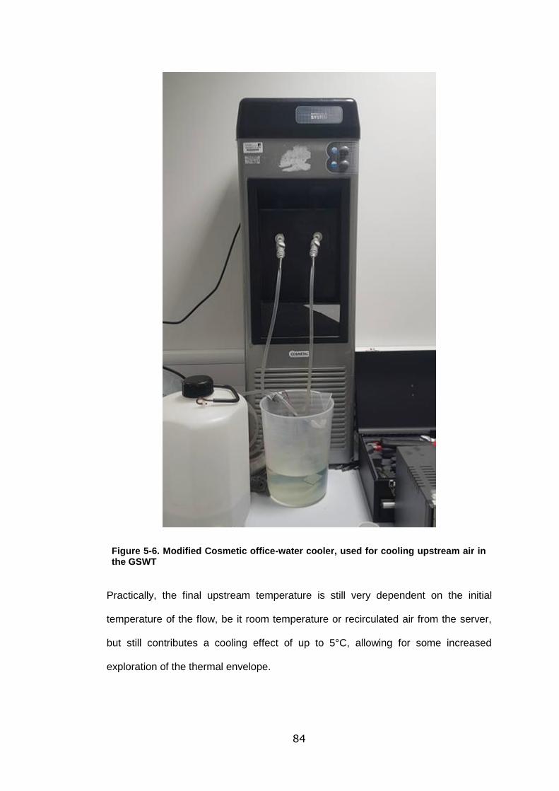
84
Figure 5-6. Modified Cosmetic office-water cooler, used for cooling upstream air in the GSWT
Practically, the final upstream temperature is still very dependent on the initial
temperature of the flow, be it room temperature or recirculated air from the server,
but still contributes a cooling effect of up to 5°C, allowing for some increased
exploration of the thermal envelope.
85
The upstream portion of the tunnel itself also initially contained two ceramic heating
plates capable of jointly providing 1300W of heating to the inlet air flow for pushing
the upper thermal envelope of server use, but concerns were raised over the safety
of utilising such a system and an alternative was ultimately used.
Either the system would remain as a closed loop for tests with raised temperatures,
using the server itself to incrementally raise the upstream temperature by re-
circulating air from the sever outlet, or if the temperature required raising more rapidly,
then the water reservoir in the cooling loop could be replaced with hot water.
Measurement and monitoring of the thermodynamic environment was conducted by
a TC-08 8-channel data logger, with three thermocouples span-wise upstream and
three downstream of the server, and one channel dedicated to logging flow rate from
the averaging pitot tube.
The TC-08 streamed data to a laptop running the PicoRecorder datalogging software.
This software allowed variation in the frequency and format of storage, and for the
purpose of these tests the hardware was polled every second across all channels.
This timestamp was then applied for each line of data, and saved to the laptop
throughout the duration of the test. Allowing the program to incrementally write the
data to an existing file throughout testing allowed for less chance of loss of data in
case of equipment failure whilst waiting until the test completed to write the output
file, especially considering each sampling period could be as long as 255 hours.
Network connections were managed by a Brocade TurboIron 24x [122], with both
Ethernet and Fibre-optic capabilities. The latter was required for networking the ARM
server in particular, as it lacked Ethernet ports. It was rack-mountable and 1U thick,
although for this purpose was located directly under the server housing of the GSWT.
Power was supplied by a 1U APC networked rack Power Distribution Unit (PDU) with
8 channels [123].
86
Acquiring values of the upstream and downstream temperatures and the flow is
necessary for determining the amount of energy each server exports, to either the lab
or data centre environment. This data helps inform the developing picture of the
energy efficiency, as well as better understanding the flow of energy through the data
centre. This data can also be used to quantify the amount of cooling required by a
data centre, and if a data centre is planning to reuse their waste heat, how much heat
they have available for this purpose prior to transmission losses to destination.
5.2 Post-Processing Scripts
The output from each test created a very large quantity of data, spread across several
media, which needed to be collated and cross-referenced to be understood. This
comprised primarily of performance and power consumption data from SPECpower,
and temperature and flow rate data from the PicoRecorder, both of which had
timestamps of differing intervals associated with them. The data from the SPECpower
tests used for these set of tests is that found in the underlying log files as opposed to
the front-end results file provided to the typical user. While the brief results file
provided enough information for those initial tests performed in 3.3, the detail provided
by the underlying log files was needed for these more complex tests.
It was necessary to create small programs or scripts to perform this task, as results
files could be millions of lines long, greater than the maximum number of lines that
spreadsheet programs such as Excel can handle and too time-consuming to consider
processing manually. These can be found in appendix C.
For the SPECpower2008 log files, designated 'ssj.testnumber.ccs-log.csv', provide a
large quantity of data, some coded, on attributes such as power analyser voltage,
amps, and power factor, operations performed on a particular load step, load step or
calibration number, idealised and realised processor loading, and operation type, all
related to the Control and Collect System timestamp, as well as system specific
software and hardware information.
87
A script called SPECprocessor.sh was written in bash to clean up and extract the
relevant information from these log files, providing usable files for each test with
information on operations performed per time-step for each load step, power
consumed per time-step, and the beginning and end time of each load, calibration, or
idle step. A dedicated folder was created for each test and duplicates of performance
and timestamp data stored there, as well as being written to larger files for use by
future scripts. The script is reproduced in appendix C1.
The master.sh script provided two sets of results files; the first called 'opsnwatt.csv'
contained information of the operations performed and the power consumed per
calibration, load, or idle step, referenced against the test number and load. The
second results file contained start and end times for each test and load, presented in
Unix time (Uresultstimes.csv) for scripted cross-referencing with other results, and
British Standard Time format (Rresultstimes.csv) for the benefit of the user, should
manual cross-referencing become necessary. This latter file proved useful for
troubleshooting issues with the SPECpower and the script itself.
The files created processing the SPECpower log files were then used to cross-
reference against other results files to consolidate information for consumption. The
cross-referenced results files would usually contain data on temperature upstream
and downstream of the server or flow-rate of air within the wind-tunnel, although early
tests looked at aspects of the server such as CPU usage as provided by the Linux
command 'top' or polled data on CPU temperatures and CPU fan RPM provided by
the IPMI.
This cross-referencing was performed by a trio of scripts titled master.sh (appendix
C2), search.sh (appendix C3) and processing.sh (appendix C4), with the former
controlling the latter two sub-scripts.
The search.sh script performs simple search functions of a given file, and extracted
start and end times for each load as specified by the master.sh script. These start
88
and end times were then passed to the processing.sh script, which extracted data
from a larger given results file and averaged each column across the time-steps
provided, writing this information to a results file.
The output of this process was a results file - in this case 'total.csv', in the same format
as that provided by the SPECproccesor.sh, allowing for easy review, comparison,
and analysis.
5.3 Results
The three input parameters; load, upstream temperature, and flow rate, were
normalised to a range of -1 to 1 to ensure easy comparison of the relative weighting
of each factor in its importance determining a particular output. For temperature this
range corresponded to 5°C to 45°C, concurrent with the most lax operating conditions
suggested by ASHRAE for an A4 class of server and inclusive of A1-A3, both
recommended and allowable [82]. For flow rate, the values of -1 and 1 corresponded
to a flow rate of 0m3/s and 1.5m3/s respectively. Both these selected ranges should
include the operating conditions of any servers in a given data centre. Although
outliers can still be included, and will just be allocated a value outside these bounds.
Five key outputs have been selected for the methodology, to be monitored across the
duration of the tests. These are;
• Operations per second (ssj_ops/s)
• Power consumption (W)
• Operations per second per watt (ssj_ops/s/W)
• Downstream temperature (K or C)
• Delta-T (K or C)
These five output variables were selected to suit a range of scenarios for a data centre
operator, such as maximising the operations performed by the server per second to
improve pure performance of the data centre, maximising the operations per watt
89
performed to improve energy efficiency, or even maximising the delta-T across the
server to make sure cooling infrastructure is being properly utilised. While co-location
data centres have no control over the utilisation of servers hosted in their racks, they
often face impositions of supply temperature for server operations in their contracts,
with the energy cost of supply temperature being dependent on the delta-T.
Understanding which has a greater effect on delta-T for a particular server - upstream
temperature or flow rate - will aid in achieving this. There is even a potential for a
desire to maximise downstream heat, if the goal is to reuse the heat, the higher the
grade of heat, the more applications it can be used for.
Analysis was performed using Quantum XL, a statistics package add-on to Microsoft
Excel developed by SigmaZone [124]. While this particular suite is designed with the
intention of creating properly populated Design of Experiments for testing purposes,
it also holds the capacity to perform analysis of historical data as was required in this
situation. The processing considers not only the first order input factors but also their
second order forms and interactions with each other to aid in the recognition of
previously unconsidered relationships between variables. Ideally a design of
experiments would be created that would efficiently sample the design points required
to fully flesh out a response surface for the desired results, but unfortunately this
would require more precise control of inputs than is currently possible and as such
any design of experiments was considered more of a guide than a rule-set for the
tests going forward.
The range of data would be regressed repeatedly to minimise unnecessary or
unreliable interactions until a transfer function was left that could be used to model
server behaviour. The regression considered 19 factors - the 3 primary first order
factors and then a further 16 first and second order interactions of each of these
primary factors as a factor in their own right. Each regression performed provided a
'P-value', or percentage of confidence of the importance said factor had to the overall
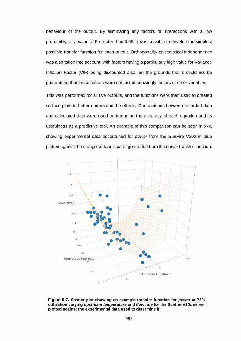
90
behaviour of the output. By eliminating any factors or interactions with a low
probability, or a value of P greater than 0.05, it was possible to develop the simplest
possible transfer function for each output. Orthogonality or statistical independence
was also taken into account, with factors having a particularly high value for Variance
Inflation Factor (VIF) being discounted also, on the grounds that it could not be
guaranteed that these factors were not just unknowingly factors of other variables.
This was performed for all five outputs, and the functions were then used to created
surface plots to better understand the effects. Comparisons between recorded data
and calculated data were used to determine the accuracy of each equation and its
usefulness as a predictive tool. An example of this comparison can be seen in xxx,
showing experimental data ascertained for power from the SunFire V20z in blue
plotted against the orange surface scatter generated from the power transfer function.
Figure 5-7. Scatter plot showing an example transfer function for power at 75% utilisation varying upstream temperature and flow rate for the Sunfire V20z server plotted against the experimental data used to determine it
91
6 GSWT Case Study Results and Analysis
The Generic Server Wind-tunnel methodology developed in chapter 5 was then
employed and analysed. These tests occurred on six different air-cooled servers. The
servers used in these case studies were a variety of ages, power densities, and
chipset architectures. The goal of utilising the developed methodology on this range
of servers was to ascertain its usefulness on a broad sample.
6.1 SunFire V20z
The first server tested was the SunFire V20z server from Sun Microsystems, released
in 2005 [125]. It was 1U thick, 430mm wide, and 724mm long, and had two AMD
Dual-Core Opteron 270- 2 GHz processors, 8GB of RAM, and a 465W power supply.
It had four small axial fans in front of each processor, two for the memory, and two
fans mounted on the power supply. The operating system was Ubuntu running the
linux kernel 3.13.0-86-generic, and the server was installed with SPECpower and all
the dependant packages and Java JDK version 1.7.0_80.
A total of 270 individual load steps each of 20 minutes were performed. Tests were
run across 0-100% CPU utilisation loads, upstream temperatures of between 20°C -
30°C, and flow rates of up to 0.75m3/s of air. As previously stated in section 5.3, for
the sake of the regression analysis these ranges were all normalised to the range -1
to +1, related to a temperature range of 5°C - 45°C and a flow rate of 0m3/s -1.5m3/s.
This normalisation allows for more intuitive understanding of the weighting and
importance of each factor by considering each coefficient in the transfer function. The
range of outputs seen in the tests were: power consumption (0-232W), floating point
operations performed per second (up to 76345), energy efficiency metric operations
per second per watt of up to 335, downstream temperatures of between 25°C and
35°C, and delta-T of nearly 8°C.

92
Input regression was repeated between two and four times depending on the output,
until all low importance (P>0.05) or high orthogonality (VIF>5) factors were
eliminated, leaving remaining only those significant and the coefficients of each
significant factor required to create the transfer functions. In some cases, lower
importance factors were kept in if they had particularly low values of orthogonality and
still had high importance relative to remaining factors. An example of the effect of
regression can be seen in Table 6-1 for the output variable operations per second. Of
the original 19 factors, 13 were eliminated as either they did not significantly
contribute to the output variable, or were not statistically independent and reliable.
The column titled Coeff denotes the coefficient for the variable to be used in the
creation of the transfer function, with standard error SE and the ratio of signal to noise
denoted by T, with a larger figure showing a stronger signal.
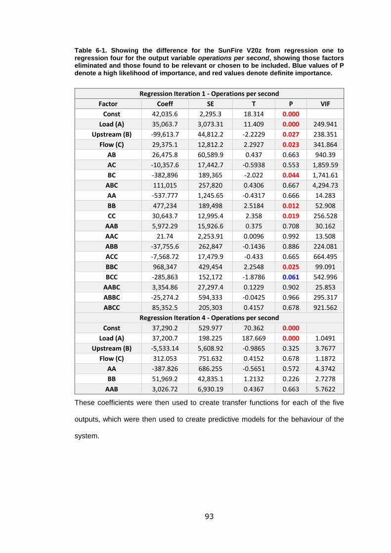
93
Table 6-1. Showing the difference for the SunFire V20z from regression one to regression four for the output variable operations per second, showing those factors eliminated and those found to be relevant or chosen to be included. Blue values of P denote a high likelihood of importance, and red values denote definite importance.
Regression Iteration 1 - Operations per second
Factor Coeff SE T P VIF
Const 42,035.6 2,295.3 18.314 0.000
Load (A) 35,063.7 3,073.31 11.409 0.000 249.941
Upstream (B) -99,613.7 44,812.2 -2.2229 0.027 238.351
Flow (C) 29,375.1 12,812.2 2.2927 0.023 341.864
AB 26,475.8 60,589.9 0.437 0.663 940.39
AC -10,357.6 17,442.7 -0.5938 0.553 1,859.59
BC -382,896 189,365 -2.022 0.044 1,741.61
ABC 111,015 257,820 0.4306 0.667 4,294.73
AA -537.777 1,245.65 -0.4317 0.666 14.283
BB 477,234 189,498 2.5184 0.012 52.908
CC 30,643.7 12,995.4 2.358 0.019 256.528
AAB 5,972.29 15,926.6 0.375 0.708 30.162
AAC 21.74 2,253.91 0.0096 0.992 13.508
ABB -37,755.6 262,847 -0.1436 0.886 224.081
ACC -7,568.72 17,479.9 -0.433 0.665 664.495
BBC 968,347 429,454 2.2548 0.025 99.091
BCC -285,863 152,172 -1.8786 0.061 542.996
AABC 3,354.86 27,297.4 0.1229 0.902 25.853
ABBC -25,274.2 594,333 -0.0425 0.966 295.317
ABCC 85,352.5 205,303 0.4157 0.678 921.562
Regression Iteration 4 - Operations per second
Const 37,290.2 529.977 70.362 0.000
Load (A) 37,200.7 198.225 187.669 0.000 1.0491
Upstream (B) -5,533.14 5,608.92 -0.9865 0.325 3.7677
Flow (C) 312.053 751.632 0.4152 0.678 1.1872
AA -387.826 686.255 -0.5651 0.572 4.3742
BB 51,969.2 42,835.1 1.2132 0.226 2.7278
AAB 3,026.72 6,930.19 0.4367 0.663 5.7622
These coefficients were then used to create transfer functions for each of the five
outputs, which were then used to create predictive models for the behaviour of the
system.
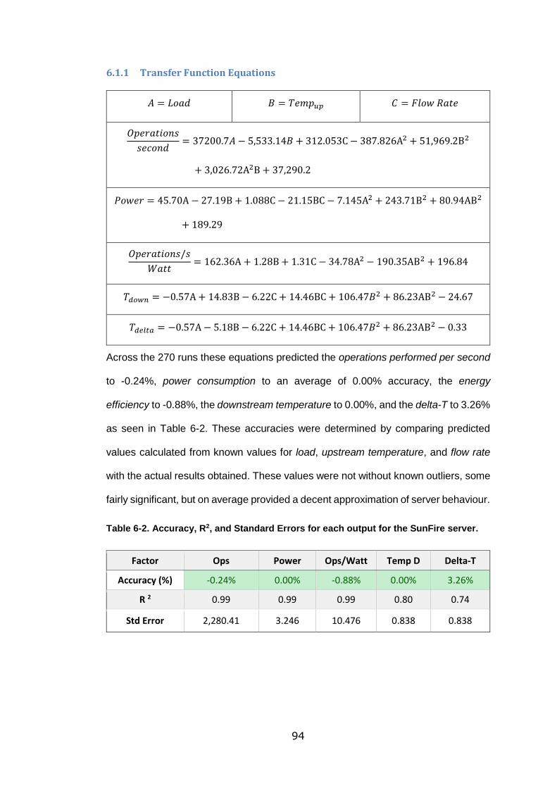
94
6.1.1 Transfer Function Equations
𝐴 = 𝐿𝑜𝑎𝑑 𝐵 = 𝑇𝑒𝑚𝑝𝑢𝑝 𝐶 = 𝐹𝑙𝑜𝑤 𝑅𝑎𝑡𝑒
𝑂𝑝𝑒𝑟𝑎𝑡𝑖𝑜𝑛𝑠
𝑠𝑒𝑐𝑜𝑛𝑑= 37200.7𝐴 − 5,533.14𝐵 + 312.053C − 387.826A2 + 51,969.2B2
+ 3,026.72A2B + 37,290.2
𝑃𝑜𝑤𝑒𝑟 = 45.70A − 27.19B + 1.088C − 21.15BC − 7.145A2 + 243.71B2 + 80.94AB2
+ 189.29
𝑂𝑝𝑒𝑟𝑎𝑡𝑖𝑜𝑛𝑠/𝑠
𝑊𝑎𝑡𝑡= 162.36A + 1.28B + 1.31C − 34.78A2 − 190.35AB2 + 196.84
𝑇𝑑𝑜𝑤𝑛 = −0.57A + 14.83B − 6.22C + 14.46BC + 106.47𝐵2 + 86.23AB2 − 24.67
𝑇𝑑𝑒𝑙𝑡𝑎 = −0.57A − 5.18B − 6.22C + 14.46BC + 106.47𝐵2 + 86.23AB2 − 0.33
Across the 270 runs these equations predicted the operations performed per second
to -0.24%, power consumption to an average of 0.00% accuracy, the energy
efficiency to -0.88%, the downstream temperature to 0.00%, and the delta-T to 3.26%
as seen in Table 6-2. These accuracies were determined by comparing predicted
values calculated from known values for load, upstream temperature, and flow rate
with the actual results obtained. These values were not without known outliers, some
fairly significant, but on average provided a decent approximation of server behaviour.
Table 6-2. Accuracy, R2, and Standard Errors for each output for the SunFire server.
Factor Ops Power Ops/Watt Temp D Delta-T Accuracy (%) -0.24% 0.00% -0.88% 0.00% 3.26%
R 2 0.99 0.99 0.99 0.80 0.74
Std Error 2,280.41 3.246 10.476 0.838 0.838
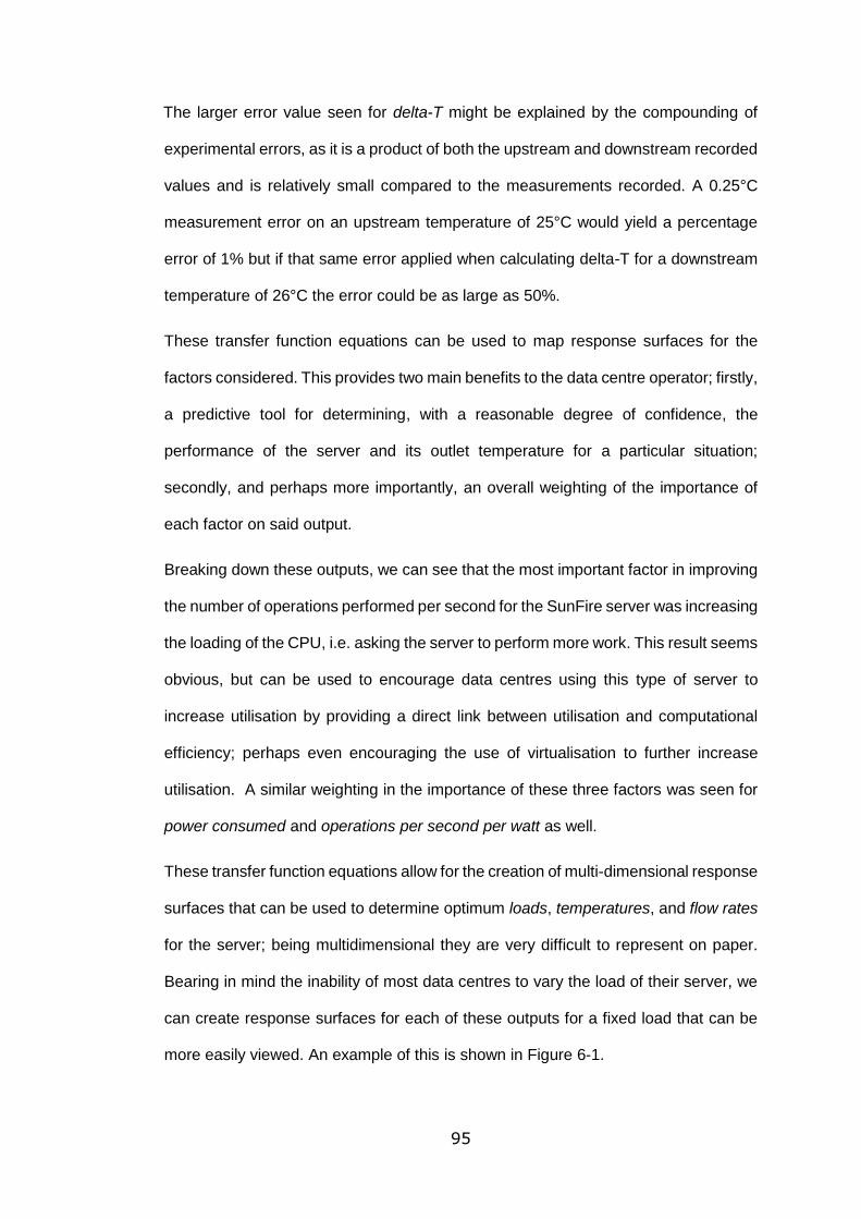
95
The larger error value seen for delta-T might be explained by the compounding of
experimental errors, as it is a product of both the upstream and downstream recorded
values and is relatively small compared to the measurements recorded. A 0.25°C
measurement error on an upstream temperature of 25°C would yield a percentage
error of 1% but if that same error applied when calculating delta-T for a downstream
temperature of 26°C the error could be as large as 50%.
These transfer function equations can be used to map response surfaces for the
factors considered. This provides two main benefits to the data centre operator; firstly,
a predictive tool for determining, with a reasonable degree of confidence, the
performance of the server and its outlet temperature for a particular situation;
secondly, and perhaps more importantly, an overall weighting of the importance of
each factor on said output.
Breaking down these outputs, we can see that the most important factor in improving
the number of operations performed per second for the SunFire server was increasing
the loading of the CPU, i.e. asking the server to perform more work. This result seems
obvious, but can be used to encourage data centres using this type of server to
increase utilisation by providing a direct link between utilisation and computational
efficiency; perhaps even encouraging the use of virtualisation to further increase
utilisation. A similar weighting in the importance of these three factors was seen for
power consumed and operations per second per watt as well.
These transfer function equations allow for the creation of multi-dimensional response
surfaces that can be used to determine optimum loads, temperatures, and flow rates
for the server; being multidimensional they are very difficult to represent on paper.
Bearing in mind the inability of most data centres to vary the load of their server, we
can create response surfaces for each of these outputs for a fixed load that can be
more easily viewed. An example of this is shown in Figure 6-1.
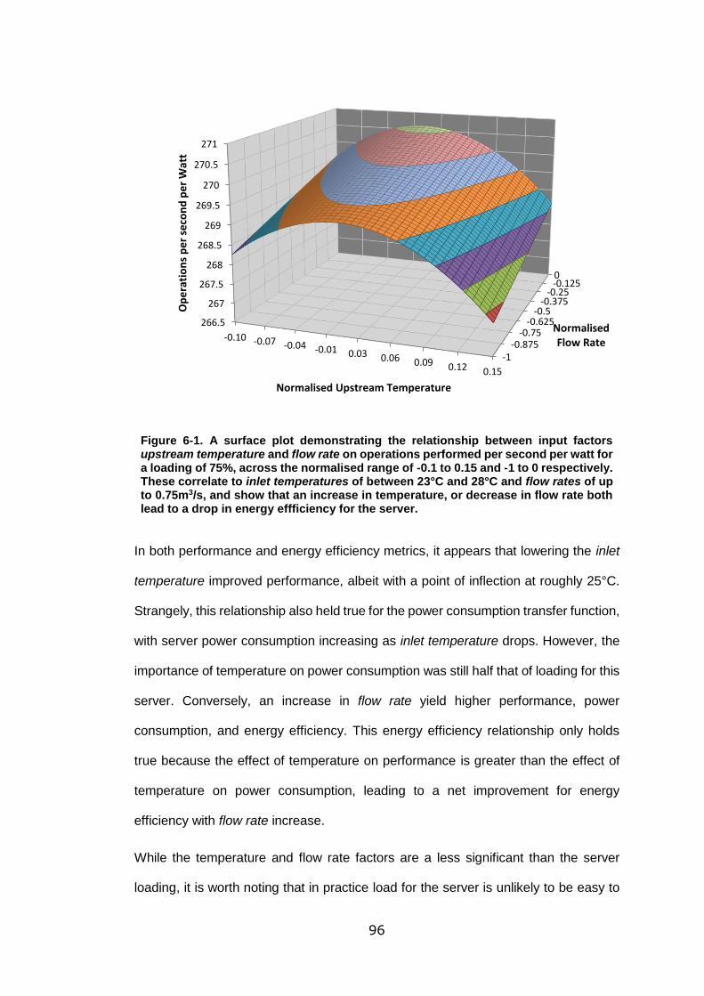
96
Figure 6-1. A surface plot demonstrating the relationship between input factors upstream temperature and flow rate on operations performed per second per watt for a loading of 75%, across the normalised range of -0.1 to 0.15 and -1 to 0 respectively. These correlate to inlet temperatures of between 23°C and 28°C and flow rates of up to 0.75m3/s, and show that an increase in temperature, or decrease in flow rate both lead to a drop in energy effficiency for the server.
In both performance and energy efficiency metrics, it appears that lowering the inlet
temperature improved performance, albeit with a point of inflection at roughly 25°C.
Strangely, this relationship also held true for the power consumption transfer function,
with server power consumption increasing as inlet temperature drops. However, the
importance of temperature on power consumption was still half that of loading for this
server. Conversely, an increase in flow rate yield higher performance, power
consumption, and energy efficiency. This energy efficiency relationship only holds
true because the effect of temperature on performance is greater than the effect of
temperature on power consumption, leading to a net improvement for energy
efficiency with flow rate increase.
While the temperature and flow rate factors are a less significant than the server
loading, it is worth noting that in practice load for the server is unlikely to be easy to
-1-0.875
-0.75-0.625
-0.5-0.375
-0.25-0.1250
266.5
267
267.5
268
268.5
269
269.5
270
270.5
271
-0.10 -0.07 -0.04 -0.01 0.03 0.06 0.09 0.12 0.15
NormalisedFlow Rate
Op
era
tio
ns
pe
r se
con
d p
er
Wat
t
Normalised Upstream Temperature
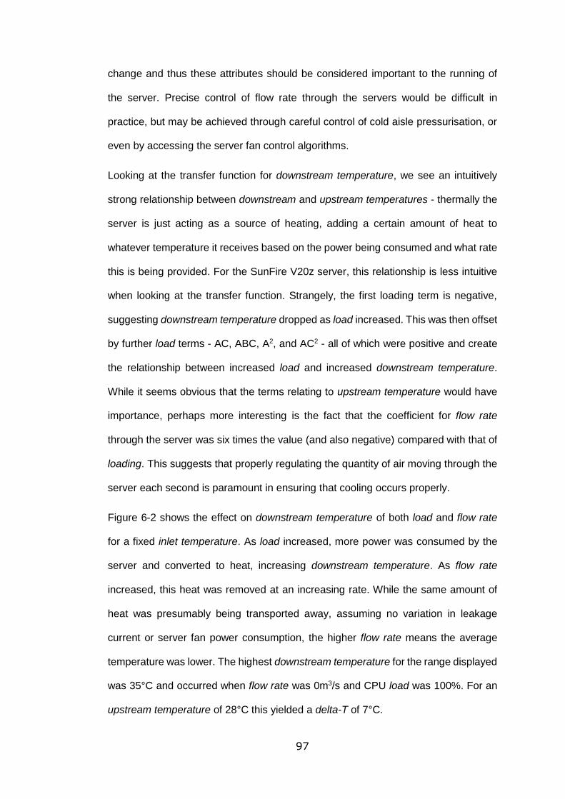
97
change and thus these attributes should be considered important to the running of
the server. Precise control of flow rate through the servers would be difficult in
practice, but may be achieved through careful control of cold aisle pressurisation, or
even by accessing the server fan control algorithms.
Looking at the transfer function for downstream temperature, we see an intuitively
strong relationship between downstream and upstream temperatures - thermally the
server is just acting as a source of heating, adding a certain amount of heat to
whatever temperature it receives based on the power being consumed and what rate
this is being provided. For the SunFire V20z server, this relationship is less intuitive
when looking at the transfer function. Strangely, the first loading term is negative,
suggesting downstream temperature dropped as load increased. This was then offset
by further load terms - AC, ABC, A2, and AC2 - all of which were positive and create
the relationship between increased load and increased downstream temperature.
While it seems obvious that the terms relating to upstream temperature would have
importance, perhaps more interesting is the fact that the coefficient for flow rate
through the server was six times the value (and also negative) compared with that of
loading. This suggests that properly regulating the quantity of air moving through the
server each second is paramount in ensuring that cooling occurs properly.
Figure 6-2 shows the effect on downstream temperature of both load and flow rate
for a fixed inlet temperature. As load increased, more power was consumed by the
server and converted to heat, increasing downstream temperature. As flow rate
increased, this heat was removed at an increasing rate. While the same amount of
heat was presumably being transported away, assuming no variation in leakage
current or server fan power consumption, the higher flow rate means the average
temperature was lower. The highest downstream temperature for the range displayed
was 35°C and occurred when flow rate was 0m3/s and CPU load was 100%. For an
upstream temperature of 28°C this yielded a delta-T of 7°C.
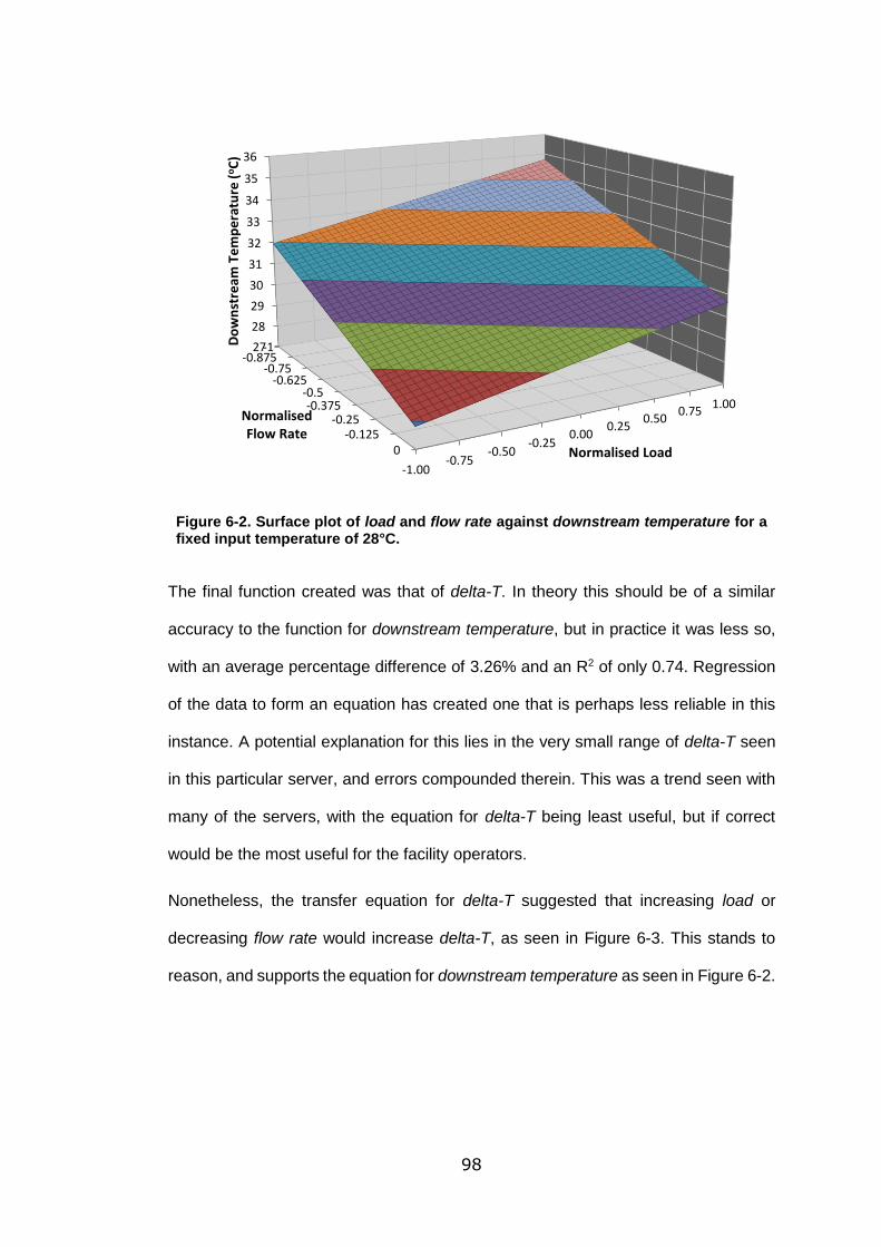
98
Figure 6-2. Surface plot of load and flow rate against downstream temperature for a fixed input temperature of 28°C.
The final function created was that of delta-T. In theory this should be of a similar
accuracy to the function for downstream temperature, but in practice it was less so,
with an average percentage difference of 3.26% and an R2 of only 0.74. Regression
of the data to form an equation has created one that is perhaps less reliable in this
instance. A potential explanation for this lies in the very small range of delta-T seen
in this particular server, and errors compounded therein. This was a trend seen with
many of the servers, with the equation for delta-T being least useful, but if correct
would be the most useful for the facility operators.
Nonetheless, the transfer equation for delta-T suggested that increasing load or
decreasing flow rate would increase delta-T, as seen in Figure 6-3. This stands to
reason, and supports the equation for downstream temperature as seen in Figure 6-2.
-1-0.875
-0.75-0.625
-0.5-0.375
-0.25-0.125
0
27
28
29
30
31
32
33
34
35
36
-1.00-0.75
-0.50-0.25
0.000.25
0.500.75
1.00NormalisedFlow Rate
Do
wn
stre
am T
em
pe
ratu
re (
oC
)
Normalised Load
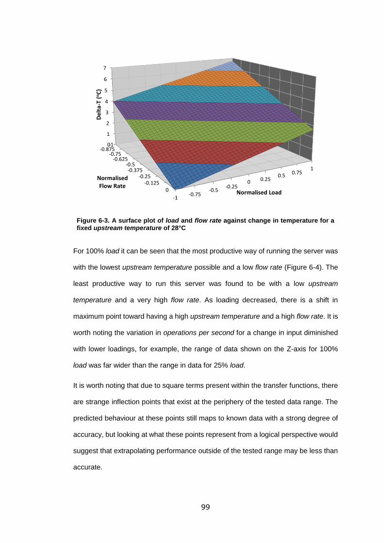
99
Figure 6-3. A surface plot of load and flow rate against change in temperature for a fixed upstream temperature of 28°C
For 100% load it can be seen that the most productive way of running the server was
with the lowest upstream temperature possible and a low flow rate (Figure 6-4). The
least productive way to run this server was found to be with a low upstream
temperature and a very high flow rate. As loading decreased, there is a shift in
maximum point toward having a high upstream temperature and a high flow rate. It is
worth noting the variation in operations per second for a change in input diminished
with lower loadings, for example, the range of data shown on the Z-axis for 100%
load was far wider than the range in data for 25% load.
It is worth noting that due to square terms present within the transfer functions, there
are strange inflection points that exist at the periphery of the tested data range. The
predicted behaviour at these points still maps to known data with a strong degree of
accuracy, but looking at what these points represent from a logical perspective would
suggest that extrapolating performance outside of the tested range may be less than
accurate.
-1-0.875
-0.75-0.625
-0.5-0.375
-0.25-0.125
0
0
1
2
3
4
5
6
7
-1-0.75
-0.5-0.25
0 0.250.5
0.751
NormalisedFlow Rate
De
lta-
T (o
C)
Normalised Load
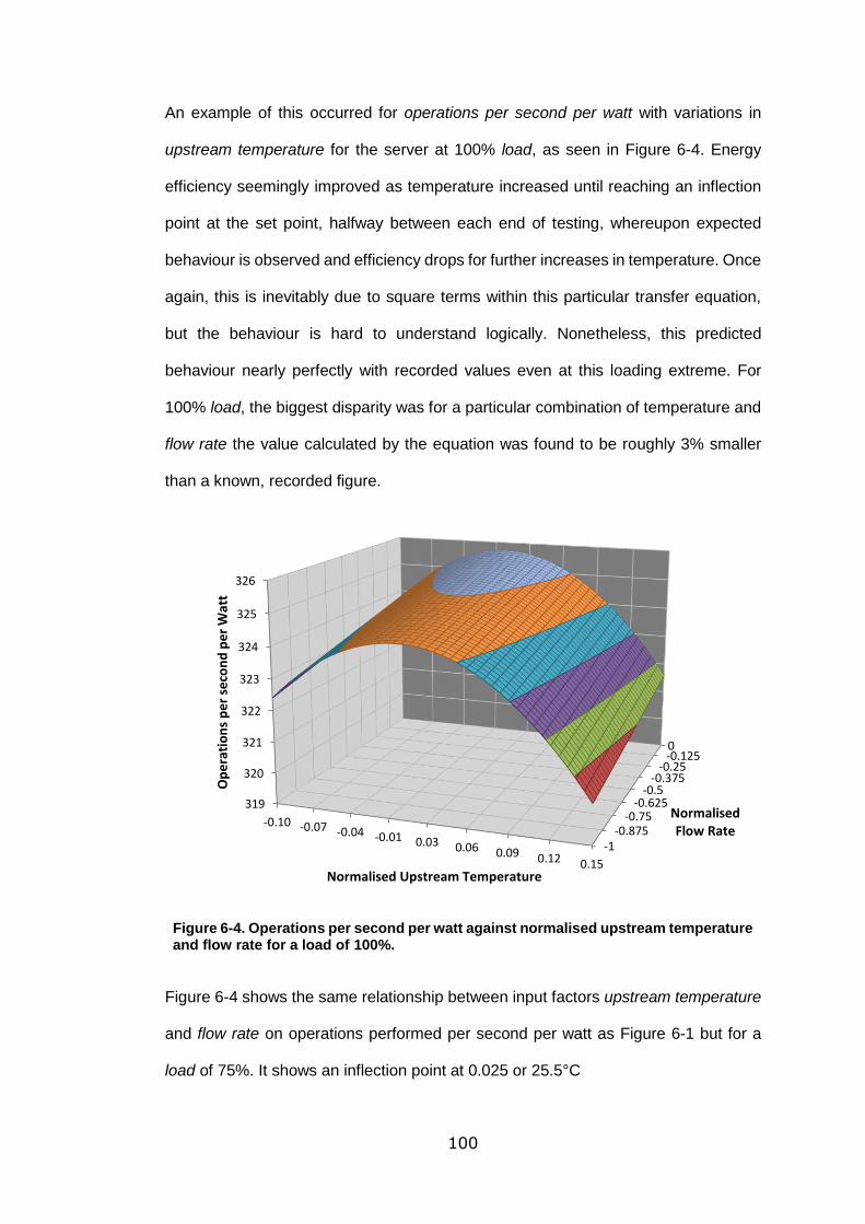
100
An example of this occurred for operations per second per watt with variations in
upstream temperature for the server at 100% load, as seen in Figure 6-4. Energy
efficiency seemingly improved as temperature increased until reaching an inflection
point at the set point, halfway between each end of testing, whereupon expected
behaviour is observed and efficiency drops for further increases in temperature. Once
again, this is inevitably due to square terms within this particular transfer equation,
but the behaviour is hard to understand logically. Nonetheless, this predicted
behaviour nearly perfectly with recorded values even at this loading extreme. For
100% load, the biggest disparity was for a particular combination of temperature and
flow rate the value calculated by the equation was found to be roughly 3% smaller
than a known, recorded figure.
Figure 6-4. Operations per second per watt against normalised upstream temperature and flow rate for a load of 100%.
Figure 6-4 shows the same relationship between input factors upstream temperature
and flow rate on operations performed per second per watt as Figure 6-1 but for a
load of 75%. It shows an inflection point at 0.025 or 25.5°C
-1-0.875
-0.75-0.625
-0.5-0.375
-0.25-0.1250
319
320
321
322
323
324
325
326
-0.10 -0.07 -0.04 -0.01 0.03 0.06 0.09 0.12 0.15
NormalisedFlow Rate
Op
era
tio
ns
pe
r se
con
d p
er
Wat
t
Normalised Upstream Temperature
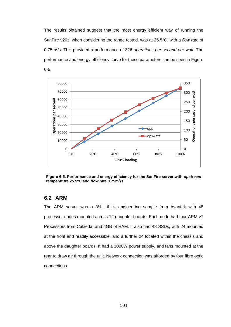
101
The results obtained suggest that the most energy efficient way of running the
SunFire v20z, when considering the range tested, was at 25.5°C, with a flow rate of
0.75m3/s. This provided a performance of 326 operations per second per watt. The
performance and energy efficiency curve for these parameters can be seen in Figure
6-5.
Figure 6-5. Performance and energy efficiency for the SunFire server with upstream temperature 25.5°C and flow rate 0.75m3/s
6.2 ARM
The ARM server was a 3½U thick engineering sample from Avantek with 48
processor nodes mounted across 12 daughter boards. Each node had four ARM v7
Processors from Calxeda, and 4GB of RAM. It also had 48 SSDs, with 24 mounted
at the front and readily accessible, and a further 24 located within the chassis and
above the daughter boards. It had a 1000W power supply, and fans mounted at the
rear to draw air through the unit. Network connection was afforded by four fibre optic
connections.
0
50
100
150
200
250
300
350
0
10000
20000
30000
40000
50000
60000
70000
80000
0% 20% 40% 60% 80% 100%
Op
era
tio
ns
pe
r se
con
d p
er
wat
t
Op
era
tio
ns
pe
r se
con
d
CPU% loading
ops
opswatt
102
The operating system was Ubuntu with linux kernel 3.5.0_42_Highbank for ARM, and
the server was installed with SPECpower and all the dependant packages and Java
version JDK 1.8.0_131.
The ARM server provided an interesting issue, in that the processors that comprise
the server architecture were particularly susceptible to heat. As it was a prototype
server where the internal layout was not considered for optimised air cooling
pathways within the chassis. This resulted in considerable hotspots forming through
the chassis, as previously described in section 3.3.1, resulting in some of the 48
nodes in the server reaching near critical temperatures even at idle. Two nodes in
particular, node 32 and node 10 (see Figure 18), proved to be in particularly strong
hotspots or to be particularly susceptible to heat and as such emergency shutdown
of these nodes was frequently seen at any load. This presented an issue for
completing the full range of tests, as nodes shutting down would interrupt any test in
process for the entire chassis. Some re-arrangement internally was undertaken to
move node 10 away from the hot-spot and after this move it was less prone to shutting
down, but node 32 remained troublesome.
For this reason, two sets of tests were run on the ARM server; those few successful
runs for the full 48 node configuration, and then a broader set of tests consisting of
only 47, with node 32 switched off from the outset. While running 47 of the 48 nodes
does not necessarily provide a fair demonstration of the capabilities of the server as
it was intended to be used, it did provide an insight into practical capabilities,
considering the issues associated with chassis design and heat distribution - in reality,
node 32 was nearly useless, and thus was excluded from the tests. It was the 47 node
tests that were used for this process.
The input and output values were once again normalised to a range of -1 to 1 based
on the upstream temperatures of 5°C to 45°C and flow rates of 0m3/s - 1.5m3/s, while
tests were conducted across the ranges seen in Table 6-3.
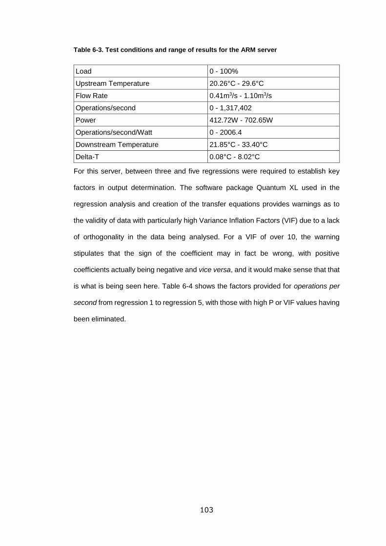
103
Table 6-3. Test conditions and range of results for the ARM server
Load 0 - 100%
Upstream Temperature 20.26°C - 29.6°C
Flow Rate 0.41m3/s - 1.10m3/s
Operations/second 0 - 1,317,402
Power 412.72W - 702.65W
Operations/second/Watt 0 - 2006.4
Downstream Temperature 21.85°C - 33.40°C
Delta-T 0.08°C - 8.02°C
For this server, between three and five regressions were required to establish key
factors in output determination. The software package Quantum XL used in the
regression analysis and creation of the transfer equations provides warnings as to
the validity of data with particularly high Variance Inflation Factors (VIF) due to a lack
of orthogonality in the data being analysed. For a VIF of over 10, the warning
stipulates that the sign of the coefficient may in fact be wrong, with positive
coefficients actually being negative and vice versa, and it would make sense that that
is what is being seen here. Table 6-4 shows the factors provided for operations per
second from regression 1 to regression 5, with those with high P or VIF values having
been eliminated.
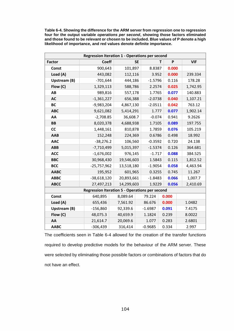
104
Table 6-4. Showing the difference for the ARM server from regression one to regression four for the output variable operations per second, showing those factors eliminated and those found to be relevant or chosen to be included. Blue values of P denote a high likelihood of importance, and red values denote definite importance.
Regression Iteration 1 - Operations per second
Factor Coeff SE T P VIF
Const 900,643 101,897 8.8387 0.000
Load (A) 443,082 112,116 3.952 0.000 239.334
Upstream (B) -701,644 444,186 -1.5796 0.116 178.28
Flow (C) 1,329,113 588,786 2.2574 0.025 1,742.95
AB 989,816 557,178 1.7765 0.077 140.883
AC -1,361,227 656,388 -2.0738 0.040 1,107.21
BC -9,983,204 4,867,130 -2.0511 0.042 763.12
ABC 9,621,082 5,414,291 1.777 0.077 1,902.14
AA -2,708.85 36,608.7 -0.074 0.941 9.2626
BB 8,020,378 4,688,938 1.7105 0.089 197.755
CC 1,448,161 810,878 1.7859 0.076 105.219
AAB 152,248 224,369 0.6786 0.498 18.992
AAC -38,276.2 106,560 -0.3592 0.720 24.138
ABB -7,710,499 5,015,397 -1.5374 0.126 364.681
ACC -1,676,002 976,145 -1.717 0.088 384.525
BBC 30,968,430 19,546,603 1.5843 0.115 1,812.52
BCC -25,757,962 13,518,180 -1.9054 0.058 4,463.94
AABC 195,952 601,965 0.3255 0.745 11.267
ABBC -38,618,120 20,893,661 -1.8483 0.066 1,007.7
ABCC 27,497,213 14,299,603 1.9229 0.056 2,410.69
Regression Iteration 5 - Operations per second
Const 640,895 8,089.64 79.224 0.000
Load (A) 655,436 7,561.92 86.676 0.000 1.0482
Upstream (B) -156,860 92,339.6 -1.6987 0.091 7.4175
Flow (C) 48,075.3 40,659.9 1.1824 0.239 8.0022
AA 21,614.7 20,069.6 1.077 0.283 2.6801
AABC -306,439 316,414 -0.9685 0.334 2.997
The coefficients seen in Table 6-4 allowed for the creation of the transfer functions
required to develop predictive models for the behaviour of the ARM server. These
were selected by eliminating those possible factors or combinations of factors that do
not have an effect.
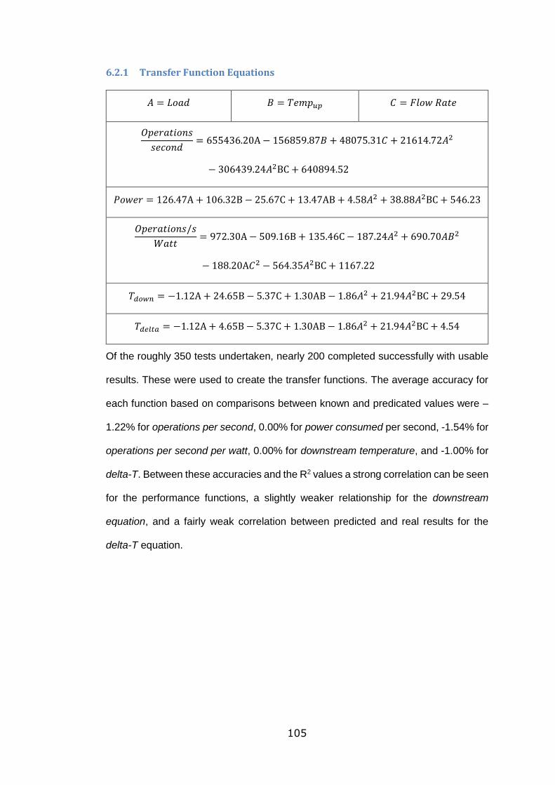
105
6.2.1 Transfer Function Equations
𝐴 = 𝐿𝑜𝑎𝑑 𝐵 = 𝑇𝑒𝑚𝑝𝑢𝑝 𝐶 = 𝐹𝑙𝑜𝑤 𝑅𝑎𝑡𝑒
𝑂𝑝𝑒𝑟𝑎𝑡𝑖𝑜𝑛𝑠
𝑠𝑒𝑐𝑜𝑛𝑑= 655436.20A − 156859.87𝐵 + 48075.31𝐶 + 21614.72𝐴2
− 306439.24𝐴2BC + 640894.52
𝑃𝑜𝑤𝑒𝑟 = 126.47A + 106.32B − 25.67C + 13.47AB + 4.58𝐴2 + 38.88𝐴2BC + 546.23
𝑂𝑝𝑒𝑟𝑎𝑡𝑖𝑜𝑛𝑠/𝑠
𝑊𝑎𝑡𝑡= 972.30A − 509.16B + 135.46C − 187.24𝐴2 + 690.70𝐴𝐵2
− 188.20A𝐶2 − 564.35𝐴2BC + 1167.22
𝑇𝑑𝑜𝑤𝑛 = −1.12A + 24.65B − 5.37C + 1.30AB − 1.86𝐴2 + 21.94𝐴2BC + 29.54
𝑇𝑑𝑒𝑙𝑡𝑎 = −1.12A + 4.65B − 5.37C + 1.30AB − 1.86𝐴2 + 21.94𝐴2BC + 4.54
Of the roughly 350 tests undertaken, nearly 200 completed successfully with usable
results. These were used to create the transfer functions. The average accuracy for
each function based on comparisons between known and predicated values were –
1.22% for operations per second, 0.00% for power consumed per second, -1.54% for
operations per second per watt, 0.00% for downstream temperature, and -1.00% for
delta-T. Between these accuracies and the R2 values a strong correlation can be seen
for the performance functions, a slightly weaker relationship for the downstream
equation, and a fairly weak correlation between predicted and real results for the
delta-T equation.
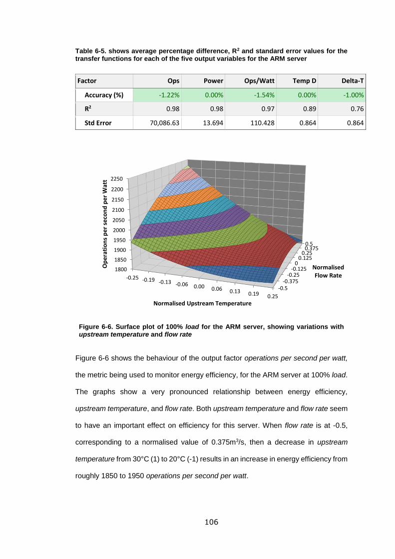
106
Table 6-5. shows average percentage difference, R2 and standard error values for the transfer functions for each of the five output variables for the ARM server
Factor Ops Power Ops/Watt Temp D Delta-T
Accuracy (%) -1.22% 0.00% -1.54% 0.00% -1.00%
R2 0.98 0.98 0.97 0.89 0.76
Std Error 70,086.63 13.694 110.428 0.864 0.864
Figure 6-6. Surface plot of 100% load for the ARM server, showing variations with upstream temperature and flow rate
Figure 6-6 shows the behaviour of the output factor operations per second per watt,
the metric being used to monitor energy efficiency, for the ARM server at 100% load.
The graphs show a very pronounced relationship between energy efficiency,
upstream temperature, and flow rate. Both upstream temperature and flow rate seem
to have an important effect on efficiency for this server. When flow rate is at -0.5,
corresponding to a normalised value of 0.375m3/s, then a decrease in upstream
temperature from 30°C (1) to 20°C (-1) results in an increase in energy efficiency from
roughly 1850 to 1950 operations per second per watt.
-0.5-0.375
-0.25-0.125
00.125
0.250.3750.5
1800
1850
1900
1950
2000
2050
2100
2150
2200
2250
-0.25 -0.19 -0.13 -0.06 0.00 0.06 0.13 0.19 0.25
NormalisedFlow Rate
Op
era
tio
ns
pe
r se
con
d p
er
Wat
t
Normalised Upstream Temperature
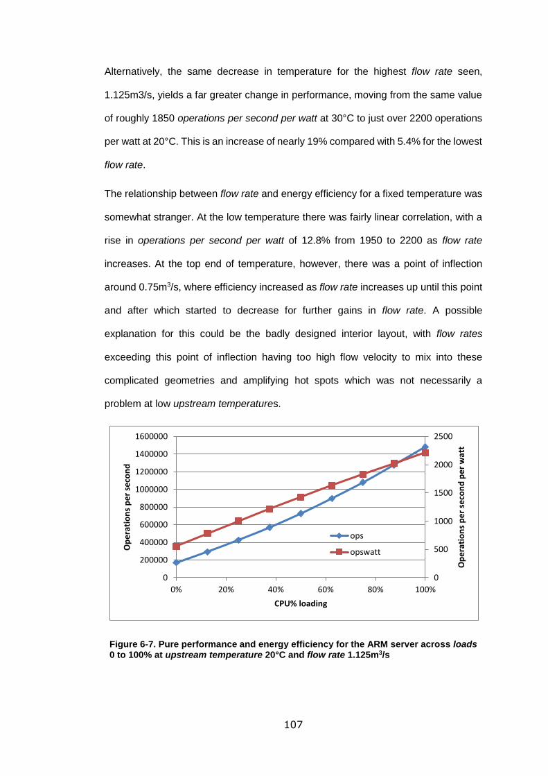
107
Alternatively, the same decrease in temperature for the highest flow rate seen,
1.125m3/s, yields a far greater change in performance, moving from the same value
of roughly 1850 operations per second per watt at 30°C to just over 2200 operations
per watt at 20°C. This is an increase of nearly 19% compared with 5.4% for the lowest
flow rate.
The relationship between flow rate and energy efficiency for a fixed temperature was
somewhat stranger. At the low temperature there was fairly linear correlation, with a
rise in operations per second per watt of 12.8% from 1950 to 2200 as flow rate
increases. At the top end of temperature, however, there was a point of inflection
around 0.75m3/s, where efficiency increased as flow rate increases up until this point
and after which started to decrease for further gains in flow rate. A possible
explanation for this could be the badly designed interior layout, with flow rates
exceeding this point of inflection having too high flow velocity to mix into these
complicated geometries and amplifying hot spots which was not necessarily a
problem at low upstream temperatures.
Figure 6-7. Pure performance and energy efficiency for the ARM server across loads 0 to 100% at upstream temperature 20°C and flow rate 1.125m3/s
0
500
1000
1500
2000
2500
0
200000
400000
600000
800000
1000000
1200000
1400000
1600000
0% 20% 40% 60% 80% 100%
Op
era
tio
ns
pe
r se
con
d p
er
wat
t
Op
era
tio
ns
pe
r se
con
d
CPU% loading
ops
opswatt
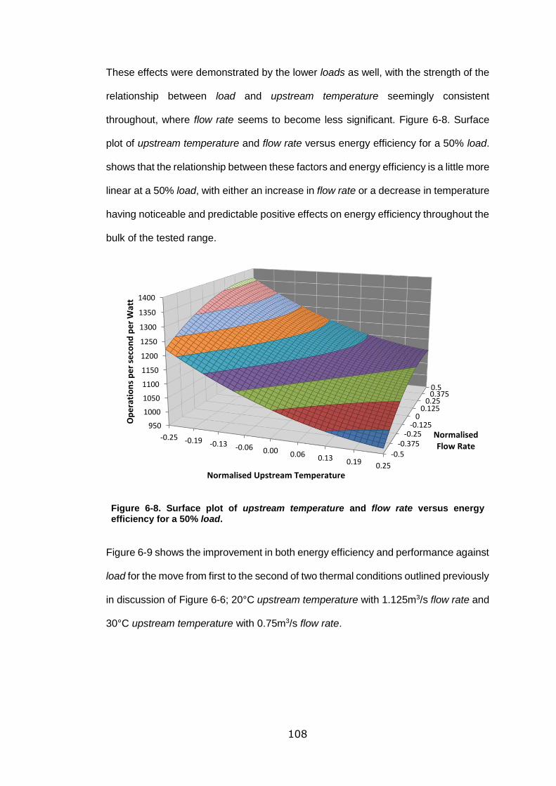
108
These effects were demonstrated by the lower loads as well, with the strength of the
relationship between load and upstream temperature seemingly consistent
throughout, where flow rate seems to become less significant. Figure 6-8. Surface
plot of upstream temperature and flow rate versus energy efficiency for a 50% load.
shows that the relationship between these factors and energy efficiency is a little more
linear at a 50% load, with either an increase in flow rate or a decrease in temperature
having noticeable and predictable positive effects on energy efficiency throughout the
bulk of the tested range.
Figure 6-8. Surface plot of upstream temperature and flow rate versus energy efficiency for a 50% load.
Figure 6-9 shows the improvement in both energy efficiency and performance against
load for the move from first to the second of two thermal conditions outlined previously
in discussion of Figure 6-6; 20°C upstream temperature with 1.125m3/s flow rate and
30°C upstream temperature with 0.75m3/s flow rate.
-0.5-0.375
-0.25-0.125
00.125
0.250.3750.5
950
1000
1050
1100
1150
1200
1250
1300
1350
1400
-0.25 -0.19 -0.13 -0.06 0.00 0.06 0.13 0.19 0.25
NormalisedFlow Rate
Op
era
tio
ns
pe
r se
con
d p
er
Wat
t
Normalised Upstream Temperature
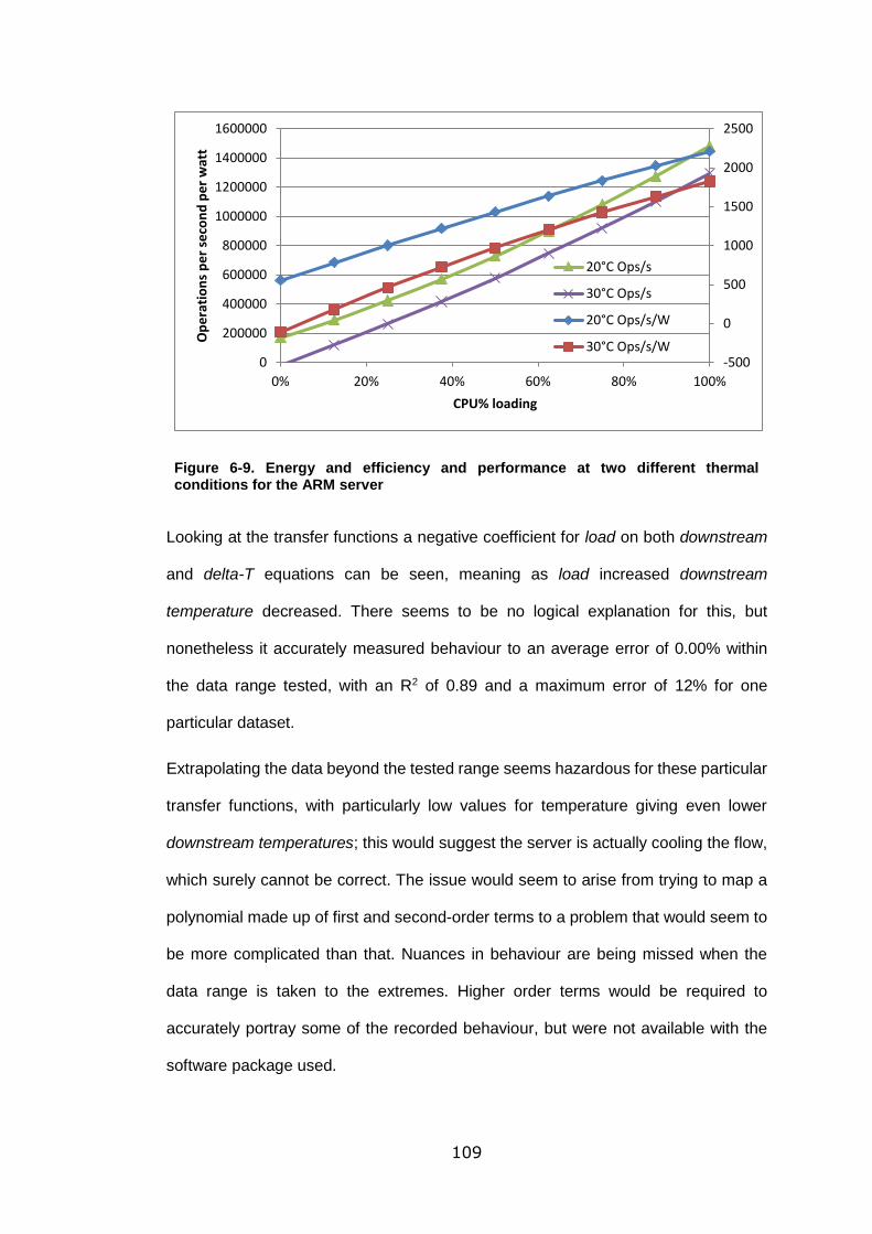
109
Figure 6-9. Energy and efficiency and performance at two different thermal conditions for the ARM server
Looking at the transfer functions a negative coefficient for load on both downstream
and delta-T equations can be seen, meaning as load increased downstream
temperature decreased. There seems to be no logical explanation for this, but
nonetheless it accurately measured behaviour to an average error of 0.00% within
the data range tested, with an R2 of 0.89 and a maximum error of 12% for one
particular dataset.
Extrapolating the data beyond the tested range seems hazardous for these particular
transfer functions, with particularly low values for temperature giving even lower
downstream temperatures; this would suggest the server is actually cooling the flow,
which surely cannot be correct. The issue would seem to arise from trying to map a
polynomial made up of first and second-order terms to a problem that would seem to
be more complicated than that. Nuances in behaviour are being missed when the
data range is taken to the extremes. Higher order terms would be required to
accurately portray some of the recorded behaviour, but were not available with the
software package used.
-500
0
500
1000
1500
2000
2500
0
200000
400000
600000
800000
1000000
1200000
1400000
1600000
0% 20% 40% 60% 80% 100%
Op
era
tio
ns
pe
r se
con
d p
er
wat
t
CPU% loading
20°C Ops/s
30°C Ops/s
20°C Ops/s/W
30°C Ops/s/W
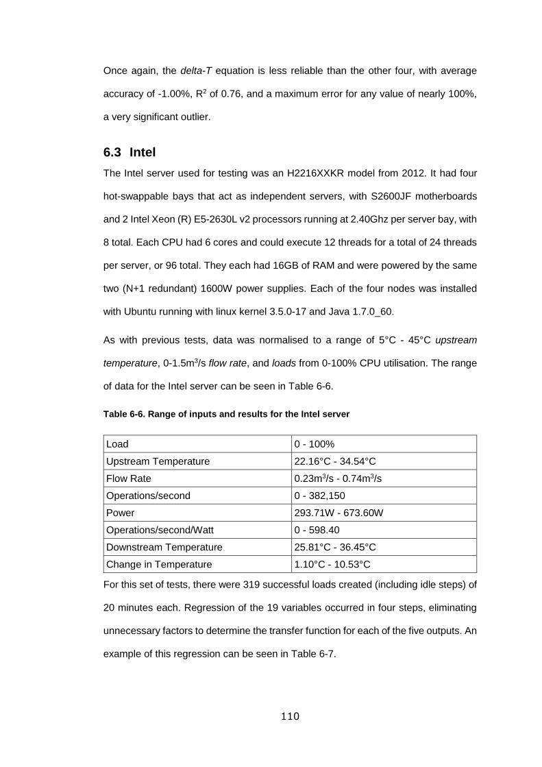
110
Once again, the delta-T equation is less reliable than the other four, with average
accuracy of -1.00%, R2 of 0.76, and a maximum error for any value of nearly 100%,
a very significant outlier.
6.3 Intel
The Intel server used for testing was an H2216XXKR model from 2012. It had four
hot-swappable bays that act as independent servers, with S2600JF motherboards
and 2 Intel Xeon (R) E5-2630L v2 processors running at 2.40Ghz per server bay, with
8 total. Each CPU had 6 cores and could execute 12 threads for a total of 24 threads
per server, or 96 total. They each had 16GB of RAM and were powered by the same
two (N+1 redundant) 1600W power supplies. Each of the four nodes was installed
with Ubuntu running with linux kernel 3.5.0-17 and Java 1.7.0_60.
As with previous tests, data was normalised to a range of 5°C - 45°C upstream
temperature, 0-1.5m3/s flow rate, and loads from 0-100% CPU utilisation. The range
of data for the Intel server can be seen in Table 6-6.
Table 6-6. Range of inputs and results for the Intel server
Load 0 - 100%
Upstream Temperature 22.16°C - 34.54°C
Flow Rate 0.23m3/s - 0.74m3/s
Operations/second 0 - 382,150
Power 293.71W - 673.60W
Operations/second/Watt 0 - 598.40
Downstream Temperature 25.81°C - 36.45°C
Change in Temperature 1.10°C - 10.53°C
For this set of tests, there were 319 successful loads created (including idle steps) of
20 minutes each. Regression of the 19 variables occurred in four steps, eliminating
unnecessary factors to determine the transfer function for each of the five outputs. An
example of this regression can be seen in Table 6-7.
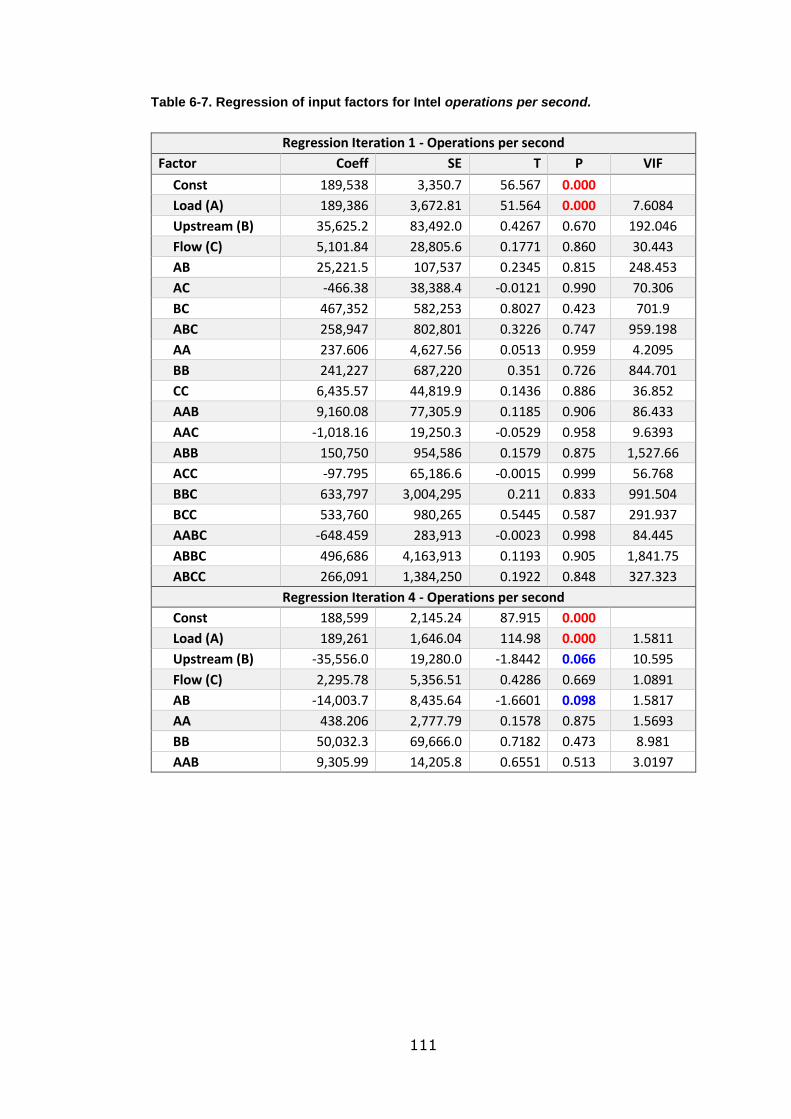
111
Table 6-7. Regression of input factors for Intel operations per second.
Regression Iteration 1 - Operations per second
Factor Coeff SE T P VIF
Const 189,538 3,350.7 56.567 0.000
Load (A) 189,386 3,672.81 51.564 0.000 7.6084
Upstream (B) 35,625.2 83,492.0 0.4267 0.670 192.046
Flow (C) 5,101.84 28,805.6 0.1771 0.860 30.443
AB 25,221.5 107,537 0.2345 0.815 248.453
AC -466.38 38,388.4 -0.0121 0.990 70.306
BC 467,352 582,253 0.8027 0.423 701.9
ABC 258,947 802,801 0.3226 0.747 959.198
AA 237.606 4,627.56 0.0513 0.959 4.2095
BB 241,227 687,220 0.351 0.726 844.701
CC 6,435.57 44,819.9 0.1436 0.886 36.852
AAB 9,160.08 77,305.9 0.1185 0.906 86.433
AAC -1,018.16 19,250.3 -0.0529 0.958 9.6393
ABB 150,750 954,586 0.1579 0.875 1,527.66
ACC -97.795 65,186.6 -0.0015 0.999 56.768
BBC 633,797 3,004,295 0.211 0.833 991.504
BCC 533,760 980,265 0.5445 0.587 291.937
AABC -648.459 283,913 -0.0023 0.998 84.445
ABBC 496,686 4,163,913 0.1193 0.905 1,841.75
ABCC 266,091 1,384,250 0.1922 0.848 327.323
Regression Iteration 4 - Operations per second
Const 188,599 2,145.24 87.915 0.000
Load (A) 189,261 1,646.04 114.98 0.000 1.5811
Upstream (B) -35,556.0 19,280.0 -1.8442 0.066 10.595
Flow (C) 2,295.78 5,356.51 0.4286 0.669 1.0891
AB -14,003.7 8,435.64 -1.6601 0.098 1.5817
AA 438.206 2,777.79 0.1578 0.875 1.5693
BB 50,032.3 69,666.0 0.7182 0.473 8.981
AAB 9,305.99 14,205.8 0.6551 0.513 3.0197
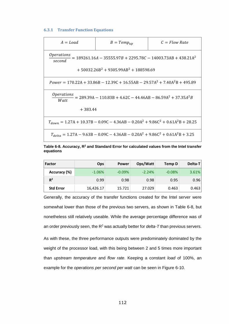
112
6.3.1 Transfer Function Equations
𝐴 = 𝐿𝑜𝑎𝑑 𝐵 = 𝑇𝑒𝑚𝑝𝑢𝑝 𝐶 = 𝐹𝑙𝑜𝑤 𝑅𝑎𝑡𝑒
𝑂𝑝𝑒𝑟𝑎𝑡𝑖𝑜𝑛𝑠
𝑠𝑒𝑐𝑜𝑛𝑑= 189261.16𝐴 − 35555.97𝐵 + 2295.78𝐶 − 14003.73AB + 438.21A2
+ 50032.26B2 + 9305.99AB2 + 188598.69
𝑃𝑜𝑤𝑒𝑟 = 170.22A + 33.86B − 12.39C + 16.55AB − 29.57A2 + 7.40A2B + 495.89
𝑂𝑝𝑒𝑟𝑎𝑡𝑖𝑜𝑛𝑠
𝑊𝑎𝑡𝑡= 289.39A − 110.83B + 4.62C − 44.46AB − 86.59A2 + 37.35𝐴2𝐵
+ 383.44
𝑇𝑑𝑜𝑤𝑛 = 1.27A + 10.37B − 0.09C − 4.36AB − 0.20A2 + 9.86C2 + 0.61A2B + 28.25
𝑇𝑑𝑒𝑙𝑡𝑎 = 1.27A − 9.63B − 0.09C − 4.36AB − 0.20A2 + 9.86C2 + 0.61A2B + 3.25
Table 6-8. Accuracy, R2 and Standard Error for calculated values from the Intel transfer equations
Factor Ops Power Ops/Watt Temp D Delta-T
Accuracy (%) -1.06% -0.09% -2.24% -0.08% 3.61%
R2 0.99 0.98 0.98 0.95 0.96
Std Error 16,426.17 15.721 27.029 0.463 0.463
Generally, the accuracy of the transfer functions created for the Intel server were
somewhat lower than those of the previous two servers, as shown in Table 6-8, but
nonetheless still relatively useable. While the average percentage difference was of
an order previously seen, the R2 was actually better for delta-T than previous servers.
As with these, the three performance outputs were predominately dominated by the
weight of the processor load, with this being between 2 and 5 times more important
than upstream temperature and flow rate. Keeping a constant load of 100%, an
example for the operations per second per watt can be seen in Figure 6-10.
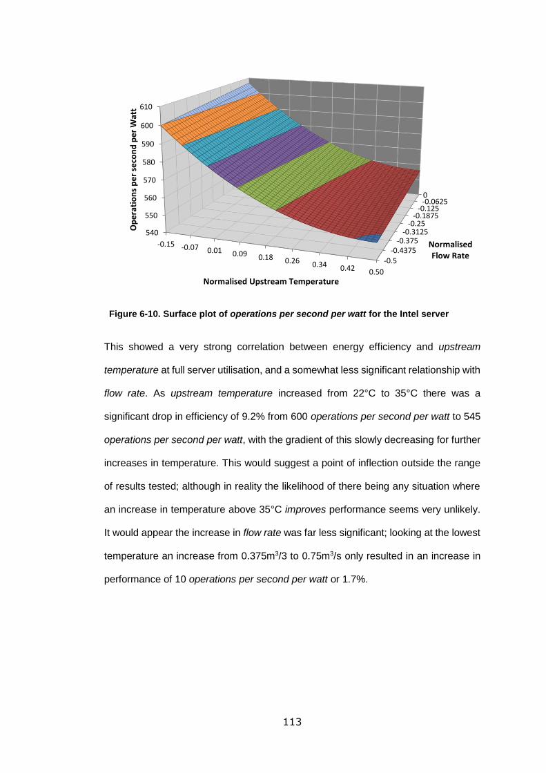
113
Figure 6-10. Surface plot of operations per second per watt for the Intel server
This showed a very strong correlation between energy efficiency and upstream
temperature at full server utilisation, and a somewhat less significant relationship with
flow rate. As upstream temperature increased from 22°C to 35°C there was a
significant drop in efficiency of 9.2% from 600 operations per second per watt to 545
operations per second per watt, with the gradient of this slowly decreasing for further
increases in temperature. This would suggest a point of inflection outside the range
of results tested; although in reality the likelihood of there being any situation where
an increase in temperature above 35°C improves performance seems very unlikely.
It would appear the increase in flow rate was far less significant; looking at the lowest
temperature an increase from 0.375m3/3 to 0.75m3/s only resulted in an increase in
performance of 10 operations per second per watt or 1.7%.
-0.5-0.4375
-0.375-0.3125
-0.25-0.1875
-0.125-0.06250
540
550
560
570
580
590
600
610
-0.15 -0.07 0.01 0.09 0.18 0.26 0.34 0.42 0.50
NormalisedFlow Rate
Op
era
tio
ns
pe
r se
con
d p
er
Wat
t
Normalised Upstream Temperature
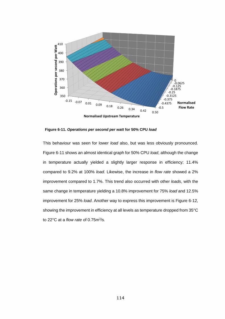
114
Figure 6-11. Operations per second per watt for 50% CPU load
This behaviour was seen for lower load also, but was less obviously pronounced.
Figure 6-11 shows an almost identical graph for 50% CPU load, although the change
in temperature actually yielded a slightly larger response in efficiency; 11.4%
compared to 9.2% at 100% load. Likewise, the increase in flow rate showed a 2%
improvement compared to 1.7%. This trend also occurred with other loads, with the
same change in temperature yielding a 10.8% improvement for 75% load and 12.5%
improvement for 25% load. Another way to express this improvement is Figure 6-12,
showing the improvement in efficiency at all levels as temperature dropped from 35°C
to 22°C at a flow rate of 0.75m3/s.
-0.5-0.4375
-0.375-0.3125
-0.25-0.1875
-0.125-0.06250
350
360
370
380
390
400
410
-0.15 -0.07 0.01 0.09 0.18 0.26 0.34 0.42 0.50
NormalisedFlow Rate
Op
era
tio
ns
pe
r se
con
d p
er
Wat
t
Normalised Upstream Temperature
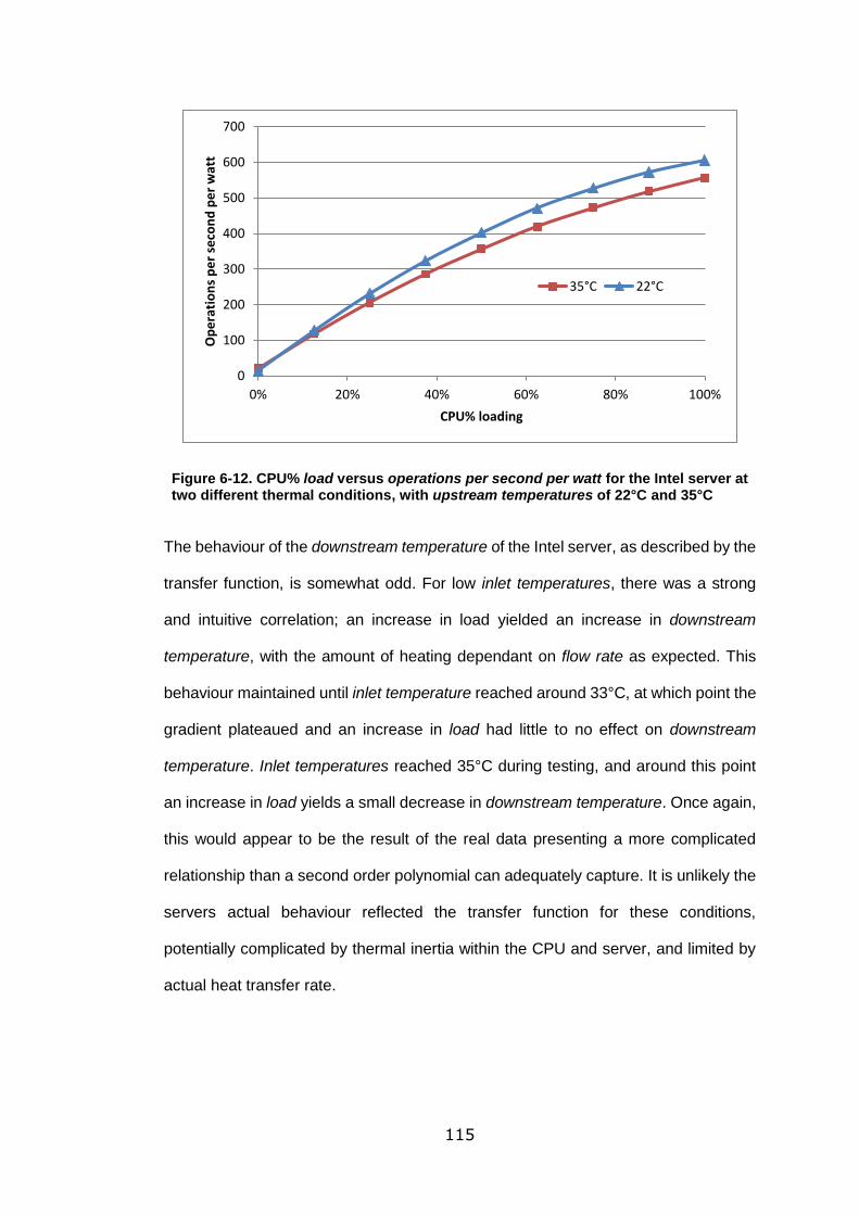
115
Figure 6-12. CPU% load versus operations per second per watt for the Intel server at two different thermal conditions, with upstream temperatures of 22°C and 35°C
The behaviour of the downstream temperature of the Intel server, as described by the
transfer function, is somewhat odd. For low inlet temperatures, there was a strong
and intuitive correlation; an increase in load yielded an increase in downstream
temperature, with the amount of heating dependant on flow rate as expected. This
behaviour maintained until inlet temperature reached around 33°C, at which point the
gradient plateaued and an increase in load had little to no effect on downstream
temperature. Inlet temperatures reached 35°C during testing, and around this point
an increase in load yields a small decrease in downstream temperature. Once again,
this would appear to be the result of the real data presenting a more complicated
relationship than a second order polynomial can adequately capture. It is unlikely the
servers actual behaviour reflected the transfer function for these conditions,
potentially complicated by thermal inertia within the CPU and server, and limited by
actual heat transfer rate.
0
100
200
300
400
500
600
700
0% 20% 40% 60% 80% 100%
Op
era
tio
ns
pe
r se
con
d p
er
wat
t
CPU% loading
35°C 22°C
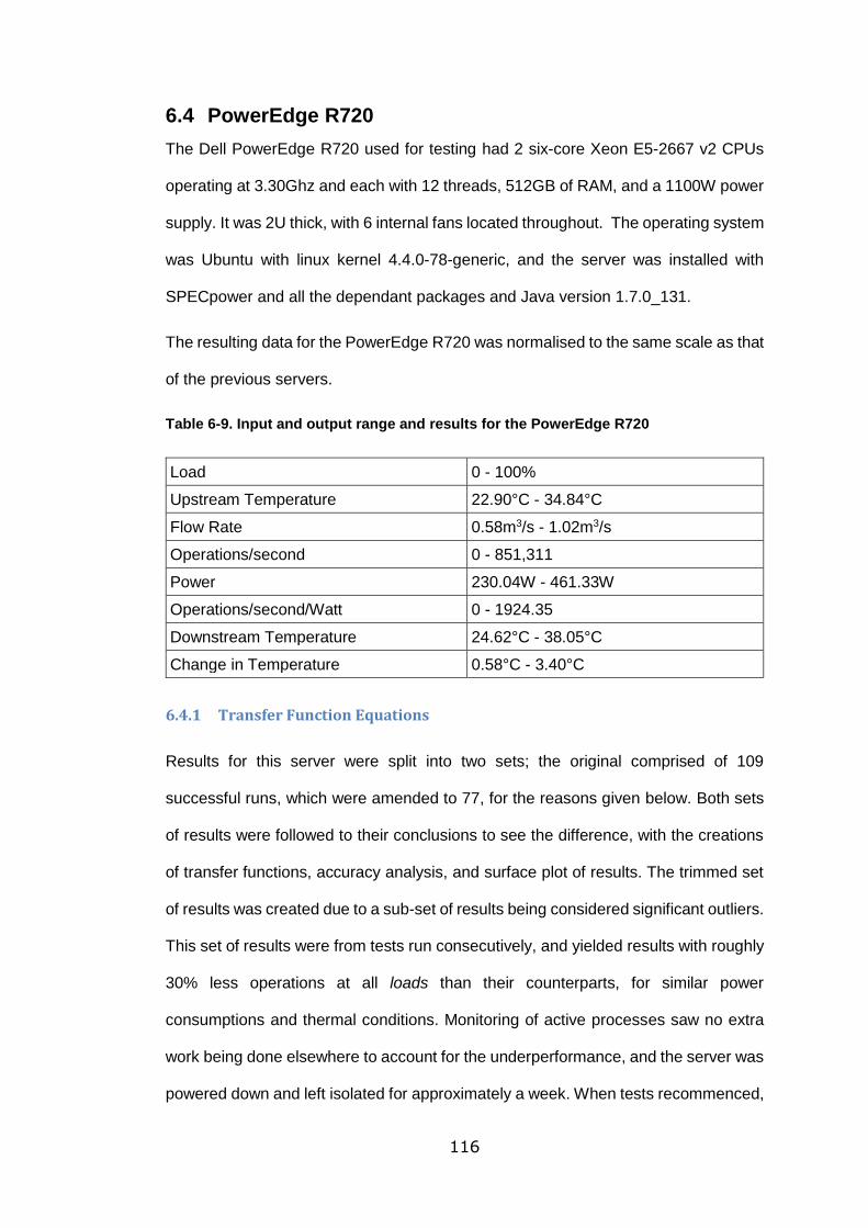
116
6.4 PowerEdge R720
The Dell PowerEdge R720 used for testing had 2 six-core Xeon E5-2667 v2 CPUs
operating at 3.30Ghz and each with 12 threads, 512GB of RAM, and a 1100W power
supply. It was 2U thick, with 6 internal fans located throughout. The operating system
was Ubuntu with linux kernel 4.4.0-78-generic, and the server was installed with
SPECpower and all the dependant packages and Java version 1.7.0_131.
The resulting data for the PowerEdge R720 was normalised to the same scale as that
of the previous servers.
Table 6-9. Input and output range and results for the PowerEdge R720
Load 0 - 100%
Upstream Temperature 22.90°C - 34.84°C
Flow Rate 0.58m3/s - 1.02m3/s
Operations/second 0 - 851,311
Power 230.04W - 461.33W
Operations/second/Watt 0 - 1924.35
Downstream Temperature 24.62°C - 38.05°C
Change in Temperature 0.58°C - 3.40°C
6.4.1 Transfer Function Equations
Results for this server were split into two sets; the original comprised of 109
successful runs, which were amended to 77, for the reasons given below. Both sets
of results were followed to their conclusions to see the difference, with the creations
of transfer functions, accuracy analysis, and surface plot of results. The trimmed set
of results was created due to a sub-set of results being considered significant outliers.
This set of results were from tests run consecutively, and yielded results with roughly
30% less operations at all loads than their counterparts, for similar power
consumptions and thermal conditions. Monitoring of active processes saw no extra
work being done elsewhere to account for the underperformance, and the server was
powered down and left isolated for approximately a week. When tests recommenced,
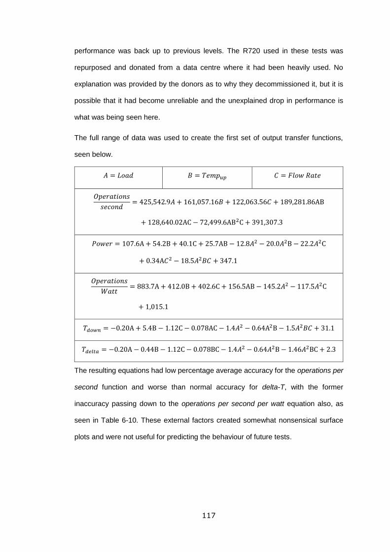
117
performance was back up to previous levels. The R720 used in these tests was
repurposed and donated from a data centre where it had been heavily used. No
explanation was provided by the donors as to why they decommissioned it, but it is
possible that it had become unreliable and the unexplained drop in performance is
what was being seen here.
The full range of data was used to create the first set of output transfer functions,
seen below.
𝐴 = 𝐿𝑜𝑎𝑑 𝐵 = 𝑇𝑒𝑚𝑝𝑢𝑝 𝐶 = 𝐹𝑙𝑜𝑤 𝑅𝑎𝑡𝑒
𝑂𝑝𝑒𝑟𝑎𝑡𝑖𝑜𝑛𝑠
𝑠𝑒𝑐𝑜𝑛𝑑= 425,542.9𝐴 + 161,057.16𝐵 + 122,063.56𝐶 + 189,281.86AB
+ 128,640.02AC − 72,499.6AB2C + 391,307.3
𝑃𝑜𝑤𝑒𝑟 = 107.6A + 54.2B + 40.1C + 25.7AB − 12.8𝐴2 − 20.0𝐴2B − 22.2𝐴2C
+ 0.34A𝐶2 − 18.5𝐴2𝐵𝐶 + 347.1
𝑂𝑝𝑒𝑟𝑎𝑡𝑖𝑜𝑛𝑠
𝑊𝑎𝑡𝑡= 883.7A + 412.0B + 402.6C + 156.5AB − 145.2𝐴2 − 117.5𝐴2C
+ 1,015.1
𝑇𝑑𝑜𝑤𝑛 = −0.20A + 5.4B − 1.12C − 0.078AC − 1.4𝐴2 − 0.64A2B − 1.5𝐴2𝐵𝐶 + 31.1
𝑇𝑑𝑒𝑙𝑡𝑎 = −0.20A − 0.44B − 1.12C − 0.078BC − 1.4𝐴2 − 0.64𝐴2B − 1.46𝐴2BC + 2.3
The resulting equations had low percentage average accuracy for the operations per
second function and worse than normal accuracy for delta-T, with the former
inaccuracy passing down to the operations per second per watt equation also, as
seen in Table 6-10. These external factors created somewhat nonsensical surface
plots and were not useful for predicting the behaviour of future tests.
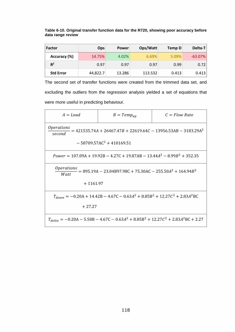
118
Table 6-10. Original transfer function data for the R720, showing poor accuracy before data range review
Factor Ops Power Ops/Watt Temp D Delta-T
Accuracy (%) 14.75% 4.02% 6.69% 5.09% -63.07%
R2 0.97 0.97 0.97 0.99 0.72
Std Error 44,822.7 13.286 113.532 0.413 0.413
The second set of transfer functions were created from the trimmed data set, and
excluding the outliers from the regression analysis yielded a set of equations that
were more useful in predicting behaviour.
𝐴 = 𝐿𝑜𝑎𝑑 𝐵 = 𝑇𝑒𝑚𝑝𝑢𝑝 𝐶 = 𝐹𝑙𝑜𝑤 𝑅𝑎𝑡𝑒
𝑂𝑝𝑒𝑟𝑎𝑡𝑖𝑜𝑛𝑠
𝑠𝑒𝑐𝑜𝑛𝑑= 421535.74𝐴 + 26467.47𝐵 + 22619.64𝐶 − 13956.53AB − 3183.29A2
− 58709.57AC2 + 410169.51
𝑃𝑜𝑤𝑒𝑟 = 107.09A + 19.92B − 4.27C + 19.87AB − 13.44𝐴2 − 8.99𝐵2 + 352.35
𝑂𝑝𝑒𝑟𝑎𝑡𝑖𝑜𝑛𝑠
𝑊𝑎𝑡𝑡= 895.19A − 23.04B97.98C + 75.30AC − 255.50𝐴2 + 164.94𝐵2
+ 1161.97
𝑇𝑑𝑜𝑤𝑛 = −0.20A + 14.42B − 4.67C − 0.63𝐴2 + 8.85B2 + 12.27𝐶2 + 2.83𝐴2BC
+ 27.27
𝑇𝑑𝑒𝑙𝑡𝑎 = −0.20A − 5.58B − 4.67C − 0.63𝐴2 + 8.85B2 + 12.27𝐶2 + 2.83𝐴2BC + 2.27
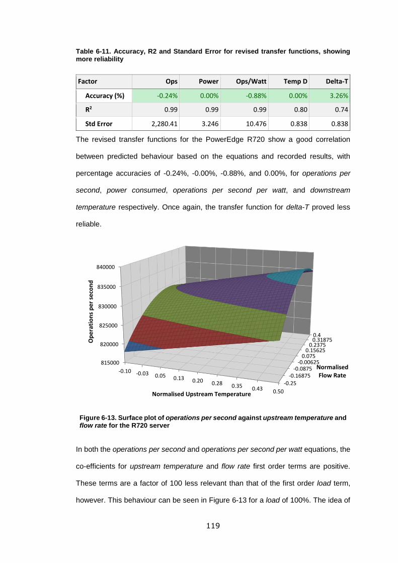
119
Table 6-11. Accuracy, R2 and Standard Error for revised transfer functions, showing more reliability
Factor Ops Power Ops/Watt Temp D Delta-T
Accuracy (%) -0.24% 0.00% -0.88% 0.00% 3.26%
R2 0.99 0.99 0.99 0.80 0.74
Std Error 2,280.41 3.246 10.476 0.838 0.838
The revised transfer functions for the PowerEdge R720 show a good correlation
between predicted behaviour based on the equations and recorded results, with
percentage accuracies of -0.24%, -0.00%, -0.88%, and 0.00%, for operations per
second, power consumed, operations per second per watt, and downstream
temperature respectively. Once again, the transfer function for delta-T proved less
reliable.
Figure 6-13. Surface plot of operations per second against upstream temperature and flow rate for the R720 server
In both the operations per second and operations per second per watt equations, the
co-efficients for upstream temperature and flow rate first order terms are positive.
These terms are a factor of 100 less relevant than that of the first order load term,
however. This behaviour can be seen in Figure 6-13 for a load of 100%. The idea of
-0.25-0.16875
-0.0875-0.00625
0.0750.15625
0.23750.318750.4
815000
820000
825000
830000
835000
840000
-0.10 -0.03 0.05 0.13 0.20 0.28 0.35 0.43 0.50
NormalisedFlow Rate
Op
era
tio
ns
pe
r se
con
d
Normalised Upstream Temperature
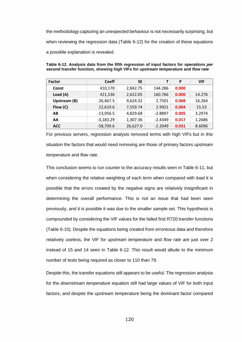
120
the methodology capturing an unexpected behaviour is not necessarily surprising, but
when reviewing the regression data (Table 6-12) for the creation of these equations
a possible explanation is revealed.
Table 6-12. Analysis data from the fifth regression of input factors for operations per second transfer function, showing high VIFs for upstream temperature and flow rate
Factor Coeff SE T P VIF
Const 410,170 2,842.75 144.286 0.000
Load (A) 421,536 2,622.05 160.766 0.000 14.276
Upstream (B) 26,467.5 9,624.32 2.7501 0.008 16.264
Flow (C) 22,619.6 7,559.74 2.9921 0.004 15.53
AB -13,956.5 4,829.68 -2.8897 0.005 3.2974
AA -3,183.29 1,307.36 -2.4349 0.017 1.2686
ACC -58,709.6 26,627.0 -2.2049 0.031 8.6096
For previous servers, regression analysis removed terms with high VIFs but in this
situation the factors that would need removing are those of primary factors upstream
temperature and flow rate.
This conclusion seems to run counter to the accuracy results seen in Table 6-11, but
when considering the relative weighting of each term when compared with load it is
possible that the errors created by the negative signs are relatively insignificant in
determining the overall performance. This is not an issue that had been seen
previously, and it is possible it was due to the smaller sample set. This hypothesis is
compounded by considering the VIF values for the failed first R720 transfer functions
(Table 6-10). Despite the equations being created from erroneous data and therefore
relatively useless, the VIF for upstream temperature and flow rate are just over 2
instead of 15 and 14 seen in Table 6-12. This result would allude to the minimum
number of tests being required as closer to 110 than 79.
Despite this, the transfer equations still appears to be useful. The regression analysis
for the downstream temperature equation still had large values of VIF for both input
factors, and despite the upstream temperature being the dominant factor compared
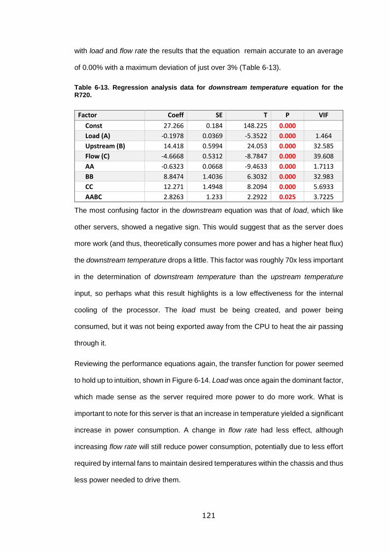
121
with load and flow rate the results that the equation remain accurate to an average
of 0.00% with a maximum deviation of just over 3% (Table 6-13).
Table 6-13. Regression analysis data for downstream temperature equation for the R720.
Factor Coeff SE T P VIF
Const 27.266 0.184 148.225 0.000
Load (A) -0.1978 0.0369 -5.3522 0.000 1.464
Upstream (B) 14.418 0.5994 24.053 0.000 32.585
Flow (C) -4.6668 0.5312 -8.7847 0.000 39.608
AA -0.6323 0.0668 -9.4633 0.000 1.7113
BB 8.8474 1.4036 6.3032 0.000 32.983
CC 12.271 1.4948 8.2094 0.000 5.6933
AABC 2.8263 1.233 2.2922 0.025 3.7225
The most confusing factor in the downstream equation was that of load, which like
other servers, showed a negative sign. This would suggest that as the server does
more work (and thus, theoretically consumes more power and has a higher heat flux)
the downstream temperature drops a little. This factor was roughly 70x less important
in the determination of downstream temperature than the upstream temperature
input, so perhaps what this result highlights is a low effectiveness for the internal
cooling of the processor. The load must be being created, and power being
consumed, but it was not being exported away from the CPU to heat the air passing
through it.
Reviewing the performance equations again, the transfer function for power seemed
to hold up to intuition, shown in Figure 6-14. Load was once again the dominant factor,
which made sense as the server required more power to do more work. What is
important to note for this server is that an increase in temperature yielded a significant
increase in power consumption. A change in flow rate had less effect, although
increasing flow rate will still reduce power consumption, potentially due to less effort
required by internal fans to maintain desired temperatures within the chassis and thus
less power needed to drive them.
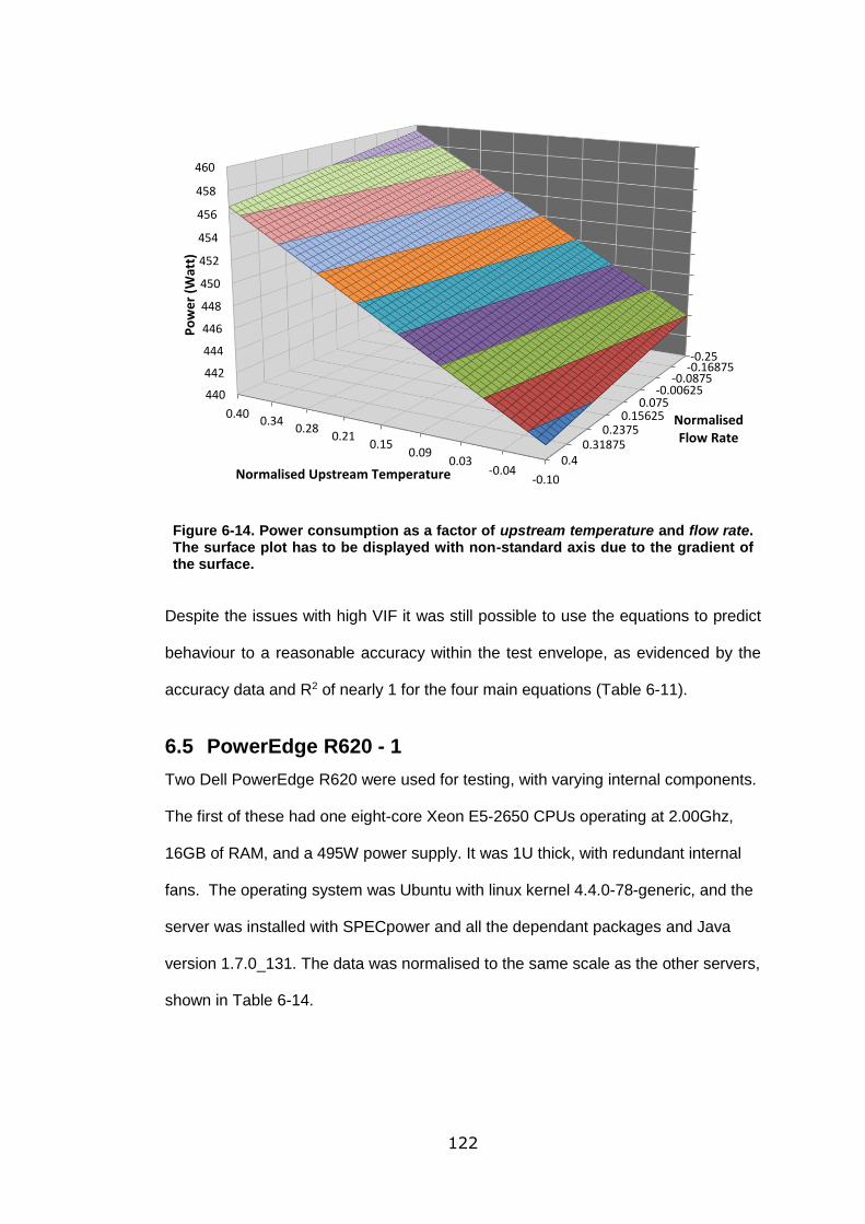
122
Figure 6-14. Power consumption as a factor of upstream temperature and flow rate. The surface plot has to be displayed with non-standard axis due to the gradient of the surface.
Despite the issues with high VIF it was still possible to use the equations to predict
behaviour to a reasonable accuracy within the test envelope, as evidenced by the
accuracy data and R2 of nearly 1 for the four main equations (Table 6-11).
6.5 PowerEdge R620 - 1
Two Dell PowerEdge R620 were used for testing, with varying internal components.
The first of these had one eight-core Xeon E5-2650 CPUs operating at 2.00Ghz,
16GB of RAM, and a 495W power supply. It was 1U thick, with redundant internal
fans. The operating system was Ubuntu with linux kernel 4.4.0-78-generic, and the
server was installed with SPECpower and all the dependant packages and Java
version 1.7.0_131. The data was normalised to the same scale as the other servers,
shown in Table 6-14.
-0.25-0.16875
-0.0875-0.00625
0.0750.15625
0.23750.31875
0.4
440
442
444
446
448
450
452
454
456
458
460
-0.10-0.04
0.030.09
0.150.21
0.280.34
0.40 NormalisedFlow Rate
Po
we
r (W
att)
Normalised Upstream Temperature
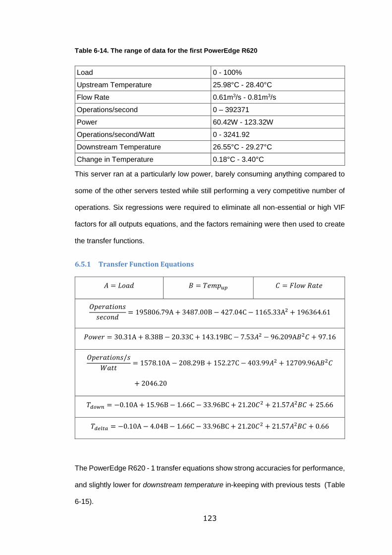
123
Table 6-14. The range of data for the first PowerEdge R620
Load 0 - 100%
Upstream Temperature 25.98°C - 28.40°C
Flow Rate 0.61m3/s - 0.81m3/s
Operations/second 0 – 392371
Power 60.42W - 123.32W
Operations/second/Watt 0 - 3241.92
Downstream Temperature 26.55°C - 29.27°C
Change in Temperature 0.18°C - 3.40°C
This server ran at a particularly low power, barely consuming anything compared to
some of the other servers tested while still performing a very competitive number of
operations. Six regressions were required to eliminate all non-essential or high VIF
factors for all outputs equations, and the factors remaining were then used to create
the transfer functions.
6.5.1 Transfer Function Equations
𝐴 = 𝐿𝑜𝑎𝑑 𝐵 = 𝑇𝑒𝑚𝑝𝑢𝑝 𝐶 = 𝐹𝑙𝑜𝑤 𝑅𝑎𝑡𝑒
𝑂𝑝𝑒𝑟𝑎𝑡𝑖𝑜𝑛𝑠
𝑠𝑒𝑐𝑜𝑛𝑑= 195806.79A + 3487.00B − 427.04C − 1165.33A2 + 196364.61
𝑃𝑜𝑤𝑒𝑟 = 30.31A + 8.38B − 20.33C + 143.19BC − 7.53𝐴2 − 96.209A𝐵2𝐶 + 97.16
𝑂𝑝𝑒𝑟𝑎𝑡𝑖𝑜𝑛𝑠/𝑠
𝑊𝑎𝑡𝑡= 1578.10A − 208.29B + 152.27C − 403.99𝐴2 + 12709.96A𝐵2𝐶
+ 2046.20
𝑇𝑑𝑜𝑤𝑛 = −0.10A + 15.96B − 1.66C − 33.96BC + 21.20𝐶2 + 21.57𝐴2𝐵𝐶 + 25.66
𝑇𝑑𝑒𝑙𝑡𝑎 = −0.10A − 4.04B − 1.66C − 33.96BC + 21.20𝐶2 + 21.57𝐴2𝐵𝐶 + 0.66
The PowerEdge R620 - 1 transfer equations show strong accuracies for performance,
and slightly lower for downstream temperature in-keeping with previous tests (Table
6-15).
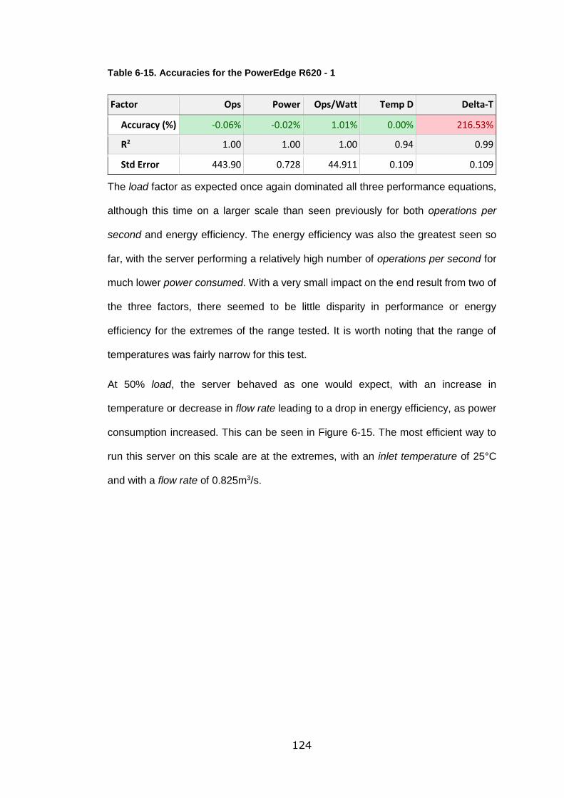
124
Table 6-15. Accuracies for the PowerEdge R620 - 1
Factor Ops Power Ops/Watt Temp D Delta-T
Accuracy (%) -0.06% -0.02% 1.01% 0.00% 216.53%
R2 1.00 1.00 1.00 0.94 0.99
Std Error 443.90 0.728 44.911 0.109 0.109
The load factor as expected once again dominated all three performance equations,
although this time on a larger scale than seen previously for both operations per
second and energy efficiency. The energy efficiency was also the greatest seen so
far, with the server performing a relatively high number of operations per second for
much lower power consumed. With a very small impact on the end result from two of
the three factors, there seemed to be little disparity in performance or energy
efficiency for the extremes of the range tested. It is worth noting that the range of
temperatures was fairly narrow for this test.
At 50% load, the server behaved as one would expect, with an increase in
temperature or decrease in flow rate leading to a drop in energy efficiency, as power
consumption increased. This can be seen in Figure 6-15. The most efficient way to
run this server on this scale are at the extremes, with an inlet temperature of 25°C
and with a flow rate of 0.825m3/s.
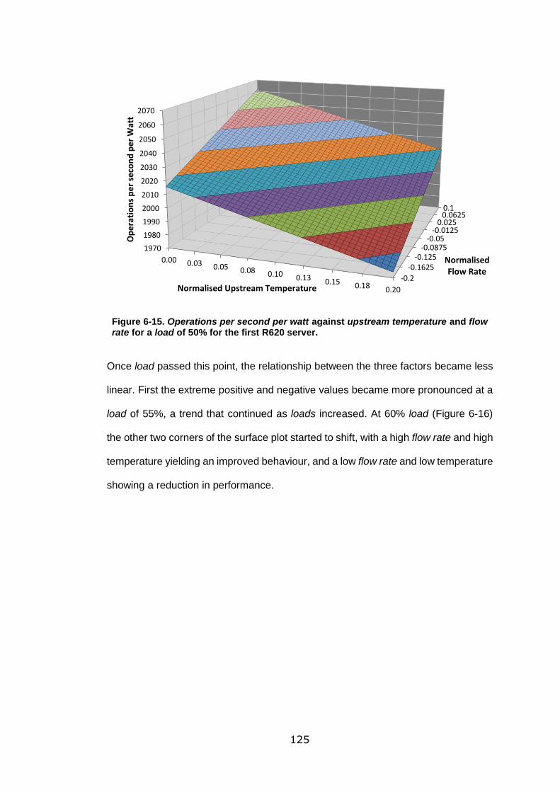
125
Figure 6-15. Operations per second per watt against upstream temperature and flow rate for a load of 50% for the first R620 server.
Once load passed this point, the relationship between the three factors became less
linear. First the extreme positive and negative values became more pronounced at a
load of 55%, a trend that continued as loads increased. At 60% load (Figure 6-16)
the other two corners of the surface plot started to shift, with a high flow rate and high
temperature yielding an improved behaviour, and a low flow rate and low temperature
showing a reduction in performance.
-0.2
-0.1625-0.125
-0.0875-0.05
-0.01250.025
0.06250.1
1970
1980
1990
2000
2010
2020
2030
2040
2050
2060
2070
0.00 0.03 0.05 0.08 0.10 0.13 0.15 0.18 0.20
NormalisedFlow Rate
Op
era
tio
ns
pe
r se
con
d p
er
Wat
t
Normalised Upstream Temperature
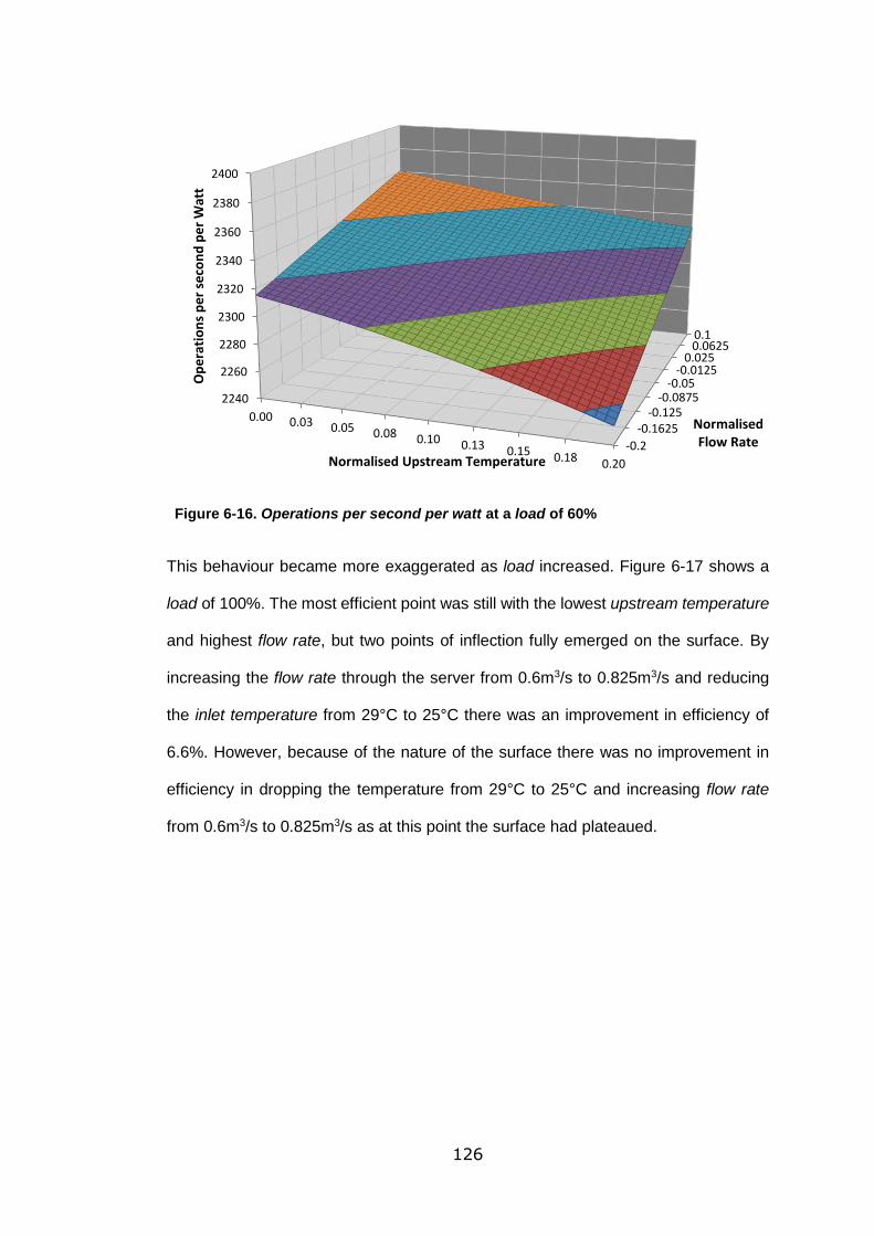
126
Figure 6-16. Operations per second per watt at a load of 60%
This behaviour became more exaggerated as load increased. Figure 6-17 shows a
load of 100%. The most efficient point was still with the lowest upstream temperature
and highest flow rate, but two points of inflection fully emerged on the surface. By
increasing the flow rate through the server from 0.6m3/s to 0.825m3/s and reducing
the inlet temperature from 29°C to 25°C there was an improvement in efficiency of
6.6%. However, because of the nature of the surface there was no improvement in
efficiency in dropping the temperature from 29°C to 25°C and increasing flow rate
from 0.6m3/s to 0.825m3/s as at this point the surface had plateaued.
-0.2
-0.1625-0.125
-0.0875-0.05
-0.01250.025
0.06250.1
2240
2260
2280
2300
2320
2340
2360
2380
2400
0.00 0.03 0.05 0.08 0.10 0.13 0.15 0.18 0.20
NormalisedFlow Rate
Op
era
tio
ns
pe
r se
con
d p
er
Wat
t
Normalised Upstream Temperature
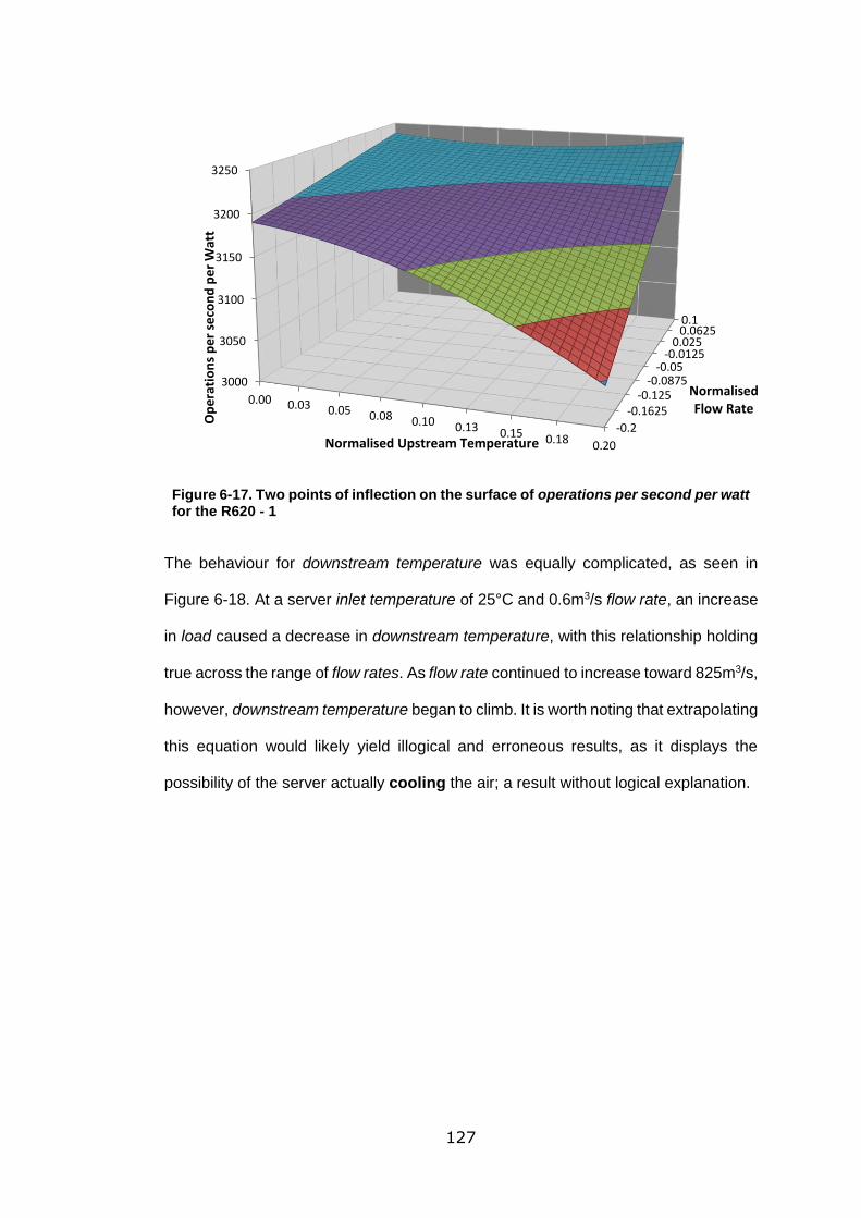
127
Figure 6-17. Two points of inflection on the surface of operations per second per watt for the R620 - 1
The behaviour for downstream temperature was equally complicated, as seen in
Figure 6-18. At a server inlet temperature of 25°C and 0.6m3/s flow rate, an increase
in load caused a decrease in downstream temperature, with this relationship holding
true across the range of flow rates. As flow rate continued to increase toward 825m3/s,
however, downstream temperature began to climb. It is worth noting that extrapolating
this equation would likely yield illogical and erroneous results, as it displays the
possibility of the server actually cooling the air; a result without logical explanation.
-0.2
-0.1625-0.125
-0.0875-0.05
-0.01250.025
0.06250.1
3000
3050
3100
3150
3200
3250
0.00 0.03 0.05 0.08 0.10 0.13 0.15 0.18 0.20
NormalisedFlow Rate
Op
era
tio
ns
pe
r se
con
d p
er
Wat
t
Normalised Upstream Temperature
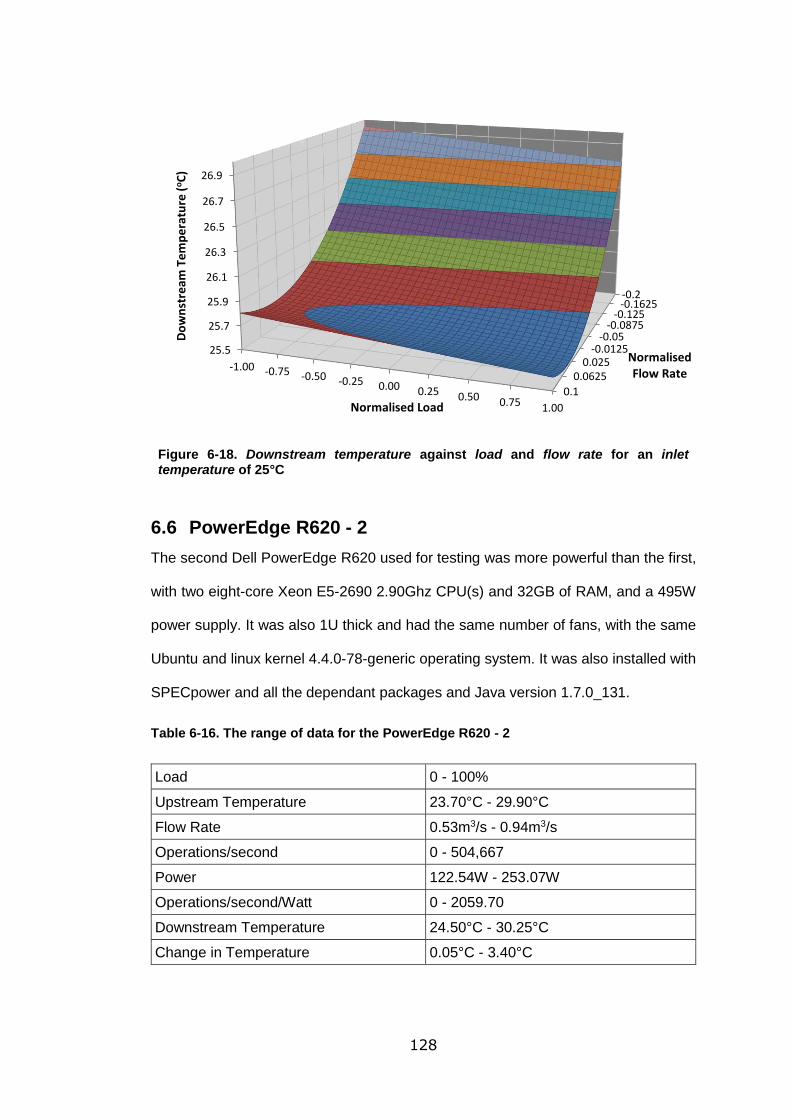
128
Figure 6-18. Downstream temperature against load and flow rate for an inlet temperature of 25°C
6.6 PowerEdge R620 - 2
The second Dell PowerEdge R620 used for testing was more powerful than the first,
with two eight-core Xeon E5-2690 2.90Ghz CPU(s) and 32GB of RAM, and a 495W
power supply. It was also 1U thick and had the same number of fans, with the same
Ubuntu and linux kernel 4.4.0-78-generic operating system. It was also installed with
SPECpower and all the dependant packages and Java version 1.7.0_131.
Table 6-16. The range of data for the PowerEdge R620 - 2
Load 0 - 100%
Upstream Temperature 23.70°C - 29.90°C
Flow Rate 0.53m3/s - 0.94m3/s
Operations/second 0 - 504,667
Power 122.54W - 253.07W
Operations/second/Watt 0 - 2059.70
Downstream Temperature 24.50°C - 30.25°C
Change in Temperature 0.05°C - 3.40°C
-0.2-0.1625
-0.125-0.0875
-0.05-0.0125
0.0250.0625
0.1
25.5
25.7
25.9
26.1
26.3
26.5
26.7
26.9
-1.00 -0.75 -0.50 -0.25 0.00 0.25 0.50 0.75 1.00
NormalisedFlow Rate
Do
wn
stre
am T
em
pe
ratu
re (
oC
)
Normalised Load
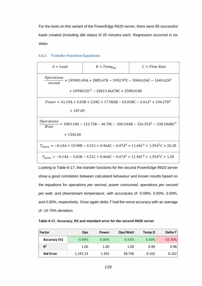
129
For the tests on this variant of the PowerEdge R620 server, there were 85 successful
loads created (including idle steps) of 20 minutes each. Regression occurred in six
steps.
6.6.1 Transfer Function Equations
𝐴 = 𝐿𝑜𝑎𝑑 𝐵 = 𝑇𝑒𝑚𝑝𝑢𝑝 𝐶 = 𝐹𝑙𝑜𝑤 𝑅𝑎𝑡𝑒
𝑂𝑝𝑒𝑟𝑎𝑡𝑖𝑜𝑛𝑠
𝑠𝑒𝑐𝑜𝑛𝑑= 249981.49A + 2885.67𝐵 − 3992.97C − 5960.65AC − 1649.62A2
+ 10948.52C2 − 24013.46A2BC + 250810.88
𝑃𝑜𝑤𝑒𝑟 = 61.19A + 5.03B + 2.04C + 17.98AB − 63.81BC − 3.41𝐴2 + 194.27𝐵2
+ 187.09
𝑂𝑝𝑒𝑟𝑎𝑡𝑖𝑜𝑛𝑠
𝑊𝑎𝑡𝑡= 1003.10A − 122.73B − 46.70C − 200.24AB − 326.35𝐴2 − 238.18AB𝐶2
+ 1342.60
𝑇𝑑𝑜𝑤𝑛 = −0.14A + 15.98B − 4.31C + 0.46AC − 0.47𝐴2 + 11.44𝐶2 + 1.39𝐴2𝐶 + 26.20
𝑇𝑑𝑒𝑙𝑡𝑎 = −0.14A − 4.02B − 4.31C + 0.46AC − 0.47𝐴2 + 11.44𝐶2 + 1.39𝐴2𝐶 + 1.20
Looking to Table 6-17, the transfer functions for the second PowerEdge R620 server
show a good correlation between calculated behaviour and known results based on
the equations for operations per second, power consumed, operations per second
per watt, and downstream temperature, with accuracies of -0.09%, 0.00%, 0.93%,
and 0.00%, respectively. Once again delta-T had the worst accuracy with an average
of -10.70% deviation.
Table 6-17. Accuracy, R2 and standard error for the second R620 server
Factor Ops Power Ops/Watt Temp D Delta-T
Accuracy (%) -0.09% 0.00% 0.93% 0.00% -10.70%
R2 1.00 1.00 1.00 0.99 0.98
Std Error 1,191.13 1.355 28.756 0.162 0.162
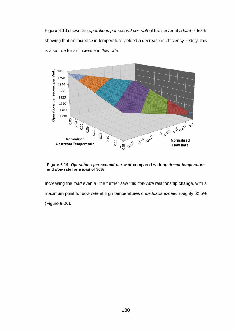
130
Figure 6-19 shows the operations per second per watt of the server at a load of 50%,
showing that an increase in temperature yielded a decrease in efficiency. Oddly, this
is also true for an increase in flow rate.
Figure 6-19. Operations per second per watt compared with upstream temperature and flow rate for a load of 50%
Increasing the load even a little further saw this flow rate relationship change, with a
maximum point for flow rate at high temperatures once loads exceed roughly 62.5%
(Figure 6-20).
1290
1300
1310
1320
1330
1340
1350
13600
.00
0.0
3
0.0
6
0.0
9
0.1
3
0.1
6
0.1
9
0.2
2
0.2
5
NormalisedFlow Rate
Op
era
tio
ns
pe
r se
con
d p
er
Wat
t
Normalised Upstream Temperature
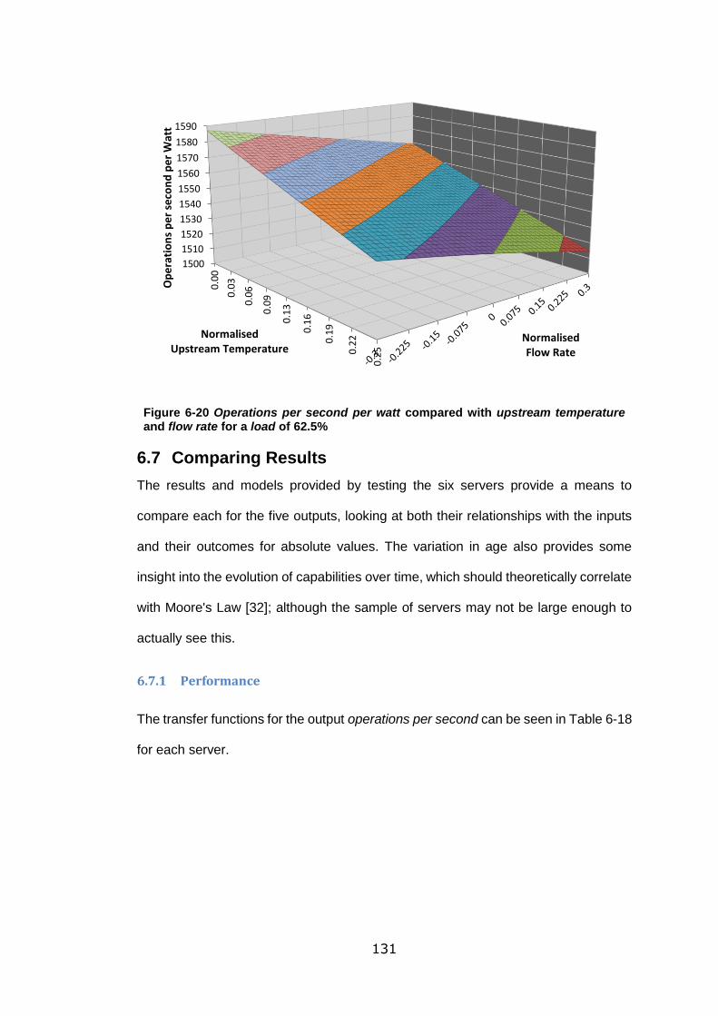
131
Figure 6-20 Operations per second per watt compared with upstream temperature and flow rate for a load of 62.5%
6.7 Comparing Results
The results and models provided by testing the six servers provide a means to
compare each for the five outputs, looking at both their relationships with the inputs
and their outcomes for absolute values. The variation in age also provides some
insight into the evolution of capabilities over time, which should theoretically correlate
with Moore's Law [32]; although the sample of servers may not be large enough to
actually see this.
6.7.1 Performance
The transfer functions for the output operations per second can be seen in Table 6-18
for each server.
1500
1510
1520
1530
1540
1550
1560
1570
1580
1590
0.0
0
0.0
3
0.0
6
0.0
9
0.1
3
0.1
6
0.1
9
0.2
2
0.2
5
NormalisedFlow Rate
Op
era
tio
ns
pe
r se
con
d p
er
Wat
t
Normalised Upstream Temperature
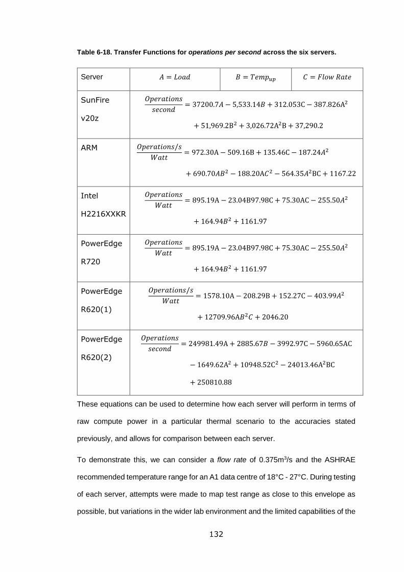
132
Table 6-18. Transfer Functions for operations per second across the six servers.
Server 𝐴 = 𝐿𝑜𝑎𝑑 𝐵 = 𝑇𝑒𝑚𝑝𝑢𝑝 𝐶 = 𝐹𝑙𝑜𝑤 𝑅𝑎𝑡𝑒
SunFire
v20z
𝑂𝑝𝑒𝑟𝑎𝑡𝑖𝑜𝑛𝑠
𝑠𝑒𝑐𝑜𝑛𝑑= 37200.7𝐴 − 5,533.14𝐵 + 312.053C − 387.826A2
+ 51,969.2B2 + 3,026.72A2B + 37,290.2
ARM 𝑂𝑝𝑒𝑟𝑎𝑡𝑖𝑜𝑛𝑠/𝑠
𝑊𝑎𝑡𝑡= 972.30A − 509.16B + 135.46C − 187.24𝐴2
+ 690.70𝐴𝐵2 − 188.20A𝐶2 − 564.35𝐴2BC + 1167.22
Intel
H2216XXKR
𝑂𝑝𝑒𝑟𝑎𝑡𝑖𝑜𝑛𝑠
𝑊𝑎𝑡𝑡= 895.19A − 23.04B97.98C + 75.30AC − 255.50𝐴2
+ 164.94𝐵2 + 1161.97
PowerEdge
R720
𝑂𝑝𝑒𝑟𝑎𝑡𝑖𝑜𝑛𝑠
𝑊𝑎𝑡𝑡= 895.19A − 23.04B97.98C + 75.30AC − 255.50𝐴2
+ 164.94𝐵2 + 1161.97
PowerEdge
R620(1)
𝑂𝑝𝑒𝑟𝑎𝑡𝑖𝑜𝑛𝑠/𝑠
𝑊𝑎𝑡𝑡= 1578.10A − 208.29B + 152.27C − 403.99𝐴2
+ 12709.96A𝐵2𝐶 + 2046.20
PowerEdge
R620(2)
𝑂𝑝𝑒𝑟𝑎𝑡𝑖𝑜𝑛𝑠
𝑠𝑒𝑐𝑜𝑛𝑑= 249981.49A + 2885.67𝐵 − 3992.97C − 5960.65AC
− 1649.62A2 + 10948.52C2 − 24013.46A2BC
+ 250810.88
These equations can be used to determine how each server will perform in terms of
raw compute power in a particular thermal scenario to the accuracies stated
previously, and allows for comparison between each server.
To demonstrate this, we can consider a flow rate of 0.375m3/s and the ASHRAE
recommended temperature range for an A1 data centre of 18°C - 27°C. During testing
of each server, attempts were made to map test range as close to this envelope as
possible, but variations in the wider lab environment and the limited capabilities of the
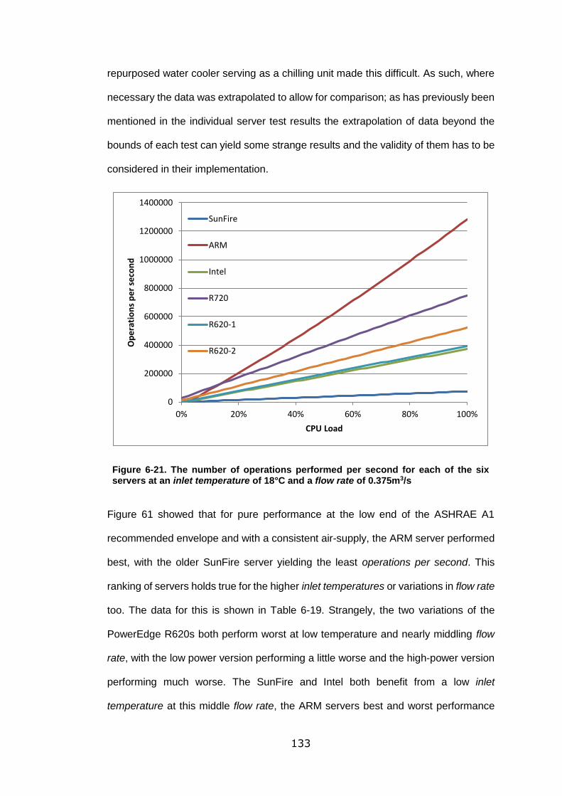
133
repurposed water cooler serving as a chilling unit made this difficult. As such, where
necessary the data was extrapolated to allow for comparison; as has previously been
mentioned in the individual server test results the extrapolation of data beyond the
bounds of each test can yield some strange results and the validity of them has to be
considered in their implementation.
Figure 6-21. The number of operations performed per second for each of the six servers at an inlet temperature of 18°C and a flow rate of 0.375m3/s
Figure 61 showed that for pure performance at the low end of the ASHRAE A1
recommended envelope and with a consistent air-supply, the ARM server performed
best, with the older SunFire server yielding the least operations per second. This
ranking of servers holds true for the higher inlet temperatures or variations in flow rate
too. The data for this is shown in Table 6-19. Strangely, the two variations of the
PowerEdge R620s both perform worst at low temperature and nearly middling flow
rate, with the low power version performing a little worse and the high-power version
performing much worse. The SunFire and Intel both benefit from a low inlet
temperature at this middle flow rate, the ARM servers best and worst performance
0
200000
400000
600000
800000
1000000
1200000
1400000
0% 20% 40% 60% 80% 100%
Op
era
tio
ns
pe
r se
con
d
CPU Load
SunFire
ARM
Intel
R720
R620-1
R620-2
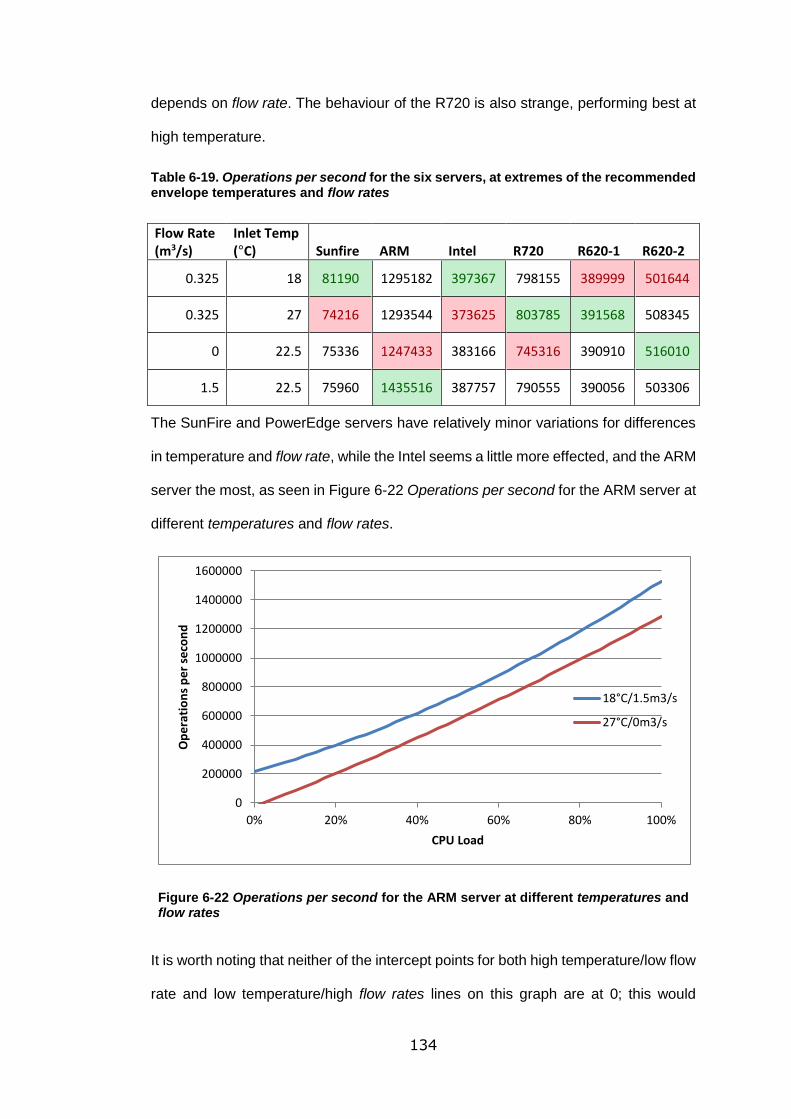
134
depends on flow rate. The behaviour of the R720 is also strange, performing best at
high temperature.
Table 6-19. Operations per second for the six servers, at extremes of the recommended envelope temperatures and flow rates
Flow Rate (m3/s)
Inlet Temp (°C) Sunfire ARM Intel R720 R620-1 R620-2
0.325 18 81190 1295182 397367 798155 389999 501644
0.325 27 74216 1293544 373625 803785 391568 508345
0 22.5 75336 1247433 383166 745316 390910 516010
1.5 22.5 75960 1435516 387757 790555 390056 503306
The SunFire and PowerEdge servers have relatively minor variations for differences
in temperature and flow rate, while the Intel seems a little more effected, and the ARM
server the most, as seen in Figure 6-22 Operations per second for the ARM server at
different temperatures and flow rates.
Figure 6-22 Operations per second for the ARM server at different temperatures and flow rates
It is worth noting that neither of the intercept points for both high temperature/low flow
rate and low temperature/high flow rates lines on this graph are at 0; this would
0
200000
400000
600000
800000
1000000
1200000
1400000
1600000
0% 20% 40% 60% 80% 100%
Op
era
tio
ns
pe
r se
con
d
CPU Load
18°C/1.5m3/s
27°C/0m3/s
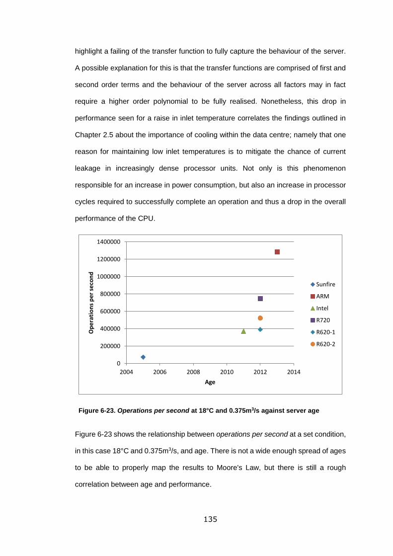
135
highlight a failing of the transfer function to fully capture the behaviour of the server.
A possible explanation for this is that the transfer functions are comprised of first and
second order terms and the behaviour of the server across all factors may in fact
require a higher order polynomial to be fully realised. Nonetheless, this drop in
performance seen for a raise in inlet temperature correlates the findings outlined in
Chapter 2.5 about the importance of cooling within the data centre; namely that one
reason for maintaining low inlet temperatures is to mitigate the chance of current
leakage in increasingly dense processor units. Not only is this phenomenon
responsible for an increase in power consumption, but also an increase in processor
cycles required to successfully complete an operation and thus a drop in the overall
performance of the CPU.
Figure 6-23. Operations per second at 18°C and 0.375m3/s against server age
Figure 6-23 shows the relationship between operations per second at a set condition,
in this case 18°C and 0.375m3/s, and age. There is not a wide enough spread of ages
to be able to properly map the results to Moore's Law, but there is still a rough
correlation between age and performance.
0
200000
400000
600000
800000
1000000
1200000
1400000
2004 2006 2008 2010 2012 2014
Op
era
tio
ns
pe
r se
con
d
Age
Sunfire
ARM
Intel
R720
R620-1
R620-2
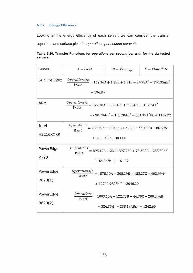
136
6.7.2 Energy Efficiency
Looking at the energy efficiency of each server, we can consider the transfer
equations and surface plots for operations per second per watt.
Table 6-20. Transfer Functions for operations per second per watt for the six tested servers.
Server 𝐴 = 𝐿𝑜𝑎𝑑 𝐵 = 𝑇𝑒𝑚𝑝𝑢𝑝 𝐶 = 𝐹𝑙𝑜𝑤 𝑅𝑎𝑡𝑒
SunFire v20z 𝑂𝑝𝑒𝑟𝑎𝑡𝑖𝑜𝑛𝑠/𝑠
𝑊𝑎𝑡𝑡= 162.36A + 1.28B + 1.31C − 34.78A2 − 190.35AB2
+ 196.84
ARM 𝑂𝑝𝑒𝑟𝑎𝑡𝑖𝑜𝑛𝑠/𝑠
𝑊𝑎𝑡𝑡= 972.30A − 509.16B + 135.46C − 187.24𝐴2
+ 690.70𝐴𝐵2 − 188.20A𝐶2 − 564.35𝐴2BC + 1167.22
Intel
H2216XXKR
𝑂𝑝𝑒𝑟𝑎𝑡𝑖𝑜𝑛𝑠
𝑊𝑎𝑡𝑡= 289.39A − 110.83B + 4.62C − 44.46AB − 86.59A2
+ 37.35𝐴2𝐵 + 383.44
PowerEdge
R720
𝑂𝑝𝑒𝑟𝑎𝑡𝑖𝑜𝑛𝑠
𝑊𝑎𝑡𝑡= 895.19A − 23.04B97.98C + 75.30AC − 255.50𝐴2
+ 164.94𝐵2 + 1161.97
PowerEdge
R620(1)
𝑂𝑝𝑒𝑟𝑎𝑡𝑖𝑜𝑛𝑠/𝑠
𝑊𝑎𝑡𝑡= 1578.10A − 208.29B + 152.27C − 403.99𝐴2
+ 12709.96A𝐵2𝐶 + 2046.20
PowerEdge
R620(2)
𝑂𝑝𝑒𝑟𝑎𝑡𝑖𝑜𝑛𝑠
𝑊𝑎𝑡𝑡= 1003.10A − 122.73B − 46.70C − 200.24AB
− 326.35𝐴2 − 238.18AB𝐶2 + 1342.60
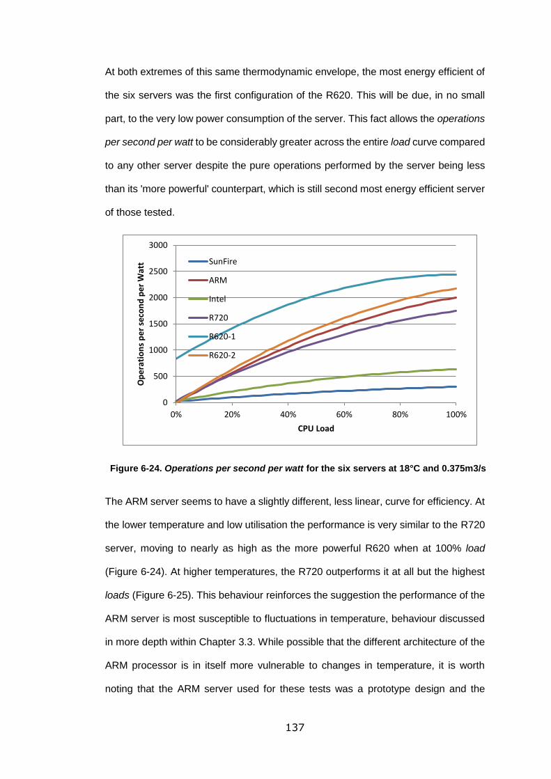
137
At both extremes of this same thermodynamic envelope, the most energy efficient of
the six servers was the first configuration of the R620. This will be due, in no small
part, to the very low power consumption of the server. This fact allows the operations
per second per watt to be considerably greater across the entire load curve compared
to any other server despite the pure operations performed by the server being less
than its 'more powerful' counterpart, which is still second most energy efficient server
of those tested.
Figure 6-24. Operations per second per watt for the six servers at 18°C and 0.375m3/s
The ARM server seems to have a slightly different, less linear, curve for efficiency. At
the lower temperature and low utilisation the performance is very similar to the R720
server, moving to nearly as high as the more powerful R620 when at 100% load
(Figure 6-24). At higher temperatures, the R720 outperforms it at all but the highest
loads (Figure 6-25). This behaviour reinforces the suggestion the performance of the
ARM server is most susceptible to fluctuations in temperature, behaviour discussed
in more depth within Chapter 3.3. While possible that the different architecture of the
ARM processor is in itself more vulnerable to changes in temperature, it is worth
noting that the ARM server used for these tests was a prototype design and the
0
500
1000
1500
2000
2500
3000
0% 20% 40% 60% 80% 100%
Op
era
tio
ns
pe
r se
con
d p
er
Wat
t
CPU Load
SunFire
ARM
Intel
R720
R620-1
R620-2
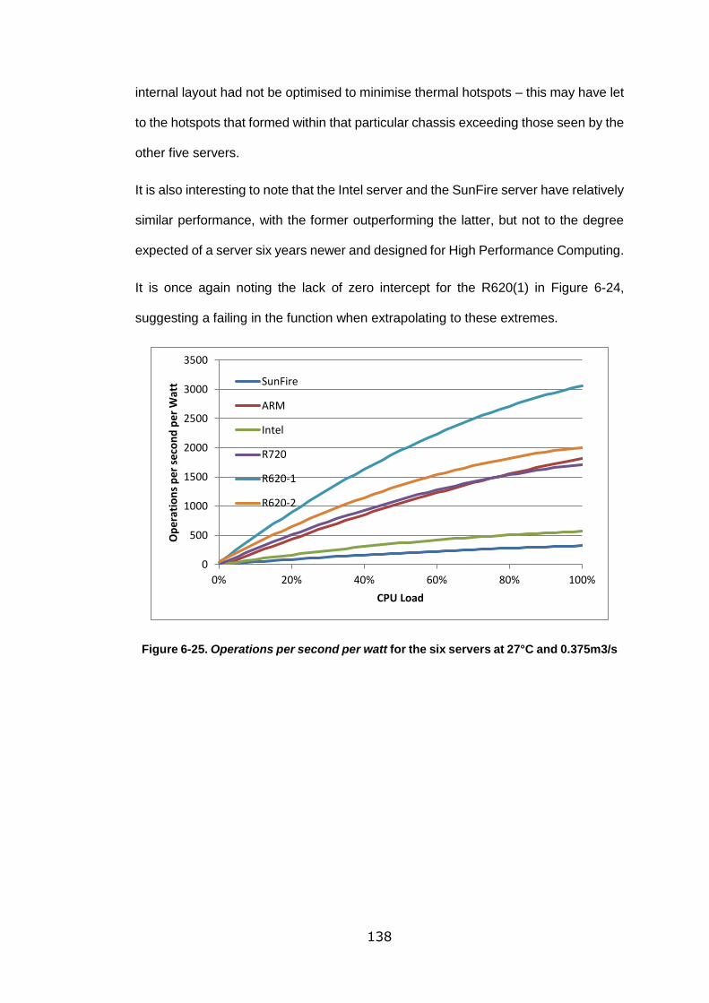
138
internal layout had not be optimised to minimise thermal hotspots – this may have let
to the hotspots that formed within that particular chassis exceeding those seen by the
other five servers.
It is also interesting to note that the Intel server and the SunFire server have relatively
similar performance, with the former outperforming the latter, but not to the degree
expected of a server six years newer and designed for High Performance Computing.
It is once again noting the lack of zero intercept for the R620(1) in Figure 6-24,
suggesting a failing in the function when extrapolating to these extremes.
Figure 6-25. Operations per second per watt for the six servers at 27°C and 0.375m3/s
0
500
1000
1500
2000
2500
3000
3500
0% 20% 40% 60% 80% 100%
Op
era
tio
ns
pe
r se
con
d p
er
Wat
t
CPU Load
SunFire
ARM
Intel
R720
R620-1
R620-2
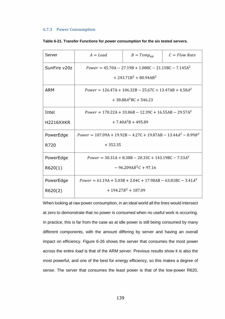
139
6.7.3 Power Consumption
Table 6-21. Transfer Functions for power consumption for the six tested servers.
Server 𝐴 = 𝐿𝑜𝑎𝑑 𝐵 = 𝑇𝑒𝑚𝑝𝑢𝑝 𝐶 = 𝐹𝑙𝑜𝑤 𝑅𝑎𝑡𝑒
SunFire v20z 𝑃𝑜𝑤𝑒𝑟 = 45.70A − 27.19B + 1.088C − 21.15BC − 7.145A2
+ 243.71B2 + 80.94AB2
ARM 𝑃𝑜𝑤𝑒𝑟 = 126.47A + 106.32B − 25.67C + 13.47AB + 4.58𝐴2
+ 38.88𝐴2BC + 546.23
Intel
H2216XXKR
𝑃𝑜𝑤𝑒𝑟 = 170.22A + 33.86B − 12.39C + 16.55AB − 29.57A2
+ 7.40A2B + 495.89
PowerEdge
R720
𝑃𝑜𝑤𝑒𝑟 = 107.09A + 19.92B − 4.27C + 19.87AB − 13.44𝐴2 − 8.99𝐵2
+ 352.35
PowerEdge
R620(1)
𝑃𝑜𝑤𝑒𝑟 = 30.31A + 8.38B − 20.33C + 143.19BC − 7.53𝐴2
− 96.209A𝐵2𝐶 + 97.16
PowerEdge
R620(2)
𝑃𝑜𝑤𝑒𝑟 = 61.19A + 5.03B + 2.04C + 17.98AB − 63.81BC − 3.41𝐴2
+ 194.27𝐵2 + 187.09
When looking at raw power consumption, in an ideal world all the lines would intersect
at zero to demonstrate that no power is consumed when no useful work is occurring.
In practice, this is far from the case as at idle power is still being consumed by many
different components, with the amount differing by server and having an overall
impact on efficiency. Figure 6-26 shows the server that consumes the most power
across the entire load is that of the ARM server. Previous results show it is also the
most powerful, and one of the best for energy efficiency, so this makes a degree of
sense. The server that consumes the least power is that of the low-power R620,
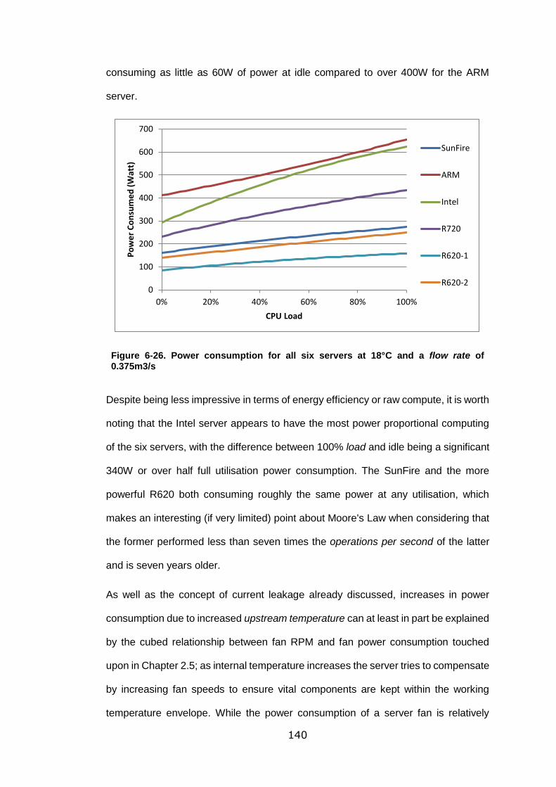
140
consuming as little as 60W of power at idle compared to over 400W for the ARM
server.
Figure 6-26. Power consumption for all six servers at 18°C and a flow rate of 0.375m3/s
Despite being less impressive in terms of energy efficiency or raw compute, it is worth
noting that the Intel server appears to have the most power proportional computing
of the six servers, with the difference between 100% load and idle being a significant
340W or over half full utilisation power consumption. The SunFire and the more
powerful R620 both consuming roughly the same power at any utilisation, which
makes an interesting (if very limited) point about Moore's Law when considering that
the former performed less than seven times the operations per second of the latter
and is seven years older.
As well as the concept of current leakage already discussed, increases in power
consumption due to increased upstream temperature can at least in part be explained
by the cubed relationship between fan RPM and fan power consumption touched
upon in Chapter 2.5; as internal temperature increases the server tries to compensate
by increasing fan speeds to ensure vital components are kept within the working
temperature envelope. While the power consumption of a server fan is relatively
0
100
200
300
400
500
600
700
0% 20% 40% 60% 80% 100%
Po
we
r C
on
sum
ed
(W
att)
CPU Load
SunFire
ARM
Intel
R720
R620-1
R620-2
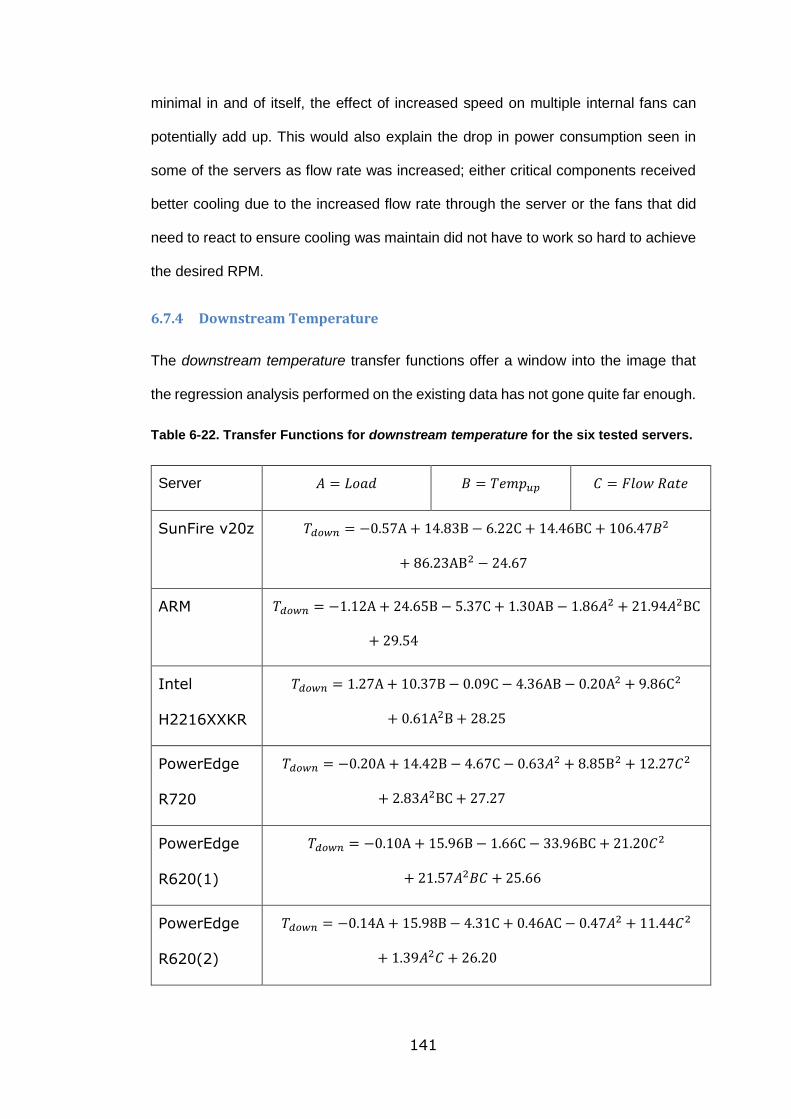
141
minimal in and of itself, the effect of increased speed on multiple internal fans can
potentially add up. This would also explain the drop in power consumption seen in
some of the servers as flow rate was increased; either critical components received
better cooling due to the increased flow rate through the server or the fans that did
need to react to ensure cooling was maintain did not have to work so hard to achieve
the desired RPM.
6.7.4 Downstream Temperature
The downstream temperature transfer functions offer a window into the image that
the regression analysis performed on the existing data has not gone quite far enough.
Table 6-22. Transfer Functions for downstream temperature for the six tested servers.
Server 𝐴 = 𝐿𝑜𝑎𝑑 𝐵 = 𝑇𝑒𝑚𝑝𝑢𝑝 𝐶 = 𝐹𝑙𝑜𝑤 𝑅𝑎𝑡𝑒
SunFire v20z 𝑇𝑑𝑜𝑤𝑛 = −0.57A + 14.83B − 6.22C + 14.46BC + 106.47𝐵2
+ 86.23AB2 − 24.67
ARM 𝑇𝑑𝑜𝑤𝑛 = −1.12A + 24.65B − 5.37C + 1.30AB − 1.86𝐴2 + 21.94𝐴2BC
+ 29.54
Intel
H2216XXKR
𝑇𝑑𝑜𝑤𝑛 = 1.27A + 10.37B − 0.09C − 4.36AB − 0.20A2 + 9.86C2
+ 0.61A2B + 28.25
PowerEdge
R720
𝑇𝑑𝑜𝑤𝑛 = −0.20A + 14.42B − 4.67C − 0.63𝐴2 + 8.85B2 + 12.27𝐶2
+ 2.83𝐴2BC + 27.27
PowerEdge
R620(1)
𝑇𝑑𝑜𝑤𝑛 = −0.10A + 15.96B − 1.66C − 33.96BC + 21.20𝐶2
+ 21.57𝐴2𝐵𝐶 + 25.66
PowerEdge
R620(2)
𝑇𝑑𝑜𝑤𝑛 = −0.14A + 15.98B − 4.31C + 0.46AC − 0.47𝐴2 + 11.44𝐶2
+ 1.39𝐴2𝐶 + 26.20
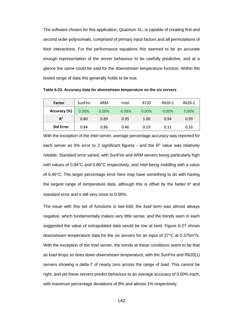
142
The software chosen for this application, Quantum XL, is capable of creating first and
second order polynomials, comprised of primary input factors and all permutations of
their interactions. For the performance equations this seemed to be an accurate
enough representation of the server behaviour to be usefully predictive, and at a
glance the same could be said for the downstream temperature function. Within the
tested range of data this generally holds to be true.
Table 6-23. Accuracy data for downstream temperature on the six servers
Factor SunFire ARM Intel R720 R620-1 R620-2
Accuracy (%) 0.00% 0.00% -0.08% 0.00% 0.00% 0.00%
R2 0.80 0.89 0.95 1.00 0.94 0.99
Std Error 0.84 0.86 0.46 0.19 0.11 0.16
With the exception of the Intel server, average percentage accuracy was reported for
each server as 0% error to 2 significant figures - and the R2 value was relatively
reliable. Standard error varied, with SunFire and ARM servers being particularly high
with values of 0.84°C and 0.86°C respectively, and Intel being middling with a value
of 0.46°C. The larger percentage error here may have something to do with having
the largest range of temperature data, although this is offset by the better R2 and
standard error and it still very close to 0.00%.
The issue with this set of functions is two-fold; the load term was almost always
negative, which fundamentally makes very little sense; and the trends seen in each
suggested the value of extrapolated data would be low at best. Figure 6-27 shows
downstream temperature data for the six servers for an input of 27°C at 0.375m3/s.
With the exception of the Intel server, the trends at these conditions seem to be that
as load drops so does down downstream temperature, with the SunFire and R620(1)
servers showing a delta-T of nearly zero across the range of load. This cannot be
right, and yet these servers predict behaviour to an average accuracy of 0.00% each,
with maximum percentage deviations of 8% and almost 1% respectively.
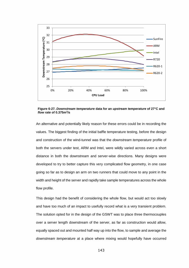
143
Figure 6-27. Downstream temperature data for an upstream temperature of 27°C and flow rate of 0.375m3/s
An alternative and potentially likely reason for these errors could be in recording the
values. The biggest finding of the initial baffle temperature testing, before the design
and construction of the wind-tunnel was that the downstream temperature profile of
both the servers under test, ARM and Intel, were wildly varied across even a short
distance in both the downstream and server-wise directions. Many designs were
developed to try to better capture this very complicated flow geometry, in one case
going so far as to design an arm on two runners that could move to any point in the
width and height of the server and rapidly take sample temperatures across the whole
flow profile.
This design had the benefit of considering the whole flow, but would act too slowly
and have too much of an impact to usefully record what is a very transient problem.
The solution opted for in the design of the GSWT was to place three thermocouples
over a server length downstream of the server, as far as construction would allow,
equally spaced out and mounted half way up into the flow, to sample and average the
downstream temperature at a place where mixing would hopefully have occurred
25
26
27
28
29
30
31
32
33
0% 20% 40% 60% 80% 100%
Do
wn
stre
am T
em
pe
ratu
re (
oC
)
CPU Load
SunFire
ARM
Intel
R720
R620-1
R620-2
144
while having minimal impact on the readings themselves. This design also neglected
leakage within the downstream portion of the wind-tunnel, which was unfortunately
unavoidable and could have potentially effected results. There was also variation
across the three temperature probes which was very server- and situation-specific,
with some values being nearly identical and some variation being as high as 1.0°C
difference between neighbouring probes. Variation between servers will have been
due to different component layouts internally, while changes in variation for different
loads will likely have been due to the presence of multiple processors on some
servers, the distribution of computing resources for a given load, and changes in
server fan behaviour.
For upstream temperatures the same configurations of thermocouples was used,
although these temperature probes were situated a little closer to the inlet than the
downstream ones were to the outlet due to the shape of the tunnel and the reliance
on the flow being more linear upstream. These K-type thermocouples were all
calibrated in the datalogger on installation. Despite this, they had been in use for at
least four years and the possibility of degradation exists. Compound that with the idea
that there simply are not enough to adequately capture the complicated flow profile
and the second-order limitations of the regression analysis software and it is possible
that a picture emerges for some of the less intuitive behaviour of these functions.
Nonetheless, it is still worth noting the accuracies recorded within the testing ranges
for each server would suggest that provided the range tested encompasses the
conditions the server will be run at in the actual data centre then the results can still
be trusted with reasonable confidence. The variation in temperature ranges tested
lies at least in part in the setting of the GSWT and the other activities in the lab space.
Upstream temperature was very much at the mercy of room temperature; a factor that
could not be controlled and would vary greatly dependant on time of day, time of year,
and other experiments occurring in the vicinity. These factors compounded to see
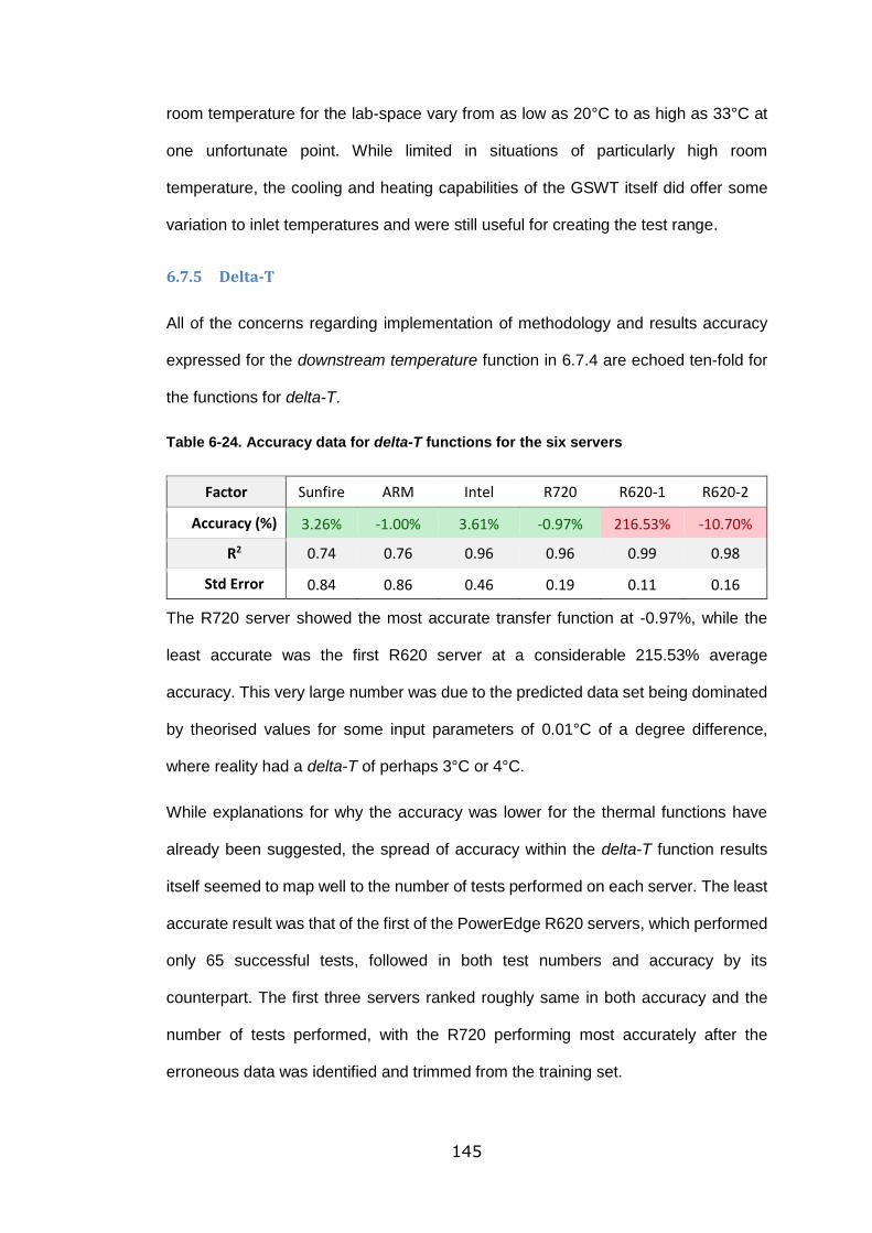
145
room temperature for the lab-space vary from as low as 20°C to as high as 33°C at
one unfortunate point. While limited in situations of particularly high room
temperature, the cooling and heating capabilities of the GSWT itself did offer some
variation to inlet temperatures and were still useful for creating the test range.
6.7.5 Delta-T
All of the concerns regarding implementation of methodology and results accuracy
expressed for the downstream temperature function in 6.7.4 are echoed ten-fold for
the functions for delta-T.
Table 6-24. Accuracy data for delta-T functions for the six servers
Factor Sunfire ARM Intel R720 R620-1 R620-2
Accuracy (%) 3.26% -1.00% 3.61% -0.97% 216.53% -10.70%
R2 0.74 0.76 0.96 0.96 0.99 0.98
Std Error 0.84 0.86 0.46 0.19 0.11 0.16
The R720 server showed the most accurate transfer function at -0.97%, while the
least accurate was the first R620 server at a considerable 215.53% average
accuracy. This very large number was due to the predicted data set being dominated
by theorised values for some input parameters of 0.01°C of a degree difference,
where reality had a delta-T of perhaps 3°C or 4°C.
While explanations for why the accuracy was lower for the thermal functions have
already been suggested, the spread of accuracy within the delta-T function results
itself seemed to map well to the number of tests performed on each server. The least
accurate result was that of the first of the PowerEdge R620 servers, which performed
only 65 successful tests, followed in both test numbers and accuracy by its
counterpart. The first three servers ranked roughly same in both accuracy and the
number of tests performed, with the R720 performing most accurately after the
erroneous data was identified and trimmed from the training set.
146
The reason for the decline in the number of tests performed was two-fold; as testing
progressed competition for lab space and equipment grew and later tests were
performed at the expense of other users' experiments and so had to be minimised in
length as much as possible. The ARM, Intel, and SunFire tests were performed
intermittently across the space of over a year, with pauses between sets of data for
review and analysis. The PowerEdge servers were acquired later, and testing of them
was performed in two-week and one-week slots for the R720 and two R620s
respectively. This served the purpose of developing new data points for analysis and
determining what effect, if any, lowering the number of points tested had on the
accuracy of the functions created. While the results for the performance functions
would suggest testing duration for the PowerEdge servers was adequate to develop
behavioural models, the delta-T (and to a lesser extent downstream temperature)
functions suggest that not enough data was collected to properly create a trend; either
in volume of data or range. Compound this with the thermal fluctuations in the ambient
conditions of the lab and therefore knock-on variations in the inlet temperature and
server fan behaviour, and it would provide one potential explanation for the lower
accuracy of these results.
6.8 Summary
The work presented in this chapter constitutes six case studies for the methodology
outlined in chapter 5. These case studies have been performed on servers from 2005
to 2013, designed for a variety of purposes and with different capabilities and power
consumptions. Three of the five outputs considered performance, specifically;
operations per second, power consumption, and operations per second per watt. The
transfer functions for these attributes correlate strongly with recorded values on
average, allowing for responses in performance behaviour due to changes in the input
factors to be predicted reliably for each server, and giving a good indication of server
behaviour trends when considered as a whole. The two other output factors

147
considered were that of downstream temperature and delta-T, the former of which
achieved similar values of accuracy as those of server performance. While average
accuracy was considerable for each transfer function generated, the presence of
outliers and the variation in coefficient of determination seen should be noted. While
the existence of some variance does not detract from the effectiveness of each
function, there exists the possibility any functions that saw very high variance may
benefit from the inclusion of addition variables outside of the three tested here. This
should certainly be done with caution however, as any regression contains the
inherent risk of over-fitting; that is creating a model that is overly influenced by the
existence out outliers and not indictive of the wider behaviour of the server itself.
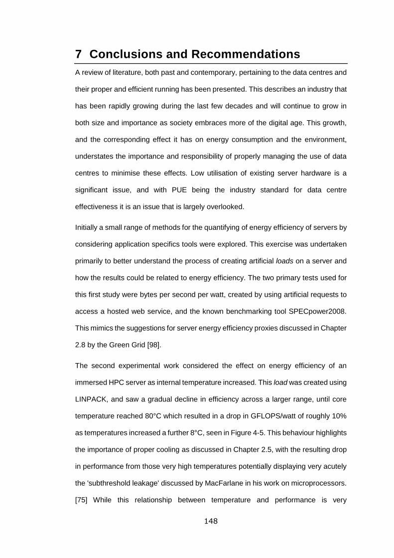
148
7 Conclusions and Recommendations
A review of literature, both past and contemporary, pertaining to the data centres and
their proper and efficient running has been presented. This describes an industry that
has been rapidly growing during the last few decades and will continue to grow in
both size and importance as society embraces more of the digital age. This growth,
and the corresponding effect it has on energy consumption and the environment,
understates the importance and responsibility of properly managing the use of data
centres to minimise these effects. Low utilisation of existing server hardware is a
significant issue, and with PUE being the industry standard for data centre
effectiveness it is an issue that is largely overlooked.
Initially a small range of methods for the quantifying of energy efficiency of servers by
considering application specifics tools were explored. This exercise was undertaken
primarily to better understand the process of creating artificial loads on a server and
how the results could be related to energy efficiency. The two primary tests used for
this first study were bytes per second per watt, created by using artificial requests to
access a hosted web service, and the known benchmarking tool SPECpower2008.
This mimics the suggestions for server energy efficiency proxies discussed in Chapter
2.8 by the Green Grid [98].
The second experimental work considered the effect on energy efficiency of an
immersed HPC server as internal temperature increased. This load was created using
LINPACK, and saw a gradual decline in efficiency across a larger range, until core
temperature reached 80°C which resulted in a drop in GFLOPS/watt of roughly 10%
as temperatures increased a further 8°C, seen in Figure 4-5. This behaviour highlights
the importance of proper cooling as discussed in Chapter 2.5, with the resulting drop
in performance from those very high temperatures potentially displaying very acutely
the 'subthreshold leakage' discussed by MacFarlane in his work on microprocessors.
[75] While this relationship between temperature and performance is very
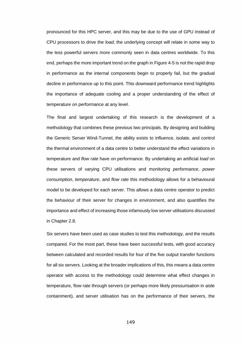
149
pronounced for this HPC server, and this may be due to the use of GPU instead of
CPU processors to drive the load, the underlying concept will relate in some way to
the less powerful servers more commonly seen in data centres worldwide. To this
end, perhaps the more important trend on the graph in Figure 4-5 is not the rapid drop
in performance as the internal components begin to properly fail, but the gradual
decline in performance up to this point. This downward performance trend highlights
the importance of adequate cooling and a proper understanding of the effect of
temperature on performance at any level.
The final and largest undertaking of this research is the development of a
methodology that combines these previous two principals. By designing and building
the Generic Server Wind-Tunnel, the ability exists to influence, isolate, and control
the thermal environment of a data centre to better understand the effect variations in
temperature and flow rate have on performance. By undertaking an artificial load on
these servers of varying CPU utilisations and monitoring performance, power
consumption, temperature, and flow rate this methodology allows for a behavioural
model to be developed for each server. This allows a data centre operator to predict
the behaviour of their server for changes in environment, and also quantifies the
importance and effect of increasing those infamously low server utilisations discussed
in Chapter 2.8.
Six servers have been used as case studies to test this methodology, and the results
compared. For the most part, these have been successful tests, with good accuracy
between calculated and recorded results for four of the five output transfer functions
for all six servers. Looking at the broader implications of this, this means a data centre
operator with access to the methodology could determine what effect changes in
temperature, flow rate through servers (or perhaps more likely pressurisation in aisle
containment), and server utilisation has on the performance of their servers, the
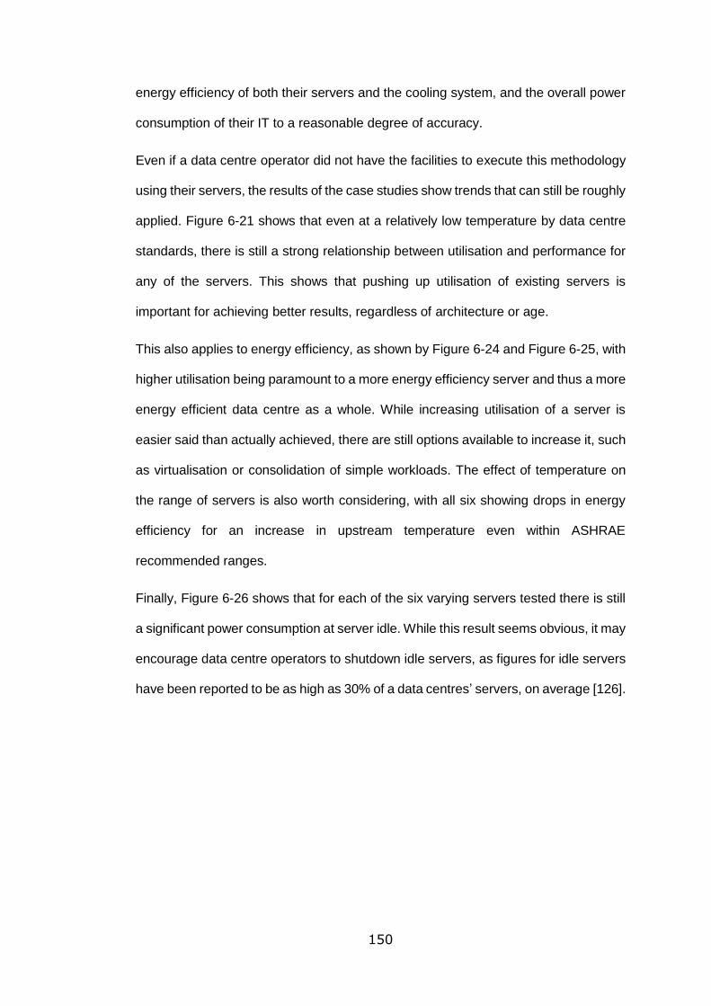
150
energy efficiency of both their servers and the cooling system, and the overall power
consumption of their IT to a reasonable degree of accuracy.
Even if a data centre operator did not have the facilities to execute this methodology
using their servers, the results of the case studies show trends that can still be roughly
applied. Figure 6-21 shows that even at a relatively low temperature by data centre
standards, there is still a strong relationship between utilisation and performance for
any of the servers. This shows that pushing up utilisation of existing servers is
important for achieving better results, regardless of architecture or age.
This also applies to energy efficiency, as shown by Figure 6-24 and Figure 6-25, with
higher utilisation being paramount to a more energy efficiency server and thus a more
energy efficient data centre as a whole. While increasing utilisation of a server is
easier said than actually achieved, there are still options available to increase it, such
as virtualisation or consolidation of simple workloads. The effect of temperature on
the range of servers is also worth considering, with all six showing drops in energy
efficiency for an increase in upstream temperature even within ASHRAE
recommended ranges.
Finally, Figure 6-26 shows that for each of the six varying servers tested there is still
a significant power consumption at server idle. While this result seems obvious, it may
encourage data centre operators to shutdown idle servers, as figures for idle servers
have been reported to be as high as 30% of a data centres’ servers, on average [126].
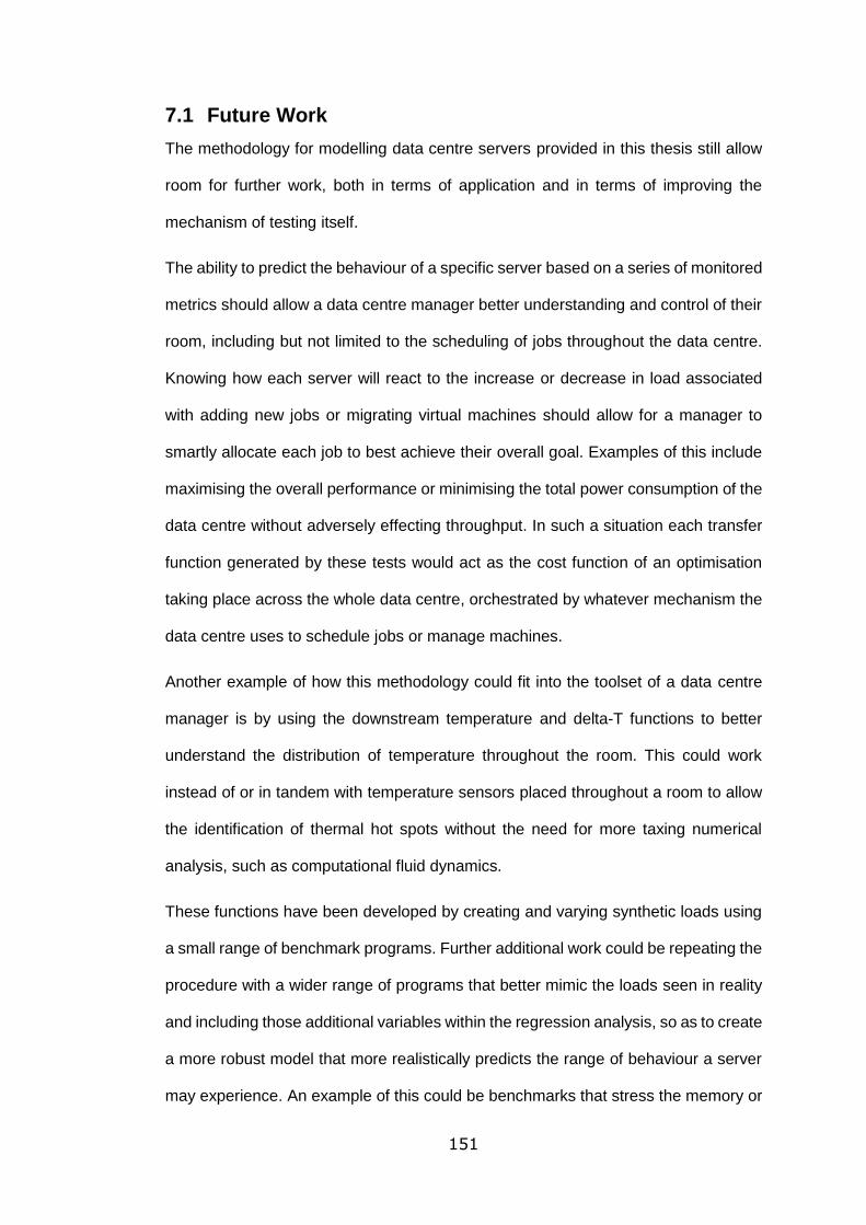
151
7.1 Future Work
The methodology for modelling data centre servers provided in this thesis still allow
room for further work, both in terms of application and in terms of improving the
mechanism of testing itself.
The ability to predict the behaviour of a specific server based on a series of monitored
metrics should allow a data centre manager better understanding and control of their
room, including but not limited to the scheduling of jobs throughout the data centre.
Knowing how each server will react to the increase or decrease in load associated
with adding new jobs or migrating virtual machines should allow for a manager to
smartly allocate each job to best achieve their overall goal. Examples of this include
maximising the overall performance or minimising the total power consumption of the
data centre without adversely effecting throughput. In such a situation each transfer
function generated by these tests would act as the cost function of an optimisation
taking place across the whole data centre, orchestrated by whatever mechanism the
data centre uses to schedule jobs or manage machines.
Another example of how this methodology could fit into the toolset of a data centre
manager is by using the downstream temperature and delta-T functions to better
understand the distribution of temperature throughout the room. This could work
instead of or in tandem with temperature sensors placed throughout a room to allow
the identification of thermal hot spots without the need for more taxing numerical
analysis, such as computational fluid dynamics.
These functions have been developed by creating and varying synthetic loads using
a small range of benchmark programs. Further additional work could be repeating the
procedure with a wider range of programs that better mimic the loads seen in reality
and including those additional variables within the regression analysis, so as to create
a more robust model that more realistically predicts the range of behaviour a server
may experience. An example of this could be benchmarks that stress the memory or

152
disk components of a server, instead of just the CPU or network tests seen within this
thesis. It is worth noting that every additional variable included in the creation of a
model will increase the time needed to perform the regression and calculate each
function.
The testing procedure itself could also be improved upon. for the purposes of the
tests, the Generic Server Wind-Tunnel had a degree of manual control and
monitoring. Ideally, future work would involve automation of some of these processes,
with the potential to fully integrate it into the existing remote architecture available in
the laboratory space in which it is housed, with adequate safety override protocols to
allow for safe remote running, as shown in Figure 7-1.
The measurement and monitoring of the thermal environment conducted by the TC-
08 8-channel data logger should relate data directly to the Control and Collect System
(CCS) as opposed to a separate laptop in the laboratory as is the case currently.
The fan is powered by a 24V nominal power supply and controlled by a separate 0-
10V signal. Currently this is manually controlled but in the future should be driven by
a digital to analogue PCI card, either directly in the CCS or in another slave of the
system. By interfacing the flow rate data provided by the averaging Pitot tube with the
outputs to the fan speed provided by the PCI card in the control system, this will allow
for precise control of the flow rate through each server under testing as well as
external control for moving from one flow rate design point to another during workload
tests.
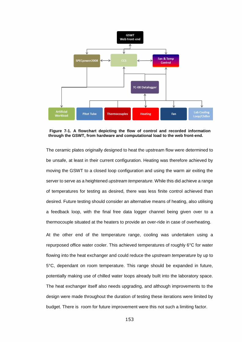
153
Figure 7-1. A flowchart depicting the flow of control and recorded information through the GSWT, from hardware and computational load to the web front-end.
The ceramic plates originally designed to heat the upstream flow were determined to
be unsafe, at least in their current configuration. Heating was therefore achieved by
moving the GSWT to a closed loop configuration and using the warm air exiting the
server to serve as a heightened upstream temperature. While this did achieve a range
of temperatures for testing as desired, there was less finite control achieved than
desired. Future testing should consider an alternative means of heating, also utilising
a feedback loop, with the final free data logger channel being given over to a
thermocouple situated at the heaters to provide an over-ride in case of overheating.
At the other end of the temperature range, cooling was undertaken using a
repurposed office water cooler. This achieved temperatures of roughly 6°C for water
flowing into the heat exchanger and could reduce the upstream temperature by up to
5°C, dependant on room temperature. This range should be expanded in future,
potentially making use of chilled water loops already built into the laboratory space.
The heat exchanger itself also needs upgrading, and although improvements to the
design were made throughout the duration of testing these iterations were limited by
budget. There is room for future improvement were this not such a limiting factor.

154
Finally, with the process fully, or more fully, automated in the future the logical
conclusion would be to stream results to a web-front end for monitoring and even
perform the require regression analysis automatically. Currently tests could be
undertaken anywhere with secure shell access, but understanding the results
required intimate experience with the process, and changing some parameters
required a physical presence. The end goal for the GSWT should be to include results
processing as an automated step and provide an intuitively understandable output
report to the user, without the current high level of post-processing to create
accessible results.
Once these changes were made to the GSWT itself, there should be more tests
conducted on a wider range of servers, with a greater variation in age and size. These
would allow for greater validation of the methodology and a more intuitive
understanding of the relationship between the input factors and general server
behaviour, and aid in developing better practices for energy efficiency and power
consumption in the wider data centre world.

155
Bibliography
[1] aql, “Colocation in Leeds,” [Online]. Available:
https://www.aql.com/news/268/. [Accessed 16 12 2014].
[2] SearchMicroServices, “colocation (colo),” 08 2015. [Online]. Available:
http://searchmicroservices.techtarget.com/definition/colocation-colo.
[Accessed 20 11 2017].
[3] J. Mitchell-Jackson, J. G. Koomey, M. Blazek and B. Nordman, “National and
regional implications of internet data center growth in the US,” Resources,
conservation and Recycling, vol. 36, no. 3, pp. 175-185, 2002.
[4] J. Glanz, “THE CLOUD FACTORIES - Power, Pollution and the Internet,” The
New York Times, 22 9 2012. [Online]. Available:
http://www.nytimes.com/2012/09/23/technology/data-centers-waste-vast-
amounts-of-energy-belying-industry-image.html?pagewanted=all&_r=1&.
[Accessed 14 12 2014].
[5] Uptime Institute, “2013 Data Center Survey Results,” 14 08 2013. [Online].
Available: http://blog.uptimeinstitute.com/2013/08/2013-data-center-industry-
survey-results/. [Accessed 14 12 2014].
[6] J. Koomey, “Growth in data center electricity use 2005 to 2010.,” A report by
Analytical Press, completed at the request of The New York Times, 2011.
[7] J. Karlsson and B. Moshfegh, “Investigation of indoor climate and power
usage in a data center,” Energy and Buildings, vol. 37, no. 10, pp. 1075-
1083, 2005.
156
[8] H. S. Dunn, “Thematic Reports, Global information society watch 2010,
Focus on ICTs and environmental sustainability (APC & HIVOS).,” 2010.
[9] G. Cook and D. Pomerantz, “Clicking clean: A guide to building the green
Internet.,” 05 2015. [Online]. Available: http://www. greenpeace. org/usa/wp-
content/uploads/legacy/Global/usa/planet3/PDFs/2015ClickingClean. pdf.
[Accessed 16 01 2017].
[10] M. Avgerinou, P. Bertoldi and L. Castellazzi, “Trends in Data Centre Energy
Consumption under the European Code of Conduct for Data Centre Energy
Efficiency.,” Energies, vol. 10, no. 10, 2017.
[11] M. Acton, L. Newcombe, J. Booth, S. Flucker, P. Latham, S. Strutt and T.
Tozer, “2017 Best Practice Guidelines for the EU Code of Conduct on Data
Centre Energy Efficiency,” Publications Office of the European Union, 2017.
[12] Y. Joshi and P. Kumar, “Introduction to Data Center Energy Flow and
Thermal Management,” in Energy Efficient Thermal Management of Data
Centers, Springer US, 2012, pp. 1-38.
[13] B. Fakhim, M. Behnia, S. Armfield and N. Srinarayana, “Cooling solutions in
an operational data centre: A case study,” Applied Thermal Engineering, vol.
31, no. 14, pp. 2279-2291, 2011.
[14] S. Shrivastava, B. Sammakia, R. Schmidt, M. Iyengar and J. Van Gilder,
“Experimental-Numerical Comparison for a High-Density Data Center: Hot
Spot Heat Fluxes in Excess of 500 W/ft2.,” in Thermal and
Thermomechanical Phenomena in Electronics Systems, 2006. ITHERM'06.
The Tenth Intersociety Conference on., 2006.
157
[15] L. A. Barroso and U. Hölzle, “The case for energy-proportional computing.,”
Computer, vol. 40, no. 12, 2007.
[16] A. Greenberg, J. Hamilton, D. Maltz and P. Patel, “The cost of a cloud:
research problems in data center networks,” ACM SIGCOMM computer
communication review, vol. 39, no. 1, pp. 68-73, 2008.
[17] M. K. Patterson, “Energy Efficiency Metrics,” in Energy Efficient Thermal
Management of Data Centres, 2012.
[18] M. Arregoces and M. Portolani, Data center fundamentals, Cisco Systems,
Inc, 2004.
[19] R. Lindsay, “Trend: Colocation facilities provide tools to manage data center
infrastructure,” Network World, 22 6 2017. [Online]. Available:
https://www.networkworld.com/article/3203026/data-center/trend-colocation-
facilities-provide-enterprises-with-tools-to-manage-data-center-
infrastructure.html. [Accessed 1 8 2016].
[20] K. Kant, “Data center evolution: A tutorial on state of the art, issues, and
challenges,” Computer Networks, vol. 53, no. 17, pp. 2939-2965, 2009.
[21] K. Ebrahimi, G. Jones and A. Fleischer, “A review of data center cooling
technology, operating conditions and the corresponding low-grade waste
heat recovery opportunities,” Renewable and Sustainable Energy Reviews,
vol. 31, pp. 622-638, 2014.
[22] X. Fan, W. D. Weber and L. A. Barroso, “Power provisioning for a
warehouse-sized computer,” ACM SIGARCH Computer Architecture News.,
vol. 35, no. 2, 2007.
158
[23] L. A. Barroso, J. Clidaras and U. Hölzle, “Datacenter Basics,” in The
Datacenter as a Computer: An Introduction to the Design of Warehouse-
Scale Machines, Madison, Morgan & Claypool Publishers, 2009, pp. 47-66.
[24] R. Miller, “Facebook Has Spent $210 Million on Oregon Data Center,” Data
Center Knowledge, 30 01 2012. [Online]. Available:
http://www.datacenterknowledge.com/archives/2012/01/30/facebook-has-
spent-210-million-on-oregon-data-center. [Accessed 10 04 2017].
[25] P. Kumar and Y. Joshi, “Fundamentals of Data Center Airflow Management,”
in Energy Efficient Thermal Management of Data Centers, Springer, 2012.
[26] D. Anderson, “IEEE Annals of the History of Computing,” in Tom Kilburn: A
Pioneer of Computer Design, IEEE, 2009, pp. 82-86.
[27] A. Bartels, “Data Center Evolution: 1960 to 2000,” CLOUD INDUSTRY
INSIGHTS , 31 8 2011. [Online]. Available:
http://www.rackspace.com/blog/datacenter-evolution-1960-to-2000/.
[Accessed 12 12 2014].
[28] M. Ellsworth, L. Campbell, R. Simons, M. Iyengar, R. Schmidt and R. Chu,
“The evolution of water cooling for IBM large server systems: Back to the
future.,” in Thermal and Thermomechanical Phenomena in Electronic
Systems, 2008. ITHERM 2008. 11th Intersociety Conference on, 2008.
[29] J. Woods, “The evolution of the data center : Timeline from the Mainframe to
the Cloud,” Silicon Angle, 5 3 2014. [Online]. Available:
http://siliconangle.com/blog/2014/03/05/the-evolution-of-the-data-center-
timeline-from-the-mainframe-to-the-cloud-tc0114/?. [Accessed 5 12 14].
159
[30] M. Walport, “The Internet of Things: making the most of the Second Digital
Revolution,” UK Government, London, 2014.
[31] G. Moore, “Cramming more components onto integrated circuits.,”
Electronics, vol. 38, 1965.
[32] G. Moore, “Progress in digital integrated electronics,” Electron Devices
Meeting, vol. 21, 1975.
[33] P. Huber and M. Mills, “Dig more coal -- the PCs are coming,” Forbes, 1999.
[34] Lawrence Berkeley National Laboratory , “COMPUTERS ARE GREEN
AFTER ALL,” Wired, 2001.
[35] R. E. Brown, E. R. Masanet, B. Nordman, W. F. Tschudi, A. Shehabi, J.
Stanley, J. G. S. D. A. Koomey and P. T. Chan, “Report to Congress on
Server and Data Center Energy Efficiency: Public Law 109-431,”
Environmental Protection Agency, 2008.
[36] A. Shehabi, S. Smith, D. Sartor, R. Brown, M. Herrlin, J. Koomey, E.
Masanet, N. Horner, I. Azevedo and W. Lintner, “United States Data Center
Energy Usage Report,” Lawrence Berkeley National Laboratory, 2016.
[37] J. Koomey, “A Decade of Data Center Efficiency: What’s Past is Prologue!,”
in Semi-Therm 2017, San Jose, 2017.
[38] International Energy Agency, Worlds Energy Outlook 2012, 2012.
[39] D. Mascola, “CRAC VS CRAH,” Data Center Huddle, 11 08 2011. [Online].
Available: http://www.dchuddle.com/2011/crac-v-crah/. [Accessed 20 12
2017].
160
[40] S. Yeo and H. H. S. Lee, “Peeling the Power Onion of Data Centers,” in
Energy Efficient Thermal Management of Data Centers, Atlanta, Springer
Science+Business Media, 2012, pp. 137-169.
[41] S. Greenberg, E. Mills, B. Tschudi, P. Rumsey and B. Myatt, “Best practices
for data centers: Lessons learned from benchmarking 22 data centers.,”
Proceedings of the ACEEE Summer Study on Energy Efficiency in Buildings
in Asilomar, CA. ACEEE,, pp. 76-87, 2006.
[42] S. Mittal, “Power Management Techniques for Data Centers: A Survey,”
2014.
[43] C. D. Patel, “A vision of energy aware computing from chips to data centers,”
in The International Symposium on Micro-Mechanical Engineering. , 2003.
[44] T. Lu, X. Lü, M. Remes and M. Viljanen, “Investigation of air management
and energy performance in a data center in Finland: Case study,” Energy and
Buildings , vol. 43, no. 12, pp. 3360-3372, 2011.
[45] LBNL, “Data centre website of Lawrence Berkeley National Laboratory;,”
2003. [Online]. Available: http://hightech.lbl.gov/datacenters. [Accessed 1 12
2014].
[46] H. S. Sun and S. E. Lee, “Case study of data centers' energy performance,”
Energy and Buildings, vol. 38, no. 5, pp. 522-533, 2006.
[47] Uptime Institute, “Heat Density Trends in Data Processing, Computer
Systems and Telecommunications Equipment,” The Upsite Network, Santa
Fe, NM, 2000.
[48] D. Lazarus, “Net Complex A Dilemma For San Jose / SERVER FARM: Plant
would tax grid,” San Francisco Chronicle, 22 3 2001.
161
[49] J. Mitchell-Jackson, J. G. Koomey, B. Nordman and M. Blazek, “Data center
power requirements: measurements from Silicon Valley,” Energy, vol. 28, no.
8, pp. 837-850, 2003.
[50] P. Parida, M. David, M. Iyengar, M. Schultz, M. Gaynes, V. Kamath, B.
Kochuparambil and T. Chainer, “Experimental investigation of water cooled
server microprocessors and memory devices in an energy efficient chiller-
less data center,” in Semiconductor Thermal Measurement and Management
Symposium (SEMI-THERM), 2012 28th Annual IEEE, 2012.
[51] M. David, M. Iyengar, P. Parida, R. Simons, M. Schultz, M. Gaynes, R.
Schmidt and T. Chainer, “Experimental characterization of an energy efficient
chiller-less data center test facility with warm water cooled servers,” in
Semiconductor Thermal Measurement and Management Symposium (SEMI-
THERM), 2012 28th Annual IEEE, 2012.
[52] J. Summers, N. Kapur and H. Thompson, “Design of Data Centre Rack
Arrangements Using Open Source Software,” in Semiconductor Thermal
Measurement and Management Symposium (SEMI-THERM), 2013 29th
Annual IEEE, 2013.
[53] E. Samadiani, Y. Joshi and F. Mistree, “The thermal design of a next
generation data center: a conceptual exposition,” Journal of Electronic
Packaging, vol. 130, no. 4, 2008.
[54] J. Marcinichen, J. Olivier and J. Thome, “On-chip two-phase cooling of
datacenters: Cooling system and energy recovery evaluation,” Applied
Thermal Engineering, vol. 41, pp. 36-51, 2012.
162
[55] A. Shah and C. Patel, “Designing environmentally sustainable electronic
cooling systems using exergo‐thermo‐volumes,” International Journal of
Energy Research, vol. 33, no. 14, pp. 1266-1277, 2009.
[56] J. Marcinichen, J. Thome and B. Michel, “Cooling of microprocessors with
micro-evaporation: A novel two-phase cooling cycle,” International Journal of
Refrigeration, vol. 33, no. 7, pp. 1264-1276, 2010.
[57] M. Iyengar, M. David, P. Parida, V. Kamath, B. Kochuparambil, D. Graybill,
M. Schultz, M. Gaynes, R. Simons, R. Schmidt and T. Chainer, “Server liquid
cooling with chiller-less data center design to enable significant energy
savings,” in Iyengar, Madhusudan, et al. "Server liquid cooling with chiller-
less data center design to enable significant energy savings." Semiconductor
Thermal Measurement and Management Symposium (SEMI-THERM), 2012
28th Annual IEEE, 2012.
[58] G. A. Brady, N. Kapur, J. L. Summers and H. M. Thompson, “A case study
and critical assessment in calculating power usage effectiveness for a data
centre,” Energy Conversion and Management, vol. 76, pp. 155-161, 2013.
[59] C. Longbottom, “Water cooling vs. air cooling: The rise of water use in data
centres,” Computer Weekly, 08 2011. [Online]. Available:
http://www.computerweekly.com/tip/Water-cooling-vs-air-cooling-The-rise-of-
water-use-in-data-centres. [Accessed 20 11 2017].
[60] R. Schmidt, E. Cruz and M. Iyengar, “Challenges of data center thermal
management,” IBM Journal of Research and Development, vol. 49, no. 4.5,
pp. 709-723, 2005.
[61] D. Dyer, “Current trends/challenges in datacenter thermal management—a
facilities perspective,” in presentation at ITHERM, San Diego, CA, 2006.
163
[62] A. Radmehr, R. Schmidt, K. Karki and S. Patankar, “Distributed leakage flow
in raised-floor data centers,” in ASME 2005 Pacific Rim Technical
Conference and Exhibition on Integration and Packaging of MEMS, NEMS,
and Electronic Systems collocated with the ASME 2005 Heat Transfer
Summer Conference., 2005.
[63] R. Schmidt and E. Cruz, “Cluster of high powered racks within a raised floor
computer data center: effect of perforated tile flow distribution on rack inlet air
temperatures,” in ASME 2003 International Mechanical Engineering
Congress and Exposition. American Society of Mechanical Engineers, 2003.
[64] R. Schmidt, K. Karki and S. and Patankar, “Raised-floor data center:
perforated tile flow rates for various tile layouts,” in Thermal and
Thermomechanical Phenomena in Electronic Systems, 2004. ITHERM'04.
The Ninth Intersociety Conference on, 2004.
[65] R. Schmidt, K. Karki, K. Kelkar, A. Radmehr and S. Patankar,
“Measurements and predictions of the flow distribution through perforated
tiles in raised floor data centers,” in Proc. of Pacific Rim/ASME International
Electronic Packaging Technical Conferenceof (IPACK), Kauai, HI, 2001.
[66] J. VanGilder and R. Schmidt, “Airflow Uniformity through perforated tiles in a
raised-floor Data Center,” in ASME 2005 Pacific Rim Technical Conference
and Exhibition on Integration and Packaging of MEMS, NEMS, and Electronic
Systems collocated with the ASME 2005 Heat Transfer Summer Conference,
2005.
[67] ASHRAE, Thermal Guidelines for Data Processing Environments, Atlanta:
ASHRAE, 2012.
164
[68] S. Shrivastava, A. Calder and M. Ibrahim, “Quantitative comparison of air
containment systems.,” in Thermal and Thermomechanical Phenomena in
Electronic Systems (ITherm), 2012 13th IEEE Intersociety Conference on.
IEEE, 2012.
[69] J. Niemann, K. Brown and V. Avelar, “Impact of hot and cold aisle
containment on data center temperature and efficiency.,” Schneider Electric
Data Center Science Center, 2011.
[70] J. Sasser, “A Look at Data Center Cooling Technologies,” Uptime Institute,
30 05 2015. [Online]. Available: https://journal.uptimeinstitute.com/a-look-at-
data-center-cooling-technologies/. [Accessed 30 09 2017].
[71] A. Bar-Cohen, M. Arik and M. Ohadi, “Direct liquid cooling of high flux micro
and nano electronic components.,” Proceedings of the IEEE, vol. 94, no. 8,
pp. 1549-1570, 2006.
[72] R. Miller, “Rise of Direct Liquid Cooling in Data Centers Likely Inevitable,”
Data Center Knowledge, 09 012 2014. [Online]. Available:
http://www.datacenterknowledge.com/archives/2014/12/09/rise-direct-liquid-
cooling-data-centers-likely-inevitable. [Accessed 29 09 2017].
[73] M. Ellsworth and M. Iyengar, “Energy efficiency analyses and comparison of
air and water cooled high performance servers,” in ASME 2009 InterPACK
Conference collocated with the ASME 2009 Summer Heat Transfer
Conference and the ASME 2009 3rd International Conference on Energy
Sustainability, 2009.
[74] G. F. Davies, G. G. Maidment and R. M. Tozer, “Using data centres for
combined heating and cooling: An investigation for London,” Applied Thermal
Engineering, vol. 94, pp. 296-304, 2016.
165
[75] G. McFarland, “The Evolution of the Microprocessor,” in Microprocessor
Design: A practical design guide from design planning to manufacturing.,
McGraw-Hill, 2006, pp. 1-37.
[76] M. Vogel, T. Chen, S. Doan, H. Harrison and R. Nair, “New approach to
system server air flow/thermal design development, validation and
advancement in green fan performance.,” in Semiconductor Thermal
Measurement and Management Symposium, 2010. SEMI-THERM 2010.
26th Annual IEEE., 2010.
[77] K. Muroya, T. Kinoshita, H. Tanaka and M. Youro, “Power reduction effect of
higher room temperature operation in data centers.,” in Network Operations
and Management Symposium (NOMS), 2010 IEEE., 2010.
[78] M. Zapater, O. Tuncer, J. Ayala, J. Moya, K. Vaidyanathan, K. Gross and A.
Coskun, “Leakage-aware cooling management for improving server energy
efficiency,” IEEE Transactions on Parallel and Distributed Systems, vol. 26,
no. 10, pp. 2764-2777, 2015.
[79] ASHRAE, “ASHRAE TC9.9 Data Center Power Equipment Thermal,” 2015.
[80] ASHRAE, “2008 ASHRAE Environmental Guidelines for Datacom Equipment
-Expanding the Recommended Environmental Envelope,” 2004.
[81] “2011 Thermal Guidelines for Data Processing Environments – Expanded
Data Center Classes and Usage Guidance,” 2011.
[82] The Green Grid, “UPDATED AIR-SIDE FREE COOLING MAPS: THE
IMPACT OF ASHRAE 2011 ALLOWABLE RANGES,” 2012.
[83] M. G. Patterson, “What is energy efficiency?: Concepts, indicators and
methodological issues.,” Energy policy, vol. 24, no. 5, pp. 377-390, 1996.
166
[84] P. Bhattacharya, “Data Center Monitoring,” in Energy Efficient Thermal
Management of Data Centers, 2012.
[85] C. Malone and C. Belady, “Metrics to characterize data center & IT
equipment energy use.,” in Proceedings of the Digital Power Forum,
Richardson, Texas, 2006.
[86] The Green Grid, “The Green Grid data center power efficiency metrics: PUE
and DCiE,” Green Grid report , 2007.
[87] EPA, “Recommendations for Measuring and Reporting Overall Data Center
Efficiency,” Energystar, 2010.
[88] International Organzation for Standardization, “ISO/IEC 30134-2:2016,” 04
2016. [Online]. Available: https://www.iso.org/standard/63451.html.
[Accessed 1 12 2017].
[89] Uptime Institute, “2013 Data Center Industry Survey,” 2013.
[90] R. Miller, “Uptime Institute: The Average PUE is 1.8,” Data Center
Knowledge, 10 05 2011. [Online]. Available:
http://www.datacenterknowledge.com/archives/2011/05/10/uptime-institute-
the-average-pue-is-1-8. [Accessed 14 09 2017].
[91] A. Sullivan, “ENERGY STAR® for Data Centers,” Energy Star, 2010.
[92] M. Salim and R. Tozer, “Data Centers’ Energy Auditing and Benchmarking-
Progress,” in ASHRAE Winter Conference, 2010.
[93] Y. Jumie and M. Roshan, “A critical analysis of Power Usage Effectiveness
and its use in communicating data center energy consumption,” Energy and
Buildings, vol. 64, pp. 90-94, 2013.
167
[94] The Green Grid, “ERE: A metric for measuring the benefit of reuse energy
from a data center,” 2010.
[95] J. Kaplan, W. Forrest and N. Kindler, “Revolutionizing data center energy
efficiency,” McKinsey & Company, 2008.
[96] S. Walker, “Three ways to boost datacenter utilization,” Ericsson, 22 03 2016.
[Online]. Available: http://cloudblog.ericsson.com/digital-services/3-ways-to-
boost-datacenter-utilization. [Accessed 01 11 2017].
[97] J. Barr, “Cloud Computing, Server Utilization, & the Environment,” Amazon,
05 05 2015. [Online]. Available: https://aws.amazon.com/blogs/aws/cloud-
computing-server-utilization-the-environment/. [Accessed 1 11 2017].
[98] The Green Grid, “Proxy Proposals for Measuring Data Center Productivity,”
2009.
[99] Standard Performance Evaluation Corporation, “SPECpower_ssj2008,”
SPEC, 05 10 2017. [Online]. Available: https://www.spec.org/power_ssj2008/.
[Accessed 2017 10 12].
[100] Fontecchio, “SPEC benchmark measures servers' performance-to-power
ratio,” 12 12 2007. [Online]. Available:
http://searchdatacenter.techtarget.com/news/1286006/SPEC-benchmark-
measures-servers-performance-to-power-ratio. [Accessed 2017 10 07].
[101] SPECpower, “SPEC_ssj2008 - ssj Design Document,” 30 05 2012. [Online].
Available: https://www.spec.org/power/docs/SPECpower_ssj2008-
Design_ssj.pdf. [Accessed 12 07 2017].
[102] Java Oracle, “Interface ScheduledExecutorService,” 2016. [Online].
Available:

168
https://docs.oracle.com/javase/7/docs/api/java/util/concurrent/ScheduledExec
utorService.html. [Accessed 11 07 2017].
[103] Standard Performance Evaluation Corporation, “Design Document - Control
and Collect System SPECpower_ssj2008,” 30 05 2012. [Online]. Available:
https://www.spec.org/power/docs/SPECpower_ssj2008-Design_ccs.pdf.
[Accessed 04 07 2017].
[104] Top500, “THE LINPACK BENCHMARK,” 05 2012. [Online]. Available:
https://www.top500.org/project/linpack/. [Accessed 05 07 2017].
[105] Green500, “TOP500 Meanderings: Supercomputers Take Big Green Leap in
2017,” 5 09 2017. [Online]. Available: https://www.top500.org/green500/.
[Accessed 12 10 2017].
[106] ARM, “Arm Processors for the Widest Range of Devices—from Sensors to
Servers,” 2017. [Online]. Available:
https://www.arm.com/products/processors. [Accessed 12 07 2017].
[107] Intel, “INTEL® CORE™ PROCESSORS,” 2017. [Online]. Available:
https://www.intel.com/content/www/us/en/products/processors/core.html.
[Accessed 12 08 2017].
[108] StressLinux, “Welcome to stresslinux,” 2016 03 15. [Online]. Available:
https://www.stresslinux.org/sl/. [Accessed 25 08 2016].
[109] T. Morgan, “Brit server maker Avantek puts its back into ARM servers,” The
Register, 05 07 2013. [Online]. Available:
https://www.theregister.co.uk/2013/07/05/avantek_calxeda_arm_server/.
[Accessed 20 10 2017].

169
[110] Zabbix, “Zabbix Documentation 2.2,” Zabbix SIA, 2014. [Online]. Available:
https://www.zabbix.com/documentation/2.2/manual/appendix/config/zabbix_s
erver. [Accessed 31 10 2016].
[111] Omega, “Thermal Handheld Anemometer with Real-Time Data Logger,”
Omega, 2017. [Online]. Available:
https://www.omega.co.uk/pptst/HHF2005HW.html. [Accessed 20 11 2017].
[112] Java Oracle, “Java SE 7 Advanced and Java SE 7 Support (formerly known
as Java for Business 7),” 2014. [Online]. Available:
http://www.oracle.com/technetwork/java/javase/documentation/javase7suppo
rtreleasenotes-1601161.html. [Accessed 23 07 2017].
[113] SPECpower Committee, “Power and Performance Benchmark Methodology
v2.2,” 12 03 2014. [Online]. Available:
https://www.spec.org/power/docs/SPEC-
Power_and_Performance_Methodology.pdf. [Accessed 27 08 2017].
[114] die.net, “ipmitool(1) - Linux man page,” 2017. [Online]. Available:
https://linux.die.net/man/1/ipmitool. [Accessed 12 06 2017].
[115] MySQL, “MySQL Downloads,” 2017. [Online]. Available:
https://www.mysql.com/downloads/. [Accessed 31 01 2017].
[116] jboss.org, “RichFaces Photo Album Application Guide,” Red Hat, 2009.
[Online]. Available:
https://docs.jboss.org/richfaces/latest_3_3_X/en/realworld/html_single/.
[Accessed 31 01 2017].
[117] Apache, “Apache JMeter™,” [Online]. [Accessed 22 04 2017].

170
[118] M. Tatchell-Evans, N. Kapur, J. Summers, H. Thompson and D. Oldham, “An
experimental and theoretical investigation of the extent of bypass air within
data centres employing aisle containment, and its impact on power
consumption.,” Applied Energy, vol. 186, pp. 457-469, 2017.
[119] ebmpapst, “Compact Fans for AC and DC - ebmpapst,” 03 2014. [Online].
Available: http://www.farnell.com/datasheets/1945647.pdf. [Accessed 30 11
2015].
[120] Furness Controls, “Single point Pitot Static Tube (FCO65),” 2017. [Online].
Available: https://www.furness-
controls.com/product/fco65/?back=products&category=flow-elementsSingle
point Pitot Static Tube (FCO65). [Accessed 12 07 2017].
[121] CGPM, “Comptes Rendus de la 10e,” 1956.
[122] Brocade Communications Systems, Inc, “DATA CENTER SWITCHES,” 2017.
[Online]. Available: http://www.brocade.com/en/products-
services/switches/data-center-switches.html. [Accessed 15 10 2017].
[123] APC, “Rack PDU, Switched, 1U, 12A/208V, 10A/230V, (8)C13,” Schneider
Electric, 2017. [Online]. Available:
http://www.apc.com/shop/uk/en/products/Rack-PDU-Switched-1U-12A-208V-
10A-230V-8-C13/P-AP7920B?isCurrentSite=true. [Accessed 15 10 2017].
[124] SigmaZone, “Quantum XL Software for Microsoft® Excel®,” SigmaZone,
2013. [Online]. Available: http://www.sigmazone.com/QuantumXL.htm.
[Accessed 1 11 2017].

171
[125] J. Domingo, “Sun Fire V20z,” PCMag, 11 07 2005. [Online]. Available:
http://uk.pcmag.com/sun-fire-v20z/27118/review/sun-fire-v20z. [Accessed 20
10 2017].
[126] J. Burt, “30 Percent of Servers Worldwide Sit Idle, Report Says,” eWeek, 15
06 2015. [Online]. Available: http://www.eweek.com/servers/30-percent-of-
servers-worldwide-sit-idle-report-says. [Accessed 04 12 2017].
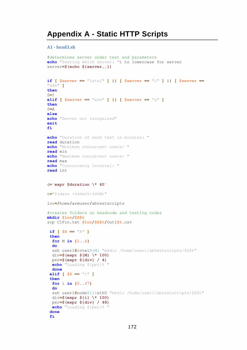
172
Appendix A - Static HTTP Scripts
A1 - head3.sh
#determines server under test and parameters
echo "Testing which server: "t to lowercase for server
server=$(echo ${server,,})
if [ $server == "intel" ] || [ $server == "i" ] || [ $server ==
"x86" ]
then
S=I
elif [ $server == "arm" ] || [ $server == "a" ]
then
S=A
else
echo "Server not recognised"
exit
fi
echo "Duration of each test in minutes: "
read duration
echo "Minimum concurrent users: "
read min
echo "Maximum concurrent users: "
read max
echo "Concurrency interval: "
read int
d=`expr $duration \* 60`
t="$(date +%d%m%Y:%H%M)"
loc=/home/armuser/abtestscripts
#creates folders on headnode and testing nodes
mkdir $loc/$S$t
scp C1Fin.txt $loc/$S$t/OutI$t.csv
if [ $S == "A" ]
then
for M in {1..4}
do
ssh user1@intel${M} "mkdir /home/user1/abtestscripts/$S$t"
div=$(expr ${M} \* 100)
per=$(expr ${div} / 4)
echo "Loading ${per}% "
done
elif [ $S == "I" ]
then
for i in {0..47}
do
ssh user1@node${i}eth0 "mkdir /home/user1/abtestscripts/$S$t"
div=$(expr ${i} \* 100)
per=$(expr ${div} / 48)
echo "Loading ${per}% "
done
fi
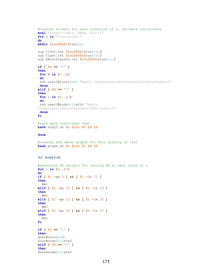
173
#creates folders for each iteration of c, variable concurrency
eval "array=({$min..$max..$int})"
for c in "${array[@]}"
do
mkdir $loc/$S$t/run${c}
scp C1Out.txt $loc/$S$t/run${c}/
scp C1per.txt $loc/$S$t/run${c}/
scp ABoutStandin.txt $loc/$S$t/run${c}/
if [ $S == "A" ]
then
for M in {1..4}
do
ssh user1@intel${M} "mkdir /home/user1/abtestscripts/$S$t/run${c}"
done
elif [ $S == "I" ]
then
for i in {0..47}
do
ssh user1@node${i}eth0 "mkdir
/home/user1/abtestscripts/$S$t/run${c}"
done
fi
#runs each individual test
bash body3.sh $c $loc $t $d $S
done
#creates and opens graphs for full history of test
bash graph.sh $c $loc $t $d $S
A2 - body3.sh
#generates 48 scripts for running AB at each value of c
for i in {0..47}
do
if [ $i -ge 0 ] && [ $i -le 11 ]
then
M=1
elif [ $i -ge 12 ] && [ $i -le 23 ]
then
M=2
elif [ $i -ge 13 ] && [ $i -le 35 ]
then
M=3
elif [ $i -ge 36 ] && [ $i -le 47 ]
then
M=4
fi
if [ $5 == "I" ]
then
dest=intel${M}
sour=node${i}eth0
elif [ $5 == "A" ]
then
dest=node${i}eth0
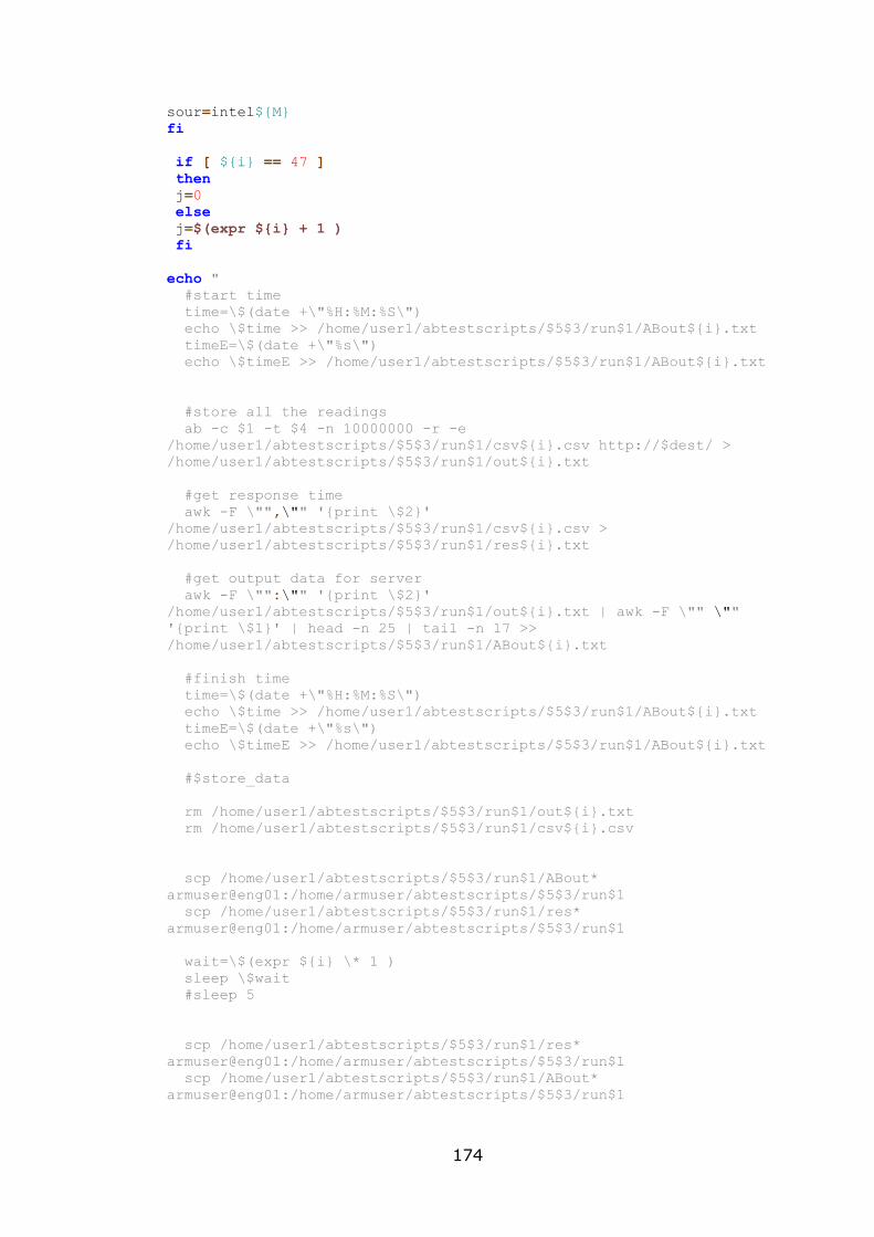
174
sour=intel${M}
fi
if [ ${i} == 47 ]
then
j=0
else
j=$(expr ${i} + 1 )
fi
echo "
#start time
time=\$(date +\"%H:%M:%S\")
echo \$time >> /home/user1/abtestscripts/$5$3/run$1/ABout${i}.txt
timeE=\$(date +\"%s\")
echo \$timeE >> /home/user1/abtestscripts/$5$3/run$1/ABout${i}.txt
#store all the readings
ab -c $1 -t $4 -n 10000000 -r -e
/home/user1/abtestscripts/$5$3/run$1/csv${i}.csv http://$dest/ >
/home/user1/abtestscripts/$5$3/run$1/out${i}.txt
#get response time
awk -F \"",\"" '{print \$2}'
/home/user1/abtestscripts/$5$3/run$1/csv${i}.csv >
/home/user1/abtestscripts/$5$3/run$1/res${i}.txt
#get output data for server
awk -F \"":\"" '{print \$2}'
/home/user1/abtestscripts/$5$3/run$1/out${i}.txt | awk -F \"" \""
'{print \$1}' | head -n 25 | tail -n 17 >>
/home/user1/abtestscripts/$5$3/run$1/ABout${i}.txt
#finish time
time=\$(date +\"%H:%M:%S\")
echo \$time >> /home/user1/abtestscripts/$5$3/run$1/ABout${i}.txt
timeE=\$(date +\"%s\")
echo \$timeE >> /home/user1/abtestscripts/$5$3/run$1/ABout${i}.txt
#$store_data
rm /home/user1/abtestscripts/$5$3/run$1/out${i}.txt
rm /home/user1/abtestscripts/$5$3/run$1/csv${i}.csv
scp /home/user1/abtestscripts/$5$3/run$1/ABout*
armuser@eng01:/home/armuser/abtestscripts/$5$3/run$1
scp /home/user1/abtestscripts/$5$3/run$1/res*
armuser@eng01:/home/armuser/abtestscripts/$5$3/run$1
wait=\$(expr ${i} \* 1 )
sleep \$wait
#sleep 5
scp /home/user1/abtestscripts/$5$3/run$1/res*
armuser@eng01:/home/armuser/abtestscripts/$5$3/run$1
scp /home/user1/abtestscripts/$5$3/run$1/ABout*
armuser@eng01:/home/armuser/abtestscripts/$5$3/run$1
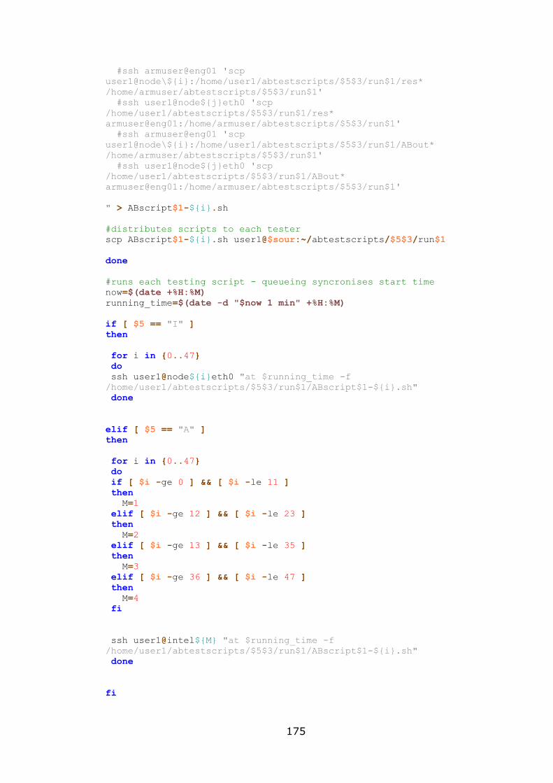
175
#ssh armuser@eng01 'scp
user1@node\${i}:/home/user1/abtestscripts/$5$3/run$1/res*
/home/armuser/abtestscripts/$5$3/run$1'
#ssh user1@node${j}eth0 'scp
/home/user1/abtestscripts/$5$3/run$1/res*
armuser@eng01:/home/armuser/abtestscripts/$5$3/run$1'
#ssh armuser@eng01 'scp
user1@node\${i}:/home/user1/abtestscripts/$5$3/run$1/ABout*
/home/armuser/abtestscripts/$5$3/run$1'
#ssh user1@node${j}eth0 'scp
/home/user1/abtestscripts/$5$3/run$1/ABout*
armuser@eng01:/home/armuser/abtestscripts/$5$3/run$1'
" > ABscript$1-${i}.sh
#distributes scripts to each tester
scp ABscript$1-${i}.sh user1@$sour:~/abtestscripts/$5$3/run$1
done
#runs each testing script - queueing syncronises start time
now=$(date +%H:%M)
running_time=$(date -d "$now 1 min" +%H:%M)
if [ $5 == "I" ]
then
for i in {0..47}
do
ssh user1@node${i}eth0 "at $running_time -f
/home/user1/abtestscripts/$5$3/run$1/ABscript$1-${i}.sh"
done
elif [ $5 == "A" ]
then
for i in {0..47}
do
if [ $i -ge 0 ] && [ $i -le 11 ]
then
M=1
elif [ $i -ge 12 ] && [ $i -le 23 ]
then
M=2
elif [ $i -ge 13 ] && [ $i -le 35 ]
then
M=3
elif [ $i -ge 36 ] && [ $i -le 47 ]
then
M=4
fi
ssh user1@intel${M} "at $running_time -f
/home/user1/abtestscripts/$5$3/run$1/ABscript$1-${i}.sh"
done
fi
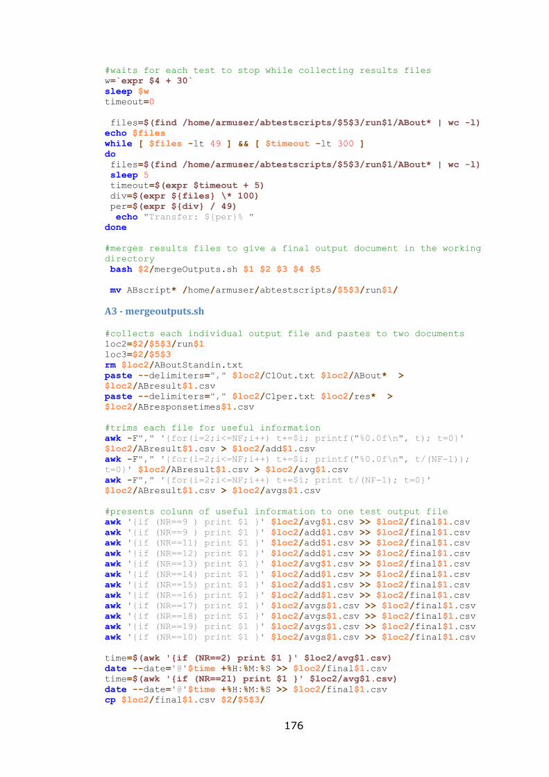
176
#waits for each test to stop while collecting results files
w=`expr $4 + 30`
sleep $w
timeout=0
files=$(find /home/armuser/abtestscripts/$5$3/run$1/ABout* | wc -l)
echo $files
while [ $files -lt 49 ] && [ $timeout -lt 300 ]
do
files=$(find /home/armuser/abtestscripts/$5$3/run$1/ABout* | wc -l)
sleep 5
timeout=$(expr $timeout + 5)
div=$(expr ${files} \* 100)
per=$(expr ${div} / 49)
echo "Transfer: ${per}% "
done
#merges results files to give a final output document in the working
directory
bash $2/mergeOutputs.sh $1 $2 $3 $4 $5
mv ABscript* /home/armuser/abtestscripts/$5$3/run$1/
A3 - mergeoutputs.sh
#collects each individual output file and pastes to two documents
loc2=$2/$5$3/run$1
loc3=$2/$5$3
rm $loc2/ABoutStandin.txt
paste --delimiters="," $loc2/C1Out.txt $loc2/ABout* >
$loc2/ABresult$1.csv
paste --delimiters="," $loc2/C1per.txt $loc2/res* >
$loc2/ABresponsetimes$1.csv
#trims each file for useful information
awk -F"," '{for(i=2;i<=NF;i++) t+=$i; printf("%0.0f\n", t); t=0}'
$loc2/ABresult$1.csv > $loc2/add$1.csv
awk -F"," '{for(i=2;i<=NF;i++) t+=$i; printf("%0.0f\n", t/(NF-1));
t=0}' $loc2/ABresult$1.csv > $loc2/avg$1.csv
awk -F"," '{for(i=2;i<=NF;i++) t+=$i; print t/(NF-1); t=0}'
$loc2/ABresult$1.csv > $loc2/avgs$1.csv
#presents colunn of useful information to one test output file
awk '{if (NR==9 ) print $1 }' $loc2/avg$1.csv >> $loc2/final$1.csv
awk '{if (NR==9 ) print $1 }' $loc2/add$1.csv >> $loc2/final$1.csv
awk '{if (NR==11) print $1 }' $loc2/add$1.csv >> $loc2/final$1.csv
awk '{if (NR==12) print $1 }' $loc2/add$1.csv >> $loc2/final$1.csv
awk '{if (NR==13) print $1 }' $loc2/avg$1.csv >> $loc2/final$1.csv
awk '{if (NR==14) print $1 }' $loc2/add$1.csv >> $loc2/final$1.csv
awk '{if (NR==15) print $1 }' $loc2/add$1.csv >> $loc2/final$1.csv
awk '{if (NR==16) print $1 }' $loc2/add$1.csv >> $loc2/final$1.csv
awk '{if (NR==17) print $1 }' $loc2/avgs$1.csv >> $loc2/final$1.csv
awk '{if (NR==18) print $1 }' $loc2/avgs$1.csv >> $loc2/final$1.csv
awk '{if (NR==19) print $1 }' $loc2/avgs$1.csv >> $loc2/final$1.csv
awk '{if (NR==10) print $1 }' $loc2/avgs$1.csv >> $loc2/final$1.csv
time=$(awk '{if (NR==2) print $1 }' $loc2/avg$1.csv)
date --date='@'$time +%H:%M:%S >> $loc2/final$1.csv
time=$(awk '{if (NR==21) print $1 }' $loc2/avg$1.csv)
date --date='@'$time +%H:%M:%S >> $loc2/final$1.csv
cp $loc2/final$1.csv $2/$5$3/
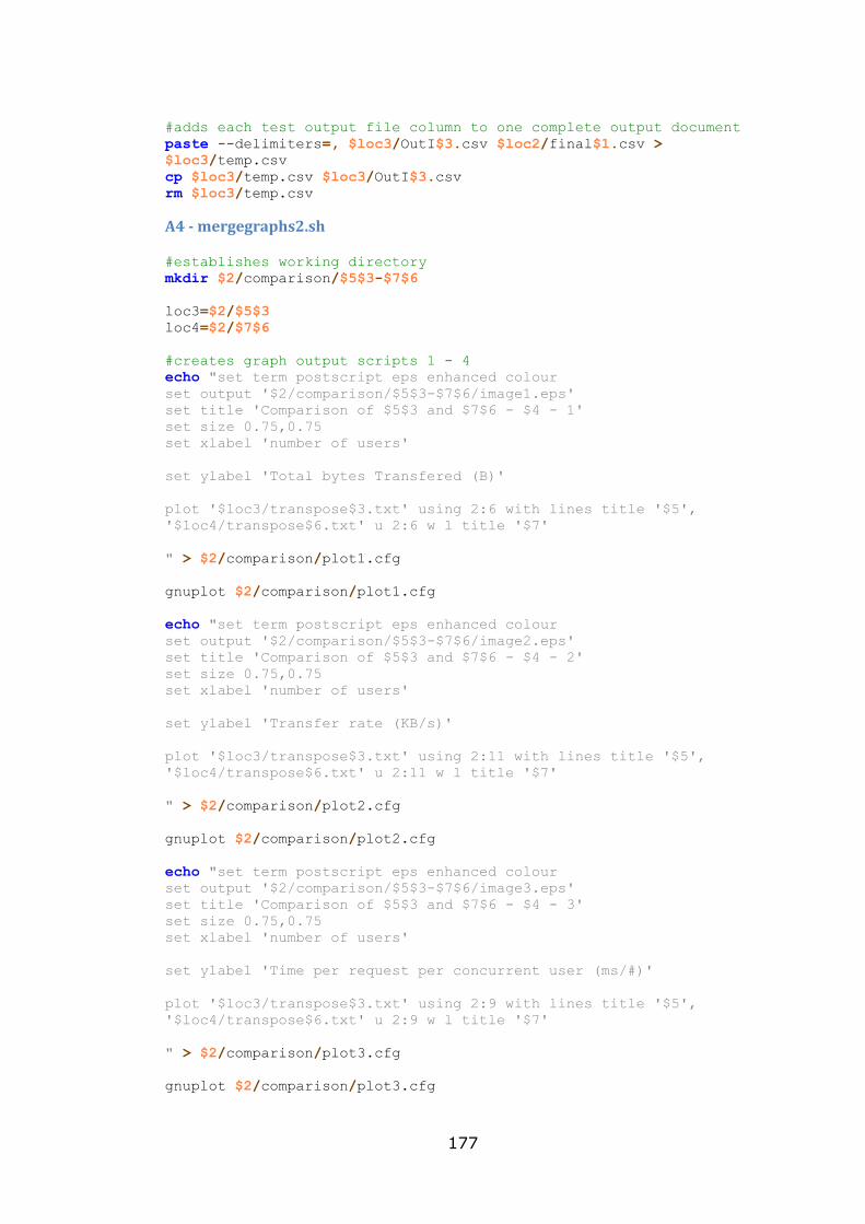
177
#adds each test output file column to one complete output document
paste --delimiters=, $loc3/OutI$3.csv $loc2/final$1.csv >
$loc3/temp.csv
cp $loc3/temp.csv $loc3/OutI$3.csv
rm $loc3/temp.csv
A4 - mergegraphs2.sh
#establishes working directory
mkdir $2/comparison/$5$3-$7$6
loc3=$2/$5$3
loc4=$2/$7$6
#creates graph output scripts 1 - 4
echo "set term postscript eps enhanced colour
set output '$2/comparison/$5$3-$7$6/image1.eps'
set title 'Comparison of $5$3 and $7$6 - $4 - 1'
set size 0.75,0.75
set xlabel 'number of users'
set ylabel 'Total bytes Transfered (B)'
plot '$loc3/transpose$3.txt' using 2:6 with lines title '$5',
'$loc4/transpose$6.txt' u 2:6 w l title '$7'
" > $2/comparison/plot1.cfg
gnuplot $2/comparison/plot1.cfg
echo "set term postscript eps enhanced colour
set output '$2/comparison/$5$3-$7$6/image2.eps'
set title 'Comparison of $5$3 and $7$6 - $4 - 2'
set size 0.75,0.75
set xlabel 'number of users'
set ylabel 'Transfer rate (KB/s)'
plot '$loc3/transpose$3.txt' using 2:11 with lines title '$5',
'$loc4/transpose$6.txt' u 2:11 w l title '$7'
" > $2/comparison/plot2.cfg
gnuplot $2/comparison/plot2.cfg
echo "set term postscript eps enhanced colour
set output '$2/comparison/$5$3-$7$6/image3.eps'
set title 'Comparison of $5$3 and $7$6 - $4 - 3'
set size 0.75,0.75
set xlabel 'number of users'
set ylabel 'Time per request per concurrent user (ms/#)'
plot '$loc3/transpose$3.txt' using 2:9 with lines title '$5',
'$loc4/transpose$6.txt' u 2:9 w l title '$7'
" > $2/comparison/plot3.cfg
gnuplot $2/comparison/plot3.cfg
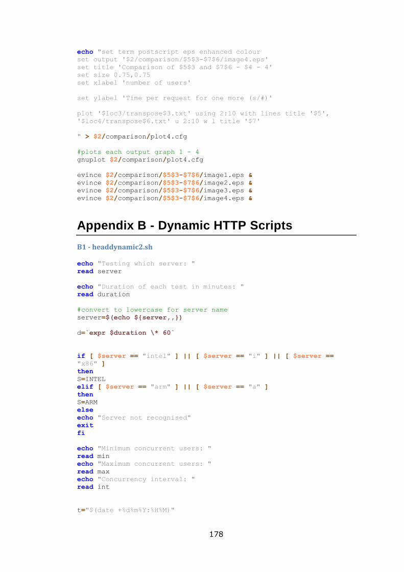
178
echo "set term postscript eps enhanced colour
set output '$2/comparison/$5$3-$7$6/image4.eps'
set title 'Comparison of $5$3 and $7$6 - $4 - 4'
set size 0.75,0.75
set xlabel 'number of users'
set ylabel 'Time per request for one more (s/#)'
plot '$loc3/transpose$3.txt' using 2:10 with lines title '$5',
'$loc4/transpose$6.txt' u 2:10 w l title '$7'
" > $2/comparison/plot4.cfg
#plots each output graph 1 - 4
gnuplot $2/comparison/plot4.cfg
evince $2/comparison/$5$3-$7$6/image1.eps &
evince $2/comparison/$5$3-$7$6/image2.eps &
evince $2/comparison/$5$3-$7$6/image3.eps &
evince $2/comparison/$5$3-$7$6/image4.eps &
Appendix B - Dynamic HTTP Scripts
B1 - headdynamic2.sh
echo "Testing which server: "
read server
echo "Duration of each test in minutes: "
read duration
#convert to lowercase for server name
server=$(echo ${server,,})
d=`expr $duration \* 60`
if [ $server == "intel" ] || [ $server == "i" ] || [ $server ==
"x86" ]
then
S=INTEL
elif [ $server == "arm" ] || [ $server == "a" ]
then
S=ARM
else
echo "Server not recognised"
exit
fi
echo "Minimum concurrent users: "
read min
echo "Maximum concurrent users: "
read max
echo "Concurrency interval: "
read int
t="$(date +%d%m%Y:%H%M)"
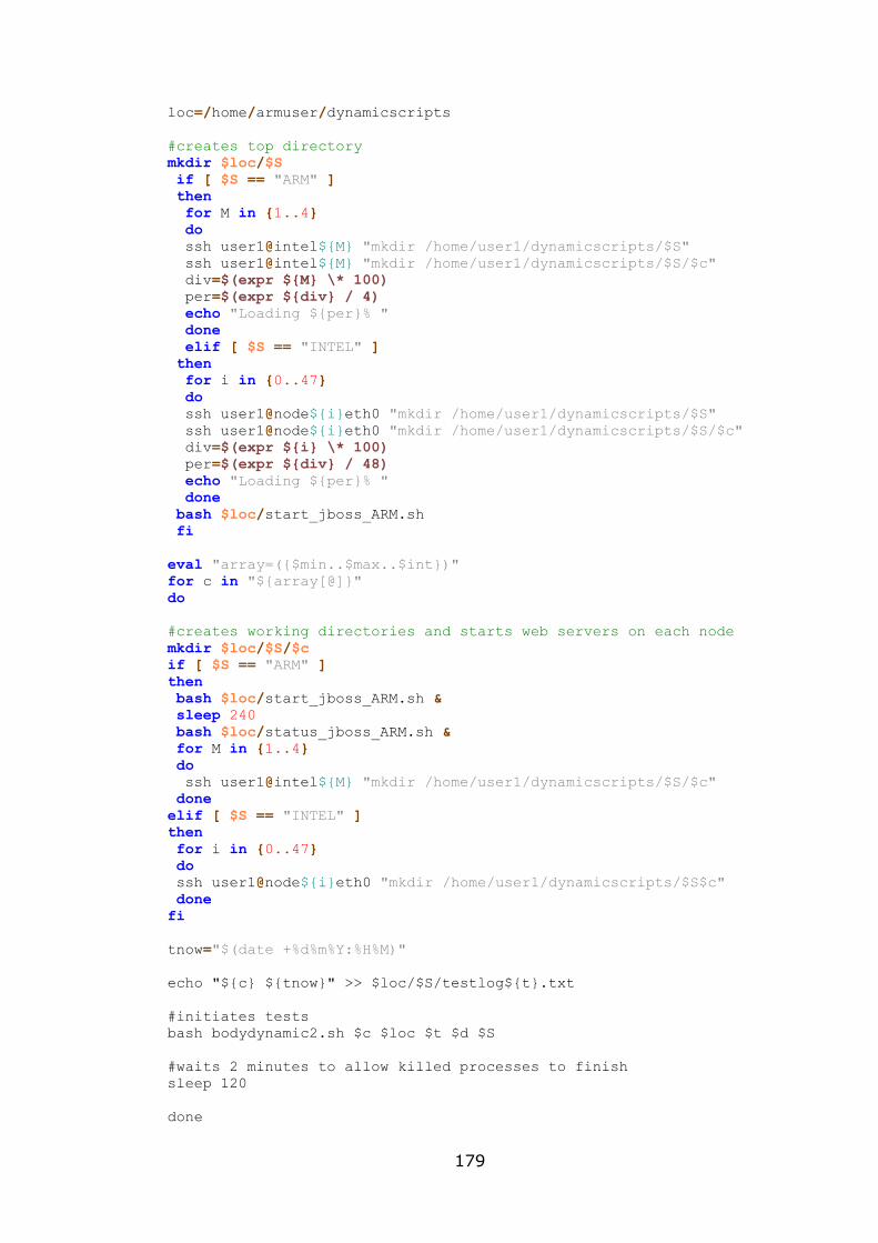
179
loc=/home/armuser/dynamicscripts
#creates top directory
mkdir $loc/$S
if [ $S == "ARM" ]
then
for M in {1..4}
do
ssh user1@intel${M} "mkdir /home/user1/dynamicscripts/$S"
ssh user1@intel${M} "mkdir /home/user1/dynamicscripts/$S/$c"
div=$(expr ${M} \* 100)
per=$(expr ${div} / 4)
echo "Loading ${per}% "
done
elif [ $S == "INTEL" ]
then
for i in {0..47}
do
ssh user1@node${i}eth0 "mkdir /home/user1/dynamicscripts/$S"
ssh user1@node${i}eth0 "mkdir /home/user1/dynamicscripts/$S/$c"
div=$(expr ${i} \* 100)
per=$(expr ${div} / 48)
echo "Loading ${per}% "
done
bash $loc/start_jboss_ARM.sh
fi
eval "array=({$min..$max..$int})"
for c in "${array[@]}"
do
#creates working directories and starts web servers on each node
mkdir $loc/$S/$c
if [ $S == "ARM" ]
then
bash $loc/start_jboss_ARM.sh &
sleep 240
bash $loc/status_jboss_ARM.sh &
for M in {1..4}
do
ssh user1@intel${M} "mkdir /home/user1/dynamicscripts/$S/$c"
done
elif [ $S == "INTEL" ]
then
for i in {0..47}
do
ssh user1@node${i}eth0 "mkdir /home/user1/dynamicscripts/$S$c"
done
fi
tnow="$(date +%d%m%Y:%H%M)"
echo "${c} ${tnow}" >> $loc/$S/testlog${t}.txt
#initiates tests
bash bodydynamic2.sh $c $loc $t $d $S
#waits 2 minutes to allow killed processes to finish
sleep 120
done
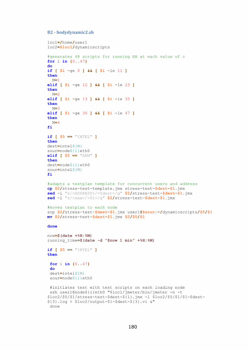
180
B2 - bodydynamic2.sh
loc1=/home/user1
loc2=$loc1/dynamicscripts
#generates 48 scripts for running AB at each value of c
for i in {0..47}
do
if [ $i -ge 0 ] && [ $i -le 11 ]
then
M=1
elif [ $i -ge 12 ] && [ $i -le 23 ]
then
M=2
elif [ $i -ge 13 ] && [ $i -le 35 ]
then
M=3
elif [ $i -ge 36 ] && [ $i -le 47 ]
then
M=4
fi
if [ $5 == "INTEL" ]
then
dest=intel${M}
sour=node${i}eth0
elif [ $5 == "ARM" ]
then
dest=node${i}eth0
sour=intel${M}
fi
#adapts a testplan template for concurrent users and address
cp $2/stress-test-template.jmx stress-test-$dest-$1.jmx
sed -i "s/>ADDRESS</>$dest</g" $2/stress-test-$dest-$1.jmx
sed -i "s/>xxx</>$1</g" $2/stress-test-$dest-$1.jmx
#moves testplan to each node
scp $2/stress-test-$dest-$1.jmx user1@$sour:~/dynamicscripts/$5/$1
mv $2/stress-test-$dest-$1.jmx $2/$5/$1
done
now=$(date +%H:%M)
running_time=$(date -d "$now 1 min" +%H:%M)
if [ $5 == "INTEL" ]
then
for i in {0..47}
do
dest=intel${M}
sour=node${i}eth0
#initiates test with test scripts on each loading node
ssh user1@node${i}eth0 "$loc1/jmeter/bin/jmeter -n -t
$loc2/$5/$1/stress-test-$dest-${1}.jmx -l $loc2/$5/$1/$1-$dest-
${3}.log > $loc2/output-$1-$dest-${3}.vi &"
done
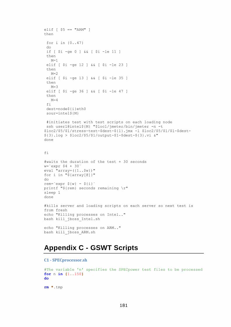
181
elif [ $5 == "ARM" ]
then
for i in {0..47}
do
if [ $i -ge 0 ] && [ $i -le 11 ]
then
M=1
elif [ $i -ge 12 ] && [ $i -le 23 ]
then
M=2
elif [ $i -ge 13 ] && [ $i -le 35 ]
then
M=3
elif [ $i -ge 36 ] && [ $i -le 47 ]
then
M=4
fi
dest=node${i}eth0
sour=intel${M}
#initiates test with test scripts on each loading node
ssh user1@intel${M} "$loc1/jmeter/bin/jmeter -n -t
$loc2/$5/$1/stress-test-$dest-${1}.jmx -l $loc2/$5/$1/$1-$dest-
${3}.log > $loc2/$5/$1/output-$1-$dest-${3}.vi &"
done
fi
#waits the duration of the test + 30 seconds
w=`expr $4 + 30`
eval "array=({1..$w})"
for i in "${array[@]}"
do
rem=`expr ${w} - ${i}`
printf "${rem} seconds remaining \r"
sleep 1
done
#kills server and loading scripts on each server so next test is
from fresh
echo "Killing processes on Intel.."
bash kill_jboss_Intel.sh
echo "Killing processes on ARM.."
bash kill_jboss_ARM.sh
Appendix C - GSWT Scripts
C1 - SPECprocessor.sh
#The variable 'n' specifies the SPECpower test files to be processed
for n in {1..150}
do
rm *.tmp
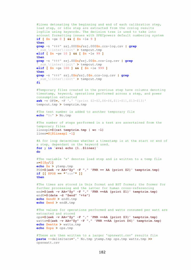
182
#Lines detonating the beginning and end of each calibration step,
load step, or idle step are extracted from the ccslog results
logfile using keywords. The decision tree is used to take into
account formatting issues with SPECpowers default numbering system
if [ $n -ge 0 ] && [ $n -le 9 ]
then
grep -n "###" ssj.000$n/ssj.000$n.ccs-log.csv | grep
'_sum_\|inter\|init' > tempcut.tmp
elif [ $n -ge 10 ] && [ $n -le 99 ]
then
grep -n "###" ssj.00$n/ssj.00$n.ccs-log.csv | grep
'_sum_\|inter\|init' > tempcut.tmp
elif [ $n -ge 100 ] && [ $n -le 999 ]
then
grep -n "###" ssj.0$n/ssj.0$n.ccs-log.csv | grep
'_sum_\|inter\|init' > tempcut.tmp
fi
#Temporary files created in the previous step have columns denoting
timestamp, keyword, operations performed across a step, and power
consumption extracted
awk -v OFS=, -F ',' '{print $2=$2,$6=$6,$11=$11,$13=$13}'
tempcut.tmp > temptrim.tmp
#The test number is added to another temporary file
echo "$n" > No.tmp
#The number of steps performed in a test are ascertained from the
temporary files
linespl=$(cat temptrim.tmp | wc -l)
lines=$[$linespl -1]
#A for loop determines whether a timestamp is at the start or end of
a step, dependant on the keyword used.
for y in `eval echo {1..$lines}`
do
#The variable 'x' denotes load step and is written to a temp file
x=$[$y/2]
echo $x > ytemp.tmp
POS=$(awk -v AA="$y" -F "," 'FNR == AA {print $2}' temptrim.tmp)
if [[ $POS == *"sum"* ]]
then
#The times are stored in Unix format and BST format; the former for
further processing and the latter for human cross-referencing
end=$(awk -v AA="$y" -F "," 'FNR ==AA {print $1}' temptrim.tmp)
endU=$(date -d "$end" "+%s")
echo $endU > endU.tmp
echo $end > endR.tmp
#The values for operations performed and watts consumed per watt are
extracted and stored
ops=$(awk -v AA="$y" -F "," 'FNR ==AA {print $3}' temptrim.tmp)
watts=$(awk -v AA="$y" -F "," 'FNR ==AA {print $4}' temptrim.tmp)
echo $watts > watts.tmp
echo $ops > ops.tmp
#These are then written to a larger 'opnswatt.csv' results file
paste --delimiters="," No.tmp ytemp.tmp ops.tmp watts.tmp >>
opsnwatt.csv
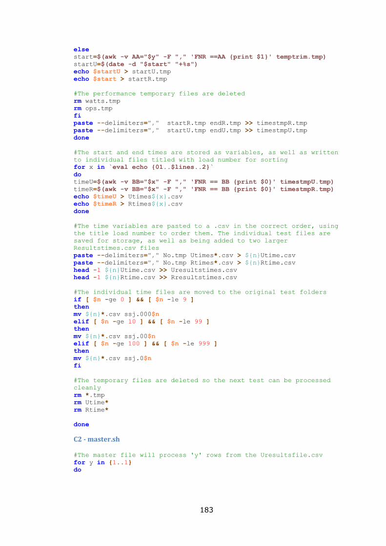
183
else
start=$(awk -v AA="$y" -F "," 'FNR ==AA {print $1}' temptrim.tmp)
startU=$(date -d "$start" "+%s")
echo $startU > startU.tmp
echo $start > startR.tmp
#The performance temporary files are deleted
rm watts.tmp
rm ops.tmp
fi
paste --delimiters="," startR.tmp endR.tmp >> timestmpR.tmp
paste --delimiters="," startU.tmp endU.tmp >> timestmpU.tmp
done
#The start and end times are stored as variables, as well as written
to individual files titled with load number for sorting
for x in `eval echo {01..$lines..2}`
do
timeU=$(awk -v BB="$x" -F "," 'FNR == BB {print $0}' timestmpU.tmp)
timeR=$(awk -v BB="$x" -F "," 'FNR == BB {print $0}' timestmpR.tmp)
echo $timeU > Utimes${x}.csv
echo $timeR > Rtimes${x}.csv
done
#The time variables are pasted to a .csv in the correct order, using
the title load number to order them. The individual test files are
saved for storage, as well as being added to two larger
Resultstimes.csv files
paste --delimiters="," No.tmp Utimes*.csv > ${n}Utime.csv
paste --delimiters="," No.tmp Rtimes*.csv > ${n}Rtime.csv
head -1 ${n}Utime.csv >> Uresultstimes.csv
head -1 ${n}Rtime.csv >> Rresultstimes.csv
#The individual time files are moved to the original test folders
if [ $n -ge 0 ] && [ $n -le 9 ]
then
mv ${n}*.csv ssj.000$n
elif [ $n -ge 10 ] && [ $n -le 99 ]
then
mv ${n}*.csv ssj.00$n
elif [ $n -ge 100 ] && [ $n -le 999 ]
then
mv ${n}*.csv ssj.0$n
fi
#The temporary files are deleted so the next test can be processed
cleanly
rm *.tmp
rm Utime*
rm Rtime*
done
C2 - master.sh
#The master file will process 'y' rows from the Uresultsfile.csv
for y in {1..1}
do
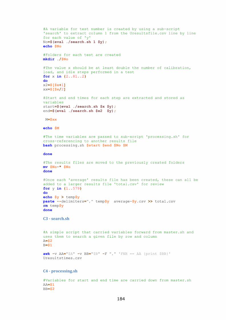
184
#A variable for test number is created by using a sub-script
'search' to extract column 1 from the Uresultsfile.csv line by line
for each value of 'y'
No=$(eval ./search.sh 1 $y);
echo $No
#Folders for each test are created
mkdir ./$No
#The value x should be at least double the number of calibration,
load, and idle steps performed in a test
for x in {2..81..2}
do
x2=$[$x+1]
xx=$[$x/2]
#Start and end times for each step are extracted and stored as
variables
start=$(eval ./search.sh $x $y);
end=$(eval ./search.sh $x2 $y);
M=$xx
echo $M
#The time variables are passed to sub-script 'processing.sh' for
cross-referencing to another results file
bash processing.sh $start $end $No $M
done
#The results files are moved to the previously created folders
mv $No-* $No
done
#Once each 'average' results file has been created, these can all be
added to a larger results file 'total.csv' for review
for y in {1..579}
do
echo $y > temp$y
paste --delimiters="," temp$y average-$y.csv >> total.csv
rm temp$y
done
C3 - search.sh
#A simple script that carried variables forward from master.sh and
uses them to search a given file by row and column
A=$2
B=$1
awk -v AA="$A" -v BB="$B" -F "," 'FNR == AA {print $BB}'
Uresultstimes.csv
C4 - processing.sh
#Variables for start and end time are carried down from master.sh
AA=$1
BB=$2
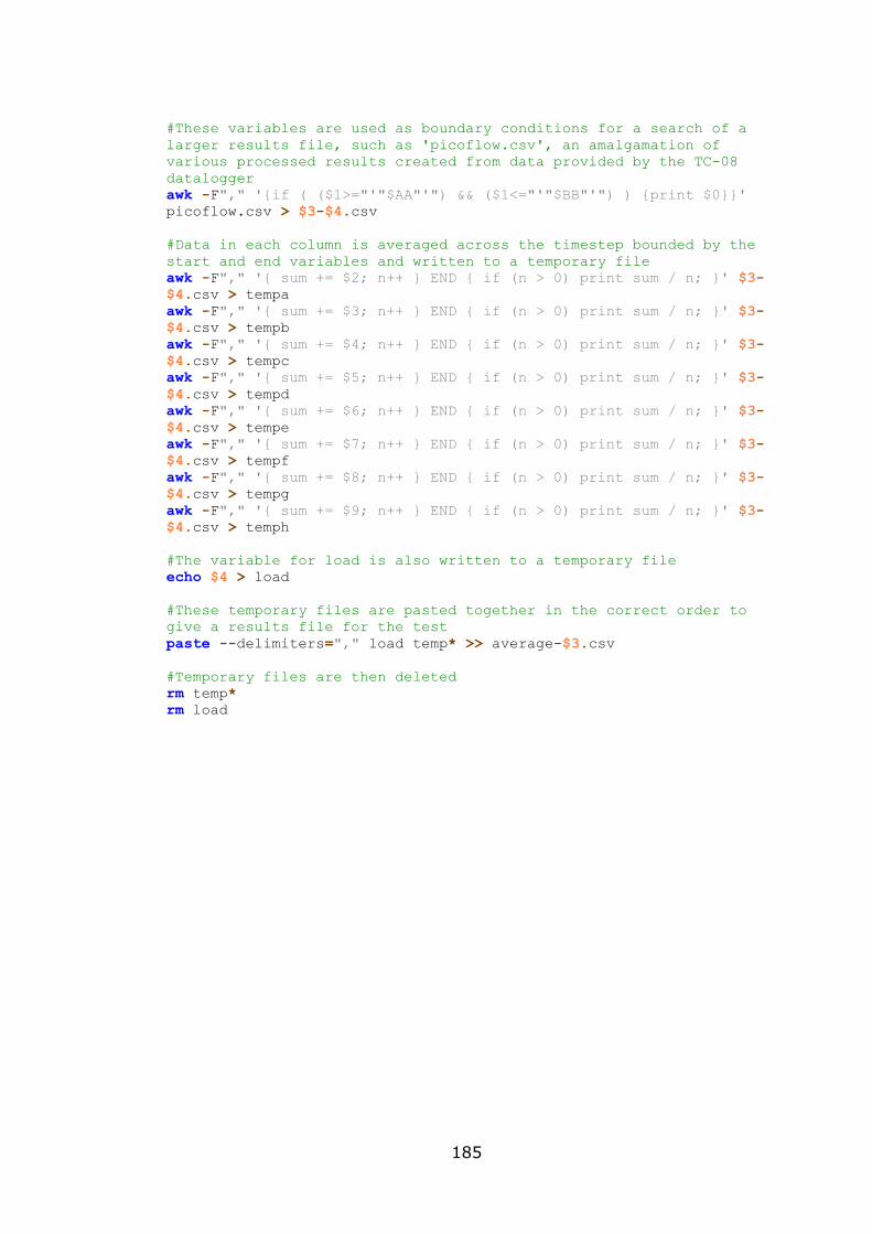
185
#These variables are used as boundary conditions for a search of a
larger results file, such as 'picoflow.csv', an amalgamation of
various processed results created from data provided by the TC-08
datalogger
awk -F"," '{if ( ($1>="'"$AA"'") && ($1<="'"$BB"'") ) {print $0}}'
picoflow.csv > $3-$4.csv
#Data in each column is averaged across the timestep bounded by the
start and end variables and written to a temporary file
awk -F"," '{ sum += $2; n++ } END { if (n > 0) print sum / n; }' $3-
$4.csv > tempa
awk -F"," '{ sum += $3; n++ } END { if (n > 0) print sum / n; }' $3-
$4.csv > tempb
awk -F"," '{ sum += $4; n++ } END { if (n > 0) print sum / n; }' $3-
$4.csv > tempc
awk -F"," '{ sum += $5; n++ } END { if (n > 0) print sum / n; }' $3-
$4.csv > tempd
awk -F"," '{ sum += $6; n++ } END { if (n > 0) print sum / n; }' $3-
$4.csv > tempe
awk -F"," '{ sum += $7; n++ } END { if (n > 0) print sum / n; }' $3-
$4.csv > tempf
awk -F"," '{ sum += $8; n++ } END { if (n > 0) print sum / n; }' $3-
$4.csv > tempg
awk -F"," '{ sum += $9; n++ } END { if (n > 0) print sum / n; }' $3-
$4.csv > temph
#The variable for load is also written to a temporary file
echo $4 > load
#These temporary files are pasted together in the correct order to
give a results file for the test
paste --delimiters="," load temp* >> average-$3.csv
#Temporary files are then deleted
rm temp*
rm load