analysis of reinforced concrete beam deflections using a fiber

ANALYSIS OF REINFORCED CONCRETE BEAM DEFLECTIONS USING A FIBER BASED

MODELING APPROACH

By

Hunter Rumball

Research Advisor

Dr. Keith Kowalkowski, PhD, PE, SE

Graduate Technical Project

This Graduate Project is for Partial Fulfillment of Requirements for the Degree of

Master of Science in Architectural Engineering

at

Lawrence Technological University

Department of Civil and Architectural Engineering

Southfield, Michigan

November, 2021

© Hunter Rumball. All rights reserved. COLLEGE OF ENGINEERING

i

ABSTRACT

The deflection analysis of reinforced concrete beams is an important step of the design process.

Deflections are calculated using service loading scenarios and are limited to prevent the damage of

structural and non-structural elements. ACI 318 addresses the maximum deflection limits to prevent

damage from occurring and to ensure the occupants feel safe under these service loads.

An important variable in calculating the deflection is the effective moment of inertia. Recently,

in the newest version of the code, ACI 318-19, a new equation for the effective moment of inertia is

adopted. With this new equation, there are new rules associated with using the effective moment of

inertia with respect to what the values of the cracked moment is versus the applied moment. This

process differs from the preceding version of the code, ACI 318-14.

Examples in this research show that in some cases, using both moment of inertia approaches will

yield similar deflection results. However, in certain cases, the deflections computed when utilizing

the ACI 318-19 code will yield approximately three times the deflection computed using the ACI

318-14 code. These discrepancies have brought uncertainty in the effective moment of inertia

equation used in both versions of the code discussed. For structural analysis, it is difficult to

determine which deflection is more accurate for a concrete beam with the same conditions and

properties.

In this research, experimental testing and analytical models were performed. For the

experimental testing, two reinforced concrete beams, three concrete cylinders and three non-

reinforced concrete beam specimens were tested. One concrete beam was reinforced with two #3

rebar while the other concrete beam was reinforced with two #5 rebar. All of the beams were

subjected to flexural failure while the cylinders were subjected to compressive loading. The cylinders

were utilized to record the compressive stress-strain curves of the concrete. The reinforced beams,

the non-reinforced beams and the cylinders were all cast and tested on the same day to allow for

equivalent concrete properties. All concrete specimens were also recorded using Digital Image

Correlation (DIC) equipment to determine the strain throughout the duration of the tests. Steel rebar

was also tested under tensile loading. The stress-strain properties of the reinforced concrete beams

and steel rebar were used for the analytical model.

The analytical approaches utilized a fiber-based approach to first derive a moment-curvature

relationship for various concrete sections. Double integration was analyzed using the trapezoidal

ii

method to determine the deflection of concrete beams under various loading conditions from the

moment-curvature relationship. The fiber analysis model utilized the concrete stress-strain curves

obtained experimentally and were verified and calibrated using the experimental concrete beams.

Two additional analytical concrete beams were tested with varying beam dimensions, lengths, and

applied loading. Both analytical beams assumed simply supported boundary conditions similar to

the experimental concrete beams.

The experimental data was not as accurate as anticipated due to inadequate DIC results. The

analytical results and ACI 318 (ACI 318-14 and ACI 318-19) code analysis compared well with

each other in the elastic range of the load-deflection relationship. The 2014 version of the code

compared less favorably to the fiber analysis results in lieu of the 2019 version of the code. The

fiber analysis results, which incorporate steel yielding, demonstrate that significant deformations

occur with a small increase in load after yielding occurs. The effective moment of inertia equations

using the 2014 and 2019 ACI codes do not account for this. However, it is anticipated that the

procedure in ACI that uses the effective moment of inertia equation is adequate for design since

deflections are evaluated under service loads and it is not anticipated that the tension steel will yield

under service loads.

Keywords

Reinforced concrete beam; Deflection; Effective moment of inertia; Fiber analysis

_________________________________________ _____________________

Advisor: Dr. Keith J. Kowalkowski, PhD, PE, SE November 16, 2021 Associate Professor and Assistant Chair Director of Master of Science in Architectural Engineering Director of Civil Engineering Graduate Programs Department of Civil and Architectural Engineering Lawrence Technological University

iii

ACKNOWLEDGEMENTS

It is in my honor to personally thank my research advisor, Associate Professor and Assistant Chair,

Director of Master of Science in Architectural Engineering and Director of Civil Engineering

Graduate Programs, Dr. Keith J. Kowalkowski, PhD, PE, SE, for all of his assistance and dedication

throughout the whole research process. None of this research would have been possible without his

hard working and enthusiastic demeanor.

I would also like to personally thank all of the faculty and student assistants at the Civil

Engineering Testing Lab. More specifically, I am most appreciative of Roger Harrison for his endless

support, time and diligence throughout the whole experimental testing process of this research.

A special thanks goes out to Trilion Quality Systems for assisting in measuring and recording

the experimental data. I personally would like to thank Andrew Leonard and Justin Bucienski for

taking their personal time and effort to help me achieve my research.

A final dedication goes out to my family and friends for their continuous support for not only

my research project, but for my whole educational career at Lawrence Technological University. I

personally would like to thank my girlfriend for her endless support and love day in and day out. She

keeps me motivated and pushes me farther than I ever thought I could be as an individual.

iv

TABLE OF CONTENTS

ABSTRACT ........................................................................................................................................... i

ACKNOWLEDGEMENTS ................................................................................................................ iii

TABLE OF CONTENTS..................................................................................................................... iv

LIST OF FIGURES ............................................................................................................................ vii

LIST OF TABLES ............................................................................................................................... xi

LIST OF VARIABLES....................................................................................................................... xii

CHAPTER 1: INTRODUCTION AND BACKGROUND .......................................................... 1

1.1 Introduction ............................................................................................................................ 1

1.2 Maximum Deflection Limits ................................................................................................. 1

1.3 Background Information ........................................................................................................ 2

1.3.1 Gross Moment of Inertia ................................................................................................ 2

1.3.2 Cracked Moment of Inertia ............................................................................................ 3

1.3.3 Effective Moment of Inertia ........................................................................................... 3

1.4 Code Conflictions .................................................................................................................. 4

1.5 Determining Deflections Using Fiber Analysis Methods ..................................................... 5

1.6 Research Scope ...................................................................................................................... 6

1.7 Research Objectives ............................................................................................................... 6

CHAPTER 2: LITERATURE REVIEW ....................................................................................... 7

2.1 Factors that Affect Deflection ............................................................................................... 7

2.2 ACI Method to Predict Deflection ........................................................................................ 7

2.2.1 Cracked Moment of Inertia ............................................................................................ 8

2.2.2 Effective Moment of Inertia ........................................................................................... 8

2.3 Stress-Strain Properties of Materials ................................................................................... 14

2.3.1 Compressive Stress-Strain Properties and Models ...................................................... 14

v

2.3.2 Tensile Stress-Strain Properties and Models ............................................................... 17

2.3.3 Steel Reinforcement Stress-Strain Properties and Models.......................................... 23

2.4 Experimental Studies of Load-Deflection Results .............................................................. 27

2.5 Analytical Models to Predict Load-Deflection Results ...................................................... 30

2.5.1 Fiber-Based Models ..................................................................................................... 30

2.5.2 Finite Element Analysis Models .................................................................................. 32

2.5.3 Other Analytical Models .............................................................................................. 40

2.6 Conclusions from the Literature Review ............................................................................ 44

CHAPTER 3: EXPERIMENTAL METHODOLOGY .............................................................. 45

3.1 General Experimental Testing ............................................................................................. 45

3.2 Concrete Mix Design Properties ......................................................................................... 46

3.3 Experimental Concrete Specimens ...................................................................................... 47

3.3.1 Concrete Flexural Tests ................................................................................................ 47

3.3.2 Concrete Compressive Tests ........................................................................................ 50

3.3.3 Concrete Flexural Tests to Determine Tensile Capacity ............................................. 51

3.4 Steel Rebar Tensile Tests ..................................................................................................... 53

CHAPTER 4: EXPERIMENTAL RESULTS ............................................................................. 55

4.1 Concrete Flexural Test Results ............................................................................................ 55

4.2 Concrete Compressive Test Results .................................................................................... 62

4.3 Steel Rebar Tensile Test Results ......................................................................................... 67

CHAPTER 5: ANALYTICAL METHODOLOGY ................................................................... 69

5.1 Analytical Modeling Approach ........................................................................................... 69

5.2 Determining Concrete Tensile Properties from Research .................................................. 72

5.3 Assumptions for Analytical Model ....................................................................................... 73

5.4 Analysis of Load-Deflection from Moment-Curvature Relationship ................................ 74

vi

CHAPTER 6: ANALYTICAL RESULTS .................................................................................. 77

6.1 Analytical Results for Beam ‘A’ ......................................................................................... 77

6.2 Analytical Results for Beam ‘B’ ......................................................................................... 82

CHAPTER 7: ANALYTICAL RESULTS OF ADDITIONAL BEAM SPECIMENS ............ 85

7.1 Analytical Results for Concentrated Loaded Case ............................................................. 87

7.2 Analytical Results for Uniformly Distributed Loaded Case............................................... 89

7.3 Summary of All Analytical Results ..................................................................................... 91

CHAPTER 8: CONCLUSIONS AND RECOMMENDATIONS ............................................. 92

8.1 Final Remarks ...................................................................................................................... 92

8.2 Future Recommendations .................................................................................................... 94

REFERENCES….. .............................................................................................................................. 95

vii

LIST OF FIGURES

Figure 2.2.2-1: Tension Stiffening response to Branson's (1965) equation with various Ig/Icr

ratios (Bischoff, 2005) .............................................................................................. 10

Figure 2.2.2-2: Shrinkage restraint stresses in concrete (Scanlon and Bischoff, 2008) .................... 12

Figure 2.2.2-3: Flexural stiffness of concrete using cracked moment versus reduced cracked

moment (Scanlon and Bischoff, 2008) .................................................................... 13

Figure 2.3.1-1: Concrete compressive test setup (Nematzadeh and Falla-Valukolaee, 2021) ......... 15

Figure 2.3.1-2: Compressive stress-strain curves (Nematzadeh and Falla-Valukolaee, 2021) ........ 16

Figure 2.3.1-3: Compressive stress-strain curves for various parameters (Naeimi and

Moustafa, 2021) ........................................................................................................ 17

Figure 2.3.2-1: Stress-strain behavior for axial tension (Iskhakov and Ribakov, 2021) .................. 18

Figure 2.3.2-2: Stress-strain behavior for transverse tension (Iskhakov and Ribakov, 2021) .......... 19

Figure 2.3.2-3: Concrete tensile test setup (Nematzadeh and Falla-Valukolaee, 2021) ................... 20

Figure 2.3.2-4: Tensile stress-strain curves (Nematzadeh and Falla-Valukolaee, 2021) .................. 21

Figure 2.3.2-5: Tensile stress-strain curve for varying steel reinforcement (Kaklauskas

and Ghaboussi, 2001) ............................................................................................... 22

Figure 2.3.2-6: Tensile stress-strain curve for varying cross-section depth (Kaklauskas

and Ghaboussi, 2001) ............................................................................................... 22

Figure 2.3.3-1: Steel rebar tensile test setup (Nematzadeh and Falla-Valukolaee, 2021) ................ 23

Figure 2.3.3-2: Stress-strain curve data for #3 rebar (Carrillo et al., 2021) ...................................... 26






Figure 2.4-1: Load-deflection diagram for steel and GFRP reinforcement (Nematzadeh

and Falla-Valukolaee, 2021) .................................................................................... 28

Figure 2.4-2: Cracking patterns along the length of each beam (Nematzadeh and

Falla-Valukolaee, 2021) ........................................................................................... 28

viii

Figure 2.4-3: Load-deflection diagram of one layer of steel versus two layers of steel

(Butean and Heghes, 2020) ...................................................................................... 29

Figure 2.5.1-1: Stress and strain curves for (a) concrete in tension and compression and

(b) steel rebar (Nematzadeh and Fallah-Valukolaee) .............................................. 30

Figure 2.5.1-2: Stress and strain distributions over the cross-section of a beam

(Nematzadeh and Fallah-Valukolaee) ...................................................................... 31

Figure 2.5.1-3: Fiber analysis versus experimental results for each reinforcement scheme

(Nematzadeh and Falla-Valukolaee, 2021) ............................................................ 32

Figure 2.5.2-1: Tension stiffening model (Patel et al., 2014) ........................................................... 33

Figure 2.5.2-2: Comparison of experimental and analytical mid-span deflections

(Patel et al., 2014) .................................................................................................... 34

Figure 2.5.2-3: Finite element analysis of CB1-1 versus experimental results (Butean

and Heghes, 2020) .................................................................................................... 35

Figure 2.5.2-4: Finite element analysis of CB1-2 versus experimental results (Butean

and Heghes, 2020) .................................................................................................... 35

Figure 2.5.2-5: Deformed shape of concrete beam using finite element analysis (Butean

and Heghes, 2020) .................................................................................................... 36

Figure 2.5.2-6: Crack width of concrete beam using finite element analysis (Butean and

Heghes, 2020) ........................................................................................................... 36

Figure 2.5.2-7: Concrete beam at initial cracking stage (Halahla, 2018) .......................................... 37

Figure 2.5.2-8: Yielding of steel reinforcement stage (Halahla, 2018) ............................................. 38

Figure 2.5.2-9: Failure of concrete beam stage (Halahla, 2018) ....................................................... 38

Figure 2.5.2-10: Load-deflection results from finite element analysis(Halahla, 2018) .................... 39

Figure 2.5.3-1: Analytical model of compressive and tensile moment-curvature and

stress-strain diagrams (Kaklauskas and Ghaboussi, 2001) .................................... 41

Figure 2.5.3-2: Stress and strain behavior at different concrete layers using an analytical

model (Kaklauskas and Ghaboussi, 2001) .............................................................. 43

Figure 3.3.1-1: Typical flexural test of reinforced concrete beams ................................................... 47

Figure 3.3.1-2: Cross-section of Beam ‘A’ ........................................................................................ 48

Figure 3.3.1-3: Elevation of Beam ‘A’ ............................................................................................... 48

Figure 3.3.1-4: Cross-section of Beam ‘B’ ........................................................................................ 49

ix

Figure 3.3.1-5: Elevation of Beam ‘B’ ............................................................................................... 49

Figure 3.3.2-1: Typical compressive test of concrete cylinder .......................................................... 50

Figure 3.3.2-2: Cross-section of concrete cylinder ............................................................................ 51

Figure 3.3.2-3: Elevation of concrete cylinder ................................................................................... 51

Figure 3.3.3-1: Typical flexural test of non-reinforced concrete beam ............................................. 52

Figure 3.3.3-2: Cross-section of non-reinforced concrete beam........................................................ 52

Figure 3.3.3-3: Elevation of non-reinforced concrete beam .............................................................. 52

Figure 3.3.4-1: Typical tensile test of steel rebar ............................................................................... 54

Figure 4.1-1: Load-deflection results for Beam ‘A’ .......................................................................... 56

Figure 4.1-2: Flexural failure of Beam ‘A’ ........................................................................................ 56

Figure 4.1-3: Load-deflection results for Beam ‘B’ ........................................................................... 57

Figure 4.1-4: Flexural failure of Beam ‘B’......................................................................................... 57

Figure 4.1-5: Load-deflection results for non-reinforced concrete beams ........................................ 58

Figure 4.1-6: Flexural failure of Beam ‘C’......................................................................................... 59

Figure 4.1-7: Flexural failure of Beam ‘D’ ........................................................................................ 59

Figure 4.1-8: Flexural failure of Beam ‘E’ ......................................................................................... 60

Figure 4.1-9: Obtaining strain values using DIC data of Beam ‘D’ .................................................. 61

Figure 4.1-10: Variation of strain results from DIC of Beam ‘D’ ..................................................... 62

Figure 4.2-1: Obtaining strain values using DIC data of Cylinder ‘A’ ............................................. 63

Figure 4.2-2: Variation of strain results from DIC of Cylinder ‘A’ .................................................. 63

Figure 4.2-3: Concrete compressive stress-strain curve for Cylinder ‘A’ ......................................... 64

Figure 4.2-4: Compressive failure of Cylinder ‘A’ ............................................................................ 64

Figure 4.2-5: Concrete compressive stress-strain curve for Cylinder ‘B’ ......................................... 65

Figure 4.2-6: Compressive failure of Cylinder ‘B’ ............................................................................ 65

Figure 4.2-7: Concrete compressive stress-strain curve for Cylinder ‘C’ ......................................... 66

Figure 4.2-8: Compressive failure of Cylinder ‘C’ ............................................................................ 66

Figure 4.3-1: Tensile stress-strain curve for #3 steel rebar ................................................................ 68

Figure 4.3-2: Tensile stress-strain curve for #5 steel rebar ................................................................ 68

Figure 5.1-1: Fiber analysis diagram of a typical singly reinforced concrete beam ......................... 69

Figure 5.2-1: Concrete tensile stress-strain curve .............................................................................. 73

Figure 6.1-1: Moment-curvature relationship for Beam ‘A’ ............................................................. 77

x

Figure 6.1-2: Curvature-moment relationship for Beam ‘A’ ............................................................. 79

Figure 6.1-3: Load-deflection results for Beam ‘A’ .......................................................................... 81

Figure 6.2-1: Moment-curvature relationship for Beam ‘B’ ............................................................. 83

Figure 6.2-2: Load-deflection results for Beam ‘B’ ........................................................................... 84

Figure 7-1: Typical cross-section of analytical beams ....................................................................... 85

Figure 7-2: Elevation of analytical beam for concetrated load case .................................................. 86

Figure 7-3: Elevation of analytical beam for uniformly distributed load case .................................. 86

Figure 7.1-1: Moment-curvature relationship for concetratedly loaded beam .................................. 87

Figure 7.1-2: Load-deflection results for concetratedly loaded beam ............................................... 88

Figure 7.2-1: Moment-curvature relationship for distributedly loaded beam ................................... 89

Figure 7.2-2: Load-deflection results for distributedly loaded beam ................................................ 90

xi

LIST OF TABLES

Table 1.2-1: Maximum allowable deflection per ACI 318 (2019) ...................................................... 1

Table 1.4-1: Comparing deflections between ACI 318-14 and ACI 318-19 ...................................... 5

Table 2.2.2-1: Values of constants for different moment values (Branson, 1965) ........................... 10

Table 2.3.3-1: Mechanical properties of steel rebar (Nematzadeh and Falla-Valukolaee, 2021) .... 24

Table 2.3.3-2: Mechanical properties of steel rebar (Carrillo et al., 2021) ....................................... 25

Table 2.4-1: Reinforced concrete beam results (Nematzadeh and Falla-Valukolaee, 2021) ............ 27

Table 3.2-1: Concrete design and quantities ...................................................................................... 46

Table 4.4-1: Properties of steel reinforcement ................................................................................... 67

Table 7.3-1: Summary of analytical model results ............................................................................ 91

Table 7.3-2: Summary of factored versice service loading for analytical results ............................. 91

xii

LIST OF VARIABLES

a = distance of compressive force in cross-section of concrete beam, in

Af = area of a fiber, in2

As = area of reinforced steel, in2

b = width of beam, in

c = distance to neutral axis in cross-section of concrete beam, in

d = effective depth of beam, in

Ec = elastic modulus of concrete, ksi

Es = elastic modulus of steel, ksi

fc’ = compressive strength of concrete, psi

Ff = the force at a particular fiber, lbs

fr = modulus of rupture of concrete, psi

ft = tensile strength of concrete, psi

fy = yield strength of reinforced steel, psi

h = height of concrete beam, in

hf = height of a fiber, in

I = moment of inertia, in4

Icr = cracked moment of inertia in concrete beam, in4

Ie = effective moment of inertia in concrete beam, in4

Ig = gross moment of inertia in concrete beam, in

k = neutral axis depth factor

L = length of concrete beam, ft

Lc = unsupported length of concrete beam, ft

Ma = applied moment in concrete beam due to service loads, kip-ft

Mcr = cracked moment in concrete beam, kip-ft

Mf = the moment at a particular fiber, lb-in

Mn = nominal moment capacity of concrete, kip-ft

Mu = demand moment capacity, kip-ft

n = modular ratio

P = unfactored concentrated load acting on concrete beam, kips

xiii

Pu = factored concentrated load acting on concrete beam, kips

Vf = fiber fraction volume

Vn = nominal shear capacity of concrete, kips

Vu = demand shear capacity, kips

w = unfactored distributed load acting on concrete beam, kips/ft

x = arbitrary distance along the length of a beam, in

yi = distance from the center of the fiber to the neutral axis of the concrete beam, in

yt = distance from the top of the concrete beam to the center of the fiber, in

∆ = calculated deflection due to service loads, in

∆i-1 = deflection at the previous increment, i-1, in

∆i (x) = deflection at an increment, i, as a function of x

∆δi (x) = differential deflection at an increment, i, as a function of x, in

δx = differential length of a beam, in

δθi = differential rotation at an increment, i

δθi (x) = differential rotation at an increment, i, as a function of x

ε1 = maximum elastic compressive strain in a concrete beam, in/in

εc = compressive strain at peak stress in cross-section of concrete beam, in/in

εf = either tensile or compressive strain at a particular fiber, in/in

εs = steel reinforcement strain in cross-section of concrete beam, in/in

εt = tensile strain in cross-section of concrete beam, in/in

εtu = ultimate tensile strain in cross-section of concrete beam, in/in

εy,c = yielding strain of concrete, in/in

εy,s = yielding strain of steel, in/in

εy,u = ultimate strain of concrete, in/in

εy,u = ultimate strain of steel, in/in

θi-1 = rotation at the previous increment, i-1

θi (x) = rotation at an increment, i, as a function of x

λ = aggregate factor of concrete (λ = 1.00 for normalweight concrete, λ = 0.75 for lightweight

concrete)

ρ = flexural reinforcement ratio of the tension steel

xiv

σcf = a compressive or tensile stress in a concrete fiber, ksi

σcf = a compressive or tensile stress in a concrete fiber, ksi

σf = a stress at a particular fiber, psi

σsf = a compressive or tensile stress in a steel fiber, ksi

σt = tensile stress of concrete, psi

φ = curvature of a reinforced concrete beam, in-1

φi = curvature at an increment, i, in-1

φi-1 = curvature at the previous increment, i-1, in-1

1

CHAPTER 1: INTRODUCTION AND BACKGROUND

1.1 Introduction

Serviceability considerations can greatly impact the design of a structural member. Structural

members need to be able to resist deflections and deformations due to serviceability loads, which

include dead and live loads. According to the American Concrete Institute (ACI) 318-19 “Building

Code Requirements for Structural Concrete” (ACI 318, 2019), Chapter 24 discusses the design of

slabs and beams to resist serviceability loads and to prevent any deformations. This chapter breaks

down the process between short-term deflections and long-term deflections. Short-term deflections

occur from unfactored service loads, while long-term deflections occur from these same unfactored

service loads with an additional time-dependent factor. This research will focus on the short-term

deflections of reinforced concrete beams by performing experimental and analytical testing to

evaluate immediate deflections.

1.2 Maximum Deflection Limits

ACI 318-19 (ACI 318, 2019) requires the maximum deflection of a structural member as a ratio of

length, represented in inches, and a coefficient. These values are provided in ACI 318-19 Table 24.2-

2, which is represented in Table 1.2-1.

Table 1.2-1: Maximum allowable deflection per ACI 318 (2019)

Member Conditions Deflection to be considered Deflection limitation

Flat roofs Not supporting or attached to nonstructural elements likely to be

damaged by large deflections Immediate deflection due to L

Immediate deflection due to maximum of Lr, S, and R L/180

Floors L/360 L/360

Roofs or floors

Supporting or attached to

nonstructural elements

Likely to be damaged by large

deflections

That part of the total deflection occurring after

attachment of nonstructural elements, which is the sum

of the time-dependent deflection due to all

sustained loads and the immediate deflection due to

any additional live load

L/480

Not likely to be damaged by large

deflections L/240

2

If the structural member has a deflection over the maximum permitted values provided in Table

1.2-1, then a recommendation to reduce the deflection is to increase the size of the reinforced

concrete member or change the material properties.

Calculating deflections in any structural member can be quite challenging. There are many

variables and factors that contribute to the deflection analysis. These factors include, but are not

limited to, the sustained loading, elastic vs. inelastic behavior, the elastic modulus of concrete, and

the moment of inertia. Per ACI 318-19, the moment of inertia depends on the applied moment versus

the moment that is assumed to initiate cracking (cracking moment). The maximum deflection of a

concrete beam occurs at the midspan of the beam for both a concentrated load located in the center

of the beam and a uniformly distributed load across the length of the beam. Assuming elastic

behavior, the deflection can be calculated using Equation 1-1 for a point load centered on the beam

and Equation 1-2 for a uniformly distributed load.

∆= 𝑃𝑃𝐿𝐿3

48𝐸𝐸𝑐𝑐𝐼𝐼𝑒𝑒 (1-1)

∆= 5𝑤𝑤𝐿𝐿4

384𝐸𝐸𝑐𝑐𝐼𝐼𝑒𝑒 (1-2)

The moment of inertia that is provided in Equation 1-1 and Equation 1-2 depends on the applied

bending moment versus the cracking bending moment as discussed later in this chapter.

1.3 Background Information

The current ACI 318-19 (ACI 318, 2019) code, in comparison to the previous version, ACI 318-14

(ACI 318, 2014), has a modification in the deflection analysis process. This difference is the

calculation of the effective moment of inertia. In order to calculate the effective moment of inertia,

one must first calculate the gross moment of inertia and the cracked moment of inertia.

1.3.1 Gross Moment of Inertia

The gross moment of inertia is the moment of inertia of the gross cross-section of a concrete beam.

This concept ignores steel reinforcement that would otherwise contribute to the moment of inertia.

To calculate the gross moment of inertia of a rectangular shape, refer to Equation 1-3.

𝐼𝐼𝑔𝑔 = 𝑏𝑏ℎ3

12 (1-3)

3

1.3.2 Cracked Moment of Inertia

The cracked moment of inertia represents the moment of inertia that is calculated assuming elastic

behavior of the steel and concrete and that the concrete has no tensile capacity. The cracked moment

of inertia can only be calculated using Equation 1-4 for a rectangular cross section. Equations 1-5

through 1-7 desribe how to calculate some of the variables in Equation 1-4.

𝐼𝐼𝑐𝑐𝑐𝑐 = 𝑏𝑏(𝑘𝑘𝑘𝑘)3

3+ 𝑛𝑛𝐴𝐴𝑠𝑠(𝑑𝑑 − 𝑘𝑘𝑑𝑑)2 (1-4)

𝑘𝑘 = �2𝜌𝜌𝑛𝑛 + (𝜌𝜌𝑛𝑛)2 − 𝜌𝜌𝑛𝑛 (1-5)

𝜌𝜌 = 𝐴𝐴𝑠𝑠𝑏𝑏𝑘𝑘

(1-6)

𝑛𝑛 = 𝐸𝐸𝑠𝑠𝐸𝐸𝑐𝑐

(1-7)

1.3.3 Effective Moment of Inertia

The effective moment of inertia is the final moment of inertia that is calculated for deflection

analysis. The effective moment of inertia is assumed to range between the cracked moment of inertia

and the gross moment of inertia. The equation utilized in ACI 318-14 was originally developed by

Dan Branson (Branson, 1965). The effective moment of inertia is used in calculations to account for

cracking that has already occurred in the concrete beam. This cracking reduces flexural stiffness

along the length of the beam. The effective moment of inertia accounts for the decrease in stiffness

as the load and cracking increases. Branson’s equations is shown as Equation 1-8.

�𝑖𝑖𝑖𝑖 𝑀𝑀𝑐𝑐𝑐𝑐 ≥ 𝑀𝑀𝑎𝑎 𝑡𝑡ℎ𝑒𝑒𝑛𝑛 𝐼𝐼𝑒𝑒 = 𝐼𝐼𝑔𝑔

𝑖𝑖𝑖𝑖 𝑀𝑀𝑐𝑐𝑐𝑐 < 𝑀𝑀𝑎𝑎 𝑡𝑡ℎ𝑒𝑒𝑛𝑛 𝐼𝐼𝑒𝑒 = �𝑀𝑀𝑐𝑐𝑐𝑐𝑀𝑀𝑎𝑎�3𝐼𝐼𝑔𝑔 + �1 − �𝑀𝑀𝑐𝑐𝑐𝑐

𝑀𝑀𝑎𝑎�3� 𝐼𝐼𝑐𝑐𝑐𝑐

(1-8)

However, additional research by Andrew Scanlon and Peter Bischoff (Scanlon and Bischoff,

2008) suggested a new effective moment of inertia equation, which can be found in Equation 1-9.

�𝑖𝑖𝑖𝑖 2

3𝑀𝑀𝑐𝑐𝑐𝑐 ≥ 𝑀𝑀𝑎𝑎 𝑡𝑡ℎ𝑒𝑒𝑛𝑛 𝐼𝐼𝑒𝑒 = 𝐼𝐼𝑔𝑔

𝑖𝑖𝑖𝑖 23𝑀𝑀𝑐𝑐𝑐𝑐 < 𝑀𝑀𝑎𝑎 𝑡𝑡ℎ𝑒𝑒𝑛𝑛 𝐼𝐼𝑒𝑒 = 𝐼𝐼𝑐𝑐𝑐𝑐

1−�23� 𝑀𝑀𝑐𝑐𝑐𝑐𝑀𝑀𝑎𝑎

�2�1−𝐼𝐼𝑐𝑐𝑐𝑐𝐼𝐼𝑔𝑔

�

(1-9)

In Equation 1-9, a new two-thirds factor is multiplied by the cracked moment, which is discussed

in detail in the next chapter. To obtain the cracked moment of a rectangular concrete beam, the

equation is based off of the modulus of rupture. The modulus of rupture is the allowable strength in

tension while the structural member is subjected to bending. The equations for the cracked moment

4

of inertia and the modulus of rupture can be found in Equation 1-10 (for a rectangular section) and

Equation 1-11, respectively.

𝑀𝑀𝑐𝑐𝑐𝑐 = 2𝑓𝑓𝑐𝑐𝐼𝐼𝑔𝑔ℎ

(1-10)

𝑖𝑖𝑐𝑐 = 7.5𝜆𝜆�𝑖𝑖𝑐𝑐′ (1-11)

1.4 Code Conflictions

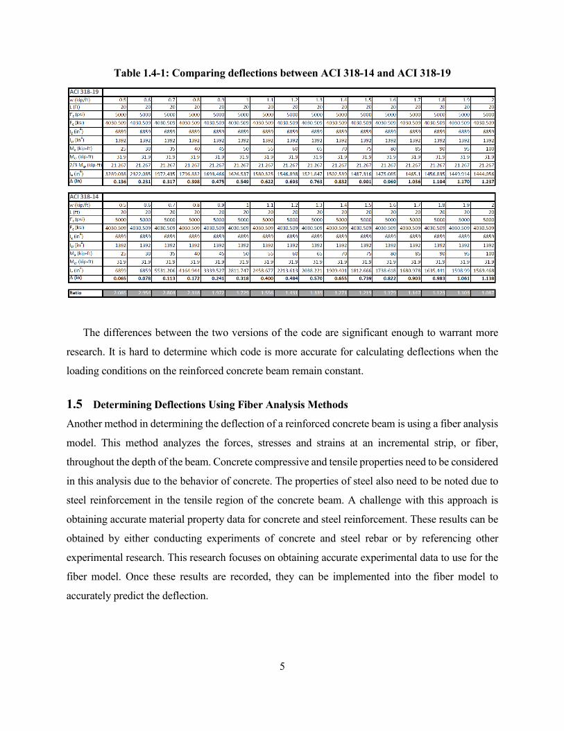
As discussed in the previous section, ACI 318-14 and ACI 318-19 suggest different equations for

calculating the effective moment of inertia, and ultimately, beam deflections. A brief example has

been conducted to compare the deflections between ACI 318-14 and ACI 318-19. The top section

in Table 1.4-1 follows ACI 318-19 and the bottom section follows the ACI 318-14 procedure.

Variables that were kept constant in this example problem include the length of the beam, the

compressive strength of concrete, the elastic modulus of concrete, the gross moment of inertia, the

cracked moment of inertia, and the cracked moment. Therefore, only the effective moment of inertia

calculations differ between the two code methods. The distributed loads range from 0.5 kip/ft to 2.0

kip/ft and the maximum moment due to service loads ranging from 25 kip-ft to 100 kip-ft.

Deflections were calculated using Equation 1-2, which is used to calculate the midspan deflection of

a beam subjected to distributed load. However, equations such as Equation 1-1 and 1-2 are derived

assuming elastic behavior and assuming the moment of inertia is constant along the length of the

beam. This is questionable for reinforced concrete beams since the effective moment of inertia is

calculated using the highest moments along the length of the beam, which occurs only at midspan

for the cases presented herein. This was studied recently by Stencel (2020) as discussed in Chapter

2.

The bottom row in Table 1.4-1 represents the ratio of the deflections from ACI 318-19 to the

deflections from ACI 318-14. The differences in deflections are significantly different when the

effective moment of inertia is closer to the gross moment of inertia than the cracked moment of

inertia. In some cases, the deflections from the newer code are almost three times higher than the

deflections from the preceding version of the code. As the effective moment of inertia approached

the cracked moment of inertia, the deflections between the two codes were almost the same in

magnitude since the calculation of obtaining the cracked moment of inertia does not change between

the two code methods.

5

Table 1.4-1: Comparing deflections between ACI 318-14 and ACI 318-19

The differences between the two versions of the code are significant enough to warrant more

research. It is hard to determine which code is more accurate for calculating deflections when the

loading conditions on the reinforced concrete beam remain constant.

1.5 Determining Deflections Using Fiber Analysis Methods

Another method in determining the deflection of a reinforced concrete beam is using a fiber analysis

model. This method analyzes the forces, stresses and strains at an incremental strip, or fiber,

throughout the depth of the beam. Concrete compressive and tensile properties need to be considered

in this analysis due to the behavior of concrete. The properties of steel also need to be noted due to

steel reinforcement in the tensile region of the concrete beam. A challenge with this approach is

obtaining accurate material property data for concrete and steel reinforcement. These results can be

obtained by either conducting experiments of concrete and steel rebar or by referencing other

experimental research. This research focuses on obtaining accurate experimental data to use for the

fiber model. Once these results are recorded, they can be implemented into the fiber model to

accurately predict the deflection.

6

1.6 Research Scope

Research focuses on accurately determining the deflection in a reinforced concrete beam using a

fiber analysis method. Experimental research and testing needed to be completed for the fiber model.

Concrete compressive and tensile stress-strain properties were determined through experimental

testing and flexural testing of reinforced concrete beams. All concrete tests were conducted using

the same design mix to ensure uniform properties for the fiber analysis model. Steel rebar was also

experimentally tested to obtain steel stress-strain properties. The fiber analysis model was conducted

utilizing the properties from all of the experimental tests. The results of the fiber model was

compared to the experimental flexural results. Through a successful comparison of the two tests,

more analytical concrete beams were tested through the fiber model. These deflection results were

compared with the deflection analysis through the two most recent versions of ACI 318 (ACI, 2014

& 2019).

The results of this research may open more doors to other types of analyses. With accurate

predictions from the analytical model of simply supported beams, other concrete beams with

different boundary conditions can be analyzed. The deflection analysis may also be used in one-way

or two-way slab design as well.

1.7 Research Objectives

The research objectives that pertain to this report are discussed in the following points:

• Compare the experimental load-deflection results with those predicted using fiber-based

analytical models and equivalent material properties.

• Understand the effectiveness of using DIC to predict the material properties of concrete.

• Evaluate deflection predictions using ACI 318-14 and ACI 318-19 and how they compare

with experimental and analytical research.

• Identify how various parameters such as reinforcement ratio, span length, loading criteria,

boundary conditions, etc. may influence the deflection analysis in reinforced concrete beams.

7

CHAPTER 2: LITERATURE REVIEW

2.1 Factors that Affect Deflection Deflection of concrete beams has been a discussion topic for many years. The important variables

when determining deflections include the force that is being applied to the beam, the length of the

beam, the elastic modulus of concrete and the moment of inertia. There are many uncertain factors

that are involved when solving for deflection, provided by Dr. Dan Branson (1965). The author

mentioned a lack of knowledge of concrete properties from a concrete mix such as modulus of

rupture, compressive strength, modulus of elasticity and shrinkage and creep effects of concrete that

may lead to inaccuracies when calculating deflection. Ambient temperature and humidity play an

important role for shrinkage and creep effects. The age of the concrete from when it was poured

greatly affects the loading that the concrete can withstand before cracking. For deflection

calculations, the concrete cross-section is assumed to behave linearly-elastic throughout the length

of the beam, which is questionable because cracking within the concrete cause non-linear behavior

to occur.

2.2 ACI Method to Predict Deflection ACI 318 Building Code Requirements for Structural Concrete (ACI, 2014) predicts the deflection

for any concrete member. For a reinforced concrete beam, one needs to calculate the gross moment

of inertia, or sometimes referred to as the uncracked moment of inertia, of the concrete cross-section.

Equation 1-3 computes the gross moment of inertia for a rectangular cross-section. As loading is

applied to a concrete beam, cracks begin to form through the length of the beam. This causes the

moment of inertia to change as more loading is applied. In response to this, the cracked moment of

inertia is calculated. The cracked moment of inertia is always less than the gross moment of inertia

because of the formation of cracks in the cross-section of the beam. However, unlike the gross

moment of inertia, it is computed utilizing the composite properties of both the steel and concrete

section. The cracked moment of inertia for a rectangular cross-section is shown as Equation 1-4.

The effective moment of inertia is an empirical equation that utilizes the gross moment of inertia,

the cracked moment of inertia and a ratio of the cracked moment versus the applied moment. This

equation was developed because the effective moment of inertia provides a transition of the

maximum, gross moment of inertia, and minimum, cracked moment of inertia, limits as a function

8

of the ratio of the cracked moment and applied moment (ACI, 2014). Throughout history, there have

been numerous studies and variations on the effective moment of inertia equation and how accurate

it is when determining the deflection from service loads.

2.2.1 Cracked Moment of Inertia

The cracked moment of inertia, or sometimes referred to as the cracked transformed moment of

inertia is used to transform the steel reinforcement in the cross-section to an equivalent area of

concrete using the modular ratio, n. The cracked moment of inertia assumes that the concrete behaves

elastically under service loading and that there is no tensile capacity in the concrete when cracking

has occurred. Due to the fact that there is no tensile capacity in the concrete, the cracked moment of

inertia is far smaller than the gross moment of inertia. The cracked moment of inertia is solely

calculated based on the section properties and fundamental mechanics of concrete.

2.2.2 Effective Moment of Inertia

Use of an effective moment of inertia equation to predict concrete deflections was first studied by

Branson (1965). He noted that the stress distribution along with the effective moment of inertia

varied throughout the length of a reinforced concrete beam when subjected to loading (Branson,

1965). The author’s equation to calculate the effective moment of inertia is shown in Equation 2-1.

𝐼𝐼𝑒𝑒 = �𝑀𝑀𝑐𝑐𝑐𝑐𝑀𝑀𝑎𝑎�𝑚𝑚𝐼𝐼𝑔𝑔 + �1 − �𝑀𝑀𝑐𝑐𝑐𝑐

𝑀𝑀𝑎𝑎�𝑚𝑚� 𝐼𝐼𝑐𝑐𝑐𝑐 (2-1)

This equation uses the ratio of the cracked moment with the applied moment, the gross moment

of inertia and the cracked moment of inertia. The exponent m was considered to be an unknown

power during Branson’s research. It has been found that by taking m = 3, the deflection analysis

compared well with experimental data. Branson’s equation, Equation 1-8, has been implemented

into the ACI 318 Building Code Requirements for Structural Concrete, through the ACI 318-14

version of the code (ACI, 2014). Throughout the past couple of decades, numerous researchers have

proved different values of the exponent m for different loading scenarios.

Al-Zaid et al. (1991) conducted experiments for different loading scenarios and the ratio of the

cracked moment of inertia to the gross moment of inertia. The authors suggested that m = 2.8 for a

uniformly distributed load when Ma > Mcr. For moderately reinforced concrete beams, ρt = 1.2%,

Icr/Ig = 0.34, the value ranged from m = 3 to m = 4.3 for Mcr < Ma < 1.5Mcr.

9

Al-Shaikh et al. (1993) also performed experiments regarding the m factor in Equation 2-1. Their

experiments focused on a point load at the mid-span of the beam. Numerous beams were tested with

varying reinforcement schemes. It was found that for lightly reinforced concrete beams, ρt = 0.8%,

Ig/Icr = 4.5, the factor ranged from m = 1.8 to m = 2.5 for 1.5Mcr < Ma < 4Mcr. For heavily reinforced

beams, ρt = 2.0%, Ig/Icr = 2.27, the factor ranged from m = 0.9 to m = 1.3. They also suggested an

equation for the m factor that directly incorporates the reinforcement ratio, which is shown in

Equation 2-2. Al-Zaid et al. (1991) and Al-Shaikh et al. (1993) both proposed on calculating the

effective moment of inertia based on the lengths of the cracks that formed throughout the length of

the beam utilizing the reinforcement ratio and loading criteria, respectively. Through different

experiments and various reinforcement ratios, the equation provided by Branson (1965), Equation

1-8, is not accurate for various design scenarios.

𝑚𝑚 = 3 − 0.8𝜌𝜌𝑡𝑡 (2-2)

Bischoff (2005) explored Branson’s (1965) equation, Equation 2-1 using m = 3. Branson ignored

the fact that concrete continues to carry tensile forces after a crack in the concrete has formed. This

is true because as a crack forms in the concrete, the bond forces transfer through the steel

reinforcement back into the concrete, or otherwise known as tension stiffening (Bischoff, 2005).

Tension stiffening is important for member stiffness, deflections and crack widths on the concrete

under service loading. Bischoff (2005) proved that tension stiffening in Equation 2-1 is dependent

on the exponential factor, m, and the ratio of Ig/Icr. The ratio of Ig/Icr depends on the reinforcement

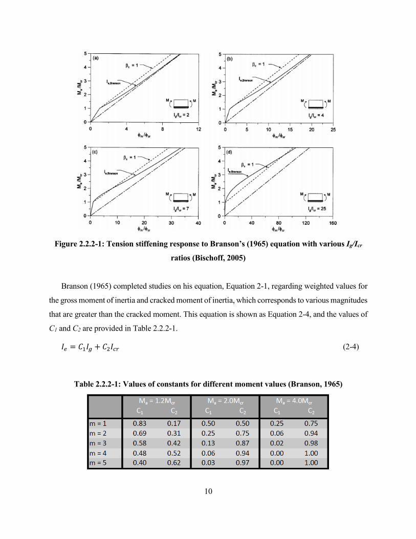
ratio and the modular ratio. Bischoff found that when m = 3 and Ig/Icr > 3, Equation 2-1 overestimates

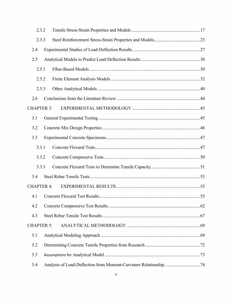
the effective moment of inertia. Figure 2.2.2-1 shows that Equation 2-1 with m = 3 and different Ig/Icr

ratios that the tension stiffening is overestimated. The βc factor in Figure 2.2.2-1 is known as the

tension stiffening factor and is found by rearranging Equation 2-1, which is shown as Equation 2-3.

𝛽𝛽𝑐𝑐 = ∆𝜙𝜙∆𝜙𝜙𝑚𝑚𝑎𝑎𝑚𝑚

=𝑀𝑀𝑎𝑎

𝑀𝑀𝑐𝑐𝑐𝑐�

1+�1−�𝑀𝑀𝑐𝑐𝑐𝑐𝑀𝑀𝑎𝑎� �

𝑚𝑚��𝐼𝐼𝑐𝑐𝑐𝑐 𝐼𝐼𝑔𝑔� ��𝑀𝑀𝑐𝑐𝑐𝑐

𝑀𝑀𝑎𝑎� �

𝑚𝑚 (2-3)

For Equation 2-1, βc = 1 when Ma = Mcr and βc = 0 when Ma = ∞. Bischoff (2005) found that

the tension stiffening factor increases as the Ig/Icr ratio increases, and the tension stiffening factor

approaches the Ma/Mcr ratio as Ig/Icr approaches infinity.

10

Figure 2.2.2-1: Tension stiffening response to Branson’s (1965) equation with various Ig/Icr

ratios (Bischoff, 2005)

Branson (1965) completed studies on his equation, Equation 2-1, regarding weighted values for

the gross moment of inertia and cracked moment of inertia, which corresponds to various magnitudes

that are greater than the cracked moment. This equation is shown as Equation 2-4, and the values of

C1 and C2 are provided in Table 2.2.2-1.

𝐼𝐼𝑒𝑒 = 𝐶𝐶1𝐼𝐼𝑔𝑔 + 𝐶𝐶2𝐼𝐼𝑐𝑐𝑐𝑐 (2-4)

Table 2.2.2-1: Values of constants for different moment values (Branson, 1965)

11

Scanlon and Bischoff (2008) proposed a new equation for the effective moment of inertia that

includes accuracy for reinforcement ratios less than one percent. The authors studied how shrinkage

restrain affects the cracked moment and ultimately the deflection of concrete beams. They state that

several sources of shrinking restraint in concrete beams and slabs include embedded reinforcing bars,

stiff supporting elements and nonlinear distribution of shrinkage over the thickness of a member

(Scanlon and Bischoff, 2008). Shrinkage is caused under drying conditions after the concrete has

been poured and the volume of concrete is held constant (ACI 224, 2001). Shrinkage can cause

tensile stresses in the concrete, which creates a decrease in flexural stiffness and cracks to form.

These stresses decrease the modulus of rupture which ultimately decreases the cracked moment

(Equation 1-10). Scanlon and Bischoff (2008) proposed a reduced effective modulus of rupture, fre,

and restraint stress, fres, shown in Equation 2-5 and Equation 2-6, respectively. Scanlon and Bischoff

(2008) adopted Gilbert’s (1999) research on how to calculate the restraint stress shown in Equation

2-6. Equation 2-7 shows the reduced cracked moment, M’cr using the reduced effective modulus of

rupture.

𝑖𝑖𝑐𝑐𝑒𝑒 = 𝑖𝑖𝑐𝑐 − 𝑖𝑖𝑐𝑐𝑒𝑒𝑠𝑠 (2-5)

𝑖𝑖𝑐𝑐𝑒𝑒𝑠𝑠 = 2.5𝜌𝜌1+50𝜌𝜌

𝐸𝐸𝑠𝑠𝜀𝜀𝑠𝑠ℎ (2-6)

𝑀𝑀𝑐𝑐𝑐𝑐′ = 𝑓𝑓𝑐𝑐𝑒𝑒

𝑓𝑓𝑐𝑐𝑀𝑀𝑐𝑐𝑐𝑐 (2-7)

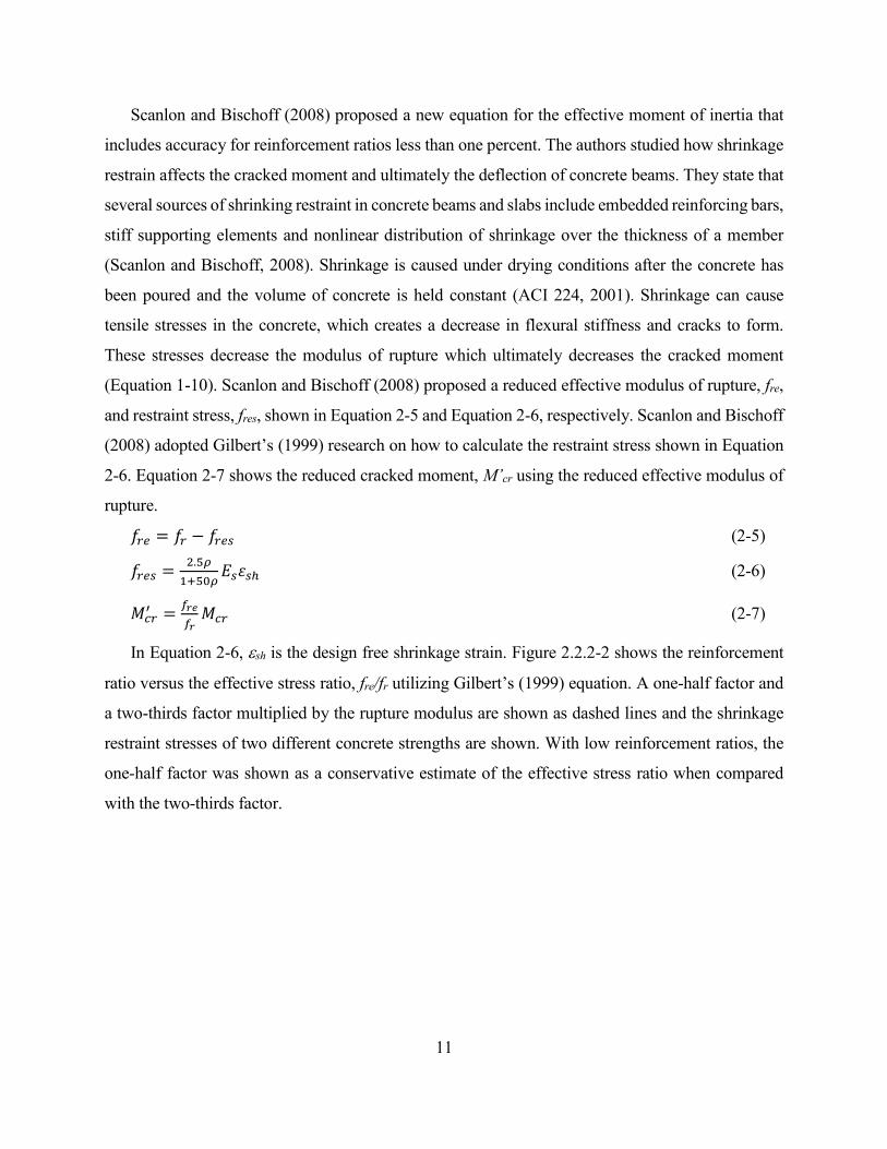
In Equation 2-6, εsh is the design free shrinkage strain. Figure 2.2.2-2 shows the reinforcement

ratio versus the effective stress ratio, fre/fr utilizing Gilbert’s (1999) equation. A one-half factor and

a two-thirds factor multiplied by the rupture modulus are shown as dashed lines and the shrinkage

restraint stresses of two different concrete strengths are shown. With low reinforcement ratios, the

one-half factor was shown as a conservative estimate of the effective stress ratio when compared

with the two-thirds factor.

12

Figure 2.2.2-2: Shrinkage restraint stresses in concrete (Scanlon and Bischoff, 2008)

In Figure 2.2.2-2, a 1.5 factor was used for Equation 2-6 because the Australian Standard (AS

3600, 2001) adopted this factor. The 1.5 factor is shown to be conservative at low reinforcement

ratios. A trend for the two concrete compressive strengths used concludes that as the reinforcing ratio

increases, the effective stress ratio decreases because there is more steel to withstand the tension

forces in the concrete. For the rupture modulus, the one-half factor corresponds to a reinforcing ratio

of 0.8 percent while a two-thirds factor corresponds to a reinforcing ratio of 0.5 percent (Scanlon

and Bischoff, 2008). The two-thirds factor was found to be more accurate for Bischoff’s (2005)

proposed equation for the effective moment of inertia, shown as Equation 2-8. The β factor is a

sustained loading factor used by the Eurocode to account for a lower cracked moment (Scanlon and

Bischoff, 2008), as shown in Equation 2-9. By substituting Equation 2-9 into Equation 2-7, and

substituting Equation 2-7 into Equation 2-8, a new equation to calculate the effective moment of

inertia is shown as Equation 2-10.

𝐼𝐼𝑒𝑒 = 𝐼𝐼𝑐𝑐𝑐𝑐

1−�1−𝐼𝐼𝑐𝑐𝑐𝑐𝐼𝐼𝑐𝑐𝑐𝑐��𝑀𝑀𝑐𝑐𝑐𝑐

′

𝑀𝑀𝑎𝑎�2 (2-8)

𝛽𝛽 = �𝑓𝑓𝑐𝑐𝑒𝑒𝑓𝑓𝑐𝑐�2 (2-9)

𝐼𝐼𝑒𝑒 = 𝐼𝐼𝑐𝑐𝑐𝑐

1−�1−𝐼𝐼𝑐𝑐𝑐𝑐𝐼𝐼𝑐𝑐𝑐𝑐��𝛽𝛽𝑀𝑀𝑐𝑐𝑐𝑐

𝑀𝑀𝑎𝑎�2 (2-10)

13

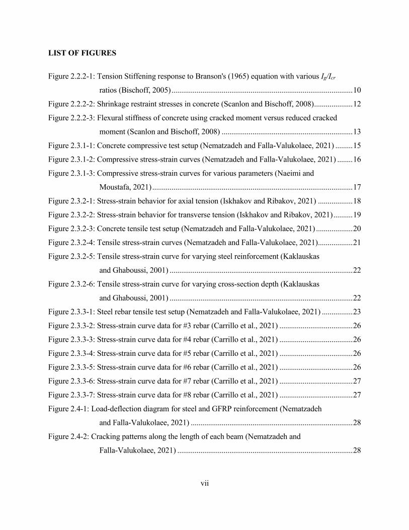
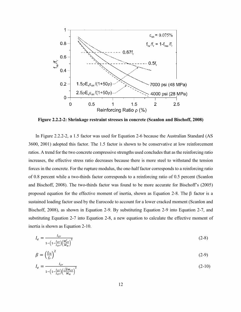
By setting β equal to 0.5 in Equation 2-10, it is almost equivalent to the two-thirds factor

multiplied by the cracked moment, as shown in Equation 1-9. Figure 2.2.2-3 shows a comparison of

the flexural stiffness of a concrete member using the cracked moment versus the reduced cracked

moment (�𝛽𝛽𝑀𝑀𝑐𝑐𝑐𝑐). Figure 2.2.2-3 uses Equation 2-10 to compare these two values.

Figure 2.2.2-3: Flexural stiffness of concrete using cracked moment versus reduced cracked

moment (Scanlon and Bischoff, 2008)

The most recent version of the ACI 318 code (ACI 318-19) adopted Scanlon and Bischoff’s

(2008) equation, Equation 2-10, to calculate the effective moment of inertia. Instead of the β factor,

the two-thirds factor is provided, as shown in Equation 1-9. The most recent version to calculate the

effective moment of inertia was found to be more accurate than the preceding version for all

reinforcement ratios.

The effective moment of inertia equation is utilized to compute beam deflections. Usually, the

effective moment of inertia is calculated using the maximum moment in the beam along the length,

and it assumes the effective moment of inertia is constant along the length, which is questionable

since in most loading applications, the applied moment is not constant. Therefore, there is a variation

of flexural cracking along the length.

Branson (1965) indicated that the effective moment of inertia should not be constant as the length

of the beam changes because the applied moment changes with respect to the length of the beam.

14

Stencel (2020) studied this concern in more detail by analytically investigating several concrete

beams with various lengths, loading conditions and cross-sectional dimensions. In this study, the

author compared the deflection results when using a constant effective moment of inertia and

assuming the effective moment of inertia varied as the applied internal moment varied along the

length. Simply supported beams were studied that were subjected to uniform loading and

concentrated loading. The results of this study showed that usually, assuming a constant effective

moment of inertia is slightly conservative for most loading conditions, meaning the predicted

deflections were close to when assuming the effective moment of inertia varied. However, for

specific point loading applications and magnitudes of loading, more significant discrepancies were

found in the results, implying that using a constant effective moment of inertia is too conservative.

2.3 Stress-Strain Properties of Materials

The stress-strain properties of a concrete beam differ between the compression and tension zones of

the cross-section. The stress-strain properties are important to determine how the forces behave

throughout the cross-section. These properties obtained from experimental tests were used for the

analytical analysis to predict the deflection of a concrete beam. Both the compressive and tensile

stress-strain properties are discussed in the proceeding sections.

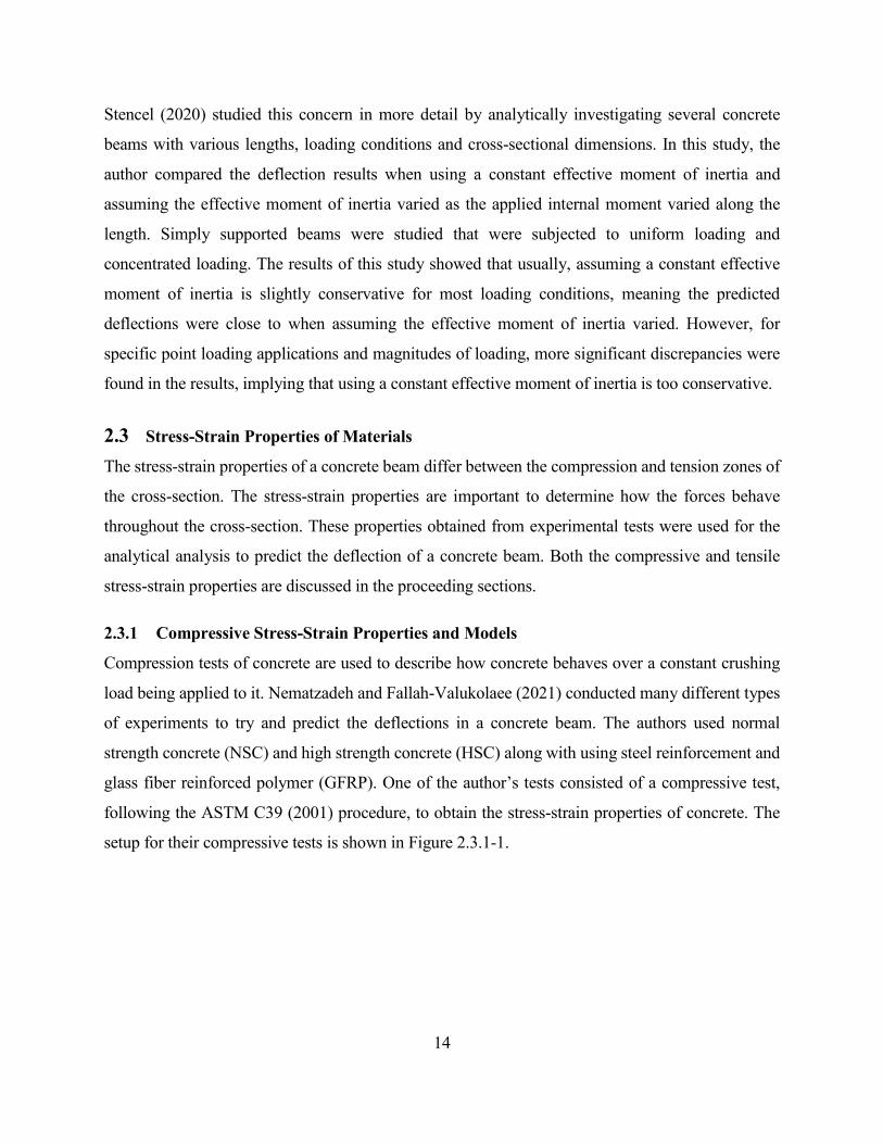
2.3.1 Compressive Stress-Strain Properties and Models

Compression tests of concrete are used to describe how concrete behaves over a constant crushing

load being applied to it. Nematzadeh and Fallah-Valukolaee (2021) conducted many different types

of experiments to try and predict the deflections in a concrete beam. The authors used normal

strength concrete (NSC) and high strength concrete (HSC) along with using steel reinforcement and

glass fiber reinforced polymer (GFRP). One of the author’s tests consisted of a compressive test,

following the ASTM C39 (2001) procedure, to obtain the stress-strain properties of concrete. The

setup for their compressive tests is shown in Figure 2.3.1-1.

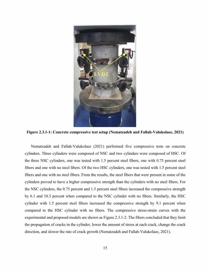
15

Figure 2.3.1-1: Concrete compressive test setup (Nematzadeh and Fallah-Valukolaee, 2021)

Nematzadeh and Fallah-Valukolaee (2021) performed five compressive tests on concrete

cylinders. Three cylinders were composed of NSC and two cylinders were composed of HSC. Of

the three NSC cylinders, one was tested with 1.5 percent steel fibers, one with 0.75 percent steel

fibers and one with no steel fibers. Of the two HSC cylinders, one was tested with 1.5 percent steel

fibers and one with no steel fibers. From the results, the steel fibers that were present in some of the

cylinders proved to have a higher compressive strength than the cylinders with no steel fibers. For

the NSC cylinders, the 0.75 percent and 1.5 percent steel fibers increased the compressive strength

by 6.1 and 10.3 percent when compared to the NSC cylinder with no fibers. Similarly, the HSC

cylinder with 1.5 percent steel fibers increased the compressive strength by 9.1 percent when

compared to the HSC cylinder with no fibers. The compressive stress-strain curves with the

experimental and proposed models are shown as Figure 2.3.1-2. The fibers concluded that they limit

the propagation of cracks in the cylinder, lower the amount of stress at each crack, change the crack

direction, and slower the rate of crack growth (Nematzadeh and Fallah-Valukolaee, 2021).

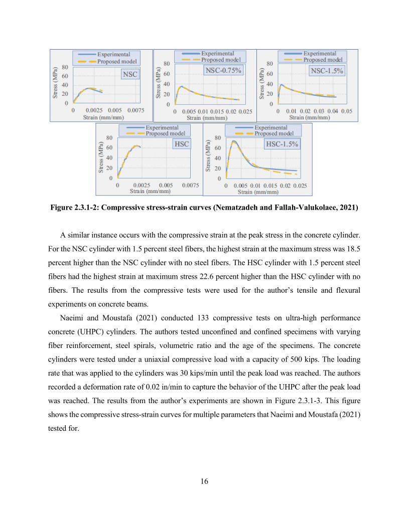
16

Figure 2.3.1-2: Compressive stress-strain curves (Nematzadeh and Fallah-Valukolaee, 2021)

A similar instance occurs with the compressive strain at the peak stress in the concrete cylinder.

For the NSC cylinder with 1.5 percent steel fibers, the highest strain at the maximum stress was 18.5

percent higher than the NSC cylinder with no steel fibers. The HSC cylinder with 1.5 percent steel

fibers had the highest strain at maximum stress 22.6 percent higher than the HSC cylinder with no

fibers. The results from the compressive tests were used for the author’s tensile and flexural

experiments on concrete beams.

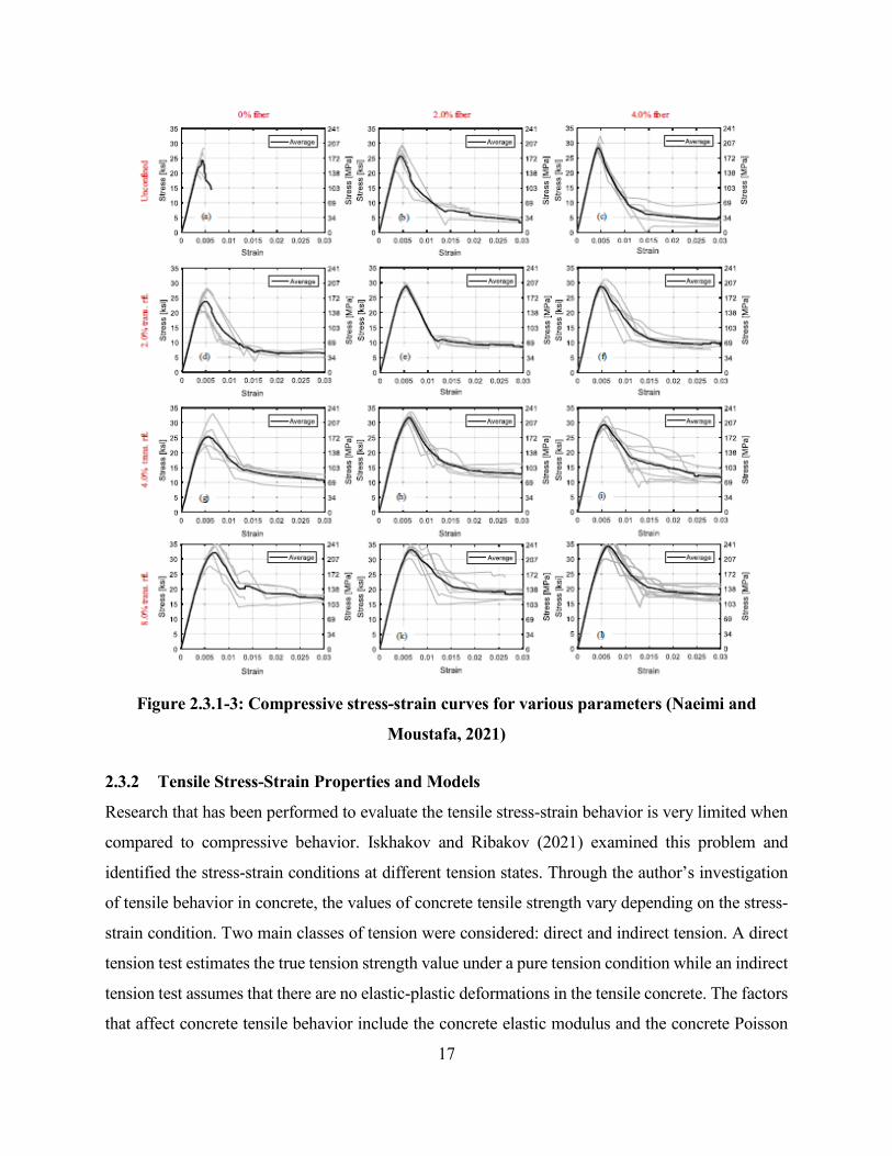
Naeimi and Moustafa (2021) conducted 133 compressive tests on ultra-high performance

concrete (UHPC) cylinders. The authors tested unconfined and confined specimens with varying

fiber reinforcement, steel spirals, volumetric ratio and the age of the specimens. The concrete

cylinders were tested under a uniaxial compressive load with a capacity of 500 kips. The loading

rate that was applied to the cylinders was 30 kips/min until the peak load was reached. The authors

recorded a deformation rate of 0.02 in/min to capture the behavior of the UHPC after the peak load

was reached. The results from the author’s experiments are shown in Figure 2.3.1-3. This figure

shows the compressive stress-strain curves for multiple parameters that Naeimi and Moustafa (2021)

tested for.

17

Figure 2.3.1-3: Compressive stress-strain curves for various parameters (Naeimi and

Moustafa, 2021)

2.3.2 Tensile Stress-Strain Properties and Models

Research that has been performed to evaluate the tensile stress-strain behavior is very limited when

compared to compressive behavior. Iskhakov and Ribakov (2021) examined this problem and

identified the stress-strain conditions at different tension states. Through the author’s investigation

of tensile behavior in concrete, the values of concrete tensile strength vary depending on the stress-

strain condition. Two main classes of tension were considered: direct and indirect tension. A direct

tension test estimates the true tension strength value under a pure tension condition while an indirect

tension test assumes that there are no elastic-plastic deformations in the tensile concrete. The factors

that affect concrete tensile behavior include the concrete elastic modulus and the concrete Poisson

18

coefficient. Some assumptions that needed to be made were that the concrete tensile strength is

equivalent to the average concrete tensile strength per design codes and the shape of the graph for

tensile deformations versus tensile stresses is equivalent to the compression counterpart, excluding

the magnitudes (Iskhakov and Ribakov, 2021).

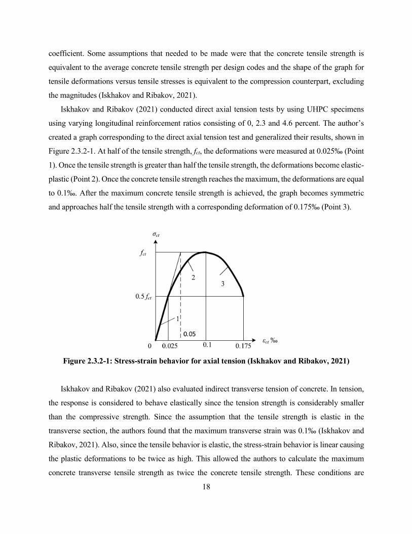
Iskhakov and Ribakov (2021) conducted direct axial tension tests by using UHPC specimens

using varying longitudinal reinforcement ratios consisting of 0, 2.3 and 4.6 percent. The author’s

created a graph corresponding to the direct axial tension test and generalized their results, shown in

Figure 2.3.2-1. At half of the tensile strength, fct, the deformations were measured at 0.025‰ (Point

1). Once the tensile strength is greater than half the tensile strength, the deformations become elastic-

plastic (Point 2). Once the concrete tensile strength reaches the maximum, the deformations are equal

to 0.1‰. After the maximum concrete tensile strength is achieved, the graph becomes symmetric

and approaches half the tensile strength with a corresponding deformation of 0.175‰ (Point 3).

Figure 2.3.2-1: Stress-strain behavior for axial tension (Iskhakov and Ribakov, 2021)

Iskhakov and Ribakov (2021) also evaluated indirect transverse tension of concrete. In tension,

the response is considered to behave elastically since the tension strength is considerably smaller

than the compressive strength. Since the assumption that the tensile strength is elastic in the

transverse section, the authors found that the maximum transverse strain was 0.1‰ (Iskhakov and

Ribakov, 2021). Also, since the tensile behavior is elastic, the stress-strain behavior is linear causing

the plastic deformations to be twice as high. This allowed the authors to calculate the maximum

concrete transverse tensile strength as twice the concrete tensile strength. These conditions are

19

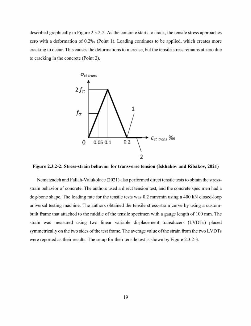
described graphically in Figure 2.3.2-2. As the concrete starts to crack, the tensile stress approaches

zero with a deformation of 0.2‰ (Point 1). Loading continues to be applied, which creates more

cracking to occur. This causes the deformations to increase, but the tensile stress remains at zero due

to cracking in the concrete (Point 2).

Figure 2.3.2-2: Stress-strain behavior for transverse tension (Iskhakov and Ribakov, 2021)

Nematzadeh and Fallah-Valukolaee (2021) also performed direct tensile tests to obtain the stress-

strain behavior of concrete. The authors used a direct tension test, and the concrete specimen had a

dog-bone shape. The loading rate for the tensile tests was 0.2 mm/min using a 400 kN closed-loop

universal testing machine. The authors obtained the tensile stress-strain curve by using a custom-

built frame that attached to the middle of the tensile specimen with a gauge length of 100 mm. The

strain was measured using two linear variable displacement transducers (LVDTs) placed

symmetrically on the two sides of the test frame. The average value of the strain from the two LVDTs

were reported as their results. The setup for their tensile test is shown by Figure 2.3.2-3.

20

Figure 2.3.2-3: Concrete tensile test setup (Nematzadeh and Fallah-Valukolaee, 2021)

Through calculations, the tensile strength of reinforced concrete beams was derived as a function

of the compression strength for both NSC and HSC cylinder specimens with and without fiber

reinforcement, shown as Equation 2-11 (Nematzadeh and Fallah-Valukolaee, 2021). A more precise

formula was derived by the authors accounting for the compressive strength of concrete and the

index of fibers shown as Equation 2-12. Vf is the volume of fibers.

𝑖𝑖𝑡𝑡 = 0.13𝑖𝑖𝑐𝑐′ 0.83 (in MPa) R2 = 0.91 (2-11)

𝑖𝑖𝑡𝑡 = 0.1𝑖𝑖𝑐𝑐′ 0.88 �1 + 43.75𝑉𝑉𝑓𝑓𝑓𝑓𝑐𝑐

�8 (in MPa) R2 = 0.91 (2-12)

Nematzadeh and Fallah-Valukolaee (2021) developed an equation that describes the strain at the

ultimate tensile strength, εt0, shown as Equation 2-13. εc’ represents the concrete compressive strain

at the maximum stress level. The authors found that the strain at the ultimate tensile strength

increased as the volume of steel fibers increased.

𝜀𝜀𝑡𝑡0 = 𝑓𝑓𝑡𝑡𝑓𝑓𝑐𝑐′𝜀𝜀𝑐𝑐′ (2-13)

21

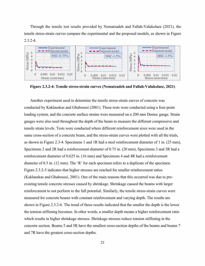
Through the tensile test results provided by Nematzadeh and Fallah-Valukolaee (2021), the

tensile stress-strain curves compare the experimental and the proposed models, as shown in Figure

2.3.2-4.

Figure 2.3.2-4: Tensile stress-strain curves (Nematzadeh and Fallah-Valukolaee, 2021)

Another experiment used to determine the tensile stress-strain curves of concrete was

conducted by Kaklauskas and Ghaboussi (2001). These tests were conducted using a four-point

loading system, and the concrete surface strains were measured on a 200 mm Demec gauge. Strain

gauges were also used throughout the depth of the beam to measure the different compressive and

tensile strain levels. Tests were conducted where different reinforcement sizes were used in the

same cross-section of a concrete beam, and the stress-strain curves were plotted with all the trials,

as shown in Figure 2.3-4. Specimens 1 and 1R had a steel reinforcement diameter of 1 in. (25 mm),

Specimens 2 and 2R had a reinforcement diameter of 0.75 in. (20 mm), Specimens 3 and 3R had a

reinforcement diameter of 0.625 in. (16 mm) and Specimens 4 and 4R had a reinforcement

diameter of 0.5 in. (12 mm). The ‘R’ for each specimen refers to a duplicate of the specimen.

Figure 2.3.2-5 indicates that higher stresses are reached for smaller reinforcement ratios

(Kaklauskas and Ghaboussi, 2001). One of the main reasons that this occurred was due to pre-

existing tensile concrete stresses caused by shrinkage. Shrinkage caused the beams with larger

reinforcement to not perform to the full potential. Similarly, the tensile stress-strain curves were

measured for concrete beams with constant reinforcement and varying depth. The results are

shown in Figure 2.3.2-6. The trend of these results indicated that the smaller the depth is the lower

the tension stiffening becomes. In other words, a smaller depth means a higher reinforcement ratio

which results in higher shrinkage stresses. Shrinkage stresses reduce tension stiffening in the

concrete section. Beams 5 and 5R have the smallest cross-section depths of the beams and beams 7

and 7R have the greatest cross-section depths.

22

Figure 2.3.2-5: Tensile stress-strain curve for varying steel reinforcement (Kaklauskas and

Ghaboussi, 2001)

Figure 2.3.2-6: Tensile stress-strain curve for varying cross-section depth (Kaklauskas and

Ghaboussi, 2001)

23

2.3.3 Steel Reinforcement Stress-Strain Properties and Models

Nematzadeh and Fallah-Valukolaee (2021) conducted steel reinforcement tensile tests per ASTM

D7205. The authors used a universal testing machine, shown in Figure 2.3.3-1, and used an

extensometer on the rebar itself to measure elongation in the bar. The type of steel reinforcement

that was used for the testing was a D10 steel rebar. The results are shown in Table 2.3.3-1 where dr

is the diameter of the rebar, Ar is the area of rebar prior to testing, Ar’ is the area of rebar after testing,

Er is the elastic modulus of the rebar, εy is the yield strain of the rebar, εp is the starting strain of

strain-hardening of the rebar and εu is the ultimate strain of the rebar.

Figure 2.3.3-1: Steel rebar tensile test setup (Nematzadeh and Fallah-Valukolaee, 2021)

24

Table 2.3.3-1: Mechanical properties of steel rebar (Nematzadeh and Fallah-Valukolaee,

2021)

Carrillo et al. (2021) performed numerous tests on steel reinforcement to determine its

mechanical properties. The authors conducted 85 monotonic tensile tests and 85 bending tests. The

authors chose to analyze five specimens of each diameter of steel, ranging from 3/8” to 1” in

diameter, from three different local manufacturing companies in Columbia. Tensile tests were

performed following ASTM A370 to determine the chemical composition of the steel bars. This

composition may vary and it affects the mechanical properties of the specimen. The tensile tests

were conducted using a Controls MC-66 universal testing machine with a tensile loading capacity

of 1,000 kN. The loading rates specified by ASTM A370 shall be between 69 MPa/min to 700

MPa/min. Carrillo et al. (2021) performed these tensile tests using a loading rate of 385 MPa/min.

Elongation in the steel bars was determined using gauge marks to identify the initial length of the

rebar. Strain-gauges were also used during the tensile tests to measure the strain in the steel bars.

The results for the tensile tests included the modulus of elasticity, yield strength, maximum (tensile)

strength, yield strain, strain hardening modulus, strain at the onset of strain hardening and strain at

the maximum strength (Carrillo et al., 2021). A table summarizing all of the properties of the tensile

test is shown in Table 2.3.3-2.

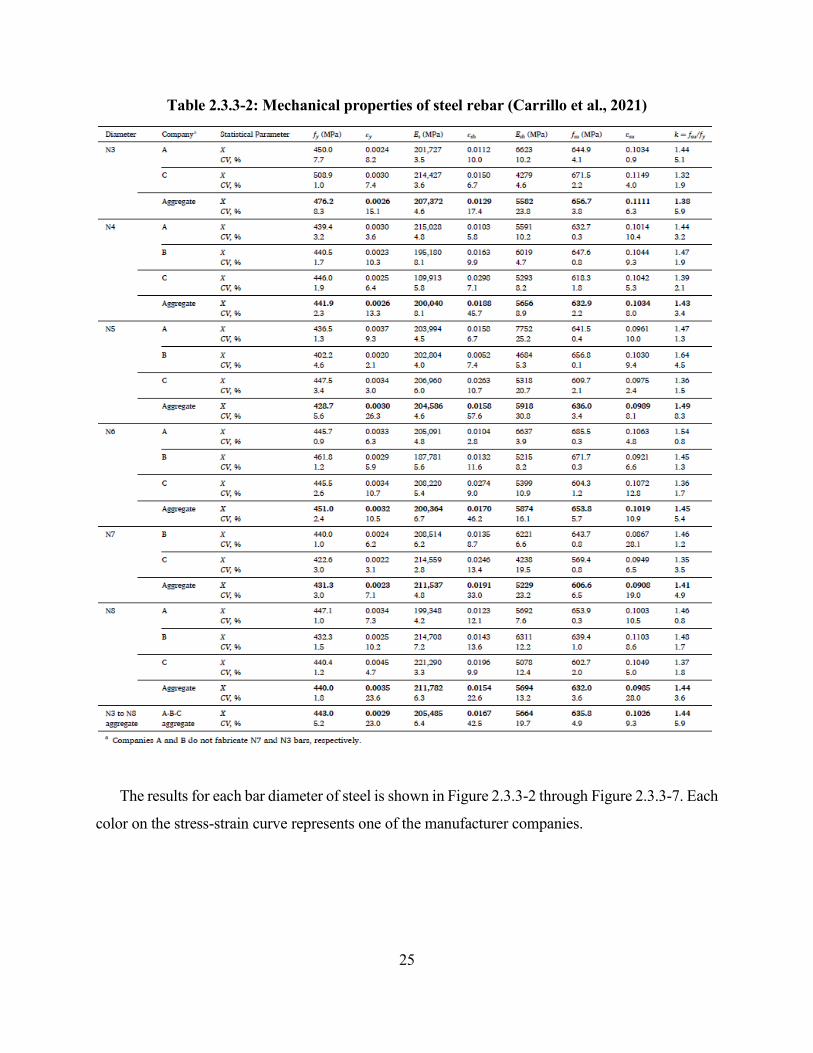
25

Table 2.3.3-2: Mechanical properties of steel rebar (Carrillo et al., 2021)

The results for each bar diameter of steel is shown in Figure 2.3.3-2 through Figure 2.3.3-7. Each

color on the stress-strain curve represents one of the manufacturer companies.

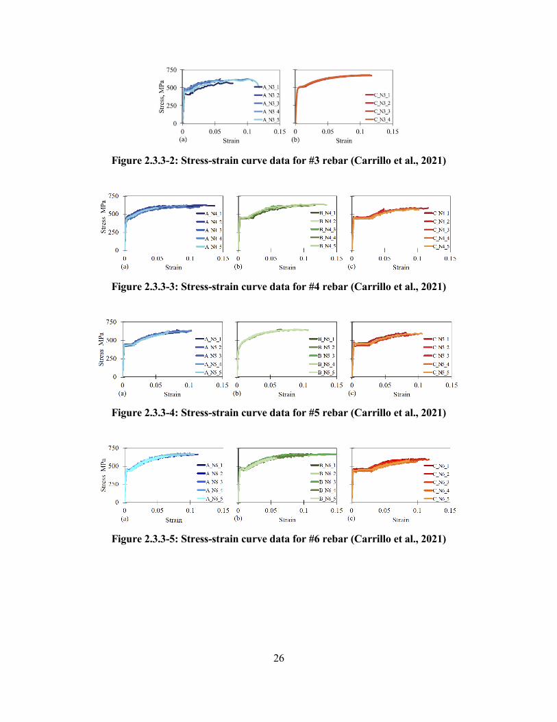
26

Figure 2.3.3-2: Stress-strain curve data for #3 rebar (Carrillo et al., 2021)




27



2.4 Experimental Studies of Load-Deflection Results

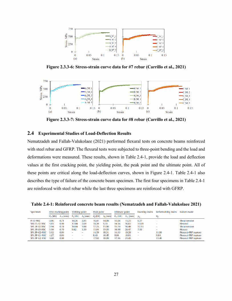
Nematzadeh and Fallah-Valukolaee (2021) performed flexural tests on concrete beams reinforced

with steel rebar and GFRP. The flexural tests were subjected to three-point bending and the load and

deformations were measured. These results, shown in Table 2.4-1, provide the load and deflection

values at the first cracking point, the yielding point, the peak point and the ultimate point. All of

these points are critical along the load-deflection curves, shown in Figure 2.4-1. Table 2.4-1 also

describes the type of failure of the concrete beam specimen. The first four specimens in Table 2.4-1

are reinforced with steel rebar while the last three specimens are reinforced with GFRP.

Table 2.4-1: Reinforced concrete beam results (Nematzadeh and Fallah-Valukolaee 2021)

28

Figure 2.4-1: Load-deflection diagram for steel and GFRP reinforcement (Nematzadeh and

Fallah-Valukolaee 2021)

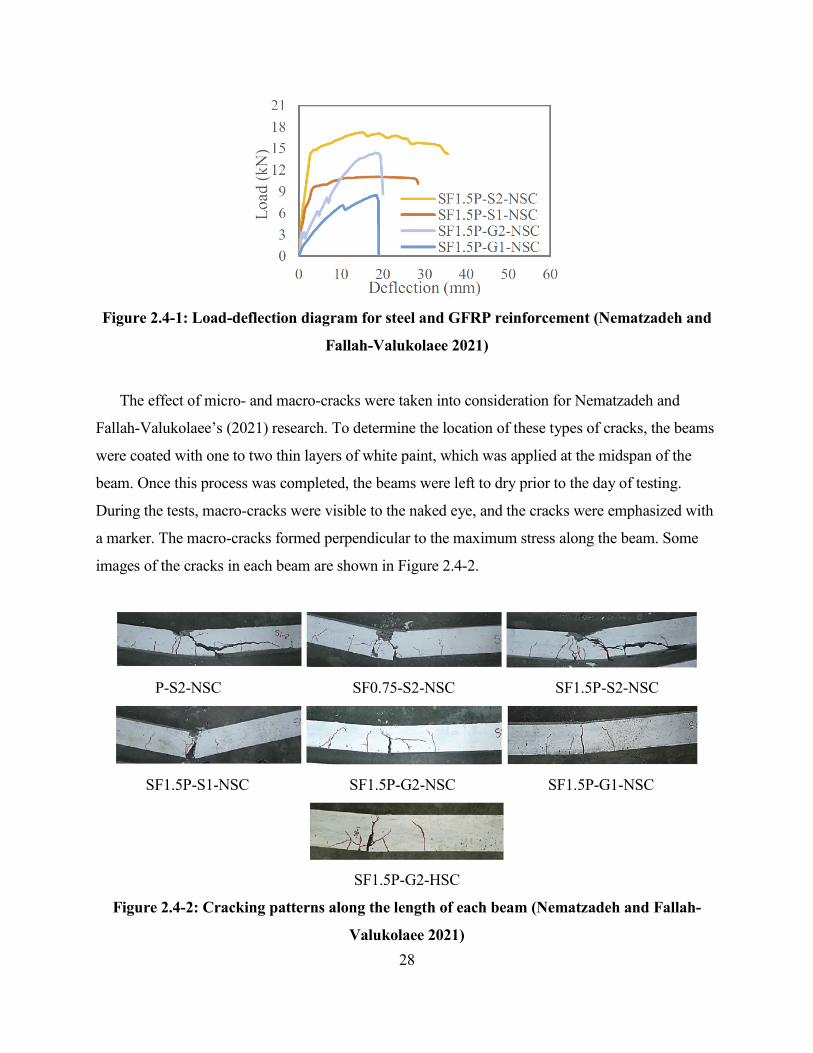
The effect of micro- and macro-cracks were taken into consideration for Nematzadeh and

Fallah-Valukolaee’s (2021) research. To determine the location of these types of cracks, the beams

were coated with one to two thin layers of white paint, which was applied at the midspan of the

beam. Once this process was completed, the beams were left to dry prior to the day of testing.

During the tests, macro-cracks were visible to the naked eye, and the cracks were emphasized with

a marker. The macro-cracks formed perpendicular to the maximum stress along the beam. Some

images of the cracks in each beam are shown in Figure 2.4-2.

P-S2-NSC SF0.75-S2-NSC SF1.5P-S2-NSC

SF1.5P-S1-NSC SF1.5P-G2-NSC SF1.5P-G1-NSC

SF1.5P-G2-HSC

Figure 2.4-2: Cracking patterns along the length of each beam (Nematzadeh and Fallah-

Valukolaee 2021)

29

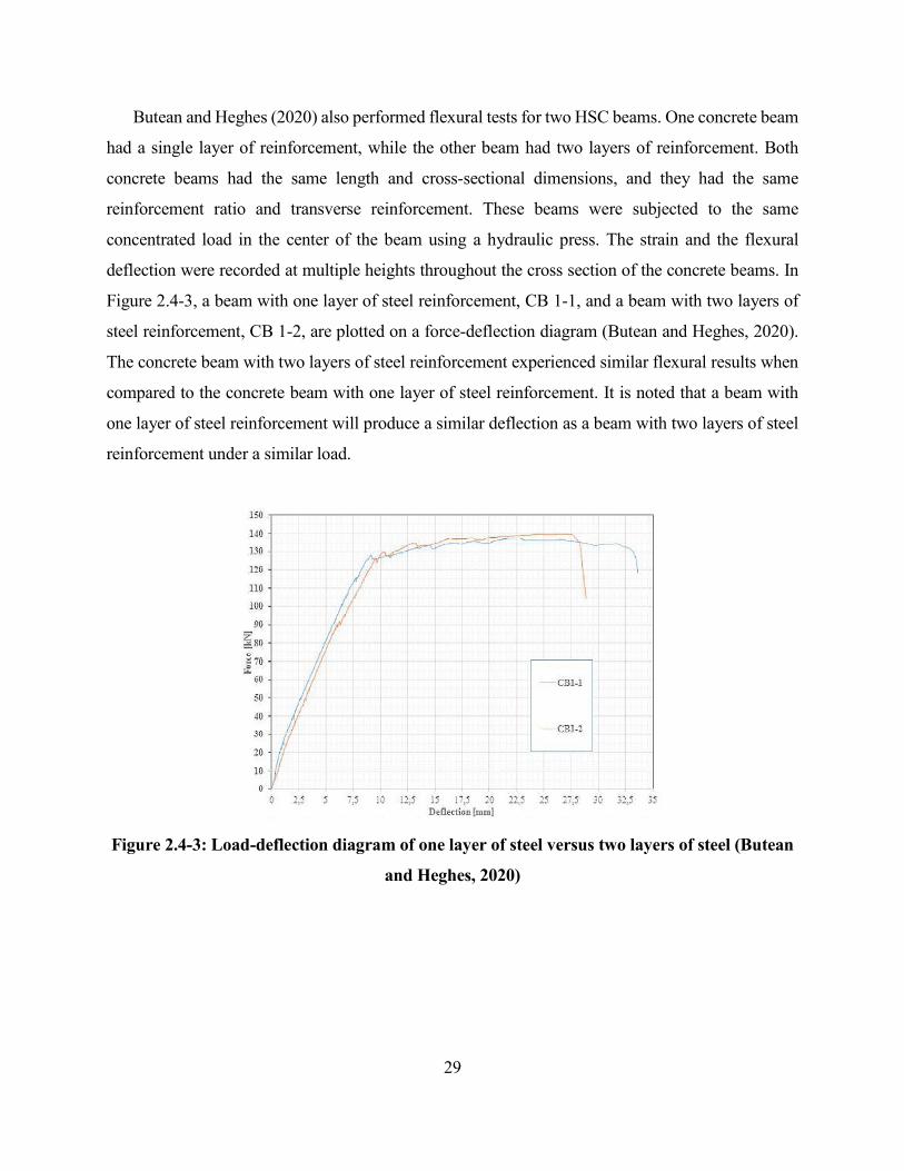
Butean and Heghes (2020) also performed flexural tests for two HSC beams. One concrete beam

had a single layer of reinforcement, while the other beam had two layers of reinforcement. Both

concrete beams had the same length and cross-sectional dimensions, and they had the same

reinforcement ratio and transverse reinforcement. These beams were subjected to the same

concentrated load in the center of the beam using a hydraulic press. The strain and the flexural

deflection were recorded at multiple heights throughout the cross section of the concrete beams. In

Figure 2.4-3, a beam with one layer of steel reinforcement, CB 1-1, and a beam with two layers of

steel reinforcement, CB 1-2, are plotted on a force-deflection diagram (Butean and Heghes, 2020).

The concrete beam with two layers of steel reinforcement experienced similar flexural results when

compared to the concrete beam with one layer of steel reinforcement. It is noted that a beam with

one layer of steel reinforcement will produce a similar deflection as a beam with two layers of steel

reinforcement under a similar load.

Figure 2.4-3: Load-deflection diagram of one layer of steel versus two layers of steel (Butean

and Heghes, 2020)

30

2.5 Analytical Models to Predict Load-Deflection Results

Many researchers who studied analytical models to predict deflections in reinforced concrete beams

also performed experimental tests to verify their results.

2.5.1 Fiber-Based Models

Along with Nematzadeh and Fallah-Valukolaee’s (2021) experimental work with reinforced

concrete beams, the authors also predicted the load-deflection behavior using an analytical model.

The mechanical properties from the steel rebar tests were used to determine an idealized stress-

strain curve. The analytical models used the experimental results of compressive and tensile stress-

strain curves from the tests shown in Figure 2.3.1-2 and Figure 2.3.2-4, respectively. An idealized

concrete model is shown in Figure 2.5.1-1 below.

(a) (b)

Figure 2.5.1-1: Stress and strain curves for (a) concrete in tension and compression and

(b) steel rebar (Nematzadeh and Fallah-Valukolaee 2021)

The analytical tests utilized a fiber analysis where the cross-section is discretized into a number

of fibers along the height. The purpose of the fiber analysis is to determine the stresses and strains

at each individual fiber along the height of the beam and for incremental loading. From the cross

section of the concrete beam, the stress-strain properties of the materials and the applied loading, a

distribution of the stresses and strains can be computed. For the strain diagram, a linear distribution

was assumed along the height of the beam (Nematzadeh and Fallah-Valukolaee, 2021). The stress

distribution for each fiber layer was obtained from the strain distribution and using the stress-strain

relationships of the materials. This concept is illustrated in Figure 2.5.1-2.

31

Figure 2.5.1-2: Stress and strain distributions over the cross-section of a beam (Nematzadeh

and Fallah-Valukolaee 2021)

A critical component of the fiber analysis is determining where the neutral axis is located. A

given curvature was calculated from the ratio of the extreme compression fiber strain to the neutral

axis depth. From this curvature, the neutral axis depth can be found from equilibrium of the

compression force and tension forces. Once the curvature and neutral axis are determined, the

strains and stresses at that particular fiber can be analyzed. From basic mechanical properties, a

force can be calculated by the stress multiplied by the area of the fiber. Finally, a moment can be

obtained from the force multiplied by the distance between the force and the neutral axis. This

procedure is repeated numerous times for different curvature values until there is enough data to

create an adequate moment-curvature diagram. From this diagram, the deflection can be calculated

using the curvature-area method, or known as the second moment-area theorem.

The experimental and analytical load-deflection diagrams were compared for each of the

different reinforcement schemes. The analytical model results were quite similar to the experimental

results. These results are shown in Figure 2.5.1-3. It is proven that the analytical approach can

accurately determine the structural behavior of a reinforced concrete beam (Nematzadeh and Fallah-

Valukolaee, 2021).

32

Figure 2.5.1-3: Fiber analysis versus experimental results for each reinforcement scheme

(Nematzadeh and Fallah-Valukolaee 2021)

2.5.2 Finite Element Analysis Models

Patel et al. (2014) experimentally and analytically predicted the deflections under given loading

conditions of reinforced concrete beams. The results of these two tests were compared with each

other to validate the analytical model. The authors developed a finite element model (FEM) using

the ABAQUS software. For a given service load, the stress-strain relationship of concrete was

assumed to be linear while in a compressive state. For the tensile state, the concrete was assumed to

be elastic before cracking occurred and softening behavior after cracking occurred. In the program,

33

the steel reinforcement was assumed to have a perfect bond between the steel and concrete. Tension

stiffening was considered for the model, and a high shear stiffness was assumed to prevent shear

deformations from occurring. The mid-span deflection was recorded with an increasing uniformly

distributed load along the length of the concrete beam. The authors created a tension stiffening model

to show how the tensile stresses behave once cracking has occurred. This diagram is shown in Figure

2.5.2-1.

Figure 2.5.2-1: Tension stiffening model (Patel et al., 2014)

The strain at cracking was considered to be 0.00012 with a reinforcement ratio of 1.2%. The

tension stress was determined using ACI 318. For the FEM, 16 elements were required when

cracking is taken into consideration. The results from the finite element analysis and the author’s

experimental studies are shown in Figure 2.5.2-2.

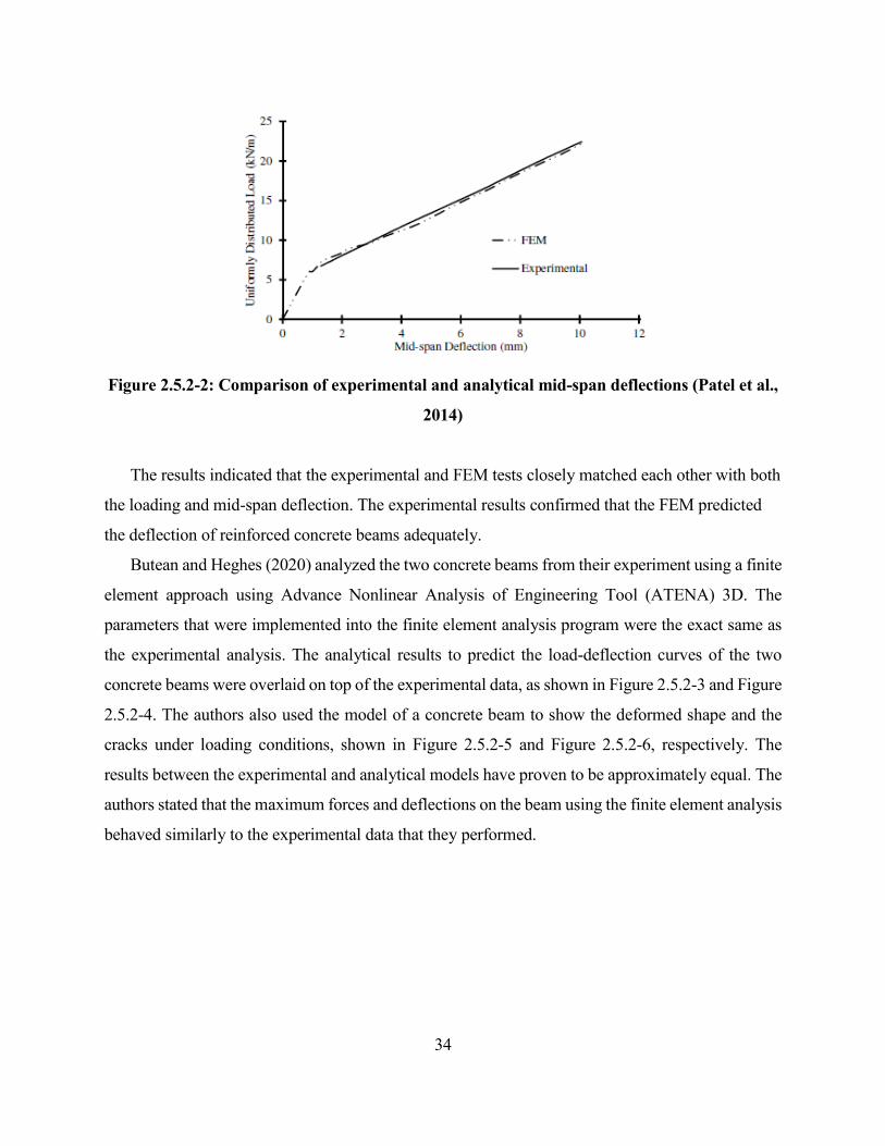
34

Figure 2.5.2-2: Comparison of experimental and analytical mid-span deflections (Patel et al.,

2014)

The results indicated that the experimental and FEM tests closely matched each other with both

the loading and mid-span deflection. The experimental results confirmed that the FEM predicted

the deflection of reinforced concrete beams adequately.

Butean and Heghes (2020) analyzed the two concrete beams from their experiment using a finite

element approach using Advance Nonlinear Analysis of Engineering Tool (ATENA) 3D. The

parameters that were implemented into the finite element analysis program were the exact same as

the experimental analysis. The analytical results to predict the load-deflection curves of the two

concrete beams were overlaid on top of the experimental data, as shown in Figure 2.5.2-3 and Figure

2.5.2-4. The authors also used the model of a concrete beam to show the deformed shape and the

cracks under loading conditions, shown in Figure 2.5.2-5 and Figure 2.5.2-6, respectively. The

results between the experimental and analytical models have proven to be approximately equal. The

authors stated that the maximum forces and deflections on the beam using the finite element analysis

behaved similarly to the experimental data that they performed.

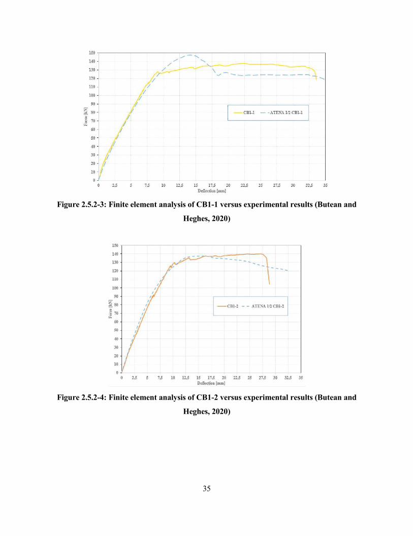
35

Figure 2.5.2-3: Finite element analysis of CB1-1 versus experimental results (Butean and

Heghes, 2020)

Figure 2.5.2-4: Finite element analysis of CB1-2 versus experimental results (Butean and

Heghes, 2020)

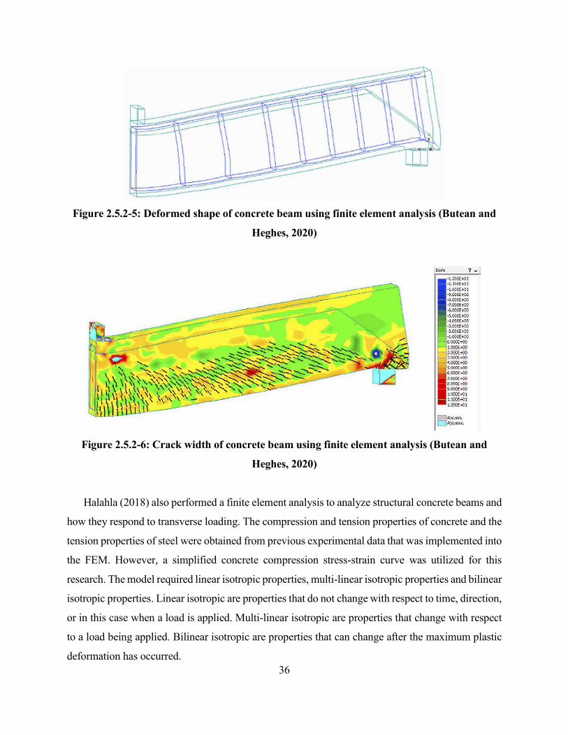
36

Figure 2.5.2-5: Deformed shape of concrete beam using finite element analysis (Butean and

Heghes, 2020)

Figure 2.5.2-6: Crack width of concrete beam using finite element analysis (Butean and

Heghes, 2020)

Halahla (2018) also performed a finite element analysis to analyze structural concrete beams and

how they respond to transverse loading. The compression and tension properties of concrete and the

tension properties of steel were obtained from previous experimental data that was implemented into

the FEM. However, a simplified concrete compression stress-strain curve was utilized for this

research. The model required linear isotropic properties, multi-linear isotropic properties and bilinear

isotropic properties. Linear isotropic are properties that do not change with respect to time, direction,

or in this case when a load is applied. Multi-linear isotropic are properties that change with respect

to a load being applied. Bilinear isotropic are properties that can change after the maximum plastic

deformation has occurred.

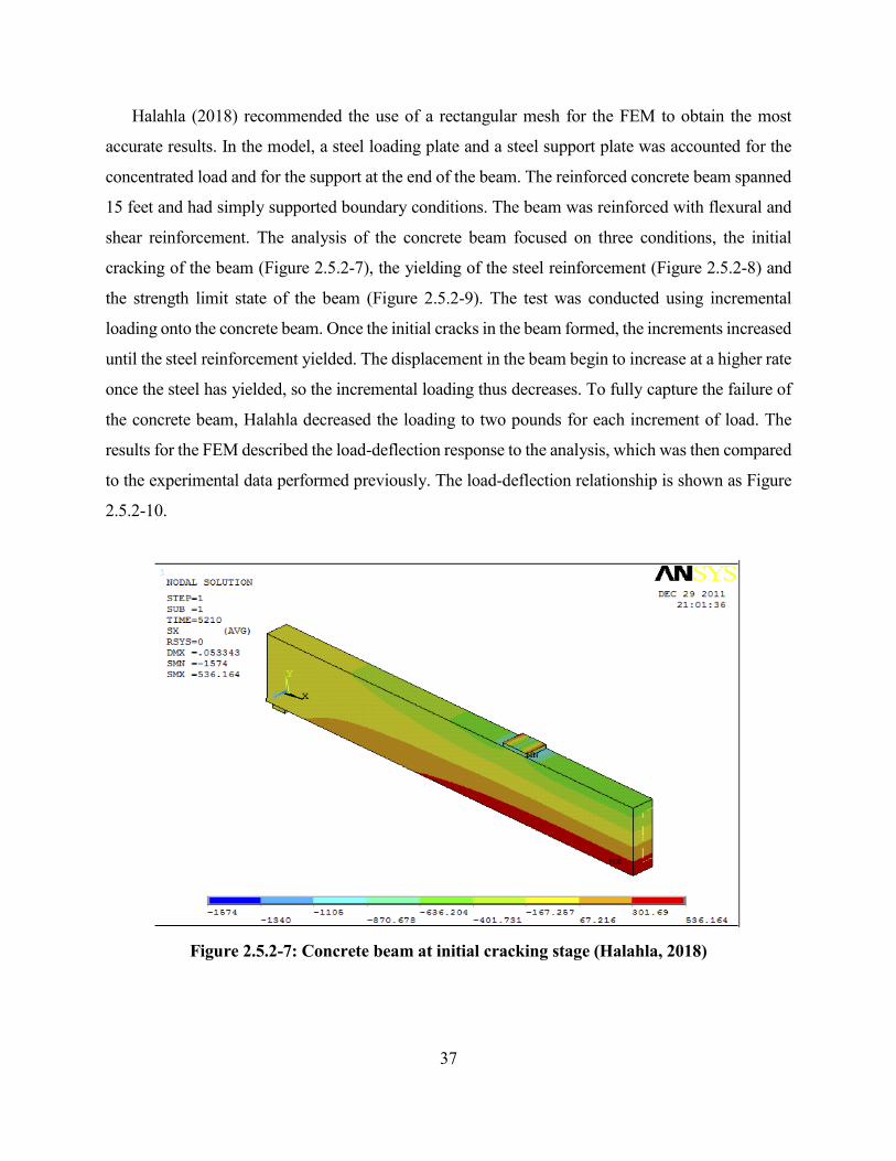
37

Halahla (2018) recommended the use of a rectangular mesh for the FEM to obtain the most

accurate results. In the model, a steel loading plate and a steel support plate was accounted for the

concentrated load and for the support at the end of the beam. The reinforced concrete beam spanned

15 feet and had simply supported boundary conditions. The beam was reinforced with flexural and

shear reinforcement. The analysis of the concrete beam focused on three conditions, the initial

cracking of the beam (Figure 2.5.2-7), the yielding of the steel reinforcement (Figure 2.5.2-8) and

the strength limit state of the beam (Figure 2.5.2-9). The test was conducted using incremental

loading onto the concrete beam. Once the initial cracks in the beam formed, the increments increased

until the steel reinforcement yielded. The displacement in the beam begin to increase at a higher rate

once the steel has yielded, so the incremental loading thus decreases. To fully capture the failure of

the concrete beam, Halahla decreased the loading to two pounds for each increment of load. The

results for the FEM described the load-deflection response to the analysis, which was then compared

to the experimental data performed previously. The load-deflection relationship is shown as Figure

2.5.2-10.

Figure 2.5.2-7: Concrete beam at initial cracking stage (Halahla, 2018)

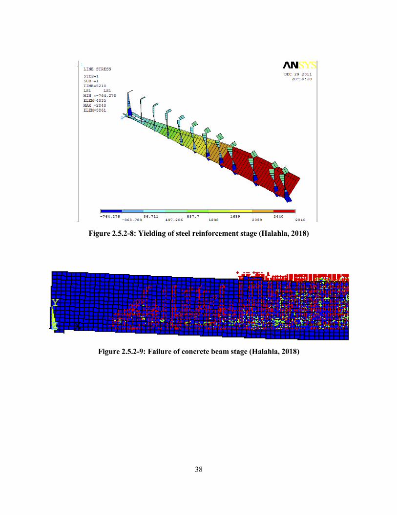
38

Figure 2.5.2-8: Yielding of steel reinforcement stage (Halahla, 2018)

Figure 2.5.2-9: Failure of concrete beam stage (Halahla, 2018)

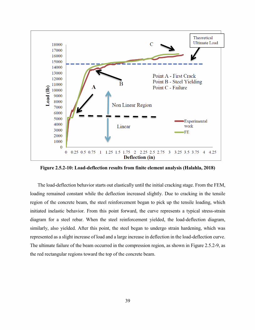
39

Figure 2.5.2-10: Load-deflection results from finite element analysis (Halahla, 2018)

The load-deflection behavior starts out elastically until the initial cracking stage. From the FEM,

loading remained constant while the deflection increased slightly. Due to cracking in the tensile

region of the concrete beam, the steel reinforcement began to pick up the tensile loading, which

initiated inelastic behavior. From this point forward, the curve represents a typical stress-strain

diagram for a steel rebar. When the steel reinforcement yielded, the load-deflection diagram,

similarly, also yielded. After this point, the steel began to undergo strain hardening, which was

represented as a slight increase of load and a large increase in deflection in the load-deflection curve.

The ultimate failure of the beam occurred in the compression region, as shown in Figure 2.5.2-9, as

the red rectangular regions toward the top of the concrete beam.

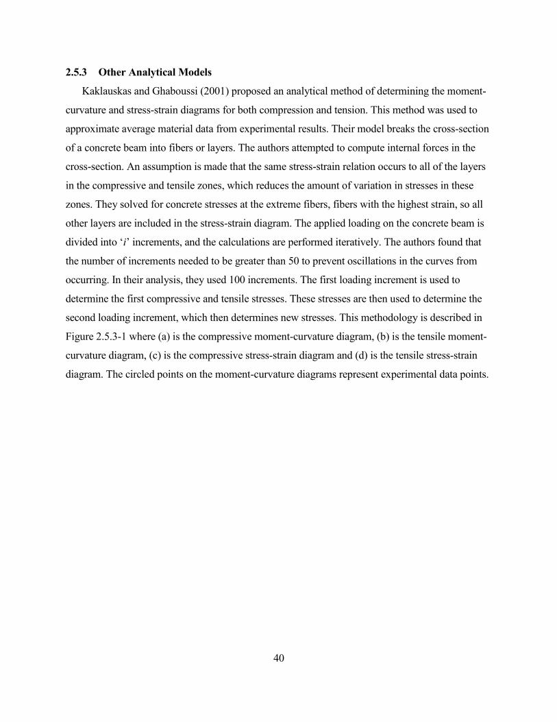
40

2.5.3 Other Analytical Models

Kaklauskas and Ghaboussi (2001) proposed an analytical method of determining the moment-

curvature and stress-strain diagrams for both compression and tension. This method was used to

approximate average material data from experimental results. Their model breaks the cross-section

of a concrete beam into fibers or layers. The authors attempted to compute internal forces in the

cross-section. An assumption is made that the same stress-strain relation occurs to all of the layers

in the compressive and tensile zones, which reduces the amount of variation in stresses in these

zones. They solved for concrete stresses at the extreme fibers, fibers with the highest strain, so all

other layers are included in the stress-strain diagram. The applied loading on the concrete beam is

divided into ‘i’ increments, and the calculations are performed iteratively. The authors found that

the number of increments needed to be greater than 50 to prevent oscillations in the curves from

occurring. In their analysis, they used 100 increments. The first loading increment is used to

determine the first compressive and tensile stresses. These stresses are then used to determine the

second loading increment, which then determines new stresses. This methodology is described in

Figure 2.5.3-1 where (a) is the compressive moment-curvature diagram, (b) is the tensile moment-

curvature diagram, (c) is the compressive stress-strain diagram and (d) is the tensile stress-strain

diagram. The circled points on the moment-curvature diagrams represent experimental data points.

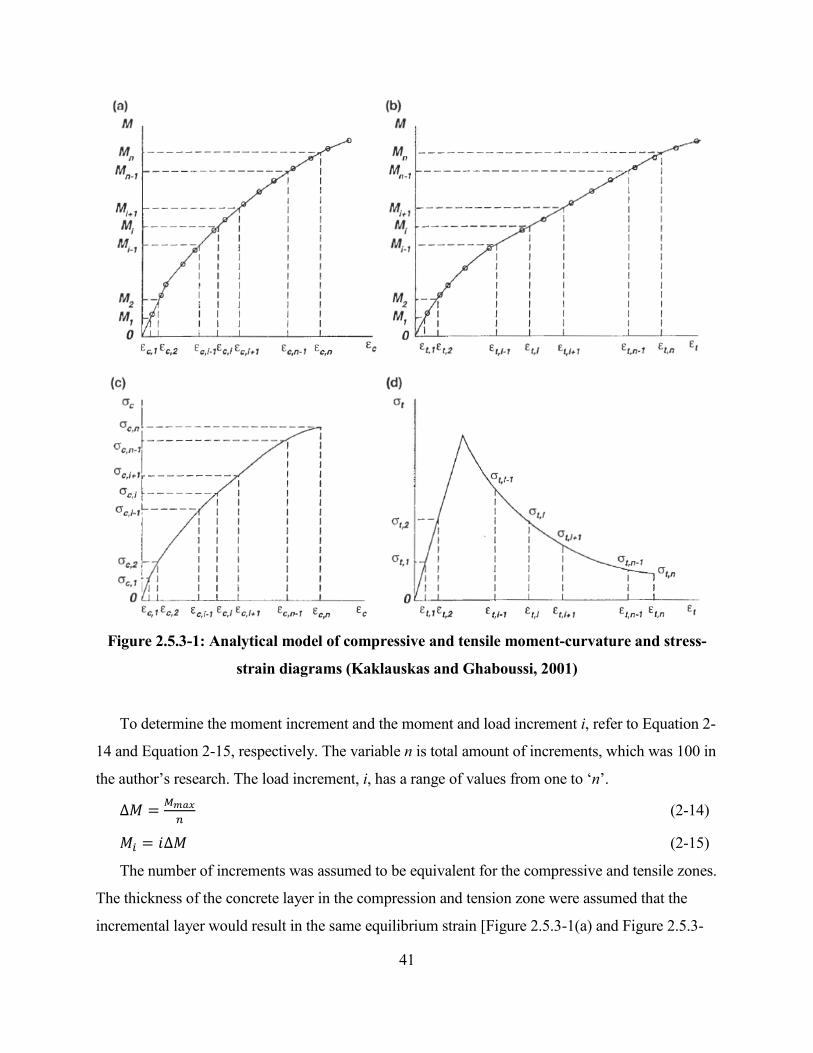
41

Figure 2.5.3-1: Analytical model of compressive and tensile moment-curvature and stress-

strain diagrams (Kaklauskas and Ghaboussi, 2001)

To determine the moment increment and the moment and load increment i, refer to Equation 2-

14 and Equation 2-15, respectively. The variable n is total amount of increments, which was 100 in

the author’s research. The load increment, i, has a range of values from one to ‘n’.

∆𝑀𝑀 = 𝑀𝑀𝑚𝑚𝑎𝑎𝑚𝑚𝑛𝑛

(2-14)

𝑀𝑀𝑖𝑖 = 𝑖𝑖∆𝑀𝑀 (2-15)

The number of increments was assumed to be equivalent for the compressive and tensile zones.

The thickness of the concrete layer in the compression and tension zone were assumed that the

incremental layer would result in the same equilibrium strain [Figure 2.5.3-1(a) and Figure 2.5.3-

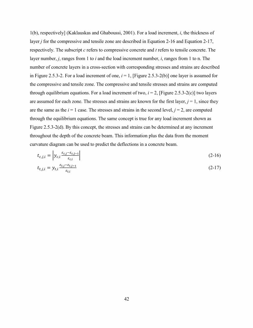
42

1(b), respectively] (Kaklauskas and Ghaboussi, 2001). For a load increment, i, the thickness of

layer j for the compressive and tensile zone are described in Equation 2-16 and Equation 2-17,

respectively. The subscript c refers to compressive concrete and t refers to tensile concrete. The

layer number, j, ranges from 1 to i and the load increment number, i, ranges from 1 to n. The

number of concrete layers in a cross-section with corresponding stresses and strains are described

in Figure 2.5.3-2. For a load increment of one, i = 1, [Figure 2.5.3-2(b)] one layer is assumed for

the compressive and tensile zone. The compressive and tensile stresses and strains are computed

through equilibrium equations. For a load increment of two, i = 2, [Figure 2.5.3-2(c)] two layers

are assumed for each zone. The stresses and strains are known for the first layer, j = 1, since they

are the same as the i = 1 case. The stresses and strains in the second level, j = 2, are computed

through the equilibrium equations. The same concept is true for any load increment shown as

Figure 2.5.3-2(d). By this concept, the stresses and strains can be determined at any increment

throughout the depth of the concrete beam. This information plus the data from the moment

curvature diagram can be used to predict the deflections in a concrete beam.

𝑡𝑡𝑐𝑐,𝑗𝑗,𝑖𝑖 = �𝑦𝑦𝑐𝑐,𝑖𝑖𝜀𝜀𝑐𝑐,𝑗𝑗−𝜀𝜀𝑐𝑐,𝑗𝑗−1

𝜀𝜀𝑐𝑐,𝑖𝑖� (2-16)

𝑡𝑡𝑡𝑡,𝑗𝑗,𝑖𝑖 = 𝑦𝑦𝑡𝑡,𝑖𝑖𝜀𝜀𝑡𝑡,𝑗𝑗−𝜀𝜀𝑡𝑡,𝑗𝑗−1

𝜀𝜀𝑡𝑡,𝑖𝑖 (2-17)

43

Figure 2.5.3-2: Stress and strain behavior at different concrete layers using an analytical

model (Kaklauskas and Ghaboussi, 2001)

44

2.6 Conclusions from the Literature Review

This literature review reviews critical previous research relevant to this research project and

focuses on material properties and studies that have been performed on deflections of reinforced

concrete beams.

Through research and experimentation, different variations of the effective moment of inertia

equation exist with the newest version adopted by ACI 318-19 (ACI 318, 2019). This recent

equation differs from the previous moment of inertia equation adopted by ACI 318-14 (ACI 318,

2014) to account for tension stiffening (Bischoff, 2005) and accuracy for reinforcement of less than

one percent (Scanlon and Bischoff, 2008).

Experimental tests were conducted to understand how the compressive and tensile stresses

behave under a concentrated loading condition. Compressive tests focused on concrete cylinders

and creating compressive stress-strain diagrams. Tensile tests focused on concrete beams and

measuring the strain using strain gauges to determine tensile stress-strain diagrams. A relationship

between the reinforcement ratio and tension stiffening exists: a higher reinforcement ratio creates

lower tension stiffening in the cross-section (Kaklauskas and Ghaboussi, 2001). Tensile stress-

strain diagrams were reported for different tension tests (Iskhakov and Ribakov, 2021). Tensile

tests for steel reinforcement were conducted by Nematzadeh and Fallah-Valukolaee (2021) to use

the mechanical properties of the steel rebar in their analytical models. Load-deflection diagrams

were also provided to compare to the analytical models.

Different analytical methods were proposed to predict the deflections of reinforced concrete

beams. Many of these researchers utilized data from their own experiments, and the results were

compared with each other. A fiber analysis model, finite element model and an iterative approach

are all different methods in predicting deflections in concrete beams. Assumptions were required to

make the analytical model appropriately match the experimental results. All three analytical

approaches accurately predicted the maximum load and deflection of the experimental counterpart.

45

CHAPTER 3: EXPERIMENTAL METHODOLOGY

3.1 General Experimental Testing

The experimental work that has been completed for this research includes flexural testing of

reinforced concrete beams, compressive testing of concrete cylinders according to the specifications

of ASTM C39 (ASTM C39, 2001), flexural testing of non-reinforced concrete beams and tensile

testing of steel reinforcement. The testing of the non-reinforced concrete beams was performed per

ASTM C78 (ASTM C78, 2002) to initially determine the tensile stress-strain behavior. However,

the tensile properties could not properly be obtained through the setup of the test. The tensile

properties for the fiber analysis utilizes Nematzadeh and Fallah-Valukolaee (2021) tensile

experimental research, which will be discussed later in this document.

The primary purpose of performing the flexural tests was to compare the load-displacement

results to that of analytical models. The compressive and tensile tests were required to determine

accurate stress-strain curves for the concrete material and to utilize this data in the analytical models.

Digital Image Correlation (DIC) by Trillion was used to capture strain on the surface of the

concrete beams and to develop stress-strain curves for the compressive tests. Load and displacement

versus time was also recorded through DIC. Two cameras were used to record at different angles

throughout the duration of the flexural tests, but only one camera was used for the concrete

compressive tests. Before the testing day, all specimens were coated with two thin layers of white

spray paint at the area of interest. After the white coating of spray paint was evenly applied, a speckle

of black paint was sprayed onto the beam to allow for the DIC to capture the incremental strain for

the full duration of the tests. The DIC cameras were placed in plane of the area of interest to minimize

any skewing throughout the test. For the concrete compressive tests, a thin piece of plexiglass was

used to allow for a clear area of recording the necessary data. The cover for the testing machine was

extremely dirty and it would have caused major inaccuracies for the recorded data. The plexiglass

was used to protect the DIC equipment because concrete cylinders may explosively break under

extreme amounts of compressive force.

As the DIC recorded data for all of the concrete tests, the data was exported to GOM Correlate

2020. This program directly measured any desired quantity, such as force, displacement or

directional strain, with respect to time through a series of images. Strain values were measured

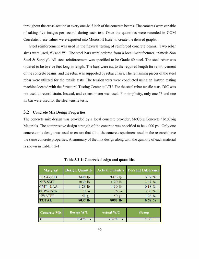
46

throughout the cross-section at every one-half inch of the concrete beams. The cameras were capable

of taking five images per second during each test. Once the quantities were recorded in GOM

Correlate, these values were exported into Microsoft Excel to create the desired graphs.

Steel reinforcement was used in the flexural testing of reinforced concrete beams. Two rebar

sizes were used, #3 and #5. The steel bars were ordered from a local manufacturer, “Smede-Son

Steel & Supply”. All steel reinforcement was specified to be Grade 60 steel. The steel rebar was

ordered to be twelve feet long in length. The bars were cut to the required length for reinforcement

of the concrete beams, and the rebar was supported by rebar chairs. The remaining pieces of the steel

rebar were utilized for the tensile tests. The tension tests were conducted using an Instron testing

machine located with the Structural Testing Center at LTU. For the steel rebar tensile tests, DIC was

not used to record strain. Instead, and extensometer was used. For simplicity, only one #3 and one

#5 bar were used for the steel tensile tests.

3.2 Concrete Mix Design Properties

The concrete mix design was provided by a local concrete provider, McCoig Concrete / McCoig

Materials. The compressive design strength of the concrete was specified to be 4,000 psi. Only one

concrete mix design was used to ensure that all of the concrete specimens used in the research have

the same concrete properties. A summary of the mix design along with the quantity of each material

is shown in Table 3.2-1.

Table 3.2-1: Concrete design and quantities

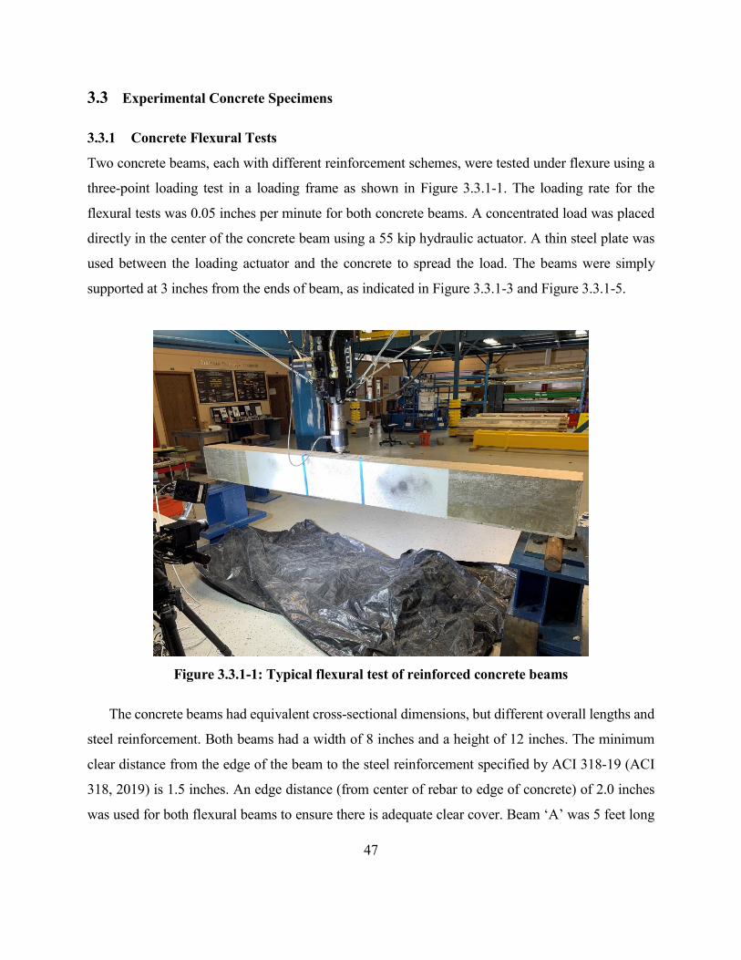
47

3.3 Experimental Concrete Specimens

3.3.1 Concrete Flexural Tests

Two concrete beams, each with different reinforcement schemes, were tested under flexure using a

three-point loading test in a loading frame as shown in Figure 3.3.1-1. The loading rate for the

flexural tests was 0.05 inches per minute for both concrete beams. A concentrated load was placed

directly in the center of the concrete beam using a 55 kip hydraulic actuator. A thin steel plate was

used between the loading actuator and the concrete to spread the load. The beams were simply

supported at 3 inches from the ends of beam, as indicated in Figure 3.3.1-3 and Figure 3.3.1-5.

Figure 3.3.1-1: Typical flexural test of reinforced concrete beams

The concrete beams had equivalent cross-sectional dimensions, but different overall lengths and

steel reinforcement. Both beams had a width of 8 inches and a height of 12 inches. The minimum

clear distance from the edge of the beam to the steel reinforcement specified by ACI 318-19 (ACI

318, 2019) is 1.5 inches. An edge distance (from center of rebar to edge of concrete) of 2.0 inches

was used for both flexural beams to ensure there is adequate clear cover. Beam ‘A’ was 5 feet long

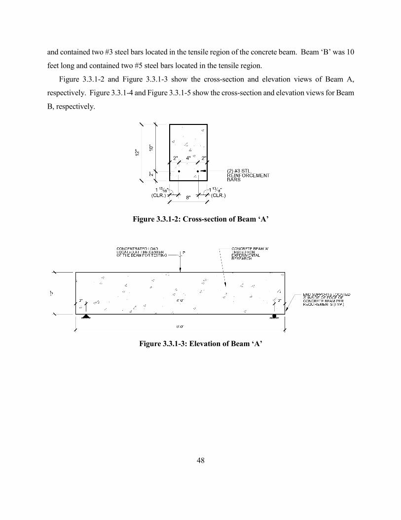
48

and contained two #3 steel bars located in the tensile region of the concrete beam. Beam ‘B’ was 10

feet long and contained two #5 steel bars located in the tensile region.

Figure 3.3.1-2 and Figure 3.3.1-3 show the cross-section and elevation views of Beam A,

respectively. Figure 3.3.1-4 and Figure 3.3.1-5 show the cross-section and elevation views for Beam

B, respectively.

Figure 3.3.1-2: Cross-section of Beam ‘A’

Figure 3.3.1-3: Elevation of Beam ‘A’

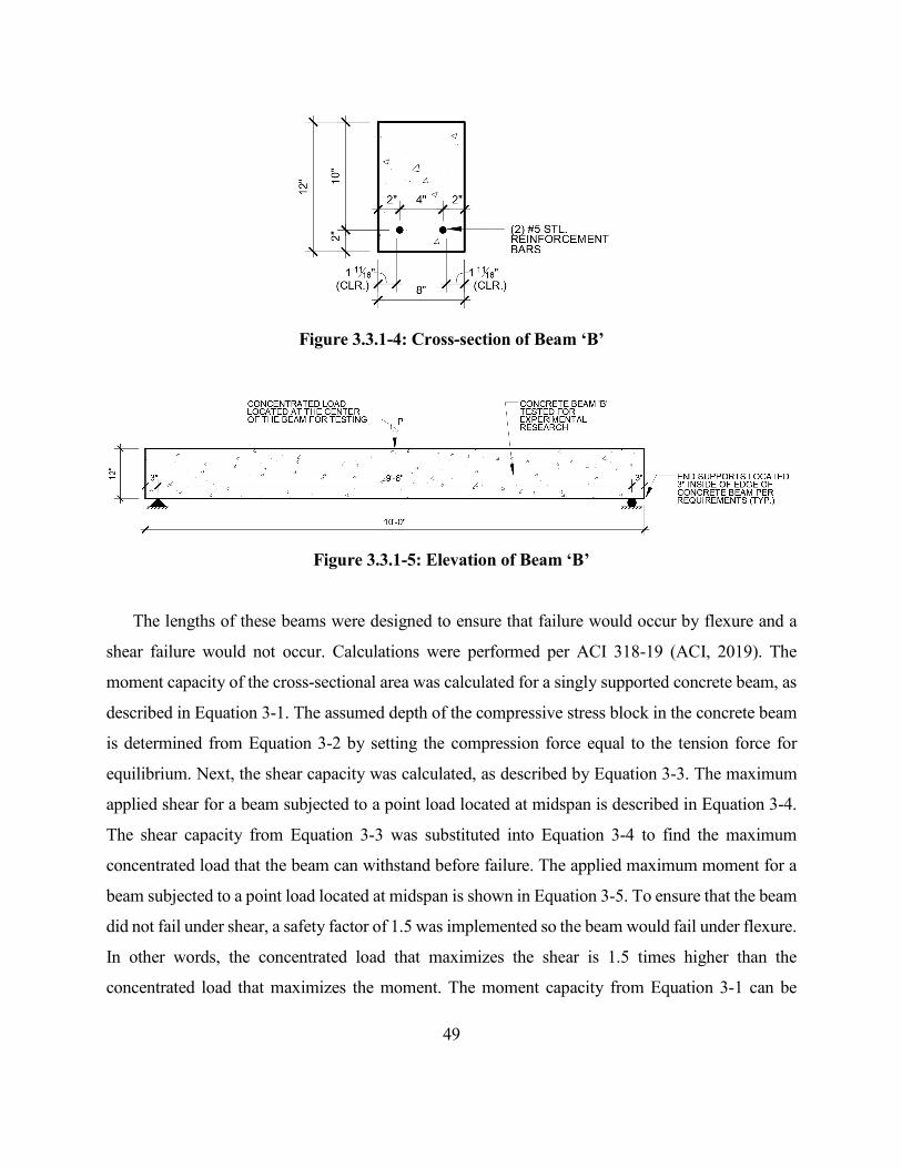
49

Figure 3.3.1-4: Cross-section of Beam ‘B’

Figure 3.3.1-5: Elevation of Beam ‘B’

The lengths of these beams were designed to ensure that failure would occur by flexure and a

shear failure would not occur. Calculations were performed per ACI 318-19 (ACI, 2019). The

moment capacity of the cross-sectional area was calculated for a singly supported concrete beam, as

described in Equation 3-1. The assumed depth of the compressive stress block in the concrete beam

is determined from Equation 3-2 by setting the compression force equal to the tension force for

equilibrium. Next, the shear capacity was calculated, as described by Equation 3-3. The maximum

applied shear for a beam subjected to a point load located at midspan is described in Equation 3-4.

The shear capacity from Equation 3-3 was substituted into Equation 3-4 to find the maximum

concentrated load that the beam can withstand before failure. The applied maximum moment for a

beam subjected to a point load located at midspan is shown in Equation 3-5. To ensure that the beam

did not fail under shear, a safety factor of 1.5 was implemented so the beam would fail under flexure.

In other words, the concentrated load that maximizes the shear is 1.5 times higher than the

concentrated load that maximizes the moment. The moment capacity from Equation 3-1 can be

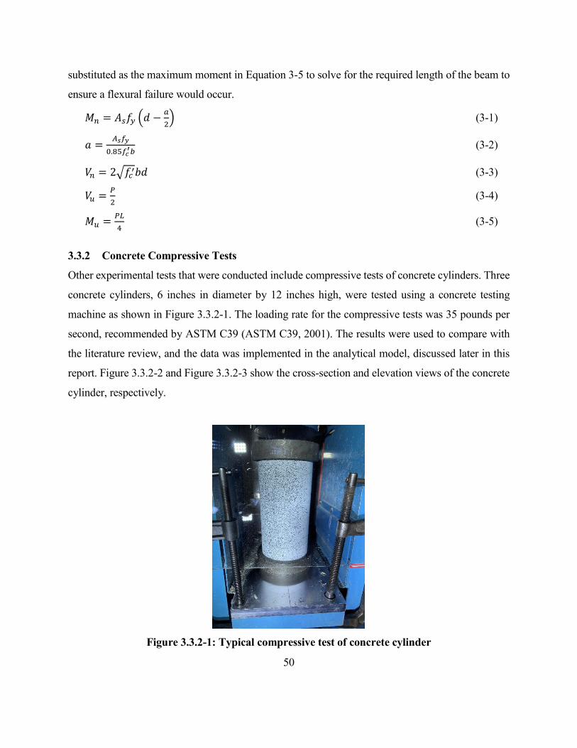
50

substituted as the maximum moment in Equation 3-5 to solve for the required length of the beam to

ensure a flexural failure would occur.

𝑀𝑀𝑛𝑛 = 𝐴𝐴𝑠𝑠𝑖𝑖𝑦𝑦 �𝑑𝑑 −𝑎𝑎2� (3-1)

𝑎𝑎 = 𝐴𝐴𝑠𝑠𝑓𝑓𝑦𝑦0.85𝑓𝑓𝑐𝑐′𝑏𝑏

(3-2)

𝑉𝑉𝑛𝑛 = 2�𝑖𝑖𝑐𝑐′𝑏𝑏𝑑𝑑 (3-3)

𝑉𝑉𝑢𝑢 = 𝑃𝑃2 (3-4)

𝑀𝑀𝑢𝑢 = 𝑃𝑃𝐿𝐿4

(3-5)

3.3.2 Concrete Compressive Tests

Other experimental tests that were conducted include compressive tests of concrete cylinders. Three

concrete cylinders, 6 inches in diameter by 12 inches high, were tested using a concrete testing

machine as shown in Figure 3.3.2-1. The loading rate for the compressive tests was 35 pounds per

second, recommended by ASTM C39 (ASTM C39, 2001). The results were used to compare with

the literature review, and the data was implemented in the analytical model, discussed later in this

report. Figure 3.3.2-2 and Figure 3.3.2-3 show the cross-section and elevation views of the concrete

cylinder, respectively.

Figure 3.3.2-1: Typical compressive test of concrete cylinder

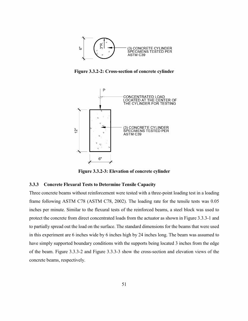
51

Figure 3.3.2-2: Cross-section of concrete cylinder

Figure 3.3.2-3: Elevation of concrete cylinder

3.3.3 Concrete Flexural Tests to Determine Tensile Capacity

Three concrete beams without reinforcement were tested with a three-point loading test in a loading

frame following ASTM C78 (ASTM C78, 2002). The loading rate for the tensile tests was 0.05

inches per minute. Similar to the flexural tests of the reinforced beams, a steel block was used to

protect the concrete from direct concentrated loads from the actuator as shown in Figure 3.3.3-1 and

to partially spread out the load on the surface. The standard dimensions for the beams that were used

in this experiment are 6 inches wide by 6 inches high by 24 inches long. The beam was assumed to

have simply supported boundary conditions with the supports being located 3 inches from the edge

of the beam. Figure 3.3.3-2 and Figure 3.3.3-3 show the cross-section and elevation views of the

concrete beams, respectively.

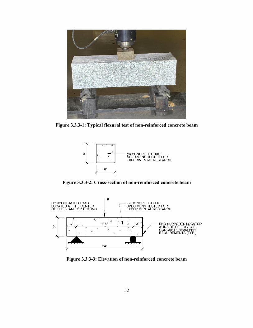
52

Figure 3.3.3-1: Typical flexural test of non-reinforced concrete beam

Figure 3.3.3-2: Cross-section of non-reinforced concrete beam

Figure 3.3.3-3: Elevation of non-reinforced concrete beam

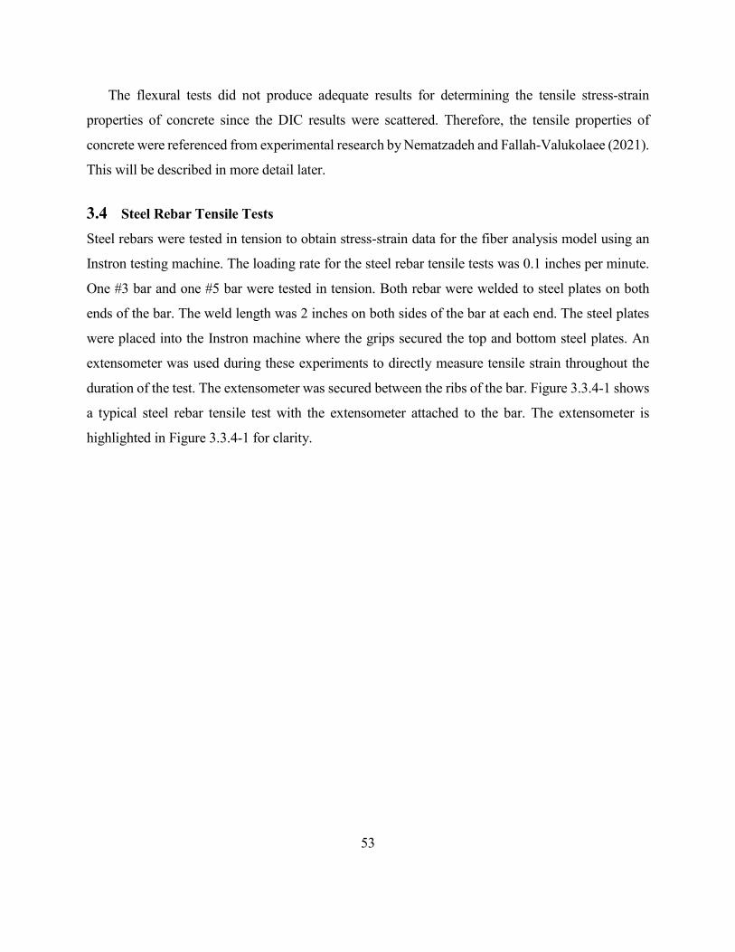
53

The flexural tests did not produce adequate results for determining the tensile stress-strain

properties of concrete since the DIC results were scattered. Therefore, the tensile properties of

concrete were referenced from experimental research by Nematzadeh and Fallah-Valukolaee (2021).

This will be described in more detail later.

3.4 Steel Rebar Tensile Tests

Steel rebars were tested in tension to obtain stress-strain data for the fiber analysis model using an

Instron testing machine. The loading rate for the steel rebar tensile tests was 0.1 inches per minute.

One #3 bar and one #5 bar were tested in tension. Both rebar were welded to steel plates on both

ends of the bar. The weld length was 2 inches on both sides of the bar at each end. The steel plates

were placed into the Instron machine where the grips secured the top and bottom steel plates. An

extensometer was used during these experiments to directly measure tensile strain throughout the

duration of the test. The extensometer was secured between the ribs of the bar. Figure 3.3.4-1 shows

a typical steel rebar tensile test with the extensometer attached to the bar. The extensometer is

highlighted in Figure 3.3.4-1 for clarity.

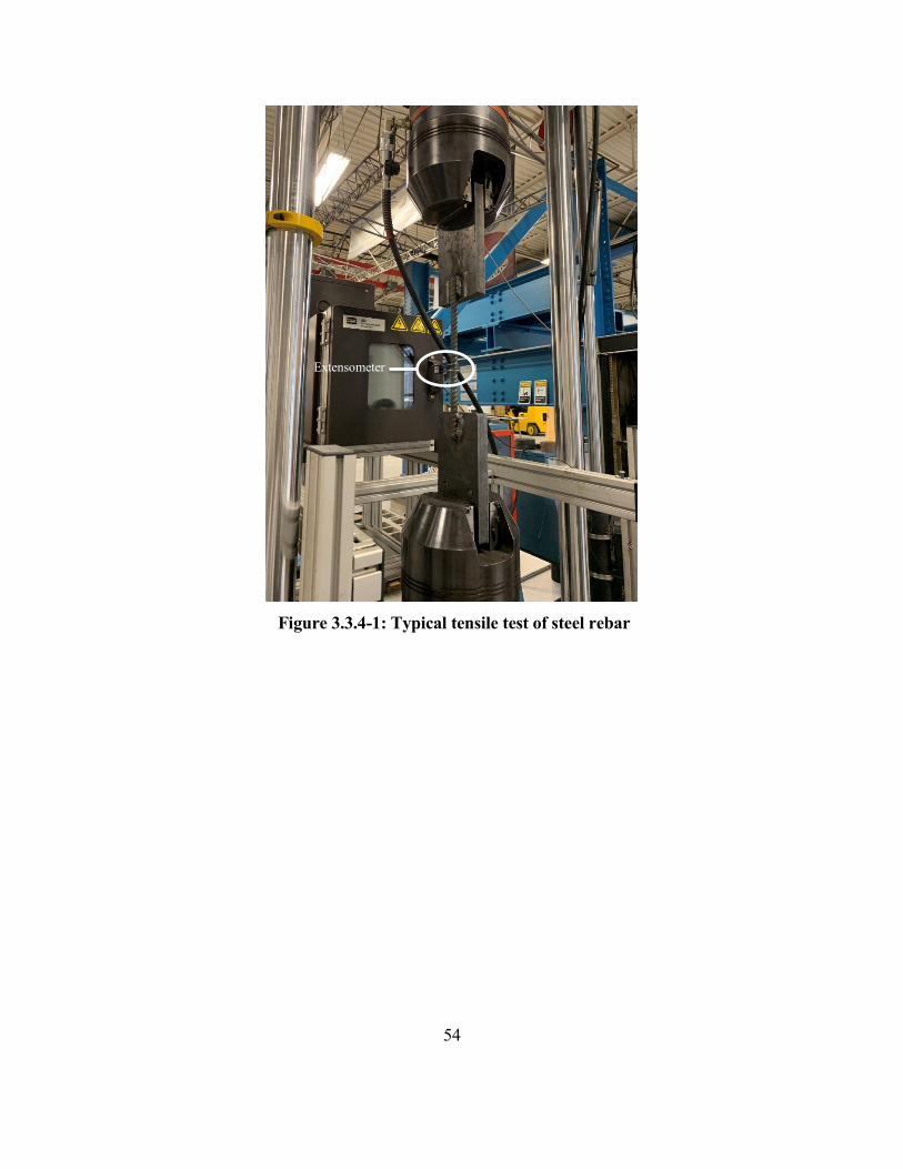
54

Figure 3.3.4-1: Typical tensile test of steel rebar

Extensometer

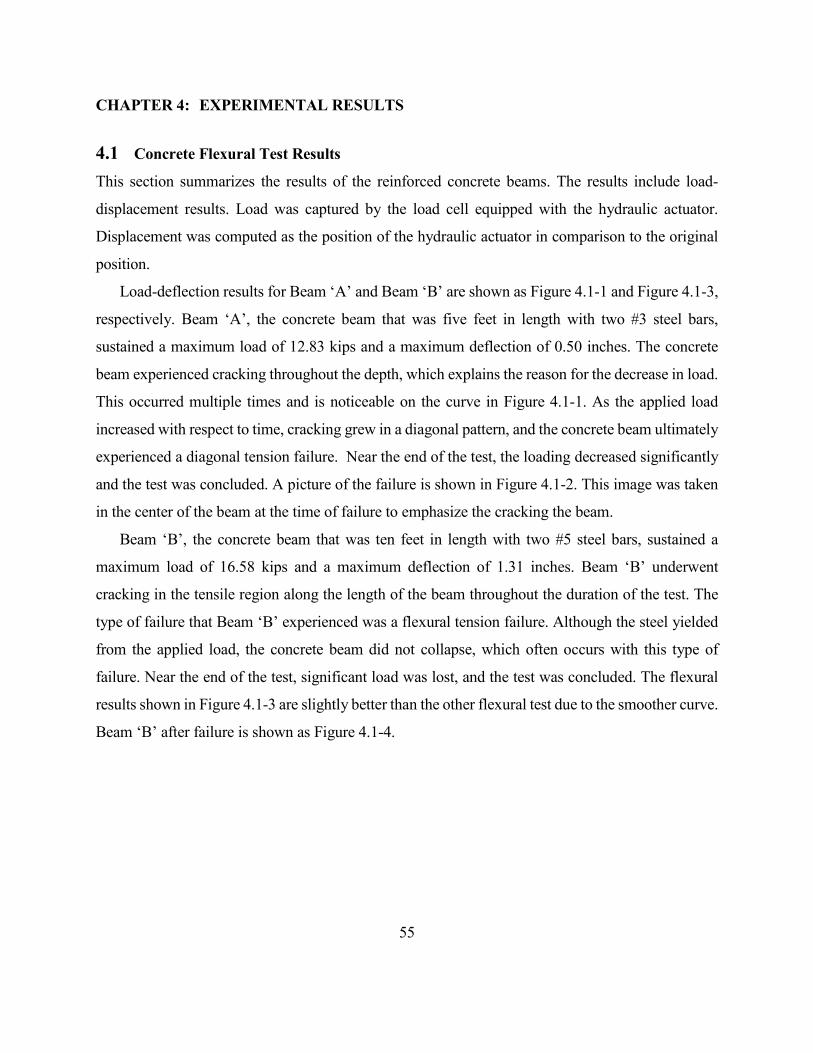
55

CHAPTER 4: EXPERIMENTAL RESULTS

4.1 Concrete Flexural Test Results

This section summarizes the results of the reinforced concrete beams. The results include load-

displacement results. Load was captured by the load cell equipped with the hydraulic actuator.

Displacement was computed as the position of the hydraulic actuator in comparison to the original

position.

Load-deflection results for Beam ‘A’ and Beam ‘B’ are shown as Figure 4.1-1 and Figure 4.1-3,

respectively. Beam ‘A’, the concrete beam that was five feet in length with two #3 steel bars,

sustained a maximum load of 12.83 kips and a maximum deflection of 0.50 inches. The concrete

beam experienced cracking throughout the depth, which explains the reason for the decrease in load.

This occurred multiple times and is noticeable on the curve in Figure 4.1-1. As the applied load

increased with respect to time, cracking grew in a diagonal pattern, and the concrete beam ultimately

experienced a diagonal tension failure. Near the end of the test, the loading decreased significantly

and the test was concluded. A picture of the failure is shown in Figure 4.1-2. This image was taken

in the center of the beam at the time of failure to emphasize the cracking the beam.

Beam ‘B’, the concrete beam that was ten feet in length with two #5 steel bars, sustained a

maximum load of 16.58 kips and a maximum deflection of 1.31 inches. Beam ‘B’ underwent

cracking in the tensile region along the length of the beam throughout the duration of the test. The

type of failure that Beam ‘B’ experienced was a flexural tension failure. Although the steel yielded

from the applied load, the concrete beam did not collapse, which often occurs with this type of

failure. Near the end of the test, significant load was lost, and the test was concluded. The flexural

results shown in Figure 4.1-3 are slightly better than the other flexural test due to the smoother curve.

Beam ‘B’ after failure is shown as Figure 4.1-4.

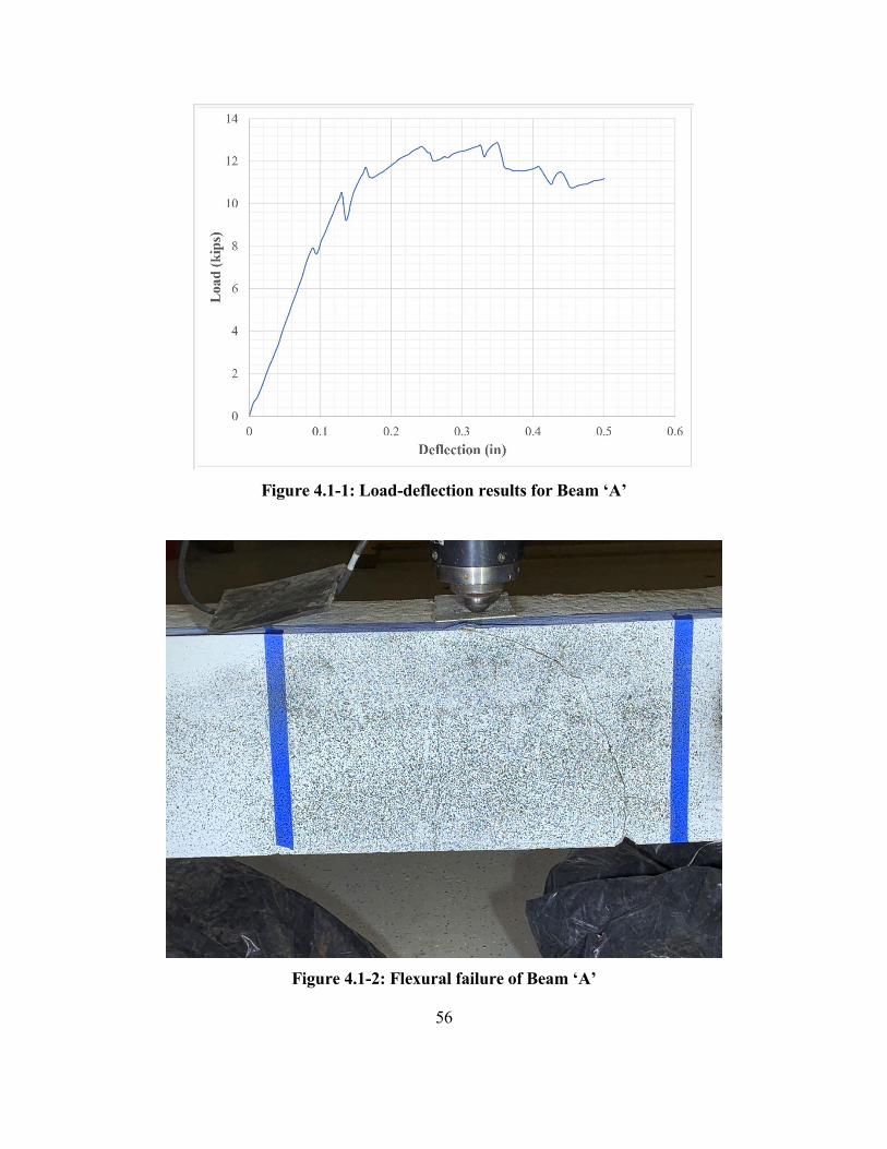
56

Figure 4.1-1: Load-deflection results for Beam ‘A’

Figure 4.1-2: Flexural failure of Beam ‘A’

57

Figure 4.1-3: Load-deflection results for Beam ‘B’

Figure 4.1-4: Flexural failure of Beam ‘B’

58

The non-reinforced concrete beams were subjected to flexural testing as well. Initially, the beams

were going to be utilized with DIC results to determine the tensile stress-strain properties of the

concrete. However, the DIC results were inadequate. The results are presented here for reference

purposes only. The three short beams were plotted together and identified as Beam ‘C’, Beam ‘D’

and Beam ‘E’. The load-displacement results are shown in Figure 4.1-5. The maximum load for

Beam ‘C’, Beam ‘D’ and Beam ‘E’ was 7.61 kips, 6.18 kips and 6.64 kips, respectively. Images of

the failures for Beam ‘C’, Beam ‘D’ and Beam ‘E’ are shown as Figure 4.1-6, Figure 4.1-7 and

Figure 4.1-8, respectively. All three concrete beams experienced a flexural failure in the center of

the beam due to the absence of steel reinforcement in the beam.

Due to the failure of concrete tensile tests, the tensile properties of concrete were calculated based

off of experimental research by Nematzadeh and Fallah-Valukolaee (2021). These results are shown

in the next chapter for the analytical model discussion.

Figure 4.1-5: Load-deflection results for non-reinforced concrete beams

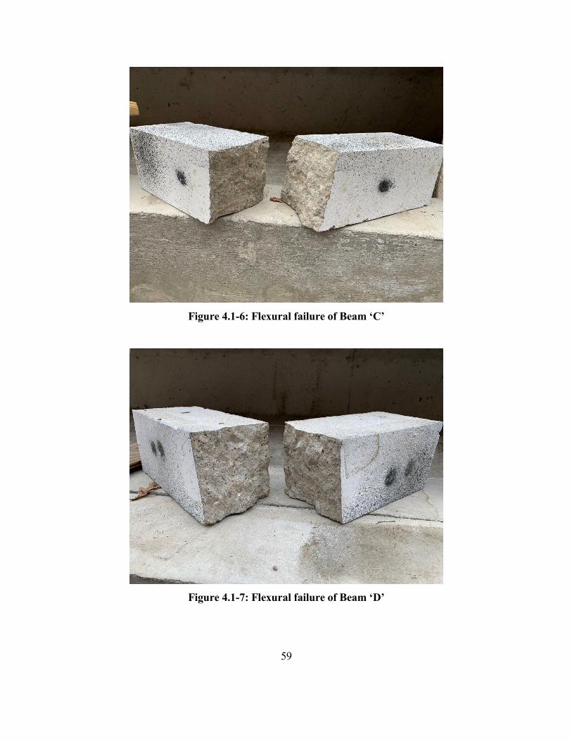
59

Figure 4.1-6: Flexural failure of Beam ‘C’

Figure 4.1-7: Flexural failure of Beam ‘D’

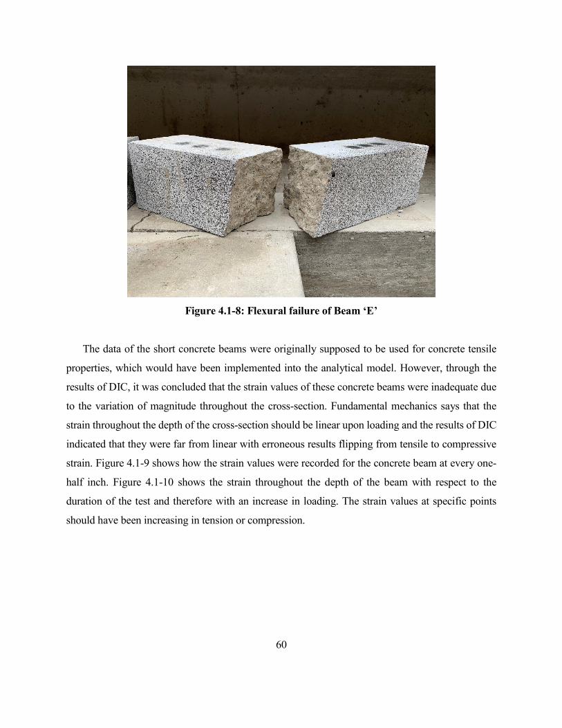
60

Figure 4.1-8: Flexural failure of Beam ‘E’

The data of the short concrete beams were originally supposed to be used for concrete tensile

properties, which would have been implemented into the analytical model. However, through the

results of DIC, it was concluded that the strain values of these concrete beams were inadequate due

to the variation of magnitude throughout the cross-section. Fundamental mechanics says that the

strain throughout the depth of the cross-section should be linear upon loading and the results of DIC

indicated that they were far from linear with erroneous results flipping from tensile to compressive

strain. Figure 4.1-9 shows how the strain values were recorded for the concrete beam at every one-

half inch. Figure 4.1-10 shows the strain throughout the depth of the beam with respect to the

duration of the test and therefore with an increase in loading. The strain values at specific points

should have been increasing in tension or compression.

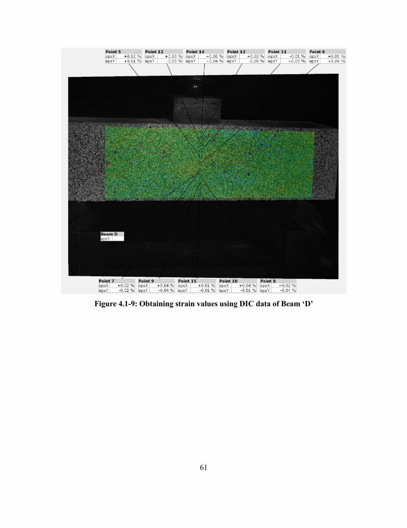
61

Figure 4.1-9: Obtaining strain values using DIC data of Beam ‘D’

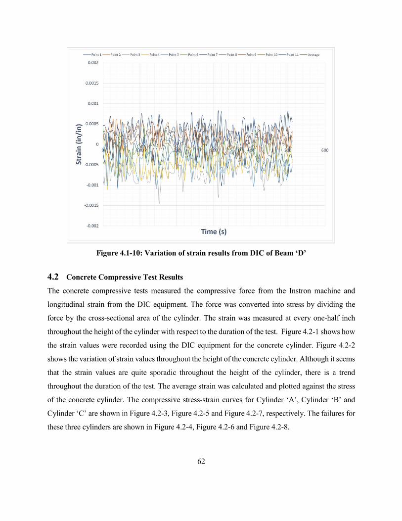
62

Figure 4.1-10: Variation of strain results from DIC of Beam ‘D’

4.2 Concrete Compressive Test Results

The concrete compressive tests measured the compressive force from the Instron machine and

longitudinal strain from the DIC equipment. The force was converted into stress by dividing the

force by the cross-sectional area of the cylinder. The strain was measured at every one-half inch

throughout the height of the cylinder with respect to the duration of the test. Figure 4.2-1 shows how

the strain values were recorded using the DIC equipment for the concrete cylinder. Figure 4.2-2

shows the variation of strain values throughout the height of the concrete cylinder. Although it seems

that the strain values are quite sporadic throughout the height of the cylinder, there is a trend

throughout the duration of the test. The average strain was calculated and plotted against the stress

of the concrete cylinder. The compressive stress-strain curves for Cylinder ‘A’, Cylinder ‘B’ and

Cylinder ‘C’ are shown in Figure 4.2-3, Figure 4.2-5 and Figure 4.2-7, respectively. The failures for

these three cylinders are shown in Figure 4.2-4, Figure 4.2-6 and Figure 4.2-8.

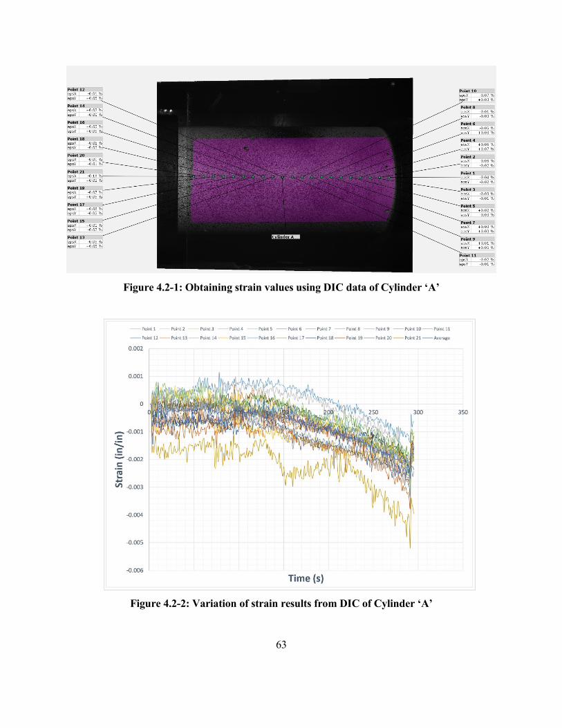
63

Figure 4.2-1: Obtaining strain values using DIC data of Cylinder ‘A’

Figure 4.2-2: Variation of strain results from DIC of Cylinder ‘A’

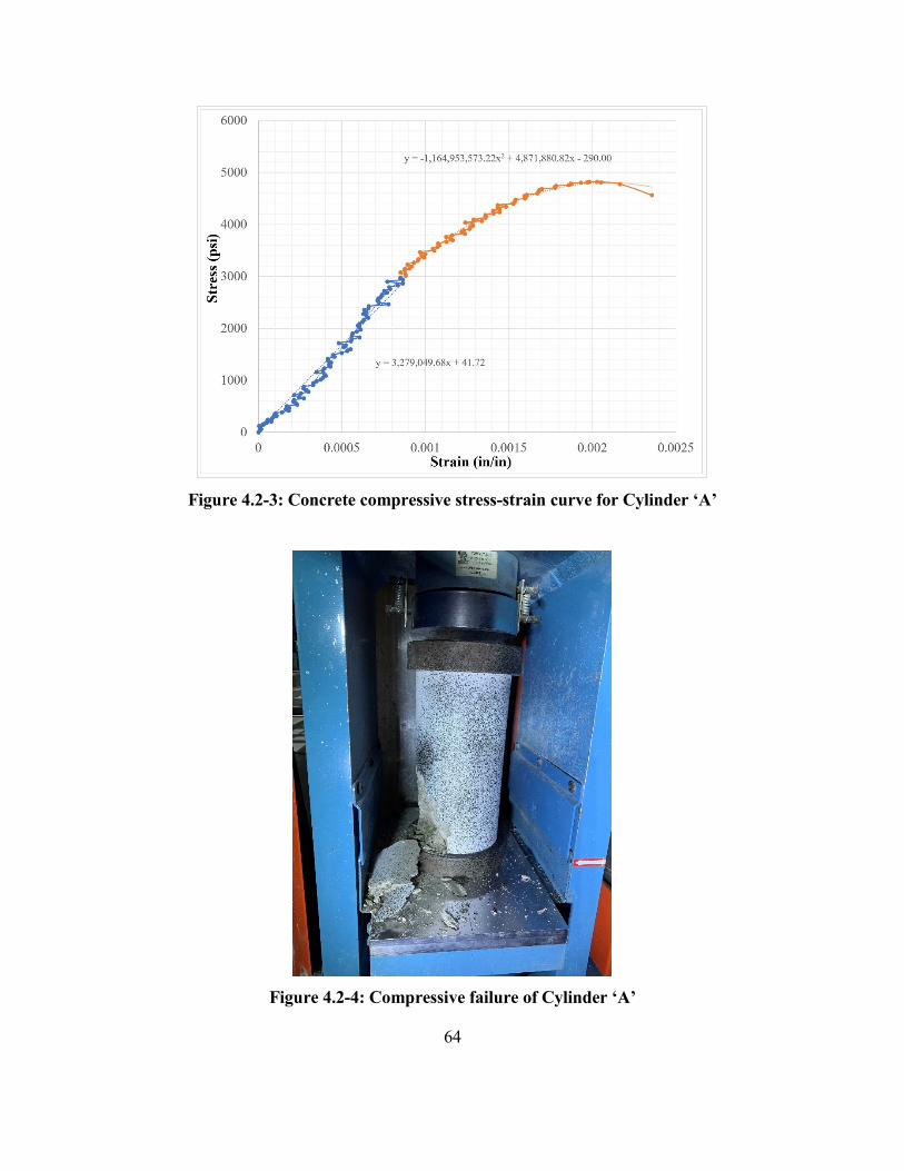
64

Figure 4.2-3: Concrete compressive stress-strain curve for Cylinder ‘A’

Figure 4.2-4: Compressive failure of Cylinder ‘A’

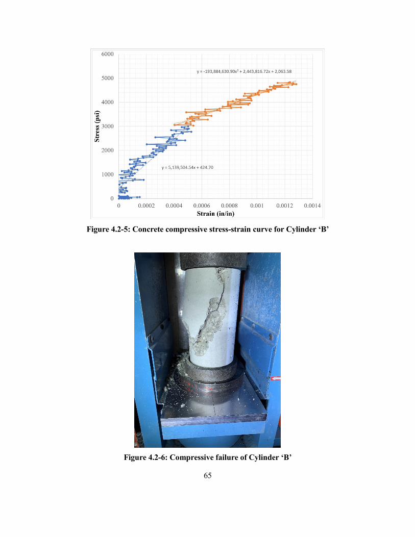
65

Figure 4.2-5: Concrete compressive stress-strain curve for Cylinder ‘B’

Figure 4.2-6: Compressive failure of Cylinder ‘B’

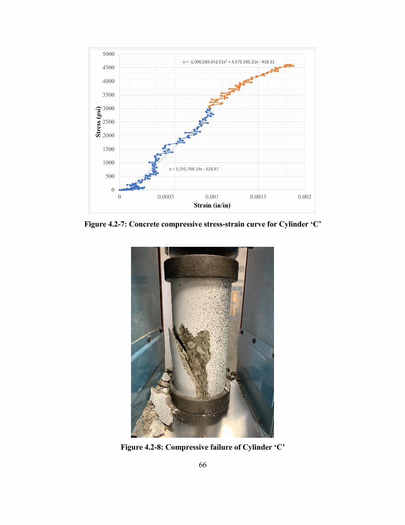
66

Figure 4.2-7: Concrete compressive stress-strain curve for Cylinder ‘C’

Figure 4.2-8: Compressive failure of Cylinder ‘C’

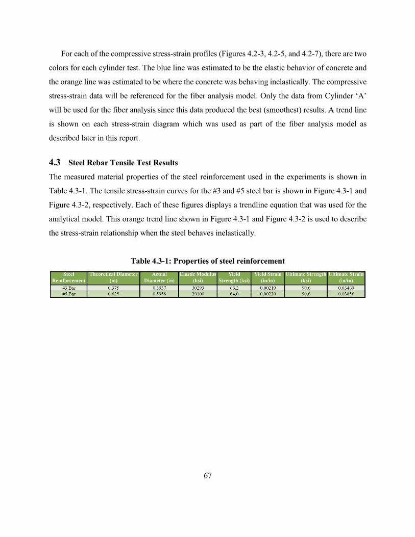
67

For each of the compressive stress-strain profiles (Figures 4.2-3, 4.2-5, and 4.2-7), there are two

colors for each cylinder test. The blue line was estimated to be the elastic behavior of concrete and

the orange line was estimated to be where the concrete was behaving inelastically. The compressive

stress-strain data will be referenced for the fiber analysis model. Only the data from Cylinder ‘A’

will be used for the fiber analysis since this data produced the best (smoothest) results. A trend line

is shown on each stress-strain diagram which was used as part of the fiber analysis model as

described later in this report.

4.3 Steel Rebar Tensile Test Results

The measured material properties of the steel reinforcement used in the experiments is shown in

Table 4.3-1. The tensile stress-strain curves for the #3 and #5 steel bar is shown in Figure 4.3-1 and

Figure 4.3-2, respectively. Each of these figures displays a trendline equation that was used for the

analytical model. This orange trend line shown in Figure 4.3-1 and Figure 4.3-2 is used to describe

the stress-strain relationship when the steel behaves inelastically.

Table 4.3-1: Properties of steel reinforcement

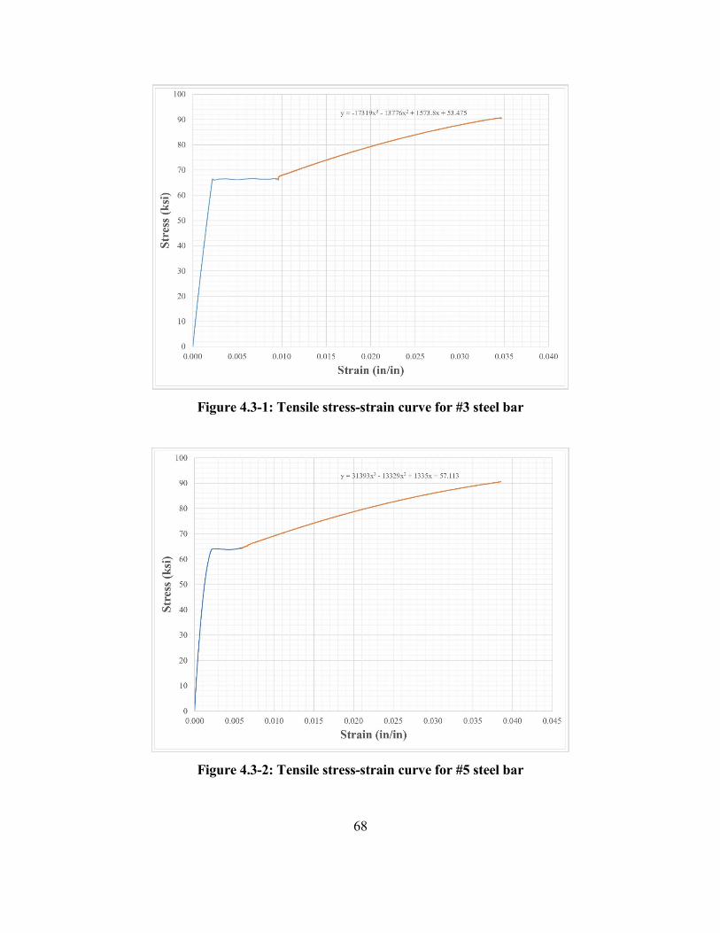
68

Figure 4.3-1: Tensile stress-strain curve for #3 steel bar

Figure 4.3-2: Tensile stress-strain curve for #5 steel bar

69

CHAPTER 5: ANALYTICAL METHODOLOGY

5.1 Analytical Modeling Approach

The analytical testing that was performed as part of this research was a fiber analysis model. A fiber

analysis model breaks up the cross-section of a specimen, in this case a reinforced concrete beam,

into a number of discrete fibers. Each fiber has a different computed value of strain, stress and force

with each increment of curvature. The most important aspect of the fiber analysis model is ensuring

there is a proper relationship between each value of strain and stress for both the concrete and the

steel fibers. Figure 5.1-1 shows a diagram of the fiber analysis method utilizing a linear strain

diagram of a typical reinforced concrete beam. The concrete was discretized in a number of fibers.

However, the steel rebar was represented by one fiber in the model.

Figure 5.1-1: Fiber analysis diagram of a typical singly reinforced concrete beam

The first step when utilizing a fiber analysis is to determine the amount of fibers to use in the

cross-section. The more fibers that are present, the more accurate the data produces and the more

refined the magnitudes of each property are. Too many fibers chosen may result in redundancy in

the fiber model, meaning the results within adjacent fibers are equivalent. For this research, the

number of fibers chosen throughout the depth of the cross-section is 200 fibers for the experimental

beams and 1,000 fibers for the additional analytical beams. The distance of the center of each fiber

70

is measured to a common reference point, which was taken as the top of the beam. Another distance

is measured from the center of each fiber to the neutral axis, shown as Equation 5-1, of the reinforced

concrete beam. This distance is critical in calculating the strain at each fiber, as shown in Equation

5-2 and determining the moment in each fiber, as shown in Equation 5-7. Equation 5-2 is derived

from basic trigonometry assumptions at a particular fiber.

𝑦𝑦𝑖𝑖 = 𝑦𝑦𝑡𝑡 − 𝑐𝑐 (5-1)

𝜀𝜀𝑓𝑓 = 𝑦𝑦𝑖𝑖𝜙𝜙 (5-2)

In Equation 5-1, ‘c’ represents the neutral axis which is determined from iteration as discussed

later. The stress calculation for concrete is based on the strain at the particular fiber, and the stress

calculation is based on whether the fiber is in compression or tension. For this analytical testing, a

positive strain is taken as tension and a negative strain is taken as compression. Therefore, the stress

is computed by Equation 5-3 utilizing the properties from Cylinder ‘A’ in Figure 4.2-3. The first and

second equation in Equation 5-3 represents the compressive properties of concrete at a single fiber

(εf). The first equation describes inelastic behavior while the second equation describes elastic

behavior. The third equation is the tensile properties of concrete as referenced from Nematzadeh and

Fallah-Valukolaee’s (2021) research. Their research is discussed in more detail in Section 5.2. The

yielding compressive strain (εy,c) and ultimate compressive strain (εu,c) were taken as -0.000859 in/in

and -0.0024 in/in, where the negative sign denotes compression. The ultimate tensile strain (εtu) was

0.000133 in/in.

⎩⎨

⎧𝜎𝜎𝑐𝑐𝑓𝑓 = −1.16 × 109𝜀𝜀𝑓𝑓2 + 4.87 × 106 𝜀𝜀𝑓𝑓 − 290 𝜀𝜀𝑢𝑢,𝑐𝑐 ≤ 𝜀𝜀𝑓𝑓 < 𝜀𝜀𝑦𝑦,𝑐𝑐 𝜎𝜎𝑐𝑐𝑓𝑓 = 3,279,049.7𝜀𝜀𝑓𝑓 𝜀𝜀𝑦𝑦,𝑐𝑐 ≤ 𝜀𝜀𝑓𝑓 < 0

𝜎𝜎𝑐𝑐𝑓𝑓 = 𝑖𝑖𝑡𝑡 �2 𝜀𝜀𝑓𝑓𝜀𝜀𝑡𝑡𝑡𝑡

− � 𝜀𝜀𝑓𝑓𝜀𝜀𝑡𝑡𝑡𝑡�2� 0 ≤ 𝜀𝜀𝑓𝑓

(5-3)

The stress calculation for steel is somewhat similar to concrete. Steel is assumed to have the

same stress-strain relationship for both tension and compression, but since the steel reinforcement is

placed in the tensile region of the concrete beam, only the tensile properties were considered. Similar

to concrete, steel behaves both elastically and inelastically, which determines which equation is to

be used to calculate the stress. From the steel tensile results, the stress calculation at a steel fiber can

be determined for a #3 bar and a #5 bar by Equation 5-4a and Equation 5-4b, respectively.

71

�𝜎𝜎𝑠𝑠𝑓𝑓 = 30,293𝜀𝜀𝑓𝑓 0 ≤ 𝜀𝜀𝑓𝑓 < 𝜀𝜀𝑦𝑦,𝑠𝑠

𝜎𝜎𝑠𝑠𝑓𝑓 = −17,319𝜀𝜀𝑓𝑓3 − 13,776𝜀𝜀𝑓𝑓2 + 1,573.8𝜀𝜀𝑓𝑓 + 53.475 𝜀𝜀𝑦𝑦,𝑠𝑠 ≤ 𝜀𝜀𝑓𝑓 < 𝜀𝜀𝑢𝑢,𝑠𝑠 (5-4a)

�𝜎𝜎𝑠𝑠𝑓𝑓 = 29,100𝜀𝜀𝑓𝑓 0 ≤ 𝜀𝜀𝑓𝑓 < 𝜀𝜀𝑦𝑦,𝑠𝑠

𝜎𝜎𝑠𝑠𝑓𝑓 = 31,393𝜀𝜀𝑓𝑓3 − 13,329𝜀𝜀𝑓𝑓2 + 1,335𝜀𝜀𝑓𝑓 + 57.113 𝜀𝜀𝑦𝑦,𝑠𝑠 ≤ 𝜀𝜀𝑓𝑓 < 𝜀𝜀𝑢𝑢,𝑠𝑠 (5-4b)

The force at a particular fiber is determined by Equation 5-5 where the area of each concrete

fiber is shown in Equation 5-6. In Equation 5-5, σf is the fiber stress per Equations 5-3 and 5-4. In

Equation 5-6, b is the width of the concrete section and hf is the height of each fiber. The moment

at contribution of each fiber is computed as Equation 5-7. The sum of the moments in all fibers is

used to create a moment-curvature diagram using each increment of curvature and the corresponding

moment.

𝐹𝐹𝑓𝑓 = 𝜎𝜎𝑓𝑓𝐴𝐴𝑓𝑓 (5-5)

𝐴𝐴𝑓𝑓 = 𝑏𝑏ℎ𝑓𝑓 (5-6)

𝑀𝑀𝑓𝑓 = 𝐹𝐹𝑓𝑓𝑦𝑦𝑖𝑖 (5-7)

The moment-curvature diagrams were created through a series of steps. The first input is setting

the curvature to zero. At this stage, there is no strain throughout the cross-section of the beam, which

results in stresses, forces and moments to all equal zero. A nonzero curvature is inputted in the model

and the output is a summation of the forces and moments in the cross-section. The summation of the

forces must be in equilibrium in order for a cross-section to be subjected to pure bending. The cross-

section at a particular curvature will sustain equilibrium by allowing the neutral axis to fluctuate. In

Microsoft Excel, this was achieved using the “Goal Seek” command by setting the sum of the forces

to zero by changing the distance of the neutral axis. In summary, the depth of the neutral axis changes

with respect to the curvature of the beam.

Through these series of steps, the sum of the moments were finalized at a certain curvature. This

process was continued for multiple points of curvature until either the strain in the top compressive

fiber exceeded the ultimate strain (per the concrete compressive stress-strain curve), or when the

steel fiber exceeded the ultimate strain (per the steel stress-strain diagram). In most cases, the

concrete beam will fail in the compression fiber (concrete crushing) before it fails in the steel tensile

fiber.

The fiber analysis method utilized equivalent beam properties as the concrete beams in the

experiment so the experimental and analytical concrete beams can directly be compared with one

72

another. Once the fiber analysis model predicted deflections similarly to the experimental

deflections, the fiber model was used to predict the deflection of two analytical beams. These

analytical beams were treated as simply supported with different loading applied to the beam. One

concrete beam had a concentrated load located directly at the midspan and the other concrete beam

had a uniformly distributed load throughout the whole length. A comparison of the deflection of the

concrete beams was made between the analytical model and the two versions of ACI 318 (ACI 318-

14 and ACI 318-19).

5.2 Determining Concrete Tensile Properties from Research

Due to the inadequate results from the experimental testing to determine the tensile properties of

concrete, an alternative approach was implemented from past research. Nematzadeh and Fallah-

Valukolaee (2021) introduced an equation to calculate the tensile strength, ft, of fiber-reinforced

concrete that is dependent on the compressive strength, fc’, as shown in Equation 5-8.

𝑖𝑖𝑡𝑡 = 0.1𝑖𝑖𝑐𝑐′ 0.88 �1 + 43.75𝑉𝑉𝑓𝑓𝑓𝑓𝑐𝑐′

�8 (5-8)

This research does not use fiber-reinforced concrete, Vf, so Equation 5-8 simplifies to Equation

5-9.

𝑖𝑖𝑡𝑡 = 0.1𝑖𝑖𝑐𝑐′ 0.88 (5-9)

By knowing the tensile and compressive strength of concrete along with the compressive strain,

εc, the ultimate tensile strain, εtu, can be determined using Equation 5-10. Equation 5-10 is equivalent

to Equation 2-13.

𝜀𝜀𝑡𝑡𝑢𝑢 = 𝑓𝑓𝑡𝑡𝑓𝑓𝑐𝑐′𝜀𝜀𝑐𝑐 (5-10)

The compressive strength and the maximum compressive strength of concrete was determined

from the results of Cylinder 1. The last unknown quantity is the tensile stress, σt, which is described

in Equation 5-11.

𝜎𝜎𝑡𝑡 = 𝑖𝑖𝑡𝑡 �2 �𝜀𝜀𝑡𝑡𝜀𝜀𝑡𝑡𝑡𝑡� − � 𝜀𝜀𝑡𝑡

𝜀𝜀𝑡𝑡𝑡𝑡�2� (5-11)

Equation 5-8 through Equation 5-11 are only valid if SI units are used. For this research, values

were converted from Imperial units to SI units and then converted back to Imperial units for

interpretation.

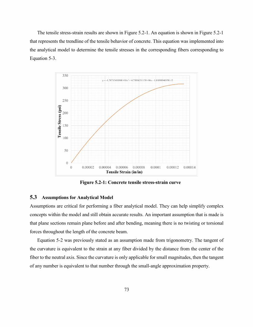
73

The tensile stress-strain results are shown in Figure 5.2-1. An equation is shown in Figure 5.2-1

that represents the trendline of the tensile behavior of concrete. This equation was implemented into

the analytical model to determine the tensile stresses in the corresponding fibers corresponding to

Equation 5-3.

Figure 5.2-1: Concrete tensile stress-strain curve

5.3 Assumptions for Analytical Model

Assumptions are critical for performing a fiber analytical model. They can help simplify complex

concepts within the model and still obtain accurate results. An important assumption that is made is

that plane sections remain plane before and after bending, meaning there is no twisting or torsional

forces throughout the length of the concrete beam.

Equation 5-2 was previously stated as an assumption made from trigonometry. The tangent of

the curvature is equivalent to the strain at any fiber divided by the distance from the center of the

fiber to the neutral axis. Since the curvature is only applicable for small magnitudes, then the tangent

of any number is equivalent to that number through the small-angle approximation property.

74

Equation 5-5 is based off of the basic stress equation of force divided by area. This equation

assumes that a uniform stress acts throughout the entire width of the concrete beam, which in reality,

may not be the case. This could be due to unequal stresses due to the bonds in the aggregate or the

presence of air gaps when the concrete was poured. Due to the fact that the height of the fibers is

small enough where the stress at each fiber is approximately equal to the actual stress at that location

in the beam, this assumption was adequate to be made.

All of these assumptions were made for the fiber analysis model for the two experimental

concrete beams and the two additional concrete beams. The results of the analytical models are

shown in next two chapters.

5.4 Analysis of Load-Deflection from Moment-Curvature Relationship

Once the moment-curvature relationship was established from the fiber analysis model, a load-

deflection diagram was necessary in order to directly compare the analytical model to the

experimental data and to the two versions of the code (ACI 318-14 and ACI 318-19). The process to

obtain the load-deflection results was obtained through an approximation of the double integration

method using the trapezoidal rule.

For the loading cases that were studied in this research (a concentrated load located at the center

of the beam and a uniformly distributed load throughout the length of the beam), the maximum

deflection occurs at midspan and there is no deflection at the two end supports. The deflection can

be described as a function with respect to the length of the beam until the function reaches the center

of the beam. The moment of the beam can also be described as a function along the length of the

beam, since moment directly relates to deflection through the double integration analysis. Through

basic statics, the moment can be calculated when any load is applied at any point along the length of

the beam up to midspan. Equation 5-12 demonstrates this concept for the concentrated load case and

Equation 5-13 is the uniformly distributed load case. These equations are valid from the end of the

beam, where x = 0, to midspan, where x = L/2. Equation 5-13 is valid throughout the length.

𝑀𝑀(𝑥𝑥) = 𝑃𝑃2𝑥𝑥 (5-12)

𝑀𝑀(𝑥𝑥) = 𝑤𝑤𝑤𝑤2

(𝐿𝐿 − 𝑥𝑥) (5-13)

75

Once the moment is known, the curvature can directly be found through the moment-curvature

relationship (the results are shown in the next chapter). This was conducted by inverting the moment-

curvature diagram (where moment is shown on the x-axis and curvature is shown on the y-axis) and

creating trendlines, or functions, of different areas along the curve. These trendlines were

approximated using a polynomial to the second degree. Different functions were taken for the elastic

range, yielding range and the inelastic range. This is discussed in more detail in the next chapter.

The rotation was found by integrating along the curvature functions. The integration was

approximated by calculating the area underneath of the functions using the trapezoidal rule. Under

this rule, the change in rotation, or incremental rotation, was determined by taking the average points

of curvature between a differential change in length. This differential length was found using

Equation 5-14. The number 800 was determined arbitrarily as the number of lengths used from the

end of the beam to midspan. The incremental rotation was determined using Equation 5-15. The

subscript ‘i’ represents an increment of curvature, in this instance, along the length of the beam. The

rotation at any increment along the length of the beam was found by adding the current incremental

rotation to the previous full rotation, shown in Equation 5-16. Under the boundary conditions for the

two load cases, the rotation at midspan is equivalent to zero, so using Equation 5-16, rotation can be

calculated backwards to determine the final rotation at the end support.

δ𝑥𝑥 = 𝐿𝐿800

(5-14)

𝛿𝛿𝜃𝜃𝑖𝑖(𝑥𝑥) = 𝜙𝜙𝑖𝑖−1+𝜙𝜙𝑖𝑖2

δ𝑥𝑥 (5-15)

𝜃𝜃𝑖𝑖(𝑥𝑥) = 𝜃𝜃𝑖𝑖−1 + 𝛿𝛿𝜃𝜃𝑖𝑖 (5-16)

Finally, the deflection was found in a similar process as rotation. The deflection was calculated

using integration over the rotation functions. The trapezoidal rule was utilized again to determine

incremental deflection, shown as Equation 5-17. The total deflection at an increment along the length

of the beam was calculated by adding the current incremental deflection to the previous full

deflection, shown as Equation 5-18. Again, using the boundary conditions for the two load cases,

the deflection at the end support is equivalent to zero, and the maximum deflection occurs at

midspan.

𝛿𝛿∆𝑖𝑖(𝑥𝑥) = 𝜃𝜃𝑖𝑖−1+𝜃𝜃𝑖𝑖2

δ𝑥𝑥 (5-17)

Δ𝑖𝑖(𝑥𝑥) = Δ𝑖𝑖−1 + δΔ𝑖𝑖 (5-18)

76

For the experimental beams (Beam ‘A’ and Beam ‘B’), load-deflection diagrams were plotted

from the experimental results and compared to the predictions from the fiber analysis model and

from using the deflection analysis from ACI 318 (ACI 2014 and ACI 2019). For two additional

analytical beams, load-deflection diagrams were plotted using the fiber analysis model and compared

to predictions using both versions of ACI. These results are discussed in the next couple chapters.

77

CHAPTER 6: ANALYTICAL RESULTS

The primary analytical results presented in this section compare the load-deflection fiber analysis

results of Beam ‘A’ and Beam ‘B’ of the experimental data (Chapter 4) with predictions using the

two different versions of the ACI code (ACI 318-14 and ACI 318-19). The deflection for both

versions of the code was calculated per Equation 1-1. Using Equation 1-1, loads were inputted as 20

pound increments until the failure load per the fiber model results was reached.

6.1 Analytical Results for Beam ‘A’

Per the fiber analysis model described in the previous chapter, a moment-curvature relationship was

established, portrayed in Figure 6.1-1.

Figure 6.1-1: Moment-curvature relationship for Beam ‘A’

1

2

3

4

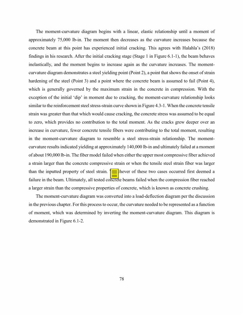
78

The moment-curvature diagram begins with a linear, elastic relationship until a moment of

approximately 75,000 lb-in. The moment then decreases as the curvature increases because the

concrete beam at this point has experienced initial cracking. This agrees with Halahla’s (2018)

findings in his research. After the initial cracking stage (Stage 1 in Figure 6.1-1), the beam behaves

inelastically, and the moment begins to increase again as the curvature increases. The moment-

curvature diagram demonstrates a steel yielding point (Point 2), a point that shows the onset of strain

hardening of the steel (Point 3) and a point where the concrete beam is assumed to fail (Point 4),

which is generally governed by the maximum strain in the concrete in compression. With the

exception of the initial ‘dip’ in moment due to cracking, the moment-curvature relationship looks

similar to the reinforcement steel stress-strain curve shown in Figure 4.3-1. When the concrete tensile

strain was greater than that which would cause cracking, the concrete stress was assumed to be equal

to zero, which provides no contribution to the total moment. As the cracks grew deeper over an

increase in curvature, fewer concrete tensile fibers were contributing to the total moment, resulting

in the moment-curvature diagram to resemble a steel stress-strain relationship. The moment-

curvature results indicated yielding at approximately 140,000 lb-in and ultimately failed at a moment

of about 190,000 lb-in. The fiber model failed when either the upper most compressive fiber achieved

a strain larger than the concrete compressive strain or when the tensile steel strain fiber was larger

than the inputted property of steel strain. Whichever of these two cases occurred first deemed a

failure in the beam. Ultimately, all tested concrete beams failed when the compression fiber reached

a larger strain than the compressive properties of concrete, which is known as concrete crushing.

The moment-curvature diagram was converted into a load-deflection diagram per the discussion

in the previous chapter. For this process to occur, the curvature needed to be represented as a function

of moment, which was determined by inverting the moment-curvature diagram. This diagram is

demonstrated in Figure 6.1-2.

Windows User

Yes, this is how you analyzed it but which one did control for this specific beam?

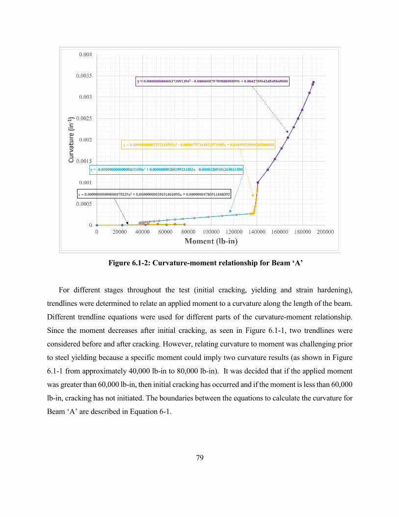
79

Figure 6.1-2: Curvature-moment relationship for Beam ‘A’

For different stages throughout the test (initial cracking, yielding and strain hardening),

trendlines were determined to relate an applied moment to a curvature along the length of the beam.

Different trendline equations were used for different parts of the curvature-moment relationship.

Since the moment decreases after initial cracking, as seen in Figure 6.1-1, two trendlines were

considered before and after cracking. However, relating curvature to moment was challenging prior

to steel yielding because a specific moment could imply two curvature results (as shown in Figure

6.1-1 from approximately 40,000 lb-in to 80,000 lb-in). It was decided that if the applied moment

was greater than 60,000 lb-in, then initial cracking has occurred and if the moment is less than 60,000

lb-in, cracking has not initiated. The boundaries between the equations to calculate the curvature for

Beam ‘A’ are described in Equation 6-1.

80

⎩⎪⎨

⎪⎧ 7.52 × 10−16𝑀𝑀𝑓𝑓

2 + 2.02 × 10−10𝑀𝑀𝑓𝑓 + 4.79 × 10−8 𝑖𝑖𝑖𝑖 0 ≤ 𝑀𝑀𝑓𝑓 < 60,000−4.32 × 10−15𝑀𝑀𝑓𝑓

2 + 2.88 × 10−9𝑀𝑀𝑓𝑓 − 4.20 × 10−5 𝑖𝑖𝑖𝑖 60,000 ≤ 𝑀𝑀𝑓𝑓 < 137,0372.94 × 10−11𝑀𝑀𝑓𝑓

2 − 7.97 × 10−6𝑀𝑀𝑓𝑓 + 5.41 × 10−1 𝑖𝑖𝑖𝑖 137,037 ≤ 𝑀𝑀𝑓𝑓 < 140,7733.74 × 10−13𝑀𝑀𝑓𝑓

2 − 7.58 × 10−8𝑀𝑀𝑓𝑓 + 4.27 × 10−3 𝑖𝑖𝑖𝑖 140,773 ≤ 𝑀𝑀𝑓𝑓 ≤ 189,434

(6-1)

Equation 6-1 shows an arbitrary moment of 60,000 lb-in, which was determined as an estimate

between the two linear slopes at the initial cracking stage. The moment of 137,037 lb-in represents

the boundary between the initial cracking and steel yielding stages. The moment of 140,773 lb-in

represents the boundary between the yielding and failure stages and the moment of 189,434 lb-in

represents the moment at failure. Similar processes were used to determine the curvature for a given

moment for Beam ‘B’ and the two additional analytical beams.

Once the curvature at a given moment was determined, the rotation and finally the deflection

was calculated using the trapezoidal rule. Loads were inputted in approximately 500 pound

increments to determine the deflection at each incremental load. The load-deflection relationship for

the fiber model was plotted with the experimental results and predictions using the two versions of

the ACI code, as shown in Figure 6.1-3.

81

Figure 6.1-3: Load-deflection results for Beam ‘A’

The different stages of the analytical load-deflection diagram are labeled in Figure 6.1-3 as

follows: Stage A is the uncracked (elastic) region, Stage B is the cracked region, Stage C is after

steel yielding region and Stage D is after strain hardening and up to failure of the beam. The

experimental and the analytical data somewhat compare well with each other. The maximum load

and maximum deflection are within an acceptable range when comparing the results. The slope of

the experimental and analytical curves approximately matches with each other after the initial

cracking (Stage B in Figure 6.1-3). The comparisons between the ACI code results and the fiber

model are promising. The fiber model is almost identical to the ACI 318-19 version prior to when

yielding occurs, which is understandable because this version of the code was proven to be more

accurate than its predecessor through additional research.

A

B

C

D

82

The analytical model experiences two different linear slopes, similar to the moment-curvature

response, before yielding occurs. The initial cracking in the beam is responsible for the change in

slope. Initial cracking for both the fiber model and for ACI 2019 occurs at almost the same load. The

only difference between the two is the absence of inelastic behavior in the code analysis. The

deflection analysis in the code only applies to members who behave elastically. This is due to the

fact that the cracked moment of inertia assumes that the steel and the concrete both behave

elastically, so the effective moment of inertia does not account for steel yielding. The equation for

the effective moment of inertia is acceptable only if the steel does not yield under service loads.

For beams, service loading is usually the sum of the dead and live loads that act on a structural

member. Factored loads are different types of loading combinations that are described in ASCE 7

(2016). On average, service loads are 1.5 times lower than factored loads. Since the beams were

designed as factored loads, then the maximum load at failure should be divided by the 1.5 factor.

This new failure load determines the validity of the code (ACI 318-19) by seeing if the steel has

yielded at this load. For example, the failure load for Beam ‘A’ was 14.032 kips per Table 7.3-1, and

the service load for Beam ‘A’ is 9.355 kips per Table 7.3-2. Coordinating with Figure 6.1-3, the

service load occurs just before the steel yields. The deflection analysis per the code is valid because

the steel has not yielded under these conditions.

6.2 Analytical Results for Beam ‘B’

Through the same procedure as Beam ‘A’, the fiber model produced a moment-curvature

relationship as shown in Figure 6.2-1.

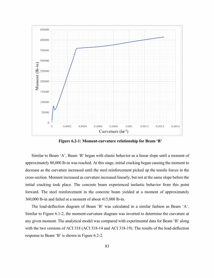
83

Figure 6.2-1: Moment-curvature relationship for Beam ‘B’

Similar to Beam ‘A’, Beam ‘B’ began with elastic behavior as a linear slope until a moment of

approximately 80,000 lb-in was reached. At this stage, initial cracking began causing the moment to

decrease as the curvature increased until the steel reinforcement picked up the tensile forces in the

cross-section. Moment increased as curvature increased linearly, but not at the same slope before the

initial cracking took place. The concrete beam experienced inelastic behavior from this point

forward. The steel reinforcement in the concrete beam yielded at a moment of approximately

360,000 lb-in and failed at a moment of about 415,000 lb-in.

The load-deflection diagram of Beam ‘B’ was calculated in a similar fashion as Beam ‘A’.

Similar to Figure 6.1-2, the moment-curvature diagram was inverted to determine the curvature at

any given moment. The analytical model was compared with experimental data for Beam ‘B’ along

with the two versions of ACI 318 (ACI 318-14 and ACI 318-19). The results of the load-deflection

response to Beam ‘B’ is shown in Figure 6.2-2.

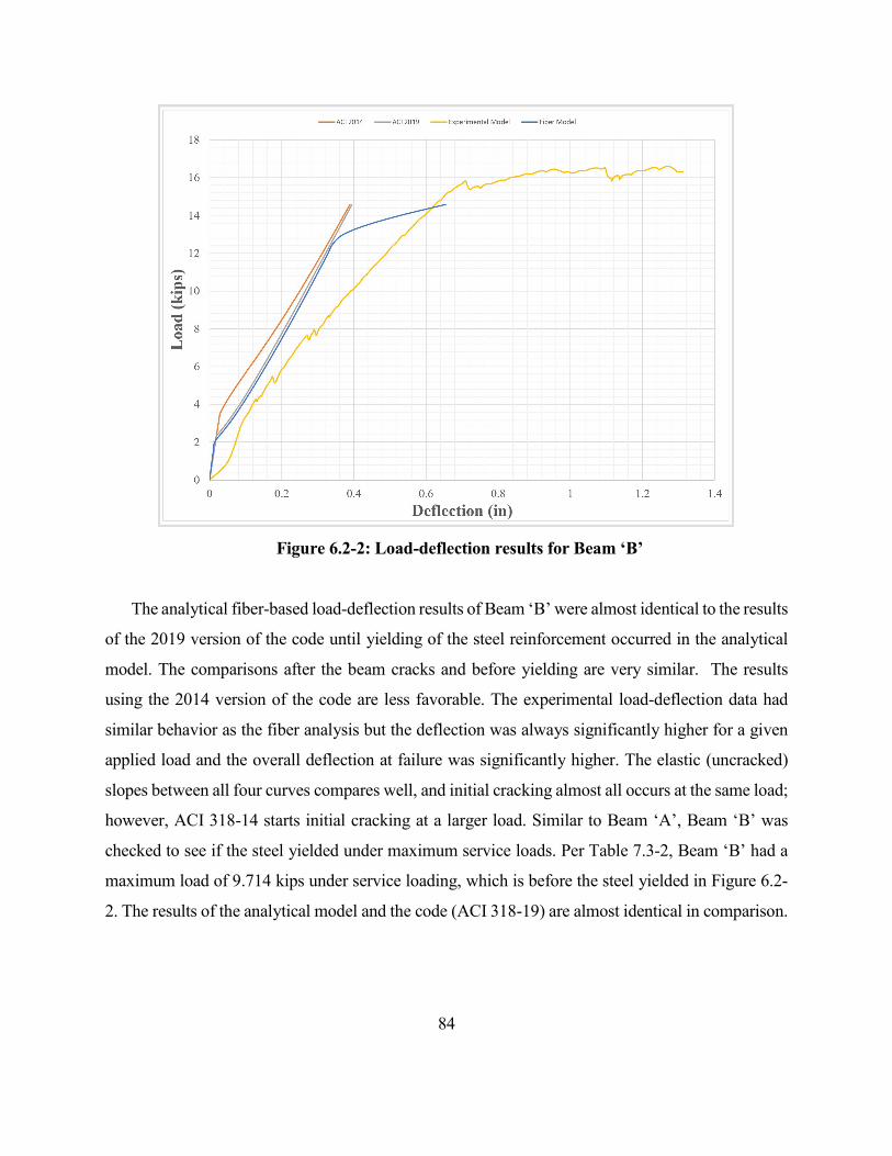
84

Figure 6.2-2: Load-deflection results for Beam ‘B’

The analytical fiber-based load-deflection results of Beam ‘B’ were almost identical to the results

of the 2019 version of the code until yielding of the steel reinforcement occurred in the analytical

model. The comparisons after the beam cracks and before yielding are very similar. The results

using the 2014 version of the code are less favorable. The experimental load-deflection data had

similar behavior as the fiber analysis but the deflection was always significantly higher for a given

applied load and the overall deflection at failure was significantly higher. The elastic (uncracked)

slopes between all four curves compares well, and initial cracking almost all occurs at the same load;

however, ACI 318-14 starts initial cracking at a larger load. Similar to Beam ‘A’, Beam ‘B’ was

checked to see if the steel yielded under maximum service loads. Per Table 7.3-2, Beam ‘B’ had a

maximum load of 9.714 kips under service loading, which is before the steel yielded in Figure 6.2-

2. The results of the analytical model and the code (ACI 318-19) are almost identical in comparison.

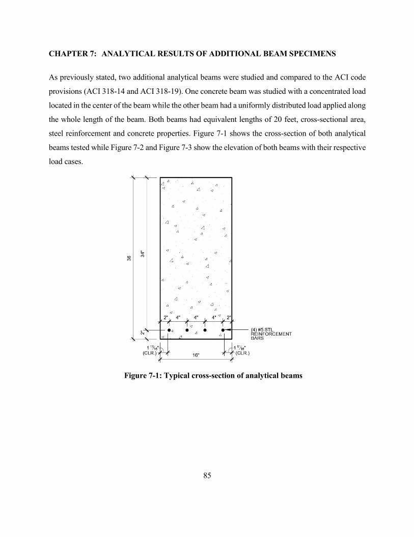
85

CHAPTER 7: ANALYTICAL RESULTS OF ADDITIONAL BEAM SPECIMENS

As previously stated, two additional analytical beams were studied and compared to the ACI code

provisions (ACI 318-14 and ACI 318-19). One concrete beam was studied with a concentrated load

located in the center of the beam while the other beam had a uniformly distributed load applied along

the whole length of the beam. Both beams had equivalent lengths of 20 feet, cross-sectional area,

steel reinforcement and concrete properties. Figure 7-1 shows the cross-section of both analytical

beams tested while Figure 7-2 and Figure 7-3 show the elevation of both beams with their respective

load cases.

Figure 7-1: Typical cross-section of analytical beams

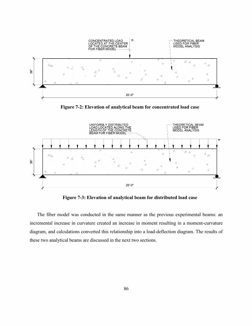
86

Figure 7-2: Elevation of analytical beam for concentrated load case

Figure 7-3: Elevation of analytical beam for distributed load case

The fiber model was conducted in the same manner as the previous experimental beams: an

incremental increase in curvature created an increase in moment resulting in a moment-curvature

diagram, and calculations converted this relationship into a load-deflection diagram. The results of

these two analytical beams are discussed in the next two sections.

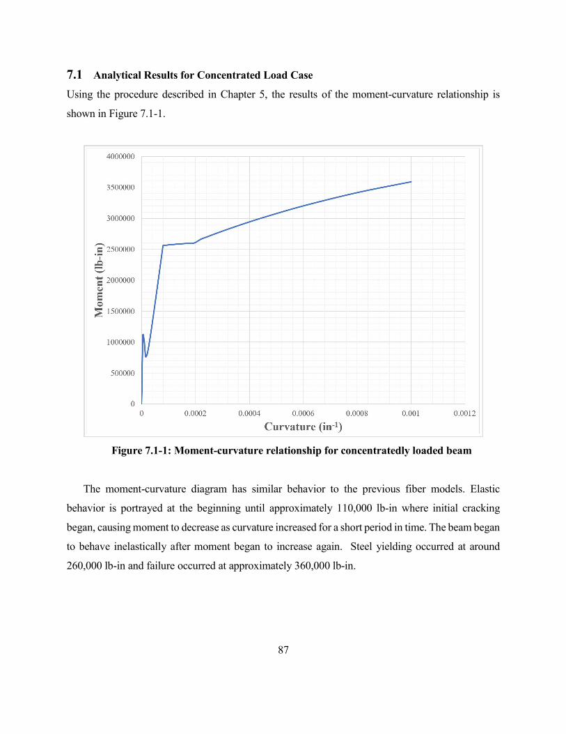
87

7.1 Analytical Results for Concentrated Load Case

Using the procedure described in Chapter 5, the results of the moment-curvature relationship is

shown in Figure 7.1-1.

Figure 7.1-1: Moment-curvature relationship for concentratedly loaded beam

The moment-curvature diagram has similar behavior to the previous fiber models. Elastic

behavior is portrayed at the beginning until approximately 110,000 lb-in where initial cracking

began, causing moment to decrease as curvature increased for a short period in time. The beam began

to behave inelastically after moment began to increase again. Steel yielding occurred at around

260,000 lb-in and failure occurred at approximately 360,000 lb-in.

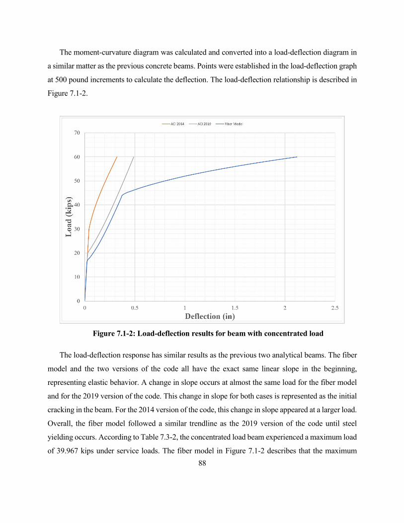
88

The moment-curvature diagram was calculated and converted into a load-deflection diagram in

a similar matter as the previous concrete beams. Points were established in the load-deflection graph

at 500 pound increments to calculate the deflection. The load-deflection relationship is described in

Figure 7.1-2.

Figure 7.1-2: Load-deflection results for beam with concentrated load

The load-deflection response has similar results as the previous two analytical beams. The fiber

model and the two versions of the code all have the exact same linear slope in the beginning,

representing elastic behavior. A change in slope occurs at almost the same load for the fiber model

and for the 2019 version of the code. This change in slope for both cases is represented as the initial

cracking in the beam. For the 2014 version of the code, this change in slope appeared at a larger load.

Overall, the fiber model followed a similar trendline as the 2019 version of the code until steel

yielding occurs. According to Table 7.3-2, the concentrated load beam experienced a maximum load

of 39.967 kips under service loads. The fiber model in Figure 7.1-2 describes that the maximum

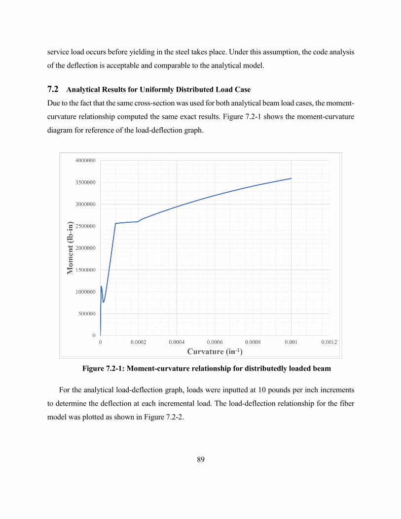
89

service load occurs before yielding in the steel takes place. Under this assumption, the code analysis

of the deflection is acceptable and comparable to the analytical model.

7.2 Analytical Results for Uniformly Distributed Load Case

Due to the fact that the same cross-section was used for both analytical beam load cases, the moment-

curvature relationship computed the same exact results. Figure 7.2-1 shows the moment-curvature

diagram for reference of the load-deflection graph.

Figure 7.2-1: Moment-curvature relationship for distributedly loaded beam

For the analytical load-deflection graph, loads were inputted at 10 pounds per inch increments

to determine the deflection at each incremental load. The load-deflection relationship for the fiber

model was plotted as shown in Figure 7.2-2.

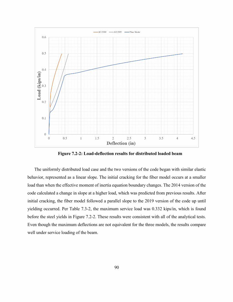
90

Figure 7.2-2: Load-deflection results for distributed loaded beam

The uniformly distributed load case and the two versions of the code began with similar elastic

behavior, represented as a linear slope. The initial cracking for the fiber model occurs at a smaller

load than when the effective moment of inertia equation boundary changes. The 2014 version of the

code calculated a change in slope at a higher load, which was predicted from previous results. After

initial cracking, the fiber model followed a parallel slope to the 2019 version of the code up until

yielding occurred. Per Table 7.3-2, the maximum service load was 0.332 kips/in, which is found

before the steel yields in Figure 7.2-2. These results were consistent with all of the analytical tests.

Even though the maximum deflections are not equivalent for the three models, the results compare

well under service loading of the beam.

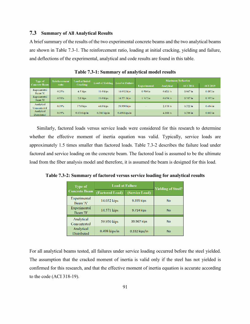
91

7.3 Summary of All Analytical Results

A brief summary of the results of the two experimental concrete beams and the two analytical beams

are shown in Table 7.3-1. The reinforcement ratio, loading at initial cracking, yielding and failure,

and deflections of the experimental, analytical and code results are found in this table.

Table 7.3-1: Summary of analytical model results

Similarly, factored loads versus service loads were considered for this research to determine

whether the effective moment of inertia equation was valid. Typically, service loads are

approximately 1.5 times smaller than factored loads. Table 7.3-2 describes the failure load under

factored and service loading on the concrete beam. The factored load is assumed to be the ultimate

load from the fiber analysis model and therefore, it is assumed the beam is designed for this load.

Table 7.3-2: Summary of factored versus service loading for analytical results

For all analytical beams tested, all failures under service loading occurred before the steel yielded.

The assumption that the cracked moment of inertia is valid only if the steel has not yielded is

confirmed for this research, and that the effective moment of inertia equation is accurate according

to the code (ACI 318-19).

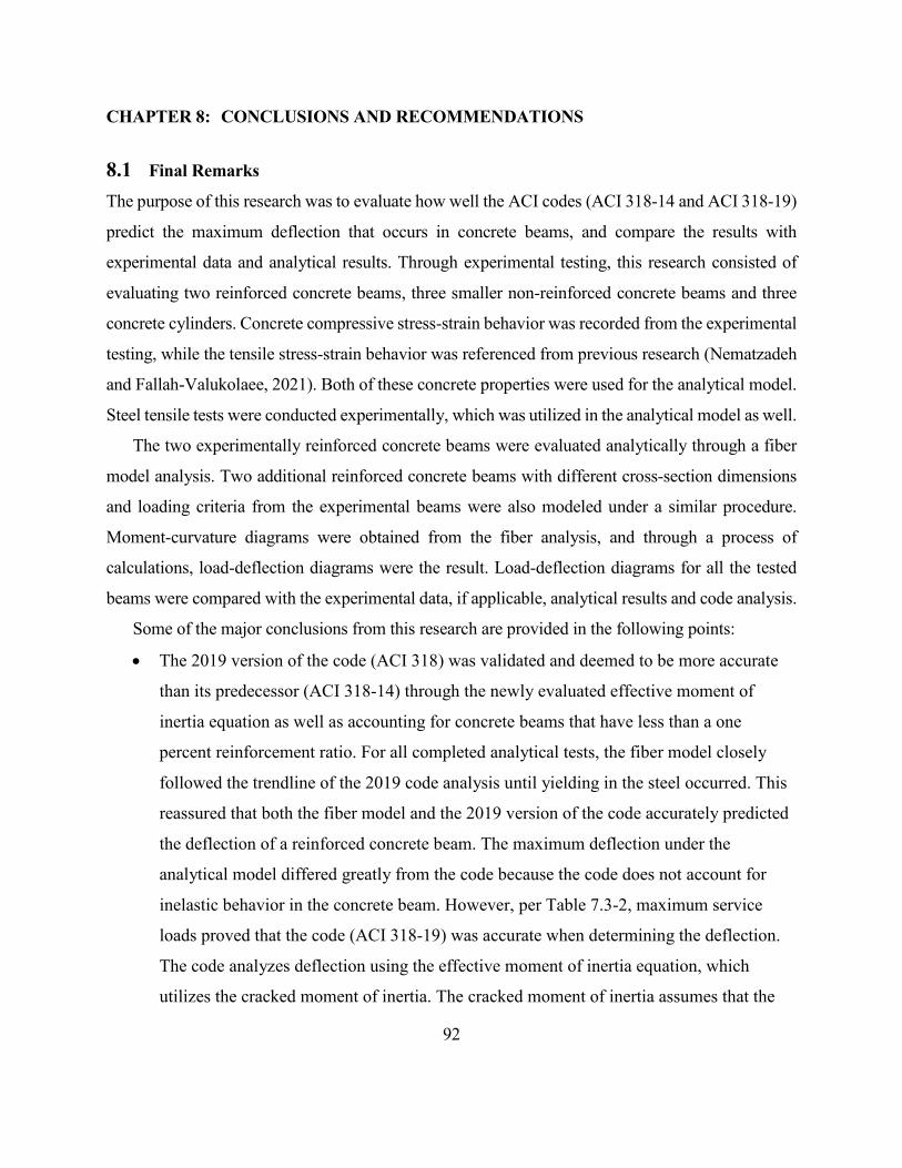
92

CHAPTER 8: CONCLUSIONS AND RECOMMENDATIONS

8.1 Final Remarks

The purpose of this research was to evaluate how well the ACI codes (ACI 318-14 and ACI 318-19)

predict the maximum deflection that occurs in concrete beams, and compare the results with

experimental data and analytical results. Through experimental testing, this research consisted of

evaluating two reinforced concrete beams, three smaller non-reinforced concrete beams and three

concrete cylinders. Concrete compressive stress-strain behavior was recorded from the experimental

testing, while the tensile stress-strain behavior was referenced from previous research (Nematzadeh

and Fallah-Valukolaee, 2021). Both of these concrete properties were used for the analytical model.

Steel tensile tests were conducted experimentally, which was utilized in the analytical model as well.

The two experimentally reinforced concrete beams were evaluated analytically through a fiber

model analysis. Two additional reinforced concrete beams with different cross-section dimensions

and loading criteria from the experimental beams were also modeled under a similar procedure.

Moment-curvature diagrams were obtained from the fiber analysis, and through a process of

calculations, load-deflection diagrams were the result. Load-deflection diagrams for all the tested

beams were compared with the experimental data, if applicable, analytical results and code analysis.

Some of the major conclusions from this research are provided in the following points:

• The 2019 version of the code (ACI 318) was validated and deemed to be more accurate

than its predecessor (ACI 318-14) through the newly evaluated effective moment of

inertia equation as well as accounting for concrete beams that have less than a one

percent reinforcement ratio. For all completed analytical tests, the fiber model closely

followed the trendline of the 2019 code analysis until yielding in the steel occurred. This

reassured that both the fiber model and the 2019 version of the code accurately predicted

the deflection of a reinforced concrete beam. The maximum deflection under the

analytical model differed greatly from the code because the code does not account for

inelastic behavior in the concrete beam. However, per Table 7.3-2, maximum service

loads proved that the code (ACI 318-19) was accurate when determining the deflection.

The code analyzes deflection using the effective moment of inertia equation, which

utilizes the cracked moment of inertia. The cracked moment of inertia assumes that the

93

concrete and the steel both behave elastically, which occurs before the steel begins to

yield. Therefore, if the maximum service load in the concrete beam occurs before the

steel yields in the load-deflection diagram, the results of this research indicate that the

effective moment of inertia equation used in ACI 318 (2019) is fairly accurate in

predicting concrete beam deflections.

• The work that has been completed using the DIC equipment in the experimental testing

was deemed as inadequate. The program that was used to extract the data was extremely

helpful in visual seeing the stress and strain distribution throughout the cross-section of

the concrete beam for the full duration of the test. However, the data itself was not as

accurate as it was anticipated to be. The values of all of the data points taken throughout

the depth of the beam was too sporadic, rather than a consistent change along the depth.

• As a larger curvature was applied to the cross-section of a beam, the moment-curvature

diagram began to replicate the steel stress-strain relationship. This concept began once

initial cracking in the concrete developed. As these cracks formed in the bottom most

concrete fibers, stress in these fibers were zero. Since these fibers have a nonexistent

stress, there is no moment contribution. As the curvature increased, cracks grew larger in

the cross-section affecting more and more fibers. Once the cracks reached the steel fibers,

the steel reinforcement took control of all of the tensile forces. As more concrete fibers

exceeded the tensile capacity (and the stress therefore was assumed zero) the behavior of

the moment-curvature diagram was similar to that of the steel stress-strain diagram. The

moment-curvature relationship also displayed a yielding phase and a failure stage similar

to the stress-strain relationship of steel.

• If the cross-section of a beam has the exact same dimensions, concrete properties and

steel reinforcement and spacing, the moment-curvature diagram will be the same

regardless of the type of loading applied. This is because as loading is applied to the

beam, rotation increases at the support (for the simply supported case), which ultimately

increases the curvature in the cross-section.

94

8.2 Future Recommendations

For future experiments related to this study, many recommendations are stated to improve the level

of research as follows:

• The studies should be repeated after obtaining more accurate stress-strain data for the

concrete material. For more accurate experimental stress and strain data, DIC equipment

can be used to record the desired data, but strain gauges shall also be used to confirm the

DIC results. If these two results differ, then the strain gauges shall be used instead of the

DIC results.

• In regards to the fiber model, more variables such as boundary conditions and loading

criteria should be studied to determine the accuracy of predicting deflections and

comparing these results to the code analysis (ACI 318-19).

• The fiber model can also be utilized for different structural analysis applications, such as

doubly reinforced concrete beams, deep beams, one-way slab design and two-way slab

design. More studies that analyze its effectiveness for these applications are

recommended.

95

REFERENCES

ACI Committee 224, 2001, “Control of Cracking in Concrete Structures (ACI 224R-01),” American

Concrete Institute, Farmington Hills, MI, 46 pp.

ACI 318 (2014). “Building code requirements for structural concrete: commentary on building code

requirements for structural concrete,” (ACI 318R-14), American Concrete Institute, 2014,

Farmington Hills, MI.

ACI 318 (2019). “Building code requirements for structural concrete: commentary on building code

requirements for structural concrete,” (ACI 318R-19), American Concrete Institute, 2019,

Farmington Hills, MI.

A. Halahla (2018). “Study the Behavior of Reinforced Concrete Beam Using Finite Element

Analysis,” Proceedings of the 3rd World Congress on Civil, Structural, and Environmental

Engineering (CSEE’18).

Al-Shaikh, A.H., Al-Zaid, R.Z., (1993). “Effect of reinforcement ratio on the effective moment of

inertia of reinforced concrete beams,” ACI Structural Journal, 90(2): 144-149.

Al-Zaid, R.Z., Al-Shaikh, A.H., Abu-Hussein, M.M., (1991). “Effect of loading type on the effective

moment of inertia of reinforced concrete beams,” ACI Structural Journal, 88(2): 184-190.

AS 3600 (2001). “Australian Standard for Concrete Structures,” Standards Australia, Sydney,

Austrialia

ASCE 7 (2016). “Minimum Design Loads and Associated Criteria for Buildings and Other

Structures,” American Society of Civil Engineers.

ASTM C39 (2001). “Standard Test Method for Compressive Strength of Cylindrical Concrete

Specimens,” ASTM International.

ASTM C78 (2002). “Standard Test Method for Flexural Strength of Concrete (Using Simple Beam

with Third-Point Loading),” ASTM International.

A. Scanlon and P. H. Bischoff (2008). “Shrinkage Restraint and Loading History Effects on

Deflections of Flexural Members,” ACI Structural Journal, 105.

C. Butean and B Heghes (2020). “Flexure Behavior of a Two Layer Reinforced Concrete Beam,”

Procedia Manufacturing, 46, 110-115.

96

D. E. Branson and G. A. Metz (1965). “Instantaneous and time-dependent deflections of simple

and continuous reinforced concrete beams,” State of Alabama Highway Dept., Bureau of

Research and Development, Auburn, AL.

G. Kaklauskas and J. Ghaboussi (2001). “Stress-Strain Relations for Cracked Tensile Concrete

from RC Beam Tests,” Journal of Structural Engineering, 127(1), 64-73.

I. Iskhakov and Y. Ribakov (2021). “Structural Phenomenon Based Theoretical Model of Concrete

Tensile Behavior at Different Stress-Strain Conditions,” Journal of Building Engineering, 33.

J. Carrillo et al. (2021). “Mechanical Properties of steel reinforcing bars for concrete structures in

central Columbia,” Journal of Building Engineering, 33.

K Patel et al. (2014). “Explicit expression for effective moment of inertia of RC beams,” Latin

American Journal of Solids and Structures, 542-560.

M. Nematzadeh and S. Fallah-Valukolaee (2021). “Experimental and Analytical Investigation on

Structural Behavior of Two-Layer Fiber-Reinforced Concrete Beams Reinforced with Steel

and GFRP Rebars,” Construction and Building Materials, 273.

N. Naeimi and M Moustafa, (2021). “Compressive behavior and stress-strain relationships of

confined and unconfined UHPC,” Construction and Building Materials, 272.

P.H. Bischoff, (2005). “Reevaluation of deflection prediction for concrete beams reinforced with

steel and fiber reinforced polymer bars,” Journal of Structural Engineering, ASCE 131(5): 752-

762.

P.H. Bischoff, A. Scanlon, (2007). “Effective moment of inertia for calculating deflections of

concrete members containing steel reinforcement and fiber-reinforced polymer reinforcement,”

ACI Structural Journal, 104(1): 68-75.

R. I. Gilbert, 1999, “Deflection Calculation for Reinforced Concrete Structures—Why We

Sometimes Get It Wrong,” ACI Structural Journal, V. 96, No. 6, Nov.-Dec., pp. 1027-1032.

R. Stencel (2020). “Incremental Deflection Analysis of Reinforced Concrete Beam Members,” Jun.

2020.

analysis of reinforced concrete beam deflections using a fiber

Documents