analysis of jpeg digital image compression process

Vol. 9, No. 4, 2019 pp. 101-111 http://doi.org/10.24368/jates.v9i4.119 11 101

© jATES: Journal of Applied Technical and Educational Sciences

http://jates.org

Journal of Applied Technical and Educational Sciences

jATES

ISSN 2560-5429

Analysis of JPEG Digital Image Compression Process

Miklós Pótha, Željen Trpovski

b

aSubotica Tech – College of Applied Sciences, Marka Oreškovića 16, 24000 Subotica, Serbia,

[email protected]

bFaculty of Technical Sciences, Trg Dositeja Obradovića 6, 21000 Novi Sad, Serbia, [email protected]

Abstract

JPEG is the most often used image compression standard that is used since 1992. It is a lossy

compression method, and is widely used in digital cameras and mobile phones. Depending on the

parameters and user needs, it can achieve a compression ratio between 10 and 50. Memory for digital

image storage is saved on the expense of decompressed image quality. The method is based on the

Discrete Cosine Transform (DCT) that separates the image into different frequency components. This

paper shows how different parameters of the algorithm influence the performance of the compression.

In the end, ideas are given how to either increase the compression ratio keeping the same

decompressed image quality, or to improve the quality without decreasing the compression ratio. The

quality between the original and the decompressed images is measured using two objective criteria:

the Peak Signal-to-Noise Ratio (PSNR) and the structural similarity index (SSIM). Different types of

8x8 image blocks (flat, impulse, ramp, ...) and their DCT transforms are analysed so the reader can

anticipate the frequency content of the blocks. Understanding of the frequency content helps in

creating customized algorithms for improving the basic JPEG.

Keywords: digital image compression, JPEG, quantization

Introduction 1.

Digital image compression is an important operation to save memory space when storing

digital images or videos. Compression algorithms take advantage of the presence of redundant

data in digital images and reduce them. The point of the compression is to eliminate the

redundancy without losing information from the image. Compression methods can be divided

into two main categories: 1/ lossless, where the original image can be restored without any

loss, and 2/ lossy, where the reconstructed image is only the approximation of the original.

Current standards allow compression ratios around 1:3 for the lossless case and between 1:10

and 1:50 for the lossy case.

The importance of digital image compression can be shown with the following example. For a

512x512 pixel 8-bit single colour digital image, the memory needed to store the image is

http://doi.org/10.24368/jates.v9i4.Z

http://jates.org/

mailto:[email protected]



768kB. One minute of full HD 1080x1920 pixel resolution video with 30 frames per second

would need around 12GB of storage space, so the importance of compression is obvious.

This paper focuses on the most widely used digital image compression standard - the JPEG

algorithm, which is based on the discrete cosine transform. Since this transform is well

documented and used since 1974 (Pennebakker, Mitchell, 1992; JPEG group, 1992; Ahmed,

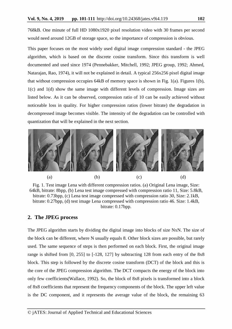
Natarajan, Rao, 1974), it will not be explained in detail. A typical 256x256 pixel digital image

that without compression occupies 64kB of memory space is shown in Fig. 1(a). Figures 1(b),

1(c) and 1(d) show the same image with different levels of compression. Image sizes are

listed below. As it can be observed, compression ratio of 10 can be easily achieved without

noticeable loss in quality. For higher compression ratios (lower bitrate) the degradation in

decompressed image becomes visible. The intensity of the degradation can be controlled with

quantization that will be explained in the next section.

(a) (b) (c) (d)

Fig. 1. Test image Lena with different compression ratios. (a) Original Lena image, Size:

64kB, bitrate: 8bpp, (b) Lena test image compressed with compression ratio 11, Size: 5.8kB,

bitrate: 0.73bpp, (c) Lena test image compressed with compression ratio 30, Size: 2.1kB,

bitrate: 0.27bpp, (d) test image Lena compressed with compression ratio 46. Size: 1.4kB,

bitrate: 0.17bpp.

The JPEG process 2.

The JPEG algorithm starts by dividing the digital image into blocks of size NxN. The size of

the block can be different, where N usually equals 8. Other block sizes are possible, but rarely

used. The same sequence of steps is then performed on each block. First, the original image

range is shifted from [0, 255] to [-128, 127] by subtracting 128 from each entry of the 8x8

block. This step is followed by the discrete cosine transform (DCT) of the block and this is

the core of the JPEG compression algorithm. The DCT compacts the energy of the block into

only few coefficients(Wallace, 1992). So, the block of 8x8 pixels is transformed into a block

of 8x8 coefficients that represent the frequency components of the block. The upper left value

is the DC component, and it represents the average value of the block, the remaining 63




values in the transformed block are the AC components and they represent the frequencies

from low to high. The basic idea behind compression is to preserve the DC and the low

frequency coefficients, and to ignore the high frequency coefficients, since the human eye will

not be capable to recognize the degradation. The operation that will zero out the high

frequency components is quantization. The trick is to find the optimal measure of degradation

that will not be visible for the human eye, since JPEG is optimized for humans.

2.1. Discrete Cosine Transform (DCT)

The Discrete Cosine Transform converts the NxN matrix into another NxN matrix. In the case

of digital image processing, these matrices represent digital images. The formulas for the

forward and inverse transformations are given in Eq. (1).

1

0

1

0 2

12cos

2

12cos,,

N

x

N

y N

vy

N

uxyxfvuvuC

1

0

1

0 2

12cos

2

12cos,,

N

u

N

v N

vy

N

uxvuCvuyxf

(1)

1,...,2,1for 2

0for 1

NuN

uN

u

As it can be seen, the core of the transform is the cosine function. The original matrix is

decomposed into its frequency components using the cosine function. The transformation is

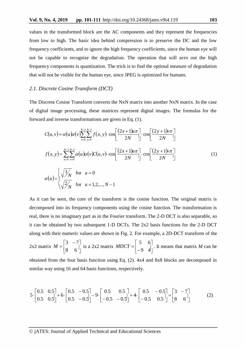
real, there is no imaginary part as in the Fourier transform. The 2-D DCT is also separable, so

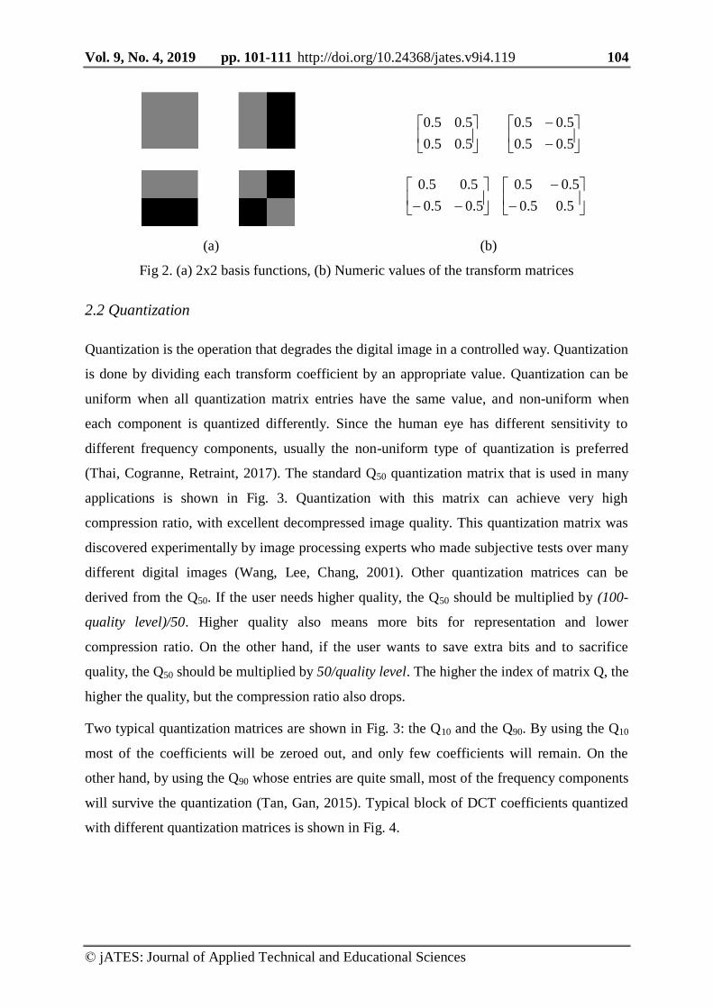
it can be obtained by two subsequent 1-D DCTs. The 2x2 basis functions for the 2-D DCT

along with their numeric values are shown in Fig. 2. For example, a 2D-DCT transform of the

2x2 matrix

68

73M is a 2x2 matrix

49

65MDCT . It means that matrix M can be

obtained from the four basis function using Eq. (2). 4x4 and 8x8 blocks are decomposed in

similar way using 16 and 64 basis functions, respectively.

(2) 68

73

5.05.0

5.05.04

5.05.0

5.05.09

5.05.0

5.05.06

5.05.0

5.05.05




5.05.0

5.05.0

5.05.0

5.05.0

5.05.0

5.05.0

5.05.0

5.05.0

(a) (b)

Fig 2. (a) 2x2 basis functions, (b) Numeric values of the transform matrices

2.2 Quantization

Quantization is the operation that degrades the digital image in a controlled way. Quantization

is done by dividing each transform coefficient by an appropriate value. Quantization can be

uniform when all quantization matrix entries have the same value, and non-uniform when

each component is quantized differently. Since the human eye has different sensitivity to

different frequency components, usually the non-uniform type of quantization is preferred

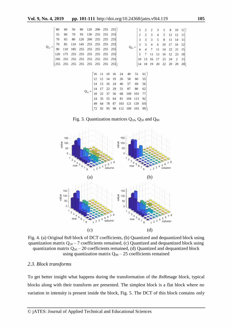
(Thai, Cogranne, Retraint, 2017). The standard Q50 quantization matrix that is used in many

applications is shown in Fig. 3. Quantization with this matrix can achieve very high

compression ratio, with excellent decompressed image quality. This quantization matrix was

discovered experimentally by image processing experts who made subjective tests over many

different digital images (Wang, Lee, Chang, 2001). Other quantization matrices can be

derived from the Q50. If the user needs higher quality, the Q50 should be multiplied by (100-

quality level)/50. Higher quality also means more bits for representation and lower

compression ratio. On the other hand, if the user wants to save extra bits and to sacrifice

quality, the Q50 should be multiplied by 50/quality level. The higher the index of matrix Q, the

higher the quality, but the compression ratio also drops.

Two typical quantization matrices are shown in Fig. 3: the Q10 and the Q90. By using the Q10

most of the coefficients will be zeroed out, and only few coefficients will remain. On the

other hand, by using the Q90 whose entries are quite small, most of the frequency components

will survive the quantization (Tan, Gan, 2015). Typical block of DCT coefficients quantized

with different quantization matrices is shown in Fig. 4.




255255255255255255255255

255255255255255255255245

255255255255255255175120

25525525525525518511090

2552552552551451108570

255255255200120806570

25525525513095706055

25525520012080506080

10Q

2020202220191814

212242117161310

18231216131175

1521221411744

121617106433

11141185333

11121254322

1210853223

90Q

9910310011298959272

10112012110387786449

921131048164553524

771031096856372218

6280875129221714

5669574024161314

5560582619141212

6151402416101116

50Q

Fig. 3. Quantization matrices Q10, Q50 and Q90

(a) (b)

(c) (d)

Fig. 4. (a) Original 8x8 block of DCT coefficients, (b) Quantized and dequantized block using

quantization matrix Q10 – 7 coefficients remained, (c) Quantized and dequantized block using

quantization matrix Q50 – 20 coefficients remained, (d) Quantized and dequantized block

using quantization matrix Q90 – 25 coefficients remained

2.3. Block transforms

To get better insight what happens during the transformation of the 8x8image block, typical

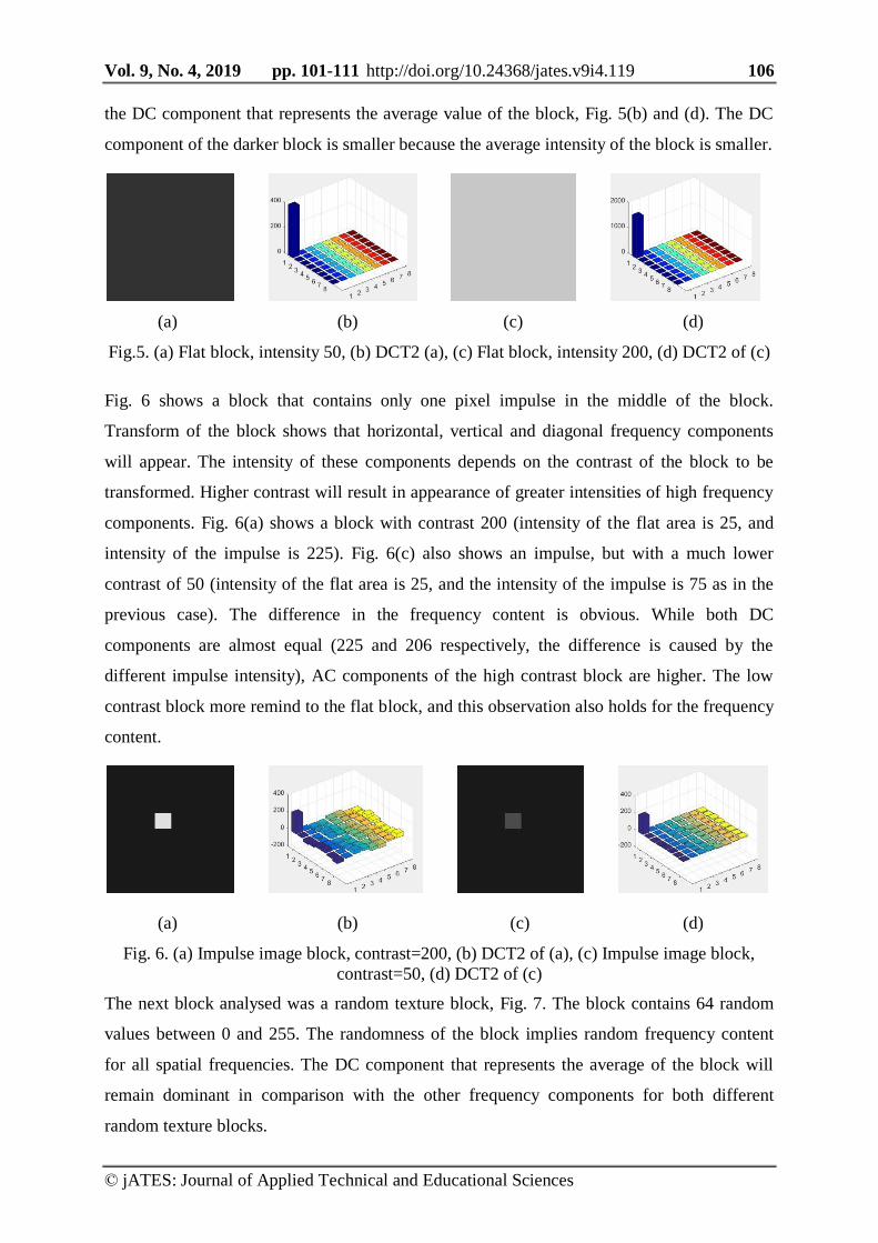
blocks along with their transform are presented. The simplest block is a flat block where no

variation in intensity is present inside the block, Fig. 5. The DCT of this block contains only




the DC component that represents the average value of the block, Fig. 5(b) and (d). The DC

component of the darker block is smaller because the average intensity of the block is smaller.

(a) (b) (c) (d)

Fig.5. (a) Flat block, intensity 50, (b) DCT2 (a), (c) Flat block, intensity 200, (d) DCT2 of (c)

Fig. 6 shows a block that contains only one pixel impulse in the middle of the block.

Transform of the block shows that horizontal, vertical and diagonal frequency components

will appear. The intensity of these components depends on the contrast of the block to be

transformed. Higher contrast will result in appearance of greater intensities of high frequency

components. Fig. 6(a) shows a block with contrast 200 (intensity of the flat area is 25, and

intensity of the impulse is 225). Fig. 6(c) also shows an impulse, but with a much lower

contrast of 50 (intensity of the flat area is 25, and the intensity of the impulse is 75 as in the

previous case). The difference in the frequency content is obvious. While both DC

components are almost equal (225 and 206 respectively, the difference is caused by the

different impulse intensity), AC components of the high contrast block are higher. The low

contrast block more remind to the flat block, and this observation also holds for the frequency

content.

(a) (b) (c) (d)

Fig. 6. (a) Impulse image block, contrast=200, (b) DCT2 of (a), (c) Impulse image block,

contrast=50, (d) DCT2 of (c)

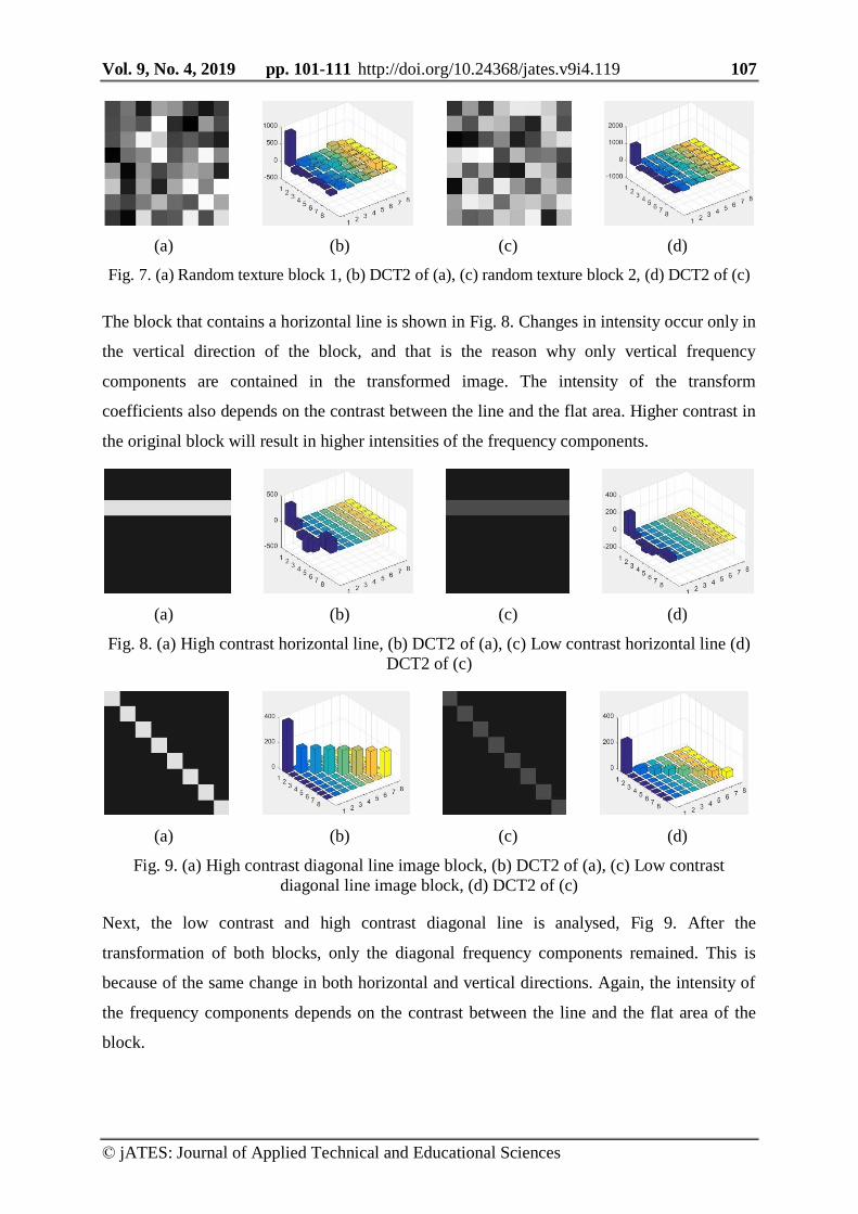
The next block analysed was a random texture block, Fig. 7. The block contains 64 random

values between 0 and 255. The randomness of the block implies random frequency content

for all spatial frequencies. The DC component that represents the average of the block will

remain dominant in comparison with the other frequency components for both different

random texture blocks.




(a) (b) (c) (d)

Fig. 7. (a) Random texture block 1, (b) DCT2 of (a), (c) random texture block 2, (d) DCT2 of (c)

The block that contains a horizontal line is shown in Fig. 8. Changes in intensity occur only in

the vertical direction of the block, and that is the reason why only vertical frequency

components are contained in the transformed image. The intensity of the transform

coefficients also depends on the contrast between the line and the flat area. Higher contrast in

the original block will result in higher intensities of the frequency components.

(a) (b) (c) (d)

Fig. 8. (a) High contrast horizontal line, (b) DCT2 of (a), (c) Low contrast horizontal line (d)

DCT2 of (c)

(a) (b) (c) (d)

Fig. 9. (a) High contrast diagonal line image block, (b) DCT2 of (a), (c) Low contrast

diagonal line image block, (d) DCT2 of (c)

Next, the low contrast and high contrast diagonal line is analysed, Fig 9. After the

transformation of both blocks, only the diagonal frequency components remained. This is

because of the same change in both horizontal and vertical directions. Again, the intensity of

the frequency components depends on the contrast between the line and the flat area of the

block.




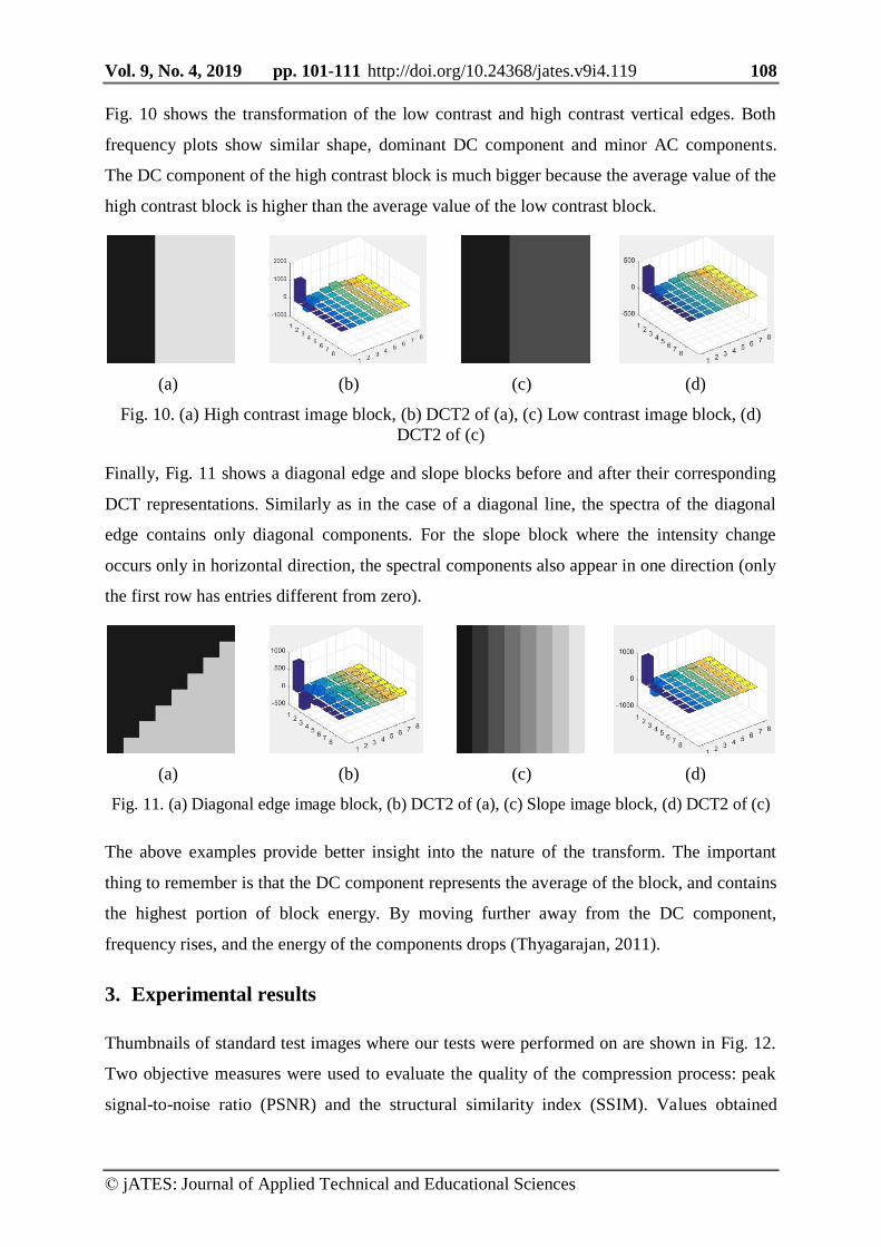
Fig. 10 shows the transformation of the low contrast and high contrast vertical edges. Both

frequency plots show similar shape, dominant DC component and minor AC components.

The DC component of the high contrast block is much bigger because the average value of the

high contrast block is higher than the average value of the low contrast block.

(a) (b) (c) (d)

Fig. 10. (a) High contrast image block, (b) DCT2 of (a), (c) Low contrast image block, (d)

DCT2 of (c)

Finally, Fig. 11 shows a diagonal edge and slope blocks before and after their corresponding

DCT representations. Similarly as in the case of a diagonal line, the spectra of the diagonal

edge contains only diagonal components. For the slope block where the intensity change

occurs only in horizontal direction, the spectral components also appear in one direction (only

the first row has entries different from zero).

(a) (b) (c) (d)

Fig. 11. (a) Diagonal edge image block, (b) DCT2 of (a), (c) Slope image block, (d) DCT2 of (c)

The above examples provide better insight into the nature of the transform. The important

thing to remember is that the DC component represents the average of the block, and contains

the highest portion of block energy. By moving further away from the DC component,

frequency rises, and the energy of the components drops (Thyagarajan, 2011).

Experimental results 3.

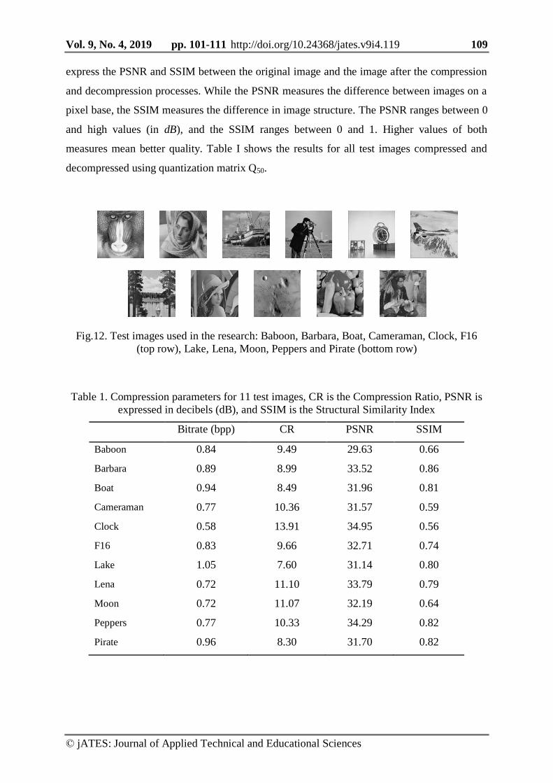
Thumbnails of standard test images where our tests were performed on are shown in Fig. 12.

Two objective measures were used to evaluate the quality of the compression process: peak

signal-to-noise ratio (PSNR) and the structural similarity index (SSIM). Values obtained




express the PSNR and SSIM between the original image and the image after the compression

and decompression processes. While the PSNR measures the difference between images on a

pixel base, the SSIM measures the difference in image structure. The PSNR ranges between 0

and high values (in dB), and the SSIM ranges between 0 and 1. Higher values of both

measures mean better quality. Table I shows the results for all test images compressed and

decompressed using quantization matrix Q50.

Fig.12. Test images used in the research: Baboon, Barbara, Boat, Cameraman, Clock, F16

(top row), Lake, Lena, Moon, Peppers and Pirate (bottom row)

Table 1. Compression parameters for 11 test images, CR is the Compression Ratio, PSNR is

expressed in decibels (dB), and SSIM is the Structural Similarity Index

Bitrate (bpp) CR PSNR SSIM

Baboon 0.84 9.49 29.63 0.66

Barbara 0.89 8.99 33.52 0.86

Boat 0.94 8.49 31.96 0.81

Cameraman 0.77 10.36 31.57 0.59

Clock 0.58 13.91 34.95 0.56

F16 0.83 9.66 32.71 0.74

Lake 1.05 7.60 31.14 0.80

Lena 0.72 11.10 33.79 0.79

Moon 0.72 11.07 32.19 0.64

Peppers 0.77 10.33 34.29 0.82

Pirate 0.96 8.30 31.70 0.82




Discussion 4.

This paper analysed the DCT of different types of 8x8 pixel image blocks. Depending on the

block type, the frequency content in the transformed domain is also changing. By analysing

the transformed blocks the reader can get a good estimate what to except after transforming

real image blocks. This is important because the transformation is followed by quantization

which is the irreversible step of the process. The decision which quantization matrix to use

can be reached if the user knows what to expect after the transformation. Many improved

JPEG algorithms exploit this property, and adapt the quantization step to the block content.

Conclusion 5.

In this paper we have analysed the JPEG process, explained how the discrete cosine transform

works, and how quantization degrades the image quality. We also showed how the

compression process saves memory space for storing digital images. By doing the

experiments with test images we showed what are the typical values for the quality measures.

In the future, it is planned to find a connection between image content and compressed digital

image quality to get higher compression ratio with no change in decompressed image quality.

References

W. B. Pennebaker, J. L. Mitchell. (1992). JPEG Still Image Data Compression Standard:

Springer Science & Business Media, New York.

Joint Photographic Expert Group (JPEG). (1992). Information technology – digital

compression and coding of continuous-tone still images – part 1: requirements and guidelines:

ISO/IEC 10918-1, ITU/CCITT Rec. T.81.

N. Ahmed, T. Natarajan, K. R. Rao. (1974). Discrete Cosine Transform: IEEE Trans. on

Computers, 23, 90-93, doi: 10.1109/T-C.1974.223784

G. K. Wallace. (1992). The JPEG still picture compression standard: IEEE Transactions on

Consumer Electronics, 38(1), doi:10.1109/30.125072

Thai, Cogranne, Retraint. (2017). JPEG Quantization Step Estimation and Its Applications to

Digital Image Forensics: IEEE Transactions on Information Forensics and Security, Vol. 12,

No. 1, 123-133., doi: 10.1109/TIFS.2016.2604208

Wang, Lee, Chang. (2001). Designing JPEG quantization tables based on human visual

system: Elsevier, signal Processing: Image communication 16, 501-506.,

doi:10.1109/ICIP.1999.82921

Tan, Gan. (2015). Perceptual Image Coding with Discrete Cosine Transform: Springer Briefs

in Electrical and Computer Engineering, doi: 10.1007/978-981-287-543-3

K. S. Thyagarajan. (2011). Still Image and Video Compression with Matlab: John Wiley &

Sons, ISBN 978-0-47048416-6




About Authors

Miklós PÓTH received his MSc. and pre-PhD degrees from the Faculty of Technical

Sciences in Novi Sad in 2001 and 2009. Since graduation in 2001, he works as a teaching

assistant (2001-2009) and lecturer (2009-) at the Subotica Tech College of Applied Sciences.

His interest include digital image processing, digital image compression and artificial

intelligence.

Željen TRPOVSKI, Rijeka, Croatia, 1957. M.Sc. (1991) and Ph.D. (1998) . prof. since 2009

at the Faculty of Technical Sciences, University of Novi Sad, Serbia. Teaching courses in

Signals and systems, Digital TV and Video Systems. He has taken part in several international

projects, including: MPEG Coding of video Sequence with very low bit rate, University of

Hannover, Germany, 1992, and WMA (Windows Media Audio) implementation,

MICRONAS, Freiburg, Germany, 2000. Member of two COST Management Committees,

COST 292 and COST IC1005.


analysis of jpeg digital image compression process

Documents