H. Kalviainen et al. (Eds.): SCIA 2005, LNCS 3540, pp. 1196 – 1207, 2005. © Springer-Verlag Berlin Heidelberg 2005

Image Compression Using Adaptive Variable Degree Variable Segment Length Chebyshev Polynomials

I.A. Al-Jarwan and M.J. Zemerly

Department of Computer Engineering Etisalat College of Engineering

PO Box: 980, Sharjah, United Arab Emirates jamal@ece.ac.ae

http://www.ece.ac.ae

Abstract. In this paper, a new lossy image compression technique based on adaptive variable degree variable segment length Chebyshev polynomials is proposed. The main advantage of this method over JPEG is that it has a direct individual error control where the maximum error in gray level difference between the original and the reconstructed images can be specified by the user. This is a requirement for medical applications where near lossless quality is needed. The compression is achieved by representing the gray level variations across any determined section of a row or column of an image by the coefficients of a Chebyshev polynomial. The performance of the method was evaluated on a number of test images and using some quantitative measures compared to the well known JPEG compression techniques.

1 Introduction

Medical applications cannot tolerate visual distortion produced by compression techniques. There is a requirement to obtain near-lossless quality from decompressed images in order to preserve the information required to make a correct diagnosis. Usually, there is a compromise between the distortion that can be tolerated and the amount of compression obtained. Sometimes also like in JPEG [1] there is no direct control over the individual error obtained. Rather, a percentage quality measure is given that may not be sufficient to medical applications as it may affect the validity of a diagnosis, for example. Increasing the percentage quality reduces the individual errors but it may require a number of attempts to control the individual pixel error to an acceptable level. In this paper, it was found that individual errors of 10 may be acceptable in most applications and to a certain extent visual distortion starts to appear if the error exceeds this level.

A new lossy image compression technique based on representing the gray level variations of an image by a series of variable degree Chebyshev polynomials is presented. Image compression is achieved by storing the polynomial coefficients obtained from fitting a variable size segment (a number of pixels) size, which are generally fewer than the original number of pixels. The coefficients are rounded-off to

Image Compression Using Adaptive VDVSL Chebyshev Polynomials 1197

be stored in a byte each to reduce their size. The decompression is obtained using the stored coefficients for each segment using a fast and efficient technique.

Previous work using polynomials concentrated on applying surface or region based fitting using implicit polynomials, which suffer from being ill formed and cannot reach high degrees [2-6]. Results of these techniques showed visual distortion that cannot be tolerated in many applications, let alone medical ones. Previous work done by the authors using Chebyshev polynomials produced 2 new lossy methods termed FDVSL and VDFSL [7, 8]. These 2 methods are also described later in this paper and will be compared with the new proposed method. The method discussed here is concerned with compressing images with no or very little visible distortion (near-lossless quality). The amount of distortion is measured also quantitatively by a number of performance measures commonly used in assessing image compression techniques such as Peak Signal-to-Noise ratio (PSNR) and Normalized Cross Correlation (NCC).

2 Problem Formulation

Chebyshev polynomials are among the most popular orthogonal polynomials that are used to approximate a set of data and are useful in such contexts as numerical analysis and circuit design [9-10]. They form an orthogonal set. A (type I) Chebyshev polynomials )(xTn

are generated via the equation:

)arccoscos()( xnxTn = (1)

Equation 1 can be combined with trigonometric identities to produce explicit

expressions for )(xTn .

So, for Chebyshev polynomials of the first order:

T0(x) =1, T1(x) = x, T2(x) = 2x2 -1 Tn+1(x) = 2x Tn(x) – Tn-1(x) for n >1 (2)

To calculate the coefficients of the Chebyshev polynomial, the following method is used:

The residual sum of squares is given by:

∑=

−=∂m

rrrii yxY

0

22 })({ (3)

where ry (r =0, 1, 2 …m) is the observed or computed values of dependent variable y

at given values rx of the independent variable x. )(xYi is the polynomial of degree i

which minimises the residual sum of squares. The polynomial )(xYi

may be obtained by truncating the series after (i+1):

...)()()( 2211 +++ xpcxpcxpc oo (4)

1198 I.A. Al-Jarwan and M.J. Zemerly

where )(xpi is a polynomial of degree i satisfying the orthogonality condition:

∑ ≠=r

rjri jixpxp )(0)()( (5)

The coefficients jc in (4) are therefore given by [10]:

∑∑

=

rrj

rrjr

jxp

xpyc

2)}({

)( (6)

Approximating a curve with Chebyshev polynomials has some important advantages. For one, if the curve is well approximated by a converging power series, one can obtain an equally accurate estimate using fewer terms of the corresponding Chebyshev series. More importantly is the property over the interval [-1, 1], each polynomial has a domain of [-1, 1]; thus, the series is nicely bounded. And because of this bounded property, approximations calculated from a Chebyshev series are less susceptible to machine rounding errors than the equivalent power series.

Variable x is obtained from the following equation where [a] and [b] are the minimum and maximum coordinates of X respectively. The usage of this variable will affect the range of approximation to be between –1 to 1 instead of two arbitrary limits a and b. [9-11]

)(

)(2

ab

abXx

−+−

= (7)

Choosing Chebyshev polynomials as a compression technique is due to a number of factors: a) they are orthogonal and numerically stable. b) they offer rapid convergence for possible truncation. c) they are normalised polynomials. d) they have the smallest maximal deviation from zero. Under this aspect they are unique:

nnn

x

xT

2

1

2

)(max

10=

<≤ [10].

Clenshaw recurrence formula is used to evaluate (reconstruct) Chebyshev polynomials efficiently using the following equations rather than the normal CPU hungry power series used in each Chebyshev polynomial [10]:

dm+1 ≡ dm ≡ 0 dj = 2x dj+1 – dj+2 + cj for j=m-1, m-2,.. , 1

0210)( cdxddxf +−=≡ (8)

There are five compression performance evaluation measures (termed statistics) that are calculated to evaluate the quality of the reconstructed compressed image. These are the Deviation per Pixel (DPP), the Normalised Cross Correlation (NCC), the

Mean Square Error ( 2msE ), the (PSNR) and the Compression Ratio (CR).

Image Compression Using Adaptive VDVSL Chebyshev Polynomials 1199

The (DPP) is given by:

YX

yxfyxf

DPP

Yy

y

Xx

xr

×

−=∑ ∑

−=

=

−=

=

1

0

1

0

),(),(

(9)

),( yxf and ),( yxf r are the gray levels of the corresponding x (column) and y

(row) in the original and reconstructed images respectively. In the above equation, X is the number of columns (width of image) and Y is the number of rows (height of image).

The (NCC) is given by:

2

11

0

1

0

21

0

1

0

2

1

0

1

0

]),([]),([

)],(),([

⎭⎬⎫

⎩⎨⎧

×

×=

∑ ∑∑ ∑

∑ ∑

−=

=

−=

=

−=

=

−=

=

−=

=

−=

=

Yy

y

Xx

xr

Yy

y

Xx

x

Yy

y

Xx

xr

yxfyxf

yxfyxf

NCC (10)

A value of NCC close to 1 means that the reconstructed image is close to the original, thus a value of 1 indicates that the image is compared to exact copy of itself [12].

The Mean Square Error 2msE is given by:

YX

yxfyxf

E

Yy

y

Xx

xr

ms ×

−=∑ ∑

−=

=

−=

=

1

0

1

0

2

2

)],(),([

(11)

The (PSNR) is given by:

][)255(

log102

2

dBE

PSNRms

⎟⎟⎠

⎞⎜⎜⎝

⎛×= (12)

The higher the PSNR, the lower the noise is in the reconstructed image [12]. The CR is given by:

C

BCR = (13)

B is the number of bytes in the original image and C is the number of bytes needed to store the compressed image [12].

3 Adaptive Chebyshev Fitting

Three methods of compression that utilize Chebyshev polynomials are described in this paper. Here, the VDVSL method (see later) was implemented and tested after implementing and testing the first two methods (VDFSL & FDVSL) in previous

1200 I.A. Al-Jarwan and M.J. Zemerly

publications [7,8]. These methods are called: Variable Degree Fixed Segment Length (VDFSL), Fixed Degree Variable Segment Length (FDVSL) and Variable Degree Variable Segment Length (VDVSL). All the three methods share the same concept of representing a group of pixels (segment) of the image as a Chebyshev polynomial; however, they are different in the fashion in which the compression of the image is achieved. First, the implemented method, VDVSL, will be described and some of the testing results obtained will be highlighted in the next section. The way in which VDFSL and FDVSL operate will be outlined later.

3.1 Variable Degree Variable Segment Length (VDVSL)

This method starts by fitting the whole row/column (depending on option) as a segment starting from zero degree and increases the degree if error is exceeded. If the segment is not compressed (reached the maximum degree allowed i.e. 7), then two new segments will be taken instead. Each new segment has half the number of pixels in the previous segment. The method will then try to compress each segment individually. If any segment is not compressed, then the process is repeated for any non-compressed segment in which the segment will be divided into two segments that have the same number of pixels. The process is repeated until reaching the minimum allowed number of pixels in a segment. The minimum allowed number of pixels in a segment could be fixed to 4 or could be made an input value entered by the user along with the maximum individual error. The compression is finished when all the rows/columns in the image are fitted. Each segment is represented by a byte followed by the coefficients. The first byte is used for the degree (in 4 bits; maximum degree i.e. 7 needs only 3 bits but negative degrees used for special cases) and the number of pixels as power of 2 (also 4 bits, i.e. if the number of pixels is 128 then 7 is stored).

As an optional input that the user can specify, there is the maximum allowed individual error between the original and the reconstructed pixel values. The default value is taken to be 10, as this amount of difference in gray levels can hardly be noticed by the human eye [12].

3.1.1 Option 1: Row-Segment Each row is compressed separately into a number of polynomials that represent segments in the same way that is described previously.

A fitted segment is represented by storing the degree of the fitting polynomial with the number of pixels in one byte followed by the coefficients of the polynomial rounded to bytes. Noted that the number of coefficients = degree +1.

3.1.2 Option 2: Column-Segment This option is identical to option 1. The only difference is that a column in an image is compressed instead of a row. Otherwise, the processing steps of the two options are identical.

3.2 Variable Degree Fixed Segment Length (VDFSL)

In this method a row/column is divided equally into a number of segments each with an equal number of pixels (or the image is divide into 4×4 portions). Starting with a degree of 0, the pixels in the segment are fitted and all reconstructed pixels are

Image Compression Using Adaptive VDVSL Chebyshev Polynomials 1201

checked against the maximum error allowed. If the maximum error is exceeded, then the degree is incremented and the fitting is repeated. The same fitting procedure is repeated until either the errors are acceptable or the degree exceeds the maximum degree allowed, which is the maximum of number of pixels in a segment divided by two or 8. In the latter case, a special value of -1 is stored (as the degree of the polynomial) and then each pixel will be represented by a value equals to the original data of the pixels minus 128 (in order to fit within a byte).

A fitted segment is represented by storing the degree of the fitting polynomial followed by the coefficients of the polynomial rounded to bytes. Note that the number of coefficients = degree +1.

3.3 Fixed Degree Variable Segment Length (FDVSL)

In this method the number of pixels in each segment is specified dynamically. That is the algorithm starts from a fixed number of pixels (in this case it is 4 for degree 2) and the pixels are fitted using the Chebyshev polynomials and if the error is acceptable the number of points is increased by one (the number of increased pixels is an input by the user to achieve better execution time). The fitting is repeated every time a new point is added and the error is checked if it is greater than the maximum individual accepted error. If no it continues adding new points until it reaches 127 pixels (because the byte can only handle numbers from -128 to 127) and start again or the error exceeds the acceptable range.

Another critical case is that when we left with less than 4 points at the end of each row we can not handle it so to solve it a special value of -1 is stored and then each pixel will be represented by a value = original gray levels -128.

A fitted segment is represented by storing the number pixels in the segment of the fitting polynomial followed by the coefficients of the polynomial. It is noted that the number of coefficients = degree +1. The special degree of -1 indicates that individual values for each pixel in the segment are stored instead of the coefficients. When the compressed file is read, this means that either the segment of 4 points was not fitted with the degree specified or the remaining points left at the end of a row is less than 4.

There are three options for FDVSL. All share the idea of representing a group of pixels (termed segment) by the coefficients of a Chebyshev polynomial. These options are: row-segment, column-segment and all-rows-together [8].

As an optional input that the user can specify, there is the maximum allowed individual error between the original and the reconstructed pixel values. The default value is taken to be 5, as this amount of difference in gray levels can hardly be noticed by the human eye [12]. The second optional input is the degree of the fitting polynomial. The default value is set to 2. A third parameter is also introduced to speed up processing which is the number of pixels to add to the segment in case the error is acceptable. The default is 1 pixel.

3.4 Compressed Image Format

The compressed image is represented and stored in a file having the extension “.ch”. As in the case of PGM, characters that locate from”#" to the next end-of-line are ignored (comments). The compressed image is represented as the following:

1202 I.A. Al-Jarwan and M.J. Zemerly

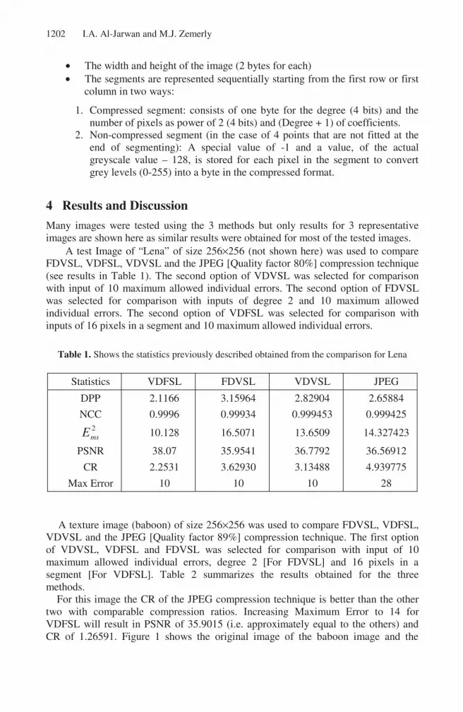
• The width and height of the image (2 bytes for each) • The segments are represented sequentially starting from the first row or first

column in two ways:

1. Compressed segment: consists of one byte for the degree (4 bits) and the number of pixels as power of 2 (4 bits) and (Degree + 1) of coefficients.

2. Non-compressed segment (in the case of 4 points that are not fitted at the end of segmenting): A special value of -1 and a value, of the actual greyscale value – 128, is stored for each pixel in the segment to convert grey levels (0-255) into a byte in the compressed format.

4 Results and Discussion

Many images were tested using the 3 methods but only results for 3 representative images are shown here as similar results were obtained for most of the tested images.

A test Image of “Lena” of size 256×256 (not shown here) was used to compare FDVSL, VDFSL, VDVSL and the JPEG [Quality factor 80%] compression technique (see results in Table 1). The second option of VDVSL was selected for comparison with input of 10 maximum allowed individual errors. The second option of FDVSL was selected for comparison with inputs of degree 2 and 10 maximum allowed individual errors. The second option of VDFSL was selected for comparison with inputs of 16 pixels in a segment and 10 maximum allowed individual errors.

Table 1. Shows the statistics previously described obtained from the comparison for Lena

Statistics VDFSL FDVSL VDVSL JPEG

DPP 2.1166 3.15964 2.82904 2.65884

NCC 0.9996 0.99934 0.999453 0.999425 2msE

10.128 16.5071 13.6509 14.327423

PSNR 38.07 35.9541 36.7792 36.56912

CR 2.2531 3.62930 3.13488 4.939775

Max Error 10 10 10 28

A texture image (baboon) of size 256×256 was used to compare FDVSL, VDFSL, VDVSL and the JPEG [Quality factor 89%] compression technique. The first option of VDVSL, VDFSL and FDVSL was selected for comparison with input of 10 maximum allowed individual errors, degree 2 [For FDVSL] and 16 pixels in a segment [For VDFSL]. Table 2 summarizes the results obtained for the three methods. For this image the CR of the JPEG compression technique is better than the other two with comparable compression ratios. Increasing Maximum Error to 14 for VDFSL will result in PSNR of 35.9015 (i.e. approximately equal to the others) and CR of 1.26591. Figure 1 shows the original image of the baboon image and the

Image Compression Using Adaptive VDVSL Chebyshev Polynomials 1203

reconstructed images obtained from FDVSL, VDFSL and VDVSL as well as that of JPEG. In these two cases no visible distortion could be seen in any of the 4 methods.

Table 2. Shows the statistics previously described obtained from the comparison

Statistics VDFSL FDVSL VDVSL JPEG

DPP 0.755325 3.41394 2.99699 3.2038

NCC 0.999871 0.999438 0.99953 0.99953 2msE

4.62044 20.0552 16.6964 16.65769

PSNR 41.484 35.1085 35.9046 35.91465

CR 1.05903 1.61523 1.53978 2.316414

Max Error 10 10 10 20

(a) (b)

(c) (d)

Fig. 1. An example of the results: (a) Original PGM image, (b) Reconstructed image using VDVSL, (c) Reconstructed image using FDVSL, and (d) Reconstructed image using JPEG

1204 I.A. Al-Jarwan and M.J. Zemerly

The proposed image compression technique was tested on a number of test images. The two options of VDVSL generally produced acceptable compression ratios when the default optional input value is used.

On the other hand, increasing the individual error led to an increase in the compression ratio, but the quality of the image deteriorated. The quality of the reconstructed compressed image became worse when reaching high individual error and differences were clearly seen in the case of maximum individual error of 15.

The first option of VDVSL was compared with the JPEG compression technique. The optional input is selected to have a maximum individual error of 10. The choice was done based on acquiring an acceptable compression ratio (1.53978), while keeping the quality of the reconstructed compressed image acceptable for use. VDVSL gave better results in the terms of calculated statistics; better NCC, DPP and maximum error (see tables 1, 2).

One major advantage of VDVSL (and other methods that depend on Chebyshev Polynomials) over JPEG is the ability to control the maximum individual error. This is clearly evident from Table 2 as the maximum individual error of VDVSL was 10 (specified maximum individual error), while that of JPEG was 20 (using quality of 89). To reduce the error in JPEG to 14 quality 93 was used and then compression ratio of only 1.051 was obtained [with DPP = 2.099, NCC = 0.999796, PSNR = 39.5216].

This system can be applied in fields where quality of the reconstructed image is the main issue with a reasonable compression ratio such as medical images. An ultrasound scan image of size 256×256 was used to compare FDVSL, VDFSL, VDVSL and the JPEG [Quality factor 75%] technique with the same specifications of the previous test. Table 3 summarizes the results obtained for the three methods.

Table 3. shows the statistics previously described obtained from the comparison

Statistics VDFSL FDVSL VDVSL JPEG

DPP 2.77173 3.11668 2.91797 2.1523

NCC 0.99748 0.99692 0.99729 0.99836 2msE

13.2404 16.2639 14.2847 5.96339

PSNR 36.9118 36.0186 36.5821 38.7588

CR 4.70365 6.211543 6.341977 7.287445

Max Error 10 10 10 21

For this image the quality of the JPEG compression technique is better (in PSNR) than the other three with comparable compression ratios. Also, VDVSL performs better than FDVSL and VDFSL in texture images but slower than the two other methods. Figure 2 shows the original image of the ultrasound scan image and the reconstructed images obtained from FDVSL, VDFSL and VDVSL as well as that of JPEG. Visual distortion in the first three reconstructed images can hardly be seen to the naked eye as the maximum individual error for any pixel is 10. No visible distortion could be seen in any of the 4 methods despite the fact that the individual error in the JPEG image is 21.

Image Compression Using Adaptive VDVSL Chebyshev Polynomials 1205

(a) (b)

(c) (d)

Fig. 2. An example of the results: (a) Original PGM image, (b) Reconstructed image using VDVSL, (c) Reconstructed image using FDVSL, and (d) Reconstructed image using JPEG

The Chebyshev methods described in this paper can be used in applications where the errors of the reconstructed compressed image needed to be directly controlled and the quality of textured areas preserved. In medical imaging, for example, an error reaching a value of 28 (as JPEG for Lena) may result in wrong diagnosis obtained from the image.

Another advantage is that VDFSL, FDVSL and VDVSL preserve the quality of the most difficult parts of the image that cannot be compressed, as they are stored without any change (only some pre-processing and post-processing operations to store the original values in a byte format).

It was observed that compression ratios obtained from the two options (row/column) on the same input image were not the same (for fixed optional inputs); one of the two compression ratios is better than the other one with little difference in the other statistics. As a different image was tested, it was found that the best compression was not generated by the same option that generated the previous best compression. The possibility of one method producing a better compression than the other one is related directly to the structure or shape of the input image. For example,

1206 I.A. Al-Jarwan and M.J. Zemerly

for the Lena image the column option gave slightly better results than the others because of vertical uniform areas. This can be considered as an advantage for these 3 methods that depend on Chebyshev Polynomials.

Also, Huffman coding is applied to the compressed data (Coefficients) for further improvement in terms of CR in both FDVSL and VDVSL.

Another observation is that in texture images VDVSL behaves slightly better than FDVSL since it will automatically tries to fit the segments by increasing the degree. In addition, in most cases VDVSL achieves slightly better in term of PSNR than FDVSL.

Note that VDVSL is not as fast as JPEG or FDVSL, but could be improved by using parallel processing. This is possible as the method lends itself readily to parallel processing since it is row or column-based. However, time to reconstruct the image is very fast.

Another improvement to these methods (i.e. VDFSL, FDVSL and VDVSL) can be introduced by fitting in the frequency domain using for example the Fast Fourier Transform (FFT).

5 Conclusions

A new compression technique based on fitting adaptive variable-degree Chebyshev polynomials to variable length segments of data of the rows or columns of an image is presented. The method offers the user direct control of individual gray level variations in the reconstructed image. The technique was tested on a number of images and the results showed slightly better quality reconstructed images but with lower compression ratios than JPEG. For medical images where the amount of visible distortion cannot be tolerated the new suggested methods performed better because of their ability to control the individual error.

References

[1] G. Wallace, “The JPEG Still Picture Compression Standard”, CACM, vol. 34, pp 33-40, Apr 1990.

[2] D.M. Bethel, D.M. Monro, “Polynomial image coding with vector quantised compensation”, Proc. ICASSP-95, vol. 4, 2499-2502.

[3] Y. Chee, K. Park, “Medical image compression using the characteristics of human visual system”, Proc. 16th Int. Conf. of the IEEE, Eng. Advances: New Opportunities for Biomedical Eng., vol. 1, 618-619, 1994.

[4] F. De Natale, et. al., “Polynomial Approximation and Vector Quantization: A Region-Based Approach”, IEEE Trans. On Communications, vol. 43, no. 2-4, Feb-Apr 1995, pp 198-206.

[5] A. Helzer, et. al, “Using implicit polynomials for image compression”, Proc. 21st IEEE Conv. of the EEEI, pp 384-388, 2000.

[6] I. Sadeh, “Polynomial Approximation of Images”, Computers Math. Applications, vol. 32, no. 5, pp 99-115, 1995.

[7] N. Al - Mutawwa, M.J. Zemerly, “Image Compression using Adaptive Chebyshev Polynomials”, WSEAS Trans. On Mathematics, Vol. 3, issue 2, pp 417-422, April 2004.

Image Compression Using Adaptive VDVSL Chebyshev Polynomials 1207

[8] I. Al - Jarwan, M.J. Zemerly, et. al, “Image Compression using Adaptive Fixed-Degree Chebyshev Polynomials”, proc. IEEE-GCC, Bahrain, Nov 2004.

[9] M.G. Cox, J.G. Hayes, “Curve Fitting: A guide and suite of Algorithms for the Non-Specialist user”, NPL Report NAC 26, Dec 1973.

[10] C.W. Clenshaw, “Mathematical Tables”, Volume 5, National Physical Laboratory, London 1962.

[11] “Numerical Recipes in c: The Art of Scientific Computing”, Cambridge University Press, 1988-1992.

[12] M.J. Zemerly, “A rule-based system for processing retinal images”, Ph.D. thesis, University of Birmingham, U.K, August 1989.