pricing american options under stochastic volatility: a new method using chebyshev polynomials to...
TRANSCRIPT

Department of EconomicsPricing American Options under Stochastic Volatility: A New Method Using
Working Paper No. 488 February 2003 ISSN 1473-0278
Elias Tzavalis and Shijun Wang
Chebyshev Polynomials to Approximate the Early Exercise Boundary

Prici ng Ame rican Options un der sto chas t ic vo latility : A ne w
method using Chebyshev polynomials to approximate the Early
Exercise Boundary
Elias Tzavalis∗ and Shijun Wang†
Department of Economics,Queen Mary, University of London
London E1 4NS, UK
This version February, 2003
Abstract
This paper presents a new numerical method for pricing Americancall options when the volatility of the price of the underlying stock isstochastic. By exploiting a log-linear relationship of the optimal exer-cise boundary with respect to volatility changes, we derive an integralrepresentation of an American call price and the early exercise premiumwhich holds under stochastic volatility. This representation is used to de-velop a numerical method for pricing the American options based on anapproximation of the optimal exercise boundary by Chebyshev polyno-mials. Numerical results show that our numerical approach can quicklyand accurately price American call options both under stochastic and/orconstant volatility.
Keywords: American call option, stochastic volatility, early exerciseboundary, Chebyshev polynomials.
JEL Classification: G12, G13, C63
∗[email protected]†[email protected]
1

1 Introduction
Pricing American options is one of the most difficult problems in option pricing
literature. The difficulty stems from the fact that, unlike a European, an Amer-
ican call (or put) option has no explicit closed form solution. This happens
because the optimal boundary above which the American call option will be
exercised is unknown and part of the option price solution. Therefore, efforts
have been concentrated on developing numerical approximation schemes which
can price the American options accurately and faster than the lattice or sim-
ulation based methods, which are time consuming and computationally more
demanding. These schemes are based on integral representations of the Amer-
ican option evaluation formula or they exploit the partial differential equation
satisfied by the option prices.1
The existing approximation schemes for pricing American call (or put) op-
tions in the literature are valid only under the assumptions of the Black and
Scholes (1973) option pricing model, which claim that the stock price of the
underlying stock is log-normally distributed conditional on the current stock
price, with constant volatility. However, these assumptions are in contrast to
most of the empirical evidence of the option and stock pricing empirical lit-
erature which indicates that stocks’ prices volatility is stochastic [see Ghysels,
Harvey and Renault (1996), for a survey].
The aim of this paper is to develop a new numerical method for pricing Amer-
ican call option prices for the case that the underlying stock’s price volatility
is stochastic, as it appears to be in reality. The lack of such type of methods
in the literature of the American options is primarily due to the fact that, un-
der stochastic volatility, the optimal exercise boundary depends, in addition to
time, on the paths of the volatility [see Broadie et al (2000)]. This considerably
1Examples of such type of numerical methods include the Barone-Adesi and Whaley (1987)analytical approximation method, the approximating methods of Geske-Johnson (1984) andBunch and Johnson (1992), the Gaussian quadrature method of Sullivan (2000), inter alia,and the recently developed exercise boundary approximation methods of Subrahmanyam andYu (1996), and Ju (1998).
2

complicates the derivation of a suitable, analytic representation for an Amer-
ican call option price upon which a numerical approximation method can be
build up. Our strategy of circumventing this problem is to approximate the
optimal exercise boundary function with a log-linear function with respect to
volatility changes over different pieces of the maturity interval.2 Based on this
approximation, we derive an analytic, integral representation of the early exer-
cise premium of the American call option price. This representation unbundles
the early exercise premium (and hence the American call option price) into a
portfolio of Arrow-Debreu type of securities [see Bakshi and Madan (2000), for
a European call option price]. The prices of these securities can be calculated
based on the joint characteristic function of the stock price and its conditional
volatility process which is derived in closed form in the paper. To complete
our numerical method for evaluating the American call option under stochas-
tic volatility, we employ Chebyshev polynomials to approximate the logarithm
of the exercise boundary function. With these polynomials, we can efficiently
approximate any non-linear pattern of the optimal exercise boundary function,
over the different pieces of the maturity interval, because we can choose the
point with the minimum approximation error to fit a high-degree polynomial
approximating function into the true function of the exercise boundary.
To appraise the pricing performance of our method, the paper reports nu-
merical results of the speed and accuracy of the method in comparison with
benchmark methods. We also compare the pricing performance of the method
for the case that volatility is constant with other numerical approximation meth-
ods for the log-normal model, which are frequently used in practice. The results
of the numerical evaluations are very encouraging. They show that a very par-
simonious, two degree approximating function of the exercise boundary based
on Chebyshev polynomials can satisfactorily price American call options for
a broad class of stock and exercise prices considered in our numerical experi-
2Note that this approach is consistent with recent evidence suggesting that, when volatilityis stochastic, the exercise boundary is smooth with respect to volatility changes [see Broadieet al (2000)].
3

ments. This is true both under stochastic and constant volatility. Our results
show that the pricing errors of our method are very close to zero, and they
are of the same order of magnitude independently on whether the volatility is
constant or stochastic. In the constant volatility case, we find that the pricing
errors of our method can become substantially smaller in magnitude than the
other approximation methods compared with, especially when the curvature of
the true optimal exercise boundary function is a high.
The paper is organised as follows. In Section 2, we present the evaluation
framework for the American call option price under stochastic volatility and de-
rive an analytic, integral representation of the American call price. In Section 3,
we show how to implement Chebyshev polynomials to approximate the optimal
exercise boundary function for the lognormal and stochastic volatility models,
respectively. In Section 4, we list and discuss numerical results of the perfor-
mance of our method to price the options. Section 5 summarizes and concludes
the paper.
2 Analytic evaluation of American call options
under stochastic volatility
In this section, in order to derive an analytic evaluation formula for an American
call option we assume that the price of the underlying stock follows a geometric
stochastic volatility process. This model of the stock price is known in the liter-
ature as the stochastic volatility (SV) model [see Heston (1993), inter alia]. The
analysis of the section proceeds as follows. First, we present a general evaluation
framework for pricing an American call option under stochastic volatility which
is in line with that of Broadie et al (2000). Based on this framework, we next
derive an analytic, integral representation of the American call option price.
4

2.1 The valuation framework
Consider Heston’s (1993) specification of the stochastic volatility (SV) model to
characterise the dynamics of the underlying stock’s price, denoted Pt, at time t.
For analytic convenience, assume that dividends are paid at the constant rate
δ and that the riskless interest rate, r, is constant. Then, the SV model implies
that the spot stock price should satisfy the following risk-neutralised process
dPtPt
= (r − δ) dt+pVtdW1,t, (1)
where the instantaneous conditional variance (volatility), Vt, follows the mean
reverting square root process
dVt = k(θ − Vt)dt+ σpVtdW2,t, (2)
where k is adjusted by the market price of volatility risk, {Wj,t, t > 0} , j =1, 2, are two correlated standard Brownian motion processes, with correlation
coefficient given by Corr(dW1,t; dW2,t) = ρdt, ρ ∈ (−1, 1) .Consider now an American call option contract for the above stock with
maturity date T and strike price K, at the exercise time. This contract gives
the holder the right of exercising the call option at any time h in the maturity
interval [t, T ], i.e. h ∈ [t, T ]. The critical stock price above which the Ameri-can call will be exercised is referred to as the optimal exercise boundary. Since
the price of the underlying stock depends on the paths of the volatility pro-
cess Vt, we will hereafter denote the time t, which represents the current time
price of the American call option contract (i.e. the American call option price)
as CA (Pt, Vt, T − t), while the optimal exercise boundary will be denoted asB (Vh, h), ∀ h ∈ [t, T ].The American call option price CA (Pt, Vt, T − t) can be calculated by the
maximum value of the discounted payoffs from the option where the maximum
5

is taken over all possible stopping (exercise) times, denoted τ , in the maturity
interval, [t, T ]. Define the optimal stopping time as
τ∗ = inf {τ ∈ [t, T ] : CA (Pt, Vt, T − t) = (Pt −K)+} . (3)
Then American call option pricing problem can be represented by the Snell
envelop3
CA (Pt, Vt, T − t) = supτ∈S[t,T ]
EQ³e−
R τtrds (Pτ −K)+
´, (4)
where S[t,T ] is the set of stopping times in the maturity interval, [t, T ], EQt de-notes the time t conditional expectation under the equivalent martingale mea-
sure Q, and (Pτ −K)+ is the payoff of the American call option at the stoppingtime τ .
The following theorem characterises the optimal solution of the problem
defined by equation (4).
Theorem 1 Let the stock price satisfy processes (1) and (2). Then, the Amer-
ican call option price CA (Pt, Vt, T − t) can be written as
CA (Pt, Vt, T − t) = CE (Pt, Vt, T − t) (5)
+EQt
TZt
e−r(s−t) (δPs − rK) I{Ps>B(Vs,s}ds,
where CE (Pt, Vt, T − t) is the value of a European call price with maturitydate T and strike price K, B(Vs, s) denotes the value of the optimal exercise
boundary, at time s ∈ [t, T ], and IA is the indicator function of the set A, de-fined as A = {Ps : Ps > B(Vs, s) and Vs ∈ R+}, which contains the pricesof the stock at which the American call will be exercised. The optimal exer-
cise boundary B(Vh, h) entered into the American call option price formula (5)
3See Karatzas (1988), inter alia.
6

should satisfy the following recursive equation
B (Vh, h)−K (6)
= CE (B(Vh, h),K, Vh, T − h)
+EQh
TZh
e−r(s−h) (δPs − rK) I{Ps≥B(Vs,s)}ds , ∀ s = h ∈ [t, T ],
with terminal condition
B (VT , T ) -K=max {K, rK/δ} . (7)
In Appendix A, we give a proof of Theorem 1 based on a decomposition of
the optimal stopping problem (4) in terms of the optimal exercise boundary [see
Myneni (1992)].
Theorem 1 shows that the American call option price CA (Pt, Vt, T − t) canbe calculated by (5), once the values of optimal exercise boundary B (Vh, h)
are provided. However, this is not a trivial calculation problem. The recursive
nature of B (Vh, h) reveals that the difficulty in deriving an analytic formula for
evaluating the American option is due to the fact that the exercise boundary
is determined as part of the solution. This problem becomes more complicated
under the SV model rather than the lognormal model because, for the SV model,
the optimal exercise boundary function depends, in addition to the time h, on
conditional variance (volatility) Vh.
2.2 An integral representation of the American call option
price for the SV model
To circumvent the above difficult calculation problem of an American call op-
tion price, in this subsection we present a new strategy for evaluating the op-
tion price CA (Pt, Vt, T − t). Based on a first-order log-linear approximation ofthe optimal exercise boundary function around the time t conditional mean of
volatility, we derive an integral representation of the American call option price
7

CA (Pt, Vt, T − t) upon which we can build up a numerical method for evaluatingthis price.
Suppose that the logarithm of the optimal exercise boundary function, at
time h, denoted b(Vh, h) ≡ lnB(Vh, h), can be approximated around the condi-tional mean of volatility EtVh by the linear in volatility function
b(Vh, h) = b0(h) + b1(h)(Vh −EtVh). (8)
Relationship (8) asserts that, for small changes of Vh around the conditional
mean of volatility EtVh, at time t, the true optimal exercise boundary function
is an exponentially smooth surface with respect to volatility changes. This
assumption can be justified by recent evidence provided by Broadie et al (2000),
who recovered the American call option price and the exercise boundary reduced
forms from the data following a non parametric statistical approach.
In the next theorem we give a two-dimension integral representation for the
price CA (Pt, Vt, T − t) and its associated optimal exercise boundary recursiveequation.
Theorem 2 For relationship (8), the American call option price CA (Pt, Vt, T − t)can be calculated as
CA (Pt, Vt, T − t)
= CE(Pt, Vt, T − t) +Z T
t
δPte−δ(s−t)Π1(b0(s), b1(s)|Pt, Vt)ds
−Z T
t
rKe−r(s−t)Π2 (b0(s), b1(s)|Pt, Vt) ds, (9)
where Π1(.) and Π2 (.) are defined in the Appendix B. The optimal exercise
8

boundary B (Vh, h) satisfies the following recursive equation
B (Vh, h)−K = CE(Ph, Vh, T − h)
+
Z T
h
δB (Vh, h) e−δ(s−h)Π01 (b0(s), b1(s)|B(Vh, h), Vh) ds
−Z T
h
rKe−r(s−h)Π02 (b0(s), b1(s)|B(Vh, h), Vh) ds, (10)
∀ s = h ∈ [t, T ], with terminal condition
B(VT , T )−K = max{K, rk/δ},
where Π01(.) and Π02 (.) are defined in the Appendix B.
The proof of the Theorem is given in Appendix B.
The integral representation of the American option price CA (Pt, Vt, T − t)and its associated exercise boundary recursive equation (10), given by Theorem
2, unbundles the early exercise boundary premium (and hence the American call
option) into a portfolio of Arrow-Debreu type of securities. The prices of these
securities can be derived by calculating the following risk neutral expectations
Π1 (b0(s), b1(s)|Pt, Vt) = EQt"PsI{(Ps,Vs):Ps=B(Vs,s)}
EQt [Ps]|Pt, Vt
#, (11)
or using the transformed measure Q1 withdQ1
dQ = PsEQh [Ps]
as
Π1 (b0(s), b1(s)|Pt, Vt) = EQ1t
hI{(Ps,Vs):Ps=B(Vs,s)}|Pt, Vt
i, (12)
and
Π2 (b0(s), b1(s)|Pt, Vt) = EQthI{(Ps,Vs):Ps=B(Vs,s)}|Pt, Vt
i(13)
[see Appendix B].
9

The above relationships indicate that the prices Π1 (b0(s), b1(s)|Pt, Vt) andΠ1 (b0(s), b1(s)|Pt, Vt) constitute the market prices of a security which pays $1in state {(Ps, Vs) : Ps = B(Vs, s)} and 0 otherwise under the measures Q1 andQ, respectively.
The integral representation of the American call option given by Theorem
2 can be reduced to that derived by Kim (2000), for the lognormal model with
constant volatility. This can be obtained by setting k = θ = σ = 0 in equations
(9) and (10) and noticing that, under the assumptions of the log-normal model,
the exercise boundary equation (8) becomes the exact relationship B(Vh, h) =
exp[b0(h)]. Then, it can be easily seen that equation (9) reduces to
CA (Pt, T − t) = CE (Pt, T − t) +Z T
t
δPte−δ(s−t)Π1(B(s)|Pt)ds (14)
−Z T
t
rKe−r(s−t)Π2 (B(s)|Pt) ds, for s > h ∈ [t, T ],
while equation (10) reduces to
B (h)−K (15)
= CE (Ph, T − t) +Z T
t
δB (h) e−δ(s−h)Π01 (B(s)|B(h)) ds
−Z T
t
rKe−r(s−h)Π02 (B(s)|B(h)) ds,
where now Π1 (B(s)|Pt) and Π2 (B(s)|Pt) are given by
Π1 (B(s)|Pt)
=1
2+1
π
∞Z0
Re
·e−iφ logB(s)F (φX − i, 0, s− h| lnPt, 0)
iφ
¸dφ
= N
µlog(B(s)/Pt)− (r − δ + 1
2σ2)(s− t)
σ√s− t
¶(16)
10

and
Π2 (B(s)|Pt)
=1
2+1
π
∞Z0
Re
·e−iφ logB(s)F (φX , 0, s− h| lnPt, 0)
iφ
¸dφ
= N
µlog(B(s)/Pt)− (r − δ − 1
2σ2)(s− t)
σ√s− t
¶, (17)
respectively.4 Note that now the prices of the Arrow-Debreu type of securities
Π1 (B(s)|Pt) andΠ2 (B(s)|Pt) reflect the prices of a security which pays $1 in thestate {Ps = B(s)} and 0 otherwise under the measures Q1 and Q, respectively.As equations (16) and (17) indicate, these prices can be calculated as the prob-
abilities of the standardized normal distribution at the values of log(B(s)/Pt)
adjusted by the quantities (r − δ + 12σ
2)(s− t) and (r − δ − 12σ
2)(s− t) underthe measures Q1 and Q, respectively.
5
3 Numerical evaluation of American call options
using Chebyshev polynomial functions to ap-
proximate the exercise boundary
The two-dimension integral representation of the American call option price
and its associated recursive optimal exercise boundary relationship given by
Theorem 2 can be used to build up a numerical approximation method for
pricing American options under stochastic volatility. In this section we introduce
such a method based on an approximation of the optimal exercise boundary
function using Chebyshev polynomials.
4The prices Π01 (B(s)|B(h)) and Π02 (B(s)|B(h)) can be defined analogously.5Note that the above two quantities differ by σ2 which reflects the fact that the price of
risk under the meassure Q1 is smaller than under measure Q. This can be attributed to thefact that under measure Q1 the payoff of the Arrow-Debreu price is scaled by the stock price[see equations (11) and (12)].
11

Our motivation to implement a numerical approach to approximate the opti-
mal exercise boundary rather than to directly approximate the whole American
value formula stems from recent evidence suggesting that this numerical group
of methods can considerably increase the computation speed of calculations
without losing much in accuracy [see Huang, Subrahmanyam and Yu (1996),
and Ju (1998)]. This happens because the boundary approximation methods
can separate the estimation problem of the optimal exercise boundary function
from that of the American call option. This can increase the computation speed
while, simultaneously, avoid accumulating pricing errors through the evaluation
steps of the American option risk neutral pricing formula. Our motivation to
employ Chebyshev polynomials to approximate the true optimal exercise bound-
ary function stems from the fact that, with these polynomials, we can efficiently
approximate any non-linear function by choosing the point with the minimum
approximation error to fit a high-degree polynomial approximating function to
the true function.6 Note that the accuracy of this method increases with the
number of polynomials terms used in the approximating function.
To better understand how to implement the Chebyshev polynomials method
to approximate the optimal exercise boundary, which will be hereafter referred
to as the CB method, we first start our analysis with the case of the lognormal
model. We next extend the analysis to the SV model.
3.1 The case of the lognormal model
To implement the CB method for the lognormal model, notice that the optimal
exercise boundary equation (15) can be reduced to the one-dimension integral
relationship:
6A brief discription of the Chebyshev function approximation is given in Appendix C.
12

B(h)−K= CE(Ph, T − h)−B(h)e−δ(T−h)N (d1 (B(h), B(T ), T − h)) +B(h)N(ξ)+Ke−r(T−h)N (d1 (B(h), B(T ), T − h))−KN(ξ)
+
TZt
B(h)e−δ(s−h)n (d1 (B(h), B(s), s− h)) ∂d1 (B(h), B(s), s− h)∂s
−TZh
Ke−r(s−h)n (d2 (B(h),B(T ), s− h)) ∂d1 (B(h), B(s), s− h)∂s
ds, (18)
where ξ = lims→hln(Bh)−ln(B(s))
σ√s−h , N (·) and n (·) denote the cumulative not
standard normal distribution and its associated probability density function,
respectively.
Let eb(h) denote an approximating function of the logarithm of the optimal
exercise boundary which consists of ν-Chebyshev polynomials terms. The func-
tional form of eb(h) is given in Appendix C. Substituting eb(h) into equation (18)implies the following system of equations
eB(h)−K= CE(Ph, T − h)− eB(h)e−δ(T−h)N ³d1 ³ eB(h), eB(T ), T − h´´+ 1
2eB(h)
+Ke−r(T−h)N³d1
³ eB(h), eB(T ), T − h´´− 12K
+
TZt
eB(h)e−δ(s−h)n³d1 ³ eB(h), eB(s), s− h´´Ãν−2Xi=0
αisi√s− h
!ds
−TZh
Ke−r(s−h)n³d1
³ eB(h), eB(s), s− h´´Ãν−2Xi=0
γisi√s− h
!ds, (19)
where eB(h) ≡ eeb(h), and ai and γi satisfy the following recursive equations
13

αi = γi =
Ã2(i+ 1)ci+1 −
νPj=i+1
cj
!/2σ, for i = 1, 2, ..., ν − 2,
and α0 =12σ
"2 (i+ 1) ci+1 −
νPj=i+1
cj + r − δ + 0.5σ2
#and γ0 = α0 − 1
2σ ,
for i = 0, where ci+1 (or cj) are the coefficients of the logarithm of the exercise
boundary approximating function eb(h) [see Appendix C].The system of equations defined by (19) consists of ν-nonlinear equations
with ν-unknown ci+1, for i = 0, 1, 2, ..., ν−2, coefficients. Based on the minmaxcriterion, we can solve out this system for ci+1, and determine the optimal ex-
ercise boundary approximating function, eB(h). The above numerical approachguarantees that eB(h) converges to its true value, B(h), as the number of thepolynomial terms (ν) of the approximating function increases. This happens
because, according to the minmax criterion, eB(h) is chosen so that to be equalto the true function B(h) at ν-zero points, where eB(h) cuts off B(h). As νincreases, eB(h) converges to B(h) by Weierstrass theorem.To increase the computation speed of the CB method without significantly
losing in accuracy, we can employ Richardson’s extrapolation scheme [see Ju
(1988), inter alia]. According to this scheme, we need to calculate the optimal
exercise boundary approximating function eB(h) over the whole maturity inter-val, which is divided into λ = 1, ..,Λ pieces (points), where Λ denotes the max-
imum number of pieces. The values of the American price corresponding to the
maturity interval with λ pieces will be hereafter denoted as CA,λ(Pt,λ(T − t)).Below, we introduce all necessary notation in order to show how to calculate
the American call price CA,λ(Pt,λ(T − t)).Let eBλl(h), where l = 1, 2, ...,λ, denote the value of eB(h) over the lth− sub-
interval of the λ pieces maturity interval. Denote by eBλl(zj), for j = 1, 2..., ν, the
ν-zero points of eBλl(h) and by ∆ the fraction of the maturity interval ∆ =T−tλ .
Then, system (19) evaluated at the ν−zero points implies the following ν × Λdimension system of equations
14

eBλl (zj)−K = CE³ eBλl (zj) , T − zj , zj
´− eBλλ (T )N
³d1³ eBλl (zj) , eBλλ (T ) , T − zj
´´+1
2eBλλ (T ) +KN
³d2
³ eBλl (zj) , eBλλ (T ) , T − zj´´− 12K
+
t+l∆Zzj
eBλl (zj) e−δ(s−zj)n
Ãd1³ eBλl (zj) , eBλl (s) , s− zj
´ ν−2Xi=0
αis√s− zi ds
!
+
t+l∆Zzj
Ke−r(s−zj)n
Ãd2
³ eBλl (zj) , eBλl (s) , s− zj´ ν−2Xi=0
γis√s− zi ds
!
+λX
h=l+1
t+h∆Zt+(h−1)∆
eBλl (zj) e−δ(s−zj)n
Ãd1
³ eBλl (zj) , eBλl (s) , s− zj´ v−2Xi=0
αis√s− zj ds
!
−λX
h=l+1
t+h∆Zt+(h−1)∆
Ke−r(s−zj)n
Ãd2³ eBλl (zj) , eBλl (s) , s− zj
´ ν−2Xi=0
γis√s− zj ds
!,
(20)
for j = 1, 2, ..., ν and l = 1, 2, ...,λ. The above system can be solved out in the
same way as system (19) in order to determine the optimal exercise boundary
approximating function eBλl(h), corresponding to the maturity interval with the
λ pieces. The American call option price CA,λ(Pt,λ(T − t)), used by Richars-don’s extrapolation scheme, can be then calculated as
15

CA,λ(Pt,λ(T − t)) = CE(Pt,λ(T − t))
+λXl=1
t+l∆Zt+(l−1)∆
δPte−δ(s−t)N
³d1
³Pt, eBλl (s) , s− t
´´ds
−λXl=1
t+l∆Zt+(l−1)∆
rKe−r(s−t)N³d2
³Pt, eBλl (s) , s− t
´´ds. (21)
3.2 The case of the SV model
The implementation of the CB method to the stochastic volatility case is slightly
more complicated than the constant volatility case, described in the previous
subsection. This happens because the optimal exercise boundary now is a func-
tion in two dimensions: the time and volatility. According to equation ((8), this
means that we need to approximate the functional forms of the two coefficients
b0(h) and b1(h) in order to approximate the optimal exercise boundary function
B (Vh, h).
Let us denote the approximating functional forms of these coefficients as
b̃0(h) and b̃1(h), respectively. Then, equation (8) implies that b̃0(h) and b̃1(h)
can be determined once two distinct values of the conditional variance (say Vh,0
and Vh,1) are provided. Denote the approximating boundary function by the
CB method at the above two values of the conditional variance as eB (Vh,i, h),i = 0, 1, respectively. Then, the coefficients b̃0(h) and b̃1(h) can be calculated
as
b̃1(h) =ln[ eB (Vh,1, h)Á eB (Vh,0, h)]
Vh,1 − Vh,0 (22)
and
b̃0(h) =ln[Vh,0 eB (Vh,1, h)Á eB (Vh,0, h)Vh,1]
Vh,0 − Vh,1 , (23)
16

respectively. For an American call option with maturity date T , natural choices
of Vh,0 and Vh,1 can be taken to be the time t expected values of the conditional
variance EtVh and EtVT , respectively. These constitute the values of the condi-
tional variance around which the future values of the conditional variance over
the maturity horizon [h, T ] are expected to fluctuate.
Equations (22) and (23) indicate that the optimal exercise boundary approx-
imating function B (Vh, h) can be estimated by implementing the CB method to
approximate the exercise boundary at the two values of the conditional variance
Vh,0 and Vh,1, i.e. eB (Vh,i, h), i = 0, 1, respectively. For a maturity interval withλ pieces, this implies that the following 2(ν × Λ) system of equations
eBλl (Vh,i, zj)−K = CE
³ eBλl (Vs,i, zj) , Vi, zj
´
+
t+l∆Zzj
δ eBλl (Vs,i, zj) e−δ(s−zj)Π01
³ebλl,0 (s) ,ebλl,1 (s) | eBλl (Vh,i, zj) , Vi
´ds
−t+l∆Zzj
rKe−r(s−zj)Π02³ebλl,0 (s) ,ebλl,1 (s) | eBλl (Vh,i, zj) , Vh,i
´ds
+λX
m=l+1
t+m∆+∆Zt+m∆
δ eBλl (Vs,i, zj) e−δ(s−zj)Π01
³ebλl,0 (s) ,ebλl,1 (s) | eBλl (Vh,i, zj) , Vh,i
´
−λX
m=l+1
t+m∆+∆Zt+m∆
rKe−r(s−zj)Π02³ebλl,0 (s) ,ebλl,1 (s) | eBλl (Vh,i, zj) , Vh,i
´ds,
(24)
for i = 0, 1, should be satisfied. Solving out this system with respect to the
coefficients of the boundary approximating functions eB (Vh,i, h), for i = 0, 1, wecan estimate the optimal exercise boundary approximating function eB (Vh, h),using relationships (22) and (23). Given eB (Vh, h), then the American call optionprice corresponding to the maturity interval with λ pieces can be calculated as
17

CA,λ (Pt, Vt,λ(T − t)) = CE (Pt, Vt,λ(T − t))
+λXl=1
t+l∆Zt+(l−1)∆
δPte−δ(s−t)Π1
³ebλl,0 (s) ,ebλl,1 (s) |Pt, Vt´ds−
λXl=1
t+l∆Zt+(l−1)∆
rKe−r(s−t)Π2³ebλl,0 (s) ,ebλl,1 (s) |Pt, Vt´ds, (25)
and the Richardson’s extrapolation scheme can be employed.
4 Numerical results of the Chebyshev approxi-
mation method
In this section we report numerical results to evaluate the performance of the
CB approximation method of the exercise boundary, developed in the previous
section, to price American call options both for the stochastic volatility and
lognormal models. The performance of the method is measured in terms of
both the speed and accuracy by with which it can price American call options
in comparison with benchmark models. For the lognormal model, we compare
the method with other existing numerical methods for pricing American call
options based on an approximation of the optimal exercise boundary. These
are the methods suggested by Huang, Subrahmanyam and Yu (1996) (hereafter
HSY-3) and the exponential exercise boundary approximation method suggested
by Ju (1998) (hereafter EXP-3). The aim of these comparisons is to investigate
whether the CB method can improve upon the other optimal exercise boundary
approximation methods, which are available for the lognormal model.7 The
7A detail comparison of the optimal exercise boundary approximating methods with theother numerical methods for pricing American call options, based on the evaluation of thewhole American call option risk neutral relationship or the finite difference methods, canbe found in Ju (1998). This study clearly shows that the exercise boundary approximationmethods are superior both in terms of accuracy and speed.
18

section has the following order. We present first the numerical results for the
lognormal model and, second, for the stochastic volatility model.
4.1 Numerical results for the lognormal model
To assess the ability of the CB method to price American call options satisfacto-
rily, compared with the other two approximation methods of the early exercise
boundary function, we calculate the prices of J = 1250 American call options,
denoted CA,j(Pt, Vt, T − t), j = 1, 2, ..., J , based on the above all methods anda benchmark method.8 The parameters of the lognormal stock price model
that we use in calculating the options prices are randomly generated from the
uniform distribution over the following intervals: [85, 115] for the current stock
price (Pt), [0.0, 0.10] for the dividend (δ) and interest rates (r), [0.1, 0.6] for
the volatility (Vt = σ) and [0.1, 3.0] of years for the maturity interval. The
strike price (K) is set as fixed, at the level of K = 100. The above intervals of
the parameters of the lognormal model cover a set of estimates that have been
reported by many studies in the empirical literature of option pricing. As a
benchmark model, we use the binomial-tree model of Cox, Ross and Rubinstein
(1979) with N = 10, 000 time steps, denoted as BT. To evaluate the relative
performance of the CB method as the degrees of the polynomial approximating
function of the optimal exercise boundary increases, we employ the CB method
with two and three degrees, denoted CB-2 and CB-3, respectively. For all the
numerical methods employed, we evaluate the American call option prices over
three-points of the maturity interval. Then, we use the three-point Richard-
son extrapolation scheme to calculate the American call options prices over the
whole maturity interval.
The computational speed of each method is measured by the CPU time
(in seconds) required for the calculation of the whole set of the American
8Note that in order to implement the HSY-3 method, we have slightly modified the pro-cedure suggested by Huang, Subrahmanyam and Yu (1996). We have only used the HSYmethod to approximate the exercise boundary. The integral terms of the American call op-tion evaluation formula are calculated numerically, as in our method. We have found thatthis modification of the HSY method considerably reduces the pricing errors of the method.
19

call options generated in all (J = 1250) experiments. The accuracy of each
method compared with the benchmark model is assessed by calculating, over
the whole set of generated option prices, the following two measures: the root
mean squared error (RMSE), which is defined RMSE =
qPJj=1(CA,j(·)−BTj)2
J ,
and the maximum of the absolute pricing errors (MAE), which is defined as
MAE = max{|CA,1(·)−BT1|, |CA,2(·)−BT2|, ..., |CA,J(·)−BTJ |}. We also cal-culate the above two measures for the option pricing errors as a percentage of
the option prices of the benchmark model, i.e. 100· CA,j(·)−BTjBTj. These measures
are denoted as RMSE% and MAE%. The numerical results of the above all
measures and the CPU time can be found in Table 1.
As was expected, the results of the table clearly show that there is a trade off
between accuracy and computational speed across all the approximation meth-
ods. In terms of accuracy, the CB-2 method can be compared with the EXP-3
method. The estimates of RMSE and MAE measures, as well as of their
counterparts for the percentage pricing errors, indicate that both the CB-2 and
EXP-3 methods approximate adequately the option prices and clearly outper-
form the HSY-3 method; with the CB-2 method performing slightly better than
the EXP-3 method. The HSY-3 seems to be superior only in terms of compu-
tational speed, which is obviously due to its functional simplicity. But this is at
the cost of larger pricing errors. Note that accuracy of the CB method increases
considerably as the degrees of the polynomial approximation ν increases, which
is consistent with the predictions of the Weierstrass’ theorem. Comparing the
results of the table with those of Ju(1998), we can conclude that the CB-2 and
EXP-3 methods perform much better than other numerical methods for pricing
American call options based on the approximation of the whole American call
option risk neutral relationship, or on the finite difference numerical methods.
The potential gains of CB method, compared with the two other approxima-
tion methods of the optimal exercise boundary function, for pricing American
call options can be better understood with the help of Figure 1. This fig-
ure presents estimates of the optimal exercise boundary function by the CB-2,
HSY-3 and EXP-3 methods, as well as those by the benchmark method, for
20

the following set of parameters of the lognormal model: {Pt = 100,K = 100,
r = 0.03, r − δ = −0.04,σ = 0.4 and T − t = 0.5}. For this set of parameters,we found that the lognormal model can generate a highly concave function of
the optimal exercise boundary function with respect to the maturity interval.
Inspection of the graphs of the figure indicate that the magnitude of the mag-
nitude of the pricing errors of the CB method are clearly smaller than those
of the HSY-3 and EXP-3 methods. The benefits, in terms of accuracy, of the
CB method is due to the fact that it achieves a good approximation error of
the true optimal exercise boundary. It does this by fitting an approximating
polynomial in the neibourhood of the minimum error point. This will have
a better pricing performance the more concave the optimal exercise boundary
function is. In contrast, the HSY-3 method approximates the optimal exercise
boundary function by fitting a straight line within each piece of the maturity
interval, while the EXP-3 method uses a tangent line at the initial point of each
piece of the interval. This will have as a consequence that the HSY method will
result in higher errors compared to the other two methods when the the true
optimal exercise boundary function is concave. The pricing errors of the EXP-3
method will depend on the degree of concavity of the optimal exercise boundary
function.
Overall, the results of this section indicate that approximating the optimal
exercise boundary by the CB-2 has proved to be a very fast and accurate method
for pricing American call options for the lognormal model. It can be compared
with other efficient approximation methods introduced in the literature, for this
model.
4.2 Numerical results for the stochastic volatility model
To assess the performance of the CB method for the SV model, we focus on the
CB-2 model which is found to perform very well in the case of the lognormal
model. To evaluate the method, we follow steps similar to those in the previous
section. We calculate the prices of J = 1250 American call option prices by
21

drawing the parameters of the SV model from the uniform distribution over the
following intervals: [90, 110] for Pt, [−1.0, 1.0] for the correlation coefficient (ρ),[0.0, 1.0] for r and δ, [0.1, 3.0] for k, [0.01, 0.2] for θ, [0.1,0.5] for σ and [0.1, 3.0]
years for T − t. As previously, the strike price is assumed to be fixed, K = 100,
in all experiments. The accuracy and speed performance of the CB-2 method
are evaluated based on the RMSE and MAE measures of the options pricing
errors (as well as their RMSE% andMAE% counterparts for the pricing errors
percentages), and the CPU time. To calculate the pricing errors, we use the
lattice model suggested by Britten-Jones and Neuberger (2000) with N = 200
steps, denoted BJ-N, as benchmark model. In Table 2 we report the results.
The results of the table clearly show that the CB-2 method can be success-
fully applied to price American call options under the SV model. The RMSE
and MAE measures, as well as their RMSE% and MAE% counterparts, in-
dicate that the magnitude of the pricing errors is very small. Note that it is
almost of the same order as that for the lognormal model. In terms of compu-
tation time, the benefits of the CB-2 method are enormous. It only takes 13.35
minutes to calculate the whole set of the American call options. To make these
calculations, we need about 6.0 hours by the benchmark model.
The success of the CB-2 method in pricing American call options under
stochastic volatility can be attributed to fact that this method successfully ap-
proximates the optimal exercise boundary surface. This can also justify the
assumption made in deriving Theorem 2 that the optimal exercise boundary
surface is smooth with respect to volatility changes. To confirm this, in Figures
2(a)-(b), we present three-dimension graphs of the optimal exercise boundary
surface implied by the SV model. This is done for the benchmark and CB-2
methods, respectively, based on the following set of parameters of the SV model:
{r = 0.03, r − δ = 0.01, k = 1.0, θ = 0.03, ρ = 0.00,σ = 0.1}.9 In Figure 3, wepresent a section of the estimated surfaces at the level of volatility Vt = 0.16.
10
9This is a set of parameters used by Heston (1993) to calibrate the SV model.10Note that these graphs are indicative. Similar graphs are taken at any other level of the
volatility.
22

Indeed, inspection of the graphs of all the figures leads to the conclusion that
a surface of the exercise boundary which is log-linear with respect to volatility
changes can adequately approximate the true optimal exercise boundary. This
justifies the assumption made in Theorem 2. From these graphs, it can be seen
that the success of the CB-2 method in effectively pricing the options prices can
be attributed to its ability to efficiently approximate the true optimal exercise
boundary for the SV model. As the graphs of Figure 3 indicate, the approxi-
mation of the optimal exercise boundary by the CB-2 method under stochastic
volatility is as closely as under constant volatility.
5 Conclusions
In this paper we introduced a new numerical method of pricing an American call
option under stochastic volatility. The method is based on an approximation
of the optimal exercise boundary by Chebyshev polynomials. To implement
the method we derived an analytic, integral representation for the American
call option price under stochastic volatility employing a log-linear function of
the optimal exercise boundary with respect to the volatility changes. This
representation unbundles the early exercise premium (and hence the American
call option price) into a portfolio of Arrow-Debreu type of securities. The prices
of these securities can be calculated by the joint characteristic function of the
price of the underlying stock and its conditional variance. The analytic form of
this function is derived in closed form in the paper. The paper presented a set of
numerical results which show that our method can approximate American call
option prices very quickly and efficiently both under stochastic and constant
volatility. The numerical results show that our method is very efficient even for
cases cases where the curvature of the true optimal exercise boundary function
is high.
23

A Appendix (Proof of Theorem 1)
In this appendix, we prove Theorem 1.
Proof. To prove the theorem we follow similar steps with Myneni (1992),
who decomposed the optimal problem (4) for an American put option under
the assumptions of the lognormal model in terms of the exercise (stopping)
boundary. To this end, notice that (4) implies
CA (Pt, Vt, T − t) = supτ∈S[t,T ]
EQt
³e−
R τtrds (Pτ −K)+
´(26)
= EQt
µe−
R τ∗tt rds
¡Pτ∗t −K
¢+
¶= EQt
³e−
R Ttrds (PT −K)+
´+EQt
µe−
R τ∗tt rds (Pτ∗ −K)+ − e−
R Ttrds (PT −K)+
¶= EQt
³e−
R Ttrds (PT −K)+
´−EQt
TZτ∗
d³e−
R strdu (Ps −K)+
´ ,where d(·) is the differential operator. Note that first term in the last equation
represents the value European option, while the second term constitutes the
value of the early exercise premium. Using differentiation rules, the integral
term of the early exercise premium term can be written as
TZτ∗t
d³e−
R strdu (Ps −K)+
´
=
TZτ∗t
e−R strdud (Ps −K)+ −
TZτ∗t
re−R strdu (Ps −K)+ ds. (27)
Using Tanaka’s formula and local time for Brownian motion at the point K, the
24
differential d (Pτ −K)+ can be written as
d (Ps −K)+ = dLPs (K) + I(Ps>K)dPs, (28)
where LPs (K) is the local time for Brownian motion at the value K of the stock
price Ps and IA is the indicator function of the set A, defined in Theorem 1.
Using (28) and applying Ito’s Lemma, equation (27) can be decomposed as
follows
TZτ∗t
d³e−
R strdu (Ps −K)+
´
=
TZτ∗t
e−R strdudLPs (K) +
TZτ∗t
e−R strduI(Ps>K)dPs −
TZτ∗t
re−R strdu (Ps −K)+ ds
=
TZτ∗t
e−R strdudLPs (K) +
TZτ∗t
e−R strduI(Ps>K) (r − δ)Psds
+
TZτ∗t
e−R strduI(Ps>K)
pVsPsdW1,s −
TZτ∗t
re−R strdu (Ps −K)+ ds
=
TZτ∗t
e−R strdudLPs (K) +
TZτ∗t
e−R strduI(Ps>K)
pVsPsdW1,s
+
TZτ∗t
e−R strduI(Ps>K)(rK − δPs)ds. (29)
Taking the conditional expectation of the last equation with respect the measure
Q yields
EQt
TZτ∗t
d³e−
R strdu (Ps −K)+
´ = EQt
TZτ∗t
e−R strduI(Ps>K)(rK − δPs)du
,(30)
25

since EQt¡dLPs (K)
¢= 0 and EQt
¡dW1,s
¢= 0.
Noticing that, by the un-connected property of the optimal exercise bound-
ary [see Broadie et al (2000), for a proof] the optimal exercise time τ∗ [see
equation (3)] can be defined as
τ∗ = inf {τ ∈ [t, T ] : Ps ≥ B(Vs, s)} , ∀ s ∈ [t, T ], (31)
equation (30) can be written as
EQt
TZτ∗t
d³e−
R τtrds (Pτ −K)+
´= EQt
TZt
e−R strduI(Ps>K)I(Ps>B(Vs,s))(rK − δPs)du
. (32)
By the property of the exercise boundary that B (Vs, s) > K, ∀ s ∈ [t, T ], thelast equation implies
EQt
TZτ∗t
d³e−
R τtrds (Pτ −K)+
´= EQt
TZt
e−R strduI(Ps>B(Vs,s))(rK − δPs)ds
. (33)
Substituting equation (33) into (26) proves the result of equation (5), given by
Theorem 1. The optimal exercise boundary recursive equation (6) can be derived
by (5) based on the arbitrage condition CA (B(Vh, h), Vh, T − h) = B(Vh, h)−K,∀ h ∈ [t, T ].
B Appendix (Proof of Theorem 2)
In this appendix, we prove Theorem 2 of the paper. To this end, we first derive
the joint conditional characteristic function (CF) of the logarithm of the stock
26

price lnPs adjusted by the term (r− δ)(s−h), ∀ s ∈ [t, T ], and the variance Vsconditional on the values of lnPh and Vh, for s > h ∈ [t, T ]. This is given in thefollowing Lemma.
Lemma 3 Let the SV model, defined by processes (1) and (2), hold. Define
Ys,h = lnPs − (r − δ)(s − h), ∀ s > h ∈ [t, T ]. Then, the joint characteristicfunction of Ys and Vs conditional on the values of Yh,h = lnPh and Vh is given
by
F (φY ,φV,s− h|Yh,h, Vh) = eg0(φY ,φV ,s−h)+g1(φY ,φV ,s−h)Yh,h+g2(φY ,φV ,s−h)Vh ,
where
g0(φY ,φV , s− h)= −kθ
σ2
½(D +B) (s− h) + 2 ln
·1− D +B + σ2iφV
2D
³1− e−D(s−h)
´¸¾
g1(φY ,φV , s− h) = iφY
g2(φY ,φV , s− h) =C(1− e−D(s−h)) + iφV
£2D− (D −B) (1− e−D(s−h))¤
2D− (D+B) (1− e−D(s−h))− φV σ2(1− e−D(s−h))
and
A = 12σ
2, B = ρσiφY − k , C = −12φ2Y − 12 iφY and D =
√B2 − 4AC.
Proof. By Ito’s Lemma, we can write
dYs,h = −12Vsds+
pVsdW1,s (34)
Denote the joint CF of Ys,h and Vs conditional on the values of Yh,h and Vh, at
time h, as F (φY ,φV,s− h|Yh,h, Vh).
27

Consider the following general affine solution for F (φY ,φV,s− h|Yh,h, Vh)
F (φY ,φV,s− h|Yh,h, Vh) = eg0(φY ,φV ,s−h)+g1(φY ,φV ,s−h)Yh,h+g2(φY ,φV ,s−h)Vh .(35)
Then, F (φY ,φV,s − h|Yh,h, Vh) should satisfy the following partial differentialequation (PDE)
∂F (φY ,φV,s− h|Yh,h, Vh)∂h
+1
2Vh
∂2F (φY ,φV,s− h|Yh,h, Vh)∂Y 2h,h
+ρσVh∂2F (φY ,φV,s− h|Yh,h, Vh)
∂Yh,h∂Vh+1
2σ2Vh
∂2F (φY ,φV,s− h|Yh,h, Vh)∂V 2h
−12Vh
∂F (φY ,φV,s− h|Yh,h, Vh)∂Yh,h
+ k(θ − Vh)∂F (φY ,φV,s− h|Yh,h, Vh)
∂Vh
= 0 (36)
Substituting (35) into (36) yields
Vh[∂g2(φY ,φV , s− h)
∂h+1
2g21(φY ,φV , s− h)
+ρσg1(φY ,φV , s− h)g2(φY ,φV , s− h)+1
2σ2g22(φY ,φV , s− h)−
1
2g1(φY ,φV , s− h)− kg2(φY ,φV , s− h)]
Yh,h∂g1(φY ,φV , s− h)
∂h+ [
∂g0(φY ,φV , s− h)∂h
+ kθg2(φY ,φV , s− h)]= 0 (37)
The CF (35) coefficients g0(φY ,φV , s−h), g1(φY ,φV , s−h) and g2(φY ,φV , s−h)can be derived by solving out the three ordinary differential equations (ODE)
implied by the above PDE, i.e.
∂g1(φY ,φV , s− h)∂h
= 0, (38)
28

∂g2(φY ,φV , s− h)∂h
= −12σ2g22(φY ,φV , s− h)− g2(φY ,φV , s− h) (ρσg1(φY ,φV , s− h)− k)
−µ1
2g21(φY ,φV , s− h)−
1
2g1(φY ,φV , s− h)
¶, (39)
and
∂g0(φY ,φV , s− h)∂s
= −kθg2(φY ,φV , s− h), (40)
subject to the following boundary conditions g0(φY ,φV , 0) = 0, g1(φY ,φV , 0) =
iφY , and g2(φY ,φV , 0) = iφV .
Solving out ODE (38) for g1(φY ,φV , s− h) yields
g1(φY ,φV , s− h) = iφY . (41)
To derive the coefficient g2(φY ,φV , s−h), substitute (41) into (39). This yields
∂g2(φY ,φV , s− h)∂h
= −12σ2g22(φY ,φV , s− h)− g2(φY ,φV , s− h) (ρσiφY − k)
−µ−12φ2Y −
1
2iφY
¶= −1
2σ2 (g2(φY ,φV , s− h)− x1) (g2(φY ,φV , s− h)− x2) , (42)
where x1 =−B+√B2−4AC
2A , x2 =−B−√B2−4AC
2A , A = 12σ
2, B = ρσiφX − k,C = −12φ2Y − 1
2 iφY and D =√B2 − 4AC. Rearranging terms in equation (42)
and integrating both sides of the resulting equation yields
1
D
Z µ1
g2(φY ,φV ,s−h) − x1− 1
g2(φY ,φV , s− h)− x2
¶dg2(φY ,φV , s− h) =
Zdh.
Using the boundary conditions of the CF’s coefficients, the last equation implies
that the closed form solution for g2(φY ,φV , s− h) is given by
29

g2(φY ,φV , s− h) =C(1− e−D(s−h)) + iφV
£2D − (D−B) (1− e−D(s−h))¤
2D − (D +B) (1− e−D(s−h))− φV σ2(1− e−D(s−h)) .
(43)
Substituting the closed form solutions of the coefficients g1(φY ,φV , s − h) andg2(φY ,φV , s−h), given by equations (41) and (43), respectively, into ODE (40)and integrating gives the closed form solution for the coefficient g0(φY ,φV , s−h):
g0(φY ,φV , s− h)= −kθ
σ2
½(D+B) (s− h) + 2 ln
·1− D+B + σ2iφV
2D
³1− e−D(s−h)
´¸¾.
Having derived the closed form solution of the CF F (φY ,φV,s− h|Yh,h, Vh),we next prove Theorem 2.
Proof. (Proof of Theorem 2). To prove the theorem, we need to derive an
integral representation of the early exercise premium
EQh
TZh
e−r(s−h) (δPs − rK) I{(Ps,Vs):Ps=B(Vs,s)}ds | B(Vh, h), Vh , (44)
defined in equation (6). This can be done as follows.
Using the law of iterated expectations, write equation (44) as
TZh
EQh
he−r(s−h) (δPs − rK) I{(Ps,Vs):Ps=B(Vs,s)}|B(Vh, h), Vh
ids, (45)
where EQh
he−r(s−h) (δPs − rK) I{(Ps,Vs):Ps=B(Vs,s)}|B(Vh, h), Vh
irepresents the
present value of the risk neutral continuous payoff of the early exercise at time
h. This value can be decomposed as follows
30

EQh
he−r(s−h) (δPs − rK) I{(Ps,Vs):Ps=B(Vs,s)}|B(Vh, h), Vh
i=
δe−r(s−h)EQh [Ps]EQh
"PsI{(Ps,Vs):Ps=B(Vs,s)}
EQh [Ps]|B(Vh, h), Vh
#
−rKe−r(s−h)EQhhI{(Ps,Vs):Ps=B(Vs,s)}|B(Vh, h), Vh
i. (46)
Equation (46) decomposes the present value of the risk neutral continuous payoff
of the early exercise time t can be unbundled into a portfolio of the Arrow-
Debreu type of securities [see Bakshi and Madan (2000)]. The prices of these
securities are defined as
EQh
"PsI{(Ps,Vs):Ps=B(Vs,s)}
EQh [Ps]|B(Vh, h), Vh
#(47)
and
EQh
hI{(Ps,Vs):Ps=B(Vs,s)}|B(Vh, h), Vh
i, (48)
respectively. Below, we derive analytic, integral representations (solutions) of
these prices based on the closed form solution of the CF F (φY ,φV,s−h|Yh,h, Vh),given by Lemma 3. Substituting these solutions into equation (46) gives the
integral representation of the optimal exercise premium. Since our early exercise
premium (44) is considered at the optimal exercise boundary price, B(Vh, h),
in applying the results of Lemma 3 we assume that now Ys,h is defined as
Ys,h = ln(B(Vs, s)) + (r − δ)(s− h) and Yh,h as Yh,h = ln(B(Vh, h)).To derive an analytic, integral representation of the security price defined
by equation (47), write EQh
hPsI{(Ps,Vs):Ps=B(Vs,s)}|B(Vh, h), Vh
ias
31

EQh
hPsI{(Ps,Vs):Ps=B(Vs,s)}|B(Vh, h), Vh
i=
∞Z−∞
dVs
Z ∞log(B(Vs,s))−(r−δ)(s−h)
e(r−δ)(s−h)+Ys,hπ(Ys,h, Vs| ln(B(Vh, h)), Vh)dYs,h,
(49)
where π(Ys,h, Vs| ln(B(Vh, h)), Vh) is the joint probability density function ofYs,h and Vs conditional on the variables Yh,h = ln(B(Vh, h)) and Vh. Denote
the marginal characteristic function of F (φY ,φV,s − h| ln(B(Vh, h)), Vh) withrespect to Vh as FV (φY , Vs| ln(B(Vh, h)), Vh), defined
FV (φY , Vs| ln(B(Vh, h)), Vh) =∞Z−∞
eiφY Ys,hπ(Ys,h, Vs| ln(B(Vh, h)), Vh)dYs,h.
Then, the exercise boundary relationship (8) implies that equation (49) can be
written in terms of one-dimension integrals as
EQh
hPsI{(Ps,Vs):Ps=B(Vs,s)}|B(Vh, h), Vh
i=
∞Z−∞
e(r−δ)(s−h)dVs
½1
2πV (Vs| ln(B(Vh, h)), Vh) +
µ1
2π
¶∞Z−∞
Re
µe−iφY [b0(s)+b1(s)Vs−(r−δ)(s−h)]FV (φY − i, Vs| ln(B(Vh, h)), Vh)
iφY
¶dφY
,(50)
where πV (Vs| ln(B(Vh, h)), Vh) is the marginal density function of joint proba-bility density π(Ys,h, Vs| ln(B(Vh, h)), Vh) with respect to Vh, i.e.
πV (Vs| ln(B(Vh, h)), Vh) =∞Z−∞
π(Ys,h, Vs| ln(B(Vh, h)), Vh)dYs,h.
32

Noticing that the CF F (φY ,φV , s−h| ln(B(Vh, h)), Vh) and its marginal CFFV (φY , Vs| ln(B(Vh, h)), Vh) are linked through the relationship
F (φY ,φV , s− h| ln(B(Vh, h)), Vh) =∞Z−∞
eiφV VsFV (φY , Vs| ln(B(Vh, h)), Vh) dVs,
equation (50) can be expressed in terms of one-dimension integrals as
EQh
hPsI{(Ps,Vs):Ps=B(Vs,s)}|B(Vh, h), Vh
i=
1
2e(r−δ)(s−h) +
µe(r−δ)(s−h)
2π
¶∞Z−∞
∞Z−∞
Re
µe−iφY [b0(s)+b1(s)Vs−(r−δ)(s−h)]FV (φY − i, Vs| ln(B(Vh, h)), Vh)
iφY
¶dVsdφY
=1
2e(r−δ)(s−h) +
µe(r−δ)(s−h)
2π
¶∞Z−∞
Re
µe−iφY [b0(s)−(r−δ)(s−h)]F (φY − i,−b1(s)φY , s− h| ln(B(Vh, h)), Vh)
iφY
¶dφY .
(51)
Having derived an integral representation ofEQh
hPsI{(Ps,Vs):Ps=B(Vs,s)}|B(Vh, h), Vh
i,
the state price defined by equation (47) can be calculated once a closed form
solution for EQh [Ps] is derived. This can be done by setting φY = −i and φV = 0in F (φY ,φV,s− h|Yh,h, Vh), yielding
EQh [Ps] = e(r−δ)(s−h)F (−i, 0,s− h| ln(B(Vh, h)), Vh)= e(r−δ)(s−h)B(Vh, h). (52)
33

Substituting equations (51) and (52) into (47) yields the integral representation
of the security price defined by (47):
Π01 (b0(s), b1(s)|B(Vh, h), Vh)
≡ EQh
"PsI{(Ps,Vs):Ps=B(Vs,s)}
EQh [Ps]|B(Vh, h), Vh
#
=1
2B(Vh, h)+
µ1
2πB(Vh, h)
¶∞Z−∞
Re
µe−iφY [b0(s)−(r−δ)(s−h)]F (φY − i,−b1(s)φY , s− h| ln(B(Vh, h)), Vh)
iφY
¶dφY .
(53)
Following similar steps with above, we can derive the following integral rep-
resentation of the security price defined by equation (48):
Π02 (b0(s), b1(s)|B(Vh, h), Vh)
≡ EQh
hI{(Ps,Vs):Ps=B(Vs,s)}|B(Vh, h), Vh
i=
1
2+
µ1
2π
¶∞Z−∞
Re
µe−iφY [b0(s)−(r−δ)(s−h)]F (φY ,−b1(s)φY , s− h| ln(B(Vh, h)), Vh)
iφY
¶dφY .
(54)
Substituting (53) and (54) into (46) proves the boundary recursive equation
(10), given by Theorem 2.
The closed form solutions of the Arrow-Debreu security prices which enter
into the American call option price evaluation formula (9) can be derived by
defining Ys,t = lnPs+(r− δ)(s− t) and Yt,t = lnPt, assuming that h = t. This
34

will give us the following
Π1 (b0(s), b1(s)|Pt, Vt)
≡ EQt
"PsI{(Ps,Vs):Ps=B(Vs,s)}
EQt [Ps]|Pt, Vt
#
=1
2Ph+
µ1
2πPh
¶∞Z−∞
Re
µe−iφY [b0(s)−(r−δ)(s−t)]F (φY − i,−b1(s)φY , s− t| lnPt, Vt)
iφY
¶dφY
and
Π2 (b0(s), b1(s)|Pt, Vt)≡ EQt
hI{(Ps,Vs):Ps=B(Vs,s)}|Pt, Vt
i=
1
2+
µ1
2π
¶∞Z−∞
Re
µe−iφY [b0(s)−(r−δ)(s−t)]F (φY ,−b1(s)φY , s− t| lnPh, Vh)
iφY
¶dφY ,
at time t.
C Appendix (Chebyshev approximation)
According to the CB method, any continuous function b(x), where x ∈ [−1, 1],can be approximated by a linear combination of ν-Chebyshev polynomials, de-
noted wj(x), as follows
b̃(x) =νXj=1
qjwj(x), (55)
35

where wj(x) denotes the ith Chebyshev polynomial, defined as
wj(x) = cos (j arccos (x)) , (56)
with wj(x) satisfying the recurrence
wj+1 (x) = 2xwj (x)−wj−1 (x) , (57)
with w0 = 1 and w1 = x.
The Chebyshev polynomials satisfy the Weierstrass theorem and meet the
minmax criterion. According to this criterion, the Chebyshev approximating
function, denoted b̃(x), is one that equals the true function b(x) at the set of
ν zeros values of wj(x), taken for x = cos (π (j − 0.5) /v), j = 1, 2, ..., v. The
ν zeros values of wj(x) imply a system of the ν equations with ν unknown
coefficients qj . Solving out this system with respect to qj can determine the
approximating function.
Although the Chebyshev approximating faction b̃(x) is defined in the finite
interval [−1, 1], we can approximate other function b̃(h), where h is defined inthe interval [t, T ], by rescaling the values of x to h as h = 1
2 ((T − t)x+ T + t).This implies that
b̃(h) = b̃
µx =
2h− T − tT − t
¶. (58)
Substituting x = 2h−T−tT−t into equation (55), the new function b̃(h) can be
written as
b̃(h) =νXi=0
cihi. (59)
36

References
[1] Bakshi G. and D. B. Madan (2000) ”Spanning and Derivative-Security
Valuation”, Journal of Financial Economics, 55, 205-238.
[2] Barone-Adesi, G., and R. Whaley (1987) ”Efficient Analytical Approxima-
tion of American Option Values”, Journal of Finance, 42, 301-320.
[3] Black, F., and M. Scholes (1973) ”The Pricing of Options and Corporate
Liabilities”, Journal of Political Economy, 81, 637-659.
[4] Brennan, M., and E. Schwartz (1977) ”The Valuation of American Put
Options”, Journal of Finance, 32, 449-462.
[5] Britten-Jones,Mark, and Anthony Neuberger (2000) ”Option Prices, Im-
plied Price Processes, and Stochastic Volatility”, Journal of Finance, Apr.,
839-866.
[6] Broadie, Mark, J. Demple, E. Ghysels, and O. Torres (2000) ”American
options with Stochastic Dividends and Volatility:A Nonparametric Investi-
gation”, Journal of Econometrics,94,53-92.
[7] Bunch, D., and H. Johnson (1992) ”A Simple and Numerically Efficient
Valuation Method for American Puts Using a Modified Geske-Johnson Ap-
proach”, Journal of Finance, 47, 809-816.
[8] Cox, J. C., S. A. Ross and M. Rubinstein (1979) ”Option Pricing: A Sim-
plified Approach”, Journal of Financial Economics, 7, 229-264.
[9] Geske, R., and H. E. Johnson (1984) ”The American Put Valued Analyti-
cally”, Journal of Finance, 39,1511-1524.
[10] Ghysels, E., A. Harvey, and E. Renault (1996): Stochastic Volatility, in
Handbook of Statistics, 14, Statistical Methods in Finance, G. S. Maddala
and C. R. Rao (eds.), North Holland.
37

[11] Heston, Steven L. (1993) ”A Closed-Form Solution for Options with
Stochastic Volatility with Applications to Bond and Currency Options”,
Review of Financial Studies,Vol. 6 No.2, 327-343.
[12] Huang, J., M. Subrahmanyam, and G. Yu (1996), ”Pricing and Hedging
American Options: A Recursive Integration Method”, Review of Financial
Studies, 9, 277-300.
[13] Ju, N. (1998) ”Pricing an American Option by Approximating Its Early
Exercise Boundary as a Multipiece Exponential Function”, Review of Fi-
nancial Studies, 11,627-646.
[14] Karatzas , I. (1988) ”On pri ci ng o f American Options”, Applied M athemat-
ics and Optimization,17,37-60.
[15] Kim, I. J. (1990) ”The Analytical Approximation for the American Op-
tions” Review of Financial Studies, 3, 547-572.
[16] Myneni, R. (1992) ”The Pricing of the American Option”, Ann. Appl.
Probab.,2,1-23
[17] Sullivan, M. A. (2000) ”Valuing American Put Options Using Gaussian
Quadrature”, Review of Financial Studies, 13, 75-94.
38

TABLE 1: NUMERICAL RESULTS FOR THE LOGNORMAL MODEL
HSY-3 EXP-3 CB-2 CB-3
RMSE 0.0059 0.0029 0.0026 0.0012
MAE 0.0679 0.0178 0.0163 0.0089
RMSE% 0.0673% 0.0251% 0.0236% 0.0171%
MAE% 0.474% 0.163% 0.142% 0.087%
CPU(secs) 3.17 9.75 9.65 67.71
The table presents the values of the RMSE andMAE measures of accuracy for
American call option prices (as well as their percentage errors, denoted by RMSE%
andMAE%, respectively) and the CPU time for the following optimal exercise bound-
ary approximation methods: HSY-3, EXP-3, CB-2 and CB-3, under the assumptions
of the lognormal model. RMSE is calculated as RMSE =
qPJj=1(CA,j(·)−BTj)2
J ,
where BT denotes the American call prices calculated by the benchmark model and
J = 1250 is the total number of the American call option prices calculated, while
MAE = max{|CA,1(·)−BT1|, |CA,2(·)−BT2|, .., |CA,J(·)−BTJ |}. To calculate
RMSE% and MAE%, we use the percentage pricing errors (100 · CA,j(·)−BTjBTj).
The prices of the options are calculated by drawing the parameters of the lognormal
model randomly from the uniform distribution over the following intervals: [85, 115]
for the current stock price (Pt), [0.0, 0.10] for the dividend (δ) and interest rates (r),
[0.1, 0.6] for the volatility (Vt = σ) and [0.1, 3.0] of years for the maturity interval.
The strike price (K) is set as K = 100.
39

TABLE 2. NUMERICAL RESULTS FOR THE SV MODEL
RMSE MAE RMSE% MAE% CPU (secs)
CB-2 0.0035 0.0123 0.063% 0.191% 801.51 (or 13.35 mins)
Notes: The table presents the values of the RMSE andMAE measures (as well
as their % counterparts) for pricing American call option prices under the SV model
based on the CB-2 approximation method. The estimates of these measures are based
on J = 1250 American call option prices drawing the parameters of the SV model
from the uniform distribution over the following intervals: [90, 110] for Pt, [−1.0, 1.0]for the correlation coefficient (ρ), [0.0, 1.0] for r and δ, [0.1, 3.0] for k, [0.01, 0.2]
for θ, [0.1,0.5] for σ and [0.1, 3.0] years for T − t. The strike price K is set up as
K = 100. As benchmark model, we use the model suggested by Britten-Jones and
Neuberger (2000), with N = 200 steps.
40

Figure 1:
Figure 1. This figure presents the graphs of the optimal exercise boundary
functions for the lognormal model estimated by the benchmark model (...) and
the CB-2 (***), HSY-3 (xxx) and EXP-3 (+++) approximating methods, for
K = 100, T − t = 0.5 yrs and the following set of parameters of the BS model{r = 0.03, r − δ = −0.04 and σ = 0.4}.
41
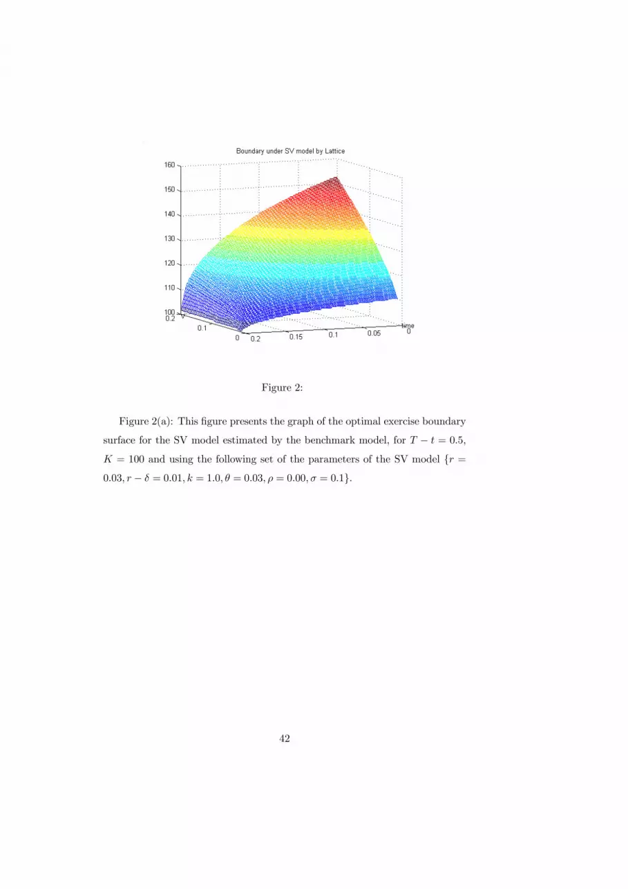
Figure 2:
Figure 2(a): This figure presents the graph of the optimal exercise boundary
surface for the SV model estimated by the benchmark model, for T − t = 0.5,K = 100 and using the following set of the parameters of the SV model {r =0.03, r − δ = 0.01, k = 1.0, θ = 0.03, ρ = 0.00,σ = 0.1}.
42

Figure 3:
Figure 2(b): This figure presents the graph of the optimal exercise boundary
surface for the SVmodel estimated by the CB-2 method, for T−t = 0.5,K = 100
and using the following set of the parameters of the SV model {r = 0.03, r−δ =0.01, k = 1.0, θ = 0.03, ρ = 0.00,σ = 0.1}, as in Figure 2(a).
43

Figure 4:
Figure 3: This figure presents a section of the optimal exercise boundary
surface of Figures 2(a)-2(b) estimated by the benchmark model (....) and the
CB-2 approximating method (...), respectively, at the level of volatility Vt =
0.16.
44

This working paper has been produced bythe Department of Economics atQueen Mary, University of London
Copyright © 2003 Elias Tzavalis and Shijun WangAll rights reserved.
Department of Economics Queen Mary, University of LondonMile End RoadLondon E1 4NSTel: +44 (0)20 7882 5096Fax: +44 (0)20 8983 3580Web: www.econ.qmul.ac.uk/papers/wp.htm