an inverse method for subcritical flows

JOURNAL OF COMPUTATIONAL PHYSICS 63, 31 l-328 (1986)

An Inverse Method for Subcritical Flows

PRABIR K. DARIPA*

Division qf Engineering, Brown University, Providence, Rhode Island 02912

AND

LAWRENCE SIROVICH

Division oJ Applied Mathematics, Brown Unwersity, Providence, Rhode Island 02912

Received December 13, 1984; revised March 29, 1985

The inverse problem in the tangent gas approximation is considered. An exact method for designing airfoils is presented. Constraints on the speed distribution are easily implemented. A simple numerical algorithm which is fast and accurate is presented. Comparison of designed airfoils using the tangent gas method with exact Euler results is found to be excellent for subcritical flows. 0 1986 Academic Press, Inc

1. INTRODUCTION

As is well known (see [ 11) certain types of pressure distributions achieve aerodynamically desirable features such as delay of transition and boundary layer control. The determination of an unknown airfoil from a specified pressure distribution is known as the inverse problem.

Numerous methods for the two dimensional incompressible case exist 12-51. Compressible inverse methods are for the most part based on some kind of iterative procedure, relying on either a Dirichlet or Neumann-type boundary condition. In the Dirichlet formulation [6-l l] a sequence of boundary value problems for the velocity potential, with wing geometry updated at each step, is solved. The updated condition arises from the normal velocity resulting at each unconverged step. For the Neumann formulation [ 12-151 a sequence of analysis problems are solved over a corresponding series of geometries. Each geometry is provided by some rational method depending on the error being driven to zero. A complete survey of such methods has been given by Slooff [ 163.

In this paper we present an exact method for two-dimensional subsonic flow within the limitations of the tangent gas approximation [17-197. Woods [20] extensively studied these equations and proposed certain iterative methods for solving both the analysis and inverse problems. We presented a substantially different

* Present address: Courant Institute of Mathematical Sciences, 251 Mercer street, New York, N.Y. 10012.

311 0021-9991/86 $3.00

Copyright 8 1986 by Academic Press, Inc. All rights of reproduclmn m any form reserved.

312 DARIPA AND SIROVICH

method for the analysis problem [21]. The inverse method developed here is non- iterative and exact.

As is shown in [21] the tangent gas solution lies very close to the Euler solution even for high subcritical flows. Therefore the design of an airfoil in this regime by our method should be an almost correct airfoil.

In this paper, we have been able to show that the direct Euler solution over the designed airfoil is very close to the input speed distribution. Moreover, the constraints necessitated by upstream condition and closure requirements are very easily incorporated.

2. BASIC EQUATIONS

Consider steady two-dimensional flow, then in the usual notation

v~(Pq)=o, vxq=o, p/p’= 1. (1)

The variables are normalized by their free stream values and linear dimensions by an appropriate length scale.

The stream function II/ and potential 4 are introduced in the usual way

pq=cVx ($k), s=Vh (2)

where k denotes a vector perpendicular to the plane of motion. The constant c has been introduced for later purposes.

If s and n are local distances along streamlines and potential lines, respectively, (2) can be written as

ds+idn=i(dcj+iid$).

Alternately, we can write

dz=dx+idy=$(dc$+iid$),

(3)

(4)

where x and y are Cartesian coordinates and 19 the flow angle. If q and 8 are taken as independent variables, then it is easy to derive from (4) that

(5)

If dependent and independent variables are interchanged and the Prandtl Meyer function

y= s :(I1 442,)“‘? (6)

EXACT METHOD FOR DESIGNING AIRFOILS 313

z plane

k+ I , I

A 1=0 lLp- - _ _---- .---- -- B

w plane

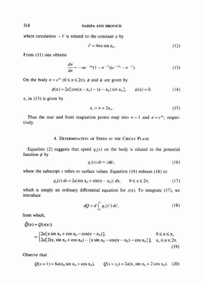
Fig. 1. Airfoil in physical z-plane and potential w-plane.

is introduced in place of q, then

iI- K(v)

v,=o, 8, + K(v) v4 = 0.

The f sign refers to subsonic and supersonic conditions, respectively, and

K(v)=bc, P(dM))

(7)

where

/I’= II -API. (9)

Typical physical z( =x + iy) and potential w( = 4 + i$) planes are shown in Fig. 1. The airfoil maps into a slit in the w plane. The gap BB’ in the potential plane corresponds to f, where circulation about the airfoil is -l-.

The system (7) is augmented by the density speed relation obtained from (1) and Bernoulli’s relation

2 1 4+- s

2 = constant. 2 YM2, P

3. MAPPINGS

The w-plane is mapped onto the exterior of the unit circle in the Q plane by

w= u(ceCiao + a-‘e’“) + i2a sin ~1~ ln(fr-‘aa), (11)


where circulation -r is related to the constant a by

r= 471a sin aO.

From (11) one obtains

(12)

dw

da= -lle -&(l ~o-I)(e-~z\~o--I), (13)

On the body r~ = e” (0 < CI < 27r), 4 and $ are given by

&a) = 2a[cos(or - a,) - (a - aO) sin a,], $(a) =O. (14)

a, in (13) is given by

r,y=7r+2ao. (15)

Thus the rear and front stagnation points map into (T = 1 and CJ = era,, respectively.

4. DETERMINATION OF SPEED IN THE CIRCLE PLANE

Equation (2) suggests that speed q,(s) on the body is related to the potential function 4 by

q,(s) ds = l4, (16)

where the subscript s refers to surface values. Equation (14) reduces (16) to

qS(s) ds = 2alsin a0 + sin(a - axo)i da, O<a627c, (17)

which is simply an ordinary differential equation for s(a). To integrate (17), we introduce

from which,

&Co = QMa))

dQ = d 1” q,Js’) ds’, 0

(18)

2a[a sin a0 + cos a, - cos(a - a,)], =

i

O<a<a, 2a[2(a, sin a0 + cos ao) - {a sin a0 - cos(a - ao) - cos a,}], a, < a < 27~.

(19)

Observe that

Q(s = 1) = &$a, sin a0 + cos a,,), Q(s = sf) = 2a(a,s sin a0 + 2 cos ao). (20)


r is related to Q(s= 1) and Q(s=s~) by

r=2Q(s=s,)-Q(s= 1)=47casina,. (21)

Here sI denotes the distance of the front stagnation point from the upperside of the trailing edge. Q(s = l), Q(s = sf), and hence f are known from the given surface speed distribution q,(s).

From (20) and (21)

Q(s=l) 2 ~ =; (a, + cot a()). r (22)

After (22) is solved for CI~ we obtain the constant a from (21). Next O(U) is computed from (19) and S(U) is obtained by inverting (18)

4~) = Q -‘(&4 (23)

and (1Jtl) = q,(s(a)) is obtained from (17). Thus far our deliberations are exact. Ideally system (7) should now be solved to

determine the body shape. For the tangent gas approximation considered next the problem can be solved by an exact method similar to the one in the incompressible case [4].

5. TANGENT GAS APPROXIMATION

The tangent gas approximation is given by (see [2 11)

(p-1)-y 1-i. ( 1

From (10) we obtain

& Pa’

(24)

(25)

where the subscript a denotes a suitable reference point. With the constant c in (8) taken as

c = l/B,> (26)

we obtain from (8)

K(v) = 1. (27)

Then for subsonic flow the system (7) becomes the Cauchy-Riemann equations

8, - v* = 0, 8, + v, = 0. (28)


Equations (28) are exact for both the tangent gas and also for incompressible flow (M=O). Henceforth, we take the tangency point (p,, l/p,) to be the free stream,

p,=pm= 1, pa=pm= 1. (29)

With this selection the following relations hold [21]

q = sinh v* cosech(v* - v), p = tanh(v* - v), 2

” = 1 - /?,coth v’ (30)

where the constant v* is given by

v*=ln M

( ) 00. l-P,

(31)

From (6) it is seen that v co = 0 and at a stagnation point (denoted by zero subscript )

2 vg= -co, CP.0 = 1+p,’ (32)

It follows from (28) that

z= -v+iCJ (33)

is an analytic function of w and hence of U. A convenient representation of r(a) is given by (see also [S]),

exp(r(o)) = (1 - c -I)~b(e~ia,-O-l)-I exp (Jo cd-(), (34)

where 6 = I~!/z, 8, the trailing edge angle. The complex constants c, are denoted by

c,=An+iB,. (35)

Note that (34) contains the Kutta condition. Two Schwarz-Christoffel factors appear in (33) because of the discontinuity in 8 at the two stagnation points. On the unit circle, (33) reduces to

exp(z(e’“)) = G(g) erqca) exp (:. cHepin’),

where

G(a) = 2 sin : I I l--6

12(sin a, + sin(a - fxo))l -l,

(36)

(37)

+)=f(l-@(n-l)+ c(+; -nU(a-a,)+a,. ( >

(38)


U(a-a,) in (38) is the unit step function. The tangent angle 8, at the body is

and

where

and

related to 8 by

e(a) = 8,(a) - 71- nU(a - a,).

Separation of (36) into real and imaginary parts leads to

F(a)= f (A,cosna+B,sinna) It=0

co B(a)= C (B,cosna-A,sinna)+n+a,

?I=0

J(a) = -v(a) - in G(a)

B(a)=H,(a)-:(I-h)(nl)(a+;).

Notice from (34) the upstream flow direction 8, is related to B, by

8,=Bo+7c+2ao,

where B. is given by

Bo=+J2xB(a)da-n-ao. 0

The free stream condition (q, = 1) is given by

A,=O. (46)

(39)

(40)

(41)

(42)

(43)

(44)

(45)

The condition for closure of the airfoil is related to the leading terms of the series (40) and (41) by (see [21])

A,=(l-6)-(l-&,)2sin2ao, (47)

B,=(l-p,)sin2a,. (48)

6. BEHAVIOUR AT STAGNATION POINTS

It is both interesting and useful to study the behavior of speed at the stagnation points. From (30) and (42) we obtain

2p, e-‘s q”N1+T-

for q,-0. (49)

318

From (37)

DARIPA AND SIROVICH

1 t-y2 cos ao) for cc-0 -N G(a) Ia,< - a[(2 cos a# for IX-X,.

From (49) and (50)

K, LX’ for a-0 &-

&la,--C(l for sc-a,,

where

K1 = ‘Pm - t? - jsca = O’( 2 cos ao), 2Pm

1+B, K2=1+/?m - ,-cc==aq2 cos ao)6.

If a, and CL* are close to LY -0, then from (51) we obtain

,Jn(B&2)/~*hH ln(a2bl 1

From (51) (52) and (53) we obtain

;,(a = 0)~ -In ( y~(2cosao)y)

co

and

?,,(a = a,) - -In (

1 + Pm (2 cos ao)-6 ) 4s(af) Ia/ - % 28, >

(50)

(51)

(52)

(53)

(54)

(55)

where ttf is close to c(, and c1i is close to zero.

7. METHOD OF SOLUTION

The speed distribution q3(s) is usually given at a finite number of points sj, .j= 0, 1, 2,..., in the interval 0 <S < 1. From this the integral in Eq. (18) can be evaluated to obtain Q(s,) as a function of qs(si). Next the circulation f is computed from the relation

l-=2Q(s=s,)- Q(s= 1).

Equation (22) is then solved to obtain a,. The second equation of (20) is next used to calculate the value of the constant a. In general ~1~ and a so obtained do not satisfy the first equation of (20) exactly because a, is calculated numerically. If

Q(S = 1) - Q(s = sf) = !-’ q6 ds si


differs slightly from Q(s = sf) - 47~2 sin ~1~ (see Eq. (21)), the speed q,(s) is modified by a constant factor over the interval sr< s < 1 to adjust the above integral to this value.

The values of D(cx~) at N (a power of 2) equally spaced points on the unit circle, u, = 2rcj/N, j= 0, l,..., N, are calculated using Eq. (19). The value of speed qS(aj) at the grid points 01~ are now easily obtained by interpolation since q,Jsj) is already known as a function of Q(s,).

The approximate value of the trailing edge angle 6 is obtained from Eq. (53). S,(a) is then obtained from Eqs. (42), (37), and (30) and its value at a stagnation point is calculated from (54) and (55). If C,(a) satisfies the constraints (46) (47), and (48) then the conjugate function &a) is calculated from (41) using the fast fourier transform. In case C,(a) does not satisfy the constraints, the prescribed speed distribution must be modified. This is discussed in the next section.

The value of the constant B, in (41) which is also needed to calculate P(U) is obtained from (44) by setting the free stream direction 0, to zero. The tangent angle 8, at the body is now obtained from &cc) using the relation (43). The body coordinates are then calculated from

cos O,(a) da,

y(a) = 6 2 sin 8,(a) da,

where ds/da is given by

lsin CI~ + sin(a - a,)[

qs(cO ’ (57)

The value of (57) at a stagnation point (a = 0, a = a,) is given by (see Eq. (51))

cosao ,-6 ds

2a-cc K,

da cos a0 2a-

K2

for a=0

for c( = ~1,~. (58)

Instead of calculating 6 from Eq. (53) as was done above, one can prescribe 6 because the constraints (46), (47), and (48) depend on 6. Modification of the speed distribution subject to these constraints will automatically satisfy the Eq. (53) because this equation is valid if the speed distribution is consistent with those constraints. In either case if v”,(a) obtained from a given speed distribution does not satisfy the constraints then the prescribed speed distribution must be modified according to the method discussed in the next section.

Even though the above method is exact theoretically, there are numerical sources of error. These errors depend on the kind of interpolation and integration scheme,


the number of data points, the number of grid points, the evaluation of a, from (22) and the use of the approximate expressions (53), (54), and (55) to calculate trailing edge angle 6, ?,(a = 0), and F,(c( = c1,), respectively.

In view of the simplicity of the procedure no attempt was made to incorporate highly accurate computations. Simpson’s rule with evenly spaced grid points and trapezoidal rule with unevenly spaced data points were used for integration. The interpolation scheme used was linear. The speed q,(s) was prescribed at 129 unevenly spaced data points on 0 <s 6 1 and the number of grid points on the unit circle was taken to be 128. a, was obtained within an accuracy of 10e6 by solving Eq. (22) by regular falsi method and the trailing edge angle 6 used was calculated by using the approximate relation (55).

The program was run on an IBM 3081 in single precision and the computation time was about a half second in most cases.

8. MODIFICATION OF SPEED DISTRIBUTION

Constraints (46), (47), and (48) must be satisfied by the prescribed speed distribution to find a closed body solution. Therefore in general any arbitrary speed distribution must be modified subject to these constraints. These constraints can be written in terms of surface values f,(a) given by

1 i

2n -

710 C,s(a) gj(a) dci = P,, j= 1,2, 3,

where gj(m) and Pi are given by (see (46), (47), and (48))

j=l

j=2

j=3

(60)

and

0, j=l

(l-s)-(l-b,)2sin2a,, j=2 (61)

(1-Bco)sin2a,, j= 3.

Linearity of (28) implies the following form of modification of prescribed values f,(a) (see C41)


where yk, k= 1, 2, 3, are constants to be determined and &(a), k = 1,2, 3, are suitable correction terms. The correction terms can be set to zero outside a specified interval (a,, ~1~) leaving speed distribution same as the prescribed one outside this interval. This is extremely useful when designing an airfoil where in general no modification of speed distribution over the suction side is desired. The speed distribution can be modified in various ways depending on the choice of functions &(a), k = 1, 2, 3, and the correction interval (aI7 a2).

Substituting (62) in (59) one obtains

3

1 Ykalk = b.,, j= 1, 2, 3, k=l

where

(63)

(64)

bj=nPj- [Ix V”,,(a) g,(a) da = xPj- j” P,(a) gj(a) da. (65) z,

Constants yk, k = 1, 2, 3, are obtained by inverting (63) and the corrected v”,(a) is then obtained from (62). The corrected speed distribution is then obtained from (42) and (30) and the body is found from (55).

The matrix ajk in (65) must be positive definite to be able to invert (63) which restricts the choice offk(a), aI, and al. These should be carefully selected so that the correction to a prescribed speed distribution is minimum. This can be done in the same spirit as in Strand [22] and Arlinger [4].

For our purpose we choose cc, = 0, a, = 27c and fk(tl) = gk(@), k = 1, 2, 3. This modifies the speed distribution over the whole interval. In this case (63) gives

b, Yl =Tj--$ y2=bz

7-c’ and Y3,3

?r

and hence (62) becomes

C,(a) = C,(a) + & (b, + 2b2 cos a + 2b, sin a).

9. RESULTS

(66)

(67)

A basic test of the inverse method is the recovery of a known airfoil from its pressure distribution. Figures 2 and 3 provide a verification of the method within the tangent gas approximation. Here a pressure distribution is computed in tangent gas approximation over a NACA 4412 airfoil (see [21]). Speed distribution is com-


+-UPPER SIDE -LOWER SIDE - - INPUT PRESSURE DlSTRlBUTlON

T+++ PRESSURE D,STRIB”T,ON ON DESlGNED AIRFOIL

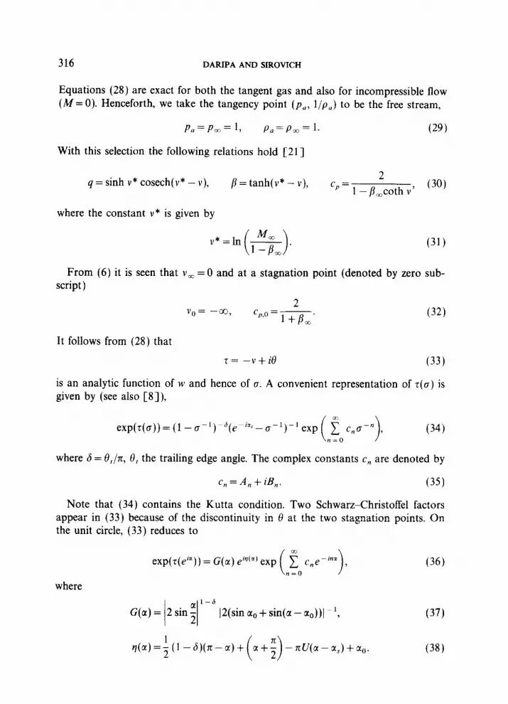
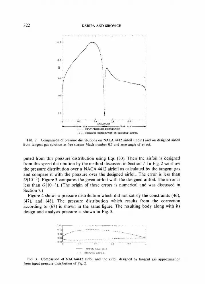
FIG. 2. Comparison of pressure distributions on NACA 4412 airfoil (input) and on designed airfoil from tangent gas solution at free stream Mach number 0.7 and zero angle of attack.

puted from this pressure distribution using Eqs. (30). Then the airfoil is designed from this speed distribution by the method discussed in Section 7. In Fig. 2 we show the pressure distribution over a NACA 4412 airfoil as calculated by the tangent gas and compare it with the pressure over the designed airfoil. The error is less than 0( 10P3). Figure 3 compares the given airfoil with the designed airfoil. The error is less than 0( lo-“). (The origin of these errors is numerical and was discussed in Section 7.)

Figure 4 shows a pressure distribution which did not satisfy the constraints (46) (47), and (48). The pressure distribution which results from the correction according to (67) is shown in the same figure. The resulting body along with its design and analysis pressure is shown in Fig. 5.

__ AIRFOIL NACA 4112

+ + “ESILNED AlRFOlL

FIG. 3. Comparison of NACA4412 airfoil and the airfoil designed by tangent gas approximation from input pressure distribution of Fig. 2.


0

++*+* t - lNP”T +***

/

-*\ +* +++ CORRECTED CP

*+ ++ +* \

*+ ++ *+**1, + *t * * +!

L 0.2

+-UPPER SIDE-LOWER SlDE F

FIG. 4. Target and corrected pressure distribution.

MACH -0 50 a=0 0 c,=i 06397 c,=o 00078

FIG. 5. Designed airfoil from input pressure distribution of Fig. 4 and pressure distribution on designed airfoil from design and direct analysis by tangent gas method.


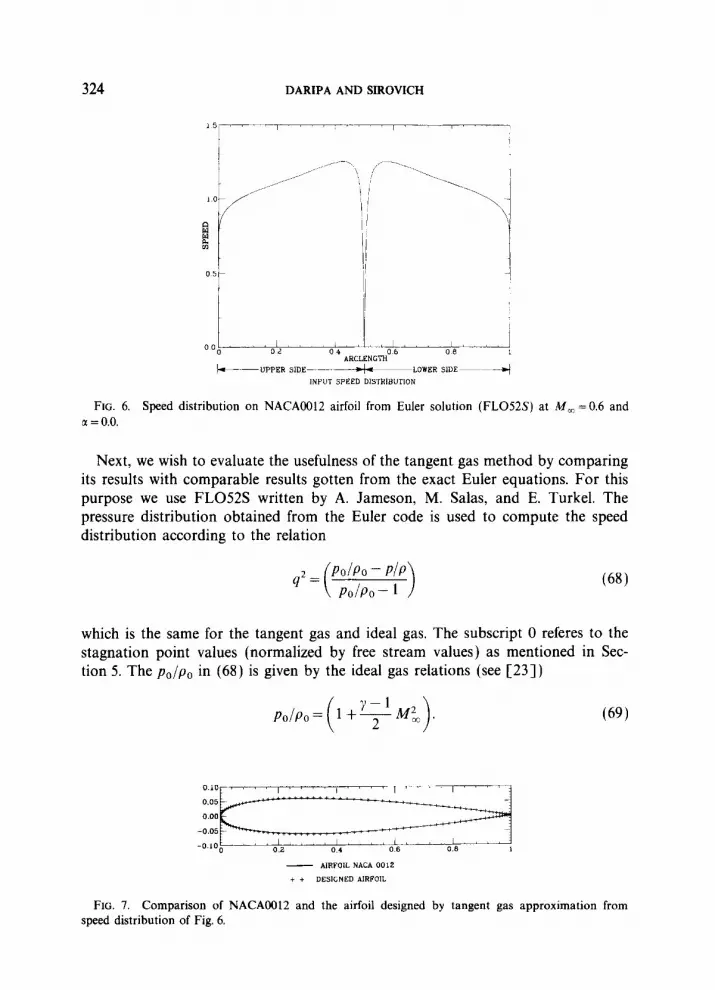
FIG. 6. Speed distribution on NACAO012 airfoil from Euler solution (FL052S) at M, =0.6 and a = 0.0.

Next, we wish to evaluate the usefulness of the tangent gas method by comparing its results with comparable results gotten from the exact Euler equations. For this purpose we use FL052S written by A. Jameson, M. Salas, and E. Turkel. The pressure distribution obtained from the Euler code is used to compute the speed distribution according to the relation

(68)

which is the same for the tangent gas and ideal gas. The subscript 0 referes to the stagnation point values (normalized by free stream values) as mentioned in Sec- tion 5. The po/pO in (68) is given by the ideal gas relations (see [23])

PO/PO= ( y - 1 1+-e

> (69)

;iij;

0 0.2 0.1 06 1

- AlRFOlL NA‘A 0012

++ DESIGNED AlRFOlL

FIG. 7. Comparison of NACAO012 and the airfoil designed by tangent gas approximation from speed distribution of Fig. 6.


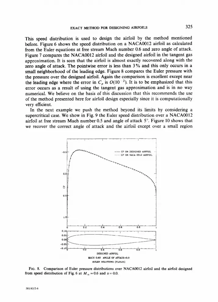
This speed distribution is used to design the airfoil by the method mentioned before. Figure 6 shows the speed distribution on a NACAO012 airfoil as calculated from the Euler equations at free stream Mach number 0.6 and zero angle of attack. Figure 7 compares the NACAO012 airfoil and the designed airfoil in the tangent gas approximation. It is seen that the airfoil is almost exactly recovered along with the zero angle of attack. The pointwise error is less than 3 % and this only occurs in a small neighborhood of the leading edge. Figure 8 compares the Euler pressure with the pressure over the designed airfoil. Again the comparison is excellent except near the leading edge where the error in C, is 0( 10 ~ *). It is to be emphasized that this error occurs as a result of using the tangent gas approximation and is in no way numerical. We believe on the basis of this discussion that this recommends the use of the method presented here for airfoil design especially since it is computationally very efficient.

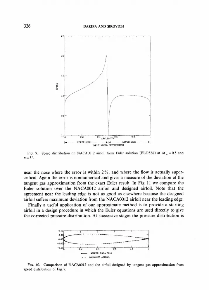
In the next example we push the method beyond its limits by considering a supercritical case. We show in Fig. 9 the Euler speed distribution over a NACAO012 airfoil at free stream Mach number 0.5 and angle of attack 5”. Figure 10 shows that we recover the correct angle of attack and the airfoil except over a small region

I I”“” “’

FIG. 8. Comparison of Euler pressure distributions over NACAO012 airfoil and the airfoil designed from speed distribution of Fig. 6 at M, = 0.6 and a = 0.0.

581/63/2-6


FIG. 9. Speed distribution on NACAW12 airfoil from Euler solution (FL052S) at M, =OS and r=S”.

near the nose where the error is within 2%, and where the flow is actually supercritical. Again the error is nonnumerical and gives a measure of the deviation of the tangent gas approximation from the exact Euler result. In Fig. 11 we compare the Euler solution over the NACAO012 airfoil and designed airfoil. Note that the agreement near the leading edge is not as good as elsewhere because the designed airfoil suffers maximum deviation from the NACAO012 airfoil near the leading edge.

Finally a useful application of our approximate method is to provide a starting airfoil in a design procedure in which the Euler equations are used directly to give the corrected pressure distribution. At successive stages the pressure distribution is

-o.K$-- ’ ’ 02 0.4 06 08 1

- AIRFOL NACA 0012

++ DESlGNED NRFOL

FIG. 10. Comparison of NACAO012 and the airfoil designed by tangent gas approximation from speed distribution of Fig. 9.


-s.,,,,,,,.,..,,,.,,., ,, ++

Om,,,,,,‘,,,. “I’ I’ “1

FIG. 11. Comparison of Euler pressure distributions over NACAO012 airfoil and the airfoil designed from speed distribution of Fig. 9 at M, = 0.5 and a = 5”.

modified to meet the design criteria and the inverse method reapplied and so forth. The interactive iteration should go quite quickly for subcritical flows. However, the value of such a procedure remains uncertain for supercritical flows.

ACKNOWLEDGMENTS

This research was supported by the National Aeronautics and Space Administration under Grant NSG-1617 and the Air Force Office of Scientific Research under Grant AFOSR-83-0336. The authors would also like to thank the reviewers for helpful criticism.

REFERENCES

1. B. S. STRATFORD, J. Fluid Mech. 5 (1959), 1. 2. S. GOLDSTEIN, “A Theory of Aerofoils of Small Thickness. Part III. Approximate Designs of Sym-

metrical Aerofoils for Specified Pressure Distributions,” Aeronautical Research Committee, London, Report, No. ARC6225, October 1942.


3. M. J. LIGHTHILL, “A New Method of Two-Dimensional Design,” Aeronautical Research Committee, London, R & M 2112, 1945.

4. B. ARLINGER, “An Exact Method of Two-Dimensional Airfoil Design,” SAAB, TN67, 1970. 5. F. T. JOHNSON, “A General Panel Method for the Analysis and Design of Arbitrary Configurations

in Incompressible Flows,” NASA CR 3079, May 1980. 6. G. VOLPE, “The Inverse Design of Closed Airfoils in Transonic Flow,” AIAA Paper, No. 83-0504,

1983. 7. T. L. TRANEN, “A Rapid Computer Aided Transonic Airfoil Design Method,” AIAA Paper,

No. 74-501, 1974. 8. F. BAUER, P. GARABEDIAN, AND D. KORN. “Supercritical Wing Sections 11,” Springer-Verlag, Berlin,

1975. 9. B. ARLINGER AND W. SCHMIDT, “Design and Analysis of Slat Systems in Transonic Flow,” ICAS

Paper, 1978. 10. L. A. CARLSON, J. Aircraft 13 (1976), 356. 11. P. A. HENNE, “An Inverse Transonic Wing Design Method,” AIAA Paper, No. 80-0330, 1980. 12. J. M. J. FRAY AND J. W. SLQOF, “A Constrained Inverse Method for the Aerodynamic Design of

Thick Wings with Given Pressure Distribution in Subsonic Flow,” AGARD CP., No. 285, Paper 16, 1980.

13. W. H. DAVIS, JR., “Technique for Developing Design Tools from the Analysis Methods of Com- putational Aerodynamics,” AIAA Paper, No. 79-1529, 1979.

14. G. B. MCFADDEN, “An Artiticaial viscosity method for the design of Supercritical Airfoils,” Ph.D. thesis, New York Univ., New York, 1979.

15. P. GARABEDIAN AND G. MCFADDEN, in “Proceedings of Symposium on Transonic, Shock and Multi- dimensional Flows,” pp. l-16, University of Wisconsin, Madison, 1981; Academic Press, New York, 1982.

16. J. W. SLOOF, in “Proceedings on ICIDES,” pp. I-68, Univ. of Texas, Austin, 1984. 17. VON KARMAN, J. Aeronaut. Sci. 8 (1941), 337. 18. H. S. TSIEN, J. Aeronaut. Sci. 6 (1939), 399. 19. S. A. CHAPLYGIN, “On Gas Jets,” NASA Technical Memorandum, No. 1063, 1944. 20. L. C., WOODS, “The Theory of Subsonic Plane Flow,” Cambridge Univ. Press, London, 1961. 21. P. K. DARIPA AND L. SIROVICH, J. Cornput. Phys., in press. 22. T. STRAND, J. Aircraf IO (1973), 651. 23. H. W. LIEPMANN AND A. ROSHKO, “Elements of Gas Dynamics,” Wiley, New York, 1957.

an inverse method for subcritical flows

Documents