Computers & Industrial Engineering 83 (2015) 226–236

Contents lists available at ScienceDirect

Computers & Industrial Engineering

journal homepage: www.elsevier .com/ locate/caie

An integrated three-stage maintenance scheduling model for unrelatedparallel machines with aging effect and multi-maintenance activities q

http://dx.doi.org/10.1016/j.cie.2015.02.0120360-8352/� 2015 Elsevier Ltd. All rights reserved.

q This manuscript was processed by Area Editor T.C. Edwin Cheng.⇑ Corresponding author at: Business Systems and Analytics Department, Lindback

Distinguished Chair of Information Systems and Decision Sciences, La SalleUniversity, Philadelphia, PA 19141, United States. Tel.: +1 215 951 1129; fax: +1267 295 2854.

E-mail addresses: tavana@lasalle.edu (M. Tavana), yacerzarok@yahoo.com(Y. Zarook), fransant@ucm.es (F.J. Santos-Arteaga).

URL: http://tavana.us/ (M. Tavana).

Madjid Tavana a,b,⇑, Yaser Zarook c, Francisco J. Santos-Arteaga d

a Business Systems and Analytics Department, Lindback Distinguished Chair of Information Systems and Decision Sciences, La Salle University, Philadelphia, PA 19141, United Statesb Business Information Systems Department, Faculty of Business Administration and Economics, University of Paderborn, D-33098 Paderborn, Germanyc Department of Industrial Engineering, Mazandaran University of Science and Technology, Babol, Irand Departamento de Economía Aplicada II, Facultad de Económicas, Universidad Complutense de Madrid, Campus de Somosaguas, 28223 Pozuelo, Spain

a r t i c l e i n f o a b s t r a c t

Article history:Received 19 April 2014Received in revised form 7 January 2015Accepted 11 February 2015Available online 2 March 2015

Keywords:Maintenance schedulingUnrelated parallel machinesFuzzy setsAHPTOPSISGoal programming

We propose an integrated three-stage model for maintenance scheduling of unrelated parallel machines(UPMs) with aging effect and multi-maintenance activities (AEMMAs) using a variety of MODM tech-niques such as the fuzzy analytic hierarchy process (AHP), the technique for order of preference by simi-larity to ideal solution (TOPSIS), and goal programming (GP). We use fuzzy AHP in the first stage of theproposed model to account for the inherent ambiguity and vagueness in real-life maintenance schedulingproblems. In the second stage, we use TOPSIS to reduce the multi-objective problem into an efficient bi-objective problem. Finally, we use GP to solve the resulting bi-objective problem and develop an optimalmaintenance schedule in the third stage of the model. We use a numerical example to demonstrate theapplicability of the proposed approach and exhibit the efficacy of the procedures and algorithms.

� 2015 Elsevier Ltd. All rights reserved.

1. Introduction

Manufacturing firms are constantly under pressure to reducetheir production costs. Maintenance costs, one of the maincomponents of production costs, substantially add to this stressin the manufacturing environment (Bevilacqua & Braglia, 2000).Although manufacturing firms constantly seek to engage all levelsand functions in an organization to maximize the overall effective-ness of production equipment, maintenance costs are unavoidableand play an important role in maintaining a machine’s reliabilityand product quality. Although manufacturers have made greatstrides in controlling maintenance cost, maintenance remains animportant topic for further study in production economics andresearch.

In deterministic scheduling problems, the job processing time isassumed constant and independent of its position or starting timein the scheduling process. However, there are many situations in

which the actual processing times of the jobs may vary due tolearning, aging or deterioration effects (readers should refer toBiskup (2008), Janiak & Rudek (2006) and Janiak & Rudek (2009)for the state of the current research). The motivation for this studystems from the metal or wood cutting process that cuts products tovarious sizes and shapes them in a parallel-machine setting. Due towearing of the cutting tool, the actual processing time of the pro-duct increases with respect to the number of products already pro-cessed on the machine. The time required for processing a productdepends on the quality of the cutting tool. Therefore, under normalcircumstances, the cutting tool is replaced with a new one or ismaintained after it has processed some products to improve itsproduction efficiency.

Maintenance activities in the literature have been classified intotwo main categories: corrective and preventive (Li, Khoo, & Tor,2006; Waeyenbergh & Pintelon, 2004). The corrective maintenanceis the maintenance that occurs after systems failure (Swanson,2001) while the preventive maintenance is the maintenance thatis performed before systems failure in order to retain equipmentin specified condition by providing systematic inspections, detec-tion, and prevention of incipient failure (Moghaddam, 2013;Wang, 2002). The model proposed in this study falls in the preven-tive maintenance category.

One of the first steps of maintenance activities is to select thebest repairmen from a pool of available repairmen. In this paper,

0

An Integrated Three-Stage Maintenance Scheduling Model for Unrelated Parallel

Machines with Aging Effect and Multi-Maintenance Activities

Madjid Tavanaa,b,* aBusiness Systems and Analytics Department

Lindback Distinguished Chair of Information Systems and Decision Sciences

La Salle University, Philadelphia, PA 19141, USA

E-mail: tavana@lasalle.edu

Web: http://tavana.us/

bBusiness Information Systems Department

Faculty of Business Administration and Economics

University of Paderborn, D-33098 Paderborn, Germany

Yaser Zarookc cDepartment of Industrial Engineering

Mazandaran University of Science and Technology, Babol, Iran

E-mail: yacerzarok@yahoo.com

Francisco J. Santos-Arteagad

dDepartamento de Economía Aplicada II

Facultad de Económicas

Universidad Complutense de Madrid

Campus de Somosaguas, 28223 Pozuelo, SPAIN

E-mail: fransant@ucm.es

____________________________

*Corresponding author at: Business Systems and Analytics Department, Lindback Distinguished Chair of

Information Systems and Decision Sciences, La Salle University, Philadelphia, PA 19141, United States. Tel.: +1 215 951 1129; fax: +1 267 295 2854.

1

An Integrated Three-Stage Maintenance Scheduling Model for Unrelated Parallel

Machines with Aging Effect and Multi-Maintenance Activities

Abstract

We propose an integrated three-stage model for maintenance scheduling of unrelated parallel

machines (UPMs) with aging effect and multi-maintenance activities (AEMMAs) using a variety

of MODM techniques such as the fuzzy analytic hierarchy process (AHP), the technique for order

of preference by similarity to ideal solution (TOPSIS), and goal programming (GP). We use fuzzy

AHP in the first stage of the proposed model to account for the inherent ambiguity and vagueness

in real-life maintenance scheduling problems. In the second stage, we use TOPSIS to reduce the

multi-objective problem into an efficient bi-objective problem. Finally, we use GP to solve the

resulting bi-objective problem and develop an optimal maintenance schedule in the third stage of

the model. We use a numerical example to demonstrate the applicability of the proposed approach

and exhibit the efficacy of the procedures and algorithms.

Keywords: Maintenance scheduling; Unrelated parallel machines; Fuzzy sets; AHP; TOPSIS;

Goal programming.

2

1. Introduction

Manufacturing firms are constantly under pressure to reduce their production costs. Maintenance

costs, one of the main components of production costs, substantially add to this stress in the

manufacturing environment (Bevilacqua and Braglia, 2000). Although manufacturing firms

constantly seek to engage all levels and functions in an organization to maximize the overall

effectiveness of production equipment, maintenance costs are unavoidable and play an important

role in maintaining a machine’s reliability and product quality. Although manufacturers have made

great strides in controlling maintenance cost, maintenance remains an important topic for further

study in production economics and research.

In deterministic scheduling problems, the job processing time is assumed constant and

independent of its position or starting time in the scheduling process. However, there are many

situations in which the actual processing times of the jobs may vary due to learning, aging or

deterioration effects (readers should refer to Biskup (2008), Janiak and Rudek (2006) and Janiak

and Rudek (2009) for the state of the current research). The motivation for this study stems from

the metal or wood cutting process that cuts products to various sizes and shapes them in a parallel-

machine setting. Due to wearing of the cutting tool, the actual processing time of the product

increases with respect to the number of products already processed on the machine. The time

required for processing a product depends on the quality of the cutting tool. Therefore, under

normal circumstances, the cutting tool is replaced with a new one or is maintained after it has

processed some products to improve its production efficiency.

Maintenance activities in the literature have been classified into two main categories:

corrective and preventive (Li et al., 2006; Waeyenbergh and Pintelon, 2004). The corrective

maintenance is the maintenance that occurs after systems failure (Swanson, 2001) while the

preventive maintenance is the maintenance that is performed before systems failure in order to

retain equipment in specified condition by providing systematic inspections, detection, and

prevention of incipient failure (Wang, 2002; Moghaddam, 2013). The model proposed in this

study falls in the preventive maintenance category.

One of the first steps of maintenance activities is to select the best repairmen from a pool

of available repairmen. In this paper, the analytic hierarchy process (AHP) is used to select the

most suitable repairmen based on a set of pre-specified evaluation criteria (Saaty, 1980). AHP can

consider both quantitative and qualitative evaluation criteria. Most qualitative evaluation criteria

3

in real-life are often accompanied by ambiguities and vagueness. Therefore, we consider fuzzy

logic and fuzzy sets to represent ambiguous and vague information in the evaluation process. The

integration of AHP and fuzzy set theory (Bellman and Zadeh, 1970) has resulted in the fuzzy AHP

method.

Parallel machine scheduling (PMS) is concerned with the allocation of a set of jobs to a

number of parallel machines. The studies on PMS in the literature have been generally categorized

into three groups: identical, uniform and unrelated PMS problem (Cheng and Sin, 1990). Among

these groups, unrelated PMS (UPMS) represents a generalization of the other two groups where

different machines perform the same job but have different processing capacities or capabilities.

However, solving real-life UPMS problems is a difficult task because they are mostly NP-hard

(Torabi et al., 2013). This paper focuses on the UPMS problems, which have been addressed much

less than the identical and uniform PMS problems in the literature (see Arnaout et al., 2010; Chang

and Chan, 2011).

In spite of huge advances in PMS research, multi-objective scheduling problems with

simultaneous consideration of repairmen selection, aging effects and maintenance activities under

unrelated parallel machine environment have not been thoroughly studied in the literature. Kuo

and Yang (2008) studied single-machine scheduling problems with a cyclic process of aging

effects and multi-maintenance activities. They investigated the problem with job-independent and

position-dependent aging effects to minimize the makespan. Zhao and Tang (2010) extended the

study of Kuo and Yang (2008) to the case with a job-dependent aging effect. Yang and Yang

(2010a) studied single-machine scheduling with simultaneous consideration of job-dependent

aging effects, multi-maintenance activities, and variable maintenance durations to minimize the

makespan. Yang and Yang (2010b) further considered single machine scheduling with aging or

deteriorating effects and deteriorating maintenance activities simultaneously to minimize the total

completion time. Yang at el. (2012) studied UPMS problems considering aging effect and multi-

maintenance activities (AEMMAs) to minimize total machine load. These studies have primarily

formulated the problem with a single objective model. Very little work has focused on multi-

objective scheduling problems (MOSPs).

Multi-objective decision making (MODM) techniques have attracted a great deal of

interest due to their adaptability to real-life decision making problems. MODM problems often

involve multiple conflicting objectives (Zhang et al., 2012; Majazi Dalfard and Mohammadi,

4

2012) and decision makers (DMs) are required to search for a trade-off between the objectives.

Generally, the MODM problem can be formulated as follows:

MODM: {𝑀𝑖𝑛 or𝑀𝑎𝑥: {𝑓1(𝑥), 𝑓2(𝑥),… , 𝑓𝑘(𝑥)}

𝑠. 𝑡: 𝑋 ∈ 𝑆 = {𝑋 ∈ 𝑅𝑛| 𝑔(𝑥) ≤ 𝑏, 𝑋 ≥ 0}

In this study we consider the following conflicting objectives: minimizing the makespan,

minimizing the total maintenance cost, minimizing the maximum tardiness time of the jobs and

minimizing the maximum earliness time of the jobs. In the proposed approach, a MODM problem

is reduced to a bi-objective problem by using the technique for order preference by similarity to

ideal solution (TOPSIS) (Khalili-Damghani et al., 2013). Next, the resulting bi-objective problem

is solved with goal programming (GP) to find solutions that simultaneously have a minimum

distance from the positive ideal solution (PIS) and a maximum distance from the negative ideal

solution (NIS).

The rest of the paper is organized as follows: In Section 2 we introduce an integrated three-

stage maintenance scheduling model for UPMs with AEMMAs. In Section 3, the problem is

formulated as a multi-objective integer linear programming (MOILP) model. In Section 4 we use

a numerical example to demonstrate the applicability of the proposed approach and exhibit the

efficacy of the procedures and algorithms. Finally, conclusions and future directions are given in

Section 5.

2. Proposed model

In this section we describe our three-stage approach for the repairmen selection and maintenance

scheduling problem. Note that, before the first phase can be initiated, it is sometimes necessary for

the DM to do an initial screening on the list of its potential repairmen. Once a suitable list of

repairmen is constructed, the repairmen are evaluated and scored using a fuzzy multi-criteria

decision making method in the first stage. In the second stage of the proposed approach, a multi-

objective scheduling problem is reduced to a bi-objective problem with the TOPSIS method

(Khalili-Damghani et al., 2013). Finally, in the third stage, the resulting bi-objective problem is

modelled with goal programming to jointly determine the optimal maintenance frequencies and

positions of the repairmen’s maintenance activities and the optimal job sequences on the machines

with respect to some supplementary constraints imposed on the mathematical model. The general

framework for our proposed approach is illustrated in Fig. 1. In the following subsections, the three

stages of the proposed model are discussed in more detail.

5

Insert Figure 1 Here

2.1. Stage 1: Evaluation of the alternative repairmen

Multi criteria decision making deals with the problem of choosing the best alternative, that is, the

one providing the highest degree of satisfaction with respect to all the relevant criteria or goals. In

order to obtain the best alternative a ranking process is required. AHP is one of the most popular

and powerful multi-criteria decision making methods for decision making and has been used for

years in service quality assessment. However, the AHP method, first developed by (Saaty, 1980),

was inadequate and defective in handling the ambiguity of the concepts that are associated with a

human being’s subjective judgment. Therefore, the fuzzy AHP method, which combines

traditional AHP with fuzzy set theory (Bellman and Zadeh, 1970), was developed for coping with

uncertain judgments (Naghadehi et al., 2009; Chen & Hung, 2010; Chiou et al., 2005) and to

express preferences as fuzzy sets or fuzzy numbers which reflect the vagueness of human thinking

(Liou et al., 2011; Cakir and Canbolat, 2008). In this study, triangular fuzzy numbers (TFNs) are

used to represent the fuzzy relative importance of each alternative and criterion. The triangular

fuzzy conversion scale used to convert such linguistic terms into fuzzy numbers in the evaluation

model is given in Table 1. A TFN 𝑁~ can be denoted by the triplet (a,b,c) with membership

function 𝜇𝑁~(𝑋), which is described as follows: the parameter “b” is the most likely value and the

parameters “a” and “c” are the lower and upper bounds that limit the field of possible evaluation,

as depicted in Equation 1.

𝜇𝑁~(𝑥) =

{

𝑥 − 𝑎

𝑏 − 𝑎, 𝑎 ≤ 𝑥 ≤ 𝑏

𝑐 − 𝑥

𝑐 − 𝑏, 𝑏 ≤ 𝑥 ≤ 𝑐

0, 𝑜𝑡ℎ𝑒𝑟𝑤𝑖𝑠𝑒

(1)

The fuzzy arithmetic operations on two TFNs M1 and M2 derived by Dubois and Prade

(1979) are as follows: if M1 = (a1,b1,c1) and M2 = (a2,b2,c2) then

M1 ⊕ M2 = (a1,b1,c1) ⊕ (a2,b2,c2) = (a1+a2,b1+b2,c1+c2) (2)

M1 ⨂ M2 = (a1,b1,c1) ⨂ (a2,b2,c2) ≅ (a1a2,b1b2,c1c2) (3)

(𝑀1)−1= (a1, b1 , c1)−1 ≅ (1/c1,1/b1,1/a1) (4)

The main steps of the fuzzy AHP are as follows:

(1) Structuring the decision hierarchy: Similar to conventional AHP, the first step is to break

down the complex decision making problem into a hierarchical structure.

6

(2) Constructing the fuzzy pairwise comparison matrices: Buckley (1985) considered a fuzzy

pairwise comparison matrix with n elements where pairwise comparison judgments are

represented by TFN 𝑎𝑖𝑗~ = (𝑙𝑖𝑗 , 𝑚𝑖𝑗, 𝑢𝑖𝑗). In conventional AHP each set of comparisons for a level

with n elements requires 𝑛(𝑛 − 1)/2 judgments such as:

𝐴~ = [𝑎𝑖𝑗~ ] = [

𝑎11~ ⋯ 𝑎1𝑛

~

⋮ ⋱ ⋮𝑎𝑛1~ ⋯ 𝑎𝑛𝑛

~] (5)

where 𝑎𝑖𝑗~ is the fuzzy comparison value of criterion (alternative) i with respect to criterion

(alternative) j. To construct the fuzzy pairwise comparison matrix we use the linguistic terms of

Table 1.

Insert Table 1 Here

In this step a geometric mean technique defines the normalized vector of criterion

(alternative) weights for each pairwise comparison matrix as follows:

𝑒𝑗~ = (𝑎𝑗1

~ ⊗𝑎𝑗2~ ⊗𝑎𝑗3

~ ⊗…⊗𝑎𝑗𝑛~ )

1

𝑛 , j=1,2,3,…,n. (6)

𝑤𝑗~ = 𝑒𝑗

~⨂(𝑒1~⨁𝑒2

~⨁𝑒3~⨁…⨁𝑒𝑛

~)−1, j=1,2,3,…,n. (7)

(3) Aggregating the priorities and ranking the alternatives: The final step aggregates local

priorities obtained at different levels of the decision hierarchy into composite global priorities for

the alternatives based on the weighted sum method. If there are i alternatives and j criteria, then

the final global priority of alternative i is given as:

𝐴𝑖=∑ 𝑤𝑗~⨂𝑤𝑖𝑗

~𝑛𝑗=1 (8)

where 𝑤𝑗~is the weight of criterion j and 𝑤𝑖𝑗

~ is the evaluation of alternative i with respect to

criterion j.

The rationale of fuzzy methods is to defuzzify imprecise values at the end of the process,

not in the beginning. Assuming Ai = (a,b,c) is a TFN, the graded mean integration representation

of Ai will be:

P(Ai) = 𝑎+4𝑏+𝑐

6 (9)

The higher the value P(Ai), the more preferred the alternative. Finally, assuming a threshold

value on P(Ai)’s, say P*, we select those alternatives Ai with P(Ai) values greater than P* as the

ones qualified to be included in the next stage.

7

2.2. Stage 2: Conversion of the MODM problem to the bi-objective problem

The TOPSIS method, introduced by Hwang and Yoon (1981) for the first time, is a well-known

multi-criteria decision making approach. A wide variety of TOPSIS applications have been

reported in the MODM literature. Abo-Sinna and Amer (2005) and Abo-Sinna et al. (2008) used

TOPSIS to solve multi-objective large-scale non-linear programming problems. Abo-Sinna and

Abou-El-Enien (2006) applied TOPSIS to large-scale multiple objective programming problems

involving fuzzy parameters. Jadidi et al. (2009) used and extended the version of the TOPSIS

method proposed by Abo-Sinna and Abou-El-Enien (2006) to solve the multi-objective supplier

selection problem using mixed integer linear programming. Lai et al. (1994) used the compromise

properties of TOPSIS to generate solutions with the shortest distance from the PIS as well as the

longest distance from the NIS while reducing a k-dimensional objective space to a two-

dimensional objective space by a first-order compromise procedure. Recently, Khalili-Damghani

et al. (2012, 2013) used a TOPSIS method to confine the objective dimension space of real-life

large-scale multi-objective multi-period project selection problems. We briefly describe the

TOPSIS method for the resulting bi-objective problem based on the original MODM problem with

the following steps:

Step 1. Consider the original multiple-objective optimization problem with k conflicting objectives

as follows:

{Optimize 𝑓𝑖(𝑥) i=1,2,…,k ; 𝑔𝑗(𝑥) ≤ 𝑏 j=1,2,…,m} (10)

Next we solve two sets of single objective optimization problems as follows:

{Min 𝑓𝑖(𝑥) i=1,2,…,k ; 𝑔𝑗(𝑥) ≤ 𝑏 j=1,2,…,m} (11)

{Max 𝑓𝑖(𝑥) i=1,2,…,k ; 𝑔𝑗(𝑥) ≤ 𝑏 j=1,2,…,m} (12)

Step 2. Using the pay-off table for the objective functions we obtain 𝑍+ and 𝑍− as follows:

𝑍−= (𝑍1−, 𝑍2

−, … , 𝑍𝑖−, … , 𝑍𝑘−1

− , 𝑍𝑘−) (13)

𝑍+= (𝑍1+, 𝑍2

+, … , 𝑍𝑖+, … , 𝑍𝑘−1

+ , 𝑍𝑘+) (14)

where 𝑍− is a vector of optimum values of the single objective problem which has been optimized

in the contrary direction of the original MODM problem (i.e., NIS) and 𝑍+ is a vector of optimum

values of the single objective problem which has been optimized in the same direction of the

original MODM problem (i.e., PIS). The range of objective functions which are maximized in the

8

original MODM problem can be estimated by 𝑍+ − 𝑍−. In contrast, the range of the objective

functions which are minimized in the original MODM problem can be estimated by 𝑍− − 𝑍+.

Step 3. Considering 𝑍+, 𝑍−, the range of the objective functions, the relative importance of the

objective functions and dividing the objective functions into 𝑡𝑤𝑜 𝑔𝑟𝑜𝑢𝑝𝑠, 𝑘1 minimizing and 𝑘 −

𝑘1 maximizing, we calculate the distance function from the PIS and the distance function from the

NIS as follows:

𝑑𝑝𝑃𝐼𝑆(𝑥) = [∑[𝑤𝑖 ×

𝑓𝑖(𝑥) − 𝑍𝑖+

𝑍𝑖− − 𝑍𝑖

+ ]

𝑝

+ ∑ [𝑤𝑖 ×𝑍𝑖+ − 𝑓𝑖(𝑥)

𝑍𝑖+ − 𝑍𝑖

− ]

𝑝𝑘

𝑖=𝑘1+1

𝑘1

𝑖=1

]

1𝑝

(15)

𝑑𝑝𝑁𝐼𝑆(𝑥) = [∑[𝑤𝑖 ×

𝑍𝑖− −𝑓𝑖(𝑥)

𝑍𝑖− − 𝑍𝑖

+ ]

𝑝

+ ∑ [𝑤𝑖 ×𝑓𝑖(𝑥)− 𝑍𝑖

−

𝑍𝑖+ − 𝑍𝑖

− ]

𝑝𝑘

𝑖=𝑘1+1

𝑘1

𝑖=1

]

1𝑝

(16)

Parameter p is a positive integer; specifically p=1 refers to the rectangular distance, p=2

refers to the Euclidean distance, etc. The parameter 𝑤𝑖 is the relative importance of the objective

functions in the original MODM problem whose sum is equal to unity. It is notable that 𝑑𝑝𝑃𝐼𝑆(𝑥)

and 𝑑𝑝𝑁𝐼𝑆(𝑥) are scale independent since they are normalized to get values in the range [0,1]

enabling us to compare the objective functions.

Step 4. The TOPSIS based bi-objective problem where S is the feasible solution space in the

original MODM problem (i.e., 𝑔𝑗(𝑥) =< 𝑏, 𝑗 = 1,2,… ,𝑚) is developed as follows:

𝑀𝑖𝑛 𝑑𝑝𝑃𝐼𝑆(𝑥) (17)

𝑀𝑎𝑥 𝑑𝑝𝑁𝐼𝑆(𝑥) (18)

s.t. 𝑥 ∈ 𝑆 (19)

2.3. Stage 3: Determination of the optimal positions and the frequencies of the maintenance

activities

Goal Programming (GP), one of the more powerful techniques for solving multi objective

optimization problems, originated from the work of Charnes and Cooper (1961) and has been

applied in a variety of situations. GP models aim to minimize deviations of the objective values

from aspiration levels which are specified by the decision maker(s). The GP’s solution depends on

the metrics used for the deviations as well as the weighting method of the different goals such as

the minimization of the weighted sum of goal deviations (Charnes and Cooper, 1977) or the

9

minimization of the maximum deviation Flavell (1976) , etc. In this paper, we use the minimization

of the weighted sum of goal deviations. A mathematical formulation of the GP model is given

below:

GP

𝑀𝑖𝑛 ∑𝑤𝑖(𝑑𝑖+ + 𝑑𝑖

−)

𝑘

𝑖=1

(20)

s.t. 𝑓𝑖(𝑥)+ 𝑑𝑖− − 𝑑𝑖

+ = 𝐺𝑖 i=1,2,…,k (21)

𝑥 ∈ 𝑆 (22)

𝑑𝑖−, 𝑑𝑖

+ ≥ 0, i=1,2,…,k (23)

where 𝑓𝑖(𝑥) is the function of the i-th goal, 𝐺𝑖 is the aspiration level of the i-th goal, 𝑤𝑖 is the

relative importance of i-th goal, 𝑑𝑖+ = max{0, 𝑓𝑖(𝑥) − 𝐺𝑖} and 𝑑𝑖

−=max{0, 𝐺𝑖 − 𝑓𝑖(𝑥)} are the

positive and negative deviations from the aspiration levels, respectively. Therefore, the GP model

for solving the TOPSIS based bi-objective problem from stage 2 can be formulated as follows:

𝑀𝑖𝑛 [(𝑤𝑃𝐼𝑆 × 𝑑𝑃𝐼𝑆+ ) + (𝑤𝑁𝐼𝑆 × 𝑑𝑁𝐼𝑆

− )] (24)

s.t. 𝑑𝑝𝑃𝐼𝑆(𝑥) + 𝑑𝑃𝐼𝑆

− − 𝑑𝑃𝐼𝑆+ = 𝐺𝑃𝐼𝑆 (25)

𝑑𝑝𝑁𝐼𝑆(𝑥) + 𝑑𝑁𝐼𝑆

− − 𝑑𝑁𝐼𝑆+ = 𝐺𝑁𝐼𝑆 (26)

𝑥 ∈ 𝑆 (27)

𝑑𝑃𝐼𝑆− , 𝑑𝑃𝐼𝑆

+ , 𝑑𝑁𝐼𝑆− , 𝑑𝑁𝐼𝑆

+ ≥ 0 (28)

3. Application of the proposed model in the UPM problems with AEMMA

The proposed approach can be used in a variety of MODM applications. Here, we illustrate the

applicability of the proposed approach to the UPM-AEMMA scheduling problem. Let us consider

a factory that uses several repairmen to maintain its machines. Stage 1 consists of determining the

best alternatives based on the relevant criteria, stage 2 converts MOILP to a bi-objective problem

and finally stage 3 jointly determine job schedule, position and frequencies of the selected

repairmen’s maintenance activities by goal programming. The assumptions, indices, parameters,

and decision variables of the problem are presented as follows:

Assumptions:

There are n independent jobs J={J1, J2,…, Jn} to be processed on m unrelated parallel machines

(Mh, h=1, 2,…, m).

Each machine is maintained by only one Repairman whereas each Repairman can take care of

more than one machine.

10

All the jobs are simultaneously available at time zero and job preemption is not allowed.

A machine can process at most one job at a time and a machine can't be idle when at least one

non-assigned job exists.

The actual processing time of a job increases if it is scheduled later due to the aging effect of

the tools and the maintenance activities that may be performed on the machines to sustain their

production efficiency.

We assume that each machine may be subject to several maintenance activities over the

scheduling horizon and the duration of each maintenance activity on machine h by Repairman

s is a constant time tsh and incurs a constant cost 𝛾𝑠ℎ (h=1, 2,…, m ; s=1,2,…,S).

We assume that each machine must process at least one job and m<n.

We assume that a maintenance activity can be scheduled on each machine immediately after it

has completed the processing of at least one job and the machine will revert to its initial

conditions.

Indices:

𝑗 Index for job (𝑗 = 1, 2,… , 𝑛)

𝑟 Index for position of job (𝑟 = 1, 2,… , 𝑢𝑔ℎ)

𝑔 Index for maintenance (𝑔 = 0,1, 2,… , 𝑘ℎ)

ℎ Index for machine (ℎ = 1,2,… , 𝑚)

𝑠 Index for repairmen (𝑠 = 1,2, … , 𝑆)

Parameters:

𝑛 Number of jobs

𝑚 Number of machines

𝑆 Number of repairmen (obtained from stage 1)

𝑈𝑔ℎ Maximum position after gth maintenance on the hth machine

𝐾ℎ Maximum maintenance on machine hth

𝑃𝑗ℎ Normal processing time of job j on machine h

𝛼𝑗ℎ Aging factor of job j on machine h

𝑑𝑗 Due date of job j

𝑡𝑠ℎ Maintenance time of machine h by repairman s

𝛾𝑠ℎ Maintenance cost of machine h by repairman s

M Large number

11

Decision variables:

𝑋𝑗𝑟𝑔ℎ = {1 if job 𝑗 is in the 𝑟th position after the 𝑔th maintenance on machine ℎ 0 otherwise

𝑌𝑠ℎ = {1 if the ℎth machine is maintained by repairman 𝑠0 otherwise

𝑍𝑔ℎ = {1 if maintenance 𝑔 is done on machine ℎ 0 otherwise

𝑄𝑔𝑠ℎ={1 𝑖𝑓 𝑌𝑠ℎ ×𝑍𝑔ℎ

0 𝑜𝑡ℎ𝑒𝑟𝑤𝑖𝑠𝑒

𝑊𝑗𝑟𝑔𝑠ℎ={1 𝑖𝑓 𝑌𝑠ℎ ×𝑋𝑗𝑟𝑔ℎ

0 𝑜𝑡ℎ𝑒𝑟𝑤𝑖𝑠𝑒

𝐶𝑗 = completion time of job j

𝐸𝑗 = early time of job j

𝑇𝑗 = tardy time of job j

MOILP:

𝑍1 = 𝑀𝑖𝑛 ∑∑∑𝑄𝑔𝑠ℎ

kh

𝑔=1

× 𝛾𝑠ℎ

𝑆

𝑠=1

m

ℎ=1

(29)

𝑍2 = 𝑀𝑖𝑛 𝐶𝑚𝑎𝑥 (30)

𝑍3 = 𝑀𝑖𝑛 𝑇𝑚𝑎𝑥 (31)

𝑍4 = 𝑀𝑖𝑛 𝐸𝑚𝑎𝑥 (32)

𝑍𝑔ℎ ≤∑𝑌𝑠ℎ

𝑆

𝑠=1

∀ ℎ, 𝑔 = 1,2,… (33)

𝑌𝑠ℎ +𝑍𝑔ℎ ≤ 𝑄𝑔𝑠ℎ +1 & 2 ∗ 𝑄𝑔𝑠ℎ ≤ 𝑌𝑠ℎ +𝑍𝑔ℎ ∀ ℎ, 𝑠, 𝑔 (34)

∑∑∑𝑋𝑗𝑟𝑔ℎ

𝑢𝑔ℎ

𝑟=1

= 1 ∀ 𝑗

kh

𝑔=0

𝑚

ℎ=1

(35)

∑∑∑𝑋𝑗𝑟𝑔ℎ ≥ 1

𝑢𝑔ℎ

𝑟=1

𝑘ℎ

𝑔=0

∀ ℎ

n

𝑗=1

(36)

∑𝑌𝑠ℎ ≤ 1

𝑆

𝑠=1

∀ ℎ (37)

𝑍𝑔 ℎ ≥ 𝑍𝑔+1 ℎ ∀ ℎ, 𝑔 (38)

∑𝑋𝑗𝑟𝑔ℎ ≥ ∑𝑋𝑗𝑟+1𝑔ℎ ∀ 𝑟, 𝑔, ℎ

𝑛

𝑗=1

𝑛

𝑗=1

(39)

12

∑𝑋𝑗𝑟𝑔ℎ

𝑛

𝑗=1

≤ 𝑍𝑔ℎ ∀ 𝑟, 𝑔, ℎ (40)

∑𝑋𝑗1𝑔ℎ

𝑛

𝑗=1

= 𝑍𝑔ℎ ∀ ℎ, 𝑔 (41)

𝐶𝑗 − 𝑔 × 𝑡𝑠ℎ −∑∑∑𝑋𝑗′𝑟′𝑔′ℎ (𝑝𝑗′ℎ + 𝛼𝑗′ℎ 𝑟′

ug′h

𝑟′

)

𝑔−1

𝑔′

𝑛

𝑗′

−∑∑𝑋𝑗"𝑟"𝑔ℎ(𝑝𝑗"ℎ +𝛼𝑗"ℎ 𝑟") ≤ (1 − 𝑊𝑗𝑟𝑔𝑠ℎ) 𝑀

r

𝑟"

𝑛

𝑗"

∀ 𝑟, 𝑔, ℎ, 𝑗, 𝑠

(42)

𝐶𝑗 − 𝑔 × 𝑡𝑠ℎ −∑∑∑𝑋𝑗′𝑟′𝑔′ℎ (𝑝𝑗′ℎ + 𝛼𝑗′ℎ 𝑟′

ug′h

𝑟′

)

𝑔−1

𝑔′

𝑛

𝑗′

−∑∑𝑋𝑗"𝑟"𝑔ℎ(𝑝𝑗"ℎ +𝛼𝑗"ℎ 𝑟")+ (1− 𝑊𝑗𝑟𝑔𝑠ℎ) 𝑀

r

𝑟"

𝑛

𝑗"

≥ 0 ∀ 𝑟, 𝑔, ℎ, 𝑗, 𝑠

(43)

𝑌𝑠ℎ +𝑋𝑗𝑟𝑔ℎ ≤𝑊𝑗𝑟𝑔𝑠ℎ +1 & 2 ∗𝑊𝑗𝑟𝑔𝑠ℎ ≤ 𝑌𝑠ℎ + 𝑋𝑗𝑟𝑔ℎ ∀ 𝑗, 𝑟, ℎ, 𝑠, 𝑔 (44)

𝐶𝑗 + 𝐸𝑗 −𝑇𝑗 = 𝑑𝑗 ∀ 𝑗 (45)

𝐶𝑚𝑎𝑥 ≥ 𝐶𝑗 ∀𝑗 (46)

𝑇𝑚𝑎𝑥 ≥ 𝑇𝑗 ∀𝑗 (47)

𝐸𝑚𝑎𝑥 ≥ 𝐸𝑗 ∀𝑗 (48)

𝑋𝑗𝑟𝑔ℎ ,𝑌𝑠ℎ & 𝑍𝑔ℎ = 0 𝑜𝑟 1 ∀ 𝑟, 𝑔, 𝑠, ℎ, 𝑗 (49)

In the above MOILP model, Equations (29-32) are the objective functions to minimize the

total maintenance cost, maximum completion time of all the jobs (Makespan), maximum earliness

time and maximum tardiness time of the jobs, respectively. Equation (33) shows that each

maintenance activity is fulfilled by one Repairman. Equation (34) is implemented to linearize Eq.

(29). Equation (35) dictates that each job should be assigned just once to one position of the

machine. Equation (36) guarantees that each machine should be assigned at least one of the jobs.

Equation (37) ensures that each machine is maintained by at most one Repairman. Equation (38)

shows that the g+1 th maintenance activity is not done on a machine, unless the g-th maintenance

activity was done on the same machine. Equation (39) ensures that the positions after each

maintenance activity on each machine must be assigned to the jobs in order. Equation (40) shows

the relationship between the two binary variables, X and Z. Equation (41) ensures that immediately

after every maintenance activity on a machine, at least one job should be assigned to the machine.

13

Equations (42-43) estimate the completion times of the jobs. These equations require some

additional intuition. The ranges on which the new indices introduced are defined are given by

𝑗′, 𝑗′′ = 1, 2,… , 𝑛, with 𝑗′, 𝑗′′ ≠ 𝑗; 𝑟′ = 1, 2,… , 𝑢𝑔′ℎ; 𝑟′′ = 1, 2,… , 𝑟 and 𝑔′ = 0,1, 2,… , 𝑔 − 1. These

equations define a limit interval for the completion time of job 𝑗 based on the jobs processed before

it. These jobs, denoted by 𝑗′ and 𝑗′′, are processed after performing either any of the 𝑔′ previous

maintenance activities (𝑗′ term on the left hand side of both equations) or the 𝑔 current one (𝑗′′

term on the left hand side of both equations). That is, when accounting for all the other jobs located

before job 𝑗, the decision maker has to consider the 𝑟′ jobs processed after performing all the

previous maintenance activities and the 𝑟′′ jobs processed after performing the current

maintenance activity 𝑔 but before 𝑟, which indicates the position of job 𝑗. Equation (44) is

implemented to linearize Eqs. (42-43). Equation (45) calculates the early/tardy time of the jobs.

Equations (46-48) compute Makespan, maximum tardiness time and maximum earliness time of

the jobs, respectively. Equation (49) defines binary decision variables.

4. Numerical example and computational results

We consider a manufacturing company with unrelated parallel machines that wants to select the

best alternatives of repairmen and assign them to the maintenance of the machines. The decision

maker (Manager) considers four alternatives as repairmen (A1–A4) with the following criteria:

Cost (C1), Time (C2) and Reliability (C3). Stage 1 is applied as follows to evaluate these

alternatives:

(1) Structuring decision hierarchy: Similar to conventional AHP, the first step is to break down

the complex decision making problem into a hierarchical structure based upon AHP as shown

in Fig. 2.

Insert Figure 2 Here

(2) Developing fuzzy pairwise comparison matrices: The decision maker uses the linguistic

variables, and their corresponding triangular fuzzy numbers shown in Table 1, to form fuzzy

comparison matrices for the objectives and for the alternatives with respect to the criteria which

are presented in Tables 2 and 3. The resulting weights of the criteria and the alternatives for

each fuzzy pairwise comparison matrix are calculated using Eqs. (6-7).

Insert Tables 2 and 3 Here

14

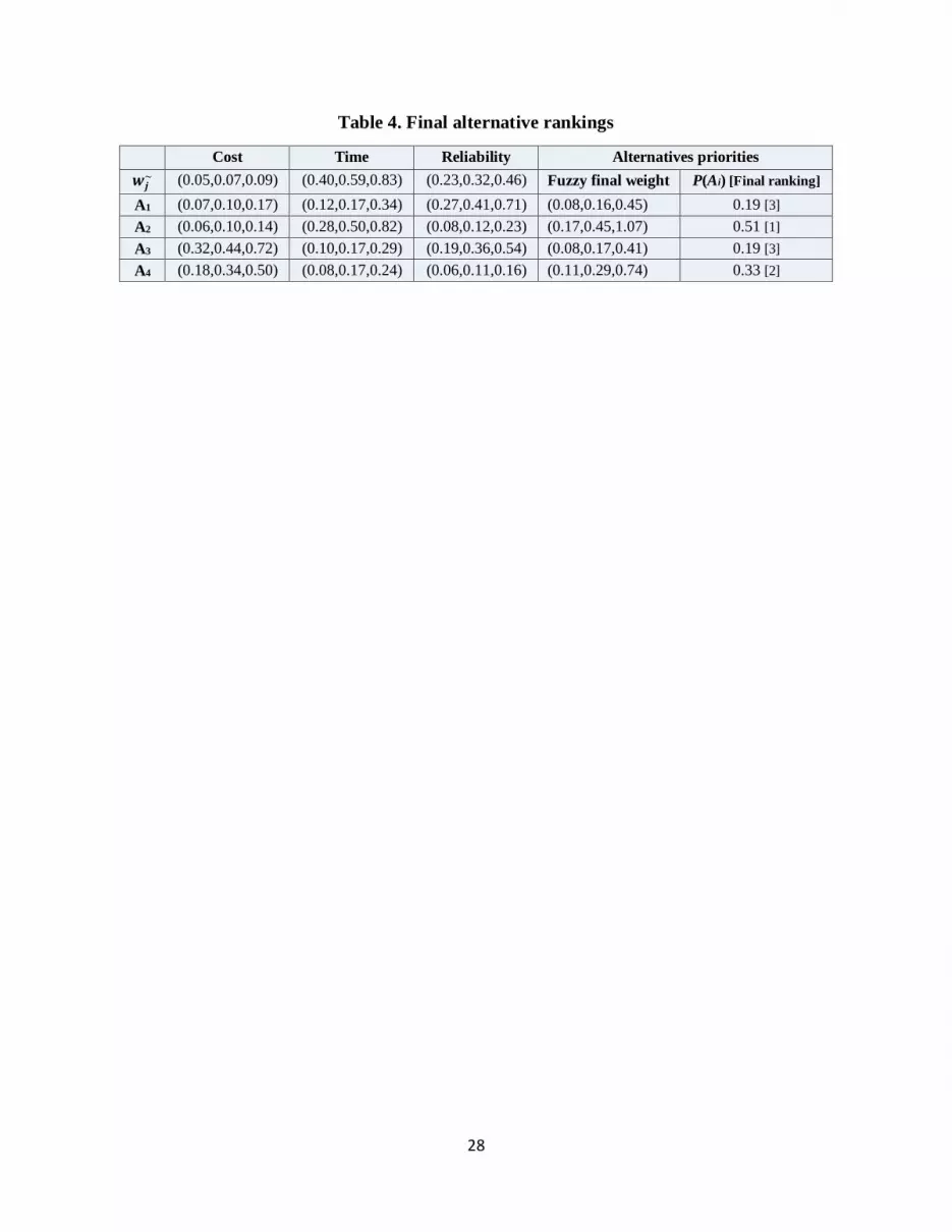
(3) Aggregation of priorities and ranking the alternatives: this step aggregates local priorities

obtained at different levels of the hierarchy into composite global priorities for the alternatives

based on the weighted sum method and using Eqs. (8-9). The results are presented in Table 4.

Insert Table 4 Here

Since P(Ai), the range of the defuzzified final weight, belongs to [0,1], a threshold value

is set equal to P*=0.3, meaning that only alternatives with a score greater than or equal to 0.3 are

selected. Therefore, alternatives A2 and A4 are selected for the next stage.

In the second stage, at first, we define the parameter values that are used in the MOILP.

Our example consists of scheduling six jobs on the three machines using two selected

repairmen (A2 & A4) from stage 1 where the aging factor matrix of each machine with respect to

each job is presented as follows:

𝛼ℎ𝑗=(6 12 57 11 66 14 5

1 10 32 10 43 11 3

)

Assume that the processing time matrix of each machine with respect to each job is as

follows:

𝑝ℎ𝑗=(8 16 79 15 88 17 7

3 14 54 14 65 13 4

)

The maintenance cost of the machines with respect to the repairmen is given by the

following matrix:

𝛾𝑠ℎ = (100 200 200100 100 50

)

The maintenance time of the machines with respect to the repairmen is as follows:

𝑡𝑠ℎ = (10 15 1510 10 5

)

The due date of the jobs is presented as follows:

𝑑𝑗 = (28,55,12,7,70,10 )

The maximum maintenance activity is the same on all three machines. The maximum

allowed job position is the same in each maintenance activity on the each machine as follows:

𝐾1 = 𝐾2 = 𝐾3 = 3; 𝑈𝑔ℎ = 4 , ∀ 𝑔, ℎ

Applying stage 2 of the proposed approach, Tables 5 and 6 present the decision variables

for the single ideal objective optimization in the original MODM problem. Tables 7 and 8 present

the decision variables for the single anti-ideal objective optimization in the original MODM

15

problem. Table 9 presents both the payoff matrix of the single objective optimization and the range

of the objective functions of the original MODM problem. The mathematical model has been

coded in Lingo 9.0 and executed on a HP Laptop 4520s model with Core i3 due CPU, 2.4 GHz,

and Windows 7 using 3 GB of RAM as follows:

Insert Tables 5-9 Here

According to Table 9 and Eqs. (15-16), the TOPSIS-based bi-objective problem will be

achieved as follows. It is notable that the values of wi, i = 1,…, 4 and p are set to 0.25 and 1,

respectively.

𝑀𝑖𝑛 𝑑1𝑃𝐼𝑆(𝑥) =∑𝑤𝑖 ×

𝑓𝑖(𝑥) − 𝑍𝑖+

𝑍𝑖− − 𝑍𝑖

+

4

𝑖=1

= 0.25 × (𝑍1 − 0

600− 0+𝑍2 − 34

140 − 34+𝑍3 − 0

118 − 0+𝑍4 − 0

46 − 0) (50)

𝑀𝑎𝑥 𝑑1𝑁𝐼𝑆(𝑥) =∑𝑤𝑖 ×

𝑍𝑖− − 𝑓𝑖(𝑥)

𝑍𝑖− − 𝑍𝑖

+

4

𝑖=1

= 0.25 × (600 − 𝑍1600 − 0

+140− 𝑍2140− 34

+118 − 𝑍3118 − 0

+46 −𝑍446 − 0

) (51)

s.t. 𝑥 ∈ 𝑆 (52)

In order to solve the above TOPSIS-based bi-objective problem, we use stage 3 of the

proposed approach (i.e,. GP) as follows:

𝑀𝑖𝑛 [(𝑤𝑃𝐼𝑆 × 𝑑𝑃𝐼𝑆+ ) + (𝑤𝑁𝐼𝑆 × 𝑑𝑁𝐼𝑆

− )] (53)

s.t. 0.25 × (𝑍1−0

600−0+

𝑍2−34

140−34+

𝑍3−0

118−0+

𝑍4−0

46−0) + 𝑑𝑃𝐼𝑆

− − 𝑑𝑃𝐼𝑆+ = 𝐺𝑃𝐼𝑆 (54)

0.25 × (600−𝑍1

600−0+140−𝑍2

140−34+118−𝑍3

118−0+46−𝑍4

46−0) + 𝑑𝑁𝐼𝑆

− −𝑑𝑁𝐼𝑆+ = 𝐺𝑁𝐼𝑆 (55)

𝑥 ∈ 𝑆 (56)

𝑑𝑃𝐼𝑆− , 𝑑𝑃𝐼𝑆

+ , 𝑑𝑁𝐼𝑆− , 𝑑𝑁𝐼𝑆

+ ≥ 0 (57)

Weights 𝑤𝑃𝐼𝑆 and 𝑤𝑁𝐼𝑆 of each goal in the objective function are set as (𝑤𝑃𝐼𝑆, 𝑤𝑁𝐼𝑆) = (0.5,

0.5). The aspiration levels of the goals are equal to (𝐺𝑃𝐼𝑆, 𝐺𝑁𝐼𝑆) = (0, 1). Note that since goals 1

and 2 have associated weights in the final objective function, the total fractional deviation is less

than the sum of the individual fractional deviations from goals 1 and 2. The results of solving the

GP are summarized in Table 10 as follows:

Insert Table 10 Here

Some final remarks regarding the scale of the problems considered are due. Note that, for

obvious reasons of manuscript length, the numerical example provided is a small scale one. In this

regard, any problem arising from the dimensionality of the model relates directly to those of the

16

standard MOILP models. However, the current setting provides an intuitive direction in which to

proceed if the dimensionality of the model becomes an issue. The current proposal is mainly

intuitive and can be further developed in future extensions of the paper.

Assume that the number of machines, the number of jobs that must be processed, or both,

lead to a MOILP model that is not solvable due to its dimension. In this case, a potential solution

would consist of partitioning the sets of machines, jobs and repairmen in two or as many subsets

as necessary to obtain a numerical solution. The partition of the sets of jobs and machines in two

(or more) subsets must be done randomly. This is due to the lack of a ranking mechanism based

on the heterogeneity of both variables in terms of aging and processing time, as can be observed

from our previous numerical example.

However, the partition of the set of repairmen can be based on their relative efficiency,

𝑃(𝐴𝑖). We can exploit this measure of performance to obtain efficient (from a repairmen

viewpoint) computable solutions for each one of the (sub)models generated. Assume, for

expositional simplicity, that we partition the sets of jobs and machines in two subsets of 𝑗/2 and

ℎ/2 elements, respectively. The number of elements can be rounded by the decision maker if the

total number of jobs or machines is odd. Similarly, a new (less efficient) repairman may be added

from the available pool if required to equate the size of the resulting subsets.

Assume that the set of 𝑠 = 1,2… , 𝑆 repairmen is ordered based on their defuzzified

efficiency score 𝑃(𝐴𝑖) from the highest to the lowest one. The suggested procedure would consist

of the following steps

1. Partition the set of repairmen in two ordered subsets based on their efficiency scores and assign

them to the groups of machines and jobs defined previously.

2. Assign the more efficient half of repairmen to a given subset of machines and jobs and the less

efficient half of repairmen to the complement subset of machines and jobs.

3. Solve the resulting model to obtain the goal score achieved relative to the corresponding

aspiration levels.

4. Switch the subset of repairmen between groups.

5. Solve the resulting model to obtain the goal score achieved relative to the corresponding

aspiration levels.

6. Compare the goal scores achieved in both cases.

17

7. Consider the case with the higher score and start shifting either one or a subset of repairmen

form the less efficient to the more efficient group. The shift must be done orderly, starting with

the initial members of the less efficient set and exchanging them with the final members of the

more efficient one. Perform the resulting calculations and solve the model again.

8. If the goal score increases, proceed orderly with further shifts. Otherwise, stop. If subsets of

repairmen are shifted, then individual shifts can be performed within each subset until the

highest goal score is achieved. Note that, in the current example, a complete shift of repairmen

from the less to the more efficient group would lead to the complement subsets considered

initially and providing a lower goal score. In this regard, note that additional shifting

combinations must be considered when accounting for more than two subsets.

This process can be repeated until the highest goal score is obtained. The intuition behind this

process follows from the completely asymmetric distribution of repairmen and the assumption that

more efficient repairmen will perform better than the less efficient ones. Note that the stochastic

component of machine and job group selection would remain when implementing this approach,

which constitutes the price to pay for numerical tractability. However, despite this stochastic

component, we can still aim at partitioning efficiently the set of repairmen among the

corresponding subsets of jobs and machines.

5. Conclusions and future research directions

In this paper we proposed a scheduling model for solving maintenance scheduling problems with

UPMs and AEMMAs. In the first stage of the evaluation process we use a fuzzy AHP approach

for repairmen selection. In the second stage we present a procedure based on the TOPSIS approach

to reduce the MODM problem to an efficient bi-objective problem. Finally, in the third stage, we

use GP and solve the resulting TOPSIS problem based on a bi-objective integer linear

programming model in which the two goals of total distance from the PIS and the NIS are taken

into consideration. A numerical example was presented to illustrate the applicability of our

proposed approach.

The contribution of the proposed performance measurement system is fourfold: (1) In spite

of tremendous advances in PMS research, multi-objective scheduling problems with simultaneous

consideration of repairmen selection, aging effects and maintenance activities in a parallel

machine environment have not been thoroughly studied in the literature; (2) We proposed a

comprehensive repairmen selection and scheduling problem that combines fuzzy AHP with

18

TOPSIS and GP in a structured and simple to use framework; (3) We considered fuzzy logic and

fuzzy sets to represent ambiguous, uncertain and imprecise information in a manufacturing

environment; and (4) The proposed method was capable of synthesizing a representative outcome

based on qualitative judgments and quantitative data.

A very practical extension of the model proposed in this study is to consider other MODM

methods in the proposed framework. Applications of the proposed method to other problems in

the manufacturing or service environments constitute another potential extension of the proposed

method.

19

References

Abo-Sinna, M.A. and Abou-El-Enien, T.H.M. (2006) ‘An interactive algorithm for large scale

multiple objective programming problems with fuzzy parameters through TOPSIS

approach’, Applied Mathematics and Computations, Vol. 177, No. 2, pp.515–527.

Abo-Sinna, M.A. and Amer, A.H. (2005) ‘Extensions of TOPSIS for multi-objective large-scale

nonlinear programming problems’, Applied Mathematics and Computations, Vol. 162,

No. 1, pp. 243–256.

Abo-Sinna, M.A., Amer, A.H. and Ibrahim, A.S. (2008) ‘Extensions of TOPSIS for large scale

multi-objective non-linear programming problems with block angular structure’, Applied

Mathematical Modeling, Vol. 32, No. 3, pp. 292–302.

Arnaout, J.-P., Rabadi, G., and Musa, R. (2010) ‘A two-stage ant colony optimization algorithm

to minimize the makespan on unrelated parallel machines with sequence-dependent

setup times’, Journal of Intelligent Manufacturing, Vol. 21, No. 6, pp. 693–701.

Bellman, R.E. and Zadeh, L.A. (1970) ‘Decision making in a fuzzy environment’, Management

Science, Vol. 17, No. 4, pp. 141–164.

Bevilacqua, M. and Braglia, M. (2000) ‘The analytic hierarchy process applied to maintenance

strategy selection’, Reliability Engineering and System Safety, Vol. 70, No. 1, pp. 71–

83.

Biskup, D. (2008) ‘A state-of-the-art review on scheduling with learning effects’, European

Journal of Operational Research, Vol. 188, No. 2, pp. 315–329.

Buckley, J.J. (1985) ‘Fuzzy hierarchical analysis’, Fuzzy Sets and Systems, Vol. 17, No. 3, pp.

233–247.

Cakir, O. and Canbolat, M. S. (2008) ‘A web-based decision support system for multi criteria

inventory classification using fuzzy AHP methodology’, Expert Systems with

Applications, Vol. 35, No. 3, pp. 1367–1378.

Chang, P.-C. and Chen, S.-H. (2011) ‘Integrating dominance properties with genetic algorithms

for parallel machine scheduling problems with setup times’, Applied Soft Computing,

Vol. 11, No. 1, pp. 1263–1274.

Charnes, A . and Cooper, W.W. (1961) ‘Management models and industrial applications of

linear programming’, Wiley, New York, USA.

20

Charnes, A. and Cooper, W.W. (1977) ‘Goal programming and multi-objective optimization’,

European Journal of Operational Research, Vol. 1, No. 1, pp. 39–45.

Chen, L.H. and Hung, C.C. (2010) ‘An integrated fuzzy approach for the selection of

outsourcing manufacturing partners in pharmaceutical R&D’, International Journal of

Production Research, Vol. 48, No. 24, pp. 7483–7506.

Cheng, T. and Sin, C. (1990) ‘A state-of-the-art review of parallel-machine scheduling research’,

European Journal of Operational Research, Vol. 47, No. 3, 271–292.

Chiou, H.K., Tzeng, G.H. and Cheng, D.C. (2005) ‘Evaluating sustainable fishing development

strategies using fuzzy MCDM approach’, Omega, Vol. 33, No. 3, pp. 223–234.

Dubois, D. and Prade, H. (1979) ‘Fuzzy real algebra: some results’, Fuzzy Sets and Systems,

Vol. 2, No. 4, pp. 327–348.

Flavell, R.B. (1976) ‘A new goal programming formulation’, Omega, Vol. 4, No. 6, pp.731–

732.

Hwang, C.L. and Yoon, K. (1981) ‘Multiple Attribute Decision Making: Methods and

Applications’, Springer-Verlag, Heidelbeg.

Jadidi, O., Hong, T.S. and Firouzi, F. (2009) ‘TOPSIS extension for multi-objective supplier

selection problem under price breaks’, International Journal of Management Sciences

and Engineering Management, Vol. 4, No. 3, pp. 217–229.

Janiak, A. and Rudek, R. (2006) ‘Scheduling problem with position dependent job processing

times’, in Janiak, A. (Ed): Scheduling in Computer and Manufacturing Systems, pp. 26–

36, Warszawa, WKL, Poland.

Janiak, A. and Rudek, R. (2009) ‘Experience based approach to scheduling problems with the

learning effect’, IEEE Transactions on Systems, Man, and Cybernetics-Part A, Vol. 39,

No. 1, pp. 344–357.

Khalili-Damghani, K., Sadi-Nezhad, S. and Tavana, M. (2013) ‘Solving multi-period project

selection problems with fuzzy goal programming based on TOPSIS and a fuzzy

preference relation’, Information Sciences, Vol. 252, pp. 42–61.

Khalili-Damghani, K., Tavana, M. and Sadi-Nezhad, S. (2012) ‘An integrated multi-objective

framework for solving multi-period project selection problems’, Applied Mathematics

and Computations, Vol. 219, No. 6, pp. 3122–3138.

21

Kuo, W.H. and Yang, D.L. (2008) ‘Minimizing the makespan in a single machine scheduling

problem with the cyclic process of an aging effect’, Journal of the Operational Research

Society, Vol. 59, No. 3, pp.416–420.

Lai, Y-J., Liu, T-Y. and Hwang, Ch-L. (1994) ‘TOPSIS for MODM’, European Journal of

Operational Research, Vol. 76, No. 3, pp.486–500.

Li, J.R., Khoo, L.P. and Tor, S.B. (2006) ‘Generation of possible multiple components

disassembly sequence for maintenance using a disassembly constraint graph’,

International Journal of Production Economics, Vol. 102, No. 1, pp. 51–65.

Liou, J.J.H., Wang, H.S., Hsu, C.C. and Yin, S.L. (2011) ‘A hybrid model for selection of an

outsourcing provider’, Applied Mathematical Modelling, Vol. 35, No. 10, pp. 5121–

5133.

Majazi Dalfard, V. and Mohammadi, G. (2012) ‘Two meta-heuristic algorithms for solving

multi-objective flexible job-shop scheduling with parallel machine and maintenance

constraints’, Computers & Mathematics with Applications, Vol. 64, No. 6, pp. 2111-

2117.

Moghaddam, K.S. (2013) ‘Multi-objective preventive maintenance and replacement scheduling

in a manufacturing system using goal programming’, International Journal of

Production Economics, Vol. 146, No. 2, pp. 704-716.

Naghadehi, M.Z., Mikaeil, R. and Ataei, M. (2009) ‘The application of fuzzy analytic hierarchy

process (FAHP) approach to selection of optimum underground mining method for

Jajarm Bauxite Mine, Iran’, Expert Systems with Applications, Vol. 36, No. 4, pp. 8218–

8226.

Saaty, T.L. (1980) ‘The Analytic Hierarchy Process, Planning, Piority Setting, Resource

Allocation’, McGraw-Hill, New York, USA.

Saaty, T.L. (1989) ‘conflict resolution’, praeger, New York, USA.

Swanson, L. (2001) ‘Linking maintenance strategies to performance’, International Journal of

Production Economics, Vol. 70, No. 3, pp. 237–244.

Torabi, S.A., Sahebjamnia, N., Mansouri, S.A. and Aramon Bajestani, M. (2013) ‘A particle

swarm optimization for a fuzzy multi-objective unrelated parallel machines scheduling

problem’, Applied Soft Computing, Vol. 13, No. 12, pp. 4750-4762.

22

Waeyenbergh, G. and Pintelon, L. (2004) ‘Maintenance concept development: A case study’,

International Journal of Production Economics, Vol. 89, No. 3, pp. 395–405.

Wang, H. (2002) ‘A survey of maintenance policies of deteriorating systems’, European Journal

of Operational Research, Vol. 139, No. 3, pp. 469–489.

Yang, D.L., Cheng, T.C.E., Yang, S.J. and Hsu, C.J. (2012) ‘Unrelated parallel-machine

scheduling with aging effects and multi-maintenance activities’, Computers &

Operations Research, Vol. 39, No. 7, pp.1458–1464.

Yang, S.J. and Yang, D.L. (2010a) ‘Minimizing the makespan on single-machine scheduling

with aging effect and variable maintenance activities’, Omega, Vol. 38, No. 6, pp. 528–

33.

Yang, S.J. and Yang, D.L. (2010b) ‘Minimizing total completion time in single-machine

scheduling with aging/deteriorating effects and deteriorating maintenance activities’,

Computers and Mathematics with Applications, Vol. 60, No. 7, pp. 2161–2169.

Zhang, D., Li, W. and Xiong, X. (2012) ‘Bidding based generator maintenance scheduling with

triple-objective optimization’, Electric Power Systems Research, Vol. 93, No. , pp. 127-

134.

Zhao, C.L. and Tang, H.Y. (2010) ‘Single machine scheduling with general job-dependent aging

effect and maintenance activities to minimize makespan’, Applied Mathematical

Modelling, Vol. 34, No. 3, pp. 837–41.

23

Stage 1: Evaluation of the alternative

repairmen

Identify the decision criteria

Select the best alternative(s)

Use fuzzy AHP to evaluate the

pair-wise comparisons matrices

Stage 2: Conversion of the MODM problem to

the bi-objective problem

Implement steps 1 and 2 of stage 1

in stage 2 to form a payoff matrix

for the original MODDM

Form the TOPSIS-based bi-

objective problem

Calculate the distance from the

NIS and the distance from the PIS

(step 3)

Stage 3: Determination of the optimal positions and the

frequencies of the maintenance activities

Use goal programming and solve the bi-objective problem (from

stage 2) according to the selected repairmen (from stage 1)

Figure 1. Proposed three-stage framework

24

Repairmen selection

Reliability (C3)Time (C2)Cost (C1)

Alternative 1

(A1)

Alternative 3

(A3)

Alternative 2

(A2)

Alternative 4

(A4)

Overall objective

Criteria

Alternatives

Figure 2. Hierarchical structure of AHP

25

Table 1. Linguistic terms for the TFNs (Saaty, 1989)

Linguistic terms Acronyms TFN

Extremely more importance EMI (8,9,10)

Very strong importance VSI (6,7,8)

Strong importance SI (4,5,6)

Moderate importance MI (2,3,4)

Equal importance EI (1,1,2)

26

Table 2. Evaluation of the criteria with respect to the goal

Linguistic terms Fuzzy terms

Goal C1 C2 C3 C1 C2 C3 Weight (𝑤𝑗~)

C1 - 1 (1/6,1/5,1/4) (1/8,1/7,1/6) (0.05,0.07,0.09)

C2 SI - MI (4,5,6) 1 (2,3,4) (0.40,0.59,0.83)

C3 VSI - (6,7,8) (1/4,1/3,1/2) 1 (0.23,0.32,0.46)

27

Table 3. Evaluation of the alternatives with respect to cost, time, and reliability

Cost

Linguistic terms Fuzzy terms

Cost A1 A2 A3 A4 A1 A2 A3 A4 Weight

A1 - EI 1 (1,1,2) (1/6,1/5,1/4) (1/4,1/3,1/2) (0.07,0.10,0.17)

A2 - (1/2,1,1) 1 (1/6,1/5,1/4) (1/4,1/3,1/2) (0.06,0.10,0.14)

A3 SI SI - EI (4,5,6) (4,5,6) 1 (1,1,2) (0.32,0.44,0.72)

A4 MI MI - (2,3,4) (2,3,4) (1/2,1,1) 1 (0.18,0.34,0.50)

Time

Linguistic terms Fuzzy terms

Time A1 A2 A3 A4 A1 A2 A3 A4 Weight

A1 - EI EI 1 (1/4,1/3,1/2) (1,1,2) (1,1,2) (0.12,0.17,0.34)

A2 MI - MI MI (2,3,4) 1 (2,3,4) (2,3,4) (0.28,0.50,0.82)

A3 - EI (1/2,1,1) (1/4,1/3,1/2) 1 (1,1,2) (0.10,0.17,0.29)

A4 - (1/2,1,1) (1/4,1/3,1/2) (1/2,1,1) 1 (0.08,0.17,0.24)

Reliability

Linguistic terms Fuzzy terms

Reliability A1 A2 A3 A4 A1 A2 A3 A4 Weight

A1 - MI EI SI 1 (2,3,4) (1,1,2) (4,5,6) (0.27,0.41,0.71)

A2 - EI (1/4,1/3,1/2) 1 (1/4,1/3,1/2) (1,1,2) (0.08,0.12,0.23)

A3 MI - MI (1/2,1,1) (2,3,4) 1 (2,3,4) (0.19,0.36,0.54)

A4 - (1/6,1/5,1/4) (1/2,1,1) (1/4,1/3,1/2) 1 (0.06,0.11,0.16)

28

Table 4. Final alternative rankings

Cost Time Reliability Alternatives priorities

𝒘𝒋~ (0.05,0.07,0.09) (0.40,0.59,0.83) (0.23,0.32,0.46) Fuzzy final weight P(Ai) [Final ranking]

A1 (0.07,0.10,0.17) (0.12,0.17,0.34) (0.27,0.41,0.71) (0.08,0.16,0.45) 0.19 [3]

A2 (0.06,0.10,0.14) (0.28,0.50,0.82) (0.08,0.12,0.23) (0.17,0.45,1.07) 0.51 [1]

A3 (0.32,0.44,0.72) (0.10,0.17,0.29) (0.19,0.36,0.54) (0.08,0.17,0.41) 0.19 [3]

A4 (0.18,0.34,0.50) (0.08,0.17,0.24) (0.06,0.11,0.16) (0.11,0.29,0.74) 0.33 [2]

29

Table 5. Ideal position of the jobs and the maintenance activities on the machines with respect to Z1 and Z2

Z1 Machine 1

Maintenance activity 0 Maintenance activity 1 Maintenance activity 2 Maintenance activity 3

Position r1 r2 r3 r4 r1 r2 r3 r4 r1 r2 r3 r4 r1 r2 r3 r4

Repairman A2 J1 J2 - - - - - - - - - - - - - -

Repairman A4 - - - - - - - - - - - - - - - -

Machine 2

Maintenance activity 0 Maintenance activity 1 Maintenance activity 2 Maintenance activity 3

Position r1 r2 r3 r4 r1 r2 r3 r4 r1 r2 r3 r4 r1 r2 r3 r4

Repairman A2 - - - - - - - - - - - - - - - -

Repairman A4 J4 J6 J5 - - - - - - - - - - - - -

Machine 3

Maintenance activity 0 Maintenance activity 1 Maintenance activity 2 Maintenance activity 3

Position r1 r2 r3 r4 r1 r2 r3 r4 r1 r2 r3 r4 r1 r2 r3 r4

Repairman A2 J3 - - - - - - - - - - - - - - -

Repairman A4 - - - - - - - - - - - - - - - -

Z2 Machine 1

Maintenance activity 0 Maintenance activity 1 Maintenance activity 2 Maintenance activity 3

Position r1 r2 r3 r4 r1 r2 r3 r4 r1 r2 r3 r4 r1 r2 r3 r4

Repairman A2 - - - - - - - - - - - - - - - -

Repairman A4 J1 J3 - - - - - - - - - - - - - -

Machine 2

Maintenance activity 0 Maintenance activity 1 Maintenance activity 2 Maintenance activity 3

Position r1 r2 r3 r4 r1 r2 r3 r4 r1 r2 r3 r4 r1 r2 r3 r4

Repairman A2 J2 J4 - - - - - - - - - - - - - -

Repairman A4 - - - - - - - - - - - - - - - -

Machine 3

Maintenance activity 0 Maintenance activity 1 Maintenance activity 2 Maintenance activity 3

Position r1 r2 r3 r4 r1 r2 r3 r4 r1 r2 r3 r4 r1 r2 r3 r4

Repairman A2 J5 J6 - - - - - - - - - - - - - -

Repairman A4 - - - - - - - - - - - - - - - -

30

Table 6. Ideal position of the jobs and the maintenance activities on the machines with respect to Z3 and Z4

Z3 Machine 1

Maintenance activity 0 Maintenance activity 1 Maintenance activity 2 Maintenance activity 3

Position r1 r2 r3 r4 r1 r2 r3 r4 r1 r2 r3 r4 r1 r2 r3 r4

Repairman A2 - - - - - - - - - - - - - - - -

Repairman A4 J4 J1 J5 - - - - - - - - - - - - -

Machine 2

Maintenance activity 0 Maintenance activity 1 Maintenance activity 2 Maintenance activity 3

Position r1 r2 r3 r4 r1 r2 r3 r4 r1 r2 r3 r4 r1 r2 r3 r4

Repairman A2 J6 - - - J2 - - - - - - - - - - -

Repairman A4 - - - - - - - - - - - - - - - -

Machine 3

Maintenance activity 0 Maintenance activity 1 Maintenance activity 2 Maintenance activity 3

Position r1 r2 r3 r4 r1 r2 r3 r4 r1 r2 r3 r4 r1 r2 r3 r4

Repairman A2 - - - - - - - - - - - - - - - -

Repairman A4 J3 - - - - - - - - - - - - - - -

Z4 Machine 1

Maintenance activity 0 Maintenance activity 1 Maintenance activity 2 Maintenance activity 3

Position r1 r2 r3 r4 r1 r2 r3 r4 r1 r2 r3 r4 r1 r2 r3 r4

Repairman A2 J3 - - - - - - - - - - - - - - -

Repairman A4 - - - - - - - - - - - - - - - -

Machine 2

Maintenance activity 0 Maintenance activity 1 Maintenance activity 2 Maintenance activity 3

Position r1 r2 r3 r4 r1 r2 r3 r4 r1 r2 r3 r4 r1 r2 r3 r4

Repairman A2 J6 J1 J2 J5 - - - - - - - - - - - -

Repairman A4 - - - - - - - - - - - - - - - -

Machine 3

Maintenance activity 0 Maintenance activity 1 Maintenance activity 2 Maintenance activity 3

Position r1 r2 r3 r4 r1 r2 r3 r4 r1 r2 r3 r4 r1 r2 r3 r4

Repairman A2 - - - - - - - - - - - - - - - -

Repairman A4 J4 - - - - - - - - - - - - - - -

31

Table 7. Anti-ideal position of the jobs and the maintenance activities on the machines with respect to Z1 and Z2

Z1 Machine 1

Maintenance activity 0 Maintenance activity 1 Maintenance activity 2 Maintenance activity 3

Position r1 r2 r3 r4 r1 r2 r3 r4 r1 r2 r3 r4 r1 r2 r3 r4

Repairman A2 - - - - - - - - - - - - - - - -

Repairman A4 J4 - - - - - - - - - - - - - - -

Machine 2

Maintenance activity 0 Maintenance activity 1 Maintenance activity 2 Maintenance activity 3

Position r1 r2 r3 r4 r1 r2 r3 r4 r1 r2 r3 r4 r1 r2 r3 r4

Repairman A2 J3 - - - J6 - - - J5 - - - J1 - - -

Repairman A4 - - - - - - - - - - - - - - - -

Machine 3

Maintenance activity 0 Maintenance activity 1 Maintenance activity 2 Maintenance activity 3

Position r1 r2 r3 r4 r1 r2 r3 r4 r1 r2 r3 r4 r1 r2 r3 r4

Repairman A2 - - - - - - - - - - - - - - - -

Repairman A4 J2 - - - - - - - - - - - - - - -

Z2 Machine 1

Maintenance activity 0 Maintenance activity 1 Maintenance activity 2 Maintenance activity 3

Position r1 r2 r3 r4 r1 r2 r3 r4 r1 r2 r3 r4 r1 r2 r3 r4

Repairman A2 J4 - - - - - - - - - - - - - - -

Repairman A4 - - - - - - - - - - - - - - - -

Machine 2

Maintenance activity 0 Maintenance activity 1 Maintenance activity 2 Maintenance activity 3

Position r1 r2 r3 r4 r1 r2 r3 r4 r1 r2 r3 r4 r1 r2 r3 r4

Repairman A2 - - - - - - - - - - - - - - - -

Repairman A4 J3 J1 J5 J2 - - - - - - - - - - - -

Machine 3

Maintenance activity 0 Maintenance activity 1 Maintenance activity 2 Maintenance activity 3

Position r1 r2 r3 r4 r1 r2 r3 r4 r1 r2 r3 r4 r1 r2 r3 r4

Repairman A2 - - - - - - - - - - - - - - - -

Repairman A4 J6 - - - - - - - - - - - - - - -

32

Table 8. Anti-ideal position of the jobs and the maintenance activities on the machines with respect to Z3 and Z4

Z3

Machine 1

Maintenance activity 0 Maintenance activity 1 Maintenance activity 2 Maintenance activity 3

Position r1 r2 r3 r4 r1 r2 r3 r4 r1 r2 r3 r4 r1 r2 r3 r4

Repairman A2 J4 - - - - - - - - - - - - - - -

Repairman A4 - - - - - - - - - - - - - - - -

Machine 2

Maintenance activity 0 Maintenance activity 1 Maintenance activity 2 Maintenance activity 3

Position r1 r2 r3 r4 r1 r2 r3 r4 r1 r2 r3 r4 r1 r2 r3 r4

Repairman A2 - - - - - - - - - - - - - - - -

Repairman A4 J1 J5 J2 J3 - - - - - - - - - - - -

Machine 3

Maintenance activity 0 Maintenance activity 1 Maintenance activity 2 Maintenance activity 3

Position r1 r2 r3 r4 r1 r2 r3 r4 r1 r2 r3 r4 r1 r2 r3 r4

Repairman A2 J6 - - - - - - - - - - - - - - -

Repairman A4 - - - - - - - - - - - - - - - -

Z4

Machine 1

Maintenance activity 0 Maintenance activity 1 Maintenance activity 2 Maintenance activity 3

Position r1 r2 r3 r4 r1 r2 r3 r4 r1 r2 r3 r4 r1 r2 r3 r4

Repairman A2 - - - - - - - - - - - - - - - -

Repairman A4 J1 J3 - - - - - - - - - - - - - -

Machine 2

Maintenance activity 0 Maintenance activity 1 Maintenance activity 2 Maintenance activity 3

Position r1 r2 r3 r4 r1 r2 r3 r4 r1 r2 r3 r4 r1 r2 r3 r4

Repairman A2 J2 J4 - - - - - - - - - - - - - -

Repairman A4 - - - - - - - - - - - - - - - -

Machine 3

Maintenance activity 0 Maintenance activity 1 Maintenance activity 2 Maintenance activity 3

Position r1 r2 r3 r4 r1 r2 r3 r4 r1 r2 r3 r4 r1 r2 r3 r4

Repairman A2 J5 J6 - - - - - - - - - - - - - -

Repairman A4 - - - - - - - - - - - - - - - -

33

Table 9. Single-objective optimization payoff matrix for the original MODM problem

Z1 Z2 Z3 Z4

Ideal calculations

Min Z1 0 64 10 14

Min Z2 0 34 27 46

Min Z3 100 68 0 9

Min Z4 0 135 65 0

Anti-ideal calculations

Max Z1 600 109 81 24

Max Z2 0 140 85 3

Max Z3 0 130 118 20

Max Z4 0 34 27 46

𝑍+ = (0,34,0,0) , 𝑍− = (600,140,118,46)

34

Table 10. Optimal position of the jobs and the maintenance activities on the machines

Machine 1

Maintenance activity 0 Maintenance activity 1 Maintenance activity 2 Maintenance activity 3

Position r1 r2 r3 r4 r1 r2 r3 r4 r1 r2 r3 r4 r1 r2 r3 r4

Repairman A2 J6 J1 J5 - - - - - - - - - - - - -

Repairman A4 - - - - - - - - - - - - - - - -

Machine 2

Maintenance activity 0 Maintenance activity 1 Maintenance activity 2 Maintenance activity 3

Position r1 r2 r3 r4 r1 r2 r3 r4 r1 r2 r3 r4 r1 r2 r3 r4

Repairman A2 - - - - - - - - - - - - - - - -

Repairman A4 J4 - - - - - - - - - - - - - - -

Machine 3

Maintenance activity 0 Maintenance activity 1 Maintenance activity 2 Maintenance activity 3

Position r1 r2 r3 r4 r1 r2 r3 r4 r1 r2 r3 r4 r1 r2 r3 r4

Repairman A2 J3 J2 - - - - - - - - - - - - - -

Repairman A4 - - - - - - - - - - - - - - - -