Journal of Intelligent Manufacturing manuscript No.(will be inserted by the editor)

A variable neighborhood descent heuristic for the problemof makespan minimisation on unrelated parallel machineswith setup times

Krzysztof Fleszar ·Christoforos Charalambous ·Khalil S. Hindi

Received: date / Accepted: date

Abstract The NP-hard problem of scheduling jobs on unrelated parallel machines,

in the presence of machine-dependent and sequence-dependent setup times, with the

objective of minimizing the makespan, is considered. A variable neighborhood descent

search algorithm, hybridized with mathematical programming elements, is presented

and its performance is evaluated on a large set of benchmark problem instances. The

extensive computational experiments show that the proposed algorithm outperforms

previously proposed methods in terms of solution quality as well as computation time.

Keywords parallel machine scheduling, hybrid optimization, neighborhood search,

makespan minimization, mixed-integer programming

This research has been supported by the Cyprus Research Promotion Foundation (ProjectTEXNO/0603/08 - NETEXNOPRO).

Krzysztof FleszarAmerican University of Beirut (AUB)Olayan School of BusinessP.O. Box 11-0236, Riad El SolhBeirut 1107 2020, LebanonE-mail: kfleszar@gmail.comE-mail: kf09@aub.edu.lb

Christoforos CharalambousFrederick UniversityDepartment of Computer Science and EngineeringP.O. Box 247291303 Nicosia, CyprusTel.: +357 22431355 ext. 116Fax: +357 22438234E-mail: c.charalambous@frederick.ac.cy

Khalil S. HindiAmerican University of Beirut (AUB)Olayan School of BusinessP.O. Box 11-0236, Riad El SolhBeirut 1107 2020, LebanonE-mail: khalil.hindi@aub.edu.lb

2

1 Introduction

The unrelated parallel machine scheduling (UPMS) problem with sequence-dependent

and machine-dependent setup times is that of scheduling n non-preemptive jobs avail-

able at time zero on m machines to minimize the makespan (maximum machine com-

pletion time). The machines are unrelated, in that the processing time of each job

depends on the machine on which it is processed. Jobs require setups, with setup times

that are sequence-dependent, in that the setup time of a job depends on which job (if

any) precedes it, and machine-dependent, in that each job has different setup times on

each machine.

The practical importance of the problem stems from the fact that it is common

in many industrial applications to have parallel resources (machines) with different

capabilities. These resources would be capable of carrying out the same tasks, but the

time taken to perform a task would depend on the resource on which it is performed.

Moreover, on each resource, setup times are incurred when switching from one item

to another. Such applications can be found in industries like painting, plastic, textile,

glass, semiconductor, chemical, and paper manufacturing, as well as in some service

industries [30].

Many variants of parallel machine scheduling (PMS) problem have been considered

in the literature; for general references and surveys, see [6,7,18,21,25,29]. Most of the

literature addresses identical machines, where the processing time of a job is the same

regardless of the machine to which it is assigned, or uniform machines, where the

processing time of a job is proportional to the speed of the machine.

Of the relatively small number of works that address UPMS, most deal with the case

without setup times. Recently, for minimization of the makespan, Martello, Soumis,

and Toth offered exact and approximation algorithms [24]; Mokotoff and Chretienne

a cutting plane algorithm [26]; Mokotoff and Jimeno [27] heuristics based on partial

enumeration; Ghirardi and Potts [14] a recovering beam search method; and Shchepin

and Vakhania [33,34] approximation algorithms. Also, Liaw et al. [22] offered a branch-

and-bound algorithm to minimize total weighted tardiness.

The works that consider UPMS with sequence-dependent (but machine-indepen-

dent) setup times are few. Among recent works, Weng, Lu, and Ren [35] consider

minimizing weighted mean completion time. Kim, Na, and Chen [20] address batch

scheduling, with the objective of minimizing total weighted tardiness in the presence

of setup times between batches. Logendran, McDonell, and Smucker [23] consider mini-

mizing total weighted tardiness in the presence of dynamic release of jobs and dynamic

availability of machines, and offer six different search algorithms based on tabu search

to identify the best schedule. Lopes and Carvalho [28] offer a branch-and-price algo-

rithm for the same problem.

The works that address UPMS with sequence-dependent and machine-dependent

setup times are even fewer. In fact, we are aware of only six, of which only four ad-

dress the objective of minimizing the makespan, considered in this paper. Al-Salem [3]

addresses the problem of minimization of the makespan and offers a three-phase par-

titioning heuristic (PH), which first assigns jobs to machines, then improves the as-

signment, and finally improves the sequence of jobs on each machine. Rabadi, Moraga,

and Al-Salem [30] address the same problem and offer a metaheuristic for randomized

priority search (Meta-RaPS), which is a general strategy that combines construction

and improvement heuristics to generate high quality solutions. Helal, Rabadi, and Al-

Salem [17] address the same problem using a tabu search algorithm. Ravetti et. al. [31]

3

consider minimization of a function combining the makespan and the total weighted

tardiness and offer a metaheuristic based on GRASP (greedy randomized adaptive

search procedure). In another work [32], the same authors offer a branch-and-bound

algorithm initiated by an upper bound found by GRASP for minimizing the total

weighted tardiness. Finally, Arnaout, Rabadi, and Musa [5] offer an ant colony opti-

mization (ACO) algorithm for the problem of minimizing the makespan when ratio of

jobs to machines is large.

In this work, the UPMS problem with sequence-dependent and machine-dependent

setup times, with the objective of minimizing the makespan, denoted here UPMSwS,

is addressed [17,30,5]. Throughout the paper, the term span is used to denote the

completion time of a machine and the term makespan to denote the maximum span in

the solution of UPMSwS. Additionally, the following notation is used:

– M = {1, . . . ,m} — the set of machines, m = number of machines

– N = {1, . . . , n} — the set of jobs, n = number of jobs

– N0 = N ∪ {0} — the set of jobs with an additional dummy job 0

– pjk — the processing time of job j on machine k

– sijk — the setup time of job j scheduled after job i on machine k

– s0jk — the setup time of job j scheduled as the first job on machine k

– M(j) — the machine to which job j is assigned

– cj — the completion time of job j

– Sk — the sequence of jobs assigned to machine k

– Ck — the span, i.e. the completion time of the last job, on machine k

– Cmax = maxj∈N cj = maxk∈M Ck — the makespan

The UPMSwS can be formally defined as follows [30]:

min Cmax (1)

subject to:

0 ≤ cj ≤ Cmax ∀j ∈ N0 (2)∑i∈N0\{j}

∑k∈M

xijk = 1 ∀j ∈ N (3)

∑i∈N0\{h}

xihk =∑

j∈N0\{h}

xhjk ∀h ∈ N,∀k ∈M (4)

ci +∑k∈M

(sijk + pjk)xijk + L

(∑k∈M

xijk − 1

)≤ cj ∀i ∈ N0,∀j ∈ N (5)

∑j∈N0

x0jk = 1 ∀k ∈M (6)

xijk ∈ {0, 1} ∀i, j ∈ N0, ∀k ∈M (7)

The following variables are used in the model:

– xijk = 1 if job j is scheduled directly after job i on machine k, 0 otherwise,

– x0jk = 1 if j is the first job scheduled on machine k, 0 otherwise,

– xi0k = 1 if i is the last job scheduled on machine k, 0 otherwise,

– cj — completion time of job j,

– Cmax — the makespan of the solution,

4

Objective (1) minimizes the makespan of the solution. Constraints (2) ensure that

the makespan is the maximum job completion time. Constraints (3) ensure that every

job is scheduled on one machine either after exactly one job or as the first job. Con-

straints (4) ensure that for each job and each machine, the number of predecessors of

the job is equal to the number of successors. Note that this number must be either 0

or 1 due to constraints (3). Constraints (5) (L is a large number) ensure correct values

of job completion times, and that jobs are scheduled in sequences without loops. Con-

straints (6) ensure that exactly one job is scheduled as the first job on each machine.

Finally, constraints (7) define domains of variables.

2 Multi-start variable neighborhood descent

The main idea behind our approach for solving the UPMSwS is to decompose the

problem into two layers: the master problem of assigning jobs to machines to minimize

the makespan, and the subproblem of sequencing jobs assigned to each machine to

minimize the span of the machine. For the master problem, the variable neighborhood

descent metaheuristic [16] will be used. For the subproblem, a fast heuristic will be

employed.

The variable neighborhood descent (VND) is a metaheuristic scheme introduced

by Hansen and Mladenovic [16]. An initial solution is improved by exploring several

neighborhood structures, Ng (g = 1, . . . , gmax), starting from N1. If an improvement

using Ng is made, the algorithm restarts exploration from N1, otherwise it moves to

Ng+1. When g exceeds gmax, the processing is terminated. The pseudo-code of VND

is shown in Algorithm 1.

Input: Initial solution XOutput: Solution Xg ← 1;while g ≤ gmax do

X′ ← the best solution from Ng(X);if X′ is better than X then X ← X′; g ← 1; else g ← g + 1;

end

Algorithm 1: VND [16]

Our algorithm for UPMSwS is a multi-start VND (MVND) based on two neigh-

borhood structures, small and large, defined later. The overall scheme of our algorithm

is shown in Algorithm 2. The VND is run 10 times and the best solution is retained.

In each run, a random initial solution is first generated. Then, the small neighborhood

search (SNS) is performed, which repeatedly improves the current solution by perform-

ing moves in the small neighborhood, until no improvement is possible. Afterwards, the

large neighborhood search (LNS) is performed, which attempts to make a single im-

proving move in the large neighborhood. If LNS succeeds, SNS is resumed; otherwise,

the run of MVND is completed.

In the following sections, the components of our MVND are explained in detail.

Section 2.1 defines an objective function used to compare solutions, which performs

better than the simple makespan minimization. Section 2.2 describes our initial-solution

heuristic. Section 2.3 describes our heuristic for optimizing a sequence of jobs assigned

5

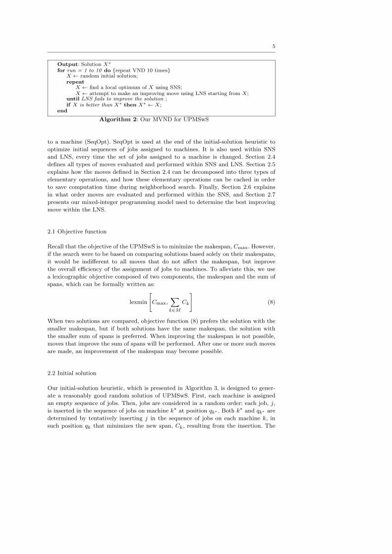
Output: Solution X∗

for run = 1 to 10 do {repeat VND 10 times}X ← random initial solution;repeat

X ← find a local optimum of X using SNS;X ← attempt to make an improving move using LNS starting from X;

until LNS fails to improve the solution ;if X is better than X∗ then X∗ ← X;

end

Algorithm 2: Our MVND for UPMSwS

to a machine (SeqOpt). SeqOpt is used at the end of the initial-solution heuristic to

optimize initial sequences of jobs assigned to machines. It is also used within SNS

and LNS, every time the set of jobs assigned to a machine is changed. Section 2.4

defines all types of moves evaluated and performed within SNS and LNS. Section 2.5

explains how the moves defined in Section 2.4 can be decomposed into three types of

elementary operations, and how these elementary operations can be cached in order

to save computation time during neighborhood search. Finally, Section 2.6 explains

in what order moves are evaluated and performed within the SNS, and Section 2.7

presents our mixed-integer programming model used to determine the best improving

move within the LNS.

2.1 Objective function

Recall that the objective of the UPMSwS is to minimize the makespan, Cmax. However,

if the search were to be based on comparing solutions based solely on their makespans,

it would be indifferent to all moves that do not affect the makespan, but improve

the overall efficiency of the assignment of jobs to machines. To alleviate this, we use

a lexicographic objective composed of two components, the makespan and the sum of

spans, which can be formally written as:

lexmin

[Cmax,

∑k∈M

Ck

](8)

When two solutions are compared, objective function (8) prefers the solution with the

smaller makespan, but if both solutions have the same makespan, the solution with

the smaller sum of spans is preferred. When improving the makespan is not possible,

moves that improve the sum of spans will be performed. After one or more such moves

are made, an improvement of the makespan may become possible.

2.2 Initial solution

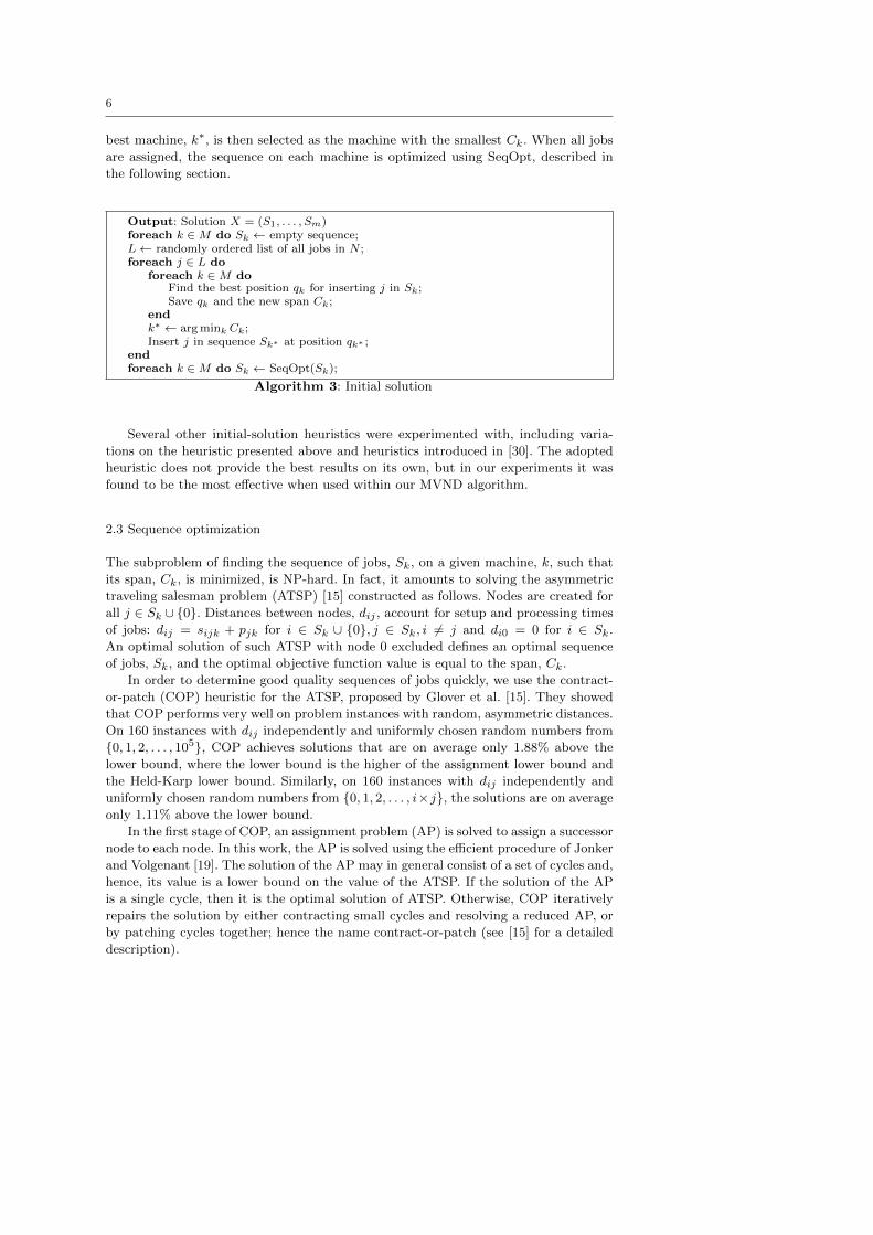
Our initial-solution heuristic, which is presented in Algorithm 3, is designed to gener-

ate a reasonably good random solution of UPMSwS. First, each machine is assigned

an empty sequence of jobs. Then, jobs are considered in a random order: each job, j,

is inserted in the sequence of jobs on machine k∗ at position qk∗ . Both k∗ and qk∗ are

determined by tentatively inserting j in the sequence of jobs on each machine k, in

such position qk that minimizes the new span, Ck, resulting from the insertion. The

6

best machine, k∗, is then selected as the machine with the smallest Ck. When all jobs

are assigned, the sequence on each machine is optimized using SeqOpt, described in

the following section.

Output: Solution X = (S1, . . . , Sm)foreach k ∈M do Sk ← empty sequence;L← randomly ordered list of all jobs in N ;foreach j ∈ L do

foreach k ∈M doFind the best position qk for inserting j in Sk;Save qk and the new span Ck;

endk∗ ← arg mink Ck;Insert j in sequence Sk∗ at position qk∗ ;

endforeach k ∈M do Sk ← SeqOpt(Sk);

Algorithm 3: Initial solution

Several other initial-solution heuristics were experimented with, including varia-

tions on the heuristic presented above and heuristics introduced in [30]. The adopted

heuristic does not provide the best results on its own, but in our experiments it was

found to be the most effective when used within our MVND algorithm.

2.3 Sequence optimization

The subproblem of finding the sequence of jobs, Sk, on a given machine, k, such that

its span, Ck, is minimized, is NP-hard. In fact, it amounts to solving the asymmetric

traveling salesman problem (ATSP) [15] constructed as follows. Nodes are created for

all j ∈ Sk ∪ {0}. Distances between nodes, dij , account for setup and processing times

of jobs: dij = sijk + pjk for i ∈ Sk ∪ {0}, j ∈ Sk, i 6= j and di0 = 0 for i ∈ Sk.

An optimal solution of such ATSP with node 0 excluded defines an optimal sequence

of jobs, Sk, and the optimal objective function value is equal to the span, Ck.

In order to determine good quality sequences of jobs quickly, we use the contract-

or-patch (COP) heuristic for the ATSP, proposed by Glover et al. [15]. They showed

that COP performs very well on problem instances with random, asymmetric distances.

On 160 instances with dij independently and uniformly chosen random numbers from

{0, 1, 2, . . . , 105}, COP achieves solutions that are on average only 1.88% above the

lower bound, where the lower bound is the higher of the assignment lower bound and

the Held-Karp lower bound. Similarly, on 160 instances with dij independently and

uniformly chosen random numbers from {0, 1, 2, . . . , i×j}, the solutions are on average

only 1.11% above the lower bound.

In the first stage of COP, an assignment problem (AP) is solved to assign a successor

node to each node. In this work, the AP is solved using the efficient procedure of Jonker

and Volgenant [19]. The solution of the AP may in general consist of a set of cycles and,

hence, its value is a lower bound on the value of the ATSP. If the solution of the AP

is a single cycle, then it is the optimal solution of ATSP. Otherwise, COP iteratively

repairs the solution by either contracting small cycles and resolving a reduced AP, or

by patching cycles together; hence the name contract-or-patch (see [15] for a detailed

description).

7

In addition to using COP, we use a sequence local search (SeqLS) algorithm for

optimizing the sequence of jobs on a machine. This method repeatedly performs the

best-improving relocation of a single job, until no improving relocation is possible.

The improvement is measured in terms of the reduction of the span effected by the

relocation.

Overall, our sequence optimization (SeqOpt) algorithm performs the following

steps. First, a given sequence is improved using SeqLS. Then, a new sequence is gen-

erated using COP followed by SeqLS. Finally, the spans of the two sequences are

compared and the better sequence is adopted.

SeqOpt is used to improve the sequence of jobs on each machine of the initial

solution. Subsequently, it is used within our MVND algorithm every time a modified

set of jobs for a machine is considered.

2.4 Moves

Since the SeqOpt procedure, described in the previous section, efficiently optimizes the

sequence of jobs every time the set of jobs on a machine changes, the moves performed

during neighborhood exploration can be defined in terms of relocation of jobs among

machines. Let M(j) denote the machine to which job j is assigned in the current

solution. In this work, the following moves are considered:

Transfer: A transfer relocates a single job j from machine M(j) to machine k 6= M(j).

Swap: For two jobs i and j on two different machines (M(i) 6= M(j)), a swap consists

of two transfers: i is transferred from M(i) to M(j) and j is transferred from M(j)

to M(i).

Path move: A path move involves a sequence of jobs j1, j2, . . . , jr and machine k,

where r ≥ 1 and M(ja) 6= M(jb) 6= k for a 6= b. Each job ja, a = 1, . . . , r − 1, is

transferred from M(ja) to M(ja+1), and the last job jr is transferred from M(jr)

to machine k. A transfer is a special case of a path move, with r = 1.

Cyclic move: A cyclic move involves a sequence of jobs j1, j2, . . . , jr, where r ≥ 2 and

M(ja) 6= M(jb) for a 6= b. Each job ja, a = 1, . . . , r − 1, is transferred from M(ja)

to M(ja+1), and job jr is transferred from M(jr) to M(j1). A swap is a special

case of a cyclic move, with r = 2.

Compound move: A compound move is a combination of any number of path and

cyclic moves, in which each machine is involved in at most one path or cyclic move.

Our SNS is based on the first two types of moves, called simple moves, while our LNS

is based on the compound moves, which comprise all the moves defined above.

Path and cyclic moves as defined above are similar to the path and cyclic ‘ex-

changes’ proposed in [2,13]. Also, Ergun, Orlin, and Steele-Feldman [9] proposed, for

routing problems with side constraints, a large-scale neighborhood search based on

compounding independent moves (2-opt, swap, and insertion). In their terminology,

our path moves and cyclic moves would be considered compound.

2.5 Elementary operations

Let an elementary operation be one of the three modifications of the sequence of jobs

assigned to a machine:

8

Addition: One job is added to a machine.

Removal: One job is removed from a machine.

Replacement: One job is removed from and another is added to a machine.

All moves defined in Section 2.4 can be decomposed into a set of elementary operations,

exactly one for each affected machine. A transfer consists of two elementary operations:

a removal of a job from its current machine and an addition of the same job to the

target machine. A swap consists of two replacement operations: on each of the two

machines involved, the selected job is replaced with the other job involved. A path

move consists of one removal, several (zero or more) replacements, and one addition.

Finally, a cyclic move consists of several (two or more) replacements.

When moves are evaluated, the impact of a set of elementary operations, one for

each of the machines involved, is computed. When an elementary operation is evaluated

for a machine, k, the new sequence, Sk, is first determined as follows: in the ‘addition’,

a job is added at the end of the original sequence; in the ‘removal’, a job is simply

removed from the original sequence; in the ‘replacement’, the added job is inserted in

the place of the removed job. Then, the resulting sequence of jobs is optimized using

SeqOpt procedure, described in Section 2.3.

Since an elementary operation can be part of more than one move, significant

computational savings can be achieved by avoiding repeated evaluations of the same

operations through the use of a cache. Every time an elementary operation needs to

be evaluated, the cache is checked; if the operation is found, it is taken directly from

the cache; otherwise, the operation is evaluated and its value (Ck) and the associated

sequence (Sk) are saved in the cache. When a move is performed, all cached elementary

operations saved for the affected machines become invalid; hence, they are removed

from the cache.

Further computational savings can be achieved through realizing that certain moves

need not be fully evaluated during the search. Recall that the first step of the COP

heuristic for solving the associated ATSP is to compute the AP lower bound on the

span. If this lower bound is higher than the current makespan, then the move involving

the elementary operation under consideration will not be improving; hence, both the

elementary operation and the move need not be evaluated fully.

2.6 Small neighborhood search

The small neighborhood search (SNS) evaluates and executes simple moves, i.e., the

transfers and swaps, defined in Section 2.4. A list of all simple moves is created and

ordered randomly. This list includes all pairs of job-machine for transfers and job-job

for swaps, even those that are currently infeasible (i.e. a job is currently on the target

machine in the case of a transfer, or the two jobs are on the same machine in the case

of a swap). The moves are tested in a cyclic fashion, with infeasible moves omitted,

and the first move that improves the objective (8) adopted. The search is terminated

when no improving simple move exists.

Each simple move requires evaluating two elementary operations for two affected

machines. The cache is used to avoid repeated evaluations of the same operation, as

described in Section 2.5. Greater computational efficiency is additionally achieved by

carefully choosing the order in which these elementary operations are considered. In the

case of a transfer, the addition is evaluated before the removal, since it is more likely to

9

be non-improving. For the same reason, in the case of a swap, the replacement for the

machine currently with the longer span is evaluated before evaluating the replacement

for the machine currently with the shorter span.

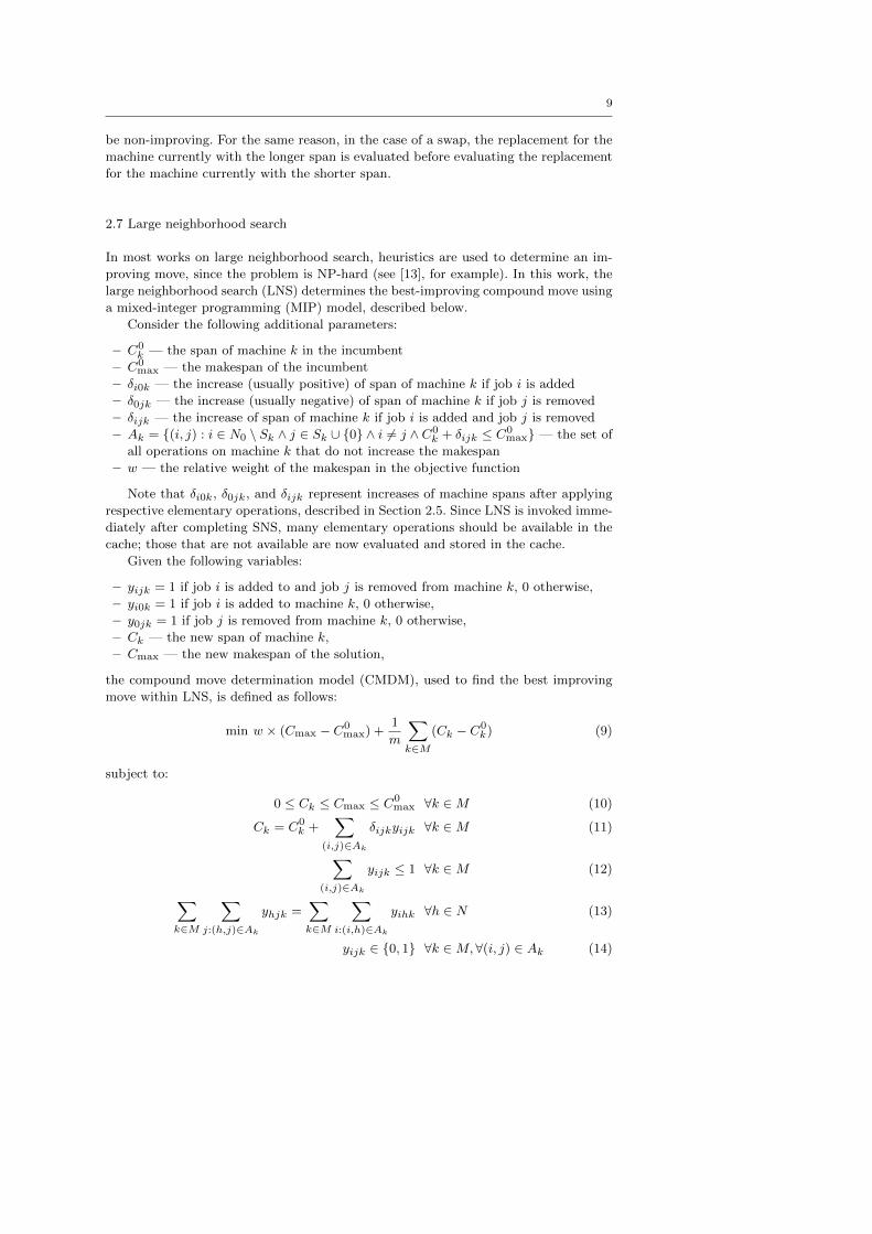
2.7 Large neighborhood search

In most works on large neighborhood search, heuristics are used to determine an im-

proving move, since the problem is NP-hard (see [13], for example). In this work, the

large neighborhood search (LNS) determines the best-improving compound move using

a mixed-integer programming (MIP) model, described below.

Consider the following additional parameters:

– C0k — the span of machine k in the incumbent

– C0max — the makespan of the incumbent

– δi0k — the increase (usually positive) of span of machine k if job i is added

– δ0jk — the increase (usually negative) of span of machine k if job j is removed

– δijk — the increase of span of machine k if job i is added and job j is removed

– Ak = {(i, j) : i ∈ N0 \ Sk ∧ j ∈ Sk ∪ {0} ∧ i 6= j ∧ C0k + δijk ≤ C0

max} — the set of

all operations on machine k that do not increase the makespan

– w — the relative weight of the makespan in the objective function

Note that δi0k, δ0jk, and δijk represent increases of machine spans after applying

respective elementary operations, described in Section 2.5. Since LNS is invoked imme-

diately after completing SNS, many elementary operations should be available in the

cache; those that are not available are now evaluated and stored in the cache.

Given the following variables:

– yijk = 1 if job i is added to and job j is removed from machine k, 0 otherwise,

– yi0k = 1 if job i is added to machine k, 0 otherwise,

– y0jk = 1 if job j is removed from machine k, 0 otherwise,

– Ck — the new span of machine k,

– Cmax — the new makespan of the solution,

the compound move determination model (CMDM), used to find the best improving

move within LNS, is defined as follows:

min w × (Cmax − C0max) +

1

m

∑k∈M

(Ck − C0k) (9)

subject to:

0 ≤ Ck ≤ Cmax ≤ C0max ∀k ∈M (10)

Ck = C0k +

∑(i,j)∈Ak

δijkyijk ∀k ∈M (11)

∑(i,j)∈Ak

yijk ≤ 1 ∀k ∈M (12)

∑k∈M

∑j:(h,j)∈Ak

yhjk =∑k∈M

∑i:(i,h)∈Ak

yihk ∀h ∈ N (13)

yijk ∈ {0, 1} ∀k ∈M,∀(i, j) ∈ Ak (14)

10

Objective (9) (w = 10, 000) is a linearization of the objective (8) defined in Sec-

tion 2.1, in which each span and the makespan are additionally decreased by their

respective incumbent values. Constraints (10) ensure that Cmax is the new makespan

and that it does not exceed the incumbent makespan. Constraints (11) ensure that Ck

is the new span of machine k. Constraints (12) ensure that at most one elementary

operation is selected for each machine. Constraints (13) ensure that a job h is removed

from a machine if and only if it is added to another machine. Finally, constraints (14)

define the domains of variables.

As the computational results presented in the next section show, solving CMDM

turns out to be efficient. This is due to the fact that the SNS, which is run before

invoking CMDM, reduces considerably the cardinality of the set of elementary opera-

tions that do not increase the makespan, represented in the model by Ak; hence, the

number of binary variables is also reduced. Additionally, the solution space is greatly

constrained by the fact that at most one elementary operation can be selected for each

machine.

It is worth pointing out that the compound move produced by solving CMDM may

in general consist of several path and cyclic moves, as long as each machine is modified

by at most one of these moves. Furthermore, the best move is always determined.

Hence, CMDM is a more powerful search engine than the commonly used heuristics

that search for a single improving path or cyclic move, as in [13].

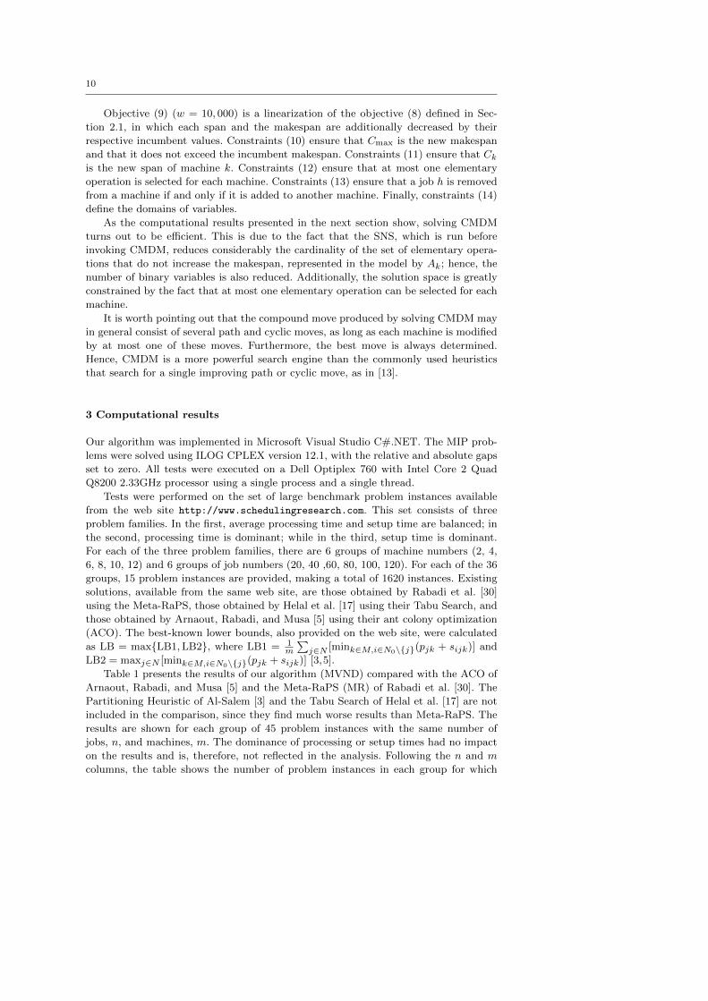
3 Computational results

Our algorithm was implemented in Microsoft Visual Studio C#.NET. The MIP prob-

lems were solved using ILOG CPLEX version 12.1, with the relative and absolute gaps

set to zero. All tests were executed on a Dell Optiplex 760 with Intel Core 2 Quad

Q8200 2.33GHz processor using a single process and a single thread.

Tests were performed on the set of large benchmark problem instances available

from the web site http://www.schedulingresearch.com. This set consists of three

problem families. In the first, average processing time and setup time are balanced; in

the second, processing time is dominant; while in the third, setup time is dominant.

For each of the three problem families, there are 6 groups of machine numbers (2, 4,

6, 8, 10, 12) and 6 groups of job numbers (20, 40 ,60, 80, 100, 120). For each of the 36

groups, 15 problem instances are provided, making a total of 1620 instances. Existing

solutions, available from the same web site, are those obtained by Rabadi et al. [30]

using the Meta-RaPS, those obtained by Helal et al. [17] using their Tabu Search, and

those obtained by Arnaout, Rabadi, and Musa [5] using their ant colony optimization

(ACO). The best-known lower bounds, also provided on the web site, were calculated

as LB = max{LB1,LB2}, where LB1 = 1m

∑j∈N [mink∈M,i∈N0\{j}(pjk + sijk)] and

LB2 = maxj∈N [mink∈M,i∈N0\{j}(pjk + sijk)] [3,5].

Table 1 presents the results of our algorithm (MVND) compared with the ACO of

Arnaout, Rabadi, and Musa [5] and the Meta-RaPS (MR) of Rabadi et al. [30]. The

Partitioning Heuristic of Al-Salem [3] and the Tabu Search of Helal et al. [17] are not

included in the comparison, since they find much worse results than Meta-RaPS. The

results are shown for each group of 45 problem instances with the same number of

jobs, n, and machines, m. The dominance of processing or setup times had no impact

on the results and is, therefore, not reflected in the analysis. Following the n and m

columns, the table shows the number of problem instances in each group for which

11

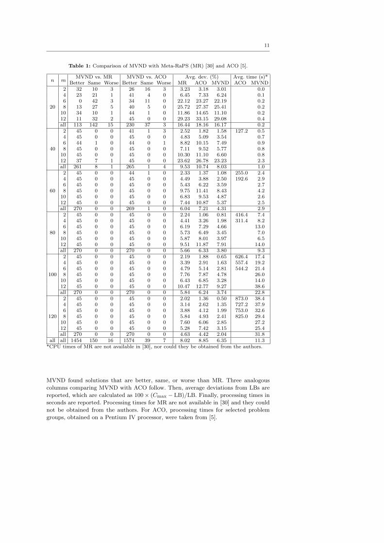
Table 1: Comparison of MVND with Meta-RaPS (MR) [30] and ACO [5].

MVND vs. MR MVND vs. ACO Avg. dev. (%) Avg. time (s)*n m

Better Same Worse Better Same Worse MR ACO MVND ACO MVND2 32 10 3 26 16 3 3.23 3.18 3.01 0.04 23 21 1 41 4 0 6.45 7.33 6.24 0.16 0 42 3 34 11 0 22.12 23.27 22.19 0.2

20 8 13 27 5 40 5 0 25.72 27.37 25.41 0.210 34 10 1 44 1 0 11.86 14.65 11.10 0.212 11 32 2 45 0 0 29.23 33.15 29.08 0.4all 113 142 15 230 37 3 16.44 18.16 16.17 0.2

2 45 0 0 41 1 3 2.52 1.82 1.58 127.2 0.54 45 0 0 45 0 0 4.83 5.09 3.54 0.76 44 1 0 44 0 1 8.82 10.15 7.49 0.9

40 8 45 0 0 45 0 0 7.11 9.52 5.77 0.810 45 0 0 45 0 0 10.30 11.10 6.60 0.812 37 7 1 45 0 0 23.62 26.78 23.23 2.3all 261 8 1 265 1 4 9.53 10.74 8.03 1.0

2 45 0 0 44 1 0 2.33 1.37 1.08 255.0 2.44 45 0 0 45 0 0 4.49 3.88 2.50 192.6 2.96 45 0 0 45 0 0 5.43 6.22 3.59 2.7

60 8 45 0 0 45 0 0 9.75 11.41 8.43 4.210 45 0 0 45 0 0 6.83 9.53 4.87 2.612 45 0 0 45 0 0 7.44 10.87 5.37 2.5all 270 0 0 269 1 0 6.04 7.21 4.31 2.9

2 45 0 0 45 0 0 2.24 1.06 0.81 416.4 7.44 45 0 0 45 0 0 4.41 3.26 1.98 311.4 8.26 45 0 0 45 0 0 6.19 7.29 4.66 13.0

80 8 45 0 0 45 0 0 5.73 6.49 3.45 7.010 45 0 0 45 0 0 5.87 8.01 3.97 6.512 45 0 0 45 0 0 9.51 11.87 7.91 14.0all 270 0 0 270 0 0 5.66 6.33 3.80 9.3

2 45 0 0 45 0 0 2.19 1.88 0.65 626.4 17.44 45 0 0 45 0 0 3.39 2.91 1.63 557.4 19.26 45 0 0 45 0 0 4.79 5.14 2.81 544.2 21.4

100 8 45 0 0 45 0 0 7.76 7.87 4.78 26.010 45 0 0 45 0 0 6.43 6.85 3.28 14.012 45 0 0 45 0 0 10.47 12.77 9.27 38.6all 270 0 0 270 0 0 5.84 6.24 3.74 22.8

2 45 0 0 45 0 0 2.02 1.36 0.50 873.0 38.44 45 0 0 45 0 0 3.14 2.62 1.35 727.2 37.96 45 0 0 45 0 0 3.88 4.12 1.99 753.0 32.6

120 8 45 0 0 45 0 0 5.84 4.93 2.41 825.0 29.410 45 0 0 45 0 0 7.60 6.06 2.85 27.212 45 0 0 45 0 0 5.28 7.42 3.15 25.4all 270 0 0 270 0 0 4.63 4.42 2.04 31.8

all all 1454 150 16 1574 39 7 8.02 8.85 6.35 11.3*CPU times of MR are not available in [30], nor could they be obtained from the authors.

MVND found solutions that are better, same, or worse than MR. Three analogous

columns comparing MVND with ACO follow. Then, average deviations from LBs are

reported, which are calculated as 100× (Cmax − LB)/LB. Finally, processing times in

seconds are reported. Processing times for MR are not available in [30] and they could

not be obtained from the authors. For ACO, processing times for selected problem

groups, obtained on a Pentium IV processor, were taken from [5].

12

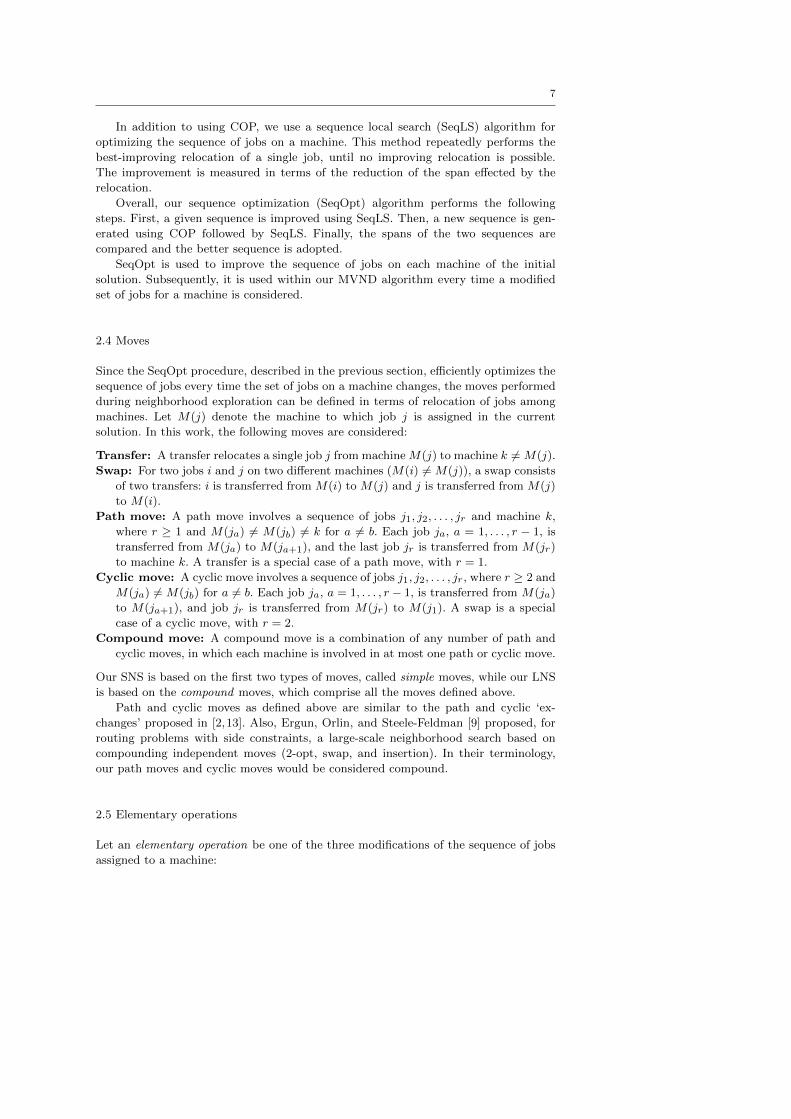
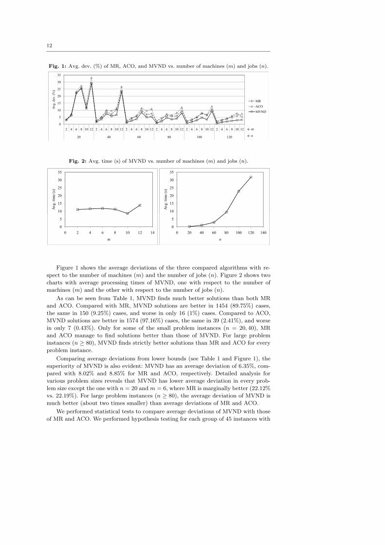
Fig. 1: Avg. dev. (%) of MR, ACO, and MVND vs. number of machines (m) and jobs (n).

5

10

15

20

25

30

35

Avg. dev. (%)

MR

ACO

MVND

0

5

10

15

20

25

30

35

2 4 6 8 10 12 2 4 6 8 10 12 2 4 6 8 10 12 2 4 6 8 10 12 2 4 6 8 10 12 2 4 6 8 10 12

20 40 60 80 100 120

Avg. dev. (%)

MR

ACO

MVND

← m

← n

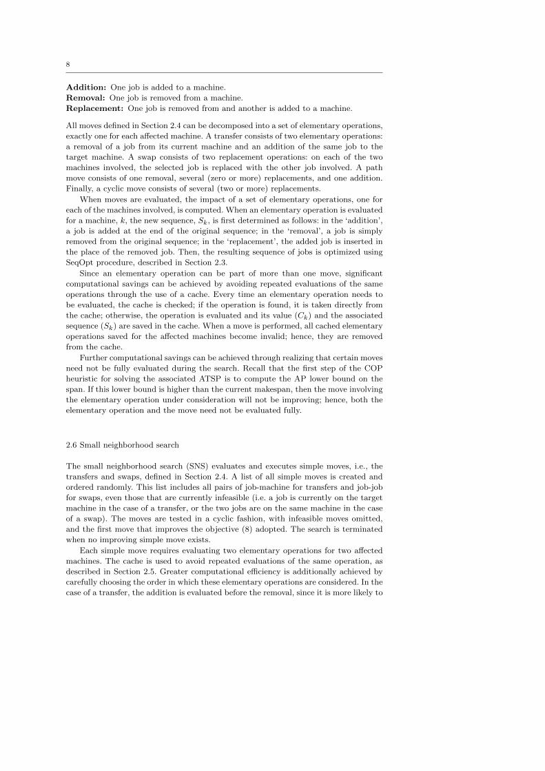
Fig. 2: Avg. time (s) of MVND vs. number of machines (m) and jobs (n).

10

15

20

25

30

35

Avg. time (s)

0

5

10

15

20

25

30

35

0 2 4 6 8 10 12 14

Avg. time (s)

m

10

15

20

25

30

35

Avg. time (s)

0

5

10

15

20

25

30

35

0 20 40 60 80 100 120 140

Avg. time (s)

n

Figure 1 shows the average deviations of the three compared algorithms with re-

spect to the number of machines (m) and the number of jobs (n). Figure 2 shows two

charts with average processing times of MVND, one with respect to the number of

machines (m) and the other with respect to the number of jobs (n).

As can be seen from Table 1, MVND finds much better solutions than both MR

and ACO. Compared with MR, MVND solutions are better in 1454 (89.75%) cases,

the same in 150 (9.25%) cases, and worse in only 16 (1%) cases. Compared to ACO,

MVND solutions are better in 1574 (97.16%) cases, the same in 39 (2.41%), and worse

in only 7 (0.43%). Only for some of the small problem instances (n = 20, 40), MR

and ACO manage to find solutions better than those of MVND. For large problem

instances (n ≥ 80), MVND finds strictly better solutions than MR and ACO for every

problem instance.

Comparing average deviations from lower bounds (see Table 1 and Figure 1), the

superiority of MVND is also evident: MVND has an average deviation of 6.35%, com-

pared with 8.02% and 8.85% for MR and ACO, respectively. Detailed analysis for

various problem sizes reveals that MVND has lower average deviation in every prob-

lem size except the one with n = 20 and m = 6, where MR is marginally better (22.12%

vs. 22.19%). For large problem instances (n ≥ 80), the average deviation of MVND is

much better (about two times smaller) than average deviations of MR and ACO.

We performed statistical tests to compare average deviations of MVND with those

of MR and ACO. We performed hypothesis testing for each group of 45 instances with

13

the same number of jobs, n, and number of machines, m. The null hypothesis was that

the average deviation of MVND is the same as the average deviation of MR and the

alternative was that it is different. There was no sufficient evidence to reject the null

hypothesis for all groups with n = 20 and for the group with n = 40 and m = 12.

In all other groups (29 out of 36), the null hypothesis was rejected with at least 95%

confidence. Hence, we conclude that MVND achievieves significantly better average

deviation than MR with 95% confidence for all groups with n ≥ 40 except for n = 40

and m = 12. Similar tests comparing MVND and ACO showed that MVND achieves

significantly better average deviation than ACO with 95% confidence for all groups

except for one with the smallest number of jobs and the smallest number of machines,

i.e. with n = 20 and m = 2.

It is interesting to note that MVND is superior to ACO for all problem sizes

for which ACO was specifically designed, namely those with a large ratio of jobs to

machines [5] (all cases for which ACO computation times are shown in Table 1).

Despite using an MIP solver, the processing times of MVND are quite modest and

appear deterministic. Figure 2 indicates that the processing time of MVND does not

depend on the number of machines and increases proportionately to the number of

jobs squared.

Taking into account the different processors used, MVND is much faster than ACO

(see the last two columns of Table 1). Average processing times of MVND are one

to two orders of magnitude smaller than average processing times of ACO. Since the

processing times of MR are not available, time comparison between MVND and MR

cannot be made. However, in view of the apparent involvement of the MR algorithm,

it can be surmised that its computation time must be significant. In fact, MR may

actually be slower than ACO, considering the fact that MR and ACO have a common

author, ACO is a newer development, and ACO solutions are on average worse than

those of MR.

4 Conclusions and future work

A variable neighborhood descent, hybridized with mathematical programming ele-

ments, for solving the NP-hard problem of scheduling unrelated parallel machines in

the presence of machine-dependent and job-sequence-dependent setup times, with the

objective of minimizing the makespan, has been presented. Performance of the pro-

posed scheme has been evaluated by comparing its solutions of a set of benchmark

problem instances to the solutions of the best available methods. The results show

that the proposed scheme finds overwhelmingly better solutions in a fraction of the

processing time.

As a rule of thumb, the larger the neighborhood in neighborhood search, the better

the quality of the locally optimal solutions, and the greater the accuracy of the final

solution [1]. However, the larger the neighborhood, the longer it takes to search it,

unless the search is done in an efficient manner. In fact, much of the power of the

proposed scheme derives from searching a large neighborhood efficiently by solving

a mixed-integer programming model that finds a combination of path and cyclic moves

at each iteration.

The choice of a well-behaved objective function is also crucial. While the real objec-

tive is the minimization of the makespan, the use of this objective would have limited

the search considerably, since it would not be possible then to differentiate among

14

many solutions having the same makespan. The adopted objective makes it possible

for a neighborhood search to adopt non-breakthrough moves that improve the efficiency

of the schedules on the machines other than the makespan machine, paving the way

for a breakthrough move that improves the makespan.

Another feature of the proposed scheme is the use of the state-of-the-art method for

job-sequence optimization based on solving the asymmetric traveling salesman problem

and a lower bound derived from the solution of a simple assignment problem. The latter

allows for discovering some non-improving modifications of solutions, which can then

be quickly discounted from further consideration, saving significant computation time.

Apart from providing an effective solution for the problem in hand, this work indi-

cates that hybridization of heuristics with some mathematical programming elements

could provide effective solution schemes for difficult combinatorial optimization prob-

lems. In fact, this appears to be in line with an increasingly popular trend typified by,

for example, [4,8,10–12].

The results presented in this paper are clearly limited to the addressed version of

the UPMS problem. Further work could investigate if other metaheuristics, such as

the tabu-search or the variable neighborhood search [16], applied to the same problem,

could benefit from the key components of the method proposed in this paper. Addition-

ally, since the problem addressed here is one of the most complex UPMS problems, it

would be interesting to investigate if simpler variants of the UPMS could be efficiently

and effectively solved by a similar approach.

5 Acknowledgements

We would like to thank Dr. G. Rabadi for providing detailed results and additional

information on the Meta-RaPS algorithm. We are also indebted to Prof. R. Jonker and

Prof. A. Volgenant for providing us with the code of their shortest augmenting path

algorithm for the simple assignment problem.

References

1. R. K. Ahuja, O. Ergun, J. B. Orlin, and A. P. Punnen. A survey of very large-scaleneighborhood search techniques. Discrete Applied Mathematics, 123:75–102, 2002.

2. R. K. Ahuja, J. B. Orlin, and D. Sharma. New neighborhood search structures for thecapacitated minimum spanning tree problem. Mathematical Programming, 91:71–97, 2001.

3. A. Al-Salem. Scheduling to minimize makespan on unrelated parallel machines with se-quence dependent setup times. Engineering Journal of the University of Qatar, 17:177–187, 2004.

4. C. Archetti, M. Grazia Speranza, and M. W. P. Savelsbergh. An optimization-basedheuristic for the split delivery vehicle routing problem. Transportation Science, 42(1):22–31, 2008.

5. J.P. Arnaout, G. Rabadi, and R. Musa. A two-stage Ant Colony Optimization algorithmto minimize the makespan on unrelated parallel machines with sequence-dependent setuptimes. Journal of Intelligent Manufacturing, 21(6):693–701, 2010.

6. J. Blazewicz, K. H. Ecker, E. Pesch, G. Schmidt, and J. Weglarz. Scheduling computerand manufacturing processes. Springer, Berlin, 1996.

7. P. Brucker. Scheduling algorithms. Springer, Berlin, 2004.8. R. De Franceschi, M. Fischetti, and Toth P. A new ILP-based refinement heuristic for

vehicle routing problems. Mathematical Programming, 105(2–3):471–499, 2006.

9. O Ergun, J. B. Orlin, and A. Steele-Feldman. Creating very large scale neighborhoods outof smaller ones by compounding moves. Journal of Heuristics, 12(1–2):115–140, 2006.

15

10. D. Espinoza, R. Garcia, M. Goycoolea, G. L. Nemhauser, and M. W. P. Savelsbergh.Per-seat, on-demand air transportation part i: problem description and an integer multi-commodity flow model. Transportation Science, forthcoming.

11. K. Fleszar and K. S. Hindi. An effective VNS for the capacitated p-median problem.European Journal of Operational Research, 2008. forthcoming.

12. K. Fleszar and K. S. Hindi. Fast, effective heuristics for the 0–1 multidimensional knapsackproblem. Computers & Operations Research, 2008. forthcoming.

13. A. Frangioni, E. Necciari, and M. G. Scutella. A multi-exchange neighborhood for min-imum makespan parallel machine scheduling problems. Journal of Combinatorial Opti-mization, 8:195–220, 2004.

14. M. Ghirardi and C. N. Potts. Makespan minimization for scheduling unrelated parallelmachines: A recovering beam search approach. European Journal of Operational Research,165(2):457–467, 2005.

15. F. Glover, G. Gutin, A. Yeo, and A. Zverovich. Construction heuristics for the asymmetricTSP. European Journal of Operational Research, 129:555–568, 2001.

16. P. Hansen, M. Mladenovic, and D. Perez-Britos. Variable neighborhood decompositionsearch. Journal of Heuristics, 7(4):335–350, 2001.

17. M. Helal, G. Rabadi, and A. Al-Salem. A tabu search algorithm to minimize the makespanfor the unrelated parallel machines scheduling problem with setup times. InternationalJournal of Operations Research, 3(3):182–192, 2006.

18. J. Hoogeveen, J. K. Lenstra, and S. van de Velde. Sequencing and scheduling. In M. Dell-Amico, F. Maffioli, and S. Martello, editors, Annotated Bibliographies in CombinatorialOptimization, volume 12, pages 181–197. Wiley, 1997.

19. R. Jonker and A. Volgenant. A shortest augmenting path algorithm for dense and sparselinear assignment problems. Computing, 38:325–340, 1987.

20. D-W. Kim, D-G. Na, and F. F. Chen. Unrelated parallel machine scheduling with setuptimes and a total weighted tardiness objective. Robotics and Computer Integrated Manu-facturing, 19:173–181, 2003.

21. C-Y. Lee and M. Pinedo. Optimization and heuristics of scheduling. In P. M. Pardalosand M. G. C. Resende, editors, Handbook of applied optimization. Oxford University Press,New York, 2002.

22. C. F. Liaw, Y. K. Lin, C. Y. Chen, and M. Chen. Scheduling unrelated parallel machinesto minimize total weighted tardiness. Computers and Operations Research, 30:1777–1789,2003.

23. R. Logendran, B. McDonell, and B. Smucker. Scheduling unrelated parallel machines withsequence-dependent setups. Computers and Operations Research, 34(11):3420–3438, 2007.

24. S. Martello, F. Soumis, and P. Toth. Exact and approximation algorithms for makespanminimization on unrelated parallel machines. Discrete Applied Mathematics, 75:169–188,1997.

25. E. Mokotoff. Parallel machine scheduling problems: A survey. Asia-Pacific Journal ofOperational Research, 18(2):193–242, 2001.

26. E. Mokotoff and P. Chretienne. A cutting plane algorithm for the unrelated parallelmachine scheduling problem. European Journal of Operational Research, 141(3):515–525,2002.

27. E. Mokotoff and J. L. Jimeno. Heuristics based on partial enumeration for the unrelatedparallel processor scheduling problem. Annals of Operations Research, 117(1–4):133–150,2002.

28. M. J. Pereira Lopes and J. M. V. de Carvalho. A branch-and-price algorithm for schedulingparallel machines with sequence dependent setup times. European Journal of OperationalResearch, 176(3):1508–1527, 2007.

29. M. Pinedo. Scheduling: Theory, Algorithms, and Systems. Prentice Hall, New Jersey, 2ndedition, 2002.

30. G. Rabadi, R. J. Moraga, and A. Al-Salem. Heuristics for the unrelated parallel machinescheduling problem with setup times. Journal of Intelligent Manufacturing, 17:85–97,2006.

31. M. G. Ravetti, G. R. Mateus, P. L. Rocha, and P. M. Pardalos. A scheduling problem withunrelated parallel machines and sequence dependent setups. Int. J. Operational Research,2(4):380–399, 2007.

32. P. L. Rocha, M. G. Ravetti, G. R. Mateus, and P. M. Pardalos. Exact algorithms for ascheduling problem with unrelated parallel machines and sequence and machine-dependentsetup times. Computers and Operations Research, 35(4):1250–1264, 2008.

16

33. E. Shchepin and N. Vakhania. An absolute approximation algorithm for scheduling unre-lated machines. Naval Research Logistics, 53(6):502–507, 2006.

34. E. V. Shchepin and N. Vakhania. An optimal rounding gives a better approximation forscheduling unrelated machines. Operations Research Letters, 33(2):127–133, 2005.

35. M. Weng, J. Lu, and H. Ren. Unrelated parallel machine scheduling with setup considera-tion and a total weighted completion time objective. International Journal of ProductionEconomics, 70:215–226, 2001.