an integrated genetic-based model of naive bayes networks for credit scoring

International Journal of Artificial Intelligence & Applications (IJAIA), Vol.4, No.1, January 2013

DOI : 10.5121/ijaia.2013.4107 85

AN INTEGRATED GENETIC-BASED MODEL OF

NAIVE BAYES NETWORKS FOR CREDIT

SCORING

Ali Zeinal Hamadani1*,

Ali shalbafzadeh2, Taghi Rezvan

3, and

AfshinShahlayi Moghadam4

1Department of Industrial Engineering, Isfahan University of Technology,

Isfahan 84156-83111, Iran.

*Corresponding author [email protected]

2Department of Electrical and Computer Engineering,

Isfahan University of Technology, Isfahan, 84156-83111, Iran. [email protected]

3Department of Industrial Engineering,


4Department of Industrial Engineering,


Abstract

Inappropriate management in some fields such as credit allocation has imposed too many losses to

financial institutions and even has forced some of them to go bankrupt. Moreover, large volume data sets

collected by credit departments has necessitated utilizing highly accurate models with less complexities.

Credit scoring models with classification and forecasting customers into two groups good and bad can

dramatically reduce risks of granting credits to customers.

In this paper, a novel integrated approach for credit scoring problem is presented. This approach utilizes

rough sets for feature selection during the data pre-processing phase and also adopts two hybrid

sequences, Naïve Bayes networks and genetic algorithm, to classify customers. In order to assess the

competitive performance of the proposed approach, it has been executed on three credit scoring datasets

from the University of California Irvine Machine Learning Repository. Computational results demonstrate

that our approach has superior performance in terms of classification accuracy and achieves higher

overall classification rate as compared to several other previous studies.

Keywords

Credit Scoring, Naïve Bayes networks, Genetic algorithm, Rough sets theory.


86

1. INTRODUCTION

During recent years, inappropriate management in the US and Europe has imposed many losses

to financial institutions such as banks and insurance companies and even has forced many of

them to go bankrupt. On 1997, only in the United States, issuers of credit cards have reported

27.19 billion dollars of loss and these losses have increased to 31.91 billion dollars on 2006 [1].

One of the main duties of a financial institution is to develop some sets of models and techniques

to enable them to predict bankruptcy and to assess credibility of customers [2, 3]. Credit scoring

is based on the idea of segregation of customers of credit cards and applicants of granting loans

into two sets of good and bad. Hence, this problem will be treated as a classification and

forecasting problem [4]. However, some researchers have used clustering techniques for pre-

processing input samples so that they can follow the credit scoring classification process more

wise [5, 6].Statistical techniques and artificial intelligence are both used in credit scoring models.

Logistic regression analysis (LRA) and linear Discriminant analysis (LDA) are two statistical

techniques which are mostly used in credit scoring applications; however there have been some

criticizes to such models since in this models it is assumed that the relation between dependent

and independent variables is linear [7, 8]. By introduction of Quadratic Discriminant Analysis

(QDA), researches prove that in comparison against LRA, QDA is more sensible to the model

assumptions.

Because of the nature of the data sets scorings and inequality covariance matrices of the accepted

and rejected sets, some researchers [9, 10] have criticized LRA and Thomas (2000)has reported

that LRA and LDA are not accurate enough for credit scoring [11].

Since artificial neural networks can easily handle nonlinear relations among dependent and

independent variables then they were the next choices for credit scoring and investigations reveal

that their accuracy is much more than LRA and LDA [12, 13]. But long process of learning

neural networks in finding topology of the optimal network has been a challenge for a long time.

Also because of black-box feature of neural networks they do not have the ability of extracting

the rules. Meanwhile, neural networks are reported to be more accurate in comparison against

decision trees and the K- Nearest Neighbour [13].

Other artificial intelligence techniques such as evolutionary computations and genetic algorithms

[14], support vector machines [15-18] have been reported to have more benefits than statistical

methods and optimization models for assessing risks according to experimental results.

Combinatorial and hybrid models are based on statistical and AI tools and as example we can

refer to neural discriminant models[19], neuro-fuzzy models [20, 21], hybrid model based on

Bayesian approach for attribute selection and support vector machines for clustering [22], neural

network models and support vector machines [15], fuzzy inference and decision trees [23],

combinatorial artificial neural networks and Multivariate Adaptive Regression Splines (MARS)

[24], hybrid models based on support vector machines and genetic algorithms [5], hybrid

techniques based neighbourhood rough set and SVM [25] and multiple kernels multi-criteria

programming approach based on evolution strategy (ES-MK-MCP) [26].

Credit scoring models mostly concentrate on the modelling and evaluation stages of the data

mining process while data pre-processing is less considered. However this stage can have great

impacts on improvement of the final model performance. Wang at el., have utilized rough sets


87

and tabu search for selecting the attributes of credit scoring models during the pre-processing

stage [27]. With selecting attributes, accuracy of models such as logistics, radial basis functions,

and support vector machines have not become worse.

Tsai and Wei investigated the performance of a single classifier as the baseline classifier to

compare with multiple classifiers and diversified multiple classifiers by using neural networks

based on three datasets [28].Nanni and Lumini investigated the performance of several systems

based on ensemble of classifiers for bankruptcy prediction and credit scoring [29]. Xu et al.

proposed hybrid approach using link analysis ranking techniques to pre-process samples into

weighted information, and SVM techniques to build classifiers [30]. Li et al. introduced a linear

combination of kernel functions to enhance the interpretability of credit scoring models, and

propose an alternative to optimize the parameters based on the evolution strategy[31]. Wang et al.

investigated the performance of three popular ensemble methods-Bagging, Boosting, and

Stacking- based on four base learners, i.e., LRA, DT, ANN and SVM on credit scoring problem

[32]. Chi and Hsu selected important variables by GA to combine the bank’s internal behavioural

scoring model with the external credit bureau scoring model to construct the dual scoring model

for credit risk management of mortgage accounts [33].Capotorti and Barbanera suggested a

hybrid model for classification based on the methodologies of rough sets, partial conditional

probability assessments and fuzzy sets for classifying credit applicants into classes of risk on the

basis of probability of default values [34].

In this paper, a novel integrated approach for credit scoring is presented which uses k-means for

discretizing data sets and rough sets for selecting attributes and also utilizes two hybrid

sequences, Naïve Bayes network and genetic algorithm, to classify customers into bad and good.

This approach is executed and evaluated on three famous data sets from Germany, Australia, and

Japan and then assessment metrics including accuracy, recall, precision, and F-measure are

calculated and the performance of the developed models are compared.

This paper has some eminences including: first, it has adopted an integrated approach for

modelling credit scoring which focuses on the data pre-processing stage and then tries to improve

the performance of the credit scoring model by hybridizing the model using Naïve Bayes network

and genetic algorithm. Second, the developed approach is tested and evaluated by three famous

data sets and its better results are verified in comparison against other researches; third,

implementation procedure of the rough set and genetic algorithm has led to lower computational

complexities and as a result execution time has been decreased successfully. The last

specification of the presented model is that by using genetic algorithm, capability of rule

extraction from credit data sets has become possible. The last specification can be used for

justifying rejected customers, conditional admission of a rejected customer, and constructing a

paradigm for customers in order to make credits.

The rest of the paper is as follows. In section2, needed tools and algorithms including rough sets,

genetic algorithm, and Naïve Bayes networks will be briefly reviewed. The developed integrated

approach is presented in section 3 and computational results will be discussed in section4.

Finally, conclusion remarks are discussed and future possible research subjects will be introduced

in section 5.


88

2. THE TOOLS OF THE PROPOSED APPROACH

The proposed integrated approach is based on three tools including: rough set in order to reduce

the problem scale and Naïve Bayes network and genetic algorithm as classifiers. Here these tools

and their related developed algorithms are briefly introduced.

2.1. Rough Set

Pawlak has introduced a rule based methodology using rough sets in order to handle problems

with high level uncertainties and non-monotonous relations among attributes which makes

statistical analysis of data a daunting task [35].

In rough sets, an information system like >=< fVQUS ,,, is a reflection of a data set that

describes the number of objects. In information system S, U is a closed universe of N objects

},...,,{ 21 Nxxx which is a non-empty finite set and Q is a non-empty finite set of n attributes

},...,,{ 21 nqqq which demonstrates the objects. qQq VUV ∈= where Vq is the value of attribute q;

VQUf →×: is an universal decision function where the information function for each Qq ∈

and Ux∈ is qVqxf ∈),( .If in this information system QA ⊆ is subset of attributes and

Uyx ∈, are objects, then x and y are indiscernible if and only if for each Aa ∈ , we have

),(),( ayfaxf = .

In an information system S a specific subset QA ⊆ of attributes determines an approximate

space ))(,( AINDUAS in S. For the sets QA ⊆ and UX ⊆ a lower approximation of A ( )XA−

from the set X in AS and an upper approximation of A ( ) from the set X in AS are defined as

relations (1):

}:{}][:{ * XYAYXxUxXA A ⊆∈∪=∅≠∩∈=−

}:{}][:{ * ∅≠∩∈∪=∅≠∩∈=−

XYAYXxUxXA A

(1)

Boundary zone A- from the set UX ⊆ in AS (uncertain zone from IND(A)) is defined as below:

XAXAXBN A−

−

−=)( (2)

To clarify the details of rough sets more, reader can refer to [35, 36]

The below algorithm is recommended for rough sets:

Step1: Constructing dual difference structures among the objects.

Procedure of lowering the attributes: for each two objects xi and xj a vector aij of the length n

(number of attributes) is constructed according to Table 1 which demonstrates the difference of

the two objects.

XA−


Table 1. Structure of the comp

q0 q1 q2

1 0 1

This vector demonstrates the difference between two objects as

step is a list of polynomial structures similar to table 1.

Step2: Omission of similar polynomial structures.

In order to omit similar polynomial structures, we utilize an algorithm called tree K

algorithm since it is similar to K

capability in omitting polynomial structures rapidly. Here this algorithm is described:

Algorithm tree K-means operates on the basis of two parameters K, number of clusters, and F,

maximum number of cluster members. Structures are being chosen from the beginning of the

polynomial structures list of step 1.

In the first level according to K some branches are established and a structure will be set in each

branch. Then, according to Euclidean distance, K+1th structure is allocated to the closest cluster

from K. The allocation process lasts until the number of allocated structures to the cluster does

not exceed F. The first structure to be allocated to each cluster will be the center of

will not be upgraded. When in a cluster there are F structures, if anothe

added to it, then that cluster is divided in to K clusters of the lower level but the center of the

upper level cluster will not be taken to the lower level. Hence, based on this methodology the

whole structures in the list will be

that they will not be omitted.

Step 3: Merging the sentences

Polynomial structures are entirely arranged according to the number of factors one. Hence, a list

is obtained where the merging procedure of its sentences having capability of merging will be as

below:

3-1-Set the ith structure equal to zero and also set the

list.

3-2-Compare the ith polynomial structure with the

polynomial structure and set the

A reducible polynomial structure is defined as follows. Two polynomial structures x and y can be

reduced to x if both of them have the para

be in y. Hence, this definition corresponds to

3-3-Reduce one unit from j

3-4- if i<j then go to 3-2.

3-5- Add one unit to i.

3-6- If I is not the last element, then go to 3


Table 1. Structure of the comparator of two records from the learning data set

q3 q4 q5 q6 q7 q

1 0 0 1 1 0

This vector demonstrates the difference between two objects as q0∧q2∧q3∧q6∧q7. Output of this

step is a list of polynomial structures similar to table 1.

Omission of similar polynomial structures.

In order to omit similar polynomial structures, we utilize an algorithm called tree K

algorithm since it is similar to K-means and trees. The reason to use such an algorithm is its

tting polynomial structures rapidly. Here this algorithm is described:

means operates on the basis of two parameters K, number of clusters, and F,


lynomial structures list of step 1.



ion process lasts until the number of allocated structures to the cluster does

not exceed F. The first structure to be allocated to each cluster will be the center of the cluster and

will not be upgraded. When in a cluster there are F structures, if another structure wants to be



whole structures in the list will be set in the tree or will be similar to the structure of clusters so


merging procedure of its sentences having capability of merging will be as

structure equal to zero and also set the jth structure equal to the last element of the

polynomial structure with the jth structure. If it is reducible then omit the

polynomial structure and set the ith equal to the result of the difference.


if both of them have the parameter iq and also there is no parameter like

. Hence, this definition corresponds to x ∧ ~ y =0.

not the last element, then go to 3-2.


89

arator of two records from the learning data set

8 q9

0 0

. Output of this

In order to omit similar polynomial structures, we utilize an algorithm called tree K-means

means and trees. The reason to use such an algorithm is its

tting polynomial structures rapidly. Here this algorithm is described:

means operates on the basis of two parameters K, number of clusters, and F,




ion process lasts until the number of allocated structures to the cluster does

the cluster and

r structure wants to be



set in the tree or will be similar to the structure of clusters so


merging procedure of its sentences having capability of merging will be as

structure equal to the last element of the

e. If it is reducible then omit the jth


and also there is no parameter like iq in x to


90

Step 4: Determine reduction and core of the attribute.

Execute the step 2 on polynomial structures which cannot be merged anymore. The remaining

sentences demonstrate the core and the reductions related to attributes.

2.2. Naïve Bayes Networks

In this section, basic concepts of Naïve Bayes networks in classifying problems are discussed.

Such concepts can be further studied in [37].

Bayesian networks are directional acyclic graphs where their vertexes consist of information

about the conditional probability values of a set of variables. In such networks, any sample x can

be described only through the reference combination of its attributes such that these attributes are

conditionally independent and the objective function f(x): vx → can have any value from the

constrained set v. Any sample x is displayed by vector ),,( 1 naa K in which the most probable

objective function value can be obtained by relation 3. In this relation, )( jvP is calculated by

counting the number of times that jv has been viewed in the training data set; but calculation of

)|,,( 1 jn vaaP K is rather impossible except in situations where the training data set is very

large.

)()|,,(maxarg 1 jjnVv

vPvaaPvj

K∈

= (3)

Using the easy assumption Naïve, in which values of attributes are conditionally independent,

probability of viewing reference combination ),,( 1 naa K for a determined objective function

value, can be calculated by multiplying probability of each attribute. Therefore relation (4) is:

∏=∈

=n

i

jijVv

NBvaPvP

j

v1

)|()(maxarg (4)

Where probabilities )( jvP and )( ji vaP are estimated by the number of iterations. Totally these

estimations construct an assumption that can be used in classifying new data. The algorithm

incorporated in Naïve Bayes networks is the same existing algorithm which is widespread in

researches [38-39].

2.3. Genetic Algorithm

Genetic algorithms are usually used in data mining for improving other algorithms or

constructing association rules. Genetic algorithms operate on a population with different

specifications in a determined framework. Genetic algorithms operational procedure is based on

applying several operators including reproduction, crossover, and selection in a combination with

mutation on genes of the initial population in order to generate an improved generation with

better characteristics. For more details on applications of genetic algorithms in the field of data

mining, reader is referred to [40-41].


91

Structure of the designed gene for this problem consists of several chromosomes where each

chromosome is an independent (conditional) attribute. This means that if a data set including n

attributes and one decision attribute, then each gene structure has 1+n chromosome. The

structure of gene has been shown in Fig.1.

Figure 1. The structure of gene

For each gene a fitness function is defined according to equation (5). In this equation, β is

considered to be larger than α. Fitness value is the gene score. Also portsup is the value that

enables a gene, having conditional attributes, to cover the learning data set. Confidence is a

value enables that a gene, with a non-zero portsup percent, to cover those decision attribute in a

specific group.

confidenceportFitness *sup* βα += (5)

In order to generate the initial population the value N is taken from the objects of the learning

data set and then some number of genes equal to the number of conditional attributes are

generated and added to this population. The value of the chromosomes in the structure of these

genes is entirely -1 except a remaining chromosome where allowed values of its corresponding

attribute is randomly allocated to. Therefore, the initial values during the first iteration will be

"attributesof"numberN + .

Selection, mutation, and crossover operators operate according to predetermined probabilities

mutationP and crossoverP in such a way that during a mutation a chromosome is randomly selected

and then a number is randomly selected from the set of possible values of the corresponding

attributes of that chromosome and -1. But in crossover operation, a point is randomly. This point

means a breaking point and crossover operator exchanges the two parts of the gene located on the

both sides of this point.

Number of operations is considered as a percentage of N and also in order to avoid

computational complexities, the maximum of population in every iteration is considered to be a

GA parameter than can be set. The number of operations and the maximum population are

displayed by %Op-Num and maxPOP respectively. Also, if crossover operator performs on the

population then it will just operate on a percentage of the population with high fitness that this

parameter is showed by %High Fitness. The below algorithm is recommended for GA:


92

Step1:Determining input parameters of the genetic algorithm (α , β , N , %Op-Num, maxPOP ,

Iteration-Num, mutationP , crossoverP , %High Fitness). The set parameters of the GA are determined

by trial and errors which are summarized in Table2.

Step2: Generating the initial population

Step3: Calculating scores of each gene according to fitness function and arranging the population.

Step4: Operating mutation and crossover operators and adding the generated genes to the

population

Step5: Until reaching Iteration-Num, execute steps 3 and 4.

During steps 3, 4, and 5 we should note that in each iteration, population size must not exceed the

maximum population size set before. If this happens then remaining must be omitted from the

arranged population.

Table2. Setting parameters of the genetic algorithm based on trial and errors.

Parameter Name Value Parameter Name Value

N 200 crossoverP 60%

%Op-Num 30 %High Fitness 30%

maxPOP 300000 α 1

Iteration-Num 100 β 4

mutationP 10%

During the last iteration, we reach an arranged population which is the set of extracted rules of the

genetic algorithm. In order to increase the quality of the rules, two predetermined threshold levels

for two “support” and “confidence” are being considered so that only high quality rules are kept.

3. THE PROPOSED INTEGRATED APPROACH

The proposed integrated approach is constructed based on the data mining process CRSP-DM. A

scheme of the approach is depicted in Fig. 2. There are pseudo codes of the used tools for creating

the proposed models. In this approach, during the preparation stage, discretization of data is done

by K-means and attribute reduction is performed by rough set. Also combination of Naïve Bayes

networks and genetic algorithm with two different sequences is utilized during the modeling

stage. Hence, according to existence of two different states during the preparation stage, with and

without attribute reduction, and two modeling states, four states are ultimately possible. Although

Naïve Bayes networks and genetic algorithms can be considered individually during the modeling

stage but it is proved that their accuracy is more in hybrid form so we individual states are not

investigated here. Assessment of the developed models is performed by K- cross validation and

also comparison of ordinary indexes.

Algorithm K-means which is used in discretization is to some extent different from the K-means

algorithm used for clustering purposes. Second root of objects determines K. In order to allocate

data to the determined sets we have: based on the number of sets, values of attributes are

allocated to sets from the first of the line until each set has one value. Then, other values are

allocated according to closeness to the center of the set. During each allocation, the center is

being updated. This process continues until all the values are allocated. At the end, each set is

being tagged and the allocated data to each set will poses the same tag.


93

Figure 2. A schematic view of the proposed integrated approach

Since a probability is estimated for each class in Naïve Bayes networks then if the difference of

estimated probabilities two classes in the hybrid model is less than the predetermined difference

then the winner class is determined by the rules extracted by the genetic algorithm. In the hybrid

model of the GA and Naïve Bayes networks, if the extracted rules by the GA are not able to

determine the new object set then Naïve Bayes classifier will be used to determine the class.

The proposed integrated approach introduced in section 3 led to 4 models called “Not Rough

+NB +GA”, “Rough +NB+GA”, “Not Rough+ GA+NB” and “Rough +GA+NB”. Flowchart of

models Rough +NB+GA” and “Rough +GA+NB” is shown in Fig. 3.In other two models, there is

notthe reduction stage by rough set theory.

4. EXPERIMENTAL ANALYSIS

4.1. Real world credit data sets

Three real world data sets including Australian, German, and Japanese data sets are depicted in

table3. These data sets can be accessed from UCI Repository of Machine Learning Databases

which is adopted to assess the newly developed models [42]. The German data set is not balanced

where 700 customer samples are good and 300 customer samples are bad. For each applicant, 20

conditional attributes are registered: history, account balances, loan purpose, loan amount,

employment status, personal information, age, housing, and job title. Australian and Japanese

data sets are nearly balanced and include 307 customers with good credit and 383 customers with

bad credit and the difference between the registered attributes for each applicant in the two data

sets is only in a single numerical attribute. In Japanese data set numerical and nominal miss value

data are completed using mean and mode, respectively

ModelDiscretization Reduction

Rough Set ResultData

BayesGenetic

GeneticBayes

K-Means


94

Figure 3. Learning process, “Rough +GA+NB” and Rough +NB+GA”

(respectively from left to right)

4.2. Results of the proposed models

The models “Not Rough +NB +GA”, “Rough +NB+GA”, “Not Rough+ GA+NB” and “Rough

+GA+NB” are executed on three data sets from Germany, Australia, and Japan and the

computational results are summarized in tables 4, 5, and 6.


95

Table 3. Credit scoring databases from the UCI Repository

Total

Features

Conditional

Features

#

Instances Of

Creditworthy

Class

#

Instances Names

Nominal

Feature

Numeric

Feature

21 7 13 700 1000 German

15 6 8 307 690 Australian

16 6 9 307 690 Japanese

According to table4, classification accuracies for the German data set for the four models are

83.60%, 88.00%, 84.00%, and 88.20%, respectively. These values are obtained for models which

use rough set for reducing the attributes of their data set. It can be seen that the sequence GA+NB

is slightly better than NB+GA. Index values of Precision parameters in contrast to Recall is low

which demonstrates that the developed models for prediction of creditworthy class are more

accurate in comparison with the other class.

Table 4. Summarized results with 5-cross validation for German credit data set

Model Name

Accuracy Recall Precision F-measure

Avg.

(%)

Std.

(%)

Avg.

(%)

Std.

(%)

Avg.

(%)

Std.

(%)

Avg.

(%)

Std.

(%)

“Not

Rough+NB+GA”

83.60 1.06 93.51 2.61 84.73 3.06 88.84 1.24

“Rough+NB+GA” 88.00 2.15 96.57 1.37 87.57 2.81 91.83 1.54

“Not Rough+

GA+NB” 84.00 1.37 94.04 2.18 84.79 2.73 89.13

1.21

“Rough+GA+NB” 88.20 2.20 96.72 1.07 87.70 2.92 91.96 1.57

According to table5, classification accuracies for the Australian data set for the four models are

88.41%, 92.61%, 85.65%, and 88.12%, respectively and accuracy of the models which have used

rough set algorithm to reduce attributes are higher. Since the values of other evaluation indexes

are high then one can say that the developed models have the same performance for prediction in

the both classes.

Table 5. Summarized results with 5-cross validation for Australian credit data set

Model Name


Avg.

(%)

Std.

(%)

Avg.

(%)

Std.

(%)

Avg.

(%)

Std.

(%)

Avg.

(%)

Std.

(%)

“Not

Rough+NB+GA”

88.41 3.12 87.95 1.72 86.40 4.40 87.10 3.02

“Rough+NB+GA” 92.61 1.88 90.56 3.38 92.83 3.80 91.60 2.07

“Not Rough+

GA+NB” 85.65 3.49 85.64 1.95 82.92 5.47 84.21

3.45

“Rough+GA+NB” 88.12 1.67 82.34 3.56 89.98 1.86 85.97 2.56


According to table6, classification accuracies for the Japanese data set for the four models are


rough set algorithm to reduce attributes are higher. Comparison of models 1 and 3 with models 2

and 4 shows the accuracy of the models without rough set to be meaningful. Also by comparing

the accuracy values we can conclude that the sequence “GA+NB” is slightly

“NB+GA”. On the other hand, low value of the attribute Recall, especially in models 2 and 4,

demonstrates that the prediction power of models for the Creditworthy class is weaker than the

other class.

Table 6. Summarized results with 5

Model

name

Accuracy

Avg.

(%)

“Not

Rough+NB+GA”

92.12

“Rough+NB+GA” 85.91

“Not Rough+

GA+NB” 92.42

“Rough+GA+NB” 86.67

Performance of the developed models on data

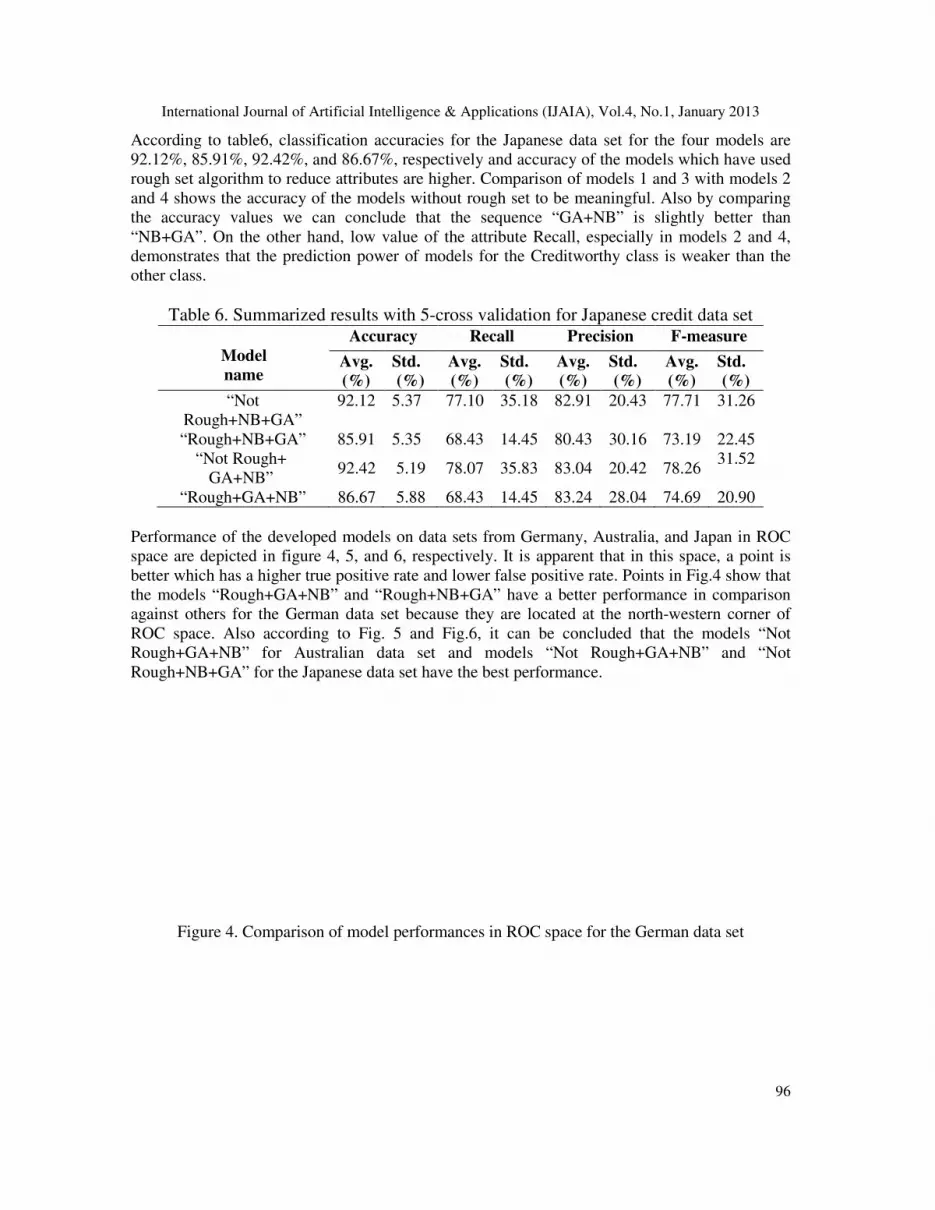
space are depicted in figure 4, 5, and 6, respectively. It is apparent that in this space, a point is

better which has a higher true positive rate and lower false positive rate. Points in Fig.4 show that

the models “Rough+GA+NB” and “Rough+NB+GA” have a better performance in comparison

against others for the German data set because they are located at the north

ROC space. Also according to Fig. 5 and Fig.6, it can be concluded that the models

Rough+GA+NB” for Australian data set and models “Not Rough+GA+NB” and “Not

Rough+NB+GA” for the Japanese data set have the best performance.

Figure 4. Comparison of model performances in ROC space for the German data set




set algorithm to reduce attributes are higher. Comparison of models 1 and 3 with models 2


the accuracy values we can conclude that the sequence “GA+NB” is slightly



Table 6. Summarized results with 5-cross validation for Japanese credit data set


Avg.

(%)

Std.

(%)

Avg.

(%)

Std.

(%)

Avg.

(%)

Std.

(%)

Avg.

(%)

92.12 5.37 77.10 35.18 82.91 20.43 77.71

85.91 5.35 68.43 14.45 80.43 30.16 73.19

92.42 5.19 78.07 35.83 83.04 20.42 78.26

86.67 5.88 68.43 14.45 83.24 28.04 74.69

Performance of the developed models on data sets from Germany, Australia, and Japan in ROC



odels “Rough+GA+NB” and “Rough+NB+GA” have a better performance in comparison

against others for the German data set because they are located at the north-western corner of

ROC space. Also according to Fig. 5 and Fig.6, it can be concluded that the models


Rough+NB+GA” for the Japanese data set have the best performance.



96



set algorithm to reduce attributes are higher. Comparison of models 1 and 3 with models 2


the accuracy values we can conclude that the sequence “GA+NB” is slightly better than



credit data set

measure

Std.

(%)

77.71 31.26

73.19 22.45

78.26 31.52

74.69 20.90

sets from Germany, Australia, and Japan in ROC



odels “Rough+GA+NB” and “Rough+NB+GA” have a better performance in comparison

western corner of

ROC space. Also according to Fig. 5 and Fig.6, it can be concluded that the models “Not




Figure 5. Comparison of model performances in ROC space for the Australian data set

Figure 6. Comparison of model performances in ROC space for the Japanese data set

According to the obtained results from Tables and Figures it can be concluded that it is better

test rough set algorithm on such data sets which have more conditional attributes. On the other

hand, it is not reasonable to conclude that if a model operates well on a data set then it will

necessarily give the same result on another data set. In fac

between customer who are applying for credits based on their culture and their socio

situation. As a conclusion, if someone wants to perform this process on another country, then

other integrated models must be tested on its data set so that a more efficient model is obtained.

4.3. Comparisons of different models

In order to evaluate the effectiveness of the proposed credit scoring models, the obtained results

are also compared with other approaches developed

from Table 7, that the proposed classifier has the best credit scoring capability in terms of the

overall classification rate.


Comparison of model performances in ROC space for the Australian data set


According to the obtained results from Tables and Figures it can be concluded that it is better



necessarily give the same result on another data set. In fact, this proves behavioral differences

between customer who are applying for credits based on their culture and their socio


e tested on its data set so that a more efficient model is obtained.

4.3. Comparisons of different models


other approaches developed in the recent literature. It can be concluded,



97

Comparison of model performances in ROC space for the Australian data set


According to the obtained results from Tables and Figures it can be concluded that it is better to



t, this proves behavioral differences

between customer who are applying for credits based on their culture and their socio-economic


e tested on its data set so that a more efficient model is obtained.


It can be concluded,



98

Table 7. Accuracies with the different methods for Australian, German and Japanese data sets

Author (year) method used Accuracy rate (%)

Australian German Japanese

Tsai and Wu (2008) [28] neural network ensembles 88.09 79.38 86.98

Luo et al. (2009) [6]

clustering-launched

classification

86.52 84.80 -

GA+SVM 86.9 77.92 -

Nanni and Lumini (2009)

[29]

Random Subspace ensemble

methods

87.05 73.93 87.34

MLP 85.74 75.00 86.96

Ping and Yongheng

(2011)[25]

Neighborhood rough set and

SVM

87.52 76.60 -

Wang et al. (2011) [32] LRA 86.56 76.14 -

DT 84.39 72.10 -

ANN 83.28 71.43 -

SVM 85.67 76.28 -

Li et al. (2011) [26] ES-MK-MCP 89.01 78.92 -

Jabeen and Baig (2012) [43] Two layered Genetic

Programming

90.79 79.00 -

Our classifiers

“Not Rough+NB+GA” 88.41 83.60 92.12

“Rough+NB+GA” 92.61 88.00 85.91

“Not Rough+ GA+NB” 85.65 84.00 92.42 “Rough+GA+NB” 88.12 88.20 86.67

5. CONCLUSIONS AND FUTURE RESEARCHES

Credit scoring is known to be one of the techniques used for reducing the risks of granting credits

to customers of banks and financial institutions and is considered as a classification problem in

the field of datamining. Presenting hybrid integrated models, this paper has increased efficacy of

credit scoring models. Such an improvement is demonstrated by testing on three data sets from

Germany, Australia, and Japan. According to the results, we can conclude that the improvements

on performance of the models in this research in comparison against past studies are

remarkable.The model “Not Rough+GA+NB” is also more efficient on the three tested data sets

comparing to other models. Although power of models in predicting two classes of the three sets

were different and prediction power of the model on the German data set in not-Creditworthy

class was better but for Japan case situation of the other class is better. Also equal power of

models for the both classes is verified by tests on the Australian model.

Developing a probabilistic or fuzzy model so that enables us to determine how much a customer

belongs to good or bad groups can be reasonable. Development of credit scoring models for

future researches can include models which assist customers in increasing his credit or in

justifying him. In other words, customer finds out his credit weaknesses.


99

Acknowledgement

This paper is dedicated to the memory of Dr. Ali Arkan, friend and colleague, who passed away

during submission of the manuscript.

Appendix Pseudo code of the used tools for creating the proposed models are as follows:

K-means for discretization ///In learning phase

for c=1 to Feature Count

For n=1 to K(c)

Count(c,n)=0

m(c,n)= feature(c) from (Random ItemSetin dataset)

For each ItemSet s1 in dataset

for each feature f in Dataset

Select n such that EqlidianDistance[ m(f,n), s1(f) ] is minimum

Count(c,n) +=1

m(c,n)= ( s1(f) - m(c,n) )/ Count(c,n)

//In prediction phase

For each feature f in Dataset

Select n such that EqlidianDistance[ m(f,n), s1(f) ] is minimum

s1(f)=n

Rough Set Theory for reduction Foreach pair of records row1, row2 in dataset

Generate Polynomial p(p1 or p2 or p3 or ..pn) where pi is column where row1.ci <>row2.ci

Add p to set(s)

Reducing Polynomial

Create List (L) from set(s)

Sort List (L) by length of polynomials

For each pair of Polynomial P1,P2 in List L

Check if P1 ^ P2= P1 then remove P2 from L

//End of simplifying list of polynomials

While List (L) is not Empty

Select Polynomial P1, P2 from List(L) and remove them

Generate CNF form of (P1^P2) and add to List (L2)

Sort List(L2) by length of polynomials

For each pair of Polynomial P1, P2 in List L2

Check if P1 ? P2= P1 then remove P1 from L2.

Name the First Polynomial in List (L2) , P

Remove every Column where it is not exist in P

//End of Rough set for reducing dimension.

Naïve Bayes Network as classifier Predict(Itemset T)

foreach class C in target values

P(C)=1


100

for each feature f in T

N(c,f)= The number of Itemsets I in Dataset which I.f=T.f and I.Target= C

pc= The number of Itemsets I in Dataset I.Target= C

P(C)=P(C)*p(c,f)/ pc

Select C with minimum P(C)

Genetic Algorithm as classifier //initial poplulation

Do for START_POP times

Select random ItemSet I from Dataset

Generate gene G from I add it to population p

// iterating

Do for MAX_ITERATE times

Sort Population by Confidence of Genes()

Do for (CROSS_OVER_RATIO * PopulationSize ) times

Select gp1,gp2 from TOP N% Population

Cross over gp1,gp2 with position random and generate gc1,gc2

Add gc1,gc2

Do for (MUTATION_RATIO * PopulationSize ) times

Select gpfrom TOP N% Population

Select position random P from gp

Generate random number r 0 or 1

If r=1 then

GP[p]=-1 // don care it

ELSE

GP[p]= random Category

If population > MAX_POPULATION

Remove Exceed Popultion

SELECT TOP N% population as rules

Remove rule which has Confidence <MinConfidence

REFERENCES

[1] L. Zhou, K.K. Lai & L. Yu, (2010) “Least squares support vector machines ensemble models for

credit scoring”, Expert Systems with Applications, Vol. 37, No. 1,pp 127-133.

[2] A. F.Atiya, (2001)“Bankruptcy prediction for credit risk using neural networks: a survey and new

results”,IEEE Transactions on Neural Networks,Vol. 12, No. 4,pp929–935.

[3] G.P. Zhang, M.Y. Hu, B.E. Patuwo, & D.C. Indro, (1999) “Artificial neural networks in bankruptcy

prediction: General framework and cross-validation analysis”, European Journal of Operational

Research,Vol. 116, No. 1,pp16–32.

[4] R. A. Johnson & D.W. Wichern, (2007) Applied multivariate statistical analysis (5th ed.), Prentice-

Hall, Upper Saddle River, NJ.

[5] N. C. Hsieh, (2005) “Hybrid mining approach in the design of credit scoring models”, Expert Systems

with Applications,Vol. 28, No. 4,pp655–665.

[6] Sh.-T. Luo, B.-W.Cheng & Ch.-H. Hsieh, (2009)“Prediction model building with clustering-launched

classification and support vector machines in credit scoring”, Expert Systems with Applications,Vol.

36, No. 4,pp7562-7566.

[7] G. Karels& A. Prakash, (1987) “Multivariate normality and forecasting of business bankruptcy”,

Journal of Business Finance Accounting, Vol. 14, No. 4,pp573–593.


101

[8] A. K. Reichert, C. C. Cho & G. M. Wagner, (1983) “An examination of the conceptual issues

involved in developing credit-scoring models”, Journal of Business and Economic Statistics, Vol.

1,pp101–114.

[9] D. West, (2000) “Neural network credit scoring models”, Computers and Operations Research,Vol.

7,pp1131–1152.

[10] W. R. Dillon & M. Goldstein (1984), Multivariate analysis methods and applications, New York, NY:

Wiley.

[11] L. C. Thomas, (2000) “A survey of credit and behavioural scoring: Forecasting financial risks of

lending to customers”, International Journal of Forecasting, Vol. 16,pp149–172.

[12] V. S. Desai, J. N. Crook & G. A. Overstreet, (1996) “A comparison of neural networks and linear

scoring models in the credit union environment”, European Journal of Operational Research, Vol.

95,pp24–37.

[13] K.Y. Tam & M.Y. Kiang, (1992) “Managerial applications of neural networks: The case of bank

failure predictions”, Management Science,Vol. 38 No. 7, pp 926–947.

[14] M.C. Chen & S.H. Huang, (2003) “Credit scoring and rejected instances reassigning through

evolutionary computation techniques”, Expert Systems with Applications, Vol. 24,pp433–441.

[15] Z., Huang, H.C. Chen, C.J. Hsu, W.H. Chen & S.S. Wu, (2004)“Credit rating analysis with support

vector machines and neural networks: a market comparative study”, Decision Support Systems, Vol.

37,pp543–558.

[16] K. K. Lai, L. Yu, L.G. Zhou & S.Y. Wang, (2006) “Credit risk evaluation with least square support

vector machine”, Lecture Notes in Artificial Intelligence, Vol. 4062, pp 490–495.

[17] K. B. Schebesch& R. Stecking, (2005) “Support vector machines for classifying and describing credit

applicants: Detecting typical and critical regions”, Journal of the Operational Research Society,Vol.

56,pp1082–1088.

[18] T.Bellotti& J. Crook, (2009)“Support vector machines for credit scoring and discovery of significant

features”, Expert Systems with Applications, Vol. 36,pp3302–3308.

[19] T.-S. Lee, C.-C.Chiu, C.-J.Lu & I.-F.Chen, (2002) “Credit scoring using the hybrid neural

discriminant technique”, Expert Systems with Applications, Vol. 23,pp245–254.

[20] R., Malhotra& D.K. Malhotra, (2002)“Differentiating between good credits and bad credits using

neuro-fuzzy systems”, European Journal of Operational Research, Vol. 136,pp190–211.

[21] S. Piramuthu, (1999)“Financial credit-risk evaluation with neural and neurofuzzy systems”, European

Journal of Operational Research,Vol. 112,pp310–321.

[22] C. Gold, A. Holub& P. Sollich, (2005)“Bayesian approach to feature selection and parameter tuning

for support vector machine classifiers”, Neural Networks,Vol. 18 No 5–6, pp 693–701.

[23] M.B. Yobas, J. Crook, & P. Ross, (2000) “Credit scoring using neural and evolutionary techniques”,

IMA Journal of Mathematics Applied in Business and Industry,Vol. 11, No. 2,pp111–125.

[24] T. S. Lee & I. F. Chen,(2005) “A two-stage hybrid credit scoring model using artificial neural

networks and multivariate adaptive regression splines”,Expert Systems with Applications, Vol.

28,pp743–752.

[25] Y. Ping & L. Yongheng, (2011) “Neighbourhood rough set and SVM based hybrid credit scoring

classifier”,Expert Systems with Applications,Vol. 38,pp11300–11304.

[26] J. Li, L. Wei, G. Li & W.Xu, (2011)“An evolution strategy-based multiple kernels multi-criteria

programming approach: The case of credit decision making”,Decision Support Systems, Vol. 51, pp

292–298.

[27] J. Wang, K. Guo& Sh. Wang, (2010) “Rough set and Tabu search based feature selection for credit

scoring”, Procedia Computer Science,Vol. 1,pp2425-2432.

[28] Ch.-F. Tsai,&Jh.-W. W, (2008) “Using neural network ensembles for bankruptcy prediction and

credit scoring”,Expert Systems with Applications, Vol. 34,pp 2639–2649.

[29] L. Nanni& A. Lumini, (2009) “An experimental comparison of ensemble of classifiers for bankruptcy

prediction and credit scoring”,Expert Systems with Applications, Vol. 36,pp3028–3033.

[30] X. Xu, Ch. Zhou, Zh. Wang, (2009) “Credit scoring algorithm based on link analysis ranking with

support vector machine”, Expert Systems with Applications, Vol. 36, pp 2625–2632.


102

[31] J. Lia, L. Wei, G. Li& W. Xu, (2011) “An evolution strategy-based multiple kernels multi-criteria

programming approach: The case of credit decision making”,Decision Support Systems,Vol.

51,pp292–298.

[32] G. Wang, J. Hao, J. Ma, H. Jiang, (2011) “A comparative assessment of ensemble learning for credit

scoring”, Expert Systems with Applications, Vol. 38, pp 223-230.

[33] B-W. Chi, Ch-Ch. Hsu, (2012) “A hybrid approach to integrate genetic algorithm into dual scoring

model in enhancing the performance of credit scoring model”, Expert Systems with Applications,

Vol.39, No. 3, pp 2650-2661.

[34] A. Capotorti, E. Barbanera, (2012) “Credit scoring analysis using a fuzzy probabilistic rough set

model”, Computational Statistics and Data Analysis,Vol. 56, No. 4, pp 981-994.

[35] Z. Pawlak, (1982)“Rough sets”, International Journal of Computer and Information Science,Vol.

11,pp341–356.

[36] Z. Pawlak, (1991) Rough Sets- Theoretical Aspects of Reasoning about Data, Kluwer Academic

Publisher, Netherlands.

[37] D. Heckerman, D. Geiger & D. M. Chickering, (1995) “Learning Bayesian Networks: The

Combination of Knowledge and Statistical Data”, Machine Learning, Vol. 20,pp197-243.

[38] P. Cheeseman& J. Stutz, (1996) Bayesian classification (AutoClass): Theory and results, In Advances

in knowledge discovery and data mining,Menlo Park, CA: AAAI Press.

[39] M.M. Morales, N.C. Ramírez, J.L.J. Andrade & R.G. Domínguez, (2004) “Bayes-N: an algorithm for

learning Bayesian networks from data using local measures of information gain applied to

classification problems”. MICAI: Advances in Artificial Intelligence, Lecture Notes in Artificial.

[40] A. Kamrani, W. Rong& R. Gonzales, (2001) “A genetic algorithm methodology for data mining and

intelligent knowledge acquisition”, Computer & industrial Engineering, Vol. 40 No. 4,pp361-377.

[41] S.P. Deepa, K.G. Srinivasa, K.R. Venugopal&L.M. Patnaik, (2005) “Dynamic association rule

mining using genetic algorithm”, Intelligent Data Analysis,Vol. 9, No. 5,pp439-453.

[42] S. Hettich, C. L. Blake, C. J. Merz, (1998). UCI repository of data mining databases, Available from:

http://www.ics.uci.edu/∼mlearn/MLRepository.html.

[43] H.Jabeen& A. R. Baig, (2012) “Two layered Genetic Programming for mixed-attribute data

classification”,Applied Soft Computing,Vol. 12,pp416–422.

Biographical notes

Ali Zinal-Hammadani is a professor in Department of Industrial Engineering at Isfahan

University of Technology, Isfahan, Iran. His research interests are in the areas of statistics,

Quality control, Multivariate statistical analysis, Data mining and reliability modeling. He

has numerous publications in international journals and conferences

Ali Shalbafzadeh received his MS degree in software engineering from Isfahan University

of Technology, Iran, in 2011. His research interests include data mining and intelligent

systems.


103

TaghiRezvan is a PhD student in Department of Industrial Engineering at Isfahan

University of Technology, Iran from 2009. His research interests are in the areas of data

mining, operation research, risk management and intelligent systems. He has published

several journal papers and conference papers in the above filed.

AfshinShahlaieMoghadam received his MS degree in industrial engineering from Isfahan

University of technology university, Iran. His fields of interests are: financial

management, strategic implementation Model especially balanced scorecard, IT project

management, Risk Analysis.

an integrated genetic-based model of naive bayes networks for credit scoring

Documents