MSE Superiority of Bayes and EmpiricalBayes Estimators in Two Generalized

Seemingly Unrelated Regressions ∗

Lichun Wang † Noel VeraverbekeDepartment of Mathematics, Beijing Jiaotong University, Beijing 100044, China

Center for Statistics, Hasselt University, 3590 Diepenbeek, Belgium

Abstract This paper deals with the estimation problem in a system of two seeminglyunrelated regression equations where the regression parameter is distributed according

to the normal prior distribution N(β0, σ2βΣβ). Resorting to the covariance adjustment

technique, we obtain the best Bayes estimator of the regression parameter and prove itssuperiority over the best linear unbiased estimator (BLUE) in terms of the mean square

error (MSE) criterion. Also, under the MSE criterion, we show that the empirical Bayesestimator of the regression parameter is better than the Zellner type estimator whenthe covariance matrix of error variables is unknown.

Keywords: Bayes method; seemingly unrelated regressions, covariance adjusted approach,mean square error criterion.2000 MSC: Primary: 62J05, 62F11; Secondary: 62C10, 62C12

1. Introduction

The seemingly unrelated regression system was first introduced by Zellner (1962,

1963) and later developed by Kementa and Gilbert (1968), Mehta and Swamy (1976)

and Wang (1988), etc. Recently, in a special issue of Journal of Statistical Planning

and Inference 88 (2000), Gao and Huang establish some finite sample properties of the

Zellner estimator in the context of m seemingly unrelated regression equations, whereas,

Liu proposes a two stage estimator and proves its superiorities over the ordinary least

square estimator and Zellner type estimator under mean square error matrix criterion.

∗Partly supported by NNSF of China (10571001) and IUAP(P6/03) of Belgium†Corresponding author: wlc@amss.ac.cn

1

Differing from the past works, in this paper we employ the Bayes and empirical

Bayes approach to construct the estimators of the regression parameter and exhibit

their MSE properties. Also, differing from the above regressions, here we do not make

the same dimension assumption of observation vectors.

A system of two generalized seemingly unrelated regression equations is given by

y1 = X1β + u1, y2 = X2γ + u2, (1.1)

where y1 and y2 are m × 1 and n × 1 vectors of observations (m 6= n, without loss of

generality, let m > n ), X1 and X2 are m × p1 and n × p2 matrices with full column

rank, β and γ are vectors of unknown parameters, u1 and u2 are m×1 and n×1 vectors

of error variables, and

E(u1) = 0, E(u2) = 0,

Cov(u1, u1) = σ11Im, Cov(u2, u2) = σ22In,

Cov(u1, u2) = σ12

(In

0

), Cov(u2, u1) = σ21(In

...0),

where Σ∗ = (σij) is a 2 × 2 non-diagonal positive definite matrix. Such a system

(usually m = n) appears in many research fields and has received considerable attention

including the above authors and Chen (1986), Lin (1991) and so on.

Denote y = (y′1, y′2)′, X = diag(X1, X2), α = (β′, γ′)′, u = (u′1, u

′2)′, Σij = Cov(ui, uj).

Then (1.1) can be represented as

y = Xα + u, E(u) = 0, Cov(u) = Σ, (1.2)

where Σ = (Σij)2×2 is a partitioned matrix.

In what follows, our main concern is how to estimate β better. To adopt the Bayes

and empirical Bayes approach, we assume that the prior distribution of the parameter

β is

β ∼ N(β0, σ2βΣβ), (1.3)

2

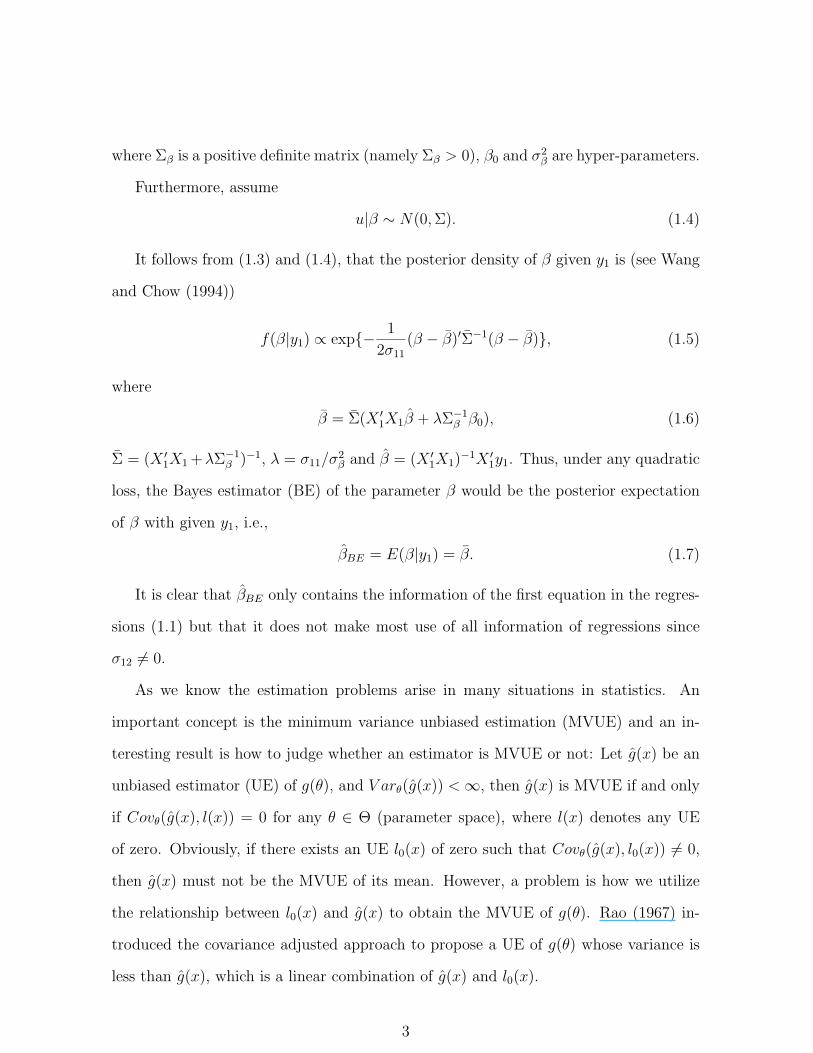
where Σβ is a positive definite matrix (namely Σβ > 0), β0 and σ2β are hyper-parameters.

Furthermore, assume

u|β ∼ N(0, Σ). (1.4)

It follows from (1.3) and (1.4), that the posterior density of β given y1 is (see Wang

and Chow (1994))

f(β|y1) ∝ exp{− 1

2σ11

(β − β)′Σ−1(β − β)}, (1.5)

where

β = Σ(X ′1X1β + λΣ−1

β β0), (1.6)

Σ = (X ′1X1 +λΣ−1

β )−1, λ = σ11/σ2β and β = (X ′

1X1)−1X ′

1y1. Thus, under any quadratic

loss, the Bayes estimator (BE) of the parameter β would be the posterior expectation

of β with given y1, i.e.,

βBE = E(β|y1) = β. (1.7)

It is clear that βBE only contains the information of the first equation in the regres-

sions (1.1) but that it does not make most use of all information of regressions since

σ12 6= 0.

As we know the estimation problems arise in many situations in statistics. An

important concept is the minimum variance unbiased estimation (MVUE) and an in-

teresting result is how to judge whether an estimator is MVUE or not: Let g(x) be an

unbiased estimator (UE) of g(θ), and V arθ(g(x)) < ∞, then g(x) is MVUE if and only

if Covθ(g(x), l(x)) = 0 for any θ ∈ Θ (parameter space), where l(x) denotes any UE

of zero. Obviously, if there exists an UE l0(x) of zero such that Covθ(g(x), l0(x)) 6= 0,

then g(x) must not be the MVUE of its mean. However, a problem is how we utilize

the relationship between l0(x) and g(x) to obtain the MVUE of g(θ). Rao (1967) in-

troduced the covariance adjusted approach to propose a UE of g(θ) whose variance is

less than g(x), which is a linear combination of g(x) and l0(x).

3

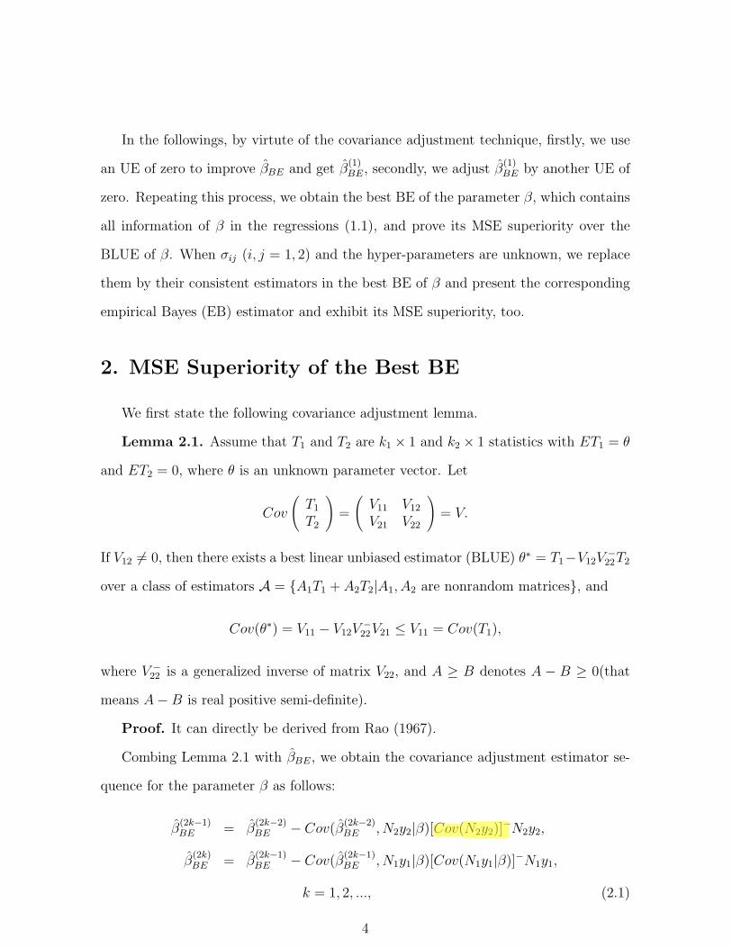
In the followings, by virtute of the covariance adjustment technique, firstly, we use

an UE of zero to improve βBE and get β(1)BE, secondly, we adjust β

(1)BE by another UE of

zero. Repeating this process, we obtain the best BE of the parameter β, which contains

all information of β in the regressions (1.1), and prove its MSE superiority over the

BLUE of β. When σij (i, j = 1, 2) and the hyper-parameters are unknown, we replace

them by their consistent estimators in the best BE of β and present the corresponding

empirical Bayes (EB) estimator and exhibit its MSE superiority, too.

2. MSE Superiority of the Best BE

We first state the following covariance adjustment lemma.

Lemma 2.1. Assume that T1 and T2 are k1 × 1 and k2 × 1 statistics with ET1 = θ

and ET2 = 0, where θ is an unknown parameter vector. Let

Cov

(T1

T2

)=

(V11 V12

V21 V22

)= V.

If V12 6= 0, then there exists a best linear unbiased estimator (BLUE) θ∗ = T1−V12V−22T2

over a class of estimators A = {A1T1 + A2T2|A1, A2 are nonrandom matrices}, and

Cov(θ∗) = V11 − V12V−22V21 ≤ V11 = Cov(T1),

where V −22 is a generalized inverse of matrix V22, and A ≥ B denotes A − B ≥ 0(that

means A−B is real positive semi-definite).

Proof. It can directly be derived from Rao (1967).

Combing Lemma 2.1 with βBE, we obtain the covariance adjustment estimator se-

quence for the parameter β as follows:

β(2k−1)BE = β

(2k−2)BE − Cov(β

(2k−2)BE , N2y2|β)[Cov(N2y2)]

−N2y2,

β(2k)BE = β

(2k−1)BE − Cov(β

(2k−1)BE , N1y1|β)[Cov(N1y1|β)]−N1y1,

k = 1, 2, ..., (2.1)

4

where β(0)BE = βBE.

Simple induction computation yields

β(2k−1)BE = ΣX ′

1(P1 + ρ2N2N1)k−1(y1 −

σ12

σ22

N2y2) + λΣΣ−1β β0,

β(2k)BE = ΣX ′

1(P1 + ρ2N2N1)ky1 − ΣX ′

1(P1 + ρ2N2N1)k−1σ12

σ22

N2y2

+λΣΣ−1β β0, (2.2)

where ρ2 = σ212/(σ11σ22), N1 = (In

...0)N1, N2 =

(In

0

)N2, and

P1 = Im −N1 = X1(X′1X1)

−1X ′1,

P2 = In −N2 = X2(X′2X2)

−1X ′2.

Therefore, we have the following theorem.

Theorem 2.1. Let β(2k−1)BE and β

(2k)BE be defined in (2.1), we have

β(∞)BE = lim

k→∞β

(2k−1)BE = lim

k→∞β

(2k)BE = ΣX ′

1

∞∑i=0

(ρ2N2N1)i(y1 −

σ12

σ22

N2y2) + λΣΣ−1β β0

= ΣX ′1(Im − ρ2N2N1)

−1(y1 −σ12

σ22

N2y2) + λΣΣ−1β β0.

Proof. Note that X ′1(P1 + ρ2N2N1)

k = X ′1

∑ki=0(ρ

2N2N1)i and λ(ρ2N2N1) < 1, we

know that Theorem 2.1 is true, where λ(A) denotes any eigenvalue of matrix A.

Remark 2.1. Following the fact that E(β(k)BE|β) = E(β

(0)BE|β) and the monotonicity

of Cov(β(k)BE|β), it is easy to see that in BE sequence (2.2) Cov(β

(k+1)BE ) ≤ Cov(β

(k)BE) and

hence MSE(β(k+1)BE ) ≤ MSE (β

(k)BE). Obviously, β

(∞)BE is the best.

In the following, note that in the regressions (1.1) X1 and X2 are m× p1 and n× p2

matrices and m > n, we partition X1 as X1 = (X ′11

...X ′12)

′ and make the following

intuitive assumption

µ(X ′11)⋂

µ(X ′12) = {0}, (2.3)

where X11 and X12 are n×p1 and (m−n)×p1 matrices, respectively, and µ(A) denotes

the space generated by the column vector of matrix A.

5

Lemma 2.2. If µ(X ′11)⋂

µ(X ′12) = {0}, then

(a) X11(X′1X1)

−1X ′12 = 0;

(b) X ′11X11(X

′1X1)

−1X ′11 = X ′

11, X ′12X12(X

′1X1)

−1X ′12 = X ′

12;

(c) X ′1N2N1 = −X ′

1P2N1, P2N1N2N1 = P2P1P2N1,

where P1 = (In...0)P1, P2 =

(In

0

)P2.

Proof. (a) Set

D = X ′11X11(X

′1X1)

−1X ′12X12, (2.4)

thus µ(D) ⊂ µ(X ′11). Note that X ′

1X1 = X ′11X11 + X ′

12X12, we can represent D as

D = X ′11X11 −X ′

11X11(X′1X1)

−1X ′11X11, (2.5)

that means D = D′. Hence, µ(D) ⊂ µ(X ′12). Since µ(X ′

11)⋂

µ(X ′12) = {0}, D = 0.

Then

X11(X′1X1)

−1X ′12 = 0. (2.6)

(b) It follows from (a),

X ′11X11(X

′1X1)

−1X ′11X11 = X ′

11X11(X′1X1)

−1(X ′11X11 + X ′

12X12) = X ′11X11.

Hence, X ′11X11(X

′1X1)

−1X ′11 = X ′

11. Similarly, we can prove the other conclusion of (b).

(c) The conclusions of (c) are direct results of (a) and (b).

Based on Lemma 2.2, we present Theorem 2.2.

Theorem 2.2. In the regressions (1.1), the BLUE of the parameter β is

βBLUE = (X ′1X1)

−1X ′1(Im − ρ2N2N1)

−1(y1 −σ12

σ22

N2y2).

Proof. From the expression of (1.2), when Σ is known, we know

αBLUE =

(βBLUE

γBLUE

)= (X ′Σ−1X)−1X ′Σ−1y. (2.7)

6

Denote Σ−1 = (Σij)2×2 and (X ′Σ−1X)−1 = (W ij)2×2, we obtain

βBLUE = (W 11X ′1Σ

11 + W 12X ′2Σ

21)y1 + (W 11X ′1Σ

12 + W 12X ′2Σ

22)y2. (2.8)

By simple algebra and induction computation, we have

βBLUE = (X ′1X1)

−1X ′1{Im − ρ2

∞∑i=0

(ρ2P2P1)iP2N1}(y1 −

σ12

σ22

N2y2). (2.9)

By the conclusion (c) of Lemma 2.2, we know

X ′1{Im − ρ2

k−1∑i=0

(ρ2P2P1)iP2N1} = X ′

1

k∑i=0

(ρ2N2N1)i. (2.10)

Together with λ(ρ2N2N1) < 1 Theorem 2.2 ’ conclusion holds.

Especially, if P11P2 = P2P11, where P11 = X11(X′1X1)

−1X ′11, then we have the

following clear and succinct results for β(∞)BE and βBLUE.

Theorem 2.3. If P11P2 = P2P11, then

β(∞)BE = ΣX ′

1(y1 −σ12

σ22

N2y2) + λΣΣ−1β β0 = β

(1)BE.

βBLUE = β − σ12

σ22

(X ′1X

′1)−1X ′

1N2y2.

Proof. Using the fact that

X ′1N2N1 = (X ′

11

...X ′12)

(In − P2 0

0 0

)(In − P11 0

0 Im−n −X12(X′1X1)

−1X ′12

)= X ′

11 −X ′11P2 −X ′

11P11 + X ′11P2P11

and X ′11P11 = X ′

11, by P11P2 = P2P11, Theorem 2.3 is obvious.

Now we state the comparison result of MSE(β(∞)BE ) and MSE (βBLUE).

Theorem 2.4. Let (β(∞)BE ) and (βBLUE) be defined in Theorem 2.1 and Theorem

2.2, respectively, then MSE(β(∞)BE ) < MSE(βBLUE).

Proof. Firstly, simple calculation shows

Cov(β(∞)BE |β) = σ11ΣCΣ, (2.11)

7

where C = X ′1(Im − ρ2N2N1)

−1[Im − ρ2N2N′2](Im − ρ2N ′

1N′2)−1X1. Similarly,

Cov(βBLUE|β) = σ11(X′1X1)

−1C(X ′1X1)

−1. (2.12)

Secondly, we have

Cov(E(β(∞)BE |β)) = σ2

βΣX ′1X1ΣβX ′

1X1Σ, (2.13)

and

Cov(E(βBLUE|β)) = σ2βΣβ. (2.14)

Hence

Cov(β(∞)BE ) = ECov(β

(∞)BE |β) + Cov(E(β

(∞)BE |β))

= σ11ΣCΣ + σ2βΣX ′

1X1ΣβX ′1X1Σ, (2.15)

and also

Cov(βBLUE) = σ11(X′1X1)

−1C(X ′1X1)

−1 + σ2βΣβ. (2.16)

Note that X ′1X1 + λΣ−1

β > X ′1X1 > 0, hence (X ′

1X1)−1 > Σ. Thus by C ≥ 0, we

have

σ11(X′1X1)

−1C(X ′1X1)

−1 ≥ σ11ΣCΣ. (2.17)

Similarly, from (X ′1X1)

−1 > Σ and X ′1X1ΣβX ′

1X1 > 0, we have

σ2βΣβ > σ2

βΣX ′1X1ΣβX ′

1X1Σ. (2.18)

It follows from (2.15)-(2.18),

Cov(β(∞)BE ) < Cov(βBLUE). (2.19)

Thus

MSE(β(∞)BE ) = trace[Cov(β

(∞)BE )] + ||Eβ

(∞)BE − β||2

< trace[Cov(βBLUE)] + ||EβBLUE − β||2

= MSE(βBLUE), (2.20)

8

since Eβ(∞)BE = E{E[β

(∞)BE |β]} = β0 = EβBLUE.

The proof of Theorem 2.4 is complete.

3. MSE Superiority of the EB Estimator

However, in many situations, the covariance of errors Σ may be unknown, so that

β(∞)BE is unavailable to use. In this Section we use observations yi (i = 1, 2) to construct

an estimator for σij (i, j = 1, 2) and present the corresponding EB estimator and its

MSE superiority.

Denote Y = (y11...y2), where y11 is the sub-vector containing the first n observations

of y1. We define the estimator for Σ∗ = (σij) as follows:

Σ∗ = (σij) =1

n− rY ′N∗Y, (3.1)

where N∗ = In −X∗[(X∗)′X∗]−(X∗)′, X∗ = (X11...X2) and rank(X∗)=r.

Note that N∗EY = 0, hence (n − r)Σ∗|β ∼ Wishart(n − r, Σ∗). Thus, there exist

n−r i.i.d. random variables Zi ∼ N2 (0, Σ∗) such that Y ′N∗Y =∑n−r

i=1 ZiZ′i. By the law

of large numbers of Kolmogorov, we have Σ∗|β a.s.−→ Σ∗, as R →∞, where R = n− r.

3.1 β0 is known

We define the EB estimator for the parameter β as follows:

β(∞)EB (Σ∗) = ΣX ′

1{Im − ρ2∞∑i=0

(ρ2P2P1)iP2N1}(y1 −

σ12

σ22

N2y2) + λ0ΣΣ−1β β0, (3.2)

where ρ2 = σ212/(σ11σ22).

Also define the estimator of the BLUE as

βBLUE(Σ∗) = (X ′1X1)

−1X ′1{Im − ρ2

∞∑i=0

(ρ2P2P1)iP2N1}(y1 −

σ12

σ22

N2y2), (3.3)

which is a Zellner type estimator.

It is necessary to notice that in this subsection we take λ as a constant λ0 for

simplicity. That means σ2β = σ11/λ0, i.e., β ∼ N(β0, λ

−10 σ11Σβ). In fact if λ = σ11/σ

2β is

9

unknown, we must define a suitable estimator, such as β since β ∼ N(β0, σ11(X′1X1)

−1+

σ2βΣβ), for the hyper-parameter σ2

β. Unfortunately, it is very very difficult to separate

σ2β from the covariance structure σ11(X

′1X1)

−1 + σ2βΣβ. Also, Arnold (1981) suggests

taking Σβ = (X ′1X1)

−1 as a convenient choice. Although it makes the above problem

easy, it is more or less unusual or unreasonable.

Theorem 3.1. Let β(∞)EB (Σ∗) and βBLUE(Σ∗) be given in (3.2) and (3.3), respectively.

If R →∞, then MSE(β(∞)EB (Σ∗)) < MSE(βBLUE(Σ∗)).

Proof. Denote B = X ′1{Im − ρ2∑∞

i=0(ρ2P2P1)

iP2N1}, we have

Cov(β(∞)EB (Σ∗)|β) = ECov(β

(∞)EB (Σ∗)|β, σij) + Cov(E(β

(∞)EB (Σ∗)|β, σij))

= σ11E[ΣB(Im + N2(σ22

σ11

σ212

σ222

− 2σ12

σ11

σ12

σ22

)N ′2)B

′Σ]. (3.4)

Similarly, we have

Cov (βBLUE(Σ∗)|β) = ECov(βBLUE(Σ∗)|β, σij) + Cov(E(βBLUE(Σ∗)|β, σij))

= σ11E[(X ′1X1)

−1B(Im + N2(σ22

σ11

σ212

σ222

− 2σ12

σ11

σ12

σ22

)N ′2)B

′(X ′1X1)

−1]. (3.5)

By the fact that σij|βa.s.−→ σij as R →∞, it is easy to see that

Cov(β(∞)EB (Σ∗)|β) ≤ Cov(βBLUE(Σ∗)|β), as R →∞. (3.6)

Note that X ′1P2N1N

∗ = X ′1N2N

∗ = X ′1P2N1N2N

∗ = 0, σij (i, j = 1, 2) are indepen-

dent of X ′1P2N1y1, X ′

1N2y2 and X ′1P2N1N2y2. Therefore, we have

E(β(∞)EB (Σ∗)|β) = E(β

(∞)BE |β), (3.7)

and

E(βBLUE(Σ∗)|β) = E(βBLUE|β). (3.8)

It follows from (3.6)-(3.8), (2.13)-(2.14) and (2.18),

Cov(β(∞)EB (Σ∗)) = E(Cov(β

(∞)EB (Σ∗)|β)) + Cov(E(β

(∞)EB (Σ∗)|β))

< E(Cov(βBLUE(Σ∗)|β)) + Cov(E(βBLUE(Σ∗)|β))

= Cov(βBLUE(Σ∗), as R →∞. (3.9)

10

Together with (3.7) and (3.8), we obtain

MSE(β(∞)EB (Σ∗)) < MSE(βBLUE(Σ∗)), as R →∞. (3.10)

Theorem 3.1 has been proved.

3.2 β0 is unknown

In this subsection, we do not make the assumption that λ is equal to a constant λ0.

Since β ∼ N(β0, σ11(X′1X1)

−1 +σ2βΣβ), we first estimate β0 by β in the second term

of the right-hand side of the expression (3.2) and hence the EB estimator of β is

ˆΣX ′1{Im − ρ2

∞∑i=0

(ρ2P2P1)iP2N1}(y1 −

σ12

σ22

N2y2) + λ ˆΣΣ−1β β, (3.11)

where σ2β is a suitable estimator for σ2

β, λ = σ11/σ2β and ˆΣ = (X ′

1X1 + λΣ−1β )−1.

However, note that Cov(β, N2y2|β) = σ12(X′1X1)

−1X ′11N2 6= 0 if X ′

11N2 6= 0 ( In

fact P11P2 6= P2P11 =⇒ X ′11N2 6= 0). Thereby, by Lemma 2.1, we adjust β by N2y2 and

obtain a better estimator β1(Σ∗). Similarly, we can use N1y1 to improve β1(Σ

∗) and get

β2(Σ∗). Repeating above steps, finally we obtain

β∞(Σ∗) = (X ′1X1)

−1X ′1{Im − ρ2

∞∑i=0

(ρ2P2P1)iP2N1}(y1 −

σ12

σ22

N2y2). (3.12)

Replacing Σ∗ by Σ∗ in (3.12) and substituting β∞(Σ∗) into (3.11), we define the

following EB estimator for the parameter β in this subsection,

β(∞)EB (Σ∗) = ˆΣX ′

1{Im − ρ2∞∑i=0

(ρ2P2P1)iP2N1}(y1 −

σ12

σ22

N2y2)

+λ ˆΣΣ−1β β∞(Σ∗). (3.13)

It is interesting to see β(∞)EB (Σ∗) = βBLUE(Σ∗) at this time. Hence, we have the

following obvious result.

Theorem 3.2. If R →∞, then the EB estimator equals to the estimator of BLUE,

i.e., β(∞)EB (Σ∗) = βBLUE(Σ∗), and

MSE(β(∞)EB (Σ∗)) = MSE(βBLUE(Σ∗)).

11

Similar to Theorem 2.3, Theorem 3.2 has the following corollary.

Corollary 3.1. If P11P2 = P2P11 and R →∞, then

β(∞)EB (Σ∗) = βBLUE(Σ∗) = β − σ12

σ22

(X ′1X

′1)−1X ′

1N2y2.

Also, it is not difficult to see that MSE(β(∞)EB (Σ∗)) = MSE(βBLUE(Σ∗)) ≤ MSE(β).

4. Conclusions

The covariance adjustment technique is a very effective approach. Combing it with

the Bayes method, under the assumption that the prior is normal, it presents the best

BE of the regression parameter in the sense of covariance. And under the MSE criterion,

the best BE performs better than the BLUE.

If the normal prior mean β0 is known, based on a covariance condition, we show

that the corresponding EB estimator is better under MSE criterion. Even though the

hyper-parameter β0 is unknown, the EB estimator can still work as good as the Zellner

type estimator. In fact, due to estimating β0 by β in βBE, following the covariance

adjustment approach, the best BE equals to the BLUE as well as the EB estimator is

the same as Zellner estimator. Also, we find the BLUE of the regression parameter can

be obtained using the covariance adjustment approach to improve β.

Acknowledgement The authors would like to thank the Editor and an anonymous

referee for helpful comments which improved the presentation of the paper.

12

References

[1] Arnold, S. F., 1981. The theory of linear model and multivariate analysis. Wiley,

New York.

[2] Chen, C. H., 1986. Optimality of two-stage estimators of seemingly unrelated re-

gression equations. Chinese Journal of Applied Probability and Statistics, 2, 112-119.

[3] Gao, D.D., Huang, R. B., 2000. Some finite sample properties of Zellner estimator

in the context of m seemingly unrelated regression equations. Journal of StatisticalPlanning and Inference, 88, 267-283.

[4] Kementa, J., Gilbert, R. F., 1968. Small sample properties of alternative estimators

of seemingly unrelated regressions. J. Amer. Statist. Assoc., 63, 1180-1200.

[5] Lin, C. T., 1991. The efficiency of least squares estimator of a seemingly unrelated

regression model. Comm. Statist. Simulation, 20, 919-925.

[6] Liu, J. S., 2000. MESM dominance of estimators in two seemingly unrelated re-

gressions. Journal of Statistical Planning and Inference, 88, 255-266.

[7] Mehta, J. S., Swamy, P.A.V.B., 1976. Further evidence on the relative efficiencies

of Zellner’s seemingly unrelated regressions estimator. J. Amer. Statist. Assoc., 71,634-639.

[8] Rao, C. R., 1967. Least squares theory using estimated dispersion matrix and its

application to measurement of signals, In Proceedings of the 5th Berkeley Sympo-sium on Math. Statist. and Prob., L. Le Cam and J. Neyman. eds., 1, 355—372.

[9] Wang, S. G., 1988. A new estimator of regression coefficients in linear regression

system. Chinese Sciences, Ser. A, 10, 1033-1040.

[10] Wang, S. G., Chow, S. C., 1994. Advanced linear models. Marcel Dekker Inc., New

York.

[11] Zellner, A., 1962. An efficient method of estimating seemingly unrelated regressions

and tests for aggregation bias. J. Amer. Statist. Assoc., 57, 348-368.

[12] Zellner, A., 1963. Estimators of seemingly unrelated regressions: some exact finite

sample results. J. Amer. Statist. Assoc., 58, 977-992.

13