an empirical examination of intraday volatility in on-the-run u.s. treasury bills

Please cite this article in press as: Hughes, M. P. et al., An empirical examination of intra-day volatility in on-the-run U.S. Treasury bills, Journal of Economics and Business (2006),doi:10.1016/j.jeconbus.2006.10.001

ARTICLE IN PRESS+ModelJEB-5450; No. of Pages 13

Journal of Economics and Business xxx (2006) xxx–xxx

An empirical examination of intraday volatilityin on-the-run U.S. Treasury bills

Michael P. Hughes a,1, Stanley D. Smith b,2, Drew B. Winters c,∗a Francis Marion University, Florence, SC, United States

b SunTrust Chair of Banking, University of Central Florida. Orlando, FL, United Statesc Jerry S. Rawls, Professor of Finance, Texas Tech University, Rawls College of Business, Area of Finance,

15th Street and Flint Avenue, Lubbock, TX 79409-2101, United States

Received 8 December 2005; received in revised form 8 September 2006; accepted 17 October 2006

Abstract

We further the empirical research on U-shaped intraday volatility patterns by investigating the U.S.Treasury bill (T-bill) market. Using hourly T-bill yields for on-the-run 13-, 26-, and 52-week T-bills from9 a.m. to 4 p.m., New York time, over the period from January 1983 through December 2000 and using avariety of methods, we find a U-shaped intraday volatility pattern for each T-bill under each method. Ourfinding of a U-shaped intraday volatility pattern in the T-bill market suggests that previously identified U-shaped intraday volatility patterns in fed funds and euro-dollar deposits are not the result of unique behaviorby depository institutions.© 2006 Elsevier Inc. All rights reserved.

JEL classification: G10; G18; G19

Keywords: Treasury auction; Intraday volatility

1. Introduction

Much has been written concerning the U-shaped intraday volatility patterns found in manymarkets (e.g., stock markets, bond markets, derivatives markets), but little has been written aboutthe occurrence of these patterns in money markets. The two exceptions to this that we are aware

∗ Corresponding author. Tel.: +1 806 742 3350; fax: +1 806 742 3197.E-mail addresses: [email protected] (M.P. Hughes), [email protected] (S.D. Smith), [email protected]

(D.B. Winters).1 Tel.: +1 843 661 1422; fax: +1 843 661 1432.2 Tel.: +1 407 823 6453; fax: +1 407 823 6676.

0148-6195/$ – see front matter © 2006 Elsevier Inc. All rights reserved.doi:10.1016/j.jeconbus.2006.10.001

dx.doi.org/10.1016/j.jeconbus.2006.10.001

mailto:[email protected]






2 M.P. Hughes et al. / Journal of Economics and Business xxx (2006) xxx–xxx

of are Cyree and Winters (2001) and Cyree, Griffiths, and Winters (2004). Cyree and Winters(2001) investigate the fed funds market and find a U-shaped intraday volatility pattern. However,the unique features and limited market entry of the fed funds market raises questions about thegenerality of their results.3 Cyree et al. (2004) examine the global euro-dollar market and findintraday U-shaped volatility patterns in local markets around the world. This suggests the findingsin the fed funds market are not specific to the unique rules of the fed funds market.

The goal of this paper is to further the empirical evidence on the U-shaped intraday volatilitypatterns in money markets. This paper extends the line of research on intraday volatility patternsin money markets by examining the U.S. Treasury-bill (T-bill) market. We chose the T-bill marketbecause it is different from the fed funds and euro-dollar markets. That is, the T-bill market isa large and open market where a transaction does not include deposits in either a depositoryinstitution or the Federal Reserve.4

We use intraday yield data for on-the-run 13-, 26-, and 52-week T-bills over the period fromJanuary 1983 through December 2000 and find intraday U-shaped volatility patterns across allthree T-bill series for all methods of analysis used. These results suggest that previous findingsof U-shaped intraday volatility in fed funds and euro-dollar deposits are not the result of uniquebehavior by depository institutions.

2. Data and analysis

This section details our empirical examination into the intraday volatility of U.S. Treasurybill (T-bill) yields using hourly T-bills yields for on-the-run 13-, 26-, and 52-week T-bills.5 Wepresent data, methods and results in this section.

2.1. Data

We use 18 years of hourly (intraday) T-bill ask yields (yield to maturity) from the daily logs ofthe Chicago Mercantile Exchange (the Merc), International Money Market (IMM) division, fromJanuary 3, 1983 to December 29, 2000.6 The Merc receives a data feed from Telerate and recordsthe data hourly in its daily log sheet. We collect the hourly observations from the log sheets. Thehourly data include ask yields from 9 a.m. to 4 p.m., New York time.7 We use this large sample inan effort to better capture regular T-bill market behavior over an extended economic time horizon.

3 Participants in the fed funds market must hold deposits on reserve at the Federal Reserve which limits participationin the fed funds market to depository institutions and a very limited number of other traders, such as Treasury primarydealers. Depository institutions must settle with the Federal Reserve on a bi-weekly basis which creates unique patternsin fed funds rates that would provide an arbitrage opportunity if market entry was not limited.

4 We recognize that depository institutions frequently buy T-bills, so they are often participants in the T-bill market.However, a T-bill transaction does not require a depository institution be part of the transaction.

5 The U-shaped pattern is also referred to as the intraday “smile” or a reverse-J shaped intraday pattern. This pattern isfound to exist in intraday volatility, volume, and returns.

6 Although several recent market microstructure studies use data of higher frequency than hourly data, we feel the useof hourly data is more than adequate to support the motivation of this study, which is to investigate intraday volatilityin on-the-run T-bills. Indeed, we use 18 years of data, through various economic conditions and calendar seasons in ouranalyses. We believe this provides a more representative picture of T-bill intraday behavior than data of greater frequency,but shorter time span.

7 Although the data are collected from the Chicago Mercantile Exchange, New York times are used in the subsequentanalyses since most U.S.-based trading is accomplished using New York time.




M.P. Hughes et al. / Journal of Economics and Business xxx (2006) xxx–xxx 3

We analyze on-the-run yields because on-the-run T-bills are by far the most actively traded billsin the secondary market.8

As Fleming (1997) discusses, Treasury securities trade around the world. Our data does notinclude hourly observations across the entire trading day in T-bills. This is not a problem forour analysis because Fleming shows that more than 99% of all T-bill trading take place duringNew York business hours, which means our hourly observations; cover almost all of the activetrading time in T-bills (see, Fleming, 1997, Table 2, p.16). Fleming states that the New Yorktrading day in Treasury securities starts at 7:30 a.m. and continues through 5:30 p.m. However,Fleming shows that there is little trading volume before 8:30 a.m. and after 4:00 p.m., so ourdata covers the active part of the New York trading day with the exception of the half-hour from8:30 a.m. to 9:00 a.m.9 Most major macroeconomic announcements occur outside our 9 a.m. to4 p.m. intraday sample period with the vast majority occurring at 8:30 a.m., New York time.10

Green (2004) examines 5-year Treasury notes and finds that the information effect of the 8:30 a.m.macroeconomic announcements dies out within 15 min of the announcement. Christie-David andChaudhry (1999) examine T-bill futures and find that the volatility effect from macroeconomicannouncements is absorbed within 15 min of the 8:30 a.m. announcement. Fleming and Remolona(1999) examine volatility in 5-year Treasury notes and show that volatility and bid-ask spreadsspike following 8:30 a.m. macroeconomic announcements, but return to near normal levels by9:00 a.m. Thus, our use of data from 9 a.m. to 4 p.m., New York time removes most, if not all, theeffects from the 8:30 a.m. macroeconomic announcements and allows us to discuss time-basedintraday volatility.11

The 2001 data are not included because the 52-week T-bill was not auctioned after February27, 2001.12 We start our sample with January of 1983 to avoid the period of October 1979 throughOctober 1982 when the Fed experimented with targeting M1, which created a period of unusualvolatility in short-term interest rates.13

8 Fleming and Fabozzi (U.S. Treasury and Agency Securities, 2001) note that analysis of data from GovPX, Inc.,indicates that in 1998, 71% of trading activity in the Treasury market was in on-the-run issues. Fleming (2002) documentsthat bid-ask spreads increase dramatically and volume declines as T-bills go off-the-run. Brandt and Kavajecz (2004,Table 1) show that net order flow for on-the-run T-bills with maturities of 6 months or less is about double the net orderflow of similar T-bills that are just off-the-run.

9 Fleming (1997) notes that afternoon trading peaks between 2:30 p.m. and 3:00 p.m. and then falls off rapidly. We noteFleming’s chart shows that the 2:30 p.m. to 3:00 p.m. period contains almost 6% of the daily trading activity while the3:00 p.m. to 4:00 p.m. period contains over 4% of the daily trading activity. So, while trading activity falls off rapidly after3:00 p.m., there is still some trading in the last hour of our data.10 Green (2004) notes that there are more macro-economic announcements at 8:30 a.m. than any other time of the day.

Christie-David and Chaudhry (1999) examine 21 different types of macro-economic announcements and show that thevolatility spike in T-bill futures following 8:30 a.m. announcements is about five times larger than the volatility spikefollowing 10:00 a.m. announcements. While we recognize there are many different macro-economic announcementsprovided by a variety of sources, we note that the majority of major macro-economic announcements are made outsideour 9 a.m. to 4 p.m. intraday sample period and occur in our overnight period.11 We recognize that an analysis of the effect of macroeconomic announcements on T-bill yields is potentially interesting.

However, our data source does not provide an 8 a.m. observation nor any observation between 8 a.m. and 9 a.m., so wemust leave this topic for future research.12 The last 52-week T-bill was auctioned on February 27, 2001, and issued on March 1, 2001.13 In 1979 the Fed entered the period of the so-called “Monetary Experiment,” where monetary policy shifted to an

attempt to control the economy through targeted reserves instead of targeted interest rates. This policy was changed inlate 1982 back to one of interest rate focus.





Table 1Hourly change in yields for 13-, 26-, and 52-week T-bills

� Yield Mean S.D. Minimum Maximum Range N

13-WeekOvernight 0.000627 0.007485 −0.114259 0.062636 0.176895 441810 −0.000055 0.003859 −0.043005 0.075304 0.118309 445211 −0.000081 0.003593 −0.031192 0.050516 0.081707 445112 −0.000166 0.003764 −0.131422 0.056948 0.188371 445213 −0.000056 0.003218 −0.046393 0.057783 0.104176 444414 0.000030 0.002858 −0.024441 0.075508 0.099949 442815 0.000059 0.003207 −0.048608 0.061694 0.110301 437716 −0.000444 0.004099 −0.096477 0.036621 0.133098 4406

26-WeekOvernight 0.000202 0.007144 −0.170345 0.042982 0.213327 436810 0.000021 0.003313 −0.033902 0.024531 0.058433 444911 −0.000015 0.003443 −0.059089 0.072817 0.131906 444812 −0.000114 0.002738 −0.046970 0.033286 0.080256 445113 0.000001 0.002754 −0.034686 0.025933 0.060619 444314 0.000106 0.002560 −0.040129 0.050469 0.090598 442715 0.000069 0.002498 −0.027909 0.024949 0.052858 437616 −0.000371 0.003103 −0.030371 0.042385 0.072756 4375

52-WeekOvernight 0.000135 0.007054 −0.082643 0.052012 0.134655 437010 0.000007 0.004332 −0.034645 0.198451 0.233096 444911 −0.000127 0.004288 −0.189346 0.032373 0.221719 445112 −0.000031 0.002922 −0.049638 0.033336 0.082974 445313 0.000059 0.002905 −0.075660 0.048494 0.124154 444514 0.000139 0.002706 −0.040671 0.070998 0.111669 442915 0.000141 0.002937 −0.030479 0.061875 0.092354 437416 −0.000430 0.003559 −0.066182 0.025571 0.091753 4374

Times are presented using a 24-h clock on New York time. The change in yield is defined as ln(yt/yt−1). The overnightresults are from 4 p.m. to 9 a.m.

2.2. Data descriptive statistics and basic analysis

To begin our analysis we look at the hourly (intraday) behavior for the three T-bill maturityseries from a change-in-yield perspective. The change in yields is defined as:

Ψi,t = ln

(yi,t

yi,t−1

)(1)

where Ψ i,t is the proportional change in yields at time t, for T-bill maturity series i, and yi,t andyi,t−1 are the yields at times t and t − 1, respectively, for T-bill maturity series i.

Table 1 presents change-in-yield descriptive statistics for 13-, 26-, and 52-week T-bills, respec-tively. Change-in-yield statistics are provided hourly from 10 a.m. to 4 p.m.14 Our conventionthroughout the paper is to refer to hourly time intervals using the time at the end of the inter-val. For example, the hourly time interval from 10 a.m. to 11 a.m. is referred to as the 11 a.m.observation. In addition, we provide the overnight period, which is from 4 p.m. to 9 a.m. on the

14 The varying number of observations within any given day is due to a small number of missing data.





Fig. 1. The hourly standard deviations of the change in yields over the 18-year data period from January 1983 to December2000 reported in Table 1. Time is presented using a 24-h clock on New York time.

next trading day. This period includes the first half-hour of active T-bill trading in New York. Inaddition, the overnight period includes the volatility effect from the relevant 8:30 a.m. macroe-conomic announcements. Having the timing of the most major macroeconomic announcementsin our overnight period isolates the macroeconomic-announcement effect in the overnight periodallowing our hourly intraday estimates from 10 a.m. to 4 p.m. to provide estimates of intradaytime-dependent volatility.

Fig. 1 illustrates the standard deviations of the hourly change in yields.15 The U-shaped patterndescribed in the literature is clearly seen here. Using simple summary statistics Fleming (1997)finds a similar volatility pattern across New York trading hours in Treasury notes and bonds. Ourinitial results suggest that U-shaped intraday volatility generalizes across Treasury securities ofdifferent maturities, with and without coupons.

At this point we note that the standard discussion in the micro-structure literature focuses onthe open and close of the trading day. Clearly, the T-bill market does not have a defined daily openand close. Hong and Wang (2000) suggest that markets need not close to create intraday patterns.Instead, they suggest that the beginning and end of regular business hours in a particular locationcreate an effective trading day. This refers to local versus global trading in 24-h markets. Theempirical results from the 24-h foreign exchange markets (Ballie & Bollerslev, 1990; Andersen& Bollerslev, 1998) and the 24-h euro-dollar market (Cyree et al., 2004) support the suggestionby Hong and Wang that volatility will cluster around the beginning and end of the regular workday even in the absence of market closure. Our results suggest that volatility has clustered at thebeginning and end of the regular trading hours for T-bills in New York.

2.3. Regression analysis

Next, we examine the behavior of hourly estimates of volatility over the day using OLSregressions. These regressions employ the use of dummy variables for all but one time of day.The omitted variable is the average low volatility point (average across all three T-bill series) ofthe trading day. From Table 1 and Fig. 1 it can readily be seen that for 13- and 52-week bills2 p.m. (14:00 h) represents the average low volatility point of the trading day. While the 26-weekT-bills 3 p.m. (15:00 h) volatility is slightly lower than their 2 p.m. volatility, in this and further

15 The overnight change in yields is left out of the graph since the intent is to model the intraday behavior and anyresulting pattern that might emerge. The inclusion of the overnight value would dominate and hence mask such a pattern.





analyses we use the 2 p.m. reference point for all T-bill maturity series. Our regression results helphighlight T-bill volatility characteristics and establish a baseline for more advanced time-seriesanalysis methods.

The regression equations for the hourly volatilities are as follows:

V13,t = α0 + αZDZ,t + α10D10,t + α11D11,t + α12D12,t + α13D13,t + α15D15,t + α16D16,t + ε13,t

V26,t = β0 + βZDZ,t + β10D10,t + β11D11,t + β12D12,t + β13D13,t + β15D15,t + β16D16,t + ε26,t

V52,t = γ0 + γZDZ,t + γ10D10,t + γ11D11,t + γ12D12,t + γ13D13,t + γ15D15,t + γ16D16,t + ε52,t

(2)

where V13,t, V26,t, and V52,t are the volatilities defined as the absolute values of the yield changesat specific times of the trading day for the 13-, 26-, and 52-week T-bills, respectively. That is, wedefine hourly (intraday) volatility, Vi,t, as:

Vi,t =∣∣∣∣ln

(yi,t

yi,t−1

)∣∣∣∣ (3)

where | | implies taking absolute value, and yi,t is the yield level at time t and yi,t−1 is the levelfrom the previous hourly observation. DZ,t is a binary dummy variable that equals one during theovernight market period, which we measure from the 4 p.m. to the 9 a.m. of the following day,New York time. The subscript i indicates the respective T-bill maturity series. Dj,t (j = 10, . . ., 16)is a binary dummy variable that represents the times of the trading day in j hours, New York time.

Table 2 presents the hourly volatility regression results for 13-, 26-, and 52-week T-bills. Theparameter estimates mostly diminish in magnitude as they approach 2 p.m. (14:00 h) during thetrading day, and then begin to rise again after 2 p.m. This is the classic U-shaped intraday patterndescribed in the market-microstructure literature. The parameters for all three T-bill maturityseries are not statistically significant at the 5% level at 1 p.m. (13:00 h) and 3 p.m. (15:00 h), whichare the times adjacent to the average low-volatility point at 2 p.m. (14:00 h). Noon (12:00 h) isnot significant for the 26- and 52-week bills. All other time variables are significantly higherthan 2 p.m. (14:00 h). Again, this is consistent with most financial security intraday volatilitypatterns.

As discussed previously the overnight period includes the first half-hour of active T-bill tradingin New York as well as 8:30 a.m. macroeconomic announcements. Again, this allows our hourlyintraday measure to isolate time-dependent volatility.

Fig. 2 graphically presents the parameter estimates in Table 2.16 The classic U-shaped intradayvolatility pattern is clearly evident. There are two curious phenomena in these plots. The first isthe sudden bump in 26-week T-bill volatility at 1 p.m. (13:00 h). However, this parameter is notstatistically different from the baseline value at 2 p.m. (14:00 h). The second is the relatively low10 a.m. volatility for the 52-week T-bill, which rises to a daily maximum at 11 a.m. (11:00 h), andthen behaves as the other T-bill maturity series thereafter. However, the 10 a.m. parameter estimateis not statistically different from the 11 a.m. parameter estimate. Since neither phenomenon isstatistically different from the following observation in the plot, we do not examine either anyfurther.

16 As with Fig. 1, the overnight volatility is left out of the graph since the intent is to model the intraday behavior andany resulting pattern that might emerge. The inclusion of the overnight value would dominate, hence mask such a pattern.





Table 2The hourly (intraday) OLS regression results for 13-, 26-, and 52-week T-bills, from January 1983 to December 2000,10 a.m. to 4 p.m. New York time

Parameter 13-Week 26-Week 52-Week

Intercept 0.001450 (0.0000) 0.001401 (0.0000) 0.001470 (0.0000)Overnight 0.002885 (0.0000) 0.002648 (0.0000) 0.002892 (0.0000)10:00 h 0.000604 (0.0000) 0.000482 (0.0000) 0.000395 (0.0000)11:00 h 0.000519 (0.0000) 0.000436 (0.0000) 0.000515 (0.0000)12:00 h 0.000215 (0.0038) 0.000087 (0.1706) 0.000120 (0.0868)13:00 h 0.000115 (0.1224) 0.000097 (0.1276) 0.000029 (0.6842)15:00 h 0.000137 (0.0646) 0.000023 (0.7218) 0.000106 (0.1314)16:00 h 0.000476 (0.0000) 0.000346 (0.0000) 0.000362 (0.0000)

p (F-stat) 0.0000 0.0000 0.0000Adjusted R2 0.0582 0.0691 0.0675

The times are presented using a 24-h clock. The regression model contains binary dummy variables for each hour ofthe trading day with the exception of the dummy for 14:00 h (2 p.m.), which we omit so the parameter estimates arerelative to 14:00 h. We omit the dummy variable for 14:00 h because that is usually the low volatility point during thetrading day. The top value is the regression parameter for each of the time regressors. The p-value of each regressor ispresented in parentheses under the parameter. Probability F statistics are provided for each of the models. These likewiseare statistically significant. Adjusted R2 values are also provided. The regression models for each T-bill maturity seriesare as follows:

V13,t = α0 + αZDZ,t + α10D10,t + α11D11,t + α12D12,t + α13D13,t + α15D15,t + α16D16,t + ε13,t

V26,t = β0 + βZDZ,t + β10D10,t + β11D11,t + β12D12,t + β13D13,t + β15D15,t + β16D16,t + ε26,t

V52,t = γ0 + γZDZ,t + γ10D10,t + γ11D11,t + γ12D12,t + γ13D13,t + γ15D15,t + γ16D16,t + ε52,t

where

Vi,t =∣∣∣ln

(yi,t

yi,t−1

)∣∣∣

Fig. 2. The OLS regression parameter estimates for hourly volatility reported in Table 2. The parameter estimates arerelative to 14:00 h (2 p.m.) so 14:00 h has a value of zero in this plot. This plot presents the intraday volatility patterns ofthe 13-, 26-, and 52-week T-bills from January 1983 to December 2000.





2.4. GARCH analysis

In this section we address some of the shortfalls of the simpler analytical methods employedup to this point, such as their inability to deal with non-linearity, conditional heteroskedasticity,and data asymmetry.17 The GARCH (1,1) model is especially popular among researchers forevaluating the variance behavior of time-series data (Nelson, 1990). A GARCH (1,1) model isdivided into two parts, a mean equation and a conditional variance equation. The general form ofthe mean equation of a GARCH (1,1) model is:

yt = γxt + εt (4)

The general form of the variance equation is:

ht = ω + αε2t−1 + βht−1 (5)

Note that ε2t−1 is referred to as the ARCH term, while ht−1 is the GARCH term.

We examine the T-bill data using the basic symmetric GARCH model, and the asymmetricEGARCH18 and TGARCH19 models. Our T-bill data show strong asymmetry; hence, we pursuean asymmetric model. TGARCH proves to be the best model for our analysis and therefore allthe GARCH results presented in the paper are from the TGARCH estimations.20 Because we areexamining intraday volatility we add dummy variables to the TGARCH models to represent thetimes of day. For consistency with our OLS model we omit the 2 p.m. dummy variable from themean equation.

The mean equation for our TGARCH model is as follows21:

Ψi,t = ci + λi,zDi,zt + λi,10Di,10t + λi,11Di,11t + λi,12Di,12t + λi,13Di,13t

+ λi,15Di,15t + λi,16Di,16t + εi,t (6)

17 The classical model of ordinary least squares regression analysis makes several assumptions, including linearity in thecoefficients and error term, lack of serial correlation in the error term, and constant variance (homoskedasticity). Financialtime-series return data have proven themselves to often violate many, if not all, of these assumptions. Nonetheless, webegin by establishing a null hypothesis of the data meeting classical OLS assumptions and then test for the presence oftime-series effects. We employ ARMA tests using Akaike information criterion and Lagrangian multiplier tests. We findthere are marked serial-correlation, moving-average, and ARCH effects in the data. Further, financial return data haveproven themselves to be asymmetric, as they do in this analysis. We find the most appropriate time-series model to befrom the ARCH family of models and, due to the asymmetric properties of the data, TGARCH to be the most appropriateform of ARCH.18 Exponential GARCH, Nelson (1991).19 Threshold GARCH, Glosten, Jaganathan, and Runkle (1993).20 Engle and Ng (1993) find that while both TGARCH and EGARCH capture asymmetry, the variability of the conditional

variance implied by EGARCH is too high. Our results are consistent with their findings, which is why we select TGARCHas the appropriate model for our analysis.21 This is a general mean equation for all three T-bill maturity series. It does not include ARMA terms as we determined

appropriate for each T-bill maturity series using Akaike Information Criteria (AIC). Those terms are added as appropriatefor each T-bill series to the mean equations. For example, for 13-week T-bills the hourly mean equation is speci-fied as: Ψ13,t = c13 + λ13,zD13,zt + λ13,10D13,10t + λ13,11D13,11t + λ13,12D13,12t + λ13,13D13,13t + λ13,15D13,15t +λ13,16D13,16t + ρ13,1Δy13,t−1 + ρ13,2Δy13,t−2 + ρ13,3Δyt−3 + ε13,t + θ13,1ε13,t−1 + θ13,2ε13,t−2 + θ13,3ε13,t−3 +θ13,4ε13,t−4. In text and tables the ARMA terms are not explicitly specified in the general mean equation specifications,but are included in the actual models. The ARMA coefficients are likewise not reported in the corresponding tables ofresults.





where

Ψi,t = ln

(yi,t

yi,t−1

)

Notice that unlike the earlier regression model, the absolute values for the three T-bill maturityseries are not used in the mean equation. As a result, the dependent variable, Ψ i,t, is defined as asimple change in yields instead of a volatility measure, Vi,t.

Volatility in TGARCH models is represented in the variance equation. That is, variance isan indicator of volatility and represents volatility in the TGARCH models used in this analysis.Hence, the term volatility is used in many of the following discussions interchangeably with theterm variance.22 Additionally, variance in the TGARCH models is a conditional variance, whichcorresponds with a related variable in the mean equation and is conditioned on the past values ofvariance (variance in prior time periods).

The conditional variance equation, ht = E(ε2i,t|Ωt−1) with a given information set (Ωt−1) at

time period t − 1, in our TGARCH (1,1) model is:

ht = ω + αε2t−1 + γε2

t−1dt−1 + βht−1 + ϕi,zDi,zt + ϕi,10Di,10t + ϕi,11Di,11t + ϕi,12Di,12t

+ ϕi,13Di,13t + ϕi,15Di,15t + ϕi,16Di,16t (7)

where dt = 1 if εt < 0, and dt = 0 otherwise.23

Looking back at our OLS results we see that the overnight volatility parameter estimate is4–7 times larger than the 10 a.m. volatility parameter estimate. This creates the potential forthe overnight volatility to swamp the time specific volatility at 10 a.m. through the GARCHterm (ht−1) in the conditional variance equation. To address this problem we chose to convert theovernight yield change to the average hourly overnight yield change. We believe this is a reasonablesolution because the focus of our discussion throughout the paper is the intraday volatility between9 a.m. and 4 p.m., New York time, and this adjustment will allow us to continue to focus on the9 a.m. to 4 p.m. time period. We recognize that the 8:30 a.m. macroeconomic announcementssignificantly impact volatility, but the empirical evidence suggests that the volatility effect frommacroeconomic announcements dies out within 30 min (see, Green, 2004; Christie-David &Chaudhry, 1999; Fleming & Remolona, 1999). Converting the overnight yield change to theaverage hourly overnight yield change allows us to control for conditional heteroskedasticity inour analysis without introducing macroeconomic announcement volatility effects into the firsthourly intraday time period (the 10 a.m. dummy variable in the model).

Table 3 presents the results from TGARCH model estimation for 13-, 26-, and 52-week T-bills. We present the results for both the mean equation and conditional variance equation forcompleteness, but we only discuss the results from the conditional variance equation since thefocus of this paper is volatility. The average hourly volatility is greatest for the 52-week T-bills, while the 26-week bills show the lowest average volatility.24 The ARCH, GARCH, and

22 Variance is still used to define the equations that evaluate this statistical moment, but discussions surrounding theanalytical results use the term volatility, since a measure of volatility is the objective.23 If εt < 0 it is considered good news, then εt > 0 is bad news. Good news impacts α + γ , whereas bad news affects α

only. The resulting differential effect is how asymmetry in volatility is controlled for. If γ does not equal zero the newsimpact is asymmetric.24 The average hourly volatility is given as the sum of 8 times the intercept term ω, plus all dummy coefficients, and the

sum of these divided by 8(1 − α − β).





Table 3The results of TGARCH of hourly volatility for 13-, 26-, and 52-week T-bills

Variables 13-Week 26-Week 52-Week

Parameter p-Value Parameter p-Value Parameter p-Value

Mean equationIntercept −0.002215 0.5033 0.004712 0.1391 0.007500 0.1473DZ(overnight) 0.006531 0.0530 −0.002247 0.4860 −0.005521 0.2867D10 −0.006186 0.2821 −0.002054 0.7090 −0.006033 0.5707D11 −0.012356 0.0192 −0.009143 0.0910 −0.017463 0.0100D12 −0.011303 0.0190 −0.015473 0.0014 −0.008805 0.1813D13 −0.001522 0.7567 −0.006623 0.1669 −0.003585 0.5522D15 0.008789 0.0579 0.000800 0.8517 0.000894 0.8941D16 −0.066673 0.0000 −0.060820 0.0000 −0.061210 0.0000

Conditional variance equationω 0.012976 0.0000 0.006900 0.0000 0.063043 0.0000α 0.037195 0.0000 0.011003 0.0000 0.010639 0.0000γ 0.003268 0.0001 0.014454 0.0000 0.013951 0.0000β 0.626339 0.0000 0.647791 0.0000 0.625148 0.0000DZ(overnight) −0.094107 0.0000 −0.059182 0.0000 −0.121677 0.0000D10 0.099178 0.0000 0.089403 0.0000 0.149792 0.0000D11 0.009299 0.0000 0.020600 0.0000 −0.105217 0.0000D12 −0.007142 0.0000 −0.003222 0.0000 −0.047296 0.0000D13 0.002577 0.0094 0.013514 0.0000 −0.061198 0.0000D15 0.024982 0.0000 0.016327 0.0000 −0.033263 0.0000D16 0.074126 0.0000 0.039767 0.0000 −0.023565 0.0000

Average hourly volatility 0.632221 0.505287 0.719140

The omitted variable is 14:00 h (2 p.m.). The mean equation is: Ψi,t = ci + λi,zDi,zt + λi,10Di,10t + λi,11Di,11t +λi,12Di,12t + λi,13Di,13t + λi,15Di,15t + λi,16Di,16t + εi,t The conditional variance equation is: ht = ω + αε2

t−1 +γε2

t−1dt−1 + βht−1 + ϕi,zDi,zt + ϕi,11Di,11t + ϕi,12Di,12t + ϕi,13Di,13t + ϕi,14Di,14t + ϕi,15Di,15t + ϕi,16Di,16t .

asymmetry coefficients are highly significant for each time series suggesting the T-bill volatilityis conditionally heteroskedastistic and asymmetric.25

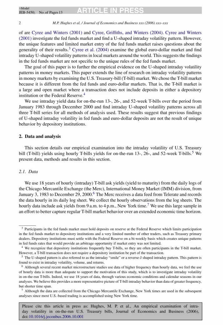
The time-of-the-day dummy variable parameter estimates suggest that after controlling for thetime-series conditional volatility, that the pattern of intraday volatility remains U-shaped. To makethis point easier to see, we plot the time specific intraday volatility for all three T-bills in Fig. 3.The intraday points in the plot equal the unconditional variance plus the parameter estimate for thetime of day.26 The 13- and 26-week T-bill intraday volatility clearly form a U-shaped pattern. The52-week intraday volatility, while not as smooth as the others, forms a general U-shaped pattern.

25 Black (1976) finds that bad news regarding a given firm is associated with large declines in the firm’s stock price,which in turn decreases the value of the firm and raises its debt to equity ratio. This changes the firm’s capital structure toa more leveraged, hence riskier position. This argument suggests that declines in stock prices lead to increased volatility.In order to capture this asymmetry, Nelson (1991), Glosten et al. (1993), and others introduce the γεt−1 term to the basicGARCH model, which following from Black is often referred to as a leverage term. However, Engle and Ng (1993) pointout that it is not yet clear that the asymmetric properties of variances are due to changing leverage. Hence, for our purposesthe so-called leverage effect simply refers to an asymmetric response to positive and negative shocks. Since we use theleverage term to indicate data asymmetry, in this paper we refer to it as an asymmetry term.26 The unconditional variance is defined as ω/(1 − α − β), where ω is the variance equation intercept, α the ARCH

parameter, and β is the GARCH parameter.





Fig. 3. The hourly time-dependent conditional volatilities for 13-, 26-, and 52-week T-bills from the TGARCH modelestimation reported in Table 3. The data period is from January 1983 to December 2000. The time-dependent conditionalvolatility at each hour is measured as the unconditional volatility plus the dummy variable parameter estimate for thathour. The value at 14:00 h (2 p.m.) is presented as the unconditional volatility since this value is the omitted variable. Theunconditional variance is defined as ω/(1 − α − β), where ω is the variance equation intercept, α the ARCH parameter,and β is the GARCH parameter.

The results in Table 3 and Fig. 3 suggest that after applying GARCH methods that allow forconditional heteroskedasticity we continue to find an intraday U-shaped volatility pattern acrossall three T-bill series.

2.5. Discussion

Our analysis finds a U-shaped intraday volatility pattern across T-bill yield series and acrossdifferent methods. These results extend the previous work by Cyree and Winters (2001) in fedfunds and Cyree et al. (2004) in euro-dollar deposits to a money market where transactions donot involve deposits at the Federal Reserve or a depository institution. Our finding of a U-shapedintraday volatility in T-bills suggests that the previous findings of U-shaped intraday volatility infed funds and euro-dollar deposits is not the result of unique behavior by depository institutions.

Our analysis is strictly an empirical analysis of intraday volatility. However, finding a U-shapedintraday volatility pattern in T-bills does suggest a line of future research that has the potential toprovide insights into the source of the U-shaped pattern.

Hasbrouck and Seppi (2001) find common factors between stock returns and order flow. Inaddition, they find that commonality in order flows explains about two-thirds of the commonalityin returns. Evans and Lyons (2002) provide a model of the effect of order flow on price changes.They state that when one maps information to prices, that order flow is a major component ofthe transmission mechanism. Accordingly, causation runs from order flow to prices. Evans andLyons state that order flow contains information about the realization of uncertain demand relatedto differential interpretation of news, shocks to hedging demands, shocks to liquidity demands,etc. Further, Evans and Lyons suggest that order flow contains two types of information: (1)information about the stream of future cash flows and (2) information about the market-clearing





discount rate. Since the single future cash flow in a T-bill is known in amount and timing withcertainty, the information in order flow must relate to the discount rate or factors related toexogenous shocks (i.e. liquidity demands). Accordingly, uncovering the reason(s) behind orderflow in T-bills should provide insights into the source of the U-shaped intraday volatility pattern inT-bills and may provide information about the source of the U-shaped intraday volatility patternin general. However, order flow information is not available for our data set, so we must leavethis question open for future research.

3. Conclusion

The goal of this paper is to further the empirical evidence on the U-shaped intraday volatilitypattern. Previously, Cyree and Winters (2001) find an intraday U-shaped volatility pattern in theovernight fed funds market and Cyree et al. (2004) find an intraday U-shaped volatility patternin local markets for euro-dollar deposits around the world. We extend the empirical results onU-shaped intraday volatility pattern by examining the T-bill market.

The U.S. T-bill market is a large and open market that does not include deposits in either adepository institution or the Federal Reserve as part of a transaction. We examine 18 years ofhourly T-bill ask yields from 13-, 26-, and 52-week T-bills using a variety of analytical methodsand find a U-shaped intraday volatility pattern for each T-bill maturity series, using each analyticalmethod. Our results suggest that the finding of a U-shaped intraday volatility pattern in fed fundsby Cyree and Winters and in euro-dollar deposits by Cyree et al. (2004) is not the result of uniquebehavior by depository institutions.

References

Andersen, T., & Bollerslev, T. (1998). Deutsche mark-dollar volatility: Intraday activity patterns, macroeconomicannouncements, and longer run dependencies. Journal of Finance, 53, 219–265.

Ballie, R., & Bollerslev, T. (1990). Intra-day and inter-market volatility in foreign exchange rates. Review of EconomicStudies, 58, 565–585.

Black, F. (1976). Studies in stock price volatility changes. In Proceedings of the 1976 Business Meeting of the Businessand Economics Statistics Section, American Statistical Association (pp. 171–181).

Brandt, M., & Kavajecz, K. (2004). Price discovery in the US treasury market: The impact of orderflow and liquidity onthe yield curve. Journal of Finance, 59, 2623–2654.

Christie-David, R., & Chaudhry, M. (1999). Liquidity and maturity effects around news releases. Journal of FinancialResearch, 22, 47–67.

Cyree, K., Griffiths, M., & Winters, D. (2004). An empirical examination of the intraday volatility in euro-dollar rates.Quarterly Review of Economics and Finance, 44, 44–57.

Cyree, K., & Winters, D. (2001). An intraday examination of the federal funds market: Implications for the theories ofthe reverse-J pattern. Journal of Business, 74, 535–556.

Engle, R., & Ng, V. (1993). Measuring and testing the impact of news on volatility. Journal of Finance, 48, 1749–1778.

Evans, M., & Lyons, R. (2002). Order flow and exchange rate dynamics. Journal of Political Economy, 110, 170–180.Fleming, M. (1997). The round-the-clock market for US Treasury securities. Federal Reserve Bank of New York Economic

Policy Review, 3, 9–32.Fleming, M. (2002). Are large Treasury issues more liquid? Evidence from bill reopenings. Journal of Money Credit and

Banking, 34, 707–735.Fleming, M., & Fabozzi, F. J. (2001). U.S. Treasury and agency securities. In F. J. Fabozzi (Ed.), The handbook of fixed

income securities (6th ed., pp. 175–196). New York: McGraw-Hill.Fleming, M., & Remolona, E. (1999). Price formation and liquidity in the treasury market: The response to public

information. Journal of Finance, 59, 1901–1915.





Glosten, L. R., Jagannathan, R., & Runkle, D. (1993). On the relation between the expected value and the volatility of thenormal excess return on stocks. Journal of Finance, 48, 1779–1801.

Green, T. C. (2004). Economic news and the impact of trading on bond prices. Journal of Finance, 59, 1201–1233.Hasbrouck, J., & Seppi, D. (2001). Common factors in prices, order flows, and liquidity. Journal of Financial Economics,

59, 383–411.Hong, H., & Wang, J. (2000). Trading and returns under periodic market closures. Journal of Finance, 55, 297–354.Nelson, D. B. (1991). Conditional heteroskedasticity in asset returns: A new approach. Econometrica, 59, 347–370.Nelson, D. B. (1990). Stationarity and persistence in the GARCH (1,1) model. Econometric Theory, 6, 318–334.


an empirical examination of intraday volatility in on-the-run u.s. treasury bills

Documents