vier.com/locate/chemolab

Chemometrics and Intelligent Laborat

An application of subagging for the improvement of prediction accuracy

of multivariate calibration models

Roberto Kawakami Harrop Galvao a, Mario Cesar Ugulino Araujo b,*,

Marcelo do Nascimento Martins a, Gledson Emidio Jose b, Marcio Jose Coelho Pontes b,

Edvan Cirino Silva b, Teresa Cristina Bezerra Saldanha b

a Instituto Tecnologico de Aeronautica, Divisao de Engenharia Eletronica, 12228-900, Sao Jose dos Campos, SP, Brazilb Universidade Federal da Paraıba, CCEN, Departamento de Quımica, Caixa Postal 5093, CEP 58051-970-Joao Pessoa, PB, Brazil

Received 18 February 2005; received in revised form 2 September 2005; accepted 19 September 2005

Available online 21 October 2005

Abstract

The term bagging refers to a class of techniques in which an ensemble model is obtained by combining different member models generated by

resampling the available data set. It has been shown that bagging can lead to substantial gains in accuracy for both classification and regression

models, specially when alterations in the training set cause significant changes in the outcome of the modelling procedure. However, in the context

of chemometrics, the use of bagging for quantitative multicomponent analysis is still incipient. More recently, an alternative aggregation scheme

termed subagging, which is based on subsampling without replacement, has been shown to provide performance improvements similar to bagging

at a smaller computational cost. The present paper proposes a strategy for using subagging in conjunction with three multivariate calibration

methods, namely Partial Least Squares (PLS) and Multiple Linear Regression with variable selection by using either the Successive Projections

Algorithm (MLR-SPA) or a Genetic Algorithm (MLR-GA). The subagging member models are generated by subsampling the pool of samples

available for modelling and then forming new calibration sets. Such a strategy is of value in analytical problems involving complex matrices, in

which reproducing the composition variability of real samples by means of optimized experimental designs may be a difficult task. The efficiency

of the proposed strategy is illustrated in a problem involving the NIR spectrometric determination of four diesel quality parameters (specific mass,

sulphur content, and the distillation temperatures T10% and T90% at which 10% and 90% of the sample has evaporated, respectively). In this case

study, the use of 30 subsampling iterations provides relative improvements of up to 16%, 33%, and 35% in the prediction accuracy of PLS, MLR-

SPA, and MLR-GA models, respectively, with respect to the expected results of individual (non-ensemble) models.

D 2005 Elsevier B.V. All rights reserved.

Keywords: Bagging; Subagging; MLR; PLS; SPA; Genetic algorithms; NIR spectrometry; Diesel analysis

1. Introduction

In regression and classification tasks where the size of the

data set is small, resampling techniques [1] are often used to

obtain better estimates of prediction accuracy, as well as to

assess the sensitivity of the modelling method with respect to

the composition of the training set [2]. A popular method,

which has long been used for this purpose is the jackknife

[3], or ‘‘leave-one-out’’ procedure, in which different models

are constructed by removing and then re-inserting one object

at a time from the training set. At the end, the variability of

0169-7439/$ - see front matter D 2005 Elsevier B.V. All rights reserved.

doi:10.1016/j.chemolab.2005.09.005

* Corresponding author. Tel.: +55 8 3216 7438; fax: +55 8 3216 7437.

E-mail address: laqa@quimica.ufpb.br (M.C.U. Araujo).

the model properties (such as regression or discriminant

coefficients, for instance) may be determined. Moreover, each

object can be used for validation once, in order to obtain a

cross-validation measure of prediction performance. The

cross-validation error may be used, for instance, to select

the best single model from a class of models, as in the case of

choosing the number of latent variables in Principal Compo-

nent Regression (PCR) and Partial-Least-Squares (PLS), or

the best subset of variables in Multiple Linear Regression

(MLR). In a related technique, known as bootstrap [4,5],

different calibration sets are formed by randomly selecting a

fixed number of objects from the available data set, with

replacement. In this manner, different models can be obtained,

as in the jackknife procedure.

ory Systems 81 (2006) 60 – 67

www.else

R.K.H. Galvao et al. / Chemometrics and Intelligent Laboratory Systems 81 (2006) 60–67 61

A less common use for such methods consists of

combining the different models obtained in the course of

resampling in order to generate a single ‘‘ensemble’’ model

[6]. For instance, the combination can be carried out by

averaging the coefficients of the models if linear structures

are employed [7]. In a more general setting, the outputs of

classifiers can be combined by majority voting [8,9] whereas

the outputs of quantitative models can be averaged [10]. As

a result, the ensemble model is often more accurate than any

of its individual members [6,8]. Such a concept was studied

in detail by Breiman [11,12], who coined the term

‘‘bagging’’ (bootstrap aggregating) for the process of

generating different modelling sets by a bootstrap procedure

and then combining the resulting models. In those seminal

papers, Breiman showed that bagging can lead to substantial

gains in accuracy for both classification and regression,

specially when alterations in the training set cause signif-

icant changes in the outcome of the modelling procedure.

More specifically, in regression tasks, where the mean-

square error of prediction is the sum of noise variance,

predictor bias, and predictor variance, bagging can be used

to reduce the predictor variance [11]. However, a modified

version of the basic bagging algorithm (‘‘iterated bagging’’)

can also lead to reductions in the predictor bias [13].

It is worth noting that bagging techniques have become

more popular for classification tasks, whereas their use in

multivariate regression problems has received comparatively

little attention. In this context, most research efforts have been

focused on neural network applications [10,14]. In such cases,

bagging can be used to reduce the statistical instability of

neural network training, whose generalization performance

may be significantly altered by small changes in the training set

and/or training parameters [15]. However, the utility of bagging

in the problem of variable selection for MLR was already

pointed out by Breiman [11,12]. In this case, changes in the

selection outcome caused by modifications in the calibration

set are smoothed by averaging the resulting models. Moreover,

bagging techniques may also be of value in the context of

Partial-Least-Squares (PLS) modelling, as described in a study

[16] concerning the determination of solid content in latex

samples by near-infrared reflectance spectrometry. In such an

application, the aggregation of 30 PLS models generated by the

bootstrap procedure led to a decrease of 7% in the mean sum of

squared errors (MSEE) with respect to the standard PLS

method. Such an MSEE statistic was obtained by applying the

models to the prediction of an independent, previously unseen

data set.

More recently, an alternative aggregation scheme based

on subsampling without replacement was also proposed [17].

In such a scheme, which was termed ‘‘subagging’’ (subsam-

ple aggregating), each individual model is constructed on

the basis of a reduced number of Mc objects extracted from

the pool of M objects available for modelling (Mc<M). The

individual models thus generated are then combined to

create an ensemble model, as in bagging. It is worth noting

that the bootstrap procedure employed in standard bagging

generates data sets with the same size M of the original

modelling set. Buhlmann and Yu argue that subagging may

have substantial computational advantages with respect to

bagging because the calibration of each individual model is

faster if fewer training objects are employed. Interestingly,

such an improved computational efficiency comes at the

cost of only a small loss in performance for the ensemble

model, as demonstrated by numerical examples [17].

In the present paper, a subagging strategy is proposed to

improve the accuracy of multivariate calibration models in

spectrometric analysis. More specifically, the resampling

factor used to generate the subagging member models

consists of extracting calibration objects from the overall

data set available for modelling purposes. It is worth noting

that this application of subagging may be of value when the

complexity of the matrix makes it difficult to reproduce the

composition variability of real samples by means of

optimized experimental designs [18]. In this case, a

representative calibration set must be extracted from a pool

of real samples [19]. The remaining samples may be used

for validation in order to guide modelling decisions such as

the choice of an appropriate subset of informative variables

in MLR [20–22].

In this context, random sampling (RS) is often employed

because of its simplicity and also because a group of data

randomly extracted from a larger set follows the statistical

distribution of the entire set. However, RS does not guarantee

the representativity of the set, nor does it prevent extrapolation

problems [23]. In fact, RS does not ensure, for instance, that

the samples on the boundaries of the set are included in the

calibration. In this sense, it may be interesting to investigate the

use of subagging in conjunction with RS in the construction of

the calibration set.

The proposed subagging strategy is employed with three

regression techniques: (a) PLS, (b) MLR with variable

selection by the Successive Projections Algorithm (MLR-

SPA) [20–22], and (c) MLR with variable selection by a

Genetic Algorithm (MLR-GA) [24,25]. For illustration, a

multivariate calibration problem involving NIR spectrometric

analysis of diesel samples is considered. Four quality

parameters are determined (specific mass, sulphur content,

and the distillation temperatures T10% and T90% at which

10% and 90% of the sample has evaporated, respectively

[26]).

2. Proposed subagging strategy

The use of subagging requires a procedure for obtaining

a model from each resampled data set and a method for

combining the resulting models. This section describes the

implementation of these procedures, as well as the definition

of a performance index for the subagging result.

The overall data set available for model-building purposes

will be termed ‘‘modelling set’’. The Mc samples extracted by

subsampling the modelling set will form the ‘‘calibration set’’.

It is worth noting that the subsampling is carried out without

replacement, as previously discussed. The Mv samples remain-

ing in the modelling set after extraction of the calibration set

R.K.H. Galvao et al. / Chemometrics and Intelligent Laboratory Systems 81 (2006) 60–6762

will form the ‘‘validation set’’. As described below, the

validation set will be employed to guide the variable selection

process in MLR-SPA and MLR-GA.

2.1. Resampling and calibration

2.1.1. PLS

In the PLS calibration, an appropriate number of latent

variables (r) is initially determined on the basis of the cross-

validation (‘‘leave-one-out’’) error obtained by using the entire

modelling set. The criterion of Haaland and Thomas is applied

to find the optimum point in the curve of prediction error sum

of squares (PRESS) vs. r [27,28]. Such a criterion consists of

employing an F-test to determine the smallest value of r for

which PRESS(r) is not significantly larger than the global

PRESS minimum. An F-ratio probability of 0.75 is adopted, as

suggested elsewhere [29].

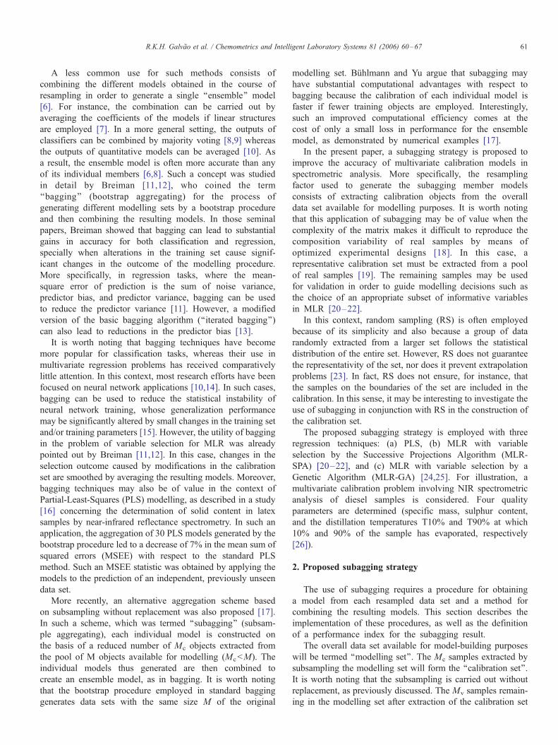
The subagging procedure for PLS is illustrated in Fig. 1a.

As can be seen, a PLS model is obtained from each calibration

set obtained by subsampling the modelling set. The regressions

Fig. 1. Subagging procedure for (a) PLS and (b) MLR-SPA or MLR-GA modelling

previously determined by cross-validation using the entire modelling data set. Th

prediction error in the validation set.

are carried out by using the number of latent variables initially

established by cross-validation.

2.1.2. MLR-SPA

In MLR-SPA, the validation set is employed to guide the

variable selection procedure [20–22]. The core of SPA consist of

projection operations carried out on the calibration data matrix

Xcal (Mc�J), whose lines and columns correspond to Mc

calibration samples and J spectral variables, respectively.

Starting from each of the J variables (columns of Xcal) available

for selection, SPA builds an ordered chain ofMc variables. Each

element in the chain is selected in order to display the least

collinearity with the previous ones. From each of the J chains

constructed in this manner, it is possible to extractMc subsets of

variables by using one up to Mc elements in the order in which

they were selected. Thus, a total of J�Mc subsets of variables

can be formed. In order to choose the most appropriate subset,

MLR models are built and compared in terms of the root-mean-

square error of prediction in the validation set (RMSEV). The

model that leads to the smallest RMSEV is then adopted.

employing n subsampling iterations. The number of latent variables for PLS is

e variable selection procedure in MLR-SPA and MLR-GA is guided by the

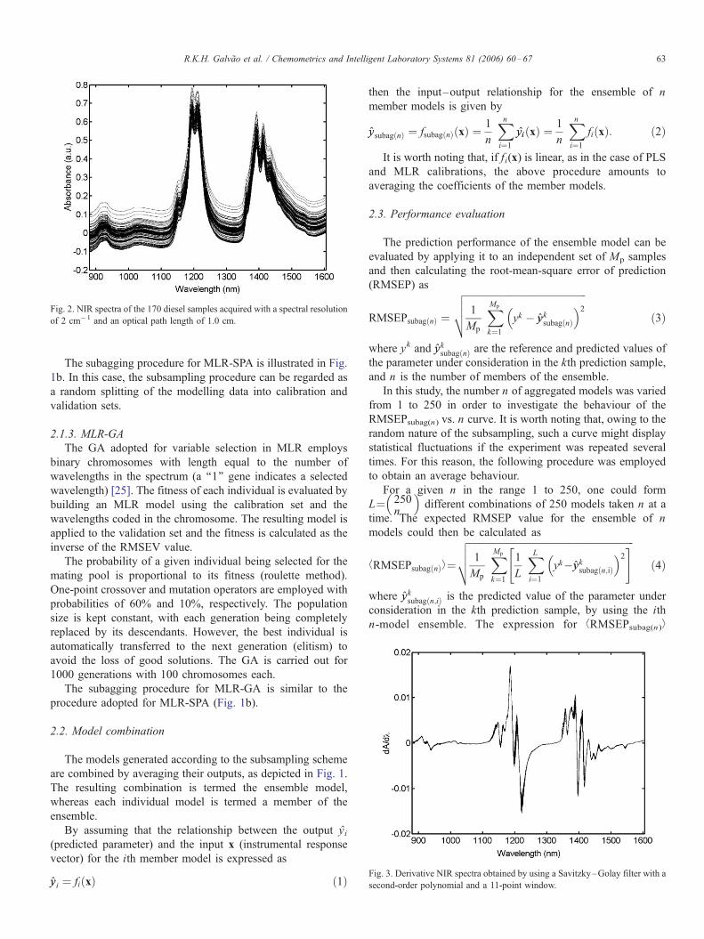
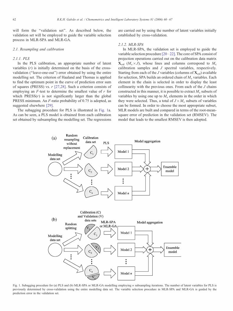
Fig. 2. NIR spectra of the 170 diesel samples acquired with a spectral resolution

of 2 cm� 1 and an optical path length of 1.0 cm.

Fig. 3. Derivative NIR spectra obtained by using a Savitzky–Golay filter with a

second-order polynomial and a 11-point window.

R.K.H. Galvao et al. / Chemometrics and Intelligent Laboratory Systems 81 (2006) 60–67 63

The subagging procedure for MLR-SPA is illustrated in Fig.

1b. In this case, the subsampling procedure can be regarded as

a random splitting of the modelling data into calibration and

validation sets.

2.1.3. MLR-GA

The GA adopted for variable selection in MLR employs

binary chromosomes with length equal to the number of

wavelengths in the spectrum (a ‘‘1’’ gene indicates a selected

wavelength) [25]. The fitness of each individual is evaluated by

building an MLR model using the calibration set and the

wavelengths coded in the chromosome. The resulting model is

applied to the validation set and the fitness is calculated as the

inverse of the RMSEV value.

The probability of a given individual being selected for the

mating pool is proportional to its fitness (roulette method).

One-point crossover and mutation operators are employed with

probabilities of 60% and 10%, respectively. The population

size is kept constant, with each generation being completely

replaced by its descendants. However, the best individual is

automatically transferred to the next generation (elitism) to

avoid the loss of good solutions. The GA is carried out for

1000 generations with 100 chromosomes each.

The subagging procedure for MLR-GA is similar to the

procedure adopted for MLR-SPA (Fig. 1b).

2.2. Model combination

The models generated according to the subsampling scheme

are combined by averaging their outputs, as depicted in Fig. 1.

The resulting combination is termed the ensemble model,

whereas each individual model is termed a member of the

ensemble.

By assuming that the relationship between the output yi(predicted parameter) and the input x (instrumental response

vector) for the ith member model is expressed as

yyi ¼ fi xð Þ ð1Þ

then the input–output relationship for the ensemble of n

member models is given by

yysubag nð Þ ¼ fsubag nð Þ xð Þ ¼1

n

Xni¼1

yiyi xð Þ ¼1

n

Xni¼1

fi xð Þ: ð2Þ

It is worth noting that, if fi(x) is linear, as in the case of PLS

and MLR calibrations, the above procedure amounts to

averaging the coefficients of the member models.

2.3. Performance evaluation

The prediction performance of the ensemble model can be

evaluated by applying it to an independent set of Mp samples

and then calculating the root-mean-square error of prediction

(RMSEP) as

RMSEPsubag nð Þ ¼

ffiffiffiffiffiffiffiffiffiffiffiffiffiffiffiffiffiffiffiffiffiffiffiffiffiffiffiffiffiffiffiffiffiffiffiffiffiffiffiffiffiffiffiffiffiffiffiffiffi1

Mp

XMp

k¼1yk � yyk

subag nð Þ

� �2vuut ð3Þ

where yk and yyksubag nð Þ are the reference and predicted values of

the parameter under consideration in the kth prediction sample,

and n is the number of members of the ensemble.

In this study, the number n of aggregated models was varied

from 1 to 250 in order to investigate the behaviour of the

RMSEPsubag(n) vs. n curve. It is worth noting that, owing to the

random nature of the subsampling, such a curve might display

statistical fluctuations if the experiment was repeated several

times. For this reason, the following procedure was employed

to obtain an average behaviour.

For a given n in the range 1 to 250, one could form

L¼�250n

�different combinations of 250 models taken n at a

time. The expected RMSEP value for the ensemble of n

models could then be calculated as

bRMSEPsubag nð Þ�¼

ffiffiffiffiffiffiffiffiffiffiffiffiffiffiffiffiffiffiffiffiffiffiffiffiffiffiffiffiffiffiffiffiffiffiffiffiffiffiffiffiffiffiffiffiffiffiffiffiffiffiffiffiffiffiffiffiffiffiffiffiffiffiffiffiffiffiffi1

Mp

XMp

k¼1

1

L

XLi¼1

yk�yyksubag n;ið Þ

� �2#"vuut ð4Þ

where yyksubag n;ið Þ is the predicted value of the parameter under

consideration in the kth prediction sample, by using the ith

n-model ensemble. The expression for bRMSEPsubag(n)�

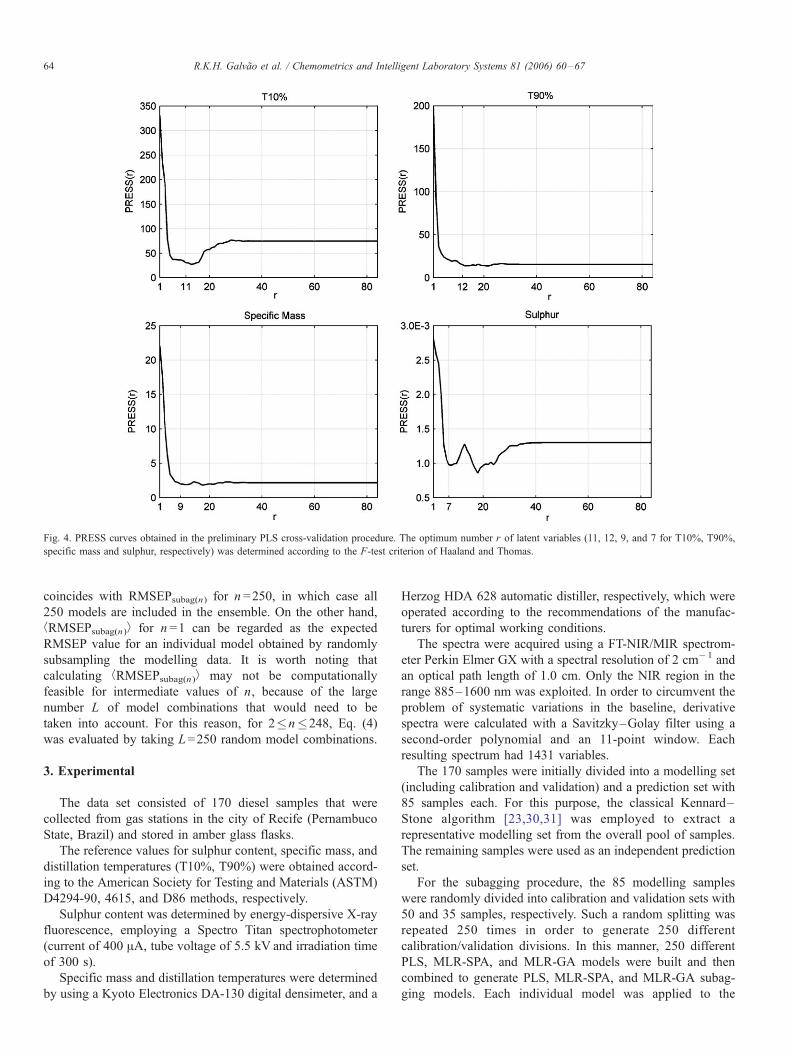
Fig. 4. PRESS curves obtained in the preliminary PLS cross-validation procedure. The optimum number r of latent variables (11, 12, 9, and 7 for T10%, T90%,

specific mass and sulphur, respectively) was determined according to the F-test criterion of Haaland and Thomas.

R.K.H. Galvao et al. / Chemometrics and Intelligent Laboratory Systems 81 (2006) 60–6764

coincides with RMSEPsubag(n) for n =250, in which case all

250 models are included in the ensemble. On the other hand,

bRMSEPsubag(n)� for n =1 can be regarded as the expected

RMSEP value for an individual model obtained by randomly

subsampling the modelling data. It is worth noting that

calculating bRMSEPsubag(n)� may not be computationally

feasible for intermediate values of n, because of the large

number L of model combinations that would need to be

taken into account. For this reason, for 2�n�248, Eq. (4)

was evaluated by taking L=250 random model combinations.

3. Experimental

The data set consisted of 170 diesel samples that were

collected from gas stations in the city of Recife (Pernambuco

State, Brazil) and stored in amber glass flasks.

The reference values for sulphur content, specific mass, and

distillation temperatures (T10%, T90%) were obtained accord-

ing to the American Society for Testing and Materials (ASTM)

D4294-90, 4615, and D86 methods, respectively.

Sulphur content was determined by energy-dispersive X-ray

fluorescence, employing a Spectro Titan spectrophotometer

(current of 400 AA, tube voltage of 5.5 kV and irradiation time

of 300 s).

Specific mass and distillation temperatures were determined

by using a Kyoto Electronics DA-130 digital densimeter, and a

Herzog HDA 628 automatic distiller, respectively, which were

operated according to the recommendations of the manufac-

turers for optimal working conditions.

The spectra were acquired using a FT-NIR/MIR spectrom-

eter Perkin Elmer GX with a spectral resolution of 2 cm�1 and

an optical path length of 1.0 cm. Only the NIR region in the

range 885–1600 nm was exploited. In order to circumvent the

problem of systematic variations in the baseline, derivative

spectra were calculated with a Savitzky–Golay filter using a

second-order polynomial and an 11-point window. Each

resulting spectrum had 1431 variables.

The 170 samples were initially divided into a modelling set

(including calibration and validation) and a prediction set with

85 samples each. For this purpose, the classical Kennard–

Stone algorithm [23,30,31] was employed to extract a

representative modelling set from the overall pool of samples.

The remaining samples were used as an independent prediction

set.

For the subagging procedure, the 85 modelling samples

were randomly divided into calibration and validation sets with

50 and 35 samples, respectively. Such a random splitting was

repeated 250 times in order to generate 250 different

calibration/validation divisions. In this manner, 250 different

PLS, MLR-SPA, and MLR-GA models were built and then

combined to generate PLS, MLR-SPA, and MLR-GA subag-

ging models. Each individual model was applied to the

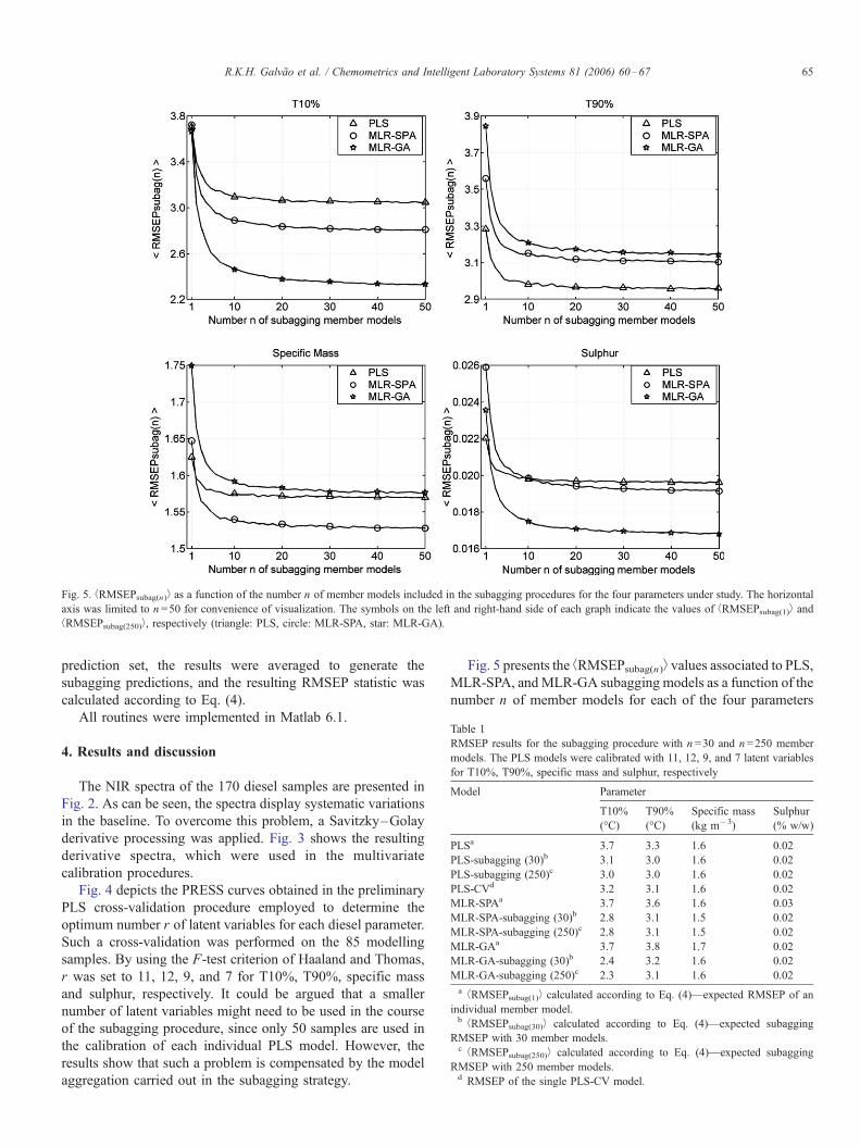
Fig. 5. bRMSEPsubag(n)� as a function of the number n of member models included in the subagging procedures for the four parameters under study. The horizontal

axis was limited to n =50 for convenience of visualization. The symbols on the left and right-hand side of each graph indicate the values of bRMSEPsubag(1)� and

bRMSEPsubag(250)�, respectively (triangle: PLS, circle: MLR-SPA, star: MLR-GA).

Table 1

RMSEP results for the subagging procedure with n =30 and n =250 member

models. The PLS models were calibrated with 11, 12, 9, and 7 latent variables

for T10%, T90%, specific mass and sulphur, respectively

Model Parameter

T10%

(-C)T90%

(-C)Specific mass

(kg m� 3)

Sulphur

(% w/w)

PLSa 3.7 3.3 1.6 0.02

PLS-subagging (30)b 3.1 3.0 1.6 0.02

PLS-subagging (250)c 3.0 3.0 1.6 0.02

PLS-CVd 3.2 3.1 1.6 0.02

MLR-SPAa 3.7 3.6 1.6 0.03

MLR-SPA-subagging (30)b 2.8 3.1 1.5 0.02

MLR-SPA-subagging (250)c 2.8 3.1 1.5 0.02

MLR-GAa 3.7 3.8 1.7 0.02

MLR-GA-subagging (30)b 2.4 3.2 1.6 0.02

MLR-GA-subagging (250)c 2.3 3.1 1.6 0.02

abRMSEPsubag(1)� calculated according to Eq. (4)—expected RMSEP of an

individual member model.bbRMSEPsubag(30)� calculated according to Eq. (4)—expected subagging

RMSEP with 30 member models.cbRMSEPsubag(250)� calculated according to Eq. (4)—expected subagging

RMSEP with 250 member models.d RMSEP of the single PLS-CV model.

R.K.H. Galvao et al. / Chemometrics and Intelligent Laboratory Systems 81 (2006) 60–67 65

prediction set, the results were averaged to generate the

subagging predictions, and the resulting RMSEP statistic was

calculated according to Eq. (4).

All routines were implemented in Matlab 6.1.

4. Results and discussion

The NIR spectra of the 170 diesel samples are presented in

Fig. 2. As can be seen, the spectra display systematic variations

in the baseline. To overcome this problem, a Savitzky–Golay

derivative processing was applied. Fig. 3 shows the resulting

derivative spectra, which were used in the multivariate

calibration procedures.

Fig. 4 depicts the PRESS curves obtained in the preliminary

PLS cross-validation procedure employed to determine the

optimum number r of latent variables for each diesel parameter.

Such a cross-validation was performed on the 85 modelling

samples. By using the F-test criterion of Haaland and Thomas,

r was set to 11, 12, 9, and 7 for T10%, T90%, specific mass

and sulphur, respectively. It could be argued that a smaller

number of latent variables might need to be used in the course

of the subagging procedure, since only 50 samples are used in

the calibration of each individual PLS model. However, the

results show that such a problem is compensated by the model

aggregation carried out in the subagging strategy.

Fig. 5 presents the bRMSEPsubag(n)� values associated to PLS,

MLR-SPA, andMLR-GA subagging models as a function of the

number n of member models for each of the four parameters

Table 2

RMSEP improvements resulting from the subagging procedure with n =30 with

respect to the expected result of individual models (n =1)

Model Parameter

T10%

(-C)

T90%

(-C)

Specific mass

(kg m� 3)

Sulphur

(% w/w)

PLS 16% 9% 0% 0%

MLR-SPA 24% 14% 6% 33%

MLR-GA 35% 16% 6% 0%

R.K.H. Galvao et al. / Chemometrics and Intelligent Laboratory Systems 81 (2006) 60–6766

under study. As can be seen, the subagging promotes a general

improvement in the prediction accuracy as n increases. For

convenience of visualization the graphs are shown up to n =50,

because the curves are seen to converge after the aggregation of

approximately 30 member models.

Table 1 presents the RMSEP results of the different

modelling strategies for each parameter under study. Subagging

results are presented for n =30 and also for n =250. For

comparison, the result of using PLS with full cross-validation

(PLS-CV) is also shown.

In almost all cases presented in Table 1, the use of subagging

with n =30 led to a smaller RMSEP in comparison with the

average result bRMSEPsubag(1)� for individual models (the only

exceptions being the determination of specific mass by PLS and

sulphur by PLS and MLR-GA, in which the RMSEP remained

the same). Such a finding is in accordance with the literature,

which claims that an ensemble model is often more accurate

than its individual members [6,8]. Moreover, PLS-subagging

displayed a smaller RMSEP than PLS with full cross-validation

(PLS-CV) for T10% and T90%. In general, extending the

subagging from n =30 to n =250 did not promote further

reductions in the RMSEP values, which is in agreement with the

convergence of the curves observed in Fig. 5. The only

exceptions were the determination of T10% by PLS and

T10%, T90% by MLR-GA. However, such improvements

may not justify the additional computational workload required.

In order to better assess the subagging benefits, a relative

RMSEP reduction was evaluated as

bRMSEPsubag 1ð Þ�� bRMSEPsubag 30ð Þ�

bRMSEPsubag 1ð Þ�� 100% ð5Þ

which indicates the improvement obtained with n =30 with

respect to the expected result of individual models (n =1).

The improvements calculated in this manner are presented in

Table 2. As can be seen, the largest RMSEP reductions were

achieved with MLR-SPA (up to 33%) and mainly with MLR-

GA (up to 35%). The PLS results were less affected by the

subagging procedure, with improvements up to 16%.

5. Conclusions

There has been a growing interest in using bagging strategies

for classification tasks, in which improvements have been

reported over the use of individual models. However, such a

research in the context of multivariate calibration has been

comparatively smaller and mostly focused on the training of

neural networks.More recently, the concept of subagging, which

employs subsampling rather than bootstrapping to generate

different calibration sets, was proposed to achieve the benefits of

bagging at a smaller computational cost. The present paper

demonstrated that subagging can be useful in conjunction with

two of the most popular multivariate calibration methods (PLS

and MLR). The proposed subagging strategy is aimed at

analytical problems involving complex matrices, where the

calibration set must be extracted from a pool of real samples.

For illustration purposes, a multivariate calibration problem

involving the determination of four diesel quality parameters

(specific mass, sulphur content, and the distillation tempera-

tures T10% and T90% at which 10% and 90% of the sample

has evaporated, respectively) by NIR spectrometry was

addressed. The results showed that the subagging procedure

leads to a general improvement in the prediction accuracy of

the multivariate calibration models for the parameters under

study. In particular, the largest improvements were achieved for

the MLR models with variable selection by SPA and GA. The

comparatively smaller improvements obtained for PLS may be

ascribed to the statistical stability of PLS regression. In fact,

bagging/subagging strategies were mainly devised for methods

that show instability with respect to changes in the composition

of the calibration set.

Future works could exploit the iterated bagging methodol-

ogy [13] to reduce the bias term of the mean-square prediction

error, which was not exploited in the present paper. Moreover,

other optimization methods for variable selection (such as

simulated annealing [32] and ant colonies [33]) may also

benefit from the use of bagging or subagging to reduce

statistical fluctuations.

Acknowledgments

The authors thank FINEP-CTPETRO (Grant 0652/00)

science funding program, PROCAD/CAPES (Grant 0064/01-

7), CNPq (Grant 475204/2004-2 and PRONEX Grant 015/98),

and FAPESP (Grant 03/09433-5) for partial financial support.

The research fellowships and scholarships granted by CNPq and

CAPES are also gratefully acknowledged. The authors are

indebted to Mr. Claudio Vicente Ferreira (Laboratorio de

Combustıveis, Departamento de Engenharia Quımica, Univer-

sidade Federal de Pernambuco) for providing the diesel samples

and the reference values of the quality parameters employed in

this study.

References

[1] P.I. Good, Resampling Methods: A Practical Guide to Data Analysis,

Birkhauser, Boston, 1999.

[2] R.O. Duda, P.E. Hart, D.G. Stork, Pattern Classification, 2nd edR, Wiley,

New York, 2001.

[3] B. Efron, The Jackknife, The Bootstrap and Other Resampling Plans,

SIAM, Philadelphia, 1982.

[4] A.C. Davison, D.V. Hinkley (Eds.), Bootstrap Methods and their

Application, Cambridge Univ. Press, Cambridge, UK, 1997.

[5] B.M. Smith, P.J. Gemperline, J. Chemom. 16 (2002) 241–246.

[6] D.W. Opitz, R.J. Maclin, Artif. Intell. Res. 11 (1999) 169–198.

[7] M. Skurichina, R.P.W. Duin, Pattern Recogn. 31 (1998) 909–930.

R.K.H. Galvao et al. / Chemometrics and Intelligent Laboratory Systems 81 (2006) 60–67 67

[8] L.K. Hansen, P. Salamon, IEEE Trans, Pattern Anal. Mach. Intell. 12

(1990) 993–1001.

[9] E. Bauer, R. Kohavi, Mach. Learn. 36 (1999) 105–139.

[10] M. Taniguchi, V. Tresp, Neural Comput. 9 (1997) 1163–1178.

[11] L. Breiman, Mach. Learn. 24 (1996) 123–140.

[12] L. Breiman, Mach. Learn. 24 (1996) 49–64.

[13] L. Breiman, Mach. Learn. 45 (2001) 261–277.

[14] M. Sugimoto, S. Kikuchi, M. Arita, T. Soga, T. Nishioka, M. Tomita,

Anal. Chem. 77 (2005) 78–84.

[15] D.K. Agrafiotis, W. Cedeno, V.S. Lobanov, J. Chem. Inf. Comput. Sci. 42

(2002) 903–911.

[16] E.B. Martin, A.J. Morris, in: J.W. Kay, D.M. Titterington (Eds.), Statistics

and Neural Networks—Advances at the Interface, Oxford Univ. Press,

Oxford, 1999, pp. 195–258.

[17] P. Buhlmann, B. Yu, Ann. Stat. 30 (2002) 927–961.

[18] D.L. Massart, B.G.M. Vandeginste, L.M.C. Buydens, S. De Jong, P.J.

Lewi, J. Smeyers-Verbeke, Handbook of Chemometrics and Qualimetrics:

Part A, Elsevier, Amsterdam, 1997.

[19] R.K.H. Galvao, M.C.U. Araujo, G.E. Jose, M.J.C. Pontes, E.C. Silva,

T.C.B. Saldanha, Talanta 67 (2005) 736–740.

[20] M.C.U. Araujo, T.C.B. Saldanha, R.K.H. Galvao, T. Yoneyama, H.C.

Chame, V. Visani, Chemom. Intell. Lab. Syst. 57 (2001) 65–73.

[21] R.K.H. Galvao, M.F. Pimentel, M.C.U. Araujo, T. Yoneyama, V. Visani,

Anal. Chim. Acta 443 (2001) 107–115.

[22] R.K.H. Galvao, G.E. Jose, H.A. Dantas Filho, M.C.U. Araujo, E.C. Silva,

H.M. Paiva, T.C.B. Saldanha, E.S.O.N. Souza, Chemom. Intell. Lab. Syst.

70 (2004) 1–10.

[23] K.R. Kanduc, J. Zupan, N. Majcen, Chemom. Intell. Lab. Syst. 65 (2003)

221–229.

[24] C. Abrahamsson, J. Johansson, A. Sparen, F. Lindgren, Chemometr. Intell.

Lab. Syst. 69 (2003) 3–12.

[25] R. Leardi, J. Chemom. 15 (2001) 559–569.

[26] C.T. Mansfield, B.N. Barman, Anal. Chem. 71 (1999) 81R–107R.

[27] D.M. Haaland, E.V. Thomas, Anal. Chem. 60 (1988) 1193–1202.

[28] J. Moros, F.A. Inon, S. Garrigues, M. de la Guardia, Anal. Chim. Acta 538

(2005) 181–193.

[29] B.X. Li, D.M. Wang, C.L. Xu, Z.J. Zhang, Microchim. Acta 149 (2005)

205–212.

[30] R.W. Kennard, L.A. Stone, Technometrics 11 (1969) 137–148.

[31] E. Bouveresse, C. Hartmann, D.L. Massart, I.R. Last, K.A. Prebble, Anal.

Chem. 68 (1996) 982–990.

[32] S.P. Brooks, N. Friel, R. King, J. R. Stat. Soc., B 65 (2003) 503–520.

[33] Q. Shen, J.H. Jiang, J.C. Tao, G.L. Shen, R.Q. Yu, J. Chem. Inf. Model 45

(2005) 1024–1029.