An Analytical Electrothermal Model of a 1-D Electrothermal MEMS Micromirror

Shane T. Todd and Huikai Xie

Department of Electrical and Computer Engineering, University of Florida, Gainesville, FL 32611, USA

ABSTRACT We have developed an analytical model that describes the steady-state thermal behavior of a 1-D electrothermal bimorph MEMS micromirror. The steady-state 1-D heat transport equation is used to solve for the temperature distribution of the device upon actuation. Three models are developed using different thermal conditions on the device. The models consider heat dissipation from conduction and convection and the temperature dependence of the actuator electrical resistor. The temperature distribution equation of each model is analyzed to find critical thermal parameters such as the position of maximum temperature, maximum temperature, average temperature, and equivalent thermal resistance. The simplest model, called the Case 1 model, is used to develop an electrothermal lumped element model that uses a single thermal power source. In the Case 1 model, it is shown that a parameter called the “balancing factor” predicts where the maximum temperature is located, the distribution of power flow, and the division of thermal resistances. The analytical models are compared to FEM simulations and agree within 20% for all of the actuation ranges and thermal conditions tested. Keywords: MEMS, Micromirror, Electrothermal Actuation, Lumped Element Modeling, Heat Transport

1. INTRODUCTION Electrothermal actuation is an important transduction mechanism used in many MEMS devices. Electrothermal actuators can achieve large displacements with low voltages compared to other types of actuation [1]. An electrothermal actuator uses an electrical resistor (usually made of polysilicon) to generate Joule heat. The heat generated creates a temperature rise in the device, and the thermoelastic properties of the device materials respond to the temperature rise and cause a displacement. The modeling of an electrothermal device is essential to predicting the device behavior as well as optimizing the device design. Modeling can be challenging because one needs to consider how an electrical input creates a non-linear temperature distribution in the device and how that temperature distribution affects the mechanical output of the device. The temperature distribution of electrothermal devices has been modeled by using numerical methods and heat transport analysis [2-5]. Many devices exhibit non-linear thermal behaviors in cases where thermal conductivities are temperature dependent, convection coefficients are temperature dependent, and/or radiation causes a significant source of heat dissipation. Numerical methods are often used to model these types of devices with non-linear thermal behaviors. For example, Geisberger et al. modeled a MEMS thermal actuator using a finite element method (FEM). The model considered the temperature-dependent thermal and electrical properties of polysilicon and predicted the mechanical response to the temperature distribution [2]. Finite element methods are useful for modeling devices that have complex geometry and/or multi-dimensional boundary conditions. However, the complexity of FEM simulations requires large computational resources and can be time-consuming. In certain cases a lumped element model (LEM) may be used to simulate the behavior of a device. LEMs can be simulated in commonly used circuit simulators, such as SPICE, and are less time consuming and lower cost compared to FEM simulators. Manginell et al. used an LEM to model the electrothermal behavior of a microbridge gas sensor [3]. This model considered conduction, convection, and the temperature dependent thermal and electrical conductivities of the polysilicon heating element. The model was constructed by partitioning the device into a network of thermal resistors and power sources and was simulated in SPICE. LEM models are simpler than FEM models, but they may require a large partition of elements to obtain accurate results. While numerical methods are essential for situations where an accurate prediction of the device performance is required, they provide limited insight into how the parameters of the device design can be changed for optimum

performance. An analytical model is needed if one wants insight into what parameters of an electothermal actuator affect the thermal behaviors of the device. If certain assumptions (such as constant convection, constant thermal conductivities, and negligible radiation) are made, the heat transport equation can be solved to create an analytical solution for the temperature distribution of an electrothermal device. Lammel et al. used the heat transport equation to develop an analytical model of the temperature distribution of a 1-D electrothermal bimorph micromirror [4]. The model assumed a uniform power distribution and considered convection from the device surface. Yan et al. also developed an analytical electrothermal model for a vertical thermal actuator [5], in which conduction, convection and the temperature dependence of the polysilicon resistor were taken into account. Problems with analytical models are that they can be very complex and hard to extract useful information from. In this paper we will describe an analytical model of an electrothermal MEMS micromirror that is developed from the heat transport theory. We will show that an LEM can be created from the analytical model that is simple and suitable for multi-domain modeling and design optimization. Three analytical models have been developed using different thermal considerations. We will give a detailed summary of the simplest model, called the Case 1 model, and we will compare the results of this model to the other models. We will show that the Case 1 model can be used to accurately predict the device behavior compared to the other models. From the Case 1 model an LEM is extracted that uses a single thermal power source, and predicts the average and maximum temperature of the device upon actuation. The results of the models are compared to FEM simulations for verification. In the next section we will introduce the device design and actuation mechanism.

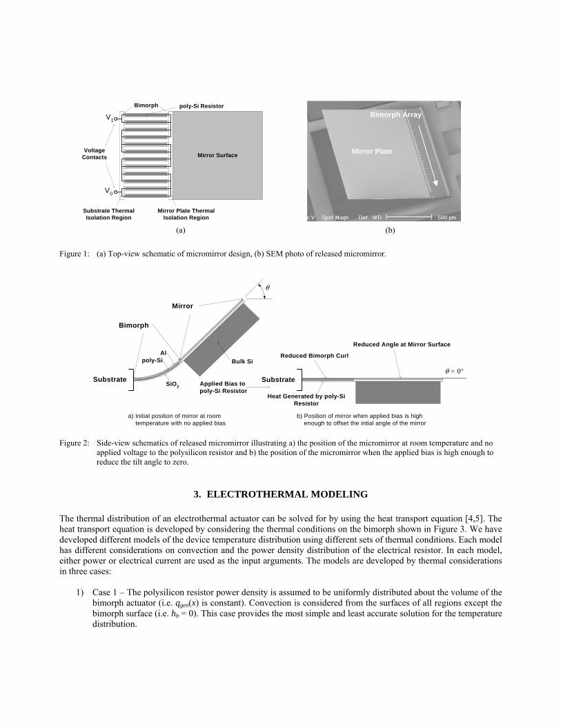
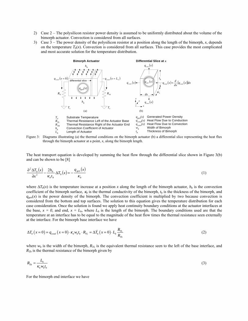
2. DEVICE DESIGN The micromirror device modeled in this paper was previously reported by Xie et al. [6]. Figure 1 shows the schematic of the micromirror design and a scanning electron micrograph (SEM) of a fabricated device. As illustrated in Figure 1(a), the device consists of a bimorph beam array attached from the substrate to a mirror plate. A bimorph beam in the array comprises an Al top layer, an SiO2 bottom layer, and a polysilicon resistor embedded in the SiO2 layer. There are 72 bimorph beams in the array. The polysilicon resistors of adjacent beams are attached in parallel yielding 36 resistors attached in series. Electrical contacts are present on the furthest left and furthest right resistors in the array. The mirror plate has a thick single crystal silicon (SCS) membrane bottom layer coated with an Al top layer. The Al layer forms the reflective surface of the mirror and the SCS membrane adds stiffness to the mirror plate to ensure reasonable surface flatness. There is also a thin SiO2 layer between the Al and SCS layers. As shown in Figure 1(a), there are two thermal isolation regions located at both ends of the bimorph beams. The substrate isolation region increases the static response of the mirror by creating additional thermal resistance between the bimorph actuator and the substrate which yields a higher bimorph temperature upon actuation. The mirror plate isolation region improves the transient response of the device because it limits the amount of heat flow from the bimorph array to the mirror plate. The mirror is fabricated using the Agilent 0.5 µm 3-metal CMOS process through MOSIS followed by a post-CMOS fabrication process for mirror release. The fabrication process is discussed in detail in [7]. The mirror is 1 mm × 1 mm in size, the bimorph beams are 160 µm long and 8.6 µm wide, and the gap between adjacent beams is 7.4 µm. The mirror tilts 36° at room temperature and the room temperature electrical resistance of the actuator is 1.2 kΩ. The mirror plate tilts up and away from the substrate at room temperature due to residual stresses present in the bimorph beams. The tilt angle of the mirror plate is equal to the tangential angle at the end of the bimorph beams and depends on the length of the bimorph beams. The mirror is actuated when a voltage is applied to the polysilicon resistor. The power dissipated by the resistor raises the bimorph temperature. Since Al has a greater coefficient of thermal expansion than SiO2, Al will exhibit greater internal strain when the temperature increases (i.e. Al wants to expand more than SiO2). The strain difference of the Al and SiO2 resulting from a temperature increase causes the bimorph to bend down. Thus the mirror is actuated by reducing the curl of the bimorph and the initial angle of the mirror plate. The actuation mechanism is demonstrated in Figure 2.

Bimorph Array

Mirror Plate Mirror Surface

V1

V0

VoltageContacts

Bimorph poly-Si Resistor

Substrate ThermalIsolation Region

Mirror Plate ThermalIsolation Region

(a) (b)

Figure 1: (a) Top-view schematic of micromirror design, (b) SEM photo of released micromirror.

Substrate

θ

Alpoly-Si

SiO2Substrate

Bulk Si

Mirror

Bimorph

θ = 0°

Reduced Bimorph Curl

Reduced Angle at Mirror Surface

Heat Generated by poly-SiResistor

a) Initial position of mirror at room temperature with no applied bias

b) Position of mirror when applied bias is high enough to offset the intial angle of the mirror

Applied Bias to poly-Si Resistor

Figure 2: Side-view schematics of released micromirror illustrating a) the position of the micromirror at room temperature and no

applied voltage to the polysilicon resistor and b) the position of the micromirror when the applied bias is high enough to reduce the tilt angle to zero.

3. ELECTROTHERMAL MODELING The thermal distribution of an electrothermal actuator can be solved for by using the heat transport equation [4,5]. The heat transport equation is developed by considering the thermal conditions on the bimorph shown in Figure 3. We have developed different models of the device temperature distribution using different sets of thermal conditions. Each model has different considerations on convection and the power density distribution of the electrical resistor. In each model, either power or electrical current are used as the input arguments. The models are developed by thermal considerations in three cases:

1) Case 1 – The polysilicon resistor power density is assumed to be uniformly distributed about the volume of the bimorph actuator (i.e. qgen(x) is constant). Convection is considered from the surfaces of all regions except the bimorph surface (i.e. hb = 0). This case provides the most simple and least accurate solution for the temperature distribution.

2) Case 2 – The polysilicon resistor power density is assumed to be uniformly distributed about the volume of the bimorph actuator. Convection is considered from all surfaces.

3) Case 3 – The power density of the polysilicon resistor at a position along the length of the bimorph, x, depends on the temperature Tb(x). Convection is considered from all surfaces. This case provides the most complicated and most accurate solution for the temperature distribution.

hb

( )bcond Lxq =−

TRRTLR

0T0T

( )0=xqcond

( )xqcond ( ) ( )[ ]dxxqdxdxq condcond +

( )xqconv

( )xqconv

bw

hb

differential slice

Differential Slice at xBimorph Actuator

qgen(x)

tb( )xq gen

dx

T0 Substrate TemperatureRTL Thermal Resistance Left of the Actuator BaseRTR Thermal Resistance Right of the Actuator Endhb Convection Coefficient of ActuatorLb Length of Actuator

qgen(x) Generated Power Densityqcond(x) Heat Flow Due to Conductionqconv(x) Heat Flow Due to Convectionwb Width of Bimorphtb Thickness of Bimorph

(a) (b)

x

yz

Figure 3: Diagrams illustrating (a) the thermal conditions on the bimorph actuator (b) a differential slice representing the heat flux

through the bimorph actuator at a point, x, along the bimorph length. The heat transport equation is developed by summing the heat flow through the differential slice shown in Figure 3(b) and can be shown to be [8]

( ) ( ) ( )b

genb

bb

bb xqxT

th

xxT

κκ−=∆−

∂∆∂ 2

2

2

(1)

where ∆Tb(x) is the temperature increase at a position x along the length of the bimorph actuator, hb is the convection coefficient of the bimorph surface, κb is the thermal conductivity of the bimorph, tb is the thickness of the bimorph, and qgen(x) is the power density of the bimorph. The convection coefficient is multiplied by two because convection is considered from the bottom and top surfaces. The solution to this equation gives the temperature distribution for each case consideration. Once the solution is found we apply heat continuity boundary conditions at the actuator interfaces at the base, x = 0, and end, x = Lb, where Lb is the length of the bimorph. The boundary conditions used are that the temperature at an interface has to be equal to the magnitude of the heat flow times the thermal resistance seen externally at the interface. For the bimorph base interface we have

( ) ( ) ( )0 0 0 TLb cond b b b TL b b

Tb

RT x q x w t R T x L

Rκ∆ = = = ⋅ ⋅ = ∆ = ⋅& (2)

where wb is the width of the bimorph, RTL is the equivalent thermal resistance seen to the left of the base interface, and RTb is the thermal resistance of the bimorph given by

bTb

b b b

LR

w tκ= (3)

For the bimorph end interface we have

( ) ( ) ( ) TRb b cond b b b b TR b b b

Tb

RT x L q x L w t R T x L L

Rκ∆ = = − = ⋅ ⋅ = −∆ = ⋅& (4)

where RTR is the equivalent thermal resistance seen to the right of the end interface. Using these boundary conditions in the heat transport equation solution gives the temperature distribution equations for all cases. We will summarize the results of the Case 1 model here. The Case 2 and Case 3 models are shown more extensively in [8]. For the Case 1 model, convection is ignored on the surface of the bimorph actuator and the power generated by the polysilicon resistor is assumed to be uniformly distributed about the bimorph volume. The uniform power distribution assumption is not accurate because the temperature dependence of the polysilicon resistor causes it to dissipate more power at points of higher temperature. Solving the heat transport equation and using the boundary conditions yields the Case 1 actuator thermal distribution equation given by

( )2

22b Tbbb

x f xT x P R f RLL

⎡ ⎤⎛ ⎞⋅∆ = − + + ⋅⎢ ⎜ ⎟⎢ ⎥⎝ ⎠⎣ ⎦

TL ⎥ (5)

where P is the total power dissipated by the electrical resistor and f is defined as the balancing factor and is given by

TRTbTL

TRTb

RRR

RR

f++

+= 2 (6)

The point of maximum temperature can be solved for by evaluating which yields ( )ˆ 0bT x x∆ = =&

ˆ bx f L= ⋅ (7)

The point of maximum temperature is independent of the applied power and just depends on the thermal resistance of the actuator and the thermal resistance seen to the left and right of the actuator. The maximum temperature upon actuation can be solved for by evaluating which yields (ˆ ˆb bT T x x∆ = ∆ = )

2ˆ2Tb

bR

T P f f R⎛∆ = ⋅ + ⋅⎜⎝ ⎠

TL⎞⎟ (8)

The average temperature upon actuation can be solved for by evaluating ( )0

1 bL

b bb

T T xL

∆ = ∆∫ dx which yields

13 2

Tbb T

RT P f f R⎡ ⎤⎛ ⎞∆ = − ⋅ + ⋅⎜ ⎟⎢ ⎥⎝ ⎠⎣ ⎦

L (9)

Now we have critical thermal parameters that describe the thermal behavior of the device upon actuation. Since the temperature is always linearly related to the applied power, as shown in Eq. 5, a lumped element model can be created from the temperature distribution using a single power source [8]. The lumped element model is shown in Figure 4 and includes nodes for the maximum, average, and actuator base and end temperature nodes. It also includes an electrical domain representing a voltage or current applied to the polysilicon resistor. The total electrical resistance of the polysilicon resistor depends on the average temperature change of the bimorph, so the LEM incorporates feedback from the thermal domain to the electrical domain by introducing a temperature dependent resistor in the electrical domain.

0T

LT∆

TLR

+

-

2311 TbRf

⋅⎟⎟⎠

⎞⎜⎜⎝

⎛−

bT∆+

-

TRR

( )2

1 TbRf ⋅−

RT∆+

-

2311 TbRf

f ⋅⎟⎟⎠

⎞⎜⎜⎝

⎛+−

bT∆+

-

0ER

0EbR RT∆γ

ER

Electrical Domain Thermal Domain

actuator end

max. temp.avg. temp.

actuatorbase ( ) Pf ⋅−1

ERVP

2

=

Pf ⋅

V

I

V Applied VoltageI Applied CurrentRE0 Initial Electrical ResistanceγR Thermal Coefficient of Electrical ResistanceRE Total Electrical ResistanceRTb Thermal Resistance of Bimorph ActuatorRTL Thermal Resistance Left of the Actuator BaseRTR Thermal Resistance Right of the Actuator End

T0 Substrate TemperatureMaximum Temperature ChangeAverage Temperature ChangeTemperature Change at Actuator BaseTemperature Change at Actuator End

P Total Applied Powerf Balancing Factor

bT∆bT∆LT∆RT∆

Figure 4: Lumped element model representing the electrothermal behavior of the bimorph actuator. By inspection of the LEM we can determine the relationship between the power and the applied current or voltage to the electrical resistor. In terms of applied current the total power is given by

20

201

E

R E T

I RP

I R Rγ=

− (10)

where TR is defined as the equivalent average thermal resistance and is given by the ratio of the average temperature to the total applied power shown as [8]

13 2

b TbT T

T RR f f

P∆ ⎛ ⎞= = − ⋅ + ⋅⎜ ⎟

⎝ ⎠LR (11)

Eq. 10 shows that the applied current provides positive feedback to the total power [9]. The LEM illustrates the importance of the balancing factor, f. The balancing factor determines not only the point of maximum temperature, but also how much power flows to each side of the actuator as well as the split of the actuator thermal resistance. The power flow to the left side of the actuator is simply a product of the balancing factor and the total power. Similarly, the power flow to the right side of the actuator is a product of 1 – f and the total power. Summing these two values gives the total power dissipated by the electrical resistor. This result can be obtained by using the thermal resistances of the LEM in a current divider to solve for the fraction of power that flows to each side. The thermal resistance of the actuator is split in a similar way. The actuator thermal resistance on the left hand side of the LEM is a product of half the actuator thermal resistance and the balancing factor. The actuator thermal resistance on the left side is split into two series resistors to create an average temperature node. By adding these resistors one obtains f·RTb/2. The actuator thermal resistance on the right hand side is given by (1 – f )·RTb/2. Summing the actuator thermal resistances on the left and right of the maximum temperature node always gives half the actuator thermal resistance, so the balancing factor “balances” the maximum temperature node at some point between half of the actuator thermal resistance.

A key point to consider in the lumped element model is the effect of the external thermal resistances seen to the left and right of the actuator on the thermal behavior of the device. The thermal resistance seen to the left of the actuator, RTL, is dominated by the thermal resistance of the substrate thermal isolation layer, which connects directly to the substrate. The thermal resistance seen to the right of the actuator, RTR, is a combination of the thermal resistance of the mirror plate thermal isolation layer and the thermal resistance due to convection on the mirror surface. RTR has no direct connection to the substrate, and depends on convection to dissipate heat. RTR is also directly related to the area of the mirror surface because the amount of heat dissipated by convection depends on the mirror surface area. The mirror surface has about 10 times the amount of area as the actuator does, so for any given convection coefficient, the mirror surface could dissipate a significant amount of heat. For very small values of convection, almost no heat will be lost to convection, causing RTR to be very large (i.e. when h → 0, RTR → ∞). In this case, Eq. 6 gives a balancing factor equal to one and the maximum temperature will be located at the actuator end. As convection increases to large levels, the mirror plate will dissipate a very large amount of heat, the thermal resistance due to convection will be very small, and RTR will approach the value of the mirror plate thermal isolation resistance. The substrate thermal isolation resistance is approximately the same as the mirror plate thermal isolation resistance. So when the convection coefficient becomes very large, RTR becomes approximately equal to RTL. In this case, Eq. 6 gives a balancing factor of one-half. Therefore, it is apparent that the balancing factor will always be given by some value greater than one-half and less than one, depending on the convection coefficient. This is why the average temperature node is put on the left side of the maximum temperature node in the LEM. No matter what the convection coefficient is, the balancing factor will always be greater than one-half, and the average temperature value will always be somewhere between the actuator left base temperature and the maximum temperature. We have created the LEM using the Case 1 model, which ignores convection from the surface of the actuator and the temperature dependence of the polysilicon electrical resistance. In the next section we will compare the Case 1 model results to the Case 2, Case 3, and FEM simulation results (which all give better consideration to other thermal effects) to determine the accuracy of the Case 1 model.

4. RESULTS FEM simulations were conducted using the MemEtherm solver in CoventorWare [10]. Sections of the micromirror structure are symmetrical about the plane orthogonal to the substrate, so the structure was cut into one section to simplify the mesh model and make the simulations more efficient. The simulations considered convection from all regions and the temperature dependence of the polysilicon resistor. The simulations were conducted to create data for comparison with the analytical models. As was mentioned previously, the Case 1 model is the least accurate but most simple model. Therefore we use the following analysis to compare the Case 1 model to the other models to determine how the simplifications used in the Case 1 model affect the predictions of the device behavior. We do this by plotting critical thermal parameters predicted by the models to sets of applied currents and convection coefficients. The first comparison is shown in Figure 5 which compares the temperature distribution of the actuator for an applied current of 7 mA and convection values of 0, 25, 100, and 200 W/Km2. Figure 5 shows that the Case 3 plot predicts the highest temperature distribution for the lower values of convection, and Case 1 predicts the highest temperature distribution for greater values of convection. The Case 3 model predicts a higher temperature distribution for lower values of convection because it considers how the temperature dependence of the polysilicon resistor increases the power dissipated along the length of the actuator. For higher values of convection the Case 1 model predicts a higher temperature distribution because it ignores the heat dissipated to convection on the actuator surface. Despite the discrepancies, the analytical plots agree with each other within 10% for all convection values used. The FEM simulation predicts a lower temperature distribution for each convection coefficient. This can be explained by discussing the nature of the thermal isolation resistance. The geometry of the substrate thermal isolation layer is a relatively complex stack of Al and SiO2 layers. In determining the thermal isolation resistance used in the analytical model, we made some simplifications that could have caused us to over-estimate the actual value of the

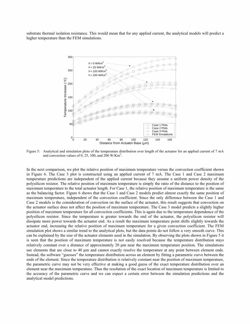
substrate thermal isolation resistance. This would mean that for any applied current, the analytical models will predict a higher temperature than the FEM simulations.

0 20 40 60 80 100 120 140 1600

50

100

150

200

250

300

Distance from Actuator Base (µm)

Tem

pera

ture

Incr

ease

( °C

)

Case 1 PlotsCase 2 PlotsCase 3 PlotsFEM Simulations

h = 0 W/Km2 h = 25 W/Km2 h = 100 W/Km2

h = 200 W/Km2

Figure 5: Analytical and simulation plots of the temperature distribution over length of the actuator for an applied current of 7 mA

and convection values of 0, 25, 100, and 200 W/Km2. In the next comparison, we plot the relative position of maximum temperature versus the convection coefficient shown in Figure 6. The Case 3 plot is constructed using an applied current of 7 mA. The Case 1 and Case 2 maximum temperature predictions are independent of the applied current because they assume a uniform power density of the polysilicon resistor. The relative position of maximum temperature is simply the ratio of the distance to the position of maximum temperature to the total actuator length. For Case 1, the relative position of maximum temperature is the same as the balancing factor. Figure 6 shows that the Case 1 and Case 2 models predict almost exactly the same position of maximum temperature, independent of the convection coefficient. Since the only difference between the Case 1 and Case 2 models is the consideration of convection on the surface of the actuator, this result suggests that convection on the actuator surface does not affect the position of maximum temperature. The Case 3 model predicts a slightly higher position of maximum temperature for all convection coefficients. This is again due to the temperature dependence of the polysilicon resistor. Since the temperature is greater towards the end of the actuator, the polysilicon resistor will dissipate more power towards the actuator end. As a result the maximum temperature point shifts slightly towards the actuator end, increasing the relative position of maximum temperature for a given convection coefficient. The FEM simulation plot shows a similar trend to the analytical plots, but the data points do not follow a very smooth curve. This can be explained by the size of the actuator elements used in the simulation. By observing the plots shown in Figure 5 it is seen that the position of maximum temperature is not easily resolved because the temperature distribution stays relatively constant over a distance of approximately 20 µm near the maximum temperature position. The simulations use elements that are close to 40 µm and cannot exactly resolve the temperature at any point between element ends. Instead, the software “guesses” the temperature distribution across an element by fitting a parametric curve between the ends of the element. Since the temperature distribution is relatively constant near the position of maximum temperature, the parametric curve may not be very effective at making a good guess of the exact temperature distribution over an element near the maximum temperature. Thus the resolution of the exact location of maximum temperature is limited to the accuracy of the parametric curve and we can expect a certain error between the simulation predictions and the analytical model predictions.

Figure 6: Plot of the position of maximum temperature versus the convection coefficient over the surface of the device.

Figure 7: Analytical and simulation plots of the average temperature increase of the actuator versus applied current for convection

0 50 100 150 200 250 300 350 400 450 5000.55

0.6

0.65

0.7

0.75

0.8

0.85

0.9

0.95

1

Convection Coefficient (W/Km2)

Rel

ativ

e P

ositi

on o

f Max

imum

Tem

pera

ture

Case 1 PlotCase 2 PlotCase 3 PlotFEM Simulation

0 1 2 3 4 5 6 7 8 9 100

50

100

150

200

250

Current (mA)

Ave

rage

Tem

pera

ture

Incr

ease

( °C

)

Case 1 PlotsCase 2 PlotsCase 3 PlotsFEM Simulations

h = 0 W/Km2 h = 25 W/Km2 h = 100 W/Km2 h = 200 W/Km2

values of 0, 25, 100, and 200 W/Km2.

parison we plot the average teFor the final com mperature increase versus the applied current shown in Figure 7. This is perhaps the most important result of this work because the average temperature of the actuator directly affects the rotation angle of the micromirror [8]. This comparison shows similar results to the previous comparisons. The Case 3 model predicts higher temperatures for lower convection values, the Case 1 model predicts higher temperatures for

higher convection values, and the FEM simulations predict a lower average temperature than the analytical models predict. Again these differences can be respectively attributed to the temperature-dependent polysilicon resistance, the convection coefficient on the actuator surface, and the difference in the substrate thermal isolation resistance between the analytical models and the FEM simulations. The analytical models agree with each other within 10% for all comparisons. This suggests that the Case 1 model can be effectively used to predict the electrothermal behavior of the device. The FEM simulations agree with the analytical models within 20% for all comparisons.

5. CONCLUSIONS

nalytical models that describe the electrothermal behavior of a 1-D electrothermal MEMS micromirror have been

ACKNOWLEDGEMENTS

The authors would like to thank Ankur Jain and Hongwei Q for discussion and fabrication of the device. The project is

REFERENCES

. J. H. Comtois, V. M. Bright, “Applications for surface-micromachined polysilicon thermal actuators and arrays,”

2. Skidmore, “Electrothermal Properties and Modeling of Polysilicon

3. al modeling

4. l, S. Schweizer, P. Renaud, Optical Microscanners and Microspectrometers Using Thermal Bimorph

5. nd modeling of a MEMS bidirectional vertical thermal actuator,”

6. d Micromirror with Large Scanning

7. OS-MEMS

8. ermal MEMS Micromirror,” M.S. Thesis,

9. wer Academic, Boston, 2001.

Adeveloped. The models predict the temperature distribution of the device upon actuation, the position of maximum temperature, the maximum temperature rise, the average temperature rise, and equivalent thermal resistances. The models were created for different thermal considerations on the device. It was shown that the simplest Case 1 model was effective at predicting the most accurate Case 3 model within 10% for practical ranges of convection and applied current. An LEM was created from the Case 1 model that used a single thermal power source. The LEM showed that a parameter called the “balancing factor” predicted the position of maximum temperature, the power flow distribution, and split of thermal resistances. The analytical models were compared to FEM simulations and agreed within 20% for all convection and current ranges tested.

u

supported by the National Science Foundation under award # 0423557.

1Sensors and Actuators A, 58 (1997), pp. 19-25. A. A. Geisberger, N. Sarkar, M. Ellis, and G. D.Microthermal Actuators” Journal of Microelectromechanical Systems, v. 12 n. 4 (2003), pp. 513-522. R. P. Manginell, J. H. Smith, A. J. Ricco, R. C. Hughes, D. J. Moreno, and R. J. Huber, “Electro-thermof a microbridge gas sensor,” SPIE Symposium on Micromachining and Microfabrication, Austin, TX (1997), pp. 360-371. G. LammeActuators, Kluwer Academic, Boston, 2002. D. Yan, A. Khajepour, R. Mansour, “Design aJournal of Micromechanics and Microengineering, 14 (2004), pp. 841-850. H. Xie, A. Jain, T. Xie, Y. Pan, G. K. Fedder, “A Single-Crystal Silicon-BaseAngle for Biomedical Applications,” Technical Digest CLEO 2003, Baltimore, MD, (2003). H. Xie, Y. Pan, G. K. Fedder, “Endoscopic optical coherence tomographic imaging with a CMmicromirror,” Sensors and Actuators A, 103 (2003), pp. 237-241. S. T. Todd, “Electrothermomechanical Modeling of a 1-D ElectrothUniversity of Florida, (May, 2005). S. Senturia, Microsystem Design, Klu

10. CoventorWare, Cary, NC, www.conventor.com.