AIMR (AZIMUTH AND INCLINATION MODELING IN

REALTIME): A METHOD FOR PREDICTION OF DOG-LEG

SEVERITY BASED ON MECHANICAL SPECIFIC ENERGY

A Dissertation

by

SAMUEL FRANS NOYNAERT

Submitted to the Office of Graduate Studies of Texas A&M University

in partial fulfillment of the requirements for the degree of

DOCTOR OF PHILOSOPHY Chair of Committee, Stephen A . Holditch Committee Members, Maria A. Barrufet Jerome J. Schubert Eduardo Gildin Head of Department, Dan A. Hill

August 2013

Major Subject: Petroleum Engineering

Copyright 2013 Samuel Frans Noynaert

ii

ABSTRACT Since the 1980’s horizontal drilling has been a game-changing technology as it allowed

the oil and gas industry to produce from reservoirs previously considered marginal or

uneconomic. However, while it is considered a mature technology, directional drilling is

still done in a reactive fashion. Although many directional drillers are quite adept at

predicting the directional response of the bottomhole assembly (BHA) in a given well,

the ability to manage all of the drilling parameters on a foot by foot basis while

accurately predicting the effects of each parameter is impossible for the human brain

alone. Given current rig rates, any amount of increased slide time and its reduced ROP

which occurred due to poorly predicted directional response can result in a significant

economic impact.

There exist many measured parameters or system inputs which have been proven to

affect the directional response of a drilling system. One parameter whose effect has not

been investigated is mechanical specific energy or MSE. MSE is measure of how

efficient the drilling process is in relation to rate of penetration. To date, MSE has

primarily been used with for vibration analysis and rate of penetration optimization.

The following dissertation covers research into the effect of MSE on the overall wellbore

direction change or dog-leg severity. Using published experimental data, a correlation

was developed which shows a clear relationship between the dog-leg severity, rate of

penetration (ROP) and MSE. The correlation requires only a few hundred feet of

drilling before it is able to be tuned to match an individual well’s results. With minimal

tuning throughout the drilling of a well, very good results can be obtained with regards

to forecasting dog-leg severity as the wellbores were drilled ahead. The correlation was

tested using data from multiple, geo-steered wells drilled in a shale reservoir. The

analysis of the correlation using real-world data proved it to be a robust and accurate

method of predicting the magnitude of dog-leg severity. The use of this correlation

results in a smoother wellbore, drilled with a faster overall ROP with a better chance of

staying within the geologic targets.

iii

DEDICATION This work is dedicated first and foremost to my wife, Courtney. Looking back, it was

obvious from the day I met you that there was no one else for me. And, from the day we

decided to embark on the journey that is this doctorate, you have supported and helped

me in innumerable ways. As Teddy Roosevelt said, “Believe you can, and you’re

halfway there”. For me, it was not mine but your belief in me which put me “halfway

there.” And, it was your love and support which helped me get from halfway to the

completion of this work. To say it was difficult for you is an understatement and I

appreciate the time and sacrifices you made to throughout the process. I cannot begin to

thank you for everything you do as a wife, mother and friend. You have been the “glue”

that held us all together during this process. Knowing that you were behind me has

given me all the inspiration I needed. I love you and thank God every day for bringing

you into my life.

I also dedicate this to my two beautiful children, Carter and Ally. I hope that I can serve

as an inspiration to you now and in the future. I know the past few years have been

difficult at times, but I’ve never seen anything but smiles and encouragement from you.

You have a bright and wonderful future in front of you, and while I wish you could stay

children forever, I can’t wait to see what you each accomplish. Most importantly, know

that being a father to both of you truly is my greatest accomplishment in life.

To all the friends and family who were part of this along the way, I thank you as well. It

gives me great joy to finally be able answer your “how’s the PhD going?” with “It’s

done!”. I would require another dissertation to discuss how each one of you contributed

through your support and words of encouragement for both myself as well as my family.

My family and I are blessed to have you in our lives and thank you for everything you

do.

Finally, although it may seem out of place in a scientific publication, I would like to note

that I genuinely feel that it was God’s help which allowed me to finish this work. There

were many paths which could have been followed and choices made which would have

iv

resulted in this work never being finished. It was with God’s help that I was able to stay

the course and get to where I am today. It is written in Philippians 4:13, “I can do all

things through him who strengthens me.” It was towards the end of the dissertation

process that I was at my lowest point I have experienced in many years. I believe God

was there when I asked for and received the strength and inspiration I needed to get to

the finish line.

v

ACKNOWLEDGEMENTS I would like to acknowledge my committee first. Dr. Stephen Holditch has been a role

model for me and my career for quite some time. His contributions to both the industry

as a whole and my personal career are almost too numerous to count. Were it not for Dr.

Holditch, I would not be in petroleum engineering and am forever grateful for this.

Dr. Jerome Schubert has been putting up with me since 2003 when I was his master’s

student. The practical manner in which he approaches his work is a model for applied

drilling research. As a sounding board and the drilling expert on the committee, he was

vital to this work. I also must thank Dr. Eduardo Gildin for his input and help. His

“non-drilling” viewpoint was essential in developing this work. The questions he asked

and the suggestions he brought from the aerospace and reservoir engineering arenas

were invaluable. Dr. Barrufet, who is partially to blame for this career path as she taught

the first petroleum engineering class I ever attended, was important as well. Her

questions and comments on this work were the key to my being able to develop a clear

narrative of what I had accomplished.

The staff in this department has been beyond helpful and supportive. I would not have

been able to teach (and thus support my family through this endeavor) were it not for the

assistance you have provided. I owe much of my teaching success to the support I

received from those that are “behind the scenes” and actually make this department run

so well.

I have had discussions over various aspects of this work with many of the faculty here at

the Texas A&M University Petroleum Engineering department. I thank each and every

one of you for taking the time to talk to me about whatever subject I was curious about

at the time.

Finally, I must acknowledge Lee Lohoefer and EOG Resources. The well data used in

this work is from EOG and it is only due to their kindly allowing me to access this data

that I was able to even consider attempting this effort.

vi

NOMENCLATURE A = Area

AAPG = American Association of Petroleum Geologists

AIMR =Azimuth and Inclination Modeling in Real-time

API = American Petroleum Institute

API = GR units (approximately 10 API units per micrograms of Radium equivalent)

BHA = bottom-hole assembly

DoF = degrees of freedom

DSATS = Drilling Systems Automation technical section of SPE

Flateral = lateral force at the bit, equivalent to SL

FEA = finite element analysis

FEM = finite element model

G = modulus of rigidity

GR =gamma-ray

I = moment of inertia

ID = inner-diameter

J = polar moment of inertia

k = radius of gyration

Kn = PDM rotation ratio

ksi = thousand psi

l = length of element

LWD = logging while drilling

M = moment or mass

vii

MD = measured depth

MPD = managed pressure drilling

MSE = mechanical specific energy, ksi

MWD = measurement while drilling

OD = outer diameter

PDM = positive displacement motor

Q = flow rate

Psi = pounds per square inch

ROP = rate of penetration, typically ft. /hr

RPM = rotations per minute

RSS = rotary steerable system

SC = sidecutting, length/length

SL = sideload, lbs. (notation used in SPE 105594)

Sr = slenderness ratio

TVD = true vertical depth

TD = total depth,

UCS = unconfined compressive strength (of rock)

WOB = weight on bit

x = length

γ = weight/ft. of drill collars in mud

β = inclination of wellbore (measured from vertical or 0o)

v = beam displacement

v = velocity

viii

������ = internal force vector for given element in local coordinate system

������� = internal force vector for given element in global coordinate system

���� = element stiffness matrix in local coordinate system

���� = element stiffness matrix in global coordinate system

������ = displacement vector for given element in local coordinate system

������� = displacement vector for given element in global coordinate system

�������� = force vector for forces resulting from geometric effects (local coordinate

system)

�������� = force vector for forces resulting from geometric effects (global coordinate

system)

� � = Transpose matrix, transitions local element stiff matrix to global coordinate

system

ix

TABLE OF CONTENTS Page

ABSTRACT ....................................................................................................................... ii

DEDICATION .................................................................................................................. iii

ACKNOWLEDGEMENTS ............................................................................................... v

NOMENCLATURE .......................................................................................................... vi

TABLE OF CONTENTS .................................................................................................. ix

LIST OF FIGURES........................................................................................................... xi

LIST OF TABLES ......................................................................................................... xvii

CHAPTER I INTRODUCTION ....................................................................................... 1

Wellbore Deviation ........................................................................................................ 1 Early Directional Wells .................................................................................................. 4 Horizontal Wells ............................................................................................................ 6 Geo-Steering .................................................................................................................. 9 Directional Drilling Technologies: Whipstocks .......................................................... 11 Directional Drilling Technologies: Mud Motors ......................................................... 15 Directional Drilling Technologies: Rotary Steerable Systems .................................... 19 Directional Drilling Process ......................................................................................... 20 Drilling Automation ..................................................................................................... 21 Contribution of Proposed Research ............................................................................. 25

CHAPTER II LITERATURE REVIEW .......................................................................... 28

Early Static BHA Analysis .......................................................................................... 28 Early BHA models ....................................................................................................... 31 Advanced Directional Drilling Models ........................................................................ 36 Rock-bit Interaction Models ........................................................................................ 49 Mechanical Specific Energy ........................................................................................ 54 Sidecutting Testing ...................................................................................................... 58

CHAPTER III THEORETICAL DEVELOPMENT ....................................................... 64

Static Finite Element Model ........................................................................................ 64 Model Solution Process ............................................................................................... 71

x

Page

Basic Sidecutting Derivation ....................................................................................... 76 Predictive Tool Development ...................................................................................... 93

CHAPTER IV SENSITIVITY STUDY ........................................................................... 96

Carthage Limestone (15,000 psi UCS) ........................................................................ 97 Bedford Limestone (3000 psi UCS) ........................................................................... 100

CHAPTER V PREDICTIVE TOOL AND PROCESS .................................................. 105

Data Requirements ..................................................................................................... 105 Predictive Process ...................................................................................................... 108

CHAPTER VI VERIFICATION AND APPLICATION .............................................. 112

Verification ................................................................................................................ 112 Application ................................................................................................................. 123

CHAPTER VII CONCLUSIONS AND FUTURE WORK........................................... 126

Conclusions ................................................................................................................ 126 Future Work ............................................................................................................... 127

REFERENCES ............................................................................................................... 130

xi

LIST OF FIGURES Page

Fig. 1 - First significant use of directional drilling technology: control of 6000 bopd blowout in Conroe Field in 1934 (Gleason 1934). ................................................. 3

Fig. 2 - Early directional drilling used when surface location was not directly above target in map view (Bourgoyne et al. 1986). .......................................................... 4

Fig. 3 - Resource triangle shows majority of available resources will require improved technology to recover (Dong et al. 2011). ............................................. 6

Fig. 4 - Horizontal and directional wells now make up significant majority of wells and total production in the United States onshore market (HPDI 2012). .............. 8

Fig. 5 - Example of successful geo-steering operation: colored log shows gamma ray (GR) readings. Wellbore went out of zone (red spike in GR) and was quickly returned back to zone. ............................................................................. 10

Fig. 6 - Three early primary methods for controlling hole direction (Bourgoyne et al. 1986; Devereux 1999) . ................................................................................... 12

Fig. 7 - Procedure for controlling hole direction with a whipstock. Whipstock is run into wellbore and oriented in desired direction, allowing deviation to occur. (Devereux 1999). .................................................................................................. 13

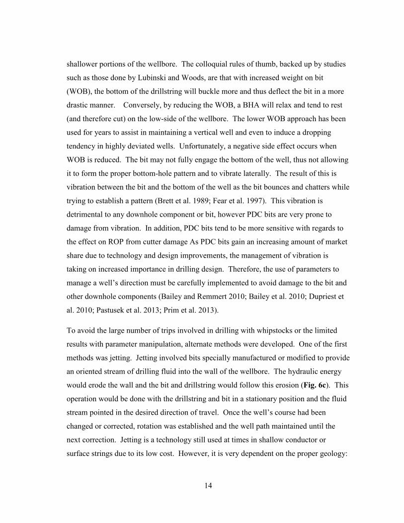
Fig. 8 - Positive displacement motor (mud motor) operation (Hughes 2009). In “rotary” mode, wellbore theoretically maintains a straight path while in “sliding” mode, the wellbore changes direction as it follows the arc created by the bend in the motor. ...................................................................................... 16

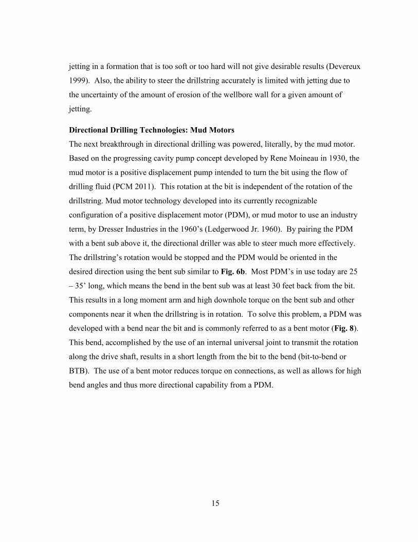
Fig. 9 - PDMs have 3 points of contact while sliding, thus creating an arc-shaped path (Hughes 2009). ............................................................................................. 17

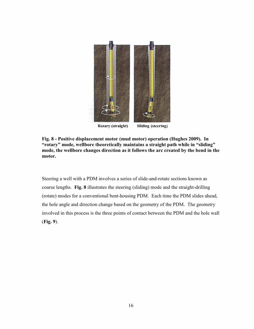
Fig. 10 - PDM manufacturers give predicted steering performance of bent motors (NOV 2005). ......................................................................................................... 17

Fig. 11 - Illustration of azimuth, inclination and dog-leg severity (Bourgoyne et al. 1986). .................................................................................................................... 18

Fig. 12 - PDMs steer through a series of slides (arcs) and rotations (tangents). .............. 19

xii

Page

Fig. 13 - Lubinski & Woods' point of tangency concept was a key component in determining dog-leg severity in their work (Lubinski and Woods 1953). ........... 29

Fig. 14 - Example of Lubinski and Woods' output, a chart showing build, hold and drop tendencies (Lubinski and Woods 1953). ...................................................... 29

Fig. 15 - Millheim, et al's approached to confining the BHA: changing elastic modulus based on displacement. Once the BHA is displaced outside the wellbore, the elastic modulus is changed to a very large number (Millheim et al. 1978). ........................................................................................................... 34

Fig. 16 - Relationship between ROP and hole enlargement developed by Birades, et al shows low ROP correlates to a much larger wellbore diameter (Birades and Fenoul 1988). ................................................................................................. 41

Fig. 17 - Example of hole enlargement adjustment factor in Orphee 3D. Plot on right shows post-adjustment fit of data has improved significantly (Birades and Fenoul 1988). ................................................................................................. 42

Fig. 18 - Pastusek, et al's work showing bit specific steering response based on RSS "steering force" for given formations (Pastusek et al. 2005). .............................. 46

Fig. 19 - Roller cone bits show a higher hypothetical tendency stay on the current path when compared to diamond bits (Bradley 1975). ........................................ 51

Fig. 20 - Decreasing RPM dramatically increases BHA vibration (Pastusek and Brackin 2003). ...................................................................................................... 55

Fig. 21 - PDC bit patterns: efficient patterns, (a), give higher ROP than inefficient, whirling bit pattern (b) (Rappold 1995). .............................................................. 57

Fig. 22 - MSE analysis allows for ROP optimization across basins due to similar trends. Increasing MSE values (blue track on right of each well) indicate low ROP due to high vibrations (Dupriest 2006). ............................................... 58

Fig. 23 - Test apparatus for SPE 7518 where lateral force applied to rock, not bit or BHA (Millheim and Warren 1978). ..................................................................... 59

Fig. 24 - Sample sidecutting tests for variety of bit designs shows significant variability of sidecutting ability (Pastusek and Brackin 2003). ........................... 60

Fig. 25- Euler-Bernoulli beam theory describes beam deflection as a function of an applied load. ......................................................................................................... 65

xiii

Page

Fig. 26 - An element at rest on an incline with a static, distributed load applied. ........... 66

Fig. 27 – Local coordinate system and vectors for single finite element. ........................ 69

Fig. 28- First rotation of the element to change from local to global coordinate system. .................................................................................................................. 70

Fig. 29 - Second rotation of the element to align with global coordinate system. ........... 70

Fig. 30 -Original analysis used large BHA components (a), but creating smaller elements (b) results in finer resolution and increased accuracy. .......................... 72

Fig. 31 – Output of static model showing deformed BHA in wellbore. .......................... 75

Fig. 32 - Data in SPE 105594 presented as "Bit Tilt" to represent "steerability" of tested bit (Pastusek et al. 2005). ........................................................................... 77

Fig. 33 - Sidecutting as a function of sideload shows non-linear behavior (Ernst et al. 2007). ............................................................................................................... 78

Fig. 34 - Sidecutting as a function of sideload shows non-linear changes in power-law coefficient and exponent (Ernst et al. 2007). ................................................. 78

Fig. 35 - Logarithmic fit of sidecutting as a function of ROP shows illogical results when projecting to higher ROPs. ......................................................................... 80

Fig. 36 - Power-law fit of sidecutting as a function of ROP shows logical results at higher ROPs. ........................................................................................................ 80

Fig. 37 - Logarithmic fit of sidecutting as a function of MSE. ........................................ 82

Fig. 38 - Power-Law fit of sidecutting as a function of MSE. ......................................... 83

Fig. 39 - MSE plotted over measured sidecutting rate in Barnett shale well shows good correlation to overall severity. ..................................................................... 84

Fig. 40 - 8 ½ in. bit used in experimental setup with passive four inch gauge (Ernst et al. 2007). ........................................................................................................... 85

Fig. 41 - Increasing sideload slightly increases percent of non-cutting material contacting rock face resulting in non-linear response. ......................................... 86

xiv

Page

Fig. 42 - For constant RPM as ROP increases, as shown in (a), total rock contacted per foot goes down resulting in less sidecutting. ................................................. 87

Fig. 43 - Sidecutting model using RPM shows good agreement between measured and modeled results. ............................................................................................. 90

Fig. 44 - Sidecutting model using MSE shows good agreement between measured and modeled results. ............................................................................................. 91

Fig. 45 - Changing RPM changes slope of sidecutting as function of sideload. .............. 92

Fig. 46 - Model of sidecutting as a function sideload modified by ROP and MSE effects for Carthage limestone tests. .................................................................... 93

Fig. 47 - Representative BHA used while drilling lateral section of wellbores. .............. 94

Fig. 48 - Projection of experimental data in Carthage limestone shows strong dependency on MSE (Carthage limestone with 500 lb. sideload). ...................... 97

Fig. 49 - When MSE range reduced, similar behavior is observed to that of the larger scale, with reduced minimum and maximum values (Carthage limestone with 1000 lb. sideload). ....................................................................... 98

Fig. 50 - Once ROP scale is reduced, the relationship between MSE, ROP and DLS becomes close to a plane shape and thus linear (Carthage limestone, 1000 lb. side force). ............................................................................................................ 98

Fig. 51 - Changing ROP from higher in (a) to a lower ROP, (b), shows increase in dog-leg severity capability in Carthage limestone. .............................................. 99

Fig. 52 - As side-load increases, the dog-leg capability increases as well (Carthage limestone sample). .............................................................................................. 100

Fig. 53 - Output from Bedford limestone equation shows stronger dependency on ROP. ................................................................................................................... 101

Fig. 54 - DLS in lower UCS rock driven primarily by ROP as opposed to MSE (Bedford limestone with 1000 lb. side force). .................................................... 101

Fig. 55 - Closer analysis of Bedford limestone shows similar behavior to Carthage limestone at intermediate level of investigation. ................................................ 102

xv

Page

Fig. 56 - Deepest level of investigation, similar to foot by foot analysis of well data, shows plane with primary slope toward high ROP (Bedford limestone - 1000 lb. side force). ............................................................................................ 103

Fig. 57 - For Bedford limestone over constant ranges of ROP and MSE, increasing sideload increases the sidecutting rate and thus dog-leg severity. ..................... 104

Fig. 58 - Example of surveys from rigsite, updated continually as surveys are taken. .. 106

Fig. 59 - Slide sheet shows tool-face and other parameters from each section of the wellbore. ............................................................................................................. 107

Fig. 60 - Sample torque and drag model output showing slack-off weight as a function of depth. These values allow us to see what the downhole weight is relative to the surface WOB. .............................................................................. 109

Fig. 61 - Model output shows good agreement between actual and modeled sidecutting rate. .................................................................................................. 110

Fig. 62 - Model output showing results in terms of DLS, confirming SC to DLS relationship. ........................................................................................................ 111

Fig. 63 - Output of model compared to actual values shows good correlation. Bounding lines represent 1 degree of DLS difference. ...................................... 111

Fig. 64 - Well #1 model output: model optimized over first 250 ft., then no further action taken. ....................................................................................................... 114

Fig. 65 - Well #2: Calibrated after 300', model is using original Bedford limestone parameters. ......................................................................................................... 115

Fig. 66 - Well #2 after drilling ahead: the last 3 surveys show significant error. The coefficient is adjusted by factor of 2.7. .............................................................. 116

Fig. 67 - Well #2 after the coefficient is adjusted, the predicted DLS values matched the measured values until the last two surveys. Another adjustment needs to be made. ............................................................................................................. 116

Fig. 68 - Well #2, after the coefficient is adjusted based on the last two surveys. Care is taken to avoid overcorrection and the well is finished with good agreement between measured values and those predicted by the correlation. ... 117

xvi

Page

Fig. 69 - Well #3: Calibrated after three surveys using a coefficient of 10E-6. After three large errors, correlation was recalibrated at 9788' MD. ............................ 118

Fig. 70 - Well #3: Correlation recalibrated at 9788' and continues to stay calibrated for almost 2000'. An obvious error trend is noted just before 12,000 ft. .......... 118

Fig. 71 - Well #3: coefficient is recalibrated to original experimental value of 3E-6 and the well is drilled to TD. The correlation remains well calibrated during remaining run. .................................................................................................... 119

Fig. 72 - Cylinder plot of Well #3 weight on bit with ROP trace in blue above and GR trace in red below. When correlation initially applied, WOB sensor showing zero. ..................................................................................................... 120

Fig. 73 - Cylinder plot of Well #3 weight on bit with ROP trace in blue above and GR trace in red below. Correlation required recalibration when WOB sensor was fixed (in highlighted area). ............................................................... 121

Fig. 74 - Cylinder plot of Well #3 weight on bit with ROP trace in blue above and GR trace in red below. Correlation required recalibration when bit was damaged (in highlighted area). .......................................................................... 122

Fig. 75 - Decreasing ROP through WOB reduction to achieve higher DLS can result in dangerously high MSE. .................................................................................. 124

xvii

LIST OF TABLES Page

Table 1 - Test results showing side-cutting in a homogeneous rock (Bedford limestone) with respect to drilling parameters (Ernst et al. 2007). ...................... 62

Table 2 - Test results showing side-cutting in a homogeneous rock (Carthage limestone) with respect to drilling parameters (Ernst et al. 2007). ...................... 63

Table 3 - End definitions for Eq. 3 (Nicholson 1972). ..................................................... 67

Table 4 - Measured and assumed drilling parameters and the resulting MSE values in ksi. .................................................................................................................... 84

Table 5 - Inputs and outputs used for initial model of sidecutting as a function of sideload, ROP and RPM. ...................................................................................... 89

Table 6 - Model parameters for Bedford and Carthage samples. ................................... 113

1

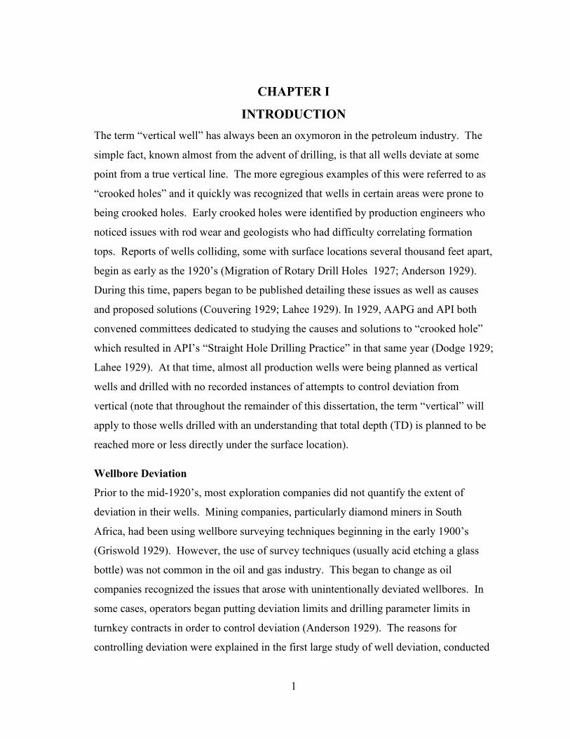
CHAPTER I

INTRODUCTION The term “vertical well” has always been an oxymoron in the petroleum industry. The

simple fact, known almost from the advent of drilling, is that all wells deviate at some

point from a true vertical line. The more egregious examples of this were referred to as

“crooked holes” and it quickly was recognized that wells in certain areas were prone to

being crooked holes. Early crooked holes were identified by production engineers who

noticed issues with rod wear and geologists who had difficulty correlating formation

tops. Reports of wells colliding, some with surface locations several thousand feet apart,

begin as early as the 1920’s (Migration of Rotary Drill Holes 1927; Anderson 1929).

During this time, papers began to be published detailing these issues as well as causes

and proposed solutions (Couvering 1929; Lahee 1929). In 1929, AAPG and API both

convened committees dedicated to studying the causes and solutions to “crooked hole”

which resulted in API’s “Straight Hole Drilling Practice” in that same year (Dodge 1929;

Lahee 1929). At that time, almost all production wells were being planned as vertical

wells and drilled with no recorded instances of attempts to control deviation from

vertical (note that throughout the remainder of this dissertation, the term “vertical” will

apply to those wells drilled with an understanding that total depth (TD) is planned to be

reached more or less directly under the surface location).

Wellbore Deviation

Prior to the mid-1920’s, most exploration companies did not quantify the extent of

deviation in their wells. Mining companies, particularly diamond miners in South

Africa, had been using wellbore surveying techniques beginning in the early 1900’s

(Griswold 1929). However, the use of survey techniques (usually acid etching a glass

bottle) was not common in the oil and gas industry. This began to change as oil

companies recognized the issues that arose with unintentionally deviated wellbores. In

some cases, operators began putting deviation limits and drilling parameter limits in

turnkey contracts in order to control deviation (Anderson 1929). The reasons for

controlling deviation were explained in the first large study of well deviation, conducted

2

by Alex Anderson. The results of his study showed that most wells experienced

significant horizontal displacement from their intended target. Some wells had exhibited

inclination readings in excess of 65 degrees (his tool’s maximum reading was 65

degrees) and it was theorized they might have ended up as horizontal wells (Anderson

1929)!

The first recorded instance of controlled deviation of a wellbore was in 1928 in the

Signal Hill field by John Eastman and the Kuster Company. (Kuster 2011) The inventor

of the technology used by Eastman, Robert E. Lee of Coleman, TX, actually drilled

several planned horizontal wells in the Big Lake Field the following year in 1929. (EIA

1993; Morgan 1992). The production results from the horizontal wells are unknown and

subsequent development of the Big Lake Field was conducted using vertical wells.

Horizontal drilling technology remained a novelty and was not used in a significant

manner until 1933. In 1933 the Conroe field experienced a pair of massive blowouts

from the Madeley No. 1 and Alexander No. 1 wells. These blowouts resulted in a large

crater (several hundred feet in diameter) that was on fire. The fire was extinguished with

a series of slant wells, drilled by George Failing, that relieved the gas flow and allowed

the fire to be extinguished. However, the oil flow continued unabated at the rate of 6000

barrels per day. Humble Oil Company brought in John Eastman to help stop the

uncontrolled flow of oil and keep the Conroe field from being ruined (Wells 2005).

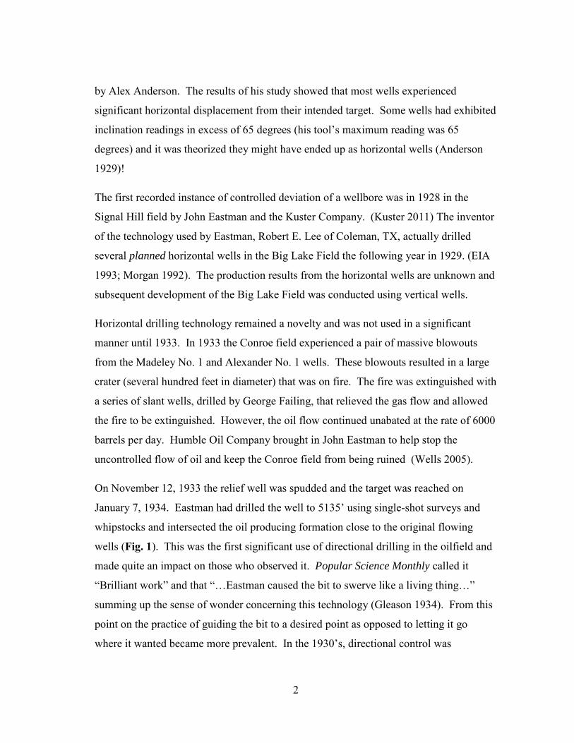
On November 12, 1933 the relief well was spudded and the target was reached on

January 7, 1934. Eastman had drilled the well to 5135’ using single-shot surveys and

whipstocks and intersected the oil producing formation close to the original flowing

wells (Fig. 1). This was the first significant use of directional drilling in the oilfield and

made quite an impact on those who observed it. Popular Science Monthly called it

“Brilliant work” and that “…Eastman caused the bit to swerve like a living thing…”

summing up the sense of wonder concerning this technology (Gleason 1934). From this

point on the practice of guiding the bit to a desired point as opposed to letting it go

where it wanted became more prevalent. In the 1930’s, directional control was

3

accomplished through the use of whipstocks or by controlling drilling parameters, such

as weight on the bit, and BHA design.

Fig. 1 - First significant use of directional drilling technology: control of 6000 bopd blowout in Conroe Field in 1934 (Gleason 1934).

4

Early Directional Wells

Onshore locations were typically located directly above their reservoir targets, but this

luxury was not afforded to most offshore wells. As soon as offshore development

began, the need for directionally drilled wells in this environment was apparent. The

first offshore development in the U.S. was in 1896 in Santa Barbara, CA in the

Summerland Field (California Department of Conservation 2005). These wells were

drilled from piers that had been built out over the water, sometimes exceeding over

1200’ offshore. Early Gulf Coast wells were drilled from barges and were also single

well locations. However, in 1947 the first well was drilled out of sight of land by Kerr-

McGee Oil and the need to consolidate drilling and production facilities in offshore

development was recognized (Hakes 2011). When the high potential flow rates from

offshore wells were coupled with the technological needs of drilling and producing oil

and gas offshore, all phases of the life of a well began to be investigated and improved

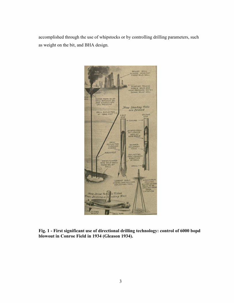
upon. The well path itself was not exempt from this process. By drilling one vertical

well followed by multiple directional wells from a single platform, large cost savings

could be realized on all facets of the well construction process.

Fig. 2 - Early directional drilling used when surface location was not directly above target in map view (Bourgoyne et al. 1986).

5

Directional drilling technology continued to gain widespread acceptance both onshore

and offshore. For the most part, directional drilling was primarily used to steer a

wellbore from a surface location to a point in the reservoir that was hundreds of feet

away in the horizontal direction from the surface location (Fig. 2). In the 1940’s and

1950’s, the desired result was typically a perpendicular or almost perpendicular

intersection with the producing formation. In some instances, issues with regards to the

earth’s surface directly above the target necessitated the need to offset the surface

location. Situations such as drilling near populated areas or in environmentally sensitive

areas resulted in surface locations that were not directly over their reservoir targets. In

addition, drilling to gain access to reserves in mountain ranges or under inland waters

required directionally steered well paths. These situations were the primary use and

justification for directional drilling until a step-change occurred concerning targeted

reserves, particularly in North America.

It has been known since the inception of the oil and gas industry that the volume of

existing hydrocarbons is much bigger than the amount of recoverable hydrocarbons.

The existing hydrocarbons in place are referred to as resources while the hydrocarbons

which are recoverable under current economic conditions using current technology are

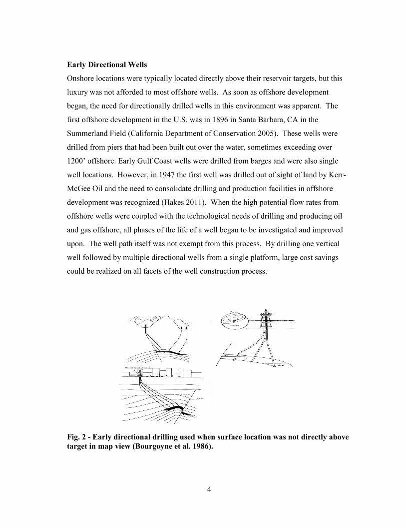
referred to as reserves. The distribution of the resources among reservoir types is seen in

Fig. 3, the resource triangle. Until the middle of the twentieth century, the majority of

reserves were what we would call conventional and would be fit into the uppermost

point of the triangle. However, as conventional reserves were depleted (especially in

North America) and world demand for energy grew, a new type of resource was

targeted: unconventional. Based on the definition by Holditch, I will define

unconventional resources as resources that have low matrix permeability or unique fluid

properties that require advanced drilling or stimulation technologies to be produced at

commercial flow rates (Holditch 2006). Unconventional reservoirs have been producing

since the 1950’s, and have become the largest resource base in most basins. The

prominence of unconventional resources is illustrated in a recent study of twenty-five

North American basins which showed the overwhelming majority of the technically

6

recoverable resources are classified as unconventional resources (Cheng et al. 2010).

Several technologies have been the key to exploiting unconventional reservoirs and each

has a specific application. One of the primary technologies used to unlock many of the

unconventional resources is horizontal drilling.

Fig. 3 - Resource triangle shows majority of available resources will require improved technology to recover (Dong et al. 2011).

Horizontal Wells

Beginning in the early 1980’s, horizontal wells became a common technology that was

used to develop unconventional resources as Elf (Europe), BP (Alaska) and assorted

domestic E&P companies (Austin Chalk, Texas) drilled productive horizontal wells in

their respective areas of operation (EIA 1993). The gains in productivity of those

horizontal over vertical wells in the same field ushered in new era of drilling that opened

up many previously uneconomic formations by increasing exposure to the pay zone. The

economics of drilling a horizontal well in a high permeability reservoir are typically not

as attractive as drilling a horizontal well in a low permeability reservoir. The reason for

this difference is because the high permeability, or conventional, reservoir will have a

7

large productivity index, and thus, there is no need to increase the exposure of the pay

zone by drilling the well horizontally. The result of a horizontal well in a high

permeability formation is a decreasing return on investment relative to permeability.

However, the reservoir performance of a low permeability reservoir is limited in the case

of a vertical well, even if it is fracture treated. By increasing the reservoir exposure by

several orders of magnitude using a horizontal well bore, the low permeability rock will

produce more hydrocarbons.

As previously noted, R.E. Coleman had actually tested horizontal wells in the Big Lake

Field in the Permian Basin. The fact that future development was vertical pointed to two

primary issues with horizontal or highly deviated wells. Horizontal wells are more

expensive and prone to operational issues, as well as needing the right reservoir in order

to justify the high cost. Little is known about Coleman’s wells, but it is assumed they

were expensive, had severe operational issues with regards to hole cleaning and wellbore

stability and that they were targeting a conventional reservoir which did not require the

high pay zone exposure to develop economically. The difference between those first

wells in 1920’s Texas and the wells in the early 1980’s was that the later wells were

targeting reservoirs which were otherwise uneconomic when accessed vertically. In

addition, technology had developed enormously, such the metallurgy of the steel used

for the drill pipe and the tools used for steering the wellbore.

As directional drilling became a common practice, the number of horizontal and highly

deviated wells and the complexity of those wells have steadily increased as technology,

capability and the demand for worldwide reserves has increased. Over the last half

century, the number of active producing vertical wells in onshore U.S. provinces has

grown by a factor of 3.5 to 350,000. In the same time period, the number of active

producing onshore directional wells, meaning wells which were intentionally deviated

but not horizontal, grew by a factor of 10 while the number of active producing onshore

horizontal wells grew by a factor of 17 (HPDI 2012). Another example shows that from

1990 to 1997, in a single basin (Gulf of Mexico), a single service company

8

(Schlumberger/Anadrill) had approximately 20,000 separate BHA runs (Lesso et al.

1999). Of these 20,000 BHA runs, 78% were classified as using steerable systems.

While few of these would have been considered horizontal, most would have been

considered directional in terms of their well paths.

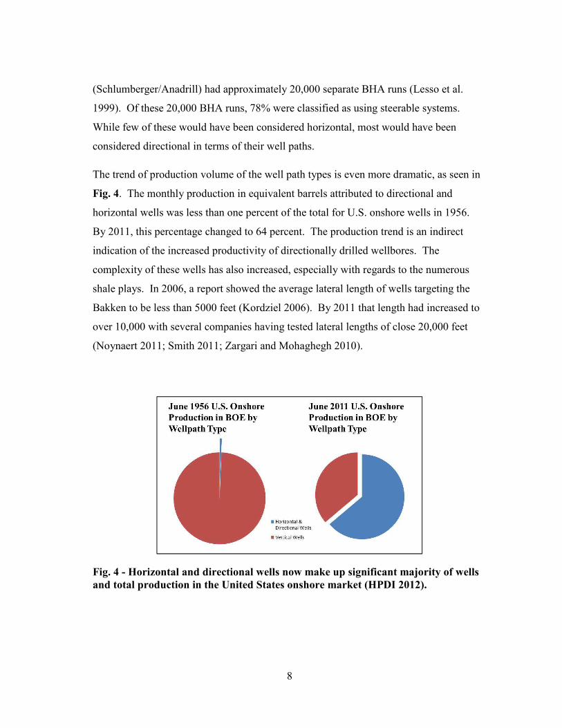
The trend of production volume of the well path types is even more dramatic, as seen in

Fig. 4. The monthly production in equivalent barrels attributed to directional and

horizontal wells was less than one percent of the total for U.S. onshore wells in 1956.

By 2011, this percentage changed to 64 percent. The production trend is an indirect

indication of the increased productivity of directionally drilled wellbores. The

complexity of these wells has also increased, especially with regards to the numerous

shale plays. In 2006, a report showed the average lateral length of wells targeting the

Bakken to be less than 5000 feet (Kordziel 2006). By 2011 that length had increased to

over 10,000 with several companies having tested lateral lengths of close 20,000 feet

(Noynaert 2011; Smith 2011; Zargari and Mohaghegh 2010).

Fig. 4 - Horizontal and directional wells now make up significant majority of wells and total production in the United States onshore market (HPDI 2012).

9

Geo-Steering

A successful directional drilling operation, particularly one involving horizontal drilling,

requires an accurately placed wellbore. The real-time process used to steer and place the

wellbore is referred to as geo-steering. Geo-steering is defined as:

“The intentional directional control of a well based on the results of downhole

geological logging measurements rather than three-dimensional targets in space,

usually to keep a directional wellbore within a pay zone. In mature areas, geo-

steering may be used to keep a wellbore in a particular section of a reservoir to

minimize gas or water breakthrough and maximize economic production ....”

(Schlumberger 2008)

Based on the definition, this is a seemingly simple task; however, the application of the

concept is difficult when undertaken within the tight tolerances of today’s geological

targeting requirements. It has been described by various practitioners as “landing a

plane on a runway in the fog, when the runway is moving up and down” (Brown 2000)

or similar to “driving a bus forward, while sitting in the back of the bus and looking

backward”. Three elements must be in place in order for a successful geo-steering

operation:

1. Geologic and drilling operation experience in the geographic area

2. Accurate geologic data prior to drilling (seismic, offset well correlations)

3. Timely and accurate drilling and formation data during the geo-steering

operation.

The reality of geo-steering, even in “easy” areas with minimal geological complexity

and high-quality real-time data is that the wellbores are rarely placed 100% in the

desired target window. An individual well may encounter local geological abnormalities

as well as difficulty in controlling the well path. The key then to geo-steering is not just

the preparation and data analysis but identifying and fixing the inevitable issues and

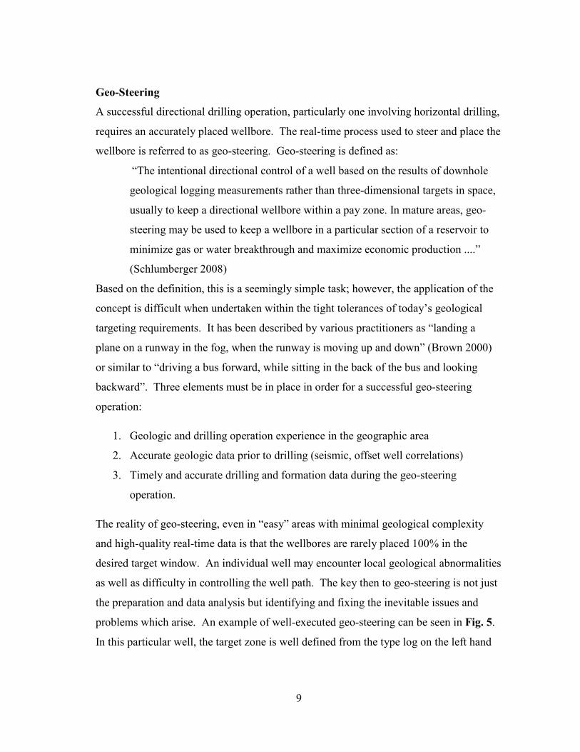
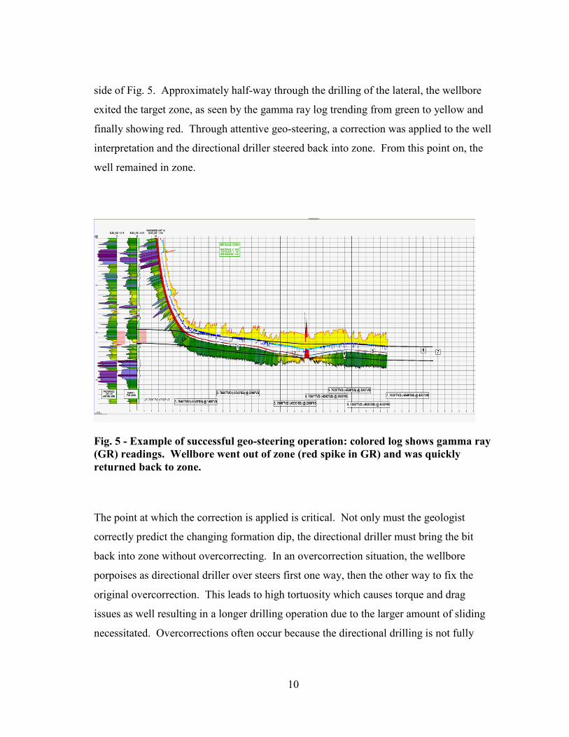
problems which arise. An example of well-executed geo-steering can be seen in Fig. 5.

In this particular well, the target zone is well defined from the type log on the left hand

10

side of Fig. 5. Approximately half-way through the drilling of the lateral, the wellbore

exited the target zone, as seen by the gamma ray log trending from green to yellow and

finally showing red. Through attentive geo-steering, a correction was applied to the well

interpretation and the directional driller steered back into zone. From this point on, the

well remained in zone.

Fig. 5 - Example of successful geo-steering operation: colored log shows gamma ray (GR) readings. Wellbore went out of zone (red spike in GR) and was quickly returned back to zone.

The point at which the correction is applied is critical. Not only must the geologist

correctly predict the changing formation dip, the directional driller must bring the bit

back into zone without overcorrecting. In an overcorrection situation, the wellbore

porpoises as directional driller over steers first one way, then the other way to fix the

original overcorrection. This leads to high tortuosity which causes torque and drag

issues as well resulting in a longer drilling operation due to the larger amount of sliding

necessitated. Overcorrections often occur because the directional drilling is not fully

11

aware of what the directional tendencies of the BHA may be. By having a better idea of

the behavior of the BHA in both sliding and rotating modes, the directional driller can

confidently plan his slide and rotate course lengths and not resort to overly corrective

actions to ensure the bit remains in the target zone.

It is obvious that directional and horizontal drilling has progressed from a novel, little-

used technology to a commonly used technology that has allowed the petroleum industry

to continue finding and developing new reserves. Without directional drilling and

horizontal drilling and their more specialized cousin, geo-steering, our world would be a

much different place. In addition to stranding a large portion of the conventional

resources, many of the unconventional resources would not be considered technically

recoverable. The resulting higher energy prices due to lower availability would provide

a crippling effect on our economy.

Directional Drilling Technologies: Whipstocks

Some portions of the directional drilling process have changed significantly since its first

introduction. The physical technology used to change the course of the well has

progressed from a simple machine (ramp in the form of a whipstock) to tool strings that

cost millions of dollars each to manufacturer. Circumstantial reports show 1895 as the

first time a whipstock was used (Inglis 1987). It was a simple wedge or ramp dropped

downhole to sidetrack a well. While it was used in what we would consider a fishing

application to get around junk in the well and the new wellbore’s direction as not

controlled, none the less it was the first recorded intentional deflection of a wellbore

from its otherwise prescribed path.

12

Fig. 6 - Three early primary methods for controlling hole direction (Bourgoyne et al. 1986; Devereux 1999) .

Whipstocks were the first tools used to control the well path. Eastman and his peers

would drill ahead in a (hopefully) straight path, and then deploy a whipstock when their

survey tools indicated a change in direction was needed. The whipstock was simple: a

wedge that was run into the wellbore. Once oriented and set in place, a bit was run in

the hole and drilled off of the original well path in the direction the whipstock was

pointing (Fig. 6a). The process of using a whipstock as shown in Fig. 7, was repeated as

many times as necessary. The use of multiple whipstocks was very laborious and took a

long time to achieve so the driller could maintain the proper trajectory to total depth

(TD).

13

Fig. 7 - Procedure for controlling hole direction with a whipstock. Whipstock is run into wellbore and oriented in desired direction, allowing deviation to occur. (Devereux 1999).

In many wells, the primary goal was just to maintain a vertical wellbore. In this event,

the manipulation of the drilling parameters was often used. Although Lubinski and

Woods are generally given credit with writing the defining paper on this subject,

manipulating drilling parameters to control wellbore deviation was a noted practice

beginning in the 1920’s (Cartwright 1928; Lubinski and Woods 1953; Mills1928). The

general idea was that by taking into account the formation dip as well as the bottom-hole

assembly (BHA) geometry, one could develop an ideal set of drilling parameters to drill

a vertical well. The primary parameter to change was weight-on-bit (WOB), although

other parameters such as revolutions-per-minute (RPM) of the drillstring as well as

hydraulic parameters were investigated as well. Drilling parameter manipulation proved

to be a useful tool in controlling well deviation but whipstocks remained the primary

method of initiating a change in the direction of a wellbore.

Parameter manipulation is still used today in many applications where steerable tools are

not used or the drilling of a vertical well is being attempted. This usually occurs in

14

shallower portions of the wellbore. The colloquial rules of thumb, backed up by studies

such as those done by Lubinski and Woods, are that with increased weight on bit

(WOB), the bottom of the drillstring will buckle more and thus deflect the bit in a more

drastic manner. Conversely, by reducing the WOB, a BHA will relax and tend to rest

(and therefore cut) on the low-side of the wellbore. The lower WOB approach has been

used for years to assist in maintaining a vertical well and even to induce a dropping

tendency in highly deviated wells. Unfortunately, a negative side effect occurs when

WOB is reduced. The bit may not fully engage the bottom of the well, thus not allowing

it to form the proper bottom-hole pattern and to vibrate laterally. The result of this is

vibration between the bit and the bottom of the well as the bit bounces and chatters while

trying to establish a pattern (Brett et al. 1989; Fear et al. 1997). This vibration is

detrimental to any downhole component or bit, however PDC bits are very prone to

damage from vibration. In addition, PDC bits tend to be more sensitive with regards to

the effect on ROP from cutter damage As PDC bits gain an increasing amount of market

share due to technology and design improvements, the management of vibration is

taking on increased importance in drilling design. Therefore, the use of parameters to

manage a well’s direction must be carefully implemented to avoid damage to the bit and

other downhole components (Bailey and Remmert 2010; Bailey et al. 2010; Dupriest et

al. 2010; Pastusek et al. 2013; Prim et al. 2013).

To avoid the large number of trips involved in drilling with whipstocks or the limited

results with parameter manipulation, alternate methods were developed. One of the first

methods was jetting. Jetting involved bits specially manufactured or modified to provide

an oriented stream of drilling fluid into the wall of the wellbore. The hydraulic energy

would erode the wall and the bit and drillstring would follow this erosion (Fig. 6c). This

operation would be done with the drillstring and bit in a stationary position and the fluid

stream pointed in the desired direction of travel. Once the well’s course had been

changed or corrected, rotation was established and the well path maintained until the

next correction. Jetting is a technology still used at times in shallow conductor or

surface strings due to its low cost. However, it is very dependent on the proper geology:

15

jetting in a formation that is too soft or too hard will not give desirable results (Devereux

1999). Also, the ability to steer the drillstring accurately is limited with jetting due to

the uncertainty of the amount of erosion of the wellbore wall for a given amount of

jetting.

Directional Drilling Technologies: Mud Motors

The next breakthrough in directional drilling was powered, literally, by the mud motor.

Based on the progressing cavity pump concept developed by Rene Moineau in 1930, the

mud motor is a positive displacement pump intended to turn the bit using the flow of

drilling fluid (PCM 2011). This rotation at the bit is independent of the rotation of the

drillstring. Mud motor technology developed into its currently recognizable

configuration of a positive displacement motor (PDM), or mud motor to use an industry

term, by Dresser Industries in the 1960’s (Ledgerwood Jr. 1960). By pairing the PDM

with a bent sub above it, the directional driller was able to steer much more effectively.

The drillstring’s rotation would be stopped and the PDM would be oriented in the

desired direction using the bent sub similar to Fig. 6b. Most PDM’s in use today are 25

– 35’ long, which means the bend in the bent sub was at least 30 feet back from the bit.

This results in a long moment arm and high downhole torque on the bent sub and other

components near it when the drillstring is in rotation. To solve this problem, a PDM was

developed with a bend near the bit and is commonly referred to as a bent motor (Fig. 8).

This bend, accomplished by the use of an internal universal joint to transmit the rotation

along the drive shaft, results in a short length from the bit to the bend (bit-to-bend or

BTB). The use of a bent motor reduces torque on connections, as well as allows for high

bend angles and thus more directional capability from a PDM.

16

Fig. 8 - Positive displacement motor (mud motor) operation (Hughes 2009). In “rotary” mode, wellbore theoretically maintains a straight path while in “sliding” mode, the wellbore changes direction as it follows the arc created by the bend in the motor.

Steering a well with a PDM involves a series of slide-and-rotate sections known as

course lengths. Fig. 8 illustrates the steering (sliding) mode and the straight-drilling

(rotate) modes for a conventional bent-housing PDM. Each time the PDM slides ahead,

the hole angle and direction change based on the geometry of the PDM. The geometry

involved in this process is the three points of contact between the PDM and the hole wall

(Fig. 9).

17

Fig. 9 - PDMs have 3 points of contact while sliding, thus creating an arc-shaped path (Hughes 2009).

Fig. 10 - PDM manufacturers give predicted steering performance of bent motors (NOV 2005).

18

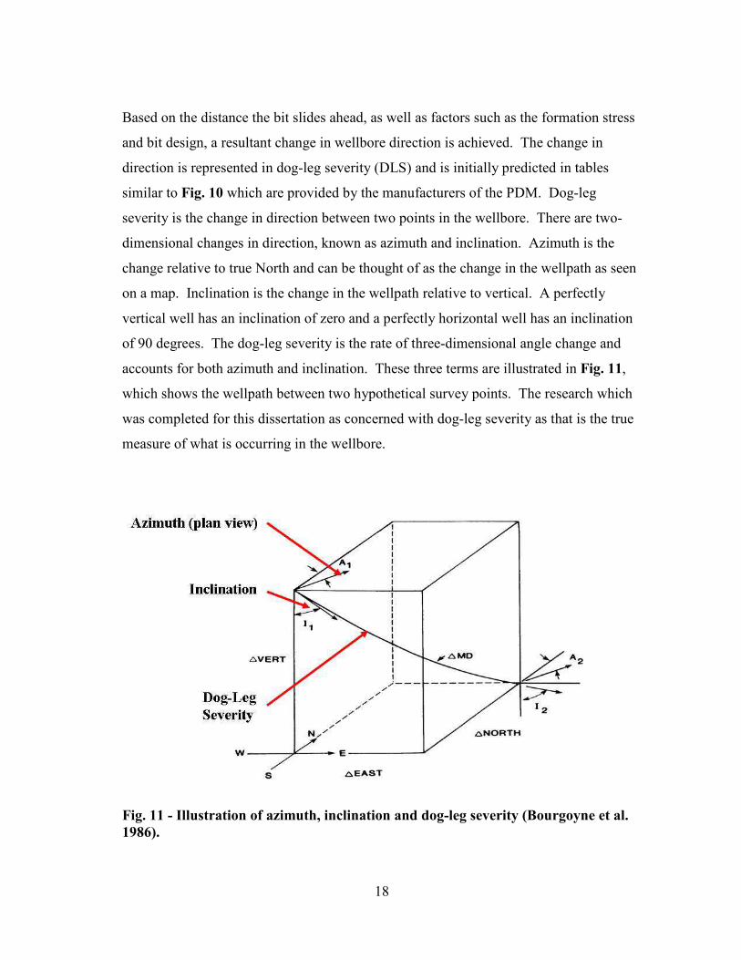
Based on the distance the bit slides ahead, as well as factors such as the formation stress

and bit design, a resultant change in wellbore direction is achieved. The change in

direction is represented in dog-leg severity (DLS) and is initially predicted in tables

similar to Fig. 10 which are provided by the manufacturers of the PDM. Dog-leg

severity is the change in direction between two points in the wellbore. There are two-

dimensional changes in direction, known as azimuth and inclination. Azimuth is the

change relative to true North and can be thought of as the change in the wellpath as seen

on a map. Inclination is the change in the wellpath relative to vertical. A perfectly

vertical well has an inclination of zero and a perfectly horizontal well has an inclination

of 90 degrees. The dog-leg severity is the rate of three-dimensional angle change and

accounts for both azimuth and inclination. These three terms are illustrated in Fig. 11,

which shows the wellpath between two hypothetical survey points. The research which

was completed for this dissertation as concerned with dog-leg severity as that is the true

measure of what is occurring in the wellbore.

Fig. 11 - Illustration of azimuth, inclination and dog-leg severity (Bourgoyne et al. 1986).

19

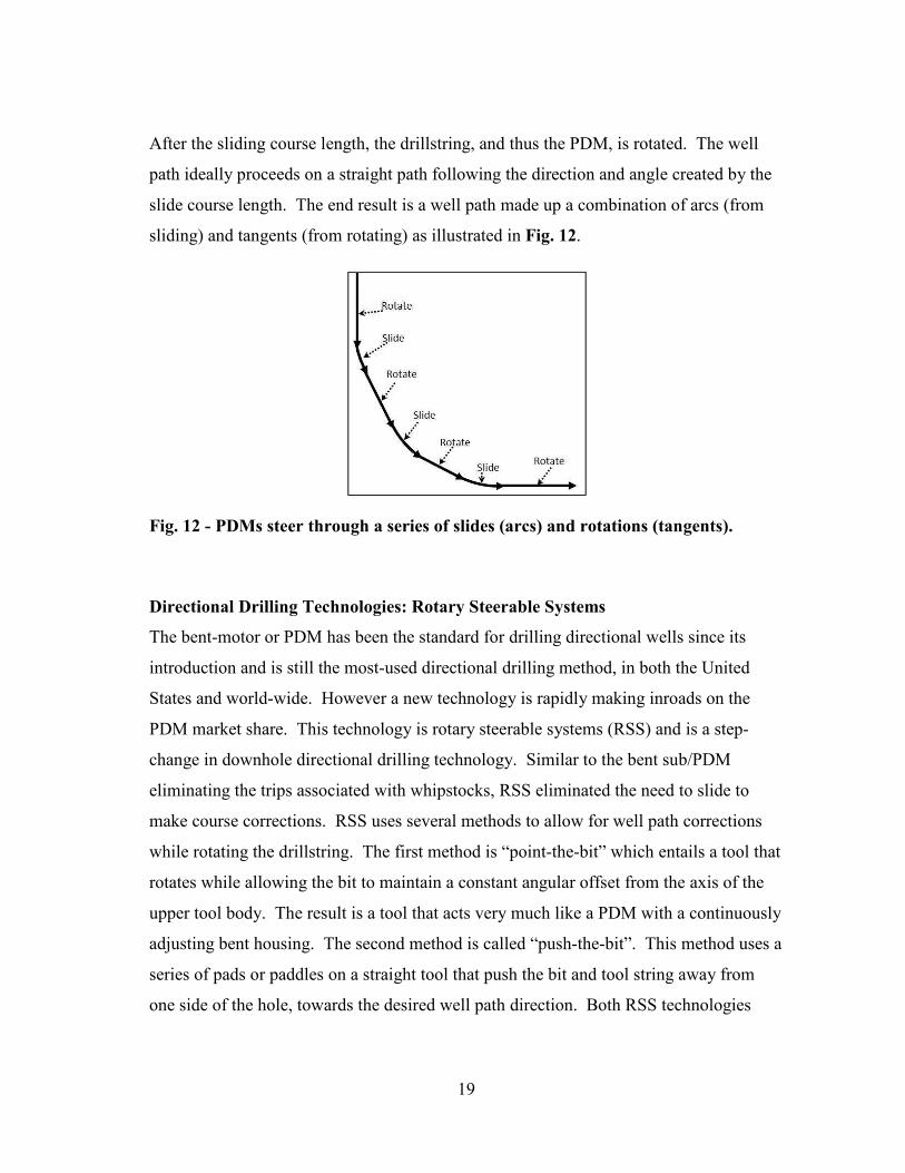
After the sliding course length, the drillstring, and thus the PDM, is rotated. The well

path ideally proceeds on a straight path following the direction and angle created by the

slide course length. The end result is a well path made up a combination of arcs (from

sliding) and tangents (from rotating) as illustrated in Fig. 12.

Fig. 12 - PDMs steer through a series of slides (arcs) and rotations (tangents).

Directional Drilling Technologies: Rotary Steerable Systems

The bent-motor or PDM has been the standard for drilling directional wells since its

introduction and is still the most-used directional drilling method, in both the United

States and world-wide. However a new technology is rapidly making inroads on the

PDM market share. This technology is rotary steerable systems (RSS) and is a step-

change in downhole directional drilling technology. Similar to the bent sub/PDM

eliminating the trips associated with whipstocks, RSS eliminated the need to slide to

make course corrections. RSS uses several methods to allow for well path corrections

while rotating the drillstring. The first method is “point-the-bit” which entails a tool that

rotates while allowing the bit to maintain a constant angular offset from the axis of the

upper tool body. The result is a tool that acts very much like a PDM with a continuously

adjusting bent housing. The second method is called “push-the-bit”. This method uses a

series of pads or paddles on a straight tool that push the bit and tool string away from

one side of the hole, towards the desired well path direction. Both RSS technologies

20

have advantages and disadvantages inherent to their method of steering. However, the

primary goal of eliminating the slide-rotate-slide pattern is achieved by both push-the-bit

and point-the-bit.

Currently RSS does not consistently produce DLS above 10 deg/100’. As most curves

in unconventional wells are drilled at 10 deg/100’ or even higher DLS, applying RSS in

this market is difficult. However, as the technology develops and customers demand

higher DLS capability, the limits of RSS are continuously changing. Another hurdle for

implementation of RSS in many markets is the cost and reliability. The complexity of

RSS lends itself to more failures than PDM’s, as well as significantly higher

manufacturing costs for the service provider and lost-in-hole cost for the operator.

Currently both PDM and RSS directional drilling technology are used in most basins

around the world. The selection of the proper technology for a given situation is the

subject of many papers and is beyond the scope of this report. However, the issues and

problems associated with directional drilling are markedly similar regardless of which

method was employed.

Directional Drilling Process

Whether the PDM or the RSS is used, the process and problems involved in the steering

decision-making are similar. The primary issue is not with the BHA or steering system

itself, it is often with the surveying and logging tools. These tools are typically placed 50

to 70 feet back from the bit. While “near-bit” tools exist for inclination and gamma ray,

these result in added cost while still not giving all of the necessary data. In particular,

the near-bit inclination is not considered to be a viable substitute for the full MWD

survey tool further up the BHA.

The result of this tool placement is that at the last known location in the wellbore, as

measured by the survey tool, there will always exist 50 or more feet of unknown

wellbore ahead of it. Within this 50 feet, multiple slide-rotate course lengths (for PDMs)

or steering strength changes (for RSS) may exist. Lithology will likely have changed to

come extent as well, even in a horizontal wellbore. Therefore, in order to accurately

21

drill ahead in a manner which keeps the wellbore in zone, assumptions must be as what

the outcomes of these steering actions were. This leaves the directional driller making a

constant series of educated guesses concerning what his recent steering actions did with

regards to wellbore direction and what he should do as he drills ahead. If the directional

driller makes a poor assumption regarding the outcome of his decision, the result either a

wellbore drilled out of zone or additional time spent steering the wellbore back onto the

desired path.

Drilling Automation

The topic of drilling automation is currently one of the hottest topics in the petroleum

industry. The SPE technical group, Drilling Systems Automation Technical Section

(DSATS) is the most active SPE technical section at the time of this writing. All major

services companies as well as several large operators have entire divisions devoted to

developing and selling technology and processes for automating the drilling process.

While much has been made of drilling automation of late, the pursuit of drilling

automation has been attempted for over a century. In fact, the first recorded instance of

drilling automation design is credited to Leonardo Da Vinci’s plans for screw-based drill

feed machine, almost 500 years ago (Brantly). The first recorded piece of drilling

automation equipment actually built was that of Rodolphe Leschot in the 1860’s.

Leschot built and used an automatic bit feed (commonly known now as an autodriller)

for use in drilling blast holes (Aldred et al. 2005). While rate of feed or weight on bit

control was the subject of most initial work in drilling automation, it was automating the

rig floor which would result in the first significant automation successes. Beginning in

the 1940’s, with BJ Company’s pneumatically controlled slips, automating or

mechanizing the rig floor has been the primary and most successful target of drilling

automation advocates. Achievements such as the iron roughneck (rig floor pipe

handling), automatic stabbing machines (replacing man in derrick during tripping) and

automated catwalks were some of the first commercial realizations in the drilling

automation arena (Boyadjieff 1988; Brugman 1987; Deguillaume and Johnson 1990;

Eustes 2007). The primary goal for rig floor automation was improving rigsite safety.

22

However, as the technologies were implemented, engineers immediately saw how

significant time and cost savings could be found through automation in addition to the

obvious safety benefits. A visit in any rig manufacturing facility today will bear this out.

The safety aspect alone does not explain the widespread use of rig floor automation

equipment. The majority of the new-build land rigs in the U.S. market incorporate most,

if not all of these pipe-handling features because customers are willing to pay for them.

The customers are willing to pay extra not only because of an increased focus on safety

but also due to the recognition of the economic benefits of rig automation.

In recent years, drilling automation has advanced from being mostly related to rig floor

equipment to an idea that is applied to all parts of the drilling process. This expanding

focus has occurred through the confluence of increased safety concerns, larger amounts

of high quality, real-time data becoming available and high oil prices which provide the

funding to develop a more automated drilling process. Attempts at automating most

parts of the drilling process are underway. For example, given the drilling fluid’s

importance to the drilling process, finding new ways to automate the mud-mixing and

measurement processes has been the focus of several groups (Forde and O'Hara 1987;

Kvame et al. 2011; Saasen et al. 2009; Stock et al. 2012). Pressure management is

another area in which automation has been a game-changing technology. Managed

pressured drilling (MPD) is a process meant to accurately control the downhole

pressures such that a well can be drilled within tight tolerances between formation

pressure and fracture pressure at the bottom of the wellbore. Whether this is due to

drilling in a depleted onshore reservoir or a deepwater well with less than a pound per

gallon of difference between fracture and pore pressures, managed pressure drilling has

enable the industry to extend the limits of what can be safely drilled. Most commercial

systems contain a significant amount of automation in both the detection as well as the

implementation of the MPD process (Calderoni et al. 2006; Fredericks et al. 2008; Laird

et al. 2005; Rehm et al. 2008; Reitsma 2005; Riet et al. 2003; Roes et al. 2006; Santos et

al. 2008; Vogel et al. 2007). MPD technology has allowed many “undrillable” wells to

become realities. The step-change in drilling capability and the impact on unlocking

23

reserves through automation of MPD is a window into the possibilities of other

automation efforts.

In a return to the initial work in automation over a hundred years ago, work on the

downhole processes such as rock-cutting has seen a resurgence in interest. This work

tends toward the automation of optimization – creating and using algorithms which

gather and analyze data with the goal of optimizing the downhole mechanics of cutting

rock. Areas such as vibration management and ROP optimization are covered by this

(Dunlop et al. 2011; Esmaeili et al. 2012; Koederitz and Johnson 2011). Technologies

and processes addressing this aspect of automation tend to look for and identify patterns,

mostly dealing with vibration of some type and recommend or enact methods to change

the pattern to one which is conducive to higher ROP, lower vibration or both (Cayeux et

al. 2012; Pastusek et al. 2013; Wardt et al. 2013).

The majority of the automation process and technologies mentioned here and in the

literature review require high quality, real-time data to properly function (Dupriest et al.

2012). These processes and technologies take advantage of the electronic rig data

gathering systems available on most rigs. These systems are a far cry from the pen and

paper geolographs of a few decades ago. A rig data gathering system can track any

process that can have a sensor placed on it. This data is gathered on a scale as fine as

once every second or down to one-tenth of a foot of hole drilled. Parameters and

measurements ranging from LWD tool readouts to drilling parameters such as RPM and

WOB are readily available at most wellsites today. The data storage is now done at

offsite servers, even for remote or offshore locations. This allows for real-time access

by those offsite such as engineers and geologists. The end result is a massive database

of available information which can be used by automation algorithms and tools to

improve the drilling process.

Overall, the term “drilling automation” is trending toward the optimization of

performance. DSATS has recently made the distinction between automation and

mechanization (Wardt et al. 2013). Examples of mechanization would be the 20th

24

century advances in rig floor automation or mechanization. Mechanization still requires

significant human input as to instructions and decision making. Automation seeks to

include the decision making process as well. For example, the connection process is

currently mechanized on many rigs. The driller pushes several buttons to bring the

drillpipe up to the rig floor, make the connection and then go back to drilling. An

automated process would recognize when the next joint of pipe was needed, make the

connection, return the bit to bottom and start drilling completely on its own, without

human intervention. The focus of the drilling automation effort is beginning be on to the

process itself. While mechanizing or automating the tools themselves is important, the

decision process must also be automated. In optimization problems, the volumes of data

currently being collected are more than a human can reasonably analyze in real-time.

Yet, the value in this data can be tremendous. By harnessing the power and insights in

this data, much could be done to analyze and improve the drilling process. As such

algorithms must be developed which can assist or take the place of a human in making

both large as well as mundane drilling decisions.

Theoretically, the ability to control a well is based on the geometric relationship between

the BHA and the wellbore. Although the underlying calculations can be complex

mathematically (Bourgoyne et al. 1986; Sawaryn and Thorogood 2005; Sawaryn and

Tulceanu 2007; Sawaryn and Tulceanu 2009), the wellpath is actually quite predictable

in a controlled environment. However, when a wellbore with varying diameter and

possibly changing fluid properties is drilled with a BHA coupled with bit that has an

unknown directional tendency in a non-homogeneous rock with anisotropic stresses,

theory doesn’t stand the test. All drilling engineers can relate stories of directionally

drilled wells following a path that differed substantially from that of the theoretical path.

The following literature review will show how many have tried to account for these

unknown or immeasurable variables, yet the overall conclusion can only be that we have

found a definitive method to do so beyond real-time “modeling” or control systems.

This modeling is informal and done by humans’ memories on a well by well basis. It is

this part of the directional drilling procedure which I am targeting for research.

25

Despite directional drilling technology’s enormous impact on not just our industry, but

our economy and world, parts of its implementation remain unchanged from almost a

century ago. Inglis described directional drilling as “the art and science involved in the

deflection of a wellbore in a specific direction in order to reach a pre-determined

objective below the surface of the Earth”(Inglis 1987). Many feel that the proportion of

science used has been increasing. This is certainly true with regards to the tools in use

that were just described. However, the art still remains in the directional driller’s back

pocket, in his tally book’s record of the drilling parameters, surveys and other notes, and

his interpretation of those records. Perhaps one of the more telling passages in Lubinski

and Wood’s groundbreaking paper on BHA modeling is the following: “Even in an

isotropic formation, a perfectly vertical hole cannot be drilled with an elastic drillstring,

unless extremely small and uneconomical weights are used” (Lubinski and Woods

1953). This quote illustrates the fundamental issue at hand: wells will not stay vertical

(or on an intended path) on their own in an economical manner. Thus a mechanism to

steer the drillstring must be used. Whether this mechanism is a bent motor, RSS or

simple drilling parameter manipulation based on observed properties and reactions,

intervention must be made to steer the well.

Contribution of Proposed Research

My research proposes to develop a correlation which will assist in the analysis of the

directional tendency of a steering system. As I have presented, the directional drilling

process and in particular the horizontal drilling process, have been in wide-spread use

for over thirty years. Yet, while the tools used have seen significant improvements, the

decision-making process has not developed at the same rate. The process relies on the

directional driller himself to make decisions based on prior experiences with the current

well, geographic area or just his career in general. Generally the directional drillers are

correct in their decisions. However, in today’s high-cost environment, there exist

significant advantages in further optimizing the directional drilling process. The many

data streams available on a rigsite and their effects on the directional drilling process are

often overlooked. The research discussed in the ensuing chapters will show how

26

mechanical specific energy affects the directional response of the directional drilling

assembly. A correlation has been developed which clearly shows the MSE-directional

response relationship. This correlation can be used as tool to predict the directional

response of a directional drilling system and allow the directional driller to adjust his

decisions accordingly. By assisting the directional driller to make a more informed

steering decision, several economic advantages will result.

The first advantage is related to time. Any steering corrections required beyond reacting

to a changing lithology are wasted time. For wells steered using downhole motors, this

is fairly obvious. To make a direction change or correction, one must slide the BHA

forward as shown in Fig. 12. While sliding, the ROP can be anywhere from 50 percent

to as low as 10 percent of the rotating ROP. In an onshore U.S. shale example, we

consider the total daily drilling costs in the lateral to be between $50,000 and $75,000.

This means that for every extra hour required to drill the well, the operator will have

spent between $2000 and $3100. Sliding to correct a wellbore may only add a few hours

to the overall time required, but even those few hours will add significant costs. While

RSS do not need to slide and thus are faster overall, the time spent correcting a poorly

steered wellbore can still add up. This time may be less than that required with a mud

motor, however since RSS adds significant additional costs to the drilling day rate, the

effect is very similar – even though the correction may take a just a few hours, the cost

of the well has been raised. Some might think this is an insignificant cost when the cost

to drill and complete a horizontal shale well ranges from $3,0000,0000 to $10,000,0000

or more. On a single well basis, this may be true. However, the development model for

unconventional plays is typically a factory-style model where many wells are drilled in

an almost assembly line manner to develop an given area. If an operator has 10 rigs

drilling in an area and each rig drills a well every 3 weeks, the operator will drill

approximately 173 wells per year. If the operator loses a only few hours per well due to

unnecessary directional corrections at a cost of $5,000/well, the result is over $850,000

in lost capital per year.

27

A second advantage to developing the ability to predict wellbore deviation is improving

the placement of the wellbore. When a well is drilled out of zone, whether due to

geological misinterpretation or a poor directional drilling decision, the result can have

long-term effects on the well’s productivity. Often, when a well is drilled out of zone,

that portion may have limited productivity or could possibly not be perforated and thus

produced from. To return back to the target zone could take several hundred feet once

the problem has been identified and the correction applied. Recently reported well

results in the Eagleford shale show estimated ultimate recoverable reserves of 400,000

bbls of equivalent oil (BOE) per well. Each well is drilled with an average lateral length

of 5,000 ft. These numbers mean that in the event a lateral is drilled out of zone for just

100 ft., the resulting loss in value would be over $700,000 using current oil prices.

The preceding numbers show there is a significant prize to be attained for the oil and gas

industry in improving the directional drilling steering process. While it is not meant to

replace a directional driller and their knowledge, the research presented will assist in the

analysis of the complex system which uses modern directional drilling tools and the

wellpath objectives demanded by today’s unconventional resources. The investigation

of dog-leg severity as a function of mechanical specific energy is novel approach and

addition the body of knowledge surrounding directional drilling. The correlation

developed should further capability of the industry predict and thus optimize the

directional drilling process which will result in lower cost wells and higher production

rates.

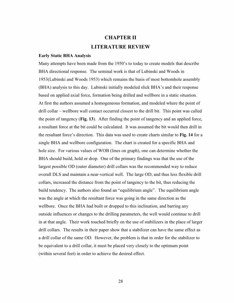
28

CHAPTER II

LITERATURE REVIEW Early Static BHA Analysis

Many attempts have been made from the 1950’s to today to create models that describe

BHA directional response. The seminal work is that of Lubinski and Woods in

1953(Lubinski and Woods 1953) which remains the basis of most bottomhole assembly

(BHA) analysis to this day. Lubinski initially modeled slick BHA’s and their response

based on applied axial force, formation being drilled and wellbore in a static situation.

At first the authors assumed a homogeneous formation, and modeled where the point of

drill collar – wellbore wall contact occurred closest to the drill bit. This point was called

the point of tangency (Fig. 13). After finding the point of tangency and an applied force,

a resultant force at the bit could be calculated. It was assumed the bit would then drill in

the resultant force’s direction. This data was used to create charts similar to Fig. 14 for a

single BHA and wellbore configuration. The chart is created for a specific BHA and

hole size. For various values of WOB (lines on graph), one can determine whether the

BHA should build, hold or drop. One of the primary findings was that the use of the

largest possible OD (outer diameter) drill collars was the recommended way to reduce

overall DLS and maintain a near-vertical well. The large OD, and thus less flexible drill

collars, increased the distance from the point of tangency to the bit, thus reducing the

build tendency. The authors also found an “equilibrium angle”. The equilibrium angle

was the angle at which the resultant force was going in the same direction as the

wellbore. Once the BHA had built or dropped to this inclination, and barring any

outside influences or changes to the drilling parameters, the well would continue to drill

in at that angle. Their work touched briefly on the use of stabilizers in the place of larger

drill collars. The results in their paper show that a stabilizer can have the same effect as

a drill collar of the same OD. However, the problem is that in order for the stabilizer to

be equivalent to a drill collar, it must be placed very closely to the optimum point

(within several feet) in order to achieve the desired effect.

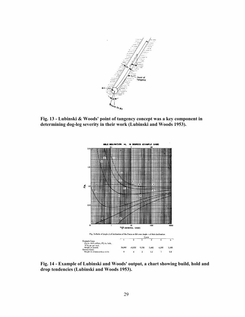
29

Fig. 13 - Lubinski & Woods' point of tangency concept was a key component in determining dog-leg severity in their work (Lubinski and Woods 1953).

Fig. 14 - Example of Lubinski and Woods' output, a chart showing build, hold and drop tendencies (Lubinski and Woods 1953).

30

The result of Lubinski and Wood’s work was the first technical paper on how to

manipulate drilling parameters to control hole direction. The authors did note in several

instances the advantage of just drilling ahead and accepting a certain amount of

deviation. This too is an important concept as it takes the idea of controlling the well’s

direction from an ideal situation into a more realistic setting. The paper also discussed

the effect of the formation on the well’s direction. This will be discussed in in the

literature review on formation effects.

Murphy and Cheatham expanded on Lubinski and Woods’ early work mathematically

and attempted to simplify several of the charts (Murphey and Cheatham Jr. 1966). They

first outlined several theories that still form the basis of most deviation models. Three of

the theories are in the rock-bit section. They also put forth the drill collar moment

theory. The drill collar moment theory applies to situation in which the bit drills through

a formation that has both soft and hard characteristics. Due to differential rate of

penetration (ROP) the weight distribution on the bottom of the hole is uneven. This

uneven distribution causes a moment to occur around the bit itself. In turn, this moment

affects the point of tangency, which changes the side force on the bit. Although the

authors used the anisotropic formation theory to make predictions on resultant force and

hole direction, they did put this fourth and final theory forward as potential alternative to

use in evaluating formation effects on wellbore inclination.

For their model, Murphy and Cheatham used elastic beam-column theory and the

anisotropic formation work from Lubinski and Woods to find the equilibrium angle.

They then expanded the analysis to include the rate of angle change, thus going beyond

the constant angle analysis of earlier publications. They included formation

heterogeneity characteristics, drill collar dimensions (and thus drill collar stiffness), drill

collar – wellbore clearance and WOB. Their primary simplification was the ignoring the

weight of the drill collar below the point of tangency or the pendulum weight. The result

was an improvement on earlier mathematical descriptions but as Arthur Lubinski said in

his review of the paper it did not “reach useful technological conclusions”.

31

Early BHA models

Beginning in the 1970’s computers began to be used to run computational BHA models.

The first published instance of using computers to solve the BHA problems was in 1972

through PhD research conducted by Nicholson at the University of Tulsa (Nicholson

1972). Nicholson created a static three-dimensional BHA model. The model used non-

linear, finite element analysis. The BHA was kept in the wellbore using a penalty

function. By accounting for the displacements at contacts of the BHA and constraining

well, Nicholson was able to find a resultant force and direction. The model does not

account for geological effects and makes the assumption that the resultant force direction

at the bit is the direction the wellpath will follow. The model’s primary limitation is that

it is for BHAs in a straight, inclined wellbore (constant angle) and thus does not deal

with rate of angle change and its effect on the trajectory projection. The model matched

results from prior publications including Lubinski and Woods’ work.

Shortly after Nicholson’s work was finished an engineer at Shell, F.J. Fischer, published

his work on a BHA model called SCHADS (Static Curved Hole Analysis of Drill

Strings) (Fischer 1974). Similar to Nicholson, Fischer uses an elastic beam finite

element model but his was solved through the finite difference method (using numerical

approximation instead of partial derivative equations). In addition, Fischer was able to

model the BHA in a curved well instead of a straight, inclined wellbore. This two-

dimensional model was able to calculate the points of contact and their forces, the

internal forces and bending moments in the BHA and the resultant force at the bit. Like

Nicholson, Fischer assumed the wellpath followed the resultant force direction. This

was the first BHA program developed by an end-user (Shell Development Co) and it

was not intended for stand-alone or quantitative analysis. Fischer seems to recognize the

inherent error in a two-dimensional static model and clearly states in several places that

his model was intended for qualitative or comparison purposes.

Fisher’s static two-dimensional model was used by Bradley to come to several

conclusions concerning directional drilling and wellbore trajectory control (Bradley

32

1975). Bradley noted that investigations of directional drilling problems will take one of

two paths. The first part of directional drilling analysis is investigation into the

drillstring mechanics. The second topic to look into is the rock-bit interaction. Bradley

used the concept of “active drillstring” to discuss the BHA analysis. Active drillstring

length referred to the length of drillstring below the point of tangency (Fig. 13). Bradley

assumed that once the point of tangency was found, all BHA components above it could

be removed from the calculation and replaced with an effective force. This is an

effective method of simplifying static calculations in order to decrease computational

time. He stated that in isotropic formations, such as massive sandstones, the bit could be

expected to reasonably follow the resultant force direction. However, in anisotropic

formations, particularly laminated dipping formations, this was not the case. In these

cases, Bradley subscribed to the preferential chip theory which is explained in greater

detail later in this literature review.

Finally, Bradley made a statement which is oddly lacking in many prior or future

publications. He stated that “The trick is to select the drillstring hookup that allows the

greatest weight on bit to be applied (thereby achieving the greatest penetration rate)…”

(Bradley 1975). While it is sometimes implied, the concept of maximizing ROP while

maintaining an intended wellbore trajectory is rarely mentioned in other publications. It

is certainly true that many of them are highly theoretical in nature; however it is my

opinion that any directional drilling model should always have the goal of maximizing

overall ROP and thus reducing well costs.

A three-dimensional BHA model was developed based on Fischer’s earlier work

(Fischer 1974) which was able to predict both inclination and azimuthal directional

behavior (Walker and Friedman 1977). Walker and Friedman developed a “shooting”

technique to solve the two third order differential equations involved in the analysis as

well as boundary conditions applied at the top, bottom and contact points of the BHA.

The shooting method is a mathematical solution to boundary value problems involving

iterations of problems with unknown initial conditions but known boundaries. The

33

results from their model matched several earlier models’ output, but were not verified

against actual data.

Another modification to Nicholson’s model was used to match data from offshore Dubai

wells (Sutko et al. 1980). Using the model developed by Nicholson (Nicholson 1972),

Sutko et al compared the model’s output to actual data. The findings showed that stiffer

BHAs with higher moments of inertia were not modeled as accurately using the

unmodified model. The authors added an effective or “interpretation length” over which

the angle caused by the resultant force occurred. This meant that stiffer assemblies

would not change angle as quickly. This concept is not used in any other BHA models

and is not fully explained or developed in this paper. Given that it addresses issues with

the flexibility of the BHA, it seems that using a discrete enough mesh in the FEA model

coupled with the ability to manipulate the material properties would result in the same

result with less user interpretation required. Sutko et al also claim, as do prior and

subsequent publications to be able to handle square drill collars. It should be noted that

while this is easily done in a simplistic model by changing the cross-sectional area and

thus related terms, it is not necessarily correct. Neither Sutko et al, nor other authors

seem to account for the two theoretical points of contact taking place with square drill

collars as opposed to the single point with round drill collars. It seems this could make a

significant difference to the drill collar stand-off and thus the calculations.

In 1976, Keith Millheim published the first of his many papers on the subject (Millheim

et al. 1978). He used a model reported on by a fellow Amoco employee that was

initially developed to study drillstring failures and casing wear (Warren 1977). In this

paper, he took the original model and began to make improvements in the calculation

methods. Millheim’s initial model used straight elastic beams as his elements and

employed a gapping element at each node. By defining a gap-strain breakpoint, the user

was able to begin applying a different stress-strain law at the higher level of stress (Fig.

15). Millheim’s model resulted in more accurate results in large-displacement scenarios

which describes the curve or other high rate of angle change areas in the wellbore. In

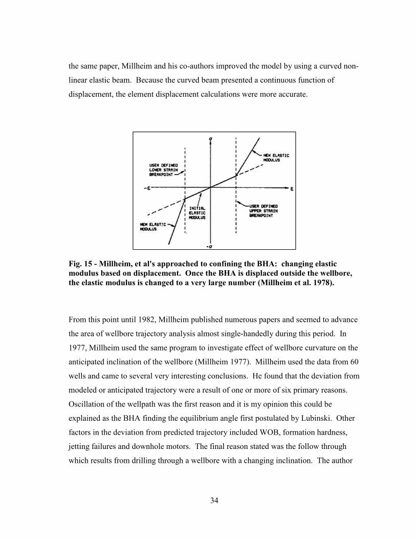
34

the same paper, Millheim and his co-authors improved the model by using a curved non-

linear elastic beam. Because the curved beam presented a continuous function of

displacement, the element displacement calculations were more accurate.

Fig. 15 - Millheim, et al's approached to confining the BHA: changing elastic modulus based on displacement. Once the BHA is displaced outside the wellbore, the elastic modulus is changed to a very large number (Millheim et al. 1978).

From this point until 1982, Millheim published numerous papers and seemed to advance

the area of wellbore trajectory analysis almost single-handedly during this period. In

1977, Millheim used the same program to investigate effect of wellbore curvature on the

anticipated inclination of the wellbore (Millheim 1977). Millheim used the data from 60

wells and came to several very interesting conclusions. He found that the deviation from

modeled or anticipated trajectory were a result of one or more of six primary reasons.

Oscillation of the wellpath was the first reason and it is my opinion this could be

explained as the BHA finding the equilibrium angle first postulated by Lubinski. Other

factors in the deviation from predicted trajectory included WOB, formation hardness,

jetting failures and downhole motors. The final reason stated was the follow through

which results from drilling through a wellbore with a changing inclination. The author

35

suggested the use of BHA models in a post-well analysis function to find the defining

inclination deviation factor for specific situation. This conclusion as well as several

conclusions from his first publication on the subject (Millheim et al. 1978) form the

basis of the reason for my research. Interestingly enough, there were no publications on

the successful application of a BHA model that incorporated prior surveys to refine a

model until after the literature review for my dissertation was started (Pirovolou et al.

2011). Given the early findings by Millheim on this aspect of BHA modeling, one

would have expected more work to be concentrated on this area.

From 1978 to 1979, Millheim reached a broader audience through an eight-part series in

the Oil & Gas Journal (Millheim 1978a, 1978b, 1979a, 1979b, 1979c, 1979d). He used

the FEM model previously developed and Amoco test well data to illustrate the current

directional drilling practices and recommendations. After an introduction to modeling

the BHA as well as actions taken to change the path of the wellbore such as jetting or

bent subs, Millheim presented two factors that affect well trajectory. First he discussed

stabilizer placement for both single and multiple stabilizer BHAs. Then he closed the

series with discussions on the effect of soft, medium and hard formations on the

wellbore trajectory. The result was a series with recommendations meant to be

practically applied by drilling engineers.

The use of BHA models was initially confined to post-well analysis. Millheim presented

a simple method to evaluate the directional drilling aspect of a well in which he

mentioned the lack of post-well analysis by most operator and directional drilling

companies (Millheim et al. 1979). He showed how to graph the drilling parameters and

the rate of trajectory change side-by-side. Once significant points in the drilling history

were noted on the graph, it often became clear what the potential causes may have been.

In the same paper, Millheim demonstrated how a three-dimensional FEA BHA model

could enhance the basic post-well analysis and assist in determining the reason behind

unplanned trajectory changes. This paper also includes a detailed explanation of

Millheim’s FEM based on a text by Przemieniecki (Przemieniecki 1968).

36

The preceding publications by Millheim covered static BHA models. The obvious issue

of what effect rotation has on the wellbore trajectory had been neglected to this point.

Millheim and his team began to develop a three-dimensional dynamic BHA model in the

early 1980’s and were able to drill several test wells specifically for the testing of the

model (Millheim and Apostal 1981). The model was based on the three-dimensional

FEA static model previously discussed (Millheim 1978a, 1978b, 1979a, 1979b, 1979c,

1979d; Millheim et al. 1979) and specifically addresses the interaction of the rotating

BHA and wellbore wall. An inertial force vector and friction force vector were added

and the result was the external load vector at a given load behaving in an oscillatory

fashion. While the model did not account for rock-bit interaction, it provided some

important insights, particularly given that it was backed up by five test runs worth of

data. As stated in the publication: “We have determined that much of the erratic

behavior of a BHA usually attributed only to geology can be explained accurately in

terms of the dynamic response of the assembly itself”.

Millheim’s final publication released the results of a seemingly finished three-

dimensional dynamic finite element BHA model (Millheim 1982). He expanded on the

dynamic three-dimensional model. He still found side forces at the bit and along the

BHA while the drillstring was in rotation. However, Millheim added in the effect of the

lithology being drilled. The model used an assumed ROP as well as assumed formation

types and strengths. These were input into a side-cutting model by developed by

Millheim and Warren at an earlier time (Millheim and Warren 1978). The output of the

side-cutting model is used to correct the amount of side cutting, and thus displacement,

predicted by the three-dimensional dynamic FEA model.

Advanced Directional Drilling Models

After Millheim’s work, trajectory models seem to progress to the next level of

sophistication. FEA was stilled used as the basis for BHA modeling and the ideas first

postulated by Lubinski and Woods, as well as Murphey and Cheatham, were the basis

for the rock-bit interaction portions of these models. However, the models are more

37

mathematically complex as well as well as taking advantage of the rapidly improving

computing capacity at the time. The first example of using these advanced models can

be seen in two publications covering the GEODYN and GEODYN2 models, developed

by Sandia National Laboratory. The first model, GEODYN, was primarily a rock-bit

interaction model (Baird et al. 1984; Tinianow et al. 1984). The final version of the

model, GEODYN2, was a three-dimensional FEA model which was capable of transient

dynamic analysis coupled with the original rock-bit interaction model presented in

earlier publications (Apostal and Baird 1987; Baird et al. 1985). GEODYN2 accounted

for bit and stabilizer interaction with the formation as well as the now-standard FEA

model of the BHA. With regards to the BHA aspect, this model included several unique

features. The most interesting was in regard to how the BHA was inserted into the

model scenario. The BHA is first placed at depth with all of the appropriate components

in place. This allows for a static solution to be found. Next, the drillstring is rotated off-

bottom to allow for a stabilization of the transient dynamic solution. Finally, a WOB is

applied to the rotating BHA and the new transient dynamic solution is found. This

method of “staging in” the load on the BHA allows the program to predetermined

“restart points”. Thus, if the user decides to vary WOB, the program reverts back to the

point at which the drillstring was rotating off –bottom, not back to the beginning

reducing the calculation time required to find a solution. Another feature was the ability

to model varying hole size. Many of the prior publications reviewed stated the explicit

assumption that the wellbore diameter was constant, yet at the same time these

publications commented on the importance of the wellbore-BHA clearance in predicting

trajectory. However, while this is an interesting feature, there exists an issue with this

capability in the form of the data required. This method would entail the need for real-

time caliper (similar to RSS capability) or confining the use of the model to post-run

analysis. GEODYN and GEODYN2 are important in both their level of model

sophistication as well as the extraordinary amount of documentation that is associated

with them. The end result of the study was a quantitative look at drillstring vibrations

38

and but only a qualitative look at wellbore trajectory results. There do not seem to be

any instances of the program being used to successfully predict wellbore trajectory.

Lubinski revisited the topic of his pioneering work in the 1950’s with a model developed

in 1986 in conjunction with J.S. Williamson (Williamson and Lubinski 1987). The

model was a two-dimensional static model which predicted inclination build rates for a

given set of BHA and geological parameters. The authors make some very good

clarifying assumptions as follows:

� The bit only follows the resultant force in non-sedimentary rocks

� The resultant drilling direction is NOT the direction the bit is currently pointing

� The bending moment at the bit is zero

� Therefore, the force at the bit can only be dependent on the BHA, not the

formation.

The second assumption could be argued, but the others are relatively clear cut. The

conclusion which may be drawn from these assumptions is that in order to develop an

accurate trajectory model, one must couple the result force caused by the BHA with the

geological effects at the bit. Woods and Lubinski use a simple version of a non-linear

beam element FEA model to mode the BHA and its resultant force on the bit. The

authors coupled this with a “formation crookedness” factor. The authors intentionally

kept the model simple in order to avoid the issue of data quality which can be found in

complex models. The result is a DLS prediction and eventually an equilibrium angle

based on static conditions. The program was used by Smith International to successfully

model the BHAs on two wells with the results agreeing with actual data.

Although it is a “blinding flash of the obvious” (Burrough and Helyar 1989), Williamson

and Lubinski make a clear and distinct statement on input data quality. The authors note

that the “main limitation” of ANY model is the input data (Williamson and Lubinski

1987). They note data such as stabilizer clearances, dip angles and hole-angle errors as

possibly having outsized effects on the model’s accuracy. This leads one to reconsider

39

models with overly complex inputs such as the GEODYN and GEODYN2 models.

While these models may be academically pleasing, they are rarely appropriate for real-

world use. An example of the effect of data quality on a project similar to the one I am

proposing occurred in the late 1990’s. A group from Schlumberger developed a system

to analyze BHA tendencies (Lesso et al. 1999). In their published results they noted that

they had spent 80% of their time performing data quality control and entry and only 20%

of their time on actual analysis!

Rafie, et al presented a paper at the same conference as Williamson and Lubinski

covering a three-dimensional BHA model intended to find directional tendencies (Rafie

et al. 1986). The authors used the large deformation theory of elasticity and solved using

the finite difference method. Their results show that the amount curvature of the

wellbore at the BHA has significant effects on the wellbore trajectory due to the BHA’s

natural tendency to return to a straight form. This finding agrees with several other

publications stating that if hole curvature is not accounted for, the BHA model will be

significantly less accurate (Fischer 1974; Millheim 1977; Warren 1977). Unlike

Williamson and Lubinski (Williamson and Lubinski 1987), Rafie et al’s model,

DIDRIL, is not reported to have been verified using actual data.

The third significant paper to come out the 1986 SPE Drilling Conference was written

by Brett and Dunbar and covered the modeling of BHA response in BHAs with bent

subs and mud motors (Brett et al. 1986). The model was a static three-dimensional finite

element BHA model coupled with a lateral and axial penetration rate model. The BHA

model used a dual coordinate system to the model bent subs. A global coordinate

system is assigned using the bit as the origin when no bent sub is in place. However,

when a bent sub is in the BHA, the origin of the first coordinate system is at the bent sub

and projects its z-axis up the BHA. As the bent sub is rotated, the x-y plane is rotated so

to always include the tool-face plan. The penetration rate model first uses drilling data

to find the rate of axial penetration and the rate of lateral penetration for a given bit and

rock strength. The models are based on work by Warren (Millheim and Warren 1978;

40

Warren 1987). Once the lateral penetration rate relationship for a given bit and lithology

is found, the wellbore trajectory can be predicted based on the side force applied at the

bit and the resultant force at the bit. The authors did note the issue of data accuracy on

the penetration rate model in that a small error in the lateral penetration rate can have

large effects on the model output.

Of particular importance to those involved in earlier modeling was computing time.

Each of the preceding reviewed publications notes the amount of processing times

needed in one way or another. The issue was the long calculation times needed for the

models. There were two ways to cut down on processing time: make a two-dimensional

model or make a static model. I am fortunate to not have to make this decision. The

Cray 2 supercomputer, considered the fastest computer in 1985, had the equivalent

capability of an iPad 2 using the LINPAC computing benchmark (Markoff 2011).

However, at the height of BHA modeling with regards to trajectory, computing power

was an issue. As such, a group at Anadrill-Schlumberger developed a model with the

intent of decreasing the computing time needed to run it (Jogi et al. 1988). The model

was an analytical three-dimensional static model and is presented as compromise

between two-dimensional static models and three-dimensional dynamic models. The

authors assumed the BHA would tend toward a state of equilibrium with the side forces

at the bit going to zero. Added or changed drilling parameters would result in new side

forces attempting to return the bit and BHA to their equilibrium position. The authors

also ignored rock anisotropy because they felt that measurements or calculations of such

were too inaccurate and would only harm the output. In addition, Jogi et al did not

predict the azimuth as they felt that the azimuth change was based on dynamic

movements of the BHA. The model was tested against actual data from wells drilled in

the Gulf of Mexico and was able to match the actual data 82% of the time. From this

data, the authors found that if equilibrium was to be reached, it would be reached within

one BHA length.

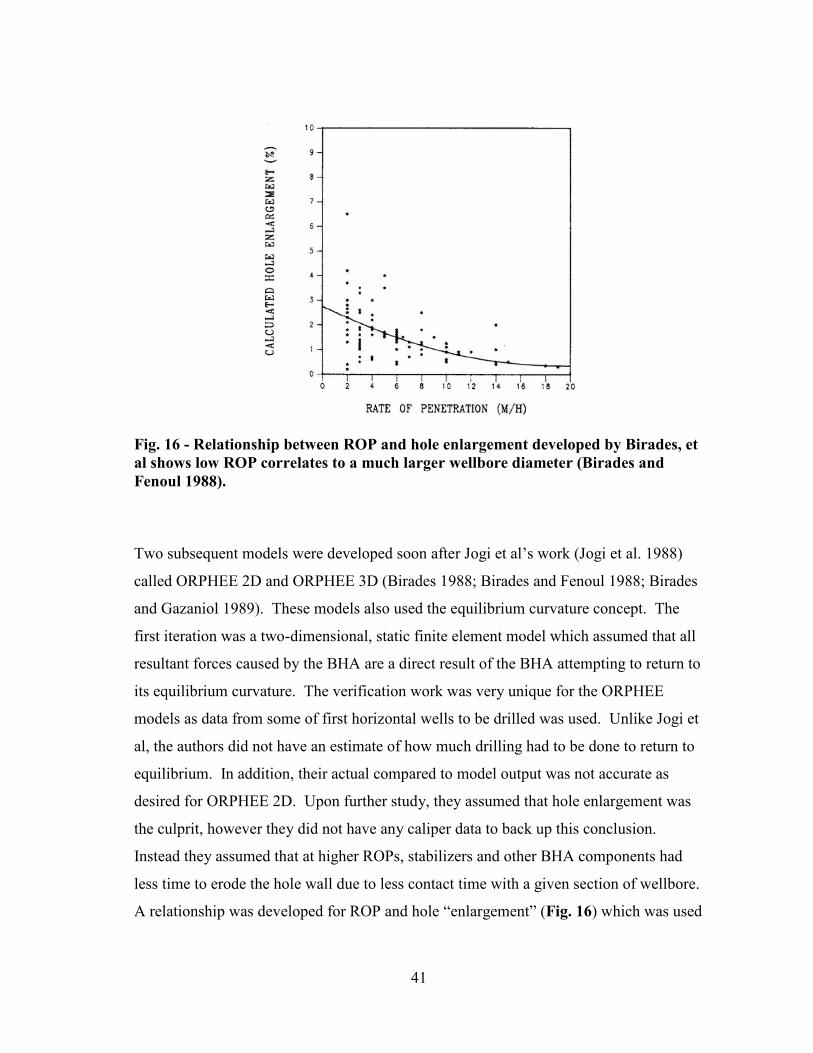
41

Fig. 16 - Relationship between ROP and hole enlargement developed by Birades, et al shows low ROP correlates to a much larger wellbore diameter (Birades and Fenoul 1988).

Two subsequent models were developed soon after Jogi et al’s work (Jogi et al. 1988)

called ORPHEE 2D and ORPHEE 3D (Birades 1988; Birades and Fenoul 1988; Birades

and Gazaniol 1989). These models also used the equilibrium curvature concept. The

first iteration was a two-dimensional, static finite element model which assumed that all

resultant forces caused by the BHA are a direct result of the BHA attempting to return to

its equilibrium curvature. The verification work was very unique for the ORPHEE

models as data from some of first horizontal wells to be drilled was used. Unlike Jogi et

al, the authors did not have an estimate of how much drilling had to be done to return to

equilibrium. In addition, their actual compared to model output was not accurate as

desired for ORPHEE 2D. Upon further study, they assumed that hole enlargement was

the culprit, however they did not have any caliper data to back up this conclusion.

Instead they assumed that at higher ROPs, stabilizers and other BHA components had

less time to erode the hole wall due to less contact time with a given section of wellbore.

A relationship was developed for ROP and hole “enlargement” (Fig. 16) which was used

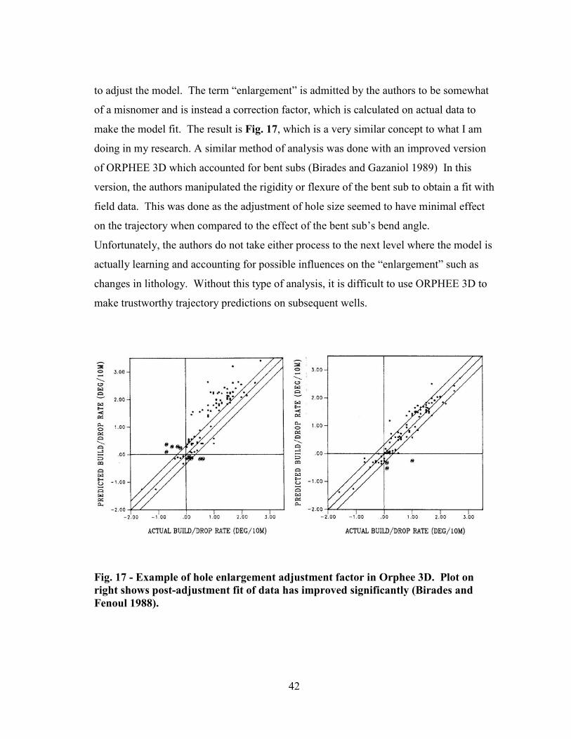
42

to adjust the model. The term “enlargement” is admitted by the authors to be somewhat

of a misnomer and is instead a correction factor, which is calculated on actual data to

make the model fit. The result is Fig. 17, which is a very similar concept to what I am

doing in my research. A similar method of analysis was done with an improved version

of ORPHEE 3D which accounted for bent subs (Birades and Gazaniol 1989) In this

version, the authors manipulated the rigidity or flexure of the bent sub to obtain a fit with

field data. This was done as the adjustment of hole size seemed to have minimal effect

on the trajectory when compared to the effect of the bent sub’s bend angle.

Unfortunately, the authors do not take either process to the next level where the model is

actually learning and accounting for possible influences on the “enlargement” such as

changes in lithology. Without this type of analysis, it is difficult to use ORPHEE 3D to

make trustworthy trajectory predictions on subsequent wells.

Fig. 17 - Example of hole enlargement adjustment factor in Orphee 3D. Plot on right shows post-adjustment fit of data has improved significantly (Birades and Fenoul 1988).

43

An improvement to the University of Tulsa model developed by Nicholson and Wolfson

was completed by J.D. Brakel and involved several unique contributions to the model

(Brakel 1987; Brakel and Azar 1989). The model is a dynamic three-dimensional finite

element BHA model coupled with a rock-bit model. The BHA model is based on linear

elastic beam columns and was solved via Gaussian elimination algorithm. What made

Brakel’s model unique was how the boundaries were handled. All prior models have

simply modeled the contact points as boundary conditions which the BHA could not

exceed. The lone improvement on this was Birades’ work, which also considered the

friction factor between the wellbore and the BHA. Brakel used elastic and torsional

springs at each node to account for contact with the wellbore well. Once the model was

finished, the springs could be interpreted to be the friction force acting at that given

point. Brakel also used two rock-bit interaction models: one for PDC bits and one for

roller-cone bits. The models were relatively complex, non-empirical models. The

results were an accurate prediction of walk tendency as well as accurate predictions.

There did exist some overbuilding of inclination in the model but overall the results were

good. Contrary to what Millheim and Apostal had to say (Millheim and Apostal 1981),

the author stated that the RPM had a limited effect on trajectory and that the key

parameter to consider was how in-gauge the wellbore may be.

Larson also published a model based on the University of Tulsa work propagated by

Wolfson, Nicholson and Brakel (Brakel and Azar 1989; Nicholson 1972). Larson

decided on a quasi-static model to predict the trajectory. The reason for the use of a

quasi-static model was for “simplification” of Brakel’s dynamic model. The FEA model

was solved using the method of springs attached to nodes contacting the wellbore wall.

As stated in Brakel’s publication, the springs not only work as constraints in the model,

they allow a force to be measured at the contact point. This force can be used to

determine the friction at that point. The quasi-static form takes what amounts to a

snapshot at a point in the wellbore. Once the trajectory projection is found, the well is

advanced a certain distance. After advancement, the process is repeated. For the rock-

bit interaction, Larson requires the input of the bedding plane strike and dip angles as

44

well as anisotropic rock indices similar to those originally proposed by Lubinski

(Lubinski and Woods 1953). Anisotropic rock indices are needed for both inclination

and azimuth planes. The resultant force at the bit, found in the BHA model, is

recomputed based on the drillability of formation in the distinct planes. The output is

not only a direction but also a magnitude and results in a quantitative prediction of

wellbore trajectory. Larson’s model was able to match actual data, by manipulating the

radial clearance between the wellbore wall and the BHA. It was noted that accurate

formation anisotropy data was a significant factor in matching the model output to the

actual data.

In 1991, Williams, Apostal and Haduch were able to model complex BHA components

in a dynamic environment using a non-linear FEA model (Williams et al. 1989). The

model could show the effects of bent subs, eccentric stabilizers, buoyancy effects,

friction and large dog-leg severities. The authors used a penalty function method to deal

with the constraints and issues of modeling the various stabilizers and bent subs. The

model is capable of handling the orienting of the tools and accounts for this action. The

authors intended this model to be used as both a predrill tool to assist in setting up BHA

designs as well as being a model to use for post-well analysis.

Another publication in the 1990’s was from a group from Schlumberger attempting to

predict BHA tendencies through statistical analysis (Lesso et al. 1999). In 1999, the

team revisited Birades, et al’s work (Birades 1988; Birades and Fenoul 1988; Birades

and Gazaniol 1989) and added a statistical review and grouping of similar data sets prior

to running the simulation. The authors clearly agree with prior work in that hole

enlargement is a key parameter. However, they deviate from many prior works in that

they ignore anisotropic formation effects. The paper does introduce slide follow-

through, which I personally believe is extremely important as well as noting that

formation strength is an important factor. The formation strength factor is similar in

concept to any of the prior models which did not consider an infinitely hard wellbore,

thus allowing stabilizer-wellbore wall cutting. The authors assumed that the side force

45

at the bit would tend toward zero. Thus, by finding a curvature which would allow the

wellbore trajectory to reach a point where side force was zero, a predicted build and

walk rate is found. In addition replicating Birades, et al’s work, the authors used the

data from 20,000 Schlumberger/Anadrill BHA runs in the Gulf of Mexico area to

accurately predict the unknown parameters such as hole enlargement. They used a

statistical technique called cluster analysis to group statistically similar wells. Then

representative wells were picked from each group and run through the model. These

runs allowed typical values of the unknown variables to found for each group. Once this

was complete, any future wells drilled which fit into the group could be modeled and the

results accurately predicted. The primary issue with this method is that in order for the

statistical analysis to work, each “group” must have a significant number of wells to

draw on for historical data.

Several Hughes Christensen engineers stumbled upon trajectory modeling while testing

the optimum length of bit gauge pads (Pastusek et al. 2005). The engineers first found

the lateral side-cutting occurred for a given bit with a constant side force in

homogeneous test blocks of marble, limestone and sandstone using a specially designed

lab apparatus. Through their testing they were able to predict, for a specific bit, the

instantaneous angle at the bit while drilling under load. To take their work further, they

applied these findings to rotary steerable drilling. To make field predictions of side

force, they used a static FEM. Their assumption was that the static model represented a

“snapshot” of the drilling at that instant. It should be noted the authors predicted the rate

of hole curvature only, not the trajectory. The extent of practical application is the

creation of graphics such as Fig. 18, which shows the anticipated dog-leg severity as a

function of formation type and RSS steering force.

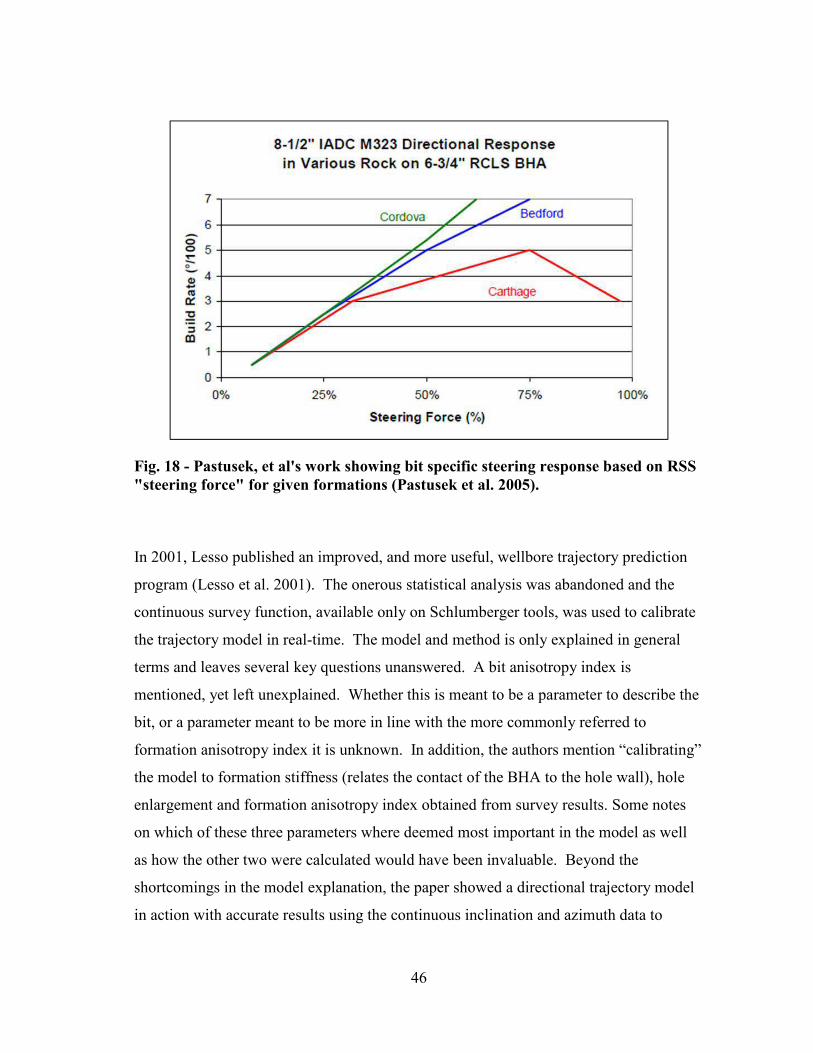
46

Fig. 18 - Pastusek, et al's work showing bit specific steering response based on RSS "steering force" for given formations (Pastusek et al. 2005).

In 2001, Lesso published an improved, and more useful, wellbore trajectory prediction

program (Lesso et al. 2001). The onerous statistical analysis was abandoned and the

continuous survey function, available only on Schlumberger tools, was used to calibrate

the trajectory model in real-time. The model and method is only explained in general

terms and leaves several key questions unanswered. A bit anisotropy index is

mentioned, yet left unexplained. Whether this is meant to be a parameter to describe the

bit, or a parameter meant to be more in line with the more commonly referred to

formation anisotropy index it is unknown. In addition, the authors mention “calibrating”

the model to formation stiffness (relates the contact of the BHA to the hole wall), hole

enlargement and formation anisotropy index obtained from survey results. Some notes

on which of these three parameters where deemed most important in the model as well

as how the other two were calculated would have been invaluable. Beyond the

shortcomings in the model explanation, the paper showed a directional trajectory model

in action with accurate results using the continuous inclination and azimuth data to

47

constantly update his model. Assuming the model functioned as advertised, with the

ability to find the hole enlargement, formation stiffness and bit anisotropy, it seemed to

have been a success. The author was able to match the model to prior results, predict

future results and make helpful directional drilling suggestions. It should be noted the

paper only covers one section of one well drilled – it is unknown whether the model was

tested on other wells. Finally, the paper depends on the continuous inclination and

azimuth measurements available from Schlumberger to obtain its results, which limits its

application.

Similar to attempts from Chinese researchers in the late 1980’s and 1990’s to revisit an

exact solution for trajectory modeling (Bai 1986; Gao 1995), an alternate, numerical

method was used by a team from Schlumberger in an attempt to bypass the FEM which

had become the standard for BHA analysis (Bayliss and Matheus 2008). This paper was

the best written, explained and presented publication on the subject I read; however that

should not detract from its limitations. By making the following series of assumptions,

the authors were able to distill the problem down to a system of 6 equations. The key

assumptions were:

� Only the first four contact points (bit, bend, top of motor and first stabilizer) had

any effect on wellbore trajectory

� Drillstring weight, inertial effects, RPM has no effect on wellbore trajectory

� All contact with the wellbore wall is point contact only and the drillstring may be

modeled as a simply supported beam

Several glaring issues were the assumption that the bit deflected the same regardless of

whether the drillstring was rotating or not as well as the seemingly lack of a boundary

condition to the keep the BHA confined to the wellbore. In addition, the assumption that

the WOB read at surface is equal to that at the bit (no mention made of drag or buckling

in the publication) is terribly wrong in sliding situations. The authors did not use real

world data, even in a history match mode, to check their model. Instead they built a

simulator which read out simulator survey and progress data as the trajectory model

48

“drilled” ahead. In all, this paper was an elegant attempt to bypass the now-standard

FEM; however its required assumptions would seem to make it less accurate. In

addition, the failure to match to real-world data means this model is relegated to an

academic curiosity.

Matheus wrote several follow-up papers (Cockburn et al. 2011; Matheus and

Naganathan 2010) in which he presented some results from a control system based on

the trajectory model from Bayliss and Matheus. A standard control algorithm was

developed for use with RSS systems. Matheus states the model is based on “a set of

equations where phenomenological models copy the dynamic of the system”.

Phenomenological research often refers to research in human-based areas and is research

which seeks mainly to describe, rather to explain behavior (Lester 1999). Unfortunately,

the authors presented only three general functions (not equations) that contain four

empirical parameters derived from historical data and no details on the final model

configuration or derivation. How this is done or what the equations are is unknown.

The reason this is unfortunate is the authors seem to have developed a working trajectory

control system. It is used primarily to hold inclination and/or azimuth, and seems to do

it more effectively than a human directional driller. They present multiple instances in

various basins where this was achieved. While it is somewhat limited in its application,

using RSS with continuous inclination and azimuth capability, it is the first instance of a

successful control system with applicability across a variety of wellbore profiles and

geographical locations.

The most recently developed model also focuses on RSS prediction and control

(Pirovolou et al. 2011). The model itself is secondary to the overall system, which is

ultimately intended be fully autonomous. The model is based on two equations, turn rate

and build rate, and four unknowns: maximum DLS, tool face offset, drop bias and turn

bias. The model supposedly “learns” the four unknowns relatively quickly. The authors

showed an example of the unknowns reaching steady-state values within 300’ of drilling.

In order for this type of convergence to occur for four separate unknowns, there has to be

49

more to the model than those two simple equations, however nothing in the publication

mentions this. The authors used the trained model to then make steering

recommendations for the next few hundred feet. This, as well as the prior publications

reviewed (Cockburn et al. 2011; Matheus and Naganathan 2010) show a high degree of

control capability. Both models show examples of the computer program output giving

better steering recommendations than the human direction driller. Pirovolou, et al noted

their steering recommendations would have resulted in less tortuosity as well.

Rock-bit Interaction Models

Up to this point in time, most authors recognize the BHA model is limited at best with

regards to trajectory prediction. The many simultaneous influences are very difficult to

account for with the BHA model or equations. The standard solution is to develop a

model or factor which describes the interaction of the rock and bit. Parameters such as

bit type, design, rock strength, lithology and formation dip have all been studied and

used as a correcting factor in the BHA model.

Lubinski et al discussed the effect of formation anisotropy in their work referenced

earlier (Lubinski and Woods 1953). They were the first to put forth the idea that rock

was able to be drilled at different rates in the axial and lateral directions with the same

energy input. This index, h’, was used to create charts for specific formations being

penetrated at specific angles. An important note by the authors was that while formation

effects certainly had an effect on the hole angle, the effect of the BHA deformation must

also be considered.

Chenevert and Gatlin conclusively proved that the Young’s modulus, and thus ability to

fail, was dependent on the orientation of the applied force (Chenevert and Gatlin 1965).

Using a triaxial cell and multiple samples of homogeneous and laminated sedimentary

rock, the authors found the sedimentary rocks had varying Young’s moduli.

Specifically, they found the rocks failed at a lower stress normal to the bedding plane.

No applications to drilling or other applications of the results were put forth, however

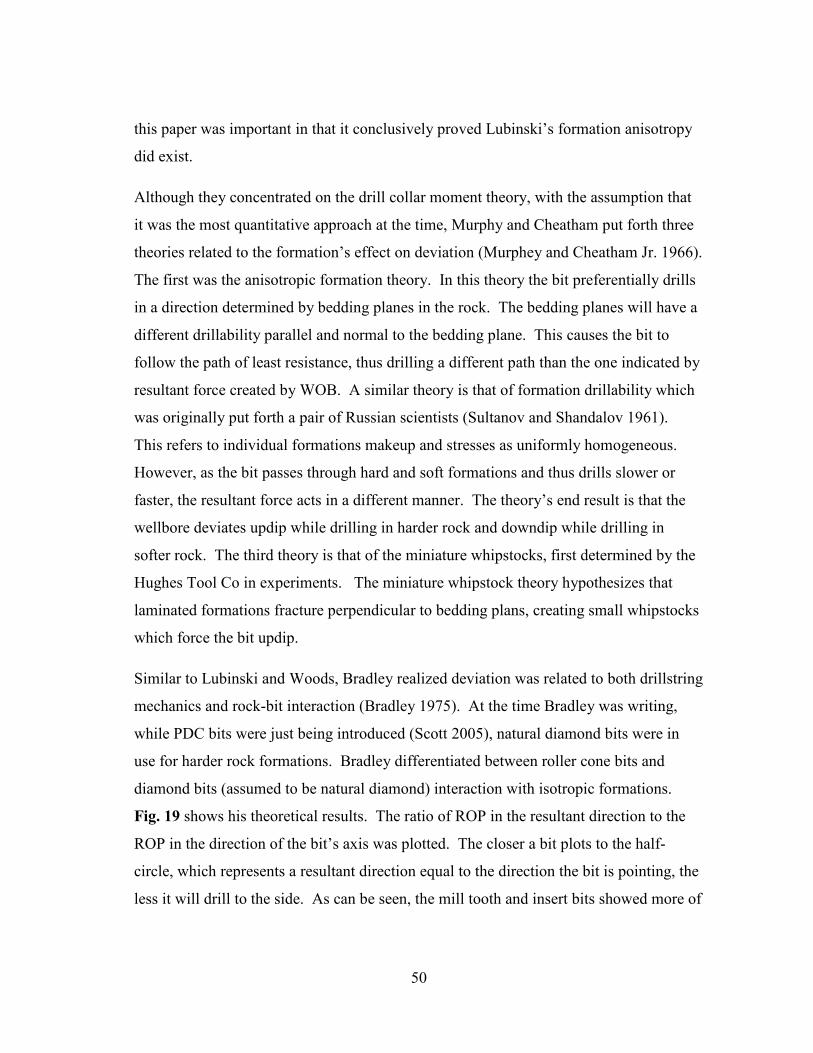
50

this paper was important in that it conclusively proved Lubinski’s formation anisotropy

did exist.

Although they concentrated on the drill collar moment theory, with the assumption that

it was the most quantitative approach at the time, Murphy and Cheatham put forth three

theories related to the formation’s effect on deviation (Murphey and Cheatham Jr. 1966).

The first was the anisotropic formation theory. In this theory the bit preferentially drills

in a direction determined by bedding planes in the rock. The bedding planes will have a

different drillability parallel and normal to the bedding plane. This causes the bit to

follow the path of least resistance, thus drilling a different path than the one indicated by

resultant force created by WOB. A similar theory is that of formation drillability which

was originally put forth a pair of Russian scientists (Sultanov and Shandalov 1961).

This refers to individual formations makeup and stresses as uniformly homogeneous.

However, as the bit passes through hard and soft formations and thus drills slower or

faster, the resultant force acts in a different manner. The theory’s end result is that the

wellbore deviates updip while drilling in harder rock and downdip while drilling in

softer rock. The third theory is that of the miniature whipstocks, first determined by the

Hughes Tool Co in experiments. The miniature whipstock theory hypothesizes that

laminated formations fracture perpendicular to bedding plans, creating small whipstocks

which force the bit updip.

Similar to Lubinski and Woods, Bradley realized deviation was related to both drillstring

mechanics and rock-bit interaction (Bradley 1975). At the time Bradley was writing,

while PDC bits were just being introduced (Scott 2005), natural diamond bits were in

use for harder rock formations. Bradley differentiated between roller cone bits and

diamond bits (assumed to be natural diamond) interaction with isotropic formations.

Fig. 19 shows his theoretical results. The ratio of ROP in the resultant direction to the

ROP in the direction of the bit’s axis was plotted. The closer a bit plots to the half-

circle, which represents a resultant direction equal to the direction the bit is pointing, the

less it will drill to the side. As can be seen, the mill tooth and insert bits showed more of

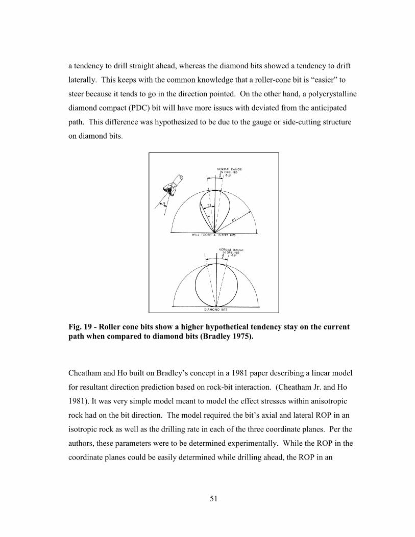
51

a tendency to drill straight ahead, whereas the diamond bits showed a tendency to drift

laterally. This keeps with the common knowledge that a roller-cone bit is “easier” to

steer because it tends to go in the direction pointed. On the other hand, a polycrystalline

diamond compact (PDC) bit will have more issues with deviated from the anticipated

path. This difference was hypothesized to be due to the gauge or side-cutting structure

on diamond bits.

Fig. 19 - Roller cone bits show a higher hypothetical tendency stay on the current path when compared to diamond bits (Bradley 1975).

Cheatham and Ho built on Bradley’s concept in a 1981 paper describing a linear model

for resultant direction prediction based on rock-bit interaction. (Cheatham Jr. and Ho

1981). It was very simple model meant to model the effect stresses within anisotropic

rock had on the bit direction. The model required the bit’s axial and lateral ROP in an

isotropic rock as well as the drilling rate in each of the three coordinate planes. Per the

authors, these parameters were to be determined experimentally. While the ROP in the

coordinate planes could be easily determined while drilling ahead, the ROP in an

52

isotropic rock would have had to already been determined in a laboratory. This makes

this particular model difficult to apply in an actual well.

Larson (Larson 1991) preferred the model, also built on Bradley’s work, set forth by

Xunyao in 1986 due to its simplicity and ease of application (Xunyao 1986). Xunyao

represented the rock-bit interaction as separate force acting on the bit. Thus, when the

bit did not follow the resultant direction, i.e. - anisotropic rock, this was due to the

formation deviating force. This force could easily be calculated through observing the

results of steering changes and the results. The theory was used to setup pendulum

assemblies in 16 separate hole intervals on five wells. The setups seemed to work in

controlling inclination and had survey results which agreed with the theoretical results.

The simplicity of the model with a single unknown led Larson to use it for his work.

A paper focusing on the three-dimensional rock-bit interaction was published in 1987

and clearly stated that in two-dimensional analysis, the results were likely deceiving (Ho

1987). In his paper, Ho first stated the need for an accurate BHA analysis program with

the outputs of the resultant force and direction as well as the bit axis direction. From

there he found a simple rock-bit interaction model. The model works by taking a length

of already drilled wellbore and running the results through the “inverse” model. Here,

the formation and bit anisotropy indexes are found using the BHA model results

(resultant force and bit tilt) as compared to the survey data. In addition, the three

dimensional dip must be known. The author notes this may be difficult to find except in

wells with dip meter runs or accurate regional dip maps such as the Texas gulf coast.

Once the bit and formation anisotropy indexes are found, the model is run in the

prediction mode to quantify the future wellpath. The obvious issue with this model is

the amount of data needed to calibrate the rock-bit model. This necessitates more

drilling ahead than is acceptable in today’s wells with very small geo-steered targets.

However, the concept of teaching the model, although not explicitly stated in that

manner by Ho, creates a model which is theoretically adaptable to different areas and

wellbores. This static model was applied by Eastman Christensen engineers in the early

53

1990’s with supposed good effects, primarily due the model’s ability to learn and adapt

to changes (Dahl and Schmalhorst 1991).

GEODYN2 was previously discussed in the BHA models literature review (Apostal and

Baird 1987; Baird et al. 1985). It was a project sponsored by Sandia National

Laboratories, and was built to provide a high degree of accuracy in modeling downhole

tools and formation interactions. The basis for GEODYN2 was GEODYN, a very

advanced rock-bit interaction model (Baird et al. 1984; Tinianow et al. 1984). The

initial reason for the model’s existence was to develop sturdier tools for geothermal

drilling projects. An ancillary benefit was the possibility to model the trajectory of the

wellbore. GEODYN is a non-linear, transient, dynamic FEA model of a drill bit

interacting with a heterogeneous formation which is modeled using a discrete point

method. The bit model is a specific to the bit being run and is a FEA model consisting

of bricks forming the shape of the bit. Cutters were modeled as points on the bit which

induce friction and thus affect the dynamic motion of the bit. The formation was

modeled as surface with elastic springs. The elastic springs were used to measure the

ROP and allow the bit to “drill” forward. The BHA was modeled, but boundary

conditions and friction effects were either neglected or not fully developed in this

iteration of GEODYN. The model was finished and the interaction of the bit and

formation was capable of being modeled. Unfortunately, no instances of matching with

real-world data were attempted. Later, GEODYN was incorporated into GEODYN2.

When Lubinski revisited trajectory prediction, he and Williamson also discussed bit

anisotropy factor (Williamson and Lubinski 1987). This factor is found using a simple

model based on the anisotropy index. The anisotropy index is calculated by the authors

based on an assumed dip angle and actual vs. projected trajectory results. The only

requirement is that anisotropy indexes used for roller cones are then used to predict the

results of drilling with tricone bits. The same is needed for PDC bits. The anisotropy

index is essentially a measurement how much the wellbore trajectory deviated from the

resultant force direction.

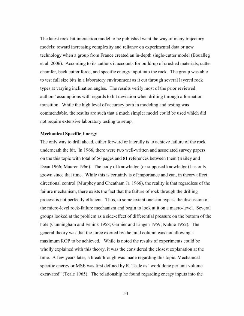
54

The latest rock-bit interaction model to be published went the way of many trajectory

models: toward increasing complexity and reliance on experimental data or new

technology when a group from France created an in-depth single-cutter model (Boualleg

et al. 2006). According to its authors it accounts for build-up of crushed materials, cutter

chamfer, back cutter force, and specific energy input into the rock. The group was able

to test full size bits in a laboratory environment as it cut through several layered rock

types at varying inclination angles. The results verify most of the prior reviewed

authors’ assumptions with regards to bit deviation when drilling through a formation

transition. While the high level of accuracy both in modeling and testing was

commendable, the results are such that a much simpler model could be used which did

not require extensive laboratory testing to setup.

Mechanical Specific Energy

The only way to drill ahead, either forward or laterally is to achieve failure of the rock

underneath the bit. In 1966, there were two well-written and associated survey papers

on the this topic with total of 56 pages and 81 references between them (Bailey and

Dean 1966; Maurer 1966). The body of knowledge (or supposed knowledge) has only

grown since that time. While this is certainly is of importance and can, in theory affect

directional control (Murphey and Cheatham Jr. 1966), the reality is that regardless of the

failure mechanism, there exists the fact that the failure of rock through the drilling

process is not perfectly efficient. Thus, to some extent one can bypass the discussion of

the micro-level rock-failure mechanism and begin to look at it on a macro-level. Several

groups looked at the problem as a side-effect of differential pressure on the bottom of the

hole (Cunningham and Eenink 1958; Garnier and Lingen 1959; Kuhne 1952). The

general theory was that the force exerted by the mud column was not allowing a

maximum ROP to be achieved. While is noted the results of experiments could be

wholly explained with this theory, it was the considered the closest explanation at the

time. A few years later, a breakthrough was made regarding this topic. Mechanical

specific energy or MSE was first defined by R. Teale as “work done per unit volume

excavated” (Teale 1965). The relationship he found regarding energy inputs into the

55

system was derived from a series of experiments. He realized that, in his experimental

setup, for rock of a given unconfined compressive strength (UCS), there was a minimum

energy to needed to fail and excavate said rock. If more energy were needed than this

minimum value, there existed inefficiencies within the system. Many “single-cutter”

experiments have been undertaken in the last few decades (Cook et al. 1991; Detournay

and Tan 2002; Gray-Stephens et al. 1994; Kolle 1996; Pei 2012; Rafatian et al. 2010;

Zijsling 1987). While key to understanding the basics of what was occurring downhole,

it was difficult to extrapolate the results to a full-scale drilling system.

Fig. 20 - Decreasing RPM dramatically increases BHA vibration (Pastusek and Brackin 2003).

In recent years, several highly informative and applicable papers have been published.

These papers concentrate on the use of MSE as opposed to the study of MSE. As the

downhole tools have become more complex and thus more expensive and delicate,

56

vibration reduction has become a targeted issue in many drilling operations. This type of

vibration, regardless of the source is manifested in a sine wave in the drillstring.

Pastusek and Brackin presented this very clearly in 2003(Pastusek and Brackin 2003).

They how changing the drilling parameters can have a significant effect on the vibration

sine wave and how there exist combinations of drilling parameters where the sine wave

will rapidly decay (high ROP or high RPM) and combinations where the sine wave will

amplify over time (lower ROP and WOB). This can be seen in Fig. 20 when the RPM is

reduced, the sine wave increases dramatically. Bit and BHA types obviously affect the

vibration also. The authors had studied this with regards to preventing wellbore

oscillations such as spirally or rippling, but it also has applicability in trajectory

prediction.

Other studies have sought to describe and mitigate the process (Bailey et al. 2008; Bailey

and Remmert 2010; Bailey et al. 2010; Prim et al. 2013). The result of many of these is

not just a FEM model or a graph, but a workflow for the personnel on the drillsite to use

in identifying and eliminating drillstring vibration. This is of vital importance in today’s

complex wells using highly technical tools, but is only peripheral to the focus of this

work.

For bits, particularly PDC bits, there exists an ideal bottomhole pattern. This perfect

pattern typically only exists in the lab and represents the most efficient paths for the bit’s

cutters to take (Fig. 21). Any inefficiencies in this cutting pattern result in vibrations

within the drillstring as well as a reduction in ROP. The reduction in ROP has been the

subject of an increasing number of papers. The damage to the tools prevents non-

productive time such as trips but increasing the ROP is a significantly larger prize in

terms of economic benefit. Most drilling operations today use digital data recorders to

record drilling parameters. Through analysis of this digital data, operators have been

able to identify and rectify sections of the well which are being drilled inefficiently

(Dupriest et al. 2012; Dupriest et al. 2005). Given that MSE is actually a relatively

straightforward relationship and is analyzed relative to prior readings on the current well.

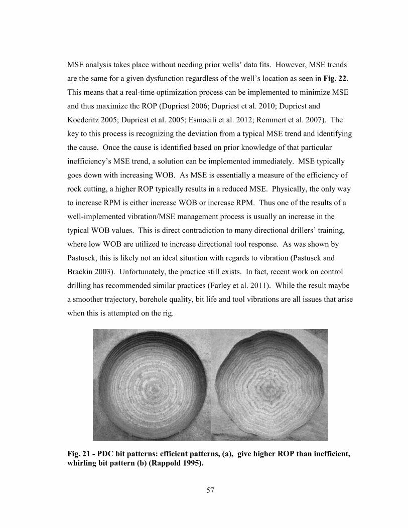
57

MSE analysis takes place without needing prior wells’ data fits. However, MSE trends

are the same for a given dysfunction regardless of the well’s location as seen in Fig. 22.

This means that a real-time optimization process can be implemented to minimize MSE

and thus maximize the ROP (Dupriest 2006; Dupriest et al. 2010; Dupriest and

Koederitz 2005; Dupriest et al. 2005; Esmaeili et al. 2012; Remmert et al. 2007). The

key to this process is recognizing the deviation from a typical MSE trend and identifying

the cause. Once the cause is identified based on prior knowledge of that particular

inefficiency’s MSE trend, a solution can be implemented immediately. MSE typically

goes down with increasing WOB. As MSE is essentially a measure of the efficiency of

rock cutting, a higher ROP typically results in a reduced MSE. Physically, the only way

to increase RPM is either increase WOB or increase RPM. Thus one of the results of a

well-implemented vibration/MSE management process is usually an increase in the

typical WOB values. This is direct contradiction to many directional drillers’ training,

where low WOB are utilized to increase directional tool response. As was shown by

Pastusek, this is likely not an ideal situation with regards to vibration (Pastusek and

Brackin 2003). Unfortunately, the practice still exists. In fact, recent work on control

drilling has recommended similar practices (Farley et al. 2011). While the result maybe

a smoother trajectory, borehole quality, bit life and tool vibrations are all issues that arise

when this is attempted on the rig.

Fig. 21 - PDC bit patterns: efficient patterns, (a), give higher ROP than inefficient, whirling bit pattern (b) (Rappold 1995).

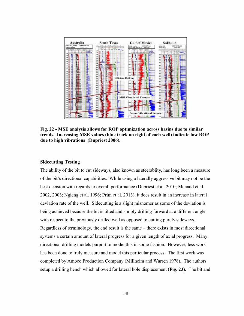
58

Fig. 22 - MSE analysis allows for ROP optimization across basins due to similar trends. Increasing MSE values (blue track on right of each well) indicate low ROP due to high vibrations (Dupriest 2006).

Sidecutting Testing

The ability of the bit to cut sideways, also known as steerablity, has long been a measure

of the bit’s directional capabilities. While using a laterally aggressive bit may not be the

best decision with regards to overall performance (Dupriest et al. 2010; Menand et al.

2002, 2003; Ngieng et al. 1996; Prim et al. 2013), it does result in an increase in lateral

deviation rate of the well. Sidecutting is a slight misnomer as some of the deviation is

being achieved because the bit is tilted and simply drilling forward at a different angle

with respect to the previously drilled well as opposed to cutting purely sideways.

Regardless of terminology, the end result is the same – there exists in most directional

systems a certain amount of lateral progress for a given length of axial progress. Many

directional drilling models purport to model this in some fashion. However, less work

has been done to truly measure and model this particular process. The first work was

completed by Amoco Production Company (Millheim and Warren 1978). The authors

setup a drilling bench which allowed for lateral hole displacement (Fig. 23). The bit and

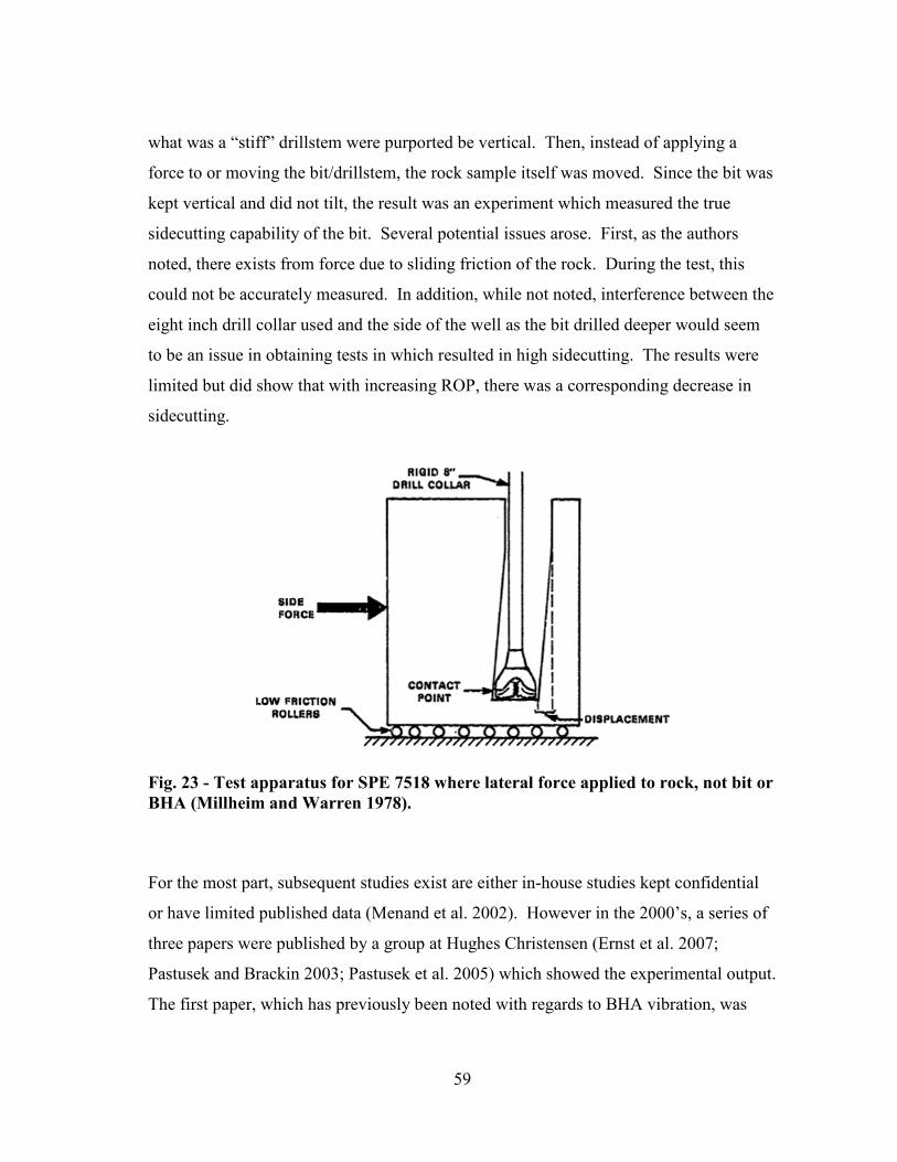
59

what was a “stiff” drillstem were purported be vertical. Then, instead of applying a

force to or moving the bit/drillstem, the rock sample itself was moved. Since the bit was

kept vertical and did not tilt, the result was an experiment which measured the true

sidecutting capability of the bit. Several potential issues arose. First, as the authors

noted, there exists from force due to sliding friction of the rock. During the test, this

could not be accurately measured. In addition, while not noted, interference between the

eight inch drill collar used and the side of the well as the bit drilled deeper would seem

to be an issue in obtaining tests in which resulted in high sidecutting. The results were

limited but did show that with increasing ROP, there was a corresponding decrease in

sidecutting.

Fig. 23 - Test apparatus for SPE 7518 where lateral force applied to rock, not bit or BHA (Millheim and Warren 1978).

For the most part, subsequent studies exist are either in-house studies kept confidential

or have limited published data (Menand et al. 2002). However in the 2000’s, a series of

three papers were published by a group at Hughes Christensen (Ernst et al. 2007;

Pastusek and Brackin 2003; Pastusek et al. 2005) which showed the experimental output.

The first paper, which has previously been noted with regards to BHA vibration, was

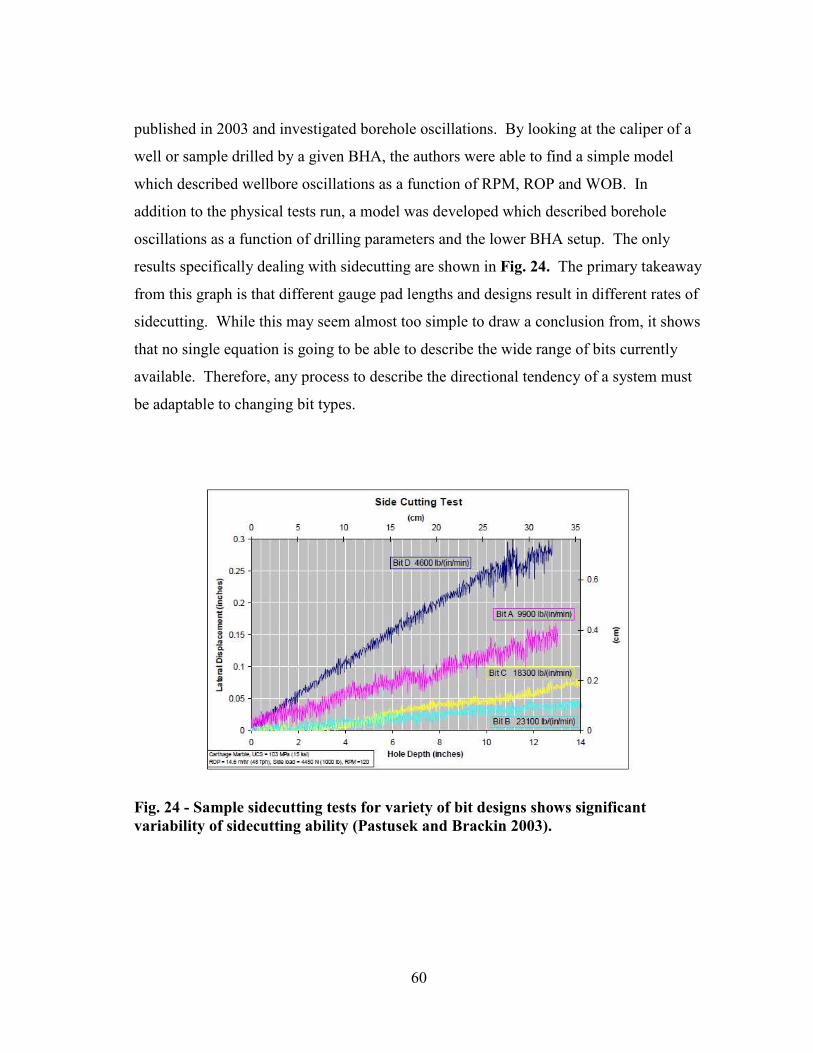
60

published in 2003 and investigated borehole oscillations. By looking at the caliper of a

well or sample drilled by a given BHA, the authors were able to find a simple model

which described wellbore oscillations as a function of RPM, ROP and WOB. In

addition to the physical tests run, a model was developed which described borehole

oscillations as a function of drilling parameters and the lower BHA setup. The only

results specifically dealing with sidecutting are shown in Fig. 24. The primary takeaway

from this graph is that different gauge pad lengths and designs result in different rates of

sidecutting. While this may seem almost too simple to draw a conclusion from, it shows

that no single equation is going to be able to describe the wide range of bits currently

available. Therefore, any process to describe the directional tendency of a system must

be adaptable to changing bit types.

Fig. 24 - Sample sidecutting tests for variety of bit designs shows significant variability of sidecutting ability (Pastusek and Brackin 2003).

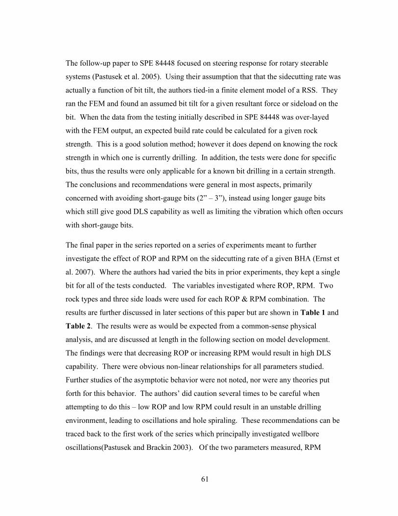
61

The follow-up paper to SPE 84448 focused on steering response for rotary steerable

systems (Pastusek et al. 2005). Using their assumption that that the sidecutting rate was

actually a function of bit tilt, the authors tied-in a finite element model of a RSS. They

ran the FEM and found an assumed bit tilt for a given resultant force or sideload on the

bit. When the data from the testing initially described in SPE 84448 was over-layed

with the FEM output, an expected build rate could be calculated for a given rock

strength. This is a good solution method; however it does depend on knowing the rock

strength in which one is currently drilling. In addition, the tests were done for specific

bits, thus the results were only applicable for a known bit drilling in a certain strength.

The conclusions and recommendations were general in most aspects, primarily

concerned with avoiding short-gauge bits (2” – 3”), instead using longer gauge bits

which still give good DLS capability as well as limiting the vibration which often occurs

with short-gauge bits.

The final paper in the series reported on a series of experiments meant to further

investigate the effect of ROP and RPM on the sidecutting rate of a given BHA (Ernst et

al. 2007). Where the authors had varied the bits in prior experiments, they kept a single

bit for all of the tests conducted. The variables investigated where ROP, RPM. Two

rock types and three side loads were used for each ROP & RPM combination. The

results are further discussed in later sections of this paper but are shown in Table 1 and

Table 2. The results were as would be expected from a common-sense physical

analysis, and are discussed at length in the following section on model development.

The findings were that decreasing ROP or increasing RPM would result in high DLS

capability. There were obvious non-linear relationships for all parameters studied.

Further studies of the asymptotic behavior were not noted, nor were any theories put

forth for this behavior. The authors’ did caution several times to be careful when

attempting to do this – low ROP and low RPM could result in an unstable drilling

environment, leading to oscillations and hole spiraling. These recommendations can be

traced back to the first work of the series which principally investigated wellbore

oscillations(Pastusek and Brackin 2003). Of the two parameters measured, RPM

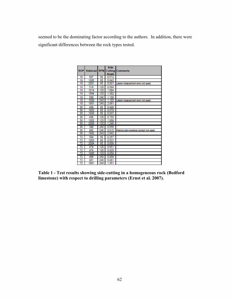
62

seemed to be the dominating factor according to the authors. In addition, there were

significant differences between the rock types tested.

Table 1 - Test results showing side-cutting in a homogeneous rock (Bedford limestone) with respect to drilling parameters (Ernst et al. 2007).

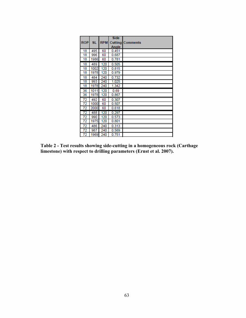
63

Table 2 - Test results showing side-cutting in a homogeneous rock (Carthage limestone) with respect to drilling parameters (Ernst et al. 2007).

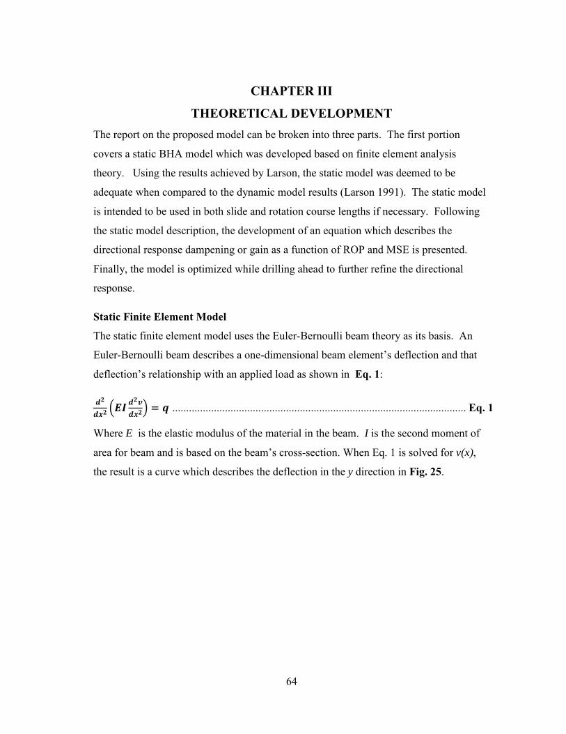
64

CHAPTER III

THEORETICAL DEVELOPMENT The report on the proposed model can be broken into three parts. The first portion

covers a static BHA model which was developed based on finite element analysis

theory. Using the results achieved by Larson, the static model was deemed to be

adequate when compared to the dynamic model results (Larson 1991). The static model

is intended to be used in both slide and rotation course lengths if necessary. Following

the static model description, the development of an equation which describes the

directional response dampening or gain as a function of ROP and MSE is presented.

Finally, the model is optimized while drilling ahead to further refine the directional

response.

Static Finite Element Model

The static finite element model uses the Euler-Bernoulli beam theory as its basis. An

Euler-Bernoulli beam describes a one-dimensional beam element’s deflection and that

deflection’s relationship with an applied load as shown in Eq. 1:

����� ��� ������� = � .......................................................................................................... Eq. 1

Where E is the elastic modulus of the material in the beam. I is the second moment of

area for beam and is based on the beam’s cross-section. When Eq. 1 is solved for v(x),

the result is a curve which describes the deflection in the y direction in Fig. 25.

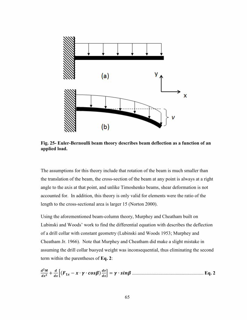
65

Fig. 25- Euler-Bernoulli beam theory describes beam deflection as a function of an applied load.

The assumptions for this theory include that rotation of the beam is much smaller than

the translation of the beam, the cross-section of the beam at any point is always at a right

angle to the axis at that point, and unlike Timoshenko beams, shear deformation is not

accounted for. In addition, this theory is only valid for elements were the ratio of the

length to the cross-sectional area is larger 15 (Norton 2000).

Using the aforementioned beam-column theory, Murphey and Cheatham built on

Lubinski and Woods’ work to find the differential equation with describes the deflection

of a drill collar with constant geometry (Lubinski and Woods 1953; Murphey and

Cheatham Jr. 1966). Note that Murphey and Cheatham did make a slight mistake in

assuming the drill collar buoyed weight was inconsequential, thus eliminating the second

term within the parentheses of Eq. 2:

������ + �

�� ����� − � ∙ ∙ !"#$% ����& = ∙ #'($ ........................................................... Eq. 2

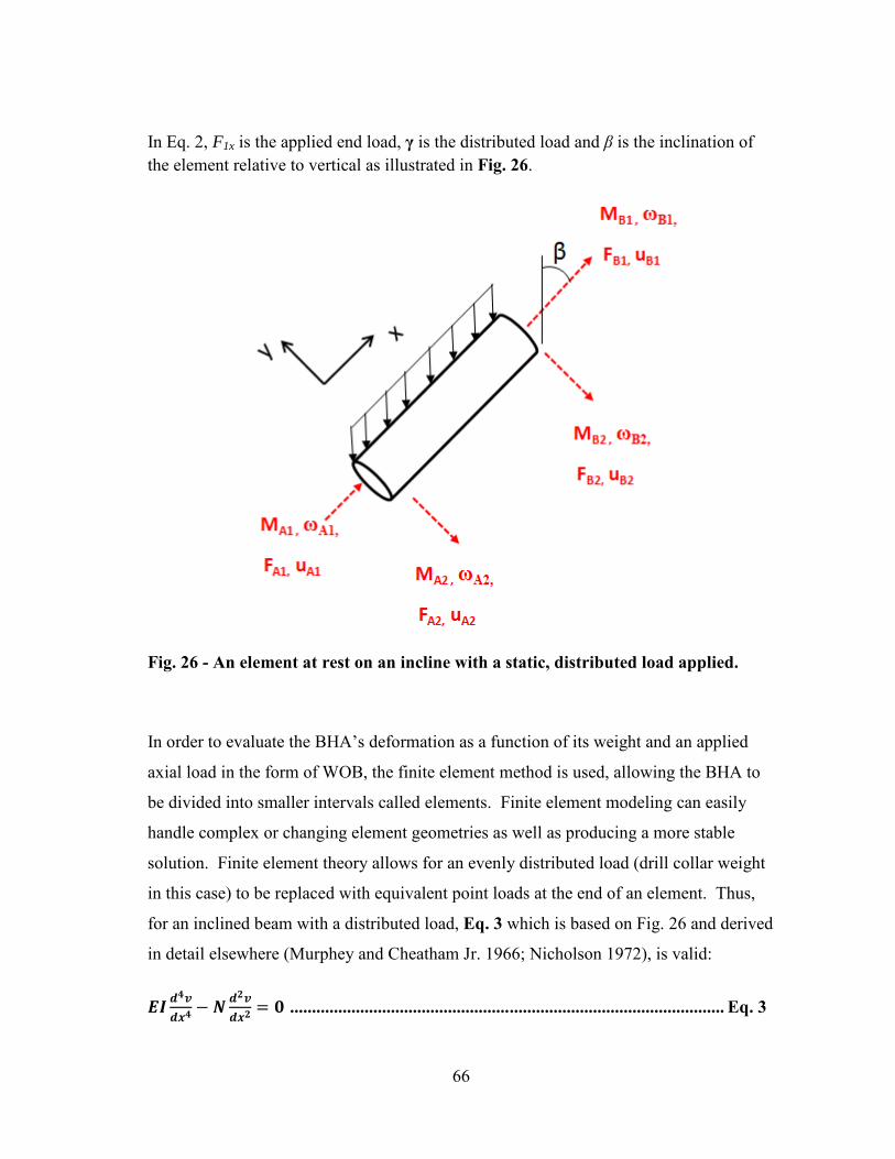
66

In Eq. 2, F1x is the applied end load, γ is the distributed load and β is the inclination of the element relative to vertical as illustrated in Fig. 26.

Fig. 26 - An element at rest on an incline with a static, distributed load applied.

In order to evaluate the BHA’s deformation as a function of its weight and an applied

axial load in the form of WOB, the finite element method is used, allowing the BHA to

be divided into smaller intervals called elements. Finite element modeling can easily

handle complex or changing element geometries as well as producing a more stable

solution. Finite element theory allows for an evenly distributed load (drill collar weight

in this case) to be replaced with equivalent point loads at the end of an element. Thus,

for an inclined beam with a distributed load, Eq. 3 which is based on Fig. 26 and derived

in detail elsewhere (Murphey and Cheatham Jr. 1966; Nicholson 1972), is valid:

�� �)���) −* ������ = + ................................................................................................... Eq. 3

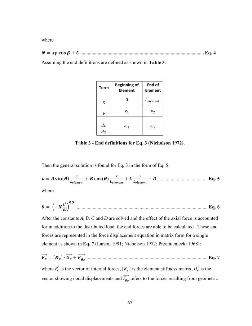
67

where

* = � ,-.$ + / .................................................................................................... Eq. 4

Assuming the end definitions are defined as shown in Table 3:

Table 3 - End definitions for Eq. 3 (Nicholson 1972).

Then the general solution is found for Eq. 3 in the form of Eq. 5:

� = 1.23�4% �567686(9 +:,-.�4% �

567686(9 + / �567686(9 + ; ......................................... Eq. 5

where:

4 = �−* 5����

+.= ........................................................................................................... Eq. 6

After the constants A, B, C and D are solved and the effect of the axial force is accounted

for in addition to the distributed load, the end forces are able to be calculated. These end

forces are represented in the force displacement equation in matrix form for a single

element as shown in Eq. 7 (Larson 1991; Nicholson 1972; Przemieniecki 1968):

�6����� = �>6� ∙ ?6������ + �@6������� ................................................................................................... Eq. 7

where ������ is the vector of internal forces, ���� is the element stiffness matrix, ������ is the

vector showing nodal displacements and �������� refers to the forces resulting from geometric

Term Beginning of

Element

End of

Element

X 0 ABCBDBEF

V v1 v2

JKJL

M1 M2

68

effects. Each element in this model contains two nodes, one at each end. Each one of

these nodes is allowed to freely move in three-dimensional space, resulting in six

degrees of freedom (DoF) at each node: three displacements and three moments. The

individual force-displacement equations for an element with six degrees of freedom can

be seen in Eq. 8 (Larson 1991; Nicholson 1972).

Eq. 8

In Eq. 8, the undefined terms are as follows:

N� = 1�5 ......................................................................................................................... Eq. 9

N� = O��5� ...................................................................................................................... Eq. 10

NP = )��5 ...................................................................................................................... Eq. 11

N) = ����5P .................................................................................................................... Eq. 12

N= = )QR5 ...................................................................................................................... Eq. 13

NO = ���5 ...................................................................................................................... Eq. 14

where A is the cross-sectional area of the element, E is the modulus of elasticity, L the length of the element, I is the mass-moment of inertia, J is the second moment of inertia and G is the modulus of rigidity.

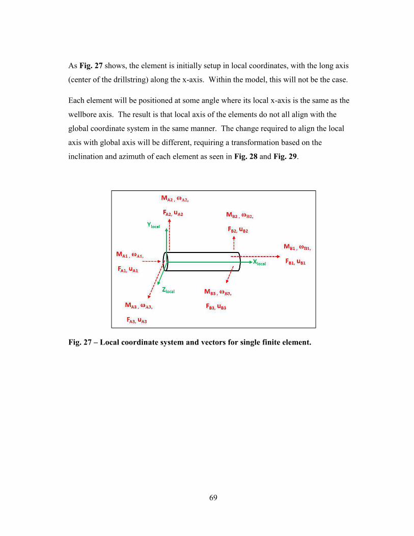
69

As Fig. 27 shows, the element is initially setup in local coordinates, with the long axis

(center of the drillstring) along the x-axis. Within the model, this will not be the case.

Each element will be positioned at some angle where its local x-axis is the same as the

wellbore axis. The result is that local axis of the elements do not all align with the

global coordinate system in the same manner. The change required to align the local

axis with global axis will be different, requiring a transformation based on the

inclination and azimuth of each element as seen in Fig. 28 and Fig. 29.

Fig. 27 – Local coordinate system and vectors for single finite element.

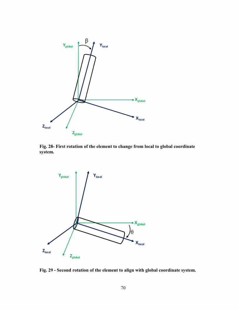
70

Fig. 28- First rotation of the element to change from local to global coordinate system.

Fig. 29 - Second rotation of the element to align with global coordinate system.

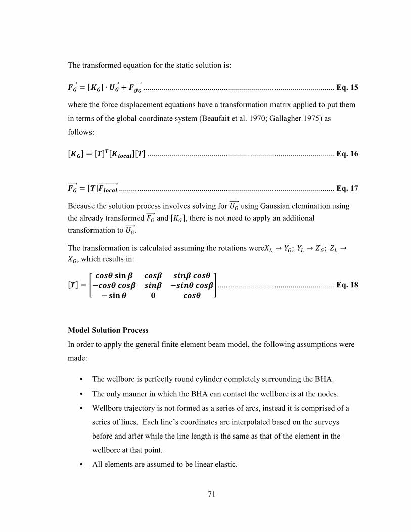
71

The transformed equation for the static solution is:

�Q������ = �>Q� ∙ ?Q������ + �@Q�������� ............................................................................................... Eq. 15

where the force displacement equations have a transformation matrix applied to put them

in terms of the global coordinate system (Beaufait et al. 1970; Gallagher 1975) as

follows:

�>Q� = �S�S�>7"!T7��S� ............................................................................................. Eq. 16

�Q������ = �S��7"!T7������������ ........................................................................................................... Eq. 17

Because the solution process involves solving for ������� using Gaussian elemination using the already transformed ������� and ����, there is not need to apply an additional transformation to �������. The transformation is calculated assuming the rotations wereUV → X�; XV → Z�; ZV →U�, which results in:

�S� = [ !"#4.23$ !"#$ #'($!"#4−!"#4!"#$ #'($ −#'(4!"#$−.234 + !"#4 \ .......................................................... Eq. 18

Model Solution Process

In order to apply the general finite element beam model, the following assumptions were

made:

• The wellbore is perfectly round cylinder completely surrounding the BHA.

• The only manner in which the BHA can contact the wellbore is at the nodes.

• Wellbore trajectory is not formed as a series of arcs, instead it is comprised of a

series of lines. Each line’s coordinates are interpolated based on the surveys

before and after while the line length is the same as that of the element in the

wellbore at that point.

• All elements are assumed to be linear elastic.

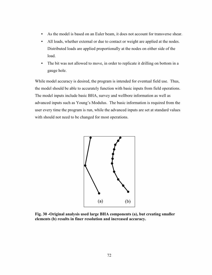
72

• As the model is based on an Euler beam, it does not account for transverse shear.

• All loads, whether external or due to contact or weight are applied at the nodes.

Distributed loads are applied proportionally at the nodes on either side of the

load.

• The bit was not allowed to move, in order to replicate it drilling on bottom in a

gauge hole.

While model accuracy is desired, the program is intended for eventual field use. Thus,

the model should be able to accurately function with basic inputs from field operations.

The model inputs include basic BHA, survey and wellbore information as well as

advanced inputs such as Young’s Modulus. The basic information is required from the

user every time the program is run, while the advanced inputs are set at standard values

with should not need to be changed for most operations.

Fig. 30 -Original analysis used large BHA components (a), but creating smaller elements (b) results in finer resolution and increased accuracy.

73

The survey file is uploaded automatically. After this, the user is prompted to input each

BHA component’s geometry. While this is done, the BHA is discretized into a mesh of

smaller elements in order to come to a more accurate solution (Fig. 30). The mesh size

is variable and depends on each BHA component’s geometry. In order to avoid creating

rigid bodies or “short columns” that will not bend in the model, the length of the

elements for a given BHA component are calculated based on a slenderness ratio

(Norton 2000):

]^ = 7_ ......................................................................................................................... Eq. 19

Where l is the length of the element such that Sr is not less than a recommended value of

15 and:

_ = `�1 ....................................................................................................................... Eq. 20

After the mesh is created, each element’s stiffness matrix, ����, is created using the

matrix and the equations shown in Eq. 8. These element stiffness matrices are

assembled using the matrix displacement method into a global stiffness matrix

(Przemieniecki 1968). It should be note the the global stiffness matrix is used in Eq. 8

along with global force and displacement vectors.

Prior to solving for the displacements, the boundary conditions are put in place. The

downhole WOB (DHWOB) is applied to the uppermost node and bit node’s

displacements are set to zero. It is assumed that at the point in time that the bit is drilling

ahead at a given depth, the hole is in-gauge and the bit is on bottom, meaning the bit is

not capable of moving laterally or axially. Once the rows and columns associated with

the displacement boundary conditions are eliminated, the displacements, �������, are found

via Gaussian elimination.

An accurate solution obviously requires the BHA to be constrained within the wellbore.

This has been solved in several different ways in the past, mostly through some type of

penalty function (Millheim et al. 1978; Nicholson 1972; Sutko et al. 1980). The model

74

currently uses the method presented by Brakel, in which springs are attached to each

node. The springs’ stiffness is then held at a minimal value while the node is within the

wellbore (to represent resistance of mud) and then increased when the node is calculated

out of the wellbore. This simply involves increasing the spring stiffness (Ks) by a ratio

of the node displacement to the initial radial clearance (RCi) as follows:

_#,(6b = �?7T96^T7,'−c/'%c/' × _#,"7� ................................................................................ Eq. 21

Once applied within the stiffness matrix, the new spring stiffness forces the node back to

the hole wall. While not wholly physically accurate as the rock surrounding the

wellbore should have a constant stiffness, this method does allow for a quick

convergence, doesn’t rely on the user to estimate rock strengths and is simple to program

and understand. It is also physically accurate to the extent the BHA is constrained in the

wellbore. The solution process is repeated as Eq. 8 is solved with the new spring

stiffnesses at each node. As the program goes through the iterations, the springs’

stiffnesses are increased or decreased as needed. Nodes that are calculated on

subsequent iterations to be inside the wellbore are reassigned the minimal value spring

stiffness while nodes that are pushed out of the wellbore as the model is solved again are

assigned a spring stiffness according to Eq. 21. This process proceeds with the spring

stiffnesses changing as needed until a convergence of the difference between the

previous displacement value and the current displacement value at each node is reached.

Once a convergence criterion is met concerning the displacement solution, the BHA’s

final displacement has been found (Fig. 31). The final forces may be calculated using

Eq. 8, including the most important force – the lateral force applied at the bit as result of

BHA deformation.

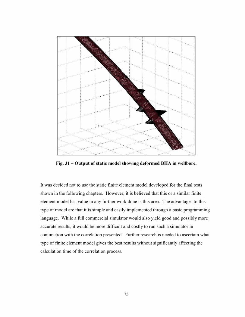
75

Fig. 31 – Output of static model showing deformed BHA in wellbore.

It was decided not to use the static finite element model developed for the final tests

shown in the following chapters. However, it is believed that this or a similar finite

element model has value in any further work done is this area. The advantages to this

type of model are that it is simple and easily implemented through a basic programming

language. While a full commercial simulator would also yield good and possibly more

accurate results, it would be more difficult and costly to run such a simulator in

conjunction with the correlation presented. Further research is needed to ascertain what

type of finite element model gives the best results without significantly affecting the

calculation time of the correlation process.

76

Basic Sidecutting Derivation

As previously discussed in the literature review ROP and RPM have a quantifiable effect

on the “steerablity” of a bit (Ernst et al. 2007; Farley et al. 2011; Hoffmann et al. 2013;

Pastusek and Brackin 2003; Pastusek et al. 2005). Much of what has been presented in

literature to date covering this concept is primarily lab related. At first glance, this

seems to have little real-world application due to the inherent differences between the

lab and the wellsite. In addition, much of the work has been implemented by bit

manufacturers, thus the focus tends toward vibration studies. This is to be expected as

downhole vibration results in significantly reduced bit life and ROP, the two primary

measures by which a bit is compared to its competitors. However, one data set did a

very good job in collecting and presenting with the directional steerablity of the bit in

mind (Ernst et al. 2007; Pastusek et al. 2005). However, the experimenters did not take

the final step to correlate the measure of vibration, MSE, with the steerablity of the bit.

The following work finishes that correlation and sets forth an equation which, when

combined with real-time drilling data, allows for the prediction and analysis of the

directional response of the BHA and bit.

The data which pointed toward this correlation and was used to create the basic equation

is shown in Table 1 and Table 2. The original study was focused more on bit design,

particularly gauge length and operating parameters’ effect on sidecutting and thus

steerablity. This was more of a trend analysis and the presentation of those trends can be

seen at the end of Ernst, et al’s paper (Ernst et al. 2007). When the data was rearranged

and looked at from a different angle, several trends emerged.

The original data set had presented sidecutting in the form of bit-tilt as seen in Fig. 32.

This was not acceptable for the work of this dissertation as it both ignored bit-tilt due to

BHA deformation as well as did not look at the physics of what was occurring where a

given amount of lateral progress was being made for a given amount of forward

progress. This bit-tilt number was converted back to what was likely the originally

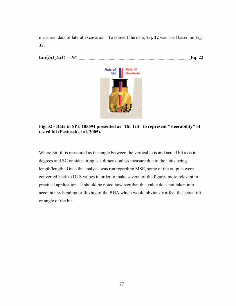
77

measured data of lateral excavation. To convert the data, Eq. 22 was used based on Fig.

32:

ef3�g'9_9'79% = ]/ Eq. 22

Fig. 32 - Data in SPE 105594 presented as "Bit Tilt" to represent "steerability" of tested bit (Pastusek et al. 2005).

Where bit tilt is measured as the angle between the vertical axis and actual bit axis in

degrees and SC or sidecutting is a dimensionless measure due to the units being

length/length. Once the analysis was run regarding MSE, some of the outputs were

converted back to DLS values in order to make several of the figures more relevant to

practical application. It should be noted however that this value does not taken into

account any bending or flexing of the BHA which would obviously affect the actual tilt

or angle of the bit.

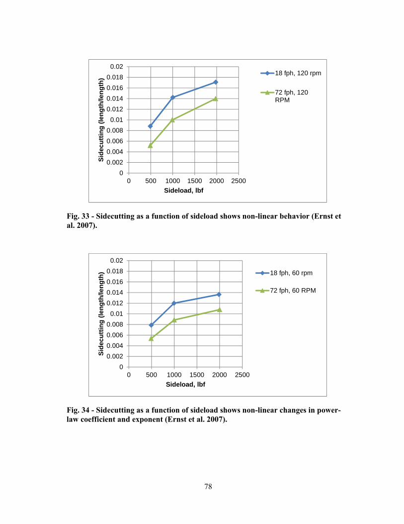
78

Fig. 33 - Sidecutting as a function of sideload shows non-linear behavior (Ernst et al. 2007).

Fig. 34 - Sidecutting as a function of sideload shows non-linear changes in power-law coefficient and exponent (Ernst et al. 2007).

0

0.002

0.004

0.006

0.008

0.01

0.012

0.014

0.016

0.018

0.02

0 500 1000 1500 2000 2500

Sid

ecu

ttin

g (

len

gth

/len

gth

)

Sideload, lbf

18 fph, 120 rpm

72 fph, 120RPM

0

0.002

0.004

0.006

0.008

0.01

0.012

0.014

0.016

0.018

0.02

0 500 1000 1500 2000 2500

Sid

ecu

ttin

g (

len

gth

/len

gth

)

Sideload, lbf

18 fph, 60 rpm

72 fph, 60 RPM

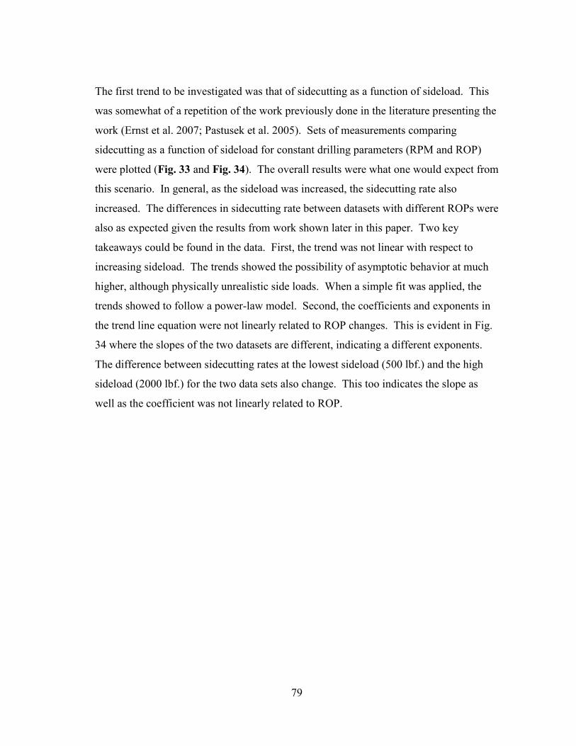
79

The first trend to be investigated was that of sidecutting as a function of sideload. This

was somewhat of a repetition of the work previously done in the literature presenting the

work (Ernst et al. 2007; Pastusek et al. 2005). Sets of measurements comparing

sidecutting as a function of sideload for constant drilling parameters (RPM and ROP)

were plotted (Fig. 33 and Fig. 34). The overall results were what one would expect from

this scenario. In general, as the sideload was increased, the sidecutting rate also

increased. The differences in sidecutting rate between datasets with different ROPs were

also as expected given the results from work shown later in this paper. Two key

takeaways could be found in the data. First, the trend was not linear with respect to

increasing sideload. The trends showed the possibility of asymptotic behavior at much

higher, although physically unrealistic side loads. When a simple fit was applied, the

trends showed to follow a power-law model. Second, the coefficients and exponents in

the trend line equation were not linearly related to ROP changes. This is evident in Fig.

34 where the slopes of the two datasets are different, indicating a different exponents.

The difference between sidecutting rates at the lowest sideload (500 lbf.) and the high

sideload (2000 lbf.) for the two data sets also change. This too indicates the slope as

well as the coefficient was not linearly related to ROP.

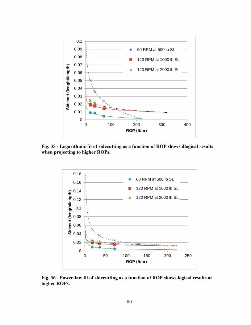
80

Fig. 35 - Logarithmic fit of sidecutting as a function of ROP shows illogical results when projecting to higher ROPs.

Fig. 36 - Power-law fit of sidecutting as a function of ROP shows logical results at higher ROPs.

0

0.01

0.02

0.03

0.04

0.05

0.06

0.07

0.08

0.09

0.1

0 100 200 300 400

Sid

ecu

tt (

len

gh

t/le

ng

th)

ROP (ft/hr)

60 RPM at 500 lb SL

120 RPM at 1000 lb SL

120 RPM at 2000 lb SL

0

0.02

0.04

0.06

0.08

0.1

0.12

0.14

0.16

0.18

0 50 100 150 200 250

Sid

ecu

t (l

eng

th/le

ng

th)

ROP (ft/hr)

60 RPM at 500 lb SL

120 RPM at 1000 lb SL

120 RPM at 2000 lb SL

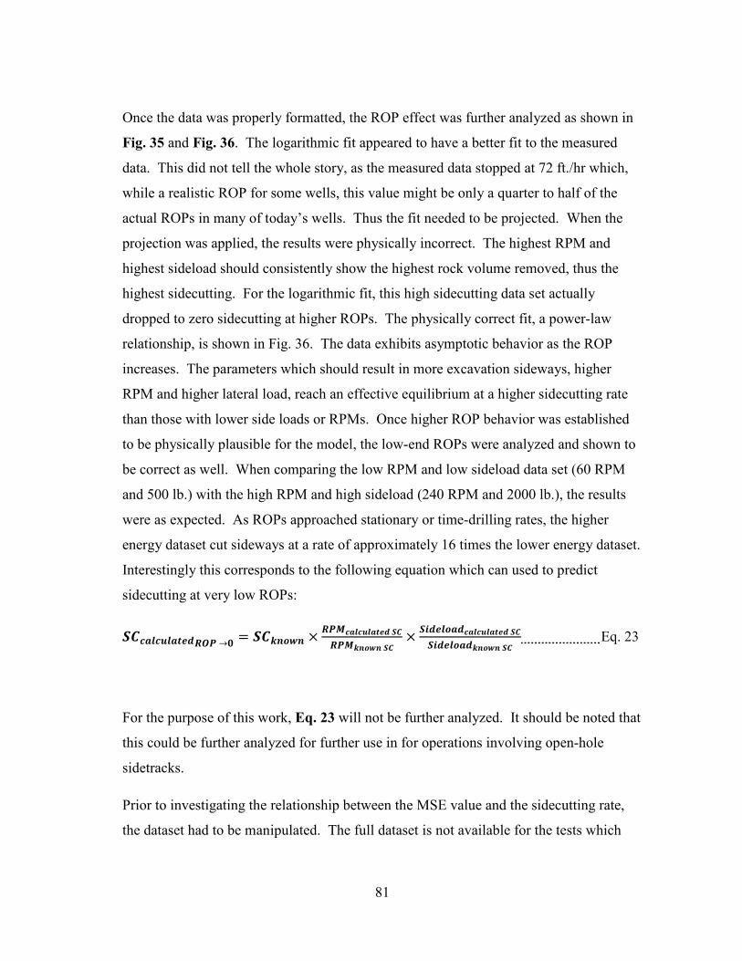
81

Once the data was properly formatted, the ROP effect was further analyzed as shown in

Fig. 35 and Fig. 36. The logarithmic fit appeared to have a better fit to the measured

data. This did not tell the whole story, as the measured data stopped at 72 ft./hr which,

while a realistic ROP for some wells, this value might be only a quarter to half of the

actual ROPs in many of today’s wells. Thus the fit needed to be projected. When the

projection was applied, the results were physically incorrect. The highest RPM and

highest sideload should consistently show the highest rock volume removed, thus the

highest sidecutting. For the logarithmic fit, this high sidecutting data set actually

dropped to zero sidecutting at higher ROPs. The physically correct fit, a power-law

relationship, is shown in Fig. 36. The data exhibits asymptotic behavior as the ROP

increases. The parameters which should result in more excavation sideways, higher

RPM and higher lateral load, reach an effective equilibrium at a higher sidecutting rate

than those with lower side loads or RPMs. Once higher ROP behavior was established

to be physically plausible for the model, the low-end ROPs were analyzed and shown to

be correct as well. When comparing the low RPM and low sideload data set (60 RPM

and 500 lb.) with the high RPM and high sideload (240 RPM and 2000 lb.), the results

were as expected. As ROPs approached stationary or time-drilling rates, the higher

energy dataset cut sideways at a rate of approximately 16 times the lower energy dataset.

Interestingly this corresponds to the following equation which can used to predict

sidecutting at very low ROPs:

]/!T7!i7T96�cjk→+ = ]/_("b( × ck�!T7!i7T96�]/ck�_("b(]/ × ]'�67"T�!T7!i7T96�]/]'�67"T�_("b(]/ Eq. 23

For the purpose of this work, Eq. 23 will not be further analyzed. It should be noted that

this could be further analyzed for further use in for operations involving open-hole

sidetracks.

Prior to investigating the relationship between the MSE value and the sidecutting rate,

the dataset had to be manipulated. The full dataset is not available for the tests which

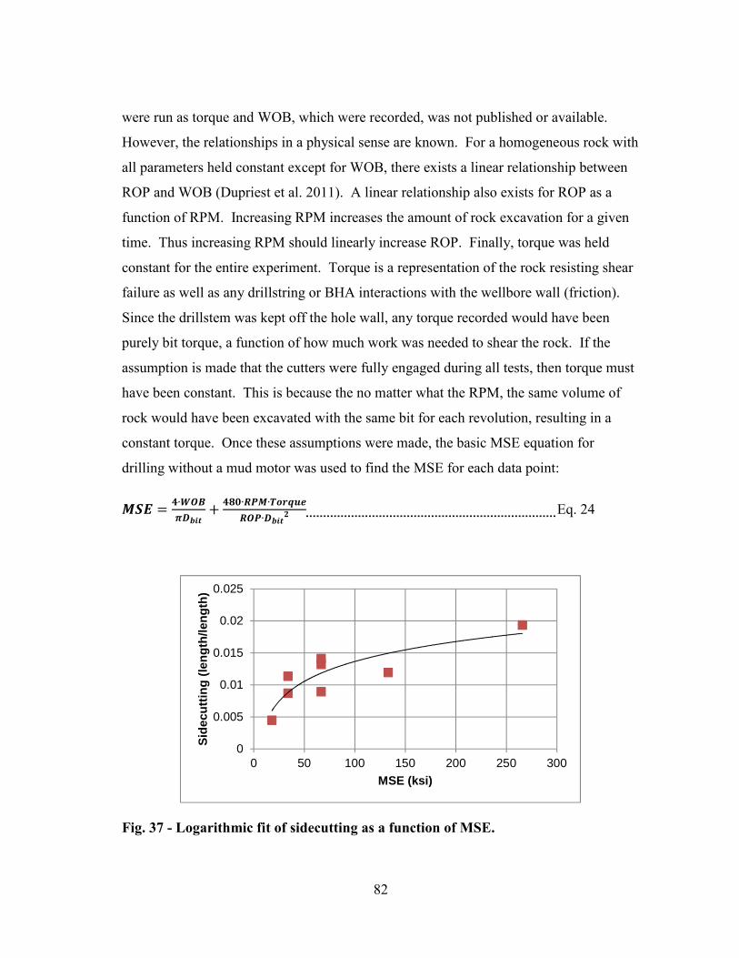
82

were run as torque and WOB, which were recorded, was not published or available.

However, the relationships in a physical sense are known. For a homogeneous rock with

all parameters held constant except for WOB, there exists a linear relationship between

ROP and WOB (Dupriest et al. 2011). A linear relationship also exists for ROP as a

function of RPM. Increasing RPM increases the amount of rock excavation for a given

time. Thus increasing RPM should linearly increase ROP. Finally, torque was held

constant for the entire experiment. Torque is a representation of the rock resisting shear

failure as well as any drillstring or BHA interactions with the wellbore wall (friction).

Since the drillstem was kept off the hole wall, any torque recorded would have been

purely bit torque, a function of how much work was needed to shear the rock. If the

assumption is made that the cutters were fully engaged during all tests, then torque must

have been constant. This is because the no matter what the RPM, the same volume of

rock would have been excavated with the same bit for each revolution, resulting in a

constant torque. Once these assumptions were made, the basic MSE equation for

drilling without a mud motor was used to find the MSE for each data point:

�]� = )∙lj:m;g'9 + )n+∙ck�∙S"^�i6

cjk∙;g'9� Eq. 24

Fig. 37 - Logarithmic fit of sidecutting as a function of MSE.

0

0.005

0.01

0.015

0.02

0.025

0 50 100 150 200 250 300

Sid

ecu

ttin

g (

len

gth

/len

gth

)

MSE (ksi)

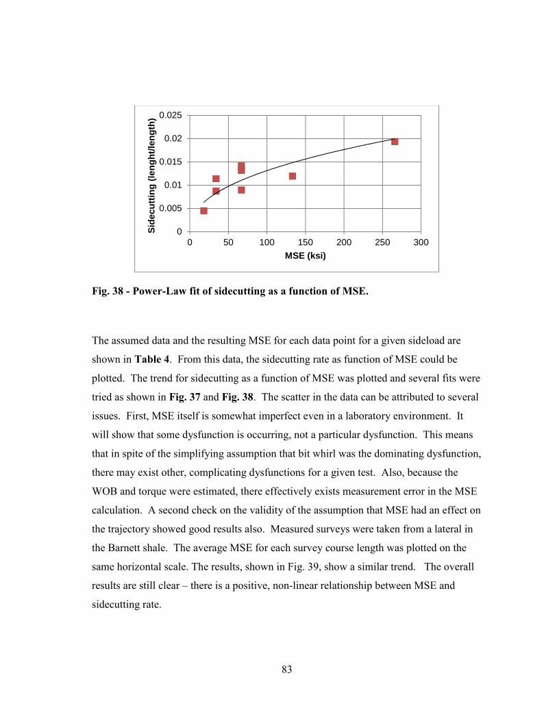
83

Fig. 38 - Power-Law fit of sidecutting as a function of MSE.

The assumed data and the resulting MSE for each data point for a given sideload are

shown in Table 4. From this data, the sidecutting rate as function of MSE could be

plotted. The trend for sidecutting as a function of MSE was plotted and several fits were

tried as shown in Fig. 37 and Fig. 38. The scatter in the data can be attributed to several

issues. First, MSE itself is somewhat imperfect even in a laboratory environment. It

will show that some dysfunction is occurring, not a particular dysfunction. This means

that in spite of the simplifying assumption that bit whirl was the dominating dysfunction,

there may exist other, complicating dysfunctions for a given test. Also, because the

WOB and torque were estimated, there effectively exists measurement error in the MSE

calculation. A second check on the validity of the assumption that MSE had an effect on

the trajectory showed good results also. Measured surveys were taken from a lateral in

the Barnett shale. The average MSE for each survey course length was plotted on the

same horizontal scale. The results, shown in Fig. 39, show a similar trend. The overall

results are still clear – there is a positive, non-linear relationship between MSE and

sidecutting rate.

0

0.005

0.01

0.015

0.02

0.025

0 50 100 150 200 250 300

Sid

ecu

ttin

g (

len

gh

t/le

ng

th)

MSE (ksi)

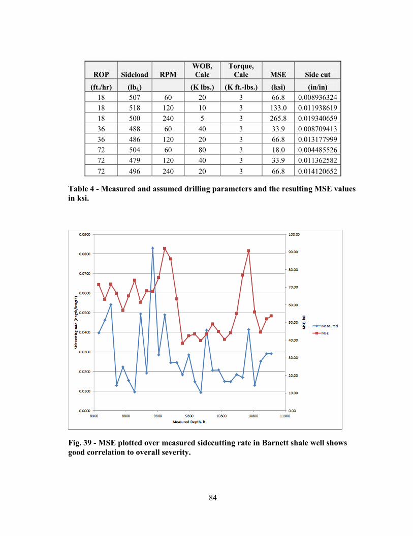
84

ROP Sideload RPM WOB, Calc

Torque, Calc MSE Side cut

(ft./hr) (lbf.) (K lbs.) (K ft.-lbs.) (ksi) (in/in) 18 507 60 20 3 66.8 0.008936324 18 518 120 10 3 133.0 0.011938619 18 500 240 5 3 265.8 0.019340659 36 488 60 40 3 33.9 0.008709413 36 486 120 20 3 66.8 0.013177999 72 504 60 80 3 18.0 0.004485526 72 479 120 40 3 33.9 0.011362582 72 496 240 20 3 66.8 0.014120652

Table 4 - Measured and assumed drilling parameters and the resulting MSE values in ksi.

Fig. 39 - MSE plotted over measured sidecutting rate in Barnett shale well shows good correlation to overall severity.

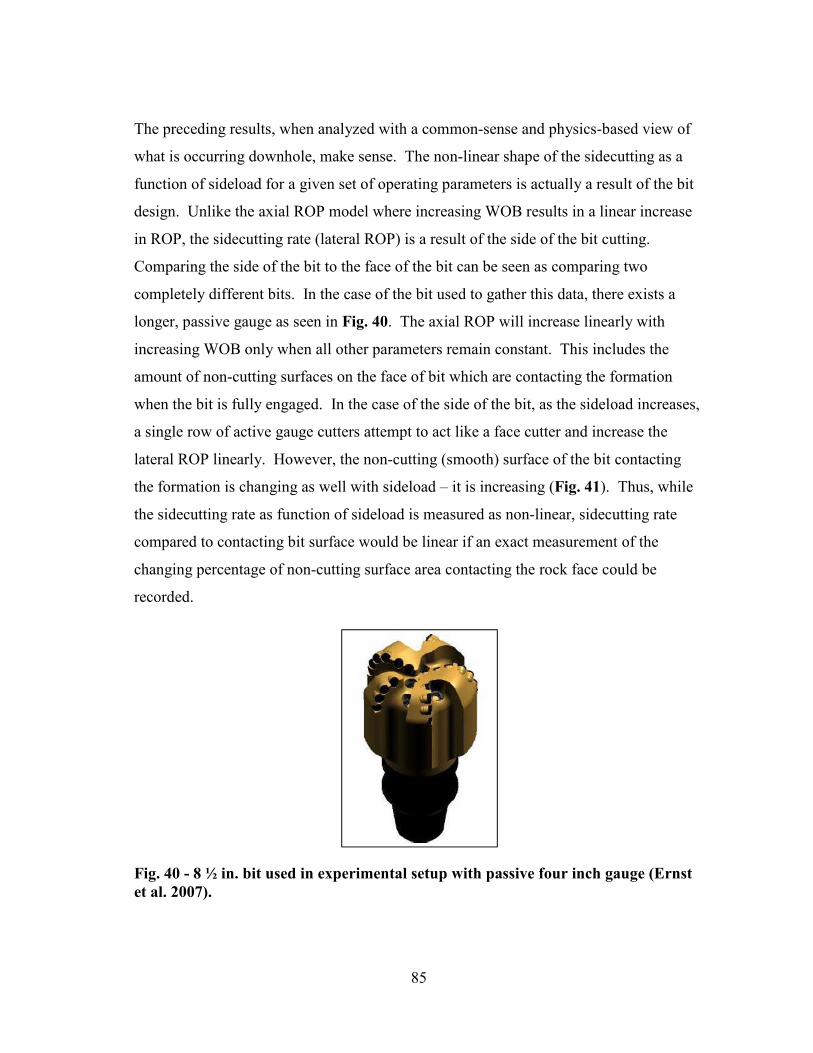
85

The preceding results, when analyzed with a common-sense and physics-based view of

what is occurring downhole, make sense. The non-linear shape of the sidecutting as a

function of sideload for a given set of operating parameters is actually a result of the bit

design. Unlike the axial ROP model where increasing WOB results in a linear increase

in ROP, the sidecutting rate (lateral ROP) is a result of the side of the bit cutting.

Comparing the side of the bit to the face of the bit can be seen as comparing two

completely different bits. In the case of the bit used to gather this data, there exists a

longer, passive gauge as seen in Fig. 40. The axial ROP will increase linearly with

increasing WOB only when all other parameters remain constant. This includes the

amount of non-cutting surfaces on the face of bit which are contacting the formation

when the bit is fully engaged. In the case of the side of the bit, as the sideload increases,

a single row of active gauge cutters attempt to act like a face cutter and increase the

lateral ROP linearly. However, the non-cutting (smooth) surface of the bit contacting

the formation is changing as well with sideload – it is increasing (Fig. 41). Thus, while

the sidecutting rate as function of sideload is measured as non-linear, sidecutting rate

compared to contacting bit surface would be linear if an exact measurement of the

changing percentage of non-cutting surface area contacting the rock face could be

recorded.

Fig. 40 - 8 ½ in. bit used in experimental setup with passive four inch gauge (Ernst et al. 2007).

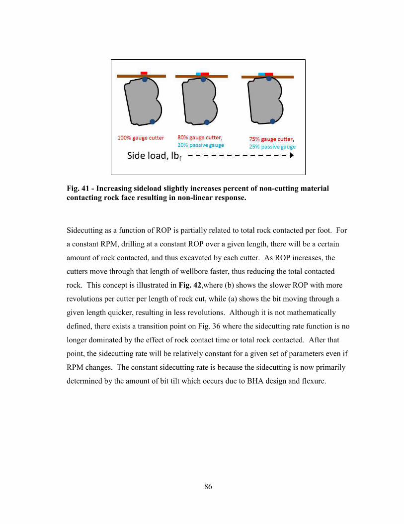
86

Fig. 41 - Increasing sideload slightly increases percent of non-cutting material contacting rock face resulting in non-linear response.

Sidecutting as a function of ROP is partially related to total rock contacted per foot. For

a constant RPM, drilling at a constant ROP over a given length, there will be a certain

amount of rock contacted, and thus excavated by each cutter. As ROP increases, the

cutters move through that length of wellbore faster, thus reducing the total contacted

rock. This concept is illustrated in Fig. 42,where (b) shows the slower ROP with more

revolutions per cutter per length of rock cut, while (a) shows the bit moving through a

given length quicker, resulting in less revolutions. Although it is not mathematically

defined, there exists a transition point on Fig. 36 where the sidecutting rate function is no

longer dominated by the effect of rock contact time or total rock contacted. After that

point, the sidecutting rate will be relatively constant for a given set of parameters even if

RPM changes. The constant sidecutting rate is because the sidecutting is now primarily

determined by the amount of bit tilt which occurs due to BHA design and flexure.

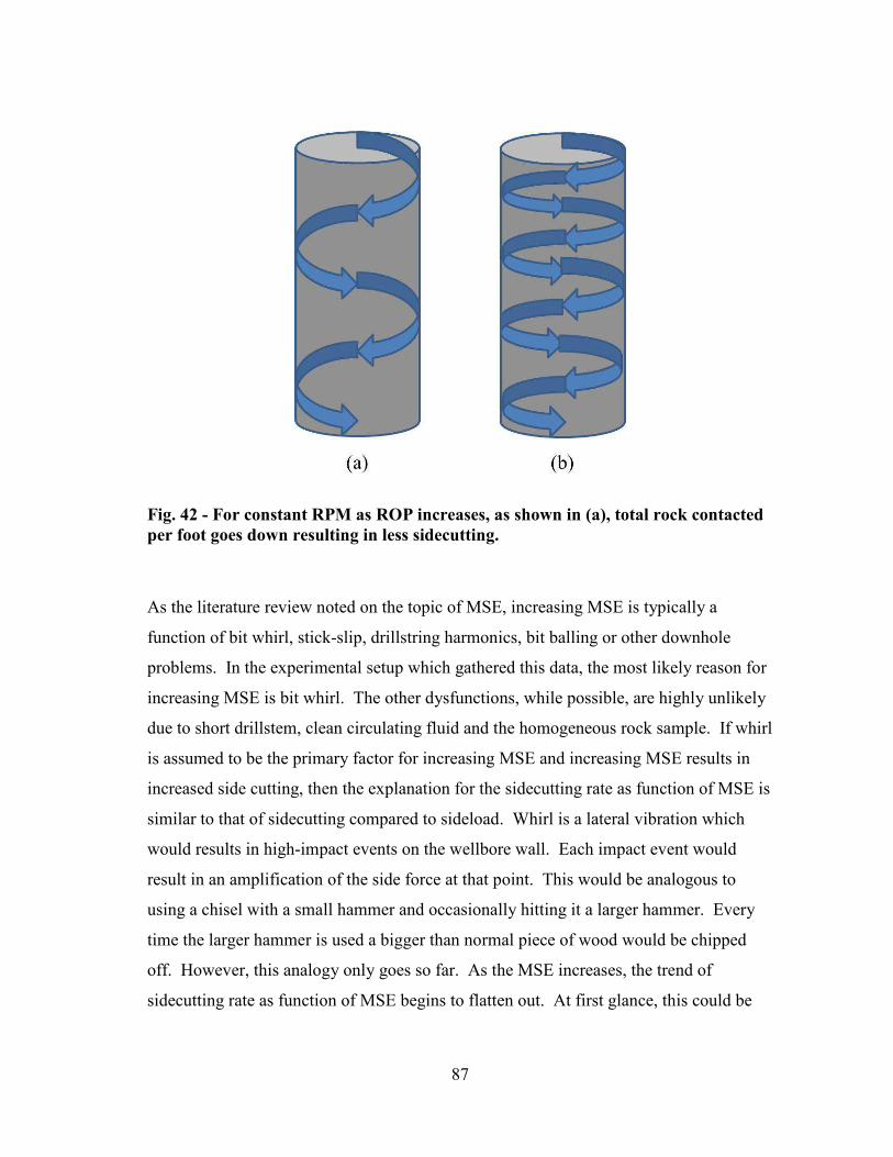
87

Fig. 42 - For constant RPM as ROP increases, as shown in (a), total rock contacted per foot goes down resulting in less sidecutting.

As the literature review noted on the topic of MSE, increasing MSE is typically a

function of bit whirl, stick-slip, drillstring harmonics, bit balling or other downhole

problems. In the experimental setup which gathered this data, the most likely reason for

increasing MSE is bit whirl. The other dysfunctions, while possible, are highly unlikely

due to short drillstem, clean circulating fluid and the homogeneous rock sample. If whirl

is assumed to be the primary factor for increasing MSE and increasing MSE results in

increased side cutting, then the explanation for the sidecutting rate as function of MSE is

similar to that of sidecutting compared to sideload. Whirl is a lateral vibration which

would results in high-impact events on the wellbore wall. Each impact event would

result in an amplification of the side force at that point. This would be analogous to

using a chisel with a small hammer and occasionally hitting it a larger hammer. Every

time the larger hammer is used a bigger than normal piece of wood would be chipped

off. However, this analogy only goes so far. As the MSE increases, the trend of

sidecutting rate as function of MSE begins to flatten out. At first glance, this could be

88

due to a similar phenomenon as what occurs for increasing sideload. The MSE amplifies

the side force to the point where a higher percentage of non-cutting bit face is contacting

the rock, thus resulting in diminishing effect of side force. This is physically possible

but an issue arises – the vibrational pattern is random and multi-directional as seen in

Fig. 21 (b). Thus the amplification of the sideload will occur at all points in the

wellbore. In this event, two things must be occurring. First, there exists a resultant

direction for the sideload such that the applied lateral force is greater on one side or

quadrant of the wellbore when compared to other areas. Also, although there is a

resultant force direction, due to rotation of the bit and drillstring, there will still be

impacts on all sides of the hole, which will be smaller in magnitude than those in the

resultant direction. Increased MSE will amplify these smaller impacts also. The result

of this will increased hole enlargement. Prior work has shown that if hole size is

increased without a corresponding increase in pipe diameter, maximum dog-leg severity

capability is reduced (Lubinski and Woods 1953; Millheim 1978a; Sutko et al. 1980;

Walker 1986). Therefore as MSE increases, the hole enlarges resulting in a reduced

DLS capability which manifests itself as a lower sidecutting rate. This offsets the effect

of MSE to some extent, particularly at high MSE’s which would result in much higher

impact forces and thus a bigger hole.

Using the MSE concept and preceding discussion one can further verify the sidecutting

as a function of ROP. Increasing ROP in the experimental setup was a function of

increasing weight on bit. In most situations, as the WOB increases, the cutters become

more fully engaged in the rock. This improves the bit’s stability, reducing whirl and

cutting a consistent bottomhole pattern (Dupriest and Koederitz 2005; Dupriest et al.

2005; Remmert et al. 2007)

The data was then used to develop the basic model for sidecutting rate as a function of

side load. The general equation as seen in Fig. 33 and Fig. 34 has the general power

form:

]/ = > ∙ �7T96^T7( Eq. 25

89

Using the experimental data only, Eq. 26 was found to model the data with a high degree

of accuracy once the effects of ROP and RPM were accounted for. The inputs and

outputs of this model for a dataset can be seen in Table 5 and Fig. 43.

]/ = $ ∙ �7T96^T7ocjkpck� Eq. 26

Table 5 - Inputs and outputs used for initial model of sidecutting as a function of sideload, ROP and RPM.

Flateral ROP RPM SCmeasured SCmodel Residual

489 18 120 0.008814 0.009331 2.6700E-07

1002 18 120 0.014225 0.012962 1.5951E-06

1978 18 120 0.017088 0.017702 3.7665E-07

488 72 120 0.005184 0.007006 3.3200E-06

990 72 120 0.010001 0.009688 9.8081E-08

1975 72 120 0.013981 0.013294 4.7156E-07

495 18 60 0.007872 0.007764 1.1618E-08

996 18 60 0.011991 0.010696 1.6773E-06

1986 18 60 0.013632 0.014674 1.0865E-06

492 72 60 0.005358 0.005818 2.1181E-07

1000 72 60 0.008849 0.008053 6.3376E-07

2000 72 60 0.010787 0.011064 7.6733E-08

9.8262E-06Total Residual:

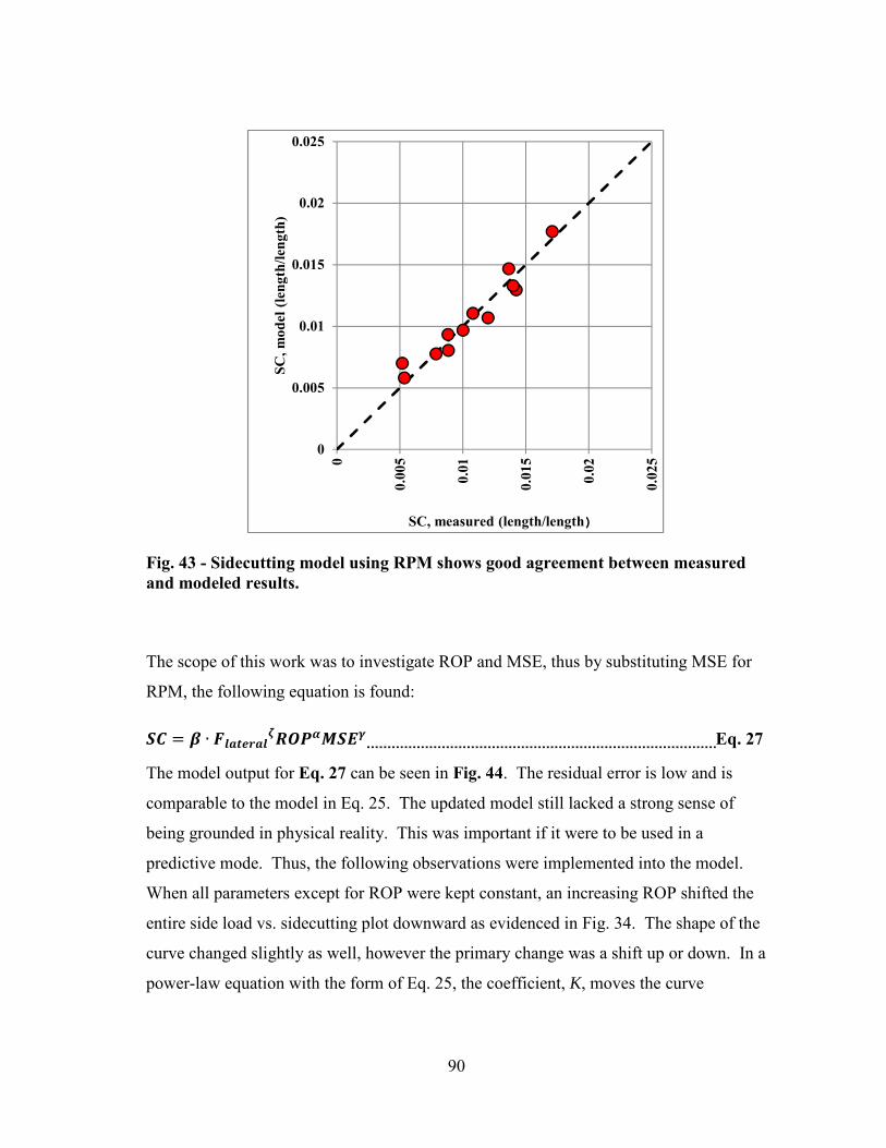
90

Fig. 43 - Sidecutting model using RPM shows good agreement between measured and modeled results.

The scope of this work was to investigate ROP and MSE, thus by substituting MSE for

RPM, the following equation is found:

]/ = $ ∙ �7T96^T7ocjkp�]� Eq. 27

The model output for Eq. 27 can be seen in Fig. 44. The residual error is low and is

comparable to the model in Eq. 25. The updated model still lacked a strong sense of

being grounded in physical reality. This was important if it were to be used in a

predictive mode. Thus, the following observations were implemented into the model.

When all parameters except for ROP were kept constant, an increasing ROP shifted the

entire side load vs. sidecutting plot downward as evidenced in Fig. 34. The shape of the

curve changed slightly as well, however the primary change was a shift up or down. In a

power-law equation with the form of Eq. 25, the coefficient, K, moves the curve

0

0.005

0.01

0.015

0.02

0.025

0

0.00

5

0.01

0.01

5

0.02

0.02

5

SC, m

odel

(len

gth/

leng

th)

SC, measured (length/length)

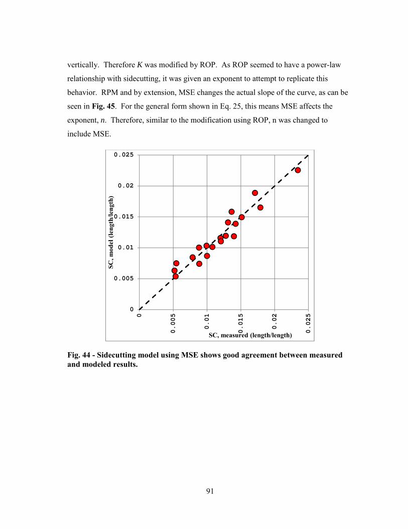
91

vertically. Therefore K was modified by ROP. As ROP seemed to have a power-law

relationship with sidecutting, it was given an exponent to attempt to replicate this

behavior. RPM and by extension, MSE changes the actual slope of the curve, as can be

seen in Fig. 45. For the general form shown in Eq. 25, this means MSE affects the

exponent, n. Therefore, similar to the modification using ROP, n was changed to

include MSE.

Fig. 44 - Sidecutting model using MSE shows good agreement between measured and modeled results.

0

0.005

0.01

0.015

0.02

0.025

0

0.005

0.01

0.015

0.02

0.025

SC, m

odel

(len

gth/

leng

th)

SC, measured (length/length)

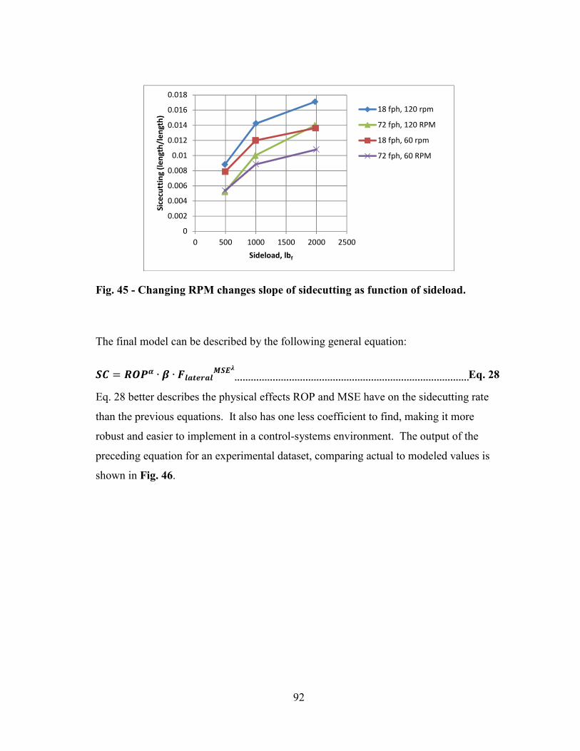
92

Fig. 45 - Changing RPM changes slope of sidecutting as function of sideload.

The final model can be described by the following general equation:

]/ = cjkp ∙ $ ∙ �7T96^T7�]�N Eq. 28

Eq. 28 better describes the physical effects ROP and MSE have on the sidecutting rate

than the previous equations. It also has one less coefficient to find, making it more

robust and easier to implement in a control-systems environment. The output of the

preceding equation for an experimental dataset, comparing actual to modeled values is

shown in Fig. 46.

0

0.002

0.004

0.006

0.008

0.01

0.012

0.014

0.016

0.018

0 500 1000 1500 2000 2500

Sic

ecu

ttin

g (

len

gth

/le

ng

th)

Sideload, lbf

18 fph, 120 rpm

72 fph, 120 RPM

18 fph, 60 rpm

72 fph, 60 RPM

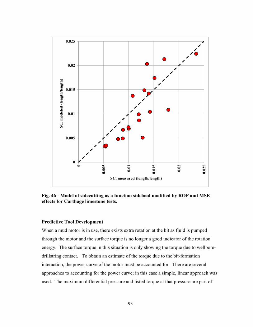
93

Fig. 46 - Model of sidecutting as a function sideload modified by ROP and MSE effects for Carthage limestone tests.

Predictive Tool Development

When a mud motor is in use, there exists extra rotation at the bit as fluid is pumped

through the motor and the surface torque is no longer a good indicator of the rotation

energy. The surface torque in this situation is only showing the torque due to wellbore-

drillstring contact. To obtain an estimate of the torque due to the bit-formation

interaction, the power curve of the motor must be accounted for. There are several

approaches to accounting for the power curve; in this case a simple, linear approach was

used. The maximum differential pressure and listed torque at that pressure are part of

0

0.005

0.01

0.015

0.02

0.025

0

0.00

5

0.01

0.01

5

0.02

0.02

5

SC, m

odel

ed (l

engt

h/le

ngth

)

SC, measured (length/length)

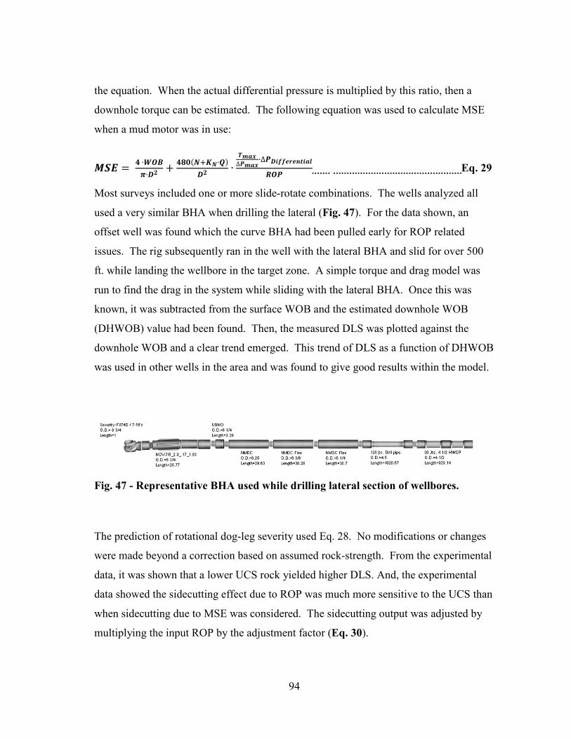
94

the equation. When the actual differential pressure is multiplied by this ratio, then a

downhole torque can be estimated. The following equation was used to calculate MSE

when a mud motor was in use:

�]� = )∙lj:m∙;� + )n+�*q>*∙r%;� ∙ S8T�∆k8T�∙∆k;'tt6^6(9'T7cjk Eq. 29

Most surveys included one or more slide-rotate combinations. The wells analyzed all

used a very similar BHA when drilling the lateral (Fig. 47). For the data shown, an

offset well was found which the curve BHA had been pulled early for ROP related

issues. The rig subsequently ran in the well with the lateral BHA and slid for over 500

ft. while landing the wellbore in the target zone. A simple torque and drag model was

run to find the drag in the system while sliding with the lateral BHA. Once this was

known, it was subtracted from the surface WOB and the estimated downhole WOB

(DHWOB) value had been found. Then, the measured DLS was plotted against the

downhole WOB and a clear trend emerged. This trend of DLS as a function of DHWOB

was used in other wells in the area and was found to give good results within the model.

Fig. 47 - Representative BHA used while drilling lateral section of wellbores.

The prediction of rotational dog-leg severity used Eq. 28. No modifications or changes

were made beyond a correction based on assumed rock-strength. From the experimental

data, it was shown that a lower UCS rock yielded higher DLS. And, the experimental

data showed the sidecutting effect due to ROP was much more sensitive to the UCS than

when sidecutting due to MSE was considered. The sidecutting output was adjusted by

multiplying the input ROP by the adjustment factor (Eq. 30).

95

1�ui#986(9Qc = v Qc!i^^6(9QcT�6^T@67T#9�=+wxP++wy(

Eq. 30

Interestingly enough, this factor was the same for both slide and rotated course lengths.

Changing the ratio or the power it is raised to did not help the model predict the

sidecutting any better. Significant amounts of work were done attempting to identify

methods to account for and inaccuracy in the data. Other than accounting for the

assumed rock strength based on the GR reading, attempts to modify the model’s output

by accounting for other parameters did not result in a better match. The final model to

predict sidecutting rate is shown in Eq. 31.

z{ = v Qc!i^^6(9QcT�6^T@67T#9�=+wxP++wy( ∙ |}~� ∙ � ∙ ������������ Eq. 31

In order to put the sidecutting rate into applicable field units of degrees per hundred feet

drilled, Eq. 32 is used.

;5] = .23�]/% Eq. 32

96

CHAPTER IV

SENSITIVITY STUDY To more fully understand Eq. 28, a brief sensitivity study was undertaken and illustrated

using three-dimensional plots. The Carthage limestone samples used were listed as

having 15 ksi UCS while the Bedford limestone was shown to have 3 ksi UCS

(Pastusek and Brackin 2003). The rock strength is an important consideration for future

application. Unconventional resources often span large geographic areas and thus

exhibit widely varied rock strength due to changing overburden and tectonic stresses.

Work in the Barnett shale regarding UCS has shown it can be estimated using the

following:

]9^6(@9�S6(#'76 =.+= �#'t9 × S�;�t9% (Waters et al. 2006) Eq. 33

]9^6(@9�S6(#'76 = ?/]�+ (T.Tran et al. 2010) Eq. 34

Based on the above verified procedure for calculating tensile strength in the Barnett

shale, the range of likely UCS is between 2500 psi and 5000 psi. However, published

reports and personal communication show the Barnett shale exhibiting behavior during

hydraulic fracturing treatments which indicate much higher UCS, sometimes as much as

30 ksi (T.Tran et al. 2010). In the case of the Barnett shale, both data sets, the Bedford

and Carthage limestones, would need to be analyzed.

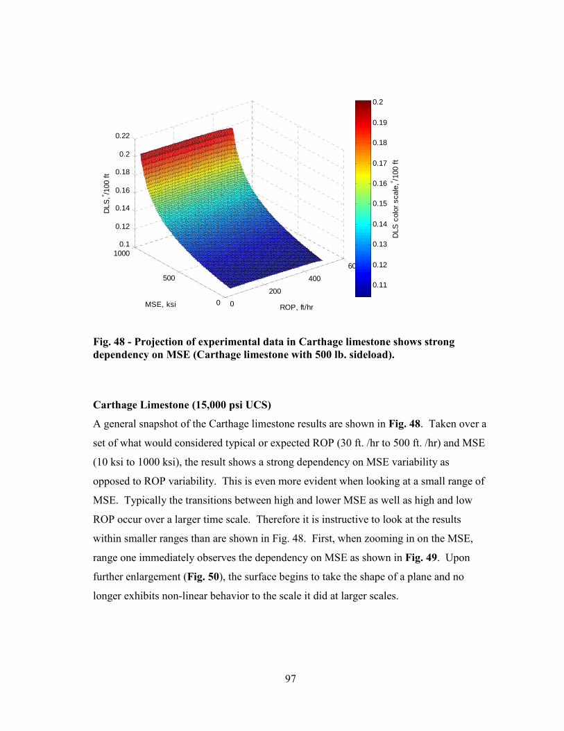
97

Fig. 48 - Projection of experimental data in Carthage limestone shows strong dependency on MSE (Carthage limestone with 500 lb. sideload).

Carthage Limestone (15,000 psi UCS)

A general snapshot of the Carthage limestone results are shown in Fig. 48. Taken over a

set of what would considered typical or expected ROP (30 ft. /hr to 500 ft. /hr) and MSE

(10 ksi to 1000 ksi), the result shows a strong dependency on MSE variability as

opposed to ROP variability. This is even more evident when looking at a small range of

MSE. Typically the transitions between high and lower MSE as well as high and low

ROP occur over a larger time scale. Therefore it is instructive to look at the results

within smaller ranges than are shown in Fig. 48. First, when zooming in on the MSE,

range one immediately observes the dependency on MSE as shown in Fig. 49. Upon

further enlargement (Fig. 50), the surface begins to take the shape of a plane and no

longer exhibits non-linear behavior to the scale it did at larger scales.

0

200

400

600

0

500

10000.1

0.12

0.14

0.16

0.18

0.2

0.22

ROP, ft/hrMSE, ksi

DLS

,° /10

0 ft

DLS

col

or s

cale

,° /10

0 ft

0.11

0.12

0.13

0.14

0.15

0.16

0.17

0.18

0.19

0.2

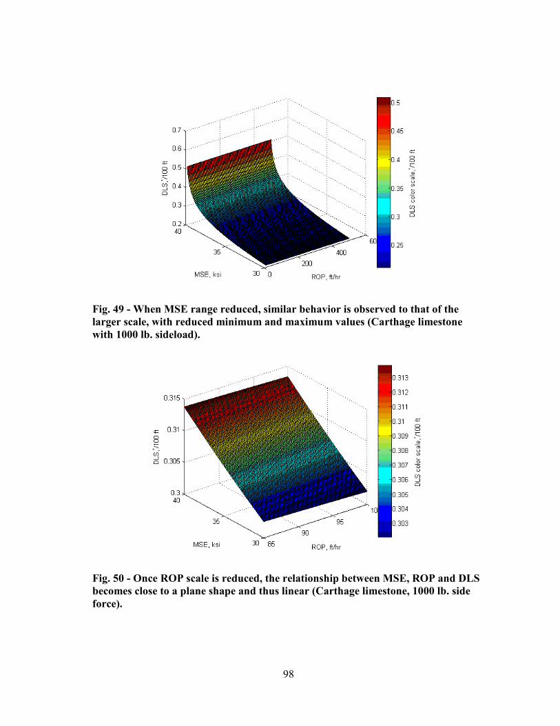
98

Fig. 49 - When MSE range reduced, similar behavior is observed to that of the larger scale, with reduced minimum and maximum values (Carthage limestone with 1000 lb. sideload).

Fig. 50 - Once ROP scale is reduced, the relationship between MSE, ROP and DLS becomes close to a plane shape and thus linear (Carthage limestone, 1000 lb. side force).

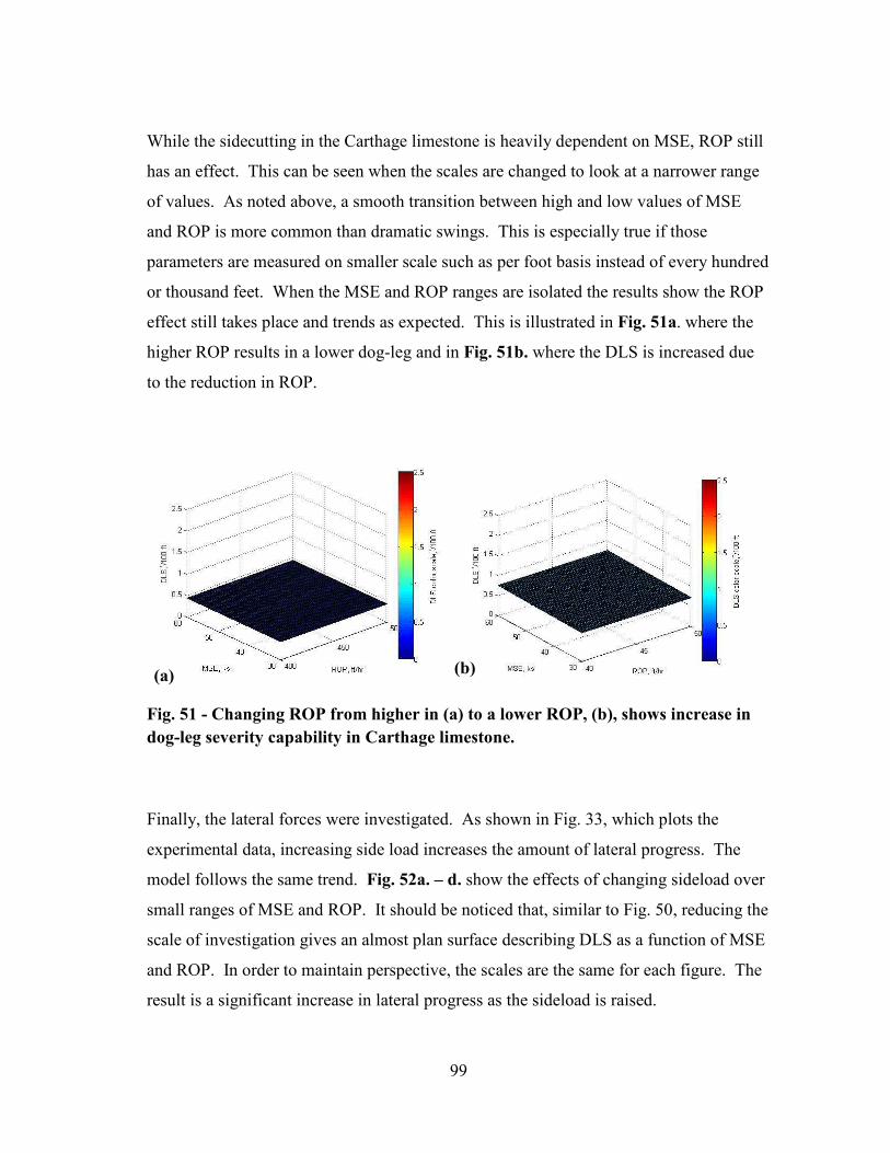
99

While the sidecutting in the Carthage limestone is heavily dependent on MSE, ROP still

has an effect. This can be seen when the scales are changed to look at a narrower range

of values. As noted above, a smooth transition between high and low values of MSE

and ROP is more common than dramatic swings. This is especially true if those

parameters are measured on smaller scale such as per foot basis instead of every hundred

or thousand feet. When the MSE and ROP ranges are isolated the results show the ROP

effect still takes place and trends as expected. This is illustrated in Fig. 51a. where the

higher ROP results in a lower dog-leg and in Fig. 51b. where the DLS is increased due

to the reduction in ROP.

Fig. 51 - Changing ROP from higher in (a) to a lower ROP, (b), shows increase in dog-leg severity capability in Carthage limestone.

Finally, the lateral forces were investigated. As shown in Fig. 33, which plots the

experimental data, increasing side load increases the amount of lateral progress. The

model follows the same trend. Fig. 52a. – d. show the effects of changing sideload over

small ranges of MSE and ROP. It should be noticed that, similar to Fig. 50, reducing the

scale of investigation gives an almost plan surface describing DLS as a function of MSE

and ROP. In order to maintain perspective, the scales are the same for each figure. The

result is a significant increase in lateral progress as the sideload is raised.

(a) (b)

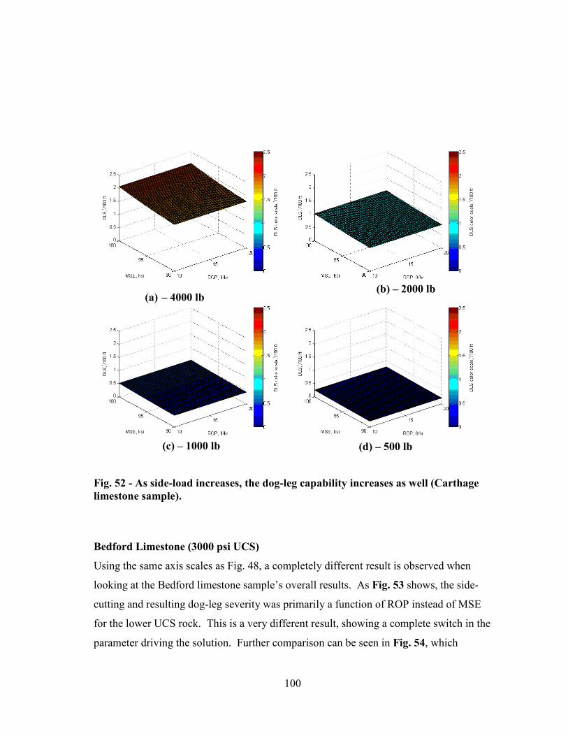
100

Fig. 52 - As side-load increases, the dog-leg capability increases as well (Carthage limestone sample).

Bedford Limestone (3000 psi UCS)

Using the same axis scales as Fig. 48, a completely different result is observed when

looking at the Bedford limestone sample’s overall results. As Fig. 53 shows, the side-

cutting and resulting dog-leg severity was primarily a function of ROP instead of MSE

for the lower UCS rock. This is a very different result, showing a complete switch in the

parameter driving the solution. Further comparison can be seen in Fig. 54, which

(a) – 4000 lb (b) – 2000 lb

(c) – 1000 lb (d) – 500 lb

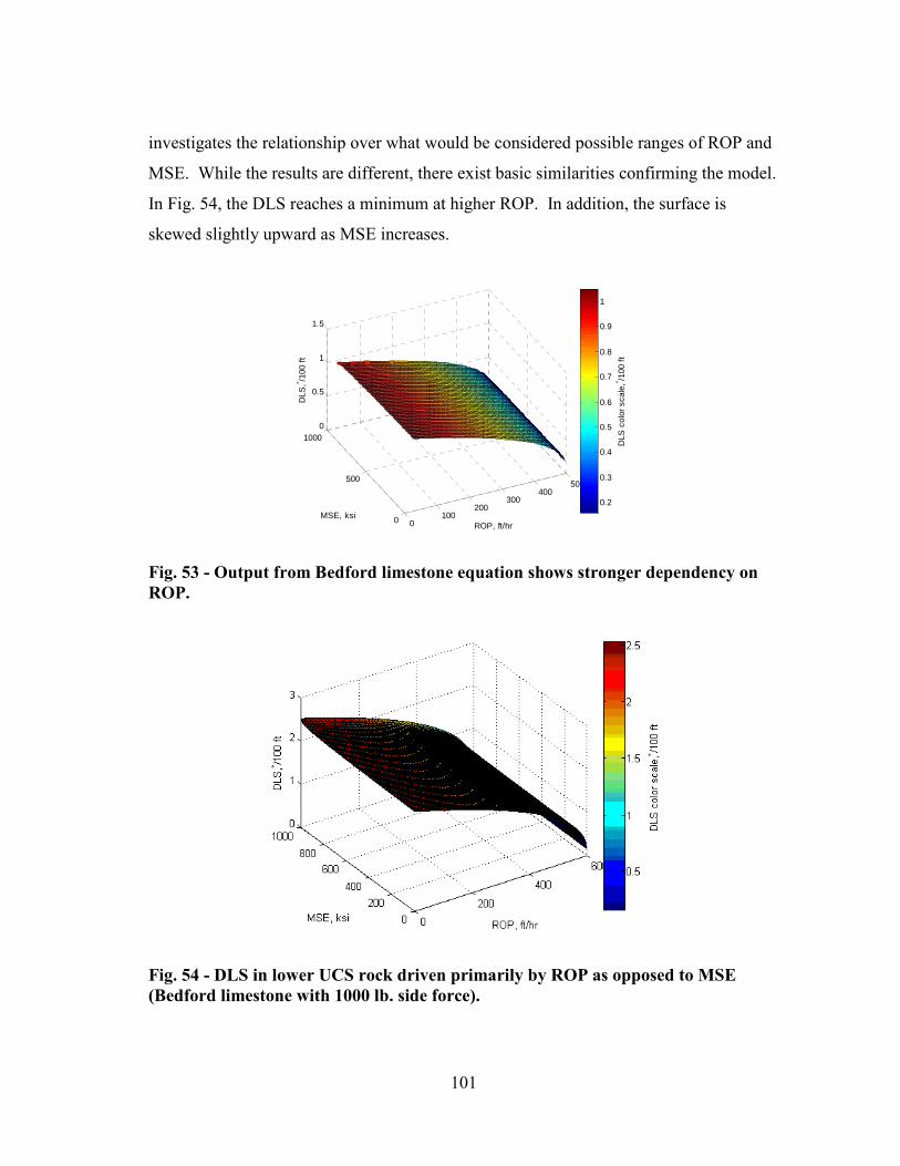
101

investigates the relationship over what would be considered possible ranges of ROP and

MSE. While the results are different, there exist basic similarities confirming the model.

In Fig. 54, the DLS reaches a minimum at higher ROP. In addition, the surface is

skewed slightly upward as MSE increases.

Fig. 53 - Output from Bedford limestone equation shows stronger dependency on ROP.

Fig. 54 - DLS in lower UCS rock driven primarily by ROP as opposed to MSE (Bedford limestone with 1000 lb. side force).

0100

200300

400500

0

500

10000

0.5

1

1.5

ROP, ft/hrMSE, ksi

DLS

,° /10

0 ft

DLS

col

or s

cale

,° /10

0 ft

0.2

0.3

0.4

0.5

0.6

0.7

0.8

0.9

1

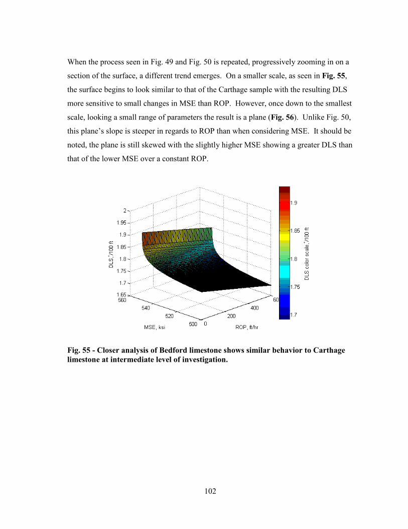
102

When the process seen in Fig. 49 and Fig. 50 is repeated, progressively zooming in on a

section of the surface, a different trend emerges. On a smaller scale, as seen in Fig. 55,

the surface begins to look similar to that of the Carthage sample with the resulting DLS

more sensitive to small changes in MSE than ROP. However, once down to the smallest

scale, looking a small range of parameters the result is a plane (Fig. 56). Unlike Fig. 50,

this plane’s slope is steeper in regards to ROP than when considering MSE. It should be

noted, the plane is still skewed with the slightly higher MSE showing a greater DLS than

that of the lower MSE over a constant ROP.

Fig. 55 - Closer analysis of Bedford limestone shows similar behavior to Carthage limestone at intermediate level of investigation.

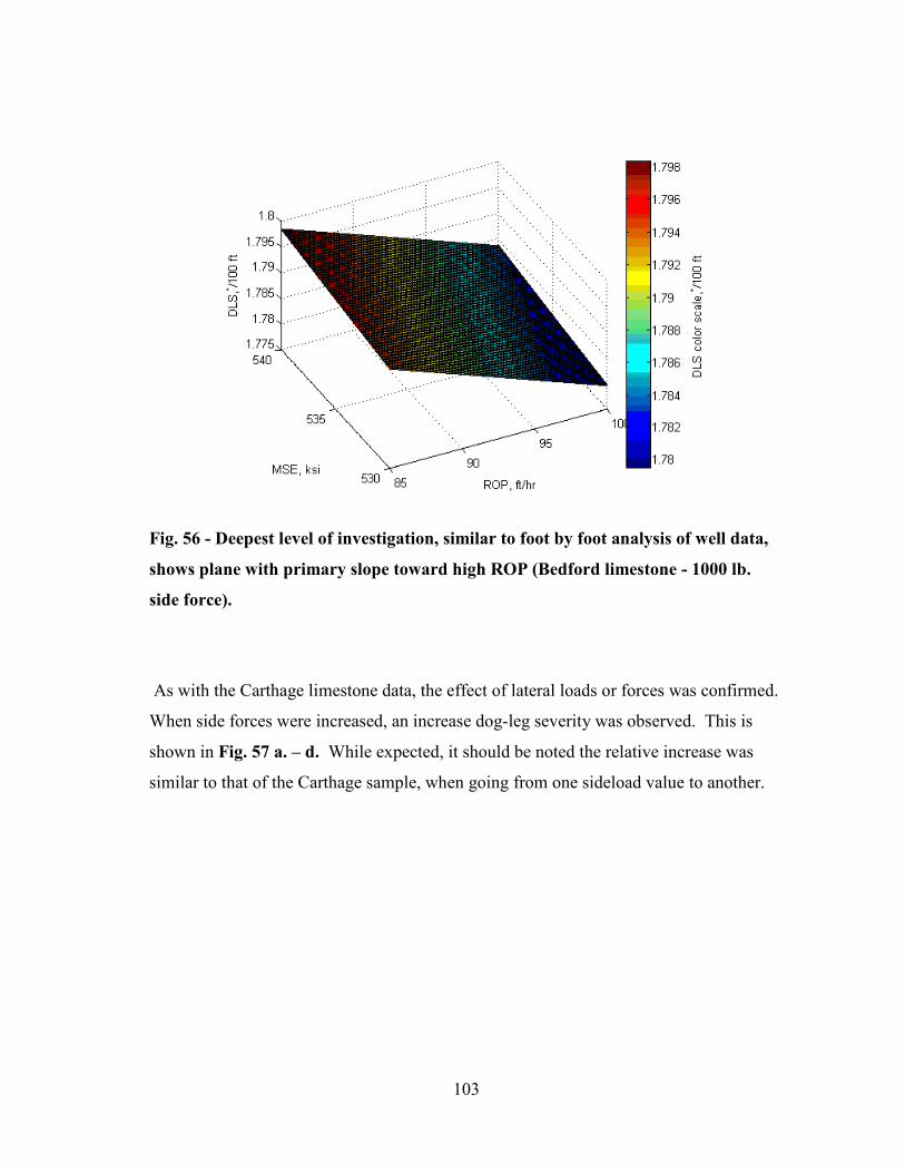
103

Fig. 56 - Deepest level of investigation, similar to foot by foot analysis of well data,

shows plane with primary slope toward high ROP (Bedford limestone - 1000 lb.

side force).

As with the Carthage limestone data, the effect of lateral loads or forces was confirmed.

When side forces were increased, an increase dog-leg severity was observed. This is

shown in Fig. 57 a. – d. While expected, it should be noted the relative increase was

similar to that of the Carthage sample, when going from one sideload value to another.

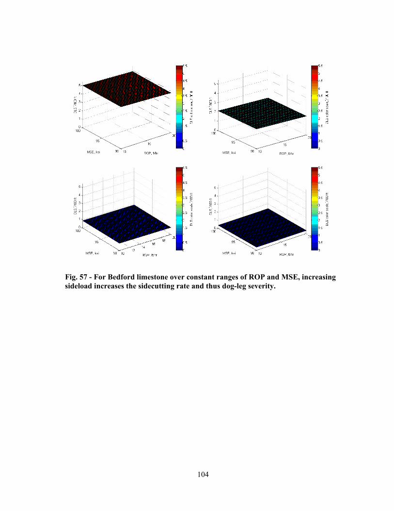
104

Fig. 57 - For Bedford limestone over constant ranges of ROP and MSE, increasing sideload increases the sidecutting rate and thus dog-leg severity.

105

CHAPTER V

PREDICTIVE TOOL AND PROCESS

Data Requirements

Once the initial model was confirmed from the published experimental data, a predictive

tool was developed which could predict the sidecutting rate or dog-leg severity based on

current drilling parameters and prior surveys. The predictive tool requires the following

data:

• Survey values for inclination, azimuth and calculated DLS

• A slide sheet

• Digital drilling parameter data

o WOB

o Surface RPM

o Instantaneous ROP

o Pump strokes

o Differential pressure

o GR values

• Estimated sideload

• Torque and drag model

• BHA

• Model parameters

The surveys are typically taken every connection, unless there are concerns about the

well’s trajectory in which case they may be taken over shorter intervals. An example of

survey values is shown in Fig. 58. This data would be updated as each survey was

measured. It should be noted that certain values are projections or possibly invalid based

on tool-error readings. Care must be taken when using these values, particularly early

on in the well as it would affect the learning capability of the model.

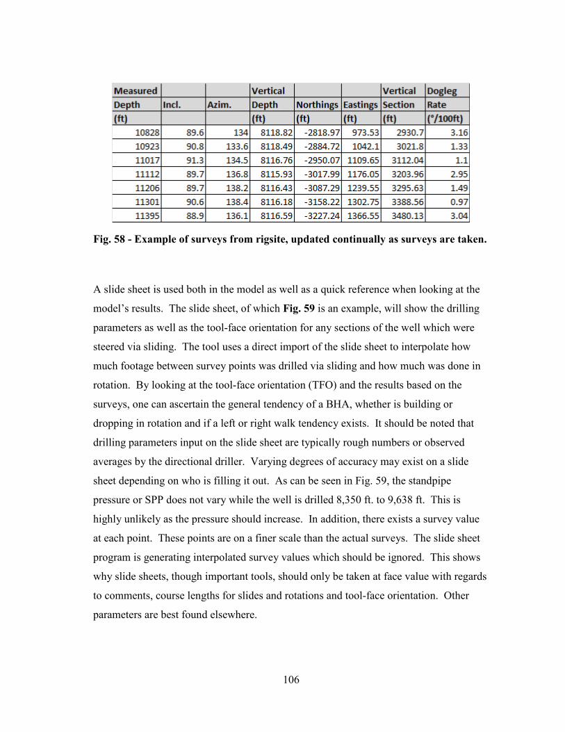
106

Fig. 58 - Example of surveys from rigsite, updated continually as surveys are taken.

A slide sheet is used both in the model as well as a quick reference when looking at the

model’s results. The slide sheet, of which Fig. 59 is an example, will show the drilling

parameters as well as the tool-face orientation for any sections of the well which were

steered via sliding. The tool uses a direct import of the slide sheet to interpolate how

much footage between survey points was drilled via sliding and how much was done in

rotation. By looking at the tool-face orientation (TFO) and the results based on the

surveys, one can ascertain the general tendency of a BHA, whether is building or

dropping in rotation and if a left or right walk tendency exists. It should be noted that

drilling parameters input on the slide sheet are typically rough numbers or observed

averages by the directional driller. Varying degrees of accuracy may exist on a slide

sheet depending on who is filling it out. As can be seen in Fig. 59, the standpipe

pressure or SPP does not vary while the well is drilled 8,350 ft. to 9,638 ft. This is

highly unlikely as the pressure should increase. In addition, there exists a survey value

at each point. These points are on a finer scale than the actual surveys. The slide sheet

program is generating interpolated survey values which should be ignored. This shows

why slide sheets, though important tools, should only be taken at face value with regards

to comments, course lengths for slides and rotations and tool-face orientation. Other

parameters are best found elsewhere.

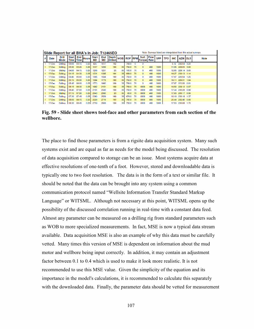
107

Fig. 59 - Slide sheet shows tool-face and other parameters from each section of the wellbore.

The place to find those parameters is from a rigsite data acquisition system. Many such

systems exist and are equal as far as needs for the model being discussed. The resolution

of data acquisition compared to storage can be an issue. Most systems acquire data at

effective resolutions of one-tenth of a foot. However, stored and downloadable data is

typically one to two foot resolution. The data is in the form of a text or similar file. It

should be noted that the data can be brought into any system using a common

communication protocol named “Wellsite Information Transfer Standard Markup

Language” or WITSML. Although not necessary at this point, WITSML opens up the

possibility of the discussed correlation running in real-time with a constant data feed.

Almost any parameter can be measured on a drilling rig from standard parameters such

as WOB to more specialized measurements. In fact, MSE is now a typical data stream

available. Data acquisition MSE is also an example of why this data must be carefully

vetted. Many times this version of MSE is dependent on information about the mud

motor and wellbore being input correctly. In addition, it may contain an adjustment

factor between 0.1 to 0.4 which is used to make it look more realistic. It is not

recommended to use this MSE value. Given the simplicity of the equation and its

importance in the model's calculations, it is recommended to calculate this separately

with the downloaded data. Finally, the parameter data should be vetted for measurement

108

and other errors. Abnormally high or low values and errors should be filtered out the

data.

The estimated sideload is an important part of the model. The side force on a bit drilling

a horizontal well is typically between 1000 to 2500 lbf. sideload for a 6 ¾” diameter

BHA. This project did not undertake the final development of a finite element model for

several reasons. And while the finite element model may be very useful in predicting

these side loads, care should be taken to reevaluate the results as the well is drilled. As

seen in the review literature on the subject, the majority of the finite element models

required some type of correction factor applied, even with the sophistication of the

models used. The BHA being used must also be recorded. The physical properties are

required for a finite element model and the performance properties of the mud motor are

also needed for the MSE equation.

Predictive Process

A torque and drag model must be run to find the estimated weight on bit while sliding.

The weight on bit will after the ability of the BHA to flex and thus achieve higher DLS.

Typically a higher force downhole for a given ROP will result in an increased DLS for

that section. The torque and drag model was a simple spread-sheet based soft string

model which required the hole size, MW, BHA and drillstring information and surveys.

If the model is being used in a predictive mode, planned surveys can be used for the hole

not yet drilled. A sample of the output of the model can be seen in Fig. 60.

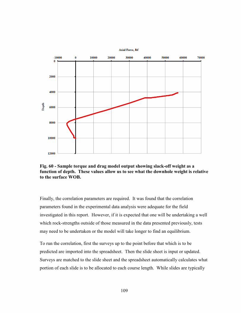
109

Fig. 60 - Sample torque and drag model output showing slack-off weight as a function of depth. These values allow us to see what the downhole weight is relative to the surface WOB.

Finally, the correlation parameters are required. It was found that the correlation

parameters found in the experimental data analysis were adequate for the field

investigated in this report. However, if it is expected that one will be undertaking a well

which rock-strengths outside of those measured in the data presented previously, tests

may need to be undertaken or the model will take longer to find an equilibrium.

To run the correlation, first the surveys up to the point before that which is to be

predicted are imported into the spreadsheet. Then the slide sheet is input or updated.

Surveys are matched to the slide sheet and the spreadsheet automatically calculates what

portion of each slide is to be allocated to each course length. While slides are typically

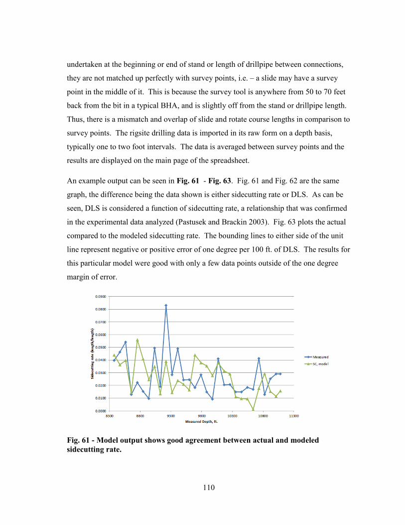
110

undertaken at the beginning or end of stand or length of drillpipe between connections,

they are not matched up perfectly with survey points, i.e. – a slide may have a survey

point in the middle of it. This is because the survey tool is anywhere from 50 to 70 feet

back from the bit in a typical BHA, and is slightly off from the stand or drillpipe length.

Thus, there is a mismatch and overlap of slide and rotate course lengths in comparison to

survey points. The rigsite drilling data is imported in its raw form on a depth basis,

typically one to two foot intervals. The data is averaged between survey points and the

results are displayed on the main page of the spreadsheet.

An example output can be seen in Fig. 61 - Fig. 63. Fig. 61 and Fig. 62 are the same

graph, the difference being the data shown is either sidecutting rate or DLS. As can be

seen, DLS is considered a function of sidecutting rate, a relationship that was confirmed

in the experimental data analyzed (Pastusek and Brackin 2003). Fig. 63 plots the actual

compared to the modeled sidecutting rate. The bounding lines to either side of the unit

line represent negative or positive error of one degree per 100 ft. of DLS. The results for

this particular model were good with only a few data points outside of the one degree

margin of error.

Fig. 61 - Model output shows good agreement between actual and modeled sidecutting rate.

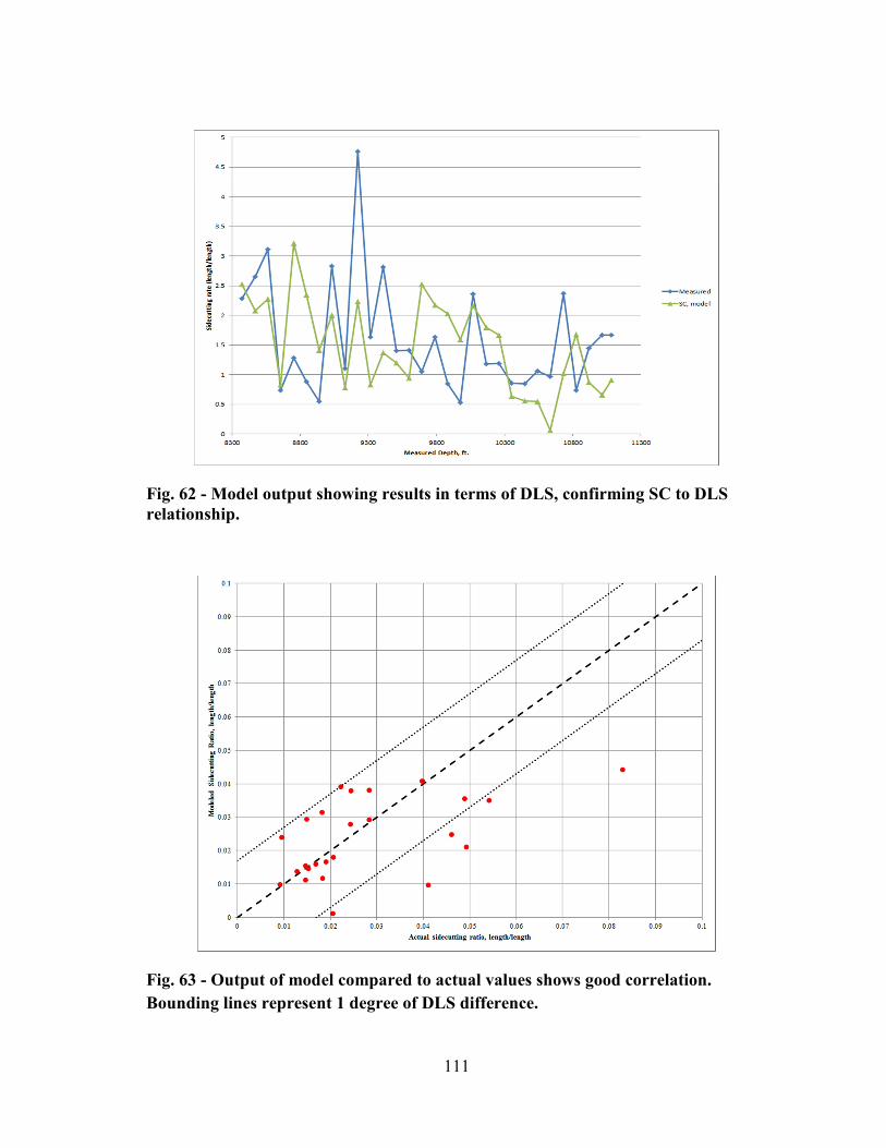
111

Fig. 62 - Model output showing results in terms of DLS, confirming SC to DLS relationship.

Fig. 63 - Output of model compared to actual values shows good correlation. Bounding lines represent 1 degree of DLS difference.

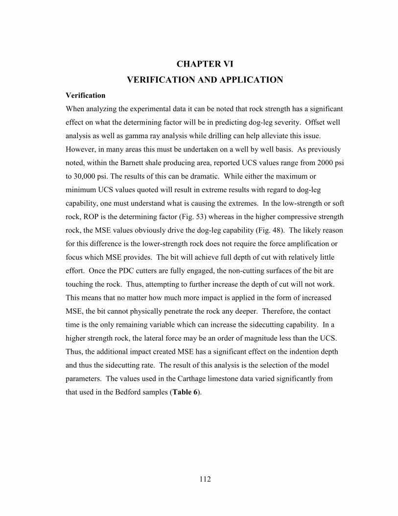
112

CHAPTER VI

VERIFICATION AND APPLICATION

Verification

When analyzing the experimental data it can be noted that rock strength has a significant

effect on what the determining factor will be in predicting dog-leg severity. Offset well

analysis as well as gamma ray analysis while drilling can help alleviate this issue.

However, in many areas this must be undertaken on a well by well basis. As previously

noted, within the Barnett shale producing area, reported UCS values range from 2000 psi

to 30,000 psi. The results of this can be dramatic. While either the maximum or

minimum UCS values quoted will result in extreme results with regard to dog-leg

capability, one must understand what is causing the extremes. In the low-strength or soft

rock, ROP is the determining factor (Fig. 53) whereas in the higher compressive strength

rock, the MSE values obviously drive the dog-leg capability (Fig. 48). The likely reason

for this difference is the lower-strength rock does not require the force amplification or

focus which MSE provides. The bit will achieve full depth of cut with relatively little

effort. Once the PDC cutters are fully engaged, the non-cutting surfaces of the bit are

touching the rock. Thus, attempting to further increase the depth of cut will not work.

This means that no matter how much more impact is applied in the form of increased

MSE, the bit cannot physically penetrate the rock any deeper. Therefore, the contact

time is the only remaining variable which can increase the sidecutting capability. In a

higher strength rock, the lateral force may be an order of magnitude less than the UCS.

Thus, the additional impact created MSE has a significant effect on the indention depth

and thus the sidecutting rate. The result of this analysis is the selection of the model

parameters. The values used in the Carthage limestone data varied significantly from

that used in the Bedford samples (Table 6).

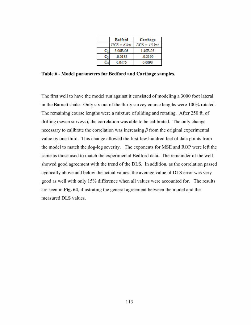
113

Table 6 - Model parameters for Bedford and Carthage samples.

The first well to have the model run against it consisted of modeling a 3000 foot lateral

in the Barnett shale. Only six out of the thirty survey course lengths were 100% rotated.

The remaining course lengths were a mixture of sliding and rotating. After 250 ft. of

drilling (seven surveys), the correlation was able to be calibrated. The only change

necessary to calibrate the correlation was increasing β from the original experimental

value by one-third. This change allowed the first few hundred feet of data points from

the model to match the dog-leg severity. The exponents for MSE and ROP were left the

same as those used to match the experimental Bedford data. The remainder of the well

showed good agreement with the trend of the DLS. In addition, as the correlation passed

cyclically above and below the actual values, the average value of DLS error was very

good as well with only 15% difference when all values were accounted for. The results

are seen in Fig. 64, illustrating the general agreement between the model and the

measured DLS values.

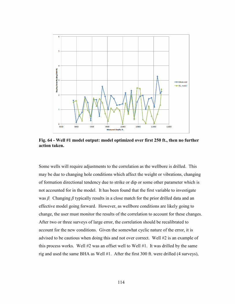
114

Fig. 64 - Well #1 model output: model optimized over first 250 ft., then no further action taken.

Some wells will require adjustments to the correlation as the wellbore is drilled. This

may be due to changing hole conditions which affect the weight or vibrations, changing

of formation directional tendency due to strike or dip or some other parameter which is

not accounted for in the model. It has been found that the first variable to investigate

was β. Changing β typically results in a close match for the prior drilled data and an

effective model going forward. However, as wellbore conditions are likely going to

change, the user must monitor the results of the correlation to account for these changes.

After two or three surveys of large error, the correlation should be recalibrated to

account for the new conditions. Given the somewhat cyclic nature of the error, it is

advised to be cautious when doing this and not over correct. Well #2 is an example of

this process works. Well #2 was an offset well to Well #1. It was drilled by the same

rig and used the same BHA as Well #1. After the first 300 ft. were drilled (4 surveys),

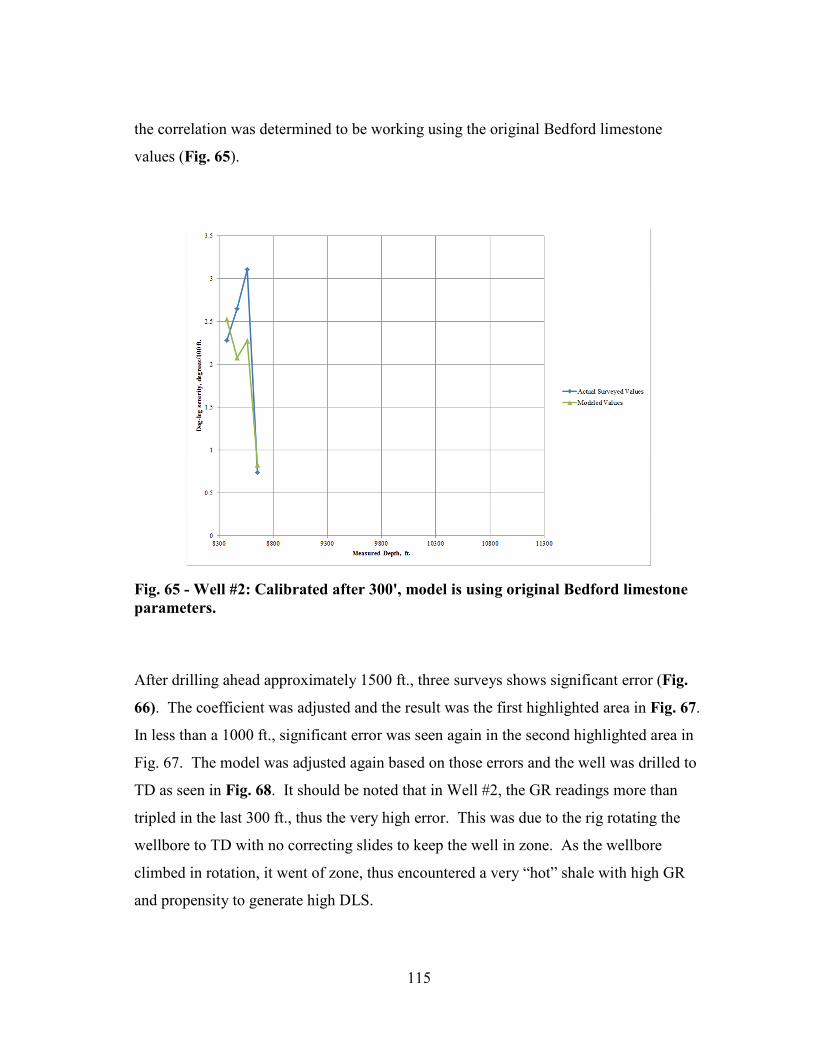
115

the correlation was determined to be working using the original Bedford limestone

values (Fig. 65).

Fig. 65 - Well #2: Calibrated after 300', model is using original Bedford limestone parameters.

After drilling ahead approximately 1500 ft., three surveys shows significant error (Fig.

66). The coefficient was adjusted and the result was the first highlighted area in Fig. 67.

In less than a 1000 ft., significant error was seen again in the second highlighted area in

Fig. 67. The model was adjusted again based on those errors and the well was drilled to

TD as seen in Fig. 68. It should be noted that in Well #2, the GR readings more than

tripled in the last 300 ft., thus the very high error. This was due to the rig rotating the

wellbore to TD with no correcting slides to keep the well in zone. As the wellbore

climbed in rotation, it went of zone, thus encountered a very “hot” shale with high GR

and propensity to generate high DLS.

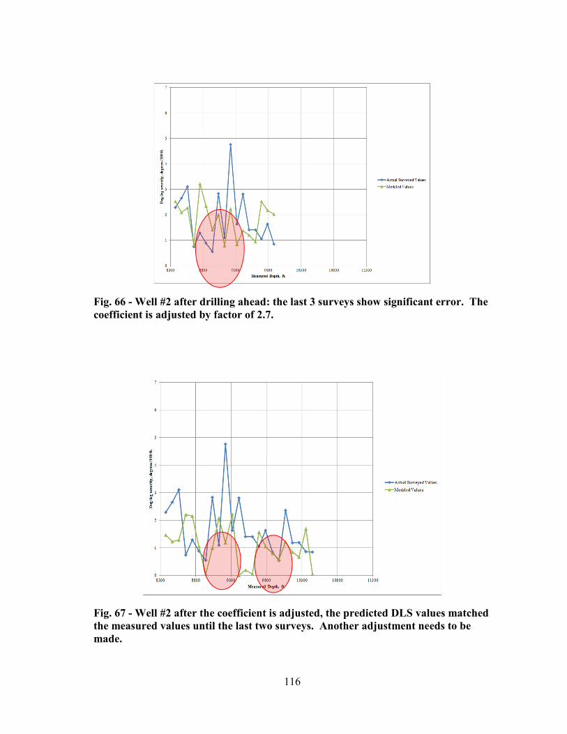
116

Fig. 66 - Well #2 after drilling ahead: the last 3 surveys show significant error. The coefficient is adjusted by factor of 2.7.

Fig. 67 - Well #2 after the coefficient is adjusted, the predicted DLS values matched the measured values until the last two surveys. Another adjustment needs to be made.

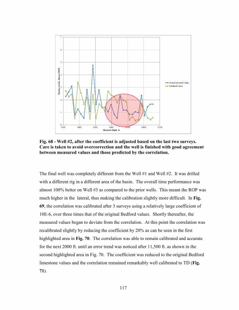
117

Fig. 68 - Well #2, after the coefficient is adjusted based on the last two surveys. Care is taken to avoid overcorrection and the well is finished with good agreement between measured values and those predicted by the correlation.

The final well was completely different from the Well #1 and Well #2. It was drilled

with a different rig in a different area of the basin. The overall time performance was

almost 100% better on Well #3 as compared to the prior wells. This meant the ROP was

much higher in the lateral, thus making the calibration slightly more difficult. In Fig.

69, the correlation was calibrated after 3 surveys using a relatively large coefficient of

10E-6, over three times that of the original Bedford values. Shortly thereafter, the

measured values began to deviate from the correlation. At this point the correlation was

recalibrated slightly by reducing the coefficient by 20% as can be seen in the first

highlighted area in Fig. 70. The correlation was able to remain calibrated and accurate

for the next 2000 ft. until an error trend was noticed after 11,500 ft. as shown in the

second highlighted area in Fig. 70. The coefficient was reduced to the original Bedford

limestone values and the correlation remained remarkably well calibrated to TD (Fig.

71).

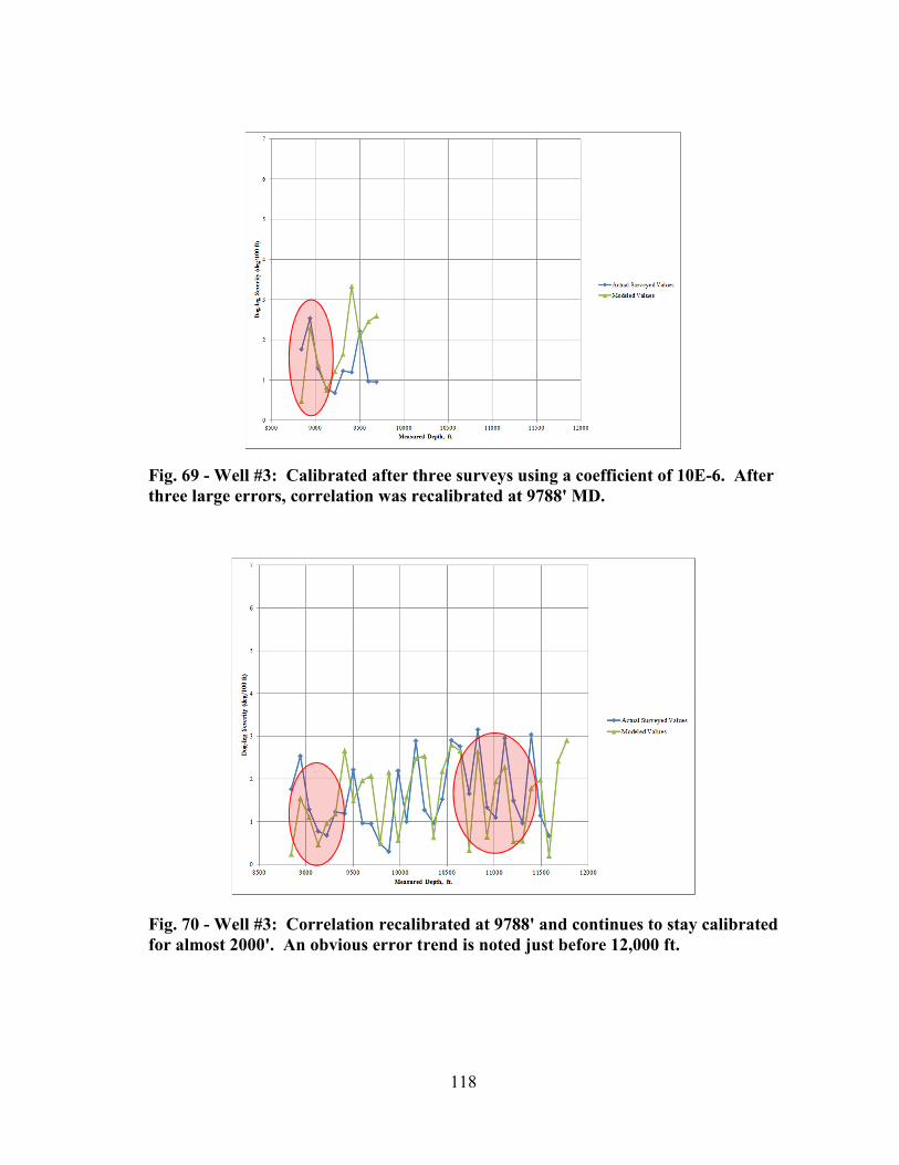
118

Fig. 69 - Well #3: Calibrated after three surveys using a coefficient of 10E-6. After three large errors, correlation was recalibrated at 9788' MD.

Fig. 70 - Well #3: Correlation recalibrated at 9788' and continues to stay calibrated for almost 2000'. An obvious error trend is noted just before 12,000 ft.

119

Fig. 71 - Well #3: coefficient is recalibrated to original experimental value of 3E-6 and the well is drilled to TD. The correlation remains well calibrated during remaining run.

For the data shown, the correlation has proved to be capable of quickly matching the

well as it is drilled and being adaptable to changing conditions. The question must asked

if the changes needed in the correlation’s coefficient are due to the correlation no longer

being valid for a dataset or are they due to the dataset itself. In other words, is

calibration required due to the correlation losing touch or is there a fundamental change

occurring within the system?

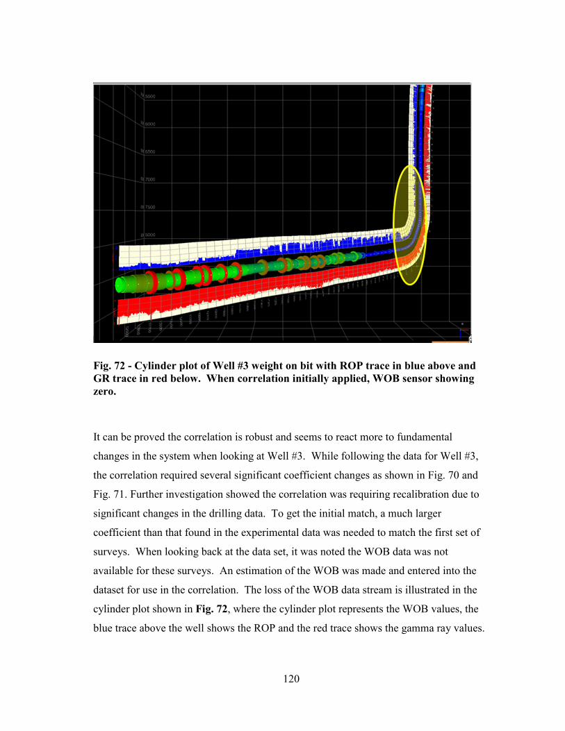
120

Fig. 72 - Cylinder plot of Well #3 weight on bit with ROP trace in blue above and GR trace in red below. When correlation initially applied, WOB sensor showing zero.

It can be proved the correlation is robust and seems to react more to fundamental

changes in the system when looking at Well #3. While following the data for Well #3,

the correlation required several significant coefficient changes as shown in Fig. 70 and

Fig. 71. Further investigation showed the correlation was requiring recalibration due to

significant changes in the drilling data. To get the initial match, a much larger

coefficient than that found in the experimental data was needed to match the first set of

surveys. When looking back at the data set, it was noted the WOB data was not

available for these surveys. An estimation of the WOB was made and entered into the

dataset for use in the correlation. The loss of the WOB data stream is illustrated in the

cylinder plot shown in Fig. 72, where the cylinder plot represents the WOB values, the

blue trace above the well shows the ROP and the red trace shows the gamma ray values.

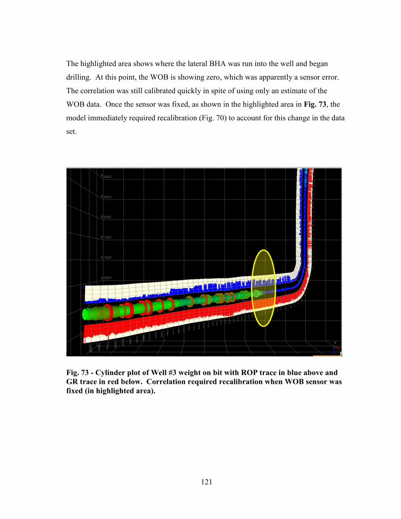
121

The highlighted area shows where the lateral BHA was run into the well and began

drilling. At this point, the WOB is showing zero, which was apparently a sensor error.

The correlation was still calibrated quickly in spite of using only an estimate of the

WOB data. Once the sensor was fixed, as shown in the highlighted area in Fig. 73, the

model immediately required recalibration (Fig. 70) to account for this change in the data

set.

Fig. 73 - Cylinder plot of Well #3 weight on bit with ROP trace in blue above and GR trace in red below. Correlation required recalibration when WOB sensor was fixed (in highlighted area).

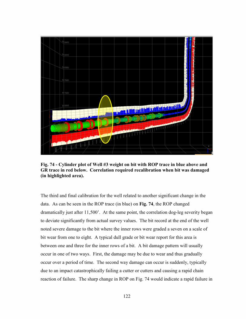
122

Fig. 74 - Cylinder plot of Well #3 weight on bit with ROP trace in blue above and GR trace in red below. Correlation required recalibration when bit was damaged (in highlighted area).

The third and final calibration for the well related to another significant change in the

data. As can be seen in the ROP trace (in blue) on Fig. 74, the ROP changed

dramatically just after 11,500’. At the same point, the correlation dog-leg severity began

to deviate significantly from actual survey values. The bit record at the end of the well

noted severe damage to the bit where the inner rows were graded a seven on a scale of

bit wear from one to eight. A typical dull grade or bit wear report for this area is

between one and three for the inner rows of a bit. A bit damage pattern will usually

occur in one of two ways. First, the damage may be due to wear and thus gradually

occur over a period of time. The second way damage can occur is suddenly, typically

due to an impact catastrophically failing a cutter or cutters and causing a rapid chain

reaction of failure. The sharp change in ROP on Fig. 74 would indicate a rapid failure in

123

the bit cutting structure. When the damage occurred, it essentially altered the bit itself

and changed the way the bit interacted with the formation. This change would have

resulted in a different dog-leg severity capability of the bit. Therefore the third and final

calibration was required at the highlighted portion of Fig. 74 was due to the bit’s quick

change its dog-leg severity capability due to the damage it incurred.

The three wells shown indicate the correlation presented in this paper can quickly

calibrate to a given well and is adaptable to changing conditions. In addition, when Well

#3 was investigated further, it can be seen that the correlation is robust and correlations

are needed primarily when dramatic wellbore, BHA or data changes occur. Data outside

the basin was not available; however the results would indicate matching DLS in other

basins would be within the realm of capability for this correlation.

Application

As the results proved, the correlation presented is robust and able to be used in a variety

of conditions. Now that the effect of MSE on the wellbore’s trajectory has been verified,

the correlation can be applied in several areas. First, it could be used in a post-well

analysis mode. Several authors have shown the value in post-well analysis of BHA

performance (Millheim et al. 1978; Millheim et al. 1979; Williams et al. 1989). In

today’s unconventional plays, this type of analysis becomes even more important.

Evaluating future wells’ drilling parameters and BHA setup as well as looking for

methods to decrease the drilling time for upcoming wells are all very important in the

unconventional plays. This is due to the “factory” style of drilling, where small gains in

efficiency can pay large dividends when large numbers of wells are drilled.

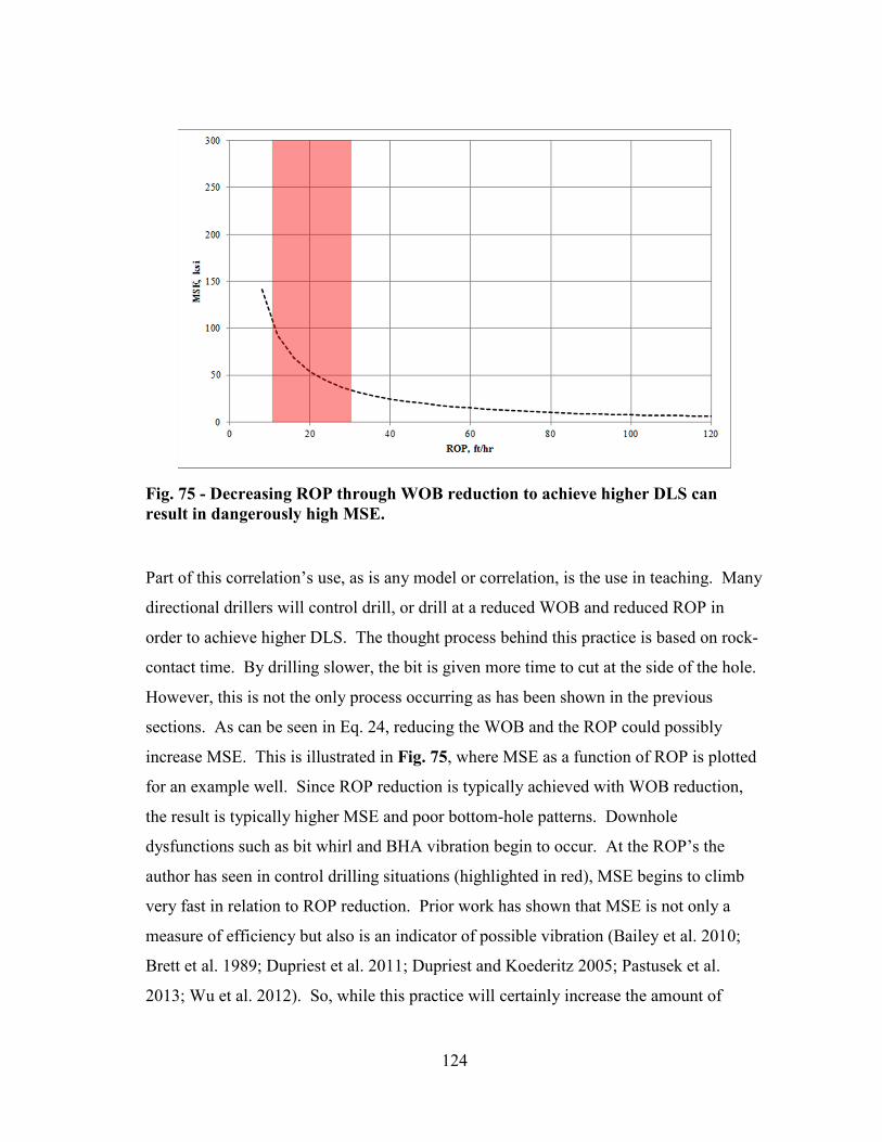
124

Fig. 75 - Decreasing ROP through WOB reduction to achieve higher DLS can result in dangerously high MSE.

Part of this correlation’s use, as is any model or correlation, is the use in teaching. Many

directional drillers will control drill, or drill at a reduced WOB and reduced ROP in

order to achieve higher DLS. The thought process behind this practice is based on rock-

contact time. By drilling slower, the bit is given more time to cut at the side of the hole.

However, this is not the only process occurring as has been shown in the previous

sections. As can be seen in Eq. 24, reducing the WOB and the ROP could possibly

increase MSE. This is illustrated in Fig. 75, where MSE as a function of ROP is plotted

for an example well. Since ROP reduction is typically achieved with WOB reduction,

the result is typically higher MSE and poor bottom-hole patterns. Downhole

dysfunctions such as bit whirl and BHA vibration begin to occur. At the ROP’s the

author has seen in control drilling situations (highlighted in red), MSE begins to climb

very fast in relation to ROP reduction. Prior work has shown that MSE is not only a

measure of efficiency but also is an indicator of possible vibration (Bailey et al. 2010;

Brett et al. 1989; Dupriest et al. 2011; Dupriest and Koederitz 2005; Pastusek et al.

2013; Wu et al. 2012). So, while this practice will certainly increase the amount of

125

sidecutting and thus DLS at that point, the result may include bit or BHA damage and

poor borehole quality.

This correlation obviously has a single primary purpose application within the petroleum

industry – as part of a directional drilling expert system. The correlation or similar

would form the basis for a fully automated directional drilling system in the future. Our

industry is trending toward more horizontal and highly deviated wells in order to access

unconventional resources and hard to reach conventional reserves (Fig. 4). As noted

earlier, the downhole tools currently used have gone through many changes and

upgrades, while the overall decision making involving the tools remains the same. Our

data collection has become better by orders of magnitude, yet the usage of that data has

not changed to a large extent. While some proprietary systems may exist, the sole

published working system relies on a single MWD company’s productions, is meant for

RSS only and does not account for lithology effects. My proposed model is applicable

to all types of directional drilling systems and will work with any MWD provider. In

summary, AIMR is meant to be a general direction drilling decision making tool capable

of working in a wide range of geologic settings with a wide range of tools.

126

CHAPTER VII

CONCLUSIONS AND FUTURE WORK Conclusions

On the basis of the theoretical and modeling work presented in this dissertation, I offer the following conclusions:

• Directional drilling prediction methods have been available for over 60

years beginning with Lubinski and Woods (Lubinski 1961; Lubinski and

Woods 1953).

• Many models purport to model and predict a portion of the directional

drilling process, yet have not proved themselves to be capable of

changing well conditions.

• A relationship has been discovered, based on published experimental

data, showing the sidecutting rate of a bit as a function of the rate of

penetration (ROP) and mechanical specific energy (MSE).

• The proposed model fits with current knowledge of the physics of

downhole vibrations and rock-bit interactions.

• By including MSE as part of the model, bit and BHA dysfunctions’

effects on the wellbore trajectory can now be quantified.

• The compressive strength of the rock being drilled will determine

whether ROP or MSE is the dominant term. For lower-strength rock,

ROP will be the primary factor while MSE will have a larger effect in

higher-strength rock.

• The model follows a power-law surface on a macro level but when

investigated on a smaller scale, the relationship can be seen as a plane.

• Based on the model developed, a predictive model has been developed

which closely mirrors the measured dog-leg severity.

127

• The tool is able to model drilled hole section which have been fully

rotated or have a combination of slide and rotation course lengths.

• The model is able to be easily calibrated in real-time as the well is drilled.

This calibration seems to be required only a few time per well, indicating

a robust model.

• Some applications for this model include post-well analysis, performance

enhancement planning and teaching.

• The most important application of this model is likely as the basis for a

directional drilling control system, either expert-type or automated.

Creating a system such as would allow for increased efficiency, faster

wells and increased accuracy in targeting when drilling geo-steered wells.

Future Work

The possibilities of future work are seemingly limitless with this topic. As the author

can attest, there are many “rabbit holes” which may be followed concerning not only the

approach used to find a solution to the directional drilling prediction problem but also

the variables which are investigated. The increase in quality and availability of drilling

data is opening up many new research areas in drilling optimization and automation and

this particular area is no different (Dupriest et al. 2012; Wardt et al. 2013; Wardt and

Rogers 2011). Thus the author encourages future researchers to look to the data first.

As the author found, depending on staid methods such as finite element models tended to

discount the treasure trove of data available even on “simple” U.S. onshore operations.

Coupled with the power of a basic personal computer, a very robust analysis can made

without having to rely on complex mathematics.

That being said, the author is not by any means discounting the mathematics involved in

more complex models. In fact, future research needs to include these mathematics.

While much of the work done in this area is interesting and seems to achieve good

results, some of it, this dissertation included, have bypassed the mathematics in order to

find and describe the general physical phenomena which occur. This is of vital

128

importance as it indicates a direction for further study. However, this further study must

begin to dig downward. When the physics can be described mathematically, the

correction factors often used in the data-based models are no longer used to gloss over

error in the model. Thus further research should continue to try to describe, via

mathematical models, the physics of what is occurring. When coupled with a data-

driven model or control system, the result is more accurate result.

Similar and perhaps in conjunction with the mathematics in the prior paragraph, is the

continued development of a finite element model. The author feels that, after seeing the

effect of ROP and MSE on sidecutting, many prior works involving dynamic finite

element models to predict the wellbore trajectory actually ended up accounting for MSE

or vibration to some extent. However, now that it has been proved that there is a

correlation between MSE (or vibration) on the trajectory; the finite element models

should be reintroduced. Similar to the mathematics, a strong dynamic finite element

model would eliminate some of the error or fuzziness in the current calculations

concerning MSE and wellbore trajectory. Reinventing the wheel is likely not necessary.

Many general, commercial finite element models would adequately model the BHA.

Certain operations should also be investigated. Eq. 23 would be something which needs

further investigation. While this may seem of little use as rigs drill faster, understanding

the sidetrack process could have significant economic benefits for operators. If the

proper parameters are applied, a cleaner sidetrack could be done in a shorter amount of

time. In addition, sidetrack techniques usually involve procedures which would be

considered detrimental to the life of the bit, when situations such as that shown in Fig.

75 are occurring. Thus a better understanding of what is occurring during the sidetrack

could lead to longer bit runs after sidetracks.

Further experiments should be undertaken similar to those that formed the basis for the

model for this work. Expanding the range of side loads and ROPs would be a key to any

future work. Experiments using a horizontal test bench, while more difficult would be

much more applicable in today’s drilling environment. Finally, expanding the rock

129

samples to include a shale would be important given the number of wells to be drilled in

the various shale plays in the United States and around the world.

The effect of formation dip has been discounted in this work. Beginning with Lubinski,

the effect of formation dip has been a significant part of most work in this area. That has

begun to be ignored in more recent work as many wells are drilled horizontally and thus

are parallel or close to parallel to the formation dip. Revisiting the effect of dip as well

as strike on horizontal well steering could prove to be important. It would likely involve

work associated with the measurement of wellbore stability or breakout and extracting a

dip and strike from those results.

The application of mass-data analyzation technologies would seem to be ideal in any

future work. Neural networks, something already used in the Texas A&M University

Petroleum Engineering department in recent drilling projects as well as the many other

methods for analyzing and finding usable trends and relationships in large volumes of

data must begin to be used. The drilling industry is no different than the rest of the

petroleum industry and the world, where the gathered data volumes are increasing

exponentially. Our ability to mine and use that data is paramount to future success.

Finally, all work should be done with an eye toward future implementation. Where and

how this work will be used is important. The drilling industry is currently on a path

toward increased process automation and optimization. By keeping drilling automation

as target application or audience, future work in this area will be relevant and useful to

our industry as a whole.

130

REFERENCES Aldred, W.D., Belaskie, J., Isangulov, R. et al. 2005. Changing the Way We Drill.

Schlumberger Oilfield Review, March 1, 2005, 8.

Anderson, A. 1929. Underground Surveys of Oil Wells. Petroleum Transactions, AIME 82: 10.

Apostal, M.C. and Baird, J.A. 1987. User Instruction Manual for GEODYN2: A Geological Formation - Bottom Hole Assembly Dynamic Interaction Finite Element Program. Albuquerque: Sandia National Laboratories.

Bai, J.Z. 1986. An Exact Solution for Bottomhole Assembly Analysis. Paper presented at the Annual Technical Meeting, Calgary, Alberta. Petroleum Society of Canada PETSOC-86-37-83. DOI: 10.2118/86-37-83.

Bailey, J.J. and Dean, R.C. 1966. Rock Mechanics and the Evolution of Improved Rock Cutting Methods. American Institute of Mining, Metallurgical, and Petroleum Engineers Inc. Permission to Distribute - American Rock Mechanics Association ARMA-66-0396.

Bailey, J.R., Biediger, E., Sundararaman, S. et al. 2008. Development and Application of a BHA Vibrations Model. Paper presented at the International Petroleum Technology Conference, Kuala Lumpur, Malaysia. International Petroleum Technology Conference IPTC-12737-MS. DOI: 10.2523/12737-ms.

Bailey, J.R. and Remmert, S.M. 2010. Managing Drilling Vibrations through BHA Design Optimization. SPE Drilling & Completion 25 (4): pp. 458-471. DOI: 10.2118/139426-pa

Bailey, J.R., Wang, L., Tenny, M. et al. 2010. Design Tools and Workflows to Mitigate Drilling Vibrations. Paper presented at the SPE Annual Technical Conference and Exhibition, Florence, Italy. Society of Petroleum Engineers SPE-135439-MS. DOI: 10.2118/135439-ms.

Baird, J.A., Caskey, B.C., Tinianow, M.A. et al. 1984. GEODYN: A Geological Formation/Drillstring Dynamics Computer Program. Paper presented at the SPE Annual Technical Conference and Exhibition, Houston, Texas. SPE-13023.

Baird, J.A., Caskey, B.C., Wormley, D.N. et al. 1985. GEODYN2: A Bottomhole Assembly/Geological Formation Dynamic Interaction Computer Program. Paper presented at the SPE Annual Technical Conference and Exhibition, Las Vegas, Nevada. SPE-14328.

131

Bayliss, M. and Matheus, J. 2008. Directional Drilling Tool Simulation and System Design. SAE Int. J. Mater. Manuf. 1 (1): 675-689. DOI: 10.4271/2008-01-1369

Beaufait, F., William Rowan, J., Hoadley, P. et al. 1970. Computer Methods of Structural Analysis. New Jersey: Prentice-Hall, Inc. Original edition. ISBN 0131659510.

Birades, M. 1988. Static and Dynamic Three-Dimensional Bottomhole Assembly Computer Models. SPE Drilling Engineering 3 (2). DOI: 10.2118/15466-pa

Birades, M. and Fenoul, R. 1988. A Microcomputer Program for Prediction of Bottomhole Assembly Trajectory. SPE Drilling Engineering 3 (2). DOI: 10.2118/15285-pa

Birades, M. and Gazaniol, D. 1989. ORPHEE 3D: Original Results on the Directional Behavior of Bha's with Bent Subs. Paper presented at the Offshore Europe, Aberdeen, United Kingdom. SPE-19244.

Boualleg, R., Sellami, H., Menand, S. et al. 2006. Effect of Formations Anisotropy on Directional Tendencies of Drilling Systems. Paper presented at the IADC/SPE Drilling Conference, Miami, Florida, USA. Society of Petroleum Engineers SPE-98865-MS. DOI: 10.2118/98865-ms.

Bourgoyne, A.T.J., Chenevert, M.E., Millheim, K. et al. 1986. Applied Drilling Engineering. Spe Textbook: Society of Petroleum Engineers. Original edition. ISBN 1-55563-001-4.

Boyadjieff, G.I. 1988. The Application of Robotics to the Drilling Process. Paper presented at the SPE/IADC Drilling Conference, Dallas, Texas. 1988 Copyright 1988, IADC/SPE Drilling Conference 00017232. DOI: 10.2118/17232-ms.

Bradley, W.B. 1975. Factors Affecting the Control of Borehole Angle in Straight and Directional Wells. SPE Journal of Petroleum Technology 27 (6). DOI: 10.2118/5070-pa

Brakel, J.D. 1987. Prediction of Wellbore Trajectory Considering Bottom Hole Assembly and Drillbit Dynamics. PhD, University of Tulsa, Oklahoma.

Brakel, J.D. and Azar, J.J. 1989. Prediction of Wellbore Trajectory Considering Bottomhole Assembly and Drill-Bit Dynamics. SPE Drilling Engineering 4 (2). DOI: 10.2118/16172-pa

Brantly, J.E. History of Oil Well Drilling. Houston: Gulf Publishing. Original edition. ISBN 087201634X.

132

Brett, J.F., Gray, J.A., Bell, R.K. et al. 1986. A Method of Modeling the Directional Behavior of Bottomhole Assembles Including Those with Bent Subs and Downhole Motors. Paper presented at the SPE/IADC Drilling Conference, Dallas, Texas. SPE-14767.

Brett, J.F., Warren, T.M., and Behr, S.M. 1989. Bit Whirl: A New Theory of PDC Bit Failure. Paper presented at the SPE Annual Technical Conference and Exhibition, San Antonio, Texas. Society of Petroleum Engineers SPE-019571-MS. DOI: 10.2118/19571-ms.

Brown, D. 2000. Geosteering: Like Landing in a Fog. AAPG Explorer 21 (12): 3.

Brugman, J.D. 1987. Automated Pipe Handling: A Fresh Approach. Paper presented at the SPE/IADC Drilling Conference, New Orleans, Louisiana. 00016065. DOI: 10.2118/16065-ms.

Burrough, B. and Helyar, J. 1989. Barbarians at the Gate: The Fall of RJR Nabisco. New York: Harper & Row. Original edition. ISBN 0-060-16172-8.

Calderoni, A., Brugman, J.D., Vogel, R.E. et al. 2006. The Continuous Circulation System - from Prototype to Commercial Tool. Paper presented at the SPE Annual Technical Conference and Exhibition, San Antonio, Texas, USA. Society of Petroleum Engineers SPE-102851-MS. DOI: 10.2118/102851-ms.

California Department of Conservation. 2003. History in California: Oil and Gas Production, ftp://ftp.consrv.ca.gov/pub/oil/history/History_of_Calif.pdf (downloaded 23 January 2013).

Cartwright. 1928. Rotary Drilling Problems. Transactions of the AIME 82 (1): 20. DOI: 10.2118/929009-G

Cayeux, E., Daireaux, B., Dvergsnes, E. et al. 2012. Early Symptom Detection on the Basis of Real-Time Evaluation of Downhole Conditions: Principles and Results from Several North Sea Drilling Operations. SPE Drilling & Completion 27 (4): pp. 546-558. DOI: 10.2118/150422-pa

Cheatham Jr., J.B. and Ho, C.Y. 1981. A Theoretical Model for Directional Drilling Tendency of a Drill Bit in Anisotropic Rock. Paper presented at the (unsolicited). Society of Petroleum Engineers SPE-00010642.

Chenevert, M.E. and Gatlin, C. 1965. Mechanical Anisotropies of Laminated Sedimentary Rocks. SPE Journal 5 (1): 10. DOI: 10.2118/890-pa

133

Cheng, K., Wu, W., Holditch, S.A. et al. 2010. Assessment of the Distribution of Technically-Recoverable Resources in North American Basins. Paper presented at the Canadian Unconventional Resources and International Petroleum Conference, Calgary, Alberta, Canada. Society of Petroleum Engineers 137599. DOI: 10.2118/137599-ms.

Cockburn, C.B., Matheus, J., and Dang, K.L.P. 2011. Automatic Trajectory Control in Extended-Reach Wells. Paper presented at the SPE Middle East Oil and Gas Show and Conference, Manama, Bahrain. Society of Petroleum Engineers 142671. DOI: 10.2118/142671-ms.

Cook, J.M., Sheppard, M.C., and Houwen, O.H. 1991. Effects of Strain Rate and Confining Pressure on the Deformation and Failure of Shale. SPE Drilling Engineering 6 (2): 100-104. DOI: 10.2118/19944-pa

Couvering, M.V. 1929. Courses of Drill Holes. AAPG Bulletin 13 (2): 7.

Cunningham, R.A. and Eenink, J.G. 1958. Laboratory Study of Effect of Overburden, Formation and Mud Column Pressures on Drilling Rate of Permeable Formations. Petroleum Transactions, AIME 217 (1): 8.

Dahl, T. and Schmalhorst, B. 1991. A New Bottomhole Assembly Analysis Program for the Prediction of the Borehole Path Based on a Sophisticated Static Algorithm. Paper presented at the SPE/IADC Drilling Conference, Amsterdam, Netherlands. SPE-21948. DOI: 10.2118/21948-MS.

Deguillaume, J. and Johnson, B. 1990. Drilling with Semiautomatic and Automatic Horizontal Racking Rigs. Paper presented at the SPE/IADC Drilling Conference, Houston, Texas. 1990 00019980. DOI: 10.2118/19980-ms.

Detournay, E. and Tan, C.P. 2002. Dependence of Drilling Specific Energy on Bottom-Hole Pressure in Shales. Paper presented at the SPE/ISRM Rock Mechanics Conference, Irving, Texas. Society of Petroleum Engineers 00078221. DOI: 10.2118/78221-ms.

Devereux, S. 1999. Drilling Technology in Nontechnical Language. Tulsa: Pennwell. Original edition.

Dodge, J.F. 1929. Straight-Hole Drilling Practices. Paper presented at the Tenth Annual Meeting of the American Petroleum Institute, Chicago, Illinois. American Petroleum Institute.

134

Dong, Z., Holditch, S.A., McVay, D. et al. 2011. Global Unconventional Gas Resource Assessments. Paper presented at the Canadian Unconventional Resources Conference, Alberta, Canada. Society of Petroleum Engineers 148365. DOI: 10.2118/148365-ms.

Dunlop, J., Isangulov, R., Aldred, W.D. et al. 2011. Increased Rate of Penetration through Automation. Paper presented at the SPE/IADC Drilling Conference and Exhibition, Amsterdam, The Netherlands. Society of Petroleum Engineers 139897.

Dupriest, F.E. 2006. Comprehensive Drill-Rate Management Process to Maximize Rate of Penetration. Paper presented at the SPE Annual Technical Conference and Exhibition, San Antonio, Texas, USA. Society of Petroleum Engineers 102210-MS. DOI: 10.2118/102210-ms.

Dupriest, F.E., Elks, W.C., Ottesen, S. et al. 2010. Borehole Quality Design and Practices to Maximize Drill Rate Performance. Paper presented at the SPE Annual Technical Conference and Exhibition, Florence, Italy. Society of Petroleum Engineers 134580-MS. DOI: 10.2118/134580-ms.

Dupriest, F.E., Jr., W.C.E., Ottesen, S. et al. 2011. Borehole-Quality Design and Practices to Maximize Drill-Rate Performance. SPE Drilling & Completion 26 (2): pp. 303-316. DOI: 10.2118/134580-pa

Dupriest, F.E. and Koederitz, W.L. 2005. Maximizing Drill Rates with Real-Time Surveillance of Mechanical Specific Energy. Paper presented at the SPE/IADC Drilling Conference, Amsterdam, Netherlands. Society of Petroleum Engineers 00092194. DOI: 10.2118/92194-ms.

Dupriest, F.E., Pastusek, P.E., and Prim, M. 2012. The Critical Role of Digital Data in a Physics-Based Drilling Performance Workflow. Paper presented at the SPE Intelligent Energy International, Utrecht, The Netherlands. Society of Petroleum Engineers 150208-MS. DOI: 10.2118/150208-ms.

Dupriest, F.E., Witt, J.W., and Remmert, S.M. 2005. Maximizing Rop with Real-Time Analysis of Digital Data and Mse. Paper presented at the International Petroleum Technology Conference, Doha, Qatar. International Petroleum Technology Conference 10607-MS. DOI: 10.2523/10607-ms.

U.S. Department of Energy, E.I.A., Office of Oil and Gas. 1993. Drilling Sideways -- a Review of Horizontal Well Technology and Its Domestic Application, by EIA. Washington, DC: U.S. Department of Energy.

135

Ernst, S., Pastusek, P.E., and Lutes, P.J. 2007. Effects of Rpm and Rop on Pdc Bit Steerability. Paper presented at the SPE/IADC Drilling Conference, Amsterdam, The Netherlands. Society of Petroleum Engineers 105594-MS. DOI: 10.2118/105594-ms.

Esmaeili, A., Elahifar, B., Fruhwirth, R.K. et al. 2012. Laboratory Scale Control of Drilling Parameters to Enhance Rate of Penetration and Reduce Drill String Vibration. Paper presented at the SPE Saudi Arabia Section Technical Symposium and Exhibition, Al-Khobar, Saudi Arabia. Society of Petroleum Engineers 160872-MS. DOI: 10.2118/160872-ms.

Eustes, A.W. 2007. The Evolution of Automation in Drilling. Paper presented at the SPE Annual Technical Conference and Exhibition, Anaheim, California. Society of Petroleum Engineers 111125-MS. DOI: 10.2118/111125-ms.

Farley, S.R., Maranuk, C.A., Hronek, B.J. et al. 2011. Controlling Well Path Trajectory with Rate of Penetration Modulation. Paper presented at the SPE/IADC Drilling Conference and Exhibition, Amsterdam, The Netherlands. Society of Petroleum Engineers 139925-MS. DOI: 10.2118/139925-ms.

Fear, M.J., Abbassian, F., Parfitt, S.H.L. et al. 1997. The Destruction of PDC Bits by Severe Slip-Stick Vibration. Paper presented at the SPE/IADC Drilling Conference, Amsterdam, Netherlands. Society of Petroleum Engineers 00037639. DOI: 10.2118/37639-ms.

Fischer, F.J. 1974. Analysis of Drillstrings in Curved Boreholes. Paper presented at the Fall Meeting of the Society of Petroleum Engineers of AIME, Houston, Texas. Society of Petroleum Engineers 5071. DOI: 10.2118/5071-MS.

Forde, R. and O'Hara, T. 1987. Operational Experiences with Automated Mud Mixing Systems. Paper presented at the SPE/IADC Drilling Conference, New Orleans, Louisiana. Society of Petroleum Engineers 16066. DOI: 10.2118/16066-ms.

Fredericks, P.D., Reitsma, D., Runggai, T. et al. 2008. Successful Implementation of First Closed Loop, Multiservice Control System for Automated Pressure Management in a Shallow Gas Well Offshore Myanmar. Paper presented at the IADC/SPE Drilling Conference, Orlando, Florida, USA. Society of Petroleum Engineers 112651-MS. DOI: 10.2118/112651-ms.

Gallagher, R.H. 1975. Finite Element Analysis: Fundamentals. New Jersey: Prentice-Hall, Inc. Original edition. ISBN 0133172481.

Gao, D. 1995. Predicting and Scanning of Wellbore Trajectory in Horizontal Well Using Advanced Models. Paper presented at the International Meeting on Petroleum Engineering, Beijing, China. Society of Petroleum Engineers 29982.

136

Garnier, A.J. and Lingen, N.H.v. 1959. Phenomena Affecting Drilling Rates at Depth. Petroleum Transactions, AIME 216 (1): 8.

Gleason, S. 1934. Slanted Oil Wells Work New Marvels. Popular Science Monthly, May 1934.

Gray-Stephens, D., Cook, J.M., and Sheppard, M.C. 1994. Influence of Pore Pressure on Drilling Response in Hard Shales. SPE Drilling & Completion 9 (4): 263-270. DOI: 10.2118/23414-pa

Griswold, E.H. 1929. Acid Bottle Method of Subsurface Well Survey and Its Application. Transactions of the AIME 82 (1): 9. DOI: 10.2118/929041-G

Hakes, J. 2011. The History of Offshore Oil and Gas in the United States. Washington, D.C.: National Commission on the BP Deepwater Horizon Oil Spill and Offshore Drilling.

Ho, H.-S. 1987. Prediction of Drilling Trajectory in Directional Wells Via a New Rock-Bit Interaction Model. Paper presented at the SPE Annual Technical Conference and Exhibition, Dallas, Texas. Society of Petroleum Engineers 16658. DOI: 10.2118/16658-MS.

Hoffmann, O., Spencer, R., Hanson, J. et al. 2013. New Directional Drilling Simulation Tool Reveals Link between Dynamic Stability and Tool Face Control. Paper presented at the 2013 SPE / IADC Drilling Conference and Exhibition, Amsterdam, The Netherlands. Society of Petroleum Engineers SPE-163467-MS. DOI: 10.2118/163467-ms.

Holditch, S.A. 2006. Tight Gas Sands. Journal of Petroleum Technology 58 (6): 86-93. DOI: 10.2118/103356-ms

HPDI. 2012. Didesktop Powered by Hpdi. Accessed 2/16/2012.

Hughes, B. 2009. Inteq Navi-Drill Motor Handbook. In. Houston: Baker Hughes.

Inglis, T.A. 1987. Directional Drilling. Petroleum Engineering and Development Studies. London: Graham & Trotman. Original edition. ISBN 0860107167.

Jogi, P.N., Burgess, T.M., and Bowling, J.P. 1988. Predicting the Build/Drop Tendency of Rotary Drilling Assemblies. SPE Drilling Engineering 3 (2). DOI: 10.2118/14768-pa

137

Koederitz, W.L. and Johnson, W.E. 2011. Real-Time Optimization of Drilling Parameters by Autonomous Empirical Methods. Paper presented at the SPE/IADC Drilling Conference and Exhibition, Amsterdam, The Netherlands. Society of Petroleum Engineers SPE-139849-MS. DOI: 10.2118/139849-ms.

Kolle, J.J. 1996. The Effects of Pressure and Rotary Speed on the Drag Bit Drilling Strength of Deep Formations. Paper presented at the SPE Annual Technical Conference and Exhibition, Denver, Colorado. Society of Petroleum Engineers 00036434. DOI: 10.2118/36434-ms.

Kordziel, W. 2006. Searching for the "Magic Bullet": The Ideal Completion of the North Dakota Bakken. Paper presented at the Williston Basin Petroleum Conference and Prospect Expo 2006, Minot, North Dakota.

Kuhne, I.G. 1952. Die Wirkungsweise Von Rotarymeiseln Und Anderen Drehenden Gesteinsbohren. Bohrtechnik-Brunnenbau: 1-5.

Kuster. Kuster Company History. http://www.kusterco.com/company.html. Accessed 3/5/2012.

Kvame, O., Blom-jensen, B., Bastesen, Y. et al. 2011. Automation of the Drilling Fluid Mixing Process, Field Experiences and Development from North Sea Operations. Paper presented at the SPE/IADC Drilling Conference and Exhibition, Amsterdam, The Netherlands. Society of Petroleum Engineers 139943-MS. DOI: 10.2118/139943-ms.

Lahee, F.H. 1929. Problem of Crooked Holes. AAPG Bulletin 13 (9): 67.

Laird, A., Edgar, J., McFadzean, K.A. et al. 2005. Offshore Implementation of through Tubing Dynamic Annulus Pressure Controlled (Dapc) Coiled Tubing Drilling. Paper presented at the Offshore Europe, Aberdeen, United Kingdom. Society of Petroleum Engineers 96404-MS. DOI: 10.2118/96404-ms.

Larson, P.A. 1991. Three-Dimensional, Quasi-Static, Drill Ahead Bha Model for Wellbore Trajectory Prediction and Control. Master of Science, University of Tulsa, Oklahoma.

Ledgerwood Jr., L.W. 1960. Efforts to Develop Improved Oilwell Drilling Methods. SPE Journal of Petroleum Technology (04). DOI: 10.2118/1458-g

Lesso, W.G., Chau, M.T., and Lesso, W.G. 1999. Quantifying Bottomhole Assembly Tendency Using Field Directional Drilling Data and a Finite Element Model. Paper presented at the SPE/IADC Drilling Conference, Amsterdam, Netherlands. Society of Petroleum Engineers 52835. DOI: 10.2118/52835-ms.

138

Lesso, W.G.J., Rezmer-Cooper, I.M., and Chau, M. 2001. Continuous Direction and Inclination Measurements Revolutionize Real-Time Directional Drilling Decision-Making. Paper presented at the SPE/IADC Drilling Conference, Amsterdam, Netherlands. Society of Petroleum Engineers 67752. DOI: 10.2118/67752-ms.

Lester, S. 1999. An Introduction to Phenomenological Research. www.sld.demon.co.uk/resmethy.pdf Accessed 3/20/2012.

Lubinski, A. 1961. Maximum Permissible Dog-Legs in Rotary Boreholes. SPE Journal of Petroleum Technology 13 (2). DOI: 10.2118/1543-g

Lubinski, A. and Woods, H.B. 1953. Factors Affecting the Angle of Inclination and Dog-Legging in Rotary Bore Holes. Paper presented at the API Spring Meeting of Mid-Continent District, Division of Production, Tulsa, Oklahoma. American Petroleum Institute 53-222.

Markoff, J. 2011. The Ipad in Your Hand: As Fast as a Supercomputer of Yore. In Bits, 2012. New York: New York Times.

Matheus, J. and Naganathan, S. 2010. Drilling Automation: Novel Trajectory Control Algorithms for Rss. Paper presented at the IADC/SPE Drilling Conference and Exhibition, New Orleans, Louisiana, USA. Society of Petroleum Engineers 127925. DOI: 10.2118/127925-ms.

Maurer, W.C. 1966. The State of Rock Mechanics Knowledge in Drilling. American Institute of Mining, Metallurgical, and Petroleum Engineers ARMA-66-0355.

Menand, S., Sellami, H., Simon, C. et al. 2002. How the Bit Profile and Gages Affect the Well Trajectory. Paper presented at the IADC/SPE Drilling Conference, Dallas, Texas. Society of Petroleum Engineers 74459. DOI: 10.2118/74459-ms.

Menand, S., Sellami, H., Simon, C. et al. 2003. How Bit Profile and Gauges Affect Well Trajectory. SPE Drilling & Completion 18 (1): 22-32. DOI: 10.2118/82412-pa

Migration of Rotary Drill Holes. 1927. Standard Oil Bulletin.

Millheim, K. 1977. The Effect of Hole Curvature on the Trajectory of a Borehole. Paper presented at the SPE Annual Fall Technical Conference and Exhibition, Denver, Colorado. Society of Petroleum Engineers 6779.

Millheim, K. 1978a. Directional Drilling - 3: Here Are Basics of Bottom-Hole Assembly Mechanics. Oil and Gas Journal: 8.

139

Millheim, K. 1978b. Directional Drilling - 4: Single-Stabilizer Behavior Described. Oil and Gas Journal: 7.

Millheim, K. 1979a. Directional Drilling - 5: Behavior of Multiple-Stabilizer Bottom-Hole Assemblies. Oil and Gas Journal: 6.

Millheim, K. 1979b. Directional Drilling - 6: Controlling Hole Direction in Very Soft Formations. Oil and Gas Journal: 3.

Millheim, K. 1979c. Directional Drilling - 7: Control Techniques for Medium-Soft and Medium Formations. Oil and Gas Journal: 8.

Millheim, K. 1979d. Directional Drilling - 8 (Conclusion): Hard-Formation Directional Drilling Calls for Special Care. Oil and Gas Journal: 4.

Millheim, K., Jordan, S., and Ritter, C.J. 1978. Bottom-Hole Assembly Analysis Using the Finite-Element Method. SPE Journal of Petroleum Technology 30 (2). DOI: 10.2118/6057-pa

Millheim, K.K. 1982. Computer Simulation of the Directional Drilling Process. Paper presented at the International Petroleum Exhibition and Technical Symposium, Beijing, China. Society of Petroleum Engineers 9990. DOI: 10.2118/9990-ms.

Millheim, K.K. and Apostal, M.C. 1981. The Effect of Bottomhole Assembly Dynamics on the Trajectory of a Bit. SPE Journal of Petroleum Technology 33 (12). DOI: 10.2118/9222-pa

Millheim, K.K., Gubler, F.H., and Zaremba, H.B. 1979. Evaluating and Planning Directional Wells Utilizing Post Analysis Techniques and a Three Dimensional Bottom Hole Assembly Program. Paper presented at the SPE Annual Technical Conference and Exhibition, Las Vegas, Nevada. American Institute of Mining, Metallurgical, and Petroleum Engineers, Inc. 8339. DOI: 10.2118/8339-ms.

Millheim, K.K. and Warren, T.M. 1978. Side Cutting Characteristics of Rock Bits and Stabilizers While Drilling. Paper presented at the SPE Annual Fall Technical Conference and Exhibition, Houston, Texas. American Institute of Mining, Metallurgical, and Petroleum Engineers, Inc. 7518. DOI: 10.2118/7518-ms.

Mills, R.V.A. 1928. Crooked Holes Discussed by Engineers. Oil and Gas Journal 27 (2): 6.

Morgan, J.H. 1992. Horizontal Drilling Applications of Petroleum Technologies for Environmental Purposes. Ground Water Monitoring & Remediation 12 (3): 5.

140

Murphey, C.E. and Cheatham Jr., J.B. 1966. Hole Deviation and Drill String Behavior. SPE Journal 6 (1): 11. DOI: 10.2118/1259-pa

Ngieng, J.N., Khalid, M.Z., Edmondson, M. et al. 1996. Unique Gauge Structure and Other Bit Modifications Improve Drilling Efficiency of Baram, Baronia Fields. Paper presented at the SPE/IADC Asia Pacific Drilling Technology, Kuala Lumpur, Malaysia. Society of Petroleum Engineers 36411. DOI: 10.2118/36411-ms.

Nicholson, R.W.J. 1972. Analysis of Constrained Directional Drilling Assemblies. Doctor of Philosophy Dissertation, The University of Tulsa, Oklahoma.

Norton, R.L. 2000. Machine Design: An Integrated Approach. New Jersey: Prentice-Hall, Inc. Original edition. ISBN 0130177067.

NOV. 2005. Motor Handbook - 6th Edition. In. Canada: National Oilwell Varco.

Noynaert, S. 2011. Discussion with Dr. Gene Beck over Brigham Exploration lateral lengths. Standard is 10,000', considering going to 20,000'. . Bakken Shale Lateral Lengths, College Station, TX.

Pastusek, P. and Brackin, V. 2003. A Model for Borehole Oscillations. Paper presented at the SPE Annual Technical Conference and Exhibition, Denver, Colorado. Society of Petroleum Engineers 84448. DOI: 10.2118/84448-ms.

Pastusek, P., Ertas, D., Wang, L. et al. 2013. Drillstring Mechanics Model for Surveillance, Root Cause Analysis, and Mitigation of Torsional and Axial Vibrations. Paper presented at the 2013 SPE / IADC Drilling Conference and Exhibition, Amsterdam, The Netherlands. Society of Petroleum Engineers SPE-163420-MS. DOI: 10.2118/163420-ms.

Pastusek, P.E., Brackin, V.J., and Lutes, P.J. 2005. A Fundamental Model for Prediction of Hole Curvature and Build Rates with Steerable Bottomhole Assemblies. Paper presented at the SPE Annual Technical Conference and Exhibition, Dallas, Texas. Society of Petroleum Engineers 95546-MS. DOI: 10.2118/95546-ms.

PCM. History of Pcm Pumps. PCM. http://www.pcm-pump.com/pump-manufacturer/history.html. Accessed 12/12/11.

Pei, J. 2012. Interpretation of Single Cutter Tests for Rock Mechanical Properties. Paper presented at the 46th U.S. Rock Mechanics/Geomechanics Symposium, Chicago, Illinois. American Rock Mechanics Association 2012-142.

141

Pirovolou, D., Chapman, C.D., Chau, M.T. et al. 2011. Drilling Automation: An Automatic Trajectory Control System. Paper presented at the SPE Digital Energy Conference and Exhibition, The Woodlands, Texas, USA. Society of Petroleum Engineers 143899.

Prim, M., James, R., Elsborg, C. et al. 2013. Design Evolution of Drilling Tools to Mitigate Vibrations. Paper presented at the 2013 SPE / IADC Drilling Conference and Exhibition, Amsterdam, The Netherlands. Society of Petroleum Engineers 163503-MS. DOI: 10.2118/163503-ms.

Przemieniecki, J.S. 1968. Theory of Matrix Structural Analysis. New York: McGraw-Hill, Inc. Original edition. ISBN 070509042.

Rafatian, N., Miska, S.Z., Ledgerwood, L.W. et al. 2010. Experimental Study of Mse of a Single Pdc Cutter Interacting with Rock under Simulated Pressurized Conditions. SPE Drilling & Completion 25 (1): pp. 10-18. DOI: 10.2118/119302-pa

Rafie, S., Ho, H.S., and Chandra, U. 1986. Applications of a BHA Analysis Program in Directional Drilling. Paper presented at the SPE/IADC Drilling Conference, Dallas, Texas. Society of Petroleum Engineers 14765.

Rappold, K. 1995. Industry Pushes Use of PDC Bits to Speed Drilling, Cut Cost. Oil and Gas Journal 93 (33): 3.

Rehm, B., Schubert, J., Haghshenas, A. et al., eds. 2008. Managed Pressure Drilling. Gulf Drilling Series. Houston: Gulf Publishing.

Reitsma, D. 2005. Development and Application of Combining a Real-Time Hydraulics Model and Automated Choke to Maintain a Relatively Constant Bottomhole Pressure While Drilling. Paper presented at the International Petroleum Technology Conference, Doha, Qatar. International Petroleum Technology Conference 10708-MS. DOI: 10.2523/10708-ms.

Remmert, S.M., Witt, J.W., and Dupriest, F.E. 2007. Implementation of ROP Management Process in Qatar North Field. Paper presented at the SPE/IADC Drilling Conference, Amsterdam, The Netherlands. Society of Petroleum Engineers 105521-MS. DOI: 10.2118/105521-ms.

Riet, E.J.v., Reitsma, D., and Vandecraen, B. 2003. Development and Testing of a Fully Automated System to Accurately Control Downhole Pressure During Drilling Operations. Paper presented at the SPE/IADC Middle East Drilling Technology Conference and Exhibition, Abu Dhabi, United Arab Emirates. Society of Petroleum Engineers 85310. DOI: 10.2118/85310-ms.

142

Roes, V.C., Reitsma, D., Smith, L. et al. 2006. First Deepwater Application of Dynamic Annular Pressure Control Succeeds. Paper presented at the IADC/SPE Drilling Conference, Miami, Florida, USA. Society of Petroleum Engineers 98077-MS. DOI: 10.2118/98077-ms.

Saasen, A., Omland, T.H., Ekrene, S. et al. 2009. Automatic Measurement of Drilling Fluid and Drill-Cuttings Properties. SPE Drilling & Completion 24 (4): pp. 611-625. DOI: 10.2118/112687-pa

Santos, H.M., Muir, K.J., Sonnemann, P. et al. 2008. Optimizing and Automating Pressurized Mud Cap Drilling with the Micro-Flux Control Method. Paper presented at the SPE Asia Pacific Oil and Gas Conference and Exhibition, Perth, Australia. Society of Petroleum Engineers 116492-MS. DOI: 10.2118/116492-ms.

Sawaryn, S.J. and Thorogood, J.L. 2005. A Compendium of Directional Calculations Based on the Minimum Curvature Method. SPE Drilling & Completion 20 (1): pp. 24-36. DOI: 10.2118/84246-pa

Sawaryn, S.J. and Tulceanu, M.A. 2007. A Compendium of Directional Calculations Based on the Minimum Curvature Method--Part 2. Paper presented at the SPE Annual Technical Conference and Exhibition, Anaheim, California, U.S.A. Society of Petroleum Engineers 110014.

Sawaryn, S.J. and Tulceanu, M.A. 2009. A Compendium of Directional Calculations Based on the Minimum Curvature Method--Part 2: Extension to Steering and Landing Applications. SPE Drilling & Completion 24 (2): pp. 311-325. DOI: 10.2118/110014-pa

Schlumberger. 2008. Schlumberger Oilfield Glossary. http://www.glossary.oilfield.slb.com/search.cfm Accessed 2/18/2011.

Scott, D.E. 2005. The History and Impact of Synthetic Diamond Cutters and Diamond Enhanced Inserts on the Oil and Gas Industry. Paper presented at the 2005 Diamond at Work Conference, Barcelona, Spain.

Smith, C. 2011. What Is the Benefit of Drilling Long Lateral Bakken Wells? http://info.drillinginfo.com/urb/bakken/engineering/2011/03/what-is-the-benefit-of-drilling-long-lateral-bakken-wells/.

Stock, T., Ronaes, E., Fossdal, T.H. et al. 2012. The Development and Successful Application of an Automated Real-Time Drilling Fluids Measurement System. Paper presented at the SPE Intelligent Energy International, Utrecht, The Netherlands. Society of Petroleum Engineers 150439-MS. DOI: 10.2118/150439-ms.

143

Sultanov, B. and Shandalov, G. 1961. Effects of Geological Conditions on Well Deviation. Izv. Vyss. Uch. Azvld. Geol i Razv. 3 (107).

Sutko, A.A., Myers, G.M., and Gaston, J.D. 1980. Directional Drilling - a Comparison of Measured and Predicted Changes in Hole Angle. SPE Journal of Petroleum Technology 32 (12). DOI: 10.2118/8336-pa

T.Tran, D., Roegiers, J.-C., and Thiercelin, M. 2010. Thermally-Induced Tensile Fractures in the Barnett Shale and Their Implications to Gas Shale Fracability. Paper presented at the 44th U.S. Rock Mechanics Symposium and 5th U.S.-Canada Rock Mechanics Symposium, Salt Lake City, Utah. American Rock Mechanics Association 10-466.

Teale, R. 1965. The Concept of Specific Energy in Rock Drilling. International Journal of Rock Mechanics and Mining Sciences & Geomechanics Abstracts 2 (1): 57-73. DOI: http://dx.doi.org/10.1016/0148-9062(65)90022-7

Tinianow, M.A., Richard L. Rotelli, J., and Baird, J.A. 1984. Phase 1 User Instruction Manual: A Geological Formation - Drill String Dynamic Interaction Finite Element Program (Geodyn). Albuquerque: Sandia National Laboratories.

Vogel, R.E., Dunn, W., and Jenner, J.W. 2007. Balanced Pressure Drilling with the Continuous Circulation System. Offshore Mediterranean Conference 2007-054.

Walker, B.H. 1986. Factors Controlling Hole Angle and Direction. Journal of Petroleum Technology 38 (11): 4. DOI: 10.2118/15963-pa

Walker, B.H. and Friedman, M.B. 1977. Three-Dimensional Force and Deflection Analysis of a Variable Cross Section Drill String. Journal of Pressure Technology: 7.

Wardt, J.d., Putra, D., Chapman, C. et al. 2013. Drilling Systems Automation - Preparing for the Big Jump Forward. Paper presented at the 2013 SPE / IADC Drilling Conference and Exhibition, Amsterdam, The Netherlands. Society of Petroleum Engineers 163422-MS. DOI: 10.2118/163422-ms.

Wardt, J.P.d. and Rogers, J. 2011. Drilling Systems Automation - a Technology That Is at a Tipping Point. Paper presented at the International Petroleum Technology Conference, Bangkok, Thailand. International Petroleum Technology Conference 14717-MS. DOI: 10.2523/14717-ms.

Warren, T. 1977. The Effect of Hole Curvature on Drill Pipe While Drilling inside Casing or Open Hole. Paper presented at the SPE Annual Fall Technical Conference and Exhibition, Denver, Colorado. Society of Petroleum Engineers 6780.

144

Warren, T.M. 1987. Penetration Rate Performance of Roller Cone Bits. SPE Drilling Engineering 2 (1). DOI: 10.2118/13259-pa

Waters, G.A., Heinze, J.R., Jackson, R. et al. 2006. Use of Horizontal Well Image Tools to Optimize Barnett Shale Reservoir Exploitation. Paper presented at the SPE Annual Technical Conference and Exhibition, San Antonio, Texas, USA. Society of Petroleum Engineers 103202-MS. DOI: 10.2118/103202-ms.

Wells, B.A. 2005. Conroe Crater: Technology Solves 1933 Oil Crisis. The Petroleum Age, June 2005, 2.

Williams, J.B., Apostal, M.C., and Haduch, G.A. 1989. An Analysis of Predicted Wellbore Trajectory Using a Three-Dimensional Model of a Bottomhole Assembly with Bent Sub, Bent Housing, and Eccentric Contact Capabilities. Paper presented at the SPE Annual Technical Conference and Exhibition, San Antonio, Texas. Society of Petroleum Engineers 19545.

Williamson, J.S. and Lubinski, A. 1987. Predicting Bottomhole Assembly Performance (Includes Associated Papers 17015 and 17075 ). SPE Drilling Engineering 2 (1). DOI: 10.2118/14764-pa

Wu, X., Karuppiah, V., Nagaraj, M. et al. 2012. Identifying the Root Cause of Drilling Vibration and Stick-Slip Enables Fit-for-Purpose Solutions. Paper presented at the IADC/SPE Drilling Conference and Exhibition, San Diego, California, USA. Society of Petroleum Engineers 151347-MS. DOI: 10.2118/151347-ms.

Xunyao, Y. 1986. An Equation of Formation Deviating Force and Its Application. Paper presented at the International Meeting on Petroleum Engineering, Beijing, China. Society of Petroleum Engineers 14850.

Zargari, S. and Mohaghegh, S.D. 2010. Field Development Strategies for Bakken Shale Formation. Paper presented at the SPE Eastern Regional Meeting, Morgantown, West Virginia, USA. Society of Petroleum Engineers 139032. DOI: 10.2118/139032-ms.

Zijsling, D.H. 1987. Single Cutter Testing - a Key for PDC Bit Development. Paper presented at the Offshore Europe, Aberdeen, United Kingdom. Society of Petroleum Engineers. 00016529. DOI: 10.2118/16529-ms.