agriculture journal volume-6 issue-6, june 2020 - ijoear
TRANSCRIPT
Page | i
Preface
We would like to present, with great pleasure, the inaugural volume-6, Issue-6, June 2020, of a scholarly
journal, International Journal of Environmental & Agriculture Research. This journal is part of the AD
Publications series in the field of Environmental & Agriculture Research Development, and is devoted to
the gamut of Environmental & Agriculture issues, from theoretical aspects to application-dependent studies
and the validation of emerging technologies.
This journal was envisioned and founded to represent the growing needs of Environmental & Agriculture as
an emerging and increasingly vital field, now widely recognized as an integral part of scientific and
technical investigations. Its mission is to become a voice of the Environmental & Agriculture community,
addressing researchers and practitioners in below areas
Environmental Research:
Environmental science and regulation, Ecotoxicology, Environmental health issues, Atmosphere and
climate, Terrestric ecosystems, Aquatic ecosystems, Energy and environment, Marine research,
Biodiversity, Pharmaceuticals in the environment, Genetically modified organisms, Biotechnology, Risk
assessment, Environment society, Agricultural engineering, Animal science, Agronomy, including plant
science, theoretical production ecology, horticulture, plant, breeding, plant fertilization, soil science and
all field related to Environmental Research.
Agriculture Research:
Agriculture, Biological engineering, including genetic engineering, microbiology, Environmental impacts
of agriculture, forestry, Food science, Husbandry, Irrigation and water management, Land use, Waste
management and all fields related to Agriculture.
Each article in this issue provides an example of a concrete industrial application or a case study of the
presented methodology to amplify the impact of the contribution. We are very thankful to everybody within
that community who supported the idea of creating a new Research with IJOEAR. We are certain that this
issue will be followed by many others, reporting new developments in the Environment and Agriculture
Research Science field. This issue would not have been possible without the great support of the Reviewer,
Editorial Board members and also with our Advisory Board Members, and we would like to express our
sincere thanks to all of them. We would also like to express our gratitude to the editorial staff of AD
Publications, who supported us at every stage of the project. It is our hope that this fine collection of articles
will be a valuable resource for IJOEAR readers and will stimulate further research into the vibrant area of
Environmental & Agriculture Research.
Mukesh Arora
(Managing Editor)
Dr. Bhagawan Bharali
(Chief Editor)
Page | ii
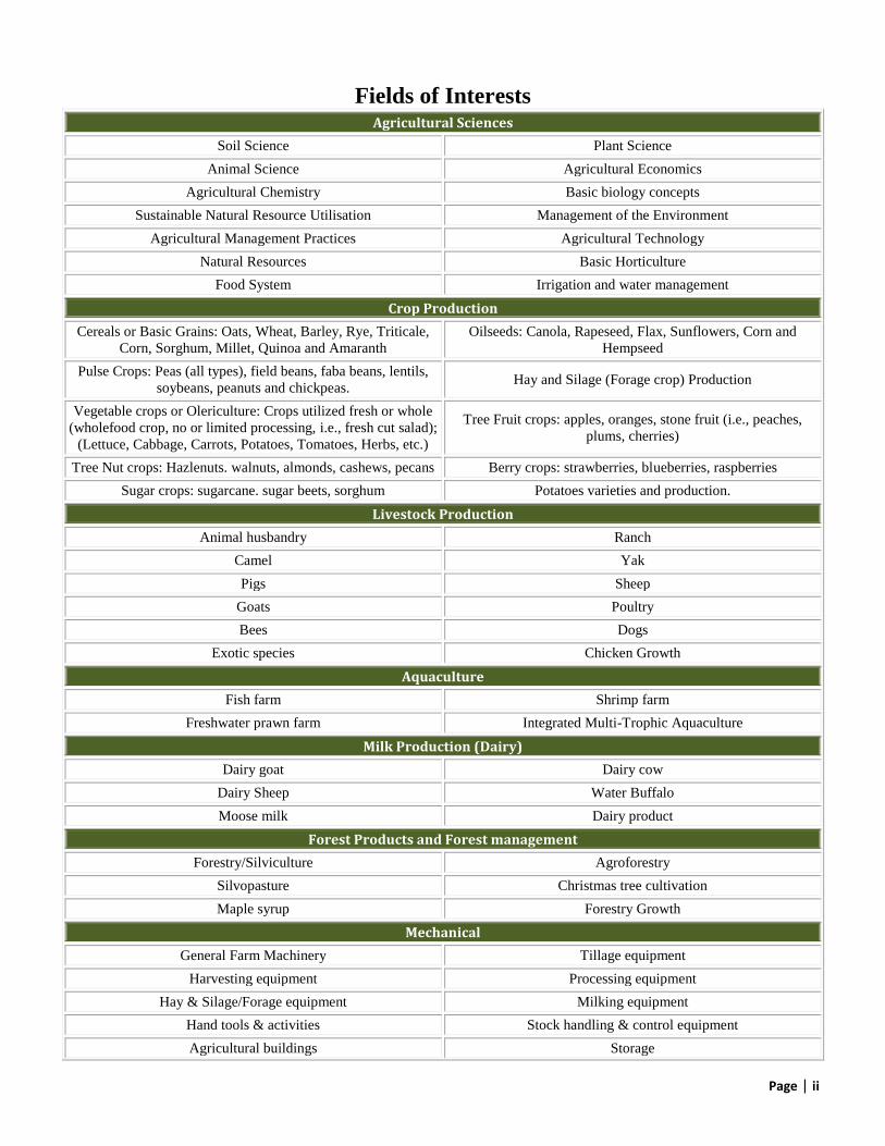
Fields of Interests Agricultural Sciences
Soil Science Plant Science
Animal Science Agricultural Economics
Agricultural Chemistry Basic biology concepts
Sustainable Natural Resource Utilisation Management of the Environment
Agricultural Management Practices Agricultural Technology
Natural Resources Basic Horticulture
Food System Irrigation and water management
Crop Production
Cereals or Basic Grains: Oats, Wheat, Barley, Rye, Triticale,
Corn, Sorghum, Millet, Quinoa and Amaranth
Oilseeds: Canola, Rapeseed, Flax, Sunflowers, Corn and
Hempseed
Pulse Crops: Peas (all types), field beans, faba beans, lentils,
soybeans, peanuts and chickpeas. Hay and Silage (Forage crop) Production
Vegetable crops or Olericulture: Crops utilized fresh or whole
(wholefood crop, no or limited processing, i.e., fresh cut salad);
(Lettuce, Cabbage, Carrots, Potatoes, Tomatoes, Herbs, etc.)
Tree Fruit crops: apples, oranges, stone fruit (i.e., peaches,
plums, cherries)
Tree Nut crops: Hazlenuts. walnuts, almonds, cashews, pecans Berry crops: strawberries, blueberries, raspberries
Sugar crops: sugarcane. sugar beets, sorghum Potatoes varieties and production.
Livestock Production
Animal husbandry Ranch
Camel Yak
Pigs Sheep
Goats Poultry
Bees Dogs
Exotic species Chicken Growth
Aquaculture
Fish farm Shrimp farm
Freshwater prawn farm Integrated Multi-Trophic Aquaculture
Milk Production (Dairy)
Dairy goat Dairy cow
Dairy Sheep Water Buffalo
Moose milk Dairy product
Forest Products and Forest management
Forestry/Silviculture Agroforestry
Silvopasture Christmas tree cultivation
Maple syrup Forestry Growth
Mechanical
General Farm Machinery Tillage equipment
Harvesting equipment Processing equipment
Hay & Silage/Forage equipment Milking equipment
Hand tools & activities Stock handling & control equipment
Agricultural buildings Storage
Page | iii
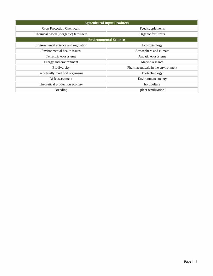
Agricultural Input Products
Crop Protection Chemicals Feed supplements
Chemical based (inorganic) fertilizers Organic fertilizers
Environmental Science
Environmental science and regulation Ecotoxicology
Environmental health issues Atmosphere and climate
Terrestric ecosystems Aquatic ecosystems
Energy and environment Marine research
Biodiversity Pharmaceuticals in the environment
Genetically modified organisms Biotechnology
Risk assessment Environment society
Theoretical production ecology horticulture
Breeding plant fertilization
Page | iv
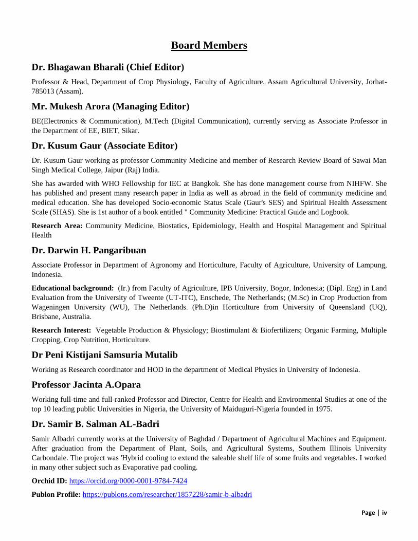
Board Members
Dr. Bhagawan Bharali (Chief Editor)
Professor & Head, Department of Crop Physiology, Faculty of Agriculture, Assam Agricultural University, Jorhat-
785013 (Assam).
Mr. Mukesh Arora (Managing Editor)
BE(Electronics & Communication), M.Tech (Digital Communication), currently serving as Associate Professor in
the Department of EE, BIET, Sikar.
Dr. Kusum Gaur (Associate Editor)
Dr. Kusum Gaur working as professor Community Medicine and member of Research Review Board of Sawai Man
Singh Medical College, Jaipur (Raj) India.
She has awarded with WHO Fellowship for IEC at Bangkok. She has done management course from NIHFW. She
has published and present many research paper in India as well as abroad in the field of community medicine and
medical education. She has developed Socio-economic Status Scale (Gaur's SES) and Spiritual Health Assessment
Scale (SHAS). She is 1st author of a book entitled " Community Medicine: Practical Guide and Logbook.
Research Area: Community Medicine, Biostatics, Epidemiology, Health and Hospital Management and Spiritual
Health
Dr. Darwin H. Pangaribuan
Associate Professor in Department of Agronomy and Horticulture, Faculty of Agriculture, University of Lampung,
Indonesia.
Educational background: (Ir.) from Faculty of Agriculture, IPB University, Bogor, Indonesia; (Dipl. Eng) in Land
Evaluation from the University of Tweente (UT-ITC), Enschede, The Netherlands; (M.Sc) in Crop Production from
Wageningen University (WU), The Netherlands. (Ph.D)in Horticulture from University of Queensland (UQ),
Brisbane, Australia.
Research Interest: Vegetable Production & Physiology; Biostimulant & Biofertilizers; Organic Farming, Multiple
Cropping, Crop Nutrition, Horticulture.
Dr Peni Kistijani Samsuria Mutalib
Working as Research coordinator and HOD in the department of Medical Physics in University of Indonesia.
Professor Jacinta A.Opara
Working full-time and full-ranked Professor and Director, Centre for Health and Environmental Studies at one of the
top 10 leading public Universities in Nigeria, the University of Maiduguri-Nigeria founded in 1975.
Dr. Samir B. Salman AL-Badri
Samir Albadri currently works at the University of Baghdad / Department of Agricultural Machines and Equipment.
After graduation from the Department of Plant, Soils, and Agricultural Systems, Southern Illinois University
Carbondale. The project was 'Hybrid cooling to extend the saleable shelf life of some fruits and vegetables. I worked
in many other subject such as Evaporative pad cooling.
Orchid ID: https://orcid.org/0000-0001-9784-7424
Publon Profile: https://publons.com/researcher/1857228/samir-b-albadri
Page | v
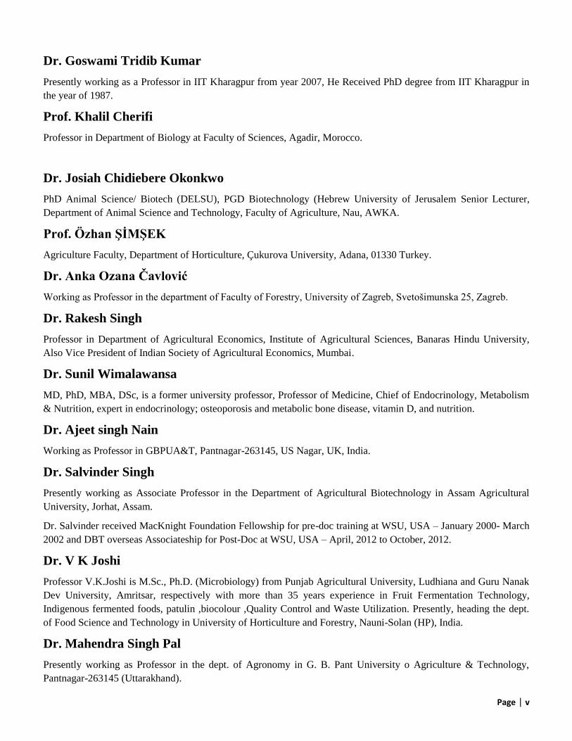
Dr. Goswami Tridib Kumar
Presently working as a Professor in IIT Kharagpur from year 2007, He Received PhD degree from IIT Kharagpur in
the year of 1987.
Prof. Khalil Cherifi
Professor in Department of Biology at Faculty of Sciences, Agadir, Morocco.
Dr. Josiah Chidiebere Okonkwo
PhD Animal Science/ Biotech (DELSU), PGD Biotechnology (Hebrew University of Jerusalem Senior Lecturer,
Department of Animal Science and Technology, Faculty of Agriculture, Nau, AWKA.
Prof. Özhan ŞİMŞEK
Agriculture Faculty, Department of Horticulture, Çukurova University, Adana, 01330 Turkey.
Dr. Anka Ozana Čavlović
Working as Professor in the department of Faculty of Forestry, University of Zagreb, Svetošimunska 25, Zagreb.
Dr. Rakesh Singh
Professor in Department of Agricultural Economics, Institute of Agricultural Sciences, Banaras Hindu University,
Also Vice President of Indian Society of Agricultural Economics, Mumbai.
Dr. Sunil Wimalawansa
MD, PhD, MBA, DSc, is a former university professor, Professor of Medicine, Chief of Endocrinology, Metabolism
& Nutrition, expert in endocrinology; osteoporosis and metabolic bone disease, vitamin D, and nutrition.
Dr. Ajeet singh Nain
Working as Professor in GBPUA&T, Pantnagar-263145, US Nagar, UK, India.
Dr. Salvinder Singh
Presently working as Associate Professor in the Department of Agricultural Biotechnology in Assam Agricultural
University, Jorhat, Assam.
Dr. Salvinder received MacKnight Foundation Fellowship for pre-doc training at WSU, USA – January 2000- March
2002 and DBT overseas Associateship for Post-Doc at WSU, USA – April, 2012 to October, 2012.
Dr. V K Joshi
Professor V.K.Joshi is M.Sc., Ph.D. (Microbiology) from Punjab Agricultural University, Ludhiana and Guru Nanak
Dev University, Amritsar, respectively with more than 35 years experience in Fruit Fermentation Technology,
Indigenous fermented foods, patulin ,biocolour ,Quality Control and Waste Utilization. Presently, heading the dept.
of Food Science and Technology in University of Horticulture and Forestry, Nauni-Solan (HP), India.
Dr. Mahendra Singh Pal
Presently working as Professor in the dept. of Agronomy in G. B. Pant University o Agriculture & Technology,
Pantnagar-263145 (Uttarakhand).
Page | vi
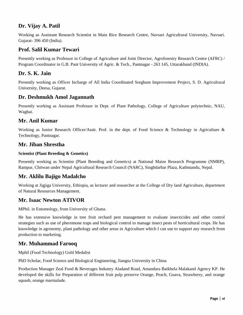
Dr. Vijay A. Patil
Working as Assistant Research Scientist in Main Rice Research Centre, Navsari Agricultural University, Navsari.
Gujarat- 396 450 (India).
Prof. Salil Kumar Tewari
Presently working as Professor in College of Agriculture and Joint Director, Agroforestry Research Centre (AFRC) /
Program Coordinator in G.B. Pant University of Agric. & Tech., Pantnagar - 263 145, Uttarakhand (INDIA).
Dr. S. K. Jain
Presently working as Officer Incharge of All India Coordinated Sorghum Improvement Project, S. D. Agricultural
University, Deesa, Gujarat.
Dr. Deshmukh Amol Jagannath
Presently working as Assistant Professor in Dept. of Plant Pathology, College of Agriculture polytechnic, NAU,
Waghai.
Mr. Anil Kumar
Working as Junior Research Officer/Asstt. Prof. in the dept. of Food Science & Technology in Agriculture &
Technology, Pantnagar.
Mr. Jiban Shrestha
Scientist (Plant Breeding & Genetics)
Presently working as Scientist (Plant Breeding and Genetics) at National Maize Research Programme (NMRP),
Rampur, Chitwan under Nepal Agricultural Research Council (NARC), Singhdarbar Plaza, Kathmandu, Nepal.
Mr. Aklilu Bajigo Madalcho
Working at Jigjiga University, Ethiopia, as lecturer and researcher at the College of Dry land Agriculture, department
of Natural Resources Management.
Mr. Isaac Newton ATIVOR
MPhil. in Entomology, from University of Ghana.
He has extensive knowledge in tree fruit orchard pest management to evaluate insecticides and other control
strategies such as use of pheromone traps and biological control to manage insect pests of horticultural crops. He has
knowledge in agronomy, plant pathology and other areas in Agriculture which I can use to support any research from
production to marketing.
Mr. Muhammad Farooq
Mphil (Food Technology) Gold Medalist
PhD Scholar, Food Science and Biological Engineering, Jiangsu University in China
Production Manager Zeal Food & Beverages Industry Aladand Road, Amandara Batkhela Malakand Agency KP. He
developed the skills for Preparation of different fruit pulp preserve Orange, Peach, Guava, Strawberry, and orange
squash, orange marmalade.
Table of Contents
S.No Title Page No.
1
Mapping of Milk Processing Units in Organized Sector: A Case Study for Haryana
Authors: Sukriti Sharma, Dr. D.K. Sharma
DOI: https://dx.doi.org/10.5281/zenodo.3923263
Digital Identification Number: IJOEAR-JUN-2020-1
01-06
2
Effect of Percent and Stage of Leaf Defoliation on the Quality of Sugarcane, at Arjo -
Dedessa Sugar Factory, in Western Ethiopia
Authors: Kasahun Tariku
DOI: https://dx.doi.org/10.5281/zenodo.3923267
Digital Identification Number: IJOEAR-JUN-2020-2
07-13
3
Economic Analysis of Fluted Pumpkin (Telfaria Occidentalis) Production in Ibadan
Metropolis, Oyo State, Nigeria
Authors: Akanni-John, R; Shaib-Rahim, H.O; Eniola O; Elesho R.O
DOI: https://dx.doi.org/10.5281/zenodo.3931168
Digital Identification Number: IJOEAR-JUN-2020-3
14-17
4
Isolation and Identification of Mycoplasma Species in Dogs
Authors: Maria Lucia Barreto, Mosar Lemos, Jenif Braga de Souza, Samara Gomes de Brito,
Ana Beatriz Pinheiro Alves, Leandro dos Santos Machado, Virgínia Léo de Almeida Pereira,
Nathalie Costa da Cunha, Elmiro Rosendo do Nascimento
DOI: https://dx.doi.org/10.5281/zenodo.3931170
Digital Identification Number: IJOEAR-JUN-2020-4
18-23
5
Effect of Genotype by Environment Interaction (GEI), Correlation, and GGE Biplot
analysis for high concentration of grain Iron and Zinc biofortified lentils and their
agronomic traits in multi-environment domains of Nepal
Authors: Rajendra Darai, Krishna Hari Dhakal, Ashutosh Sarker, Madhav Prasad Pandey,
Shiv Kumar Agrawal, Surya Kant Ghimire, Dhruba Bahadur Thapa, Jang Bahadur Prasad,
Rabendra Prasad Sah, Keshav Pokhrel
DOI: https://dx.doi.org/10.5281/zenodo.3931172
Digital Identification Number: IJOEAR-JUN-2020-5
24-40
International Journal of Environmental & Agriculture Research (IJOEAR) ISSN:[2454-1850] [Vol-6, Issue-6, June- 2020]
Page | 1
Mapping of Milk Processing Units in Organized Sector: A Case
Study for Haryana Sukriti Sharma
1*, Dr. D.K. Sharma
2
*1MSC in Geography (NET Qualified), Social Scientist, Mission Green Foundation, Hisar
2District Extension Scientist, Krishi Vigyan Kendra, Bhiwani, Haryana
Abstract— The State Haryana is known for its major crops like wheat and rice and stands at the second largest contributor
of food grains in India. Just like that Haryana ranks second in milk production. Dairy farming is also a form of agriculture
in which milk is extracted from cow, buffalo, goat etc. then it sell by vendors from different rural and suburb regions to
informal sector agents or to cooperative agents. This milk distributed further in different ways. Milk production is no more
subsistence in nature and organized sector is a best example to prove it because cooperatives is an independent association
of persons those fulfill their economic needs and distribution of milk and milk products is all a business as we can see it in
“Haryana Dairy Development Cooperative Federation Ltd.” This federation is famous by vita brand which was opened by
the Haryana govt. on the pattern of Amul.
Keywords— Dairy, Federations, Informal sector, Milk Production, Organized sector.
I. INTRODUCTION
Dairy is an agricultural industry in which milk alone valued more than combined value of wheat and rice. It covers about
1/3rd
of gross income of rural households. Haryana, in spite of being a small state with only 1.3 % of total geographical area
has a prominent space in the livestock map of the country. Haryana contributes 98.09 lakh tones milk per year which is more
than 5.6% of the nation’s total milk production. Before 1970s, the condition of dairy farming was not as appreciable as it is
now because there is so much miscoordinance between rural milk producers and organized milk sectors. So this kind of poor
connectivity creates problems like- poor rural milk producers didn’t know the real price of their milk and on the other side,
organized milk plants were deprived of from the valuable milk of rural area. But as we can say nothing is impossible, so on
13th
January 1970, the “White Revolution” was started by Indian government with the objective to push the limits of dairy
farming and to make it more valuable and economically more productive. This idea of “Operation Flood” was come through
the success of “Green Revolution” in India. This revolution made dairy farming, a single self – sustaining industry in India.
Over the span of three decades, India has transformed from a country of acute milk shortage to the world’s leading milk
producer. India is the largest producer of milk in the world since 1998. During 2016-17, the annual output was 165.40
million tons accounting for 20% of the world milk share. The per capita availability of milk during 2016-17 was 352 gm per
day as against world average of 299 gm per day. After that, Haryana ranks second in country with availability of 877 grm. of
milk per person today.
II. OBJECTIVES OF THE STUDY
1) To understand the problem of organized sector in dairy farming according to their demand and prize in Haryana State.
2) To mapping the formal sectors of milk production in Haryana.
3) To generalize the changes in milk production after white revolution.
III. DATA AND METHODOLOGY
The data has been collected for the study of organized sector of dairy farming and their problems in Haryana at local and
state level. The required data was collected from secondary sources are- the websites looked into in order to gather the prior
information and the related literature about the topic. This information is descriptive and analytical in nature.
IV. ROLE OF THE WHITE REVOLUTION AND HOW IT BECOMES BENEFICIAL FOR HARYANA’S MILK
PRODUCTION
The father of White Revolution is Verghese kurrin who firstly introduced this concept and suggests ideas in development in
the production of milk on its top level in India.
International Journal of Environmental & Agriculture Research (IJOEAR) ISSN:[2454-1850] [Vol-6, Issue-6, June- 2020]
Page | 2
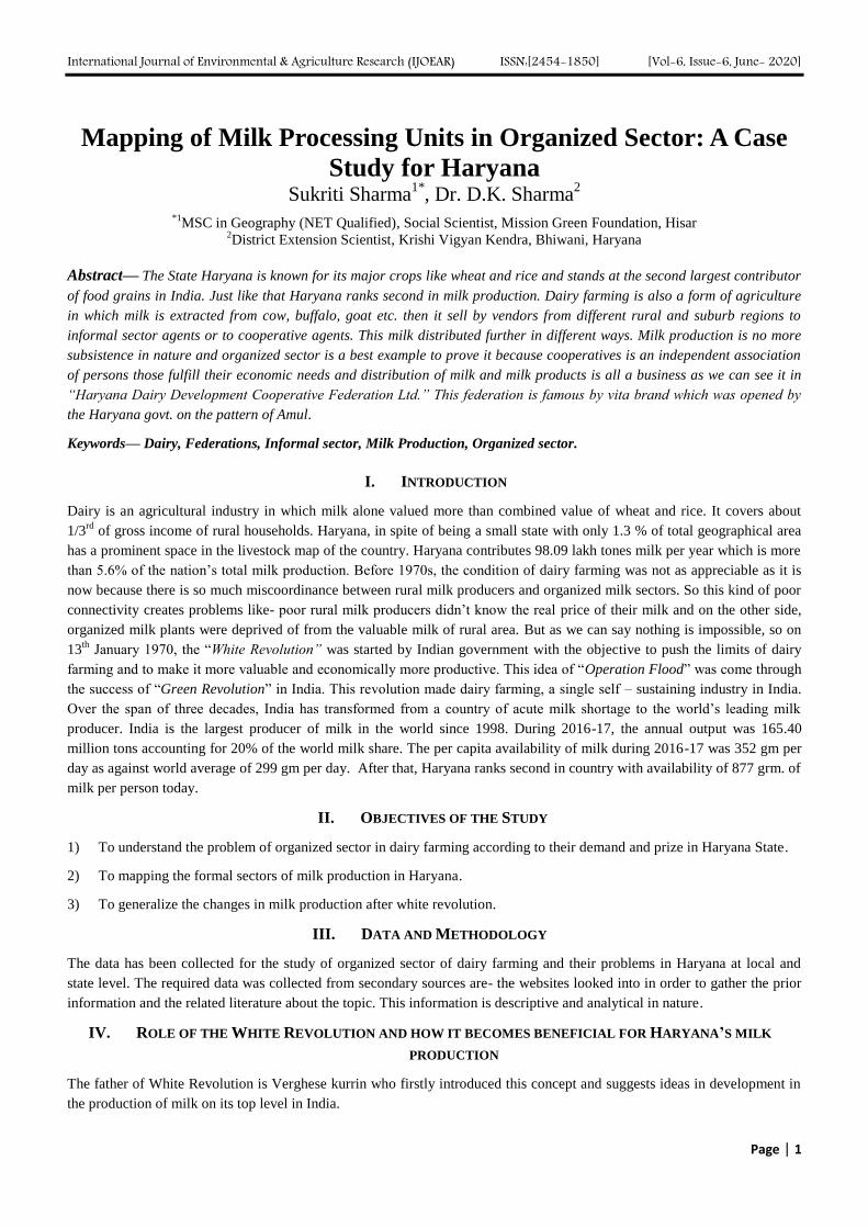
Haryana stands on second rank in the country as per capita per day availability of milk. Haryana is known for his
commendable development in dairy industry and called as a milk pail of India. As we can see in the table given below that
from the year 1966 to 2016, the production is increased chronically. As we discussed in the introduction that during 1970
when the revolution came in India, the production is hiked up tremendously in Haryana from 10.89 lakh tonnes to 17.27 lakh
tones.
TABLE 1
YEAR-WISE MILK PRODUCTION IN HARYANA STATE (LAC TONNES)
Year Milk Production
1966-67 10.89
1977-78 17.27
1981-82 22.75
1991-92 35.65
2000-01 48.49
2005-06 52.59
2006-07 53.67
2007-08 54.51
2008-09 57.45
2009-10 60.06
2010-11 62.67
2011-12 66.61
2012-13 70.40
2013-14 74.42
2014-15 79.01
2015-16 83.81
Source –Animal and dairying dept. of Haryana
There are 60.8 lakh buffaloes are in Haryana, in which “Murrah” buffalo is the most famous because of its buffer milk
production. There are four types of cows in State like Exotic – (those are imported from foreign), Indigenous –
(autochthonic, originating where it is found), Crossbreed – (Hybrid), Non- Descript – (ordinary) and two of buffalos
(Indigenous and Non- Descript). Murrah is an autochthonic. In Table-2, trying to show the distribution of milk production
through cows, buffalo and goats in different districts of Haryana with the help of survey which was done by Animal
Husbandry and Dairying Department of Haryana in year 2017- 2018. Through this table I identified that Sirsa with
213.51('000' tonnes) cow’s milk production, which is the highest from all other districts of the state. As given data of
buffalo’s milk production in which the state Bhiwani is leading with 668.36('000' tonnes) production and in goat’s milk,
Mahendragarh is the district which leads over other districts. But if talking about the total annual milk production in state
then Bhiwani has won the race with 802.84 ('000' tonnes) production. The state’s total milk production is about 9808.94('000'
tonnes) which is second largest production after Uttar Pradesh in India. This is how it proved that how white revolution left a
deep impression on state.
International Journal of Environmental & Agriculture Research (IJOEAR) ISSN:[2454-1850] [Vol-6, Issue-6, June- 2020]
Page | 3
TABLE 2
DISTRICT WISE MILK PRODUCTION (IN '000' TONNES) IN HARYANA STATE 2017- 2018
Sr.
no. Districts
Total Cow’s Milk
Production
Total Buffalo’s
Milk Production
Total Goat’s
Milk Production
Annual Milk
Production
1 Ambala 83.66 306.76 1.15 391.57
2 Bhiwani 127.66 668.36 6.81 802.84
3 Faridabad 45.74 189.84 1.38 236.96
4 Fatehabad 71.13 403.85 1.72 476.69
5 Gurugram 72.00 239.07 1.55 312.69
6 Hisar 94.61 634.12 2.45 731.18
7 Jhajjar 53.12 349.45 1.22 403.78
8 Jind 65.33 575.92 1.24 642.49
9 Kaithal 73.64 575.72 1.00 650.37
10 Karnal 188.34 445.19 1.39 634.93
11 Kurukshetra 119.44 282.04 0.54 402.02
12 Mahendragarh 60.04 350.72 7.82 418.58
13 Nuh 38.38 300.09 4.61 343.08
14 Palwal 43.67 387.24 1.18 432.09
15 Panchkula 22.18 105.91 1.45 129.54
16 Panipat 61.80 307.21 0,65 369.65
17 Rewari 62.13 295.24 3.77 361.13
18 Rohtak 45.29 347.56 0.80 393.65
19 Sirsa 213.51 423.55 5.48 642.53
20 Sonepat 102.71 476.70 1.25 580.65
21 Yamunanagar 176.10 275.19 1.32 452.60
22 Charkhi Dadri - - - -
State Total 1820.46 7939.71 48.77 9808.94
Source- Animal Husbandry and Dairying Department of Haryana (Sample Survey Report 2017 – 2018)
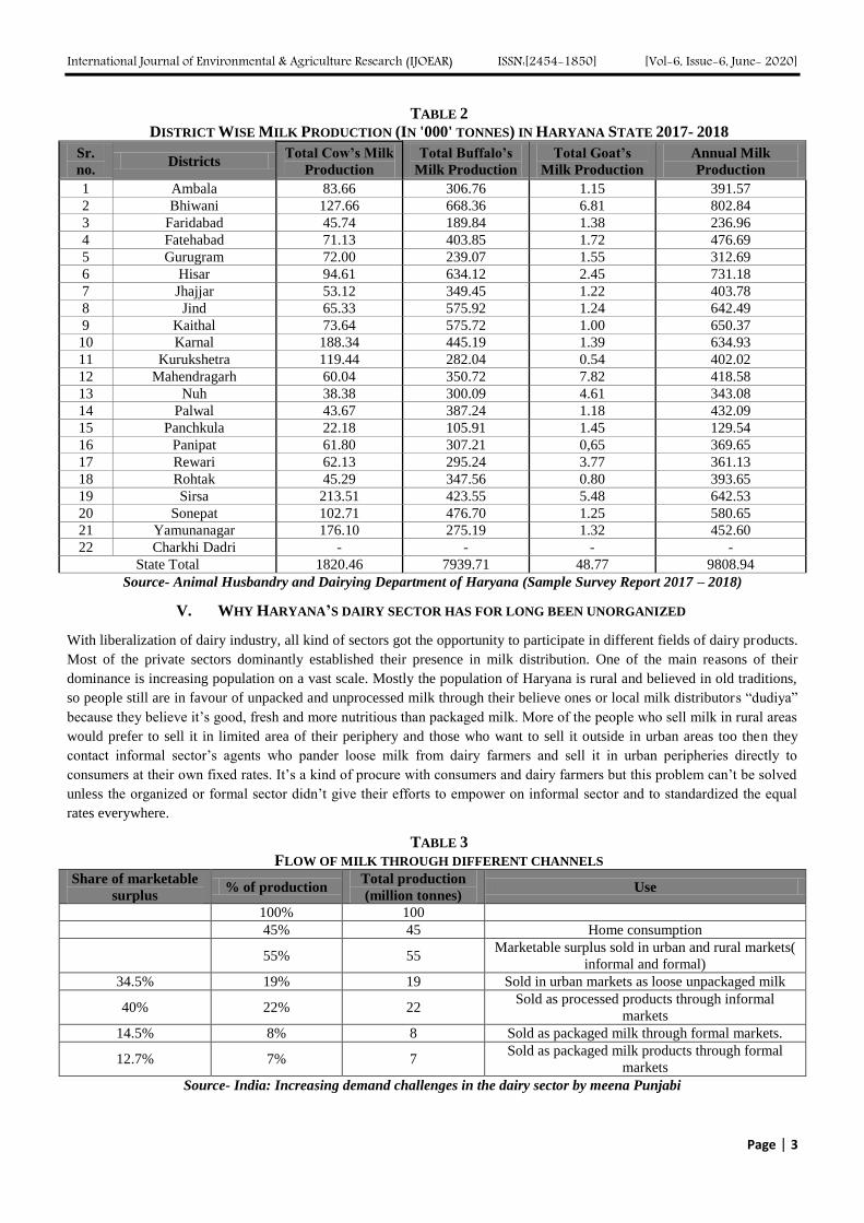
V. WHY HARYANA’S DAIRY SECTOR HAS FOR LONG BEEN UNORGANIZED
With liberalization of dairy industry, all kind of sectors got the opportunity to participate in different fields of dairy products.
Most of the private sectors dominantly established their presence in milk distribution. One of the main reasons of their
dominance is increasing population on a vast scale. Mostly the population of Haryana is rural and believed in old traditions,
so people still are in favour of unpacked and unprocessed milk through their believe ones or local milk distributors “dudiya”
because they believe it’s good, fresh and more nutritious than packaged milk. More of the people who sell milk in rural areas
would prefer to sell it in limited area of their periphery and those who want to sell it outside in urban areas too then they
contact informal sector’s agents who pander loose milk from dairy farmers and sell it in urban peripheries directly to
consumers at their own fixed rates. It’s a kind of procure with consumers and dairy farmers but this problem can’t be solved
unless the organized or formal sector didn’t give their efforts to empower on informal sector and to standardized the equal
rates everywhere.
TABLE 3
FLOW OF MILK THROUGH DIFFERENT CHANNELS Share of marketable
surplus % of production
Total production
(million tonnes) Use
100% 100
45% 45 Home consumption
55% 55 Marketable surplus sold in urban and rural markets(
informal and formal)
34.5% 19% 19 Sold in urban markets as loose unpackaged milk
40% 22% 22 Sold as processed products through informal
markets
14.5% 8% 8 Sold as packaged milk through formal markets.
12.7% 7% 7 Sold as packaged milk products through formal
markets
Source- India: Increasing demand challenges in the dairy sector by meena Punjabi
International Journal of Environmental & Agriculture Research (IJOEAR) ISSN:[2454-1850] [Vol-6, Issue-6, June- 2020]
Page | 4
VI. THINGS THAT ORGANIZED SECTOR SHOULD PERFORM FOR BETTER RESULTS:
1) Quality or guarantee of freshness in products are the big issues in informal sector so if formal or organized sector
wants to compete then they should take care of their quality of products for better results.
2) Organized milk producing agencies must enhance their interaction with small farmers and rural dairy vendors to earn
their trust.
3) Area like Haryana where milk production is not even in all the districts so the formal sectors should engage their
agents or managers to collect the ground reality data of dairy farms and to convey the milk sellers by giving them
better packages more than the Informal’s.
4) Raise packaged milk distribution in more areas.
5) Make policies that attract farmers to get a higher price for milk.
6) Make farmers more secure and give them strength in enhancing their production by animal insurances.
7) Prices should be same everywhere on the bases of amount of fat in milk.
8) Encourage commercial dairy farming and breed development.
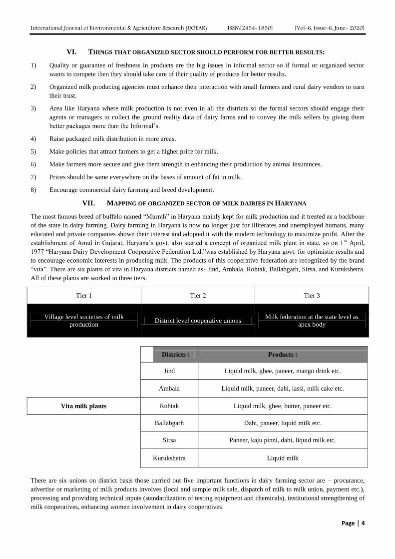
VII. MAPPING OF ORGANIZED SECTOR OF MILK DAIRIES IN HARYANA
The most famous breed of buffalo named “Murrah” in Haryana mainly kept for milk production and it treated as a backbone
of the state in dairy farming. Dairy farming in Haryana is now no longer just for illiterates and unemployed humans, many
educated and private companies shown their interest and adopted it with the modern technology to maximize profit. After the
establishment of Amul in Gujarat, Haryana’s govt. also started a concept of organized milk plant in state, so on 1st April,
1977 “Haryana Dairy Development Cooperative Federation Ltd.”was established by Haryana govt. for optimistic results and
to encourage economic interests in producing milk. The products of this cooperative federation are recognized by the brand
“vita”. There are six plants of vita in Haryana districts named as- Jind, Ambala, Rohtak, Ballabgarh, Sirsa, and Kurukshetra.
All of these plants are worked in three tiers.
Tier 1 Tier 2 Tier 3
Village level societies of milk
production District level cooperative unions
Milk federation at the state level as
apex body
Districts : Products :
Jind Liquid milk, ghee, paneer, mango drink etc.
Ambala Liquid milk, paneer, dahi, lassi, milk cake etc.
Vita milk plants Rohtak Liquid milk, ghee, butter, paneer etc.
Ballabgarh Dahi, paneer, liquid milk etc.
Sirsa Paneer, kaju pinni, dahi, liquid milk etc.
Kurukshetra Liquid milk
There are six unions on district basis those carried out five important functions in dairy farming sector are – procurance,
advertise or marketing of milk products involves (local and sample milk sale, dispatch of milk to milk union, payment etc.),
processing and providing technical inputs (standardization of testing equipment and chemicals), institutional strengthening of
milk cooperatives, enhancing women involvement in dairy cooperatives.
International Journal of Environmental & Agriculture Research (IJOEAR) ISSN:[2454-1850] [Vol-6, Issue-6, June- 2020]
Page | 5
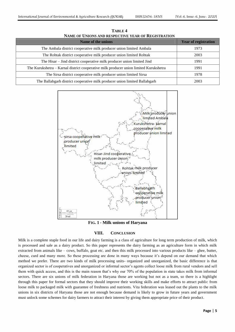
TABLE 4
NAME OF UNIONS AND RESPECTIVE YEAR OF REGISTRATION
Name of the unions Year of registration
The Ambala district cooperative milk producer union limited Ambala 1973
The Rohtak district cooperative milk producer union limited Rohtak 2003
The Hisar – Jind district cooperative milk producer union limited Jind 1991
The Kurukshetra – Karnal district cooperative milk producer union limited Kurukshetra 1991
The Sirsa district cooperative milk producer union limited Sirsa 1978
The Ballabgarh district cooperative milk producer union limited Ballabgarh 2003
FIG. 1 - Milk unions of Haryana
VIII. CONCLUSION
Milk is a complete staple food in our life and dairy farming is a class of agriculture for long term production of milk, which
is processed and sale as a dairy product. So this paper represents the dairy farming as an agriculture form in which milk
extracted from animals like – cows, buffalo, goat etc. and then this milk processed into various products like – ghee, butter,
cheese, curd and many more. So these processing are done in many ways because it’s depend on our demand that which
method we prefer. There are two kinds of milk processing units- organized and unorganized, the basic difference is that
organized sector is of cooperatives and unorganized or informal sector’s agents collect loose milk from rural vendors and sell
them with quick access, and this is the main reason that’s why our 70% of the population in state takes milk from informal
sectors. There are six unions of milk federation in Haryana those are working but not as a team, so there is a highlight
through this paper for formal sectors that they should improve their working skills and make efforts to attract public from
loose milk to packaged milk with guarantee of freshness and nutrients. Vita federation was leased out the plants to the milk
unions in six districts of Haryana those are not enough because demand is likely to grow in future years and government
must unlock some schemes for dairy farmers to attract their interest by giving them appropriate price of their product.
International Journal of Environmental & Agriculture Research (IJOEAR) ISSN:[2454-1850] [Vol-6, Issue-6, June- 2020]
Page | 6
ACKNOWLEDGEMENTS
This paper was accomplished by the proper guidance of my co-author and guide Mr. D.K. Sharma who encouraged and
developed my skills in this research work. I am highly gratitude for having such a support and overwhelming guidance. I also
thanked my parents for believing in me and motivate me to keep going in research work.
REFERENCES
[1] Jesse,E.V. et.al. (2006). The Dairy Sector of India: A Country Study, the babcock institute for international dairy research and
development uni. Of wiscon- madison pp. 21-23
[2] Ramphul. (2012). Global Competitiveness in Dairy Sector
[3] Goel, S. (2014). Health Care System in Haryana; An Overview , ISSN 2320-6314
[4] Chawla,A. (2009). Milk and Dairy Products in India- Production, Consumption and Exports, second edition
[5] National Action Plan for Dairy Development, vision 2022(2018) Department of Animal Husbandry, Dairying and fisheries
[6] Sharma,V.P.(2015). Determinants of Small Milk Producer’s Participation in organized Dairy Value Chains: Evidance from India pp
247-261
[7] Murgod,R.M.,et.al. (2016). Fodder Inclusive Value Chain Analysis of Milk in Organized Sector of Karnataka
[8] Lal,P. and Chandel, B.S. (2017). Total Factor Productivity in Milk Production in Haryana
[9] Statistical Abstract of Haryana (2017-18), by dept. of Economic and Statistical Analysis
[10] Elumalai,K. and Pandey,U.K.(2004). Technological Change in Livestock Sector of Haryana, Indian Journal of Agri. Econo.Vol.59,
No. 2
[11] Singh,P. et.al.(2015). Constraints Faced by Farmers in Adoption of Dairy as Entrepreneurship
[12] Lal, P. and Chandel,B.S.(2016). Economics of Milk Production and Cost Elasticity Analysis in Sirsa District of Haryana
[13] Bhupal, D.S.(2012). Agricultural profile of Haryana, Agricultural Economics Research Centre
[14] Rajendran,K. and Mohanty,S.(2004). Dairy Cooperatives and Milk Marketing in India: Constraints and Opportunities, Journal of
food Distribution Research
[15] Kumar,M .et.al.(2015). Economic Analysis of Milk Production in Rewari District of Haryana
[16] Hemme,T. et.al.(2003). A Review of Milk Production in India with Particular Emphasis on Small- Scale Producers
[17] Punjabi,M.India: Increasing demand challenges in the dairy sector, www.fao.org.
International Journal of Environmental & Agriculture Research (IJOEAR) ISSN:[2454-1850] [Vol-6, Issue-6, June- 2020]
Page | 7
Effect of Percent and Stage of Leaf Defoliation on the Quality of
Sugarcane, at Arjo - Dedessa Sugar Factory, in Western Ethiopia Kasahun Tariku
Ethiopian Sugar Corporation, Research and Development Center, Research Center Coordinator, Agronomy and Crop
Protection Research Program, Wonji Research Center, Ethiopia
Abstract— The research was conducted at Arjo-Didessa Sugar Factory which is located in East Wollega Zone of Oromia
Regional State with the objective to determine the effect of leaf defoliation at different stages of sugarcane (Saccharum
officinarum) on the quality. Sugarcane (Saccharum spp.) is unusual among field crops in that it is not the seed that have
economic values, but rather the stalk. Sucrose is extracted from the large stalks that are produced by sugarcane plants. The
effect of percent and stage of leaf defoliation on sucrose content as well as recovery percentage of sugar cane is still
unknown. Effect of leaf defoliation at three different stages on quality of sugarcane juice was studied under field conditions.
The methodology used include seven percent of leaf defoliation comprises of 10%, 20%, 30%, 40%, 50%, 60% and 0% as a
check and three growth stages of defoliation at 9, 10 & 11 month of sugarcane was arranged in Randomized Complete Block
Design. The results depicted that, significant variation among leaf removal and cane age was noted for quality parameters.
Thus, significantly higher percent of sucrose percent (11.70%) at 30% of leaf removal and (11.50%) at20% of leaf removal
were obtained from 11 and 10 month age of NCO-334 sugarcane variety respectively ,however, lower percent of sucrose
(9.03%) at 11month age was recorded from undefoliated (check).In addition to these results the sugar cane plants that could
be partially defoliated with changing sucrose production and retention of defoliated leave between furrow providing
advantage, that increase soil moisture leads to water conservation especially for sugarcane grown under rainfall condition
like Arjo Dedessa sugar factory, reduce weed growth, and prevent substantial losses of C and N due to sugarcane leaf
burning at harvesting time. However, further future research is required to strengthen the investigation by confirming
similar research on different location are necessary to recommend to all Ethiopian sugar factories.
Keywords— sugarcane, defoliation, stage, quality.
I. INTRODUCTION
Sugarcane is one of the most important crops in the world (Dagar et al., 2002). Sugarcane belongs to the genus (Saccharum
L.,) of the grass family (Poaceae) and originated in Papua New Guinea, as original habitat and from where it spread to south
East Asia and India in the course of few thousand years (Bull, 2000).
The Office of Agricultural Economy, (2008) reported that the sugarcane burned in the field had many disadvantages such as
weight reduction, microorganism destroyed easily, rapid decrease of sweetness, high production cost of plant, that organic
material and structure in soil were destroyed and decreased sugar production. Sugarcane harvesting is a critical step that must
be managed to maintain good quality and quantity of sugarcane production. Farmers harvesting sugarcane have a leaves-
removing or leave defoliating step and cut the stem closing to the soil, then cut the top of sugarcane stem. Leaves and leaf
sheaths of sugarcane caused delay of harvesting. Moreover, the sugarcane crop that has not been fully leaves-removed (leave
defoliations) could carry some soil, sand and mud, thus damaging the downstream sugarcane process machine and reduced
sugar yield (Yangyeun and Wongpicheth, 2008).
The contamination will be increased more when using the car to grip sugarcane to the truck. Sugarcane leaf-defoliating tools
could help to speed up sugarcane harvest and reduce contamination. However, researchers in the past had focused on tools or
equipments used to help harvest sugarcane crop; for example, sugarcane harvester, knife used for sugarcane crop on
performance to sugarcane harvester. However, leaf-removal machinery can solve the problems of sugarcane burning and
reduce contaminants. Retention of unburned residues can increase nutrient conservation, reduce weed growth, and conserve
soil moisture on the other hand substantial losses of C and N due to sugarcane residue burning have been reported (Viator et
al., 2006).
In general physiological and morphological responses of individual plants to defoliation was evaluated in chronological
sequence beginning with plant function during "steady state" growth prior to defoliation, followed by the short-term effects
of defoliation, and concluding with long-term processes contributing to the reestablishment of "steady-state" growth
(Steingraeber et al., 1993). Particularly according to Gutierrez et al (2004), mechanical defoliation of sugar cane plants
International Journal of Environmental & Agriculture Research (IJOEAR) ISSN:[2454-1850] [Vol-6, Issue-6, June- 2020]
Page | 8
(Saccharum spp.) will provide leaves that can be used as fodder but the effect of partial mechanical defoliation on sucrose
content, enzyme activities and agronomic parameters of sugar cane is still unknown and also the concentration of sucrose in
the stems of partial defoliated plants was significantly different from that found in intact plants. Similarly, Dendooven et al
(2004) indicated that some agronomic parameters and enzyme activities were different in defoliated plants compared with
intact plants except for the moisture content which was higher in defoliated plants than in intact ones. These makes sugar
cane plants could be partially defoliated changing sucrose production and agronomic parameters while providing leaves that
could be used as fodder.
The Ethiopian Government is building modern sugar factories and expanding the existing ones with the aim of maximizing
the production volume to alleviate the scarcity of sugar in the country (EIA, 2008). This work was conducted in view of the
limited information on the effect of leaf defoliation at different stages of sugarcane on biomass yield and quality but the
hypotheses tested in these studies, the effect of leaf defoliation at different stages of sugarcane on biomass yield and quality
were superior in defoliated than undefoliated sugarcane. This research was initiated with the objective of to evaluate the
effect of defoliation at different stages on quality, and response of sugarcane crop to defoliation and its advantage to increase
sugar recovery at Arjo-Didessa Sugar Factory which is located in East Wollega Zone of Oromia Regional State.
II. MATERIALS AND METHODS
2.1 Description of the Study Area
The experiment was conducted at Arjo-Didessa Sugar Factory located in East Wollega Zone of Oromia Regional State. Arjo
Dedessa Sugar Factory is located at 09041
m48
s6
ms N latitude and 036
026
m01
s9
ms E longitudes, with an altitude of 1053-1600
masl. The area has a mean maximum and minimum monthly temperature is 31.1c and 19.1c, respectively with annual rain
fall of 358.4mm (Source: Arjo metrological station). Based on Arjo Dedessa feasibility study report (2005) the soil types of
the experimental site are dominated by Vertisol and Luvisol.
2.2 Experimental Materials and Design
NCO -334 sugarcane varieties was used as an experimental material. Treatments comprising six levels of defoliation percent
of 10 %, 20 %, 40 %, 50 %, 60 % and one control of 0 % of percent of defoliation at three different stages of sugarcane, that
is, at 9 month growth stage (S1), 10 month growth stage (S2) and at 11 month growth stage (S3) and each of which replicated
three times. The percent of defoliation was made after counting total number of leaf from three randomly sampled and the
leaf was defoliated according to percent of defoliation treatment. The two factors were combined factorially and arranged in
randomized complete block design (RCBD). The actual experimental area was designed with PL = number of treatment x
plot length + spacing between plot x number of block – 1i.e (7 X 5m + 2m x 3 -1= 40m) and PW = number of block x plot
width + spacing between block + number of spacing (3 x 7.25m + 2m x2 =25.75m). The total area used was 40m x 25.75m
(1030m2). Plot width = 1.45 x 5 and plot length= 5m, the distance between block used were 2m, between plot were 1m and
the sugarcane was spaced at 1.45m between rows.
2.3 Data Collection and Sampling
The data were collected on four quality parameters (%Brix, %Pol, % purity and cane recovery (sucrose %) attributes. The
middle two rows out of the four rows in each plot were used for data collection, the number of plants per row was 1260 and
the distance between rows were 1.45m. Brix % was measured in the cane juice analytical laboratory of Arjo Dedesa Sugar
Factory with the help of bench refracto meter. The refracto meter was adjusted to zero with distilled water. A drop of juice
was placed on the refracto meter then the brix was read (Blackburn, 1984)
The polarization of juice was measured by a Polari meter according to the method described by Horne's dry lead (South
African Sugar Technologist's Association (1985). Approximately 150 ml of the sample was taken in a bottle provided with
stopper. Sufficient lead sub acetate powder (1.5g) was added for clarification, shacked vigorously to disperse the lead sub-
acetate completely and then allowed to stand and filtered through a fluted filter paper held in the funnel. Some of the filtrate
was used for rinsing the Pol tube and filled completely. Then the polarization (Saccharimeter reading) was read. The Pol %
obtained from Schmitz’s table by using the Brix of the sample and Saccharimeter reading. Pol % is actually cane sugar
present in the juice, expressed in percentage (Khedkar et. al. 2000).
There for Purity % was determined with the help of the following relationship following Islam et al., (2011).
𝑃𝑢𝑟𝑖𝑡𝑦 % =(Pol %) x 100
Brix %
International Journal of Environmental & Agriculture Research (IJOEAR) ISSN:[2454-1850] [Vol-6, Issue-6, June- 2020]
Page | 9
Sugar recovery was calculated with the help of the following formula following Islam et al., (2011).
Recoverable Sucrose (%) = [% Pol- (%brix-%Pol) 0.52] 0.75
Where: 0.52 = Non-sugar factor
0.75 = Cane factor
2.4 Data Analysis
The data collected were subjected to analysis of variance (ANOVA) using SAS software (SAS, 2004). Treatment means that
exhibited significant differences were separated using the least significant difference at 5% level of significance (SAS, 2004).
III. RESULT AND DISCUSSION
The of analysis of variance result for different characters are presented in Table 1 design. The analysis of variance table for
percent of defoliation showed a highly significance difference for all quality parameters while stage of defoliation showed
significantly (P< 0.05) affect all the parameters except for sucrose %. However, their interaction effect showed that a
significance difference for all characters except for purity percent (Table 1).
TABLE 1
MEAN SQUARE VALUES FOR THE PARAMETERS RECORDED AS AFFECTED BY PERCENT DEFOLIATION,
STAGE OF DEFOLIATION, AND PERCENT BY STAGE OF DEFOLIATION INTERACTION OF SUGARCANE GROWN
AT ARJO DEDESSA IN 2014/15 CROPPING SEASON.
Characters Sources of Variation
PD ST PD X ST MSE REP
Internodes number 70.88**
3.19ns
4.91* 3.41 5.28
Internodes length 11.83**
2.49ns
3.45* 2.72 3.15
Stem diameter 292.86**
3.05ns
12.89**
10.39 90.04
Internodes weight 113476.73**
2997.57ns
12844**
7548.7 1.34
Sugarcane height 0.032**
0.0043ns
0.061**
0.012 0.02
Leaf area index 61.14**
7.43**
3.75**
0.2 0.54
Biomass yield 14.97**
3.70**
1.08* 0.43 4.3
Number of leaf 3.75**
1.15* 1.17
* 0.65 2.49
Brix % 16.82**
1.03* 2.03
* 0.58 0.97
Polarity % 22.99* 4.58
ns 16.39
* 14.42 17.63
Purity % 575.65**
533.36**
366.68ns
378.58 553.1
Sucrose %. 3.78**
0.011ns
0.25* 0.22 0.4
*, ** and ns indicate significance at the 0.05 and 0.01 probability levels and non-significance level, respectively. PD =
Percent of defoliation, ST = Stage of growth, PD x ST = Interaction of percent of defoliation and stage of growth, MSE =
Mean square error and REP = Replication
3.1 Effect of Defoliation on Brix %
When 20 % of leaf removal at 11 month growth stage was applied significantly higher brix % was recorded as 22.70 %
(Table 2). But the lowest brix % was recorded at undefoliated with nine month growth stage as18.42 % (Table 2). While
defoliating from 60 % of leaf removal at nine month growth stage, 30 % of leaf removal at ten month growth stage and 50 %
of leaf removal at11 month growth stage was not significantly different from 40 % of leaf removal at 11 month growth stage
(Table 2). This shows that defoliation from 30 % – 60 % recorded indicates the positive in increasing the total soluble solid
in the juice.
On average mean value of total soluble solid in juice (brix %) recorded for the three growths stage gave 20.80% (Table 2).
From this experimental study brix the highest % was recorded as different stage and percent of defoliation significantly
increases. In general in this study the total solids content present in the juice expressed in percentage were unaffected by
defoliation but increases quality of sugar (Table 2).
International Journal of Environmental & Agriculture Research (IJOEAR) ISSN:[2454-1850] [Vol-6, Issue-6, June- 2020]
Page | 10
TABLE 2
MEAN VALUES FOR BRIX %, POLARITY % AND SUCROSE % AS AFFECTED BY PERCENT DEFOLIATION AND
STAGE OF DEFOLIATION INTERACTION OF SUGARCANE GROWN AT ARJO DEDESSA IN 2014/15 CROPPING
SEASON
Parameter Brix % Polarity %
DF % Stage of defoliation Stage of defoliation
9 10 11 9 10 11
0 18.42 21.9 19.02 21.15 19 21.83
10 19.34 19 19.28 20.5 20.5 21.44
20 19.27 18.9 22.7 21.47 20.9 20.3
30 21.6 22.2 21.59 21.36 30.6 20.43
40 21.93 20.7 22.13 19.77 19.1 19.35
50 21.24 21.9 22.34 19.72 19.8 19.64
60 22.01 21.9 19.6 19.92 19.6 20.44
Mean 20.8 20.8
CV % 3.67 18.23
LSD 0.05 0.47 0.29
*, ** and ns indicate significance at the 0.05 and 0.01 probability levels.
Studies on the quality parameters of cane stalk, juice and leaves in comparison to defoliation have been conducted in a
number of cane growing regions. Results from Louisiana (Birkett, 1965), South Africa (Muir et al., 2009; Reid & Lionnet,
1989; Scott et al., 1978) and Australia (Ivin & Doyle, 1989) shows that the presence of reasonable amounts of brix and fiber
in the defoliated cane juice than undefoliated.
The results suggest that the stage of defoliation induces significant changes in sugarcane juice brix % composition and its
sensory attributes. The effect of late leaf removal was much more effective than early leaf removal in affecting final brix
composition and quality. Brix % from the late defoliation treatment was rated the most preferred as of global value. It has
also found that in grape the removal of some of the leaf material from the canopy whilst berry ripening occurs can increase
Brix in the fruit (Holzapfel and Rogiers, 2002). It is suggested that it was due to the increased photosynthetic rate of the
remaining un-defoliated leave. Conversely (Ezahounani and Williams, 2003) leave defoliation of basal has shown to have no
effect on Brix.
3.2 Effect of Defoliation on Polarization (Pol %)
The mean value recorded for polarity percent in table 2, was 20.80 % at overall growth stage. The highest polarity percent
was recorded from 30 % of leaf removal at ten month growth stage (Table 2). However, the lowest polarity percent was
recorded from 0 % of leaf removal at10 month of growth stage (Table 2). This shows that defoliation at 30 % was more
beneficial than at 0 % to increase the actual sugar in the juice. Although defoliation affected by 0 %, 20 % and 30 % of leaf
removal at 9 month growth stage was not significantly different from 10 % of leaf removal at 11 month of growth stage
(Table 2). This indicates defoliation percent was more beneficial than growth stage in this study.
From the result obtained even if differences exist among defoliation treatment after defoliation polarity percent was increased
which have the advantage of having good quality of the actual cane sugar present in the juice. This is due to the increase in
the photosynthetic potential of the remaining leaves and leads to enhanced Pol % resulted in biomass accumulation and
sucrose yield. Khan and Ahsan (2000) working on B. juncea showed that eliminating the cost of maintaining senescing
leaves by leaf removal may lead to increased plant yield. The Pol for the second stage of sugarcane sample meets maximum
Pol 99.9oZ set for sugar yield (USC, 2008) and was significantly (p>0.05) higher than for the first and third stage of
sugarcane development. Polarization for both defoliated and un-defoliated samples was measured by automatic Polari-meter
calibrated in (ISS).
International Journal of Environmental & Agriculture Research (IJOEAR) ISSN:[2454-1850] [Vol-6, Issue-6, June- 2020]
Page | 11
3.3 Effect of Defoliation on Purity %
On average the mean value of purity percent recorded was 91.1 % at all growth stage (Table 3). The highest purity percent
(96.36 %) was recorded from 9 month growth stage but the lowest (86.31 %) purity percent was recorded at 11 month growth
stage (Table 3); this shows that a higher purity indicates the presence of higher sucrose content out of the total solids. The
purity of sugar cane process stream products (e.g., cane juice, molasses, raw sugar etc.) is a measure of product quality and
was determined by calculating the ratio of % Sucrose and % total Solids as a percentage which were measured by double
polarization and dry substance measurements.
TABLE 3
MEAN VALUE ANALYSIS FOR PURITY % AS AFFECTED STAGE DEFOLIATION EFFECT OF SUGARCANE
GROWN AT ARJO - DEDESSA IN 2014/ 2015 CROPPING SEASON
Stage of defoliation % purity % Defoliation % purity
9 Month 96.36a 0 89.10
b
10 Month 90.63a 10 91.72
b
11 Month 86.31b 20 91.72
b
Mean 91.1
30 94.96a
CV 21.35
40 86.30b
LSD 12.13
50 92.40ab
60 91.60
b
Mean 91.1
CV 21.35
LSD 18.53
Mean within columns followed by the same letters are not significantly different
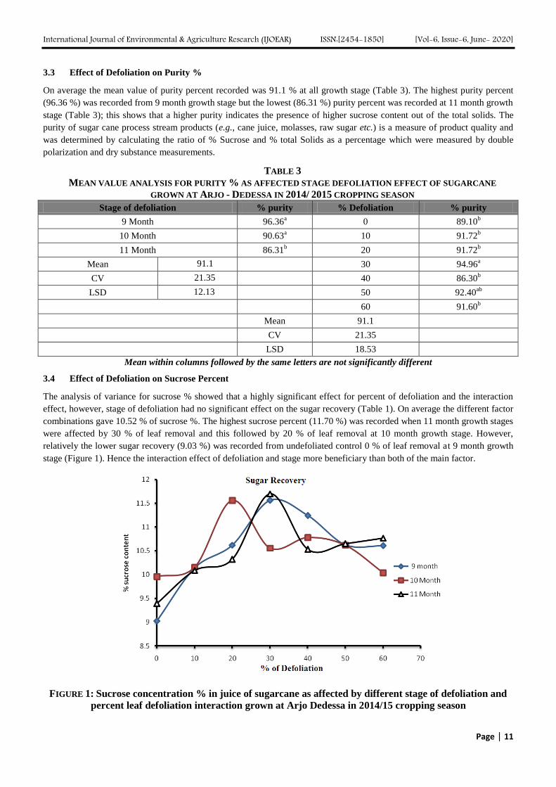
3.4 Effect of Defoliation on Sucrose Percent
The analysis of variance for sucrose % showed that a highly significant effect for percent of defoliation and the interaction
effect, however, stage of defoliation had no significant effect on the sugar recovery (Table 1). On average the different factor
combinations gave 10.52 % of sucrose %. The highest sucrose percent (11.70 %) was recorded when 11 month growth stages
were affected by 30 % of leaf removal and this followed by 20 % of leaf removal at 10 month growth stage. However,
relatively the lower sugar recovery (9.03 %) was recorded from undefoliated control 0 % of leaf removal at 9 month growth
stage (Figure 1). Hence the interaction effect of defoliation and stage more beneficiary than both of the main factor.
FIGURE 1: Sucrose concentration % in juice of sugarcane as affected by different stage of defoliation and
percent leaf defoliation interaction grown at Arjo Dedessa in 2014/15 cropping season
International Journal of Environmental & Agriculture Research (IJOEAR) ISSN:[2454-1850] [Vol-6, Issue-6, June- 2020]
Page | 12
Therefore results obtained after affecting the different growth stage by defoliation treatment significantly increases quality of
sugar recovery within the juice used to increase the actual cane sugar. Results obtained indicated that the interaction effect
was more beneficial than defoliations and stage for improving cane biomass yield and sugar recovery and also defoliated
leaves could be used as animal fodder after 9month of crop age without affecting sugarcane yield.
The sucrose concentration in defoliated sugarcane was significantly different from the un-defoliated sugarcane and there
were also significance differences between treatments of defoliations (Figure 1). This agreed with A study by Pammenter and
Allison (2002) has shown that defoliation of alternate fully emerged lamina of sugarcane (Saccharum officinarum L.) at 155
d decreased the laminas area by 40% and also resulted in proportional partitioning of assimilate in leaves and stem with
increased accumulation of sucrose.
Other studies also reported that Partial defoliation has resulted in increases of sucrose contents in Cherry trees (Prunus
Cereasus) (Layne and Flore 1995), but (Neefs et al., 2002) reported that mechanical partial defoliation of witloof chicory
(Cichorium intybus) affected plant growth. They found that the total fresh weight of defoliated plants stayed markedly lower
compared with intact plants. Integrating production of sugar and using the leaves as fodder will be economically (Naseeven
1986, Namer 1991) and ecologically beneficial. Studies on B. juncea have shown that removal of shaded leaves (50% of
lower leaves at 40 DAS) increases the supply of assimilate more than demand and thus improves growth and photosynthetic
potential of the rest of the leaves (Khan et al., 2002b). Anten and Ackerly (2001) reported that partial defoliation (50 and
66% of leaves removed) in palm (Chamaedorea elegans Mart.) significantly increased the light available to the remaining
leaves and light-saturated photosynthesis per unit leaf area by 10–18%. Recently, (Li et al., 2010) reported that defoliation at
flowering in chickpea (Cicer arietinum L.) when crop canopy is closed allows light penetration into deeper canopy and
improves photosynthesis.
Partial defoliation has rejuvenating (make younger) effect on the remaining leaves, restoring the photosynthetic capacity to
near the value of newly formed leaves (Wareing et al., 1968, Khan et al., 2008). The plants after defoliation require more
assimilates for re growth which is balanced by the increased leaf assimilatory capacity and efficient N use (Lone and Khan
2007).
Ryle et al., (1985) reported that recovery of N2 fixation in T. repens after removal of half of the shoot tissue was related to
the reestablishment and increased photosynthetic capacity after 5, 6, or 9 d of re growth. C4 plants accumulate greater
quantities of carbohydrate than C3 plants (Downton 1971). This 'extra' photosynthetic could be used for re growth following
defoliation. An advantage of the C4 system is that its net photosynthesis, compared to C3 plants, is greatest in young foliage
(Long et al., 2006). Thus, the new foliage produced in response to defoliation would replenish the carbohydrate reserves
(sucrose) more rapidly in C4 species than in C3 species.
IV. CONCLUSION
In light of the results obtained, the different levels and stages of defoliation have a significant effect on all the parameters
studied .Partial defoliation in sugarcane (i.e. removal of half leaves) has been shown to not have a long-term negative effect
on the quality parameters. Generally the results obtained in this study are based on data of superimpose experiment and,
hence do not warrant the formulation of a clear-cut recommendation, However, suggestive enough to draw the following
recommendations:
When defoliation was applied on 30 % of leaf removal at 11 month growth stage in relative to other percent of
defoliation and stage higher recovery percentage was recorded. On the other hand trash or leave without defoliating
that is delivered with the stalks to the factory could also reduce the quality of sugarcane juice. However, further
study is required to support some leaves defoliated in the field should be utilized as a soil fertilizer there is still
plenty available for use as biomass; retention of unburned leave can increase nutrient conservation, reduce weed
growth, conserve soil moisture and also defoliated leaves could be used as animal fodder after 9month of crop age
without affecting sugarcane yield.
Defoliation could also be used to renew, refresh and increase growth and photosynthetic rate in sugarcane plants
under abiotic stress conditions. However, further research is required to strengthen the investigation and repeating
similar research on different location are necessary to recommend to all Ethiopian sugar factories.
International Journal of Environmental & Agriculture Research (IJOEAR) ISSN:[2454-1850] [Vol-6, Issue-6, June- 2020]
Page | 13
REFERENCES
[1] Anten, N., P., R., Ackerly, D., D. (2001). Canopy-Level Photosynthetic Compensation After Defoliation in a Tropical Understorey
Funct: P. 252-262. Palm.Ecol.
[2] Birkett, L., S. (1965). The Influence of Tops and Trash onthe Economics of Sugar Production. P: 1636-1642.Proceedings of the
International Society of Sugarcane Technologists.
[3] Blackburn, F. (1984). Sugar-Cane.(1st Edition). P: 414 pages. Longman, London and New York (Tropical Agriculture Series).
[4] Bull, T. (2000). The Sugarcane Plant.In "Manual of cane growing", M Hogarth, P Allsopp, eds. P: 71-83. Bureau of Sugar
Experimental Stations, Indooroopilly, Australia
[5] Dagar, P., S., K. Pahuja, S., P. Kadian and S., Singh. (2002). Evaluation Of Phenotypic Variability In Sugarcane Using Principal
Factor Analysis. P: 95-100 Indian Journal of Sugarcane Technology.
[6] Dendooven, H (2004). The Development Of The Cultivated Sorghum. Crop plant evaluation, Cambridge University Press.
[7] Downton, W., J., S. (1971). Adaptive And Evolutionary Aspects of C4 Synthesis. p: 3-17, New York – London – Sydney – Toronto
[8] EIA, (Ethiopian Investment Agency).(2008). Investment Opportunity Profile For Sugar Cane Plantation And Processing In
Ethiopia.EIA, Addis Ababa, Ethiopia.
[9] ESESISC, (2008). Investment Opportunity Profile for Sugar Cane Plantation and Processing In Ethiopia
[10] Gutiérrez-Miceli, F.,A. Morales-Torres, R. de Jesús Espinosa-Castañeda, Y. Rincón- Rosales, R. Mentes-Molina, J. Oliva-Llaven,
M.,A. Dendooven, L. (2004).Effects OfPartial Defoliation Journal of Agronomy and Crop Science On Sucrose Accumulation,
Enzyme Activity Jou Journal of Agronomy and Crop Science of Agronomy and Crop Science And Agronomic parameters InSugar
cane (Saccharum spp.). P: 256–261.Journal of Agronomy and Crop Science.
[11] Khan, N., A. Khan, M. Samiullah, (2002b), Changes In Ethylene Level Associated With Defoliation And Its Relationship With Seed
Yield In Rapeseed-Mustard. P: 12-17. Brassica
[12] Khan, N., A. Ahsan (2000). Auxin And Defoliation Effects On Photosynthesis And Ethylene Evolution In Mustard. P: 43-51. Sci.
Hort.
[13] Khan, N., A. Anjum, N., A. Nazar, R., Lone, P., M. (2008). Activity Of 1- Aminocyclopropane Carboxylic Acid Synthase And
Growth Of Mustard (Brassica Juncea) Following Defoliation. P: 151-157. Plant Growth Regul.
[14] Layne, D., R. and J., A. Flore, (1995). End-Product Inhibition Of Photosynthesis In Prunus Cereasus L. In Response To Whole-Plant
Source-Sink Manipulation. P: 583-599. J. Amer. Soc. Hort. Sci.
[15] Li, L. Gan, Y., T. Bueckert, R. Warkentin, T., D. (2010). Shading, Defoliation And Light Enrichment Effects On Chickpea In
Northern Latitudes. P: 220-230. . J. Agron. Crop Sci.
[16] Lone, P., M., Khan, N., A. (2007). The Effects Of Rate And Timing Of N Fertilizer On Growth, Photosynthesis, N Accumulation
And Yield Of Mustard (Brassica Juncea) Subjected To Defoliation. . P: 318-323. Environ. Exp. Bot
[17] Long, S., P. Zhu, X., G. Naidu, S. Ort, D.R. (2006). Can Improvement In Photosynthesis Increase Crop Yields? P: 315-330. Plant
Cell Environ.
[18] Muir, B., M. Eggleston. G & Barker, B. (2009). The effect of green cane on downstream factory processing. P: 164-199 Proceedings
of the South African Sugar Technologists' Association.
[19] Naseeven, R.S. (1986). A Test Of Compensatory Photosynthesis In The Field Implications For Herbivory Tolerance. P: 311-318.
Oecologia
[20] Neefs, V., I. Mare´chal, R. Herna´ndez-Martı´nez, and P., M. de Prof, (2002) The Influence Of Mechanical Defoliation And
Ethephon Treatment On The Dynamics Of Nitrogen Compounds In Chicory (Cichorium Intybus L). P: 217-227. Scient.Hort.
[21] Pammenter, N., W. Allison, J., C., S. (2002).Effects Of Treatments Potentially Influencing The Supply Of Assimilate On Its
Partitioning In Sugarcane. P: 123–129. Journal of Experimental Botany
[22] Reid, M., S & Lionnet, G., R., E. (1989).The effects of tops and trash on cane milling based on trials at Maidstone. P: 3-6.
Proceedings of the South African Sugar Technologists' Association
[23] Ryle, G., J., A. Powell, C., E. Gordon, A., J. (1985). Defoliation In White Clover: Re Growth, Photosynthesis And N2 Fixation. –p:
9-18. Ann. Bot.
[24] SAS, (2004).GLM procedure SAS software (SAS, 2004).Ver 6.4th Edition. SAS Institute, Inc.
[25] Scott, R. P., Falconer, D., & Lionnet, G. R. E. (1978). A Laboratory Investigation Of The Effects Of Tops And Trash On Extraction,
Juice Quality And Clarification. P: 51-53. Proceedings of the South African Sugar Technologists' Association
[26] South African Sugar Technologists` Association, (1985). Proceedings Of The Fifty –Ninth Annual Congress Held At Durban And
Mount Edgecombe.
[27] The Office of Agriculture Economy, (2008).Monthly Export For Sugar In Quantity And Value.
[28] USC (United Sugar Company), (2008). Quality Specification Of White Refined Sugar Approved For Coca Cola Production. Jeddah,
Saud Arabiya.
[29] Viator, R., P., R., M. Johnson, C., C. Grimm, and E., P. Richard, Jr. (2006). Allelopathic, Autotoxic, And Hormetic Effects Of
Postharvest Sugarcane Residue. P: 1526-1531. Agron. J.
[30] Wareing, P., F. Khalifa, M., M., Treharne, K., J. (1968). Rate-Limiting Processes In Photosynthesis At Saturating Light Intensities.
P: 453-457. Nature
[31] Yangyeun, Z and Wongpicheth, D., J (2008). Experimental Assessment Of The Impact Of Defoliation On Growth And Production Of
Water-Stressed Maize And Cotton Plants. P: 189-199. Experimental Agriculture.
International Journal of Environmental & Agriculture Research (IJOEAR) ISSN:[2454-1850] [Vol-6, Issue-6, June- 2020]
Page | 14
Economic Analysis of Fluted Pumpkin (Telfaria Occidentalis)
Production in Ibadan Metropolis, Oyo State, Nigeria Akanni-John, R
1; Shaib-Rahim, H.O
2; Eniola O
3; Elesho R.O
4
1Federal College of Forestry and Mechanization, Afaka, Kadunna, Nigeria.
2,3,4Federal College of Forestry, P.M.B 5087, Ibadan, Nigeria.
Abstract— The study was carried out to analyze the economics of fluted pumpkin production in Ibadan metropolis. A total
of 80 fluted pumpkin farmers were selected using multistage sampling method. Data were collected using a set of
questionnaire. Analysis of the data obtained from the questionnaire was carried out through the use of descriptive statistics
such as frequency, percentage, profit function analysis, gross margin and multiple regression analysis. From the analysis, all
the farmers interviewed were literate. From the gross margin analysis, fluted pumpkin production was found to be a
profitable venture in the study area. The profit function analysis result of R2 (0.8910) showed that 89.01 percent of the
variability in profit in explained by the combined effect of the variable price items in the function. This is indicative of the
price variable for output price had a positive significant effect on the profit level of farmers. The regression result showed
that the coefficient for farming experience was positive and significant at 5 percent level. Recommendations from the study
area include among others, government should provide inputs such as chemicals and planting seed at subsidized rate to
farmers and also aim at solving the problems in vegetables production.
Keywords— Gross margin, Profit function, Production, Fluted Pumpkin, Chi-squre.
I. INTRODUCTION
Agricultural production in Nigeria is dominated by small-scale farmers who produce the bulk of the food consumed in the
country. One of the major crops produced are fluted pumpkin which represent an essential part of agricultural products. Their
production remains entrenched in Nigerian agriculture and forms an important condiment in the national diet (Nwangwa et
al., 2007). Agriculture is considered the largest sector in Nigeria’s economy. It employs 70 percent of the nation’s labor
force, contributes at least 40 percent of the gross domestic product and accounts for over three-quarters of the non-oil foreign
exchange earnings (Ajekigbe, 2007). Fluted pumpkin is a very important vegetable that is popular in West Africa. It belongs
to the family Telfaria Occidentalis Hook F. cucurbitaceae. It is a leafy vegetable that produces fruits. (Enabulele and
Uavbarhe, 2001). Tindall, (1989) defined leafy vegetables as herbaceous plants used for culinary purposes. They are used to
increase the dietary quality of soups. The fruit on full maturity has a weight of 10kg. and an appearance of 10 distinctive
longitudinal ribs on the surface. It is popular in West Africa. The edible part of this vegetable are the large red seeds, leaves
and young shoots used for traditional soup. Protein rich seed can be roasted or grounded for use in porridge. The flesh of the
fruit has good oil content which can be used as cooking oil.
Amongst the different vegetable foods, production and consumption of fluted pumpkin is very important because of their
contribution to good health by providing inexpensive sources of minerals and vitamins needed to supplement people’s diet
which are mainly carbohydrates (Yang et al., 2002) cited in Abu and Asember (2011). Fluted pumpkin is the most important
and extensively cultivated food and income generating crops in many parts of Africa (Adebisi-Adelani et al., 2011).Fluted
pumpkin is a very important vegetable that is popular in West Africa. It belongs to the family Telfaria Occidentalis Hook F.
cucurbitaceae . It is a leafy vegetable that produces fruits. (Enabulele and Uavbarhe, 2001).
Fluted pumpkin consumption has improved over the years and it is an important component of the daily diets of Nigerians
(Okoli and Mgbeogu, 2003). Due its hypolipidemic action, it lowers blood cholesterol and thus protects from a large range of
associated complications like cardiac problems, hypertension and diabetes (Margret, 2011).
II. MATERIAL AND METHOD
2.1 Area of Study
Ibadan, the capital of Oyo State is the third largest city in Nigeria by population (after Lagos and Kano), and the largest in
geographical area. At independence, Ibadan was the largest and the most populous city in Nigeria and the third in Africa after
Cairo and Johannesburg. The city of Ibadan is located approximately on longitude 3°55East of the Greenwich Meridian and
latitude 7°23North of the Equator at a distance some 145 kilometers Northeast of Lagos. Ibadan is located in southwestern
Nigeria about 120 km east of the border with the Republic of Benin in the forest zone close to the boundary between the
International Journal of Environmental & Agriculture Research (IJOEAR) ISSN:[2454-1850] [Vol-6, Issue-6, June- 2020]
Page | 15
forest and the savanna. There are eleven local governments in Ibadan metropolitan area consisting of five urban local
governments in the city and six semi-urban local governments in the fewer cities. The five urban local governments are:
North East, North Ibadan, Northwest Ibadan, Southeast Ibadan, and Southwest Ibadan. Urban cores (high-density) and
hinterlands (low-density) characterized Ibadan metropolis. The population of Ibadan metropolis is 2, 550,593 according to
2006 census. However, its population at 2016 is estimated to be 3.16 million. The general land use pattern of the Ibadan
metropolitan area shows a clear distinction purely residential use. According to Ayeni (1994) residential land use is the most
predominant among all land uses in the built up part of Ibadan. The administrative and commercial importance of Ibadan has
resulted in land being a key investment, an asset and a status symbol for the population.
2.2 Sampling Techniques
Multi-stage sampling procedure was use to sample the respondent for proper data collection during the field survey as stated
below. 1st stage: identification of fluted pumpkin farmers use in the study area of many marketers in the market. 2
nd stage: the
farmers of fluted pumpkin production in the market was sample for proper data collection. 3rd
stage: 80 copies well structure
questionnaire was randomly distributed to the respondent and allow them to have equal chance when the survey is being
carried out.
2.3 Method of Data Analysis
Statistical tools such as frequency distribution, Gross Margin, Chi-square and Profit function analysis. Multiple regression
analysis was used to identify the determinant of peasant farmer production in the study area. Below is the model
specification:
Y= b0 + X1 + X2 + X3 + X4 + X5 + X6 + X7 + X8 + μ
Where Y = Output (kg), X1 = Age, X2 = Educational level , X3 = Farming experience , X4 = problem farmer facing , X5 =
solution to famer’s problem , X6 = Farm size, X7 = Capital, X8 = Labour used = Coefficient μ = error team.
III. RESULTS AND DISCUSSION
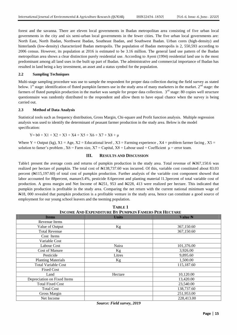
Table1 present the average costs and returns of pumpkin production in the study area. Total revenue of N367,150.6 was
realized per hectare of pumpkin. The total cost of N138,737.60 was incurred. Of this, variable cost constituted about 83.03
percent (N115,197.60) of total cost of pumpkin production. Further analysis of the variable cost component showed that
labor accounted for 88percent, manure3.4%, pesticide 8.6percent and planting material l1.3percent of total variable cost of
production. A gross margin and Net Income of N251, 953 and N228, 413 were realized per hectare. This indicated that
pumpkin production is profitable in the study area. Comparing the net return with the current national minimum wage of
N18, 000 revealed that pumpkin production is a profitable venture in the study area, hence can constitute a good source of
employment for our young school leavers and the teeming population.
TABLE 1
INCOME AND EXPENDITURE BY PUMPKIN FAMERS PER HECTARE Items Units Value ₦
Revenue Items
Value of Output Kg 367,150.60
Total Revenue 367,150.60
Cost Items
Variable Cost
Labour Cost Naira 101,376.00
Cost of Manure Kg 3,926.00
Pesticide Litres 9,895.60
Planting Materials Kg 1,500.00
Total Variable Cost 115,187.60
Fixed Cost
Land Hectare 10,120.00
Depreciation on Fixed Items 13,420.00
Total Fixed Cost 23,540.00
Total Cost 138,737.60
Gross Margin 251,953.00
Net Income 228,413.00
Source: Field survey, 2019
International Journal of Environmental & Agriculture Research (IJOEAR) ISSN:[2454-1850] [Vol-6, Issue-6, June- 2020]
Page | 16
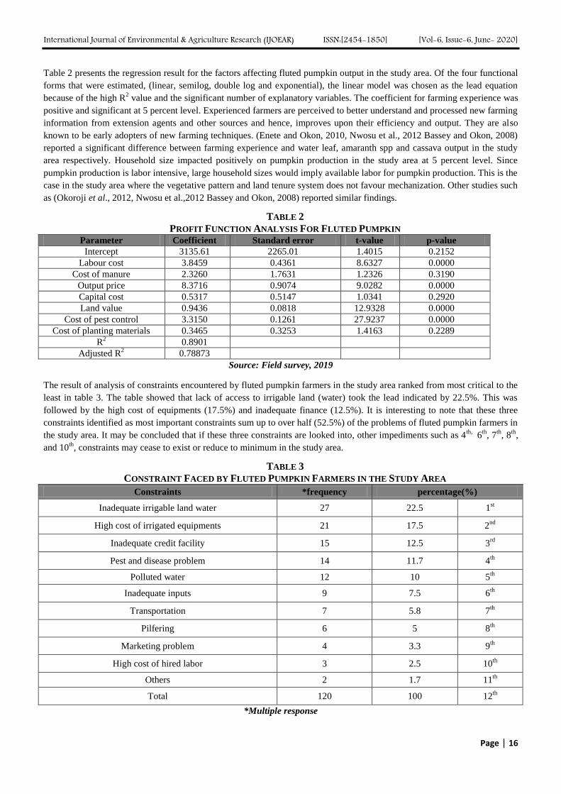
Table 2 presents the regression result for the factors affecting fluted pumpkin output in the study area. Of the four functional
forms that were estimated, (linear, semilog, double log and exponential), the linear model was chosen as the lead equation
because of the high R2 value and the significant number of explanatory variables. The coefficient for farming experience was
positive and significant at 5 percent level. Experienced farmers are perceived to better understand and processed new farming
information from extension agents and other sources and hence, improves upon their efficiency and output. They are also
known to be early adopters of new farming techniques. (Enete and Okon, 2010, Nwosu et al., 2012 Bassey and Okon, 2008)
reported a significant difference between farming experience and water leaf, amaranth spp and cassava output in the study
area respectively. Household size impacted positively on pumpkin production in the study area at 5 percent level. Since
pumpkin production is labor intensive, large household sizes would imply available labor for pumpkin production. This is the
case in the study area where the vegetative pattern and land tenure system does not favour mechanization. Other studies such
as (Okoroji et al., 2012, Nwosu et al.,2012 Bassey and Okon, 2008) reported similar findings.
TABLE 2
PROFIT FUNCTION ANALYSIS FOR FLUTED PUMPKIN Parameter Coefficient Standard error t-value p-value
Intercept 3135.61 2265.01 1.4015 0.2152
Labour cost 3.8459 0.4361 8.6327 0.0000
Cost of manure 2.3260 1.7631 1.2326 0.3190
Output price 8.3716 0.9074 9.0282 0.0000
Capital cost 0.5317 0.5147 1.0341 0.2920
Land value 0.9436 0.0818 12.9328 0.0000
Cost of pest control 3.3150 0.1261 27.9237 0.0000
Cost of planting materials 0.3465 0.3253 1.4163 0.2289
R2 0.8901
Adjusted R2 0.78873
Source: Field survey, 2019
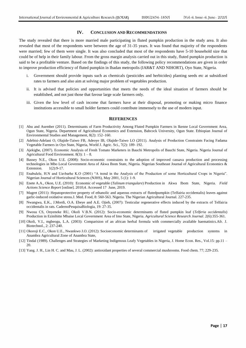
The result of analysis of constraints encountered by fluted pumpkin farmers in the study area ranked from most critical to the
least in table 3. The table showed that lack of access to irrigable land (water) took the lead indicated by 22.5%. This was
followed by the high cost of equipments (17.5%) and inadequate finance (12.5%). It is interesting to note that these three
constraints identified as most important constraints sum up to over half (52.5%) of the problems of fluted pumpkin farmers in
the study area. It may be concluded that if these three constraints are looked into, other impediments such as 4th,
6th
, 7th
, 8th
,
and 10th
, constraints may cease to exist or reduce to minimum in the study area.
TABLE 3
CONSTRAINT FACED BY FLUTED PUMPKIN FARMERS IN THE STUDY AREA
Constraints *frequency percentage(%)
Inadequate irrigable land water 27 22.5 1st
High cost of irrigated equipments 21 17.5 2nd
Inadequate credit facility 15 12.5 3rd
Pest and disease problem 14 11.7 4th
Polluted water 12 10 5th
Inadequate inputs 9 7.5 6th
Transportation 7 5.8 7th
Pilfering 6 5 8th
Marketing problem 4 3.3 9th
High cost of hired labor 3 2.5 10th
Others 2 1.7 11th
Total 120 100 12th
*Multiple response
International Journal of Environmental & Agriculture Research (IJOEAR) ISSN:[2454-1850] [Vol-6, Issue-6, June- 2020]
Page | 17
IV. CONCLUSION AND RECOMMENDATIONS
The study revealed that there is more married male participating in fluted pumpkin production in the study area. It also
revealed that most of the respondents were between the age of 31-35 years. It was found that majority of the respondents
were married; few of them were single. It was also concluded that most of the respondents have 5-10 household size that
could be of help in their family labour. From the gross margin analysis carried out in this study, fluted pumpkin production is
said to be a profitable venture. Based on the findings of this study, the following policy recommendations are given in order
to improve production efficiency of fluted pumpkin in Ibadan metropolis (IAR&T AND NIHORT), Oyo State, Nigeria.
i. Government should provide inputs such as chemicals (pesticides and herbicides) planting seeds etc at subsidized
rates to farmers and also aim at solving major problem of vegetables production.
ii. It is advised that policies and opportunities that meets the needs of the ideal situation of farmers should be
established, and not just those that favour large scale farmers only.
iii. Given the low level of cash income that farmers have at their disposal, promoting or making micro finance
institutions accessible to small holder farmers could contribute immensely to the use of modern input.
REFERENCES
[1] Abu and Asember (2011). Determinants of Farm Productivity Among Fluted Pumpkin Farmers in Ikenne Local Government Area,
Ogun State, Nigeria. Department of Agricultural Economics and Extension, Babcock University, Ogun State. Ethiopian Journal of
Environmental Studies and Management, 8(2): 152–160.
[2] Adebisi-Adelani O, Olajide-Taiwo FB, Adeoye IB, Olajide-Taiwo LO (2011). Analysis of Production Constraints Facing Fadama
Vegetable Farmers in Oyo State, Nigeria, World J. Agric. Sci., 7(2): 189–192.
[3] Ajekigbe, (2007). Economic Analysis of Fresh Tomato Marketers in Bauchi Metropolis of Bauchi State, Nigeria. Nigeria Journal of
Agricultural Food Environment. 8(3): 1 – 8.
[4] Bassey N.E., Okon U.E. (2008): Socio-economic constraints to the adoption of improved cassava production and processing
technologies in Mbo Local Government Area of Akwa Ibom State, Nigeria. Nigerian Southeast Journal of Agricultural Economics &
Extension. 1(2):9-17.
[5] Enabulele, H.N and Uavbarhe K.O (2001) “A trend in the Analysis of the Production of some Horticultural Crops in Nigeria”.
Nigerian Journal of Horticultural Sciences (NJHS), May 2001, 5 (1): 1-9.
[6] Enete A.A., Okon, U.E. (2010): Economic of vegetable (Talinum triangulare) Production in Akwa Ibom State, Nigeria. Field
Actions Science Report [online]. 2010;4. Accessed 17 June, 2019.
[7] Magret (2011): Hepatoprotective property of ethanolic and aqueous extracts of flutedpumpkin (Telfairia occidentalis) leaves against
garlic-induced oxidative stress.J. Med. Food, 8: 560-563. Nigeria. The Nigerian Agricultural Journal. 227-235.
[8] Nwangwa, E.K., J.Mordi, O.A. Ebeye and A.E. Ojieh, (2007): Testicular regenerative effects induced by the extracts of Telfairia
occidentalis in rats. CadernoPesquisaBiologia, 19: 27-35.
[9] Nwosu CS, Onyeneke RU, Okoli V.B.N. (2012): Socio-economic determinants of fluted pumpkin leaf (Telferia occidentalis)
Production in Ezinihitte Mbaise Local Government Area of Imo State, Nigeria. Agricultural Science Research Journal. 2(6):355-361.
[10] Okoli, V.I., mgbeogu, L.A. (2003): Comparision of an african herbal formula with commercially available haematinics.Afr. J.
Biotechnol., 2: 237-240.
[11] Okoroji E.C., Okon U.E., Nwankwo J.O. (2012): Socioeconomic determinants of irrigated vegetable production systems in
Anambra Agricultural Zone of Anambra State,
[12] Tindal (1989). Challenges and Strategies of Marketing Indigenous Leafy Vegetables in Nigeria, J. Home Econ. Res., Vol.15: pp.11 –
20.
[13] Yang. J. H., Lin H. C. and Mau, J. L. (2002): antioxidant properties of several commercial mushrooms. Food chem. 77; 229-235.
International Journal of Environmental & Agriculture Research (IJOEAR) ISSN:[2454-1850] [Vol-6, Issue-5, May- 2020]
Page | 18
Isolation and Identification of Mycoplasma Species in Dogs Maria Lucia Barreto
1, Mosar Lemos
1,2, Jenif Braga de Souza
3, Samara Gomes de Brito
1,
Ana Beatriz Pinheiro Alves2, Leandro dos Santos Machado
2, Virgínia Léo de Almeida
Pereira2, Nathalie Costa da Cunha
2, Elmiro Rosendo do Nascimento
2
1Immunobiology Department and Laboratory Animal Nucleus, Universidade Federal Fluminense. NITERÓI, BRAZIL
2Department of Collective Veterinary Medicine and Public Health, Universidade Federal Fluminense. NITERÓI, BRAZIL
3University of the state of Rio de Janeiro and Oswaldo Cruz Foundation (Fiocruz). RIO DE JANEIRO, BRAZIL.
Abstract— Mycoplasmas can be associated with several canine health issues, mainly when dogs do not respond to
antimicrobial treatment usually aimed at bacterial infections. Different mycoplasma species can be found in both healthy and
sick animals; however, the following subjects have yet to be fully understood: The role played by mycoplasmas in canine
habitats and the various diseases caused by them. The aim of the present study is to assess the presence of mycoplasma in
dog samples at NUDMIC/UFF, RJ, Brazil, over a timeframe of ten years. Out of all assessed dogs, 9.67% (15/155) had
respiratory symptoms, whereas the rest of them were asymptomatic. Moreover, 29.96% of the cultured samples (77/257)
were positive for mycoplasmas. Typical colonies of said samples were divided into 42.86% (33/77) of oropharynx samples,
51.95% (40/77) of urogenital samples and 5.19% (4/77) of samples from other sources. Species Mycoplasma canis,
Mycoplasma edwardii and Mycoplasma cynos were identified by PCR and/or immunoperoxidase. The most common species
was M. canis. M. cynos was found in a dog with signs of respiratory disease. Despite the recent improvement in early
identification and the biomolecular knowledge surrounding canine mycoplasma, the etiopathogenesis of canine
mycoplasmosis remains uncertain..
Keywords— Diseases, dogs, isolation, Mycoplasma, PCR.
I. INTRODUCTION
It has been more than 80 years since Shoetensack first reported mycoplasma species in dogs. The initial studies were very
slow and fruitless due to the challenge of growing mycoplasmas in samples contaminated by other bacteria. In addition, there
were few techniques to isolate the mycoplasma mixtures available (Rosendal 1979). It is worth remembering that Watson
and Crick (1953) published their studies on DNA structure in 1953, and that Mullis et al. (1986) only developed the
Polymerase Chain Reaction (PCR) technique in the 1980s. Nevertheless, mycoplasmas in dogs were little studied until the
2000s, when several reports started to arise more often in many countries. However, many mycoplasma, acholeplasma and
ureaplasma species had already been described, namely: Mycoplasma cynos, M. canis, M. edwardii, M. bovigenitalium, M.
gateae, M. spumans, M. feliminutum, Acholeplasma laidlawii and Ureaplasma sp. The first three species were the most
commonly reported in dogs. A new species, Mycoplasma mucosicanis SP. Nov., was isolated from both the mucosa and the
urogenital tract of asymptomatic dogs (Spergser et al. 2011).
M. Canis and M. edwardii may often appear alone or combined with other mycoplasma species in the upper respiratory tract.
However, these species do not seem to be associated with respiratory disease as a primary pathogen (Chalker et al. 2004;
Johnson et al. 2013). On the other hand, M. cynos affects the lower respiratory tract, causing pneumonia alone or often
combined with Canine Infectious Respiratory Disease Complex (CIRD) (Chalker et al. 2004; Johnson et al. 2013). The most
common symptoms of this disease are dry cough, anorexia and apathy. Lesions caused by M. cynos similar to those caused
by M. pulmonis infection and found in laboratory rodents (Barreto et al. 2003; Souza et al. 2016) — are pathognomonic for
mycoplasma pneumonia (Hong and Kim 2012).
M. canis is the species most associated with infertility, mucopurulent discharges and cystitis in the urogenital system
(L’Abee-Lund et al. 2003; Ulgen et al. 2006). However, other species, such as M. edwardii and M. spumans, may also be
isolated in healthy animals (Maksimović et al. 2018).
Although the respiratory and urogenital tracts are affected by most isolated species in dogs, M. edwardii was isolated from a
12-year-old female dog that has presented acute polyarthritis followed by septicemia (Stenske et al. 2005). Moreover, a
picture of purulent meningoencephalitis indicated a brain tissue condition in a six-week-old female dog (Ilha et al. 2010).
Mycoplasma spp. was isolated from the ear canal of healthy dogs with external otitis for the first time in Paraíba State, Brazil
(Santos et al. 2016).
International Journal of Environmental & Agriculture Research (IJOEAR) ISSN:[2454-1850] [Vol-6, Issue-5, May- 2020]
Page | 19
Mycoplasma canis and Mycoplasma spumans were isolated in a cat (Walker et al. 1995) after a dog bite; likewise, M. canis
was isolated in a 62-year-old woman (Klein, Klotz, and Eigenbrod 2018). These findings suggest the existence of a new
mode of mycoplasma transmission.
Isolation had originally prevailed as the diagnostic method, however, PCR has been the method of choice for detecting and
typifying mycoplasma in dogs since 2000 (Chalker 2005; Janowski et al. 2008; L’Abee-Lund et al. 2003). This method has
contributed to raise the number of reports. The difficulty in obtaining specific antisera for mycoplasma in dogs is an obstacle
to serological typing (Chalker 2005). Alternatively, methods such as immunoperoxidase and immunofluorescence are
extremely useful in typing mycoplasma isolates, mainly the canine ones (Nascimento et al. 2010).
Despite the onset of enzymatic and biomolecular techniques, isolation remains the gold standard for the diagnosis of animal
mycoplasmosis such as the canine one. Therefore, isolation is essential for the validation of PCR methods (Chalker 2005)
and to enable the application of immunoenzymatic techniques such as immunofluorescence and immunoperoxidase (Santos
et al. 2010; Zeugswetter et al. 2007).
Laboratory challenges in the diagnosis of canine mycoplasmosis lead to underreported cases and to poorly informed
veterinarians and breeders, who often use antibiotics that do not work for mycoplasma (Chalker 2005). This scenario results
from factors inherent to microorganisms and hosts (Berčič et al. 2012; Maksimović et al. 2018; Mannering et al. 2009)
involved in sample preparation and cultivation methods (Chalker 2005; L’Abee-Lund et al. 2003).
In Brazil, Oliveira, Costa, and Silva (1998) assessed the vaginal microbiota diversity of healthy female dogs, but did not
isolate mycoplasma. However, Costa et al. (2004) and Nascimento et al. (2010) isolated Mycoplasma spp. from the
respiratory and urogenital tracts of asymptomatic dogs. These mycoplasma species were then identified as M. canis and M.
edwardii through Indirect Immunoperoxidase, thus confirming the presence of mixed infections in dogs (Nascimento et al.
2010).
Due to the difficulty of diagnosis and of contributing to the knowledge regarding the occurrence of canine mycoplasma. The
aim of the present study was to assess the presence of Mycoplasma spp. in dogs with and without mycoplasmosis over a
timeframe of ten years.
II. MATERIALS AND METHODS
2.1 Study design
Samples were collected from dogs (n=155) in academic or private veterinary clinics in Niterói and Rio de Janeiro Cities.
Some of the samples were collected from pet dogs belonging to veterinary students, under their request. The samples were
processed at the Diagnostic Mycoplasma Laboratory (NUDMIC) of UFF Veterinary School.
Samples were subjected to cultivation and the isolates were identified by indirect immunoperoxidase. These samples were
concurrently assessed by generic PCR, if positive; they were subjected to specific PCR identification.
2.2 Sample collection
Main samples were collected from the oropharynx and urogenital tracts. However, ear and conjunctival swab samples were
eventually collected. All the samples were placed in sterile tubes filled with appropriate transport medium (modified Frey's
agar and glycerol – 1:1).
2.3 Cultivation and isolation
Aliquots of 0.1 ml were removed from the transport medium. Then, the aliquots were inoculated into 0.9 ml of modified
Frey’s broth enriched with 50% horse serum and 50% swine serum, and into 0.1 ml of modified Frey’s agar plate at 37 ºC
under microaerophilic conditions, usually used in the NUDMIC. The cultures were followed up for 21 days by optical
screening in a Novex RZ series stereomicroscope at 6.5-45x magnification range.
2.4 Immunoperoxidase
The indirect immunoperoxidase was performed according to Imada, Uchida, and Hashimoto (1987). The antisera were
M.canis, M. edwardii, M. gateae. M. molare and M. arginini, in the 1/20 dilution. Mycoplasma agalactiae was used as
negative control at the same dilution; as conjugated to goat anti-rabbit IgG conjugated with peroxidase at 1/80 dilution. The
wash buffer was made up of TBBS, horse serum and Tween 20, and the developing solution was made with cold methanol,
4-chloro-1-naphtol, TBS and 30% hydrogen peroxide. Plates were screened for stained colonies in stereomicroscope.
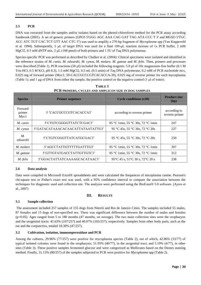
International Journal of Environmental & Agriculture Research (IJOEAR) ISSN:[2454-1850] [Vol-6, Issue-5, May- 2020]
Page | 20
2.5 PCR
DNA was extracted from the samples and/or isolates based on the phenol-chloroform method for the PCR assay according
Sambrook (2001). A set of generic primers (GPO3 5'GGG AGC AAA CAG GAT TAG ATA CCC T 3' and MGSO 5'TGC
ACC ATC TGT CAC TCT GTT AAC CTC 3'') was used to amplify a 270-bp fragment of Mycoplasma spp (Van Kuppeveld
et al. 1994). Subsequently, 5 μL of target DNA was used for a final 100-μL reaction mixture of 1x PCR buffer, 2 mM
MgCl2, 0.5 mM dNTP mix, 2 μL (100 pmol) of both primers and 1.5U of Taq DNA polymerase.
Species-specific PCR was performed as described by Chalker et al. (2004): Clinical specimens were isolated and identified in
the reference strains of M. canis, M. edwardii, M. cynos, M. molare, M. gateae and M. felis. Then, primers and processes
were described (Table 1). PCR reactions (50 µl) included the following reagents: 5.0 µl of 10x magnesium-free buffer (0.1 M
Tris-HCl, 0.5 M KCl, pH 8.3), 1.5 mM MgCl2, 0.5 mL (0.5 units) of Taq DNA polymerase, 0.2 mM of PCR nucleotide mix,
0.025 mg of forward primer (Myc1; 59-CACCGCCCGTCACACCA-39), 0.025 mg of reverse primer for each mycoplasma
(Table 1); and 1 μg of DNA from either the sample, the positive control or the negative control (1 μl of water).
TABLE 1
PCR PRIMERS, CYCLES AND AMPLICON SIZE IN DOG SAMPLES
Species Primer sequence Cycle conditions (x30) Product size
(bp)
Forward
primer
Myc1
5 ’CACCGCCCGTCACACCA3’ according to reverse primer according to
reverse primer
M. canis 5’CTGTCGGGGTTATCTCGAC3’ 95 °C 1min, 55 °C 30s, 72 °C 1min 247
M. cynos 5’GATACATAAACACAACATTATAATATTG3’ 95 °C 45s, 55 °C 30s, 72 °C 20s 227
M.
edwardii 5’CTGTCGGGTTATCATGCGAC3’ 95 °C 45s, 55 °C 30s, 72 °C 20s 250
M. molare 5’AGCCTATTGTTTTTGATTTG3’ 95 °C 1min, 55 °C 30s, 72 °C 1min 397
M. gateae 5’GTTGTATGACCTATTGTTGTC3’ 95 °C 1min, 55 °C 30s, 72 °C 1min 312
M. felis 5’GGACTATTATCAAAAGCACATAAC3’ 95°C 45 s, 51°C 30 s, 72°C 20 s 238
2.6 Data analysis
Data were compiled in Microsoft Excel® spreadsheets and were calculated the frequences of micoplasma canine. Pearson's
chi-square test or Fisher's exact test was used, with a 95% confidence interval to compare the association between the
techniques for diagnostic used and collection site. The analyzes were performed using the BioEstat® 5.0 software. (Ayres et
al., 2007)
III. RESULTS
3.1 Sample collection
The assessment included 257 samples of 155 dogs from Niterói and Rio de Janeiro Cities. The samples included 55 males,
87 females and 13 dogs of non-specified sex. There was significant difference between the number of males and females
(p<0.05). Ages ranged from 5 to 180 months (47 months, on average). The two main collection sites were the oropharynx
and the urogenital tracts: 41.63% (107/257) and 40.07% (103/257), respectively. Samples from other body parts, such as the
ear and the conjunctiva, totaled 18.30% (47/257).
3.2 Cultivation, isolation, immunoperoxidase and PCR
Among the cultures, 29.96% (77/257) were positive for mycoplasma species (Table 2), out of which, 42.86% (33/77) of
typical isolated colonies were found in the oropharynx; 51.95% (40/77), in the urogenital tract; and 5.19% (4/77), in other
sites (Table 3). These positive samples fermented glucose and were categorized as Mollicutes based on the Dienes staining
method. Finally, 31.13% (80/257) of the samples subjected to PCR were positive for Mycoplasma spp (Table 2).
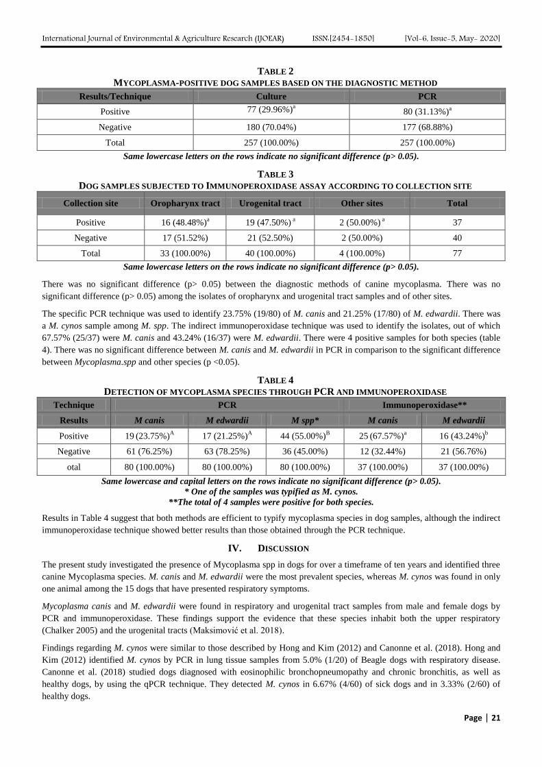
International Journal of Environmental & Agriculture Research (IJOEAR) ISSN:[2454-1850] [Vol-6, Issue-5, May- 2020]
Page | 21
TABLE 2
MYCOPLASMA-POSITIVE DOG SAMPLES BASED ON THE DIAGNOSTIC METHOD
Results/Technique Culture PCR
Positive 77 (29.96%)a
80 (31.13%)
a
Negative 180 (70.04%) 177 (68.88%)
Total 257 (100.00%) 257 (100.00%)
Same lowercase letters on the rows indicate no significant difference (p> 0.05).
TABLE 3
DOG SAMPLES SUBJECTED TO IMMUNOPEROXIDASE ASSAY ACCORDING TO COLLECTION SITE
Collection site Oropharynx tract Urogenital tract Other sites Total
Positive 16 (48.48%)a
19 (47.50%) a
2 (50.00%) a
37
Negative 17 (51.52%) 21 (52.50%) 2 (50.00%) 40
Total 33 (100.00%)
40 (100.00%)
4 (100.00%)
77
Same lowercase letters on the rows indicate no significant difference (p> 0.05).
There was no significant difference (p> 0.05) between the diagnostic methods of canine mycoplasma. There was no
significant difference (p> 0.05) among the isolates of oropharynx and urogenital tract samples and of other sites.
The specific PCR technique was used to identify 23.75% (19/80) of M. canis and 21.25% (17/80) of M. edwardii. There was
a M. cynos sample among M. spp. The indirect immunoperoxidase technique was used to identify the isolates, out of which
67.57% (25/37) were M. canis and 43.24% (16/37) were M. edwardii. There were 4 positive samples for both species (table
4). There was no significant difference between M. canis and M. edwardii in PCR in comparison to the significant difference
between Mycoplasma.spp and other species (p <0.05).
TABLE 4
DETECTION OF MYCOPLASMA SPECIES THROUGH PCR AND IMMUNOPEROXIDASE
Technique PCR Immunoperoxidase**
Results M canis M edwardii M spp* M canis M edwardii
Positive 19 (23.75%)
A 17 (21.25%)
A 44 (55.00%)
B 25
(67.57%)
a 16 (43.24%)
b
Negative 61 (76.25%) 63 (78.25%) 36 (45.00%) 12 (32.44%) 21 (56.76%)
otal 80 (100.00%) 80 (100.00%) 80 (100.00%) 37 (100.00%) 37 (100.00%)
Same lowercase and capital letters on the rows indicate no significant difference (p> 0.05).
* One of the samples was typified as M. cynos.
**The total of 4 samples were positive for both species.
Results in Table 4 suggest that both methods are efficient to typify mycoplasma species in dog samples, although the indirect
immunoperoxidase technique showed better results than those obtained through the PCR technique.
IV. DISCUSSION
The present study investigated the presence of Mycoplasma spp in dogs for over a timeframe of ten years and identified three
canine Mycoplasma species. M. canis and M. edwardii were the most prevalent species, whereas M. cynos was found in only
one animal among the 15 dogs that have presented respiratory symptoms.
Mycoplasma canis and M. edwardii were found in respiratory and urogenital tract samples from male and female dogs by
PCR and immunoperoxidase. These findings support the evidence that these species inhabit both the upper respiratory
(Chalker 2005) and the urogenital tracts (Maksimović et al. 2018).
Findings regarding M. cynos were similar to those described by Hong and Kim (2012) and Canonne et al. (2018). Hong and
Kim (2012) identified M. cynos by PCR in lung tissue samples from 5.0% (1/20) of Beagle dogs with respiratory disease.
Canonne et al. (2018) studied dogs diagnosed with eosinophilic bronchopneumopathy and chronic bronchitis, as well as
healthy dogs, by using the qPCR technique. They detected M. cynos in 6.67% (4/60) of sick dogs and in 3.33% (2/60) of
healthy dogs.
International Journal of Environmental & Agriculture Research (IJOEAR) ISSN:[2454-1850] [Vol-6, Issue-5, May- 2020]
Page | 22
The detection of M. cynos in only one case of respiratory disease suggests that the likelihood of M. cynos infection is low and
facilitated by the following complications: Serious respiratory diseases such as CIRD, and association with other
microorganisms (Chalker et al. 2004; Mannering et al. 2009); moreover, M. cynos is more easily detected through PCR
(Mitchell et al. 2017). Such species has been defined as an emerging pathogen (Priestnall et al. 2014) associated with other
CIRD microorganisms; nevertheless, its ability to cause disease on its own has not yet been proven, since it can be detected
both in asymptomatic dogs (Lavan and Knesl 2015) and in dogs vaccinated against CIRD (Mitchell et al. 2017).
The urogenital tract is the common isolation site of several mycoplasma species. However, the association of the urogenital
and respiratory tracts to mycoplasmosis remains uncertain due to the incidence of isolation in both healthy animals and in
animals with urogenital disorders (L’Abee-Lund et al. 2003; Maksimović et al. 2018; Ulgen et al. 2006).
L’Abee-Lund et al. (2003) isolated M. canis in dogs with clinical signs of urogenital disease and suggested that this
microorganism could be the causative agent of it. However, the present study showed that M. canis was more common in
healthy dogs than in the sick ones, as reported by Janowski et al. (2008) and Maksimović et al. (2018). Janowski et al. (2008)
suggested that M. canis was a part of the vaginal microbiota of healthy female dogs. Maksimović et al (2018) isolated M.
canis, M. spumans, M. edwardii and Mycoplasma spp in vaginal samples from domestic and street female dogs who were
either healthy, intact or subjected to total hysterectomy. The present study also evidenced M. edwardii and Mycoplasma spp
in the urogenital tract of healthy animals, but M. cynos was not found in it, a fact to be unusual in this site; however, it has
been reported in dogs with urogenital disease, along with M. canis and M. spumans (Jang et al. 1984).
The diagnostic results of the comparison between isolation and PCR have supported the findings by Costa et al. (2004), since
there was no significant difference between the aforementioned techniques; thus, both of them can be recommended for
diagnosis.
The detection of M. canis and M. edwardii alone and/or in mixed infections by indirect immunoperoxidase reaction in both
the respiratory and urogenital tracts by the present study had already been previously reported (Nascimento et al. 2010).
Based on this finding, these species can be part of the microbiota found in both the respiratory and urogenital tracts. Indirect
immunoperoxidase can be used to identify mycoplasma species in dogs (Nascimento et al. 2010) and in other animals alike
(Santos et al. 2010).
V. CONCLUSION
Canine mycoplasmas have been found in sick animals, but they are more likely to be found in seemingly healthy
animals.
M. canis and M. edwardii were the most prevalent species in the assessed sites and through the diagnostic method.
M. cynos was detected in a single animal who presented a respiratory disease.
The highly consistent detection of mycoplasma species in dogs encourages instructive studies on their
etiopathogenesis.
REFERENCES
[1] M.L. Barreto, E.R. Nascimento, R. Presgrave, C.A.M. Campos, M.G.F. Nascimento and G.B. Lignon (2003) Diagnóstico patológico da micoplasmose respiratória murina em Rattus novergicus. Acta Scientiae Veterinariae 31(2), 81–7.
[2] R.L. Berčič, I. Cizelj, M. Benčina, M. Narat, J.M. Bradbury, P. Dovč, and D. Benčina (2012) Demonstration of neuraminidase
activity in Mycoplasma neurolyticum and of neuraminidase proteins in three canine Mycoplasma species. Veterinary Microbiology 155(2), 425–429.
[3] A.M. Canonne, I. Peters, E. Roels, L. Desquilbet, and C. Clercx (2018) Detection of specific bacterial agents by quantitative PCR
assays in the bronchoalveolar lavage fluid of dogs with eosinophilic bronchopneumopathy vs. dogs with chronic bronchitis and healthy dogs. The Veterinary Journal 232, 52–56.
[4] V.J. Chalker (2005). Canine mycoplasmas. Research in Veterinary Science 79(1), 1–8.
[5] V.J. Chalker, W.M.A. Owen, C. Paterson, E. Barker, H. Brooks, A.N. Rycroft, and J. Brownlie (2004) Mycoplasmas associated with canine infectious respiratory disease. Microbiology (Reading, England) 150(10), 3491–3497.
[6] C.L.A. Costa, E.R. Nascimento, M.O. Platenik, V.L.A. Pereira, M.L. Barreto, M.B.O. Chaudon, M.L.G. Ferreira, and P.B. Doria
(2004) Isolamento e PCR na detecção de Mycoplasma spp. em cães (Canis familiaris) assintomáticos e suspeitos de micoplasmose. Revista Universidade Rural. Série Ciências Da Vida 24, 61–62.
[7] S. Hong and O. Kim (2012) Molecular identification of Mycoplasma cynos from laboratory beagle dogs with respiratory disease. Laboratory Animal Research 28(1), 61–66.
International Journal of Environmental & Agriculture Research (IJOEAR) ISSN:[2454-1850] [Vol-6, Issue-5, May- 2020]
Page | 23
[8] M.R.S. Ilha, S. Rajeev, C. Watson, and M. Woldemeskel (2010) Meningoencephalitis caused by Mycoplasma edwardii in a dog. Journal of Veterinary Diagnostic Investigation 22(5), 805–808.
[9] Y. Imada, I. Uchida, and K. Hashimoto (1987) Rapid identification of mycoplasmas by indirect immunoperoxidase test using small square filter paper. Journal of Clinical Microbiology 25(1), 17–21.
[10] S.S. Jang, G.V. Ling, R. Yamamoto, and A.M. Wolf (1984) Mycoplasma as a cause of canine urinary tract infection. Journal of the American Veterinary Medical Association 185(1), 45–47.
[11] T. Janowski, A. Zdu, A. Jurczak, and P. Socha (2008) Incidence of Mycoplasma canis in the vagina in three groups of bitches. Bulletin- Veterinary Institute in Pulawy 52, 533–535.
[12] L.R. Johnson, E.V. Queen, W. Vernau, J.E. Sykes, and B.A. Byrne (2013) Microbiologic and Cytologic Assessment of
Bronchoalveolar Lavage Fluid from Dogs with Lower Respiratory Tract Infection: 105 Cases (2001–2011). Journal of Veterinary Internal Medicine 27(2), 259–267.
[13] S. Klein, M. Klotz, and T. Eigenbrod (2018) First isolation of Mycoplasma canis from human tissue samples after a dog bite. New Microbes and New Infections 25, 14–15.
[14] T.M. L’Abee-Lund, R. Heiene, N.F. Friis, P. Ahrens, and H. Sørum (2003) Mycoplasma canis and urogenital disease in dogs in Norway. The Veterinary Record 153(8), 231–235.
[15] R. Lavan and O. Knesl (2015) Prevalence of canine infectious respiratory pathogens in asymptomatic dogs presented at US animal shelters. The Journal of Small Animal Practice 56(9), 572–576.
[16] Z. Maksimović, A. Maksimović, A. Halilbašić, and M. Rifatbegović (2018) Genital mycoplasmas of healthy bitches. Journal of Veterinary Diagnostic Investigation 30(4), 651–653.
[17] S.A. Mannering, L. McAuliffe, J.R. Lawes, K. Erles, and J. Brownlie (2009) Strain typing of Mycoplasma cynos isolates from dogs with respiratory disease. Veterinary Microbiology 135(3–4), 292–296.
[18] J.A. Mitchell, J.M. Cardwell, H. Leach, C.A. Walker, S. Le Poder, N. Decaro, M. Rusvai, H. Egberink, P. Rottier, M. Fernandez, et
al. (2017) European surveillance of emerging pathogens associated with canine infectious respiratory disease. Veterinary
Microbiology 212, 31–38.
[19] K. Mullis, F. Faloona, S. Scharf, R. Saiki, G. Horn, and H. Erlich (1986) Specific enzymatic amplification of DNA in vitro: the
polymerase chain reaction. Cold Spring Harbor Symposia on Quantitative Biology 51 Pt 1, 263–273.
[20] E.R. Nascimento, M.J. Fonseca, M.L. Barreto, V.L.A. Pereira, V.Y. Takeuti, J.F. de Almeida, M. Nascimento, and S.B. Santos
(2010) Detection of Mycoplasma canis and Mycoplasma edwardii by Indirect Immunoperoxidase in Brazil. Presented at the 18th international Congress of the International Organization for Mycoplasmology (IOM), Chianciano Terme, Italy.
[21] C.M. Oliveira, E.O. Costa, and J.A.P. Silva (1998) Microbiota aeróbica em fêmeas caninas hígidas durante o ciclo estral: Avaliação da sensibilidade aos antimicrobianos. Revista Brasileira de Medicina Veterinária 20(2), 78–84.
[22] S.L. Priestnall, J.A. Mitchell, C.A. Walker, K. Erles, and J. Brownlie (2014) New and emerging pathogens in canine infectious respiratory disease. Veterinary Pathology 51(2), 492–504.
[23] S. Rosendal (1979) Canine and Feline Mycoplasmas. In The Mycoplasmas: Human and Animal Mycoplasmas, eds. J.G. Tully and R.F. Whitcomb, 1st ed., Vol. 2, 217–234. Academic Press, New York.
[24] J. Sambrook (2001) Molecular Cloning: A Laboratory Manual, Third Edition 3rd edition. Cold Spring Harbor Laboratory Press,
Cold Spring Harbor, N.Y.
[25] S.B. Santos, E.R. Nascimento, J.L.H. Faccini, M.L. Barreto, J.F. Almeida, V.L.A. Pereira, and C.A.M. Campos (2010) Detection of
Mycoplasma mycoides cluster by indirect immunoperoxidase (IPI) and PCR-REA in the ear canal of bovines. Pesquisa Veterinária Brasileira 30(5), 465–469.
[26] S. Santos, M. Almeida, L. Silva, J. Oliveira, C. Leal, J. Júnior, and R.A. Mota (2016) Report of Mollicutes in the Ear Canal of Domestic Dogs in Brazil. OALib Journal 3, 1–5.
[27] J.B. Souza, M.T. Oliveira, E.R. Nascimento, M.A. Verícimo, and M.L. Barreto (2016) Mycoplasma pulmonis, agente da micoplasmose respiratória murina: revisão. Archives of Veterinary Science 21(4), 8-25.
[28] J. Spergser, S. Langer, S. Muck, K. Macher, M. Szostak, R. Rosengarten, and H.J. Busse (2011) Mycoplasma mucosicanis sp. nov.,
isolated from the mucosa of dogs. International Journal of Systematic and Evolutionary Microbiology 61(4), 716–721.
[29] K.A. Stenske, D.A. Bemis, K. Hill, and D.J. Krahwinkel (2005) Acute polyarthritis and septicemia from Mycoplasma edwardii after surgical removal of bilateral adrenal tumors in a dog. Journal of Veterinary Internal Medicine 19(5), 768–771.
[30] Ulgen M, C Cetin, S Sentürk, AE Ozel, and U Ozdemir (2006) Urinary tract infections due to Mycoplasma canis in dogs. Journal of Veterinary Medicine. A, Physiology, Pathology, Clinical Medicine 53(7), 379–382.
[31] F.J. van Kuppeveld, K.E. Johansson, J.M. Galama, J. Kissing, G. Bölske, J.T. van der Logt, and W.J. Melchers (1994) Detection of
mycoplasma contamination in cell cultures by a mycoplasma group-specific PCR. Applied and Environmental Microbiology 60(1), 149–152.
[32] R.D. Walker, R. Walshaw, C.M. Riggs, and T. Mosser (1995) Recovery of two mycoplasma species from abscesses in a cat following bite wounds from a dog. Journal of Veterinary Diagnostic Investigation 7(1), 154–156.
[33] J.D. Watson and F.H.C. Crick (1953) Molecular Structure of Nucleic Acids: A Structure for Deoxyribose Nucleic Acid. Nature 171(4356), 737–738.
[34] F. Zeugswetter, H. Weissenböck, S. Shibly, J. Hassan, and J. Spergser (2007) Lethal bronchopneumonia caused by Mycoplasma cynos in a litter of golden retriever puppies. Veterinary Record 161(18), 626–628.
International Journal of Environmental & Agriculture Research (IJOEAR) ISSN:[2454-1850] [Vol-6, Issue-6, June- 2020]
Page | 24
Effect of Genotype by Environment Interaction (GEI),
Correlation, and GGE Biplot analysis for high concentration of
grain Iron and Zinc biofortified lentils and their agronomic traits
in multi-environment domains of Nepal Rajendra Darai
1*, Krishna Hari Dhakal
2, Ashutosh Sarker
3, Madhav Prasad Pandey
4,
Shiv Kumar Agrawal5, Surya Kant Ghimire
6, Dhruba Bahadur Thapa
7,
Jang Bahadur Prasad8, Rabendra Prasad Sah
9, Keshav Pokhrel
10
1,9Nepal Agricultural Research Council, National Grain Legumes Research Program, Khajura , Nepalgunj, Banke
Province no.5, Nepal 2 ,4,6
Faculty of Agriculture, Department of Genetics and Plant Breeding, Agriculture and Forestry University (AFU),
Rampur, Chitwan, Bagmati Province, Nepal 3
South Asia and China Regional Program (ICARDA), NASC Complex, New Delhi, India 5
International Center for Agricultural Research in the Dry Areas (ICARDA), Rabat, Morroco 8Directorate of Agriculture Research, Parwanipur, Bara, Province # 2 , Nepal
10Directorates of Agricultural Research, Dashrathpur, Surkhet, Karnali Province, Nepal
7National Plant Breeding and Genetics Research Centre, Khumaltar, Lalitpur, Bagmati Province, Nepal
Abstract— Lentil (Lens culinaris Medik. culinaris ) is a cool season food legume contains the high quality of proteins and
minerals. Selecting genotypes for high mean yield and yield stability has been a challenge for lentil breeders. The
complexities of genotype × environment interaction (GEI) make selection difficult to identify the best performing and most
stable genotypes. Therefore, this study was carried out to apply a GGE biplot and AMMI analysis model to evaluate the
magnitude of the effect of GE interaction on grain yield of 25 lentil accessions at three environments during the year of 2016
and 2017 seasons in alpha-lattice design (5x5) with three locations and to evaluate relationships between test environments
for identification of favorable genotypes for lentil production areas. Combined pooled mean analysis of variance for grain
yield tested at three environments over the two subsequent years 2016 and 2017 showed that highly significant differences in
genotypes, environment and G x E interaction effect indicating the possibility of selection for stable accessions. The stability
of the assessed genotypes using some stability statistics derived from three types of statistical concepts (variance and
regression analyses), AMMI (additive main effect and multiplicative interaction) analysis and GGE biplot (genotype main
effects and genotype-by-environment interaction effects) models were applied to obtain good understanding of the
interrelationship and overlapping among the used stability statistics. Research results showed that lentil accession WBL-77
(1451 kg ha-1) , RL-79(1446 kg ha-1) and PL-4(1429 kg ha-1) were the best performer and well adopted across the
environments and over the years. AMMI analysis of variance for lentil grain yield (tha-1
) of lentil accessions tested at three
environments over the years showed that 80.71% of the total sum of squares was attributed to environmental effects, only
8.38 % to genotypic effects and 10.90% to genotype × environment interaction effects. The partitioning of GGE sum of
squares through the GGE biplot analysis showed that PC1and PC2 accounted 74.75%, and 25.24% of GGE sum of squares
respectively over the years. Accessions ILL8006, RL-6, Shital, ILL3490 and simal were more close to the center point and
indicated that stable across the environments. In another words, the genotypes which have low stability value (ASV) is said
to be stable and the breeder chose the stable genotypes along with grain yield above the mean grand yield. In this experiment
accessions RL-6(G-2) ranked 1st stability (ASV-0.53) followed by Simal (ASV-2.05), ILL-3490 (ASV-2.42) and Shital (ASV-
2.72) and suitable for all environment.
Keywords— Stability parameters, lentil, GGE biplot, AMMI-additive main effects and multiplicative interaction; ASV–
AMMI stability value.
I. INTRODUCTION
Lentil (Lens culinaris Medik. culinaris ) is a cool season food legume and "the house of essential nutrients", contains the high
quality and quantity of proteins (up to 35%) and minerals calcium, phosphoros, potassium, folic acids, iron, zinc, selenium and
vitamins. Lentil is the fourth most important crop grown after rice, maize, wheat & millet in terms of area (MoAD, 2016). In
Nepal, it is mostly eaten as dal (Concentrated soup) with rice besides various food preparations. Rice or wheat bread and dal are
the best combination in daily dish of low income people of Nepal who cannot afford the animal products. Virtually the major
International Journal of Environmental & Agriculture Research (IJOEAR) ISSN:[2454-1850] [Vol-6, Issue-6, June- 2020]
Page | 25
proportion of rural people relies on lentil and other pulses for their nutritional security. It has diverse role in farming system which
adds 42-75 kg biological nitrogen fixation. Lentil seed is rich in protein for human consumption, and lentil straw is a valued
animal feed. It is also known as the exportable commodity, in 2016/17 lentil was exported in the value of USA $ 10 million
from Nepal. It is grown as sole crop as well as mixed crop and intercropped with sugarcane, mustard, linseed, wheat, mango-
orchard etc. In general, lentil is commonly grown as relay cropping system prior to rice harvest and in Nepal, still 0.24 million
hectares of lands are rice fallows and has a great scope to vertical and horizontal expansion. In most lentils producing areas yield
seems to be not more than one-half of potential yields while improved genotypes contribute to increase lentil production (Erskine,
2009). Lentil is adapted to low rainfall and is predominantly grown in the winter in regions (Sarker et al., 2003). Selecting
genotypes for high mean yield and yield stability has been a challenge for lentil breeders. Yield is a quantitative trait while
GxE interaction showed the yield stability and micronutrients heritability. It is also the interplay in the effect of genetic and
non-genetic on development of any genotypes. Consequently Gx E interaction helps breeder to select the desirable varieties
in the process of evaluation & increase efficiency of selection (Sabaghnia et al., 2008). It is reported the main environmental
effects (E) and Genotype by Environment Interaction (GEI) as the most important sources of variation for the measured yield
of crops. The yield is a combined result of the effects of the genotype (G), E and GE interaction. Environment is responsible
more than 80% effects of the total yield variation, while Genotype and G x E interaction has small effect. Environmental
factors include soil moisture, sowing time, fertility, temperature and day length which is strong influenced during the various
stages of plant growth (Bull et al., 1992). Therefore GEI is an extremely important in the development and evaluation of
plant varieties. Flores et al. (1998) compared 22 univariate and multivariate methods to analyze genotype by environment
(GE) interactions. There are two possible strategies for interpreting GE interaction with univariate parametric methods
including analysis of variance and simple linear regression analysis of cultivar yield. The requirement for stable genotypes
that perform well over a wide range of environments becomes increasingly important as farmers need reliable production
quantity (Gauch et al.,2008). Therefore, identifying most stable genotypes is an important objective in many plant breeding
programs for all crops, including lentil. The performance of a genotype is determined by three factors: genotypic main effect
(G), environmental main effect (E) and their interaction (Yan et al.,2007). Understanding genotype by environment (GE)
interactions is necessary to accurately determine stability in lentil genotypes and help breeding programs by increasing
efficiency of selection (Sabaghnia et al.,2008). The complexities of genotype × environment interaction (GEI) make selection
difficult to identify the best performing and most stable genotypes (Yau, 1995). Thus, first we need to identify the stable
genotypes for their yield and yield component traits. Stability of genotypes over wide range of environments is desirable and
depends upon GEI (Ali and Sawar, 2008). AMMI analysis has been shown to improve both the post-dictive and predictive
success of yield trials by altering the noise (random variation) from the data pattern, thereby improving predictive accuracy
(Gauch and Zobel, 1988). Understanding the structure and nature of GEI is of utmost significance in crop improvement
programs because the significant GEI can seriously impair efforts in selecting the superior genotypes (Danyaliet al., 2012).
The objectives of this investigation were: to apply a GGE biplot and AMMI analysis model to evaluate the magnitude of the
effect of GEI on grain yield of 25 high grain Fe and Zn lentil accessions tested across the three locations over the years and
to evaluate relationships between test environments for identification of favorable genotypes for lentil production areas in
terai agro-domains.
II. MATERIALS AND METHODS
2.1 Description of the Study Sites
G x E interaction trials were conducted at Grain Legumes Research Program (GLRP), Khajura, Banke at 810 37” East longitudes
and 280 06” North latitude and an altitude of 181 meters above mean sea level, NMRP/NCRP, Rampur, Chitwan at 27
o 40′ N
latitude, 84o19′ E longitude at an altitude of 228m above mean sea level and RARS, Parwanipur at the latitude 27
0 4’40.9’’N
and longitude 84056’9.85”E as well altitude 75m above sea level for two consecutive cropping seasons (October 2016 to March
2017) in Nepal.
2.2 Plant Materials
For this study, 25 high grain concentrations of iron (Fe) and zinc (Zn) lentil accessions including local landraces was planted for
phenotypic evaluation. Sources of these accessions were originated from SAARC countries (14 accessions: Nepal-7, India-6,
Bangladesh-1) and ICARDA (11 accessions). Released lentil varieties Shital and Simal was used as a check.
2.3 Experimental Layout and Design
Present experiment was carried out in Alpha-lattice design (5 x 5) with three replications. A unit plot comprise 2-meter length row
with a plot size of (3 m2). The accessions were planted in the third week of October to 2
nd week of November. Seeds of each
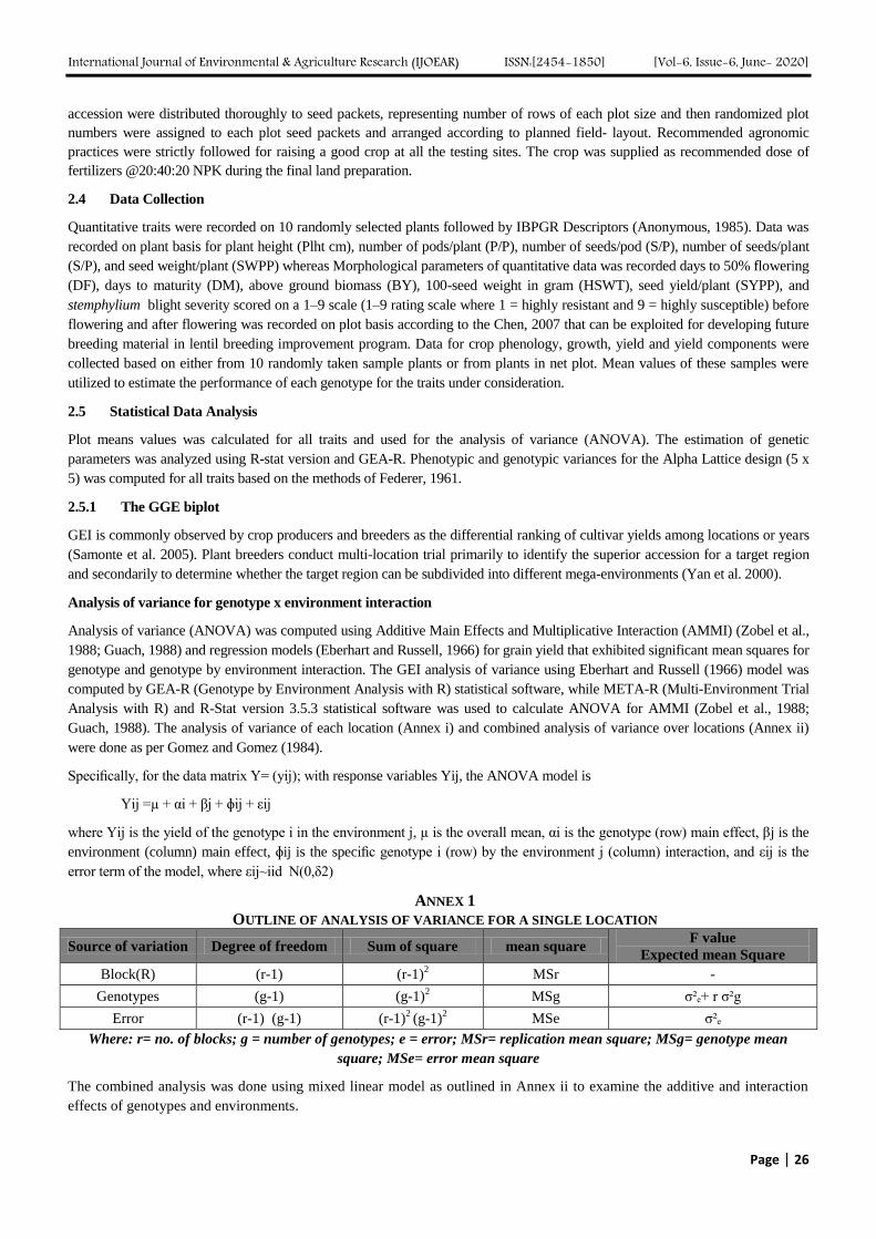
International Journal of Environmental & Agriculture Research (IJOEAR) ISSN:[2454-1850] [Vol-6, Issue-6, June- 2020]
Page | 26
accession were distributed thoroughly to seed packets, representing number of rows of each plot size and then randomized plot
numbers were assigned to each plot seed packets and arranged according to planned field- layout. Recommended agronomic
practices were strictly followed for raising a good crop at all the testing sites. The crop was supplied as recommended dose of
fertilizers @20:40:20 NPK during the final land preparation.
2.4 Data Collection
Quantitative traits were recorded on 10 randomly selected plants followed by IBPGR Descriptors (Anonymous, 1985). Data was
recorded on plant basis for plant height (Plht cm), number of pods/plant (P/P), number of seeds/pod (S/P), number of seeds/plant
(S/P), and seed weight/plant (SWPP) whereas Morphological parameters of quantitative data was recorded days to 50% flowering
(DF), days to maturity (DM), above ground biomass (BY), 100-seed weight in gram (HSWT), seed yield/plant (SYPP), and
stemphylium blight severity scored on a 1–9 scale (1–9 rating scale where 1 = highly resistant and 9 = highly susceptible) before
flowering and after flowering was recorded on plot basis according to the Chen, 2007 that can be exploited for developing future
breeding material in lentil breeding improvement program. Data for crop phenology, growth, yield and yield components were
collected based on either from 10 randomly taken sample plants or from plants in net plot. Mean values of these samples were
utilized to estimate the performance of each genotype for the traits under consideration.
2.5 Statistical Data Analysis
Plot means values was calculated for all traits and used for the analysis of variance (ANOVA). The estimation of genetic
parameters was analyzed using R-stat version and GEA-R. Phenotypic and genotypic variances for the Alpha Lattice design (5 x
5) was computed for all traits based on the methods of Federer, 1961.
2.5.1 The GGE biplot
GEI is commonly observed by crop producers and breeders as the differential ranking of cultivar yields among locations or years
(Samonte et al. 2005). Plant breeders conduct multi-location trial primarily to identify the superior accession for a target region
and secondarily to determine whether the target region can be subdivided into different mega-environments (Yan et al. 2000).
Analysis of variance for genotype x environment interaction
Analysis of variance (ANOVA) was computed using Additive Main Effects and Multiplicative Interaction (AMMI) (Zobel et al.,
1988; Guach, 1988) and regression models (Eberhart and Russell, 1966) for grain yield that exhibited significant mean squares for
genotype and genotype by environment interaction. The GEI analysis of variance using Eberhart and Russell (1966) model was
computed by GEA-R (Genotype by Environment Analysis with R) statistical software, while META-R (Multi-Environment Trial
Analysis with R) and R-Stat version 3.5.3 statistical software was used to calculate ANOVA for AMMI (Zobel et al., 1988;
Guach, 1988). The analysis of variance of each location (Annex i) and combined analysis of variance over locations (Annex ii)
were done as per Gomez and Gomez (1984).
Specifically, for the data matrix Y= (yij); with response variables Yij, the ANOVA model is
Yij =µ + αi + βj + ɸij + εij
where Yij is the yield of the genotype i in the environment j, µ is the overall mean, αi is the genotype (row) main effect, βj is the
environment (column) main effect, ɸij is the specific genotype i (row) by the environment j (column) interaction, and εij is the
error term of the model, where εij~iid N(0,δ2)
ANNEX 1
OUTLINE OF ANALYSIS OF VARIANCE FOR A SINGLE LOCATION
Source of variation Degree of freedom Sum of square mean square F value
Expected mean Square
Block(R) (r-1) (r-1)2 MSr -
Genotypes (g-1) (g-1)2 MSg ζ²ₑ+ r ζ²g
Error (r-1) (g-1) (r-1)2 (g-1)
2 MSe ζ²ₑ
Where: r= no. of blocks; g = number of genotypes; e = error; MSr= replication mean square; MSg= genotype mean
square; MSe= error mean square
The combined analysis was done using mixed linear model as outlined in Annex ii to examine the additive and interaction
effects of genotypes and environments.
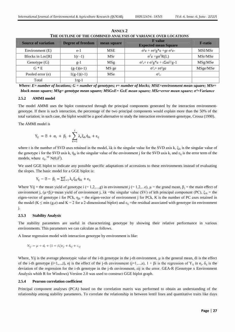
International Journal of Environmental & Agriculture Research (IJOEAR) ISSN:[2454-1850] [Vol-6, Issue-6, June- 2020]
Page | 27
ANNEX 2
THE OUTLINE OF THE COMBINED ANALYSIS OF VARIANCE OVER LOCATIONS
Source of variation Degree of freedom mean square F value
Expected mean Square F-ratio
Environment (E) e-1 MSE ζ²e + rζ²g*e +gr ζ²e- MSl/MSr
Blocks in Loc[R] 1(r -1) MSr ζ2e +gζ
2R(L) MSr/MSe
Genotype (G) g-1 MSg ζ²ₑ+ r ζ²g*e + rΣαi²/g-1 MSg/MSe
G * E (g-1)(e-1) MS ge ζ²ₑ+ rζ²ge MSge/MSe
Pooled error (e) 1(g-1)(r-1) MSe ζ²ₑ
Total 1rg-1
Where: E= number of locations; G = number of genotypes; r= number of blocks; MSE=environment mean square; MSr=
block mean square; MSg= genotype mean square; MSGxE= GxE mean square; MSe=error mean square; σ²=Variance
2.5.2 AMMI model
The model AMMI uses the biplot constructed through the principal components generated by the interaction environment-
genotype. If there is such interaction, the percentage of the two principal components would explain more than the 50% of the
total variation; in such case, the biplot would be a good alternative to study the interaction environment-genotype, Crossa (1990).
The AMMI model is
Yij = µ + αi + βj + λκξikήik + εij
𝑡
𝑘=1
where t is the number of SVD axes retained in the model, λk is the singular value for the SVD axis k, ξik is the singular value of
the genotype i for the SVD axis k, ήjk is the singular value of the environment j for the SVD axis k, and εij is the error term of the
models, where εij~iid
N(0,δ2).
We used GGE biplot to indicate any possible specific adaptations of accessions to these environments instead of evaluating
the slopes. The basic model for a GGE biplot is:
Yij − µ − βj = λκξikήik + εij 𝐾𝑘=1
Where Yij = the mean yield of genotype i (= 1,2,...,g) in environment j (= 1,2,...e), µ = the grand mean, β j = the main effect of
environment j, (µ+βj)=mean yield of environment j, λk =the singular value (SV) of kth principal component (PC), ξ ik = the
eigen-vector of genotype i for PCk, ηjk = the eigen-vector of environment j for PCk, K is the number of PC axes retained in
the model (K ≤ min (g,e) and K = 2 for a 2-dimensional biplot) and εij =the residual associated with genotype iin environment
j.
2.5.3 Stability Analysis
The stability parameters are useful in characterizing genotype by showing their relative performance in various
environments. This parameters we can calculate as follows.
A linear regression model with interaction genotype by environment is like:
Where, Yij is the average phenotypic value of the i-th genotype in the j-th environment, µ is the general mean, di is the effect
of the i-th genotype (i=1,...,t), ej is the effect of the j-th environment (j=1,...,s), 1 + βi is the regression of Yij in ej, δij is the
deviation of the regression for the i-th genotype in the j-th environment, εij is the error. GEA-R (Genotype x Environment
Analysis whith R for Windows) Version 2.0 was used to construct GGE biplot graph.
2.5.4 Pearson correlation coefficient
Principal component analyses (PCA) based on the correlation matrix was performed to obtain an understanding of the
relationship among stability parameters. To correlate the relationship in between lentil lines and quantitative traits like days
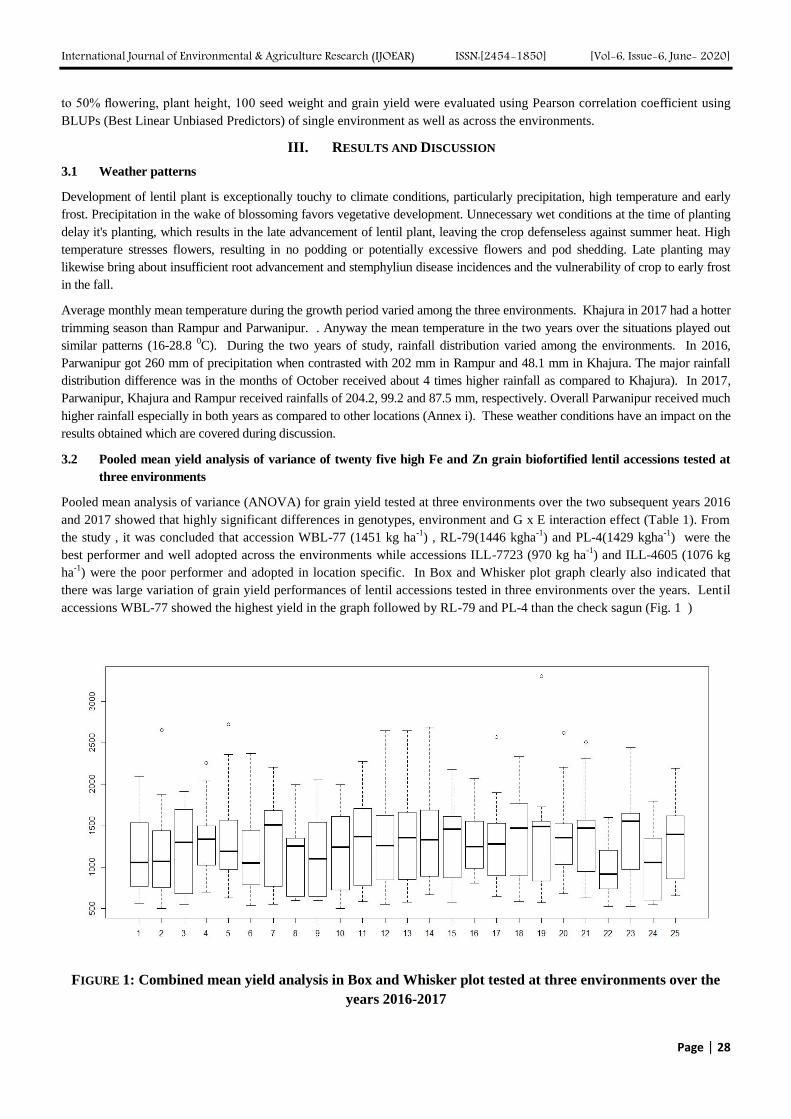
International Journal of Environmental & Agriculture Research (IJOEAR) ISSN:[2454-1850] [Vol-6, Issue-6, June- 2020]
Page | 28
to 50% flowering, plant height, 100 seed weight and grain yield were evaluated using Pearson correlation coefficient using
BLUPs (Best Linear Unbiased Predictors) of single environment as well as across the environments.
III. RESULTS AND DISCUSSION
3.1 Weather patterns
Development of lentil plant is exceptionally touchy to climate conditions, particularly precipitation, high temperature and early
frost. Precipitation in the wake of blossoming favors vegetative development. Unnecessary wet conditions at the time of planting
delay it's planting, which results in the late advancement of lentil plant, leaving the crop defenseless against summer heat. High
temperature stresses flowers, resulting in no podding or potentially excessive flowers and pod shedding. Late planting may
likewise bring about insufficient root advancement and stemphyliun disease incidences and the vulnerability of crop to early frost
in the fall.
Average monthly mean temperature during the growth period varied among the three environments. Khajura in 2017 had a hotter
trimming season than Rampur and Parwanipur. . Anyway the mean temperature in the two years over the situations played out
similar patterns (16-28.8 0C). During the two years of study, rainfall distribution varied among the environments. In 2016,
Parwanipur got 260 mm of precipitation when contrasted with 202 mm in Rampur and 48.1 mm in Khajura. The major rainfall
distribution difference was in the months of October received about 4 times higher rainfall as compared to Khajura). In 2017,
Parwanipur, Khajura and Rampur received rainfalls of 204.2, 99.2 and 87.5 mm, respectively. Overall Parwanipur received much
higher rainfall especially in both years as compared to other locations (Annex i). These weather conditions have an impact on the
results obtained which are covered during discussion.
3.2 Pooled mean yield analysis of variance of twenty five high Fe and Zn grain biofortified lentil accessions tested at
three environments
Pooled mean analysis of variance (ANOVA) for grain yield tested at three environments over the two subsequent years 2016
and 2017 showed that highly significant differences in genotypes, environment and G x E interaction effect (Table 1). From
the study , it was concluded that accession WBL-77 (1451 kg ha-1
) , RL-79(1446 kgha-1
) and PL-4(1429 kgha-1
) were the
best performer and well adopted across the environments while accessions ILL-7723 (970 kg ha-1
) and ILL-4605 (1076 kg
ha-1
) were the poor performer and adopted in location specific. In Box and Whisker plot graph clearly also indicated that
there was large variation of grain yield performances of lentil accessions tested in three environments over the years. Lentil
accessions WBL-77 showed the highest yield in the graph followed by RL-79 and PL-4 than the check sagun (Fig. 1 )
FIGURE 1: Combined mean yield analysis in Box and Whisker plot tested at three environments over the
years 2016-2017
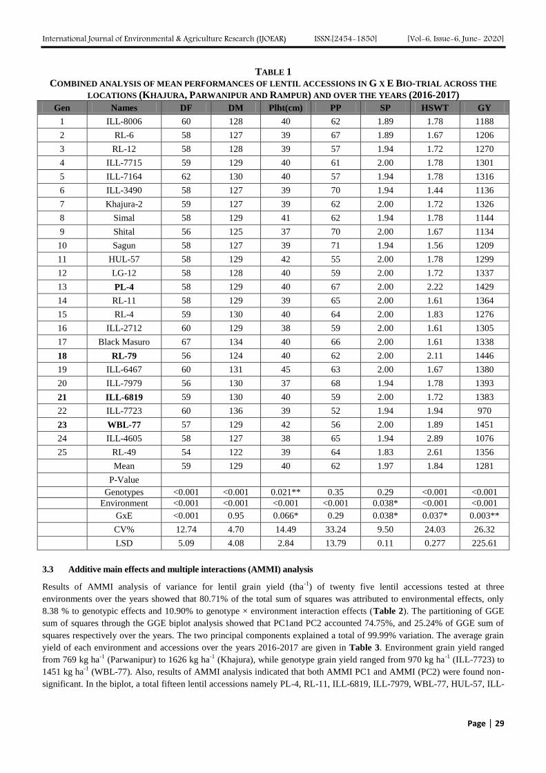
International Journal of Environmental & Agriculture Research (IJOEAR) ISSN:[2454-1850] [Vol-6, Issue-6, June- 2020]
Page | 29
TABLE 1
COMBINED ANALYSIS OF MEAN PERFORMANCES OF LENTIL ACCESSIONS IN G X E BIO-TRIAL ACROSS THE
LOCATIONS (KHAJURA, PARWANIPUR AND RAMPUR) AND OVER THE YEARS (2016-2017)
Gen Names DF DM Plht(cm) PP SP HSWT GY
1 ILL-8006 60 128 40 62 1.89 1.78 1188
2 RL-6 58 127 39 67 1.89 1.67 1206
3 RL-12 58 128 39 57 1.94 1.72 1270
4 ILL-7715 59 129 40 61 2.00 1.78 1301
5 ILL-7164 62 130 40 57 1.94 1.78 1316
6 ILL-3490 58 127 39 70 1.94 1.44 1136
7 Khajura-2 59 127 39 62 2.00 1.72 1326
8 Simal 58 129 41 62 1.94 1.78 1144
9 Shital 56 125 37 70 2.00 1.67 1134
10 Sagun 58 127 39 71 1.94 1.56 1209
11 HUL-57 58 129 42 55 2.00 1.78 1299
12 LG-12 58 128 40 59 2.00 1.72 1337
13 PL-4 58 129 40 67 2.00 2.22 1429
14 RL-11 58 129 39 65 2.00 1.61 1364
15 RL-4 59 130 40 64 2.00 1.83 1276
16 ILL-2712 60 129 38 59 2.00 1.61 1305
17 Black Masuro 67 134 40 66 2.00 1.61 1338
18 RL-79 56 124 40 62 2.00 2.11 1446
19 ILL-6467 60 131 45 63 2.00 1.67 1380
20 ILL-7979 56 130 37 68 1.94 1.78 1393
21 ILL-6819 59 130 40 59 2.00 1.72 1383
22 ILL-7723 60 136 39 52 1.94 1.94 970
23 WBL-77 57 129 42 56 2.00 1.89 1451
24 ILL-4605 58 127 38 65 1.94 2.89 1076
25 RL-49 54 122 39 64 1.83 2.61 1356
Mean 59 129 40 62 1.97 1.84 1281
P-Value
Genotypes <0.001 <0.001 0.021** 0.35 0.29 <0.001 <0.001
Environment <0.001 <0.001 <0.001 <0.001 0.038* <0.001 <0.001
GxE <0.001 0.95 0.066* 0.29 0.038* 0.037* 0.003**
CV% 12.74 4.70 14.49 33.24 9.50 24.03 26.32
LSD 5.09 4.08 2.84 13.79 0.11 0.277 225.61
3.3 Additive main effects and multiple interactions (AMMI) analysis
Results of AMMI analysis of variance for lentil grain yield (tha-1
) of twenty five lentil accessions tested at three
environments over the years showed that 80.71% of the total sum of squares was attributed to environmental effects, only
8.38 % to genotypic effects and 10.90% to genotype × environment interaction effects (Table 2). The partitioning of GGE
sum of squares through the GGE biplot analysis showed that PC1and PC2 accounted 74.75%, and 25.24% of GGE sum of
squares respectively over the years. The two principal components explained a total of 99.99% variation. The average grain
yield of each environment and accessions over the years 2016-2017 are given in Table 3. Environment grain yield ranged
from 769 kg ha-1
(Parwanipur) to 1626 kg ha-1
(Khajura), while genotype grain yield ranged from 970 kg ha-1
(ILL-7723) to
1451 kg ha-1
(WBL-77). Also, results of AMMI analysis indicated that both AMMI PC1 and AMMI (PC2) were found non-
significant. In the biplot, a total fifteen lentil accessions namely PL-4, RL-11, ILL-6819, ILL-7979, WBL-77, HUL-57, ILL-
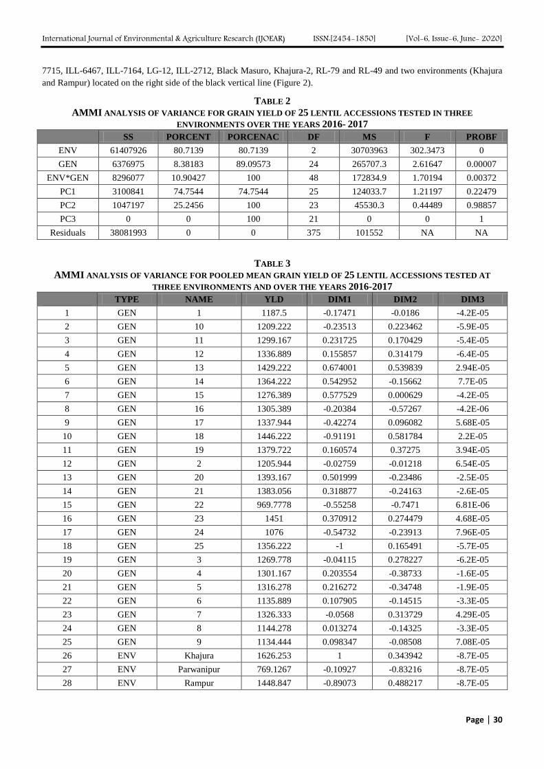
International Journal of Environmental & Agriculture Research (IJOEAR) ISSN:[2454-1850] [Vol-6, Issue-6, June- 2020]
Page | 30
7715, ILL-6467, ILL-7164, LG-12, ILL-2712, Black Masuro, Khajura-2, RL-79 and RL-49 and two environments (Khajura
and Rampur) located on the right side of the black vertical line (Figure 2).
TABLE 2
AMMI ANALYSIS OF VARIANCE FOR GRAIN YIELD OF 25 LENTIL ACCESSIONS TESTED IN THREE
ENVIRONMENTS OVER THE YEARS 2016- 2017
SS PORCENT PORCENAC DF MS F PROBF
ENV 61407926 80.7139 80.7139 2 30703963 302.3473 0
GEN 6376975 8.38183 89.09573 24 265707.3 2.61647 0.00007
ENV*GEN 8296077 10.90427 100 48 172834.9 1.70194 0.00372
PC1 3100841 74.7544 74.7544 25 124033.7 1.21197 0.22479
PC2 1047197 25.2456 100 23 45530.3 0.44489 0.98857
PC3 0 0 100 21 0 0 1
Residuals 38081993 0 0 375 101552 NA NA
TABLE 3
AMMI ANALYSIS OF VARIANCE FOR POOLED MEAN GRAIN YIELD OF 25 LENTIL ACCESSIONS TESTED AT
THREE ENVIRONMENTS AND OVER THE YEARS 2016-2017
TYPE NAME YLD DIM1 DIM2 DIM3
1 GEN 1 1187.5 -0.17471 -0.0186 -4.2E-05
2 GEN 10 1209.222 -0.23513 0.223462 -5.9E-05
3 GEN 11 1299.167 0.231725 0.170429 -5.4E-05
4 GEN 12 1336.889 0.155857 0.314179 -6.4E-05
5 GEN 13 1429.222 0.674001 0.539839 2.94E-05
6 GEN 14 1364.222 0.542952 -0.15662 7.7E-05
7 GEN 15 1276.389 0.577529 0.000629 -4.2E-05
8 GEN 16 1305.389 -0.20384 -0.57267 -4.2E-06
9 GEN 17 1337.944 -0.42274 0.096082 5.68E-05
10 GEN 18 1446.222 -0.91191 0.581784 2.2E-05
11 GEN 19 1379.722 0.160574 0.37275 3.94E-05
12 GEN 2 1205.944 -0.02759 -0.01218 6.54E-05
13 GEN 20 1393.167 0.501999 -0.23486 -2.5E-05
14 GEN 21 1383.056 0.318877 -0.24163 -2.6E-05
15 GEN 22 969.7778 -0.55258 -0.7471 6.81E-06
16 GEN 23 1451 0.370912 0.274479 4.68E-05
17 GEN 24 1076 -0.54732 -0.23913 7.96E-05
18 GEN 25 1356.222 -1 0.165491 -5.7E-05
19 GEN 3 1269.778 -0.04115 0.278227 -6.2E-05
20 GEN 4 1301.167 0.203554 -0.38733 -1.6E-05
21 GEN 5 1316.278 0.216272 -0.34748 -1.9E-05
22 GEN 6 1135.889 0.107905 -0.14515 -3.3E-05
23 GEN 7 1326.333 -0.0568 0.313729 4.29E-05
24 GEN 8 1144.278 0.013274 -0.14325 -3.3E-05
25 GEN 9 1134.444 0.098347 -0.08508 7.08E-05
26 ENV Khajura 1626.253 1 0.343942 -8.7E-05
27 ENV Parwanipur 769.1267 -0.10927 -0.83216 -8.7E-05
28 ENV Rampur 1448.847 -0.89073 0.488217 -8.7E-05
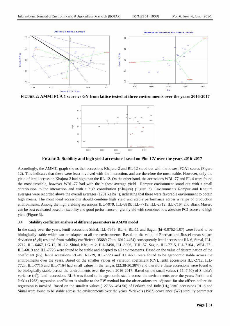
International Journal of Environmental & Agriculture Research (IJOEAR) ISSN:[2454-1850] [Vol-6, Issue-6, June- 2020]
Page | 31
FIGURE 2: AMMI PCA 1 score vs GY from lattice tested at three environments over the years 2016-2017
FIGURE 3: Stability and high yield accessions based on Plot CV over the years 2016-2017
Accordingly, the AMMI1 graph shows that accessions Khajura-2 and RL-12 stood out with the lowest PCA1 scores (Figure
12). This indicates that these were least involved with the interaction, and are therefore the most stable. However, only the
yield of lentil accession Khajura-2 had high than the RL-12. On the other hand, the accessions WBL-77 and PL-4 were found
the most unstable, however WBL-77 had with the highest average yield. Rampur environment stood out with a small
contribution to the interaction and with a high contribution (Khajura) (Figure 3). Environments Rampur and Khajura
averages were recorded above the overall averages (1281 kg ha–1
), indicating that these were favorable environment to obtain
high means. The most ideal accessions should combine high yield and stable performance across a range of production
environments. Among the high yielding accessions ILL-7979, ILL-6819, ILL-7715, ILL-2712, ILL-7164 and Black Masuro
can be best evaluated based on stability and good performance of grain yield with combined low absolute PC1 score and high
yield (Figure 3).
3.4 Stability coefficient analysis of different parameters in AMMI model
In the study over the years, lentil accessions Shital, ILL-7979, RL_6, RL-11 and Sagun (bi=0.9752-1.07) were found to be
biologically stable which can be adapted to all the environments. Based on the value of Eberhart and Russel mean square
deviation (S2di) resulted from stability coefficient -35689.79 to -6012.4454) consequently lentil accessions RL-6, Simal, ILL-
2712, ILL-6467, LG-12, RL-12, Shital, Khajura-2, ILL-3490, ILL-8006, HUL-57, Sagun, ILL-7715, ILL-7164 , WBL-77 ,
ILL-6819 and ILL-7723 were found to be stable and adapted to all environments. Based on the value of determination of the
coefficient (R2), lentil accessions RL-49, RL-79, ILL-7723 and ILL-4605 were found to be agronomic stable across the
environments over the years. Based on the smaller values of variation coefficient (CV), lentil accessions ILL-2712, ILL-
7723, ILL-7715 and ILL-7164 had small values in the ranges (22.38-30.38%) and therefore these accessions were found to
be biologically stable across the environments over the years 2016-2017. Based on the small values (-1147.50) of Shukla's
variance (ri2), lentil accessions RL-6 was found to be agronomic stable across the environments over the years. Perkin and
Jink’s (1968) regression coefficient is similar to the FW method but the observations are adjusted for site effects before the
regression is invoked. Based on the smallest values (127.56 -454.56) of Perkin's and Jinks(DJi) lentil accessions RL-6 and
Simal were found to be stable across the environments over the years. Wricke’s (1962) ecovalance (W2) stability parameter
-1.0 -0.5 0.0 0.5 1.0
-1.0
-0.5
0.0
0.5
1.0
AMMI GY from a Lattice
Factor 1 ( 74.75 %)
Fact
or 2
( 25
.25
%)
1
1011
12
13
14
15
16
17
18
19
2
2021
22
23
24
25
3
45
6
7
8
9
Khajura
Parwanipur
Rampur
800 1000 1200 1400 1600
-1.0
-0.5
0.0
0.5
1.0
AMMI PCA1 Score vs GY from a Lattice
GY
Fact
or 1
( 74
.75
%)
1
10
11
12
13
1415
16
17
18
19
2
20
21
22
23
24
25
3
4 5
6
7
8
9
Khajura
Parwanipur
Rampur
1000 1100 1200 1300 1400
2530
3540
45
Mean
CV(%
) 1
1011
12
13
14
1518
19
2
22
23
24
25
3
6
7
8
9
16
17 20
21
45
Good performance and stable
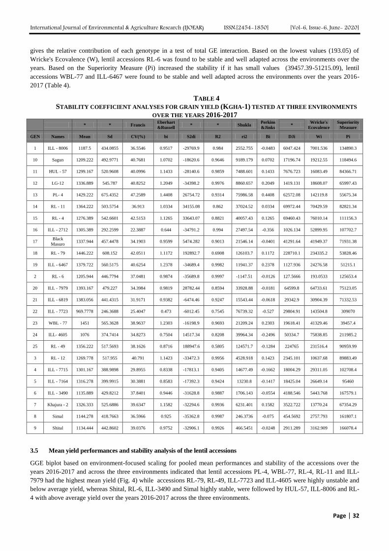
International Journal of Environmental & Agriculture Research (IJOEAR) ISSN:[2454-1850] [Vol-6, Issue-6, June- 2020]
Page | 32
gives the relative contribution of each genotype in a test of total GE interaction. Based on the lowest values (193.05) of
Wricke's Ecovalence (W), lentil accessions RL-6 was found to be stable and well adapted across the environments over the
years. Based on the Superiority Measure (Pi) increased the stability if it has small values (39457.39-51215.09), lentil
accessions WBL-77 and ILL-6467 were found to be stable and well adapted across the environments over the years 2016-
2017 (Table 4).
TABLE 4
STABILITY COEFFICIENT ANALYSES FOR GRAIN YIELD (KGHA-1) TESTED AT THREE ENVIRONMENTS
OVER THE YEARS 2016-2017
* * Francis
Eberhart
&Russell * * Shukla
Perkins
&Jinks *
Wricke's
Ecovalence
Superiority
Measure
GEN Names Mean Sd CV(%) bi S2di R2 ri2 Bi DJi Wi Pi
1 ILL - 8006 1187.5 434.0855 36.5546 0.9517 -29769.9 0.984 2552.755 -0.0483 6047.424 7001.536 134890.3
10 Sagun 1209.222 492.9771 40.7681 1.0702 -18620.6 0.9646 9189.179 0.0702 17196.74 19212.55 118494.6
11 HUL - 57 1299.167 520.9608 40.0996 1.1433 -28140.6 0.9859 7488.601 0.1433 7676.723 16083.49 84366.71
12 LG-12 1336.889 545.787 40.8252 1.2049 -34398.2 0.9976 8860.657 0.2049 1419.131 18608.07 65997.43
13 PL- 4 1429.222 675.4352 47.2589 1.4408 26754.72 0.9314 75986.58 0.4408 62572.08 142119.8 55675.34
14 RL - 11 1364.222 503.5754 36.913 1.0334 34155.08 0.862 37024.52 0.0334 69972.44 70429.59 82821.34
15 RL - 4 1276.389 542.6601 42.5153 1.1265 33643.07 0.8821 40057.43 0.1265 69460.43 76010.14 111156.3
16 ILL - 2712 1305.389 292.2599 22.3887 0.644 -34791.2 0.994 27497.54 -0.356 1026.134 52899.95 107702.7
17 Black
Masuro 1337.944 457.4478 34.1903 0.9599 5474.282 0.9013 21546.14 -0.0401 41291.64 41949.37 71931.38
18 RL - 79 1446.222 608.152 42.0511 1.1172 192892.7 0.6908 126103.7 0.1172 228710.1 234335.2 53828.46
19 ILL - 6467 1379.722 560.5175 40.6254 1.2378 -34689.4 0.9982 11941.37 0.2378 1127.936 24276.58 51215.1
2 RL - 6 1205.944 446.7794 37.0481 0.9874 -35689.8 0.9997 -1147.51 -0.0126 127.5666 193.0533 125653.4
20 ILL - 7979 1393.167 479.227 34.3984 0.9819 28782.44 0.8594 33928.88 -0.0181 64599.8 64733.61 75123.05
21 ILL - 6819 1383.056 441.4315 31.9171 0.9382 -6474.46 0.9247 15543.44 -0.0618 29342.9 30904.39 71332.53
22 ILL - 7723 969.7778 246.3688 25.4047 0.473 -6012.45 0.7545 76739.32 -0.527 29804.91 143504.8 309070
23 WBL - 77 1451 565.3628 38.9637 1.2303 -16198.9 0.9693 21209.24 0.2303 19618.41 41329.46 39457.4
24 ILL- 4605 1076 374.7414 34.8273 0.7504 14517.34 0.8208 39964.34 -0.2496 50334.7 75838.85 211985.2
25 RL - 49 1356.222 517.5693 38.1626 0.8716 188947.6 0.5805 124571.7 -0.1284 224765 231516.4 90959.99
3 RL - 12 1269.778 517.955 40.791 1.1423 -33472.3 0.9956 4528.918 0.1423 2345.101 10637.68 89883.49
4 ILL - 7715 1301.167 388.9898 29.8955 0.8338 -17813.1 0.9405 14677.49 -0.1662 18004.29 29311.05 102708.4
5 ILL - 7164 1316.278 399.9915 30.3881 0.8583 -17392.3 0.9424 13230.8 -0.1417 18425.04 26649.14 95460
6 ILL - 3490 1135.889 429.8212 37.8401 0.9446 -31628.8 0.9887 1706.143 -0.0554 4188.546 5443.768 167579.1
7 Khajura - 2 1326.333 525.6886 39.6347 1.1582 -32294.6 0.9936 6231.401 0.1582 3522.722 13770.24 67354.29
8 Simal 1144.278 418.7663 36.5966 0.925 -35362.8 0.9987 246.3736 -0.075 454.5692 2757.793 161807.1
9 Shital 1134.444 442.8602 39.0376 0.9752 -32906.1 0.9926 466.5451 -0.0248 2911.289 3162.909 166078.4
3.5 Mean yield performances and stability analysis of the lentil accessions
GGE biplot based on environment-focused scaling for pooled mean performances and stability of the accessions over the
years 2016-2017 and across the three environments indicated that lentil accessions PL-4, WBL-77, RL-4, RL-11 and ILL-
7979 had the highest mean yield (Fig. 4) while accessions RL-79, RL-49, ILL-7723 and ILL-4605 were highly unstable and
below average yield, whereas Shital, RL-6, ILL-3490 and Simal highly stable, were followed by HUL-57, ILL-8006 and RL-
4 with above average yield over the years 2016-2017 across the three environments.
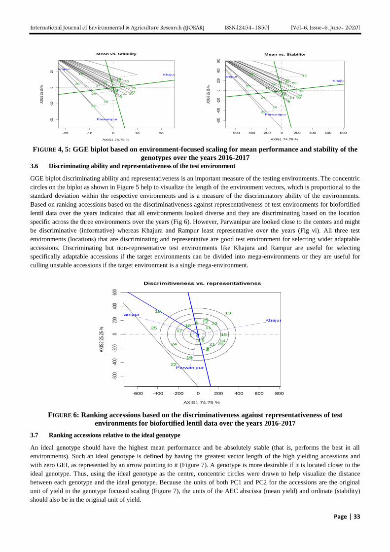
International Journal of Environmental & Agriculture Research (IJOEAR) ISSN:[2454-1850] [Vol-6, Issue-6, June- 2020]
Page | 33
FIGURE 4, 5: GGE biplot based on environment-focused scaling for mean performance and stability of the
genotypes over the years 2016-2017 3.6 Discriminating ability and representativeness of the test environment
GGE biplot discriminating ability and representativeness is an important measure of the testing environments. The concentric
circles on the biplot as shown in Figure 5 help to visualize the length of the environment vectors, which is proportional to the
standard deviation within the respective environments and is a measure of the discriminatory ability of the environments.
Based on ranking accessions based on the discriminativeness against representativeness of test environments for biofortified
lentil data over the years indicated that all environments looked diverse and they are discriminating based on the location
specific across the three environments over the years (Fig 6). However, Parwanipur are looked close to the centers and might
be discriminative (informative) whereas Khajura and Rampur least representative over the years (Fig vi). All three test
environments (locations) that are discriminating and representative are good test environment for selecting wider adaptable
accessions. Discriminating but non-representative test environments like Khajura and Rampur are useful for selecting
specifically adaptable accessions if the target environments can be divided into mega-environments or they are useful for
culling unstable accessions if the target environment is a single mega-environment.
FIGURE 6: Ranking accessions based on the discriminativeness against representativeness of test
environments for biofortified lentil data over the years 2016-2017
3.7 Ranking accessions relative to the ideal genotype
An ideal genotype should have the highest mean performance and be absolutely stable (that is, performs the best in all
environments). Such an ideal genotype is defined by having the greatest vector length of the high yielding accessions and
with zero GEI, as represented by an arrow pointing to it (Figure 7). A genotype is more desirable if it is located closer to the
ideal genotype. Thus, using the ideal genotype as the centre, concentric circles were drawn to help visualize the distance
between each genotype and the ideal genotype. Because the units of both PC1 and PC2 for the accessions are the original
unit of yield in the genotype focused scaling (Figure 7), the units of the AEC abscissa (mean yield) and ordinate (stability)
should also be in the original unit of yield.
-20 -10 0 10 20
-20
-10
010
Mean vs. Stability
AXIS1 74.75 %
AXIS
2 25
.25
%
1
1011
12
14
15
16
17
18
19
2
2021
22
23
24
253
45
6
7
89
Khajura
Parwanipur
Rampur
-600 -400 -200 0 200 400 600 800
-600
-400
-200
020
040
060
0
Mean vs. Stability
AXIS1 74.75 %
AXIS
2 25
.25
%
1
1011
12
13
14
15
16
17
18
19
2
2021
22
23
24
25
3
45
6
7
89
Khajura
Parwanipur
Rampur
-600 -400 -200 0 200 400 600 800
-600
-400
-200
020
040
060
0
Discrimitiveness vs. representativenss
AXIS1 74.75 %
AXIS
2 25
.25
%
1
1011
12
13
14
15
16
17
18
19
2
2021
22
23
24
25
3
45
6
7
89
Khajura
Parwanipur
Rampur
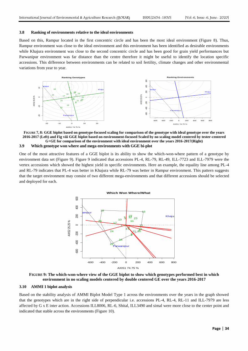
International Journal of Environmental & Agriculture Research (IJOEAR) ISSN:[2454-1850] [Vol-6, Issue-6, June- 2020]
Page | 34
3.8 Ranking of environments relative to the ideal environments
Based on this, Rampur located in the first concentric circle and has been the most ideal environment (Figure 8). Thus,
Rampur environment was close to the ideal environment and this environment has been identified as desirable environments
while Khajura environment was close to the second concentric circle and has been good for grain yield performances but
Parwanipur environment was far distance than the centre therefore it might be useful to identify the location specific
accessions. This difference between environments can be related to soil fertility, climate changes and other environmental
variations from year to year.
FIGURE 7, 8: GGE biplot based on genotype-focused scaling for comparison of the genotype with ideal genotype over the years
2016-2017 (Left) and Fig viii GGE biplot based on environment-focused Scaled by no scaling model centered by tester-centered
G+GE for comparison of the environment with ideal environment over the years 2016-2017(Right)
3.9 Which genotype won where and mega environments with GGE bi-plot
One of the most attractive features of a GGE biplot is its ability to show the which-won-where pattern of a genotype by
environment data set (Figure 9). Figure 9 indicated that accessions PL-4, RL-79, RL-49, ILL-7723 and ILL-7979 were the
vertex accessions which showed the highest yield in specific environments. Here an example, the equality line among PL-4
and RL-79 indicates that PL-4 was better in Khajura while RL-79 was better in Rampur environment. This pattern suggests
that the target environment may consist of two different mega-environments and that different accessions should be selected
and deployed for each.
FIGURE 9: The which-won-where view of the GGE biplot to show which genotypes performed best in which
environment in no scaling models centered by double centered GE over the years 2016-2017
3.10 AMMI 1 biplot analysis
Based on the stability analysis of AMMI Biplot Model Type 1 across the environments over the years in the graph showed
that the genotypes which are in the right side of perpendicular i.e. accessions PL-4, RL-4, RL-11 and ILL-7979 are less
affected by G x E inter action. Accessions ILL8006, RL-6, Shital, ILL3490 and simal were more close to the center point and
indicated that stable across the environments (Figure 10).
-20 -10 0 10 20
-20
-10
010
Ranking Genotypes
AXIS1 74.75 %
AX
IS2
25.2
5 %
1
1011
12
14
15
16
17
18
19
2
2021
22
23
24
253
45
6
7
89
Khajura
Parwanipur
Rampur
-600 -400 -200 0 200 400 600 800
-600
-400
-200
020
040
060
0
Ranking Environments
AXIS1 74.75 %
AXIS
2 25
.25
%
Khajura
Parwanipur
Rampur
-600 -400 -200 0 200 400 600 800
-600
-400
-200
020
040
060
0
Which Won Where/What
AXIS1 74.75 %
AX
IS2
25.2
5 %
1
1011
12
13
14
15
16
17
18
19
2
2021
22
23
24
25
3
45
6
7
89
Khajura
Parwanipur
Rampur
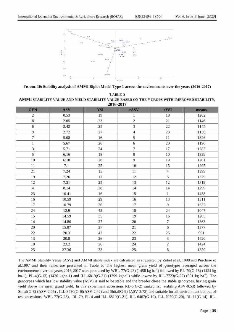
International Journal of Environmental & Agriculture Research (IJOEAR) ISSN:[2454-1850] [Vol-6, Issue-6, June- 2020]
Page | 35
FIGURE 10: Stability analysis of AMMI Biplot Model Type 1 across the environments over the years (2016-2017)
TABLE 5
AMMI STABILITY VALUE AND YIELD STABILITY VALUE BASED ON THE # CROPS WITH IMPROVED STABILITY,
2016-2017
GEN ASV YSI rASV rYSI means
2 0.53 19 1 18 1202
8 2.05 23 2 21 1146
6 2.42 25 3 22 1145
9 2.72 27 4 23 1136
7 5.08 16 5 11 1326
1 5.67 26 6 20 1196
3 5.71 24 7 17 1283
5 6.16 18 8 10 1329
10 6.18 28 9 19 1201
11 7.1 25 10 15 1295
21 7.24 15 11 4 1399
19 7.26 17 12 5 1379
12 7.31 25 13 12 1319
4 8.14 28 14 14 1299
23 10.41 16 15 1 1458
16 10.59 29 16 13 1311
17 10.79 26 17 9 1332
24 12.9 42 18 24 1047
15 14.59 35 19 16 1285
14 14.86 27 20 7 1363
20 15.87 27 21 6 1377
22 20.3 47 22 25 991
13 20.8 26 23 3 1420
18 23.2 26 24 2 1424
25 27.36 33 25 8 1359
The AMMI Stability Value (ASV) and AMMI stable index are calculated as suggested by Zobel et al, 1998 and Purchase et
al.1997 and their ranks are presented in Table 5. The highest mean grain yield of genotypes averaged across the
environments over the years 2016-2017 were produced by WBL-77(G-23) (1458 kg ha-1
) followed by RL-79(G-18) (1424 kg
ha-1), PL-4(G-13) (1420 kgha-1) and ILL-6819(G-21) (1399 kgha-1
) while lowest by ILL-7723(G-22) (991 kg ha-1
). The
genotypes which has low stability value (ASV) is said to be stable and the breeder chose the stable genotypes, having grain
yield above the mean grand yield. In this experiment accessions RL-6(G-2) ranked 1st stability(ASV-0.53) followed by
Simal(G-8) (ASV-2.05) , ILL-3490(G-6)(ASV-2.42) and Shital(G-9) (ASV-2.72) and suitable for all environment but out of
test accessions; WBL-77(G-23), RL-79, PL-4 and ILL-6819(G-21), ILL-6467(G-19), ILL-7979(G-20), RL-11(G-14), RL-
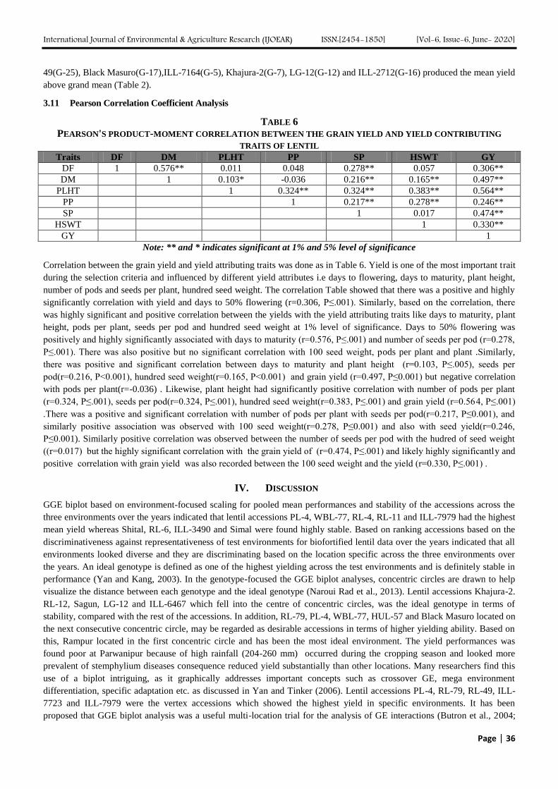
International Journal of Environmental & Agriculture Research (IJOEAR) ISSN:[2454-1850] [Vol-6, Issue-6, June- 2020]
Page | 36
49(G-25), Black Masuro(G-17),ILL-7164(G-5), Khajura-2(G-7), LG-12(G-12) and ILL-2712(G-16) produced the mean yield
above grand mean (Table 2).
3.11 Pearson Correlation Coefficient Analysis
TABLE 6
PEARSON'S PRODUCT-MOMENT CORRELATION BETWEEN THE GRAIN YIELD AND YIELD CONTRIBUTING
TRAITS OF LENTIL Traits DF DM PLHT PP SP HSWT GY
DF 1 0.576** 0.011 0.048 0.278** 0.057 0.306**
DM 1 0.103* -0.036 0.216** 0.165** 0.497**
PLHT 1 0.324** 0.324** 0.383** 0.564**
PP 1 0.217** 0.278** 0.246**
SP 1 0.017 0.474**
HSWT 1 0.330**
GY 1
Note: ** and * indicates significant at 1% and 5% level of significance
Correlation between the grain yield and yield attributing traits was done as in Table 6. Yield is one of the most important trait
during the selection criteria and influenced by different yield attributes i.e days to flowering, days to maturity, plant height,
number of pods and seeds per plant, hundred seed weight. The correlation Table showed that there was a positive and highly
significantly correlation with yield and days to 50% flowering (r=0.306, P≤.001). Similarly, based on the correlation, there
was highly significant and positive correlation between the yields with the yield attributing traits like days to maturity, plant
height, pods per plant, seeds per pod and hundred seed weight at 1% level of significance. Days to 50% flowering was
positively and highly significantly associated with days to maturity (r=0.576, P≤.001) and number of seeds per pod (r=0.278,
P≤.001). There was also positive but no significant correlation with 100 seed weight, pods per plant and plant .Similarly,
there was positive and significant correlation between days to maturity and plant height (r=0.103, P≤.005), seeds per
pod(r=0.216, P<0.001), hundred seed weight(r=0.165, P<0.001) and grain yield (r=0.497, P≤0.001) but negative correlation
with pods per plant(r=-0.036) . Likewise, plant height had significantly positive correlation with number of pods per plant
(r=0.324, P≤.001), seeds per pod(r=0.324, P≤.001), hundred seed weight(r=0.383, P≤.001) and grain yield (r=0.564, P≤.001)
.There was a positive and significant correlation with number of pods per plant with seeds per pod(r=0.217, P≤0.001), and
similarly positive association was observed with 100 seed weight(r=0.278, P≤0.001) and also with seed yield(r=0.246,
P≤0.001). Similarly positive correlation was observed between the number of seeds per pod with the hudred of seed weight
((r=0.017) but the highly significant correlation with the grain yield of (r=0.474, P≤.001) and likely highly significantly and
positive correlation with grain yield was also recorded between the 100 seed weight and the yield (r=0.330, P≤.001) .
IV. DISCUSSION
GGE biplot based on environment-focused scaling for pooled mean performances and stability of the accessions across the
three environments over the years indicated that lentil accessions PL-4, WBL-77, RL-4, RL-11 and ILL-7979 had the highest
mean yield whereas Shital, RL-6, ILL-3490 and Simal were found highly stable. Based on ranking accessions based on the
discriminativeness against representativeness of test environments for biofortified lentil data over the years indicated that all
environments looked diverse and they are discriminating based on the location specific across the three environments over
the years. An ideal genotype is defined as one of the highest yielding across the test environments and is definitely stable in
performance (Yan and Kang, 2003). In the genotype-focused the GGE biplot analyses, concentric circles are drawn to help
visualize the distance between each genotype and the ideal genotype (Naroui Rad et al., 2013). Lentil accessions Khajura-2.
RL-12, Sagun, LG-12 and ILL-6467 which fell into the centre of concentric circles, was the ideal genotype in terms of
stability, compared with the rest of the accessions. In addition, RL-79, PL-4, WBL-77, HUL-57 and Black Masuro located on
the next consecutive concentric circle, may be regarded as desirable accessions in terms of higher yielding ability. Based on
this, Rampur located in the first concentric circle and has been the most ideal environment. The yield performances was
found poor at Parwanipur because of high rainfall (204-260 mm) occurred during the cropping season and looked more
prevalent of stemphylium diseases consequence reduced yield substantially than other locations. Many researchers find this
use of a biplot intriguing, as it graphically addresses important concepts such as crossover GE, mega environment
differentiation, specific adaptation etc. as discussed in Yan and Tinker (2006). Lentil accessions PL-4, RL-79, RL-49, ILL-
7723 and ILL-7979 were the vertex accessions which showed the highest yield in specific environments. It has been
proposed that GGE biplot analysis was a useful multi-location trial for the analysis of GE interactions (Butron et al., 2004;
International Journal of Environmental & Agriculture Research (IJOEAR) ISSN:[2454-1850] [Vol-6, Issue-6, June- 2020]
Page | 37
Fan et al., 2007; Laffont et al., 2007; Yan and Kang, 2003; Samonte et al., 2005) and had been exploited in the variety
evaluation of wheat (Yan and Hunt 2001; Yan et al., 2000), Maize (Fan et al., 2007) and soybean (Yan and Rajcan, 2002).
Based on the stability analysis of AMMI Biplot Model Type 1 across the environments over the years in the graph showed
that the genotypes which are in the right side of perpendicular i.e. accessions PL-4, RL-4, RL-11 and ILL-7979 are less
affected by G x E interaction. Accessions ILL8006, RL-6, Shital, ILL3490 and simal were more close to the center point and
indicated that stable across the environments. In another words, the genotypes which have low stability value (ASV) is said
to be stable and the breeder chose the stable genotypes along with grain yield above the mean grand yield. In this experiment
accessions RL-6(G-2) ranked 1st stability (ASV-0.53) followed by Simal (ASV-2.05), ILL-3490 (ASV-2.42) and Shital
(ASV-2.72) and suitable for all environment. Based on the value of Eberhart and Russel mean square deviation (S2di)
resulted from stability coefficient (-35689.79 to -6012.4454) consequently lentil accessions RL-6, Simal, ILL-2712, ILL-
6467, LG-12, RL-12, Shital, Khajura-2, ILL-3490, ILL-8006, HUL-57, Sagun, ILL-7715, ILL-7164 , WBL-77, ILL-6819
and ILL-7723 were found to be stable and adapted to all environments. Based on the lowest values (193.05) of Wricke's
Ecovalence (W), lentil accessions RL-6 was found to be stable and well adapted across the environments over the years.
Based on the small values (-1147.50) of Shukla's variance (ri2), lentil accessions RL-6 was found to be agronomic stable
across the environment. These stability coefficient parameters showed the diverse results of stable accessions however
accession RL-6 was found the most stable accession because all the stability parameters provided the same results.
Plant breeders consistently face GE interactions when testing genotypes across the environments. Combined pooled mean
analysis of variance (ANOVA) for grain yield tested at three environments over the two subsequent years showed that highly
significant differences in genotypes, environment and G x E interaction effect. From the study, it was concluded that
accession WBL-77 (1451 kg ha-1
), RL-79(1446 kgha-1
) and PL-4(1429 kgha-1
) were the best performer and well adopted
across the environments. The different performance of genotypes across environments could also be indicative of wide
variation in climatic conditions and soil types in the different growing environments. Consequently, comparisons can only be
made in each environment separately (Breese, 1969). Crossa et al. (1991) had noted that the use of AMMI in G x E
interaction analysis would lead to the selection of superior genotypes even in the field experiment. Here, AMMI analysis of
variance for lentil grain yield (tha-1
) of lentil accessions tested at three environments over the years showed that 80.71% of
the total sum of squares was attributed to environmental effects, only 8.38 % to genotypic effects and 10.90% to genotype ×
environment interaction effects. The partitioning of GGE sum of squares through the GGE biplot analysis showed that
PC1and PC2 accounted 74.75%, and 25.24% of GGE sum of squares respectively over the years. In the biplot, a total of
fifteen lentil accessions namely PL-4, RL-11, ILL-6819, ILL-7979, WBL-77, HUL-57, ILL-7715, ILL-6467, ILL-7164, LG-
12, ILL-2712, Black Masuro, Khajura-2, RL-79 and RL-49 and two environments (Khajura and Rampur) located on the right
side of the black vertical line showed the highest yield and more stable accessions. It seems that other statistical models such
as regression procedures are more useful for understanding and describing G x E interactions. The GxE interaction is an
important source of variation in any crop. Geographic differentiation of landraces of lentil emphasizes the specific adaptation
of this crop (Erskine, 1997). According to Freeman (1972), one of the main reasons for growing genotypes over a wide range
of environments is to estimate their stability and adaptability. Biological stability is not acceptable to most plant breeders,
who prefer an agronomic concept of stability. In this concept of stability, it is not necessary for the genotypic response to
environmental conditions to be equal for all genotypes.
V. CONCLUSION
Pooled mean analysis of variance for grain yield tested at three environments over the two subsequent years showed that
highly significant differences in genotypes, environment and G x E interaction effect indicating the possibility of selection
for stable accessions. Research results showed that lentil accession WBL-77 (1451 kg ha-1) , RL-79(1446 kg ha-1) and PL-
4(1429 kg ha-1) were the best performer and well adopted across the environments and over the years. AMMI analysis of
variance for lentil grain yield (tha-1
) of lentil accessions tested at three environments over the years showed that 80.71% of
the total sum of squares was attributed to environmental effects, only 8.38 % to genotypic effects and 10.90% to genotype ×
environment interaction effects. Based on the value of Eberhart and Russel mean square deviation (S2di) resulted from
stability coefficient (-35689.79 to -6012.4454) consequently lentil accessions RL-6, Simal, ILL-2712, ILL-6467, LG-12, RL-
12, Shital, Khajura-2, ILL-3490, ILL-8006, HUL-57, Sagun, ILL-7715, ILL-7164 , WBL-77, ILL-6819 and ILL-7723 were
found to be stable and adapted to all environments. Accessions ILL8006, RL-6, Shital, ILL3490 and simal were more close
to the center point and indicated that stable across the environments. In another words, the genotypes which have low
stability value (ASV) is said to be stable and the breeder chose the stable genotypes along with grain yield above the mean
International Journal of Environmental & Agriculture Research (IJOEAR) ISSN:[2454-1850] [Vol-6, Issue-6, June- 2020]
Page | 38
grand yield. In this experiment accessions RL-6(G-2) ranked 1st stability (ASV-0.53) followed by Simal (ASV-2.05), ILL-
3490 (ASV-2.42) and Shital (ASV-2.72) and suitable for all environment.
ACKNOWLEDGEMENTS
The authors would like to thanks to Agriculture and Food Security Project (AFSP) and NARC management team for
executing the G x E trials in different station. We would also like to acknowledge the Department of Genetics and Plant
Breeding, Agriculture and Forestry University, Rampur, Chitwan for frequent guiding to record the traits. Special thanks go
to the technical staffs of Grain Legumes Research Program for helping to conduct the experiment in the station.
REFERENCES
[1] Ali, Y., and Sarwar, G., (2008). Genotype x environment interaction of cowpea genotypes. International. Journal of Environmental
Research 2: 125-132.
[2] Allard, R W, and Bradshaw, A D. 1964. Implications of genotype-environmental interactions in applied plant breeding. Crop Sci, 4,
503–508.
[3] Ariyo , Omolayo and Ayo-Vaughan, Monininuola, 2000, Analysis of genotype x environment interaction of okra (Abelmoschus
esculentus (L) Moench) published in Journal of Genetics and Breeding 54(1):35-40
[4] BECKER H.C., 1981. Correlations among some statistical measures of phenotypic stability. Euphytica 30, 835-840.
[5] Breese, E. L., 1969. The measurement and significance of genotype environment interactions in grasses. Heredity 24: 27–44.
[6] Bull, J.K., Cooper, M., Delacy, I.H., Bassford, K.E. and Woodruff, D.R. 1992. Utility of repeated checks for hierarchical
classification of data from plant breeding trials. Field Crop Res., 30: 79-95.
[7] Ceccarelli, S., 1989. Wide adaptation: How wide. Euphytica, 40: 197-205.
[8] COMSTOCK, R. E. and MOLL' R. H. 1963. Genotype-environment interactions. Pages 164-196 in Statistical genetics and plant
breeding. Nat. Acad. Sci.-Nat' Res. Counc' Publ. No. 982. Washington, D.C
[9] Danyali, S. F., Razavi, F., Ebadi-Segherloo, A., Dehghani, H., Sabaghpour, S. H., (2012). Yield stability in chickpea (Cicer arietinum
L.) and study relationship among the univariate and multivariate stability parameters. Research in Plant Biology, 2: 46-61
[10] DELACY I.H., BASFORD K.E., COOPER M., BULL J.K., MCLAREN C.G., 1996. Analysis of multi-environment trail an
historical perspective. In: Plant adaptation and crop improvement (Cooper M., Hammer G.L., eds). CAB International: Wallingford,
UK. pp.39-124
[11] Eberhart SA, Russell WA (1969) Yield stability for a 10-line diallel of single-cross and double-cross maize hybrids. Crop Sci 9:357–
361
[12] Eberhart, S.A., and W. A. Russell. 1966. Stability parameters for comparing varieties. Crop Sciences 6:36-40.
[13] Erskine, W. 2009. Global production, supply and demand. In: W. Erskine et al., editors, The lentil: Botany, production and uses.
CAB Int., Wallingford, UK. p. 4–12
[14] Finlay, K.W., and G.N. Wilkinson. 1963. Th e analysis of adaptation in a plant-breeding program. Aust. J. Agric. Res. 14:742–754.
[15] Flores, F., M.T. Moreno, and J.I. Cubero. 1998. A comparison of univariate and multivariate methods to analyze environments. Field
Crops Res. 56:271–286.
[16] Flores, G.V., Daga, A., Kalhor, H.R., Banerjee, U. (1998). Lozenge is expressed in pluripotent precursor cells and patterns multiple
cell types in the Drosophila eye through the control of cell-specific transcription factors. Development 125(18): 3681--3687.
[17] France YE, et al. (2006) The polarity-establishment component Bem1p interacts with the exocyst complex through the Sec15p
subunit. J Cell Sci 119(Pt 5):876-88
[18] Francis T R and Kannenberg L W. 1978. Yield stability studies in short-season maize: I. A descriptive method for grouping
genotypes. Canadian Journal of Plant Science 58 (4): 1029–34.
[19] Funnah, S.M. and C. Mak. 1980. Yield stability studies in soybean. Expt. Agr. 16:357-392
[20] Gauch, H.G. 1988. Model selection for yield trials with interaction. Biometrics 44:705–715.
[21] Gauch, H.G., and R.W. Zobel. 1988. Predictive and postdictive success of statistical analyses of yield trials. Th eor. Appl. Genet.
76:1–10.
[22] Gauch, H.G., and R.W. Zobel. 1996. AMMI analysis of yield trials. p. 85–122. In M.S. Kang and H.G. Gauch, Jr. (ed.) Genotype by
environment interaction.
[23] Gebremedhin, W, M. Firew and B. Tesfye. 2014. Stability analysis of food barley genotypes in northern Ethiopia. African Crop
Science Journal 22,145–153.
[24] Gollob, H.F. 1968. A statistical model that combines features of factor analysis and analysis of variance techniques. Psycrometrika
33: 73-115.
[25] HERNÁNDEZ C.M., CROSSA J., CASTILLO A., 1993. The area under the function: an index for selecting desirable genotypes.
Theor Appl Genet 87, 409-415.
[26] Hinsta, G, A. Hailemariam and T. Belay. 2011. Genotype-byenvironment interaction and grain yield stability of early maturing bread
wheat (Triticum aestivum L) genotypes in the drought prone areas of Tigray region, Northern Ethiopia. Ethiopian Journal of Applied
Science and Technology 2: 51– 57. Hintsa,
International Journal of Environmental & Agriculture Research (IJOEAR) ISSN:[2454-1850] [Vol-6, Issue-6, June- 2020]
Page | 39
[27] Hintsa Gebru and Fetien Abay. 2013. Evaluation of bread wheat varieties for their adaptability in wheat growing areas of Tigray
region, northern Ethiopia. Journal ofbiodiversity and enda ngered species. 1:12-18.
[28] Ilker, E., Tatar, O., Aykut Tonk, F., Tosun, M., Turk, J. (2011). Determination of Tolerance Level of Some Wheat Genotypes to
Post-Anthesis Drought. Turkish Journal of Field Crops, 16(1): 59-63.
[29] LIN C.S., BINNS M.R., 1988. A superiority measure of cultivar performance for cultivar × location data. Can J Plant Sci 68, 193-
198.
[30] MOAD (2016) Statistical Information of Nepalese Agriculture. Agri-Business Promotion and Statistics Division, Ministry of
Agriculture Development, Kathmandu, Nepal
[31] Naroui, M.R.R., M.A. Kadir, M. Y. Rafii, Z. E. Hawa Jaafar, M. R. Naghavi and F. Ahmadi. 2013. Genotype × environment
interaction by AMMI and GGE biplot analysis in three consecutive generations of wheat (Triticum aestivum) under normal and
drought stress conditions. AJS 7 (7):956-961.
[32] Perkins, Jean M, and Jinks, J L. 1968a. Environmental and genotype-environmental components of variability. III. Multiple lines and
crosses. Heredity, 23, 339–356.
[33] Perkins, Jean M, and Jinks, J L. 1968b. Environmental and genotype-environmental components of variability. IV. Non-linear
interactions for multiple inbred lines. Heredity, 23, 525–535.
[34] PINTHUS J.M., 1973. Estimate of genotype value: a proposed method. Euphytica 22, 121-123
[35] Sabaghnia N, Mohammadi M. Karimizadeh R (2012b). The evaluation of genotype × environment interactions of durum wheat’s
yield using of the AMMI model. Agric. Fores. 55:5–21.
[36] Sabaghnia, N., S.H. Sabaghpour, and H. Dehghani. 2008. The use of an AMMI model and its parameters to analyse yield stability in
multi-environment trials. Journal of Agricultural Science 146:571-581.
[37] Samonte, S.O.P.B., L.T. Wilson, A.M. McClung, and J.C. Medley. 2005. Targeting cultivars onto rice growing environments using
AMMI and SREG GGE biplot analyses. Crop Sci. 45:2414–2424.
[38] Sarker A., W. Erskine and M. Singh, 2003. Regression models for lentil seed and straw yields in Near East. Agr. Forest Meteorol.,
116: 61-72.
[39] SHUKLA G.K., 1972. Some statistical aspects of partitioning genotype environmental components of variability. Heredity 29,
237–245.
[40] Shukla, G K. 1972a. Some statistical aspects of partitioning genotype-environmental components of variability. Heredity, 29, 237–
245.
[41] Shukla, G K. 1972b. Application of some multivariate techniques in the analysis and interpretation of the genotype-environment
interaction. Paper presented at the Symposium on Genotype × Environment Interactions, Birmingham University, September, 1972.
[42] WRICKE G., 1962. Über eine Methode zur Erfassung der ökologischen Streubreite in Feldversuchen. Z Pflanzenzücht 47, 92-96. [In
German].
[43] Wricke, G. 1962. Uber eine Methode zur Erfassung der ökologischen Streubreite in Feldversuchen. Z Pflzücht, 47, 92–96.
[44] Yan W, Tinker NA (2006). Biplot analysis of multi-environment trial data: principles and application. Candian J. Plant Sci. 86:623-
645.
[45] Yan, W and I. Rajcan. 2002. Biplots analysis of the test sites and trait relations of soybean in Ontario. Crop Science 42: 11-20
[46] Yan, W. 2001. GGE biplot–A windows application for graphical analysis of multienvironment trial data and other types of two-way
data. Agron. J. 93:1111–1118.
[47] Yan, W. 2002. Singular value partitioning in biplot analysis of multi environment trial data. Agron. J. 94:990–996. ISSN: 1435-
0645.
[48] Yan, W. 2002. Singular value partitioning in biplot analysis of multievironment trial data. Agron. J. 94:990–996.
[49] Yan, W., and Holland, J. B. (2010). A heritability-adjusted GGE biplot for test environment evaluation. Euphytica 171, 355–369.
doi: 10.1007/s10681-009-0030-5
[50] Yan, W., and I. Rajcan. 2002. Biplot evaluation of test sites and trait relations of soybean in Ontario. Crop Sci. 42:11–20.
[51] Yan, W., L.A. Hunt, Q. Sheng and Z. Szlavnics. 2000. Cultivar evaluation and mega-environment investigation based on the GGE
biplot. Crop Sci. 40:597–605. ISSN 1435-0653.
[52] Yan, W., M.S. Kang, B. Ma, S. Woods and P.L. Cornelius. 2007. GGE biplot vs. AMMI analysis of genotype-by-environment data.
Crop Science 47: 643–655.
[53] Yan, W., P.L. Cornelius, J. Crossa and L.A. Hunt. 2001. Two types of GGE biplots for analyzing multi-environment trial data. Crop
Sci. 41:656-663.
[54] Yang R.-C, Crossa J, Cornelius PL, Burgueo J (2009). Biplot analysis of geno-type environment interaction: Proceed with caution.
Crop Sci. Soc. Am. 49:1564-1576.
[55] Yates, F, and Cochran, W G. 1938. The analysis of groups of experiments. J agric Sci, Camb, 28, 556–580.
[56] Yau, S.K. 1995. Regression and AMMI analyses of genotype × environment interactions: An empirical comparison. Agron. J.
87:121–126.
[57] Zobel, R.W., M.J. Wright, and H.G. Gauch, Jr. 1988. Statistical analysis of a yield trial. Agron. J. 80:388–393
[58] Gauch HG (1988) Model selection and validation for yield trials with interaction. Biometrics 44:705–715
[59] Gauch HG, Piepho HP and Annicchiarico P (2008) Statistical analysis of yield trials by AMMI and GGE: Further considerations.
Crop Sci. 48:866–889.
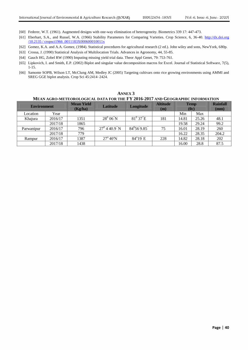
International Journal of Environmental & Agriculture Research (IJOEAR) ISSN:[2454-1850] [Vol-6, Issue-6, June- 2020]
Page | 40
[60] Federer, W.T. (1961). Augmented designs with one-way elimination of heterogeneity. Biometrics 339 17: 447-473.
[61] Eberhart, S.A., and Russel, W.A. (1966) Stability Parameters for Comparing Varieties. Crop Science, 6, 36-40. http://dx.doi.org
/10.2135 / cropsci1966 .0011183X000600010011x
[62] Gomez, K.A. and A.A. Gomez, (1984). Statistical procedures for agricultural research (2 ed.). John wiley and sons, NewYork, 680p.
[63] Crossa, J. (1990) Statistical Analysis of Multilocation Trials. Advances in Agronomy, 44, 55-85.
[64] Gauch HG, Zobel RW (1990) Imputing missing yield trial data. Theor Appl Genet, 79: 753-761.
[65] Lipkovich, I. and Smith, E.P. (2002) Biplot and singular value decomposition macros for Excel. Journal of Statistical Software, 7(5),
1-15.
[66] Samonte SOPB, Wilson LT, McClung AM, Medley JC (2005) Targeting cultivars onto rice growing environments using AMMI and
SREG GGE biplot analysis. Crop Sci 45:2414–2424.
ANNEX 3
MEAN AGRO-METEOROLOGICAL DATA FOR THE FY 2016-2017 AND GEOGRAPHIC INFORMATION
Environment Mean Yield
(Kg/ha) Latitude Longitude
Altitude
(m)
Temp
(0c)
Rainfall
(mm)
Location Year Min Max
Khajura 2016/17 1351 280 06
”N 81
0 37
”E 181 14.81 25.26 48.1
2017/18 1865 19.58 29.24 99.2
Parwanipur 2016/17 796 270 4
’40.9
’’N 84
056
’9.85
” 75 16.01 28.19 260
2017/18 779 16.22 28.35 204.2
Rampur 2016/17 1387 27o 40′N 84
o19
′ E 228 14.82 28.18 202
2017/18 1438 16.00 28.8 87.5