Advances in Network Tomography

Edoardo M. Airoldi

Center for Automated Learning and Discovery

eairoldi@cs.cmu.edu

October 2003

CMU-CALD-03-101

School of Computer ScienceCarnegie Mellon University

Pittsburgh, PA 15213

Abstract

Knowledge about the origin-destination (OD) traffic matrix allows us to solve problems in design,routing, configuration debugging, monitoring and pricing. Direct measurement of these flows isusually not implemented because it is too expensive. A recent work provided a quick methodto learn the OD traffic matrix from a set of available standard measurements, which correspondtraffic flows observed on the link of a network every 5 minutes. Such a time span allows for morecomputationally expensive methods that in turn yield a better estimate of the OD traffic matrix.In this work we are the first to explicitly introduce time in learning the OD traffic matrix. Thesecond contribution is that we are the first to use realistic non-Gaussian marginals, specificallythe Gamma and the successful log-Normal ones. We combine both these ideas in a novel, doublystochastic and time-varying Bayesian dynamical system, and provide a simple and elegant solutionto obtain informative prior distributions for the stochastic dynamical behavior. Our method out-performs existing solutions in a realistic setting.

Keywords: Origin-Destination Traffic Flows, Link Loads, Inverse Problem, TransportationProblem, Log-Normal, Gamma, State-Space Model, MCMC, Bayesian Dynamical System, ParticleFilter, Stochastic Dynamics, Informative Priors, non-parametric Empirical Bayes

Acknowledgments

I am grateful to my advisor Prof. Christos N. Faloutsos for presenting me with the problem ofthe reconstruction of the origin-destination flows from observable link loads, for valuable commentsand suggestions, and for his enthusiasm and his continuous support during all the phases of thisexciting project.

I wish to thank Prof. Srinivasan Seshan, Dr. Russel Yount and Dr. Frank Kietzke for providingme with their expertise, and for retrieving origin-destination traffic flows and link loads on CarnegieMellon local area network, necessary to validate the methods we proposed. Dr. Frank Kietzkecontributed during several stages of this study with comments and suggestions, and kindly providedme with detailed explanations on technical aspects of the problem.

Further I wish to thank Prof. Stephen E. Fienberg, and Prof. Christopher Genovese for theircomments and suggestions at an early stage of this project, and Prof. Anthony Brockwell for helpfuldiscussion of several aspects of the problem, and for pointing me towards relevant literature.

1

Contents

1 Introduction 31.1 Problem Definition . . . . . . . . . . . . . . . . . . . . . . . . . . . . . . . . . . . . . 3

2 Literature Review 52.1 Transportation Research . . . . . . . . . . . . . . . . . . . . . . . . . . . . . . . . . . 82.2 Statistical Research . . . . . . . . . . . . . . . . . . . . . . . . . . . . . . . . . . . . . 8

2.2.1 A Recent Local Maximum Likelihood Approach . . . . . . . . . . . . . . . . . 9

3 Proposed Methods 123.1 Explicit Dynamics for Gaussian Origin-Destination Flows . . . . . . . . . . . . . . . 12

3.1.1 A State-Space Representation for the Model . . . . . . . . . . . . . . . . . . . 133.1.2 Ad-Hoc M-Step for the EM Algorithm . . . . . . . . . . . . . . . . . . . . . . 143.1.3 Two-Stages Maximization of the Likelihood . . . . . . . . . . . . . . . . . . . 15

3.2 1-Time Non-Gaussian Origin-Destination Flows . . . . . . . . . . . . . . . . . . . . . 153.2.1 Computing the Support . . . . . . . . . . . . . . . . . . . . . . . . . . . . . . 163.2.2 Irreducibility of the Chain . . . . . . . . . . . . . . . . . . . . . . . . . . . . . 163.2.3 Gamma and log-Normal Models . . . . . . . . . . . . . . . . . . . . . . . . . 173.2.4 Informative priors . . . . . . . . . . . . . . . . . . . . . . . . . . . . . . . . . 19

3.3 Combining Dynamics and Non-Gaussianity . . . . . . . . . . . . . . . . . . . . . . . 193.3.1 Informative Priors for Stochastic Dynamics . . . . . . . . . . . . . . . . . . . 193.3.2 Bayesian Dynamical Systems . . . . . . . . . . . . . . . . . . . . . . . . . . . 203.3.3 Particle Filter via SIR-Move Algorithm . . . . . . . . . . . . . . . . . . . . . 20

3.4 Multivariate Integration . . . . . . . . . . . . . . . . . . . . . . . . . . . . . . . . . . 21

4 Experiments 224.1 Exploring Carnegie Mellon Network . . . . . . . . . . . . . . . . . . . . . . . . . . . 22

4.1.1 Empirical Distributions of the OD Flows . . . . . . . . . . . . . . . . . . . . . 244.1.2 Modeling the Coefficients of Constant Association αij . . . . . . . . . . . . . 25

4.2 Exact Recovery Algorithms for Sparse Traffic Situations . . . . . . . . . . . . . . . . 254.3 Intense Traffic Sub-Networks at Carnegie Mellon . . . . . . . . . . . . . . . . . . . . 25

4.3.1 Naive SVD Solution for Strongly Correlated Flows . . . . . . . . . . . . . . . 254.3.2 Local Dynamical Behavior . . . . . . . . . . . . . . . . . . . . . . . . . . . . . 264.3.3 A Case Study: the Star Network Topology . . . . . . . . . . . . . . . . . . . 27

5 Conclusions 32

A Gaussian Dynamical System 35A.1 EM algorithm . . . . . . . . . . . . . . . . . . . . . . . . . . . . . . . . . . . . . . . . 35A.2 More computational efficiency . . . . . . . . . . . . . . . . . . . . . . . . . . . . . . . 36A.3 KF posteriors . . . . . . . . . . . . . . . . . . . . . . . . . . . . . . . . . . . . . . . . 36

A.3.1 One Y to one X . . . . . . . . . . . . . . . . . . . . . . . . . . . . . . . . . . 36A.3.2 One Y to many Xs . . . . . . . . . . . . . . . . . . . . . . . . . . . . . . . . . 37

B The Key to fig n.10. 39

2

1 Introduction

Knowledge about the origin-destination (OD) traffic matrix allows us to solve problems in design,routing, configuration debugging, monitoring and pricing; in fact the OD traffic matrix provides uswith valuable information about who is communicating with whom in a local area network, at anygiven time. Most routers are not able to measure the OD traffic flows, though. Further the directmeasurement of OD traffic flows via SNMP queries is never implemented on the few models thatwould technically allow it, because usually infeasible. Approximate methods have been recentlyproposed in order to infer the OD traffic matrix from a set of standard measurements, trafficloads on the links of the network produced every 5 minutes. Such a delay between successivemeasurements allows for computational methods that produce better estimates for the OD trafficmatrix.

We improved the models present in the literature by introducing two realistic assumptions: (1)we modeled the marginal OD traffic flows with skewed distributions like Gamma and log-Normal,and (2) we introduced time dependence among the OD flows explicitly by means of a stochasticdynamical behavior, in our self-organizing Bayesian dynamical system. The Gamma and log-Normal models reduced by 25% and 38%, respectively, the estimation error yielded by recentlyproposed solutions; the introduction of explicit stochastic local dynamics reduced the estimationerror up to 41% and 46%, respectively. The magnitude of the improvements entailed by the simpleideas we propose went far beyond that of state-of-the-art resampling schemes that could be usedto refine any given set of estimates. Further the stochastic dynamics played an essential role in ourmodels; it served as the right channel where to introduce prior information about the OD flows, andmitigated the problem of multiple modes in a certain probabilistic mapping to be defined below.

The outline of this report is as follows: in the remainder of this section we formulate theproblem with Xs and Y s; in section 2 we survey past approaches to the problem and point outtheir weaknesses; in section 3 we detail our proposed methods; in section 4 we explore real data fromCarnegie-Mellon Local Area Network, apply our methods and models, and compare our estimatesto those provided by current state-of-the-art solutions; and finally in section 5 we conclude withsome remarks.

1.1 Problem Definition

We begin by giving a mathematical characterization of the problem.

Problem. Given observations Y (t) := [Y1(t), . . . , Y`(t)]′ over times t = 1, . . . , T , and a ma-

trix A(`×κ) such that Y (t) = AX(t) ∀t, we want to estimate the unobservable inputs X(t) :=

[X1(t), . . . , Xκ(t)]′ over times t = 1, . . . , T . It is always κ ≥ `, and in general κ = O(`2).

The formulation above is common to many applications; in this project we were interested innetwork traffic analysis. We observed traffic loads on the links of a network with terminal nodes,and routing nodes1, and we were interested in estimating the traffic flows between all, or selectedpairs, of terminal nodes. Hence in our problem the vector of observations Y (t) would contain the setof measurements on the links of the network available at time t, and the vector X(t) would containnon-observable origin-destination flows between pairs of terminal nodes at time t. The relevantinformation to characterize the structure of the network2 would be contained in the matrix A, timeindependent, which tells us exactly how the flows X(t) combine to form the observed link loadsY (t) through the equations Y (t) = AX(t) at each point in time.

1Namely routers and switches, which did not create or absorb traffic, but merely filtered it and/or redirected it.2We restricted our attention to the cases where A would entail a deterministic routing scheme.

3

A First Example

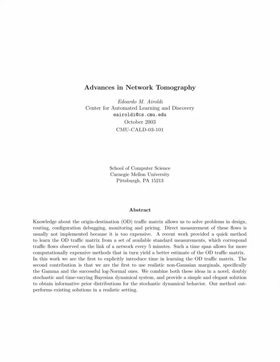
Consider figure 1, the central node represents a router, whereas the external nodes represent sub-networks. In the terminology above the router is a routing node, and the sub-networks are terminalnodes, and we wanted to estimate the flows between them. Throughout this report we referred tothe non-observable flows between pairs of terminal nodes (the dashed arrows) as origin-destination(OD) flows, whereas we referred to the measurable loads on the directed links of the graph (thesolid arrows) as link flows. We studied traffic flows in terms of Kbytes. More precisely we wereinterested in estimating the probability of observing a certain amount of traffic Xi(t) over eachorigin-destination route i. In the sample network in figure 1 the information transits through the

Node

no.2

Node

no.1

Y2

Y1 Y4

Y3

OD FLOWS

LINK LOADS

X

Y

X4

X3

X2

X1

Figure 1: Basic routing scheme

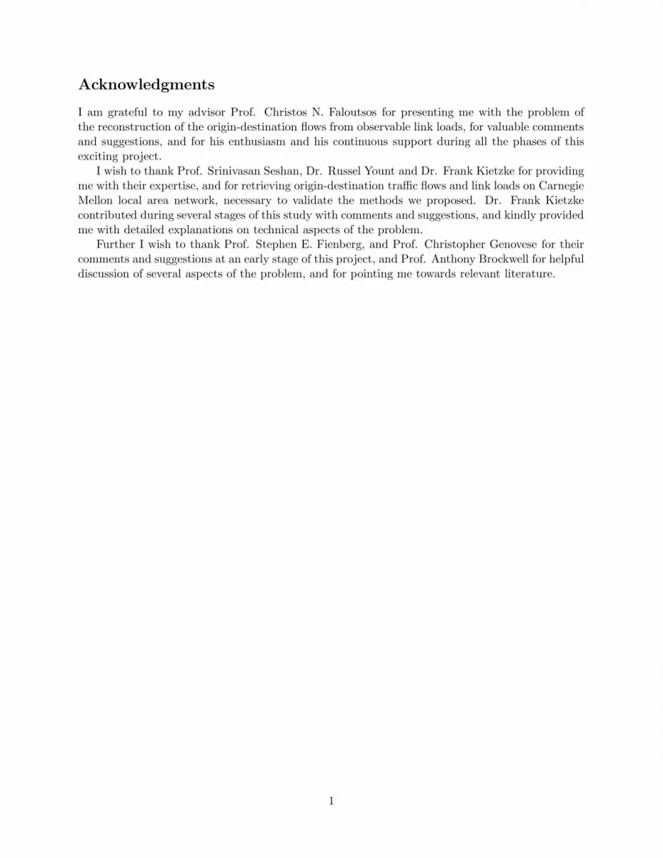
routing node in the form of packets of different sizes. The four terminal nodes are connected toit through cables. The observation vector Y (t) consists of four components at each time tick (5minutes), namely the directed link loads we would measure at each of the four interfaces wherethe physical cables are connected; two measurements for the Kbytes going into the router, andtwo measurements for the Kbytes going out of the router. With two terminal nodes connected tothe routing node the number of possible OD routes is 4, allowing for traffic from a node to itself3.Notice that since the router neither generates, nor absorbs traffic each one of the measurements canbe recovered from the other three. In figure 2 we represented the mathematical problem in terms

OD FLOWS

EDGE FLOWS

X1

X4

X2

X3

Y1

Y3

Y2

Y4

Node

no.1

Node

no.2

Node

no.2

Node

no.1

Figure 2: Basic mathematics with Xs and Y s.

3The function of a routing node is to filter the packets that it receives, and redirect them. Traffic from a node i

to itself amounts to the traffic that the router keeps local to that node i, by filtering it and sending it back.

4

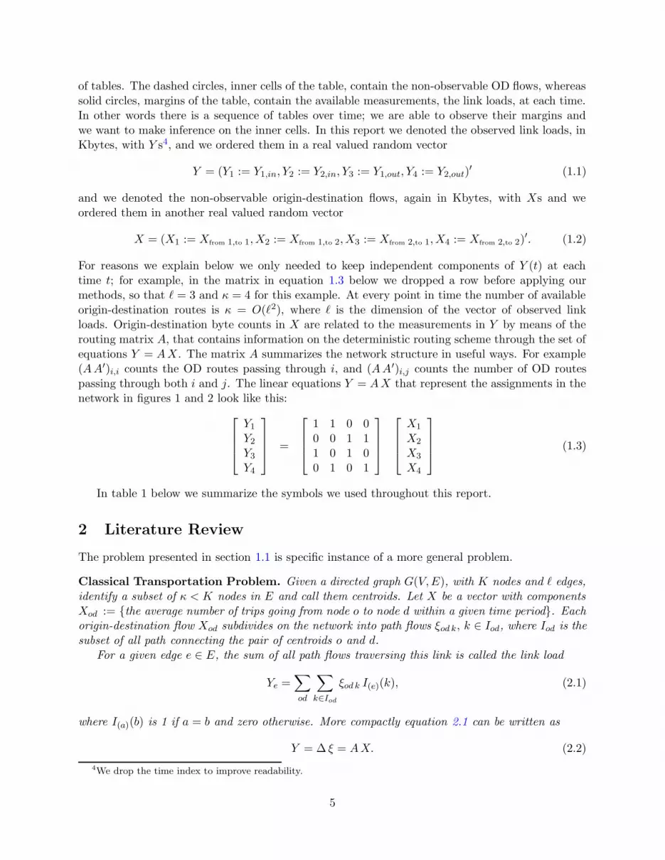
of tables. The dashed circles, inner cells of the table, contain the non-observable OD flows, whereassolid circles, margins of the table, contain the available measurements, the link loads, at each time.In other words there is a sequence of tables over time; we are able to observe their margins andwe want to make inference on the inner cells. In this report we denoted the observed link loads, inKbytes, with Y s4, and we ordered them in a real valued random vector

Y = (Y1 := Y1,in, Y2 := Y2,in, Y3 := Y1,out, Y4 := Y2,out)′ (1.1)

and we denoted the non-observable origin-destination flows, again in Kbytes, with Xs and weordered them in another real valued random vector

X = (X1 := Xfrom 1,to 1, X2 := Xfrom 1,to 2, X3 := Xfrom 2,to 1, X4 := Xfrom 2,to 2)′. (1.2)

For reasons we explain below we only needed to keep independent components of Y (t) at eachtime t; for example, in the matrix in equation 1.3 below we dropped a row before applying ourmethods, so that ` = 3 and κ = 4 for this example. At every point in time the number of availableorigin-destination routes is κ = O(`2), where ` is the dimension of the vector of observed linkloads. Origin-destination byte counts in X are related to the measurements in Y by means of therouting matrix A, that contains information on the deterministic routing scheme through the set ofequations Y = AX. The matrix A summarizes the network structure in useful ways. For example(AA′)i,i counts the OD routes passing through i, and (AA′)i,j counts the number of OD routespassing through both i and j. The linear equations Y = AX that represent the assignments in thenetwork in figures 1 and 2 look like this:

Y1

Y2

Y3

Y4

=

1 1 0 00 0 1 11 0 1 00 1 0 1

X1

X2

X3

X4

(1.3)

In table 1 below we summarize the symbols we used throughout this report.

2 Literature Review

The problem presented in section 1.1 is specific instance of a more general problem.

Classical Transportation Problem. Given a directed graph G(V,E), with K nodes and ` edges,identify a subset of κ < K nodes in E and call them centroids. Let X be a vector with componentsXod := the average number of trips going from node o to node d within a given time period. Eachorigin-destination flow Xod subdivides on the network into path flows ξod k, k ∈ Iod, where Iod is thesubset of all path connecting the pair of centroids o and d.

For a given edge e ∈ E, the sum of all path flows traversing this link is called the link load

Ye =∑

od

∑

k∈Iod

ξod k I(e)(k), (2.1)

where I(a)(b) is 1 if a = b and zero otherwise. More compactly equation 2.1 can be written as

Y = ∆ ξ = AX. (2.2)

4We drop the time index to improve readability.

5

Symbol Meaning

Y (t), Yt (`× 1) column random vector containing the observable links loads at time t, as orderedaccording to equation 1.1. Yt will be used when it is clear that we are considering vectors.

Yi(t), Y it Random number representing measurements of traffic loads at time t on the ith link of

the network, according to the ordering established in equation 1.1.Y Set of random vectors as in Y = Y (1), ..., Y (T ).

X(t), Xt (κ×1) column random vector containing the unobservable origin-destination flows at timet, as ordered according to equation 1.2. We also call X(t) the traffic matrix, followingthe interpretation of figure 2 in terms of tables. Xt will be used when it is clear that weare considering vectors.

Xi(t), X it Random number representing unobservable flows at time t between the ith origin-

destination route in the network, according to the ordering established in equation 1.2.X Set of random vectors as in X = X(1), ..., X(T ).A (` × κ) routing matrix. Contains information about the deterministic routing scheme,

through the set of equations Y (t) = A X(t). It does not change over time.` Number of links in the network for which we obtain measurements Yi(t) over time.κ Number of origin-destination flows X(t) in the network which we are interested in esti-

mating over time.Θ, Θt, Ψ, Ψt Generic vectors of parameters to be defined. Subscript t indicates time dependence.

ND (λ, Σ) Is a multivariate normal density on RD, with mean column vector λ and variance covari-ance matrix Σ.

diag (λ) It is (D × D) diagonal matrix, for λ (D × 1) column vector, with diagonal elements[diag (λ)](i,i) = λi, i = 1, ..., D.

φ, φt Scalar. Provides extra variability. Subscript t indicates time dependence.tW Scalar. Amplitude of the time window for local likelihood methods.OD Origin-destination, refers to the Xs.

IPFP Iterative Proportional Fitting Procedure.

Table 1: Summary of symbols and abbreviations.

In the definition of the problem above the centroids are the terminal nodes of our network, theassignment matrix ∆ contains the same information as our routing matrix A, and X,Y are thevectors of origin-destination flows and link loads, respectively. An even more general version ofthe problem had been given, which would include random costs Ce(Y ) for traveling on a certainedge e, function on the observed traffic Y , random costs Uk(Y ) for choosing a certain path k, andproportional trip demand P(C), possibly an implicit function of the travel cost vector C, that wouldyield a slightly different expression for the observed link loads, as in

Y = ∆P (C)X, (2.3)

and we would redefine the assignment map A(X) := ∆P (C)X, possibly non linear.

Underlying Assumptions

The transportation problem in all its formulations is “old”, and several solutions had been proposedand rediscovered over the years. In order to keep track of the different characterizations we mentionhere some relevant dimensions: (L1) there is only one vector of flows X, that does not chance overthe sampling period; (L2) the link loads Y are measured with error; (L3) the assignment mappingA(X) is endogenous A(X) := ∆P (C)X = ∆P ∗(Y )X = A(X,Y ); (L4) the assignment mappingA(X) is deterministic, as opposed to random; (L5) the assignment mapping A(X) entails unique

6

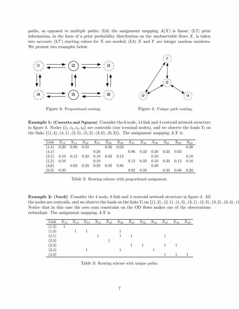
paths, as opposed to multiple paths; (L6) the assignment mapping A(X) is linear; (L7) priorinformation, in the form of a prior probability distribution on the unobservable flows X, is takeninto account; (L7’) starting values for X are needed; (L8) X and Y are integer random numbers.We present two examples below.

i5

i2 i3

i6

i1

i4

Figure 3: Proportional routing.

i2 i4

i3

i1

Figure 4: Unique path routing.

Example 1: (Cascetta and Nguyen) Consider the 6 node, 14 link and 4 centroid network structurein figure 3. Nodes i1, i3, i4, i6 are centroids (our terminal nodes), and we observe the loads Yl onthe links (1, 4) , (4, 1) , (2, 5) , (5, 2) , (3, 6) , (6, 3). The assignment mapping AX is

Link X13 X14 X16 X31 X34 X36 X41 X43 X46 X61 X63 X64

(1,4) 0.20 0.86 0.33 0.33 0.02 0.20(4,1) 0.20 0.86 0.33 0.20 0.33 0.02(2,5) 0.10 0.12 0.33 0.10 0.33 0.12 0.10 0.10(5,2) 0.10 0.10 0.12 0.33 0.10 0.33 0.12 0.10(3,6) 0.02 0.33 0.20 0.33 0.86 0.20(6,3) 0.20 0.02 0.33 0.33 0.86 0.20

Table 2: Routing scheme with proportional assignment.

Example 2: (Vardi) Consider the 4 node, 8 link and 4 centroid network structure in figure 4. Allthe nodes are centroids, and we observe the loads on the links Yl on (1, 2) , (2, 1) , (1, 3) , (3, 1) , (2, 3) , (3, 2) , (3, 4) , (4, 3).Notice that in this case the zero sum constraint on the OD flows makes one of the observationsredundant. The assignment mapping AX is

Link X12 X13 X14 X21 X23 X24 X31 X32 X34 X41 X42 X43

(1,2) 1(1,3) 1 1 1(2,1) 1 1 1 1(2,3) 1(3,2) 1 1 1 1(3,4) 1 1 1(4,3) 1 1 1

Table 3: Routing scheme with unique paths.

7

The estimation problem boils down to finding reasonable origin-destination flows X thatmatch the observed link loads. The assignment mapping is usually not invertible and there is morethan one feasible solution.

2.1 Transportation Research

A relevant part of the literature dealt with transportation analysis (the number of travelers thatcommute, or the amount of freight shipped), and with traffic monitoring problems (the numberof cars that move between different metropolitan areas of a city). If we exclude time (L1) andendogeneity of the assignment mapping (L3) the all proposed solutions to the estimation problemboiled down to the following problem.

Minimization problem:

minX

p ·D1(X, Xobs) + q ·D2(Y (X), Yobs) s.t. Y = fA(X) and X ≥ 0. (2.4)

where D1 and D2 are distance measures, and the constraints make sure X,Y represent one of thepositive, feasible solutions. Notice that the solution X is constant over time.

Intuition: in general there are many feasible origin-destination traffic matrices5 X matching theobserved loads Y , in fact in section 1.1 we counted the number of unobservable flows κ = O(`2),` being the number of available measurements. The minimization helps us choose among all thepositive, feasible solutions the one OD traffic matrix (X) that best matches the constraints on themeasurements we have in terms of D2, and is closest according to D1 to the prior information weare willing to consider, properly weighting these criteria through p and q. e.g. D1 could be theentropy, D2 the Euclidean distance, and Y = fA(X) = AX.

The solutions given over the years were both deterministic and stochastic in nature, and foundtheir rationale rooted in maximum likelihood estimation, generalized least squares, Bayesian infer-ence, information theory and economics.

2.2 Statistical Research

In Statistics, early works dealt with inferences for the inner cells of a table, given values for themargins — again a constant solution would be obtained for the inner cells, starting from severalsets of margins. A geometrical framework for the tables was given, then the focus shifted todifferent models for the counts, to slowly time-varying tables with constant parameters over time,and eventually to real valued cell entries and time-varying parameters.

Tables

Deming and Stephan (1940) first tackled the problem and gave their Iterative Proportional FittingProcedure (IPFP) that returns a feasible solution for the inner cells, given any set of positive startingpoints that do not necessarily meet the constraints on the margins. Fienberg (1968) showed howany (r × c) two-way table can be represented by points within the (rc − 1) dimensional simplex,and a complete account of the geometry of such objects is given in Fienberg (1968) and Fienberg(1970a). From Fienberg (1970b) we learned that any (r× c) two-way table can be identified by itsmargins and the (r−1) · (c−1) association coefficients αi,j . Further given any starting positive OD

5Recall that X is a vector that derives from a matrix through equation 1.2.

8

matrix — hence a set of (r − 1) · (c − 1) coefficients αi,j — and a set of margins (Y) IPFP wouldguarantee a solution consistent with the margins, and with the same association coefficients αi,j .The path towards the solution lies on the manifold of constant interaction defined by the associationcoefficients of the initial OD matrix, and ends where the latter meets the (r − 1) manifold definedby the row margins and the (c− 1) manifold defined by the column margins — the three manifoldsmeet in exactly one point. Ireland and Kullback (1968) showed that IPFP solution minimizes thediscrimination information, and not the variation of the χ2 statistic due to Neyman, as originallyconjectured by Deming and Stephan (1940). They showed the solution is BAN.

Origin-Destination Traffic Matrices

Vanderebei and Iannone (1994) assumed independent Poisson traffic counts for the entries of theOD matrix, developed three equivalent formulations of the EM algorithm and studied the fixedpoints of the EM operator. They were not able to prove that the log-likelihood function for theirmodel was convex in general, but gave some partial results.

Vardi (1996) studied independent Poisson traffic counts, both under fixed and probabilisticrouting schemes. He showed that the likelihood function may have an absolute maximum on theboundary whereas the unique solution of the maximum likelihood equations yields an internal, localmaximum.

Tebaldi and West (1998) pointed out the need for informative priors in a conjugate and timeindependent setting. They studied independent Poisson traffic counts P (Xt |Θt) following Vardi(1996), and then choose independent conjugate priors for the parameters P (Θt). At any given time,they wanted to find the posterior distribution P (Xt,Θt |Yt) using one set of measurements Yt only.They found that the data was only able to limit the support of the Posterior distribution withoutadding information about likely values, and the priors would drive their inferences.

Cao et al. (2000) assumed independent Gaussian OD traffic flows, and used EM algorithm toderive estimates for the parameters, that depended on t. Their method involved finding a firstapproximation for the OD flows at time t (full details in section 2.2.1 below) and then using IPFPto get the final estimates X(t) perfectly matching the observed link loads. The main drawbacks oftheir approach were the assumptions: traffic IID over time, and Gaussian OD flows. Further, sincein order to estimate Θt (time-dependent) they used a window of contiguous observations centeredaround time t, their method cannot provide estimates for X(t) at the beginning and at the end ofthe time series. Cao et al. (2002) proposed the same model, and suggested a divide-and-conquerstrategy to deal with larger scale problems as the number of origin-destination pairs grows.

2.2.1 A Recent Local Maximum Likelihood Approach

In this section we present the model proposed by Cao et al. (2000) and (2002), in order to point outsome unsatisfactory aspects of it that we fully address in section 3. Denote the origin-destinationflows by Xs, the link loads by Y s, and the routing matrix by A, as discussed above. The followingthree equations

Xt ∼ NI(λ,Σ) iidΣ = φ · diag(λτ ), τ is a known constantYt = AXt

(2.5)

define a Gaussian process for the available measurements Yt ∼ ND(Aλ,AΣA′), that sort of ap-proximates a multivariate Poisson process with parameter vector λ. Sort of approximate since theparameter φ allows for extra Poisson variability.

9

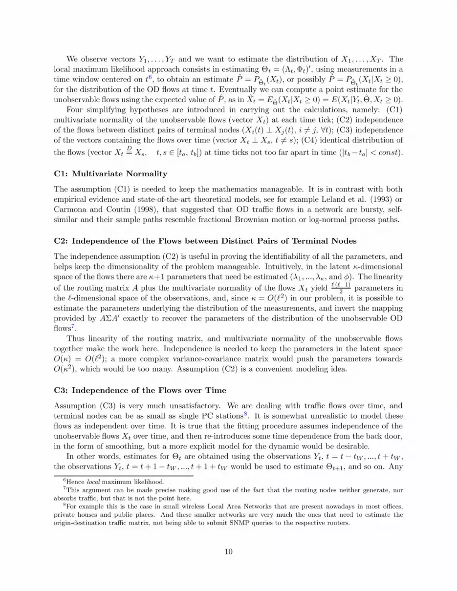
We observe vectors Y1, . . . , YT and we want to estimate the distribution of X1, . . . , XT . Thelocal maximum likelihood approach consists in estimating Θt = (Λt,Φt)

′, using measurements in atime window centered on t6, to obtain an estimate P = PΘt

(Xt), or possibly P = PΘt(Xt|Xt ≥ 0),

for the distribution of the OD flows at time t. Eventually we can compute a point estimate for theunobservable flows using the expected value of P , as in Xt = EΘ(Xt|Xt ≥ 0) = E(Xt|Yt, Θ, Xt ≥ 0).

Four simplifying hypotheses are introduced in carrying out the calculations, namely: (C1)multivariate normality of the unobservable flows (vector Xt) at each time tick; (C2) independenceof the flows between distinct pairs of terminal nodes (Xi(t) ⊥ Xj(t), i 6= j, ∀t); (C3) independenceof the vectors containing the flows over time (vector Xt ⊥ Xs, t 6= s); (C4) identical distribution of

the flows (vector XtD= Xs, t, s ∈ [ta, tb]) at time ticks not too far apart in time (|tb− ta| < const).

C1: Multivariate Normality

The assumption (C1) is needed to keep the mathematics manageable. It is in contrast with bothempirical evidence and state-of-the-art theoretical models, see for example Leland et al. (1993) orCarmona and Coutin (1998), that suggested that OD traffic flows in a network are bursty, self-similar and their sample paths resemble fractional Brownian motion or log-normal process paths.

C2: Independence of the Flows between Distinct Pairs of Terminal Nodes

The independence assumption (C2) is useful in proving the identifiability of all the parameters, andhelps keep the dimensionality of the problem manageable. Intuitively, in the latent κ-dimensionalspace of the flows there are κ+1 parameters that need be estimated (λ1, ..., λκ, and φ). The linearity

of the routing matrix A plus the multivariate normality of the flows Xt yield ` (`−1)2 parameters in

the `-dimensional space of the observations, and, since κ = O(`2) in our problem, it is possible toestimate the parameters underlying the distribution of the measurements, and invert the mappingprovided by AΣA′ exactly to recover the parameters of the distribution of the unobservable ODflows7.

Thus linearity of the routing matrix, and multivariate normality of the unobservable flowstogether make the work here. Independence is needed to keep the parameters in the latent spaceO(κ) = O(`2); a more complex variance-covariance matrix would push the parameters towardsO(κ2), which would be too many. Assumption (C2) is a convenient modeling idea.

C3: Independence of the Flows over Time

Assumption (C3) is very much unsatisfactory. We are dealing with traffic flows over time, andterminal nodes can be as small as single PC stations8. It is somewhat unrealistic to model theseflows as independent over time. It is true that the fitting procedure assumes independence of theunobservable flows Xt over time, and then re-introduces some time dependence from the back door,in the form of smoothing, but a more explicit model for the dynamic would be desirable.

In other words, estimates for Θt are obtained using the observations Yt, t = t− tW , ..., t + tW ,the observations Yt, t = t + 1− tW , ..., t + 1 + tW would be used to estimate Θt+1, and so on. Any

6Hence local maximum likelihood.7This argument can be made precise making good use of the fact that the routing nodes neither generate, nor

absorbs traffic, but that is not the point here.8For example this is the case in small wireless Local Area Networks that are present nowadays in most offices,

private houses and public places. And these smaller networks are very much the ones that need to estimate theorigin-destination traffic matrix, not being able to submit SNMP queries to the respective routers.

10

two successive estimates would have the observations Yt, t = t+1− tW , ..., t+ tW in common, henceintroducing dependence between Θt and Θt+1 and, through these, between the estimates Xt andXt+1. Notice that Xt and Xt+1 were assumed independent.

C4: Identical Distribution of the Flows

This assumption is questionable; Cao et al. assumed Θ constant for all of the observations in awindow [Yt−tW , Yt+tW ] to be able to estimate it precisely. Eventually non-constant estimates Θt

are obtained for all of the observations in the window [Yt−tW , Yt+tW ].

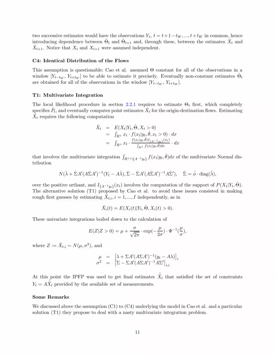
T1: Multivariate Integration

The local likelihood procedure in section 2.2.1 requires to estimate Θt first, which completelyspecifies Pt, and eventually computes point estimates Xt for the origin-destination flows. EstimatingXt requires the following computation

Xt = E(Xt|Yt, Θ, Xt > 0)

=∫

R+ xt · f(xt|yt, θ, xt > 0) · dx

=∫

R+ xt ·f(xt|yt,θ)IA−1yt

(xt)∫

R+ f(xt|yt,θ)dx· dx

that involves the multivariate integration∫

R+∩A−1ytf(xt|yt, θ)dx of the multivariate Normal dis-

tribution

N(λ + ΣA′(AΣA′)−1(Yt −Aλ), Σ− ΣA′(AΣA′)−1AΣ′), Σ = φ · diag(λ),

over the positive orthant, and IA−1yt(xt) involves the computation of the support of P (Xt|Yt, Θ).The alternative solution (T1) proposed by Cao et al. to avoid these issues consisted in makingrough first guesses by estimating Xt,i, i = 1, ..., I independently, as in

Xi(t) = E(Xi(t)|Yt, Θ, Xi(t) > 0).

These univariate integrations boiled down to the calculation of

E(Z|Z > 0) = µ +σ√2π· exp(− µ

2σ) · Φ−1(

µ

σ),

where Z := Xt,i ∼ N(µ, σ2), and

µ =[

λ + ΣA′(AΣA′)−1(yt −Aλ)]

iσ2 =

[

Σ− ΣA′(AΣA′)−1AΣ′]

i,i

At this point the IPFP was used to get final estimatesˆXt that satisfied the set of constraints

Yt = AˆXt provided by the available set of measurements.

Some Remarks

We discussed above the assumption (C1) to (C4) underlying the model in Cao et al. and a particularsolution (T1) they propose to deal with a nasty multivariate integration problem.

11

• Multivariate normality of the unobservable OD flows (C1) contrasts with both empirical andtheoretical evidence, and is unsatisfactory. The independence of the unobservable flows (C3)could be relaxed introducing some explicit form of dynamics.

• The solution (T1) proposed to deal with the multivariate integration is unsatisfactory as wemay be spoiling our efforts to obtain good estimates by integrating independently componentby component.

• The local likelihood approach does not provide estimates that cover the whole sequence oftimes for which we have measurements available. This point is particularly painful if weconsider that we can measure the link loads every 5 minutes, so that even using a prettyminimal window of 5 time ticks we would be ten minutes behind in terms of estimated ODtraffic flows.

3 Proposed Methods

We want to make inferences about non-observable origin-destination flows in a Local Area Net-work, starting from a set of measurable link loads. In such a situation a higher likelihood of themeasurements may or may not yield better estimates of the non-observable flows. Good inferenceswould require a realistic model, able to capture relevant features of the data. Our best modelcontains explicit time dependence of the OD flows, a stochastic dynamical behavior, and skeweddistributions for the OD flows; it is a step forward in comparison to the models present in theliterature both in terms of degree of realism of the underlying assumptions, and goodness of theinferences. The Bayesian dynamical system we propose outperformed state-of-the-art models byreducing the estimation error of more than 45%, in `2 distance9, in a realistic setting.

The major problem we had to cope with was the existence of multiple modes in the filteringdistributions P (ODt |Y1, ..., Yt) at each time t. We solved it by introducing informative priors oncertain parameters governing the dynamics of the system in order to identify a single, most likelyposterior mode among possibly many of them.

In section 3.1 we introduce time dependence and make use of a simple linear Gaussian systemto obtain preliminary estimates for the OD flows; in section 3.2 we introduce more realistic Gammaand log-Normal models for the OD flows, and we properly use the measurements at every timepoint t in order to make inferences on the OD flows at the same time t; in section 3.3 we combinerealistic non-Gaussian models for the traffic flows and explicit dynamical behavior by means of aBayesian dynamical system, and obtain excellent estimates for the OD flows.

3.1 Explicit Dynamics for Gaussian Origin-Destination Flows

The dynamical model we propose here entails first-order Markov dependence between the non-observable flows at different time points, and its corresponding graphical representation is displayedin the right panel of figure 5 below. The left panel, instead, displays the graphical representationof the recent model proposed in Cao et al. (2000), where the absence of arrows between the non-observable (dashed) nodes indicates that the OD traffic flows at different times are independent. Asthe graphs suggest our model includes Cao’s model as a special case. Briefly, the time dependencewe introduced among the non-observable OD flows with the graphical representation in figure 5,

9We performed several experiments using validation data, obtained by monitoring about 12321 OD traffic flowsat Carnegie Mellon University.

12

X(0) X(1) X(2)

Y(1) Y(2)

X(1) X(2)

Y(1) Y(2)

TIME INDEPENDENT TIME DEPENDENT

Figure 5: Left: graphical representation for a model with independent OD flows. Right: graphicalrepresentation for the model we propose in section 3.1 with first-order Markov dependence amongthe OD flows.

mathematically translates into a contribution of P (Xt+1|Xt) in computing the posterior distributionP (Xt+1|Yt+1, ..., Y1) as the few lines below show for t + 1 = 2:

P (X2|Y2, Y1) ∝∫

P (X2, X1, Y2|Y1) dX1

(State-Space computation includes P (X2|X1)) =∫

P (X2|X1)P (X1|Y1)P (Y2|X2) dX1

(if the time points were IID P (X2|X1) = P (X2)) = P (X2)P (Y2|X2) ·∫

P (X1|Y1) dX1

(and the posterior would simplify into) = P (X2)P (Y2|X2)

3.1.1 A State-Space Representation for the Model

The model we used is defined as follows:

Xt+1 = Ft+1 ·Xt + Qt+1 · ι + εt+1

Yt = A ·Xt + ηt

=

[

Xt+1

1

]

=

[

Ft+1 Qt+1

0 I

]

·[

Xt

ι

]

+

[

εt+1

1

]

Yt = [A| 0 ] ·[

Xt

1

]

+ ηt

=

Xt+1 = Ft+1 · Xt + εt+1

Yt = A · Xt + ηt

(3.1)

for t ≥ 1, where ι = ι · (1, ..., 1)′ is a constant vector of the length κ, the parameter φt enters intothe variance-covariance matrix of εt ∼ N(0, φt · Qt), X1 ∼ N(0, V1), ηt ∼ N(0, Rt), X1 ⊥ εt andX1 ⊥ ηt for all t ≥ 1, and finally Qt is a diagonal matrix with elements (qτ

t,1, ..., qτt,κ), where τ is

a known constant. In the model above whenever Ft = 0 there is a one-to-one mapping between(qτ

t,1, ..., qτt,κ, φt)

′ and the unique elements in E(Yt), V (Yt). Further the following lemma holds.

Lemma. The linear Gaussian state-space model in equations 3.1 contains the model in Cao et al.(2000) defined by equations 2.5 in section 2.2.1 as a special case. Such a model can be obtainedby simply setting ι = 1 and Ft = 0, ∀t, hence imposing independence among the origin-destinationflows Xt at different times.

13

Local Linear Dynamics

In this report we considered a local linear dynamics for the OD flows. The local linearity assumptionis not really a constraint as any non-linear dynamical behavior can be locally approximated to thefirst order by a linear behavior. Extensions of the Kalman recursions as the Extended KalmanFilter or the Unscented Kalman Filter deal more precisely with non-linear dynamics, but a locallinear dynamical behavior will do for us without the need for further complications. In section 4.3.2we provide some empirical evidence to support our choice for a diagonal Ft in our model.

3.1.2 Ad-Hoc M-Step for the EM Algorithm

In order to estimate the OD flows at successive times it was natural to compute the sequence ofposterior distributions X1|Y1, X2|Y1 and X2|Y1, Y2, X3|Y1, Y2 and X3|Y1, Y2, Y3, and so on. We usedthe Kalman Filter to recursively compute filtered and smoothed posterior probability distributionsfor the OD flows; the celebrated Kalman Filter provides in fact recursions to find MS-optimalestimates of the hidden states once we know the other parameters of the state-space model —Ft, Qt, φt, Rt, X1, V1.

We needed estimates for these parameters as well, and a major concern was the estimationof Ft, because of its possibly enormous variance. In our case it was possible to write down thelikelihood as:

f( (Y1, . . . , YT ) |Θ) = (2π)−T`/2

(

T∏

i=1

detΣi

)−1/2

exp

−1

2

T∑

i=1

(Yi − Yi)T Σ−1

i (Yi − Yi)

,

and maximize it directly10, or alternatively use the EM algorithm, in the spirit of Ghahramani andHinton (1996). Let’s consider the simple case Ft = F,Qt = Q and Rt = R for all t ≥ 1. Theparameters would be X, A, F,Q,R,X1, V1, and the EM algorithm would give the recursions toupdate the quantities involved, including the OD flows, X.

The E-step

The quantity of interest is the expected value of the log-likelihood of the complete data, given theobservations Q = E [log P (X, Y )|Y ]. We can write:

log P (X, Y ) = log P (X1) ·∏T

t=2 P (Xt|Xt−1) ·∏T

t=1 P (Yt|Xt)

= −T (`+I)2 log 2π − 1

2X ′1V

−11 X1 − 1

2 log |V1|

−12

∑Tt=2

(

[Xt − FXt−1]′Q−1[Xt − FXt−1]

)

− T−12 log |Q|

−12

∑Tt=2

(

[Yt −AXt]′R−1[Yt −AXt]

)

− T2 log |R|

and making use of some properties of the trace operator it is easy to see that the expecta-tion Q = E [log P (X, Y )|Y ] depends on the three quantities E[Xt|Y ], E[XtX

′t|Y ] and

E[XtX′t−1|Y ]. The derivations of the recursions needed for the E-step follows that of Ghahramani

and Hinton (1996), for the model in section 3.1.1 in terms of the new variables (tilde).

10In the equation above Yi and Σi are the means and variances of the one-step-ahead projections.

14

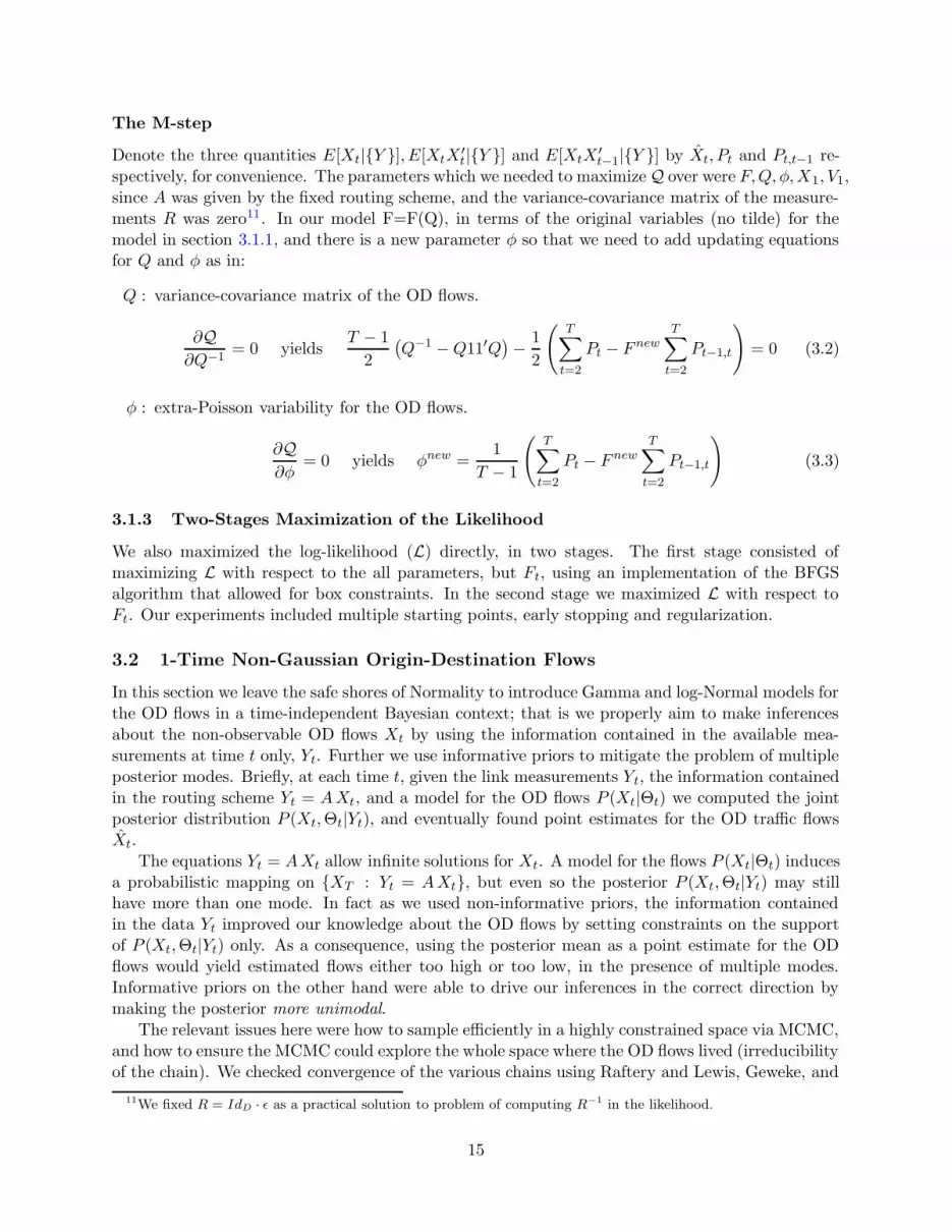
The M-step

Denote the three quantities E[Xt|Y ], E[XtX′t|Y ] and E[XtX

′t−1|Y ] by Xt, Pt and Pt,t−1 re-

spectively, for convenience. The parameters which we needed to maximizeQ over were F,Q, φ,X1, V1,since A was given by the fixed routing scheme, and the variance-covariance matrix of the measure-ments R was zero11. In our model F=F(Q), in terms of the original variables (no tilde) for themodel in section 3.1.1, and there is a new parameter φ so that we need to add updating equationsfor Q and φ as in:

Q : variance-covariance matrix of the OD flows.

∂Q∂Q−1

= 0 yieldsT − 1

2

(

Q−1 −Q11′Q)

− 1

2

(

T∑

t=2

Pt − F newT∑

t=2

Pt−1,t

)

= 0 (3.2)

φ : extra-Poisson variability for the OD flows.

∂Q∂φ

= 0 yields φnew =1

T − 1

(

T∑

t=2

Pt − F newT∑

t=2

Pt−1,t

)

(3.3)

3.1.3 Two-Stages Maximization of the Likelihood

We also maximized the log-likelihood (L) directly, in two stages. The first stage consisted ofmaximizing L with respect to the all parameters, but Ft, using an implementation of the BFGSalgorithm that allowed for box constraints. In the second stage we maximized L with respect toFt. Our experiments included multiple starting points, early stopping and regularization.

3.2 1-Time Non-Gaussian Origin-Destination Flows

In this section we leave the safe shores of Normality to introduce Gamma and log-Normal models forthe OD flows in a time-independent Bayesian context; that is we properly aim to make inferencesabout the non-observable OD flows Xt by using the information contained in the available mea-surements at time t only, Yt. Further we use informative priors to mitigate the problem of multipleposterior modes. Briefly, at each time t, given the link measurements Yt, the information containedin the routing scheme Yt = AXt, and a model for the OD flows P (Xt|Θt) we computed the jointposterior distribution P (Xt,Θt|Yt), and eventually found point estimates for the OD traffic flowsXt.

The equations Yt = AXt allow infinite solutions for Xt. A model for the flows P (Xt|Θt) inducesa probabilistic mapping on XT : Yt = AXt, but even so the posterior P (Xt,Θt|Yt) may stillhave more than one mode. In fact as we used non-informative priors, the information containedin the data Yt improved our knowledge about the OD flows by setting constraints on the supportof P (Xt,Θt|Yt) only. As a consequence, using the posterior mean as a point estimate for the ODflows would yield estimated flows either too high or too low, in the presence of multiple modes.Informative priors on the other hand were able to drive our inferences in the correct direction bymaking the posterior more unimodal.

The relevant issues here were how to sample efficiently in a highly constrained space via MCMC,and how to ensure the MCMC could explore the whole space where the OD flows lived (irreducibilityof the chain). We checked convergence of the various chains using Raftery and Lewis, Geweke, and

11We fixed R = IdD · ε as a practical solution to problem of computing R−1 in the likelihood.

15

Heidelberger and Welch convergence diagnostics. The results in this section extend to continuous,non-conjugate analysis the results in Tebaldi and West (1998). In the remainder of this section wedrop the time subscripts, since the models we propose are to be fitted time by time.

3.2.1 Computing the Support

The routing matrix A is full row rank, by construction. In order to sample efficiently we tookadvantage of the following fact.

Fact. There exists a permutation ρ of the columns of A(`×κ) such that [A](i,ρ(j)) = [A1 |A2], whereA1 is (`× `) and has full rank, and A2 is (`× (κ− `)).

As a consequence we were able to permute the components of X to get [X]′ρ(i) = [X1 |X2]′, and

Y = AX = A1 X1 +A2 X2, and we then ran chains in the lower dimensional space where X2 lived,obtaining X1(X2, Y ) at each step, like so:

X1 = A−11 · (Y −A2 X2)

The space where X2 lived was itself constrained by the available measurement Y , at anygiven time. Using a χ2 proposal in the Metropolis steps, properly defining the full conditionalsP (X2,i|X2,−i, Y ) to be zero if, say, a negative value for X2,i was sampled as a candidate, and ac-cepting the candidate conditionally to a further check that all the corresponding X1(X2, Y ) werepositive, allowed us to avoid a direct and expensive computation of the support.

3.2.2 Irreducibility of the Chain

We need to make sure that the chains we used were able to explore the entire space of OD trafficflows. It is possible to show that the positivity condition introduced by Besag (1974) holds, whichis sufficient to ensure the irreducibility of the chain. Moreover we show that the support of theunivariate full conditional distributions is convex.

εX(t)

X(t+1)

ε

Figure 6: The chain is at X(t), the circles represent the joint support. The possible moves according to theGibbs scheme X(t)+ [0, ε]′ or X(t)+ [ε, 0]′ would yield outside of joint support, whereas a move X(t)+ [ε, ε]′

would yield inside. We show that such a situation cannot happen, and whenever X(t) + [ε, ε]′ yields a validpoint of the support of the joint distribution, the Gibbs moves also do.

Proof: (convexity of the support) We want to show that if the two (κ− `)-dimensional vectorsx = (x1, ..., xi, ..., xκ−`)

′ and y = (x1, ..., yi, ..., xκ−`)′ differ in the ith component, and if both

16

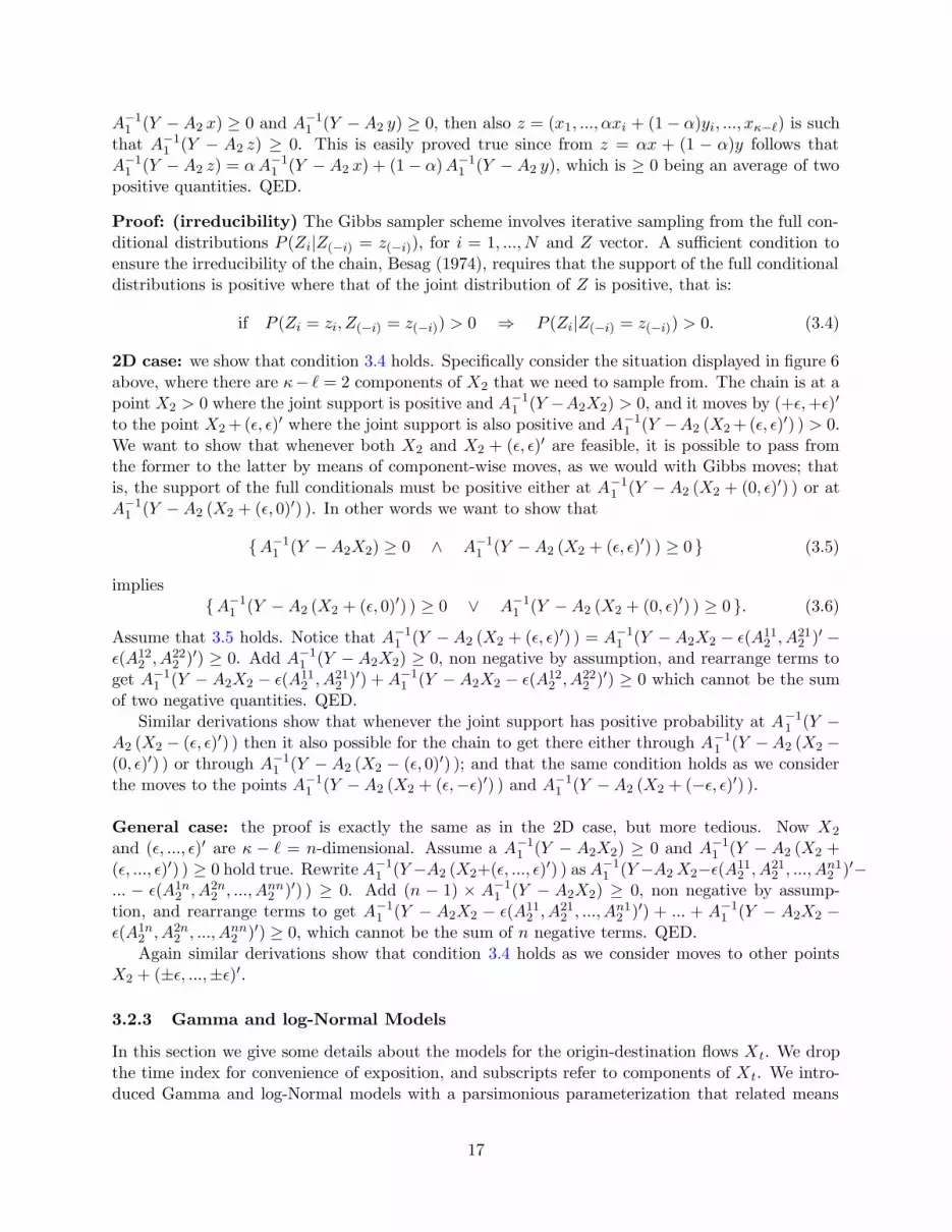
A−11 (Y −A2 x) ≥ 0 and A−1

1 (Y −A2 y) ≥ 0, then also z = (x1, ..., αxi + (1− α)yi, ..., xκ−`) is suchthat A−1

1 (Y − A2 z) ≥ 0. This is easily proved true since from z = αx + (1 − α)y follows thatA−1

1 (Y −A2 z) = α A−11 (Y −A2 x) + (1− α)A−1

1 (Y −A2 y), which is ≥ 0 being an average of twopositive quantities. QED.

Proof: (irreducibility) The Gibbs sampler scheme involves iterative sampling from the full con-ditional distributions P (Zi|Z(−i) = z(−i)), for i = 1, ..., N and Z vector. A sufficient condition toensure the irreducibility of the chain, Besag (1974), requires that the support of the full conditionaldistributions is positive where that of the joint distribution of Z is positive, that is:

if P (Zi = zi, Z(−i) = z(−i)) > 0 ⇒ P (Zi|Z(−i) = z(−i)) > 0. (3.4)

2D case: we show that condition 3.4 holds. Specifically consider the situation displayed in figure 6above, where there are κ− ` = 2 components of X2 that we need to sample from. The chain is at apoint X2 > 0 where the joint support is positive and A−1

1 (Y −A2X2) > 0, and it moves by (+ε,+ε)′

to the point X2 +(ε, ε)′ where the joint support is also positive and A−11 (Y −A2 (X2 +(ε, ε)′) ) > 0.

We want to show that whenever both X2 and X2 + (ε, ε)′ are feasible, it is possible to pass fromthe former to the latter by means of component-wise moves, as we would with Gibbs moves; thatis, the support of the full conditionals must be positive either at A−1

1 (Y − A2 (X2 + (0, ε)′) ) or atA−1

1 (Y −A2 (X2 + (ε, 0)′) ). In other words we want to show that

A−11 (Y −A2X2) ≥ 0 ∧ A−1

1 (Y −A2 (X2 + (ε, ε)′) ) ≥ 0 (3.5)

impliesA−1

1 (Y −A2 (X2 + (ε, 0)′) ) ≥ 0 ∨ A−11 (Y −A2 (X2 + (0, ε)′) ) ≥ 0 . (3.6)

Assume that 3.5 holds. Notice that A−11 (Y −A2 (X2 + (ε, ε)′) ) = A−1

1 (Y −A2X2 − ε(A112 , A21

2 )′ −ε(A12

2 , A222 )′) ≥ 0. Add A−1

1 (Y − A2X2) ≥ 0, non negative by assumption, and rearrange terms toget A−1

1 (Y − A2X2 − ε(A112 , A21

2 )′) + A−11 (Y − A2X2 − ε(A12

2 , A222 )′) ≥ 0 which cannot be the sum

of two negative quantities. QED.Similar derivations show that whenever the joint support has positive probability at A−1

1 (Y −A2 (X2 − (ε, ε)′) ) then it also possible for the chain to get there either through A−1

1 (Y −A2 (X2 −(0, ε)′) ) or through A−1

1 (Y − A2 (X2 − (ε, 0)′) ); and that the same condition holds as we considerthe moves to the points A−1

1 (Y −A2 (X2 + (ε,−ε)′) ) and A−11 (Y −A2 (X2 + (−ε, ε)′) ).

General case: the proof is exactly the same as in the 2D case, but more tedious. Now X2

and (ε, ..., ε)′ are κ − ` = n-dimensional. Assume a A−11 (Y − A2X2) ≥ 0 and A−1

1 (Y − A2 (X2 +(ε, ..., ε)′) ) ≥ 0 hold true. Rewrite A−1

1 (Y−A2 (X2+(ε, ..., ε)′) ) as A−11 (Y−A2 X2−ε(A11

2 , A212 , ..., An1

2 )′−... − ε(A1n

2 , A2n2 , ..., Ann

2 )′) ) ≥ 0. Add (n − 1) × A−11 (Y − A2X2) ≥ 0, non negative by assump-

tion, and rearrange terms to get A−11 (Y − A2X2 − ε(A11

2 , A212 , ..., An1

2 )′) + ... + A−11 (Y − A2X2 −

ε(A1n2 , A2n

2 , ..., Ann2 )′) ≥ 0, which cannot be the sum of n negative terms. QED.

Again similar derivations show that condition 3.4 holds as we consider moves to other pointsX2 + (±ε, ...,±ε)′.

3.2.3 Gamma and log-Normal Models

In this section we give some details about the models for the origin-destination flows Xt. We dropthe time index for convenience of exposition, and subscripts refer to components of Xt. We intro-duced Gamma and log-Normal models with a parsimonious parameterization that related means

17

and variances. i.e. we assumed single OD flows Xi ∼ Gamma (αi, β) with distinct parameters αi,and we imposed a common scale parameter β, as in

Xi ∼ Gamma(αi, β) =Xαi−1

i e−Xiβ

βαi Γ(αi), Xi > 0, i = 1, ..., κ, (3.7)

or, alternatively, we assumed single OD flows Xi ∼ log-Normal (µi, φ · µki ), for a fixed constant k,

with distinct means and variances proportional to them times a common scaling factor φ, as in

Xi ∼ log-Normal(µi, φ µki ) =

1√

2πφµki

e− 1

2φ µki

(log(Xi)−µi)2

, Xi > 0, i = 1, ..., κ, (3.8)

Full Conditionals

Say Θ = (α1, ..., ακ, β)′ then P (X,Θ) =∏κ

i=1 P (Xi|Θ)P (Θ) =∏κ

i=1 P (Xi|αi, β)P (αi)P (β). Wewanted αi ∈ (0,∞) and β ∈ (0,∞). We assumed improper priors for αi and 1/β. Then, noticingthat P (Θ|X,Y ) = P (Θ|X) IA−1Y (X), we obtained the following full conditionals.

P ( 1β |X,Y ) ∝ ∏

P (Xi|αi, β) · P ( 1β )

∝ exp

∑

(αi − 1) log(Xi)−∑ Xi

β +∑

αi log( 1β )

∝ Gamma [∑

αi + 1, 1∑

Xi]

P (αi|X,Y ) ∝ P (Xi|αi, β) · P (αi)

∝ exp

(αi − 1) log(Xi)− Xi

β − αi log(β)− log Γ(αi)

∝ e−αi log(

βXi

)

Γ(αi), αi > 0

whereas for P (X|Y,Θ) we used the fact in 3.2.1 to conclude that P (X|Y,Θ) = P (X2|Y,Θ) ××P (X1(X2)|Y,Θ); hence for Xi ∈ X2 and Xj ∈ X1 it followed:

P (Xi|X(−i), Y,Θ) ∝ P (Xi|Θ) · P (X1|Y,Θ)

= GammaXi(αi, β) ·∏j GammaXj

(αj , β) IA−1Y (Xj)(3.9)

We explored the posterior distributions using the Gibbs algorithm, with Metropolis steps tosample from P (Xi|Y,Θ) and P (αi|X,Y ), using χ2 and Uniform proposals, an improper prior foralpha proportional to a constant, and several priors for β: one proportional to a constant, oneproportional to 1

β , and one proportional to 1β2 .

In the same fashion we obtained the full conditionals for the log-Normal model, with constantprior for µi and priors proportional to 1

φ2 (used in the calculations below), and to 1φ for φ.

P (µi|X,Y ) ∝ ∏

P (Xi|µi, φ) · P (µi)

∝ 1

µIk2

i

e− 1

2φ

(

log(Xi)−µi

µki

)2

P (φ|X,Y ) ∝ P (Xi|µi, φ) · P (φ)

∝ 1

φI2 +2

e− 1

2φ

∑

i

(

log(Xi)−µi

µki

)2

P (Xi|X(−i), Y,Θ) ∝ P (Xi|Θ) · P (X1|Y,Θ)

= log-NormalXi(µi, φ) ·∏j log-NormalXj

(µj , φ) IA−1Y (Xj)

18

3.2.4 Informative priors

In order to mitigate the loss of precision of the estimates Xt, due to the many feasible solutions, weintroduced informative priors for the parameters in Θ = (αi, β) = (µi, φ) governing the distributionof the OD flows. In doing so we basically imposed soft constraints on the parameters, and madethe posterior distributions more unimodal.

In the Gamma model, the priors for the αis were truncated Normal distributions with a hugevariance, centered around the preliminary estimates obtained with the linear dynamical system insection 3.1, and the prior for β was proportional to 1

β2 . Similarly, for the log-Normal model we use

truncated Normal priors for the µis and a prior proportional to 1φ2 for φ. As a result the posterior

mode closer to the preliminary estimates would become more likely than the other modes, andthe bias introduced by these other modes would fade. Hypothetically, though, if the preliminaryestimates were off by large from the true OD flows, and at the same time corresponded to a posteriormode, then the estimates would be driven towards the wrong feasible solution. This never happenedin our experiments in section 4, where the estimates consistently improved. Further in 60% of thetime points we obtained better estimates even with non-informative priors. The results we obtainedwere quite interesting.

3.3 Combining Dynamics and Non-Gaussianity

In this we section combine skewed distributions and explicit time dependence for the OD flows,and we show how we mitigated the loss of precision of the estimates due to the possibly multipleposterior modes in this dynamic setting. In the absence of a dynamical behavior suggested by somephysical law, or known to some degree, we took leave from the classical analysis of time series andfound the solution, again, in the use of informative priors. in a Bayesian dynamical system.

Briefly a Bayesian dynamical system provides a set of posterior distributions P (Xt,Θt|Yt, ..., Y1)as t varies, whereas in section 3.2 we obtained a series of posterior distributions P (Xt,Θt|Yt). Inthis setting we used informative priors on the parameters underlying the stochastic dynamics Ft ofthe Bayesian dynamical systems defined in section 3.3.2, instead of informative priors on Xt. Weestimated the parameters using a Particle Filter; one of the problem of particle filters, partiallyaddresses by the resample-move algorithm proposed by Gilks and Berzuini (2001), is to guaranteea set of particles rich enough to describe the state of the system at any given time. We used thesequence of posterior distributions P (Xt,Θt|Yt), that contain information about the state of thesystem, to improve our inferences.

3.3.1 Informative Priors for Stochastic Dynamics

We propose the use of informative priors on the explicit stochastic dynamics Ft, in order to providea set of particles Θ(t), at every time t, such that their distribution P (Θ(t)) ≈ P (Θt|Yt) wouldcorrespond to the marginal posterior we obtained in the static Bayesian analysis of section 3.2. Inother words we propose a stochastic Ft that solves the convolution problem Θt+1 = Ft Θt, giventhat we have roughly good ideas about how Θt should look like at every time t, that is, accordingto P (Θt|Yt).

In the Gamma model the convolution could not be solved exactly, since the product of Gammadistributions is no longer a Gamma. We took advantage of the fact that the ratio of Gamma distri-butions is Pearson Type VI, and we estimated the parameters underlying the random variables Ft ∼InverseGamma, such that Θt+1 = Ft Θt, where Θt ∼ Gamma, and Θt+1 ∼ PearsonType V I.The log-Normal distribution has the nice property that the product of log-Normals is log-Normal,

19

hence we were able to solve the convolution problem exactly at all times. We estimated theparameters underlying the random variables Ft ∼ log-Normal, such that Θt+1 = Ft Θt, whereΘt,Θt+1 ∼ log-Normal.

3.3.2 Bayesian Dynamical Systems

For the Gamma model define Θt := (αt, βt)′ and Ψt := (γt, δt)

′. Then:

Θt+1 = Ft ·Θt

P (X it |Θt) ∼ Gamma(αt,i, βt) i = 1, ...κ

Yt = A ·Xt, t ≥ 1(3.10)

where P (Θi0) ∼ Gammai, and P (F ii

t |Ψt) ∼ Inv Gamma(γt,i, δt,i), i = 1, ...κ. For the log-Normalmodel define Θt := (µt, φt)

′ and Ψt := (γt, δt)′. Then:

Θt+1 = Ft ·Θt

P (X it |Θt) ∼ log-Normal(µt,i, φt · µτ

t,i) i = 1, ...κ

Yt = A ·Xt, t ≥ 1

(3.11)

where τ is a fixed scalar, P (Θi0) ∼ log-Normali, and P (F ii

t |Ψt) ∼ log-Normal(γt,i, δt,i), i = 1, ...κ.We estimated Ψt from the posterior distributions P (Θt|Yt), that represented our best guesses

about the evolution of Θt at each time t.

3.3.3 Particle Filter via SIR-Move Algorithm

In order to filter the posterior distributions of the origin-destination flows and estimate the pa-rameters of the models above, we implemented the sample-resample-move algorithm of Gilks andBerzuini (2001), which we briefly outline below:

1. Initialization, t = 0.

For i = 1, . . . , N , sample x(i)0 ∼ PX0 and set t=1.

2. Importance sampling step

For i = 1, . . . , N , sample x(i)0 ∼ P

Xt|X(i)t−1

and set x(i)0:t =

(

x(i)0:t−1, x

(i)t

)

.

For i = 1, . . . , N , evaluate the importance weights ω(i)t = P

Yt|Xt=x(i)0

(yt).

Normalize the importance weights.

3. Resampling step

Resample with replacement N particles(

x(i)0:t : i = 1, . . . , N

)

from the set(

x(i)0:t : i = 1, . . . , N

)

according to the importance weights

4. Move step

Move each of the N particles(

x(i)0:t : i = 1, . . . , N

)

a few steps according to the MCMC in

section 3.2

5. Set t← t + 1 and go to step 2.

The key point of this algorithm is to be able to sample from both PX0 and PXt+1|Xt, and to be

able to compute the importance weights.

20

3.4 Multivariate Integration

The local maximum likelihood approach of Cao et al. involves the estimation of Θ to obtain P , andthen the computation of the multivariate integral E(Xt|Yt, Θ, Xt > 0) to obtain point estimates forthe OD flows Xt. The multivariate integral is nasty and the solution (T1) proposed by Cao et al.is to estimate Xi(t) component-wise by means of a convenient closed form solution, and then toadjust these one-dimensional estimates using IPFP so that they satisfy the constraints imposed bythe observed link loads Yt. The approximate component-wise integrations ignore joint informationand introduce an additional source of error in a non-controllable way.

We show in section 4 that the need for inference arises in situations where the traffic is intense,and it is rare to observe no traffic between two nodes over the time window used to estimate Θt. Asa consequence an unconstrained multivariate integration would rarely give negative results, and ifit did that may be an indication of zero traffic12, especially if the negative flows in Xt were limitedto few components. Further, in the convenient Gaussian setting it is possible to find the exactvalue for the integral with an iterative procedure. We propose two different solutions to deal withthe multivariate integration (T1):

(1) Estimate Xt using the mean of the unconstrained integral E(Xt|Yt, Θ) and adjust the resultingOD pairs when negative, as in maxXt, 0.

(2) Estimate Xt using the solution to the constrained minimization problem:

∣

∣

∣

∣

∣

∣

∣

Xt = arg minX

1

2(X − λt)

′ Σ−1 (X − λt) +1

2(Yt −AX)′ (AΣtA

′)−1 (Yt −AX)

subject to X ≥ `.

(3.12)

provided by Lagrange method.

The heuristic in (1) is not unknown in statistics; it underlies proposed corrections to manyestimators derived using method of moments, as well as the famous Stein estimator for the meanof a multivariate normal distribution. Moreover we show that such a correction is more sensible tothe extent of preserving some geometric properties of the estimates that we obtain. In fact oncewe estimate Θ, the statistical relation among OD flows X and observations Y is known to be

(Xt, Yt)′|Θ ∼ N

([

λ

Aλ

]

,

[

Σ ΣA′

AΣ AΣA′

])

, (3.13)

and estimating Xt component-wise would introduce a non-controllable source of error.The solution in (2) is the exact solution to the problem of finding E(Xt|Yt, Θ, Xt > 0), the

posterior means we would get using Normal prior and Normal likelihood. The closed form solutionis hard to obtain, but we give an iterative algorithm that converges to the exact solution, and maybe preferred in those cases where the correction in (1) involves several coordinates and an alternativemethod may be preferred. Suppressing the time subscript of Xt we can write the Lagrangian forthe problem as

L(X, ν) =1

2

[

(X − λt)′ Σ−1 (X − λt) + (Yt −AX)′ (AΣtA

′)−1 (Yt −AX)]

+

κ∑

i=1

νi · (Xi − `i)

12Notice that multiple solutions may exist.

21

and solving for X we get

X =(

Σ−1 + A′(AΣtA′)−1A

)−1 (

Σ−1λ + A′(AΣtA′)−1Y + ν

)

. (3.14)

A reasonable algorithm is to start with the unconstrained multipliers by setting νi = 0 fori = 1, ..., κ, and then iterate until convergence: compute X from 3.14 and set

νi =

max

0, νi − (Xi−`i)∂Xi∂`i

if Xi > `i

νi − (Xi−`i)∂Xi∂`i

if Xi < `i

for i = 1, ..., κ, to get (X, ν) at each iteration.

4 Experiments

Here we present the results we obtained on star network topologies, using real network traffic dataof the Carnegie Mellon LAN, and of a small LAN at Lucent Technologies.

4.1 Exploring Carnegie Mellon Network

The exploratory data analysis revealed an uneven distribution of the traffic over the possible routes,and a continuous flow of traffic to and from the external world. The origin-destination flows inthe validation dataset we were able to retrieve were definitely not Gaussian, but rather skewed.Sub-problems where the OD traffic was sparse could be reduced and solved exactly when small,and solved by entropy related heuristics when large; to this extent we gave and employed twoalgorithms, match and split-match, whose underlying assumptions were validated by the data.The idea underlying the algorithms is that traffic one-to-many13 is more likely to happen whentraffic volume is intense. As the traffic volume got intense we used the models we proposed insection 3 to recover the origin-destination flows.

Carnegie Mellon Data Collection

The data was gathered by Dr. Frank Kietzke and Dr. Russel Yount at the Carnegie Mellon NetworkGroup, using the machines of Prof. Srinivasan Seshan at Information Networking Institute.

Carnegie Mellon network is very complex and even as our large CISCO routers implement allthe sets of SNMP protocols we could not obtain validation data directly via SNMP queries to therouters; in this pilot study we obtained validation data via a network management application. Fourdatasets were collected, and we helped discover critical bugs in the network management programalong the way, as some of the data we collected did not make sense. We experimented first handhow critical the collection of origin-destination flow is! A consequence of collecting data through thenetwork management application, was that whenever the traffic became too intense, the programwould trash OD flows in the queue before we could actually measure them, and this fact resultedin slightly lower traffic flows. There was enough traffic in the data, though, to actually see theexpected daily patterns, though, and the overall volume was reasonable, so that we considered thevalidation data we collected as being the real origin-destination flows.

For more information, or to glance at the on-line link loads on the various routers, please visitthe Carnegie Mellon University Network Group home page at http://stats.net.cmu.edu/.

13One source to many destinations in a 5-minute time interval.

22

Carnegie Mellon Data Overview

The table below summarizes the observed volume over a period of slightly less than two days.

Over about 40hr (480 measurements):

--------------------------------------

. to ext world 3513.963.250.400 3514GB 49.55%

. from ext world 2053.731.241.843 2054GB 28.96%

. CMU (tcp/ip) 1523.047.061.952 1523GB 21.48%

. CMU (other) 312.847.796 313MB 0.01%

We fitted a simple linear model to get an idea of how much traffic CMU generated on averageover the collection period; it was about 14GB every 5 minutes.

20:00 4:20 12:40 21:00 5:20 13:40 22:000

1000

2000

3000

4000

5000

6000

7000Total Traffic

period from Feb 12 to Feb 14.

Gig

a By

tes

total trafficregression line

Figure 7: Total traffic in GB.

50 100 150 200 250 300 350 400 450 500

−250

−200

−150

−100

−50

0

50

100

150

200

Residual Case Order Plot

Resid

uals

Case Number

Figure 8: Case vs. residuals.

b = 13.9194 b.Int (95%) = [13.8981, 13.9406] R2 = 0.9720

There was a pattern in the residuals. It was not very clear in the differenced traffic, but itpopped up looking at the percentages of traffic by destination. Carnegie Mellon network can bethought as a collection of local routers (mainly corresponding to physical buildings), all of themconnected to two main router-switches (the Cores). The two Cores serve two different purposes.Core no.1 is the main switch, whereas Core no.2 is mainly a backup system, which in turn filtersmost of the traffic to and from the external world.

Total traffic:

CORE.1 CORE.2

. CMU internal 1099 GB/5min 423 GB/5min

. to external world 1476 GB/5min 2038 GB/5min

. from external world 935 GB/5min 1120 GB/5min

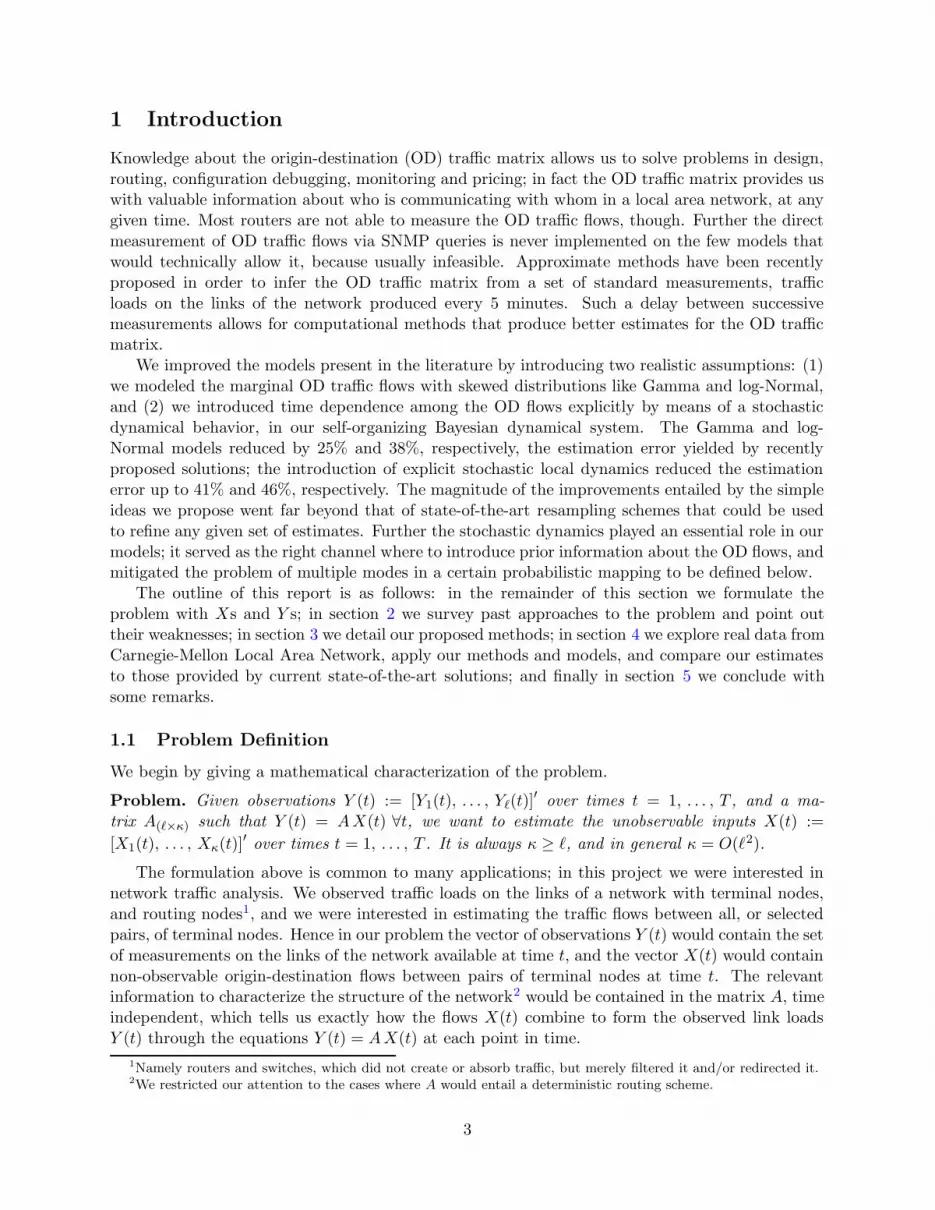
A seasonal component would have been desirable in our models, but we did not have enoughdata to carry out a meaningful analysis; estimating the seasonal component using one day datawas not a sensible thing to do. We notice, however, that our estimates Xt provide a good startingpoint to fit, for example, a non-parametric seasonal component in the non-observable space wherethe OD flows live, should more data be available in the future.

23

0 5 10 15 20 25

Log Bytes

Cou

nts

1.2 1.4 1.6 1.8 2 2.2 2.4 2.6 2.8 3 3.2

Log−Log Bytes

Cou

nts

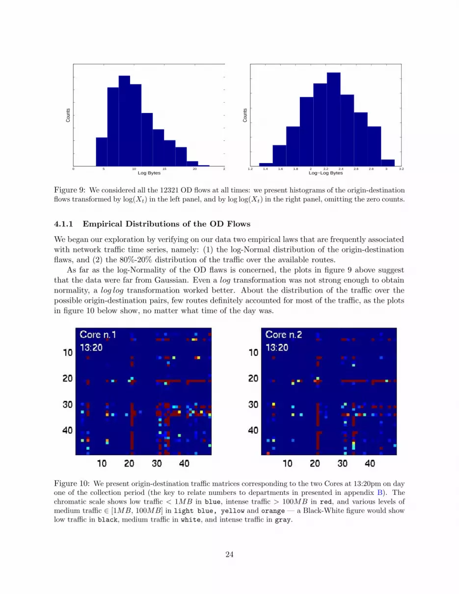
Figure 9: We considered all the 12321 OD flows at all times: we present histograms of the origin-destinationflows transformed by log(Xt) in the left panel, and by log log(Xt) in the right panel, omitting the zero counts.

4.1.1 Empirical Distributions of the OD Flows

We began our exploration by verifying on our data two empirical laws that are frequently associatedwith network traffic time series, namely: (1) the log-Normal distribution of the origin-destinationflaws, and (2) the 80%-20% distribution of the traffic over the available routes.

As far as the log-Normality of the OD flaws is concerned, the plots in figure 9 above suggestthat the data were far from Gaussian. Even a log transformation was not strong enough to obtainnormality, a log log transformation worked better. About the distribution of the traffic over thepossible origin-destination pairs, few routes definitely accounted for most of the traffic, as the plotsin figure 10 below show, no matter what time of the day was.

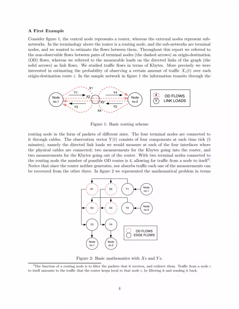
Figure 10: We present origin-destination traffic matrices corresponding to the two Cores at 13:20pm on dayone of the collection period (the key to relate numbers to departments in presented in appendix B). Thechromatic scale shows low traffic < 1MB in blue, intense traffic > 100MB in red, and various levels ofmedium traffic ∈ [1MB, 100MB] in light blue, yellow and orange — a Black-White figure would showlow traffic in black, medium traffic in white, and intense traffic in gray.

24

4.1.2 Modeling the Coefficients of Constant Association αij

We computed the coefficients of constant association αij corresponding to the sequence of ODtraffic matrices looking for some patterns. The aim was to see whether it was possible to modelthese coefficients directly. The coefficients were as irregular as the data itself, in all the possibleparameterizations, though. To model them would have required the same effort as to model thedata, hence in this report we chose to model the data directly.

4.2 Exact Recovery Algorithms for Sparse Traffic Situations

Before studying inference methods for the OD flows, we devise two algorithms that are able torecover exactly the flows in sparse traffic situations. The algorithms match and split-match arebased on the simple assumption that whenever some in and out link loads match exactly (say xbytes out of node B and x bytes into node A), and the traffic is low, we can safely attribute thetraffic observed on the matching pair of links (B,A) to the corresponding origin-destination flow(traffic from B to A).

The 5-minute data are sparse. This fact alone allowed us to recover exactly the origin-destinationflows for 91.97% of the time points, in example sub-networks like CFA, Wean, Baker-Porter.The algorithm match allowed us to recover exactly up to 98.08% of the data. The algorithmsplit-match augments match to deal with situations where only one link load is zero, and allowedus to recover exactly up to 98.51% of the data. An extension of the heuristic underlying thesealgorithms to cases where link loads do not match exactly entails arguments based on entropy.

4.3 Intense Traffic Sub-Networks at Carnegie Mellon

In this section we use the methods we presented in section 3: in section 4.3.2 we explore differentdynamical behaviors; in section 4.3.3 we fully develop an example star network, and compare ourmethods, in terms of estimation error, to the state-of-the-art methods available today.

4.3.1 Naive SVD Solution for Strongly Correlated Flows

The nature of the problem suggested generalized inverses. We computed the solution correspondingto a Moore-Penrose generalized inverse, based on SVD decomposition. The fact that we had morenon-observable OD flows than available measurements at each time point, made the results reliableonly in presence of strong cross-correlations among the OD flows. The more the origin-destinationflows got uncorrelated, the worse got the inferences based on the generalized inverse. Since we can-not observe the origin-destination flows, decisions on whether to there is cross-correlation amongthem or not should be based on the observable link loads: this seemed impractical and we took adifferent direction.

It is worth mentioning that classical time series analysis would find the solution to the under-determinacy of the problem in the presence of cross-correlations, and/or in partial knowledge aboutthe dynamics underlying the traffic. Given the heterogeneity of the communication networks,assuming a specific form for these would harm the generality of our approach. This is the reasonwhy we looked for a solution elsewhere: namely in the multiple use of data, and informative priors.

25

4.3.2 Local Dynamical Behavior

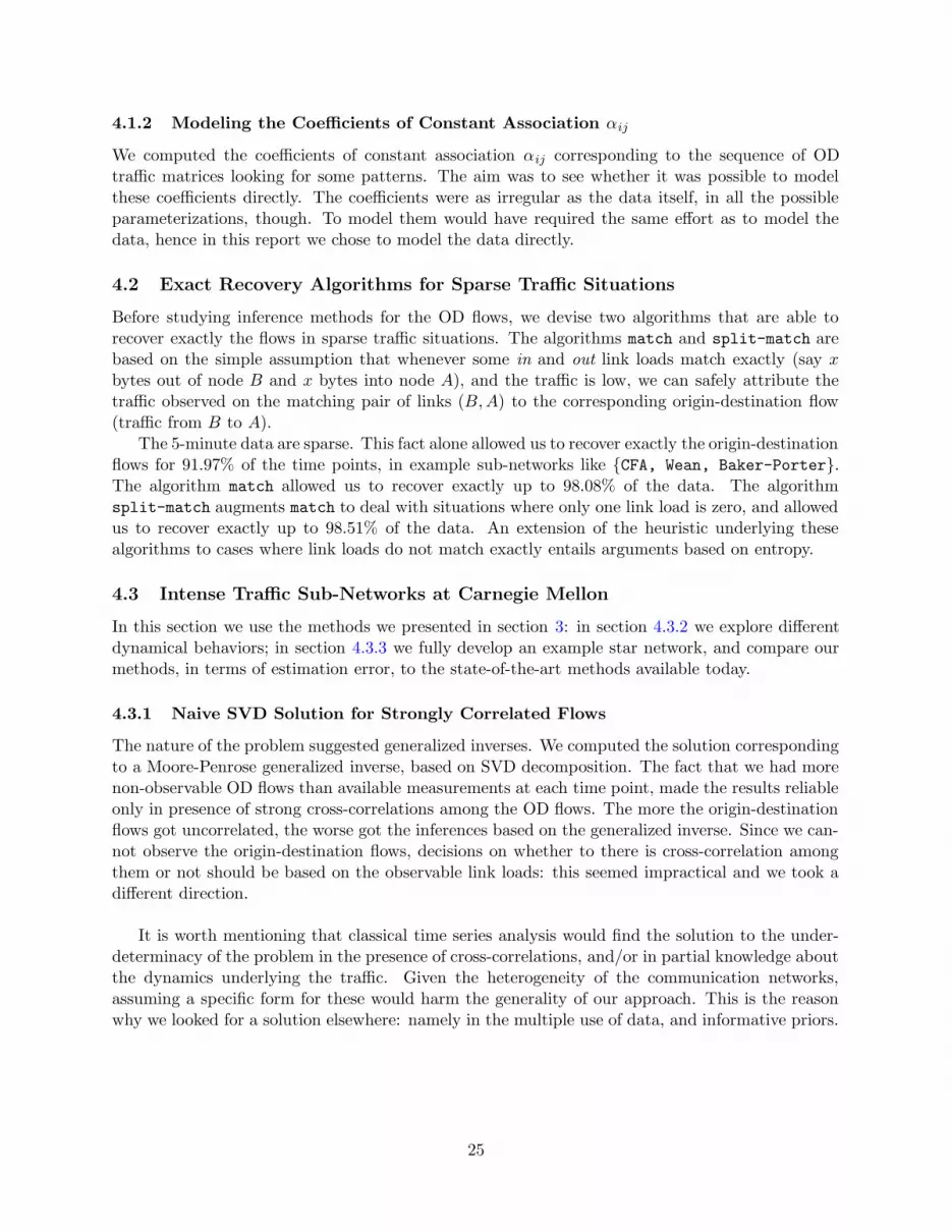
Here we provide some evidence to suggest that using a diagonal matrix Ft in the model defined byequations 3.1 is a reasonable choice. Considerations about the variability and bias of the inferencesguided our choice. We played with the matrix Ft and tried several structures for it. We presentbelow a plot for each Ft structure; the black (solid) lines represent the true origin-destination flows,and we superimpose the sequence of posterior modes obtained with the Kalman recursions (red,dashed lines), along with the upper bands at +3 posterior standard deviations (red, dotted lines).First we considered independent OD flows, by setting Ft = 0.

t

K

Forcing the absence of dynamics had an explosive effect on the variance of the posterior distribu-tions, especially if compared to a diagonal Ft = F , independent AR(1) processes, below.

t

K

Using a fully unconstrained Ft = F , fixed in time, gave bad estimates with a strong drift.

t

K

Finally we had to decide between a diagonal time-varying Ft, which yielded

t

K

and a full time-varying Ft, which yielded

t

K

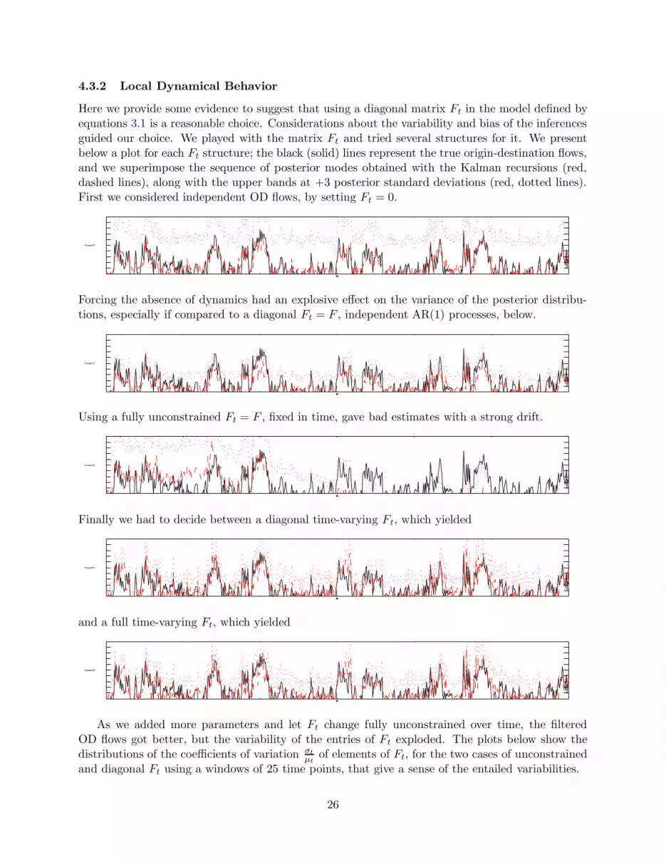
As we added more parameters and let Ft change fully unconstrained over time, the filteredOD flows got better, but the variability of the entries of Ft exploded. The plots below show thedistributions of the coefficients of variation σt

µtof elements of Ft, for the two cases of unconstrained

and diagonal Ft using a windows of 25 time points, that give a sense of the entailed variabilities.

26

1.5 2 2.5 3 3.5 40

0.2

0.4

0.6

0.8

1

1.2

1.4

σ/µ distribution − F25

diagonal

Figure 11: As we consider a fully unconstrained matrix Ft an index of the pure variability of its entries (σµ)

explodes. Left: Ft diagonal. Right: Ft unconstrained.

We concluded that a diagonal dynamic matrix Ft, that can vary quickly over time, was areasonably good choice.

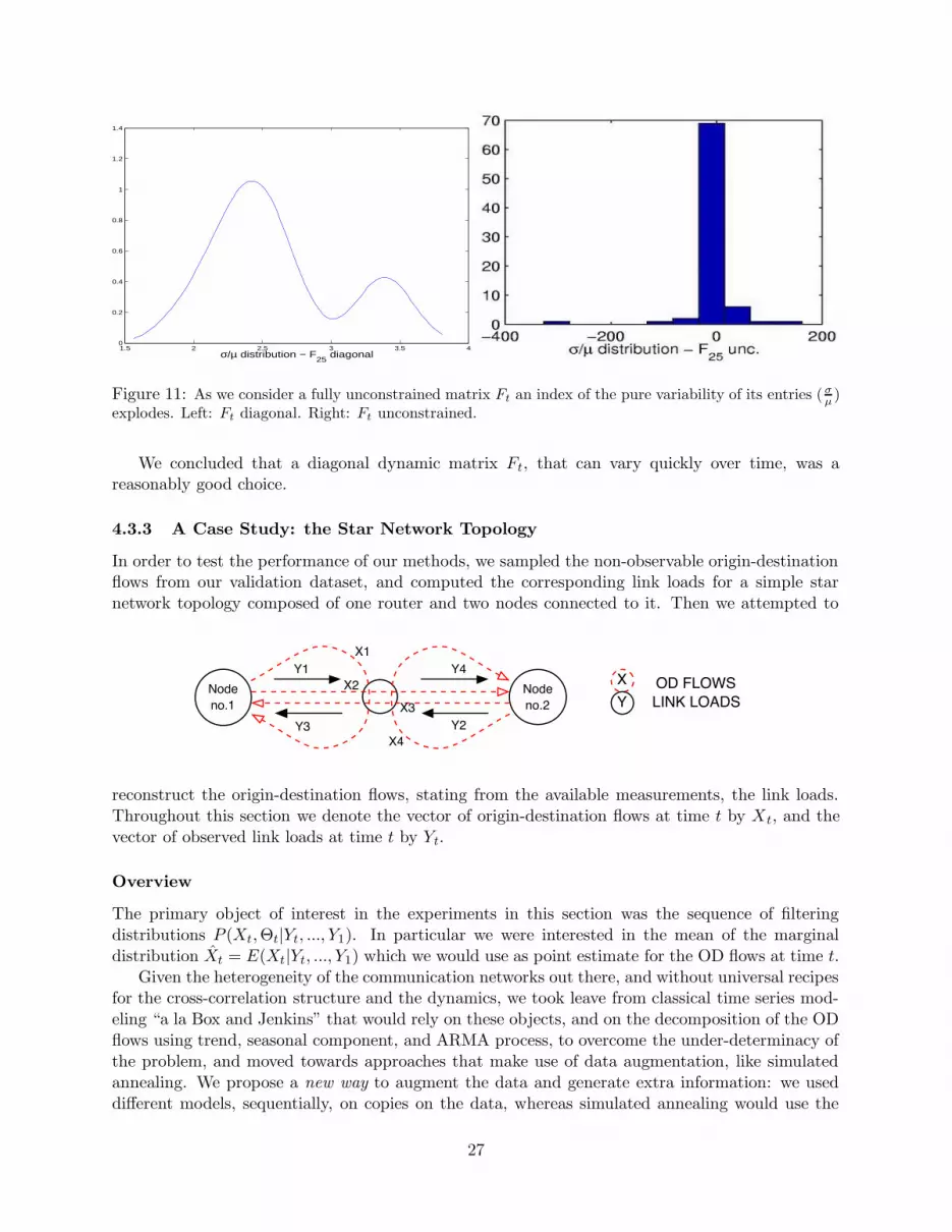
4.3.3 A Case Study: the Star Network Topology

In order to test the performance of our methods, we sampled the non-observable origin-destinationflows from our validation dataset, and computed the corresponding link loads for a simple starnetwork topology composed of one router and two nodes connected to it. Then we attempted to

Node

no.2

Node

no.1

Y2

Y1 Y4

Y3

OD FLOWS

LINK LOADS

X

Y

X4

X3

X2

X1

reconstruct the origin-destination flows, stating from the available measurements, the link loads.Throughout this section we denote the vector of origin-destination flows at time t by Xt, and thevector of observed link loads at time t by Yt.

Overview

The primary object of interest in the experiments in this section was the sequence of filteringdistributions P (Xt,Θt|Yt, ..., Y1). In particular we were interested in the mean of the marginaldistribution Xt = E(Xt|Yt, ..., Y1) which we would use as point estimate for the OD flows at time t.

Given the heterogeneity of the communication networks out there, and without universal recipesfor the cross-correlation structure and the dynamics, we took leave from classical time series mod-eling “a la Box and Jenkins” that would rely on these objects, and on the decomposition of the ODflows using trend, seasonal component, and ARMA process, to overcome the under-determinacy ofthe problem, and moved towards approaches that make use of data augmentation, like simulatedannealing. We propose a new way to augment the data and generate extra information: we useddifferent models, sequentially, on copies on the data, whereas simulated annealing would use the

27

same model on copies of the data, simultaneously. In other words instead of maximizing a power

Prior

for Xt

Gaussian

System

Static Bayes:

Gamma, log-Normal

P( Xt | Yt )Off-line

Estimation of Ft

Filtered

OD flows

Prior

for Ft

Observed

Link Loads

Dynamic Bayes:

Gamma, log-Normal

of the likelihood of the data P τ (Yt|Xt,Θt), we translated preliminary estimates into informativepriors and then used Bayes theorem to compute the posteriors and obtain new, refined estimates;the use of different models allowed us to take advantage of a larger set of useful properties, whichcould not be packed into one single model.

In order to compare inferences obtained with different methods we computed the estimationerrors; the `2 distance between the true OD flows in the validation set, and the estimates. Wefirst compared our linear Gaussian dynamical system with the local likelihood approach in Caoet al. The Gaussian system in section 3.1.1 yielded better estimates, as we expected, since we

Figure 12: The bars represent the estimation errors (`2 distance between the true OD flows in a validationset and the estimates) obtained with our linear Gaussian dynamical system, and with the method proposedby Cao et al. In the example star topology we considered, there were 4 OD flows that needed be estimated.

showed the model by Cao et al. is a special case of it. At this stage we tried also to learn thestructure of Ft by means of the EM algorithm in Ghahramani and Hinton (1996) and explored some

28

more classical time series modeling without exciting results, mainly because of the few observationsabout the link loads available. Before passing to the next method is worth noticing that thecontribution of the Gaussian system, fitted using a two-stage maximization of the likelihood, isthat its parameterization entails a one-to-one correspondence between the parameters that governmeans and variances of the non-observable OD flows, and the parameters that govern means andvariances of the observable link loads. This feature allowed us to roughly identify a most likely areawere to look for the correct solution, among the many feasible ones. Asymptotic properties of theestimates based on local likelihood methods were discussed in Loader (1999).

Next we compared the static Bayesian method in section 3.2 with our Gaussian system, andthe method by Cao et al. We used informative priors as soft thresholds in order to make more

Figure 13: Example posterior distributions for the OD flows: X3 and X4 at time t = 244. The traffic onthe X axes is measured in Kbytes, and the figures show the posterior distributions we obtained with non-informative priors (top panel) and with informative priors (bottom panel) based on our Gaussian system.The triangles represent the true OD Flows, whereas our point estimates for the OD flows would correspondto the means of the posterior distributions. Making the posterior distributions more unimodal improved theinferences, reducing the bias entailed by extra modes.

unimodal the posterior distribution of the OD flows; these distributions would represent our bestprobabilistic guesses about the amount of traffic on each OD route at time t, given the observedlink loads at time t only. The informative priors we used had a huge variance, but were centeredon the point estimates obtained with the Gaussian system. Modeling the OD flows with realistic,non-Gaussian distributions improved a lot our point estimates, means of the posterior distributionsabove. Further informative priors helped reduce the bias entailed by multiple modes.

29

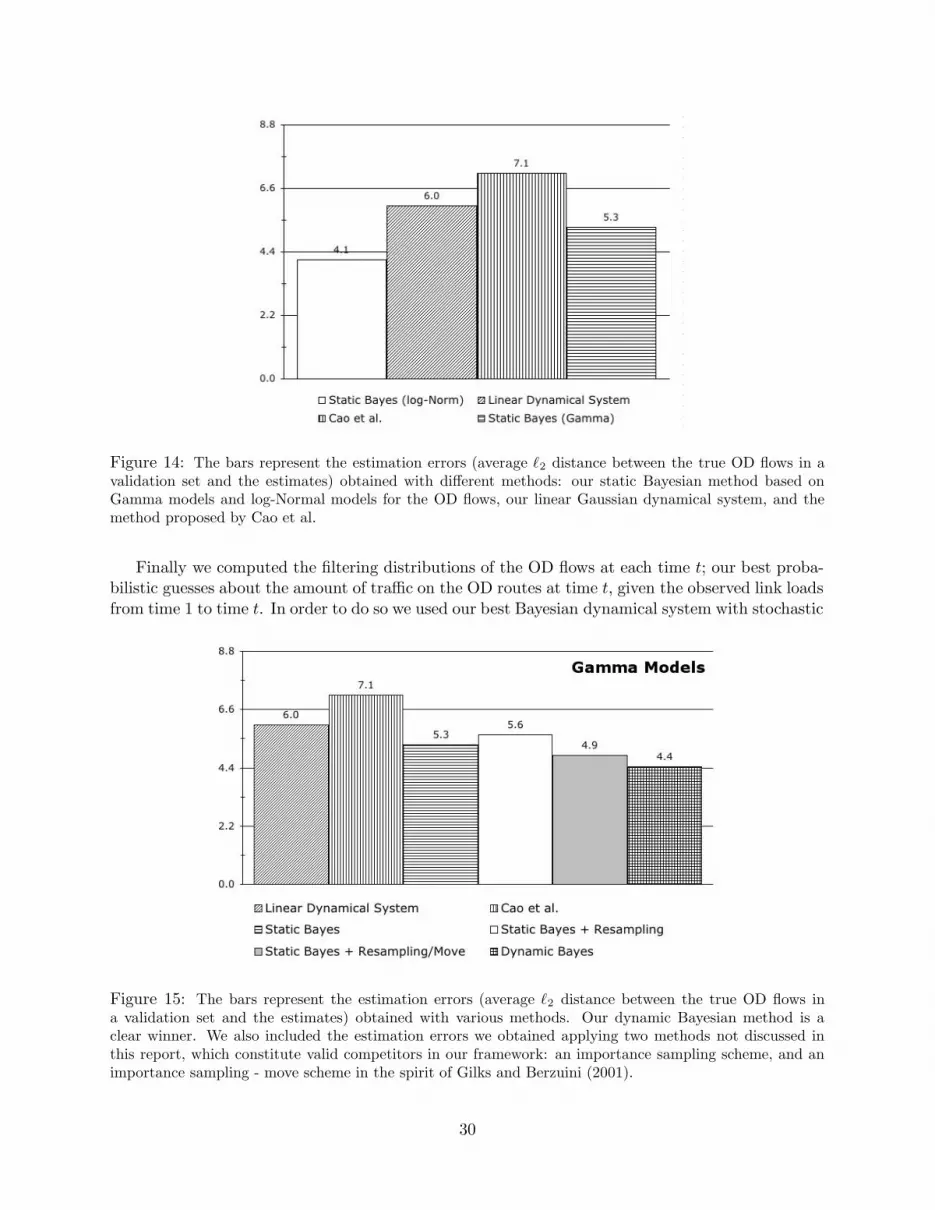
Figure 14: The bars represent the estimation errors (average `2 distance between the true OD flows in avalidation set and the estimates) obtained with different methods: our static Bayesian method based onGamma models and log-Normal models for the OD flows, our linear Gaussian dynamical system, and themethod proposed by Cao et al.

Finally we computed the filtering distributions of the OD flows at each time t; our best proba-bilistic guesses about the amount of traffic on the OD routes at time t, given the observed link loadsfrom time 1 to time t. In order to do so we used our best Bayesian dynamical system with stochastic

Figure 15: The bars represent the estimation errors (average `2 distance between the true OD flows ina validation set and the estimates) obtained with various methods. Our dynamic Bayesian method is aclear winner. We also included the estimation errors we obtained applying two methods not discussed inthis report, which constitute valid competitors in our framework: an importance sampling scheme, and animportance sampling - move scheme in the spirit of Gilks and Berzuini (2001).

30

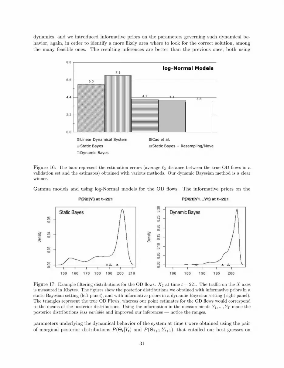
dynamics, and we introduced informative priors on the parameters governing such dynamical be-havior, again, in order to identify a more likely area where to look for the correct solution, amongthe many feasible ones. The resulting inferences are better than the previous ones, both using

Figure 16: The bars represent the estimation errors (average `2 distance between the true OD flows in avalidation set and the estimates) obtained with various methods. Our dynamic Bayesian method is a clearwinner.

Gamma models and using log-Normal models for the OD flows. The informative priors on the

Figure 17: Example filtering distributions for the OD flows: X2 at time t = 221. The traffic on the X axesis measured in Kbytes. The figures show the posterior distributions we obtained with informative priors in astatic Bayesian setting (left panel), and with informative priors in a dynamic Bayesian setting (right panel).The triangles represent the true OD Flows, whereas our point estimates for the OD flows would correspondto the means of the posterior distributions. Using the information in the measurements Y1, ..., YT made theposterior distributions less variable and improved our inferences — notice the ranges.

parameters underlying the dynamical behavior of the system at time t were obtained using the pairof marginal posterior distributions P (Θt|Yt) and P (Θt+1|Yt+1), that entailed our best guesses on

31

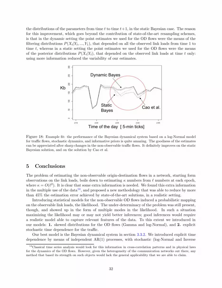
the distributions of the parameters from time t to time t+1, in the static Bayesian case. The reasonfor this improvement, which goes beyond the contribution of state-of-the-art resampling schemes,is that in the dynamic setting the point estimates we used for the OD flows were the means of thefiltering distributions P (Xt|Yt, ..., Y1), that depended on all the observed link loads from time 1 totime t, whereas in a static setting the point estimates we used for the OD flows were the meansof the posterior distributions P (Xt|Yt), that depended on the observed link loads at time t only:using more information reduced the variability of our estimates.

Figure 18: Example fit: the performance of the Bayesian dynamical system based on a log-Normal modelfor traffic flows, stochastic dynamics, and informative priors is quite amazing. The goodness of the estimatescan be appreciated after sharp changes in the non-observable traffic flows. It definitely improves on the staticBayesian solution, and on the solution by Cao et al.

5 Conclusions

The problem of estimating the non-observable origin-destination flows in a network, starting formobservations on the link loads, boils down to estimating κ numbers from ` numbers at each epoch,where κ = O(`2). It is clear that some extra information is needed. We found this extra informationin the multiple use of the data14, and proposed a new methodology that was able to reduce by morethan 45% the estimation error achieved by state-of-the-art solutions, in a realistic setting.

Introducing statistical models for the non-observable OD flows induced a probabilistic mappingon the observable link loads, the likelihood. The under-determinacy of the problem was still present,though, and showed up in the form of multiple modes in the likelihood. In such a situationmaximizing the likelihood may or may not yield better inferences; good inferences would requirea realistic model able to capture relevant features of the data. To this extent we introduced inour models: 1. skewed distributions for the OD flows (Gamma and log-Normal), and 2. explicitstochastic time dependence for the traffic.

Our best model is the Bayesian dynamical system in section 3.3.2. We introduced explicit timedependence by means of independent AR(1) processes, with stochastic (log-Normal and Inverse

14Classical time series analysis would look for this information in cross-correlation patterns and in physical lawsfor the dynamics of the OD flows. However, given the heterogeneity of the communication networks out there, anymethod that based its strength on such objects would lack the general applicability that we are able to claim.

32

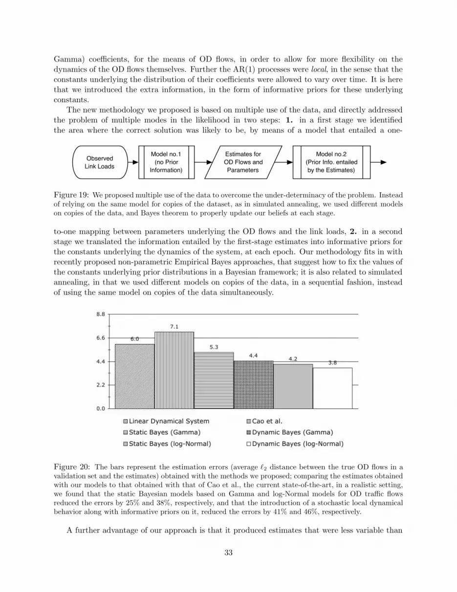
Gamma) coefficients, for the means of OD flows, in order to allow for more flexibility on thedynamics of the OD flows themselves. Further the AR(1) processes were local, in the sense that theconstants underlying the distribution of their coefficients were allowed to vary over time. It is herethat we introduced the extra information, in the form of informative priors for these underlyingconstants.

The new methodology we proposed is based on multiple use of the data, and directly addressedthe problem of multiple modes in the likelihood in two steps: 1. in a first stage we identifiedthe area where the correct solution was likely to be, by means of a model that entailed a one-

Model no.1

(no Prior

Information)

Observed

Link Loads

Model no.2

(Prior Info. entailed

by the Estimates)

Estimates for

OD Flows and

Parameters

Figure 19: We proposed multiple use of the data to overcome the under-determinacy of the problem. Insteadof relying on the same model for copies of the dataset, as in simulated annealing, we used different modelson copies of the data, and Bayes theorem to properly update our beliefs at each stage.

to-one mapping between parameters underlying the OD flows and the link loads, 2. in a secondstage we translated the information entailed by the first-stage estimates into informative priors forthe constants underlying the dynamics of the system, at each epoch. Our methodology fits in withrecently proposed non-parametric Empirical Bayes approaches, that suggest how to fix the values ofthe constants underlying prior distributions in a Bayesian framework; it is also related to simulatedannealing, in that we used different models on copies of the data, in a sequential fashion, insteadof using the same model on copies of the data simultaneously.

Figure 20: The bars represent the estimation errors (average `2 distance between the true OD flows in avalidation set and the estimates) obtained with the methods we proposed; comparing the estimates obtainedwith our models to that obtained with that of Cao et al., the current state-of-the-art, in a realistic setting,we found that the static Bayesian models based on Gamma and log-Normal models for OD traffic flowsreduced the errors by 25% and 38%, respectively, and that the introduction of a stochastic local dynamicalbehavior along with informative priors on it, reduced the errors by 41% and 46%, respectively.

A further advantage of our approach is that it produced estimates that were less variable than

33

those obtained with state-of-the-art solutions. We solved the problem in a dynamic setting, wherethe primary object of interest was the sequence of filtering distributions P (Xt,Θt|Yt, ..., Y1). Inparticular the point estimates we used for the OD flows were the means of the marginal distributionsXt = E(Xt|Yt, ..., Y1), which depended on the whole sequence of observed link loads Yt, ..., Y1,and hence were less variable than the solutions given in a static setting present in the literature,based on a small set of observations around time t.

In conclusion, estimating origin-destination flows from link loads in a dynamic setting, usingskewed models for the traffic, is the best available option at this time. We encourage the use ofinformative priors based on the data, in a novel spirit, to overcome the under-determinacy of theproblem. Our Bayesian dynamical system based on a log-Normal model and informative priorsreduced by more than 45% the estimation error achieved by state-of-the-art solutions in a realisticsetting.

34

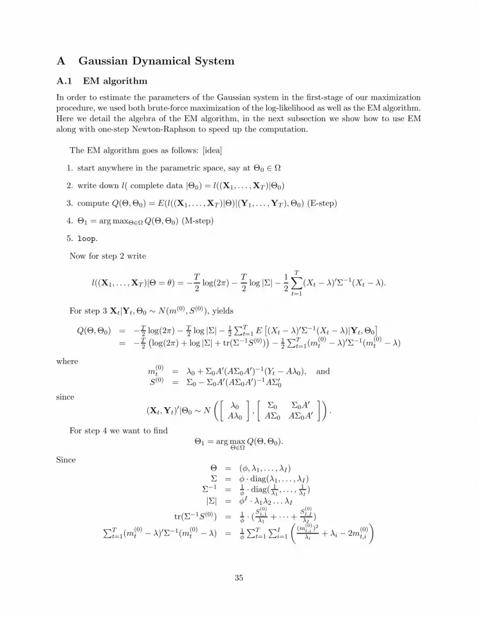
A Gaussian Dynamical System

A.1 EM algorithm

In order to estimate the parameters of the Gaussian system in the first-stage of our maximizationprocedure, we used both brute-force maximization of the log-likelihood as well as the EM algorithm.Here we detail the algebra of the EM algorithm, in the next subsection we show how to use EMalong with one-step Newton-Raphson to speed up the computation.

The EM algorithm goes as follows: [idea]

1. start anywhere in the parametric space, say at Θ0 ∈ Ω

2. write down l( complete data |Θ0) = l((X1, . . . ,XT )|Θ0)

3. compute Q(Θ,Θ0) = E(l((X1, . . . ,XT )|Θ)|(Y1, . . . ,YT ),Θ0) (E-step)

4. Θ1 = arg maxΘ∈Ω Q(Θ,Θ0) (M-step)

5. loop.

Now for step 2 write

l((X1, . . . ,XT )|Θ = θ) = −T

2log(2π) − T

2log |Σ| − 1

2

T∑

t=1

(Xt − λ)′Σ−1(Xt − λ).

For step 3 Xt|Yt,Θ0 ∼ N(m(0), S(0)), yields

Q(Θ,Θ0) = −T2 log(2π)− T

2 log |Σ| − 12

∑Tt=1 E

[

(Xt − λ)′Σ−1(Xt − λ)|Yt,Θ0

]

= −T2

(

log(2π) + log |Σ|+ tr(Σ−1S(0)))

− 12

∑Tt=1(m

(0)t − λ)′Σ−1(m

(0)t − λ)

wherem

(0)t = λ0 + Σ0A

′(AΣ0A′)−1(Yt −Aλ0), and

S(0) = Σ0 − Σ0A′(AΣ0A

′)−1AΣ′0

since

(Xt,Yt)′|Θ0 ∼ N

([

λ0

Aλ0

]

,

[

Σ0 Σ0A′

AΣ0 AΣ0A′

])

.

For step 4 we want to findΘ1 = arg max

Θ∈ΩQ(Θ,Θ0).

SinceΘ = (φ, λ1, . . . , λI)Σ = φ · diag(λ1, . . . , λI)

Σ−1 = 1φ · diag( 1

λ1, . . . , 1

λI)

|Σ| = φI · λ1λ2 . . . λI

tr(Σ−1S(0)) = 1φ · (

S(0)1,1

λ1+ · · ·+ S

(0)I,I

λI)

∑Tt=1(m

(0)t − λ)′Σ−1(m

(0)t − λ) = 1

φ

∑Tt=1

∑Ii=1

(

(m(0)t,i )2

λi+ λi − 2m

(0)t,i

)

35

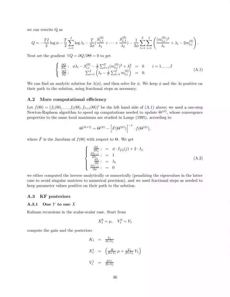
we can rewrite Q as

Q = −TI

2log φ− T

2

I∑

i=1

log λi −T

2φ(S

(0)1,1

λ1+ · · · +

S(0)I,I

λI)− 1

2φ

T∑

t=1

I∑

i=1

(

(m(0)t,i )2

λi+ λi − 2m

(0)t,i

)

.

Next set the gradient OQ = ∂Q/∂Θ = 0 to get

∂Q∂λi

: φλi − S(0)i,i − 1

T

∑Tt=1(m

(0)t,i )2 + λ2

i = 0 i = 1, . . . , I∂Q∂φ :

∑Ii=1

(

λi − 1T

∑Tt=1 m

(0)t,i

)

= 0.(A.1)

We can find an analytic solution for λ(φ), and then solve for φ. We keep φ and the λs positive ontheir path to the solution, using fractional steps as necessary.

A.2 More computational efficiency

Let f(Θ) = (f1(Θ), . . . , fI(Θ), fI+1(Θ))′ be the left hand side of (A.1) above; we used a one-stepNewton-Raphson algorithm to speed up computations needed to update Θ(it), whose convergenceproperties to the same local maximum are studied in Lange (1995), according to

Θ(it+1) = Θ(it) −[

F (Θ(it))]−1· f(Θ(it)),

where F is the Jacobian of f(Θ) with respect to Θ. We get

∂fi

∂λj: = φ · Ii(j) + 2 · λj

∂fI+1

∂λj: = 1

∂fi

∂φ : = λi∂fI+1

∂φ : = 0

(A.2)

we either computed the inverse analytically or numerically (penalizing the eigenvalues in the lattercase to avoid singular matrices to numerical precision), and we used fractional steps as needed tokeep parameter values positive on their path to the solution.

A.3 KF posteriors

A.3.1 One Y to one X

Kalman recursions in the scalar-scalar case. Start from

X01 = µ, V 0

1 = V1

compute the gain and the posteriors

K1 = V1R+V1

X11 =

(

RR+V1

µ + V1R+V1

Y1

)

V 11 = R V1

R+V1

36

and then again, project and correct

X12 = F

(

RR+V1

µ + V1R+V1

Y1

)

V 12 = F 2

(

R V1R+V1

)

+ Q

K2 =

[

F 2(

R V1R+V1

)

+Q]

R+[

F 2(

R V1R+V1

)

+Q]

X22 = R

R+[

F 2(

R V1R+V1

)

+Q]

[

F(

RR+V1

µ + V1R+V1

Y1

)]

+

[

F 2(

R V1R+V1

)

+Q]

R+[

F 2(

R V1R+V1

)

+Q] Y2

V 22 =

R[

F 2(

R V1R+V1

)

+Q]

R+[

F 2(

R V1R+V1

)

+Q]

to obtain the general recursive formulas

V t−1t = F 2

(

V t−1t−1

)

+ Q

Xt−1t = F Xt−1

t−1

Kt =[V t−1

t ]R+[V t−1

t ]

Xtt = R

R+[F 2 (V t−1t−1 )+Q]

[

F Xt−1t−1

]

+[F 2 (V t−1

t−1 )+Q]R+[F 2 (V t−1

t−1 )+Q]Yt

= (1−Kt)[

F Xt−1t−1

]

+ Kt Yt

= Kt Yt + (1−Kt)Kt−1 F Yt−1 + (1−Kt)(1−Kt−1)Kt−2 F 2 Yt−2 + . . .· · ·+ (1−Kt)× · · · ×K1 F t−1 Y1 + (1−Kt)× · · · ×K1 F t−1 µ

V tt =

R [F 2 (V t−1t−1 )+Q]

R+[F 2 (V t−1t−1 )+Q]

=R Q+R F 2 V t−1

t−1

R+Q+F 2 V t−1t−1

A.3.2 One Y to many Xs

Here we show how the Kalman recursions work, when the vector of observations Y has a lowerdimension than the vector of states X: in this example Y is a scalar and X is a 2-dimensionalvector. The information coming from Y is spread over the states in X; the attribution takes intoaccount the initial variance-covariance matrix of X and that of the corresponding error, and thevariance of Y , and outlines how the states in X are projected, in the sense of L2, on the spacespanned by the observation Y . Start from

X01 =

[

m1

m2

]

, V 01 =

[

s1 00 s2

]

37

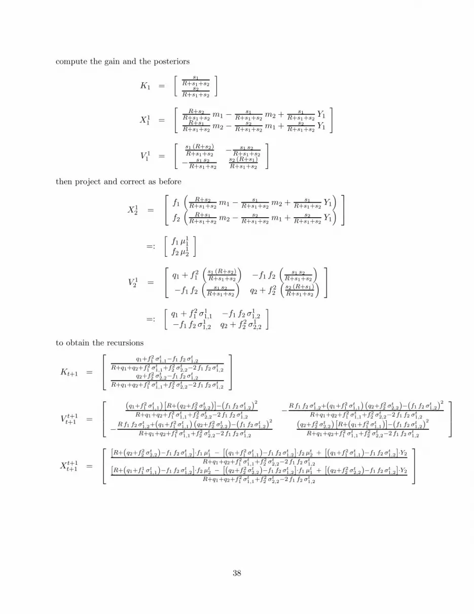
compute the gain and the posteriors

K1 =

[ s1R+s1+s2

s2R+s1+s2

]

X11 =

[

R+s2R+s1+s2

m1 − s1R+s1+s2

m2 + s1R+s1+s2

Y1R+s1

R+s1+s2m2 − s2

R+s1+s2m1 + s2

R+s1+s2Y1

]

V 11 =

[

s1 (R+s2)R+s1+s2

− s1 s2R+s1+s2

− s1 s2R+s1+s2

s2 (R+s1)R+s1+s2

]

then project and correct as before

X12 =

f1

(

R+s2R+s1+s2

m1 − s1R+s1+s2

m2 + s1R+s1+s2

Y1

)

f2

(

R+s1R+s1+s2

m2 − s2R+s1+s2

m1 + s2R+s1+s2

Y1

)

=:

[

f1 µ11

f2 µ12

]

V 12 =

q1 + f21

(

s1 (R+s2)R+s1+s2

)

−f1 f2

(

s1 s2R+s1+s2

)

−f1 f2

(

s1 s2R+s1+s2

)

q2 + f22

(

s2 (R+s1)R+s1+s2

)

=:

[

q1 + f21 σ1

1,1 −f1 f2 σ11,2

−f1 f2 σ11,2 q2 + f2

2 σ12,2

]

to obtain the recursions

Kt+1 =

q1+f21 σt

1,1−f1 f2 σt1,2

R+q1+q2+f21 σt

1,1+f22 σt

2,2−2 f1 f2 σt1,2

q2+f22 σt

2,2−f1 f2 σt1,2

R+q1+q2+f21 σt

1,1+f22 σt

2,2−2 f1 f2 σt1,2

V t+1t+1 =

(q1+f21 σt

1,1) [R+(q2+f22 σt

2,2)]−(f1 f2 σt1,2)

2

R+q1+q2+f21 σt

1,1+f22 σt

2,2−2 f1 f2 σt1,2

−R f1 f2 σt1,2+(q1+f2

1 σt1,1) (q2+f2

2 σt2,2)−(f1 f2 σt

1,2)2

R+q1+q2+f21 σt

1,1+f22 σt

2,2−2 f1 f2 σt1,2

−R f1 f2 σt1,2+(q1+f2

1 σt1,1) (q2+f2

2 σt2,2)−(f1 f2 σt

1,2)2

R+q1+q2+f21 σt

1,1+f22 σt

2,2−2 f1 f2 σt1,2

(q2+f22 σt

2,2) [R+(q1+f21 σt

1,1)]−(f1 f2 σt1,2)

2

R+q1+q2+f21 σt

1,1+f22 σt

2,2−2 f1 f2 σt1,2

Xt+1t+1 =

[R+(q2+f22 σt

2,2)−f1 f2 σt1,2]·f1 µt

1 − [(q1+f21 σt

1,1)−f1 f2 σt1,2]·f2 µt

2 + [(q1+f21 σt

1,1)−f1 f2 σt1,2]·Y2

R+q1+q2+f21 σt

1,1+f22 σt

2,2−2 f1 f2 σt1,2

[R+(q1+f11 σt

1,1)−f1 f2 σt1,2]·f2 µt

2 − [(q2+f22 σt

2,2)−f1 f2 σt1,2]·f1 µt

1 + [(q2+f22 σt

2,2)−f1 f2 σt1,2]·Y2

R+q1+q2+f21 σt

1,1+f22 σt

2,2−2 f1 f2 σt1,2

38

B The Key to fig n.10.

1 Alcoa Users*

2 Alumni Network*

3 Anycast Addresses*

4 CERT*

5 CS*

6 Cyert Lab 128*

7 Electrical Computer Engineering*

8 GSIA QuickReg*

9 Groats*

10 Gruel*

11 INI Projects*

12 LAB-TEST 128.237*

13 Loopback (New)*

14 Loopback Router*

15 Math - Parallel Cluster*

16 Off Campus*

17 PSC Private*

18 Reserved 100*

19 S29-Reserved*

20 S30-Alcoa (Alcoa-side ISDN)*

21 S30-BuyersMart (T1)*

22 SEI 2*

23 Spirit House (dorm)*

24 Telerama CMU Housing*

25 Test Subnet*

26 VPN Local IP Space*

27 West-Net*

28 _offcampus - theplanet.com*

29 authbridge

30 bp

31 campus

32 cfa

33 cyh

34 cyh-a100

35 dh

36 gsia

37 hbh

38 hl

39 hyper

40 macosxlabs.com*

41 mi

42 mmch

43 ptc

44 res

45 sei-private*

46 sysdev

47 uc

48 voip

49 weh

39

References

[BFK01] Z. Bi, C.N. Faloutsos, and F. Korn. The “DGX” distribution for mining massive, skeweddata. In Seventh International ACM SIGKDD Conference on Knowledge Discovery andData Mining, San Francisco, 2001.

[CDVY00] J. Cao, D. Davis, S. VanDer Wiel, and B. Yu. Time-varying network tomography:router link data. Journal of the American Statistical Association, 95:1063–1075, 2000.

[CVYZ02] J. Cao, S. VanDer Wiel, B. Yu, and Z. Zhu. A scalable method for estimating networktraffic matrices from link counts. Technical report, Bell Labs, 2002.

[DER86] I.S. Duff, A.M. Erisman, and J.K. Reid. Direct methods for sparse matrices. ClarendonPress, 1986.

[DLR77] A.P. Dempster, N.M. Laird, and D.B. Rubin. Maximum likelihood from incompletedata via the EM algorithm, with discussion. Journal of the Royal Statistical Society,Series B, Methodological, 39:1–38, 1977.

[Fie70] S.E. Fienberg. An iterative procedure for estimation in contingency tables. Annals ofMathematical Statistics, 41:907–917, 1970.

[GB01] W.R. Gilks and C. Berzuini. Following a moving target — Monte Carlo inference fordynamic Bayesian models. Journal of the Royal Statistical Society, Series B, Method-ological, 63:127–146, 2001.

[Hig01] T. Higuchi. Self-organizing time series model. In A. Doucet, N. de Freitas, and N. Gor-don, editors, Sequential Monte Carlo Methods in Practice, pages 429–444. Springer-Verlag, 2001.

[Lan95] K. Lange. A gradient algorithm locally equivalent to the EM algorithm. Journal of theRoyal Statistical Society, Series B, Methodological, 57:425–437, 1995.

[RC99] C. Robert and G. Casella. Monte Carlo Statistical Methods. Springer-Verlag, 1999.

[TW98] C. Tebaldi and M. West. Bayesian inference on network traffic using link count data.Journal of the American Statistical Association, 93:557–576, 1998.

[Var96] Y. Vardi. Network tomography: estimating source-destination traffic intensities fromlink data. Journal of the American Statistical Association, 91:365–377, 1996.

[VI94] R.J. Vanderbei and J. Iannone. An EM approach to od matrix estimation. TechnicalReport SOR 94-04, Princeton University, 1994.

[WH97] M. West and J. Harrison. Bayesian forecasting and dynamic models. Springer-Verlag,1997.

40