advanced methods for finite element simulation
TRANSCRIPT

ADVANCED METHODS FOR FINITE ELEMENT SIMULATION
FOR PART AND PROCESS DESIGN IN TUBE HYDROFORMING
DISSERTATION
Presented in Partial Fulfillment of the Requirements for
the Doctoral Degree of Philosophy in the
Graduate School of the Ohio State University
By
Suwat Jirathearanat, M.S.
* * * * *
Department of Mechanical Engineering
The Ohio State University
2004
Dissertation Committee: Approved by
Professor Taylan Altan, Adviser
Professor Gary Kinzel
Professor Rajiv Shivpuri ________________________________
Associate Professor Jerald Brevick Adviser
Department of Mechanical Engineering

Copyright by
Suwat Jirathearanat
December, 2003

ii
ABSTRACT
Tube hydroforming (THF) is a process of forming closed-section, hollow parts with
different cross sections by applying an internal hydraulic pressure and additional axial
compressive loads to force a tubular blank to conform to the shape of a given die cavity.
This innovative manufacturing process offers several advantages over the conventional
manufacturing via stamping and welding; a) part consolidation, b) weight reduction, c)
improved structural stiffness, d) lower tooling cost, e) fewer secondary operations, and
f) tight dimensional tolerances. To increase the implementation of this technology in the
automotive industry, dramatic improvements for hydroformed part design and process
development are imperative. The current development method of THF processes is
plagued with long lead times, which is resulted from much iteration on prototyping. The
formability of hydroformed tubular parts is affected by a large number of parameters
such as material properties, tube geometry, complex die-tube interface lubrication, and
process loading paths. FE simulation is perceived by the industry to be a cost-effective
process analysis tool compared to the conventional hard tooling prototyping.
Unfortunately, the prevalent trial-and-error based simulation method becomes very
costly when the process analyzed is complex.
More powerful design methods are needed to help the engineers design better THF part
geometries and process parameters, thus reducing lead times and costs. This work is
intended to develop methodologies for design of part geometries and process
parameters in THF. The methodologies in design of process parameters will include
analytical equations, FEA modeling, and FEA modeling enhanced with numerical
optimization algorithms and a kind of control rules. These tools will enable engineers to
quickly and effectively select loading paths (i.e. pressure curve and axial feed curve

iii
versus time) optimized for successfully hydroforming of simple to complex tubular
parts such as T-shapes, Y-shapes, cross members, and engine cradles.
The ultimate goal on loading paths determination through FEA in this work is to
completely replace the trial-and-error FEA approach by more efficient FEA approaches.
There are two main methods in determination of �optimized� THF loading paths
through FEA: a) iterative FE simulations with numerical optimization methods (i.e.
gradient based or non-gradient based) and b) adaptive simulation (control-system-based
simulation). The adaptive simulation method generates feasible loading paths within a
few simulation runs or only single simulation run. The optimization based simulation
generates optimum solution with the expense of a long computational time.
The research contributions that are associated with this dissertation work are:
• Systematic FEA simulation strategies such as analytical method and self-feeding
method to calculate proper THF loading paths or process parameters,
hydroformability limits, and required tool geometry for simple to moderate complex
part geometries.
• Procedure of automatic optimization of THF loading paths (i.e. pressure, axial feed
velocity, and counter punch force curve versus time) using PAM-STAMP and a
general optimization code, PAM-OPT, for typical THF complex part geometries
such as, simple bulges, Y-shapes, and automotive structural parts.
• Adaptive Simulation (AS) program that works with a commercial code (PAM-
STAMP) to automatically determine feasible loading paths of any given THF parts.
The current AS program can handle only simple part geometries such as
axisymmetric bulges.
• Framework of adaptive simulation method that can be adopted for process
parameter design of other metal forming operations such as sheet metal forming.

iv
For my parents,
my sisters,
and my wife
∞ ∞ ∞ ∞ ∞ ∞ ∞ ∞

v
ACKNOWLEDGEMENTS
I express my sincere thank to my advisor, Dr. Taylan Altan for taking the time to
mentor and tutor me throughout the years of my graduate study program. His insight,
wisdom, support, and trust were indispensable. I also would like to give special thank
all of my friends, at the Engineering Research Center for Net Shape Manufacturing,
who have helped make this research effort possible. Their invaluable assistance in
technical areas and their uplifting emotional support will always be remembered.
Further, I would like to thank the following governmental agencies and industrial
companies for their generous financial and technical support:
• Engineering Research Center for Net Shape Manufacturing
• Tube Hydroforming Consortium at the ERC/NSM
• Engineering Systems International
In closing, I would like to express my gratitude to my entire family for their unyielding
support and love.

vi
VITA
October 2, 1973 ....................................Born � Bangkok, Thailand
1994 .....................................................B.S. Mechanical Engineering,
Kasetsart University, Bangkok, Thailand
1994 � 1995 .........................................Project Engineer,
Air Daikin Company, Bangkok, Thailand
1995 � 1996 .........................................Aircraft Engineer,
Thai Airways International Public Company,
Bangkok, Thailand
1996 � present ......................................Graduate Research Associate,
Engineering Research Center for Net Shape
Manufacturing,
The Ohio State University, Columbus, Ohio
PUBLICATIONS
Peer Reviewed Journals: M. Koc, T. Allen, S. Jirathearanat, and T. Altan, �The Use of FEA and Design of
Experiments to Establish Design Guidelines for Simple Hydroformed Parts�, International Journal of Machine Tools & Manufacture 40 (2000) 2249-2266
vii
S. Jirathearanat, V. Vazquez, C. Rodríguez, and T. Altan, �Virtual Processing � Application of Rapid Prototyping for Visualization of Metal Forming Processes�, Journal of Materials Processing Technology 98 (2000) 116-124
Conference Proceedings: T. Altan, S. Jirathearanat, S. Kaya, �Process Simulation for Hydroforming Components
from Sheet and Tube � How can we improve the accuracy of the prediction?�, Proceedings from Chemnitz Conference, Germany 2002
T. Altan, S. Jirathearanat, M. Strano and S. G. Shr, �Adaptive FEM Process Simulation for Hydroforming Tubes�, Proceedings from International Conference on Hydroforming 2001 at University of Stuttgart, Germany
M. Strano, S. Jirathearanat and T. Altan, �Adaptive FEM Simulation: a Geometric-based for Wrinkle Detection�, CIRP Annals - Manufacturing Technology, v 50, n 1, 2001, pp.185-190
S. Jirathearanat, V. Kenthapadi, K. Hertell and T. Altan, �Prototype Development for Tube Hydroforming � Simulation and Tryout�, Proceeding from Tube Hydroforming Technology 2001, AFFT and SME, September 19-29, 2001, Novi, Michigan
S. Jirathearanat, M. Strano and T. Altan, �Selection of THF Loading Paths through FEA Simulation�, Proceedings from Innovations in Tube Hydroforming Technology Conference, SME, June 13-14 2000, Detroit, MI
Trade Journals: S. Jirathearanat, C. Hartl and T. Altan, �Hydroforming Y-shaped Stainless Steel
Exhaust Components�, Hydroforming Journal, Tube and Pipe Journal, December 2001
S. Jirathearanat, and T. Altan, �Successful Tube Hydroforming�, Hydroforming Journal, Tube and Pipe Journal, December 1999
FIELDS OF STUDY
Major Field: Mechanical Engineering
Studies in: Design and Manufacturing, Rapid Prototyping & Tooling, Dies &
Molds, Metal Forming

viii
TABLE OF CONTENTS
Page
ABSTRACT .............................................................................................................. ii
ACKNOWLEDGEMENTS ..............................................................................................v
VITA ............................................................................................................. vi
TABLE OF CONTENTS .............................................................................................. viii
LIST OF FIGURES....................................................................................................... xiii
LIST OF TABLES....................................................................................................... xxiii
NOMENCLATURE..................................................................................................... xxiv
CHAPTER 1. INTRODUCTION, PROBLEM STATEMENT, AND GOALS .................................................................................................1
1.1 Introduction..........................................................................................1
1.2 Problem Statement ..............................................................................3
1.3 Dissertation Organization ...................................................................3
CHAPTER 2. LITERATURE REVIEW ...................................................................4
2.1 Tube Hydroforming.............................................................................4 2.1.1 Tube Hydroforming Process as a System..............................................4
2.1.2 Classification of Tube Hydroformed Part..............................................5
2.2 FEA of Tube Hydroforming ...............................................................6 2.2.1 FEA Modeling .......................................................................................6

ix
2.2.2 Failure Analysis .....................................................................................7
2.3 Design of Process Parameters...........................................................10 2.3.1 Empirical and Analytical Methods ......................................................11
2.3.2 Numerical Methods..............................................................................12 2.3.2.1 Optimization Simulation Methods.......................................................12 2.3.2.2 Feedback Control Simulation Methods ...............................................15 2.3.2.3 Adaptive Simulation Methods .............................................................16
CHAPTER 3. TUBE HYDROFORMING PART AND PROCESS DESIGN USING FEA MODELING...............................................18
3.1 Tube Hydroforming Process and FE Simulation............................19 3.1.1 Hydroforming of Y-shape....................................................................19
3.1.1.1 Tube Hydroforming Process Procedure...............................................21 3.1.1.2 Determination of the Process Parameters ............................................23
3.1.2 FE Modeling of Y-shape Hydroforming .............................................29 3.1.2.1 FE Modeling with PAM-STAMP........................................................29 3.1.2.2 FE Simulation Results and Verification ..............................................32
3.1.3 Considerations in FE Modeling of THF processes..............................36 3.1.3.1 Type of FE Formulations.....................................................................36 3.1.3.2 Types of Finite Elements .....................................................................37 3.1.3.3 Shell Element Size ...............................................................................40
3.2 Effect of Geometric Parameters on Hydroformability ..................41 3.2.1 Tube Spline Length Effect ...................................................................41
3.3 Effect of Process Parameters on Hydroformability........................47 3.3.1 Effect of Axial Feed and Pressure on Protrusion Height.....................51
3.3.2 Effect of Counter Punch Force on Protrusion Height..........................53
CHAPTER 4. SYSTEMATIC APPROACH TO SELECT LOADING PATH USING PROCESS FEA SIMULATION............................55
4.1 Self-Feeding Simulation Approach ..................................................55 4.1.1 Natural Axial Feed Curve Concept......................................................55
4.1.2 Loading Path Determination Procedure...............................................57
4.2 THF Process Case Studies.................................................................59

x
4.2.1 Automotive Structural Part #1 .............................................................59 4.2.1.1 Determination of Loading Paths ..........................................................62 4.2.1.2 Hydroforming Simulation and Experiment .........................................66
4.2.2 Automotive Structural Part #2 .............................................................70 4.2.2.1 Determination of Loading Paths ..........................................................70 4.2.2.2 Hydroforming Simulation and Experiment .........................................75
CHAPTER 5. AUTOMATIC APPROACH TO SELECT LOADING PATH USING OPTIMIZATION BASED SIMULATION ..........78
5.1 Overview of Numerical Optimization Theory.................................78 5.1.1 Components of Optimization...............................................................81
5.1.2 Optimization Algorithms .....................................................................83
5.2 Optimization in Metal Forming � Process Parameter Design.......84 5.2.1 Design Variables..................................................................................86
5.2.2 Objective Function...............................................................................88
5.2.3 Constraint Functions and Design Variable Bounds.............................89
5.3 Interfacing PAM-OPT with PAM-STAMP.....................................91
5.4 THF Process Optimization Case Studies .........................................92 5.4.1 Simple Bulge........................................................................................92
5.4.1.1 FE Model Descriptions ........................................................................92 5.4.1.2 Optimization Descriptions ...................................................................94 5.4.1.3 Optimization Results..........................................................................100
5.4.2 Y-shape ..............................................................................................103 5.4.2.1 FE Model Descriptions ......................................................................105 5.4.2.2 Optimization Descriptions .................................................................105 5.4.2.3 Optimization Results..........................................................................110
5.4.3 Structural Part ....................................................................................117 5.4.3.1 FE Model Descriptions ......................................................................117 5.4.3.2 Optimization Descriptions .................................................................117 5.4.3.3 Optimization Results..........................................................................121
CHAPTER 6. AUTOMATIC APPROACH TO SELECT LOADING PATH USING ADAPTIVE SIMULATION.................................125
6.1 Adaptive Simulation Concept .........................................................125

xi
6.2 Implementation of Adaptive Simulation Method .........................127 6.2.1 Adaptive Simulation Procedure .........................................................127
6.2.1.1 Defect Detection Module...................................................................129 6.2.1.2 Parameter Adjustment Module ..........................................................132
6.2.2 Integration of Adaptive Simulation Program to PAM-STAMP ........134
6.2.3 Adaptive Simulation with Dynamic Explicit Code ...........................137
6.3 Part Defect Indicators .....................................................................138 6.3.1 Geometric Wrinkle Criteria ...............................................................138
6.3.1.1 First Derivative Wrinkle Criterion (Iwd) ...........................................139 6.3.1.2 Length to Area Wrinkle Criterion ( Iwla ) ..........................................141 6.3.1.3 Surface Area to Volume Criterion ( Iwsv ) .........................................148 6.3.1.4 Considerations to the Geometric Wrinkle Indicators ........................154
6.3.2 Fracture Criteria .................................................................................155
6.4 Process Parameter Adjustment Algorithms..................................155 6.4.1 Calibration Stage................................................................................156
6.4.2 Hydroforming Stage ..........................................................................159 6.4.2.1 Wrinkle Control Strategy...................................................................160 6.4.2.2 Pure Shear Control Strategy ..............................................................162 6.4.2.3 Modified Wrinkle Control Strategy...................................................162
CHAPTER 7. CONCLUSIONS AND FUTURE WORK.....................................168
7.1 Performance Comparison of Different Loading Path Determination Methods...................................................................168
7.2 Selection of the Loading Path Determination methods................174 7.2.1 THF Part Classifications Based on Geometry ...................................174
7.2.2 THF Part Classifications Based on Process Window ........................178
7.3 Conclusions.......................................................................................180
7.4 Future Work.....................................................................................184
LIST OF REFERENCES..............................................................................................185
APPENDIX A FLOW STRESS DETERMINATION................................................192

xii
APPENDIX B DETERMINATION OF FRICTION COEFFICIENT AT GUIDING ZONE .............................................................................195
APPENDIX C OPTIMIZATION ALGORITHMS....................................................197
APPENDIX D INTERFACING BETWEEN PAM-OPT AND PAM-STAMP .......203
APPENDIX E ADAPTIVE SIMULATION PROGRAM..........................................209

xiii
LIST OF FIGURES
Figure Page
Figure 1.1: a) THF sequence [Dohmann, 1991] and b) selected loading paths generate different deformation modes of the protrusion [Asnafi, 2000]...................................................................2
Figure 2.1: The tube hydroforming system ..............................................................4
Figure 2.2: Tube hydroformed part features (a) bent feature, (b) crushed feature, (c) bulge feature, (d) protrusion feature (referred as Y-shape), and (e) automotive hydroformed structural part (SPS, Germany) ...............................................................5
Figure 2.3: Common failure modes that limit THF process, winkling, buckling, and bursting [Koc, 2002].......................................8
Figure 2.4: Energy-based method, regions where wrinkles are predicted to occur in a cup hydroforming process [Nordlund, 1997].......................................................................................9
Figure 2.5: Geometry-based method, difference in the strains at the upper and lower skins of the tubular shells [Doege, 2000] ..........................................................................................................10
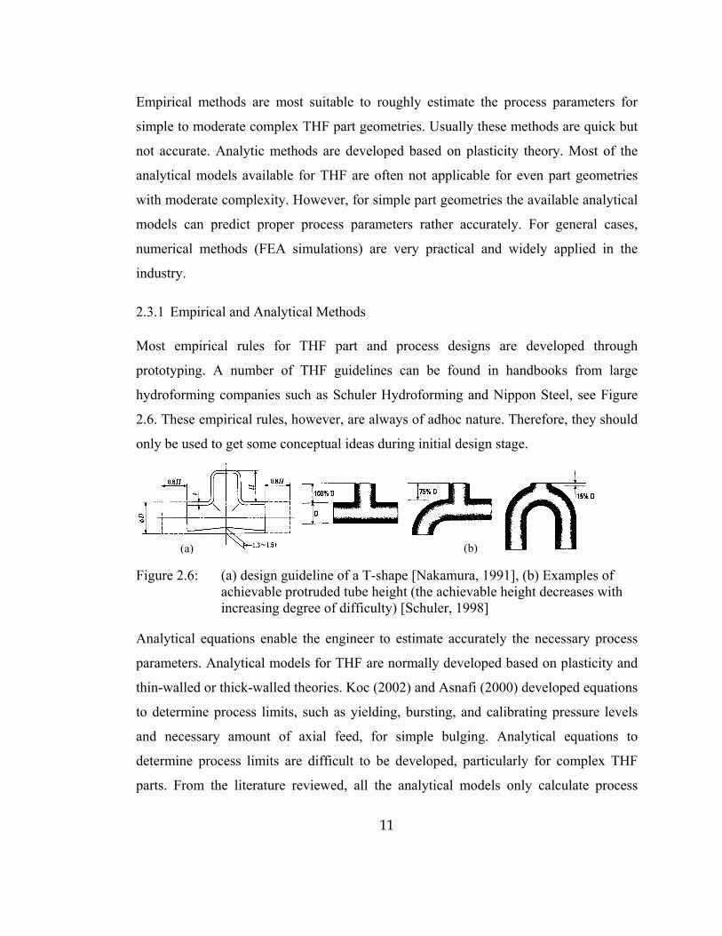
Figure 2.6: (a) design guideline of a T-shape [Nakamura, 1991], (b) Examples of achievable protruded tube height (the achievable height decreases with increasing degree of difficulty) [Schuler, 1998].......................................................................11
Figure 2.7: Bizier curves representing a) forging die profile as design parameters, b) THF loading path as design parameters [Yang, 2001b] ......................................................................14
Figure 2.8: General flow chart of the feedback control simulation method for process design in metal forming......................................16

xiv
Figure 3.1: a) Schematic of hydroforming tooling of a Y-shape, b) dimensions of the Y-shape and c) a stainless steel (SS 304) Y-shape hydroformed at SPS (Siempelkamp Pressen Systeme, Germany) ..................................................................20
Figure 3.2: Y-shape hydroforming process procedure [SPS, Germany] .................................................................................................22
Figure 3.3: SPS hydroforming press specifications................................................23
Figure 3.4: Geometric parameters of the Y-shape..................................................25
Figure 3.5: Process parameters measured from the Y-shape hydroforming experiments: a) internal pressure, b) axial feed, and c) counter punch displacement and force versus time curves ..................................................................................28
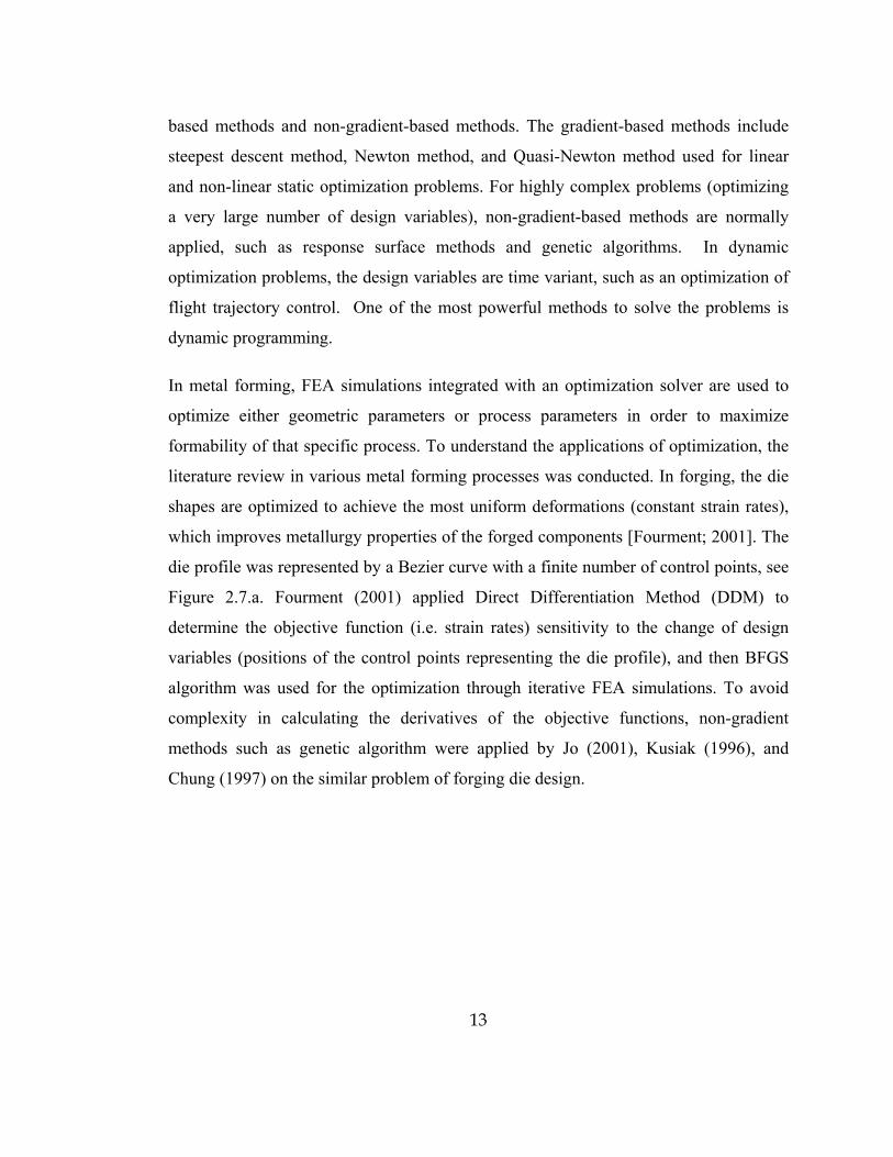
Figure 3.6: a) Finite element model of Y-shape and b) tube material properties and dimensions, see Appendix A for tube material flow stress determination.......................................................30
Figure 3.7: FEA simulation demonstrates intermediate hydroforming steps of a Y-shape, a) Pressure, b) axial feeds and c) counter punch force versus time curves used to hydroform SS 304 Y-shapes.....................................................34
Figure 3.8: Comparison of thickness distributions of SS304 Y-shape from FEA and experiments along longitudinal direction.................35
Figure 3.9: Comparison of SS 304 Y-shape thickness distributions (upper longitudinal direction) from FEM and experiments (OD = 50 mm, L0 = 320 mm, t0 = 1.5 mm, and 584.0)06.0(471.1 εσ += GPa).............................................................39
Figure 3.10: FEM simulation of thick-walled T-shape ............................................39
Figure 3.11: Wrinkled parts simulated with different tube mesh sizes ...........................................................................................................40
Figure 3.12: Examples of long structural tubular parts with many part geometrical features: a) engine cradle (Schafer Hydroforming) and b) a portion of exhaust manifold ......................42

xv
Figure 3.13: Schematic drawing of the Y-shape part and tooling geometry, experimental setup...............................................................44
Figure 3.14: Internal pressure versus time curve and axial feed versus time curves used in all the experiments, see Figure 3.13................................................................................................45
Figure 3.15: Experimental results: comparisons of protrusion height, HP, of Y-shapes with different part spline lengths.............................46
Figure 3.16: Drawing of a simplified structural part with a T-shape that can only be hydroformed with one-sided axial feeding. .....................................................................................................49
Figure 3.17: Geometry of the T-shape die cavity and part geometry with one-side axial feeding (dimensions are in mm; 25.4 mm = 1 in.) .......................................................................................49
Figure 3.18: a) axial feed versus time curves used in all simulation cases (25.4 mm = 1 in), and b) pressure versus time curves corresponding to the different axial feeds (1 GPa = 145,038 psi) ...........................................................................................50
Figure 3.19: Effect of axial feed on protrusion height (all the simulated parts have maximum thinning of 30%).............................52
Figure 3.20: Effect of internal pressure at different axial feeds on protrusion height ....................................................................................52
Figure 3.21: simulation results of T-shape hydroforming with axial feeding of 50 mm, medium pressure curve (see Figure 3.18) and counter punch force, a) samples of counter punch force versus time curves, and b) effect of counter punch force on protrusion height and maximum thinning ....................................................................................................54
Figure 4.1: Self-feeding simulation concept............................................................56
Figure 4.2: A flowchart of Self-Feeding (SF) simulation procedure....................56
Figure 4.3: Automotive structural part geometry [Kawasaki Steel, Japan] ........................................................................................................60

xvi
Figure 4.4: Geometry of preformed/bent tube [Kawasaki Steel, Japan] ........................................................................................................61
Figure 4.5: Thinning distributions along profiles A and B of the bent tube after bending simulation, including springback (negative values indicate thickening and positive values indicate thinning) ........................................................61
Figure 4.6: Simulation #1, SF: input pressure and output punch velocity curves.........................................................................................63
Figure 4.7: Simulation #2, SF: punch velocity curves as a result of the modified pressure curve..................................................................63
Figure 4.8: Modified axial feed velocity curves (the right axial feed velocity is represented in negative values, left axial feed is in positive values) ...............................................................................64
Figure 4.9: Simulation #3, Normal Simulation: smoothened punch velocities and the modified pressure curve ........................................64
Figure 4.10: Summary of the axial feed curves from the simulations conducted to �optimize� the loading paths through SF simulation approach...............................................................................65
Figure 4.11: �Optimized� loading paths from SF: pressure, left axial feed, right axial feed ...............................................................................65
Figure 4.12: Intermediate tube hydroforming steps: side view and front view .................................................................................................68
Figure 4.13: Thinning distribution on the final simulated part and a table comparing the simulation and experimental results at some specific areas.................................................................69
Figure 4.14: FEA modeling of hydroforming crossmember [Schuler Hydroforming] ........................................................................................71
Figure 4.15: Pressure curves and corresponding nodal velocity from the right tube end, obtained from SF simulations..............................73
Figure 4.16: Plots of axial feeds (left and right tube ends) selected through SF simulation approach ..........................................................73
xvii
Figure 4.17: Plots of pressure and right axial feed versus left axial feed (case B, Figure 4.16)........................................................................74
Figure 4.18: Intermediate simulation results of crossmember hydroforming ..........................................................................................75
Figure 4.19: Plots of pressure and right axial feed versus left axial feed used in the experiments.................................................................76
Figure 4.20: Crossmember parts hydroformed with the loading curves above [Schuler Hydroforming] ................................................76
Figure 4.21: Thinning measurements of the Cross member from prototyping ..............................................................................................77
Figure 5.1: A flowchart of the optimal design formulation procedure [Deb; 1998] ............................................................................80
Figure 5.2: Typical shapes of (a) pressure versus time curve and (b) axial feed versus time curve represented by piecewise linear curves.............................................................................................87
Figure 5.3: Axial feed velocity versus time curve represented by piecewise linear curves often used in optimization instead of axial feed (Figure 5.2.b)........................................................87
Figure 5.4: Flow chart of THF optimization using PAM-OPT and PAM-STAMP...........................................................................................91
Figure 5.5: Simple bulge geometry and material properties [Yang, 2001b]........................................................................................................93
Figure 5.6: Loading curves presented by piecewise-linear curves: design variables.......................................................................................95
Figure 5.7: Objective function: minimizing part thickness variations ................98
Figure 5.8: Constraint functions: part dimension accuracy using controlled volume...................................................................................98
Figure 5.9: Optimized axial feed velocity curve and pressure curve................101
Figure 5.10: Evolution of objective function and constraint function.................101

xviii
Figure 5.11: Initial and optimized loading paths for simple bulging .................102
Figure 5.12: Part thinning distribution of optimized simple bulge.....................102
Figure 5.13: Optimized loading paths for simple bulging ...................................104
Figure 5.14: Part thinning distributions of the simple bulge ...............................104
Figure 5.15: Design variables: counter punch force versus time curve and pressure versus time curve ..........................................................107
Figure 5.16: Left and right axial punch velocity versus time curves ..................107
Figure 5.17: Objective function: maximizing the protrusion height or maximizing the part controlled volume............................................109
Figure 5.18: Constraint functions: a) tube-to-die distance, b) protrusion corner curvature, and c) part maximum thinning ..................................................................................................109
Figure 5.19: Objective function: evolution of part controlled volume................111
Figure 5.20: Constraint functions: evolutions of a) tube-to-die distance, b) corner curvature, and c) part maximum thinning ..................................................................................................111
Figure 5.21: Optimized counter punch force curve and pressure curve versus time ..................................................................................112
Figure 5.22: RSM Objective function: part controlled volume.............................114
Figure 5.23: RSM constraint functions: a) tube-to-die distance, b) corner curvature, and c) maximum thinning....................................114
Figure 5.24: RSM optimized a) counter punch force curve and b) pressure curve .......................................................................................115
Figure 5.25: Comparison of part qualities obtained from Gradient-based method and RSM method; a) part thinning distributions, and b) protrusion profiles ...........................................116
Figure 5.26: FE model of structural part: part geometry and material properties [Kawasaki Hydromechanics, Japan] ...............................119
xix
Figure 5.27: Constraint function: tube-to-die distance..........................................119
Figure 5.28: Initial design parameters: left and right axial feed velocity versus time curve and pressure versus time curve........................................................................................................120
Figure 5.29: Optimized loading paths .....................................................................122
Figure 5.30: Evolution curves of a) objective function and b) constraint function................................................................................123
Figure 5.31: Optimized loading paths for prototyping.........................................123
Figure 5.32: Part thinning distribution along the longitudinal direction..................................................................................................124
Figure 6.1: Schematic of the AS procedure, Piy: internal yielding pressure; ∆Pi: internal pressure increment; ∆Da: axial feed increment. ......................................................................................126
Figure 6.2: General conceptual flow chart of the adaptive simulation interfacing with PAM-STAMP during a simulation time step .............................................................................128
Figure 6.3: a) intermediate part with alive wrinkle, which, at the process end, can turn into b) good final part, or c) bad final part with dead wrinkle................................................................131
Figure 6.4: a) loading path in the THF forming window, and b) in-plane strain plot.....................................................................................133
Figure 6.5: Adaptive Simulation programming descriptions and interfacing with PAM-STAMP............................................................135
Figure 6.6: a) prescribed line on the bulge forming tube mesh, b) prescribed line seen on wrinkle-free part, c) prescribed line seen on wrinkled part ...................................................................140
Figure 6.7: Length-to-area wrinkle criterion: a) definitions of tube (Lt) and die (Ld) profile arch lengths, b) good final part condition, and c) bad final part with dead wrinkles (all the figures are the tube and die profiles cut by the Y-Z plane, refer to Figure 6.6.a) ..................................................................142

xx
Figure 6.8: a) shortest arch length illustration and b) parameters used in length-to-area wrinkle criterion............................................144
Figure 6.9: Different loading paths used to hydroform the simple bulge........................................................................................................146
Figure 6.10: Normalized length versus normalized area curves of the parts formed with three different LP�s........................................146
Figure 6.11: Surface area-to-volume wrinkle criterion: a) example of control box over a the expansion zone of a simple bulge, and b) parameter definitions of tube and die ...................................149
Figure 6.12: Plots of normalized surface area versus normalized volume of part simulated with a) pure expansion with free tube ends (i.e. SF LP), b) Optimal LP, and c) bad LP; and snap shots of all the simulated parts at the same normalized part volume (V=0.6) ........................................................152
Figure 6.13: a ) plot of area-to-volume wrinkle indicator ( svIw ) of the part formed with the optimal LP and bad LP, see Figure 6.9, and b) a triangular trajectory (so called �wrinkle control limit�) approximating the Opt svIw curve ...........................152
Figure 6.14: Part quality plots: a) surface area-to-volume wrinkle indicator versus normalized volume curves, b) fracture indicator versus normalized volume curves, and c) normalized volume versus simulation time step curve ..................157
Figure 6.15: Adjustments of process parameters: a) internal pressure, b) axial feed displacement, and c) axial feed punch velocity versus time (simulation time steps) curves......................................................................................................158
Figure 6.16: Loading path predicted by AS showing different stages of simple bulge hydroforming process and control strategies (from Figure 6.15.a and b)..................................................161
Figure 6.17: Plot of hoop and axial stresses showing pure shear control strategy......................................................................................161

xxi
Figure 6.18: Adaptive simulation results using modified wrinkle control strategy: a) plot of part wrinkle state, and b) predicted loading path for the simple bulge ....................................164
Figure 6.19: Comparison of maximum thinning evolutions of parts from all the adaptive simulation cases including the initial SF simulation: A - wrinkle control strategy and B - modified wrinkle control strategy ...................................................165
Figure 6.20: Smoothened loading path approximating the loading path predicted using the modified wrinkle control strategy for the simple bulging...........................................................165
Figure 7.1: Comparisons of a) loading paths predicted, and b) part maximum thinning versus normalized part volume, and c) longitudinal part thinning distributions obtained from all the loading path determination methods...........................169
Figure 7.2: Searching of the simple bulge loading path using the SF method, compared with the optimized loading path from OPT method .................................................................................170
Figure 7.3: Common THF part geometrical features: a) Y-shape protrusion, b) bulge, and c) bend .......................................................175
Figure 7.4: Complex THF parts with multiple geometrical features: a) exhaust manifolds with protrusions and bends (different spline configurations), and b) SPS engine cradle: long automotive structural part with bulges and bends:......................................................................................................177
Figure 7.5: Typical trend curve of material displacement along axial direction of a simplified long structural part (showing only one half of the part) being hydroformed with axial feed = d0ax applied at the tube end at a given pressure curve .......................................................................................177
Figure 7.6: Flow chart of selection of process parameter design methods ..................................................................................................181
Figure A.1: Hydraulic Bulge tooling: the flow stress determination procedure ...............................................................................................192

xxii
Figure A.2: Measured internal pressure versus bulge height, SS304 with OD = 50 mm, to = 1.5 mm...........................................................193
Figure A.3: Effective stress � effective strain curve, SS304 with OD = 50 mm, to = 1.5 mm ..............................................................................193
Figure B.1: ERC friction tooling: testing friction coefficient in the THF guiding zone .................................................................................195
Figure C.1: a) original one variable optimization objective function [F(x)] and constraint functions [g1(x)] and [g2(x)], and b) pseudo-objective functions [Φ(x,rp)] with different penalty multipliers [Vanderplaats, 1984] ..........................................198
Figure C.2: Augmented Lagrangian Optimization flow chart [ESI Software, 2001] ......................................................................................199
Figure C.3: Wavy function in PAM-OPT [ESI Software, 2001]...........................200
Figure C.4: Example of optimization (2 design variables) progression using PAM-OPT adaptive response surface method [ESI Software, 2001] ...............................................................202
Figure D.1: General PAM-OPT algorithm flow chart [ESI Software, 2001] ........................................................................................................204
Figure D.2: PAM-OPT input data structure [ESI Software, 2001] ......................205
Figure E.1: Basic flowchart of the adaptive simulation procedure....................210
Figure E.2: Simple bulge hydroforming FE model for AS simulation runs .........................................................................................................212

xxiii
LIST OF TABLES
Table Page
Table 3.1: Comparison of explicit and implicit FE formulations [Hora, 1999]..............................................................................................37
Table 4.1: Tube dimensions and material mechanical properties, n
OK )( εεσ += ......................................................................60
Table 4.2: Summary table of all the simulations conducted with the SF approach.......................................................................................66
Table 4.3: Material properties, tube dimensions and coefficient of friction used in the FE simulations.......................................................71
Table 4.4: Results from simulations based on SF Approach (SF #1 is similar to SF #2, with different pressure curves applied).....................................................................................................74
Table 7.1: Comparisons of performance of all the loading path determination methods for simple bulge ..........................................170
Table 7.2: Advantages and disadvantages of the trial-and-error simulation method................................................................................172
Table 7.3: Comparison of advantages and disadvantages of all the loading path determination methods developed in this work ........................................................................................................173
Table 7.4: Classification of automotive THF parts according to their functionality .................................................................................175
Table A.1: Mechanical properties of SS304 tubes used in the Y-shape hydroforming experiments ..................................................... 194
Table B.1: Friction coefficients determined for Gleitmo 965 at various internal pressure levels and sliding speeds ........................196

xxiv
NOMENCLATURE
Glossary
THF = Tube HydroForming
LP = Loading Paths (pressure vs. axial feed)
DOE = Design of Experiment
CCD = Central Composite Design
SF = Self Feeding Simulation
AS = Adaptive Simulation
OPT = OPTimization-based simulation
FLD = Forming Limit Diagram
PAM-STAMP = FEM simulation code
PAM-OPT = General optimization code
Process Parameters
pi(t) = internal pressure curve versus time
(pi)y = yielding pressure
(pi)b = bursting pressure
(pi)max = calibrating pressure
da(t) = axial feed curve versus time
daL = left axial feed
daR = right axial feed
Geometrical Parameters
Lp1 or LLO = initial tube length on the left
side
Lp2 or LRO = initial tube length on the
right side
LL1 = final tube length on the left side
LR1 = final tube length on the right side
Dp = prtrusion diameter
Re = branch radius (or fillet radius)
Hp, H = protrusion height
Self-feeding Simulation selfleftd = left axial feed from SF simulation
selfrightd = right axial feed from SF simulation
asf = axial feed scaling factor

xxv
Optimization-based Simulation
kx = design variable vector
nxpxpxp ,..., 21 = pressure design variables
mxfxfxf ,..., 21 = axial feed design variables
)(xf = objective function
)(xgi = constraint function
tubeVol = part controlled volume
dieVol = die control volume
ih = part elemental thickness
0h = tube initial thickness
1id = tube-to-die distance
Adaptive Simulation
ti = simulation time step
Tj = control time step
Lt = part profile arch length
Ld = die cavity profile arch length
At = part profile enclosed area
Ad = part-die profile enclosed area
Iwla = length-to-area wrinkle indicator
St = part surface area
Sd = die cavity surface area
Vt = part fluid cell volume
Vd = die cavity internal volume
Iwsv = surface area-to-volume wrinkle
indicator
V = normalized part fluid cell volume

1
CHAPTER 1.
INTRODUCTION, PROBLEM STATEMENT, AND GOALS
1.1 Introduction
Tube HydroForming (THF) is a process of forming closed-section, hollow parts with
different cross sections by applying an internal hydraulic pressure and additional axial
compressive loads to force a tubular blank to conform to the shape of a given die cavity,
see Figure 1.1.a. With the advancements in computer controls and high-pressure
hydraulic systems, this process has become a viable method for mass production,
especially with the use of internal pressures of up to 6000 bars [Dohmann, 1991]. Tube
hydroforming offers several advantages as compared to conventional manufacturing via
stamping and welding [Brewster, 1996] [Shah, 1997]. These advantages include; a) part
consolidation, b) weight reduction through more efficient section design, c) improved
structural strength and stiffness, d) lower tooling cost due to fewer parts, e) fewer
secondary operations (no welding of sections required and holes may be pierced during
hydroforming), and f) tight dimensional tolerances. Despite several benefits over
stamping process, THF technology is still not fully implemented in the automotive
industry due its time-consuming part and process development. To increase the
implementation of this technology in automotive industry, dramatic improvements on
hydroformed part design and process development are imperative.
In THF, compressive stresses occur in regions where the tube material is axially fed,
and tensile stresses occur in expansion regions. The main failure modes are buckling,
wrinkling (excessively high compressive stress) and bursting (excessively high tensile
stress). It is clear that only an appropriate relationship between internal pressure curve
versus time pi(t) and axial feed curve versus time da(t), so called �Loading Paths� (LP),

2
guarantees a successful THF process without any of the failures, see Figure 1.1.b. Both
parameters pi(t) and da(t) are dependent on part geometry, tube material, and lubrication
conditions.
Effective classifications of hydroformed tubular parts are necessary for development of
THF part design and process systematically. Finite Element Analysis (FEA)
simulations can be used as a tool to extensively analyze THF. Design of the process
parameters are normally selected through time-consuming, trial-and-error iterative FEA
simulations. FEA simulation enhanced with optimization schemes can greatly reduce
the lead-time spent in the process development.
Figure 1.1: a) THF sequence [Dohmann, 1991] and b) selected loading paths generate different deformation modes of the protrusion [Asnafi, 2000]
Wrinkling
Axial feed (da)
Internal pressure (pi)
Uniaxial tension
Pure shear
Plane strain
Tube
Tube
a) b)

3
1.2 Problem Statement
The development of tube hydroforming processes is plagued with long lead times,
which result from much iteration of tryouts either on trial-and-error based FEA
simulations or on expensive prototype tooling. Hydroformability of tubular parts is
affected by a large number of parameters such as material properties, tube geometry,
complex die-tube interface lubrication, and process parameters, i.e. loading paths. More
powerful design tools are needed to help engineers design better products and processes
and to reduce lead times and cost. Therefore the goals of the proposed work are:
♦ Develop part design guidelines for THF processes that facilitate engineers to bring
conceptual THF part designs to production more efficiently by early eliminating bad
designs considering manufacturability issues and arriving to successful part designs.
♦ Develop methodologies for design and optimize loading paths in THF. The
methodologies will utilize systematic FEA simulations and FEA enhanced with
numerical optimization methods and �Adaptive Simulation� (AS) method. These
tools will enable the engineers to select loading paths (i.e. pressure curve, axial feed
curve, and counter punch force curve versus time) optimized for simple to complex
tube hydroforming processes such as T-shapes, Y-shapes, cross members, and
engine cradles.
1.3 Dissertation Organization
Finally, the outline of this dissertation proposal by chapters is:
Chapter 1: Introduction and Problem Statement
Chapter 2: Literature Review
Chapter 3: Tube Hydroforming Part and Process Design using FEA Modeling
Chapter 4: Systematic Approach to Select Loading Paths using FEA Simulation
Chapter 5: Automatic Approach to Select Loading Paths using Optimization-based
Simulation
Chapter 6: Automatic Approach to Select Loading Paths using Adaptive Simulation
Chapter 7: Summary and Future Work

4
CHAPTER 2.
LITERATURE REVIEW
2.1 Tube Hydroforming
2.1.1 Tube Hydroforming Process as a System
In a typical tube hydroforming system, there are many components that play an
important role in the success of the process. Theses components need to be addressed
thoroughly when developing any THF part and process. The main components and key
issues of a complete THF system (see Figure 2.1) can be listed as follows:
A. Quality and material properties of incoming tubes;
B. Preforming and bending design and production methods;
C. Die and tool design guidelines;
D. Die-workpiece interface issues: wear, friction and lubrication;
E. Mechanics of the different deformation zones;
F. Equipment, press and environment related issues;
G. Specifications and requirement of the hydroformed part.
C Tools / Dies
A Incoming
Tube
D Tool-Workpiece
Interface
E Deformation Mechanics
FEquipment /Environment / Press
G Hydroformed
part
B Bending /
Preforming
Figure 2.1: The tube hydroforming system

5
2.1.2 Classification of Tube Hydroformed Part
Hydroformed tubular parts vary over a wide range of shapes. This variety goes from a
simple bulged tube to an engine cradle with multiple part features such as bends,
protrusions, and complex cross sections. It is necessary to classify the THF parts into
different categories with respect to common characteristics that they have in order to
handle the design process more efficiently. Mainly, THF parts have the following
common features on them, see Figure 2.2: (more detail on THF part classifications can
be found in [Koc, 1998]).
Bend: a tube is bent in order to obtain a designed spline geometry that accommodates
alignment of the tube in the THF die cavity.
Crushing: a crushed shape is given into a tube in the pre-forming stage not only to
facilitate the tube alignment into the die but also to accumulate the tube material locally
for the subsequence expansion process. Crushed geometries are found frequently in
automotive structural parts.
Bulge: bulges are typically tube expansions, mostly axisymmetric about the tube axis.
Protrusion: protrusions are local expansions, stemmed out from the tube axis. They are
normally manufactured as connectors, i.e. T-shapes and Y-shapes, used particularly in
exhaust manifolds.
(a)
(b)
(c)
(d)
(e)
Figure 2.2: Tube hydroformed part features (a) bent feature, (b) crushed feature, (c) bulge feature, (d) protrusion feature (referred as Y-shape), and (e) automotive hydroformed structural part (SPS, Germany)

6
2.2 FEA of Tube Hydroforming
FEA for hydroforming process assists die designers and process engineers to (a) assess
the manufacturability of parts at the design stage, (b) explore alternative design
schemes, and eventually (c) arrive at an optimized design in a cost effective and timely
fashion. With the aid of FEA simulation, the part quality control, and the design of the
tube hydroforming process can be easily implemented and monitored. FEA simulations
provide insights on the necessary process parameters/ loading paths (i.e. internal
pressure and axial feed), part geometry, and part formability by analyzing the thinning,
thickening, and strain distribution in the deformed tube.
2.2.1 FEA Modeling
There are a few analytical equations to predict formability, i.e. thickness distribution, of
simple THF parts such as T-shapes [Shen-Zhang; 1999] and simple axisymmetric
bulges [Asnafi, 1999]. However, compared to FEA, the analytical equations have
limited applicability for THF of general part geometries [Lei, 2001a]. FEA assists the
die designers and process engineers to (a) assess manufacturability of a part during the
design stage, (b) explore alternative designs, and eventually (c) arrive at an optimized
design in a cost effective and timely fashion. FEA simulations provide insights about
the part formability by predicting its stress and strain distributions in the deformed tube.
This information facilitates selection/optimization of the process parameters (i.e.
internal pressure and axial feed curves versus time), as well as part geometry
modification if necessary.
Until now a number of researchers have applied three-dimensional FEA on several THF
processes: simple bulges [Donald, 2001], T-shapes and Y-shapes [Lei, 2001a]
[Jirathearanat, 2001a], and automotive structural parts [Yang, 2001a] [Kim, 2002]
[Jirathearanat, 2001a]. Most of the FEA simulations were conducted by Dynamic
Explicit FEA packages, e.g. PAM-STAMP or LS-DYNA, which have advantages in
fast changing boundary conditions necessary in forming with complex die surfaces and

7
capability to handle large deformation forming. Some researchers prefer applying the
Static Implicit FEA formulation for its more reliable and rigorous scheme in
determining equilibrium at each step of deformation. However, there exist intrinsic
problems associated with the Implicit FEA formulation such as convergence and long
computation time [Lei, 2001a]. Therefore, the implicit FEA packages are normally
limited to hydroforming of simple tubular part geometries.
2.2.2 Failure Analysis
Major failure modes in THF are buckling, wrinkling and fracture (bursting), Figure 2.3.
Robust methods of predicting and analyzing failures in stamping parts have been under
intensive investigation by a number of researchers. However, a reliable analysis method
for the failure problems in THF has not yet been established. Due to the lack of reliable
failure prediction methods, the methods used in sheet metal forming are inevitably
applied in tube hydroforming processes. Forming Limit Diagrams (FLD) are generated
experimentally based on assumption of proportional loading path. Levy (1999) applied
FLDs to predict formability in THF. He suggested that FLDs for THF should be above
the FLDs determined from a flat sheet of the tubular material. Another competing
method is ductile fracture criteria. Unlike the FLDs, these ductile fracture criteria are
not loading path dependent. Fracture is predicted when the ductile integral value
exceeds a critical value, which is determined experimentally through tensile tests. Filice
(2001) successfully implemented Crokroft and Latham ductile fracture criterion on
simple bulge simulations, and validated the criterion experimentally. Lei (2001b)
applied Oyane ductile fracture criterion on simulations of a bumper rail and a subframe.
However, no experimental data was used to validate the simulation studies. Maximum
thinning criterion is also considered another good way of predicting fracture. However,
maximum thinning criterion is not reliable when biaxial tensile state of stress is
dominant.
The analyses of onset and growth of wrinkles in the literature are found mostly on sheet
metal forming. The analyses are generally based on three main methods: a) plastic

8
bifurcation theory, b) energy method, and c) geometry method. The underlying idea of
the plastic bifurcation theory [Hill, 1958] [Hutchinson, 1974] is that, for unperturbed
(perfect) shell structures, wrinkles may take shape when the solution to an energy
equation describing the solid mechanic problem (elastic and plastic regions) is not
unique. After this bifurcation point, wrinkles may appear or the unwrinkled state may
hold until another bifurcation point. A drawback of the plastic bifurcation theory is that
it only deals with initially unperturbed structures. In THF processes, wrinkling may
appear at any stage of the process where the part is deforming.
Figure 2.3: Common failure modes that limit THF process, winkling, buckling, and bursting [Koc, 2002]
Nordlund (1997) proposed a wrinkle detection method based on an energy quantity. In
his method, a formation of wrinkles is characterized by the occurrence of areas where
the deformation is dominated by strong local out of plane rotation. This behavior can be
traced by following the evolution of second-order increment of the internal work. A
wrinkle is detected when this energy quantity becomes negative (see Figure 2.4). The
main advantages of this approach are: 1) no assumption is made a priori on the shape
and frequency of the wrinkles, 2) it is not limited to detection of wrinkle onset for
unperturbed shells, and 3) it is not necessary to solve the eigenvalue problem associated
with the bifurcation theory. The approach has been widely tested in both explicit and
implicit FEM codes [Nordlund, 1998] and also applied to hydroforming of non-tubular
metal sheets. It seems to be very effective in the early detection of wrinkles. The only
drawback is that it fails when large rigid-body rotations occur or when dealing with low
frequency (large-scale) wrinkles.

9
Figure 2.4: Energy-based method, regions where wrinkles are predicted to occur in a cup hydroforming process [Nordlund, 1997]
Even though the wrinkle detection criteria discussed above were invented many years
ago, they have been implemented only on �in-house� FEA codes. Commercial FEA
codes, such as PAM-STAMP, still have not implemented those criteria. Nevertheless,
different types of wrinkles in sheet metal forming (flange wrinkles, sidewall wrinkles
and wrinkles beneath the punch) can be predicted by PAM-STAMP, where a wrinkled
part is depicted by its deformed mesh [Aita, 1992]. In PAM-STAMP, wrinkles are
predicted based on the energy minimization of plastic deformation combined with some
intrinsic numerical round off in its explicit FEA formulation. This method may not
predict onset of wrinkles as accurately as predicted by the previously mentioned
criteria. However, unlike in stamping, wrinkles in a hydroformed part may be
controlled/straightened by an appropriate increase of internal pressure. Therefore, it is
justified to detect wrinkles as they have formed to a relatively small size (noticeable
wrinkle amplitude). This simplifies the wrinkle detection in THF simulations. The
wrinkles can be identified based on simple geometrical considerations, rather than on
energy/stresses.
In using most of FEA commercial codes for THF, some measurements/quantities of the
visible wrinkles based on their geometric considerations need to be devised, in order to
enable adjustment/optimization of the part and process design. There are several
advantages of a geometry base approach. It is simpler mathematically than most of the
other criteria. A small amount of wrinkles in the THF part may be even helpful in
preventing excessive thinning in the bulging area, since it is a way to accumulate

10
material in the expansion zone. The simplest geometric criterion, proposed by
Jirathearanat (2000a), calculates slopes of a tube profile along a section passing through
the tube axis to determine hills and valleys. This method can be extended to gradients of
the deforming surface. However, the slope method becomes difficult, as the part
geometry is more complex. A better method was proposed by Doege (2000). This
method considers the difference of strains at the upper and lower skins of the tubular
shell. In order to distinguish real wrinkles for surface curvatures due to its conformity to
the die surfaces, the method checks also the nodal normal velocity of the potentially
wrinkled elements (see Figure 2.5). If the velocity is low, the tube surface is probably
following the die and the situation is considered acceptable (no wrinkle detected). If the
strain difference and the normal velocity are both high, then a wrinkle is detected.
Figure 2.5: Geometry-based method, difference in the strains at the upper and lower skins of the tubular shells [Doege, 2000]
2.3 Design of Process Parameters
The main process parameters in THF are pressure, axial feeds, and counter punch force.
These are also often referred to as �loading paths� or �part program� when presented in
time domain. The success of THF processes is largely dependent on the choice of the
loading paths. Part geometry, tubular material, and lubrication conditions need to be
taken into account in designing of loading paths. The selection of proper loading paths
can be done using empirical methods, analytical methods, or numerical methods.
11
Empirical methods are most suitable to roughly estimate the process parameters for
simple to moderate complex THF part geometries. Usually these methods are quick but
not accurate. Analytic methods are developed based on plasticity theory. Most of the
analytical models available for THF are often not applicable for even part geometries
with moderate complexity. However, for simple part geometries the available analytical
models can predict proper process parameters rather accurately. For general cases,
numerical methods (FEA simulations) are very practical and widely applied in the
industry.
2.3.1 Empirical and Analytical Methods
Most empirical rules for THF part and process designs are developed through
prototyping. A number of THF guidelines can be found in handbooks from large
hydroforming companies such as Schuler Hydroforming and Nippon Steel, see Figure
2.6. These empirical rules, however, are always of adhoc nature. Therefore, they should
only be used to get some conceptual ideas during initial design stage.
Figure 2.6: (a) design guideline of a T-shape [Nakamura, 1991], (b) Examples of achievable protruded tube height (the achievable height decreases with increasing degree of difficulty) [Schuler, 1998]
Analytical equations enable the engineer to estimate accurately the necessary process
parameters. Analytical models for THF are normally developed based on plasticity and
thin-walled or thick-walled theories. Koc (2002) and Asnafi (2000) developed equations
to determine process limits, such as yielding, bursting, and calibrating pressure levels
and necessary amount of axial feed, for simple bulging. Analytical equations to
determine process limits are difficult to be developed, particularly for complex THF
parts. From the literature reviewed, all the analytical models only calculate process
(a) (b)

12
parameter limits, such as yielding and bursting pressures. None of the equations can
predict the necessary loading paths (i.e. evolution of process parameters in time) for
successful THF. Most of these analytical equations are developed for particular THF
features, i.e. simple bulges and T-shapes, see Figure 2.2. The analytical equations
become inefficient if not useless when designing a complex THF part, which consists of
many THF features, and its process. It is noted here that even though the empirical
rules and analytical equations provides guidelines on THF part and process design,
many more design iterations are often necessary. FEA simulations are normally used in
the design improvement stage. The process parameters are modified till successful THF
process is obtained.
2.3.2 Numerical Methods
Trial-and-error simulation method for the process design can be very time consuming,
i.e. pressure and axial feed curves versus time are selected to conduct a simulation. If
the results are not satisfactory, the input curves are modified by �intuition� and the
simulation is run again until satisfactory results are obtained. Fortunately, this iterative
FEA method can be done systematically and automatically with kinds of optimization.
For example, determination of the loading paths can be treated as a classical
optimization problem. By this way the resultant loading paths are optimized to
maximize the part formability. Alternative approaches, aimed at efficient process FEA
modeling are under development in several research institutes and companies. Three
main different strategies can be followed: a) Optimization Simulation Methods, b)
Feedback Control Simulation Methods, and c) Adaptive Simulation Methods
2.3.2.1 Optimization Simulation Methods
Optimization can be broadly divided into two main groups: a) static optimization and b)
dynamic optimization. In static optimization problems, design variables are time
invariant, such as optimizing dimensions of a mechanical component to minimize its
weight. There are two main methods to solve static optimization problems; gradient-
13
based methods and non-gradient-based methods. The gradient-based methods include
steepest descent method, Newton method, and Quasi-Newton method used for linear
and non-linear static optimization problems. For highly complex problems (optimizing
a very large number of design variables), non-gradient-based methods are normally
applied, such as response surface methods and genetic algorithms. In dynamic
optimization problems, the design variables are time variant, such as an optimization of
flight trajectory control. One of the most powerful methods to solve the problems is
dynamic programming.
In metal forming, FEA simulations integrated with an optimization solver are used to
optimize either geometric parameters or process parameters in order to maximize
formability of that specific process. To understand the applications of optimization, the
literature review in various metal forming processes was conducted. In forging, the die
shapes are optimized to achieve the most uniform deformations (constant strain rates),
which improves metallurgy properties of the forged components [Fourment; 2001]. The
die profile was represented by a Bezier curve with a finite number of control points, see
Figure 2.7.a. Fourment (2001) applied Direct Differentiation Method (DDM) to
determine the objective function (i.e. strain rates) sensitivity to the change of design
variables (positions of the control points representing the die profile), and then BFGS
algorithm was used for the optimization through iterative FEA simulations. To avoid
complexity in calculating the derivatives of the objective functions, non-gradient
methods such as genetic algorithm were applied by Jo (2001), Kusiak (1996), and
Chung (1997) on the similar problem of forging die design.

14
Figure 2.7: Bizier curves representing a) forging die profile as design parameters, b) THF loading path as design parameters [Yang, 2001b]
A few researchers applied static optimization methods through iterative FEA
simulations to determine metal forming process parameters in time domain. In forging,
ram speeds at which a workpiece is being formed are optimized so that the deformation
is uniform. In sheet metal forming the blank holder force is also optimized so that final
stamping part has the highest obtainable drawn depth with no wrinkles and fracture. In
tube hydroforming, pressure and axial feed curves versus time (loading paths) are also
optimized [Yang, 2001b]. The loading path is often described by a Bezier curve
representation whose control points are the design variables in the optimization
problem, see Figure 2.7.b. The objective function can be strain rate variations, part
thickness variations, or maximum thinning, which are minimized. The problem is then
reduced to determination of the positions of control points so to minimize the objective
function value. Ghouati (2000) and Yang (2001b) applied this optimization method to
determine the loading path for a simple axisymmetric bulging. ♦ Design parameters are the control points (pi) describing a B-spline function of
loading path (Figure 2.7).
♦ Objective function takes into account of element thickness variations after each
forming simulation run:
21
2
0
0
0
1)(
−Σ== h
hhpf iN
iN
where N is the total number of elements considered, h0 is the initial thickness and hi is the final thickness of element ith, which is an implicit function of design parameters (pi).
Forging die profile THF loading path
a) b)
Control points

15
♦ Constraint function represents the distance from the desired shape to the final part at
simulation end:
21
2
0)(
Σ=
= i
M
idpg
where M is the total number of nodes considered, and di is the distance of node i to the tool (final desired part shape), which is an implicit function of design parameters (pi).
This optimization method may be called �global optimization of process parameters in
time domain�. This method tends to generate very complex and non-linear objective
functions as the number of control points (design variables) increases, which may lead
to non-convergent solutions.
2.3.2.2 Feedback Control Simulation Methods
Control theories have been applied in many industrial applications for many years, such
as control of temperatures in chemical processes. A controller regulates some quantities
to stabilize a process by automatically adjusting a variable(s) (controlled variable) in
real time. The simplest and most widely used control schemes are PID controllers. For
highly non-linear processes, non-mathematics based controllers, such as fuzzy logic
controller, and neural network controller are preferred. A few researchers have applied
feedback control schemes in conjunction with metal forming process FEA simulations
[Cao, 1994]. With the help of a feedback controller integrated into a process FEA code,
the process parameters can be adjusted at every simulation time step to achieve high
process formability predicted through the simulation.
The main difference in determination of process parameters through FEA using
optimization methods mentioned above and feedback controllers is apparent in the time
duration where corrective actions, i.e. adjusting process parameters, take place. The
optimization simulation method requires many simulation runs. After the end of a
simulation, a parameter correction is done and applied into the next simulation run with
the attempt to minimize the objective function value. A feedback controller adjusts
process parameters at every time step in one simulation run in order to maintain the
controlled quantities, i.e. formability, see Figure 2.8. The advantage of the feedback

16
control simulation method is that it requires less total computation time in predicting the
process parameters than the optimization simulation method does.
Cao (1994) controlled wrinkles and maximum strains in a conical cup drawing
simulation by automatically adjusting the binder force by using a PI controller. Thomas
(1998) further developed Cao�s work by introducing the control of stresses as well.
Grandhi (1993) and Feng (2000) implemented optimal feedback controllers in
simulation of forging processes. The controller tried to regulate the ram speed to track
the predefined strain rate of the part being forged. In tube hydroforming, Doege (2000)
applied fuzzy logic control theory to simulations of tube hydroforming. The controller
adjusted the internal pressure and axial feed curves in order to prevent wrinkles
throughout the process.
Figure 2.8: General flow chart of the feedback control simulation method for process design in metal forming
2.3.2.3 Adaptive Simulation Methods
This method makes use of both optimization method and feedback control method in
design of process parameters. The adjustments of process parameters are carried out at
each time step (or certain interval of simulation time step) during a single simulation
run similar to the feedback control method. However, the adjustments of process
parameters are done with the help of optimization methods. By this way, the automatic
design of the process parameters can be done quickly and in an optimized manner.
Metal forming FEA at one time increment
PID controller Good part
Formability
Desired formability
Parameter Adjustment
Defect Identification
(ti) to (t1+1)
(tend) Process
Parameters

17
There have been two slightly different methods, proposed for THF process parameter
design, which fall into the adaptive simulation category:
ERC applied adaptive control theory combined with optimization in selecting of THF
loading paths [Strano, 2001a]. This adaptive simulation method uses a quadratic
objective function considering a wrinkle quantity (failure indicator) to be minimized at
each time step. To implement this method, a linear plant model is generated and
updated and each time step to describe evolution of the wrinkle quantity through the
forming time in a function of pressure and axial feed. The coefficients in this model are
evaluated at every time step.
Gelin (2002) devised a kind of adaptive simulation with function interpolation and
optimization techniques. In his paper, the thickness variation of the THF part is
minimized. To generate the objective function, a spline formulation was used to model
the evolution of the thickness variation in a function of pressure and axial feed. Unlike
the method mentioned above, this method requires many simulation runs in each time
step with perturbed process parameters to interpolate the thickness function. In respect
to the optimization simulation methods mentioned earlier, this method may be named
�local-time optimization of process parameters.

18
CHAPTER 3.
TUBE HYDROFORMING PART AND PROCESS DESIGN
USING FEA MODELING
In all metal forming processes, part and process design is an essential step in successful
manufacturing of any products. Tube HydroForming (THF) process demands a lot of
engineering knowledge starting from the part design which is constrained by part
functionality and geometry, to the process design where appropriate combination of
internal pressure, axial feed, and counter punch pressure (if necessary) need to be
determined. It has always been of a primary concern in the industry to reduce the lead-
time in part and process design developments and produce better parts with lower costs.
One of the most efficient ways to achieve this goal is utilize Finite Element Analysis
(FEA) during the part and process development stage. Specifically, due to the lack of
extensive knowledge in both analytical and experimental in THF, FE modeling of THF
processes is very useful in 1) reducing or even eliminating the need for trial-and-error in
the developing stage, and 2) optimizing the part and process to minimize the
manufacturing costs (i.e. increasing the robustness of the process thus reducing the
scrap rate).
This chapter discusses FE modeling of THF process and it applications. Considerations
of modeling any THF processes by FE simulation are given. Simulation and
experiments of hydroforming of a Y-shape is used as an example in this chapter. Some
simulation work was also conducted in an attempt to understand mechanics of the
deformation process. Through this study, effects of tubular part geometry (initial tube
length) and process parameters (pressure and axial feed) on hydroformability were also
explained. At last some THF part and process guidelines are given.

19
3.1 Tube Hydroforming Process and FE Simulation
In FE modeling of any metal forming processes, a good understanding of the FEA code
is as important as an understanding of the process itself. Typically, A THF process
requires two motivational forces, i.e. axial force exerting on the tube ends and internal
pressure acting normally to the tube inner surface. These two forces (i.e. loading paths)
should be applied appropriately on the tube if a sound part is to be produced. In terms of
process design, FEA is used to verify and refine loading paths. This section first gives
an overview of the Y-shape hydroforming process. Then, FE modeling of the Y-shape
hydroforming is discussed. PAM-STAMP (explicit dynamic non-linear FEA code) is
used throughout this work. There are some considerations in using any dynamic codes
to simulate THF processes. These considerations are also discussed at the end of this
section.
3.1.1 Hydroforming of Y-shape
Y-shapes are (see Figure 3.1) commonly used as fitting parts in automotive exhaust
manifolds. The parts are usually made of stainless steels 304, which is rust resistant.
Typically, in hydroforming of these Y-shapes, a counter punch is usually used to
support the protrusion tip while it is growing. By this way, premature protrusion
bursting is delayed and thus increasing the useful height of the protrusion (useful
protrusion height is defined in Section 3.3). However, the use of a counter punch adds
one more process parameter to be controlled properly with the axial feeds and internal
pressure. The Y-shape studied in this work has a protrusion that is angled to the tube
axis by 60 degrees. The detailed dimensions of the part are given in Figure 3.1. The
load paths and tube material properties of this part will be discussed shortly in the next
section.

20
Internal Pressure
Axial Punches
Counter Punch
Internal Pressure
Axial Punches
Counter Punch
Figure 3.1: a) Schematic of hydroforming tooling of a Y-shape, b) dimensions of the Y-shape and c) a stainless steel (SS 304) Y-shape hydroformed at SPS (Siempelkamp Pressen Systeme, Germany)
a)
b)
c)

21
3.1.1.1 Tube Hydroforming Process Procedure
Figure 3.2 shows pictures of Y-shape hydroforming procedure. These pictures are taken
from Y-shape hydroforming experiments (conducted at research facility of SPS,
Germany) that are to be discussed later in this chapter. General specifications of the
SPS hydroforming press used are given in Figure 3.3. Please note that in these forming
experiments, from which the photos are taken, the counter punch was not used. The
process descriptions are given below. 1. Upper and lower die inserts were installed onto the press. The axial punches were
connected to the pressure intensifiers with high-pressure hoses. Figure 3.2.a shows
the lower die insert.
2. A rough drawing of the axial punch is shown in Figure 3.2.b. The punch has a
conical shape at the tube-punch contact area. In this case, the tube blank has OD =
50 mm, and to = 1.5 mm. For good sealing performance, the punches were designed
to have 5 mm of sealing distance (i.e. initial axial punch displacement of 5 mm
without internal pressure build-up).
3. The tubes were spray-lubed with a solid film lubricant (Gleitmo 965). The tubes
were allowed to air-dry for about 2-3 hours.
4. Figure 3.2.b shows how a tube blank was placed and positioned in the lower die
cavity. The axial punches were fully retracted to their home positions, while the
counter punch axis was not in operation and rested at its home position.
5. Figure 3.2.c shows a completely formed Y-shape (without any use of a counter
punch). It is shown that the length of the final part has been shortened due to the
axial feeds. Axial feed was 40 mm and 80 mm on the left and right side,
respectively. The maximum internal pressure was 600 bars. The protrusion height,
Hp, was measured and considered as �formability index� in this study.

22
Figure 3.2: Y-shape hydroforming process procedure [SPS, Germany]
Counter Punch Axis (no counter punch attached)
Right Punch Left Punch
Y-shape
LLO LRO
80 mm 40 mm
Hp
Y-shape
LLO LRO
Tube Blank Sealing Distance
5 mm
1.5 mm
a)
b)
c)

23
SPS HYDROFORMING PRESS
Closing Force 25,000 kN (2,500 ton)
Max. Axial Cylinder Force 1250 kN (at Max. punch speed)
Max. Counter Cylinder Force 24.7 kN
Max. Axial Punch Speed 40 mm/s
Figure 3.3: SPS hydroforming press specifications
3.1.1.2 Determination of the Process Parameters
A successful THF process largely depends on process parameters (loading paths), part
geometry, initial geometry of the tube, and interface friction conditions. In THF of a
given tubular part geometry, the main process parameters to be determined are the
following:
• Axial feeds vs. time
• Internal pressure vs. time
• Counter punch force vs. time (for some part geometries with protrusions)
Initial estimates of these parameters can be obtained from simple metal forming
equations. Typically, these estimated parameters are not accurate depending on the
complexity of part geometry and non-linearity of material properties. The parameters
will then be tried out and �tuned� through iterative FEA simulations till satisfactory
results are obtained. It is certainly preferred that the initial process parameters be
reasonably well estimated. Thus, the number of iterative simulations, necessary to
obtain the best process conditions, can be reduced. Design of the process parameters for
Y-shape hydroforming is discussed here. Analytical equations were used to determine

24
pressure levels and axial feeds necessary. These estimated parameters were then
applied and refined in process FEA simulations using PAM-STAMP.
Axial Feed: The concept of volume constancy is applied here to estimate the axial feeds
(at the left, daL, and right, daR, tube ends) necessary to form a Y-shape with a desired
protrusion height (H), Figure 3.4. The original tube wall thickness is assumed to remain
unchanged. However, it is also possible to assume that the part final thickness is linearly
distributed (thickened at the tube ends and thinned at the protrusion tip), which is more
realistic. For simplicity, in this case study, the part final thickness distribution is
assumed to the same as the original tube wall thickness. The material volume at the
protrusion section of the Y-shape is converted to obtain the necessary axial feed. The Y-
shape geometry with a fixed angle is shown in Figure 3.1. The tube blank outside
diameter (D0) is 50.5 mm (1.988�), tube initial thickness (t0) is 1.5 mm (0.059�), the
protrusion diameter (Dp) is 50.5 mm (1.988�).
The volume of material formed into the protrusion area was calculated. Each half of the
protrusion was assumed to have been contributed from the axial feed applied on the
corresponding side of the protrusion. For this Y-shape geometry with the specified
angles and Dp=D0, the relationship approximated between necessary axial feeds to the
protrusion height (H) indicated that the left axial feed (daL) and right axial feed (daR)
should be about H and 2H, respectively.
This procedure to estimate the axial feeds can be applied to hydroforming of any other
Y-shape geometries. Once the axial feeds have been estimated, the initial tube length
(the sum of LL0 and LR0) can be calculated by adding the approximated axial feeds (daL,
daR) to the designed final Y-shape lengths (LL1 and LR1). It should be noted that this
axial feed calculated is just an initial estimate. The necessary axial feed also depends
on the length of the Y-shape, tube material, and interface friction conditions. Therefore,
a few FEA simulations are usually necessary to optimize the initial tube length.

25
LL0 LR0
t0
LL1 LR1
H
Dp
D
da L da R
Geometry Description Value α Protrusion angle 60 degrees D Tube diameter (outside) 50.5 mm (1.988�)
Dp Protrusion diameter (outside) 50.5 mm (1.988�) t0 Tube initial wall thickness 1.5 mm (0.059�) H Protrusion height to be designed
Geometry Estimation formulas
daL H daR 2H LL0 LL1 + daL LR0 LR1 + daR
Figure 3.4: Geometric parameters of the Y-shape
α

26
Internal Pressure Limits: A yielding pressure (Pi)y is the minimum pressure required to
initiate deformation in hydroforming process. The level of this yielding pressure varies
depending on tube material and geometry. An equation to approximate this yielding
pressure is derived; based on a simple axisymmetric expansion of a tube with fixed
ends, see Equation (1). Although the calculated yielding pressure is accurate only for a
simple tube expansion with fixed ends, it is also a good initial guess for hydroforming
of more complex parts (i.e. Y-shapes) with axial feed applied.
(Pi)y = )(2
00
0
tDt
y −σ Eq.1
: yσ = Yield strength of the tube material, : t0 = Initial tube thickness, : D0= Outside Tube diameter
Bursting pressure (Pi)b is the maximum pressure that expands a tube without bursting.
Equation (2) estimates the bursting pressure for a Y-shape hydroforming in which no
counter punch is applied. It is based on a balanced biaxial bulging of sheet metals. This
equation is used because balanced biaxial tensile state prevails, approximately, in the
top area of Y-shape protrusion with no counter punch applied [Jirathearanat, 2000b].
Clearly, the bursting pressure is expected to be larger than that calculated by equation
(2) when a counter punch is applied.
(Pi)b = )(
4
0
0
tDt
pu −
σ Eq. 2 : uσ = Ultimate tensile strength, : Dp = Protrusion diameter, : t0 = Initial tube wall thickness
Calibrating pressure (Pi)max is the internal pressure level required to form/coin a tube
wall into small die corners (coining). The calibrating pressure can be estimated by using
Equation (3) [Koc, 2002].
(Pi)max =
− 0
ln3
2tr
r
b
bfσ Eq. 3
: fσ = Flow stress of tube material, : rb = Die corner radius, : t0 = Initial tube wall thickness
With all the estimated pressure limits, i.e. yielding, bursting, and calibrating pressures,
an initial pressure curve for THF of the corresponding Y-shape can be constructed using
linear lines connecting these pressure limits. The �optimal� pressure curve will be

27
determined through iterative FEA simulations. In cases where initial estimates of the
process parameters are difficult to determine such as complex automotive tubular parts,
a kind of process optimization scheme integrated in FEA should be used to design the
process parameters. This will be discussed in Chapter 5 and 6.
Counter Punch Force: Due to complexity of the deformation, there is no simple formula
available to analytically determine appropriate counter punch force curve versus time.
However, the counter punch force profile can be estimated through FEA simulations.
The displacement curve governing the counter punch movement can be modified until a
good Y-shape with a designed protrusion height can be formed. Then, the necessary
counter punch force can be obtained from the contact force between the counter-punch-
tube-protrusion interface. Alternatively, one may also utilize the optimization based
simulation method to determine optimal counter punch force curve versus time. This
technique is demonstrated in Chapter 5.
The estimates of axial feed, pressure limits and counter punch force were used to
construct the linear loading paths. These linear paths were then improved through
conducting FE simulations. The process modeling of this process will be discussed
shortly after this section. The final loading paths used in the experiments are shown in
Figure 3.5. Based on the axial punch velocity of 4 and 8 mm/s for the left and right
punch, respectively, the total forming time was calculated to be 12 sec (i.e. 10 sec for
hydroforming and the last 2 sec for calibrating). It should be noted that, in a real
forming process, the total forming time can be sped up depending on the capability of
the hydroforming press. It is, however, important that the relationship of each process
parameters is held at all time (e.g. plot of pressure versus axial feed remains unchanged
regardless of total forming time applied). A small study [Jirathearanat 2000] showed
that forming speed might result in different part quality. Different interface friction
conditions as a result of different forming speeds were assumed to be the cause this
phenomenon.

28
Figure 3.5: Process parameters measured from the Y-shape hydroforming experiments: a) internal pressure, b) axial feed, and c) counter punch displacement and force versus time curves
0
200
400
600
800
1000
1200
1400
1600
0 5 10 15Time (sec)
Pres
sure
(bar
s)
0
2900
5800
8700
11600
14500
17400
20300
23200
(Psi
)
t = 0 � 1 sec: sealing
t = 1 � 11 sec: hydroforming
t = 11 � 13 sec: calibrating
Yielding pressure = 200 bars
Max. hydroforming pressure = 800 bars
Calibrating pressure = 1,300 bars
-20
0
20
40
60
80
100
0 5 10 15
Time (sec)
Axi
al F
eed
(mm
)
-0.8
0.0
0.8
1.6
2.4
3.1
3.9
(inch
)
Sealing displacement = 5 mm
Left axial feed = 40 mm
Right axial feed = 80 mm
Left axial punch speed = 4 mm/sec
Right axial punch speed = 8 mm/sec
0
20
40
60
80
100
120
140
0 2 4 6 8 10 12 14Time (sec)
Cou
nter
Pun
ch F
orce
(kN
)
0
5
10
15
20
25
30
Cou
nter
Pun
ch D
ispl
acem
ent
(mm
)
Force
Displacement
Left axial feed
Right axial feed
a)
b)
c)

29
3.1.2 FE Modeling of Y-shape Hydroforming
A majority of the 3D FEA codes are of dynamic explicit non-linear formulation type,
such as PAM-STAMP and LS-DYNA. These codes are originally for simulations of
transient dynamics responses such as car crashing simulations. However, it has been
proven in the past decade that these dynamic explicit codes can simulate quasi-static
processes found in sheet metal forming as well. There are an increasing number of
literatures in using explicit FEA code for simulating tube hydroforming process.
3.1.2.1 FE Modeling with PAM-STAMP
This section discusses how to model the Y-shape simulation using PAM-STAMP. The
information from the experiment explained in the previous section (i.e. tube material,
geometry and process parameters estimated) is used to setup the simulation. Appendix
A and B give some details on the flow stress determination of the SS304 and
determination of tube-die friction interface coefficient for the lubricant used in the Y-
shape hydroforming experiments.
Tube-die geometry & finite elements: Tube hydroforming tooling components are
typically consisted of a) die cavity inserts, b) axial punches, and c) counter punch. The
tooling surfaces (i.e. surfaces that are to be in contact with the tube) are discretized with
rigid quadrilateral shell elements. The tube is discretized by elastic-plastic quadrilateral
shell elements, Figure 3.6.a. Tube dimensions are given in the table below, Figure 3.6.b.
The tube element size must be smaller (normally by half in length) than the die element
size to guarantee good contact force calculation. In this Y-shape simulation, the tube
element size was 2mm and 4mm for the tooling surfaces. Though, most THF parts can
be modeled using shell elements, care must be taken when modeling hydroforming of
small tubular parts. As a general rule of thumb, if the ratio of initial tube radius to its
wall thickness is larger than 10 shell elements can be used with a valid membrane
theory assumption. Otherwise, brick elements should be used to model the tube. In such
cases, DEFORM 2D or 3D is more suitable than PAM-STAMP.
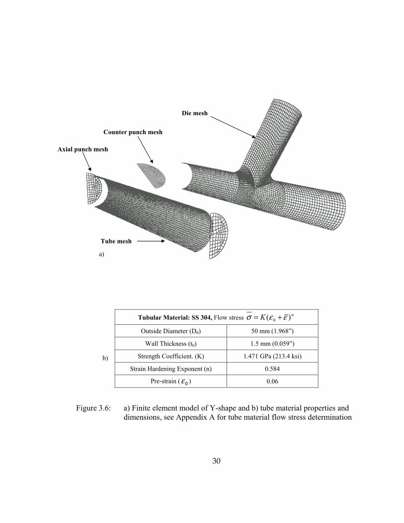
30
Tubular Material: SS 304, Flow stress nK )( 0 εεσ +=
Outside Diameter (D0) 50 mm (1.968�)
Wall Thickness (t0) 1.5 mm (0.059�)
Strength Coefficient. (K) 1.471 GPa (213.4 ksi)
Strain Hardening Exponent (n) 0.584
Pre-strain ( 0ε ) 0.06
Figure 3.6: a) Finite element model of Y-shape and b) tube material properties and dimensions, see Appendix A for tube material flow stress determination
Counter punch mesh
Axial punch mesh
Die mesh
Tube mesh
a)
b)

31
Constitutive modeling and flow stress equation: Hill�s 1948 constitutive model is used
to represent the elastic-plastic-planar-anisotropic behavior of the tubular material. This
constitutive model works well with most Low Carbon steels and Stainless steels. There
are two main methods of tube manufacturing: a) roll forming and b) extrusion. Roll
formed tubing seems to behave anisotropically, which is derived from the original sheet
material. Due to the complexity of the tube making process, the real anisotropy of the
tubular material is still not known. Typically, the anisotropy value of the original sheet
material, if available, is used in the THF simulation. In this case, the tube is assumed
isotropic.
Sliding friction contact: There are two main sliding friction contact algorithms available
in PAM-STAMP: a) penalty method and b) Lagrangian method. Lagrangian method is
normally chosen over penalty method in tube hydroforming simulations. Coulomb�s
friction of 0.05-0.06 is normally assumed for the tube-die interface friction.
Loading: The explicit time integration scheme of PAM-STAMP requires very small
time steps (about 10E-5 sec) to guarantee reliable and stable solutions. To reduce the
computational time, the work-piece mass is increased or forming time is sped up
artificially. Typically, in sheet forming simulations, the forming time is sped up by
approximately 1000 times without any dynamic effect (i.e. erroneous stresses due to
mass inertia). In this Y-shape simulation, the loading curves applied are sped up by
1000 times. Therefore, the total forming time is now 12 ms and the left and right punch
speeds are now 4 and 8 mm/ms.
Pressure is applied to the interior of the tube elements along their normal directions.
The fluid cell option in PAM-STAMP builds up internal pressure by an artificial fluid
medium flowing into the �fluid cell� (i.e. closed deforming tube). A limiting pressure
curve is input as to regulate the pressure build up inside the fluid cell through an
artificial relieve valve.

32
Axial feeds from both tube ends can be prescribed to the axial punches using a)
displacement boundary condition or b) velocity boundary condition. The velocity
boundary condition is safer to apply than using the displacement boundary condition in
terms of preventing erroneous inertial stresses from happening in the simulation. As a
rule of thumb, which is borrowed from sheet metal forming simulation, the speeds of
tooling components such as those of axial punches should be kept below 10-15 mm/s to
minimize such erroneous stresses (dynamic effect).
As mentioned earlier, accurate counter punch force curve versus time is difficult to
estimate a priori due to part complexity and material non-linearity. The most convenient
way to prescribe a boundary condition on the counter punch is by using velocity
boundary condition. However, this is an iterative procedure.
3.1.2.2 FE Simulation Results and Verification
The estimated process parameters (pressure, axial feeds, and counter punch force) were
refined through conducting FE simulations, i.e. the process parameters are adjusted in
the consecutive simulations based on the results of the previous simulations. Through
this exercise, a sound Y-shape was simulated with part maximum thinning of 23% and
without any wrinkles. These loading paths, determined from conducting FE simulations,
were used to hydroform the real Y-shapes. The procedure of Y-shape hydroforming is
discussed in the beginning of this chapter. The process parameters were measured from
the real process as shown in Figure 3.7.
From the simulation results, deformation of the Y-shape can be observed clearly. The
Y-shape hydroforming process can be roughly divided into three main stages, see
Figure 3.7, a) free expansion, b) expansion against a counter punch, and c) calibration.
The counter punch is positioned in the die just above the left die corner radius such that
it would not pinch the growing protrusion in the early hydroforming stage. After the
protrusion has come in contact with the counter punch, the counter punch will slide

33
slowly upwards as it is supporting the growing protrusion and come to a stop during the
calibration stage.
The internal pressure curve (input and measured from the press), shown in Figure 3.7.a,
consists of two main stages, i.e., forming stage (1-11 sec) (including free expansion and
expansion against the counter punch) and calibrating stage (11-15 sec). During the
forming stage, the pressure goes up from 0 bar to 800 bars, the left and right axial feeds
are 40 mm and 80 mm, respectively (see Figure 3.7.b). The real axial punch
displacement curves exceed the axial feeds of 40 mm and 80 mm due to some
additional axial punch displacement for sealing at the beginning of the process.
During the calibrating stage, there are no axial feeds as can be seen from Figure 3.7.b;
the axial punches stopped moving. The axial feeds are not applied during the
calibrating stage because the calibrating pressure is usually very high, so that the tube-
die interface friction force becomes too large for the tube material to be fed in. Figure
3.7.c shows the counter punch force curve and the displacement of the counter punch,
which determines the protrusion height of the Y-shape.
The Y-shapes hydroformed in the experiments were cut and measured for thickness
distributions along the tube axis direction. Figure 3.8 shows a comparison of thickness
distributions of the Y-shape simulated with FEA and measured from the experiments.
The comparison results indicate that FEA simulation accurately predicted the metal
flow in the Y-shapes when compared with the real part.

34
0
200
400
600
800
1000
1200
1400
1600
0 5 10 15Time (sec)
Pres
sure
(bar
s)
0
2900
5800
8700
11600
14500
17400
20300
23200
(Psi
)
-20
0
20
40
60
80
100
0 5 10 15
Time (sec)
Axi
al F
eed
(mm
)
-0.8
0.0
0.8
1.6
2.4
3.1
3.9
(inch
)
0
20
40
60
80
100
120
140
0 2 4 6 8 10 12 14Time (sec)
Cou
nter
Pun
ch F
orce
(kN
)
0
5
10
15
20
25
30
Cou
nter
Pun
ch D
ispl
acem
ent
(mm
)
Figure 3.7: FEA simulation demonstrates intermediate hydroforming steps of a Y-shape, a) Pressure, b) axial feeds and c) counter punch force versus time curves used to hydroform SS 304 Y-shapes
Position of counter punch
Protrusion comes in contact with the counter punch
Time = 0
Time = 5
Time = 15
Calibrated
Time = 11
Right axial feed
Left axial feed
a)
Counter punch displacement
Counter punch force
b)
c)

35
1.00
1.25
1.50
1.75
2.00
2.25
2.50
2.75
3.00
0 50 100 150 200 250Curvilinear Distance (mm)
Thic
knes
s (m
m)
EXP # 9 ( 2 samples)FEM # 1
Figure 3.8: Comparison of thickness distributions of SS304 Y-shape from FEA and experiments along longitudinal direction
Max. thinning 23%

36
3.1.3 Considerations in FE Modeling of THF processes
It is important that all the FEA parameters affecting calculations of the metal forming
process be understood, if reliable prediction results are to be determined. This section
discusses several important aspects of FE process modeling using PAM-STAMP, a
dynamic explicit FEA code, which is used in conducting THF simulations throughout
this work.
3.1.3.1 Type of FE Formulations
The two main types of metal process simulation codes are a) incremental FE simulation
and b) one step FE simulation. One step simulation or inverse method simulation
considers only the initial and final steps of the simulation, and ignores all the
intermediate steps. Only material properties, initial, and final part geometry are required
to conduct a one step THF simulation. Friction condition of work piece-tool contact is
not taken into account during the forming simulation. This simplification enables quick
calculations at a cost of exact calculations of the forming. One step FEM codes find
applications in tube bending and simple tube calibration operations [Hora, 1999]. For
more complex THF operations, in which combined applications of displacement
boundary conditions (axial feed at tube ends) and force boundary conditions (internal
pressure) are applied, reasonable prediction results can only be obtained through using
incremental FEM simulation codes.
Dynamic explicit and Quasi-static implicit are the two main FE formulations for
incremental FE simulation. As discussed previously, dynamic explicit codes (e.g. PAM-
STAMP and LS-DYNA) dominate sheet metal forming and THF process simulations.
Hora (1999) compared pros and cons of these two incremental FE formulations in
sheet/tube hydroforming operations, Table 3.1:

37
Dynamic Explicit FE methods Quasi-static Implicit FE methods
Commercial FE Codes PAM-STAMP, LS-DYNA DEFORM 2D, DEFORM 3D
Advantages
• Fast changing boundary conditions
found in sheet and tube hydroforming operations can be readily simulated
• Buckles and wrinkles do not cause
numerical instability • Typically, less computation time is
required in comparison to using the implicit FE method
• Static equilibrium condition is satisfied,
therefore, true quasi static solutions can be obtained
• Total calculation time is not affected by
the use of adaptive mesh refinement
Disadvantages
• Total calculation time increases as
sheet/tube elements become smaller (adaptive mesh refinement), i.e. necessary stable simulation time step deceases with deformable element size
• Artificial numerical acceleration of the
forming operation can lead to erroneous initia stresses
• Complex boundary conditions often
lead to solution convergent problems • Total calculation time is frequently
larger than that of explicit FE method, if the simulation time step has to be deceased to correct the convergent problem due to problematic contacts
• The use of shell elements can be
difficult due to large differences between the stiffness in stretching and bending
Table 3.1: Comparison of explicit and implicit FE formulations [Hora, 1999]
3.1.3.2 Types of Finite Elements
Most of sheet/tube metal forming process FEA codes often adopt shell elements to
model the work piece with an underlying assumption of membrane theory (i.e. thin-
shell theory). Closed-shell structures can be assumed thin shells only if its wall
thickness to smallest radius ratio is smaller than 1/10. Fortunately, with the light-weight
driven design in the automotive industry, this thin-shell assumption is valid for most
THF automotive parts with its thin wall compared to relatively large diameter. Figure

38
3.9 shows an example of a Y-shape (exhaust manifold component) hydroforming
simulation. Due to its small ratio of t0 to OD, this part can be simulated correctly with
shell elements in PAM-STAMP. The thickness distributions of the Y-shape are well
predicted.
THF is also being applied outside the automotive industry, especially in medical and
sanitary industry. Those tubular parts are usually much smaller in radius as compared to
automotive tubular parts but the wall thickness remains much the same. In other words,
the ratio of wall thickness to tube radius becomes larger, and often large enough to
violate the thin-shell assumption used in most 3D sheet FEA codes. In such cases, brick
elements have to be used to model the tube forming process if accurate thickness
predictions are to be obtained. Figure 3.10 shows a hydroforming simulation of a
copper T-shape (a plumbing fitting) conducted by DEF0RM 3D using brick elements.
The thickness to radius ratio of this initial tube is much larger than 1/10. In this case, the
material buildup at the center of final part interior greatly deteriorates the very
functionality of the fitting. Therefore, accurate predictions of final part interior
geometry (i.e. part thickness distributions) are crucial to the process design of this part.
The use of brick elements in a THF simulation though yields best thickness predictions;
it often requires much longer computation time as compared to use of shell elements.
When working with hydroforming of thin-walled parts, the proper choice of finite
element types really depends on the prediction accuracy demanded by the metal
forming problem. For example, the ERC formability hydraulic bulge test (all the test
samples are thin-walled tubes) requires very accurate thickness predictions, as these will
be used to calculate the tubular material flow stress accurately. Therefore, DEFORM is
used to simulate this bulging with brick elements.

39
0.50
0.75
1.00
1.25
1.50
1.75
2.00
2.25
2.50
0 50 100 150 200 250
Thic
knes
s (m
m)
FEMEXP1-sample1EXP1-sample2EXP1-sample3Initial Thickness
Part: SS304 Y-shape FEM code: PAM-STAMP FE: Quadrilateral shell elements
Figure 3.9: Comparison of SS 304 Y-shape thickness distributions (upper longitudinal direction) from FEM and experiments (OD = 50 mm, L0 = 320 mm, t0 = 1.5 mm, and 584.0)06.0(471.1 εσ += GPa)
Stage: Intermediate FE: 1 layer - brick elements
Stage: Final FE: Multiple layers -
brick elements
Part: Copper T-shape FEM code: DEFORM 3D
Figure 3.10: FEM simulation of thick-walled T-shape

40
3.1.3.3 Shell Element Size
The size of elements is very important in the wrinkle prediction. Four simulations were
conducted with different tube mesh sizes ranging from 2.5, 4.0, 6.0 mm without any
adaptive meshing and 6.0 mm with adaptive meshing. The die mesh size was 4.5 mm.
Wrinkled tube profiles from these simulations were compared in Figure 3.11. It was
concluded that the smallest tube mesh size (2.5 mm) seemed to predict the most
reasonable wrinkle size compared to the others. Big tube mesh size (4 and 6 mm) under
predicted the wrinkle compared to that of 2.5 mm mesh size. Though this different
seemed small but this may cause a large error when applied to geometric wrinkle
parameters (to be discussed in chapter 6 � adaptive simulation). Tube mesh size of 6
mm with adaptive meshing seemed to give good results compared to the simulation
with tube mesh size of 2.5mm
0
5
10
15
20
25
30
0 20 40 60 80 100 120 140 160 180Tube Profile in Radial Direction (mm)
Cur
vilie
r Dis
tanc
e (m
m)
mesh size = 2.5 x 2.5
mesh size = 4.0 x 4.0
mesh size = 6.0 x 6.0
mesh size = 6.0 x 6.0 +adap. mesh
Figure 3.11: Wrinkled parts simulated with different tube mesh sizes

41
3.2 Effect of Geometric Parameters on Hydroformability
Part geometry design can greatly affect part formability. Therefore, hydroformability of
THF parts should be considered early on in the designing stage. As hydroforming is
gaining momentum in the industry to replace traditional stamping of automotive parts,
part design methodology has to be executed with added constraints imposed by the tube
hydroforming process itself. Small part corner radii demand very high hydraulic
pressures. Only certain sizes of part corner radii can be hydroformed depending on the
base material, wall thickness and press capacity. The length of the part measured along
the main axis of the tube (so called �spline length�) also plays an important role in
imparting sound parts. In this study, the effect of part spline length to hydroformability
is studied through hydroforming of the Y-shape; discussed earlier, see Figure 3.2.
3.2.1 Tube Spline Length Effect
The Y-shape is considered here again to investigate the effect of part spline length to
the part formability. This knowledge is particularly useful when working with long
automotive structural parts such as an engine cradle whose part geometrical features
such as bulges, protrusions, and bends are located along the part spline axis, Figure
3.12. Axial feed from both tube ends may only facilitate the forming of part geometrical
features located near the tube ends but may not benefit in forming the ones that are far
removed from the tube ends. Thus, those part geometrical features end up being formed
only by pure expansion, which are subject to premature bursting. Typically, in the
engine cradle case, tube performing/crushing is done such that extra material is
accumulated in the large expansion area to improve the formability, Figure 3.12.a.
It is clear now that the effectiveness of axial feeding depends on ability of the tube
material to flow from the guiding zones (i.e. tube end areas) into to the tube expansion
zone (i.e. part geometrical feature areas). This ability to flow of the metal is influenced
by many factors such as part geometrical features adjacent to the tube ends, tube-die
interface frictional force, tube material strain hardening, and part spline length.

42
Figure 3.12: Examples of long structural tubular parts with many part geometrical features: a) engine cradle (Schafer Hydroforming) and b) a portion of exhaust manifold
a)
b)
3 protrusion features
2 bend features
Axial feed Axial feed
Large expansion
far away from tube end

43
Y-shapes with different spline lengths were studied in this work. The part spline lengths
are measured (LL1 and LR1) along the tube axis of the final part, see Figure 3.13. SS304
tubing with 1.5mm wall thickness and 50 mm in diameter was used. There were three
sets of experiments. In each experiment, the final part spline lengths on the left (LL1)
and right (LR1) ends are varied, see Figure 3.13. The pressure and axial feed amounts
were all the same for all the experiments, Figure 3.14. The pressure and axial feed
curves were determined from the metal forming equations as discussed earlier and
refined through iterative FE simulations. The axial feed from each end is 40 mm and 80
mm for the left and right end, respectively. The initial tube lengths on the left and right
sides (LL0 and LR0) were determined simply by adding LL1 and LR1 with the
corresponding axial feeds; LL0 = LL1 + da L and LR0 = LR1 + da R. The hydroforming
experiments were conducted at SPS research center, Aalen, Germany [Jirathearanat,
2001b].
Three tube samples were formed in each forming experiment. Figure 3.15 summarizes
and compares protrusion heights (Hp) measured from parts of experiments 1 to 3, refer
to Figure 3.13. It can be concluded from the figure that different part spline lengths
(LL1 and LR1) affect the obtainable protrusion height of the Y-shapes. It can be shown
that variations of the protrusion heights among the three part samples from the same
experiment are much less than those caused by changing the part spline lengths. It is
now obvious that reduction of the right spline length (LR1) from 80 mm to 45 mm
increased the protrusion height, Hp, by 5 mm; comparing experiments of LL1 = 120 and
LR1 = 80 mm to LL1 = 120 and LR1 = 45 mm. More improvement on the protrusion
height was achieved by reducing the left spline length; comparing experiments of LL1 =
120 and LR1 = 45 mm to LL1 = 85 and LR1 = 45 mm. The conclusion drawn from the
results, seen in Figure 3.15, is that, with this particular Y-shape geometry, a larger
protrusion height HP can be achieved by reducing LR1 and LL1. No significant variations
in thinning percentage were observed between different samples. The maximum
thinning was in the range of 19.5% to 21.5%.

44
LL1 LR1
H
da L da R
Y-shape Spline Length Axial Feed Initial Tube Geometry
EXP. #
LL1 (mm) LR1 (mm) da L and da R (mm)
LLO (mm)
LRO (mm)
Material DIA x Thick
(mm)
1 120 80 160 160
2 120 45 160 125
3 85 45
40 - 80
125 125
SS304
50 x 1.5
Figure 3.13: Schematic drawing of the Y-shape part and tooling geometry, experimental setup
LL0 LR0
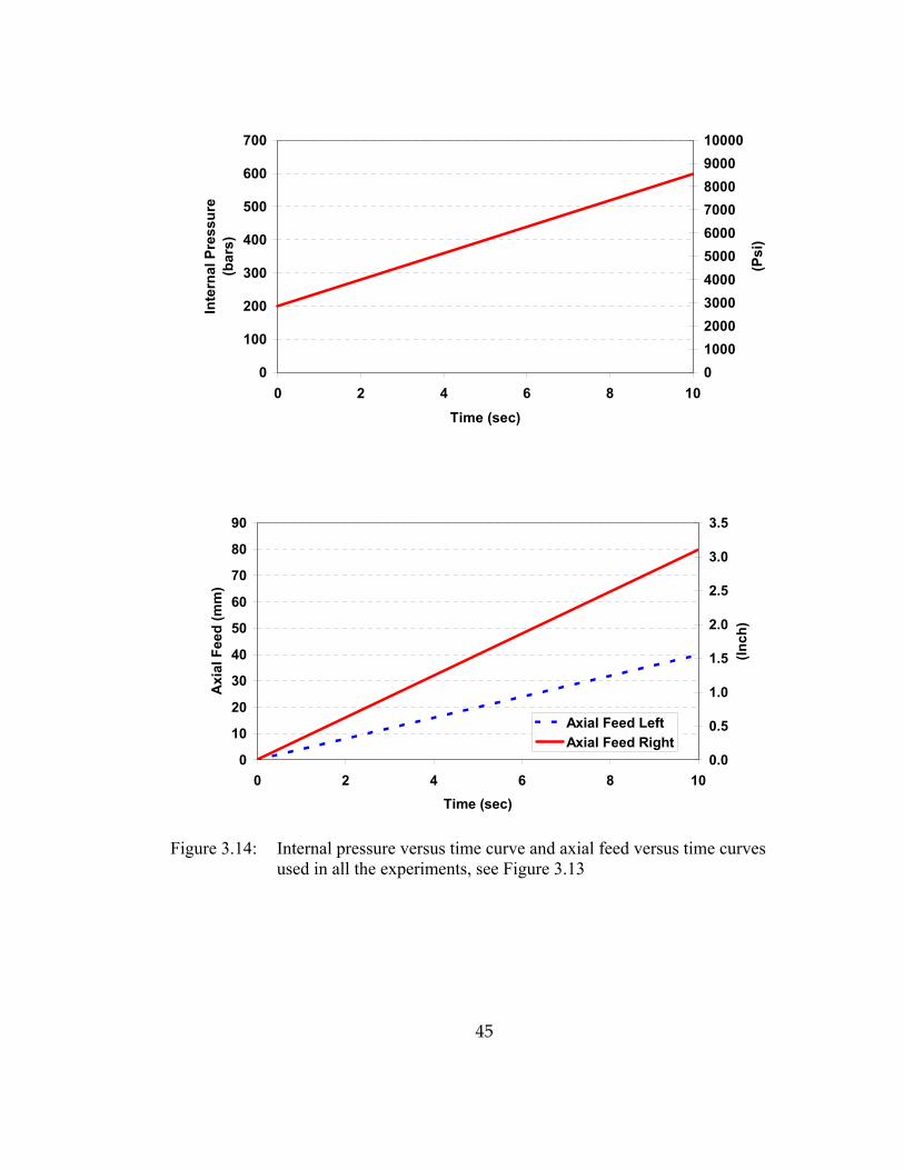
45
0
100
200
300
400
500
600
700
0 2 4 6 8 10Time (sec)
Inte
rnal
Pre
ssur
e (b
ars)
010002000300040005000600070008000900010000
(Psi
)
0
10
20
30
40
50
60
70
80
90
0 2 4 6 8 10Time (sec)
Axi
al F
eed
(mm
)
0.0
0.5
1.0
1.5
2.0
2.5
3.0
3.5
(Inch
)Axial Feed LeftAxial Feed Right
Figure 3.14: Internal pressure versus time curve and axial feed versus time curves used in all the experiments, see Figure 3.13

46
110 112 114 116 118 120 122 124
85-45
120-45
120-80
Protrusion Height Hp (mm)
avg. Hp115.2 mm
avg. Hp120.4 mm
avg. Hp122.1 mm
Figure 3.15: Experimental results: comparisons of protrusion height, HP, of Y-shapes with different part spline lengths
85 45
120 80
120 45

47
3.3 Effect of Process Parameters on Hydroformability
The use of proper internal pressure and axial feeding versus time curves is very crucial
in THF. Typically, yielding pressure and some axial feed (for sealing purposes) are
initially applied to start plastic deformation of the tube. Then, the pressure is raised to
expand the protrusion as well as prevent/straighten wrinkles, but controlled under the
bursting level. Axial feeding is applied simultaneously with the pressure forcing the
material to flow into the expansion zone.
This study focuses on hydroforming of a T-shape. Particularly, hydroforming of T-
shapes that only one-sided axial feeding is effective due to the part geometry. This
forming difficulty arises often in hydroforming of automotive structural parts with large
ratios of part length to diameter. Figure 3.16 shows a simplified structural part that is
consisted of many part geometrical features (i.e. two bends, a bulge, and a T-shape).
Due to the bend on the left side, left axial feeding (daL) will not improve formability of
the part. The right axial feeding (daR) is possible but only beneficial to the T-shape
forming. A quick part geometry analysis would suggest that the bulge will be
hydroformed through pure expansion, and the T-shape will be hydroformed with only
one-sided axial feeding. Several simulations were conducted here to study the effect of
pressure, one-sided axial feed, counter punch force curves on the T-shape
hydroformability.
Figure 3.17 shows the geometry of the initial tube and the final T-Shape part. Four
different initial lengths of tubes for simulations with a set of four different axial feeds
(i.e. daR = 30, 50, 70, 90 mm) were chosen in such a way that the final part spline length
will be the same for all simulated parts regardless of the amount of axial feed, i.e. the
distance L1 marked in the final part will remain constant for all the simulations. Only
the protrusion height will vary from one simulation to the other because of variation in
axial feed (daR) and internal pressure. The useful portion of protrusion height (Huseful)
may be regarded as the total protrusion height (Htotal) minus the corner radius at top, see
Figure 3.17. All the simulations were modeled with a LCS material expressed by the

48
power law 19.0)02.0(500 εσ += MPa ( 19.0)02.0(5.72 εσ += ksi). The coefficient of
friction was kept as 0.05 in all the simulations.
Axial Feed and Internal Pressure
For the present study, simple linear loading paths were chosen for internal pressure and
axial feed, Figure 3.18, since such linear loading paths had been used successfully to
form T-shapes at the ERC [Jirathearanat, 1999]. According to the past experiments and
simulations for low carbon steels, thinning of 30% + 0.5% was selected as a failure
criterion to stop the simulations. Any value of the thinning above this limit is
considered as unacceptable, and the simulation is re-run with suitable changes (i.e.
decrease or increase the maximum pressure) to obtain the part maximum thinning
within the prescribed limits.
Axial feeds of 30 mm, 50 mm, 70 mm and 90 mm were applied in the all simulations.
The internal pressure was quickly increased to reach the yield pressure py and then
gradually increased linearly to reach a specified maximum value pm in the given process
time (Figure 3.18). The maximum pressure pm was to be such that the thinning did not
exceed the set limit of 30% + 0.5%. However, this value of pm can only be
approximated using the equations discussed earlier. In the actual process, the protrusion
portion will not be symmetrical (due to one-sided axial feeding) and the thickness will
not be uniform over the protrusion. Moreover the area of maximum thinning will have a
reduced radius of curvature that will increase the internal pressure required to cause
more thinning. Hence it is more appropriate to determine the pm through iterative FE
simulations.

49
Figure 3.16: Drawing of a simplified structural part with a T-shape that can only be hydroformed with one-sided axial feeding.
Figure 3.17: Geometry of the T-shape die cavity and part geometry with one-side axial feeding (dimensions are in mm; 25.4 mm = 1 in.)
One sided axial feed (da R) T-shape hydroforming
Feature # 3: Bulge
Feature # 2: Bend
Feature #4: Bend
da L = 0
da R > 0
Feature # 1: T-shape
R = 10
D = 63.5
Dp = 63.5
Initial Tube
T-shape
t0 = 2
L0
L1 da R
Htotal
Huseful
da L = 0 da R > 0
50
0102030405060708090
100
0 2 4 6 8 10 12Time (ms)
Axi
al F
eed
(mm
)
Feed 90 mmFeed 70 mmFeed 50 mmFeed 30 mm
0.0000
0.0100
0.0200
0.0300
0.0400
0.0500
0.0600
0.0700
0 2 4 6 8 10 12Time (ms)
Inte
rnal
Pre
ssur
e (G
Pa)
HighMedLow
Figure 3.18: a) axial feed versus time curves used in all simulation cases (25.4 mm = 1 in), and b) pressure versus time curves corresponding to the different axial feeds (1 GPa = 145,038 psi)

51
3.3.1 Effect of Axial Feed and Pressure on Protrusion Height
As the material is pushed from only one side, the shape of the protrusion is not
symmetrical around the protrusion axis. The material on the feeding side of the
protrusion has less curvature and that on the other side has more curvature. This makes
a distinct difference between the total protrusion height and the useful protrusion height.
Figure 3.19 shows the plot of protrusion height as a function of axial feed. It may be
noted that for all the simulations, the thinning is 30% + 0.5%, and the maximum
internal pressure varies accordingly. Although the protrusion height increases with axial
feeding, not the entire portion of protrusion is usable, because a considerable portion of
the protrusion does not conform to the die wall.
Another interesting point is the effect of a large axial feed as in the case of axial feed of
90 mm. Contrary to usual expectations, the highest thinning is observed at the region
where protrusion intersects the non-feeding side of the tube. When excessive axial
feeding is forced upon, the tube thickens and wrinkles heavily at the right die-fillet
region, which, in turn, restricts metal flow towards the protrusion top. Meanwhile, the
increasing internal pressure tries to draw in material towards the protrusion top, which
is hindered by the wrinkling and thickening. Thus the material at the intersection of
protrusion portion and non-feeding side of the tube is forced to thin down. At the end of
the process, it is observed that the thinning at this junction is more than that at the
protrusion-top. Thus, for the present geometry, it is not advisable to apply such a large
axial feeding which is nearly 150% of the tube diameter.
From the plot of protrusion height vs. peak pressure (pm) for different axial feeds,
Figure 3.20, it is clear that the pressure does not contribute to protrusion height
considerably even at different levels of axial feed. For highly non-axisymmetric parts
such as T-shapes, the internal pressure is only required to help pushing metal flow
upwards to the protrusion and prevent wrinkle from occurring.

52
0
10
20
30
40
50
60
70
30 40 50 60 70 80 90Axial Feed (mm)
Hei
ght (
mm
)
0.036
0.037
0.038
0.039
0.04
0.041
0.042
Max
Pre
ssur
e (G
Pa)
H total
H useful
Max. Press
Figure 3.19: Effect of axial feed on protrusion height (all the simulated parts have maximum thinning of 30%)
25
30
35
40
45
50
55
60
65
0.03200 0.03400 0.03600 0.03800 0.04000 0.04200
Max. Pressure (GPa)
Tota
l pro
trus
ion
Hei
ght
(mm
)
Feed 90 mmFeed 70 mmFeed 50 mmFeed 30 mm
Figure 3.20: Effect of internal pressure at different axial feeds on protrusion height
Htotal Huseful
da

53
3.3.2 Effect of Counter Punch Force on Protrusion Height
A counter punch force is applied in hydroforming of parts with protrusions for two main
reasons: a) to support the growing protrusion thus increasing the obtainable protrusion
height, and b) to flatten the protrusion top curvature thus improving the protrusion
geometry.
In this study, the T-shape, discussed earlier, formed successfully with 50 mm axial feed
and medium pressure curve (Max. pressure = 0.04 GPa), see Figure 3.18, is investigated
here again with added application of a counter punch force. Different counter punch
forces were applied on the T-shape to study its effect and how it improves the
protrusion. A few samples of various counter punch force curves versus time are shown
Figure 3.21.a. The counter punch force is increased from zero to the maximum value
within a short time once the protrusion tip touches the counter punch, and then it is kept
constant till the end of the process. The pressure and axial feed curves versus time are
kept piecewise linear as applied in the simulations without counter punch, Figure 3.18.
In THF simulations with counter punch application, for a given axial feed and internal
pressure loading path, it was found that the total protrusion height obtained is less
compared to that obtained in THF without counter punch. However the useful
protrusion height is significantly increased than that obtained without counter punch
application. Also relatively, the maximum thinning for a given loading path is
considerably reduced.
Figure 3.21.b shows the effect of counter punch force on useful protrusion height. It can
be noticed the total protrusion height decreases as the counter punch force increases.
However the useful protrusion height keeps on increasing as the counter punch force
increases. The maximum thinning becomes lesser for increased values of the counter
punch force.

54
0
5
10
15
20
25
30
0 2 4 6 8 10 12
Time (ms)
Coun
ter p
unch
forc
e (k
N)
Trial #1Trial #2Trial #3
0
10
20
30
40
50
60
0 5 10 15 20 25 30
Counter punch force (kN)
Hei
ght (
mm
)
0
5
10
15
20
25
30
Max
thin
ning
(%)
H total
H useful
Max. Thin%
Figure 3.21: simulation results of T-shape hydroforming with axial feeding of 50 mm, medium pressure curve (see Figure 3.18) and counter punch force, a) samples of counter punch force versus time curves, and b) effect of counter punch force on protrusion height and maximum thinning
H t H u H u

55
CHAPTER 4.
SYSTEMATIC APPROACH TO SELECT LOADING PATH
USING PROCESS FEA SIMULATION
4.1 Self-Feeding Simulation Approach
4.1.1 Natural Axial Feed Curve Concept
Often the amount of necessary axial feed is difficult to calculate using the volume
constancy, particularly, when hydroforming complex structural parts. As an alternative,
an approximate value of the necessary axial feed can be figured out by running a few
special preliminary simulations, so called "Self-Feeding"(SF) simulation technique. In
applying the SF technique, the tube ends are free of constraints (i.e. no boundary
conditions - no axial feeds applied), the interface friction is set zero, and only internal
pressure is applied to form the part. As a result, the contractions of the tube ends (left
and right) would be caused by a pure expansion, see Figure 4.1. These contractions at
the tube ends can be considered as an initial estimate of axial feeds. These axial feeds
do not represent the real axial feeds as they are only obtained from simulation with zero
friction. However, these values, determined by SF, can be scaled up to arrive at the
"good" axial feeds that form a good part. A general flowchart of this procedure is shown
in Figure 4.2. Please note that this SF approach is not suitable for parts with strong non-
axisymmetric features, e.g. y-shapes. The useful results obtained from a SF simulation
are: 1) the ratio axial feeds necessary at left and right tube ends, and 2) the relationship
between axial feeds to the input pressure curve.

56
Figure 4.1: Self-feeding simulation concept
Estimate press. curve
SF simulation
dao L, dao R
Scaled up by asf
Normal simulation
Excessive thinning?
Yes No
Good part
(Analytical models)
Figure 4.2: A flowchart of Self-Feeding (SF) simulation procedure
No interface friction
No interface frictionNo end constraints
Pure expansion
Tube end contractions

57
4.1.2 Loading Path Determination Procedure
The following are systematic steps using SF and some iterative simulations to determine
�good� loading paths, see Figure 4.2:
Step 1. Calculate the required calibration pressure ( MAXP ) considering the smallest
corner radius of the final part geometry, see Chapter 3
Step 2. Run SF simulation:
• with a linear pressure curve from [0 to MAXP ] to expand the part to the die
cavity,
• without any boundary conditions on the tube ends � no external axial feeds, and
• without tube-die interface friction,
• to obtain the SF axial feeds: selfleftd (left feed) and self
rightd (right feed) from the SF
simulation
Step 3. Rerun self-feeding simulation:
• With adjusted pressure (to be discussed in detail) curve in order to reduce abrupt changes in self
leftd and selfrightd , and to reduce dynamic effect due to large
accelerations of the tube elements (i.e. dynamic effect) • without any boundary conditions on the tube ends � no external axial feeds, and • without tube-die interface friction, • to obtain SF axial feeds: self
leftd and selfrightd , and smooth out the obtained axial
feeds as to be used in the subsequent simulations: leftd and rightd Step 4. Run �real� hydroforming simulation:
• with the pressure curve applied in step 3 • with axial feeds leftd and rightd (smoothened self
leftd and selfrightd obtained from Step
3) applied at the tube ends • with tube-die interface friction
Step 5. Iteratively run a few more hydroforming simulations (by modifying the axial
feed amount) until a good part with an acceptable maximum thinning can be
formed:
• with scaled-up axial feeds )( leftsf da and )( rightsf da , scaling factor 1>sfa • with the pressure curve applied in step 3 and interface friction

58
There exists an upper limit to this scaling factor, sfa . This can be estimated by applying
volume constancy onto the part with uniform thickness assumption to calculate the
maximum axial feed necessary. Then, the maximum axial feed at left end, maxleftd , and
right end, maxrightd , can be determined based on the SF axial feed ratio leftd : rightd found in
step 3. The maximum scaling factor can then be calculated: right
right
left
leftsf d
ddd
amaxmax
max == .
Therefore, the possible range of the scaling factor runs between max1 sfsf aa << , in which
the optimal scaling factor can be found. The optimal sfa should be such that it yields
the axial feeds (left and right tube ends) that form the part with an acceptable part
maximum thinning depending on the part materials (e.g. 25-30% for Low carbon steels
and 10-15% for Aluminum alloys), and without any wrinkles or minimum wrinkles
depending part functionality.
Additionally, some proper optimization schemes can be implemented here to automate
the search for the optimum scale factor (asf). For example, the scale factor (asf) can be
the design parameter describing the loading path to be determined through optimizing
hydroformability of the part (minimum thinning with no wrinkles on the final part).
However, this method limits the optimized load path to be only within a family of
curves imparted from the SF simulation approach.

59
4.2 THF Process Case Studies
4.2.1 Automotive Structural Part #1
This part geometry was provided by Kawasaki Steel (KS) Corp., Japan, see Figure 4.3.
There are three bends in the part. The left side of the part is bigger in size than that of
the right size. Therefore, this left side of the part will be of a critical forming area in this
case. The forming sequence for this part includes a) three bending operations, b)
crushing operation, and c) hydroforming operation. The crushing operation is done in
the same dies as the hydroforming dies. The SF simulation method was applied to
determine a proper loading path (LP) for the hydroforming operation of this part. Then,
the predicted LP was used to form the real parts successfully at the hydroforming press
facility of Aida Engineering, Ltd., JAPAN.
Bending Simulation: The bending simulations were conducted using the tube material
data from Table 4.1. The bent tube dimensions are given by relative parameters, see
Figure 4.4. FEA simulations of all the three bends were conducted in a total of six
simulations in order; a bending simulation for the 1st bend followed by a springback
simulation then repeat the same simulation procedure for the other two bends. General
descriptions of tube bending operations and FEA modeling are discussed in a past ERC
report No. 99-R-01 [Shr, 1999].
Thinning distributions along the longitudinal top and bottom profiles of the simulated
bent tube (after spring back simulation) are shown in Figure 4.5. It can be seen that the
bends on the left and right sides (along profile A) have larger thinning values than that
in the middle of the tube. This is because of the bend radius of the middle bend is larger
than those of the bends on the sides. Therefore, one needs to pay attention to the part
formability of the part areas on the sides, particularly, during expansion in the
hydroforming process.
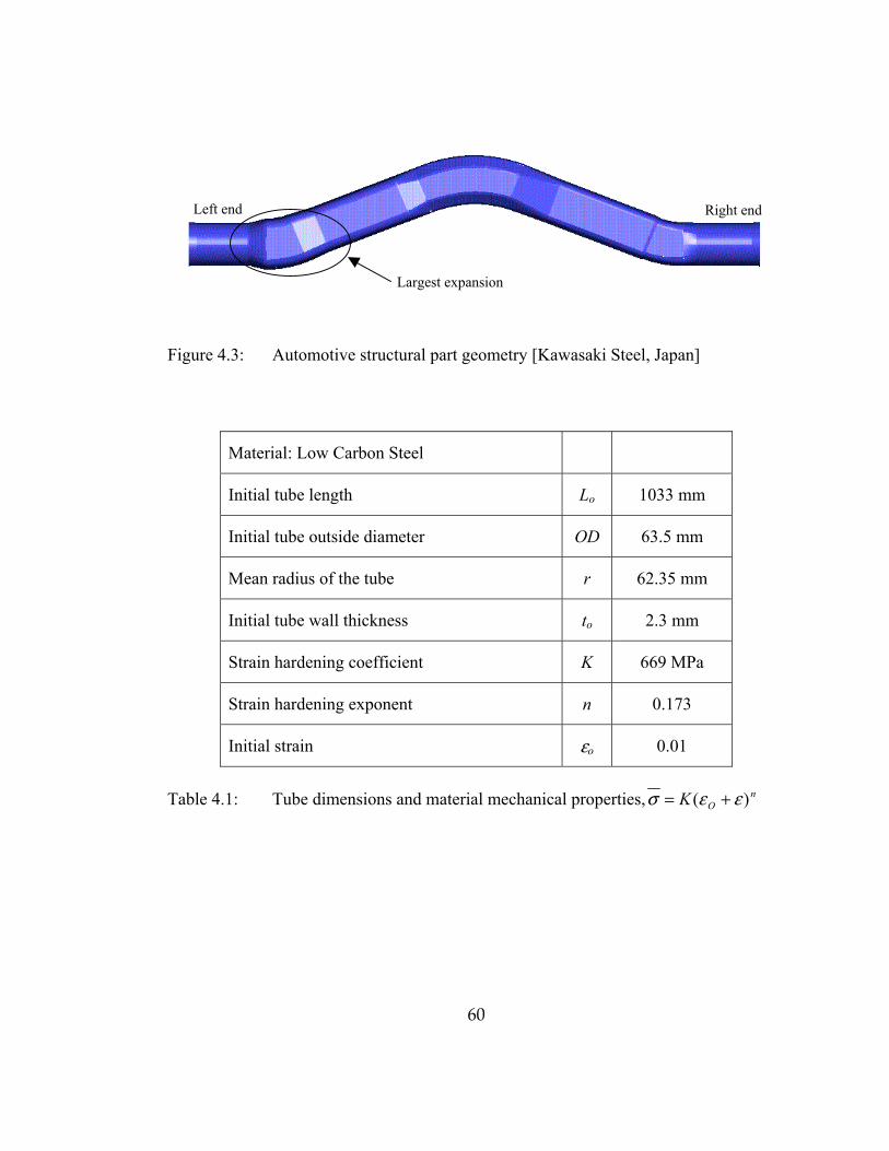
60
Figure 4.3: Automotive structural part geometry [Kawasaki Steel, Japan]
Material: Low Carbon Steel
Initial tube length Lo 1033 mm
Initial tube outside diameter OD 63.5 mm
Mean radius of the tube r 62.35 mm
Initial tube wall thickness to 2.3 mm
Strain hardening coefficient K 669 MPa
Strain hardening exponent n 0.173
Initial strain εo 0.01
Table 4.1: Tube dimensions and material mechanical properties, nOK )( εεσ +=
Left end Right end
Largest expansion

61
Angle: X°
1st Bend Radius: R mm
Angle: 2X°
Angle: X°
3rd Bend Radius: R mm
1000 mm
OD
63
.5 m
m
2nd Bend Radius: ~ 1.4R mm
Figure 4.4: Geometry of preformed/bent tube [Kawasaki Steel, Japan]
-15.00
-10.00
-5.00
0.00
5.00
10.00
15.00
20.00
0 100 200 300 400 500 600 700 800 900 1000 1100
Curvilinear Distance (mm)
Thin
ning
%
Profile AProfile B
Figure 4.5: Thinning distributions along profiles A and B of the bent tube after bending simulation, including springback (negative values indicate thickening and positive values indicate thinning)
B
A

62
4.2.1.1 Determination of Loading Paths
Figure 4.6 shows the pressure curve (input in the SF simulation, no tube ends
constrained, no tube-die interface friction applied), and the resultant velocity curves of
the left and right punches. From the resultant velocity curves, the following adjustments
were made to determine the �optimized� loading paths:
• The slope of the pressure curve was reduced in the SF simulation #2; see Figure
4.7, at the portion where the resultant punch velocity curves (from SF simulation,
see Figure 4.6) seemed to be abruptly increasing (large accelerations).
• The resultant punch velocities from the SF simulation #2 exhibited irregular
shapes, which may be difficult to implement in any real hydroforming presses.
The next step was to smoothen out the punch velocity curves as seen in Figure
4.8.
• With the smoothened axial feeds, simulation #3 can be run. In this simulation,
tube-die interface friction was applied. Coulomb friction coefficient of 0.06 was
used in all the bending-crushing-hydroforming simulations. The loading paths are
shown in Figure 4.9 (simulation #3)
• From the simulation #3, the axial feed curves were to be scaled up depending on
the severity of the maximum part thinning that occurred in the resultant part. In
this case study, the best scale factor, asf, was 1.5.
• With the axial feed curves applied in simulation #3 multiplied by 1.5, simulation
#4 was conducted. Figure 4.10 shows the development of the amount of the axial
feed curves necessary for successful hydroforming of the part. Figure 4.11 shows
the �optimized� loading paths applied in simulation #4. Table 4.2 summarizes all
the simulations conducted through SF simulation method to determine the proper
loading paths.
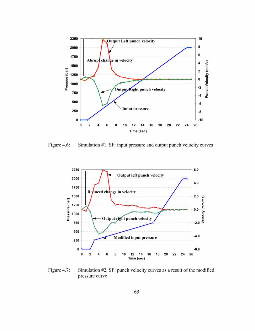
63
0
250
500
750
1000
1250
1500
1750
2000
2250
0 2 4 6 8 10 12 14 16 18 20 22 24 26Time (sec)
Pres
sue
(bar
)
-10
-8
-6
-4
-2
0
2
4
6
8
10
Punc
h Ve
loci
ty (m
m/s
)
Figure 4.6: Simulation #1, SF: input pressure and output punch velocity curves
0
250
500
750
1000
1250
1500
1750
2000
2250
0 2 4 6 8 10 12 14 16 18 20 22 24 26Time (sec)
Pres
sure
(bar
)
-6.0
-4.0
-2.0
0.0
2.0
4.0
6.0
Velo
city
(mm
/ms)
Figure 4.7: Simulation #2, SF: punch velocity curves as a result of the modified pressure curve
Output Left punch velocity
Output Right punch velocity
Input pressure
Abrupt change in velocity
Modified input pressure
Output left punch velocity
Output right punch velocity
Reduced change in velocity

64
-4.0
-3.0
-2.0
-1.0
0.0
1.0
2.0
3.0
4.0
5.0
6.0
0 2 4 6 8 10 12 14 16 18 20 22 24 26
Time (sec)
Velo
city
(mm
/ms)
Figure 4.8: Modified axial feed velocity curves (the right axial feed velocity is represented in negative values, left axial feed is in positive values)
0
250
500
750
1000
1250
1500
1750
2000
0 2 4 6 8 10 12 14 16 18 20 22 24 26Time (sec)
Pres
sure
(bar
)
-6
-4
-2
0
2
4
6
Punc
h Ve
loci
ty (m
m/s
ec)
Figure 4.9: Simulation #3, Normal Simulation: smoothened punch velocities and the modified pressure curve
Left punch velocity
Right punch velocity
Pressure
Left punch velocity
Right punch velocity

65
-45.0
-35.0
-25.0
-15.0
-5.0
5.0
15.0
25.0
35.0
45.0
0 5 10 15 20 25 30
Time (sec)
Axi
al F
eed
(mm
) Simulation #2: Self-feedingSimulation #3: Normal simulation Asf=1Simulation #4: Normal simulation Asf=1.5
Figure 4.10: Summary of the axial feed curves from the simulations conducted to �optimize� the loading paths through SF simulation approach
0
250
500
750
1000
1250
1500
1750
2000
2250
0 2 4 6 8 10 12 14 16 18 20 22 24 26Time (sec)
Pres
sure
(bar
)
-50
-40
-30
-20
-10
0
10
20
30
40
50
Axi
al F
eed
(mm
)
Figure 4.11: �Optimized� loading paths from SF: pressure, left axial feed, right axial feed
Left
Right
Left axial feed
Right axial feed
Pressure
41 mm
37 mm
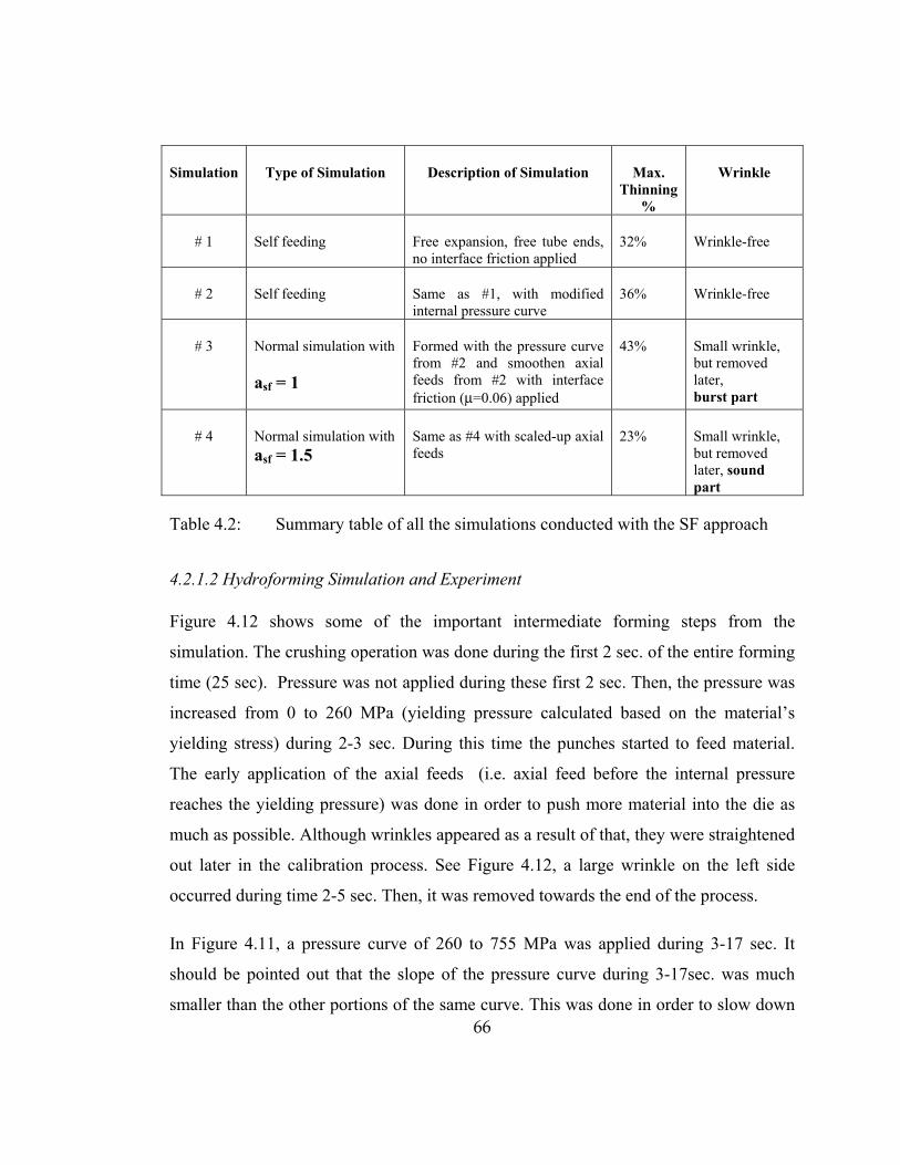
66
Simulation Type of Simulation Description of Simulation Max. Thinning
%
Wrinkle
# 1 Self feeding Free expansion, free tube ends, no interface friction applied
32% Wrinkle-free
# 2 Self feeding Same as #1, with modified internal pressure curve
36% Wrinkle-free
# 3 Normal simulation with
asf = 1
Formed with the pressure curve from #2 and smoothen axial feeds from #2 with interface friction (µ=0.06) applied
43% Small wrinkle, but removed later, burst part
# 4 Normal simulation with asf = 1.5
Same as #4 with scaled-up axial feeds
23% Small wrinkle, but removed later, sound part
Table 4.2: Summary table of all the simulations conducted with the SF approach
4.2.1.2 Hydroforming Simulation and Experiment
Figure 4.12 shows some of the important intermediate forming steps from the
simulation. The crushing operation was done during the first 2 sec. of the entire forming
time (25 sec). Pressure was not applied during these first 2 sec. Then, the pressure was
increased from 0 to 260 MPa (yielding pressure calculated based on the material�s
yielding stress) during 2-3 sec. During this time the punches started to feed material.
The early application of the axial feeds (i.e. axial feed before the internal pressure
reaches the yielding pressure) was done in order to push more material into the die as
much as possible. Although wrinkles appeared as a result of that, they were straightened
out later in the calibration process. See Figure 4.12, a large wrinkle on the left side
occurred during time 2-5 sec. Then, it was removed towards the end of the process.
In Figure 4.11, a pressure curve of 260 to 755 MPa was applied during 3-17 sec. It
should be pointed out that the slope of the pressure curve during 3-17sec. was much
smaller than the other portions of the same curve. This was done in order to slow down
67
the rate of material necessary to be fed into the expansion zone. Consequently, the left
and right punches could be controlled to move at a reasonable speed to feed an adequate
amount of material into the expansion zone. The pressure of 755-2000 MPa was
applied during the rest of the forming time (17-25 sec) for calibration purpose.
It should be noted that the relation between the axial feeds and the pressure, see Figure
4.11, should be held at all time. During the real hydroforming, the forming time
duration might be changed depending on capability of the press (for example, forming
time can be shortened from 25 sec to 12.5 sec or it can be elongated to 50 sec).
However, if the punch velocities are to be input to the press, they have to be
recalculated based on the required axial feeds (for example, if the forming time is
shortened from 25 to 12.5 sec, the velocities have to be doubled).
Figure 4.13 shows the thinning contour plotted on the final simulated part, and also
compares the thickness distribution of the part from simulation and experiment at the
most critical areas. The most thinned areas according to the simulation results were in
the areas A (flat area) with thinning of 17% and B (corner area) with thinning of 22.5%.
A sample of the automotive part was hydroformed at KS, Japan, with the same pressure
and axial feed curves, see Figure 4.11, as used to conduct the simulation. The part was
successfully hydroformed without any wrinkles or fracture. The thickness
measurements of the real part showed that the most thinned area was at the area A with
the thinning of 23%, which was in accordance with the highly thinned area A from the
simulation results.

68
Figure 4.12: Intermediate tube hydroforming steps: side view and front view
T = 0 sec
T = 2 sec, end of crushing operation
T = 5 sec, wrinkles appear
T = 18 sec, wrinkles disappear
T = 2 sec, end of crushing operation
T = 5 sec, wrinkles appear
T = 18 sec, wrinkles disappear
Wrinkle

69
Thickness (mm) Thinning (%)
Locations
FEM EXP. FEM EXP
A 1.91 1.76 17.0 23.0
B 1.78 1.89 22.5 18.0
Figure 4.13: Thinning distribution on the final simulated part and a table comparing the simulation and experimental results at some specific areas
Most thinned
A
B

70
4.2.2 Automotive Structural Part #2
In this work, a crossmember, Figure 4.14, provided by Schuler Hydroforming, USA,
was used as a case study. Crushing and hydroforming of this part were conducted
through FEA simulations and experiments. SF simulation approach was again applied
here to design LP for the hydroforming operation of this part. The LP determined
through SF approach was applied to hydroform the part successfully with only a few
adjustments.
The preforming/crushing and hydroforming operations are done in the same
hydroforming die set, Figure 4.14. A straight tube is placed in the lower die, and then
crushed to fit into the die cavity as the upper die and four side segmented dies are
closing. Hydroforming of the part starts right after the dies has been closed up and the
crushed tube has been sealed by the axial punches. At the end of the hydroforming
operation, the internal pressure is increased to a very high value to calibrate the part.
The material properties, along with the tube dimensions and interface friction
coefficient used as input for the simulations are listed in Table 4.3.
4.2.2.1 Determination of Loading Paths
Figure 4.15 and Figure 4.16 show the pressure curves and axial feed curves found
during the application of the SF simulation approach for hydroforming of the cross
member. Due to its confidentiality, the dimensions of the part cannot be disclosed. The
following are the steps conducted in determining the proper LP:
• Run the 1st SF simulation (indicated as SF#1 in Figure 4.15) with a linear pressure
curve [0 � calibrated pressure]. Run the 2nd SF simulation (indicated as SF#2 in
Figure 4.15) with a modified pressure curve in order to reduce the nodal velocities
at the tube end.

71
Figure 4.14: FEA modeling of hydroforming crossmember [Schuler Hydroforming]
Material Low Carbon Steel
Initial tube length Lo 1250 mm
Initial tube outside diameter OD 101.6 mm
Initial tube wall thickness to 3.8 mm
Strain hardening coefficient K 590 MPa
Strain hardening exponent n 0.223
Initial strain εo 0.0188
Table 4.3: Material properties, tube dimensions and coefficient of friction used in the FE simulations.
Dip in the part
Upper Die
Lower Die
Side Segmented Dies
Right End
Left End

72
• Smoothen the end nodal velocity curves obtained from SF#2, then used them as
initial baseline axial feed rate curves in the subsequent normal simulations (i.e.
with interface friction) where these curves are scaled up by different asf factors.
• Determine the �good� axial feeds from normal simulations (friction applied): Run
normal simulations (with friction) with the minimum axial feeds (smoothened
axial feed rate curves from SF#2) scaled up by a factor asf until a good part is
formed, i.e. a part with an acceptable thinning (<30%). The determination of the
�best� factor asf can be done considering the resulting part maximum thinning, see
Figure 4.16.
By conducting a few simulations (5 simulation runs) following the SF simulation
approach, �good� LP for hydroforming of the crossmember was determined, as
summarized in Table 4.4. The simulation results suggested the pressure curve of 0 �
2800 bars, (indicated as SF#2, Figure 4.15), left axial feed of 62 mm, and right axial
feed of 73 mm (indicated as Case B, Figure 4.16). The maximum thinning in the part
was found to be 27%, indicating a sound part. Figure 4.17 shows plots of the pressure
and right axial feed versus left axial feed. These curves were tried out as an initial guess
during the prototyping of the cross member hydroforming.
Figure 4.18 shows simulation results of crushing/hydroforming of the cross member at
different states. This part was simulated with the pressure curve labeled SF#2, and the
axial feeds labeled case B, selected using the SF simulation approach.
A few samples of the cross member were prototyped using the determined LP at the
Schuler Hydroforming, Canton MI. The loading curves, obtained from SF approach,
shown in Figure 4.17 were simplified as an input to the press as shown in Figure 4.19,
pressure 1st trial.
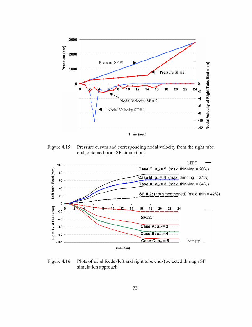
73
-3000
-2000
-1000
0
1000
2000
3000
0 2 4 6 8 10 12 14 16 18 20 22 24
Time (sec)
Pres
sure
(bar
)
-12
-10
-8
-6
-4
-2
0
2
4
6
8
10
12
Nod
al V
eloc
ity a
t Rig
ht T
ube
End
(mm
)
Figure 4.15: Pressure curves and corresponding nodal velocity from the right tube end, obtained from SF simulations
-100
-80
-60
-40
-20
0
20
40
60
80
100
0 2 4 6 8 10 12 14 16 18 20 22 24
Time (sec)
Left
Axi
al F
eed
(mm
)R
ight
Axi
al F
eed
(mm
)
Figure 4.16: Plots of axial feeds (left and right tube ends) selected through SF simulation approach
Pressure SF #1
Nodal Velocity SF # 1
Pressure SF #2
Nodal Velocity SF # 2
Case A: asf = 3 (max. thinning = 34%) Case B: asf = 4 (max. thinning = 27%)
Case C: asf = 5 (max. thinning = 20%)
SF # 2: (not smoothened) (max. thin = 42%)
SF#2:
Case A: asf = 3
Case B: asf = 4 Case C: asf = 5
LEFT
RIGHT

74
Simulation Name Scaling Factor asf
Left Axial Feed (mm)
Right Axial Feed (mm)
Maximum thinning % Wrinkles?
SF # 2 - 18.7 20.8 42 No
Case A 3 46.2 54.5 34 No
Case B 4 61.7 72.7 27 No
Case C 5 77.1 90.8 20 Yes (Small)
Table 4.4: Results from simulations based on SF Approach (SF #1 is similar to SF #2, with different pressure curves applied)
0
500
1000
1500
2000
2500
3000
0 10 20 30 40 50 60 70Left Axial Feed (mm)
Pres
sure
(bar
)
0
10
20
30
40
50
60
70
80
Rig
ht A
xial
Fee
d (m
m)
Figure 4.17: Plots of pressure and right axial feed versus left axial feed (case B, Figure 4.16)
Right axial feed
Pressure
left
right

75
Figure 4.18: Intermediate simulation results of crossmember hydroforming
4.2.2.2 Hydroforming Simulation and Experiment
Part #1, see Figure 4.20, was hydroformed with the pressure curve 1st trial and the axial
feed curve shown in Figure 4.19. As seen from the picture, part #1 has a severe wrinkle
occurring on the left side of the part. In an attempt to remove the wrinkle, part #2 was
hydroformed with a modified pressure (pressure 2nd trial, Figure 4.19), while the axial
feeds were kept the same. The pressure curve was shifted up by 100 bars before the
pressure curve starts to rapidly increase for calibrating. With just a single adjustment of
the pressure curve, the wrinkle was removed and a good crossmember could be formed,
i.e. part #2. Thinning measurements from the part #2, Figure 4.21, confirm that the part
#2 is a sound part, i.e. thinning <<25% and no wrinkles. The prototyping of the
crossmember was successful and efficient. The SF approach seems to result in �good�
initial loading curves. This leads to reduced lead-time and effort during the prototype
development stage for tube hydroforming processes.
Crushed Tube
Hydroformed Crossmember
Hydroformed/Calibrated Crossmember
Left Axial Feed
Right Axial Feed
Max thinning 27%

76
0
500
1000
1500
2000
2500
3000
0 10 20 30 40 50 60 70Left Axial Feed (mm)
Pres
sure
(bar
)
0
10
20
30
40
50
60
70
80
Rig
ht A
xial
Fee
d (m
m)
Figure 4.19: Plots of pressure and right axial feed versus left axial feed used in the experiments
Figure 4.20: Crossmember parts hydroformed with the loading curves above [Schuler Hydroforming]
PART #1 With pressure curve 1st trial : wrinkled part
PART #2 With pressure curve 2nd trial : sound part, no wrinkle
Wrinkle
Wrinkle disappears
Left end
Right axial feed
Pressure 1st trial
Pressure 2nd trial
left
right

77
0.0
5.0
10.0
15.0
20.0
25.0
a b c d e f g h
Thin
ning
(%)
Figure 4.21: Thinning measurements of the Cross member from prototyping
a b c
d
e f g
h
a a
Left end
Right end
Left end
Right end

78
CHAPTER 5.
AUTOMATIC APPROACH TO SELECT LOADING PATH
USING OPTIMIZATION BASED SIMULATION
In determination of THF loading paths, the Self-Feeding (SF) simulation approach,
discussed in the previous chapter, offers a means to apply FE simulation systematically.
However, the loading paths resulted from the SF approach is not optimized. This
chapter discusses a new approach to automatically determine optimum THF loading
paths using numerical optimization techniques integrated into FE process simulations.
PAM-OPT, a general commercial optimization code by ESI, was utilized in this work.
Several hydroforming processes, i.e. a simple bulge, a Y-shape, and a complex
structural part, were formulated into optimization problems to optimize their loading
paths. These optimization formulations are the essence of this chapter.
5.1 Overview of Numerical Optimization Theory
Formulations of optimization in engineering designs can be very different from one
problem to another problem depending on the design objective, the associated design
parameters and constraints. Consequently, there is no universally applicable formulation
of optimization that can be applied to all the engineering design problems. Depending
on the problem at hand, an appropriate set of design variables and mathematical
definitions of the optimization problem must be developed. More importantly,
optimization algorithms must be chosen and applied appropriately to the type of the
given problem in order to obtain the optimum solutions efficiently. In general, most
nonlinear constrained optimization problems can be written mathematically as follows:

79
Minimize:
Objective function )(xf
Subject to:
Inequality constraint functions ii cxg ≤)( Ii ,...,2,1=
Equality constraint functions 0)( =xhl Ll ,...,2,1=
Design variable bounds jjj bxa ≤≤ Jj ,...,2,1=
Where, design variables Tkk xxxx ],...,,[ 21= Equation
(5.1)
The optimization solution method involves searching for the optimum design variable
vector ∧x that minimizes the objective function ( )
∧xf , while the optimum vector
∧x is
bounded in the feasible set defined as:
≤≤∀⋅⋅≤∀=∧∧∧
jjjii bxajcxgixS :&)(:| .
In general, there is a common procedure in creating mathematical models for most
optimization problems, see Figure 5.1, [Deb; 1998]. According to the procedure, the
very first thing to do in formulating an optimization problem is to realize the need for
using optimization in a specific design problem. The designer needs to identify the
important design parameters associated with the design problem. Then, some or all of
these design parameters are to be chosen as optimization design variables depending on
the design goal interested. The formulation of optimization problems requires some
other important components such as constraint functions, objective functions, and
variable bounds. The procedure, see Figure 5.1, usually goes from top to bottom.
However, very often, all the steps are interrelated. Therefore, some iterations in the
formulation procedural steps are necessary. All of the components in formulating
optimization problem are discussed in detail below.

80
Figure 5.1: A flowchart of the optimal design formulation procedure [Deb; 1998]
Need for optimization
Choose design variables
Formulate constraint functions
Formulate objective functions
Set up variable bounds
Choose an optimization algorithm
Obtain solution (s)

81
5.1.1 Components of Optimization
Design Variables
The most relevant parameters for the proper working of the design are chosen to be
design variables on which the objective function and the constraint functions depend.
For a given optimization problem, a design variable vector can be written as:
TNxxxx ],...,,[ 21=
Typically, an initial set of the design variables x0 are specified, which are updated
iteratively. The common form of the iterative procedure to update the design variables
is:
kkkk dαxxxx 1 ×+=∆+=+
Where, k is the iteration number, d is the search direction vector in the design space,
and α is a scalar indicating the distance to move the design variables in the direction
vector. By iteratively varying these variables (using certain techniques described later),
a set of optimum design variables that minimizes the objective function, and obeys all
the constraints may be found. It is well known that the optimization efficiency depends
on total number of the design variables. The total number of the design variables should
be kept as small as possible. More design variables can be added to the optimization if
necessary.
Constraint Functions
Constraints are normally expressed in functions of the design variables and other
relevant design parameters to satisfy certain physical limitations of the design problems.
This is to ensure that the optimization results are not just simply numerically possible
but also realistically applicable. Therefore, the design variables, while being varied
82
iteratively, should satisfy the constraint functions, which restrict the design variables to
a certain region of the design space. These constraint functions can be either:
a) Inequality functions: ii cxg ≤)( , Ii ,...,2,1=
b) Equality functions: 0)( =xhl , Ll ,...,2,1=
Objective Function
An objective function )(xf expresses specific design intentions that need to be
minimized (or maximized). In other words, the objective function is a performance
measure of whatever the design problem intends to optimize. There are two main types
of objective functions: a) functions to be minimized, and b) functions to be maximized.
Fortunately, based on the duality principle, the maximization problems can be
converted to minimization problems by simply multiplying the objective functions by �
1. Objective functions may be explicit or implicit in )(x and may be evaluated by
analytical or numerical techniques (i.e. FE simulation). Specific objective function,
design variables and the constraint functions used for the determination of pressure
curve, axial feed curves, and/or counter punch curve versus time for THF processes are
demonstrated in optimization of various THF processes in Section 5.4.
Variable Bounds
Upper and lower bounds limit the search algorithm of the design variables within a
smaller design space as opposed to all the entire design space of specific design
variables, These are sometimes considered as another specific type of constraint.
jjj bxa ≤≤ Jj ,...,2,1=
These bounds may not be necessary for some optimization problems. However, in some
cases where there are a large number of design variables and the problem is quite
complex (i.e. the objective and constraint functions are very non-linear functions of the

83
design variables) such as in optimization of metal forming processes. The optimization
process may be more efficient if some or all of the design variables are bounded.
Convergence Criteria
The search for optimum design variables will be stopped once imposed convergence
criteria are satisfied. Most common convergence criteria are based on design variable
variations during the update in each iteration, i.e. if the update distance becomes smaller
than a certain value. In other words, when the design variables are not significantly
moving in the design space, then the optimum solutions are found. This criterion is
typically expressed as follows:
ε<−
−−
+
)1()(
)()1(
kk
kk
xx
xx, usually 1.0=ε
In some cases, a hard stopping criterion is imposed such that if total number of the
iterations exceeds a certain number then the optimization process will be ended. This is
to save unnecessary computational time.
5.1.2 Optimization Algorithms
There exist many optimization algorithms. Proper choice of optimization algorithm
relies on the types of the problems. Most constrained non-linear problems are
traditionally solved by gradient-based methods (e.g. Augmented Lagrangian method
and BFGS). However, for some problems where a total number of design variables is
large, non-traditional optimization algorithms (e.g. the function surfaces are
approximated by Response Surface Method �RSM, then gradient methods or other
evolutionary algorithms are applied to find the minimum) may be most efficient. In this
work, two types of optimization schemes are used; a) Augmented Lagrangian method
and b) RSM. The theoretical details of each of the methods are given in Appendix C.
84
In determination of optimum values for the design variables using gradient-based
methods, there are two main steps corresponding to the determination of two parameters
namely, � (i) search direction, and (ii) step length. The search direction is a vector,
which denotes the direction in which the design variables should be moved such that the
value of the objective function decreases. The step length is a scalar, which denotes the
magnitude of movement of the design variables along the search direction.
Optimization using RSM algorithm uses two iterative steps in searching for the
optimum solution.
i. Calculation of point sets of the objective function and constraint functions. These
point data are then used to construct Response Surfaces (of the objective and
constraint functions) on the design variable space.
ii. Determination of the optimal in that objective response surface, constructed in step
#1, using gradient or genetic algorithms
More response surfaces are constructed around that optimum solution found in step #2
from the previous iteration. Then, a new optimum solution is calculated for the newly
generated response surfaces. These steps are repeated until the convergence criteria are
satisfied, so the true optimum is found.
5.2 Optimization in Metal Forming � Process Parameter Design
Most complex metal forming processes (e.g. sheet metal forming and tube
hydroforming) can only be analyzed numerically, i.e. FE simulations. In formulating
optimization problems of these metal forming processes, proper optimization algorithms
have to be applied in conjunction with FE simulations. Generally, part characteristics
such as part/die dimensions, shape, and weight are to be optimized. For example,
optimization of forging performs in order to maximize/improve the part formability.
This numerical optimization can also be applied for selection of the loading profiles, i.e.
for optimization of time-dependent process parameters (nodal displacement, forces,
pressures, and etc.).

85
In contrast to typical metal forming design optimization where one searches for the
optimal values of part characteristics, process optimization addresses the problem of
determining the process variables that influence the form and quality or formability of
the final part.
Particularly, for the tube hydroforming process, the loading path that minimizes part
thickness variations, and maximizes part dimensional accuracy (eliminates or minimizes
wrinkles) is searched for. This process optimization is very challenging because it
involves a number of issues that are either not well understood or are computationally
complex [Gomes et al., 2001].
a) It is not clear that there is an obvious or universally applicable definition for the
objective function to be optimized, and thus one needs to develop an appropriate
metric to measure the quality of the part.
b) Given the large number of variables that could influence this measure of
performance, one must identify the (relatively few) variables that have a sufficiently
significant effect and separate these from the (relatively many) ones that have only a
marginal effect. Moreover, these variables may not be independent from each other
and there may be significant interactions between them.
c) There may not be closed-form analytical characterizations of the objective function
as a function of the parameter values, which rules out direct differentiation based-
search methods. However, this problem of not being able to use gradient-based
optimization methods can be handled by using FE simulations to numerically
evaluate the gradients (which is already discussed earlier).
d) Objective function evaluation is very time consuming since each such evaluation
typically involves a call to the FE program that conducts a detailed finite element
analysis. The results of this analysis will then be used to arrive at a single number
that captures the objective function value.

86
The detailed formulations of design variables, constraint functions, and objective
function for tube hydroforming processes are discussed next.
5.2.1 Design Variables
For typical THF operations, one usually searches for optimum pressure versus time
curve and axial feed versus time curve. In the optimization framework, these curves can
be represented by piece-wise linear curves, of which the control points are the design
variables. Let the design variables are as follows:
],...,|,...,[ 2121 mn xfxfxfxpxpxpx =
Where nxpxpxp ,..., 21 are the design variables (control points) of the pressure piece-
wise linear curve, and mxfxfxf ,..., 21 are the design variables of the axial feed piece-wise
linear curve, see Figure 5.2. The number of the design variables is n and m for the
pressure curve and axial feed curve, respectively. Total number of the design variables
(n+m) should be kept minimum because the efficiency of the optimization largely
depends on the size of the design variables.
An appropriate number of the design variables (control points) can vary depending on
how well these control points can represent the shape of the process parameter curve of
interest. For most tube hydroforming processes, typical good pressure versus time curve
and axial feed versus time curve seem to take certain shapes. The pressure curve usually
slightly increases during the tube expansion stage, and then rapidly ramps up to its
maximum value during the calibration stage, see Figure 5.2.a. As for the axial feed
curve, unlike the pressure curve, during the tube expansion stage, the axial feed
increases rapidly to feed material into the expansion zone as much as possible.
However, as soon as the calibration phase starts the axial feeding starts to slow down
and stop increasing soon after, see Figure 5.2.b. Five design variables (control points)
seem to be sufficient for capturing the shapes of these process parameter curves, see
Figure 5.2.

87
Time (ms)
Pre
ssur
e (G
Pa)
Time (ms)
Axi
al fe
ed (m
m)
Figure 5.2: Typical shapes of (a) pressure versus time curve and (b) axial feed versus time curve represented by piecewise linear curves
Time (ms)
Axi
al p
unch
vel
ocity
(mm
/ms)
Figure 5.3: Axial feed velocity versus time curve represented by piecewise linear curves often used in optimization instead of axial feed (Figure 5.2.b)
a)
b)
xp1 xp2
xp4
xp3
xp5
xf1
xf2 xf3 xf4 xf5
Design variables
Fixed point
xf1 xf2
xf3
xf4
xf5
88
Normally, in conducting a THF simulation in PAM-STAMP, the axial feed (axial punch
displacement) at the tube ends is accomplished by imposing velocity boundary
conditions on the tube end nodes. Velocity boundary condition is normally used instead
of displacement boundary condition to prevent unrealistic dynamic effect. This
erroneous effect may occur if there exist large nodal accelerations due to sudden change
of nodal displacements, which is quite possible during the optimum variable search in
the application of optimization-based FE simulation. Typical shape of axial feed
velocity is the derivative curve of the axial feed displacement curve. The axial feed
velocity curve usually increase rapidly in the beginning and decrease toward the end,
see Figure 5.3. Five design variables (control points) also seem to be sufficient to
represent this curve by a piecewise linear curve.
5.2.2 Objective Function
In general, the main goal of optimization in any THF process is to determine the best
loading paths that would hydroform the given part with the most uniform part thickness
distribution. However, this is not so for all the THF parts. Common objective functions
for tube hydroforming are the following:
• Minimum part thickness variation or maximum uniform part thickness distribution:
This is by far the most desirable quality for most THF parts. The objective function
of this type can be expressed using the roost-mean-squared formula to evaluate
uniformity of part thickness distribution. Let [ Ii hhhh ,...,, 21= ] be the part thickness
at various locations. The objective function to maximize the part thickness
uniformity is as follows:
( )
= Σ
=
21
2
1
1)( i
I
ih
IMinxf
where Ii hhhh ,...,, 21= are the part thickness at different locations. These thickness
values are implicit functions of x , the design variable vector. This is discussed
more in section 5.4.1.

89
• Minimize the maximum part thinning: Parts with complex geometry tend to prevent
large axial feed to be applied, thus resulting in parts with excessive thinning. These
difficult-to-form parts are usually very challenging to find proper loading paths that
would form the part successfully. Proper forming goal in this case should be to find
the best loading paths that can form the part with minimum possible part thinning.
The objective function for this part quality can be expressed as follows:
( )[ ]ihMaxMinxf =)(
where Ii hhhh ,...,, 21= are the part thickness at all the locations in the entire part.
These thickness values are implicit functions of x , the design variable vector. This
is discussed more in section 5.4.1.
• Maximize the protrusion height: For parts with protrusion features such as T-shapes
and Y-shapes, the main objective in the optimization problem is to form the part
successfully without any fracture and with largest protrusion height obtainable. The
objective function of this type is discussed in detail in section 5.4.2
5.2.3 Constraint Functions and Design Variable Bounds
Constraints are imposed in design optimization problems to ensure realistic results. The
optimized pressure and axial feed versus time curves should be such that they can be
implemented in hydroforming presses, i.e. maximum pressure and axial feed should not
exceed the press capability. Besides the physical limitations of the machines, certain
part qualities (e.g. part dimensional accuracy, part maximum thinning, and etc.) can be
imposed as constraints as well. This is usually the case in forming processes where a
certain part quality competes with another part quality; in other words, these two part
qualities cannot (or are difficult to) be optimized at the same time.
For example, hydroforming of a difficult-to-form part requires that the part thickness
distribution be most uniform possible and also the part dimensions be the most accurate.
Though, it is possible to achieve these two goals, i.e. a) most possible uniform thickness
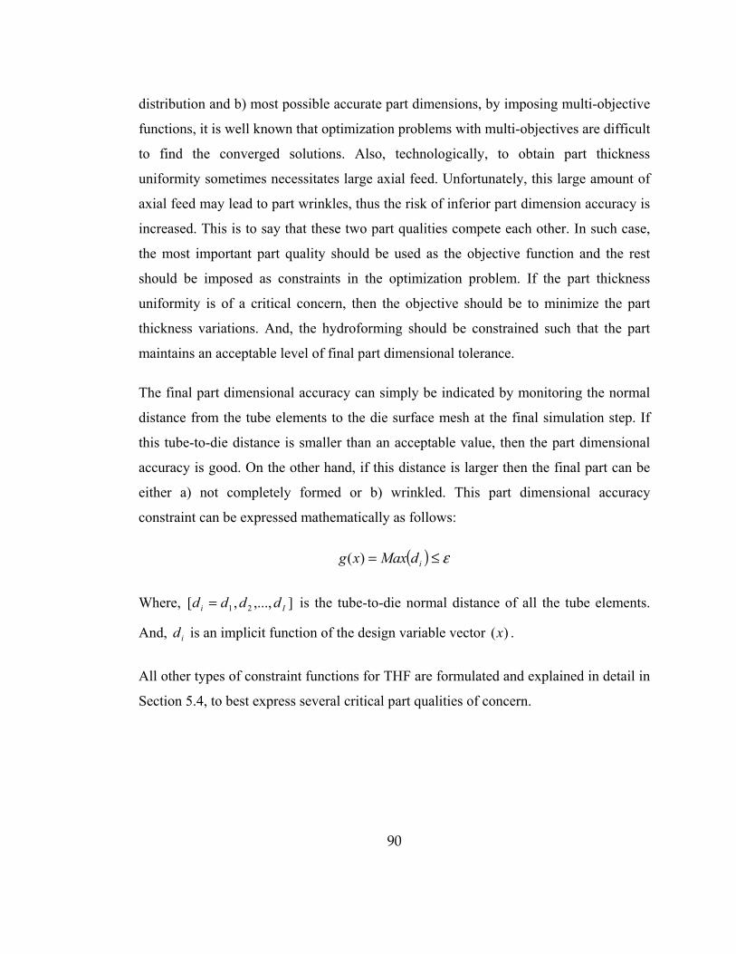
90
distribution and b) most possible accurate part dimensions, by imposing multi-objective
functions, it is well known that optimization problems with multi-objectives are difficult
to find the converged solutions. Also, technologically, to obtain part thickness
uniformity sometimes necessitates large axial feed. Unfortunately, this large amount of
axial feed may lead to part wrinkles, thus the risk of inferior part dimension accuracy is
increased. This is to say that these two part qualities compete each other. In such case,
the most important part quality should be used as the objective function and the rest
should be imposed as constraints in the optimization problem. If the part thickness
uniformity is of a critical concern, then the objective should be to minimize the part
thickness variations. And, the hydroforming should be constrained such that the part
maintains an acceptable level of final part dimensional tolerance.
The final part dimensional accuracy can simply be indicated by monitoring the normal
distance from the tube elements to the die surface mesh at the final simulation step. If
this tube-to-die distance is smaller than an acceptable value, then the part dimensional
accuracy is good. On the other hand, if this distance is larger then the final part can be
either a) not completely formed or b) wrinkled. This part dimensional accuracy
constraint can be expressed mathematically as follows:
( ) ε≤= idMaxxg )(
Where, ],...,,[ 21 Ii dddd = is the tube-to-die normal distance of all the tube elements.
And, id is an implicit function of the design variable vector )(x .
All other types of constraint functions for THF are formulated and explained in detail in
Section 5.4, to best express several critical part qualities of concern.
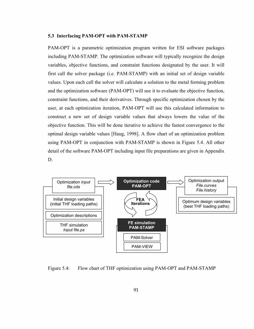
91
5.3 Interfacing PAM-OPT with PAM-STAMP
PAM-OPT is a parametric optimization program written for ESI software packages
including PAM-STAMP. The optimization software will typically recognize the design
variables, objective functions, and constraint functions designated by the user. It will
first call the solver package (i.e. PAM-STAMP) with an initial set of design variable
values. Upon each call the solver will calculate a solution to the metal forming problem
and the optimization software (PAM-OPT) will use it to evaluate the objective function,
constraint functions, and their derivatives. Through specific optimization chosen by the
user, at each optimization iteration, PAM-OPT will use this calculated information to
construct a new set of design variable values that always lowers the value of the
objective function. This will be done iterative to achieve the fastest convergence to the
optimal design variable values [Haug, 1998]. A flow chart of an optimization problem
using PAM-OPT in conjunction with PAM-STAMP is shown in Figure 5.4. All other
detail of the software PAM-OPT including input file preparations are given in Appendix
D.
Figure 5.4: Flow chart of THF optimization using PAM-OPT and PAM-STAMP
FE simulation PAM-STAMP
Optimization code PAM-OPT
PAM-Solver
PAM-VIEW
Optimization input file.cds
Initial design variables (initial THF loading paths)
Optimization descriptions
THF simulation Input file.ps
Optimization output File.curves File.history
Optimum design variables (best THF loading paths) Iterations
FEA
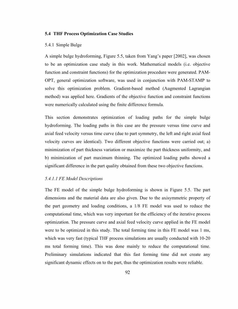
92
5.4 THF Process Optimization Case Studies
5.4.1 Simple Bulge
A simple bulge hydroforming, Figure 5.5, taken from Yang�s paper [2002], was chosen
to be an optimization case study in this work. Mathematical models (i.e. objective
function and constraint functions) for the optimization procedure were generated. PAM-
OPT, general optimization software, was used in conjunction with PAM-STAMP to
solve this optimization problem. Gradient-based method (Augmented Lagrangian
method) was applied here. Gradients of the objective function and constraint functions
were numerically calculated using the finite difference formula.
This section demonstrates optimization of loading paths for the simple bulge
hydroforming. The loading paths in this case are the pressure versus time curve and
axial feed velocity versus time curve (due to part symmetry, the left and right axial feed
velocity curves are identical). Two different objective functions were carried out; a)
minimization of part thickness variation or maximize the part thickness uniformity, and
b) minimization of part maximum thinning. The optimized loading paths showed a
significant difference in the part quality obtained from these two objective functions.
5.4.1.1 FE Model Descriptions
The FE model of the simple bulge hydroforming is shown in Figure 5.5. The part
dimensions and the material data are also given. Due to the axisymmetric property of
the part geometry and loading conditions, a 1/8 FE model was used to reduce the
computational time, which was very important for the efficiency of the iterative process
optimization. The pressure curve and axial feed velocity curve applied in the FE model
were to be optimized in this study. The total forming time in this FE model was 1 ms,
which was very fast (typical THF process simulations are usually conducted with 10-20
ms total forming time). This was done mainly to reduce the computational time.
Preliminary simulations indicated that this fast forming time did not create any
significant dynamic effects on to the part, thus the optimization results were reliable.

93
Part Geometry / Material Properties Value / Units
Tube initial length (L0) 128 (mm)
Tube outside diameter (OD0) 42 (mm)
Tube wall thickness (t0) 1.98 (mm)
Expansion length (W) 64 (mm)
Final part maximum outside diameter (OD1) 54(mm)
Strength coefficient (K) 0.567 (GPa)
Strain hardening coefficient (n) 0.264
Pre strain (e0) 0.007
Figure 5.5: Simple bulge geometry and material properties [Yang, 2001b]
L0/2
OD0/2
W/2
OD1/2

94
5.4.1.2 Optimization Descriptions
5.4.1.2.1 Optimization Problem
The main goal of this simple bulge hydroforming is to optimize the loading paths that
would improve the part quality in two different cases, a) minimize the part thickness
variations, and b) minimize the part maximum thinning. These two objectives suggest
two different tube hydroforming approaches.
5.4.1.2.2 Optimization Data � Design Variables, Objective Function, Constraints
Design Variables
The design variables in this problem are the points controlling the piecewise linear
curves representing the pressure and axial feed velocity curves versus time, see Figure
5.6. The design variable vector is written as follows:
],...,|,...,[ 2121 mn xfxfxfxpxpxpx =
521 ,..., xpxpxp = Design variables for pressure curve
521 ,..., xfxfxf = Design variables for axial feed velocity curve
The total number of design variables is 10, 5 of which are for the pressure and axial
feed velocity, respectively. In Figure 5.6, the initial sets of the design parameters and
bounds are given. These initial curves of the axial feed velocity and pressure are
calculated using the simple metal forming equations (i.e. using volume constancy to
calculate axial feed and axial feed velocity necessary, and bursting pressure equation).
The initial axial feed velocity is 5 mm/ms constant throughout the process; the total
initial axial feed is then 5 mm. The first two points of the velocity curves are fixed as
shown in the figure to ensure that some axial feed is applied in the beginning for tube
sealing. The last five points are to be optimized. The initial pressure curve linearly
increases from zero to 0.06 GPa (600 bar). Only the starting point is fixed to zero; the
rest of the points are to be optimized.

95
0
5
10
15
20
25
0 0.2 0.4 0.6 0.8 1Time (ms)
Axi
al fe
ed v
eloc
ity (m
m/m
s)
0
0.02
0.04
0.06
0.08
0 0.2 0.4 0.6 0.8 1Time (ms)
Pres
sure
(GPa
)
Figure 5.6: Loading curves presented by piecewise-linear curves: design variables
xf1 xf2 xf3 xf4 xf5
Upper bound
Lower bound
Fixed points
Design variables
xp1
xp2
xp3
xp4
xp5
Upper bound
Lower bound Fixed point
Design variables

96
In Figure 5.6, the design variable bounds limit the feasible region of the design
variables. Without these bounds the search for the optimal variables may not be
efficient. The axial feed curve is allowed to have more room to move around, whereas
the possible movement of the pressure curve is more restricted. This is done because of
the idea that the axial feed should be applied as much as possible and the pressure is just
applied enough to prevent wrinkles. The pressure curve is allowed to have more room
to move towards the process end such that an increased pressure for calibration would
be possible. Please notice that the bounds are governing only the design variables not
the fixed points.
The design variable bounds for axial feed velocity can be calculated (or estimated) from
a) maximum allowable axial feed of the initial tube relative to the die (i.e. tube cannot
be fed in so much such that the tube end is pushed beyond the guiding zone into the
expansion zone), and b) maximum allowable thickening of the final part; in this case
study, the first method is used to determine the maximum axial feed (25 mm), thus the
maximum velocity is 25 mm/ms over the forming time period, see the velocity upper
bound in Figure 5.6. Of curse, this velocity upper bound does not have to be such a
horizontal straight line. It can be of any sensible shapes with a total area underneath the
curve of 25 mm.
The pressure bounds are more difficult to estimate. In this work, usually, the pressure
lower bound is a straight line increasing from zero at the first control point to 80%-90%
of the initial pressure at the last control point. The pressure upper bound is constructed
such that it would make a narrow band bounding the initial pressure curve with a gap
between the lower and upper bound of about 0.02 GPa (200 bar). Finally, a pressure of
110%-120% of the calibration pressure calculated for the given part can be used as the
last point of the pressure upper bound.
These design variable bounds sometimes can be impossible to estimate. As a rule of
thumb, it is advised to always use the strictest bounds sensible first. Then, if the

97
optimized variables are all placed on the bounds imposed, the bounds may need to be
expanded in the next optimization run.
Objective Function
The objective function of minimizing the part thickness variations is applied here first.
Then, at the end of this section, the second objective function of minimizing part
(maximum) thinning is applied to the exact same problem. Finally, both of these two
results are then compared in terms of the part quality.
Figure 5.7 shows the tube mesh used in formulating the objective function. To consider
the part thickness variation along the tube axis, three chosen tube elements are spread
out from the tube center (which is subject to excessive thinning) to the tube end (which
is subject to excessive thickening). The thickness values of these chosen tube elements
at the final simulation step are extracted and then used to evaluate the objective function
of minimizing part thickness variation. This objective function can be expressed as
below using the root-mean-squared formula: ( )
++=
21
23
22
213
1)( hhhMinxf
Where the h1, h2, and h3 are the tube elemental thicknesses at the final simulation step.
The chosen elements are on the same longitudinal line due to the fact that the part is
axisymmetric. More tube elements can be considered in the objective function if a
tighter tolerance of the part thickness variations is to be obtained.
Constraint functions
The final part should be formed completely and without any wrinkle at the final
simulation step. The constraint function in this case should reflect that goal. One
convenient way to check the final part dimensional accuracy and part wrinkle-free
condition is to consider the controlled volume of the final part (controlled part volume
is the part volume calculated within a fixed imaginary boundary over the expansion
zone, see Figure 5.8).

98
Figure 5.7: Objective function: minimizing part thickness variations
Figure 5.8: Constraint functions: part dimension accuracy using controlled volume
Controlled volume
Voltube < Voldie Process start
Controlled volume
Voltube = VoldieProcess end
h1 h2 h3 Tube axis
Centerline

99
If the controlled volume of the final part ( tubeVol ) is the same as that of the die ( dieVol )
then the part is successfully formed. If the controlled part volume is less than that of
the die cavity, then that part is not completely formed or has some wrinkles. The detail
of this concept is elaborated more in Chapter 6. This constraint function can be
expressed as below:
1100*)( ≤
−=
die
dietube
VolVolVol
xg
The alternative way of imposing the part dimensional accuracy constraint is to monitor
the final tube-to-die distance, as explained earlier. However, considering all the nodal
tube-to-die distance can become quite inefficient if the number of element is large. The
part volume is just one single scalar readily calculated. The use of the controlled part
volume to check the completeness of the part may not be as accurate as the part
becomes bigger, e.g. structural parts, due to larger numerical errors in calculating the
total part volume from the facetted tube mesh. In those cases, the tube-to-die distance of
some critical part locations (i.e. areas that are wrinkle prone) is a better option to
impose this constraint.
5.4.1.2.3 Optimization Algorithms
In this optimization of the simple bulge hydroforming, the problem is relatively simple.
The metal flow only experiences a simple biaxial state of stress without any shear
stresses (i.e. axisymmetric forming and thin shell assumption). Therefore, this
optimization problem is solved using the gradient-based method (i.e. Augmented
Lagrangian method). In general, gradient-based methods are known to converge the
fastest among all the optimization methods. Unfortunately, if the problem is too
complex (a large number of design variables or the problem is very non-linear)
sometimes the gradient-based methods do not converge at all. However, this is not the
case here.

100
5.4.1.3 Optimization Results
Each simulation run typically takes about 2 min. Therefore, the total computational time
is about 500 min.
The optimized axial feed velocity curve and pressure curve are shown in Figure 5.9. It
can be seen from the velocity curve that the optimized axial punch moves faster in the
beginning and slows down toward the end of the forming. The optimized pressure
curve, on the other hand, reduces from the initial value during the beginning of the
process and increases towards the process end. This increase of the pressure at the end
is needed for calibration of the part.
Figure 5.10 shows evolutions of the objective function and constraint function. The total
of 25 optimization iterations were required to arrive at a converged solution. Since there
are 10 design variables in this problem, the total number of simulation runs is 23 *
(10+1) = 253 runs. The objective function value reduces exponentially to the minimum
value. Also most of all the iterations were within the constraint bounds.
The initial loading path (before optimization) and the optimized loading path are plotted
in Figure 5.11. The optimized loading path exhibits the typical THF loading path shape,
i.e. large axial feed in the beginning while the pressure is kept low then towards the end
the pressure is increased to remove part wrinkles and calibrate the part while the axial
feed becomes almost stagnant. The resultant part has very good thickness uniformity,
see Figure 5.12. The maximum thinning is only 3% and the maximum thickening is
only 4%. The total axial feed amount on each tube end is 9 mm with the maximum
pressure of 0.75 GPa (750 bar).
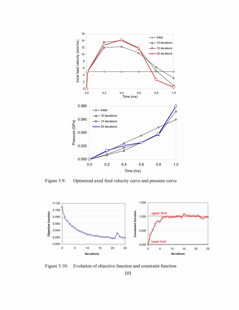
101
0
2
4
6
8
10
12
14
16
0.0 0.2 0.4 0.6 0.8 1.0Time (ms)
Axi
al fe
ed v
eloc
ity (m
m/m
s)
Initial
10 iterations
15 iterations
25 iterations
0.000
0.020
0.040
0.060
0.080
0.0 0.2 0.4 0.6 0.8 1.0
Time (ms)
Pre
ssur
e (G
Pa)
Initial
10 iterations
15 iterations
25 iterations
Figure 5.9: Optimized axial feed velocity curve and pressure curve
0.000
0.020
0.040
0.060
0.080
0.100
0.120
0 5 10 15 20 25
Iterations
Obj
ectiv
e fu
nctio
n
0.000
0.500
1.000
1.500
0 5 10 15 20 25
Iterations
Con
stra
int f
unct
ion upper limit
lower limit
Figure 5.10: Evolution of objective function and constraint function

102
0.00
0.02
0.04
0.06
0.08
0 2 4 6 8 10Axial feed (mm)
Pres
sure
(GPa
)
Optimal
Initial
Figure 5.11: Initial and optimized loading paths for simple bulging
-0.14-0.12-0.10-0.08-0.06-0.04-0.020.000.020.04
0 10 20 30 40 50 60
Longitudinal Curvilinear Distance (mm)
Par
t Thi
nnin
g
Figure 5.12: Part thinning distribution of optimized simple bulge

103
Another run of the optimization is carried out on the same simple bulge using a
different objective function, i.e. minimizing the part maximum thinning. The objective
function for this problem can be expressed as follows:
−=
0
0)(h
hhMaxMinxf i
Where ih = all the tube elemental thickness at the final simulation step and 0h = initial
tube thickness.
The optimized loading paths and the part thinning distribution are shown in Figure 5.13
and Figure 5.14. It can be seen that in this case the total axial feed is 11 mm, which is
larger that from the first case. The maximum part thinning now is reduced to 2%.
However, due to the large amount of axial feed applied, the thickening on the tube end
is increased to 12%. Obviously, this part has unnecessary thickening. However, this
situation often happens in difficult-to-form part. For this simple bulge geometry, this
situation is done only for an example.
5.4.2 Y-shape
Hydroforming of parts with protrusions is usually more challenging than typical THF
due to the added process parameter, counter punch force versus time curve. Normally,
the counter punch force versus time curve cannot be calculated analytically. Trial-and-
error FE method is usually used to figure out the proper values of the counter punch
force. In this optimization case study, the Y-shape, used in Chapter 3, is chosen again to
be the case study for demonstrating how to optimize the counter punch force versus
time curve.

104
0.00
0.02
0.04
0.06
0.08
0 2 4 6 8 10 12
Axial feed (mm)
Pre
ssur
e (G
Pa)
OptimalInitial
Figure 5.13: Optimized loading paths for simple bulging
-0.14
-0.12-0.10
-0.08
-0.06-0.04
-0.02
0.000.02
0.04
0 20 40 60
Curvilinear distance (mm)
Par
t Thi
nnin
g
Figure 5.14: Part thinning distributions of the simple bulge
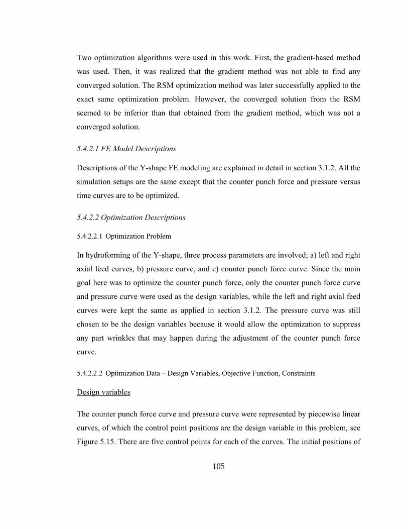
105
Two optimization algorithms were used in this work. First, the gradient-based method
was used. Then, it was realized that the gradient method was not able to find any
converged solution. The RSM optimization method was later successfully applied to the
exact same optimization problem. However, the converged solution from the RSM
seemed to be inferior than that obtained from the gradient method, which was not a
converged solution.
5.4.2.1 FE Model Descriptions
Descriptions of the Y-shape FE modeling are explained in detail in section 3.1.2. All the
simulation setups are the same except that the counter punch force and pressure versus
time curves are to be optimized.
5.4.2.2 Optimization Descriptions
5.4.2.2.1 Optimization Problem
In hydroforming of the Y-shape, three process parameters are involved; a) left and right
axial feed curves, b) pressure curve, and c) counter punch force curve. Since the main
goal here was to optimize the counter punch force, only the counter punch force curve
and pressure curve were used as the design variables, while the left and right axial feed
curves were kept the same as applied in section 3.1.2. The pressure curve was still
chosen to be the design variables because it would allow the optimization to suppress
any part wrinkles that may happen during the adjustment of the counter punch force
curve.
5.4.2.2.2 Optimization Data � Design Variables, Objective Function, Constraints
Design variables
The counter punch force curve and pressure curve were represented by piecewise linear
curves, of which the control point positions are the design variable in this problem, see
Figure 5.15. There are five control points for each of the curves. The initial positions of

106
the control points were taken from past experience on hydroforming simulation of this
part. The design variables are expressed as follows:
],...,|,...,[ 2121 mn xfxfxfxpxpxpx =
521 ,..., xpxpxp = Design variables for pressure curve
521 ,..., xfxfxf = Design variables for counter punch force curve
The variable bounds on these two curves were estimated and imposed in the same way
as in the optimization of the simple bulge, i.e. the design space for the pressure curve
was small and more room was given only for the calibration stage. And, on the other
hand, the counter punch force curve was given a lot of design space. This was to give
more freedom to the search of optimal counter punch force. As a result of the axial
feeds used in this Y-shape, the growing protrusion did come in contact with the counter
punch until around the time of 0.4 ms. Therefore, the counter punch force curve was
fixed at zero till around the time of 0.4 ms. The left and right axial feed velocity curves
were the same as applied in chapter 3, see Figure 5.16.
Objective function.
The goal of this optimization was to determine the best combination of counter punch
force curve and pressure curve versus time such that the height of the protrusion was
maximum obtainable, which is, typically, a desirable feature for parts with protrusions.
In this work, the part controlled volume was used to express the protrusion height. It is
obvious that the protrusion height should be directly proportional to its part controlled
volume, see Figure 5.17. The objective of this problem can be expressed as follows:
( )tubeVolMaxxf =)(
Constraint functions
Three different constrains, see Figure 5.18 were necessary in this optimization problem.
These constrains were imposed onto the problem in order to guarantee that final part
obtained is successful. All the constrains are explained below:
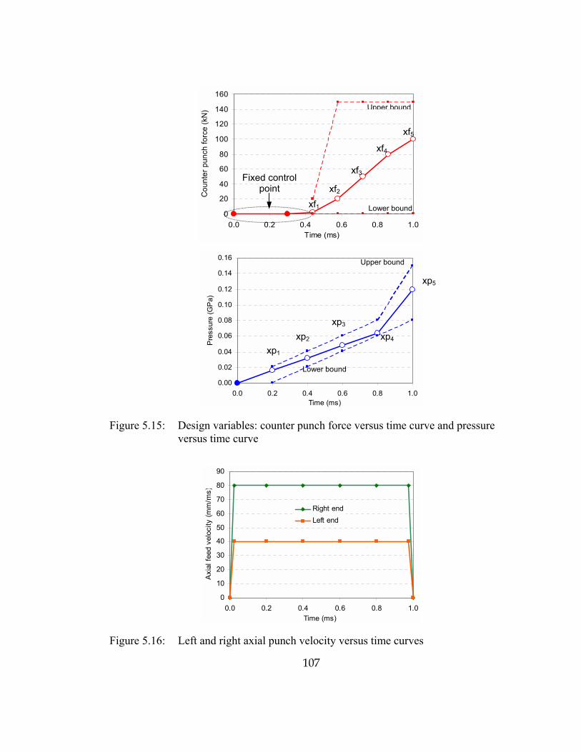
107
0
20
40
60
80
100
120
140
160
0.0 0.2 0.4 0.6 0.8 1.0Time (ms)
Cou
nter
pun
ch fo
rce
(kN
)
0.00
0.02
0.04
0.06
0.08
0.10
0.12
0.14
0.16
0.0 0.2 0.4 0.6 0.8 1.0Time (ms)
Pre
ssur
e (G
Pa)
Figure 5.15: Design variables: counter punch force versus time curve and pressure versus time curve
0
10
20
30
40
50
60
70
80
90
0.0 0.2 0.4 0.6 0.8 1.0Time (ms)
Axi
al fe
ed v
eloc
ity (m
m/m
s)
Right endLeft end
Figure 5.16: Left and right axial punch velocity versus time curves
xf1
xf2
xf3
xf4
xf5
Upper bound
Lower bound
xp1
xp2 xp3
xp4
xp5
Upper bound
Lower bound
Fixed control point

108
Tube-to-die distance: This constraint was imposed in order to prevent the final part
from wrinkling. The constraint considered distance from the part surface normal to the
die surface (so called �tube-to-die� distance) at the end of the forming process. If this
distance exceeded a certain value then part was not formed successfully, i.e. not
completely formed or wrinkled. As for the Y-shape forming, the part was prescribed
with profiles along which the tube-to-die distances at the process end were monitored.
These profiles were put on the part�s most wrinkle-prone areas, as shown in Figure
5.18.a. The constraints are expressed as follow: ( ) 121
1 ,)( ε≤= ii ddMaxxg
1id is the tube-to-die distance along the profile #1 and 2
id is the tube-to-die distance
along the profile #2. In PAM-STAMP, the tube-to-die distance is calculated from the
normal distance from the tube middle plane to the interior die surface. Therefore, the
above constraint value (upper bound) usually runs from 05.0 h to 0h , where 0h be the
initial tube wall thickness.
Protrusion corner radius: Not only the protrusion should be formed with maximum
obtainable height but it should also have a tight corner radius. This sharp corner radius
is beneficial in maximizing the useful protrusion height (refer to section 3.3). In FE
simulation, curvatures of shell elements can be easily calculated. Curvature is equal to
an inversed radius value. Thus, the smallest part radius is the largest part curvature.
Therefore, the tight protrusion corner radius constraint can be expressed as follows:
( ) 22 *1)( ερ ≤−= iMaxxg
iρ are the curvature values of all shell elements of the part.
Part maximum thinning: To aim for obtaining the maximum protrusion height is at the
same time to run a risk of having excessive part thinning right at the protrusion top, see
Figure 5.18.c. Therefore, it was necessary to constrain the final optimized part from
exceeding the maximum allowable thinning value. The part thinning constraint can be
expressed as follows:

109
Figure 5.17: Objective function: maximizing the protrusion height or maximizing the part controlled volume
Figure 5.18: Constraint functions: a) tube-to-die distance, b) protrusion corner curvature, and c) part maximum thinning
Controlled volume
Hp
Hp α Voltube
a) b)
c)
Max. thinning
Corner curvature
Tube-to-die distance profiles

110
30
03 )( ε<
−=
hhh
Maxxg i
Where ih = all the part elemental thickness at the final simulation step and 0h = initial
tube thickness.
5.4.2.2.3 Optimization Algorithms
Both gradient and RSM method were used in this optimization problem. First the
optimization results from the gradient method are discussed. Then, the results from the
RSM method are given in comparisons with the previous results.
5.4.2.3 Optimization Results
The gradient-based method was not able to find a converged solution. The objective
curve fluctuates and shows no sign of converging, see Figure 5.19. The constraint
function curves are shown in Figure 5.20. The tube-to-die distance constraint curve
seemed to stay within the bound. This indicated that the final part completely took the
shape of the die and had no wrinkles. However, the other two constrains, i.e. maximum
thinning and corner curvature, went out of the upper bound many times during the
optimization. Since the optimization did not seem to be converging, it was terminated at
the iteration 16, where all the constraints were satisfied. The resultant counter punch
force curve and pressure curve taken from the optimization at iteration #3 and #16
(these curves satisfied all the constraints) are shown in Figure 5.21. Since the results
from iteration #16 are the best, its resultant counter punch force curve and pressure
curve are considered the best from this optimization using gradient method.
The optimized counter punch force increased up to 50 kN then decreased to 10 kN at
0.6-0.8 ms, and finally increased up to 90 kN at the end, see Figure 5.21.

111
148000
150000
152000
154000
156000
158000
160000
0 2 4 6 8 10 12 14 16Interation
Obj
ectiv
e fu
nctio
n - V
olum
e (m
m3)
Figure 5.19: Objective function: evolution of part controlled volume
0.00
0.20
0.40
0.60
0.80
1.00
0 2 4 6 8 10 12 14 16Interation
Tube
-to-d
ie d
ista
nce
(mm
) upper limit
lower limit
0.20
0.25
0.30
0.35
0.40
0 2 4 6 8 10 12 14 16Interation
Cor
ner c
urva
ture
(1/m
m)
upper limit
lower limit
0.15
0.20
0.25
0.30
0.35
0 2 4 6 8 10 12 14 16Interation
Max
imum
thin
ning
upper limit
lower limit
Figure 5.20: Constraint functions: evolutions of a) tube-to-die distance, b) corner curvature, and c) part maximum thinning
Non-converging
a) b)
c)
Out of bound
Out of bound

112
0
20
40
60
80
100
120
0.0 0.2 0.4 0.6 0.8 1.0
Time (ms)
Cou
nter
pun
ch fo
rce
(kN
)
Initial5 Iterations16 Iterations
0.00
0.02
0.04
0.06
0.08
0.10
0.12
0.14
0.16
0.0 0.2 0.4 0.6 0.8 1.0
Time (ms)
Pre
ssur
e (G
Pa)
Initial5 Iterations16 Iterations
Figure 5.21: Optimized counter punch force curve and pressure curve versus time

113
From an observation of the simulation, the protrusion grew the fastest during the time of
0.6-0.8 ms (the counter punch force fluctuated between 10-50 kN), then its growth
slowed down and the protrusion corner formed into a tighter radius during the process
end (the counter punch force curve increased to the maximum value at the process end).
The final part from this gradient optimization has the maximum part thinning under the
critical thinning of 25%.
RSM optimization method was applied to solve this exact problem with an attempt to
find a converged solution to this problem. Figure 5.22, Figure 5.23, and Figure 5.24
show evolution of the objective function, constraint functions, and the optimal loading
paths, respectively. With the application of RSM method, a converged solution was
found and all the constraint functions were converging inside the lower and upper
bounds.
Though the RSM took much less number of iterations than the gradient-based method
did (3 iterations with 35 simulation runs in RSM method and 16 iteration with 176
simulation runs in gradient-based method) the RSM optimum solution seems to be just
a local optimum not a global one. This is clearer if one compares results from the RSM
method to that of the gradient method, see Figure 5.25. The part protrusion height from
the gradient-based method is lager than that from the RSM optimization method, see
Figure 5.25.b. The protrusion maximum thinning of the RSM part is smaller than that of
the gradient method simply because the RSM part has a smaller protrusion, see Figure
5.25.a.
The optimization of counter punch force and pressure curve for the hydroforming of Y-
shape has shown to be a rather difficult task. The gradient-based method did not seem to
be able to find any converged solution. This usually happens in cases where the
problems being optimized are very non-linear (i.e. the objective and constraints are
strong non-linear functions of the design variables), and have a large number of design
variables. RSM optimization method is known to be able to handle such problems.
However, in this case study, through RSM, only local optimum seems to be found.

114
149000
150000
151000
152000
153000
154000
0 1 2 3Interation
Obj
ectiv
e fu
nctio
n - V
olum
e (m
m3)
Figure 5.22: RSM Objective function: part controlled volume
0.00
0.20
0.40
0.60
0.80
1.00
0 1 2 3Interation
Tube
-to-d
ie d
ista
nce
(mm
) upper limit
lower limit
0.15
0.2
0.25
0.3
0.35
0 1 2 3Interation
Cor
ner c
urva
ture
(1/m
m)
upper limit
lower limit
0.15
0.20
0.25
0.30
0.35
0 1 2 3Interation
Max
imum
thin
ning
upper limit
lower limit
Figure 5.23: RSM constraint functions: a) tube-to-die distance, b) corner curvature, and c) maximum thinning
a) b)
c)

115
0
20
40
60
80
100
120
140
0.0 0.2 0.4 0.6 0.8 1.0
Time (ms)
Cou
nter
pun
ch fo
rce
(kN
) Initial1 Iteration
3 Iteration
0.00
0.02
0.04
0.06
0.08
0.10
0.12
0.14
0.0 0.2 0.4 0.6 0.8 1.0
Time (ms)
Pre
ssur
e (G
Pa)
Initial1 Iteration
3 Iteration
Figure 5.24: RSM optimized a) counter punch force curve and b) pressure curve
a)
b)

116
-1.00
-0.80
-0.60
-0.40
-0.20
0.00
0.20
0.40
0 50 100 150 200 250
Curvilinear distance (mm)
Par
t thi
nnin
g
0
10
20
30
40
50
60
70
80
50 75 100 125 150 175 200 225 250
Tube X-coordinates (mm)
Tube
Y-c
oord
inat
es (m
m)
Figure 5.25: Comparison of part qualities obtained from Gradient-based method and RSM method; a) part thinning distributions, and b) protrusion profiles
Gradient-based method RSM
a)
b)
Gradient
RSM
Gradient
RSM

117
5.4.3 Structural Part
In this case study, an optimization of THF loading paths for a medium-sized structural
part was carried out, see Figure 5.26. The pressure versus time curve and axial feed
versus time curve were the main process parameters in this forming process. Since the
part was not symmetric on left and right sides, two different axial feed velocity curves
(i.e. for left and right tube ends) were necessary. Unlike the previous case studies, in
this problem, there were three process parameter curves (a total of 15 design variables)
that needed to be optimized. Consequently, the RSM optimization method was applied
here due to the large size of the problem.
5.4.3.1 FE Model Descriptions
The dimensions and material properties of the part (SS304) are given in Figure 5.26.
This part geometry was designed by Kawasaki Hydromechanics, Japan. Due to the
part�s symmetry about the axis and of the geometry and loadings, only 1/8th of the part
was modeled in the simulation, Figure 5.27.
5.4.3.2 Optimization Descriptions
5.4.3.2.1 Optimization Problem
Similar to the simple bulge hydroforming, this particular problem required
determination of optimized axial feed curves and pressure curve. The loading paths
determined should be such that the part was successfully formed without any wrinkles
and excessive thinning.
5.4.3.2.2 Optimization Data � Design Variables, Objective Function, Constraints
Design variables: There were a total of 15 design variables in this problem, the design
variables were used to represent the piecewise linear pressure and left and right axial
feed velocity versus time curves. All the design variables are shown in Figure 5.28. The
variable bounds were also given in the Figures. The initial design variables and bounds

118
of the left and right axial feed velocity were the same. The design variables can be
expressed as the following:
],...,|,...,[ 2121 mn xfxfxfxpxpxpx =
521 ,..., xpxpxp = Design variables for pressure curve
521 ,..., xfxfxf = Design variables for left axial feed velocity curve
1076 ,..., xfxfxf = Design variables for right axial feed velocity curve
Objective function: The main goal of this forming was to successfully hydroform that
part with minimum part thinning possible. Therefore, the objective function can be
expressed as follows:
−=
0
0)(h
hhMaxMinxf i
Where, ih = all the tube elemental thickness and 0h = initial tube thickness.
Constraint functions: This part was a rather difficult to form due to its non-symmetry
feature from left side to right side of the part. A substantial amount of axial feed was
necessary for forming of this part, which in turn heightened the risk of part wrinkling.
Therefore, wrinkles in the final part were the main concern. The tube-to-die distance
constraint was imposed along the profile shown in Figure 5.27. This profile was placed
on the tube surface along the tube axis direction and close to the part corner. This area
was largely unsupported, thus most susceptible to wrinkles.
5.4.3.2.3 Optimization Algorithms
This current optimization problem had a large number of design variables (i.e. 15
variables compared to 10 variables of the previous case studies). Based on the
experience gained from the previous case study, the gradient-based method was not able
to find any converged solution for rather complex problems; it was decided to use the
RSM optimization method in this problem.
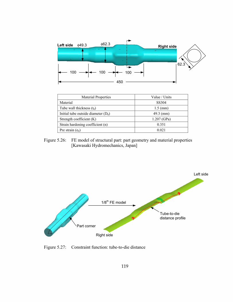
119
Material Properties Value / Units Material SS304 Tube wall thickness (t0) 1.5 (mm) Initial tube outside diameter (D0) 49.3 (mm) Strength coefficient (K) 1.207 (GPa) Strain hardening coefficient (n) 0.351 Pre strain (e0) 0.021
Figure 5.26: FE model of structural part: part geometry and material properties [Kawasaki Hydromechanics, Japan]
Figure 5.27: Constraint function: tube-to-die distance
Tube-to-die distance profile
1/8th FE model
Left side
Right side
Part corner
Left side Right side
450
100 100 100
62.3
φ62.3φ49.3

120
0
10
20
30
40
50
60
0.0 0.2 0.4 0.6 0.8 1.0
Time (ms)
Left/
Rig
ht a
xial
feed
vel
ocity
(mm
/ms)
0.00
0.05
0.10
0.15
0.20
0.25
0.0 0.2 0.4 0.6 0.8 1.0
Time (ms)
Pre
ssur
e (G
Pa)
Figure 5.28: Initial design parameters: left and right axial feed velocity versus time curve and pressure versus time curve
xp1 xp2
xp3 xp4
xp5 Upper bound
Lower bound
xf1 xf2 xf3 xf4 xf5
Upper bound
Lower bound
121
5.4.3.3 Optimization Results
The optimization took 6 iterations (96 simulation runs) to find a converged solution.
Figure 5.29 shows the optimum axial feed velocity curves for the left and right axial
punches and pressure curve. The objective function and constraint function are given in
Figure 5.30. The evolution of tube-to-die distance constraint is completely bounded,
which means that that final part has an acceptable part dimensional accuracy.
The optimum velocity curve, Figure 5.29, for the left axial punch seemed to be
unrealistic that it fluctuated sharply during 0.4-0.8 mm. This is because this curve is on
a simulation time scale, which was sped up unrealistically for numerical purposes.
However, when put in practice, this velocity curve can be adjusted to be applicable to
the hydroforming press capability. Only the relationship between the right axial punch
displacement, left axial punch displacement, and pressure has to be maintained
throughout the forming process, see Figure 5.31 for the optimized loading paths for
THF of this part. It is seen from Figure 5.31 that the right punch displacement is larger
than the one on the left side. This agrees with the part geometry whose the right portion
of the part is larger than that of the left side.
The part thinning distribution along the tube axis direction is given in Figure 5.32. The
part maximum thinning is only 8% and the maximum thickening is 14%. This part was
optimized with an objective to reduce the maximum part thinning. Therefore, the
thickness variation was a bit large. If this part had been optimized with an objective to
minimize the thickness variation (refer to section 5.4.1) a better part with a more
uniform thickness distribution should have been resulted.
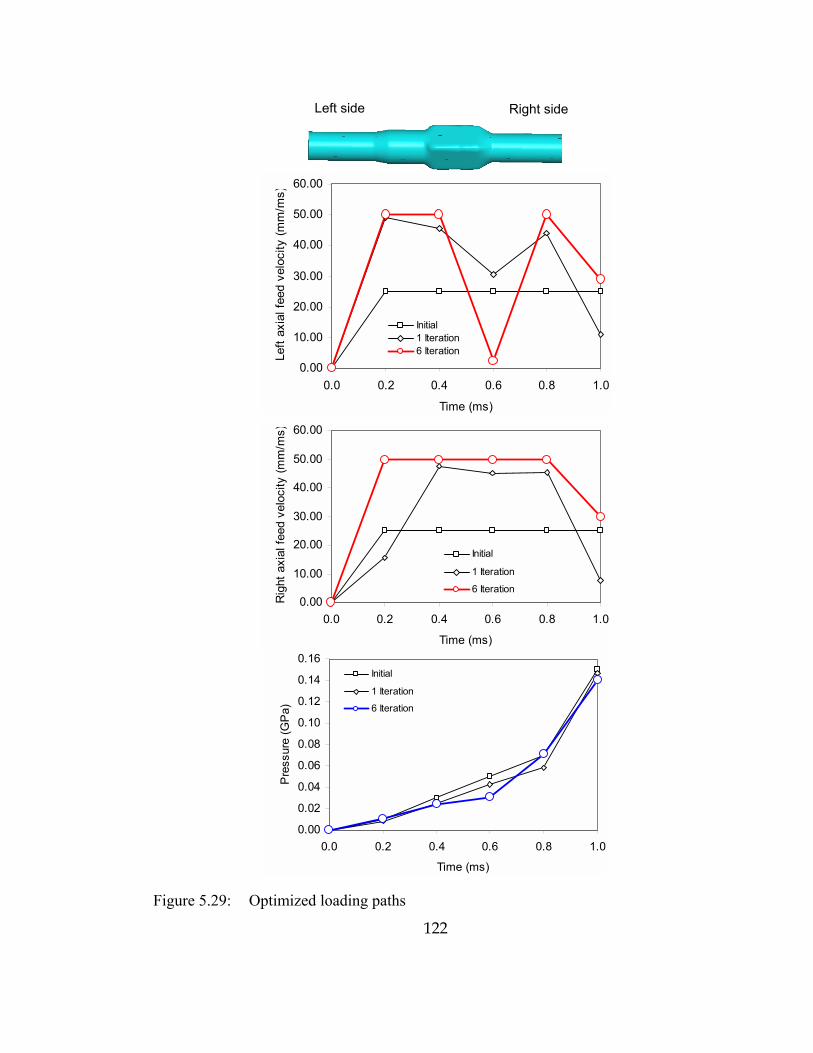
122
0.00
10.00
20.00
30.00
40.00
50.00
60.00
0.0 0.2 0.4 0.6 0.8 1.0
Time (ms)
Left
axia
l fee
d ve
loci
ty (m
m/m
s)
Initial1 Iteration6 Iteration
0.00
10.00
20.00
30.00
40.00
50.00
60.00
0.0 0.2 0.4 0.6 0.8 1.0
Time (ms)
Rig
ht a
xial
feed
vel
ocity
(mm
/ms)
Initial
1 Iteration
6 Iteration
0.00
0.02
0.04
0.06
0.08
0.10
0.12
0.14
0.16
0.0 0.2 0.4 0.6 0.8 1.0
Time (ms)
Pre
ssur
e (G
Pa)
Initial
1 Iteration
6 Iteration
Figure 5.29: Optimized loading paths
Left side Right side

123
0.00
0.05
0.10
0.15
0.20
0.25
0 1 2 3 4 5 6
Iteration
Par
t max
imum
thin
ning
0.00
0.20
0.40
0.60
0.80
1.00
1.20
1.40
0 1 2 3 4 5 6
Iteration
Tube
-die
dis
tanc
e (m
m) upper limit
lower limit
Figure 5.30: Evolution curves of a) objective function and b) constraint function
0.000
0.020
0.040
0.060
0.080
0.100
0 5 10 15 20 25 30 35 40
Right axial feed (mm)
Pre
ssur
e (G
Pa)
0
5
10
15
20
25
30
35
Left
axia
l fee
d (m
m)
Figure 5.31: Optimized loading paths for prototyping
a) b)
Right axis(main axis) Left axis
Pressure
Pressure
Left axial feed

124
-0.15
-0.10
-0.05
0.00
0.05
0.10
0 50 100 150 200 250 300 350 400 450
Curvilinear distance (mm)
Par
t thi
nnin
g
Figure 5.32: Part thinning distribution along the longitudinal direction

125
CHAPTER 6.
AUTOMATIC APPROACH TO SELECT LOADING PATH
USING ADAPTIVE SIMULATION
The attempt to develop methodologies for automatic determination of THF Loading
Paths (LP) continues further in this chapter. The optimization-based process simulation
method, from last chapter, enables automatic determination of optimum process
parameter curves (LP) for, virtually, any THF of parts with simple to complex
geometries. However, admittedly, the optimized LP comes with a price of long
computational time. In the industrial settings where the lead-time is so valuable, one
may only wish to obtain just a good or feasible THF process parameter curves (LP)
without sacrificing a lot of computational time in the FE process simulation. Adaptive
Simulation (AS) approach has been developed to meet this need. A conceptual
schematic of the AS procedure is shown in Figure 6.1.
This chapter mainly discusses the development of different components (such as part
defect determination module, and process parameter adjustment module) of the adaptive
simulation approach. A computer program was written and interfaced with PAM-
STAMP to implement this adaptive simulation. A couple of simple part geometries
were used in this study. The adaptive simulation at this stage is only capable of
determining a feasible LP for simple part geometries.
6.1 Adaptive Simulation Concept
The ultimate goal of the adaptive simulation approach is to completely eliminate the
trial-and-error simulation approach and to generate feasible process parameter curves
(LP) within only a few or just one simulation run.

126
t0
t1
t2
t3
Piy
Tube
Wrinkle
∆DaPiy
∆Da Piy+∆Pi
2∆Da Piy+∆Pi
Wrinklet4
Time (t0-t1): yielding pressure (Piy) is applied without any axial feed to initiate the
deformation.
Time (t1-t2): pressure is kept constant (or may be reduced) while an axial feed increment
(∆Da) is applied.
Time (t2-t3): a wrinkle is detected at t2; no axial feed is applied while a pressure increment
(∆Pi) is added.
Time (t3-t4): the wrinkle has been removed at t3; the pressure is kept constant (or may be
reduced) while another axial feed increment is applied.
Figure 6.1: Schematic of the AS procedure, Piy: internal yielding pressure; ∆Pi: internal pressure increment; ∆Da: axial feed increment.

127
In adaptive simulation, the process parameters for the future simulation step are to be
predicted to proper values based on the forming part quality information collected from
the past and current simulation time steps. In other words, during a THF process
simulation run, the simulation intermediate results about forming part qualities (i.e. part
wrinkles, part thinning, and etc) up to the current time step is deduced through
knowledge of THF mechanics and then used it to calculate/project appropriate process
parameters for the next simulation time step. This is in contrast to the traditional
application of FE process simulations where only the simulation results at the final step
are considered and used to infer parameter adjustments for the next trial simulation run
in an attempt to improve/optimize the forming process.
The adaptive simulation approach relies on ability to detect/identify an existence of
defects (i.e. wrinkling and fracture) in the part being formed, and appropriate
adjustments of the relevant process parameters to correct these defects during the
following simulation time steps. The essential parameter adjustment strategy of the
proposed method is to maximize axial feed as it prevents the part from excessive
thinning and minimize pressure just to be sufficient to prevent the part from wrinkling.
Upon completion of adaptive simulation, the evolution of process parameters predicted
by the methodology is the resultant feasible loading paths.
6.2 Implementation of Adaptive Simulation Method
6.2.1 Adaptive Simulation Procedure
A general conceptual flow chart of the adaptive simulation procedure integrated with
PAM-STAMP is shown in Figure 6.2. AS starts with a normal THF simulation model
that consists of the tube mesh, tooling mesh and all the boundary conditions. As the
simulation is progressing at each time step, the AS program will execute the following
tasks:

128
Figure 6.2: General conceptual flow chart of the adaptive simulation interfacing with PAM-STAMP during a simulation time step
PAMSTAMP
THF SIMULATION TIME STEP (N+1)
Maximum Thinning Calculation
? Stop Simulation
?
PAM-STAMP
THF SIMULATION TIME STEP (N)
Move Punch
Hold Internal Pressure
Stop Punch
Increase Internal Pressure
YES
YES NO
Thinning > Max. Value?
Wrinkling?
Wrinkle Indicator Calculation
Defect Detection
Parameter Adjustment

129
a. The �Maximum Thinning Calculation� routine will determine part maximum
thinning. The simulation will be stopped if the maximum thinning exceeds the
predefined critical thinning value (e.g. for LCS, thinning of 25% is generally
considered being an onset of necking).
b. If the current maximum thinning is below the critical value, the �Wrinkle Indicator�
routine will determine the severity of wrinkles occurring in the part.
c. Whenever a wrinkle is detected, the axial punch will be stopped (i.e., punch velocity
is reduced to zero thus no axial feed during the following time steps) while the
internal pressure will be increased during the following time steps till the wrinkle is
removed.
d. When no more wrinkles are detected, the pressure level may be kept constant or
reduced while the punch velocity is brought back to the predefined velocity (punch
velocity that does not cause severe dynamic in the simulation, i.e. slow punch
velocity) to apply more axial feed into the expansion area.
There are two main components in the AS procedure: a) defect detection module, and b)
process parameter adjustment module, see Figure 6.2. The developments of these two
modules and their algorithms will be discussed in detail later. The defect detection
module basically monitors the formability, i.e. wrinkle and bursting, of the simulated
part at every simulation time step. The part formability information is then passed on to
the process parameter adjustment module. This module will process the part formability
information to command the adjustment of pressure and axial feed curve accordingly.
The two modules were coded using FORTRAN and linked to the internal solver of
PAM-STAMP.
6.2.1.1 Defect Detection Module
The two most undesirable defects in THF parts are wrinkles and fracture. In some
applications, such as motorcycle exhaust pipes, part surface finish is also important.
However, in this research, wrinkles and fractures are of the main concern, especially for
automotive structure applications. Wrinkles are undesirable not only for cosmetic

130
reasons but also for part rigidity reasons. Part fracture, obviously, should be avoided at
all costs. A less obvious defect is large part thickness variations. For structural parts,
uniform thickness variations are preferred due to part rigidity and weight reasons. Some
smaller parts also require tight part thickness variations as well such as musical wind
instruments as large part thickness variations would deviate the sound quality of the
instruments.
Monitoring of intermediate simulation results enables a realization of the part defects as
they first appear and grow. The defect detection module in AS has to be able to identify
both existence and severity of these defects as this information will be used as
performance indexes for decision-making in the process parameter adjustment module.
In THF process, sometimes, it is only possible to hydroform a difficult-to-form part
successfully if some tolerable wrinkles are allowed during the intermediate forming,
with the condition that these wrinkles can be straightened out at the end of the forming
process, see Figure 6.3. Two types of part wrinkles are defined in this work: a) dead
wrinkle and b) alive wrinkle. Dead wrinkles are defined as part wrinkles that exist in
the final part, see Figure 6.3. And, alive wrinkles exist in intermediate forming parts
whose surfaces are still far away from the die cavity wall. There are two types of alive
wrinkles: b.1) good alive wrinkles, which are defined as part wrinkles that can
potentially be strengthened out at the process end, and b.2) bad alive wrinkles, which
are defined as part wrinkles that cannot be strengthen out at the process end.
The following are requirements on calculations of the defect detection module:
• Detect existence and severity of part wrinkles
• Identify good alive wrinkle, bad alive wrinkle, and dead wrinkle
• Detect part thinning and its thinning rate
• Quantify the above defect attributes into non-dimensional performance index value
so called �wrinkle indicator ( Iw)� and �fracture indicator (If)�

131
Figure 6.3: a) intermediate part with alive wrinkle, which, at the process end, can turn into b) good final part, or c) bad final part with dead wrinkle
Good part Tube Die Process end
Process endDead wrinkle
C.L.
During forming Alive wrinkle
a)
b)
c)

132
6.2.1.2 Parameter Adjustment Module
This module predicts and commands the change in process parameters based on the
defect indicators provided by the defect detection module. The two main process
parameters in a typical THF process are pressure versus time curve and axial feed
versus time curves from tube ends. For some THF parts, a counter punch force curve is
also an added parameter. This research work does not consider pre-hydroforming
operations such as tube crushing/performing where other tool motions (i.e. upper die
displacement versus time) need to be applied in addition to pressure versus time.
However, the concept of AS may be adopted for determination of process parameters
for these operations as well.
As discussed in Chapter 3, the simplest way to estimate a loading path to hydroform a
part is to calculate the pressure limits, i.e. yielding, bursting, and calibrating pressure,
and necessary axial feed. Then, a simple piece-wise linear loading path can be
constructed from these calculated discrete points (initial point representing the
beginning of the process and final point representing the process end). This method of
designing loading paths often fails when hydroforming complex parts. Clearly
depending on the complexity of part geometry, material properties, and friction
condition, a proper loading path for hydroforming of any given parts can be a simple
straight path from the process start to process end, or it must follow a non-linear load
path if a sound part is to be hydroformed.
If one considers hydroforming of a simple single bulge as shown in Figure 6.4, one can
see that depending on the relation of pressure and axial feed the final bulge can result in
different part quality. Relatively speaking, excessive pressure would result in excessive
part thinning leading to bursting; excessive axial feed would result in a wrinkled part
(dead wrinkle as defined earlier). The bulges in these two extreme cases can be mapped
onto the two-dimensional strain space, Figure 6.4, as being in the neighborhood of plane
strain to balance bi-axial state for the bursting case and pure shear state for the wrinkled
case.

133
Figure 6.4: a) loading path in the THF forming window, and b) in-plane strain plot
Axial feed
Pressure
Yielding
Bursting
Wrinkling
Typical THF loading path
ε1
ε2
Balanced bi-axial Pure shear
Plane strain
Wrinkle
FLD Bursting
THF
(a)
(b)

134
Figure 6.4 shows a process window of a typical THF process. The feasible process
window is bounded by the leaking, wrinkling, bursting as explained above. A successful
THF process requires a load path that lies inside this feasible window. However, the
boundary of this feasible window cannot (if possible at all) be derived easily prior to
selection of proper load paths for a given part. When considering this problem in the
framework of AS approach, one can see that the defect detection module can be used to
estimate the boundary of the feasible process window. And, the parameter adjustment
module has to be devised to navigate the loading path inside this feasible process
window to the final process end.
Ideally, all hydroformed parts demand uniform part thickness variation and wrinkle-free
quality. In practice, these stringent requirements are relaxed depending on the intended
part functionality and the hydroformability of part itself. The goal of the parameter
adjustment module is essentially to select loading path that would result in �best� part
quality possible. It should be noted that global optimum part quality cannot be obtained
through using AS approach as it only utilizes the simulation results on part formability
from past up until current simulation time step to project the �best� future loading path
in the following time step. No global optimization is attempted in this AS approach.
6.2.2 Integration of Adaptive Simulation Program to PAM-STAMP
The adaptive simulation program was written in FORTRAN and linked to the internal
solver of PAM-STAMP called �PAMSOL�. The schematic description of the adaptive
simulation program is shown in Figure 6.5. This section discusses only the general
description of the program. The details of the AS program are given in Appendix E.
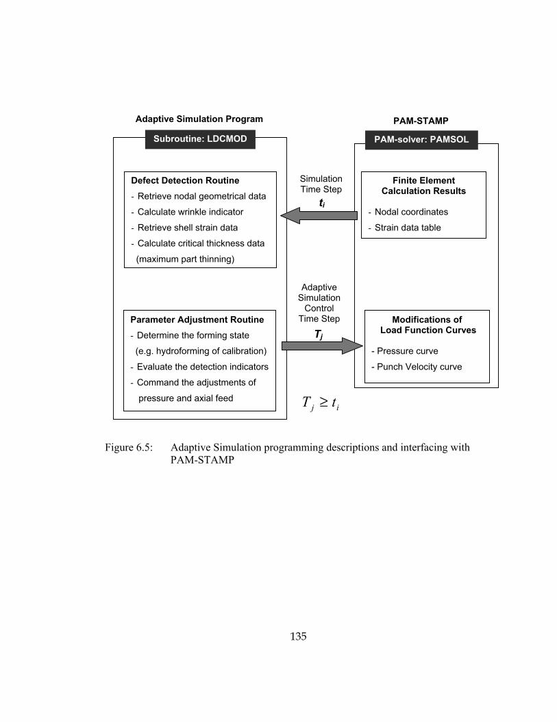
135
Figure 6.5: Adaptive Simulation programming descriptions and interfacing with PAM-STAMP
Defect Detection Routine - Retrieve nodal geometrical data
- Calculate wrinkle indicator
- Retrieve shell strain data
- Calculate critical thickness data
(maximum part thinning)
Parameter Adjustment Routine - Determine the forming state
(e.g. hydroforming of calibration)
- Evaluate the detection indicators
- Command the adjustments of
pressure and axial feed
Finite Element Calculation Results
- Nodal coordinates
- Strain data table
Modifications of Load Function Curves
- Pressure curve
- Punch Velocity curve
Subroutine: LDCMOD
ti
Tj
PAM-solver: PAMSOL
PAM-STAMP Adaptive Simulation Program
Simulation Time Step
Adaptive Simulation
Control Time Step
ij tT ≥

136
The two main AS modules were programmed on a special PAM-STAMP subroutine
�LDCMOD�. This subroutine allows access to virtually all the node and shell FE
calculations computed by PAMSOL at every simulation time step, e.g. displacement
field table and stress-strain table. LDCMOD also permits, at any simulation time step,
manipulations of all the function curves, e.g. pressure versus time curve, and tool
velocity versus time curves.
At the end of every simulation time step (ti), PAMSOL calls LDCMOD to execute all
the necessary tasks in the defect detection and parameter adjustment modules. The
defect detection module reads the nodal and shell geometrical and strain information of
the deforming part, and evaluates the defect indicator values. This task is usually carried
out at every simulation time step to monitor the part formability as best as possible. A
collection of the defect indicator values then can be used in the parameter adjustment
module. Depending on the part hydroformability, an adjustment of the parameters is
done at every simulation time step or every certain number of simulation time steps.
This duration is defined as control time step (Tj). If the part being worked on is very
susceptible to wrinkle or fracture, in other words, it has low hydroformability, Tj should
be as small as ti. However, if the part is wrinkle and thinning tolerant (high
hydroformability) Tj can be much longer than ti as to reduce the computation time and
avoid an overly controlled situation.

137
6.2.3 Adaptive Simulation with Dynamic Explicit Code
As already discussed in Chapter 3, erroneous inertial stresses may result from large
acceleration of nodes caused by imposed velocity boundary conditions. These velocity
curves (for axial feeding at the tube ends) are usually designed such that at the
beginning the velocity curve is gradually increased up to the desired level; this is done
to prevent the unrealistic inertial stresses. Therefore, it can be seen that, if designed
correctly; the punch velocity curve can result in minimum or no dynamic effect.
Adaptive simulation adjusts pressure curve and axial feed speed curves at every control
time step (Tj). Increments of pressure and axial feed speed are applied over the next
control time step duration. Depending on the parameter adjustment schemes (will be
discussed in detail later this chapter) used, the amount of these increments can be
positive or negative and constant or variable. Care must be taken when applying the
calculated process parameter increments over a control time step. For example, an
increasing increment of axial punch speed over a short control time step can results in
really high nodal accelerations, which leads to erroneous inertial stresses.
Abrupt changes of the axial punch velocity lead to near infinite acceleration. A gradual
change (i.e. both increasing and decreasing) over a time can avoid large accelerations
thus accurate simulation results can be obtained. Considerations must be taken for
changes of the pressure curve as well. Though, pressure boundary (or force) is more
forgiving than velocity boundary in terms of causing the dynamic effect. In the
following sections, the issue of applying calculated parameter changes over the control
time steps appropriately such that the dynamic effect can be avoided is of a significant
concern.
138
6.3 Part Defect Indicators
Wrinkling prediction in FEA is generally based on three main methods: 1) plastic
bifurcation theory, 2) energy method, and 3) geometry method. While the first two
methods predict of onset of wrinkles, the geometry method, which is mainly employed
in this work, aims at indicating the presence of wrinkles. Geometry method is also the
simplest and most applicable to THF among the others because: a) a small amount of
wrinkles in the THF part may be even helpful in preventing excessive thinning in the
bulging area and b) it is simpler mathematically than the other methods. Contrasting to
THF, in sheet metal forming, even small existing amount of wrinkle during the forming
process often has an adverse effect on the final part quality. Nevertheless, as mentioned
earlier in THF, alive wrinkles can be beneficial as long as they do not develop into dead
wrinkles on the final part. Therefore, wrinkle criteria for THF should be able to:
a. Indicate the existence of wrinkle
b. Quantify the severity of wrinkle
c. Distinguish wrinkles that are beneficial (good alive wrinkles) from the ones that
are not beneficial (bad alive wrinkles, which will turn into dead wrinkles)
6.3.1 Geometric Wrinkle Criteria
The tube mesh nodal coordinates can be used to calculate important geometric
properties (such as curvatures, arc lengths, surface areas, and volumes) that can indicate
wrinkling condition of the part. Moreover, these geometric properties may be used to
reflect progress of the forming i.e. whether the part is completely formed or not. The
following are the geometric wrinkle criteria developed to be used in the wrinkle
detection module. Hydroforming of a simple bulge was used throughout in the
development of these criteria.

139
6.3.1.1 First Derivative Wrinkle Criterion (Iwd)
The simplest geometric criterion, first derivative criterion calculates slopes of a tube
profile cut by a plane passing through the tube axis to determine hills and valleys in the
forming tube, see Figure 6.6. This method is only capable of detecting wrinkles in
axisymmetric parts, as its tube profile reflects the entire part geometry. However, this
method may be extended to consider gradients of deforming part surfaces in order to
detect wrinkles in non-axisymmetric parts.
Figure 6.6 shows how the calculated slope variations are interpreted to existence of
wrinkles. The slope calculation is applied on the tube profile enclosed by a control
window, see Figure 6.6. In this case study, the control window covers from the
symmetry line to the point where the die radius meets the straight portion of the guiding
zone. The slopes ( dZdY / ) are simply calculated from nodal coordinates. It can be seen
that the slope variations of the wrinkled part, Figure 6.6.c, change the sign from positive
to negative. Unlike the wrinkled part, the slope variations of the wrinkle-free part do not
change the sign between positive and negative, Figure 6.6.b. Therefore, the variations
of the calculated slopes can be used to indicate an existence of wrinkles in a forming
tubular part.
1
1
−
−
−−=
ii
ii
i
i
XXyY
dXdY , Where i = 1�n (n+1 = number of node number)
Iwd = 0 -> wrinkle free condition: when there is no change in sign of the slope
Iwd = 1 -> wrinkled condition: when there is a change in sign of the slope
This slope criterion though is very simple but it has some drawbacks. First, it only
works for simple bulge geometry. Second, this slope criterion will not distinguish part
wrinkles from part geometry with curvatures. Last, this criterion is not able to indicate
whether the wrinkles detected are alive wrinkles or dead wrinkles as defined in section
6.2.1.1.

140
dZdY
dZ
Y
Y
Z
Z
dY
Slopes along Z axis: (dY/dZ) 1-5 < 0 (dY/dZ) 5-6 = 0
Slopes along Z axis: (dY/dZ) 1-2 > 0 (dY/dZ) 2-5 < 0 (dY/dZ) 5-6 = 0
Tube
Symmetry Line
1 2 3
4 5 6
12
3 4
5 6 Tube
Symmetry Line
Center Line
Center Line
Figure 6.6: a) prescribed line on the bulge forming tube mesh, b) prescribed line seen on wrinkle-free part, c) prescribed line seen on wrinkled part
Y Symmetry
Line
Z T ube Axis
Tube Profile
a)
b)
c)
Cutting Y-Z plane

141
6.3.1.2 Length to Area Wrinkle Criterion ( Iwla )
This criterion was developed to distinguish between alive wrinkles and dead wrinkles.
Let us consider hydroforming of the same bulge used in the previous section, see Figure
6.6.a. In this criterion, both geometrical information of tube and die are used. Within a
control window, the cutting plane makes a tube profile with an arch length of (Lt) and a
die profile with an arch length of (Ld), see Figure 6.7.a. It is noted here that the control
window used in this criterion normally has to be large enough to cover the entire
forming area (i.e. expansion zone, excluding guiding zone). But due to symmetry of the
bulge, only a half control window is applied in this specific case.
The basic idea is based an observation that when a wrinkle-free bulge is hydroformed
completely against the die cavity surfaces the tube profile arch length will be the same
as that of the die profile, see Figure 6.7.b (i.e. for a wrinkle-free part at process end: Lt
= Ld). If the final part is formed badly with some dead wrinkles then the tube profile
arch length is now longer that of the die profile, see Figure 6.7.c, (i.e. for a dead-
wrinkled part at process end: Lt > Ld).
This idea may be extended further to distinguish part with good alive wrinkles from part
with bad alive wrinkles (i.e. bad alive wrinkles are those that can potentially turn into
dead wrinkles at the final part). At any instance during the forming, if the tube profile
arch length, Lt(ti), becomes greater than the die profile arch length, Ld, then bad alive
wrinkles are indicated (i.e. Lt(ti) > Ld, where ti is intermediate simulation time step).
The concept discussed above suggests some idea about how much the process can
tolerate having part wrinkles during the forming (i.e. alive wrinkles) which can be
removed at the process end. The main assumption here is that the tube profile always
lies on the cutting plane throughout the hydroforming. In other words, there should be
no in-plane shear in the part during the hydroforming. With this constraint, therefore,
this criterion is valid only for axisymmetric parts.

142
Figure 6.7: Length-to-area wrinkle criterion: a) definitions of tube (Lt) and die (Ld) profile arch lengths, b) good final part condition, and c) bad final part with dead wrinkles (all the figures are the tube and die profiles cut by the Y-Z plane, refer to Figure 6.6.a)
Centerline
Symmetry Line
Control Window
Tube Die
Expansion zoneGuiding zone
Guiding zone
Ld
Lt
Lt = Ld
Symmetry Line
TubeDie
Centerline
Control Window
Lt > Ld
Symmetry Line
Tube Die
Centerline
Control Window
a) During forming ( ti )
b) Final forming ( tfinal ) Good part (no wrinkle)

143
In AS, it is also necessary that severity of part wrinkles be quantified. Basic knowledge
of geometry can be used to quantify the severity of part wrinkles. If one considers all
arbitrary 2D shapes that share a common straight portion and all have the same enclosed
area, as shown in Figure 6.8.a, an arch of a perfect circle must have the shortest length
compared to all the other shapes. Under the same geometrical constraints, it is also true
that a non-convex shape will have a longer arch length than that of any convex shapes.
By the same analogy, see Figure 6.8.b, considering the area on the cutting plane
bounded by the tube centerline, the tube profile and the control window, among all
possible shapes of the hydroformed bulge with the same bounded tube interior area the
following are true:
a. Wrinkled bulge has a longer tube profile length than that of a wrinkle free bulge
b. More severe wrinkled part (with larger wrinkle amplitudes) has a longer tube profile
length than that of a mildly wrinkled bulge (with smaller wrinkle amplitudes)
Formulation of the length-to-area wrinkle indicator (see the parameters in Figure 6.8.b)
Let Ld: be an arch length of the enclosed die profile
Lt (ti): be an arch length of the enclosed forming tube profile and at any time ti
Ad: be the enclosed area of the cutting plane bounded by the die profile, tube center line, and control window
At (ti): be the enclosed area of the cutting plane bounded by the tube profile, tube centerline, and control window at time ti
ti: be simulation time step where i = 0�n, n be the final time step
Then, the bounded arch length of the forming tube profile and the bounded tube interior area at any time step ti can be normalized as the following:
)()()(
)(0
0
tLtLdtLttLt
tL ii −
−= : Normalized tube profile length
)()()(
)(0
0
tAtAdtAttAt
tA ii −
−= : Normalized tube interior area

144
Figure 6.8: a) shortest arch length illustration and b) parameters used in length-to-area wrinkle criterion
Common straight portion
Arch length of perfect circle = L1
Arch length of wrinkled circle = L2
(Equal enclosed area)
L2 > L1
Control Window
Ld
Lt ( ti )
Control Window
Symmetry Line
Symmetry Line
Centerline
Centerline
Die
Ad
At ( ti )
Tube
a)
b)
(Non-convex) (Convex)
145
The normalized tube interior area ( A ) can be used to indicate whether the part is
completely formed or not:
• A = 0: The part is at the process beginning (no deformation).
• 0 < A < 1: The part is not completely formed.
• A = 1: The part is completely and successfully formed.
The normalized tube profile length ( L ) can be used to indicate the severity of wrinkles:
• L = 0: The part is at the process beginning (no deformation).
• 0 < L < 1: The part is not completely formed.
• L = 1: The part may only be completely and successfully formed if A =
1.
• L > 1: The final part may have dead wrinkles.
To assist the understanding of this length-to-area wrinkle criterion, the simple bulge
hydroforming used in Chapter 5, Figure 5.5, was used again as an example. Three
different loading paths were applied to form the bulge: 1) Self-feeding LP, 2) optimal
LP (taken from Yang, 2002), and 3) bad LP with excessive axial feed, see Figure 6.9.
The self-feeding LP was applied here to form a wrinkle-free part to be used as a
reference part. However, as discussed before, self-feeding part would result in a
wrinkle-free part with excessive thinning. The optimal LP would form the final part
without any wrinkles and acceptable thinning. The bad LP would result in a final part
with dead wrinkles. From the simulation results, the normalized tube profile lengths
( L ) of the parts were plotted against their corresponding normalized tube interior areas
( A ), Figure 6.10.
From Figure 6.10, all the normalized length-to-area curves start from the same point
L = 0 with A = 0; however, the shape of the curves depends on the state of wrinkle
happening in the part during the forming process.

146
0
0.010.02
0.03
0.04
0.050.06
0.07
0 2 4 6 8 10 12 14 16 18 20
Axial feed (mm)
Pres
sure
(GPa
)
SF LP Optimized LP Bad LP
Figure 6.9: Different loading paths used to hydroform the simple bulge
0
0.2
0.4
0.6
0.8
1
1.2
1.4
1.6
0 0.2 0.4 0.6 0.8 1
Norm cutting plane area [A]
Norm
par
t arc
h le
ngth
[L]
Opt LP
SF LP
Bad LP
Figure 6.10: Normalized length versus normalized area curves of the parts formed with three different LP�s
Control window
Control window
Process start: Opt LP
Process end: Opt LP

147
The curve of the SF part represents a wrinkle-free state of the part throughout the
forming process (i.e. any normalized length-to-area curves laid above this curve of the
SF part would indicate existence of alive or dead wrinkles). It gradually increases from
the starting point to the process end at L = 1 with A = 1, which indicates a successful
forming. The curve of the optimal part ends at L = 1 with A = 1, which also indicates a
successful forming, see Figure 6.10. During the forming of the optimal part, the curve is
well above the SF part curve. This suggests that during the hydroforming process of the
optimal part there are some wrinkles (alive wrinkles) that are straightened out at the
process end. It should be noticed that toward the process end the curve goes L > 1,
which indicates the risk of having dead wrinkles in the final part. However, in this case,
the calibration pressure is large enough to suppress those wrinkles and bring the curve
down to L = 1. Unlike, the optimal part, the part formed with the bad LP (with
excessive axial feed) yields the curve that never comes down to the end point of L = 1
with A = 1. This indicates that the part is formed unsuccessfully with some dead
wrinkles. It can be seen that the part starts to have dead wrinkles ( L > 1) at the middle
of the process ( A = 0.4). The wrinkles are too severe such that the calibration pressure
cannot suppress those wrinkles by the process end.
Unfortunately, the length-to-area wrinkle criterion discussed above is good only for
hydroforming of axisymmetric bulges. When dealing with non-axisymmetric parts, the
length-to-area wrinkle criterion does not work any longer for the following reasons: a)
geometrical information from just a single cutting plane is simply inadequate for non-
axisymmetric parts and b) existence of in-plane shear stress state.
However, the length-to-area wrinkle criterion can still be useful if applied to many
different locations of the part, see. Especially, it should be applied on the hard-to-form
area such as corners and complex geometry. Based on this wrinkle criterion, a better
geometrical wrinkle criterion is developed in the next section.

148
6.3.1.3 Surface Area to Volume Criterion ( Iwsv )
The length-to-area wrinkle indicator can be considered as a local parameter because it
only utilizes 2D geometric information of the part. For this reason, the length-to-area
criterion works well for axisymmetric parts. To apply the length-to-area wrinkle
criterion on a non-axisymmetric part, a number of tube and die profiles are needed to
monitor the wrinkle state of the part. A more global wrinkle criterion, surface area-to-
volume wrinkle criterion, using 3D geometric information of the part is developed in
this section. This geometric criterion considers the evolution of the forming part surface
area and volume enclosed by a control box, Figure 6.11.
Based on the geometry concept developed for the length-to-area criterion that a
wrinkled part has a longer profile length than that of a wrinkle-free part at the same
section area (i.e. tube interior area):
• It is true that a wrinkled part has a larger surface area, St, than that of a wrinkle-
free part at the same part volume, Vt.
• It is also true that at a given of part volume, Vt, the surface area, St, is larger for
the part with more severe wrinkles than that of part with mild wrinkled.
• Moreover, at the process end, a wrinkled part will have surface area, St(tfinal),
larger than the die cavity surface area, Sd, (i.e. when St(tfinal) > Sd, the final part
has some dead wrinkles). On the other hand, if the part is successfully formed,
the part surface area will be equal to the die cavity surface area (i.e. St(tfinal) =
Sd).
The main assumptions underlying the statements above are a) the tube surface is a
monotonously increasing function of the fluid volume St=St(Vt) and b) the volume is a
monotonously increasing function of the maximum bulge height Vt=Vt (Hp). These two
assumptions can be considered correct only if St and Vt are calculated in a fixed control
box, centered on the bulge area, as in Figure 6.11. In fact, for many THF parts (as for T-
shapes and Y-shapes) the total value of Vt, if calculated including the guiding zones,
can even decrease as the bulge height grows.
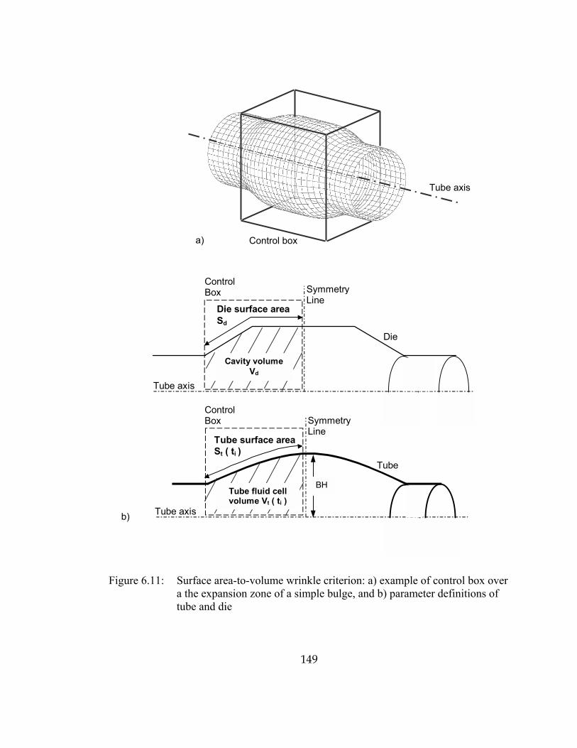
149
Control Box
Die surface areaSd
Tube surface area St ( ti )
Control Box
Symmetry Line
Symmetry Line
Tube axis
Tube axis
Die
Cavity volume Vd
Tube fluid cell volume Vt ( ti )
Tube
BH
Figure 6.11: Surface area-to-volume wrinkle criterion: a) example of control box over a the expansion zone of a simple bulge, and b) parameter definitions of tube and die
Tube axis
Control box a)
b)
150
The evolution of part surface area, St, as the part volume, Vt, increases is not known a
priori. In order to use it for indication of existence of wrinkles, it is necessary to track and
compare its evolution with a known wrinkle-free state deformation history. Similar to the
length-to-area wrinkle criterion, an ideal simulation with the self-feeding condition is run
to obtain an evolution of a wrinkle-free state deformation history (i.e. part surface area
and part volume).
Formulation of the surface area-to-volume wrinkle indicator (refer to Figure 6.11)
Let Sd be the bounded die cavity surface area
St(ti) be the bounded tubular part surface area at any time ti
Vd be the bounded die cavity volume
Vt(ti) be the bounded tubular part volume at time ti
ti be simulation time step where i = 0�n, n be the final time step
Then, the tubular part surface area and volume at any time step ti can be normalized as:
)()()(
)(0
0
tStSdtSttSt
tS ii −
−= : Normalized part surface area
)()()(
)(0
0
tVtVdtVttVt
tV ii −
−= : Normalized part volume
Let ))(( itVS be a normalized part surface area in a function of a normalized part
volume at time ti, from a normal hydroforming simulation.
))(( jsf tVS be a normalized part surface area in a function of a normalized part
volume at time tj, from a self-feeding simulation.
Finally the surface area-to-volume wrinkle indictor svIw is defined as:
)()()( VSVSVIw sfsv −=

151
The surface area-to-volume wrinkle indicator )(VIwsv is basically the difference of
normalized surface area of a forming part being considered )(VS to that of self-feeding
simulation )(VS sf calculated at the same normalized part volume V . From the
formulation of the wrinkle indicator above the following are the cases that can happen in
any hydroforming operation:
At the process end ( finali tt = )
a. 1)( =finaltV : The part is completely formed without any wrinkle.
b. 1)(0 << finaltV : The part is not formed successfully
During the process ( finali ttt <<0 )
a. 0)( =VIwsv : The forming part does not have any wrinkles. The part surface area of
the forming part is equal to that of the self-feeding part.
b. 0)( >VIwsv : The forming part has some wrinkles. The part surface area of the
forming part is larger than that of the self-feeding part. As discussed earlier, if during
the forming process, 1)( ≥VS (normalized surface area of the forming part becomes
one or more than one) then the final part will likely to have some dead wrinkle.
When applying this concept (i.e. dead wrinkle concept) to the svIw indicator, the
following can be written:
i. )(1)(0 VSVIw sfsv −<< : The part has some alive wrinkles
ii. )(1)( VSVIw sfsv −≥ : The part will likely to have dead wrinkles
The surface area-to-volume wrinkle indicator svIw was applied to the same simple bulge
considered in the preceding section. Also, the same three LP�s were used to simulate
hydroforming of the part, see Figure 6.9. Bounded part surface areas and volumes of the
three parts were recorded, normalized, and plotted in Figure 6.12.

152
V =0.6
Self-feeding LP
Optimal LP
0
0.2
0.4
0.6
0.8
1
1.2
1.4
1.6
0 0.2 0.4 0.6 0.8 1
Norm part volume [V]
Norm
sur
face
are
a [S
]
Opt LP
SF LP
Bad LP
Bad LP (excessive axial feed)
Figure 6.12: Plots of normalized surface area versus normalized volume of part simulated with a) pure expansion with free tube ends (i.e. SF LP), b) Optimal LP, and c) bad LP; and snap shots of all the simulated parts at the same normalized part volume (V=0.6)
0
0.2
0.4
0.6
0.8
1
0 0.2 0.4 0.6 0.8 1
Norm part volume [V]
Surf-
to-V
ol w
rinkl
e in
dica
tor [
Iwsv
]
Bad LP
Opt LP
Dead wrinkle limit[ 1-Ssf(V) ]
0
0.02
0.04
0.06
0.08
0.1
0 0.2 0.4 0.6 0.8 1
Norm part volume [V]
Surf-
to-V
ol w
rinkl
e in
dica
tor [
Iwsv
]
Opt LP
Wrinkle control
limit
Figure 6.13: a ) plot of area-to-volume wrinkle indicator ( svIw ) of the part formed with the optimal LP and bad LP, see Figure 6.9, and b) a triangular trajectory (so called �wrinkle control limit�) approximating the Opt svIw curve
a) b)

153
It can be seen from Figure 6.12 that both SF LP and OPT LP formed the bulge
successfully as their surface-to-volume curves ended where both normalized surface area
and volume becomes one ( 1=S and 1=V ). Generally speaking, due to more axial feed
applied, the OPT part obviously has less maximum thinning than that of the SF part (i.e.
2% to 14%).
From the snap shots of the parts at 6.0=V , the OPT intermediate part has some wrinkles
as compared to the SF intermediate part. The wrinkles in the OPT part are straightened
out at the process end. The )(VS curves of the OPT and SF parts exhibit the same trends
as found in the length-to-area criterion, compare Figure 6.12 to Figure 6.10. Due to the
excessively large axial feed, the bad LP unsuccessfully formed the bulge. This is evident
from its )(VS curve, Figure 6.12. The curve ends at 6.0=V , which suggests that the
final part is not completely formed against the die surface. Also the )(VS curve shoots
pass the 1)( =VS borderline, which indicates that the part will most likely to have dead
wrinkles, see snap shot of the final part at Figure 6.12.
The surface area-to-volume wrinkle indicators )()()( VSVSVIw sfsv −= , of the parts
formed with Opt LP and Bad LP are plotted in Figure 6.13.a. From the concept that any
forming part will likely to develop dead wrinkles if its )(VS curve exceeds the 1)( =VS
borderline, on the plot of svIw , the dead wrinkle limit line is simply calculated by
)(1 VS sf− . The svIw plot of the bad LP clearly exceeds the dead wrinkle limit line. This
svIw plot is useful in adaptive simulation because it can be used to:
1. indicate wrinkle severity: the larger svIw is the more severe the wrinkle is,
2. indicate how far away the part from developing dead wrinkles: distance from the dead wrinkle limit line, )(1 VS sf− ,
3. indicate whether the part is completely formed or not: the part is completely formed when 0.1=V .

154
In the adaptive simulation, the process parameter adjustment algorithm requires a
trajectory of part quality desired such that the process parameters are adjusted to achieve
that part quality throughout the process. Figure 6.13.b shows the svIw curve from the
OPT LP. It can be seen that the curve resembles a triangle. Therefore, a triangle wrinkle
control trajectory will be used in the process parameter adjustment algorithm. This will
be discusses in detail later.
6.3.1.4 Considerations to the Geometric Wrinkle Indicators
The area-to-volume criterion is considered to be a more global wrinkle criterion than the
first derivative and length-to-volume criteria. This is because the area-to-volume criterion
can indicate existence of part wrinkles but cannot pinpoint locations of the wrinkles, or
sometime it can fail to catch small part wrinkles. In most cases where the parts are simple
this area-to-volume criterion is informative enough for process parameter adjustment in
AS. However, when working with rather complex parts, some local geometric
information of the part is needed. The area-to-volume wrinkle indicator is normally
applied with some wrinkle tolerance. It is entirely possible that a small dead wrinkle may
be forming in the part and the apparent area-to-volume wrinkle indicator is still below the
tolerable value. In this case, the length-to-area wrinkle indicator can be used (i.e. placing
the cutting plane across the section that is wrinkle prone) to obtain local geometry
information thus enhancing the ability to monitor the wrinkle state of the part. Therefore,
it can be seen that both length-to-area and surface-to-volume criteria can be used together
to better monitor wrinkles in hydroforming of parts.
Calculation accuracy of the FE geometrical information used in area-to-volume criterion
can be influenced by certain numerical parameters. For this reason, the simulation should
be carried out with numerical parameters similar (or equal) to those used in the SF
simulation. The most important precautions to be taken are listed as follows:
♦ The initial mesh and the mesh adaptivity factors should be equal, since the mesh size
affects the calculation of St and Vt.

155
♦ Since the THF simulation is usually carried out with explicit codes, the range of
axial feed rates used should be similar to that used in the SF simulation.
6.3.2 Fracture Criteria
Maximum Thinning Criterion ( Ifth )
The main methods of localized necking prediction in sheet metal forming are FLDs,
FLSDs, and ductile fracture criteria. Due to the fact that prediction of localized necking
in THF is not yet well established, maximum thinning criterion, which is commonly used
in the industry, is currently applied in the adaptive simulation. For example, critical
thinning of 15%, 25%, and 30% are typically the fracture criteria for aluminum alloys,
low carbon steels, and stainless steels, respectively. Therefore, the current fracture
criterion is defined as:
thinningcriticalmaterialthinningimumpartIf th __
_max_=
According to the fracture defined above, the closer thIf is to 1 the likelihood that the part
will fracture is greater. According to the proposed adaptive simulation strategy, an
indicator that quantifies forming window of the part in terms of �fracture� failure needs
to be devised. Besides the currently used thinning criterion, any of the prediction methods
mentioned above can be applied in the adaptive simulation as well if necessary in the
future. Particularly, ductile fracture criteria such as Oyane�s criterion can easily replace
the thinning criterion. The difference between the calculated damage value to the critical
damage value can be used as a fracture indicator.
6.4 Process Parameter Adjustment Algorithms
This section mainly focuses on how the adaptive simulation program adjusts the pressure
curve and axial feed curve (or axial feed velocity curve) using the wrinkle and fracture
indicators developed in the previous section. The example application of the simple

156
bulging continues here from the last section. A few important process parameter
adjustment schemes are discussed. The details of each process adjustment schemes are
given in the Appendix E to keep the chapter concise.
The adaptive simulation program adjusts the pressure and axial feed curves at every
control time steps (Tj) based on the part formability (or part qualities) known at current
simulation time step (ti), see Figure 6.5. Figure 6.14 and Figure 6.15 show the part
qualities and the adjusted process parameters, respectively, from an adaptive simulation
run of the simple bulging. These curves will now be referred to repeatedly to explain how
process adjustments are carried out in the AS program.
The part qualities considered in the current program are part wrinkles, part thinning, and
part volume. Figure 6.14.a and Figure 6.14.b show the progress curves of the first two
part qualities (i.e. surface area-to-volume wrinkle indicator and maximum part thickness
strain) starting from the beginning to the end of the forming process. These curves are
plotted against the normalized part volume, as it is a convenient way to indicate progress
of the hydroforming process (V = 1 implies that the part is completely formed). However,
the pressure and axial feed (or axial feed velocity) curves must still be applied into FE
simulation in the time domain, see Figure 6.15. In this specific example of a simple
bulge, the part volume progresses through the simulation time as shown in Figure 6.14.c.
6.4.1 Calibration Stage
In order to properly adjust the process parameters in any THF processes, it is important to
first identify the two main forming stages: a) hydroforming and b) calibration. This can
be done by using the normalized part volume versus time curve, Figure 6.14.c, to
determine an appropriate time the start the calibration stage (i.e. stop the axial feeding
and rapidly increase the pressure to calibrate the part). Typically, the calibration stage
should begin when the part is almost fully formed against the die cavity surfaces. This is
to ensure that there is no large surface expansions of the part during the calibration,
which will result in excessive part thinning or fracture.

157
0.00
0.02
0.04
0.06
0.08
0.10
0.12
0.0 0.2 0.4 0.6 0.8 1.0Norm part volume [V]
Surf-
to-V
ol In
dica
tor [
Iw s
v] Upper wrinkle limitLower wrinkle limit
AS part wrinkle
0.00
0.10
0.20
0.30
0.0 0.2 0.4 0.6 0.8 1.0Norm part volume [V]
Max
imum
thic
knes
s st
rain
Fracture strain limit = 0.25
AS part thinning
SF part thinning
0.00.10.20.30.40.50.60.70.80.91.0
0 20 40 60 80 100 120
Time [FE time step x 100]
Nor
m p
art v
olum
e [V
]
CalibratingHydroforming
Figure 6.14: Part quality plots: a) surface area-to-volume wrinkle indicator versus normalized volume curves, b) fracture indicator versus normalized volume curves, and c) normalized volume versus simulation time step curve
a)
b)
c)

158
0.00
0.05
0.10
0.15
0 20 40 60 80 100 120
Time [FE time step x 100]
Pres
sure
[GPa
]
V = 0.9
Hydroforming Calibrating
0
2
4
6
8
0 20 40 60 80 100 120
Time [FE time step x 100]
Axia
l fee
d [m
m]
V = 0.9
Hydroforming Calibrating
0
1
2
3
4
5
0 20 40 60 80 100 120Time [FE time step x 100]
Axi
al fe
ed v
eloc
ity [m
m/m
s]
V = 0.9
Hydroforming Calibrating
Figure 6.15: Adjustments of process parameters: a) internal pressure, b) axial feed displacement, and c) axial feed punch velocity versus time (simulation time steps) curves
a)
b)
c)

159
In this example, the part volume of 90 % (i.e. normalized part volume V = 0.9) is chosen
to be the �calibration part volume cutoff�, see Figure 6.14.c. From Figure 6.15, it can be
seen that starting from the time when V = 0.9 the pressure is ramped up while the axial
feed is stopped (axial feed velocity is zero) until the process ends where the part is
completely formed, V = 1.
6.4.2 Hydroforming Stage
During the period where the part forms with 0 < V < 0.9, the process parameters should
be applied such that the tube material be fed in as much as possible to prevent fracture
without causing any part wrinkles. This has been the main concept in implementation of
this adaptive simulation approach, as discussed earlier. From the general flow chart of AS
procedure, Figure 6.2, one can see that the state of wrinkles demands changes of the
pressure and axial feed, while the state of part thinning only checks for fracture failure in
the part, but does not influence the process adjustment (i.e. the adaptive simulation is
aborted if the critical thinning is exceeded). Fortunately, applying �maximized� axial
feed following the concept, stated above, should also result in �minimized� part thinning.
Therefore, the part wrinkle is used as the main control state variable in this work.
Figure 6.14.a shows the winkle control trajectories (upper and lower limits) and an
example of a wrinkle state plot of the simple bulging. These wrinkle control trajectories
are derived from the optimum forming of the same part in Figure 6.13.b. The main goal
here is to develop process control strategies that would form the part with the wrinkle
state tracking closely along these wrinkle control limit trajectories. The physical meaning
of tracking this triangle wrinkle trajectory is to adjust both pressure and axial feed at the
control time step such that the part has some beneficial alive wrinkle during the forming
and has none at the end of the process. On the other hand, if the wrinkle trajectory is flat,
the tracking of this trajectory will result in a part that has no wrinkles at all time during
the forming, i.e. part formed by pure expansion or self-feeding part.

160
Of course, in practice these wrinkle control trajectories are not known a priory.
Experience gained from using this adaptive simulation on several different parts may be
useful to approximate proper trajectories for resembling part geometries. Nevertheless,
the shape of the trajectories should such that it allows some wrinkles (only alive wrinkles,
refer to Figure 6.13.a) during the forming process and allows no wrinkles at the process
end, e.g. the triangle shape. The amount of the alive winkles allowed depends on the part
formability. Some level of trial-and-error is, unfortunately, necessary here.
The current AS program has two main process adjustment strategies for the hydroforming
state: a) Wrinkle Control Strategy and b) Pure Shear Control Strategy. Figure 6.16 shows
the loading path predicted by AS with these two strategies for the simple bulging.
6.4.2.1 Wrinkle Control Strategy
The first process parameter adjustment scheme was first based only on the wrinkle
control strategy, where the pressure is increased while the axial feed is stopped when the
part wrinkle state exceeds the upper limit trajectory and the pressure is kept constant
while the axial feed is increased when the part wrinkle state goes below the lower limit
trajectory. This strategy results in the loading paths that are of a step-liked shape, see
Figure 6.16.
It was found that this strategy could not handle the tracking of part winkle state during
the first half of the process (0 < V < 0.5), where the trajectory demands the part to have
increasing (or more severe) amount of wrinkles. The part always fractured due to the
increased pressure during this period. This does not necessarily mean that the tracking of
wrinkle state in the first half of the process is impossible. A better and more sophisticated
control strategy is needed to achieve this task. As an alternative solution, the pure shear
control strategy, discussed next, was developed to handle the process adjustment during
the early forming stage, see Figure 6.16. The wrinkle control strategy was found to work
better in the later forming stage, especially (0.5 < V < 1), when the wrinkle limit
trajectory tapers down to zero, see Figure 6.14.a.

161
0.00
0.05
0.10
0.15
0 2 4 6 8Axial feed [mm]
Pres
sure
[GPa
]
Calibrating
Pure shear control
Wrinkle control(step-liked shape)
Hydroforming
Figure 6.16: Loading path predicted by AS showing different stages of simple bulge hydroforming process and control strategies (from Figure 6.15.a and b)
-0.3-0.2-0.1
00.10.20.30.40.5
0.0 0.2 0.4 0.6 0.8 1.0
Norm part volume [V]
Stre
ss [G
Pa]
Pure shear control
σ hoop
σ axial
ε normal = 0
Figure 6.17: Plot of hoop and axial stresses showing pure shear control strategy
Axial
Hoop σ Hoop
σ Axial

162
6.4.2.2 Pure Shear Control Strategy
It is well known, based on mechanics of sheet metal forming, that the pure shear state of
stress will deform the sheet metal without changing the sheet thickness. This strategy
attempts to regulate the pressure and axial feed such that the critical part area (i.e.
excessive-thinning-prone area), see Figure 6.17, deforms with an in-plane pure shear state
of stress at all time.
Theoretically, when applying this pure shear control strategy, the tubular part should
form with that critical part area having the same thickness throughout the forming
process. However, due to intrinsic sphere-liked shape of most THF parts while being
expanded, the tensile biaxial state of stress tends to eventually dominate the critical area
of the part. The pure shear state of stress will simply break down and be no longer
possible to enforce it later in the process, when the tube has become sphere-liked.
Therefore, this pure shear control strategy is only applied in the beginning of the process.
In this example, the pure shear control is active till the part wrinkle state exceeds the
upper wrinkle limit, after which the wrinkle control strategy becomes active instead; see
Figure 6.14.a and Figure 6.16. It should be pointed out, from Figure 6.14. a and b, that
during period where the part volume is 0 < V < 0.6, where the pure shear control is
active, the part maximum thinning is kept quite small. This is the direct result of the pure
shear control that tries to keep σ hoop = -σ axial, see Figure 6.17.
6.4.2.3 Modified Wrinkle Control Strategy
The wrinkle control strategy that gives a step-liked loading path, previously discussed,
actually does not track the wrinkle control trajectory so well, see Figure 6.14.a. The part
wrinkle state actually goes under the lower wrinkle limit trajectory (starting around V =
0.7) until almost at the end of the process. This is because of the use of constant pressure
while increasing axial scheme in and attempt to maximize the axial feed. This constant
pressure level induces increased tensile hoop stresses the instance when the part grows
larger in diameter that is caused by the pushing of the axial feed. This hidden

163
shortcoming of the step-liked process adjustment strategy actually thins out the part
unnecessarily.
The modified wrinkle control strategy, so called �increased-decreased pressure� process
adjustment strategy, is developed to better track the wrinkle control limit trajectories.
Figure 6.18 shows the part wrinkle state plot and the loading path of the same simple
bulging process predicted by the same pure shear control strategy and the modified
wrinkle control strategy. The comparison of maximum thinning curves of the parts,
Figure 6.19, clearly shows that the modified control strategy reduces the maximum
thinning consistently during 0.7 < V < 1.0. The only difference of the �increased-
decreased pressure� control strategy from the �step-liked� control strategy is that the
pressure is decreased while the axial feed is increased when the part wrinkle state goes
below the lower wrinkle limit trajectory (i.e. attempting to maximize the axial feed).
One may question the practicality of the rather zigzag loading path predicted. Figure
6.20 shows the smoothened loading path, which closely approximates the predicted one.
From FE simulation results, this smoothened loading path forms this simple bulge
successfully with the part maximum thinning of 8%.
So far, this newly developed adaptive simulation program has been applied successfully
with a very simple geometry such as a simple bulge. The applications of this program to
more complex parts have not yet been shown successful. The main problem lays on the
development of the process parameter adjustment strategies. It may be because of the fact
that the adaptive simulation only has the part quality information from the current and
part time steps to project the proper process parameters in the future. Unlike the adaptive
simulation approach, the optimization based simulation approach has access to entire
deformation history to use for generating the optimum process. Of course, the trade off is
the large computation time. Clearly, the adaptive simulation approach is still worth
further research, as it is an attractive approach for a rapid loading path determination.

164
0
0.02
0.04
0.06
0.08
0.1
0.12
0.0 0.2 0.4 0.6 0.8 1.0
Norm part volume [V]
Surf-
to-V
ol in
dica
tor [
Iw s
v] Upper wrinkle limit
Lower wrinkle limit
Better wrinkle control
(a)
0
0.01
0.02
0.03
0.04
0.05
0.06
0.07
0.08
0 2 4 6 8Axial feed (mm)
Pres
sure
(GPa
)
Wrinkle control(increased-decreased pressure)
(b)
Figure 6.18: Adaptive simulation results using modified wrinkle control strategy: a) plot of part wrinkle state, and b) predicted loading path for the simple bulge

165
0.00
0.02
0.04
0.06
0.08
0.10
0.12
0.14
0.16
0.0 0.2 0.4 0.6 0.8 1.0
Norm part volume [V]
Max
imum
thic
knes
s st
rain SF part thinning
A
B
Figure 6.19: Comparison of maximum thinning evolutions of parts from all the adaptive simulation cases including the initial SF simulation: A - wrinkle control strategy and B - modified wrinkle control strategy
0
0.01
0.02
0.03
0.04
0.05
0.06
0.07
0.08
0 2 4 6 8Axial feed (mm)
Pres
sure
(GPa
)
Figure 6.20: Smoothened loading path approximating the loading path predicted using the modified wrinkle control strategy for the simple bulging

168
CHAPTER 7.
CONCLUSIONS AND FUTURE WORK
7.1 Performance Comparison of Different Loading Path Determination Methods
So far in this research, three main different methods for loading path determination
were developed: a) Self-Feeding simulation (SF), b) Optimization-based simulation
(OPT), and Adaptive simulation (AS). These methods have different advantages and
disadvantages depending mainly on the complexity of part geometries and lead-time
dedicated for designing of loading paths. In this section, all of these methods were
benchmarked through applying them in determining loading paths for the same simple
bulging, discussed in the earlier chapters. The loading path determination of this simple
bulge using OPT and AS is already discussed in chapter 5 and 6, respectively. The
detailed SF simulation work on the simple bulge is omitted in this report due to its
simplicity. The SF method is explained in details with application examples of more
complex part geometries in Chapter 4.
Figure 7.1.a compares all the different LP�s determined by the methods. Figure 7.1.b
and Figure 7.1.c show the developments of part maximum thinning versus normalized
part volume, and the part thinning distributions, respectively. Then, Table 7.1 compares
the performance of these methods. The performance criteria are the computational time
spent in obtaining the final loading paths, the final part maximum thinning, and the total
axial feed amount (for one side). Simulation computational time varies from computer
to computer. Therefore, in this comparison, the number of simulation runs required in
each method is compared. For the specific HP workstation machine used in this work, it
took about 2 minutes for a single simulation run of this simple bulging.
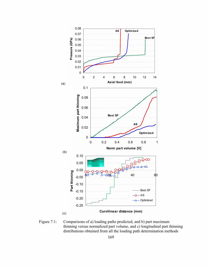
169
(a)
0
0.01
0.02
0.03
0.04
0.05
0.06
0.07
0.08
0 2 4 6 8 10 12 14Axial feed (mm)
Pres
sure
(GPa
)
AS Optimized
Best SF
(b)
0
0.02
0.04
0.06
0.08
0.1
0 0.2 0.4 0.6 0.8 1
Norm part volume [V]
Max
imum
par
t thi
nnin
g
AS
Optimized
Best SF
(c)
-0.25
-0.20
-0.15
-0.10
-0.05
0.00
0.05
0.10
0 20 40 60
Curvilinear distance (mm)
Part
thin
ning
Best SF
AS
Optimized
Figure 7.1: Comparisons of a) loading paths predicted, and b) part maximum thinning versus normalized part volume, and c) longitudinal part thinning distributions obtained from all the loading path determination methods

170
SF AS OPT (Gradient)
Total simulation runs 4 2 275 (Finite difference)
Part max. thin (%) 9.5 8.0 2.5
Total axial feed (mm) 12.30 7.30 8.80
Table 7.1: Comparisons of performance of all the loading path determination methods for simple bulge
0
0.01
0.02
0.03
0.04
0.05
0.06
0.07
0.08
0 2 4 6 8 10 12 14
Axial feed (mm)
Pres
sure
(GPa
)
SF#1SF#3
Best SFSF#2
Optimized
axial feed scaling : LP stretching
Figure 7.2: Searching of the simple bulge loading path using the SF method, compared with the optimized loading path from OPT method

171
AS required the smallest number of simulation runs among all the other methods. Only
2 simulation runs were needed to obtain a feasible loading path using AS, while the SF
method required 4 runs and the OPT method spent over 275 runs. However, the OPT
yielded the optimum loading path that minimized the part maximum thinning, while the
other two methods resulted in only feasible (i.e. not optimum) loading paths that
hydroformed successfully without any wrinkles or fracture.
All the loading paths predicted by the three methods show similarity in the typical shape
of proper THF loading paths � smaller pressure with large axial feed in the beginning
then high pressure with small axial feed towards the end of the process, see Figure
7.1.a. The AS loading path is most similar to the OPT loading path in both shape and
value. However, their part maximum thinning progress curves, Figure 7.1.b, are quite
different. The AS part has a much larger maximum thinning than that of the OPT part at
the end of the process (i.e. 8.0% compared to 2.5%). This shows that this THF part (i.e.
parts with large expansion in general) is very sensitive to the shape and value of loading
path. Nevertheless, it is encouraging that the AS method seemed to predict a feasible
loading path that is close to the optimum loading path. This implies that the AS method
can give a good initial loading path that may shorten lead-time in further numerical
optimization or physical process prototyping.
The maximum thinning of the AS part is just slightly smaller than that of the SF part
(i.e. 8.0% compared to 9.5%). The improvement in terms of maximum thinning from
the AS method may seem insignificant when compared to that of the SF part.
Interestingly, the SF part needs a much larger axial feed (40% more, 12.30 mm
compared to 7.30 mm) than that of the AS part. In other words, SF method predicts the
loading path with unnecessarily large axial feed. This large axial feed results in
excessive thickening of the part in the guiding zone area, see Figure 7.1.c, when
compared with the thinning distributions of the AS and OPT parts. This SF part can be
undesirable in cases where part weight is of a primary concern.

172
This problem of large axial feed in the SF part comes directly from the scaling-up
method of axial feed used in the current SF method - through the simulation sequence
of the SF method, while pressure curve is fixed, axial feed is continuously being scaled
up until part maximum thinning falls below the fracture level. This SF method basically
searches for the �best� loading path by stretching the first found loading path (i.e.
loading path obtained from pure expansion without any forced axial feed, refer to
Chapter 4) along the X-axis, see Figure 7.2. In the figure, it can be seen that the SF#2
loading path is the most similar to the optimized loading path. It may be speculated that
if the pressure level in the SF#2 loading path had been lowered the resultant part could
have been as of good thinning distribution as that of the OPT loading path. However,
since there is no mechanism to adjust the pressure level in the current SF method, this
method always tends to give unnecessary large axial feed. Unlike the SF methods, the
AS and OPT methods, both axial feed and pressure are free to be adjusted. This allows
more degree of freedom in the process parameter design thus parts can be hydroformed
to more strict part quality (i.e. small thickening in the guiding zone).
Table 7.2 lists the pros and cons of the common trail-and-error simulation method for
THF loading path determination. From the brief comparisons of all the loading path
determination methods and the earlier discussions in this report, the main advantages
and disadvantages of the three methods are summarized and compared in Table 7.3.
This summary is useful in selecting the proper method when designing process
parameters for any given parts.
Methods Advantages Disadvantages
Trial-and-error
simulation
(Traditional
Simulation)
• Requires no extra programs
• Near optimum loading path can be
found by a very experienced process
designer
• Very time consuming process
• Requires experienced users
• Sometimes, the process modification
can be non-systematic (no clear
directions)
Table 7.2: Advantages and disadvantages of the trial-and-error simulation method

173
Methods Advantages Disadvantages
SF (Self-Feeding
Simulation)
• Suitable for axisymmetric and non
axisymmetric parts with moderate
expansion
• Process modification is systematic
• Predicts a feasible loading path
• Takes only just a few simulation runs
(normally < 5)
• Requires little knowledge of the process
• Requires no extra programs
• Not suitable for very non
axisymmetric parts, e.g. Y-shape
• Pressure curve has to be estimated
• Does not allow adjustments of
pressure curve
• Tends to predict unnecessarily large
axial feed (i.e. excessive thickening)
• Simulation sequence requires human
involvement
OPT (Optimization-based
Simulation)
• Results in the optimum loading path
• Once running, no human involvement is
required
• Works for any given part geometries
• Very versatile for the fact that any
objective and constraint functions are
allowed in the optimization problem to
achieve different part quality
requirements
• Very large computational time is
required (normally >>100 runs)
• Computational time increases with
the number of design variables
• Non-converging problem can occur
when using a large number of design
variables
• Experience is required to formulate
the process optimization effectively
• Initially guessed loading path is
required and can affect the optimized
results
AS (Adaptive Simulation)
• Results in a feasible loading path
• The predicted loading path seems to be
close to the optimized one.
• Takes only two simulations (normally =
2 runs)
• No initially-guessed loading path is
required
• Allows some alive wrinkle during the
process as a way to accumulate material
for large expansion
• Currently, only works for simple part
geometries, e.g. a simple bulge
• Part wrinkle control trajectory has to
be designed a priory
• Process parameter adjustment
scheme is difficult to generate. An
universal scheme does not seem to
exist
Table 7.3: Comparison of advantages and disadvantages of all the loading path determination methods developed in this work

174
7.2 Selection of the Loading Path Determination methods
This section focuses on how to apply these methods of loading path determination in the
process planning of any given part geometries. First, existing THF part classifications
based on geometry are investigated with an objective to generate a new part
classification based on process parameters. This new part classification will enable
systematic selection of process parameter design methods.
7.2.1 THF Part Classifications Based on Geometry
From the literature review, most THF parts are typically classified according to their
function as an end product [Koc, 2001], [Klaas, 2000]. Based on a functional
classification, most automotive THF parts can be classified into three categories in
Table 7.4: a) piping, b) structural parts (chassis and body, steering and suspension,
safety), and c) engine and drive cases. However, this kind of classification based on part
functionality is not very useful in for process parameter designing phase.
A more relevant classification for process planning can be found in [Koc, 1998], where
parts are classified according to their fundamental geometrical features. The most
common THF part geometrical features are as follows:
• Protrusions (T-shape or Y-shape). A protrusion can be identified when the tube
asymmetrically expand in a side branch.
• Bulges. A bulge can be identified when the tube cross sectional perimeter rapidly
increases (with either a round, square or irregular shape) without any preferential
radial direction.
• Bends. In this work, the part spline shapes (1-D, 2-D, and 3-D) are also considered
as bend features.
Most small THF parts have one of these geometrical features that come in different
sizes and shapes, see Figure 7.3. For larger THF parts, see Figure 7.4, the parts are
usually consisted of these common geometrical features located along the part axis
spline.

175
Categories Materials Part Examples
Piping • Stainless Steel (AISI 304, AISI 309)
• Aluminum alloys
Exhaust pipes, engine tubes, catalytic converters, pressure tubes, tail pipes, connectors and manifolds
Chassis and body: front and rear engine cradles, ladder frames, hitch bars, side roof rails and roof bows, instrument panel beams, radiator frames, space-frame components, windshield headers, body side rails
steering and suspension: control arms, trailing links, steering columns
Structural parts
• Low to medium carbon steels (A 570 Gr. 36, A 738, etc.)
• Aluminum (AA 1050, AA 5015, etc.)
safety: roll-over bars, seat frames and shock absorber housings, bumper beams
Engine and drive cases
• Case hardening steel (SAEM 1015, SAE 1045, SAES 115)
Hollow camshafts, drive shafts and gear shafts
Table 7.4: Classification of automotive THF parts according to their functionality
Aluminum rear axle part, courtesy: BMW, 1997
(a) (b) (c)
Figure 7.3: Common THF part geometrical features: a) Y-shape protrusion, b) bulge, and c) bend

176
The following is an attempt in trying to connect this part classification to a kind of
process-based part classification, to eventually generate a systematic way of selecting
proper process design methods. In order to make connections between the part
geometrical features to process parameter design, an example is given here to clearly
show how part geometrical features can influence the working process window of any
THF parts.
If one considers a long THF structural part, e.g. Figure 7.4.b, one can think of the part
as an array of common THF geometrical features connected together along the part axis
spline. Figure 7.5 shows a schematic drawing of a long part (showing only one half of
the part symmetry line) consisting of many common THF geometrical features and a
typical plot of metal flow displacement in the axial direction (i.e. effective axial feed) in
each of the features. Considering the displacement of the tube material in the guiding
zone, material movement in axial direction will decease along the guiding length due to
the effect of friction and guiding geometry. This is also true for other portions along the
entire part as evident when this material movement in the axial direction becomes
almost zero in the part feature located at the most far removed location (i.e. center of the
part) from the tube ends where the axial feeding action takes place.
The above example clearly shows how individual geometrical part feature can influence
(limit or narrow) the part working process window. From Figure 7.5, it is entirely
possible that the T-shape, located closet to the part center, may or may not be
hydroformed successfully due to inadequate material to form the protrusion. Suddenly,
the design of process parameters for this part becomes challenging. In this case, the T-
shape part geometry may need to be redesigned to make the forming possible with the
effective axial feed available to it.

177
1D
2D
3D
(a) (b)
Figure 7.4: Complex THF parts with multiple geometrical features: a) exhaust manifolds with protrusions and bends (different spline configurations), and b) SPS engine cradle: long automotive structural part with bulges and bends:
Axial feed (material disp.) d0ax
Part symmetry line: Assumed no feed
Straight (guiding zone)
Straight Bend Simple Bulge T-shape
Material displacement
d0ax d1ax
d2a d3ax
d4ax
d1ax d2a d3ax d4ax
Figure 7.5: Typical trend curve of material displacement along axial direction of a simplified long structural part (showing only one half of the part) being hydroformed with axial feed = d0ax applied at the tube end at a given pressure curve
178
7.2.2 THF Part Classifications Based on Process Window
Generally speaking, part geometry and materials determine the proper choice of process
sequence which can be of any combinations of the following: a) crushing as a way to
accumulate material for later expansions, b) hydroforming, in which both pressure and
axial feed are applied simultaneously, c) calibrating, in which only pressure is applied,
and d) intermediate annealing (only used when a, b, and c, cannot form the part
successfully). More specifically, the choice of process sequence depends on the forming
process window of the given part (i.e. allowable amount of axial feed with respect to
pressure for a successful process). When limiting the analysis to only part geometry,
one can find three distinct process window scenarios: a) pressure-dominant process, b)
axial-feed-dominant process, and c) pressure-axial-feed-driven process. These process
categories will later assist in choosing proper methods for loading path determination.
• Pressure-dominant process: Parts that fall into this category normally have
geometrical features (such as sharp bends located near the tube ends) that really
limit effective axial feed into the center of the part or totally prevent possibility of
axial feeding. In this case, the process almost becomes like pure expansion without
any axial feed. In other words, there is no need to control the axial feed in this case.
o Suggested Process Design Methods: The Adaptive Simulation (AS) and Self
Feeding (SF) approaches are inappropriate since there is no need to find the
axial feed curve. Moreover, the pressure curve can just be applied linearly and
can be analytically calculated using the calibrating pressure formulas already
available. An optimization-based simulation approach (OPT) could be applied
but not for process design; instead it can be used to determine the best value of
the initial tube diameter or the correct choice for the shape of the extrusion (i.e.
optimum part/preform geometry design).
• Axial-feed-dominant process: Contrasting to parts in the above category, parts that
have a protrusion with a straight and short spline belong to this category. In this
case, axial feed is not only possible, but also required in order to obtain a significant
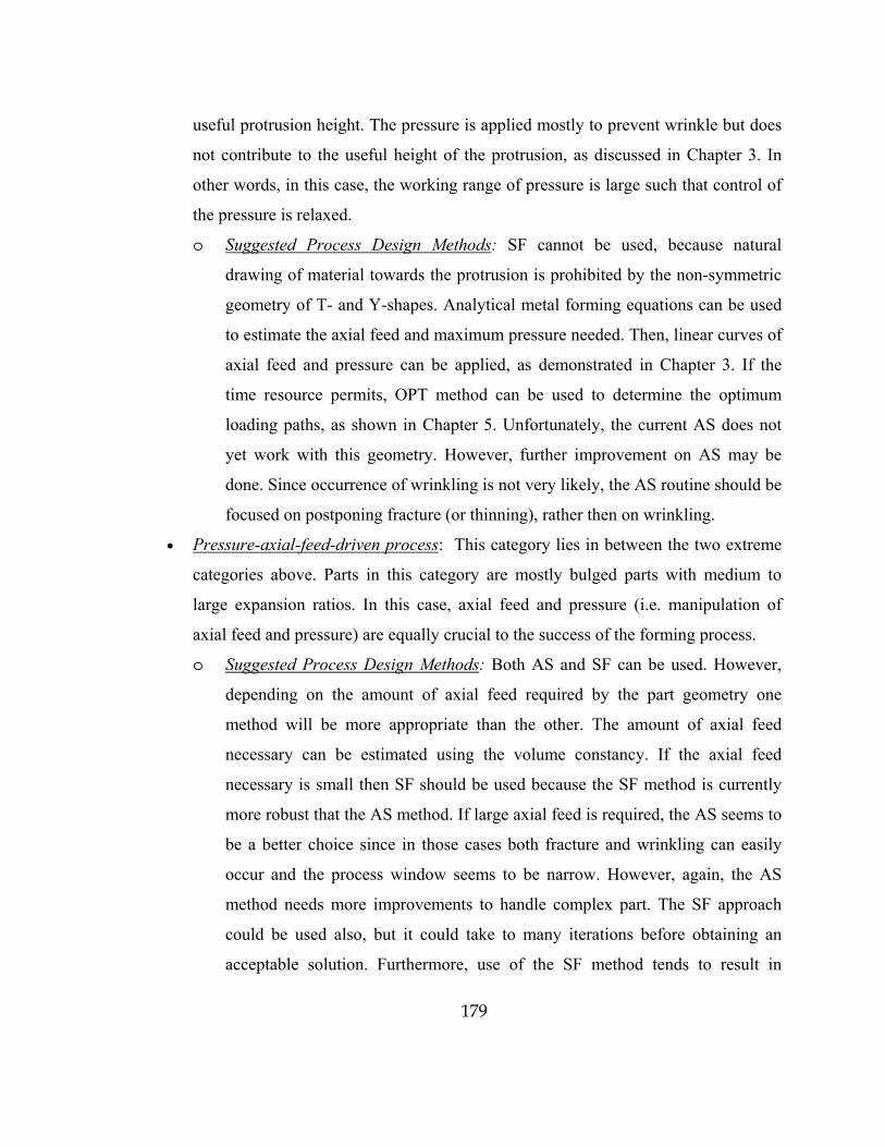
179
useful protrusion height. The pressure is applied mostly to prevent wrinkle but does
not contribute to the useful height of the protrusion, as discussed in Chapter 3. In
other words, in this case, the working range of pressure is large such that control of
the pressure is relaxed.
o Suggested Process Design Methods: SF cannot be used, because natural
drawing of material towards the protrusion is prohibited by the non-symmetric
geometry of T- and Y-shapes. Analytical metal forming equations can be used
to estimate the axial feed and maximum pressure needed. Then, linear curves of
axial feed and pressure can be applied, as demonstrated in Chapter 3. If the
time resource permits, OPT method can be used to determine the optimum
loading paths, as shown in Chapter 5. Unfortunately, the current AS does not
yet work with this geometry. However, further improvement on AS may be
done. Since occurrence of wrinkling is not very likely, the AS routine should be
focused on postponing fracture (or thinning), rather then on wrinkling.
• Pressure-axial-feed-driven process: This category lies in between the two extreme
categories above. Parts in this category are mostly bulged parts with medium to
large expansion ratios. In this case, axial feed and pressure (i.e. manipulation of
axial feed and pressure) are equally crucial to the success of the forming process.
o Suggested Process Design Methods: Both AS and SF can be used. However,
depending on the amount of axial feed required by the part geometry one
method will be more appropriate than the other. The amount of axial feed
necessary can be estimated using the volume constancy. If the axial feed
necessary is small then SF should be used because the SF method is currently
more robust that the AS method. If large axial feed is required, the AS seems to
be a better choice since in those cases both fracture and wrinkling can easily
occur and the process window seems to be narrow. However, again, the AS
method needs more improvements to handle complex part. The SF approach
could be used also, but it could take to many iterations before obtaining an
acceptable solution. Furthermore, use of the SF method tends to result in

180
unnecessarily large axial feed, previously discussed. The question of the exact
amount of axial feed to be considered small or large is still difficult to answer.
Experience, unfortunately, plays an important role here.
Based on the discussions above, a flow chart is given; see Figure 7.6, to systematize the
procedure of how to select proper FE methods to determine loading paths for THF
parts.
7.3 Conclusions
This research work was intended to develop methodologies for design of part
geometries and process parameters in tube hydroforming processes. The specific goals
of this study were to develop a) part design guidelines for THF processes that facilitate
engineers to bring conceptual THF part designs to production more efficiently and b)
methodologies for design and optimize loading paths in THF using process FE
simulation.
It was realized during this study that THF part geometries could vary so much from
very simple to very complex. Thus, generating new THF part design guidelines (besides
the guidelines already available in literature) seemed to be a very backbreaking task and
may not be as useful. It was then realized that part geometry and process parameters
were very much interrelated (i.e. design for manufacturing). Thus, the main goal was to
focus only on developing systematic and time-efficient FE approaches to determine
proper process parameters (i.e. loading paths). This could be used to evaluate THF part
design for manufacturability, thus, in turn, fulfilling the part design guideline objective
as well.
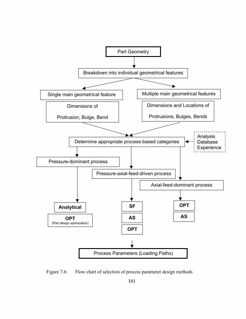
181
Figure 7.6: Flow chart of selection of process parameter design methods
Part Geometry
Breakdown into individual geometrical features
Single main geometrical feature Multiple main geometrical features
Dimensions of
Protrusion, Bulge, Bend
Dimensions and Locations of
Protrusions, Bulges, Bends
Determine appropriate process-based categories
Pressure-dominant process
Pressure-axial-feed-driven process
Analysis Database Experience
Process Parameters (Loading Paths)
Axial-feed-dominant process
SF
OPT (Part design optimization)
AS
Analytical
OPT
AS
OPT

182
Through extensive applications of process FE simulation and some experimental work
necessary, several design guidelines and advanced FE approaches for THF process
designs have been developed. In this work, the main process FE simulation package
used was PAM-STAMP. Simple bulge part geometry was used throughout this work in
developing all the guidelines and methodologies. Also, many real THF parts (e.g. T-
shape, Y-shape, Cross member, and sizable structural parts) taken from the automotive
industry were used in the study. The accomplishments in this study are summarized
below:
• Hydroforming of a Y-shape and a T-shape were analyzed numerically and
experimentally. In this study, both effect of part geometry (spline length effect) and
process parameters (effects of pressure, axial feed, and counter punch force) on
hydroformability were investigated and quantified. These findings enabled thorough
understanding of mechanics of THF process and interactions of part geometry and
process, which was crucial in developing FE methodologies in the design of process
parameters.
• Self-feeding simulation approach (SF) was developed. It was applied successfully to
determine proper loading paths (pressure and axial feed) for many automotive THF
part geometries. This approach was proven to be quick, systematic and simple
enough for inexperienced users but still robust enough to yield good loading paths.
• Optimization-based simulation approach (OPT) was developed. A general
optimization code, PAM-OPT, was applied to optimize loading paths (pressure,
axial feed, and counter punch force) for several THF part geometries. The main
contributions here are procedures to setup and formulate a normal THF process
simulation into an optimization-based simulation run to optimize the process
loading paths. Many sets of mathematical formulas for objective and constraint
functions were created to best express several different part qualities to be
optimized. This OPT approach seemed to be the most powerful tool (but certainly

183
not the most time-efficient) in determination of THF process parameters, simply
because it is very versatile in that it takes most mathematical expressions into the
formulations. However, this approach required a very experienced user in both
optimization and THF processes. Moreover, a very large computational time is
inevitable.
• Adaptive simulation approach (AS) for rapid THF loading path determination was
developed. An AS program (in FORTRAN) was coded and integrated into the
internal solver of PAM-STAMP. A couple of geometrical wrinkle indicators and
process parameter adjustment schemes were created and implemented as the main
working components in the AS program. The program was, so far, only applied
successfully on the simple bulging process. The current AS program is not
sophisticated and robust enough to handle more complex part geometries. The main
problem is to come up with a proper scheme of process parameter adjustment for
those parts. This approach clearly requires further research. Nevertheless, this study
provided a general framework of adaptive simulation method, which may be
adopted for process parameter design of other metal forming operations such as
sheet metal forming.
• All these advanced FE methods developed in this study for loading pat
determination certainly have shortcomings as they always come with benefits. Pros
and cons of all the methods were compared quantitatively and qualitatively in terms
of lead-time, final part quality obtained, and practicality. Some practical guidelines
were also given in selecting proper methods for determination of loading paths for
most typical THF parts.

184
7.4 Future Work
Though these advanced FE methods developed in this study have disadvantages, there
are many tasks that can be implemented to improve the methods. Among these tasks,
the most important ones are as follows:
• Develop combined applications of OPT and SF: a) using SF results as the initial
guess, b) using SF results to reduce the number of design variables of the loading
path. All of these is to mainly cut down the large computational time in the normal
OPT approach.
• Develop combined applications of OPT and AS: Integrating some simple
optimization schemes into each control time step of the AS program. This is to
make the process parameter adjustment scheme more robust. However, more
simulation runs may result.
• Apply the AS program to more THF part geometries as continuously improve the
process parameter adjustment schemes.
• Collect the loading paths and experience gain from usages of these FE methods and
store them in THF-PAL* database for future use. (* THF-PAL: a THF database for
part and process design, on-going effort in the ERC-THF consortium)

185
LIST OF REFERENCES [Aita, S., 1992] S. Aita, �Industrial sheet metal forming simulations issues in
code development, material modeling, validation and design methods, COMPLAS III�, Conference, Barcelona (Spain), April 1992.
[Allen et al.; 1999] T. Allen; L.Yu; �Low Cost Experimental Methods Applied to Aerospace Related Design�, Proceedings of the 3rd World Congress of Structural and Multidisciplinary Optimization, Niagara Falls/Amherst, New York, May 17-21, 1999
[Asnafi, 1999] N. Asnafi, �Analytical Modeling of Tube Hydroforming�, Thin-walled Structures 34 (1999), pp. 295-330
[Asnafi, 2000] N. Asnafi, and A. Skogsgardh, �Theoretical and Experimental Analysis of Stroke-controlled Tube Hydroforming�, Materials Science and Engineering, A279, 2000, pp. 95-110
[Aue-U-Lan; 1999] Aue-U-Lan, Y.,Koc, K., and, Altan, T., �Prediction of Tubular Material Properties for Aluminum Alloy 6260 � T4�, ERC/NSM report, THF/ERC/NSM-99-R-09, June 1999
[Brewster, 1996] K. Brewster, K. Sutter, M. Ahmetoglu and T. Altan, �Hydroforming Tube�, The Tube & Pipe Quarterly, vol. 7, no. 4, pp. 34-40, July/August, 1996.
[Cao, 1994] J. Cao and M. C. Boyce, �Design and Control of Forming Parameters using Finite Element Analysis�, Computational Material Modeling, ASME 1994, AD-Vol. 42/PVP-Vol. 294, pp. 265-285

186
[Chung, 1997] J.S. Chung and S.M. Hwang, �Application of a Genetic Algorithm to the Optimal Design of the Die Shape in Extrusion�, J. Mater. Proc. Technol. 72, 1997, pp. 69-77
[Deb; 1998] F. Deb, �Optimization for Engineering Design Algorithms and Examples�, Prentive-Hall of India, 1998
[Dohmann, 1991] F. Dohmann and A. Böhm, �The Significance of Process Simulation In Liquid Bulge Forming� (in German), Bänder Bleche Rohre, vol. 1, 1991, pp.26-34.
[Dohmann, 1996] F. Dohmann and Ch. Hartl, �Hydroforming � a Method to Manufacture Light-weight Parts�, J. Mater. Proc. Technol. 60, 1996, pp.669-676
[Doege, 2000] E. Doege, R. Kosters, C. Ropers and M.I. Rotareseu, �Computation of Hydroforming Process Parameters by Mean of Fuzzy Logic Control in FEM Simulation�, 2nd CIRP International Seminar on Intelligence Computation in Manufacturing Engineering, June 21-23, 2000, Capri, Italy
[Donald, 2001] B.J.M Donald, �Three Dimensional Finite Element Simulation of Asymmetric Bulge Forming�, Simulation of Materials Processing: Theory, Methods and Applications (2001), pp.903-908
[ESI Software, 2001] ESI Software, �PAM-OPT Solver2001 Manual�, 2001
[Feng, 2000] J.P. Feng, and Z.J. Luo, �A Method for the Optimal Control of Forging Process Variables using the Finite Element Method and Control Theory�, J. Mater. Proc. Technol. 108, 2000, pp.79-84

187
[Fourment, 2001] L. Fourment, D. Vieilledent, S.H. Chung, J.L. Chenot and P.J. Spence, �Direct Differentiation and Adjoint State Methods for Shape Optimization of Non-steady Forming Process�, Simulation of Materials Processing: Theory, Methods and Applications, 2001, pp. 133-138
[Filice, 2001] L. Filice, L. Fratini and F. Micari, �A Simple Experiment to Characterize Material Formability in Tube Hydroforming�, Annals of the CIRP Vol. 50, 2001, pp. 181-184
[Gelin, 2002] J. C. Gelin, and C. Labergere, �Numerical Control Strategies for THF Hydroforming of Thin Walled Metallic Tubes�, Proceedings from NUMISHEET 2002, October 21-25, 2002, Korea, pp. 499-504
[Ghouati, 2000] O. Ghouati, H. Lenoir, and J. C. Gelin, �Optimal Design of Forming Process Using the Finite Element Methods�, Advanced Engineering Materials 2000, No. 7, pp. 438-442
[Gomes et al., 2001] C.J. Gomes, B. Norman, O. Onipede, J. Rajgopal, M. Lovell, �Analysis of Springback Using Simulation and Experimental Design�, presented at NAMRC XXIX, May 2001, Gainesville, Florida.
[Grandhi, 1993] R. Grandhi, A. Kumar, A. Chaudhary, and J. C. Malas, �State-space Representation and Optimal Control of Non-linear Material Deformation using the Finite Element Method�, International Journal for Numerical Methods in Engineering, Vol. 36, 1967-1986 (1993)
[Haug, 1998] E. Haug and P.Guyon, PAM-OPT/PAM-SOLID: �Optimization of Transport Vehicle Crash and Safety Design and Forming Processes�, DETC98, Design Automation Conference, September 13-16, 1998, Atlanta, Georgia
[Hill, 1958] R. Hill, �A General Theory of Uniqueness and Stability in Elastic/Plastic Solids�. J. Mech. Phys. Solids Vol. 6, 1958, pp.236-249.

188
[Hora, 1999] P. Hora, M. Skrikerud, T. Longchang, �Possibilities and Limitations of FEM-Simulation in Hydroforming Operations�, Stuttgart Hydroforming Conference 1999
[Hutchinson, 1974] J.W. Hutchinson, �Plastic Buckling�. Adv. Applied Mech., vol. 14, 1974, pp. 67-144.
[Jirathearanat, 2000a] S. Jirathearanat, M. Strano and T. Altan, �Selection of THF Loading Paths through FEA Simulation�, Proceedings from Innovations in Tube Hydroforming Technology Conference, June 13-14 2000, Detroit, MI
[Jirathearanat, 2000b] S. Jirathearanat, K. Tibari, T. Altan, �Evaluation of Metal Flow in Tube Hydroforming of Y-shapes: Progress Report � FE Simulations�, ERC/NSM report, THF/ERC/NSM-99-R-41a, December 1999
[Jirathearanat, 2001a] S. Jirathearanat, V. Kenthapadi, K. Hertell and T. Altan, �Prototype Development for Tube Hydroforming � Simulation and Tryout�, Proceeding from Tube Hydroforming Technology 2001, Michigan
[Jirathearanat, 2001b] S. Jirathearanat, C. Hartl and T. Altan, �Hydroforming Y-shaped Stainless Steel Exhaust Components�, Hydroforming Journal, Tube and Pipe Journal, December 2001
[Jo; 2001] H. H. Jo, S. K. Lee, D. C. Ko, and B. M. Kim, �A Study on the Optimal Tool Shape Design in a Hot Forming Process�, J. Mater. Proc. Technol. 111, 2001, pp. 127-131
[Kim et al.; 1993] H. J. Kim; B. H. Jeon; H. Y. Kim; J. J. Kim; �Finite Element Analysis of the Liquid Bulge Forming Processes�, Advanced Technology of Plasticity 1993 � Proceeding of the Fourth International Conference on Technology of Plasticity, pp. 545-550

189
[Kim, 2002] J. Kim, L.P. Lei, S.M. Hwang and S.J. Kang, �Manufacturing of an Automotive Lower Arm by Hydroforming�, International Journal of Machine Tools and Manufacturing, 42 (2002) pp. 69-78
[Koc, 1998] M. Koc and T. Altan, �Development of Design Guidelines for Part, Process and Tooling in THF- Classification of Parts & Prediction of Process Parameters�, ERC report no. THF/ERC/NSM-98-R-34, 1998
[Koc, 2002] M. Koc and T. Altan, �Prediction of Forming Limits and Parameters in the Tube Hydroforming Process�, International Journal of Machine Tools & Manufacturing 42 (2002) pp. 123-138
[Kusiak; 1996] J. Kusiak, �A Technique of Tool-shape Optimization in Large Scale Problems of Metal Forming�, J. Mater. Proc. Technol. 57, 1996, pp.79-84
[Lei, 2001a] L.P. Lei, D. H. Kim, S.J. Kang, S.M. Hwang and B.S. Kang, �Analysis and Design of Hydroforming Processes by the Rigid Plastic Finite Element Method�, J. Mater. Proc. Technol. 114, 2001, pp.201-206
[Lei, 2001b] L.P. Lei, B.S. Kang and S.J. Kang, �Prediction of the Forming Limit in Hydroforming Process using the Fintie Element Methods and a Ductile Fracture Criterion�, J. Mater. Proc. Technol. 113, 2001, pp.673-679
[Levy, 1999] B.S. Levy, �Recommendations on the Use of Forming Limit Curves for Hydroforming Steel�, Hydroforming of Tubes, Extrusions and Sheet Metals, Proceedings from �International Conference on Hydroforming�, October 12-13, 1999, Stuttgart, pp.77-96

190
[Nordlund, 1997] P. Nordlund and B. Haggblad, �Prediction of Wrinkle Tendencies in Explicit Sheet Metal-Forming Simulations�. International Journal for Numerical Methods in Engineering, vol. 40, 1997 pp. 127-143
[Nordlund, 1998] P. Nordlund, �Adaptivity and Wrinkle Indication in Sheet Metal Forming�. Computer methods in applied mechanics and engineering, 161, 1998, pp. 127-143
[Mosca, 1995] E. Mosca, �Optimal, Predictive and Adaptive Control�. Prentice Hall Information and System Sciences Series, 1998
[Roux, 1998] W.J. Roux, N. Stander, R.T. Haftka, �Response Surface Approximations for Structural Optimization�, International Journal for Numerical Methods in Engineering, 42, 1998, pp.517-534
[Schuler, 1998] Schuler GmbH, �Metal Forming Handbook�, Springer, 1998, pp. 417
[Shah, 1997] S. Shah and C. Bruggemann, �Hydroforming Products and Process Requirements and Implementation� proceeding of the 2nd Annual Automotive Tube Conference, p. 85, Dearborn, Michigan, May 13-14, 1997.
[Shr, 1999] S. Shr, M. Koc, M. Ahmetoglu, and T. Altan, �Bending of Tube Hydroforming � A State of the Art Review and Analysis�, ERC report THF/ERC/NSM-99-R-01, 1999
[Shen-Zhang; 1999] H. Shen-Zhang, W. Guo-xiang and Z. Zhen-peng, �Technological Analysis and Engineering Calculation on Hydraulic Extrusion Bulge Forging of Multi-way Tube Joint�, Advanced Technology of Plasticity, Vol.2, Proceedings of the 6th ICTP, Sept. 19-24,1999
191
[Strano, 2001a] M. Strano, G. Ngaile, and T. Altan, �Selection of the Loading Paths in the Hydroforming of Tubes with Variable Cross Sections: Experiments and FEA Simulations�, ERC report no. THF/ERC/NSM-00-R-05A, 2001
[Strano, 2001b] M. Strano, S. Jirathearanat and T. Altan, �Adaptive FEM Simulation: a Geometric-based for Wrinkle Detection�, CIRP Annals - Manufacturing Technology, v 50, n 1, 2001, pp.185-190
[Thomas, 1998] W. J. Thomas, �Product, Tool, and Process Design Methodology for Deep Drawing and Stamping of Sheet Metal� Dissertation, 1998, Ohio State University
[Tibari; 2000] K. Tibari, and T. Altan, �Determination of Friction Coefficient at Guiding Zone in Tube Hydroforming�, to be issued in October 2000
[Vanderplaats, 1984] G. Vanderplaats, �Numerical Optimization Techniques for Engineering Design with Applications�, McGraw-Hill Book Company, 1984
[Whittle, 1982] P. Whittle, �Optimization over Time, Dynamic Programming and Stochastic Control�. Vol. 1. Wiley Series in Probability and Mathematical Statistics, 1982
[Yang, 2001a] J.B. Yang, B.H. Joen and S.I. Oh, �The Tube Bending Technology of a Hydroforming Process for an Automotive Part�, J. Mater. Proc. Technol. 111, 2001, pp.175-181
[Yang, 2001b] J.B. Yang, B.H. Joen and S.I. Oh, �Design Sensitivity Analysis and Optimization of the Hydroforming Process�, J. Mater. Proc. Technol. 113, 2001, pp.666-672

192
APPENDIX A FLOW STRESS DETERMINATION
The Hydraulic Bulge tooling was designed and manufactured by the ERC/NSM. This
tooling is used for determination of flow stress data of tubular materials. The flow stress
determination procedure is shown schematically in Figure A.1. The detailed procedure
can be found in the THF/ERC report, �Prediction of Tubular Material Properties for
Aluminum Alloy 6260 � T4�, [Aue-U-Lan; 1999]. With online displacement
measurement in the testing tooling, point data of bulge height (hi) versus internal
pressure (Pi) are obtained, and then accurate flow stress can be determined.
The Hydraulic Bulge tooling was used to determine the flow stress of the SS304 tubing
used in the Y-shape hydroforming experiments, see Chapter 3. Figure A.2 shows the
pressure versus bulge height measured from bulging experiments of SS304 (to = 1.5
mm). Then, the flow stress curve, Figure A.3, was calculated from the pressure vs.
bulge height curve.
Pi
hi
Pi = internal pressure
hi = bulge height
Flow Stress Curve
Data Acquisition
Tube Stress(compute data)
True Strain
nK )( 0 εεσ +=
Potentiometer
Pi
hi
Pi = internal pressure
hi = bulge height
Flow Stress Curve
Data Acquisition
Tube Stress(compute data)
True Strain
nK )( 0 εεσ +=
Potentiometer
Figure A.1: Hydraulic Bulge tooling: the flow stress determination procedure

193
0
1000
2000
3000
4000
5000
6000
7000
8000
9000
0 2 4 6 8 10 12Bulge height (mm)
Pres
sure
(psi
)
-10
0
10
20
30
40
50
60
Pres
ssur
e (M
Pa)
Figure A.2: Measured internal pressure versus bulge height, SS304 with OD = 50 mm, to = 1.5 mm
0
100
200
300
400
500
600
700
800
900
1000
0 0.1 0.2 0.3 0.4 0.5Effective strain
Effe
ctiv
e st
ress
(MPa
)
Figure A.3: Effective stress �effective strain curve, SS304 with OD = 50 mm, to = 1.5 mm
Deformation starts
Bursting point
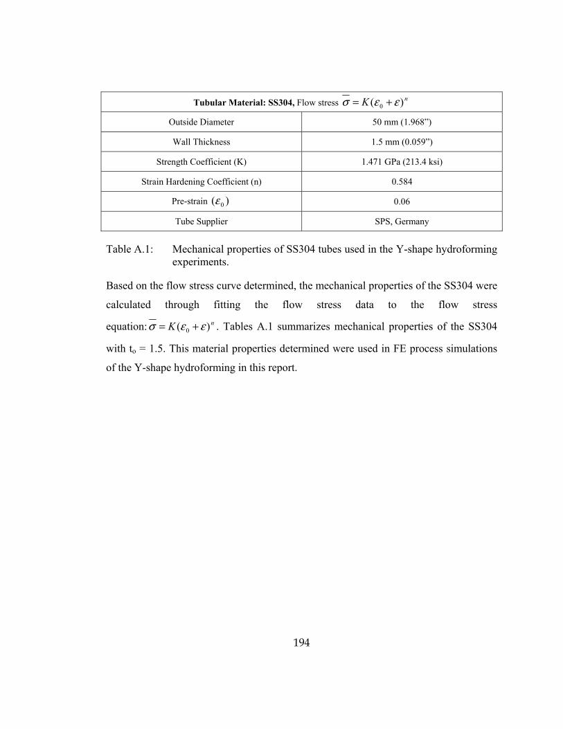
194
Tubular Material: SS304, Flow stress nK )( 0 εεσ +=
Outside Diameter 50 mm (1.968�)
Wall Thickness 1.5 mm (0.059�)
Strength Coefficient (K) 1.471 GPa (213.4 ksi)
Strain Hardening Coefficient (n) 0.584
Pre-strain )( 0ε 0.06
Tube Supplier SPS, Germany
Table A.1: Mechanical properties of SS304 tubes used in the Y-shape hydroforming experiments.
Based on the flow stress curve determined, the mechanical properties of the SS304 were
calculated through fitting the flow stress data to the flow stress
equation: nK )( 0 εεσ += . Tables A.1 summarizes mechanical properties of the SS304
with to = 1.5. This material properties determined were used in FE process simulations
of the Y-shape hydroforming in this report.
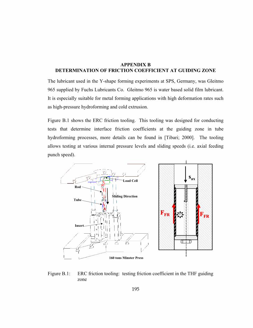
195
APPENDIX B DETERMINATION OF FRICTION COEFFICIENT AT GUIDING ZONE
The lubricant used in the Y-shape forming experiments at SPS, Germany, was Gleitmo
965 supplied by Fuchs Lubricants Co. Gleitmo 965 is water based solid film lubricant.
It is especially suitable for metal forming applications with high deformation rates such
as high-pressure hydroforming and cold extrusion.
Figure B.1 shows the ERC friction tooling. This tooling was designed for conducting
tests that determine interface friction coefficients at the guiding zone in tube
hydroforming processes, more details can be found in [Tibari; 2000]. The tooling
allows testing at various internal pressure levels and sliding speeds (i.e. axial feeding
punch speed).
pi
Fa Fa
Ff
sax
FFR FFR
Load Cell
Sliding Direction
Rod
Tube
Insert
160 tons Minster Press
pi
Fa Fa
Ff
sax
pi
Fa Fa
Ff
sax
FFR FFR
Load Cell
Sliding Direction
Rod
Tube
Insert
160 tons Minster Press
FFR FFR
Load Cell
Sliding Direction
Rod
Tube
Insert
160 tons Minster Press
Figure B.1: ERC friction tooling: testing friction coefficient in the THF guiding zone
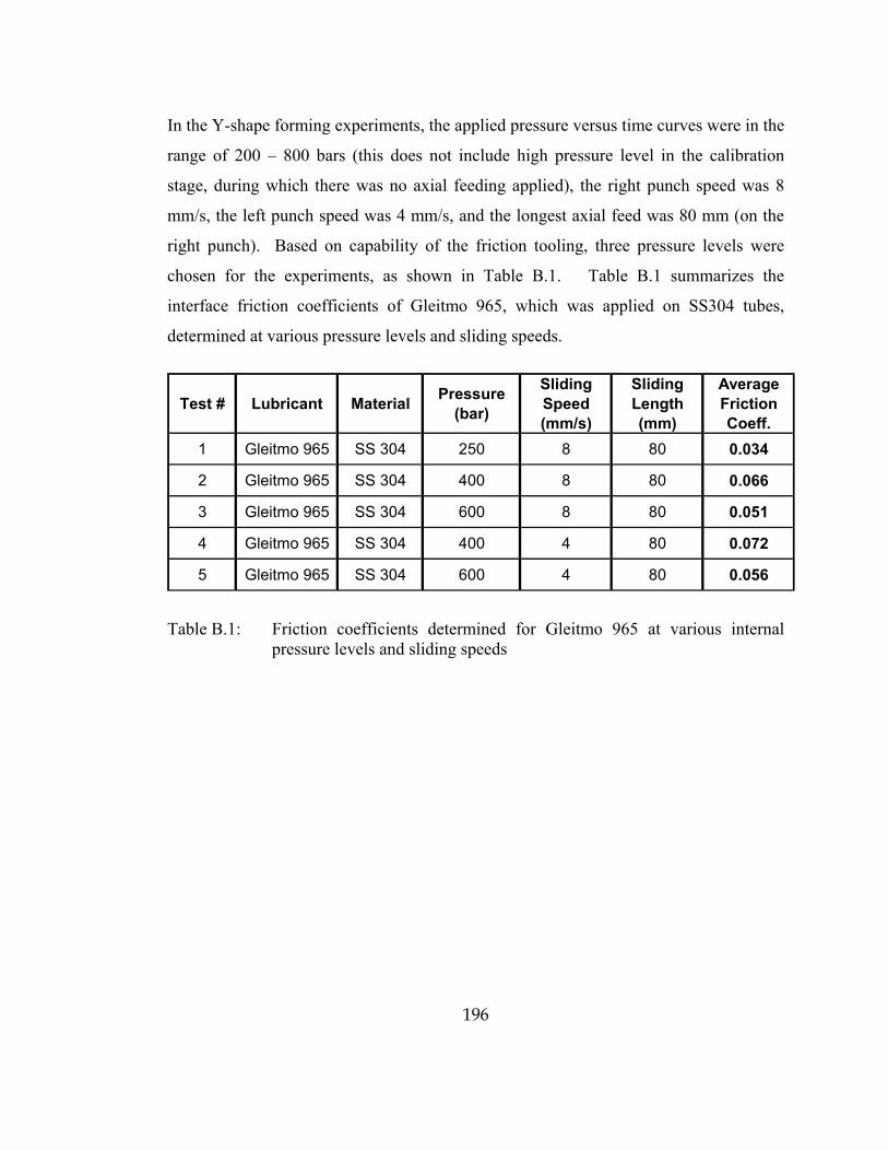
196
In the Y-shape forming experiments, the applied pressure versus time curves were in the
range of 200 � 800 bars (this does not include high pressure level in the calibration
stage, during which there was no axial feeding applied), the right punch speed was 8
mm/s, the left punch speed was 4 mm/s, and the longest axial feed was 80 mm (on the
right punch). Based on capability of the friction tooling, three pressure levels were
chosen for the experiments, as shown in Table B.1. Table B.1 summarizes the
interface friction coefficients of Gleitmo 965, which was applied on SS304 tubes,
determined at various pressure levels and sliding speeds.
Test # Lubricant Material Pressure (bar)
Sliding Speed (mm/s)
Sliding Length (mm)
Average Friction Coeff.
1 Gleitmo 965 SS 304 250 8 80 0.034
2 Gleitmo 965 SS 304 400 8 80 0.066
3 Gleitmo 965 SS 304 600 8 80 0.051
4 Gleitmo 965 SS 304 400 4 80 0.072
5 Gleitmo 965 SS 304 600 4 80 0.056
Table B.1: Friction coefficients determined for Gleitmo 965 at various internal pressure levels and sliding speeds
197
APPENDIX C OPTIMIZATION ALGORITHMS
The optimization algorithms applied in the Optimization-based simulation approach,
Chapter 5, are a) gradient approach using Augmented Lagrangian Method, and b)
Response Surface Method (RSM), which are both available in PAM-OPT. These two
different optimization algorithms have their applications different optimization
scenarios (i.e. generally, gradient methods are suitable for problems with a small
number of design variables; and RSM methods are suitable for problems with a large
number of design variables). This appendix gives a brief mathematical overview of
these two optimization algorithms.
Augmented Lagrangian Method (ALM)
In solving non-linear optimization problems with constraints, one of the most popular
set of techniques is �Sequential Unconstrained Minimization Techniques� (SUMT).
Generally, this approach is designed to minimize the objective function as
unconstrained function but to provide some penalty to limit constraint violations. The
classical approach to using SUMT is to create a pseudo-objective function of the form
[Vanderplaats, 1984]: )()(),( xPrxFrx pp +=φ , where, )(xF is the original objective
function and )(xP is an imposed penalty function, the form of which depends on the
SUMT being employed. The scalar pr is a multiplier which determines the magnitude
of the penalty, and pr is held constant for a complete unconstrained minimization; the
subscript p is the unconstrained minimization number. Figure C.1 shows how the
penalty function transforms a constrained optimization problem to an unconstrained
optimization problem using pseudo-objective function.

198
(a) (b)
Figure C.1: a) original one variable optimization objective function [F(x)] and constraint functions [g1(x)] and [g2(x)], and b) pseudo-objective functions [Φ(x,rp)] with different penalty multipliers [Vanderplaats, 1984]
Augmented Lagrangian Method (ALM) provides a way to include the conditions for
optimality, which is derived from Kuhn-Tucker conditions, into the SUMT in order to
improve its efficiency and reliability. This method can reduce the dependency of the
algorithm on the choice of the penalty parameters and the way by which they are
updated during the optimization process [Vanderplaats, 1984]. The ALM function can
be written as follows:
∑
++=
iiii xrxxfrxL )(
2)()(),,( 2ψψλλ
With
−=
rxgMaxx i
iiλψ ),([)(
Where f(x) is the objective function, gi(x) are the constraint functions number i = 1,�, I
with an upper bound equal to 0 (gi <= 0), λi are the Lagrange multipliers of the
constrain functions number i = 1,�, I, r is the penalty factor, and Ψi is the augmented
constraint functions number i = 1,�, I.

199
The augmented method consists in minimizing the function L(x,λ,r) on x with λ and r
being constants. Then, one modifies values of λ and r according to the iteration
strategies )()()()1( ni
nni
ni r ψλλ +=+ , which tend towards the classical Lagrange multipliers
and, )()1( nn rr α=+ , where the value of the penalty factor r is increasing if the constraint
violation doe not decrease, with α being constant, and where n is the number of current
iteration [Haug, 1998]. Figure C.2 shows the iteration scheme of this method. The
minimization of the pseudo-objective function is solved by the quasi-Newton methods
such as Davidson-Fletcher-Powell (DFP) and Broyden-Fletcher-Goldfarb-Shannon
(BFGS). As for the unidirectional minimization (line search), an algorithm of quadratic
approximation is used.
Figure C.2: Augmented Lagrangian Optimization flow chart [ESI Software, 2001]
In gradient calculation of the functions (objective and constraints), discrete FE
simulation results of perturbed design variables are used to approximate the gradients
with the finite difference scheme. Often times, these types of functions generated by
explicit FE solvers are not very smooth (i.e. wavy). The functions can oscillate around
a mean value for small variations of the design variables, see Figure C.3. PAM-OPT has
a special option that provides proper step-size, by which the finite difference schemes
uses, that avoids calculations of bad derivatives due to oscillating objective or constraint
functions [ESI Software, 2001].

200
Figure C.3: Wavy function in PAM-OPT [ESI Software, 2001]
Response Surface Method (RSM)
This optimization approach minimizes the real objective function through successive
resizing and narrowing of response surfaces approximating the objective function in the
design space until the optimum is bounded and found.
Experimental design techniques and response surface methodology are used to construct
these approximate functions. Considering a response y dependent on a set of variables x,
the exact functional relationship between them is )(xy η= . One wants to use an
approximation for the functional relationship )()( xfx ≅η over some region of interest
)(xR . The response is evaluated at pxxx ,...,, 21 for a total p experiments in )(xR , and
the experimental error is rε .
The real physical model can now be written as: rxy εη += )( .
Using the approximating function, the real response is now: rxxfy εδ ++= )()(
, with the modeling (bias) error: )()()( xfxx −= ηδ . The modeling error is dependent
only on the choice of approximating function and sub-region size [Roux, 1998]. In this
study, since this RSM is applied to approximate numerical responses from FE
simulation of metal forming processes (i.e. real processes), the experimental error is
zero. Therefore, the real response model is reduced to: )()( xxfy δ+= .

201
Typically, the standard response surface uses an approximated function of low-order
polynomials in order to reduce the number of experiments (i.e. simulation runs):
xm xxxxf ββββ ++++= ...)( 22110
When the linear function is no longer adequate to describe the response, a higher-order
model is needed, such as the second-order polynomial model:
∑ ∑∑∑=
<=
+++=m
i i jjijiij
m
iiixi xxxxxf
1,
1
20)( ββββ
Unlike the standard RSM, the PAM-OPT RSM algorithm uses approximated functions,
which have similar characteristics to the B-Splines in CAD applications. The main
characteristics are as follows [ESI Software, 2001]:
♦ The number of points is free (in the standard RSM, the number of points is equal to
the number of coefficients of the polynomial: (n+1)(n+2)/2, n = design variables)
♦ The approximated functions pass through all points, and the approximated function
values, calculated in a given position, only depend on points close to this position.
♦ The shape of these approximated functions is always good. For example, these
approximated functions cannot create artificial local minima like polynomials can
do.
During optimization iterations of the PAM-OPT RSM algorithm, it is possible to
increase the response surface accuracy by locally reconstructing the response surface
bounding the solution point found from the previous iteration. This requires calculations
of a few new points. The algorithm then uses the full set of all calculated points to
reconstruct new response surfaces, which will be used to find a new solution. The
design parameter domain is kept the same throughout the optimization process. This
algorithm is called �Adaptive Response Surface Method�. Figure C.4 shows how this
algorithm works in a two design variable space, X1 and X2.
♦ The first figure shows the design domain specified by the design variables.
♦ The second figure shows the first iteration. Four initial points are calculated
(launching of solvers: PAM-STAMP) on the design domain. The calculated point
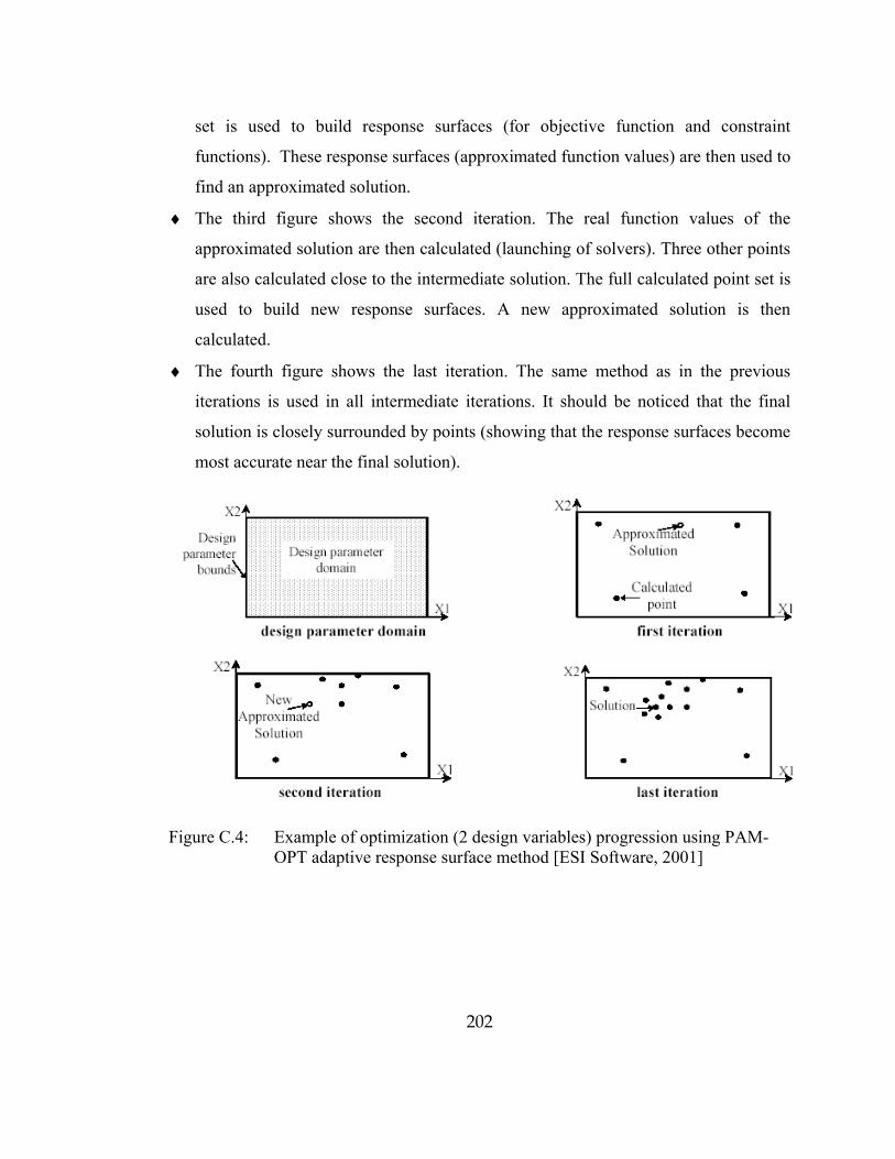
202
set is used to build response surfaces (for objective function and constraint
functions). These response surfaces (approximated function values) are then used to
find an approximated solution.
♦ The third figure shows the second iteration. The real function values of the
approximated solution are then calculated (launching of solvers). Three other points
are also calculated close to the intermediate solution. The full calculated point set is
used to build new response surfaces. A new approximated solution is then
calculated.
♦ The fourth figure shows the last iteration. The same method as in the previous
iterations is used in all intermediate iterations. It should be noticed that the final
solution is closely surrounded by points (showing that the response surfaces become
most accurate near the final solution).
Figure C.4: Example of optimization (2 design variables) progression using PAM-OPT adaptive response surface method [ESI Software, 2001]
203
APPENDIX D INTERFACING BETWEEN PAM-OPT AND PAM-STAMP
This appendix gives a brief overview of the interaction (interfacing) between PAM-
OPT and PAM-STAMP. First, a general flow chart of the PAM-OPT algorithm is
given, and each important component in the algorithm is described. An example of THF
optimization input file is also given and explained as to demonstrate how PAM-OPT
formulates the problem and extracts the simulation results from PAM-STAMP. The
example given in this appendix is the loading path optimization of the simple bulge
hydroforming using the ALM gradient method, discussed in Chapter 5.
General PAM-OPT� Algorithm flow chart
Figure D.1 shows the general flow chart of PAM-OPT in both user level and internal
algorithm level. The following files are in the user level [ESI Software, 2001]:
Algorithm Input Data Set File: To initialize an optimization, the user must prepare an
input file to the PAM-OPT� Algorithm. This file set is actually consisted of two files:
a) Composite Data Set file (*.cds), and b) Auxiliary set file, see Figure D.2. The
composite data set file contains information that defines the problem of optimization:
- Definition of design variables, - Definition of constraint functions and of the objective function, - Design variable values which define the starting point (initialization), - Optimization method used, and convergence parameters
The auxiliary set file contains executable UNIX commands that �extract� simulation
results from the solver results (PAM-STAMP) using PAM-VIEW script commands.
Algorithm Signal file: In addition, the user can make a signal file to change
convergence parameters of a running optimization.

204
Algorithm Output Files: Upon execution, the PAM-OPT� Algorithm automatically
creates a number of output files (history file, curve file, restart file).
The Algorithm reads design variable values from the Algorithm input data set file to
initialize the optimization. Then, it calls a process, which works out optimization
function (and gradient) values, as well as constraint set values. In this process level, the
FE process simulation PAM-STAMP solver is run according to the input data. The
called process reads design variable values from the process input data set file and it
will write function (gradient) and constraint set values onto the Algorithm process
output data set file. During an optimization run, the user can interact with the Algorithm
module via the Algorithm signal file. Finally, the Algorithm module will write the
results of the optimization on several Algorithm output files.
Figure D.1: General PAM-OPT algorithm flow chart [ESI Software, 2001]
PAM-STAMP
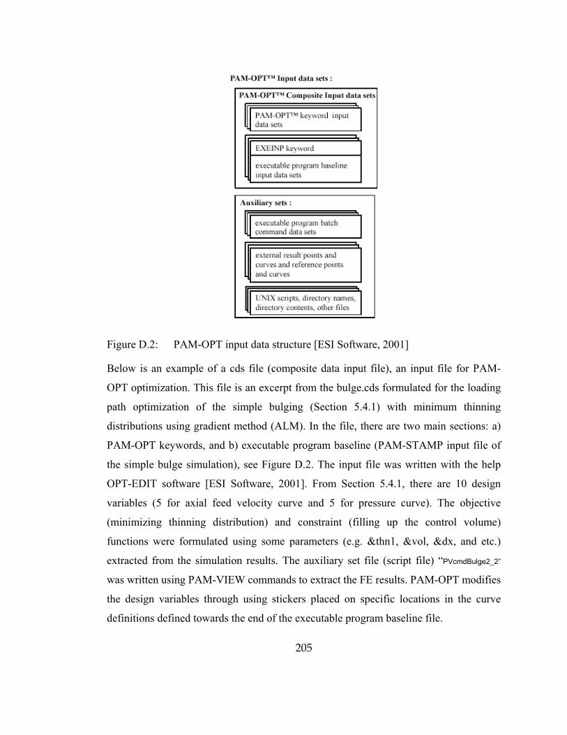
205
Figure D.2: PAM-OPT input data structure [ESI Software, 2001]
Below is an example of a cds file (composite data input file), an input file for PAM-
OPT optimization. This file is an excerpt from the bulge.cds formulated for the loading
path optimization of the simple bulging (Section 5.4.1) with minimum thinning
distributions using gradient method (ALM). In the file, there are two main sections: a)
PAM-OPT keywords, and b) executable program baseline (PAM-STAMP input file of
the simple bulge simulation), see Figure D.2. The input file was written with the help
OPT-EDIT software [ESI Software, 2001]. From Section 5.4.1, there are 10 design
variables (5 for axial feed velocity curve and 5 for pressure curve). The objective
(minimizing thinning distribution) and constraint (filling up the control volume)
functions were formulated using some parameters (e.g. &thn1, &vol, &dx, and etc.)
extracted from the simulation results. The auxiliary set file (script file) �PVcmdBulge2_2�
was written using PAM-VIEW commands to extract the FE results. PAM-OPT modifies
the design variables through using stickers placed on specific locations in the curve
definitions defined towards the end of the executable program baseline file.
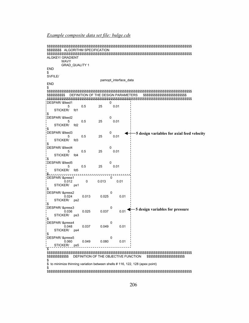
206
Example composite data set file: bulge.cds $$$$$$$$$$$$$$$$$$$$$$$$$$$$$$$$$$$$$$$$$$$$$$$$$$$$$$$$$$$$$$$$$$$$$$$$$$$$$$$$ $$$$$$$$ ALGORITHM SPECIFICATION $$$$$$$$$$$$$$$$$$$$$$$$$$$$$$$$$$$$$$$$$$$$$$$$$$$$$$$$$$$$$$$$$$$$$$$$$$$$$$$$ ALGKEY/ GRADIENT WAVY GRAD_QUALITY 1 END $ SVFILE/ pamopt_interface_data END $ $$$$$$$$$$$$$$$$$$$$$$$$$$$$$$$$$$$$$$$$$$$$$$$$$$$$$$$$$$$$$$$$$$$$$$$$$$$$$$$$ $$$$$$$$$$ DEFINITION OF THE DESIGN PARAMETERS $$$$$$$$$$$$$$$$$$$$$$$$ $$$$$$$$$$$$$$$$$$$$$$$$$$$$$$$$$$$$$$$$$$$$$$$$$$$$$$$$$$$$$$$$$$$$$$$$$$$$$$$$ DESPAR/ &feed1 0 5 0.5 25 0.01 STICKER/ fd1 $ DESPAR/ &feed2 0 5 0.5 25 0.01 STICKER/ fd2 $ DESPAR/ &feed3 0 5 0.5 25 0.01 STICKER/ fd3 $ DESPAR/ &feed4 0 5 0.5 25 0.01 STICKER/ fd4 $ DESPAR/ &feed5 0 5 0.5 25 0.01 STICKER/ fd5 $ DESPAR/ &press1 0 0.012 0 0.013 0.01 STICKER/ ps1 $ DESPAR/ &press2 0 0.024 0.013 0.025 0.01 STICKER/ ps2 $ DESPAR/ &press3 0 0.036 0.025 0.037 0.01 STICKER/ ps3 $ DESPAR/ &press4 0 0.048 0.037 0.049 0.01 STICKER/ ps4 $ DESPAR/ &press5 0 0.060 0.049 0.080 0.01 STICKER/ ps5 $ $$$$$$$$$$$$$$$$$$$$$$$$$$$$$$$$$$$$$$$$$$$$$$$$$$$$$$$$$$$$$$$$$$$$$$$$$$$$$$$$ $$$$$$$$$$$$ DEFINITION OF THE OBJECTIVE FUNCTION $$$$$$$$$$$$$$$$$$$$$ $ $ to minimize thinning variation between shells # 116, 122, 128 (apex point) $ $$$$$$$$$$$$$$$$$$$$$$$$$$$$$$$$$$$$$$$$$$$$$$$$$$$$$$$$$$$$$$$$$$$$$$$$$$$$$$$$
5 design variables for axial feed velocity
5 design variables for pressure

207
OBJFCT/ &thinn 0 0 SQRT ( ( 1 / 3 ) * ( ( ( ABS ( &thn1 ) ) ^ 2 ) + ( ( ABS ( &thn2 ) ) ^ 2 ) + ( ( ABS ( &thn3 ) ) ^ 2 ) ) ) END $ $$$$$$$$$$$$$$$$$$$$$$$$$$$$$$$$$$$$$$$$$$$$$$$$$$$$$$$$$$$$$$$$$$$$$$$$$$$$$$$$ $$$$$$$$$$$$ DEFINITION OF THE CONSTRAINT FUNCTIONS $$$$$$$$$$$$$$$$$$$$$ $ $ The part volume is to be filled as equal to the control volume $ $$$$$$$$$$$$$$$$$$$$$$$$$$$$$$$$$$$$$$$$$$$$$$$$$$$$$$$$$$$$$$$$$$$$$$$$$$$$$$$$ CSTFCT/ &vol_final 0 -1.0 1.0 ( ( 17742.1905 - ( &vol - ( 25 - &dx ) * 313.1825 ) ) / 17742.1905 ) * 100 END $ $$$$$$$$$$$$$$$$$$$$$$$$$$$$$$$$$$$$$$$$$$$$$$$$$$$$$$$$$$$$$$$$$$$$$$$$$$$$$$$$ $$$$$$$$$$ EXECUTION OF PAMSTAMP $$$$$$$$$$$$$$$$$$$$$$$$$$$$$$$$$$$$$$$ $$$$$$$$$$$$$$$$$$$$$$$$$$$$$$$$$$$$$$$$$$$$$$$$$$$$$$$$$$$$$$$$$$$$$$$$$$$$$$$$ SCLCAL/ 0 1 pamstamp END $ $$$$$$$$$$$$$$$$$$$$$$$$$$$$$$$$$$$$$$$$$$$$$$$$$$$$$$$$$$$$$$$$$$$$$$$$$$$$$$$$ $$$$$$$$$$$$$$$$$$$$ EXECUTION OF PAMVIEW $$$$$$$$$$$$$$$$$$$$$$$$$$$$$$$$ $ VIECAL/ 0 2 pamview 0 PVcmdBulge2_2 $ $$$$$$$$$$$$$$$$$$$$$$$$$$$$$$$$$$$$$$$$$$$$$$$$$$$$$$$$$$$$$$$$$$$$$$$$$$$$$$$$ GETCRV/ &&thn_crv3 0 0 thn_crv3 2 $ GETCRV/ &&thn_crv2 0 0 thn_crv2 2 $ GETCRV/ &&thn_crv1 0 0 thn_crv1 2 $ GETCRV/ &&dx_crv 0 0 dx_crv 2 $ GETCRV/ &&vol_crv 0 0 vol_crv 2 $ $$$$$$$$$$$$$$$$$$$$$$$$$$$$$$$$$$$$$$$$$$$$$$$$$$$$$$$$$$$$$$$$$$$$$$$$$$$$$$$$ CALVAL/ &thn3 1 &&thn_crv3 YEND 0 $ CALVAL/ &thn2 1 &&thn_crv2 YEND 0 $ CALVAL/ &thn1 1 &&thn_crv1 YEND 0 $ CALVAL/ &dx 1 &&dx_crv
Objective function: minimize RMS of three thinning values distributed on the bulge part
Auxiliary set file: extracting FE results
Read the curve files extracted above
Extracting specific data point from the files read above

208
YEND 0 $ CALVAL/ &vol 1 &&vol_crv YEND 0 $ $$$$$$$$$$$$$$$$$$$$$$$$$$$$$$$$$$$$$$$$$$$$$$$$$$$$$$$$$$$$$$$$$$$$$$$$$$$$$$$$ CPFILE/ 2 AUXILIARYset $---5---10----5---20----5---30----5---40----5---50----5---60----5---70----5---80 $ $$$$$$$$$$$$$$$$$$$$$$$$$$$$$$$$$$$$$$$$$$$$$$$$$$$$$$$$$$$$$$$$$$$$$$$$$$$$$$$$ EXEINP/ $ $ This file is generated by PAM-GENERIS version 2000.1 on 2002/08/29 at 17:27:12 $ PAM-GENERIS Version 2000.1 - Compiled 2001/05/03 $ . . $ $ FUNCTIONS CARDS $ $---5---10----5---20----5---30----5---40----5---50----5---60----5---70----5---80 #GPNAM Curve 1 FUNCT / 1 7 1 1 0 0 0 0 0.01 5 #STICKER/fd1,-1 # ?????? 0.2 5 #STICKER/fd2,-1 # ?????? 0.4 5 #STICKER/fd3,-1 # ?????? 0.6 5 #STICKER/fd4,-1 # ?????? 0.8 5 #STICKER/fd5,-1 # ?????? 1.05 5 #GPNAM Curve 2 FUNCT / 2 6 1 1 0 0 0 0 #STICKER/ps1,-1 # ?????? 0.2 0.012 #STICKER/ps2,-1 # ?????? 0.4 0.024 #STICKER/ps3,-1 # ?????? 0.6 0.036 #STICKER/ps4,-1 # ?????? 0.8 0.048 #STICKER/ps5,-1 # ?????? 1.05 0.06 ENDDATA
Beginning of PAM-STAMP input date file
PAM-OPT changes axial feed velocity variables here in the velocity curve function definition
PAM-OPT changes pressure variables here in the velocity pressure function definition

209
APPENDIX E ADAPTIVE SIMULATION PROGRAM
This chapter explains in detail the preparation of the inputs to the adaptive sub-routine.
Before going into the details of the input file preparation, an overall understanding of
how the sub-routine is implemented to determine a THF loading path is given. In this
appendix, adaptive simulation case of the simple bulge hydroforming is given. The
adaptive sub-routines consist of files as explained below:
1 ldcmod.f: This source code file is a PAM-STAMP user-subroutine that allows the
user to access all the metal forming simulated data and to adjust any loading curve
functions at any simulation time step while the simulation is running. The
abbreviation stands for �LoaDing Curve MODification�. The user can develop his
own control strategies (i.e. process parameter adjustment algorithms) and
implement them in into the user-subroutine using FORTRAN commands and some
key words provided by Engineering Systems International (ESI). The detailed
information of these commands is given later in this appendix.
2 v2kpa7_102.a: This is a library file containing the PAM-STAMP core solver
program provided by ESI.
3 make: This is a batch file which executes the commands to compile the core
program with the user subroutine to generate the adaptive simulation executable
file.
All these files are contained in the same directory, under which by running the batch
file, �make�, the source code ldcmod.f is compiled and linked with the library file
v2kpa7_102.a to generate an executable program, v2kpa7_102.x (referred to as AS
executable or program), as shown in Figure E.1.
As explained earlier, two simulation runs are needed in the adaptive simulation
procedure of THF loading path determination. The first adaptive simulation is to

210
basically record the hydroforming history of the part in the self-feeding condition in
order to obtain the progression curve of part surface area and volume. This is to be used
as reference data in the second adaptive simulation run (i.e. the surface area-to-volume
wrinkle criterion). From Figure E.1, in the first simulation run, the AS program takes in
the control parameter inputs from the user through an input file called control.prm, and
the PAM-STAMP simulation input file, SF_bulge.ps, which is setup with the self-
feeding condition. In this step, the control.prm provides the part geometric information
(cross section area, boundary of the control volume, and etc.) necessary for calculating
the surface area-volume progression of the part in self-feeding condition, which is
stored in the output file called SF_results.out. All the other output files are the usual
PAM-STAMP output files, see Figure E.1, in the 1st adaptive simulation run.
Figure E.1: Basic flowchart of the adaptive simulation procedure
ldcmod.fsource code
v2kpa7_102.a PAM-STAMP library file
v2kpa7_102.x AS executable file
SF_bulge.ps
control.prm
SF_bulge.DSY SF_bulge.THP SF_bulge.OUT
SF_results.out
v2kpa7_102.x AS executable file
AS_bulge.ps
control.prm
AS_bulge.DSY AS_bulge.THPAS_bulge.OUT
AS_results.out SF_results.out (from 1st run)
Compile and link (make)
1st adaptive simulation run
2nd adaptive simulation run

211
In the second adaptive simulation run, the input files to the AS program are: a) PAM-
STAMP simulation input file, AS_bulge.ps, b) control.prm, and c) the output file from
the 1st run, SF_results.out. The AS program extracts the results from the FE simulation,
monitors the simulation for any defects (i.e. wrinkling using the surface-volume
criterion and thinning), adjusts the pressure curve and axial feed velocity curve (i.e.
loading curves) if the wrinkle indicator deviates from wrinkle control trajectories, and
gives the adjusted loading curve values in an output file called AS_results.out, Figure
E.1.
Contents of the control parameter input file: control.prm
The user needs to enter some important parameters to the adaptive program through an
input file called control.prm. These parameters are mainly used in a) geometric defect
detection criteria, and b) process adjustment algorithms. Some of the important input
parameters to be given in this file are explained below in detail (some of the input
parameters are omitted here to keep this appendix readable and focused). The units used
here should be the same as the units that one wants to use in the *.ps file of PAM-
STAMP, since the values given in control.prm are used for calculating the variation of
the THF loading paths in the simulation. For example, the pressure increment, DELUP,
is to be given in GPa; the axial feed velocity increment, DELUD, is to be given in
mm/ms. The first part of the control.prm collects all the geometric information of the
part necessary: (see Figure E.2)
XLT: X-coordinate on the left side of the control box (or volume)
XRT: X-coordinate on the right side of the control box. The control box should be
placed over all the expansion area.
ENOD: Number of a node located at the tube end. This is used to track the axial feed.
ENODXC: The X-coordinate of the ENOD.
CRSAREA: Cross sectional area of the blank tube.
ARCLEN: Arch length of the tube blank along the circumferential direction.
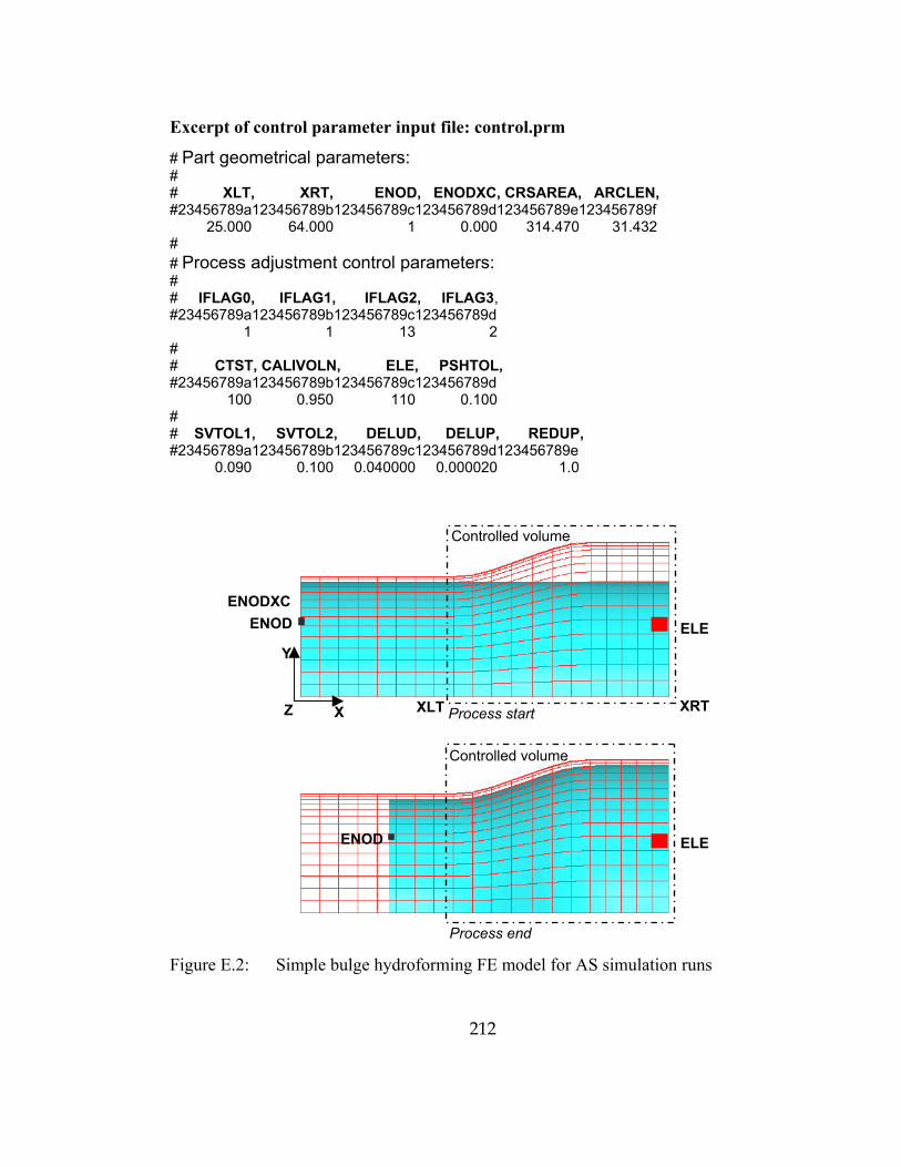
212
Excerpt of control parameter input file: control.prm
# Part geometrical parameters: # # XLT, XRT, ENOD, ENODXC, CRSAREA, ARCLEN, #23456789a123456789b123456789c123456789d123456789e123456789f 25.000 64.000 1 0.000 314.470 31.432 # # Process adjustment control parameters: # # IFLAG0, IFLAG1, IFLAG2, IFLAG3, #23456789a123456789b123456789c123456789d 1 1 13 2 # # CTST, CALIVOLN, ELE, PSHTOL, #23456789a123456789b123456789c123456789d 100 0.950 110 0.100 # # SVTOL1, SVTOL2, DELUD, DELUP, REDUP, #23456789a123456789b123456789c123456789d123456789e 0.090 0.100 0.040000 0.000020 1.0
Figure E.2: Simple bulge hydroforming FE model for AS simulation runs
Controlled volume
Process start
Controlled volume
Process end
X
Y
Z XLT XRT
ENODENODXC
ELE
ELE ENOD

213
The second portion of the control.prm file requires all the necessary parameter for the
process parameter adjustment algorithms. These parameters indicate the user intention
of how best the loading paths should be adjusted depending on the part geometry. It is
noted here that the options available in the current AS program are suitable for simple
bulge hydroforming only. The following are the descriptions of the parameters:
IFLAG0: Types of simulation run � <0> self-feeding simulation run (1st simulation
run, see Figure E.1), <1> adaptive simulation run (2nd simulation run, see
Figure E.1), <2> normal simulation run (this option is used to extract all the
adaptive simulation related results from a normal simulation with already
defined loading paths).
IFLAG1: Type of geometrical wrinkle criterion applied - <1> surface area-to-volume
wrinkle criterion (IWSV), <2> arch length-to-area wrinkle criterion
(IWLA). In the current AS program, two of these criterion options are
available to calculate the relevant wrinkle indicators (IWSV and IWLA), but
only the area-to-volume is being used in the process parameter adjustment.
IFLAG2: Process parameter adjustment pattern -
<11> impulse loading path: in this option, the pressure is applied only when
this is wrinkling, and the axial feed is applied only when this is no wrinkling.
This impulse loading path pattern ((loading path � plot of pressure versus
axial feed) is implemented here for the purpose of parameter adjustment
demonstration, but it is not practical for real hydroforming presses.
<12> step loading path: this loading path pattern is originally proposed in
the preliminary work on adaptive simulation concept for THF, see Figure
6.1. In this option, the axial feed is applied while the pressure is kept
constant when wrinkling is not present, and the axial feed is stop while the
pressure is increased when wrinkle is present. Thus the loading path is a step
function.
<13> step loading path with decreased pressure: this loading path pattern is

214
similar to that of the step loading path but the pressure is decreased while the
axial feed is applied when wrinkling is not present. This option is developed
to reduce the excessive thinning that normally occurs when using the step
loading path pattern, see Section 6.4.2.3.
IFLAG3: Process parameter adjustment at the process beginning:
<1> no control: this option allows the process adjustment pattern defined in
IFLAG2 take action since the process beginning. This option was originally
used. It was found out that none of the algorithms in defined in IFLAG2
could handle the tracking of the wrinkle control trajectory, which resulted in
premature excessive thinning.
<2> pure shear control: this option adjusts the loading path such that the
chosen critical part element (ELE) stays in a pure shear state of stress until
the first wrinkle is present (according to the surface area-to-volume wrinkle
criterion). This option offers a reasonable way to accumulate material in the
expansion zone, thus reduce the risk of having premature excessive thinning
during the process beginning. Please note that this pure shear control only
works for early stage of THF process whose tube blank is not crushed or
bent. In other words, the part geometry should resemble simple bulging in
the early hydroforming stage. This is because the adjustment of pressure in
this pure shear control is based on a simple stress calculation of simple bulge
geometry. The principle of this control algorithm is that the axial feed is
applied steadily at a constant punch velocity (DELUD) but the pressure is
increased or decreased to make the hoop tensile stress have the same
magnitude as that of the longitudinal stress.
CTST: Control time step. This is defined in multiples of simulation time steps, e.g
CTST = 100 means that the process parameters will be adjusted every 100
simulation time steps.
CALIVOLN: Normalized part volume cutoff for starting the calibration, after which
the axial feed is stopped and the pressure is increased until VOLN becomes

215
1.0 or it reaches the maximum pressure limited by hydroforming press
capability.
ELE: Number of tube mesh element located in the critical area of the part (subject
to most excessive thinning, see Figure E.2). This element will be used in the
pure shear control.
PSHTOL: Pure shear state tolerance. This value determines the stress state window of
the chosen part element to be consider pure shear or else. If
0<PSHI<PSHTOL then the pure shear state is present. If PSHI>PSHTOL
then only shear state (not pure shear) is present or PSHI<0 then tensile
biaxial state is present (see example of the output file for the definition of
PSHI).
SVTOL1 and SVTOL2: Lower and upper apex values of the triangle wrinkle control
trajectories, see Figure 6.15a.
DELUD: Axial feeding velocity increment for adjustments (both increasing and
deceasing) of the axial feed over one single time step in a ramping fashion.
Care must be taken in using this parameter. As discussed in Chapter 6, if this
DELUD value is too large dynamic effect error will result. The
determination of a proper value of this parameter relies on experience and
trial and error. For this simple bulge geometry and material, a value of
DELUD = 0.040 mm/ms seems to be appropriate.
DELUP: Pressure increment for adjustments (both increasing and deceasing) of the
pressure over one single time step in a ramping fashion. To avoid the
dynamic effect in the adaptive simulation, a value of DELUP = 0.000020
GPa is suitable for this simple bulge geometry.
REDUP: Multiply factor for the reduction in pressure increment. This parameter is
used along with the IFLAG2 = 13 (step loading path with decreased
pressure). This is to increase the rate of pressure reduction to prevent the
excessive thinning while applying axial feeding. A value between 1-2 should
be used to avoid the dynamic effect.

216
Preparation of PAM-STAMP simulation input for the 1st run: SF_bulge.ps
In the 1st adaptive simulation run, a self-feeding simulation is conducted to record the
surface area and volume data of the part at all the simulation time steps. This data will
be used in the 2nd adaptive simulation run. The simple bulge, Figure E.2, is used as an
example here, all the tube and die dimension are already given earlier. Self-feeding
loading curves are applied here where the pressure is applied linearly from zero to
calibration pressure (0.060 GPa), there is no forced axial feed at the tube end (i.e. the
tube end nodes are not constrained), and no tube-die friction interface. There are a few
requirements in setting up this simulation to work with the AS program, see Figure E.2:
1. The tube axis should be aligned with the global X-axis in the simulation.
2. The symmetry plane of the tube axis should be placed on the X-Z plane at Y = 0.
3. The fluid cell volume calculation vector should point in the Y direction.
Output file from the 1st run: SF_results.out
This file, SF_results.out, contains the output from the first run of the adaptive program,
v2kpa7_102.x, see Figure E.1. An excerpt of the output file is given below. It records
relevant geometrical parameters of part as well as the shell element stresses. Each line
of the data is recorded at each simulation time step. In this file excerpt, the shown data
are from the beginning of the forming and towards the end of the forming. The example
output file below is taken from the simple bulge adaptive simulation case. The
following are some descriptions of the parameters recorded:
SURF: Part (FE mesh model) surface area bounded in the control box (unit = mm2)
VOL: Part (FE mesh model) enclosed volume or the PAM-STAMP fluid cell volume
bounded in the control box (unit: mm3). These two parameters (SURF and
VOL) are used for the surface area-volume wrinkle criterion in the 2nd run.
SMXTHN: Part maximum thinning value (engineering strain through thickness
direction)
SFD: Axial feed or the tube end node displacement (unit: mm)

217
SFD: Internal pressure (unit: GPa)
MSIG11: Stress in the circumferential direction of the chosen element, see
control.prm explanation above (unit: GPa)
MSIG22: Stress in the longitudinal direction of the chosen element (unit: GPa). These
two stress parameters are used for the pure shear state control, will be discussed
later.
LEN1: Arch length of the part bounded by the control box (unit: mm)
ARE1: Die-tube profile enclosed area bounded by the control box (unit: mm2). These
two parameters (LEN1 and ARE1) are for the length-area wrinkle criterion, but
they are not used in the process adjustment in this case.
Example of the SF_results.out:
SURF VOL SMXTHN SFD SFP MSIG11 MSIG22 LEN1 ARE1
1223.758 12181.94 0.00 0 0.00005 0.000095 0.000028 39.000 191.757
1223.763 12182.00 0.00 0.000001 0.000105 0.000723 0.000208 39.000 191.754
1223.768 12182.11 0.00 0.000013 0.000161 0.001765 0.000423 39.000 191.751
1223.771 12182.20 0.00 0.000053 0.000216 0.002543 0.000411 39.000 191.748
. . . . . . . . .
. . . . . . . . .
1498.325 17680.59 0.14 4.074892 0.04581 0.221191 -0.079302 39.879 36.884
1498.320 17680.08 0.14 4.077746 0.045865 0.216184 -0.097425 39.879 36.893
1498.329 17680.14 0.14 4.074459 0.045921 0.219557 -0.084367 39.879 36.887
1498.318 17680.30 0.14 4.066472 0.045976 0.232466 -0.048132 39.879 36.876
Please note that, the output parameters shown above are not the entire output parameters
from then 1st simulation run. However, they are the most important and relevant to the
user. It should also be noted that these results from the 1st simulation (self-feeding
simulation) serve mainly as reference data for the real adaptive simulation in the 2nd
simulation run, see Figure E.1. In the future, the AS program can be improved such that
the 1st simulation is conducted automatically without any human-machine interaction.

218
Preparation of PAM-STAMP simulation input for the 2nd run: AS_bulge.ps
The PAM-STAMP simulation input for the 2nd adaptive simulation run should be the
exact same FE model used in the 1st simulation run, only the loading boundary, die-tube
interface conditions, and total simulation time should be changed:
♦ The die-tube interface: a realistic friction coefficient should be applied between the
tube and die (e.g. µ=0.06). In this 1st simulation, the friction is assumed zero to
achieve the self-feeding condition.
♦ Simulation time: as explained earlier in Chapter 6, in AS simulation, a part is
formed completely when the normalized volume VOLN = 1. Only the adjustments
of the pressure and axial feed (not simulation time) will influence the progression of
VOLN. Therefore, simulation time should be given to be long enough for the
parameter adjustment algorithm to form the part. In this simple bulge case, a total
simulation time of 5 ms is appropriate.
♦ The loading condition: the AS program is written such that the adjustments of
pressure and axial feed velocity will be active beginning at the second time control
step (CTST), see control.prm. In the simulation input (*.ps), it is recommended to
applied a small pressure and axial feed velocity during the first control time step.
These small values can be the same as the pressure increment (DELUP) and
velocity increment (DELUD) defined in control.prm.
Output file from the 1st run: AS_results.out
This file, AS_results.out, contains the output from the second run of the adaptive
program, v2kpa7_102.x. Each row of record in this output file is from each control time
step (CTST). The excerpt of the file below shows some output results from both the
beginning of the simple bulging process and towards the end of the process (this can be
noticed by considering the value of VOLN, which increases from 0.000 in the
beginning to 0.987 towards the process end). The following are descriptions of the
output parameters:

219
Example of the SF_results.out:
VOLN SURFNAS IWSV IWSVTOL1 IWSVTOL2 SMXTHN AFEED ASD ASP PSHI
0.000 -0.001 -0.000018 0.000031 0.000034 0.000 0.002 0.000 0.000 0.723
0.001 0.000 -0.000061 0.000201 0.000223 0.000 4.002 0.047 0.000 0.964
0.012 0.011 -0.000088 0.002136 0.002373 0.000 4.002 0.140 0.014 0.482
0.024 0.023 -0.000188 0.004371 0.004857 0.001 4.002 0.232 0.008 0.079
0.030 0.030 -0.000540 0.005483 0.006092 0.000 4.002 0.324 0.008 0.399
0.041 0.041 -0.000397 0.007429 0.008254 0.000 4.002 0.417 0.013 0.159
0.052 0.051 -0.000077 0.009306 0.010340 0.001 4.002 0.509 0.010 0.091
. . . . . . . . . .
. . . . . . . . . .
0.987 0.999 0.000857 0.002317 0.002574 0.090 0.042 7.374 0.185 -1
0.987 0.999 0.000872 0.002313 0.002570 0.090 0.042 7.375 0.187 -1
0.987 0.999 0.000892 0.002310 0.002567 0.090 0.042 7.375 0.189 -1
0.987 0.999 0.000909 0.002307 0.002563 0.090 0.042 7.376 0.191 -1
0.987 0.999 0.000926 0.002303 0.002559 0.090 0.042 7.377 0.193 -1
0.987 0.999 0.000946 0.002299 0.002555 0.090 0.042 7.378 0.195 -1 VOLN: Normalized part volume
SURFNAS: Normalized part surface area
IWSV: Surface area-to-volume wrinkle criterion
IWSVTOL1: Upper wrinkle control trajectory
IWSVTOL2: Lower wrinkle control trajectory
SMXTHM: Part maximum thinning
AFEED: Axial feed punch velocity (unit: mm/ms)
ASD: Axial feed distance (unit: mm) � axial feed curve predicted
ASP: Internal pressure (unit: GPa) � pressure curve predicted
PSHI: Pure shear indicator calculated from 22111
MSIGMSIGPSHI −= when
MSIG11(hoop stress)>0 and MSIC22(axial stress)<0. And, PSHI = -1 when
both MSIG11 and MSIG22 > 0 indicating tensile biaxial state of stress.
Please note that, the output parameters shown above are not the entire output parameters
from then 2nd simulation run. However, they are the most important in AS procedure.

220
Keywords provided by ESI
The adaptive subroutine is written in FORTRAN. The user has any FORTRAN
command at his or her disposal. In addition, the following commands are provided by
ESI to the user:
DXYZ: Array of nodal coordinates
DISP: Array of nodal displacements
VEL: Array of nodal velocities
ACC: Array of nodal accelerations
INOD(N): External number of internal node number N
ISHEL(N): External number of internal element number N
IMAT(N): External number of internal material number N
TIME: Current time of simulation
NUMCON: Number of contact interfaces
CONFORCE(1,N): Contact force X-direction of contact interface N
CONFORCE(2,N): Contact force Y-direction of contact interface N
CONFORCE(3,N): Contact force X-direction of contact interface N
NUMNOD: Number of nodes
LABNOD(N): External node number of internal node number N
NUMSHE: Number of shell elements
LABSHE(N): External element number of internal element number N
KONSHE(N,M): For N=1, the internal material number is returned for element M. For N=2,3,4,5, the internal node numbers of element M are returned. For N=6, the number of through thickness integration points of internal element M is returned.
INDEX(N): Address of internal element N in the index table.

221
STRTAB(N): Return various strain and stress values from the index table.
NUMCUR: Number of velocity and forces curves
LABCUR(N): External curve number of internal curve number N
FUNVAL(N): Current value of internal curve N
MATTYP(N): Material type of internal material number N
CCM(N,M): For N=68,69,70, returns the G, F, and N values from Hill's Yield Function for internal element M.
ESI has also provided a routine which iteratively returns various strain and stress values
for each and every element successively in a DO loop. The various values and their
names are listed below.
THO: Original thickness
THK: Current thickness
THN: Current thinning
S1(I): Normal stress in the X-direction for integration point I
S2(I): Normal stress in the Y-direction for integration point I
S3(I): Shear stress integration point I
LSIG11: Lower surface normal stress in the X-direction
LSIG22: Lower surface normal stress in the Y-direction
LSIG12: Lower surface shear stress
USIG11: Upper surface normal stress in the X-direction
USIG22: Upper surface normal stress in the Y-direction
USIG12: Upper surface shear stress
MSIG11: Middle surface normal stress in the X-direction

222
MSIG22: Middle surface normal stress in the Y-direction
MSIG12: Middle surface shear stress
MSIG1: Middle surface first principal stress
MSIG2: Middle surface second principal stress
MEPSPL: Middle surface plastic strain
LEPS11: Lower surface normal strain in the X-direction
LEPS22: Lower surface normal strain in the Y-direction
LEPS12: Lower surface shear strain
UEPS11: Upper surface normal strain in the X-direction
UEPS22: Upper surface normal strain in the Y-direction
UEPS12: Upper surface shear strain
STRESSEQ: Equivalent stress
Please note that the elemental values above correspond to the local coordinate system of
each element. ESI has also provided a routine which will find the maximum stress in
the sheet at every time step, the element number of this maximum stress, and the
coordinates of the center of gravity of this element. The variables used are:
STRESSMAX: Value of the maximum stress in the sheet
NBSHEMAX: Internal element number of the maximum stress
XCOG: Coordinate X of the center of gravity of the maximum stress element
YCOG: Coordinate Y of the center of gravity of the maximum stress element
ZCOG: Coordinate Z of the center of gravity of the maximum stress element
One thing to keep in mind is that Pam-Stamp renumbers nodes, elements, materials, and
curves internally. Therefore, if you want to get the stress of element 100. Then you
must find the internal numbering of the external element 100 by using the command
"ISHEL".