advanced control of variable speed wind turbine based on
TRANSCRIPT
THE UNIVERSITY of L IVERPOOL
Advanced Control of Variable Speed Wind Turbine based onDoubly-Fed Induction Generator
Thesis submitted in accordance with the
requirements of the University of Liverpool
for the degree of Doctor of Philosophy
in
Electrical Engineering and Electronics
by
Lei Wang, B.Sc.(Eng.), M.Sc.(Eng.)
September 2012

Advanced Control of Variable Speed Wind Turbine based on Doubly-Fed
Induction Generator
by
Lei Wang
Copyright 2012
ii

Acknowledgements
I would like to give my sincerely thanks to my supervisor, Dr.L. Jiang, for his
help, inspiration, and encouragement. The research skill,writing skill and present-
ing skill he taught me will benefit me throughout my life. Without his consistent
and illuminating instruction, my research work could not proceed to this stage.
I would like to show my gratitude to Professor Q.H. Wu, my second supervisor,
for his kind guidance with his knowledge of power system.
I offer my regards and blessings to all of the members of Electrical Drives, Pow-
er and Control Research Group, the University of Liverpool,especially to Dr. W.H.
Tang, Dr. H.L. Liao, Dr. D.Y. Shi, Mr. J. Chen, Mr. C.K. Zhang and Mr. L. Zhu.
Special thanks also go to my friends, Alpha, Y. Dong, S. Lin and Y.Q. Pei, for their
support and friendship. My thanks also go to the Department of Electrical Engi-
neering and Electronics at the University of Liverpool, forproviding the research
facilities that made it possible for me to carry out this research.
Last but not least, my thanks go to my beloved family for theirloving consider-
ations and great confidence in me through these years.
iii
Abstract
This thesis deals with the modeling, control and analysis ofdoubly fed induc-
tion generators (DFIG) based wind turbines (DFIG-WT). The DFIG-WT is one of
the mostly employed wind power generation systems (WPGS), due to its merits
including variable speed operation for achieving the maximum power conversion,
smaller capacity requirement for power electronic devices, and full controllability
of active and reactive powers of the DFIG.
The dynamic modeling of DFIG-WT has been carried out at first in Chapter 2,
with the conventional vector control (VC) strategies for both rotor-side and grid-side
converters. The vector control strategy works in a synchronous reference frame,
aligned with the stator-flux vector, became very popular forcontrol of the DFIG.
Although the conventional VC strategy is simple and reliable, it is not capable of
providing a satisfactory transient response for DFIG-WT under grid faults. As the
VC is usually designed and optimized based on one operation point, thus the overall
energy conversion efficiency cannot be maintained at the optimal point when the
WPGS operation point moves away from that designed point dueto the time-varying
wind power inputs.
Compared with VC methods which are designed based on linear model obtained
from one operation point, nonlinear control methods can provide consistent optimal
performance across the operation envelope rather than at one operation point. To
improve the asymptotical regulation provided by the VC, which can’t provide sat-
isfactory performance under voltage sags caused by grid faults or load disturbance
of the grid, input-output feedback linearization control (IOFLC) has been applied to
develop a fully decoupled controller of the active& reactive powers of the DFIG in
Chapter 3. Furthermore, a cascade control strategy is proposed for power regulation
iv
of DFIG-WT, which can provide better performance against the varying operation
points and grid disturbance.
Moreover, to improve the overall energy conversion efficiency of the DFIG-WT,
FLC-based maximum power point tracking (MPPT) has been investigated. The
main objective of the FLC-based MPPT in Chapter 4 is to designa global optimal
controller to deal with the time-varying operation points and nonlinear characteristic
of the DFIG-WT. Modal analysis and simulation studies have been used to verify
the effectiveness of the FLC-based MPPT, compared with the VC. The system mod-
e trajectory, including the internal zero-dynamic of the FLC-MPPT are carefully
examined in the face of varied operation ranges and parameter uncertainties.
In a realistic DFIG-WT, the parameter variability, the uncertain and time-varying
wind power inputs are existed. To enhance the robustness of the controller, a non-
linear adaptive controller (NAC) via state and perturbation observer for feedback
linearizable nonlinear systems is applied for MPPT controlof DFIG-WT in Chap-
ter 5. In the design of the controller, a perturbation term isdefined to describe the
combined effect of the system nonlinearities and uncertainties, and represented by
introducing a fictitious state in the state equations. As follows, a state and perturba-
tion observer is designed to estimate the system states and perturbation, leading to
an adaptive output-feedback linearizing controller whichuses the estimated pertur-
bation to cancel system perturbations and the estimated states to implement a linear
output feedback control law for the equivalent linear system. Case studies includ-
ing with and without wind speed measurement are carried out and proved that the
proposed NAC for MPPT of DFIG-WT can provide better robustness performance
against the parameter uncertainties.
Simulation studies for demonstrating the performance of the proposed control
methods in each chapter, are carried out based on MATLAB/SIMULINK.
v

Declaration
The author hereby declares that this thesis is a record of work carried out in the
Department of Electrical Engineering and Electronics at the University of Liverpool
during the period from October 2008 to September 2012. The thesis is original in
content except where otherwise indicated.
vi

Contents
List of Figures ix
List of Tables xii
1 Introduction 11.1 Background . . . . . . . . . . . . . . . . . . . . . . . . . . . . . . 11.2 Challenges & Problems . . . . . . . . . . . . . . . . . . . . . . . . 2
1.2.1 Nonlinear dynamics of DFIG-WT . . . . . . . . . . . . . . 21.2.2 Uncertain wind power inputs . . . . . . . . . . . . . . . . . 51.2.3 Fault ride through requirement . . . . . . . . . . . . . . . . 51.2.4 Voltage and stability support of power networks . . . . .. . 7
1.3 Motivations . . . . . . . . . . . . . . . . . . . . . . . . . . . . . . 81.4 Thesis Outline . . . . . . . . . . . . . . . . . . . . . . . . . . . . . 9
2 Models of a DFIG based Variable Speed Wind Turbine 112.1 Introduction . . . . . . . . . . . . . . . . . . . . . . . . . . . . . . 112.2 Aerodynamics of Wind Turbines & Drive Train Model . . . . . .. 162.3 Dynamic Model of DFIG . . . . . . . . . . . . . . . . . . . . . . . 19
2.3.1 State space model in thea-b-c natural frame . . . . . . . . . 192.3.2 Clarke transformation . . . . . . . . . . . . . . . . . . . . 222.3.3 Park transformation . . . . . . . . . . . . . . . . . . . . . . 25
2.4 Model of Grid-side Converter and DC-link . . . . . . . . . . . . .. 282.5 Summary . . . . . . . . . . . . . . . . . . . . . . . . . . . . . . . 31
3 Nonlinear Power Control of DFIG based Wind Turbine 323.1 Problem Description . . . . . . . . . . . . . . . . . . . . . . . . . 323.2 Vector Control . . . . . . . . . . . . . . . . . . . . . . . . . . . . . 34
3.2.1 Control of rotor-side converter (RSC) . . . . . . . . . . . . 353.2.2 Control of grid-side converter (GSC) . . . . . . . . . . . . 41
3.3 Direct Power Control (DPC) via Feedback Linearization Control . . 423.4 Cascaded Power Control via Rotor Current Regulation (RC& FLC) 45
3.4.1 The inner control loop: IOFLC . . . . . . . . . . . . . . . . 453.4.2 The outer loop: rotor current reference calculation .. . . . 48
vii

3.5 Simulation Studies . . . . . . . . . . . . . . . . . . . . . . . . . . 493.5.1 Variation of operation points . . . . . . . . . . . . . . . . . 503.5.2 Grid disturbance . . . . . . . . . . . . . . . . . . . . . . . 50
3.6 Summary . . . . . . . . . . . . . . . . . . . . . . . . . . . . . . . 53
4 Nonlinear Control based Maximum Power Point Tracking 564.1 Problem Formulation . . . . . . . . . . . . . . . . . . . . . . . . . 56
4.1.1 Maximum Power Point Tracking . . . . . . . . . . . . . . . 584.1.2 Control objective . . . . . . . . . . . . . . . . . . . . . . . 60
4.2 Feedback Linearization Control . . . . . . . . . . . . . . . . . . . 604.2.1 Principle of FLC . . . . . . . . . . . . . . . . . . . . . . . 604.2.2 Control Design for MPPT . . . . . . . . . . . . . . . . . . 63
4.3 Modal Analysis . . . . . . . . . . . . . . . . . . . . . . . . . . . . 644.3.1 Introduction of modal analysis method . . . . . . . . . . . 644.3.2 Case studies . . . . . . . . . . . . . . . . . . . . . . . . . . 67
4.4 Simulation studies . . . . . . . . . . . . . . . . . . . . . . . . . . . 734.4.1 Wind speed with large step changes . . . . . . . . . . . . . 754.4.2 Wind speed with random changes . . . . . . . . . . . . . . 784.4.3 Low-voltage ride through capability . . . . . . . . . . . . . 834.4.4 Parameter uncertainty . . . . . . . . . . . . . . . . . . . . 86
4.5 Summary . . . . . . . . . . . . . . . . . . . . . . . . . . . . . . . 87
5 Nonlinear Adaptive Control for Maximum Power Point Tracki ng 915.1 Introduction . . . . . . . . . . . . . . . . . . . . . . . . . . . . . . 915.2 Problem Formulation . . . . . . . . . . . . . . . . . . . . . . . . . 925.3 Nonlinear Adaptive Control based on Perturbation Estimation . . . 94
5.3.1 Input-Output linearization . . . . . . . . . . . . . . . . . . 945.3.2 Perturbation observer . . . . . . . . . . . . . . . . . . . . . 955.3.3 Design of NAC controller . . . . . . . . . . . . . . . . . . 97
5.4 Controller Design . . . . . . . . . . . . . . . . . . . . . . . . . . . 975.4.1 With wind speed measurement . . . . . . . . . . . . . . . . 975.4.2 Without wind speed measurement . . . . . . . . . . . . . . 100
5.5 Simulation Studies . . . . . . . . . . . . . . . . . . . . . . . . . . 1035.5.1 With wind speed measurement . . . . . . . . . . . . . . . . 1035.5.2 Without wind speed measurement . . . . . . . . . . . . . . 1135.5.3 Parameter uncertainties . . . . . . . . . . . . . . . . . . . . 118
5.6 Summary . . . . . . . . . . . . . . . . . . . . . . . . . . . . . . . 121
6 Conclusion and Future Work 1236.1 Conclusion . . . . . . . . . . . . . . . . . . . . . . . . . . . . . . 1236.2 Future Works . . . . . . . . . . . . . . . . . . . . . . . . . . . . . 125
References 127
viii
List of Figures
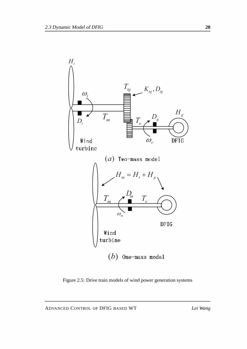
2.1 Schematic diagram of a fixed-speed wind turbine . . . . . . . .. . 122.2 Schematic diagram of Type B wind turbine . . . . . . . . . . . . . 142.3 Schematic diagram of Type C wind turbine . . . . . . . . . . . . . 152.4 Schematic diagram of Type D wind turbine . . . . . . . . . . . . . 152.5 Drive train models of wind power generation systems . . . .. . . . 202.6 DFIM phase circuits . . . . . . . . . . . . . . . . . . . . . . . . . 212.7 a-b-c to α-β axes transformation of stationary frame . . . . . . . . . 232.8 Transformation between stationary reference frames for stator and
rotor variables . . . . . . . . . . . . . . . . . . . . . . . . . . . . . 242.9 Park transformation . . . . . . . . . . . . . . . . . . . . . . . . . . 262.10 Transformation of reference frames . . . . . . . . . . . . . . . .. 262.11 Dynamicd-q equivalent circuits of machine . . . . . . . . . . . . . 272.12 Power converter in DFIG based wind turbine . . . . . . . . . . .. 29
3.1 Power control under stator flux oriented frame . . . . . . . . .. . . 383.2 Power control under stator voltage oriented frame . . . . .. . . . . 403.3 Vector control scheme of grid-side converter . . . . . . . . .. . . . 403.4 Reference computation of rotor current from stator active and reac-
tive power . . . . . . . . . . . . . . . . . . . . . . . . . . . . . . . 493.5 References of stator active and reactive power . . . . . . . .. . . . 513.6 Stator active power regulation by RC & FLC, VC and tracking error 513.7 Stator active power regulation by RC & FLC, DPC and tracking error 523.8 Stator reactive power regulation by RC & FLC, VC and tracking error 523.9 Stator reactive power regulation by RC & FLC, DPC and tracking
error . . . . . . . . . . . . . . . . . . . . . . . . . . . . . . . . . . 533.10 Responses of stator active power under grid disturbance . . . . . . . 543.11 Responses of stator reactive power under grid disturbance . . . . . . 54
4.1 Wind turbine operation regions . . . . . . . . . . . . . . . . . . . . 594.2 The power coefficientCp versus tip speed ratio at different pitch angles 604.3 ψqs mode loci under time-varying wind speed . . . . . . . . . . . . 694.4 ψds mode loci under time-varying wind speed . . . . . . . . . . . . 704.5 ψdr mode loci under time-varying wind speed . . . . . . . . . . . . 70
ix
4.6 ψds mode loci under grid disturbance . . . . . . . . . . . . . . . . . 724.7 ψdr mode loci under grid disturbance . . . . . . . . . . . . . . . . . 724.8 ψds mode loci under parameter uncertainty . . . . . . . . . . . . . . 734.9 ψdr mode loci under parameter uncertainty . . . . . . . . . . . . . . 744.10 Wind speed with large step changes . . . . . . . . . . . . . . . . . 754.11 The power coefficient and its ITAE under the step change of wind
speed . . . . . . . . . . . . . . . . . . . . . . . . . . . . . . . . . 764.12 The rotor speed and its ITAE under the step change of windspeed . 774.13 The electric power and its ITAE under the step change of wind speed 784.14 The stator reactive power under the step change of wind speed . . . 794.15 The rotor voltage ind- andq-axis under the step change of wind speed 794.16 Time-varying wind speed . . . . . . . . . . . . . . . . . . . . . . . 804.17 The power coefficient under the random wind speed . . . . . .. . . 814.18 The rotor speed under the random wind speed . . . . . . . . . . .. 814.19 The electric power under the random speed . . . . . . . . . . . .. 824.20 The stator reactive power under the random wind speed . .. . . . . 824.21 The rotor voltage ind- andq-axis under the random wind speed . . 834.22 The grid disturbance . . . . . . . . . . . . . . . . . . . . . . . . . 844.23 The power coefficient under the grid disturbance . . . . . .. . . . . 844.24 The rotor speed under the grid disturbance . . . . . . . . . . .. . . 854.25 The electric power under the grid disturbance . . . . . . . .. . . . 854.26 The stator reactive power under the grid disturbance . .. . . . . . . 864.27 The time-varying rotor resistance . . . . . . . . . . . . . . . . .. . 874.28 The power coefficient under the time-varying rotor resistance . . . . 884.29 The rotor speed under the time-varying rotor resistance . . . . . . . 884.30 The electric power under the time-varying rotor resistance . . . . . 894.31 The stator reactive power under the time-varying rotorresistance . . 894.32 The rotor voltage ind- andq-axis under the time-varying rotor re-
sistance . . . . . . . . . . . . . . . . . . . . . . . . . . . . . . . . 90
5.1 The typical power versus speed characteristics withoutwind speedmeasurement . . . . . . . . . . . . . . . . . . . . . . . . . . . . . 93
5.2 Control scheme of NAC with wind speed measurement . . . . . .. 1005.3 Control scheme of NAC without wind speed measurement . . .. . 1035.4 Step change of wind speed . . . . . . . . . . . . . . . . . . . . . . 1045.5 Power coefficient under step change of wind speed . . . . . . .. . 1055.6 Response of rotor speed under step change of wind speed . .. . . . 1055.7 Response of electric power under step change of wind speed . . . . 1065.8 Response of stator reactive power under step change of wind speed . 1065.9 Rotor voltage of NAC and FLC ind-axis . . . . . . . . . . . . . . . 1075.10 Rotor speedωr estimation and estimate error . . . . . . . . . . . . . 1075.11 Perturbation response off1 under step change of wind speed . . . . 1085.12 Stator reactive powerQs estimation and estimate error . . . . . . . 108
x
5.13 Perturbation response off2 under step change of wind speed . . . . 1095.14 Time-varying wind speed . . . . . . . . . . . . . . . . . . . . . . . 1105.15 Power coefficient under time-varying wind speed . . . . . .. . . . 1105.16 Response of rotor speed under time-varying wind speed .. . . . . . 1115.17 Response of electric power under time-varying wind speed . . . . . 1115.18 Response of stator reactive power under time-varying wind speed . . 1125.19 Rotor voltage of NAC and FLC ind-axis . . . . . . . . . . . . . . . 1125.20 Rotor speedωr estimation and estimate error . . . . . . . . . . . . . 1135.21 Perturbation response off1 under time-varying wind speed . . . . . 1145.22 Stator reactive powerQs estimation and estimate error . . . . . . . 1145.23 Perturbation response off2 under time-varying wind speed . . . . . 1155.24 Case of without wind speed measurement . . . . . . . . . . . . . .1155.25 Response of rotor speed without wind speed measurement. . . . . 1165.26 Response of electric power without wind speed measurement . . . . 1165.27 Response of stator reactive power without wind speed measurement 1175.28 Rotor voltage of NAC and FLC ind-axis without wind speed mea-
surement . . . . . . . . . . . . . . . . . . . . . . . . . . . . . . . . 1175.29 Electric power errors under uncertainties of rotor resistance . . . . . 1185.30 System outputs errors under uncertainties of rotor resistance . . . . 1195.31 Electric power errors under tower shadow . . . . . . . . . . . .. . 1205.32 System outputs errors under tower shadow . . . . . . . . . . . .. . 1205.33 Electric power errors under grid voltage dips . . . . . . . .. . . . . 1215.34 System outputs errors under grid voltage dips . . . . . . . .. . . . 122
xi

List of Tables
2.1 Cp coefficientsαi,j . . . . . . . . . . . . . . . . . . . . . . . . . . 18
3.1 Control parameters of FLC and proposed controller . . . . .. . . . 50
4.1 Behaviors for different eigenvalues . . . . . . . . . . . . . . . .. . 684.2 Eigenvalues under nominal operation point . . . . . . . . . . .. . 70
xii

Chapter 1
Introduction
1.1 Background
Wind power, as a clean and sustainable energy, has obtained highly concentra-
tions during the past decade [1], [2]. Research and development of renewable ener-
gy has gained tremendous momentum in the past decade as the cost of conventional
electrical power generation continuously escalate due to the limited fuel resources,
and the general public becomes increasingly concerned of the environmental im-
pacts caused by the thermal and nuclear generation. Among many technologies
promising green power, the utilization of wind energy via wind power generation
system (WPGS) is one of the most mature and well developed. Across the world,
the total capacity of wind generation has already exceeded giga-watt (GW) rating
and larger wind farms are constantly being planned and commissioned [3], [4], [5].
The main components of a WPGS includes the turbine rotor, gearbox, generator,
transformer, and possible power electronics. The turbine rotor converts the fluctu-
ating wind energy into mechanical energy, which is converted into electrical power
through the generator, and then transferred into the grid through a transformer and
transmission line. Wind turbines capture the power from thewind by means of
aerodynamically designed blades and convert it to rotatingmechanical power. The
number of blades is normally three and the rotational speed decreases as the radius
of the blade increases. For meag-watt range wind turbines the rotational speed will
1

1.2 Challenges & Problems 2
be 10-15 rpm. The weight-efficient way to convert the low-speed, high-torque pow-
er to electrical power is to use a gearbox and a generator withstandard speed. The
gearbox adapts the low speed of the turbine rotor to the high speed of the generator.
The gearbox may be not necessary for multi-pole generator systems.
The generator converts the mechanical power into electrical energy, which is
fed into a grid through a power electronic converter, and a transformer with circuit
breakers and electricity meters. The connection of wind turbines to the grid is possi-
ble at low voltage, medium voltage, high voltage, and even atthe extra high voltage
system since the transmittable power of an electricity system usually increases with
increasing the voltage level. While most of the turbines arenowadays connected to
the medium voltage system, large offshore wind farms are connected to the high and
extra high voltage level.
Doubly fed induction generators (DFIG) based wind turbines(DFIG-WT), a typ-
ical employed WPGS, have be widely used to achieve the maximum power conver-
sion, smaller capacity of power electronic devices and fullcontrollability of active
and reactive power of the DFIG [6], due to their characteristics such as varying speed
operation. The stator circuit of the DFIG is connected to thegrid directly, while the
rotor circuit is fed via a back-to-back power converter. Theback-to-back converter
consists of two converters, i.e., rotor-side converter andgrid-side converter, which
are connected ”back-to-back”. Between the two converters adc-link capacitor is
placed, as energy storage, in order to keep the voltage variations (or ripple) in the
dc-link small.
1.2 Challenges & Problems
1.2.1 Nonlinear dynamics of DFIG-WT
The DFIG-WT is a dynamic system with strong nonlinear coupled characteris-
tics and time varying uncertain inputs. The aerodynamic of wind turbine introduces
strong nonlinearities and uncertainties [28]. Objectivesof the wind-turbine con-
troller depend upon the operating area defined via wind speed[29]. For low wind
speeds, it is more important to maximize wind power capture while it is recommend-
ADVANCED CONTROL OFDFIG BASED WT Lei Wang

1.2 Challenges & Problems 3
ed to limit power production and rotor speed above the rated wind speed to protect
the mechanical part of the WPGS. The power regulation of the wind turbine is a
highly nonlinear system as the plant, actuation and controlobjectives are all strong
nonlinear [30].
As an induction machine, the DFIG is also a typical nonlinearsystem as induc-
tion motor, which has been used widely as a test benchmark fornonlinear control
system design. With the time-varying and intermittent windpower input, DFIG-WT
is required to operate at an operation envelope with a wide range rather than one op-
eration point. Moreover, during voltage sags due to grid load disturbances or grid
faults, DFIG-WT will operate far away from its normal operation point. During the
grid fault period and post-fault period, terminal voltage normally dropped close to
the ground and cause the strong dynamics in the stator and rotor currents, and such
that stator-flux will not be remained as constant as well. This will destroy the condi-
tion of the mostly used VC schemes for DFIG-WTs and dynamic ofthe active and
reactive power of the DFIG are still coupled during the transient period of stator-
flux or stator-voltage. As all vector control schemes dependupon the assumptions
of constant voltage and flux to realize asymptotical decoupling control of the active
and the reactive power, it can expect that their performancewill be degraded during
voltage sags and grid faults. On the other side, unlike the vector control of induction
motor in which the rotor flux is controlled directly, stator-flux of the DFIG normally
is not one of the controlled variables and thus not controlled directly.
The control function within the vector control scheme has commonly been per-
formed by using PI controllers. One challenge is how to tune the parameters of
the PI loops to provide optimal performance around one special operation point
and cope with the time-varying operation points. For examples, many results have
been done to automatically tune the PI controller’s parameters, such as using ge-
netic algorithm [42] and particle swarm optimization [43].Automatic tuning based
on artificial intelligence and gain schedule technique havebeen proposed to provide
optimal performance for a varying operation condition. Input/output linearization
have been proposed to fully decoupling control of inductionmotor [50, 85]. When
the wind turbine operates at varying speed to achieve the maximum wind power con-
ADVANCED CONTROL OFDFIG BASED WT Lei Wang
1.2 Challenges & Problems 4
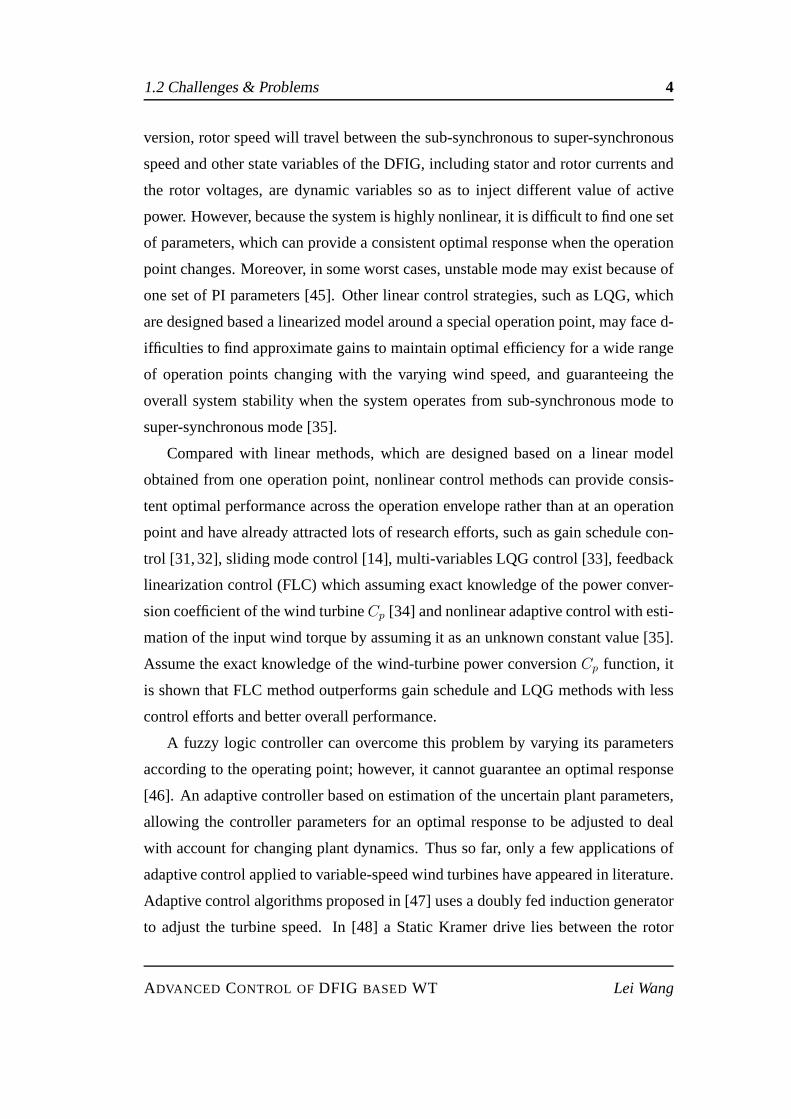
version, rotor speed will travel between the sub-synchronous to super-synchronous
speed and other state variables of the DFIG, including stator and rotor currents and
the rotor voltages, are dynamic variables so as to inject different value of active
power. However, because the system is highly nonlinear, it is difficult to find one set
of parameters, which can provide a consistent optimal response when the operation
point changes. Moreover, in some worst cases, unstable modemay exist because of
one set of PI parameters [45]. Other linear control strategies, such as LQG, which
are designed based a linearized model around a special operation point, may face d-
ifficulties to find approximate gains to maintain optimal efficiency for a wide range
of operation points changing with the varying wind speed, and guaranteeing the
overall system stability when the system operates from sub-synchronous mode to
super-synchronous mode [35].
Compared with linear methods, which are designed based on a linear model
obtained from one operation point, nonlinear control methods can provide consis-
tent optimal performance across the operation envelope rather than at an operation
point and have already attracted lots of research efforts, such as gain schedule con-
trol [31,32], sliding mode control [14], multi-variables LQG control [33], feedback
linearization control (FLC) which assuming exact knowledge of the power conver-
sion coefficient of the wind turbineCp [34] and nonlinear adaptive control with esti-
mation of the input wind torque by assuming it as an unknown constant value [35].
Assume the exact knowledge of the wind-turbine power conversionCp function, it
is shown that FLC method outperforms gain schedule and LQG methods with less
control efforts and better overall performance.
A fuzzy logic controller can overcome this problem by varying its parameters
according to the operating point; however, it cannot guarantee an optimal response
[46]. An adaptive controller based on estimation of the uncertain plant parameters,
allowing the controller parameters for an optimal responseto be adjusted to deal
with account for changing plant dynamics. Thus so far, only afew applications of
adaptive control applied to variable-speed wind turbines have appeared in literature.
Adaptive control algorithms proposed in [47] uses a doubly fed induction generator
to adjust the turbine speed. In [48] a Static Kramer drive lies between the rotor
ADVANCED CONTROL OFDFIG BASED WT Lei Wang

1.2 Challenges & Problems 5
circuit and the grid. Using this configuration the generatortorque and hence the
turbine speed is changed by adjusting the firing angle of the inverter. A similar
scheme was used in [35], where the excitation voltage acrossthe rotor circuit was
also adjusted.
1.2.2 Uncertain wind power inputs
Variable speed operation of DFIG-WT operates under time-varying uncertain
wind power input, due to time-varying wind speed. Besides the wind turbulence,
tower shadow effect of the horizontal axis wind turbine willalso cause periodical
variation on the input wind power, even with constant average wind speed. Most
works do not consider the time-varying characteristics of the wind power at the
designing stage, while validate the effect of the controller to reject the time-varying
wind power via simulation. The wind speed is assuming to be constant such that
the input torque is treated as a constant. A few works are treating it as a time-
varying input. Most adaptive control of WT assumes the inputtorque as an unknown
constant or slow time-varying and updates it via an estimator, because there is not an
effective method in the control filed to estimate the fast andtime-varying unknown
parameters and dynamics. Sliding mode methods treats the time-varying input as
parts of the uncertainties [49].
1.2.3 Fault ride through requirement
With the penetration level of wind energy increased in the current power grid,
fault ride through (FRT) capability has been introduced into most grid codes as one
of the important requirements for the WPGS [15]. The FRT capability, or known
as low voltage ride through (LVRT) capability, specifies that the WPGS must be
connected to the power grid during a grid fault to provide active power control to the
grid during and after the grid fault and to help re-establishthe grid voltage after the
clearance of the grid fault. The FRT capability is necessaryin integrating large-scale
wind power generations into the power networks, because it reduces the spinning
reserve demands required for the intermittent wind power and impacts of voltage
ADVANCED CONTROL OFDFIG BASED WT Lei Wang

1.2 Challenges & Problems 6
and stability of the grid.
The FRT is of special interest to DFIG-WT since the stator of the DFIG is con-
nected directly with the grid and is sensitive to voltage sags caused by grid faults
or load disturbances. The voltage sags of the stator will result in a sharp increase
of the stator-flux and over currents of the stator and the rotor windings due to the
magnetic coupling between the stator and the rotor windings. These over currents,
called inrush currents, may be raised up to three times of their rated values and
will damage the rotor and stator windings. And the most serious consequence of
such inrush currents is that they can lead to the breakdown ofthe rotor-side power
electronic converter. The voltage sags will also yield the fluctuation of the DC-link
voltage, which is controlled via the grid-side converter, and will in turn, affect the
dynamic of the rotor-side converter since the DC voltage is required to be remained
as constant for operation of the rotor-side converter.
Traditionally, the FRT capability of the DFIG-WT is achieved by the installing
crowbar protection of the rotor-side converter [16–18]. However, this solution can-
not avoid the disconnection of the wind turbine with the gridduring the fault. A
sudden loss of large-capacity wind power during the fault will introduce frequency
and voltage control problems in the network. Moreover, short-circuit of the rotor
of the DFIG converts the DFIG into a squirrel-cage inductiongenerator and loss
control over the power of the DFIG, which will consume more reactive power and
worsen the voltage sag as the voltage regulation from the power network needs re-
active power support during the fault clearing and after thefault period.
Other two methods of improving the FRT capability are hardware modification
and designing/modifying of the control of the DFIG-WT [19–22]. There is a lots of
efforts on investigating and improving of the LVRT of the DFIG-WT via improving
and designing an advanced controller to limit the peak valueof rotor inrush current
and the fluctuation of the dc-link voltage [20–22]. However,most results reported
are based on vector control schemes, which rely on the assumptions of a constant
stator-flux and stator-voltage. Due to the relatively smaller value to the stator re-
sistance compared with the mutual inductanceLs, stator resistanceRs is always
supposed to be zero in the VC scheme. In fact, dynamic of the stator-flux is a poorly
ADVANCED CONTROL OFDFIG BASED WT Lei Wang
1.2 Challenges & Problems 7
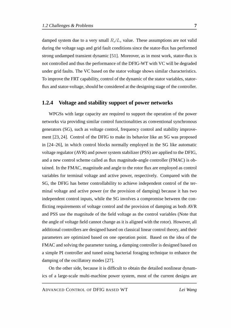
damped system due to a very smallRs/Ls value. These assumptions are not valid
during the voltage sags and grid fault conditions since the stator-flux has performed
strong undamped transient dynamic [51]. Moreover, as in most work, stator-flux is
not controlled and thus the performance of the DFIG-WT with VC will be degraded
under grid faults. The VC based on the stator voltage shows similar characteristics.
To improve the FRT capability, control of the dynamic of the stator variables, stator-
flux and stator-voltage, should be considered at the designing stage of the controller.
1.2.4 Voltage and stability support of power networks
WPGSs with large capacity are required to support the operation of the power
networks via providing similar control functionalities asconventional synchronous
generators (SG), such as voltage control, frequency control and stability improve-
ment [23, 24]. Control of the DFIG to make its behavior like anSG was proposed
in [24–26], in which control blocks normally employed in theSG like automatic
voltage regulator (AVR) and power system stabilizer (PSS) are applied to the DFIG,
and a new control scheme called as flux magnitude-angle controller (FMAC) is ob-
tained. In the FMAC, magnitude and angle to the rotor flux are employed as control
variables for terminal voltage and active power, respectively. Compared with the
SG, the DFIG has better controllability to achieve independent control of the ter-
minal voltage and active power (or the provision of damping)because it has two
independent control inputs, while the SG involves a compromise between the con-
flicting requirements of voltage control and the provision of damping as both AVR
and PSS use the magnitude of the field voltage as the control variables (Note that
the angle of voltage field cannot change as it is aligned with the rotor). However, all
additional controllers are designed based on classical linear control theory, and their
parameters are optimized based on one operation point. Based on the idea of the
FMAC and solving the parameter tuning, a damping controlleris designed based on
a simple PI controller and tuned using bacterial foraging technique to enhance the
damping of the oscillatory modes [27].
On the other side, because it is difficult to obtain the detailed nonlinear dynam-
ics of a large-scale multi-machine power system, most of thecurrent designs are
ADVANCED CONTROL OFDFIG BASED WT Lei Wang
1.3 Motivations 8
carried out based on a single-machine-infinite-bus (SMIB) system, and then veri-
fy the controller’s performance in the multi-machine powersystems via simulation
studies. Interactions with the power networks require thatthe dynamic of the pow-
er networks must be considered during the design stage of thecontroller, i.e., the
design of the controllers did better be carried out in multi-machine-power-systems.
Decentralised nonlinear control has been proposed for the improvement of transient
stability of a power system, in which terminal voltage of theDFIG and slip speed
are decoupled controlled viad-q components of the rotor voltage [36]. The design is
based on a simplified third-order model of the DFIG with stator dynamics ignored,
while the input prime wind power is assumed as constant.
1.3 Motivations
The performance of DFIG-WT depends heavily upon the controllers applied on
the generator side and the wind turbine side. The DFIG-WT is usually controlled via
a cascaded structure including an inner fast-loop for powerregulation of the DFIG
and an outer relative slow loop for the speed control of drivetrain. The reference of
active power of the DFIG is determined based on the maximum energy conversion,
which is defined as maximum power point tracking (MPPT), whenwind speed is
below the rated value; while constant reference is given when wind speed is above
the rated value. The wind turbine also employs pitch angle control to regulate the
extracted power from wind source by wind turbine for wind speed above the rated
value, while pitch angle is fixed when wind speed below the rated value.
Main purposes of this thesis are to develop advanced controlstrategies for DFIG-
WTs to improve the energy conversion efficiency and the transient dynamics of
DFIG-WTs, by considering nonlinear dynamics, uncertain wind power inputs and
grid faults. At first, modeling of a DFIG-WT and the conventional vector control
have been reviewed and prepared for the following research.Then a fully decoupled
power controller is proposed by using nonlinear control to improve the asymptot-
ically decoupled characteristics provided by VCs. Thirdly, nonlinear control has
been proposed for the Maximum Power Point Tracking (MPPT) ofDFIG-WTs op-
ADVANCED CONTROL OFDFIG BASED WT Lei Wang
1.4 Thesis Outline 9
erating below the rated wind speed. Both modal analysis and simulation studies
have been carried out. Finally, to improve the robustness ofthe nonlinear control
and to compensate the time-varying and uncertain wind powerinputs, a nonlinear
adaptive control based on perturbation estimation has beenstudied for the MPPT of
DFIG-WTs.
1.4 Thesis Outline
• Chapter 2 presents the modeling of a doubly fed induction generator based
variable-speed wind turbine, including dynamic model of wind turbine, drive
train, DFIG and power electrical converters. For the controller design, the
dynamic model of DFIG is obtained under the two-phased-q rotating ref-
erence frame by applying Clarke and Park’s transformationsof the original
three-phase natural reference frame.
• Chapter 3 proposes a nonlinear power control for DFIG. The conventional
used power control strategy, vector control, is recalled atfirst. As vector con-
trol can only achieve the asymptotical regulation of the active/reactive powers
of the DFIG, a fully decoupled nonlinear power control basedon feedback
linearization control is designed for the direct power control of the DFIG.
Moreover, a cascade two stages nonlinear controller, whichconsists of an
outer loop to provide current reference for the rotor current from the stator ac-
tive and reactive powers, and an inner loop applies the input/output feedback
linearization control for the current regulation.
• In Chapter 4, the nonlinear control based maximum power point tracking is
studied. The operation regions of wind turbine are introduced at first, where
MPPT control normally works in the range between the cut-in and rated wind
speed. Both VC and FLC are applied for MPPT control under time-varying
wind speeds, to achieve the maximum power extraction from the wind power.
Modal analysis is used to analysis the dynamics of DFIG-WT provided by
VC and FLC respectively, which shows that the FLC can provideconsistent
ADVANCED CONTROL OFDFIG BASED WT Lei Wang

1.4 Thesis Outline 10
dynamics with time-varying wind power inputs.
• Chapter 5 investigates the nonlinear adaptive control for DFIG-WT in order
to deal with the parameter uncertainties, uncertain wind power inputs and
improve the robustness of the nonlinear controller proposed in Chapter 4. The
proposed adaptive controller designs a perturbation observer to estimate the
real time perturbation and uses it to compensate the real uncertainties and
disturbances. The design includes two cases: with and without wind speed
measurement are carried out, followed by simulation studies.
• Chapter 6 presents conclusions and possible future works.
ADVANCED CONTROL OFDFIG BASED WT Lei Wang
Chapter 2
Models of a DFIG based Variable
Speed Wind Turbine
This chapter describes models of a wind power generation system equipped with
doubly fed induction generator for variable speed wind turbine. Different typical
configurations of WPGS are reviewed at first. The aerodynamicof wind turbine,
drive train, generator(DFIG), and power electrical converters are investigated re-
spectively. Detailed models of the DFIG based on different reference frames are
given.
2.1 Introduction
Most modern WPGSs use horizontal axis design, three blades and upwind wind
turbines. The larger WTs tend to operate at variable speed whereas smaller, simpler
turbines are of fixed speed. For a fixed-speed wind turbine, the turbulence of the
wind results in power variations, and thus affect the power quality of the grid. As in
a variable-speed wind turbine, the generator is controlledby power electronic equip-
ments, which makes it possible to control the rotor speed to maximize the energy
conversion efficiency. In this way, the power fluctuations caused by wind variation-
s can be absorbed by changing the rotor speed. Thus power variation originating
from the wind variations and the stress of the drive train canbe reduced. Hence, the
11
2.1 Introduction 12
power quality impact caused by the wind turbine can be improved, compared to a
fixed-speed turbine.
Fixed-speed wind turbines
This type of turbines are also called Type A turbine. Fixed-speed wind turbines
are electrically fairly simple devices consisting of a WT rotor, a low-speed shaft, a
gearbox, a high-speed shaft and an induction (or called as asynchronous) genera-
tor. From the electrical system viewpoint, they are perhapsbest considered as large
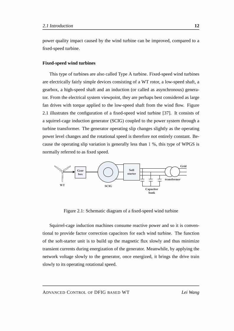
fan drives with torque applied to the low-speed shaft from the wind flow. Figure
2.1 illustrates the configuration of a fixed-speed wind turbine [37]. It consists of
a squirrel-cage induction generator (SCIG) coupled to the power system through a
turbine transformer. The generator operating slip changesslightly as the operating
power level changes and the rotational speed is therefore not entirely constant. Be-
cause the operating slip variation is generally less than1 %, this type of WPGS is
normally referred to as fixed speed.
SCIGWT
Soft
starterGear
box
Grid
Capacitor
bank
transformer
Figure 2.1: Schematic diagram of a fixed-speed wind turbine
Squirrel-cage induction machines consume reactive power and so it is conven-
tional to provide factor correction capacitors for each wind turbine. The function
of the soft-starter unit is to build up the magnetic flux slowly and thus minimize
transient currents during energization of the generator. Meanwhile, by applying the
network voltage slowly to the generator, once energized, itbrings the drive train
slowly to its operating rotational speed.
ADVANCED CONTROL OFDFIG BASED WT Lei Wang
2.1 Introduction 13
Variable speed wind turbine
During the past few years, variable-speed wind turbines have become the dom-
inant type among the installed wind turbines. Variable-speed wind turbines are
designed to achieve maximum aerodynamic efficiency over a wide range of wind
speeds. With a variable-speed operation, it has become possible continuously to
adapt (accelerate or decelerate) the rotational speedωr of the wind turbine to the
wind speedVwind. Thus, the tip speed ratioλ can be controlled at a predefined
optimal value that corresponds to the maximum power coefficient. Contrary to a
fixed-speed system, the variations in wind are absorbed by changes in the generator
speed. The electrical system of a variable-speed wind turbine is more complicated
than that of a fixed-speed wind turbine. It is typically equipped with an induc-
tion or synchronous generator and connected to the grid through power converters.
The power converters control the generator speed; that is, the power fluctuation-
s caused by wind variations are absorbed mainly by changes inthe rotor speed of
generator and consequently in the rotor speed of wind turbine. The advantages of
variable-speed wind turbines are an increased energy capturing efficiency, improved
power quality and reduced mechanical stress on the wind turbine. The disadvan-
tages are losses in power electronics converters, the use ofmore components and
the increased cost of equipment and maintenance because of the power electronic-
s. The introduction of variable-speed wind-turbine types increases the number of
applicable generator types and also introduces several degrees of freedom in the
combination of generator typed and power converter type [38].
Most common used variable speed wind turbine configurationsare listed as fol-
lows.
a Limited variable speed (Type B)
b Variable speed with partial scale frequency converter (Type C)
c Variable speed with full scale frequency converter (Type D)
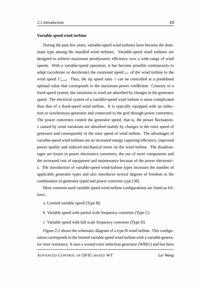
Figure 2.2 shows the schematic diagram of a type B wind turbine. This configu-
ration corresponds to the limited variable speed wind turbine with a variable genera-
tor rotor resistance. It uses a wound rotor induction generator (WRIG) and has been
ADVANCED CONTROL OFDFIG BASED WT Lei Wang
2.1 Introduction 14
used by the Danish manufacturer Vestas since mid 1990s. The generator is directly
connected to the grid. A capacitor bank performs the reactive power compensation.
A smoother grid connection is achieved by using a soft-starter. The unique feature
of this concept is that it has a variable additional rotor resistance, which can be
changed by an optimally controlled converter mounted on therotor shaft. Thus, the
total rotor resistance is controllable. This optical coupling eliminates the need for
costly slip rings that need brushes and maintenance.
WRIGWT
Soft
starterGear
box
Grid
Capacitor
bank
transformer
Variable
resistance
Figure 2.2: Schematic diagram of Type B wind turbine
The rotor resistance can be changed and thus the slip is controlled to regulate
the power output of the WPGS. The range of the speed control depends on the
size of the variable rotor resistance. Typically, the speedrange is from0 to 10 %
above synchronous speed. Wallace and Oliver (1998) describe an alternative concept
by using passive components instead of a power electronic converter, which can
achieves a10 % slip range.
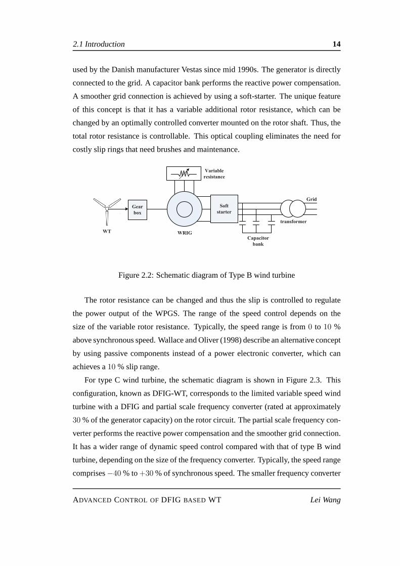
For type C wind turbine, the schematic diagram is shown in Figure 2.3. This
configuration, known as DFIG-WT, corresponds to the limitedvariable speed wind
turbine with a DFIG and partial scale frequency converter (rated at approximately
30 % of the generator capacity) on the rotor circuit. The partial scale frequency con-
verter performs the reactive power compensation and the smoother grid connection.
It has a wider range of dynamic speed control compared with that of type B wind
turbine, depending on the size of the frequency converter. Typically, the speed range
comprises−40 % to+30 % of synchronous speed. The smaller frequency converter
ADVANCED CONTROL OFDFIG BASED WT Lei Wang
2.1 Introduction 15
makes this concept attractive from an economical point of view. Compared with
type B, its main drawbacks are the use of slip rings and protection of the converters
in the case of grid faults.
WRIG
WT
Gear
box
Grid
transformer
Partial scale
frequency converter
Figure 2.3: Schematic diagram of Type C wind turbine
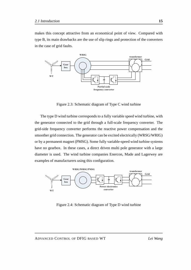
The type D wind turbine corresponds to a fully variable speedwind turbine, with
the generator connected to the grid through a full-scale frequency converter. The
grid-side frequency converter performs the reactive powercompensation and the
smoother grid connection. The generator can be excited electrically (WRSG/WRIG)
or by a permanent magnet (PMSG). Some fully variable-speed wind turbine systems
have no gearbox. In these cases, a direct driven multi pole generator with a large
diameter is used. The wind turbine companies Enercon, Made and Lagerwey are
examples of manufacturers using this configuration.
WRIG/WRSG/PMSG
WT
Gear
box
Grid
transformer
Power electronics
converter
Figure 2.4: Schematic diagram of Type D wind turbine
ADVANCED CONTROL OFDFIG BASED WT Lei Wang

2.2 Aerodynamics of Wind Turbines & Drive Train Model 16
2.2 Aerodynamics of Wind Turbines & Drive Train
Model
Wind turbines produce electricity by converting the mechanical power of the
wind to drive an electrical generator. Wind passes over the blades, generating lift and
exerting a turning force. The rotating blades turn a shaft inside the nacelle, which
goes into a gearbox. The gearbox increases the rotational speed to an appropriate
value for the generator, which uses magnetic fields to convert the mechanical energy
into electrical energy.
The power contained in the wind is given by the kinetic energyof the flowing
air mass per unit time [39]. That is
Pair =1
2ρπR2V 3
wind (2.2.1)
wherePair is the power contained in wind (in W),ρ is the air density (1.225 kg/m2 at
15 degree and normal pressure),R is the blade length (in m), andVwind is the wind
velocity (in m/s) without rotor interference, i.e., ideally locating at infinite distance
from the rotor.
The power captured by the wind turbinePm is given by the power conversion
coefficient
Cp =Pm
Pair
(2.2.2)
Pm = Pair × Cp =1
2CpρπR
2V 3wind (2.2.3)
whereCp is the power conversion coefficient.
A maximum value ofCp is defined by the Betz limit, which states that a turbine
can never extract more than0.593 of the power from an air stream. In reality, wind
turbine haveCp values in the range0.25-0.45.
For a given wind turbine, the coefficientCp is dependent upon the aerodynamic
characteristic of the wind turbine, and a complex nonlinearfunction of the blade tip
speed ratioλ = ωrRVwind
(whereωr is the angular speed of the rotor) and the blade pitch
angleβ. Generally,Cp can be obtained experimentally by carrying out wind tunnel
tests and measuring the real output of the wind turbine underdifferent wind speeds
ADVANCED CONTROL OFDFIG BASED WT Lei Wang
2.2 Aerodynamics of Wind Turbines & Drive Train Model 17
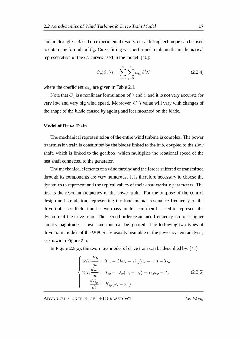
and pitch angles. Based on experimental results, curve fitting technique can be used
to obtain the formula ofCp. Curve fitting was performed to obtain the mathematical
representation of theCp curves used in the model: [40]:
Cp(β, λ) =4∑
i=0
4∑
j=0
αi,jβiλj (2.2.4)
where the coefficientαi,j are given in Table 2.1.
Note thatCp is a nonlinear formulation ofλ andβ and it is not very accurate for
very low and very big wind speed. Moreover,Cp’s value will vary with changes of
the shape of the blade caused by ageing and ices mounted on theblade.
Model of Drive Train
The mechanical representation of the entire wind turbine iscomplex. The power
transmission train is constituted by the blades linked to the hub, coupled to the slow
shaft, which is linked to the gearbox, which multiplies the rotational speed of the
fast shaft connected to the generator.
The mechanical elements of a wind turbine and the forces suffered or transmitted
through its components are very numerous. It is therefore necessary to choose the
dynamics to represent and the typical values of their characteristic parameters. The
first is the resonant frequency of the power train. For the purpose of the control
design and simulation, representing the fundamental resonance frequency of the
drive train is sufficient and a two-mass model, can then be used to represent the
dynamic of the drive train. The second order resonance frequency is much higher
and its magnitude is lower and thus can be ignored. The following two types of
drive train models of the WPGS are usually available in the power system analysis,
as shown in Figure 2.5.
In Figure 2.5(a), the two-mass model of drive train can be described by: [41]
2Ht
dωt
dt= Tm −Dtωt −Dtg(ωt − ωr)− Ttg
2Hg
dωr
dt= Ttg +Dtg(ωt − ωr)−Dgωr − Te
dTtgdt
= Ktg(ωt − ωr)
(2.2.5)
ADVANCED CONTROL OFDFIG BASED WT Lei Wang

2.2 Aerodynamics of Wind Turbines & Drive Train Model 18
Table 2.1:Cp coefficientsαi,j
i j αi,j
4 4 4.9686e-010
4 3 -7.1535e-008
4 2 1.6167e-006
4 1 -9.4839e-006
4 0 1.4787e-005
3 4 -8.9194e-008
3 3 5.9924e-006
3 2 -1.0479e-004
3 1 5.7051e-004
3 0 -8.6018e-004
2 4 2.7937e-006
2 3 -1.4855e-004
2 2 2.1495e-003
2 1 -1.0996e-002
2 0 1.5727e-002
1 4 -2.3895e-005
1 3 1.0683e-003
1 2 -1.3934e-002
1 1 6.0405e-002
1 0 -6.7606e-002
0 4 1.1524e-005
0 3 -1.3365e-004
0 2 -1.2406e-002
0 1 2.1808e-001
0 0 -4.1909e-001
ADVANCED CONTROL OFDFIG BASED WT Lei Wang

2.3 Dynamic Model of DFIG 19
whereωt andωr are the turbine and generator rotor speed, respectively;Tm and
Te are the mechanical torque applied to the turbine and the electrical torque of the
generator, respectively;Ttg is an internal torque of the model;Ht andHg are the
inertia constants of the turbine and the generator, respectively; Dt andDg are the
damping coefficients of the turbine and the generator, respectively;Dtg is the damp-
ing coefficient of the flexible coupling between the two masses; Ktg is the shaft
stiffness.
To simplify the analysis, the drive train system can also be modeled as a single
lumped-mass system with a lumped inertia constantHm as in Figure 2.5(b):
Hm = Ht +Hg (2.2.6)
Therefore, one-mass model of drive trains is given by
2Hm
dωr
dt= Tm − Te −Dmωr (2.2.7)
whereDm is the damping of the lumped-mass system.
2.3 Dynamic Model of DFIG
Nowadays doubly fed induction machine has been widely used in WPGS. These
types of machines can be used resolutely as a generator or a motor. Though demands
as motor is less because of its mechanical wear at the slip rings but they have gained
their prominence for generator application in wind and hydro power plant because
of its obvious adoptability capacity and nature of controllability of power. In this
section, detailed model of DFIG has been given.
2.3.1 State space model in thea-b-c natural frame
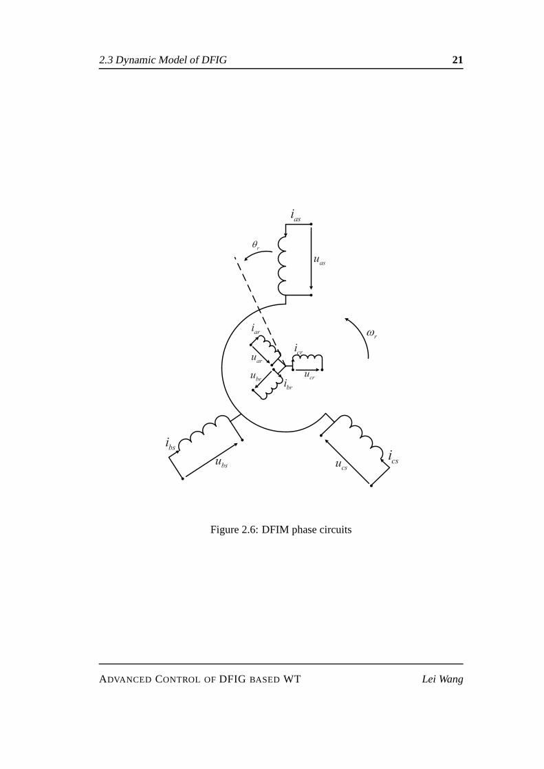
The DFIM is provided with laminated stator and rotor cores with uniform slots
in which three-phase winding are placed as shown in Figure 2.6. Usually, the rotor
winding is connected to copper slip-rings. Brushes on the stator collect the rotor cur-
rents from the rotor-side static power converter. For the time being, the resistances
ADVANCED CONTROL OFDFIG BASED WT Lei Wang
2.3 Dynamic Model of DFIG 20
t
tDmT
tgT ,tg tgK D
eT
r
gDgH
tH
( )a
m
mD
m t gH H H !
mT eT
( )b
Figure 2.5: Drive train models of wind power generation systems
ADVANCED CONTROL OFDFIG BASED WT Lei Wang
2.3 Dynamic Model of DFIG 21
asi
asur
r
cri
bri
ari
aru
bru cru
bsi
csibsu csu
Figure 2.6: DFIM phase circuits
ADVANCED CONTROL OFDFIG BASED WT Lei Wang
2.3 Dynamic Model of DFIG 22
of slip-ring-brush system are lumped into rotor phase resistances, and the convert-
er is replaced by an ideal controllable voltage source. The three-phase model of a
DFIG can be described as:
uas =dψas
dt+ iasRs
ubs =dψbs
dt+ ibsRs
ucs =dψcs
dt+ icsRs
(2.3.1)
uar =dψar
dt+ iarRr
ubr =dψbr
dt+ ibrRr
ucr =dψcr
dt+ icrRr
(2.3.2)
whereias, ibs, ics are the three-phase stator currents;iar, ibr, icr are the three-phase
rotor currents;uas, ubs, ucs are the three-phase stator voltages;uar, ubr, ucr are the
three-phase rotor voltages;ψas, ψbs, ψcs are the three-phase stator flux linkages;ψar,
ψbr, ψcr are the three-phase rotor flux linkages;Rs andRr are stator and rotor re-
sistances. Note that, the stator equations are representedin the stator natural frame,
and the rotor equations are described in the rotor natural frame.
2.3.2 Clarke transformation
Considering a symmetrical three phase induction machine with stationarya-
phase,b-phase andc-phase axes are placed at120 angle to each other, as shown in
Figure 2.7. The main aim of a Clarke transformation is to transform the three-phase
stationary frame variables into a two-phase stationary frame variablesα-β ,and vice
versa.
Any three-phase voltage or currentx in a-b-c components can be converted into
α-β components via Clarke transformation and can be represented in the matrix
form as
ADVANCED CONTROL OFDFIG BASED WT Lei Wang

2.3 Dynamic Model of DFIG 23
,a
sx
x
sx
b
c
Figure 2.7:a-b-c to α-β axes transformation of stationary frame
xα
xβ
x0
= TC
xa
xb
xc
(2.3.3)
whereTC is the transformation matrix of Clarke transformation,
TC =2
3
0 −12
−12
0√32
−√32
12
12
12
(2.3.4)
x0 is the zero sequence component, which equals to zero for symmetrical three-
phase variable. For example, the reference transformationof stator and rotor cur-
rents are described as follows, and the reference frames canbe seen in Figure 2.7.
iαs
iβs
i0s
= TC
ias
ibs
ics
(2.3.5)
ADVANCED CONTROL OFDFIG BASED WT Lei Wang

2.3 Dynamic Model of DFIG 24
rs
s
r
r
Figure 2.8: Transformation between stationary reference frames for stator and rotorvariables
iαr
iβr
i0r
= TC
iar
ibr
icr
(2.3.6)
where i0s and i0r are the zero sequence components of stator and rotor current,
respectively.
The rotor variables represented in the rotor stationary reference frame can be
referred to the stator stationary reference frame by a transformation matrixTθr, as
shown in Figure 2.8.[
isαr
isβr
]
= Tθr
[
iαr
iβr
]
(2.3.7)
where
Tθr =
[
cos θr − sin θr
sin θr cos θr
]
(2.3.8)
Note that, for simplified representation, the followingiαr andiβr are described for
the rotor current vectors referred to the stator stationaryreference frame, like in
Figure 2.9(a).
ADVANCED CONTROL OFDFIG BASED WT Lei Wang
2.3 Dynamic Model of DFIG 25
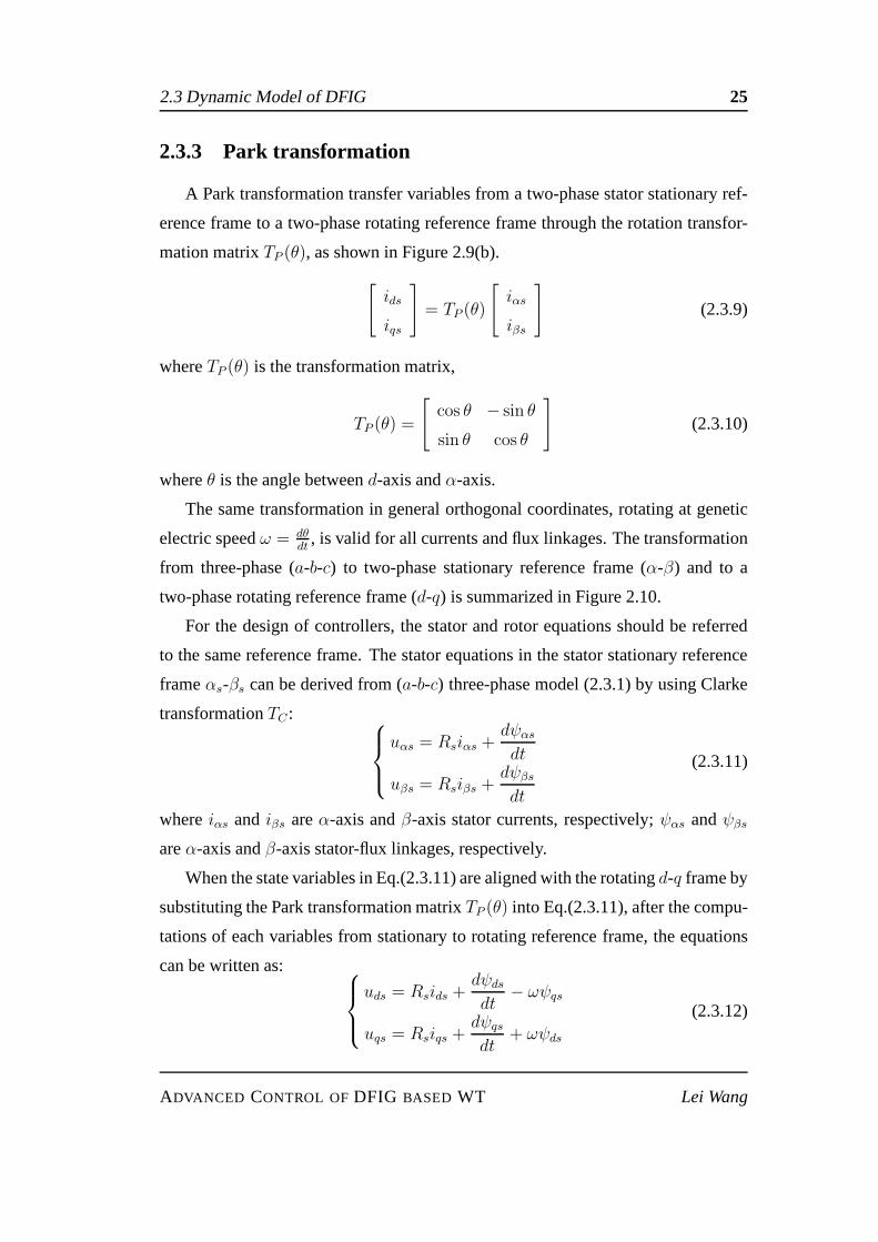
2.3.3 Park transformation
A Park transformation transfer variables from a two-phase stator stationary ref-
erence frame to a two-phase rotating reference frame through the rotation transfor-
mation matrixTP (θ), as shown in Figure 2.9(b).
[
ids
iqs
]
= TP (θ)
[
iαs
iβs
]
(2.3.9)
whereTP (θ) is the transformation matrix,
TP (θ) =
[
cos θ − sin θ
sin θ cos θ
]
(2.3.10)
whereθ is the angle betweend-axis andα-axis.
The same transformation in general orthogonal coordinates, rotating at genetic
electric speedω = dθdt
, is valid for all currents and flux linkages. The transformation
from three-phase (a-b-c) to two-phase stationary reference frame (α-β) and to a
two-phase rotating reference frame (d-q) is summarized in Figure 2.10.
For the design of controllers, the stator and rotor equations should be referred
to the same reference frame. The stator equations in the stator stationary reference
frameαs-βs can be derived from (a-b-c) three-phase model (2.3.1) by using Clarke
transformationTC :
uαs = Rsiαs +dψαs
dt
uβs = Rsiβs +dψβs
dt
(2.3.11)
whereiαs andiβs areα-axis andβ-axis stator currents, respectively;ψαs andψβs
areα-axis andβ-axis stator-flux linkages, respectively.
When the state variables in Eq.(2.3.11) are aligned with therotatingd-q frame by
substituting the Park transformation matrixTP (θ) into Eq.(2.3.11), after the compu-
tations of each variables from stationary to rotating reference frame, the equations
can be written as:
uds = Rsids +dψds
dt− ωψqs
uqs = Rsiqs +dψqs
dt+ ωψds
(2.3.12)
ADVANCED CONTROL OFDFIG BASED WT Lei Wang

2.3 Dynamic Model of DFIG 26
r
r !
"
d
q
!s
r
r
s
a) b)
Figure 2.9: Park transformation
a
b
c
s
s d
qClarke
Transformation
CT
Park
Transformation
( )PT
Stator and rotor
natural reference frame
Stator stationary
reference frame
sr
sr
Rotor stationary
reference frame
rT
Rotating reference
frame
Figure 2.10: Transformation of reference frames
ADVANCED CONTROL OFDFIG BASED WT Lei Wang
2.3 Dynamic Model of DFIG 27
su
si
sj !sR lsL lrL rR ( )r rj !"
ri
rus r mL
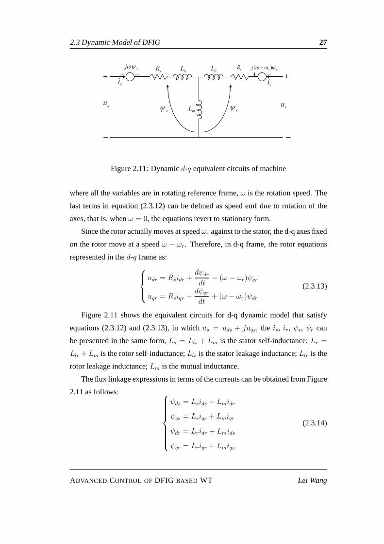
Figure 2.11: Dynamicd-q equivalent circuits of machine
where all the variables are in rotating reference frame,ω is the rotation speed. The
last terms in equation (2.3.12) can be defined as speed emf dueto rotation of the
axes, that is, whenω = 0, the equations revert to stationary form.
Since the rotor actually moves at speedωr against to the stator, the d-q axes fixed
on the rotor move at a speedω − ωr. Therefore, in d-q frame, the rotor equations
represented in thed-q frame as:
udr = Rsidr +dψdr
dt− (ω − ωr)ψqr
uqr = Rsiqr +dψqr
dt+ (ω − ωr)ψdr
(2.3.13)
Figure 2.11 shows the equivalent circuits for d-q dynamic model that satisfy
equations (2.3.12) and (2.3.13), in whichus = uds + juqs, the is, ir, ψs, ψr can
be presented in the same form,Ls = Lls + Lm is the stator self-inductance;Lr =
Llr + Lm is the rotor self-inductance;Lls is the stator leakage inductance;Llr is the
rotor leakage inductance;Lm is the mutual inductance.
The flux linkage expressions in terms of the currents can be obtained from Figure
2.11 as follows:
ψds = Lsids + Lmidr
ψqs = Lsiqs + Lmiqr
ψdr = Lridr + Lmids
ψqr = Lriqr + Lmiqs
(2.3.14)
ADVANCED CONTROL OFDFIG BASED WT Lei Wang

2.4 Model of Grid-side Converter and DC-link 28
The electromagnetic torque equation is represented as
Te = ψdsiqs − ψqsids = Lm(iqsidr − idsiqr) = ψdriqr − ψqridr (2.3.15)
In summary, the model of DFIG underd-q rotating reference frame can be
obtained by applying Clarke and Park transformations from equations (2.3.1) and
(2.3.2):
dψds
dt= uds − Rsids + ωψqs
dψqs
dt= uqs −Rsiqs − ωψds
dψdr
dt= udr − Rridr + (ω − ωr)ψqr
dψqr
dt= uqr − Rriqr − (ω − ωr)ψdr
(2.3.16)
The speedω of above model may take arbitrary value and result in conversion
among different reference frames: stator stationary reference frame (ω = 0), rotor
stationary reference frame (ω = ωr), synchronous rotating reference frame (ω =
ωs), whereωs is synchronous speed.
The active and reactive stator power equations are presented as:
Ps = udsids + uqsiqs
Qs = uqsids − udsiqs(2.3.17)
with the mathematical equations for computing the active and reactive powers
of rotor side
Pr = udridr + uqriqr
Qr = uqridr − udriqr(2.3.18)
2.4 Model of Grid-side Converter and DC-link
As shown in Figure 2.12, the power converter is made up of a back-to-back
converter connecting the rotor circuit and the grid, which is known as a Scherbius
scheme. The converters are typically made of voltage-fed current regulated invert-
ers, which enable a two-directional power flow. The invertervalves make use of
ADVANCED CONTROL OFDFIG BASED WT Lei Wang
2.4 Model of Grid-side Converter and DC-link 29
Rotor-side
converterDC-link
chopper
DC-link
capacitor
Grid-side
converter
Rotor-side
filter
Grid-side
filter
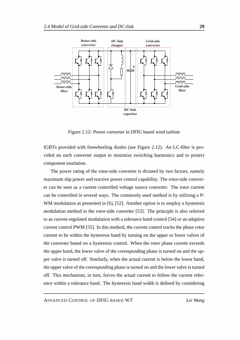
Figure 2.12: Power converter in DFIG based wind turbine
IGBTs provided with freewheeling diodes (see Figure 2.12).An LC-filter is pro-
vided on each converter output to minimize switching harmonics and to protect
component insulation.
The power rating of the rotor-side converter is dictated by two factors, namely
maximum slip power and reactive power control capability. The rotor-side convert-
er can be seen as a current controlled voltage source converter. The rotor current
can be controlled in several ways. The commonly used method is by utilizing a P-
WM modulation as presented in [6], [52]. Another option is toemploy a hysteresis
modulation method to the rotor-side converter [53]. The principle is also referred
to as current-regulated modulation with a tolerance band control [54] or an adaptive
current control PWM [55]. In this method, the current control tracks the phase rotor
current to be within the hysteresis band by turning on the upper or lower valves of
the converter based on a hysteresis control. When the rotor phase current exceeds
the upper band, the lower valve of the corresponding phase isturned on and the up-
per valve is turned off. Similarly, when the actual current is below the lower band,
the upper valve of the corresponding phase is turned on and the lower valve is turned
off. This mechanism, in turn, forces the actual current to follow the current refer-
ence within a tolerance band. The hysteresis band width is defined by considering
ADVANCED CONTROL OFDFIG BASED WT Lei Wang
2.4 Model of Grid-side Converter and DC-link 30
the switching frequency limitations and the switching losses of the IGBTs [56].
The power rating of the grid-side converter is mainly dictated by maximum slip
power since it usually operates at a unity power factor. A typical output voltage of
the gride-side converter is 480 V [57].
The grid-side converter is normally dedicated to control the dc-link voltage and
reactive power exchange between DC-link and the grid. It canalso be utilized to
support grid reactive power during a fault [58] and to enhance grid power qual-
ity [59]. However, these abilities are seldom utilized since they require a larger
converter rating. In stability studies, it is well acceptedto disregard the switching
dynamics of the converter and treat them as an ideal device. In addition, converters
are assumed to be able to follow the demanded values of the converter current fast
enough [60].
A detailed model of a grid-side converter presented in [6] isrecalled, where
the converter is modeled as a current-controlled voltage source. This constitutes a
representation of the dc-link capacitor and the grid-side filter in the model.
The ac-side circuit equation of the GSC can be written as
digabcdt
= −Rg
Lg
igabc +1
Lg
(ugabc − usabc) (2.4.1)
whereigabc, ugabc, usabc are the grid-side current, voltage and stator voltage in vec-
tors, respectively;Rg andLg are the reactance and inductance of grid-side converter.
By substituting the Clarke and Park transformation matrix Eq. (2.3.4) and (2.3.10)
into Eq. (2.4.1), the equation of the GSC will be representedin the rotating refer-
ence frame. After that, aligning thed-axis of the state variables with the grid voltage
vectorus (uds = us, uqs = 0), the followingd-q vector model can be obtained for
modeling the GSC ac-side:
udg = Rgidg + Lg
didgdt
− ωsLgiqg + us
uqg = Rgiqg + Lg
diqgdt
+ ωsLgidg
(2.4.2)
Neglecting harmonics due to switching and the losses in the GSC, the filtering
inductor and the transformer, the power balance equation can be obtained as
PDC = Pr − Pg = CuDC
duDC
dt(2.4.3)
ADVANCED CONTROL OFDFIG BASED WT Lei Wang
2.5 Summary 31
wherePr is the active power at the AC terminal of the rotor-side converter;Pg is the
active power at the AC terminal of the grid-side converter;PDC is the active power
of DC link. These are given by
Pr = udridr + uqriqr (2.4.4)
Pg = udgidg + uqgiqg (2.4.5)
PDC = uDCiDC (2.4.6)
whereidr andiqr are the d and q axis rotor currents, respectively;idq andiqg are the
d and q axis currents of grid-side converter, respectively;udq anduqg are the d and q
axis voltages of grid-side converter, respectively;vDC is the capacitor DC voltage;
iDC is the current of the capacitor.
2.5 Summary
In this chapter, different topologies of wind turbine generation system were re-
viewed. Types of variable-speed wind turbines are implemented in the current wind
power generation system more frequently than fix-speed windturbine, as the wind
power output is time-varying and uncertainty. Thereby, thecontrol design for dif-
ferent objectives will be worked out, base on the variable-speed wind turbine with a
doubly-fed induction generator in this thesis.
As follows, the dynamic modeling of drive train was investigated, and the one-
mass lumped model of drive train run through the following studies. The detailed
model of the DFIG system was also studied, with the Clarke andPark transforma-
tions. By apply the transformations, the state variables ofthe DFIG system can
be transformed into the two-phase vectors oriented with different rotating reference
frame, for simply controller design.
Finally, the dynamic of the DC-link capacitor and the grid-side converter con-
sidering the output filter were investigated for the studieson the control of grid-side
converter.
ADVANCED CONTROL OFDFIG BASED WT Lei Wang
Chapter 3
Nonlinear Power Control of DFIG
based Wind Turbine
3.1 Problem Description
Currently, variable speed WPGSs are continuously increasing their market share,
since they are capable of tracking the wind speed variationsby adapting the shaft
speed, and thus, achieving the optimal power generation. The mostly used WPGS
are based on DFIG, which stator is connected to the grid directly and rotor connects
through back to back converters. The major advantage of these facilities lies in
the fact that the power rate of the inverters is around the 25-30 % of the nominal
generator power.
The conventional control method for DFIG is vector control in whichd-q com-
ponents of rotor currents are directly linked with stator active power/reactive power
(or torque/ flux) and thus the current components can be used to control the stator
active and reactive power, respectively, by transforming all variables into a refer-
ence frame fixed to stator flux vector (or voltage vector) [61], [62]. Regarding to
this method, an accurate synchronization with the stator flux vector enables a de-
coupled control of the injection of the stator active power (Ps) and reactive power
(Qs), via theq-axis and thed-axis component of the rotor’s currents. In addition
to the decoupled control of the statorPs andQs, the synchronous rotating reference
32
3.1 Problem Description 33
frame transforms enables the vector control to treat the state variables of the machine
as DC signals. This feature has resulted in its implementation in most DFIG-WTs,
though the tuning of the controller parameters is not an easyjob.
Another drawback of the vector control is several transformations involved, as
well as the heavenly dependence with the stator flux positionmeasurement or es-
timation. Moreover, this method also requires accurate value of machine parame-
ters such as resistances and inductances and nonlinear operation of the DFIG is not
considered for tuning current controllers. Then performance of the vector control
method is affected by changing machine parameters and operation condition.
In [53], DFIG control mechanisms are reported using the stator-flux-oriented
frame with the position of the stator-flux space estimated through the measurement
of the stator-flux space vector inα-β reference frame. In [63], a stator-flux-oriented
DFIG control strategy is proposed, in which the position of the stator-flux space vec-
tor is estimated through the measurements of stator voltageand rotor-current space
vectors inα-β reference frame. In [64], a stator-flux-oriented control ofa cascaded
doubly-fed induction machine is proposed, in which one of the main approaches
used to estimate the position of stator flux space vector is toadd a delay angle
of 90o to the stator voltage space vector. Other control approaches are also pro-
posed recently, such as direct-power-control strategies using the stator-flux-oriented
frame [11], [12].
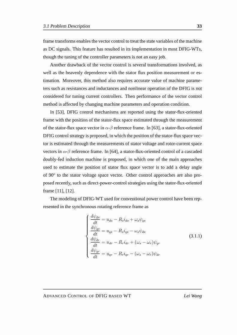
The modeling of DFIG-WT used for conventional power controlhave been rep-
resented in the synchronous rotating reference frame as
dψds
dt= uds −Rsids + ωsψqs
dψqs
dt= uqs − Rsiqs − ωsψds
dψdr
dt= udr −Rridr + (ωs − ωr)ψqr
dψqr
dt= uqr − Rriqr − (ωs − ωr)ψdr
(3.1.1)
ADVANCED CONTROL OFDFIG BASED WT Lei Wang
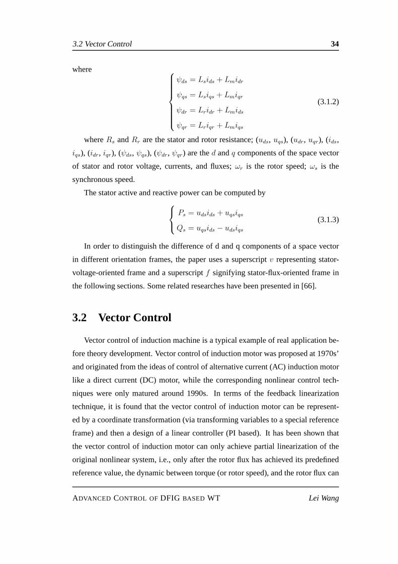
3.2 Vector Control 34
where
ψds = Lsids + Lmidr
ψqs = Lsiqs + Lmiqr
ψdr = Lridr + Lmids
ψqr = Lriqr + Lmiqs
(3.1.2)
whereRs andRr are the stator and rotor resistance; (uds, uqs), (udr, uqr), (ids,
iqs), (idr, iqr), (ψds, ψqs), (ψdr, ψqr) are thed andq components of the space vector
of stator and rotor voltage, currents, and fluxes;ωr is the rotor speed;ωs is the
synchronous speed.
The stator active and reactive power can be computed by
Ps = udsids + uqsiqs
Qs = uqsids − udsiqs(3.1.3)
In order to distinguish the difference of d and q components of a space vector
in different orientation frames, the paper uses a superscript v representing stator-
voltage-oriented frame and a superscriptf signifying stator-flux-oriented frame in
the following sections. Some related researches have been presented in [66].
3.2 Vector Control
Vector control of induction machine is a typical example of real application be-
fore theory development. Vector control of induction motorwas proposed at 1970s’
and originated from the ideas of control of alternative current (AC) induction motor
like a direct current (DC) motor, while the corresponding nonlinear control tech-
niques were only matured around 1990s. In terms of the feedback linearization
technique, it is found that the vector control of induction motor can be represent-
ed by a coordinate transformation (via transforming variables to a special reference
frame) and then a design of a linear controller (PI based). Ithas been shown that
the vector control of induction motor can only achieve partial linearization of the
original nonlinear system, i.e., only after the rotor flux has achieved its predefined
reference value, the dynamic between torque (or rotor speed), and the rotor flux can
ADVANCED CONTROL OFDFIG BASED WT Lei Wang
3.2 Vector Control 35
be decoupled; and then the relationship between the torque and the corresponding
current component is linear. During the transient period ofthe rotor flux, such as the
flux-weaken technique used in the high speed operation of induction motor to pre-
vent the voltage saturation, dynamic between torque and rotor flux is still coupled.
However, application of such techniques for DFIG has not reported in the available
literatures.
In the past two decades, modeling and control of DFIG-WT haveattracted ex-
tensive research efforts [6–14]. Among those results, the vector control (VC) with
proportional-integral (PI) loops is the most used control algorithm for the regula-
tion of the output power of the DFIG [6, 7] and is the current industrial standard,
due to the capability of decoupling control of active and reactive power and simple
structure. VC mainly consists of two steps: transforming the two-phase (α-β) sta-
tionary reference frame of DFIG model to a two-phased-q rotating reference frame
in which thed-axis is aligned with the vector of one of stator variables ofthe DFIG
(stator-flux or stator-voltage); and decoupling the interaction among state variables,
and independently controlling the active power and the reactive power by using the
PI loops, through thed-q components of the rotor voltage. Most used reference
frames are the stator-flux [6] and stator voltage orientatedframe [8, 9]. Transfor-
mation of variables of the DFIG into a new rotating referenceframe makes some
components of the state variable under the new reference frame be zero, thus the
decoupling of torque/active and reactive power and the linear relationship between
the rotor current/voltage and the controlled variables canbe achieved.
3.2.1 Control of rotor-side converter (RSC)
In this section, the conventional vector control methods for control of rotor-side
converter are investigated, which the state vectors are oriented with two reference
frames respectively. The control outputs are defined as the stator active and reactive
power, after the frame transformation, the linear relationship between the control
outputs and rotor current vectors can be obtained.
ADVANCED CONTROL OFDFIG BASED WT Lei Wang

3.2 Vector Control 36
Stator flux orientation (SFO) frame
In the stator-flux orientation frame, thed-axis of the reference frame is aligned
along the stator-flux vector so that the statorq-axis flux linkage is zero, andd-axis
flux linkage is constant, equal to the amplitude of the statorflux |ψs|, that is
ψfds = |ψs|
ψfqs = 0
(3.2.1)
Then, we can obtain that
ψfds
dt= 0
ψfqs
dt= 0
(3.2.2)
Based on first two equations of (3.1.1), and the assumption ofignoring the small
stator winding resistance (Rs ≈ 0), we have
dψfds
dt= ufds − Rsi
fds + ωsψ
fqs = 0
dψfqs
dt= ufqs − Rsi
fqs − ωsψ
fds = 0
(3.2.3)
Thereby, by substituting the assumptionRs ≈ 0 and the relationship given in Eq.
(3.2.1) into (3.2.3), the stator voltage in stator-flux orientation frame can be obtained
as:
ufds = 0
ufqs = ωsψfds = |us|
(3.2.4)
where the statord-axis voltage is zero, andq-axis stator voltage is equal to the
amplitude of the stator voltage|us|.From (3.1.2), we have
|ψs| = Lsifds + Lmi
fdr
0 = Lsifqs + Lmi
fqr
(3.2.5)
then
ifds =|ψs|Ls
− Lm
Ls
ifdr
ifqs = −Lm
Ls
ifqr
(3.2.6)
ADVANCED CONTROL OFDFIG BASED WT Lei Wang
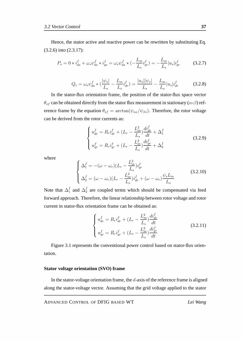
3.2 Vector Control 37
Hence, the stator active and reactive power can be rewrittenby substituting Eq.
(3.2.6) into (2.3.17):
Ps = 0 ∗ ifds + ωsψfds ∗ ifqs = ωsψ
fds ∗ (−
Lm
Ls
ifqr) = −Lm
Ls
|us|ifqr (3.2.7)
Qs = ωsψfds ∗ (
|ψs|Ls
− Lm
Ls
ifdr) =|us||ψs|Ls
− Lm
Ls
|us|ifdr (3.2.8)
In the stator-flux orientation frame, the position of the stator-flux space vector
θsf can be obtained directly from the stator flux measurement in stationary (α-β) ref-
erence frame by the equationθsf = arctan(ψαs/ψβs). Therefore, the rotor voltage
can be derived from the rotor currents as:
ufdr = Rrifdr + (Lr −
L2m
Ls
)difdrdt
+∆f1
ufqr = Rrifqr + (Lr −
L2m
Ls
)difqrdt
+∆f2
(3.2.9)
where
∆f1 = −(ω − ωr)(Lr −
L2m
Ls
)ifqr
∆f2 = (ω − ωr)(Lr −
L2m
Ls
)ifdr + (ω − ωr)ψsLm
Ls
(3.2.10)
Note that∆f1 and∆f
2 are coupled terms which should be compensated via feed
forward approach. Therefore, the linear relationship between rotor voltage and rotor
current in stator-flux orientation frame can be obtained as:
ufdr = Rrifdr + (Lr −
L2m
Ls
)difdrdt
ufqr = Rrifqr + (Lr −
L2m
Ls
)difqrdt
(3.2.11)
Figure 3.1 represents the conventional power control basedon stator-flux orien-
tation.
Stator voltage orientation (SVO) frame
In the stator-voltage orientation frame, thed-axis of the reference frame is aligned
along the stator-voltage vector. Assuming that the grid voltage applied to the stator
ADVANCED CONTROL OFDFIG BASED WT Lei Wang
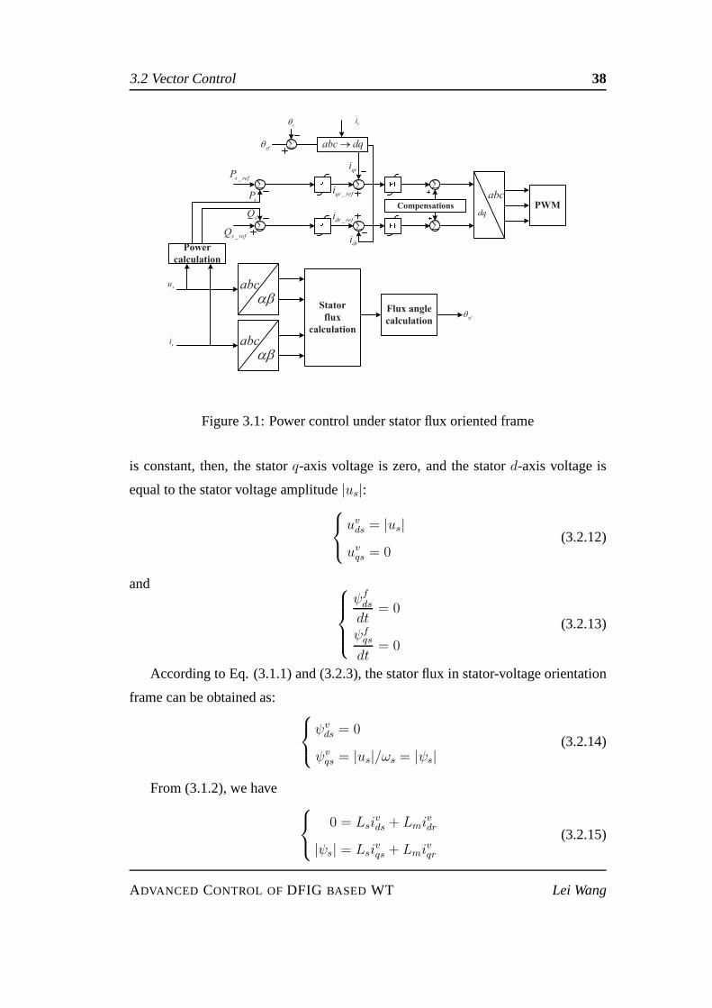
3.2 Vector Control 38
abc
dq
abc !
abc !
Stator
flux
calculation
su
si
Flux angle
calculationsf
abc dq
!
!
sP
sQ
_s refQ
_s refP
_dr refi
_qr refi
qri
dri
Compensations
sf !
r ri
Power
calculation
PWM
Figure 3.1: Power control under stator flux oriented frame
is constant, then, the statorq-axis voltage is zero, and the statord-axis voltage is
equal to the stator voltage amplitude|us|:
uvds = |us|
uvqs = 0(3.2.12)
and
ψfds
dt= 0
ψfqs
dt= 0
(3.2.13)
According to Eq. (3.1.1) and (3.2.3), the stator flux in stator-voltage orientation
frame can be obtained as:
ψvds = 0
ψvqs = |us|/ωs = |ψs|
(3.2.14)
From (3.1.2), we have
0 = Lsivds + Lmi
vdr
|ψs| = Lsivqs + Lmi
vqr
(3.2.15)
ADVANCED CONTROL OFDFIG BASED WT Lei Wang
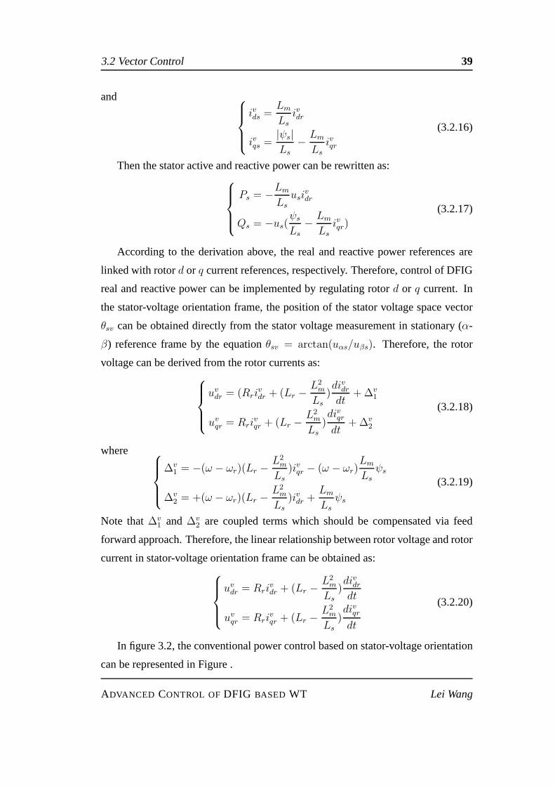
3.2 Vector Control 39
and
ivds =Lm
Ls
ivdr
ivqs =|ψs|Ls
− Lm
Ls
ivqr
(3.2.16)
Then the stator active and reactive power can be rewritten as:
Ps = −Lm
Ls
usivdr
Qs = −us(ψs
Ls
− Lm
Ls
ivqr)
(3.2.17)
According to the derivation above, the real and reactive power references are
linked with rotord or q current references, respectively. Therefore, control of DFIG
real and reactive power can be implemented by regulating rotor d or q current. In
the stator-voltage orientation frame, the position of the stator voltage space vector
θsv can be obtained directly from the stator voltage measurement in stationary (α-
β) reference frame by the equationθsv = arctan(uαs/uβs). Therefore, the rotor
voltage can be derived from the rotor currents as:
uvdr = (Rrivdr + (Lr −
L2m
Ls
)divdrdt
+∆v1
uvqr = Rrivqr + (Lr −
L2m
Ls
)divqrdt
+∆v2
(3.2.18)
where
∆v1 = −(ω − ωr)(Lr −
L2m
Ls
)ivqr − (ω − ωr)Lm
Ls
ψs
∆v2 = +(ω − ωr)(Lr −
L2m
Ls
)ivdr +Lm
Ls
ψs
(3.2.19)
Note that∆v1 and∆v
2 are coupled terms which should be compensated via feed
forward approach. Therefore, the linear relationship between rotor voltage and rotor
current in stator-voltage orientation frame can be obtained as:
uvdr = Rrivdr + (Lr −
L2m
Ls
)divdrdt
uvqr = Rrivqr + (Lr −
L2m
Ls
)divqrdt
(3.2.20)
In figure 3.2, the conventional power control based on stator-voltage orientation
can be represented in Figure .
ADVANCED CONTROL OFDFIG BASED WT Lei Wang
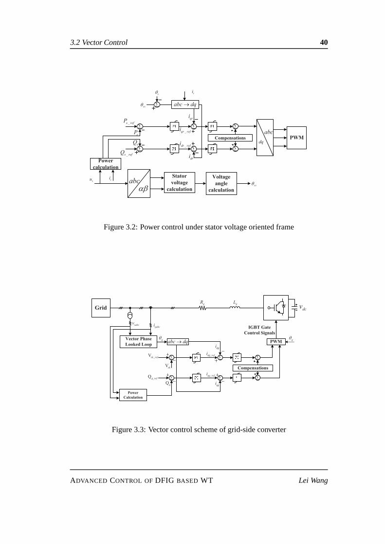
3.2 Vector Control 40
abc
dq
abc !
Stator
voltage
calculation
su si Voltage
angle
calculationsv
abc dq
!
!
sP
sQ
_s refQ
_s refP
_dr refi
_qr refi
qri
dri
Compensations
sv !
r ri
Power
calculation
PWM
Figure 3.2: Power control under stator voltage oriented frame
Grid dcv
Vector Phase
Looked Loopabc dq
Power
Calculation
Compensations
PWM
IGBT Gate
Control Signals
sabcvgabci
Qg
_Qg ref
Vdc
_Vdc ref
g
dgi
_dg refi
_qg refi
qgi
gR gL
g
Figure 3.3: Vector control scheme of grid-side converter
ADVANCED CONTROL OFDFIG BASED WT Lei Wang
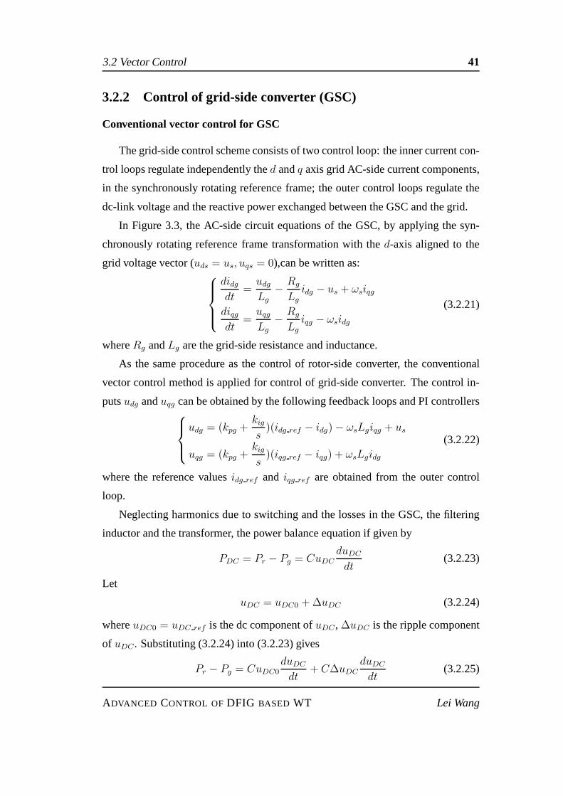
3.2 Vector Control 41
3.2.2 Control of grid-side converter (GSC)
Conventional vector control for GSC
The grid-side control scheme consists of two control loop: the inner current con-
trol loops regulate independently thed andq axis grid AC-side current components,
in the synchronously rotating reference frame; the outer control loops regulate the
dc-link voltage and the reactive power exchanged between the GSC and the grid.
In Figure 3.3, the AC-side circuit equations of the GSC, by applying the syn-
chronously rotating reference frame transformation with the d-axis aligned to the
grid voltage vector (uds = us, uqs = 0),can be written as:
didgdt
=udgLg
− Rg
Lg
idg − us + ωsiqg
diqgdt
=uqgLg
− Rg
Lg
iqg − ωsidg
(3.2.21)
whereRg andLg are the grid-side resistance and inductance.
As the same procedure as the control of rotor-side converter, the conventional
vector control method is applied for control of grid-side converter. The control in-
putsudg anduqg can be obtained by the following feedback loops and PI controllers
udg = (kpg +kigs)(idg ref − idg)− ωsLgiqg + us
uqg = (kpg +kigs)(iqg ref − iqg) + ωsLgidg
(3.2.22)
where the reference valuesidg ref and iqg ref are obtained from the outer control
loop.
Neglecting harmonics due to switching and the losses in the GSC, the filtering
inductor and the transformer, the power balance equation ifgiven by
PDC = Pr − Pg = CuDC
duDC
dt(3.2.23)
Let
uDC = uDC0 +∆uDC (3.2.24)
whereuDC0 = uDC ref is the dc component ofuDC , ∆uDC is the ripple component
of uDC. Substituting (3.2.24) into (3.2.23) gives
Pr − Pg = CuDC0duDC
dt+ C∆uDC
duDC
dt(3.2.25)
ADVANCED CONTROL OFDFIG BASED WT Lei Wang

3.3 Direct Power Control (DPC) via Feedback Linearization Control 42
Since∆uDC ≪ uDC0, (3.2.25) can be written as
Pr − Pg ≈ CuDC0duDC
dt(3.2.26)
Therefore, the transfer function fromPg to uDC is given by
uDC(s)
Pg(s)=
1
CuDC0s(3.2.27)
Since
Pg =3
2udsidg =
3
2usidg (3.2.28)
Therefore, it is possible to design a feedback loop and PI controller to generate the
reference value ofidg as follows:
idg ref = (kpu +kius)(uDC ref − uDC) (3.2.29)
The reactive power exchanged between the GSC and the grid is given by
Qg = −3
2udsiqg = −3
2|us|iqg (3.2.30)
Therefore, the reference value ofidg can be determined directly from the reactive
power command.
3.3 Direct Power Control (DPC) via Feedback Lin-
earization Control
In this section, the feedback linearization control methodis applied to directly
control stator active and reactive powers, compared with the asymptotical charac-
teristics of DFIG provided by the VC. To design nonlinear decoupled controller for
stator active and reactive power, the DFIG system in stationary reference frame can
be rewritten in a compact form as:
x = f(x) + b1uαr + b2uβr (3.3.1)
wherex = [ψαs ψβs ψαr ψβr ωr]T
f(x) =
uαs − Rsiαs
uβs − Rsiβs
−Rriαr − ωrψβr
−Rriβr + ωrψαr
(3.3.2)
ADVANCED CONTROL OFDFIG BASED WT Lei Wang

3.3 Direct Power Control (DPC) via Feedback Linearization Control 43
and
b1 = [0 0 1 0]T (3.3.3)
b2 = [0 0 0 1]T (3.3.4)
According to the equation 3.1.2, the stator and rotor currents represented in the
stationary reference frame can be written as:
iαs = −Lr
Lσ
ψαs +Lm
Lσ
ψαr
iβs = −Lr
Lσ
ψβs +Lm
Lσ
ψβr
iαr =Lm
Lσ
ψαs −Ls
Lσ
ψαr
iβr =Lm
Lσ
ψβs −Ls
Lσ
ψβr
(3.3.5)
Stator active powerPs and reactive powerQs can be represented in terms of
stator voltages and currents under the stationary reference frame as:
Ps = uαsiαs + uβsiβs
Qs = uβsiαs − uαsiβs(3.3.6)
Let stator active powerPs and reactive powerQs as the controlled outputs,
y1 = Ps
y2 = Qs
, (3.3.7)
then we can obtain
Ps = F1 +LmuαsLσ
uαr +LmuβsLσ
uβr
Qs = F2 +LmuβsLσ
uαr −LmuαsLσ
uβr
(3.3.8)
where
F1 = −Lr
Lσ(uαs(uαs − Rsiαs)− uβs(uβs − Rsiβs))
+Lm
Lσ(uαs(−Rriαr − ωrψβr) + uβs(−Rriβr + ωrψαr))
(3.3.9)
F2 = −Lr
Lσ(uβs(uαs − Rsiαs) + uαs(uβs −Rsiβs))
+Lm
Lσ(uβs(−Rriαr − ωrψβr)− uαs(−Rriβr + ωrψαr))
(3.3.10)
ADVANCED CONTROL OFDFIG BASED WT Lei Wang

3.3 Direct Power Control (DPC) via Feedback Linearization Control 44
Define the tracking errors as:
e1 = Ps − Ps ref
e2 = Qs −Qs ref
(3.3.11)
wherePs ref andQs ref are the reference values of the active and the reactive power,
respectively. The dynamical system of the track error can beobtained based on
equation (3.3.8) as:
[
e1
e2
]
=
[
F1 − Ps ref
F2 − Qs ref
]
+B
[
uαr
uβr
]
(3.3.12)
B =
[
Lm
Lσuαs
Lm
Lσuβs
Lm
Lσuβs −Lm
Lσuαs
]
(3.3.13)
whereB is the control gains matrix which is not singular whendet(B) = −L2m
L2σ(u2αs+
u2βs) 6= 0, when|us| 6= 0.
The FLC control can be obtained as[
uαr
uβr
]
= B−1
[
−F1 + Ps ref
−F2 + Qs ref
]
+
[
v1
v2
]
(3.3.14)
[
v1
v2
]
=
[
−k1e1−k2e2
]
(3.3.15)
wherev1 andv2 are control input of the linear system,k1, k2 are the feedback gains.
The linearized system is
[
e1
e2
]
=
[
v1
v2
]
(3.3.16)
And resulted linear system as
e1 + k1e1 = 0
e2 + k2e2 = 0(3.3.17)
ADVANCED CONTROL OFDFIG BASED WT Lei Wang

3.4 Cascaded Power Control via Rotor Current Regulation (RC& FLC) 45
3.4 Cascaded Power Control via Rotor Current Reg-
ulation (RC & FLC)
In this section, the input/output feedback linearization control (IOFLC) tech-
nique is used to design a fully decoupled power control law toimprove the asymp-
totical characteristics of DFIG provided by VC, based on a full-order DFIG model
in the synchronous reference frame. The stator stationary frame model of the DFIG
will be used to improve the transient dynamics under unsymmetrical grid faults.
This control strategy consists of an outer loop, obtaining the rotor current references
from the stator active and reactive powers, and an inner loop, which applies the
IOFLC for the current regulation. The dynamic model of DFIG has been rewritten
in the state variable of stator and rotor current vectors as
diαsdt
=Lm
Lσ
uαr −Lr
Lσ
uαs +RsLr
Lσ
iαs −RrLm
Lσ
iαr − ωrLm
Lriβr + LmiβsLσ
diβsdt
=Lm
Lσ
uβr −Lr
Lσ
uβs +RsLr
Lσ
iβs −RrLm
Lσ
iβr + ωrLm
Lriαr + LmiαsLσ
diαrdt
=Lm
Lσ
uαs −Ls
Lσ
uαr −RsLm
Lσ
iαs +RrLs
Lσ
iαr + ωrLs
Lriβr + LmiβsLσ
diβrdt
=Lm
Lσ
uβs −Ls
Lσ
uβr −RsLm
Lσ
iβs +RrLs
Lσ
iβr − ωrLs
Lriαr + LmiαsLσ
(3.4.1)
3.4.1 The inner control loop: IOFLC
For the controller design, the state vector of (3.4.1) can besplit into two parts
is = A11is + A12ir +B1us + C1ur (3.4.2)
ir = A21is + A22ir +B2us + C2ur (3.4.3)
where
is =
[
iαs
iβs
]
(3.4.4)
ir =
[
iαr
iβr
]
(3.4.5)
ADVANCED CONTROL OFDFIG BASED WT Lei Wang
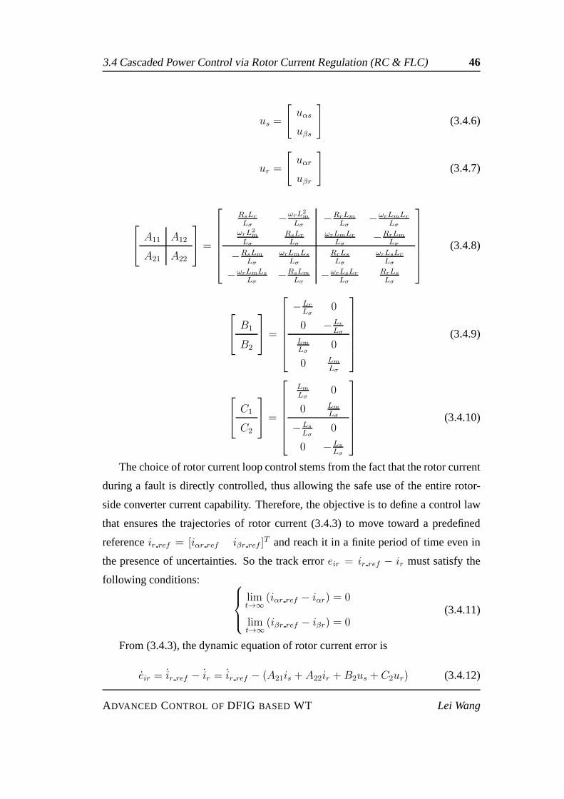
3.4 Cascaded Power Control via Rotor Current Regulation (RC& FLC) 46
us =
[
uαs
uβs
]
(3.4.6)
ur =
[
uαr
uβr
]
(3.4.7)
A11 A12
A21 A22
=
RsLr
Lσ−ωrL
2m
Lσ−RrLm
Lσ−ωrLmLr
Lσ
ωrL2m
Lσ
RsLr
Lσ
ωrLmLr
Lσ−RrLm
Lσ
−RsLm
Lσ
ωrLmLs
Lσ
RrLs
Lσ
ωrLsLr
Lσ
−ωrLmLs
Lσ−RsLm
Lσ−ωrLsLr
Lσ
RrLs
Lσ
(3.4.8)
B1
B2
=
−Lr
Lσ0
0 −Lr
Lσ
Lm
Lσ0
0 Lm
Lσ
(3.4.9)
C1
C2
=
Lm
Lσ0
0 Lm
Lσ
−Ls
Lσ0
0 −Ls
Lσ
(3.4.10)
The choice of rotor current loop control stems from the fact that the rotor current
during a fault is directly controlled, thus allowing the safe use of the entire rotor-
side converter current capability. Therefore, the objective is to define a control law
that ensures the trajectories of rotor current (3.4.3) to move toward a predefined
referenceir ref = [iαr ref iβr ref ]T and reach it in a finite period of time even in
the presence of uncertainties. So the track erroreir = ir ref − ir must satisfy the
following conditions:
limt→∞
(iαr ref − iαr) = 0
limt→∞
(iβr ref − iβr) = 0(3.4.11)
From (3.4.3), the dynamic equation of rotor current error is
eir = ir ref − ir = ir ref − (A21is + A22ir +B2us + C2ur) (3.4.12)
ADVANCED CONTROL OFDFIG BASED WT Lei Wang

3.4 Cascaded Power Control via Rotor Current Regulation (RC& FLC) 47
After addingA22ir ref − A22ir ref , it becomes
eir = A22eir − C2ur + g (3.4.13)
whereg is given by
g = ir ref − A21is −B2us − A22ir ref (3.4.14)
Design the nonlinear feedback control inputur as
ur = C−12 (A22e + g − v) (3.4.15)
whereC2 is nonsingular for all time in the domain of interest, asdet(C2) =
L2s/L
2σ 6= 0; v = [v1 v2]
T is the linear control input.
The dynamic system of the track error (3.4.12) can also be presented as follows:
eir =
[
e1
e2
]
=
[
iαr ref − F1
iβr ref − F2
]
− C2
[
uαr
uβr
]
(3.4.16)
where
F1 =Lm
Lσ
uαs −RsLm
Lσ
iαs +RrLs
Lσ
iαr + ωrLs
Lriβr + LmiβsLσ
F2 =Lm
Lσ
uβs −RsLm
Lσ
iβs +RrLs
Lσ
iβr − ωrLs
Lriαr + LmiαsLσ
(3.4.17)
The FLC control (3.4.15) can be rewritten in
[
uαr
uβr
]
= C−12
[
iαr ref − F1
iβr ref − F2
]
−[
v1
v2
]
(3.4.18)
[
v1
v2
]
=
[
−k1e1−k2e2
]
(3.4.19)
wherev1 andv2 are control input of the linear system,k1, k2 are the feedback
gains. As a result, the linearized system can be written as:
e1 + k1e1 = 0
e2 + k2e2 = 0(3.4.20)
ADVANCED CONTROL OFDFIG BASED WT Lei Wang

3.4 Cascaded Power Control via Rotor Current Regulation (RC& FLC) 48
3.4.2 The outer loop: rotor current reference calculation
Assumptions
• In a sinusoidal steady state at a fundamental grid frequency, the amplitude and
frequency of stator current are constants
• The transient response of stator power reference is ignored
• The controller proposed in (3.4.15) works properly
Under the assumptions, the rotor current vector erroreir can beeir = 0. In order
to obtain the reference of rotor current from stator current, substituting (3.4.14) and
(3.4.15) into (3.4.2) results in
is = (A11−C1C−12 A21)is+(B1−C1C
−12 )us+(A12−C1C
−12 A22)ir ref+C1C
−12 ir ref
(3.4.21)
The time derivative of the rotor and stator currents can be expressed as
ir ref =
[
0 ωs
−ωs 0
]
ir ref (3.4.22)
is =
[
0 ωs
−ωs 0
]
is (3.4.23)
In this section, the outputs of the DFIG based WT to be controlled are the stator
active and reactive power. They can be expressed in terms of stator currents and
voltages and represented as
[
Ps
Qs
]
=
[
uαs uβs
uβs −uαs
][
iαs
iβs
]
(3.4.24)
Then the stator current vectorsis can be represented in terms of stator voltages
and powers:[
iαs
iβs
]
=1
u2αs + u2βs
[
uαs uβs
uβs −uαs
][
Ps
Qs
]
(3.4.25)
ADVANCED CONTROL OFDFIG BASED WT Lei Wang
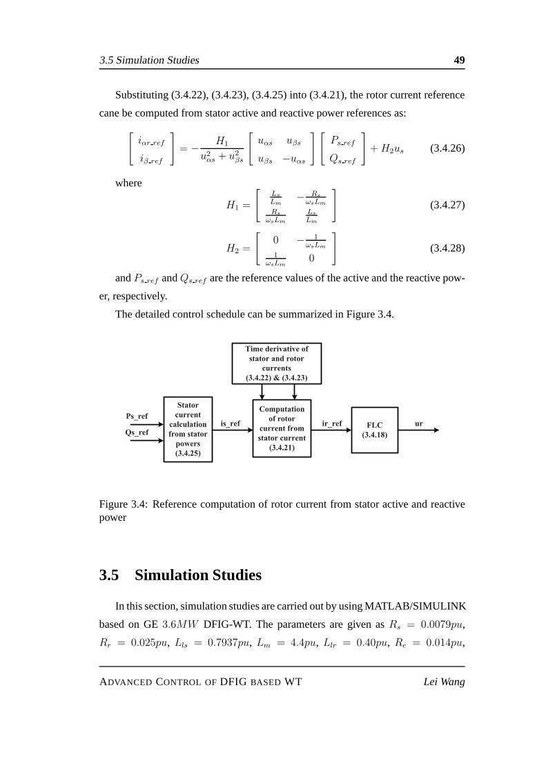
3.5 Simulation Studies 49
Substituting (3.4.22), (3.4.23), (3.4.25) into (3.4.21),the rotor current reference
cane be computed from stator active and reactive power references as:
[
iαr ref
iβ ref
]
= − H1
u2αs + u2βs
[
uαs uβs
uβs −uαs
][
Ps ref
Qs ref
]
+H2us (3.4.26)
where
H1 =
[
Ls
Lm− Rs
ωsLm
Rs
ωsLm
Ls
Lm
]
(3.4.27)
H2 =
[
0 − 1ωsLm
1ωsLm
0
]
(3.4.28)
andPs ref andQs ref are the reference values of the active and the reactive pow-
er, respectively.
The detailed control schedule can be summarized in Figure 3.4.
Stator
current
calculation
from stator
powers
(3.4.25)
Ps_ref
Qs_ref
Computation
of rotor
current from
stator current
(3.4.21)
is_ref
Time derivative of
stator and rotor
currents
(3.4.22) & (3.4.23)
ir_ref FLC
(3.4.18)
ur
Figure 3.4: Reference computation of rotor current from stator active and reactivepower
3.5 Simulation Studies
In this section, simulation studies are carried out by usingMATLAB/SIMULINK
based on GE3.6MW DFIG-WT. The parameters are given asRs = 0.0079pu,
Rr = 0.025pu, Lls = 0.7937pu, Lm = 4.4pu, Llr = 0.40pu, Re = 0.014pu,
ADVANCED CONTROL OFDFIG BASED WT Lei Wang
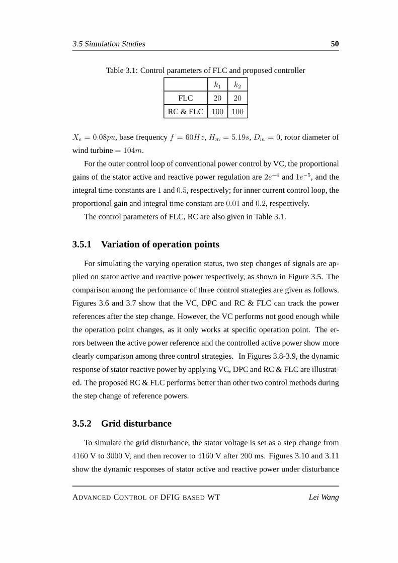
3.5 Simulation Studies 50
Table 3.1: Control parameters of FLC and proposed controller
k1 k2
FLC 20 20
RC & FLC 100 100
Xe = 0.08pu, base frequencyf = 60Hz, Hm = 5.19s, Dm = 0, rotor diameter of
wind turbine= 104m.
For the outer control loop of conventional power control by VC, the proportional
gains of the stator active and reactive power regulation are2e−4 and1e−5, and the
integral time constants are1 and0.5, respectively; for inner current control loop, the
proportional gain and integral time constant are0.01 and0.2, respectively.
The control parameters of FLC, RC are also given in Table 3.1.
3.5.1 Variation of operation points
For simulating the varying operation status, two step changes of signals are ap-
plied on stator active and reactive power respectively, as shown in Figure 3.5. The
comparison among the performance of three control strategies are given as follows.
Figures 3.6 and 3.7 show that the VC, DPC and RC & FLC can track the power
references after the step change. However, the VC performs not good enough while
the operation point changes, as it only works at specific operation point. The er-
rors between the active power reference and the controlled active power show more
clearly comparison among three control strategies. In Figures 3.8-3.9, the dynamic
response of stator reactive power by applying VC, DPC and RC &FLC are illustrat-
ed. The proposed RC & FLC performs better than other two control methods during
the step change of reference powers.
3.5.2 Grid disturbance
To simulate the grid disturbance, the stator voltage is set as a step change from
4160 V to 3000 V, and then recover to4160 V after 200 ms. Figures 3.10 and 3.11
show the dynamic responses of stator active and reactive power under disturbance
ADVANCED CONTROL OFDFIG BASED WT Lei Wang
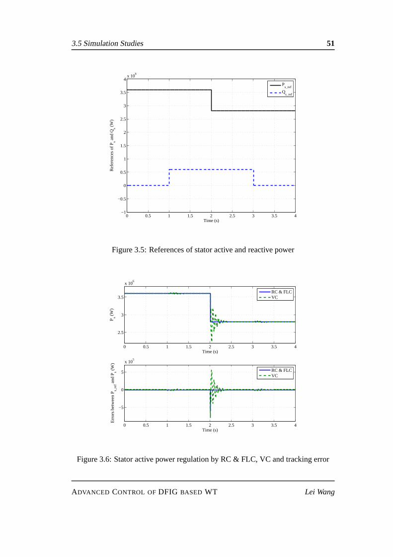
3.5 Simulation Studies 51
0 0.5 1 1.5 2 2.5 3 3.5 4−1
−0.5
0
0.5
1
1.5
2
2.5
3
3.5
4x 10
6
Time (s)
Ref
eren
ces
of P s a
nd Q
s (W
)
P
s_ref
Qs_ref
Figure 3.5: References of stator active and reactive power
0 0.5 1 1.5 2 2.5 3 3.5 4
2.5
3
3.5
x 106
Time (s)
P s (W
)
RC & FLCVC
0 0.5 1 1.5 2 2.5 3 3.5 4
−5
0
5
x 105
Time (s)
Err
ors
betw
een
P s_re
f and
P s (W
)
RC & FLCVC
Figure 3.6: Stator active power regulation by RC & FLC, VC andtracking error
ADVANCED CONTROL OFDFIG BASED WT Lei Wang

3.5 Simulation Studies 52
0 0.5 1 1.5 2 2.5 3 3.5 4
2.6
2.8
3
3.2
3.4
3.6
3.8x 10
6
Time (s)
P s (W
)
RC & FLCDPC
0 0.5 1 1.5 2 2.5 3 3.5 4
−5
0
5
10x 10
5
Time (s)
Err
ors
betw
een
P s_re
f and
P s (W
)
RC & FLCDPC
Figure 3.7: Stator active power regulation by RC & FLC, DPC and tracking error
0 0.5 1 1.5 2 2.5 3 3.5 4
−5
0
5
10
x 105
Time (s)
Qs (
W)
RC & FLCVC
0 0.5 1 1.5 2 2.5 3 3.5 4
−5
0
5
x 105
Time (s)
Err
ors
betw
een
Q s_re
f and
Qs (
W)
RC & FLCVC
Figure 3.8: Stator reactive power regulation by RC & FLC, VC and tracking error
ADVANCED CONTROL OFDFIG BASED WT Lei Wang
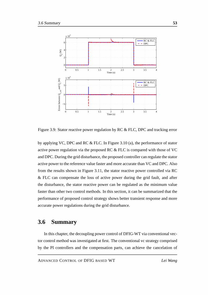
3.6 Summary 53
0 0.5 1 1.5 2 2.5 3 3.5 4
0
2
4
6
x 105
Time (s)
Qs (
W)
RC & FLCDPC
0 0.5 1 1.5 2 2.5 3 3.5 4
−5
0
5
x 105
Time (s)
Err
ors
betw
een
Q s_re
f and
Qs (
W)
RC & FLCDPC
Figure 3.9: Stator reactive power regulation by RC & FLC, DPCand tracking error
by applying VC, DPC and RC & FLC. In Figure 3.10 (a), the performance of stator
active power regulation via the proposed RC & FLC is comparedwith those of VC
and DPC. During the grid disturbance, the proposed controller can regulate the stator
active power to the reference value faster and more accuratethan VC and DPC. Also
from the results shown in Figure 3.11, the stator reactive power controlled via RC
& FLC can compensate the loss of active power during the grid fault, and after
the disturbance, the stator reactive power can be regulatedas the minimum value
faster than other two control methods. In this section, it can be summarized that the
performance of proposed control strategy shows better transient response and more
accurate power regulations during the grid disturbance.
3.6 Summary
In this chapter, the decoupling power control of DFIG-WT viaconventional vec-
tor control method was investigated at first. The conventional vc strategy comprised
by the PI controllers and the compensation parts, can achieve the cancelation of
ADVANCED CONTROL OFDFIG BASED WT Lei Wang
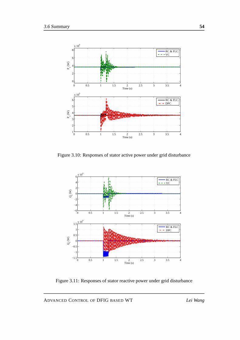
3.6 Summary 54
0 0.5 1 1.5 2 2.5 3 3.5 4
0
2
4
6
8
x 106
Time (s)
P s (W
)
RC & FLCVC
0 0.5 1 1.5 2 2.5 3 3.5 41
2
3
4
5
6
x 106
Time (s)
P s (W
)
RC & FLCDPC
Figure 3.10: Responses of stator active power under grid disturbance
0 0.5 1 1.5 2 2.5 3 3.5 4−6
−4
−2
0
2
4
6x 10
6
Time (s)
Qs (
W)
RC & FLCVC
0 0.5 1 1.5 2 2.5 3 3.5 4−1.5
−1
−0.5
0
0.5
1
1.5x 10
6
Time (s)
Qs (
W)
RC & FLCDPC
Figure 3.11: Responses of stator reactive power under grid disturbance
ADVANCED CONTROL OFDFIG BASED WT Lei Wang
3.6 Summary 55
coupled dynamics at the feed forward control loop. However,the VC method is
not capable of providing a satisfactory transient responsefor DFIG-WT under the
time-varying operation points and grid disturbance due to the following reasons:
The parameters of PI control loop can only provide optimal performance around
one special operation point, which not valid for time-varying operation points; The
control performance will be degraded, as the assumptions for control design were
destroyed during the grid faults or voltage sags.
To improve the transient response and achieve full decoupling power control,
two control schemes were proposed based on the nonlinear feedback linearization
control method. One of them is the direct stator active and reactive power control
(DPC), and the other one is called as the cascaded power control via rotor current
(RC & FLC). The RC & FLC scheme consists of an outer control loop, for obtaining
the rotor current references from stator active and reactive powers, and an inner
control loop, which applied the input/output feedback linearization control for the
rotor current regulation.
To demonstrate the performance of the proposed control schemes, case studies
on the variation of operation points, and grid disturbance were carried out. Accord-
ing to the simulation results and analysis, it shows that theproposed RC & FLC is
able to achieve smooth and satisfactory power regulation during the time-varying
operation and grid disturbance.
ADVANCED CONTROL OFDFIG BASED WT Lei Wang

Chapter 4
Nonlinear Control based Maximum
Power Point Tracking
4.1 Problem Formulation
To achieve high efficiency in wind power conversion system, the maximum pow-
er point tracking (MPPT) in variable-speed WPGS equipped with doubly-fed induc-
tion generator (DFIG) or permanent magnetic synchronous generator (PMSG) has
attracted lots of attention [67], [68], [69]. Basically, the MPPT methods proposed
include three strategies, namely, (1) the methods relying on the measurement of
wind speed, (2) the methods relying on output power measurement and calculation,
and (3) the methods relying on the optimal power versus rotorspeed characteristic
curve.
When maximum wind energy is tracked without measuring wind speed, there
are mainly polynomial estimation of the power coefficient [78], power mapping [79]
and look-up table [80] methods. Polynomial estimation needs online iteration com-
puting for many times, which increases the complexity and reduces the applicability
of the control system. Power mapping takes a lot of storage space. Otherwise, the
required control accuracy can not be achieved. The slownessof look-up table also
affects the tracking effect.
Recently, a proposed topology of employing the power versusrotor speed char-
56
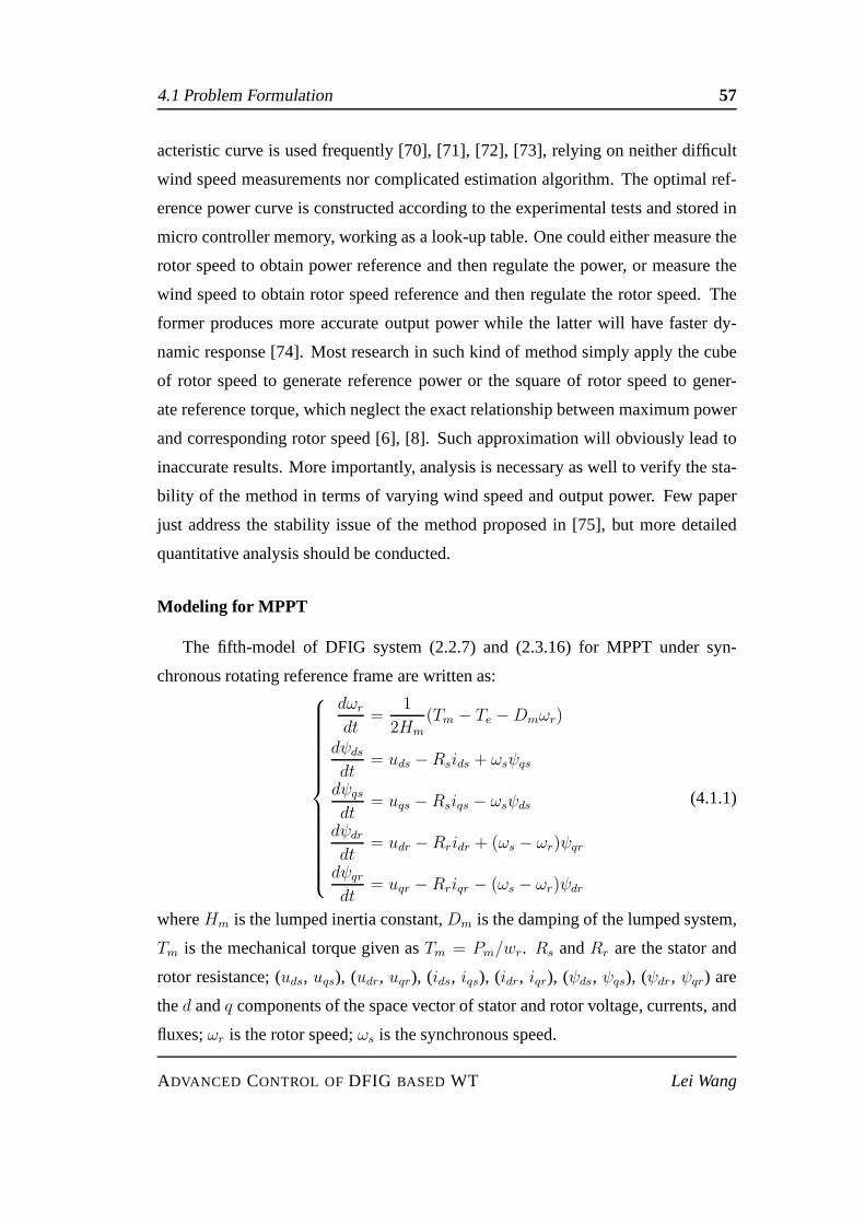
4.1 Problem Formulation 57
acteristic curve is used frequently [70], [71], [72], [73],relying on neither difficult
wind speed measurements nor complicated estimation algorithm. The optimal ref-
erence power curve is constructed according to the experimental tests and stored in
micro controller memory, working as a look-up table. One could either measure the
rotor speed to obtain power reference and then regulate the power, or measure the
wind speed to obtain rotor speed reference and then regulatethe rotor speed. The
former produces more accurate output power while the latterwill have faster dy-
namic response [74]. Most research in such kind of method simply apply the cube
of rotor speed to generate reference power or the square of rotor speed to gener-
ate reference torque, which neglect the exact relationshipbetween maximum power
and corresponding rotor speed [6], [8]. Such approximationwill obviously lead to
inaccurate results. More importantly, analysis is necessary as well to verify the sta-
bility of the method in terms of varying wind speed and outputpower. Few paper
just address the stability issue of the method proposed in [75], but more detailed
quantitative analysis should be conducted.
Modeling for MPPT
The fifth-model of DFIG system (2.2.7) and (2.3.16) for MPPT under syn-
chronous rotating reference frame are written as:
dωr
dt=
1
2Hm
(Tm − Te −Dmωr)
dψds
dt= uds −Rsids + ωsψqs
dψqs
dt= uqs − Rsiqs − ωsψds
dψdr
dt= udr −Rridr + (ωs − ωr)ψqr
dψqr
dt= uqr − Rriqr − (ωs − ωr)ψdr
(4.1.1)
whereHm is the lumped inertia constant,Dm is the damping of the lumped system,
Tm is the mechanical torque given asTm = Pm/wr. Rs andRr are the stator and
rotor resistance; (uds, uqs), (udr, uqr), (ids, iqs), (idr, iqr), (ψds, ψqs), (ψdr, ψqr) are
thed andq components of the space vector of stator and rotor voltage, currents, and
fluxes;ωr is the rotor speed;ωs is the synchronous speed.
ADVANCED CONTROL OFDFIG BASED WT Lei Wang

4.1 Problem Formulation 58
The flux linkage expressions in terms of the currents are given by
ψds = Lsids + Lmidr
ψqs = Lsiqs + Lmiqr
ψdr = Lridr + Lmids
ψqr = Lriqr + Lmiqs
(4.1.2)
The electromagnetic torque equation is represented in
Te = ψdsiqs − ψqsids = Lm(iqsidr − idsiqr) = ψdriqr − ψqridr (4.1.3)
4.1.1 Maximum Power Point Tracking
Operation of a typical wind turbine can be divided into 4 regions as shown in
Figure 4.1. In region 1, wind speed is too low to drive the windturbine. Hence
wind turbine would not rotate until wind speed reaches the minimum speed that
able to drive the wind turbine rotating. This typical wind speed is so-called cut-
in speed. When wind turbine start operating, power output keep increasing as the
wind speed increases. When the output power reaches a rated value of the electrical
generator, power output will stop increasing. The minimum wind speed that enables
wind turbine constantly maintains at the rated power is called rated wind speed. The
range between cut-in speed and rated speed is defined as region 2, maximum power
point tracking (MPPT) control is applied in this region in order to maximize power
output of the wind turbine, pitch angle is fixed in this regionto enable the blades
receive maximum pressure from the air. As output power increases when wind
speed increases, wind turbine will reach its rated power output, pitch angle control
is applied to regulate the blades to receive proper pressuresuch that the input power
from wind will not exceed the rated power of the generator. Wind turbine will be
cut out and stopped to protect itself from damaged from the maximum mechanical
stress when the wind speed is higher than the range of pitch angle control. Region
3 is defined between rated wind speed and cut-out speed. When wind turbine is
stopped generating power, its operation belongs to region 4.
ADVANCED CONTROL OFDFIG BASED WT Lei Wang
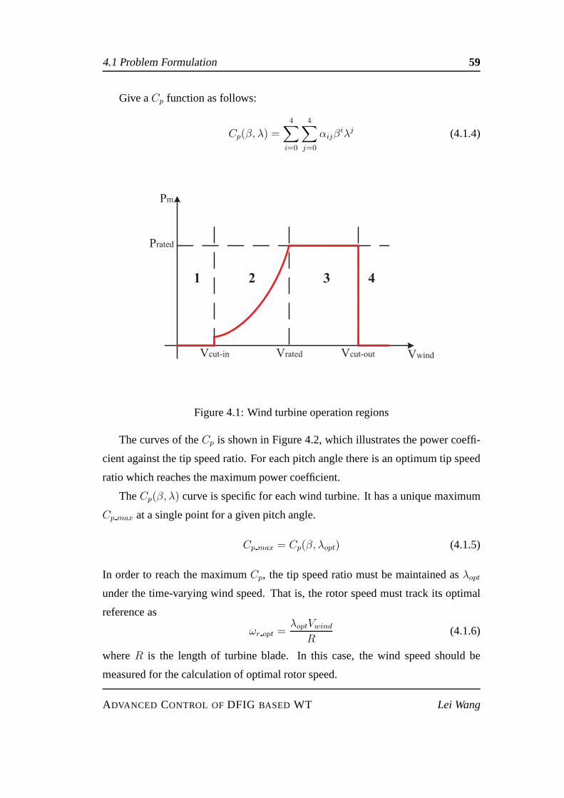
4.1 Problem Formulation 59
Give aCp function as follows:
Cp(β, λ) =
4∑
i=0
4∑
j=0
αijβiλj (4.1.4)
Pm
Prated
VwindVcut-outVratedVcut-in
1 2 3 4
Figure 4.1: Wind turbine operation regions
The curves of theCp is shown in Figure 4.2, which illustrates the power coeffi-
cient against the tip speed ratio. For each pitch angle thereis an optimum tip speed
ratio which reaches the maximum power coefficient.
TheCp(β, λ) curve is specific for each wind turbine. It has a unique maximum
Cp max at a single point for a given pitch angle.
Cp max = Cp(β, λopt) (4.1.5)
In order to reach the maximumCp, the tip speed ratio must be maintained asλopt
under the time-varying wind speed. That is, the rotor speed must track its optimal
reference as
ωr opt =λoptVwind
R(4.1.6)
whereR is the length of turbine blade. In this case, the wind speed should be
measured for the calculation of optimal rotor speed.
ADVANCED CONTROL OFDFIG BASED WT Lei Wang
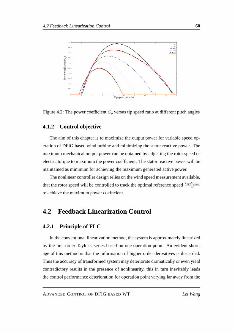
4.2 Feedback Linearization Control 60
0 2 4 6 8 10 12 14 16 18 200
0.05
0.1
0.15
0.2
0.25
0.3
0.35
0.4
0.45
0.5
Tip speed ratio (λ)
Pow
er c
oeffi
cien
t (C p)
1o
3o
5o
7o
9o
Figure 4.2: The power coefficientCp versus tip speed ratio at different pitch angles
4.1.2 Control objective
The aim of this chapter is to maximize the output power for variable speed op-
eration of DFIG based wind turbine and minimizing the statorreactive power. The
maximum mechanical output power can be obtained by adjusting the rotor speed or
electric torque to maximum the power coefficient. The statorreactive power will be
maintained as minimum for achieving the maximum generated active power.
The nonlinear controller design relies on the wind speed measurement available,
that the rotor speed will be controlled to track the optimal reference speedλoptVwind
R
to achieve the maximum power coefficient.
4.2 Feedback Linearization Control
4.2.1 Principle of FLC
In the conventional linearization method, the system is approximately linearized
by the first-order Taylor’s series based on one operation point. An evident short-
age of this method is that the information of higher order derivatives is discarded.
Thus the accuracy of transformed system may deteriorate dramatically or even yield
contradictory results in the presence of nonlinearity, this in turn inevitably leads
the control performance deterioration for operation pointvarying far away from the
ADVANCED CONTROL OFDFIG BASED WT Lei Wang
4.2 Feedback Linearization Control 61
linearized operation point.
Feedback linearization is a typical approach in nonlinear control design. The
central idea is to algebraically transform a nonlinear system dynamics into an equiv-
alent (fully or partly) linear one through an appropriate coordinate transformation
and a nonlinear control input, after that linear control techniques can be then ap-
plied. The nonlinearity of the system is entirely comsidered in the global state space
and can be used for both stabilization and tracking control tasks.
The basic concept of input-output linearization is briefly recalled. By input-
output linearization, it means the generation of a linear differential relation between
the outputy and a new inputv, then designu to cancel the nonlinearity. A linear
controller is systematically synthesized for the linear input-state model to impose
the desired linear dynamics. Without the loss of generality, consider a standard
affine nonlinear MIMO system in a neighborhood of a pointx0 of the form
x = f(x) + g(x)u
y = h(x)(4.2.1)
wherex ∈ Rn is the state vector,u ∈ Rm is the control input vector,y ∈ Rm is
the output vector,f(x), g(x) andh(x) are the smooth and continuous vector fields.
The input-output linearisation of a MIMO system is obtainedvia differentiating the
outputyi of the system until the inputuj appears, assuming thatri is the smallest
integer such that at least one of the inputs explicitly appears iny(ri)i
y(ri)i = Lri
f hi +m∑
j=1
LgjLri−1f hiuj (4.2.2)
wherey(ri)i denotes theith-order derivative ofyi, if LgjLri−1f hi(x) 6= 0 for at least
onej, by continuity that relation is preserved in a finite neighborhoodΩi of the point
x0. Performing the above procedure for each outputyi gives
y(r1)1
...
y(rm)m
=
Lr1f h1...
Lrmf hm
+B(x)
u1...
um
(4.2.3)
ADVANCED CONTROL OFDFIG BASED WT Lei Wang

4.2 Feedback Linearization Control 62
B(x) =
Lg1Lr1−1f h1 · · · LgmL
r1−1f h1
......
...
Lg1Lrm−1f hm · · · LgmL
rm−1f hm
(4.2.4)
HereB(x) is them×m control gain matrix. Define theΩ as the intersection of the
Ωi. If the partial “relative degrees”ri are all well defined, thenΩ is itself a finite
neighborhood ofx0. Furthermore, ifB(x) is invertible, the physical control law of
the MIMO nonlinear system is calculated immediately by
u = B(x)−1
−Lr1f h1...
−Lrmf hm
+
v1...
vm
(4.2.5)
wherevi are new inputs of the equivalent linear systems expressed as
y(ri)i = vi (4.2.6)
Since the inputvi only affects the outputyi it is called the decoupling control law,
and the invertible matrixB(s) is called the decoupling matrix of the system. The
system Eq. (4.2.1) is then said to have relative degree(r1, . . . , rm) at x0, and the
scalarr = r1 + . . .+ rm is called the total relative degree of the system atx0.
Assume now it is desired to track a prespecified trajectoryyid = [y(ri)id y
(ri−1)id . . . yid].
Choosing the artificial inputv as a simple linear pole-placement controller provides
any guarantee about the stability of the overall system:
vi = y(ri)id − αri−1e
(ri−1)i − . . .− α1ei − α0ei (4.2.7)
whereei = yi−yid leads to the tracking error dynamics andαi are the control gains,
the proposed control law yields the following characteristic equation
s(ri) + αri−1s(ri−1) + . . .+ α1s + α0 = 0 (4.2.8)
Now nominal stability of the system, and therefore boundedness of the output, is
ensured if the controller tuning coefficientsαi are chosen such that Eq. (4.2.8) is a
Hurwitz polynomial. To this end, any desired dynamics can beimposed on the new
system.
ADVANCED CONTROL OFDFIG BASED WT Lei Wang

4.2 Feedback Linearization Control 63
4.2.2 Control Design for MPPT
Choosing the rotor speedωr and stator reactive powerQs as the controlled out-
puts it obtains
y1 = ωr
y2 = Qs
(4.2.9)
Let ωr opt andQ∗s be the given references of the rotor speed and reactive power
respectively, and define the tracking errore = [e1 e2]T as:
e =
[
e1
e2
]
=
[
ωr − ωr opt
Qs −Q∗s
]
(4.2.10)
The input/output feedback linearization of equation (4.1.1) can be obtained as:[
e1
e2
]
=
[
f1 − ωr opt
f2 − Q∗s
]
+B(x)
[
udr
uqr
]
(4.2.11)
where
f1 =Tm
2Hm− 1
2Hm((−uqs +Rsiqs + ωsψds)(
Lr
Lσψds + ids)
+(uds −Rsids + ωsψqs)(iqs +Lr
Lσψqs)− Lm
Lσψds(Rriqr
+(ωs − ωr)ψdr)− Lm
Lσψqs(−Rridr + (ωs − ωr)ψqr))
(4.2.12)
f2 = uqsLm
Lσ(−Rridr + (ωs − ωr)ψqr)− uqs
Lr
Lσ(uds−
Rsids + ωqs)− udsLm
Lσ(−Rriqr − (ωs − ωr)ψdr)+
udsLr
Lσ(uqs − Rsiqs − ωsψds)
(4.2.13)
and
B(x) =
[
Lm
2HmLσψqs − Lm
2HmLσψds
Lm
Lσuqs −Lm
Lσuds
]
(4.2.14)
whereB0(x) = B(x)|Lm=Lm0, ∆B(x) = B(x)− B0(x). Note that whendet(B) =
0.5 L2m
HmL2σ(−ψqsuds + ψdsuqs) 6= 0, system (4.2.11) can be linearized as following
[
e1
e2
]
=
[
v1
v2
]
(4.2.15)
wherev = [v1 v2]T is the control input of the linear system defined as
[
v1
v2
]
= −[
k11e1 + k12e1
k21e2
]
(4.2.16)
ADVANCED CONTROL OFDFIG BASED WT Lei Wang
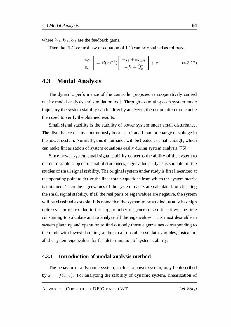
4.3 Modal Analysis 64
wherek11, k12, k21 are the feedback gains.
Then the FLC control law of equation (4.1.1) can be obtained as follows
[
udr
uqr
]
= B(x)−1(
[
−f1 + ωr opt
−f2 + Q∗s
]
+ v) (4.2.17)
4.3 Modal Analysis
The dynamic performance of the controller proposed is cooperatively carried
out by modal analysis and simulation tool. Through examining each system mode
trajectory the system stability can be directly analyzed, then simulation tool can be
then used to verify the obtained results.
Small signal stability is the stability of power system under small disturbance.
The disturbance occurs continuously because of small load or change of voltage in
the power system. Normally, this disturbance will be treated as small enough, which
can make linearization of system equations easily during system analysis [76].
Since power system small signal stability concerns the ability of the system to
maintain stable subject to small disturbances, eigenvalueanalysis is suitable for the
studies of small signal stability. The original system under study is first linearized at
the operating point to derive the linear state equations from which the system matrix
is obtained. Then the eigenvalues of the system matrix are calculated for checking
the small signal stability. If all the real parts of eigenvalues are negative, the system
will be classified as stable. It is noted that the system to be studied usually has high
order system matrix due to the large number of generators so that it will be time
consuming to calculate and to analyze all the eigenvalues. It is most desirable in
system planning and operation to find out only those eigenvalues corresponding to
the mode with lowest damping, and/or to all unstable oscillatory modes, instead of
all the system eigenvalues for fast determination of systemstability.
4.3.1 Introduction of modal analysis method
The behavior of a dynamic system, such as a power system, may be described
by x = f(x, u). For analyzing the stability of dynamic system, linearization of
ADVANCED CONTROL OFDFIG BASED WT Lei Wang

4.3 Modal Analysis 65
dynamic equations should be carried out first. Letx0 be the initial state vector and
u0 the input vector corresponding to the equilibrium point about which the small-
signal performance is to be investigated. Whenx0 andu0 satisfy the equation above,
we have
x0 = f(x0, u0) = 0 (4.3.1)
Let’s perturb the system from above state, by settingx = x0+∆x andu = u0+∆u,
where the prefix∆ denotes a small deviation. The new state should also satisfy
equationx = f(x, u). Hence,
x = x0 +∆x+ f [(x0 +∆x), (u0 +∆u)] (4.3.2)
As the perturbations are assumed to be small, the nonlinear functionsf(x, u) can be
expressed in terms of Taylor’s series expansion . With termsinvolving second and
higher order powers of∆x and∆u neglected, we can write
xi = xi0 +∆xi = fi[(x0 +∆x), (u0 +∆u)]
= fi(x0, u0) +∂fi∂x1
∆x1 + . . .+ ∂fi∂xn
∆xn +∂fi∂u1
∆u1 +∂fi∂ur
∆ur (4.3.3)
Sincexi0 = fi(x0, u0), we obtain
∆xi =∂fi∂x1
∆x1 + . . .+∂fi∂xn
∆xn +∂fi∂u1
∆u1 + . . .+∂fi∂ur
∆ur (4.3.4)
with i=1,2,...,n. Therefore, the linearized forms ofx = f(x, u) can be written as
∆x = A∆x+B∆u (4.3.5)
where
A =
∂f1∂x1
. . . ∂f1∂xn
. . . . . . . . .∂fn∂x1
. . . ∂fn∂xn
B =
∂f1∂u1
. . . ∂f1∂ur
. . . . . . . . .∂fn∂u1
. . . ∂fn∂ur
ADVANCED CONTROL OFDFIG BASED WT Lei Wang

4.3 Modal Analysis 66
The above partial derivatives are evaluated at the equilibrium point about which the
small perturbation is being analyzed. By taking the Laplacetransform of the above
equations, we obtain the state equations in the frequency domain:
s∆x(s)−∆x(0) = A∆x(s) +B∆u(s) (4.3.6)
Rearranging it, we have
(sI − A)∆x(s) = ∆x(0) +B∆u(s) (4.3.7)
We can see that the Laplace transform of∆x have two components, on dependent on
the initial conditions and the other on the inputs. These arethe Laplace transforms
of the free and zero-state components of the state and outputvectors.
The poles of∆x(s) are the roots of the equation
det(sI − A) = 0 (4.3.8)
where the values ofs are known as eigenvalues of matrixA, and equation above is
referred to as the characteristic equation of matrixA.
For example, the eigenvalues of a matrix are given by the values of the scalar
parameterλi for which there exist non-trivial solutions to the equation
AΦ = λiΦ (4.3.9)
whereA is an n*n matrix,Φ is an n*1 vector
To find the eigenvalues, the equation may be written in the form
(A− λiI)Φ = 0 (4.3.10)
For a non-trivial solution
det(A− λiI) = 0 (4.3.11)
Expansion of the determinant gives the characteristic equation. Then solutions of
λi = λ1, λ2, ...λn are eigenvalues ofA. The eigenvalues may be real or complex. If
A is real, complex eigenvalues always occur in conjugate pairs.
The time dependent characteristic of a mode corresponding to an eigenvalueλi is
ADVANCED CONTROL OFDFIG BASED WT Lei Wang

4.3 Modal Analysis 67
given byeλit. Therefore, the stability of the system is determined by theeigenvalues
as follows:
(a) A real eigenvalue corresponds to a non-oscillatory mode. A negative real
eigenvalue represents a decaying mode. The larger its magnitude, the faster the
decay. A positive real eigenvalue represents aperiodic instability.
(b) Complex eigenvalues occur in conjugate pairs, and each pair corresponds to
an oscillatory mode.
The associated eigenvectors will have appropriate complexvalues so as to make
the entries ofx(t) real at every instant of time. For example(a+ jb)e(σ−jω)t + (a−jb)e(σ+jω)t has the formeσt sin(ωt + θ), which represents a damped sinusoid for
negativeσ.
The real component of the eigenvalues gives the damping, andthe imaginary
component gives the frequency of oscillation. A negative real part represents a
damped oscillation whereas a positive real part representsoscillation of increasing
amplitude. Thus for a complex pair of eigenvalues:
λi = σ ± jω (4.3.12)
The frequency of oscillation in Hz is given by
f =ω
2π(4.3.13)
This represents the actual or damped frequency. The dampingratio is given by
ζ =−σ√σ2 + ω2
(4.3.14)
The damping ratioζ determines the rate of decay of the amplitude of the oscillation.
The time constant of amplitude decay is1/|σ|. In other words, the amplitude decays
to 1/e of the initial amplitude in1/|σ| seconds or in1/2πζ cycles of oscillation.
The stability status can be judged from eigenvalue of matrixA according to
Table 4.1.
4.3.2 Case studies
In this section, case studies are carried out based on the system linearized around
an operation point and the eigenvalue analysis of the matrixA, for assessing the
ADVANCED CONTROL OFDFIG BASED WT Lei Wang

4.3 Modal Analysis 68
Table 4.1: Behaviors for different eigenvalues
Eigenvalues (λi) solution of differential equation Stability status
positive real rootλi = σ ∆δ = ceσt non-periodic unstable
negative real rootλi = −σ ∆δ = ce−σt non-periodic stable
conjugate imaginary root ∆δ = c sin(βt+ ϕ) continuous oscillation
λi = ±jβcomplex root with positive ∆δ = c sin(θt+ ϕ)eγt unstable oscillation
real partλi = γ ± jθ
complex root with negative ∆δ = c sin(θt + ϕ)e−γt stable damping oscillation
real partλi = −γ ± jθ
small-signal stability of the system.
Realization of MPPT
In order to harvest the maximum amount of energy from the wind, the wind
turbine must have a specific rotational speed to maintain itstip-speed ratioλ as
close as possible to its optimal valueλopt, this concept is well-known as MPPT. In
Figure 4.10 a series of wind step changevwind = 7 − 11[m/s] are tested to show
the control performance of FLC, the smoother and faster tracking capability within
different wind speed manifests its significant superiorityin MPPT, which can be
clearly explained by the inherent characteristic of the system mode.
To begin with, Table 4.2 gives the system eigenvalues under nominal operation
point. Polesλ1,2, λ3,4 andλ5 represent the stator, rotor fluxes and mechanical mode
respectively. Hereλi = σi ± jωi, σi determines theith mode evolution speed while
ωi determines the corresponding oscillation frequency. In the stator flux mode FLC
is thoroughly independent andω1,2 = 0means a non-oscillatory characteristic, while
in rotor flux mode both strategies are of the similar conjugative form, at last the
smallerσ5 can definitely provide more damping to system.
By varying the system operation point the system mode loci can now be ob-
tained. The single most striking observation to emerge fromFigure 4.3 is thatψqs
mode of FLC is invariant under varying operation range, which can be interpreted
ADVANCED CONTROL OFDFIG BASED WT Lei Wang
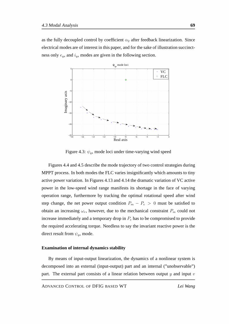
4.3 Modal Analysis 69
as the fully decoupled control by coefficientα2 after feedback linearization. Since
electrical modes are of interest in this paper, and for the sake of illustration succinct-
ness onlyeqs andiqs modes are given in the following section.
−18 −16 −14 −12 −10 −8 −6 −4 −2 0−25
−20
−15
−10
−5
0
5
Real axis
Imag
inar
y ax
isψ
qs mode loci
VCFLC
Figure 4.3:ψqs mode loci under time-varying wind speed
Figures 4.4 and 4.5 describe the mode trajectory of two control strategies during
MPPT process. In both modes the FLC varies insignificantly which amounts to tiny
active power variation. In Figures 4.13 and 4.14 the dramatic variation of VC active
power in the low-speed wind range manifests its shortage in the face of varying
operation range, furthermore by tracking the optimal rotational speed after wind
step change, the net power output conditionPm − Pe > 0 must be satisfied to
obtain an increasingωr, however, due to the mechanical constraintPm could not
increase immediately and a temporary drop inPe has to be compromised to provide
the required accelerating torque. Needless to say the invariant reactive power is the
direct result fromψqs mode.
Examination of internal dynamics stability
By means of input-output linearization, the dynamics of a nonlinear system is
decomposed into an external (input-output) part and an internal (”unobservable”)
part. The external part consists of a linear relation between outputy and inputv
ADVANCED CONTROL OFDFIG BASED WT Lei Wang
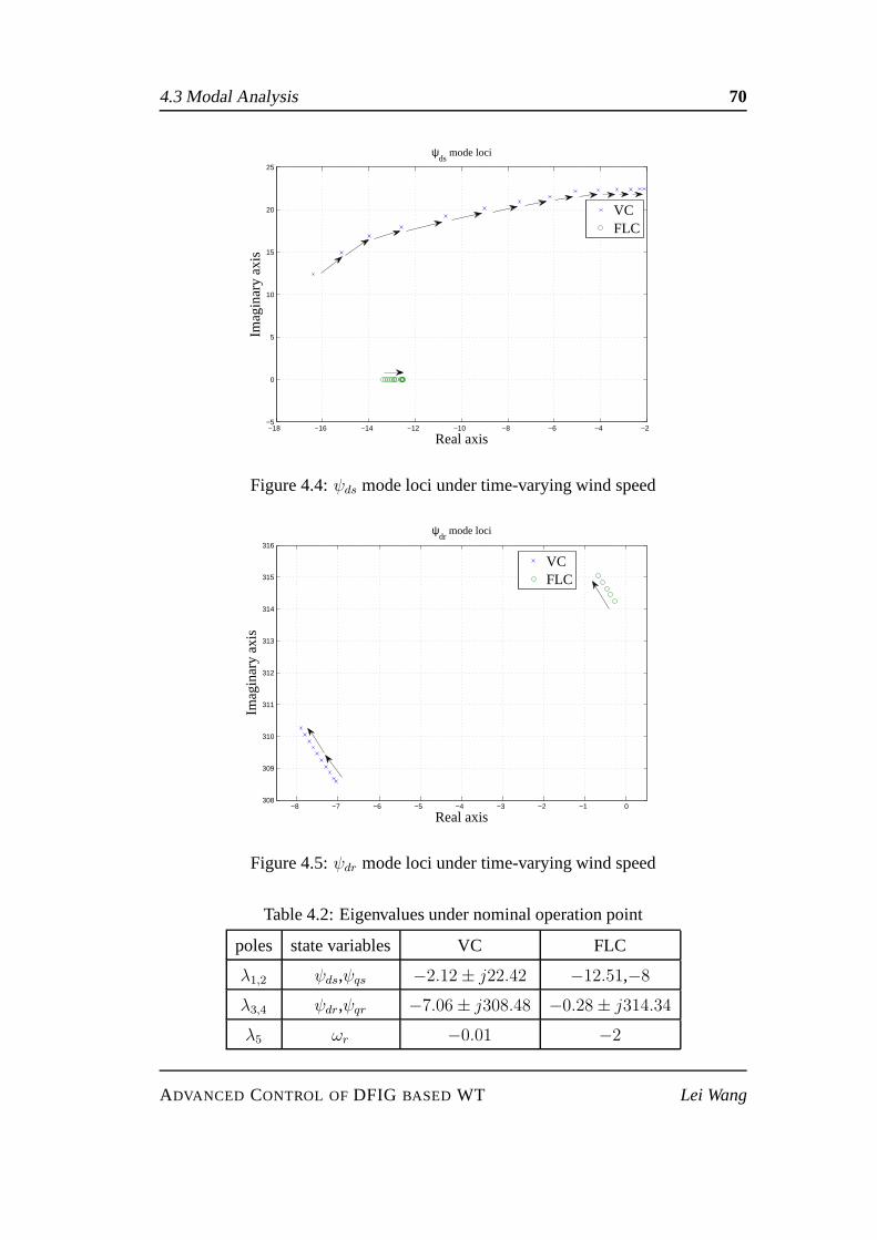
4.3 Modal Analysis 70
−18 −16 −14 −12 −10 −8 −6 −4 −2−5
0
5
10
15
20
25
Real axis
Imag
inar
y ax
is
ψds
mode loci
VCFLC
Figure 4.4:ψds mode loci under time-varying wind speed
−8 −7 −6 −5 −4 −3 −2 −1 0308
309
310
311
312
313
314
315
316
Real axis
Imag
inar
y ax
is
ψdr
mode loci
VCFLC
Figure 4.5:ψdr mode loci under time-varying wind speed
Table 4.2: Eigenvalues under nominal operation point
poles state variables VC FLC
λ1,2 ψds,ψqs −2.12± j22.42 −12.51,−8
λ3,4 ψdr,ψqr −7.06± j308.48 −0.28± j314.34
λ5 ωr −0.01 −2
ADVANCED CONTROL OFDFIG BASED WT Lei Wang
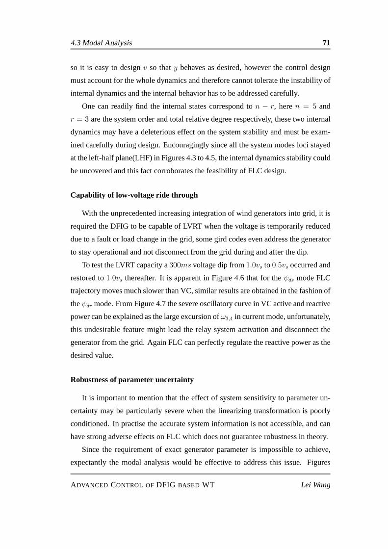
4.3 Modal Analysis 71
so it is easy to designv so thaty behaves as desired, however the control design
must account for the whole dynamics and therefore cannot tolerate the instability of
internal dynamics and the internal behavior has to be addressed carefully.
One can readily find the internal states correspond ton − r, heren = 5 and
r = 3 are the system order and total relative degree respectively, these two internal
dynamics may have a deleterious effect on the system stability and must be exam-
ined carefully during design. Encouragingly since all the system modes loci stayed
at the left-half plane(LHF) in Figures 4.3 to 4.5, the internal dynamics stability could
be uncovered and this fact corroborates the feasibility of FLC design.
Capability of low-voltage ride through
With the unprecedented increasing integration of wind generators into grid, it is
required the DFIG to be capable of LVRT when the voltage is temporarily reduced
due to a fault or load change in the grid, some gird codes even address the generator
to stay operational and not disconnect from the grid during and after the dip.
To test the LVRT capacity a300ms voltage dip from1.0vs to 0.5vs occurred and
restored to1.0vs thereafter. It is apparent in Figure 4.6 that for theψds mode FLC
trajectory moves much slower than VC, similar results are obtained in the fashion of
theψdr mode. From Figure 4.7 the severe oscillatory curve in VC active and reactive
power can be explained as the large excursion ofω3,4 in current mode, unfortunately,
this undesirable feature might lead the relay system activation and disconnect the
generator from the grid. Again FLC can perfectly regulate the reactive power as the
desired value.
Robustness of parameter uncertainty
It is important to mention that the effect of system sensitivity to parameter un-
certainty may be particularly severe when the linearizing transformation is poorly
conditioned. In practise the accurate system information is not accessible, and can
have strong adverse effects on FLC which does not guarantee robustness in theory.
Since the requirement of exact generator parameter is impossible to achieve,
expectantly the modal analysis would be effective to address this issue. Figures
ADVANCED CONTROL OFDFIG BASED WT Lei Wang
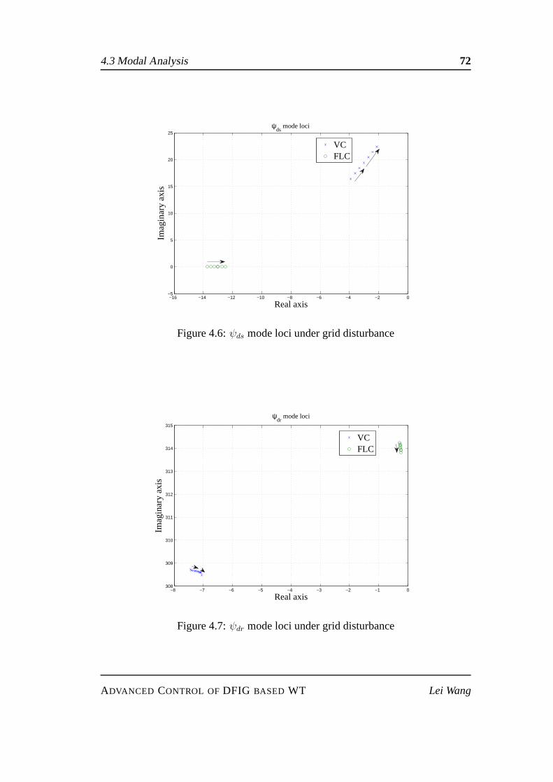
4.3 Modal Analysis 72
−16 −14 −12 −10 −8 −6 −4 −2 0−5
0
5
10
15
20
25
Real axis
Imag
inar
y ax
is
ψds
mode loci
VCFLC
Figure 4.6:ψds mode loci under grid disturbance
−8 −7 −6 −5 −4 −3 −2 −1 0308
309
310
311
312
313
314
315
Real axis
Imag
inar
y ax
is
ψdr
mode loci
VCFLC
Figure 4.7:ψdr mode loci under grid disturbance
ADVANCED CONTROL OFDFIG BASED WT Lei Wang
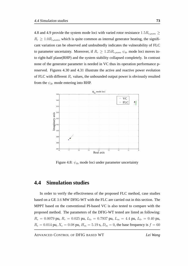
4.4 Simulation studies 73
4.8 and 4.9 provide the system mode loci with varied rotor resistance1.5Rr nom ≥Rr ≥ 1.0Rr nom, which is quite common as internal generator heating, the signifi-
cant variation can be observed and undoubtedly indicates the vulnerability of FLC
to parameter uncertainty. Moreover, ifRr ≥ 1.25Rr nom ψdr mode loci moves in-
to right-half plane(RHP) and the system stability collapsed completely. In contrast
none of the generator parameter is needed in VC thus its operation performance p-
reserved. Figures 4.30 and 4.31 illustrate the active and reactive power evolution
of FLC with differentRr values, the unbounded output power is obviously resulted
from theψdr mode entering into RHP.
−8 −7 −6 −5 −4 −3 −2 −1 0307
308
309
310
311
312
313
314
315
316
Real axis
Imag
inar
y ax
is
ψds
mode loci
VCFLC
Figure 4.8:ψds mode loci under parameter uncertainty
4.4 Simulation studies
In order to verify the effectiveness of the proposed FLC method, case studies
based on a GE3.6 MW DFIG-WT with the FLC are carried out in this section. The
MPPT based on the conventional PI-based VC is also tested to compare with the
proposed method. The parameters of the DFIG-WT tested are listed as following:
Rs = 0.0079 pu,Rr = 0.025 pu,Lls = 0.7937 pu,Lm = 4.4 pu,Llr = 0.40 pu,
Re = 0.014 pu,Xe = 0.08 pu,Hm = 5.19 s,Dm = 0, the base frequency isf = 60
ADVANCED CONTROL OFDFIG BASED WT Lei Wang
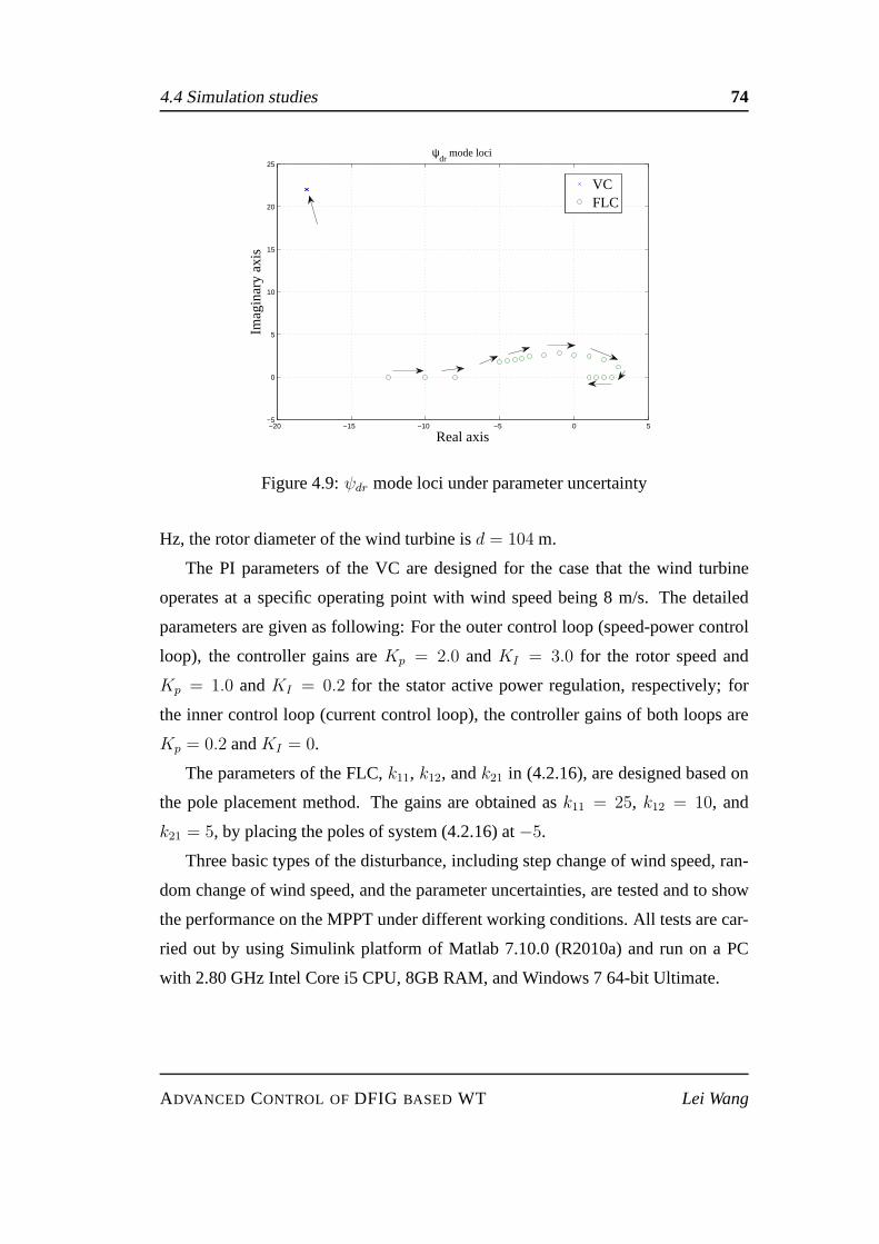
4.4 Simulation studies 74
−20 −15 −10 −5 0 5−5
0
5
10
15
20
25
Real axis
Imag
inar
y ax
is
ψdr
mode loci
VCFLC
Figure 4.9:ψdr mode loci under parameter uncertainty
Hz, the rotor diameter of the wind turbine isd = 104 m.
The PI parameters of the VC are designed for the case that the wind turbine
operates at a specific operating point with wind speed being 8m/s. The detailed
parameters are given as following: For the outer control loop (speed-power control
loop), the controller gains areKp = 2.0 andKI = 3.0 for the rotor speed and
Kp = 1.0 andKI = 0.2 for the stator active power regulation, respectively; for
the inner control loop (current control loop), the controller gains of both loops are
Kp = 0.2 andKI = 0.
The parameters of the FLC,k11, k12, andk21 in (4.2.16), are designed based on
the pole placement method. The gains are obtained ask11 = 25, k12 = 10, and
k21 = 5, by placing the poles of system (4.2.16) at−5.
Three basic types of the disturbance, including step changeof wind speed, ran-
dom change of wind speed, and the parameter uncertainties, are tested and to show
the performance on the MPPT under different working conditions. All tests are car-
ried out by using Simulink platform of Matlab 7.10.0 (R2010a) and run on a PC
with 2.80 GHz Intel Core i5 CPU, 8GB RAM, and Windows 7 64-bit Ultimate.
ADVANCED CONTROL OFDFIG BASED WT Lei Wang
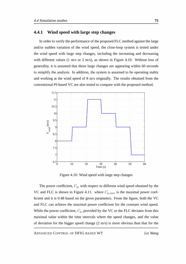
4.4 Simulation studies 75
4.4.1 Wind speed with large step changes
In order to verify the performance of the proposed FLC methodagainst the large
and/or sudden variation of the wind speed, the close-loop system is tested under
the wind speed with large step changes, including the increasing and decreasing
with different values (1 m/s or 2 m/s), as shown in Figure 4.10. Without loss of
generality, it is assumed that those large changes are appearing within 60 seconds
to simplify the analysis. In addition, the system is assumedto be operating stably
and working at the wind speed of 8 m/s originally. The resultsobtained from the
conventional PI-based VC are also tested to compare with theproposed method.
0 10 20 30 40 50 606.5
7
7.5
8
8.5
9
9.5
10
10.5
11
11.5
Time (s)
Vw
ind (
m/s
)
Figure 4.10: Wind speed with large step changes
The power coefficient,Cp, with respect to different wind speed obtained by the
VC and FLC is shown in Figure 4.11. whereCp max is the maximal power coef-
ficient and it is 0.48 based on the given parameters. From the figure, both the VC
and FLC can achieve the maximal power coefficient for the constant wind speed.
While the power coefficient,Cp, provided by the VC or the FLC deviates from this
maximal value within the time intervals where the speed changes, and the value
of deviation for the bigger speed change (2 m/s) is more obvious than that for the
ADVANCED CONTROL OFDFIG BASED WT Lei Wang
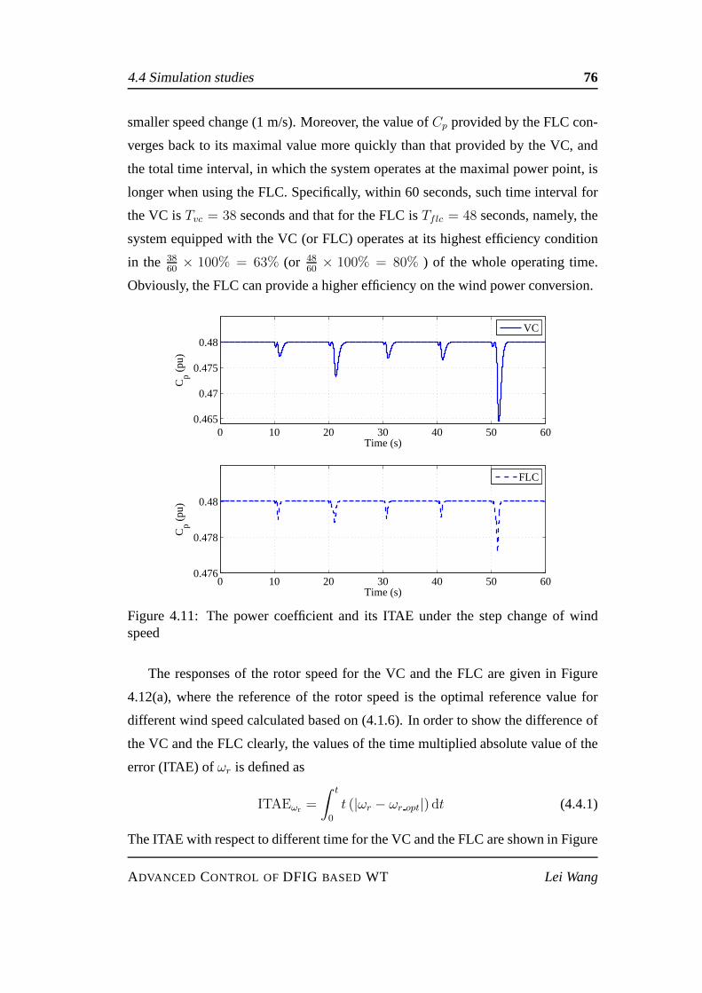
4.4 Simulation studies 76
smaller speed change (1 m/s). Moreover, the value ofCp provided by the FLC con-
verges back to its maximal value more quickly than that provided by the VC, and
the total time interval, in which the system operates at the maximal power point, is
longer when using the FLC. Specifically, within 60 seconds, such time interval for
the VC isTvc = 38 seconds and that for the FLC isTflc = 48 seconds, namely, the
system equipped with the VC (or FLC) operates at its highest efficiency condition
in the 3860
× 100% = 63% (or 4860
× 100% = 80% ) of the whole operating time.
Obviously, the FLC can provide a higher efficiency on the windpower conversion.
0 10 20 30 40 50 600.476
0.478
0.48
Time (s)
Cp (
pu)
0 10 20 30 40 50 600.465
0.47
0.475
0.48
Time (s)
Cp (
pu)
VC
FLC
Figure 4.11: The power coefficient and its ITAE under the stepchange of windspeed
The responses of the rotor speed for the VC and the FLC are given in Figure
4.12(a), where the reference of the rotor speed is the optimal reference value for
different wind speed calculated based on (4.1.6). In order to show the difference of
the VC and the FLC clearly, the values of the time multiplied absolute value of the
error (ITAE) ofωr is defined as
ITAEωr=
∫ t
0
t (|ωr − ωr opt|) dt (4.4.1)
The ITAE with respect to different time for the VC and the FLC are shown in Figure
ADVANCED CONTROL OFDFIG BASED WT Lei Wang
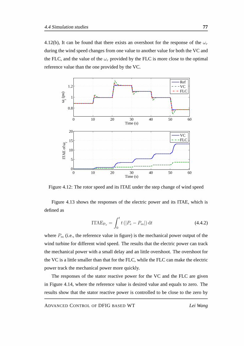
4.4 Simulation studies 77
4.12(b), It can be found that there exists an overshoot for the response of theωr
during the wind speed changes from one value to another valuefor both the VC and
the FLC, and the value of theωr provided by the FLC is more close to the optimal
reference value than the one provided by the VC.
0 10 20 30 40 50 60
0.8
1
1.2
Time (s)
ωr (
pu)
RefVCFLC
0 10 20 30 40 50 600
5
10
15
20
Time (s)
ITA
E o
f ωr
VCFLC
Figure 4.12: The rotor speed and its ITAE under the step change of wind speed
Figure 4.13 shows the responses of the electric power and itsITAE, which is
defined as
ITAEPe=
∫ t
0
t (|Pe − Pm|) dt (4.4.2)
wherePm (i.e., the reference value in figure) is the mechanical poweroutput of the
wind turbine for different wind speed. The results that the electric power can track
the mechanical power with a small delay and an little overshoot. The overshoot for
the VC is a little smaller than that for the FLC, while the FLC can make the electric
power track the mechanical power more quickly.
The responses of the stator reactive power for the VC and the FLC are given
in Figure 4.14, where the reference value is desired value and equals to zero. The
results show that the stator reactive power is controlled tobe close to the zero by
ADVANCED CONTROL OFDFIG BASED WT Lei Wang
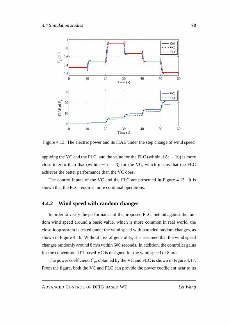
4.4 Simulation studies 78
0 10 20 30 40 50 600.2
0.4
0.6
0.8
1
Time (s)
P e (pu
)
RefVCFLC
0 10 20 30 40 50 600
10
20
30
Time (s)
ITA
E o
f Pe
VCFLC
Figure 4.13: The electric power and its ITAE under the step change of wind speed
applying the VC and the FLC, and the value for the FLC (within±5e− 10) is more
close to zero than that (within±1e − 3) for the VC, which means that the FLC
achieves the better performance than the VC does.
The control inputs of the VC and the FLC are presented in Figure 4.15. It is
shown that the FLC requires more continual operations.
4.4.2 Wind speed with random changes
In order to verify the performance of the proposed FLC methodagainst the ran-
dom wind speed around a basic value, which is more common in real world, the
close-loop system is tested under the wind speed with bounded random changes, as
shown in Figure 4.16. Without loss of generality, it is assumed that the wind speed
changes randomly around 8 m/s within 600 seconds. In addition, the controller gains
for the conventional PI-based VC is designed for the wind speed of 8 m/s.
The power coefficient,Cp, obtained by the VC and FLC is shown in Figure 4.17.
From the figure, both the VC and FLC can provide the power coefficient near to its
ADVANCED CONTROL OFDFIG BASED WT Lei Wang

4.4 Simulation studies 79
0 10 20 30 40 50 60−1
−0.5
0
0.5
1x 10
−3
Time (s)
Qs (
pu)
0 10 20 30 40 50 60−5
0
5x 10
−10
Time (s)
Qs (
pu)
RefVC
RefFLC
Figure 4.14: The stator reactive power under the step changeof wind speed
0 10 20 30 40 50 60
0.02
0.04
0.06
Time (s)
u dr (
pu)
0 10 20 30 40 50 60
−0.2
0
0.2
0.4
Time (s)
u qr (
pu)
VCFLC
VCFLC
Figure 4.15: The rotor voltage ind- andq-axis under the step change of wind speed
ADVANCED CONTROL OFDFIG BASED WT Lei Wang
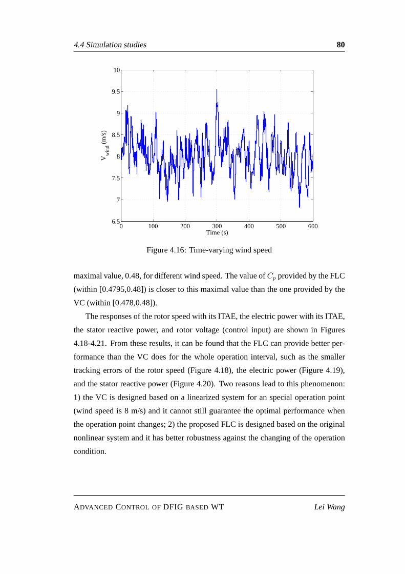
4.4 Simulation studies 80
0 100 200 300 400 500 6006.5
7
7.5
8
8.5
9
9.5
10
Time (s)
Vw
ind (
m/s
)
Figure 4.16: Time-varying wind speed
maximal value, 0.48, for different wind speed. The value ofCp provided by the FLC
(within [0.4795,0.48]) is closer to this maximal value thanthe one provided by the
VC (within [0.478,0.48]).
The responses of the rotor speed with its ITAE, the electric power with its ITAE,
the stator reactive power, and rotor voltage (control input) are shown in Figures
4.18-4.21. From these results, it can be found that the FLC can provide better per-
formance than the VC does for the whole operation interval, such as the smaller
tracking errors of the rotor speed (Figure 4.18), the electric power (Figure 4.19),
and the stator reactive power (Figure 4.20). Two reasons lead to this phenomenon:
1) the VC is designed based on a linearized system for an special operation point
(wind speed is 8 m/s) and it cannot still guarantee the optimal performance when
the operation point changes; 2) the proposed FLC is designedbased on the original
nonlinear system and it has better robustness against the changing of the operation
condition.
ADVANCED CONTROL OFDFIG BASED WT Lei Wang
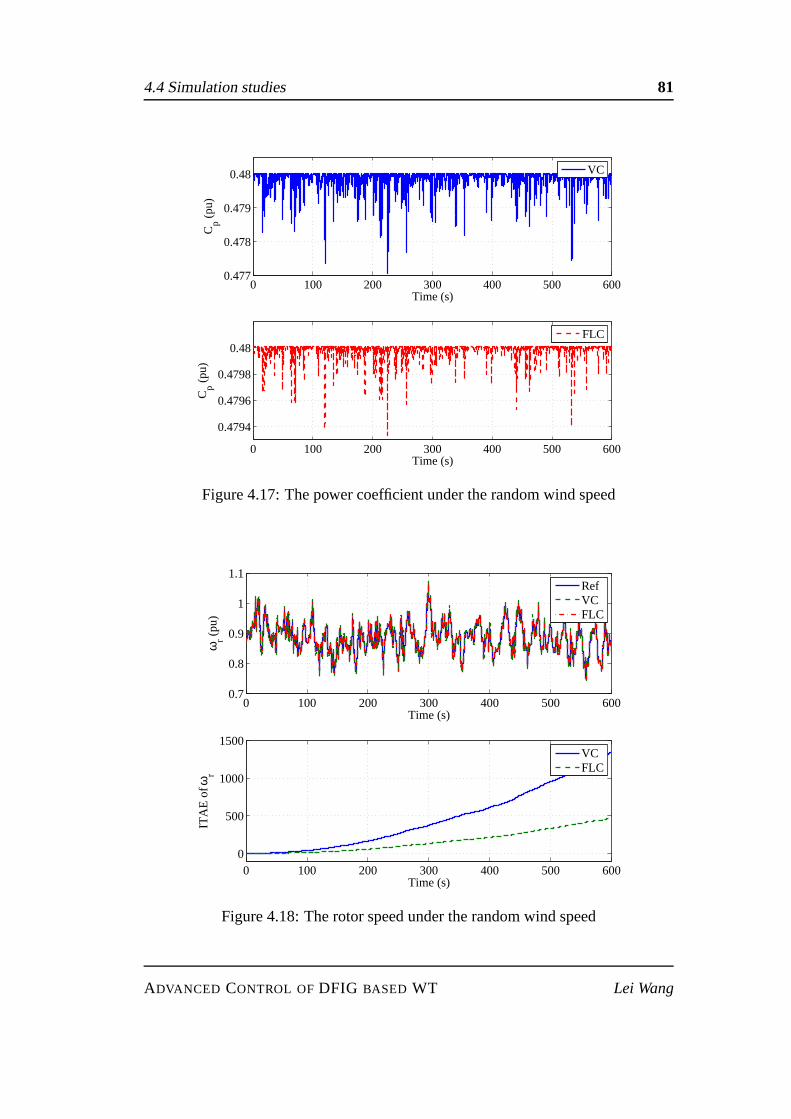
4.4 Simulation studies 81
0 100 200 300 400 500 6000.477
0.478
0.479
0.48
Time (s)
Cp (
pu)
0 100 200 300 400 500 600
0.4794
0.4796
0.4798
0.48
Time (s)
Cp (
pu)
VC
FLC
Figure 4.17: The power coefficient under the random wind speed
0 100 200 300 400 500 6000.7
0.8
0.9
1
1.1
Time (s)
ωr (
pu)
0 100 200 300 400 500 6000
500
1000
1500
Time (s)
ITA
E o
f ωr
RefVCFLC
VCFLC
Figure 4.18: The rotor speed under the random wind speed
ADVANCED CONTROL OFDFIG BASED WT Lei Wang
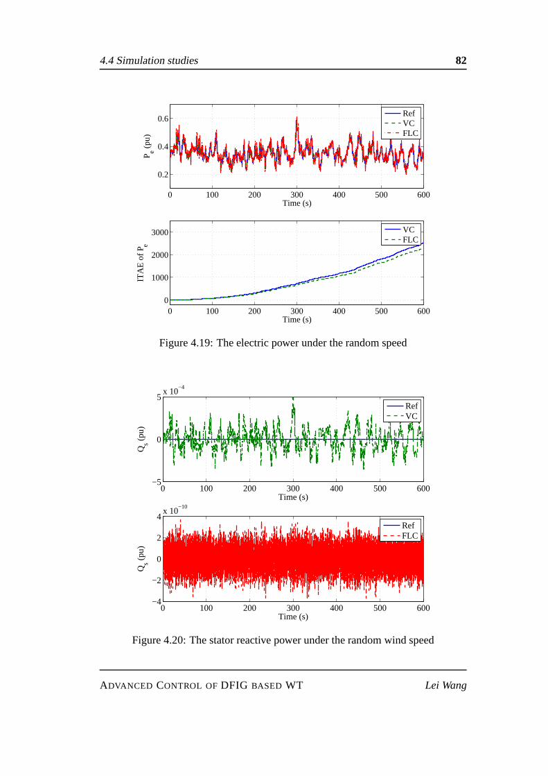
4.4 Simulation studies 82
0 100 200 300 400 500 600
0.2
0.4
0.6
Time (s)
P e (pu
)
0 100 200 300 400 500 6000
1000
2000
3000
Time (s)
ITA
E o
f Pe
RefVCFLC
VCFLC
Figure 4.19: The electric power under the random speed
0 100 200 300 400 500 600−5
0
5x 10
−4
Time (s)
Qs (
pu)
0 100 200 300 400 500 600−4
−2
0
2
4x 10
−10
Time (s)
Qs (
pu)
RefVC
RefFLC
Figure 4.20: The stator reactive power under the random windspeed
ADVANCED CONTROL OFDFIG BASED WT Lei Wang
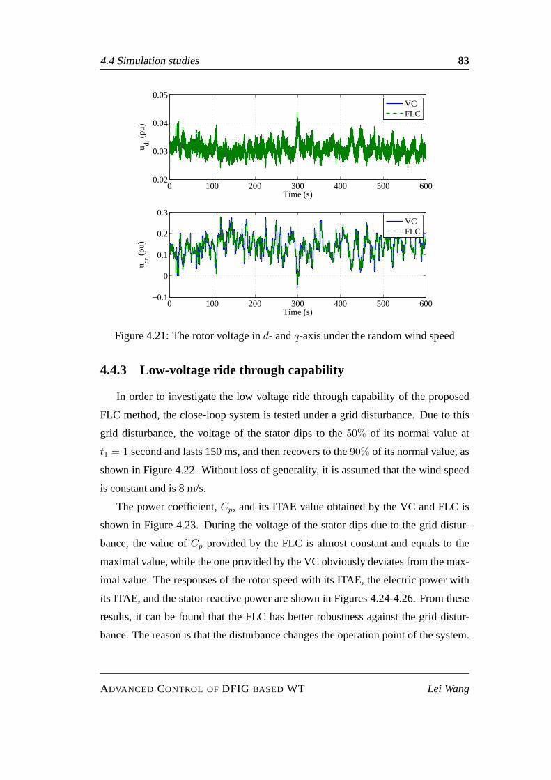
4.4 Simulation studies 83
0 100 200 300 400 500 6000.02
0.03
0.04
0.05
Time (s)
u dr (
pu)
VCFLC
0 100 200 300 400 500 600−0.1
0
0.1
0.2
0.3
Time (s)
u qr (
pu)
VCFLC
Figure 4.21: The rotor voltage ind- andq-axis under the random wind speed
4.4.3 Low-voltage ride through capability
In order to investigate the low voltage ride through capability of the proposed
FLC method, the close-loop system is tested under a grid disturbance. Due to this
grid disturbance, the voltage of the stator dips to the50% of its normal value at
t1 = 1 second and lasts 150 ms, and then recovers to the90% of its normal value, as
shown in Figure 4.22. Without loss of generality, it is assumed that the wind speed
is constant and is 8 m/s.
The power coefficient,Cp, and its ITAE value obtained by the VC and FLC is
shown in Figure 4.23. During the voltage of the stator dips due to the grid distur-
bance, the value ofCp provided by the FLC is almost constant and equals to the
maximal value, while the one provided by the VC obviously deviates from the max-
imal value. The responses of the rotor speed with its ITAE, the electric power with
its ITAE, and the stator reactive power are shown in Figures 4.24-4.26. From these
results, it can be found that the FLC has better robustness against the grid distur-
bance. The reason is that the disturbance changes the operation point of the system.
ADVANCED CONTROL OFDFIG BASED WT Lei Wang

4.4 Simulation studies 84
0 1 2 3 4 5 6 7 80.4
0.5
0.6
0.7
0.8
0.9
1
1.1
Time (s)
Vol
tage
of s
tato
r (p
u)
Figure 4.22: The grid disturbance
0 1 2 3 4 5 6 7 80.465
0.47
0.475
0.48
Time (s)
Cp (
pu)
VCFLC
0 1 2 3 4 5 6 7 80
0.01
0.02
0.03
Time (s)
ITA
E o
f Cp
VCFLC
Figure 4.23: The power coefficient under the grid disturbance
ADVANCED CONTROL OFDFIG BASED WT Lei Wang
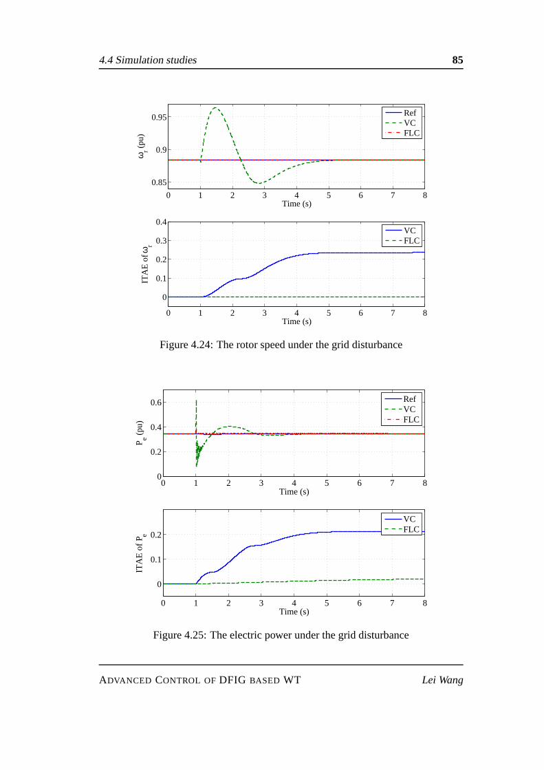
4.4 Simulation studies 85
0 1 2 3 4 5 6 7 8
0.85
0.9
0.95
Time (s)
ωr (
pu)
RefVCFLC
0 1 2 3 4 5 6 7 8
0
0.1
0.2
0.3
0.4
Time (s)
ITA
E o
f ωr
VCFLC
Figure 4.24: The rotor speed under the grid disturbance
0 1 2 3 4 5 6 7 80
0.2
0.4
0.6
Time (s)
P e (pu
)
RefVCFLC
0 1 2 3 4 5 6 7 8
0
0.1
0.2
Time (s)
ITA
E o
f Pe
VCFLC
Figure 4.25: The electric power under the grid disturbance
ADVANCED CONTROL OFDFIG BASED WT Lei Wang
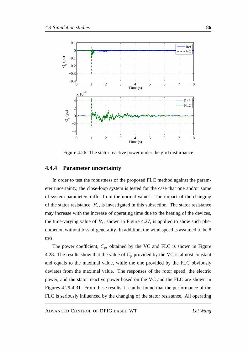
4.4 Simulation studies 86
0 1 2 3 4 5 6 7 8−0.4
−0.3
−0.2
−0.1
0
0.1
Time (s)
Qs (
pu)
RefVC
0 1 2 3 4 5 6 7 8
−4
−2
0
2
4
x 10−11
Time (s)
Qs (
pu)
RefFLC
Figure 4.26: The stator reactive power under the grid disturbance
4.4.4 Parameter uncertainty
In order to test the robustness of the proposed FLC method against the param-
eter uncertainty, the close-loop system is tested for the case that one and/or some
of system parameters differ from the normal values. The impact of the changing
of the stator resistance,Rr, is investigated in this subsection. The stator resistance
may increase with the increase of operating time due to the heating of the devices,
the time-varying value ofRr, shown in Figure 4.27, is applied to show such phe-
nomenon without loss of generality. In addition, the wind speed is assumed to be 8
m/s.
The power coefficient,Cp, obtained by the VC and FLC is shown in Figure
4.28. The results show that the value ofCp provided by the VC is almost constant
and equals to the maximal value, while the one provided by theFLC obviously
deviates from the maximal value. The responses of the rotor speed, the electric
power, and the stator reactive power based on the VC and the FLC are shown in
Figures 4.29-4.31. From these results, it can be found that the performance of the
FLC is seriously influenced by the changing of the stator resistance. All operating
ADVANCED CONTROL OFDFIG BASED WT Lei Wang

4.5 Summary 87
variables, includingCp, ωr, Pe, andQs, deviate from their desired optimal values
(reference values in the figures) when the value ofRr is different from the one that
applied to design the FLC. The reason is that the design of theFLC has strong
connection with such parameter, as shown in (4.2.17). That is to say, the control
effort of the FLC is no longer suitable during the value ofRr is different from the
one used in the controller. This can be found from the responses of the control input,
as shown in Figure 4.32, in which the comparison of the VC and FLC shows that
the desired control input and the actual control input of theFLC is inconsistent, for
example, from 35 second to 50 second, the desired control input of udr should be
bigger than 0.03 based on the VC, while the actual control input of udr provided by
FLC is smaller than 0.03.
0 10 20 30 40 50 600.045
0.05
0.055
0.06
0.065
0.07
0.075
0.08
Time (s)
Rr
(pu)
Figure 4.27: The time-varying rotor resistance
4.5 Summary
In this chapter, the nonlinear control design for maximum power power tracking
(MPPT) control of DFIG-WT was investigated. The wind turbine operation regions
ADVANCED CONTROL OFDFIG BASED WT Lei Wang

4.5 Summary 88
0 10 20 30 40 50 60
0.48
0.48
0.48
0.48
0.48
Time (s)
Cp (
pu)
0 10 20 30 40 50 60
0.2
0.4
Time (s)
Cp (
pu)
VC
FLC
Figure 4.28: The power coefficient under the time-varying rotor resistance
0 10 20 30 40 50 60
0.88
0.885
0.89
Time (s)
ωr (
pu)
0 10 20 30 40 50 600.8
1
1.2
1.4
Time (s)
ωr (
pu)
RefVC
RefFLC
Figure 4.29: The rotor speed under the time-varying rotor resistance
ADVANCED CONTROL OFDFIG BASED WT Lei Wang
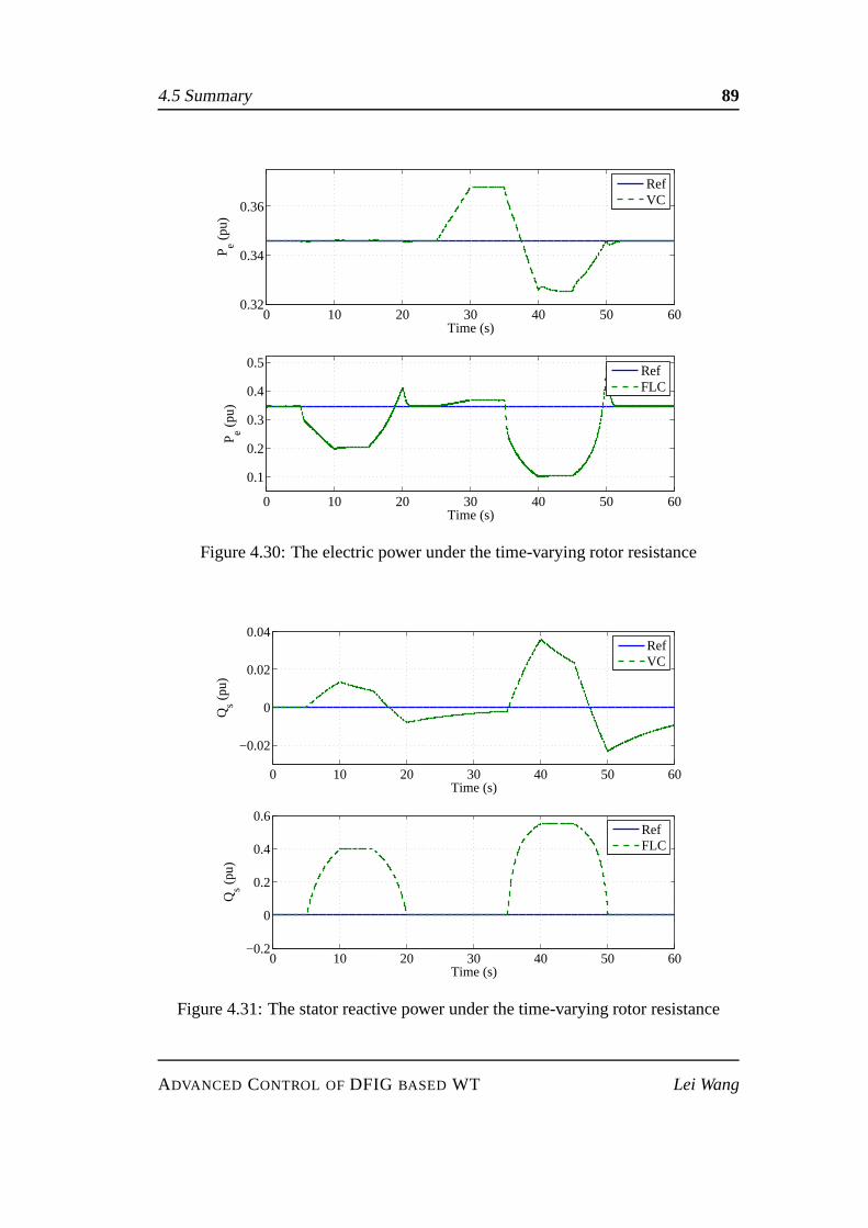
4.5 Summary 89
0 10 20 30 40 50 600.32
0.34
0.36
Time (s)
P e (pu
)
0 10 20 30 40 50 60
0.1
0.2
0.3
0.4
0.5
Time (s)
P e (pu
)
RefVC
RefFLC
Figure 4.30: The electric power under the time-varying rotor resistance
0 10 20 30 40 50 60
−0.02
0
0.02
0.04
Time (s)
Qs (
pu)
0 10 20 30 40 50 60−0.2
0
0.2
0.4
0.6
Time (s)
Qs (
pu)
RefVC
RefFLC
Figure 4.31: The stator reactive power under the time-varying rotor resistance
ADVANCED CONTROL OFDFIG BASED WT Lei Wang
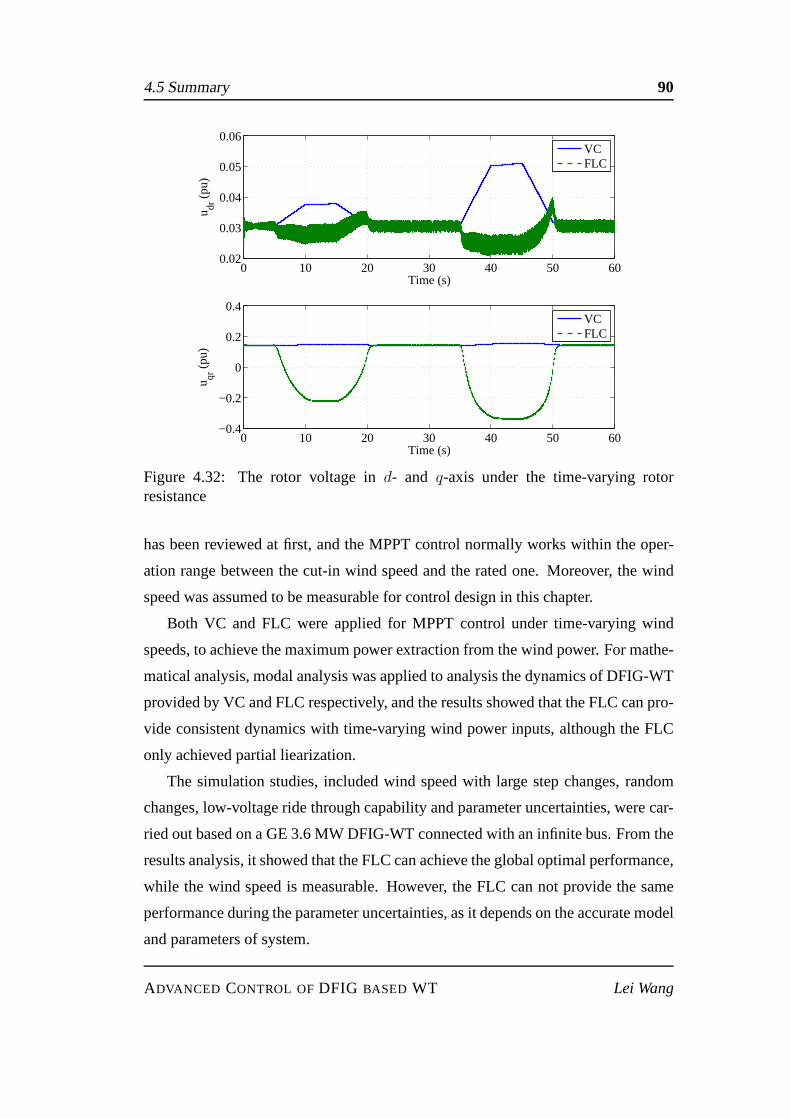
4.5 Summary 90
0 10 20 30 40 50 600.02
0.03
0.04
0.05
0.06
Time (s)
u dr (
pu)
0 10 20 30 40 50 60−0.4
−0.2
0
0.2
0.4
Time (s)
u qr (
pu)
VCFLC
VCFLC
Figure 4.32: The rotor voltage ind- and q-axis under the time-varying rotorresistance
has been reviewed at first, and the MPPT control normally works within the oper-
ation range between the cut-in wind speed and the rated one. Moreover, the wind
speed was assumed to be measurable for control design in thischapter.
Both VC and FLC were applied for MPPT control under time-varying wind
speeds, to achieve the maximum power extraction from the wind power. For mathe-
matical analysis, modal analysis was applied to analysis the dynamics of DFIG-WT
provided by VC and FLC respectively, and the results showed that the FLC can pro-
vide consistent dynamics with time-varying wind power inputs, although the FLC
only achieved partial liearization.
The simulation studies, included wind speed with large stepchanges, random
changes, low-voltage ride through capability and parameter uncertainties, were car-
ried out based on a GE 3.6 MW DFIG-WT connected with an infinitebus. From the
results analysis, it showed that the FLC can achieve the global optimal performance,
while the wind speed is measurable. However, the FLC can not provide the same
performance during the parameter uncertainties, as it depends on the accurate model
and parameters of system.
ADVANCED CONTROL OFDFIG BASED WT Lei Wang

Chapter 5
Nonlinear Adaptive Control for
Maximum Power Point Tracking
5.1 Introduction
The model of DFIG-WT belongs to the nonlinear multiple-input multiple-output
class, with great nonlinearities existing in the aerodynamics of the WT and the
electro-magnetic dynamics of the DFIG. Nonlinear feedbacklinearization controller-
s (FLC) has shown an excellent performance in controlling the nonlinear system.
This method transforms the original nonlinear system into decoupled linear system,
and the controller is performed via linear control laws [81], [82], [83], [84], [85].
It allows nonlinear controllers to be easily designed so that good performance is
guaranteed for a wide range of operating points. In [7], the asymptotic regulation
of active and reactive power was achieved by means of direct closed-loop control
of active and reactive components of the stator current vector, presented in a line-
voltage-oriented reference frame. In [?], the linear quadratic regulator (LQR) de-
sign method was introduced to design the optimal control forthe linearized system,
and the nonlinear control for DFIG-WT obtained by the inverse coordinate trans-
formation only depends on the parameters of DFIG-WT. All those results require
the availability of accurate system models and have more complex control laws than
linear methods. In practice, those assumptions are not realistic.
91

5.2 Problem Formulation 92
In order to deal with the parameter uncertainties, nonlinear adaptive control has
been investigated for DFIG-WT. Nonlinear adaptive controller based on parame-
ter identification has been investigated for DFIG-WT in [35], with the mechanical
torque considered as constant. The proposed controller is based on the feedback
linearization technique and includes a disturbance observer for estimation of pa-
rameter uncertainties. In [34], an adaptive feedback linearization strategy for an
WECS with slip power recovery is presented. The proposed adaptive law allows
system linearization even in the presence of an imprecise turbine description. Then,
the closed-loop dynamic behavior can be determined by a simple tuning of the con-
troller parameters.
5.2 Problem Formulation
Under different wind speed, there exists a maximum output mechanical power
Pm, which is mainly related with the turbine shaft speed and thewind velocity. As a
result of time-varying wind speed, the rotor speedωr can be controlled to make the
wind turbine output power reach this value. Thus the maximumpower is a function
of rotor speedωr [44]
Pm opt = Koptω3r (5.2.1)
and the optimal curve of mechanical torque can be computed by
Tm opt = Koptω2r (5.2.2)
where the optimal gainKopt is defined as [44]
Kopt =1
2ρπR5Cp max
λ3opt(5.2.3)
According to the equation 2.2.7, the reference of electric torque can be defined as
Te ref = Koptω2r −Dmωr (5.2.4)
The curve in Figure 5.1 illustrates the power versus rotor speed characteristics
without wind speed measurement. While wind speed varies from Vwind1 to Vwind2,
the extracted power increases from pointA to B, andλB < λC whereλC is the
ADVANCED CONTROL OFDFIG BASED WT Lei Wang
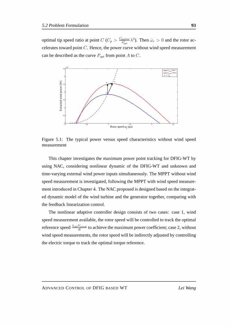
5.2 Problem Formulation 93
optimal tip speed ratio at pointC (Cp >Cp max
λ3
opt
λ3). Thenωr > 0 and the rotor ac-
celerates toward pointC. Hence, the power curve without wind speed measurement
can be described as the curvePopt from pointA toC.
0 0.5 1 1.5 2 2.50
0.5
1
1.5
2
2.5
3
3.5x 10
6
Rotor speed ωr (pu)
Ext
ract
ed w
ind
pow
er (
W)
V
wind1=9m/s
Vwind2
=10m/s
Popt
A
BC
Figure 5.1: The typical power versus speed characteristicswithout wind speedmeasurement
This chapter investigates the maximum power point trackingfor DFIG-WT by
using NAC, considering nonlinear dynamic of the DFIG-WT andunknown and
time-varying external wind power inputs simultaneously. The MPPT without wind
speed measurement is investigated, following the MPPT withwind speed measure-
ment introduced in Chapter 4. The NAC proposed is designed based on the integrat-
ed dynamic model of the wind turbine and the generator together, comparing with
the feedback linearization control.
The nonlinear adaptive controller design consists of two cases: case 1, wind
speed measurement available, the rotor speed will be controlled to track the optimal
reference speedλoptVwind
Rto achieve the maximum power coefficient; case 2, without
wind speed measurements, the rotor speed will be indirectlyadjusted by controlling
the electric torque to track the optimal torque reference.
ADVANCED CONTROL OFDFIG BASED WT Lei Wang

5.3 Nonlinear Adaptive Control based on Perturbation Estimation 94
5.3 Nonlinear Adaptive Control based on Perturba-
tion Estimation
The nonlinear adaptive control based on perturbation observer proposed in [86],
[87] will be recalled briefly as following steps. A multi-input multi-output (MIMO)
system is transformed as interacted subsystems via input/output linearisation at first.
Then for each subsystem, a perturbation term is defined to include all subsystem
nonlinearities, interactions between subsystems and uncertainties and estimated by
designing perturbation observers. The estimates of perturbations are used to com-
pensate the real perturbation and implement an adaptive linearisation and decoupled
control of the original nonlinear system.
5.3.1 Input-Output linearization
Consider a MIMO system
x = f(x) + g(x)u
y = h(x)(5.3.1)
wherex ∈ Rn is the state vector,u ∈ Rm is the control input vector,y ∈ Rm is
the output vector,f(x), g(x) andh(x) are smooth vector fields. The input-output
linearisation of a MIMO system is obtained via differentiating the outputyi of the
system until the inputuj appears. Thus, assuming thatri is the smallest integer such
that at least one of the inputs explicitly appears iny(ri)i
y(ri)i = Lri
f hi +
m∑
j=1
LgjLri−1f hiuj (5.3.2)
wherey(ri)i is the ith-order derivative ofyi, LgjLri−1f hi(x) 6= 0 for at least onej.
Performing the above procedure for each outputyi yields
y(r1)1
...
y(rm)m
=
Lr1f h1...
Lrmf hm
+B(x)
u1...
um
(5.3.3)
ADVANCED CONTROL OFDFIG BASED WT Lei Wang

5.3 Nonlinear Adaptive Control based on Perturbation Estimation 95
B(x) =
Lg1Lr1−1f h1 · · · LgmL
r1−1f h1
......
...
Lg1Lrm−1f hm · · · LgmL
rm−1f hm
(5.3.4)
whereB(x) is am × m control gain matrix. IfB(x) is invertible, the feedback
linearisation control of the the MIMO nonlinear system can be obtained as
u = B(x)−1
−Lr1f h1...
−Lrmf hm
+
v1...
vm
(5.3.5)
wherevi are new inputs of the system. Now the input-output relationsare given by
y(ri)i = vi (5.3.6)
At this point, desired dynamics can be imposed on the system by the new system
inputs.
5.3.2 Perturbation observer
Assume all nonlinearities of system (5.3.3) are unknown, and define perturbation
terms as
Ψ1
...
Ψm
=
Lr1f h1...
Lrmf hm
+ (B(x)−B0)
u1...
um
(5.3.7)
whereΨi is the perturbation term,B0 = B(x)|x=x(0) is the nominal control gain.
Then system (5.3.3) can be rewritten as
y(r1)1
...
y(rm)m
=
Ψ1(x)...
Ψm(x)
+B0
u1...
um
(5.3.8)
For theith subsystem, defining state variables aszi1 = yi, · · · , ziri = y(ri−1)i and
a virtual state to represent the perturbationzi(ri+1) = Ψi, theith subsystem can be
ADVANCED CONTROL OFDFIG BASED WT Lei Wang
5.3 Nonlinear Adaptive Control based on Perturbation Estimation 96
represented as
zi1 = zi2...
ziri = zi(ri+1) +B0iu
zi(ri+1) = Ψi
(5.3.9)
whereB0i is theith row of theB0. The perturbation observer has been developed
as an important technique for the design of NAC proposed in [86], [87]. Several
types of perturbation observers, such as sliding mode observer, high gain observer
and linear Lunberger observer have been introduced to obtain the online estimate
of the perturbation. High gain observer is introduced in this paper as an example.
When all states are available, the perturbation is estimated by a second-order pertur-
bation observer (PO) which use the last statezi(ri−1) as measurement. A states and
perturbation observer (SPO) will be designed to obtain the states and perturbation
together when only one system statezi1 = yi is available.
When all states are available, the perturbation is estimated by a second-order
perturbation observer (PO) which use the last stateziri as measurement as follows
˙ziri = zi1 + hi1(zi1 − ziri) +B0iu
˙zi(ri+1) = hi2(ziri − ziri),(5.3.10)
wherehi1 andhi2 are gains of the high gain observer. Throughout this paper,ziri
represents the estimate ofziri . By choosing
hi1 =αi1
ǫi, hi2 =
αi2
ǫ2i, (5.3.11)
whereǫi, 0 < ǫi < 1 is a positive constant to be specified and the positive constants
αij , j = 1, 2, are chosen such that the roots of
s2 + αi1s+ αi2 = 0 (5.3.12)
are in the open left-half complex plan.
When only the system outputyi = zi1 is available, a(ri + 1)th-order state and
perturbation observer (SPO) can be designed to estimate thesystem states and per-
ADVANCED CONTROL OFDFIG BASED WT Lei Wang

5.4 Controller Design 97
turbation as
˙zi1 = zi2 + hi1(zi1 − zi1)
. . .
˙ziri = ziri + hiri(zi1 − zi1) +B0iu
˙zi(ri+1) = hi(ri+1)(zi1 − zi1),
(5.3.13)
wherehij =αij
ǫji
, j = 1, · · · , ri+1 are gains of the high gain observer,ǫi, 0 < ǫi < 1
is a positive constant to be specified and the positive constantsαij , j = 1, · · · , ri+1,
are chosen such that the roots of
sri+1 + αi1sri + · · ·+ αiris+ αi(ri+1) = 0 (5.3.14)
are in the open left-half complex plan.
5.3.3 Design of NAC controller
Using the estimate of perturbationΨi = zi(ri+1) to compensate the real system
perturbation, the control law of the NAC can be obtained as
u = B−10
−Ψ1
...
−Ψm
+
v1...
vm
(5.3.15)
wherevi = −Kizi is the state feedback control of theith linear system when a PO
is designed, or an output feedbackvi = −Kizi when a SPO is designed.Ki =
[ki1, · · · , ki(ri−1)]T are the linear feedback controller gains which can be determined
via linear system method.
5.4 Controller Design
5.4.1 With wind speed measurement
Feedback linearization Control
Choose the rotor speedωr and stator reactive powerQs as the controlled outputs:
y1 = ωr
y2 = Qs
(5.4.1)
ADVANCED CONTROL OFDFIG BASED WT Lei Wang

5.4 Controller Design 98
Let ωr opt andQs ref be the given references of the rotor speed and reactive power,
and define the tracking errore = [e1 e2]T as:
e =
[
e1
e2
]
=
[
ωr − ωr opt
Qs −Q∗s
]
(5.4.2)
The input/output feedback linearization of equation (4.1.1) can be obtained as:[
e1
e2
]
=
[
f1 − ωr opt
f2 − Q∗s
]
+B(x)
[
udr
uqr
]
(5.4.3)
where
f1 =Tm
2Hm− 1
2Hm((−uqs +Rsiqs + ωsψds)(
Lr
Lσψds + ids)
+(uds −Rsids + ωsψqs)(iqs +Lr
Lσψqs)− Lm
Lσψds(Rriqr
+(ωs − ωr)ψdr)− Lm
Lσψqs(−Rridr + (ωs − ωr)ψqr))
(5.4.4)
f2 = uqsLm
Lσ(−Rridr + (ωs − ωr)ψqr)− uqs
Lr
Lσ(uds−
Rsids + ωqs)− udsLm
Lσ(−Rriqr − (ωs − ωr)ψdr)+
udsLr
Lσ(uqs −Rsiqs − ωsψds)
(5.4.5)
and
B(x) =
[
Lm
2HmLσψqs − Lm
2HmLσψds
Lm
Lσuqs −Lm
Lσuds
]
(5.4.6)
whereB0(x) = B(x)|Lm=Lm0, ∆B(x) = B(x)− B0(x). Note that whendet(B) =
0.5 L2m
HmL2σ(−ψqsuds + ψdsuqs) 6= 0, system (5.4.3) can be linearized as following
[
e1
e2
]
=
[
v1
v2
]
(5.4.7)
wherev = [v1 v2]T is the control input of the linear system defined as
[
v1
v2
]
=
[
−k11e1 − k12e1
−k21e2
]
(5.4.8)
wherek11, k12, k21 are the feedback gains.
Then the FLC control law of equation (4.1.1) can be obtained as follows[
udr
uqr
]
= B(x)−1(
[
−f1 + ωr opt
−f2 + Qs ref
]
+ v) (5.4.9)
ADVANCED CONTROL OFDFIG BASED WT Lei Wang

5.4 Controller Design 99
Nonlinear adaptive control
FLC control law (5.4.9) assumes all states and parameters are known accurately
and is very complex. Moreover, in [35], [?], Tm is equal to zero, asTm is assumed
be constant during the transient period, which is correspond to constant wind speed.
Based on equation (5.4.3), perturbationsΨ1(x) andΨ2(x) are defined as
Ψ1(x) = f1(x)− ωr ref +∆B(x)11u1 +∆B(x)12u2
Ψ2(x) = f2(x)− Qs ref +∆B(x)11u1 +∆B(x)12u2(5.4.10)
whereu1 = udr, u2 = uqr.
Note that∆B(x) represents parameter uncertainties of control gains.
Defining the state vectorsz11 = y1, z12 = y1, z13 = Ψ1(x), z21 = y2, z22 =
Ψ2(x). Dynamic equations of the subsystemsq1 andq2 are described as follows:
q1 :
z11 = z12
z12 = z13 +B0(x)11u1 +B0(x)12u2
z13 = Ψ1(x)
q2 :
z21 = z22 +B0(x)21u1 +B0(x)22u2
z22 = Ψ2(x)
(5.4.11)
A third-order SPO, based on equation (5.3.13), is designed for the sub-system
q1.
˙z11 = z12 + h11(z11 − z11)
˙z12 = z13 + h12(z11 − z11) +B0(x)11u1 +B0(x)12u2˙z13 = h13(z11 − z11)
(5.4.12)
where[h11 h12 h13] = [α11
ǫ1
α12
ǫ21
α13
ǫ31
] are gains of the observer.
A second-order PO designed based on equation (5.3.10) is to estimate the sub-
systemq2 perturbation as follows:
˙z21 = z22 + h21(z21 − z21) +B0(x)21u1 +B0(x)22u2˙z22 = h22(z21 − z21)
(5.4.13)
where[h21 h22] = [α21
ǫ2
α22
ǫ22
] are gains of the observer.
ADVANCED CONTROL OFDFIG BASED WT Lei Wang
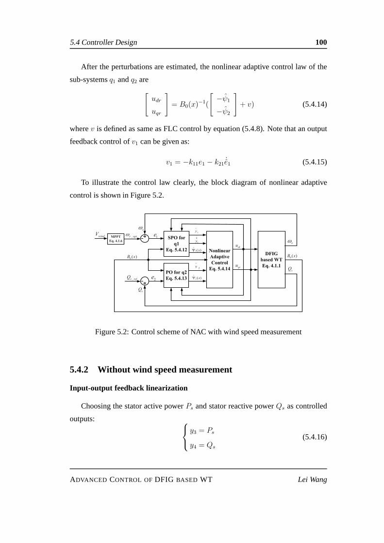
5.4 Controller Design 100
After the perturbations are estimated, the nonlinear adaptive control law of the
sub-systemsq1 andq2 are
[
udr
uqr
]
= B0(x)−1(
[
−ψ1
−ψ2
]
+ v) (5.4.14)
wherev is defined as same as FLC control by equation (5.4.8). Note that an output
feedback control ofv1 can be given as:
v1 = −k11e1 − k21 ˙e1 (5.4.15)
To illustrate the control law clearly, the block diagram of nonlinear adaptive
control is shown in Figure 5.2.
windVMPPT
Eq. 4.1.6
_r opt
r
1e
_s refQ
sQ
2e
0 ( )B x
dru
qru
1y
1y
!
1( )x
!
2 ( )x
!
2y
r
sQ
0 ( )B x
Figure 5.2: Control scheme of NAC with wind speed measurement
5.4.2 Without wind speed measurement
Input-output feedback linearization
Choosing the stator active powerPs and stator reactive powerQs as controlled
outputs:
y3 = Ps
y4 = Qs
(5.4.16)
ADVANCED CONTROL OFDFIG BASED WT Lei Wang
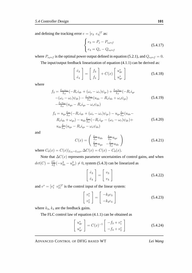
5.4 Controller Design 101
and defining the tracking errore = [e3 e4]T as:
e3 = Ps − Ps ref
e4 = Qs −Qs ref
(5.4.17)
wherePs ref is the optimal power output defined in equation (5.2.1), andQs ref = 0.
The input/output feedback linearization of equation (4.1.1) can be derived as:[
e3
e4
]
=
[
f3
f4
]
+ C(x)
[
u∗dr
u∗qr
]
(5.4.18)
where
f3 =Lmuds
Lσ(−Rridr + (ωs − ωr)ψqr) +
Lmuqs
Lσ(−Rriqr
−(ωs − ωr)ψdr)− Lruds
Lσ(uds −Rsids + ωsψqs)
−Lruqs
Lσ(uqs − Rsiqs − ωsψds)
(5.4.19)
f4 = uqsLm
Lσ(−Rridr + (ωs − ωr)ψqr)− uqs
Lr
Lσ(uds−
Rsids + ωqs)− udsLm
Lσ(−Rriqr − (ωs − ωr)ψdr)+
udsLr
Lσ(uqs − Rsiqs − ωsψds)
(5.4.20)
and
C(x) =
(
Lm
Lσuds
Lm
Lσuqs
Lm
Lσuqs −Lm
Lσuds
)
(5.4.21)
whereC0(x) = C(x)|Lm=Lm0, ∆C(x) = C(x)− C0(x).
Note that∆C(x) represents parameter uncertainties of control gains, and when
det(C) = L2m
L2σ(−u2ds − u2qs) 6= 0, system (5.4.3) can be linearized as
[
e3
e4
]
=
[
v3
v4
]
(5.4.22)
andv∗ = [v∗1 v∗2]T is the control input of the linear system:
[
v∗1
v∗2
]
=
[
−k3e3−k4e4
]
(5.4.23)
wherek3, k4 are the feedback gains.
The FLC control law of equation (4.1.1) can be obtained as[
u∗dr
u∗qr
]
= C(x)−1
[
−f3 + v∗1
−f4 + v∗2
]
(5.4.24)
ADVANCED CONTROL OFDFIG BASED WT Lei Wang

5.4 Controller Design 102
Perturbation estimation
The perturbationsΨ3(x) andΨ4(x) for two subsystemsq3 andq4 are expressed
respectively as:
Ψ3(x) = f3(x)− Ps ref +∆C(x)11u∗1 +∆C(x)12u
∗2
Ψ4(x) = f4(x)− Qs ref +∆C(x)11u∗1 +∆C(x)12u
∗2
(5.4.25)
whereu∗1 = u∗dr, u∗2 = u∗qr.
Defining the state vectorsz∗11 = y3, z∗12 = Ψ3(x), z∗21 = y4, z
∗22 = Ψ4(x). The
dynamic equations of the system can be described as
q3 :
z∗11 = z∗12 + C0(x)11u∗1 + C0(x)12u
∗2
z∗12 = Ψ3(x)
q4 :
z∗21 = z∗22 + C0(x)21u∗1 + C0(x)22u
∗2
z∗22 = Ψ4(x)
(5.4.26)
Based on equation (5.3.10), two second-order PO is designedto estimate the
sub-systemq′1 andq′2 perturbation as follows:
˙z∗11 = z∗12 + h∗11(z∗11 − z∗11) + C0(x)11u
∗1 + C0(x)12u
∗2
˙z∗12 = h∗12(z∗11 − z∗11)
(5.4.27)
and
˙z∗21 = z∗22 + h∗21(z∗21 − z∗21) + C0(x)21u
∗1 + C0(x)22u
∗2
˙z∗22 = h∗22(z∗21 − z∗21)
(5.4.28)
where[h∗11 h∗12] = [α∗
11
ǫ∗1
α∗
12
ǫ∗21
] and[h∗21 h∗22] = [α∗
21
ǫ∗2
α∗
22
ǫ∗22
] are gains of the observer.
After the perturbation estimation, the nonlinear adaptivecontroller of sub-systems
q3 andq4 can be derived as[
u∗dr
u∗qr
]
= C0(x)−1(
[
−ψ3
−ψ4
]
+ v∗) (5.4.29)
herev∗ is defined as[
v∗1
v∗2
]
=
[
−k3e3−k4e4
]
(5.4.30)
Figure 5.3 shows the block diagram of nonlinear adaptive control without wind
speed measurement.
ADVANCED CONTROL OFDFIG BASED WT Lei Wang
5.5 Simulation Studies 103
MPPT
Eq. 5.2.1
r 3e
_s refQ
sQ
4e
0 ( )C x
dru
3y
3( )x
!
4 ( )x
!
4y
sP
sQ
0 ( )C x
_m optP
sP
r
qru
Figure 5.3: Control scheme of NAC without wind speed measurement
5.5 Simulation Studies
In this section, the simulation studies are carried out to verify the effectiveness
of the proposed NAC by the following case studies: MPPT control with wind speed
measurement and without wind speed measurement, parameteruncertainties during
constant wind speed. The parameters of the DFIG-WT tested are the same as listed
in chapter 4.
5.5.1 With wind speed measurement
Step change of wind speed
For verifying the performance of the proposed NAC method against the large
step change of the wind speed, shown in Figure 5.4, the simulation studies on MPPT
of DFIG-WT are carried out by applying FLC and NAC.
From the Figure 5.5, it can be clearly seen that, both the FLC and NAC can
achieve the maximum power coefficient during the constant wind speed. However,
while the wind speed changes, an increasing error ofCp provided by the FLC can
be observed clearly when the large step change of wind speed occurs at50s. The
simulation result shows that the proposed NAC can provide better performance on
power coefficient.
ADVANCED CONTROL OFDFIG BASED WT Lei Wang
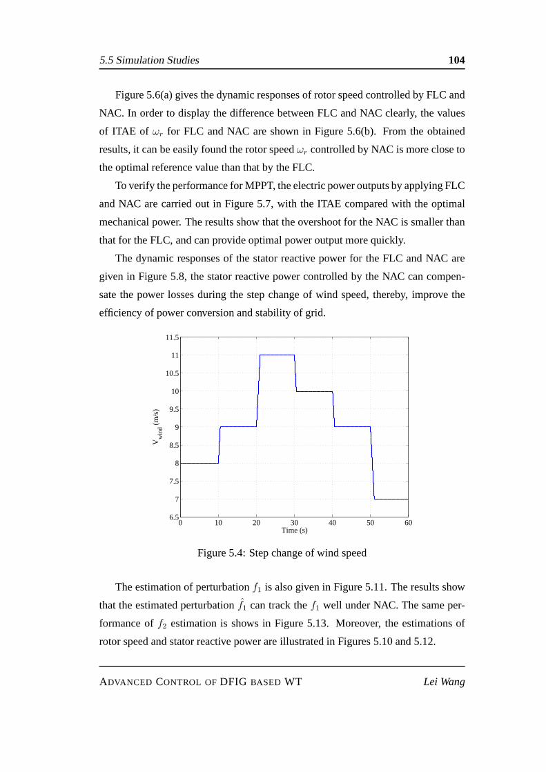
5.5 Simulation Studies 104
Figure 5.6(a) gives the dynamic responses of rotor speed controlled by FLC and
NAC. In order to display the difference between FLC and NAC clearly, the values
of ITAE of ωr for FLC and NAC are shown in Figure 5.6(b). From the obtained
results, it can be easily found the rotor speedωr controlled by NAC is more close to
the optimal reference value than that by the FLC.
To verify the performance for MPPT, the electric power outputs by applying FLC
and NAC are carried out in Figure 5.7, with the ITAE compared with the optimal
mechanical power. The results show that the overshoot for the NAC is smaller than
that for the FLC, and can provide optimal power output more quickly.
The dynamic responses of the stator reactive power for the FLC and NAC are
given in Figure 5.8, the stator reactive power controlled bythe NAC can compen-
sate the power losses during the step change of wind speed, thereby, improve the
efficiency of power conversion and stability of grid.
0 10 20 30 40 50 606.5
7
7.5
8
8.5
9
9.5
10
10.5
11
11.5
Time (s)
Vw
ind (
m/s
)
Figure 5.4: Step change of wind speed
The estimation of perturbationf1 is also given in Figure 5.11. The results show
that the estimated perturbationf1 can track thef1 well under NAC. The same per-
formance off2 estimation is shows in Figure 5.13. Moreover, the estimations of
rotor speed and stator reactive power are illustrated in Figures 5.10 and 5.12.
ADVANCED CONTROL OFDFIG BASED WT Lei Wang
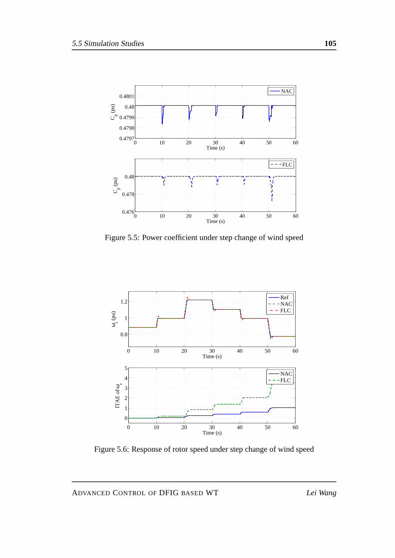
5.5 Simulation Studies 105
0 10 20 30 40 50 600.4797
0.4798
0.4799
0.48
0.4801
Time (s)
Cp (
pu)
NAC
0 10 20 30 40 50 600.476
0.478
0.48
Time (s)
Cp (
pu)
FLC
Figure 5.5: Power coefficient under step change of wind speed
0 10 20 30 40 50 60
0.8
1
1.2
Time (s)
ωr (
pu)
RefNACFLC
0 10 20 30 40 50 60
0
1
2
3
4
5
Time (s)
ITA
E o
f ωr
NACFLC
Figure 5.6: Response of rotor speed under step change of windspeed
ADVANCED CONTROL OFDFIG BASED WT Lei Wang
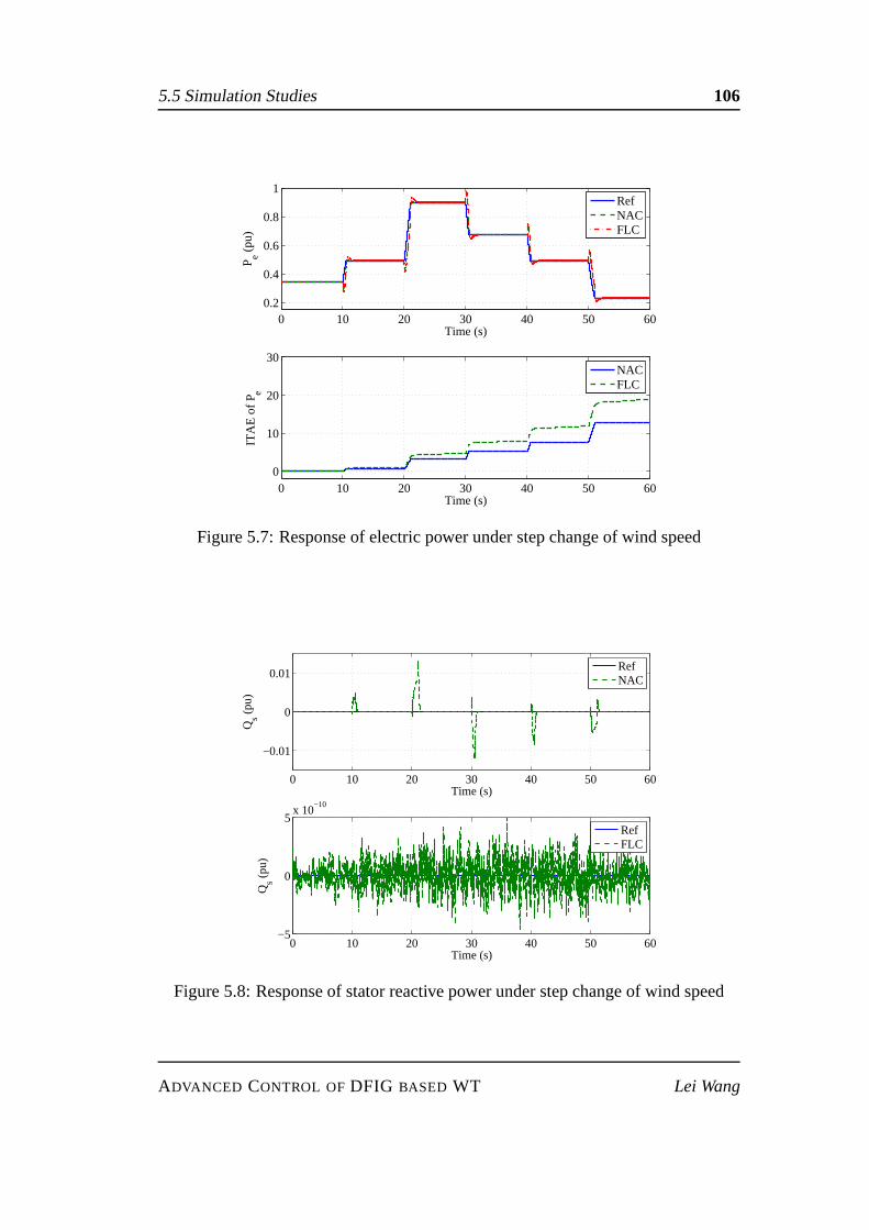
5.5 Simulation Studies 106
0 10 20 30 40 50 600.2
0.4
0.6
0.8
1
Time (s)
P e (pu
)
RefNACFLC
0 10 20 30 40 50 600
10
20
30
Time (s)
ITA
E o
f Pe
NACFLC
Figure 5.7: Response of electric power under step change of wind speed
0 10 20 30 40 50 60
−0.01
0
0.01
Time (s)
Qs (
pu)
RefNAC
0 10 20 30 40 50 60−5
0
5x 10
−10
Time (s)
Qs (
pu)
RefFLC
Figure 5.8: Response of stator reactive power under step change of wind speed
ADVANCED CONTROL OFDFIG BASED WT Lei Wang

5.5 Simulation Studies 107
0 10 20 30 40 50 60
0.02
0.04
0.06
Time (s)
u dr (
pu)
NACFLC
0 10 20 30 40 50 60
−0.2
0
0.2
0.4
Time (s)
u qr (
pu)
NACFLC
Figure 5.9: Rotor voltage of NAC and FLC ind-axis
0 10 20 30 40 50 60
0.7
0.8
0.9
1
1.1
1.2
1.3
Time (s)
Est
imat
ed ω
r (pu
)
0 10 20 30 40 50 60−2
−1
0
1
2x 10
−8
Time (s)
Est
imat
ed e
rror
of ω
r (pu
)
Figure 5.10: Rotor speedωr estimation and estimate error
ADVANCED CONTROL OFDFIG BASED WT Lei Wang
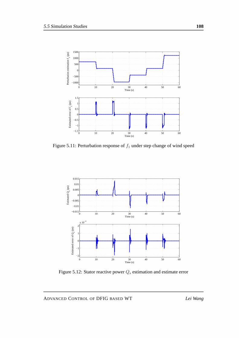
5.5 Simulation Studies 108
0 10 20 30 40 50 60
−1000
−500
0
500
1000
1500
Time (s)
Per
turb
atio
n es
timat
ion
f1 (
pu)
0 10 20 30 40 50 60−1.5
−1
−0.5
0
0.5
1
1.5
Time (s)
Est
imat
ed e
rror
of f 1 (
pu)
Figure 5.11: Perturbation response off1 under step change of wind speed
0 10 20 30 40 50 60−0.015
−0.01
−0.005
0
0.005
0.01
0.015
Time (s)
Est
imat
ed Q s (
pu)
0 10 20 30 40 50 60−2
−1
0
1
2x 10
−4
Time (s)
Est
imat
ed e
rror
of Q
s (pu
)
Figure 5.12: Stator reactive powerQs estimation and estimate error
ADVANCED CONTROL OFDFIG BASED WT Lei Wang
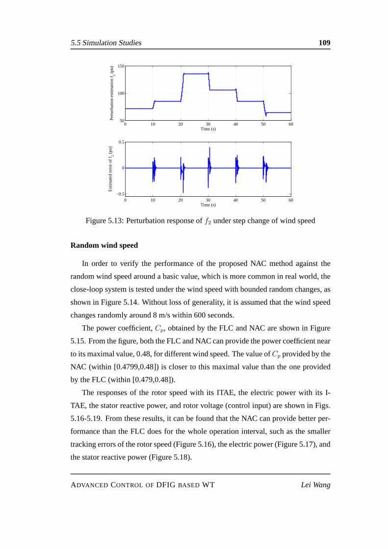
5.5 Simulation Studies 109
0 10 20 30 40 50 6050
100
150
Time (s)
Per
turb
atio
n es
timat
ion
f2 (
pu)
0 10 20 30 40 50 60−0.5
0
0.5
Time (s)
Est
imat
ed e
rror
of f 2 (
pu)
Figure 5.13: Perturbation response off2 under step change of wind speed
Random wind speed
In order to verify the performance of the proposed NAC methodagainst the
random wind speed around a basic value, which is more common in real world, the
close-loop system is tested under the wind speed with bounded random changes, as
shown in Figure 5.14. Without loss of generality, it is assumed that the wind speed
changes randomly around 8 m/s within 600 seconds.
The power coefficient,Cp, obtained by the FLC and NAC are shown in Figure
5.15. From the figure, both the FLC and NAC can provide the power coefficient near
to its maximal value, 0.48, for different wind speed. The value ofCp provided by the
NAC (within [0.4799,0.48]) is closer to this maximal value than the one provided
by the FLC (within [0.479,0.48]).
The responses of the rotor speed with its ITAE, the electric power with its I-
TAE, the stator reactive power, and rotor voltage (control input) are shown in Figs.
5.16-5.19. From these results, it can be found that the NAC can provide better per-
formance than the FLC does for the whole operation interval,such as the smaller
tracking errors of the rotor speed (Figure 5.16), the electric power (Figure 5.17), and
the stator reactive power (Figure 5.18).
ADVANCED CONTROL OFDFIG BASED WT Lei Wang
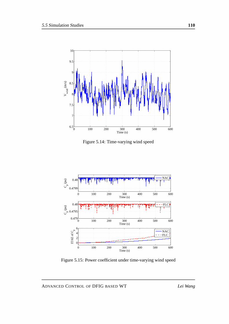
5.5 Simulation Studies 110
0 100 200 300 400 500 6006.5
7
7.5
8
8.5
9
9.5
10
Time (s)
Vw
ind (
m/s
)
Figure 5.14: Time-varying wind speed
0 100 200 300 400 500 600
0.4799
0.48
Time (s)
Cp (
pu)
NAC
0 100 200 300 400 500 6000.479
0.4795
0.48
Time (s)
Cp (
pu)
FLC
0 100 200 300 400 500 600
0
2
4
6
Time (s)
ITA
E o
f Cp
NACFLC
Figure 5.15: Power coefficient under time-varying wind speed
ADVANCED CONTROL OFDFIG BASED WT Lei Wang
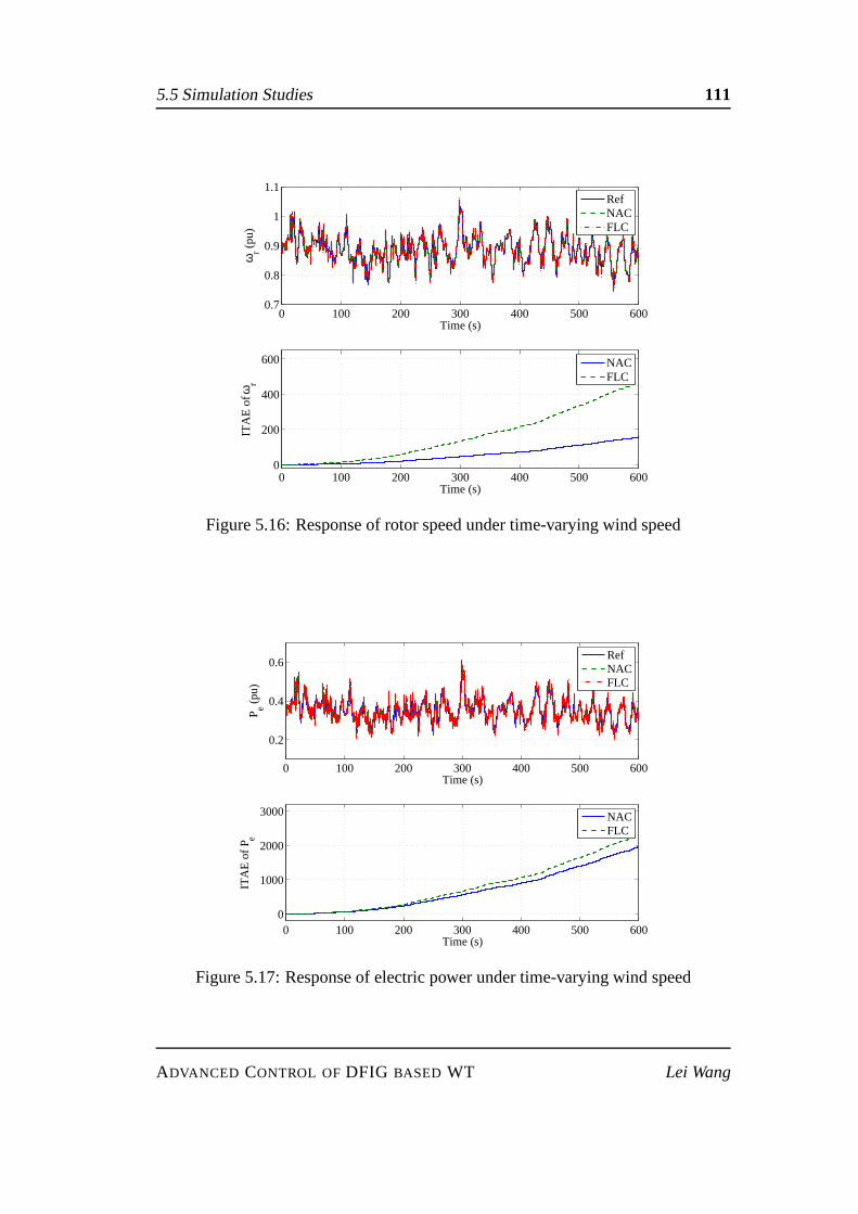
5.5 Simulation Studies 111
0 100 200 300 400 500 6000.7
0.8
0.9
1
1.1
Time (s)
ωr (
pu)
RefNACFLC
0 100 200 300 400 500 6000
200
400
600
Time (s)
ITA
E o
f ωr
NACFLC
Figure 5.16: Response of rotor speed under time-varying wind speed
0 100 200 300 400 500 600
0.2
0.4
0.6
Time (s)
P e (pu
)
RefNACFLC
0 100 200 300 400 500 6000
1000
2000
3000
Time (s)
ITA
E o
f Pe
NACFLC
Figure 5.17: Response of electric power under time-varyingwind speed
ADVANCED CONTROL OFDFIG BASED WT Lei Wang
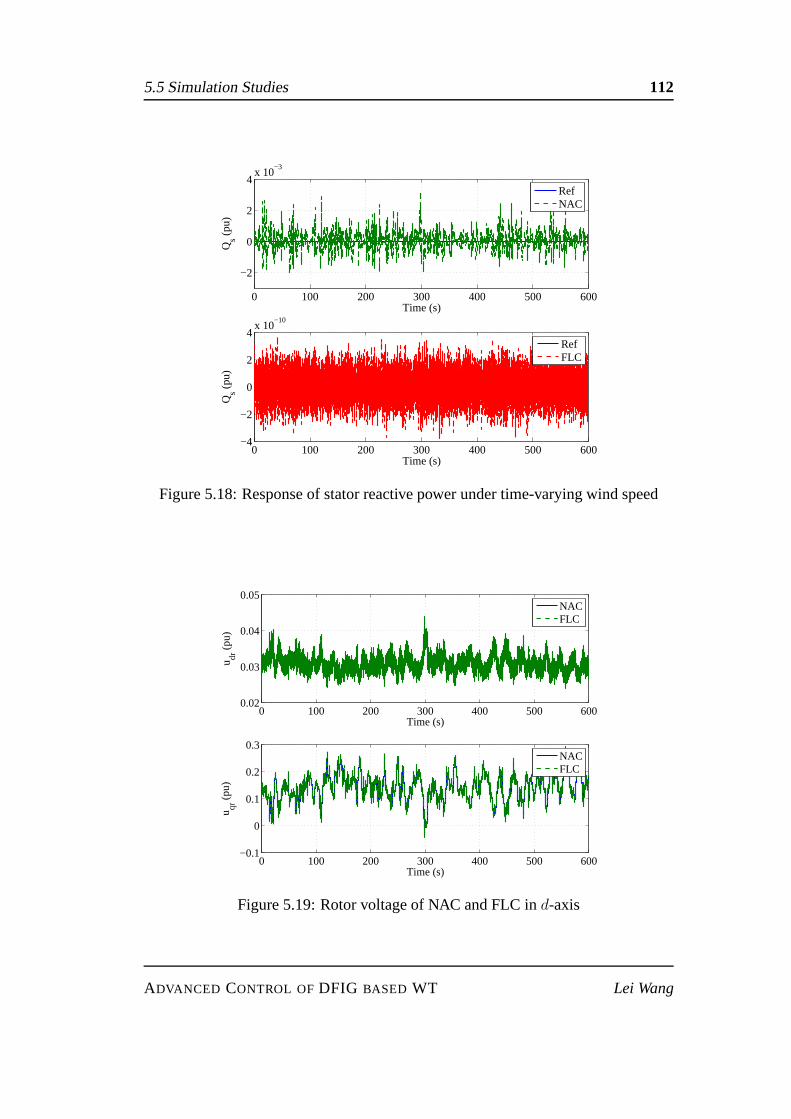
5.5 Simulation Studies 112
0 100 200 300 400 500 600
−2
0
2
4x 10
−3
Time (s)
Qs (
pu)
RefNAC
0 100 200 300 400 500 600−4
−2
0
2
4x 10
−10
Time (s)
Qs (
pu)
RefFLC
Figure 5.18: Response of stator reactive power under time-varying wind speed
0 100 200 300 400 500 6000.02
0.03
0.04
0.05
Time (s)
u dr (
pu)
NACFLC
0 100 200 300 400 500 600−0.1
0
0.1
0.2
0.3
Time (s)
u qr (
pu)
NACFLC
Figure 5.19: Rotor voltage of NAC and FLC ind-axis
ADVANCED CONTROL OFDFIG BASED WT Lei Wang
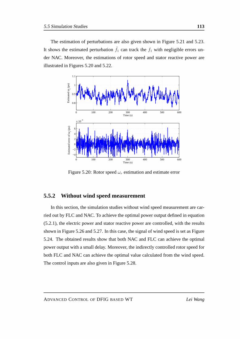
5.5 Simulation Studies 113
The estimation of perturbations are also given shown in Figure 5.21 and 5.23.
It shows the estimated perturbationf1 can track thef1 with negligible errors un-
der NAC. Moreover, the estimations of rotor speed and statorreactive power are
illustrated in Figures 5.20 and 5.22.
0 100 200 300 400 500 600
0.8
0.9
1
1.1
Time (s)
Est
imat
ed ω
r (pu
)
0 100 200 300 400 500 600
−4
−2
0
2
4
6
x 10−9
Time (s)
Est
imat
ed e
rror
of ω
r (pu
)
Figure 5.20: Rotor speedωr estimation and estimate error
5.5.2 Without wind speed measurement
In this section, the simulation studies without wind speed measurement are car-
ried out by FLC and NAC. To achieve the optimal power output defined in equation
(5.2.1), the electric power and stator reactive power are controlled, with the results
shown in Figure 5.26 and 5.27. In this case, the signal of windspeed is set as Figure
5.24. The obtained results show that both NAC and FLC can achieve the optimal
power output with a small delay. Moreover, the indirectly controlled rotor speed for
both FLC and NAC can achieve the optimal value calculated from the wind speed.
The control inputs are also given in Figure 5.28.
ADVANCED CONTROL OFDFIG BASED WT Lei Wang
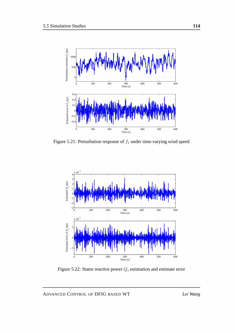
5.5 Simulation Studies 114
0 100 200 300 400 500 600
0
500
1000
Time (s)
Per
turb
atio
n es
timat
ion
f1 (
pu)
0 100 200 300 400 500 600
−0.4
−0.2
0
0.2
0.4
0.6
Time (s)
Est
imat
ed e
rror
of f 1 (
pu)
Figure 5.21: Perturbation response off1 under time-varying wind speed
0 100 200 300 400 500 600−3
−2
−1
0
1
2
3
4x 10
−3
Time (s)
Est
imat
ed Q s (
pu)
0 100 200 300 400 500 600
−5
0
5
x 10−5
Time (s)
Est
imat
ed e
rror
of Q
s (pu
)
Figure 5.22: Stator reactive powerQs estimation and estimate error
ADVANCED CONTROL OFDFIG BASED WT Lei Wang
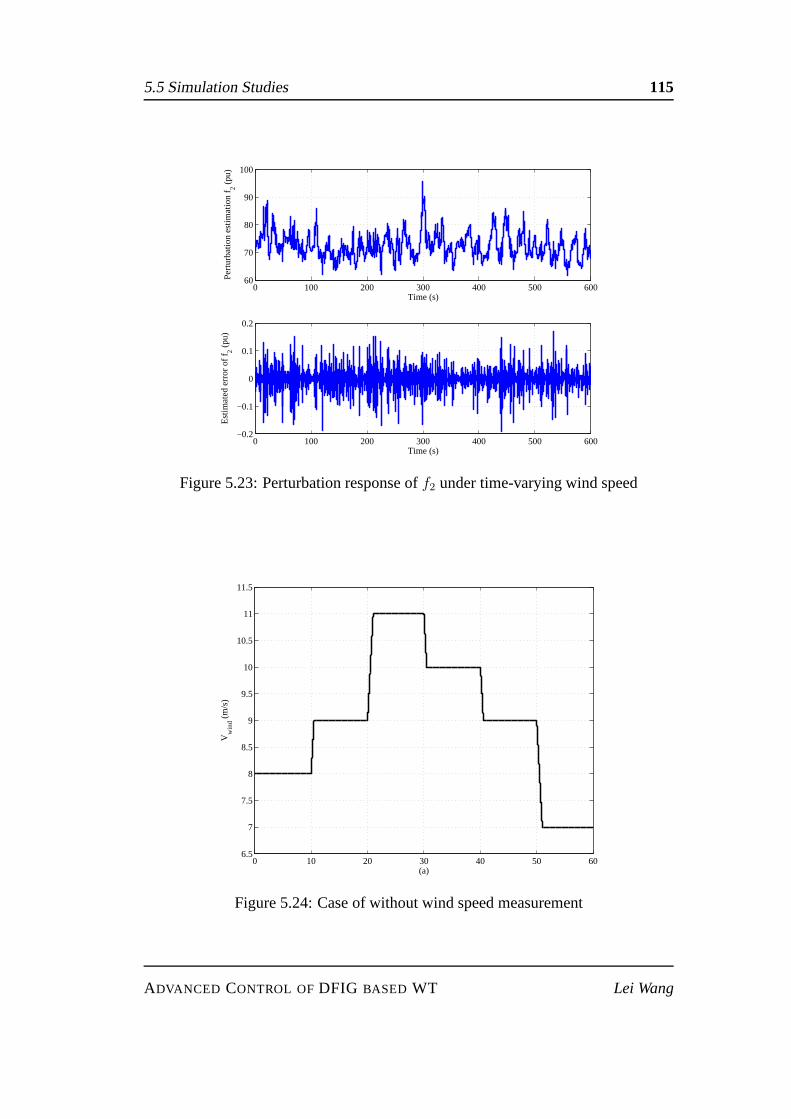
5.5 Simulation Studies 115
0 100 200 300 400 500 60060
70
80
90
100
Time (s)
Per
turb
atio
n es
timat
ion
f2 (
pu)
0 100 200 300 400 500 600−0.2
−0.1
0
0.1
0.2
Time (s)
Est
imat
ed e
rror
of f 2 (
pu)
Figure 5.23: Perturbation response off2 under time-varying wind speed
0 10 20 30 40 50 606.5
7
7.5
8
8.5
9
9.5
10
10.5
11
11.5
(a)
Vw
ind (
m/s
)
Figure 5.24: Case of without wind speed measurement
ADVANCED CONTROL OFDFIG BASED WT Lei Wang
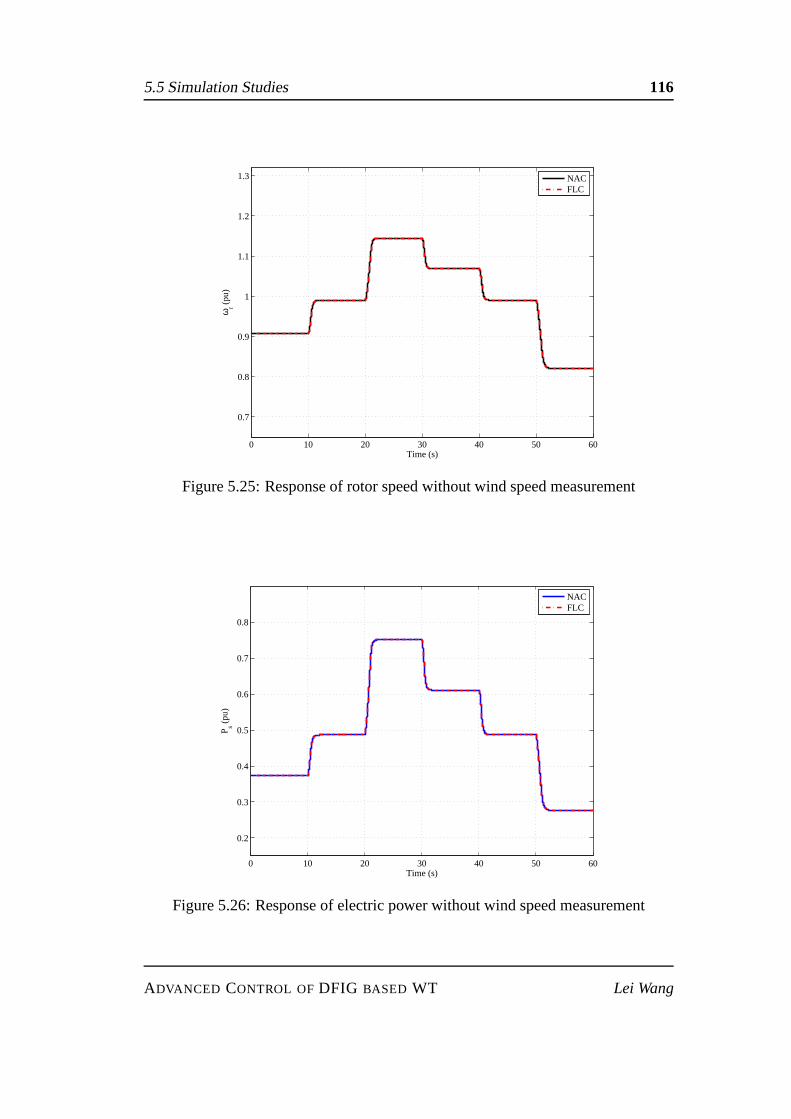
5.5 Simulation Studies 116
0 10 20 30 40 50 60
0.7
0.8
0.9
1
1.1
1.2
1.3
Time (s)
ωr (
pu)
NACFLC
Figure 5.25: Response of rotor speed without wind speed measurement
0 10 20 30 40 50 60
0.2
0.3
0.4
0.5
0.6
0.7
0.8
Time (s)
P s (pu
)
NACFLC
Figure 5.26: Response of electric power without wind speed measurement
ADVANCED CONTROL OFDFIG BASED WT Lei Wang
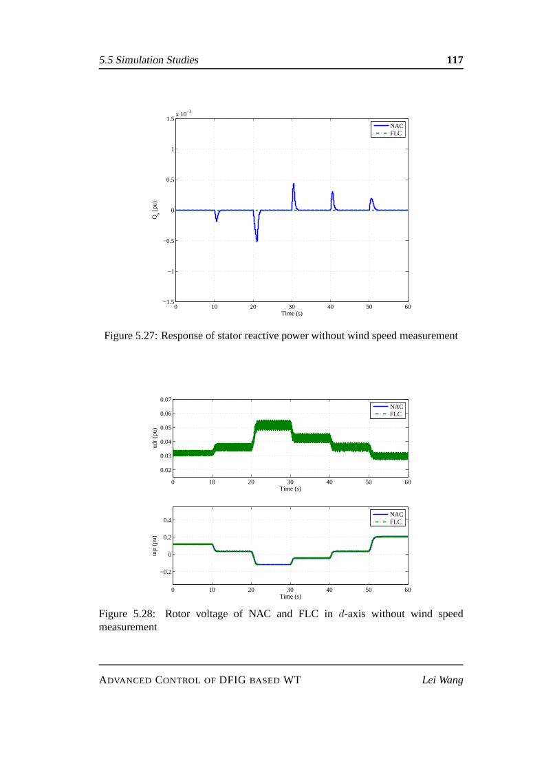
5.5 Simulation Studies 117
0 10 20 30 40 50 60−1.5
−1
−0.5
0
0.5
1
1.5x 10
−3
Time (s)
Qs (
pu)
NACFLC
Figure 5.27: Response of stator reactive power without windspeed measurement
0 10 20 30 40 50 60
0.02
0.03
0.04
0.05
0.06
0.07
Time (s)
udr
(pu)
NACFLC
0 10 20 30 40 50 60
−0.2
0
0.2
0.4
Time (s)
uqr
(pu)
NACFLC
Figure 5.28: Rotor voltage of NAC and FLC ind-axis without wind speedmeasurement
ADVANCED CONTROL OFDFIG BASED WT Lei Wang
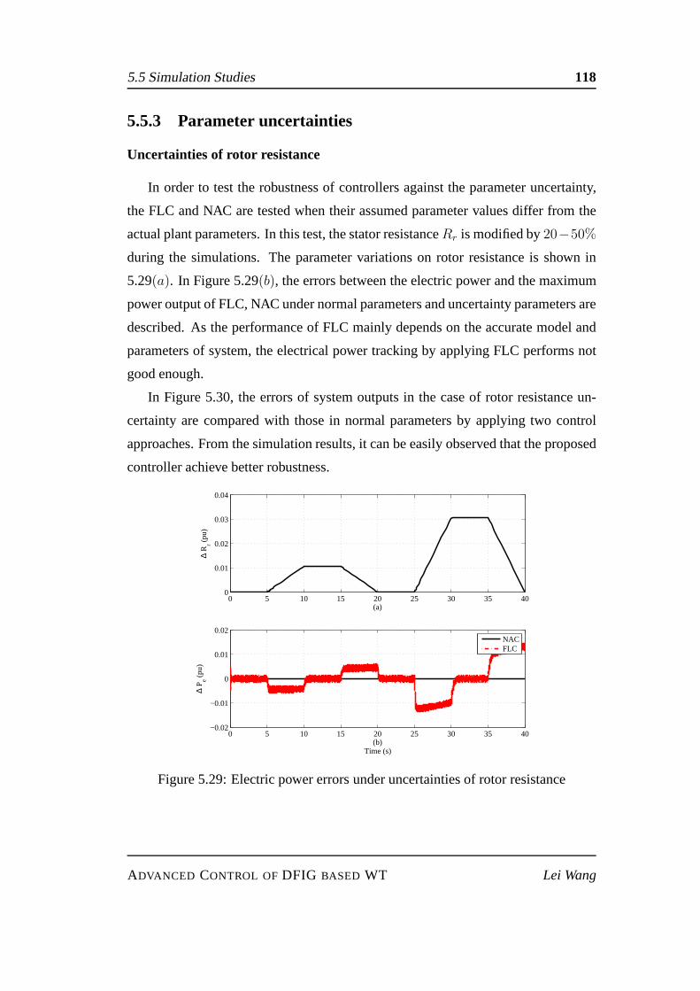
5.5 Simulation Studies 118
5.5.3 Parameter uncertainties
Uncertainties of rotor resistance
In order to test the robustness of controllers against the parameter uncertainty,
the FLC and NAC are tested when their assumed parameter values differ from the
actual plant parameters. In this test, the stator resistanceRr is modified by20−50%
during the simulations. The parameter variations on rotor resistance is shown in
5.29(a). In Figure 5.29(b), the errors between the electric power and the maximum
power output of FLC, NAC under normal parameters and uncertainty parameters are
described. As the performance of FLC mainly depends on the accurate model and
parameters of system, the electrical power tracking by applying FLC performs not
good enough.
In Figure 5.30, the errors of system outputs in the case of rotor resistance un-
certainty are compared with those in normal parameters by applying two control
approaches. From the simulation results, it can be easily observed that the proposed
controller achieve better robustness.
0 5 10 15 20 25 30 35 400
0.01
0.02
0.03
0.04
(a)
∆ R
r (pu
)
0 5 10 15 20 25 30 35 40−0.02
−0.01
0
0.01
0.02
(b)Time (s)
∆ P e (
pu)
NACFLC
Figure 5.29: Electric power errors under uncertainties of rotor resistance
ADVANCED CONTROL OFDFIG BASED WT Lei Wang

5.5 Simulation Studies 119
0 5 10 15 20 25 30 35 40−0.05
0
0.05
0.1
0.15
0.2
0.25
(a)
∆ ω
r (pu
)
0 5 10 15 20 25 30 35 40
0
0.2
0.4
0.6
(b)Time (s)
∆ Q
s (pu
)
NACFLC
NACFLC
Figure 5.30: System outputs errors under uncertainties of rotor resistance
Tower shadow
In the wind energy conversion systems, tower shadow and windshear contribute
to periodic fluctuations in electrical power output of a windturbine generator. In this
case, the signal shown in Figure 5.31(a) simulates the fluctuation caused by tower
shadow. The differences of the electrical power output errors by applying FLC and
NAC are represented in Figure 5.31(b).
The system outputs errors during tower shadow fluctuation can be also observed
from Figure 5.32. As shown in the obtained results, the proposed nonlinear adap-
tive controller given no steady-state error and the same behavior as in the normal
parameter.
Grid voltage dip
During the period of conventional power generation, the short-term voltage dips
also affect the electrical power output of DFIG-WT. A200ms voltage drop is sim-
ulated in Figure 5.33(a). From Figure 5.33(b), the better performance of electrical
power output can be obtained by applying NAC than that of FLC .In Figure 5.34,
the errors of system outputs controlled by FLC, and NAC are compared with each
ADVANCED CONTROL OFDFIG BASED WT Lei Wang
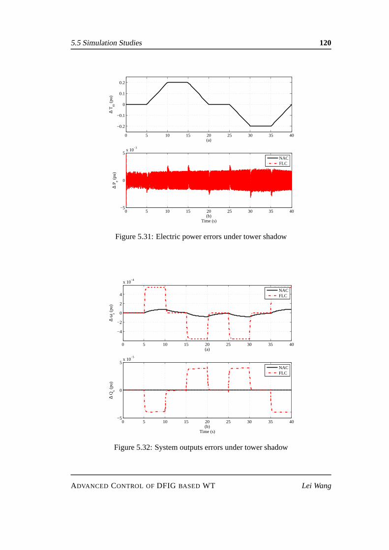
5.5 Simulation Studies 120
0 5 10 15 20 25 30 35 40
−0.2
−0.1
0
0.1
0.2
(a)
∆ T
m (
pu)
0 5 10 15 20 25 30 35 40−5
0
5x 10
−3
(b)Time (s)
∆ P e (
pu)
NACFLC
Figure 5.31: Electric power errors under tower shadow
0 5 10 15 20 25 30 35 40
−4
−2
0
2
4
x 10−4
(a)
∆ ω
r (pu
)
NACFLC
0 5 10 15 20 25 30 35 40−5
0
5x 10
−5
(b)Time (s)
∆ Q
s (pu
)
NACFLC
Figure 5.32: System outputs errors under tower shadow
ADVANCED CONTROL OFDFIG BASED WT Lei Wang
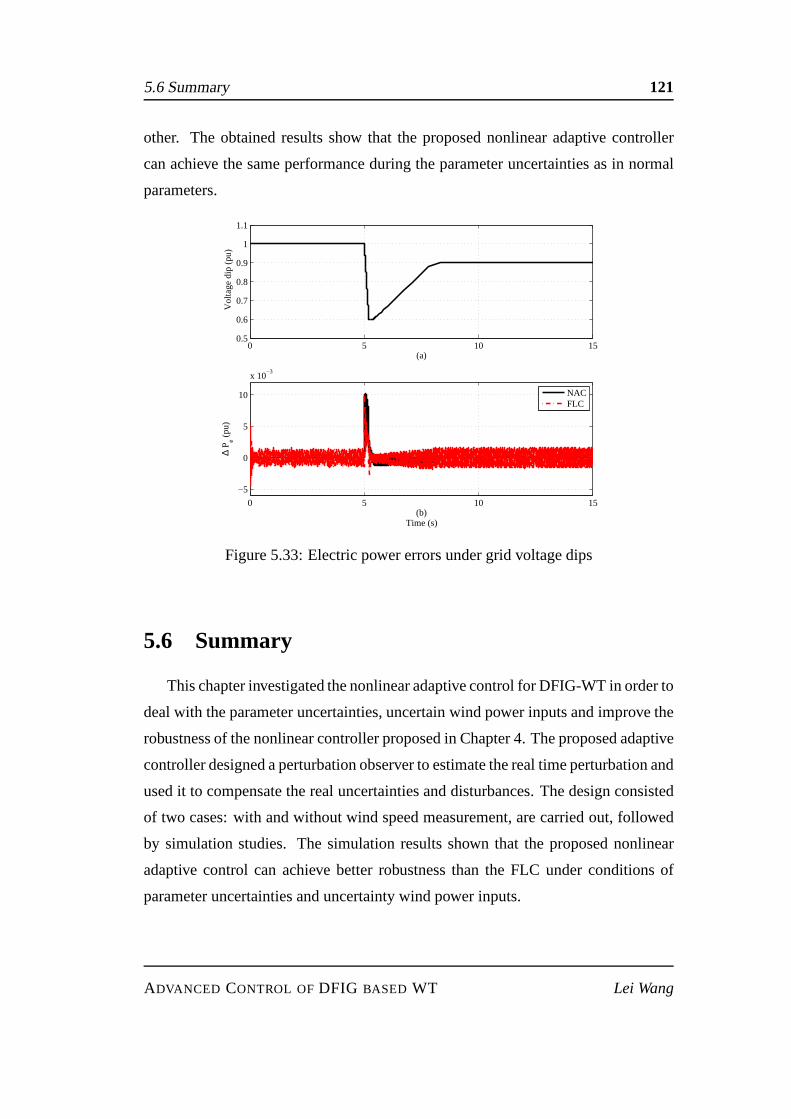
5.6 Summary 121
other. The obtained results show that the proposed nonlinear adaptive controller
can achieve the same performance during the parameter uncertainties as in normal
parameters.
0 5 10 150.5
0.6
0.7
0.8
0.9
1
1.1
(a)
Vol
tage
dip
(pu
)
0 5 10 15
−5
0
5
10
x 10−3
(b)Time (s)
∆ P e (
pu)
NACFLC
Figure 5.33: Electric power errors under grid voltage dips
5.6 Summary
This chapter investigated the nonlinear adaptive control for DFIG-WT in order to
deal with the parameter uncertainties, uncertain wind power inputs and improve the
robustness of the nonlinear controller proposed in Chapter4. The proposed adaptive
controller designed a perturbation observer to estimate the real time perturbation and
used it to compensate the real uncertainties and disturbances. The design consisted
of two cases: with and without wind speed measurement, are carried out, followed
by simulation studies. The simulation results shown that the proposed nonlinear
adaptive control can achieve better robustness than the FLCunder conditions of
parameter uncertainties and uncertainty wind power inputs.
ADVANCED CONTROL OFDFIG BASED WT Lei Wang
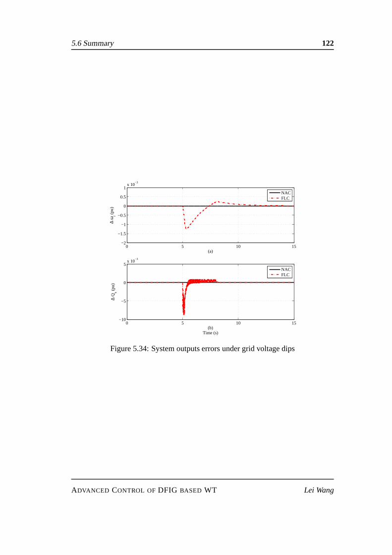
5.6 Summary 122
0 5 10 15−2
−1.5
−1
−0.5
0
0.5
1x 10
−3
(a)
∆ ω
r (pu
)
NACFLC
0 5 10 15−10
−5
0
5x 10
−3
(b)Time (s)
∆ Q
s (pu
)
NACFLC
Figure 5.34: System outputs errors under grid voltage dips
ADVANCED CONTROL OFDFIG BASED WT Lei Wang
Chapter 6
Conclusion and Future Work
6.1 Conclusion
Wind power, as one of the clean and alternative energy sources, is expect to be-
come one one mainstream energy source and probably the largest renewable energy
source in Europe in the next decades, researches on maximizing the power conver-
sion coefficient, and improving the power quality are essential. In this thesis, the
advanced control strategies of doubly fed induction generator based variable speed
wind turbine have been investigated and developed.
This thesis focuses on improving the power conversion efficiency and transient
dynamics of DFIG-WT. The DFIG-WT is a dynamic system with strong nonlinear
coupled characteristics and time-varying uncertain inputs, and during voltage sags
due to grid load disturbances or grid faults, DFIG-WT will operate far away from
its normal operation point. For these requirements, the control strategies of DFIG-
WT should be designed to operate at an operation envelope with a wide range during
time-varying inputs, and maintain a robust transient response under grid disturbance
or parameter uncertainties.
For the controller design, the modeling of DFIG-WT including wind turbine,
drive train, DFIG and power electrical converters were investigated at first. As the
dynamic response of the DFIG-WT’s electrical part is fasterthan that of mechani-
cal part, the model of drive train normally can be simplified as one-mass model for
123
6.1 Conclusion 124
the studies on the power regulation of DFIG-WT. The detaileddynamic model of
DFIG has been obtained in the two-phase (d-q) rotating reference frame by apply-
ing Clarke and Park Transformations, for the method based onthree-phase natural
reference frame. This type transformation (via transforming variables to a special
reference frame) resulted in the simple design of linear PI based vector controller,
however, the PI based vector controller can only achieve partial linearization of the
original nonlinear system. Moreover, the dynamic of the grid-side converter and
DC-link capacitor were also investigated.
The conventional power control method, vector control, hasbeen studied in
chapter 3 at first. As the conventional control strategy can only achieve the asymp-
totical regulation of the stator active and reactive power of the DFIG, a fully de-
coupled nonlinear power control based on feedback linearization control has been
designed for the direct power control of the DFIG. Moreover,a cascade nonlinear
controller, which consisted of two stages, an outer loop provide rotor current ref-
erence from the stator active and reactive powers, and an inner loop applied the
input/output feedback linearization control for current regulation. Two cases were
studied to verify the performance of the proposed control strategy: (1) The opera-
tion points of system outputs were varying at the same time, thereby, the shortage of
PI based vector control appeared. In other hand, it shows that the nonlinear control
strategies can achieve fully decoupling control and globaloptimization; (2) Face to
the sudden grid voltage drop, the proposed cascaded controlstrategy provided the
best transient response during the disturbance.
The maximum power point tracking (MPPT) control of DFIG-WT focuses on
improving the power conversion coefficient and dynamic response during the time-
varying and uncertainty wind power inputs. In chapter 4, thenonlinear feedback
control based maximum power point tracking (MPPT) has been studied. Both VC
and FLC are applied for MPPT control under time-varying windspeeds, to achieve
the maximum power extraction form the wind power. Modal analysis was used to
analysis the dynamics of DFIG-WT provided by VC and FLC respectively, which
show that the FLC can provide consistent dynamics with time-varying wind power
inputs.
ADVANCED CONTROL OFDFIG BASED WT Lei Wang
6.2 Future Works 125
In order to deal with the parameter uncertainties and uncertain wind power in-
puts, Chapter 5 investigated the nonlinear adaptive control for MPPT of DFIG-WT.
For improving the robustness of the nonlinear controller proposed in Chapter 4, The
proposed adaptive controller designed a perturbation observer to estimate the real
time perturbation and used it to compensate the real uncertainties and disturbances.
The simulation results proved that the proposed NAC for MPPTof DFIG-WT can
supply better robustness performance than FLC during the parameter uncertainties
and uncertain wind power inputs.
6.2 Future Works
The possible future work is listed based on the following ideas.
I The zero-dynamic of the FLC-based power control and the FLC-based MPPT
controller has not been investigated, though the stabilityof controllers have
been studied via modal analysis (the FLC-MPPT) or simulation studies (the
FLC-power & the FLC-MPPT). Future work will investigate thezero-dynamic
of the FLC based controllers remained internal dynamic.
II NAC can be also applied on pitch control of WT to reduce the mechanical
stress on the drive train and improve the energy conversion efficiency of the
WT operating above the rated wind speed. The design will be based on the
two-mass model of the WT, while simulation studies will focus on the de-
tailed model provided by the FAST (Fatigue, aerodynamics, structures, and
turbulence) software package. The designed NAC will work together with the
NAC power control for DFIG.
III NAC for grid-side converter of DFIG-WT. This work is to design a NAC-
based converter controller and applied for the grid-side converter of DFIG-
WT to stabilize the DC-link voltage and maintain the unity power factor, and
then for the grid-side converter of the WPGS with the full-rated converter to
improve the FRT capability and robustness of the converter controller, respec-
tively. The coordination and decoupling of the proposed NACs for DFIG-WT
ADVANCED CONTROL OFDFIG BASED WT Lei Wang

6.2 Future Works 126
will be verified by simulation studies.
ADVANCED CONTROL OFDFIG BASED WT Lei Wang
References
[1] R. Swisher, C. R. De Azua, J. Clendenin, “Strong winds on the horizon: wind
power comes of age,”IEEE Proceedings, vol. 89, no. 12, pp. 1757-1764, Dec.
2001.
[2] S. Heier,Grid integration of wind energy conversion systems. John Wiley and
Sons, New York, 1998.
[3] M. Ahlstrom, L. Jones, R. Zavadil, and W. Grant, “The Future of Wind Fore-
casting and Utility Operation,”IEEE Power and Energy Magazine, vol. 3, no.
6, pp. 57-64, Nov./Dec. 2005.
[4] R. Piwko, D. Osborn, R. Gramlich, G. Jordan, D. Hawkins, and K. Porter,
“Wind Energy Delivery Issues,”IEEE Power and Energy Magazine, vol. 3,
no. 6, pp. 47-56, Nov./Dec. 2005
[5] J. Ekanauake, L. Holdsworth, and N. Jenkins, “Control ofDFIG Wind Tur-
bines,”IEEE Power Engineer, vol. 17, pp. 28-32, Feb. 2003.
[6] R. Pena, J.C. Clare and G.M. Asher, “Doubly fed inductiongenerator using
back-to-back PWM converters and its application to variable speed wind-
energy generation,”IEE Proceedings Electrical Power Applications, vol. 143,
no. 3, pp. 231-241, May 1996.
[7] S. Peresada, A. Tilli and A. Tonielli, “Power control of adoubly fed induction
machine via output feedback,”Control Engineering Practice, vol. 12, no. 1,
pp. 41-57, Jan. 2004.
127
REFERENCES 128
[8] S. Muller, M. Deicke and R. W. De Doncker, “Doubly fed induction generator
systems for wind turbines,”IEEE Industry Applications Magazine, vol. 8, no.
3, pp. 26-33, May-Jun. 2002.
[9] A. Petersson, L. Harnefors and T. Thiringer, “Evaluation of current con-
trol methods for wind turbines using doubly-fed induction machines,”IEEE
Transactions on Power Electronics, vol. 20, no. 1, pp. 227-235, Jan. 2005.
[10] R. Datta and V. T. Ranganathan, “Direct power control ofgrid-connected
wound rotor induction machine without rotor position sensors,” IEEE Trans-
actions on Power Electronics, vol. 16, no. 3, pp. 390-399, May 2001.
[11] L. Xu and P. Cartwright, “Direct active and reactive power control of DFIG
for wind energy generation,”IEEE Transactions on Energy Conversion, vol.
21, no. 3, pp. 750-758, Sep. 2006
[12] D. W. Zhi and L. Xu, “Direct power control of DFIG with constant switch-
ing frequency and improved transient performance,”IEEE Transactions on
Energy Conversion, vol. 22, no. 1, pp. 110-118, Mar. 2007.
[13] J. Hu, H. Nian, B. Hu, Y. He and Z. Q. Zhu, “Direct active and reactive power
regulation of DFIG using sliding mode control approach,”IEEE Transactions
on Energy Conversion, vol. 25, no. 4, pp. 1028-1039, Dec. 2010.
[14] L. Shang and J. B. Hu, “Sliding-mode-based direct powercontrol of grid-
connected wind-turbine-driven doubly fed induction generators under unbal-
anced grid voltage conditions,”IEEE Transactions on Energy Conversion,
vol. 27, no. 2, pp. 362-373, Jun. 2012.
[15] A. Mullane, G. Lightbody and R. Yacamini, “Wind turbinefault ride-through
enhancement,”IEEE Transactions on Power Systems, vol. 20, no. 4, pp. 1929-
1937, Nov. 2005.
[16] J. Niiranen, “Voltage dip ride through of a double-fed generator equipped
with an active crowbar,” InNordic Wind Power Conference, pp. xx-xx, Swe-
den, Mar. 2004.
ADVANCED CONTROL OFDFIG BASED WT Lei Wang
REFERENCES 129
[17] P. Zhou, “Control strategy of an active crowbar for DFIGbased wind turbine
under grid voltage dips,” InProceedings of 2007 International Conference on
Electrical Machines and Systems, pp. 259-264, Korea, Oct. 2007.
[18] S. R. Kalantarian, “A new crowbar protection method forimprovement in
performance of doubly fed induction generator under fault conditions,” In
Proceedings of the 10th International Conference on Environment and Elec-
trical Engineering, pp. 1-4, Iran, May 2011.
[19] J. Morren and S. W. H. de Haan, “Ride-through of wind turbines with doubly
fed induction generator during a voltage dip,”IEEE Transactions on Energy
Conversion, vol. 20, no. 2, pp. 435-441, Jun. 2005.
[20] D. Xiang, L. Ran, P. J. Tavner, and S. Yang, “Control of a doubly fed induc-
tion generator in a wind turbine during grid fault ride-through,” IEEE Trans-
actions on Energy Conversion, vol. 21, no. 3, pp. 652-662, Sep. 2006.
[21] J. Yao, H. Li, Y. Liao, and Z. Chen, “An improved control strategy of limiting
the DC-link voltage fluctuation for a doubly fed induction wind generator,”
IEEE Transactions on Power Electronics, vol. 23, no. 3, pp. 1205-1213, May
2008.
[22] M. Rahimi and M. Parniani, “Grid-fault ride-through analysis and control of
wind turbines with doubly fed induction generators,”Electric Power Systems
Research, vol. 80, no. 2, pp. 184-195, Jun. 2010.
[23] D. Gautam, V. Vittal, T. Harbour, “Impact of increased penetration of DFIG-
based wind turbine generators on transient and small signalstability of power
systems,”IEEE Transactions on Power Systems, vol. 24, no. 3, pp. 1426-
1434, Aug. 2009.
[24] F. M. Hughes, O. A. Lara, N. Jenkins and G. Strbac, “Control of DFIG-based
wind generation for power network support,”IEEE Transactions on Power
Systems, vol. 20, no. 4, pp. 1958-1966, Nov. 2005.
ADVANCED CONTROL OFDFIG BASED WT Lei Wang

REFERENCES 130
[25] F. M. Hughes, O. A. Lara, N. Jenkins and G. Strbac, “A power system stabiliz-
er for DFIG-based wind generation,”IEEE Transactions on Power Systems,
vol. 21, no. 2, pp. 763-772, May 2006.
[26] R. D. Fernandez, P. E. Battaiotto and R. J. Mantz, “Wind farm nonlinear
control for damping electromechanical oscillations of power systems,”Re-
newable Energy, vol.33, no. 10, pp. 2258-2265, Oct. 2008.
[27] Y. Mishra, S. Mishra, M. Tripathy, N. Senroy and Z.Y. Dong, “Improving
stability of a DFIG-based wind power system with tuned damping controller,”
IEEE Transactions on Energy Conversion, vol. 24, no. 3, pp. 650-660, Sep.
2009.
[28] W. E. Leithead and B. Connor, “Control of variable speedwind turbines:
dynamic models,”International Journal of Control, vol. 73, no. 13, pp. 1173-
1188, Sep. 2000.
[29] J. Lopez, P. Sanchis, X. Roboam and L.Marroyo, “Wind turbines based
on doubly fed induction generator under asymmetrical voltage dips,”IEEE
Transactions on Energy Conversion, vol. 23, no. 1, pp. 321-330, Mar. 2008.
[30] W. E. Leithead and B. Connor, “Control of variable speedwind turbines:
design task,”International Journal of Control, vol. 73, no. 13, pp. 1189-1212,
Sep. 2000.
[31] E. B. Muhando, T. Senjyu, A. Uehara and T. Funabashi, “Gain-scheduled H-
infinity control for WECS via LMI techniques and parametrically dependent
feedback part I: Model development fundamentals,”IEEE Transactions on
Industrial Electronics, vol. 58, no. 1, pp. 48-56, Jan. 2011.
[32] E. B. Muhando, T. Senjyu, A. Uehara and T. Funabashi, “Gain-scheduled H-
infinity control for WECS via LMI techniques and parametrically dependent
feedback part II: Controller design and implementation,”IEEE Transactions
on Industrial Electronics, vol. 58, no. 1, pp. 57-65, Jan. 2011.
ADVANCED CONTROL OFDFIG BASED WT Lei Wang
REFERENCES 131
[33] E. B. Muhando, T. Senjyu, A. Uehara, T. Funabashi and C. H. Kim, “ LQG
design for megawatt-class WECS with DFIG based on functional models’
fidelity prerequisites,”IEEE Transactions on Energy Conversion, vol. 24, no.
4, pp. 893-904, Dec. 2009.
[34] F. Valenciaga, P. F. Puleston, P. E. Battaiotto and R. J.Mantz, “An adap-
tive feedback linearization strategy for variable speed wind energy conver-
sion systems,”International Journal of Energy Research, vol. 24, no. 2, pp.
151-161, Feb. 2000.
[35] J. M. Mauricio, A. E. Leon, A. Gomez-Exposito and J. A. Solsona, “An adap-
tive nonlinear controller for DFIM-based wind energy conversion system,”
IEEE Transactions on Energy Conversion, vol. 23, no. 4, pp. 1025-1035,
Dec. 2008.
[36] F. Wu and X. P. Zhang, “Decentralized nonlinear controlof wind turbine with
doubly fed induction generator,”IEEE Transactions on Power Systems, vol.
23, no. 2, pp. 613-621, May 2008.
[37] L. Holdsworth, X.Wu, J. B. Ekanayake and N.Jenkins, “Comparison of fixed
speed and doubly-fed induction wind turbines during power system distur-
bances,”IEE Proceedings Generation Transmission and Distribution, vol.
150, no. 3, pp. 342-352, May 2003.
[38] T. Ackermann,Wind power in power systems. John Wiley and sons, England,
2005.
[39] S. N. Bhadra, D. Kastha and S. Banerjee,Wind Electrical Systems. Oxford
University Press, New Delhi, 2009.
[40] N. W. Miller, W. W. Price, and J. J. Sanchez-Gasca, “Dynamic modeling of
GE 1.5 and 3.6 wind turbine-generators,”GE-Power Systems Energy Con-
sulting, General Electric International, Inc., 2003.
ADVANCED CONTROL OFDFIG BASED WT Lei Wang
REFERENCES 132
[41] F. Mei and B. Pal, “Modal analysis of grid-connected doubly fed induction
generators,”IEEE Transactions on Energy Conversion, vol, 22, no. 3, pp.
728-736, Sep. 2007.
[42] J. P. A. Vieira, M. N. A. Nunes and U. H. Bezerra, “Design of optimal PI
controllers for doubly fed induction generators in wind turbines using genet-
ic algorithm,” In Proceedings of the 2008 IEEE Power and Energy Society
General Meeting, pp. 1-7, Pittsburgh, Jul. 2008,.
[43] W. Qiao, G. K. Venayagamoorthy and R. G. Harley, “Designof optimal con-
trol PI controllers for doubly fed induction generators driven by wind tur-
bines using particle swarm optimization,” InInternational Joint Conference
on Neural Networks, pp. 1982-1987, Canada, Jul. 2006.
[44] S. M. B. Wilmshurst, “Control strategy for wind turbines,” Wind Eng., vol.
12, no. 4, pp. 236-250, 1988.
[45] X. P. Zhang, K. Godfrey and P. Ju, “Small signal stability analysis and op-
timal control of a wind turbine with doubly fed induction generator,” IET
Generation, Transmission & Distribution, vol. 1, no. 5, pp. 751-760, Sep.
2007.
[46] R. G. Almeida, J. A. Pecas Lopes and J. A. L. Barreiros, “Improving power
system dynamic behavior through doubly fed induction machines controlled
by static converter using fuzzy control,”IEEE Transactions Power Systems,
vol. 19, no. 4, pp. 1942-1950, Nov. 2004.
[47] Z. Song, T. Shi, C. Xia and W. Chen, “A novel adaptive control scheme for
dynamic performance improvement of DFIG-Based wind turbines,”Energy,
vol. 38, no. 1, pp. 104-117, Feb. 2012.
[48] L. Jiang, Q. H. Wu, G. P. Liu and D. Rees, “Robust adaptivecontrol of induc-
tion motor based on perturbation observer,” InIEEE Electrical Machine and
Drives Conference 2007, vol. 1, pp. 101-106, Turkey, May 2007.
ADVANCED CONTROL OFDFIG BASED WT Lei Wang
REFERENCES 133
[49] B. Beltran, M. E. Benbouzid and T. Ahmed-Ali, “Second-order sliding mode
control of a doubly fed induction generator driven wind turbine,” IEEE Trans-
actions on Energy Conversion, vol. 27, no. 2, pp. 261-269, Jun. 2012.
[50] R. Marino, S. Peresada and P. Valigi, “Adaptive input-output linearising con-
trol of induction motor,”IEEE Transactions on Automatic Control, vol. 38,
no. 2, pp. 208-221, Feb. 1993.
[51] F. K. A. Lima, A. Luna, P. Rodriguez, E. H. Watanabe and F.Blaabjerg,
“Rotor voltage dynamic in the doubly fed induction generator during grid
faults,” IEEE Transactions on Power Electronics, vol. 25, no. 1, pp. 118-130,
Jan. 2010.
[52] A. Tapia, G. Tapia, J. Ostolaza, , and J. Saenz, “Modeling and control of a
wind turbine driven doubly fed induction generator,”IEEE Transactions on
Energy Conversion, vol. 18, no. 2, pp. 194-204, Jun. 2003.
[53] B. Chowdhury and S. Chellapilla, “Double-fed induction generator control
for variable speed wind power generation,”Electric Power Systems Research,
vol. 76, no. 9, pp. 786-800, Jun. 2006.
[54] N. Mohan, T. Undeland, and W. Robbins,Power electronics. Converters, ap-
plications and design, 3rd ed. John Wiley and Sons, Inc., 2003.
[55] B. Bose,Power electronics and ac drives. Englewood Cliffs, New Jersey:
Prentice-Hall, 1986.
[56] L. Chang, R. Doraiswami, T. Boutot, and H. Kojabadi, “Development of a
wind turbine simulator for wind energy conversion systems,” in Canadian
Conference on Electrical and Computer Engineering, vol. 1, pp. 550-554,
Mar. 2000.
[57] S. Bolik, “Modelling and analysis of variable speed wind turbines with induc-
tion generator during grid fault,” PhD Thesis, Aalborg University, Aalborg,
Denmark, Oct. 2004.
ADVANCED CONTROL OFDFIG BASED WT Lei Wang

REFERENCES 134
[58] A. Hansen and G. Michalke, “Voltage grid support of DFIGwind turbines
during grid faults,” inProc. European Wind Energy Conference and Exhibi-
tion 2007 (EWEC 2007), Milan, Italy, May. 2007.
[59] E. Tremblay, A. Chandra, and P. Lagace, “Grid-side converter control of D-
FIG wind turbines to enhance power quality of distribution network,” in IEEE
Power Engineering Society General Meeting, pp. 6, Jun. 2006.
[60] V. Akhmatov, “Modelling of variable speed wind turbines with doubly-fed
induc tion generators in short-term stability investigations,” in Proc. of In-
ternational Workshop on Transmission networks for Offshore Wind Farms,
Stockholm, Sweden, Apr. 2002.
[61] J. Smajo, “Rotor power feedback control of wind turbinesystem with doubly-
fed induction generator,” inProceedings of the 6th WSEAS International Con-
ference on Simulation, Modelling and Optimization, pp. 48-53, Spain, 2006.
[62] S.H Li, R. Challoo, “Comparative study of DFIG power control using stator-
voltage and stator-flux oriented frames,”2009 IEEE Power and Energy Soci-
ety General Meeting, PES ’09, July 2009.
[63] L. Morel, H. Godfroid, A. Mirzaian, J.M. Kauffmann, “Double-fed induction
machine: converter optimization and field oriented controlwithout position
sensor,”IEE Proceedings: Electric Power Applications, vol. 145, no. 4, pp.
360-368, July 1998.
[64] B. Hopfensperger, D. Atkinson, and R. A. Lakin, “Statorflux oriented con-
trol of a cascaded doubly-fed induction machine,”IEE Proceedings: Electric
Power Applications, vol. 146, no. 6, pp. 597C605, Nov. 1999.
[65] P. C. Krause, O. Wasynczuk, S. D. Sudhoff,Analysis of electric machinery
and drive systems, A John Wiley and Sons, UK, 2002.
[66] A. Arash, P. Mojtaba, M. Ali, ”Analyzing vector controlof a grid-connected
DFIG under simultaneous changes of two inputs of control system,” Euro-
pean Journal of Scientific Research, vol.45, no.2 , pp.221-231, 2010.
ADVANCED CONTROL OFDFIG BASED WT Lei Wang
REFERENCES 135
[67] H. Li, Z. Chen, “Overview of different wind generator systems and their com-
parisons,”IET Renew. Power Gen., vol. 2, no. 2, pp. 123-l38, 2008.
[68] S. Soter, R. Wegener, “Development of induction machines in wind power
technology,”IEEE Intel. Elec. Mach. And Drives Conf, pp. 1490-1495, 2007.
[69] J.A. Baroudi, V. Dinavahi, A.M. Knight, “A review of power converter
topologies for wind generators,”IEEE International Conference on Electric
Machines and Drives, pp. 458-465, 2005.
[70] L.M. Fernandez, C.A. Garcia, F. Jurado, et aI., “Control system of doubly fed
induction generators based wind turbines with production limits,” IEEE Intel.
Conf. Electic. Mach. and Drives, pp. 1936-1941, 2005.
[71] FA. Bhuiyan and A. Yazdani, “Multimode control of a DFIG-Based wind-
power unit for remote applications,”IEEE Trans. Power Del., vol. 24, no. 4,
pp. 2079-2089, Oct. 2009.
[72] X. Yuan, F Wang, D. Boroyevich, et aI., “DC-link voltagecontrol of a full
power converter for wind generator operating in weak-grid systems,”IEEE
Trans. Power Electr., vol. 24, no. 9, pp. 2178-2192, 2009.
[73] L. Yang, G.Y. Yang, Z. Xu, et aI., ”Optimal controller design of a doubly-fed
induction generator wind turbine system for small signal stability enhance-
ment,”IET Generation, Transmission and Distribution, vol. 4, no. 5, pp. 579-
597, 2010.
[74] L. Sun, Z. Mi, Y. Yu, et. aI., “Active power and reactive power regulation ca-
pacity study of DFIG wind turbine,”Inter. Conf. Sustain. Power Gen. Supply,
pp. 1-6, 2009.
[75] B. Shen, B. Mwinyiwiwa, Y. Zhang, et. aI., “Sensorless maximum power
point tracking of wind by DFIG using rotor position phase lock loop,” IEEE
Trans. Power Elec., vol. 24, no. 4, pp. 942-951, 2009.
[76] P. KUNDUR,Power System Stability and Control, Mc Graw Hill, 1994.
ADVANCED CONTROL OFDFIG BASED WT Lei Wang
REFERENCES 136
[77] M. Fei and B. Pal, “Modelling of doubly-fed induction generator for power
system stability study,”Power and Energy Society General Meeting - Con-
version and Delivery of Electrical Energy in the 21st Century, pp. 1-8, Jul.
2008.
[78] R. Datta, VT. Ranganathan, “A simple position sensorless algorithm for rotor
side field oriented control of wound rotor induction machine,” IEEE Trans-
actions on Industrial Electronics, vol. 48, no. 4, pp. 786-793, 2001.
[79] P. Ledesma, J. Usaola, “Doubly fed induction generatormodel for transient
stability analysis,”IEEE Transactions on Energy Conversion, vol. 20, no. 2,
pp. 388-397, 2005.
[80] K. Tan, S. Islam, “Mechanical sensorless robust control of wind turbine driv-
en permanent magnet synchronous generator for maximum power operation,”
International Journal of Renewable Energy Engineering, vol. 3, no. 2, pp.
379-384, 2001.
[81] B. Boukhezzar, H. Siguerdidjane, “Nonlinear control with wind estimation of
a DFIG variable speed wind turbine for power capture optimization”,Energy
Conversion and Management, vol.50, no.4, pp. 885-892, April. 2009.
[82] A. Kumar, K. Stol, “Simulating Feedback Linearizationcontrol of wind tur-
bines using high-order models”,Wind Energy, vol. 13, no. 5, pp. 419-432,
July 2010.
[83] A.F. Payam, B.M. Dehkordi, M. Moallem, “Adaptive input-output feedback
linearization controller for doubly-fed induction machine drive”,Internation-
al Aegean Conference on Electrical Machines and Power Electronics, 2007.
ACEMP ’07., pp. 830-835, Sep. 2007.
[84] W. Qiao, W. Zhou, J. M. Aller and R. G. Harley, “Wind speedestimation
based sensorless output maximization control for a wind turbine driving a
DFIG”, IEEE Trans. on Power Electronics, vol. 23, pp. 1156-1169, 2008.
ADVANCED CONTROL OFDFIG BASED WT Lei Wang
REFERENCES 137
[85] A. F. Payam, “An adaptive input-output feedback linearization controller for
doubly-fed induction machine drives,”Serbian Journal of Electrical Engi-
neering, vol. 5, no. 1, pp. 139-154, May 2008.
[86] L. Jiang, Q. H. Wu and J. Y. Wen, “Decentralized Nonlinear Adaptive Con-
trol for Multimachine Power Systems Via High-Gain Perturbation Observer”,
IEEE Trans. on Circuits and Systems I: Regular Papers, vol. 51, pp. 2052-
2059, 2004.
[87] L.Jiang, Q.H. Wu “Observer-based nonlinear control ofsynchronous gener-
ator with perturbation estimation”,International Journal of Electrical Power
and Energy Systems, vol. 23, pp. 359-367, June, 2001.
[88] J. Carrasco, L. Franquelo, J. Bialasiewicz, E. Galvan,R. Guisado, M. Prats, J.
Leon and N. Moreno-Alfons, “Power-electronic systems for the grid integra-
tion of renewable energy sources: A survey,”IEEE Transactions on Industrial
Electronics, vol. 53, no. 4, pp. 1002-1016, Aug. 2006.
[89] J. Arbi, M.-B. Ghorbal, I. Slama-Belkhodja, and L. Charaabi, “Direct virtu-
al torque control for doubly fed induction generator grid connection,”IEEE
Transactions on Industrial Electronics, vol. 56, no. 10, pp. 4163-4173, Oct.
2009.
[90] B. Rabelo, W. Hofmann, J. da Silva, R. de Oliveira and S. Silva, “Reactive
power control design in doubly fed induction generators forwind turbines,”
IEEE Transactions on Industrial Electronics, vol. 56, no. 10, pp. 4154-4162,
Oct. 2009.
[91] S. Shao, E. Abdi, F. Barati and R. McMahon, “Stator-flux-oriented vector
control for brushless doubly fed induction generator,”IEEE Transactions on
Industrial Electronics, vol. 56, no. 10, pp. 4220-4228, Oct. 2009.
[92] J. Niiranen, “Voltage dip ride through of doubly-fed generator e-
quipped with active crowbar,” presented at the Nordic Wind Pow-
er Conf., Goteborg, Sweden, Mar. 1-2, 2004 [Online]. Available:
ADVANCED CONTROL OFDFIG BASED WT Lei Wang
REFERENCES 138
http://www.elteknik.chalmers.se/Publikationer/EMKE.publ/NWPCO4/papers/NIRRANEN.pdf,
Chalmers Univ. Technol.
[93] K. Rothenhagen and F. Fuchs, “Current sensor fault detection, isolation, and
reconfiguration for doubly fed induction generators,”IEEE Transactions on
Industrial Electronics, vol. 56, no. 10, pp. 4239-4245, 2009.
[94] J. Lopez, E. Gubia, E. Olea, J. Ruiz and L. Marroyo, “Ridethrough of wind
turbines with doubly fed induction generator under symmetrical voltage dip-
s,” IEEE Transactions on Industrial Electronics, vol. 56, no. 10, pp. 4246-
4254, Oct. 2009.
[95] R. Fadaeinedjad, G. Moschopoulos and M. Moallem, “Voltage sag impact on
wind turbine tower vibration,”Proc. IEEE Power Eng. Soc. Gen. Meeting,
pp. 1-8, 2007
[96] S. Papathanassiou and M. Papadopoulos, “Mechanical stresses in fixed-speed
wind turbines due to network disturbances,”IEEE Transactions on Energy
Conversion, vol. 16, no. 4, pp. 361-367, 2001.
[97] I. Canay, “Calculation of negative-sequence losses and negativesequence re-
sistance of turbogenerators,”IEEE Transactions on Power Apparatus and
Systems, vol. PAS-94, no. 3, pp. 764-773, May-Jun. 1975.
[98] A. Petersson, L. Harnefors and T. Thiringer, “Modelingand experimental
verification of grid interaction of a DFIG wind turbine,”IEEE Transactions
on Energy Conversion, vol. 20, no. 4, pp. 878-886, Dec. 2005.
[99] T. Brekken and N. Mohan, “A novel doubly-fed induction wind generator
control scheme for reactive power control and torque pulsation compensation
under unbalanced grid voltage conditions,”Proc. IEEE 34th Annu. Power
Electron. Spec. Conf., vol. 2, pp. 760-764, 2003.
[100] L. Shi, S. Dai, Y. Ni, L. Yao, and M. Bazargan, “Transient stability of power
systems with high penetration of DFIG based wind farms,”Proc. IEEE Power
Electron. Spec. Gen. Meeting, pp. 1-6, 2009.
ADVANCED CONTROL OFDFIG BASED WT Lei Wang
REFERENCES 139
[101] R. Cardenas, R. Pena, G. Tobar, J. Clare, P. Wheeler, and G. Asher, “Stability
analysis of a wind energy conversion system based on a doublyfed induc-
tion generator fed by a matrix converter,”IEEE Transactions on Industrial
Electronics, vol. 56, no. 10, pp. 4194-4206, 2009.
[102] Y. Wang and L. Xu, “Control of DFIG based wind generation systems un-
der unbalanced network supply,”IEEE International Electric Machines and
Drives Conference (IEMDC 2007), pp. 430-435, 2007.
[103] L. Xu, “Coordinated control of DFIG’s rotor and grid side converters during
network unbalance,”IEEE Transactions on Industrial Electronics, vol. 23,
no. 3, pp. 1041-1049, May 2008.
[104] G. Abad, “Direct power control of doubly-fed-induction-generator-based
wind turbines under unbalanced grid voltage,”IEEE Transactions on Pow-
er Electronics, vol. 25, no. 2, pp. 442-452, Feb. 2010.
[105] J. P. da Costa, J. R. Massing, and H. Pinheiro, “Controlof doubly fed induc-
tion generator during disturbances in the grid: Crowbar active and reactive
support,”Proc. XVII Brazilian Conf. Automatica, pp. 1-7, 2008.
[106] A. Luna, F. K. A. Lima, P. Rodriguez, E. H. Watanabe and R. Teodorescu,
“Comparison of power control strategies for DFIG wind turbines,”Proc. 34th
IEEE IECON, pp. 2131C2136, 2008.
[107] S. Karimi, A. Gaillard, P. Poure, and S. Saadate, “FPGA-based real-time
power converter failure diagnosis for wind energy conversion systems,”IEEE
Transactions on Industrial Electronics, vol. 55, no. 12, pp. 4299-4308, 2008.
ADVANCED CONTROL OFDFIG BASED WT Lei Wang