doubly fed drives for variable speed wind turbines
TRANSCRIPT
General rights Copyright and moral rights for the publications made accessible in the public portal are retained by the authors and/or other copyright owners and it is a condition of accessing publications that users recognise and abide by the legal requirements associated with these rights.
Users may download and print one copy of any publication from the public portal for the purpose of private study or research.
You may not further distribute the material or use it for any profit-making activity or commercial gain
You may freely distribute the URL identifying the publication in the public portal If you believe that this document breaches copyright please contact us providing details, and we will remove access to the work immediately and investigate your claim.
Downloaded from orbit.dtu.dk on: Jul 25, 2022
Doubly Fed Drives for Variable Speed Wind Turbines
Lindholm, Morten
Publication date:2004
Document VersionPublisher's PDF, also known as Version of record
Link back to DTU Orbit
Citation (APA):Lindholm, M. (2004). Doubly Fed Drives for Variable Speed Wind Turbines. Technical University of Denmark.
Morten Lindholm
Doubly Fed Drives for Variable
Speed Wind Turbines
A 40kW laboratory setup
Technical University of Denmark
Ørsted
2800 Lyngby
Denmark


To Katrina, Oskar and Frederik


vii
Student: M.Sc.E.E. Morten LindholmID# : s928912
Company: NEG Micon Control Systems A/SFrankrigsvej8450 HammelDenmarkTel: (+45) 87 62 26 00
University: Technical University of DenmarkØrsted.DTUAnker Engelundsvej2800 LyngbyDenmark
Financing: This project is fully funded byNEG Micon Control Systems A/S.
Supervisor:University main supevisor: Jørgen Kaas PedersenApril 2000 - April 2002: Technical University of DenmarkRetired Ørsted.DTU
April 2000 - September 2003: Tonny W. RasmussenTechnical University of DenmarkØrsted.DTU
University secondary supervisor Kurt AndersenApril 2002 - September 2003: Technical University of Denmark
Ørsted.DTU
Industrial supervisor: Jan KristiansenNEG Micon Control Systems

Abstract
This thesis deals with the use of variable speed wind turbines. Differentwind turbine generator topologies are described. In particular, the reducedvariable speed turbine, which uses a doubly fed induction generator, iscovered.
An overview of the power electronic inverters of interest to the field ofwind energy is given and a topology for a laboratory model is selected.The discipline of Pulse Width Modulation is presented.
The vector control principles of induction machines and grid connectedinverters are derived. Having the stator connected directly to the grid itis given that the flux level in the machine, is nearly constant. This meansthat changes in either the flux or torque producing current in the rotorcircuit are limited by the transient time constant of the machine.
A 40 kW laboratory model with a doubly fed induction generator and a3-level neutral point clamped back to back power converter is constructed.
Adaptive active filters are used to reduce harmonics and slip harmonicsin the stator current. The filters are implemented in both inverters.
The active filters reduce the stator harmonics by 20-30 dB. The filterscan reduce the slip harmonics at variable speed.


Resume
Denne Ph.D. afhandling omhandler brugen af variabel hastighed vindmøller.Forskellige vindmølle generator typer er beskrevet. Specielt med focuspa reduceret variabel hastigheds vindmøller, herunder den dobbelt fødetasynkron generator.
Der er givet et gennemgang af de forskellige effektelektroniske invertertopologi, der har interesse for brug i forbindelse med vindmøller. Eentopologi er valgt til brug for en laboratorie model. En detaljeret gennem-gang af pulsbredde modulation er givet.
Principperne for vektor kontrol af asynkron maskiner og nettilsluttedeinvertere er beskrevet. Resultater, for vektor kontrol af dobbelt fødet, viserat bade den moment og den felt producerende rotor strøm vector har ensrespons tid, idet at statoren er koblet direkte til nettet, og dermed er felteti motoren næsten konstant.
En 40 kW laboratorie model er opbygget med en dobbelt fødet asynkrongenerator med tilhørende effektelektronisk styring. En 3 niveau neutralpoint clamped back to back effektkonverter er konstrueret.
Adaptive aktive filtre er anvendt til a reducere harmoniske og slip har-moniske stator strømme. Filterne er implementeret i begge invertere.
Malinger viser at de aktive filtere kan reducere stator strømme med 20-30 dB. Filterne kan reduce de slipharmoniske selv ved variabel hastighed.


Acknowledgements
This thesis is fully funded by NEG Micon Control Systems. I would liketo thank the company for its financial support throughout the project.
I would like to thank my main supervisor for the first two years as-sociate professor Jørgen Kaas Pedersen, and associate professor TonnyW. Rasmussen for the last year as main supervisor, but who followed theproject from the beginning.
One person is to blame for the birth of this project, Ole Nymann,without whom the project would never have been a reality.
Thanks to associate professor Kurt Andersen for his supervision.I would like thank all my colleagues at Ørsted.dtu, Technical University
of Denmark, but also thanks to my colleagues at NEG Micon ControlSystems, especially in the final months of this project.
Finally, a thanks goes to my wife, Katrina, who has had to live withme during this project and proof read the thesis.

Contents
1 Introduction . . . . . . . . . . . . . . . . . . . . . . . . . . . . . . . . . . . . . . . . . . . 11.1 Background . . . . . . . . . . . . . . . . . . . . . . . . . . . . . . . . . . . . . . . . . 11.2 Thesis outline . . . . . . . . . . . . . . . . . . . . . . . . . . . . . . . . . . . . . . . 2
Part I Wind Turbines and Doubly Fed Induction generators
2 Wind Energy Generation . . . . . . . . . . . . . . . . . . . . . . . . . . . . . . 72.1 Wind Energy . . . . . . . . . . . . . . . . . . . . . . . . . . . . . . . . . . . . . . . . 82.2 Stall control . . . . . . . . . . . . . . . . . . . . . . . . . . . . . . . . . . . . . . . . . 9
2.2.1 Active stall . . . . . . . . . . . . . . . . . . . . . . . . . . . . . . . . . . . . 102.3 Pitch control . . . . . . . . . . . . . . . . . . . . . . . . . . . . . . . . . . . . . . . . 112.4 Power Quality of Wind Turbines . . . . . . . . . . . . . . . . . . . . . . . 12
2.4.1 Voltage Fluctuations . . . . . . . . . . . . . . . . . . . . . . . . . . . . 132.4.2 Harmonics . . . . . . . . . . . . . . . . . . . . . . . . . . . . . . . . . . . . . 14
3 Generator Topologies in Wind Turbines . . . . . . . . . . . . . . . . 153.1 Constant speed system . . . . . . . . . . . . . . . . . . . . . . . . . . . . . . . . 153.2 Variable speed systems . . . . . . . . . . . . . . . . . . . . . . . . . . . . . . . . 16
3.2.1 Full range variable speed system . . . . . . . . . . . . . . . . . . 163.2.2 Full range variable speed system, without gear . . . . . 173.2.3 Limited range variable speed system . . . . . . . . . . . . . . 18
4 Reference Frame Conversion . . . . . . . . . . . . . . . . . . . . . . . . . . . 214.1 Transformation from a Three Phase to a Two Phase System 21
xvi Contents
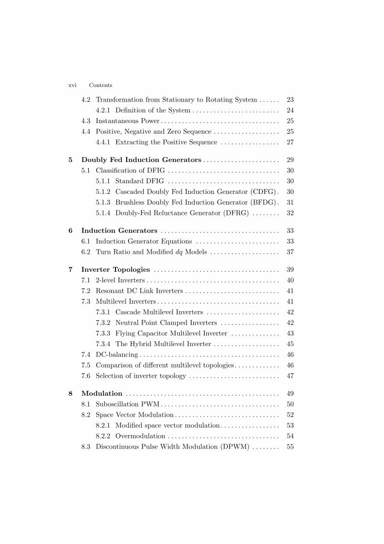
4.2 Transformation from Stationary to Rotating System . . . . . . 234.2.1 Definition of the System . . . . . . . . . . . . . . . . . . . . . . . . . 24
4.3 Instantaneous Power . . . . . . . . . . . . . . . . . . . . . . . . . . . . . . . . . . 254.4 Positive, Negative and Zero Sequence . . . . . . . . . . . . . . . . . . . 25
4.4.1 Extracting the Positive Sequence . . . . . . . . . . . . . . . . . 27
5 Doubly Fed Induction Generators . . . . . . . . . . . . . . . . . . . . . . 295.1 Classification of DFIG . . . . . . . . . . . . . . . . . . . . . . . . . . . . . . . . 30
5.1.1 Standard DFIG . . . . . . . . . . . . . . . . . . . . . . . . . . . . . . . . 305.1.2 Cascaded Doubly Fed Induction Generator (CDFG) . 305.1.3 Brushless Doubly Fed Induction Generator (BFDG) . 315.1.4 Doubly-Fed Reluctance Generator (DFRG) . . . . . . . . 32
6 Induction Generators . . . . . . . . . . . . . . . . . . . . . . . . . . . . . . . . . . 336.1 Induction Generator Equations . . . . . . . . . . . . . . . . . . . . . . . . 336.2 Turn Ratio and Modified dq Models . . . . . . . . . . . . . . . . . . . . 37
7 Inverter Topologies . . . . . . . . . . . . . . . . . . . . . . . . . . . . . . . . . . . . 397.1 2-level Inverters . . . . . . . . . . . . . . . . . . . . . . . . . . . . . . . . . . . . . . 407.2 Resonant DC Link Inverters . . . . . . . . . . . . . . . . . . . . . . . . . . . 417.3 Multilevel Inverters . . . . . . . . . . . . . . . . . . . . . . . . . . . . . . . . . . . 41
7.3.1 Cascade Multilevel Inverters . . . . . . . . . . . . . . . . . . . . . 427.3.2 Neutral Point Clamped Inverters . . . . . . . . . . . . . . . . . 427.3.3 Flying Capacitor Multilevel Inverter . . . . . . . . . . . . . . 437.3.4 The Hybrid Multilevel Inverter . . . . . . . . . . . . . . . . . . . 45
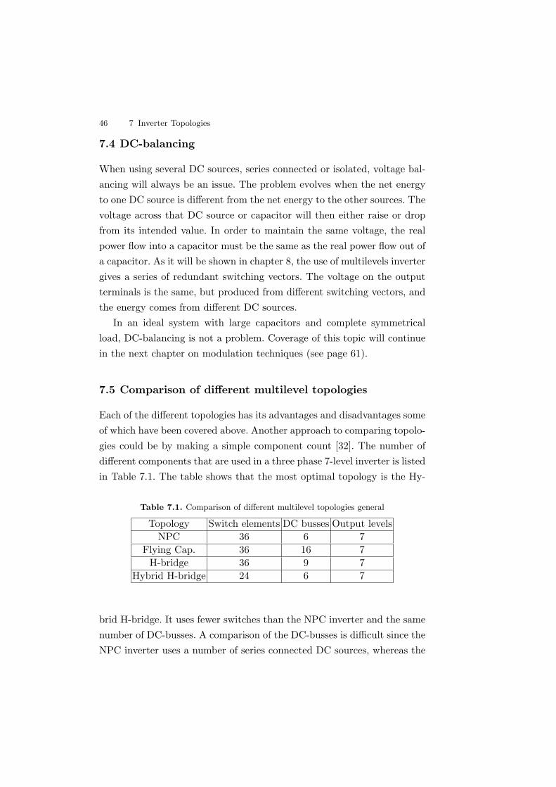
7.4 DC-balancing . . . . . . . . . . . . . . . . . . . . . . . . . . . . . . . . . . . . . . . . 467.5 Comparison of different multilevel topologies . . . . . . . . . . . . . 467.6 Selection of inverter topology . . . . . . . . . . . . . . . . . . . . . . . . . . 47
8 Modulation . . . . . . . . . . . . . . . . . . . . . . . . . . . . . . . . . . . . . . . . . . . . 498.1 Suboscillation PWM . . . . . . . . . . . . . . . . . . . . . . . . . . . . . . . . . . 508.2 Space Vector Modulation . . . . . . . . . . . . . . . . . . . . . . . . . . . . . . 52
8.2.1 Modified space vector modulation . . . . . . . . . . . . . . . . . 538.2.2 Overmodulation . . . . . . . . . . . . . . . . . . . . . . . . . . . . . . . . 54
8.3 Discontinuous Pulse Width Modulation (DPWM) . . . . . . . . 55
Contents xvii
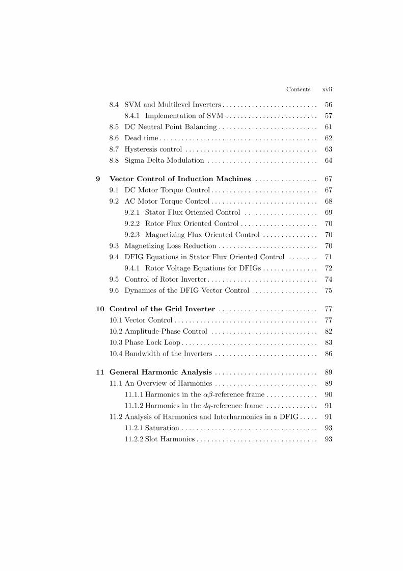
8.4 SVM and Multilevel Inverters . . . . . . . . . . . . . . . . . . . . . . . . . . 568.4.1 Implementation of SVM . . . . . . . . . . . . . . . . . . . . . . . . . 57
8.5 DC Neutral Point Balancing . . . . . . . . . . . . . . . . . . . . . . . . . . . 618.6 Dead time . . . . . . . . . . . . . . . . . . . . . . . . . . . . . . . . . . . . . . . . . . . 628.7 Hysteresis control . . . . . . . . . . . . . . . . . . . . . . . . . . . . . . . . . . . . 638.8 Sigma-Delta Modulation . . . . . . . . . . . . . . . . . . . . . . . . . . . . . . 64
9 Vector Control of Induction Machines . . . . . . . . . . . . . . . . . . 679.1 DC Motor Torque Control . . . . . . . . . . . . . . . . . . . . . . . . . . . . . 679.2 AC Motor Torque Control . . . . . . . . . . . . . . . . . . . . . . . . . . . . . 68
9.2.1 Stator Flux Oriented Control . . . . . . . . . . . . . . . . . . . . 699.2.2 Rotor Flux Oriented Control . . . . . . . . . . . . . . . . . . . . . 709.2.3 Magnetizing Flux Oriented Control . . . . . . . . . . . . . . . 70
9.3 Magnetizing Loss Reduction . . . . . . . . . . . . . . . . . . . . . . . . . . . 709.4 DFIG Equations in Stator Flux Oriented Control . . . . . . . . 71
9.4.1 Rotor Voltage Equations for DFIGs . . . . . . . . . . . . . . . 729.5 Control of Rotor Inverter . . . . . . . . . . . . . . . . . . . . . . . . . . . . . . 749.6 Dynamics of the DFIG Vector Control . . . . . . . . . . . . . . . . . . 75
10 Control of the Grid Inverter . . . . . . . . . . . . . . . . . . . . . . . . . . . 7710.1 Vector Control . . . . . . . . . . . . . . . . . . . . . . . . . . . . . . . . . . . . . . . 7710.2 Amplitude-Phase Control . . . . . . . . . . . . . . . . . . . . . . . . . . . . . 8210.3 Phase Lock Loop . . . . . . . . . . . . . . . . . . . . . . . . . . . . . . . . . . . . . 8310.4 Bandwidth of the Inverters . . . . . . . . . . . . . . . . . . . . . . . . . . . . 86
11 General Harmonic Analysis . . . . . . . . . . . . . . . . . . . . . . . . . . . . 8911.1 An Overview of Harmonics . . . . . . . . . . . . . . . . . . . . . . . . . . . . 89
11.1.1 Harmonics in the αβ-reference frame . . . . . . . . . . . . . . 9011.1.2 Harmonics in the dq-reference frame . . . . . . . . . . . . . . 91
11.2 Analysis of Harmonics and Interharmonics in a DFIG . . . . . 9111.2.1 Saturation . . . . . . . . . . . . . . . . . . . . . . . . . . . . . . . . . . . . . 9311.2.2 Slot Harmonics . . . . . . . . . . . . . . . . . . . . . . . . . . . . . . . . . 93

xviii Contents
12 Adaptive Active Filtering . . . . . . . . . . . . . . . . . . . . . . . . . . . . . . 9712.1 The Least Mean Squares Algorithm . . . . . . . . . . . . . . . . . . . . 9712.2 Adaptive Filtering of Higher Harmonics . . . . . . . . . . . . . . . . . 9812.3 Implementation . . . . . . . . . . . . . . . . . . . . . . . . . . . . . . . . . . . . . . 100
12.3.1 Grid Side Filter . . . . . . . . . . . . . . . . . . . . . . . . . . . . . . . . 10112.3.2 Rotor Side Filter . . . . . . . . . . . . . . . . . . . . . . . . . . . . . . . 101
Part II Laboratory Setup
13 Hardware Specifications . . . . . . . . . . . . . . . . . . . . . . . . . . . . . . . . 10713.1 The Rotating Machinery . . . . . . . . . . . . . . . . . . . . . . . . . . . . . . 10813.2 Power Inverters . . . . . . . . . . . . . . . . . . . . . . . . . . . . . . . . . . . . . . 10813.3 DC-link . . . . . . . . . . . . . . . . . . . . . . . . . . . . . . . . . . . . . . . . . . . . . 11013.4 Line filter . . . . . . . . . . . . . . . . . . . . . . . . . . . . . . . . . . . . . . . . . . . 11213.5 Voltage and Current Sensors . . . . . . . . . . . . . . . . . . . . . . . . . . . 11413.6 Control hardware . . . . . . . . . . . . . . . . . . . . . . . . . . . . . . . . . . . . 116
13.6.1 Digital Signal Processor board . . . . . . . . . . . . . . . . . . . 11613.6.2 Digital board . . . . . . . . . . . . . . . . . . . . . . . . . . . . . . . . . . 11713.6.3 Analogue board . . . . . . . . . . . . . . . . . . . . . . . . . . . . . . . . 119
14 Software . . . . . . . . . . . . . . . . . . . . . . . . . . . . . . . . . . . . . . . . . . . . . . . 12114.1 Program Structure . . . . . . . . . . . . . . . . . . . . . . . . . . . . . . . . . . . 121
14.1.1 Program Flow . . . . . . . . . . . . . . . . . . . . . . . . . . . . . . . . . . 12314.2 Controller Dynamics . . . . . . . . . . . . . . . . . . . . . . . . . . . . . . . . . . 12414.3 Digital Filters . . . . . . . . . . . . . . . . . . . . . . . . . . . . . . . . . . . . . . . 12414.4 Space Vector Modulation . . . . . . . . . . . . . . . . . . . . . . . . . . . . . . 12514.5 Neutral Point Balancing . . . . . . . . . . . . . . . . . . . . . . . . . . . . . . 126
15 Measurements . . . . . . . . . . . . . . . . . . . . . . . . . . . . . . . . . . . . . . . . . 12715.1 General Measurements . . . . . . . . . . . . . . . . . . . . . . . . . . . . . . . . 129
15.1.1 DC-link Charge . . . . . . . . . . . . . . . . . . . . . . . . . . . . . . . . 12915.1.2 Phase and Line Voltages . . . . . . . . . . . . . . . . . . . . . . . . . 13015.1.3 Rotor Measurements . . . . . . . . . . . . . . . . . . . . . . . . . . . . 13115.1.4 Grid Inverter Measurements . . . . . . . . . . . . . . . . . . . . . 132
Contents xix
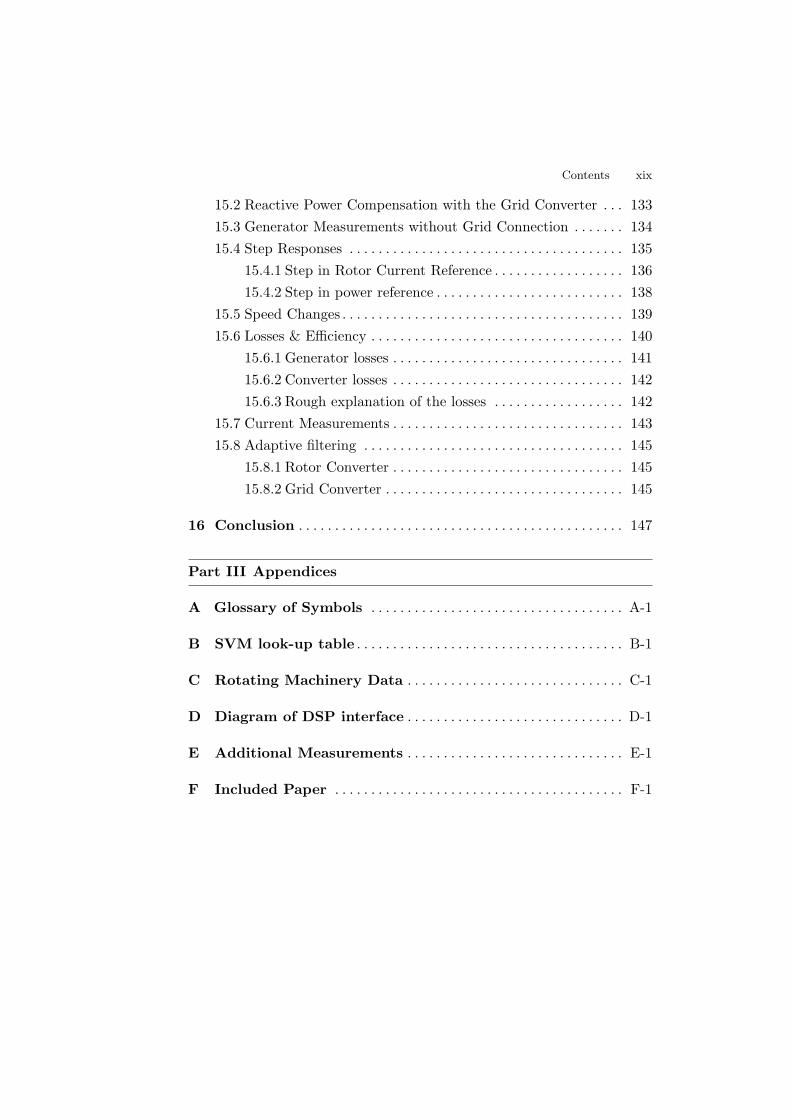
15.2 Reactive Power Compensation with the Grid Converter . . . 13315.3 Generator Measurements without Grid Connection . . . . . . . 13415.4 Step Responses . . . . . . . . . . . . . . . . . . . . . . . . . . . . . . . . . . . . . . 135
15.4.1 Step in Rotor Current Reference . . . . . . . . . . . . . . . . . . 13615.4.2 Step in power reference . . . . . . . . . . . . . . . . . . . . . . . . . . 138
15.5 Speed Changes . . . . . . . . . . . . . . . . . . . . . . . . . . . . . . . . . . . . . . . 13915.6 Losses & Efficiency . . . . . . . . . . . . . . . . . . . . . . . . . . . . . . . . . . . 140
15.6.1 Generator losses . . . . . . . . . . . . . . . . . . . . . . . . . . . . . . . . 14115.6.2 Converter losses . . . . . . . . . . . . . . . . . . . . . . . . . . . . . . . . 14215.6.3 Rough explanation of the losses . . . . . . . . . . . . . . . . . . 142
15.7 Current Measurements . . . . . . . . . . . . . . . . . . . . . . . . . . . . . . . . 14315.8 Adaptive filtering . . . . . . . . . . . . . . . . . . . . . . . . . . . . . . . . . . . . 145
15.8.1 Rotor Converter . . . . . . . . . . . . . . . . . . . . . . . . . . . . . . . . 14515.8.2 Grid Converter . . . . . . . . . . . . . . . . . . . . . . . . . . . . . . . . . 145
16 Conclusion . . . . . . . . . . . . . . . . . . . . . . . . . . . . . . . . . . . . . . . . . . . . . 147
Part III Appendices
A Glossary of Symbols . . . . . . . . . . . . . . . . . . . . . . . . . . . . . . . . . . . A-1
B SVM look-up table . . . . . . . . . . . . . . . . . . . . . . . . . . . . . . . . . . . . . B-1
C Rotating Machinery Data . . . . . . . . . . . . . . . . . . . . . . . . . . . . . . C-1
D Diagram of DSP interface . . . . . . . . . . . . . . . . . . . . . . . . . . . . . . D-1
E Additional Measurements . . . . . . . . . . . . . . . . . . . . . . . . . . . . . . E-1
F Included Paper . . . . . . . . . . . . . . . . . . . . . . . . . . . . . . . . . . . . . . . . F-1

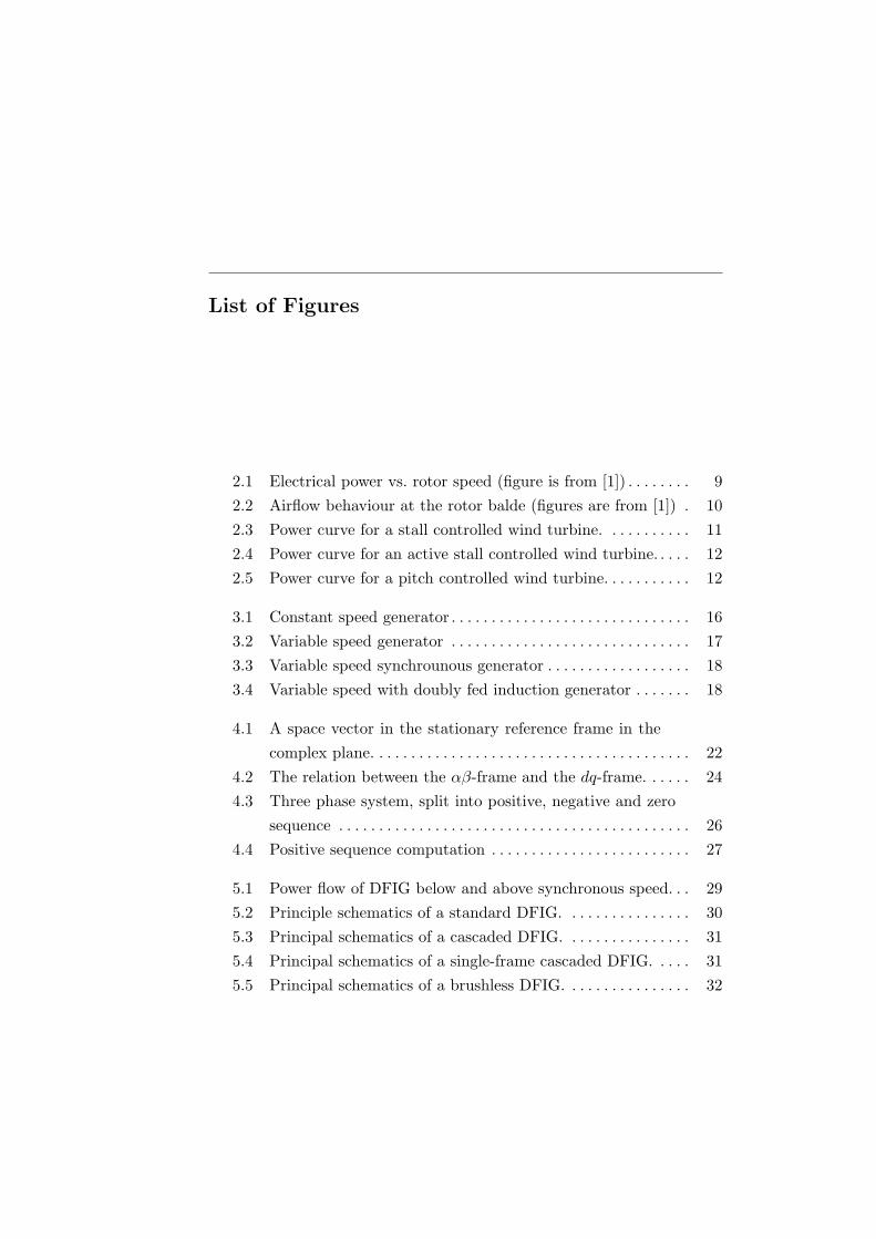
List of Figures
2.1 Electrical power vs. rotor speed (figure is from [1]) . . . . . . . . 92.2 Airflow behaviour at the rotor balde (figures are from [1]) . 102.3 Power curve for a stall controlled wind turbine. . . . . . . . . . . 112.4 Power curve for an active stall controlled wind turbine. . . . . 122.5 Power curve for a pitch controlled wind turbine. . . . . . . . . . . 12
3.1 Constant speed generator . . . . . . . . . . . . . . . . . . . . . . . . . . . . . . 163.2 Variable speed generator . . . . . . . . . . . . . . . . . . . . . . . . . . . . . . 173.3 Variable speed synchrounous generator . . . . . . . . . . . . . . . . . . 183.4 Variable speed with doubly fed induction generator . . . . . . . 18
4.1 A space vector in the stationary reference frame in thecomplex plane. . . . . . . . . . . . . . . . . . . . . . . . . . . . . . . . . . . . . . . . 22
4.2 The relation between the αβ-frame and the dq-frame. . . . . . 244.3 Three phase system, split into positive, negative and zero
sequence . . . . . . . . . . . . . . . . . . . . . . . . . . . . . . . . . . . . . . . . . . . . 264.4 Positive sequence computation . . . . . . . . . . . . . . . . . . . . . . . . . 27
5.1 Power flow of DFIG below and above synchronous speed. . . 295.2 Principle schematics of a standard DFIG. . . . . . . . . . . . . . . . 305.3 Principal schematics of a cascaded DFIG. . . . . . . . . . . . . . . . 315.4 Principal schematics of a single-frame cascaded DFIG. . . . . 315.5 Principal schematics of a brushless DFIG. . . . . . . . . . . . . . . . 32

xxii List of Figures
6.1 Standard steady state equivalent diagram of an inductionmachine. . . . . . . . . . . . . . . . . . . . . . . . . . . . . . . . . . . . . . . . . . . . . 37
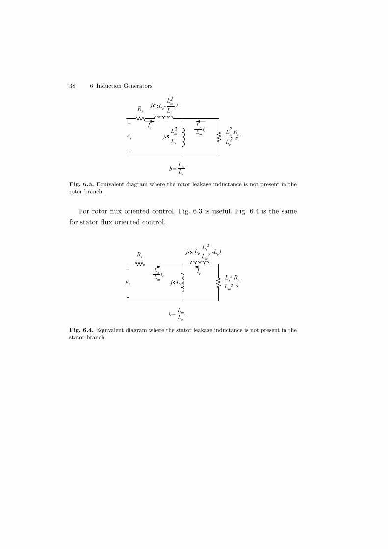
6.2 Equivalent diagram for any values of b. . . . . . . . . . . . . . . . . . . 376.3 Equivalent diagram where the rotor leakage inductance is
not present in the rotor branch. . . . . . . . . . . . . . . . . . . . . . . . . 386.4 Equivalent diagram where the stator leakage inductance is
not present in the stator branch. . . . . . . . . . . . . . . . . . . . . . . . 38
7.1 2-level inverter . . . . . . . . . . . . . . . . . . . . . . . . . . . . . . . . . . . . . . . 407.2 Resonant DC-link converter . . . . . . . . . . . . . . . . . . . . . . . . . . . 417.3 5-level H-bridge inverter single phase . . . . . . . . . . . . . . . . . . . . 427.4 3-level Neutral Point Clamped inverter single phase . . . . . . . 437.5 Two different types of 7-level NPC with the same number
of diodes, single phase . . . . . . . . . . . . . . . . . . . . . . . . . . . . . . . . 447.6 Three-level flying capacitor, single phase . . . . . . . . . . . . . . . . 447.7 7-level hybrid H-bridge inverter single phase . . . . . . . . . . . . . 45
8.1 CB-PWM with mi =0.7854, mf = 20 . . . . . . . . . . . . . . . . . . . 518.2 2-level inverter and its space vectors . . . . . . . . . . . . . . . . . . . . 528.3 Overmodulation . . . . . . . . . . . . . . . . . . . . . . . . . . . . . . . . . . . . . . 558.4 Plot of four different discontinuous modulation schemes . . . 568.5 Space vectors of a 3-level inverter . . . . . . . . . . . . . . . . . . . . . . . 578.6 3-level hexagonal in (g,h)-coordinate system . . . . . . . . . . . . . 588.7 Phase-phase signal of 3-level and 4-level modulation,
Fs = 4kHz . . . . . . . . . . . . . . . . . . . . . . . . . . . . . . . . . . . . . . . . . . 608.8 Hysteresis current control . . . . . . . . . . . . . . . . . . . . . . . . . . . . . 648.9 Flow diagram of Σ∆-modulation for one bridge leg. . . . . . . 65
9.1 Orientation of the field flux and armature MMF in a DCmachine. . . . . . . . . . . . . . . . . . . . . . . . . . . . . . . . . . . . . . . . . . . . . 67
9.2 Vector control in stator flux oriented control. . . . . . . . . . . . . 699.3 Relationship between the stationary reference frame and
the SFO frame. . . . . . . . . . . . . . . . . . . . . . . . . . . . . . . . . . . . . . . 719.4 Stator flux oriented vector control for the DFIG system . . . 74
List of Figures xxiii
10.1 Grid inverter control . . . . . . . . . . . . . . . . . . . . . . . . . . . . . . . . . . 7910.2 Vector control of grid inverter. . . . . . . . . . . . . . . . . . . . . . . . . . 8010.3 Principle of voltage angle control. . . . . . . . . . . . . . . . . . . . . . . 8210.4 Phase lock loop with full signal . . . . . . . . . . . . . . . . . . . . . . . . 8510.5 Phase lock loop with positive sequence signal. . . . . . . . . . . . . 8510.6 Measured frequency spectrum of two different types of PLL. 86
11.1 Directions of different harmonics in the αβ-frame. . . . . . . . . 9011.2 Frequency spectrum of DFIG at synchronous speed
without stator conn. to grid (1500 RPM) . . . . . . . . . . . . . . . . 9211.3 Frequency spectrum of DFIG stator and rotor current
measured at ±10% slip. . . . . . . . . . . . . . . . . . . . . . . . . . . . . . . . 9411.4 Frequency spectrum of the DFIG at 1350 RPM without
stator conn. to grid . . . . . . . . . . . . . . . . . . . . . . . . . . . . . . . . . . . 9511.5 Frequency spectrum of DFIG at 1650 RPM without stator
conn. to grid . . . . . . . . . . . . . . . . . . . . . . . . . . . . . . . . . . . . . . . . . 96
12.1 Single frequency adaptive LMS filter . . . . . . . . . . . . . . . . . . . 9912.2 Laboratory setup with torque producing motor to the left
and the DFIG machine to the right. . . . . . . . . . . . . . . . . . . . . 105
13.1 Schematics of the DFIG laboratorie setup. . . . . . . . . . . . . . . . 10713.2 Photograph of the gate driver connected on three single
phase inverter PCBs. . . . . . . . . . . . . . . . . . . . . . . . . . . . . . . . . . 11013.3 Top view of the power converters. . . . . . . . . . . . . . . . . . . . . . . 11113.4 The DC-link capacitor with dual voltage measurement. . . . . 11213.5 Line filter with contactor and pre-charge contactor. . . . . . . 11313.6 Measurements with Hall elements. . . . . . . . . . . . . . . . . . . . . . . 11513.7 Functional diagram of the control hardware. . . . . . . . . . . . . . 11613.8 Photograph of the digital interface board. . . . . . . . . . . . . . . . 11813.9 Photograph of the analogue interface with the AD-converters.119
14.1 Flow chart of the main program. . . . . . . . . . . . . . . . . . . . . . . . 123
15.1 Time trace of DC-link precharge. . . . . . . . . . . . . . . . . . . . . . . . 129

xxiv List of Figures
15.2 Converter phase to zero voltage. . . . . . . . . . . . . . . . . . . . . . . . . 13015.3 Rotor voltage and current measured with Ps = 25kW ,
10% slip. . . . . . . . . . . . . . . . . . . . . . . . . . . . . . . . . . . . . . . . . . . . . 13115.4 Stator and grid inverter current measured with adaptive
filter, 1350 RPM. . . . . . . . . . . . . . . . . . . . . . . . . . . . . . . . . . . . . . 13215.5 Converter voltages, with the grid side converter working
as a STATCOM. . . . . . . . . . . . . . . . . . . . . . . . . . . . . . . . . . . . . . 13315.6 Frequency spectrum of rotor current and stator current,
with the stator connected to resistors, Is = 6A. Speed=1200 RPM. . . . . . . . . . . . . . . . . . . . . . . . . . . . . . . . . . . . . . . . . 134
15.7 Step variation in the rotor current direct axis. . . . . . . . . . . . . 13515.8 Step variation in the rotor current quadrature axis. . . . . . . . 13615.9 Step responses for d and q zoom of Fig. 15.8 and 15.7. . . . . 13715.10Step response for Ps, 5kW to 25kW, at 1350 RPM. . . . . . . . 13815.11Speed charge 1200 rpm -1800 rpm . . . . . . . . . . . . . . . . . . . . . . 13915.12Speed change 1650 - 1350 RPM . . . . . . . . . . . . . . . . . . . . . . . . 14015.13Difference between Pgrid and Ir with rotor magn. (solid)
and stator magn. (dotted) (measured in Hammel) . . . . . . . . 14115.14Spectrum stator and rotor current, speed: 1350 RPM . . . . . 14315.15Spectrum stator and rotor current, speed: 1650 RPM . . . . . 14415.16Current spectrums w. & w.out adaptive filtering at 1350
RPM (10% slip) . . . . . . . . . . . . . . . . . . . . . . . . . . . . . . . . . . . . . . 14515.17Spectrum of the grid side current without and with
adaptive filter. . . . . . . . . . . . . . . . . . . . . . . . . . . . . . . . . . . . . . . . 146
D.1 Buffer circuit . . . . . . . . . . . . . . . . . . . . . . . . . . . . . . . . . . . . . . . . D-2D.2 PWM latch . . . . . . . . . . . . . . . . . . . . . . . . . . . . . . . . . . . . . . . . . . D-3D.3 Relay outputs . . . . . . . . . . . . . . . . . . . . . . . . . . . . . . . . . . . . . . . . D-4D.4 Connector diagram . . . . . . . . . . . . . . . . . . . . . . . . . . . . . . . . . . . D-5D.5 Encoder decoder circuit . . . . . . . . . . . . . . . . . . . . . . . . . . . . . . . D-6D.6 Aux. I/O-diagram . . . . . . . . . . . . . . . . . . . . . . . . . . . . . . . . . . . . D-7D.7 gatedriver . . . . . . . . . . . . . . . . . . . . . . . . . . . . . . . . . . . . . . . . . . . D-8D.8 Voltage measurements . . . . . . . . . . . . . . . . . . . . . . . . . . . . . . . . D-9D.9 Current measurements . . . . . . . . . . . . . . . . . . . . . . . . . . . . . . . . D-10
List of Figures xxv
D.10 ”High” current measurements . . . . . . . . . . . . . . . . . . . . . . . . . . D-11D.11 AD converter PCB . . . . . . . . . . . . . . . . . . . . . . . . . . . . . . . . . . . D-12D.12 Anti-aliasing filter for sigma-delta AD-converter . . . . . . . . . . D-13D.13 NPC diagram . . . . . . . . . . . . . . . . . . . . . . . . . . . . . . . . . . . . . . . . D-14
E.1 Measured frequency spectrum of two different types ofPLL (Hammel). . . . . . . . . . . . . . . . . . . . . . . . . . . . . . . . . . . . . . . E-1
E.2 Rotor magnetizing with a speed change 1650 - 1350 RPM(Hammel) . . . . . . . . . . . . . . . . . . . . . . . . . . . . . . . . . . . . . . . . . . . E-2
E.3 Stator magnetizing with a speed change 1650 - 1350 RPM(Hammel) . . . . . . . . . . . . . . . . . . . . . . . . . . . . . . . . . . . . . . . . . . . E-3

1
Introduction
1.1 Background
The penetration of wind energy into the electrical grid has increasedtremendously in the last 10 years, especially in Denmark and Germany.Other countries have also had an increase in installed wind energy pro-duction capacity, e.g. Spain. In Denmark, installed wind power is 28% ofthe total installed electrical power.
Five to ten years ago, the standard wind turbine was a simple andhighly reliable stall controlled turbine. This type of turbine was designed toproduce electricity whenever the wind speed was high enough and the gridwas stable. In situations of grid instability, the turbine would disconnect.For a small number of wind turbines, this works fine, but in the case of alarge penetration of wind energy, turbines have to help stabilize the grid.This requires turbines that are more controllable.
A way to make more controllable turbines is variable speed. Variablespeed turbines can store some of the power fluctuations due to turbulenceby increasing the rotor speed. By pitching the rotor blades, these turbinescan control the power output at any given wind speed. As will be describedin this thesis, a way to transfer the wind energy from a variable speedturbine to the electrical grid is a combination of an electrical generatorand a power converter.
2 1 Introduction
The doubly fed induction generator with a power converter is a simpleand highly controllable way to transform the mechanical energy from thevariable speed rotor to a constant frequency electrical utility grid.
One of the main objectives of this Ph.D. project was to set up a labo-ratory model of a variable speed generator with power electronic inverters.The generator used for the model is a doubly fed induction generator, withtwo back to back 3-level neutral point clamped inverters.
1.2 Thesis outline
This thesis is organized as follows:Chapter 2 General description of wind energy production from a his-
torical perspective. Introduction to different aerodynamic control princi-ples. Finally, a brief overview of power quality.
Chapter 3 An overview of different generator topologies that are ofinterest with respect to wind turbines.
Chapter 4 The different reference frames used throughout the thesisare presented. The nature of positive, negative and zero sequence is shown.
Chapter 5 Presents a classification of the different types of doubly fedinduction generators.
Chapter 6 Deals with equations related to the induction generator andthe doubly fed induction generator. Describes the problem of turn ratioin relation to doubly fed machines and shows the steady state equivalentdiagram.
Chapter 7 Covers different three phase inverter topologies, including2-level inverters hard or soft switched and multilevel inverters. Introducesthe problem of neutral point balancing.
Chapter 8 Describes some of the features of PWM, including suboscil-lation PWM, space vector modulation and various discontinuous PWMmethods. Space vector modulation together with 3-level inverter are cov-ered. A simple method to implement space vector modulation in 3-levelinverters is described. Finally, a more in-depth discussion of the neutralpoint balancing problem.

1.2 Thesis outline 3
Chapter 9 In this chapter, the principles of vector control are stated,with a discussion of the different flux oriented frames. Vector control ofthe doubly fed induction generator is more thoroughly described.
Chapter 10 Presentation of vector control and amplitude-phase con-trol of a grid connected inverter. A comparison of different phase lockloops is presented.
Chapter 11 Gives an overview of the harmonics in the stationaryand synchronously rotating reference frames. Presents a table with theharmonics in the doubly fed induction generator.
Chapter 12 In this chapter, an adaptive filter is presented. Both in-verters can be used as an active filter.
Chapter 13 Description of the hardware used in the laboratory setup.
Chapter 14 A short presentation of some of the software.Chapter 15 Presents the measurements and results.Chapter 15 The conclusion.Appendix A Glossary of symbols, superscripts and subscripts that
are used in the thesis.Appendix B Includes the look-up table used in relation to the space
vector modulation.Appendix C List of parameters of the doubly fed induction generator
and the motor used as the load.Appendix D Includes schematics of the PCBs used in the laboratory
model.Appendix E Includes additional measurements.Appendix F Includes the programming source code (Not include in
the public version).Appendix G Contains a submitted and accepted paper with the title:
“Harmonic Analysis of Doubly Fed Induction Generators”.


Part I
Wind Turbines and Doubly Fed Induction
generators


2
Wind Energy Generation
For more one than thousand years, wind energy has been used by hu-mans [1]. Until the end of the 19th century, wind power was only usedin mechanical constructions, such as grain grinding, etc. In 1891, DanishPoul la Cour started his work on the electrical wind turbine at Askov folkhigh school; this was the start of Danish wind turbines [6]. During WorldWar I and II, Denmark was cut off from its supply of oil and electricalenergy from wind turbines was important, though not sufficient. In 1957,J. Juul made his 200 kW Gedser wind turbine. During the oil crises in themid-1970s, it became apparent that alternative energy to oil was needed.That started the Danish wind energy industry.
In the beginning of the 1980s, the first wind turbine gold rush in Cal-ifornia happened. Back then, the traditional Danish wind turbine drivetrain was also made up of a 3-bladed rotor, a gear box and an inductiongenerator, better known as the ”Danish standard”. The average turbinecontained a 55 kW induction generator. During the 1980s, turbines in-creased in size, but the penetration of wind energy into the electrical gridwas marginal. There were no major problems, with the induction gener-ators drawing reactive power from the grid. At the end of the 1980s, thelarger Danish turbines were equipped with a 35 m rotor and a 350-450kW induction generator [6].
More advanced drive trains have been made since the beginning of the1980s, but not on a large commercial basis. The drive train topologies canbe divided into two groups: fixed speed and variable speed. Both groups
8 2 Wind Energy Generation
can again be split into two groups one with induction generators and onewith synchronous generators. In addition there is a drive train without agear box. The generators used here are with multipole synchronous ma-chines.
Today the biggest commercial turbines are 4-5 MW. Enercon has devel-oped a prototype of a 5 MW synchronous multipole direct driven turbine,and NEG Micon is producing a 4.2 MW doubly fed induction generatorturbine with gear box. Both are with pitch controlled rotor.
2.1 Wind Energy
The power available in the wind flowing through an area A is given by
Pwind =12ρv3
wA (2.1)
where A is the area swept by the turbine blades, ρ is the air density, vw
is the velocity of the wind.The mechanical power produced by the wind turbine can be expressed
as [7]
Pmech =12Cpρv3
wA (2.2)
where Cp is the power performance coefficient. The maximum Cp for atypical wind turbine is 0.48-0.50. The theoretical maximum of Cp is calledBetz limit and is equal to 16/27 = 0.59 [1].
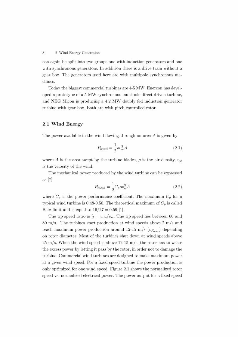
The tip speed ratio is λ = vtip/vw. The tip speed lies between 60 and80 m/s. The turbines start production at wind speeds above 2 m/s andreach maximum power production around 12-15 m/s (vPmax) dependingon rotor diameter. Most of the turbines shut down at wind speeds above25 m/s. When the wind speed is above 12-15 m/s, the rotor has to wastethe excess power by letting it pass by the rotor, in order not to damage theturbine. Commercial wind turbines are designed to make maximum powerat a given wind speed. For a fixed speed turbine the power production isonly optimized for one wind speed. Figure 2.1 shows the normalized rotorspeed vs. normalized electrical power. The power output for a fixed speed
2.2 Stall control 9
Fig. 2.1. Electrical power vs. rotor speed (figure is from [1])
turbine can be drawn on the figure as a vertical line at n/nn equal to one,optimal production is only meet at 11 m/s. The curves in Fig. 2.1 canbe shifted left or right, in order to optimize the turbine to a given site. Avariable speed turbine on the other hand can optimize its speed, so optimalpower is meet for any wind speed, this is showed by the thicker line in Fig.2.1. Power extraction from the wind can be controlled in different ways,including stall control and pitch control.
2.2 Stall control
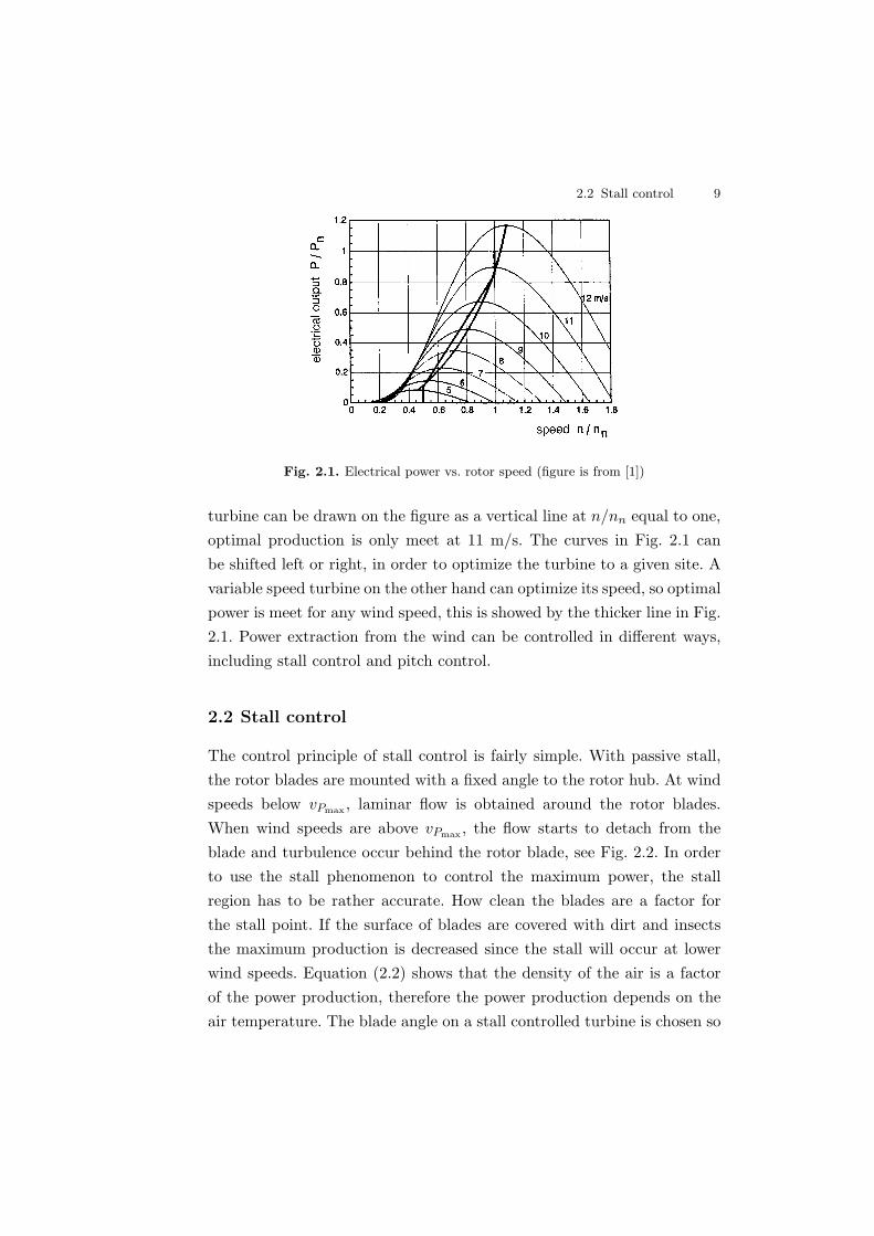
The control principle of stall control is fairly simple. With passive stall,the rotor blades are mounted with a fixed angle to the rotor hub. At windspeeds below vPmax , laminar flow is obtained around the rotor blades.When wind speeds are above vPmax , the flow starts to detach from theblade and turbulence occur behind the rotor blade, see Fig. 2.2. In orderto use the stall phenomenon to control the maximum power, the stallregion has to be rather accurate. How clean the blades are a factor forthe stall point. If the surface of blades are covered with dirt and insectsthe maximum production is decreased since the stall will occur at lowerwind speeds. Equation (2.2) shows that the density of the air is a factorof the power production, therefore the power production depends on theair temperature. The blade angle on a stall controlled turbine is chosen so
10 2 Wind Energy Generation
(a) laminar flow (b) stalling
Fig. 2.2. Airflow behaviour at the rotor balde (figures are from [1])
that its production is maximized at a given temperature. Which in turncauses problems with changing seasons. In order to overcome this issue,NEG Micon now sells a hub with the possibility of slowly changing theblade angle 1-2 degrees, this feature is sold under the name Power TrimTM.
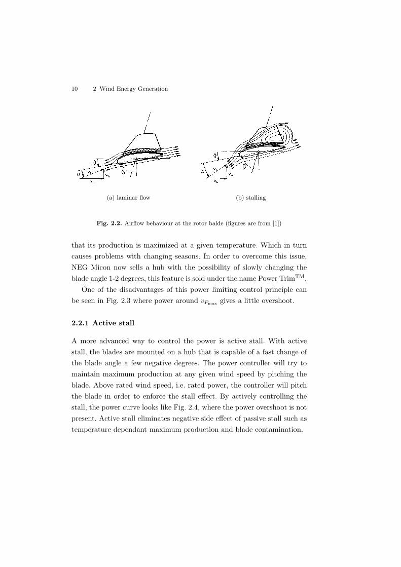
One of the disadvantages of this power limiting control principle canbe seen in Fig. 2.3 where power around vPmax gives a little overshoot.
2.2.1 Active stall
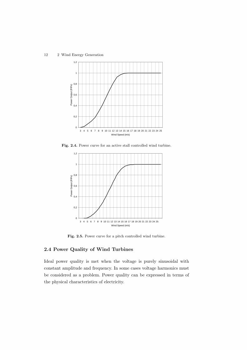
A more advanced way to control the power is active stall. With activestall, the blades are mounted on a hub that is capable of a fast change ofthe blade angle a few negative degrees. The power controller will try tomaintain maximum production at any given wind speed by pitching theblade. Above rated wind speed, i.e. rated power, the controller will pitchthe blade in order to enforce the stall effect. By actively controlling thestall, the power curve looks like Fig. 2.4, where the power overshoot is notpresent. Active stall eliminates negative side effect of passive stall such astemperature dependant maximum production and blade contamination.
2.3 Pitch control 11
2.3 Pitch control
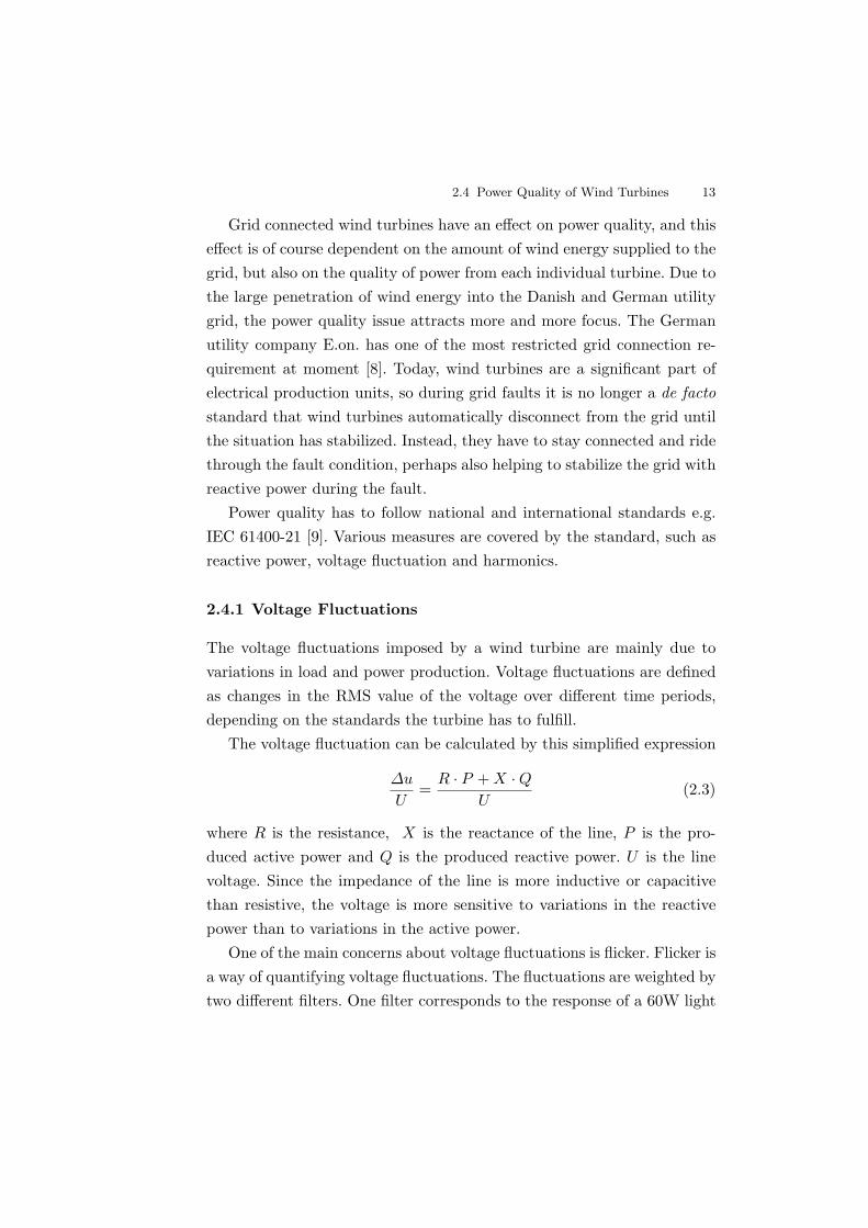
When controlling a wind turbine with pitch control, blade angle is changedwith a positive angle, as opposed to stall where a negative angle is used.Instead of forcing stall to occur, the blades are pitched out of the wind.As in stall controlled turbines the controller will try to maintain max Cp.Above rated wind speed, the blades are pitched out of the wind and whenthe wind speed reduces again, the blades are pitched back into the wind.This results in a lot of trimming of the pitch angle compared to activestall. The angle the blades have to be pitched is about 10-20 degrees.
Since pitch control limits power by pitching the blade out of the wind,fast power fluctuations in the wind above rated wind speed will also re-sult in a fast electrical power fluctuation above rated power, unless theblades can be pitched fast enough to overcome the fluctuation. This cannot be accomplished. Therefore some kind of variable speed has to beused together with pitch controlled turbines. For stall controlled turbines,power limitation occurs due to the physics of the aerodynamics of the stallprinciple.
0
0,2
0,4
0,6
0,8
1
1,2
3 4 5 6 7 8 9 10 11 12 13 14 15 16 17 18 19 20 21 22 23 24 25Wind Speed (m/s)
Pow
er O
utpu
t (P
/Pn)
Fig. 2.3. Power curve for a stall controlled wind turbine.
12 2 Wind Energy Generation
0
0,2
0,4
0,6
0,8
1
1,2
3 4 5 6 7 8 9 10 11 12 13 14 15 16 17 18 19 20 21 22 23 24 25
Wind Speed (m/s)
Pow
er O
utpu
t (P
/Pn)
Fig. 2.4. Power curve for an active stall controlled wind turbine.
0
0,2
0,4
0,6
0,8
1
1,2
3 4 5 6 7 8 9 10 11 12 13 14 15 16 17 18 19 20 21 22 23 24 25
Wind Speed (m/s)
Pow
er O
utpu
t (P
/Pn)
Fig. 2.5. Power curve for a pitch controlled wind turbine.
2.4 Power Quality of Wind Turbines
Ideal power quality is met when the voltage is purely sinusoidal withconstant amplitude and frequency. In some cases voltage harmonics mustbe considered as a problem. Power quality can be expressed in terms ofthe physical characteristics of electricity.
2.4 Power Quality of Wind Turbines 13
Grid connected wind turbines have an effect on power quality, and thiseffect is of course dependent on the amount of wind energy supplied to thegrid, but also on the quality of power from each individual turbine. Due tothe large penetration of wind energy into the Danish and German utilitygrid, the power quality issue attracts more and more focus. The Germanutility company E.on. has one of the most restricted grid connection re-quirement at moment [8]. Today, wind turbines are a significant part ofelectrical production units, so during grid faults it is no longer a de factostandard that wind turbines automatically disconnect from the grid untilthe situation has stabilized. Instead, they have to stay connected and ridethrough the fault condition, perhaps also helping to stabilize the grid withreactive power during the fault.
Power quality has to follow national and international standards e.g.IEC 61400-21 [9]. Various measures are covered by the standard, such asreactive power, voltage fluctuation and harmonics.
2.4.1 Voltage Fluctuations
The voltage fluctuations imposed by a wind turbine are mainly due tovariations in load and power production. Voltage fluctuations are definedas changes in the RMS value of the voltage over different time periods,depending on the standards the turbine has to fulfill.
The voltage fluctuation can be calculated by this simplified expression
∆u
U=
R · P + X ·QU
(2.3)
where R is the resistance, X is the reactance of the line, P is the pro-duced active power and Q is the produced reactive power. U is the linevoltage. Since the impedance of the line is more inductive or capacitivethan resistive, the voltage is more sensitive to variations in the reactivepower than to variations in the active power.
One of the main concerns about voltage fluctuations is flicker. Flicker isa way of quantifying voltage fluctuations. The fluctuations are weighted bytwo different filters. One filter corresponds to the response of a 60W light

14 2 Wind Energy Generation
bulb and the other to the response of the human eye and brain to variationsin luminance of the light bulb [10]. According to the IEC 61400-21, flickeremission should not be determined purely from voltage measurements. Inorder not to measure background flicker, a set of 3 current and 3 voltagemeasurements are used to measure flicker.
2.4.2 Harmonics
Wind turbines equipped with power electronic converters will cause somesort of higher harmonics. Eventhough IEC 61400-21 does not have anyrequirements for turbines without power electronics, the generator itselfwill cause some harmonics. For turbines with converters, the harmonics arespecified for frequencies up to the 50th harmonic of the fundamental gridfrequency, plus there are some restrictions on the level of interharmonics.
3
Generator Topologies in Wind Turbines
As discussed in last chapter wind turbines are working either at fixed speed(small speed changes due to the generator slip) or variable speed. Variablespeed is here understood as 5% to 100% variation of norminal speed. Onvariable speed turbines, energy can be stored in the rotor as increasedrotational energy, this is not the case for fixed speed turbines. Thereforewill the turbulence of the wind cause fluctuations in the instantaneouspower from a fixed speed turbine. The variable speed turbines are usuallycontrolled by power electronic converters together with the generator. Bymeans of power electronics the rotor speed is controlled, the turbulenceof the wind is accumulated in the rotor speed. Hence, the power qualityimpact from the wind turbine is improved by using variable speed [11].
In the following there will be a short overview of various wind turbinegenerator topologies, it is not complete and detailed.
3.1 Constant speed system
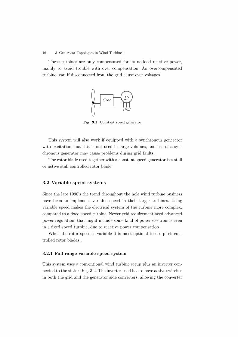
The generator in the constant speed system is most often an inductiongenerator, see Fig. 3.1, connected directly to the grid, and mechanicallythe rotor is connected through a gear box. In order to reduce power fluc-tuations the induction generator in this setup is designed with a higherslip than normal.
16 3 Generator Topologies in Wind Turbines
These turbines are only compensated for its no-load reactive power,mainly to avoid trouble with over compensation. An overcompensatedturbine, can if disconnected from the grid cause over voltages.
GearI.G.
Grid
Fig. 3.1. Constant speed generator
This system will also work if equipped with a synchronous generatorwith excitation, but this is not used in large volumes, and use of a syn-chronous generator may cause problems during grid faults.
The rotor blade used together with a constant speed generator is a stallor active stall controlled rotor blade.
3.2 Variable speed systems
Since the late 1990’s the trend throughout the hole wind turbine businesshave been to implement variable speed in their larger turbines. Usingvariable speed makes the electrical system of the turbine more complex,compared to a fixed speed turbine. Newer grid requirement need advancedpower regulation, that might include some kind of power electronics evenin a fixed speed turbine, due to reactive power compensation.
When the rotor speed is variable it is most optimal to use pitch con-trolled rotor blades .
3.2.1 Full range variable speed system
This system uses a conventional wind turbine setup plus an inverter con-nected to the stator, Fig. 3.2. The inverter used has to have active switchesin both the grid and the generator side converters, allowing the converter
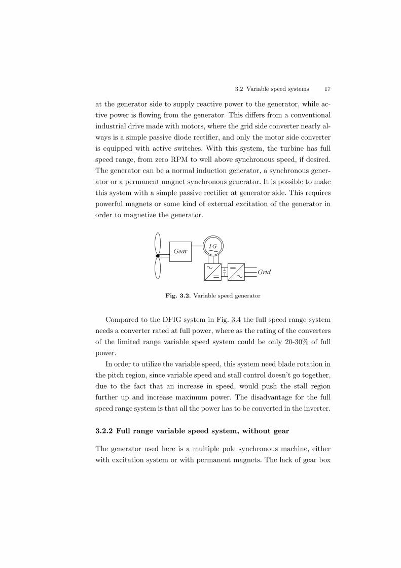
3.2 Variable speed systems 17
at the generator side to supply reactive power to the generator, while ac-tive power is flowing from the generator. This differs from a conventionalindustrial drive made with motors, where the grid side converter nearly al-ways is a simple passive diode rectifier, and only the motor side converteris equipped with active switches. With this system, the turbine has fullspeed range, from zero RPM to well above synchronous speed, if desired.The generator can be a normal induction generator, a synchronous gener-ator or a permanent magnet synchronous generator. It is possible to makethis system with a simple passive rectifier at generator side. This requirespowerful magnets or some kind of external excitation of the generator inorder to magnetize the generator.
GearI.G.
Grid
Fig. 3.2. Variable speed generator
Compared to the DFIG system in Fig. 3.4 the full speed range systemneeds a converter rated at full power, where as the rating of the convertersof the limited range variable speed system could be only 20-30% of fullpower.
In order to utilize the variable speed, this system need blade rotation inthe pitch region, since variable speed and stall control doesn’t go together,due to the fact that an increase in speed, would push the stall regionfurther up and increase maximum power. The disadvantage for the fullspeed range system is that all the power has to be converted in the inverter.
3.2.2 Full range variable speed system, without gear
The generator used here is a multiple pole synchronous machine, eitherwith excitation system or with permanent magnets. The lack of gear box
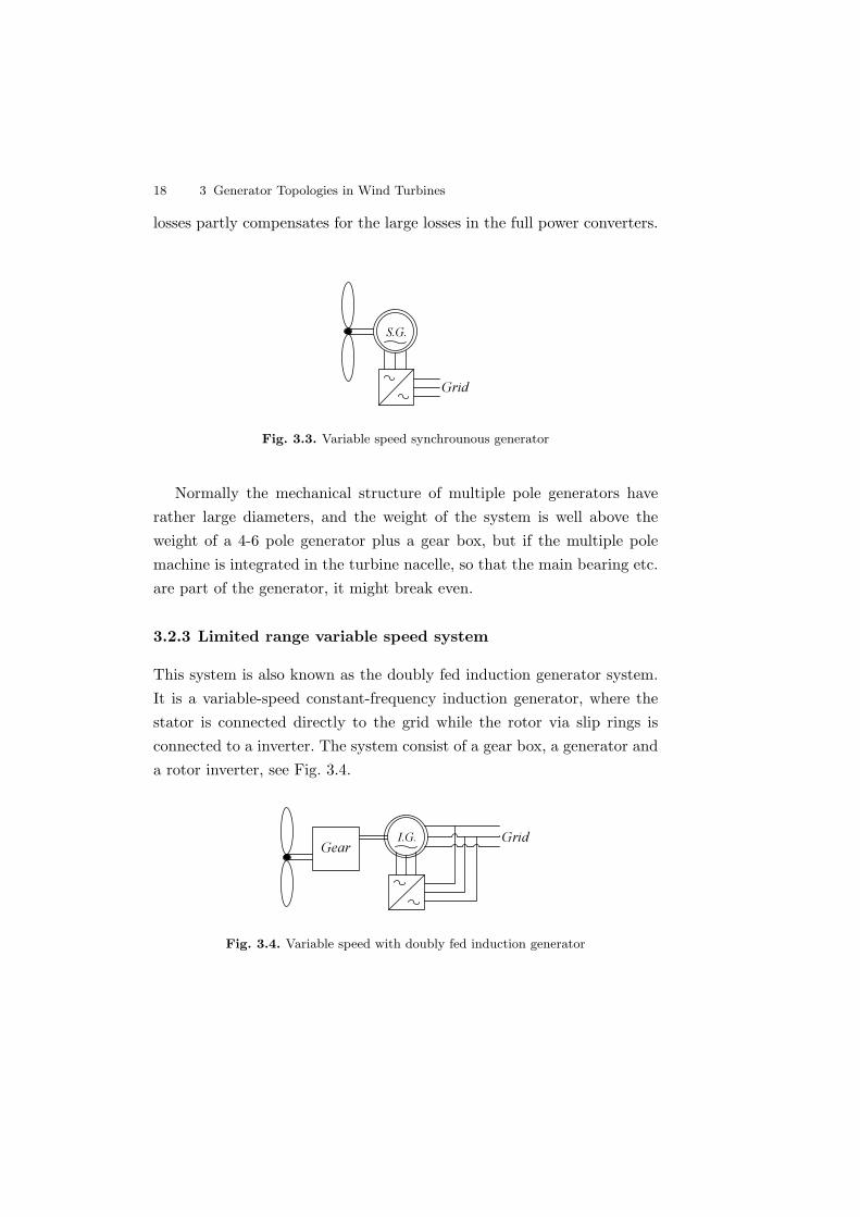
18 3 Generator Topologies in Wind Turbines
losses partly compensates for the large losses in the full power converters.
S.G.
Grid
Fig. 3.3. Variable speed synchrounous generator
Normally the mechanical structure of multiple pole generators haverather large diameters, and the weight of the system is well above theweight of a 4-6 pole generator plus a gear box, but if the multiple polemachine is integrated in the turbine nacelle, so that the main bearing etc.are part of the generator, it might break even.
3.2.3 Limited range variable speed system
This system is also known as the doubly fed induction generator system.It is a variable-speed constant-frequency induction generator, where thestator is connected directly to the grid while the rotor via slip rings isconnected to a inverter. The system consist of a gear box, a generator anda rotor inverter, see Fig. 3.4.
GearI.G. Grid
Fig. 3.4. Variable speed with doubly fed induction generator

3.2 Variable speed systems 19
The limitation in the speed range is limited by the frequency converter,since the speed range is proportional to the power flowing in the rotor.The rotor blades in the system are pitched controlled.
A more in depth coverage of the doubly fed induction generator willbe presented in the following chapters.


4
Reference Frame Conversion
When working with three phase systems, it is often more convenient to doa transformation to a two phase system in the complex plane. Doing thisfor a system without a zero connection, all the information is kept. Usingthe signals from the two phase system in feedback control is not desirabledue to the sinusoidal property of the signals. In order to overcome this, atransformation from the stationary reference frame to a rotating referenceframe is used. As a result, the fundamental part of the signal appear asconstant values in steady state.
The content of this chapter was first intended to be in the appendix.However, many definitions stated here are used in the following chapters,thus this topic is covered here.
4.1 Transformation from a Three Phase to a Two Phase
System
The three quantities (sa, sb and sc) can be transformed to a two phasevector system by
~sαβ = sα + jsβ = c(sae
j0 + sbej 2π
3 + saej 4π
3
)(4.1)
or expressed in matrix notation
22 4 Reference Frame Conversion
[sα
sβ
]= c
[1 −1
2 −12
0√
32 −
√3
2
]·
sa
sb
sc
(4.2)
If extended with a zero system the matrix notation is given by
sα
sβ
so
= c
1 −12 −1
2
0√
32 −
√3
2√2
2
√2
2
√2
2
·
sa
sb
sc
(4.3)
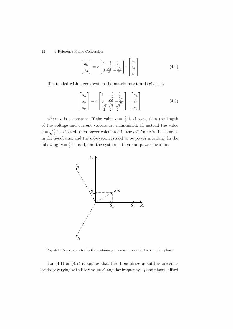
where c is a constant. If the value c = 23 is chosen, then the length
of the voltage and current vectors are maintained. If, instead the valuec =
√23 is selected, then power calculated in the αβ-frame is the same as
in the abc-frame, and the αβ-system is said to be power invariant. In thefollowing, c = 2
3 is used, and the system is then non-power invariant.
S
S
Sa
Sb
Sc
S(t)
Re
Im
Fig. 4.1. A space vector in the stationary reference frame in the complex plane.
For (4.1) or (4.2) it applies that the three phase quantities are sinu-soidally varying with RMS value S, angular frequency ω1 and phase shifted
4.2 Transformation from Stationary to Rotating System 23
2π3 in time given by
sa =√
2S cos(ω1t)sb =
√2S cos(ω1t− 2π
3 )sc =
√2S cos(ω1t− 4π
3 )
(4.4)
The RMS value S can then be expressed as
~sαβ =√
3Sejω1t (4.5)
The transformation in (4.2) and (4.3) is valid for voltage u, current i
and flux ψ in any measuring system: stator, rotor or magnetizing flux.When the voltage measurements are done using two line to line mea-
surements, the equations are
[uα
uβ
]=
[13 −1
3
− 1√3− 1√
3
]·[
uBA
uAC
](4.6)
where
uBA = uA − uB (4.7)
uCB = uB − uC (4.8)
uAC = uC − uA (4.9)
uA + uB + uC = 0 (4.10)
4.2 Transformation from Stationary to Rotating System
A vector in the stationary reference αβ-frame is transformed into thesynchronously rotating reference dq-frame oriented in the direction givenby the angle θ
~sdq = sd + jsq = ~sαβe−j(ω1t−π2 ) = ~sαβe−jθ (4.11)
This can also be written in matrix form
24 4 Reference Frame Conversion
[sd
sq
]=
[cos θ sin θ
− sin θ cos θ
]·[
sα
sβ
](4.12)
d
q
(t)
(t)
g(t)
sdsq
s
s
(t)
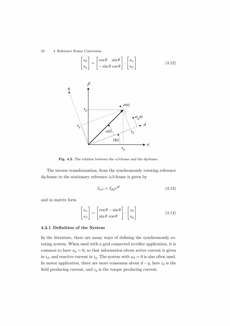
Fig. 4.2. The relation between the αβ-frame and the dq-frame.
The inverse transformation, from the synchronously rotating referencedq-frame to the stationary reference αβ-frame is given by
~sαβ = ~sdqejθ (4.13)
and in matrix form[
sα
sβ
]=
[cos θ − sin θ
sin θ cos θ
]·[
sd
sq
](4.14)
4.2.1 Definition of the System
In the literature, there are many ways of defining the synchronously ro-tating system. When used with a grid connected rectifier application, it iscommon to have uq = 0, so that information about active current is givenin id, and reactive current in iq. The system with ud = 0 is also often used.In motor application, there are more consensus about d− q, here id is thefield producing current, and iq is the torque producing current.

4.4 Positive, Negative and Zero Sequence 25
In this text, the definition where uq = 0 is used for the grid rectifier,while the standard definition is used for the rotor inverter. It may seeminconsistent to use two definitions for basically the same thing. However,the reason for this is that the grid rectifier was implemented first, anddefined as mentioned, whereafter the rotor inverter was implemented, andthere it was most correct to use the other definition.
The following notation is used for the transformation of the rotor sideto the dq-frame [
urα
urβ
]=
[cos θ sin θ
− sin θ cos θ
]·[
urd
urq
](4.15)
and the inverse transformation[
urd
urq
]=
[cos θ − sin θ
sin θ cos θ
]·[
urα
urβ
](4.16)
4.3 Instantaneous Power
When defining the voltage and current in 2-phase systems (rotating andstationary), the power equations for both cases are the following
P =32(udid + uqiq) =
32(uαiα + uβiβ) (4.17)
Q =32(udiq + uqid) =
32(uαiβ − uβiα) (4.18)
for a system with uq = 0, this simplifies the power equations to
P =32udid (4.19)
Q =32udiq (4.20)
4.4 Positive, Negative and Zero Sequence
In an unsymmetrical three phase system, the vectors can be split into:
• Positive sequence
26 4 Reference Frame Conversion
• Negative sequence• Zero sequence
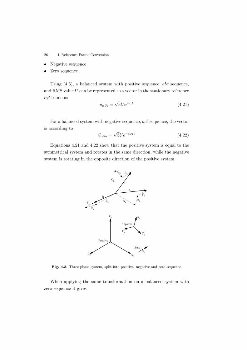
Using (4.5), a balanced system with positive sequence, abc sequence,and RMS value U can be represented as a vector in the stationary referenceαβ-frame as
~uαβp =√
3Uejω1t (4.21)
For a balanced system with negative sequence, acb sequence, the vectoris according to
~uαβn =√
3Ue−jω1t (4.22)
Equations 4.21 and 4.22 show that the positive system is equal to thesymmetrical system and rotates in the same direction, while the negativesystem is rotating in the opposite direction of the positive system.
Positive
Negative
ApBp
Cp An
Bn Cn
ZeroF0
AnAp
F0
F0
F0
Bn
Bp
Cp
Cn
CA
B
Fig. 4.3. Three phase system, split into positive, negative and zero sequence
When applying the same transformation on a balanced system withzero sequence it gives
4.4 Positive, Negative and Zero Sequence 27
~uαβz = 0 (4.23)
So the zero sequence components are not represented in the station-ary reference αβ-frame. The zero sequence contain information about thedisplacement from the zero point. In order to keep the information theextended abc → αβ0 transformation (4.3) are needed, though this givesno reduction in number of scalars. For the three phase systems, zero se-quence will not be present. Unless there is a neutral conductor, in whichthe zero sequence can flow.
12
12
12 3
12 3
-
--
-
-
-+
+
+
+
ua
ub
uc
uapubpucp
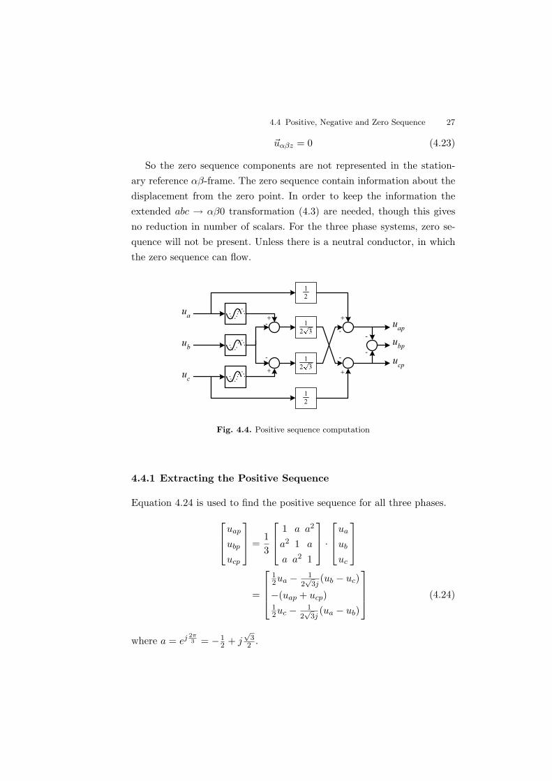
Fig. 4.4. Positive sequence computation
4.4.1 Extracting the Positive Sequence
Equation 4.24 is used to find the positive sequence for all three phases.
uap
ubp
ucp
=
13
1 a a2
a2 1 a
a a2 1
·
ua
ub
uc
=
12ua − 1
2√
3j(ub − uc)
−(uap + ucp)12uc − 1
2√
3j(ua − ub)
(4.24)
where a = ej 2π3 = −1
2 + j√
32 .

28 4 Reference Frame Conversion
A practical implementation of this requires a filter with a 90 phaseshift and constant gain. This can accomplished by using a Hilbert trans-formation [12]. The Hilbert transformation can be implemented as a highorder FIR filter, and the rest is simple calculations, see figure 4.4.
5
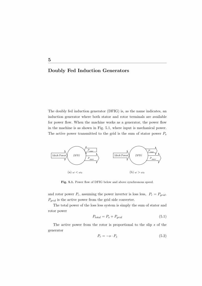
Doubly Fed Induction Generators
The doubly fed induction generator (DFIG) is, as the name indicates, aninduction generator where both stator and rotor terminals are availablefor power flow. When the machine works as a generator, the power flowin the machine is as shown in Fig. 5.1, where input is mechanical power.The active power transmitted to the grid is the sum of stator power Ps
Mech Power
Protor
Pstator
DFIG
(a) ω < ω0
Mech PowerProtor
Pstator
DFIG
(b) ω > ω0
Fig. 5.1. Power flow of DFIG below and above synchronous speed.
and rotor power Pr, assuming the power inverter is loss less, Pr = Pgrid.Pgrid is the active power from the grid side converter.
The total power of the loss less system is simply the sum of stator androtor power
Ptotal = Ps + Pgrid (5.1)
The active power from the rotor is proportional to the slip s of thegenerator
Pr = −s · Ps (5.2)

30 5 Doubly Fed Induction Generators
where the slip here is defined as
s =ωs − ωr
ωs(5.3)
5.1 Classification of DFIG
In the literature, many different kinds of DFIGs have been presented andmany of are also used in practice. DFIGs can be grouped into brushedor brushless, and then again into other subgroups. Hopfensperger andAtkinson have made a classification of the different types [13].
5.1.1 Standard DFIG
The standard DFIG is a wound rotor generator with slip-rings for therotor circuit. Fig. 5.2 shows a principle diagram of the setup. The statorcircuit is connected to the grid, while the rotor circuit is connected to afrequency converter, which is then connected to the grid [14]- [18].
Fig. 5.2. Principle schematics of a standard DFIG.
This type of generator is referred to as DFIG in the rest of the thesis.Other types mentioned here will not be covered in more detail.
5.1.2 Cascaded Doubly Fed Induction Generator (CDFG)
The cascaded DFIG consist of two doubly fed induction machines, con-nected mechanically and electrically through the rotor. The stator termi-nals of one side are connected directly to the grid, while the other statoris connected to a frequency converter, see Fig. 5.3.

5.1 Classification of DFIG 31
Fig. 5.3. Principal schematics of a cascaded DFIG.
The rotor voltage of the two machines are equal. The machine con-nected to the converter controls the other machine. This setup is notpractical, since it does not give any advantages compared to the standardsolution, while it uses an extra machine. The losses from this setup areexpected to be higher than for the standard solution, due to the largernumber of windings [13].
Single-Frame Cascaded Doubly Fed Induction Generator
(S-CDFG)
The single-frame cascaded doubly-fed induction generator uses a singleframe instead of two separate frames. Although this machine is mechani-cally more robust than the dual framed, it still suffers from comparativelylow efficiency [13].
Fig. 5.4. Principal schematics of a single-frame cascaded DFIG.
5.1.3 Brushless Doubly Fed Induction Generator (BFDG)
The brushless doubly fed induction generator is a single frame machinewith two stators using the same slots and sharing a common magneticcircuit. One winding is used for power and the other for control. In order

32 5 Doubly Fed Induction Generators
to avoid transformer coupling between the two windings, they must havea different number of pole pairs.
Fig. 5.5. Principal schematics of a brushless DFIG.
To avoid unbalanced magnetic pull on the rotor, the difference in polepair numbers must be higher than one [19]. The number of pole pairs inthe rotor must equal the sum of pole pairs of the two stator windings [19].
5.1.4 Doubly-Fed Reluctance Generator (DFRG)
The doubly fed reluctance generator has the same stator as the BFDG,but instead of a cage rotor it uses a reluctance type rotor, with the sameconstraints as for the BFDG [19]. This machine has almost the same equiv-alent diagram as the DFIG [20].
6
Induction Generators
The equations for a doubly fed induction machine and a normal squirrelcage machine are indentical, except that the rotor voltage is different fromzero in the DFIG, while it is zero in the squirrel cage machine due to theshort circuit of the rotor.
This chapter covers the equations used together with the inductionmachines. For a more in-depth discussion of the topic, the reader shouldconsult an electrical machinery textbook [21], [22] or [23].
In the following equations, many of the variables are functions of time,but are written without their time variable, e.g. the stator current ias(t),will be displayed as ias.
6.1 Induction Generator Equations
The stator voltage equations in stationary reference frame are
uas = Rasias +dψas
dt(6.1a)
ubs = Rbsibs +dψbs
dt(6.1b)
ucs = Rcsics +dψcs
dt(6.1c)
Likewise for the rotor voltage equations, they are given as
34 6 Induction Generators
uar = Rariar +dψar
dt(6.2a)
ubr = Rbribr +dψbr
dt(6.2b)
ucr = Rcricr +dψcr
dt(6.2c)
The turn ratio Nr/Ns between the rotor and the stator windings, hasto be taken into account when working with an induction motor, since themotor is a coupled magnetic circuit and is related to the transformer.Equations (6.3a) to (6.3e) give the most common rotor quantities ex-pressed at the stator side. They are denoted with superscript s for thestator side. The same can be found for stator quantities expressed at therotor side. These are denoted with superscript r.
(Ns
Nr
)ur = us
r (6.3a)(
Ns
Nr
)ψr = ψs
r (6.3b)(
Nr
Ns
)ir = isr (6.3c)
(Ns
Nr
)2
Rr = Rsr (6.3d)
(Ns
Nr
)2
Llr = Lslr (6.3e)
In most textbooks, when modelling induction machines, the rotor para-meters are referred to the stator. For slipring machines the rotor terminalsare available and rotor voltages and current can be measured. For the ma-chine used in this project the ratio is Nr
Ns= vs
vr= 400V
1600V = 0.25.Transforming a rotor quantity to the stator side, when working with a
squirrel cage motor is easily done. The same for a DFIG machine raisessome questions, e.g. if the rotor voltage ur is transformed to stator side.Connecting the rotor to a converter supplying the power to the grid, wherethe stator is also connected. Then the voltages from the two different sys-tems get mixed. The conclusion to this problem is that all parameter areexpressed at the side where they belong, except the magnetizing induc-
6.1 Induction Generator Equations 35
tance Lm that is in between the rotor and the stator. In the following, Lm
seen from the stator will be denoted Lm and from the rotor Lrm, calculated
as
(Nr
Ns
)2
Lm = Lrm (6.4)
Lr = Llr +(
Nr
Ns
)2
Lm = Llr + Lrm (6.5)
Ls = Lls + Lm (6.6)
where Lls is the stator leakage inductance, Llr is the rotor leakage induc-tance and Ls is the stator inductance.
The stator and rotor flux linkages can be expressed as
~ψs = Ls~is + Lm
~isrejθr (6.7)
~ψr = Lr~ir + Lr
m~irse
−jθr (6.8)
Using (6.1)-(6.2) together with (6.7)-(6.8), the voltage equations forthe induction machine are shown as space vectors
~us = Rs~is + Ls
d~isdt
+ Lmd(~isre
jθr)dt
(6.9)
~ur = Rr~ir + Lr
d~irdt
+ Lrm
d(~irse−jθr)
dt(6.10)
When employing the rules of differentiation, the voltage equations be-comes
~us = Rs~is + Ls
d~isdt
+ Lmd~isrdt
ejθr + jωrLm~isre
jθr (6.11)
~ur = Rr~ir + Lr
d~irdt
+ Lrm
d~irsdt
e−jθr − jωrLrm~irse
−jθr (6.12)
The stator and rotor equations (6.1) and (6.2) can be expressed in atwo phase system using (4.2). This can be displayed in a single matrix

36 6 Induction Generators
uαs
uβs
uαr
uβr
=
Rs + pLs 0 NrNs
pLrm cos θr −Nr
NspLr
m sin θr
0 Rs + pLsNrNs
pLrm sin θr
NrNs
pLrm cos θr
NsNr
pLm cos θrNsNr
pLm sin θr Rr + pLr 0−Ns
NrpLm sin θr
NsNr
pLm cos θr 0 Rr + pLr
·
iαs
iβs
iαr
iβr
(6.13)where p is the differential operator.
Equation (6.13) can be shown in a synchronously rotating referenceframe, rotating with the speed ωg
uds
uqs
udr
uqr
=
Rs + pLs −ωgLsNrNs
pLrm −Nr
NsωgL
rm
ωgLs Rs + LspNrNs
ωgLrm
NrNs
pLrm
NsNr
pLrm −Ns
Nr(ωg − ωr)Lr
m Rr + pLr −(ωg − ωr)Lr
NsNr
(ωg − ωr)Lrm
NsNr
pLrm (ωg − ωr)Lr Rr + pLr
·
ids
iqs
idr
iqr
(6.14)The torque equation for the induction machine in the synchronous
rotating reference frame is given as
te = −32PLm
~is ×~isr (6.15)
=32PLm(iqsi
sdr − idsi
sqr) (6.16)
or as the cross product between rotor current and stator flux linkage
te = −32P
Lm
Ls
~ψs ×~isr (6.17)
where~isr is the space phasor of the rotor current expressed in the stationaryreference frame, but transformed to the stator side.
The mechanical equation for the machine is given by
te − tload = Jdωr
dt(6.18)
where te and tload are the electrical and load torque, respectively, and J
is the inertia.Fig. 6.1 shows the steady-state equivalent diagram for the induction
machine.

6.2 Turn Ratio and Modified dq Models 37
Rs j Lls j Llr
j Lmus
+
-
Rrs
ur
+
-
Fig. 6.1. Standard steady state equivalent diagram of an induction machine.
6.2 Turn Ratio and Modified dq Models
The equivalent in Fig. 6.1 can be reduced to a less complex model byintroducing an arbitrary constant b. By doing so, one of the leakage in-ductances is eliminated in the equivalent digram. The voltage equationswith the constant b are given as
~udqs = (Rs + Ls(p + jω))~idqs + bLm(p + jω)~idqr
b(6.19)
b~udqr = bLm(p + j(ω − ωr))~idqs + b2(Rr + Lr(p + j(ω − ωr)))~idqr
b(6.20)
where b can be any value, except b = 0 or b = ∞. In Fig. 6.2, the constantb is used together with (6.19) and (6.20) for a general case.
Rs j (Ls-bLm)
j bLm
j (b2Lr-bLm)
b2Rrs
Irb
Isus
+
-
Fig. 6.2. Equivalent diagram for any values of b.
Selecting b so either the stator or the rotor leakage inductances cancelout, the equivalent diagrams are shown in Fig. 6.3 and 6.4. Grouping theinductances becomes very practical later when vector control of inductionmachines is discussed.
38 6 Induction Generators
Rs
Lm2
Lr
IsLm
Lr
Ir
Lr
Lm
Rrs22j
Ls-Lm2
Lr
j )
b=LmLr
us
+
-
Fig. 6.3. Equivalent diagram where the rotor leakage inductance is not present in therotor branch.
For rotor flux oriented control, Fig. 6.3 is useful. Fig. 6.4 is the samefor stator flux oriented control.
Rs
us
+
-
Ls2
Lm2
Rrsj Ls
b=LmLs
jLs
2
Lm2
Lr -Ls )
Ir
Ls
Lm
Ir
Fig. 6.4. Equivalent diagram where the stator leakage inductance is not present in thestator branch.
7
Inverter Topologies
This chapter gives a short overview of the different inverter topologiesthat apply to the field of variable speed wind turbines. It is not meantto be a complete list of all published topologies. All topologies mentionedhere are voltage source inverters (VSI), oppose to a current source inverter(CSI). As mentioned previously, the type of generator is not limited to anAC generator. Basically inverters can be grouped into conventional 2-levelinverter or multilevel inverters.
All the topologies are presented with a standard type switch. Differenttypes of power electronic switches can be used, though the Insulated GateBipolar Transistor (IGBT) is the most commonly used power electronicswitch together with 2-level topologies and AC-voltages below 1kV. TheIntegrated Gate Commutated Thyristor (IGCT) or other medium/highvoltage self-commutated switches are often used with multilevel inverters[24]. Which type of switch should be used with the different topologies,depends on voltage, current and other parameters.
At the beginning of this Ph.D. project a DFIG machine with mediumvoltage rotor was still a possibility. Today most generator manufacturesdo not recommend rotor voltages above 1000 V due to insulation of theslip rings. With this in mind, the use of a 3-level inverter together with aDFIG system may not be the optimal solution. It was also important thatthe inverter topology could be used in a full speed range system (p16).For such a system, the multilevel inverter is very competitive due to the
40 7 Inverter Topologies
high power level used in modern wind turbines. These considerations hadan influence on the studied topologies.
7.1 2-level Inverters
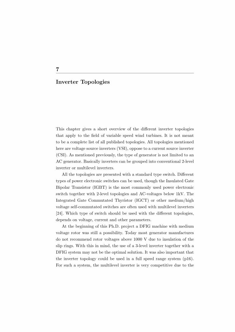
For three-phase systems the most widely used inverter topology is the2-level inverter, consisting of 3 half-bridge inverters with a common DC-capacitor.
Fig. 7.1. 2-level inverter
This type of inverter can produce an output voltage to each phase thatis either connected to the negative side of the DC-link or to the positiveside, thus the name 2-level inverter. When using a 2-level inverter, eachswitch must as a minimum be able to withstand the DC-link voltage UDC ,which is the voltage over the non-conducting switch, when the other switchis conducting.
There are some drawbacks to this inverter type. Because the invertermust switch with relatively high frequency, the switching losses are muchhigher than the devices conduction losses. This applies in particular tolarge MW inverters. Mega Watt inverters will probaly be the size used infuture DFIG wind turbines, and definitely the type used in full scale in-verter turbines. Other problems include high dV/dt and voltage surges dueto switching. This may cause motor/generator bearing current, dielectricstresses and corona discharges [25].
7.3 Multilevel Inverters 41
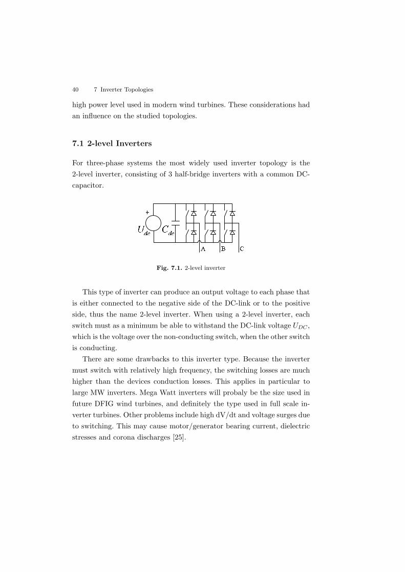
7.2 Resonant DC Link Inverters
Divan [26] presented this topology in 1986, and since then many new typeshave been proposed e.g. [27]. The resonant DC link uses one resonantcircuit to provide soft switching for the entire converter, see Fig. 7.2. TheDC link is forced to oscillate, so the resonance circuit is located on theDC link side and not on the load side, since only one resonant circuit isrequired instead of one for each phase.
Cres
Lres Iconv
Udc
L++ Cdc Ures
ILr
ICr
Three-phase load
Fig. 7.2. Resonant DC-link converter
The idea with the resonant converter is that ideally the convertershould only change state at zero link voltage. The resonant circuit isformed by Lres and Cres, where the resonant capacitor is many timessmaller than the DC link capacitor Cdc. The resonant link voltage swingsbetween zero and twice the DC link voltage, which means that the voltagerating of the switches has to be higher. The modulation strategy for thistopology requires that the resonance frequency is much higher than theswitching frequency.
7.3 Multilevel Inverters
In the literature, three topologies for multilevel inverters have been pre-sented: the cascade inverter, the neutral point clamped inverter, and theflying capacitor inverter.
42 7 Inverter Topologies
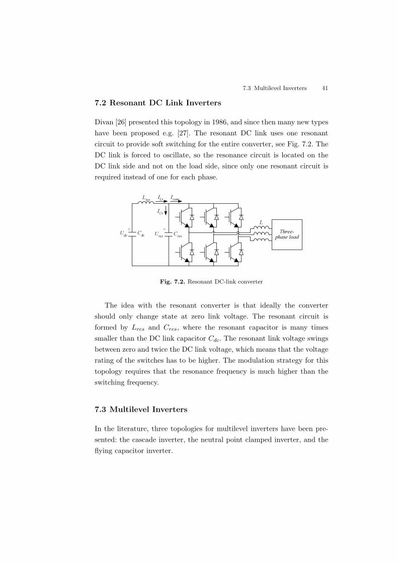
7.3.1 Cascade Multilevel Inverters
The cascaded multilevel inverter is often in the literature called a H-bridge,due to the “H” formed by the four switches in the diagram. Each switchhas an anti-parallel diode. One single H-bridge can form three differentvoltage levels, by switch combinations. Fig. 7.3 shows a 5-level single phase
Cdc
Cdc
Uout
n
Udc
+
Udc
+
Fig. 7.3. 5-level H-bridge inverter single phase
inverter based on two H-bridges [28]. To construct a three phase inverterrequires 3 times of that shown in the figure. Each voltage source/capacitorhas to be electrically isolated from the rest, so the complexity of the systemis high. The number of output phase voltage levels in a H-bridge inverteris defined by m = 2n + 1, where n is the number of DC sources.
7.3.2 Neutral Point Clamped Inverters
The Neutral Point Clamped (NPC) inverter was first proposed by Nabaeet. al. [29]. Since then many publications have been based on this topology.The NPC consists of four switches, each with a free wheeling diode andtwo clamping diodes, see Fig 7.4.
The principle of the NPC inverter is that half of the switching ele-ments are turned on, the other half are turned off. For a 3-level topology,either s1+s2, s2+s3 or s3+s4 are on to generator positive, zero or nega-tive output, respectively. Each active device is only switched once every
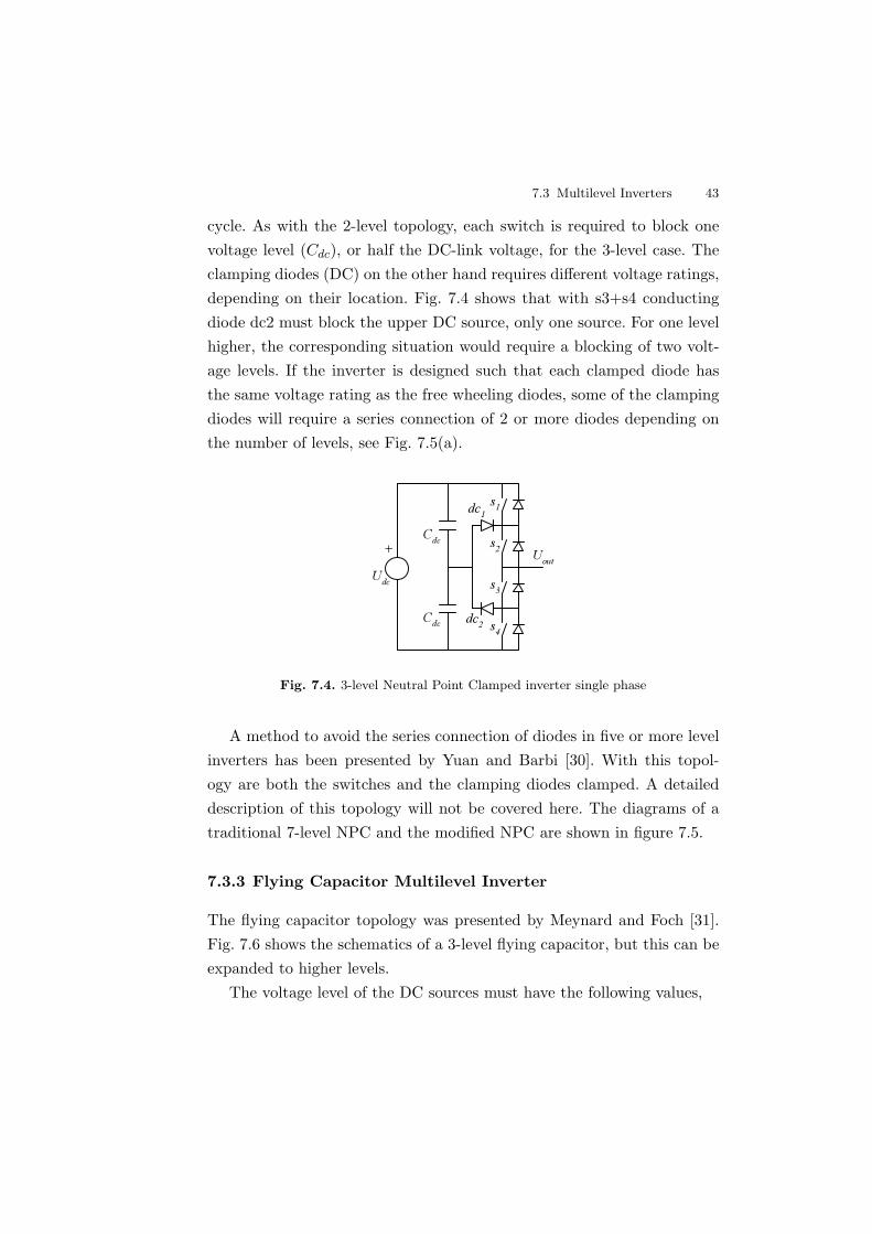
7.3 Multilevel Inverters 43
cycle. As with the 2-level topology, each switch is required to block onevoltage level (Cdc), or half the DC-link voltage, for the 3-level case. Theclamping diodes (DC) on the other hand requires different voltage ratings,depending on their location. Fig. 7.4 shows that with s3+s4 conductingdiode dc2 must block the upper DC source, only one source. For one levelhigher, the corresponding situation would require a blocking of two volt-age levels. If the inverter is designed such that each clamped diode hasthe same voltage rating as the free wheeling diodes, some of the clampingdiodes will require a series connection of 2 or more diodes depending onthe number of levels, see Fig. 7.5(a).
Cdc
CdcUout
Udc
+
s1
s2
s3
s4
dc1
dc2
Fig. 7.4. 3-level Neutral Point Clamped inverter single phase
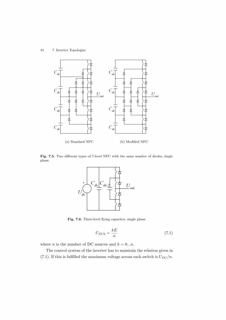
A method to avoid the series connection of diodes in five or more levelinverters has been presented by Yuan and Barbi [30]. With this topol-ogy are both the switches and the clamping diodes clamped. A detaileddescription of this topology will not be covered here. The diagrams of atraditional 7-level NPC and the modified NPC are shown in figure 7.5.
7.3.3 Flying Capacitor Multilevel Inverter
The flying capacitor topology was presented by Meynard and Foch [31].Fig. 7.6 shows the schematics of a 3-level flying capacitor, but this can beexpanded to higher levels.
The voltage level of the DC sources must have the following values,
44 7 Inverter Topologies
Cdc
Cdc
UoutCdc
Cdc
(a) Standard NPC
Cdc
Cdc
UoutCdc
Cdc
(b) Modified NPC
Fig. 7.5. Two different types of 7-level NPC with the same number of diodes, singlephase
Udc
+ UoutCdc Cdc/2
Fig. 7.6. Three-level flying capacitor, single phase
UDCk =kE
n(7.1)
where n is the number of DC sources and k = 0...n.
The control system of the inverter has to maintain the relation given in(7.1). If this is fulfilled the maximum voltage across each switch is UDC/n.
7.3 Multilevel Inverters 45
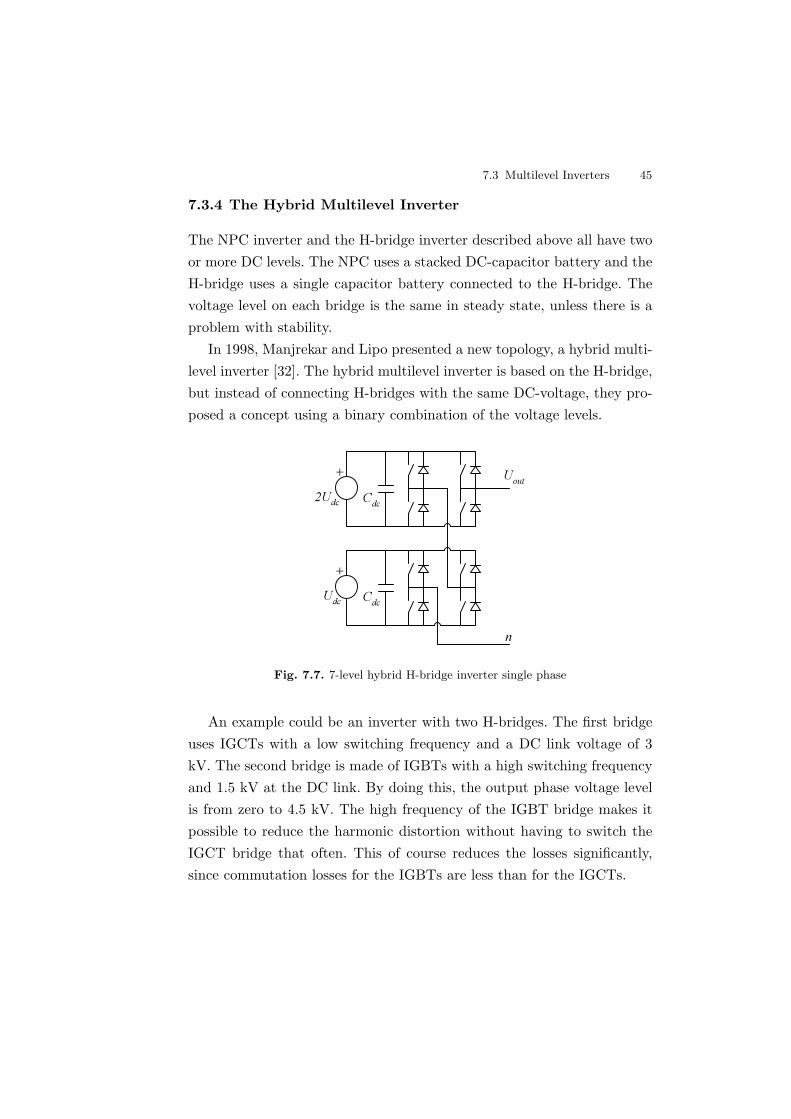
7.3.4 The Hybrid Multilevel Inverter
The NPC inverter and the H-bridge inverter described above all have twoor more DC levels. The NPC uses a stacked DC-capacitor battery and theH-bridge uses a single capacitor battery connected to the H-bridge. Thevoltage level on each bridge is the same in steady state, unless there is aproblem with stability.
In 1998, Manjrekar and Lipo presented a new topology, a hybrid multi-level inverter [32]. The hybrid multilevel inverter is based on the H-bridge,but instead of connecting H-bridges with the same DC-voltage, they pro-posed a concept using a binary combination of the voltage levels.
Cdc
Cdc
Uout
n
2Udc
+
Udc
+
Fig. 7.7. 7-level hybrid H-bridge inverter single phase
An example could be an inverter with two H-bridges. The first bridgeuses IGCTs with a low switching frequency and a DC link voltage of 3kV. The second bridge is made of IGBTs with a high switching frequencyand 1.5 kV at the DC link. By doing this, the output phase voltage levelis from zero to 4.5 kV. The high frequency of the IGBT bridge makes itpossible to reduce the harmonic distortion without having to switch theIGCT bridge that often. This of course reduces the losses significantly,since commutation losses for the IGBTs are less than for the IGCTs.
46 7 Inverter Topologies
7.4 DC-balancing
When using several DC sources, series connected or isolated, voltage bal-ancing will always be an issue. The problem evolves when the net energyto one DC source is different from the net energy to the other sources. Thevoltage across that DC source or capacitor will then either raise or dropfrom its intended value. In order to maintain the same voltage, the realpower flow into a capacitor must be the same as the real power flow out ofa capacitor. As it will be shown in chapter 8, the use of multilevels invertergives a series of redundant switching vectors. The voltage on the outputterminals is the same, but produced from different switching vectors, andthe energy comes from different DC sources.
In an ideal system with large capacitors and complete symmetricalload, DC-balancing is not a problem. Coverage of this topic will continuein the next chapter on modulation techniques (see page 61).
7.5 Comparison of different multilevel topologies
Each of the different topologies has its advantages and disadvantages someof which have been covered above. Another approach to comparing topolo-gies could be by making a simple component count [32]. The number ofdifferent components that are used in a three phase 7-level inverter is listedin Table 7.1. The table shows that the most optimal topology is the Hy-
Table 7.1. Comparison of different multilevel topologies general
Topology Switch elements DC busses Output levelsNPC 36 6 7
Flying Cap. 36 16 7H-bridge 36 9 7
Hybrid H-bridge 24 6 7
brid H-bridge. It uses fewer switches than the NPC inverter and the samenumber of DC-busses. A comparison of the DC-busses is difficult since theNPC inverter uses a number of series connected DC sources, whereas the
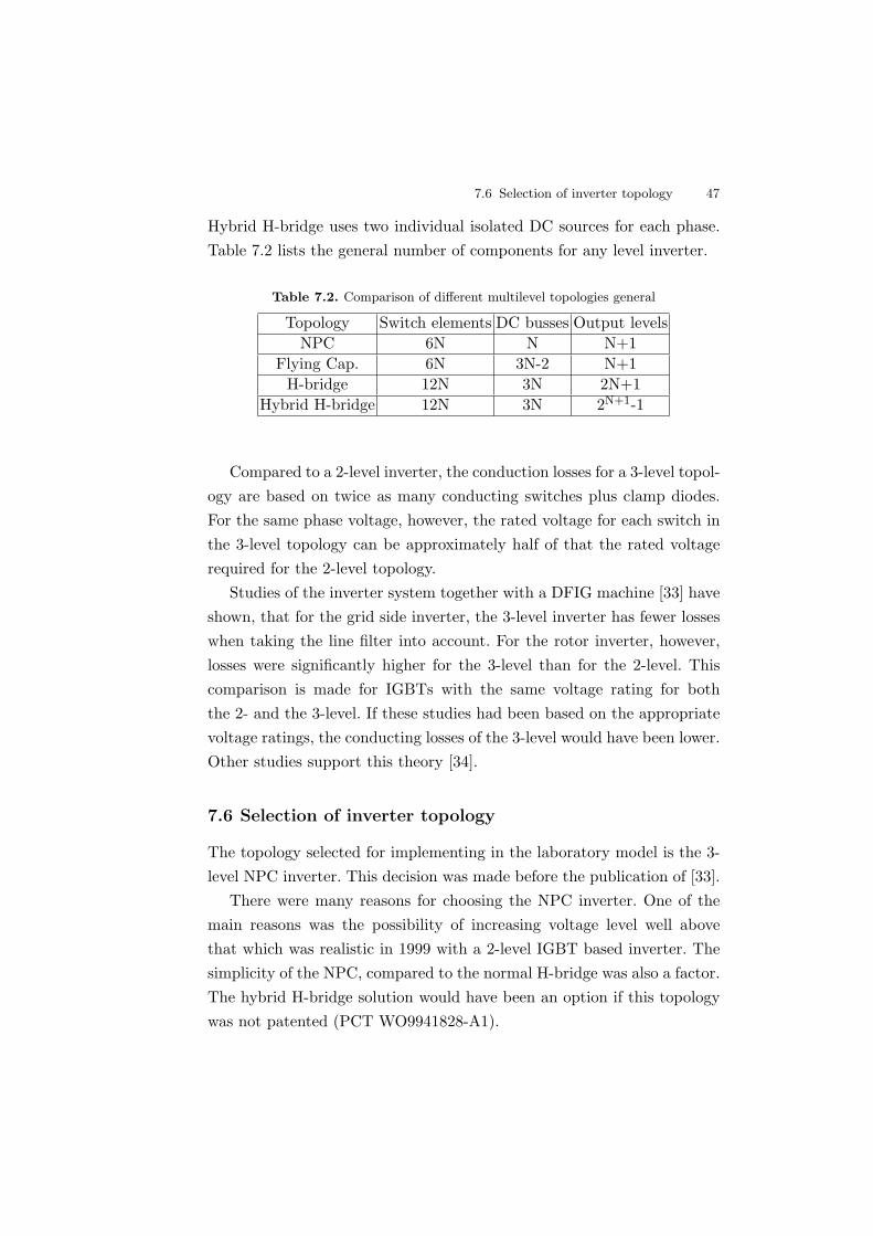
7.6 Selection of inverter topology 47
Hybrid H-bridge uses two individual isolated DC sources for each phase.Table 7.2 lists the general number of components for any level inverter.
Table 7.2. Comparison of different multilevel topologies general
Topology Switch elements DC busses Output levelsNPC 6N N N+1
Flying Cap. 6N 3N-2 N+1H-bridge 12N 3N 2N+1
Hybrid H-bridge 12N 3N 2N+1-1
Compared to a 2-level inverter, the conduction losses for a 3-level topol-ogy are based on twice as many conducting switches plus clamp diodes.For the same phase voltage, however, the rated voltage for each switch inthe 3-level topology can be approximately half of that the rated voltagerequired for the 2-level topology.
Studies of the inverter system together with a DFIG machine [33] haveshown, that for the grid side inverter, the 3-level inverter has fewer losseswhen taking the line filter into account. For the rotor inverter, however,losses were significantly higher for the 3-level than for the 2-level. Thiscomparison is made for IGBTs with the same voltage rating for boththe 2- and the 3-level. If these studies had been based on the appropriatevoltage ratings, the conducting losses of the 3-level would have been lower.Other studies support this theory [34].
7.6 Selection of inverter topology
The topology selected for implementing in the laboratory model is the 3-level NPC inverter. This decision was made before the publication of [33].
There were many reasons for choosing the NPC inverter. One of themain reasons was the possibility of increasing voltage level well abovethat which was realistic in 1999 with a 2-level IGBT based inverter. Thesimplicity of the NPC, compared to the normal H-bridge was also a factor.The hybrid H-bridge solution would have been an option if this topologywas not patented (PCT WO9941828-A1).

8
Modulation
Conversion of DC power to AC power has to be performed in the switchedmode. This can be done by temporary connection of power semiconductorswith fast repetition, which enable a fast and highly efficient electroniccontrol. The modulation of the three phases of a motor drive or a gridconnected inverter can most simply be done by using a 2-level inverter asshown in Fig. 8.2(a)a. The desired current waveform can be achieved bycontrolling the changing of the duty cycles sinusoidally with time. This isthe technique called Pulse Width Modulation (PWM).
The modulation strategy is an important factor for the performanceof the power converter. Research has been done in the field of modula-tion technique with a focus on reducing the switching frequency, withoutincreasing the distortion of the current [35].
When considering the performance of a given modulation technique theharmonic currents are used to get the loss factor. The harmonic currentsare:
Ih,rms =
√1T
∫
T[i(t)− i1(t)]
2 dt (8.1)
where i(t) and i1(t) are the total current and the fundamental current,respectively. The loss factor is
d2 =I2h,rms
I2h,rms,sixstep
(8.2)

50 8 Modulation
The loss factor is independent of the load induction due to normaliza-tion with the harmonic distortion of the sixstep operation.
In the following, the main focus is on carrier-based modulation, espe-cially the suboscillation PWM and the space vector method, the suboscil-lation is a phase modulation technique, while space vector works with thevoltage space vector.
8.1 Suboscillation PWM
Before signal processors and micro controllers became cheap enough tobe used together with PWM unit, the most commonly used modulationprinciple was the carrier based PWM. Each phase needs an individual car-rier modulator, whereas the triangular carrier can be shared. The carriersignal is divided into two subcycles with duration T0 = fs
2 . During eachsubcycle, every half-bridge will switch once, and then be switched back inthe next subcycle.
The frequency modulation ratio is defined by
mf =fs
f1(8.3)
where f1 is the fundamental frequency of the inverter output voltage.The harmonics in the inverter output voltage are located as sidebands
centered around the switching frequency fs, and multiples there of [3].The following is valid for mf = 9.
The frequency of the voltage harmonics is
fh = (jmf ± k)f1 (8.4)
where h is the harmonics order, k is the sideband number and j timesthe frequency modulation ratio mf . The different harmonics are given as
h = j(mf )± k (8.5)
If j is even, there exist only harmonics of odd values of k, while for oddvalues of j there exist only harmonics of even values of k.
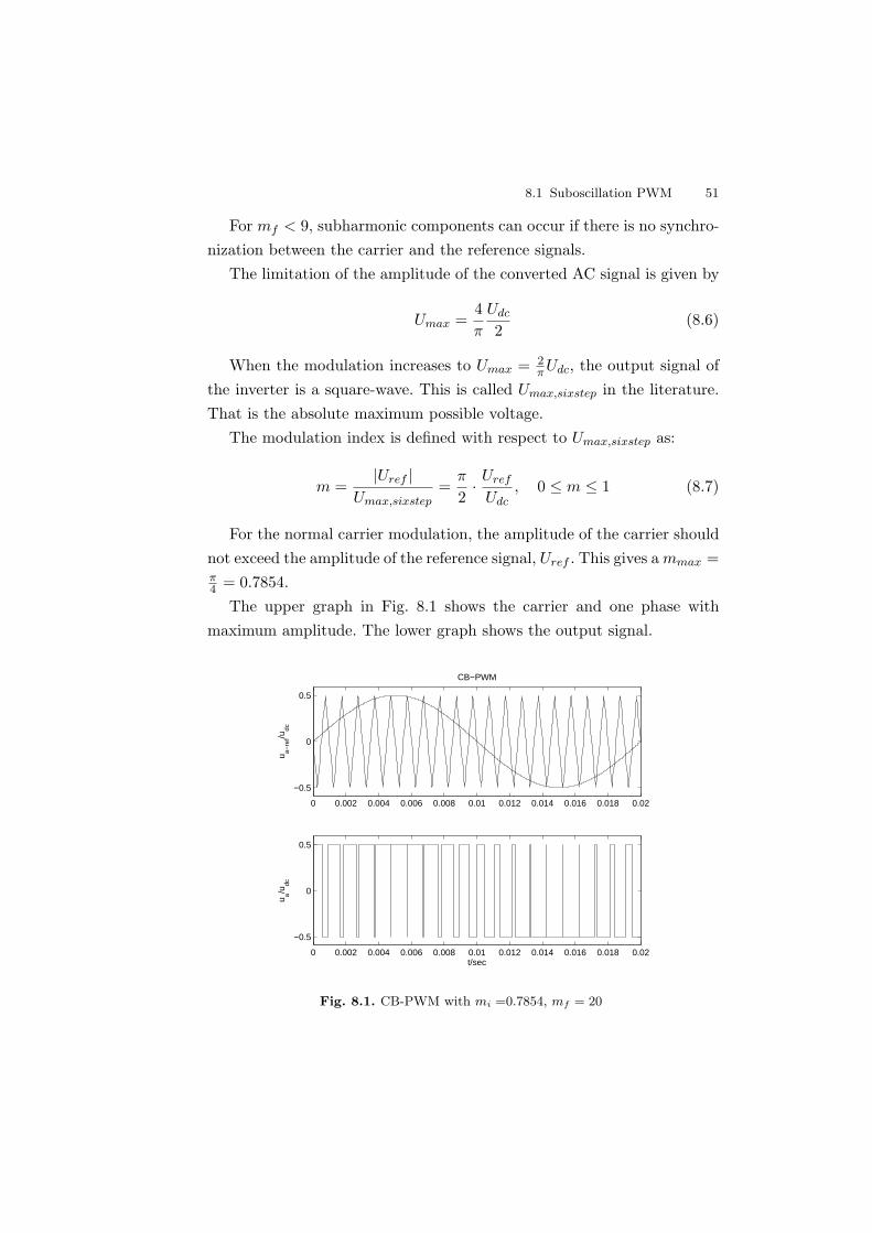
8.1 Suboscillation PWM 51
For mf < 9, subharmonic components can occur if there is no synchro-nization between the carrier and the reference signals.
The limitation of the amplitude of the converted AC signal is given by
Umax =4π
Udc
2(8.6)
When the modulation increases to Umax = 2πUdc, the output signal of
the inverter is a square-wave. This is called Umax,sixstep in the literature.That is the absolute maximum possible voltage.
The modulation index is defined with respect to Umax,sixstep as:
m =|Uref |
Umax,sixstep=
π
2· Uref
Udc, 0 ≤ m ≤ 1 (8.7)
For the normal carrier modulation, the amplitude of the carrier shouldnot exceed the amplitude of the reference signal, Uref . This gives a mmax =π4 = 0.7854.
The upper graph in Fig. 8.1 shows the carrier and one phase withmaximum amplitude. The lower graph shows the output signal.
0 0.002 0.004 0.006 0.008 0.01 0.012 0.014 0.016 0.018 0.02
−0.5
0
0.5
CB−PWM
u a−re
f/udc
0 0.002 0.004 0.006 0.008 0.01 0.012 0.014 0.016 0.018 0.02
−0.5
0
0.5
t/sec
u a/udc
Fig. 8.1. CB-PWM with mi =0.7854, mf = 20
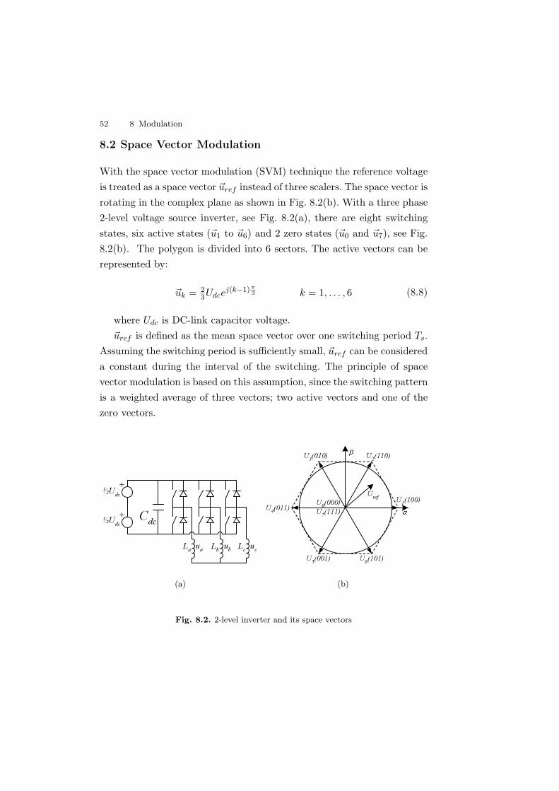
52 8 Modulation
8.2 Space Vector Modulation
With the space vector modulation (SVM) technique the reference voltageis treated as a space vector ~uref instead of three scalers. The space vector isrotating in the complex plane as shown in Fig. 8.2(b). With a three phase2-level voltage source inverter, see Fig. 8.2(a), there are eight switchingstates, six active states (~u1 to ~u6) and 2 zero states (~u0 and ~u7), see Fig.8.2(b). The polygon is divided into 6 sectors. The active vectors can berepresented by:
~uk = 23Udce
j(k−1)π3 k = 1, . . . , 6 (8.8)
where Udc is DC-link capacitor voltage.~uref is defined as the mean space vector over one switching period Ts.
Assuming the switching period is sufficiently small, ~uref can be considereda constant during the interval of the switching. The principle of spacevector modulation is based on this assumption, since the switching patternis a weighted average of three vectors; two active vectors and one of thezero vectors.
Cdc
½Udc
½Udc
+
+
La
Lb
Lcuc
ub
ua
(a)
Uref U1(100)
U2(110)U3(010)
U4(011)
U5(001) U6(101)
U0(000)U7(111)
(b)
Fig. 8.2. 2-level inverter and its space vectors
8.2 Space Vector Modulation 53
~uref = 2fs · (t1~ua + t2~ub) (8.9)
t0 =1
2fs− (t1 + t2) (8.10)
where ~ua and ~ub are the two switching vectors adjacent in space to ~uref .The dwell time at each vector is given by
t1 =1
2fs~uref
3π
(cos
(α′
)− 1√3sin
(α′
))(8.11)
t2 =1
2fs~uref
2√
3π
sin(α′
)(8.12)
t0 =1
2fs− (t1 + t2) (8.13)
where α′ is the angle α transformed to first sector, i.e. α′ = α mod π3 .
To achieve the same properties for SVM as for suboscillation PWM,each half-bridge has to change state once in every subcycle. At the end ofthe cycle, the switches are unchanged. Compared to the normal suboscil-lation PWM, the SVM utilizes the zero vectors at the beginning and endof every subcycle.
If α is less than 60, the two non-zero vectors are ~u1 and ~u2. Theswitching sequence then becomes
~u0 〈t0/2〉 → ~u1 〈t1〉 → ~u2 〈t2〉 → ~u7 〈t0/2〉 → (8.14a)
~u7 〈t0/2〉 → ~u2 〈t1〉 → ~u1 〈t2〉 → ~u0 〈t0/2〉 (8.14b)
Each transition from one vector to another requires that only one half-bridge switches state.
8.2.1 Modified space vector modulation
The modified space vector modulation is given by
~u0 〈t0/3〉 → ~u1 〈2t1/3〉 → ~u2 〈2t2/3〉 → (8.15a)
~u2 〈2t2/3〉 → ~u1 〈2t1/3〉 → ~u0 〈t0/3〉 (8.15b)
54 8 Modulation
The modified SVM uses one switching state less compared to the nor-mal SVM. Since it only uses one zero vector at each subcycle, the on timesare reduced to 2
3 of those in the normal SVM. The modified SVM performbetter than normal SVM if m > 0.59 [35].
Clearly, the largest possible voltage that may be achieved using normalSVM corresponds to the radius of the largest circle that can be inscribedwithin the hexagon in Fig. 8.2(b). The largest radius must be the radiusto the midpoint of the outer line in each triangle
|~uref |max =23Udc
√3
2=
Udc√3
(8.16)
Using (8.16) together with the definition in (8.7), the maximum mod-ulation index can be derived,
mmax,cont =|~uref |max
Umax,sixstep=
1√3Udc
2πUdc
=π
2√
3= 0.9069 (8.17)
It has been shown that SVM and carrier modulation for two level in-verters are the same, when appropriate zero sequence offset are added tothe carrier of the carrier modulation [36]. The same applies to space vectormodulation for multilevel inverters [37].
8.2.2 Overmodulation
When m > 0.9069, the modulation is no longer continuous, which for theCB-PWM means that the triangular carrier is below the reference voltageand some switching cycles are skipped.
Overmodulation can be grouped into two modes. Mode I is where themagnitude of the reference vector is kept inside the hexagon. This extendsthe modulation index to 0.952. Mode II is for 0.952<M<1. The overmod-ulation region can be seen in Fig. 8.3.
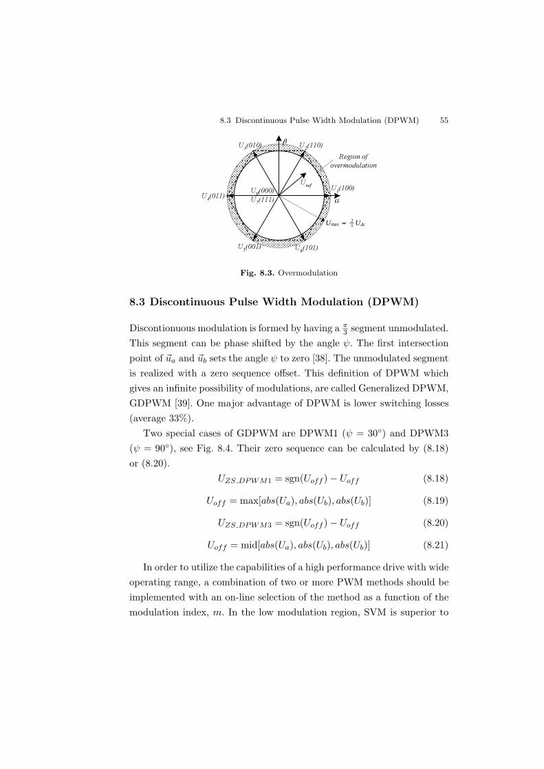
8.3 Discontinuous Pulse Width Modulation (DPWM) 55
Uref U1(100)
U2(110)U3(010)
U4(011)
U5(001) U6(101)
U0(000)U7(111)
Region ofovermodulation
Umax = 2π Udc
Fig. 8.3. Overmodulation
8.3 Discontinuous Pulse Width Modulation (DPWM)
Discontionuous modulation is formed by having a π3 segment unmodulated.
This segment can be phase shifted by the angle ψ. The first intersectionpoint of ~ua and ~ub sets the angle ψ to zero [38]. The unmodulated segmentis realized with a zero sequence offset. This definition of DPWM whichgives an infinite possibility of modulations, are called Generalized DPWM,GDPWM [39]. One major advantage of DPWM is lower switching losses(average 33%).
Two special cases of GDPWM are DPWM1 (ψ = 30) and DPWM3(ψ = 90), see Fig. 8.4. Their zero sequence can be calculated by (8.18)or (8.20).
UZS DPWM1 = sgn(Uoff )− Uoff (8.18)
Uoff = max[abs(Ua), abs(Ub), abs(Ub)] (8.19)
UZS DPWM3 = sgn(Uoff )− Uoff (8.20)
Uoff = mid[abs(Ua), abs(Ub), abs(Ub)] (8.21)
In order to utilize the capabilities of a high performance drive with wideoperating range, a combination of two or more PWM methods should beimplemented with an on-line selection of the method as a function of themodulation index, m. In the low modulation region, SVM is superior to
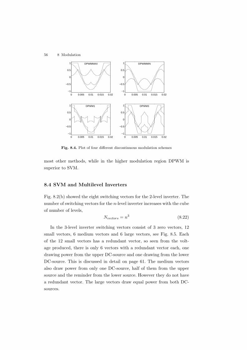
56 8 Modulation
0 0.005 0.01 0.015 0.02−1
−0.5
0
0.5
1
0 0.005 0.01 0.015 0.02−1
−0.5
0
0.5
1
0 0.005 0.01 0.015 0.02−1
−0.5
0
0.5
1
0 0.005 0.01 0.015 0.02−1
−0.5
0
0.5
1
DPWMMAX DPWMMIN
DPWM3DPWM1
Fig. 8.4. Plot of four different discontinuous modulation schemes
most other methods, while in the higher modulation region DPWM issuperior to SVM.
8.4 SVM and Multilevel Inverters
Fig. 8.2(b) showed the eight switching vectors for the 2-level inverter. Thenumber of switching vectors for the n-level inverter increases with the cubeof number of levels,
Nvectors = n3 (8.22)
In the 3-level inverter switching vectors consist of 3 zero vectors, 12small vectors, 6 medium vectors and 6 large vectors, see Fig. 8.5. Eachof the 12 small vectors has a redundant vector, so seen from the volt-age produced, there is only 6 vectors with a redundant vector each, onedrawing power from the upper DC-source and one drawing from the lowerDC-source. This is discussed in detail on page 61. The medium vectorsalso draw power from only one DC-source, half of them from the uppersource and the reminder from the lower source. However they do not havea redundant vector. The large vectors draw equal power from both DC-sources.
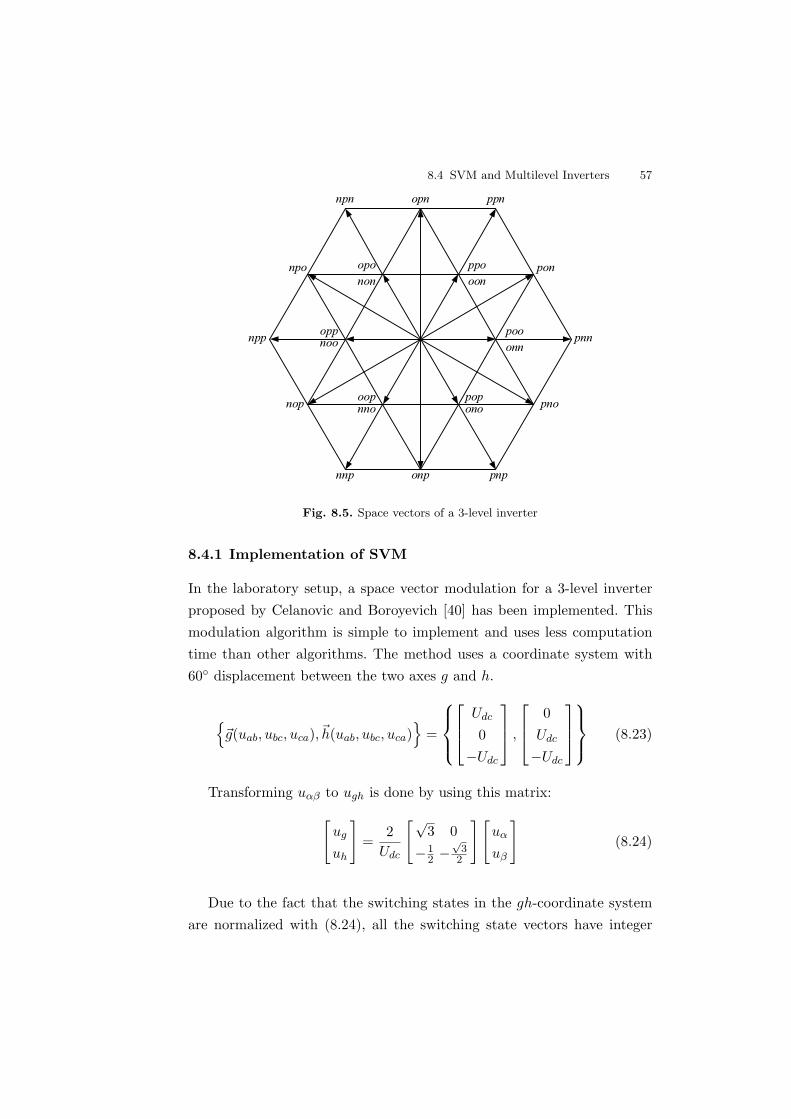
8.4 SVM and Multilevel Inverters 57
npn opn ppn
pon
pnn
pno
pnponpnnp
nop
npp
npo oponon oon
ppo
pooonn
popono
oopnno
oppnoo
Fig. 8.5. Space vectors of a 3-level inverter
8.4.1 Implementation of SVM
In the laboratory setup, a space vector modulation for a 3-level inverterproposed by Celanovic and Boroyevich [40] has been implemented. Thismodulation algorithm is simple to implement and uses less computationtime than other algorithms. The method uses a coordinate system with60 displacement between the two axes g and h.
~g(uab, ubc, uca),~h(uab, ubc, uca)
=
Udc
0−Udc
,
0Udc
−Udc
(8.23)
Transforming uαβ to ugh is done by using this matrix:
[ug
uh
]=
2Udc
[√3 0
−12 −
√3
2
][uα
uβ
](8.24)
Due to the fact that the switching states in the gh-coordinate systemare normalized with (8.24), all the switching state vectors have integer
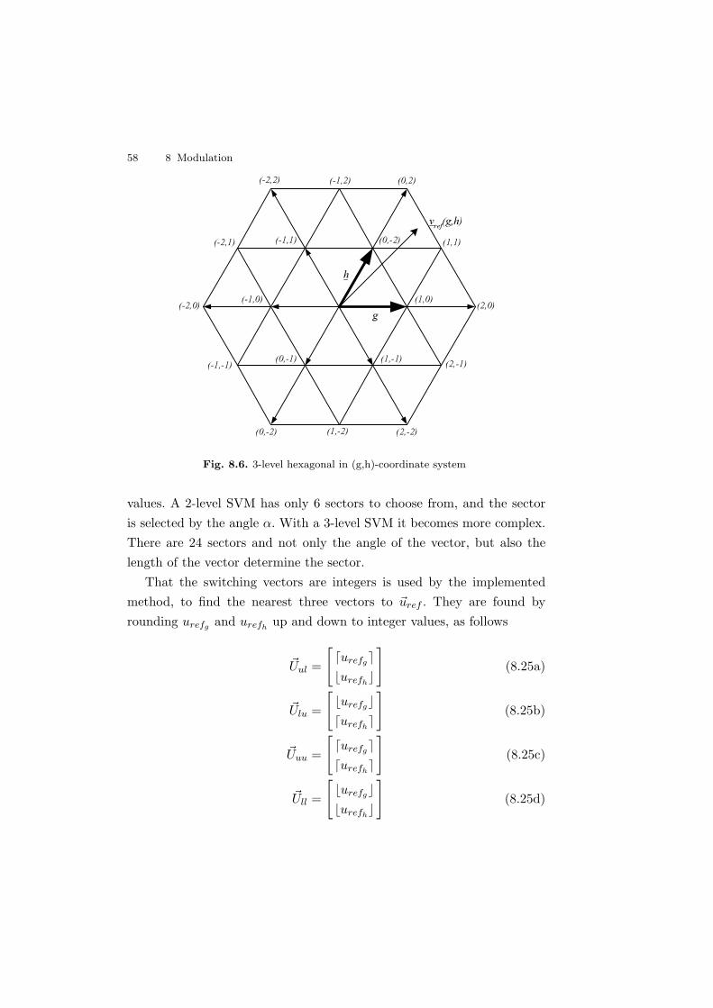
58 8 Modulation
(-1,2) (0,2)
(1,1)
(2,0)
(2,-1)
(2,-2)(1,-2)(0,-2)
(-1,-1)
(-2,0)
(-2,1) (-1,1) (0,-2)
(1,0)
(1,-1)(0,-1)
(-1,0)
h
g
vref(g,h)
(-2,2)
Fig. 8.6. 3-level hexagonal in (g,h)-coordinate system
values. A 2-level SVM has only 6 sectors to choose from, and the sectoris selected by the angle α. With a 3-level SVM it becomes more complex.There are 24 sectors and not only the angle of the vector, but also thelength of the vector determine the sector.
That the switching vectors are integers is used by the implementedmethod, to find the nearest three vectors to ~uref . They are found byrounding urefg and urefh
up and down to integer values, as follows
~Uul =
[durefgeburefh
c
](8.25a)
~Ulu =
[burefgcdurefh
e
](8.25b)
~Uuu =
[durefgedurefh
e
](8.25c)
~Ull =
[burefgcburefh
c
](8.25d)
8.4 SVM and Multilevel Inverters 59
These four vectors form a parallelogram that divides into two triangles,the diagonal connecting the vectors ~Uul and ~Ulu. ~Uul and ~Ulu are two ofthe three nearest vectors needed. The last one is found by evaluating thesign of the following equation,
0 < Uulg + Uulh − (g + h) (8.26)
If the sign is positive, then the third nearest vector is ~Uuu, and if notthe vector is ~Ull. This method can be used for any (n + 1)−level inverter.After identification of the nearest three vectors, what remains is to findthe corresponding duty cycles.
For the 2-level inverter (8.9)
~Uref = 2fs · (t1~ua + t2~ub) (8.27)
was used. Similarly for the multilevel inverter we have
~Uref = (d1~u1 + d2~u2 + d3~u3) (8.28)
with the constraint that the sum of the duty cycles should be equal to one
1 = d1 + d2 + d3 (8.29)
The three vectors ~u1, ~u2 and ~u3 are substituted so ~u1 = ~Uul, ~u2 = ~Ulu,and ~u3 = ~Ull or ~u3 = ~Uuu.
Because all the switching vectors have integer value coordinates, theduty cycles are simply the remaining fractional part of the ~uref coordi-nates,
dul = Urefg − Ullg (8.30a)
dlu = Urefh− Ullh (8.30b)
dll = 1− dul − dlu (8.30c)
if ~u3 = ~Ull, or
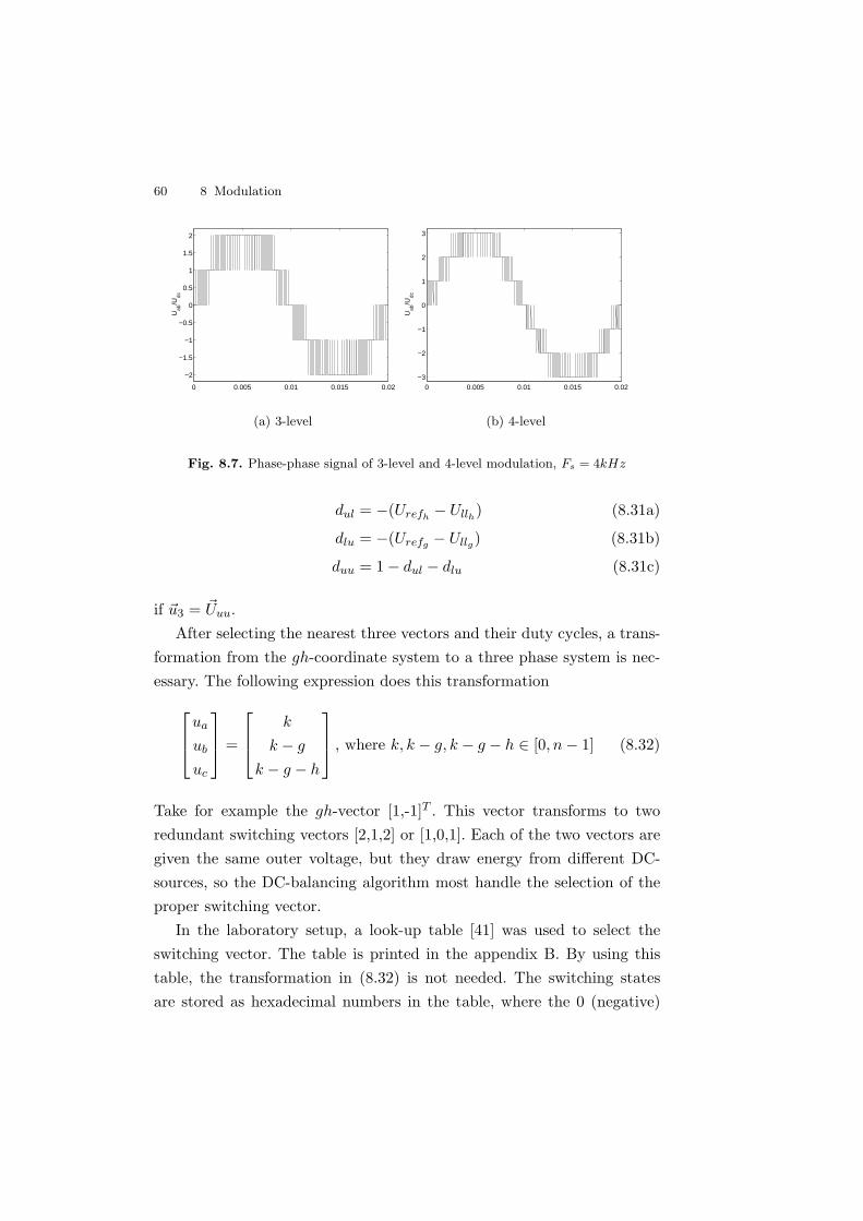
60 8 Modulation
0 0.005 0.01 0.015 0.02
−2
−1.5
−1
−0.5
0
0.5
1
1.5
2
Uab
/Udc
(a) 3-level
0 0.005 0.01 0.015 0.02−3
−2
−1
0
1
2
3
Uab
/Udc
(b) 4-level
Fig. 8.7. Phase-phase signal of 3-level and 4-level modulation, Fs = 4kHz
dul = −(Urefh− Ullh) (8.31a)
dlu = −(Urefg − Ullg) (8.31b)
duu = 1− dul − dlu (8.31c)
if ~u3 = ~Uuu.After selecting the nearest three vectors and their duty cycles, a trans-
formation from the gh-coordinate system to a three phase system is nec-essary. The following expression does this transformation
ua
ub
uc
=
k
k − g
k − g − h
, where k, k − g, k − g − h ∈ [0, n− 1] (8.32)
Take for example the gh-vector [1,-1]T . This vector transforms to tworedundant switching vectors [2,1,2] or [1,0,1]. Each of the two vectors aregiven the same outer voltage, but they draw energy from different DC-sources, so the DC-balancing algorithm most handle the selection of theproper switching vector.
In the laboratory setup, a look-up table [41] was used to select theswitching vector. The table is printed in the appendix B. By using thistable, the transformation in (8.32) is not needed. The switching statesare stored as hexadecimal numbers in the table, where the 0 (negative)

8.5 DC Neutral Point Balancing 61
equivalent switch is coded with #3, the 1 (zero) is coded with #6, andthe 2 (positive) is coded with #C. The small vectors have a fourth digithexadecimal numbers counted from right to left. This is used to tell whichphase the neutral point current is drawn from.
Switch selection is based on this formula,
switch state = 7(g + h + 2) + (h + 2). (8.33)
If the selected switch state is a small vector, there are two switchingcombinations. The other switching combination is located at the addressswitch state + 4.
8.5 DC Neutral Point Balancing
As described earlier the use of multilevel inverters can cause balancingproblems with the DC-levels. The following is valid for the 3-level inverter,but also applies to more levels.
There are a series of things to consider in order to balance the DCvoltages. The SVM methods described above can be used in many waysto reduce the DC balancing problem [42] and [43]. Snubbers often have tobe used together with high power switching devices due to the discharge ofthe snubber capacitor. A minimum on-time is introduced for the switching.This sets some constraints on how to select an optimal DC balancing. Sinceit is no longer possible to use vector combinations, with dwell time lessthan the minimum on-time.
Having back to back inverters that share the same DC-link and alsothe same neutral point, raises some questions about which inverter is re-liable for the neutral point. Since reactive load leads to reduced neutralpoint control capability [44], the converter with the lowest reactive loadshould control the neutral point level. This depends on the specific workingsituation for the DFIG system. Using the redundant switching states forneutral point control might increase the harmonics due to nonsymmetricalharmonic voltage waveform [45]. Thus, neutral point control should not
62 8 Modulation
be done by the grid side inverter unless the rotor side inverter is laggingpower.
The laboratory setup uses snubber free switches. Whenever a redun-dant switch vector is selected, the neutral point level and the currentpolarity of the phase that affects the neutral point are monitored. Thisdetermines which of the two vectors that should be selected, called bang-bang dwell time control [43]. In the last column of Table B.1 in appendixB, the phase and direction the neutral point current comes from, are shownfor the small vectors.
It is obvious that the closer the space vector amplitude is to the cen-ter of the hexagon, the easier DC balancing will be since it gives moreon time for the small vectors. Large space vectors will give less on timeto DC balancing. Low fundamental frequency operation results in slowerneutral point swing [46], which is more difficult to control. Fortunately,low fundamental frequencies only occur at the rotor side converter. Havinga low fundamental frequency at the rotor side, also means that the rotorvoltage is low, hence the small voltage vectors are used for a large part ofthe duty cycle, which help stabilize the neutral point.
Under normal circumstances, the zero sequence is by nature of theSVM balanced. Thus without a neutral conductor, the zero sequence cannot flow. Using the redundant switch vectors for neutral point balancingresults in lack of control of the zero sequence injected in the phase voltage.The zero sequence will then flow even without a neutral conductor. With aback to back converter, it is obvious that when using the grid side inverterfor DC balancing, the inverter will produce a zero sequence that will bereflected as 3rd, 9th, etc. harmonics. The same applies to the machineside, but here the appearance of a zero sequence is less critical, though itwill have some effect on a DFIG system, since the zero sequence then willappear in the stator current as well.
8.6 Dead time
When turning off large power electronic devices, there will be some storageeffect. The storage time Tst is dependent on the current and the operating
8.7 Hysteresis control 63
temperature. In order to not get a short circuit through the inverter half-bridge when turning one switch off and the other one switch on, somedead time Td is introduced. This requires that Td > Tst. Td should belarge enough to constantly avoid a short circuit, or Td can be a functionof current and temperature plus a safety margin [47].
The effect of dead time depends on the current direction. For a positiveload current, the turn-on of the upper switch will be delayed Td and theturn-off will be delayed with Tst. Since Td > Tst the on time for the upperswitch Ton, will be decreased by Td − Tst. Likewise for the negative loadcurrent, the upper switch Ton will be increased by Td−Tst. The dead timeproduces a nonlinear distortion of the average voltage vector trajectory.This distortion does not depend on the magnitude of the fundamentalvoltage and hence the effect is more inherent for lower voltage magnitudesi.e. in the lower speed range. Analysis shows that the dead time alsodepends on the magnitude of the fundamental during the dead time period[48].
Using a hardware solution to compensate for dead time effects givesa fast and simple solution, but it will not be able to consider the actualvoltage during the dead time. Software solutions are better and varioussolutions have been proposed [48].
Eventhough snubber-less switches do not require a minimum on-time, itis advantageous to use some sort of minimum on-time. Short time durationswitching states do not affect the output voltage. This is because thesemiconductor switch requires some time to reach its on- and off-state,so the switch is barely turned on before it has to be turned off again,resulting of increased switching losses.
8.7 Hysteresis control
In order to use hysteresis control, a feedback of the current in each phaseis essential. The principle of hysteresis control is to maintain the currentwithin the hysteresis band. This is done with a nonlinear feedback loopwith two level hysteresis comparators [49], see Fig. 8.8.
There are disadvantages to this modulation [35], such as
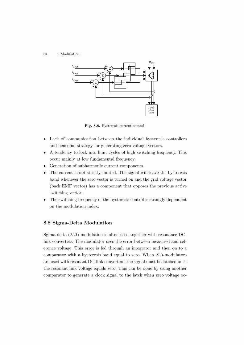
64 8 Modulation
ia.ref
Three-phaseload
-
+ -
+ -
+ib.refic.ref
uDC
Fig. 8.8. Hysteresis current control
• Lack of communication between the individual hysteresis controllersand hence no strategy for generating zero voltage vectors.
• A tendency to lock into limit cycles of high switching frequency. Thisoccur mainly at low fundamental frequency.
• Generation of subharmonic current components.• The current is not strictly limited. The signal will leave the hysteresis
band whenever the zero vector is turned on and the grid voltage vector(back EMF vector) has a component that opposes the previous activeswitching vector.
• The switching frequency of the hysteresis control is strongly dependenton the modulation index.
8.8 Sigma-Delta Modulation
Sgima-delta (Σ∆) modulation is often used together with resonance DC-link converters. The modulator uses the error between measured and ref-erence voltage. This error is fed through an integrator and then on to acomparator with a hysteresis band equal to zero. When Σ∆-modulatorsare used with resonant DC-link converters, the signal must be latched untilthe resonant link voltage equals zero. This can be done by using anothercomparator to generate a clock signal to the latch when zero voltage oc-
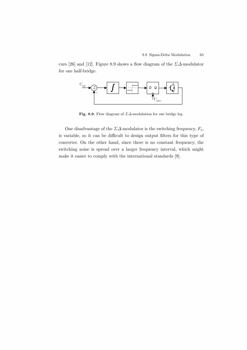
8.8 Sigma-Delta Modulation 65
curs [26] and [12]. Figure 8.9 shows a flow diagram of the Σ∆-modulatorfor one half-bridge.
D QUref
Uzero
-
Fig. 8.9. Flow diagram of Σ∆-modulation for one bridge leg.
One disadvantage of the Σ∆-modulator is the switching frequency, Fs,is variable, so it can be difficult to design output filters for this type ofconverter. On the other hand, since there is no constant frequency, theswitching noise is spread over a larger frequency interval, which mightmake it easier to comply with the international standards [9].

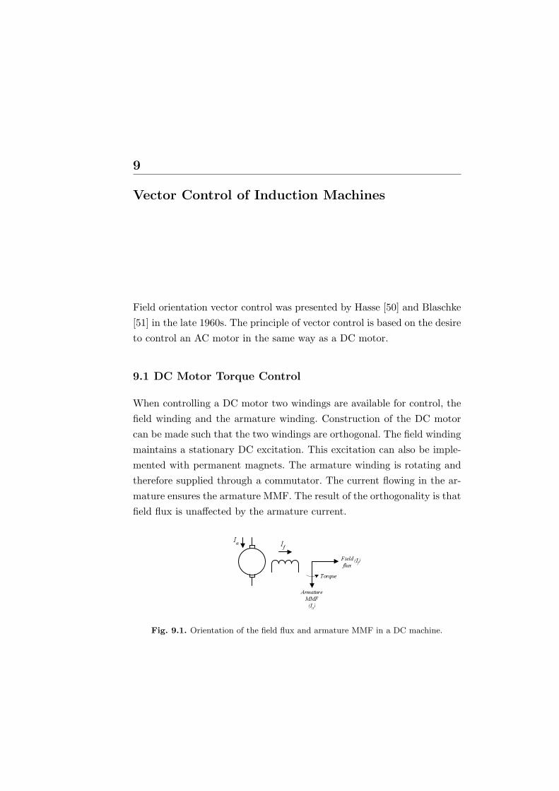
9
Vector Control of Induction Machines
Field orientation vector control was presented by Hasse [50] and Blaschke[51] in the late 1960s. The principle of vector control is based on the desireto control an AC motor in the same way as a DC motor.
9.1 DC Motor Torque Control
When controlling a DC motor two windings are available for control, thefield winding and the armature winding. Construction of the DC motorcan be made such that the two windings are orthogonal. The field windingmaintains a stationary DC excitation. This excitation can also be imple-mented with permanent magnets. The armature winding is rotating andtherefore supplied through a commutator. The current flowing in the ar-mature ensures the armature MMF. The result of the orthogonality is thatfield flux is unaffected by the armature current.
IfIa
Fieldflux
ArmatureMMF(Ia)
(If)
Torque
Fig. 9.1. Orientation of the field flux and armature MMF in a DC machine.

68 9 Vector Control of Induction Machines
The torque equation for the DC machine is
Te =P
2Laf
Lf× ~ψf ×~ia (9.1)
From (9.1) it follows that when the field flux vector and the armatureMMF vector are orthogonal, the torque equation is reduced to
Te = c · ψf · ia (9.2)
The field flux is controlled independent of the armature current, if theorthogonality is disturbed the two vectors are no longer independent.
9.2 AC Motor Torque Control
From the DC motor torque control, we have to follow some criteria, inorder to have AC motor torque control [23]:
• Independently controlled armature current;• Independently controlled or constant field flux;• Independently controlled orthogonal angle between flux and MMF
axes, to avoid interaction of the flux and the MMF.
If all three requirements are fulfilled, the torque instantaneously followsthe current. If the requirements are only met in steady state, steady statetorque control will result, while in transient periods, there will not becomplete torque control.
A common feature of all vector controlled drives is that the modulusand phase angle of AC excitation are controlled hence the name “vectorcontrol”. The implementation of vector control requires an accurate flux-linkage estimation. If incorrect modulus and angle of the flux-linkage spacevector are used, the decoupling of torque and flux is lost. This decouplingis, as mentioned above, required for vector control.
When using vector control, an important thing to consider is the refer-ence frame for the flux vector. This frame follows the flux vector synchro-
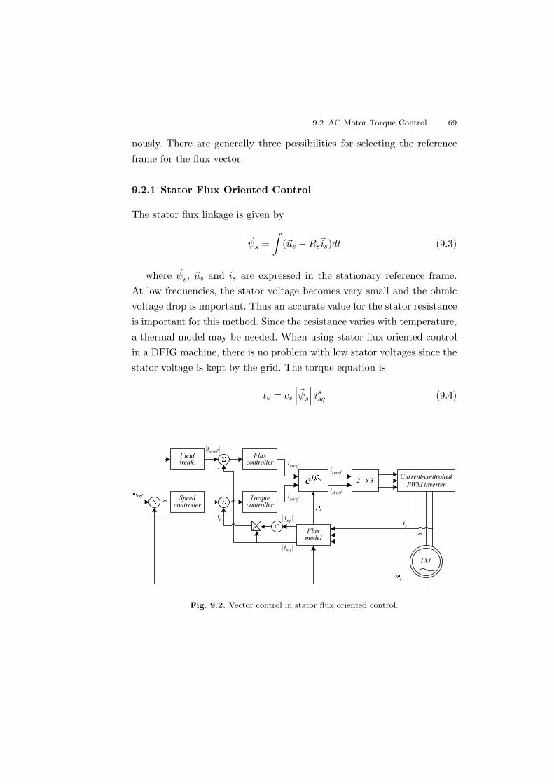
9.2 AC Motor Torque Control 69
nously. There are generally three possibilities for selecting the referenceframe for the flux vector:
9.2.1 Stator Flux Oriented Control
The stator flux linkage is given by
~ψs =∫
(~us −Rs~is)dt (9.3)
where ~ψs, ~us and ~is are expressed in the stationary reference frame.At low frequencies, the stator voltage becomes very small and the ohmicvoltage drop is important. Thus an accurate value for the stator resistanceis important for this method. Since the resistance varies with temperature,a thermal model may be needed. When using stator flux oriented controlin a DFIG machine, there is no problem with low stator voltages since thestator voltage is kept by the grid. The torque equation is
te = cs
∣∣∣~ψs
∣∣∣ issq (9.4)
ej s Current-controlledPWM inverter2 3
Torquecontroller
Fluxcontroller
Speedcontroller
Fluxmodel
I.M.
Fieldweak.
ref
Cisq
isxref
isyref
isaref
isbref
s
r
te--
-
imref
ims
is
Fig. 9.2. Vector control in stator flux oriented control.

70 9 Vector Control of Induction Machines
9.2.2 Rotor Flux Oriented Control
The rotor flux linkage can be obtained by applying appropriate modifica-tions to the stator flux-linkage ~ψs as shown here
~ψ′r =
Lr
Lm
(~ψs − σLs
~is
)(9.5)
This model requires accurate knowledge of the motor inductances,which can be difficult since they vary with the saturation level. Figure9.2 shows an example of rotor flux oriented control. The torque equationis
te = cr
∣∣∣~ψr
∣∣∣ irsq (9.6)
9.2.3 Magnetizing Flux Oriented Control
When selecting the magnetizing flux linkage, either a Hall sensor can beused to obtain the flux or the same approach as for the rotor flux-linkagecan be used, where the flux is obtained from the stator flux-linkage ~ψs
given by~ψ′r = ~ψs − Lls
~is (9.7)
where Lls is the stator leakage inductance. The torque equation is
te = cm
∣∣∣~ψm
∣∣∣ imsq (9.8)
9.3 Magnetizing Loss Reduction
For a variable speed system with a stator fed inverter, the magnetizinglosses can be reduced by running the generator on a flux that minimizesmagnetizing losses in the generator. The DFIG system allows for at leasttwo ways to reduce magnetizing losses. One way is to short circuit thestator of the generator at low power production, and get all the powerout of the rotor. This setup works as a normal variable speed system witha shorted rotor. The only difference is that here it is the stator that isshort circuited. Another way to reduce losses can be by having the stator∆-connected at high power levels and Y-connected at low power levels.
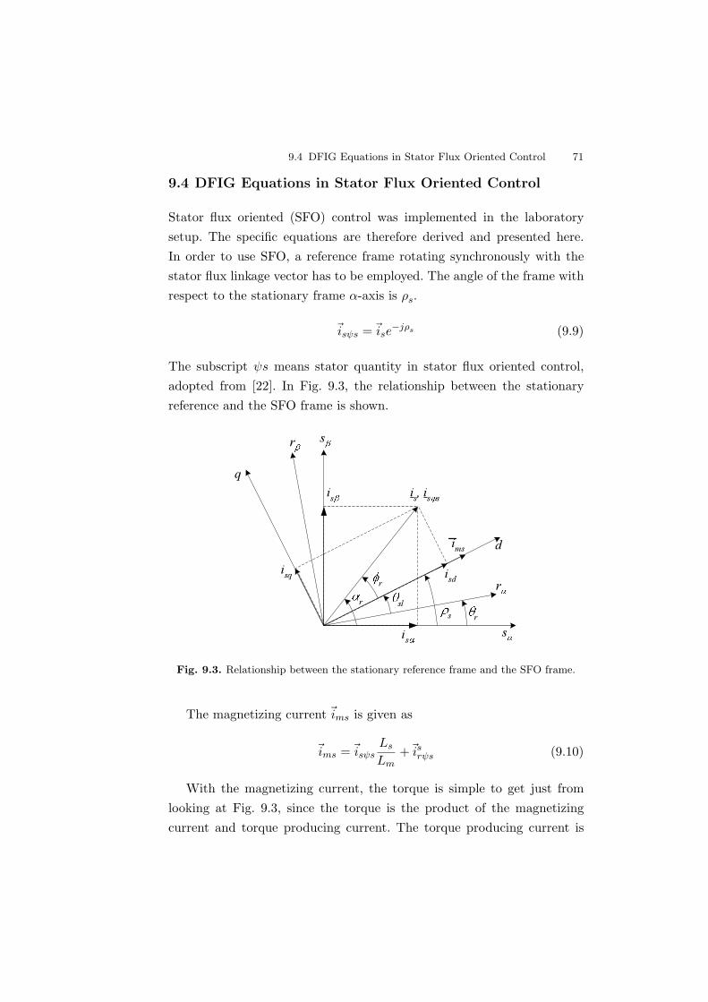
9.4 DFIG Equations in Stator Flux Oriented Control 71
9.4 DFIG Equations in Stator Flux Oriented Control
Stator flux oriented (SFO) control was implemented in the laboratorysetup. The specific equations are therefore derived and presented here.In order to use SFO, a reference frame rotating synchronously with thestator flux linkage vector has to be employed. The angle of the frame withrespect to the stationary frame α-axis is ρs.
~isψs =~ise−jρs (9.9)
The subscript ψs means stator quantity in stator flux oriented control,adopted from [22]. In Fig. 9.3, the relationship between the stationaryreference and the SFO frame is shown.
s
s
r
r
is, is s
imsisq
q
d
is
is
sr
r
slr
isd
Fig. 9.3. Relationship between the stationary reference frame and the SFO frame.
The magnetizing current ~ims is given as
~ims =~isψsLs
Lm+~isrψs (9.10)
With the magnetizing current, the torque is simple to get just fromlooking at Fig. 9.3, since the torque is the product of the magnetizingcurrent and torque producing current. The torque producing current is

72 9 Vector Control of Induction Machines
the orthogonal vector to the magnetizing current. So if angle ρs is correct,we have
te =32PLm
∣∣∣~ims
∣∣∣ isq (9.11)
The stator voltage for the DFIG can be expressed by
~usψs = Rs~isψs + Ls
d~isψs
dt+ Lm
d~irψs
dt+ jωms(Ls
~isψs + Lm~irψs) (9.12)
By substituting (9.10) into (9.12), we get
~usψs = RsLm
Ls(∣∣∣~ims
∣∣∣−~irψs) + Lm
d∣∣∣~ims
∣∣∣dt
+ jωmsLm
∣∣∣~ims
∣∣∣ (9.13)
If the stator time constant is Ts = Ls/Rs, the differential equation (9.13)of the stator can be written as
Ts
d∣∣∣~ims
∣∣∣dt
+∣∣∣~ims
∣∣∣ (1 + jωmsTs) = usψsLs
RsLm+~irψs (9.14)
If the space vectors are split into two-axis components, the equations are
Ts
d∣∣∣~ims
∣∣∣dt
+∣∣∣~ims
∣∣∣ = usdLs
RsLm+ ird (9.15a)
ωmsTs
∣∣∣~ims
∣∣∣ = usqLs
RsLm+ irq (9.15b)
9.4.1 Rotor Voltage Equations for DFIGs
The rotor voltage for the DFIG can be expressed by
urψs = Rr~irψs+Lr
d~irψs
dt+Lm
d~isψs
dt+j(ωms−ωr)(Lr
~irψs+Lm~isψs) (9.16)
By substitution of (9.10) into (9.16), and given that ωsl = ωms − ωr isthe angular slip frequency
urψs = (Rr + σLr)~irψs +L2
m
Lsp
∣∣∣~ims
∣∣∣ + jωsl(L2
m
Ls
∣∣∣~ims
∣∣∣ + σLr~irψs) (9.17)
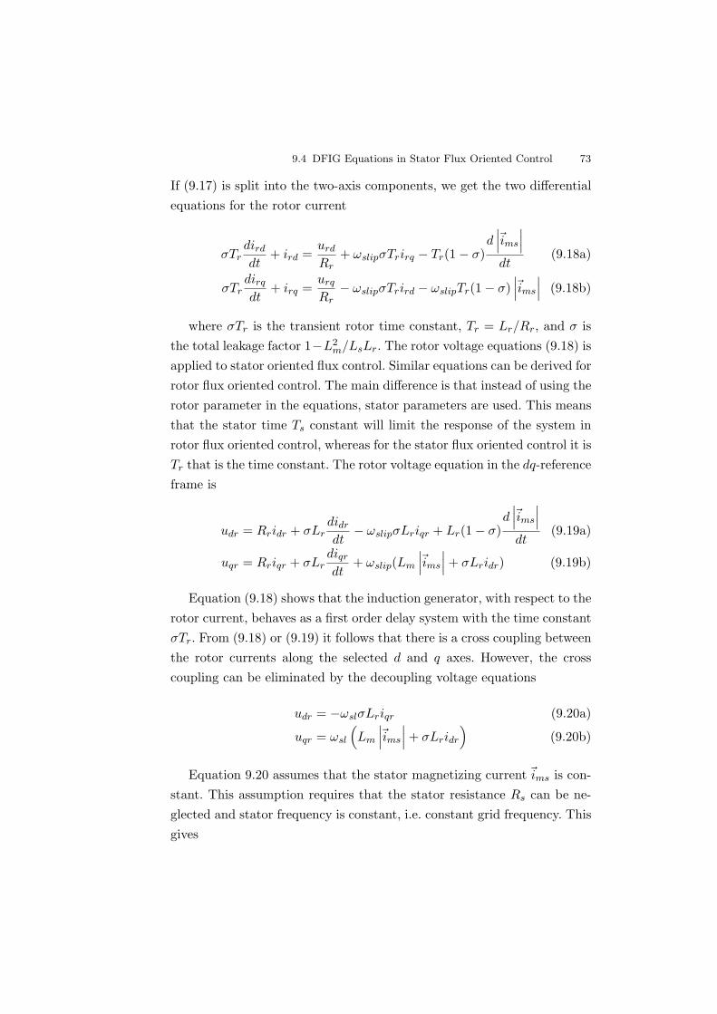
9.4 DFIG Equations in Stator Flux Oriented Control 73
If (9.17) is split into the two-axis components, we get the two differentialequations for the rotor current
σTrdird
dt+ ird =
urd
Rr+ ωslipσTrirq − Tr(1− σ)
d∣∣∣~ims
∣∣∣dt
(9.18a)
σTrdirq
dt+ irq =
urq
Rr− ωslipσTrird − ωslipTr(1− σ)
∣∣∣~ims
∣∣∣ (9.18b)
where σTr is the transient rotor time constant, Tr = Lr/Rr, and σ isthe total leakage factor 1−L2
m/LsLr. The rotor voltage equations (9.18) isapplied to stator oriented flux control. Similar equations can be derived forrotor flux oriented control. The main difference is that instead of using therotor parameter in the equations, stator parameters are used. This meansthat the stator time Ts constant will limit the response of the system inrotor flux oriented control, whereas for the stator flux oriented control it isTr that is the time constant. The rotor voltage equation in the dq-referenceframe is
udr = Rridr + σLrdidr
dt− ωslipσLriqr + Lr(1− σ)
d∣∣∣~ims
∣∣∣dt
(9.19a)
uqr = Rriqr + σLrdiqr
dt+ ωslip(Lm
∣∣∣~ims
∣∣∣ + σLridr) (9.19b)
Equation (9.18) shows that the induction generator, with respect to therotor current, behaves as a first order delay system with the time constantσTr. From (9.18) or (9.19) it follows that there is a cross coupling betweenthe rotor currents along the selected d and q axes. However, the crosscoupling can be eliminated by the decoupling voltage equations
udr = −ωslσLriqr (9.20a)
uqr = ωsl
(Lm
∣∣∣~ims
∣∣∣ + σLridr
)(9.20b)
Equation 9.20 assumes that the stator magnetizing current ~ims is con-stant. This assumption requires that the stator resistance Rs can be ne-glected and stator frequency is constant, i.e. constant grid frequency. Thisgives
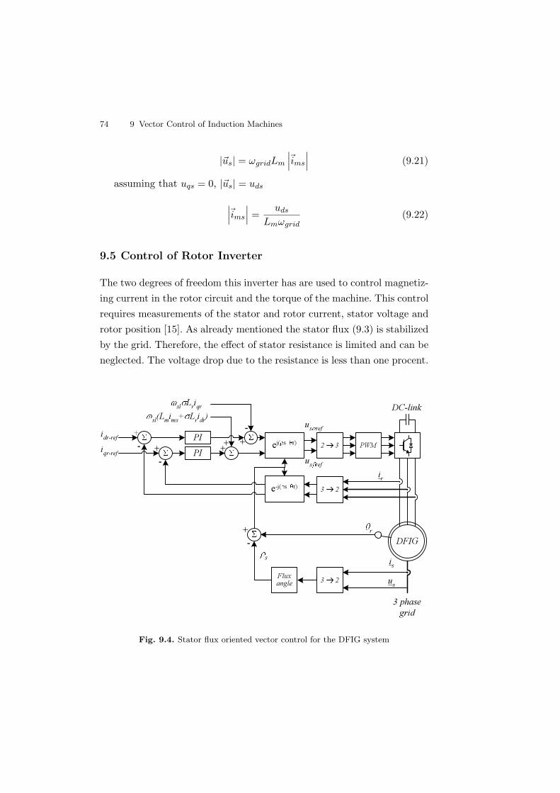
74 9 Vector Control of Induction Machines
|~us| = ωgridLm
∣∣∣~ims
∣∣∣ (9.21)
assuming that uqs = 0, |~us| = uds
∣∣∣~ims
∣∣∣ =uds
Lmωgrid(9.22)
9.5 Control of Rotor Inverter
The two degrees of freedom this inverter has are used to control magnetiz-ing current in the rotor circuit and the torque of the machine. This controlrequires measurements of the stator and rotor current, stator voltage androtor position [15]. As already mentioned the stator flux (9.3) is stabilizedby the grid. Therefore, the effect of stator resistance is limited and can beneglected. The voltage drop due to the resistance is less than one procent.
DFIG
us ref
r
DC-link
3 2
PWM2 3
-
+ ej( s r)++
PIPI
-
+
e-j( s r)
3 2
3 phasegrid
Fluxangle
s
-
+
-
+us refidr-ref
iqr-ref
sl Lriqrsl(Lmims+ Lridr)
us
is
ir
Fig. 9.4. Stator flux oriented vector control for the DFIG system
9.6 Dynamics of the DFIG Vector Control 75
Figure 9.4 shows a diagram of the structure for the implementation ofthe stator flux oriented control. The feed forward terms in the upper partof the diagram are the decoupling equations (9.20). The control system isonly shown with the control for the rotor current. Additional controllerscan be added to the left side of the diagram, so that the active and reactivepower can be controlled by means of the rotor current. If implemented,the direct current idr controls the reactive power and the active power iscontrolled by the quadrature current iqr. If an extra PI-controller is addedin front of the quadrature current iqr, the quadrature current iqr loop canbe used in a speed controller instead.
9.6 Dynamics of the DFIG Vector Control
When keeping the flux constant in the machine by a constant magnetizingcurrent, a fast torque response is possible. This is a well known char-acteristic of vector control for a stator fed induction machine. It meansthat the direct current has to be kept constant, while quadrature currentcan change momentarily. With the DFIG, on other hand, the stator isconnected to the grid. The magnetizing current can be supplied throughthe stator or the rotor. The flux level is assumed to be nearly constant,with constant grid voltage. From (9.18) it follows that the time constantfor both the direct and the quadrature current is σTr. This means thatchanging the flow of reactive power from the inverter is as fast as changingthe active power flow, see Fig. 15.9.

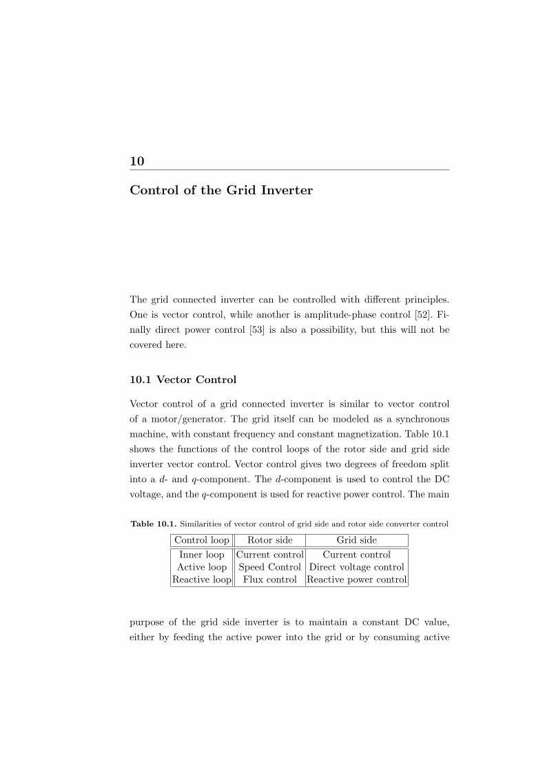
10
Control of the Grid Inverter
The grid connected inverter can be controlled with different principles.One is vector control, while another is amplitude-phase control [52]. Fi-nally direct power control [53] is also a possibility, but this will not becovered here.
10.1 Vector Control
Vector control of a grid connected inverter is similar to vector controlof a motor/generator. The grid itself can be modeled as a synchronousmachine, with constant frequency and constant magnetization. Table 10.1shows the functions of the control loops of the rotor side and grid sideinverter vector control. Vector control gives two degrees of freedom splitinto a d- and q-component. The d-component is used to control the DCvoltage, and the q-component is used for reactive power control. The main
Table 10.1. Similarities of vector control of grid side and rotor side converter control
Control loop Rotor side Grid sideInner loop Current control Current controlActive loop Speed Control Direct voltage control
Reactive loop Flux control Reactive power control
purpose of the grid side inverter is to maintain a constant DC value,either by feeding the active power into the grid or by consuming active
78 10 Control of the Grid Inverter
power from the grid, depending on the speed of the DFIG, according toFig. 5.1. Secondly, the inverter can be used to produce reactive power.A complex strategy can be implemented for the control of the reactivepower for the complete system. The generator can be neutral with respectto reactive power, depending on the level of magnetizing. If the generator isnot fully magnetized from the rotor, the stator will consume some reactivepower. The grid inverter must then produce reactive power to keep thedesired cosϕ equal to one. Both inverters can help produce reactive power,depending on their active current load.
When considering the whole DFIG system with generator and back toback inverter, the system actually forms an Unified Power Flow Control(UPFC), where the generator is a rotating transformer. The UPFC is madeof two back to back inverters, one connected in series with the grid and theother in parallel with the grid [54]. Considering the system as an UPFCgives many possibilities for control. The use of the grid side inverter forreactive compensation is less attractive, because the generator amplifiesthe current with the turn ratio, and the limiting factor for the invertersare mainly the current.
The voltage equation of the inverter reactors is
ua
ub
uc
= R
ia
ib
ic
+ L
d
dt
ia
ib
ic
+
uinva
uinvb
uinvc
(10.1)
The DC side of the system is modeled as
CDCdUDC
dt= idc − irotor (10.2)
When transforming (10.1) into dq-reference frame we get:
[ud
uq
]=
[R 00 R
][id
iq
]+
[L 00 L
]d
dt
[id
iq
]+
[0 −ωeL
ωeL 0
][id
iq
]+
[uinv
d
uinvq
]
(10.3)or
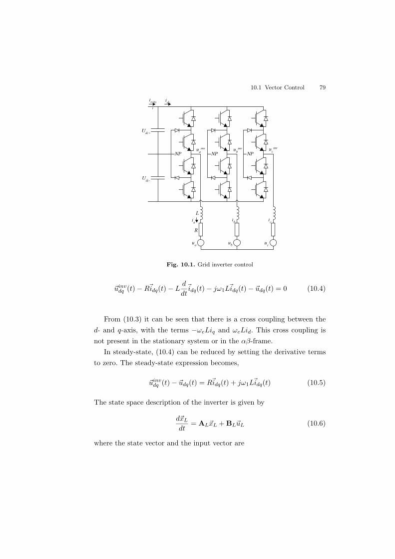
10.1 Vector Control 79
Udc-
Udc+
NP NP NP
ia ib icR
L
ua ub uc
ubinv ucinvuainv
idcirotor
Fig. 10.1. Grid inverter control
~uinvdq (t)−R~idq(t)− L
d
dt~idq(t)− jω1L~idq(t)− ~udq(t) = 0 (10.4)
From (10.3) it can be seen that there is a cross coupling between thed- and q-axis, with the terms −ωeLiq and ωeLid. This cross coupling isnot present in the stationary system or in the αβ-frame.
In steady-state, (10.4) can be reduced by setting the derivative termsto zero. The steady-state expression becomes,
~uinvdq (t)− ~udq(t) = R~idq(t) + jω1L~idq(t) (10.5)
The state space description of the inverter is given by
d~xL
dt= AL~xL + BL~uL (10.6)
where the state vector and the input vector are

80 10 Control of the Grid Inverter
ug ref
DC-link
3 2
PWM2 3+-
--
PIPI
-
+
e-j( ) 3 2
3 phasegrid
+
+
-
+ug ref
idg-ref
iqg-ref
ug
ige-j( )
ej( )
L
L
udg
idgiqg
PIUdc-ref
-+
Fig. 10.2. Vector control of grid inverter.
~xL =
[id
iq
](10.7)
and
~uL =
uinvd
uinvq
ud
uq
(10.8)
the system matrix and input matrix are given by
AL =
[−R
L ω1
−ω1 −RL
](10.9)
and
BL =
[1L 0 − 1
L 00 1
L 0 − 1L
](10.10)
10.1 Vector Control 81
The state equation for the AC side of the system is linear as opposedto the DC side (10.2) which is non-linear, as well as time variant due tothe switching function. If the DC-link is maintained at a constant value, alinearized small-signal model can be used to obtain the transfer functionmatrix [55]. When keeping the DC-link at a nearly constant value, theeffect of the non-linearities is minor.
The power equations of the system given by (4.17) are repeated here
P =32(udid + uqiq) =
32(uαiα + uβiβ) (10.11)
Q =32(udiq − uqid) =
32(uαiβ − uβiα) (10.12)
If neglecting harmonics due to switching and due to harmonics in thegrid voltage and the losses in the inverter and inductor resistance, we havethe AC power and the DC power as
PAC =23
Re~uαβ~i∗αβ (10.13)
PDC = uDCiDC (10.14)
where the asterisk denotes the complex conjugate. The AC power insynchronously rotating reference frame
PAC =23(udid + uqiq) (10.15)
since uq = 0 we have,
PAC =23udid (10.16)
Substituting (10.14) into (10.16), this gives an expression for the aver-age DC link capacitor current iCDC
iCDC=
23
ud
UDCid (10.17)
The differential equation of the DC link voltage gives [56]
dUDC
dt=
23
1CDC
ud
UDCid (10.18)
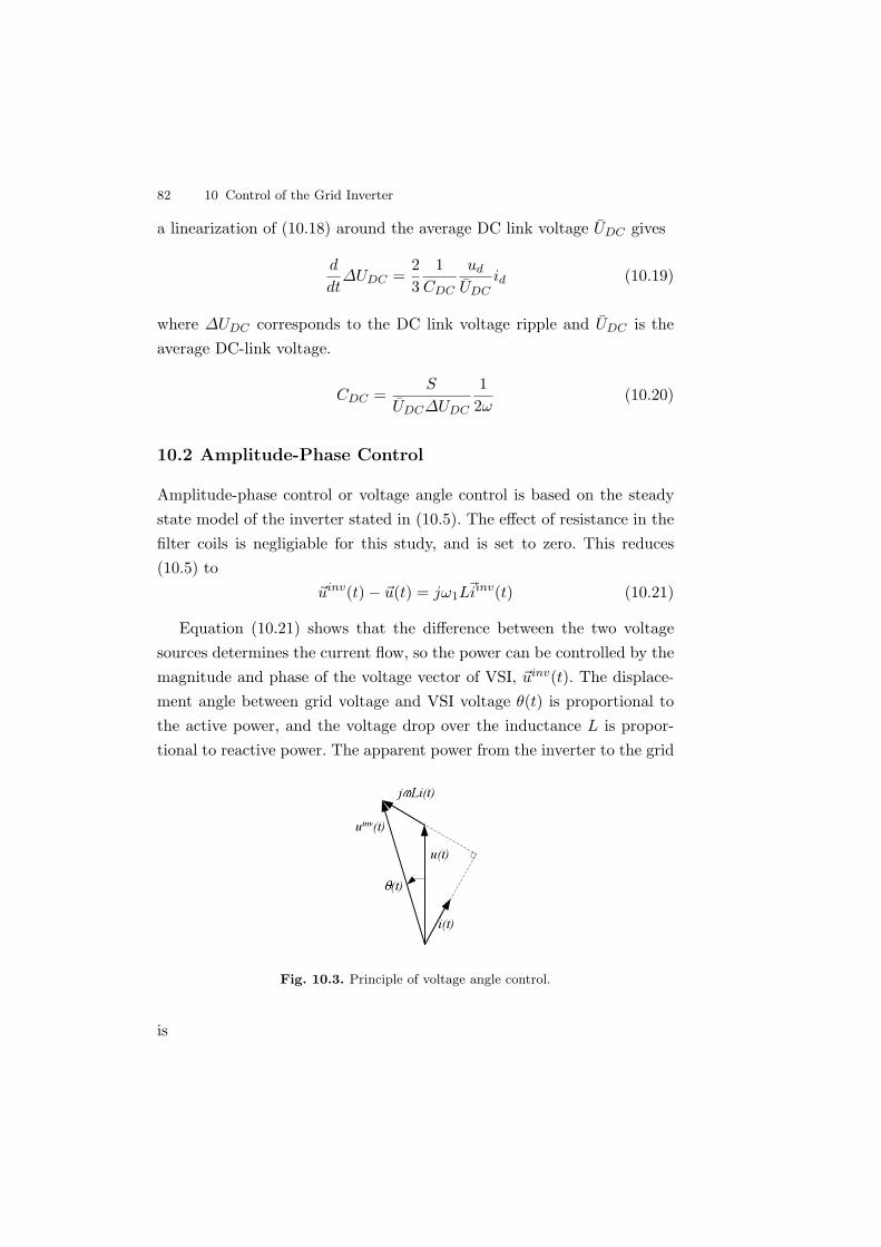
82 10 Control of the Grid Inverter
a linearization of (10.18) around the average DC link voltage UDC gives
d
dt∆UDC =
23
1CDC
ud
UDCid (10.19)
where ∆UDC corresponds to the DC link voltage ripple and UDC is theaverage DC-link voltage.
CDC =S
UDC∆UDC
12ω
(10.20)
10.2 Amplitude-Phase Control
Amplitude-phase control or voltage angle control is based on the steadystate model of the inverter stated in (10.5). The effect of resistance in thefilter coils is negligiable for this study, and is set to zero. This reduces(10.5) to
~uinv(t)− ~u(t) = jω1L~iinv(t) (10.21)
Equation (10.21) shows that the difference between the two voltagesources determines the current flow, so the power can be controlled by themagnitude and phase of the voltage vector of VSI, ~uinv(t). The displace-ment angle between grid voltage and VSI voltage θ(t) is proportional tothe active power, and the voltage drop over the inductance L is propor-tional to reactive power. The apparent power from the inverter to the grid
u(t)
i(t)
uinv(t)
j Li(t)
(t)
Fig. 10.3. Principle of voltage angle control.
is
10.3 Phase Lock Loop 83
S = U · I∗ = ~u(t) ·~iinv(t)∗ = (ud(t) + juq(t))(id(t)− jiq(t)) (10.22)
Active power and reactive power can be derived from (10.21) and (10.22),
P = Re(S) (10.23)
=U · U inv
ωeLsin θ
Q = Im(S) (10.24)
=U
ωeL(U − U inv cos θ)
Amplitude-phase control is simple to implement in a controller, but thebandwidth of the system is limited, since it is based on a steady statemodel
10.3 Phase Lock Loop
When connecting a power converter to the electrical grid, it is importantto have a fast and accurate measure of the grid phase angle in order to beable control the power flow in or out of the power converter. Therefore, aphase lock loop (PLL) is implemented in the software. The function of thePLL is to keep track of the phase angle under any condition. The difficultyof this task is of course when the grid is distorted. In well balanced gridsystems, a zero crossing detection works sufficiently as a PLL. The zerocrossing point is sensitive to distortion of the waveform, and the variationof each phase is not considered in this form of angle detection [57]. Usinga zero crossing detection in a system with power electronics will causeproblems due to noise from the switching.
A simple way to get information about the phase angle is to use theangle of the voltage vector in the αβ-frame
θ = arctanuβ
uα(10.25)
Using arctan of the voltage ratio works well with an ideal grid withoutdisturbances. If the signals are distorted, the output of this method will
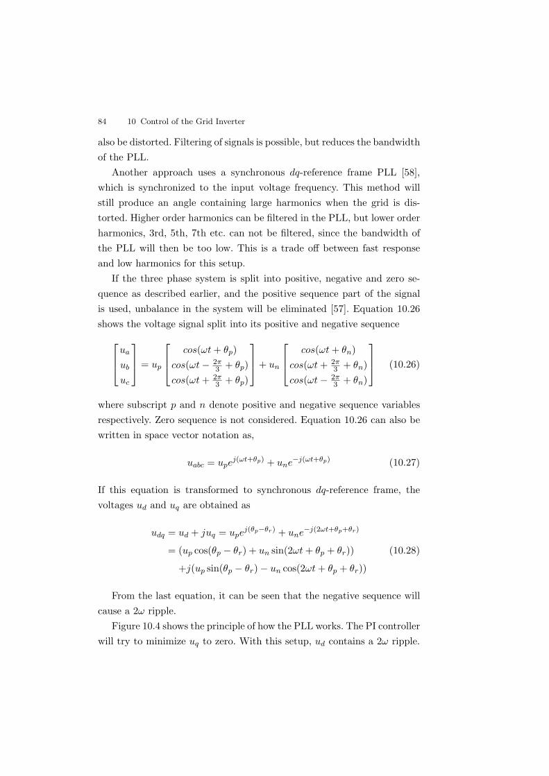
84 10 Control of the Grid Inverter
also be distorted. Filtering of signals is possible, but reduces the bandwidthof the PLL.
Another approach uses a synchronous dq-reference frame PLL [58],which is synchronized to the input voltage frequency. This method willstill produce an angle containing large harmonics when the grid is dis-torted. Higher order harmonics can be filtered in the PLL, but lower orderharmonics, 3rd, 5th, 7th etc. can not be filtered, since the bandwidth ofthe PLL will then be too low. This is a trade off between fast responseand low harmonics for this setup.
If the three phase system is split into positive, negative and zero se-quence as described earlier, and the positive sequence part of the signalis used, unbalance in the system will be eliminated [57]. Equation 10.26shows the voltage signal split into its positive and negative sequence
ua
ub
uc
= up
cos(ωt + θp)cos(ωt− 2π
3 + θp)cos(ωt + 2π
3 + θp)
+ un
cos(ωt + θn)cos(ωt + 2π
3 + θn)cos(ωt− 2π
3 + θn)
(10.26)
where subscript p and n denote positive and negative sequence variablesrespectively. Zero sequence is not considered. Equation 10.26 can also bewritten in space vector notation as,
uabc = upej(ωt+θp) + une−j(ωt+θp) (10.27)
If this equation is transformed to synchronous dq-reference frame, thevoltages ud and uq are obtained as
udq = ud + juq = upej(θp−θr) + une−j(2ωt+θp+θr)
= (up cos(θp − θr) + un sin(2ωt + θp + θr)) (10.28)
+j(up sin(θp − θr)− un cos(2ωt + θp + θr))
From the last equation, it can be seen that the negative sequence willcause a 2ω ripple.
Figure 10.4 shows the principle of how the PLL works. The PI controllerwill try to minimize uq to zero. With this setup, ud contains a 2ω ripple.

10.3 Phase Lock Loop 85
ej e
PI VCOuqref
= 0
uq
ud
e
3 2uabc
+ -
Fig. 10.4. Phase lock loop with full signal
To avoid the ripple, only the positive sequence should be used. Lee [57]has proposed a setup where only the positive sequence part of the voltagesignal is used , similar is presented in [59]. Figure 10.5 shows how to usethe positive sequence together with PLL.
12
12
12 3
12 3
3 2-
--
-
-
-+
+
+
+
va
vb
vc
v
v
ej e
PI VCOvqref= 0
vq
vd e
Fig. 10.5. Phase lock loop with positive sequence signal.
Figure 10.6 shows a spectrum of sin(θe), where θe is the measuredphase angle with a full PLL system, as in Fig. 10.5, compared with thelower graph which shows similar but with a simple PLL only using theuβ/uα ratio, as in (10.25). In the lower graph, it is easy to see the gridharmonics, as well as the generator slot harmonics around 1000 Hz, withthe generator running at 1300 RPM. The upper graph shows an almostperfect PLL signal, where the harmonics from the grid voltage are rejected,and therefore have no affect on the output of the PLL. The gain and
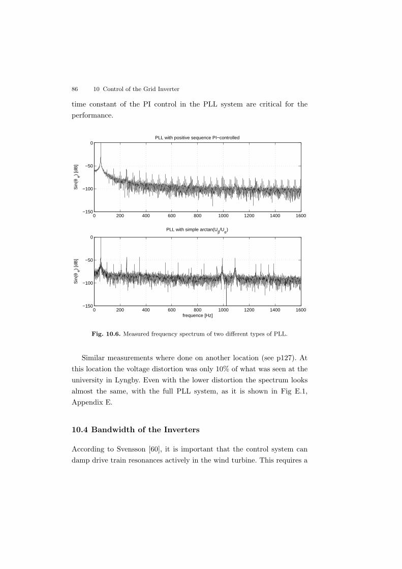
86 10 Control of the Grid Inverter
time constant of the PI control in the PLL system are critical for theperformance.
0 200 400 600 800 1000 1200 1400 1600−150
−100
−50
0PLL with positive sequence PI−controlled
Sin
(θ e)
[dB
]
0 200 400 600 800 1000 1200 1400 1600−150
−100
−50
0
PLL with simple arctan(Uβ/Uα)
frequence [Hz]
Sin
(θ e)
[dB
]
Fig. 10.6. Measured frequency spectrum of two different types of PLL.
Similar measurements where done on another location (see p127). Atthis location the voltage distortion was only 10% of what was seen at theuniversity in Lyngby. Even with the lower distortion the spectrum looksalmost the same, with the full PLL system, as it is shown in Fig E.1,Appendix E.
10.4 Bandwidth of the Inverters
According to Svensson [60], it is important that the control system candamp drive train resonances actively in the wind turbine. This requires a

10.4 Bandwidth of the Inverters 87
bandwidth above 10 Hz, which is not the case for amplitude-phase control.Therefore, the control principle used is vector control.
Studies by Blasko et. al. [61] have shown that the bandwidth of a volt-age source inverter is approximately 10-30 times smaller than the switchingfrequency. Sampling of the signal twice in every switch period increasesthe bandwidth to about 1/10 of the switching frequency. With synchro-nous sampling once in every cycle, the bandwidth is 1/20. The samplingused in the laboratory model is synchronous once in every sampling.

11
General Harmonic Analysis
Electrical equipment with power electronics connected to the grid causenonsinusoidal grid currents, due to non-linear characteristics of the powerelectronics. Since the grid voltage is nearly sinusoidal and the voltageproduced by the power electronics is often far from sinusoidal, the currentfrom the power electronics will contain harmonics. According to Fourieranalysis, any periodic waveform consists of a sum of sinusoidal waveformswith different frequency and phase, i.e. the fundamental frequency ω1 andmultiples of the fundamental frequency hω1.
11.1 An Overview of Harmonics
Harmonics can be grouped into positive, negative and zero sequence:Harmonics of the order h = 6k + 1, k = 1, 2, 3, . . . are of a positive
sequence. These harmonics will rotate in the direction of the fundamental.The lowest order positive sequence harmonics are 7th, 13th and 19th.
Harmonics of the order h = 6k − 1, k = 1, 2, 3, . . . are of a negativesequence. These harmonics will rotate in the opposite direction of thefundamental. The lowest order negative sequence harmonics are 5th, 11thand 17th.
Harmonics of the order h = 3k, k = 1, 2, 3, . . . are of zero sequence.The lowest order of zero sequence harmonics are 3rd, 9th and 15th.
It is practical to have a measure of the distortion of a distorted currentwaveform. This can be done by calculating the total harmonic distortion
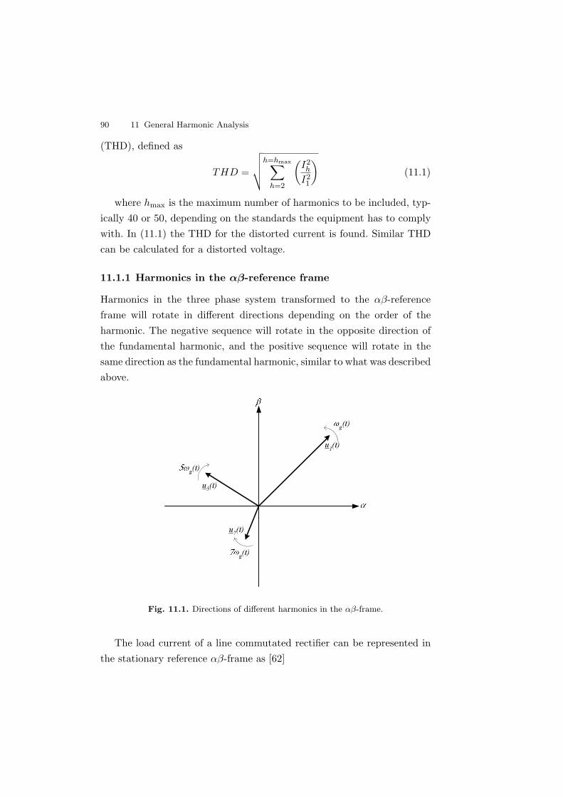
90 11 General Harmonic Analysis
(THD), defined as
THD =
√√√√h=hmax∑
h=2
(I2h
I21
)(11.1)
where hmax is the maximum number of harmonics to be included, typ-ically 40 or 50, depending on the standards the equipment has to complywith. In (11.1) the THD for the distorted current is found. Similar THDcan be calculated for a distorted voltage.
11.1.1 Harmonics in the αβ-reference frame
Harmonics in the three phase system transformed to the αβ-referenceframe will rotate in different directions depending on the order of theharmonic. The negative sequence will rotate in the opposite direction ofthe fundamental harmonic, and the positive sequence will rotate in thesame direction as the fundamental harmonic, similar to what was describedabove.
u1(t)
g(t)
u7(t)
u5(t)g(t)
g(t)
Fig. 11.1. Directions of different harmonics in the αβ-frame.
The load current of a line commutated rectifier can be represented inthe stationary reference αβ-frame as [62]
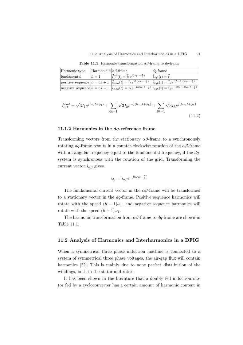
11.2 Analysis of Harmonics and Interharmonics in a DFIG 91
Table 11.1. Harmonic transformation αβ-frame to dq-frame
Harmonic type Harmonic n αβ-frame dq-frame
fundamental h = 1 ~iαβ1 (t) =~i1e
j(ω1t−π2 ) ~idq1(t) =~i1
positive sequence h = 6k + 1 ~iαβh(t) =~ihejh(ω1t−π2 ) ~idqh(t) =~ihej(h−1)(ω1t−π
2 )
negative sequence h = 6k − 1 ~iαβh(t) =~ihe−jh(ω1t−π2 ) ~idqh(t) =~ihe−j(h+1)(ω1t−π
2 )
~iloadαβ =
√3I1e
j(ω1t+φ1) +∑
6k−1
√3Ihe−j(hω1t+φh) +
∑
6k−1
√3Ihej(hω1t+φh)
(11.2)
11.1.2 Harmonics in the dq-reference frame
Transforming vectors from the stationary αβ-frame to a synchronouslyrotating dq-frame results in a counter-clockwise rotation of the αβ-framewith an angular frequency equal to the fundamental frequency, if the dq-system is synchronous with the rotation of the grid. Transforming thecurrent vector iαβ gives
idq = iαβe−j(ω1t−π2)
The fundamental current vector in the αβ-frame will be transformedto a stationary vector in the dq-frame. Positive sequence harmonics willrotate with the speed (h − 1)ω1, and negative sequence harmonics willrotate with the speed (h + 1)ω1.
The harmonic transformation from αβ-frame to dq-frame are shown inTable 11.1.
11.2 Analysis of Harmonics and Interharmonics in a DFIG
When a symmetrical three phase induction machine is connected to asystem of symmetrical three phase voltages, the air-gap flux will containharmonics [22]. This is mainly due to none perfect distribution of thewindings, both in the stator and rotor.
It has been shown in the literature that a doubly fed induction mo-tor fed by a cycloconverter has a certain amount of harmonic content in
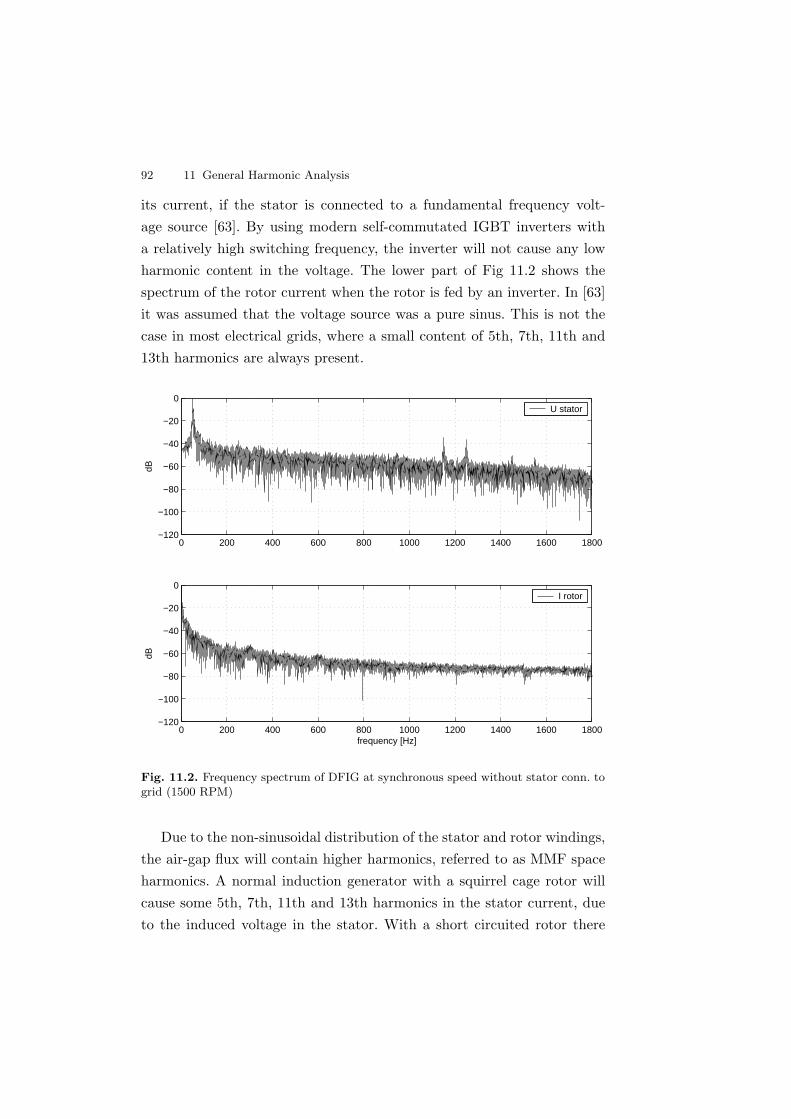
92 11 General Harmonic Analysis
its current, if the stator is connected to a fundamental frequency volt-age source [63]. By using modern self-commutated IGBT inverters witha relatively high switching frequency, the inverter will not cause any lowharmonic content in the voltage. The lower part of Fig 11.2 shows thespectrum of the rotor current when the rotor is fed by an inverter. In [63]it was assumed that the voltage source was a pure sinus. This is not thecase in most electrical grids, where a small content of 5th, 7th, 11th and13th harmonics are always present.
0 200 400 600 800 1000 1200 1400 1600 1800−120
−100
−80
−60
−40
−20
0
dB
0 200 400 600 800 1000 1200 1400 1600 1800−120
−100
−80
−60
−40
−20
0
frequency [Hz]
dB
U stator
I rotor
Fig. 11.2. Frequency spectrum of DFIG at synchronous speed without stator conn. togrid (1500 RPM)
Due to the non-sinusoidal distribution of the stator and rotor windings,the air-gap flux will contain higher harmonics, referred to as MMF spaceharmonics. A normal induction generator with a squirrel cage rotor willcause some 5th, 7th, 11th and 13th harmonics in the stator current, dueto the induced voltage in the stator. With a short circuited rotor there
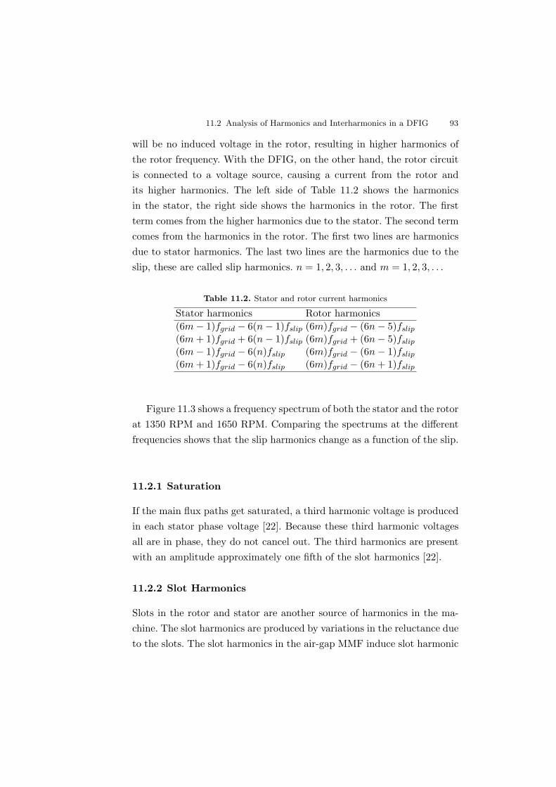
11.2 Analysis of Harmonics and Interharmonics in a DFIG 93
will be no induced voltage in the rotor, resulting in higher harmonics ofthe rotor frequency. With the DFIG, on the other hand, the rotor circuitis connected to a voltage source, causing a current from the rotor andits higher harmonics. The left side of Table 11.2 shows the harmonicsin the stator, the right side shows the harmonics in the rotor. The firstterm comes from the higher harmonics due to the stator. The second termcomes from the harmonics in the rotor. The first two lines are harmonicsdue to stator harmonics. The last two lines are the harmonics due to theslip, these are called slip harmonics. n = 1, 2, 3, . . . and m = 1, 2, 3, . . .
Table 11.2. Stator and rotor current harmonics
Stator harmonics Rotor harmonics(6m− 1)fgrid − 6(n− 1)fslip (6m)fgrid − (6n− 5)fslip
(6m + 1)fgrid + 6(n− 1)fslip (6m)fgrid + (6n− 5)fslip
(6m− 1)fgrid − 6(n)fslip (6m)fgrid − (6n− 1)fslip
(6m + 1)fgrid − 6(n)fslip (6m)fgrid − (6n + 1)fslip
Figure 11.3 shows a frequency spectrum of both the stator and the rotorat 1350 RPM and 1650 RPM. Comparing the spectrums at the differentfrequencies shows that the slip harmonics change as a function of the slip.
11.2.1 Saturation
If the main flux paths get saturated, a third harmonic voltage is producedin each stator phase voltage [22]. Because these third harmonic voltagesall are in phase, they do not cancel out. The third harmonics are presentwith an amplitude approximately one fifth of the slot harmonics [22].
11.2.2 Slot Harmonics
Slots in the rotor and stator are another source of harmonics in the ma-chine. The slot harmonics are produced by variations in the reluctance dueto the slots. The slot harmonics in the air-gap MMF induce slot harmonic
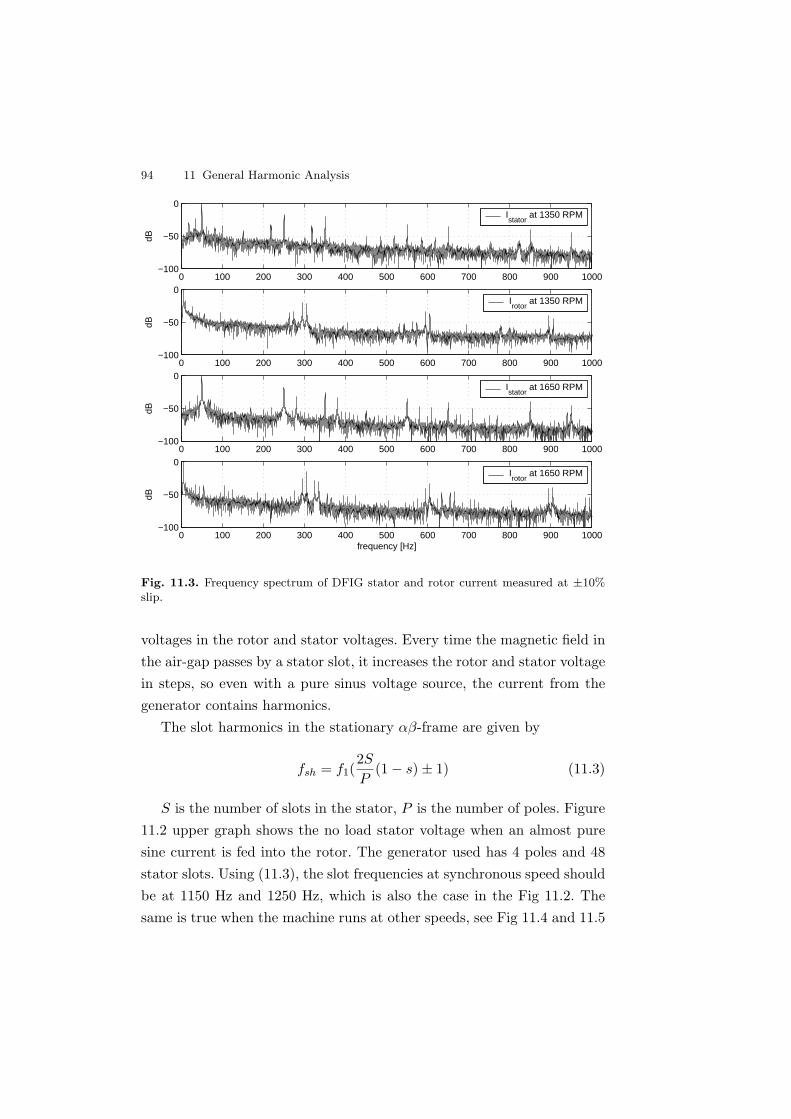
94 11 General Harmonic Analysis
0 100 200 300 400 500 600 700 800 900 1000−100
−50
0
dB
0 100 200 300 400 500 600 700 800 900 1000−100
−50
0
dB
0 100 200 300 400 500 600 700 800 900 1000−100
−50
0
dB
0 100 200 300 400 500 600 700 800 900 1000−100
−50
0
frequency [Hz]
dB
Istator
at 1350 RPM
Irotor
at 1350 RPM
Istator
at 1650 RPM
Irotor
at 1650 RPM
Fig. 11.3. Frequency spectrum of DFIG stator and rotor current measured at ±10%slip.
voltages in the rotor and stator voltages. Every time the magnetic field inthe air-gap passes by a stator slot, it increases the rotor and stator voltagein steps, so even with a pure sinus voltage source, the current from thegenerator contains harmonics.
The slot harmonics in the stationary αβ-frame are given by
fsh = f1(2S
P(1− s)± 1) (11.3)
S is the number of slots in the stator, P is the number of poles. Figure11.2 upper graph shows the no load stator voltage when an almost puresine current is fed into the rotor. The generator used has 4 poles and 48stator slots. Using (11.3), the slot frequencies at synchronous speed shouldbe at 1150 Hz and 1250 Hz, which is also the case in the Fig 11.2. Thesame is true when the machine runs at other speeds, see Fig 11.4 and 11.5
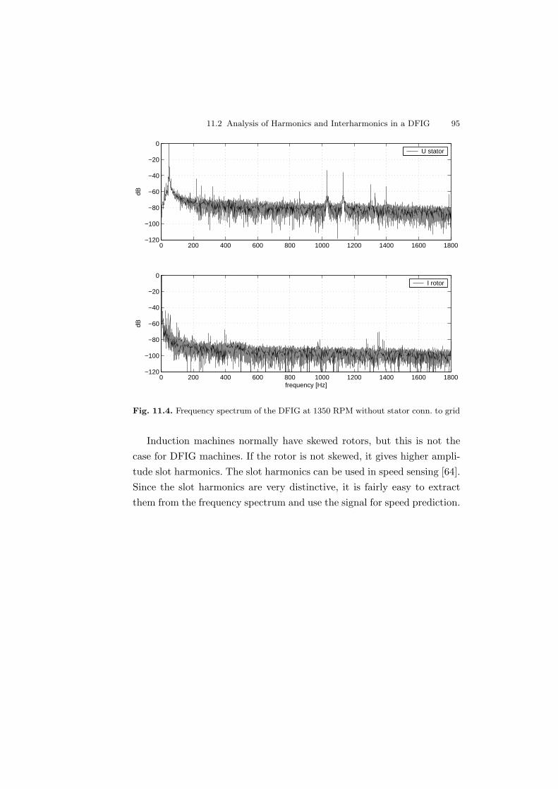
11.2 Analysis of Harmonics and Interharmonics in a DFIG 95
0 200 400 600 800 1000 1200 1400 1600 1800−120
−100
−80
−60
−40
−20
0dB
0 200 400 600 800 1000 1200 1400 1600 1800−120
−100
−80
−60
−40
−20
0
frequency [Hz]
dB
U stator
I rotor
Fig. 11.4. Frequency spectrum of the DFIG at 1350 RPM without stator conn. to grid
Induction machines normally have skewed rotors, but this is not thecase for DFIG machines. If the rotor is not skewed, it gives higher ampli-tude slot harmonics. The slot harmonics can be used in speed sensing [64].Since the slot harmonics are very distinctive, it is fairly easy to extractthem from the frequency spectrum and use the signal for speed prediction.
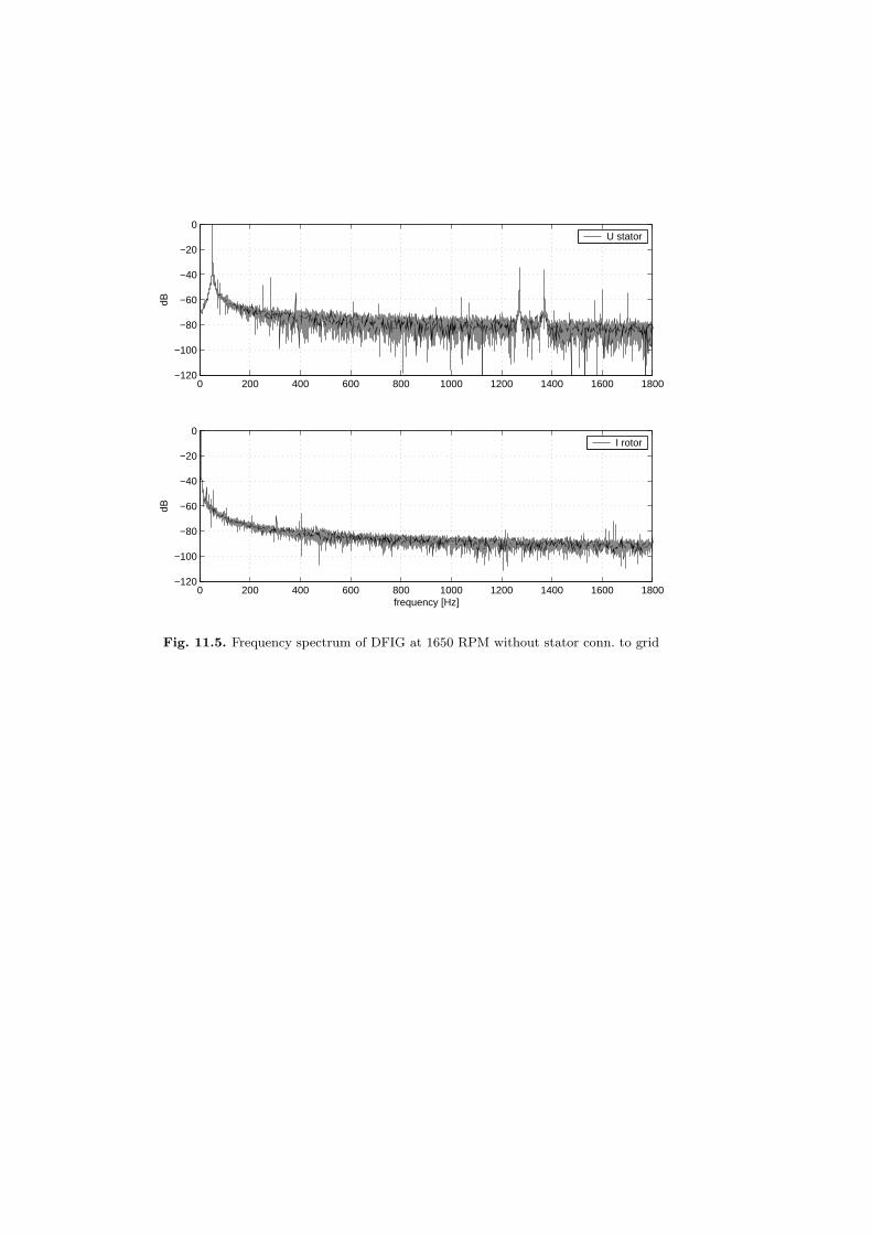
0 200 400 600 800 1000 1200 1400 1600 1800−120
−100
−80
−60
−40
−20
0
dB
0 200 400 600 800 1000 1200 1400 1600 1800−120
−100
−80
−60
−40
−20
0
frequency [Hz]
dB
U stator
I rotor
Fig. 11.5. Frequency spectrum of DFIG at 1650 RPM without stator conn. to grid

12
Adaptive Active Filtering
An active shunt filter consists of a controllable voltage source converterwith a DC voltage link and a filter inductance, like the grid inverter de-scribed in chapter 10. The principle of an active shunt filter is to inject theundesired components of the load current into the load current, in orderto eliminate their presence in the line current. In this chapter, an adaptiveactive filter is implemented.
12.1 The Least Mean Squares Algorithm
The harmonics described in the previous chapter often have to be reducedin some sort of a filter in order to comply with the international stan-dards for wind turbines [9]. A normally tuned passive filter will filter theharmonics from the stator, but the slip harmonics from the rotor vary infrequency as a function of the slip, making a tuned filter useless. Insteadan active filter implemented in the power converter will work. The fil-ter will have to change its characteristics when the slip changes. Anotherapproach to reduce the harmonics is to use an adaptive filter, where anadaptation algorithm sets the weights of the filter. A simple and often usedadaptation algorithm is the Least Mean Squares (LMS). This algorithm,first presented by Widrow and Hoff [65], is given by the equations.
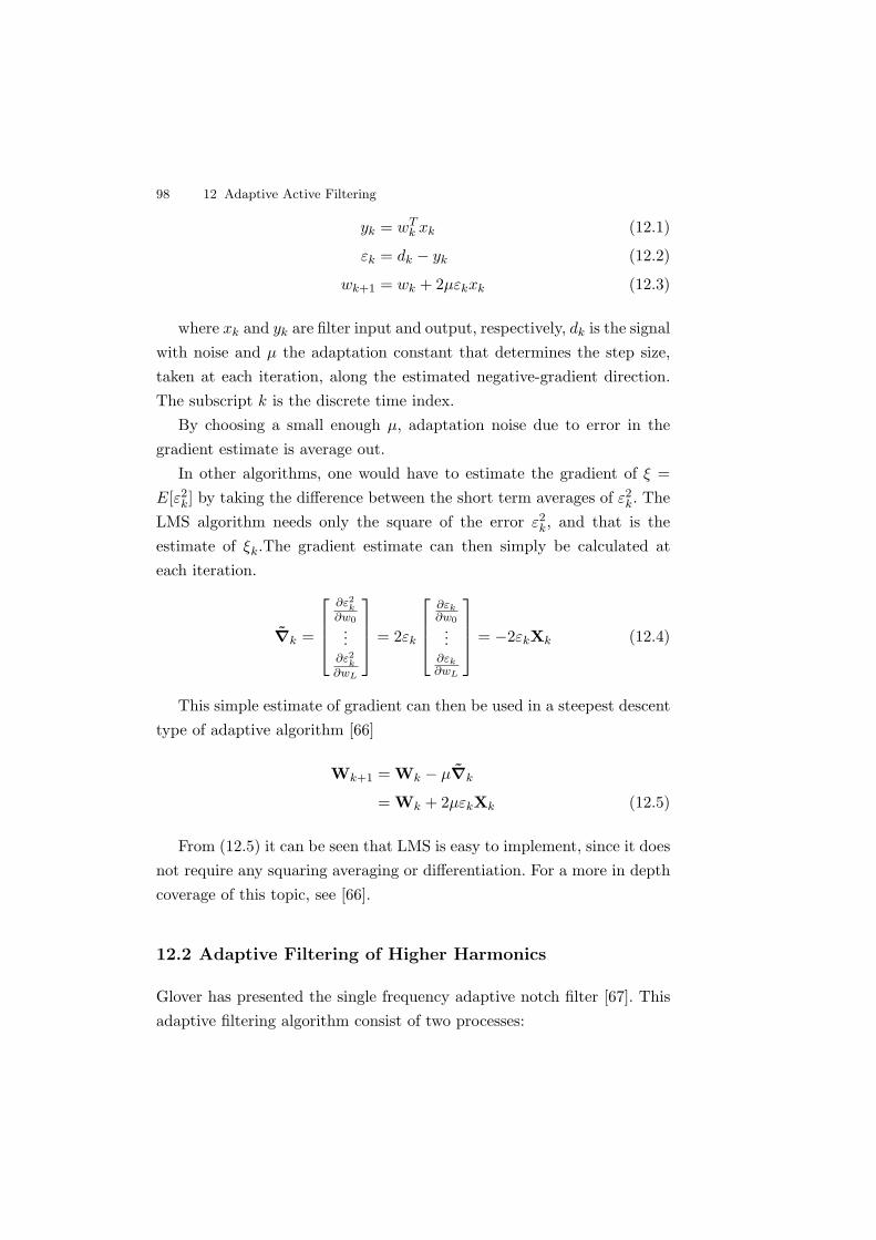
98 12 Adaptive Active Filtering
yk = wTk xk (12.1)
εk = dk − yk (12.2)
wk+1 = wk + 2µεkxk (12.3)
where xk and yk are filter input and output, respectively, dk is the signalwith noise and µ the adaptation constant that determines the step size,taken at each iteration, along the estimated negative-gradient direction.The subscript k is the discrete time index.
By choosing a small enough µ, adaptation noise due to error in thegradient estimate is average out.
In other algorithms, one would have to estimate the gradient of ξ =E[ε2
k] by taking the difference between the short term averages of ε2k. The
LMS algorithm needs only the square of the error ε2k, and that is the
estimate of ξk.The gradient estimate can then simply be calculated ateach iteration.
∇k =
∂ε2k
∂w0...
∂ε2k
∂wL
= 2εk
∂εk∂w0...
∂εk∂wL
= −2εkXk (12.4)
This simple estimate of gradient can then be used in a steepest descenttype of adaptive algorithm [66]
Wk+1 = Wk − µ∇k
= Wk + 2µεkXk (12.5)
From (12.5) it can be seen that LMS is easy to implement, since it doesnot require any squaring averaging or differentiation. For a more in depthcoverage of this topic, see [66].
12.2 Adaptive Filtering of Higher Harmonics
Glover has presented the single frequency adaptive notch filter [67]. Thisadaptive filtering algorithm consist of two processes:
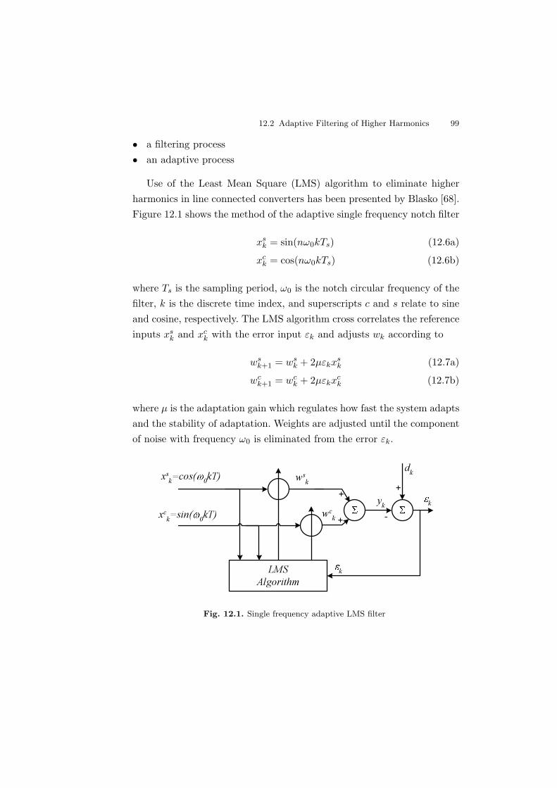
12.2 Adaptive Filtering of Higher Harmonics 99
• a filtering process• an adaptive process
Use of the Least Mean Square (LMS) algorithm to eliminate higherharmonics in line connected converters has been presented by Blasko [68].Figure 12.1 shows the method of the adaptive single frequency notch filter
xsk = sin(nω0kTs) (12.6a)
xck = cos(nω0kTs) (12.6b)
where Ts is the sampling period, ω0 is the notch circular frequency of thefilter, k is the discrete time index, and superscripts c and s relate to sineand cosine, respectively. The LMS algorithm cross correlates the referenceinputs xs
k and xck with the error input εk and adjusts wk according to
wsk+1 = ws
k + 2µεkxsk (12.7a)
wck+1 = wc
k + 2µεkxck (12.7b)
where µ is the adaptation gain which regulates how fast the system adaptsand the stability of adaptation. Weights are adjusted until the componentof noise with frequency ω0 is eliminated from the error εk.
+
+yk
LMSAlgorithm
dkxsk=cos( 0kT)
xck=sin( 0kT)
wsk
wck
k
k
+
-
Fig. 12.1. Single frequency adaptive LMS filter
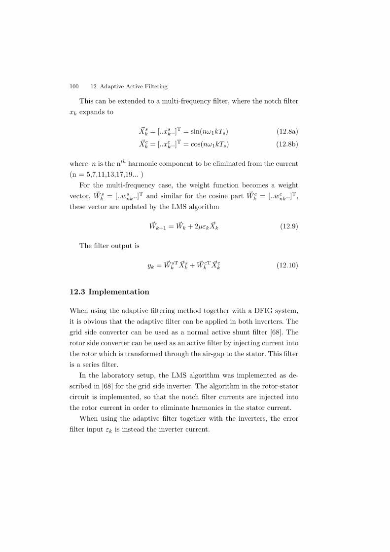
100 12 Adaptive Active Filtering
This can be extended to a multi-frequency filter, where the notch filterxk expands to
~Xsk = [..xs
k..]T = sin(nω1kTs) (12.8a)
~Xck = [..xc
k..]T = cos(nω1kTs) (12.8b)
where n is the nth harmonic component to be eliminated from the current(n = 5,7,11,13,17,19... )
For the multi-frequency case, the weight function becomes a weightvector, ~W s
k = [..wsnk..]
T and similar for the cosine part ~W ck = [..wc
nk..]T,
these vector are updated by the LMS algorithm
~Wk+1 = ~Wk + 2µεk~Xk (12.9)
The filter output is
yk = ~W sTk
~Xsk + ~W cT
k~Xc
k (12.10)
12.3 Implementation
When using the adaptive filtering method together with a DFIG system,it is obvious that the adaptive filter can be applied in both inverters. Thegrid side converter can be used as a normal active shunt filter [68]. Therotor side converter can be used as an active filter by injecting current intothe rotor which is transformed through the air-gap to the stator. This filteris a series filter.
In the laboratory setup, the LMS algorithm was implemented as de-scribed in [68] for the grid side inverter. The algorithm in the rotor-statorcircuit is implemented, so that the notch filter currents are injected intothe rotor current in order to eliminate harmonics in the stator current.
When using the adaptive filter together with the inverters, the errorfilter input εk is instead the inverter current.
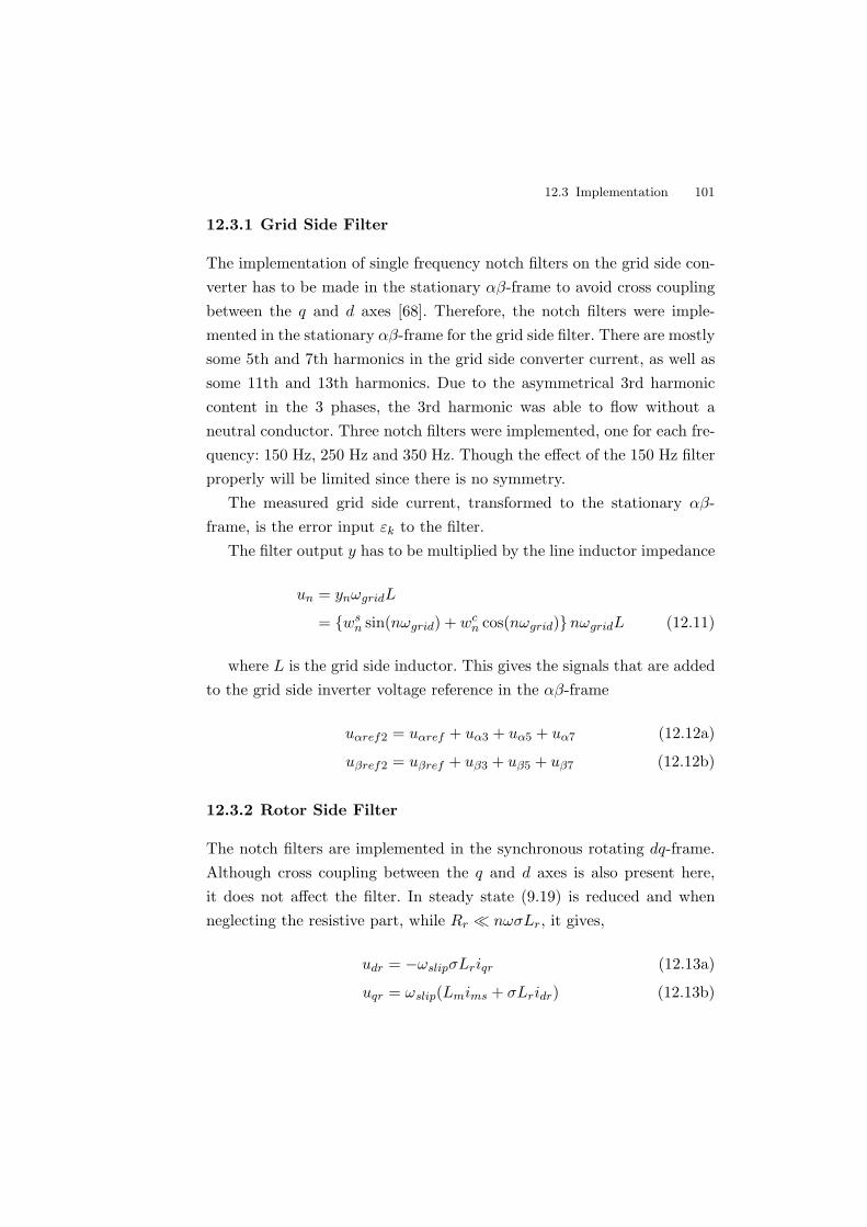
12.3 Implementation 101
12.3.1 Grid Side Filter
The implementation of single frequency notch filters on the grid side con-verter has to be made in the stationary αβ-frame to avoid cross couplingbetween the q and d axes [68]. Therefore, the notch filters were imple-mented in the stationary αβ-frame for the grid side filter. There are mostlysome 5th and 7th harmonics in the grid side converter current, as well assome 11th and 13th harmonics. Due to the asymmetrical 3rd harmoniccontent in the 3 phases, the 3rd harmonic was able to flow without aneutral conductor. Three notch filters were implemented, one for each fre-quency: 150 Hz, 250 Hz and 350 Hz. Though the effect of the 150 Hz filterproperly will be limited since there is no symmetry.
The measured grid side current, transformed to the stationary αβ-frame, is the error input εk to the filter.
The filter output y has to be multiplied by the line inductor impedance
un = ynωgridL
= wsn sin(nωgrid) + wc
n cos(nωgrid)nωgridL (12.11)
where L is the grid side inductor. This gives the signals that are addedto the grid side inverter voltage reference in the αβ-frame
uαref2 = uαref + uα3 + uα5 + uα7 (12.12a)
uβref2 = uβref + uβ3 + uβ5 + uβ7 (12.12b)
12.3.2 Rotor Side Filter
The notch filters are implemented in the synchronous rotating dq-frame.Although cross coupling between the q and d axes is also present here,it does not affect the filter. In steady state (9.19) is reduced and whenneglecting the resistive part, while Rr ¿ nωσLr, it gives,
udr = −ωslipσLriqr (12.13a)
uqr = ωslip(Lmims + σLridr) (12.13b)
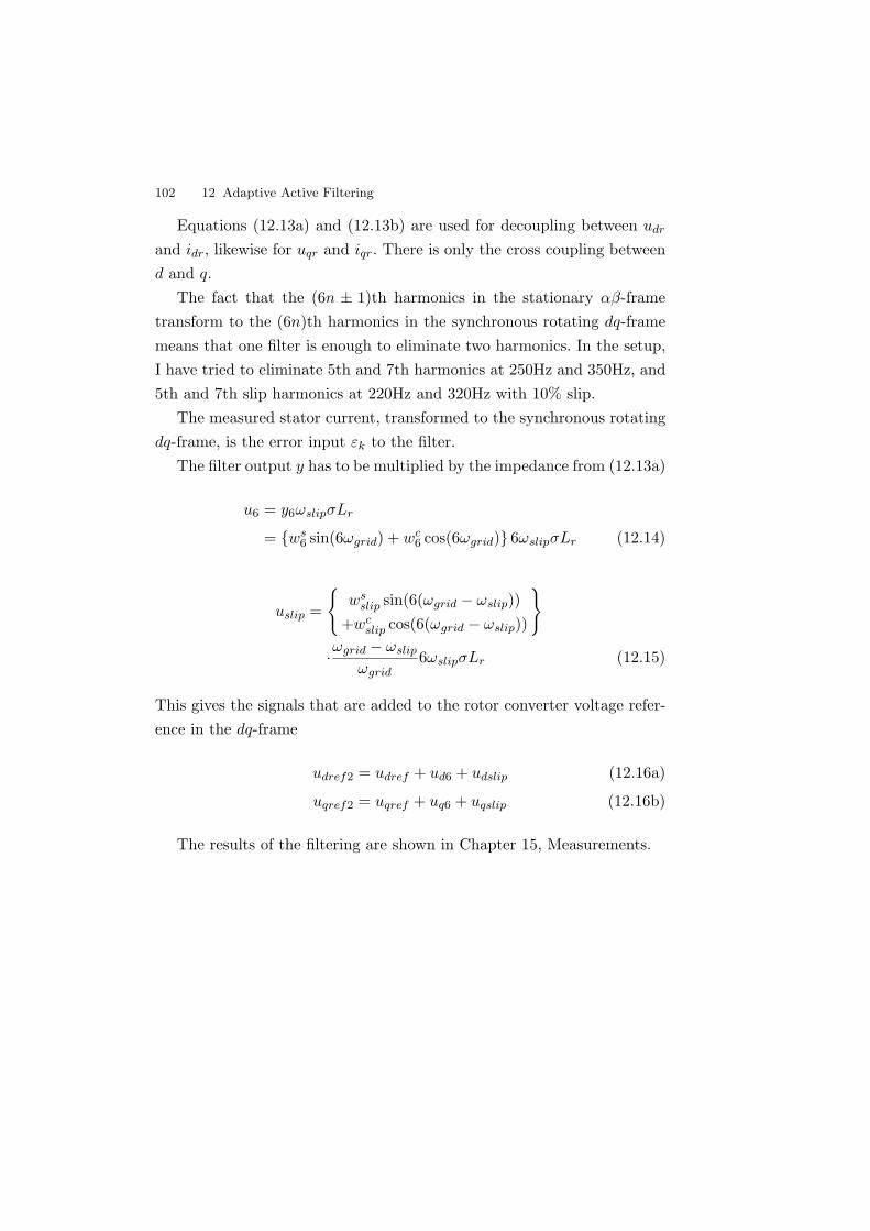
102 12 Adaptive Active Filtering
Equations (12.13a) and (12.13b) are used for decoupling between udr
and idr, likewise for uqr and iqr. There is only the cross coupling betweend and q.
The fact that the (6n ± 1)th harmonics in the stationary αβ-frametransform to the (6n)th harmonics in the synchronous rotating dq-framemeans that one filter is enough to eliminate two harmonics. In the setup,I have tried to eliminate 5th and 7th harmonics at 250Hz and 350Hz, and5th and 7th slip harmonics at 220Hz and 320Hz with 10% slip.
The measured stator current, transformed to the synchronous rotatingdq-frame, is the error input εk to the filter.
The filter output y has to be multiplied by the impedance from (12.13a)
u6 = y6ωslipσLr
= ws6 sin(6ωgrid) + wc
6 cos(6ωgrid) 6ωslipσLr (12.14)
uslip =
ws
slip sin(6(ωgrid − ωslip))+wc
slip cos(6(ωgrid − ωslip))
·ωgrid − ωslip
ωgrid6ωslipσLr (12.15)
This gives the signals that are added to the rotor converter voltage refer-ence in the dq-frame
udref2 = udref + ud6 + udslip (12.16a)
uqref2 = uqref + uq6 + uqslip (12.16b)
The results of the filtering are shown in Chapter 15, Measurements.

Part II
Laboratory Setup

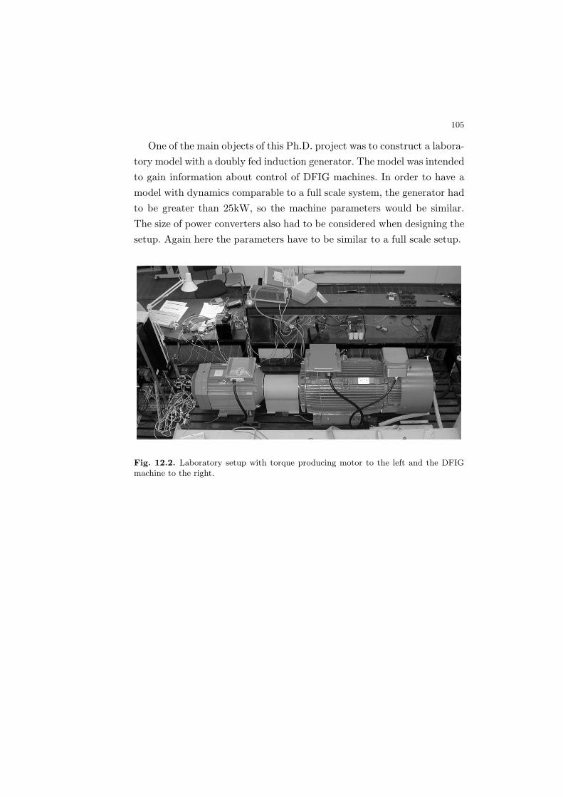
105
One of the main objects of this Ph.D. project was to construct a labora-tory model with a doubly fed induction generator. The model was intendedto gain information about control of DFIG machines. In order to have amodel with dynamics comparable to a full scale system, the generator hadto be greater than 25kW, so the machine parameters would be similar.The size of power converters also had to be considered when designing thesetup. Again here the parameters have to be similar to a full scale setup.
Fig. 12.2. Laboratory setup with torque producing motor to the left and the DFIGmachine to the right.

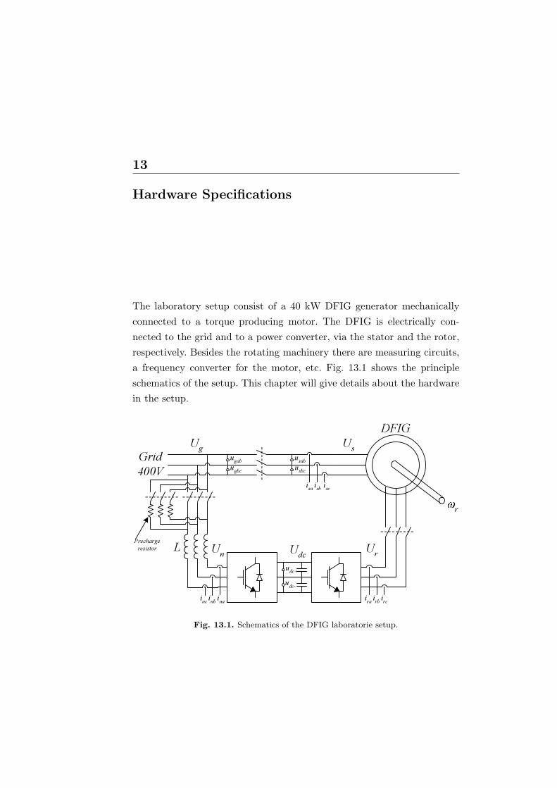
13
Hardware Specifications
The laboratory setup consist of a 40 kW DFIG generator mechanicallyconnected to a torque producing motor. The DFIG is electrically con-nected to the grid and to a power converter, via the stator and the rotor,respectively. Besides the rotating machinery there are measuring circuits,a frequency converter for the motor, etc. Fig. 13.1 shows the principleschematics of the setup. This chapter will give details about the hardwarein the setup.
DFIG
Grid400V
Udc
Us
Ur
r
Un
Ugugabugbc
usabusbc
udc+udc-
iscisbisa
ircirbirainc inb ina
LPrechargeresistor
Fig. 13.1. Schematics of the DFIG laboratorie setup.

108 13 Hardware Specifications
13.1 The Rotating Machinery
The main component in the setup is a 40kW DFIG produced by Leroy-Somer. It is a 4 pole generator. The generator is connected with a Y-connected stator and rotor.
The torque-producing-motor or load-motor is a 37 kW induction motormade by ABB. The motor is stator fed by a torque controlled frequencyconverter, ABB ACS601-0037-4.
Data for both machines can be found in the appendix C.
Temperature sensors
Three PT-100 sensors have been placed in the stator windings of the DFIG.The sensors are monitored by a PT-100 transducer (PR-Electronics 2271).Only one single transducer is used for all three sensor. They are connectedin series forming a PT-300 sensor. This requires a uniform heating of thestator or reduced maximum allowed temperature. The transducer supplya 4-20 mA output signal. This signal is used to display the actual statortemperature in the control panel, for the load motor’s frequency converter(ACS601). The transducer also has a relay, that when activated trip theACS601 and the control system for the DFIG.
Speed sensor
The DFIG is equipped with an encoder at the non-drive end. The en-coder has two channels, each with 1024 pulses. If detecting the edges, itgives a total resolution of 4096 increments per round. The encoder signalsare transmitted to a digital interface board. The speed of the DFIG andthe load motor is also monitored by the ACS601. If the speed is below1100 RPM, a relay in the ACS601 will open and the stator contactor willdisconnect the DFIG from the grid for safety reasons.
13.2 Power Inverters
The two back to back inverters are designed on the specification in table13.1 and 13.2.
13.2 Power Inverters 109
Table 13.1. Design specifications for grid side inverter
rated power Sg 14kVAgrid voltage Ug 400Vgrid current Ig 20Agrid frequency f1 50Hzswitching freq. fsw 4kHzDC-link volt. UDC,max 720V
Table 13.2. Design specifications for rotor side inverter
rated power Sr 14kVArotor voltage Ur,max 400Vrotor current Ir 20Arotor frequency fr 0-12.5Hzswitching freq. fsw 4kHzDC-link volt. UDC,max 720V
As discussed in chapter 7, the power converters used in the laboratorysetup are IGBT based 3-level neutral point clamped converters (see p43).The IGBTs are Intersil’s HGTG20N120CND. It is a 1200V IGBT with anintegrated anti-parallel hyperfast diode [69]. The clamp diodes are Inter-sil’s RHRP15100, a 1000V hyperfast diode [70]. Each single phase NPCinverter is mounted on a PCB, equipped with the four switches, the twoclamp diodes and the gate resistors.
Each three phase converter has twelve IGBTs, therefore a normal threephase gate-driver module for a 2-level inverter is not sufficient. Each in-verter is equipped with two six-pack driver circuits from Semikron SKHI61. This driver takes care of interlocking and dead time. Both SKHI 61modules are mounted on a gate-driver PCB, see Fig. 13.2. Under normaloperation, the SKHI 61 has an interlocking function, that sets the deadtime to prevent both the top and the bottom IGBT from being switchedon simultaneously. This function can be disabled, but then the dead timeis set to 0 µs. Otherwise the dead time is between 1-4 µs. Having the twoSKHI 61 modules connected to the three phases so that IGBT switch S1and S2 are driven by one gate-driver module, and similar for S3 and S4,
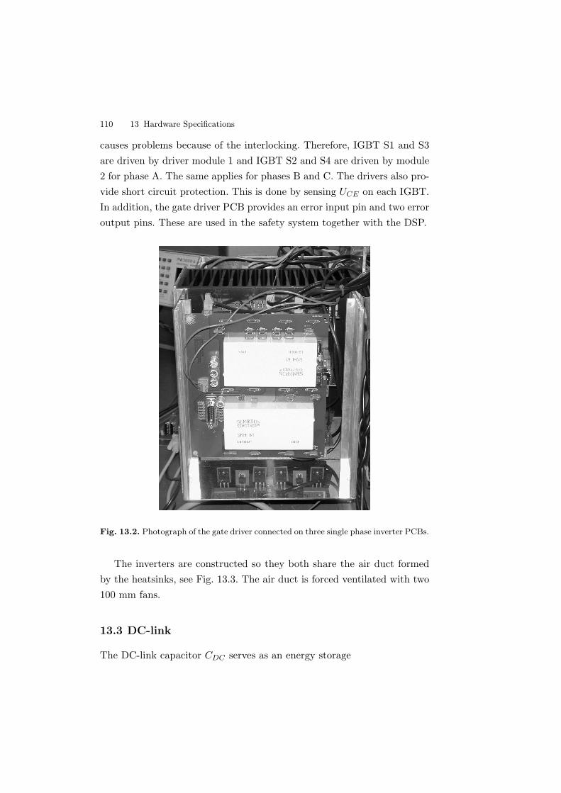
110 13 Hardware Specifications
causes problems because of the interlocking. Therefore, IGBT S1 and S3are driven by driver module 1 and IGBT S2 and S4 are driven by module2 for phase A. The same applies for phases B and C. The drivers also pro-vide short circuit protection. This is done by sensing UCE on each IGBT.In addition, the gate driver PCB provides an error input pin and two erroroutput pins. These are used in the safety system together with the DSP.
Fig. 13.2. Photograph of the gate driver connected on three single phase inverter PCBs.
The inverters are constructed so they both share the air duct formedby the heatsinks, see Fig. 13.3. The air duct is forced ventilated with two100 mm fans.
13.3 DC-link
The DC-link capacitor CDC serves as an energy storage
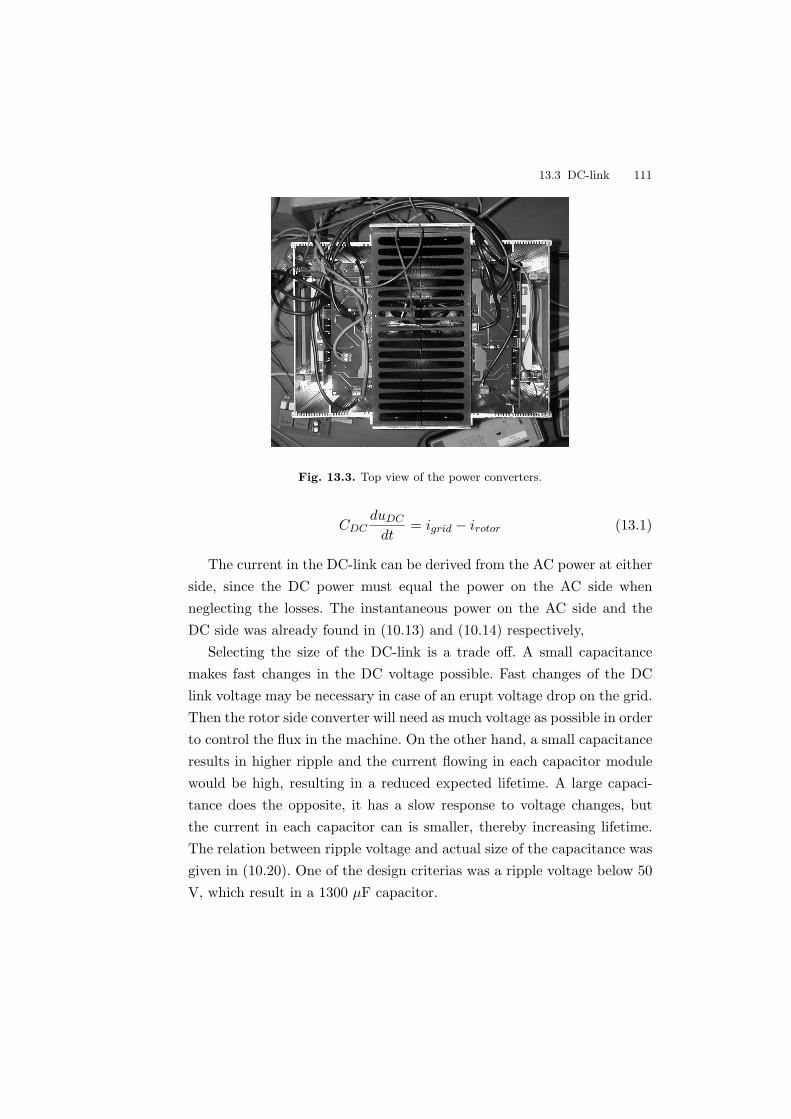
13.3 DC-link 111
Fig. 13.3. Top view of the power converters.
CDCduDC
dt= igrid − irotor (13.1)
The current in the DC-link can be derived from the AC power at eitherside, since the DC power must equal the power on the AC side whenneglecting the losses. The instantaneous power on the AC side and theDC side was already found in (10.13) and (10.14) respectively,
Selecting the size of the DC-link is a trade off. A small capacitancemakes fast changes in the DC voltage possible. Fast changes of the DClink voltage may be necessary in case of an erupt voltage drop on the grid.Then the rotor side converter will need as much voltage as possible in orderto control the flux in the machine. On the other hand, a small capacitanceresults in higher ripple and the current flowing in each capacitor modulewould be high, resulting in a reduced expected lifetime. A large capaci-tance does the opposite, it has a slow response to voltage changes, butthe current in each capacitor can is smaller, thereby increasing lifetime.The relation between ripple voltage and actual size of the capacitance wasgiven in (10.20). One of the design criterias was a ripple voltage below 50V, which result in a 1300 µF capacitor.
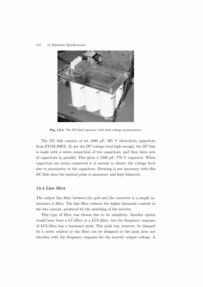
112 13 Hardware Specifications
Fig. 13.4. The DC-link capacitor with dual voltage measurement.
The DC link consists of six 1000 µF, 385 V electrolytic capacitorsfrom EVOX-RIFA. To get the DC voltage level high enough, the DC linkis made with a series connection of two capacitors, and then three setsof capacitors in parallel. This gives a 1500 µF, 770 V capacitor. Whencapacitors are series connected it is normal to derate the voltage leveldue to asymmetry in the capacitors. Derating is not necessary with thisDC-link since the neutral point is measured, and kept balanced.
13.4 Line filter
The output line filter between the grid and the converter is a simple in-ductance L-filter. The line filter reduces the higher harmonic content inthe line current, produced by the switching of the inverter.
This type of filter was chosen due to its simplicity. Another optionwould have been a LC-filter or a LCL-filter, but the frequency responseof LCL-filter has a resonance peak. This peak can, however, be dampedby a series resistor or the filter can be designed so the peak does notinterfere with the frequency response for the inverter output voltage. A
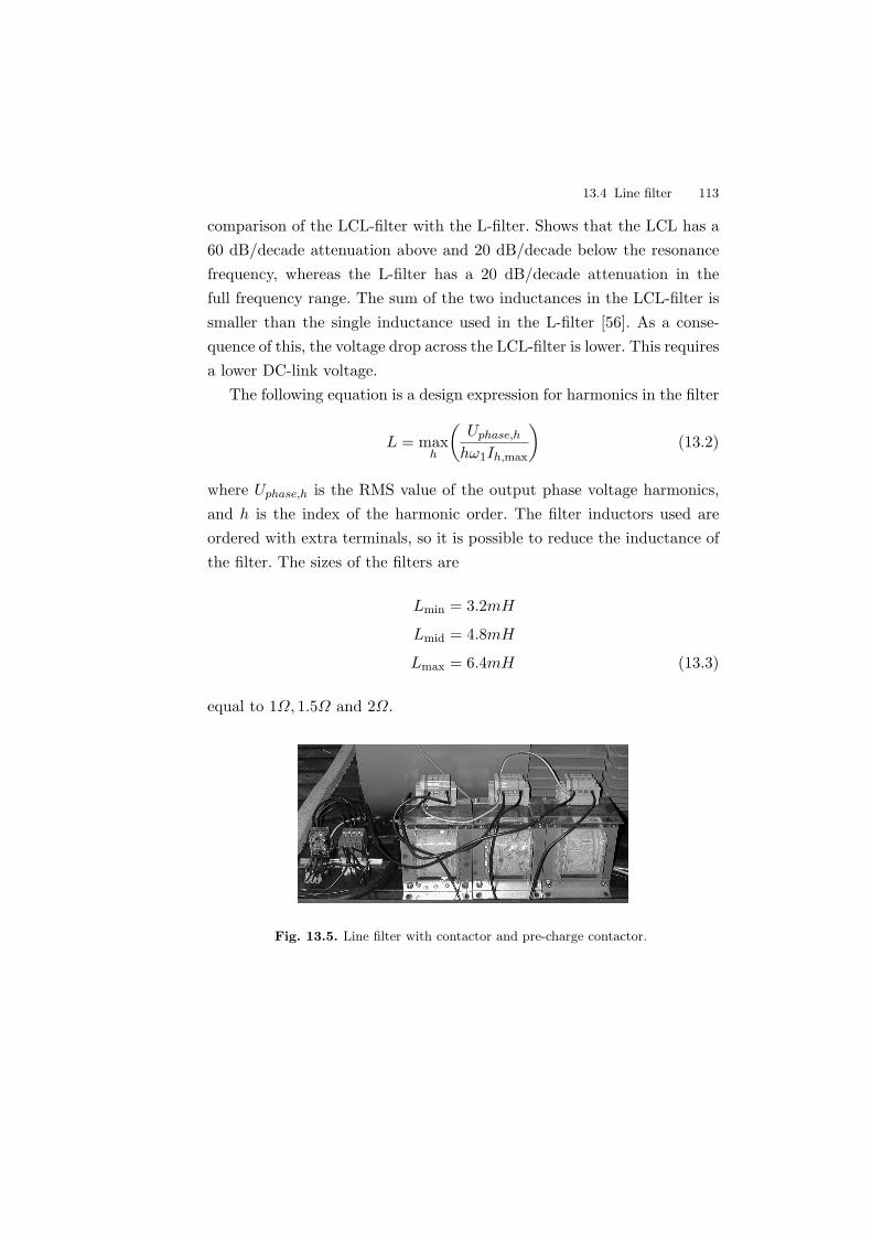
13.4 Line filter 113
comparison of the LCL-filter with the L-filter. Shows that the LCL has a60 dB/decade attenuation above and 20 dB/decade below the resonancefrequency, whereas the L-filter has a 20 dB/decade attenuation in thefull frequency range. The sum of the two inductances in the LCL-filter issmaller than the single inductance used in the L-filter [56]. As a conse-quence of this, the voltage drop across the LCL-filter is lower. This requiresa lower DC-link voltage.
The following equation is a design expression for harmonics in the filter
L = maxh
(Uphase,h
hω1Ih,max
)(13.2)
where Uphase,h is the RMS value of the output phase voltage harmonics,and h is the index of the harmonic order. The filter inductors used areordered with extra terminals, so it is possible to reduce the inductance ofthe filter. The sizes of the filters are
Lmin = 3.2mH
Lmid = 4.8mH
Lmax = 6.4mH (13.3)
equal to 1Ω, 1.5Ω and 2Ω.
Fig. 13.5. Line filter with contactor and pre-charge contactor.
114 13 Hardware Specifications
13.5 Voltage and Current Sensors
The actual signals are measured using hall-effect current transformersmade by LEM. In Table 13.3 the measuring signals are listed. All sig-nals are measured with a sampling frequency of 4 kHz. The location ofthe different sensors are shown in Fig. 13.1.
Table 13.3. Measuring signals.
Signal Range Peak range TransducerIrA, IrB, IrC 25Arms ±80A LTS 25-NPInA, InB, InC 25Arms ±80A LTS 25-NPIsA, IsB, IsC 100Arms ±150A LA 100-PUabn, Ubcn 480Vrms ±670V LV25-PUabs, Ubcs 480Vrms ±670V LV25-PUdc+, Udc− 480Vrms ±670V LV25-P
For the current sensors, all three phases are measured eventhough twophase would have been sufficient. The additional sensors were made inorder to detect whether one of the signals was wrong. It was also intendedto be used in an earth leakage protection system, but this was never im-plemented.
There are three sets of voltage sensors. The first set is for the two DC-link voltages, where the DC neutral point is very important. The secondset is used to measure the grid voltage. It measures two phase to phasevoltages. By doing so, the information about zero sequence is lost, butit is still possible to split into positive and negative sequence systems.Information about the zero sequence could have been captured by usingthe ground plane where the machines are standing as a zero point. The lastset of voltage sensors are two phase to phase voltages at stator terminals onthe generator. These sensors are needed in order to connect the generatorin phase with the grid.
The voltage sensors are also based on a current transformer. Thesesensors use a shunt resistor that is dimensioned so a current of 10 mA
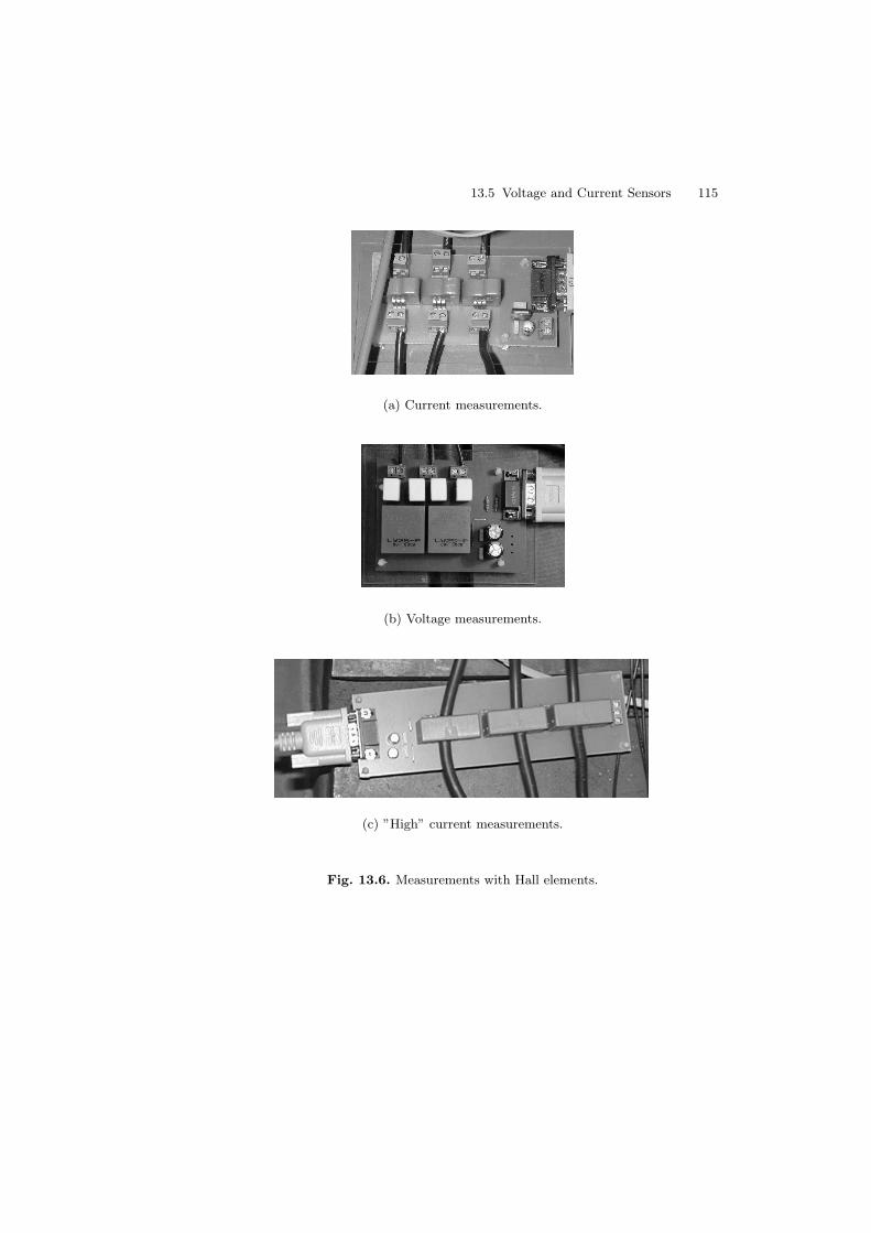
13.5 Voltage and Current Sensors 115
(a) Current measurements.
(b) Voltage measurements.
(c) ”High” current measurements.
Fig. 13.6. Measurements with Hall elements.
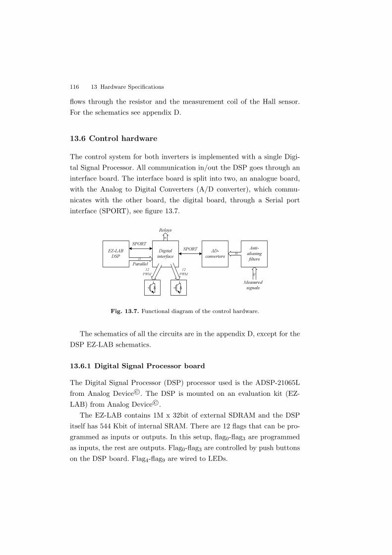
116 13 Hardware Specifications
flows through the resistor and the measurement coil of the Hall sensor.For the schematics see appendix D.
13.6 Control hardware
The control system for both inverters is implemented with a single Digi-tal Signal Processor. All communication in/out the DSP goes through aninterface board. The interface board is split into two, an analogue board,with the Analog to Digital Converters (A/D converter), which commu-nicates with the other board, the digital board, through a Serial portinterface (SPORT), see figure 13.7.
EZ-LABDSP
Digitalinterface
AD-converters
SPORT
12PWM
SPORT
12
Parallel
Anti-aliasingfilters
18
Measuredsignals
Relays
12PWM
Fig. 13.7. Functional diagram of the control hardware.
The schematics of all the circuits are in the appendix D, except for theDSP EZ-LAB schematics.
13.6.1 Digital Signal Processor board
The Digital Signal Processor (DSP) processor used is the ADSP-21065Lfrom Analog Device©. The DSP is mounted on an evaluation kit (EZ-LAB) from Analog Device©.
The EZ-LAB contains 1M x 32bit of external SDRAM and the DSPitself has 544 Kbit of internal SRAM. There are 12 flags that can be pro-grammed as inputs or outputs. In this setup, flag0-flag3 are programmedas inputs, the rest are outputs. Flag0-flag3 are controlled by push buttonson the DSP board. Flag4-flag9 are wired to LEDs.
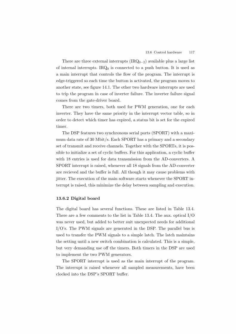
13.6 Control hardware 117
There are three external interrupts (IRQ0−2) available plus a large listof internal interrupts. IRQ0 is connected to a push button. It is used asa main interrupt that controls the flow of the program. The interrupt isedge-triggered so each time the button is activated, the program moves toanother state, see figure 14.1. The other two hardware interrupts are usedto trip the program in case of inverter failure. The inverter failure signalcomes from the gate-driver board.
There are two timers, both used for PWM generation, one for eachinverter. They have the same priority in the interrupt vector table, so inorder to detect which timer has expired, a status bit is set for the expiredtimer.
The DSP features two synchronous serial ports (SPORT) with a maxi-mum data rate of 30 Mbit/s. Each SPORT has a primary and a secondaryset of transmit and receive channels. Together with the SPORTs, it is pos-sible to initialize a set of cyclic buffers. For this application, a cyclic bufferwith 18 entries is used for data transmission from the AD-converters. ASPORT interrupt is raised, whenever all 18 signals from the AD-converterare recieved and the buffer is full. All though it may cause problems withjitter. The execution of the main software starts whenever the SPORT in-terrupt is raised, this minimize the delay between sampling and execution.
13.6.2 Digital board
The digital board has several functions. These are listed in Table 13.4.There are a few comments to the list in Table 13.4. The aux. optical I/Owas never used, but added to better suit unexpected needs for additionalI/O’s. The PWM signals are generated in the DSP. The parallel bus isused to transfer the PWM signals to a simple latch. The latch maintainsthe setting until a new switch combination is calculated. This is a simple,but very demanding use off the timers. Both timers in the DSP are usedto implement the two PWM generators.
The SPORT interrupt is used as the main interrupt of the program.The interrupt is raised whenever all sampled measurements, have beenclocked into the DSP’s SPORT buffer.
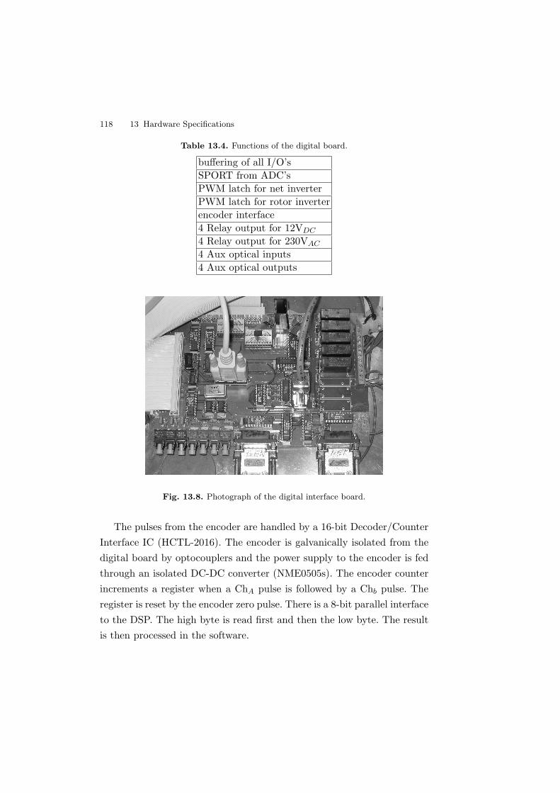
118 13 Hardware Specifications
Table 13.4. Functions of the digital board.
buffering of all I/O’sSPORT from ADC’sPWM latch for net inverterPWM latch for rotor inverterencoder interface4 Relay output for 12VDC
4 Relay output for 230VAC
4 Aux optical inputs4 Aux optical outputs
Fig. 13.8. Photograph of the digital interface board.
The pulses from the encoder are handled by a 16-bit Decoder/CounterInterface IC (HCTL-2016). The encoder is galvanically isolated from thedigital board by optocouplers and the power supply to the encoder is fedthrough an isolated DC-DC converter (NME0505s). The encoder counterincrements a register when a ChA pulse is followed by a Chb pulse. Theregister is reset by the encoder zero pulse. There is a 8-bit parallel interfaceto the DSP. The high byte is read first and then the low byte. The resultis then processed in the software.
13.6 Control hardware 119
13.6.3 Analogue board
On the analogue board, there are three A/D converters with six 16-bitsigma delta converters each (AD73360 from Analog Device). The externalclock frequency of the A/D converters is 16.384 MHz (MCLK), that isreduced by a factor of two internally. The internal sampling rate of thesigma delta modulator is then 1.024 MHz. With the desired samplingfrequency of 4 kHz the group delay of each channel is 373 µs.
Fig. 13.9. Photograph of the analogue interface with the AD-converters.
In front of each channel on the A/D converters, there is a single poleanti-aliasing filter with a cut-off frequency at 33 kHz. The filter causesa 5µs lag at 4kHz. The filters are made with an op-amp, so the gain ofthe signal and the DC offset of the signal are fitted with the input rangeof the A/D converter. The A/D converters have a serial interface, so allthree A/D converters are connected in cascade. The clock frequency of theserial port is a quarter of MCLK. The signals from A/D converter#1 gothrough A/D converter#2 and A/D converter#3 and then to the SPORTin the DSP. This is also the case with the signals from A/D converter#2,which only passes through A/D converter#3. This setup is practical froma wire count perspective, but when three times six 16-bit signals have tobe clocked into a SPORT, the disadvantages of the cascade connectionbecome obvious. It takes a minimum of 36 µs, and each sampling period

120 13 Hardware Specifications
is equal to 250 µs at Fs = 4 kHz. The delays of signal measurements addedtogether give a total of 415 µs (Tdelay), so when the data is used in thecontrol loop they are about 1.7 Tsamp old. This will caurse some distortionin the control system, and should be taken care of in the control loop.
In a redesign of the measurement circuit some changes may be required.Instead of using the same sampling frequency as the switch frequency, ahigh speed A/D converter circuit with digital filter implemented in theDSP would be better.

14
Software
The software developed for the laboratory setup is made with the softwareenvironment Visual DSP++
R©from Analog Device©. Nearly all the pro-
gramming code is written in the programming language C. This gives anoverhead compared to Assembly code, due to processor stack operations.The code optimization is enabled in the compiler and the code producedis quite efficient. A few routines are made in the Assembly language. Pro-gramming in Assembly is a long and complicated process, when makingprograms for new developments. When the fact that C-code is not thefastest is accepted, the disadvantages with programming in C are negligi-ble. The biggest advantage using C-code is a reduction in the developmenttime. Another thing is software up dates. It can be quite a job to workon somebody else’s old Assembly code, whereas C-code is often easier tounderstand right away.
14.1 Program Structure
The structure of the program is controlled by interrupts. As describedearlier, there are different interrupt levels. The sampling rate of the analogmeasurements is 4 kHz, the signals are transmitted to the DSP by a serialport and buffered in a cyclic serial port buffer with 18 entries. Wheneverthe buffer is full, a serial port interrupt is raised. This interrupt calls thecontrol loop, because whenever the buffer is full all measured signal areready. When analyzing this setup one of the things to point out is the
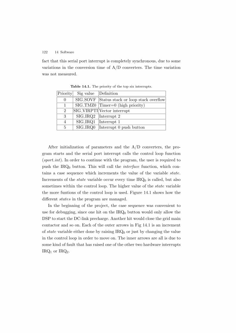
122 14 Software
fact that this serial port interrupt is completely synchronous, due to somevariations in the conversion time of A/D converters. The time variationwas not measured.
Table 14.1. The priority of the top six interrupts.
Priority Sig value Definition0 SIG SOVF Status stack or loop stack overflow1 SIG TMZ0 Timer=0 (high priority)2 SIG VIRPTI Vector interrupt3 SIG IRQ2 Interrupt 24 SIG IRQ1 Interrupt 15 SIG IRQ0 Interrupt 0 push button
After initialization of parameters and the A/D converters, the pro-gram starts and the serial port interrupt calls the control loop function(sport int). In order to continue with the program, the user is required topush the IRQ0 button. This will call the interface function, which con-tains a case sequence which increments the value of the variable state.Increments of the state variable occur every time IRQ0 is called, but alsosometimes within the control loop. The higher value of the state variablethe more funtions of the control loop is used. Figure 14.1 shows how thedifferent states in the program are managed.
In the beginning of the project, the case sequence was convenient touse for debugging, since one hit on the IRQ0 button would only allow theDSP to start the DC-link precharge. Another hit would close the grid maincontactor and so on. Each of the outer arrows in Fig 14.1 is an incrementof state variable either done by raising IRQ0 or just by changing the valuein the control loop in order to move on. The inner arrows are all is due tosome kind of fault that has raised one of the other two hardware interruptsIRQ1 or IRQ2.
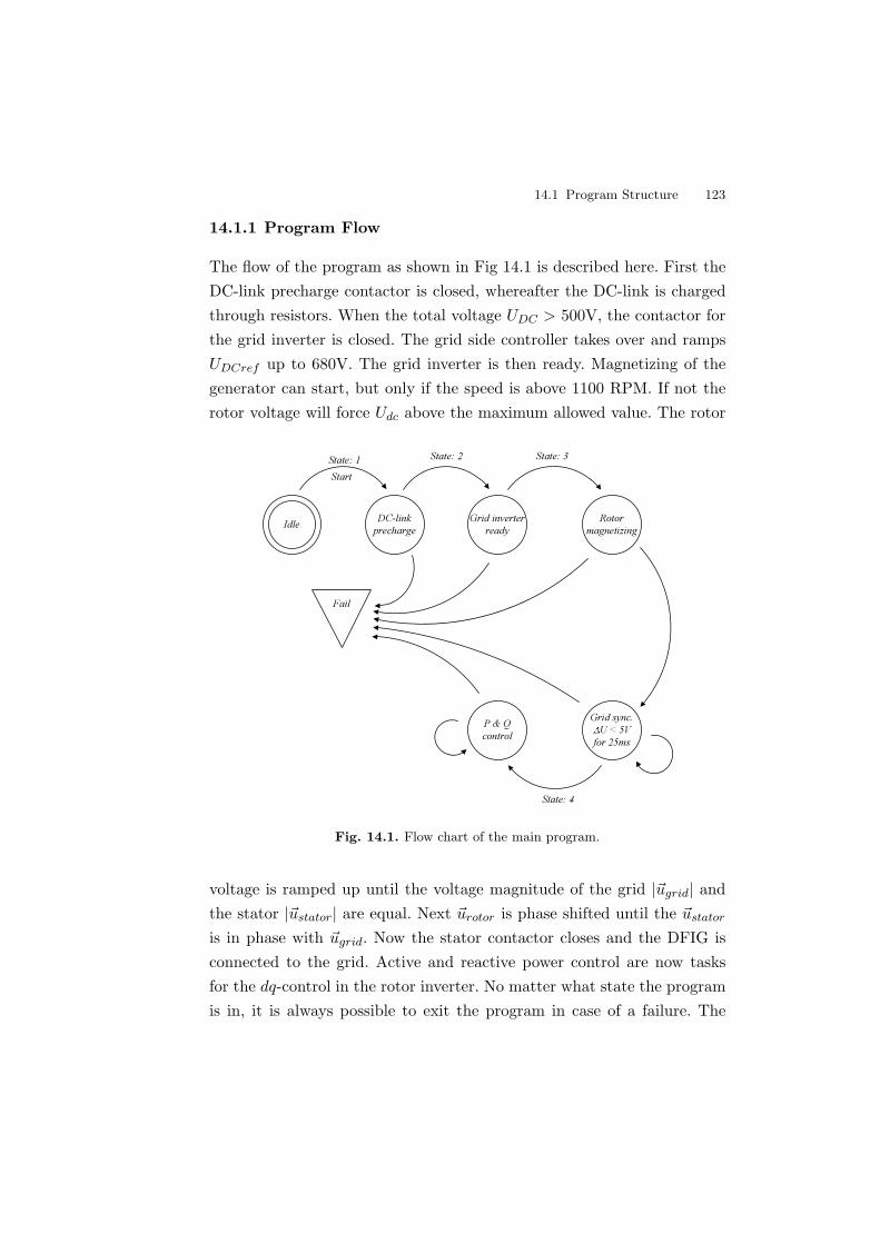
14.1 Program Structure 123
14.1.1 Program Flow
The flow of the program as shown in Fig 14.1 is described here. First theDC-link precharge contactor is closed, whereafter the DC-link is chargedthrough resistors. When the total voltage UDC > 500V, the contactor forthe grid inverter is closed. The grid side controller takes over and rampsUDCref up to 680V. The grid inverter is then ready. Magnetizing of thegenerator can start, but only if the speed is above 1100 RPM. If not therotor voltage will force Udc above the maximum allowed value. The rotor
Idle DC-linkprecharge
Grid inverterready
Rotormagnetizing
Grid sync.U < 5V
for 25ms
P & Qcontrol
Fail
State: 1Start
State: 2 State: 3
State: 4
Fig. 14.1. Flow chart of the main program.
voltage is ramped up until the voltage magnitude of the grid |~ugrid| andthe stator |~ustator| are equal. Next ~urotor is phase shifted until the ~ustator
is in phase with ~ugrid. Now the stator contactor closes and the DFIG isconnected to the grid. Active and reactive power control are now tasksfor the dq-control in the rotor inverter. No matter what state the programis in, it is always possible to exit the program in case of a failure. The

124 14 Software
four input flags wired to push buttons are used for changing variables, e.g.control references Ps−ref .
A set of ten parameter is logged at the end of the program function andthe data are stored in SDRAM on the EZ-LAB board. The parametersare logged for the final four seconds before program termination. Many ofthe results presented in the next chapter were measured in this way.
14.2 Controller Dynamics
All the controllers implemented in the software are PI-controllers (Proportional-integral). The controller consists of a gain and an integrator, the last inorder to avoid stationary errors. There is no derivative element since thatwould amplify the disturbances, such as higher harmonics and quantiza-tion noise.
The transfer function for the PI-controller is [71]
D(z) = K
(1 + Ts
2τ i
)−
(1− Ts
2τ i
)z−1
1− z−1(14.1)
It has a pole at zp = 1 and a zero at zz ' 1− Tsτ i
Equation 14.1 can be changed to:
D(z) = K
((1 +
Ts
2τ i
)+
1τ i· Tsz
−1
1− z−1
)(14.2)
The PI controllers are implemented as functions, using two arguments:the error and a structure with the parameters and the integral value [72].
14.3 Digital Filters
Two types of filters are used in the software. As mentioned on p28 theHilbert filters used to extract the postitve sequence of the voltage signalsare implemented as high order FIR filters . The FIR filter can be used asa standard function by this expression
Vabch[0] = fir(Vabc[0], hilbert_coeffs, hilbert_states0, 401);
14.4 Space Vector Modulation 125
The coefficients are saved in the second argument and the filter statesin the third argument. In order to get unity gain at 50Hz, a 400th orderfilter is used.
The other type of filters used are the IIR filters. A set of 4th order lowpass Butterworth filters with different cut off frequencies are implemented.Again here a standard function is used
omega_r=iir(omega_r,a_100_4,b_100_4,encoder_states,4);
The IIR filter uses both numerator and denominator coefficient.In the initial programming phase of the project, most of the measure-
ments where filtered through one of these Butterworth filters. The resultwas slow response time and problems with the control system. At theend, the filters were only used at two incidents: To filter the speed signal,here a 100 Hz filter was used, and to filter grid and stator voltages in thesynchronous rotating reference frame in order to make synchronization.The stator voltage signals are only used for synchronization, and the gridvoltage signal are not used filtered in the control loop.
The use of digital filters is convenient, but with a setup where thesignals are sampled with the same frequency as the switch frequency, theeffect is limited.
14.4 Space Vector Modulation
The software implementation of the space vector modulation is done inthe same way as it was described functionally in chapter 8.
Both timers are used, one for each converter. There is only one highpriority timer interrupt, and both timers are set to trigger the high timerinterrrupt. A sticky bit in the CNT EXP0 register in the DSP is eitherset or cleared depending on which timer ended. This bit can then be readto detect which timer ended.

126 14 Software
14.5 Neutral Point Balancing
The neutral point balancing algorithm is used in both the grid side andthe rotor side inverter, except during some specific measurements. Thefourth digit in the switch vector table, column five, in Appendix B storesthe information about which phase the neutral point current comes from.The following code is used to select the right switch vector in order tominimize DC neutral point variations,
for (i=0; i<=2; i++)
..
NP = states[u0[i]]>>12;//shifts to extract NP curr.
if (NPL > 0 )
if ((NP == 1) & (In[2] < 0)) u0[i]=u0[i]+4;
else if ((NP == 2) & (In[0] < 0)) u0[i]=u0[i]+4;
else if ((NP == 3) & (In[1] < 0)) u0[i]=u0[i]+4;
else if (NPL < 0 )
if ((NP == 1) & (In[2] > 0)) u0[i]=u0[i]+4;
else if ((NP == 2) & (In[0] > 0)) u0[i]=u0[i]+4;
else if ((NP == 3) & (In[1] > 0)) u0[i]=u0[i]+4;
The code shown above is for the grid side inverter, but the rotor sidecode is identical.

15
Measurements
In this chapter, the measurements made on the laboratory model are pre-sented. As already mentioned, the DSP are programmed to log ten vari-ables for four seconds, or fewer variables for a longer time period. Thisfunction was widely used to get data for documentation. It was also usefulin the debugging phase. Other measurements were made using an oscillo-scope, and some with a power analyzer. The measurements were made attwo locations.
The first location was at the Technical University of Denmark in Lyn-gby. Here the THDvoltage was equal to 4-5% during most of the time themeasurements were captured. The voltage harmonics were mainly 5th,7th, 11th and 13th.
The second location was in Hammel, Denmark at NEG Micon ControlSystems. The THDvoltage was about 0.5% during measurements. Also herethe distortion was due to 5th, 7th, 11th and 13th harmonics. The mea-surements were taken before the laboratory equipment was connected tothe grid.
Since the grid in Hammel was so much better, I hoped this would yieldmeasurements with a really low distortion in the current. In reality thelaboratory setup performed in almost the same way in Hammel as it haddone in Lyngby. The setup was moved to Hammel at the end of the projectperiod, because the laboratory setup was financed by NEG Micon ControlSystems. Most of the figures presented in this chapter and also previous

128 15 Measurements
chapters are showing measurements from Lyngby. If a Figure show datafrom Hammel, it is stated.
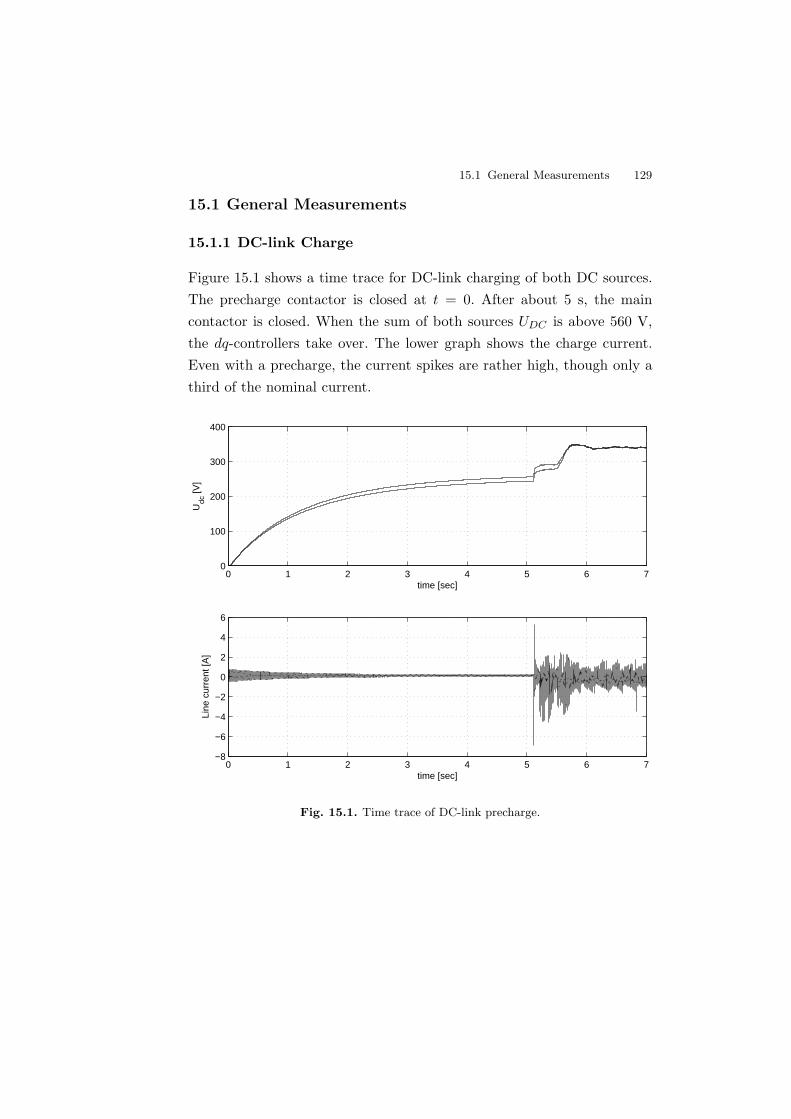
15.1 General Measurements 129
15.1 General Measurements
15.1.1 DC-link Charge
Figure 15.1 shows a time trace for DC-link charging of both DC sources.The precharge contactor is closed at t = 0. After about 5 s, the maincontactor is closed. When the sum of both sources UDC is above 560 V,the dq-controllers take over. The lower graph shows the charge current.Even with a precharge, the current spikes are rather high, though only athird of the nominal current.
0 1 2 3 4 5 6 70
100
200
300
400
time [sec]
Udc
[V]
0 1 2 3 4 5 6 7−8
−6
−4
−2
0
2
4
6
time [sec]
Line
cur
rent
[A]
Fig. 15.1. Time trace of DC-link precharge.
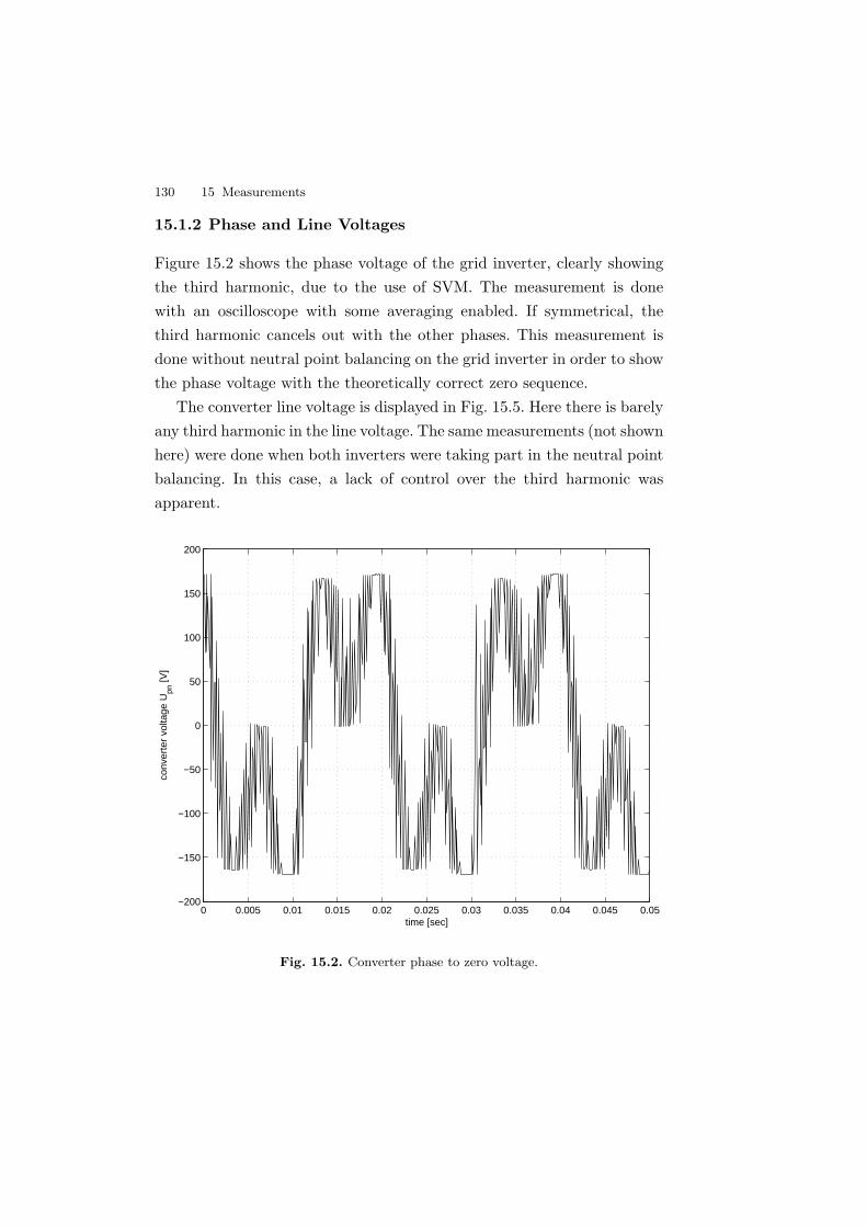
130 15 Measurements
15.1.2 Phase and Line Voltages
Figure 15.2 shows the phase voltage of the grid inverter, clearly showingthe third harmonic, due to the use of SVM. The measurement is donewith an oscilloscope with some averaging enabled. If symmetrical, thethird harmonic cancels out with the other phases. This measurement isdone without neutral point balancing on the grid inverter in order to showthe phase voltage with the theoretically correct zero sequence.
The converter line voltage is displayed in Fig. 15.5. Here there is barelyany third harmonic in the line voltage. The same measurements (not shownhere) were done when both inverters were taking part in the neutral pointbalancing. In this case, a lack of control over the third harmonic wasapparent.
0 0.005 0.01 0.015 0.02 0.025 0.03 0.035 0.04 0.045 0.05−200
−150
−100
−50
0
50
100
150
200
time [sec]
conv
erte
r vo
ltage
Upn
[V]
Fig. 15.2. Converter phase to zero voltage.
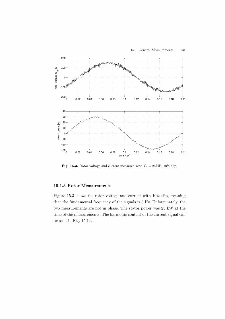
15.1 General Measurements 131
0 0.02 0.04 0.06 0.08 0.1 0.12 0.14 0.16 0.18 0.2−200
−100
0
100
200ro
tor
volta
ge U
pp [V
]
0 0.02 0.04 0.06 0.08 0.1 0.12 0.14 0.16 0.18 0.2−30
−20
−10
0
10
20
30
40
time [sec]
roto
r cu
rren
t [A
]
Fig. 15.3. Rotor voltage and current measured with Ps = 25kW , 10% slip.
15.1.3 Rotor Measurements
Figure 15.3 shows the rotor voltage and current with 10% slip, meaningthat the fundamental frequency of the signals is 5 Hz. Unfortunately, thetwo measurements are not in phase. The stator power was 25 kW at thetime of the measurements. The harmonic content of the current signal canbe seen in Fig. 15.14.
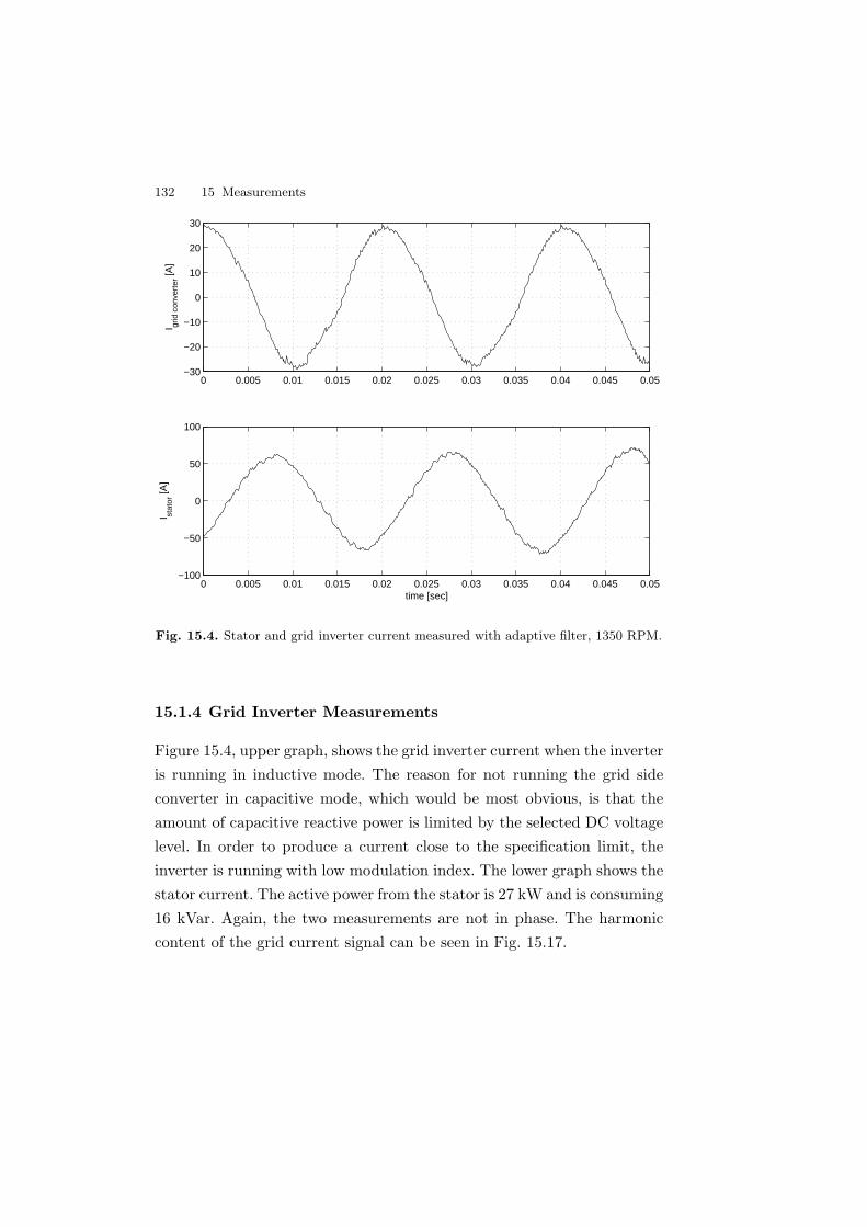
132 15 Measurements
0 0.005 0.01 0.015 0.02 0.025 0.03 0.035 0.04 0.045 0.05−30
−20
−10
0
10
20
30
I grid
con
vert
er [A
]
0 0.005 0.01 0.015 0.02 0.025 0.03 0.035 0.04 0.045 0.05−100
−50
0
50
100
time [sec]
I stat
or [A
]
Fig. 15.4. Stator and grid inverter current measured with adaptive filter, 1350 RPM.
15.1.4 Grid Inverter Measurements
Figure 15.4, upper graph, shows the grid inverter current when the inverteris running in inductive mode. The reason for not running the grid sideconverter in capacitive mode, which would be most obvious, is that theamount of capacitive reactive power is limited by the selected DC voltagelevel. In order to produce a current close to the specification limit, theinverter is running with low modulation index. The lower graph shows thestator current. The active power from the stator is 27 kW and is consuming16 kVar. Again, the two measurements are not in phase. The harmoniccontent of the grid current signal can be seen in Fig. 15.17.
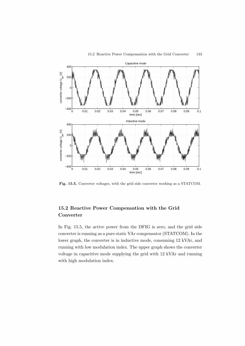
15.2 Reactive Power Compensation with the Grid Converter 133
0 0.01 0.02 0.03 0.04 0.05 0.06 0.07 0.08 0.09 0.1−400
−200
0
200
400
time [sec]
conv
erte
r vo
ltage
Upp
[V]
Capacitive mode
0 0.01 0.02 0.03 0.04 0.05 0.06 0.07 0.08 0.09 0.1−400
−200
0
200
400
time [sec]
conv
erte
r vo
ltage
Upp
[V]
Inductive mode
Fig. 15.5. Converter voltages, with the grid side converter working as a STATCOM.
15.2 Reactive Power Compensation with the Grid
Converter
In Fig. 15.5, the active power from the DFIG is zero, and the grid sideconverter is running as a pure static VAr compensator (STATCOM). In thelower graph, the converter is in inductive mode, consuming 12 kVAr, andrunning with low modulation index. The upper graph shows the convertervoltage in capacitive mode supplying the grid with 12 kVAr and runningwith high modulation index.
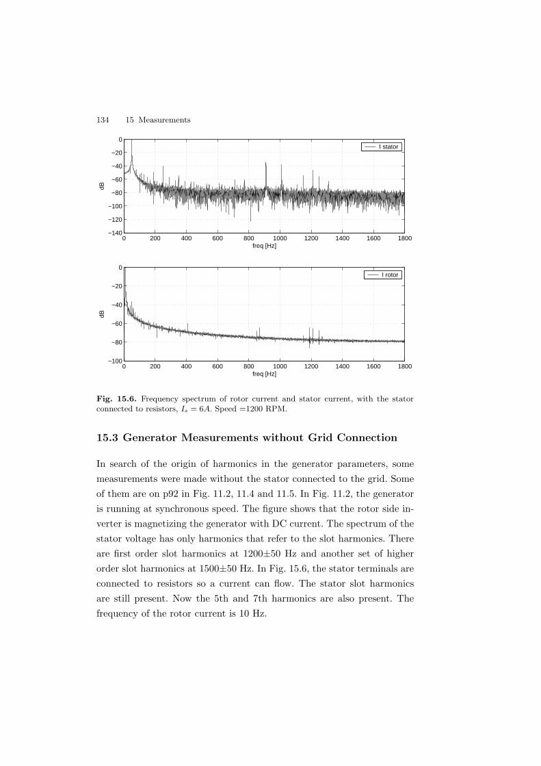
134 15 Measurements
0 200 400 600 800 1000 1200 1400 1600 1800−140
−120
−100
−80
−60
−40
−20
0
freq [Hz]
dB
0 200 400 600 800 1000 1200 1400 1600 1800−100
−80
−60
−40
−20
0
freq [Hz]
dB
I stator
I rotor
Fig. 15.6. Frequency spectrum of rotor current and stator current, with the statorconnected to resistors, Is = 6A. Speed =1200 RPM.
15.3 Generator Measurements without Grid Connection
In search of the origin of harmonics in the generator parameters, somemeasurements were made without the stator connected to the grid. Someof them are on p92 in Fig. 11.2, 11.4 and 11.5. In Fig. 11.2, the generatoris running at synchronous speed. The figure shows that the rotor side in-verter is magnetizing the generator with DC current. The spectrum of thestator voltage has only harmonics that refer to the slot harmonics. Thereare first order slot harmonics at 1200±50 Hz and another set of higherorder slot harmonics at 1500±50 Hz. In Fig. 15.6, the stator terminals areconnected to resistors so a current can flow. The stator slot harmonicsare still present. Now the 5th and 7th harmonics are also present. Thefrequency of the rotor current is 10 Hz.
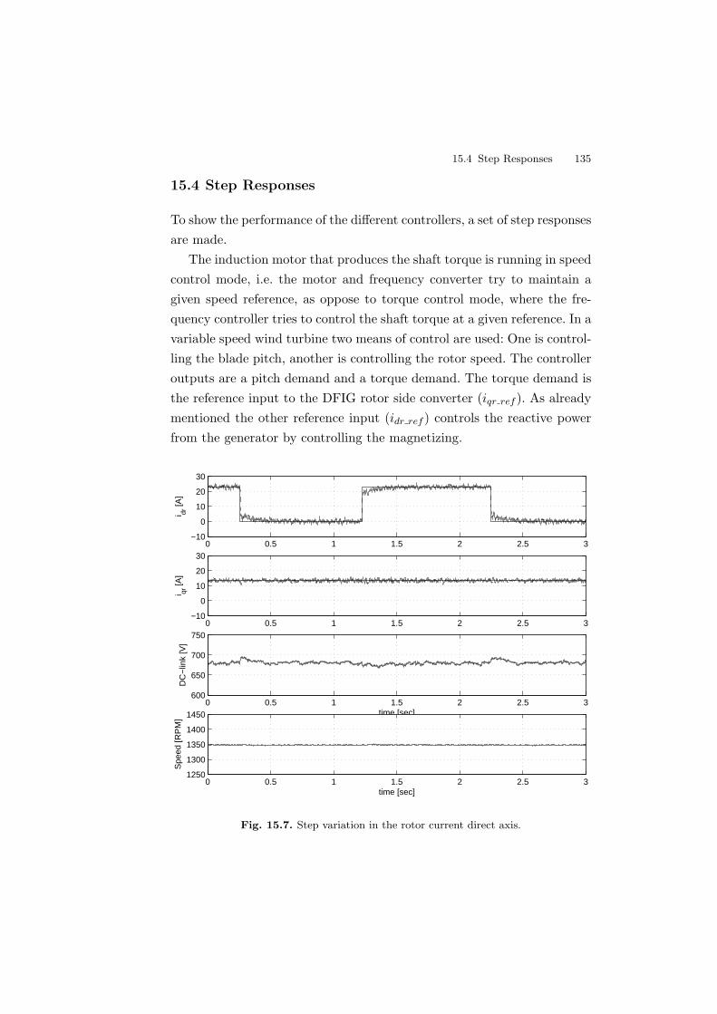
15.4 Step Responses 135
15.4 Step Responses
To show the performance of the different controllers, a set of step responsesare made.
The induction motor that produces the shaft torque is running in speedcontrol mode, i.e. the motor and frequency converter try to maintain agiven speed reference, as oppose to torque control mode, where the fre-quency controller tries to control the shaft torque at a given reference. In avariable speed wind turbine two means of control are used: One is control-ling the blade pitch, another is controlling the rotor speed. The controlleroutputs are a pitch demand and a torque demand. The torque demand isthe reference input to the DFIG rotor side converter (iqr ref ). As alreadymentioned the other reference input (idr ref ) controls the reactive powerfrom the generator by controlling the magnetizing.
0 0.5 1 1.5 2 2.5 3−10
0
10
20
30
i dr [A
]
0 0.5 1 1.5 2 2.5 3−10
0
10
20
30
i qr [A
]
0 0.5 1 1.5 2 2.5 3600
650
700
750
time [sec]
DC
−lin
k [V
]
0 0.5 1 1.5 2 2.5 31250
1300
1350
1400
1450
time [sec]
Spe
ed [R
PM
]
Fig. 15.7. Step variation in the rotor current direct axis.
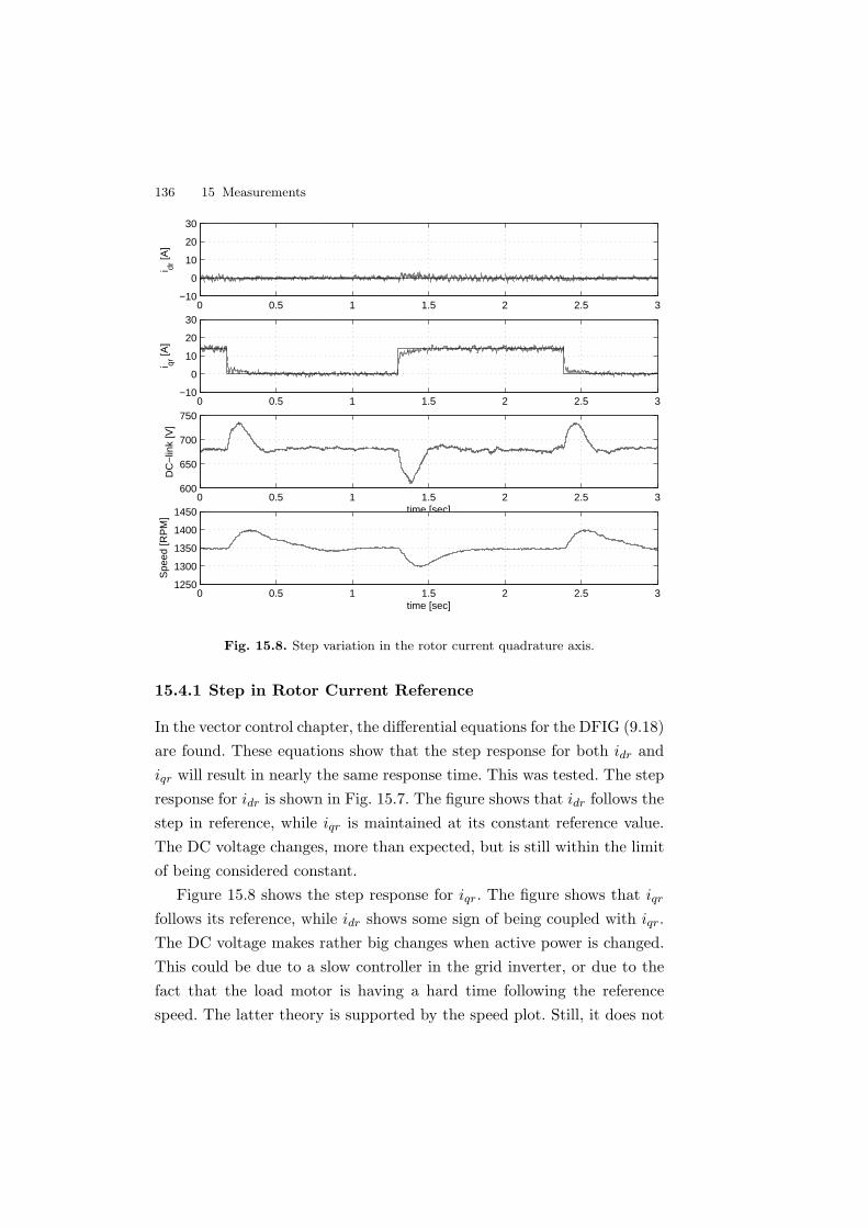
136 15 Measurements
0 0.5 1 1.5 2 2.5 3−10
0
10
20
30
i dr [A
]
0 0.5 1 1.5 2 2.5 3−10
0
10
20
30
i qr [A
]
0 0.5 1 1.5 2 2.5 3600
650
700
750
time [sec]
DC
−lin
k [V
]
0 0.5 1 1.5 2 2.5 31250
1300
1350
1400
1450
time [sec]
Spe
ed [R
PM
]
Fig. 15.8. Step variation in the rotor current quadrature axis.
15.4.1 Step in Rotor Current Reference
In the vector control chapter, the differential equations for the DFIG (9.18)are found. These equations show that the step response for both idr andiqr will result in nearly the same response time. This was tested. The stepresponse for idr is shown in Fig. 15.7. The figure shows that idr follows thestep in reference, while iqr is maintained at its constant reference value.The DC voltage changes, more than expected, but is still within the limitof being considered constant.
Figure 15.8 shows the step response for iqr. The figure shows that iqr
follows its reference, while idr shows some sign of being coupled with iqr.The DC voltage makes rather big changes when active power is changed.This could be due to a slow controller in the grid inverter, or due to thefact that the load motor is having a hard time following the referencespeed. The latter theory is supported by the speed plot. Still, it does not
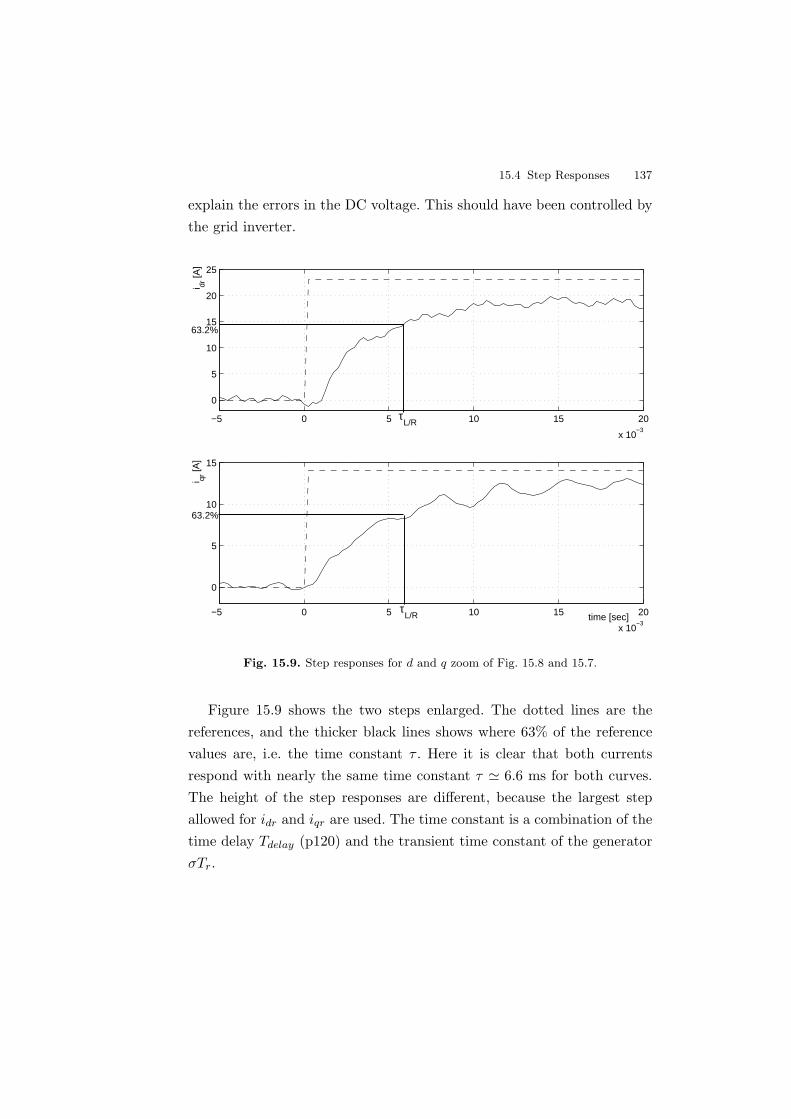
15.4 Step Responses 137
explain the errors in the DC voltage. This should have been controlled bythe grid inverter.
−5 0 5 10 15 20
x 10−3
0
5
10
15
20
25
i dr [A
]
−5 0 5 10 15 20
x 10−3
0
5
10
15
time [sec]
i qr [A
]
63.2%
63.2%
τL/R
τL/R
Fig. 15.9. Step responses for d and q zoom of Fig. 15.8 and 15.7.
Figure 15.9 shows the two steps enlarged. The dotted lines are thereferences, and the thicker black lines shows where 63% of the referencevalues are, i.e. the time constant τ . Here it is clear that both currentsrespond with nearly the same time constant τ ' 6.6 ms for both curves.The height of the step responses are different, because the largest stepallowed for idr and iqr are used. The time constant is a combination of thetime delay Tdelay (p120) and the transient time constant of the generatorσTr.
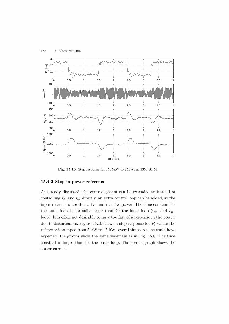
138 15 Measurements
0 0.5 1 1.5 2 2.5 3 3.5 4600
650
700
750
UD
C [v
]
0 0.5 1 1.5 2 2.5 3 3.5 41300
1350
1400
time [sec]
Spe
ed [R
PM
]
0 0.5 1 1.5 2 2.5 3 3.5 40
10
20
30
Ps [k
W]
0 0.5 1 1.5 2 2.5 3 3.5 4−100
0
100
I stat
or [A
]
Fig. 15.10. Step response for Ps, 5kW to 25kW, at 1350 RPM.
15.4.2 Step in power reference
As already discussed, the control system can be extended so instead ofcontrolling idr and iqr directly, an extra control loop can be added, so theinput references are the active and reactive power. The time constant forthe outer loop is normally larger than for the inner loop (idr- and iqr-loop). It is often not desirable to have too fast of a response in the power,due to disturbances. Figure 15.10 shows a step response for Ps where thereference is stepped from 5 kW to 25 kW several times. As one could haveexpected, the graphs show the same weakness as in Fig. 15.8. The timeconstant is larger than for the outer loop. The second graph shows thestator current.
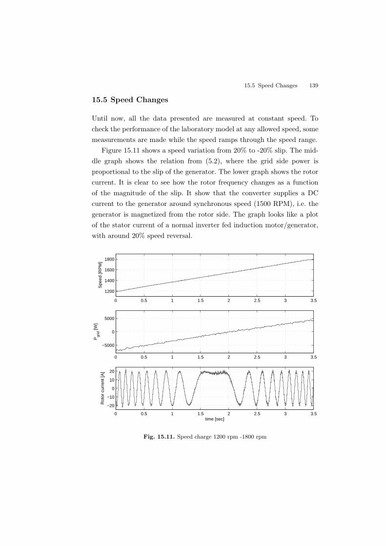
15.5 Speed Changes 139
15.5 Speed Changes
Until now, all the data presented are measured at constant speed. Tocheck the performance of the laboratory model at any allowed speed, somemeasurements are made while the speed ramps through the speed range.
Figure 15.11 shows a speed variation from 20% to -20% slip. The mid-dle graph shows the relation from (5.2), where the grid side power isproportional to the slip of the generator. The lower graph shows the rotorcurrent. It is clear to see how the rotor frequency changes as a functionof the magnitude of the slip. It show that the converter supplies a DCcurrent to the generator around synchronous speed (1500 RPM), i.e. thegenerator is magnetized from the rotor side. The graph looks like a plotof the stator current of a normal inverter fed induction motor/generator,with around 20% speed reversal.
0 0.5 1 1.5 2 2.5 3 3.5
1200
1400
1600
1800
Spe
ed [R
PM
]
0 0.5 1 1.5 2 2.5 3 3.5
−5000
0
5000
Pgr
id [W
]
0 0.5 1 1.5 2 2.5 3 3.5
−20
−10
0
10
20
time [sec]
Rot
or c
urre
nt [A
]
Fig. 15.11. Speed charge 1200 rpm -1800 rpm
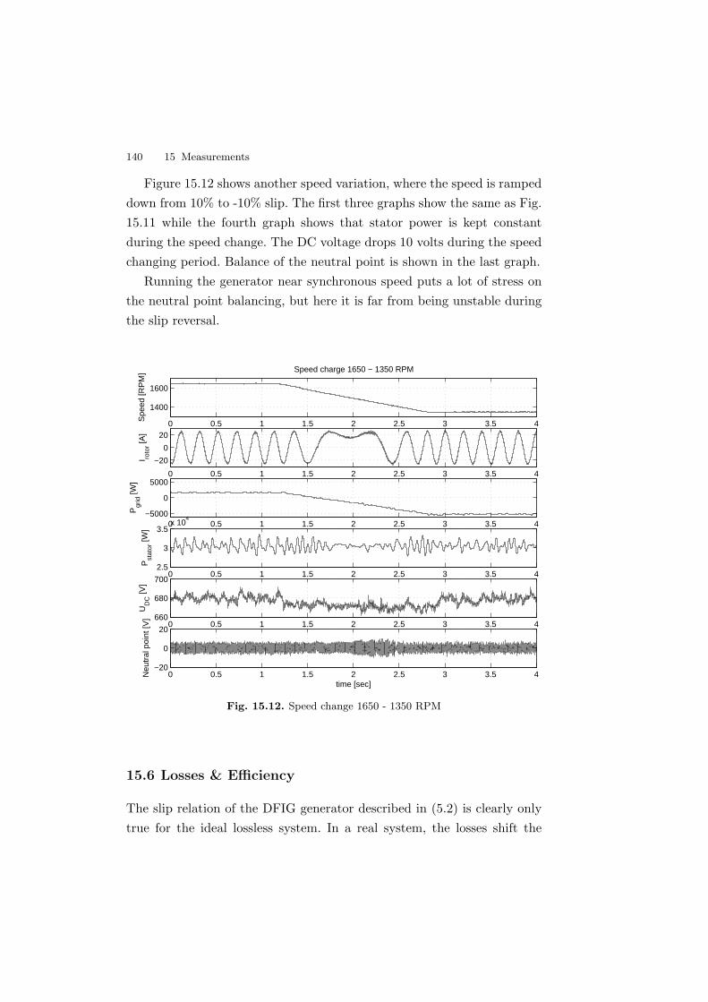
140 15 Measurements
Figure 15.12 shows another speed variation, where the speed is rampeddown from 10% to -10% slip. The first three graphs show the same as Fig.15.11 while the fourth graph shows that stator power is kept constantduring the speed change. The DC voltage drops 10 volts during the speedchanging period. Balance of the neutral point is shown in the last graph.
Running the generator near synchronous speed puts a lot of stress onthe neutral point balancing, but here it is far from being unstable duringthe slip reversal.
0 0.5 1 1.5 2 2.5 3 3.5 4
1400
1600
Speed charge 1650 − 1350 RPM
Spe
ed [R
PM
]
0 0.5 1 1.5 2 2.5 3 3.5 4
−20
0
20
I roto
r [A]
0 0.5 1 1.5 2 2.5 3 3.5 4−5000
0
5000
Pgr
id [W
]
0 0.5 1 1.5 2 2.5 3 3.5 42.5
3
3.5x 10
4
Pst
ator
[W]
0 0.5 1 1.5 2 2.5 3 3.5 4660
680
700
time [sec]
UD
C [V
]
0 0.5 1 1.5 2 2.5 3 3.5 4−20
0
20
time [sec]
Neu
tral
poi
nt [V
]
Fig. 15.12. Speed change 1650 - 1350 RPM
15.6 Losses & Efficiency
The slip relation of the DFIG generator described in (5.2) is clearly onlytrue for the ideal lossless system. In a real system, the losses shift the
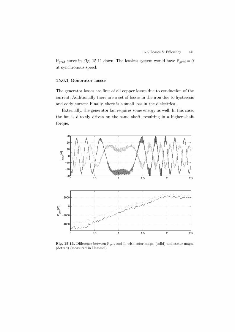
15.6 Losses & Efficiency 141
Pgrid curve in Fig. 15.11 down. The lossless system would have Pgrid = 0at synchronous speed.
15.6.1 Generator losses
The generator losses are first of all copper losses due to conduction of thecurrent. Additionally there are a set of losses in the iron due to hysteresisand eddy current Finally, there is a small loss in the dielectrica.
Externally, the generator fan requires some energy as well. In this case,the fan is directly driven on the same shaft, resulting in a higher shafttorque.
0 0.5 1 1.5 2 2.5
−4000
−2000
0
2000
Pgr
id [W
]
0 0.5 1 1.5 2 2.5−30
−20
−10
0
10
20
30
I roto
r [A]
Fig. 15.13. Difference between Pgrid and Ir with rotor magn. (solid) and stator magn.(dotted) (measured in Hammel)

142 15 Measurements
15.6.2 Converter losses
The direct converter losses can be grouped into switching and conductionlosses. The indirect losses are due to losses in the DC-link and the filterinductors.
The conduction loss for an IGBT is given by
Pconduction = IC avUCE + I2C rmsRCE (15.1)
Similar expressions can be found for free wheeling and clamp diodes bysubstituting the appropriate values.
The switching losses are the product of the actual energy loss of eachon and off switching multiplied by the switching frequency
Pswitch = (Eon + Eoff )fsw (15.2)
The efficiency of the converters is measured with a power analyzer(Voltech PM3000). With a load of 2-4 kVA, the efficiency is around 96%from the DC-link to either side AC. The total losses in the back to backare about 8% of the total apparent power.
15.6.3 Rough explanation of the losses
The study of the losses for this DFIG system is performed in order toshow that the slip relation (5.2) is only valid for an ideal lossless sys-tem. Performing an accurate study of the losses for this system would notcontribute to the understanding of the DFIG system, it would only be atedious process.
Some of the losses can be clarified by using two sets of measurements.One with the generator magnetized from the stator and one where mag-netizing comes from the rotor. By doing so, the rotor winding in the firstcase will only have to carry the current from the active slip power, whereasin the second case, the winding will carry a much larger current. Figure15.13 shows how Pgrid shifts depending on where magnetizing of the gen-erator comes from. The measurements are similar to Fig. 15.12, but withincreasing speed instead. The entire set of measurements are to be found
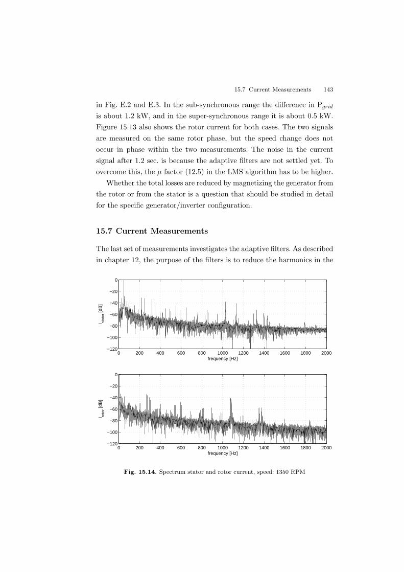
15.7 Current Measurements 143
in Fig. E.2 and E.3. In the sub-synchronous range the difference in Pgrid
is about 1.2 kW, and in the super-synchronous range it is about 0.5 kW.Figure 15.13 also shows the rotor current for both cases. The two signalsare measured on the same rotor phase, but the speed change does notoccur in phase within the two measurements. The noise in the currentsignal after 1.2 sec. is because the adaptive filters are not settled yet. Toovercome this, the µ factor (12.5) in the LMS algorithm has to be higher.
Whether the total losses are reduced by magnetizing the generator fromthe rotor or from the stator is a question that should be studied in detailfor the specific generator/inverter configuration.
15.7 Current Measurements
The last set of measurements investigates the adaptive filters. As describedin chapter 12, the purpose of the filters is to reduce the harmonics in the
0 200 400 600 800 1000 1200 1400 1600 1800 2000−120
−100
−80
−60
−40
−20
0
frequency [Hz]
I stat
or [d
B]
0 200 400 600 800 1000 1200 1400 1600 1800 2000−120
−100
−80
−60
−40
−20
0
frequency [Hz]
I roto
r [dB
]
Fig. 15.14. Spectrum stator and rotor current, speed: 1350 RPM
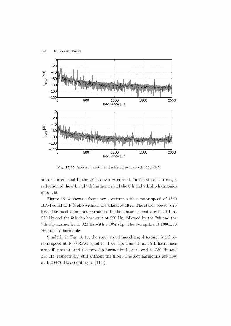
144 15 Measurements
0 500 1000 1500 2000−120
−100
−80
−60
−40
−20
0
frequency [Hz]
I stat
or [d
B]
0 500 1000 1500 2000−120
−100
−80
−60
−40
−20
0
frequency [Hz]
I roto
r [dB
]
Fig. 15.15. Spectrum stator and rotor current, speed: 1650 RPM
stator current and in the grid converter current. In the stator current, areduction of the 5th and 7th harmonics and the 5th and 7th slip harmonicsis sought.
Figure 15.14 shows a frequency spectrum with a rotor speed of 1350RPM equal to 10% slip without the adaptive filter. The stator power is 25kW. The most dominant harmonics in the stator current are the 5th at250 Hz and the 5th slip harmonic at 220 Hz, followed by the 7th and the7th slip harmonics at 320 Hz with a 10% slip. The two spikes at 1080±50Hz are slot harmonics.
Similarly in Fig. 15.15, the rotor speed has changed to supersynchro-nous speed at 1650 RPM equal to -10% slip. The 5th and 7th harmonicsare still present, and the two slip harmonics have moved to 280 Hz and380 Hz, respectively, still without the filter. The slot harmonics are nowat 1320±50 Hz according to (11.3).
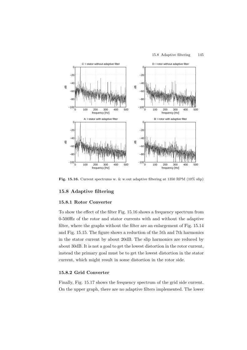
15.8 Adaptive filtering 145
0 100 200 300 400 500−100
−80
−60
−40
−20
0A: I stator with adaptive filter
frequency [Hz]
dB
0 100 200 300 400 500−100
−80
−60
−40
−20
0B: I rotor with adaptive filter
frequency [Hz]
dB
0 100 200 300 400 500−100
−80
−60
−40
−20
0C: I stator without adaptive filter
frequency [Hz]
dB
0 100 200 300 400 500−100
−80
−60
−40
−20
0D: I rotor without adaptive filter
frequency [Hz]
dB
Fig. 15.16. Current spectrums w. & w.out adaptive filtering at 1350 RPM (10% slip)
15.8 Adaptive filtering
15.8.1 Rotor Converter
To show the effect of the filter Fig. 15.16 shows a frequency spectrum from0-500Hz of the rotor and stator currents with and without the adaptivefilter, where the graphs without the filter are an enlargement of Fig. 15.14and Fig. 15.15. The figure shows a reduction of the 5th and 7th harmonicsin the stator current by about 20dB. The slip harmonics are reduced byabout 30dB. It is not a goal to get the lowest distortion in the rotor current,instead the primary goal must be to get the lowest distortion in the statorcurrent, which might result in some distortion in the rotor side.
15.8.2 Grid Converter
Finally, Fig. 15.17 shows the frequency spectrum of the grid side current.On the upper graph, there are no adaptive filters implemented. The lower
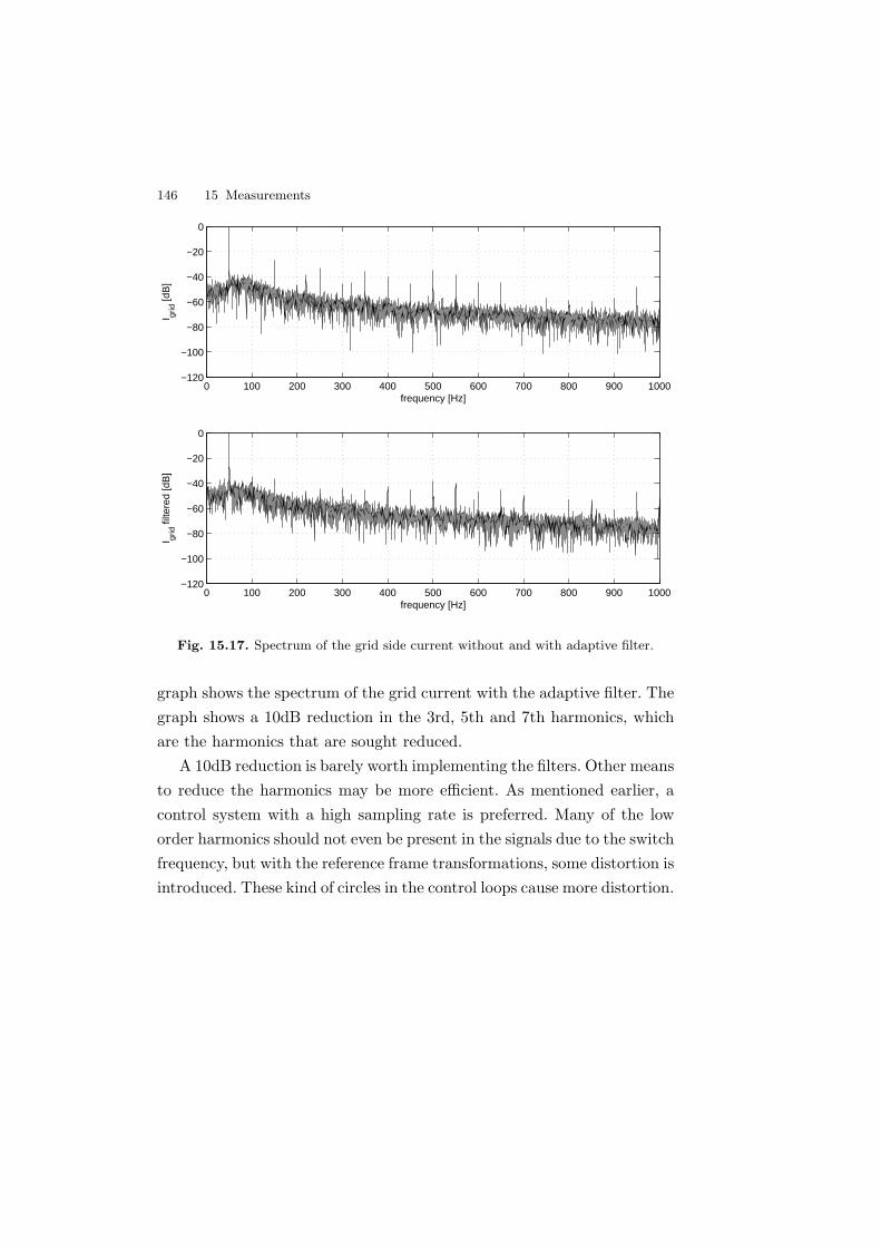
146 15 Measurements
0 100 200 300 400 500 600 700 800 900 1000−120
−100
−80
−60
−40
−20
0
frequency [Hz]
I grid
[dB
]
0 100 200 300 400 500 600 700 800 900 1000−120
−100
−80
−60
−40
−20
0
frequency [Hz]
I grid
filte
red
[dB
]
Fig. 15.17. Spectrum of the grid side current without and with adaptive filter.
graph shows the spectrum of the grid current with the adaptive filter. Thegraph shows a 10dB reduction in the 3rd, 5th and 7th harmonics, whichare the harmonics that are sought reduced.
A 10dB reduction is barely worth implementing the filters. Other meansto reduce the harmonics may be more efficient. As mentioned earlier, acontrol system with a high sampling rate is preferred. Many of the loworder harmonics should not even be present in the signals due to the switchfrequency, but with the reference frame transformations, some distortion isintroduced. These kind of circles in the control loops cause more distortion.

16
Conclusion
In this thesis, control of a doubly fed induction generator has been in-vestigated. In order to do so, a full scaled running laboratory model hasbeen implemented. A back to back 3-level NPC inverter with space vectormodulation is implemented together with the generator.
DC-link balancing, where zero sequence injects into the voltage of ei-ther one or both inverters, results in uncontrolled 3rd harmonics. Thatfact makes multilevel inverters less attractive for use together with DFIGmachines, since zero sequence injected at the rotor side becomes presentat the stator side.
Using the same sampling and switch frequency makes it difficult to usedigital filters in the software, due to delays in the filters.
Proof and verification, that the transient time constant, σTr for boththe direct and quadrature current is the same, are presented. This makesit possible to change the flow of reactive power from the generator as fastas the active power flow.
Adaptive active filters are used to reduce harmonics in the stator cur-rent and in the grid side inverter current. A method for using the rotorside inverter to reduce stator harmonics has been presented, and verifiedexperimentally. The method gives an easy and reliable way to eliminate orreduce harmonics from the DFIG generator. Even the slip harmonics thatvaries in frequency was reduced. The implementation of the adaptive filterin the rotor side converter gives a fairly good reduction in the harmonicfrequencies applied.

148 16 Conclusion
Further Research
The topics in the thesis are not at all a complete coverage of the fieldof DFIG generator systems for wind turbine applications. There are stillmany topics to do further work on, a few of them are listed below.
Sensorless Control
The use of an encoder or other types of position sensors causes alwaysa risk of some mechanical failure. Therefore sensorless control would bedesirable. During start-up, some problems could occur with sensorless con-trol due to lack of information.
Grid Faults
How the wind turbines react during grid faults is one of the most importantquestions to be answered. The demands from the utility companies aremoving towards a situation where the turbines must stay connected tothe grid no matter what happens on the grid.
Crowbar
During grid faults, some sort of equipment is required to get rid of theenergy stored in the generator. This can be a thyristor-controlled crowbaror a switched crowbar using IGBTs. It is important that the crowbar isfast and reliable.
References
[1] S. Heier, Grid Integration of Wind Energy Conversion Systems, JohnWiley Sons, 1998.
[2] Marian P. Kazmierkowski, R. Krishnan, and Frede Blaabjerg, Controlin Power Electronics, Academic Press, 2002.
[3] Ned Mohan, Tore M. Undeland, and William P. Robbins, PowerElectronics: Converters, Applications and Design, Wiley, 2nd edition,1995.
[4] G. F. Franklin, J. D. Powell, and A Emami-Naeini, Feedback Controlof Dynamic Systems, Addison-Wesley, 2nd edition, 1991.
[5] W. Leonhard, Control of Electrical Drives, Springer Verlag, 2ndedition, 1997.
[6] Bent Rasmussen and Flemming Øster, “Power production from thewind”, in Wind Energy in Denmark, research and technological de-velopment, 1990.
[7] Per Lundsager Helge Petersen Peter S. Andersen, Ulrik Krabbe, Ba-sismateriale for Beregning af Propelvindmller, Forsøgsanlæg Risø,1980.
[8] E·on Netz GmbH, “Erganzende netzanschlussregeln fur winden-ergieanlagen”, 2001.
[9] International Electrotechnical Commision, “Iec 61400-21, wind tur-bine generator systems - part 21: Measurement and assessment ofpower quality characteristics of grid connected wind turbines”, Tech.Rep., IEC, 2000.
150 References
[10] Ake Larsson, The Power Quality of Wind Turbines, PhD thesis,Chalmers University of Technology, 2000.
[11] Ake Larsson, Poul Sørensen, and Fritz Santjer, “Grid impact ofvariable-speed wind turbines”, European Wind Energy Conference1999. Proceedings of the, 1999.
[12] J. Proakis and D. Manolakis, Digital Signal Processing, MacmillanPublishing Company, 2nd edition, 1992.
[13] B. Hopfensperger and D.J. Atkinson, “Doubly-fed a.c. machines: clas-sification and comparison”, 9th European Conference on Power Elec-tronics and Applications. EPE 2001, p. 17 pp., 2001.
[14] R. Pena, J.C. Clare, and G.M. Asher, “A doubly fed induction gen-erator using back-to-back pwm converters supplying an isolated loadfrom a variable speed wind turbine”, Electric Power Applications,IEE Proceedings-, vol. 143, no. 5, pp. 380–387, 1996.
[15] R. Pena, J.C. Clare, and G.M. Asher, “Doubly fed induction genera-tor using back-to-back pwm converters and its application to variable-speed wind-energy generation”, Electric Power Applications, IEEProceedings-, vol. 143, no. 3, pp. 231–241, 1996.
[16] R.S. Pena, R. Cardenas, G.M. Asher, and J.C. Clare, “Vector controlstrategy of a harmonic and reactive power compensator”, EPE’97.7th European Conference on Power Electronics and Applications, pp.848–53 vol.4, 1997.
[17] S. Muller, M. Deicke, and R.W. De Doncker, “Adjustable speed gen-erators for wind turbines based on doubly-fed induction machines and4-quadrant igbt converters linked to the rotor”, Conference Record ofthe 2000 IEEE Industry Applications Conference. Thirty-Fifth IASAnnual Meeting and World Conference on Industrial Applications ofElectrical Energy (Cat. No.00CH37129), pp. 2249–54 vol.4, 2000.
[18] B. Eggert, “1.5 mw wind power station with low ac-line distortionusing a standard doubly-fed generator system with field orientationcontrol”, EPE’97. 7th European Conference on Power Electronicsand Applications, pp. 739–42 vol.2, 1997.
[19] A.K. Wallace, R. Spee, and G.C. Alexander, “The brushless doubly-
References 151
fed machine: its advantages, applications and design methods”, Elec-trical Machines and Drives, 1993. Sixth International Conference on,pp. 511–517, 1993.
[20] L. Xu, F. Liang, and T.A. Lipo, “Transient model of a doubly excitedreluctance motor”, Energy Conversion, IEEE Transaction on, vol. 6,no. 1, pp. 126–133, 1991.
[21] P. C. Krause, Analysis of Electric Machinery and Drive Systems,Wiley Interscience, 2002.
[22] Peter Vas, Sensorless Vector and Direct Torque Control, OxfordUniversity Press, 1998.
[23] D. W. Novotny and T. A. Lipo, Vector Control and Dynamics of ACDrives, Oxford University Press, 1996.
[24] A. Zuckerberger, E. Suter, C. Schaub, A. Klett, and P. Steimer, “De-sign, simulation and realization of high power npc converters equippedwith igcts”, Industry Applications Conference, 1998. Thirty-ThirdIAS Annual Meeting. The 1998 IEEE, vol. 2, pp. 865 –872 vol.2,1998.
[25] Leon M. Tolbert and Fang Z. Peng, “Multilevel converters for largeelectric drives”, Conference Proceedings - IEEE Applied Power Elec-tronics Conference and Exposition - APEC, vol. 2, pp. 530–536, 1998.
[26] D.M. Divan, “The resonant dc link converter-a new concept in staticpower conversion”, Conference Record of the 1986 IEEE Industry Ap-plications Society Annual Meeting (Cat. No.86CH2272-3), pp. 648–56vol.1, 1986.
[27] Per Karlson, Quasi Resonant DC Link Converters, PhD thesis, LundInstitute of Technology, 1999.
[28] Fang Zheng Peng, Jih-Sheng Lai, J. McKeever, and J. VanCoever-ing, “A multilevel voltage-source inverter with separate dc sourcesfor static var generation”, Industry Applications Conference, 1995.Thirtieth IAS Annual Meeting, IAS ’95., Conference Record of the1995 IEEE, vol. 3, pp. 2541 –2548 vol.3, 1995.
[29] A. Nabae, I. Takahashi, and H. Akagi, “A new neutral point clampedpwm inverter”, IEEE Transactions on Industry Applications, vol.
152 References
IA-17, no. 5, pp. 518–23, 1981.[30] Xiaoming Yuan and I. Barbi, “A new diode clamping multilevel in-
verter”, Applied Power Electronics Conference and Exposition, 1999.APEC ’99. Fourteenth Annual, vol. 1, pp. 495–501 vol.1, 1999.
[31] T.A. Meynard and H. Foch, “Multi-level choppers for high voltageapplications”, EPE Journal, vol. 2, no. 1, pp. 45–50, 1992.
[32] M.D. Manjrekar and T.A. Lipo, “A hybrid multilevel inverter topol-ogy for drive applications”, Applied Power Electronics Conferenceand Exposition, 1998. APEC ’98. Conference Proceedings 1998.,Thirteenth Annual, vol. 2, pp. 523–529 vol.2, 1998.
[33] L. Helle and S. Munk-Nielsen, “Comparison of converter efficiency inlarge variable speed wind turbines”, APEC 2001. Sixteenth AnnualIEEE Applied Power Electronics Conference and Exposition (Cat.No.01CH37181), pp. 628–34 vol.1, 2001.
[34] O. Al-Naseem, R.W. Erickson, and P. Carlin, “Prediction of switchingloss variations by averaged switch modeling”, Applied Power Elec-tronics Conference and Exposition, 2000. APEC 2000. Fifteenth An-nual IEEE, vol. 1, pp. 242–248 vol.1, 2000.
[35] J. Holtz, “Pulsewidth modulation-a survey”, Industrial Electronics,IEEE Transactions on, vol. 39, no. 5, pp. 410–420, 1992.
[36] D.G. Holmes, “The general relationship between regular-sampledpulse-width-modulation and space vector modulation for hardswitched converters”, Industry Applications Society Annual Meet-ing, 1992., Conference Record of the 1992 IEEE, pp. 1002–1009 vol.1,1992.
[37] B.P. McGrath, D.G. Holmes, and T.A. Lipo, “Optimised space vectorswitching sequences for multilevel inverters”, Applied Power Electron-ics Conference and Exposition, 2001. APEC 2001. Sixteenth AnnualIEEE, vol. 2, pp. 1123–1129, 2001.
[38] A.M. Hava, R.J. Kerkman, and T.A. Lipo, “Simple analytical andgraphical methods for carrier-based pwm-vsi drives”, Power Elec-tronics, IEEE Transactions on, vol. 14, no. 1, pp. 49–61, 1999.
References 153
[39] A.M. Hava, R.J. Kerkman, and T.A. Lipo, “A high performance gen-eralized discontinuous pwm algorithm”, Applied Power ElectronicsConference and Exposition, 1997. APEC ’97 Conference Proceedings1997., Twelfth Annual, vol. 2, pp. 886–894 vol.2, 1997.
[40] N. Celanovic and D. Boroyevich, “A fast space-vector modulation al-gorithm for multilevel three-phase converters”, Industry Applications,IEEE Transactions on, vol. 37, no. 2, pp. 637–641, 2001.
[41] Nikola Celanovic, Space Vector Modulation and Control of Multi-level Converters, PhD thesis, Virginia Polytechnic Institute an StateUniversity, 2000.
[42] Dongsheng Zhou and D.G. Rouaud, “Experimental comparisons ofspace vector neutral point balancing strategies for three-level topol-ogy”, Power Electronics, IEEE Transactions on, vol. 16, no. 6, pp.872–879, 2001.
[43] F. Wang, “Coordinated control of regenerative three-level neutralpoint clamped pwm voltage source inverters”, Industry ApplicationsConference, 2002. 37th IAS Annual Meeting. Conference Record ofthe, vol. 1, pp. 537–543, 2002.
[44] Nikola Celanovic and Dusan Borojevic, “Comprehensive study ofneutral-point voltage balancing problem in three-level neutral-point-clamped voltage source pwm inverters”, Conference Proceedings -IEEE Applied Power Electronics Conference and Exposition - APEC,vol. 1, pp. 535–541, 1999.
[45] F. Wang, “Sine-triangle vs. space vector modulation for three-levelpwm voltage source inverters”, Conference Record of the 2000 IEEEIndustry Applications Conference. Thirty-Fifth IAS Annual Meetingand World Conference on Industrial Applications of Electrical Energy(Cat. No.00CH37129), pp. 2482–8 vol.4, 2000.
[46] S. Ogasawara and H. Akagi, “Analysis of variation of neutral pointpotential in neutral-point-clamped voltage source pwm inverters”,Industry Applications Society Annual Meeting, 1993., ConferenceRecord of the 1993 IEEE, pp. 965–970 vol.2, 1993.
[47] J Holtz, “Pulsewidth modulation for electronic power conversion (in-

154 References
vited paper)”, IEEE Proceedings, vol. 82, no. 8, pp. 1194–1214, 1994.[48] Dongsheng Zhou and D.G. Rouaud, “Dead-time effect and compensa-
tions of three-level neutral point clamp inverters for high-performancedrive applications”, Power Electronics, IEEE Transactions on, vol.14, no. 4, pp. 782–788, 1999.
[49] A.B. Plunkett, “A current-controlled pwm transistor inverter drive”,Industry Application Society IEEE-IAS Annual Meeting, pp. 785–92,1979.
[50] K. Hasse, “Speed control methods for fast-reversing drives usingcontrolled rectifier fed induction motors with squirrel-cage rotors”,Regelungstechnik und Prozess-Datenverarbeitung, vol. 20, no. 2, pp.60–6, 1972.
[51] F. Blaschke, “The principle of field orientation as applied to the newtransvektor closed-loop control system for rotating-field machines”,Siemens Review, vol. 39, no. 5, pp. 217–20, 1972.
[52] Morten Lindholm, “Digitalt reguleret reaktiv effekt kompensator”,Master’s thesis, Technical University of Denmark, 1997.
[53] M. Malinowski, M.P. Kazmierkowski, and A.M. Trzynadlowski, “Acomparative study of control techniques for pwm rectifiers in ac ad-justable speed drives”, Industrial Electronics Society, 2001. IECON’01. The 27th Annual Conference of the IEEE, vol. 2, pp. 1114–1118vol.2, 2001.
[54] Boon Teck Ooi and Bin Lu, “C-upfc: a new facts controller with 4degrees of freedom”, 2000 IEEE 31st Annual Power Electronics Spe-cialists Conference. Conference Proceedings (Cat. No.00CH37018),pp. 961–6 vol.2, 2000.
[55] Michael Lindgren, Modeling and Control of Voltage Source ConvertersConnected to the Grid, PhD thesis, Chalmers University of Technol-ogy, 1998.
[56] Martin Bojrup, Advanced Control of Active Filters in a BatteryCharger Application, PhD thesis, Lund Institute of Technology, 1999.
[57] Sang-Joon Lee, Jun-Koo Kang, and Seung-Ki Sul, “A new phasedetecting method for power conversion systems considering distorted
References 155
conditions in power system”, Industry Applications Conference, 1999.Thirty-Fourth IAS Annual Meeting. Conference Record of the 1999IEEE, vol. 4, pp. 2167–2172 vol.4, 1999.
[58] V. Kaura and V. Blasko, “Operation of a phase locked loop sys-tem under distorted utility conditions”, Industry Applications, IEEETransactions on, vol. 33, no. 1, pp. 58–63, 1997.
[59] Su Chen and G. Joos, “A novel dsp-based adaptive line synchro-nization system for three-phase utility interface power converters”,Power Electronics Specialists Conference, 2001. PESC. 2001 IEEE32nd Annual, vol. 2, pp. 528–532 vol.2, 2001.
[60] Jan Svensson, Grid-Connected Voltage Source Converter -ControlPrinciples and Wind Energy Apllications, PhD thesis, Chalmers Uni-versity of Technology, 1998.
[61] V. Blasko, V. Kaura, and W. Niewiadomski, “Sampling of discon-tinuous voltage and current signals in electrical drives: a system ap-proach”, Industry Applications, IEEE Transactions on, vol. 34, no.5, pp. 1123–1130, 1998.
[62] R. Carbone, A. Testa, D. Menniti, R.E. Morrison, and E. Delaney,“Harmonic and interharmonic distortion in current source type in-verter drives”, Power Delivery, IEEE Transactions on, vol. 10, no. 3,pp. 1576–1583, 1995.
[63] M. Yamamoto and O. Motoyoshi, “Active and reactive power controlfor doubly-fed wound rotor induction generator”, Power Electronics,IEEE Transactions on, vol. 6, no. 4, pp. 624–629, 1991.
[64] A. Ferrah, P.J. Hogben-Laing, K.J. Bradley, G.M. Asher, and M.S.Woolfson, “The effect of rotor design on sensorless speed estimationusing rotor slot harmonics identified by adaptive digital filtering usingthe maximum likelihood approach”, IAS ’97. Conference Record ofthe 1997 IEEE Industry Applications Conference Thirty-Second IASAnnual Meeting (Cat. No.97CH36096), pp. 128–35 vol.1, 1997.
[65] Bernard Widrow and Marcian E. Hoff, “Adaptive switching circuits”,Wescon Conference Record, pp. 96–104, 1960.
156 References
[66] Bernard Widrow and Samuel D. Stearns, Adaptive Signal Processing,Prentice-Hall, 1985.
[67] Jr. Glover, J.R., “Adaptive noise canceling applied to sinusoidal in-terferences”, IEEE Transactions on Acoustics, Speech and SignalProcessing, vol. ASSP-25, no. 6, pp. 484–91, 1977.
[68] V. Blasko, “Adaptive filtering for selective elimination of higher har-monics from line currents of a voltage source converter”, IndustryApplications Conference, 1998. Thirty-Third IAS Annual Meeting.The 1998 IEEE, vol. 2, pp. 1222–1228 vol.2, 1998.
[69] Intersil, “Hgtg20n120cnd data sheet”, 1 1, 2000.[70] Intersil, “Rhrp15100 data sheet”, 1 1, 2000.[71] Kurt Andersen, samplede Reguleringssystemer (vol. 1 & 2), Servolab-
oratoriet, 1982.[72] Torsten Lund, “Sensorless control of an induction machine”, Master’s
thesis, Technical University of Denmark, 2001.

Part III
Appendices

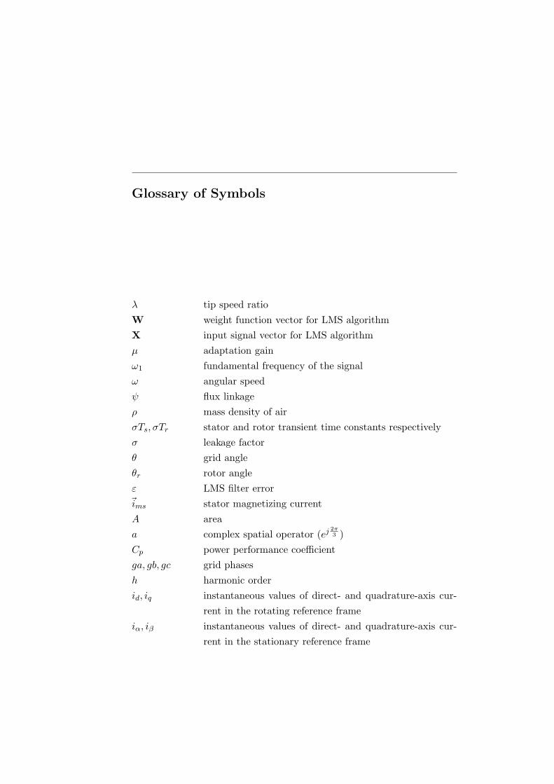
Glossary of Symbols
λ tip speed ratioW weight function vector for LMS algorithmX input signal vector for LMS algorithmµ adaptation gainω1 fundamental frequency of the signalω angular speedψ flux linkageρ mass density of airσTs, σTr stator and rotor transient time constants respectivelyσ leakage factorθ grid angleθr rotor angleε LMS filter error~ims stator magnetizing currentA areaa complex spatial operator (ej 2π
3 )Cp power performance coefficientga, gb, gc grid phasesh harmonic orderid, iq instantaneous values of direct- and quadrature-axis cur-
rent in the rotating reference frameiα, iβ instantaneous values of direct- and quadrature-axis cur-
rent in the stationary reference frame

A-2
J inertia of the rotorj complex operatorL dynamic inductanceLm magnetizing inductanceLr, Llr self- and leakage inductances of the rotor respectivelyLs, Lls self- and leakage inductances of the stator respectivelym modulation indexMMF Magneto Motive ForceN number of turnsP active powerp = d/dt differential operatorQ reactive powerR resistancera, rb, rc rotor phasessa, sb, sc stator phasesT time constantte instantaneous value of the electromagnetic torqueTs, Tr stator and rotor time constants respectivelyud, uq instantaneous values of direct- and quadrature-axis volt-
age in the rotating reference frameuα, uβ instantaneous values of direct- and quadrature-axis volt-
age in the stationary reference framevw velocity of the windvtip blade tip speedV Ar Volt Ampere reactivew weight function for LMS algorithmx input signal for LMS algorithmFIR Finite Impulse ResponseIIR Infinite Impulse Response

B
SVM look-up table
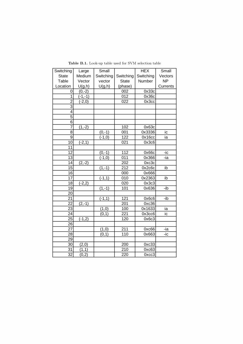
Table B.1. Look-up table used for SVM selection table
Switching Large Small HEX SmallState Medium Switching Switching Switching VectorsTable Vector vector State Number NP
Location U(g,h) U(g,h) (phase) Currents0 (0,-2) 002 0x33c1 (-1,-1) 012 0x36c2 (-2,0) 022 0x3cc34567 (1,-2) 102 0x63c8 (0,-1) 001 0x3336 ic9 (-1,0) 122 0x16cc ia
10 (-2,1) 021 0x3c61112 (0,-1) 112 0x66c -ic13 (-1,0) 011 0x366 -ia14 (2,-2) 202 0xc3c15 (1,-1) 212 0x2c6c ib16 000 0x66617 (-1,1) 010 0x2363 ib18 (-2,2) 020 0x3c319 (1,-1) 101 0x636 -ib2021 (-1,1) 121 0x6c6 -ib22 (2,-1) 201 0xc3623 (1,0) 100 0x1633 ia24 (0,1) 221 0x3cc6 ic25 (-1,2) 120 0x6c32627 (1,0) 211 0xc66 -ia28 (0,1) 110 0x663 -ic2930 (2,0) 200 0xc3331 (1,1) 210 0xc6332 (0,2) 220 0xcc3
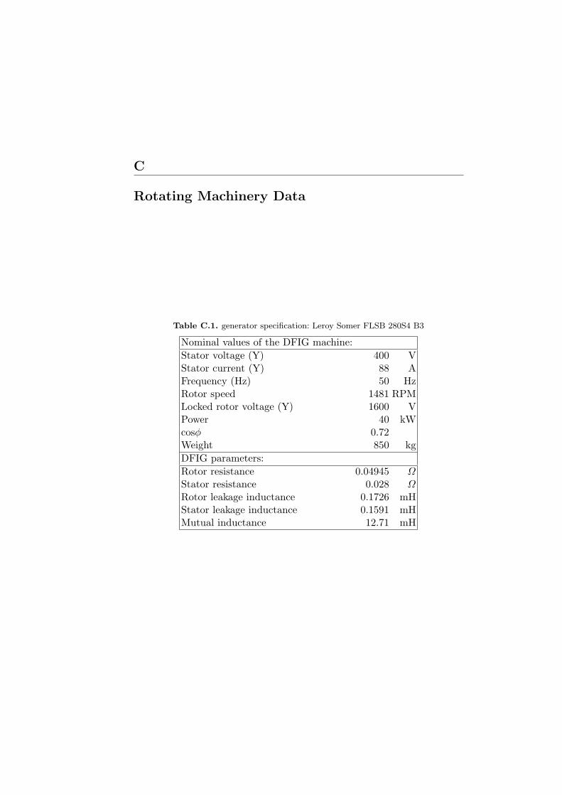
C
Rotating Machinery Data
Table C.1. generator specification: Leroy Somer FLSB 280S4 B3
Nominal values of the DFIG machine:Stator voltage (Y) 400 VStator current (Y) 88 AFrequency (Hz) 50 HzRotor speed 1481 RPMLocked rotor voltage (Y) 1600 VPower 40 kWcosφ 0.72Weight 850 kgDFIG parameters:Rotor resistance 0.04945 ΩStator resistance 0.028 ΩRotor leakage inductance 0.1726 mHStator leakage inductance 0.1591 mHMutual inductance 12.71 mH
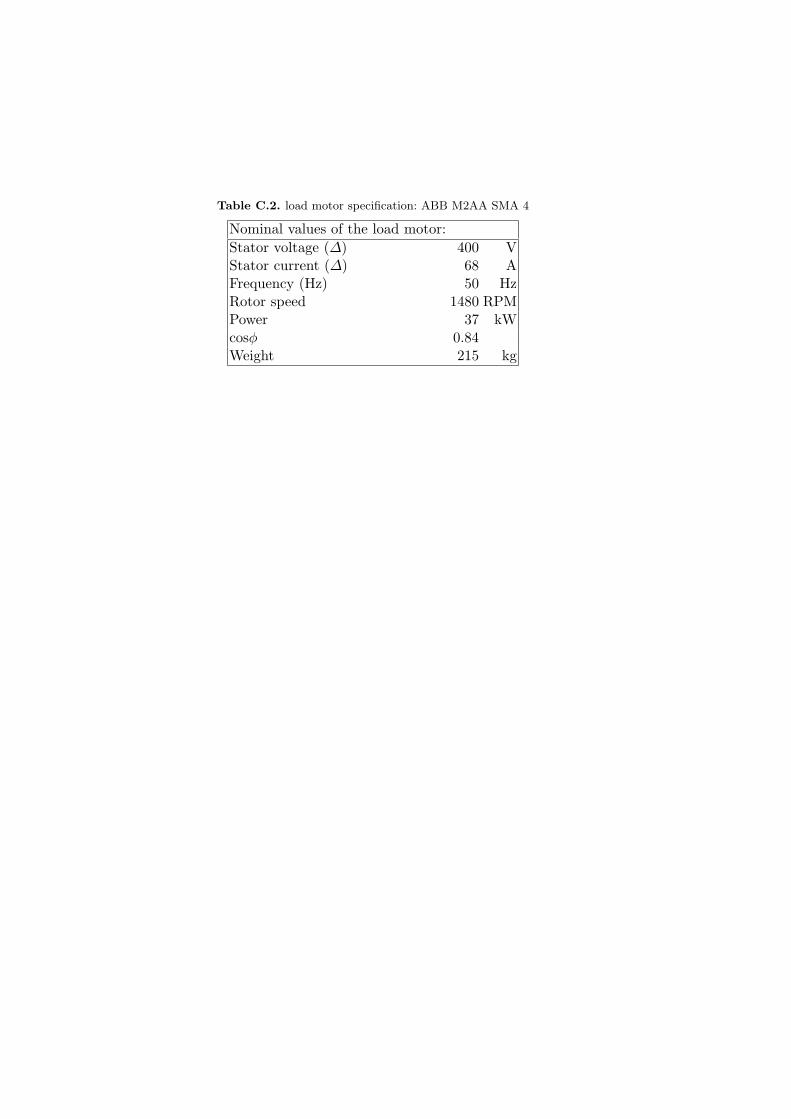
Table C.2. load motor specification: ABB M2AA SMA 4
Nominal values of the load motor:Stator voltage (∆) 400 VStator current (∆) 68 AFrequency (Hz) 50 HzRotor speed 1480 RPMPower 37 kWcosφ 0.84Weight 215 kg

D
Diagram of DSP interface
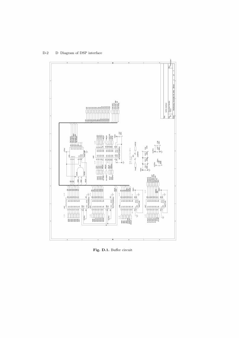
D-2 D Diagram of DSP interface5 5
4 4
3 3
2 2
1 1
DD
CC
BB
AA
On
= F
ram
e
SN
74LV
TH
2245
Mod
e se
lect
for
AD
C's
3.3V
3.3V3.
3V
3.3V
3.3V
5.0V
5.0V
5.0V
5.0V
3.0V
<D
oc>
<R
evC
ode>
Buf
fer
inte
rfac
e
A4
17
Wed
nesd
ay, N
ovem
ber
06, 2
002
Titl
e
Siz
eD
ocum
ent N
umbe
rR
ev
Dat
e:S
heet
of
D7
MS
1#
WR
#
D2
D4
A0
D15
A1
D1
FL0
D7
A3
D0
IRQ
1#
RD
#
D2
D13
MS
2#
SD
ID10
D10
D3
A1
D12
D3
D0
D9
D15
RD
#
SD
IFS
D9
WR
#
D13
IRQ
2#
A0
RD
#
D4
A2
D11
FL3
Enc
oder
hig
h#
D8
A2
Enc
oder
low
#
D14
D6
D5
D11D6
D5
D8
FL2
D1
SD
OF
SS
DO
FL1
SC
LKD
14
D12
MS
2#
Set
Rel
ay#
Net
latc
h#G
en la
tch#
+5V
cc
+5V
cc
+3.
3Vcc
+5V
cc
+3.
3Vcc
+5V
cc
+5V
cc
+3.
3Vcc
+5V
cc
+3.
3Vcc
U16
74H
CT
245
2 3 4 5 6 7 8 9 19 1
18 17 16 15 14 13 12 11 20 10
A1
A2
A3
A4
A5
A6
A7
A8
G DIR
B1
B2
B3
B4
B5
B6
B7
B8
VC
CG
ND
C45
100n
12
U60
SN
74C
BT
D33
84/S
O
112
13242 5 6 9 10 1615 19 20 23
3 4 7 8 11 14 17 18 21 22
1OE
GN
D2O
EV
CC
1B1
1B2
1B3
1B4
1B5
2B2
2B1
2B3
2B4
2B5
1A1
1A2
1A3
1A4
1A5
2A1
2A2
2A3
2A4
2A5
U12 74
LVT
H22
45A
/SO
202 3 4 5 6 7 8 9
18 17 16 15 14 13 12 11 10
1 19
VC
C
A1
A2
A3
A4
A5
A6
A7
A8
B1
B2
B3
B4
B5
B6
B7
B8
GN
D
DIR
OE
C41
100n
12
U14
74LV
TH
2245
A/S
O
202 3 4 5 6 7 8 9
18 17 16 15 14 13 12 11 10
1 19
VC
C
A1
A2
A3
A4
A5
A6
A7
A8
B1
B2
B3
B4
B5
B6
B7
B8
GN
D
DIR
OE
C46
100n
12
U17
74H
CT
245
2 3 4 5 6 7 8 9 19 1
18 17 16 15 14 13 12 11 20 10
A1
A2
A3
A4
A5
A6
A7
A8
G DIR
B1
B2
B3
B4
B5
B6
B7
B8
VC
CG
ND
C42 10
0n12 C
5810
0n12
JP1
JUM
PE
R
12
C57
100n
12
U11
74H
CT
138
1 2 3 6 4 5
15 14 13 12 11 10 9 7
A B C G1
G2A
G2B
Y0
Y1
Y2
Y3
Y4
Y5
Y6
Y7
C43 10
0n12
C44 10
0n12
U13
A
74F
08
1 23
14 7
D3
MD
14
D2
MD
8
FLA
G2
FLA
G1
D8
SD
IFS
DR
0A
FLA
G9
Ena
ble-
NE
T
RF
S0
MA
2
Err
-NE
T
Out
put3
D11
MD
6
FLA
G8
FLA
G5
MD
3
MA
0
D1
SC
LK
TF
S0
D9
FLA
G0
SD
O
TF
S0
FLA
G6
FLA
G3
MD
5
D0
MD
1
AD
C-r
eset
MD
7
D6
RF
S0
MD
10
Out
put2
MD
12
RX
CLK
0
DM
RD
#
MD
15
MD
9
DM
S2#MD
13
FLA
G4
FLA
G7
D10
MD
11
MD
0
MD
4
D13
D4
Gen
latc
h
D5
MA
3 DT
0A
Enc
oder
low
Net
latc
h
D12
D15
Enc
oder
hig
h
DM
WR
#
IRQ
1#
SD
ISD
OF
S
IRQ
2#
Out
put1
Ena
ble-
GE
N
MA
1
D7
Err
-GE
ND
14
MD
2
Set
Rel
ay
Inpu
t1In
put2
Inpu
t3In
put4
Fig. D.1. Buffer circuit
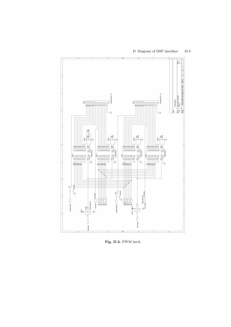
D Diagram of DSP interface D-3
5 5
4 4
3 3
2 2
1 1
DD
CC
BB
AA
<D
oc>
A
Gat
esig
nals
A4
67
Wed
nesd
ay, N
ovem
ber
06, 2
002
Titl
e
Siz
eD
ocum
ent N
umbe
rR
ev
Dat
e:S
heet
of
D11
D9
D7
D10
D7
D11
D4
D3
D6
D3
Err
-NE
T
D4
D2
D1
D5
D6
D10
Err
-GE
N
D0
D5
D2
D9
D1
D0
D8
D8
+5V
cc
+5V
cc
+5V
cc
+5V
cc
+5V
cc +5V
cc
K10
Bre
aker
12
3
JR3
CO
NN
RC
PT
15
123456789101112131415
123456789101112131415C
6010
0n
U20
74H
CT
574
2 3 4 5 6 7 8 9 11 1
19 18 17 16 15 14 13 12 20 10
D1
D2
D3
D4
D5
D6
D7
D8
CLK
OC
Q1
Q2
Q3
Q4
Q5
Q6
Q7
Q8
VC
CG
ND
C53
100n
U24
74H
CT
574
2 3 4 5 6 7 8 9 11 1
19 18 17 16 15 14 13 12 20 10
D1
D2
D3
D4
D5
D6
D7
D8
CLK
OC
Q1
Q2
Q3
Q4
Q5
Q6
Q7
Q8
VC
CG
ND
U21
A
74H
C14
/SO
_0
12
14 7
U22
74H
CT
574
2 3 4 5 6 7 8 9 11 1
19 18 17 16 15 14 13 12 20 10
D1
D2
D3
D4
D5
D6
D7
D8
CLK
OC
Q1
Q2
Q3
Q4
Q5
Q6
Q7
Q8
VC
CG
ND
U21
B
74H
C14
/SO
_0
34
14 7
JR4
CO
NN
RC
PT
15
123456789101112131415
123456789101112131415C
5510
0n
K9
Bre
aker
12
3
C56
100n
C54
100n
U23
74H
CT
574
2 3 4 5 6 7 8 9 11 1
19 18 17 16 15 14 13 12 20 10
D1
D2
D3
D4
D5
D6
D7
D8
CLK
OC
Q1
Q2
Q3
Q4
Q5
Q6
Q7
Q8
VC
CG
ND
D6
Err
-GE
N
Net
latc
h
D5
D1
D3
D2
Err
-NE
T
D11
D7
D4
D0
Ena
ble-
GE
N D9
Ena
ble-
NE
T
Gen
latc
h
D10
D8
Fig. D.2. PWM latch
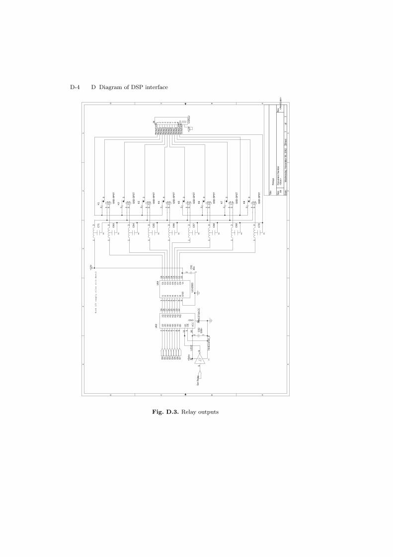
D-4 D Diagram of DSP interface5 5
4 4
3 3
2 2
1 1
DD
CC
BB
AA
Husk 12V supply eller stik dertil
<D
oc>
<R
evC
ode>
Rel
ays
A4
77
Wed
nesd
ay, N
ovem
ber
06, 2
002
Titl
e
Siz
eD
ocum
ent N
umbe
rR
ev
Dat
e:S
heet
of
Rel
ayE
arth
Rel
ay5
Rel
ay1
Rel
ayC
om2
Rel
ay8
Rel
ay3
Rel
ay6
Rel
ay4
Rel
ay2
Rel
ay7
Rel
ayC
om1
+5V
cc
+12
V
+12
V
J6 CO
N12
1 2 3 4 5 6 7 8 9 10 11 12
K1 G
6D-S
PS
T
23
1 5
U21
C
74H
C14
/SO
_0
56
14 7C
6210
0n12
C61
10u
12
K3
G6D
-SP
ST
23
1 5
K5
G6D
-SP
ST
23
1 5
K7
G6D
-SP
ST
23
1 5
U64
ULN
2803
1 2 3 4 5 6 7 8 9
18 17 16 15 14 13 12 11 10
I1 I2 I3 I4 I5 I6 I7 I8 GN
D
O1
O2
O3
O4
O5
O6
O7
O8 Vc
C63
2
13
U63
74H
C57
3/LC
C
1
10
11 20
19 18 17 16 15 14 13 12
2 3 4 5 6 7 8 9
OE
GND
LE VC
C
1Q 2Q 3Q 4Q 5Q 6Q 7Q 8Q
1D 2D 3D 4D 5D 6D 7D 8D
C64
2
13
C65
2
13
C66
2
13
C67
2
13
K2 G
6D-S
PS
T
23
1 5
K4
G6D
-SP
ST
23
1 5
C68
2
13
K6
G6D
-SP
ST
23
1 5
K8
G6D
-SP
ST
23
1 5
C69
2
13
C70
2
13
C71
2
13
Set
Rel
ay
D1
D5
D4
D0
D3
D2
D6
D7
Fig. D.3. Relay outputs
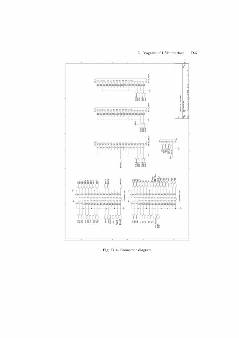
D Diagram of DSP interface D-5
5 5
4 4
3 3
2 2
1 1
DD
CC
BB
AA
001
<R
evC
ode>
Con
nect
ion
to E
VA
-BO
AR
D
A4
27
Wed
nesd
ay, N
ovem
ber
06, 2
002
Titl
e
Siz
eD
ocum
ent N
umbe
rR
ev
Dat
e:S
heet
of
+3.
3Vcc
+5V
cc
Vin
Vin
J4 CO
N9
1 2 3 4 5 6 7 8 9
JR1
CO
NN
RE
CT
30x
2
27252321191715131197531
282624222018161412108642
2930
3132
3334
3536
3738
3940
4142
4344
4546
4748
4950
5152
5354
5556
5758
5960
27252321191715131197531
282624222018161412108642
2930
3132
3334
3536
3738
3940
4142
4344
4546
4748
4950
5152
5354
5556
5758
5960
JDR
8A
DIN
96_
AB
C-R
1234567891011121314151617181920212223242526272829303132
A1
A2
A3
A4
A5
A6
A7
A8
A9
A10
A11
A12
A13
A14
A15
A16
A17
A18
A19
A20
A21
A22
A23
A24
A25
A26
A27
A28
A29
A30
A31
A32
JDR
8B
DIN
96_
AB
C-R
3334353637383940414243444546474849505152535455565758596061626364
B1
B2
B3
B4
B5
B6
B7
B8
B9
B10
B11
B12
B13
B14
B15
B16
B17
B18
B19
B20
B21
B22
B23
B24
B25
B26
B27
B28
B29
B30
B31
B32
JDR
8C
DIN
96_
AB
C-R
6566676869707172737475767778798081828384858687888990919293949596
C1
C2
C3
C4
C5
C6
C7
C8
C9
C10
C11
C12
C13
C14
C15
C16
C17
C18
C19
C20
C21
C22
C23
C24
C25
C26
C27
C28
C29
C30
C31
C32
JR2
CO
NN
RE
CT
30x
2
27252321191715131197531
282624222018161412108642
2930
3132
3334
3536
3738
3940
4142
4344
4546
4748
4950
5152
5354
5556
5758
5960
27252321191715131197531
282624222018161412108642
2930
3132
3334
3536
3738
3940
4142
4344
4546
4748
4950
5152
5354
5556
5758
5960
MD
20
FLA
G2
DM
WR
#
RE
SE
T#
MD
4
DM
S1#
A11
A19
DR
0B
MD
14
A15
MD
15
DR
1A
MD
13
FLA
G5
MD
7
RX
CLK
1
MD
16 MA
7
A13
TX
CLK
0
MD
1
RF
S1
MD
22 MA
8
A12
EX
T C
LK
MD
2
MD
12
RF
S0
DM
S0#
MA
4
MA
1
A18
DM
RD
#
A22
MD
0
A10
FLA
G10
A14
DT
0A
MD
18
FLA
G3
DR
0A
RX
CLK
0
BR
2#
MD
10 DM
AG
2#
IRQ
0#
MA
0
MD
3
DM
AG
1#
TX
CLK
1
FLA
G1
MD
23
DT
0B
DT
1A
DM
AR
1#
MD
9
DM
AR
2#
A9
RE
DY
#
IRQ
2#
FLA
G6
DM
S3#
FLA
G9
MD
11
MD
24
A21
A16
FLA
G7
MD
8M
D6
MD
21
PW
M E
VE
NT
1
TF
S1
MA
3
FLA
G4
A23
DR
1B
PW
M E
VE
NT
0
DT
1BA
17
MA
2
MA
6
MD
19
MD
5
A20
MA
5
FLA
G0
MD
17
SW
#
TF
S0
IRQ
1#
DM
S2#
FLA
G8
FLA
G10
SC
LKSD
IS
DIF
S
SD
OF
S
AD
C-s
e
SD
O
Fig. D.4. Connector diagram
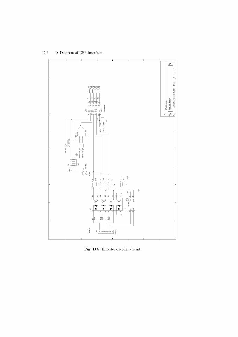
D-6 D Diagram of DSP interface5 5
4 4
3 3
2 2
1 1
DD
CC
BB
AA
Enc
oder
conn
ecto
r
Min 102 kHz
Max 16 MHz
Enc
oder
Cou
nter
A
DF
AG
Inte
rfac
e
A4
37
Wed
nesd
ay, N
ovem
ber
06, 2
002
Titl
e
Siz
eD
ocum
ent N
umbe
rR
ev
Dat
e:S
heet
of
D7
D6
D4
D1
D0
D5
D2
D3
+5V
cc
+5V
cc
+5V
cc
+5V
cc
U18
A
SN
7408
1 23
J3
CO
N91 2 3 4 5 6 7 8 9
U72
New
port
5/5
2 1
4 3
Vcc
GN
D
V+
0V
R38
3K3
R39
3K3
C
R41 SIP
4.7
k
1 234
C59
100n
U61
PC
844
1 2 3 4 5 6 7 8910111213141516
C47
2
13
R37
3K3
X1 2MH
z
123
4
C50
100n
C48
2
13
C49
2
13
C51
2
13
U62
HC
TL-
2016
12 3 4 5 6 7 16
9101112131415
8
D0
CLK
SE
LO
ER
ST
Ch
BC
h A
Vdd
D7
D6
D5
D4
D3
D2
D1
GN
D
D0
D2
D6
D1
D7
D3
D5
D4
EC
LK
#Enc
oder
Low
#Enc
oder
Hig
h
Fig. D.5. Encoder decoder circuit
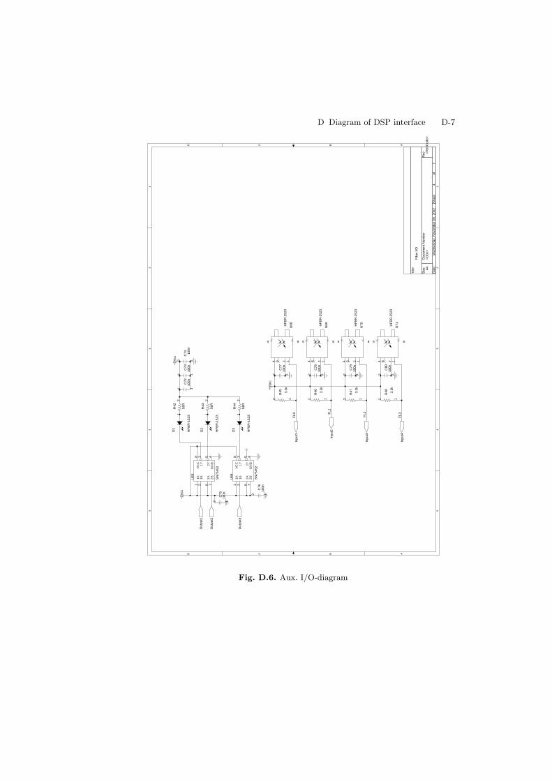
D Diagram of DSP interface D-7
5 5
4 4
3 3
2 2
1 1
DD
CC
BB
AA
<D
oc>
<R
evC
ode>
Fib
er I/
O
A4
47
Wed
nesd
ay, N
ovem
ber
06, 2
002
Titl
e
Siz
eD
ocum
ent N
umbe
rR
ev
Dat
e:S
heet
of
FL3FL2
FL0 F
L1
+5V
cc
+5V
cc
+5V
cc
R45 3.
3k
2 1
C73
100n
12
U69HF
BR
-252
314 23
5 8
C72
100n
12
D3
HF
BR
-152
3
D2
HF
BR
-152
3C
7510
0n12
D1
HF
BR
-152
3
R46 3.
3k
2 1
U71HF
BR
-252
314 23
5 8
C76
100n
12
U65
SN
7545
2
1 2 6 7
3 58 4
1A 1B 2A 2B
1Y 2Y
VC
C
GN
D
R42
56R
21
R43
56R
21
U68HF
BR
-252
314 23
5 8
R44
56R
21
C74 10
0n12
R47 3.
3k
2 1
U66
SN
7545
2
1 2 6 7
3 58 4
1A 1B 2A 2B
1Y 2Y
VC
C
GN
D
U70HF
BR
-252
314 23
5 8
C78
100n
12
C79
100n
12
C80
100n
12
R48 3.
3k
2 1
C77
100n
12
Inpu
t1
Inpu
t4
Inpu
t3
Inpu
t2
Out
put2
Out
put1
Out
put3
Fig. D.6. Aux. I/O-diagram
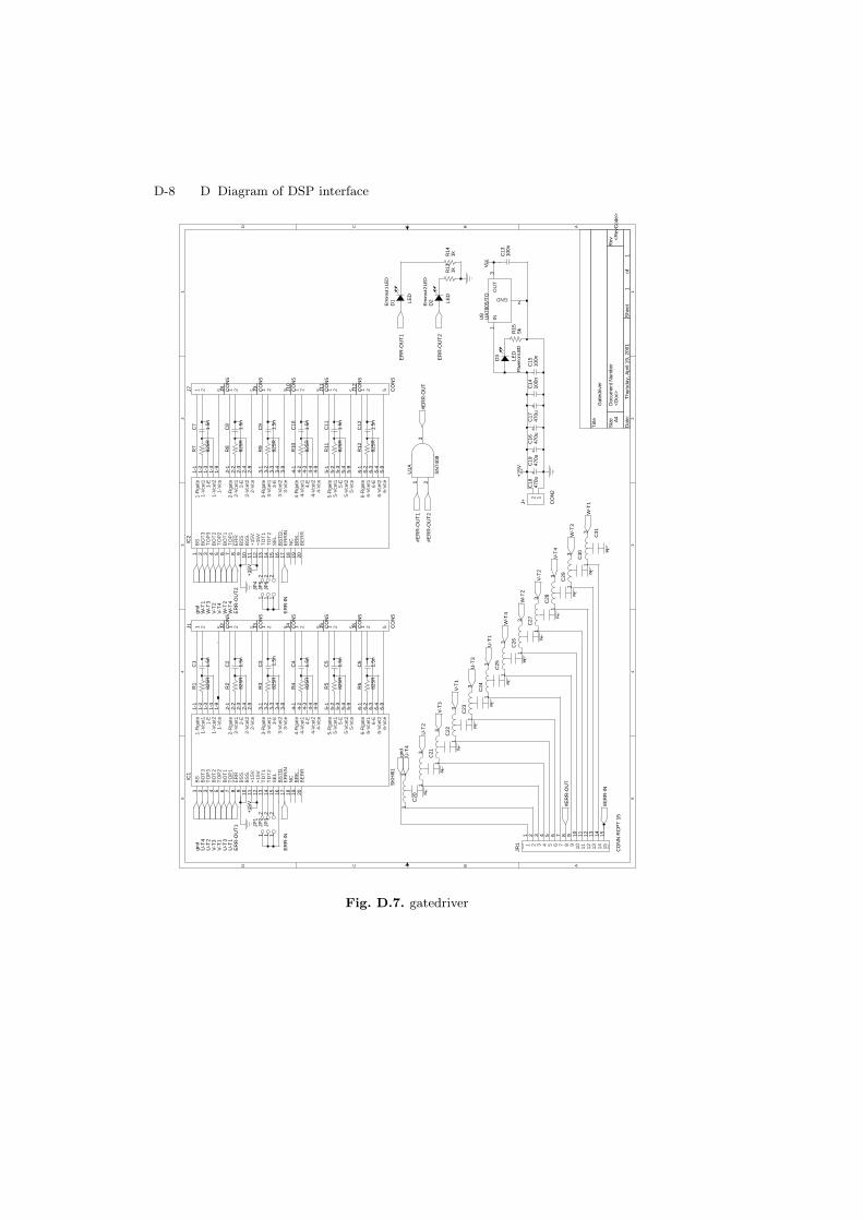
D-8 D Diagram of DSP interface5 5
4 4
3 3
2 2
1 1
DD
CC
BB
AA
Pow
er o
n LE
D
Error
out 1
LED
Error
out 2
LED
<D
oc>
<R
evC
ode>
Gat
edriv
er
A4
11
Thu
rsda
y, A
pril
19, 2
001
Titl
e
Siz
eD
ocum
ent N
umbe
rR
ev
Dat
e:S
heet
of
+15
V+
15V
Vcc
+15
V
J5 CO
N5
1 2 5
C19
470u
J6 CO
N5
1 2 5
D1 LE
D
D2 LE
D
R12
825R
J9 CO
N5
1 2 5
D3
LED
J10
CO
N5
1 2 5
C1
1.5n
J11
CO
N5
1 2 5
C2
1.5n
J12
CO
N5
1 2 5
R1
825R
J8 CO
N5
1 2 5
C23
2
13
U1A
SN
7408
1 23
IC1
SK
HI6
1
1-1
1-2
1-4
1-9
1 2 3 4 5 6 7 8 9 10 11 12 13 14 15 16 17 18 19 20
1-3
2-1
2-2
2-3
2-4
2-9
3-1
3-2
3-3
3-4
3-9
4-1
4-2
4-3
4-4
4-9
5-1
5-2
5-3
5-4
5-9
6-1
6-2
6-3
6-4
6-9
1-R
gate
1-V
cet1
1-V
cet2
1-V
ce
BS
BO
T3
TO
P3
BO
T2
TO
P2
BO
T1
TO
P1
ER
RB
SS
BS
S.
+15
V.
+15
VT
DT
1T
DT
2S
EL
BS
TD
ER
RIN
NC
BR
KB
ER
R
1-E
2-R
gate
2-V
cet1
2-E
2-V
cet2
2-V
ce
3-R
gate
3-V
cet1
3-E
3-V
cet2
3-V
ce
4-R
gate
4-V
cet1
4-E
4-V
cet2
4-V
ce
5-R
gate
5-V
cet1
5-E
5-V
cet2
5-V
ce
6-R
gate
6-V
cet1
6-E
6-V
cet2
6-V
ce
C24
2
13
JR1
CO
NN
RC
PT
15
1 2 3 4 5 6 7 8 9 10 11 12 13 14 15
1 2 3 4 5 6 7 8 9 10 11 12 13 14 15
IC2
1-1
1-2
1-4
1-9
1 2 3 4 5 6 7 8 9 10 11 12 13 14 15 16 17 18 19 20
1-3
2-1
2-2
2-3
2-4
2-9
3-1
3-2
3-3
3-4
3-9
4-1
4-2
4-3
4-4
4-9
5-1
5-2
5-3
5-4
5-9
6-1
6-2
6-3
6-4
6-9
1-R
gate
1-V
cet1
1-V
cet2
1-V
ce
BS
BO
T3
TO
P3
BO
T2
TO
P2
BO
T1
TO
P1
ER
RB
SS
BS
S.
+15
V.
+15
VT
DT
1T
DT
2S
EL
BS
TD
ER
RIN
NC
BR
KB
ER
R
1-E
2-R
gate
2-V
cet1
2-E
2-V
cet2
2-V
ce
3-R
gate
3-V
cet1
3-E
3-V
cet2
3-V
ce
4-R
gate
4-V
cet1
4-E
4-V
cet2
4-V
ce
5-R
gate
5-V
cet1
5-E
5-V
cet2
5-V
ce
6-R
gate
6-V
cet1
6-E
6-V
cet2
6-V
ce
C25
2
13C3 1.5n
C20
2
13
R2
825R
C4
1.5n
C26
2
13
C5
1.5n
C31
2
13
C6
1.5n
R3
825R
C16
470u
R4
825R
C22
2
13
C27
2
13
C21
2
13
JP1
12
C7
1.5n
R5
825R
R15
5k
C28
2
13
JP2
12
C8
1.5n
C14
100n
J+ CO
N2
12
R6
825R
C15
100n
JP3
12
C9
1.5n
C29
2
13
J7 CO
N5
1 2 5
C18
470u
C10
1.5n
R7
825R
C30
2
13
C11
1.5n
C13
100n
C12
1.5n
R8
825R
U8
UA
7805
/TO
1
2
3IN
GND
OU
T
R14
1k
R9
825R
JP4
12
R13
1k
J1 CO
N5
1 2 5
C17
470u
R10
825R
JP5
12
JP6
12
R11
825R
J2 CO
N5
1 2 5 J3 CO
N5
1 2 5 J4 CO
N5
1 2 5
V-T
1U
-T3
ER
R-O
UT
1E
RR
-OU
T2
W-T
1
V-T
3
U-T
1
U-T
2
#ER
R-O
UT
#ER
R-IN
#ER
R-O
UT
2
#ER
R-O
UT
1#E
RR
-OU
T
ER
R-IN
W-T
3
ER
R-IN
V-T
2
W-T
4W
-T2
V-T
4
ER
R-O
UT
2
ER
R-O
UT
1gn
d
U-T
4gn
dgn
d
U-T
1
U-T
4
U-T
3
U-T
2
V-T
1
V-T
3
W-T
1
W-T
4
W-T
3
W-T
2
V-T
4
V-T
2
Fig. D.7. gatedriver
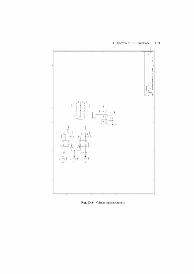
D Diagram of DSP interface D-9
5 5
4 4
3 3
2 2
1 1
DD
CC
BB
AA
U WV
<D
oc>
<R
evC
ode>
Gat
edriv
er
A4
11
Wed
nesd
ay, N
ovem
ber
06, 2
002
Titl
e
Siz
eD
ocum
ent N
umbe
rR
ev
Dat
e:S
heet
of
+15
V -15V
-15V
+15
V
-15V
+15
V
+15
V
-15V
C1
470u
C2 10
0n
R2 15
k
C5 10
0n
R3 20
0R
JDR
25
9
4
8
3
7
2
6
1
59
48
37
26
1
J2 CO
N2
12
R1
33k
C3
470u
R6 20
0R
T1
LV25
-P
+H
T
-HT
+ - M
J1 CO
N2
12
R4
33k
J5 CO
N3
123T
2
LV25
-P
+H
T
-HT
+ - M
R5 15
k
J6 CO
N2
12
mea
s2m
eas1
mea
s1
mea
s2
Fig. D.8. Voltage measurements
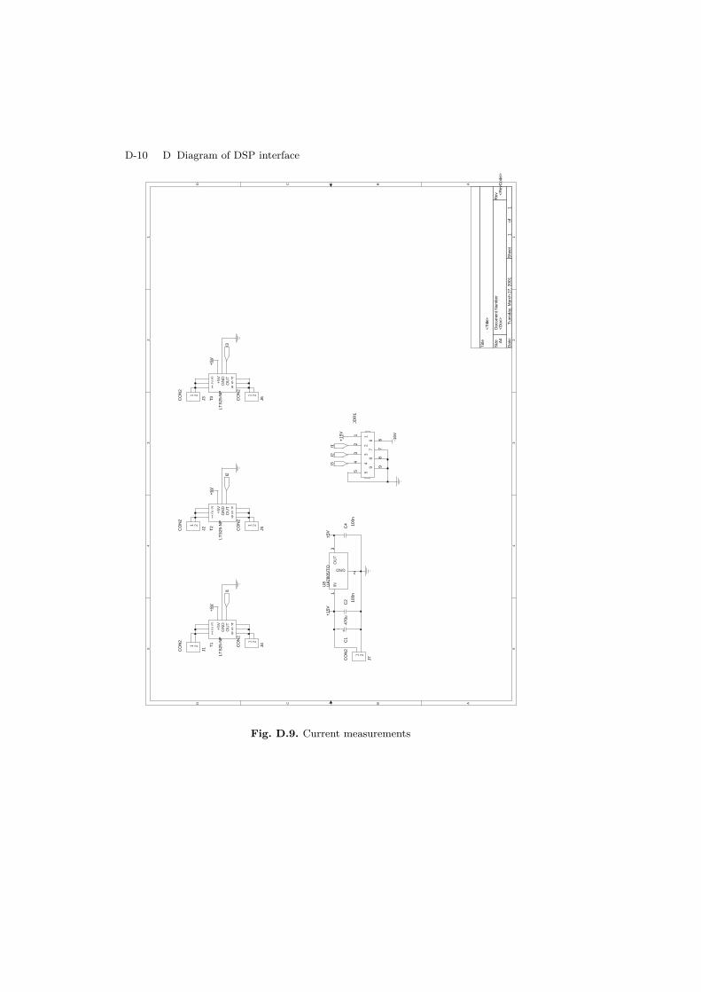
D-10 D Diagram of DSP interface5 5
4 4
3 3
2 2
1 1
DD
CC
BB
AA
<D
oc>
<R
evC
ode>
<T
itle>
A4
11
Tue
sday
, Mar
ch 2
7, 2
001
Titl
e
Siz
eD
ocum
ent N
umbe
rR
ev
Dat
e:S
heet
of
+5V
+15
V
+5V
+5V
+15
V
-15V
+5V
C1
470u
J2CO
N2
1 2 C4 10
0n
J3CO
N2
1 2
J6CO
N2
1 2
J5CO
N2
1 2
J4CO
N2
1 2
T2
LTS
25-N
P+
5VG
ND
OU
T
123
654
J7CO
N2
1 2
JDR
15
9
4
8
3
7
2
6
1
59
48
37
26
1
C2 10
0n
U8
UA
7805
/TO
1
2
3IN
GND
OU
T
T1
LTS
25-N
P+
5VG
ND
OU
T
123
654
J1CO
N2
1 2
T3
LTS
25-N
P+
5VG
ND
OU
T
123
654
I1
I2I3
I1
I2I3
Fig. D.9. Current measurements
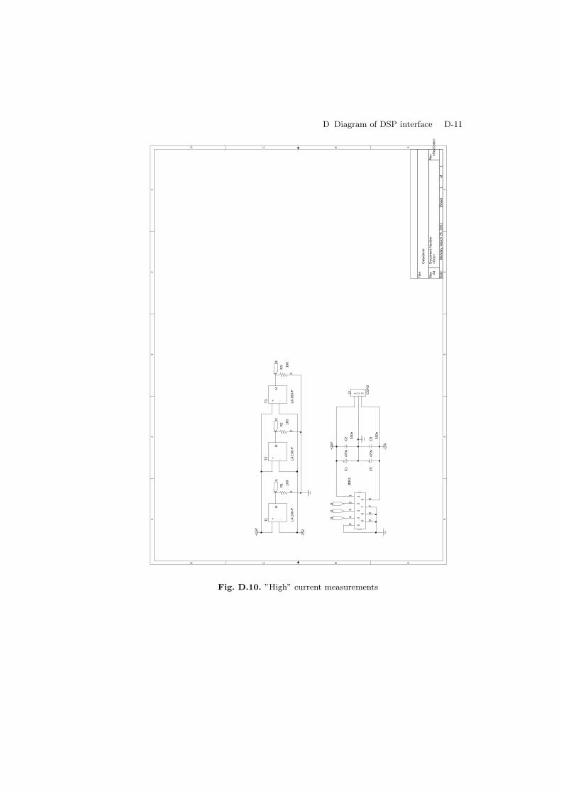
D Diagram of DSP interface D-11
5 5
4 4
3 3
2 2
1 1
DD
CC
BB
AA
<D
oc>
<R
evC
ode>
Gat
edriv
er
A4
11
Mon
day,
Mar
ch 2
6, 2
001
Titl
e
Siz
eD
ocum
ent N
umbe
rR
ev
Dat
e:S
heet
of
-15V
+15
V
+15
V
-15V
C1
470u
T1 LA 1
00-P
+ -M
T2
LA 1
00-P
+ -M
T3
LA 1
00-P
+ -M
C2 10
0n
R1 10
021
R3 10
021
C6 10
0n
R2 10
021
JDR
15
9
4
8
3
7
2
6
1
59
48
37
26
1
C5
470u
J? CO
N3
1 2 3
I3I1
I1I3
I2
I2
Fig. D.10. ”High” current measurements
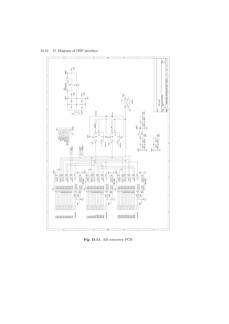
D-12 D Diagram of DSP interface5 5
4 4
3 3
2 2
1 1
DD
CC
BB
AA
001
A
AD
C b
oard
A4
14
Wed
nesd
ay, D
ecem
ber
06, 2
000
Titl
e
Siz
eD
ocum
ent N
umbe
rR
ev
Dat
e:S
heet
of
RE
SE
T
SE
+5V
+5V
+5V
cc+
5V
+5V
cc
+5V
+5V
cc
+5V
+5V
cc
+5V
+5V
cc
+5V
cc
AV
DD
+5V
cc
+15
VA
VD
D
-15V
+5V
cc
C44
470u
IC1
AD
7336
0
1 23 4 5 6
7 8910 11 12 13 14 15 16 18
19
17
2021 2223 2425 2627 28
VIN
P2
VIN
N2
VIN
P1
VIN
N1
RE
FO
UT
RE
FC
AP
AV
DD
2A
GN
D2
DG
ND
DV
DD
RE
SE
TS
CLK
MC
LK
SD
OS
DO
FS
SD
IFS
SE
AG
ND
1
SD
I
AV
DD
1
VIN
P6
VIN
N6
VIN
P5
VIN
N5
VIN
P4
VIN
N4
VIN
P3
VIN
N3
IC2
AD
7336
0
1 23 4 5 6
7 8910 11 12 13 14 15 16 18
19
17
2021 2223 2425 2627 28
VIN
P2
VIN
N2
VIN
P1
VIN
N1
RE
FO
UT
RE
FC
AP
AV
DD
2A
GN
D2
DG
ND
DV
DD
RE
SE
TS
CLK
MC
LK
SD
OS
DO
FS
SD
IFS
SE
AG
ND
1
SD
I
AV
DD
1
VIN
P6
VIN
N6
VIN
P5
VIN
N5
VIN
P4
VIN
N4
VIN
P3
VIN
N3
C30
100n
C46 10
0n
IC3
AD
7336
0
1 23 4 5 6
7 8910 11 12 13 14 15 16 18
19
17
2021 2223 2425 2627 28
VIN
P2
VIN
N2
VIN
P1
VIN
N1
RE
FO
UT
RE
FC
AP
AV
DD
2A
GN
D2
DG
ND
DV
DD
RE
SE
TS
CLK
MC
LK
SD
OS
DO
FS
SD
IFS
SE
AG
ND
1
SD
I
AV
DD
1
VIN
P6
VIN
N6
VIN
P5
VIN
N5
VIN
P4
VIN
N4
VIN
P3
VIN
N3
C45 10
0n
C28
100n
C29
100n
C48 10
0n
C32
100n
12
C35
100n
12
L2 Bea
d
12
C41
100n
C34
100n
12
U1A
74H
C74
2 3
5 6
4 1
D
CLK
Q Q
PR CL
U1B
74H
C74
12 11
9 8
10 13
D
CLK
Q Q
PR CL
C36
100u
C42
100n
C37
100n
C47
470u Y1
XL/
SM
123
4
J5 CO
N3
123
J6 CO
N9
1 2 3 4 5 6 7 8 9
U8
UA
7805
/TO
1
2
3IN
GND
OU
T
C43
100n
C38
100n
VP
9
VN
2
VN
13
VP
1
VP
14
SD
I
VN
10
VP
18
VN
1
VP
15
FLA
G10
SC
LK
VN
8
VN
16
VP
11
VP
5
VP
2
RE
FO
UT
1
VN
18
VP
4
SD
OF
S
VP
16
VP
3
VP
7
VP
17
VN
4
SD
O
VN
15
SD
IFS
VN
12
VN
7
VN
6V
P6
VN
3
VN
14
VN
11
VP
10
RE
FO
UT
3
VP
13
RE
FO
UT
2
VN
9
AD
C-s
e
VP
12
VN
17
VN
5
VP
8
SC
LKS
DO
SD
I
AD
C-s
eF
LAG
10S
DO
FS
SD
IFS
Fig. D.11. AD converter PCB
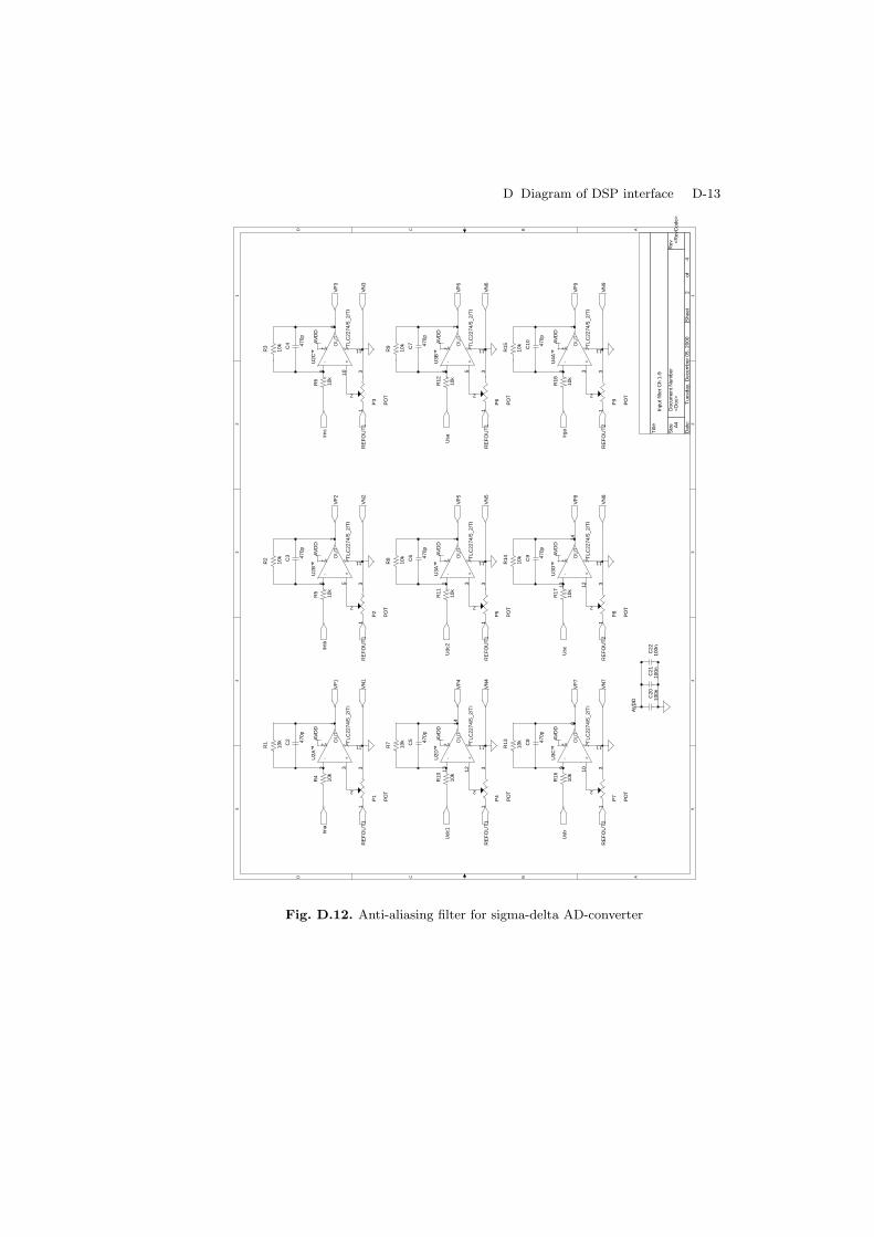
D Diagram of DSP interface D-13
5 5
4 4
3 3
2 2
1 1
DD
CC
BB
AA
<D
oc>
<R
evC
ode>
Inpu
t filt
er C
h 1-
9
A4
24
Tue
sday
, Dec
embe
r 05
, 200
0
Titl
e
Siz
eD
ocum
ent N
umbe
rR
ev
Dat
e:S
heet
of
AV
DD
AV
DD
AV
DD
AV
DD
AV
DD
AV
DD
AV
DD
AV
DD
AV
DD
AV
DD
P3
PO
T
13
2
U3C
TLC
2274
/5_2
/TI
109
4 11
8
+-
V+ V-OU
T
R3
10k
U3D
TLC
2274
/5_2
/TI
1213
4 11
14
+-
V+ V-OU
T
R1
10k C5 47
0p
P7
PO
T
13
2
P8
PO
T
13
2
R13
10k
C7 47
0p
R14
10k
C2 47
0p
R18
10k
C20
100n
R5
10k
R11
10k
R4
10k
C4 47
0p
P1
PO
T
13
2
U4A
TLC
2274
/5_2
/TI
32
4 11
1
+-
V+ V-OU
T
C21
100n
C22
100n
U2B
TLC
2274
/5_2
/TI
56
4 11
7
+-
V+ V-OU
T
C8 47
0p
U3A
TLC
2274
/5_2
/TI
32
4 11
1
+-
V+ V-OU
T
P9
PO
T
13
2
C9 47
0p
R10
10k
P2
PO
T
13
2
R15
10k
P5
PO
T
13
2
R2
10k
R8
10k
R12
10k
U2D
TLC
2274
/5_2
/TI
1213
4 11
14
+-
V+ V-OU
T
U3B
TLC
2274
/5_2
/TI
56
4 11
7
+-
V+ V-OU
T
P4
PO
T
13
2
U2A
TLC
2274
/5_2
/TI
32
4 11
1
+-
V+ V-OU
T
R7
10k
P6
PO
T
13
2
R6
10k
R9
10k C10 47
0p
C3 47
0p
C6 47
0p
R16
10k
U2C
TLC
2274
/5_2
/TI
109
4 11
8
+-
V+ V-OU
T
R17
10k
VP
4
VN
1
VN
9
VP
3
VN
4
RE
FO
UT
2
Irna
RE
FO
UT
1
Irnb
RE
FO
UT
2
Udc
2
RE
FO
UT
1
VP
2
VN
7
VP
6
RE
FO
UT
1V
N2
VN
6
Usa
VN
8
VP
1
VN
3
Udc
1
VP
5
Usc
RE
FO
UT
1
VP
9
Irga
RE
FO
UT
1
Usb
Irnc
VN
5
RE
FO
UT
2
RE
FO
UT
1
VP
8V
P7
Fig. D.12. Anti-aliasing filter for sigma-delta AD-converter
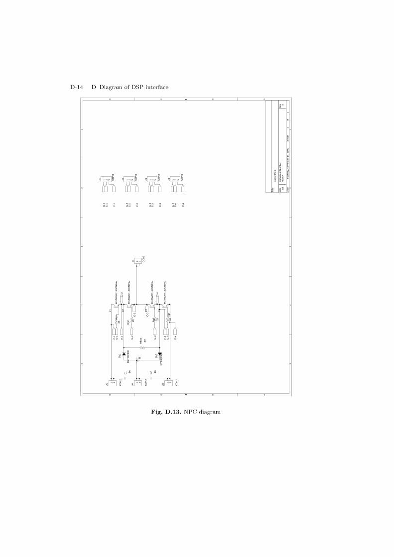
D-14 D Diagram of DSP interface5 5
4 4
3 3
2 2
1 1
DD
CC
BB
AA
<D
oc>
a
Pow
er P
CB
A4
11
Tue
sday
, Nov
embe
r 14
, 200
0
Titl
e
Siz
eD
ocum
ent N
umbe
rR
ev
Dat
e:S
heet
of
0
J2 CO
N3
1 2 5 J3 CO
N3
1 2 5 J4 CO
N3
1 2 5
Rflo
at
1M
Dc1
BY
T30
P60
0
J5 CO
N2
12
J8 CO
N2
12
Rg1
33
Rg4
33
Rg2 33
Z1
HG
TG
20N
120C
N/H
A
C1 1n C2 1n
Rg3 33
Z2
HG
TG
20N
120C
N/H
A
Z3
HG
TG
20N
120C
N/H
A
J7 CO
N2
1 2
J1 CO
N3
1 2 5
Z4
HG
TG
20N
120C
N/H
A
Dc2
BY
T30
P60
0
J6 CO
N2
12
G-1
E-1
C-3
C-2
G-4
E-4
G-1
G-2
G-3
G-4
E-1
E-2
C-3
E-3
E-4
C-4
C-2
C-1
C-1
G-3
E-3
E-2
G-2
C-4
Fig. D.13. NPC diagram
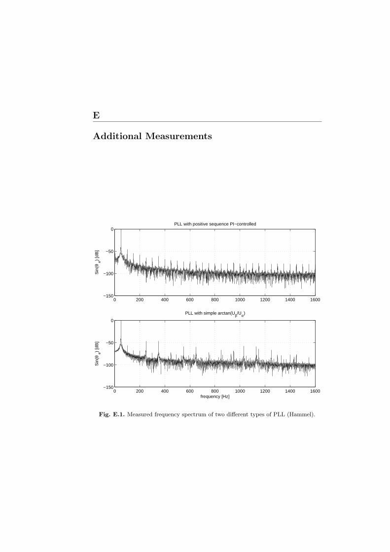
E
Additional Measurements
0 200 400 600 800 1000 1200 1400 1600−150
−100
−50
0PLL with positive sequence PI−controlled
Sin
(θ e)
[dB
]
0 200 400 600 800 1000 1200 1400 1600−150
−100
−50
0
PLL with simple arctan(Uβ/Uα)
frequency [Hz]
Sin
(θ e)
[dB
]
Fig. E.1. Measured frequency spectrum of two different types of PLL (Hammel).

0 0.5 1 1.5 2 2.51200
1400
1600
1800
Spe
ed [R
PM
]
0 0.5 1 1.5 2 2.5
−20
0
20
I roto
r [A]
0 0.5 1 1.5 2 2.5
−50000
5000
Pgr
id [W
]
0 0.5 1 1.5 2 2.5 3 3.5 42.5
3
3.5x 10
4
Pst
ator
[W]
0 0.5 1 1.5 2 2.5660
680
700
Udc
[V]
0 0.5 1 1.5 2 2.5−10
0
10
time [sec]
Neu
tral
poi
nt [V
]
Fig. E.2. Rotor magnetizing with a speed change 1650 - 1350 RPM (Hammel)
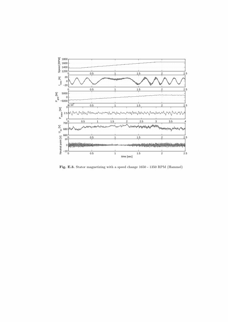
0 0.5 1 1.5 2 2.51200
1400
1600
1800S
peed
[RP
M]
0 0.5 1 1.5 2 2.5
−20
0
20
I roto
r [A]
0 0.5 1 1.5 2 2.5
−50000
5000
Pgr
id [W
]
0 0.5 1 1.5 2 2.5 3 3.5 42
2.5
3x 10
4
Pst
ator
[W]
0 0.5 1 1.5 2 2.5660
680
700
Udc
[V]
0 0.5 1 1.5 2 2.5−10
0
10
time [sec]
Neu
tral
poi
nt [V
]
Fig. E.3. Stator magnetizing with a speed change 1650 - 1350 RPM (Hammel)


F
Included Paper
M. Lindholm, T. W. Rasmussen, ”Harmonic analysis of Doubly Fed In-duction Generators.” IEEE Power Electronics and Drives Systems (PEDS2003), Singapore 17-20 November 2003. Accepted for oral presentation.

F-2 F Included Paper
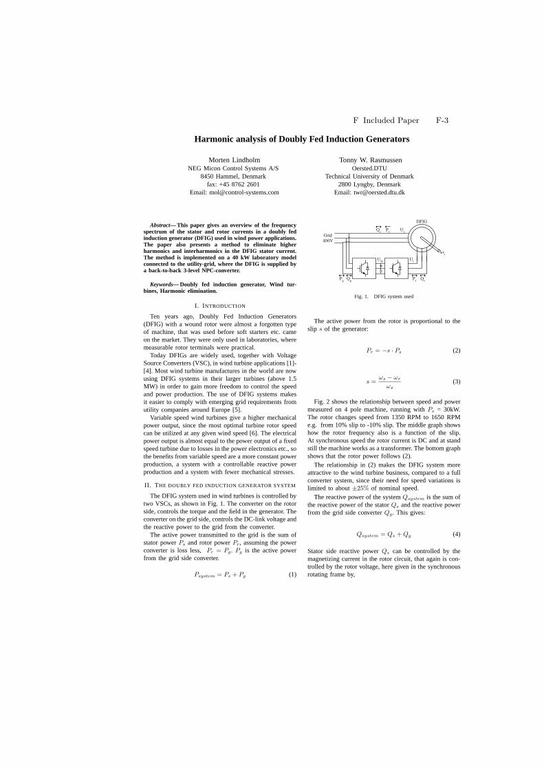
F Included Paper F-3
Harmonic analysis of Doubly Fed Induction Generators
Morten LindholmNEG Micon Control Systems A/S
8450 Hammel, Denmarkfax: +45 8762 2601
Email: [email protected]
Tonny W. RasmussenOersted.DTU
Technical University of Denmark2800 Lyngby, Denmark
Email: [email protected]
Abstract— This paper gives an overview of the frequencyspectrum of the stator and rotor currents in a doubly fedinduction generator (DFIG) used in wind power applications.The paper also presents a method to eliminate higherharmonics and interharmonics in the DFIG stator current.The method is implemented on a 40 kW laboratory modelconnected to the utility-grid, where the DFIG is supplied bya back-to-back 3-level NPC-converter.
Keywords— Doubly fed induction generator, Wind tur-bines, Harmonic elimination.
I. I NTRODUCTION
Ten years ago, Doubly Fed Induction Generators(DFIG) with a wound rotor were almost a forgotten typeof machine, that was used before soft starters etc. cameon the market. They were only used in laboratories, wheremeasurable rotor terminals were practical.
Today DFIGs are widely used, together with VoltageSource Converters (VSC), in wind turbine applications [1]-[4]. Most wind turbine manufactures in the world are nowusing DFIG systems in their larger turbines (above 1.5MW) in order to gain more freedom to control the speedand power production. The use of DFIG systems makesit easier to comply with emerging grid requirements fromutility companies around Europe [5].
Variable speed wind turbines give a higher mechanicalpower output, since the most optimal turbine rotor speedcan be utilized at any given wind speed [6]. The electricalpower output is almost equal to the power output of a fixedspeed turbine due to losses in the power electronics etc., sothe benefits from variable speed are a more constant powerproduction, a system with a controllable reactive powerproduction and a system with fewer mechanical stresses.
II. T HE DOUBLY FED INDUCTION GENERATOR SYSTEM
The DFIG system used in wind turbines is controlled bytwo VSCs, as shown in Fig. 1. The converter on the rotorside, controls the torque and the field in the generator. Theconverter on the grid side, controls the DC-link voltage andthe reactive power to the grid from the converter.
The active power transmitted to the grid is the sum ofstator powerPs and rotor powerPr, assuming the powerconverter is loss less,Pr = Pg. Pg is the active powerfrom the grid side converter.
Psystem = Ps + Pg (1)
DFIG
Grid400V
rUdc
Ps
PsQs
QsQgPg
Us
Ur
Fig. 1. DFIG system used
The active power from the rotor is proportional to theslip s of the generator:
Pr = −s · Ps (2)
s =ωs − ωr
ωs
(3)
Fig. 2 shows the relationship between speed and powermeasured on 4 pole machine, running withPs = 30kW.The rotor changes speed from 1350 RPM to 1650 RPMe.g. from 10% slip to -10% slip. The middle graph showshow the rotor frequency also is a function of the slip.At synchronous speed the rotor current is DC and at standstill the machine works as a transformer. The bottom graphshows that the rotor power follows (2).
The relationship in (2) makes the DFIG system moreattractive to the wind turbine business, compared to a fullconverter system, since their need for speed variations islimited to about±25% of nominal speed.
The reactive power of the systemQsystem is the sum ofthe reactive power of the statorQs and the reactive powerfrom the grid side converterQg. This gives:
Qsystem = Qs + Qg (4)
Stator side reactive powerQs can be controlled by themagnetizing current in the rotor circuit, that again is con-trolled by the rotor voltage, here given in the synchronousrotating frame by,
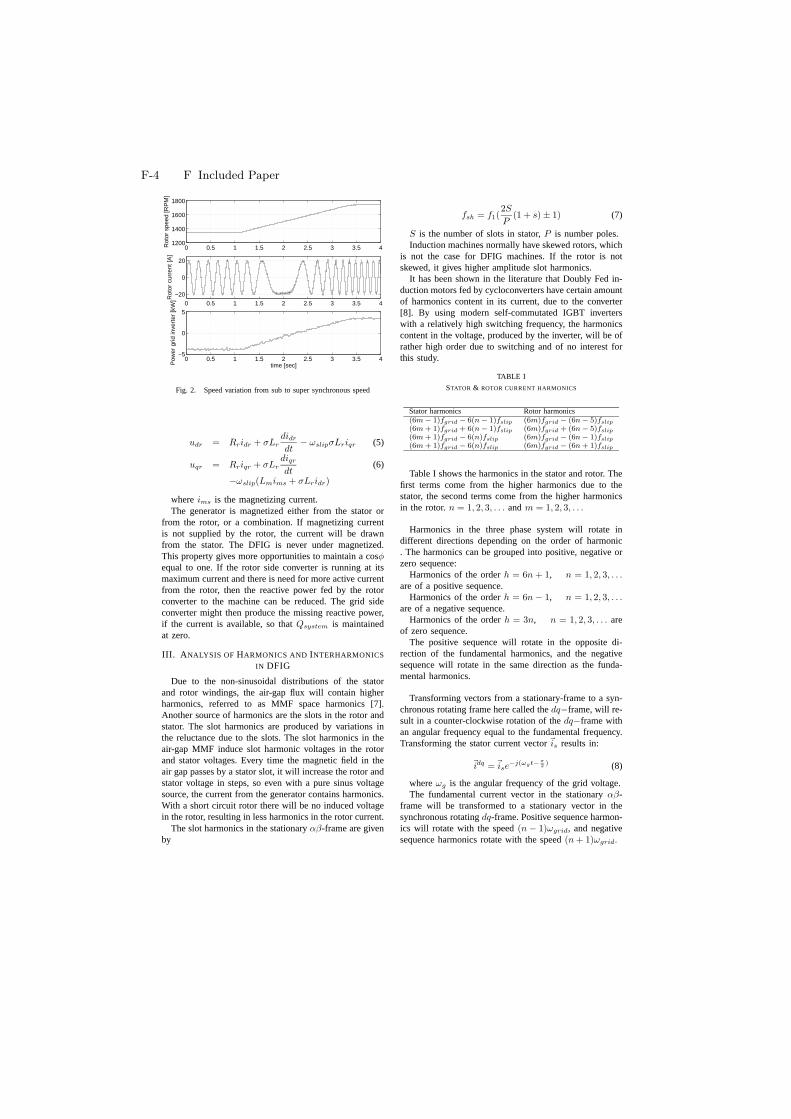
F-4 F Included Paper
0 0.5 1 1.5 2 2.5 3 3.5 41200
1400
1600
1800
Rot
or s
peed
[RP
M]
0 0.5 1 1.5 2 2.5 3 3.5 4
−20
0
20
Rot
or c
urre
nt [A
]
0 0.5 1 1.5 2 2.5 3 3.5 4−5
0
5
time [sec]Pow
er g
rid in
vert
er [k
W]
Fig. 2. Speed variation from sub to super synchronous speed
udr = Rridr + σLr
didr
dt− ωslipσLriqr (5)
uqr = Rriqr + σLr
diqr
dt(6)
−ωslip(Lmims + σLridr)
whereims is the magnetizing current.The generator is magnetized either from the stator or
from the rotor, or a combination. If magnetizing currentis not supplied by the rotor, the current will be drawnfrom the stator. The DFIG is never under magnetized.This property gives more opportunities to maintain a cosφ
equal to one. If the rotor side converter is running at itsmaximum current and there is need for more active currentfrom the rotor, then the reactive power fed by the rotorconverter to the machine can be reduced. The grid sideconverter might then produce the missing reactive power,if the current is available, so thatQsystem is maintainedat zero.
III. A NALYSIS OF HARMONICS AND INTERHARMONICS
IN DFIG
Due to the non-sinusoidal distributions of the statorand rotor windings, the air-gap flux will contain higherharmonics, referred to as MMF space harmonics [7].Another source of harmonics are the slots in the rotor andstator. The slot harmonics are produced by variations inthe reluctance due to the slots. The slot harmonics in theair-gap MMF induce slot harmonic voltages in the rotorand stator voltages. Every time the magnetic field in theair gap passes by a stator slot, it will increase the rotor andstator voltage in steps, so even with a pure sinus voltagesource, the current from the generator contains harmonics.With a short circuit rotor there will be no induced voltagein the rotor, resulting in less harmonics in the rotor current.
The slot harmonics in the stationaryαβ-frame are givenby
fsh = f1(2S
P(1 + s) ± 1) (7)
S is the number of slots in stator,P is number poles.Induction machines normally have skewed rotors, which
is not the case for DFIG machines. If the rotor is notskewed, it gives higher amplitude slot harmonics.
It has been shown in the literature that Doubly Fed in-duction motors fed by cycloconverters have certain amountof harmonics content in its current, due to the converter[8]. By using modern self-commutated IGBT inverterswith a relatively high switching frequency, the harmonicscontent in the voltage, produced by the inverter, will be ofrather high order due to switching and of no interest forthis study.
TABLE I
STATOR & ROTOR CURRENT HARMONICS
Stator harmonics Rotor harmonics(6m − 1)fgrid − 6(n − 1)fslip (6m)fgrid − (6n − 5)fslip
(6m + 1)fgrid + 6(n − 1)fslip (6m)fgrid + (6n − 5)fslip
(6m + 1)fgrid − 6(n)fslip (6m)fgrid − (6n − 1)fslip
(6m + 1)fgrid − 6(n)fslip (6m)fgrid − (6n + 1)fslip
Table I shows the harmonics in the stator and rotor. Thefirst terms come from the higher harmonics due to thestator, the second terms come from the higher harmonicsin the rotor.n = 1, 2, 3, . . . andm = 1, 2, 3, . . .
Harmonics in the three phase system will rotate indifferent directions depending on the order of harmonic. The harmonics can be grouped into positive, negative orzero sequence:
Harmonics of the orderh = 6n + 1, n = 1, 2, 3, . . .
are of a positive sequence.Harmonics of the orderh = 6n − 1, n = 1, 2, 3, . . .
are of a negative sequence.Harmonics of the orderh = 3n, n = 1, 2, 3, . . . are
of zero sequence.The positive sequence will rotate in the opposite di-
rection of the fundamental harmonics, and the negativesequence will rotate in the same direction as the funda-mental harmonics.
Transforming vectors from a stationary-frame to a syn-chronous rotating frame here called thedq−frame, will re-sult in a counter-clockwise rotation of thedq−frame withan angular frequency equal to the fundamental frequency.Transforming the stator current vector~is results in:
~idq =~ise−j(ωgt−π
2) (8)
whereωg is the angular frequency of the grid voltage.The fundamental current vector in the stationaryαβ-
frame will be transformed to a stationary vector in thesynchronous rotatingdq-frame. Positive sequence harmon-ics will rotate with the speed(n − 1)ωgrid, and negativesequence harmonics rotate with the speed(n + 1)ωgrid.
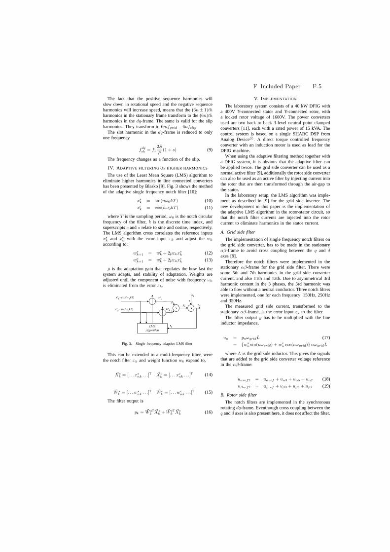
F Included Paper F-5
The fact that the positive sequence harmonics willslow down in rotational speed and the negative sequenceharmonics will increase speed, means that the (6n± 1)thharmonics in the stationary frame transform to the (6n)thharmonics in thedq-frame. The same is valid for the slipharmonics. They transform to6mfgrid − 6nfslip.
The slot harmonic in thedq-frame is reduced to onlyone frequency
fdqsh = f1
2S
P(1 + s) (9)
The frequency changes as a function of the slip.
IV. A DAPTIVE FILTERING OF HIGHER HARMONICS
The use of the Least Mean Square (LMS) algorithm toeliminate higher harmonics in line connected convertershas been presented by Blasko [9]. Fig. 3 shows the methodof the adaptive single frequency notch filter [10]:
xsk = sin(nω0kT ) (10)
xck = cos(nω0kT ) (11)
whereT is the sampling period,ω0 is the notch circularfrequency of the filter,k is the discrete time index, andsuperscriptsc ands relate to sine and cosine, respectively.The LMS algorithm cross correlates the reference inputsxs
k and xck with the error inputεk and adjust thewk
according to:
wsk+1 = ws
k + 2µεkxsk (12)
wck+1 = wc
k + 2µεkxck (13)
µ is the adaptation gain that regulates the how fast thesystem adapts, and stability of adaptation. Weights areadjusted until the component of noise with frequencyω0
is eliminated from the errorεk.
+
+yk
LMSAlgorithm
dkxsk=cos( 0kT)
xck=sin( 0kT)
wsk
wck
k
k
+
-
Fig. 3. Single frequency adaptive LMS filter
This can be extended to a multi-frequency filter, werethe notch filterxk and weight functionwk expand to,
~Xsk = [. . . xs
nk . . .]T ~Xck = [. . . xc
nk . . .]T (14)
~W sk = [. . . ws
nk . . .]T ~W ck = [. . . wc
nk . . .]T (15)
The filter output is
yk = ~W sTk
~Xsk + ~W cT
k~Xc
k (16)
V. I MPLEMENTATION
The laboratory system consists of a 40 kW DFIG witha 400V Y-connected stator and Y-connected rotor, witha locked rotor voltage of 1600V. The power convertersused are two back to back 3-level neutral point clampedconverters [11], each with a rated power of 15 kVA. Thecontrol system is based on a single SHARC DSP fromAnalog Devicec©. A direct torque controlled frequencyconverter with an induction motor is used as load for theDFIG machine.
When using the adaptive filtering method together witha DFIG system, it is obvious that the adaptive filter canbe applied twice. The grid side converter can be used as anormal active filter [9], additionally the rotor side convertercan also be used as an active filter by injecting current intothe rotor that are then transformed through the air-gap tothe stator.
In the laboratory setup, the LMS algorithm was imple-ment as described in [9] for the grid side inverter. Thenew development in this paper is the implementation ofthe adaptive LMS algorithm in the rotor-stator circuit, sothat the notch filter currents are injected into the rotorcurrent to eliminate harmonics in the stator current.
A. Grid side filter
The implementation of single frequency notch filters onthe grid side converter, has to be made in the stationaryαβ-frame to avoid cross coupling between theq and d
axes [9].Therefore the notch filters were implemented in the
stationaryαβ-frame for the grid side filter. There weresome 5th and 7th harmonics in the grid side convertercurrent, and also 11th and 13th. Due to asymmetrical 3rdharmonic content in the 3 phases, the 3rd harmonic wasable to flow without a neutral conductor. Three notch filterswere implemented, one for each frequency: 150Hz, 250Hzand 350Hz.
The measured grid side current, transformed to thestationaryαβ-frame, is the error inputεk to the filter.
The filter outputy has to be multiplied with the lineinductor impedance,
un = ynωgridL (17)
= wsn sin(nωgrid) + wc
n cos(nωgrid)nωgridL
whereL is the grid side inductor. This gives the signalsthat are added to the grid side converter voltage referencein the αβ-frame:
uαref2 = uαref + uα3 + uα5 + uα7 (18)
uβref2 = uβref + uβ3 + uβ5 + uβ7 (19)
B. Rotor side filter
The notch filters are implemented in the synchronousrotatingdq-frame. Eventhough cross coupling between theq andd axes is also present here, it does not affect the filter.
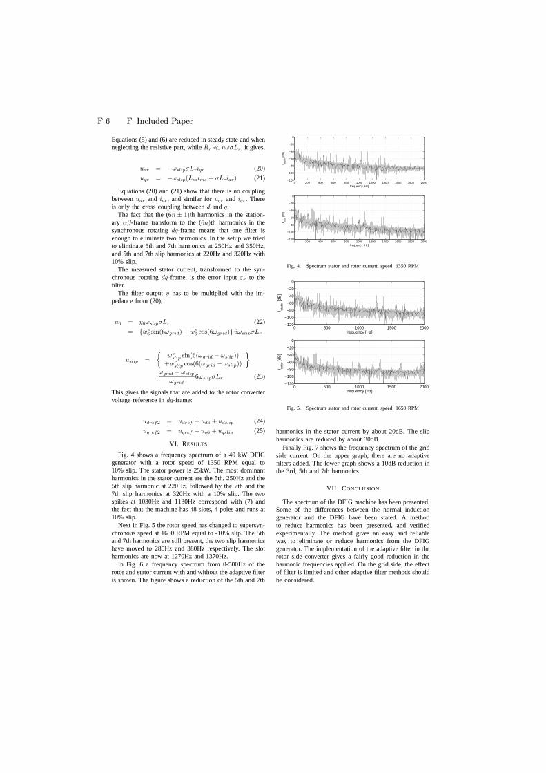
F-6 F Included Paper
Equations (5) and (6) are reduced in steady state and whenneglecting the resistive part, whileRr ¿ nωσLr, it gives,
udr = −ωslipσLriqr (20)
uqr = −ωslip(Lmims + σLridr) (21)
Equations (20) and (21) show that there is no couplingbetweenudr and idr, and similar foruqr and iqr. Thereis only the cross coupling betweend andq.
The fact that the (6n ± 1)th harmonics in the station-ary αβ-frame transform to the (6n)th harmonics in thesynchronous rotatingdq-frame means that one filter isenough to eliminate two harmonics. In the setup we triedto eliminate 5th and 7th harmonics at 250Hz and 350Hz,and 5th and 7th slip harmonics at 220Hz and 320Hz with10% slip.
The measured stator current, transformed to the syn-chronous rotatingdq-frame, is the error inputεk to thefilter.
The filter outputy has to be multiplied with the im-pedance from (20),
u6 = y6ωslipσLr (22)
= ws6sin(6ωgrid) + wc
6cos(6ωgrid) 6ωslipσLr
uslip =
wsslip sin(6(ωgrid − ωslip))
+wcslip cos(6(ωgrid − ωslip))
·ωgrid − ωslip
ωgrid
6ωslipσLr (23)
This gives the signals that are added to the rotor convertervoltage reference indq-frame:
udref2 = udref + ud6 + udslip (24)
uqref2 = uqref + uq6 + uqslip (25)
VI. RESULTS
Fig. 4 shows a frequency spectrum of a 40 kW DFIGgenerator with a rotor speed of 1350 RPM equal to10% slip. The stator power is 25kW. The most dominantharmonics in the stator current are the 5th, 250Hz and the5th slip harmonic at 220Hz, followed by the 7th and the7th slip harmonics at 320Hz with a 10% slip. The twospikes at 1030Hz and 1130Hz correspond with (7) andthe fact that the machine has 48 slots, 4 poles and runs at10% slip.
Next in Fig. 5 the rotor speed has changed to supersyn-chronous speed at 1650 RPM equal to -10% slip. The 5thand 7th harmonics are still present, the two slip harmonicshave moved to 280Hz and 380Hz respectively. The slotharmonics are now at 1270Hz and 1370Hz.
In Fig. 6 a frequency spectrum from 0-500Hz of therotor and stator current with and without the adaptive filteris shown. The figure shows a reduction of the 5th and 7th
0 200 400 600 800 1000 1200 1400 1600 1800 2000−120
−100
−80
−60
−40
−20
0
frequency [Hz]
I stat
or [d
B]
0 200 400 600 800 1000 1200 1400 1600 1800 2000−120
−100
−80
−60
−40
−20
0
frequency [Hz]
I roto
r [dB
]
Fig. 4. Spectrum stator and rotor current, speed: 1350 RPM
0 500 1000 1500 2000−120
−100
−80
−60
−40
−20
0
frequency [Hz]
I stat
or [d
B]
0 500 1000 1500 2000−120
−100
−80
−60
−40
−20
0
frequency [Hz]
I roto
r [dB
]
Fig. 5. Spectrum stator and rotor current, speed: 1650 RPM
harmonics in the stator current by about 20dB. The slipharmonics are reduced by about 30dB.
Finally Fig. 7 shows the frequency spectrum of the gridside current. On the upper graph, there are no adaptivefilters added. The lower graph shows a 10dB reduction inthe 3rd, 5th and 7th harmonics.
VII. C ONCLUSION
The spectrum of the DFIG machine has been presented.Some of the differences between the normal inductiongenerator and the DFIG have been stated. A methodto reduce harmonics has been presented, and verifiedexperimentally. The method gives an easy and reliableway to eliminate or reduce harmonics from the DFIGgenerator. The implementation of the adaptive filter in therotor side converter gives a fairly good reduction in theharmonic frequencies applied. On the grid side, the effectof filter is limited and other adaptive filter methods shouldbe considered.
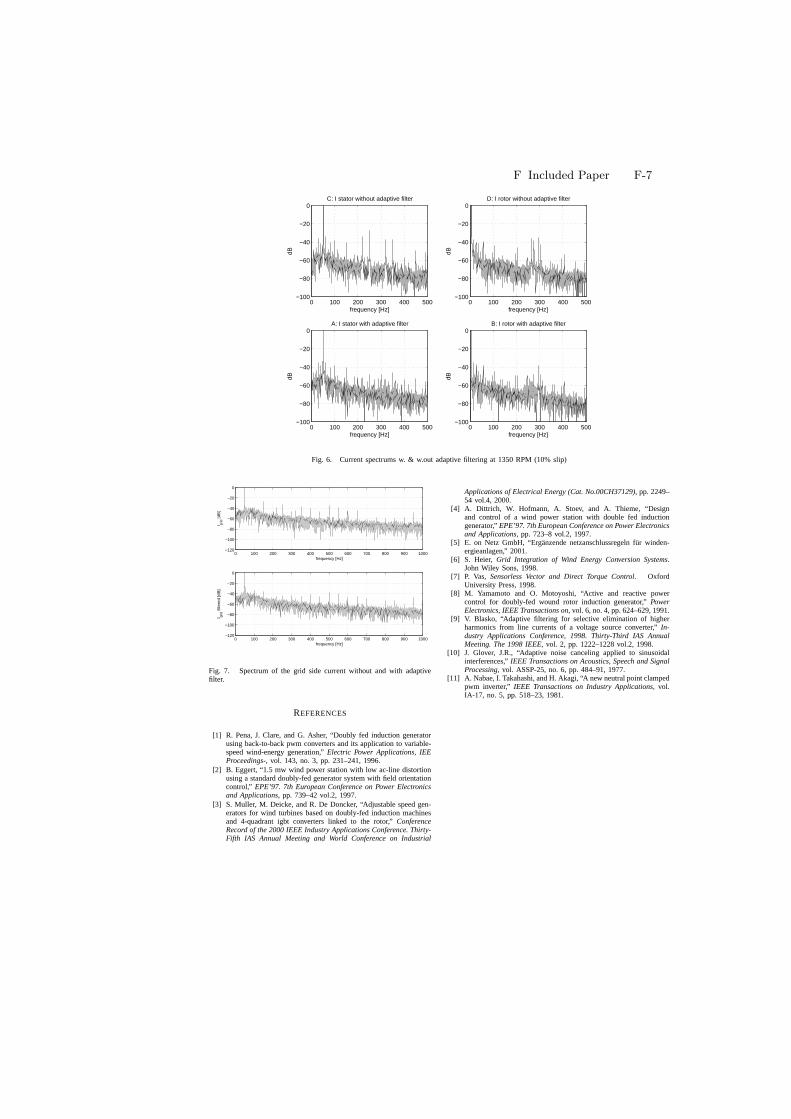
F Included Paper F-7
0 100 200 300 400 500−100
−80
−60
−40
−20
0A: I stator with adaptive filter
frequency [Hz]
dB
0 100 200 300 400 500−100
−80
−60
−40
−20
0B: I rotor with adaptive filter
frequency [Hz]
dB
0 100 200 300 400 500−100
−80
−60
−40
−20
0C: I stator without adaptive filter
frequency [Hz]
dB
0 100 200 300 400 500−100
−80
−60
−40
−20
0D: I rotor without adaptive filter
frequency [Hz]
dB
Fig. 6. Current spectrums w. & w.out adaptive filtering at 1350 RPM (10% slip)
0 100 200 300 400 500 600 700 800 900 1000−120
−100
−80
−60
−40
−20
0
frequency [Hz]
I grid
[dB
]
0 100 200 300 400 500 600 700 800 900 1000−120
−100
−80
−60
−40
−20
0
frequency [Hz]
I grid
filte
red
[dB
]
Fig. 7. Spectrum of the grid side current without and with adaptivefilter.
REFERENCES
[1] R. Pena, J. Clare, and G. Asher, “Doubly fed induction generatorusing back-to-back pwm converters and its application to variable-speed wind-energy generation,”Electric Power Applications, IEEProceedings-, vol. 143, no. 3, pp. 231–241, 1996.
[2] B. Eggert, “1.5 mw wind power station with low ac-line distortionusing a standard doubly-fed generator system with field orientationcontrol,” EPE’97. 7th European Conference on Power Electronicsand Applications, pp. 739–42 vol.2, 1997.
[3] S. Muller, M. Deicke, and R. De Doncker, “Adjustable speed gen-erators for wind turbines based on doubly-fed induction machinesand 4-quadrant igbt converters linked to the rotor,”ConferenceRecord of the 2000 IEEE Industry Applications Conference. Thirty-Fifth IAS Annual Meeting and World Conference on Industrial
Applications of Electrical Energy (Cat. No.00CH37129), pp. 2249–54 vol.4, 2000.
[4] A. Dittrich, W. Hofmann, A. Stoev, and A. Thieme, “Designand control of a wind power station with double fed inductiongenerator,”EPE’97. 7th European Conference on Power Electronicsand Applications, pp. 723–8 vol.2, 1997.
[5] E. on Netz GmbH, “Erganzende netzanschlussregeln fur winden-ergieanlagen,” 2001.
[6] S. Heier, Grid Integration of Wind Energy Conversion Systems.John Wiley Sons, 1998.
[7] P. Vas, Sensorless Vector and Direct Torque Control. OxfordUniversity Press, 1998.
[8] M. Yamamoto and O. Motoyoshi, “Active and reactive powercontrol for doubly-fed wound rotor induction generator,”PowerElectronics, IEEE Transactions on, vol. 6, no. 4, pp. 624–629, 1991.
[9] V. Blasko, “Adaptive filtering for selective elimination of higherharmonics from line currents of a voltage source converter,” In-dustry Applications Conference, 1998. Thirty-Third IAS AnnualMeeting. The 1998 IEEE, vol. 2, pp. 1222–1228 vol.2, 1998.
[10] J. Glover, J.R., “Adaptive noise canceling applied to sinusoidalinterferences,”IEEE Transactions on Acoustics, Speech and SignalProcessing, vol. ASSP-25, no. 6, pp. 484–91, 1977.
[11] A. Nabae, I. Takahashi, and H. Akagi, “A new neutral point clampedpwm inverter,” IEEE Transactions on Industry Applications, vol.IA-17, no. 5, pp. 518–23, 1981.