adaptive sampling with topological scores

International Journal for Uncertainty Quantification, 1(1):xxx–xxx, 2012

ADAPTIVE SAMPLING WITH TOPOLOGICAL SCORES

Dan Maljovec,1 Bei Wang,1,∗ Ana Kupresanin,2 Gardar Johannesson,2 Va-lerio Pascucci,1 & Peer-Timo Bremer1,2

1Scientific Computing and Imaging Institute, University of Utah, 72 South Central CampusDrive, Salt Lake City, UT 841122Lawrence Livermore National Laboratory, 7000 East Avenue, Livermore, CA 94550-9234

Original Manuscript Submitted: 07/18/2012; Final Draft Received: 07/18/2012

Understanding and describing expensive black box functions such as physical simulations is a common problem inmany application areas. One example is the recent interest in uncertainty quantification with the goal of discoveringthe relationship between a potentially large number of input parameters and the output of a simulation. Typically,the simulation of interest is expensive to evaluate and thus the sampling of the parameter space is necessarily small.As a result choosing a “good” set of samples at which to evaluate is crucial to glean as much information as possiblefrom the fewest samples. While space-filling sampling designs such as Latin Hypercubes provide a good initial coverof the entire domain, more detailed studies typically rely on adaptive sampling: Given an initial set of samples, thesetechniques construct a surrogate model and use it to evaluate a scoring function which aims to predict the expectedgain from evaluating a potential new sample. There exist a large number of different surrogate models as well asdifferent scoring functions each with their own advantages and disadvantages. In this paper we present an extensivecomparative study of adaptive sampling using four popular regression models combined with six traditional scoringfunctions compared against a space filling design. Furthermore, for a single high-dimensional output function, weintroduce a new class of scoring functions based on global topological rather than local geometric information. The newscoring functions are competitive in terms of the root mean square prediction error but are expected to better recoverthe global topological structure. Our experiments suggest that the most common point of failure of adaptive samplingschemes are ill-suited regression models. Nevertheless, even given well-fitted surrogate models many scoring functionsfail to outperform a space-filling design.

KEY WORDS: adaptive sampling, experimental design, topological techniques

1. INTRODUCTION

As the accuracy and availability of computer simulations improves, their results are increasingly used to informfar reaching decisions. Experts in areas ranging from building and automobile design to national energy policyregularly use predictive simulations to evaluate alternative approaches. However, virtually all simulations are basedon approximate models and an incomplete knowledge of the underlying physics and thus do not accurately predict thephenomena of interest. Furthermore, there typically do exist a large number of parameters, e.g. material properties,boundary conditions, sub-scale parameters, etc., that influence the outcome and are used to tune the simulation tomatch experiments or observations. Nevertheless, usually no perfect set of parameters exists nor is this type offitting possible for the most interesting case of truly predictive simulations, e.g. weather or climate forecasts. In suchscenarios the simulation parameters represent a significant source of uncertainty and a single best guess even by anexpert is not very reliable. Consequently, understanding the uncertainty involved in a prediction, the range of possibleoutcomes, and the confidence in the results is of interest.

One common approach to address these issues is to create not one but an ensemble of simulations each withslightly different parameter settings. The resulting collection of outcomes is then analyzed to determine the likelihoodof various scenarios to occur and to assess the confidence in the prediction. The challenge lies in the fact that the

∗Correspond to: Bei Wang, E-mail: [email protected], URL: http://www.sci.utah.edu/∼beiwang/

2152–5080/10/$35.00 c© 2012 by Begell House, Inc. 1

2 Maljovec, Wang, Kupresanin, Johannesson, Pascucci & Bremer

dimension of the parameter space can be large, e.g. tens or hundreds of parameters, and each simulation might beexpensive, e.g. taking hundreds or thousands of CPU hours. Therefore, the space of possible solutions can only besampled very sparsely and each simulation must be carefully chosen to provide the maximal amount of information.A first order solution is to sample the parameter space as evenly as possible and there exist a number of approachessuch as the Latin Hypercube design [1], orthogonal arrays [2], and related techniques [3] that address this issue.

However, in practice much of the parameter space might be invalid, producing clearly unphysical results, or simplyuninteresting and easy to predict. In these situations a space-filling sampling would waste a large amount of resources.Instead, adaptive sampling is used to iteratively guide the choice of future computer runs by repeatedly analyzing themodel based on the existing samples. The most common approach to do adaptive sampling is based on the use ofstatistical prediction models (also known as surrogate models, response functions, statistical emulators, meta models)such as Gaussian processes models (GPMs) [4] or multivariate adaptive regression splines (MARS) [5]. The basicconcept of adaptive sampling is relatively simple and well established: First, one constructs a prediction model basedon an initial set of samples (training points); Second, a large set of candidate points is chosen in the parameter spaceand the prediction model is evaluated at these points; Third, each candidate point is assigned a score based on, forexample the estimated prediction error; Finally, the candidate(s) with the highest score are selected and evaluated byrunning the corresponding simulation.

While the basic pipeline of adaptive sampling is universally accepted, combining different regression models withdifferent scoring functions often leads to drastically different results. Here, we present an extensive experimentalstudy combining four popular statistical models, a GPM [4], two implementations of MARS [5] (available in themda and the earth libraries of the statistical programming language R), and a neural network (NNET) [6] (fromthe nnet library in R), with six traditional as well as three new topology based scoring functions. Using a varietyof test functions in two to five dimensions each combination is compared against a Latin Hypercube design of thesame sample size to evaluate the potential advantage of adaptive sampling in general. As discussed in more detailin Section 4, the most dominant factor in the results is the choice of the statistical prediction model as some modelsappear to be ill-suited for several test functions and for all scoring functions they produce unsatisfactory results. Givenan appropriate prediction model some trends appear that favor information theoretic scoring functions even thoughfor several experiments all scoring functions fail to out-perform the space filling design.

In addition to the experimental results we also introduce a new class of scoring functions based on global topo-logical rather than local geometric information. In particular, we define three new scoring functions primarily aimedat recovering the global structure of a function. Nevertheless, our results show that the new scoring functions remaincompetitive in terms of mean square prediction error.

2. BACKGROUND AND RELATED WORK

Here we introduce some of the necessary background and discuss related work in both adaptive sampling as well astopological analysis and visualization.

2.1 Statistical Prediction Models

Since computer simulations are generally computationally expensive, a standard approach to analyze them is to builda statistical prediction model (PM), and use it in place of the actual simulation code in further analysis, to guide theselection of upcoming ensemble of simulations. We now give a brief overview of some commonly used statisticalPMs; see Fang, Li, and Sudjianto [7] for further details.

Let y(x) denote the output of the simulation code, where the vector input variable, x, is restricted to the d-dimensional unit cube [0, 1]d . This assumption is easily relaxed to any “rectangular” input space. Let x1, . . . ,xn ∈[0, 1]d be an ensemble of n input vectors and denote the resulting simulation data of interest by yi = y(xi), i =1, . . . , n.

Gaussian Process Model (GPM). One of the statistical models most frequently used for prediction is the Gaussianprocess model (GPM), first used in the context of computer experiments by Sacks [8] in 1989. A common practice

International Journal for Uncertainty Quantification

Adaptive Sampling with Topological Scores 3

is to place a homogeneous GP prior on the family of possible output functions. Then, the predictor is given by theposterior mean conditional on the output of the computer experiment.

The GPM places a prior on the class of possible functions y(x). We denote by Y (x) the random functionwhose distribution is determined by the prior. Suppose that Y (x) = µ + Z(x), where µ is a mean parameterand Z(x) is a Gaussian stochastic process with mean 0, constant variance σ2, and an assumpted (parametric) cor-relation function. An example of popular correlation model is the power exponential correlation function, given byR(x,x′) = exp(−h(x,x′)), where h(x,x′) =

∑dj=1 θj |xj − x′j |pj with θj ≥ 0 and 1 ≤ pj ≤ 2. Here, µ,σ2, θj , pj

are the parameters of the prior model. The values of these parameters are estimated using the ensemble data, (xi, yi),i = 1, . . . , n, typically using a likelihood-based objective function. In situations where the output is quite smooth, itis often the case that pj = 2 holds for all j, resulting in a Gaussian correlation function.

The predictor Y (x) for Y (x) is the posterior mean of Y (x) given {(xi, yi)} and is available in a closed formexpression. Similarly, the mean squared prediction error (MSPE) of Y (x) (the prediction error variance), taking intoaccount the uncertainty from estimating µ by maximum likelihood (but not estimating the correlation parameters), isalso available in a closed form. For more details, see Rasmussen [4].

Multivariate Adaptive Regression Splines (MARS). Another popular class of PMs are Friedman’s multivariateadaptive regression splines [5] (see also Hastie, Tibshirani, and Friedman [9] for a gentle introduction).

MARS is a non-parametric regression method that uses a collection of simple basis functions to build a complexand flexible response function. At the core of MARS are piecewise linear basis functions, given by max(0, x − k)and max(0, k − x), where k is the knot (the break point). These simple functions are used to build a collection ofbasis functions, {max(0, xj − k),max(0, k − xj)}, where k ∈ {x1j , . . . , xnj) for j = 1, . . . , d. If all the inputvalues are different in the training data this will yield 2nd basis functions. The MARS predictor is then given byy(x) = β0 +

∑Mm=1 βmhm(x), where the βm’s are coefficients and the hm’s are basis functions, which are either

given by a single function from the collection of simple basis functions or a product of two or more of such functions.For a given set of basis functions, h1, . . . , hm, the β coefficients are estimated using least squares. The main

novelty of the MARS is how the basis functions are selected using a forward selection process, followed by a backwardelimination process. The forward pass starts with a model that only includes the constant term β0 and then addssimple basis functions in pairs in a greedy fashion. This yields a model that over fits the training data (i.e. has toomany terms). The backward elimination process drops terms using the generalized cross-validation (GCV) criterion,which compromises between the fidelity of the model and its complexity (size).

As with most non-parametric regression methods, there is no direct method to assess their prediction error. How-ever, the prediction error can be estimated by bootstrap methods [10]. In short, an ensemble of MARS models iscreated by repeatedly resampling, with replacement, the original training data {(xi, yi)} and a MARS model is fittedto each batch of resampled data. An estimate of the prediction error is then given by the standard deviation of thepredictions provided by the bootstrap ensemble.

Neural Networks (NNET). Another popular class of PMs is given by neural networks (NNETs), in particular bysimple feed-forward neural networks with a single hidden layer (see e.g. Ripley [6] and Hastie et al. [9] for furtherdetails).

The single layer NNET is simply a non-linear statistical model, where the response of interest is modeled as alinear combination of M derived features (the hidden units of the NNET); y(x) = β0 + βT z, z = (z1, . . . , zM )T ,where zm = σ(α0m + αT

mx). The activation function, σ(v) is usually taken as the sigmoid function, σ(v) =1/(1 + e−v).

The unknown parameters of the NNET, which we denote by θ and are often referred to as weights, and consistof the M(d + 1) α’s of the hidden layer and the M + 1 β’s for the response model. The weights are estimated byminimizing the sum-of-squares, R(θ) =

∑ni=1(yi − y(xi))

2. However, for a large NNET, the resulting NNET over-fits the data (i.e., the NNET fits the training data well, but performs poorly on independent validation data). A commonsolution is to add a regularization term that shrinks the weights to zero, such as J(θ) =

∑Mm=0 β

2m+

∑M,dm=0,j=1 α

2mj ,

and then minimize R(θ) + λJ(θ). The minimization can be carried out in an efficient manner using gradient-basedmethods, as the gradient of the NNET can be computed easily using the chain rule for differentiation. As in the caseof MARS, the prediction error of the NNET can be estimated using bootstrap methods.

Volume 1, Number 1, 2012


2.2 Design of Computer Experiments

Experimental designs relevant to computer experiments (i.e. sampling) are often broadly categorized into two classes:space-filling and criterion-based designs. Intuitively, it is natural to consider a space-filling design strategy to minimizethe overall prediction error and a number of approaches have been studied. These include methods based on selectingrandom samples e.g. Latin hypercube designs, distance-based designs and uniform designs. A thorough discussions ofthe various strategies may be found in Satner et al. [11], Koehler and Owen [12], and Bates et al. [13]. Intuitively, thegoal is to ensure that the input points are uniformly distributed over the range of each input dimension. In our setting,space-filling designs are attractive for an initial exploratory analysis. However, their applicability for detailed studies islimited by their very construction rationale, that is, the assumption that the features of the response model are equallylikely to be found anywhere in the input space. More specifically, following a space-filling design, we will have nofreedom to adapt our selection of input points to information gathered as simulations are completed. Instead, usingthe knowledge contained in a partially constructed model may allows us to adaptively select the samples in regionsof interest. If samples are chosen correctly, this strategy will greatly improve prediction accuracy and efficiencycompared to a pure space-filling design.

This leads to the second class of experimental designs: those constructed by adding one or several points at atime to the initial model. New points are selected from a large candidate set based on various statistical criteria andthe prediction of the existing (partial) model. Due to their iterative nature these designs are usually referred to assequential, or adaptive. Sequential designs based on optimizing statistical criteria such as mean squared predictionerror or the notion of entropy have also been used to construct designs for computer experiments [11]. Here we usea simple sampling of the range space, see Section 3.1, as well as the mean squared prediction error (MSPE) and theexpected improvement as criteria.

Maximum mean squared prediction error. The mean square prediction error (MSPE) is simply the predictionerror of PM at a given new input point. In the case of the GPM, the prediction error is available in a closed form, butis estimated using bootstrap for MARS and NNET. The MSPE criterion aims at selecting the point from the candidateset that has the largest MSPE.

In the case of a stationary GPM with a constant mean, this results in criterion that spreads points out, but atdifferent density along each axis, and typically starts out by populating points near the boundary of the input space.In the case of MARS and NNET, which can capture very non-stationary behavior, the criterion typically populatespoints in the region of the input space which is most sensitive to bootstrap resampling, that is, where there is a largevariation in the response.

Maximum expected improvement (EI). The expected improvement (EI) criterion was proposed by [14] and origi-nally developed in the context of global optimization [15]. Lam [16] considered a modification of this criterion withthe goal of obtaining a good global fit of the GPM instead of locating the global optimum or optima. Intuitively, theobjective here is to search for “informative” regions in the domain that will help improve the global fit of the model,where “informative” means regions with significant variation in the response variable.

In case of the GPM, for each potential input point x, Lam defined the improvement as I(x) = (Y (x)− y(xj∗))2,

where y(xi∗) is the observed output at the sampled point xi∗ closest (in Euclidean distance) to the candidate point x.The maximum expected improvement criterion advises to select as the next point the one that maximizes the expectedimprovement EI(x) = (Y (x)− y(xi∗))

2+ σ2(x). One typically works with the square-root of the E(I), which is atthe same scale as response. For the details of the derivation of E(I) using a GPM, we refer to [16]. The EI criterioncan be extended to MARS and NNET by simply replacing Y (x) with the bootstrap average and the prediction varianceσ2(x) with the bootstrap variance.

The estimate of expected improvement uses two search components, one local and one global. The first (local)component of the expected improvement will tend to be large at points where the increase in response over the nearestsampled points is large. The second (global) component is large at points with the largest prediction error.



2.3 Morse-Smale Complex and Its Approximation

To quantify the expected topological impact of a point during adaptive sampling, we introduce a key topologicalstructure, the Morse-Smale Complex, which forms the basis for the new scoring functions introduced in Section 3.2.

Topological structures, such as contour trees [17], Reeb graphs [17–20] and Morse-Smale complexes [21, 22]provide abstract representations for scalar functions. These structures can be used to define a wide variety of featuresin various applications, ranging from medical [23], to physics [24, 25] and material science [26]. To analyze andvisualize high-dimensional data, several topological approaches have been proposed, in particular, [27, 28].

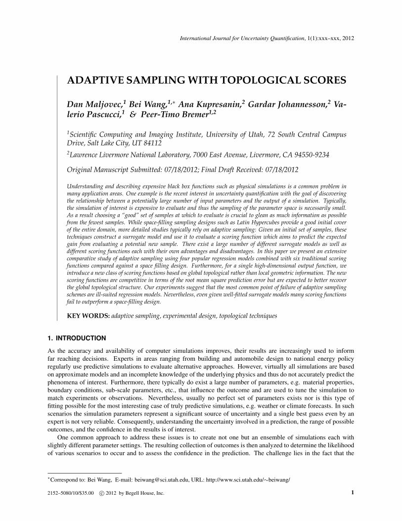
Let M be a smooth manifold without boundary and f : M→ R be a smooth function with gradient ∇ f . A pointx ∈M is called critical if∇ f(x) = 0, otherwise it is regular. If the Hessian matrix at a critical point is non-singularthen the critical point is called non-degenerate. At any regular point x the gradient is well-defined and integrating itin both directions traces out an integral line, γ : R → M, which is a maximal path whose tangent vectors agree withthe gradient [21]. Each integral line begins and ends at critical points of f . The ascending/descending manifolds of acritical point p is defined as all the points whose integral lines start/end at p. The descending manifolds form a complexcalled a Morse complex of f and the ascending manifolds define the Morse complex of −f . The set of intersectionsof ascending and descending manifolds creates the Morse-Smale complex of f . Each cell (crystal) of the Morse-Smale complex is a union of integral lines that all share the same origin and the same destination. In other words,all the points inside a single crystal have uniform gradient flow behavior. These crystals yield a decomposition intomonotonic, non-overlapping regions of the domain, as shown in Fig. 1(a)-(c) for a two-dimensional height function.

(a) (b) (c) (d) (e)

FIG. 1: Left: (a) Ascending manifolds, (b) descending manifolds and (c) Morse-Smale complex. Right: A 2D Morse-Smale complex before (c) and after (d) persistence simplification. Maxima are red, minima are blue and saddles aregreen.

In two and three dimensions, discrete Morse-Smale complex on piecewise linear functions can be constructed[17, 21, 22, 29]. For high dimensional point cloud data, the Morse-Smale complex can only be approximated [30, 31].Here, we give an overview of the approximation approach in high dimension detailed in [31, 32], which is crucial inour algorithm pipeline. First, the domain is approximated by a k nearest neighbor (kNN) graph. The algorithm uses adiscrete approximation of the integral line by following the paths of steepest accent and descent among neighboringpoints in the graph, based on a quick-shift algorithm [33]. The neighbors of a point xi is defined as adj (xi) ={xj | xj ∈ knn (xi) or xi ∈ knn (xj)}. Its steepest ascent is argmaxxj∈adj (x) ||f(xj) − f(xi)||/||xi − xj ||, whileits steepest descent is argmaxxj∈adj (x) ||f(xi) − f(xj)||/||xi − xj ||. Each point xi is then assigned to a crystalof the Morse-Smale complex which is a union of approximated integral lines that all share the same origin and thesame destination. The domain is then partitioned into regions {C1, C2, ..., Cl} where

⋃i Ci = {xi}ni=1. In this

approximated Morse-Smale complex, a maximum/minimum has no ascending/descending neighbors, respectively.

2.4 Persistence

One advantage of the Morse-Smale complex is that it can be used to associate a notion of significance to the criticalpoints. For example, as shown in Fig. 1(d), the left peak (the circled red maxima) is considered less importanttopologically than its nearby peak (un-circled red maxima to the right) as it is lower. Therefore, at certain scale,we would like to represent this feature as a single peak instead of two separate peaks, as shown in Fig. 1(e). Thissimplification procedure and the notion of scale is defined through the concept of persistence.



The theory of persistence was first introduced in [34, 35], but borrows from the conventional notion of the saliencyof watersheds in image segmentation. It has since been applied to a number of problems, including sensor networks[36], surface description and reconstruction [37], protein shapes [38], images analysis [39], and topological de-noising[40]. In visualization, it has been used to simplify Morse-Smale complexes [41, 42], Reeb graphs [43] and contourtrees [23]. Here we introduce persistence for a 1D (single variable) function [38] and refer to [34, 35, 44] for itsgeneral settings.

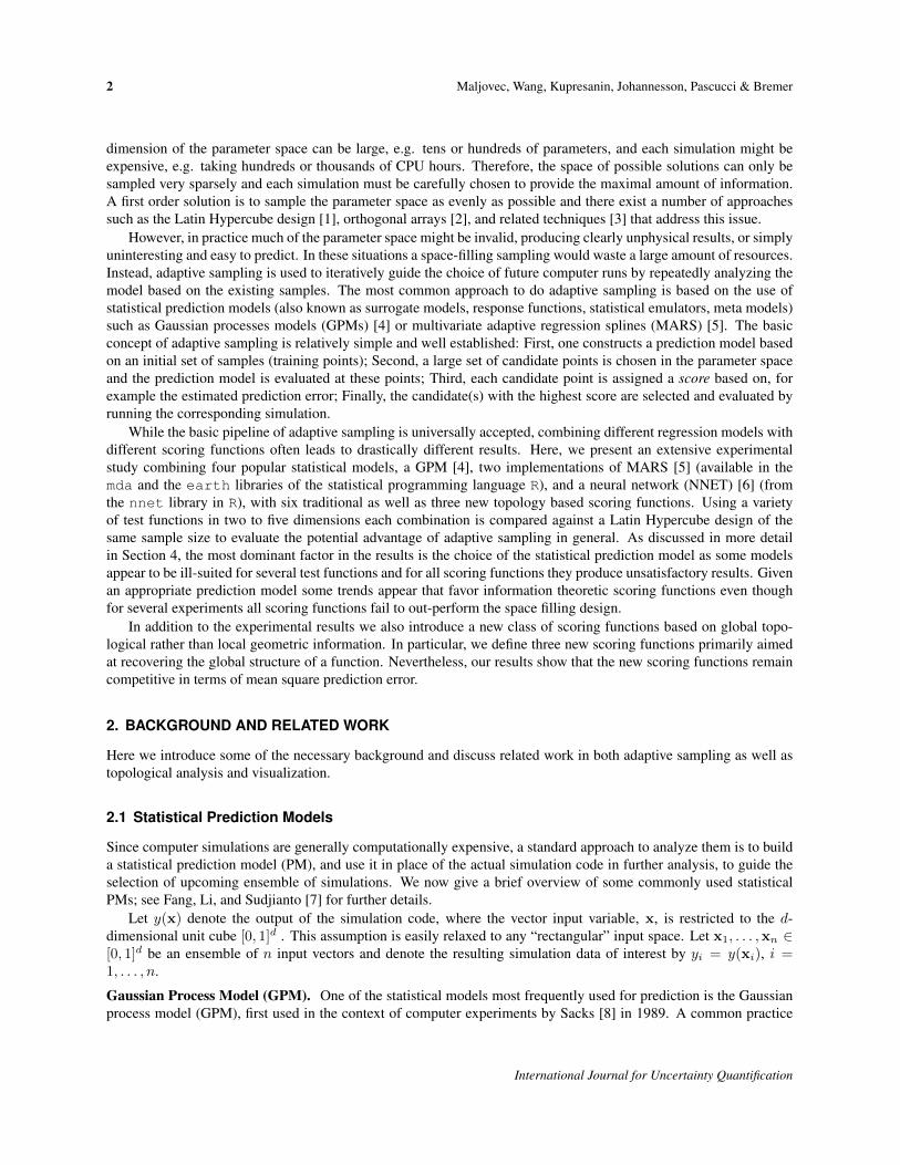
For a one-dimensional smooth function f : R→ R, persistence can be described through the number of connectedcomponents in the sublevel sets, and by tracking the birth and death of these components. In particular, componentsare created and destroyed only at sublevel sets containing critical points. Pairing the critical point that creates acomponent with the one that destroys it thus creates a pairing of critical points. Suppose f has non-degenerate criticalpoints with distinct function values. We have two types of critical points, (local) maxima and (local) minima. Weconsider the sublevel sets of f , Ft = f−1(−∞, t] and track the connectivity of Ft as we increase t from −∞. Asshown in Fig. 2(a), when we pass the minimum point a, a new component appears in the sublevel sets, which isrepresented by the minimum a, with a birth time f(a). Similarly when we pass the minimum b and c, two newcomponents are born with birth time f(b) and f(c), respectively. When we pass the maximum d, two componentsrepresented by a and c are merged and the maxima is paired with the younger (higher) of the two minimum thatrepresent the two components, that is, d and c are paired, where f(d) is the death time of the component representedby c. We define the persistence of the pair to be f(d) − f(c), which corresponds to the significant of a topologicalfeature. We then encode persistence in the persistence diagram, Dgm(f), by mapping the critical point pair to a point(f(c), f(d)) on the 2D plane. Similarly we pair e with b and f with a, resulting two more points in Dgm(f). Fortechnical reasons, the diagonal is considered as part of the persistence diagram that contains an infinite number ofpoints.

birth

death

a

b

c

birth

death

d

e

f

(a) (b)

FIG. 2: (a) A 1D function with three local minima and three local maxima. The critical points are paired, and eachpair is encoded as a point in the persistence diagram on the right. (b) Left, two functions f, g : R → R with smallL∞-distance. Right, their corresponding persistence diagrams Dgm(f) (circles) and Dgm(g) (squares) have smallbottleneck distance.

Recent results show that persistence diagrams are stable under small perturbations of the functions [44, 45]. Letp = (p1, p2), q = (q1, q2) be two points in the persistence diagram, let ||p − q||∞ = max{|p1 − q1|, |p2 − q2|}. Forfunctions f, g : R→ R, ||f−g||∞ = supx |f(x)−g(x)|. The bottleneck distance between two multi-sets of points inDgm(f) and Dgm(g) is dB(Dgm(f),Dgm(g)) = infγ supx ||x − γ(x)||∞, where x ∈ Dgm(f) and y ∈ Dgm(g)range over all points, and γ ranges over all bijections from Dgm(f) to Dgm(g) [45]. The Stability Theorem statesthat the persistence diagrams satisfy: dB(Dgm(f),Dgm(g)) ≤ ||f − g||∞. This is illustrated in Fig. 2(b).

Using the Morse-Smale complex the persistence pairing can be created by successively canceling the two criticalpoints connected in the complex with minimal persistence while avoiding certain degenerate situations. This assignsa persistence to each critical point in the complex which, intuitively, describes the scale at which a critical pointwould disappear through simplification. Note that in the approximate Morse-Smale complexes created from highdimensional point clouds [32] only a subset of theoretically possible cancellations can be performed which changesthe persistences slightly. However, we have not observed any negative effects of the approximation.



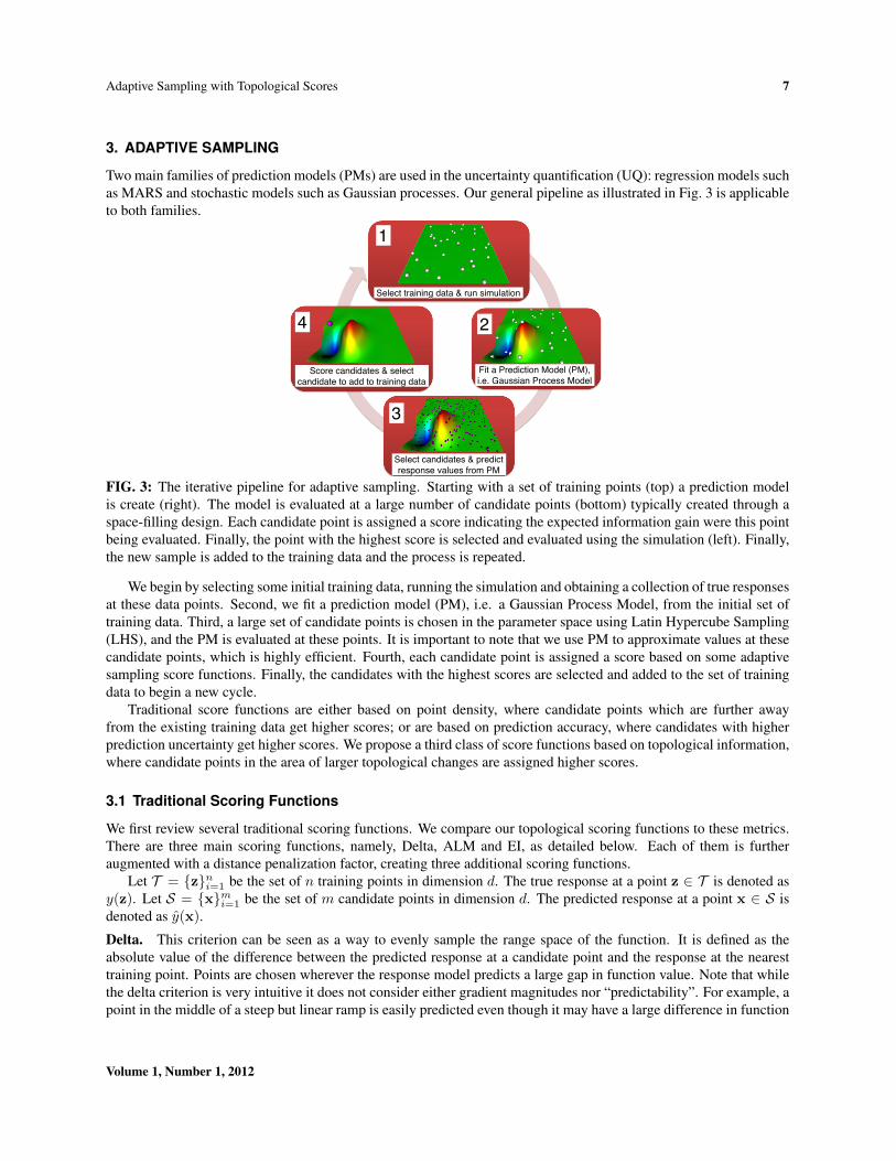
3. ADAPTIVE SAMPLING

Two main families of prediction models (PMs) are used in the uncertainty quantification (UQ): regression models suchas MARS and stochastic models such as Gaussian processes. Our general pipeline as illustrated in Fig. 3 is applicableto both families.

Select training data & run simulation

Fit a Prediction Model (PM), i.e. Gaussian Process Model

Select candidates & predictresponse values from PM

Score candidates & select candidate to add to training data

1

2

3

4

FIG. 3: The iterative pipeline for adaptive sampling. Starting with a set of training points (top) a prediction modelis create (right). The model is evaluated at a large number of candidate points (bottom) typically created through aspace-filling design. Each candidate point is assigned a score indicating the expected information gain were this pointbeing evaluated. Finally, the point with the highest score is selected and evaluated using the simulation (left). Finally,the new sample is added to the training data and the process is repeated.

We begin by selecting some initial training data, running the simulation and obtaining a collection of true responsesat these data points. Second, we fit a prediction model (PM), i.e. a Gaussian Process Model, from the initial set oftraining data. Third, a large set of candidate points is chosen in the parameter space using Latin Hypercube Sampling(LHS), and the PM is evaluated at these points. It is important to note that we use PM to approximate values at thesecandidate points, which is highly efficient. Fourth, each candidate point is assigned a score based on some adaptivesampling score functions. Finally, the candidates with the highest scores are selected and added to the set of trainingdata to begin a new cycle.

Traditional score functions are either based on point density, where candidate points which are further awayfrom the existing training data get higher scores; or are based on prediction accuracy, where candidates with higherprediction uncertainty get higher scores. We propose a third class of score functions based on topological information,where candidate points in the area of larger topological changes are assigned higher scores.

3.1 Traditional Scoring Functions

We first review several traditional scoring functions. We compare our topological scoring functions to these metrics.There are three main scoring functions, namely, Delta, ALM and EI, as detailed below. Each of them is furtheraugmented with a distance penalization factor, creating three additional scoring functions.

Let T = {z}ni=1 be the set of n training points in dimension d. The true response at a point z ∈ T is denoted asy(z). Let S = {x}mi=1 be the set of m candidate points in dimension d. The predicted response at a point x ∈ S isdenoted as y(x).

Delta. This criterion can be seen as a way to evenly sample the range space of the function. It is defined as theabsolute value of the difference between the predicted response at a candidate point and the response at the nearesttraining point. Points are chosen wherever the response model predicts a large gap in function value. Note that whilethe delta criterion is very intuitive it does not consider either gradient magnitudes nor “predictability”. For example, apoint in the middle of a steep but linear ramp is easily predicted even though it may have a large difference in function



value. Similarly, a point with a large difference in function value far away from the nearest sample may not be asinteresting as a slightly smaller difference in a highly sampled region. Formally, for a point x ∈ S , Delta(x) is theabsolute difference, to the q-th power, between the predicted response and the response observed at the closest pointin the training sample, as measured by the Lp distance metric, that is, d(x,x′) = (

∑di=1 |xi − x′i|p)1/p. That is, for

some fixed parameters p and q, let x∗ = argminz∈T d(x, z), then Delta(x) = |y(x)−y(x∗)|q . In the default setting,p = 2 and q = 2.

ALM. This is the Active Learning MacKay criterion described in [46] which attempts to optimize the predictivevariance. The idea is that the variance represents a notion of uncertainty in the prediction and new samples shouldbe evaluated in the least well understand regions of the parameter space. For the GPM the variance can be computeddirectly from the model which appears to be a significant advantage (see Section 4). For the other prediction modelswe use bootstrapping (as described in Section 2.1 and APPENDIX B) to estimate the variance.

EI. This is the expected improvement criterion. As discussed in Section 2.2, this can be seen as a combination of theexpected prediction error used in the ALM method and the Delta criterion. Points are chosen that either show a largeuncertainty in their current prediction or have a large discrepancy with the closest existing sample. Our predicationmodel uses EI(x) = (|y(x)− y(x∗)|2 +ALM(x))1/2.

Distance Penalization. Each of the above three scoring functions can be augmented with a distance penalizationfactor, therefore creating three additional scoring functions, namely, DeltaDP, ALMDP and EIDP. For DeltaDP, theDelta criterion with an additional penalty term, we can prevent samples from lying too close to the training set. Thescaling attempts to balance the goal of sampling in areas of large function variance with the ability to detect yetunknown features by preferring under-sampled areas. For a point x ∈ S , DeltaDP (x) = Delta(x) ∗ ρx, where ρxis the distance scaling factor. Recall dx = d(x,x∗) is the distance from x to the closest point in the training data,and D is a distance vector of dx for all x ∈ S . ρx = ρx(dx, d0, p0), where d0 is the range and q0 is the quantile (bydefault, d0 is the q0 quantile of D). If dx > d0, set ρx = 1, otherwise ρx = 1.5dx − 0.5d3x, where the coefficients aretaken from spherical semivariogram. Similarly we define ALMDP (x) = ALM(x) ∗ρx, where we approach a morespace-filling point selection; and EIDP (x) = EI(x) ∗ ρx. By default we use q0 = 0.5.

3.2 Topological Scoring Functions

All of the scoring functions discussed above pick sample points more or less directly based on the idea of globallyimproving the prediction accuracy. However, these points are not necessarily the optimal candidates. Imagine, forexample, a steep mountain that (by random chance) has already been sampled both close to its peak as well assomewhere near the base. For points on the slope of the mountain, the prediction will show a large difference infunction value thus making it attractive for most standard techniques. However, evaluating the prediction in moredetail would also show that even taking a sizable prediction error into account the global structure of the mountainwould not change by adding a point on its slope. More specifically, the single mountain would remain a singlemountain for a wide range of potential new values even considering errors and uncertainty. This rationale leads totopology based scoring function aimed at discovering the global structure – the topology – of a function rather than itsdetailed geometry. In particular, we propose three different topology based scoring functions, named, TopoHP, TopoPand TopoB as detailed below, illustrated in Fig. 4.

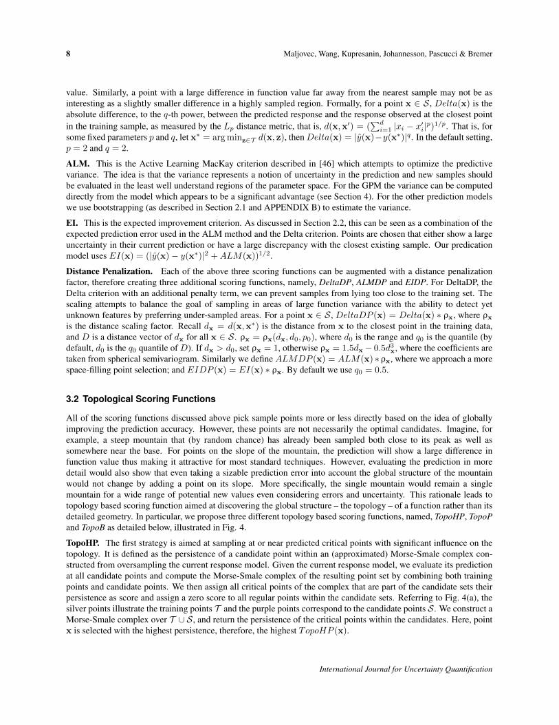
TopoHP. The first strategy is aimed at sampling at or near predicted critical points with significant influence on thetopology. It is defined as the persistence of a candidate point within an (approximated) Morse-Smale complex con-structed from oversampling the current response model. Given the current response model, we evaluate its predictionat all candidate points and compute the Morse-Smale complex of the resulting point set by combining both trainingpoints and candidate points. We then assign all critical points of the complex that are part of the candidate sets theirpersistence as score and assign a zero score to all regular points within the candidate sets. Referring to Fig. 4(a), thesilver points illustrate the training points T and the purple points correspond to the candidate points S. We construct aMorse-Smale complex over T ∪ S , and return the persistence of the critical points within the candidates. Here, pointx is selected with the highest persistence, therefore, the highest TopoHP (x).



(a) (b)birth

death

(c)

FIG. 4: (a) TopoHP: Construct a Morse-Smale complex from training data (silver) as well as all candidates withpredicted responses (purple), return the persistence of the critical points within the candidates. Point x is selectedwith the highest TopoHP (x). (b) TopoP: average change in persistence for all extrema before (left) and after (right)inserting a candidate x into the Morse-Smale complex. (c) Morse-Smale complexes before (left) and after (middle)inserting a candidate point x; TopoB (right): bottleneck distance between the corresponding persistence diagramsbefore (circles) and after (squares) insertion.

TopoP. Similar to a bootstrapping approach, this strategy aims to evaluate how much the topology (as represented bythe persistences) would change if a new candidate point is added. It is defined as the average change of persistence forall current extrema when a given candidate point with its predicted response is inserted into the Morse-Smale complex.As shown in Fig. 4(b), we first construct the Morse-Smale complex of all training data T (silver points). Then foreach candidate point x ∈ S, we construct a new Morse-Smale complex consisting of T ∪x (Fig. 4(b) right). To scorethe candidate x, we compute the change in persistence for each training point x ∈ T that remains as an extrema pointbetween the original and enhanced Morse-Smale complex, and average these changes to obtain a single, nonnegativevalue.

TopoB. For each point x ∈ S , TopoB(x) is defined as the bottleneck distance between the persistence diagram ofthe Morse-Smale complex over T versus the Morse-Smale complex consisting of T ∪ x. This strategy is similar tothe TopoP scoring except that the bottleneck distance not only takes the persistence values into account but also theorder and nesting of the corresponding simplification. This is shown in Fig. 4(c), where left and middle illustratethe (approximated) Morse-Smale complexes before and after inserting a candidate point x, and right displays thecorresponding persistence diagrams of these complexes. TopoB(x) is defined as the bottleneck distance betweenthem.

4. EXPERIMENTS

This section summarizes the different experiments and highlights apparent trends and interesting behaviors.

Example Data Sets. To evaluate the different scoring functions and understand the behavior in different scenarioswe have conducted a series of experiments with well-known analytic functions, which can be generalized to high-dimensions. For example, a widely used multimodal test function from the optimization literature Ackley [47], aswell as easily controlled test functions such as Gaussian Mixtures, and the Diagonal function. The Diagonal functionconsists of a sin curve aligned with the main diagonal of the unit (hyper-)cube convolved with a Gaussian kernel inthe hyperplane orthogonal to the diagonal (see [31]). The Diagonal function is attractive for testing as it is not axisaligned, its topological structure is well understood and can be computed analytically, and its complexity is easilycontrolled. All functions with their closed forms and their 2D contour plots are shown in APPENDIX A.

Plot and Specifications. All graphs show the root mean squared error (RMSE) of a given regression model versusthe number of samples used for training. The RMSE is computed using points evaluated on a grid. For the 2D case, thetotal number of points is 2601 evenly spaced at an interval of 0.02. The 3D case uses a total of 9261 points with a gridspacing of 0.05. The 4D case uses a total of 14641 points with a spacing of 0.1, and the 5D case uses a total of 7776validation points with a spacing of 0.2. All plots show the median RMSE of 10 trial runs. We use the median valuesince, as discussed below, several regression techniques seem to fail for particular sets of samples and the median ismore robust against the resulting outliers in the RMSE. For a fixed prediction model, all trials start from the same



LHS initial training sample T . |T | = 20, 30, 100, and 200 in 2D, 3D, 4D, and 5D respectively. Curves are coloredby scoring function with the thicker black line indicating an LHS sample of the given size. During each step of theadaptive sampling, a point is chosen among all |S| = 200 ∗ d candidate points selected using LHS with the highestscore. We have opted to not show variances or percentiles alongside the medians as the resulting plots become toocluttered. Nevertheless, as discussed below even without an explicit representation several of the plots suggest drasticdifferences in the stability of the regression.

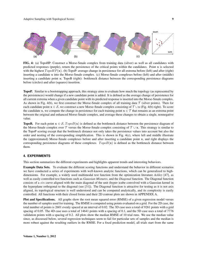
(1) (2) (3) (4)FIG. 5: Adaptive sampling of the 2D Ackley function using different regression techniques and different scoringfunctions. (1) GPM; (2) EARTH; (3) MDA; and (4) NNET.

Discussions on Results. Unsurprisingly, the most significant factor in the success of any scoring function is thequality of the regression model. Unfortunately, many experiments even in lower dimensions failed in the sense thatthe regression based on the space filling design did not converge within the number of samples tried. In fact, forsome functions some techniques did not show signs of improvement with an increasing number of samples. Whileit is possible that these results could be improved through manual parameter tuning, this would likely not be feasiblein a real world application where no ground truth is known and the number of samples is typically severely limited.Furthermore, any manual or semi-automatic parameter tuning would make comparing models even more challengingand potentially bias the results. Therefore, we have selected to run all experiments with the default values providewith the various regression packages listed in APPENDIX B. Subsequently, we only consider experiments in whichthe space filling design indicated a valid surrogate model.

(1) (2) (3) (4)

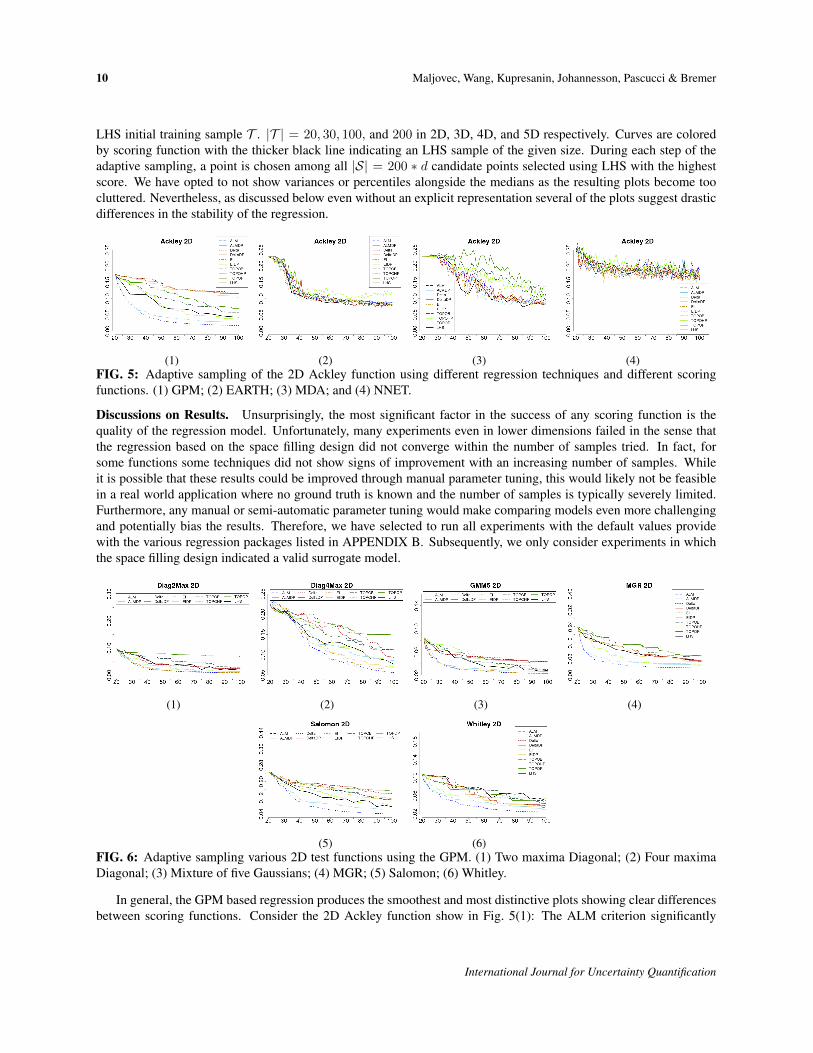
(5) (6)FIG. 6: Adaptive sampling various 2D test functions using the GPM. (1) Two maxima Diagonal; (2) Four maximaDiagonal; (3) Mixture of five Gaussians; (4) MGR; (5) Salomon; (6) Whitley.

In general, the GPM based regression produces the smoothest and most distinctive plots showing clear differencesbetween scoring functions. Consider the 2D Ackley function show in Fig. 5(1): The ALM criterion significantly



outperforms all other scoring functions with the TopoHP the only other criterion that beats the space filling design.Compare this to the EARTH model shown in Fig. 5(2): Most scoring functions except TopoHP perform qualitativelysimilar and barely achieve the same quality as the LHS sampling. Furthermore, all curves are less smooth suggesting ahigh variance among the different trials. The other MARS implementation, MDA, performs slightly worse (Fig. 5(3))but qualitatively similar with very rough curves without clear trends that fail to achieve the same performance as thespace filling sample. Finally, the NNET implementation shown in Fig. 5(4) barely shows any improvement in RMSEwith increasing samples, and all sampling strategies including the LHS sample seem to perform similar with largefluctuations. Overall, NNET achieves by far the worst fit at an RMSE almost an order of magnitude larger than thatof the GPM model.

(1) (2) (3) (4)

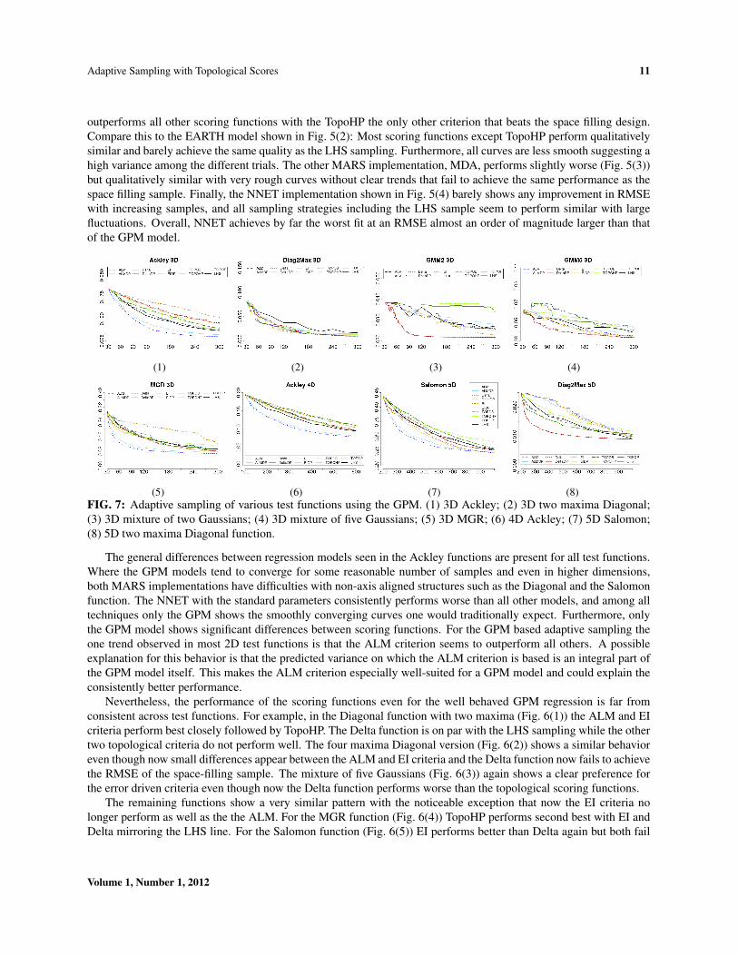
(5) (6) (7) (8)FIG. 7: Adaptive sampling of various test functions using the GPM. (1) 3D Ackley; (2) 3D two maxima Diagonal;(3) 3D mixture of two Gaussians; (4) 3D mixture of five Gaussians; (5) 3D MGR; (6) 4D Ackley; (7) 5D Salomon;(8) 5D two maxima Diagonal function.

The general differences between regression models seen in the Ackley functions are present for all test functions.Where the GPM models tend to converge for some reasonable number of samples and even in higher dimensions,both MARS implementations have difficulties with non-axis aligned structures such as the Diagonal and the Salomonfunction. The NNET with the standard parameters consistently performs worse than all other models, and among alltechniques only the GPM shows the smoothly converging curves one would traditionally expect. Furthermore, onlythe GPM model shows significant differences between scoring functions. For the GPM based adaptive sampling theone trend observed in most 2D test functions is that the ALM criterion seems to outperform all others. A possibleexplanation for this behavior is that the predicted variance on which the ALM criterion is based is an integral part ofthe GPM model itself. This makes the ALM criterion especially well-suited for a GPM model and could explain theconsistently better performance.

Nevertheless, the performance of the scoring functions even for the well behaved GPM regression is far fromconsistent across test functions. For example, in the Diagonal function with two maxima (Fig. 6(1)) the ALM and EIcriteria perform best closely followed by TopoHP. The Delta function is on par with the LHS sampling while the othertwo topological criteria do not perform well. The four maxima Diagonal version (Fig. 6(2)) shows a similar behavioreven though now small differences appear between the ALM and EI criteria and the Delta function now fails to achievethe RMSE of the space-filling sample. The mixture of five Gaussians (Fig. 6(3)) again shows a clear preference forthe error driven criteria even though now the Delta function performs worse than the topological scoring functions.

The remaining functions show a very similar pattern with the noticeable exception that now the EI criteria nolonger perform as well as the the ALM. For the MGR function (Fig. 6(4)) TopoHP performs second best with EI andDelta mirroring the LHS line. For the Salomon function (Fig. 6(5)) EI performs better than Delta again but both fail



to beat the space-filling sample. Finally, the Whitley function (Fig. 6(6)) shows overall a better performance with EIand Delta both outperforming the topological scoring functions.

The 3D experiments using the GPM show largely similar results as shown in Fig. 7. The ALM function generallyperforms best with the remaining scoring functions in different combinations behind. However, a notable and interest-ing exception are the mixtures of two and five Gaussians. For both functions the Delta criterion performs significantlybetter than the rest. One explanation is that these functions are characterized by a few large mountains which, oncefound, almost entirely determine the function. In such cases the Delta functional may perform well as it picks valuespurely based on the observed range. It is unclear, however, why such a behavior is not present in the 2D versions.

A similar behavior can be seen in higher dimensions: The 4D Ackley (Fig. 7(6)) and the 5D Salomon function(Fig. 7(7)) show the expected advantage of the ALM criterion while the 5D two maxima Diagonal function (Fig. 7(8))again prefers the Delta criterion. However, in this case all three topological functions outperform the remaining scorefunctions even though they only perform on par with the LHS samples.

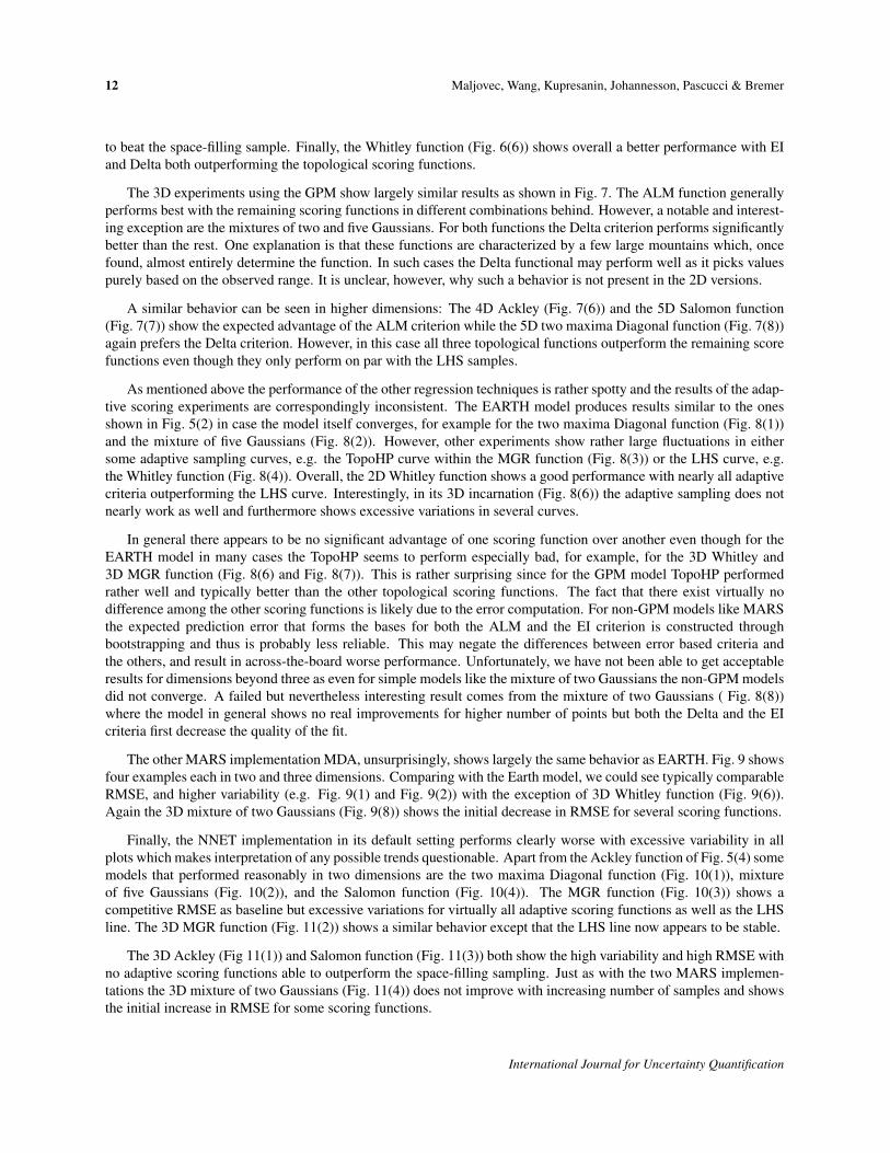
As mentioned above the performance of the other regression techniques is rather spotty and the results of the adap-tive scoring experiments are correspondingly inconsistent. The EARTH model produces results similar to the onesshown in Fig. 5(2) in case the model itself converges, for example for the two maxima Diagonal function (Fig. 8(1))and the mixture of five Gaussians (Fig. 8(2)). However, other experiments show rather large fluctuations in eithersome adaptive sampling curves, e.g. the TopoHP curve within the MGR function (Fig. 8(3)) or the LHS curve, e.g.the Whitley function (Fig. 8(4)). Overall, the 2D Whitley function shows a good performance with nearly all adaptivecriteria outperforming the LHS curve. Interestingly, in its 3D incarnation (Fig. 8(6)) the adaptive sampling does notnearly work as well and furthermore shows excessive variations in several curves.

In general there appears to be no significant advantage of one scoring function over another even though for theEARTH model in many cases the TopoHP seems to perform especially bad, for example, for the 3D Whitley and3D MGR function (Fig. 8(6) and Fig. 8(7)). This is rather surprising since for the GPM model TopoHP performedrather well and typically better than the other topological scoring functions. The fact that there exist virtually nodifference among the other scoring functions is likely due to the error computation. For non-GPM models like MARSthe expected prediction error that forms the bases for both the ALM and the EI criterion is constructed throughbootstrapping and thus is probably less reliable. This may negate the differences between error based criteria andthe others, and result in across-the-board worse performance. Unfortunately, we have not been able to get acceptableresults for dimensions beyond three as even for simple models like the mixture of two Gaussians the non-GPM modelsdid not converge. A failed but nevertheless interesting result comes from the mixture of two Gaussians ( Fig. 8(8))where the model in general shows no real improvements for higher number of points but both the Delta and the EIcriteria first decrease the quality of the fit.

The other MARS implementation MDA, unsurprisingly, shows largely the same behavior as EARTH. Fig. 9 showsfour examples each in two and three dimensions. Comparing with the Earth model, we could see typically comparableRMSE, and higher variability (e.g. Fig. 9(1) and Fig. 9(2)) with the exception of 3D Whitley function (Fig. 9(6)).Again the 3D mixture of two Gaussians (Fig. 9(8)) shows the initial decrease in RMSE for several scoring functions.

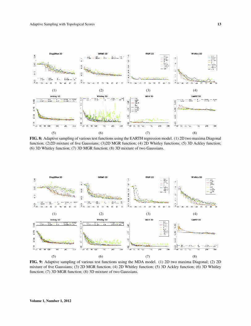
Finally, the NNET implementation in its default setting performs clearly worse with excessive variability in allplots which makes interpretation of any possible trends questionable. Apart from the Ackley function of Fig. 5(4) somemodels that performed reasonably in two dimensions are the two maxima Diagonal function (Fig. 10(1)), mixtureof five Gaussians (Fig. 10(2)), and the Salomon function (Fig. 10(4)). The MGR function (Fig. 10(3)) shows acompetitive RMSE as baseline but excessive variations for virtually all adaptive scoring functions as well as the LHSline. The 3D MGR function (Fig. 11(2)) shows a similar behavior except that the LHS line now appears to be stable.

The 3D Ackley (Fig 11(1)) and Salomon function (Fig. 11(3)) both show the high variability and high RMSE withno adaptive scoring functions able to outperform the space-filling sampling. Just as with the two MARS implemen-tations the 3D mixture of two Gaussians (Fig. 11(4)) does not improve with increasing number of samples and showsthe initial increase in RMSE for some scoring functions.



(1) (2) (3) (4)

(5) (6) (7) (8)

FIG. 8: Adaptive sampling of various test functions using the EARTH regression model. (1) 2D two maxima Diagonalfunction; (2)2D mixture of five Gaussians; (3)2D MGR function; (4) 2D Whitley functions; (5) 3D Ackley function;(6) 3D Whitley function; (7) 3D MGR function; (8) 3D mixture of two Gaussians.

(1) (2) (3) (4)

(5) (6) (7) (8)

FIG. 9: Adaptive sampling of various test functions using the MDA model. (1) 2D two maxima Diagonal; (2) 2Dmixture of five Gaussians; (3) 2D MGR function; (4) 2D Whitley function; (5) 3D Ackley function; (6) 3D Whitleyfunction; (7) 3D MGR function; (8) 3D mixture of two Gaussians.



(1) (2) (3) (4)

FIG. 10: Adaptive sampling of various 2D test functions using the NNET model. (1) Two maxima Diagonal function;(2) Mixture of five Gaussians; (3) MGR function; (4) Salomon function.

(1) (2) (3) (4)

FIG. 11: Adaptive sampling of various 3D test functions using the NNET model. (1) Ackley function; (2) MGRfunction; (3) Salomon function; (4) Mixture of two Gaussians.

5. DISCUSSION

After running an extensive set of experiments in two to five dimensions with nine different scoring functions somegeneral trends appear even though the fundamental question of which particular scoring function to use remains largelyinconclusive. The results given in the paper is only a small first step in the this direction. The first, not necessarilysurprisingly result is that the quality of the underlying regression model plays a key role in the performance of anyadaptive sampling technique. In this study the GPM model performs the best and is the only one showing significantdifferences between scoring functions. Overall, it seems that the combination of ALM and GPM is the preferredchoice even though some functions perform well with the Delta criteria.

The remaining regression models all show problems fitting many of the test functions and the large variabilitysuggest that they are sensitive to specific sample locations. In the cases where reasonable fits have been achieved allscoring functions perform equally well (or poorly).

The new topological scoring functions are largely competitive in terms of RMSE and often perform among thetop scoring functions. Some results suggest that detailed fits with a high number of samples are less well suited fortopological scoring functions as they are designed to recover larger scale features. Nevertheless, topological scoringfunctions are expected to better recover the global structure of a function, and finding quantitative metrics to test thishypothesis as well as expanding the class of such functions will be the focus of future research.

ACKNOWLEDGMENTS

This work performed under the auspices of the U.S. Department of Energy by Lawrence Livermore National Lab-oratory under Contract DE-AC52-07NA27344. LLNL-JRNL-519591. In particular the Uncertainty QuantificationStrategic Initiative Laboratory Directed Research and Development Project at LLNL under project tracking code10-SI-013.



REFERENCES

1. McKay, M. D., Beckman, R., and Conover, W. J., A comparison of three methods for selecting values of inputvariables in the analysis of output from a computer code, Technometrics, 21:239–245, 1979.

2. Tang, B., Orthogonal array-based latin hypercubes, Journal of the American Statistical Association,88(424):1392–1397, 1993.

3. Dam, E. R.v., Two-dimensional minimax latin hypercube designs, Discrete Applied Mathematics, 156:3483–3493, 2008.

4. Rasmussen, C. E. and Williams, C. K. I., Gaussian Processes for Machine Learning, MIT Press, 2006.5. Friedman, J., Multivariate adaptive regression splines, The Annals of Statistics, 19(1):1–67, 1991.6. Ripley, B. D., Pattern Recognition and Neural Networks, Cambridge University Press, 1996.7. Fang, K.-T., Li, R., and Sudjianto, A., Design and Modeling of Computer Experiments, Chapman and Hall/CRC,

2005.8. Sacks, J., Schiller, S. B., and Welch, W., Design for computer experiments, Technometrics, 31:41–47, 1989.9. Hastie, T., Tibshirani, R., and Friedman, J., The Elements of Statistical Learning, Springer-Verlag, 2009.

10. Davison, A. C. and Hinkley, D. V., Bootstrap Methods and their Application, Cambridge University Press, 1997.11. Santner, T. J., Williams, B., and Notz, W. I., The Design and Analysis of Computer Experiments, Springer-Verlag,

2003.12. Koehler, J. R. and Owen, A. B. Computer experiments. In: Ghosh, S. and Rao, C. R. (Eds.), Handbook of

Statistics. Elsevier Science, 1996.13. Bates, R. A., Buck, R. J., Riccomagno, E., and Wynn, H. P., Experimental design and observation for large

systems, Journal of the Royal Statistical Society, Series B: Methodological, 58:77–94, 1996.14. Schonlau, M. Computer Experiments and Global Optimization. PhD thesis, University of Woterloo, 1997.15. Jones, D., Schonlau, M., and Welch, W., Efficient global optimization of expensive black-box functions, Journal

of Global Optimization, 13:455–492, 1998.16. Lam, C. Q. Sequential Adaptive Designs In Computer Experiments For Response Surface Model Fit.

http://etd.ohiolink.edu/, 2008.17. Carr, H., Snoeyink, J., and Axen, U., Computing contour trees in all dimensions, Computational Geometry

Thoery and Applications, 24(3):75–94, 2003.18. Reeb, G., Sur les points singuliers d’une forme de pfaff complement integrable ou d’une fonction numerique,

Comptes Rendus de L’Academie ses Seances Paris, 222:847–849, 1946.19. Pascucci, V., Scorzelli, G., Bremer, P.-T., and Mascarenhas, A., Robust on-line computation of reeb graphs:

simplicity and speed, ACM Transactions on Graphics, 26(3):58, 2007.20. Boyell, R. L. and Ruston, H., Hybrid techniques for real-time radar simulation, In Proceedings Fall Joint Com-

puter Conference, pp. 445–458, 1963.21. Edelsbrunner, H., Harer, J., and Zomorodian, A. J., Hierarchical Morse-Smale complexes for piecewise linear

2-manifolds, Discrete and Computational Geometry, 30:87–107, 2003.22. Gyulassy, A., Natarajan, V., Pascucci, V., and Hamann, B., Efficient computation of Morse-Smale complexes for

three-dimensional scalar functions, IEEE Transactions on Visualization and Computer Graphics, 13:1440–1447,2007.

23. Carr, H., Snoeyink, J., and Panne, M.v. d., Simplifying flexible isosurfaces using local geometric measures, InProceedings 15th IEEE Visualization, pp. 497–504, 2004.

24. Laney, D., Bremer, P.-T., Mascarenhas, A., Miller, P., and Pascucci, V., Understanding the structure of the tur-bulent mixing layer in hydrodynamic instabilities, IEEE Transactions on Visualization and Computer Graphics,



12:1052–1060, 2006.25. Bremer, P.-T., Weber, G., Pascucci, V., Day, M., and Bell, J., Analyzing and tracking burning structures in lean

premixed hydrogen flames, IEEE Transactions on Visualization and Computer Graphics, 16(2):248–260, 2010.26. Gyulassy, A., Duchaineau, M., Natarajan, V., Pascucci, V., E.Bringa, , Higginbotham, A., and Hamann, B.,

Topologically clean distance fields, IEEE Transactions on Visualization and Computer Graphics, 13(6):1432–1439, 2007.

27. Oesterling, P., Heine, C., Jaenicke, H., Scheuermann, G., and Heyer, G., Visualization of high-dimensional pointclouds using their density distribution’s topology, IEEE Transactions on Visualization and Computer Graphics,17(11):1547–1559, 2011.

28. Correa, C. D. and Lindstrom, P., Towards robust topology of sparsely sampled data, IEEE Transactions onVisualization and Computer Graphics, 17(12), 2011.

29. Edelsbrunner, H., Harer, J., Natarajan, V., and Pascucci, V., Morse-Smale complexes for piecewise linear 3-manifolds, In Proceedings 19th Annual Symposium on Computational Geometry, pp. 361–370, 2003.

30. Chazal, F., Guibas, L. J., Oudot, S. Y., and Skraba, P., Analysis of scalar fields over point cloud data, In Proceed-ings 20th Annual ACM-SIAM Symposium on Discrete Algorithms, pp. 1021–1030, 2009.

31. Gerber, S., Bremer, P.-T., Pascucci, V., and Whitaker, R. T., Visual exploration of high dimensional scalar func-tions, IEEE Transactions on Visualization and Computer Graphics, 16:1271–1280, 2010.

32. Gerber, S., Rubel, O., Bremer, P.-T., Pascucci, V., and Whitaker, R. T., Morse-Smale regression, Journal ofComputational and Graphical Statistics, 2012, in press.

33. Vedaldi, A. and Soatto, S., Quick shift and kernel methods for mode seeking, In Proceedings European Confer-ence on Computer Vision, pp. 705–718, 2008.

34. Edelsbrunner, H., Letscher, D., and Zomorodian, A. J., Topological persistence and simplification, Discrete andComputational Geometry, 28:511–533, 2002.

35. Carlsson, G., Zomorodian, A. J., Collins, A., and Guibas, L. J., Persistence barcodes for shapes, In ProceedingsEurographs/ACM SIGGRAPH Symposium on Geometry Processing, pp. 124–135, 2004.

36. Silva, V.d. and Ghrist, R., Coverage in sensor networks via persistent homology, Algebraic and Geometric Topol-ogy, 7:339–358, 2007.

37. Carlsson, E., Carlsson, G., and Silva, V.d., An algebraic topological method for feature identification, Interna-tional Journal of Computational Geometry and Applications, 16:291–314, 2003.

38. Edelsbrunner, H. and Harer, J., Persistent homology - a survey, Contemporary Mathematics, 453:257–282, 2008.39. Carlsson, G., Ishkhanov, T., Silva, V.d., and Zomorodian, A., On the local behavior of spaces of natural images,

International Journal of Computer Vision, 76:1–12, 2008.40. Kloke, J. and Carlsson, G. Topological de-noising: strengthening the topological signal. Manuscript, 2010.41. Bremer, P.-T., Edelsbrunner, H., Hamann, B., and Pascucci, V., A topological hierarchy for functions on triangu-

lated surfaces, IEEE Transactions on Visualization and Computer Graphics, 10(385-396), 2004.42. Gyulassy, A., Natarajan, V., Pascucci, V., Bremer, P. T., and Hamann, B., Topology-based simplification for

feature extraction from 3D scalar fields, In Proceedings 16th IEEE Visualization, pp. 535–542, 2005.43. Cole-McLaughlin, K., Edelsbrunner, H., Harer, J., Natarajan, V., and Pascucci, V., Loops in reeb graphs of

2-manifolds, In Proceedings 19th Annual Symposium on Computational Geometry, pp. 344–350, 2003.44. Chazal, F., Cohen-Steiner, D., Glisse, M., Guibas, L. J., and Oudot, S. Y., Proximity of persistence modules and

their diagrams, In Proceedings 25th Annual Symposium on Computational Geometry, pp. 237–246, 2009.45. Cohen-Steiner, D., Edelsbrunner, H., and Harer, J., Stability of persistence diagrams, Discrete and Computa-

tional Geometry, 37:103–120, 2007.46. MacKay, D., Information-based objective functions for active data selection, Neural Computation, 4(4):589–603,



1992.47. Ackley, D. H., A connectionist machine for genetic hillclimbing, Kluwer Academic Publishers, 1987.48. Grollman, D. Sparse online gaussian process. http://lasa.epfl.ch/ dang/code.shtml, 2011.49. Csato, L. and Opper, M., Sparse online gaussian processes, Neural Computation, 14:641–668, 2002.50. Csato, L., Gaussian processes - iterative sparse approximations, PhD thesis, Aston University, 2002.51. Milborrow, S. earth: Multivariate Adaptive Regression Spline Model, 2011. R package version 3.2-1, Derived

from mda:mars by T. Hastie and R. Tibshirani.52. Hastie, T., Tibshirani, R., Leisch, F., Hornik, K., and Ripley, B. D. mda: Mixture and flexible discriminant

analysis, 2011. R package version 0.4-2.53. Venables, W. N. and Ripley, B. D., Modern Applied Statistics with S, Spinger, 2002.54. Carnell, R. lhs: Latin Hypercube Samples, 2009. R package version 0.5.

APPENDIX A. EXAMPLE TEST FUNCTIONS CLOSED FORMS AND PLOTS

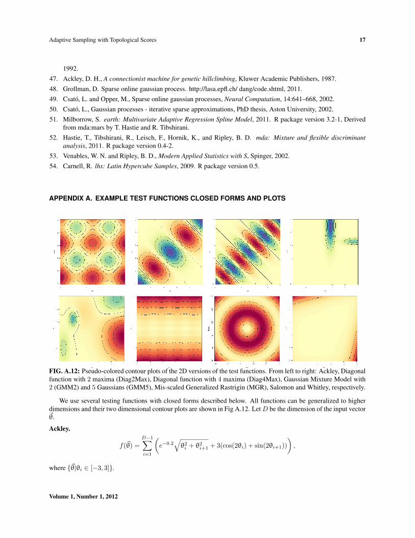
FIG. A.12: Pseudo-colored contour plots of the 2D versions of the test functions. From left to right: Ackley, Diagonalfunction with 2 maxima (Diag2Max), Diagonal function with 4 maxima (Diag4Max), Gaussian Mixture Model with2 (GMM2) and 5 Gaussians (GMM5), Mis-scaled Generalized Rastrigin (MGR), Salomon and Whitley, respectively.

We use several testing functions with closed forms described below. All functions can be generalized to higherdimensions and their two dimensional contour plots are shown in Fig A.12. Let D be the dimension of the input vector~θ.

Ackley.

f(~θ) =

D−1∑i=1

(e−0.2

√θ2i + θ2i+1 + 3(cos(2θi) + sin(2θi+1))

),

where {~θ|θi ∈ [−3, 3]}.



Diagonal. Let m be the number of maxima along the main diagonal,

f(~θ) = 12 sin

(π

(12 + ((m+ 1) mod 2) +

m(∑D

i=1 θi)D

))× e

((∑Di=1 θ2

i−(∑D

i=1 θi)2

D

)(log(0.001)√

D

)),

where {~θ|θi ∈ [−1, 1]}.Random Gaussian Mixture Model.

Let m be the number of extrema in the domain. Let ai be the amplitude of the ith extrema. Let ci,j be the jth

coordinate of the ith extrema. Let σi,j be the standard deviation of the ith extrema with respect to the jth coordinate.

f(~θ) =

m∑i=1

(aie−(∑D

j=1

(θi,j−ci,j)2

2σ2i,j

))

where {~θ|θi ∈ [0, 1]}.Mis-scaled Generalized Rastrigin.

f(~θ) = 10D +

D∑i=1

((10

i−1D−1 θi)

2 − 10 cos(2π(10i−1D−1 θi))

)where {~θ|θi ∈ [−2, 2]}.Salomon.

f(~θ) = − cos

(2π

D∑i=1

θ2i

)+ 0.1

√√√√ D∑i=1

θ2i + 1

where {~θ|θi ∈ [−1, 1]}.Whitley.

f(~θ) =

D∑i=1

D∑j=1

(k2ij4000

− cos(kij) + 1

)

where {~θ|θi ∈ [−1, 2]}, and kij = (100(θ2i − θj)2 + (1− θj)

2).

APPENDIX B. SOFTWARE PACKAGES AND PARAMETER SETTINGS

Now we give details on packages and parameter settings used in our experiments.For GPM, we use the Sparse Online Gaussian Process (SOGP) C++ library [48], which is based on

work in [49, 50]. The default parameters are employed, see [50] for details, i.e. we use the Radial Basis Kernel witha spherical covariance set to σ2

0 = 0.1, the widths are uniformly set to 0.1, and the amplitude A = 1.For EARTH, MDA and NNET, we use non-parametric bootstrapping using 250 samples without cross-validation.For EARTH, we use the earth library in R [51]. We use the following parameter settings, see [51] for details. If

a parameter is not listed, the default value given by the package is used.

degree=3 // Maximum degree of interaction (Friedman’s mi)nk=63 //Maximum number of model terms before pruningminspan=1 //Min. dist. between knots, 1 for non-noisy datathresh=1e-8 //Forward stepping thresholdpenalty=3 //Generalized Cross Validation Penalty per knot

For MDA, we use mda library in R, with the following parameters (see [52] for details, non-listed parameters usepackage defaults),



degree=3 // Maximum degree of interaction (Friedman’s mi)nk=63 //Maximum number of model termsthresh=1e-8 // Forward stepping thresholdpenalty=3 // The cost per degree of freedom charge

For NNET, we use nnet library in R, with the following parameters (see [53] for details, non-listed parametersuse package defaults),

size=1+ceiling(sqrt(D)) // Number of units in the hidden layer// D is the dimensionality of the input

decay=1e-3 // Parameter for weight decayskip=TRUE // Add skip-layer connections from input to outputlinout=TRUE // Linear output units, as opposed to logistic

To create the space filling samplings, the lhs library in R [54] is used. More specifically, we use the randomLHSfunction, which chooses uniform, random samples without any attempts to optimize the design, to construct thetraining data, candidate data, and LHS samples in the plots shown.


adaptive sampling with topological scores

Documents