adaptable transformation-based similarity search in
TRANSCRIPT

Adaptable Transformation-BasedSimilarity Search in Multimedia
Databases
Von der Fakultät für Mathematik, Informatik und Naturwissenschaften der RWTH
Aachen University zur Erlangung des akademischen Grades eines Doktors der
Naturwissenschaften genehmigte Dissertation
vorgelegt von
Diplom-Informatiker
Marc Wichterich
aus Haan
Berichter: Universitätsprofessor Dr. rer. nat. Thomas Seidl
Universitätsprofessor Dr. rer. nat. Andreas Henrich
Tag der mündlichen Prüfung: 12.10.2010
Diese Dissertation ist auf den Internetseiten der Hochschulbibliothek online verfügbar.

To those who supported me during the past five years.

Contents
Abstract / Zusammenfassung 1
I Introduction to Distance-Based Similarity Search 5
1 Distance-Based Similarity Model 9
1.1 Object Feature Representations . . . . . . . . . . . . . . . . . . . . . 9
1.2 Distance Measures . . . . . . . . . . . . . . . . . . . . . . . . . . . . 14
2 Distance-Based Similarity Queries 19
2.1 Range Queries . . . . . . . . . . . . . . . . . . . . . . . . . . . . . . . 19
2.2 Nearest Neighbor Queries . . . . . . . . . . . . . . . . . . . . . . . . 21
2.3 Ranking Queries . . . . . . . . . . . . . . . . . . . . . . . . . . . . . . 22
3 Efficient Similarity Query Processing 25
3.1 Lower Bounds and Multi-Step Processing . . . . . . . . . . . . . . 25
3.2 Indexing Structures . . . . . . . . . . . . . . . . . . . . . . . . . . . . 27
4 An Example for Similarity Search Using Simple Distance Mea-
sures 31
4.1 Introduction . . . . . . . . . . . . . . . . . . . . . . . . . . . . . . . . 31
4.2 Preliminaries . . . . . . . . . . . . . . . . . . . . . . . . . . . . . . . . 34
4.3 Dimensionality Reduction for the Voronoi Approach to NN Search 38
4.4 Experiments . . . . . . . . . . . . . . . . . . . . . . . . . . . . . . . . 51
4.5 Summary . . . . . . . . . . . . . . . . . . . . . . . . . . . . . . . . . . 56
i
ii CONTENTS
II Transformation-Based Distance Measures 57
5 The Edit Distance 61
5.1 Formal Definition . . . . . . . . . . . . . . . . . . . . . . . . . . . . . 61
5.2 Illustration of Core Concepts of Transformation-Based Distances 63
5.3 Computation . . . . . . . . . . . . . . . . . . . . . . . . . . . . . . . . 64
6 The Dynamic Time Warping Distance 67
6.1 Introduction . . . . . . . . . . . . . . . . . . . . . . . . . . . . . . . . 67
6.2 Formal Definition . . . . . . . . . . . . . . . . . . . . . . . . . . . . . 69
6.3 Computation . . . . . . . . . . . . . . . . . . . . . . . . . . . . . . . . 71
7 The Earth Mover’s Distance 75
7.1 Introduction . . . . . . . . . . . . . . . . . . . . . . . . . . . . . . . . 75
7.2 Applications . . . . . . . . . . . . . . . . . . . . . . . . . . . . . . . . 79
7.3 Formal Definition . . . . . . . . . . . . . . . . . . . . . . . . . . . . . 80
7.4 Computation . . . . . . . . . . . . . . . . . . . . . . . . . . . . . . . . 84
7.5 Approximations of the EMD . . . . . . . . . . . . . . . . . . . . . . . 86
III Fast Searching with the Earth Mover’s Distance 91
8 Efficient Search Via Flexible Dimensionality Reduction 95
8.1 Introduction . . . . . . . . . . . . . . . . . . . . . . . . . . . . . . . . 95
8.2 Dimensionality Reduction for the EMD . . . . . . . . . . . . . . . . 97
8.3 Query Processing Algorithm . . . . . . . . . . . . . . . . . . . . . . . 113
8.4 Experiments . . . . . . . . . . . . . . . . . . . . . . . . . . . . . . . . 116
8.5 Summary . . . . . . . . . . . . . . . . . . . . . . . . . . . . . . . . . . 126
9 Direct Indexing and Vector Approximation 127
9.1 Introduction . . . . . . . . . . . . . . . . . . . . . . . . . . . . . . . . 127
9.2 Direct Indexing of the EMD . . . . . . . . . . . . . . . . . . . . . . . 129
9.3 Vector Approximation for the EMD . . . . . . . . . . . . . . . . . . 133
9.4 Experiments . . . . . . . . . . . . . . . . . . . . . . . . . . . . . . . . 143
9.5 Summary . . . . . . . . . . . . . . . . . . . . . . . . . . . . . . . . . . 148

CONTENTS iii
IV Effective Searching with the Earth Mover’s Distance 149
10 Metric Adaptation of the Earth Mover’s Distance 153
10.1 Introduction . . . . . . . . . . . . . . . . . . . . . . . . . . . . . . . . 153
10.2 Mathematical Framework for Adapting a Metric EMD . . . . . . . 154
10.3 Summary . . . . . . . . . . . . . . . . . . . . . . . . . . . . . . . . . . 166
11 Exploring Multimedia Databases via Relevance Feedback 169
11.1 Introduction . . . . . . . . . . . . . . . . . . . . . . . . . . . . . . . . 169
11.2 Relevance Feedback with the Earth Mover’s Distance . . . . . . . 172
11.3 Experiments . . . . . . . . . . . . . . . . . . . . . . . . . . . . . . . . 188
11.4 Summary . . . . . . . . . . . . . . . . . . . . . . . . . . . . . . . . . . 196
V The Earth Mover’s Distance in Context of StructuredObjects 197
12 Feature-Based Graph Similarity with the Earth Mover’s Dis-
tance 201
12.1 Introduction . . . . . . . . . . . . . . . . . . . . . . . . . . . . . . . . 201
12.2 Preliminaries . . . . . . . . . . . . . . . . . . . . . . . . . . . . . . . . 203
12.3 Graph Similarity Model . . . . . . . . . . . . . . . . . . . . . . . . . 204
12.4 Experimental Evaluation . . . . . . . . . . . . . . . . . . . . . . . . . 209
12.5 Summary and Outlook . . . . . . . . . . . . . . . . . . . . . . . . . . 213
13 Reducing the Number of DTW Ground Distance Computations 215
13.1 Introduction . . . . . . . . . . . . . . . . . . . . . . . . . . . . . . . . 215
13.2 Anticipatory DTW . . . . . . . . . . . . . . . . . . . . . . . . . . . . . 218
13.3 Experiments . . . . . . . . . . . . . . . . . . . . . . . . . . . . . . . . 232
13.4 Summary and Outlook . . . . . . . . . . . . . . . . . . . . . . . . . . 239

iv CONTENTS
VI Summary and Outlook 241
VII Appendices I
Naming Conventions III
List of Symbols V
List of Algorithms VII
Bibliography IX
Collaboration / Acknowledgments XXIX
List of Publications XXXIII
Curriculum Vitae XXXV

Abstract
Efficient and effective methods of making data accessible to its consumers – be
they humans or algorithms – are crucial for turning ever-growing data dumps
into data mines.
Of particular importance to the user are access methods that allow for query-
based searching of databases. However, for vast collections of complex data
objects such as digital image libraries and music databases, querying methods
that necessitate an accurate, algebraic description of what the user is looking
for cannot cover all search needs. For instance, a prototypical object might be
known to the user and yet he or she may be unable to describe which qualities
make the object prototypical. Similarity search systems based on the query-by-
example paradigm can help the user in such situations by retrieving objects from
the database that exhibit a high degree of similarity to the prototypical query
object. For this purpose, the system must decide algorithmically which objects
are to be deemed similar to each other.
After giving an introduction and reviewing preliminaries in parts I and II,
the following three parts of this thesis address novel techniques regarding the
efficiency, effectiveness, and applicability of a particularly intuitive and flexible
class of distance measures where the distance (i.e., dissimilarity) between two
objects is modeled as the minimum amount of work that is required for trans-
forming the feature representation of one object into the feature representation
of the other. As the cost of transforming a feature into another can be chosen
depending on the features at hand, these transformation-based distance mea-
sures are highly adaptable and do not assume that the underlying features are
perceptually independent.
1


Zusammenfassung
Mit dem stetigen Größenzuwachs heutiger Multimedia-Datenbanken laufen die-
se Gefahr, zu reinen Datenhalden zu verkommen. Um dies zu verhindern, sind
Methoden, welche einen effizienten und effektiven Zugriff auf die Daten er-
möglichen, für den Benutzer (ob Mensch oder Algorithmus) von hohem Stel-
lenwert. Aus Benutzersicht kommt hierbei anfragebasierten Suchmethoden eine
besondere Bedeutung zu. Allerdings können für Multimedia-Datensammlungen
nicht alle Suchbedarfe mittels exakten, algebraischen Anfragebeschreibungen
abgedeckt werden. So mag dem Benutzer ein prototypisches Bild oder Musik-
stück bekannt sein, ohne dass es ihm/ihr möglich ist, formal zu beschreiben,
welche Eigenschaften den prototypischen Charakter ausmachen. Systeme zur
Ähnlichkeitssuche, welche auf dem query-by-example Paradigma beruhen, kön-
nen dem Benutzer helfen, die Datenbank nach Objekten mit einem hohen Grad
an Ähnlichkeit zum Prototyp zu durchsuchen. Hierfür muss das System auf
algorithmische Weise entscheiden, welche Objekte zueinander ähnlich sind.
Nach einer Einleitung und einem Überblick über die Grundlagen der Ar-
beit in den Teilen I und II, zeigen die darauf folgenden drei Teile Techniken
auf, welche die Effizienz, die Effektivität und die Anwendbarkeit einer beson-
ders flexiblen und intuitiven Klasse von Distanzmaßen betreffen. Die Distanz
zweier Objekte wird hier als Maß für die Unähnlichkeit dieser interpretiert und
als minimales Pensum an Arbeit modelliert, welches für die Umwandlung der
Merkmalsrepräsentation des einen Objekts in die des anderen aufzuwenden ist.
Da die Kosten der für die Transformation aufzuwendenden Arbeit den auftre-
tenden Objektmerkmalen entsprechend gewählt werden können, sind transfor-
mationsbasierte Distanzmaße in höchstem Maße anpassbar und vermögen es
wahrnehmungsbezogene Abhängigkeiten der Merkmale zu berücksichtigen.
3


Part I
Introduction to Distance-Based
Similarity Search
5


Introduction to Distance-Based Similarity Search 7
Ways of making data accessible to its consumers – be they humans or algo-
rithms – are crucial for turning ever-growing data dumps into data mines.
Of particular importance to the user are access methods that allow for query-
based searching of databases. For vast collections of complex data objects such
as large text document corpora, digital image libraries, and music databases,
querying methods that necessitate an accurate, algebraic description of what
the user is looking for cannot cover all search needs. The user may only have
a vague idea of the types of objects he or she would like to retrieve from the
database. A prototypical object might be known to the user and yet he or she
may be unable to describe, in an algebraic way, which qualities make the object
prototypical. Similarity search systems are employed in such situations to help
the user query the database. Given a rough sketch or an example of a prototyp-
ical query object, the task of a similarity search system is to return objects from
the database that exhibit a high degree of similarity to the query object. For this
purpose, the similarity search system typically establishes the degree of similar-
ity between the query object and the database objects based on a measure of
similarity that compares characteristic features of the objects.
Having a computer-evaluable measure of similarity is also of great impor-
tance in a number of algorithms and applications beyond query-driven retrieval.
In the field of data mining, data clustering aims at grouping objects according to
their similarity while the classification of data can be accomplished by assigning
class labels to objects according to their similarity to objects with known class
labels. In computer vision, image registration is often based on finding regions
within an image that are similar to subimages or templates of a reference image.
The utility of a similarity measure greatly depends on the degree with which
it can match the user’s notion of similarity (effectiveness) and on the speed with
which search algorithms can find similar objects in the database (efficiency).
If the system returns objects that the user would not judge as relevant or if it
returns relevant objects but only after an excessive amount of time, the result is
of little use.
In distance-based similarity search, the similarity of two objects is described
by a distance function between representations of their features. A low distance
value stands for a high similarity while a large distance value indicates that the

8 Introduction to Distance-Based Similarity Search
objects are dissimilar. Finding the most similar objects thus turns into finding
the closest objects in distance-based similarity search.
Parts III through V of this work address novel techniques regarding the effi-
ciency, effectiveness and applicability of a particularly intuitive and flexible class
of distance functions where the distance between two objects is modeled as the
amount of work that is required for transforming the features of one object into
the features of the other. As the cost of transforming a feature into another
feature can be chosen depending on the features at hand, these transformation-
based distance measures are highly adaptable and do not assume that the un-
derlying features are mutually independent. The distance measures discussed
have been shown to be effective in a large number of applications as detailed in
Part II, where several transformation-based distance measures are introduced.

Chapter 1
Distance-Based Similarity Model
Distance-based similarity models for searching within multimedia databases
typically consist of two parts: An object representation and a distance measure.
Multimedia databases often describe the objects they contain via the distribution
of features that the objects exhibit. The selection, extraction, and representa-
tion of object features determines which attributes are to be considered relevant
for the notion of similarity that is to be reflected by the distance measure. The
selection and extraction of object features is largely application-dependent and
shall not be the focus of this work. Exemplified with a simple feature extraction
method, Section 1.1 formally defines the object representations encountered
throughout the main part of this work. Section 1.2 discusses relevant properties
of distance measures and gives examples of commonly encountered distance
measures that are relevant to the remainder of this work.
1.1 Object Feature Representations
While pairwise distances between all objects in a database could theoretically
be known a priori (e.g., given by domain experts), this information does not
suffice to answer similarity queries in the query-by-example framework, where
a database is searched for objects that are similar to a user-given sample object
that is not necessarily included in the database. The distance from the sample
object to the database objects has to be computed based on a representation of
9

10 Distance-Based Similarity Model
R
G B
Figure 1.1: From objects to feature vectors
the features of the objects. This section formally introduces representations and
notations that are of importance for the main parts of this work.
1.1.1 Representations of Feature Distributions
In this work, it is assumed that each object of a multimedia database at hand
can be described in terms of a set of features from some feature space. For
the example case of image objects, possible feature spaces are 3-dimensional
color spaces such as RGB, HSV, or CIE Lab. These feature spaces could also be
enriched with location information resulting in a 5-dimensional feature space
such as XYHSV. A simple feature extraction method then is to measure the loca-
tion and color information of (a sample of) the pixels of an image. The process
is depicted in Figure 1.1 for the RGB feature space and a toy sample of four
pixels. Other types of multimedia objects require different feature spaces.
Given a set of feature vectors in the feature space, feature histograms are
compact, approximate representations of the feature distribution∗.
Definition 1.1 (Fixed-Binning Feature Histogram)
Given an object o and a disjoint partitioning P1, ..., Pn of a feature space FS, the
fixed-binning feature histogram ho for object features f o1 , ..., f o
m from FS is defined
∗In the literature, a histogram in vector form is sometimes called a feature vector. In thiswork, a feature vector lives in a feature space such as RGB. A histogram in vector form is afeature representation vector and lives in a feature representation space.

1.1. Object Feature Representations 11
as a vector ho in Rn with
ho[ j] =1
m
m∑
i=1
1 if f oi ∈ Pj,
0 otherwise.∀1≤ j ≤ n.
Notation: Where clear from context, o is used instead of ho and |ho|Σ =∑n
i=1 o[i].
The value ho[ j] stands for the relative frequency of features from a partition
Pj of the feature space. As the term fixed-binning indicates, the partitioning of
the feature space is determined only once (e.g., data-independently or by clus-
tering feature vectors from a sample of the database) and used for the whole
database and all queries. This fixed binning leads to efficiency advantages when
comparing two histograms in later chapters but can lead to undesirable quan-
tization effects. As the binning is not tailored to any single image, there might
not be a bin that represents the pink parts of the example image in Figure 1.1
sufficiently well while at the same time there might be several bins for colors
such as turquoise and yellow that do not have to be differentiated for the ex-
ample image. Adaptive-binning histograms counter this quantization effect by
tailoring the partitioning to the features of each object.
Definition 1.2 (Adaptive-Binning Feature Histogram)
Given an object o and a disjoint partitioning Po1 , ..., Po
n of a feature space FS, the
adaptive-binning feature histogram for object features f o1 , ..., f o
m from FS is defined
as a set so =¦
(ro1 , wo
1), . . . , (ron , wo
n)©
of n tuples from FS×R with feature weights
woj =
1
m
m∑
i=1
1 if f oi ∈ Po
j ,
0 otherwise.∀1≤ j ≤ n
and roj as some representative vector for partition Po
j .
Notation: Where clear from context, o is used instead of so and |so|Σ =∑n
i=1 woi .
With the partitioning being potentially different for each adaptive-binning
histogram, its semantics have to be stored for each histogram. In Definition 1.2,

12 Distance-Based Similarity Model
(a) fixed-binning (b) original (c) adaptive-binning
(d) fixed-binning (e) original (f) adaptive-binning
Figure 1.2: Image reconstruction using 15 colors
the bin representatives roj are intended to fulfill this purpose. A method for
determining the partitioning of FS is to cluster the feature vectors f oj and to
determine roj as the centroid of the j th cluster. For the example image in Fig-
ure 1.1, the large homogeneous pink area would assure that this color is well-
represented in the adaptive-binning histogram even for relatively small n.
The ability of the adaptive approach to tailor its partitioning and represen-
tative vectors to the feature distribution of each object is exemplified by Fig-
ure 1.2. Figure 1.2 (c) shows a 15-color reconstruction of the image in Fig-
ure 1.2 (b). Each pixel is colored according to its corresponding representative
vector roj that has been determined via a k-means clustering of the color features
of the original image. Several shades of green, gray, and blue are differentiated
along with a pink bin that represents the paint of the building. Figure 1.2 (f)
shows the same kind of reconstruction for the image in Figure 1.2 (e). As the
image in Figure 1.2 (e) has considerably different colors than the one in (b),
the partitions of the feature space (and thus the representative vectors) are also
different. Multiple shades of brown and pale turquoise are differentiated in this
case. A fixed-binning histogram cannot tailor its feature space partitioning to

1.1. Object Feature Representations 13
each object in the database. Figures 1.2 (a) and (d) show according reconstruc-
tions for a feature space partitioning that was derived from a clustering of the
features of a database with ∼ 500 images. The fixed-binning partitioning of
the feature space lacks colors that are necessary for a truthful reconstruction
of the two images. A considerably larger number of bins would be required to
achieve a level of quality that matches the one of the reconstruction based on
the adaptive-binning histograms.
1.1.2 Feature Sequences
The order of the bins or dimensions of feature histograms are arbitrarily (but
consistently) chosen for the fixed-binning approach and without a predefined
order for the adaptive-binning approach. For some types of multimedia objects,
there is an inherent order for one of the dimensions that plays an important
role for comparing objects. A good example are video sequences, which can
be modeled as a time-series of images or frames. The order of the frames is
highly important when describing the video sequence as changing the order
changes the semantics of the video sequence. Further examples of objects with
an order-equipped dimension that is of high importance for the understanding
of the data that they represent include stock data and other recurring time-based
measurements.
Definition 1.3 (Feature Sequences)
A feature sequence to for an object o with m ordered feature descriptions is a
sequence¬
to1, . . . , to
m
¶
where toi represents the ith feature description of o.
Definition 1.3 is kept general in that toi can be any feature description includ-
ing a scalar value or an adaptive feature histogram. Its main purpose is to make
the importance of the ordered dimension explicit and to allow for convenient
access to the feature descriptions in Chapter 13, which focuses on time series.

14 Distance-Based Similarity Model
1.2 Distance Measures
In distance-based similarity search, the degree of (dis)similarity between objects
is given by a distance function. In its most general form, a distance function is
defined as any function that assigns a non-negative value to a pair of objects.
Definition 1.4 (Distance Function)
Given a set S, a distance function d : S × S → R+ assigns to each pair of objects
from S a non-negative distance value.
Throughout the remainder of this work, distance functions are defined with
S as a set of object features or of object feature representations according to
Chapter 1.1.
1.2.1 Properties of Distance Measures
In a number of scenarios, certain properties of a distance function are of impor-
tance either for the processing of queries or for the kind of similarity they can
represent. The most widely regarded properties are the metric properties.
Definition 1.5 (Metric Distance Function)
A distance function d on S is called metric if and only if it has the following three
properties:
1. definiteness: ∀s, t ∈ S : d(s, t) = 0⇔ s = t.
2. symmetry: ∀s, t ∈ S : d(s, t) = d(t, s).
3. triangle inequality: ∀s, t, u ∈ S : d(s, t)≤ d(s, u) + d(u, t).
The three metric properties influence the notion of (dis)similarity that a dis-
tance function can represent.
The definiteness property ensures that all objects have the lowest possible
distance and thus the highest possible similarity when compared reflexively to
themselves. It also demands that only identical objects have a distance value
of 0. If the similarity of two objects is evaluated based on their features and
S is a feature representation space, a weaker form (semi-definiteness) is given

1.2. Distance Measures 15
on the level of the objects since two distinct objects might exhibit the same
feature representation. In that case it holds that if two objects are identical, the
distance between their feature representations is 0. The inverse statement is not
necessarily true.
The symmetry property implies that similarity is a non-directed concept and
for any two objects s and t, s is as similar to t as t is to s. Many distance
functions employed for similarity search are inherently symmetric even though
symmetry is not necessarily a property of similarity from a perceptional point
of view. Examples of asymmetry in the perception of similarity can be found in
psychological literature. [Tve77] notes that “we say ‘the portrait resembles the
person’ rather than ‘the person resembles the portrait.’ [...] We say ‘an ellipse
is like a circle,’ not ‘a circle is like an ellipse,’ and we say ‘North Korea is like
Red China’ rather than ‘Red China is like North Korea.”’ In [TG82] it is observed
that “a prominent object or a prototype is less similar to a non-prominent object
or a variant than vice versa.” Thus, symmetry for a distance function is often a
postulate stemming from advantages in similarity query processing (efficiency)
and not from the notion of similarity that the distance function reflects (effec-
tiveness).
Lastly, the triangle inequality stipulates that there is no shortcut via some
intermediate object u. It is the pivotal property for metric indexing methods
that determine parts of the database as too dissimilar to an object s by looking
at (possibly precomputed) values of d(s, u) and d(u, t) for so-called vantage
or routing objects u. Like the symmetry property, the benefit of the triangle
inequality from an effectiveness point of view can be questioned. [Tve77] gives
an example showing that the triangle inequality is not intrinsically given for
all notions of similarity: “Jamaica is similar to Cuba (because of geographical
proximity); Cuba is similar to Russia (because of their political affinity); but
Jamaica and Russia are not similar at all.” He goes on to note that “although
such examples do not necessarily refute the triangle inequality, they indicate
that it should not be accepted as a cornerstone of similarity models.”
Many commonly employed distance measures (such as the ones reviewed
in Section 1.2.2) are metric distance measures. The transformation-based dis-
tance measures discussed in parts II through V can be metric distance measures

16 Distance-Based Similarity Model
dark blue magentalight blue
dLp( , ) = dLp( , )
object histogram distance
(1, 0, 0) (0, 1, 0) (0, 0, 1)
Figure 1.3: Perceptual independence assumption for bin-by-bin distances
but can also be flexibly adapted such that they reflect non-metric notions of
similarity.
1.2.2 Examples of Distance Measures
Throughout this work, a number of simple distance measures induced by Lp
norms are used in differing contexts. They are also commonly used for distance-
based similarity search in the database literature.
Definition 1.6 (Lp Distance Measures)
Given an n-dimensional vector space S and a parameter p ∈ R with p > 0, the Lp
distance dLpis defined by
dLp(s, t) =
n∑
i=1
|s[i]− t[i]|p!
1p
∀s, t ∈ S.
Prominent examples of this family of distance functions are dL1, which is
known as the Manhattan distance, and dL2, which is known as the Euclidean dis-
tance (and what is considered as the crow flies in 3-dimensional spatial space).
The Lp distance functions are also defined for 0 < p < 1 but in that case they
are not based on a norm and the triangle inequality does not hold. In addition,
the maximum distance dL∞ is defined as dL∞(r, s) =maxi∈1,...,n |s[i]− t[i]| and
measures the greatest difference among all dimensions.

1.2. Distance Measures 17
It is apparent from definition of the Lp distances that each dimension of a
vector s is only compared with the same dimension of the vector t. In distance-
based similarity search, such bin-by-bin distances can be problematic. Here,
the value assigned to a dimension reflects the frequency of a certain (range of)
feature(s) observed for an object. For example, a color histogram might encode
in its first dimension the portion of pixels in an image that fall in the category
light blue while other dimensions might stand for dark blue and magenta. The
dimensions are obviously not all perceptually orthogonal or independent, as
light blue and dark blue are perceptually similar while light blue and magenta
are not. In the example of Figure 1.3, comparing an all light blue image with an
all dark blue image yields the same distance as comparing an all light blue image
with an all magenta image since bin-by-bin distances ignore the semantics of the
dimensions that they compare.
The transformation-based distances that are the focus of this work allow for
abandoning this assumption of independence by incorporating a cost measure
for transforming one feature into another. In that manner, transforming light
blue features into dark blue features can be set to be cheaper than transforming
them into magenta features.
The idea of breaking the assumption of independence is also present in a
generalization of dL2called quadratic form distance [HSE+95]. Its efficiency
[SK97, ABKS98, BUS10] and effectiveness [ISF98, WBS08, BUS09] has been
the focus of past and present database and information retrieval research.
Definition 1.7 (Quadratic Form Distance Measure)
Given an n-dimensional vector space S and a similarity matrix A ∈ Rn×n, the
quadratic form distance dQFAis defined by
dQFA(s, t) =
p
(s− t) A (s− t)T ∀s, t ∈ S.
Entry A[i, j] encodes the similarity of bin/dimension i and j.
While the focus of this work is on transformation-based distances that mini-
mize a cost measure in an intuitive manner, quadratic form distances will surface
as approximations and as heuristic initializations in chapters 7 and 11.

18 Distance-Based Similarity Model
dL1 dL2
dL∞ dQFA
Figure 1.4: Iso-distance surfaces for Lp distance measures and quadratic forms
Figure 1.4 is a graphical representation of points that are at equal distance
from a given central point for the aforementioned distance measures. The ellip-
soid iso-distance shapes that quadratic form distances can take are a generaliza-
tion of the circle-shaped iso-distance surface of dL2. The rotation and proportion
of the ellipsoid depends on matrix A with a unit matrix leading to dL2.

Chapter 2
Distance-Based Similarity Queries
Given a query object q, the task of finding objects in a database DB that are
similar to q according to some distance measure d can be formalized in a num-
ber of ways. Each formalization characterizes a type of query in the query-
by-example similarity search framework that reflects a certain use case. Query
types vary in their input parameters and in their desired outcome, which is de-
fined in terms of the subset of the database that they retrieve. Common query
types include range queries, (k-)nearest-neighbor queries, and ranking queries.
The next sections review these query types. A simple sequential algorithm that
computes the result set is given for each type. More sophisticated and effi-
cient algorithms exist in the database literature. Prominent approaches such
as [HS95, RKV95, KSF+96, SK98] are based on multi-step query processing,
dimensionality reduction, data space or distance indexing, or on a combination
thereof. These concepts are reviewed in Chapter 3 with a detailed account being
available for instance in [Sam05].
2.1 Range Queries
A range query determines all objects in a database that are at least as similar to
q as stipulated by a predefined cutoff or threshold value. In the distance-based
similarity model, said threshold defines the maximum distance ε from q that
objects in the result set may exhibit.
19

20 Distance-Based Similarity Queries
q
ε
Figure 2.1: Range query example
Definition 2.1 (Range Query)
Given a query object q, a range threshold ε, and a database DB, the result of a
range query according to distance measure d is defined as
RangeQq, ε, d, DB =
o ∈ DB | d(q, o)≤ ε
.
In the two-dimensional example of Figure 2.1 where d is the Euclidean dis-
tance, three of the ten objects in the database are within the ε-range indicated
by the dotted circle centered around the query object q. Algorithm 2.1 deter-
mines RangeQq, ε, d, DB by sequentially checking the distance constraint for every
element in the database and including in the result set those elements from the
database that are close enough to q.
Threshold-based range queries seem to be very intuitive at first but in prac-
tice it is often not easy for a user to determine a suitable threshold ε. A low
Algorithm 2.1: rangeQ(q, ε, d, DB)
ResultSet = ;;1
for o ∈ DB do2
if d(q, o) ≤ ε then3
ResultSet = ResultSet ∪ o;4
endif5
endfor6
return ResultSet;7

2.2. Nearest Neighbor Queries 21
q
3NN
1NN
2NN
Figure 2.2: k Nearest Neighbor query example for k=3
threshold might result in a very small or empty result set while a high thresh-
old might return a large portion of the database or the whole database. A user
typically does not know what constitutes a low or high threshold. While range
queries are often not suitable for users to define their desired similarity search
result, range queries are useful tools in a number of algorithms such as the
multi-step nearest-neighbor algorithm in [KSF+96].
2.2 Nearest Neighbor Queries
Instead of necessitating a threshold ε, a nearest-neighbor query (NN query) sim-
ply returns the object with the highest similarity. If more objects are required, a
k-nearest-neighbor query (kNN query) returns the k most similar objects.
Definition 2.2 (k-Nearest-Neighbor Query)
Given a query object q, a parameter k ∈ N1, and a database DB, the result of a
k-nearest-neighbor query according to distance measure d is defined as
NNQq, k, d, DB =
o ∈ DB | @S ⊆ DB : |S|= k ∧∀p ∈ S : d(q, p)< d(q, o)
.
The cardinality of the result set can directly be specified via parameter k.
Only when multiple objects share the same distance and qualify as the kth neigh-
bor to q, the result set is larger than indicated by k. In that case, the result set
may be forced to include exactly k objects by, for instance, using a tie-breaker
22 Distance-Based Similarity Queries
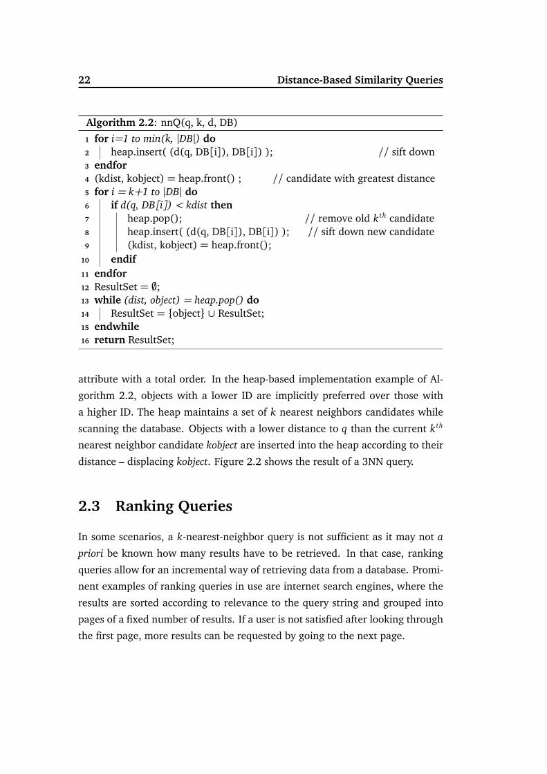
Algorithm 2.2: nnQ(q, k, d, DB)
for i=1 to min(k, |DB|) do1
heap.insert( (d(q, DB[i]), DB[i]) ); // sift down2
endfor3
(kdist, kobject) = heap.front() ; // candidate with greatest distance4
for i = k+1 to |DB| do5
if d(q, DB[i]) < kdist then6
heap.pop(); // remove old kth candidate7
heap.insert( (d(q, DB[i]), DB[i]) ); // sift down new candidate8
(kdist, kobject) = heap.front();9
endif10
endfor11
ResultSet = ;;12
while (dist, object) = heap.pop() do13
ResultSet = object ∪ ResultSet;14
endwhile15
return ResultSet;16
attribute with a total order. In the heap-based implementation example of Al-
gorithm 2.2, objects with a lower ID are implicitly preferred over those with
a higher ID. The heap maintains a set of k nearest neighbors candidates while
scanning the database. Objects with a lower distance to q than the current kth
nearest neighbor candidate kobject are inserted into the heap according to their
distance – displacing kobject. Figure 2.2 shows the result of a 3NN query.
2.3 Ranking Queries
In some scenarios, a k-nearest-neighbor query is not sufficient as it may not a
priori be known how many results have to be retrieved. In that case, ranking
queries allow for an incremental way of retrieving data from a database. Promi-
nent examples of ranking queries in use are internet search engines, where the
results are sorted according to relevance to the query string and grouped into
pages of a fixed number of results. If a user is not satisfied after looking through
the first page, more results can be requested by going to the next page.

2.3. Ranking Queries 23
q
Figure 2.3: Ranking query example for the second iteration and k=3
Definition 2.3 (Ranking Query)
Given a query object q, cardinality and iteration parameters k ∈ N1, i ∈ N1, and
a database DB, the result of a ranking query according to distance measure d is
defined as
RankingQq, i, k, d, DB = NNQq, k, d, DBi
withDBi = DB−
i−1⋃
j=1
RankingQq, j, k, d, DB .
The first iteration of a ranking query is identical to a kNN query due to DB1 =DB. For higher iterations, the ranking query is formulated in terms of a k-
nearest-neighbor query evaluated on a database from which objects that have
been returned in earlier iterations have been removed. Analogously, the state-
less Algorithm 2.3 retrieves the i ∗ k nearest neighbors but discards the first
(i-1)*k objects of the intermediate result. This simplification is possible if kNN
queries return exactly k objects as in the nnQ algorithm. More sophisticated
stateful algorithms reuse intermediate results from earlier iterations. Figure 2.3
shows the result of the second ranking iteration RankingQq, 2, 3, d, DB where three
more results over those from the 3NN query in Figure 2.2 are retrieved.
Algorithm 2.3: rankingQ(q, i, k, d, DB)
return nnQ(q, i*k, d, DB)[1+(i-1)*k : i*k];1


Chapter 3
Efficient Similarity Query
Processing
For large databases and computationally expensive distance measures, the sim-
ple sequential algorithms from Chapter 2 often cannot meet the efficiency re-
quirements of real world applications. This chapter gives a quick introduction
to concepts from the database research field that are employed to lower compu-
tational costs and speed up the search process. A concrete example of how these
concepts can be employed and combined for dL2is given in Chapter 4. Novel
techniques specific to transformation-based distances are described in Part III
and in Chapter 13.
3.1 Lower Bounds and Multi-Step Processing
The query paradigms from Chapter 2 all exclude from their result set objects
from a certain distance on. For range queries, this pruning distance is explicitly
given. For nearest neighbor and ranking queries, the distance is incrementally
determined as the distance to the object with the largest distance within the
intermediate result set during the search. By incorporating a function d ′ that is a
lower bound of the distance function d, multi-step query processing approaches
filter the database such that fewer objects that are ultimately not part of the
result set have to be compared with q using d.
25

26 Efficient Similarity Query Processing
DB
d'(q,o) > ε d(q,o) > ε
d(q,o) ≤ εflter
refnement
Figure 3.1: Multi-step query processing with filter and refinement
Definition 3.1 (Lower Bound)
Given a distance function d : S × S → R+, a function d ′ : S × S → R is called a
lower bound of d iff d ′(s, t)≤ d(s, t) for all s, t ∈ S.
If for a query object q and a database object o the value given by d ′(q, o) is not
below the pruning distance, then o is not part of the result set of the query as
d(q, o) is always equal to or larger than d ′(q, o). The database can be filtered
using d ′ in a filter step and the final result set is obtained using d on the filtered
database in what is referred to as a refinement step. The general process is
visualized in Figure 3.1 in the form of a Sankey diagram.
If using a lower bound d ′ in the query processing is to improve the efficiency
of the whole process, d ′ has to satisfy certain criteria termed the ICES-criteria
in [AWS06]: Indexability, Completeness, Efficiency, and Selectivity. Selectivity
pertains to the number of objects that can be excluded from further investiga-
tion. If d ′ gives values close to d, many objects can be pruned and the filter
has a good selectivity. Efficiency regards the computational cost of determining
values of d ′ which should be lower than the computational cost of determining
values of d. Completeness of the filter step requires that no false dismissals oc-
cur. If d ′ is a lower bound of d, completeness can be guaranteed for commonly
used multi-step algorithms. Indexability refers to the desirable ability to support
the query processing using an indexing scheme for d ′ (cf. Section 3.2).
A number of multi-step query processing algorithms that use a lower bound
d ′ for a distance function d exist in the literature. A range query can be an-
3.2. Indexing Structures 27
swered by evaluating rangeQ(q, ε, d, rangeQ(q, ε, d ′, DB)) as proposed for ex-
ample by [AFS93]. That is, first the subset of objects o in the database that sat-
isfy d ′(q, o)< ε is determined and only for those objects d(q, o)< ε is checked.
[KSF+96] gives a multi-step k-nearest-neighbor algorithm that is based on a
lower bound in the filter step. The first k nearest neighbors according to the
filter distance d ′ are retrieved and refined with d. Afterward, a range query
with the maximum of the k refined distances is issued using again d ′. Finally,
the candidates returned by the range query are refined with d and the k closest
objects are returned as the k nearest neighbors according to d. In [SK98], a
multi-step k-nearest-neighbor algorithm that is optimal in terms of the number
of refinement distance computations is given. It is based on a ranking query
for the lower bounding distance d ′ and iteratively refines candidates until the
distance of a candidate according to d ′ is greater than the refined distance of
the current kth nearest neighbor candidate according to d.
Depending on the distance function d, finding a suitable lower bound d ′ that
fulfills the ICES-criteria to a satisfactory degree can be a challenge. A prominent
strategy is dimensionality reduction where objects from a high-dimensional fea-
ture representation space are mapped to objects in a representation space with
a reduced dimensionality. For example, in the case of dL2on fixed-binning his-
tograms, dropping any number of dimensions results in a lower-dimensional
representation of the histogram on which dL2itself is a lower bound. Dimen-
sionality reduction will be the focus of Chapter 4 and Chapter 8.
3.2 Indexing Structures
The foremost aim of indexing structures is identical to that of the query pro-
cessing algorithms based on lower bounds from the last section: to enable a fast
identification of a small superset of the final result set. Unlike the lower bounds
described in the last section that are based on properties of the distance func-
tions they approximate, indexing structures are designed to achieve this goal
by collecting information on the objects contained in the database. Using this
data-dependent information, similarity search algorithms that make use of such

28 Efficient Similarity Query Processing
(a) R-Tree Spatial View (b) R-Tree Topological View
Figure 3.2: Structure of the R-Tree [Gut84]
indexing structures can rule out or prune parts of the database without having
to look at all of the database objects.
The number of indexing structures that have been proposed for supporting
distance-based queries has grown considerably with every year over the past
few decades. They differ in many ways, including the nature of the data they
index, the distance measures and query types they support, the query loads
they are optimized for, and in their support for object insertions and deletions.
A recent account is given in [Sam05]. As even that immensely extensive work
cannot cover all indexing structures for distance-based query processing, no
such attempt shall be made here. Instead, a quick overview of those concepts
and indexing structures important for the following parts is given in this section.
Further details will be provided in the according chapters as required.
From a database research perspective, the R-Tree [Gut84] and its variants
are typically considered the most well-known secondary memory indexing struc-
tures for multi-dimensional, spatial data (i.e., points or objects with an extent
in a vector space equipped with a distance function). The general idea of R-
Trees and many other hierarchical indexing structures is to map spatial prox-
imity (cf. Figure 3.2(a)) of the objects in the database to topological proximity
(cf. Figure 3.2(b)) in the data structure by grouping objects according to their
membership in nested bounding geometries. In the case of the R-Tree, an in-
ner node of this multi-way tree describes each of its subtrees in terms of an
axis-parallel minimum bounding rectangle (MBR) and an identifier that allows
for the retrieval of a subtree from the storage system. The leaf nodes contain

3.2. Indexing Structures 29
Algorithm 3.1: rtree-rangeQ(q, ε, d, minDist, RTree)
return rec-rtree-rangeQ(q, ε, d, minDist, RTree.rootnode);1
Algorithm 3.2: rec-rtree-rangeQ(q, ε, d, minDist, node)
ResultSet = ;;1
if node.isleaf then2
for o ∈ node.dataobjects do3
if d(q, o) ≤ ε then4
ResultSet = ResultSet ∪ o;5
endif6
endfor7
else8
for childnode ∈ node.childnodes do9
if minDist(q, childnode.mbr) ≤ ε then10
ResultSet = ResultSet ∪ rec-rtree-rangeQ(q, ε, d, minDist,11
childnode);endif12
endfor13
endif14
return ResultSet;15
the database objects (vectors or extended objects and potentially further infor-
mation). The MBRs of R-Trees can overlap and the capacity of each node is
restricted as it is to be stored in secondary memory where the capacity is chosen
as a multiple of the smallest addressable unit of memory of the storage system.
The R-Tree family is large [SRF87, BKSS90, BKK96], with new members such as
[KCK01, BS09] joining even a quarter of a century after Guttman’s publication.
When processing a similarity search query, the MBRs are used to decide
whether objects in the subtree can be pruned from the search. For this purpose,
a smallest possible distance from the query to the bounding rectangle of a sub-
tree is defined. This so-called MinDist is a lower bound for all objects in said
subtree and can thus be compared with the pruning distance of a search. The
definition of the MinDist depends on the distance measure that is employed.
Algorithms 3.1 and 3.2 list pseudo-code for simple recursive range query pro-
cessing akin to the rectangular overlap query from [Gut84]. Similarly, nearest

30 Efficient Similarity Query Processing
neighbor algorithms such as the Depth-first Traversal algorithm of [RKV95] and
the Priority Search algorithm described in [HS95] use the R-Tree (and other
indexing structures) to prune whole branches of the tree once the feature space
region they represent can be guaranteed to not include the nearest neighbor.
A second group of indexing structures often employed to speed up the sim-
ilarity search process relies on the metric properties – in particular on the tri-
angle inequality property – that many distance functions possess. Instead of
grouping objects with explicit bounding geometries, metric indexing structures
like the M-Tree [CPZ97] gather information regarding the distance of objects in
the database to a set of (sometimes hierarchically structured) pivot or vantage
points. Given the distance from the query to a pivot point and the precomputed
distance from the pivot point to a database point, the distance required for the
similarity search (i.e., from the query to the database object) can be estimated
using Definition 1.5. By storing the maximum distance from a pivot point to
all data objects in according subtrees, an implicit sphere around the pivot point
is established that allows for pruning of the search space. As metric indexing
structures only require the distance function to be metric, they are not restricted
to the vector space model.
When trying to index higher-dimensional points (where “higher” starts at
about 5–10 for many indexing structures), the pruning capability of hierarchical
indexing structures rapidly declines due to the curse of dimensionality. Both
the R-Tree and the M-Tree suffer from a large degree of overlap of the MBRs
or implicit spheres. The VA-file [WSB98] exemplifies efforts to speed up the
process of scanning the whole database while searching the database. Here,
dimension-wise quantization is used to approximate the location of objects as
within a certain rectangular region. As the quantized information is compact
and as the dimension-wise boundaries of the rectangular regions are known
in advance, a scan over all quantized data is comparatively fast and partial
distance information can be precomputed. Only when the approximate location
of an object is not enough to establish whether it is part of the result set must
its full representation be retrieved and compared with the query object.

Chapter 4
An Example for Similarity Search
Using Simple Distance Measures
This chapter gives an example of how various techniques introduced in Part I can
be put together to forge a similarity query system (cf. [BWS06]) that is tailored
to support efficient nearest neighbor query processing based on the Euclidean
distance measure. In a multi-step query processing framework, Voronoi cells –
which reflect local neighborhood information – are indexed to create a fast filter
for the nearest neighbor search.
4.1 Introduction
Utilizing spatial index structures on secondary memory for nearest neighbor
search in high-dimensional spaces has been the subject of much research. How-
ever, a growing number of applications demanding a high query throughput
stand to benefit from a shift toward index structures tailored for main memory
indexing. Server-based similarity search services are examples of such types
of applications. In this scenario a large number of querying clients demands a
low response time from a server that bases its service on static or semi-static
data. Other examples include algorithms that implement a classification or
density-based clustering method based on the concept of nearest neighbors.
The “(re)index rarely, query frequently” behavior of those applications allows
31

32 An Example for Similarity Search Using Simple Distance Measures
flter: point in cuboid? refne: compute distances
query
index
candidates
refnement
nearest neighbor
Figure 4.1: Query processing using indexed Voronoi cell-bounding cuboids
for an extensive preprocessing phase in which the index is built from scratch.
The volatile nature of main memory is not a disadvantage in this scenario as
the data is stored on secondary memory and only a copy is loaded into main
memory to be accessed at a high frequency. The economic impact of reserving
a few hundred megabytes or a few gigabytes of RAM to host larger indexes in
main memory is diminishing fast while the increase in efficiency that goes along
with it can be significant.
One approach that relies on an extensive preprocessing step consists of in-
dexing the solution space for nearest neighbor queries in the form of approx-
imate Voronoi cells [BEK+98, BKKS00]. Voronoi cells describe a covering of
the underlying feature representation space such that each data object is as-
signed to the cell that contains all its possible nearest neighbor locations. A pre-
processing step is used to approximate the complex Voronoi cells with simpler
high-dimensional axis-aligned bounding rectangles (i.e., rectangular cuboids)
in order to enable low query response times. While its low CPU-utilization
makes the approach a natural candidate for main memory indexing, it resists
attempts to incorporate effective dimensionality reduction techniques. Straight-
forward solutions prove to be unsuitable. This severely limits the application
domain of the approximate Voronoi approach as approximate Voronoi cells in
high-dimensional spaces are neither feasible to compute nor efficient for index-
ing.
Sections 4.1.1 and 4.2 review related work and the approximate Voronoi ap-

4.1. Introduction 33
proach. The problems of incorporating dimensionality reduction techniques to
support multimedia similarity search are described in Section 4.3.1 and approx-
imation-based methods to efficiently overcome these difficulties are introduced.
A second dimensionality reduction (on the level of the cuboids) presented in
Section 4.3.2 improves response times through limiting the dimensionality of
the bounding cuboids themselves. The cuboids in the reduced dimensionality
are indexed by facilitating either hierarchical or bitmap-based index structures
in main memory as described in Section 4.3.3. It is possible to find a complete
set of nearest neighbor candidates for a query point in a filtering step through
simple point-in-cuboid tests (cf. Figure 4.1). The significant performance im-
provements over other approaches achieved for the Voronoi-based technique
through these two dimensionality reduction steps are shown in Section 4.4 for
real world datasets.
The result is a filter-and-refine query processing system for rapid nearest
neighbor search based on the Euclidean distance with speedup factors of up to
five versus other evaluated RAM-resident indexing structures.
4.1.1 Related Work
The concept of partitioning a space to describe nearest neighborhood informa-
tion utilized in this chapter was developed in the early twentieth century by G.
Voronoi [Vor08] and is a generalization of the 2- and 3-dimensional diagrams
already used by Dirichlet in [Dir50] and informally described by Descartes in
[Des44]. It is still a widespread and important topic of extensive research in
the field of computational geometry [AK00]. A first algorithm that efficiently
computes the nearest neighbor of a query based on a Voronoi diagram was
proposed in [DL76]. The algorithm performs nearest neighbor queries on m
points in the 2-dimensional Euclidean plane in worst-case-optimal time com-
plexity of O(log m). However, the algorithm does not extend well to dimen-
sionalities higher than two. In [BEK+98, BKKS00], a technique using approxi-
mate Voronoi cells was introduced and enabled the use of datasets with low to
medium dimensionalities. The technique also reaches its limits with increasing
dimensionality. By enabling dimensionality reduction to be used with the ap-

34 An Example for Similarity Search Using Simple Distance Measures
q
(a) Voronoi diagram (b) half space intersections
Figure 4.2: A Voronoi diagram and the definition of a Voronoi cell
proximate Voronoi approach, the techniques in this chapter expand on the work
in [BEK+98, BKKS00].
Due to main memory becoming significantly larger in capacity and signifi-
cantly cheaper in price, research interest on indexes in main memory has been
renewed in the database community. Well-known secondary memory indexing
structures that utilize the concepts reviewed in Section 3.2 have been investi-
gated and modified for the main memory scenario. For example, the CR-Tree
[KCK01] improves on the cache-consciousness of the R-Tree [Gut84] by apply-
ing MBR compression techniques while both the pkT-Tree [BMR01] and the
CSB+-Tree [RR00] focus on low-dimensional main memory indexing.
4.2 Preliminaries
4.2.1 Voronoi Cells
A Voronoi diagram for a set of m points in a given space is a covering of said
space by m cells that indicate the nearest neighbor areas of the points. It is
thus directly tied to the problem of finding nearest neighbors. Figure 4.2(a)
shows such a partitioning for six points in the Euclidean plane. For each point,
the respective surrounding cell describes the area for which that point is closer
than any of the other points. Given a query position q in the plane, the nearest
neighbor can be found by determining the cell that includes that position. As

4.2. Preliminaries 35
Algorithm 4.1: voronoi-nnQ(q, VDDB,S)
for VCp,S ∈ VDDB,S do1
if q ∈ VCp,S then2
return p;3
endif4
endfor5
long as q remains inside the same cell, its nearest neighbor does not change.
The edges and vertices in the diagram describe positions for which more than
one point is at minimum distance. Voronoi cells can formally be described using
the concept of half spaces as follows.
Definition 4.1 (Voronoi Cell)
Given a space S, a metric distance function d : S × S → R+, and a finite set of
points DB ⊆ S, a Voronoi cell V C p,S for point p ∈ DB is defined as the intersection
of S and |DB| − 1 half spaces:
VCp,S = S ∩
⋂
r ∈ (DB−p)
HSp|r
where
HSp|r = s ∈ S|d(s, p)≤ d(s, r).
Definition 4.2 (Voronoi Diagram)
A Voronoi diagram VDDB,S is defined as the set of the Voronoi cells:
VDDB,S = VCp,S|p ∈ DB
Figure 4.2(b) shows the half space intersections for a Voronoi cell in light
blue where the half space separation lines are shown as dashed lines. Algo-
rithm 4.1 exemplifies how a Voronoi diagram can be used to find the nearest
neighbor of a query.

36 An Example for Similarity Search Using Simple Distance Measures
Algorithm 4.2: approx-voronoi-nnQ(q, d, AVDDB,S)
CandidateSet = ;;1
for AVCp,S ∈ AVDDB,S do2
if q ∈ AVCp,S then3
CandidateSet = CandidateSet ∪ p;4
endif5
endfor6
return nnQ(q, 1, d, CandidateSet) ; // see page 227
4.2.2 Approximate Voronoi cells
In more than two dimensions (as is the case for feature representation spaces in
many multimedia similarity search applications) the cells become highly com-
plex [Kle80, Sei87]. Due to this complexity, neither computing nor storing or
inclusion-testing is efficient for nearest neighbor search directly based on these
cells. Therefore, the preprocessing step in this chapter determines approximate
Voronoi cells of lesser complexity without requiring the exact representations of
the latter to be known while still allowing for fast nearest neighbor search. To
avoid false dismissals during nearest neighbor query processing, each approxi-
mate cell must be a superset or bounding geometry of the original Voronoi cell.
Algorithm 4.2 shows how an approximate Voronoi diagram AVD (consisting of
approximate Voronoi cells AVC) can generally be used to find the nearest neigh-
bor of a query in a filter-and-refine manner. Here, the filter is not based on
a lower-bounding distance function of d. Instead, an inclusion test is used to
rule out those objects for which query q falls outside their according approxi-
mate nearest neighbor region. For the remaining objects in the candidate set, a
nearest neighbor query using d is performed.
Among the potential bounding geometries, axis-aligned bounding cuboids
offer several advantages. For n-dimensional points, they enable inclusion tests
in O(n) time, they can be stored in O(n|DB|) space, and they are computable
through well-studied linear optimization algorithms [PTVF92].

4.2. Preliminaries 37
p
(a) tight cuboid approx.
p'
p
(b) non-tight cuboid approx.
Figure 4.3: Voronoi cell approximations
4.2.3 Computation of Approximate Voronoi Cells
A bounding cuboid of a Voronoi cell V C p,S (p ∈ Rn) can be computed by solv-
ing 2n linear optimization problems. In linear optimization a linear objective
function is maximized or minimized over a range of values restricted by a set
of linear constraints. In the context of Voronoi cell approximation, the required
linear constraints are defined by
• the set of half spaces outlining the cell and
• the space boundaries of S.
For the approximation approach to Voronoi cells chosen here, it is required that
S ⊂ Rn be of convex shape such as the n-dimensional unit hypercube [0,1]n. All
potential query points are also assumed to be from within S.
The n objective functions are used to find the outermost points in each of
the n dimensions of a cell VCp,S described by the linear constraints. For this
purpose, functions f1 to fn with fi(x1, ..., xn) = x i are each minimized and max-
imized once per Voronoi cell. The extremal values directly represent the respec-
tive boundaries of the cuboid that tightly bounds the Voronoi cell. The space
boundaries must be added to the set of constraints to avoid that these extremal
values extend outside the data space in some of the dimensions – potentially
causing the cuboid to unnecessarily grow within S for other dimensions.

38 An Example for Similarity Search Using Simple Distance Measures
Only a subset of all potential half spaces may be used in order to signifi-
cantly speed up the calculation of the bounding cuboids during the preprocess-
ing step. Half spaces that are redundant due to not constraining a Voronoi cell
can be left out without affecting the result of the cell approximation. Leav-
ing out non-redundant half spaces leads to a non-minimum bounding cuboid,
which potentially introduces more nearest neighbor candidates and slows down
nearest neighbor searches by requiring more refinement calculations but never
misses a valid solution. Therefore the choice of the subset of half spaces is very
important. In [BEK+98] some heuristics for the choice of an appropriate subset
of half spaces are introduced. This chapter concentrates on a heuristic that se-
lects a limited number of nearest neighbor points from DB for each data point
p ∈ DB and uses the corresponding half spaces to approximate the Voronoi cell
VCp,S since the half spaces defined by the nearest neighbors of p are likely to
actually restrict the cell. For the range of parameters evaluated in Section 4.4,
restricting the number of nearest neighbors used for the approximation to 1%
of the database has proven to yield good results.
Figure 4.3(a) shows the approximate cell belonging to object p where all
half spaces were used while in Figure 4.3(b) the half space HSp|p′ is left out,
resulting in a slightly larger cuboid.
4.3 Dimensionality Reduction for the Voronoi Ap-
proach to Nearest Neighbor Search
The potentially high dimensionality of the object representation in multimedia
applications hinders the efficient utilization of the Voronoi approach to nearest
neighbor search in three ways.
First, a high dimensionality results in the data representation space being
sparsely populated with data points. Thus the bounding cuboids of the Voronoi
cells are relatively large in this case as only comparatively few other cells are
available to restrict each cell in all possible directions. In extreme cases, all
cuboids overlap the complete space since each cell includes points on both the
upper and lower space boundary of each dimension. These unrestricted cuboid
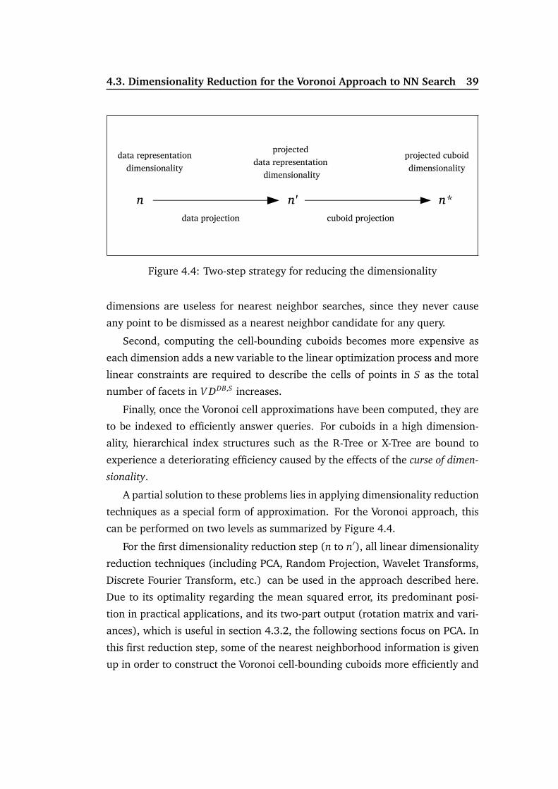
4.3. Dimensionality Reduction for the Voronoi Approach to NN Search 39
data representationdimensionality
projected data representation
dimensionalityprojected cuboiddimensionality
n' n* data projection cuboid projection
n
Figure 4.4: Two-step strategy for reducing the dimensionality
dimensions are useless for nearest neighbor searches, since they never cause
any point to be dismissed as a nearest neighbor candidate for any query.
Second, computing the cell-bounding cuboids becomes more expensive as
each dimension adds a new variable to the linear optimization process and more
linear constraints are required to describe the cells of points in S as the total
number of facets in V DDB,S increases.
Finally, once the Voronoi cell approximations have been computed, they are
to be indexed to efficiently answer queries. For cuboids in a high dimension-
ality, hierarchical index structures such as the R-Tree or X-Tree are bound to
experience a deteriorating efficiency caused by the effects of the curse of dimen-
sionality.
A partial solution to these problems lies in applying dimensionality reduction
techniques as a special form of approximation. For the Voronoi approach, this
can be performed on two levels as summarized by Figure 4.4.
For the first dimensionality reduction step (n to n′), all linear dimensionality
reduction techniques (including PCA, Random Projection, Wavelet Transforms,
Discrete Fourier Transform, etc.) can be used in the approach described here.
Due to its optimality regarding the mean squared error, its predominant posi-
tion in practical applications, and its two-part output (rotation matrix and vari-
ances), which is useful in section 4.3.2, the following sections focus on PCA. In
this first reduction step, some of the nearest neighborhood information is given
up in order to construct the Voronoi cell-bounding cuboids more efficiently and
40 An Example for Similarity Search Using Simple Distance Measures
lessen the effects of the curse of dimensionality. A sizable number of dimensions
can often be removed in this way while only introducing minor inaccuracies.
The feature extraction process employed for a similarity search application can
result in dimensions that are insignificant to the application at hand. This is
the case when one dimension is dominated by other dimensions either due to
differences in the variance of the dimensions or due to correlation effects. In-
troducing some minor inaccuracies through this first dimensionality reduction
can often be acceptable in return for a more efficient preprocessing step and for
faster query processing.
In the second dimensionality reduction step described in section 4.3.2, the
dimensionality of the resulting cuboids can be further reduced prior to indexing.
Unlike the first reduction step, this reduction does not influence the effective-
ness but only the efficiency of the nearest neighbor search process.
The overall dimensionality reduction process outlined by Figure 4.4 is thus to
first reduce the data representation dimensionality from n to n′ in a lossy fashion
by as much as the application allows for and then to reduce the approximation
dimensionality from n′ to n∗ in order to improve the efficiency of the search
process while ensuring that the correct answer on the level of the chosen n′ is
still returned.
Looking at the ICES filter quality criteria (cf. page 26), the filter-and-refine
process is complete (C) on level of n′ and an inclusion test for a cuboid with
reduced dimensionality is efficient (E). The indexability (I) will be handled in
Section 4.3.3 and the selectivity (S) is evaluated in the experiments.
4.3.1 The Bounding Constraints Problem
Unlike other nearest neighbor algorithms, the Voronoi approach described here
depends on the data space being included in a polytope whose facets are used to
define the outer constraints for the linear optimizations of the bounding cuboid
computation. Dimensionality reduction techniques for the Voronoi approach
have to take this property into account.
For similarity search based on fixed-binning histograms examined in this
chapter, all histograms hpi = (hpi[1], . . . , hpi[n]) of pi ∈ DB share a common sum

4.3. Dimensionality Reduction for the Voronoi Approach to NN Search 41
1. rotate
2. project
Figure 4.5: 3-dim. common-sum vectors bounded by 3 lines in a 2-dim. plane
1.0 = |hpi |Σ. For these vectors, there is an (n− 1)-dimensional convex polytope
with n vertices and n facets that includes all vectors. After rotating and project-
ing all points to eliminate the redundant dimension hpi[n] = 1.0−∑n−1
j=1 hpi[ j],the n vertices of the polytope consist of the accordingly transformed unit vec-
tors. The transformed polytope serves as the data representation space S that
confines the Voronoi cells and contributes linear constraints to the approximate
Voronoi cell computation. Figure 4.5 illustrates the transformation for the case
of n = 3 where all points are enclosed by the three lines between the three
transformed unit vectors in a two-dimensional subspace.
In practical applications, the originally sum-normalized data is often linearly
transformed. Scaling of individual dimensions is used to compute weighted dis-
tances and both rotations and projections are common in dimensionality reduc-
tion (PCA, DFT, Random Projection and others). The aim is to find the trans-
formed convex polytope defining the data space – in particular after projections
into a dimensionality n′ < n. A linear transform of a convex polytope is an-
other convex polytope where the vertices of the transformed polytope are (a
subset of) the transformed original vertices. Thus, one way to find the trans-
formed polytope is to transform all original polytope vertices P and then find
the convex hull for those points P ′. This approach has a worst-case time com-
plexity of O(m log m+mbn′/2c) for m points in the (possibly lower) transformed
dimensionality n′ [Ede87].
The high complexity of the convex hull leads to another problem. Each facet

42 An Example for Similarity Search Using Simple Distance Measures
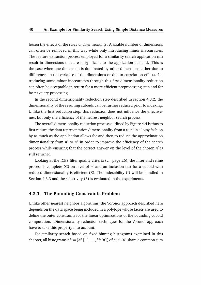
2 4 6 8 10 12 14 16 18 20 22 24 26
27D image data 7 111 675 3199 9263 22980 49917 61450 45229 24739 6644 805 2727D phoneme data 4 8 22 204 507 706 928 423 340 121 141 69 27
1
10
100
1000
10000
100000
num
ber o
f fac
ets o
f con
vex
hull
projected dimensionality n'
Figure 4.6: Number of facets for convex hulls in the projected dimensionality n’
of the convex hull produces a constraint for the linear optimizations for each
Voronoi cell. Hence, that number must be low for practical reasons. Contrary
to that, a convex hull with m vertices in n′ dimensions can have in the order
of O(mbn′/2c) facets [Ede87]. Figure 4.6 shows these values computed via the
QHull algorithm [BBDH96] for two real world datasets used in Section 4.4.
While the convex hulls for the phoneme dataset remain sufficiently simple, the
image histogram dataset quickly goes beyond values reasonable for a practical
computation of the Voronoi cell-bounding cuboids. Due to that fact, a number
of methods to conservatively approximate the convex hull are introduced in the
following pages. An approximation of the convex hull of a set of points is called
conservative in this context if all points are also contained in the approximation
of the convex hull.
A Bounding Cuboid Approximating The Convex Hull
A simple way to conservatively approximate the convex hull of a set of points P ′
with (n′− 1)-dimensional planes is to find a bounding cuboid for the hull. This
can be done by determining the minimum and maximum values among the set
P ′ for each dimension. The resulting 2n′ planes defined by the cuboid facets are
suitable as constraints for the Voronoi cell approximations. However, the shape
of the convex hull of P ′ can be quite different from an axis-aligned cuboid. If a
greater precalculation cost is acceptable to improve the selectivity for queries, it
is worth finding a more complex but closer approximation of the convex hull.

4.3. Dimensionality Reduction for the Voronoi Approach to NN Search 43
vx
(a) tilted planes
vx
p' i2p' i1
p' i3
(b) inner polytope
Figure 4.7: Planes approximating a convex hull
Tilted Planes Approximating the Convex Hull
A potentially closer approximation can be found by using the vertices of the
bounding cuboid. For each of the 2n′ vertices, the adjacent n′ vertices span a
hyperplane with a normal vector v as depicted in Figure 4.7(a) for vertex x of
the cuboid bounding the convex hull. Each such tilted hyperplane is then pushed
outwards along its normal vector until all points in P ′ are located either on the
hyperplane or behind it as defined by the orientation of the normal vector. This
plane-fitting algorithm has a time complexity of O(n′|P ′|).
Inner Polytopes Approximating the Convex hull
Like the bounding cuboid approach, the tilted planes method makes little use of
the geometric shape of the convex hull being approximated. The normal vectors
of the hyperplanes are only influenced by the total extent of the convex hull in
each dimension. A variant is proposed here that attempts to find more suitable
normal vectors for the plane fitting. The idea is to define a less complex convex
polytope residing inside the convex hull of P ′ that still reflects its general shape.
Once the facets of the inner polytope have been determined, they are pushed
outwards along their normal vectors to include all the points in P ′.

44 An Example for Similarity Search Using Simple Distance Measures
The polytope used in this proposal is defined through its vertices, which form
a subset of the vertices of the convex hull of P ′.
Definition 4.3 (Set of Extremal Points)
Let R= r1, r2, ... be a finite set of n-dimensional points. The set of extremal points
ExtR is defined as
ExtR = ExtMinR ∪ ExtMaxR
with
ExtMinR = ri ∈ R|∃k ∈ 1, ..., n : ∀r j ∈ R− ri :
(ri[k]< r j[k])∨ ((ri[k] = r j[k])∧ (i < j))
and
ExtMaxR = ri ∈ R|∃k ∈ 1, ..., n : ∀r j ∈ R− ri :
(ri[k]> r j[k])∨ ((ri[k] = r j[k])∧ (i < j)).
Intuitively, these are the points that are located on an axis-aligned minimum
bounding cuboid of the set R. If more than one point is located on the same
facet of the cuboid, a tie-breaker is used. Given ExtP ′ , points p′i1 , ..., p′in′ ⊆ ExtP ′
are selected for each vertex x of the bounding cuboid of P ′ as illustrated by
Figure 4.7(b). These are the points that were included in ExtP ′ due to their
position on a facet of the cuboid that has x as one of its vertices. If none of
the points are duplicate for vertex x , the n′ points define a facet of an inner
polytope of the convex hull which can then be pushed outwards by the plane-
fitting method detailed earlier. In higher dimensionalities with relatively few
points in P ′, it often happens that one point is extremal for more than one
dimension and thus the maximum number of 2n′ facets is rarely reached for the
inner polytope. In the illustration of Figure 4.7(b), this would be the case if one
of the three points selected for x was either on an edge of the cuboid or on a
vertex of the cuboid. The resulting inner polytope would then have five or four
vertices only versus the expected six vertices (three from ExtMinP ′ and ExtMaxP ′
each).

4.3. Dimensionality Reduction for the Voronoi Approach to NN Search 45
Greedy Point Selection
Further inner polytopes can be defined by using other methods to select a subset
T ⊂ P ′ and then constructing the less complex convex hull for T . The facets of
the hull are then pushed outwards along their normal vectors until they include
all points in P ′. In order for T to represent the general shape of P ′, a greedy
heuristic for selecting points t1, ..., t|T | is proposed: choose any one point in
P ′ that is located on the convex hull of P ′ as t1. Then choose t i+1 as the point
p from (P ′ − t1, ..., t i) with the greatest accumulated distance∑i
j=1 d(p, t j).The greedy selection algorithm runs in O(n′ · |P ′|+n′ · |T |2) time followed by the
computation of the convex hull for |T | points.
Combinations and Variations
The strategies described for finding a convex polytope that conservatively ap-
proximates the space in which data points potentially reside offer practical al-
ternatives to the convex hull with its high facet count. More approaches can di-
rectly be derived from the previous approximations. An intersection of two con-
servative, convex approximations yields another conservative, convex approx-
imation. Thus, all approaches can be combined by using constraining planes
from more than one approach. Adding the 2n′ axis-aligned facets of the con-
vex hull-bounding cuboid to constraints from another approximation hardly in-
duces any computational effort but helps reduce the size of the also axis-aligned
Voronoi cell-bounding cuboids and ensures that the data space is bounded ap-
propriately in all dimensions. Similarly, the hyperplanes retrieved from a greedy
point selection can be augmented by both the cuboid and the inner polytope hy-
perplanes.
4.3.2 Reduction of the Bounding Cuboid Dimensionality
The dimensionality reduction discussed enables efficient computation of the
bounding cuboids by projecting the data points from dimensionality n to a space
of dimensionality n′. However, it does so by sacrificing nearest neighborhood
information. Though justifiable to some extent, it is often not viable to reduce

46 An Example for Similarity Search Using Simple Distance Measures
the dimensionality to a level where indexing the cuboids is efficient. Therefore,
a further reduction to a dimensionality n∗ < n′ (cf. Figure 4.4) is proposed that
does not sacrifice the effectiveness of the approach.
First, a query vector q is transformed and projected to q′ in dimensionality
n′ by the same method used to reduce the data dimensionality. Without the
cuboid projection, vector q′ would then be tested for inclusion in the Voronoi
cell-bounding cuboids defined by their respective upper and lower boundary
vertices. Instead, after computing the Voronoi cell-bounding cuboids for the
projected data points in dimensionality n′, those cuboids themselves are pro-
jected to dimensionality n∗ by dropping some of the dimensions. This produces
the same nearest neighbor as in the case of the cuboids in dimensionality n′ as
dropping dimensions relaxes the query inclusion test in Algorithm 4.2. While
no candidates are lost in this process, there might however be additional false
positives. Formally, the characteristic function of the filter regarding all n′ di-
mensions is a lower bound of the characteristic function of the filter regarding
only a subset of n∗ dimensions.
Definition 4.4 (Characteristic Function of a Filter)
The characteristic function χ : S × S→ 0, 1 of a filter for objects from S returns
0 on (q, o) if object o is filtered out with respect to q and 1 if it passes the filter.
Definition 4.5 (Characteristic Function for the approximate Voronoi filter)
Let DB ⊂ S be a finite set of n-dimensional points within space S, E ⊆ 1, ..., n a
set of dimensions, and AVDDB,S = AVCo,S|o ∈ DB the set of Voronoi cell-bounding
cuboids with lower and upper boundary vertices lo and uo. Then the characteristic
function χ E : S×S→ 0,1 for the approximate Voronoi inclusion-test filter based
on dimensions E is defined as
χ E(q, o) =
(
1 if (o ∈ DB)∧∀e ∈ E : lo[e]≤ q[e]≤ uo[e]0 otherwise.
If E∗ is a subset of dimensions E′ then χ E∗ is an upper bound of χ E′ since a
filter based on E∗ instead of E′ might allow more but not fewer objects to pass.
The selectivity of the filter step (cf. Figure 4.1) worsens as more dimensions are

4.3. Dimensionality Reduction for the Voronoi Approach to NN Search 47
dropped. However, fewer dimensions can result in a faster filter step execution.
The following question then arises: Which dimensions are to be dropped and
which ones are to be retained? Unfortunately, there are∑n′
e=1
n′
e
combinations
to consider in an exhaustive search. The search space must be vastly reduced
by concentrating on promising combinations.
Empirical Selectivities for Finding Dimensions to Retain
Given a sample query workload Q, average selectivity values can be used to find
dimensions with a good selectivity. The aim is to find a filter for which both
the number of dimensions and the average selectivity is low (i.e., the filter shall
only let a low number of candidates pass).
Definition 4.6 (Empirical Selectivity)
Given a database DB and a query workload Q, the empirical selectivity of a filter
is defined via its characteristic function χ as
1
|Q|
∑
q∈Q
1
|DB|
∑
o∈DB
χ(q, o).
The heuristic proposed in this section vastly reduces the search space by as-
sessing the selectivity of each of the n′ dimensions without regard to the other
dimensions. A high empirical selectivity value for χk with 1 ≤ k ≤ n′ indi-
cates that the kth dimension is unable to filter out many objects. Using a greedy
selection of dimensions in the order of the worsening individual empirical se-
lectivity is optimal if the filtering events are mutually independent. In that case,
the empirical selectivity of two combined dimensions is expected to be close to
the product of both individual empirical selectivities. While statistic indepen-
dence cannot be expected in general, the PCA utilized for the reduction from
n to n′ dimensions does eliminate the covariance between the n′ dimensions
(which in the case of a multivariate normal distribution entails independence).
After PCA reduction to a dimensionality of 10 for the 27-dimensional image
histogram dataset from the experimental section, the two dimensions with the
highest variance exhibit an empirical selectivity of 15% and 10.8%. The ex-
pected combined selectivity would be close to 15% · 10.8% = 1.62% in case of

48 An Example for Similarity Search Using Simple Distance Measures
independence. The measured value was 1.95%. With an increasing number
of dimensions, the relative gap widens to an expected 0.0027% for 10 dimen-
sions and 0.0596% measured as additional dependencies are introduced. Still,
the proposed order of dropping dimensions resulted in combined selectivities
rarely outperformed by spot samples of the same number of dimensions, which
justifies using the heuristic proposed in this section.
Using Variances to Find Dimensions to Retain
To avoid having to find a suitable query set Q and compute empirical selectivi-
ties, another simplification can be employed when PCA has been used to reduce
the data dimensionality. As a by-product of the PCA, the variances for each di-
mension of the rotated and projected data points are known. Instead of using
the worsening selectivity order to pick dimensions to retain, the descending or-
der of the variances can be used. While a high variance for a dimension does not
necessarily imply a good selectivity for that dimension, it can be a good indicator
as dimensions with a low variance tend to produce Voronoi cells that stretch far
in said dimensions. Measured correlation coefficients for inverted variances and
measured selectivities of individual dimensions were 0.957, 0.504 and 0.937 for
the three real world datasets used in the experiments.
On the Number of Dimensions to Retain
The question of how many dimensions are to be retained remains. The decision
depends on the index structure used. One possibility would be to produce up
to n′ indexes using 1 to n′ dimensions selected via the methods proposed above
and then select the one index with the best average query performance. Without
further information about the index structure, this might be the only method to
pursue. Experiments in Section 4.4 show that the X-Tree greatly benefits from
the additional projection while the evaluated bitmap-based structure does not.

4.3. Dimensionality Reduction for the Voronoi Approach to NN Search 49
4.3.3 Main Memory Indexing for the Voronoi Approach
Data page access and read times are not the foremost cost factors of performing
nearest neighbor queries when the index structure is stored in main memory.
The querying time can be decomposed into a filter part (decide which points
in DB need further examination) and a refinement part (compute the distances
to the query point q). Both parts vary widely for the available algorithms and
index structures. While the linear scan (cf. page 22) does not spend any time on
filtering but computes the distances from q to all data points in DB, the Priority
Search algorithm [HS95] for hierarchical index structures carefully considers
which data points warrant a distance computation.
The filter step of the Voronoi approach presented here is based on point-
in-cuboid tests. Since the Voronoi cell-bounding cuboids are axis-aligned, the
R-Tree family (normally based on secondary memory) is an obvious candidate to
support the filtering step. Due to its better suitability for data with a dimension-
ality beyond approximately six, the X-Tree [BKK96] was chosen to be adapted
to run in main memory for tests in Section 4.4. In addition, a bitmap-based
index structure described in [GPB03] was implemented. The authors originally
used the Bitvector Index for fixed-range queries in a memory-resident similar-
ity search system but its design makes it a promising option for Voronoi-based
nearest neighbor queries.
For each dimension i of the space to be indexed, the Bitvector Index stores
a number b of bitvectors BVi,1, ..., BVi,b together with b+ 1 delimitation values
bi,0, bi,1, ..., bi,b. When indexing m cuboids, each BVi, j has m bit entries denoting
which of the cuboids cover part of the interval [bi, j−1, bi, j] in dimension i. In
the example depicted in Figure 4.8, only the cuboids c2, c3 and c4 overlap the
hatched interval belonging to BV1,2.
When considering the query point q in Figure 4.8, only cuboids that overlap
the crossed area are of interest during a nearest neighbor query using Voronoi
cell-approximating cuboids. These can be found by using a bit-wise ‘and’ op-
eration on BV1,2 and BV2,1. Hence, only c2 must be further examined in the
example. A nearest neighbor algorithm using this index structure and Voronoi
cell-approximating cuboids goes through four steps.

50 An Example for Similarity Search Using Simple Distance Measures
c1
c3
c4
BV1,1 BV1,2 BV1,3
BV2,3
BV2,2
BV2,1
b1,0 b1,1 b1,2 b1,3
b2,2
b2,3
b2,1
b2,0=(0,1,0,0,1)
=(0,1,1,1,0)
c5
c2
q
Figure 4.8: Bitvector Index for five cuboids
1. Find interval in which the query point falls (binary search per dimension).
2. Combine the respective bitvectors via bitwise ‘and’.
3. Retrieve list of indices represented by the set bits in resulting bitvector.
4. Find nearest neighbor among data points belonging to the list of indices.
On m data points in n′ dimensions with cuboids of dimensionality n∗, the
time complexity for the first three steps (the filter) is O(ld(b) · n∗ + n∗ ·m) and
the fourth step has a worst-case time complexity of O(n′ ·m). The space com-
plexity of the index is O(n∗ · b · m). While the worst-case time complexity is
linear in m for fixed n′, n∗, and b, the index has the potential to achieve a signif-
icant performance boost compared with the sequential scan through packing for
example 32 bits of a bitvector into an unsigned integer of that length. Thus, in-
stead of computing 32 n′-dimensional floating point distances only n∗−1 32-bit
integer ‘and’ operations are required to create an integer that has its bits set to 1
for a superset of cuboids that contain the query point q. Only for these cuboids
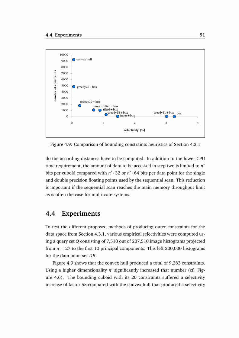
4.4. Experiments 51
boxinner+boxtilted+box
inner+tilted+box
greedy11+boxgreedy15+box
greedy19+box
greedy23+box
convex hull
0
1000
2000
3000
4000
5000
6000
7000
8000
9000
10000
0 1 2 3 4
num
ber o
f con
stra
ints
selectivity [%]
Figure 4.9: Comparison of bounding constraints heuristics of Section 4.3.1
do the according distances have to be computed. In addition to the lower CPU
time requirement, the amount of data to be accessed in step two is limited to n∗
bits per cuboid compared with n′ · 32 or n′ · 64 bits per data point for the single
and double precision floating points used by the sequential scan. This reduction
is important if the sequential scan reaches the main memory throughput limit
as is often the case for multi-core systems.
4.4 Experiments
To test the different proposed methods of producing outer constraints for the
data space from Section 4.3.1, various empirical selectivities were computed us-
ing a query set Q consisting of 7,510 out of 207,510 image histograms projected
from n = 27 to the first 10 principal components. This left 200,000 histograms
for the data point set DB.
Figure 4.9 shows that the convex hull produced a total of 9,263 constraints.
Using a higher dimensionality n′ significantly increased that number (cf. Fig-
ure 4.6). The bounding cuboid with its 20 constraints suffered a selectivity
increase of factor 55 compared with the convex hull that produced a selectivity

52 An Example for Similarity Search Using Simple Distance Measures
0123456789
10
1 2 3 4 5 6 7 8 9 10
avg.
que
ry ti
mes
[ms]
reduced cuboid dimensionality n*
Voronoi X-treeVoronoi Bitmap
Figure 4.10: Comparison of query processing speeds at various reduced dimen-sionalities
of roughly 0.06%. Adding all 20 existing inner polytope planes to the cuboid
helped reduce the increase to factor 24 while the 1,024 tilted planes resulted
in a factor of 15. Using all three approaches together with 1,064 constraints
brought the factor down to 11. Compared with that, the greedy point selec-
tion using 11, 15, 19, and 23 points out of the convex hull vertices shows that
it is a well-suited approach that allows for a very favorable trade-off between
the number of constraints and the resulting selectivity. For all further experi-
ments, the box, the inner polytope, and a number of points selected using the
greedy heuristic were chosen. As the number of constraints influences the time
spent on the preprocessing step, the number of points selected via the greedy
heuristic was limited such that no more than 2,000 constraints resulted for the
experiments.
All run-time experiments were performed using C++ implementations on a
computer with a 2.4GHz Pentium 4 CPU (512 kilobytes of second level cache)
with one gigabyte of 266MHz main memory hosting the respective index struc-
ture and data points for each measurement.
Using the variance-based heuristic from Section 4.3.2 for deciding the order

4.4. Experiments 53
0
2
4
6
8
10
12
14
16
18
20
4 6 8 10 12 14 16
avg.
que
ry ti
mes
[ms]
dimensionality n'
Linear ScanCR-Tree HS95X-Tree HS95Voronoi X-TreeVoronoi Bitmap
Figure 4.11: Query times at varying dimensionality n′ (cardinality m =200,000)
of dropping dimensions, the axis-aligned projection of the Voronoi cell-bounding
cuboids results in a definite advantage when indexing the cuboids in an X-Tree.
With just four out of the ten dimensions, Figure 4.10 shows the overall nearest
neighbor querying speed to double. The Bitvector Index, on the other hand,
hardly benefits from said projection. This can be explained by the relatively
cheap computation of the final bitvector compared with a high computational
cost of both decoding the vector in order to find the relevant data points (where
bits are set to one) and computing their distances to the query point. The decod-
ing phase benefits from a sparsely populated bitvector, which necessitates a low
selectivity in the filtering step of the nearest neighbor search. The lower num-
ber of bit-wise ‘and’ operations that resulted from using only the five dimensions
with the highest variances versus all ten dimensions was roughly compensated
by the two-fold selectivity increase in the former case.
Figures 4.11 and 4.12 show average response times subject to the projected
data dimensionality n′ and the cardinality m of DB. The linear scan is included
as a baseline solution for the nearest neighbor computation. In addition to the
two Voronoi-based indexes explained in Section 4.3.3, memory-resident variant

54 An Example for Similarity Search Using Simple Distance Measures
0
2
4
6
8
10
12
14
16
18
20
50,000 100,000 150,000 200,000
avg.
que
ry ti
mes
[ms]
database cardinality m
Linear ScanCR-Tree HS95X-Tree HS95Voronoi X-TreeVoronoi Bitmap
Figure 4.12: Query times at varying cardinality m (dimensionality n′ = 16)
of the X-Tree [BKK96] and the CR-Tree [KCK01] are included as competing
approaches using conventional nearest neighbor algorithms. The Priority Search
algorithm [HS95] outperformed the Depth-first Traversal algorithm of [RKV95]in all test runs. The latter was thus omitted from the figures. For the 200,000
image histograms of Figure 4.11, all shown indexes outperformed the linear
scan over the whole range of examined dimensionalities. Without exceptions,
the Voronoi-based Bitvector Index has the lowest querying times followed by the
Voronoi-based X-Tree. For the latter, the indexed dimensionality proved optimal
at n∗ = 4 for n′ ∈ [4,12] and n∗ = 3 for the rest.
The same order of comparative querying speeds was observed over the whole
range of evaluated cardinalities m for fixed n′ = 16 as depicted by Figure 4.12.
Here the point-based hierarchical indexes increasingly outperform the linear
scan as the number of data points grows. This is also true for the Voronoi-based
X-Tree. Perhaps surprisingly at first, even the Bitvector Index with a linear time
complexity displays a seemingly sub-linear behavior. While this is not true in the
strict theoretical sense, its slowing increase is explained by the decreasing se-
lectivity that the approximation of the Voronoi cells exhibits with an increasing
number of smaller cells. A linear behavior would be expected once the selectiv-

4.4. Experiments 55
0
200
400
600
800
1,000
1,200
1,400
image data set
avg.
que
ries p
er se
cond
Linear Scan CR-Tree HS95 X-Tree HS95 Voronoi X-Tree Voronoi Bitmap
0
2,000
4,000
6,000
8,000
10,000
12,000
14,000
stocks data set
0200400600800
1,0001,2001,4001,6001,8002,000
phoneme data set
Figure 4.13: Query throughputs per dataset
ity closes in on the ideal value of 1/m at the latest. At n′ = 16 and m= 200, 000
the speedup factor of the bitmap-based Voronoi approach compared with the
next fastest competing approach was over 2.5.
All described indexes and algorithms were evaluated for two more real world
datasets in the final experiment depicted in Figure 4.13. In addition to the
200,000 image histograms (taken from TV screen shots), the same number
of phoneme-based histograms were extracted from 12,374 spoken and tran-
scribed sentences [Wah00]. A sliding extraction window of one second with
a window-to-window overlap of 74% was used to count the occurrences of
27 phonemes. The extraction resulted in approximately 5% non-unique his-
tograms (i.e., windows with identical phoneme counts). Both the image and
the phoneme dataset were projected from n = 27 to n′ = 10 dimensions via
PCA. Lastly, 60,000 ratios comparing the per-minute amount of money spent
on 10 blue chip stocks were calculated from a subset of the data available in
[KF02] and projected to the first six principal components.
In order to visualize the distribution of the resulting histogram vectors in
Figure 4.13, all datasets were projected to their first two respective principal
components. The hierarchical methods were not as efficient for the latter two

56 An Example for Similarity Search Using Simple Distance Measures
datasets, while the Bitvector Index enabled a vastly increased query throughput
for all datasets with a speedup factor in excess of five for the phoneme data.
Acknowledgments
Thanks go to Eammon Keogh and Theodoros Folias for providing access to their
Time Series Data Mining Archive [KF02] at the Computer Science & Engineering
Department, University of California and to Arne Theres for his work on the
phoneme dataset at the Chair of Computer Science 6, RWTH Aachen University.
4.5 Summary
This chapter served as an example of an efficient similarity search system based
on a simple distance measure. The efficiency stems from a combination of
the techniques reviewed in Chapter 3. The employment of Voronoi diagrams
for nearest neighbor search requires special attention regarding the data repre-
sentation space when reducing the dimensionality of the data from n to n′ di-
mensions. Conservative approximations of Voronoi cells ensure that the correct
nearest neighbor for dimensionality n′ is found. A hierarchical and a bitmap-
based index structure enable the fast computation of a candidate set via point-
in-cuboid tests (optionally using a second dimensionality reduction). The near-
est neighbor is found among the candidates in the refinement step by computing
according distances.
The preprocessing step during which the cell approximations are computed
implicitly relies on the Voronoi cells to be of convex shape. This property holds
for the Euclidean distance dL2examined here, but breaks down for other Lp-
based distances and for more complex distance functions such as the Earth
Mover’s Distance examined in Part II of this work. Thus, other techniques for
improving the efficiency of query processing are required (cf. Part III).

Part II
Transformation-Based Distance
Measures
57


Transformation-Based Distance Measures 59
Compared with the simple distance functions discussed so far, transformation-
based distance functions take a different view on defining a distance between
two object representations. Instead of measuring the difference between two
object representations in a bin-by-bin fashion, they identify the commonality
of the representations and assess the amount of work that is required to over-
come the remaining differences through transformation of the object represen-
tations. Transformation-based distances owe their high degree of flexibility and
adaptability to this concept of transformation work. The amount of work that
different transformations induce can be flexibly chosen to suit the application
requirements. A number of transformation-based distance functions have been
proposed in the literature. They are differentiated by the type of data (represen-
tation) that they work with, the type of transformations that they allow, and the
constraints that may be in place for the transformations. Three transformation-
based distance functions that have seen extensive use in similarity search appli-
cations will be reviewed in the following chapters.
The Edit Distance[Lev66] for discrete structures is probably the most well-
known transformation-based distance. It considers the minimum number of
transformation steps (deletions, insertions, and replacements) required to have
one discrete structure match the other. While it will not be of importance for
the rest of this work, a short introduction to the Edit Distance on discrete-valued
sequences will be given in Chapter 5 as it is well-suited to illustrate key concepts
of transformation-based distances.
The Dynamic Time Warping distance[Ita75, SC78] is a continuous cousin to
the Edit Distance. Instead of deleting or replacing discrete values in a sequence,
it effectively replicates existing continuous values and measures the residual dif-
ferences between the two sequences after an optimal set of replication steps. An
introduction to Dynamic Time Warping is given in Chapter 6 with a novel tech-
nique for improving its efficiency in a similarity search context in Chapter 13.
The main part of this work is concerned with the efficiency, effectiveness,
and applicability of a third transformation-based distance function called the
Earth Mover’s Distance [RTG98]. It compares feature distributions of two ob-
jects in the form of either fixed-binning or adaptive-binning histograms. The
details will be introduced in greater depth in Chapter 7.


Chapter 5
The Edit Distance
The Edit Distance[Lev66] is defined by the amount of work that is required
to transform a discrete structure into another. The more work that is required
for the transformation, the greater the value of the Edit Distance. It was first
introduced in [Lev66] for correcting errors in sequences of symbols. Since
then, its concept has been extended to several more complex discrete struc-
tures. For example, [ZWS96] introduced the Edit Distance for acyclic graphs
(i.e., trees) in face of the NP-hard runtime complexity of the Edit Distance on
general graphs [BA83].
This chapter illustrates two core concepts of transformation-based distance
measures using the Edit Distance on character sequences as an example. This
early and well-known transformation-based distance, which is also known as the
Levenshtein Distance, has a variety of applications that range from automatic
spelling correction [OTK76] to analyzing RNA data in the life sciences [XLS08].A variation that is used to compare real-valued time series will be discussed in
Chapter 6.
5.1 Formal Definition
The Edit Distance between two sequences of symbols (i.e., strings) with gen-
eralized transformation costs is recursively defined as the minimum over three
Edit Distances calculated for prefixes of the two sequences.
61
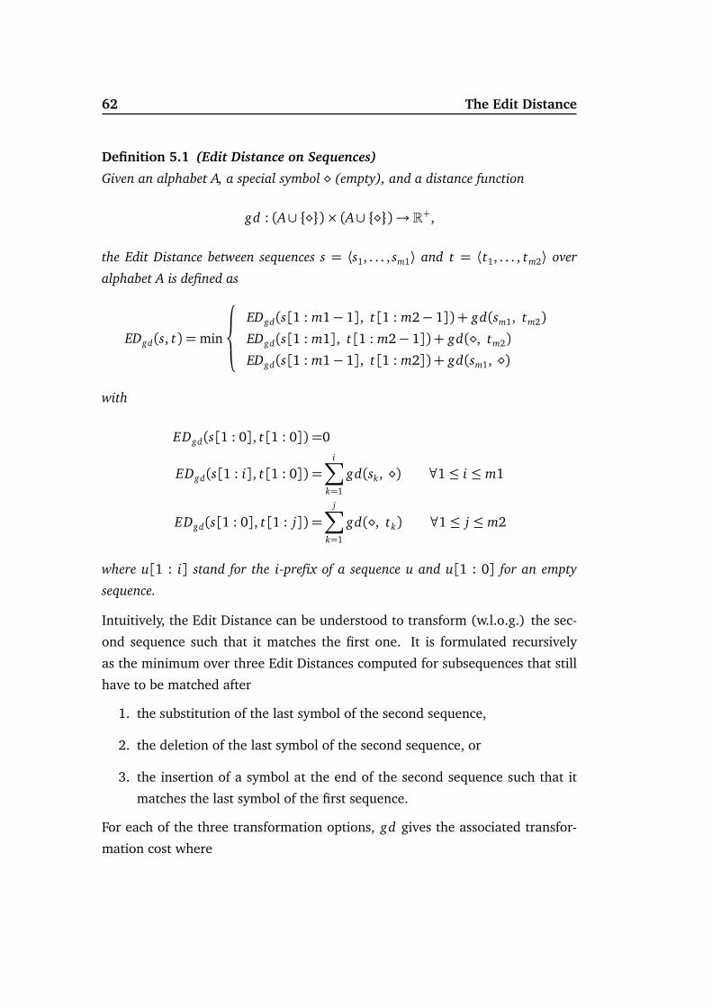
62 The Edit Distance
Definition 5.1 (Edit Distance on Sequences)
Given an alphabet A, a special symbol (empty), and a distance function
gd : (A∪ )× (A∪ )→ R+,
the Edit Distance between sequences s = ⟨s1, . . . , sm1⟩ and t = ⟨t1, . . . , tm2⟩ over
alphabet A is defined as
EDgd(s, t) =min
EDgd(s[1 : m1− 1], t[1 : m2− 1]) + gd(sm1, tm2)EDgd(s[1 : m1], t[1 : m2− 1]) + gd(, tm2)EDgd(s[1 : m1− 1], t[1 : m2]) + gd(sm1, )
with
EDgd(s[1 : 0], t[1 : 0]) =0
EDgd(s[1 : i], t[1 : 0]) =i∑
k=1
gd(sk, ) ∀1≤ i ≤ m1
EDgd(s[1 : 0], t[1 : j]) =j∑
k=1
gd(, tk) ∀1≤ j ≤ m2
where u[1 : i] stand for the i-prefix of a sequence u and u[1 : 0] for an empty
sequence.
Intuitively, the Edit Distance can be understood to transform (w.l.o.g.) the sec-
ond sequence such that it matches the first one. It is formulated recursively
as the minimum over three Edit Distances computed for subsequences that still
have to be matched after
1. the substitution of the last symbol of the second sequence,
2. the deletion of the last symbol of the second sequence, or
3. the insertion of a symbol at the end of the second sequence such that it
matches the last symbol of the first sequence.
For each of the three transformation options, gd gives the associated transfor-
mation cost where

5.2. Illustration of Core Concepts of Transformation-Based Distances 63
1. gd(sm1, tm2) is the cost of a substitution (sm1 instead of tm2),
2. gd(, tm2) the cost of deletion (empty instead of tm2), and
3. gd(sm1, ) the cost of insertion (sm1 instead of empty).
As all three operations result in a shortening of at least one of the sequences, the
transformation process always terminates after a finite number of steps. In the
end, the Edit Distance identifies an optimal set of transformative operations that
results in a match between the two sequences. The value of the Edit Distance is
the sum of the costs of the set of optimal transformative operations.
5.2 Illustration of Core Concepts of Transformation-
Based Distances
As a simple example, the two names Levenshtein and Löwenstein shall be com-
pared using the Edit Distance with constant edit operation costs of 1 for unequal
symbols and 0 for equal symbols. The following table shows how the two names
can be aligned using two substitutions (e for ö and v for w) and one insertion:
L e v e n s h t e i n
m m ⇓L ö w e n s t e i n
This turns out to be an optimal set of transformations and the Edit Distance
equals 3 as the number of required transformative operations. Another set of
transformations is given by the following alignment.
L e v e n s h t e i n
⇓ ⇓ ⇓ ⇓ ⇓ ⇓ ⇓ ⇓ ⇓ ⇓ ⇓ ⇑ ⇑ ⇑ ⇑ ⇑ ⇑ ⇑ ⇑ ⇑ ⇑L ö w e n s t e i n
Here, the second sequence is transformed to match the first one by inserting
all symbols of the first sequence and deleting all symbols in the second se-
quence. The minimum operator of the Edit Distance causes this non-optimal

64 The Edit Distance
Algorithm 5.1: editDistance(s,t,gd)
m1 = length(s); m2 = length(t);1
ED = new Array[m1+1,m2+1]; // one extra dimension for empty string2
ED[1,1] = 0; // edit distance for two empty strings3
// Fill extra row and column (match s, t to empty strings)for i= 2 to m1+1 do ED[i,1] = ED[i-1,1] + gd(s[i-1], );4
for j= 2 to m2+1 do ED[1,j] = ED[1,j-1] + gd(, t[j-1]);5
// Fill ED matrix for subsequences of s and tfor i= 2 to m1+1 do6
for j= 2 to m2+1 do7
ED[i,j] = min(ED[i-1,j-1] + gd(s[i-1],t[j-1]),8
ED[i,j-1] + gd(,t[j-1]),9
ED[i-1,j] + gd(s[i-1],) );10
endfor11
endfor12
return ED[m1+1,m2+1];13
solution with cost 21 to be disregarded. This reflects the first core concept of the
transformation-based distances discussed in this work. Transformation-based
distance measures investigate a potentially great number of feasible transfor-
mations but the final distance value depends on an optimal transformation only.
The optimality criterion is based on the second core concept.
Transformation-based distances make use of a measure of transformation
cost (typically in the form of a second distance function that is called the ground
distance). This allows for great flexibility regarding the modeling of the notion
of similarity that is to be reflected by the distance measure. If, for example,
the Edit Distance is to be used to model phonetic similarity, the substitution
operation for similar-sounding letters such as the labial consonants v and w can
be assigned a smaller ground distance. In that case, Levenshtein is judged to be
closer to Löwenstein than to Lötenstein (since t is an alveolar consonant).
5.3 Computation
The recursive definition of the Edit Distance can directly be transfered to a re-
cursive algorithm for its computation. However, the number of recursive calls is

5.3. Computation 65
in O(3m1+m2). Instead, dynamic programming can be used (cf. Algorithm 5.1)
to compute the Edit Distance in O(m1 ·m2) by avoiding recurring computations
of the Edit Distance for identical subsequences.
After computing the non-recursive cases (first row and first column of array
ED), the algorithm iteratively fills the rest of the array such that ED[i+1, j+1] is
the edit distance for subsequences s[1:i] and t[1:j]. The value of ED[i+1, j+1]is based on the three adjacent entries given by Definition 5.1. The following
table shows the complete array for the earlier example.
L e v e n s h t e i n
0 1 2 3 4 5 6 7 8 9 10 11
L 1 0 1 2 3 4 5 6 7 8 9 10
ö 2 1 1 2 3 4 5 6 7 8 9 10
w 3 2 2 2 3 4 5 6 7 8 9 10
e 4 3 2 3 2 3 4 5 6 7 8 9
n 5 4 3 3 3 2 3 4 5 6 7 8
s 6 5 4 4 4 3 2 3 4 5 6 7
t 7 6 5 5 5 4 3 3 3 4 5 6
e 8 7 6 6 5 5 4 4 4 3 4 5
i 9 8 7 7 6 6 5 5 5 4 3 4
n 10 9 8 8 7 6 6 6 6 5 4 3
The final distance of 3 is stored in ED[m1+ 1, m2+ 1].With the core concepts of transformation-based distances illustrated (the
ground distance as a cost measure for transformative operations and the mini-
mum sum of transformations as the overall distance), the next chapter reviews
a related measure that is used for real-valued sequences and will be the focus of
Chapter 13.


Chapter 6
The Dynamic Time Warping
Distance
6.1 Introduction
Time series arise in many different applications that depend on sequential data
such as sensor data, stocks data, or videos. For example, large amounts of time-
dependent data are created, acquired, and analyzed as a basis for decision and
policy-making on ecological issues.
For the scope of this work, a time series is of the form of a feature sequence
to = ⟨to1, . . . , to
m⟩ where toi describes the features of o at point in time i (cf. Defi-
nition 1.3). The analysis of this data requires a notion of similarity between time
series to determine like patterns. A simple approach for comparing time series
consists of aggregating the differences in values for each point in time (e.g., by
using the Euclidean distance dL2). Comparing univariate time series (i.e., to
i is
scalar) based on Euclidean distance is straightforward. The two time series are
interpreted as vectors and differences between values of corresponding points
in time are squared and summed up.
dTS−L2(s, t) =
s
m∑
i=1
(si − t i)2
67

68 The Dynamic Time Warping Distance
(a) Euclidean distance (b) DTW
Figure 6.1: Comparing two time series with the Euclidean Distance and DTW
The definition can be generalized to multivariate time series where toi is a vector.
dTS−L2(s, t) =
s
m∑
i=1
dL2(si, t i)2
While computationally inexpensive, similarity measures that regard time series
in a point-in-time by point-in-time manner are inadequate for many applica-
tions. A slight shift in the start time or in the length of a relevant pattern can
produce a large distance value and thus a low similarity score. The Dynamic
Time Warping (DTW) concept was introduced in the field of speech recogni-
tion to address the shortcomings that stem from inflexibility along the time axis
[Ita75, SC78] and was transfered to pattern recognition in databases later on
[BC94]. The DTW distance computes an optimal alignment of two time series
by allowing for stretching and squeezing of the time series. In this manner, it
tries to find an assignment of points in time of one time series to points in time
in the other time series such that the two time series are as similar as possible
to each other after an according transformation of the time axis of one of the
time series. DTW then measures the residual difference of the two time series
after optimal transformation.
An example for the simple univariate case with a scalar attribute is given in
Figure 6.1. Two time series are compared using the Euclidean Distance (a) and
DTW (b). The thin lines indicate which values are matched by the respective

6.2. Formal Definition 69
distance functions. The vertical extent of the thin lines indicates the amount of
dissimilarity that is contributed by the matching of points in time for the two
models. The Euclidean distance computes a large dissimilarity value between
the two time series even though they show a very similar pattern shifted along
the time axis. DTW matches the time series such that the pattern is better
aligned by transforming or warping the time axis of both time series. Warping
here means that a point in time of one series may be assigned to a different
point in time of the other time series, as long as the assignment is monotonic
(i.e., if t i is assigned to s j, t i+1 may only be assigned to s j′ with j′ ≥ j).
The improved handling of the time axis and the possibility to base the cost
of assigning t i to s j on a ground distance make the DTW a very flexible distance
measure for sequential data. This in turn led to its adoption and adaptation
for diverse application domains going well beyond the speech recognition for
which DTW was originally envisioned. Examples of application domains include
the alignment of gene expressions [AC01], the registration of the time axis of
image sequences [CLC04], the search for similar 2D shapes [KWX+06], and the
detection of near-duplicate videos [AK09, AKS10].
6.2 Formal Definition
The DTW distance computes the best possible match between two time series
with respect to the overall warping cost given by a ground distance. It is defined
recursively on the length of the sequences.
Definition 6.1 (Dynamic Time Warping)
The Dynamic Time Warping distance between two time series s and t of length m1
and m2 based on a ground distance gd is defined as:
DTWgd(s, t) = gd(sm1, tm2) +min
DTWgd(s[1 : m1− 1], t[1 : m2− 1])DTWgd(s[1 : m1], t[1 : m2− 1])DTWgd(s[1 : m1− 1], t[1 : m2])

70 The Dynamic Time Warping Distance
with
DTWgd(s[1 : 0], t[1 : 0]) =0
DTWgd(s[1 : i], t[1 : 0]) =∞ ∀1≤ i ≤ m1
DTWgd(s[1 : 0], t[1 : j]) =∞ ∀1≤ j ≤ m2
where t[1 : i] stand for the i-prefix of time series t and t[1 : 0] for an empty time
series.
Thus, DTW is defined recursively on the minimal cost of possible matches of
prefixes shorter by one element – much like the Edit Distance. There are three
possibilities:
1. to match the prefixes of both s and t,
2. to match s with the prefix of t, or
3. to match the prefix of s with t.
This definition immediately gives rise to a recursive (but inefficient) algorithm
for computing the DTW that computes the assignment cost gd(sm1, tm2) for the
last elements of both time series, recursively computes the three DTW values
for shorter time series, takes the minimum of all three DTW values, and finally
adds that minimum to the gd value.
Effectively, the transformation that DTW performs consists of the replication
of existing values within the time series. The set of replications that results in
the smallest residual difference defines the distance value.
For long time series, infinite warping is typically not desirable. To avoid de-
generated matchings where many values of one time series are assigned to very
few values of the other one, warping is often restricted via global constraints
termed bands. A band describes how much warping is allowed (i.e., how far
apart any two assigned points in time can be with respect to the time axis).
To disallow a transformation that would leave the feasible band, the ground
distance is changed to infinity.

6.3. Computation 71
Definition 6.2 (k-band Dynamic Time Warping)
The Dynamic Time Warping distance between two time series s and t of length
m1 and m2 (w.l.o.g. m1 ≤ m2) based on a ground distance gd with respect to a
bandwidth k is defined as:
DTWgd,bandk(s, t) =gdbandk
(sm1, tm2)
+min
DTWgd,bandk(s[1 : m1− 1], t[1 : m2− 1])
DTWgd,bandk(s[1 : m1], t[1 : m2− 1])
DTWgd,bandk(s[1 : m1− 1], t[1 : m2])
with
gdbandk(si, t j) =
(
gd(si, t j) if |i−
j·m1m2
£
| ≤ k
∞ otherwise
and
DTWgd,bandk(s[1 : 0], t[1 : 0]) =0
DTWgd,bandk(s[1 : i], t[1 : 0]) =∞ ∀1≤ i ≤ m1
DTWgd,bandk(s[1 : 0], t[1 : j]) =∞ ∀1≤ j ≤ m2.
In this definition, the time warping is restricted to a band of width k in the
time dimension by setting the cost of all overstretched assignments to infinity.
The band corresponds to a so-called Sakoe-Chiba band [SC78] where the band-
width is fixed over the whole time series. Another frequently used band [Ita75]allows less warping at the beginning and at the end of the time series.
6.3 Computation
The DTW distance can be computed in O(m1 ·m2) time via dynamic program-
ming analogous to the computation of the edit distance. Instead of computing
all possible alignments, the recursive definition of DTW is used to fill a cumu-
lative distance matrix. An entry at position (i, j) of the matrix corresponds to
the best alignment between the prefixes s[1 : i] and t[1 : j] of the time series.
Using a k-band, the complexity is reduced to O(k ∗maxm1, m2).

72 The Dynamic Time Warping Distance
si
tj
= gd(si , tj) + min( )
Figure 6.2: Cumulative distance matrix
The computation of the matrix entries is illustrated in Figure 6.2, where two
time series are depicted to the left (rotated) and at the top of the figure. The
optimal assignment of points in time is illustrated by the black line in the matrix.
The horizontal segment at the lower left indicates that the first six points in time
of the time series at the top are assigned to the first point in time of the time
series at the left. With the gray matrix entries representing the band of the
DTW, the black path is invalid while the green path is valid. The DTW finds the
optimal path from the bottom left to the top right of the matrix using only gray
entries. The cumulative distance matrix D is filled analogously to the formula
in Definition 6.2.
Definition 6.3 (Cumulative Distance Matrix)
The cumulative distance matrix D ∈ Rm1×m2 for two time series s and t of length
m1 and m2 is calculated as
D[i, j] = gd(si, t j) +minD[i− 1, j− 1] , D[i, j− 1] , D[i− 1, j]
with
D[1, 1] =gd(s1, t1)
D[i, 1] =gd(si, t1) + D[i− 1,1] ∀1< i ≤ m1
D[1, j] =gd(s1, t j) + D[1, j− 1] ∀1< j ≤ m2.

6.3. Computation 73
The best matching for two time series is recursively obtained from the match-
ings that are possible for the time series shorter by one. This means that the en-
try D[i, j] is computed from its three adjacent entries D[i−1, j−1], D[i−1, j],and D[i, j− 1] to its bottom left (cf. Figure 6.2).
The calculation of entries D[i, j] proceeds column-wise. Starting with the
entry at the bottom left (i.e., matrix D[1,1] – the matrix is vertically mirrored
in Figure 6.2 for illustrative reasons), the entries within the band of each col-
umn are calculated before continuing with the next column to the right. Global
warping path constraint are expressed by setting the matrix entries that are not
within the band to infinity. The DTW distance is the value of entry D[m1, m2]in the top right corner. It corresponds to a matching called the warping path.
From the cumulative distance matrix, the warping path that corresponds to the
minimal matching can easily be constructed as a sequence of matrix cells that
correspond to a series of minima that connect the beginnings and ends of the
two time series.


Chapter 7
The Earth Mover’s Distance
Both the Edit Distance and DTW are based on the existence of some form of
structure in the feature representation. In particular, the Edit Distance for se-
quences and the DTW distance rely on an inherent total order that allows for a
meaningful definition of a prefix for their recursive formulation of the optimiza-
tion over feasible transformations. The transformation-based distance focused
on in this chapter does not require any order for the object features. Instead, it
is based on a form of feature representation that includes the adaptive-binning
histograms from Section 1.1. Its intuition, application, formal definition, com-
putation, and relevant related work are discussed in this chapter with novel
techniques that address its efficiency, effectiveness, and applicability being af-
forded their own chapters in parts III to V.
7.1 Introduction
The Earth Mover’s Distance (EMD) was first introduced in the field of Computer
Vision by Rubner et al. [RTG98, RTG00, RT01] with the intention of assessing
the similarity between digital images based on low-level features such as color,
texture, and position. It transfers the Monge-Kantorovich mass translocation
problem [Mon81, Kan42] to the realm of similarity search by defining a dis-
tance measure on the feature representation level (e.g., color histograms) via
an optimization-based transformation process. The optimization is formulated
75

76 The Earth Mover’s Distance
012345678910
0 1 2 3 4 5 6 7 8 9 10
2/72/7
2/71/7
(a) 1st histogram (hills)
012345678910
0 1 2 3 4 5 6 7 8 9 10
1/7
2/72/7
2/7
(b) 2nd histogram (valleys)
Figure 7.1: Two examplary adaptive-binning histograms to be compared viaEMD
Figure 7.2: EMD: moving earth from hills to valleys
such that it explicitly takes a notion of similarity in the feature space (e.g., color
space) into account. In this way the EMD breaks with the assumption of per-
ceptual independence regarding the bins of feature histograms, which distance
measures that treat histogram bins in a bin-by-bin fashion are forced to make.
An image with a large proportion of pixels falling into the emerald green bin can
thus be identified to be more similar to an image with an according portion of
kelly green pixels that may have resulted from a slight change in lighting than
to an image with largely purple pixels.
The name of the Earth Mover’s Distance stems from the intuition behind
its transformation process: Given two feature representations in the form of

7.1. Introduction 77
Figure 7.3: Movement or flow of earth from hills to valleys
adaptive-binning histograms, one is treated as a collection of hills where the
amount of earth that comprises a hill is given by the feature frequency or bin
weight and the position of the hill is given by the coordinates of the feature rep-
resentative in the feature space. For the second histogram, the weights define
the depth of corresponding valleys. Figures 7.1 and 7.2 illustrate the concept for
an abstract two-dimensional feature space where the two histograms each have
four components with distinct representatives (illustrated by the position of the
discs in the two-dimensional space) and varying weights (illustrated by the size
of the discs in Figure 7.1 and the height/depth of hills/valleys in Figure 7.2).
The Earth Mover’s Distance is defined as the least-cost cut-and-fill earth trans-
formation that levels the ground. The cost of moving a unit of earth from a hill
to a valley is given by a ground distance measure in the feature space. The more
similar the representative that defines the position of a hill is to the represen-
tative that defines the position of a valley, the less expensive is the according
displacement of earth.
Figure 7.3 shows an example of an EMD computation in a similarity search
setting. For the two images in the top left and top right, adaptive-binning his-
tograms with 20 components were determined via a kmeans clustering of pixels
in a 5-dimensional spatio-spectral feature space (depicted in the bottom left and
bottom right). An optimal transformation is depicted in the middle of the figure.
In its most general definition, the EMD is not restricted to adaptive-binning
histograms that share a common total weight of 1.0 but can handle object fea-
ture representations with differing total weights (termed signatures in the con-

78 The Earth Mover’s Distance
text of the EMD; cf. Definition 7.1). In that case it performs a partial matching
of the earth. If the target signature that defines the valleys in the above example
has a lower total weight than the source signature, the EMD finds the transfor-
mation that fills all valleys at lowest possible cost. The excess earth remains at
its original position. If the source signature has a lower weight than the target
signature, a transformation is found that moves all the earth from the positions
of the hills to the valleys. Some valleys will not be filled completely.
A number of variants of the EMD have been proposed in the literature. To
give an overview on how the concept of the EMD can be adapted to suit differ-
ing requirements, a number of them shall briefly be mentioned here; they will
not play a role in the rest of this work. In [RT01], a variant called the Partial
EMD is introduced together with the Restricted EMD. The former only requires
a percentage γ of the signature with the smaller total weight to be matched,
which makes it more robust against outliers and missing data. The latter re-
stricts the distance that earth can be moved from any of the hills and measures
the percentage of earth that has to remain at its original position under said
restriction. A similar idea is followed by the Local EMD [Sri04], where earth
may only be moved within a local window around the hills. This restriction can
make sense from a perceptual point of view for some applications and can sim-
plify the underlying optimization problem. Unlike Restricted EMD, Local EMD
measures the cost of transformation. However, it is not guaranteed that a fea-
sible solution exists in this setting. As a last example for variants of the EMD,
the Proportional Transportation Distance [GV02] modifies the EMD such that
it obeys the triangular inequality for signatures with unequal total weights. It
handles that case by proportionally rescaling the weights of the lighter signature
to match the total weight of the heavier signature. In the case of equal-weight
signatures (and thus histograms), it is identical to the EMD.
The EMD itself can also be considered a variant of another distance measure.
In [LB01] it is noted that the EMD on signatures with equal weight and with
a ground distance derived from an Lp-norm is a special case of the Mallows
distance (or Wasserstein distance) from probability theory, which is defined on
continuous probability distributions.
7.2. Applications 79
7.2 Applications
As the signatures that the EMD takes as its input are of a very flexible nature
and comprise both fixed and adaptive-binning histograms and as the ground
distance measure in the feature space can be freely chosen, the EMD can readily
be adapted to suit a great number of applications. Its relevance to solving real
world problems is backed by its successful deployment in fields as diverse as
musicology and phishing detection. This section reviews recent applications of
the EMD with a focus on medical applications and a brief overview of other
application domains.
In the medical field, [DMHE+06] uses the EMD to distinguish personal char-
acteristics from common search patterns in a study on cognitive processes asso-
ciated with visual search. [LOEA+07] employs the EMD to quantify patterns of
cortical behavior associated with surgical expertise based on data derived from
multidimensional functional Near Infrared Spectroscopy. Based on CT scans,
the EMD is employed to measure the severity of emphysema in [MRM+05]and the progression of advanced cancers in [NC08]. In [EMLB08], parame-
ters of a computational model on chemotaxis-based cell aggregation are itera-
tively fine-tuned by comparing the results to in vitro experiments using the EMD.
[HNZ+08] proposes the use of the EMD to measure discrepancies between sim-
ulated and estimated dipole amplitudes for EEG/MEG source reconstruction as
it “provides a meaningful measure for arbitrary types of source distributions.”
Among many other medical applications, the EMD has also been found to be
an effective distance measure for medical image registration [CB07] and for
clinical decision-making based on gastroscopic images [WT09], optical coher-
ence tomography [SL09], and multidetector CT [ZBR07]. Evaluating MRI data
in breast cancer research, [STN+05] notes that “compared [to] the euclidean
distance a considerably improved classification accuracy could be observed” by
using the EMD.
Beyond the medical applications just described and the many applications
in the computer vision domain for which it was originally devised (e.g., im-
age retrieval [RTG00, IT03], video retrieval [UHMS06, AKS10], face recog-
nition [LWT05], and image denoising [Kac10]), the EMD has been success-

80 The Earth Mover’s Distance
fully used in many more applications. In [TGV+03, TVW04], notated music is
grouped according to melody and authors of anonymous pieces are identified
using the EMD. In [LBH98], the EMD is used to compare vector fields that are
useful for the modeling of computational and experimental flow fields in physics
and engineering. In the field of IT security, the EMD has been used to help iden-
tify phishing sites that imitate websites of e-commerce companies in order to
gain access to authentication credentials of unsuspecting users [FWD06].
While far from constituting a complete list of applications, the diversity of
the aforementioned applications are a good indication of the flexibility and ef-
fectiveness of the EMD as a measure of similarity. In their empirical study, the
authors of [PBRT99] conclude that “EMD is especially attractive since it allows
superior classification and retrieval performance with a much more compact
representation.”
7.3 Formal Definition
The feature signatures that the EMD takes as its input are generalizations of
adaptive-binning histograms (cf. Definition 1.2 on page 11).
Definition 7.1 (Feature Signature)
Given a feature space FS and an object o, a feature signature for o is a set
so =¦
(ro1 , wo
1), . . . , (ron , wo
n)©
of tuples from FS×R+ with feature weights woj and feature representatives ro
j .
Notation: Where clear from context, o is used instead of so and |so|Σ =∑n
i=1 woi .
Compared with the adaptive-binning histograms, the only assumption that is
made for the feature weights is their non-negativeness. This allows the EMD to
perform partial matching. However, much of the remainder of this work will
use signatures with a total weight of 1.0.
The EMD itself is defined as a linear optimization problem where linear con-
straints describe the set of feasible combinations of transformations. The ob-
jective function to be optimized is the total cost of transformation. That is, the

7.3. Formal Definition 81
EMD determines a feasible combination of transformations such that the total
cost of transformation is minimized.
Definition 7.2 (Earth Mover’s Distance)
Given two signatures sq, so and a ground distance gd, the Earth Mover’s Distance
between sq and so is defined as a minimum over feasible transformations F ∈R|sq|×|so|:
EMDgd(sq, so) =min
F
(
1
ew
∑
i
∑
j
F[i, j] · gd(rqi, ro
j)
Constraints
)
with
ew =min
|sq|Σ , |so|Σ
where
Constraints ≡ CNNeg ∧ CSource ∧ CTarget ∧ CWeight
defines the feasible transformations with
CNNeg≡ ∀i, j : F[i, j]≥ 0
CSource≡ ∀i :∑
j F[i, j]≤ wqi
CTarget≡ ∀ j :∑
i F[i, j]≤ woj
CWeight≡∑
i
∑
j F[i, j] = ew
In the literature, the optimization variable F is referred to as a flow matrix where
an entry F[i, j] stands for the flow of earth or mass from the ith hill to the jth
valley. The optimal solution consists of a combination of flows that conforms
with all constraints and minimizes the overall cost.
The four subsets of constraints define what constitutes a feasible flow in
agreement with the intuition of the cut-and-fill process. CNNeg forces all flows
to be non-negative as earth is to be translocated from hills to valleys only. A neg-
ative value would constitute a flow of “negative earth” or a flow from a valley
to a hill as depicted in Figure 7.4(a) where hills are shown in magenta and val-
leys in blue. CSource and CTarget require that in total no more earth is moved
from a hill than is available from that hill and that no more earth is moved to

82 The Earth Mover’s Distance
-2/7
1/7
1/7
2/7
2/7
2/7
2/7
2/7
2/7
(a) Violation of CNNeg
1/7
1/7
1/7
1/7
1/7
2/7
2/7
2/7
2/7
2/7
2/7
(b) Violation of CSource
2/7 2/7
1/7
1/7
2/7
2/7
2/7
2/7
2/7
2/7
(c) Violation of CTarget
1/7
1/7
2/7
2/7
2/7
2/7
2/7
2/7
(d) Violation of CWeight
2/7
2/7
1/7
1/7
1/7
1/7
1/7
2/7
2/7
2/7
2/7
2/7
2/7
(e) Non-optimal transformation cost
1/7
1/7
2/7
1/7
1/7
1/7
1/7
1/7
2/7
2/7
2/7
2/7
2/7
2/7
(f) Optimal transformation cost
Figure 7.4: Movement or flow of earth from hills (magenta) to valleys (blue)

7.3. Formal Definition 83
a valley than the valley can hold. Assuming that the larger hills/valleys have
a height/depth of 2/7, the flows depicted in figures 7.4(b) and 7.4(c) are in
violation of the according constraints. The last constraint CWeight ensures that
the signature of lower weight is moved completely. Without the last constraint,
the trivial solution of F[i, j] = 0 depicted in Figure 7.4(d) minimizes the ob-
jective function. Figures 7.4(e) and 7.4(f) show transformations that conform
to all constraints. Assuming the Euclidean distance as the ground distance, the
former is not optimal and thus dismissed by the EMD. The total cost of transfor-
mation is
1/7 ·p
50+ 1/7 ·p
10+ 1/7 ·p
45+ 2/7 ·p
4+ 2/7 ·p
2= 3.4.
For the optimal case, the total cost of transformation is
1/7 ·p
8+ 1/7 ·p
2+ 2/7 ·p
10+ 1/7 ·p
16+ 1/7 ·p
4+ 1/7 ·p
17= 2.9.
In the case of adaptive-binning histograms with a total weight of 1.0, the
formulation of the EMD can be simplified.
Definition 7.3 (Earth Mover’s Distance on Adaptive-Binning Histograms)
Given two adaptive-binning histograms sq, so and a ground distance gd, the Earth
Mover’s Distance between sq and so is defined as a minimum over feasible transfor-
mations F ∈ R|sq|×|so|:
EMDgd(sq, so) =min
F
(
∑
i
∑
j
F[i, j] · gd(rqi, ro
j)
Constraints
)
where
Constraints ≡ CNNeg ∧ CSource ∧ CTarget
defines the feasible transformations with
CNNeg≡ ∀i, j : F[i, j]≥ 0
CSource≡ ∀i :∑
j F[i, j] = wqi
CTarget≡ ∀ j :∑
i F[i, j] = woj
84 The Earth Mover’s Distance
By changing CSource and CTarget to equality constraints, it is ensured that all
hills are cut completely and that all valleys are filled completely. In addition,
the normalization factor 1/ew is not required anymore.
The Earth Mover’s Distance can also be defined for fixed-binning histograms.
In that case, the ground distance only has to be defined partially as all query
objects and all database objects share the same histogram bins. The partial
ground distance is typically represented by a square cost matrix C .
Definition 7.4 (Earth Mover’s Distance on Fixed-Binning Histograms)
Given two n-dimensional fixed-binning histograms hq, ho and a transformation
cost matrix C ∈ Rn×n, the Earth Mover’s Distance between hq and ho is defined as
a minimum over feasible transformations F ∈ Rn×n:
EMDC(hq, ho) =min
F
(
∑
i
∑
j
F[i, j] · C[i, j]
Constraints
)
where
Constraints ≡ CNNeg ∧ CSource ∧ CTarget
defines the feasible transformations with
CNNeg≡ ∀i, j : F[i, j]≥ 0
CSource≡ ∀i :∑
j F[i, j] = hq[i]
CTarget≡ ∀ j :∑
i F[i, j] = ho[ j]
Analogously to the feature signature case, vectors of differing total weight
can be compared by introducing an otherwise redundant constraint CWeight,
changing CSource and CTarget to inequalities, and normalizing the sum by ew.
7.4 Computation
Since the EMD is formulated as a linear optimization problem, the same algo-
rithms from the literature that were used to compute Voronoi cell approxima-
tions in Chapter 4 can be used to compute the EMD. The formulation allows for

7.4. Computation 85
a stream-lined simplex algorithm known as the MoDi method or u-v method to
be used [HL04]. The outline of the algorithm is as follows:
1. It finds a feasible solution (i.e., an initial F that satisfies all constraints)
using for example the North-West corner rule or a more sophisticated
techniques such as Vogel’s or Russell’s approximation method described
in [HL04].
2. It finds the flow F[i, j] = 0 that is not part of the current solution and
has the greatest potential for a cost reduction by being included in the
solution.
3. If there is no variable with potential for a cost reduction, the solution is
optimal and the algorithm terminates.
4. Otherwise, starting at F[i, j], it finds a closed loop of flows that are part
of the current solution. Each flow of the loop has to either come from the
same source/hill or go to the same destination/valley as the last one.
5. Starting at F[i, j], it adds φ to every other element of the loop and sub-
tracts it from the remaining elements. The value φ is chosen such that
one element of the loop is reduced to zero.
6. The algorithm returns to step 2.
The analysis of the run-time complexity of the transportation simplex is non-
trivial. The simplex algorithm that it is based on is known to have an expo-
nential worst-case complexity on some inputs. However, [ST01] states that
“polynomial complexity [is] observed in practice” and that “there has been no
satisfactory theoretical explanation of its excellent performance.” Rubner et al.
note accordingly in [RTG00] that compared with the exponential worst-case
complexity of the simplex algorithm “in practice, because of the special struc-
ture in our case and the good initial solution, the performance [of the EMD] is
much better.” The authors of [SJ08a] note an “empirical time complexity” be-
tween O(n3) and O(n4). Experiments in later chapters were performed using an
adaptation of the EMD algorithm by Rubner that implements the stream-lined

86 The Earth Mover’s Distance
transportation-simplex algorithm and Russell’s approximation method. The al-
gorithm is in Ω(|sq| · |so|) since it has to perform at least one optimality test.
If the Manhattan Distance dL1is used as the ground distance and signature
representatives are fixed to a small grid, the run-time can be improved using the
tree-based technique from [LO07]. Alternatively, the transportation problem
can also be phrased as a minimum-cost network flow problem with |sq| sources,
|so| sinks, and |sq|·|so| edges. This formulation of the EMD can result in improved
runtime performance if the ground distance is limited to a set maximum value
since this property allows for a reduction of edges in the flow problem [PW09].
7.5 Approximations of the EMD
7.5.1 Lower Bounds
As discussed in Section 3.1, lower bounds to a distance measure can be utilized
to speed up similarity search query processing. A number of lower bounds to
the EMD have been proposed in the literature and shall be reviewed here. The
proofs can be found in the according publications.
Centroid-Based Lower Bound
A versatile lower bound for the EMD on adaptive-binning histograms with a
norm-based ground distance was introduced by Rubner et al. in [RTG98].
Theorem 7.1 (Centroid Lower Bound for the EMD)
For a norm-based ground distance gd, the EMD between two adaptive binning
histograms sq =¦
(rq1 , wq
1), . . . , (rqn1, wq
n1)©
and so =¦
(ro1 , wo
1), . . . , (ron2, wo
n2)©
is
lower-bounded by the ground distance between the weighted centroids of the his-
togram representatives.
LBRubner(sq, so) = gd(
n1∑
i=1
wqi · r
qi ,
n2∑
i=1
woi · r
oi )≤ EM Dgd(s
q, so)
The lower bound is easy to compute and typically achieves relatively good ap-
proximation quality. For fixed-binning histograms, the partial ground distance
7.5. Approximations of the EMD 87
information encoded in the transformation cost matrix C does not suffice to
apply Rubner’s approximation since the weighted centroids and the ground dis-
tance between these centroids need to be defined. Thus, it is required to have
access to a fully-defined ground distance gd and feature space partition repre-
sentatives ri, ..., rn with C[i, j] = gd(ri, r j) to apply LBRubner on fixed-binning
histograms.
Projection-Based Lower Bounds
When using dL1as a ground distance for the EMD, a projection-based lower
bound of the EMD can be applied. The idea is to project the representatives
of the signatures to a line through the origin and compute the EMD for the
projected signatures. A number of projection-based lower bounds are given in
[CG97]. Projections onto the feature space axes result in the following bound.
Theorem 7.2 (Projection-based Lower Bound for EM DdL1)
EM DdL1is lower-bounded by a sum of EMD computation in projections of the m-
dimensional feature space:
LBPro jec t ion−L1(sq, so) =
m∑
i=1
EM DdL1(sq[i], so[i])≤ EM DdL1
(sq, so)
where sq[i] and so[i] designate projected signatures where all representatives of
signatures sq and so are reduced to their ithdimension (combining signature com-
ponents with common projected representatives).
Instead of computing the EMD for an m-dimensional feature space, m 1-dimen-
sional EMD computations are performed. In a 1-dimensional space, EM DdL1
can be solved in linear time, as it is equivalent to the Manhattan distance on
cumulative histograms. [CG97] includes a similar lower bound for gd= dL2.
Lp-Based Lower Bounds
In [AWS06], Assent et al. present three lower bounds to the EMD for fixed-
binning histograms. All three bounds are based on weighted Lp distances and

88 The Earth Mover’s Distance
thus have a runtime complexity that is linear in the number of histogram di-
mensions.
Theorem 7.3 (Weighted L1 Lower Bound for the EMD)
For a transformation cost matrix C based on a metric ground distance, the weighted
Manhattan distance LBL1with weights wi =min j 6=iC[i, j]/2 is a lower bound to
EM DC on fixed-binning histograms.
LBL1(hq, ho) =
∑
i
wi|hq[i]− ho[i]| ≤ EM DC(hq, ho)
Theorem 7.4 (Weighted L2 Lower Bound for the EMD)
For a transformation cost matrix C based on a metric ground distance, the weighted
Euclidean distance with weights wi = (min j 6=iC[i, j]/2)2 is a lower bound to
EM DC on fixed-binning histograms.
LBL2(hq, ho) =
r
∑
i
wi(hq[i]− ho[i])2 ≤ EM DC(hq, ho)
Theorem 7.5 (Weighted L∞ Lower Bound for the EMD)
For a transformation cost matrix C based on a metric ground distance, the weighted
maximum distance with weights wi = min j 6=iC[i, j] is a lower bound to EM DC
on fixed-binning histograms.
LBL∞(hq, ho) =max
iwi|hq[i]− ho[i]| ≤ EM DC(h
q, ho)
It is shown in [AWS06] that LBL2(hq, ho)≤ LBL1
(hq, ho). The authors’ evaluation
indicates that the L1 bound outperforms the L∞ bound regarding its selectivity
in a multi-step query-and-refine setup. However, Rubner’s lower bound comes
out ahead of the Lp-based lower bounds in the majority of experiments.
Constraint Relaxation-Based Lower Bound
In addition to the Lp-based bounds, [AWS06] also proposes a lower bound based
on constraint relaxation, which builds on a minimum of any set being no larger
than the minimum of any of its subsets. In the case of the EMD, a superset of

7.5. Approximations of the EMD 89
feasible flow matrices F is constructed by relaxing one of the constraints.
Definition 7.5 (Independent Minimization distance LBI M)
Given two n-dimensional fixed-binning histograms hq, ho and a transformation cost
matrix C ∈ Rn×n, the LBI M distance between hq and ho is defined as a minimum
over feasible transformations F ∈ Rn×n:
LBI M(hq, ho) =min
F
(
∑
i
∑
j
F[i, j] · C[i, j]
ConsI M
)
where
ConsI M ≡ CNNeg ∧ CSource ∧ CTargetI M
defines the feasible transformations with CNNeg, CSource as in Definition 7.4 and
CTargetI M ≡ ∀i, j : F[i, j]≤ ho[ j].
Theorem 7.6 (LBI M is a lower bound to the EMD)
The Independent Minimization distance is a lower bound to EM DC on fixed-binning
histograms.
LBI M(hq, ho)≤ EM DC(h
q, ho)
In the relaxed optimization problem, the only restriction for the target histogram
is that no movement of earth from a single hill may exceed the capacity of a
valley. As a result, the optimization can be decomposed into n smaller optimiza-
tion problems – one for each hill. After an off-line sorting of the rows of C , each
optimization problem can be solved in linear worst-case time complexity. Ex-
periments in [AWS06] show that LBI M has very good approximation qualities.
The concept can also be generalized to adaptive-binning histograms, where
the smaller optimizations have to be solved on-line, leading to a runtime com-
plexity of O(n2 log n). For feature signatures of unequal total weight, a global
sorting of transformation costs is required.
Dimensionality Reduction-Based Lower Bound
Chapter 8 discusses lower bounds based on dimensionality reduction in detail.

90 The Earth Mover’s Distance
A Result on Rubner’s Centroid-Based Lower Bound
When considering Rubner’s Averaging Bound on n-dimensional fixed-binning
histograms together with a Euclidean ground distance between fixed feature
space partition representatives pi ∈ Rm, the following equations hold for P =[p1
T ; . . . ; pnT]T ∈ Rn×m as a matrix with pi as its rows:
LBRubner(hq, ho) = dL2
n∑
i=1
hq[i] · pi,n∑
i=1
ho[i] · pi
!
= dL2(hqP, hoP)
=p
(hqP − hoP)(hqP − hoP)T
=p
(hq − ho)PPT (hq − ho)T
= dQFPPT(hq, ho)
Thus, Rubner’s lower bound turns out to be a quadratic form distance in this
case. In fact, it is an optimal lower-bounding quadratic form distance for the
EMD as the n-dimensional ellipsoid of the quadratic form iso-distance surface
touches all n(n− 1) vertices of the polytope that describes the EMD on fixed-
binning histograms (cf. Chapter 10).
7.5.2 Non-Lower-Bounding Approximations
While approximations of the EMD that are not guaranteed to be lower (or up-
per) bounds cannot be used in a multi-step filter-and-refine setup without sacri-
ficing the completeness of the result, they can be used as measures of similarity
in their own right. Approximations of the EMD have been proposed for instance
in [SJ08a], where a metric on wavelet coefficients of a low-dimensional dif-
ference histogram is shown to approximate the EMD within loose theoretical
and good practical bounds. Based on an approximation technique proposed
in [IT03], an approximate grid-based L1-embedding of the EMD is used in
[GD04] to match two-dimensional shapes represented by point clouds. Non-
lower-bounding approximations will not surface in the remainder of this work
as the focus here is on similarity models that are based on the exact EMD.
Part III
Fast Searching with the Earth
Mover’s Distance
91


Fast Searching with the Earth Mover’s Distance 93
After reviewing relevant concepts of distance-based similarity search in Part I
and of transformation-based distance measures in Part II, the following chapters
present original research [WAKS08, AWMS08] on two techniques for improving
the efficiency of similarity search query processing for the EMD on fixed-binning
histograms.
Chapter 8 describes a technique that takes characteristics of the EMD into
account when performing dimensionality reduction on fixed-binning feature his-
tograms. After showing how suitable reductions can be found in a preprocess-
ing step by analyzing the database and/or the EMD and its ground distance, the
reduced EMD is utilized as a lower-bounding filter in a filter-and-refine frame-
work.
Chapter 9 defines the MinDist for the EMD, which allows for indexing the
EMD in both hierarchical and sequential structures that are based on (mini-
mum) bounding rectangles.
The empirical evaluation of both techniques shows that they are capable of
significantly improving the efficiency of the querying process.


Chapter 8
Efficient Search Via Flexible
Dimensionality Reduction
The EMD has been successfully adopted in a multitude of applications with
low to medium dimensionality. However, multimedia applications commonly
exhibit high-dimensional feature representations for which the computational
complexity of the EMD hinders its adoption. An efficient query processing ap-
proach that mitigates and overcomes this effect is crucial. This chapter proposes
dimensionality reduction techniques for the EMD on fixed-binning histograms
in a filter-and-refine architecture for efficient and lossless similarity search. An
experimental evaluation on real world datasets demonstrates a substantial re-
duction of the number of expensive high-dimensional EMD computations and
thus remarkably faster response times. The techniques are fully flexible in the
number of reduced dimensions, which is a novel feature in approximation tech-
niques for the EMD.
8.1 Introduction
The EMD is defined as the minimal amount of work required to change one
feature representation into another. To compute the EMD, a linear optimization
problem has to be solved. This can be achieved using the simplex algorithm
for transportation problems[HL04] as seen in Chapter 7. While the exponen-
95

96 Efficient Search Via Flexible Dimensionality Reduction
tial worst-case complexity is rarely observed in practice, the computation of the
EMD is at least quadratic in the feature dimensionality. This is clearly infeasible
for high-dimensional feature representations common in multimedia applica-
tions. For EMD-based similarity search in this setting, efficient query processing
is crucial. Existing multi-step approaches rely on specialized lower-bounding
filter functions [RTG98, LBS06, AWS06]. These filters are employed to derive
a set of candidates, which are refined using the Earth Mover’s Distance. All of
these filter approaches improve the query efficiency without loss of effective-
ness but their design is inflexible in the input dimensionality. The approaches
in [RTG98] and [AWS06] devise filter distance functions that are limited by
the dimensionality of the underlying features space (e.g., 3 for a 3-dimensional
color space) or by the dimensionality of the feature representation space (e.g.,
64 for 64-dimensional histograms). The filter proposed in [LBS06] only allows
for limited flexibility regarding the reduced dimensionality in fixed hierarchical
steps of factor 4 and is limited to its grid-based image tiling application domain.
Neither of these filtering approaches makes use of information regarding the
database at hand.
A different approach for fast EMD retrieval consists of deriving distance func-
tions that serve as approximations of the EMD. Examples of such approxima-
tions include [IT03, GD04]where the EMD is embedded into a high-dimensional
L1 space with an upper bound for the distortion and [SJ08b] where the EMD
is approximated by a sum over wavelet coefficients of the difference histogram.
These approaches allow for efficient approximate similarity search but do not
guarantee completeness of the retrieval process according to the EMD.
Dimensionality reduction allows for efficiency improvement by means of
EMD alone and offers flexibility through choice of the target dimensionality. By
reducing the size of the feature representations of the Earth Mover’s Distance,
the run-time of the adapted linear program is lowered substantially. For smaller
linear programs, average solution times are much lower than for the original
problem as the complexity is clearly super-linear. To ensure that dimensionality
reduction is a complete filter in the filter-and-refine architecture, the reduced
EMD must be a lower bound to the original EMD [KSF+96, SK98].
Techniques for dimensionality reduction of the Earth Mover’s Distance that

8.2. Dimensionality Reduction for the EMD 97
significantly improve the efficiency of query processing on fixed-binning his-
tograms are proposed in this chapter. The reduction of the EMD is formalized
in Section 8.2.1 with proofs for the completeness of the approach and for the
optimality of the presented reduced cost matrix in Section 8.2.2. The key to
efficient retrieval is then to determine appropriate reductions. A flexible data-
independent reduction as a generalization of [LBS06] and a data-dependent
method – which incorporates an analysis of EMD transformations – are devel-
oped in sections 8.2.3 and 8.2.4. In a filter-and-refine architecture, the EMD
at a reduced dimensionality is used in the filter step. The resulting set of can-
didates is refined using the EMD at the original dimensionality as detailed in
Section 8.3. The experimental section 8.4 shows that the proposed approaches
improve the query efficiency by producing fewer candidates for the computa-
tionally expensive refinement step.
Advantages of the proposed reduction techniques include the reduced com-
putational complexity (efficiency), the arbitrary number of reduced dimensions
(flexibility), the possibility of combining them with other EMD lower bounds
(chaining) and the absence of false dismissals (completeness).
8.2 Dimensionality Reduction for the EMD
Dimensionality reduction does not rely on separate classes of filter distance
functions. Instead, the original distance function is used, albeit on a smaller rep-
resentation of the features. This is especially helpful for distance functions with
super-linear complexity, like the Earth Mover’s Distance. For smaller dimension-
alities, distance calculations can be performed in reasonable time. Moreover,
dimensionality reduction can be chained with existing filter functions for the
EMD. That is, an existing filter can additionally be applied to the reduced data
as the result of the dimensionality reduction is again an Earth Mover’s Distance.
For bin-by-bin distances like the L2 norm, a simple form of dimensionality re-
duction can be devised in a straightforward manner. By discarding dimensions,
only non-negative addends are dropped and the resulting distance is guaranteed
to be a lower bound. For the Earth Mover’s Distance, discarding dimensions can
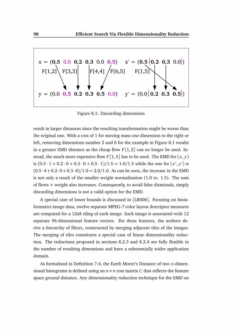
98 Efficient Search Via Flexible Dimensionality Reduction
x = (0.5 0.0 0.2 0.3 0.0 0.5)
y = (0.0 0.5 0.2 0.3 0.5 0.0)
x' = (0.5 0.2 0.3 0.0 )
y' = (0.0 0.2 0.3 0.5 )
F[1,2] F[3,3] F[6,5]F[4,4] F[1,5]
Figure 8.1: Discarding dimensions
result in larger distances since the resulting transformation might be worse than
the original one. With a cost of 1 for moving mass one dimension to the right or
left, removing dimensions number 2 and 6 for the example in Figure 8.1 results
in a greater EMD distance as the cheap flow F[1,2] can no longer be used. In-
stead, the much more expensive flow F[1, 5] has to be used. The EMD for (x , y)is (0.5 · 1+ 0.2 · 0+ 0.3 · 0+ 0.5 · 1)/1.5 = 1.0/1.5 while the one for (x ′, y ′) is
(0.5 ·4+0.2 ·0+0.3 ·0)/1.0= 2.0/1.0. As can be seen, the increase in the EMD
is not only a result of the smaller weight normalization (1.0 vs. 1.5). The sum
of flows × weight also increases. Consequently, to avoid false dismissals, simply
discarding dimensions is not a valid option for the EMD.
A special case of lower bounds is discussed in [LBS06]. Focusing on bioin-
formatics image data, twelve separate MPEG-7 color layout descriptor measures
are computed for a 12x8 tiling of each image. Each image is associated with 12
separate 96-dimensional feature vectors. For these features, the authors de-
rive a hierarchy of filters, constructed by merging adjacent tiles of the images.
The merging of tiles constitutes a special case of linear dimensionality reduc-
tion. The reductions proposed in sections 8.2.3 and 8.2.4 are fully flexible in
the number of resulting dimensions and have a substantially wider application
domain.
As formalized in Definition 7.4, the Earth Mover’s Distance of two n-dimen-
sional histograms is defined using an n×n cost matrix C that reflects the feature
space ground distance. Any dimensionality reduction technique for the EMD on

8.2. Dimensionality Reduction for the EMD 99
histogram vectors thus has to specify two reductions: one for the histogram
vectors themselves and one for the cost matrix.
8.2.1 Formalization of the Dimensionality Reduction
Formally, a linear dimensionality reduction from n to n′ can be described via a
matrix.
Definition 8.1 (General linear dimensionality reduction)
A general linear dimensionality reduction from dimensionality n to n′ is character-
ized by a reduction matrix R ∈ Rn×n′ . The reduction of an n-dimensional vector x
to a n′-dimensional vector x ′ is defined as:
x ′ = x · R
A subtype of linear dimensionality reductions especially useful for the reduction
of the EMD are those reductions that combine one or more original dimensions
to form a single reduced dimension.
Definition 8.2 (Combining linear dimensionality reduction)
The set Rn,n′ ⊂ 0,1n×n′ of linear dimensionality reduction matrices that reduce
the data dimensionality from n to n′ by combining original dimensions to form
reduced dimensions is defined by:
R ∈ Rn,n′⇔ ∀1≤ i ≤ n :∑n′
j=1 R[i, j] = 1 (8.1)
Restriction (8.1) together with R[i, j] ∈ 0, 1 asserts that each original di-
mension is assigned to exactly one reduced dimension. With i|R[i, i′] = 1 as
the set of dimensions i that are combined to the reduced dimension i′, it holds
that
1.⋃n′
i′=1i|R[i, i′] = 1= 1, . . . , n (all dimensions are assigned) and
2. (i′ 6= j′) ⇒ (i|R[i, i′] = 1 ∩ j|R[ j, j′] = 1 = ;) (no dimension is as-
signed twice).

100 Efficient Search Via Flexible Dimensionality Reduction
x
y
C
original feature space
reducedfeature space
x'
y'
C'
R1
R2
R2R1
dimensionality reduction
EMD C
EMD C'
Figure 8.2: Influence of R1 and R2 on x , y , and C
Additionally, restriction (8.1) ensures that the reduced vector is of the same
total weight as the original vector (|x |Σ = |x · R|Σ).
A reduced Earth Mover’s Distance is defined via a reduction for the query
vector and a reduction for the database vectors. Both reductions are used to
compute a reduced cost matrix (cf. Figure 8.2).
Definition 8.3 (Reduced Earth Mover’s Distance)
For a cost matrix C, two n-dimensional vectors x and y, and two reduction ma-
trices R1 ∈ Rn,n1 and R2 ∈ Rn,n2, the lower-bounding reduced EMD is defined
as:
EM DR1,R2C (x , y) = EM DC ′(x · R1, y · R2)
where C ′ ∈ Rn1×n2 is a lower-bounding reduced cost matrix.
The lower-bounding reduced cost matrix C ′ is formally introduced in Def-
inition 8.4. This reduced cost matrix is based on a worst-case assumption to
guarantee the lower-bounding property for the filter step. The sparse combin-
ing reduction matrices according to Definition 8.2 limit the worst cases that can
occur (cf. Section 8.2.2) when compared with dimensionality reduction tech-
niques such as PCA, ICA and Random Projection where R[i, j] ∈ R. For example,
preliminary tests with PCA (amended by an extra dimension to preserve the to-
tal mass) resulted in very poor retrieval efficiency due to the concessions that
had to be made for the reduced cost matrix in order to guarantee the lower-
bounding property.

8.2. Dimensionality Reduction for the EMD 101
The two possibly differing reduction matrices R1 and R2 of possibly differing
dimensionality applied to the EMD operands (requiring only minor extension of
Definition 7.4 to support two differing vector dimensionalities) allow for han-
dling the feature vectors in the database separately from the feature vectors of
the queries. In particular, a database reduction to a low dimensionality for in-
dexing in multidimensional structures, and, at the same time, only slight or no
reduction of the query for high approximation quality is generally possible with
this approach.
8.2.2 Optimal Dimensionality Reduction
In this section, optimality of dimensionality reduction is defined with respect to
the efficiency of the similarity search process. During multi-step query process-
ing, dimensionality reduction is used to generate a set of candidates which is
refined using the original dimensionality. Smaller candidate sets induce fewer
refinement computations and thus result in less computation time for the re-
finement step. For given target dimensionalities, the optimal dimensionality re-
duction is therefore the reduction that yields the smallest candidate sets during
query processing.
Optimal Cost Matrix Reduction
Any reduction of the dimensionality of the Earth Mover’s Distance requires spec-
ification of a corresponding reduced cost matrix. This cost matrix provides the
ground distance in the new reduced feature space. Consequently, the reduced
cost matrix depends on the reduction matrices of Definition 8.2. The optimal
cost matrix with respect to given reduction matrices is the one that provides
the greatest lower bound to the EMD in the original dimensionality. As will
be proven on the following pages, the optimal reduced cost matrix consists of
minima over the original cost entries.
To illustrate why those minima have to be chosen for C ′, a worst case ex-
ample is considered: To ensure the lower bound property, underestimating the
true distance means assuming the worst case. That worst case occurs if all orig-
inal mass is transfered at minimum cost by the EMD. For x = (0,1, 0,0) and

102 Efficient Search Via Flexible Dimensionality Reduction
y = (0,0, 1,0) with a ground distance of C[i, j] = |i − j|, the Earth Mover’s
Distance from x to y is 1 (moving one unit of mass via flow F[2,3] at ground
distance |2− 3| = 1). Combining the first two and the last two dimensions, the
reduced vectors are x ′ = (1,0) and y ′ = (0, 1). The minimum cost entry from
the original dimensions 1 or 2 to dimensions 3 or 4 is C[2, 3], which is indeed
the cost that was used in the original EMD. If this value were to be exceeded by
C ′[1, 2], the lower bound property would be lost.
Definition 8.4 (Optimal Reduced Cost Matrix)
For a cost matrix C, two n-dimensional vectors x and y, and a reduced EM DR1,R2C
according to definition 8.3, the optimal reduced cost matrix C ′ is defined by:
C ′[i′, j′] =minC[i, j] | R1[i, i′] = 1∧ R2[ j, j′] = 1 (8.2)
In case of R1 = R2 ∈ Rn,n′ , the reduced cost matrix C ′ defined by (8.2)
is equivalent to the lower bounding cost matrix of [LBS06]. Theorem 8.1 as-
serts that C ′ is lower bounding for R1 6= R2, too. Furthermore, Theorem 8.2
states that the reduced cost matrix results in a greatest lower bound for given
reduction matrices R1 and R2.
Theorem 8.1 (Lower bound)
Given two reduction matrices R1 ∈ Rn,n1 and R2 ∈ Rn,n2 and a cost matrix C ∈Rn×n, the reduced cost matrix C ′ according to (8.2) provides a lower bound for the
EMD:
∀x , y : EM DC ′(x · R1, y · R2)≤ EM DC(x , y)
Proof 8.1
Let bF denote the optimal flow matrix for the original EM DC and let eF ′ denote the
flows combined according to R1 and R2:
eF ′[i′, j′] =∑
i|R1[i,i′]=1
∑
j|R2[ j, j′]=1
bF[i, j]

8.2. Dimensionality Reduction for the EMD 103
Then
EM DC(x , y) =n∑
i=1
n∑
j=1
bF[i, j] · C[i, j]
(i)=
n1∑
i′=1
n2∑
j′=1
∑
i|R1[i,i′]=1
∑
j|R2[ j, j′]=1
bF[i, j] · C[i, j]
(ii)≥
n1∑
i′=1
n2∑
j′=1
∑
i|R1[i,i′]=1
∑
j|R2[ j, j′]=1
bF[i, j]
·
min
C[i, j] | R1[i, i′] = 1∧ R2[ j, j′] = 1
︸ ︷︷ ︸
Definition 8.4
(iii)=
n1∑
i′=1
n2∑
j′=1
∑
i|R1[i,i′]=1
∑
j|R2[ j, j′]=1
bF[i, j]
· C ′[i′, j′]
(iv)=
n1∑
i′=1
n2∑
j′=1
eF ′[i′, j′] · C ′[i′, j′](v)≥ EM DC ′(x · R1, y · R2)
Step (i) splits the sum over all combinations of i and j into sums over the
reduced dimensions, making use of each dimension pair (i,j) being assigned to
exactly one reduced dimension pair (i′, j′) by R1 and R2.
Step (ii) replaces the individual costs within the brackets by the minimum over
all these costs. Hence, the sum can only decrease.
Since this complies with Equation 8.2, it is replaced with C ′[i′, j′] in step (iii).
Step (iv) substitutes the summed flows in the brackets with the combined flows
introduced above.
Step (v) holds since eF ′[i′, j′] on the left side of the equation is a feasible solution
to the transportation problem of the EMD on the right, albeit not necessarily a
minimal one.
To help prove the optimality of C ′ for given R1 and R2, a monotony property
of the EMD is introduced. The monotony property ensures that the quality of a
lower bound derived via dimensionality reduction increases if the values in the
cost matrix increase.

104 Efficient Search Via Flexible Dimensionality Reduction
Theorem 8.2 (Monotony of the EMD)
Given two cost matrices C1, C2 ∈ Rn×n it holds:
C1≤ C2 ⇔ ∀x , y : EM DC1(x , y)≤ EM DC2(x , y)
where
C1≤ C2⇔ (C1= C2)∨ (C1< C2)
C1< C2⇔ (∀i, j : C1[i, j]≤ C2[i, j]) ∧ (∃i, j : C1[i, j]< C2[i, j])
Proof 8.2
Case 1 (C1 = C2): The statement trivially holds.
Case 2 (C1 < C2):
“⇒” Let bF be optimal for EM DC2(x , y) =∑
i
∑
jbF[i, j]C2[i, j]. Due to C2 >
C1 it holds that∑
i
∑
jbF[i, j]C2[i, j]≥
∑
i
∑
jbF[i, j]C1[i, j] and since bF is a fea-
sible combination of flows for EM DC1(x , y),∑
i
∑
jbF[i, j]C1[i, j]≥ EM DC1(x , y).
“⇐” The proof is given by contradiction: Assume that the statement does not
hold (i.e., C1 6≤ C2 but still EM DC1(x , y) ≤ EM DC2(x , y) for all x and y), then
there exists at least one pair of dimensions (i, j) with C1[i, j]> C2[i, j]. For (i, j),a counter example can be constructed with vectors x and y where
x[i] =
(
1 , if i = i
0 , otherwiseand y[ j] =
(
1 , if j = j
0 , otherwise.
For these vectors, the assumption does not hold:
EM DC1( x , y) = 1 · C1[i, j]> 1 · C2[i, j] = EM DC2( x , y)
After proving the lower bounding property and the monotony of the EMD,
the next proof shows that there is no better reduced cost matrix for any given
reduction matrices R1 and R2 than the one given by Definition 8.4.
Theorem 8.3 (Optimality)
Given a cost matrix C ∈ Rn×n and two reduction matrices R1 ∈ Rn,n1, R2 ∈ Rn,n2,
8.2. Dimensionality Reduction for the EMD 105
there is no greater lower bound than the one provided by C ′ according to (8.2):
¬∃C ′′ ∈ Rn1×n2 ∀x , y : Greater∧ LB∧ (C ′′ 6= C ′)
where
LB≡ EM DC ′′(x · R1, y · R2)≤ EM DC(x , y)
Greater≡ EM DC ′(x · R1, y · R2)≤ EM DC ′′(x · R1, y · R2)
Proof 8.3
For a proof by contradiction, assume the negation:
∃C ′′ 6= C ′ ∀x , y : Greater∧ LB
To comply with the Greater constraint, the monotony of the EMD requires C ′ ≤C ′′. Since C ′ 6= C ′′, there must be a pair of dimensions (i, j) with C ′[i, j] <C ′′[i, j]. As C ′ was computed according to Definition 8.4, it holds that C ′[i, j] =minC[i, j] | R1[i, i] = 1∧ R2[ j, j] = 1.
The following two vectors x and y contradict the LB constraint. Let the two
original dimensions i∗ ∈ i|R1[i, i] = 1 and j∗ ∈ j|R2[ j, j] = 1 be the ones that
result in C ′[i, j] = C[i∗, j∗] and set
x[i] =
(
1 , if i = i∗
0 , otherwiseand y[ j] =
(
1 , if j = j∗
0 , otherwise
As the only flow of mass for EM DC is between x[i∗] and y[ j∗] it follows that
EM DC( x , y) =n∑
i=1
n∑
j=1
bF[i, j]·C[i, j] = bF[i∗, j∗]·C[i∗, j∗] = 1·C[i∗, j∗] = C ′[i, j]
and due to i∗ ∈ i|R1[i, i] = 1 and j∗ ∈ j|R2[ j, j] = 1
EM DC ′′( x · R1, y · R2) =n1∑
i′=1
n2∑
j′=1
cF ′′[i′, j′] · C ′′[i′, j′]
= cF ′′[i, j] · C ′′[i, j] = 1 · C ′′[i, j]

106 Efficient Search Via Flexible Dimensionality Reduction
which together with C ′[i, j]< C ′′[i, j] contradicts LB:
EM DC( x , y) = C ′[i, j]< C ′′[i, j] = EM DC ′′( x · R1, y · R2)
Theorem 8.3 shows that the reduction of a cost matrix C to C ′ according
to Definition 8.4 is an optimal lower bound for any given reduction matrices
R1 and R2. Therefore, finding good reduction matrices R1 and R2 is the key
to good retrieval efficiency. In the following, only R1 = R2 is considered and
EM DRC(x , y) is written for EM DR,R
C (x , y). However, the methods can gener-
ally be extended to different simultaneous reductions. In that case, the two
matrices should not be chosen completely independently from each other as
Definition 8.4 would lead to low values for C ′. Instead, R2 could for example
be chosen to be a coarser / finer version of R1.
Optimal Flow Reduction
As discussed above, the optimal reduction of the cost matrix of the Earth Mover’s
Distance depends entirely on the reduction matrices. Consequently, the effi-
ciency of any EMD reduction according to Definition 8.3 depends solely on the
choice of the reduction matrix R. While it is possible to define what would
constitute an optimal choice of R for a given query workload in a multi-step
filter-and-refine query processing framework (akin to Section 4.3.2), that opti-
mal R is not attainable in practice. Thus, viable heuristics for finding a suitable
R are required. After looking at the optimal R in this section, such heuristics are
developed in sections 8.2.3 and 8.2.4.
Given an n-dimensional query vector q and a query distance ε, an optimal
reduction R ∈ Rn,n′ to dimensionality n′ can be defined in terms of the number
of refinements required to answer an ε range query for a database DB. The
according characteristic function of the filter (cf. page 46) that uses the EMD in
the reduced dimensionality is given by
χR,ε(q, o) =
(
1 if (o ∈ DB)∧ EM DRC(q, o)< ε
0 otherwise.

8.2. Dimensionality Reduction for the EMD 107
Due to the lower-bounding property, only elements o for which χR,ε(q, o) = 1
can potentially still have a refined distance below ε. Since this optimality is
only concerned with one single query q, one typically chooses a workload Q
representative of the expected queries and defines optimality with respect to
said workload.
Definition 8.5 (Optimal EMD reduction)
Given a query workload Q = (q1,ε1), . . . , (qt ,εt), where qi is a query vector and
εi the corresponding range threshold, the optimal reduction R∗ ∈ Rn,n′ for Q is:
R∗ = argminR∈Rn,n′
∑
(q,ε)∈Q
∑
o∈DB
χR,ε(q, o)
While this equation describes the desired optimal reduction, the search space
for the optimization is immense even for small databases and small dimension-
alities. Due to the size of the combining reduction matrix, an (n · n′)-variable
0-1 integer optimization problem with constraints according to Definition 8.2
has to be solved. Summing over the workload, the objective function consists
of |Q| · |DB| individual (n′ · n′)-variable EMD optimization problems. Exhaus-
tive enumeration of all possible reductions requires the computation of a total
of n′n · |Q| · |DB| reduced EMD values. Even for a reduction from 16 to 8 di-
mensions of a database of size 1000 and a workload of size 100, this requires
over 2.8 · 1019 EMD computations. As this is clearly infeasible even for small
databases, heuristics that result in efficient reductions are discussed next.
8.2.3 Clustering-Based Reduction
The first approach proposed here is a data-independent dimensionality reduc-
tion which is a generalization of [LBS06]. It is motivated by the monotony of
the Earth Mover’s Distance (cf. Theorem 8.2).
Monotony induces that a cost matrix with greater entries than another cost
matrix is more desirable for dimensionality reduction when used in a filter-and-
refine framework. Therefore, this section proposes a method that combines
the original dimensions in such a way that the distances between the result-

108 Efficient Search Via Flexible Dimensionality Reduction
C= 0 1 3 41 0 2 33 2 0 14 3 1 0
0 22 0C'=
min3, 4, 2, 3
R= 1 0 1 00 10 1
lost ''intra-class'' informationFigure 8.3: Information lost and preserved during reduction
ing reduced dimensions are as great as possible. At the same time the distance
information that is lost shall be as small as possible. These two demands cor-
respond to the well-known clustering goals of maximum inter-class dissimilarity
and minimum intra-class dissimilarity.
Figure 8.3 gives an example for n = 4 and n′ = 2, where the first two
original dimensions are combined to the first reduced dimension and the last
two original dimensions to the second reduced dimension. The distance that is
preserved between the two reduced dimensions is C[2, 3] = C[3, 2] = 2, which,
according to Definition 8.4, is the minimum of the shaded entries. This inter-
class distance should be as large as possible. The distance information C[3, 4] =C[4,3] = 1 within the new second dimension is lost due to the reduction and
should thus be as small as possible.
A further postulate for dimensionality reductions is the flexibility in terms of
the number of reduced dimensions n′. This flexibility allows full control of the
trade-off between the quality of the approximation and the efficiency of the filter
step computation. For lower values of n′, the EMD computations in the filter
are less expensive to perform but at the same time, the reduced approximation
quality results in more refinement computations. The approach discussed here
is fully flexible in n′ while the approach of [LBS06] is limited to n′ = n/4i when
merging tiles in a hierarchical manner.
The idea that allows for the flexible criterion to be met is to cluster the
dimensions based on the ground distance as used by the EMD. Specification of n′

8.2. Dimensionality Reduction for the EMD 109
is possible for partitioning clustering algorithms such as k-means or k-medoids
[KR90]. Both of these algorithms start with an initial random partition of the
data into k groups, where k is the user-specified number of clusters. Working
in an iterative manner, they assign objects to the nearest cluster center and
re-compute these centers for the new partitioning until the clustering is stable
with respect to a quality criterion. k-means uses the arithmetic mean as center
of clusters, whereas k-medoids chooses a central point from the dataset as a
cluster representative. The objects in our case refer to the original dimensions
of the feature space. As the k-medoids algorithm does not require an explicit
distance function for the feature space but merely a distance matrix between the
objects to be clustered, it is chosen over k-means here. Thus, the dimensionality
reduction approach can be applied even if the ground distance function is not
explicitly known.
The clustering-based algorithm for finding a reduction matrix starts by ran-
domly choosing n′ representatives (medoids) from the set of original dimensions
(i.e., setting one entry in the reduction matrix to 1 for each column with a limit
of one non-zero entry per row). It then assigns the remaining dimensions to
their nearest medoid according to the cost matrix (i.e., setting a total of n− n′
entries to 1 in the according columns). The quality of the clustering is deter-
mined as the total distance based on the reduction matrix R defined as:
T D =n′∑
i′=1
∑
i|R[i,i′]=1
C[i, i′]
The total distance thus reflects the degree of dissimilarity within the clusters
(e.g., the distance information that will be lost during reduction) and is the
objective function that the algorithm tries to minimize. In the next step, the
algorithm aims at improving the clustering. It determines the total distance that
results when swapping a non-medoid with a medoid. In a greedy manner, the
configuration with the lowest total distance is chosen and the corresponding
pair is swapped. The algorithm terminates if no swapping leads to a further
improvement of the total distance. The result is a reduction matrix that reflects
a clustering of the dimensions into n′ partitions where the partition membership

110 Efficient Search Via Flexible Dimensionality Reduction
of the original dimensions is encoded in the columns of the reduction matrix.
All original dimensions belonging to a partition are combined to a new reduced
dimension.
Since only knowledge about the cost matrix is incorporated in this approach,
it is likely that one sacrifices great potential of improving the choice of the re-
duction matrix. The data-dependent method for dimensionality reduction pre-
sented in the next section exploits knowledge that can be derived from the data-
base at hand.
8.2.4 Flow-Based Reduction
The second, data-dependent method for dimensionality reduction introduced
here incorporates knowledge on the database at hand to generate a better re-
duction. It collects flow-information of unreduced EMD computations to guide
the process of generating reduction matrices and will thus be referred to as
flow-based reduction.
Computing unreduced EMDs to define reduced EMDs for fast retrieval might
seem like a paradox at first. However, the unreduced EMDs from which the
flow-information is collected are computed in a preprocessing step only and
this computational investment is more than justified through faster search times
during query processing.
The unreduced EMD is a sum of terms F[i, j] · C[i, j]. For a close lower
bound, the aim is to achieve largest possible terms F ′[i′, j′] · C ′[i′, j′] for the
reduced EMD. Since the optimal reduced cost matrix C ′ can be determined by
applying Theorem 8.3, the key is to increase the reduced flows with respect to
C ′[i′, j′]. In this way, the reduced EMDs increase in value and can filter more
false candidates in a filter-and-refine setup.
Figure 8.4 illustrates the steps taken to compute a reduction matrix with the
flow-based heuristic. In the first step a sample S is drawn from the database.
Pairwise EMDs (original dimensionality) are calculated on the sample in the
second step. The information that is extracted here is the average flow matrix
FS with
FS [i, j] =1
|S |2∑
x∈S
∑
y∈S
bF x ,y[i, j].

8.2. Dimensionality Reduction for the EMD 111
original DB
sample calculate EMDs /collect fows optimize
initial solution
S FS R
Figure 8.4: Process of computing a flow-based reduction matrix
where bF x ,y[i, j] is the flow that occurred from dimension i to dimension j in the
optimal solution of the EMD between x and y from some sample S ⊂ DB. Each
entry FS [i, j] reflects the average amount of flow from original dimension i to
original dimension j.
The third and main step of the approach iteratively improves an initial re-
duction matrix by utilizing the aggregated flow information.
To estimate the quality of a reduction matrix, the flows occurring in reduced
EMDs are first approximated by the average original flows FS aggregated ac-
cording to the reduction matrix that is being investigated.
aggrFlow(F, R, i′, j′) =∑
i|R[i,i′]=1
∑
j|R[ j, j′]=1
F[i, j]
The aim is to maximize aggrFlow(F, R, i′, j′) · C ′[i′, j′] in place of the signif-
icantly more costly F ′[i′, j′] · C ′[i′, j′], which would require pairwise reduced
EMD computations for each investigated reduction matrix. The experiments in
Section 8.4 show that this approximation leads to good results.
Overall, the expected quality of a reduction R is estimated as the sum of the
aggregated flows FS weighted by the cost matrix C ′ optimally reduced accord-
ing to R:
quality(R, FS ) =n′∑
i′=1
n′∑
j′=1
aggrFlow(FS , R, i′, j′) · C ′[i′, j′]

112 Efficient Search Via Flexible Dimensionality Reduction
Algorithm 8.1: optimizeFB_MOD(R, C, F, n, n’)
origDim = 1; lastOrigDimChanged = 1;1
// get the expected quality of R without any changescurrentQuality = calcQuality(R, C, F, 1, R.getAssignment(1), n’);2
// iterate over original dimensions and change their assignmentrepeat3
threshold = currentQuality * THRESH; // improvement threshold4
// try each assignment to a reduced dimensionfor redDim = 1 to n’ do5
swapQuality = calcQuality(R, C, F, origDim, redDim, n’);6
if (swapQuality - currentQuality > threshold) then7
R.reassign(origDim, redDim); // change assignment8
lastOrigDimChanged = origDim; // track last change9
currentQuality = swapQuality;10
break; // found improvement, exit for-loop11
endif12
endfor13
origDim = 1 + (origDim % n); // go to next dimension14
until (origDim == lastOrigDimChanged) ;15
return R;16
The global optimization of this term requires computing all possible reduc-
tions which is clearly infeasible (cf. Section 8.2.2). Therefore, two variants of
hill-climbing algorithms that step-by-step reassign a single original dimension
to a new reduced dimension are proposed.
Algorithm 8.1 lists pseudo code for the first proposed variant named FB-Mod
(flow-based reduction - modulo). The algorithm takes the current reduction
matrix, starts at the first original dimension, and changes its assignment. To
this end, it iteratively assesses the assignment of the original dimension to each
reduced dimension. If the quality of the resulting reduction matrix is better
than the one of the current solution (by some relative margin threshold), the
change is made persistent and the algorithm continues with the next original
dimension. Once it reaches the last original dimension it starts over at the first
one until it visits the same original dimension twice without any reassignments
in between.
The expected quality of a reduction matrix that has a single original di-

8.3. Query Processing Algorithm 113
Algorithm 8.2: calcQuality(R, C, F, origDim, newRedDim, n’)
// compute quality of R where origDim is reassigned to newRedDimquality = 0.0;1
R’ = R.copy();2
R’.reassign(origDim, newRedDim);3
C’ = reduceCostMatrix(C, R’);4
// sum up the reduced costs times the aggregated flowsfor i’=1 to n’ do5
for j’=1 to n’ do6
quality = quality + aggrFlow(F, R, i’, j’) * C’[i’,j’];7
endfor8
endfor9
return quality;10
mension reassigned to a different reduced dimension is calculated using the
calcQuality method that is listed in Algorithm 8.2.
The second algorithm proposed does not necessarily apply the first reassign-
ment that yields a better solution (FB-All of Alg. 8.3). Instead, it evaluates all
possibilities before choosing the one single reassignment that results in the best
reduction matrix. It then starts the next iteration until no further improvement
is achieved.
The remaining building block for the process laid out in Figure 8.4 is the
choice of the initial reduction matrix. Two possibilities are proposed here. For
a baseline solution, all original dimensions can be assigned to the first reduced
dimension. Alternatively, the result from the clustering-based dimensionality
reduction (Section 8.2.3) can be used. In this case, the proposed algorithms
start from a solution that reflects the ground distances in the feature space. In
the experiments of Section 8.4, the two initial reductions are referred to as Base
and KMed.
8.3 Query Processing Algorithm
This section describes how a multi-step query-and-refine framework can be
forged using the dimensionality reduction technique as a filter step. The focus
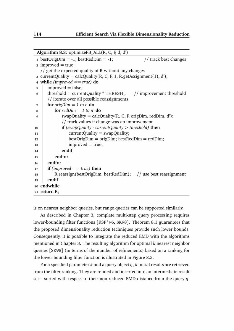
114 Efficient Search Via Flexible Dimensionality Reduction
Algorithm 8.3: optimizeFB_ALL(R, C, F, d, d’)
bestOrigDim = -1; bestRedDim = -1; // track best changes1
improved = true;2
// get the expected quality of R without any changescurrentQuality = calcQuality(R, C, F, 1, R.getAssignment(1), d’);3
while (improved == true) do4
improved = false;5
threshold = currentQuality * THRESH ; // improvement threshold6
// iterate over all possible reassignmentsfor origDim = 1 to n do7
for redDim = 1 to n’ do8
swapQuality = calcQuality(R, C, F, origDim, redDim, d’);9
// track values if change was an improvementif (swapQuality - currentQuality > threshold) then10
currentQuality = swapQuality;11
bestOrigDim = origDim; bestRedDim = redDim;12
improved = true;13
endif14
endfor15
endfor16
if (improved == true) then17
R.reassign(bestOrigDim, bestRedDim); // use best reassignment18
endif19
endwhile20
return R;21
is on nearest neighbor queries, but range queries can be supported similarly.
As described in Chapter 3, complete multi-step query processing requires
lower-bounding filter functions [KSF+96, SK98]. Theorem 8.1 guarantees that
the proposed dimensionality reduction techniques provide such lower bounds.
Consequently, it is possible to integrate the reduced EMD with the algorithms
mentioned in Chapter 3. The resulting algorithm for optimal k nearest neighbor
queries [SK98] (in terms of the number of refinements) based on a ranking for
the lower-bounding filter function is illustrated in Figure 8.5.
For a specified parameter k and a query object q, k initial results are retrieved
from the filter ranking. They are refined and inserted into an intermediate result
set – sorted with respect to their non-reduced EMD distance from the query q.

8.3. Query Processing Algorithm 115
original DB
query
Red-IMranking
EMDk-NN
Red-EMDrankingcand. cand. res.
R2
R1
Figure 8.5: Multi-step setup for query processing
Next, the base ranking is queried for the next best object with respect to the filter
distance. If the filter distance is smaller than the current kth nearest neighbor
in the intermediate result set, the object is refined and compared against the
current kth nearest neighbor with respect to the non-reduced EMD distance. If
smaller, it is sorted into the intermediate result set, displacing the largest one
from the set. This is repeated until the filter distance is larger than the current
kth result distance. As soon as the filter distance is larger, none of the remaining
objects have a smaller filter distance. And since the filter distance is a lower
bound of the non-reduced distance, the non-reduced distance is also larger. The
intermediate result set now contains the correct k nearest neighbors.
The dimensionality reduction techniques presented can be flexibly combined.
As the reduced distance function again is an EMD computation, it is possible to
use existing filters for the EMD on the reduced dimensionality. This chaining of
lower-bounding filters allows for efficient query processing as the experiments
show. The LBI M technique from [AWS06] is such a lower bound with respect
to the Earth Mover’s Distance. In the proposed setup, the ranking Red-EMD re-
quired for the k-nearest-neighbor search based on the EMD is thus again based
on a ranking – based on LBI M for the objects with reduced dimensionality.
By integrating LBI M in the multi-step setup, a total of three distance func-
tions with increasing computational complexity work together to efficiently find
nearest neighbors. Even if no index structure is available to support the ranking
queries on the filter level of the k-nearest-neighbor algorithm, only the most

116 Efficient Search Via Flexible Dimensionality Reduction
(a) RETINA [LBS06] (b) IRMA [DMC+07]
Figure 8.6: Datasets used in experiments. (a) 3,932 feline retina scans, (b)10,000 radiography images
dataset average EMD varianceRETINA1-All 1.1998 0.5478RETINA3-All 0.3890 0.1951RETINA2-All 0.3642 0.1224RETINA11-All 0.1241 0.0112
......
RETINA7-All 0.0756 0.0011
Table 8.1: Average and variance of EMD distances in the 12 RETINA datasets(sorted by decreasing variance)
efficient distance function has to be evaluated for all objects of the database.
Pseudo-code for the algorithm is given in [WAKS08].
8.4 Experiments
8.4.1 Setup
The reported results in this section are averages over a workload of 100 k-
nearest neighbor queries. Each complete dataset (denoted by postfix -All) was
divided into a query set (postfix -Q), containing the 100 query objects, and the
database (postfix -DB), containing the remaining objects. From the database
a sample set was drawn for the data-dependent methods of Section 8.2.4. All
experiments were executed on Pentium 4 2.4GHz work stations with 1GB of
RAM running Windows XP.
8.4. Experiments 117
8.4.2 Datasets
The proposed dimensionality reduction approaches are evaluated on two real
world datasets referred to as RETINA and IRMA (cf. Figure 8.6). The first im-
age dataset consists of 3, 932 feline retina scans labeled with various antibodies
and was used in experiments on EMD lower bounds in [LBS06]. For each im-
age, twelve 96-dimensional histograms reflecting a tile-based spatial distribu-
tion of twelve MPEG-7 color layout descriptor measures were computed by the
authors of [LBS06]. The normalized histograms (sum of 1) result in datasets
RETINA1-All through RETINA12-All, from which 100 histograms were each
split off for the experiments here to form RETINA1-Q and RETINA1-DB through
RETINA12-Q and RETINA12-DB. As RETINA4-All through RETINA12-All exhib-
ited a very low variance in Earth Mover’s distances (cf. Table 8.1), looking for
nearest neighbors in those sets is not meaningful. Thus, the experiments are lim-
ited to RETINA1-All to RETINA3-All where data-dependent reduction matrices
were computed based on 10% samples of RETINA1-DB through RETINA3-DB.
The larger scale experiments use a dataset of 10,000 radiography images
from the Image Retrieval in Medical Applications (IRMA) project [LGT+04].The dataset was part of the 2005 ImageCLEFmed image retrieval competition
[DMC+07]. For each image, small patches were collected at both salient points
and on a uniform grid. A Linde-Buzo-Gray clustering using the Euclidean dis-
tance on 40 principal component coefficients of the patches resulted in 199 clus-
ter centers after applying a threshold algorithm to remove insignificantly small
clusters. Details on the feature extraction process can be found in [DKN05].The dataset IRMA-All comprises the image-wise cluster frequencies stored as
199-dimensional histograms. The 40-dimensional Euclidean distances between
the 199 cluster centers are used to compute the cost matrix for the EMD. The
data-dependent reduction matrices were calculated on a sample set of 1, 000
images derived from the database IRMA-DB, which has a cardinality of 9, 900
(i.e., 10,000 images of IRMA-DB minus the 100 query images in IRMA-Q).
8.4.3 Techniques
The following techniques are compared using the architecture from Section 8.3.

118 Efficient Search Via Flexible Dimensionality Reduction
• the proposed clustering-based dimensionality reduction (kMedoids)
• the four proposed flow-based dimensionality reduction variants (denoted
as FB-All-Base, FB-All-KMed, FB-Mod-Base, and FB-Mod-KMed depending
on optimization and initialization)
• the independent minimization filter from [AWS06] (IM)
• the 24-dimensional filter from [LBS06] (Ljosa) which effectively is a lower
resolution 6× 4 grid imposed on images from Figure 8.6(a)
• the weighted averaging lower bound from [RTG98] (Rubner)
The lower bound by Ljosa is not applicable for the IRMA database as the
40-dimensional feature space is not organized in a grid-like fashion. The gener-
alized approach from section 8.2.3 (kMedoids) can be applied. As the averaging
filter (Rubner) requires a ground distance while the reductions deliver a reduced
cost matrix, Rubner can only be applied to the original EMD and is thus run in
a direct filter-and-refine setup. All EMD computations are based on dL2ground
distance.
8.4.4 RETINA Experiments
The top left of Figure 8.7 shows that the greatest averaged original “flow ×cost” components in RETINA2 occur in a vertical direction roughly between the
two bands of antibody labels that can be seen in Figure 8.6(a). The proposed
flow-based reductions keep dimensions separate that induce great “flow × cost”
components in the original EMD while combining those dimensions that con-
tribute low “flow × cost” components. As can be seen in Figure 8.7, all four
variants adapt to the largely vertical flows by assigning different rows to differ-
ent reduced dimensions. This also keeps the reduced costs between the new
dimensions high compared with the kMedoids reduction where each dimension
has between 3 and 6 neighboring reduced dimensions with distance 1. The
FB-All-Base approach (which has the greatest freedom to find a locally optimal
solution) combines a large number of central dimensions to the new dimension

8.4. Experiments 119
1
2
3 4 3
6 7 6
5
8
12
9
10
11
1
2
3
4
6
7
65
8
12
9 10
11
55 6
9 910
30 greatest flows FB-All-KMed FB-Mod-KMed
1
2 3
4
6
7
5
8
12
9 10
11
1 2
3 4
6
7
5
8
12
9 10
11
1 2 1 2 1
3 43 4 3
9 10 9 10 9
1
2
3
4
6
7
5
8
12
9
10
11
554 4 45
7 8 7 8 7 8
kMedoids FB-All-Base FB-Mod-Base
Figure 8.7: Top left: Greatest flows within the feature space of a sample ofRETINA2-All. Other: Partitioning of the feature space into 12 dimensions viafive reduction approaches
7 as there is little flow originating from this area. The same algorithm initial-
ized with the kMedoids solution shows a more balanced distribution of the new
dimensions. For the two modulo variants, little difference can be be seen for the
12-dimensional reduction. They are both rather balanced and adapt well to the
vertical flows.
Figure 8.8 shows the 50-nearest neighbor query processing time (on an ex-
ponential scale) averaged over datasets RETINA1-DB to RETINA3-DB. The re-
duced dimensionality is varied for the proposed approaches while the compet-
ing approaches are either fixed in their dimensionality (Ljosa) or do not have a
reduced dimensionality (sequential EMD without filters, Rubner, and IM). Com-
puting 3,832 expensive high-dimensional EMD distances each for the feature
histograms of RETINA1-DB to RETINA3-DB takes on average ∼ 37 seconds.

120 Efficient Search Via Flexible Dimensionality Reduction
2
4
8
16
32
64
n/a 12 18 24 30 36
avg.
k-N
N qu
ery
proc
essin
g tim
e [s
]
reduced dimensionality
avg. over RETINA1-DB to RETINA3-DB, k=50
EMD
IM
Rubner
Ljosa
kMedoids
FB-All-KMed
FB-All-Base
FB-Mod-KMed
FB-Mod-Base
Figure 8.8: Overall computation time vs. reduced dimensionality
At ∼ 10 seconds, the result of the fixed grid reduction (Ljosa) is a significant
improvement. The 3.1s advantage of Ljosa over kMedoids at 24 reduced dimen-
sions may stem from the original feature space partitioning being a regular grid,
which is a perfect match for the Ljosa approach. Ultimately, the overall query
processing time is of importance. The flexibility of kMedoids in the number of
reduced dimensions allows it to outperform Ljosa using 36 reduced dimensions
even though it is not optimized for grid-based datasets.
The two direct filter-and-refine approaches (Rubner, IM) give still faster re-
sults compared with Ljosa (5.0s and 7.4s respectively) but they are both sur-
passed by all of the four proposed flow-based approaches at a large majority of
reduced dimensionalities evaluated for this experiment (12, 18, 24, 30, and
36). At 2.5 seconds, the FB-All-KMed dimensionality reduction with 18 re-
duced dimensions shows the lowest overall processing time, closely followed
by FB-Mod-Base and FB-Mod-KMed. This means that the flow-based reductions
achieve an average response time speedup of factor 15 compared with the se-
quential EMD and are 2 times faster than the next best competitor (Rubner in
this case). The approach with the greatest freedom to choose a reduction matrix
(FB-All-Base), which produced a rather large combined area in the middle of the
feature space (cf. Figure 8.7), is faster than all data-independent approaches,

8.4. Experiments 121
-4
0
4
8
12
16
20
24
12 18 24 30 36
quer
y pr
oces
sing
time
redu
ctio
n [%
]
reduced dimensionality
effect of Red-IM, avg. over RETINA1-DB to RETINA3-DB, k=50
LjosakMedoidsFB-All-KMedFB-All-BaseFB-Mod-KMedFB-Mod-Base
Figure 8.9: Relative speedup from applying Red-IM as the first filter chain link
but seems to have overfitted the sample set on which the reduction matrices
were computed. The three other variants that produced more balanced reduc-
tions are faster in all evaluated configurations. The reduction to 12 dimensions
being a less efficient filter is explained by it producing more candidates than the
reduction to 18 or more dimensions. This leads to higher overall response times
even though the 12-dimensional EMD computations are less costly than the 18-
dimensional ones (cf. Figure 8.11 for an experiment regarding this behavior).
Figure 8.9 illustrates the advantage that the reduction-based approaches
achieved by including a reduced IM as the first filter chain link according to
Figure 8.5. While removing this extra filter step does not change the overall
order of approaches seen in Figure 8.8, it is favorable to have this option as it
reduces absolute processing times in almost all cases that were studied. The
higher the reduced dimensionality, the more it is worth to apply the filter.
When varying the parameter k of nearest neighbors to retrieve (cf. Fig-
ure 8.10), the observed order of relative speed remains stable but for one ex-
ception. The performance of the IM filter improves significantly when reducing
k to very low values. It is consistently faster than Rubner at k ≤ 15 but matches
the proposed flow-based reductions only for k = 1. This means that IM was
particularly good at approximating distances of very similar histograms. IM re-

122 Efficient Search Via Flexible Dimensionality Reduction
1/2
1
2
4
8
16
32
64
0 10 20 30 40 50
avg.
k-N
N qu
ery
proc
essin
g tim
e [s
]
k
avg. over RETINA1-DB to RETINA3-DB, red. dimensionality = 24
EMD
IM
Rubner
Ljosa
kMedoids
FB-All-KMed
FB-All-Base
FB-Mod-KMed
FB-Mod-Base
Figure 8.10: Computation time vs. number of nearest neighbors
turns the nearest neighbor in 0.74s for k = 1 where the proposed reduction
approaches show response times between 0.81s and 1.06s. Even for k as small
as 5, all four flow-based dimensionality reductions outperform all competitors.
8.4.5 IRMA Experiments
Figure 8.11 shows the trade-off between the decreasing selectivity and rising
processing time of the filter step with increasing dimensionality n′. For the larger
IRMA dataset with 199 original dimensions, the required number of computa-
tionally expensive EMD refinements drops to 2% at a reduced dimensionality of
80 when using FB-All-KMed. At the same time, the superlinear complexity of
the EMD causes the share of time spent on the filter step to decrease rapidly for
low reduced dimensionalities. The optimum for finding 50 nearest neighbors
is achieved at a reduced dimensionality of 60 where roughly 36% of the time
is spent on filtering and the remainder of the time is spent on computing high-
dimensional EMD refinements for 3.2% of the data. For the same setting, the
average filter selectivity of IM is at 21% and at 18.1% for Rubner. The clustering-
based reduction from Section 8.2.3 achieves a four-fold selectivity improvement
over those two competing results.
Due to the larger number of histograms and the significantly higher dimen-
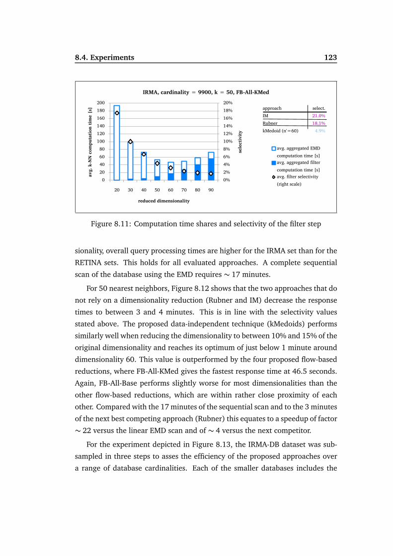
8.4. Experiments 123
0%2%4%6%8%10%12%14%16%18%20%
020406080
100120140160180200
20 30 40 50 60 70 80 90
sele
ctiv
ity
avg.
k-N
N co
mpu
tatio
n tim
e [s
]
reduced dimensionality
IRMA, cardinality = 9900, k = 50, FB-All-KMed
avg. aggregated EMD computation time [s]avg. aggregated filter computation time [s]avg. filter selectivity (right scale)
approachIMRubnerkMedoid (n'=60)
select.21.0%18.1%4.9%
Figure 8.11: Computation time shares and selectivity of the filter step
sionality, overall query processing times are higher for the IRMA set than for the
RETINA sets. This holds for all evaluated approaches. A complete sequential
scan of the database using the EMD requires ∼ 17 minutes.
For 50 nearest neighbors, Figure 8.12 shows that the two approaches that do
not rely on a dimensionality reduction (Rubner and IM) decrease the response
times to between 3 and 4 minutes. This is in line with the selectivity values
stated above. The proposed data-independent technique (kMedoids) performs
similarly well when reducing the dimensionality to between 10% and 15% of the
original dimensionality and reaches its optimum of just below 1 minute around
dimensionality 60. This value is outperformed by the four proposed flow-based
reductions, where FB-All-KMed gives the fastest response time at 46.5 seconds.
Again, FB-All-Base performs slightly worse for most dimensionalities than the
other flow-based reductions, which are within rather close proximity of each
other. Compared with the 17 minutes of the sequential scan and to the 3 minutes
of the next best competing approach (Rubner) this equates to a speedup of factor
∼ 22 versus the linear EMD scan and of ∼ 4 versus the next competitor.
For the experiment depicted in Figure 8.13, the IRMA-DB dataset was sub-
sampled in three steps to asses the efficiency of the proposed approaches over
a range of database cardinalities. Each of the smaller databases includes the
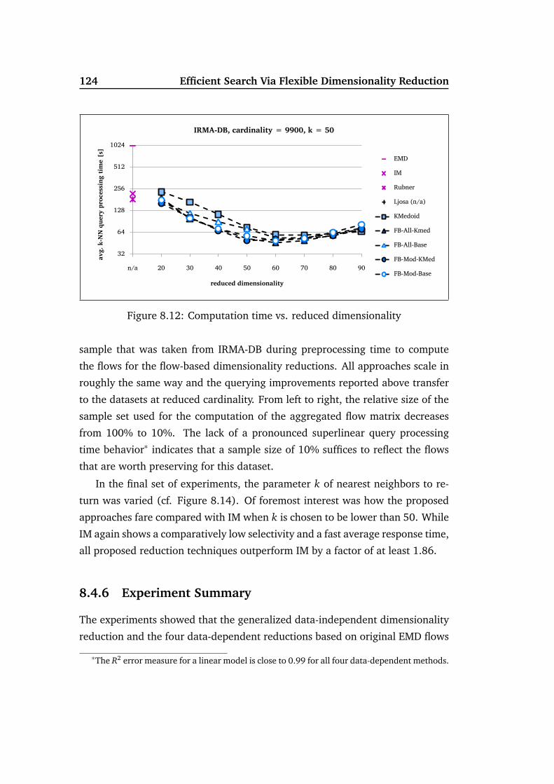
124 Efficient Search Via Flexible Dimensionality Reduction
32
64
128
256
512
1024
n/a 20 30 40 50 60 70 80 90
avg.
k-N
N qu
ery
proc
essin
g tim
e [s
]
reduced dimensionality
IRMA-DB, cardinality = 9900, k = 50
EMD
IM
Rubner
Ljosa (n/a)
KMedoid
FB-All-Kmed
FB-All-Base
FB-Mod-KMed
FB-Mod-Base
Figure 8.12: Computation time vs. reduced dimensionality
sample that was taken from IRMA-DB during preprocessing time to compute
the flows for the flow-based dimensionality reductions. All approaches scale in
roughly the same way and the querying improvements reported above transfer
to the datasets at reduced cardinality. From left to right, the relative size of the
sample set used for the computation of the aggregated flow matrix decreases
from 100% to 10%. The lack of a pronounced superlinear query processing
time behavior∗ indicates that a sample size of 10% suffices to reflect the flows
that are worth preserving for this dataset.
In the final set of experiments, the parameter k of nearest neighbors to re-
turn was varied (cf. Figure 8.14). Of foremost interest was how the proposed
approaches fare compared with IM when k is chosen to be lower than 50. While
IM again shows a comparatively low selectivity and a fast average response time,
all proposed reduction techniques outperform IM by a factor of at least 1.86.
8.4.6 Experiment Summary
The experiments showed that the generalized data-independent dimensionality
reduction and the four data-dependent reductions based on original EMD flows
∗The R2 error measure for a linear model is close to 0.99 for all four data-dependent methods.

8.4. Experiments 125
16
32
64
128
256
512
1024
1000 4000 7000 10000
avg.
k-N
N qu
ery
proc
essin
g tim
e [s
]
database cardinality
IRMA-DB, reduced dimensionality = 60, k = 50
EMD
IM
Rubner
Ljosa (n/a)
KMedoid
FB-All-Kmed
FB-All-Base
FB-Mod-KMed
FB-Mod-Base
Figure 8.13: Computation time vs. cardinality
are able to outperform competing techniques in a large number of settings. This
is in part due to their flexibility regarding the reduced dimensionality, which
allows them to make use of the trade-off between decreasing filter selectivity
and rising filter processing time. The preprocessing step required for the four
flow-based approaches has proven to result in significantly lower query response
times, especially for data that exhibits pronounced flow patterns matched by the
queries. The reduction matrix derived from the data-independent kMedoids ap-
proach showed to be a good starting point for the computation of flow-based
reductions. Using this initialization, the −All variant slightly outperformed the
−Mod variant in most cases. Speedup factors of up to 22 compared with a
sequential scan and up to 4 compared with the next competing approach were
achieved.
Acknowledgments
Thanks go to Vebjørn Ljoså, Thomas Deserno, and Thomas Deselaers for provid-
ing their datasets.

126 Efficient Search Via Flexible Dimensionality Reduction
8
16
32
64
128
256
512
1024
0 10 20 30 40 50
avg.
k-N
N qu
ery
proc
essin
g tim
e [s
]
k
IRMA-DB, reduced dimensionality = 60, cardinality = 9900
EMD
IM
Rubner
Ljosa (n/a)
KMedoid
FB-All-Kmed
FB-All-Base
FB-Mod-KMed
FB-Mod-Base
Figure 8.14: Computation time vs. number of nearest neighbors
8.5 Summary
The Earth Mover’s Distance is inherently adaptable to the feature space through
its flexible cost matrix. Its computation requires costly minimization of flows be-
tween histograms with respect to this cost matrix. In this chapter, novel dimen-
sionality reduction techniques have been proposed for the EMD. The clustering-
based reduction relies only on the original cost matrix information to create re-
duced cost matrices. The approximation quality of the reduced EMD is greatly
improved for the flow-based reductions that incorporate EMD flow information
from the data. All reduction techniques guarantee completeness in multi-step
query processing.

Chapter 9
Direct Indexing and Vector
Approximation
This chapter proposes two techniques to enable the indexing of the Earth Mover’s
Distance on fixed-binning histograms. Key to both techniques is the develop-
ment of a MinDist measure that gives the lowest possible EMD distance be-
tween a query object and a hyper-rectangle. This measure allows EMD-based
retrieval to be supported by a large number of established index structures
that organize the feature representation space in rectangles that summarize the
database histograms. In addition to hierarchical index structures such as the
R-Tree family[Gut84], a lower bound to the MinDist proposed here enables a
quantization-based approach to be used for the search process.
9.1 Introduction
With the rapid growth of multimedia data seen in recent years, similarity search
in multimedia databases heavily depends on efficient query processing. At the
same time, users demand high-quality similarity models. However, high-quality
models such as the EMD often induce a high computational cost that contra-
venes the efficient processing to the point where it turns ineffective. As dis-
cussed in Chapter 8, lower bounds such as [RTG98, AWS06, LBS06, WAKS08]can be used to reduce the number of costly refinement computations. Another
127

128 Direct Indexing and Vector Approximation
method to increase the speed of distance-based similarity search is the exploita-
tion of index structures that help guide the search process. The aim of such
index structures is to collect and structure information on the database in a
manner that allows for non-relevant parts of the database to be pruned. Well-
established index structures that organize the database in such a way include
the R-tree family [Gut84], which hierarchically groups database objects in min-
imum bounding rectangles (MBRs). During query processing, the query his-
togram is compared with the MBRs in a top-down manner to decide whether the
subtrees summarized by an MBR are relevant to the query. In this way, search
algorithms based on index structures aim at being selective regarding the input
they investigate while pure filter-and-refine frameworks are concerned with the
selectivity of their filter output.
For high dimensionalities, the MBRs tend to overlap due to the curse of di-
mensionality [BGRS99], which forces most MBRs to be examined, requiring ran-
dom accesses to almost the entire database. Consequently, the sequential scan
is eventually faster. This phenomenon has spurred the search for alternative
means of indexing. The VA-File from [WSB98] quantizes the data representa-
tion space to provide compact representation of features for optimized sequen-
tial scans and can be seen as a hybrid between scan-based filter-and-refine and
space organizing index structures.
In this chapter, it is shown how indexing based on the VA-File can be em-
ployed for the Earth Mover’s Distance. As the EMD is intrinsically dimension-
interdependent while the VA-File exploits dimension-wise precomputed infor-
mation, a combination of the two is not trivial. The integration of the EMD
query processing with the VA-File is based on a MinDist measure between the
query histogram and the fixed grid cells of the VA-File. The efficiency of the
query processing is further improved by deriving distance components that go
beyond the information stored in a VA-File lookup table without overestimating
the true EMD distance.
The MinDist measure formally introduced in Section 9.2 for the first time
enables the indexing of the Earth Mover’s Distance with a large number of well-
established index structures (i.e., those based on bounding rectangles). This
type of indexing is referred to as direct indexing as the MinDist is directly based

9.2. Direct Indexing of the EMD 129
q
u
l
y
Figure 9.1: The EMD MinDist between a vector q and a rectangle defined by land u is reached at a point y on the rectangle.
on the distance measure that is used in the search (the EMD). In contrast to that,
approaches such as [AWS06] index only a lower bound of the EMD or treat the
EMD as a black box by using metric indexing techniques [LBS06, CPZ97].
9.2 Direct Indexing of the EMD
Direct indexing using any indexing technique that relies on bounding rectangles
to describe similar feature representation vectors on an abstract level requires
the computation of a MinDist measure between a query and the bounding rect-
angles stored in the index (cf. Figure 9.1). In this chapter, the point-to-rectangle
MinDist for the EMD is developed. It enables the direct indexing of the Earth
Mover’s Distance using any index based on rectangular bounding regions such
as the R-tree family.
Definition 9.1 (Point-to-Rectangle MinDist for the EMD)
For a cost matrix C, a non-negative n-dimensional vector q of weight |q|Σ = 1,
and an n-dimensional rectangle with lower and upper boundaries l and u with
|l|Σ ≤ |q|Σ ≤ |u|Σ, the point-to-rectangle MinDist for the EMD is defined as
MinDistC(q, l, u) =minyEM DC(q, y) | ConsMinDist

130 Direct Indexing and Vector Approximation
where
ConsMinDist ≡ CSum∧ CL∧ CU
CSum ≡ |y|Σ = |q|ΣCL ≡ ∀1≤ j ≤ n : y[ j]≥ l[ j]
CU ≡ ∀1≤ j ≤ n : y[ j]≤ u[ j]
CSum ensures that only vectors y of suitable weight are considered while
CL and CU restrict the search for the closest vector y from q to the according
rectangle. For solving this minimization in practice, the MinDist is restated as a
flow minimization and then transformed into a transportation problem. In the
end, the MinDist for the EMD has the form of an EMD itself.
Theorem 9.1 (MinDist as Flow Minimization)
For C, q, l, u according to Definition 9.1 and for constraints CNNeg and CSource
according to Definition 7.4, the point-to-rectangle MinDist of the EMD can be stated
as
MinDistC(q, l, u) =minF
n∑
i=1
n∑
j=1
F[i, j] · C[i, j] | ConsFlow
with
ConsFlow ≡ CNNeg∧ CSource∧ CMin∧ CMax
CMin ≡ ∀1≤ j ≤ n :n∑
i=1
F[i, j]≥ l[ j] (9.1)
CMax ≡ ∀1≤ j ≤ n :n∑
i=1
F[i, j]≤ u[ j] (9.2)
Proof 9.1
Starting with Definition 9.1, it holds:
MinDistC(q, l, u)
(i)=min
y EM DC(q, y) | ConsMinDist

9.2. Direct Indexing of the EMD 131
(ii)= min
ymin
F
n∑
i=1
n∑
j=1
F[i, j] · C[i, j]|Constraints | ConsMinDist
(iii)= min
y,F
n∑
i=1
n∑
j=1
F[i, j] · C[i, j]|CNNeg∧ CSource∧ CTarget∧ CSum∧ CL∧ CU
(iv)= min
F
n∑
i=1
n∑
j=1
F[i, j] · C[i, j]|CNNeg∧ CSource∧∑n
j=1
∑ni=1 F[i, j] =
∑ni=1 q[i]
∧∀1≤ j ≤ n :∑n
i=1 F[i, j]≥ l[ j]
∧∀1≤ j ≤ n :∑n
i=1 F[i, j]≤ u[ j]
(v)= min
F
n∑
i=1
n∑
j=1
F[i, j] · C[i, j]|CNNeg∧ CSource∧ CMin∧ CMax
Step (i) is by Definition 9.1 and step (ii) simply expands the definition of the
EMD. In step (iii), the two minimizations are combined. In step (iv), the mini-
mization no longer looks for an optimal flow matrix F given some y conforming
with ConsMinDist but instead looks for the optimal flow matrix that results in a tar-
get y which conforms with ConsMinDist. The choice of F entirely determines y due
to CTarget. Hence, CTarget can be eliminated from the constraints and y from the
minimization search space after replacing y[ j] in all other constraints by the sum
of flows going to y[ j] according to CTarget. In step (v), CSum is dropped, as it
is a redundant relaxation of CSource while CL and CU become equivalent to CMin
and CMax after the replacement of y[ j].
While also a linear programming problem, this formulation is not in the
form of a transportation problem due to the inequalities (9.1) and (9.2). For
a transportation problem, which has a favorable structure that allows for more
efficient solving, the total weight of both the source and the target must match
exactly and all weight from the source must be moved to the target. This can
be remedied according to [HL04] by transforming the problem such that each
target dimension j is split into two parts that are each afforded their own target
dimension j and (n+ j) in the transformed problem. The first part records how
much flow at least has to be sent towards the old target dimension (l[ j]). The
second part tracks the amount of flow that can additionally be allotted to the
old target dimension (u[ j]− l[ j]). The source is extended with the additional

132 Direct Indexing and Vector Approximation
weight required to match the weight of the transformed target.
Theorem 9.2 (MinDist as a Transportation Problem)
For C, q, l, u according to Definition 9.1, the point-to-rectangle MinDist of the
EMD can be stated as
MinDistC(q, l, u) =minF
n+1∑
i=1
2n∑
j=1
F[i, j] · C ′′[i, j] | ConsTransp= EM DC ′′(q′′, y ′′)
with
ConsTransp ≡ CNNeg′′ ∧ CSource′′ ∧ CTarget′′
C ′′ =
C C
∞·· ·∞ 0 · · ·0
q′′ =
q[1], ..., q[n], |u|Σ− |q|Σ
y ′′ = (l[1], ..., l[n], (u[1]− l[1]), ..., (u[n]− l[n]))
where CNNeg′′, CSource′′, and CTarget′′ equal the according constraints of the EMD
but for the adapted boundaries for indexes i and j and for the replacement of q and
y with q′′ and y ′′.
Proof 9.2 (Sketch)
To obtain a so-called augmented linear program that fits the transportation prob-
lem model, inequality constraints are converted to equivalent equalities using slack
variables. Slack variables F[i, j + n] are introduced here for assignments that ex-
ceed the lower boundaries l[ j]. The columns of C are doubled in C ′′ as the cost for
using a slack variable is to equal the cost of using an original variable. With the last
dimension of the source only flowing to slack variables (at no cost), it is ensured
that slack variables are only used if the according original variables are already
maxed out. The resulting augmented model represents the same solution space as
the original one but provides favorable algebraic properties. The transformation to
an augmented linear program is discussed in detail in [HL04].
With the theorems from this chapter, fixed-binning histograms can now be
managed by MBR-based index structures such as R-Trees. Hierarchical query

9.3. Vector Approximation for the EMD 133
processing algorithms [HS95, RKV95] can utilize the MinDist to guide their
search progress through the index. Due to Theorem 9.2, it is possible to use
the same EMD implementation that is used for determining the distance be-
tween two histograms to compute the MinDist of the EMD (but for the weight
increase from |q|Σ to |u|Σ which has to be accounted for but is not included in
the following section for the sake of readability).
9.3 Vector Approximation for the EMD
In this section, a technique is proposed that reduces the computational over-
head during query processing by efficiently precalculating distance components
between the query histogram and the MBRs. This requires three properties.
1. The number of upper and lower boundaries of MBRs in the index has to
be relatively small,
2. the MinDist computation has to be reduced to dimension-wise distance
components, and
3. it has to be possible to efficiently reassemble the dimension-wise distance
components to the overall MinDist.
In the next section, the first property is tackled.
9.3.1 Reducing the Number of Boundaries via Quantization
In indexes such as the R-tree, bounding rectangles around feature histograms
describe the data. For each of the linear number of leaf nodes in the tree,
an MBR is stored in its parent’s node. Whenever a node is searched during
query processing, a MinDist computation has to be performed for each of the
child nodes. As the MBRs on one level of the tree do not generally coincide in
their boundaries, no distance components can be reused for these rectangles. In
the following paragraphs, it is demonstrated how distance components can be
precalculated once per query based on a priori knowledge of the boundaries in

134 Direct Indexing and Vector Approximation
111110101100011010001000
000 001 010 011 100 101 110 111
3rd interval b2,3 in the 2nd dimension
encoded as 001010
x
Figure 9.2: Quantization
a quantization approach. This approach could be integrated into a quantized R-
Tree but for the sake of simplicity and because of its promised efficiency for high-
dimensional feature representation spaces, a non-hierarchical structure (the VA-
File [WSB98]) was chosen here.
Quantization maps potentially continuous feature values to fixed intervals in
each dimension. Instead of the exact features, bit codes of intervals are stored.
Given a real-valued histogram x and a quantization of each dimension j into
intervals b j,1, . . . , b j,m of range [l j,1, u j,1), . . . , [l j,m, u j,m), the number (k − 1) of
b j,k is recorded x[ j] ∈ b j,k.
In Figure 9.2, an abstract two-dimensional feature representation space is
quantized using a regular decomposition with 3 bits, i.e., m = 23 = 8 inter-
vals. For example, x = (0.1875,0.3125) in b1,2 in the first dimension and b2,3
in the second dimension has a quantized representation of (2 − 1,3 − 1). Its
bounding rectangle is given by the corresponding interval ranges [l1,2, u1,2) =[0.125, 0.250), and [l2,3, u2,3) = [0.250, 0.375). In the actual implementation,
the quantized representation (1, 2) of x is encoded as the concatenated bit string
001010. This explains the shift of −1 in the index k, as the three bits encode
a range of [0, 23 − 1]. For the sake of simplicity, this encoding and the index
shift is ignored in the following sections (i.e., x is quantized to (2, 3) instead of
001010.
Using such a quantization technique, the fixed interval boundaries consti-
tute a priori knowledge of possible rectangle boundaries, and their number n ·m

9.3. Vector Approximation for the EMD 135
is relatively low and does not depend on the database cardinality. In the VA-
File approach, the bit strings are scanned and a MinDist from the query ob-
ject to the rectangle in which the point falls is computed. The actual distance
to the non-quantized object is only computed if the MinDist does not exceed
the current distance threshold of, for instance, the range or k-nearest-neighbor
query algorithm. For simple distance functions such as dL2, the overall MinDist
can be reduced to dimension-wise components in the form of (q[ j]− l j,k)2 or
(u j,k−q[ j])2. These components can be computed once per query and stored in
a lookup table such that the MinDist for dL2is reduced to adding entries of the
lookup table based on the bit string of the encoded database object.
However, for the EMD, which globally optimizes flow of mass across di-
mensions, direct usage of a dimension-wise lookup table is not possible. The
next section shows which distance components may nevertheless be stored in a
lookup table and how the result from the lookup table can be efficiently aug-
mented with further distance components without sacrificing the completeness
of similarity search algorithms.
9.3.2 Lookup-Table Lower Bound
As direct usage of a lookup-table is not possible for the MinDist of the EMD,
a lower bound that contains the lookup-table-compatible components for the
MinDist of the EMD is proposed here. The idea is to relax the source constraint
to obtain a dimension-wise minimization and to only look at target dimensions
where it is clear that at least some mass has to be moved from another di-
mension. Even though the exact mass of a vector in a quantization interval is
unknown a priori, it is required that mass at least equal to the lower boundary
of the interval is moved.
The lookup-table enabled lower bound of the MinDist is defined as follows.
Definition 9.2 (MinDist lower bound LBLT )
For C ′′, CNNeg′′, q′′, and y ′′ according to Theorem 9.2, the lookup-table-enabled
lower bound LBLT of the EMD MinDist is defined as a minimization over all possible
flows F under non-negativity constraints CNNeg′′, source constraints CSourceLT ,

136 Direct Indexing and Vector Approximation
and target constraints CTargetLT :
LBLTC′′(q′′, y ′′) =min
F
n+1∑
i=1
2n∑
j=1
F[i, j] · C ′′[i, j] | ConsLT
with
ConsLT ≡ CNNeg′′ ∧ CSourceLT ∧ CTargetLT
CSourceLT ≡ ∀1≤ i ≤ n+ 1 : ∀1≤ j ≤ 2n : F[i, j]≤ q′′[i]
CTargetLT ≡ ∀1≤ j ≤ n : (q′′[ j]< y ′′[ j])⇒n∑
i=1
F[i, j] = y ′′[ j]
The following theorem states that the above definition indeed constitutes a
lower bound of the EMD MinDist.
Theorem 9.3 (LBLT lower bounds EMD MinDist)
For C ′′, q′′ and y ′′ according to Theorem 9.2:
LBLTC′′(q′′, y ′′)≤ EM DC ′′(q
′′, y ′′) (=MinDistC(q, l, u)).
Proof 9.3
The difference in the definition of LBLT and the MinDist of the EMD in Theorem
9.2 is the set of constraints. Assuming that the constraints of the lower bound are
weaker (i.e., F | ConsLT ⊇ F | ConsTransp), the theorem would follow:
F | ConsLT ⊇ F | ConsTransp(i)⇔
F ′ ∈ F | ConsTransp ⇒ F ′ ∈ F | ConsLT
(ii)⇔
F ′ ∈ F | CNNeg′′ ∧ CSource′′ ∧ CTarget′′
⇒ F ′ ∈ F |CNNeg′′ ∧ CSourceLT ∧ CTargetLT
(iii)⇒ min
F
n+1∑
i=1
2n∑
j=1
F[i, j] · C ′′[i, j] | ConsLT
≤minF
n+1∑
i=1
2n∑
j=1
F[i, j] · C ′′[i, j] | ConsTransp
(iv)⇔ LBLTC′′
(q′′, y ′′)≤ EM DC ′′(q′′, y ′′)

9.3. Vector Approximation for the EMD 137
Step (i) holds by definition of the subset relation and step (ii) by definition of
ConsTransp and ConsLT . Step (iii) follows as the minimum over a subset cannot be
smaller than the minimum over the whole set. Step (iv) is true by definition of
LBLTC′′and EM DC ′′ .
For the whole theorem to hold, one of the first three statements has to be proven.
If F | CSource′′ ⊆ F | CSourceLT and F | CTarget′′ ⊆ F | CTargetLT then the
third statement holds and thus the whole theorem holds, too.
Looking at the definition of CSource′′ ≡ ∀1 ≤ i ≤ n+ 1 :∑2n
j=1 F[i, j] = q[i]and CSourceLT from above, the first inclusion holds because requiring that a sum
of non-negative elements F[i, j] equals q[i] is a stronger constraint than requiring
that each element of the sum is at most equal to q[i].
As for CTarget′′ ≡ ∀1≤ j ≤ 2n :∑n+1
i=1 F[i, j] = y ′′[ j], the constraint CTargetLT
simply limits fewer of the columns in F in the same way CTarget′′ does.
The main advantage of LBLTC′′over the MinDist is that the optimization can
be performed per column of the flow matrix F ∈ R(n+1)×2n. For columns j with
j > n or q′′[ j] ≥ y ′′[ j] = l[ j], the only restriction is that the entries F[i, j]are in the interval [0, q′′[i]]. A choice of 0 trivially minimizes the sum. For the
remaining columns ( j ≤ n and q′′[ j] < y ′′[ j] = l[ j]), an amount of mass equal
to y ′′[ j] = l[ j] has to be distributed to entries F[i, j] ∈ [0, q′′[i]]. Unlike for
EM DC ′′ , a choice for a value F[i, j] in such a column does not influence optimal
choices outside that column and the order of optimal assignment within the
column only depends on the cost matrix C ′′.
The computation of the complete lookup-table LT for a quantization with
lower quantization boundaries LBoundaries is given in Algorithm 9.1. If q[ j] is
less than the kth lower boundary value LBoundaries[ j][k] in dimension j ≤ n,
mass equal to the lower boundary is successively moved to dimension j from
dimensions given by the ordering of source dimensions in the input parameter
ColSorting[ j]. The value of ColSorting[ j][i] is the row index of the i th smallest
cost entry in column j of C . If not enough mass is available from one source, the
next more expensive source is chosen. The algorithm has a run-time complexity
of O(n2m) for m lower boundaries in n dimensions.
After computing LT once for a query q, values LBLT ≤ MinDist(q, o) for

138 Direct Indexing and Vector Approximation
Algorithm 9.1: computeLT(C, q, ColSorting, LBoundaries)
for j=1 to n do1
for k=1 to m do2
// Calculate minimum sum of flows × costs for kth lowerboundary in the j th dimension
dist = 0;3
if (q[j] < LBoundaries[j][k]) then4
mass = LBoundaries[j][k];5
for i=1 to n do6
// iterate over the j th column of C in ascending cost ordernextsource = ColSorting[j][i];7
smallermass = min(q[ nextsource ], mass);8
dist = dist + smallermass * C[nextsource, j];9
mass = mass - smallermass;10
if (mass == 0) then break;11
endfor12
endif13
LT[j][k] = dist;14
endfor15
endfor16
return LT;17
o ∈ DB can be computed with simple table lookups in O(n) time as shown
by Algorithm 9.2 where approx_o is the quantized representation of the n-
dimensional database object o.
The range query performed by Algorithm 9.3 shows that LT is only com-
puted once per query q and that ColSorting is independent of q. In addition to
the parameters of the rangeQ algorithm (cf. page 20), the sorting of cost entries
in C and the VA-File with quantization boundaries and vector approximations
are required as inputs. The sorting of cost entries can be performed offline
in O(n2 log n) for n dimensions. The lower bound to the MinDist of the EMD
can similarly be integrated into the two k-nearest-neighbor algorithms VA-SSA
and VA-NOA given in the technical report [WB97] that details the techniques
presented in [WSB98].

9.3. Vector Approximation for the EMD 139
Algorithm 9.2: computeLBLT(approx_o, LT)
sum = 0;1
for j=1 to n do2
sum = sum + LT[j][approx_o[j]];3
endfor4
return sum;5
Algorithm 9.3: LB_LT-rangeQ(q, ε, EMDC , DB, ColSorting, VA)
ResultSet = ;;1
LT = computeLT(C, q, ColSorting, VA.LBoundaries);2
for i=1 to |DB| do3
if computeLBLT(VA.approximations[i], LT) ≤ ε then4
if EMDC(q, DB[i]) ≤ ε then5
ResultSet = ResultSet ∪ DB[i];6
endif7
endif8
endfor9
return ResultSet;10
9.3.3 Optimization of the Lookup-Table Lower Bound for Met-
ric EMD
The quantization approach up to here did not make use of any properties of the
ground distance (i.e., there is no restriction on C). However, for the popular
class of metric ground distances, an optimization can be made as some of the
flows for EM DC ′′(q′′, y ′′) are known. In particular, the definiteness of a metric
ground distance results in a matrix C ′′ of the form
C ′′ =
0 0... . . .
0 0
∞ · · · ∞ 0 · · · 0
with non-zero entries in all other positions.
An improved lower bound for metric EMDs can be achieved by considering

140 Direct Indexing and Vector Approximation
u[i]
l[i]
case1: q[i] < l[i] case3: u[i] ≤ q[i]case2: l[i] ≤ q[i] < u[i]iii
i i+n
iq[i] 0
∑=l[i]
l[i] q[i]-l[i]
i i+n
l[i] u[i]-l[i]
i i+n
q q q
Figure 9.3: Three cases of mass distribution
the mass that the lower bound did not yet take into account. According to the
constraint CTargetLT , only those target dimensions j < n for which q[ j]< l[ j] =y ′′[ j] are taken into account by LBLT . The amount of mass that is distributed
to such target dimensions j by LBLT is the same as the mass distributed by
EM DC ′′; however, LBLT may move the mass at lower cost due to having fewer
restrictions. For all other columns of F , a flow of 0 is allowed by LBLT wherever
C ′′ is greater than 0. For EM DC ′′ , this is not the case. The cost of moving
the mass that occurs in those other columns for EM DC ′′ can be conservatively
estimated by distributing the mass in ascending cost order similar to the mass
distribution starting in line 5 of Algorithm 9.1. To determine the amount of
mass that is transfered at cost by the EMD and not yet accounted for by LBLT , it
is helpful to divide the dimensions of q into three cases illustrated in Figure 9.3.
The first case is already accounted for by LBLT with a mass of y ′′[i] = l[i] in
column i of F due to CTargetLT . In the second case, the EMD moves l[i] via
9.3. Vector Approximation for the EMD 141
F[i, i] and q[i]− l[i] via F[i, i + n] for a total of q[i] at cost zero. In the third
case, the EMD moves l[i] via F[i, i] and u[i]− l[i] via F[i, i + n] for a total of
u[i] at cost zero. Since the slack dimension q′′[n+ 1] = |u|Σ− |q|Σ is moved at
zero cost, the sum of mass accounted for by LBLT equals
∑
q[i]<l[i]
l[i]
and the sum of unaccounted mass that is moved by the EMD at zero cost is
∑
l[i]≤q[i]<u[i]
q[i]
+
∑
u[i]≤q[i]
u[i]
+ (|u|Σ− |q|Σ).
With the total mass moved by the EMD being |u|Σ =∑n
i=1 q[i] + (|u|Σ − |q|Σ),the amount of mass that is transfered at cost by the EMD and not yet considered
by LBLT is equal to
∆=∑
q[i]<l[i]
(q[i]− l[i]) +∑
u[i]≤q[i]
(q[i]− u[i]).
The last task left is to conservatively estimate at what cost the mass∆ can be
moved without jeopardizing the lower bounding property. By adding that cost
to LBLT , a closer lower bound of the MinDist for the EMD is established. The
general idea is to assume that as much mass as possible moves at as low cost as
possible. This can be achieved with a fast greedy algorithm that assigns mass
from dimension i to j in the order of ascending entries of C[i, j] where entries
that will not be used for this mass by the EMD can be excluded. In the third
case of Figure 9.3, it is clear that the target constraints are already satisfied for
dimensions i and i+ n. Thus, the i th column of C can be ignored in that case. It
is also clear from the discussion above that the mass does not flow at zero cost.
The amount of mass that the greedy algorithm may move from dimension i to
other dimensions can be limited to q[i] while the amount of mass being moved
to dimension j is left unrestricted to allow for a greedy solution algorithm.
As the distribution algorithm depends on its input ∆ in the form of a sum
over differences of q minus the quantization boundaries, this technique is not

142 Direct Indexing and Vector Approximation
Algorithm 9.4: LB_LT+-rangeQ(q, ε, EMDC , DB, ColSorting, EntrySorting,VA)
ResultSet = ;;1
LT = computeLT(C, q, ColSorting, VA.LBoundaries);2
for i=1 to |DB| do3
LB_LT = computeLBLT(VA.approximations[i], LT);4
if LB_LT ≤ ε then5
if LB_LT + greedyMassAssigment(q, C, VA.LBoundaries,6
VA.UBoundaries, EntrySorting) ≤ ε thenif EMDC(q, DB[i]) ≤ ε then7
ResultSet = ResultSet ∪ DB[i];8
endif9
endif10
endif11
endfor12
return ResultSet;13
compatible with the lookup-table but has to be computed as an optimization for
every pair of q′′ and y ′′ (cf. Algorithm 9.4). However, for high-dimensional EMD
computations, the additional computational overhead pales compared with the
EMD and pruning a few more percent points of EMD computations is well worth
the effort.
9.3.4 Multistep Algorithm
The lookup table lower bound LBLT proposed allows for efficient query process-
ing in a nearest neighbor multi-step algorithm [SK98]. As illustrated in Fig-
ure 9.4, the lower bound LBLT+ (i.e., LBLT on the lookup table plus the online
optimization) is used as a filter on the database to quickly generate a small set of
candidates. Additionally, LBI M further reduces this candidate set. Finally, EMD
refinement ensures that the correct result set is obtained. Since the proposed
lower bounds underestimate the true EMD MinDist, completeness in multi-step
processing is ensured.
The k-nearest-neighbor query processing algorithm used in the evaluation
section begins by computing a ranking according to the lower bound LBLT of the

9.4. Experiments 143
original DB
LBLT+q cand.
VA-File
LBIM cand. EMD result
Figure 9.4: Multi-step algorithm
EMD MinDist. This ranking ensures that the number of computations in query
processing is minimized, as discussed in [SK98]. More precisely, a ranking ac-
cording to the filter distance is used to compare the next best filter candidate
against the worst refined distance result so far. As soon as the filter distance
exceeds the worst refined neighbor distance in the intermediate result set, the
set of nearest neighbors is complete. Any of the following candidates are guar-
anteed to have higher filter distances and thus higher true EMD distances than
the set of nearest neighbors already retrieved. Consequently, they can be safely
pruned.
The ranking is computed using an efficient sequential scan on quantized
histograms of the compact VA-File [WSB98]. Starting with the nearest neigh-
bors according to this filter distance, exact representations of the histograms
are used to compute the LBI M lower bound from [AWS06] and the EMD is only
computed if a candidate cannot be pruned by either filter.
9.4 Experiments
9.4.1 Setup and Datasets
The main experiments in this sections use the database of 200,000 color TV
images from Section 4.4. For a random sample of the images (size 10,000), a
random sample of pixels (size 500) was selected. For those pixels, relative x and

144 Direct Indexing and Vector Approximation
y position, the three color features of the CIE Lab model, and local texture mea-
sures (contrast and coarsity) were computed and normalized according to their
standard deviation. The resulting five million seven-dimensional feature vectors
were clustered using k-means to determine a given number of cluster centers,
which served as partition representatives for the subsequent fixed-binning his-
togram computation of all images. The Euclidean distance between those cen-
ters was used to compute the cost matrix for the EMD. A second image dataset
consisted of 50,000 heterogeneous digital photos and was processed in the same
manner. For each set, 50 separate images were selected as query images. All ex-
periments were executed on Pentium 4 2.4GHz work stations with 1GB of RAM
where a warmed up system state was simulated by posing 25 queries and then
recording the query processing times for next 25 queries.
9.4.2 Techniques
Besides the VA-File using the proposed MinDist lower bound LBLT+ for a regular
4 bit quantization grid, the EMD-based MinDist from Section 9.2 was utilized
for the direct indexing of the EMD in an R-Tree with a node block size of 16kb.
The index selectivity was computed as the percentage of objects that had to
be loaded from the original database by the indexing structure. For the VA-
File with its ranking based nearest-neighbor search, this measure equates to the
relative number of times that a refinement step on the non-quantized data is
required. For the R-Tree, the selectivity is the number of data points read in
a leaf nodes divided by the database size. In addition, a linear scan over the
database was performed as a baseline that loaded all database objects. In all
three cases, the expensive EMD in the refinement step is preceded by an LBI M
filter computation.
9.4.3 Results
In the first set of experiments, the database size was fixed to 100,000 data points
and 10 nearest neighbors were computed for dimensionalities between 5 and
100. As was expected and is shown in Figure 9.5, the selectivity of the R-Tree

9.4. Experiments 145
0102030405060708090
100
5 10 15 20 25 30 35 40 45 50 55 60 65 70 75 80 85 90 95 100
sele
ctiv
ity [
%]
dimensionality
TV dataset, 100,000 data points, 10 nearest neighbors
LinScanIM
VAFileIM 4bit
RtreeIM 16kb
Figure 9.5: Dimensionality vs selectivity
drops rapidly and crosses the 50% line at around 10 dimensions. At the same
time, the VA-File with LBLT+ manages to maintain a very good index selectivity
over the complete range of dimensionalities.
The low number of data points that have to be examined by the LBI M in
the refinement step leads to a low number of expensive EMD computations that
have to be computed in the end. Figure 9.6 shows that out of 100,000 data
points, on average no more than 70 extra EMD computations have to be per-
formed by the VA-File approach to find the 10 nearest neighbors. Even though
the R-Tree does not prune many data points from the search space for high
dimensionalities, it still manages to outperform the linear scan in the number
of EMD computations as the order of accessing the data nodes determined by
the MinDist guides the search to more quickly find database objects with small
EMD values. This in turn results in more candidate dismissals by the LBI M filter
in the following steps. However, the R-Tree uses additional expensive MinDist
computations during the search.
Figure 9.7 shows the average query time for a 10-nearest-neighbor search
with a logarithmic scale. Up to a dimensionality of ten, the R-Tree exhibited
the by far fastest response times, making it a top choice for the low dimen-

146 Direct Indexing and Vector Approximation
050
100150200250300350400450
5 10 15 20 25 30 35 40 45 50 55 60 65 70 75 80 85 90 95 100
num
ber o
f EM
D co
mpu
tatio
ns
dimensionality
TV dataset, 100,000 data points, 10 nearest neighbors
LinScanIM
VAFileIM 4bit
RtreeIM 16kb
Figure 9.6: Dimensionality vs total number of EMD computations
100
1000
10000
5 10 15 20 25 30 35 40 45 50 55 60 65 70 75 80 85 90 95 100
quer
y tim
es [
ms]
dimensionality
TV dataset, 100,000 data points, 10 nearest neighbors
LinScanIM
VAFileIM 4bit
RtreeIM 16kb
Figure 9.7: Dimensionality vs query times
sional case. For higher dimensionalities, the random accesses, MBR overlaps,
and increasingly expensive MinDist computations during the directory traversal
make the R-Tree performance decrease rapidly. Contrary to that, from dimen-
sionality 10 onwards, the VA-File runs about one order of magnitude faster than

9.4. Experiments 147
0
10000
20000
30000
40000
50000
60000
50000 75000 100000 125000 150000 175000 200000
quer
y tim
es [
ms]
database size
TV dataset, 50 dimensions, 10 nearest neighbors
LinScanIM
VAFileIM 4bit
RtreeIM 16kb
Figure 9.8: Database size vs query times
the linear scan utilizing LBI M , making it the clear favorite for the medium to
high-dimensional case.
For the experiment shown in Figure 9.8, the database cardinality was varied
with a fixed dimensionality of 50. As discussed before, the R-Tree can not com-
pete in this 50-dimensional setting. The VA-File on the other hand scales very
well. Its slightly super-linear behavior can be explained by the logarithmic time
operations on the larger heap it maintains while computing rankings according
to LBLT+.
In order to see whether the behavior of the three approaches was highly
specific to the TV dataset where some dense clusters exist (scenes with long
lasting backgrounds), a subset of the experiments were performed on a more
heterogeneous database consisting of a web collection of user-uploaded digital
photos with a large variety of categories. As Figure 9.9 shows, there was hardly
any difference in behavior for otherwise identical settings. Some additional
experiments on the parameter k of objects to be retrieved and on the database
cardinality can be found in [AWMS08].

148 Direct Indexing and Vector Approximation
10
100
1000
10000
5 10 15 20 25 30 35 40 45 50 55 60 65 70 75 80 85 90 95100
quer
y tim
es [
ms]
dimensionality
50,000 data points, 10 nearest neighbors
TV LinScanIM
TV VAFileIM 4bit
TV R-TreeIM 16kb
Photo LinScanIM
Photo VAFileIM 4bit
Photo R-TreeIM 16kb
Figure 9.9: Dimensionality vs query times for two datasets
9.5 Summary
In this chapter, a point-to-rectangle MinDist measure was provided for the EMD.
It is a key prerequisite for the integration of the EMD in any index structure
based on multi-dimensional bounding rectangles. Moreover, an optimized quan-
tization-based indexing technique based on the MinDist and the VA-File was
proposed. Devising a lookup-table and a conservative approximation of remain-
ing costs, the search for similar objects in a database can be significantly sped up
as shown by the experiments. The completeness of the multi-step algorithm is
proven by showing that the filter is indeed a lower bound of the EMD MinDist.

Part IV
Effective Searching with the Earth
Mover’s Distance
149


Effective Searching with the Earth Mover’s Distance 151
The ground distance that defines the transformation cost within the fea-
ture space for the EMD is the focus of original research [BWS09, WBSS09a,
WBSS09b] that is presented in Part IV of this work. The adaptability of the
ground distance offers an opportunity to improve the effectiveness of similar-
ity search tasks and allows for custom fitting of the EMD to user or application
requirements.
Chapter 10 describes a framework for adapting the ground distance of the
EMD on fixed-binning histograms while preserving its metric properties. Given a
metric EMD, mathematical constraints for the adaptation of the ground distance
are developed together with a mapping of adaptation preferences to the space
of feasible adaptations.
Chapter 11 proposes a relevance feedback process for the EMD on both fixed
and adaptive-binning histograms. The method treats the ground distance of the
EMD as a variable in an iterative optimization process. The evaluation shows
that it can be well worth finding a suitable ground distance instead of relying
on a default distance measure.


Chapter 10
Metric Adaptation of the Earth
Mover’s Distance
While the efficiency of EMD-based multimedia retrieval has been explored in
Part III of this work and in the related literature, the ground distances as the
decisive factor for the effectiveness of the Earth Mover’s Distance has largely
been treated as a given. Assuming that the ground distance is obvious from
the application domain and static in nature is both overly simplifying the issue
and sacrificing the flexibility of the EMD as one of its key advantages. In this
chapter, a mathematical framework for adapting the ground distance of the EMD
is proposed. The object of investigation of this chapter is the metric quality of
the EMD for fixed-binning histograms. Given a metric EMD, how can the ground
distance be adapted without losing the metric properties? Using the proposed
mathematical framework, the ground distance of the EMD and thus the overall
similarity model can be adapted to meet application or user requirements.
10.1 Introduction
Being based on a ground distance in the feature space, the Earth Mover’s Dis-
tance is a highly adaptable similarity measure. The ground distance determines
how costly a transformation of one feature into another is. Changing the rela-
tive cost of transformation for pairs of feature values results in a changed overall
153

154 Metric Adaptation of the Earth Mover’s Distance
similarity measure as the Earth Mover’s Distance optimizes the overall cost of
the transformation. Yet, the choice of the ground distance of the EMD has re-
ceived comparatively little attention in the previous chapters and in much of
the applicable literature. It is typically assumed that a suitable ground distance
is apparent from the application domain or given by an expert user. However,
since the feature space can be arbitrarily complex and contain dimensions from
very different domains (e.g., spatial and spectral dimensions), it is prudent to
consider the possibility of a ground distance that is not optimally suited for the
retrieval task at hand. In this case changes to the relative transformation costs
may result in a more effective retrieval process.
For some of the techniques that improve the efficiency of EMD-based re-
trieval, the ground distance is taken into account insofar as certain properties
are assumed. Optimizations of the lower bound LBI M in [AWS06] and of the
Lookup-Table lower bound in Chapter 9 require that the ground distance is met-
ric (cf. page 14). Similarly, metric indexing as applied in [LBS06] requires a
metric EMD. As shown in the appendix of [RTG00], a metric ground distance
results in a metric EMD if the feature representations being compared share an
equal total weight.
In this chapter, a mathematical framework for adapting the ground distance
of the EMD on fixed-binning histograms of equal total weight is proposed. The
adaptation is based on a number of preference statements by the user that de-
mand relative changes to one or more of the transformation costs and ensures
that the adapted EMD remains metric. In this way, the Earth Mover’s Distance
can be adapted to potentially suit the application demands better than a de-
fault or static ground distance would. At the same time, efficiency improving
techniques based on the metric property of the EMD remain applicable.
10.2 Mathematical Framework for Adapting a Met-
ric EMD
Figure 10.1 gives an overview over the proposed framework for adapting a met-
ric ground distance for the EMD. Given the according cost matrix C , limits α−i j

10.2. Mathematical Framework for Adapting a Metric EMD 155
adaptation
metricEMD
adapted metric EMD
userpreferences
limits of adaptabilityC α-, α+
β, λ
C'
Figure 10.1: Overview over the framework for adapting the EMD
and α+i j for the adaptation are established in Section 10.2.1. Adaptations out-
side those limits result in a non-metric ground distance. Together with user
preferences expressed by parameters βi j and λ described in Section 10.2.2, a
cost matrix C ′ that results in an adapted metric EMD is derived. Section 10.2.3
discusses some techniques to obtain preference parameters βi j and λ. Other
techniques to determine preferences regarding relative transformation costs can
be incorporated into the proposed framework as seen fit.
10.2.1 Limits of the Adaptability
As discussed in [RTG00], a metric ground distance results in a metric Earth
Mover’s Distance (given feature representations of equal weight such as the
fixed-binning feature histograms). It is easy to show that the converse holds,
too.
Theorem 10.1 (Non-Metric ground distance implies non-metric EMD)
Given a non-metric ground distance gd for a feature space FS, the Earth Mover’s
Distance EM Dgd based on that ground distance is not metric.
Proof 10.1
If gd is non-metric, then by definition
1. ∃(r, t) ∈ FS × FS : (r 6= t)∧ (gd(r, t) = 0), or

156 Metric Adaptation of the Earth Mover’s Distance
2. ∃r ∈ FS : gd(r, r) 6= 0, or
3. ∃(r, t) ∈ FS× FS : gd(r, t) 6= gd(t, r), or
4. ∃(r, t, u) ∈ FS× FS × FS : gd(r, u)> gd(r, t) + gd(t, u).
For signatures sr = (r, 1), st = (t, 1), and su = (u, 1), it holds for case
1. (sr 6= st)∧ (EM Dgd(sr , st) = gd(r, t) = 0),
2. EM Dgd(sr , sr) = gd(r, r) 6= 0,
3. EM Dgd(sr , st) = gd(r, t) 6= gd(t, r) = EM Dgd(st , sr),
4. EM Dgd(sr , su) = gd(r, u)> gd(r, t) + gd(t, u)= EM Dgd(sr , st) + EM Dgd(st , su).
Thus, EM Dgd is not metric.
Since feature signatures in the proof are generalizations of fixed-binning feature
histograms, the theorem holds for the latter as well, insofar as the non-metric
properties of gd influence the cost matrix C .
Corollary 10.1
The Earth Mover’s Distance EM DC on fixed-binning histograms of dimensionality
n with a cost matrix C ∈ Rn×n is metric iff
1. definiteness: ∀1≤ i, j ≤ n : C[i, j] = 0⇔ i = j,
2. symmetry: ∀1≤ i, j ≤ n : C[i, j] = C[ j, i], and
3. triangle inequality: ∀1≤ i, j, k ≤ n : C[i, j]≤ C[i, k] + C[k, j].
If one of the properties is violated for the cost matrix C , an example with an
according violation of the metric properties of the EMD can easily be derived
analogously to Proof 10.1. Since metric properties of the cost matrix as given by
the corollary induce metric properties for the EMD on fixed-binning histograms,
limits for adapting the ground distance of the EMD without sacrificing the metric
property of the EMD can be determined in terms of C .

10.2. Mathematical Framework for Adapting a Metric EMD 157
The adaptation of an entry C[i, j] within the framework proposed here will
be executed via multiplication with a factor αi j. It is useful to define matrices
that result from element-wise multiplication for this purpose.
Definition 10.1 (Element-Wise Matrix Multiplication)
Given matrices A, B ∈ Rn×m, the element-wise multiplication A• B is defined via
(A• B)[i, j] = A[i, j] · B[i, j].
Definition 10.2 (Single-Element Matrix Multiplication)
Given a matrix A∈ Rn×m and a factor αi j associated with dimensions i and j of A,
the matrix (A•αi j) is defined as
(A•αi j)[i′, j′] =
A[i′, j′] ·αi j if (i, j) = (i′, j′),
A[i′, j′] otherwise.
In the following theorems, necessary restrictions on factors αi j = α ji are
derived such that the EMD based on ((C •αi j) •α ji) is metric if the EMD based
on C is metric.
The symmetry property holds by design due to αi j = α ji. The definiteness
property holds for αi j > 0. The triangle inequality depends on relative values of
the entries in C . Limits for αi j are given in Theorem 10.2 and 10.3.
Theorem 10.2 (Smallest upper bound)
Given a cost matrix C ∈ Rn×n of a metric Earth Mover’s Distance EM DC on fixed-
binning feature histograms, the smallest upper bound α+i j = α+ji for factors αi j = α ji
(i 6= j) such that the triangle inequalities hold for EM DC ′ with C ′ = ((C •αi j)•α ji)is given by
α+i j =mink 6=i, jC[i, k] + C[k, j]
C[i, j].
Proof 10.2
The limit α+i j is derived such that at least one triangle inequality is fulfilled by an
equality. Choosing αi j > α+i j directly leads to a violation of a triangle inequality.

158 Metric Adaptation of the Earth Mover’s Distance
Thus, α+i j is the smallest upper bound such that the triangle inequalities hold for
C+ = ((C •α+i j) •α+ji). The adapted value C+[i, j] appears in three sets of triangle
inequalities that have to be shown to still hold (and analogous sets for C+[ j, i]):
1. ∀g : C+[i, j]≤ C+[i, g] + C+[g, j]
2. ∀h : C+[i, h]≤ C+[i, j] + C+[ j, h]
3. ∀l : C+[l, j]≤ C+[l, i] + C+[i, j]
Due to the metric properties of C, according equations are known to hold for
αi j = 1. For that reason, α+i j is known to be greater than or equal to 1.
Let k∗ = argmink 6=i, jC[i, k] + C[k, j].
1. For g = k∗, the inequality holds with equality:
C+[i, j] = C[i, j] ·α+i j = C[i, k∗] + C[k∗, j] = C+[i, k∗] + C+[k∗, j].
For g = i, the inequality holds trivially:
C+[i, g] + C+[g, j] = C+[i, i] + C+[i, j]≥ C+[i, j].
For g = j, the inequality holds analogously to g = i.
For all other g, the inequalities hold due to
C+[i, j] = C[i, k∗] + C[k∗, j]≤ C[i, g] + C[g, j] = C+[i, g] + C+[g, j].
2. The inequality holds for h= j due to case 1 with g = j and it trivially holds
for h= i.
For h 6= i, j, the changed value C+[i, j] appears only on the right hand side
of the inequality and is greater or equal to the original value. Thus:
C+[i, h] =C[i, h]≤ C[i, j] + C[ j, h] = C[i, j] + C+[ j, h]
≤C+[i, j] + C+[ j, h].
3. Analogous to case 2.

10.2. Mathematical Framework for Adapting a Metric EMD 159
Theorem 10.3 (Greatest lower bound)
Given a cost matrix C ∈ Rn×n of a metric Earth Mover’s Distance EM DC on fixed-
binning feature histograms, the greatest lower bound α−i j = α−ji for factors αi j = α ji
(i 6= j) such that the triangle inequalities hold for EM DC ′ with C ′ = ((C •αi j)•α ji)is given by
α−i j =maxk 6=i, j|C[i, k]− C[k, j]|
C[i, j].
Proof 10.3
The proof is based on the same reasoning as Proof 10.2 with α−i j ≤ 1, C− = ((C •α−i j) •α
−ji), and k∗ = arg maxk 6=i, j|C[i, k]− C[k, j]|.
1. The first set of inequalities holds since the changed value appears on the left
hand side of the inequalities and C−[i, j] ≤ C[i, j]. It still holds if C−[i, j]and/or C−[ j, i] appear on the right hand side, too.
2. For h= i, the inequality holds due to
C−[i, h] = C−[i, i] = 0≤ C−[i, j] + C−[ j, i] = C−[i, j] + C−[ j, h].
For h= j, the inequality holds due to
C−[i, h] = C−[i, j]≤ C−[i, j] + C−[ j, h].
For all other h, the inequalities hold due to
C−[i, j] + C−[ j, h] =|C[i, k∗]− C[k∗, j]|+ C[ j, h]
≥|C[i, h]− C[h, j]|+ C[ j, h]
≥C[i, h]− C[h, j] + C[ j, h] = C[i, h] = C−[i, h].
3. Analogous to case 2.
For any value αi j ∈ [α−i j,α+i j]∩(0,∞), the adapted cost matrix induces a met-
ric EMD. The influence of αi j on the EMD is illustrated in Figure 10.2 where the
location of histograms with equal distance to a 3-dimensional query histogram

160 Metric Adaptation of the Earth Mover’s Distance
q
x-axis
y-axis
z-axis
emdv3 1
(a) Iso-distance surface for query q
q
y-axis
x-axisz-axis
emdv3 1
(b) Different view (α31 = 1)
q
y-axis
x-axisz-axis
emdv3 1
(c) α31 = α+31 = (8+ 4)/8
q
y-axis
x-axisz-axis
emdv3 1
(d) α31 > α+31
q
y-axis
x-axisz-axis
emdv3 1
(e) α31 = α−31 = |8− 4|/8
q
y-axis
x-axisz-axis
emdv3 1
(f) αi j ≥ 1 instead of α31 < 1
Figure 10.2: Iso-distance surfaces of the EMD in a three-dimensional featurerepresentation space
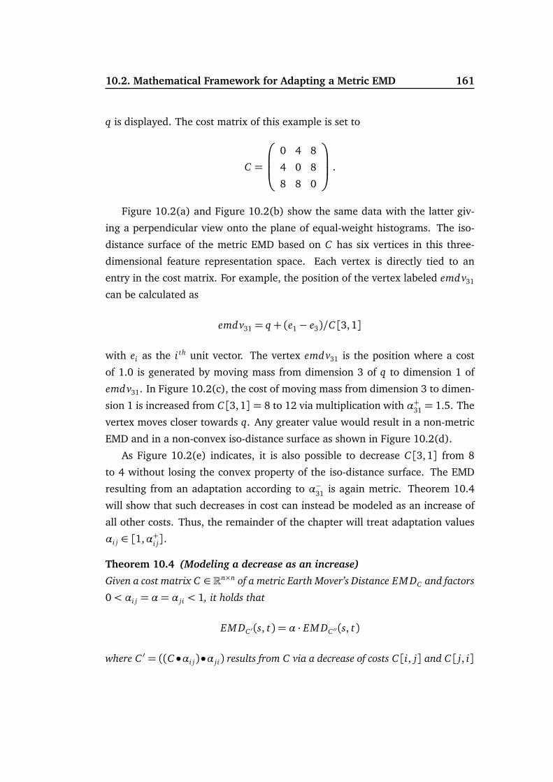
10.2. Mathematical Framework for Adapting a Metric EMD 161
q is displayed. The cost matrix of this example is set to
C =
0 4 8
4 0 8
8 8 0
.
Figure 10.2(a) and Figure 10.2(b) show the same data with the latter giv-
ing a perpendicular view onto the plane of equal-weight histograms. The iso-
distance surface of the metric EMD based on C has six vertices in this three-
dimensional feature representation space. Each vertex is directly tied to an
entry in the cost matrix. For example, the position of the vertex labeled emdv31
can be calculated as
emdv31 = q+ (e1− e3)/C[3,1]
with ei as the i th unit vector. The vertex emdv31 is the position where a cost
of 1.0 is generated by moving mass from dimension 3 of q to dimension 1 of
emdv31. In Figure 10.2(c), the cost of moving mass from dimension 3 to dimen-
sion 1 is increased from C[3, 1] = 8 to 12 via multiplication with α+31 = 1.5. The
vertex moves closer towards q. Any greater value would result in a non-metric
EMD and in a non-convex iso-distance surface as shown in Figure 10.2(d).
As Figure 10.2(e) indicates, it is also possible to decrease C[3, 1] from 8
to 4 without losing the convex property of the iso-distance surface. The EMD
resulting from an adaptation according to α−31 is again metric. Theorem 10.4
will show that such decreases in cost can instead be modeled as an increase of
all other costs. Thus, the remainder of the chapter will treat adaptation values
αi j ∈ [1,α+i j].
Theorem 10.4 (Modeling a decrease as an increase)
Given a cost matrix C ∈ Rn×n of a metric Earth Mover’s Distance EM DC and factors
0< αi j = α= α ji < 1, it holds that
EM DC ′(s, t) = α · EM DC ′′(s, t)
where C ′ = ((C •αi j)•α ji) results from C via a decrease of costs C[i, j] and C[ j, i]

162 Metric Adaptation of the Earth Mover’s Distance
and C ′′ results from C via an increase of all other costs by factor 1α.
Proof 10.4
The cost matrix C ′′ that arises from an increase of all costs other than C[i, j] and
C[ j, i] can be stated as C ′′ = 1α((C •αi j)•α ji). It only differs from C ′ in the factor
1α: C ′′ = 1
αC ′. A cost matrix uniformly scaled with factor 1
α> 1 yields the same
optimal flow F ∗ for the EMD. Thus,
α · EM DC ′′(s, t) =α ·n∑
i=1
n∑
j=1
F ∗[i, j]C ′′[i, j]
=α ·n∑
i=1
n∑
j=1
F ∗[i, j](1
αC ′)[i, j]
=α
α·
n∑
i=1
n∑
j=1
F ∗[i, j]C ′[i, j]
=EM DC ′(s, t).
Any adaptation of a metric EMD similarity measure via a symmetric decrease
in values C[i, j] and C[ j, i] can thus be modeled via an according increase of
all other cost values. Figure 10.2(f) shows that the iso-distance surface for the
EMD using matrix C ′′ equals the surface of Figure 10.2(e) except for scale. The
vertices emdv31 and emdv13 remain in their original position (cf. Figure 10.2(b))
while all other vertices move closer to q. In many similarity search algorithms,
the final scaling of the EMD values by factor α can either be skipped as only
the relative distance values are important (e.g., ranking and nearest-neighbor
queries) or can be incorporated in the similarity threshold (e.g., range queries).
10.2.2 Reconciling Adaptation Preferences with the Limits of
Adaptability
After discussing the limits of the adaptability that stem from the original met-
ric cost matrix in Section 10.2.1, the adaptation preferences are mapped to the
interval of valid cost increases [1,α+i j]. The specific way of determining adapta-
tion preferences will be abstracted from within this section. A short treatment
10.2. Mathematical Framework for Adapting a Metric EMD 163
of the topic is given in Section 10.2.3. For the remainder of this subsection, it
is assumed that preferred adaption values βi j ∈ [0,1] with βi j = β ji and βii = 0
are given. A value of βi j = 0 indicates a preference for no increase in cost while
a value of βi j = 1 indicates a preference for maximum possible cost increase for
transformations from dimension i to j. The aim is to find admissible modifica-
tion values αi j ∈ [1,α+i j] that reflect the proportionate relation of the preferred
adaptations βi j as much as possible. Ideally, βi j = h · βi′ j′ results in an h times
stronger relative increase of C[i, j] compared with C[i′, j′].
As a first step, intermediate modification factors eαi j ∈ [1,α+i j] that reflect the
proportionate adaptation preferences are defined.
Definition 10.3 (Intermediate modification factors)
Given a cost matrix C ∈ Rn×n of a metric Earth Mover’s Distance EM DC and
preferred cost increase values βi j ∈ [0,1], the intermediate adaptation factors eαi j
are defined by
eαi j = βi j · (α+min− 1) + 1
with α+min = minα+i′ j′ |(1 ≤ i′, j′ ≤ n) ∧ (i′ 6= j′) ∧ (βi′ j′ > 0) and α+i′ j′ according
to Theorem 10.2.
Since α+min is the smallest of all relevant upper bounds for the adaptation and
since βi j ≤ 1, all intermediate adaptation values are within admissible limits.
Furthermore, the definition of the upper bounds implicates that an increase of
one cost entry in the cost matrix does not decrease the limit of possible increases
for any other cost entry. Thus, all adaptations eαi j can be executed together
without jeopardizing the metric properties. With eA = [eαi j] as the matrix of
intermediate adaptation values, the intermediate adapted matrix eC is given byeC = C • eA. If there is a preference to increase a cost value that may on its own
not be increased without losing the metric property, the preferences can only
partially be heeded in this manner. If α+min = 1, the offending preference may
either be disregarded or (partially) be regarded in a later adaptation.
Factors eαi j from Definition 10.3 result in a metric adaptation of the cost
matrix within a minimal admissible interval. It is not guaranteed that the largest
admissible increase that respects the relative preferences has been found by eαi j.

164 Metric Adaptation of the Earth Mover’s Distance
By adding a single additional parameter λ ∈ [0,1], it is possible to control
the overall adaptation magnitude. Together with this parameter the adaptation
factors αi j can be defined as follows.
Definition 10.4 (Adaptation factors)
Given a cost matrix C ∈ Rn×n of a metric Earth Mover’s Distance EM DC , pre-
ferred cost increase values βi j ∈ [0,1], and an overall magnitude of adaptation λ,
adaptation factors αi j are defined as
αi j = λ ·ρ · (eαi j − 1) + 1
where ρ is to be chosen such that αi j ≤ α+i j for all 1 ≤ i, j ≤ n and αi j = α+i j for at
least one pair (i, j) for λ= 1.
The missing factor ρ that ensures that a maximum adaptation magnitude is
reached for λ= 1 can be derived from the smallest increase of the intermediate
factors (on a percentage basis).
Theorem 10.5
For αi j according to Definition 10.4 with λ= 1 and
ρ =min
(
α+i′ j′ − 1
eαi′ j′ − 1
(1≤ i′, j′ ≤ n)∧ (i′ 6= j′)∧ (βi′ j′ > 0)
)
it holds that
∃(i∗, j∗) :
αi∗ j∗ = α+i∗ j∗ ∧∀(i
′, j′) 6= (i∗, j∗) : αi′ j′ ≤ α+i′ j′
Proof 10.5
For (i∗, j∗) as a pair of indices for which ρ is minimal according to Theorem 10.5

10.2. Mathematical Framework for Adapting a Metric EMD 165
it holds:
αi∗ j∗ =λ ·ρ · (eαi∗ j∗ − 1) + 1
=α+i∗ j∗ − 1
eαi∗ j∗ − 1· (eαi∗ j∗ − 1) + 1
=α+i∗ j∗
For (i′, j′) 6= (i∗, j∗) with i′ 6= j′ and βi′ j′ > 0 it holds:
αi′ j′ =λ ·ρ · (eαi′ j′ − 1) + 1
≤1 ·ρ · (eαi′ j′ − 1) + 1 =α+i∗ j∗ − 1
eαi∗ j∗ − 1· (eαi′ j′ − 1) + 1
≤α+i′ j′ − 1
eαi′ j′ − 1· (eαi′ j′ − 1) + 1 =α+i′ j′
For i′ = j′ and for βi′ j′ = 0, it holds that αi′ j′ = 1 and thus the triangle
inequalities remain unaffected.
Definition 10.4 enables the metric adaptation C ′ = C • [αi j] of the Earth
Mover’s Distance on fixed-binning histograms based on cost increase preferences
βi j. A few exemplary choices for deriving preferences βi j from interaction with
the user are discussed next.
10.2.3 Determination of Adaptation Preferences
The proposed metric adaptation of the Earth Mover’s Distance modifies the cost
matrix of the EMD based on adaptation preferences βi j. The mathematical
framework is independent from the manner in which preferences βi j are deter-
mined. Some options for deriving according values heuristically are discussed
in the following paragraphs.
If elements from the feature space in which the ground distance of the EMD
is calculated can be illustrated appropriately, a user may be asked to assign
scores for the dissimilarity of pairs of histogram bin representatives. For ex-

166 Metric Adaptation of the Earth Mover’s Distance
ample, in the case of a color space as the feature space, two bin colors can be
shown to the user. An assessment on a scale from “identical/very similar” to
“very dissimilar” can then be mapped to appropriate values for βi j if the degree
of dissimilarity is not sufficiently reflected by the default cost matrix. It may
however be unreasonable to expect the user to be able to give consistent scores
for multiple feature pairs. In that case, it is possible to simplify the decision for
the user by presenting three features for which only the relative dissimilarity has
to be decided upon. E.g., given a turquoise bin representative, the user could
be asked to decide if it is to be treated as “more green” or “more blue” by asking
for the more similar color of the two. In this manner, mismatches of the default
ground distance and the perception of the user can be determined and turned
into preference values βi j.
Instead of asking for assessments in a conceivably abstract feature space,
techniques similar to those found in Relevance Feedback systems (cf. Chap-
ter 11) can be used to derive information regarding the perception of similarity
in the feature space based on feedback regarding the similarity of objects in a
database. Given sets of similar objects as determined by the user, it may be pos-
sible to draw conclusions regarding the relative perception of similarity in the
feature space from statistical information gathered for the feature representa-
tion of those objects. A related method is proposed in Section 11.2.3 of the next
chapter. Together with such data-based techniques the framework may be used
to form an EMD-specific Distance Metric Learning [YJ06] method.
10.3 Summary
This chapter proposed a mathematical framework for adapting a metric Earth
Mover’s Distance on fixed-binning histograms. Given a method to derive adap-
tation preferences, it produces an adapted Earth Mover’s Distance that is again
metric. This allows for query processing algorithms and optimizations that are
based on metric properties to be utilized.
Guided by insight gained through analyzing the iso-distance surface of the
EMD, limitations of metric adaptations are derived based on the initial cost

10.3. Summary 167
matrix of the EMD. Next, a method for mapping multiple given adaptation pref-
erences to adaptation factors was proposed such that the resulting EMD both
conforms to the limitations of metric adaptation and proportionally reflects the
adaptation preferences. Finally, several options for deriving adaptation prefer-
ences were pointed out.


Chapter 11
Exploring Multimedia Databases
via Relevance Feedback
In this chapter, a technique to adapt the EMD to feedback from the user of a
similarity search system is proposed. It is applicable to both fixed-binning his-
tograms and adaptive-binning histograms (signatures). In contrast to the last
chapter, the metric property is sacrificed in return for an improved flexibility that
can be exploited to increase the retrieval effectiveness of the similarity search
system. While not the focus of this chapter, some methods that improve the effi-
ciency of the approach can still be applied without relying on metric properties
of the EMD.
11.1 Introduction
Two common challenges of distance-based similarity search are the formulation
of the query and the definition of a suitable distance measure. Query objects
in similarity search based on the query-by-example paradigm by definition can
be no more than imprecise descriptions of what users are looking for in the
database. Additionally, even for high-quality similarity models, the distance
measure can only be an approximation of the users’ notion of similarity as said
notion may be different from application to application, from user to user, and
ultimately from query to query.
169

170 Exploring Multimedia Databases via Relevance Feedback
feedback
results
feedback system
similarity model
database
user
Figure 11.1: The Relevance Feedback Loop
Distance-based Relevance Feedback (RF) approaches [Roc71, ISF98, OBM04,
FdSTGF08] address these issues on the basis of relevance information gathered
from the user. They aim to increasingly reflect the user’s notion of similarity and
return a larger amount of relevant objects from the database. Returning more
relevant objects in earlier iterations turns effectiveness of the similarity model
into efficiency for the user in this scenario.
An extension of the traditional feedback loop (cf. Fig. 11.1) is proposed
in this chapter that takes an adaptable similarity measure (i.e., the EMD) and
improves the quality of the search result through back-testing based on prior
feedback. To this end, the similarity adaptation is formulated as an optimiza-
tion problem that minimizes discrepancies between relevance information and
the distance measure. Two statistics-based heuristics for the adaption of the
EMD to feedback information are introduced as initializations to the optimiza-
tion process – one for fixed-binning histograms and one for adaptive-binning
histograms. Experiments on real world databases show that significantly more
relevant objects are returned in fewer iterations resulting in a faster exploration
of the database than existing EMD-based query movement techniques allow for.
11.1.1 Related Work
The distance-based Relevance Feedback framework allows for the utilization of
database techniques such as spatial access methods. As an early example of

11.1. Introduction 171
Relevance Feedback for the vector space model, [Roc71] proposed the reformu-
lation of a query by moving the vector that represents the query towards known
relevant objects and away from known non-relevant objects. Systems such as
MindReader [ISF98] and MARS [OBM04] complement the query movement by
determining an adapted distance function based on (co-)variance information
present in the feedback.
In the text retrieval domain, an algorithm for basing the adaptation of the
query on an iterative optimization process that takes the user’s feedback into
account was proposed in [BS95]. For their text retrieval system, a query con-
sists of a number of terms and according weights that can be updated by the
optimization process. Another optimization-based RF approach that adapts a
similarity measure was recently presented in [FdSTGF08]. It uses genetic pro-
gramming to optimize the arithmetic combination of a number of general sim-
ilarity functions. Inspired by the Simulated Annealing (SA) optimization tech-
nique, [CFPF03, CPFGF05] propose a system where each iteration of a feed-
back process is a single iteration in a search process that becomes more and
more focused over time akin to the idea of SA. Some image retrieval systems
based on RF break with the convention that each object in the database has to
be described by a single vector. Region-based RF [JLZ+03, LH08] exploits the
position, size, shape, and/or feature distribution of connected regions within
images. Recently, Li et al. [LH08] proposed representing objects as graphs with
nodes that represent image regions and edges between nodes of neighboring
regions. The nodes are annotated with feature information for the correspond-
ing regions. Their RF process uses two optimization steps – one for matching
graphs and the other for updating the query graph. While the features stored
in the nodes of the query graph are updated using relevance information, the
structure of the query graph itself remains unchanged, which limits the flexibil-
ity of the approach.
In the limited number of Relevance Feedback approaches where the EMD
is utilized as a similarity measure, the EMD itself is not adapted to the user
feedback but instead the approaches rely on its good default retrieval effective-
ness. In [RT01], a Relevance Feedback approach termed Query-by-Refinement is
proposed that combines feature representations from relevant objects to a rep-

172 Exploring Multimedia Databases via Relevance Feedback
resentation of a new virtual query object. Thus, Query-by-Refinement performs
query adaptation only but the EMD itself remains unchanged. In [JLZ+03], the
EMD is used as a kernel function for an SVM-based Relevance Feedback system.
The query results are iteratively improved by re-weighting the query signature
and training an SVM classifier according to user feedback. The feedback is not
used to adapt the underlying EMD.
The flexibility of the EMD with regards to its ground distance will be ex-
ploited in the following sections by adapting the ground distance based on feed-
back from the user.
11.2 Relevance Feedback with the Earth Mover’s
Distance
The main Relevance Feedback process for the Earth Mover’s Distance is formally
introduced in section 11.2.1. Section 11.2.2 describes the proposed optimization-
based extension of the feedback process that adapts a similarity measure such
that the discrepancy between all user-given feedback and the distance measure
is minimized. It is not strictly specific to the Earth Mover’s Distance and can be
adopted in conjunction with other flexible similarity measures. Sections 11.2.3
and 11.2.4 detail proposals for EMD-based Relevance Feedback on feature his-
tograms and on signatures. A statistics-based heuristic for adapting the Earth
Mover’s Distance is proposed in each section. The heuristics can be used on
their own or serve as initial solutions for the optimization-based extension from
Section 11.2.2.
11.2.1 The Feedback Process
Algorithm 11.1 lists pseudo-code for the Relevance Feedback process that is the
basis for the remainder of the chapter. It acts as a framework for all following
techniques in that it takes as input parameters two procedures for adapting the
query representation and the ground distance of the EMD. Differing implemen-
tations will be defined in later sections leading to differing relevance feedback
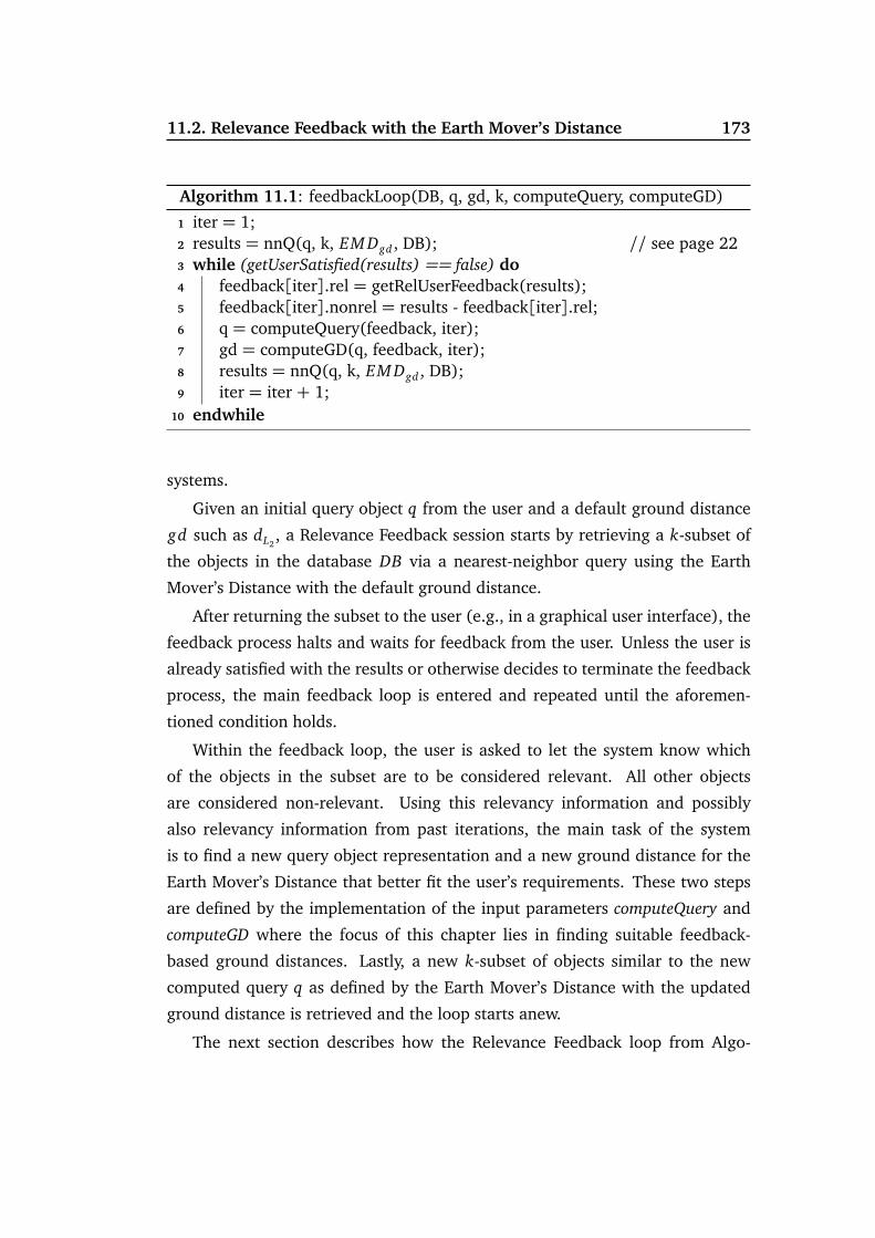
11.2. Relevance Feedback with the Earth Mover’s Distance 173
Algorithm 11.1: feedbackLoop(DB, q, gd, k, computeQuery, computeGD)
iter = 1;1
results = nnQ(q, k, EM Dgd , DB); // see page 222
while (getUserSatisfied(results) == false) do3
feedback[iter].rel = getRelUserFeedback(results);4
feedback[iter].nonrel = results - feedback[iter].rel;5
q = computeQuery(feedback, iter);6
gd = computeGD(q, feedback, iter);7
results = nnQ(q, k, EM Dgd , DB);8
iter = iter + 1;9
endwhile10
systems.
Given an initial query object q from the user and a default ground distance
gd such as dL2, a Relevance Feedback session starts by retrieving a k-subset of
the objects in the database DB via a nearest-neighbor query using the Earth
Mover’s Distance with the default ground distance.
After returning the subset to the user (e.g., in a graphical user interface), the
feedback process halts and waits for feedback from the user. Unless the user is
already satisfied with the results or otherwise decides to terminate the feedback
process, the main feedback loop is entered and repeated until the aforemen-
tioned condition holds.
Within the feedback loop, the user is asked to let the system know which
of the objects in the subset are to be considered relevant. All other objects
are considered non-relevant. Using this relevancy information and possibly
also relevancy information from past iterations, the main task of the system
is to find a new query object representation and a new ground distance for the
Earth Mover’s Distance that better fit the user’s requirements. These two steps
are defined by the implementation of the input parameters computeQuery and
computeGD where the focus of this chapter lies in finding suitable feedback-
based ground distances. Lastly, a new k-subset of objects similar to the new
computed query q as defined by the Earth Mover’s Distance with the updated
ground distance is retrieved and the loop starts anew.
The next section describes how the Relevance Feedback loop from Algo-

174 Exploring Multimedia Databases via Relevance Feedback
feedback
resultsadapted similarity
model
similarity model, feedback
Loop Extension
Figure 11.2: The extended Relevance Feedback Loop
rithm 11.1 can be extended with an optimization-based step that improves on
heuristically computed ground distances.
11.2.2 Optimization of the Similarity Measure
While heuristics for computeGD such as the ones presented in sections 11.2.3
and 11.2.4 are able to produce ground distances for the EMD that enable the
retrieval of more relevant database objects than is possible without adapting
the ground distance, they do not necessarily reflect the user’s feedback in an
optimal way. Instead of returning the results as determined by the EMD based
on the heuristic ground distance, the proposed extension to the feedback loop
depicted in Figure 11.2 first tests if the ground distance can be improved upon.
The adaptation of the ground distance by the extension is phrased as an opti-
mization problem that ties the ground distance as the optimization variable to
the consistency of the EMD-based similarity model with the user feedback as the
optimization criterion. The approach is conceptually related to [BS95], where
a greedy optimization was chosen to find an improved query representation via
changing term weights in text retrieval. Unlike [BS95], the similarity measure
itself is optimized here. This concept is not exclusively tied to the EMD and can
be transferred to other flexible distance measures such as quadratic form dis-
tances where the orientation and the extent of the ellipsoid-shaped iso-distance
surface would be subject to the optimization.

11.2. Relevance Feedback with the Earth Mover’s Distance 175
Adaptation as an Optimization Problem
The central building block of phrasing the adaptation of a similarity measure
as an optimization problem is the definition of a suitable optimization criterion.
Obviously, the optimization process cannot know if including an arbitrary object
from the database in the result set will increase the number of relevant objects
returned to the user. It is not possible to adapt the similarity measure, compute a
new k-nearest-neighbors set and check if the adaptation was favorable in terms
of, for instance, recall/precision since the optimization process does not have
access to the user to determine the quality of the result. Otherwise the extension
would merely be another feedback loop.
However, it is possible to test if the adaptation resulted in a similarity mea-
sure that is consistent with the user’s past feedback. To this end, the objects from
all previous result sets are ranked according to the adapted similarity measure.
A good measure results in a ranking of the feedback where the objects already
identified as relevant appear before those not identified as relevant. An unsuit-
able measure has all non-relevant objects appear before the relevant ones.
To automatically decide how beneficial a given ranking of the feedback is,
a quality measure that reduces the ranking to a single value is required. One
example of such a quality measure is given in the following definition. Other
quality measures for rankings from the literature can also be used.
Definition 11.1 (Average Precision at Relevant Positions)
Given a database DB of objects, relevant objects ℜ ⊆ DB, and a ranking function
rank : DB→ N1, the average precision of the ranking is defined as
avgPrecision(rank,ℜ) =1
|ℜ|
∑
o∈ℜ
|o ∈ ℜ|rank(o)≤ rank(o)|rank(o)
Intuitively, a higher number of relevant objects appearing at the front of
the ranking results in a higher avgPrecision-value. A ranking with all relevant
objects at the front of the ranking has the optimal value of 1. The following
table gives an example for four different rankings where relevant objects are
denoted by 1 and all other objects are denoted by 0.

176 Exploring Multimedia Databases via Relevance Feedback
ranking avgPrecision
1 1 1 1 0 0 0 1.000
1 1 1 0 1 0 0 0.950
0 0 1 1 1 1 0 0.525
0 0 0 1 1 1 1 0.430
Using a measure such as avgPrecision for judging the quality of a ranking, it
is possible to formulate the similarity measure adaptation as follows.
Definition 11.2 (Optimal Relevancy-Consistent Similarity Measure)
Given query q, database DB, and relevant objects ℜ ⊆ DB, the optimal relevancy-
consistent similarity measure Sim∗ with respect to avgPrecision from Definition 11.1
is
Sim∗ = argmaxSimavgPrecision(rankSim,ℜ)
where rankSim determines the ranking of objects in DB by descending similarity to
q according to similarity measure Sim.
During the Relevance Feedback process, the quality measure is evaluated
on the subset of the database for which the user has already given relevancy
information to the system. By optimizing the quality measure on the objects fed
back to the system, the final similarity measure will be one that in the best case
separates known relevant from known non-relevant objects. Objects for which
the user has not given any feedback are not taken into account as the system
cannot know if they are to be considered relevant or not without asking the user.
The Optimization Algorithm
The goal of the optimization algorithm in this section is to find Sim∗ of Defi-
nition 11.2. The distance and ranking computations necessary to calculate the
value of the optimization criterion make the influence that the parameters of
the similarity measure have on this optimization criterion all but trivial and
an analytical optimization infeasible. This is especially true in the case of the
Earth Mover’s Distance, where the parameter that defines the EMD-based sim-
ilarity measure is the ground distance function and where the computation of

11.2. Relevance Feedback with the Earth Mover’s Distance 177
Algorithm 11.2: optimize(C, q, feedback)
extern maxIter, coolFactor, T 0;1
optIter = 0; T = T 0;2
avgpOld = avgpBest = avgpNew = avgPrecision(C, q, feedback);3
Cbest = C;4
while (optIter < maxIter) do5
C’ = modify(C) ; // move in solution space6
avgpNew = avgPrecision(C’, q, feedback); // evaluate solution7
if (avgpNew≥avgpOld) || (rand()<exp((avgpNew-avgpOld)/T)) then8
C= C’; avgpOld = avgpNew ; // adopt new solution9
if (avgpNew ≥ avgpBest) then10
Cbest = C’; avgpBest = avgpNew ; // remember best solution11
endif12
endif13
T = T * coolingFactor ; // turn search less erratic14
optIter = optIter + 1;15
endwhile16
return Cbest;17
the optimization criterion requires the iterative optimization of multiple trans-
formation problems according to Definition 7.2. However, there is a subclass of
optimization algorithms that is well-suited for finding an approximate solution
this situation.
Algorithm 11.2 is an instance of the family of probabilistic optimization
heuristics referred to as Simulated Annealing algorithms [KGV83]. The main
idea is to start the optimization at a given point in the solution space (i.e., pa-
rameter collection C that defines the similarity measure) and randomly navigate
through the solution space (via procedure modify) while evaluating the opti-
mization criterion (avgPrecision) on the way. Unlike greedy algorithms, worse
solutions can temporarily be adopted with a certain probability in order to over-
come local optimums. The worse a solution is, the less likely is its adoption. In
addition, the probability also decreases over time as the so-called temperature
of the optimization process (T) tends towards zero. The optimization termi-
nates after a set number of iterations (maxIter). In this fashion, the algorithm
first moves rather erratically while looking for regions with good solutions. As it

178 Exploring Multimedia Databases via Relevance Feedback
0%
20%
40%
60%
80%
100%
1 101 201 301 401
aver
age p
reci
sion
optimization iteration
Figure 11.3: Optimization progress over 500 iterations
progresses, it slowly converges towards a greedy algorithm. At the end, the best
solution found during the optimization process is returned. Figure 11.3 shows
four examples of the progress. The average precision of the currently adopted
solution (avgpOld) may at first decrease in order to get out of local maximums.
In later iterations, worse solutions are rarely adopted.
Choices of the annealing parameters coolFactor, maxIter, and T 0 that proved
suitable for the EMD Relevance Feedback process are listed the evaluation sec-
tion. The modify procedure depends on the variability of the similarity measure.
EMD-specific definitions are given in sections 11.2.3 and 11.2.4. The extended
feedback framework presented in this section can be utilized to optimize other
adaptable distance functions by defining a suitable modification procedure.
11.2.3 EMD-based Relevance Feedback on Histograms
Unlike feature signatures, fixed-binning histograms∗ share a common partition-
ing of the feature space. As a consequence, it suffices to partially define the
ground distance gd between those partitions. Adapting the Earth Mover’s Dis-
∗Referred to as histograms in the rest of the chapter.

11.2. Relevance Feedback with the Earth Mover’s Distance 179
Algorithm 11.3: computeGD-QM(q, feedback, iter)
return dL2;1
tance is reduced to adapting a finite set of distance values that are specified in a
cost matrix C ∈ Rn×n where n is the dimensionality of the histograms. Possibil-
ities and limits of adapting a metric cost matrix C based on directly expressed
user preferences were described in Chapter 10. This section will develop an
automatic derivation of a cost matrix based on user feedback.
In the following two subsections, the adaptation of the query representation
q and a statistics-based heuristic for adapting the ground distance of the EMD
based on the user feedback are described. The subsection hereafter shows how
the optimization algorithm from section 11.2.2 ties in with the partially defined
ground distance for the case of fixed-binning histograms.
Query Adaptation
Since the focus of this chapter is on adapting the similarity measure, a sim-
ple query reformulation that has been used in several distance-based Relevance
Feedback systems is adopted.
Definition 11.3 (Query adaptation)
Given a set ℜi of relevant fixed-binning feature histograms in iteration i of the
relevance feedback process, the new query representation qi+1 for the next iteration
is defined as
qi+1 =1
|ℜi|
∑
o∈ℜi
o
The new query qi+1 is shifted to the center of relevant feature histograms
in the feature representation space. Passing an according algorithm and the
procedure computeGD-QM listed in Algorithm 11.3 to the feedback algorithm
from page 173 results in a baseline Relevance Feedback process that uses the
Euclidean distance as the fixed ground distance for the EMD and moves the
query to the center of relevant objects after each iteration.

180 Exploring Multimedia Databases via Relevance Feedback
Algorithm 11.4: computeGD-Histogram-Heur(q, feedback, iter)
if |feedback[iter].rel| ≤ 1 then return dL2;1
CHeur = computeGD-Histogram-Heur-Matrix(q, feedback, iter);2
return new CostMatrixDistance(CHeur);3
Algorithm 11.5: computeGD-Histogram-Heur-Matrix(q, feedback, iter)
Σ∗ = minFixedInverse(covmatrix(feedback[iter].rel));1
for i= 1 to |Σ∗.rows| do2
for j= 1 to |Σ∗.cols| do3
CHeur[i, j] = sqrt(Σ∗[i, i] + Σ∗[ j, j] - 2Σ∗[i, j]);4
endfor5
endfor6
return CHeur;7
Heuristic for Adapting the Ground Distance
The ground distance of the Earth Mover’s Distance on feature histograms de-
scribes transformation costs between individual feature space partitions shared
by all feature histograms. The ground distance can be partially but sufficiently
specified by a cost matrix C . Here, the transformation costs of the Earth Mover’s
Distance shall be defined on the basis of the dissimilarity between the feature
space partitions common to all relevant objects ℜi. The dissimilarity between
feature space partitions is estimated as the dissimilarity between histograms of
objects that have all features concentrated in a single partition. Thus, the aim is
to define cost matrix entry C[i, j] as
C[i, j]≈ dissimilarity(ei, e j)
where ei and e j are unit vectors with the same dimensionality as the feature
histograms. The dissimilarity between those histograms is to be derived from
the user feedback.
Based on the feature distribution described by the histograms of the rele-
vant objects, the Mahalanobis distance defines a dissimilarity measure that fits
the requirements. The Mahalanobis distance for a given feature distribution is

11.2. Relevance Feedback with the Earth Mover’s Distance 181
computed using its inverse covariance matrix Σ−1:
dMan−Σ(s, t) =p
(s− t) ·Σ−1 · (s− t)T
Using the Mahalanobis distance on the histograms ei and e j to determine a
dissimilarity between feature space partitions i and j, appropriate transforma-
tion costs C[i, j] can be computed.
C[i, j] = dMan−Σ(ei, e j) (11.1)
=p
(ei − e j) ·Σ−1 · (ei − e j)T
=p
Σ−1[i, i] +Σ−1[ j, j]− 2 ·Σ−1[i, j]
The inverse covariance matrix Σ−1 is derived from the feature histograms de-
termined as relevant in the current feedback iteration by the user. Directions in
the feature representation space with a large variability in the feedback result
in a small transformation cost while directions with a compact distribution of
values result in a high transformation cost. The intuition of the heuristic is that
compact feedback represents a preference by the user to stay in the according
area of the feature representation space.
If the number of relevant feature histograms is small, the inverse covariance
matrix may not be defined since some of the eigenvalues of the covariance ma-
trix equal zero. Intuitively, this means that there is not enough information in
the feedback to estimate dissimilarity in all directions of the feature representa-
tion space. To overcome this obstacle, eigenvalues equal to zero can be replaced
with the smallest eigenvalue greater than zero during the matrix inversion pro-
cess as suggested in [YX03]. This effectively sets the dissimilarity of directions
without variability to a high value without making them infinitely dissimilar.
The procedure computeGD-Histogram-Heur of Algorithm 11.4 computes the
proposed heuristic adaptation of the Earth Mover’s Distance on fixed-binning
histograms with the help of Algorithm 11.5, which reflects equation (11.1) with
accommodations for eigenvalues of zero. The result is a distance function that
is defined via CHeur ∈ Rn×n for the n feature partition representatives of the
histograms.

182 Exploring Multimedia Databases via Relevance Feedback
Algorithm 11.6: computeGD-Histogram-Opt(q, feedback, iter)
if |feedback[iter].rel| ≤ 1 then return dL2;1
CHeur = computeGD-Histogram-Heur-Matrix(q, feedback, iter);2
COpt = optimize(CHeur , q, feedback);3
return new CostMatrixDistance(COpt);4
Similarity Optimization
To apply the optimization-based similarity adaptation from section 11.2.2 to the
EMD on fixed-binning feature histograms, two things are required:
1. a mapping from the ground distance of the EMD to the parameter collec-
tion that the optimization algorithm treats as possible solutions and
2. a method that randomly modifies the parameter collection to navigate
through the solution space.
The parameter that defines the EMD is its ground distance in the form of a
cost matrix. As an initial solution, the heuristically determined cost matrix CHeur
can be passed to the optimization algorithm 11.2.
Algorithm 11.7 modifies a cost matrix according to the externally set param-
eter modRowWeight that determines the modification magnitude. Each row in
the cost matrix reflects the transformation costs from one histogram partition of
the query object to the histogram partitions of objects in the database. For each
row, modRowWeight determines how much the row is to be changed. The total
size of the matrix is n× n where n is the dimensionality of the histograms.
To update the row, its entries are randomly partitioned into two sets of equal
cardinality ±1. The entries of the first partition are increased by modRowWeight
percent of the sum of row costs while the entries of the second partition are
decreased accordingly. The roles of the two entry partitions are switched if a
decrease of the second partition would lead to negative costs. One of the two
modifications is always possible with modRowWeight from [0,0.5). Lastly, the
new cost matrix is returned to the optimization algorithm for evaluation via the
average precision measure and possibly further iterative modification.

11.2. Relevance Feedback with the Earth Mover’s Distance 183
Algorithm 11.7: modify(C)
extern modRowWeight;1
C’ = C;2
for row ∈ C ′.rows do3
delta = |row|Σ * modRowWeight;4
(entries 1, entries2) = randomPartitioning(row);5
sum1 = |entries1|Σ; sum2 = |entries2|Σ;6
if sum2 ≤ delta then delta = -delta;7
for entry1 ∈ entries1 do entry1 = entry1 * (sum1 + delta) / sum1;8
for entry2 ∈ entries2 do entry2 = entry2 * (sum2 - delta) / sum2;9
endfor10
return C’;11
11.2.4 EMD-based Relevance Feedback on Signatures
As discussed in Section 1.1, adaptive-binning histograms or feature signatures of
the form s =
(r1, w1), . . . , (rn, wn)
are more flexible in representing a feature
distribution than fixed-binning histograms. In this section, the flexibility of the
EMD on signatures is exploited for Relevance Feedback.
The structure of this section follows the same outline as the section on EMD
adaptation for fixed-binning histograms. After a short description of the query
adaptation, a statistics-based heuristic for the derivation of a ground distance
from user feedback is proposed and then optimized via the extension to the
feedback loop from Section 11.2.2.
Query Adaptation
There exist some methods for combining several feature signatures into a new
signature in the literature [RT01, JLZ+03]. They are based on region reweight-
ing [JLZ+03] and clustering of partition representatives [RT01]. Since the fo-
cus here is on adapting the similarity measure, the approach from [RT01]with a
simple k-means algorithm was implemented for the experiments of Section 11.3.
The main idea is to collect all signature components from all relevant signatures,
cluster their representatives, and set the new weights to the median weight of
the components in the clusters. Clusters with contributions from less than half of

184 Exploring Multimedia Databases via Relevance Feedback
Algorithm 11.8: computeGD-Signature-Heur(q, feedback, iter)
if |feedback[iter].rel| ≤ 1 then return dL2;1
CHeur = computeGD-Signature-Heur-Matrix(q, feedback, iter);2
return new Distance(CHeur);3
the relevant signatures are removed and a normalization of the weights ensures
that the total weight is not greater than 1. Together with a fixed Euclidean
ground distance produced by computeGD-QM from page 179, this reflects the
Query-by-Refinement Relevance Feedback algorithm from [RT01] and serves as
a baseline for the similarity adaptation algorithms on feature signatures pro-
posed in the following subsections.
Heuristic for Adapting the Ground Distance
EMD-based Relevance Feedback on signatures requires a new adaptation heuris-
tic. Since the partitioning representatives are different for every object in the
database, their signatures do not live in a simple n-dimensional space for which
statistical information could be captured in the same way as in Section 11.2.3.
In addition, a cost matrix does not suffice in the signature case. Instead, a
ground distance gd : FS× FS→ R has to be defined for the feature space FS in
which the partitioning representatives of the signature components are situated.
The proposal in this section defines a ground distance based on the variance
information of the partitioning representatives derived from feedback informa-
tion. The key to defining a suitable ground distance is the observation that the
ground distance does in fact not have to be defined for each pair of points in
FS but only for
⋃
(rq ,wq)∈q rq
× FS. For each iteration of the feedback process,
the similarity search process computes the Earth Mover’s Distance from a single
object q to objects in the database. Thus, a ground distance that defines distance
values from the partitioning representatives of q to points in FS fully suffices.
The heuristic for signatures utilizes the local variance information of the
feedback around the query representatives to partially define the ground dis-
tance. If representatives from the feedback are within a compact region in a
dimension of the feature space around a query representative, the heuristic as-

11.2. Relevance Feedback with the Earth Mover’s Distance 185
Algorithm 11.9: computeGD-Signature-Heur-Matrix(q, feedback, iter)
// assign feedback representatives to query representativesfor s ∈ feedback[iter].rel do1
for (r s, ws) ∈ s do2
i∗ = argminidL2(r s, rq
i )|(rqi , wq
i ) ∈ q;3
Subset[i∗] = Subset[i∗] ∪r s; // remember that r s is closest to rqi∗4
endfor5
endfor6
// for query representative, compute variance of assigned feedbackfor i= 1 to |q| do7
varianceVector = variance(Subset[i]);8
// for each representative dimensionfor j = 1 to n do CHeur[i, j] = 1 / varianceVector[j];9
// normalize row to sum of 1.0for j = 1 to n do CHeur[i, j] = CHeur[i, j] / |CHeur[i]|Σ;10
endfor11
return CHeur;12
signs a high cost to transports out of this region. If the user picked relevant
objects with a large variance around a query representative, the according cost
is chosen to be low.
The procedure computeGD-Signature-Heur in Algorithm 11.8 takes all signa-
tures of objects deemed relevant by the user in the current feedback iteration
and assigns all their representatives to the closest query representative via Al-
gorithm 11.9. For each query representative rqi , Subset[i] collects the repre-
sentatives from the feedback that are closer to rqi than to any rq
j (i 6= j). The
dimension-wise variance information of Subset[i] is stored in the ith row of a
matrix CHeur , where CHeur[i, j] is normalized inverse variance of Subset[i] in
the jth dimension of the feature space FS. The matrix CHeur is of size |q| × n
where |q| is the number of representatives in the query signature and n is the
dimensionality of the feature space FS.
Using the variance information in CHeur , the ground distance between a
query representative rqi and an arbitrary other representative r ∈ FS is com-

186 Exploring Multimedia Databases via Relevance Feedback
r
rq1
rq3
rq2
CHeur[1
,2]-1
CHeur[1,1]-1
Figure 11.4: EMD ground distance example for signatures
puted as a weighted Euclidean distance
gd(rqi , r) =
p
(rqi − r) · diag(CHeur[i]) · (rq
i − r)T
where diag(CHeur[i]) is a diagonal matrix with the values from the ith row of
CHeur as its entries. Figure 11.4 shows an example for a representative r from
a signature of a database object and three query representatives r1, r2, r3 with
the corresponding iso-distance lines of the weighted Euclidean distances. In
the example, the first query representative has a higher variance in the vertical
dimension than in the horizontal dimension. The opposite holds for the sec-
ond representative while the third one has equal variance in both dimensions.
The cost for transforming features from rqi to r is defined by the local variance
information around rqi only.
The resulting ground distance thus adapts the EMD to the user’s feedback
by assigning high cost to mass transports in directions where the low variance
indicates compact feedback information around a query representative. Similar
to the heuristic for histograms, the idea is that compact feedback represents a
preference by the user to stay in the area of the feature space.
Similarity Optimization
The optimization-based adaptation of the ground distance for feature signatures
via computeGD-Signature-Opt is built on the same concepts as the optimization

11.2. Relevance Feedback with the Earth Mover’s Distance 187
Algorithm 11.10: computeGD-Signature-Opt(q, feedback, iter)
if |feedback[iter].rel| ≤ 1 then return dL2;1
CHeur = computeGD-Signature-Heur-Matrix(q, feedback, iter);2
COpt = optimize(CHeur , q, feedback);3
return new Distance(COpt);4
for the histograms. In fact, the same implementation for the modification of
intermediate solutions during the optimization can be used. However, the in-
terpretation is different in one key aspect. As described in the last section,
CHeur consists of rows with weights for weighted Euclidean distances and not of
transformation costs. The updating algorithm modify thus adapts these weights
for each individual query representative when it modifies a row of CHeur . This
modification during the optimization process translates to an adaptation of the
extents of the iso-distance ellipsoid in the example of Figure 11.4.
11.2.5 Efficient Query Processing
While not the focus of this chapter, it is worthwhile to consider options to speed
up both the k-nearest-neighbor computation in Algorithm 11.1 and the rank-
ing computation in the Algorithm 11.2 in order to achieve interactive query
processing times. For the k-nearest-neighbor computation within a multimedia
database, multi-step retrieval techniques from [AWS06] are well-suited to cope
with the changing nature of the transformation cost matrix in the feedback ap-
proach. In particular, the lower bound LBI M which is based on a constraint
relaxation of the EMD showed a very good selectivity and good computation
times in a prototype implementation. For feature signatures with unequal to-
tal weights, LBI M has to be computed in a slightly adapted manner (i.e., by
transforming in the global cost order instead of the dimension-wise order). The
indexing technique from Chapter 9 is applicable in the histogram case. Due
to their lower-bounding property, these multi-step retrieval techniques return
results fast without loss of quality.
A further speed-up can be achieved by trading quality for efficiency. For the
optimization process, the maximum iteration count can be decreased resulting

188 Exploring Multimedia Databases via Relevance Feedback
(a) PHOTO (b) ALOI
Figure 11.5: Query images for the PHOTO and the ALOI databases
in a less optimized similarity model. Additionally, the EMD computation re-
quired to calculate the ranking of the relevant objects within the target function
of the optimization can be replaced with an approximate measure such as LBI M .
Finally, the CPU-bound ranking computations on the feedback in the opti-
mization algorithm can easily be parallelized for multi-core systems.
As the focus of this chapter is on retrieving satisfactory query results with
fewer feedback iterations, only quality-preserving measures were implemented
in the evaluation prototype (LBI M -based filtering and parallel EMD computa-
tion). On a dual Intel XEON E5420 server with 2.5GHz, typical query process-
ing times for the experiments detailed in the evaluation section were around 1.5
seconds.
11.3 Experiments
To evaluate whether the adaptation of the EMD ground distance can improve the
retrieval effectiveness over the Query-By-Refinement [RT01] method from the
literature that relies on query movement alone, a series of automated Relevance
Feedback runs were performed. The employed databases and the experimental
setup are detailed in Section 11.3.1 with Section 11.3.2 and 11.3.3 giving the
results for the adaptation of the EMD on fixed-binning feature histograms and
feature signatures.

11.3. Experiments 189
11.3.1 Setup and Datasets
All experiments were conducted using features extracted from two image data-
bases. The first database (PHOTO) includes 59,896 color photographs and im-
ages from a wide variety of themes. Each theme includes 99-100 images. The
second database (ALOI) includes 72,000 freely available images of 1,000 objects
that were physically rotated around the vertical axis in 5 degree steps [GBS05].The variation per object is much smaller than the variation per theme in the
PHOTO database. In addition, the images in ALOI exhibit a homogeneous black
background. For all images, 20-dimensional histograms were extracted using
a sampled k-means clustering of features from a 7-dimensional feature space
(2 position components, 3 CIE Lab color components, and contrast & coarse-
ness texture components). Signatures with up to 20 components were created
using the same clustering method per image instead of per database plus a post-
processing step to remove clusters that largely contained noise. For both data-
bases, 20 themes / objects were chosen as relevant for 20 automated feedback
runs. The choice was random for the ALOI database. For the PHOTO data-
base, the visual features were often drastically different for images even within
single themes. Given the low-level feature extraction process detailed above,
themes like “recreation” and “sports” exhibit a very large visual diversity within
the themes and significant overlap among the themes. They are thus not suit-
able for the automated evaluation method used here. To address this issue, the
themes were sorted by ascending approximate overlap with other themes and
twenty themes with limited overlap were chosen while excluding themes that
exhibited hardly any feature diversity. Figure 11.5 show the initial query images
that were randomly chosen for the relevant themes/objects. The diversity per
relevant PHOTO theme is still vastly greater than the diversity per ALOI object.
Given the query objects, the first feedback iteration was started by retrieving
the k closest objects according to the Earth Mover’s Distance with a Euclidean
ground distance. Parameter k was set to equal the number of relevant images
(99-100 for PHOTO and 72 for ALOI) such that the optimal result could po-
tentially be attained. The k images together with the relevant/non-relevant
rating derived from the theme/object information were then used to generate

190 Exploring Multimedia Databases via Relevance Feedback
automated feedback for the next iteration. After each iteration, precision/recall
data was collected by ranking the database up to the point where all relevant
images were found. A precision/recall value of 0.75/0.5 for 72 relevant objects,
for example, means that ranking objects according to their descending similar-
ity value until 0.5 · 72 = 36 relevant objects are found on average produced
36/0.75 = 48 objects total and 48 · (1− 0.75) = 12 non-relevant objects. The
precision/recall curves are computed as described in [MRS08] and averaged
over the 20 queries. The first iteration always starts with a precision value of
1.0 since the 20 initial queries are contained in the database. Given a data-
base (PHOTO or ALOI) and a feature representation (histograms or signatures),
the first iteration is identical for all adaptation approaches (query movement,
heuristic EMD adaptation, and optimization-based EMD adaptation) since no
feedback has been collected up to that point.
The starting temperature T 0 of the optimization process was set to the largest
possible difference in average precision which is |ℑ||ℜ|·∑|ℑ|+|ℜ|
i=|ℑ|+11i
where |ℜ| is the
number of relevant objects and |ℑ| the number of non-relevant objects present
in the feedback. The number of iterations was limited to maxIter = 500 while
the modification magnitude was set to modRowWeight = 5%. Preliminary ex-
periments showed that the optimization on signatures was able to benefit from
a slower temperature decrease compared with the optimization on histograms.
A value of coolFactor = 0.85 was used for all signatures experiments while 0.8
was used for the histogram experiments.
11.3.2 EMD Adaptation for Fixed-Binning Feature Histograms
Figures 11.6 and 11.7 show empirical results for the two histogram databases.
The baseline algorithm (a) with a fixed Euclidean ground distance is contrasted
with the proposed heuristic and optimization-based adaptations in (b) and (c).
For both databases, the adaptation approaches consistently show consider-
able improvements regarding the quality of the query results. The second itera-
tions (i.e., the first EMD adaptation) of both the heuristic and the optimization
outperform even the fifth iteration of the query movement approach by return-
ing fewer irrelevant objects for all recall levels. Furthermore, the optimization

11.3. Experiments 191
0 0.1 0.2 0.3 0.4 0.5 0.6 0.7 0.8 0.9 10
0.1
0.2
0.3
0.4
0.5
0.6
0.7
0.8
0.9
1100 relevant objects, 5 iterations
recall
prec
isio
n
Iter. 1Iter. 2Iter. 3Iter. 4Iter. 5
(a) Query Movement
0 0.1 0.2 0.3 0.4 0.5 0.6 0.7 0.8 0.9 10
0.1
0.2
0.3
0.4
0.5
0.6
0.7
0.8
0.9
1100 relevant objects, 5 iterations
recall
prec
isio
n
(b) Heuristic
0 0.1 0.2 0.3 0.4 0.5 0.6 0.7 0.8 0.9 10
0.1
0.2
0.3
0.4
0.5
0.6
0.7
0.8
0.9
1100 relevant objects, 5 iterations
recall
prec
isio
n
(c) Optimization
0
20
40
60
80
100
120
2 3 4 5
avg.
incr
ease
in #
of r
elev
ant o
bjec
ts[%
]
iteration
100 relevant objects, 5 iterations
Heuristic
Optimization
(d) Rel. objects per iteration
Figure 11.6: Averaged results over 20 runs on the PHOTO histogram database
approach is able to significantly improve on the heuristic approach for iterations
three to five.
The diagram series (a) to (c) gives information on full rankings of the data-
bases and shows the overall quality of the adaptation approaches. The precision
within the subset of the database that is retrieved in the feedback iterations gives
important additional information for assessing the relevance feedback process.
For the first k objects, Figure 11.6 (d) shows improvements of more than 50%
for the heuristic and more than 100% for the optimization-based adaptation
compared with the query movement technique on the PHOTO database. For
the homogeneous ALOI database, the baseline algorithm with the fixed ground
distance is already able to retrieve a large fraction of all relevant objects. Still,

192 Exploring Multimedia Databases via Relevance Feedback
0 0.1 0.2 0.3 0.4 0.5 0.6 0.7 0.8 0.9 10
0.1
0.2
0.3
0.4
0.5
0.6
0.7
0.8
0.9
172 relevant objects, 5 iterations
recall
prec
isio
n
Iter. 1Iter. 2Iter. 3Iter. 4Iter. 5
(a) Histogram Query Movement
0 0.1 0.2 0.3 0.4 0.5 0.6 0.7 0.8 0.9 10
0.1
0.2
0.3
0.4
0.5
0.6
0.7
0.8
0.9
172 relevant objects, 5 iterations
recall
prec
isio
n
(b) Histogram Heuristic
0 0.1 0.2 0.3 0.4 0.5 0.6 0.7 0.8 0.9 10
0.1
0.2
0.3
0.4
0.5
0.6
0.7
0.8
0.9
172 relevant objects, 5 iterations
recall
prec
isio
n
(c) Histogram Optimization
0
20
40
60
80
100
120
2 3 4 5
avg.
incr
ease
in #
of r
elev
ant o
bjec
ts[%
]
iteration
72 relevant objects, 5 iterations
Heuristic
Optimization
(d) Rel. objects per iteration
Figure 11.7: Averaged results over 20 runs on the ALOI histogram database
the similarity adaptation techniques produce 13-21% more relevant objects per
iteration as shown in Figure 11.7 (d).
11.3.3 EMD Adaptation for Feature Signatures
Figures 11.8 and 11.9 show results for the adaptation of the EMD on signatures.
The heuristic approach for the EMD on the PHOTO signatures gives con-
sistently better results than the query movement approach (around 7.5% ac-
cording to Figure 11.8 (d)). As a comparison between Figure 11.6 (c) and
Figure 11.8 (c) demonstrates, the optimization-based EMD adaptation is able
to successfully exploit the flexibility of both the EMD similarity measure and
the signature representation. The baseline algorithm is not able to improve its
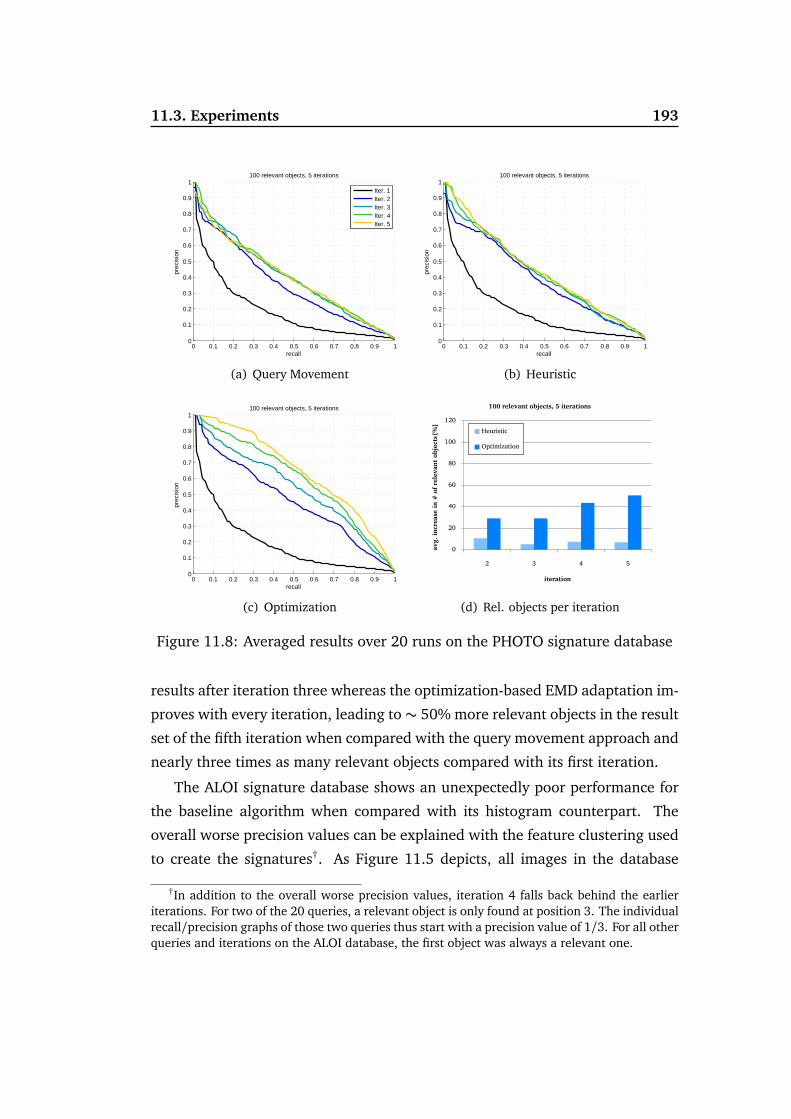
11.3. Experiments 193
0 0.1 0.2 0.3 0.4 0.5 0.6 0.7 0.8 0.9 10
0.1
0.2
0.3
0.4
0.5
0.6
0.7
0.8
0.9
1100 relevant objects, 5 iterations
recall
prec
isio
n
Iter. 1Iter. 2Iter. 3Iter. 4Iter. 5
(a) Query Movement
0 0.1 0.2 0.3 0.4 0.5 0.6 0.7 0.8 0.9 10
0.1
0.2
0.3
0.4
0.5
0.6
0.7
0.8
0.9
1100 relevant objects, 5 iterations
recall
prec
isio
n
(b) Heuristic
0 0.1 0.2 0.3 0.4 0.5 0.6 0.7 0.8 0.9 10
0.1
0.2
0.3
0.4
0.5
0.6
0.7
0.8
0.9
1100 relevant objects, 5 iterations
recall
prec
isio
n
(c) Optimization
0
20
40
60
80
100
120
2 3 4 5
avg.
incr
ease
in #
of r
elev
ant o
bjec
ts[%
]
iteration
100 relevant objects, 5 iterations
Heuristic
Optimization
(d) Rel. objects per iteration
Figure 11.8: Averaged results over 20 runs on the PHOTO signature database
results after iteration three whereas the optimization-based EMD adaptation im-
proves with every iteration, leading to∼ 50% more relevant objects in the result
set of the fifth iteration when compared with the query movement approach and
nearly three times as many relevant objects compared with its first iteration.
The ALOI signature database shows an unexpectedly poor performance for
the baseline algorithm when compared with its histogram counterpart. The
overall worse precision values can be explained with the feature clustering used
to create the signatures†. As Figure 11.5 depicts, all images in the database
†In addition to the overall worse precision values, iteration 4 falls back behind the earlieriterations. For two of the 20 queries, a relevant object is only found at position 3. The individualrecall/precision graphs of those two queries thus start with a precision value of 1/3. For all otherqueries and iterations on the ALOI database, the first object was always a relevant one.

194 Exploring Multimedia Databases via Relevance Feedback
0 0.1 0.2 0.3 0.4 0.5 0.6 0.7 0.8 0.9 10
0.1
0.2
0.3
0.4
0.5
0.6
0.7
0.8
0.9
172 relevant objects, 5 iterations
recall
prec
isio
n
Iter. 1Iter. 2Iter. 3Iter. 4Iter. 5
(a) Query Movement
0 0.1 0.2 0.3 0.4 0.5 0.6 0.7 0.8 0.9 10
0.1
0.2
0.3
0.4
0.5
0.6
0.7
0.8
0.9
172 relevant objects, 5 iterations
recall
prec
isio
n
(b) Heuristic
0 0.1 0.2 0.3 0.4 0.5 0.6 0.7 0.8 0.9 10
0.1
0.2
0.3
0.4
0.5
0.6
0.7
0.8
0.9
172 relevant objects, 5 iterations
recall
prec
isio
n
(c) Optimization
0
20
40
60
80
100
120
2 3 4 5
avg.
incr
ease
in #
of r
elev
ant o
bjec
ts[%
]
iteration
72 relevant objects, 5 iterations
Heuristic
Optimization
(d) Rel. objects per iteration
Figure 11.9: Averaged results over 20 runs on the ALOI signature database
exhibit large, homogeneous black areas around the borders. The color and tex-
ture subclusters in this database result in signature representatives with almost
random values for the non-clustered spatial dimension within the border area,
which in turn dominate the EMD.
The proposed EMD adaptation approaches overcome this challenge. The
statistics-based heuristic leads to low costs for transports in feature space dimen-
sions with high variances. In this way, the adaptation makes the EMD largely
ignore the random spatial dimensions for representatives in the border area.
This property of the heuristic for signatures leads to substantial improvements
regarding the query results as depicted in Figures 11.9 (b) and (d), where even
the second iteration shows significantly better precision values than any of the

11.3. Experiments 195
Figure 11.10: Example for query results after 5 iterations
baseline iterations and relative improvements of up to 80% compared with the
baseline for the number of relevant objects returned per iteration.
The optimization-based Relevance Feedback technique still exceeds these ef-
fectiveness gains as it takes the objects deemed relevant as well as the objects
deemed non-relevant into account when minimizing the discrepancy between
the feedback and the similarity measure defined via the adapted EMD. Fig-
ure 11.9 (d) shows that the substantial improvements depicted in the precision-
recall graph of Figure 11.9 (c) translate to up to twice the number of relevant
objects being returned compared with the query movement algorithm that does
not alter the EMD.
Lastly, as an example of the images being returned from the PHOTO data-
base, Figure 11.10 shows the first 15 results of the fifths relevance feedback iter-
ation for the query image depicted in the bottom left of Figure 11.5. The query
consisted of a feature signature for a massive blue door with a light background.
The query movement technique (a) gives a mixed result with six non-relevant
objects of which the first one is returned at position 2. Among the non-relevant
objects are images of a telephone, a penguin, and a power supply. The heuristic
approach (b) shows three non-relevant objects with the first one at position 9
only. Given the simple low-level features, the result can be deemed acceptable.
The optimization approach is able to return 15 images from the relevant theme
of heavy doors in this example. It is noteworthy that the optimization approach
had to abstract from the blue color of the door in the query in order to retrieve
more relevant objects.

196 Exploring Multimedia Databases via Relevance Feedback
11.4 Summary
This chapter described how the flexibility of the Earth Mover’s Distance can be
exploited to explore multimedia databases via a Relevance Feedback process.
The key to the adaptation of the EMD is its ground distance, which can be
adapted to effectively reflect a query-dependent notion of similarity in the fea-
ture space. To that end, an optimization-based extension to the traditional feed-
back loop and two statistics-based heuristics were proposed. They enable the
user to retrieve significantly more relevant objects from the database in fewer
iterations compared with existing EMD-based query movement techniques. The
optimization-based extension to the feedback loop is general enough to be eas-
ily transfered to other adaptable distance functions by defining the parameters
that describe the adaptability.

Part V
The Earth Mover’s Distance in
Context of Structured Objects
197


The Earth Mover’s Distance in Context of Structured Objects 199
In the literature, the EMD has primarily been applied to assess the similarity
between objects that do not possess a strong notion of structure. The last con-
tent part of this work presents original research on new ways of applying the
EMD in the context of objects such as graphs and time series, where ignoring
the order or structure within the objects would be detrimental to the similarity
model.
Chapter 12 focuses on the use of the EMD to assess the similarity between
medium-sized graphs based on their structure. The approach considers the con-
nectivity degree of nodes on paths through a graph and maps them to signatures
to be compared using the EMD.
Chapter 13 presents original research (cf. [AWK+09]) that is motived by the
desire to use the EMD as a ground distance for the DTW on time series of mul-
timedia objects. As a preparation for the use of DTWEM D for similarity search
in multimedia databases, the high number of ground distance computations for
each DTW computation is reduced by exploiting information from the filter step
of DTW-based retrieval algorithms.


Chapter 12
Feature-Based Graph Similarity
with the Earth Mover’s Distance
Graph structures are utilized to represent a wide range of objects including nat-
urally graph-like objects such as molecules and derived graph structures such
as connectivity graphs for region-based image retrieval. This chapter proposes
to extend the applicability of the EMD to graph objects by deriving a similarity
model with a representation of structural graph features that is compatible with
the feature signatures of the EMD. The aim is to support the search for a graph
in a database from which the query graph may have originated through limited
structural modification. Such query graphs with missing or additional vertices
or edges may be the result of natural processes of decay or mutation or may
stem from measuring methods that are inherently error-prone, to name a few
examples.
12.1 Introduction
In the absence of a canonical representation of graphs, deciding if two graphs
are isomorph (i.e., identical but for a renaming of the vertices) is a computa-
tionally expensive task. Its generalization, the subgraph isomorphism problem,
is known to be NP-complete. When attempting to find all graphs in a database
that contain a subgraph that is isomorph to some query graph, it is possible to
201

202 Feature-Based Graph Similarity with the Earth Mover’s Distance
use techniques similar to the lower-bounding filtering reviewed in Section 3.1
to quickly rule out some candidates and refine the rest with the computationally
expensive exact matching. For example, the GraphGrep approach indexes labels
along paths within a graph to perform the filtering [SWG02].
For similarity search, deciding whether (sub)graphs are isomorph does not
suffice. In the case of the two graphs not being identical, similarity search re-
quires an assessment of the degree to which the graphs in question differ from
another.
The comparison of two graphs can be performed by directly considering
the structure of the graphs. This approach is, for example, taken by the graph
edit distance [BA83] that calculates how many transformations have to be per-
formed to turn one graph into the other, and also by measures that consider
common subgraphs or the size of the largest common subgraph [BS98]. While
these measures are suitable for small graphs and for graphs with limitations
regarding their structure and/or the operations that may be performed (e.g.,
the degree-2 edit distance for connected, undirected, acyclic trees [ZWS96]),
even medium-sized general graphs quickly lead to a query processing time that
is bound to overburden the patience of the user.
Akin to content-based image retrieval, feature-based graph similarity models
instead derive (approximate) structural information from the graphs and assess
the similarity of the graphs based on these features. For example, so-called spec-
tral approaches [Ume88, LWH03] compare graphs based on an eigen-decompo-
sition of the adjacency matrix. The model presented in [PM99] compares two
graphs by computing the difference in the number of nodes that have a given
connectivity degree. The latter is the basis for the generalized approach de-
scribed in this chapter. Connectivity information collected along paths in graphs
is collected and represented in a way that is compatible with feature signa-
tures (cf. Definition 1.2), thus allowing graphs to be flexibly compared using
the EMD. In a recent related approach, graphs derived from images have been
compared using the EMD [GXTL08]. However, the approach uses the EMD to
compare the direction of edges/lines that occur in the graph and thus requires
the vertices to have a spatial position. The approach described here does not
make such an assumption.

12.2. Preliminaries 203
12.2 Preliminaries
The basic graph-related definitions for concepts used in the rest of the chapter
are given in this section with a small example on page 204.
A general graph with at most one edge from one vertex to another is defined
via its set of vertices and its edge relation.
Definition 12.1 (Graph)
A graph G of size m is a tuple G = (V, E) with vertices V = v1, . . . , vm and edges
E ⊆ V × V .
If a graph does not have single-vertex loops (i.e., the edge relation is irreflexive)
and is undirected (i.e., the edge relation is symmetric), it is called simple.
Definition 12.2 (Simple Graph)
Given a graph G = (V, E), G is simple iff for all v, w ∈ V
(v, w) ∈ E⇔ (w, v) ∈ E and (v, w) ∈ E⇒ v 6= w.
All graphs examined in the remainder of this chapter are assumed to be simple.
If all vertices of a graph are connected to all other vertices of the graph by a
series of edges, it is called connected.
Definition 12.3 (Connected Graph)
Given a graph G = (V, E), G is connected iff for all v, w ∈ V:
(v 6= w)⇒ (v, w) ∈ E
∨
∃vi1 , . . . , vim′∈ V : (v, vi1) ∈ E ∧ (vim′
, w) ∈ E
∧∀1≤ j ≤ m′− 1 : (vi j, vi j+1
) ∈ E
.
The graphs in the database are assumed to be connected in this chapter. A query
graph with missing vertices or edges may however break down into several non-
connected components.
The degree of a vertex in a graph is the number of other vertices it is directly
connected to.

204 Feature-Based Graph Similarity with the Earth Mover’s Distance
v4 v3
v5 v2
v1
(a) Graph G1
v1 v2 v3 v4 v5
v1 0 1 0 0 1v2 1 0 1 0 1v3 0 1 0 1 0v4 0 0 1 0 1v5 1 1 0 1 0
(b) Adjacency matrix of G1
v4 v3
v5 v2
v1
(c) Graph G2
Figure 12.1: Example graphs
Definition 12.4 (Vertex Degree Function)
Given a graph G = (V, E), the outgoing vertex degree function δG : V → N0 for G
is defined by
δG(v) = |w ∈ V |(v, w) ∈ E|.
The ingoing vertex degree function can be defined analogously. For the simple
graphs of this chapter, the two functions are identical and thus do not have to
be differentiated here.
The example graph G1 in Figure 12.1(a) is a simple, connected graph with
5 vertices and 6 edges. Figure 12.1(b) gives the adjacency matrix of G1 where
an entry of 1 indicates the existence of an edge while an entry of 0 indicates
the absence of an edge between two vertices. As a result of Definition 12.2, the
diagonal entries are all zero and the matrix is symmetric. The degree of a vertex
equals the row sum in the adjacency matrix. Vertices v1, v3, and v4 have degree
2 while vertices v2 and v5 have degree 3. The graph G2 is neither simple (due to
the loop at v5) nor connected (due to having two separate components).
12.3 Graph Similarity Model
In order to find graphs in a database that might be related to a query graph
through a process of decay, mutation, or generally structural change, a repre-
sentation of statistical graph features is proposed in Section 12.3.1 and distance
measures suitable for the feature representation are given in Section 12.3.2.
The similarity of two graphs can be assessed by combining these two parts.

12.3. Graph Similarity Model 205
12.3.1 Graph Feature: Degree Co-Occurrence Multisets
A representation of graph features that encodes structural information is re-
quired for detecting small structural changes between graphs in a feature-based
approach. In this section, statistical features of the vertices that occur in the
graphs and their connectivity relationship are discussed. In the simplest form,
a graph can be represented by the distribution of the degrees of its vertices
as in [PM99]. However, by looking at each vertex separately, one of the core
concepts of graphs is ignored. Graphs are useful as they model relationship in-
formation between the vertices. Thus, this section proposes to utilize statistical
information on the co-occurrence of vertices. In this way, the feature represen-
tation encodes which kinds of vertices are connected within a graph – and how
frequent this coupling occurs. The co-occurrence concept can be generalized
by looking at occurrences along paths in the graph and noting which kinds of
vertices occur close to each other / in sequence. In the following definitions, the
generalized co-occurrence concept is formally introduced on the basis of vertex
degrees as this information is common to all graphs. If other categorical infor-
mation (e.g., vertex class labels) is available, the approach could be adapted to
incorporate that information.
Definition 12.5 (Simple Vertex Path)
With G = (V, E) as a graph, the (m + 1)-tuple (vi0 , . . . , vim) ∈ V m+1 is a simple
(non-looping) vertex path of length m in G iff
∀0≤ j < j′ ≤ m : vi j6= vi j′
and
∀0≤ j < m : (vi j, vi j+1
) ∈ E.
The set of all simple paths of length m in G is denoted as PGm .
For the cases of path lengths m = 0 and m = 1, sets PG0 and PG
1 equal the
set of vertices V and the set of edges E. Using the set of simple paths of length
m, a co-occurrence multiset of degree m captures the frequencies of vertex class
(here, vertex degree) sequences.

206 Feature-Based Graph Similarity with the Earth Mover’s Distance
Definition 12.6 (Vertex Degree Co-occurrence Multisets)
With G = (V, E) as a graph, the Vertex Degree Co-Occurrence Multiset DGm of degree
m for graph G is defined as a tuple
DGm =
DSGm, f G
m
where
DSGm = (δ
G(vi0), . . . ,δG(vim)) | (vi0 , . . . , vim) ∈ PGm
is the set of all vertex degree sequences occurring on paths of length m in G and
f Gm (dg0, . . . , dgm) =
(vi0 , . . . , vim) ∈ PGm | ∀0≤ j ≤ m : dg j = δ
G(vi j)
the frequency function of such sequences in G.
The set DSGm abstracts from individual vertices by only considering their type
(i.e., vertex degree in this example). The degree m of the multiset is not related
to the degree of the vertices in the graphs but only to the length of the examined
paths.
As an example, the graph G1 in Figure 12.1(a) has five paths of length m= 0
(i.e., PG10 = V = v1, . . . , v5). The occurring vertex degrees are DSG1
0 = (2), (3)with frequencies f G1
0 (2) = 3 and f G10 (3) = 2. For m= 1, there are six paths (i.e.,
one per edge). The combinations of vertex degrees occurring along those paths
are DSG11 = (2, 2), (2, 3), (3, 2), (3, 3). The frequencies of those paths are
f G11 (2, 2) = 2, f G1
1 (2,3) = 4, f G11 (3, 2) = 4, and f G1
1 (3,3) = 2. Generally, the
number of paths grows for greater lengths m and for denser graphs. The set of
vertex degree sequences DSG12 is of cardinality 6 and DSG1
3 of cardinality 8. The
experiments in Section 12.4 show good results for m as low as 2. For greater
lengths, techniques such as random path sampling could be applied to speed up
the feature extraction process.
Figure 12.2 shows a visualization of the co-occurrence multisets DG1 (on the
far left) and DG2 (on the far right) in the form of bubble charts. The x , y , and
z axes denote the degree of the first, second, and third vertex on a path in G.
The size of the bubbles is proportional to the frequency of the according vertex
degree sequences that is also denoted inside the bubble. For m = 1, the short

12.3. Graph Similarity Model 207
0 1 2 3 40
1
2
3
4
2
2 4
4
2 2
3 3
24
2
4
2
0 1 2 30
1
2
3
4
4
2
3
GDG 1 DG
2
2
4
Figure 12.2: Visualization for the multiset feature representation of a graph G
arrows next to the graph in the middle of the figure show all paths (i.e., edges)
that contribute to the multiset DG1 . The long arrow in the upper section of the
graph shows a path that contributes to the bubble at coordinate 3-2-3 in the far
right of the figure representing DG2 .
With the above definitions, a co-occurrence multiset can be associated with
each graph in the database and with the query graph. The similarity of the
graphs can then be assessed in terms of the co-occurrence multisets that contain
statistical information on the structure of the graphs.
12.3.2 Similarity Measure
Element-Wise Multiset Comparison
As the multisets have a finite domain DS for any finite graph, element-wise
comparisons can be applied. By treating the multisets as a sparse representa-
tion of high-dimensional vectors, norm-based distance measures such as the Lp
distances can be adapted to compare two graphs.
Definition 12.7 (Lp Distance on Vertex Degree Co-Occurrence Multisets)
Given two graphs G1 and G2 with associated vertex degree co-occurrence multisets
DG1m = (DSG1
m , f G1m ) and DG2
m = (DSG2m , f G2
m ) according to Definition 12.6, the Lp
208 Feature-Based Graph Similarity with the Earth Mover’s Distance
distance between the two multisets is defined as
dLp(DG1
m , DG2m ) =
∑
ds∈(DSG1m ∩DS
G2m )
| f G1m (ds)− f G2
m (ds)|p
+∑
ds∈(DSG1m −DS
G2m )
| f G1m (ds)|p
+∑
ds∈(DSG2m −DS
G1m )
| f G2m (ds)|p
1/p
.
In the case of m = 0 and p = 1, the similarity model reflects the one of [PM99]where graphs are compared using simple vertex degree histograms and the Man-
hattan distance.
Transformation-Based Multiset Comparison
The co-occurrence multisets are a close match to the signatures that the EMD
takes as its input. The similarity of two graphs can be assessed using the EMD
by defining a transformation from the multisets to the signatures of the EMD.
Definition 12.8 (Feature Signatures of Graphs)
Given a graph G with an associated vertex degree co-occurrence multiset DGm =
(DSGm, f G
m ), the feature signature sGm of G for comparison with the Earth Mover’s
Distance is defined as
sGm =
¨
(r, w) | r ∈ DSGm ∧w =
f Gm (r)|DSG
m|
«
.
The cost for transforming one degree sequence into another one can be de-
fined via a ground distance function. In the simplest case, the sequences can
be treated as vectors from N0m and compared using dLp
from Definition 1.6 on
page 16. In this way, a degree sequence that deviates from another for example
by starting with a degree of 3 instead of 4 will induce a lower transformation
cost than one that starts with 1 instead of 4. Distance measures such as the
Edit Distance, which take the sequential character of the representatives r into
12.4. Experimental Evaluation 209
account, could also be employed. For undirected graphs, the fact that each se-
quence of vertex degrees appears twice in both directions should be accounted
for by adjusting either the signature definition or the ground distance.
12.4 Experimental Evaluation
12.4.1 Synthetic Graph Generation
For the experiments shown here, a number of synthetic graph databases of dif-
fering cardinalities were created. A synthetic graph of size m can be generated
through a randomized process in a number of ways. The simplest is to assume
the edge relation to be independent and identically-distributed (IID). The exis-
tence of an edge between any two of the m vertices has a fixed probability p.
This graph generating process is called the Erdõs-Rényi model [ER59] and re-
sults in a binomial vertex-degree distribution where a large number of vertices
has a degree of medium value with smaller and greater degrees being less likely.
As discussed in [AB02], graphs found in real applications often do not follow
a binomial vertex-degree distribution resulting from the IID edge relation. An
increasing number of graphs have instead been found to follow a power-law
distribution where a large majority of vertices have a small degree with very
few vertices having a large degree (i.e., they function as hubs). Examples listed
include small graphs such as predator-prey relationship of animals in closed
habitats with a low 3-digit number of vertices (i.e., species) and large graphs
such as the world wide web linking graph with millions of vertices (i.e., web
pages).
The synthetic graph databases used in the experiments were generated using
the method detailed in [VL05] based on sequences of vertex degrees following
a power-law distribution with modifications to ensure that the graphs are con-
nected and simple. Figure 12.3 illustrates the resulting vertex degree distribu-
tion for ten random graphs as used in the experiments (size 100, vertex degrees
between 1 and 15, and an average degree of 3) and contrasts them to according
graphs following the simple Erdõs-Rényi model.

210 Feature-Based Graph Similarity with the Earth Mover’s Distance
0%5%
10%15%20%25%30%35%40%45%
0 1 2 3 4 5 6 7 8 9 10 11 12 13 14 15
rela
tive
frequ
ency
vertex degree
Power-Law Graphs
Erdõs-Rényi Graphs
Figure 12.3: Distribution of vertex degrees
12.4.2 Results
In the first set of experiments, 100 graphs were randomly chosen from the data-
base as the basis for 15 query graphs each that represent different levels of struc-
tural deviation regarding the edge relation. For each of the 15 levels, a random
edge was either inserted or deleted with equal probability. Not accounting for
edges that may have been deleted and consecutively been added again, up to
10% of the the edge relation may have been changed in this process.
The vertical axis of Figure 12.4 shows how often the graph on which the
query graph was based was identified as the most similar one out of all 1000
graphs in the database. A greater path length (denoted as PL in the figure)
for the vertex degree co-occurrence multisets results in a similarity model that
is more robust with regard to the structural change for this experiment. The
greater the structural difference, the more can the multisets based on longer
paths distinguish themselves from those of lower degree. The Manhattan dis-
tance on simple vertex degree histograms (cf. [PM99]) is always outperformed
by the multisets of higher degree (i.e., based on longer paths) in this exper-
iment. The EMD with a Manhattan ground distance slightly outperforms the
Manhattan distance for equal path lengths. The EMD for path length zero is not
plotted here, as the results equal those of the Manhattan distance in the case of
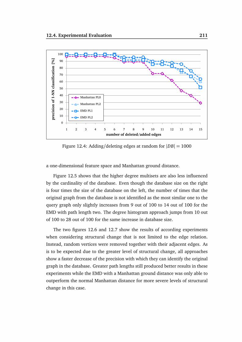
12.4. Experimental Evaluation 211
0
10
20
30
40
50
60
70
80
90
100
1 2 3 4 5 6 7 8 9 10 11 12 13 14 15
prec
ision
of 1
-NN
clas
sific
atio
n [%
]
number of deleted/added edges
Manhattan PL0
Manhattan PL2
EMD PL1
EMD PL2
Figure 12.4: Adding/deleting edges at random for |DB|= 1000
a one-dimensional feature space and Manhattan ground distance.
Figure 12.5 shows that the higher degree multisets are also less influenced
by the cardinality of the database. Even though the database size on the right
is four times the size of the database on the left, the number of times that the
original graph from the database is not identified as the most similar one to the
query graph only slightly increases from 9 out of 100 to 14 out of 100 for the
EMD with path length two. The degree histogram approach jumps from 10 out
of 100 to 28 out of 100 for the same increase in database size.
The two figures 12.6 and 12.7 show the results of according experiments
when considering structural change that is not limited to the edge relation.
Instead, random vertices were removed together with their adjacent edges. As
is to be expected due to the greater level of structural change, all approaches
show a faster decrease of the precision with which they can identify the original
graph in the database. Greater path lengths still produced better results in these
experiments while the EMD with a Manhattan ground distance was only able to
outperform the normal Manhattan distance for more severe levels of structural
change in this case.

212 Feature-Based Graph Similarity with the Earth Mover’s Distance
0
10
20
30
40
50
60
70
80
90
100
250 500 750 1000
prec
ision
of 1
-NN
clas
sific
atio
n [%
]
number of graphs
Manhattan PL0
Manhattan PL2
EMD PL1
EMD PL2
Figure 12.5: Adding/deleting 10 edges at random
0
10
20
30
40
50
60
70
80
90
100
1 2 3 4 5 6 7 8 9 10 11 12 13 14 15
prec
ision
of 1
-NN
clas
sific
atio
n [%
]
number of deleted vertices
Manhattan PL0
Manhattan PL2
EMD PL1
EMD PL2
Figure 12.6: Deleting vertices at random for |DB|= 1000

12.5. Summary and Outlook 213
0
10
20
30
40
50
60
70
80
90
100
250 500 750 1000
prec
ision
of 1
-NN
clas
sific
atio
n [%
]
number of graphs
Manhattan PL0
Manhattan PL2
EMD PL1
EMD PL2
Figure 12.7: Deleting 5 vertices at random
12.5 Summary and Outlook
This chapter showed how complex data objects in the form of graphs can be
compared using the EMD by defining a suitable representation of graph features
that capture statistical information regarding the structure of the graphs. In this
way, it is possible to identify graphs that resulted from some other graph through
a process of structural change without having to resort to typically very expen-
sive similarity measures that directly take the graph structure into account.
The general viability of the approach was shown using a Manhattan ground
distance for the EMD together with vertex degrees as the sole information re-
garding the vertices. For this ground distance, the projection-based lower bound
of Section 7.5.1 and the EMD-L1 algorithm from [LO07] could be employed to
speed up retrieval. While the results using this simple ground distance were also
generally good, the Manhattan ground distance potentially limits the benefits of
longer co-occurrence sequences that are used as signature component represen-
tatives for the EMD. Other ground distances that take the sequence character of
the feature representatives (i.e., sequences of vertex degrees in this case) into
account may present an opportunity to further improve the results.


Chapter 13
Reducing the Number of DTW
Ground Distance Computations
The desire to use a transformation-based distance measure as a ground dis-
tance for another transformation-based distance measure is the motivation for
the development of techniques that reduce the number of ground distance com-
putations in a similarity search system since the determination of each ground
distance is computationally expensive in this scenario. In this chapter, a concept
called Anticipatory Pruning is proposed for speeding up DTW-based retrieval on
both univariate and multivariate time series in this manner. Intuitively, Antici-
patory Pruning reduces the number of ground distance computations by antici-
pating the DTW refinement result through exploiting information from previous
filters in a multi-step filter-and-refine algorithm.
13.1 Introduction
Time series or feature sequences (cf. Definition 1.3) record the value of one or
more attributes as they change over a span of time. For example, temperature
measurements from several spatial locations of observation could be recorded
at each full hour for each full year enabling year-to-year climate change anal-
ysis. Another example where the value of a number of attributes is recorded
are digital videos. In this case, each point in time corresponds to a frame of the
215

216 Reducing the Number of DTW Ground Distance Computations
video and the values in the time series are either the raw pixel values of each
frame or a representation of the features that describe characteristic properties
of the frame (e.g., color histograms). When comparing two time series with
complex feature representations such as video sequences, the effectiveness of
the overall model depends on both the similarity measure used to compare the
feature representation for two points in time and on the similarity measure used
to aggregate the point-in-time similarity measures to an overall similarity score
for the time series. As discussed in the previous chapters, the Earth Mover’s Dis-
tance is well suited for comparing histogram-based feature representations. For
time series retrieval, the DTW distance is a prime candidate when effectiveness
is of concern. Integrating the two measures to form DTWEM D as proposed by
the video retrieval model in [AK09] promises to yield a high-quality similarity
measure for time series of histogram-based features representations. However,
the potential quality comes at a high computational cost. For each entry in
the valid band of the cumulative distance matrix (cf. Section 6.3), an Earth
Mover’s Distance has to be computed. Thus, a reduction of the number of dis-
tance matrix entry computations during query processing leads to a significant
performance improvement for similarity search on time series using DTW with
a computationally expensive ground distance.
The Anticipatory DTW (aDTW) algorithm proposed here for the purpose of
reducing the number of ground distance computations for DTW is lossless for a
certain class of lower-bounding filters that are characterized in Definition 13.3.
Widely used state-of-the-art approaches belong to this class. Additionally, as
aDTW efficiently reuses information from previous filter steps, it incurs very lit-
tle computational overhead. The experiments in Section 13.3 demonstrate the
performance improvements that can be achieved. As aDTW is orthogonal to
existing lower-bounding filtering, indexing, and dimensionality reduction tech-
niques, it can be flexibly combined with such techniques for additional speed-up.
13.1.1 Related Work
Techniques to speed up the retrieval of time series based on DTW can be catego-
rized as either correct or approximate with respect to the result set they deliver.

13.1. Introduction 217
Approximate techniques that do not return the exact same result set that a
simple scan with DTW would produce include [YJF98, CFY03, CKHP02, SC04,
SC07, APP+08]. In [YJF98] an approximate embedding of DTW into Euclidean
space is proposed. This technique is extended to a technique based on the Haar
wavelet transform for fewer false positives [CFY03], but possibly more false
negatives. Iterative Deepening DTW [CKHP02] computes different levels of
dimensionality reduction from piecewise linear approximations. Using a prob-
abilistic model based on sample approximation errors, time series are either
pruned or compared at a finer level of approximation. The FastDTW approach
[SC04, SC07] computes approximations of the warping path at different levels
of granularity. The recent embedding-based subsequence matching technique
[APP+08] hashes subsequences of the original time series to vectors based on
their DTW distance to reference time series. Subsequences that are identified
as potentially similar to the query are then refined using the DTW. All of these
techniques provide efficiency gains by sacrificing the correctness of the result as
they are approximate in nature.
Correctness of the result is guaranteed by lower-bounding filter-and-refine
techniques. The time series representation of the Piecewise Aggregate Approxi-
mation (PAA) method is composed of averages of consecutive values along the
time axis [KCPM01]. The Adaptive Piecewise Constant Approximation adapts
the number of values that are averaged to reduce the approximation error
[KCPM00]. For these representations, lower-bounding distance functions for
DTW have been proposed. Another lossless approach is based on four character-
istic values of time series: their starting and ending value, their minimum, and
their maximum [KPC01]. LBKeogh provides a lower-bound that uses the warping
path constraint to compute an envelope on the warping cost for PAA segments
[Keo02]. This approach has been extended to 2-dimensional envelopes around
trajectories in [VHGK03, RM02]. Improved versions of the envelope technique
have been proposed in [ZS03] and [ZW07]. The Fast search method for Time
Warping (FTW) uses different resolutions to gradually refine the optimal warp-
ing path [SYF05]. Using Early Stopping, only the warping paths with a DTW
distance not exceeding some pruning distance are evaluated. This technique is
also known as Early Abandoning [KWX+06].

218 Reducing the Number of DTW Ground Distance Computations
TS DB
flterq cand. APD1 result APDm...
anticipatory pruning
Figure 13.1: Overview of the structure of aDTW
The technique proposed here can be integrated with these lower-bounding
distance functions to improve the overall retrieval performance. More details
on the integration are given in Section 13.2.8.
13.2 Anticipatory DTW
The multi-step approach proposed in this chapter extends the classic filter-and-
refine algorithms for DTW and is called Anticipatory DTW or aDTW for short.
It is based on a number of properties of existing lower-bounding filters (Sec-
tions 13.2.4 to 13.2.6) and makes use of an Anticipatory Pruning Distance APD
(Section 13.2.7). Theorem 13.3 shows that APD is a lower bound for the DTW
distance, which implies that aDTW is complete with regard to its result set.
13.2.1 Structure of aDTW
The general structure of aDTW is similar to the multi-step filter-and-refine frame-
works used in chapters 8 and 9. However, there are three design characteristics
specific to aDTW (illustrated by Figure 13.1).
1. There are at least two filters in the chain – the first one is taken from the
literature and the second one is the proposed Anticipatory Pruning.
2. The computation of APD is performed in a number of incremental steps.

13.2. Anticipatory DTW 219
After each step, a pruning decision is made.
3. APD is not independent of the filter from the literature but efficiently ex-
ploits its information.
Traditional filter-and-refine algorithms compute the full DTW if the filter does
not prune the candidate. The pruning decision is made by comparing a lower-
bounding filter distance with a pruning threshold given, for example, by the
range of a range query or by distances encountered so far during k-nearest-
neighbor search. An existing improvement of this technique is known as Early
Stopping [SYF05] or Abandoning [KWX+06], where the computation of DTW
in the refinement step is stopped as soon as an intermediate result exceeds the
pruning threshold. The aDTW concept proposed here goes beyond Early Stop-
ping.
If the first filter cannot prune a candidate, APD1 is computed. If APD1 does
not allow for pruning either, APD2 is computed. This process is continued until
either pruning is possible or APDm has been computed. In a step 1≤ i ≤ m, APDi
is based on the DTW computation up to column i of the cumulative distance
matrix from Chapter 6 – just as in Early Stopping. Additionally, APDi anticipates
the steps i + 1 to m by reusing information from the first filter as indicated by
the arrows at the top of the figure. Thus, APD has an improved approximation
quality compared with Early Stopping alone. The computation of APDm includes
all information required to derive the DTW distance. No further refinement step
is necessary.
13.2.2 Preliminaries
As some of the theorems and proofs in this chapter depend on the warping path
within a given valid band for DTW (cf. Definition 6.2), the valid band and the
warping path shall be defined here along with some elementary properties of
warping paths. The Sakoe-Chiba band is assumed for ease of discussion, but the
technique can be easily adapted to other bands as well.
Definition 13.1 (Valid matrix band for k-band Dynamic Time Warping)
The valid cells with respect to a band parameter k in the cumulative DTW distance

220 Reducing the Number of DTW Ground Distance Computations
matrix of size m1×m2 (w.l.o.g. m1 ≤ m2) for two time series s and t of length
m1 and m2 are
band =⋃
1≤ j≤m2
band j
with band j as the valid cells in column j:
band j = (i, j) | 1≤ i ≤ m1 , | i−
j ·m1
m2
|≤ k
Definition 13.2 (Warping path)
The warping path P for two time series s and t of length m1 and m2 is defined as
a set of matrix cells
P = p1, ..., pl with p1 = (0,0), pl = (m1, m2).
Proposition 13.1 (Properties of warping paths)
For any two pi = (a, b), pi+1 = (c, d) of a warping path P in a cumulative distance
matrix D of DTWgd , the following holds:
1. monotony: c− a ≥ 0∧ d − b ≥ 0
2. continuity: c− a ≤ 1∧ d − b ≤ 1
3. alignment: D[c, d] = gd(sc, td) + D[a, b]
A warping path is monotonic in the sense that the time does not go backwards.
The path is continuous in that there are no omitted points in time; successive
path elements correspond to consecutive points in time. The alignment property
ensures that each cell pi arose from its direct predecessor pi−1.
13.2.3 The Idea of aDTW
The Anticipatory Pruning Distance APD is based on three properties.
1. DTW computation is incremental, i.e., the entries in the cumulative dis-
tance matrix increase in value with the sequence length.

13.2. Anticipatory DTW 221
2. Many existing lower-bounding filters for the DTW distance can be charac-
terized as piecewise, i.e., a subsequence of the filter computation is a valid
filter for a subsequence of a time series.
3. DTW is reversible, i.e., computing the warping path from the beginning to
the end is the same as doing so from the end to the beginning.
The Anticipatory DTW algorithm uses these three properties by calculating
piecewise filter distances on reversed time series in the filter step of the frame-
work depicted in Figure 13.1. During the incremental computation of APD
(non-reversed), the information from the piecewise filter serves as a lower-
bounding anticipatory estimate of the DTW parts yet to be calculated. The
exploitation of this additional information allows for stopping the calculation
sooner than would have been possible without the anticipatory part. If no stop-
ping is possible, the last step of computing APD corresponds to the last step of
computing the DTW distance.
The proposed aDTW is highly flexible in that it can be combined with many
existing lower-bounding filters. It is easy to integrate with these filtering ap-
proaches, as all the information required for Anticipatory Pruning can readily
be derived from existing filter calculations. Moreover, the pruning capability of
aDTW comes at hardly any additional cost, as the filter distances have already
been computed in the filter step.
In the following sections, the properties important for aDTW are discussed.
13.2.4 Incremental Computation of DTW
Anticipatory Pruning uses filter information for additional pruning checks. These
checks are based on the proposed anticipatory estimate and the fact that DTW
is incremental.
Theorem 13.1 (DTW is incremental)
For any cumulative distance matrix D ∈ Rm1×m2 as defined in Definition 6.3, the
column minima are monotonically non-decreasing:
∀1≤ (y − 1)< y ≤ m2 : min1≤i≤m1
D[i, y − 1] ≤ min1≤i≤m1
D[i, y].

222 Reducing the Number of DTW Ground Distance Computations
Proof 13.1
The theorem follows from the definition of the cumulative distance matrix: D[i, j] =gd(si, t j) +minD[i − 1, j − 1] , D[i, j − 1] , D[i − 1, j]. Let i∗ be the smallest
row index such that D[i∗, y] is minimal in column y. Due to gd(si∗ , t y) ≥ 0 and
D[i∗ − 1, y] > D[i∗, y], the value of D[i∗, y] cannot be based on D[i∗ − 1, y]in the same column. Thus, it must either be based on D[i∗ − 1, y − 1] or on
D[i∗, y − 1]. W.l.o.g., let it be based on D[i∗, y − 1]. Then gd(si∗ , t y) ≥ 0 implies
that D[i∗, y−1]≤ D[i∗, y] =min1≤i≤m1D[i, y]. The minimum in column y−1
can thus be no larger than the minimum in column y.
The value D[m1, m2] that represents the DTW distance is trivially lower-
bounded by the minimum of column m2. Due to Theorem 13.1, it is also lower-
bounded by the non-decreasing sequence of column minima. This property
allows for Early Stopping/Abandoning of the DTW computation. As soon as
one of the column minima exceeds the pruning threshold, the complete DTW
does not have to be computed as the final DTW will exceed the threshold, too.
The definition of APD will go beyond column minima as it adds anticipa-
tory pieces of filter information for a closer estimate of the DTW. Entries D[i, j]in the cumulative distance matrix correspond to the minimum cost of possible
warping paths between subsequences s[1 : i] and t[1 : j]. The aim is to find a
lower bound for the cost of the remaining warping path that has not yet been
computed. Provided that a lower bound for the whole warping path can be de-
composed such that one piece serves as a lower bound on the remaining postfix
of the warping path, this piece can be combined with the column minimum for
an overall estimate that will be defined as the Anticipatory Pruning Distance.
13.2.5 Piecewise Filter Computation for DTW
Anticipatory Pruning can also be understood as an incremental refinement of
a filter with DTW distance information. As illustrated in Figure 13.2, the cu-
mulative distance matrix for DTW computation is filled as usual. For example,
columns 1 to 5 have been computed in the leftmost figure. The column min-
imum in the fifth column is a lower bound for the DTW distance. Up to this
point, only partial time series have been accounted for (namely up to the sev-

13.2. Anticipatory DTW 223
DTWesti
mate
DTWesti
mate
DTW
estimate
step 5 step 6 step 75 6 6 7 7 8
Figure 13.2: Estimates being replaced with cumulative distance matrix entries
enth entry for the first and up to the fifth entry for the second time series). For
the remaining subsequences of the time series, starting in the sixth column, APD
includes an estimate derived from the preceding filter step (cf. Figure 13.1). The
estimate is a piece of filter information corresponding to subsequences of time
series starting in the last seven columns.
This estimate on partial time series alignments requires that the filter be
piecewise, i.e., decomposable into a series of lower bounds for all time series
prefixes of increasing length.
Definition 13.3 (Piecewise DTW lower bound)
A piecewise lower-bounding filter for the DTW distance between two time series s
and t of length m1 and m2 is a set pf = pf0, ..., pf m2 with the following property:
pf0(s, t) = 0
∀0< j ≤ m2 :pf j(s, t)≤ min(i, j)∈band j
DTW (s[1 : i], t[1 : j])
Intuitively, a piecewise lower-bounding filter can be decomposed into a se-
ries of lower bounds for all possible partial DTW warping paths that start at the
beginning of both time series and end in a respective column. The piecewise
property is not a major constraint, as many existing lower-bounding filters for
DTW can be decomposed in such a manner as will be shown in Section 13.2.8.

224 Reducing the Number of DTW Ground Distance Computations
13.2.6 Reversible Computation of DTW
The piecewise property of a DTW lower bound and the incremental computation
property of DTW together do not suffice to combine pieces of the filter with par-
tial DTW computations. To derive an overall lower bound, partial DTW compu-
tations up to some column j of the cumulative distance matrix have to be com-
bined with piecewise filter information for the remaining columns ( j+1), ..., m2
corresponding to postfixes of the time series. However, the piecewise filter only
provides information for prefixes of the time series. Fortunately, DTW computa-
tion is reversible, i.e., computing the distance for the reversed time series (from
the end to the beginning) yields exactly the same result as computing it for the
original time series.
Theorem 13.2 (DTW is reversible)
For any two time series s =
s1, . . . , sm1
and t =
t1, . . . , tm2
and for according
reversed time series s← and t← it holds:
DTW (s, t) = DTW (s←, t←)
Proof 13.2
Assuming that this property does not hold and to the contrary (w.l.o.g.):
DTW (s, t)< DTW (s←, t←)
Let p1, ..., pl1 and p←1 , ..., p←l2 be warping paths with minimal cost for the non-
reversed and for the reversed time series. Since reversing path p1, ..., pl1 yields a
valid warping path for the reversed time series (properties monotony, continuity,
and alignment of Definition 13.2 follow from the according properties of the non-
reversed path) and since its cost remains unchanged and equals DTW (s, t), it
follows that p←1 , ..., p←l2 with cost DTW (s←, t←) cannot be a warping path with
minimal cost. As this contradicts the assumption, DTW is reversible.
Reversibility is important for the proposed Anticipatory Pruning, as it allows
for deriving a lossless estimate of the DTW distance from any piecewise lower-
bounding filter. By reversing the order of time series during the first filter com-

13.2. Anticipatory DTW 225
putation, the same filter distance is obtained as if the filter was computed on the
original time series. However, the pieces of the filter computation from the end
of the time series backwards to the current point of DTW computation may now
be used as an estimate of the remaining path cost. As both this estimate and
the column minima lower-bound the DTW on the according subsequences, APD
as the sum of those two components is lower-bounding DTW on the complete
time series. This statement will be formally proven in Theorem 13.3 after the
definition and an example for the Anticipatory Pruning Distance APD are given.
13.2.7 Anticipatory Pruning Distance
Anticipatory DTW includes a sequence of pruning checks. After every column
of the cumulative distance matrix that has been computed, piecewise filter in-
formation is added to yield an overall lower bound for the exact DTW distance.
It can therefore be seen as a series of m2 filters for time series s and t of length
m1 and m2, where the final step provides the information for the actual DTW
distance. Formally, the proposed Anticipatory Pruning Distance is defined as
follows:
Definition 13.4 (Anticipatory Pruning Distance (APD))
Given two time series s and t of length m1 and m2, a cumulative distance matrix
D as defined in Definition 6.3, a piecewise lower-bounding filter pf for the reversed
time series s← and t← as defined in Definition 13.3, and a value j ∈ 1, ..., m2,the jth step of the Anticipatory Pruning Distance APD for the k-band DTW distance
between s and t is defined as
APD j(s, t) = min1≤i≤m1
D[i, j]+ pf m2− j(s←, t←).
The Anticipatory Pruning distances are thus a sequence of DTW column min-
ima with added pieces of filter information for the remainder of the time series.
During computation step j, the column minimum of the partial path between
s[1 : i] and t[1 : j] according to DTW is combined with the anticipatory infor-
mation for the rest of the alignment available from the lower-bounding filter.
The resulting estimate of the entire cost of the warping path in step j is APD j.

226 Reducing the Number of DTW Ground Distance Computations
2 5
33 3527 2823
18 211917 2116
15 171413 1612
13 1398 106
7 6
3
3453483910
8 2 0 2 6 6 4 0 2
25
1 2 3 4 5 6 7 8 9 1002 5 6 10 13 15 17 18 21 28
18 15 14 11 10 10 10 10 7 01820 20 20 21 23 25 27 28 28 28
pf10-j APD
ESstep j
t:
s:
0
5
10
15
20
25
30
35
40
0 1 2 3 4 5 6 7 8 9 10
dist
ance
step j
DTW
Pruning ThresholdES
pf
APD
10-j
Figure 13.3: Anticipatory Pruning example
Figure 13.3 gives an example for the Anticipatory Pruning Distance. The
left part of the figure shows two univariate time series s and t together with
their cumulative distance matrix. For reasons of simplicity, this example uses an
L1-based variant of the LBKeogh lower bound for the filter pf . The relationship
between the DTW distance (35 as seen in the top right corner of the matrix),
the pruning threshold (chosen as 22), and the components of APD j are depicted
in the right part of the figure.
The filter distance pf between the reversed s← and t← yields the following
piecewise results: 0,7,...,18. Thus, the filter step distance is 18. To make the
computation of the Anticipatory Pruning Distance more intuitive, the order of
the piecewise filter results are reversed in the figure. As the filter distance of 18
does not exceed the pruning threshold of 22, t cannot be pruned by the filter
and DTW would normally have to be computed now (potentially with Early
Stopping). Instead, aDTW starts with filling the cumulative distance matrix
for DTW(s, t) and remembers the minimum of column j (denoted as ES j =min1≤i≤m1D[i, j]) in step j. For example, the first column minimum is 2 and
accounts for the mappings of the 1-prefix of t to the two prefixes of s permitted
by band1. As can be seen in the figure, the minima of the first few columns are
only loose bounds and a pruning with Early Stopping alone is only possible in
the very last step in this example.

13.2. Anticipatory DTW 227
Algorithm 13.1: APD(q, t, ε, pf, gd, band)
m1 = |q|; m2 = |t|;1
col = new double[m1+1]; // define dummy column with m1+1 entries2
col[1] = 0 ; // dummy row within dummy column3
for i=2 to m1+1 do4
col[i] =∞;5
endfor6
// iterate over all columns of the cumulative distance matrixfor j=1 to m2 do7
// Fill a column with DTW componentscol = CalcDTWColumn(q, t[j], col, gd, band[j]);8
APDj = min(col) + pf[m2+1-j] ; // pf starts with pf[1] = 09
if APDj > ε then return∞ ; // pruning10
endfor11
// return DTW value that is now stored in last entry of colreturn col[m1+1];12
For Anticipatory Pruning, the filter piece pf←10−1 is added. It lower-bounds all
possible alignments for reversed time series starting in cell (10, 10) and ending
in column 2. Thus APD1 is obtained as “ES+pf←”= 2+ 18= 20, which is much
closer to the DTW distance than the column minimum alone. Yet it is lower
than the pruning threshold of 22. Continuing with filling the matrix, the second
column minimum is 5 and the filter entry pf←2 is 15, yielding 20 again. In step
5, the column minimum is 13 and the corresponding filter distance piece is 10.
The sum of 23 exceeds the pruning threshold 22. Hence, the DTW computation
can be stopped. Thus, half of the ground distance computations are skipped and
t is discarded.
The computation of APD for a query q, a database time series t, a pruning
threshold ε, a piecewise filter pf , a ground distance gd, and a band for the
DTW is given by Algorithm 13.1. The computation of the column entries of the
cumulative cost matrix is performed by Algorithm 13.2 as in the normal DTW
case. Thus, the APD algorithm can return the final DTW distance without further
calculations if no pruning was possible. The worst-case time complexity of APD
is unchanged from the one of DTW. Compared with the according definitions,
the algorithms use indices shifted by one for array pf (as arrays start at index 1

228 Reducing the Number of DTW Ground Distance Computations
Algorithm 13.2: CalcDTWColumn(q, tj, col, gd, bandj)
m1 = |q|;1
// create a new column for the result; initialize the dummy rownewcol[1]=∞;2
// iterate over rows of the cumulative distance matrix; skip dummy rowfor i=2 to m1+1 do3
if (i-1) ∈ bandj then4
// compute DTW entry; adjust for dummy rownewcol[i] = gd(q[i-1], tj) + min(newcol[i-1], col[i], col[i-1]);5
else6
newcol[i] =∞;7
endif8
endfor9
return newcol;10
here) and for the number of rows in a column (as the introduction of a guardian
or dummy dimension simplifies the implementation).
Algorithm 13.3 shows how APD can be used for a range-based similarity
search. Since APD returns either the DTW value or∞ in case of a pruning deci-
sion, the algorithm is virtually identical to a conventional multi-step DTW algo-
rithm. The definition of the procedure calcPiecewiseFilter depends on the piece-
wise filter that is to be used (possible choices are discussed in Section 13.2.8).
It returns an array of piecewise filter results instead of a single lower-bounding
value. The only other necessary change is the call to APD in line 6 instead of the
usual refinement call to a DTW procedure. Algorithms for k-nearest-neighbor
searches and ranking queries can be adapted accordingly.
The following theorem states that APD j is a lower bound for the DTW in
each step j. This property is central for the completeness of the result sets of
similarity search algorithms based on APD.
Theorem 13.3 (AP lower-bounds DTW)
The Anticipatory Pruning Distance APD j as given by Definition 13.4 is a lower
bound of the DTW distance between two time series s and t of length m1 and m2.
∀1≤ j ≤ m2 : APj(s, t) = min1≤i≤m1
D[i, j]+ pf m2− j(s←, t←)≤ DTW (s, t)

13.2. Anticipatory DTW 229
Algorithm 13.3: aDTW-rangeQ(q, ε, gd, band, DB)
ResultSet = ;;1
for t ∈ DB do2
m2 = |t|;3
pf = calcPiecewiseFilter(q, t, gd, band);4
// check if final result from filter allows pruningif pf[m2+1] ≤ ε then5
// check if APD allows pruning; returns∞ if so; DTW otherwiseif APD(q, t, ε, pf, gd, band) ≤ ε then6
ResultSet = ResultSet ∪ t;7
endif8
endif9
endfor10
return ResultSet;11
Proof 13.3
The overall proof is based two properties of the DTW.
1. For all steps j, the column minimum is a lower bound of the path costs for
paths ending in column j.
2. DTW is reversible.
The first property is trivially true due to min(A∪ t) ≤ t for any finite set A⊂ Rand t ∈ R. The second property was proven in in Section 13.2.6.
The remainder of the proof shows that these two properties together result in the
lower-bounding property of APD as a series of partial warping path costs combined
with a lower-bounding estimate of DTW values for time series postfixes.
Due to the continuity of DTW, a warping path P = p1, ..., pl of minimal cost
(cf. Definition 13.2) passes through all columns and thus also through both column
j and column j + 1 of the cumulative distance matrix D. Thus, the path can be
decomposed into two parts P1 = p1, ..., pu and P2 = pu+1, ..., pl such that P1
starts in the first column and ends in column j while P2 starts in column j+1 and
ends in the last column.
With pu = (x , j) and pu+1 = (y, j+1) for some 1≤ x , y ≤ m1, the right-hand

230 Reducing the Number of DTW Ground Distance Computations
side of the inequality can be rewritten as
DTW(s, t) = D[x , j] + DTW (s[y : m1], t[( j+ 1) : m2]).
From property 1 it follows that
min1≤i≤m1
D[i, j] ≤ D[x , j].
From property 2 it follows that
DTW (s[y : m1], t[( j+ 1) : m2]) = DTW (s[m1 : y], t[m2 : ( j+ 1)]).
This term is underestimated by pf m− j(s←, t←) by definition of the piecewise lower
bound pf . Together, the theorem follows.
Now that it has been shown that APD is a lower bound of DTW given some
piecewise lower bound pf , it immediately follows that Algorithm 13.3 is lossless
and returns the same result as rangeQ(q, ε, DTWgd,band , DB) from page 20.
13.2.8 Piecewise Lower-Bounding Filters
In this section, existing piecewise lower-bounding filter techniques for DTW are
discussed. The piecewise property is shown for the LBKeogh lower bound of the
DTW with details on other lower bounds in [AWK+09].
Linearization
The basic idea for linearization of the DTW computation for efficient and exact
indexing is based on computing an envelope of upper and lower values around
the query time series q of length m with respect to the k-band:
UBq[i] = maxi−k≤ j≤i+k
q[ j]
LBq[i] = mini−k≤ j≤i+k
q[ j].

13.2. Anticipatory DTW 231
The MinDist of the ground distance between time series t and the rectangle de-
fined by vectors UBq and LBq lower-bounds the k-band DTW distance [Keo02]:
LBKeogh(q, t) = MinDist L2(t, LBq, UBq)≤ DTWdL2
,k−band(q, t)
with
MinDist L2(x , l, u) =
√
√
√
√
√
√
m∑
i=1
(x[i]− u[i])2 x[i]> u[i](x[i]− l[i])2 x[i]< l[i]0 otherwise.
Theorem 13.4
LBKeogh is a piecewise lower-bounding filter as defined in Definition 13.3.
Proof 13.4 (Sketch)
As LBKeogh is a dimension-wise summation of distance components, the decomposi-
tion into a set of filters pf j for increasing sequence length j is straightforward:
pf j(q, t) =
√
√
√
√
√
√
j∑
i=1
(t[i]− UBq[i])2 t[i]> UBq[i](t[i]− LBq[i])2 t[i]< LBq[i]0 otherwise.
As the sum takes the worst-case estimate that the warping path has one cell per col-
umn (there is only one entry in the sum per column) and that this cell contributes
no more than the least possible ground distance amount from the column (LB and
UB are the minimum/maximum over entries from q according to band j), it does
not only lower-bound DTW(q[1 : j], t[1 : j]) but also DTW(q[1 : i], t[1 : j]) for
(i, j) ∈ band j.
In the experiments, Anticipatory Pruning is evaluated for LBKeogh with a
tighter version of the envelope [ZS03] in combination with Piecewise Aggre-
gate Approximation (PAA) of the time series.

232 Reducing the Number of DTW Ground Distance Computations
Corner Boundaries
A generalization of the approach above can be found in [ZW07]. The general-
ized lower bounds are based on sets of non-overlapping regions or boundaries
in the cumulative distance matrix through which any warping path has to cross.
A sum over lower bounds of distance entries of the regions through which the
warping path must pass results in a lower bound for the DTW. The authors pro-
pose several boundaries among which the hybrid approach LBH y brid has corner-
shaped boundaries for the bottom left and top right of the matrix and straight
vertical lines in the middle part of the matrix. The piecewise lower bound can
be defined similar to the one above by summing over a subset of the boundaries.
Dimensionality Reduction and Indexing
Dimensionality reduction is a useful technique for efficiency gains in time series
similarity search as many time series are considerably long (in this context the
length of a time series is customarily interpreted as its dimensionality). Several
approaches have been suggested. The aforementioned Piecewise Aggregate Ap-
proximation (PAA) used for instance in [Keo02] replaces parts of the original
time series with constant approximations. As the name PAA suggests, the seg-
ments are piecewise by their very nature and fulfill the respective requirement
of Anticipatory Pruning.
A number of DTW speed-up techniques also use indexing structures (e.g., R-
trees in [Keo02] or sequential structures in [SYF05]). As Anticipatory Pruning is
orthogonal to such techniques, using Anticipatory Pruning with index structures
requires merely a change in the computation of the refinement step.
13.3 Experiments
13.3.1 Setup and Datasets
All experiments described in this section were executed on 2.33GHz Intel XEON
CPU cores running JAVA implementations of the algorithms. The following de-
fault parameters were used where not stated otherwise: width of DTW band
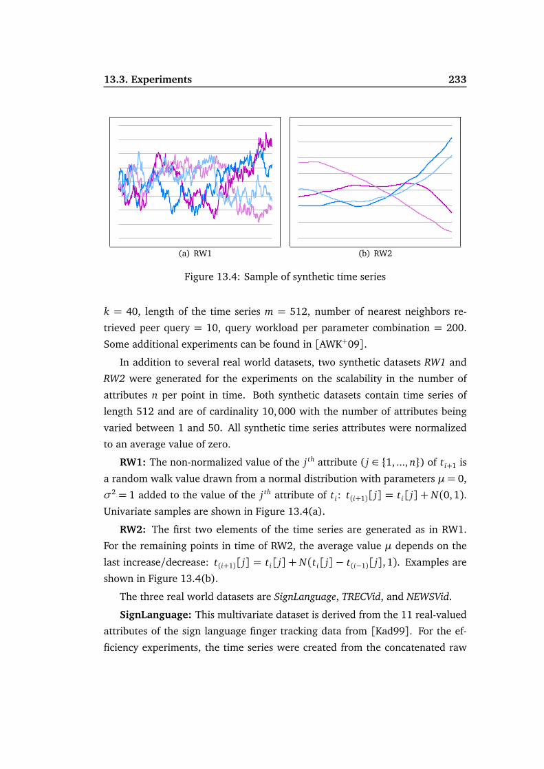
13.3. Experiments 233
(a) RW1 (b) RW2
Figure 13.4: Sample of synthetic time series
k = 40, length of the time series m = 512, number of nearest neighbors re-
trieved peer query = 10, query workload per parameter combination = 200.
Some additional experiments can be found in [AWK+09].
In addition to several real world datasets, two synthetic datasets RW1 and
RW2 were generated for the experiments on the scalability in the number of
attributes n per point in time. Both synthetic datasets contain time series of
length 512 and are of cardinality 10,000 with the number of attributes being
varied between 1 and 50. All synthetic time series attributes were normalized
to an average value of zero.
RW1: The non-normalized value of the j th attribute ( j ∈ 1, ..., n) of t i+1 is
a random walk value drawn from a normal distribution with parameters µ= 0,
σ2 = 1 added to the value of the j th attribute of t i: t(i+1)[ j] = t i[ j] + N(0,1).Univariate samples are shown in Figure 13.4(a).
RW2: The first two elements of the time series are generated as in RW1.
For the remaining points in time of RW2, the average value µ depends on the
last increase/decrease: t(i+1)[ j] = t i[ j] + N(t i[ j]− t(i−1)[ j], 1). Examples are
shown in Figure 13.4(b).
The three real world datasets are SignLanguage, TRECVid, and NEWSVid.
SignLanguage: This multivariate dataset is derived from the 11 real-valued
attributes of the sign language finger tracking data from [Kad99]. For the ef-
ficiency experiments, the time series were created from the concatenated raw

234 Reducing the Number of DTW Ground Distance Computations
1/8
1/4
1/2
1
256 128 64 32 16 8
aver
age
quer
y tim
e [s
] lo
g. sc
ale
reduced length
LBKeogh
Early Stopping
AP_LBKeogh
(a) LBKeogh
1/8
1/4
1/2
1
256 128 64 32 16 8
aver
age
quer
y tim
e [s
] lo
g. sc
ale
reduced length
LBHybrid
ES_LBHybrid
AP_LBHybrid
(b) LBHybrid
Figure 13.5: Absolute efficiency improvement (average query time) on RW2
data by extracting non-overlapping windows of equal length. The length m of
the non-overlapping time series was varied between 64 and 512 and the band k
was varied between 10 and 150. The number of time series was fixed at 1, 400.
TRECVid & NEWSVid: The two remaining datasets are derived from videos.
The first one is based on the TRECVid benchmark data [SOK06]. The NEWSVid
dataset consists of TV news shows that were recorded at 30 fps. 20-dimensional
HSV histograms were computed for each video frame (i.e., the time series are
multivariate with n= 20). The length m of the non-overlapping video sequences
was varied between 64 and 2048 frames. The cardinality of the database de-
pends on the length of the time series and varies between 650 and 2,000 for
TRECVid and between 2, 000 and 8,000 for NEWSVid.
13.3.2 Results
The runtime performance and the number of ground distance calculations of
aDTW are compared with those of the full DTW and DTW with Early Stopping.
As aDTW depends on a piecewise filter, variants LBKeogh and LBH y brid from Sec-
tion 13.2.8 are investigated. The result sets computed in the experiments are
identical for all approaches.
Dimensionality Reduction
In the first set of experiments, the efficiency of aDTW with respect to dimension-
ality reduction in the filter step is evaluated on the RW2 dataset. Figure 13.5

13.3. Experiments 235
0
20
40
60
80
100
256 128 64 32 16 8
rela
tive
impr
ovem
ent [
perc
ent]
reduced length
AP_LBKeoghES_LBKeoghAP_LBHybridES_LBHybrid
Figure 13.6: Relative efficiency improvement (average query time) on RW2
shows the average runtime for the lower-bounding filters on a logarithmic scale.
Anticipatory pruning, denoted as AP in the experiments, yields substantial run-
time improvements compared with the base methods LBKeogh and LBH y brid . It
also outperforms the Early Stopping approach (ES) [SYF05] for both filters. An-
ticipatory Pruning is especially helpful for strong reductions where it makes up
for the loss in selectivity of the filter step by pruning during the refinement.
Figure 13.6 summarizes the experiment by showing the relative improvement
versus the respective filter-and-refine method with full DTW refinement compu-
tations. To abstract from implementation details, figures 13.7 to 13.11 demon-
strate the reduction of the number of required ground distance calculations
compared with the full DTW computation.
For the second synthetic dataset, a summary of the relative improvement is
given by Figure 13.7(b). For this dataset of time series that rapidly oscillate
around the mean value, the improvements are pronounced and less sensitive to
the reduction parameter. The largest difference in the number of calculations
can be seen for the LBH y brid method, which shows a reduction of 75% (An-
ticipatory Pruning) versus 40% (Early Stopping). On the real world NEWSVid
dataset, the behavior is quite similar to the one on RW1.

236 Reducing the Number of DTW Ground Distance Computations
0
20
40
60
80
100
256 128 64 32 16 8
rela
tive
impr
ovem
ent [
perc
ent]
reduced length
AP_LBKeogh
ES_LBKeogh
AP_LBHybrid
ES_LBHybrid
(a) DB=RW2
0
20
40
60
80
100
256 128 64 32 16 8
rela
tive
impr
ovem
ent [
perc
ent]
reduced length
(b) DB=RW1
0
20
40
60
80
100
256 128 64 32 16 8
rela
tive
impr
ovem
ent [
perc
ent]
reduced length
(c) DB=NEWSVid
Figure 13.7: Efficiency improvement (#calc.) for varying reductions
0
20
40
60
80
100
1 5 10 20 30 40 50
rela
tive
impr
ovem
ent [
perc
ent]
number of attributes
AP_LBKeogh
ES_LBKeogh
AP_LBHybrid
ES_LBHybrid
(a) DB=RW2
0
20
40
60
80
100
1 5 10 20 30 40 50
rela
tive
Impr
ovem
ent [
perc
ent]
number of attributes
(b) DB=RW1
Figure 13.8: Efficiency improvement (#calc.) for varying numbers of attributes
Univariate and Multivariate Time Series
The next set of experiments evaluates the effect of the number of attributes n
on Anticipatory Pruning. Based on the results shown in Figure 13.5, a reduction
to 16 dimensions was chosen, which also represents an approximate upper limit
for the indexing of time series in structures such as the R-Tree. As depicted in
Figure 13.8(a) for the RW2 dataset, Anticipatory Pruning shows significant im-
provements for both filters. For higher numbers of attributes, the improvements
of Anticipatory Pruning over Early Stopping increase with Early Stopping be-
ing unable to skip a significant number of computations for both the boundary
and the linearization approach on the noisier dataset. On RW1, Anticipatory
Pruning outperforms Early Stopping but both methods show good results for
the univariate case, where a large difference in the starting value of two time
series with high probability results in a large difference for the whole band of
the first few columns.

13.3. Experiments 237
0
20
40
60
80
100
10 30 50 70 90 110 130 150
rela
tive
impr
ovem
ent [
perc
ent]
bandwidth
AP_LBKeoghES_LBKeoghAP_LBHybridES_LBHybrid
(a) DB=NEWSVid
0
20
40
60
80
100
10 30 50 70 90 110 130 150
rela
tive
impr
ovem
ent [
perc
ent]
bandwidth
(b) DB=TRECVid
0
20
40
60
80
100
10 30 50 70 90 110 130 150
rela
tive
impr
ovem
ent [
perc
ent]
bandwidth
(c) DB=SignLanguage
Figure 13.9: Efficiency improvement (#calc.) for varying DTW bandwidths(Sakoe-Chiba band)
0
20
40
60
80
100
64 128 256 512 1024 2048
rela
tive
impr
ovem
ent [
perc
ent]
sequence length
AP_LBKeogh
ES_LBKeogh
AP_LBHybrid
ES_LBHybrid
(a) DB=NEWSVid
0
20
40
60
80
100
64 128 256 512 1024 2048
rela
tive
Impr
ovem
ent [
perc
ent]
sequence length
(b) DB=TRECVid
0
20
40
60
80
100
64 128 256 512
rela
tive
Impr
ovem
ent [
perc
ent]
sequence length
(c) DB=SignLanguage
Figure 13.10: Efficiency improvement (#calc.) for varying time series lengths
Bandwidth
In Figure 13.9(a), the influence of the bandwidth constraint is studied on the
NEWSVid dataset. The dimensionality reduction parameter was again set to
16 dimensions. A remarkable reduction in the number of calculations can be
observed for the proposed Anticipatory Pruning based on both lower-bounding
filters and for all evaluated bandwidths. The relative number of calculations
avoided by Anticipatory Pruning is not very sensitive to the overall number of
calculations that have to be performed. Even for extremely wide bands of 150
points in time, Anticipatory Pruning yields substantial relative improvements.
The effect is also present for both the TRECVid dataset (Figure 13.9(b)) and the
SignLanguage dataset (Figure 13.9(c)).

238 Reducing the Number of DTW Ground Distance Computations
0
20
40
60
80
100
1 3 5 7 9 11 13 15
rela
tive
impr
ovem
ent [
perc
ent]
number of nearest neighbors
AP_LBKeoghES_LBKeoghAP_LBHybridES_LBHybrid
Figure 13.11: Efficiency improvement (#calc.) for varying numbers of NN
Length of Time Series
For many applications, the length of the time series to be compared is of greater
importance than the bandwidth of the DTW. In the experiment shown in Fig-
ure 13.10, the dimensionality reduction parameter in the filter was set to one
quarter of the original time series length. Figure 13.10(a) and Figure 13.10(b)
show improvements for the lower-bounding filters on the video datasets with
remarkable improvements for Anticipatory Pruning when the length increased.
The longer the time series is, the more distance information (in relative terms)
does the anticipatory part contribute at the beginning of the APD computation.
As Figure 13.10(c) shows, the results are similar on the SignLanguage dataset.
Number of Nearest Neighbors
As the last experiment, the effect of the number of nearest neighbors to be
retrieved from the NEWSVid dataset are depicted in Figure 13.11. Neither Early
Stopping nor Anticipatory Pruning are very sensitive to this parameter with a
slight decrease being expected as a larger number of nearest neighbors results
in a larger pruning distance.

13.4. Summary and Outlook 239
13.4 Summary and Outlook
Existing techniques for speeding up DTW-based similarity searches aim at ef-
ficiently filtering the database and computing the full DTW in the refinement
step. Unlike these algorithms, the aDTW approach proposed here exploits un-
used information from the filter step during the refinement and allows for a fast
rejection of false candidates without having to calculate all ground distances
of the cumulative distance matrix. As aDTW is a drop-in replacement for the
DTW refinement distance, it can be integrated with other filter and indexing
approaches whenever a piecewise filter is available. The significant reduction in
the number of ground distance computations that aDTW achieves is robust with
regard to many of the common parameters encountered when searching for sim-
ilar time series. Together, these properties make the utilization of more expen-
sive DTW ground distances viable as has been recently discussed for DTWEM D
in [AK09, AKS10], where an efficient and effective video copy detection system
is forged.


Part VI
Summary and Outlook
241

Summary and Outlook 243
In distance-based similarity search, a field of research that is relevant to
both data mining and information retrieval tasks, a distance measure quantifies
a degree of similarity between two objects. In this context, a large distance value
is interpreted as a small degree of similarity and vice versa. The effectiveness of
the employed distance measures with regards to reflecting a desired notion of
similarity and the efficiency of search algorithms based on these measures are
of foremost importance for the overall system performance.
This work addressed a particularly intuitive and flexible class of distance
measures. Transformation-based distance measures define a distance value be-
tween two objects by computing the least-cost transformation from a feature
representation of one object to a feature representation of the other object. The
cost of a single transformation in the feature space is modeled via a ground
distance measure, which enables the incorporation of perceptual correlation
across differing features. These two concepts make transformation-based dis-
tance measures computationally more expensive than many simple distance
measures such as the Euclidean distance but they also endow them with a high
degree of flexibility and a great effectiveness potential. Transformation-based
distance measures thus constitute a sensible choice for a large number of simi-
larity search tasks.
After having introduced the general concepts of distance-based similarity
search in Part I, three prominent representatives of the class of transformation-
based distance measures were reviewed in Part II: The Edit Distance, the Dy-
namic Time Warping distance, and the Earth Mover’s Distance, the latter of
which was the focus of much of the rest of this work. Part III proposed two tech-
niques that address the efficiency of the Earth Mover’s Distance. The first tech-
nique was based on a dimensionality reduction of the feature representations
while the second technique explored direct and vector approximation-based in-
dexing of the Earth Mover’s Distance. In Part IV, the effectiveness of the Earth
Mover’s Distance as a measure of dissimilarity was addressed by giving a frame-
work for its metric adaptation and showing how its flexibility in terms of the
ground distance can be exploited in a Relevance Feedback setup. Finally, Part V
explored new ways of applying transformation-based distances to objects that
exhibit a structure such as graphs and time series. An application of the Earth

244 Summary and Outlook
Mover’s Distance to graph similarity search was described based on a mapping
from vertex degree co-occurrences to feature signatures, and the use of the Earth
Mover’s Distance as a ground distance for Dynamic Time Warping was prepared
by reducing the ground distance computations for the latter in a multi-step simi-
larity search system. The results of empirical evaluations presented in this work
show considerable improvement over existing techniques and/or baseline solu-
tions.
Since 2005, the Earth Mover’s Distance as a transformation-based distance
measure has been a prominent topic at the group of Professor Seidl at RWTH
Aachen University. Parts of the research presented in this work were funded
by grants SE1039/1-2 and SE1039/1-3 of the German Research Foundation
DFG ending in 2010 (German title: “Schnelle inhaltsbasierte Suche in großen
Multimedia-Datenbanksystemen mittels der Earth Mover’s Distance”). Addition-
ally, the application of transformation-based distance functions to fingerprint-
based authentication was explored as part of the joint BioKeyS project con-
ducted in collaboration with the German Federal Office for Information Security
(BSI), Fraunhofer IGD, Darmstadt University, and LMU Munich.
Beyond the potential for further research identified in chapters 8 to 13, the
concept of feature signatures is being explored in the context of quadratic form
distances in the group of Professor Seidl, and topics such as the application of
the Earth Mover’s Distance and related distance measures to closed-loop control
of combustion engines via the incorporation of higher moment information are
envisioned to be explored as part of the second funding round of the DFG-
funded special research field SFB686 at RWTH Aachen University starting in
2010.

Part VII
Appendices
I


Naming Conventions
Throughout the document, the following conventions were followed unless in-
dicated otherwise for the sake of readability.
• objects: Database and query objects are denoted in lower case after n in
the alphabet (e.g., o, p, q, r, s, t, u).
• sets: Sets start with an upper case letter (e.g., S, DB, Feasible).
• vector and matrix access: Individual dimensions of vectors and entries
of matrices are accessed with square brackets (e.g., c[1], A[1, 2]).
• set access: Sorted set elements are accessed with square brackets (e.g.,
DB[1], KNN[k]).
• range access: Ranges are given by a colon (e.g., DB[k : 2k], c[1 : n′]).
• enumeration: Numbered objects have a lower index (e.g., o1, o2).
• association: General association of an object with another object is de-
noted by an upper or lower index (e.g., cP , EM Dgd).
For example, cP2 [1 : n′] is the second vector c associated with set P projected on
the first n′ dimensions while DB[5][3] is the value of the third dimension of the
5th object in DB where set DB is accessed as an ordered set of vectors/arrays.
III


List of Symbols
q query object
o, p, r, s, t, u database objects
ho fixed-binning feature histogram of object o (p. 10)
so adaptive-binning feature histogram/signature of object o (p.
11)
⟨to1, . . . , to
m⟩ feature sequence of object o (p. 13)
t← reversed sequence/time series ⟨tom, . . . , to
1⟩ (p. 225)
|o|Σ sum of entries for vectors and matrices (p. 10) or sum of weights
for adaptive-binning histograms / signatures (p. 11)
HSp|r half space that is closer to p than to r (p. 35)
VCp,S Voronoi cell of point p in a space S (p. 35)
VDDB,S Voronoi diagram of point set DB in a space S (p. 35)
χ a characteristic filter function (p. 46)
Rn,n′ the set of combining linear reduction matrices (p. 99)
A• B the element-wise matrix multiplication (p. 157)
(A•αi j) single-element matrix multiplication (p. 157)
ℜ the set of relevant objects in a database (p. 175)
δG(v) the edge degree of vertex v in a graph G (p. 204)
PGm the set of all simple paths of length m in G (p. 205)
DGm the vertex degree co-occurrence multiset of degree m for graph
G (p. 206)
R,R+ the set of real numbers and the set of non-negative real numbers
N0,N1 the set of natural numbers starting with 0 and 1
Z the set of integers
V


List of Algorithms
2.1 rangeQ(q, ε, d, DB) . . . . . . . . . . . . . . . . . . . . . . . . . . . 20
2.2 nnQ(q, k, d, DB) . . . . . . . . . . . . . . . . . . . . . . . . . . . . . 22
2.3 rankingQ(q, i, k, d, DB) . . . . . . . . . . . . . . . . . . . . . . . . 23
3.1 rtree-rangeQ(q, ε, d, minDist, RTree) . . . . . . . . . . . . . . . . 29
3.2 rec-rtree-rangeQ(q, ε, d, minDist, node) . . . . . . . . . . . . . . 29
4.1 voronoi-nnQ(q, VDDB,S) . . . . . . . . . . . . . . . . . . . . . . . . 35
4.2 approx-voronoi-nnQ(q, d, AVDDB,S) . . . . . . . . . . . . . . . . . 36
5.1 editDistance(s,t,gd) . . . . . . . . . . . . . . . . . . . . . . . . . . . 64
8.1 optimizeFB_MOD(R, C, F, n, n’) . . . . . . . . . . . . . . . . . . . 112
8.2 calcQuality(R, C, F, origDim, newRedDim, n’) . . . . . . . . . . . 113
8.3 optimizeFB_ALL(R, C, F, d, d’) . . . . . . . . . . . . . . . . . . . . 114
9.1 computeLT(C, q, ColSorting, LBoundaries) . . . . . . . . . . . . 138
9.2 computeLBLT(approx_o, LT) . . . . . . . . . . . . . . . . . . . . . 139
9.3 LB_LT-rangeQ(q, ε, EMDC , DB, ColSorting, VA) . . . . . . . . . . 139
9.4 LB_LT+-rangeQ(q, ε, EMDC , DB, ColSorting, EntrySorting, VA) 142
11.1 feedbackLoop(DB, q, gd, k, computeQuery, computeGD) . . . . 173
11.2 optimize(C, q, feedback) . . . . . . . . . . . . . . . . . . . . . . . 177
11.3 computeGD-QM(q, feedback, iter) . . . . . . . . . . . . . . . . . 179
11.4 computeGD-Histogram-Heur(q, feedback, iter) . . . . . . . . . . 180
11.5 computeGD-Histogram-Heur-Matrix(q, feedback, iter) . . . . . 180
11.6 computeGD-Histogram-Opt(q, feedback, iter) . . . . . . . . . . 182
VII

VIII LIST OF ALGORITHMS
11.7 modify(C) . . . . . . . . . . . . . . . . . . . . . . . . . . . . . . . . 183
11.8 computeGD-Signature-Heur(q, feedback, iter) . . . . . . . . . . 184
11.9 computeGD-Signature-Heur-Matrix(q, feedback, iter) . . . . . . 185
11.10 computeGD-Signature-Opt(q, feedback, iter) . . . . . . . . . . . 187
13.1 APD(q, t, ε, pf, gd, band) . . . . . . . . . . . . . . . . . . . . . . . 227
13.2 CalcDTWColumn(q, tj, col, gd, bandj) . . . . . . . . . . . . . . . 228
13.3 aDTW-rangeQ(q, ε, gd, band, DB) . . . . . . . . . . . . . . . . . . 229
Bibliography
[AB02] Réka Albert and Albert-László Barabási. Statistical Mechanics of
Complex Networks. Reviews of Modern Physics, 74:47–97, 2002.
[ABKS98] Mihael Ankerst, Bernhard Braunmüller, Hans-Peter Kriegel, and
Thomas Seidl. Improving Adaptable Similarity Query Processing
by Using Approximations. In Proceedings of the International Con-
ference on Very Large Data Bases (VLDB), pages 206–217, 1998.
[AC01] John Aach and George M. Church. Aligning Gene Expression Time
Series with Time Warping Algorithms. Bioinformatics, 17(6):495–
508, 2001.
[AFS93] Rakesh Agrawal, Christos Faloutsos, and Arun N. Swami. Efficient
Similarity Search in Sequence Databases. In Foundations of Data
Organization and Algorithms (FODO), pages 69–84, 1993.
[AK00] Franz Aurenhammer and Rolf Klein. Handbook of Computational
Geometry, pages 201–290. Elsevier Science Publishers, 2000.
[AK09] Ira Assent and Hardy Kremer. Robust Adaptable Video Copy De-
tection. In Proceedings of the International Symposium on Spatial
and Temporal Databases (SSTD), pages 380–385, 2009.
[AKS10] Ira Assent, Hardy Kremer, and Thomas Seidl. Speeding up Com-
plex Video Copy Detection Queries. In Proceedings of the Inter-
national Conference on Database Systems for Advanced Applications
(DASFAA), pages 307–321, 2010.
IX

X BIBLIOGRAPHY
[APP+08] Vassilis Athitsos, Panagiotis Papapetrou, Michalis Potamias,
George Kollios, and Dimitrios Gunopulos. Approximate
Embedding-Based Subsequence Matching of Time Series. In Pro-
ceedings of the ACM International Conference on Management of
Data (SIGMOD), pages 365–378, 2008.
[AWK+09] Ira Assent, Marc Wichterich, Ralph Krieger, Hardy Kremer, and
Thomas Seidl. Anticipatory DTW for Efficient Similarity Search in
Time Series Databases. In Proceedings of the International Confer-
ence on Very Large Data Bases (VLDB), pages 826–837, 2009.
[AWMS08] Ira Assent, Marc Wichterich, Tobias Meisen, and Thomas Seidl.
Efficient Similarity Search Using the Earth Mover’s Distance for
Large Multimedia Databases. In Proceedings of the IEEE Inter-
national Conference on Data Engineering (ICDE), pages 307–316,
2008.
[AWS06] Ira Assent, Marc Wichterich, and Thomas Seidl. Adaptable
Distance Functions for Similarity-Based Multimedia Retrieval.
Datenbank-Spektrum, 19:23–31, 2006.
[BA83] Horst Bunke and Gudrun Allermann. Inexact Graph Matching
for Structural Pattern Recognition. Pattern Recognition Letters,
1(4):245–253, 1983.
[BBDH96] C. Bradford Barber, David P. Dobkin, and Hannu Huhdanpaa. The
Quickhull Algorithm for Convex Hulls. ACM Transactions on Math-
ematical Software, 22(4):469–483, 1996.
[BC94] Donald J. Berndt and James Clifford. Using Dynamic Time Warp-
ing to Find Patterns in Time Series. In AAAI Workshop on KDD,
pages 229–248, 1994.
[BEK+98] Stefan Berchtold, Bernhard Ertl, Daniel A. Keim, Hans-Peter
Kriegel, and Thomas Seidl. Fast Nearest Neighbor Search in High-
Dimensional Spaces. In Proceedings of the IEEE International Con-
ference on Data Engineering (ICDE), pages 209–218, 1998.

BIBLIOGRAPHY XI
[BGRS99] Kevin Beyer, Jonathan Goldstein, Raghu Ramakrishnan, and Uri
Shaft. When is “Nearest Neighbor” Meaningful? In Proceedings
of the International Conference on Database Theory (ICDT), pages
217–235, 1999.
[BKK96] Stefan Berchtold, Daniel A. Keim, and Hans-Peter Kriegel. The
X-Tree: An Index Structure for High-Dimensional Data. In Pro-
ceedings of the International Conference on Very Large Data Bases
(VLDB), pages 28–39, 1996.
[BKKS00] Stefan Berchtold, Daniel A. Keim, Hans-Peter Kriegel, and Thomas
Seidl. Indexing the Solution Space: A New Technique for Nearest
Neighbor Search in High-Dimensional Space. IEEE Transactions on
Knowledge & Data Engineering (TKDE), 12(1):45–57, 2000.
[BKSS90] Norbert Beckmann, Hans-Peter Kriegel, Ralf Schneider, and Bern-
hard Seeger. The R*-Tree: An Efficient and Robust Access Method
for Points and Rectangles. In Proceedings of the ACM International
Conference on Management of Data (SIGMOD), pages 322–331,
1990.
[BMR01] Philip Bohannon, Peter McIlroy, and Rajeev Rastogi. Main-
Memory Index Structures with Fixed-Size Partial Keys. In Proceed-
ings of the ACM International Conference on Management of Data
(SIGMOD), pages 163–174, 2001.
[BS95] Chris Buckley and Gerard Salton. Optimization of Relevance Feed-
back Weights. In Proceedings of the ACM Conference on Research
and Development in Information Retrieval (SIGIR), pages 351–357,
1995.
[BS98] Horst Bunke and Kim Shearer. A Graph Distance Metric Based
on the Maximal Common Subgraph. Pattern Recognition Letters,
19(3-4):255–259, 1998.
[BS09] Norbert Beckmann and Bernhard Seeger. A Revised R*-Tree in
Comparison with Related Index Structures. In Proceedings of the
XII BIBLIOGRAPHY
ACM International Conference on Management of Data (SIGMOD),
pages 799–812, 2009.
[BUS09] Christian Beecks, Merih Seran Uysal, and Thomas Seidl. Signature
Quadratic Form Distances for Content-Based Similarity. In Pro-
ceedings of the ACM International Conference on Multimedia (MM),
pages 697–700, 2009.
[BUS10] Christian Beecks, Merih Seran Uysal, and Thomas Seidl. Efficient
k-Nearest Neighbor Queries with the Signature Quadratic Form
Distance. In Proceedings of the International Workshop on Ranking
in Databases (DBRank) in conjunction with the IEEE International
Conference on Data Engineering (ICDE), 2010.
[BWS06] Christoph Brochhaus, Marc Wichterich, and Thomas Seidl. Ap-
proximation Techniques to Enable Dimensionality Reduction for
Voronoi-Based Nearest Neighbor Search. In Proceedings of the In-
ternational Conference on Extending Data Base Technology (EDBT),
pages 204–221, 2006.
[BWS09] Christian Beecks, Marc Wichterich, and Thomas Seidl. Metrische
Anpassung der Earth Mover’s Distanz zur Ähnlichkeitssuche in
Multimedia-Datenbanken. In Proceedings of the GI Conference on
Database Systems for Business, Technology, and the Web (BTW),
pages 207–216, 2009.
[CB07] Christophe Chefd’hotel and Guillaume Bousquet. Intensity-Based
Image Registration Using Earth Mover’s Distance. In Medical Imag-
ing 2007: Image Processing, pages 65122B.1–65122B.8, 2007.
[CFPF03] Matthieu Cord, Jérome Fournier, and Sylvie Philipp-Foliguet. Ex-
ploration and Search-by-Similarity in CBIR. In Proceedings of the
Brazilian Symposium on Computer Graphics and Image Processing
(SIBGRAPI), pages 175–182, 2003.
[CFY03] Franky K.-P. Chan, Ada W.-C. Fu, and Clement Yu. Haar wavelets
for efficient similarity search of time-series: With and without

BIBLIOGRAPHY XIII
time warping. IEEE Transactions on Knowledge & Data Engineer-
ing (TKDE), 15(3):686–705, 2003.
[CG97] Scott D. Cohen and Leonidas J. Guibas. The Earth Mover’s Dis-
tance: Lower Bounds and Invariance under Translation. Technical
Report STAN-CS-TR-97-1597, Stanford University, 1997.
[CKHP02] Selina Chu, Eamonn Keogh, David Hart, and Michael Pazzani. Iter-
ative deepening dynamic time warping for time series. In Proceed-
ings of the SIAM International Conference on Data Mining (SDM),
2002.
[CLC04] An-Pin Chen, Sheng-Fuu Lin, and Yi-Chang Cheng. Time Registra-
tion of Two Image Sequences by Dynamic Time Warping. In Pro-
ceedings of the IEEE International Conference on Networking, Sens-
ing and Control (ICNSC), pages 418–423, 2004.
[CPFGF05] Matthieu Cord, Sylvie Philipp-Foliguet, Philippe-Henri Gosselin,
and Jérôme Fournier. Interactive Exploration for Image Retrieval.
EURASIP Journal on Applied Signal Processing, 2005(14):2173–
2186, 2005.
[CPZ97] Paolo Ciaccia, Marco Patella, and Pavel Zezula. M-Tree: An Ef-
ficient Access Method for Similarity Search in Metric Spaces. In
Proceedings of the International Conference on Very Large Data Bases
(VLDB), pages 426–435, 1997.
[Des44] René Descartes. Principia Philosophiæ. Ludovicum Elzevirium,
1644.
[Dir50] G. Lejeune Dirichlet. Über die Reduction der positiven quadratis-
chen Formen mit drei unbestimmten ganzen Zahlen. Journal für
die reine und angewandte Mathematik, 40:209–227, 1850.
[DKN05] Thomas Deselaers, Daniel Keysers, and Hermann Ney. Discrimi-
native Training for Object Recognition Using Image Patches. In

XIV BIBLIOGRAPHY
Proceedings of the IEEE Conference on Computer Vision and Pattern
Recognition (CVPR), pages 157–162, 2005.
[DL76] David P. Dobkin and Richard J. Lipton. Multidimensional Search-
ing Problems. SIAM Journal on Computing, 5(2):181–186, 1976.
[DMC+07] Thomas Deselaers, Henning Müller, Paul Clogh, Hermann Ney,
and Thomas M. Lehmann. The CLEF 2005 Automatic Medical
Image Annotation Task. International Journal of Computer Vision,
74(1):51–58, 2007.
[DMHE+06] Laura Dempere-Marco, Xiao-Peng Hu, Stephen Ellis, David
Hansell, and Guang-Zhong Yang. Analysis of Visual Search Pat-
terns with EMD Metric in Normalized Anatomical Space. IEEE
Transactions on Medical Imaging (TMI), 25:1011–1021, 2006.
[Ede87] Herbert Edelsbrunner. Algorithms in Combinatorial Geometry.
Springer Verlag, 1987.
[EMLB08] Manolya Eyiyurekli, Prakash Manley, Peter I. Lelkes, and David E.
Breen. A Computational Model of Chemotaxis-Based Cell Aggre-
gation. Biosystems, 93:226–239, 2008.
[ER59] Paul Erdõs and Alfréd Rényi. On Random Graphs I. Publicationes
Mathematicae, 6:290–297, 1959.
[FdSTGF08] Cristiano D. Ferreira, Ricardo da S. Torres, Marcos André
Gonçalves, and Weiguo Fan. Image Retrieval with Relevance Feed-
back Based on Genetic Programming. In Proceedings of the Brazil-
ian Symposium on Databases (SBBD), pages 120–134, 2008.
[FWD06] Anthony Y. Fu, Liu Wenyin, and Xiaotie Deng. Detecting Phish-
ing Web Pages with Visual Similarity Assessment Based on Earth
Mover’s Distance (EMD). IEEE Transactions on Dependable and Se-
cure Computing, 3(4):301–311, 2006.

BIBLIOGRAPHY XV
[GBS05] Jan-Mark Geusebroek, Gertjan J. Burghouts, and Arnold W. M.
Smeulders. The Amsterdam Library of Object Images. Interna-
tional Journal on Computer Vision, 61(1):103–112, 2005.
[GCK07] Matt Groening, David X. Cohen, and Ken Keeler. Futurama: Ben-
der’s Big Score. 20th Century Fox Television, 2007.
[GD04] Kristen Grauman and Trevor Darrell. Fast Contour Matching Using
Approximate Earth Mover’s Distance. In Proceedings of the IEEE
Conference on Computer Vision and Pattern Recognition (CVPR),
pages 220–227, 2004.
[GPB03] Jonathan Goldstein, John C. Platt, and Christopher J. C. Burges.
Indexing High Dimensional Rectangles for Fast Multimedia Iden-
tification. Technical Report MSR-TR-2003-38, Microsoft Research,
2003.
[Gut84] Antonin Guttman. R-Trees: A Dynamic Index Structure for Spatial
Searching. In Proceedings of the ACM International Conference on
Management of Data (SIGMOD), pages 47–57, 1984.
[GV02] Panos Giannopoulos and Remco C. Veltkamp. A Pseudo-Metric for
Weighted Point Sets. In Proceedings of the European Conference on
Computer Vision, pages 715–730, 2002.
[GXTL08] Xinbo Gao, Bing Xiao, Dacheng Tao, and Xuelong Li. Image Cate-
gorization: Graph Edit Distance + Edge Direction Histogram. Pat-
tern Recognition, 41(10):3179–3191, 2008.
[HL04] Frederick S. Hillier and Gerald J. Lieberman. Introduction to Op-
erations Research. McGraw-Hill, eighth edition, 2004.
[HNZ+08] Stefan Haufe, Vadim V. Nikulin, Andreas Ziehe, Klaus-Robert
Müller, and Guido Nolte. Combining sparsity and rotational in-
variance in eeg/meg source reconstruction. NeuroImage, 42:726–
738, 2008.

XVI BIBLIOGRAPHY
[HS95] Gísli R. Hjaltason and Hanan Samet. Ranking in Spatial Data-
bases. In Proceedings of the International Symposium on Advances
in Spatial Databases (SSD), pages 83–95, 1995.
[HSE+95] James Hafner, Harpreet S. Sawhney, Will Equitz, Myron Flick-
ner, and Wayne Niblack. Efficient Color Histogram Indexing for
Quadratic Form Distance Functions. IEEE Transactions on Pattern
Analysis and Machine Intelligence (PAMI), 17(7):729–736, 1995.
[ISF98] Yoshiharu Ishikawa, Ravishankar Subramanya, and Christos
Faloutsos. MindReader: Querying databases through multiple ex-
amples. In Proceedings of the International Conference on Very Large
Databases (VLDB), pages 218–227, 1998.
[IT03] Piotr Indyk and Nitin Thaper. Fast Image Retrieval via Embed-
dings. In Workshop on Statistical and Computational Theories of
Vision (SCTV), 2003.
[Ita75] Fumitada Itakura. Minimum prediction residual principle applied
to speech recognition. IEEE Transactions on Acoustics, Speech, and
Signal Processing, 23(1):67–72, 1975.
[JLZ+03] Feng Jing, Mingjing Li, Lei Zhang, Hong-Jiang Zhang, and
Bo Zhang. Learning in Region-Based Image Retrieval. In Proceed-
ings of the Conference on Image and Video Retrieval (CIVR), pages
206–215, 2003.
[Kac10] Nezamoddin N. Kachoui. Image Denoising Using Earth Mover’s
Distance and Local Histograms. International Journal of Image
Processing (IJIP), 4:66–76, 2010.
[Kad99] Mohammed W. Kadous. Australian sign language data set 1.
http://www.cse.unsw.edu.au/~waleed/tml/data/, 1999.
[Kan42] Leonid Kantorovich. On the Translocation of Masses. Doklady
Akademii Nauk SSSR, 37:199–201, 1942.

BIBLIOGRAPHY XVII
[KCK01] Kihong Kim, Sang Kyun Cha, and Keunjoo Kwon. Optimizing Mul-
tidimensional Index Trees for Main Memory Access. In Proceedings
of the ACM International Conference on Management of Data (SIG-
MOD), pages 139–150, 2001.
[KCPM00] Eamonn Keogh, Kaushik Chakrabarti, Michael Pazzani, and
Sharad Mehrotra. Locally Adaptive Dimensionality Reduction for
Indexing Large Time Series Databases. In Proceedings of the ACM
International Conference on Management of Data (SIGMOD), pages
151–162, 2000.
[KCPM01] Eamonn Keogh, Kaushik Chakrabarti, Michael Pazzani, and
Sharad Mehrotra. Dimensionality Reduction for Fast Similarity
Search in Large Time Series Databases. Journal of Knowledge and
Information Systems (KAIS), 3(3):263–286, 2001.
[Keo02] Eamonn Keogh. Exact Indexing of Dynamic Time Warping. In
Proceedings of the International Conference on Very Large Databases
(VLDB), pages 406–417, 2002.
[KF02] Eamonn Keogh and Theodoros Folias. The UCR Time Series Data
Mining Archive. http://www.cs.ucr.edu/~eamonn/TSDMA/
index.html, 2002.
[KGV83] Scott Kirkpatrick, C. D. Gelatt, and Mario P. Vecchi. Optimization
by Simulated Annealing. Science, 220(4598):671 – 680, 1983.
[Kle80] Victor Klee. On the Complexity of d-dimensional Voronoi Dia-
grams. Archiv der Mathematik, 34:75–80, 1980.
[KPC01] San-Wook Kim, Sanghyun Park, and Wesley W. Chu. An Index-
Based Approach for Similarity Search Supporting Time Warping in
Large Sequence Databases. In Proceedings of the IEEE International
Conference on Data Engineering (ICDE), pages 607–614, 2001.
[KR90] Leonard Kaufman and Peter J. Rousseeuw. Finding Groups in Data.
An Introduction to Cluster Analysis. Wiley-Interscience, 1990.
XVIII BIBLIOGRAPHY
[KSF+96] Flip Korn, Nikolaos Sidiropoulos, Christos Faloutsos, Eliot Siegel,
and Zenon Protopapas. Fast Nearest Neighbor Search in Medical
Image Databases. In The VLDB Journal, pages 215–226, 1996.
[KWX+06] Eamonn Keogh, Li Wei, Xiaopeng Xi, Sang-Hee Lee, and Michail
Vlachos. LB_Keogh Supports Exact Indexing of Shapes under
Rotation Invariance with Arbitrary Representations and Distance
Measures. In Proceedings of the International Conference on Very
Large Databases (VLDB), pages 882–893, 2006.
[LB01] Elizaveta Levina and Peter J. Bickel. The Earth Mover’s Distance is
the Mallows Distance: Some Insights from Statistics. In Proceed-
ings of the International Conference On Computer Vision (ICCV),
pages 251–256, 2001.
[LBH98] Yingmei Lavin, Rajesh Batra, and Lambertus Hesselink. Feature
Comparisons of Vector Fields Using Earth Mover’s Distance. In
Proceedings of the IEEE Conference on Visualization (Vis), pages
103–109, 1998.
[LBS06] Vebjørn Ljoså, Arnab Bhattacharya, and Ambuj K. Singh. Index-
ing Spatially Sensitive Distance Measures Using Multi-Resolution
Lower Bounds. In Proceedings of the International Conference on
Extending Database Technology (EDBT), pages 865–883, 2006.
[Lev66] Vladimir I. Levenshtein. Binary Codes Capable of Correcting
Deletions, Insertions, and Reversals. Soviet Physics Doklady,
10(8):707–710, 1966.
[LGT+04] Thomas M. Lehmann, Mark O. Güld, Christian Thies, Benedikt
Fischer, Klaus Spitzer, Daniel Keysers, Hermann Ney, M. Kohnen,
Henning Schubert, and Berthold B. Wein. Content-Based Im-
age Retrieval in Medical Applications. Methods of Information in
Medicine, 43(4):354–361, 2004.

BIBLIOGRAPHY XIX
[LH08] Cheuh-Yu Li and Chiou-Ting Hsu. Image Retrieval With Relevance
Feedback Based on Graph-Theoretic Region Correspondence Esti-
mation. IEEE Transactions on Multimedia (TMM), 10(3):447–456,
2008.
[LO07] Haibin Ling and Kazunori Okada. An Efficient Earth Mover’s
Distance Algorithm for Robust Histogram Comparison. IEEE
Transactions on Pattern Analysis and Machine Intelligence (TPAMI),
29(5):840–853, 2007.
[LOEA+07] Daniel R. Leff, Felipe Orihuela-Espina, Louis Atallah, Ara Darzi,
and Guang-Zhong Yang. Functional Near Infrared Spectroscopy in
Novice and Expert Surgeons – a Manifold Embedding Approach.
In Proceedings of the International Conference on Medical Image
Computing and Computer-Assisted Intervention (MICCAI), pages
270–277, 2007.
[LWH03] Bin Luo, Richard C. Wilson, and Edwin R. Hancock. Spectral Em-
bedding of Graphs. Pattern Recognition, 36(10):2213–2230, 2003.
[LWT05] Jiangwei Li, Yunhong Wang, and Tieniu Tan. Video-Based Face
Recognition Using Earth Mover’s Distance. In Proceedings of the
International Conference on Audio- and Video-Based Biometric Per-
son Authentication (AVBPA), pages 229–238, 2005.
[Mon81] Gaspard Monge. Mémoire sue la Théorie des Déblais et de Rem-
blais. In Histoire de l’Académie Royale des Sciences de Paris, avec
les Mémoires de Mathématique et de Physique pour la même année,
pages 666–704. Académie des Sciences, 1781.
[MRM+05] Dirk R. Mendonça, Paulo R. S.and Padfield, James C. Ross,
James V. Miller, Sandeep Dutta, and Sardar Mal Gautham. Quan-
tification of Emphysema Severity by Histogram Analysis of CT
Scans. In Proceedings of the International Conference on Medi-
cal Image Computing and Computer-Assisted Intervention (MICCAI),
pages 738–744, 2005.

XX BIBLIOGRAPHY
[MRS08] Christopher D. Manning, Prabhakar Raghavan, and Hinrich
Schütze. Introduction to Information Retrieval. Cambridge Uni-
versity Press, 2008.
[NC08] Ifeoma Nwogu and Jason J. Corso. Exploratory Identification of
Image-Based Biomarkers for Solid Mass Pulmonary Tumors. In
Proceedings of the International Conference on Medical Image Com-
puting and Computer-Assisted Intervention (MICCAI), pages 612–
619, 2008.
[OBM04] Michael Ortega-Binderberger and Sharad Mehrotra. Relevance
Feedback Techniques in the MARS Image Retrieval System. Multi-
media Systems, 9(6):535–547, 2004.
[OTK76] Teruo Okuda, Eiichi Tanaka, and Tamotsu Kasai. A Method for the
Correction of Garbled Words Based on the Levenshtein Metric.
IEEE Transactions on Computers, C-25(2):172–178, 1976.
[PBRT99] Jan Puzicha, Joachim Buhmann, Yossi Rubner, and Carlo Tomasi.
Empirical Evaluation of Dissimilarity Measures for Color and Tex-
ture. In Proceedings of the IEEE International Conference on Com-
puter Vision (ICCV), pages 1165–1173, 1999.
[PM99] Apostolos N. Papadopoulos and Yannis Manolopoulos. Structure-
Based Similarity Search with Graph Histograms. In Proceedings of
the International Workshop on Database and Expert Systems Appli-
cations (DEXA), pages 174–178, 1999.
[PTVF92] William H. Press, Saul A. Teukolsky, William T. Vetterling, and
Brian P. Flannery. Numerical Recipes in C: The Art of Scientific Com-
puting. Cambridge University Press, 1992.
[PW09] Ofir Pele and Michael Werman. Fast and Robust Earth Mover’s
Distances. In Proceedings of the IEEE International Conference on
Computer Vision, 2009.

BIBLIOGRAPHY XXI
[RKV95] Nick Roussopoulos, Stephen Kelley, and Frédéic Vincent. Nearest
Neighbor Queries. In Proceedings of the ACM International Confer-
ence on Management of Data (SIGMOD), pages 71–79, 1995.
[RM02] Toni Rath and R. Manmatha. Lower-Bounding of Dynamic Time
Warping Distances for Multivariate Time Series. Technical Report
MM-40, University of Massachusetts Amherst - Center for Intelli-
gent Information Retrieval, 2002.
[Roc71] J. J. Rocchio. The SMART Retrieval System: Experiments in Auto-
matic Document Processing, chapter Relevance Feedback in Infor-
mation Retrieval. Prentice-Hall, 1971.
[RR00] Jun Rao and Kenneth A. Ross. Making B+-Trees Cache Conscious
in Main Memory. In Proceedings of the ACM International Confer-
ence on Management of Data (SIGMOD), pages 475–486, 2000.
[RT01] Yossi Rubner and Carlo Tomasi. Perceptual Metrics for Image Data-
base Navigation. Kluwer Academic, 2001.
[RTG98] Yossi Rubner, Carlo Tomasi, and Leonidas J. Guibas. A Metric for
Distributions with Applications to Image Databases. In Proceedings
of the IEEE International Conference on Computer Vision (ICCV),
pages 59–66, 1998.
[RTG00] Yossi Rubner, Carlo Tomasi, and Leonidas J. Guibas. The Earth
Mover’s Distance as a Metric for Image Retrieval. International
Journal of Computer Vision, 40(2):99–121, 2000.
[Sam05] Hanan Samet. Foundations of Multidimensional and Metric Data
Structures. Morgan Kaufmann Publishers Inc., 2005.
[SC78] Hiroaki Sakoe and Seibi Chiba. Dynamic Programming Algorithm
Optimization for Spoken Word Recognition. IEEE Transactions on
Acoustics, Speech, and Signal Processing, 26(1):43–49, 1978.

XXII BIBLIOGRAPHY
[SC04] Stan Salvador and Philip Chan. FastDTW: Toward Accurate Dy-
namic Time Warping in Linear Time and Space. In KDD Workshop
on Mining Temporal and Sequential Data (KDD/TDM), pages 70–
80, 2004.
[SC07] Stan Salvador and Philip Chan. Toward Accurate Dynamic Time
Warping in Linear Time and Space. Intelligent Data Analysis (IDA),
11(5):561–580, 2007.
[Sei87] Raimund Seidel. On the Number of Faces in Higher-Dimensional
Voronoi Diagrams. In Symposium on Computational Geometry,
pages 181–185, 1987.
[SJ08a] Sameer Shirdhonkar and David W. Jacobs. Approximate Earth
Mover’s Distance in Linear Time. In Proceedings of the IEEE Con-
ference on Computer Vision and Pattern Recognition (CVPR), 2008.
[SJ08b] Sameer Shirdhonkar and David W. Jacobs. Approximate Earth
Mover’s Distance in Linear Time. In Proceedings of the IEEE Con-
ference on Computer Vision and Pattern Recognition (CVPR), 2008.
[SK97] Thomas Seidl and Hans-Peter Kriegel. Efficient User-Adaptable
Similarity Search in Large Multimedia Databases. In Proceedings
of the International Conference on Very Large Data Bases (VLDB),
pages 506–515, 1997.
[SK98] Thomas Seidl and Hans-Peter Kriegel. Optimal Multi-Step k-
Nearest Neighbor Search. In Proceedings of the ACM International
Conference on Management of Data (SIGMOD), pages 154–165,
1998.
[SL09] Yankui Sun and Ming Lei. Method for Optical Coherence Tomog-
raphy Image Classification using Local Features and Earth Mover’s
Distance. Journal of Biomedical Optics, 14:054037–1–054037–6,
2009.

BIBLIOGRAPHY XXIII
[SOK06] Alan F. Smeaton, Paul Over, and Wessel Kraaij. Evaluation Cam-
paigns and TRECVid. In Proceedings of the ACM International
Workshop on Multimedia Information Retrieval (MIR), 2006.
[SRF87] Timos K. Sellis, Nick Roussopoulos, and Christos Faloutsos. The
R+-Tree: A Dynamic Index for Multi-Dimensional Objects. In Pro-
ceedings of the International Conference on Very Large Data Bases
(VLDB), pages 507–518, 1987.
[Sri04] S. H. Srinivasan. Local Earth Mover’s Distance and Face Warping.
In Proceedings of the IEEE International Conference on Multimedia
and Expo (ICME), pages 1227–1230, 2004.
[ST01] Daniel Spielman and Shang-Hua Teng. Smoothed Analysis of Al-
gorithms: Why the Simplex Algorithm Usually Takes Polynomial
Time. In Proceedings of the ACM Symposium on Theory of Comput-
ing (STOC), pages 296–305, 2001.
[STN+05] Axel Saalbach, Thorsten Twellmann, Tim W. Nattkemper, Axel
Wismüller, Jörg Ontrup, and Helge Ritter. A Hyperbolic Topo-
graphic Mapping for Proximity Data. In Proceedings of the IASTED
International Conference on Artificial Intelligence and Applications
(ICAIA), pages 106–111, 2005.
[SWG02] Dennis Shasha, Jason T. L. Wang, and Rosalba Giugno. Algorith-
mics and Applications of Tree and Graph Searching. In Proceedings
of the ACM Symposium on Principles of Database Systems (PODS),
pages 39–52, 2002.
[SYF05] Yasushi Sakurai, Masatoshi Yoshikawa, and Christos Faloutsos.
FTW: Fast Similarity Search under the Time Warping Distance.
In Proceedings of the ACM Symposium on Principles of Database
Systems (PODS), pages 326–337, 2005.
[TG82] Amosand Tversky and Itamar Gati. Similarity, Separability, and
the Triangle Inequality. Psychological Review, 89(2):123–154,
1982.

XXIV BIBLIOGRAPHY
[TGV+03] Rainer Typke, Panos Giannopoulos, Remco C. Veltkamp, Frans
Wiering, and Rene van Oostrum. Using Transportation Distances
for Measuring Melodic Similarity. In Proceedings of the Interna-
tional Conference on Music Information Retrieval (ISMIR), 2003.
[Tve77] Amos Tversky. Features of Similarity. Psychological Review,
84(4):327–352, 1977.
[TVW04] Rainer Typke, Remco C. Veltkamp, and Frans Wiering. Searching
notated polyphonic music using transportation distances. In Pro-
ceedings of the ACM International Conference on Multimedia (MM),
pages 128–135, 2004.
[UHMS06] Mats Uddenfeldt, Keiichiro Hoashi, Kazunori Matsumoto, and Fu-
miaki Sugaya. Adaptive Video News Story Tracking Based on
Earth Mover’s Distance. Proceedings of the IEEE International Con-
ference on Multimedia and Expo (ICME), pages 1029–1032, 2006.
[Ume88] Shinji Umeyama. An Eigendecomposition Approach to Weighted
Graph Matching Problems. IEEE Transactions on Pattern Analysis
and Machine Intelligence, 10(5):695–703, 1988.
[VHGK03] Michail Vlachos, Marios Hadjieleftheriou, Dimitrios Gunopulos,
and Eamonn Keogh. Indexing Multi-Dimensional Time-Series with
Support for Multiple Distance Measures. In Proceedings of the ACM
International Conference on Knowledge Discovery and Data Mining
(KDD), pages 216–225, 2003.
[VL05] Fabien Viger and Matthieu Latapy. Efficient and Simple Genera-
tion of Random Simple Connected Graphs with Prescribed Degree
Sequence. In Proceedings of the International Computing and Com-
binatorics Conference (COCOON), pages 440–449, 2005.
[Vor08] Georgy Voronoi. Nouvelles applications des paramètres continus
à la théorie des formes quadratiques. Journal für die reine und
angewandte Mathematik, 133:97–178, 1908.

BIBLIOGRAPHY XXV
[Wah00] Wolfgang Wahlster. Verbmobil: Foundations of Speech-to-Speech
Translation, pages 537–631. Springer Verlag, 2000.
[WAKS08] Marc Wichterich, Ira Assent, Philipp Kranen, and Thomas Seidl.
Efficient EMD-Based Similarity Search in Multimedia Databases
via Flexible Dimensionality Reduction. In Proceedings of the ACM
International Conference on Management of Data (SIGMOD), pages
199–212, 2008.
[WB97] Roger Weber and Stephen Blott. An Approximation-Based Data
Structure for Similarity Search. Technical Report 24 of ESPRIT
Project HERMES, Institute of Information Systems, ETH Zurich,
1997.
[WBS08] Marc Wichterich, Christian Beecks, and Thomas Seidl. Ranking
Multimedia Databases via Relevance Feedback with History and
Foresight Support. In Proceedings of the International Workshop
on Ranking in Databases (DBRank) in conjunction with the IEEE
International Conference on Data Engineering (ICDE), pages 596–
599, 2008.
[WBSS09a] Marc Wichterich, Christian Beecks, Martin Sundermeyer, and
Thomas Seidl. Exploring Multimedia Databases via Optimization-
Based Relevance Feedback and the Earth Mover’s Distance. In
Proceedings of the ACM Conference on Information and Knowledge
Management (CIKM), pages 1621–1624, 2009.
[WBSS09b] Marc Wichterich, Christian Beecks, Martin Sundermeyer, and
Thomas Seidl. Relevance Feedback for the Earth Mover’s Distance.
In Workshop on Adaptive Multimedia Retrieval, 2009.
[WSB98] Roger Weber, Hans-Jörg Schek, and Stephen Blott. A Quantitative
Analysis and Performance Study for Similarity-Search Methods in
High-Dimensional Spaces. In Proceedings of the International Con-
ference on Very Large Data Bases (VLDB), pages 194–205, 1998.

XXVI BIBLIOGRAPHY
[WT09] Chengyu Wu and Xiaoying Tai. Application of Gray Level Variation
Statistic in Gastroscopic Image Retrieval. In Proceedings of the
IEEE/ACIS International Conference on Computer and Information
Science (ICIS), pages 342–346, 2009.
[XLS08] Jian-Hua Xu, Fei Li, and Qiu-Feng Sun. Identification of MicroRNA
Precursors with Support Vector Machine and String Kernel. Ge-
nomics, Proteomics & Bioinformatics, 6(2):121–128, 2008.
[YJ06] Liu Yang and Rong Jin. Distance Metric Learning: A Compre-
hensive Survey. http://citeseerx.ist.psu.edu/viewdoc/
summary?doi=10.1.1.91.4732, 2006.
[YJF98] Byoung-Kee Yi, H. V. Jagadish, and Christos Faloutsos. Efficient
Retrieval of Similar Time Sequences under Time Warping. In Pro-
ceedings of the IEEE International Conference on Data Engineering
(ICDE), pages 201–208, 1998.
[YX03] Hangjun Ye and Guangyou Xu. Similarity Measure Learning for
Image Retrieval Using Feature Subspace Analysis. In Proceedings
of the International Conference on Computational Intelligence and
Multimedia Applications (ICCIMA), pages 131–136, 2003.
[ZBR07] Vanessa A. Zavaletta, Brian J. Bartholmai, and Richard A. Robb.
High Resolution Multidetector CT-Aided Tissue Analysis and
Quantification of Lung Fibrosis. Academic Radiology, 14:772–787,
2007.
[ZS03] Yunyue Zhu and Dennis Shasha. Warping Indexes with Envelope
Transforms for Query by Humming. In Proceedings of the ACM
International Conference on Management of Data (SIGMOD), pages
181–192, 2003.
[ZW07] Mi Zhou and Man H. Wong. Boundary-Based Lower-Bound Func-
tions for Dynamic Time Warping and Their Indexing. In Pro-
ceedings of the IEEE International Conference on Data Engineering
(ICDE), pages 1307–1311, 2007.

BIBLIOGRAPHY XXVII
[ZWS96] Kaizhong Zhang, Jason T.-L. Wang, and Dennis Shasha. On the
Editing Distance Between Undirected Acyclic Graphs. Interna-
tional Journal of Foundations of Computer Science, 7(1):43–58,
1996.


Collaboration / Acknowledgments
This thesis would not have been possible without the close collaboration in the
group of Professor Seidl. Many of the presented ideas and techniques evolved
from numerous fruitful discussions in the group. The close-contact style of ad-
vising students encouraged by Professor Seidl allowed many of my ideas to be
evaluated, scrapped, rethought, refined, reevaluated and sometimes published
in collaboration with my advisees and colleagues. While the high level of col-
laboration both in the group and with the students constitutes a key factor for
the productive environment I found at Professor Seidl’s group, it makes it hard
to pinpoint individual contributions. I will try to clarify my contributions to
the publications that resulted from the work presented in this thesis in order
to give the outside reader a more complete picture than can be obtained by
looking at the order of authors on the publications. While not listed explicitly
for every publication, Professor Seidl is clearly to be credited with making nu-
merous suggestions for improvements and additions that ultimately helped get
many of the concepts and techniques I worked on accepted for publication in
the proceedings of major database conferences.
The work I did while being advised by Christoph Brochhaus served as the
foundation for the paper on Voronoi-based nearest neighbor processing pub-
lished in the proceedings of EDBT. Its general framework was developed in co-
operation with Christoph, who also helped with the selection of a subset of
techniques to be included in the paper, with the choice of experiments to be
presented, and with part of the formulation of the text. I devised the core con-
cepts and formalized, implemented, and evaluated them for the EDBT paper.
Since this paper was my first publication at a major conference, Christoph’s
strategic advice on how to formulate and present techniques for submission and
XXIX

XXX Collaboration / Acknowledgments
ultimately acceptance was most helpful.
The dimensionality reduction for the Earth Mover’s Distance described in
Chapter 8 is based on work done in close collaboration with Philipp Kranen,
whom I tasked with looking at differing reductions for his diploma thesis. In his
thesis that Ira Assent helped co-advising, Philipp went to great length to identify
which reduction techniques had potential and which did not. This allowed me to
focus on describing, implementing, and evaluating linear reductions with sparse
reduction matrices for the paper published in the proceedings of SIGMOD. Both
Ira Assent and student-turned-colleague Philipp Kranen were involved with the
structuring and the formulation of the paper. Ira in particular helped with the
description of the general EMD model and Philipp worked on the reduction-
specific text together with me.
In the ICDE publication on indexing techniques for the Earth Mover’s Dis-
tance on which Chapter 9 is based, my work was focused on the direct indexing
part, the MinDist, its lower-bounding proof, and its experimental evaluation
(experiment design & implementation). The ideas presented in the part on the
VA-File are to be largely credited to Ira Assent and Tobias Meisen; here, I helped
putting them into writing.
The framework for metric adaptation of the EMD presented in Chapter 10
is based on a German publication in the proceedings of the BTW conference.
The general concept spun off in the course of advising Christian Beecks on his
diploma thesis. Christian and I later revised the concept for publication. Addi-
tional formalizations, a discussion on the EMD iso-surface, and further proofs
that I worked on and go beyond the published paper are included in Chapter 10.
The ideas for optimization-based relevance feedback for the EMD was de-
veloped while advising Martin Sundermeyer on his diploma thesis. In addition
to describing, formalizing, and structuring the ideas, the evaluation (and the
underlying implementation) were my doing. Christian Beecks helped with the
planning of papers that started during at the 2008 Dagstuhl school on informa-
tion retrieval and with the formulation of parts of both the paper published in
the proceedings of CIKM and the paper accepted for the AMR workshop. Mar-
tin was available for proof-reading both papers. Chapter 11 includes additional
techniques on fixed-binning histograms not included in the two publications.

Collaboration / Acknowledgments XXXI
Credit to part of the graph-related implementation for the evaluations in
Chapter 12 goes to Anca Ivanescu, whom I advised during her diploma thesis
on the topic of graph similarity, and to student assistant Marcel Rosenthal. In
this work, I described my idea that was the outset for Anca’s thesis.
The idea of the lower bound for the DTW (cf. Chapter 13) was largely
devised by Ira Assent, Ralph Krieger, and their advisee Hardy Kremer. I joined
the team of authors at a later stage and worked on the proofs, on the line of
reasoning, on the way of presenting the ideas in the paper, and on the design
and choice of experiments to be included. I additionally collaborated with Hardy
Kremer on the main post-submission work including the author feedback round
that turned out to be crucial for the publication in the proceedings of VLDB and
on the final rewriting that put some of the concepts and proofs more precisely
and concisely.


List of Publications
[AWK+09] Ira Assent, Marc Wichterich, Ralph Krieger, Hardy Kremer, and
Thomas Seidl. Anticipatory DTW for Efficient Similarity Search in
Time Series Databases. In Proceedings of the International Confer-
ence on Very Large Data Bases (VLDB), pages 826–837, 2009.
[AWMS08] Ira Assent, Marc Wichterich, Tobias Meisen, and Thomas Seidl.
Efficient Similarity Search Using the Earth Mover’s Distance for
Large Multimedia Databases. In Proceedings of the IEEE Inter-
national Conference on Data Engineering (ICDE), pages 307–316,
2008.
[AWS06] Ira Assent, Marc Wichterich, and Thomas Seidl. Adaptable
Distance Functions for Similarity-Based Multimedia Retrieval.
Datenbank-Spektrum, 19:23–31, 2006.
[BWS06] Christoph Brochhaus, Marc Wichterich, and Thomas Seidl. Ap-
proximation Techniques to Enable Dimensionality Reduction for
Voronoi-Based Nearest Neighbor Search. In Proceedings of the In-
ternational Conference on Extending Data Base Technology (EDBT),
pages 204–221, 2006.
[BWS09] Christian Beecks, Marc Wichterich, and Thomas Seidl. Metrische
Anpassung der Earth Mover’s Distanz zur Ähnlichkeitssuche in
Multimedia-Datenbanken. In Proceedings of the GI Conference on
Database Systems for Business, Technology, and the Web (BTW),
pages 207–216, 2009.
XXXIII

XXXIV List of Publications
[GGW04] Tom Georgoulias, Sarah J. Greenwald, and Marc Wichterich. Fu-
turama πk – Mathematics in the Year 3000. Math Horizons,
11(4):12–15, 2004.
[WAKS088] Marc Wichterich, Ira Assent, Philipp Kranen, and Thomas Seidl.
Efficient EMD-Based Similarity Search in Multimedia Databases
via Flexible Dimensionality Reduction. In Proceedings of the ACM
International Conference on Management of Data (SIGMOD), pages
199–212, 2008.
[WBS08] Marc Wichterich, Christian Beecks, and Thomas Seidl. Ranking
Multimedia Databases via Relevance Feedback with History and
Foresight Support. In Proceedings of the International Workshop
on Ranking in Databases (DBRank) in conjunction with the IEEE
International Conference on Data Engineering (ICDE), pages 596–
599, 2008.
[WBS08b] Marc Wichterich, Christian Beecks, and Thomas Seidl. History
and Foresight for Distance-Based Relevance Feedback in Multi-
media Databases. In Workshop on Future Directions in Multimedia
Knowledge Management (MMKM), poster & abstract, 2008.
[WBSS09a] Marc Wichterich, Christian Beecks, Martin Sundermeyer, and
Thomas Seidl. Exploring Multimedia Databases via Optimization-
Based Relevance Feedback and the Earth Mover’s Distance. In
Proceedings of the ACM Conference on Information and Knowledge
Management (CIKM), pages 1621–1624, 2009.
[WBSS09b] Marc Wichterich, Christian Beecks, Martin Sundermeyer, and
Thomas Seidl. Relevance Feedback for the Earth Mover’s Dis-
tance. In Workshop on Adaptive Multimedia Retrieval (AMR), 2009
(to appear).
[WKAS10] Marc Wichterich, Philipp Kranen, Ira Assent, Thomas Seidl. Data-
base Technology for Life Sciences and Medicine, chapter Efficient
EMD-based Similarity Search in Medical Image Databases. World
Scientific Publishing, 2010 (to appear).

Curriculum VitaeName Marc Wichterich
Academic Degree Diplom-Informatiker
Born on September 16th, 1978
Born in Haan, Germany
Nationality German
Education
from 05/2005 RWTH Aachen University, Germany
Computer science: Doctoral Studies
10/1999 – 04/2005 RWTH Aachen University, Germany
Computer science: Diplom Informatik
08/1989 – 06/1998 Hochdahl Secondary School (Gymnasium), Germany
Professional Experience
from 10/2005 Computer Science 9, RWTH Aachen, Germany
Research assistant
05/2005 – 09/2005 Computer Science 9, RWTH Aachen, Germany
Graduate assistant
11/2001 – 01/2002 Eonyt Unternehmensberatung GmbH, Germany
Project work
11/1999 – 03/2000 Parsytec AG, Germany
Student assistant
07/1999 – 08/1999 Parsytec Computer GmbH, Germany
Internship
07/1998 – 07/1999 ASB Düsseldorf, Germany
Mandatory civilian service in lieu of military service


“I’m sciencing as fast as I can!” Professor H. Farnsworth [GCK07]