ad-a2 7 - dtic
TRANSCRIPT
AD-A•257 '•466• "•AD-A2 7 SESMIC TECHNICAL REPORT GL-86-7
_ _ _EISMIC STABILITY EVALUATION OF ALBENUS__'my_____BARKLEY LOCK AND DAM PROJECT
Volume 4
LIQUEFACTION SUSCEPTIBILITY EVALUATIONAND POST-EARTHQUAKE STRENGTH DETERMINATION
byRonald E. Wahl, Richard S. Olsen, Paul F. Bluhm
Donald E. Yule, Mary E. Hynes
Geotechnical Laboratory
DEPARTMENT OF THE ARMYWaterways Experiment Station, Corps of Engineers
- ~ 3909 Halls Ferry Road, Vicksburg, Mississippi 39180-6199
5k
BESTAVAILABLE COPY v
September 1992* Final Report
I > 'I' Approved For Public Reloaso; Distribution Is Unlimited
0
S92-028858
Prepared for US Army Engineer District, NashvilleLABORATORY Nashville, Tennessee 37202-1070
Destroy this report when no longer needed. Do not return
it to the originator.
The findings in this report are not to be construed as an official
Department of the Army position unless so designatedby other authorized documents.
The contents of this report are not to be used foradvertising, publication, or promotional purposes.
Citation of trade names does not constitute anofficial endorsement or approval of the use of
such commercial products.
Form Approved
REPORT DOCUMENTATION PAGE OMr proe d-08Public reporing burden for this collection of information is estimated to average I hour per response, including the time for 0e0iew8ng instructons. sarching ex8sting data sources.
gathering and maintaining the data needed, and completing and reviewing the collection of information Send comments regarding this burden estimate or any other aspect of thiscollection of Information. including suggestions for reducing this burden, to Washington Headquarters Services. Directorate for Information Operations and Reports. 1215 JeffesonDavis Highway. Suite 1204, Arlington. VA 22202-4302, and to the Office of Management and Budget. Paperwork Reduction Project (0704-0188). Washington. DC 20503
1. AGENCY USE ONLY (Leave blank) 2. REPORT DATE 3. REPORT TYPE AND DATES COVERED
I September 1992 Final report4. TITLE AND SUBTITLE Seismic Stability of Alben Barkley Lock 5. FUNDING NUMBERS
and Dam Project; Volume 4: Liquefaction SusceptibilityEvaluation and Post-Earthquake Strength Determination
6. AUTHOR(S)
Ronald E. Wahl, Richard S. Olsen, Paul F. Bluhm,Donald E. Yule, Mary E. Hynes
7. PERFORMING ORGANIZATION NAME(S) AND ADDRESS(ES) 8. PERFORMING ORGANIZATIONUSAE Waterways Experiment Station REPORT NUMBER
Geotechnical Laboratory, 3909 Halls Ferry Road Technical ReportVicksburg, MS 39180-6199 GL-86-7
9. SPONSORING /MONITORING AGENCY NAME(S) AND ADDRESS(ES) 10. SPONSORING/ MONITORINGAGENCY REPORT NUMBER
US Army Engineer District, NashvilleNashville, TN 37202-1070
11. SUPPLEMENTARY NOTES
Available from National Technical Information Service, 5285 Port Royal Road,Springfield, VA 22161.
12a. DISTRIBUTION /AVAILABILITY STATEMENT 12b. DISTRIBUTION CODE
Approved for public release; distribution is unlimited.
13. ABSTRACT (Maximum 200 words)
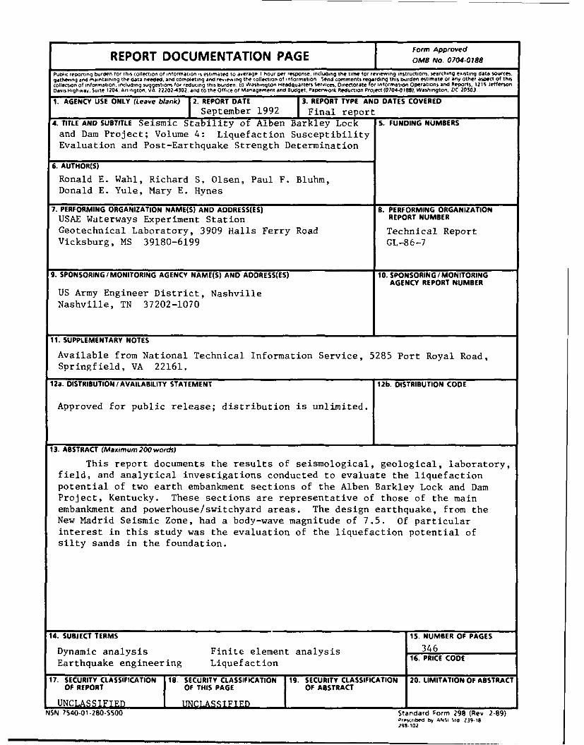
This report documents the results of seismological, geological, laboratory,field, and analytical investigations conducted to evaluate the liquefactionpotential of two earth embankment sections of the Alben Barkley Lock and DamProject, Kentucky. These sections are representative of those of the mainembankment and powerhouse/switchyard areas. The design earthquake, from theNew Madrid Seismic Zone, had a body-wave magnitude of 7.5. Of particularinterest in this study was the evaluation of the liquefaction potential ofsilty sands in the foundation.
14. SUBJECT TERMS 15. NUMBER OF PAGES
Dynamic analysis Finite element analysis 346
Earthquake engineering Liquefaction 16. PRICE CODE
17. SECURITY CLASSIFICATION 18. SECURITY CLASSIFICATION 19. SECURITY CLASSIFICATION 20. LIMITATION OF ABSTRACTOF REPORT OF THIS PAGE OF ABSTRACT
UNCLASSIFIED UNCLASSIFTED I I _I
NSN 7540-01-280-5500 Standard Form 298 (Rev 2-89)Prescribed by ANSI StO 139-18298-102
PREFACE
The US Army Engineer Waterways Experiment Station (WES) was authorized
to conduct this study by the US Army Engineer District, Nashville (ORN), by
Intra-Army rder for Reimbursable Services Nos. 77-31 and 77-112. This report
is Volume 4 of a 5-volume set which documents the seismic stability evaluation
of Alben Barkley Dam and Lake Project. The 5 volumes are as follows:
Volume 1: Summary Report
Volume 2: Geological and Seismological Evaluation
Volume 3: Field and Laboratory Investigations
Volume 4: Liquefaction Susceptibility Evaluation and Post-Earthquake Strength Determination
Volume 5: Stability Evaluation of Geotechnical Structures
The work discussed in this volume is a joint endeavor between ORN and
WES. Mr. Paul F. Bluhm, of the Geotechnical Branch (ORNED-G) at ORN, coordi-
nated the contributions from ORN. Mr. Ronald E. Wahl of Soil and Rock Mechan-
ics Division, Richard S. Olsen and Dr. M. E. Hynes of the Earthquake Engineer-
ing and Geophysics Division (WESGG-H) at WES, coordinated the work by WES.
The preliminary stages of this project were conducted by
Dr. William F. Marcuson III, who was Principal Investigator from 1976 to 1979.
From 1979 to 1988, Dr. M. E. Hynes was Principal Investigator. Mr. Wahl was
Principal Investigator from 1988 to project completion. Significant engineer-
ing support was provided by Mr. Donald E. Yule of WESGG-H. Additionally,
Mr. Daniel Habeeb, Mr. Melvin Seid, and Ms. Charlotte Caples provided valuable
assistance in the preparation of this report.
Overall direction at WES was provided by Dr. A. G. Franklin, Chief,
WESGH, and Dr. Marcuson, Chief, Geotechnical Laboratory.
Overall direction at ORN was provided by Mr. James E. Paris, Chief,
Soils and Embankment Design Section, Mr. Marvin D. Simmons, Chief, Geology
Section, and Mr. Frank B. Couch, Jr., Chief, Geotechnical Branch. Mr. E. C.
Moore was Chief, Engineering Division. Former District Commanders during the
study were COL Robert K. Tenner, COL Lee W. Tucker, and COL William K.
Kirkpatrick, COL Edward A. Starbird, and COL James P. King. The current Dis-
trict Commander "s LTC Stephen M. Sheppard.
Technical Advisors to the project were the late Professor H. B. Seed
(University of California, Berkeley), Professors Alberto Nieto (University of
1
Illinois, Champaigne- Urbana) and L. Timothy Long (Georgia Institute of Tech-
nology), and Dr. Gonzalo Castro (Geotechnical Engineers, Inc.).
At the time of publication of this report, Director of WES was Dr.
Robert W. Whalin. Commander and Deputy Director was COL Leonard G. Hassell,
Accc•i: .L or
NTIS ('T ,
Byj
~Di7'
ALA v, ii Y ýt, ,C-j,'Av~~.. :~~..............
Distt Ava.;, ••
-I2
2
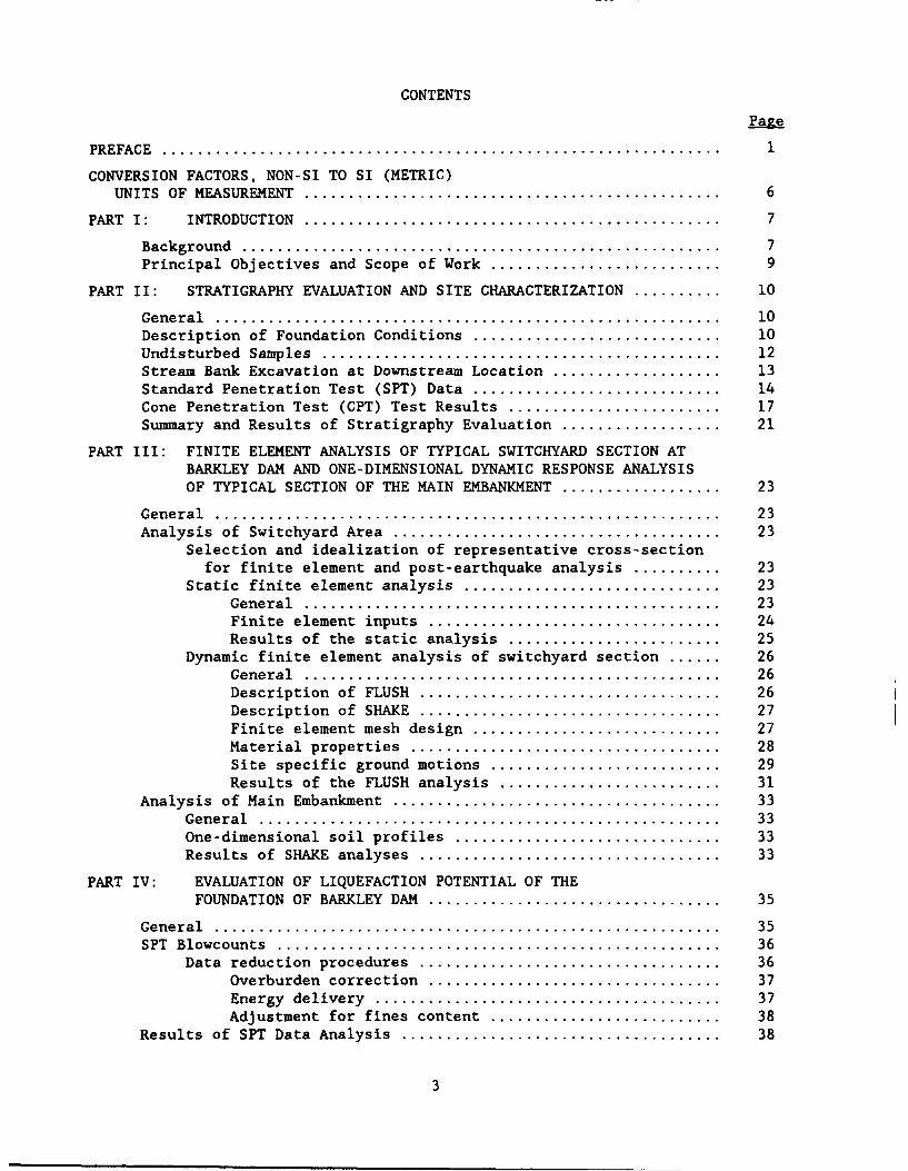
CONTENTSPage•
PREFACE ............................................................... 1
CONVERSION FACTORS, NON-SI TO SI (METRIC)UNITS OF MEASUREMENT .................................................... 6
PART I: INTRODUCTION .................................................... 7
Background ...................................................... 7Principal Objectives and Scope of Work ............................. 9
PART II: STRATIGRAPHY EVALUATION AND SITE CHARACTERIZATION .......... 10
General ......................................................... 10
Description of Foundation Conditions ............................... 10Undisturbed Samples ................................................. 12Stream Bank Excavation at Downstream Location ..................... 13Standard Penetration Test (SPT) Data ............................... 14Cone Penetration Test (CPT) Test Results ........................... 17Summary and Results of Stratigraphy Evaluation .................... 21
PART III: FINITE ELEMENT ANALYSIS OF TYPICAL SWITCHYARD SECTION ATBARKLEY DAM AND ONE-DIMENSIONAL DYNAMIC RESPONSE ANALYSISOF TYPICAL SECTION OF THE MAIN EMBANKMENT .................... 23
General ......................................................... 23Analysis of Switchyard Area ......................................... 23
Selection and idealization of representative cross-sectionfor finite element and post-earthquake analysis .......... 23
Static finite element analysis ................................ 23General ................................................... 23Finite element inputs .................................... 24Results of the static analysis ........................... 25
Dynamic finite element analysis of switchyard section ...... 26General ................................................... 26Description of FLUSH ..................................... 26Description of SHAKE ..................................... 27Finite element mesh design ............................... 27Material properties ...................................... 28Site specific ground motions ............................. 29Results of the FLUSH analysis ............................ 31
Analysis of Main Embankment ......................................... 33General .................................................... 33One-dimensional soil profiles ................................. 33Results of SHAKE analyses ..................................... 33
PART IV: EVALUATION OF LIQUEFACTION POTENTIAL OF THEFOUNDATION OF BARKLEY DAM .................................... 35
General ......................................................... 35SPT Blowcounts ...................................................... 36
Data reduction procedures ..................................... 36Overburden correction .................................... 37Energy delivery ........................................... 37Adjustment for fines content ............................. 38
Results of SPT Data Analysis ........................................ 38
3
Page
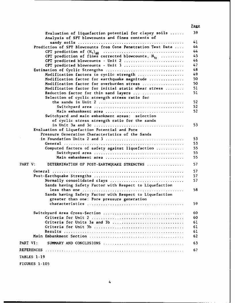
Evaluation of liquefaction potential for clayey soils ...... 39Analysis of SPT blowcounts and fines contents of
sandy soils .................................................. 41Prediction of SPT Blowcounts from Cone Penetration Test Data .... 44
CPT prediction of (N1)6 ....................................... 44CPT prediction of fines corrected blowcounts, Nit ........... 45CPT predicted blowcounts - Unit 2 ............................. 46CPT predicted blowcounts - Unit 3 ............................. 47
Estimation of Cyclic Strengths ..................................... 48Modification factors to cyclic strength ...................... 49Modification factor for earthquake magnitude ................. 50Modification factor for overburden stress .................... 50Modification factor for initial static shear stress ........ 51Reduction factor for thin sand layers ......................... 51Selection of cyclic strength stress ratio for
the sands in Unit 2 ..... .................................... 52Switchyard area ..... ...................................... 52Main embankment area ..................................... 52
Switchyard and main embankment areas: selectionof cyclic stress strength ratio for the sandsin Unit 3a and 3c ........................................... 53
Evaluation of Liquefaction Potential and PorePressure Generation Characteristics of the Sandsin Foundation Units 2 and 3 ..................................... 53
General .................................................... 53Computed factors of safety against liquefaction ............ 55
Switchyard area ........................................... 55Main embankment area ..................................... 55
PART V: DETERMINATION OF POST-EARTHQUAKE STRENGTHS .................. 57
G ene ra l ......................................................... 57Post-Earthquake Strengths ........................................... 57
Normally consolidated clays ................................... 57Sands having Safety Factor with Respect to Liquefaction
less than one ................................................ 58Sands having Safety Factor with Respect to Liquefaction
greater than one: Pore pressure generationcharacteristics .............................................. 59
Switchyard Area Cross-Section ...................................... 60Criteria for Unit 2 ............................................ 60Criteria for Units 3a and 3b .................................. 61Criteria for Unit 3b ..... ...................................... 61R esu lts .................................................... 6 1
Main Embankment Section ............................................. 62
PART VI: SUMMARY AND CONCLUSIONS ....................................... 63
REFERENCES ............................................................ 67
TABLES 1-19
FIGURES 1-105
4

APPENDIX A: SPT DATA PLOTS
APPENDIX B: CPT DATA PLOTS
APPENDIX C: TABULATIONS OF SPT LABORATORY AND FIELD DATA
5
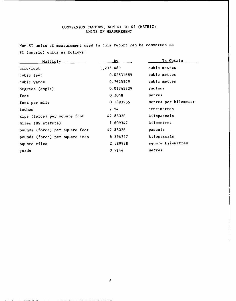
CONVERSION FACTORS. NON-SI TO SI (METRIC)
UNITS OF MEASUREMENT
Non-SI units of measurement used in this report can be converted to
SI (metric) units as follows:
Multiply By To Obtain
acre-feet 1,233.489 cubic metres
cubic feet 0.02831685 cubic metres
cubic yards 0.7645549 cubic metres
degrees (angle) 0.01745329 radians
feet 0.3048 metres
feet per mile 0.1893935 metres per kilometer
inches 2.54 centimetres
kips (force) per square foot 47.88026 kilopascals
miles (US statute) 1.609347 kilometres
pounds (force) per square foot 47.88026 pascals
pounds (force) per square inch 6.894757 kilopascals
square miles 2.589998 square kilometres
yards 0.9144 metres
6
SEISMIC STABILITY EVALUATION OF ALBEN
BARKLEY DAM AND LAKE PROJECT
LIQUEFACTION SUSCEPTIBILITY AND
POST-EARTHQUAKE STRENGTH DETERMINATION
PART I: INTRODUCTION
Background
1. This report is one of a series of five reports which document the
investigations and results of a seismic stability evaluation of the Alben
Barkley Dam and Lake Project, located on the Cumberland River, approximately
25 miles upstream of Paducah, Kentucky. This seismic safety evaluation was
performed as a cooperative effort between the US Army Engineer Waterways
Experiment Station (WES) and the US Army Engineer District, Nashville (ORN),
and in accordance with Engineering Regulation 1110-2-1806, dated 16 May 1983.
Construction of the Barkley Project began in 1957 and was completed in 1966.
As a key unit in the comprehensive plan of the development of the Cumberland
River, the multipurpose Barkley Project provides flood control, hydroelectric
power, navigation, and recreational facilities. The reservoir is contained by
a concrete gravity section flanked by earth embankment dams. The concrete
gravity section includes a gated spillway, a lock, and a powerhouse. The dam
supports a railroad track system which traverses most of the dam crest. A
canal, large enough for barge traffic, connects Barkley and Kentucky Lakes
about 2.5 miles upstream from the dam. A location map and plan view of the
project are shown in Figure 1. The reader is referred to Volume 3 of this
series for a more detailed description of the site.
2. At the maximum flood control pool, Elevation 375 ft, the reservoir
stores 2,082,000 acre-feet of water, with 13 ft of freeboard (minimum crest
Elevation 388 ft). For normal operation, the pool elevation varies from
354 to 359 ft, and stored volume varies from 610,000 to 869,000 acre-feet,
respectively. The maximum pool of record over the period 1966 to 1987 was
370.04 ft (on 13 May 1989). The guide curve for the reservoir levels is shown
in Figure 2. A pool elevation of 360 ft was used for the seismic stability
7
evaluation. A pool elevation of 360 ft leaves an aailable freeboard of 28 ft
at the time the design earthquake is assumed to occur.
3. The geological and seismological investigations for the project are
documented in Volume 2 of this series (Krinitzsky 1986). The most severe
seismic threat was determined to be an earthquake of body-wave magnitude
(mb) of 7.5, at a distance of about 118 km, in the New Madrid source zone.
The S48°E component of the Santa Barbara Courthouse record from the Kern
County, CA earthquake of 21 July 1952 was scaled to a horizontal peak accel-
eration of 0.24 g to represent this design earthquake. The resulting peak
velocity was 35 cm/sec and the duration above 0.05 g was about 60 sec.
4. The concrete gravity dam, powerhouse, and lock system are 109 ft
tall at the maximum section and are founded on a limestone bedrock. The
embankment dams are founded on an alluvial deposit with a maximum thickness of
approximately 120 ft. The alluvium is underlain by the limestone bedrock.
This alluvium, a complex system of interbedded clays, silty sands, and
gravels, is the focus of concern in the seismic safety assessment due to the
possibility of liquefaction during the design earthquake. Generally, the
alluvium beneath the embankment can be viewed as consisting of three units as
shown on the profile in Figure 3. The first zone, Unit 1, extends from the
ground surface to a depth of 10 to 20 ft and is generally made up of a medium
stiff clay with low to moderate plasticity. This material is an overbank
deposit laid down on the flood plain during flooding. The second zone,
Unit 2, extends from the bottom of Unit I to a depth of about 50 ft and con-
sists of a highly stratified sequence of clays, sands, and, silty sands.
These are overbank deposits whose interbedded layers vary widely with respect
to grain size and thickness. Unit 3 extends from the bottom of Unit 2 to a
depth of 120 ft and consists of gravels and denser sands (denser than Unit 2)
with some clay also being present. These materials are channel deposits laid
down as the river meandered across the valley. The different depositional
environments for each of the three units described above probably resulted
from changing base levels that occurred in the geologic past. These deposits
range widely in grain size.
8
Principal Objectives and Scope of Work
5. The principal objective of this project was to evaluate the
performance of the alluvial foundation underlying two specific areas of the
right embankment dam in the event of the design earthquake. The first area
studied was that of the switchyard located between Sta 38+00 (at the interface
of the concrete dam and earth embankment) and Sta 43+00. The second area of
interest was that of the main embankment, located between Sta 43+00 and
Sta 88+00. The stationing used in this report are shown on the cross sec-
tional and plan views of Figures 4 and 5, respectively.
6. The specific tasks undertaken and reported herein include:
a. Characterization and stratigraphic evaluation of the foundationalluvium beneath the dam.
b. A site specific dynamic analysis to determine the response ofthe embankment and foundation to the design earthquake motions.
c. Evaluation of the potential for and extent of liquefaction inthe alluvial soils. The evaluation was made based on a compari-son of the cyclic strength and dynamic shear stresses induced bythe earthquake.
d. Estimation of the post-earthquake strength of the embankment andfoundation alluvium for a post-earthquake stability analysis.
7. The results of the field and laboratory investigations reported inVolume 3 provided input to the stratigraphy evaluation, the dynamic response
analysis, and the determination of the post-earthquake strengths. The results
of the post-earthquake stability analysis are reported in Volume 5 of this
series.
9
PART II: STRATIGRAPHY EVALUATION AND SITE CHARACTERIZATION
General
8. A stratigraphy evaluation performed for characterizing and idealiz-
ing the site was an essential step in the seismic stability analysis of this
dam. The stratigraphy evaluation described in this Part was based on data
obtained from an extensive exploration program of the site which included
field and laboratory tests. This program was reported in detail in Volume 3
of this series. The major sources of data upon which the stratigraphy evalua-
tion is based included Standard Penetration Tests (SPT), Cone Penetration
Tests (CPT), undisturbed soil sampling, and analysis of a downstream exposure
of one of the dam's major foundation units.
9. It must be stressed that the stratigraphy of the foundation soils
is complex and could only be evaluated by analysis of all the major sources of
data rather than that from any one source alone. Consideration was given to
the strengths and weaknesses of each source of information in order to develop
as complete an understanding of the foundation conditions as possible. After
a brief discussion of the foundation conditions, the following sections of
this part of the report provide discussions of the factors from each data
source which were :eighed and used in evaluating the characteristics of the
foundation soils for this study. These discussions are not presented in the
sequence in which the various source of information were obtained, but are
rather presented in an order intended to produce, as clearly as possible, a
picture of the site's foundation conditions.
Descrittion of Foundation Conditions
10. This section was excerpted from Volume 3 and briefly describes the
major foundation units present in the subsurface. These descriptions provide
a useful background with which to begin the discussion. Subsequent analysis
of data documented later in this section will add some detail and refinement
to the initial interpretation.
11. The foundation beneath Barkley Dam is complex and can be viewed as
consisting of three basic units: Units 1, 2, and 3. Longitudinal cross-
sections along the toe and centerline showing the three foundation units are
10
shown in Figures 3 and 4. Unit 1 is a medium stiff clay whose thickness
varies between 20 and 30 ft. In the switchyard area (between Sta 38+00 and
Sta 43+00) the thickness of Unit 1 extends to Elevation 320. In the area
along the main embankment (between Sta 43+00 and 88+00) this unit is somewhat
thinner where it only extends to Elevations between 330 and 325 ft. The
exploration program revealed that some sand layers are present but the number
and extent of these layers are very limited. The average liquid limit, plas-
tic limit and natural water content in this unit are about 30, 17, and 23 per-
c-int respectively.
12. Unit 2, directly below Unit I, extends to elevations approximately
between 305 and 300 in the switchyard area. Beneath the main embankment
Unit 2 lies a little deeper where it extends between the elevations 300 and
295. Unit 2 is dominated by a very soft clay which contains layers of
interbedded sands and silty sands. These layers are frequently very thin,
generally having thicknesses of less than 6 in. The SPT and CPT data
collected during the field investigations showed that the sand (and clays) had
low penetration resistances. The average fines content was determined to be
about 28 percent based on laboratory tests of samples. The low penetration
resistance indicated that the sandy layers had the potential for liquefaction
and that the prediction of their seismic performance should be a major element
in the evaluation of the dam's post-earthquake stability. This concern made
it imperative to determine the lateral extent and continuity of these sand
layers since the dimensions of materials with high liquefaction potential are
important factors in evaluating the seismic stability of an embankment.
13. Foundation Unit 3 is made up of sands and gravels although some
layers of clay are occasionally present. One continuous layer of clay was
found in the switchyard and free field area between elevations 295 and 290 ft.
The CPT and SPT data indicate that the sands and gravels of Unit 3 are denser
than the sands in Unit 2. Also, the sands of Unit 3 are cleaner than those of
Unit 2 and have an average fines content of about 15 percent. The liquefac-
tion potential of the cohesionless materials in Unit 3 were also evaluated as
part of this analysis.
11
Undisturbed Samples
14. Undisturbed samples were obtained from eleven borings which are
listed in Table 1. The locations of these borings are shown in Figure 5.
Undisturbed samples were obtained from each of the three foundation units for
the purposes of estimating density, providing materials for laboratory
strength tests (both cyclic and static), and to provide an opportunity to view
the characteristics of the stratigraphy in the foundation. This section of
the report is reserved for discussion concerning only the latter purpose.
Discussions of the details of the other aspects of undisturbed sampling pro-
gram are included in Volume 3. In the following paragraphs photographs of
representative undisturbed samples from Units 2 and 3 are discussed and quali-
tatively illustrate some of the characteristic traits of the soils in these
units.
15. Figures 6 and 7 contain photographs of two of the undisturbed
samples taken from Boring DS-l. Boring DS-I is located just off the down-
stream toe of the main embankment near Sta 65+00 as shown on Figure 5. Sam-
ple 14 (shown in Figure 6) shows the interbedding of sand and clay layers.
The dark and light colored materials in the photograph represent the clay and
sand layers in Unit 2, respectively. The photograph shows that the sand lay-
ers are very thin and do not exceed seven inches in thickness and appear to be
interbedded within the clay material. This and other photographs show that
this type of interbedding is a characteristic trait of Unit 2. More photo-
graphs of the undisturbed samples can be seen in Appendix G to Volume 3. It
was not possible to tell whether or not the sand layers are continuous on the
basis of the photographs of undisturbed samples.
16. Sample 20 from DS-I shown in Figure 7 is considered to be a
representative sample of the sands and gravels retrieved from Unit 3. This
photograph (and others) shows that the sand is by far the dominate material in
the sample and suggests that the sand layers in Unit 3 are a great deal
thicker than those of Unit 2. Some thin clay layers (similar in appearance to
those of Unit 2) are evident in other pictures from Unit 3 samples.
12
Stream Bank Excavation at Downstream Location
17. An excavation was performed along the streambank at a location
downstream of the Barkley damsite in an exposure of Unit 2. The excavation
site was located approximately two miles downstream from the dam. A more
detailed presentation of the procedures, equipment, and results of the analy-
sis of the excavation is provided in Volume 3.
18. In the analysis of data obtained from soil borings, it was not
possible to map individual sand layers encountered in Unit 2 from one boring
to the next thereby making it impossible to determine the continuity and
lateral extent of these layers. The excavation was performed in hopes of
overcoming this difficulty. The exposure and excavation are in the direction
of river flow. From geological reasoning, it was presumed that individual
soil layers would be more continuous in the direction of river flow which is
perpendicular to the axis of the dam.
19. The exposed soils on the face of the excavation were mapped and
photographed. The dimensions of the exposure in the excavation were about
30 ft in length by about 6 ft in height. The detailed geologic cross section
of the exposed soils is shown on Figure 8. Two typical photographs of the
exposed face of the excavation are presented in Figure 9. Both the map and
the photographs yielded important information as to the complex stratigraphy
present in the Unit 2 soils. Paraphrasing the findings of Volume 3, the anal-
ysis of these two items shows clearly that the clay is the dominant material
in the unit. The sand beds have an average thickness of about 2 to 4 in. The
maximum thickness observed in one of the sand beds was 1.5 ft. The lengths of
the sand beds varied greatly, from just a few inches to greater than the 30 ft
which is the length of the excavation. One bed, located outside the limits of
the exposure, was traced for a distance of 150 ft. The evidence also shows
that the sand beds undulate and horizontal planes of constant elevation do not
remain in contact with any bed for more than a distance of about 20 ft. Based
on these findings, it was concluded in Volume 3 that significant continuity
may exist in the sand layers in the direction parallel to the river. Due to
the orientation of the exposure it was not possible to determine the degree of
continuity in the direction perpendicular to the river flow.
13
Standard Penetration Test Data
20. A comprehensive SPT program was performed at the damsite for the
purpose of determining the penetration resistances in terms of blowcounts for
the foundation units and also to obtain disturbed samples for soil classifica-
tion and natural water content. The penetration resistances were later used
as an index in the determination of liquefaction resistance as well as to aid
in the evaluation of stratigraphy. The samples retrieved from SPT testing
were also useful in evaluating the characteristics of the soils in the three
foundation units and in evaluating the liquefaction potential of the founda-
tion soils.
21. Forty-four SPT soundings were performed at the Barkley Dam during
the period between 1977-1984. The SPT boring locations are shown in the plan
of Figure 5. These tests employed various types of equipment and procedures
which are discussed in Volume 3. The basic data gathered from these SPT bor-
ings included blowcounts, jar samples, and laboratory index tests (Atterberg
Limits and grain size analysis) from each split spoon sample. This informa-
tion was stored in a computerized database for referral during analysis.
22. Information stored in the database is included in Appendices A and
B to Volume 3. Additionally, plots of depth versus measured SPT blowcount,
grain size data, mean grain size, and fines contents were developed to aid
evaluation of the liquefaction potential and to assist in the stratigraphic
evaluation.
23. Data obtained from boring BEQ-1O are considered typical of the SPT
data gathered from the three foundation units at the site. Boring BEQ-1O is
located just off the downstream toe of the main embankment near Station 54+00.
The SPT plot for boring BEQ-10 is shown in Figure 10. Similar plots for all
SPT borings are presented in Appendix A. Table 2 is a companion to the plot
and lists data obtained from laboratory index tests performed on split spoon
(disturbed) samples of this boring. Superimposed on the left hand side of
Figure 10 are the locations of boundaries of the three foundation Units 1, 2,
and 3.
24. The measured penetration resistances (blowcounts) from borings
located along the downstream toe of the main embankment are plotted on the
cross section shown in Figure 11. The data on the cross section and the soil
classifications from the database were used to develop the boundaries between
14
the three foundation units and to help characterize the soils within each
unit. Examination of the data shows that each unit has certain characteris-
tics which distinguish it from the others. These characteristics will be
discussed in the following paragraphs.
25. Unit 1 is characterized by measured blowcounts which have a general
tendency to decrease with depth. The cross section shows that Unit 1 extends
from the ground surface to approximately Elevation 325 ft. The classifica-
tions of soil samples in the reach show (See Appendix A to Volume 3) that the
Unit 1 materials are clays which classify as CL materials though some sand is
present. The tendency for blowcounts to decrease with depth suggests that
these clays are overconsolidated due to desiccation.
26. Unit 2, situated mainly between Elevations 325 and 295 in the area
of the main embankment, contains the interbedded sands and clays which were
discussed earlier. Figure Il shows that the measured blowcounts in Unit 2 are
relatively low, typically between 5 and 15. Matching the soil classification
data up with the blowcount data at corresponding depths shows that the blow-
counts with the higher values will nearly always be associated with sands
while the lower values tend to be associated with the clayey materials. The
sands in the clayey materials generally classified as SM materials and the
clays generally classified as CL. A histogram showing the distribution of
mean grain size (D5 0 in mm) for samples recovered in Unit 2 between Eleva-
tions 320 and 305 is shown on Figure 12. This elevation range was selected to
represent Unit 2 throughout this study even though some variations occur at
various locations about the site. This plot shows that the average D50 is
about 0.15 mm. A histogram of the percentage passing the No. 200 sieve for
sands, shown on Figure 13, shows a fairly uniform distribution over the range
0 to 50 percent. The mean value is about 30 percent which indicates that the
sands in Unit 2 are fairly dirty. Examination of the database also shows that
the fines are non-plastic. The distributions include samples retrieved from
all SPT borings at the site including those in the switchyard area.
27. Unit 3 is located below about elevation 295 in the area of the main
embankment. Unit 3 consists mainly of sands and gravels which are character-
ized by higher penetration resistances than those observed in the sands in
Unit 2. This indicates that the Unit 3 sands are denser than those in Unit 2.
The measured penetration resistance is generally above 30 blows/ft which is
significantly greater than that of the sands in Unit 2. The histogram in
15
Figure 14 of mean grain size for the sandy materials in Unit 3 shows that the
D,0 is about 0.20 mm. These are only slightly coarser than the D50 of the
Unit 2 samples. A histogram showing the percentage of fines is shown on Fig-
ure 15. This plot shows the average fines content of these sands is about
10 percent and indicates that the sandy materials of Unit 3 are cleaner than
those of Unit 2. The database shows that the fines ot Unit 3 sands are also
non-plastic. The database showed that 344 sand samples were recovered from
Unit 3 while only 162 sand samples were recovered from Unit 2. These totals
translate to 250 jar samples recovered per 1000 ft of drilling in Unit 2 com-
pared to 970 jar samples recovered per 1000 ft in Unit 3. These figures sug-
gest that there is a significantly greater amount of sand in Unit 3 than in
Unit 2. Most of the SPT borings in Unit 3 terminated at depths well before
bedrock was encountered.
28. The discussions of the previous paragraphs indicate that the SPT
borings provided some very useful information regarding the characteristics of
the three foundation units at the damsite. The principle advantage in using
the SPT on this project was the fact that it provided hundreds of samples from
which the component soils of each foundation unit could be classified. Soil
classification is important in evaluating the liquefaction potential of a
deposit as different soil types respond differently to earthquake shaking.
The soil classifications also assisted greatly in assessing the stratigraphy.
However, the SPT has several limitations as well, particularly with respect to
its use in Unit 2 where the thin sand layers interbedded within the clay are
suspected of having a high liquefaction potential. The SPT blowcount data
does not provide a sufficiently high enough degree of resolution to clearly
assess all the sand layers encountered by the boring. This is because the
blowcounts are taken over a one foot depth interval. A one-foot drive dis-
tance is greater than the thickness of most of these layers which are only a
few inches thick. Thus, the measured penetration resistance includes a con-
tribution from the softer clay. Also, many of the sand layers went undetected
due to the thinness of the layers and the fact that the penetration resistance
observed while the split-spoon is actually in the sand is influenced by the
softer underlying clays. It was also impossible to correlate the continuity
of individual sand layers from one boring to the next. These limitations were
less of a problem in Unit 3 where the sand layers were thicker.
16
Cone Penetration Test (CPT) Test Results
29. Sixty-five Cone Penetration Tests were performed in the switchyard
area for the purpose of estimating strength and evaluating the stratigraphy of
the foundation soils. The estimation of cyclic and post-earthquake strengths
from the CPT data are discussed in Parts IV and V of this report. This sec-
tion is reserved for the discussion of how the CPT data were used to evaluate
the stratigraphy of the foundation soils. The location of the CPT soundings
is shown in the plan of Figure 16. The locations of these tests were concen-
trated in the switchyard area because the preliminary liquefaction and slope
stability studies indicated that the switchyard area was the most critical
area in terms of the dam's seismic stability. As with the other types of
insitu tests performed at the damsite the details concerning the equipment and
conduct of the CPT tests at the damsite are included in Volume 3.
30. The advantages of the CPT include its ability to provide a
continuous record of data and to resolve stratigraphic changes with a resolu-
tion of a few inches. These advantages were particularly useful at Barkley
Dam in light of the complex foundation conditions there. Additionally, the
CPT is relatively low in cost when compared with the more conventional SPT and
undisturbed sampling programs. The principle disadvantage of the CPT is the
fact that there is no sample recovery. However, this disadvantage was offset
to a large degree by the fact that samples recovered from the SPT and undis-
turbed sampling program (discussed previously) proved to be useful supplements
to the CPT data gathered from the Barkley site.
31. The CPT's advantages are illustrated in Figure 17. In this figure,
the CPT penetration resistance (cone tip resistance measured in tsf) is com-
pared with the SPT penetration resistance (blowcounts). Data from Boring
BEQ-26 and CPT-36, located in close proximity to each other near Sta 39+50
(See Figure 16), were selected for the comparison. The measured SPT blow-
counts for BEQ-26 are shown on the left side of the figure and the cone tip
resistances (in TSF) are shown on the right. The CPT penetration resistance
is represented by two traces: the measured (raw) cone resistance, qc' and the
corrected cone resistance (adjusted to overburden stresses of 1 tsf), qcn •
Clearly, the CPT reveals more detail than the SPT. This is especially true inUnit 2 where the sand layers are detected as spikes of relatively high pene-
tration resistance which are superimposed on the low penetration resistance
17
background of Unit 2's soft clays. The width of the spikes is an indication
of the thickness of the sand layer. Conversely, a detailed manifestation of
the sand layers is not revealed by the SPT blowcounts; however, the sands were
sampled by the split spoon and identified in the lab analysis. The lack of
detail in the SPT data is an outcome of the discontinuous nature of the test-
ing procedure. The thin sand layers often have a negligible effect over the
18 in. drive intervals of the blowcounts. Thus, if a sand layer is very thin
its contribution to the blowcount may be insignificant. For both SPT and CPT,
the true penetration resistances of the thin sands may be underestimated due
to the effect of the underlying soft clay which strains before being encoun-
tered by the penetrometer. The effect is greater for the SPT split spoon
sampler than for the cone penetrometer since the split-spoon sampler has an
outside diameter of 2 in. which is greater than the 1.40 in. diam of the cone.
32. The CPT test can also be used as an aid to classify soils. A clas-
sification scheme devised by Olsen (1984) was used to identify the types of
soils encountered by the CPT probe. The procedure which correlates basic CPT
data to soil types is discussed in this paper. The chart used in the CPT soil
classification scheme is shown in Figure 18. The basic idea behind Olsen's
system is that basic soil types can be identified by the combinations of cor-
rected values of sleeve friction and cone resistance, fsn and qcn. The
corrected parameters, fan and qcn, are the results of adjustments made to
the measured values of sleeve friction and cone resistance, fs and qc
These adjustments correct the measured values to overburden stress conditions
of I TSF. The adjusted CPT parameters are mapped onto the soil classification
chart with the outcome being a Soil Characterization Number (SCN) which corre-
lates to basic soil types. A CPT SCN of 0.5 is a typical clay, the range of
SCN of I to 2 represents silt mixtures, SCN's for sands range from 2 to 4, and
a fine sand has a SCN between 2.5 and 3.5. The SCN numbers for various com-
bination of normalized sleeve and cone tip resistances are also shown on
Figure 18.
33. Data from CPT-36, shown in Figure 19, were used as an example of
the application of the CPT soil classification. The left and center panels
show the cone and sleeve readings (both measured and corrected) which were
used to enter the chart shown in Figure 18 to determine the SCN's and soil
types which are shown in the right panel.
18
34. Charts similar to that in Figure 19 were made up for each of the
65 CPT soundings at the damsite. These are included in Appendix B to this
report. The CPT cone resistance and soil classification charts were used to
evaluate the stratigraphy in the switchyard area by developing cross sections
along lines of CPT soundings. Three cross sections were developed from lines
of CPT shown on the plan in Figure 15. These cross sections were developed
along three lines: B'-B' which is parallel to the axis of the dam and runs
along the toe of the switchyard berm, A'-A' which is also parallel to the axis
and runs along the top of switchyard berm at Elevation 366 ft, and D'-D' which
is perpendicular to the axis of the dam. Cross sections displaying the cone
resistances, qc and qc, and CPT soil classifications were prepared for each
of these lines. The cone resistance and soil classification cross sections
for line D'-D' (perpendicular to axis) are shown on Figures 20 and 21, respec-
tively. Those for line B'-B' (along toe of switchyard berm) are shown on
Figures 22 and 23, and those for A'-A' are shown on Figures 24 and 25.
35. From analysis of these sections a refined interpretation was made
of the foundation stratigraphy of the damsite. In Unit 1 the cone resistances
have a general tendency to decrease with depth. Since the CPT is an index of
undrained shear strength, this feature indicates that the clays are likely to
be overconsolidated due to desiccation. The cross sections also show that
some sands are present. The cross sections show that the boundary between
Unit 1 and Unit 2 undulates to some degree but generally the boundary lies
between Elevations 325 and 320 in the switchyard area.
36. In Unit 2, CPT cone resistances profiles are characterized by
spikes superimposed upon relatively low penetration resistance as was
discussed earlier. The spikes are indicative of sands and the low values
are indicative of clays. The points of the qcn trace for the clays aline
themselves in a nearly vertical line which indicates that the clays in Unit 2
are normally consolidated. The CPT classifications alternate between sand
mixtures and clays and show that the clays are the dominant material in
Unit 2. This is consistent with the laboratory classifications of SPT sam-
ples. It was not possible to correlate the continuity of the individual sand
layers from sounding to sounding in Unit 2 from the CPT data. The boundary
between Units 2 and 3 undulates to a minor degree in both directions but gen-
erally lies between elevations 305 and 300 in the switchyard area only. The
CPT data reveal that Unit 3 is generally made up of sandy materials with some
19
interbedded clays. Unit 3 was subdivided into three basic zones of materials
t ed on analysis of the CPT data: Units 3a, 3b, and 3c. The interpreted
boundaries of each of are shown on Figures 20 through 25. In general there is
a marked increase in penetration resistance as the probe crosses the boundary
between Units 2 and 3a. The increase is due to an increase in density in the
sands and the presence of gravel of Unit 3a. The CPT classification suggests
that the Unit 3a sands are cleaner than those of Unit 2 as evidenced by the
SCN which is typically much higher for the Unit 3 sands. This is consistent
with the grain size data from the SPT sand samples. The CPT data shows that
the Unit 3a sand layers are probably much thicker than the Unit 2 sand layers
which is another possible reason for their higher penetration resistance
values.
37. A zone of low cone resistance, designated as Unit 3b, was generally
detected between the elevations of 295 ft and 288 ft. The cone resistance
profiles of this zone have an appearance which is remarkably similar to those
of Unit 2 with some thin sand lenses interbedded within the clay. This zone
is extensive as it was detected by nearly all of the CPT soundings performed
in the switchyard area, therefore it was treated as a characteristic of the
site in the switchyard area. The foundation materials below the low blowcount
zone were designated Unit 3c and have characteristics similar to those of
Unit 3a.
38. A technique was developed during the project which uses the CPT
data to quantify the percentage of sand present for any elevation across the
site. The estimate was made by dividing the foundation into 0.1 ft intervals
between elevations 283 and 350. The CPT database was queried to determine the
SCN of the material occupying each elevation interval for each sounding. In
this analysis, an interval was considered to be occupied by a sand if the SCN
value was greater than two. Thus, an area-wide percentage of sand at a par-
ticular elevation was estimated by computing the ratio of the number of times
the CPT probe encountered a sandy material (having a SCN > 2) divided by the
total number of CPT soundings passing through that elevation interval.
39. Sand contents were estimated for the switchyard area, the free
field area just downstream of the switchyard area, and the combined total for
both areas. The results are shown in Figure 26. The charts show that the
normally consolidated clays discussed earlier are by far the dominant material
in Unit 2 (approximately between elevations 320 and 305 ft) and that the sands
20
make up less than 20 percent of the material in this unit. There is even less
sand in Unit 2 in the switchyard area than in the free field area. Sand is
the dominant material comprising about 60 percent of the material in Unit 3
(below 305). In the switchyard, the presence of Unit 3b is detected between
elevations 288 and 293 where the sand percentage decreases. The sand percent-
age in the switchyard increases in Unit 3c below elevation 288.
Summary and Results of Stratigraphy Evaluation
40. Data collected from SPT, CPT, undisturbed samples, and an excavated
exposure of a foundation unit were analyzed in order to determine an under-
standing of the foundation conditions at the Barkley site. The results are a
synthesis of the data with consideration given to the strengths and weaknesses
of all the various sources of information.
41. The analysis showed that the foundation could be modeled by three
basic foundation units: Unit I, Unit 2, and Unit 3. The overall foundation
thickness is approximately 120 ft. The data showed that each unit had traits
which distinguished it from the others. An idealized cross section of the
switchyard area showing the spatial relationships between the three foundation
units is shown in Figure 27. Foundation Unit 1 consists of clays which typi-
cally classify as CL materials. These clays which can be viewed as a
topstratum are probably overconsolidated due to desiccation. Generally speak-
ing, Unit 1 is thirty feet thick and lies between the Elevations of 350 and
320 ft. Unit 2 consists of silty sand layers interbedded within a matrix of
soft clays (CL). The silty sand layers are generally very thin, on the order
of only a few inches thick. These silty sand layers are dirty and on the
average contain about 30 percent nonplastic fines. Unit 2 lies between eleva-
tion 320 and 305 in the switchyard area and is a little thicker beneath the
main dam where it generally lies between Elevations 330 - 295 ft. The bound-
ary between Units 2 and 3 is not flat and is crowned with its peak elevation
being between Station 65+00 and 70+00 on the cross section (See Figure 10).
Unit 3 is subdivided into three subunits: Units 3a, 3b, and 3c. Unit 3a
contains dense sands and gravels which have a relatively high penetration
resistance as compared to the sands layers in Unit 2. These sands typically
contain less than 15 percent fines and are relatively clean compared to those
in Unit 2. Unit 3a lies generally lies between elevation 305 and 295 in the
21
switchyard area. There are some clay layers present in Unit 3a. Unit 3b,
located bezween elevation 295 and 288, is typified by clays (CL) of low pene-
tration resistance. These clays were detected by nearly all of the CPT's in
the switchyard and appear to be a characteristic of this area of the damsite.
Unit 3c lies between elevation 288 and bedrock and based on limited amounts of
data appear to have characteristics similar to Unit 3a.
42. A quantitative analysis of the CPT data showed that sands make up
less than 20 percent of the material of Unit 2. In Unit 3, sand is the domi-
nant material comprising about 60 percent of the total material.
43. Preliminary studies showed that the materials in foundation Unit 2
had a high potential for liquefaction. Thus, in the stratigraphy evaluation
it was essential not only to identify and classify the material type but to
map its lateral extent. It was not possible to map the extent of individual
sand layers from one CPT or SPT sounding to another. However, an excavation
in a downstream exposure of Unit 2 revealed that some of these layers were
undulating and continuous over fairly long distances in the direction of river
flow. This result was carried into the liquefaction studies where the sandy
materials in Unit 2 were treated as continuous. The cross section of Fig-
ure 27 represents-the idealized stratigraphy upon which the seismic response
and performance of the dam and foundation were based.
22
PART III: FINITE ELEMENT ANALYSIS OF TYPICAL SWITCHYARD SECTION ATBARKLEY DAM AND ONE-DIMENSIONAL DYNAMIC RESPONSE ANALYSIS OF
TYPICAL SECTION OF THE MAIN EMBANKMENT
General
44. Finite element and l-D dynamic response analyses were used to eval-
uate the dynamic responses of representative cross section of both the switch-
yard and main embankment areas. Static and dynamic finite element analyses
were performed on a representative cross-section through the switchyard area,
located between Sta 35+00 and Sta 44+00, to evaluate the pre-earthquake static
stresses, dynamic response, and liquefaction potential of the embankment and
the foundation materials beneath Barkley Dam. The static analysis was neces-
sary since the cyclic strengths (liquefaction resistance) of the foundation
and embankment soils are dependent upon pre-earthquake states of stress. The
dynamic response analysis was performed to evaluate the response of the dam
and foundation to earthquake vibrations and to determine the dynamic shear
stresses induced in the soils by the earthquake. A series of 1-D wave propa-
gation analyses were used to approximate the 2-D dynamic response of a typical
section of the main embankment (located between Sta 44+00 and Sta 90+00).
45. This part of the report presents the results of the analytical
studies. A discussion of the determination of liquefaction resistance is
included in Part IV of this report.
Analysis of Switchyard Area
Selection and idealization ofrepresentative cross-section finiteelement and post-earthquake analysis
46. The cross-section used for the finite element analysis is section
A-A shown on Figure 27. Preliminary liquefaction and post-earthquake analyses
performed on this and other cross sections at Barkley Dam indicated that this
was the most critical section in the switchyard area and was an appropriate
section to be idealized for the finite element analysis.
Static finite element analysis
47. General: The computer program FEADAM84 developed by Duncan, Seed,
Wong, and Ozawa (1984) was used to perform the static analysis of Barkley Dam.
23
FEADAM84 is a two-dimensional, plane strain, finite element solution developed
for calculation of the static stresses, strains, and displacements in earth
and rockfill dams and their foundations. The program uses a nonlinear hyper-
bolic constitutive model developed by Duncan et al. (1980) to estimate the
stress history dependent, non-linear stress strain behavior of the soils.
Nine parameters are required for the hyperbolic constitutive model. The pro-
gram is used to perform incremental calculations to simulate the addition of
layers of fill placed during construction of an embankment. A description of
the consuitutive model, procedures for evaluating the parameters, and a data-
base of typical parameter values are given by Duncan et al. (1980).
48. Finite element inputs: FEADAM84 was used to compute the pre-
earthquake static states of stress in the embankment. Seven different
material types were modeled in the cross-section:
a. Random embankment fill.
b. Compacted embankment fill.
c. Unit 1 - Lean alluvial clay.
d. Units 2 and Unit 3a - Silty sand.
e. Units 2 and 3b - Clay.
f. Unit 3c - Sands and gravels.
Z. Submerged compacted embankment fill.
49. The distribution of these materials is shown in Figure 28. Table 3
contains a list of the hyperbolic parameters used in FEADAM84 to model the
nonlinear stress strain behavior of each of the materials in the cross-
section. Submerged unit weights were used for all materials located beneath
the )hreatic line. Submerged macerials were assigned the same hyperbolic
parameters as were their non-submerged counterparts. The hyperbolic parame-
ters were determined by Duncan and Seed (1984) in an earlier study.
50. The finite element mesh developed for the static analysis is shown
in Figure 29. This mesh has a total of 265 elements and 293 nodal points.
The phreatic line representing the boundary between submerged and nonsubmerged
elements is indicated in this figure. This mesh is different than the one
used in the dynamic analysis. The mesh used in the dynamic analysis will be
discussed in the next section of this part of the report.
51. The dam and its foundation were numerically constructed in two
basic stages. In the first stage, the alluvial foundation was "constructed"
in ten lifts with each lift being one element high. The computed stresses for
24
the 221 foundation elements were treated as input to the second stage of the
analysis. In the second stage, the 44 elements comprising the embankment were
"constructed" upon the preexisting foundation elements in four construction
layers, each one element high.
52. Results of the static analysis: The results of the FEADAM84 static
stress analysis are presented in the form of contour plots of vertical effec-
tive stress, shear stress on horizontal planes, and alpha (ratio of horizontal
shear stress to vertical effective stress) in Figure 30 through 32, respec-
tively. The contours were derived from the stresses computed at the centroid
of each of the elements in the mesh. The data plotted in Figure 30 show that
the contours of vertical effective stress follow the surface geometry of the
cross-section. As would be expected, the plot shows that the vertical stress-
es increase with increasing depth below the ground surface. Additionally, the
vertical effective stresses at corresponding depths on the downstream side of
the dam are slightly greater than those on the upstream side due to the effect
of submergence. The vertical effective stresses are slightly in excess of
10 ksf just above the rock surface at centerline of the dam.
53. Figure 31 shows a contour plot of the initial static shear stresses
acting on horizontal planes in the cross section. Due to the sign convention
of the program the stresses on the downstream side of the centerline (nega-
tive) have the opposite sign of those on the upstream side (positive). The
contour of zero shear stress was located near the centerline of the dam
(at X - 0). The contours show that the absolute values of shear stress are
greatest beneath sloping sections of the surface geometry. It is important to
note that beneath the switchyard berm is a zone of relatively low shear
stresses, which is a consequence of the relatively flat surface geometry of
the berm section.
54. Figure 32 shows contours of the alpha ratio. The alpha values
shown represent the ratio of initial static shear stresses acting on horizon-
tal planes to the vertical effective stress. The signs of the alpha values on
the downstream side (negative) are opposite those on the upstream side
(positive) and reflect the signs of initial shear stresses in these locations.
The contours show that the absolute value of alpha ranges from 0 near the
centerline to 0.3 on the upstream slope. As was the case with the static
shear stresses, the higher alpha values are located immediately beneath
sloping sections in the surface geometry on both the upstream and downstream
25
sides of the centerline. In contrast to this, the alpha values are less than
0.05 in the upstream and downstream free field areas where the ground is level
and below the switchyard berm section where the slopes are relatively flat.
55. The pre-earthquake static stress conditions are used in subsequent
portions of the seismic stability analysis. They were used in the determina-
tion of the cyclic strengths at various locations in the foundation soils,
since the cyclic strength at a location is dependent upon the vertical effec-
tive stress and alpha value at that point.
Dynamic finite element
analysis of switchyard section
56. General: A two-dimensional dynamic finite element analysis was
performed with the computer program FLUSH (Lysmer et al. 1973) to calculate
the dynamic response of the idealized cross section to the specified motions.
The objectives of this analysis were to determine dynamic shear stresses, peak
accelerations at selected points in the cross section, earthquake-induced
strain levels, and the fundamental period of the dam at the earthquake-induced
strain levels. The information gained from the dynamic analysis is used later
as input to the evaluation of liquefaction potential and seismic stability of
the idealized cross-section in the event of the design earthquake.
57. Free field ground motions applicable to the Barkley site were input
to FLUSH. The free field motions were developed using the computer program
SHAKE. SHAKE is a one-dimensional wave propagation code developed at the
University of California - Berkeley (Schnabel, Lysmer, and Seed 1972). As is
the case with FLUSH, SHAKE uses the equivalent linear model to simulate
non-linear soil behavior. A discussion of the processing scheme by which the
free field ground motions were developed will be discussed in a following
section.
58. Descriution of FLUSH: FLUSH is a finite element computer program
developed at the University of California, Berkeley by Lysmer, Udaka, Tsai,
and Seed (1973). The program solves the equations of motion using the complex
response technique assuming constant effective stress conditions. Non-linear
soil behavior is approximated with an equivalent linear constitutive model
which relates shear modulus and damping ratio to the dynamic strain level
developed in the material. In FLUSH the differential equations of motions are
solved in the frequency domain and an iterative procedure is used to determine
the appropriate modulus and damping values to be compatible with the developed
26
level of strain. Plane strain conditions are assumed in FLUSH. As a two-
dimensional, total stress, equivalent linear solution, possible pore water
pressure generation and dissipation are not accounted for during the
earthquake. Each element in the mesh is assigned properties of unit weight,
shear modulus, and strain-dependent modulus degradation and damping ratio
curves. FLUSH input parameters for the various zones in the cross section are
described later in this part of the report.
59. Description of SHAKE: The one-dimensional computer program SHAKE
was used to develop site specific ground motions for input to FLUSH and also
to evaluate the dynamic response of the free field at the damsite. SHAKE was
developed by Schnabel, Lysmer, and Seed at the University of California,
Berkeley (1972). In SHAKE, the wave equation is solved in the frequency
domain through the use of the Fast Fourier Transform (FFT). The nonlinear
strain dependent soil properties of shear modulus and damping are handled with
the equivalent linear procedure, an iterative process which converges upon
strain compatible values for modulus and damping. The equivalent linear model
is the same constitutive model used in FLUSH. The one-dimensional analysis
performed in SHAKE is a total stress analysis. The strain dependent damping
and modulus degradation curves for this study are shown in Figure 33.
60. SHAKE is based upon the following assumptions:
a. All layers in the profile are horizontal and of infinitelateral extent. Level ground conditions are assumed to exist,thus prior to the earthquake there are no static shear stressesexisting on horizontal planes.
b. Each soil layer in the profile is defined and described by itsshear modulus, damping, total density, and thickness.
c. The response of the soil is caused by horizontally polarizedshear waves propagating through the soil layers in the system.
d. The acceleration history which excites the soil profile areshear waves.
e. The equivalent linear procedure satisfactorily models thenonlinear strain dependent modulus and damping of the soils inthe profile.
61. Finite element mesh design: The mesh used in the dynamic analysis
is presented on Figure 34. This mesh has 531 elements and 571 nodes. This
mesh is finer than the mesh used in the static analysis which had 265 elements
and 293 nodes. The elements were designed to insure that motions in the fre-
quency range of interest propagated through the mesh without being filtered by
27
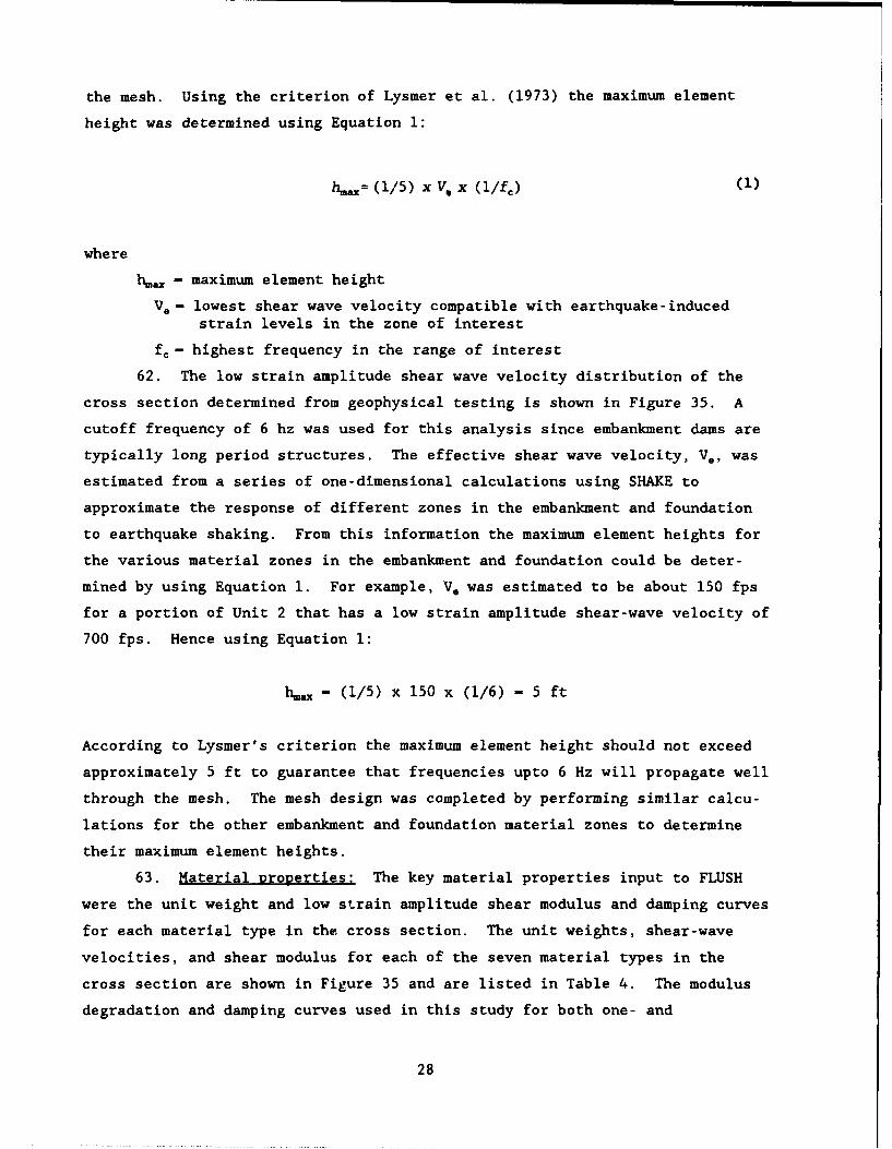
the mesh. Using the criterion of Lysmer et al. (1973) the maximum element
height was determined using Equation 1:
hm.= (1/5) x V, x (1/f) (1)
where
1.= - maximum element height
V* - lowest shear wave velocity compatible with earthquake-inducedstrain levels in the zone of interest
f= - highest frequency in the range of interest
62. The low strain amplitude shear wave velocity distribution of the
cross section determined from geophysical testing is shown in Figure 35. A
cutoff frequency of 6 hz was used for this analysis since embankment dams are
typically long period structures. The effective shear wave velocity, V., was
estimated from a series of one-dimensional calculations using SHAKE to
approximate the response of different zones in the embankment and foundation
to earthquake shaking. From this information the maximum element heights for
the various material zones in the embankment and foundation could be deter-
mined by using Equation 1. For example, V. was estimated to be about 150 fps
for a portion of Unit 2 that has a low strain amplitude shear-wave velocity of
700 fps. Hence using Equation 1:
h.= - (1/5) x 150 x (1/6) - 5 ft
According to Lysmer's criterion the maximum element height should not exceed
approximately 5 ft to guarantee that frequencies upto 6 Hz will propagate well
through the mesh. The mesh design was completed by performing similar calcu-
lations for the other embankment and foundation material zones to determine
their maximum element heights.
63. Material properties: The key material properties input to FLUSH
were the unit weight and low strain amplitude shear modulus and damping curves
for each material type in the cross section. The unit weights, shear-wave
velocities, and shear modulus for each of the seven material types in the
cross section are shown in Figure 35 and are listed in Table 4. The modulus
degradation and damping curves used in this study for both one- and
28
two-dimensional dynamic response analyses are shown in Figure 33. These
curves were developed by Seed, et al. (1984) for cohesionless soils.
64. Site specific ground motions: In Volume 2 of this series Krinitsky
(1986) specified peak ground motion parameters for a firm soil site near
Barkley Dam. The design event is a magnitude mb- 7.5 based on a repeat of
the New Madrid events of 1811-12. Krinitsky (1986) recommended using the
Santa Barbara Courthouse Record, $480 E component, from the Kern County, CA
earthquake of 21 July 1952 as the design accelerogram. This record was to be
scaled to 0.24 g and applied to the ground surface of the firm soil site.
After scaling, this accelerogram had a peak velocity of 35 cm/sec and a dura-
tion (>- 0.05 g) of about 60 sec. Figures 36 and 37 show the acceleration
history of the scaled Santa Barbara record and its response spectra, respec-
tively. These motions represent the response that would be measured at the
surface of a firm soil site in the vicinity of Barkley dam. The periods of
interest for this study range from about 0.5 to 2 sec. Examination of the
response spectra in Figure 37 shows that these periods occur in the portion of
the spectra with the strongest response, thereby indicating that the Santa
Barbara record was sufficiently rich in the frequencies of interest and would
be appropriate for the dynamic response calculations. The earthquake record
and scaling specifications were approved by the Technical Advisors
(Drs. H. B. Seed, C. Castro, L. T. Long, and A. Nieto) on 27 August 1980. (See
Appendix A to Volume 1).
65. The site specific input to the FLUSH analysis were developed using
the a process illustrated in Figure 38. The discussion which follows is keyed
to numbers which are tied to locations on the schematic. A firm soil profile
and a deconvolution procedure using SHAKE were employed to bring the motions
to the site's free field soil profile. The firm soil profile (left hand side
of Figure 38) is shown in Figure 39. The profile used in this analysis was
developed from data available from the soils beneath the Santa Barbara record-
ing station. The scaled Santa Barbara Courthouse record was input to SHAKE at
the ground surface of this profile. These motions were propagated through the
profile for the purpose of obtaining the acceleration history at the rock
outcrop location (Point 3). The peak acceleration at baserock (Point 2) of
the firm soil profile was 0.18 g and the peak acceleration at the rock outcrop
position (Point 3) was 0.18 g. A comparison of the peak accelerations at the
ground surface (0.24 g) and at base rock indicates that the baserock motions
29
were amplified as they propagated through the firm soil profile. The acceler-
ation history at the rock outcrop location, Point 3, and its response spectra
for 5 percent damping level are presented in Figures 40 and 41, respectively.
66. The evaluation of the dynamic response of the free field soil pro-
file at Barkley dam was the next step in the development of the ground motions
input to FLUSH. The free field soil profile used in the analysis is presented
in Figure 42. Figure 42 shows that the idealized free field profile has a
height of 90 ft and was subdivided into 13 soil layers for analysis. As docu-
mented in Volume 3, the 90 ft height of this soil profile was determined from
borings used for geophysical testing located downstream of the switchyard
area. Figure 42 shows the total velocities and low-strain amplitude densities
assigned to each of the layers in the profile. These properties were deter-
mined based on information obtained from the geophysical and soil exploration
programs. The dynamic response analysis was performed by exciting the profile
with the rock outcrop accelerogram (Point 3) shown previously in Figure 40.
Key information sought from the response were the earthquake-induced peak
accelerations, dynamic shear stresses in each layer, and the acceleration
history at the ground surface of the profile. Figure 43 is a plot of the peak
accelerations as a function of depth for the profile. The plot shows that the
general trend is for the peak accelerations to decrease with depth indicating
that the soil profile amplifies the baserock motions. The baserock motions
(Point 4 on Figure 38) were 0.16 g and the motions at ground surface (Point 5)
were 0.26 g. The peak acceleration at the outcrop location (Point No. 3) is
slightly higher than that of the baserock location (Point No. 3) because the
outcrop location represents a free surface where the energy from incident
seismic waves is totally reflected. On the other hand, at baserock a portion
of the energy is transmitted across soil-rock interface, and the remainder is
reflected.
67. Figure 44 is a plot of the effective dynamic shear stresses induced
by the earthquake. The effective stresses are 65 percent of the value of the
peak shear stresses. Figure 44 shows that the dynamic stresses increase with
depth.
68. The ground surface acceleration history (Point 5) is presented in
Figure 45. These motions were subsequently used as input to the FLUSH analy-
sis. The response spectra for this accelerogram is shown in Figure 46.
30
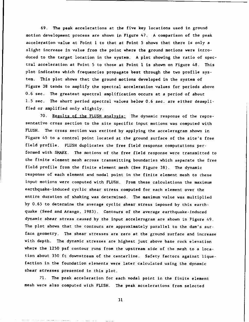
69. The peak accelerations at the five key locations used in ground
motion development process are shown in Figure 47. A comparison of the peak
acceleration value at Point I to that at Point 5 shows that there is only a
slight increase in value from the point where the ground motions were intro-
duced to the target location in the system. A plot showing the ratio of spec-
tral acceleration at Point 5 to those at Point 1 is shown on Figure 48. This
plot indicates which frequencies propagate best through the two profile sys-
tem. This plot shows that the ground motions developed in the system of
Figure 38 tends to amplify the spectral acceleration values for periods above
0.6 sec. The greatest spectral amplification occurs at a period of about
1.5 sec. The short period spectral values below 0.6 sec. are either deampli-
fied or amplified only slightly.
70. Results of the FLUSH analysis: The dynamic response of the repre-
sentative cross section to the site specific input motions was computed with
FLUSH. The cross section was excited by applying the accelerogram shown in
Figure 45 to a control point located at the ground surface of the site's free
field profile. FLUSH duplicates the free field response computations per-
formed with SHAKE. The motions of the free field response were transmitted to
the finite element mesh across transmitting boundaries which separate the free
field profile from the finite element mesh (See Figure 38). The dynamic
response of each element and nodal point in the finite element mesh to these
input motions were computed with FLUSH. From these calculations the maximum
earthquake-induced cyclic shear stress computed for each element over the
entire duration of shaking was determined. The maximum value was multiplied
by 0.65 to determine the average cyclic shear stress imposed by this earth-
quake (Seed and Arango, 1983). Contours of the average earthquake-induced
dynamic shear stress caused by the input accelerogram are shown in Figure 49.
The plot shows that the contours are approximately parallel to the dam's sur-
face geometry. The shear stresses are zero at the ground surface and increase
with depth. The dynamic stresses are highest just above base rock elevation
where the 1250 psf contour runs from the upstream side of the mesh to a loca-
tion about 350 ft downstream of the centerline. Safety factors against lique-
faction in the foundation elements were later calculated using the dynamic
shear stresses presented in this plot.
71. The peak acceleration for each nodal point in the finite element
mesh were also computed with FLUSH. The peak accelerations from selected
31
nodal points are presented in Figure 50. The data in the figure show that
there is a general trend for the peak acceleration to decrease with depth
below the ground surface. The maximum peak acceleration occurred at the crest
of the dam where the value was 0.28 g.
72. The effective strain levels induced by the Santa Barbara Courthouse
record in the FLUSH analysis are shown in Figure 51. The cross hatched area
indicates the zone of elements which had the largest earthquake effective
cyclic shear strains in the FLUSH analysis. The effective strains in these
elements ranged from 0.7 to 1 percent. This area coincides largely with the
foundation soils of Units 2 (interbedded sands within clay) and 3b (weak clay
layer). This area extends completely across the section from the downstream
in the vicinity of the switchyard to the upstream side of the dam. The modu-
lus degradation curves in Figure 33 shows that for the these levels of strain
the modulus would degrade to about 8 percent of its maximum value. This level
of strain is consistent with that estimated in the mesh design for this region
of the foundation and corresponds to a cutoff frequency of about 6 hz. Fig-
ure 51 also shows that the strain levels for elements in the embankment and
foundation Units I and 3c would have effective strains ranging between
0.06 and 0.2 percent. The strain levels in these areas are approximately
one-half to one order of magnitude lower than those for the cross hatched
area.
73. The lengthening of the embankment fundamental period during earth-quake shaking is another measure of strain softening in the embankment materi-
als. The pre-earthquake period of the embankment and foundation system were
estimated using a simplified procedure developed by Sarma (1979). FLUSH was
used to estimate the period of the embankment and its foundation at the earth-
quake induced strain levels. The calculations shown in Figure 52 show that
the pre-earthquake fundamental period of Barkley Dam was 0.75 sec. The period
at the earthquake induced strain levels was determined to be 1.75 sec. A
comparison of the two values indicates that the period lengthens by a factor
greater than two as a result of the straining caused by the earthquake. This
result is consistent with the results of the FLUSH analysis which showed a
significant amount of softening was occurring in Units 2 and 3b due to the
large strains induced by the earthquakes. A comparison of the pre-earthquake
and effective fundamental periods of the dam and foundations system with the
response spectra of the input ground motions from Point 5 (of Figure 46) is
32
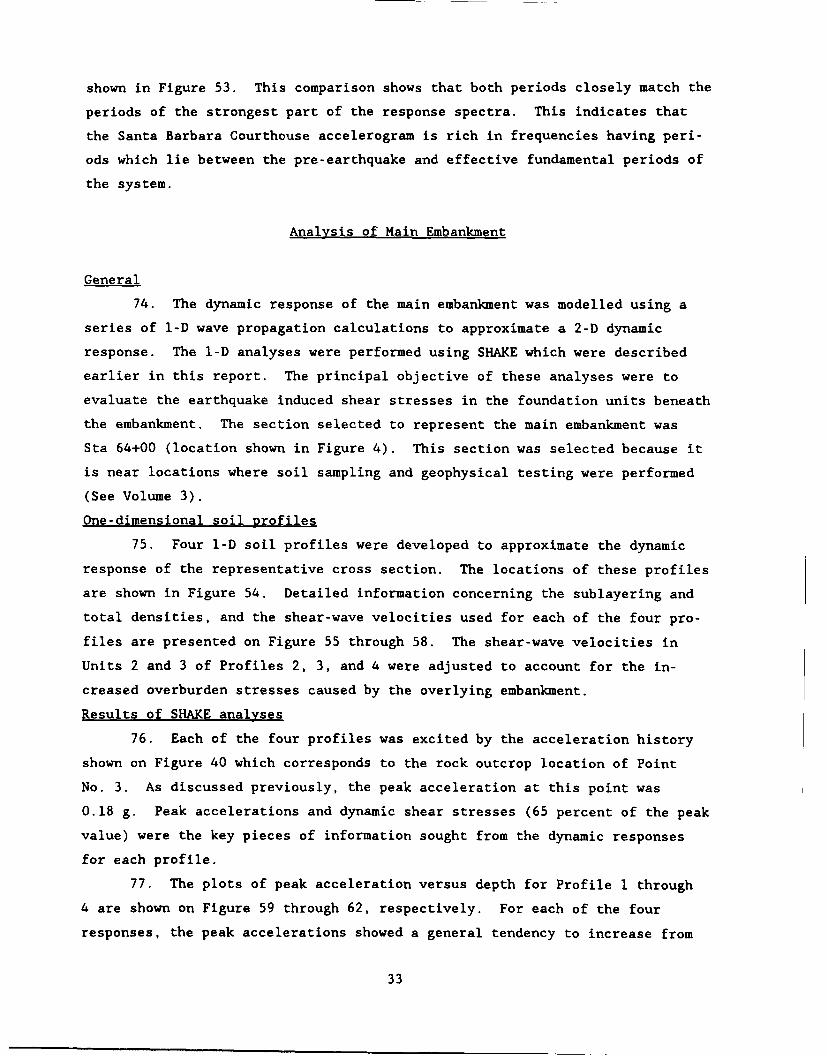
shown in Figure 53. This comparison shows that both periods closely match the
periods of the strongest part of the response spectra. This indicates that
the Santa Barbara Courthouse accelerogram is rich in frequencies having peri-
ods which lie between the pre-earthquake and effective fundamental periods of
the system.
Analysis of Main Embankment
General
74. The dynamic response of the main embankment was modelled using a
series of 1-D wave propagation calculations to approximate a 2-D dynamic
response. The I-D analyses were performed using SHAKE which were described
earlier in this report. The principal objective of these analyses were to
evaluate the earthquake induced shear stresses in the foundation units beneath
the embankment. The section selected to represent the main embankment was
Sta 64+00 (location shown in Figure 4). This section was selected because it
is near locations where soil sampling and geophysical testing were performed
(See Volume 3).
One-dimensional soil profiles
75. Four 1-D soil profiles were developed to approximate the dynamic
response of the representative cross section. The locations of these profiles
are shown in Figure 54. Detailed information concerning the sublayering and
total densities, and the shear-wave velocities used for each of the four pro-
files are presented on Figure 55 through 58. The shear-wave velocities in
Units 2 and 3 of Profiles 2, 3, and 4 were adjusted to account for the in-
creased overburden stresses caused by the overlying embankment.
Results of SHAKE analyses
76. Each of the four profiles was excited by the acceleration history
shown on Figure 40 which corresponds to the rock outcrop location of Point
No. 3. As discussed previously, the peak acceleration at this point was
0.18 g. Peak accelerations and dynamic shear stresses (65 percent of the peak
value) were the key pieces of information sought from the dynamic responses
for each profile.
77. The plots of peak acceleration versus depth for Profile 1 through
4 are shown on Figure 59 through 62, respectively. For each of the four
responses, the peak accelerations showed a general tendency to increase from
33
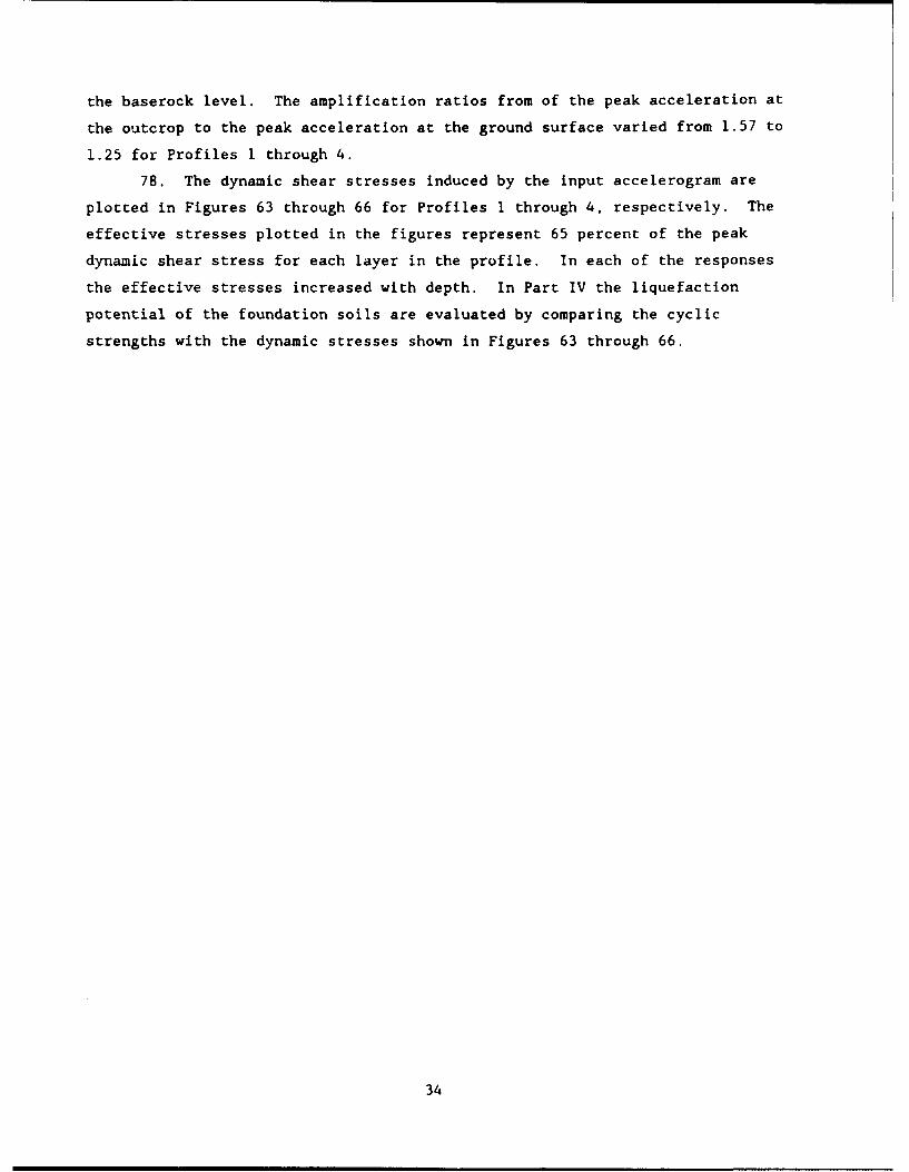
the baserock level. The amplification ratios from of the peak acceleration at
the outcrop to the peak acceleration at the ground surface varied from 1.57 to
1.25 for Profiles 1 through 4.
78. The dynamic shear stresses induced by the input accelerogram are
plotted in Figures 63 through 66 for Profiles 1 through 4, respectively. The
effective stresses plotted in the figures represent 65 percent of the peak
dynamic shear stress for each layer in the profile. In each of the responses
the effective stresses increased with depth. In Part IV the liquefaction
potential of the foundation soils are evaluated by comparing the cyclic
strengths with the dynamic stresses shown in Figures 63 through 66.
34
PART IV: EVALUATION OF LIQUEFACTION POTENTIAL OF THEFOUNDATION OF BARKLEY DAM
General
79. The liquefaction potential of the soils in the three foundation
units beneath the switchyard and main embankment areas was evaluated with
Seed's performance-based approach (Seed et al. 1983, 1984). The liquefaction
potential is quantified by computation of safety factors against liquefaction
(FSL) which compare the cyclic strength of the soil with the dynamic stress
induced by the earthquake. Seed's approach uses Standard Penetration Test
(SPT) blowcounts to determine the cyclic strength (liquefaction resistance) of
a soil deposit. The SPT blowcounts are corrected to a confining stress of
1 tsf and an energy level of 60 percent. The dynamic stresses were determined
from the finite element analysis documented in Part IV of this report. The
Seed procedures were developed for evaluating the liquefaction potential of
sand, silts, silty sands, and gravels, however, screening criteria are
included for distinguishing liquefiable clays from nonliquefiable clays.
80. For this study, liquefaction is defined as that condition which is
reached in a soil deposit when earthquake induced cyclic stresses of suffi-
cient magnitude, sustained for a sufficient number of cycles, cause the
deposit to reach strain levels large enough to increase pore pressures and
reach the residual strength of the soil.
81. In this study, the Seed approach was used to identify and estimate
the extent of the soil deposits in the foundation most likely to liquefy as a
consequence of the design earthquake ground motions. Additionally, the Seed
method was extended to estimate the earthquake induced pore pressure buildup
in areas of the foundation where safety factors against liquefaction are grea-
ter than unity. Zones showing the extent of liquefied material were plotted
on the idealized cross section. Information from the liquefaction analysis
was used to estimate the post-earthquake strengths.
82. The cyclic strengths estimated from the Seed approach depend pri-
marily upon the SPT blowcounts and the fines content of the material. The
application of this approach is complicated by the fact that the alluvial
foundation consists of many thin sand soil layers with varying amounts of
fines. In sandy deposits of this sort it is difficult to estimate the "true"
35
SPT penetration resistance of these materials. The CPT with its abilities to
provide great detail and a continuous record of information was used to over-
come some of these difficulties. Procedures were developed to convert the CPT
penetration resistances into their equivalent SPT blowcounts so that Seed's
performance-based charts could be used to estimate the cyclic strength.
SPT Blowcounts
83. As described in Volume 3 of this series, 44 Standard Penetration
Test and eleven undisturbed borings were made to investigate the nature of the
three units in the alluvial foundation. A variety of procedures were used to
conduct the SPT borings: for some holes rope and pulley systems were used,
and in other holes trip hammer equipment was used. In some holes the SPT
spoon was driven continuously with no clean-out distance between drives, and
in other holes the clean-out distance was at least one foot as recommended for
standard driving procedures (ASTM, 1991). Since the split spoon typically
crossed several layers over the 18-in. drive, several jar samples were taken
from each split spoon to identify the layers involved in the drives. All
information pertaining to the driving procedure and the laboratory index tests
from the jar samples were stored in a large database for analysis of the Stan-
dard Penetration Test data from the site.
84. Sands, silts, silty sands, and gravels are material types which in
the past have been known to liquefy as a result of earthquake shaking. Thus,
in order to evaluate the cyclic strength and subsequent liquefaction potential
of the sand layers, particularly those in Unit 2, it was necessary to deter-
mine the SPT blowcounts of the sand layers present in the foundation.
Data reduction procedures
85. The measured blowcounts were corrected to determine the value that
would be obtained had the Standard Penetration Test been performed under a
specified set of standard conditions. Blowcounts applicable to standard con-
ditions can be compared directly on a one to one basis. Factors which have a
major influence on the measured SPT blowcounts include: the energy efficiency
of the drilling procedure, the effective vertical stress, and the fines con-
tent of the soil. According to the Seed procedure, the standard conditions to
which all blowcounts are reduced include: a vertical effective stress of
1 tsf, 60 percent energy efficiency, and a fines content of less than or equal
36
to 5 percent. Blowcounts reduced to the standard conditions are designated
N1C. The following paragraphs discuss the data reduction procedures employed
to determine the blowcounts for standard conditions.
86. Overburlen correction: The field measured blowcounts were cor-
rected to a vertical effective stress of 1 tsf by the factor C. shown in
Figure 67. The curve on this plot shows that CM is a function of the over-
burden stress. The vertical effective stresses were determined in the static
finite element analysis described in Part III of this report. The effective
stress correction factor CM can be expressed in an equation and is approxi-
mately equal to the vertical effective stress in tsf raised to the power of n,
where n - -0.55 for a relative density of approximately 50 percent and -0.45
for a relative density of approximately 70 percent. An exponent of -0.5 was
used in this study which is generally adequate for most calculations. The
equations used for the overburden corrections are shown below:
N1 =Nas x CM (2)
/an (3)C = (O)
where
N1 - SPT blowcount corrected to an effective stress of 1 tsf
Nmea - field-measured SPT blowcount
CM - overburden correction factor
ov' - vertical effective stress (TSF) from static finite elementanalysis
n - -0.55 for a relative density of about 50 percent
- -0.45 for a relative density of about 70 percent
87. Energy delivery: The field measured blowcounts were corrected to
an energy delivery of 60 percent efficiency in accordance with the guidelines
described by Seed, Tokimatsu, Harder, and Chung, (1984). This energy correc-
tion accounts for the efficiencies of the different types of equipment used in
performance of the Standard Penetration Test in the field. No correction was
made to account for continuous Standard Penetration Testing, that is, testing
with no clean-out space between 18-in. drives. Upon comparison of
37
continuously measured SPT's and standard SPT's with a clean-out depth of at
least 1 ft, no corrections seem to be warranted. In the manner described
above and in the preceding paragraph, the field measured SPT blowcounts were
corrected to a confining stress of 1 tsf and to an energy efficiency of
60 percent. These corrected blowcounts, designated as (NI)6, along with
knowledge of the fines content of the soil were used to enter the cyclic
strength charts for liquefaction evaluation shown in Figure 68. The cyclic
strengths pulled off the chart apply to Magnitude 7.5 events.
88. Adjustment for fines content: An additional adjustment was made to
each blowcount, (NI)6 to correct for the effect of the fines content (per-
centage passing the No. 200 sieve). The corrected blowcount is termed the
equivalent sand blowcount and designated as N1c. The subscript c indicates
that corrections for overburden pressure, energy efficiency, and fines content
have been performed on the field value of blowcount. The equivalent sand
blowcount, N1c, has the same cyclic strength as the (NI)6. For example, the
N1C value is 15 blows/ft for a material having a (NI)6 value of 12 blows/ft
and a fines content of 15 percent as illustrated in Figure 68. The determina-
tion of N1C for all SPT blowcounts allows SPT data obtained in materials
having different fines contents to be compared on a one-to-one basis.
89. Many samples retrieved with the SPT sampler crossed several sand
layers during the 18 in. drive. The fines content of SPT's performed in
predominately sandy materials represented a weighted average of the fines
contents of each of the thin sand layers retrieved with the split spoon. The
fines contents of each of these sand layers was determined by dividing the
18 in. sample into smaller samples. The equivalent clean sand blowcount was
then determined from the (N,)6 value and the observed fines contents.
Results of SPT Data Analysis
90. Analysis of the SPT data was complicated by the complexities of the
three foundation units at the damsite, particularly those of Unit 2. Meaning-
ful results could only be obtained by keeping the findings of the stratigraphy
evaluation in mind during the analysis of the data. Thus, the data were
analyzed with the view that the interbedded sands and clays were
distinguishable components and Lhat the characteristics of each should be
examined separately.
38
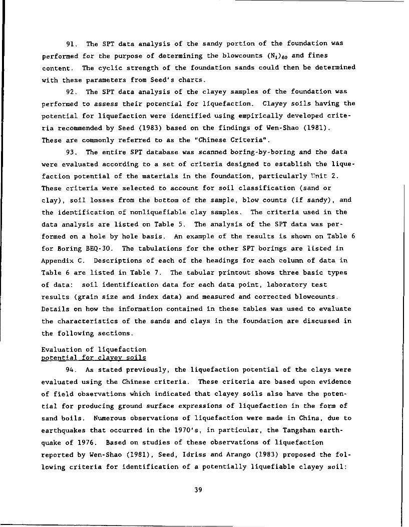
91. The SPT data analysis of the sandy portion of the foundation was
performed for the purpose of determining the blowcounts (N,) 6 0 and fines
content. The cyclic strength of the foundation sands could then be determined
with these parameters from Seed's charts.
92. The SPT data analysis of the clayey samples of the foundation was
performed to assess their potential for liquefaction. Clayey soils having the
potential for liquefaction were identified using empirically developed crite-
ria recommended by Seed (1983) based on the findings of Wen-Shao (1981).
These are commonly referred to as the "Chinese Criteria".
93. The entire SPT database was scanned boring-by-boring and the data
were evaluated according to a set of criteria designed to establish the lique-
faction potential of the materials in the foundation, particularly Unit 2.
These criteria were selected to account for soil classification (sand or
clay), soil losses from the bottom of the sample, blow counts (if sandy), and
the identification of nonliquefiable clay samples. The criteria used in the
data analysis are listed on Table 5. The analysis of the SPT data was per-
formed on a hole by hole basis. An example of the results is shown on Table 6
for Boring BEQ-30. The tabulations for the other SPT borings are listed in
Appendix C. Descriptions of each of the headings for each column of data in
Table 6 are listed in Table 7. The tabular printout shows three basic types
of data: soil identification data for each data point, laboratory test
results (grain size and index data) and measured and corrected blowcounts.
Details on how the information contained in these tables was used to evaluate
the characteristics of the sands and clays in the foundation are discussed in
the following sections.
Evaluation of liquefaction
potential for clayey soils
94. As stated previously, the liquefaction potential of the clays were
evaluated using the Chinese criteria. These criteria are based upon evidence
of field observations which indicated that clayey soils also have the poten-
tial for producing ground surface expressions of liquefaction in the form of
sand boils. Numerous observations of liquefaction were made in China, due to
earthquakes that occurred in the 1970's, in particular, the Tangshan earth-
quake of 1976. Based on studies of these observations of liquefaction
reported by Wen-Shao (1981), Seed, Idriss and Arango (1983) proposed the fol-
lowing criteria for identification of a potentially liquefiable clayey soil:
39
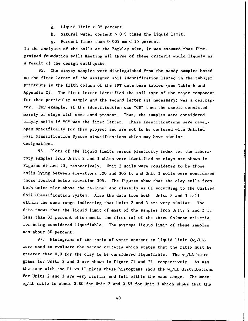
A. Liquid limit < 35 percent.
b. Natural water content > 0.9 times the liquid limit.
c. Percent finer than 0.005 mm < 15 percent.
In the analysis of the soils at the Barkley site, it was assumed that fine-
grained foundation soils meeting all three of these criteria would liquefy as
a result of the design earthquake.
95. The clayey samples were distinguished from the sandy samples based
on the first letter of the assigned soil identification listed in the tabular
printouts in the fifth column of the SPT data base tables (see Table 6 and
Appendix C). The first letter identified the soil type of the major component
for that particular sample and the second letter (if necessary) was a descrip-
tor. For example, if the identification was "CS" then the sample consisted
mainly of clays with some sand present. Thus, the samples were considered
clayey soils if "C" was the first letter. These identifications were devel-
oped specifically for this project and are not to be confused with Unified
Soil Classification System classifications which may have similar
designations.
96. Plots of the liquid limits versus plasticity index for the labora-
tory samples from Units 2 and 3 which were identified as clays are shown in
Figures 69 and 70, respectively. Unit 2 soils were considered to be those
soils lying between elevations 320 and 305 ft and Unit 3 soils were considered
those located below elevation 305. The figures show that the clay soils from
both units plot above the "A-Line" and classify as CL according to the Unified
Soil Classification System. Also the data from both Units 2 and 3 fall
within the same range indicating that Units 2 and 3 are very similar. The
data shows that the liquid limit of most of the samples from Units 2 and 3 is
less than 35 percent which meets the first (a) of the three Chinese criteria
for being considered liquefiable. The average liquid limit of these samples
was about 30 percent.
97. Histograms of the ratio of water content to liquid limit (w,/LL)
were used to evaluate the second criteria which states that the ratio must be
greater than 0.9 for the clay to be considered liquefiable. The wn/LL histo-
grams for Units 2 and 3 are shown in Figure 71 and 72, respectively. As was
the case with the PI vs LL plots these histograms show the wn/LL distributions
for Units 2 and 3 are very similar and fall within the same range. The mean
wn/LL ratio is about 0.80 for Unit 2 and 0.85 for Unit 3 which shows that the
40
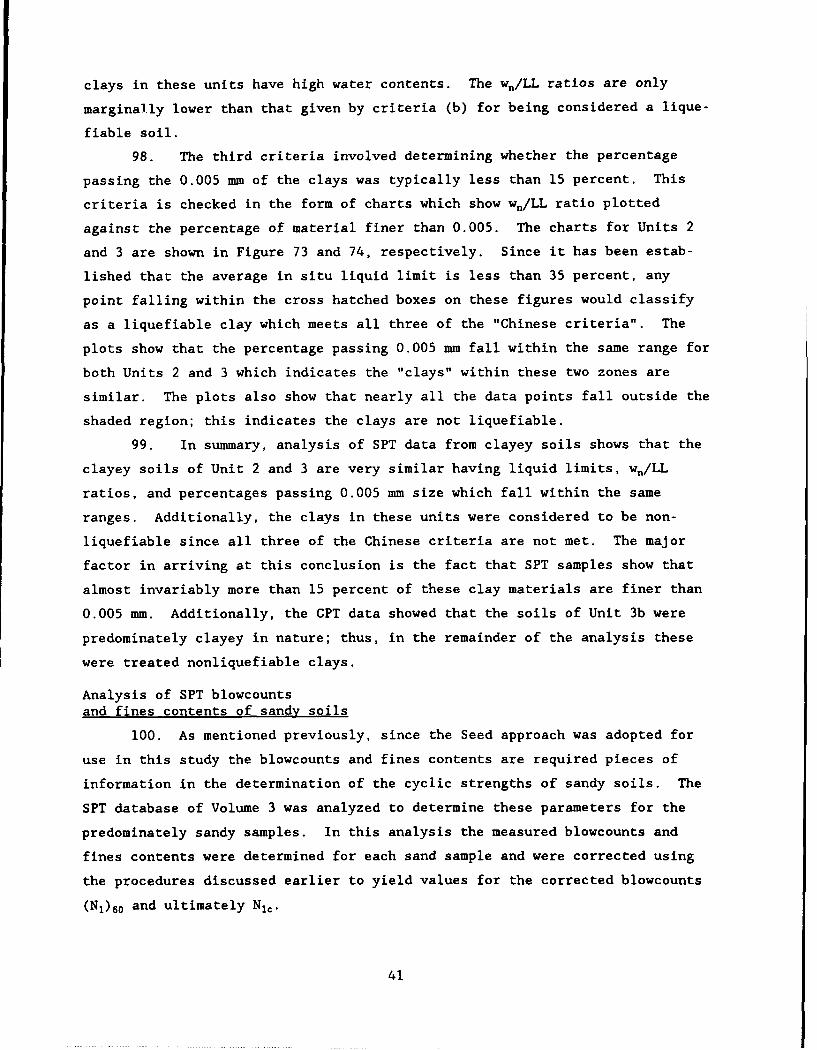
clays in these units have high water contents. The wn/LL ratios are only
marginally lower than that given by criteria (b) for being considered a lique-
fiable soil.
98. The third criteria involved determining whether the percentage
passing the 0.005 mm of the clays was typically less than 15 percent. This
criteria is checked in the form of charts which show wn/LL ratio plotted
against the percentage of material finer than 0.005. The charts for Units 2
and 3 are shown in Figure 73 and 74, respectively. Since it has been estab-
lished that the average in situ liquid limit is less than 35 percent, any
point falling within the cross hatched boxes on these figures would classify
as a liquefiable clay which meets all three of the "Chinese criteria". The
plots show that the percentage passing 0.005 mm fall within the same range for
both Units 2 and 3 which indicates the "clays" within these two zones are
similar. The plots also show that nearly all the data points fall outside the
shaded region; this indicates the clays are not liquefiable.
99. In summary, analysis of SPT data from clayey soils shows that the
clayey soils of Unit 2 and 3 are very similar having liquid limits, wn/LL
ratios, and percentages passing 0.005 mm size which fall within the same
ranges. Additionally, the clays in these units were considered to be non-
liquefiable since all three of the Chinese criteria are not met. The major
factor in arriving at this conclusion is the fact that SPT samples show that
almost invariably more than 15 percent of these clay materials are finer than
0.005 mm. Additionally, the CPT data showed that the soils of Unit 3b were
predominately clayey in nature; thus, in the remainder of the analysis these
were treated nonliquefiable clays.
Analysis of SPT blowcounts
and fines contents of sandy soils
100. As mentioned previously, since the Seed approach was adopted for
use in this study the blowcounts and fines contents are required pieces of
information in the determination of the cyclic strengths of sandy soils. The
SPT database of Volume 3 was analyzed to determine these parameters for the
predominately sandy samples. In this analysis the measured blowcounts and
fines contents were determined for each sand sample and were corrected using
the procedures discussed earlier to yield values for the corrected blowcounts
(N1 ) 60 and ultimately Nl,.
41
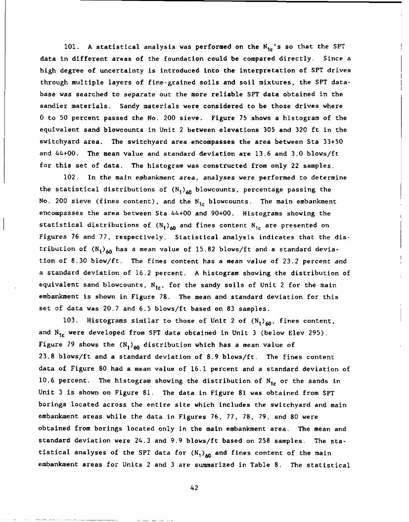
101. A statistical analysis was performed on the N1¢'s so that the SPT
data in different areas of the foundation could be compared directly. Since a
high degree of uncertainty is introduced into the interpretation of SPT drives
through multiple layers of fine-grained soils and soil mixtures, the SPT data-
base was searched to separate out the more reliable SPT data obtained in the
sandier materials. Sandy materials were considered to be those drives where
0 to 50 percent passed the No. 200 sieve. Figure 75 shows a histogram of the
equivalent sand blowcounts in Unit 2 between elevations 305 and 320 ft in the
switchyard area. The switchyard area encompasses the area between Sta 33+50
and 44+00. The mean value and standard deviation are 13.6 and 3.0 blows/ft
for this set of data. The histogram was constructed from only 22 samples.
102. In the main embankment area, analyses were performed to determine
the statistical distributions of (NI)6 blowcounts, percentage passing the
No. 200 sieve (fines content), and the NIC blowcounts. The main embankment
encompasses the area between Sta 44+00 and 90+00. Histograms showing the
statistical distributions of (NI)w and fines content NIc are presented on
Figures 76 and 77, respectively. Statistical analysis indicates that the dis-
tribution of (NI)6 has a mean value of 15.82 blows/ft and a standard devia-
tion of 8.30 blow/ft. The fines content has a mean value of 23.2 percent and
a standard deviation of 16.2 percent. A histogram showing the distribution of
equivalent sand blowcounts, NIC, for the sandy soils of Unit 2 for the main
embankment is shown in Figure 78. The mean and standard deviation for this
set of data was 20.7 and 6.5 blows/ft based on 83 samples.
103. Histograms similar to those of Unit 2 of (N,)6, fines content,
and N1C were developed from SPT data obtained in Unit 3 (below Elev 295).
Figure 79 shows the (NI)w distribution which has a mean value of
23.8 blows/ft and a standard deviation of 8.9 blows/ft. The fines content
data of Figure 80 had a mean value of 16.1 percent and a standard deviation of
10.6 percent. The histogram showing the distribution of N1C or the sands in
Unit 3 is shown on Figure 81. The data in Figure 81 was obtained from SPT
borings located across the entire site which includes the switchyard and main
embankment areas while the data in Figures 76, 77, 78, 79, and 80 were
obtained from borings located only in the main embankment area. The mean and
standard deviation were 24.3 and 9.9 blows/ft based on 258 samples. The sta-
tistical analyses of the SPT data for (NI)6 and fines content of the main
embankment areas for Units 2 and 3 are summarized in Table 8. The statistical
42
analysis of the data for the equivalent clean sand blowcounts, NIt, obtained
from the SPT are summarized in Table 9.
104. The following conclusions were drawn from analysis of the data
presented in Figures 75 through 81:
a. The Unit 2 equivalent sand blowcounts, N1 , in the switchyardarea blowcount generally are lower than those of the mainembankment area.
b. The equivalent sand blowcounts, N1j, in Unit 3 are higher thanthe Unit 2 blowcounts for both the switchyard and main embank-ment areas.
There are several possible explanations for the above results. Conclusion
(a) suggests that the Unit 2 sand layers of main embankment area are either
denser and/or thicker than those of the switchyard area. The small number of
samples (23) obtained in switchyard area of Unit 2 provides further evidence
of this since it is more difficult to find predominately sandy samples if the
layers are thinner based on the rationale that thinner layers are more diffi-
cult to sample. Additionally, the blowcounts in these thin sand layers proba-
bly do not reflect the true penetration resistance of these sands since they
are influenced by the soft clays which dominate Unit 2. Better estimates of
the equivalent sand blowcounts were observed in Unit 2 of the main embankment
area (83) and Unit 3 where a far greater number of samples were recovered
(248). The results indicate that the sands obtained here were thick enough
allow the true penetration resistance in these areas to be approximated with
the SPT.
105. The low blowcounts measured with the SPT in Unit 2 of the
switchyard area suggested that this section of the foundation would be the
most critical in terms of the seismic stability of the embankment. However,
the cyclic strength of the sands in this area were difficult to evaluate due
to the problems associated with the sampling and the performance of the SPT in
thin sand layers embedded in the soft clays. Hence, the Cone Penetration Test
(CPT) was used to obtain more and higher quality data with regard to the pene-
tration resistances of the thin sand layers. This data was used to better
evaluate the cyclic strength of the thin sand layers as will be discussed in
the next section.
43
Prediction of SPT Blowcounts from Cone Penetration Test Data
CPT prediction of (No0f
106. The CPT prediction of the Standard Penetration Test (SPT) blow
count, N, is an important requirement for the evaluation of the liquefaction
potential of Unit 2. Seed's empirically-based liquefaction analysis (Seed,
1979; Seed et al. 1983; Seed et al. 1984;, and Seed, 1986) was developed from
large amounts SPT data and observations of liquefaction in the field. During
the period of this study an adequate independent database relating CPT values
to liquefaction susceptibility did not exist and the most advanced method for
SPT (N1 )6 prediction from CPT data was that developed by Olsen (1984) and
Olsen and Farr (1986). The (N1 )6 prediction chart used in this study is
shown in Figure 82. This method uses the results of both the tip resistance
(qc) and sleeve friction (f$) measurements from the CPT, and is sensitive to
the soil type and consistency.
107. For the last 20 years, a qc/N ratio of 4 to 5 was used to estimate
the SPT blowcount in sand (Robertson et al. 1983). A widely used qc/N tech-
nique for SPT prediction requires an estimate of D50 from a nearby boring to
determine the qc/N ratio from which the SPT N value is calculated (See Fig-
ure 83 taken from Robertson, Campenella, and Wightman 1983). Additional
research (Schmertmann, 1976, 1979a, and 1979b; Douglas, Olsen, and Martin,
1981) has shown that the SPT side friction can be a major contributing factor
for loose and overconsolidated soil conditions. Therefore, the CPT sleeve
resistance can make an important contribution in some sands. The side fric-
tion and end-bearing resistance components of stress acting on the SPT sampler
during driving can be modeled with the CPT probe as shown in Figure 84. Con-
tours of qc/NI shown on ths Soil Characterization-N, Prediction Chart (Fig-
vre 82) are not parallel to the CPT soil characterization lines (i.e. soil
type lines), which indicates that the use of the D50 to qc/N correlation may
lead to erroneous results. Figure 82 does show that a clean sand in the nor-
mal consistency zone of the CPT soil characterization chart has a qcn/N1 of 4
to 4.5 which equals that determined from Figure 83 for a D50 of 0.25 mm.
Since the qc and N require different confining pressure correction factors,
the ratio qcn/Nl more accurately predicts SPT blowcounts, especially at high
confining stress levels. Olsen's technique was used to interpret the CPT data
44
from the Barkley site because of the perceived advantages described above,
particularly because the me,._ is sensitive to soil type and consistency.
CPT prediction of fines
corrected blowcounts, Nlc
108. The CPT prediction of the Standard Penetration Test (SPT) blow-
count, N, is an important factor for liquefaction evaluation. Prediction of
N1, allows not only clean sands but dirty sands and sandy mixtures to be eval-
uated for liquefaction resistance.
109. In the SPT liquefaction evaluation procedure, the percent passing
the No. 200 sieve is used to determine the increase required in N, to correct
for the fines content to determine the equivalent sand value of Nj,. CPT
Soil Characterization Numbers (SCN) can be matched to the percent passing the
No. 200 sieve (Douglas and Olsen, 1981) in order to calculate the blowcount
corrected for fines, Nj,. Figure 85 shows estimated SCN lines which cor-
respond to 5 and 35 percent passing the No. 200 sieve. These lines also cor-
respond to soils having mean grain sizes of 0.25 mm and 0.15 mm.
110. Also shown in this figure are the fines corrections to be added to
the measured blowcounts to determine N1, based on the D50 and percent passing
the No. 200 sieve when the fines correction was determined. The CPT predicted
fines correction is somewhat higher for clayey and mixture materials (e.g.
clayey sands) than the SPT approaches because the CPT approach distinguishes
(to some extent) between silty fines and clayey fines, whereas the SPT method
has the same correction for both silty and clayey fines. The CPT fines cor-
rection is based on the trends from cyclic laboratory tests as well as SPT
trends for sands and dirty sands. The combination of this data indicates an
increased fines correction to determine Njc for soil mixtures with more clayey
than silty fines.
111. As shown in Figure 86, the fines-corrected equivalent sand blow-
count, N1j, can be determined by adding the appropriate fines-content correc-
tion, AN,, to the predicted blowcount. The fines corrections from Figure 85
were combined with the predicted blowcounts (values that would be measured in
the field), corrected to 1 tsf, N1 , from Figure 82, to obtain the overburden
pressure-corrected, fines-corrected blowcounts, N1j, shown in Figure 87.
112. In situ, a SPT measurement requires a drive of 1.5 ft (ASTM 1991).
At layered sites, use of the CPT to predict SPT-N values has some advantages
over actual SPT drives because the CPT is more precise for measuring the prop-
45
erties of thin layers. A commonly used rule of thumb suggests that a soil
layer should have a thickness of between 10 and 20 times the diameter of the
cone before the "true" penetration resistance can be observed (Robertson and
Campanella 1986). Thus, in the case of a standard cone with a diameter of
1.4 in. the rule of thumb suggests the minimum layer thickness for full tip
resistance should be between 14 and 28 in. to reliably correlate CPT data to
engineering properties. However, for this study it was hypothesized that due
to compensating errors in soil classification and fines corrections, the CPT
could predict N1, for soil layers less than 1 ft thick. The reasoning behind
these compensating errors is described in the following paragraphs.
113. For the Barkley project the majority of the thin sand lenses of
concern are on the order of 6 to 12 inches thick. Figure 88 illustrates how
both the tip resistance and friction sleeve readings are influenced in a thin
sand layer surrounded by thicker layers of softer clay. When the probe is in
the sand layer, the tip resistances are influenced by the softer underlying
clay which is yielding ahead of the probe. This behavior causes the measured
tip resistance to be lower than the "true" tip resistance. This results in
the Nlr blowcount being underestimated after the CPT to SPT correlations are
applied. Conversely, since the thickness of the sand layer is not all that
much different than the 4-inch length of the friction sleeve, the clay layers
contribute to the friction sleeve values observed while the probe is in the
sand. This situation leads to an overestimation of the fines contznt of the
sands and an error in the CPT soil classification. This results in the N1c
blowcount being overestimated after the correlations are applied.
114. The errors described in the preceding paragraph are compensating.
However, it was felt that error in the fines content only partially compen-
sated for the error in the observed tip resistances. Hence, the equivalent
Nlr blowcount predicted by the correlations was less than the "true" value.
As a result, the cyclic strengths were increased by a factor to account for
the thin sand layers present in Unit 2. This factor,KIay.r, is further de-
scribed later in this part of the report.
CPT predicted
blowcounts - Unit 2
115. A statistical analysis was performed on CPT predicted (N,) 60 and
N1, blowcounts to determine the appropriate values to use for the determina-
tion of cyclic strength for the sands in Unit 2. The CPT predicted blowcounts
46
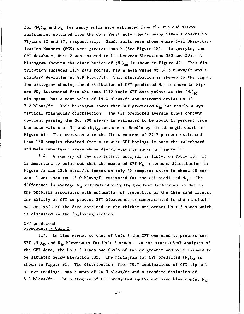
for (NI)6 and Ni€ for sandy soils were estimated from the tip and sleeve
resistances obtained from the Cone Penetration Tests using Olsen's charts in
Figures 82 and 87, respectively. Sandy soils were those whose Soil Character-
ization Numbers (SCN) were greater than 2 (See Figure 18). In querying the
CPT database, Unit 2 was assumed to lie between Elevations 320 and 305. A
histogram showing the distribution of (NI)6 is shown in Figure 89. This dis-
tribution includes 1119 data points, has a mean value of 14.5 blows/ft and a
standard deviation of 8.9 blows/ft. This distribution is skewed to the right.
The histogram showing the distribution of CPT predicted NiC is shown in Fig-
ure 90, determined from the same 1119 basic CPT data points as the (N0)6
histogram, has a mean value of 19.0 blows/ft and standard deviation of
7.2 blows/ft. This histogram shows that CPT predicted NiC has nearly a sym-
metrical triangular distribution. The CPT predicted average fines content
(percent passing the No. 200 sieve) is estimated to be about 15 percent from
the mean values of N1C and (N0)6 and use of Seed's cyclic strength chart in
Figure 68. This compares with the fines content of 27.7 percent estimated
from 160 samples obtained from site-wide SPT borings in both the switchyard
and main embankment areas whose distribution is shown in Figure 13.
116. A summary of the statistical analysis is listed on Table 10. It
is important to point out that the measured SPT NiC blowcount distribution in
Figure 75 was 13.6 blows/ft (based on only 22 samples) which is about 28 per-
cent lower than the 19.0 blows/ft estimated for the CPT predicted NI¢. The
difference in average NIC determined with the two test techniques is due to
the problems associated with estimation of properties of the thin sand layers.
The ability of CPT to predict SPT blowcounts is demonstrated in the statisti-
cal analysis of the data obtained in the thicker and denser Unit 3 sands which
is discussed in the following section.
CPT predicted
blowcounts - Unit 3
117. In like manner to that of Unit 2 the CPT was used to predict the
SPT (NI)6 and NI¢ blowcounts for Unit 3 sands. In the statistical analysis of
the CPT data, the Unit 3 sands had SCN's of two or greater and were assumed to
be situated below Elevation 305. The histogram for CPT predicted (N )0 is
shown in Figure 91. The distribution, from 7037 combinations of CPT tip and
sleeve readings, has a mean of 24.3 blows/ft and a standard deviation of
8.9 blows/ft. The histogram of CPT predicted equivalent sand blowcounts, N1 C,
47
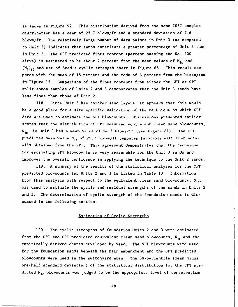
is shown in Figure 92. This distribution derived from the same 7037 samples
distribution has a mean of 25.7 blows/ft and a standard deviation of 7.6
blows/ft. The relatively large number of data points in Unit 3 (as compared
to Unit 2) indicates that sands constitute a greater percentage of Unit 3 than
in Unit 2. The CPT predicted fines content (percent passing the No. 200
sieve) is estimated to be about 7 percent from the mean values of Nit and
(NI)6 and use of Seed's cyclic strength chart in Figure 68. This result com-
pares with the mean of 15 percent and the mode of 6 percent from the histogram
in Figure 15. Comparison of the fines contents from either the CPT or SPT
split spoon samples of Units 2 and 3 demonstrates that the Unit 3 sands have
less fines than those of Unit 2.
118. Since Unit 3 has thicker sand layers, it appears that this would
be a good place for a site specific validation of the technique by which CPT
data are used to estimate the SPT blowcounts. Discussions presented earlier
stated that the distribution of SPT measured equivalent clean sand blowcounts,
N1c, in Unit 3 had a mean value of 24.3 blows/ft (See Figure 81). The CPT
predicted mean value NIC of 25.7 blows/ft compares favorably with that actu-
ally obtained from the SPT. This agreement demonstrates that the technique
for estimating SPT blowcounts is very reasonable for the Unit 3 sands and
improves the overall confidence in applying the technique to the Unit 2 sands.
119. A summary of the results of the statistical analyses for the CPT
predicted blowcounts for Units 2 and 3 is listed in Table 10. Information
from this analysis with respect to the equivalent clean sand blowcounts, N1i,
was used to estimate the cyclic and residual strengths of the sands in Units 2
and 3. The determination of cyclic strength of the foundation sands is dis-
cussed in the following section.
Estimation of Cyclic Strengths
120. The cyclic strengths of foundation Units 2 and 3 were estimated
from the SPT and CPT predicted equivalent clean sand blowcounts, NIC and the
empirically derived charts developed by Seed. The SPT blowcounts were used
for the foundation sands beneath the main embankment and the CPT predicted
blowcounts were used in the switchyard area. The 30-percentile (mean minus
one-half standard deviation) of the statistical distribution for the CPT pre-
dicted N1C blowcounts was judged to be the appropriate level of conservatism
48
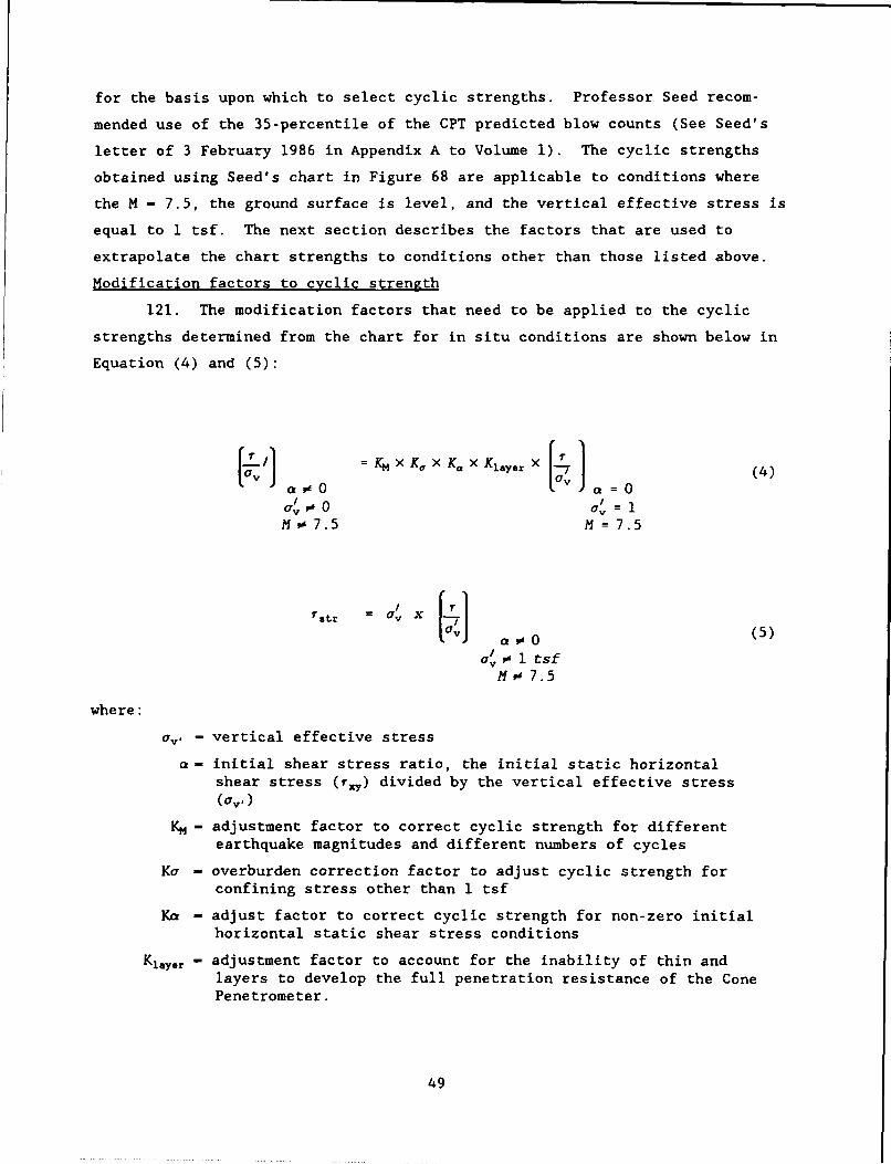
for the basis upon which to select cyclic strengths. Professor Seed recom-
mended use of the 35-percentile of the CPT predicted blow counts (See Seed's
letter of 3 February 1986 in Appendix A to Volume 1), The cyclic strengths
obtained using Seed's chart in Figure 68 are applicable to conditions where
the M - 7.5, the ground surface is level, and the vertical effective stress is
equal to 1 tsf. The next section describes the factors that are used to
extrapolate the chart strengths to conditions other than those listed above.
Modification factors to cyclic strength
121. The modification factors that need to be applied to the cyclic
strengths determined from the chart for in situ conditions are shown below in
Equation (4) and (5):
a~ 00[a/a 0al OW 0 a/ =1M e'7.5 M = 7.5
7 str = av
( 0 (5)UaV 0 1 tsf
M o7.5
where:
av, - vertical effective stress
S- initial shear stress ratio, the initial static horizontalshear stress (r,) divided by the vertical effective stress(Ov,)
Km- adjustment factor to correct cyclic strength for differentearthquake magnitudes and different numbers of cycles
Ka - overburden correction factor to adjust cyclic strength forconfining stress other than 1 tsf
Ka - adjust factor to correct cyclic strength for non-zero initialhorizontal static shear stress conditions
Klayer - adjustment factor to account for the inability of thin andlayers to develop the full penetration resistance of the ConePenetrometer.
49
r I - cyclic shear stress ratioa - 0 (liquefaction resistance) determined
a,, - 1 tsf from empirical charts which correspond toM -7.5 av, - I tsf, a - 0, and M - 7.5.
C -- - cyclic shear stress ratioJa 0 (liquefaction resistance) determined
Or0* I tsf from empirical charts which correspond toM o 7.5 -v, 1 I tsf, a 0 0, and M o 7.5.
The modification factors KM , K, , and K. are described in more detail in
the following sections.
Modification factor
for earthquake magnitude
122. The factor KM accounts for the number of dynamic shear stress
cycles the soil will experience during an earthquake of a particular magni-
tude. Larger numbers of cycles are associated with larger magnitudes and
smaller numbers of cycles are associated with smaller magnitudes. The empiri-
cal charts have been developed for an earthquake of Magnitude 7.5. Table 11
shows the values of KM associated with earthquake magnitudes that range from
5.25 to 8.5. The number of representative dynamic shear stress cycles are
also shown in this table; they range from 2 to 3 for a magnitude 5.25 event to
26 cycles for a magnitude 8.5 event. For the Barkley site the design earth-
quake has a body-wave magnitude of Mb of 7.5. For the Seed cyclic strength
chart, this equates to a Richter magnitude of 8.5 (Nuttli and Herrmann, 1982).
Consequently, a KM equal to 0.89 was used in the liquefaction analysis.
Modification factor
for overburden stress
123. The overburden correction factor, K, , is applied to the cyclic
strength to adjust for the nonlinear relationship between resistance to lique-
faction and confining stress. The empirical charts give cyclic strengths that
correspond to an effective confining stress of 1 tsf. The factor K, is used
to adjust the chart values to confining stresses less than or greater than
1 tsf. The relationship between vertical effective stress and K, used in
this study is shown in Figure 93.
50
Modification factor forinitial static shear stress
124. The factor K. is applied to the cyclic shear strength to adjust
for the increase in liquefaction resistance due to the presence of pre-
earthquake static shear stresses, typically caused by nonlevel ground sur-
faces. The value a is the ratio the initial horizontal shear stress to the
vertical effective stress. Both of these stresses were determined at various
locations within the critical cross section from the static analysis using
FEADAM in Part III of this report.
125. Based on the work of Szerdy (1986) and others (See Rollins, 1987,
for summary) it is known that K. is a function of relative density of the
soil. For relative densities greater than 45 percent a values greater than
zero will result in an increase in cyclic strength. For relative densities of
approximately 45 percent a has no effect on the cyclic strength. For rela-
tive densities less than 45 percent the presence of initial horizontal shear
stresses is detrimental and there is a reduction in cyclic strength. These
trends are shown in Figure 94 and were taken from Rollins (1987). The equiva-
lent sand NJ, in the Unit 2 sands average 19 blows per foot which correlates
to a relative density of about 65 percent according to the chart in Figure 95
developed by Tokimatsu and Seed, 1987. In Unit 3 the equivalent sand NJ, is
25.7 blows/ft which correlates to a relative density about 75 percent. The
K, curve for a relative density of 55 percent in Figure 94 was used in this
analysis to determine K. for the sands in both Units 2 and 3.
Reduction factor for thin sand layers
126. As discussed earlier, the thin sand layers in Unit 2 posed a major
problem with respect to measuring the "true" CPT tip resistance in these sands
since the measurements were influenced to a large degree by the softer under-
lying clay soils. Professor H. Bolton Seed, a Technical Advisor to this pro-
ject, recommended increasing the measured CPT tip resistances to account for
the fact that the full penetration resistance may not be measured when thin
sand layers are underlain by soft clays and to account for the uncertainty
involved regarding the continuity of the individual sand layers in the soil
profile (See Appendix D, Seed's letter dated 3 February 1986). As a result of
Seed's recommendation the cyclic strengths determined from the CPT data of
Unit 2 and from Seed's charts were increased by 25 percent (K1ay.r - 1.25) to
account for these effects. This adjustment also reflects the belief that on
51
the average the compensating errors related to the CPT estimates of the soil
classification and fines contents discussed in earlier in this Part did not
exactly balance. Additionally, in Unit 3 where the sand layers were thicker,
the cyclic strengths were not adjusted for the thinness and continuity of the
sand layers and Kiay.r was equal to one.
Selection of cyclic strength
stress ratio for the sands in Unit 2
127. Switchyard area: The cyclic strengths in the switchyard area were
determined from the CPT predicted blowcount data. The statistical analysis
presented for the CPT predicted blowcounts presented earlier in this part of
the report showed that the statistical distribution for N1, had a mean value
of 19.0 blows/ft and a standard deviation of 7.2 blows/ft (See Table 10). As
stated earlier, the 30-percentile level of the N1, distribution was adopted
for selecting the cyclic strength stress ratio from Seed's chart in Figure 68.
The 30-percentile is equal to the blowcount value which is one-half standard
deviation less than the mean value. Thus the 30-percentile value for N1, is:
Nlr - 19.0 - (7.2/2)
= 15.4 blows/ft, Say 15 blows/ft
Entering Figure 68 at 15 blows/ft results in a cyclic stress ratio of 0.165
for the Unit 2 sands. The cyclic strength stress ratio was corrected to a
value of 0.184 after multiplying by the factors KM (0.89) and Kly,r
(1.25) to account for the effects of a Magnitude 8+ event and the thin layers.
128. Main embankment area: The cyclic strengths of the Unit 2 sands
beneath the main embankment area were determined directly from the statistical
analysis of the SPT blowcounts presented earlier in Table 9. The statistical
analysis indicated that the distribution of N1I blowcounts had a mean value of
20.7 blows/ft and a standard deviation of 6.5 blows/ft. Thus, the 30 percen-
tile value for N1, was estimated to be:
Nl, - 20.7 - 6.5/2
- 17.45 blows/ft, say 17.5 blows/ft
The cyclic strength stress ratio for a vertical effective stress of I TSF and
level ground conditions was estimated to be 0.195 based on Seed's chart on
52
Figure 68. The cyclic strength stress ratio was corrected to a value of
0.174 after multiplying by the KM factor of 0.89 to account for a Magnitude
8+ event.
Switchyard and main embankment areas:selection of cyclic stress strengthratio for the sands in Unit 3a and 3c
129. The cyclic strength of the Unit 3 sands in both the switchyard and
main embankment areas were estimated from the CPT predicted Njc blowcounts.
In a similar manner as that for Unit 2, the statistical analysis of the
distribution for the CPT predicted Njr blowcounts of Unit 3 sands showed that
the mean value was 25.7 blows/ft and that the standard deviation was
7.6 blows/ft. Thus, at the 30-percentile the equivalent sand blowcount, Njc,
was 21.9 blows/ft which was rounded to 22 blows/ft. From Seed's charts in
Figure 68, 22 blows/ft results in a cyclic strength stress ratio of 0.241.
The cyclic strength stress ratio was corrected to a value of 0.214 after
multiplying by the Km factor of 0.89 to account for a Magnitude 8+ event.
In the switchyard area these results were applied to Units 3a and 3c which
were the sandier portions of Unit 3. Unit 3b was treated as a nonliquefiable
clay. In the main embankment area this cyclic strength was applied over the
entire thickness of Unit 3.
Evaluation of Liquefaction Potential and Pore PressureGeneration Characteristics of the Sands
in Foundation Units 2 and 3
General
130. Safety factors against liquefaction, FSL, were computed to evalu-
ate the liquefaction potential and pore pressure generation characteristics of
the sands in Units 2 and 3 for the representative cross section of both the
switchyard (See Figure 27) and main embankment areas (See Figure 54). The FSL
is defined as the ratio between cyclic strength and earthquake induced shear
stress as expressed in Equation 6 below:
FSL = .Lt (6)3 d
53
131. For the switchyard area the FSL'S were computed at the centers of
gravity for each of the foundation elements of the finite element mesh shown
on Figure 34 for Units 2, 3a, and 3c. The cyclic strengths, •str, for each of
these elements were evaluated using Equations 4 and 5. The cyclic stress
ratios (adjusted for magnitude) estimated from the CPT predicted equivalent
sand blowcounts were 0.184 for Unit 2 and 0.214 for Units 3a and 3c. Values
of K•,, and K. were determined from the vertical effective stress and alpha
ratio (from the FEADAM analysis) and the relationships shown in Figures 93
and 94, respectively. Since the static and dynamic finite element meshes were
different the static stresses were interpolated to positions of the centers of
gravity on the dynamic mesh. The earthquake induced stresses, r y, deter-
mined from the dynamic analysis (See Part III) using FLUSH are shown in
Figure 49. Having determined rstr and Tdy the safety factors for each ele-
ment were evaluated with Equation 6.
132. For the main embankment area, the FSL'S were computed at the cen-
ters of the layers for each of the four one-dimensional soil profiles shown in
Figures 55 through 58. As for the switchyard area, the cyclic strengths were
computed using Equations 4 and 5. The magnitude adjusted cyclic strengths
used for the sands of Units 2 and 3 were 0.174 and 0.214, respectively. The
Klayer factor for Unit 2 was set equal to one because the sands layers in
Unit 2 beneath the main embankment are thicker than those beneath the switch-
yard. A KIay.r factor equal to one was also assigned to Unit 3. The values of
K. were estimated based on the static finite element analysis of the switch-
yard area described in Part III. Static stress determined from the FEADAM
analysis at locations upstream of the centerline were applied to corresponding
locations on the upstream side of the main embankment because the upstream
slope geometry and foundation conditions of the switchyard area approximate
those of the main embankment. Values of K, and K. were determined from
the vertical effective stresses and a ratios (See Figures 30 and 32) and the
relationships shown in Figures 93 and 94, respectively. The earthquake
induced stresses used in the evaluation of the liquefaction potential for the
foundation beneath the main embankment were presented in Figures 63
through 66.
133. In this analysis, the pore pressure generation characteristics of
the sands in the Units 2 and 3 were related to values of safety factor against
54
liquefaction. The pore pressure generation characteristics are discussed in
Part V of this report.
Computed factors of
safety against liauefaction
134. Switchyard area: Contours of the computed safety factors against
liquefaction were drawn on the idealized cross section and shown in Figure 96.
The cross hatched zone on the drawing represent zones where FSL values were
less than one and enable visualization of the extent of the predicted zones of
liquefaction. The method of analysis predicts that any sands located within
the cross hatched areas will liquefy due to the motions of the design earth-
quake. In Figure 96, in Unit 2 liquefaction of the sands is predicted to
occur in three basic areas: (a) from the downstream freefield to a location
approximately 450 ft downstream of the centerline; (b) directly beneath the
level section of the switchyard berm from about 325 ft to 125 ft downstream of
the centerline; and (c) and from a location 100 ft upstream of the centerline
and extending out to the upstream free field area. There will be two zones in
Unit 2 where liquefaction is not predicted: (a) directly beneath the sloping
section of the switchyard berm (between locations 450 and 325 ft downstream of
the centerline) and (b) directly beneath the main portion of the embankment
from locations about 125 ft downstream to 100 ft upstream of the centerline.
Safety factors in the first reach have values which are as high as 1.2 and in
the second are as high as 1.4.
135. In Unit 3, liquefaction is predicted in the sands of 3a and 3c at
locations near the upstream and downstream freefields. The downstream zone of
liquefaction extends from the free field area to about 500 ft downstream of
the centerline. The upstream zone of liquefaction extends from the free field
to about 225 ft upstream of the centerline. A significant portion of Unit 3
located between the two liquefiable zones is not predicted to liquefy. The
FSL values within this zone tend to increase in directions away from the two
liquefiable areas and reach a maximum near the centerline where the FSL con-
tours reach values of about 1.4. As stated previously, the clay layer which
comprises Unit 3b was treated as a nonliquefiable clay and safety factors
against liquefaction were not computed for it.
136. Main embankment area: The results of the computed FSL'S of
Units 2 and 3 are presented in Tables 12 through 16 for the one-dimensional
profiles shown in Figure 54. All of the parameters and factors used in
55
evaluating the foundation FSL'S of each profile are listed in these tables.
The values of alpha (determined from the static analysis) used for Profiles 1
though 3 are plotted versus depth in Figures 97 through 99, respectively.
Values of alpha for Profile 4 at the centerline were equal to zero.
137. In this analysis, the dynamic stresses for Profile 1 were used to
evaluate the FSL'S at locations in the free field and at the toe of the
embankment as shown in Figure 56. At the location of the free field profile,
the initial geostatic stresses are not influenced by the presence of the
embankment. In this case, the FSL'S for each layer were computed by setting
K., equal to one to reflect level ground conditions (See Table 12). Under
level ground conditions, shear stresses on horizontal planes are zero, hence,
a is equal to zero. In the second case, the initial stresses are effected by
the presence of the embankment and K. was selected according to the stresses
determined from the static analysis (See Table 13).
138. The safety factors against liquefaction from Tables 12 through
16 were synthesized into the cross section shown in Figure 100. The plot
shows the average values for FSL computed from layers in Units 2 and 3 for
each profile. In Unit 2, the analysis indicates that liquefaction can be
expected in both the upstream and downstream free field areas of the main
embankment. The FSL'S improve to values ranging between 1.1 and 1.25 beneath
the sloping sections of the embankment where the contribution of initial shear
stresses have their greatest effect in increasing the cyclic strength of the
foundation sands. Figure 100 shows that liquefaction is predicted in Unit 2
near the centerline where the FSL'S are only 0.9. Some liquefaction is pre-
dicted to occur in the upper reaches of the Unit 3 sands between elevations
285 and 295 ft beyond the upstream and downstream toes. Liquefaction is not
expected in Unit 3 directly beneath the embankments where the analysis shows
that FSL'S are greater than 1.3. A cross section of the main embankment show-
ing the zones in the foundation where liquefaction was predicted are shown in
Figure 101.
56
PART V: DETERMINATION OF POST-EARTHQUAKE STRENGTHS
General
139. In this part, the strengths postulated to exist in the various
zones of the foundation immediately after the end of the earthquake were
determined for input to the post-earthquake stability analysis. The post-
earthquake strengths were selected by independent consideration of the charac-
teristics of Units 2 and 3 (including subunits). Post-earthquake strengths
were first selected for each of the major material types in the foundation
which include: the normally consolidated clays of Units 2 and 3b and the
sands of the Units 2 and Units 3a and 3c. Finally, a set of criteria was
adopted which lead to conservative choices in the assignment of the post-
earthquake strengths of the foundation soils in the in the idealized cross
section. The criteria adopted for this study for each of the foundation units
are discussed in the sections which follow. Ultimately, post-earthquake
strengths were recommended for the foundation soils of two cross sections:
the idealized cross sections of the switchyard (Figure 28) and the main
embankment (See Figure 54). A stability analysis was performed on the repre-
sentative sections of each area in Volume 5 using the recommended post-
earthquake strengths.
Post-Earthquake Strengths
Normally consolidated clays
140. The clayey portions of Units 2 and 3b were determined to be nor-
mally consolidated based on the results of the Cone Penetration Testing (See
Part II). Normally consolidated clays typically have c/p ratios equal to
about 0.31. If the clays are assumed to lose 20 percent of their strength
due to the earthquake shaking the post-earthquake c/p ratio will be equal to
0.25 (0.31 x 0.80) (Seed and Thiers 1968). Thus, according to criteria to be
described later elements determined to be controlled by the criteria for clay
were assigned the post-earthquake c/p ratio of 0.25.
57
Sands havingFSL.less than one
141. Sands which have a safety factor, FSL, less than one are assumed
to have liquefied due to the motion of the design earthquake. The post-
earthquake strengths of the liquefied sands in Units 2 and Units 3a and 3 L
were estimated from the CPT predicted equivalent sand blowcounts, N1 C. A per-
formance based chart that relates SPT blowcounts to post-earthquake strength
for (materials that liquefied) evaluation of post-earthquake slope stability
was introduced by Seed (1986). This chart, shown in Figure 102, was developed
from back-calculated undrained strengths, Sur, required to produce a safety
factor of one against sliding in embankments that have failed by sliding due
to liquefaction. These strengths were related to SPT blowcounts made at the
sites. The data from which the chart was developed came primarily from sites
having sands and silty sands.
142. Seed's work (1986) demonstrated that the correlation between SPT
blowcounts and Sur were dependent upon the fines content of the liquefied
soil. Thus, the effective blowcount value, N1eff, upon which the Sur value
of a liquefied soil is based is arrived at by adjusting the overburden cor-
rected blowcount, Ni, for the percentage of material passing the No. 200
sieve. The fines correction made for the determination of Sur is different
than that made for cyclic strength discussed in Part IV. The value for N1eff
is determined using the following equation:
Nieff - (N1I)eas + AN1 (7)
where:
Nleff - fines corrected blowcount used to determine the undrainedresidual strength of a liquefied soil.
(N1)meas - measured blowcount corrected to a vertical effective stress of1 tsf. In this study, (Ni)m.as was assumed to be equal to(N)O• *
AN, - correction for fines content.
Values for AN, for different fines contents are listed in Table 17. Conserva-
tively, the lower bound curve in Figure 102 was used to estimate the Sur val-
ues from the N¶eff blowcounts for the liquefied sands in Units 2 and 3 in both
the switchyard and main embankment areas.
58
143. Switchyard area: The residual strengths of the liquefied sands in
Units 2 and 3 of the switchyard area were based upon the mean CPT predicted
values for (N1 ) 6 0 and fines contents listed in Table 18. The use of the mean
value was justified because no correction was applied to increase the residual
strength to account for the effect of thin layers on the penetration resis-
tance as was done for the cyclic strength discussed previously. The CPT pre-
dicted fines contents rather than the SPT predicted fines contents were used
in the main embankment area because their use resulted in a smaller AN, which
yielded a conservative value for Su. Thus, the Sur of liquefied sands in
Unit 2 was determined from the chart on Figure 102 to be 450 psf based on an
N1 .ff blowcount of 15.5 blows/ft. In Unit 3 of the switchyard, the Sur value
was determined to be 800 psf based on an N16 ff value of 25.0 blows/ft. This
choice is conservative in that it does not extrapolate beyond Seed's basic set
of data.
144. Main embankment area: The post-earthquake undrained residual
strength, Sur, of the liquefied sands of Unit 2 was determined using mean
values of the SPT blowcounts and fines contents determined in the statistical
analysis discussed in Part IV (See Table 8). The data upon which Sur was
based are presented in Table 19. Based on an (N0)6 0 blowcount of
15.8 blows/ft and a fines content of 23.1 percent N1*ff was estimated to be
17.5 blows/ft. Thus, from Figure 102 the Sur of the liquefied sands of Unit 2
was estimated to be 700 psf. The Sur of Unit 3 in the main embankment area
was estimated to be 800 psf on the same basis as that for the switchyard area.
Sands having FSL greaterthan one: pore pressuregeneration characteristics
145. Pore pressure generation can occur in sands even though the
deposit does not liquefy. Tokimatsu and Yoshimi (1983) showed that the earth-
quake induced residual excess pore pressures (normalized with respect to ver-
tical effective stress) are related to the stress ratio (ratio of actual shear
stress ratio to the stress ratio causing liquefaction) as shown on Figure 103.
Tokimatsu and Yoshimi found that for most sands the relationship between nor-
malized parameters falls within the shaded area in the figure. The FSL is
represented by the reciprocal of the normalized stress ratio on the abscissa.
In this analysis, the elements with FSL greater than one were assigned excess
pore pressure ratios, r., according to the relationship defined by the dashed
59
line in the center of the shaded area on Figure 103. In this study r. , is
the ratio of excess pore pressure (u,) vertical effective stress as defined by
Equation 8 below:
u- (8)av
146. The excess pore-pressures generated by the earthquake was essen-
tial information to be input to the post-earthquake seismic stability analysis
documented in Volume 5 of this series. In Units 2, 3a, and 3c, the strengths
of nonliquefied sands were determined from the r. value, the vertical effec-
tive stress, and a friction angle of 31 deg. A friction angle of 31 deg was
used for Unit 2 to evaluate the stability in the initial design of the dam
(US Army Engineer District-Nashville 1960).
Switchyard Area Cross-section
147. Post-earthquake strengths were assigned to each element according
to criteria developed specifically for each of foundation Units 2, 3a, 3b, and
3c. These criteria account for the material types found in each unit and try
to be conservative as to the final strength selected for each element. The
criteria used for each of the foundation units are outlined in the following
paragraphs.
Criteria for Unit 2
148. The criteria for foundation Unit 2 recognized that within any ele-
ment there were both sands and clays as determined in Part II of this report.
Hence, depending on the conditions it was possible to assign either the resid-
ual strength, S,,, or a Mohr-Coulomb strength (friction ratio of 31 deg with a
ru value) for sands, or a strength based on the post-earthquake c/p ratio of
0.25 for normally consolidated clays. The assignment of the proper earthquake
strength first depended upon whether or not the sands in the element were
determined to liquefy (See Figure 96). If the safety factor, FSL, of the
element was less than one (i.e. sands liquefied), the strength assigned to the
element was the lower of the residual strength (Sur- 450 psf) and the un-
drained strength, c , based on a post-earthquake c/p ratio of 0.25. The
60
c/p based strength was determined by multiplying the vertical effective
stress by 0.25. If the safety factor, FSL , was greater than one and if the
Sur was greater than the Mohr-Coulomb based strength then the post-earthquake
strength was based on the minimum value of the c/p based strength and the
Sur IThis criteria controlled for cases where the safety factor was only
marginally greater than one and guaranteed the element would be assigned a
post-earthquake strength at least as great as that of either the Sur or the
c/p based value. If the safety factor, FSL , was greater than one and if
the Sur was less than the Mohr-Coulomb strength than the post- earthquake
strength was assigned based on the smaller of the Mohr-Coulomb and c/p based
strengths. This criteria controlled for FSL values which were more than
nominally greater than one.
Criteria for Units 3a and 3b
149. These units were treated as consisting only of sands and thus the
logic for assigning post-earthquake strength is somewhat simpler than that for
Unit 2. Units 3a and 3b were treated identically. Again, the criteria
depended on the whether or not the sands in Units 3a and 3c are predicted to
liquefy. If the FSL is less than one the post-earthquake strength is
assigned the undrained residual strength value, Sur , of 800 psf which was
determined based on the CPT predicted blowcounts. If the value of FSL was
greater than one then the post-earthquake strength assigned to the element
under consideration was the minimum of the Mohr-Coulomb based strength and the
residual strength value. This criteria guaranteed that the strength in these
units would be at least as large as the Sur for safety factors only slightly
greater than one. The Mohr-Coulomb strength of these sands was a friction
angle of 31 deg and the ru value for the estimated value of FSL.
Criteria for Unit 3b
150. Unit 3b was determined to consist of normally consolidated nonliq-
uefiable clays. Hence, the strengths were based on the post !arthquake c/p
ratio of 0.25 only.
Results
151. The post-earthquake strengths ultimately assigned to the switch-
yard cross section upon which the finite element analysis was based are shown
in Figure 104. Zones (groups of elements) where the undrained residual
strength controlled are indicated by the value of Sur . Zones where the
post-earthquake c/p ratio governed are also indicated by the c/p value
61
of 0.25. Areas in the foundation where the Mohr-Coulomb strengths controlled
are indicated by the excess pore pressures values, r. , to be assigned to
these areas. Friction angles of 31 and 35 deg were assigned to these areas in
Units 2 and 3, respectively. The strengths shown on Figure 104 are
recommended for the post-earthquake stability analysis of the switchyard
section.
Main Embankment Section
152. The one-dimensional dynamic response and liquefaction analysis of
the four profiles of the main embankment were discussed previously in Part IV.
The results were presented in terms of the safety factors against liquefac-
tion, FSL , given in Tables 12 through 15 and Figures 100 and 101. The anal-
ysis showed that liquefaction was predicted in the upstream and downstream
free field and in the area immediate to the centerline of Unit 2. Liquefac-
tion was not predicted in Unit 2 in areas directly beneath the slopes of the
embankment where FSL'S ranged from about 1.1 to 1.25. Liquefaction was
predicted to occur in the upper reaches of Unit 2 of the free field between
elevations 285 and 295. The FSL'S in all other areas of Unit 3 were greater
than 1.2 (free field) and 1.3 (beneath the embankment).
153. The liquefaction analysis indicates that widespread liquefaction
of Units 2 and 3 is not expected beneath the main embankment. Nonetheless, as
a conservative measure undrained residual strengths are recommended for both
Units 2 and 3 in the post-earthquake stability analysis. The recommended
strengths are presented on the cross-section on Figure 105. An undrained
residual strength, Sur , of 700 psf is recommended for the entire breadth of
Unit 2 and 800 psf is recommended for Unit 3.
62
PART VI: SUMMARY AND CONCLUSIONS
154. This report describes the procedures used to interpret the data
obtained from field investigations to determine the liquefaction potential and
post-earthquake strengths of the foundation soils at Barkley Dam. The basic
components of this report include the interpretation of the field data to
evaluate the stratigraphy of the foundation and characterize the site, dynamic
response analyses to evaluate the performance of the foundation of two repre-
sentative embankment sections, the analysis and interpretation of Cone and
Standard Penetration Test data to determine the cyclic strengths for evalua-
tion of the potential for liquefaction and the post-earthquake strengths of
the foundation soils. The post-earthquake strengths were recommended for
input to the seismic stability analysis documented in Volume 5.
155. The stratigraphy analysis was based on data collected from Stan-
dard Penetration Tests (SPT), Cone Penetration Tests (CPT), undisturbed sam-
ples, and an excavation of an exposure of a critical foundation material. The
data were analyzed in order to clarify the conditions in the foundation at the
dam site. The strengths and weaknesses of all the basic sources of informa-
tion were considered in arriving at an idealized interpretation of the site.
The analysis showed that the foundation could be modeled by three basic foun-
dation units: Unit 1, Unit 2, and Unit 3. The overall foundation thickness
is approximately 120 ft. The data showed that each unit had traits which
distinguished it from the others. Unit 1 consists primarily of clays which
classify as CL materials. These clays which can be viewed as a topstratum are
overconsolidated due to desiccation. Generally speaking, Unit 1 is thirty
feet thick and lies between the elevations of 350 and 320 ft. Unit 2 consists
of sand layers interbedded within a matrix of soft normally consolidated clay
(CL). The sand layers are generally very thin being on the order of only a
few inches thick. These sand layers are dirty and contain a fairly high per-
centage of nonplastic fines (on the order of 30 percent). Unit 2 generally
lies between elevation 320 and 305 in the switchyard area and is a little
thicker beneath the main dam where it extends to approximately elevation
295 ft. Unit 3 is subdivided into three subunits: Units 3a, 3b, and 3c.
Unit 3a contains dense sands and gravels which have a relatively high penetra-
tion resistance as compared to the sands layers in Unit 2. These sands typi-
cally contain less than 15 percent fines and are relatively clean compared to
63
those in Unit 2. Unit 3a generally lies between elevation 305 and 295 in the
switchyard area. Unit 3b, located between elevation 295 and 288, is typified
by clays (CL) of low penetration resistance. Unit 3c lies between eleva-
tion 288 and bedrock and based on limited amounts of data appears to have
characteristics similar to Unit 3a. Top of bedrock is generally encountered
between elevation 230 and 240 beneath the switchyard and main embankment
areas.
156. Preliminary studies showed that the sandy materials in foundation
Unit 2 had a high potential for liquefaction in the event of the design earth-
quake and would be the main focus of the investigation. Thus, in the stra-
tigraphy evaluation it was essential not only to identify and classify these
materials but to attempt to their map lateral extent. Unfortunately, it was
not possible to map the extent of individual sand layers from one CPT or SPT
sounding to another. However, an excavation in a downstream exposure of
Unit 2 revealed that some of these layers were undulating and continuous over
fairly long distances in the direction of river flow. This result was car-
ried into the liquefaction studies where the sandy materials in Unit 2 were
conservatively treated as contiuuous.
157. The dynamic response of two representative cross sections were
conducted to evaluate their overall performance due to the design earthquake.
One cross section was located in the switchyard area and the second was repre-
sentative of the main embankment area between Sta 43+00 and Sta 88+00. A two
dimensional dynamic finite element analysis was performed using the computer
program FLUSH to calculate the response of the representative switchyard sec-
tion. This cross section was deemed critical due to the low SPT blowcounts
that were measured in Unit 2 in the area of the switchyard. The cross section
was excited with the motions generated by a magnitude (mb) - 7.5 event based
on the 1811-12 New Madrid event. The design accelerogram was scaled to a peak
acceleration of 0.24 g and applied to the ground surface of a firm soil site.
The S480E component of the Santa Barbara Courthouse record of the Kern County
Earthquake of 21 July 1952 was used as the input ;..celerogram. The dynamic
earthquake induced stresses to be used in the evaluation of the liquefaction
analysis were computed with FLUSH. The results of the analysis predict that
large levels of cyclic strain which are on the order of about 1 percent are
expected to occur in Unit 2 due to the design motions. This zone of large
strains extends completely across the section from the downstream free field
64
to the upstream free field. A comparison of the dam's pre- (0.75 sec) and
effective earthquake fundamental periods (1.75 sec) with the response spectra
of the input accelerogram shows that the dam will resonate if subjected to
these motions. The lengthening of the period indicates that significant
strain softening of materials will occur in the foundation units. A series of
one-dimensional dynamic response calculations using the computer code SHAKE
were performed to approximate the earthquake induced stresses in the represen-
tative section of the main embankment. These analyses indicated that large
strains could be expected to develop in Unit 2 due to earthquake shaking.
158. The cyclic strengths were determined from Seed's empirically based
approach which uses SPT blowcounts. However, due to the complex nature of the
thin interbedded sand lenses in Unit 2 - good estimates of the "true" SPT
blowcounts were not attainable in the switchyard area where the critical sec-
tion was located. Hence, a technique developed by Olsen (1984) was used to
predict the SPT blowcounts from CPT test data. The CPT offered the advantage
of high resolution and excellent sensitivity in the detection of the thin sand
lenses.
159. For both the main embankment and switchyard section, the liquefac-
tion potential was evaluated by computation of safety factors with respect to
liquefaction in which the cyclic strengths are compared with the dynamic shear
stresses. The results for the switchyard section are presented in Figure 96.
Liquefaction is predicted in the foundation sands of Unit 2 over three basic
areas: the upstream free field, beneath the switchyard berm and the down-
stream free field. Liquefaction is not expected to occur in Unit 2 just under
the sloping section of the embankment and in the area near the centerline of
the dam. Liquefaction is predicted in the sands of Unit 3 in the upstream and
downstream free field areas, but is not expected to occur in Unit 3 sands
directly beneath the embankment.
160. The results of the liquefaction analysis of the main embankment
area are presented in Tables 12 through 16 and in Figures 100 and 101. These
analyses showed that liquefaction of Unit 2 was predicted in the upstream and
downstream free field and in the area under the centerline. Liquefaction was
not predicted in Unit 2 in areas directly beneath the slopes of the embank-
ment. Liquefaction was also expected in the upper reaches of Unit 2 of the
free field between elevations 285 and 295. Liquefaction was not expected in
all other areas of Unit 3 and in Unit 1.
65
161. Post-earthquake strengths were determined for both the switchyard
and main embankment sections. The strengths were determined based on the
results of the liquefaction analysis and the CPT predicted and SPT blowcounts.
Seed's empirical technique which uses SPT blowcounts was used to estimate
undrained residual strengths in areas where liquefaction of the sands was
predicted. Earthquake indu ed excess pore pressures and strengths of clays
were determined for areas where liquefaction is not expected. The post-
earthquake strengths recommended for use in the stability analysis for the
switchyard section are presented in Figure 104. The recommended post-
earthquake strengths for the main embankment section are presented on
Figure 105.
66
REFERENCES
American Society for Testing and Materials. 1991. 1991 Annual Book of ASTMStandards, Designation D 1586: "Standard Method for Penetration Test andSplit-Barrel Sampling of Soils," Philadelphia, PA.
Bieganousky, Wayne A., and Marcuson, William F. III. 1975. "LiquefactionPotential of Dams and Foundations - Report 1: Laboratory Standard PenetrationTests on Ried Bedford Model and Ottawa Sands," WES report S-76-2, Oct., 1976.
Douglas, Bruce J. and Olsen, Richard S. 1981 October. "Soil ClassificationUsing the Electric Cone Penetrometer," Cone Penetration Testing and Experi-ence, ASCE Fall Convention.
Douglas, Bruce J., Olsen, Richard S., and Martin, Geoffrey R. 1981. October."Evaluation of the Cone Penetrometer for SPT-Liquefaction Assessment," ASCEPreprint 81-544, St. Louis, Oct. 1981.
Duncan, J. M., Byrne, P., Wong, K. S. and Mabry, P. 1980. "Strength, Stress-Strain and Bulk Modulus Parameters for Finite Element Analyses of Stresses andMovements in Soil Mosses," Report No. UCB/GT/80-01, Geotechnical Engineering,Department of Civil Engineering, University of California, Berkeley, CA.
Duncan, J. M., and Seed, R. B. 1984. Letter report to the US Army Corps ofEngineers District-Nashville containing the results of a static analysis ofBarkley Dam.
Duncan, J. M., Seed, R. B., Wong, W. S., and Ozawa, Y. 1984. "FEADAM84: AComputer Program for Finite Element Analysis of Dams," Research ReportNo. SU/GT/84-03. Stanford University, Stanford, CA.
Krinitzsky, E. L. 1986. "Seismic Stability Evaluation of Alben Barkley Damand Lake Project" US Army Engineer Waterways Experiment Station, TechnicalReport GL-86-7, Volume 2, Vicksburg, MS.
Lysmer, J., Udaka, T., Tsai, C. F., and Seed, H. B. 1973. "FLUSH: A Com-puter Program for Approximate 3-D Analysis of Soil-Structure Interaction Prob-lem." Report No. EERC 75-30. Earthquake Engineering Research Center,University of California, Berkeley, CA.
Nuttli, 0. W. and Herrmann, R. B. 1982. "Earthquake Magnitude Scales."Journal of Geotechnical Engineering, ASCE, Vol. 108, No. GT5, May 1982.
Olsen, Richard S. 1984 July. "Liquefaction Analysis Using the Cone Penetro-meter Test (CPT)," Proceedings of the Eighth World Conference on EarthquakeEngineering, San Francisco, California.
Olsen, Richard S. and Farr, John V. 1986. "Site Characterization Using theCone Penetrometer Test," Proceedings of INSITU 86, ASCE Specialty Conferenceon the Use of In-situ testing in Geotechnical Engineering, Blacksburg, VA.
Robertson, P. K. and Campanella, R. G. 1986. "Guidelines for Use, Interpre-tation and Application of the Electric Cone Penetration Test," Third Edition.Hogentogler and Company, Inc. Gaithersburg, MD.
Robertson, P. K., Campanella, R. G., and Wightman, A. 1983. "SPT- CPT Corre-lations," Journal of Geotechnical Engineering, ASCE, Vol. 109, No. GTl1,November 1982, pp 1449-1459.
67
Rollins, Kyle M. 1987. "The Influence of Buildings on Potential LiquefactionDamage," Dissertation for Doctor of Philosophy, University of California,Berkeley.
Sarma, S. K. 1979. "Response and Stability of Earth Dams During StrongEarthquakes." Miscellaneous Paper GL-79-13, US Army Engineer Waterways Exper-iment Station, CE, Vicksburg, MS.
Schmertmann, John H. 1976 October. "Predicting the qc/N Ratio," Final ReportD-636, "Engineering and Industrial Experiment Station, Department of CivilEngineering, University of Florida, Gainesville, FL.
Schmertmann, John H. 1979a. "Energy Dynamics of SPT," Journal of Geotechni-cal Engineering, ASCE, Vol 105, No. GT8, Aug. 1979.
Schmertmann, John H. 1979b. "Statics of the SPT," Journal of GeotechnicalEngineering, ASCE, Vol 105, No. GT5, May 1979, pp 655-670.
Schnabel, P. B., Lysmer, J., and Seed, H. B. 1972. "SHAKE, A ComputerProgram for Earthquake Response Analysis of Horizontally Layered Sites,"Report No. EERC 72-12, Earthquake Engineering Research Center, College ofEngineering, University of California, Berkeley, CA.
Schnabel, Per B., Lysmer, John, and Seed, H. Bolton. 1972. "SHAKE A ComputerProgram for Earthquake Response Analysis of Horizontally Layered Sites,"Report No. EERC 72-12, Earthquake Engineering Research Center, University ofCalifornia at Berkeley, December 1972.
Seed, H. Bolton. 1979. "Soil Liquefaction and Cyclic Mobility Evaluation forLevel Ground During Earthquake," Journal of Geotechnical Engineering Division,ASCE, Vol 105, No. GT2, Proceedings Paper 14380, pp. 201-255.
Seed, H. Bolton. 1983 May. "Earthquake-Resistant Design of Earth Dams,"Proceedings of the Seismic Design of Embankments and Caverns, ASCE, Philadel-phia, Pennsylvania, pp 41-64.
Seed, H. B., Idriss, I. M., and Arango, I. 1983. "Evaluation of LiquefactionPotential Using Field Performance Data," Journal of Geotechnical Engineering,ASCE, Vol 109, No. GT3, March 1983, pp 458-482.
Seed, H. B., Tokimatsu, K., Harder, L. F., and Chung, Riley M. 1984. "TheInfluence of SPT Procedures in Soil Liquefaction Resistance Evaluations,"Report No. UCB/EERC-84/15, University of California at Berkeley, EarthquakeEngineering Research Center, October 1984.
Seed, H. B., Wong, R. T., Idriss, I. M., and Tokimatsu, K. 1984. "Moduli andDamping Factors for Dynamic Analyses of Cohesionless Soils." Report No. EERC84-14. Earthquake Engineering Research Center, University of California,Berkeley, CA.
Seed, H. B. 1986. "Design Problems in Soil Liquefaction," ReportNo. UCB/EERC-86/02, University of California at Berkeley, Earthquake Engineer-ing Research Center, February 1986.
Szerdy, F. 1986. "Flow Slide Failures Associated with Low Level Vibrations,"Dissertation for Doctor of Philosophy in Civil Engineering, University ofCalifornia, Berkeley.
Wen-Shao, W. 1981. "Foundation Problems in Aseismatic Design of HydraulicStructures," Proceedings of the US-PRC Microzonation Workshop, China.
68
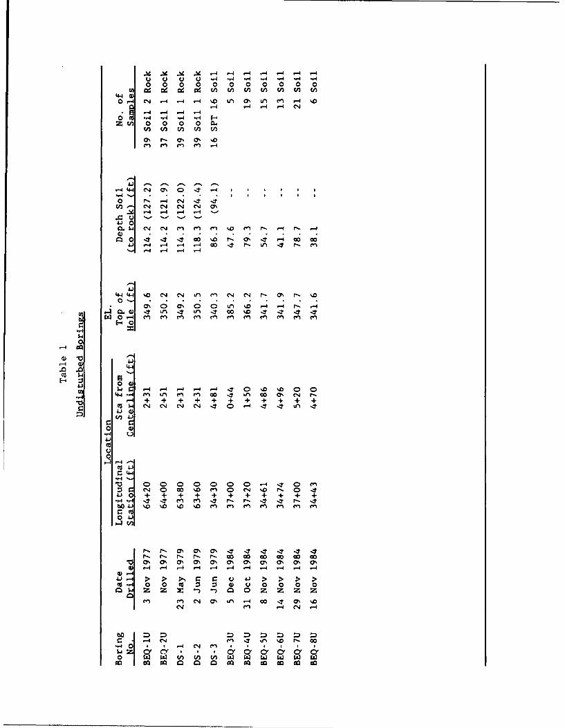
-4 M~ .4 'A -4 -4 .-4 -4 - 4 1-4 1'4
IL) 0 U U ~-4 *-,4 -4 ... ..4 ..4 -40 0 0 0 0 0 00 00 0
wn~t i C~u ~ r44a 0
0,-4 C4 .-4 .-4 v-4 1.0 LM C0% LA (fn -4 %.01-4 1-4 .-4 r-4 (N4
--4 -4 -40 "4 ý -. 4 -- a '4
zcim 0 0 0 0 cw
0% r. 0% Ch '.0
r-4 44. (4 0% 0 -4 -4 a
0 P, .-4 C- 4En~ (N (4 C14 (N M%
.ý' -- 4 -4 -4 '
4.s4 (A N %0 c, c,4tn c'4 cj c, 4 r- a% r, %
44.W -4 M- M- M- en M 4 M~ en en Mne-4 E-4 -4
"44.
-.4
0 4
-4 C1 I I 1 4L
'-4 0
0 4)"-4J u - 4444 . .0
0 0
(4 L4".4.
c, D c Q e 0 c4 % U410.....
0 4
~4)-4
*14J ý4 >4 >4 >~ >~ >4 >. ... 4V(0j -,4 0 '0 '0 z 0 e 0 u 0
4 0 0
M C4 (7% Ln .-4 W4 .4 4 0
Clq m -4 -4 -4
(4 N -4 (N -
(0 C4 LAC?1
0 w/ w wa wa
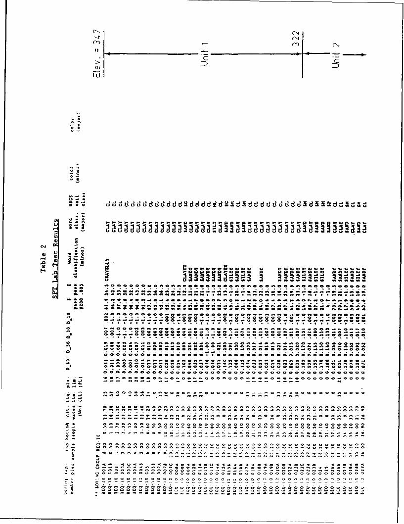
("4
> c
00
-) c
.4-4 3w 01 8Sa: - 1444 14 O..JJ
LP to to
CD C!4t Ct Ct C! 4! i UUU 4!4 !4 ! t' !i4!nI! .. .. !
*Z z-.n e= 1= 720" 0 w4!ot 0 1 ! ! ý1! al !V!0!4 ý0 C 1 ! :q!4
460C 00 ~ 0%i ve .m4%u 42
00IC
C' 3 0 . . . .: .g .. . . . .. .b . .O .Ob. .
*0
Z3 "40
0 ' 44 C 1 4o2C !4!I!C 1!000 0 0.4! C! 4! 0 0 4 .. 0 .4! -! 4!- 00 4 C01'04#
-000 D . 0 .0 4,0 paa0 ...R0 2 0.0 a.0 ; ;000;004ýC C"*a a*- 0 -a,431C o aaa - 00
0.4 ~ 'C .4-. 0.4 @ @-.. 0.4D40 0 0: 4 * 4 @ 0
'o .. .* . 0 S X . * S . a C* C. al .01
CO. 00 go-0000.Z .. 4@. . 0 Z0. *.400 000.0 U,....4 C.0
9* 00 0 0 0 0 0000 a00 .02@ 0 0 00 000000 al 000 C, 0
0 #4C #4. 0 0 C.4o.4.C> 4o.0.40o--s-4.-4-4.-4e -.-.4 -.4 -o-.4-
0 000000)00000 0 0 0 0 0 0 0> 0
w. -44 084.. w4 . . 0 .ý -.. .4I.4 ---- - - - -4 - -. -- P w - f w -w 4 -- - - -0- - - - 0- - - - - 0-- - - 0 - - - - - - - - - - - - - -
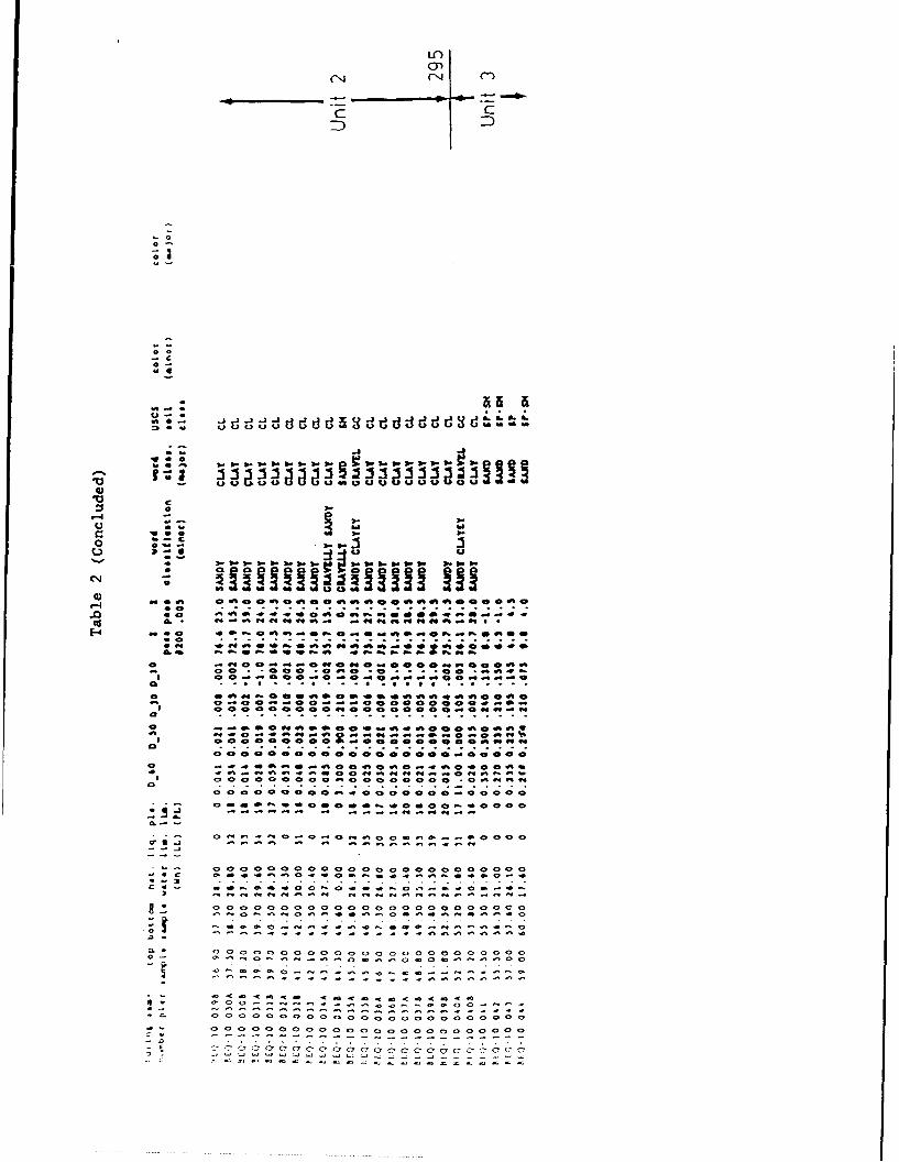
00)
001
Cc010
3wV-3-3 3-3- 1- 1.3. .W
bc *c 00001w
01 414.. 0 1
C2. 10 " a a .ý-
cooC
0~ 2*
- .7- 7
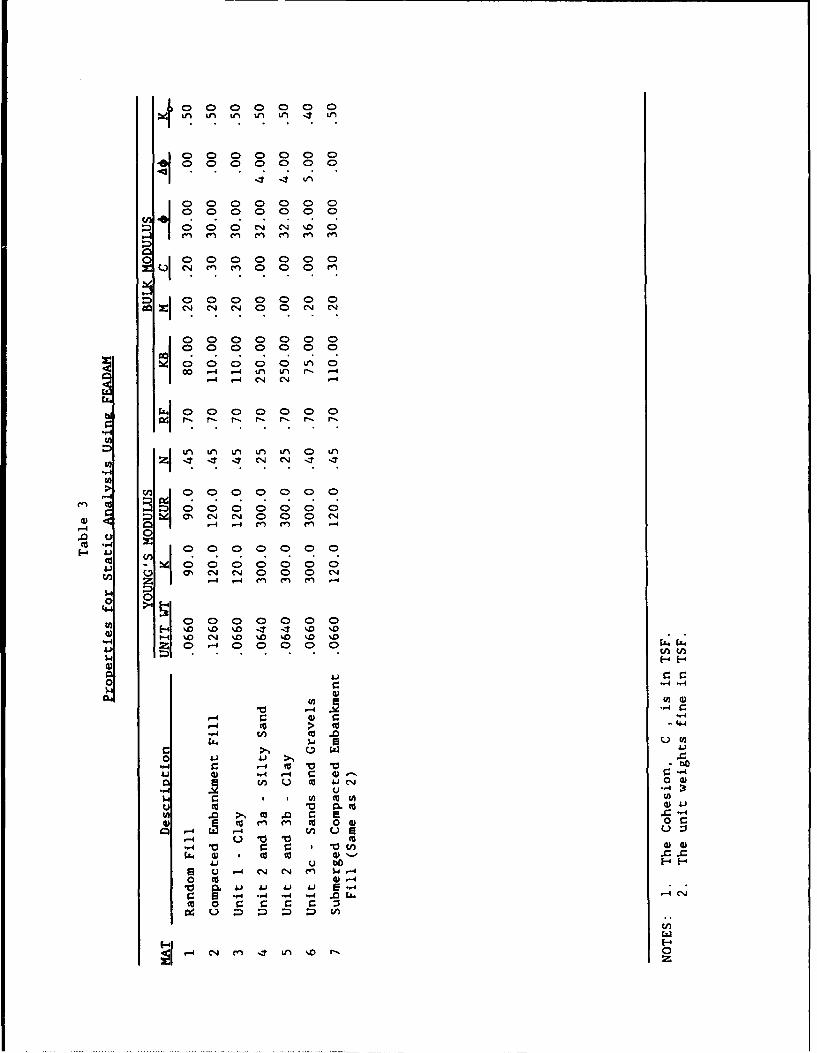
Cf Cf C ý CA I ri - j
0 o0 (D (N "00
0
0 00o0 LAO
r0-4 -4 tn Ln r-. .-4I 4 -4 (N4 C(4N
".4 .I
Ln LA ) r ) W
"44
>~ I0 0 0 0000
.0 0 C
.-4 -4 M~ M
414
0 0
U)
4))
U) KU) 4)
-4 -4
0
" -4 r-4 IV " 0v
0 W m'N 4)ý4 -4 3t
'-4 W M( E C-) V
u v IV aCC )~
0 - CC) 4)4 U ý4
4. 4) 4j AU aU 0'
" "5 ,4 .. 4 -.4 ".4 .0 LL.-4C
CU 0n %0 r
z
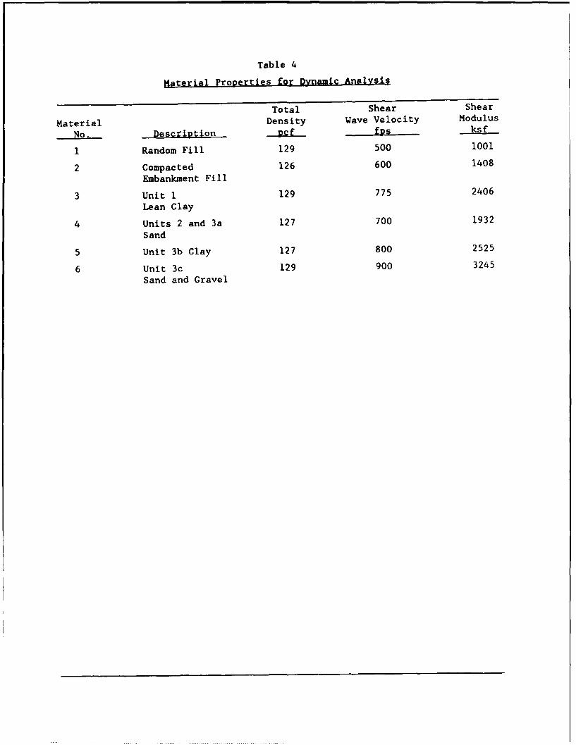
Table 4
Material Properties for Dynamic Analysis
Total Shear Shear
Material Density Wave Velocity Modulus
No. Description Rcf •fD ksf
I Random Fill 129 500 1001
2 Compacted 126 600 1408
Embankment Fill
3 Unit 1 129 775 2406
Lean Clay
4 Units 2 and 3a 127 700 1932
Sand
5 Unit 3b Clay 127 800 2525
6 Unit 3c 129 900 3245
Sand and Gravel
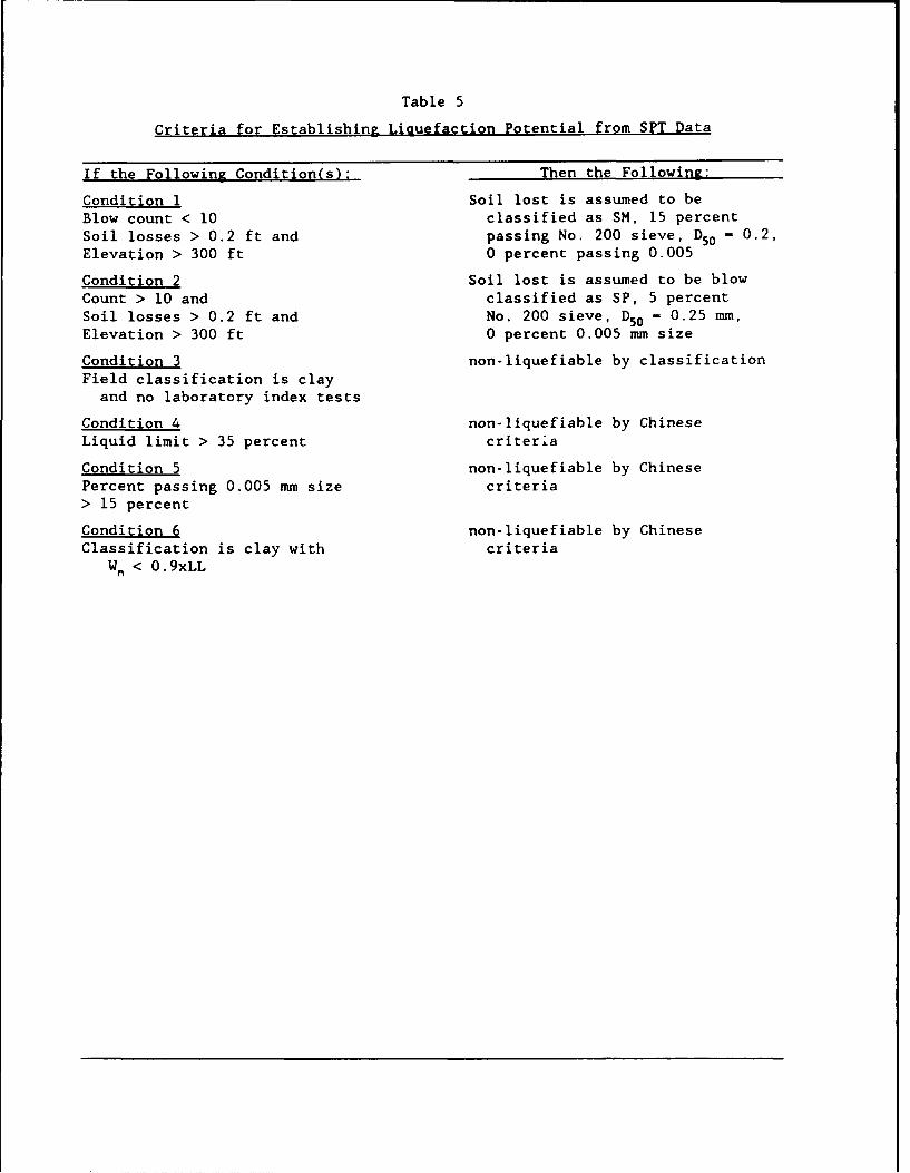
Table 5
Criteria for Establishing Liauefaction Potential from SPT Data
If the Following Condition(s): Then the Following:
Condition 1 Soil lost is assumed to beBlow count < 10 classified as SM, 15 percentSoil losses > 0.2 ft and passing No. 200 sieve, D50 - 0.2,Elevation > 300 ft 0 percent passing 0.005
Condition 2 Soil lost is assumed to be blowCount > 10 and classified as SP, 5 percentSoil losses > 0.2 ft and No. 200 sieve, D50 - 0.25 mm,Elevation > 300 ft 0 percent 0.005 mm size
Condition 3 non-liquefiable by classificationField classification is clay
and no laboratory index tests
Condition 4 non-liquefiable by ChineseLiquid limit > 35 percent criteria
Condition 5 non-liquefiable by ChinesePercent passing 0.005 mm size criteria> 15 percent
Condition 6 non-liquefiable by ChineseClassification is clay with criteria
Wn < 0.9xLL
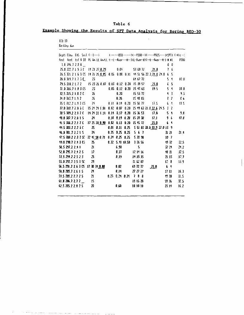
Table 6
Examvle Showing the Results of SPT Data Analysis for Boring BEO-30
DF.:kI t'V&-
[tpl, [ICeu (US Sall (--:---- --- )(.. -- P200-->( ----- POS. SPt> <-Nit--
feet feet tsf t 10 PL Un LL Ur,/L (-4-L-uer---H--)(i-, er-IfX--t--Auer--I-) HNI P2001.0 3%.67 2. 030
2S.0 3?2.7 1.5 3 1 1! 21 27 0.79 8.0i S3 E0 72 21.8 7 626.S 32121,63(5 13 21 250.85 0.06 008 0.11 1 51 56 22.3 21.0 21.8 6 S28.0 319.7 1.7 1 1 23 6 76? 72 5 1 10.029.S 318.2 1.7 2 15 232 0.87 0.03 0-12 0.20 IS 3895? 23.8 t 531.0 316.7 1.8 3 CS 23 O.OS 0.12 0.20 151 63 19.5 S 1 10.032.S 315.2 1.8 2 1 26 0.20 IS 1 3 72 4 3 9.331.0 313.7 1.9 2 26 0.20 11 4 2 .6
35.5 31?.? 1.9 3 IS 21 0.11 0.11 0.20 IS 15 77 17.5 6 1 10537.0 310.7 2.0 3 15 21 211.01 0.02 0.07 0.20 151 9 63 21.0 22.6 21.5 3 238.5 30912 2.02£ 1121221.11 0.11 0.17 0.20 1S36c3 17.0 S I 9.'10.0 307.7 2.0 1 S 21 0.18 0.19 0.20 IS 20 30 12.1 9 6 I0.s11.S 30.2 2.1 2 £ 17 2S 28 0.90 0.02 0.13 0.20 15 ,1 72 23.0 6 141.S 383.2 2.2 3 I 25 0.01 0.11 0.25 S S 83 30.0 33.9 37.0 13 916.0 301.72.215 21 0.25 0.S 0.25 S 6 7 31 21 21.117.S 300.2 2.3 3,S 3? 1158 0.71 0.24 0.25 0.25 S 390 10 719.0 29.7 2.1 3 CS 2 0.32 5.11 10.50 3 56 19 32 2.S5G.S 2M7.2 2.1 I 21 6.90 S j7,1 21.252.0 295.7 2.1 2 S 17 0.27 12,11 1H 101 32 .C53.5 294.2 2.5 2 S 25 8.19 111 15 15 21 13 17.7SS.0 292.7 2.5 3 SC 29 31 287 1288 13.95.5 291.2 2.6 3 (S 17 30 3 .8 0.02 69 72 77 23.0 6 I58.0 289.7 2.6 I S 21 0.11 27 27 27 17 11 16.359.5 222.2 2.7 2 S 21 0.23 0.21 0.2i 7 8 8 19 30 31 .61.0 2867 2.7 2 _ 1s 101S 20 59 36 32.562.5 295.? 2.9 2 S 20 0.60 10 10 10 2311 I.?

Table 7
Description of SPT Liguefaction Printout
Title Description
Depth feet Bottom 1/3 depth of 1.5 ft drive of SPT sampler (feet)
Elev feet Elevation of SPT sampler depth
EVS (tsf) Effective vertical stress (tsf)
No. Number of soil samples in this SPT sampler
Soil Ib* Two letter soil classification based on soil sample code(major and minor)
C claysM mixturesS sands(i.e. CM is mostly clay with some soil samples of
mixture)
PL Plastic Limit (averaged) in percent
Wn Natural water content (Wn) (averaged) in percent
LL Liquid Limit (averaged) in percent
Wn/LL Water content divided by Liquid Limit
D50 Aver Statistical D50 average of the soil samples
D50 L The lowest D50 of the soil sample range
D50 H The highest Ds0 of the soil sample range
P200 Aver Statistical average of the percent passing the No. 200sieve
P200 L The lowest percent passing the No. 200 sieve
P200 H The highest percent passing the No. 200 sieve
P005 Aver Statistical average of the percent grain size of0.005 mm
P005 L The lowest of the percent grain size of 0.005 mmrange
P005 H The highest of the percent grain size of 0.005 mmrange
SPT N Measured SPT blowcount from 0.5 to 1.5 ft below thebore hole bottom
SPT NI Calculated N, based on the Cn correction factor
Nlc P200 N1C silt correction based on the percent passing theNo. 200 sieve
* Not to be confused with USCS classifications.
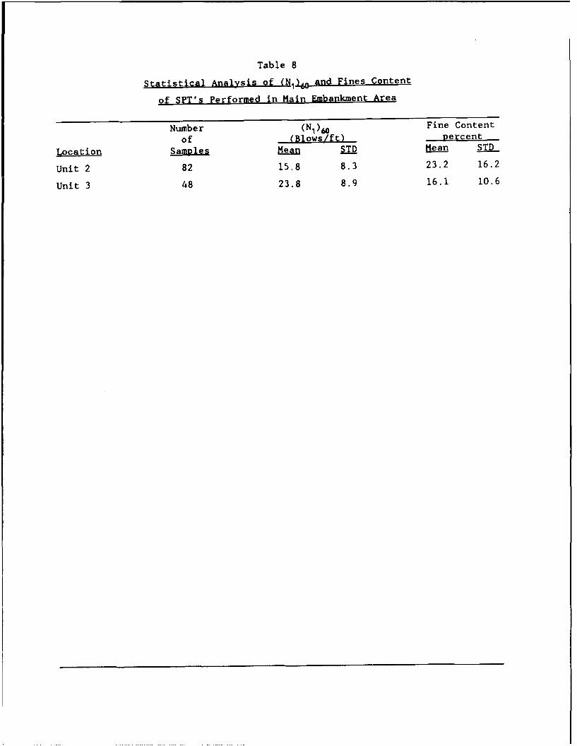
Table 8
Statistical Analysis of (NI, and Fines Content
of SPT's Performed in Main Embankment Area
Number (N)60 Fine Content
of (Blows/ft) percent
Location SaMples Mean STD Mean STD
Unit 2 82 15.8 8.3 23.2 16.2
Unit 3 48 23.8 8.9 16.1 10.6
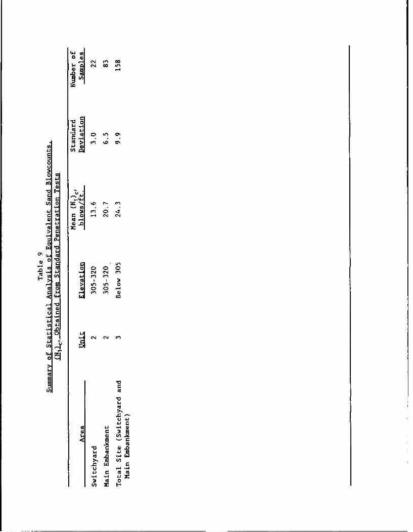
44,
0
00
'-4 . .
0
Cu
C0 t.- 4 0j
00044
"4-J41
SZ r 4 1 1
,4 4.4)4
W o 10
,4. Cu 4.3%n 5toC 0 ) 0 0 .- 4C
41 cz:
'."4 C4 I,- M-
0 u
(n 1
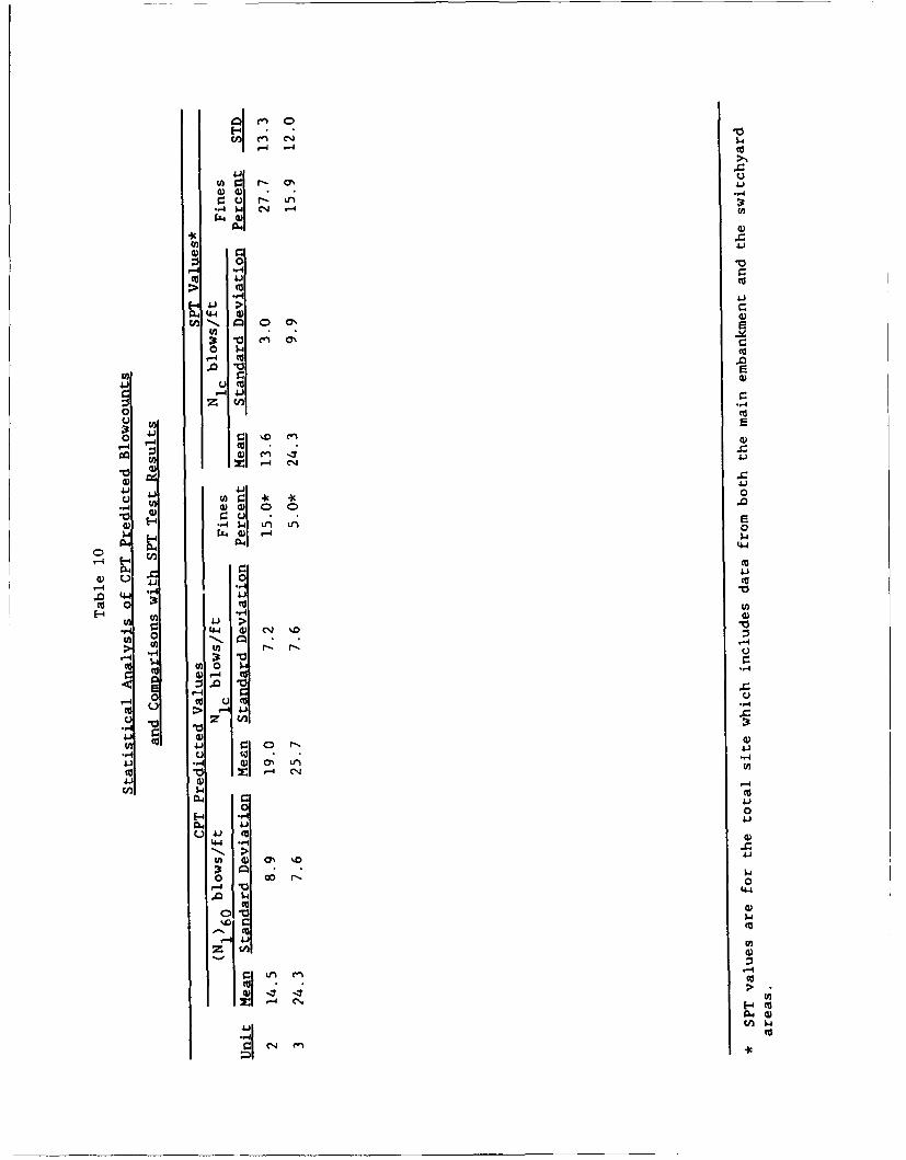
Cu
Wa)
0 .0
-. 41
-4 4 J- >,.4
i3..
04 -44 Q)4
tn a)u-0 00'
43 CO ( 0
o 1..' l
41 1
-4 Cu .
EV~ 0) eM M -4 )
o) C4
4.) Aj~ 0)- -4 4)(k
E • mE
wn 411-4a)4.
4.) 0.0 44 -Ic 4
co 0 0
>o r•
0) j- .4-4 CC L~
'- -4 to cc-
>. ~ -4
Sa41
4 °N04 0
4.)
0 0~E- .4 "4 4J %
(n4 -4
0n 00 r- .
C -4 4.
4.)
4~) -,-I WI0) en
Culr-4 Cu t
C-)
04 04 Cu na
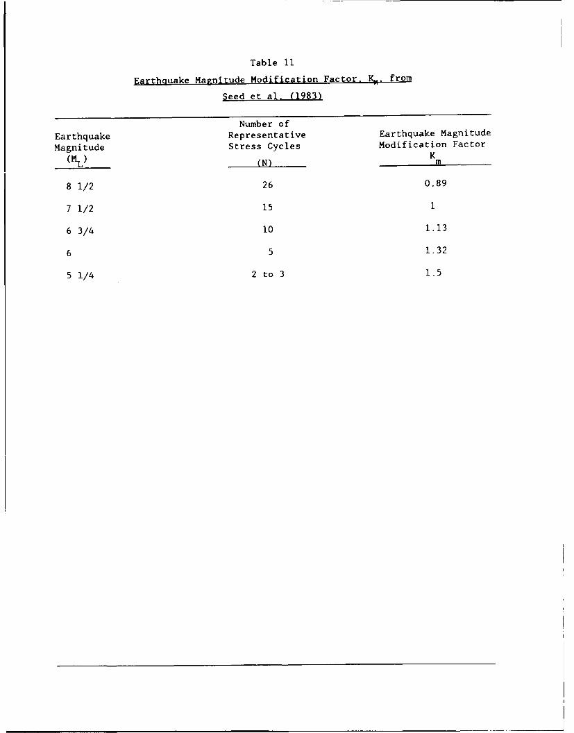
Table 11
Earthquake Magnitude Modification Factor. K.. from
Seed et al. (1983)
Number ofEarthquake Representative Earthquake Magnitude
Magnitude Stress Cycles Modification Factor
(ML) (N) Km
8 1/2 26 0.89
7 1/2 15 1
6 3/4 10 1.13
6 5 1.32
5 1/4 2 to 3 1.5
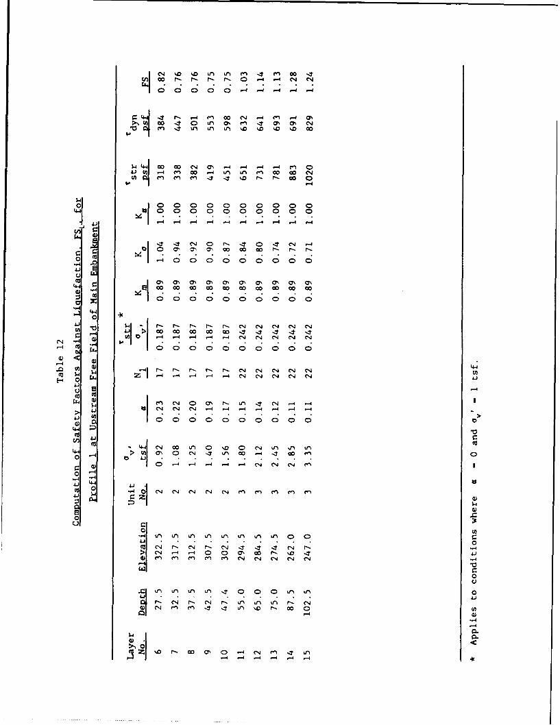
e4N %D %.0 Ln Ln m 4 t
r~- ,-4~ ~ (N -4 -4 . 4N0.4 CA) A '0 '. . .
m wl LA LA %D %D (NýD G
W "N M -4 '-4 .-4 -4 M1
U), M4 en en% r- fl- c 0
4. I0000000000
'4.I ,-.4 C) '14 0 '1. C4 .-4
cc0 (7 % a\ 0% ON a\ (, ON c7o4 Cu - 0 0 0 0 0
.04.) 4.
c 4 )-, ..4)co, IIC000000000
0 L
-4 CN C4 4 -4 -1 -4 -4 - -4 -4 -4(N .~ .~ . . ..I41 1 0 0 0 0 0 0 0 0 0 00>
. o Cf 1 h
-4 4 0 a\ 0 C4 7' -4 '1 co c"o. -- 44
CO 0ý4 0 C,4 (N 00% C - A4 (N- m -4m f
z )
00
w -I -4 (N (N 04 'N "
00
-41
Cu 01 -40 (N (N_ (N (N (N C"' C'4
0-4-4
C-CL
14 - 4 -4 (N r-4-
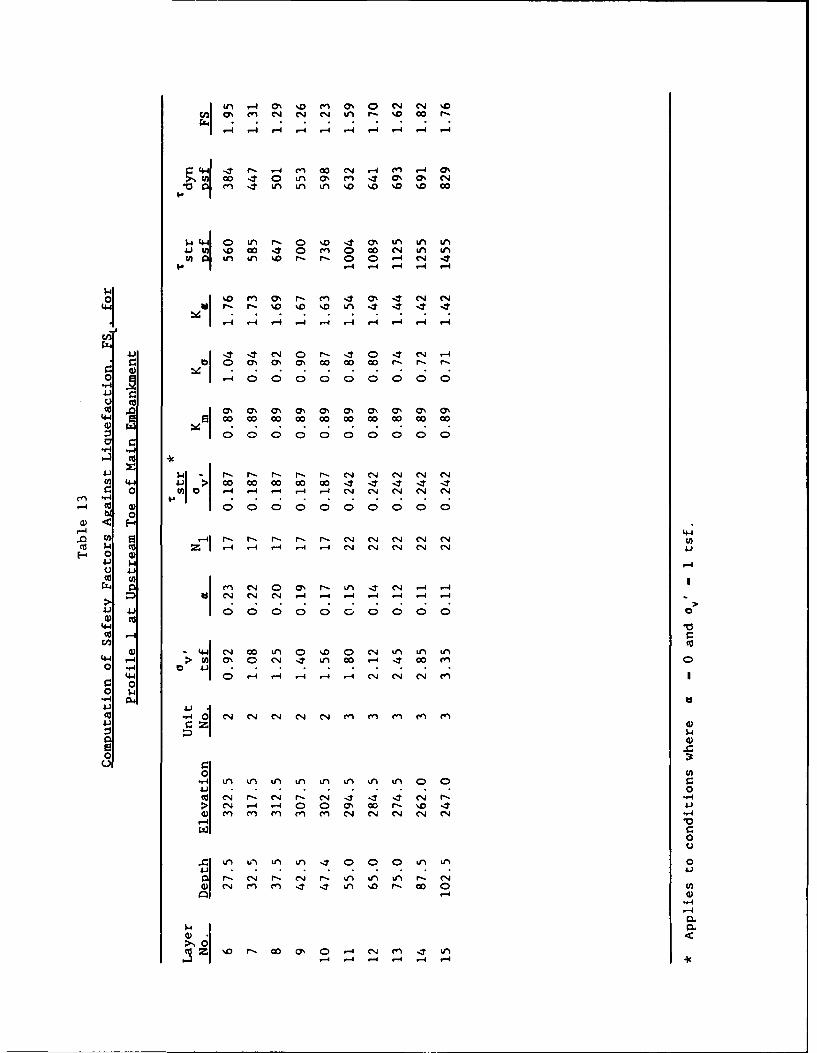
ILn ý40 m .%D 0% 0 "N (4 %o
4-4 -4 0l W C4 -4 MA LA 0%U) 0~ 4 0 Ln 0 en (N 0 0%
U) ~ILn tn %0 r- r- 00 1-4 04 -4t ~ I14 .- 4 r-.4 .-4 ,-4
%HI .0 en) ON r- en '10% 04 (N%D4 %D rý - . . .o Ln A 44 '1
4.)ý4 r-4, r40 4* (N.4
41 0~ 0 r- r-40 N0 O 00 co r- 6 5 o o r
0u 0'0 0' 0% 0' 0' 0% 0'
.~ .
141 r" r" r , - 1 C 4
r. 0- M 0 4- 4- 4C4 C4 04 C4 C4
*-4 cu o 0 0 C> 0 0 0 0 0 0 0bl0
1-4
.0 0 -41 r- a-- r-- a-- r- (N (4 (N4 C(4 C4mu W- C ZI -4 .- 4 .- 4 1-4 .- 4 (N (N4 (N (N (NE-4 00
4.) -4
en% (N 0 0%N a- Ln I (Nj -4 .- 4Uj (N (N (NC -4 1-4 .-4 .-4 .-4 -4 -f
4-4
Cu 44. n D0i- nL
44 4 > 0 M. 0 (N IA LA I0-4A0f0 -4 0 4
(4-4 -4 C1-4 1, C1, M
0I0 $4
0 3t
0 U*-4 IA IA LA LA LA LA LA LA n
> 04 -4 '-4 0) 0 a, W r- '.D 1 410 en n en) en~ (Nj (j (j CN (Nj .4
0
Ln I iA LA LA 4' 00I LA LA 0413
c,4 m0nI L Dr o0(.- 4
-4
CZi 110 a-- M M 0 1-4 (N " C-1 4
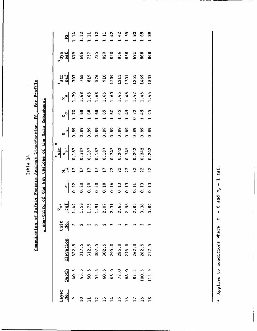
0' C-4 -4 C4 ý -N LA 0 0 M. M 4r4 ~ ~ (N VLA A- 4 LA %''0 w.
0% %0 - Ln 0 0 %D co 0 00 Go
.0 %j r- r- co00 co 00 Eco %0 .7 Go
r- 0 ON4 r- 0 (7 %-4 kM MA CV41 0 D - l -4 0 '- w
4 M
4 tM %D
-4 P4 4 r v44
4.40
p 0 c '0 0 c.0 '0 '0 44l 4M 4 4AL41)
w 1 4 r4 r4 ro0
'4.1
o Ia' 0' C 0' 0' 0' 0' 0' a' a 0
.go
4j"~4J 1> 0 .0 .0 0 0 0 00000
0) 0,4 -4 r-4
0 14.
o C 00C)000 %.D C" M -4 M~ en~a4.)C4 14 C -4 -4 -4 -4 -4 -4 -4
CU IOOOOOO '.t'0 0
> '4441 0 '
CUd-4 -4 M -4 (N -4 (N %N (N %('
'44 4.)
00
0 U)5 4 LA 'LA LAe LA) 0 00a0 LA LAir
to (Nr ~ L, L, Cý ci>CN - -4 0 0'00~'0 r.%DO0L 41)
('- fn (N (nM M C% % N C(N C(N 04 -4
0Q
SLA LA LA LA LA 0 0 0 LAl LA uLA 0
JO LAO0 LA 0'000'~0L1? .-4 Ln L D % - CO c -4 0)
,4 -4 4)-14
06
00
z N0 r4 C14 'A .0%D l- V c-4 ý 4 4 - 4 -4 -4 .. 4 -4 9
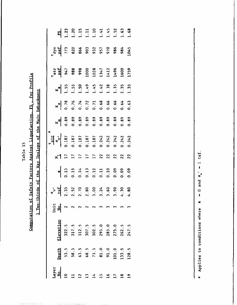
1ý ~ ~ Cý -!
r-a (1 %D 0 Cn L r 0 00 -4r- Go o as0 O ON C7 0% 0% I
I r~-4 4 r4 -4 r4 r4 -4-,4
01.4 LA Ln 0 a . 4 0 LA LA
44-
. .00UD ~ r4 '0 %.0 %D0 M. .
04 CU4 ON o0 ON 7% ON 0% 00ý 0% 0% 00
L44~
4.4I $4(Ný r ý - C l l c-i (Nj0 ~ 41 00 00 00 00 It 41 - 4 4
&-4 "- 0 0 0 0 0 00
a)~ 4
-4 "10 44o0 A oA 41r- 4, r r-, ( r-4 0N a' Cq a'
4J W ) Z .4 -4 -4 -a -a C4 C14 0 1 0 1 0
> -4
La.4LA %n 0 M C1 -0 0Y 0~ CUto -4 (N 4 - 4 4 -0 -0 -
4-41 10 LA 0 0 0 (N '0 0 0 00
> oo. a 0 n r N % N m G
0v 4-) .1. . . . .
4-4
0 is
(3 (U (~ N C14 CN r 4 MN M LA LA MN0 (N -I 0)00 0 0 - '"4 -4
00
LA 0 0 0 LA A
-4 100CO
0~
-4 -4 -4a4
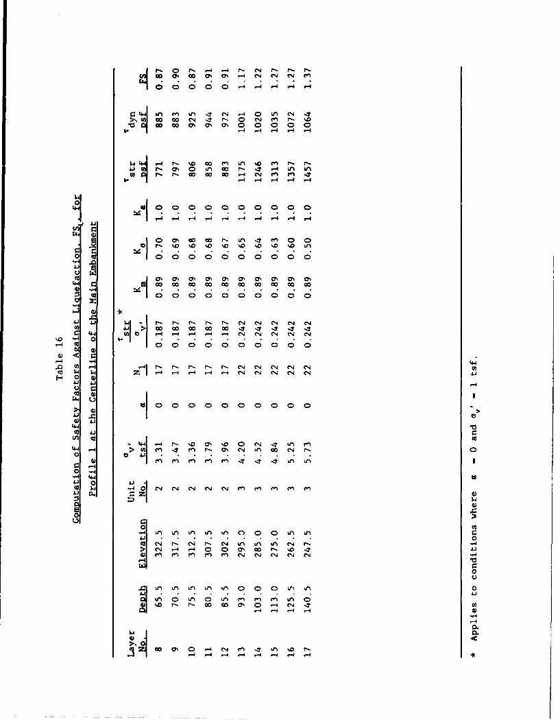
w ~ ~ w t- 0 4(n r- i.U
co co %0% 0% ON00 00 0I I-4 -4 ý4 - r-4
,- -'o~~ LM %Do m r, r-0% 9. rl 4 V4 %n, LM .
-4 -4 -4 r-4 -4
01
'4 41 WI 0 0 0 0 0 0 0 0 0 0
0 0% o co r- tn m 0 00
0%0%0 0% 0% 0 0% 0 0
0 441 -> r- F - r- r'- (N 04 C(N (N C-4
(AI co 00 co. 4 '1 '1 '1 .40 44 'AI C -4 4 .-4 .-4 .- 4 (j (N (N (N4 (N
'.0 0 . . . ..I
0
-4 '-4 -4
4.V 41)-
CL4 0 0 0 0 0 0 0 0 0 Cý r
0
W .,4 0 - a-- '.0v' 0 (N .4 mA e) m041 r-- L(l (l . - ' N L N -0
0 Z 4-
to C14 cý V4, cl: .4 .4* .4* iA in
0 *.-0
5n 0 n L mmm
o -4 C1 I
..- 4L -4 -A LA LA 0 0 0)A LJ-)I. 0(UI( a-. (N a- ( LA A LA (N
a - 4, -4, ý4 (N (N (N (N (Nao ~ 00 o, o-- -'.0m.4
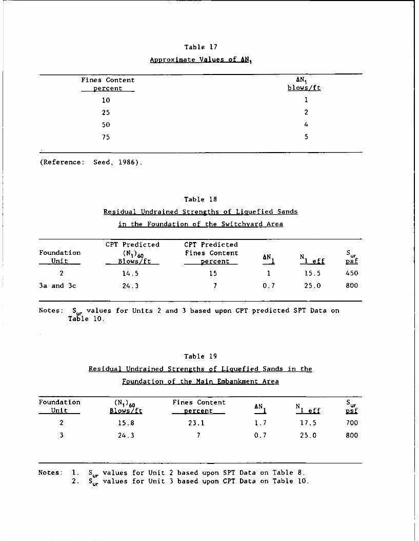
Table 17
Approximate Values of AN1
Fines Content ANIpercent blows/ft
10 1
25 2
50 4
75 5
(Reference: Seed, 1986).
Table 18
Residual Undrained Strengths of Liquefied Sands
in the Foundation of the Switchyard Area
CPT Predicted CPT PredictedFoundation (NI)6 Fines Content AN N Sur
Unit Blows/ft percent 1 1 eff psf
2 14.5 15 1 15.5 450
3a and 3c 24.3 7 0.7 25.0 800
Notes: Sur values for Units 2 and 3 based upon CPT predicted SPT Data onTable 10.
Table 19
Residual Undrained Strengths of Liquefied Sands in the
Foundation of the Main Embankment Area
Foundation (NO)w Fines Content AN1 N1 SurUnit Blows/ft percent II eff Psf
2 15.8 23.1 1.7 17.5 700
3 24.3 7 0.7 25.0 800
Notes: 1. Sur values for Unit 2 based upon SPT Data on Table 8.2. Sur values for Unit 3 based upon CPT Data on Table 10.
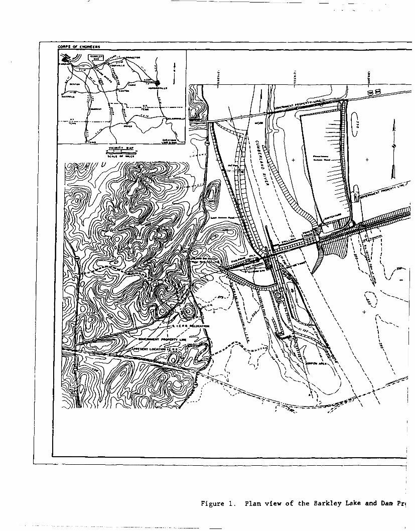
CORPS or E(IWngEfS____________________________________ ________
It-I O3D
XNI +
&tc.~~~ a\.=4.ci-m
Figure 1. Plan view of the Barkley Lake and Damn PpI
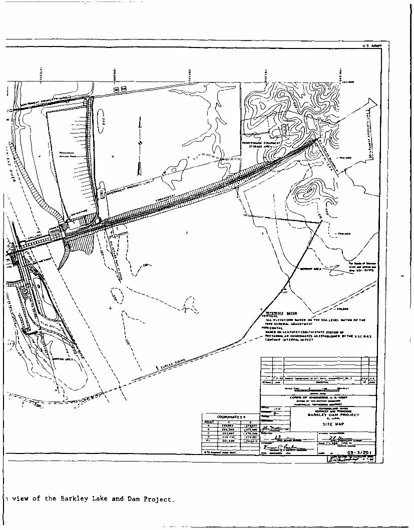
US ARMY
/0.
801O AMA ~ -
'~I N
# AA. CLIVATIONS BASCO 00 TNE SEA LEVEL "TUN Of T$W~~~-\ IV G129 A ASE A. bD"STo[WT-"N OSZ0TA#,
- Of
CONTO...Bam 61(54. WER(
N~~BARLE DA -PROJEi uCT
N - ~P6AMA ___________________________S
" NT' I iT A\ -> , . A *in1110 f
)0 -3/20.1
Svie of the Barle Lake an Da Project
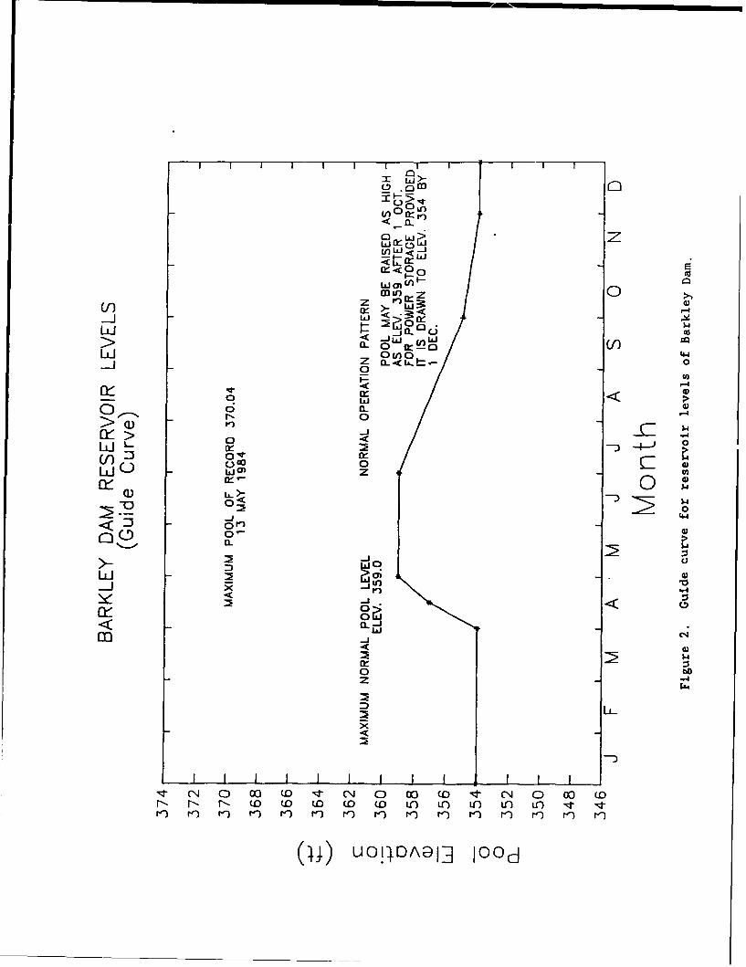
M r)
< - L
0 ci
ý--4
LU ocn E -mi Z 00>
0L j( Cl
0< 0L LIE
-~ 00
0 r
2L C)Cl0 zU
< 0
>- I I I I 0 I
(iiJ Uc1DG) 400
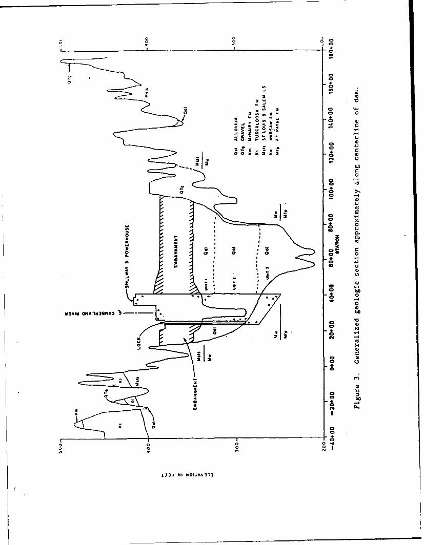
40
44
0 Cl 0+
44
0 0
a. CDa
41
1*4
00
z CC
-03
En
2 bo* 0
0
40 "
.j~
:3
+ "4CD
0 0 00* 0-
L331 O NOIVA31
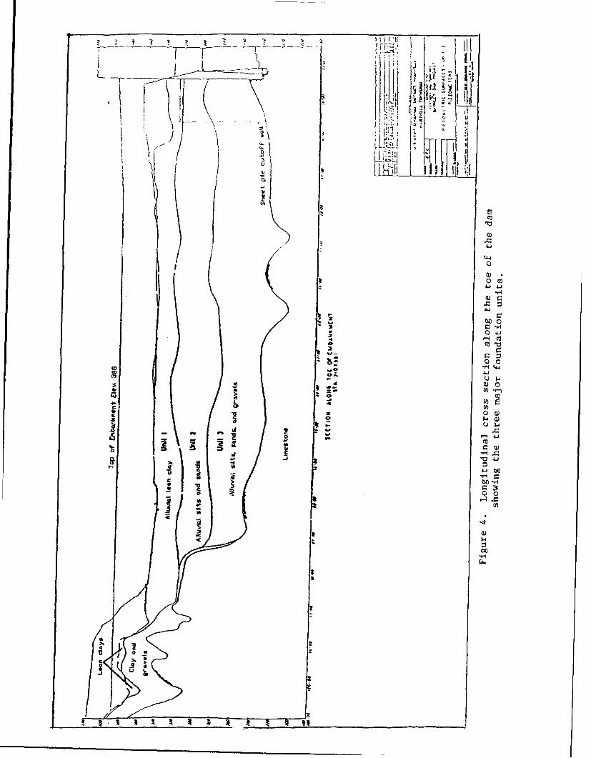
_ _ _r il
) uju
4-40
z 4'J
t4 o4C -
-~00
-o~.0
0 0
d
15 0
:i PiA IWa
4-
0 U'
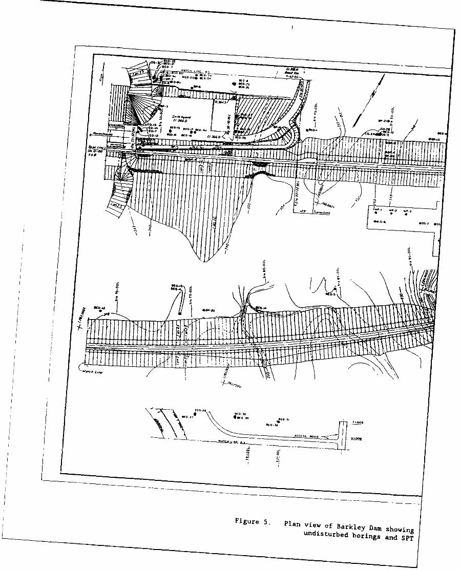
to, rQ~L MO U
.70.4 KO
/ - ~ ½ Xi0..... ..... .I ...
*E4fI
I :I / .cc
Figu e 5 . Pla vie of ark ey D m sh winu n i t r e b o i g /n S P
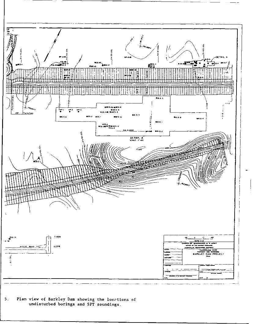
SA.
-• • __________ '11 ________-$- _____14 T'T' ! rT -nim ''11 1=JOA01 OS-71,4/ O IKO.. G 0
S'. 2.000 - emo-2
Sa 00002
-- •k-- -- IARqKLEY OMM PROJECT
5. Plan view of Barkley Dam showing the locotions ofundisturbed borings and SPT soundings.
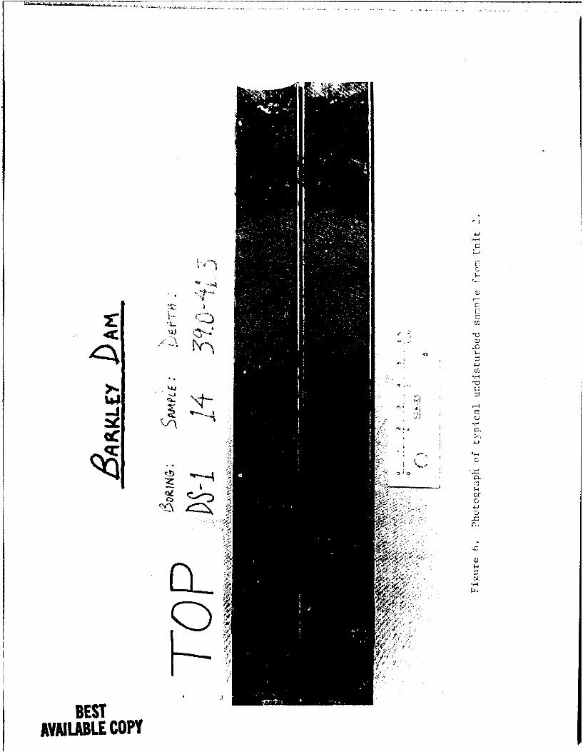
f7-
a1-
ccJ
-4,
BESTAVAILABLE COPY
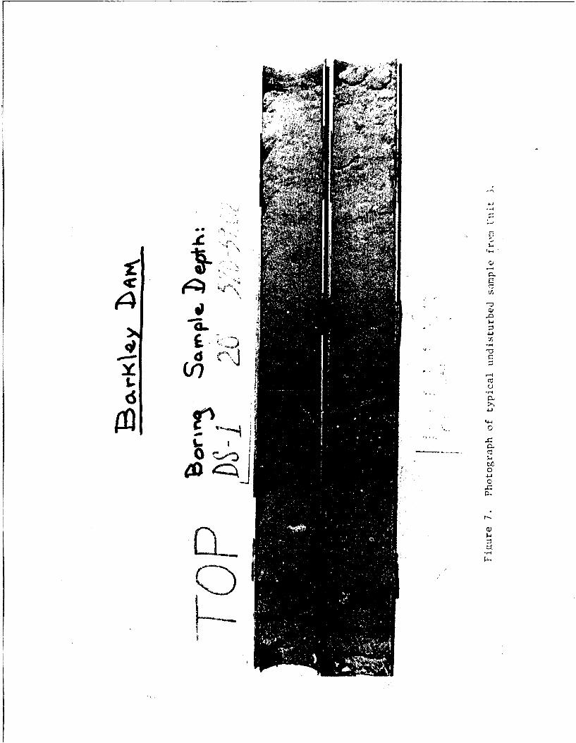
>2t
5~~UE1 Aj
V -o
4D 4::-4
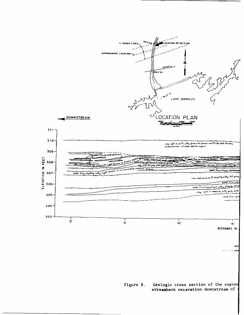
IL POWER LINES ~L~ LOCATION4 OF SECTION
APPROXIMATE LOCATIONI-,>--
MILE So6
L AKE 8AYKL EY
DOWNSTREAM LOCATION PLAN2000 a' 2000, 00W*
SCALE
310
309
W 308 -:5 r.I ~ ~eb-- IftA - 16q. Ii,& 'aI * h ' a
0 0
I-.
305 -~ ~,
304-
303.0, 15
OISTANCIE IN
REP
Figure 8. Geologic cross section of the expos]streambank excavation downstream of
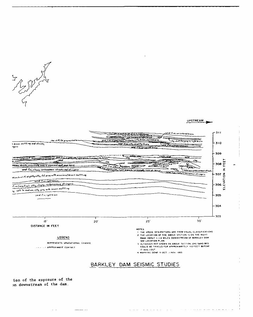
UPSTREAM
31f
309
-304
_T _ -T- 303
15* 20' 25' 30'
DISTANCE IN FEETNOTES
ITH4E ABOVE DESCRIPTIONS ARE FROM VISUAL. CLASSIFICATION$
2 THE LOCATION OF THE ABOVE SECTION IS ON THE RIGHT
LEGEND BANK ABOUT I_-I12 MILES DOWNSTREAM Of BARKLEY DAM
REPITESENTS GRADATIONAL CHANGE ALTHOUGH NOT '"OWN ON ABOVE SEC TION. ONE SAND BED
------ APRPOXIMATE CONTACT COULD BE TR FE OR APPROXIMATELY v50 FEET BEFORE
IT WAS LOST4 MAPPING DONE 51 OCT , NOV -9e3
BARKLEY DAM SEISMIC STUDIES
ion of the exposure of the)n downstream of the damn.
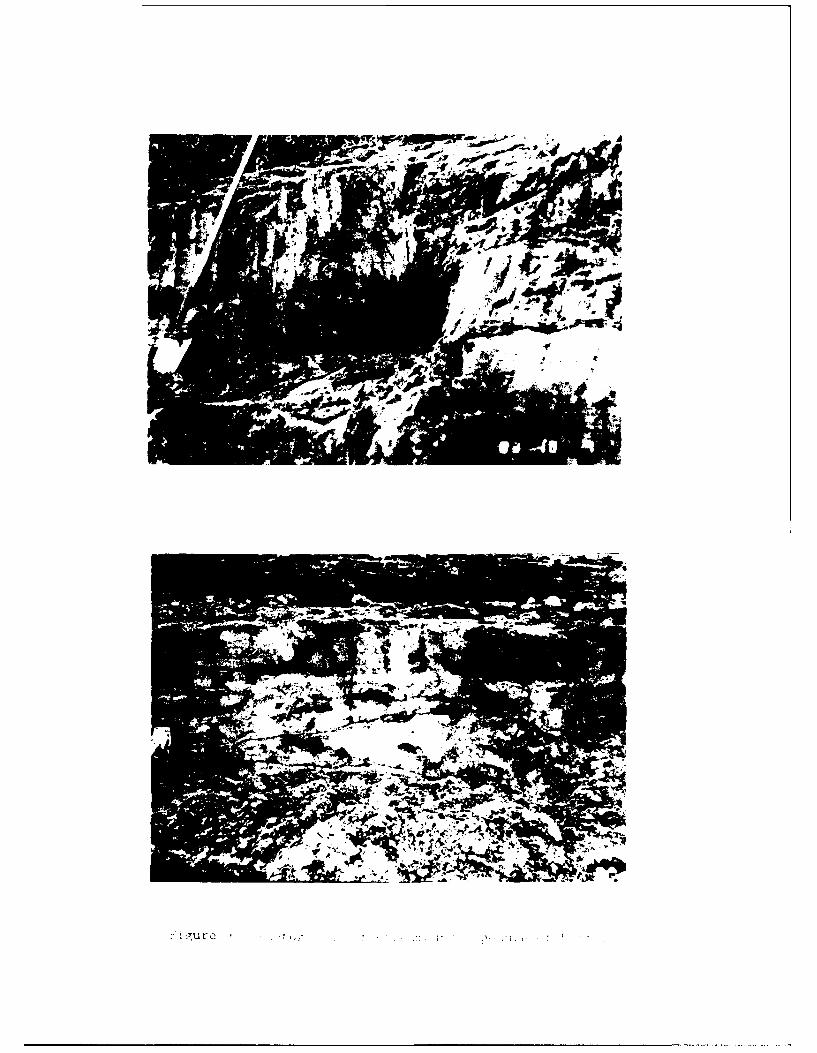
ýYuro
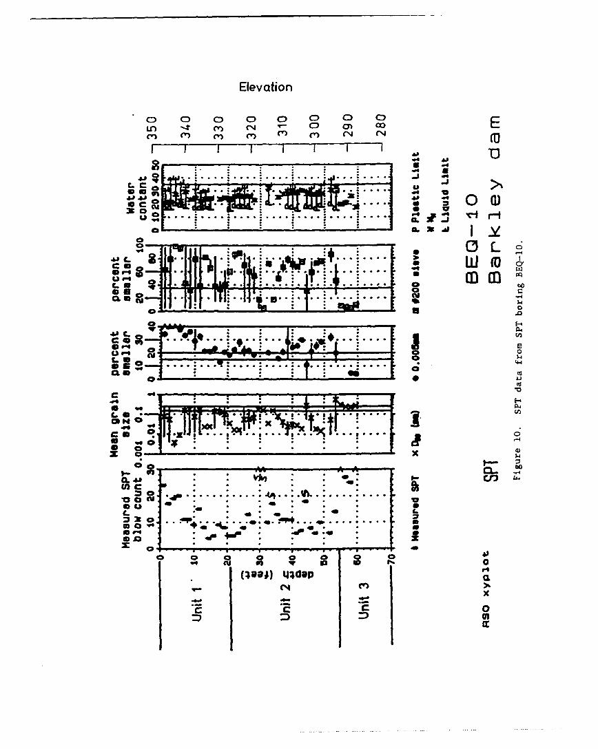
Elevation
0 0 0 0 0 0 0 0 CELuO *t m V1 0 0E
° I IT! ' I " I I '
C-•... C
........ .. .............. ..
. . . .
:I .: .. .
0"o a._ -alp:.... ....... ...... . :
* ' * • I -a = . .I 4
CQ , . t . x
C. a- -Ilk C
co rO° " • a
0 0 0 o
rth
('-4
0• •ueo 93
(49; 44de r"
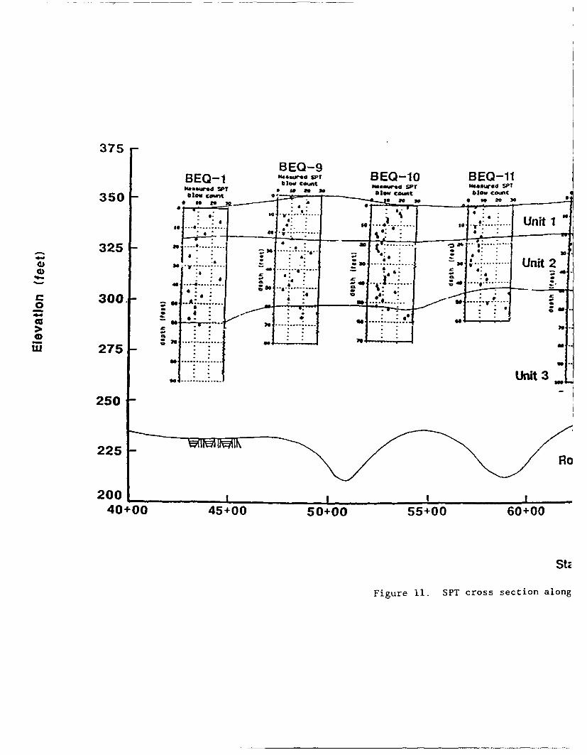
375
BEQ-9BEQ-1 -, BEQ-1O BEQ-11B Q-"'oew Count W 84eid, d SY r$iosoud SPT$00" c T blow count blow count350 blow Count zo 30 0 Be2030 4
*I 4. 4
-o.I 4 . ... . ... . . .
03 0- -----
S. . .. a 4 _
a= I f : .... so...
". .... Unit 3" ................................. .............................................. ..... :.........
"4, , :-- .. :.. ,,- .;; ....0*. •,".0- • .. .. t " .4 "U i .0 ..... -4-
. *.• 30.
itu 275 m
. .... : ... :....Unit 3 ,
250
225RO
20040+00 45+00 50+00 55+00 60+00
Stz
Figure 11. SPT cross section along
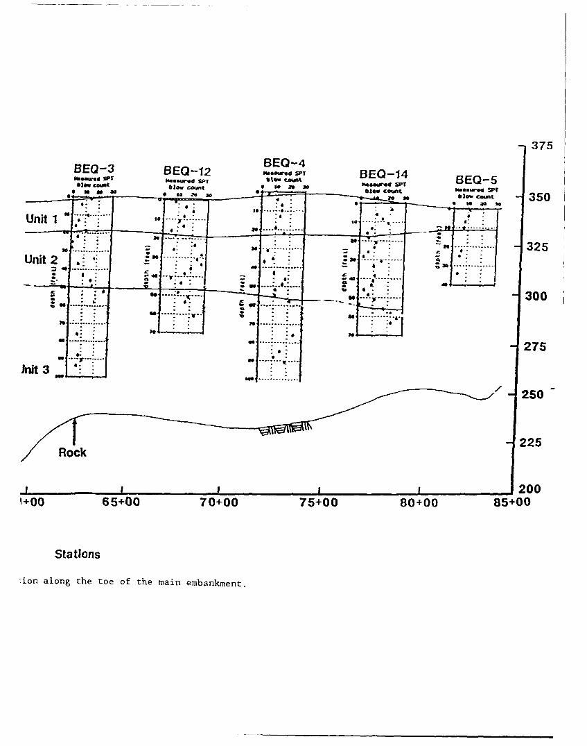
375BEQ-4BEQ-3 BEO12"Oaurd PT BO1Ifmsure wr Peaajtod SP blwq -t BEQ-48E 5blow count blow con * o - - wead WPT
blo cont 350
.. . . .. .. .
. 300
0..
275
250
225
1 Rock 10
1+00 65+00 70+00 75+00 80+00 85+00
Stations
:ion along the toe of the main embankment.
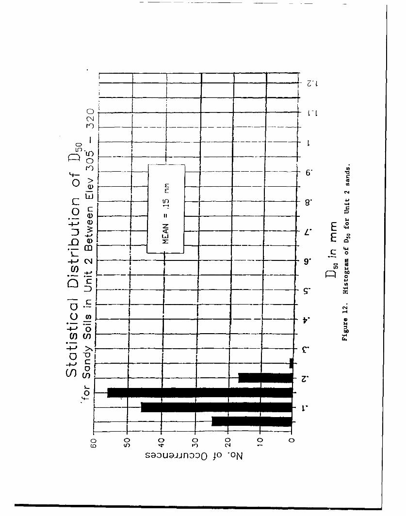
+ -4
V) - _ _ -
'-I---
bo
* .4J
c3C1 ___ I
0 .,
0u __ __ 0 0 00II I,'q
-4--JO'uiioo ___ -ON __ __
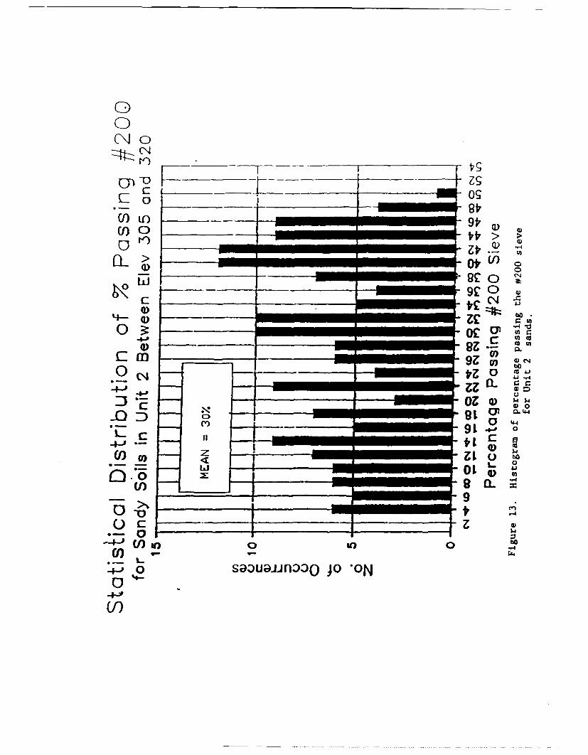
0
00
C)J>4zz \ a ,
_ _ _ _ _
---- 1~--t, I
CIJ) 9c___0
9c 0
ZE~
Cm _ _ _ 0)
A) 0
-4-'~~ 44--
4-9t 0
4_ 9 )0 '-4
-4 o(flo oi 0 o"
4 4J
Co"
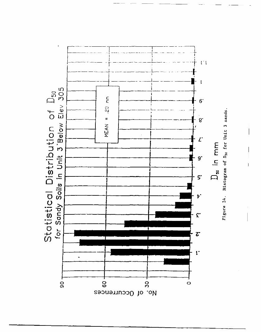
Lo-
ICD
oQ)
0 i~j0
0D <0-6~
0 _ __
-1-' 0
00
4-JUJfl~ JO 3
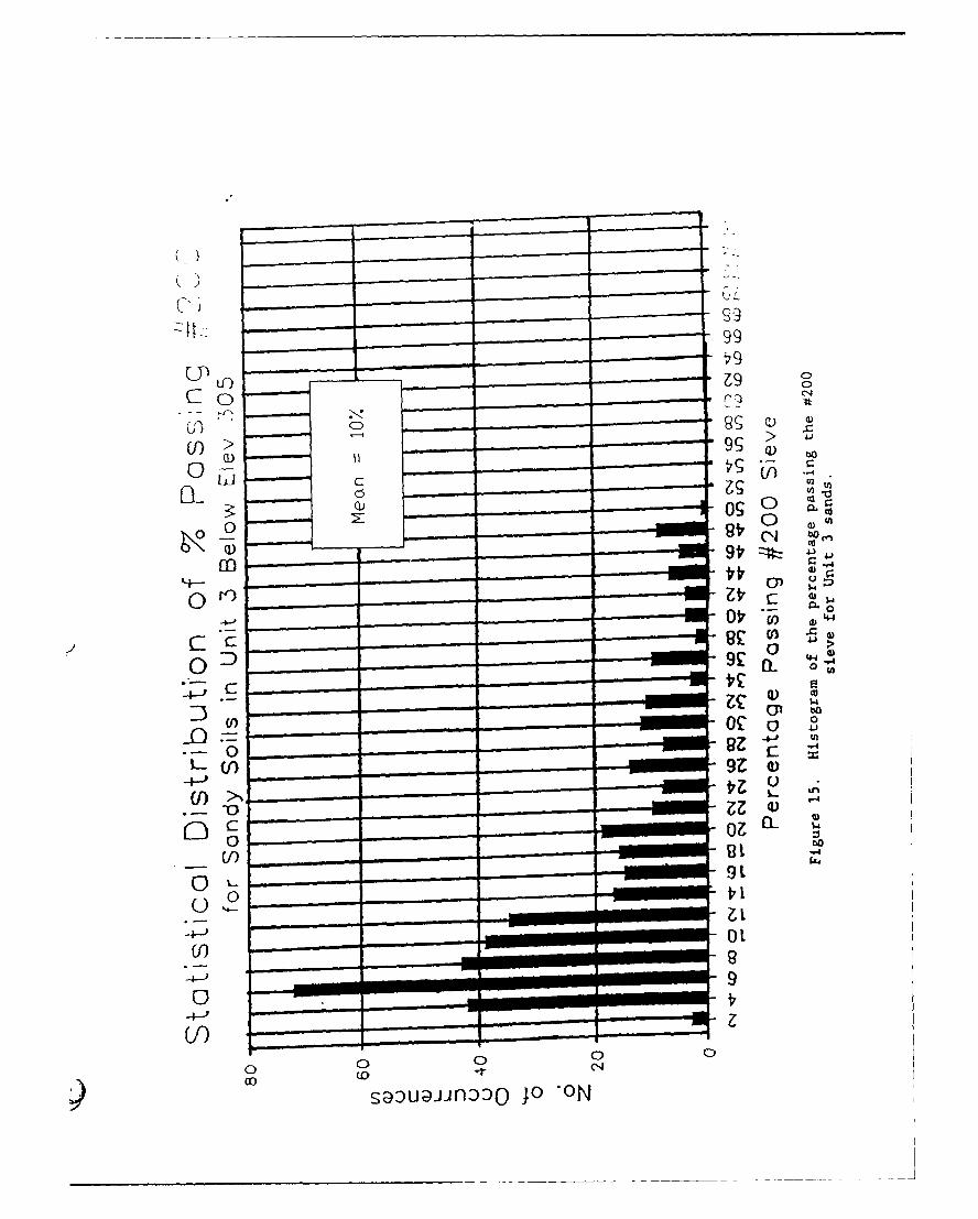
99
C>
G):
o:Qjo 0 C,
£0 9V t
-4- *C) 4)4
00
(9z
OU) _ _ _ _ _ _
_ 0 00 - c'
(0zs~u~ncO JOho
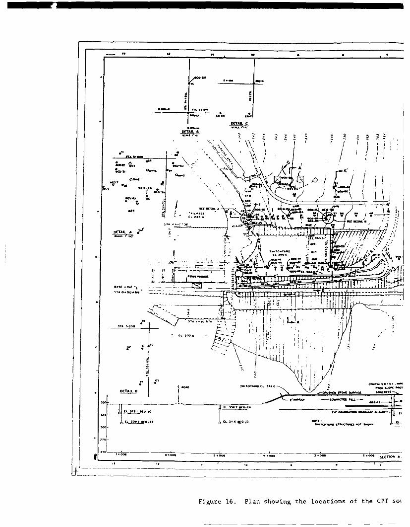
J 0-II
DETAIL C
DETAIL 8
.4 -", * I) "~
se0-11 1-0 k
We.
DETAIL A
* *~j.* ~ ~ 1[- ~ ~ ~ ~ ~ ~ o as*aY J. 4 nnq~
-,roF~
00C 5,6 0-I 0
330-A CWo m VI g-7So ~ ~ ~ I IM?,CO *- , 1-14
$: 3290 (3.5 J4v*mF1, mfl / I /L~CT
CL 31 O-3/T 10 E
4. 0 6. ow S3 304090 -. 000 3 0 62 a E TO
Figure 16 Plnsoigtelctoso1h P o
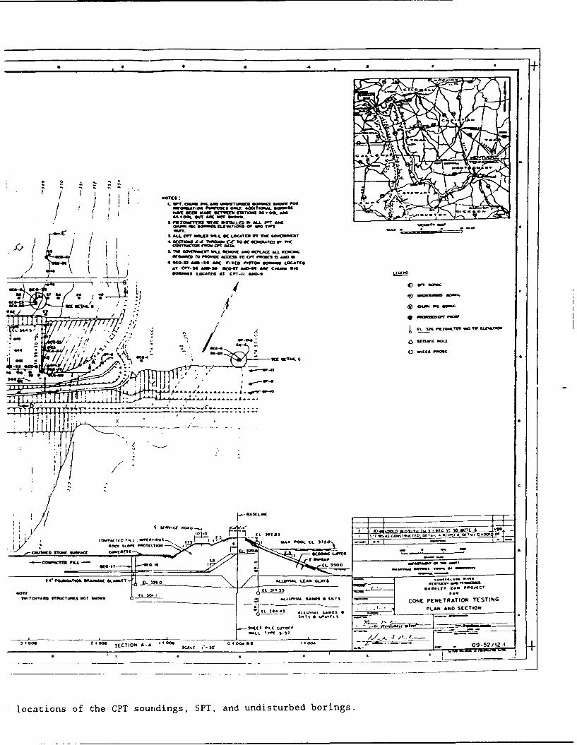
I- OPTW. @4AWdr .. am 400,1TWO *0 1100U w b6 1f ~~O00IIIAT4C 01(M0"S ~0043 0TS1OVAL. 00"
OWE GEM 04MA OLTWU IFUT-NS So# COO AMI *6S444 045? AM IM? 35006
= 0" 6010"31 UIEAT.O.S 01 WO TOP ..
3, ALL CPT 001-US WILL DC L.K0WD ITT flW WV0MT
\ 4wommm MOA 0on A? CPTI MO NIS 5AM
IS* 0 -4)- Iw60
am am /TI~ * ý
US 14-* `TV CIEkO
* . ~~-SUOL AIL C
II T T --- ------ - - - -- -
I /-LSL
406C. SLOCh1 00010(1500
CO.6CLT6 FILL - is3 km
34MAT 1000*050 "1504 kU440 IN~s.
10500*0 IETL1 c (L .1 3S ca.q~ 0* 0 PROCT
S-IO"A11 060UW
L A
________SAMSaskis CO RE PENETRATION TESTINGt -. ,.t .o PLAN5 *50 SECTION
3. SECTION A-h *m s 0 00*06 a00
locations of the CPT soundings, SPT, and undisturbed borings.
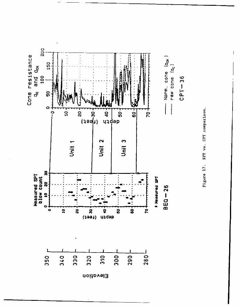
o
a) " I"
4u
10 = . . . . . . . ° . . . . . . . . . . . . . . .
ri, . , ,0 W23 ,. 4I.:-
u . . ..E:T t."l 0 w CI-- . Z L.
o • . . .. . . . . . Z. . "
0 0 0 0 0 0 oc- J I i tn W I-
(48a4) 41:4 a p0
E-4
- • ,* 40.4 ' * . 4 0C(D o , -- ..:* .. - .IW ....... .. ... .. ....... .......... . ........ -
a u .4 , ar- La * .*
xr' . * * " Z L
=1 39 .... . _..,.... , 1%. ,
0 (•Baj) u:IdaPus 0
40
I I I I I I I
o 0 0 0 0 0 0 0UOCAe( t 04lo0C') C') C3) C') C) Co C> CD
UOIIDA013
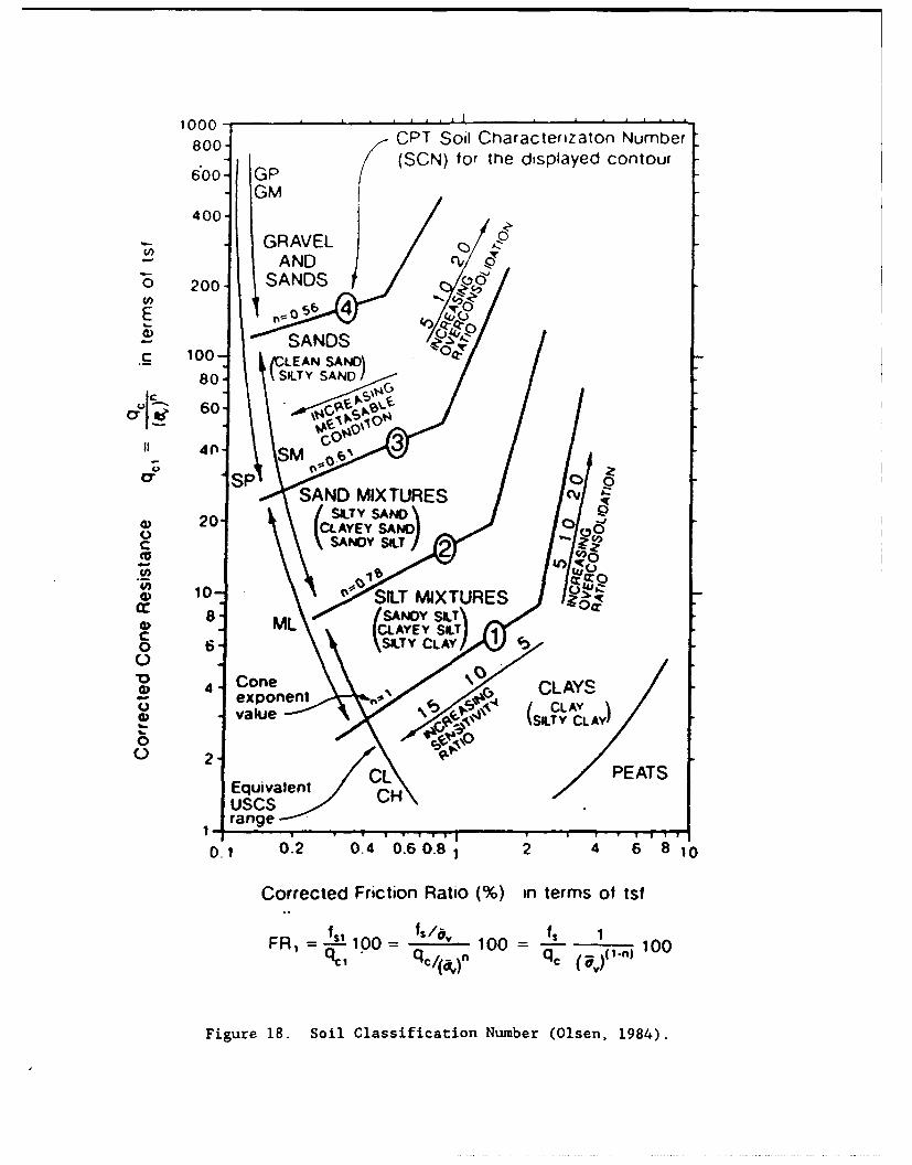
1000-800 CPT Soil Characterizaton Number
600 GP (SCN) for the displayed contour
GM400-
- GRAVELAND
Z 200 SANDS
E 05 4SANDS
C 100- CLEAN SAND,
80- SILTY SAND I G
c,.f 1 60
II 4r-,
SAND MIXTURES e v
S20•, CLAYEY SAND Z.oo/.o \ SANDY S&T• &'0 2
- 0 .. ~U wQ
0 0 t-SILT MIXTURESa: 8: ISANDY SILT /..•a - MLCLAYEY SlI
Con
exponent CLAYS~. v a lu e • , V% '(.,: ' / C L A Va)(s5 CAY)".,• .••,•,••<4 •ILT Y CLAY
o 2C
Equivalent PEATSuscs V
range
0.1 0.2 0.4 0.60.81 2 4 6 810
Corrected Friction Ratio (%) in terms of tsf
fslfli fsFRI -=S100 100 = in100
FCcation Num qclen- 194.
Fi[gure 1_8. Soil1 Classi[ficati:on Nu~mber (Olsen, 1-984).
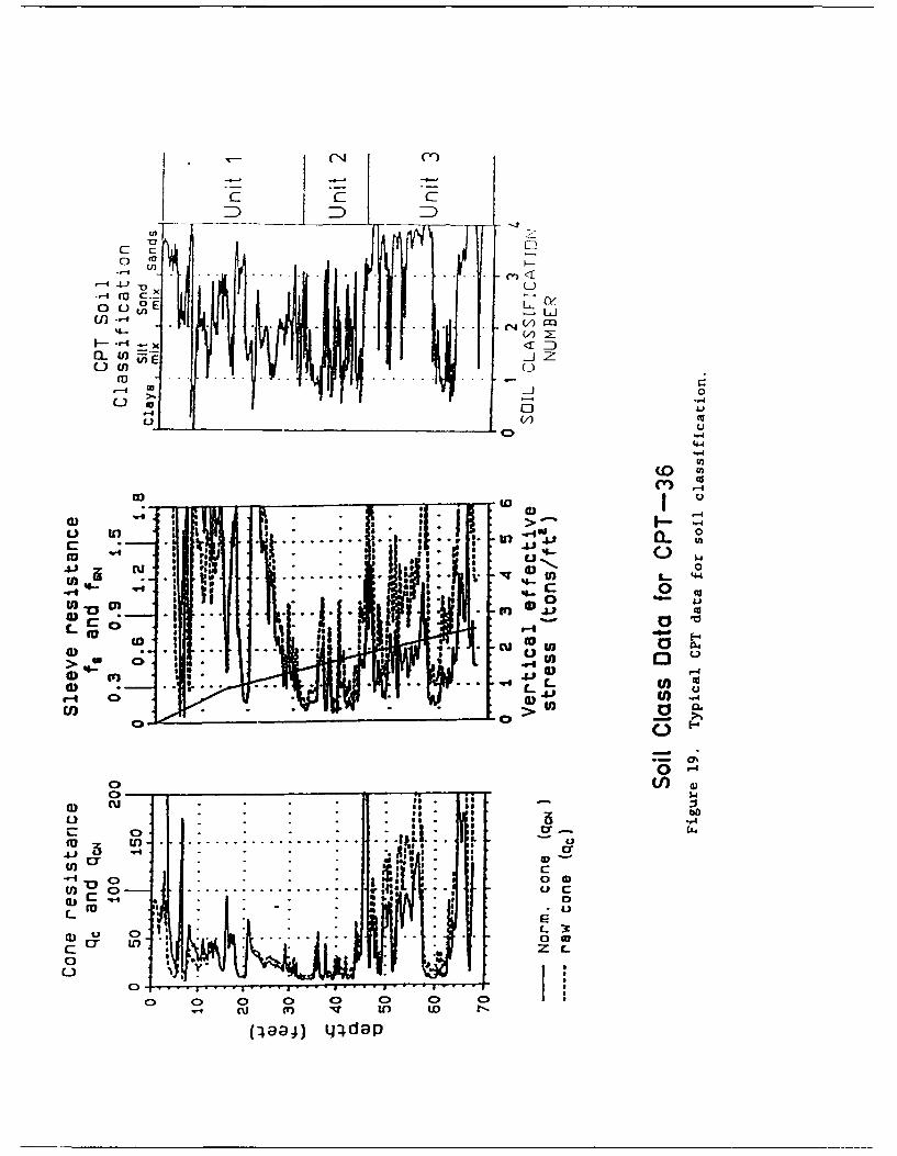
(\4 Cr)
c c:DD
Cc
0-4.4) V) La
1-~~- -r z E
L) U) (
C-)(/ cc
44
(0
a) a
in 4-4
.- )L)U
to)t
ul- .0
oc U)__ _ 0)
0) 4J . -U. 8
cab
C.)
-ý0 0 0C00, 0 0)'4 aU .. .. .. .. .. .. . In ID c"
C>24 Lj d3p
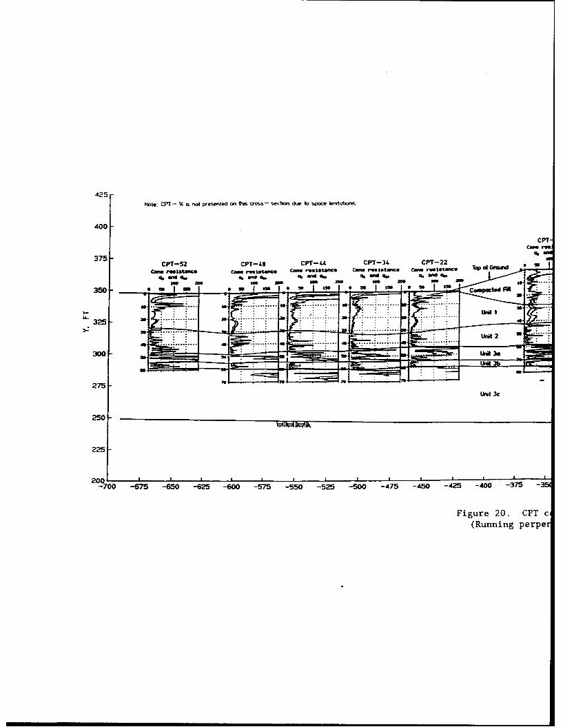
425Note: •PT- 14 i not presmted on, Os cooss- se<gton due lo spoc hWTow,
400
CPT-Com. rs
375- wCPT-52 CPT--/.$ CPT--3 CPT-22
Cm. reslstance Cone resstante Cc"reslstance Cow re istance cone rsimstacn Top c .G .n .
uS as so. we 20 ase 200 s as....350 -s I tme 2!s e 0 so a 0 so m a 0 S se Coomp cted Fi
. 25-all . .-I .s . .. :.... . .... ....
300 • .• " "unit 1aas ... 3 .. ..... .. .a
• "- -'- -_ _. •_,_ _ _ __._,,'•t • '
275 LL "-..-..-"--
ur! 3c
250
225
200I
-700 -675 -650 -625 -600 -575 -550 -525 -500 -475 -450 -425 -400 -375 -5,
Figure 20. 3 PT c
(Running perpe•
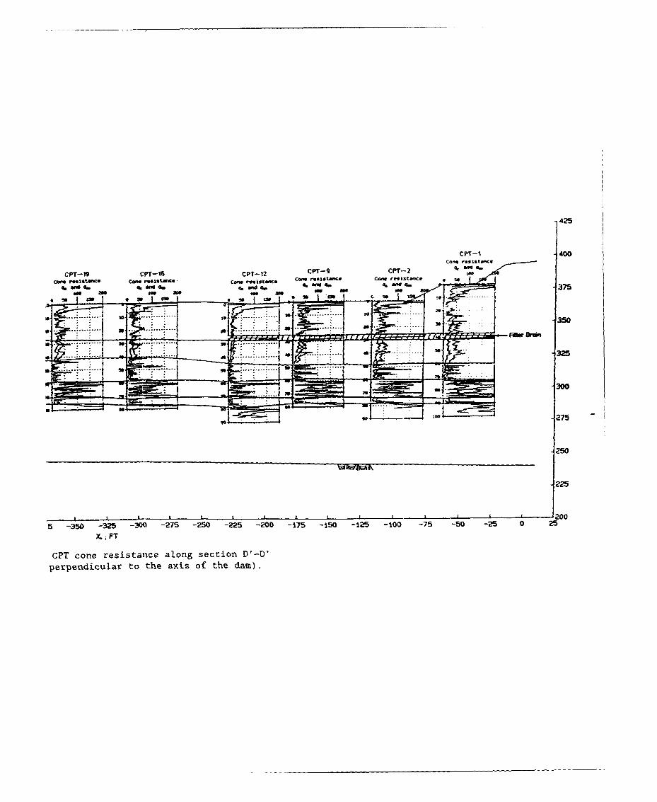
425
CPT-1 -400
CPT-"9 CPT-16 CPT-12 P9 T-tocam. reststm'C* cm'. elsafte C"n rosAIM&nc C*di mresseAflC cale rellista"Ce so
WW 0 q.Mid .ad 4.We . am4. 375
,sis
.1 1*350
......... -32
.275 -
.250
-225
t - -200
5 -350 -325 -300 -275 -250 -:25 -200 -1L75 -S50 -125 -1i00 -75 -50 -25 0 25
X.i FT
CPT cone resistance along section D'-D'
perpe~ndicular to the axis of the damn).
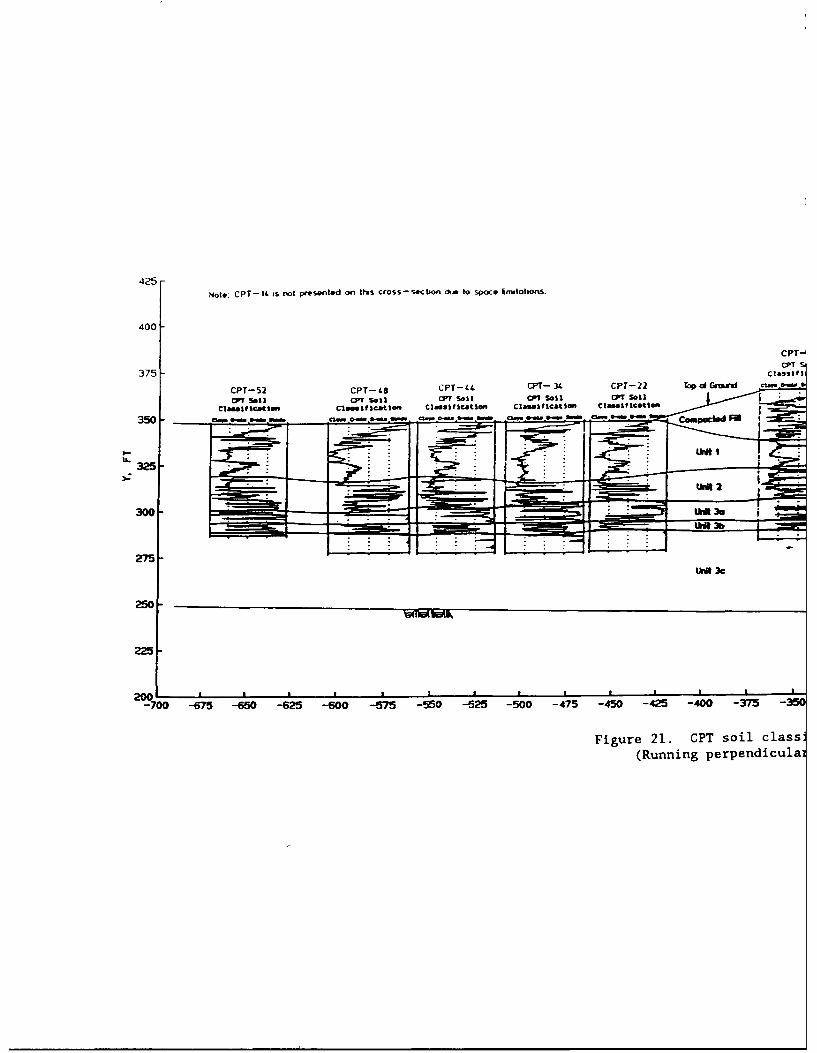
425-
Note: CPT-11 is rmt prass.oted oo Dtls cross-secbon &,i to spoce kiTntatiofls.
400
CPT-375- CPTS
CPT-52 CPT-48 CPT-44CT-3 CPT-22 Top d clrm-d
CPT Sell CPT sell CP s SIl CPT 51 Sell CP Si
CINWIFlcatt.A ClAIM1111catlomt ClegslItcatIO lan a"lflcatlm Cla..IflcatlesI
325-
300 _____
________ I.W 3b
275-Wrdt3c
250-
225-
200 1a ----700 -675 -650 -625M -600 -575 -550 --525 -500 -475 -450 -425 -400 -375 -35
Figure 21. CPT soil classi(Running perpendiculai
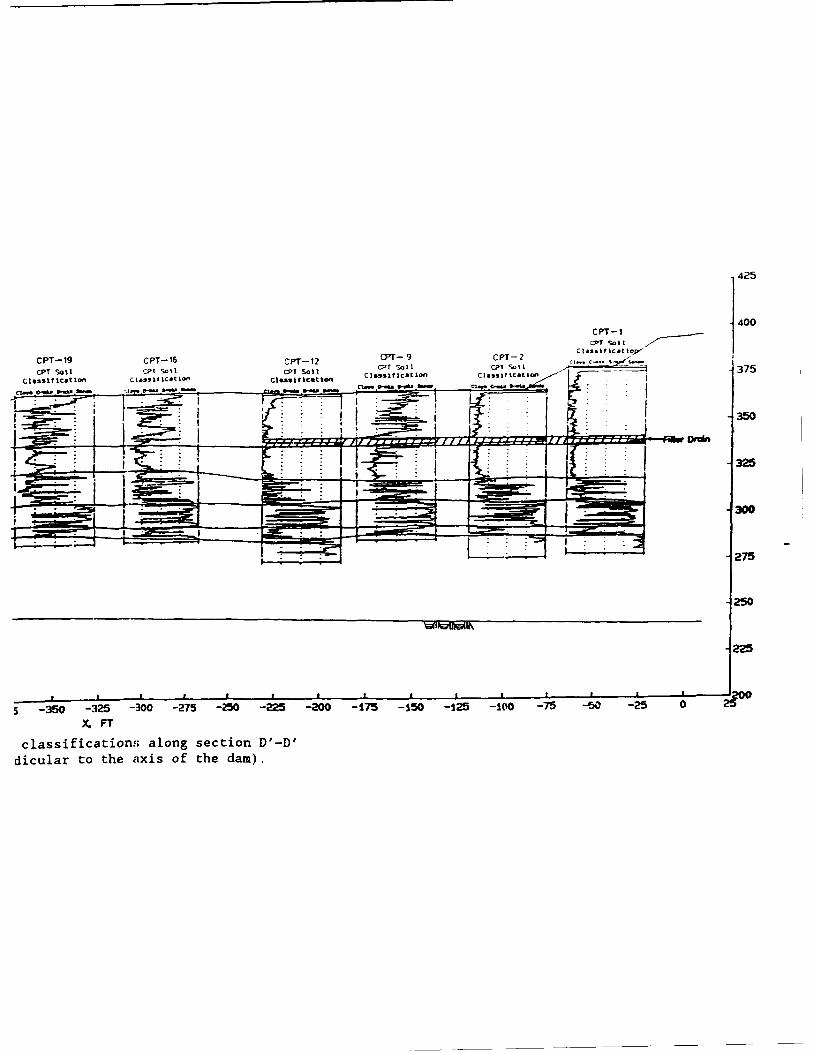
-425
-400C PT- I
CPT SoI I
CPT-19 CPT- 16 CPT- 12CP-9PT2
cPT Soil cpf ol CPT Soi lT CPSSOICT ol 375
300
3275
-250
-225
5 -350 -325 -300 -275 -20 -225 -tO -1'75 -1I50 -1L25 -100D -7 -0 -2 0X FT
classifications; along section D'-D'dicular to the axis of the damn).
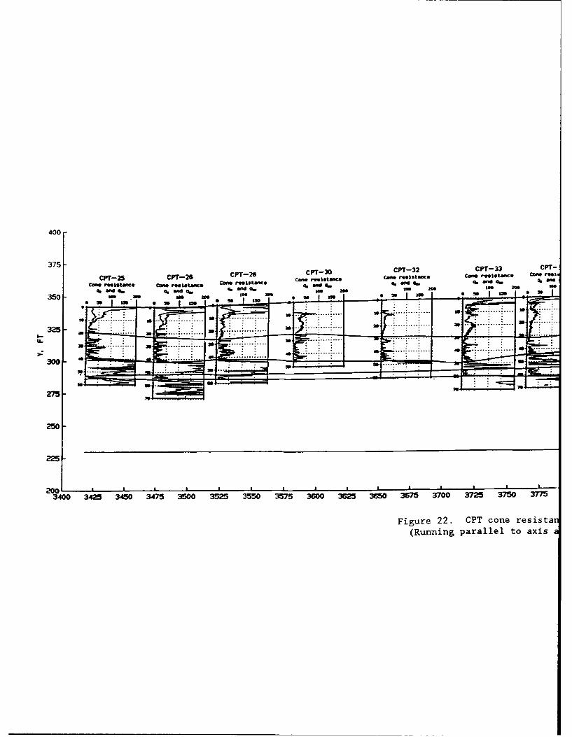
400-
350-~~~ we no* go an s m
3250 a
340 342 35 347 d50 3525 350 37 60 355 35 65 300 32 70 37
....... Figure. 22 .P .. one resis..a(Rnnn paale t*ai
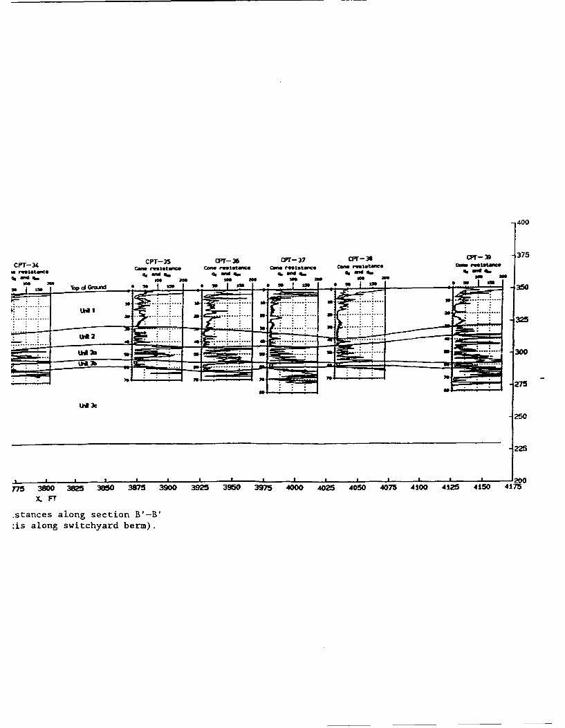
400
CPT-31 CPT-35 (]PT- 36 CYT- 37 CPr- 38 CP -- 39 375
*reT--•l e Cone resistace Came resistnmce Cone rmletace Cown ests Cown resitance
reitac % an . o.rHS~~~t•€.a a- •€k -W 4. %q end •Q. .ad b•1
ain se 2e we as n1" 2
"
Top Gm~d so 2" g Am250
.. .. .. . . .. • .. . . ..... ... .. . .a--". . sm
. ..........
.. • ... .. :.. ._ ... . . - -... . . ..... ... ... o
225
10 f ....... I 0
Ufa 3 ....... SO ... - 00
775 3800 3825 3850 3875 3900 3925 3950 3975 4000 4025 4050 4075 4100 4125 4150 4175
is -F---s . .
.stances along section B'-B':is along switchyard berm).
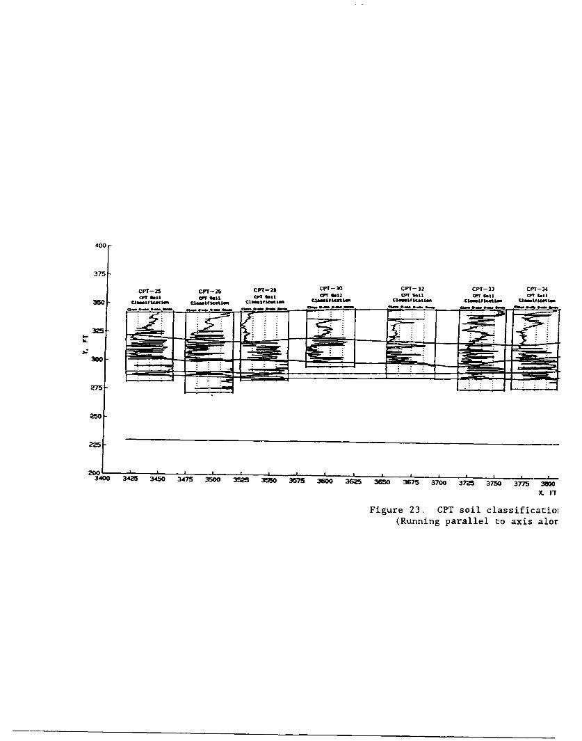
400
375
CPT-2-S CPT-26 CPIT-28 CPT-30 CfrT- 32 CPT-33 CPT-34CPT ls3 0•' ll C" tit C'T tll C" sail CPT Sell *t .11
3welcatI. olgcti, Clmolhlmtloo C.lain tl CISelwfltti w. C tO.slfkau c.mlflmtl.
325k.
250
225
20013400 3425 3450 3475 3500 3&25 3550 3575 3600 3625 3650 3675 3700 37 3750 3775 3
X. FT'
Figure 23. CPT soil classificatioi(Running parallel to axis alor
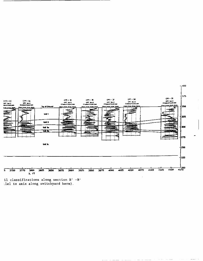
-400
-375
CPT-33 CPT-34 F-3 CPT- 36 CPr-D 37a,,.38C- 39
CPT 5.11 CPr 5.&1 C2 ,T Sol I CPT sz'T51 V 5.11 CTsII l fca, t .1
-- k-- ToIp d &WAsd 350--- - - - _____
U'a 2
-2W0
-225
5 3750 3775 3800 3825 380 3875 3900 3925 3950 3975 400 405 0150 4075 41*00 4125 4150 4175
il classifications along section B' -B'.lel to axis along switchyard berm).
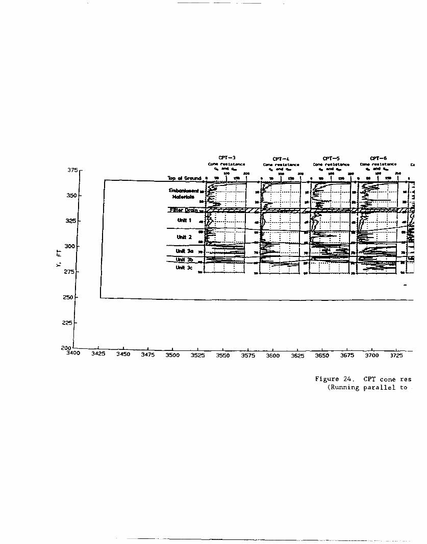
CFPT-3 CPT-I. cT--5 PIT-6Cone resistance Con er eitance Done res istance Can re•istance c
375 A.md . %ad -q.ad w -0 4d..we0 am 00 m 0 am we as
T lopoGrounde 1ý 20 IS -0 SO VS -0 10 IS
Emb....................350 -. . " " . - -
325 1- .
U"r~t 2
300 - .........
275 ISt~
>: al t
3400 3425 3450 3475 3500 3525 3550 3575 3600 3625 3650 3675 3700 3725
Figure 24. CPT cone res(Running parallel to,
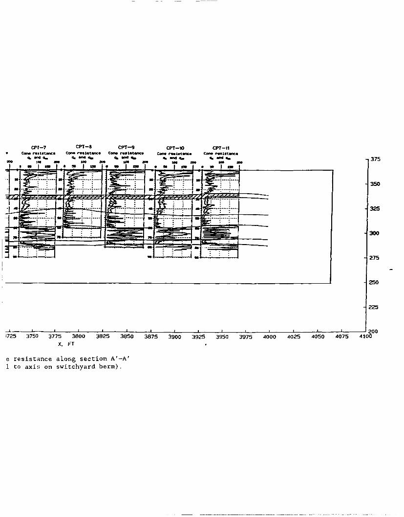
cPr-7 CPT-8 CPT.-9 CPT-1O CPTl-tCome r-elstm~o Cam u rel.stnco Cone res" tance C wN. rels'atw•• , Cane rie'lstarw
OW.. -W .3fld. q. % a" * % -W 375-g am No am 00 aDS we Ji1MP:;* 350S.............
.. ,, ,. . . .. .. ... : ....
: 4. : ... -32
300
-I " • • L~.. i ..... .... :3
" ""275
250
225
--- -_-J 200;725 3750 3775 3800 3825 3850 3875 3900 3925 3950 3975 4000 4025 4050 ,4075 4100
X. FT
e resistance along section A'-A'1 to axi.; on switchyard berm).
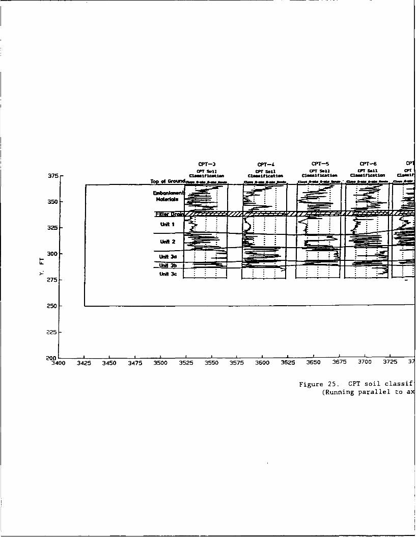
CPT-3 cPT-/. CT CPT-6 UOWT Sall Orr Sall C~T Sall an Wol a
375 clma"fieatuan cla"Ifutleoin ca~faii~tioe aa~gmgatu' clawlt
325- n
300-I-m
275-
250-
225
200 1 1 1 1 1 1 -j I
3400 3425 3450 3475 3500 3525 3550 3575 3600 3625 3650 3675 3700 3725 3
Figure 25. CPT soil classif!(Running parallel to ax
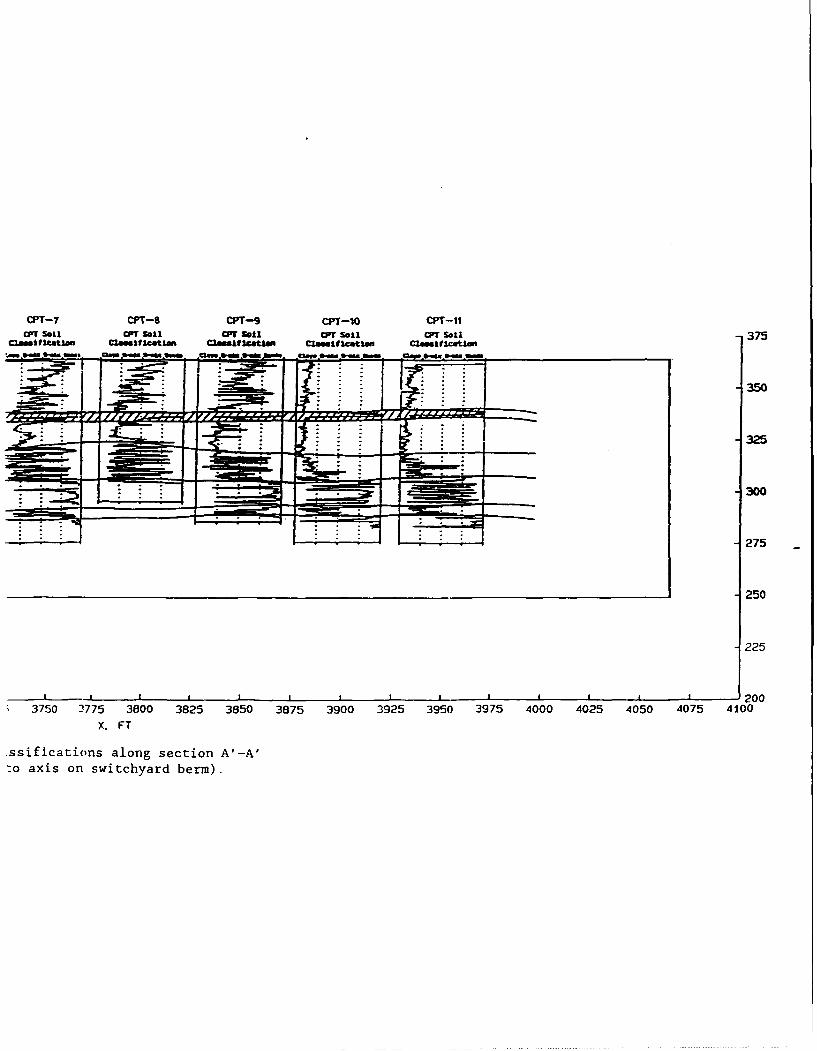
CPT-7 CrT-8 CPT-_9 CPT-1O CPT-11C~T Sell CPT Soil CPT soil 07 fr Soil Orr Soil 375
350
LI 325
300
275
250
225
a I 2003750 2775 3800 3825 3850 3875 3900 3925 3950 3975 4000 4025 4050 4075 4100
X. FT
.ssifications along section A'-A'-o axis on switchyard berm).
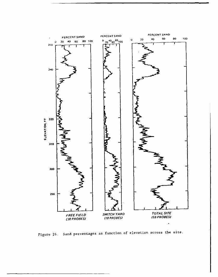
PERCENTSANO PERCENT SAND PERCENT SAND
0 20 40 60 80 100 0 2040 6080100 0 20 40 60 80 100
350 20- 60I
340 -
1-- 320W
0
-
usu
310
300 -
290
FREE FIELD SWITCH YARD TOTAL SITE
(38 PRO6ESJ (18 PROBES) (59 PROBES)
Figure 26. Sand percentages as function of elevation across the site.
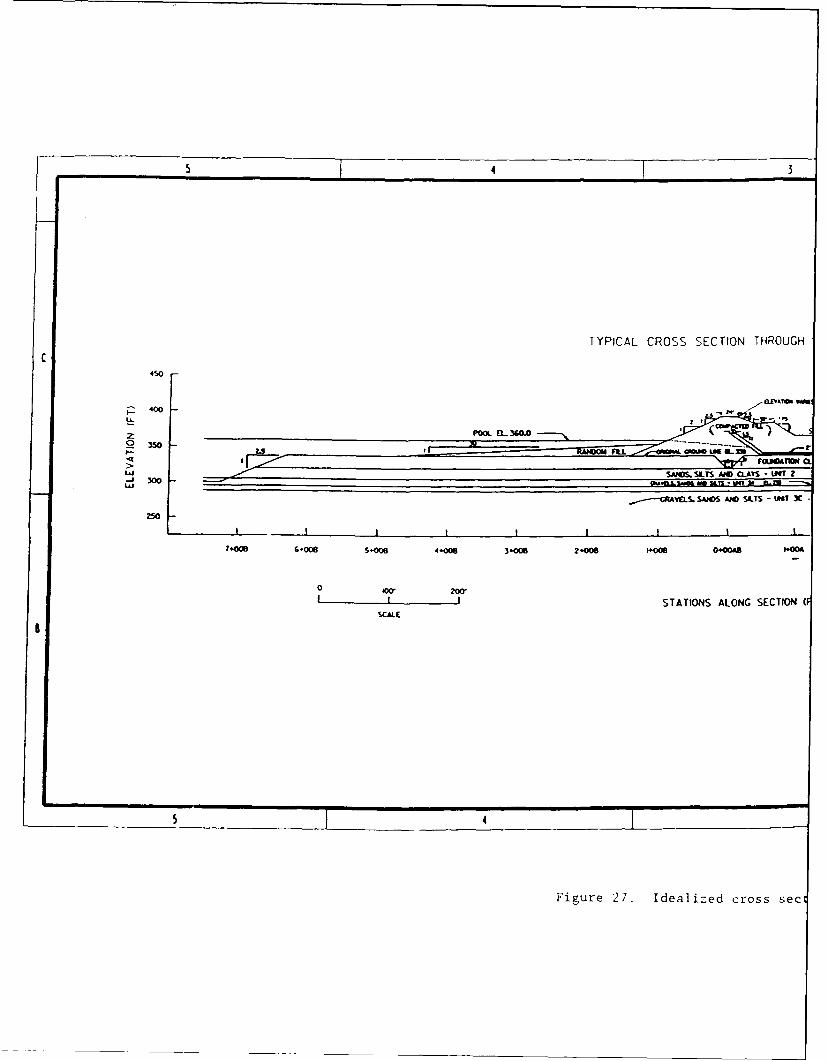
54 3
TYPICAL CROSS SECTION THROUGH
C450
z 400 - , "
> FSA N L S TION
SCALE
Figure 27. Idealized cross seci
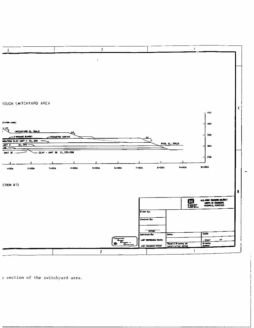
3 ~~~2__ _ _ _
MCUH SWITCHYARD AREAC
-450
Ev~rm OKS -400
LuOY~f. 36LO
SCADW COYT LOOT I - G- MO -
L94T 2 EL 305 POOL~ Pa- . 305.030
*LOOT 3C C-LAY - LAT 38 EL. Zr,288
250
F.00A 2.00A 3.00* 4+OOA 5400A G.00* 7+00A 8+00A %-0* .00MA
CTION (FT)
SLAW Vol SS
0ww~d Op Dat
MawflVrm" 00 or,
3 section of the switchvard area.
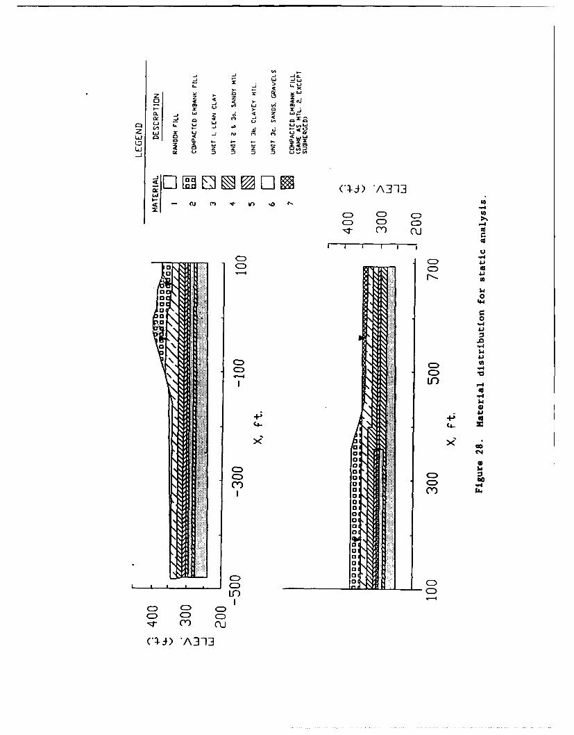
to C-
im V LJ- z
a. Li Z L2
w Li o jv0. -J I id k ; Li
L'i L. L) fu m ) a
1..I IZ4 -C 4c - 4 La9o C. ,
Lo z x t:6-xLLI -C z z z )1:)
ix L) n D _- -14Ci
CI- J0)3i
4u m V,~) ' In %0CZ) C) CC:) D CD 1.
(Y) CU
CD C:)CD CD 0a,
44-
-41
-41.
C=)I
O r-4
"-4141
bo
CD
C)C))CD
C) CD CD
(1- -4 'A u1
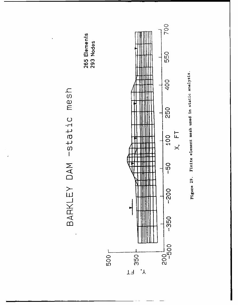
CC
cc
E 44
0 C0
to -4
C)
E C0
uw
Lo
Cl))C> C) 0
CD 0OC
LO c0
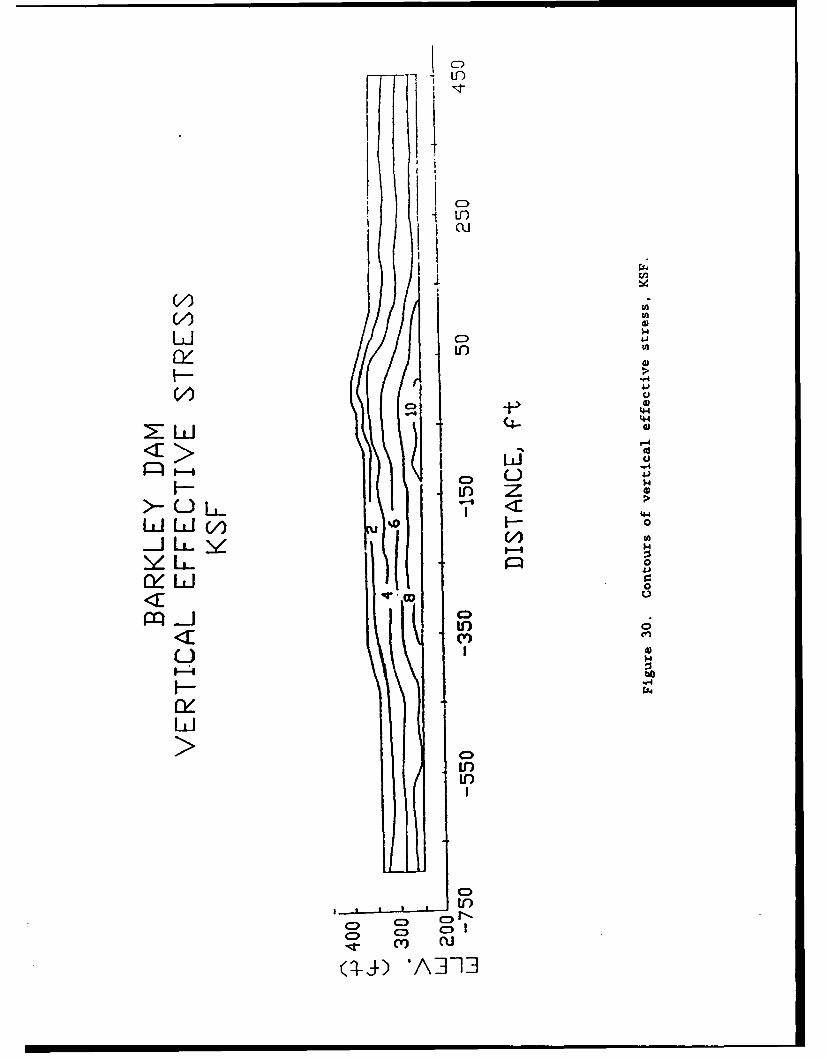
I-
cuc
W 4J
U)OU
4)
0C U.C
U < P,4~'4-
LJ LLJO0
Li-i
0O
ef)
o I a)CD
C) U)
CV) c u
01-J) 'A]231
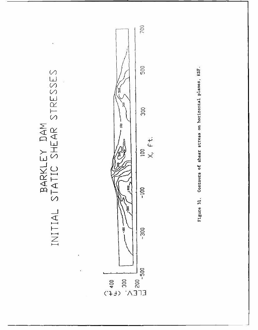
CDU
CDC
U-))
C>1E 0 ~CDU
00
<1 0
-44
V) C:) t
4400
CY :%
C>PQ~
C) C) C
C) C) C<I .,)4i
( C>f Al]
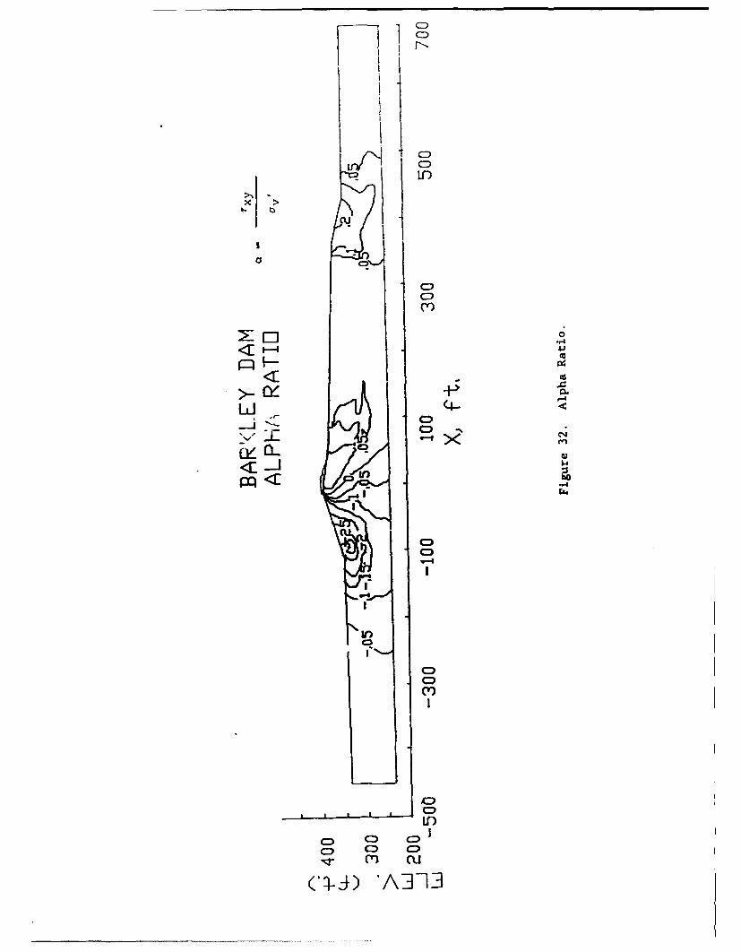
lCD
C1)
4: ý1Cd
-F;4
LJ(CD
< -J4
CDCC)4
CD"
,'I- m 0
'A3 1
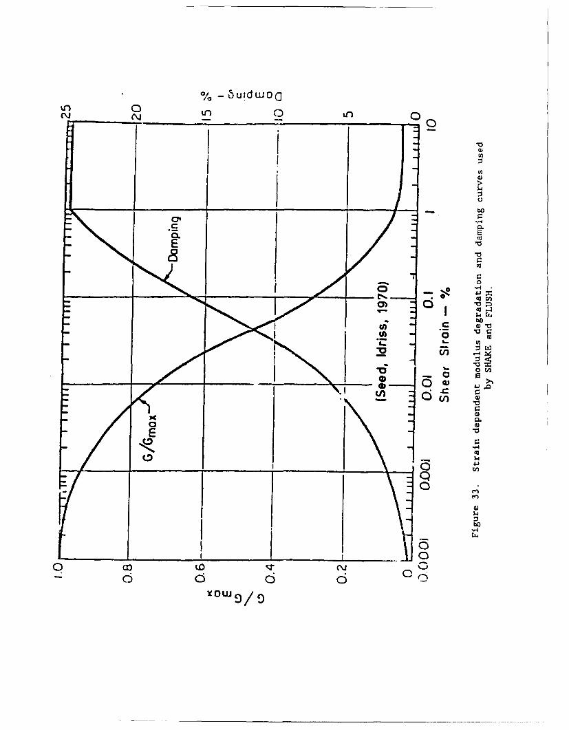
% - 5uidwooUN 0 _f 0 0
bo
' 0
crtI
cou
0 2
0
C0 o
C ,°
1) V
c 1 %I U)C
00<o631W 9 /
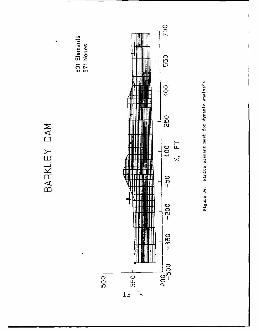
C:
w z 4L0
C)u
(D .4
00
(4-
I-D0 ILL4
0) IC) v-aC
If) c0
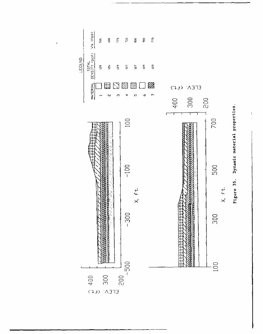
0.
U)
D ý- >- a, 10 0' N3 0 0
LA
< (U (1) tn \0 '0x~~ CD CD C
CD CD CD(Y m j
ý4
CD CDCD 0
(30I
'.4
4)
4 U-)
ElI
0 CD
00
CD CDI
S m cu
'K)A:]]3
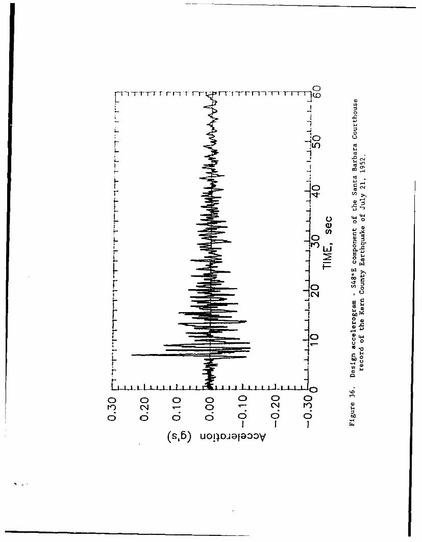
[1VFrT-Tr T, rri Fr-- Trr1rr11vFT FF11c]
0,
0
-7dLL
-- 4
-io4j1-
'Aj
4.44
Lj a
o~~~ a 0o-I ~.g~jw
F') ~ .'r- 1
6 En 6 60 I I I(s,5)UOE~D~j~to
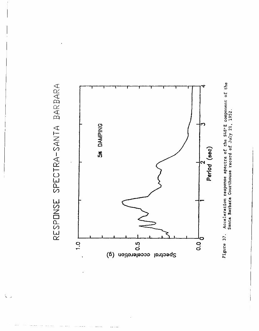
KE ON0U
H-4
C-)4 4,' 4~
00.
0))
a0
LiiW ,
0
4)U
0• w
.1.
OS.r
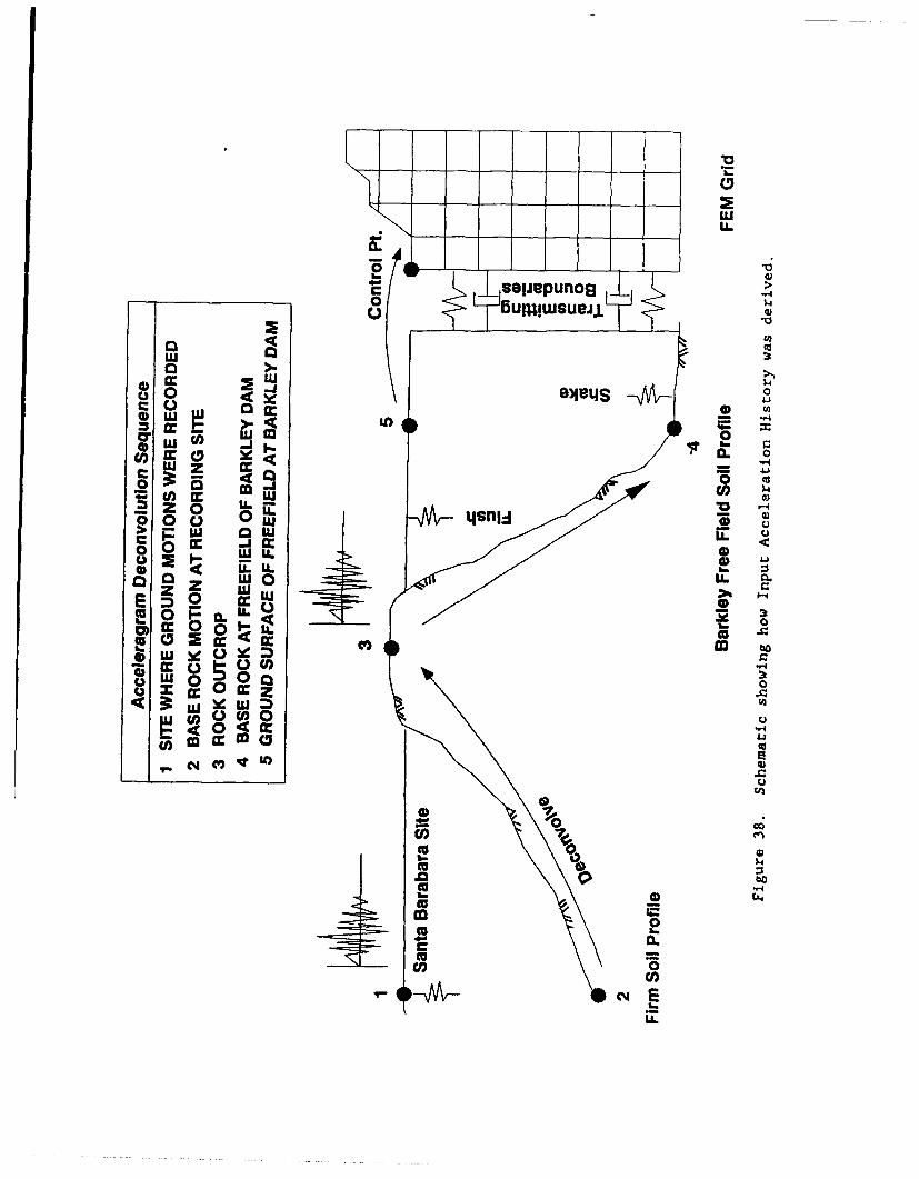
LULL
C - selpepunos -0i1
o uwwui£0
c0 04D Lu
C0-- 1c l0 Co
U) -1c
000 (0 .t
U.LL00 w 0 - .
- 0 w W0 1-. L.
0 0 U.
in 00
CJ M 0
0 g cc
0.
~ 00)0
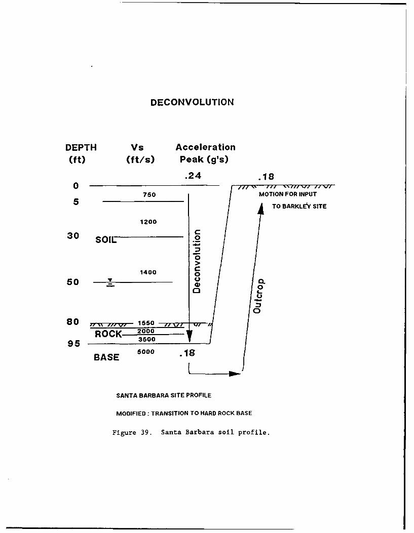
DECONVOLUTION
DEPTH Vs Acceleration(ft) (ft/s) Peak (g's)
.24 .180 ill/
750 MOTION FOR INPUT
TO BARKLE'Y SITE
1200
30 SOIL 0
1400 C
0
t-4so0 0
0
ROCK. 2000
95 3500
BASE 5000 .18
SANTA BARBARA SITE PROFILE
MODIFIED: TRANSITION TO HARD ROCK BASE
Figure 39. Santa Barbara soil profile.
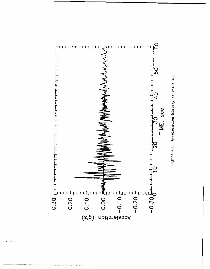
0
rrFTrnT r v t -rrii IF -I -r Fri] Tý(
IrF
-4410 41
h 014
LL 4* -4
0
.4 4
0 C-4
(Sib 0)0DJ;j9
......... .. . .... .. .
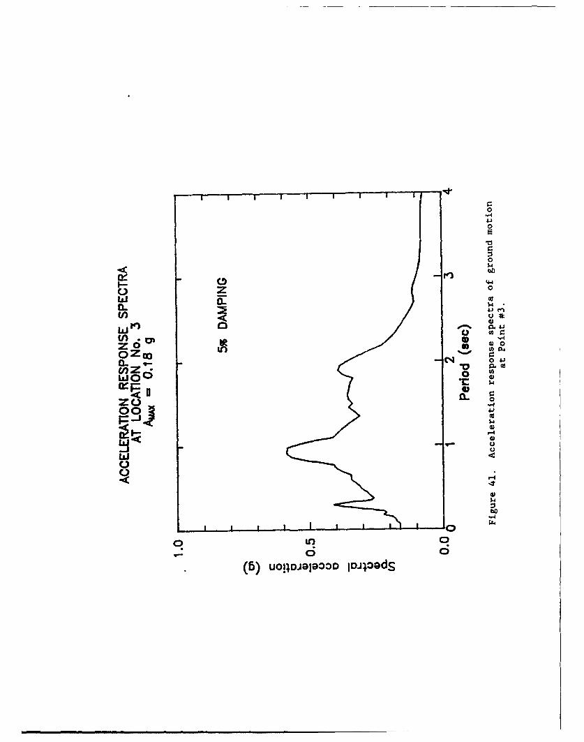
z 0
00
C~) Z 00
ZI 0 .) co
0L 0 to4
0~0
1-4
4a)
0 04
wt0c
001JOGO '-41od
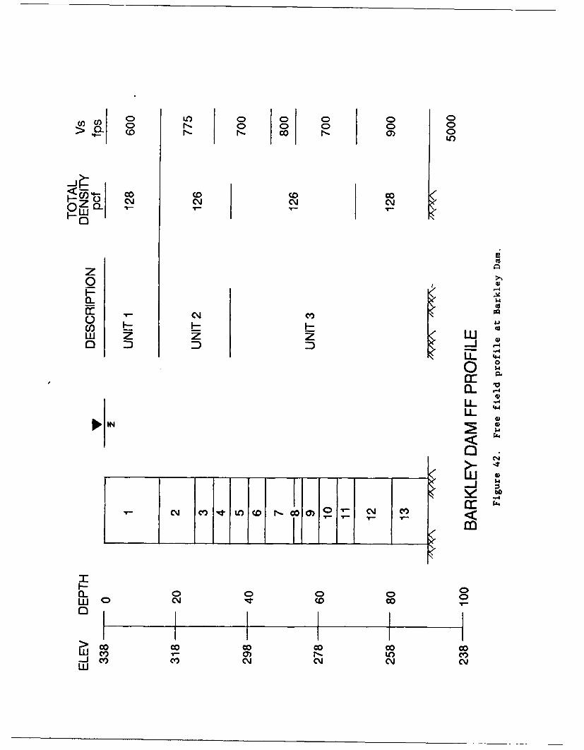
C> CU)
OZ CD C
zn0
C) 4U) F- - c¶d ~w zz z K W
00
IL C
ILL"
IN)
0 0 0~ 0oc
0
CO m CO CO CO COwj~ -0 -U
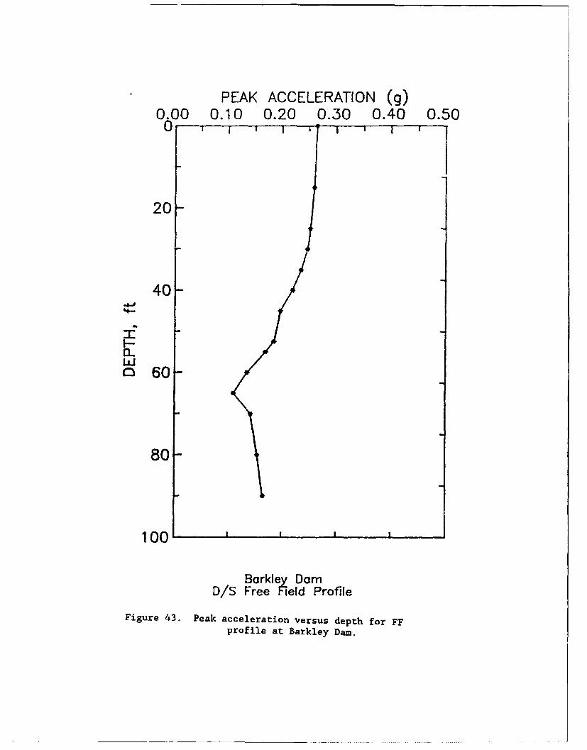
PEAK ACCELERATION (g)0.00 0.10 0.20 0.30 0.40 0.500
20
40
I--
LiiO 60
80-
100
Barkley DamD/S Free Field Profile
Figure 43. Peak acceleration versus depth for FFprofile at Barkley Dam.
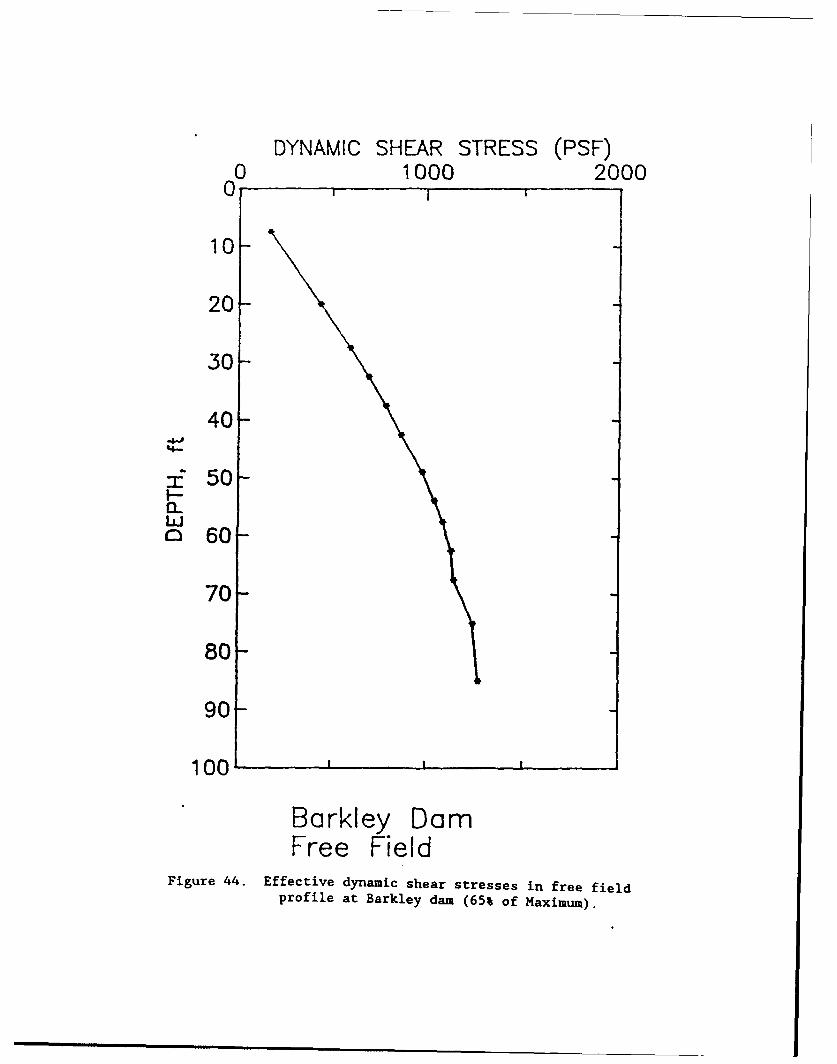
DYNAMIC SHEAR STRESS (PSF)0 1000 2000
0 I I
10O
20
30
40-i-
"150
O60
70
80
90
100-
Barkley DomFree Field
Figure 44. Effective dynamic shear stresses in free fieldprofile at Barkley dam (65% of Maximum).
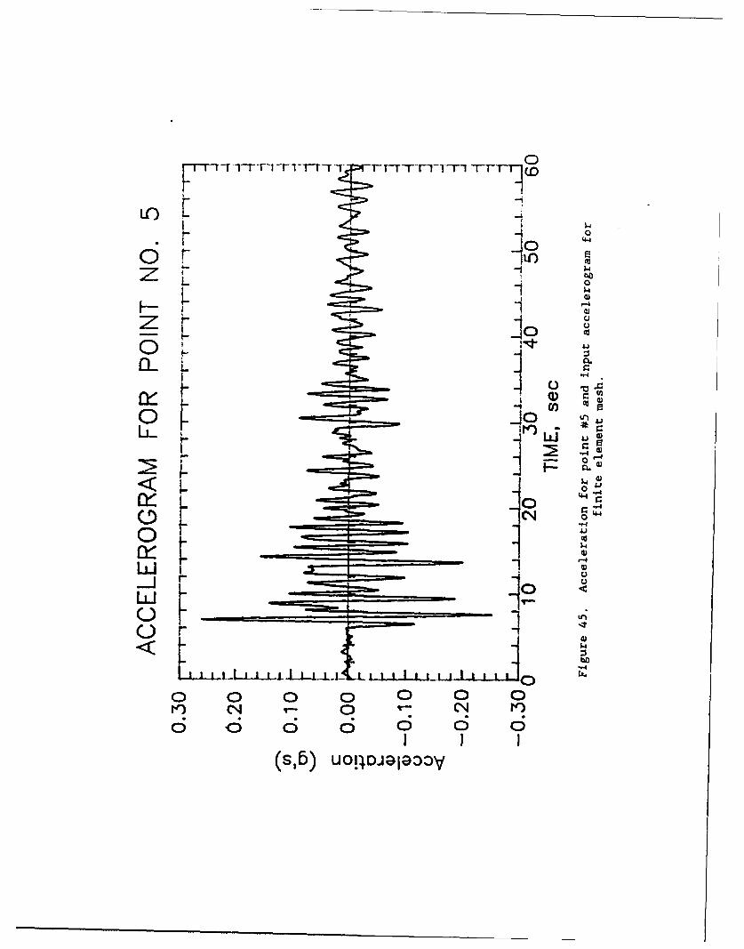
-T -vi-ri rirrr -Tr -TT"-'T -r r T- (Fr CF
Lot
'4-
-1
cLLi
0 Ld
0'4
11c0 4-
o a 0 0 0CI40 )
66~C 6 66 3Ib I 1DI19 3
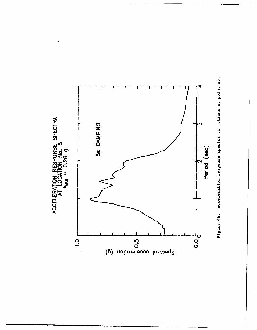
1 0
z 94-4
CL)
W~0.
z~ 0
(n z-WC4-)
zo IL
WOO 0
(a
C.-)
C; C;
uoiloolooD I~lood
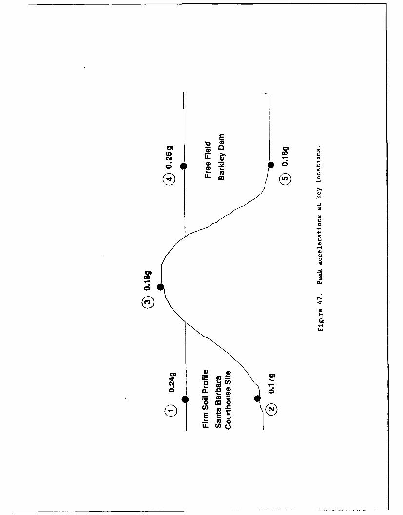
ECO~ . 0 0c
00)
(00
cc 0 0
I-I
$4)
0
b)"-4
0 U)NCc;)
0cc
E *Cw
b- M
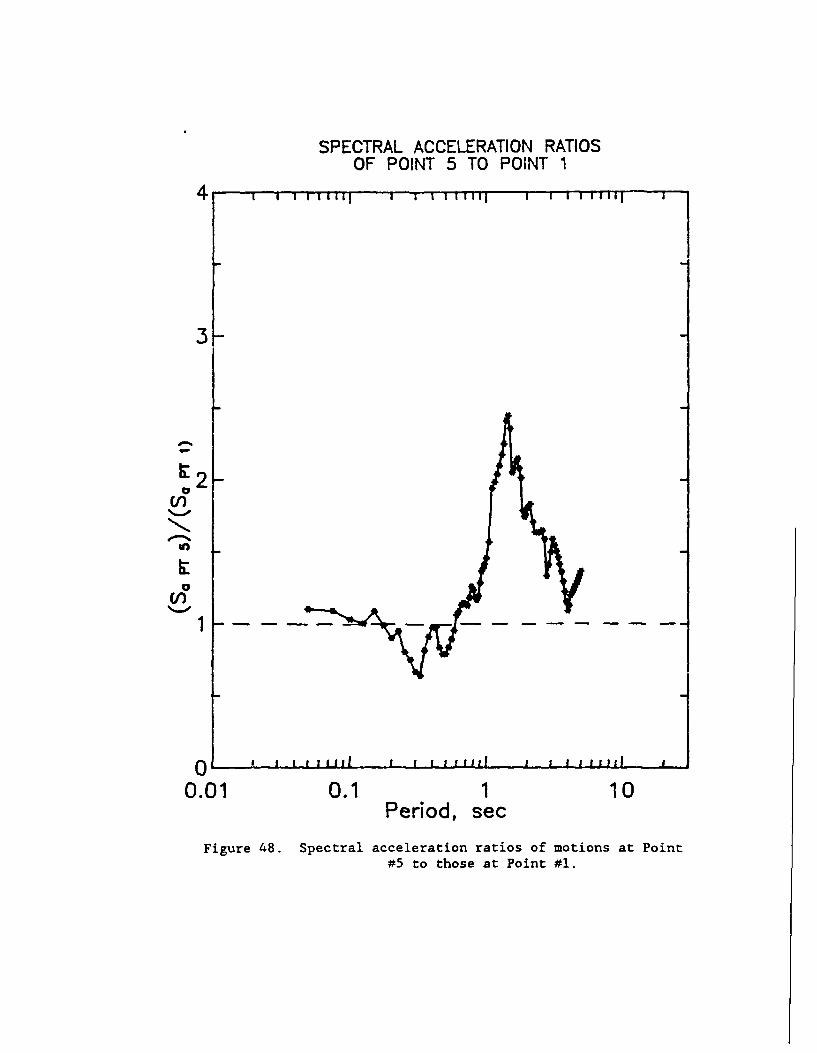
SPECTRAL ACCELERATION RATIOSOF POINT 5 TO POINT 1
4 1111111liI I 1 1 1111I I 1111111 5Ii
3-
'2 -
V)
00
V)
0.01 0.1 110Period, sec
Figure 48. Spectral acceleration ratios of motions at Point#5 to those at Point #1.
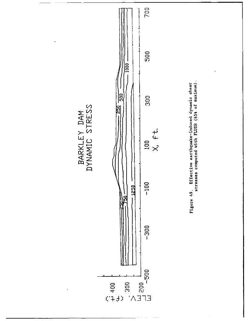
C)-C)
cJ LfC)
01 .C1
C1C
Cý 00
4).
~4
14.4
14J
4a4>0
p~" UL4-1C0 ul0
0) 4)44 CA
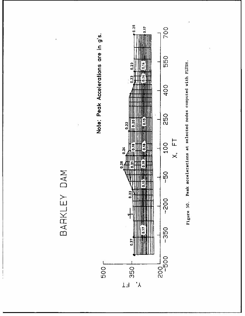
(00o; 0
CL
00
a '.~ C)C3,,
J-4
U C3)
oc04
0~0
a)
law)
C)C
0 in 0DLn (Y)04
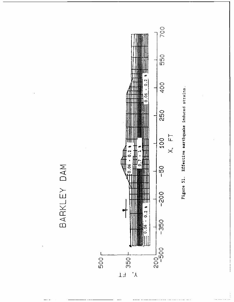
0)0)
IC)
CCj
ccV
CUd
400
4,
.2o IL 44
"-4
'44LL'4C)
1Z3 'c4
dp0
ritZi
m L
0 0 IC)
IC) C~) C) L
C) I AnC
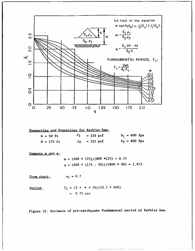
Ist root of the equGtion
m tanlq•n) = Jo(•n) I J,(6n)u'• ••Ihi' = __SIP1
c• I H m $2 P2•• S2" P2
0 •_.•r_ sI (H - h)
Io-m I• FUNDAMENTAL PERIOD, TI:
l=a-•l• mo ,o
00 .25 .50 .75 I-0 1.25 150 1-75 2-0
q
properties and Dimensions for Barkley Dam;
h - 50 ft Pl - 125 pcf S1 - 600 fps
H - 175 ft P2 - 125 pcf S2 - 800 fps
Compute m and q:
m - (600 * 125)/(800 "125) - 0.75
q - (600 * (175 - 50))/(800 * 50) - 1.875
From chart: aI - 0.7
Period: TI - (2 * • * 50)/(0.7 * 600)
= 0.75 sec
Figure 52. Estimate of pre-earthquake fundamental period of Barkley Dam.
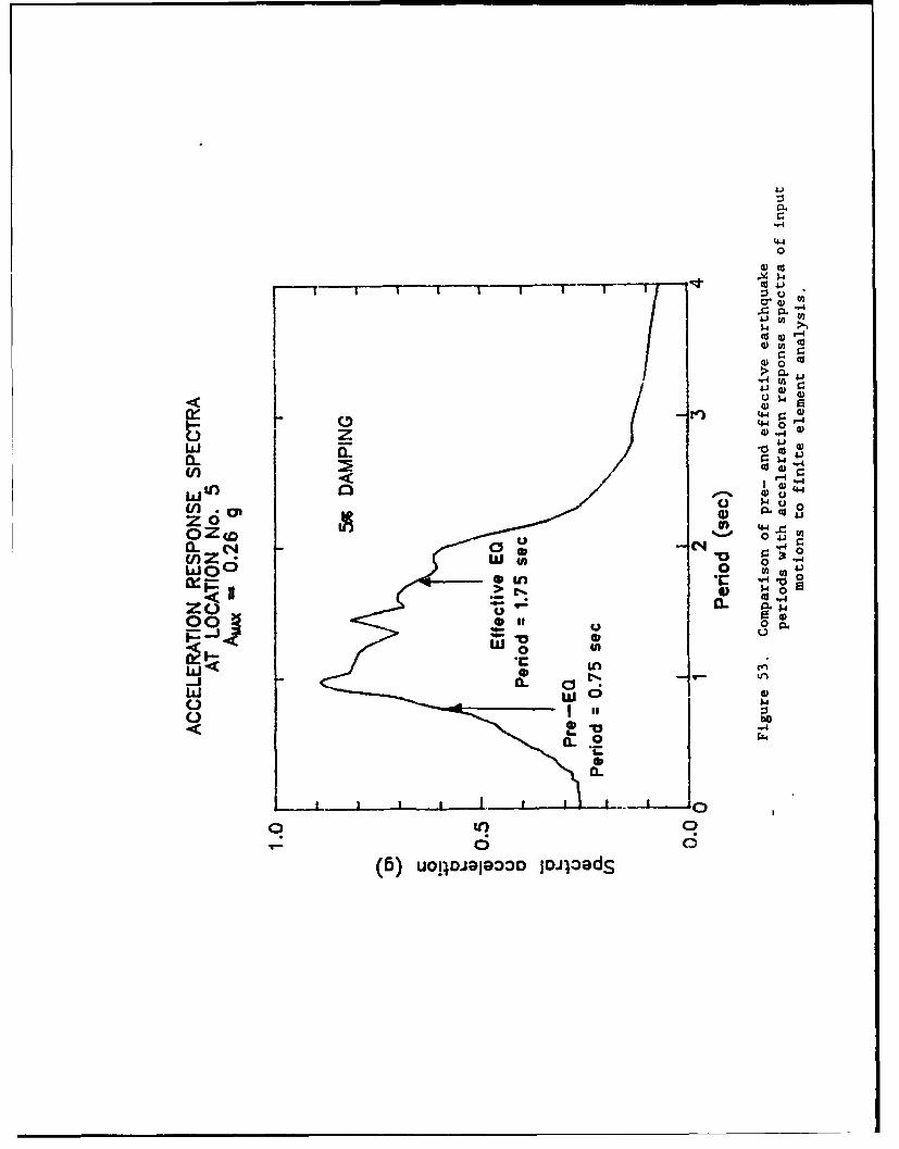
4-40
'.4
4) r-4
0 Z
>0 0
__ 4-4 -
OZw C' I
LLuOs, oQ
0 3) la0c
sOtO 00 K1 Y-J C1 "4
o It) 00
0 0
(6)~ ~ UU)a93DIid
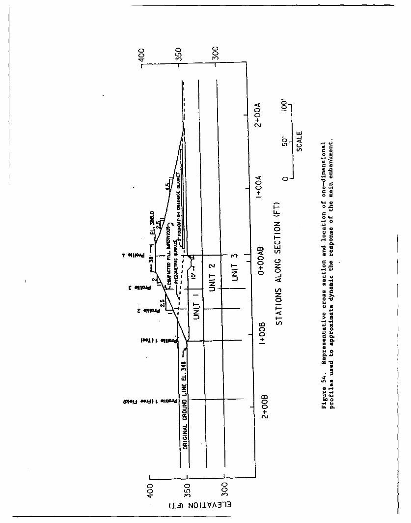
o 0 0o Ln* 0
0I 0I +
o <d
00
0004 01-
cc 0a 44)
041
00-4 0c
0 C
IGI
0vC4 ;7- u l
-d0)
-I0
14boo
-z
£30+
o 0
Iv'
(13) NQIIVA3J13
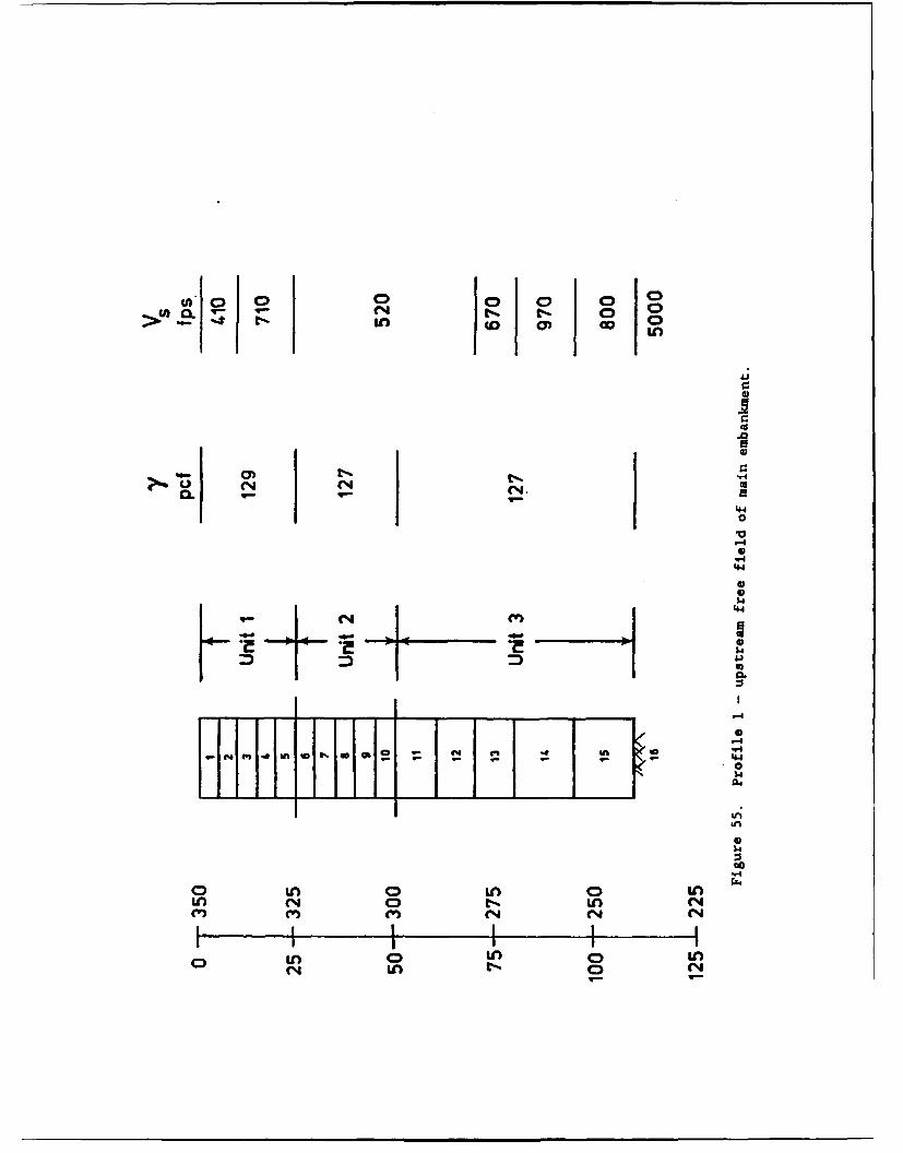
t- %tLn Go 0Lin
Cc
CMU
.0
"-4
a. (N.
44
r-4
tol
0
1.4
Ii
1-BI1I{ t- - 44
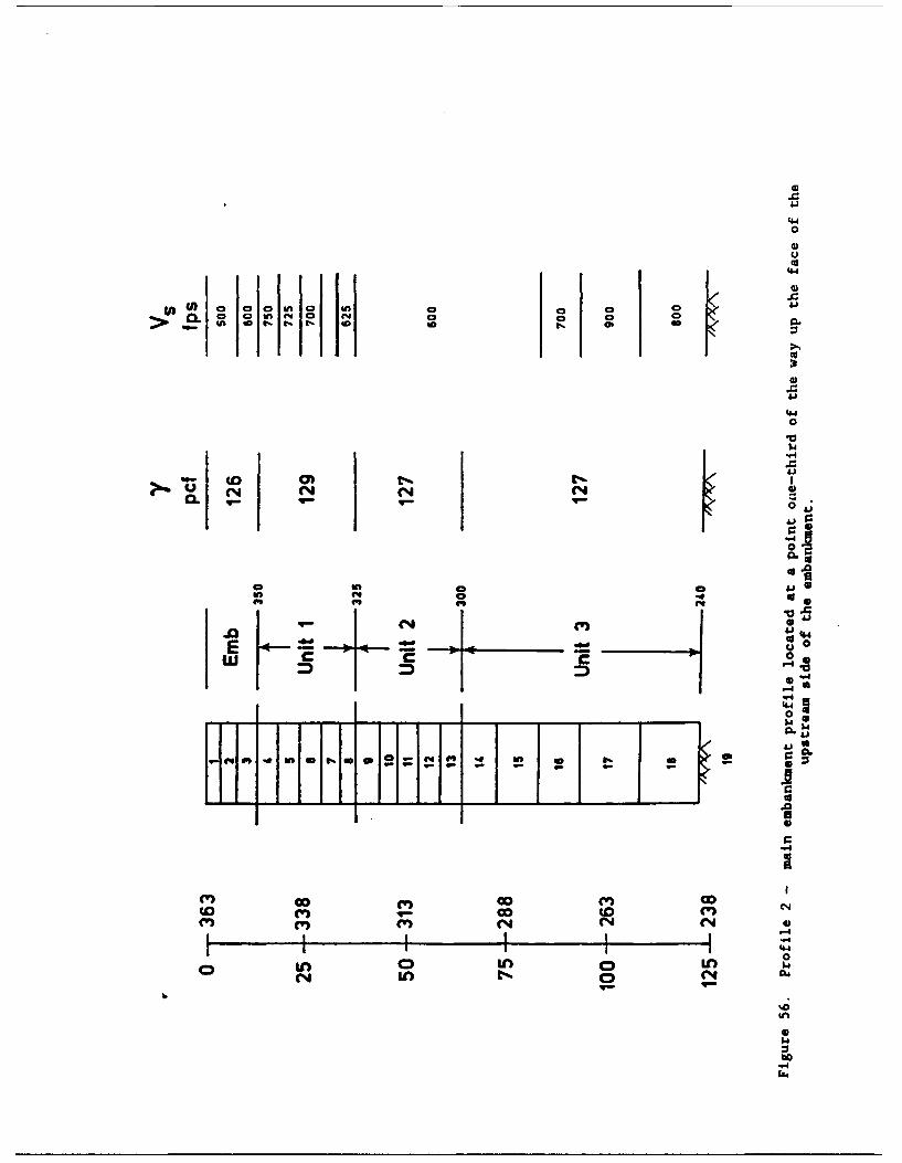
4.40
I +4)
U, Ci p C4 0
In 40
cc
0
3.4
-.4
0) 0
Q.~
w 0 0 aJ
444
N C')w We
Go) Go Go) C(M GY o ( CV)
0
04 on C40
bb
-4DW4
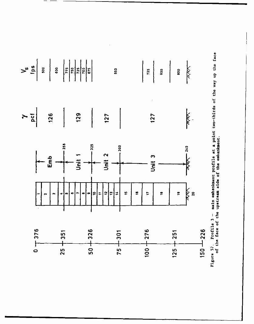
ci
4.4
o
Sin
'440U)
I~.d
* -- o•
(N Fo
" •~a,
In CD C 'ene 14 3-
cne00
NN 44
44,41 0
to ,W4 00
L 4 C) I. ! 0 ca
,4
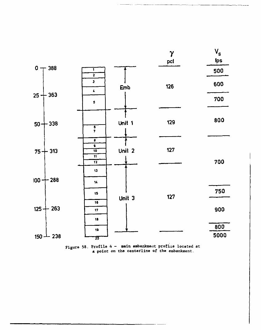
7 Vs
pct fps0 -- 388 1 500
23' Emb 126 600
25 -- 363 5m 700
50-338 Unit 1 129 800
750- - 3-8-
6
I
75- 313 10 Unit 2 12711
12 - 70013
00- 288 1,
Unit 3 127 750
16
125 263 17 900
Is
19 ,___ 800
150 238 5000
Figure 58. Profile 4 - main embankmeat profiie located ata point on the centerline of the embankment.
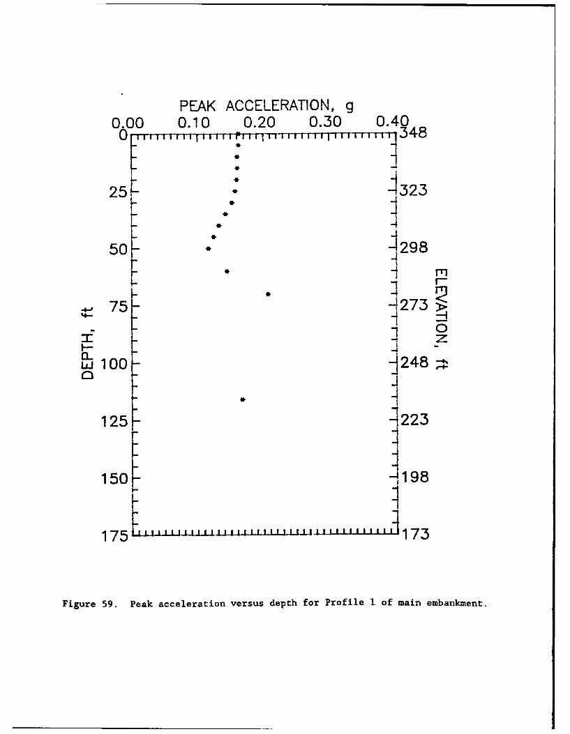
PEAK ACCELERATION, g0.00 0.10 0.20 0.30 0.40
O , i.irTi 'i i i348
r*
25 1323!1.1
50 **" i298
75r q273
j 02: z
o. -j248Li, 100- 248
* -4
125- -1223
150 -4198
1759 .Peak acceleration e d f Profile I o 173
Figure 59. Peak acceleration versus depth for Profile 1 of main embankment.
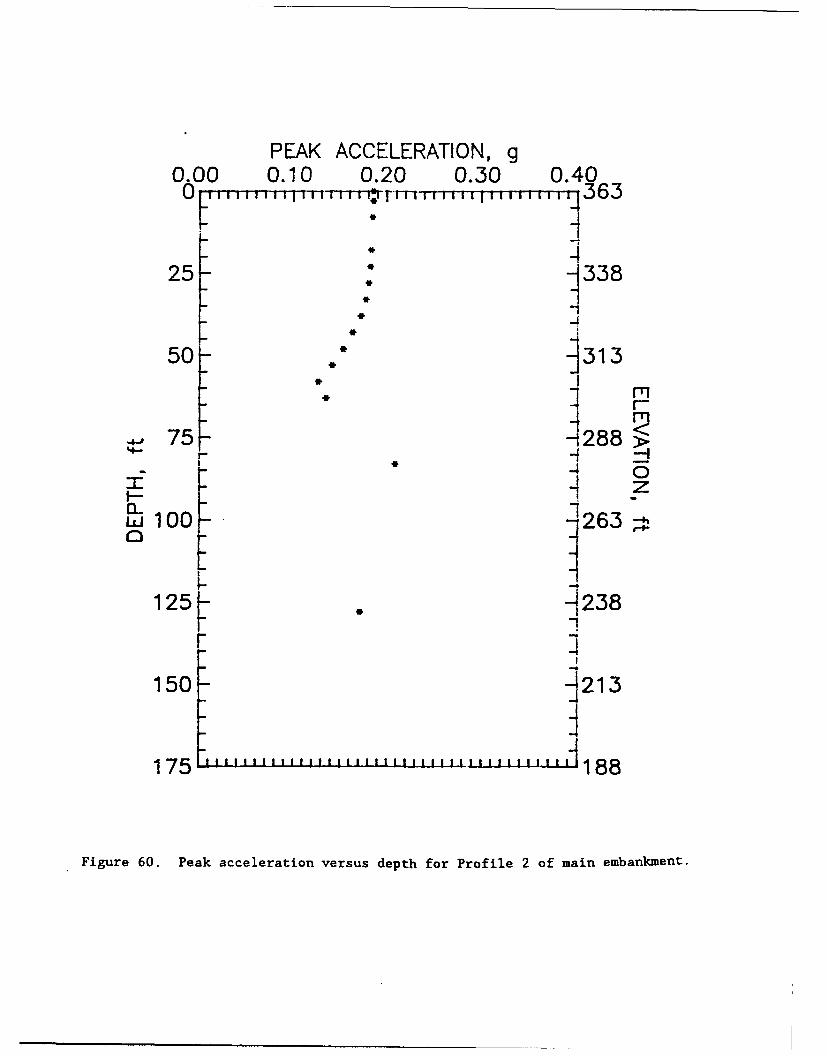
PEAK ACCELERATION, g0.00 0.10 0.20 0.30 0.40OrrrrrTTrr'|rl-rTrl-r ]'i.r" i 11iii 1115 a i""1363
25-" 338
o ~1
50- .313*M
-* -
75 - 288>- 0
125 * 4238
1m 1
150 d213
175 60. Pea"a'elraionvesusde'h'"r188
Figure 60. Peak acceleration versus depth for Profile 2 of main embankment-
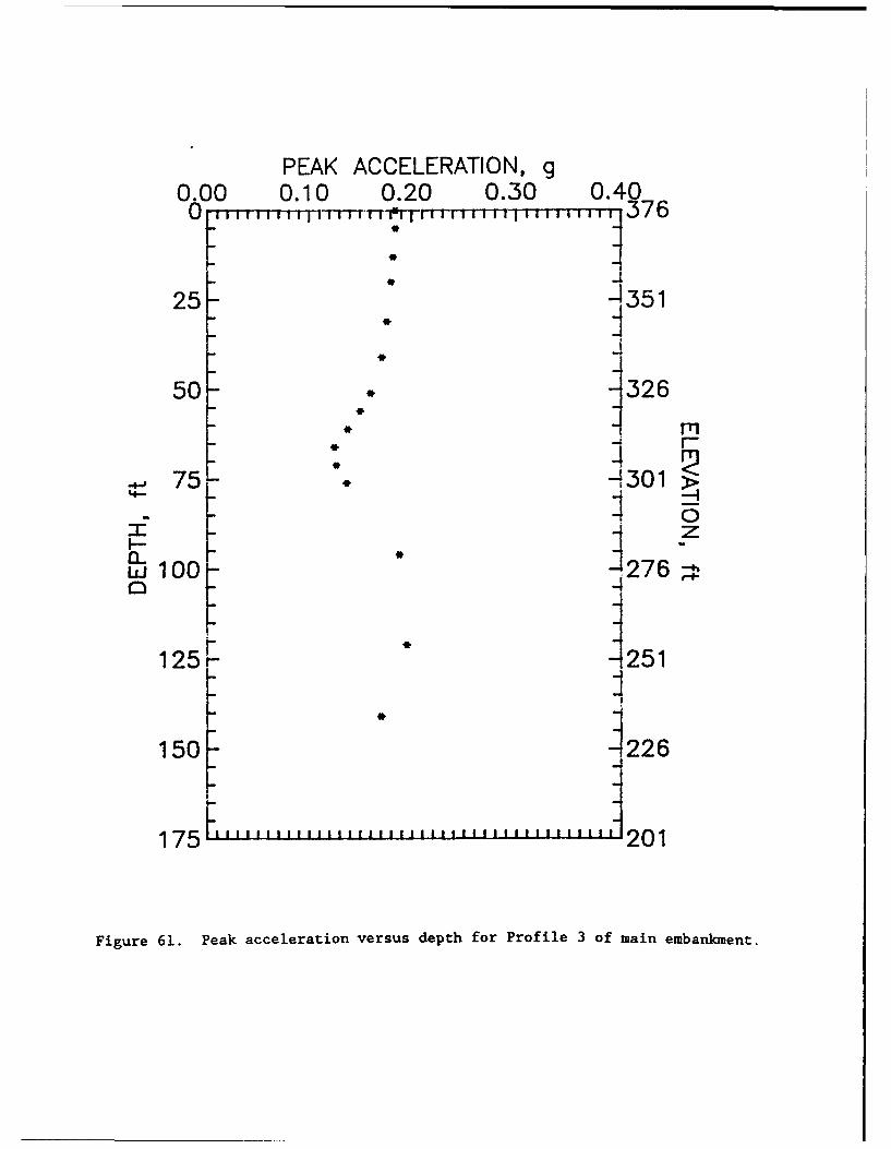
PEAK ACCELERATION, g0.00 0.10 0.20 0.30 0.40
0__ T-l Iilryrm-iln 376
25- - 351
50 -326
-4. 75- 1301
- - 0
0--
,,J 100- -27604
125- - 251
150 -4226
175P1 '"1111 '""1111'1"1"11"'1'' 201
Figure 61. Peak acceleration versus depth for Profile 3 of main embankment.
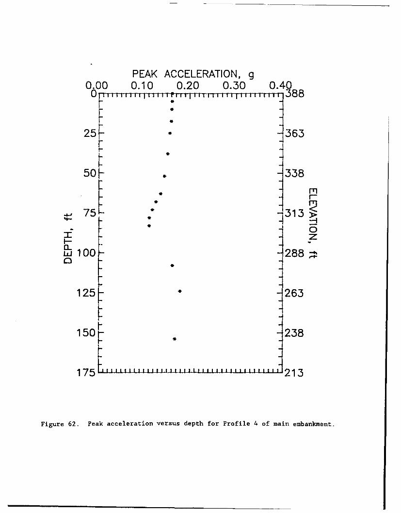
PEAK ACCELERATION, g0.00 0.10 0.20 0.30 0.400 U I-388
F -25[-- 363
r
501- -338
75 -~313 >
[ -I
00•ý z
Du100- 288
125 * J263
150 -238
175 62.,Pakacelera ionversudepthfrProfil 213
Figure 62. Peak acceleration versus depth for Profile 4 of main embankment.
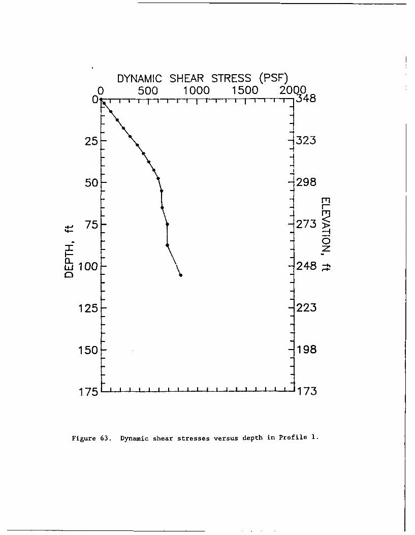
DYNAMIC SHEAR STRESS (PSF)0 500 1000 1500 20000 1 1 348
25- 3323
50 - 298
75- 273o
ILI S- z
,100 248
125- 223
150 -198
175 F , , '-- 173
Figure 63. Dynamic shear stresses versus depth in Profile 1.
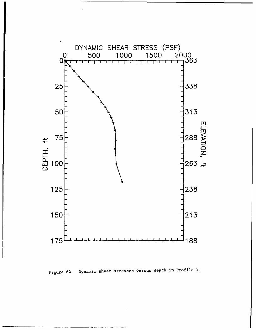
DYNAMIC SHEAR STRESS (PSF)0 500 1000 1500 2000
0, 1 1 - ',,1363
25 338
50 -j313
-+J 75- "1288,
100 -26
125 - 238
150 213
175 , , ,.1,, , , , , ', , , , , , , 1- 188
Figure 64. Dynamic shear stresses versus depth in Profile 2.
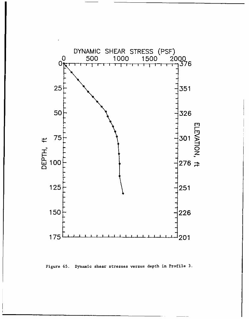
DYNAMIC SHEAR STRESS (PSF)0 500 1000 1500 2000
ON,, • , i , , , l i , , I • , , 376
257 -351
50- -4326
S -301
w 100- 276
125 -251
150 -226
17 ' ' ' ' I " ' 1 ' ' ' ' ' 201
Figure 65. Dynamic shear stresses versus depth in Profile 3.
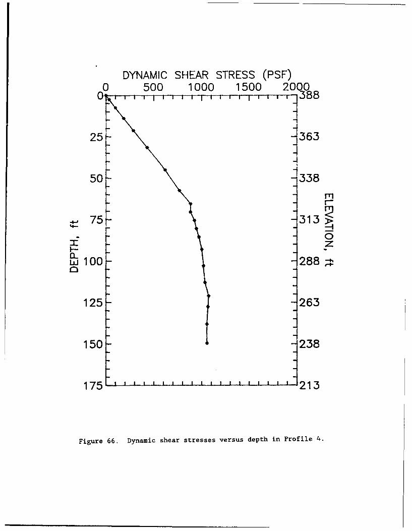
DYNAMIC SHEAR STRESS (PSF)0 500 1000 1500 2000
0 fi l l ,1, ,1-,, 1 , , , 388
-1
5 0 L '3338
75 -313 >F 0
w 100 -288-
125 -263
150 1238
175 ' ' ' ' ' "-" ' '' t ' ' 213
Figure 66. Dynamic shear stresses versus depth in Profile 4.
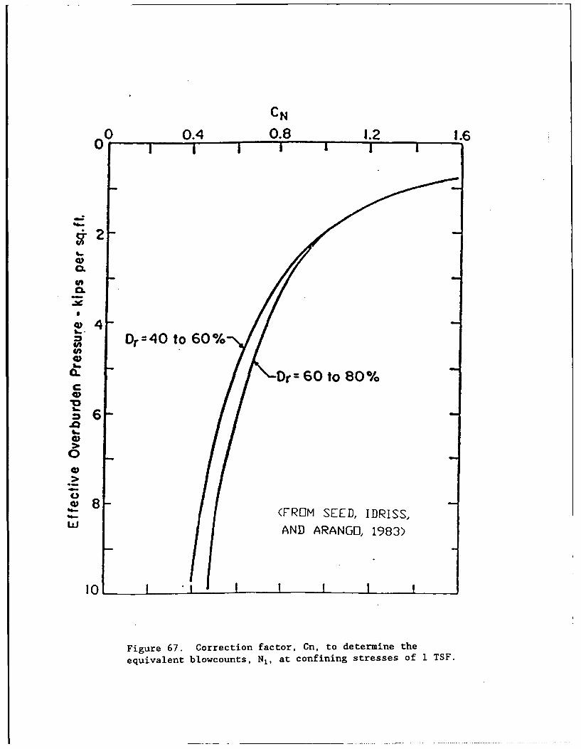
CN
0 0.4 0.8 1.2 1.60 I
2
a.
o4
0
0..---4o60to60%
8
U/ AND ARANGO, 1983)
10
Figure 67. Correction factor, Cn, to determine theequivalent blowcounts, N1, at confining stresses of 1 TSF.
---- --- ---
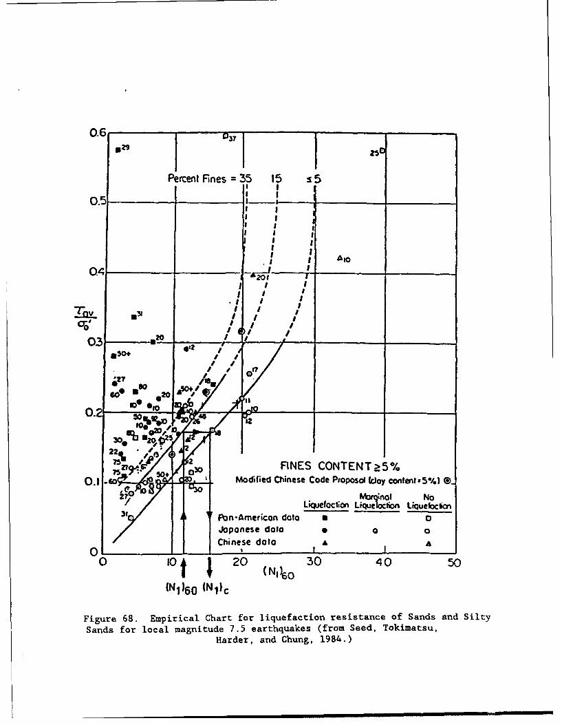
0.6 U32
Percent Fnes 35 15 15
SI
0.5.
__________ I I _ _ _ _ _ _ _ _ _ _
I II I
.0 1
I.• # I I!, I
20 /low
6, 03 so 2" 4 W 4
03 - a -" ____ ___ ___
0.2-50w *Io
"/ // / _
600a.60 11a
30* Zci22%"503A FINES CONTENT>5%
0.1 "G _Modified Chinese Code Proposol (cloy contleiz5%) 0-"7Q Mar inI, No
Liquefaction Liqueloon iQuefockion1 Pon-Americon doto " 0
Japonese doto o 0
Chinese doto A I a
0 lot I 20 (NI) 6 0 30 40 50
(N1)6 0 (N1)c
Figure 68. Empirical Chart for liquefaction resistance of Sands and SiltySands for local magnitude 7.5 earthquakes (from Seed, Tokimatsu,
Harder, and Chung, 1984.)
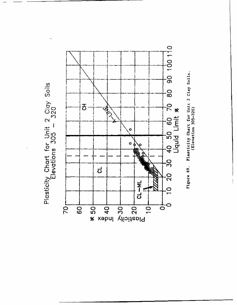
I- -o0 4
I 00
0 0A
044
oD C) 0O -0
ro .4,j w-- -
C)Q cr u0
CO- -.--. -
1 ' I cc0 r4
-- C-Li -0
N 0 0Q 0- 0) 0 0
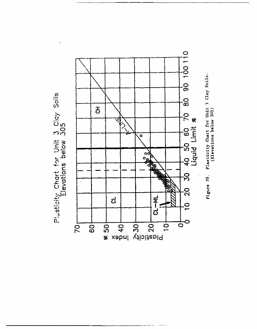
0
- 0
U,
.,4
(1) 00V) - -
U) I ) 00
0~ 0)
E3 44-4
- -& -
to $4
C 1
£0 r-)"4)
4Ur -0 -1 - -
-- Uccc
0 0 0 0 0 0 00
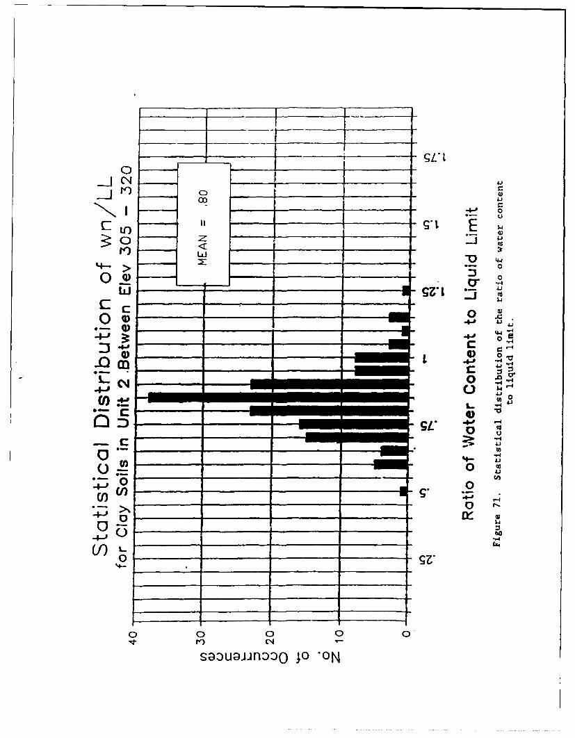
jCCD
Lo% 4- )
4-. >
0 4) _ _ _ _ _ _
4-
z1 0f'41
__ _ _ _ __ _ _ _-
D -W ~ ~0
C c _ _ _ _1__ _
0 En___ _ __
44-1
0~ __ _ 4
0 0 0 0J
________:Do 4-' -O
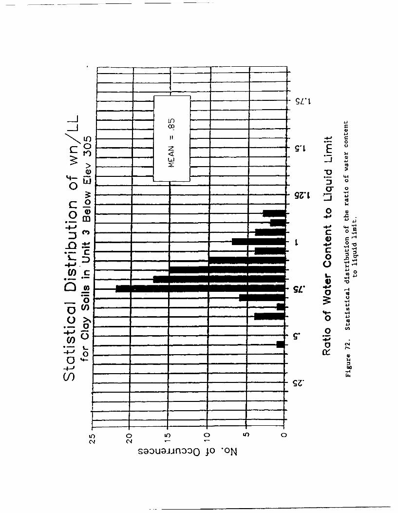
- _____ -LL
I'co _
-
0i - 4, 4
Z - E_ -LLI 4.J_
> ____ to___ _____-
9z-, 1_ _
4.D
m 41 C
____ 0
_ _ _ _ _ _ 0 LO4
I-0
it)~~- 0 t 0tC\J (""4
S~3~1Jl3 r_4
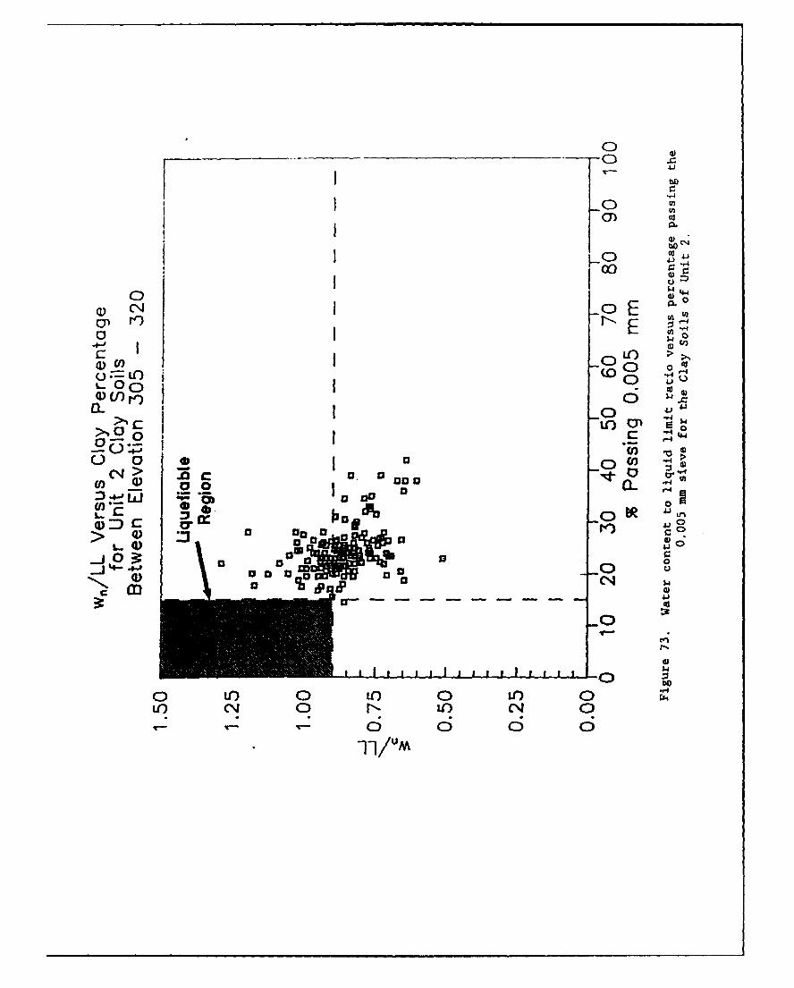
C)
Oc,4
0~- M- I
oEo
a.. DN0 1 -0 12
5o c.
* 0
-00
(p o
o -.4
-0-
C-4->0) U)04) U .U) aN 00 )(
1a 03 0a> :3 a i/UM
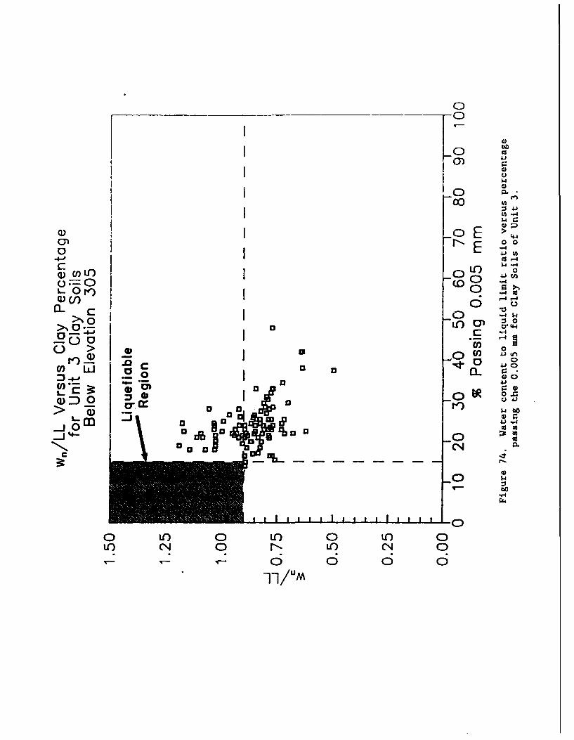
00
-0-
0 ca
co
cCf 0IQ)~a U)LO-0 "11
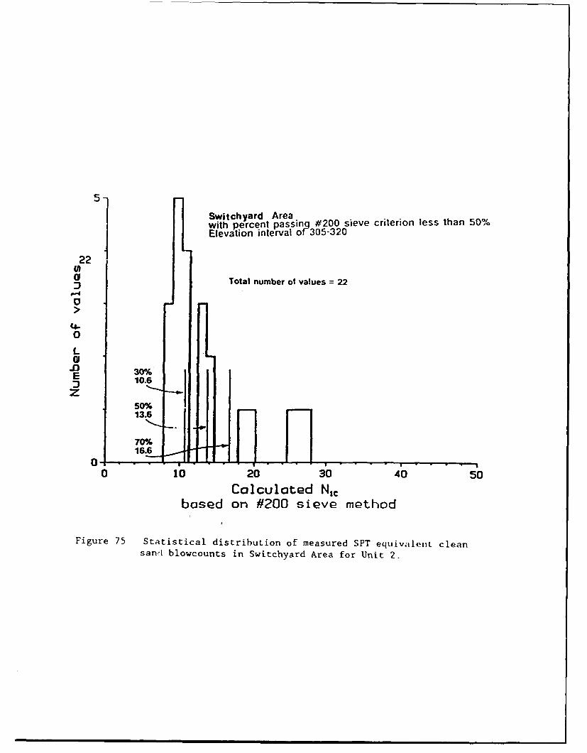
Switchyard Areawith percent passing #200 sieve criterion less than 50%Elevation interval of305-320
22
Total number of values = 22
0
0
L. 30%E
10.6Z
50%13.6
70% ..16.6 ti
0 10 20 i[ 40 50Calculated Nic
based on #200 sieve method
Figure 75 Statistical distribuLion of measured SPT equivamleti cleansand blowcounts in Switchyard Area for Unit 2.
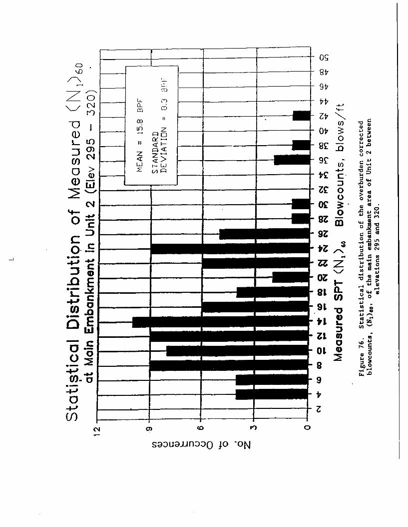
zL 0
jO)0
0 E$4J
CC
0
0)9 CD )
c ~ ~ ~ l3 0O in
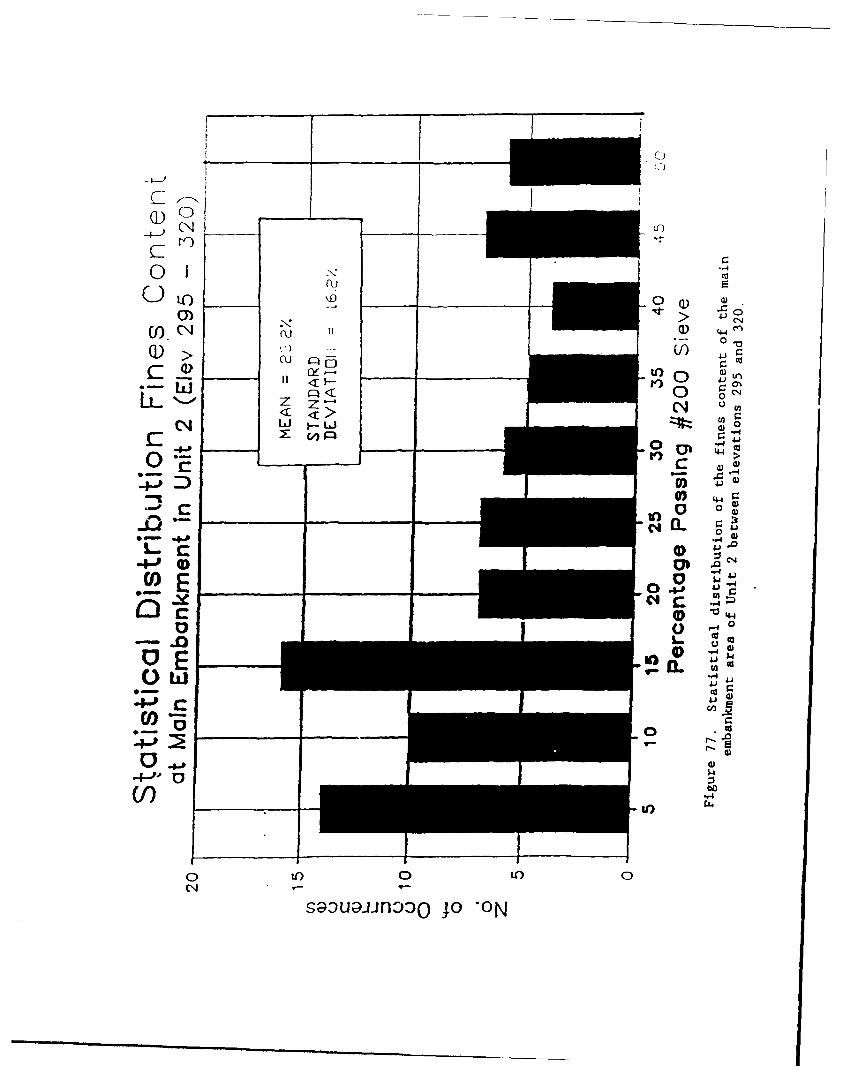
C_-
0J0
U>
to Q)
00-. 04
4-P 4-J
I) '44
if)
0C' (L 0 O
(NJN
Z~Ua~flZ~Y3 ~ 0
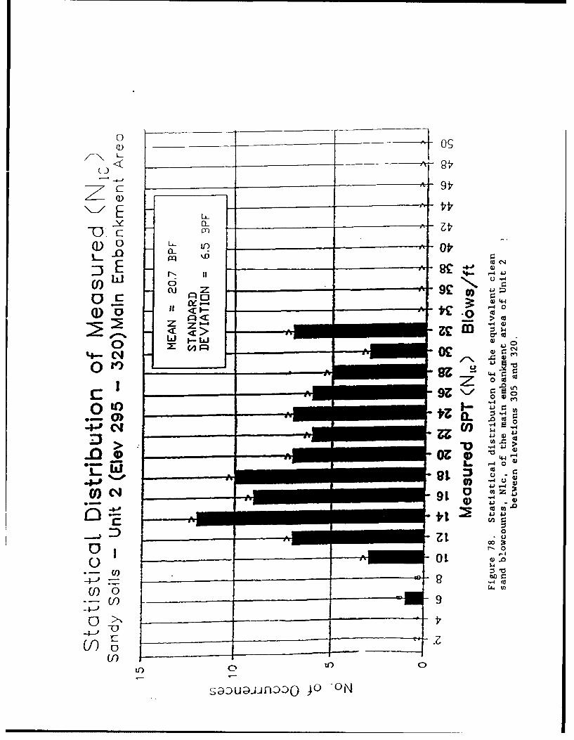
C)
Q) 0
0) i z - __z_ _
<1 .0 cN 0(U z ý4(1
Li- w-L wQ I.- O
9~z r.-2.~4.)-1-~~~~~. Cl _____- I
_ _ _ _ _ _ 0
4, *%,1jtd 41 C4
0
-,~ -
r-0
(co ýt~
0>0
(notU. t
SacuawjInDDO 40) C)N
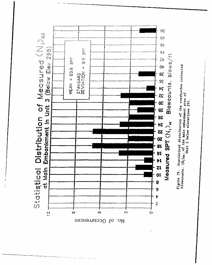
_ ~ _ I.
cu 0jO
U)0<c9Z2-
C)<
.oE
4-,400
024 0) (0 01,
S~3~JflMc 114 0
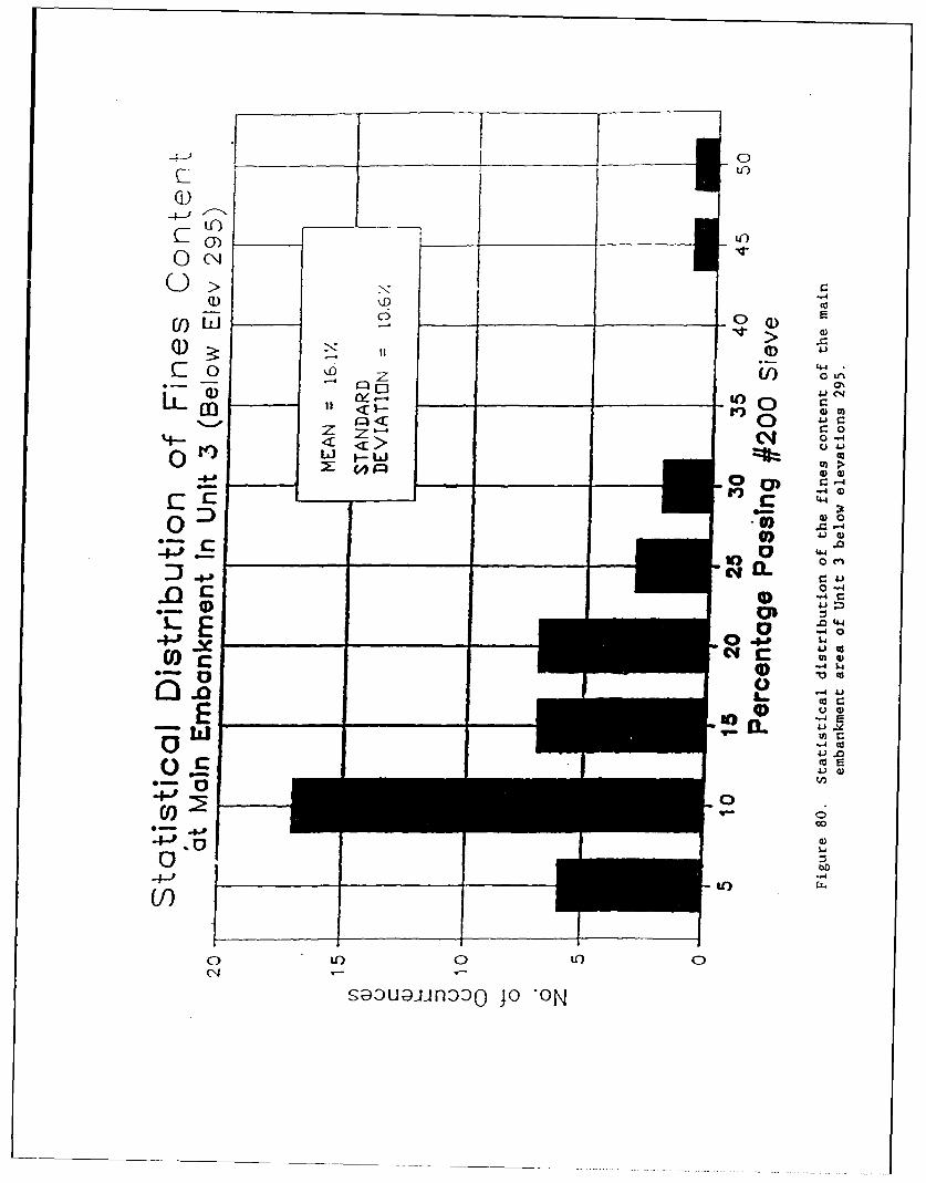
C1 _ 0) 1 -------
Cf)>
Cq) _ _J
(-9>
Co
0 G\
r..14. .0
__<_ >_ _ A0LLJ I.- IO-
0ne
cl a. CA
L_ LC~ .0 4
ý40
0 0
.0 0)0U
E ~ ~ G~lD o0
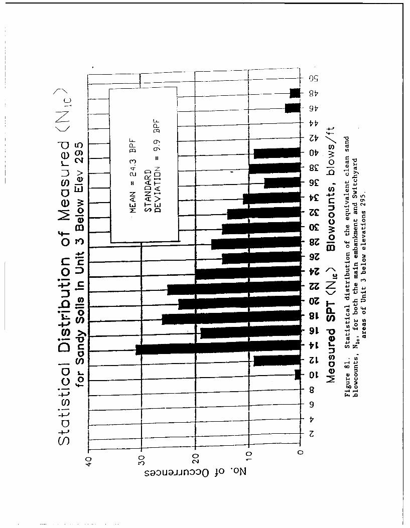
z t~t'- U L O ClNc
P:) II,
>I) Cl) 0*
:z Z Z'--
0~' _ __ll)(:
4-1'
00
9z 0
-4--,
0 0 0 04
00 r)Cd91ua~l9 -0 44 N
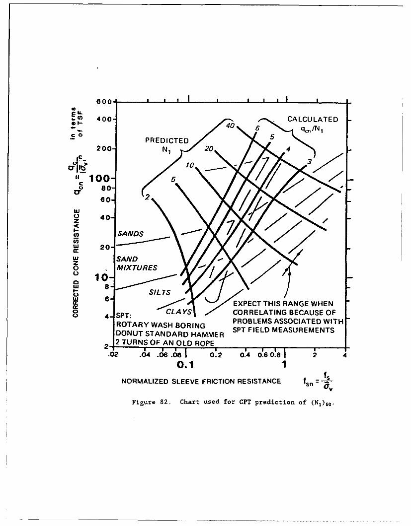
600-
400- CALCULATED
-- PREDICTED
200-
"ci 10030 so
so0 2
wo 40-z
W SAND
o MIXTURESo 1020-" S SILTS
w 6r CAEXPECT THIS RANGE WHENO CORRELATING BECAUSE OFO 4- SPT:ROTARY WASH BORING PROBLEMS ASSOCIATED WITHDONUT STANDARD HAMMER SPT FIELD MEASUREMENTS
2- 2 TURNS OF AN OLD ROPE2 ,
.02 .04 .A6 .08| 0.2 0.4 0.60.81 2 4
0.1 1
NORMALIZED SLEEVE FRICTION RESISTANCE fsn -
pno
Figure 82. Chart used for CPT prediction of (N1)60 -
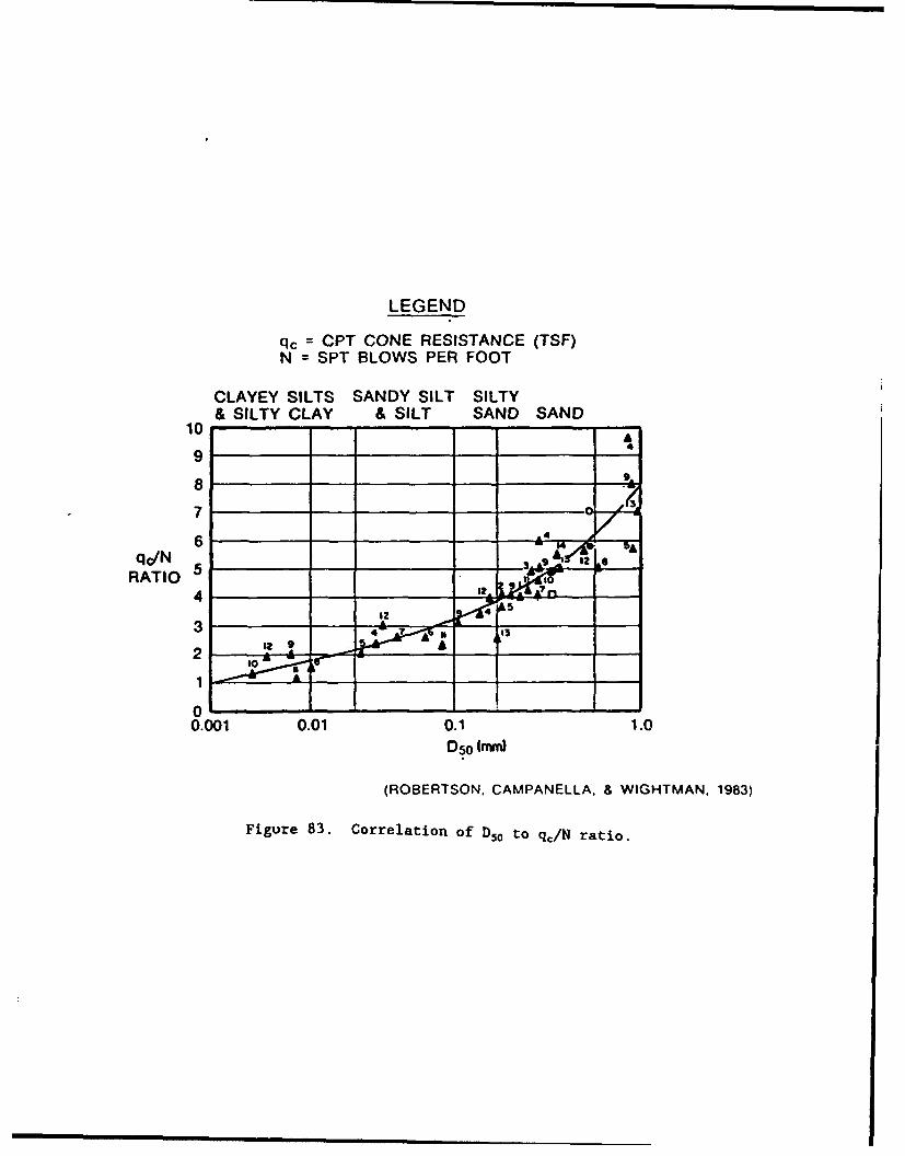
LEGEND
qc = CPT CONE RESISTANCE (TSF)N = SPT BLOWS PER FOOT
CLAYEY SILTS SANDY SILT SILTY& SILTY CLAY & SILT SAND SAND
10
98~9.
7 0
6 .4 7i.
qdN 3_-__&,
RATIO 5 ki, ,04 *4.
3
10
0.001 0.01 0.1 1.0D50 (mm)
(ROBERTSON. CAMPANELLA. & WIGHTMAN. 1983)
Figure 83. Correlation of D50 to qc/N ratio.
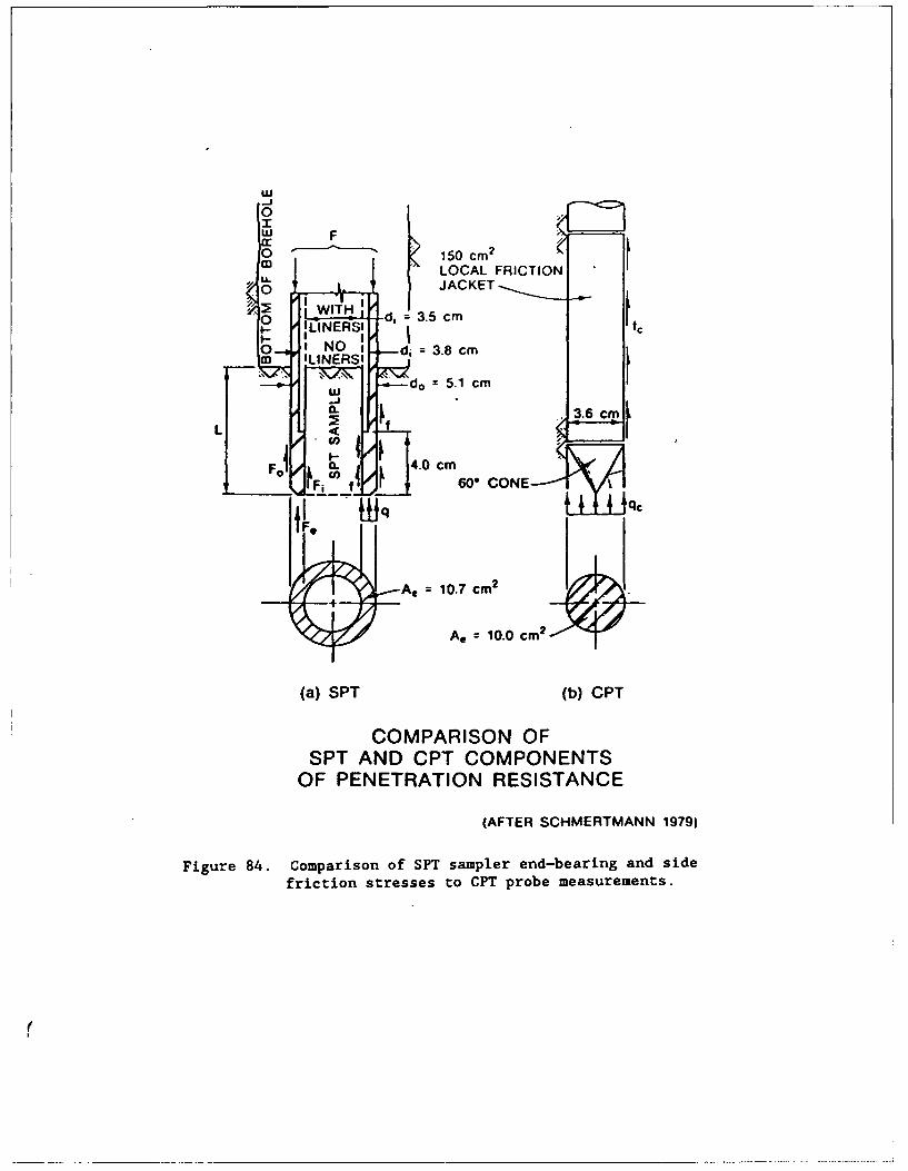
0I
F 150 cm2
1 1. 1 1JACKET
I WITH LOA0RITOS, - = 3.5 cm
00 LINER"SI fc
o i NO ,NER d = 3.8 cmM 'LINERS'__ ! -..\o '. ocUi do 5.1lcm
Fl 0 3. 4.0c
Fod 0 fti. 0 IFF f _ 60° CONE
/F*
Ae = 10.0 cm2
(a) SPT (b) CPT
COMPARISON OFSPT AND CPT COMPONENTS
OF PENETRATION RESISTANCE
(AFTER SCHMERTMANN 1979)
Figure 84. Comparison of SPT sampler end-bearing and side
friction stresses to CPT probe measurements.
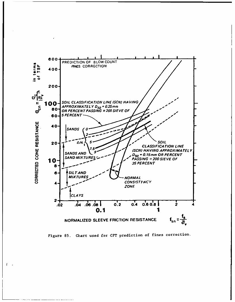
60 ~ I I I I a I mPREDICTION OF BLOW COUNT
I. FINES CORRECTION[.0 400
"2001
gg 100 SOIL CLASSIFICA TION LINE (SCNJ HA VING / / _0 APPROXIMA TEL Y D50 =0.25rmm OF .0
80- OR PERCENTPASSING =20 SIEVE OF
4 o SANDS 0 • "
C 20 1 6N SOIL
-- CLASSIFICATION LINEZSDA \7"9'/ -"7 (SCN) HA VING APPROXIMA TEL Yo N D50 -0.15mm OR PERCENT
1SANDMIXTURE '- PASSING =200SIEVE OF
lo- 35 PERCENTw a--6SIZ TAND 01I Imix ruREs.,,"- .. ,- NORM•AL
t-1 rL J •. •.CONS1STf#VCYI..-"":"ZONE
tCLA YS
.02 .4 .&.0; 1 0'2 0.4 060'.81 O 4
0.1 1
NORMALIZED SLEEVE FRICTION RESISTANCE fsn -(TV
Figure 85. Chart used for CPT prediction of fines correction.
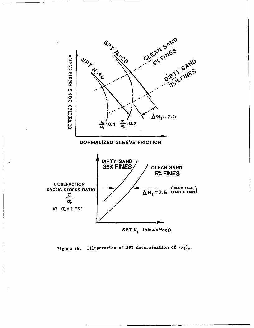
" .•.'~-_ . --=.
wca: +
0 000
0 Wo1~O AN~z7.5
NORMALIZED SLEEVE FRICTION
DIRTY SAND
35% FINES. CLEAN SAND5% FINES
LIQUEFACTION
CYCLIC STRESS RATIO 1N1a (1EE )3
AT dv TSF
SPT N1 (blows/foot)
Figure 86. Illustration of SfT determination of (NI),.
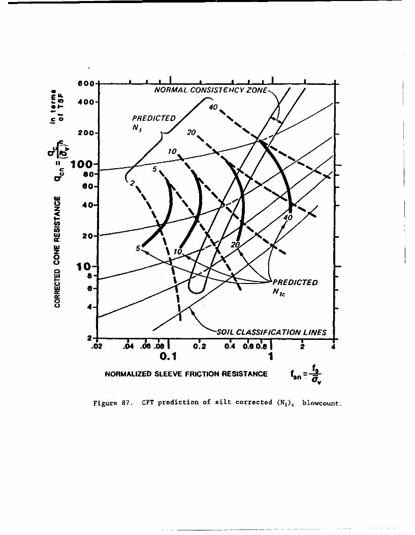
so I. I I I I IL II,
* NORMAL CONSISTENCY ZONEE IL
o 400. -440
0 " PREDICTED %
200- N 20%
"C 10
0* 80so - 2%
zu 40" ,zI-
040car-
0
SJ ~ m '-SOIL CLASSIFICATION L INES
.02 .04 .06.0e 0.2 0.4 o~ol 2 40.1NORMALZ SLEEVE FRICTION RESISTANCE fDICT
Figure 87. CPT prediction of silt corrected (N1 )c blowcount.
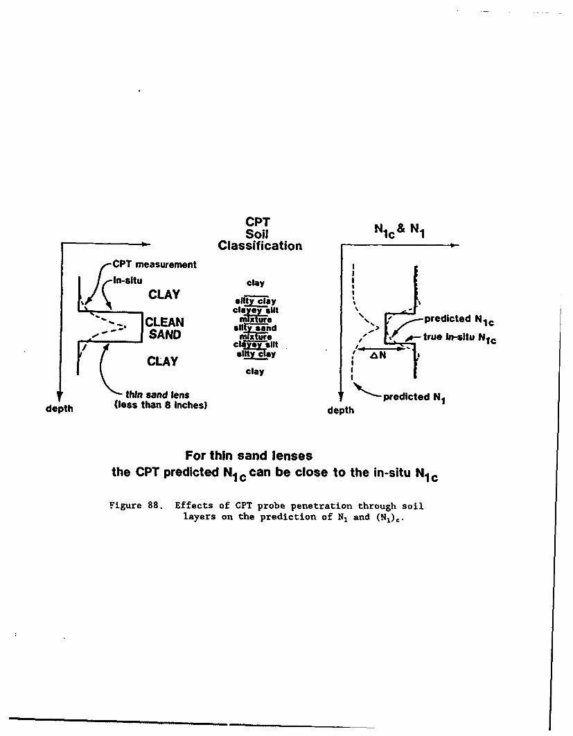
CPT N &NSoil 1c I
ClassificationCPT measurement I
Iln-situ clayCLAY- silt~y___a y
ciaynd silt- SAND FOLXtue n-UtuN 1
afltyclay # a N(~rn CLAY ca
thin sand lens *-,predicted N1depth (less than 8 inches) depth
For thin sand lensesthe CPT predicted Nlc can be close to the In-situ N1 C
Figure 88. Effects of CPT probe penetration through soillayers on the prediction of N, and (N1 ),.
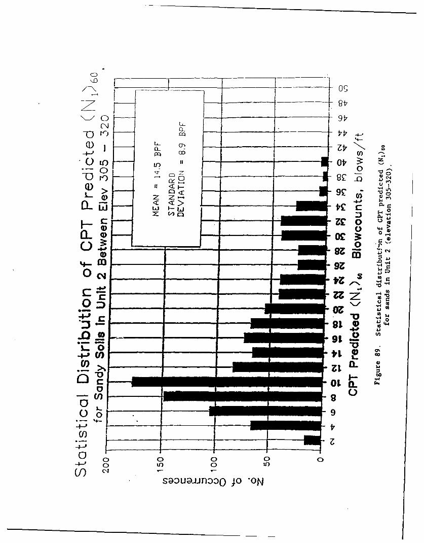
zt
V)) 0~
00
9C' .4
ccn:34.0
~~0m >__
444
or- _ _ _ _r
0 ~ 10 0l 0r
-i--' 0U) 0UU(I) C~ a-za
4~~JfZ3 0O oz 1
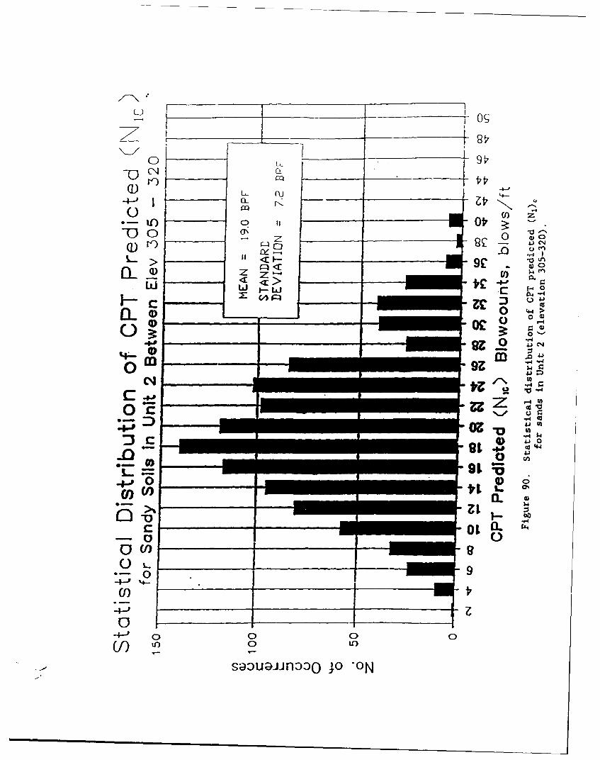
CL _ _ _ _ _
4-P
*-C)f0 C
0~0< 9
z b__4
mA - -.0 44 >
j~ 4)4
coco flL.
-o 0QU) -9C
-0 9z
0 4-- '0 %0 0 0
(f) c 4.)
S~ZU~~flsW 4i *0N
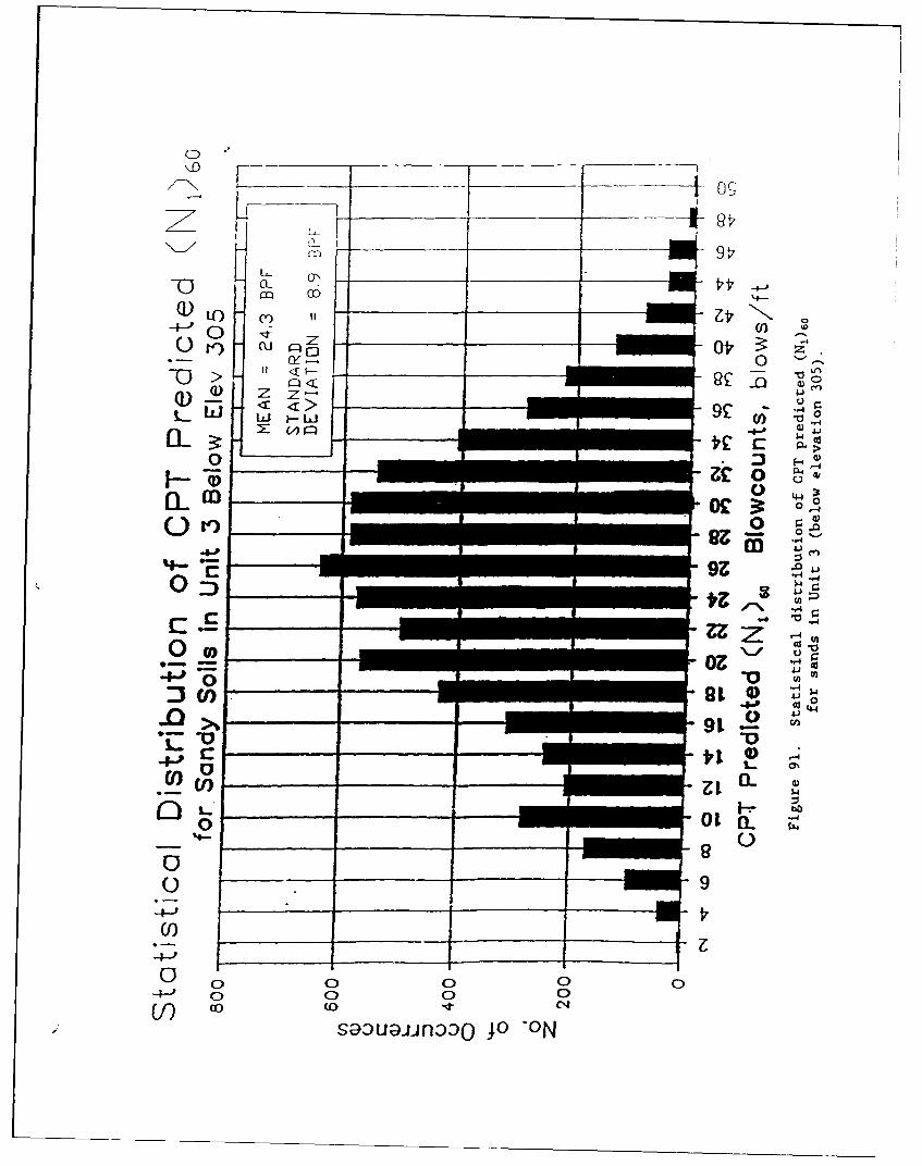
CD
m co -~
0~ "1- ::,
LW~~" Lin-J )
.0-0
~4~00
J U) -I O
00WE -0 9t - .
'4--
0auino 00 'O0N
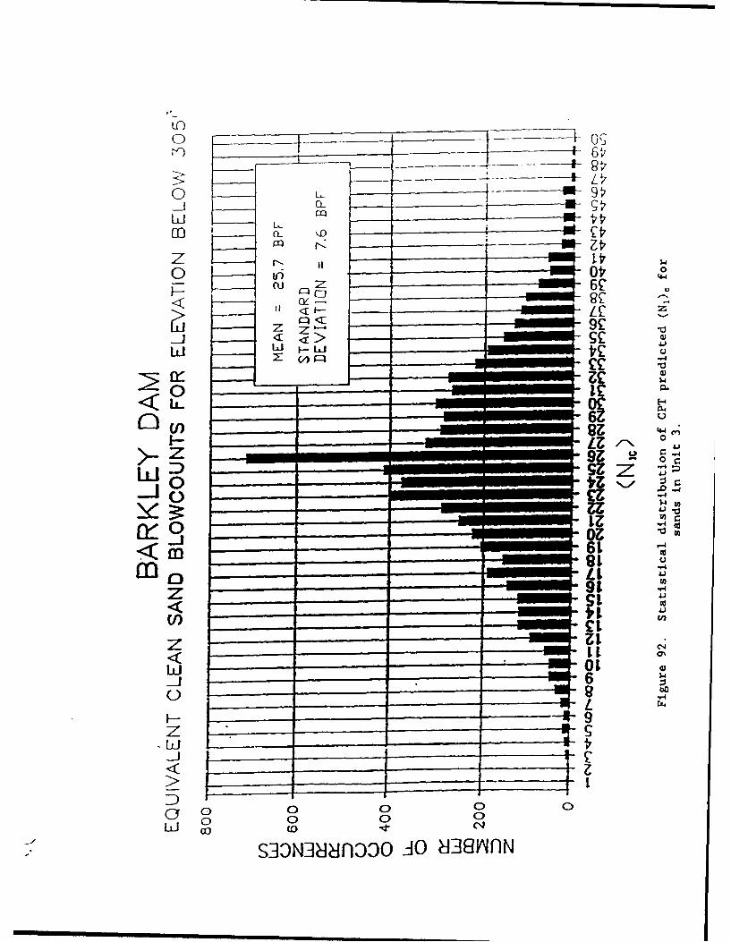
In)__ _
1CY) -
< LLW
C) U) 6E_ __
9z 4
z~ LIP
9z
L GI
zr __4_
U) ____ L
-J4W
0z t(0 C14
SJDN~~d--AWOL tA tI8Jl

-4--4
U) _ _ __ _
0 4) L-
Ld
-4--a
Lio l:
I-. (I) ý
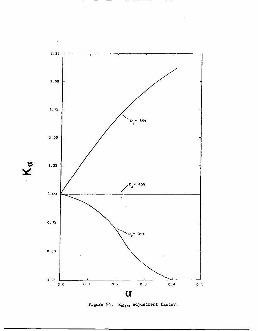
2.25
2.00
1.75
D 55%
I. 5O
1.50
1.25
Dr= 45%
1.00
0.75
D =35%
0.50
0.25$0.0 0.1 0.2 0.3 0.4 0.S
aFigure 94. KaIpha adjustment factor.
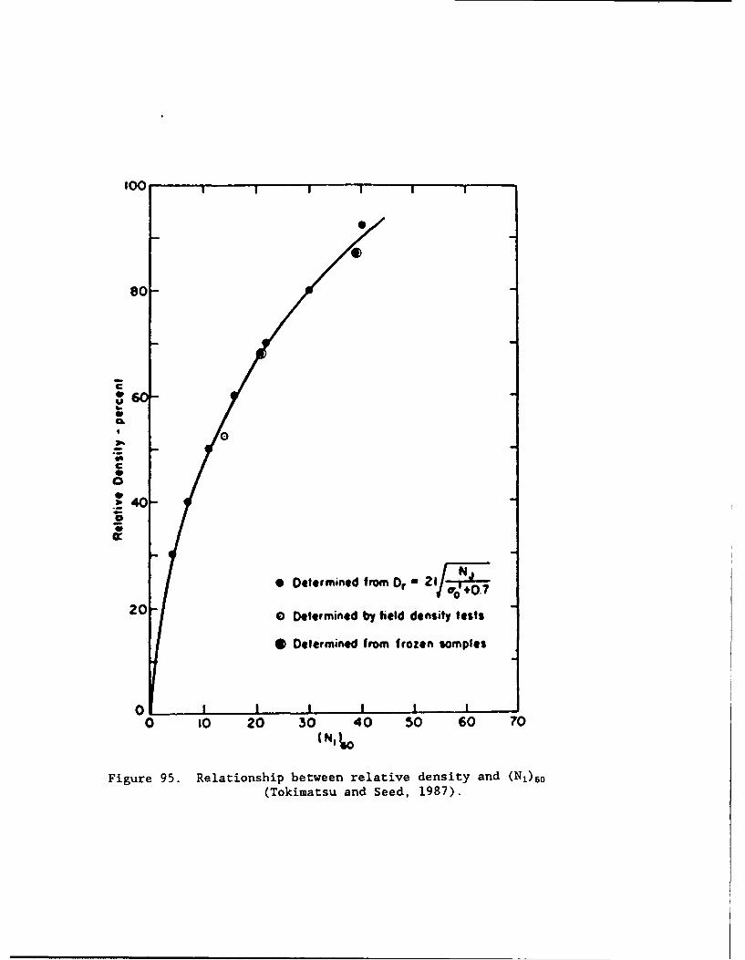
100
'80080,
CS
0 A
CSa
.1 2 40U
(t* Determined fro Dr " 21 T•
20 0 Determined by field density tests
* Determined from frozen somples
00 I I I
0 I0 20 30 40 50 60 70
Figure 95. Relationship between relative density and (N1 ) 60
(Tokimatsu and Seed, 1987).
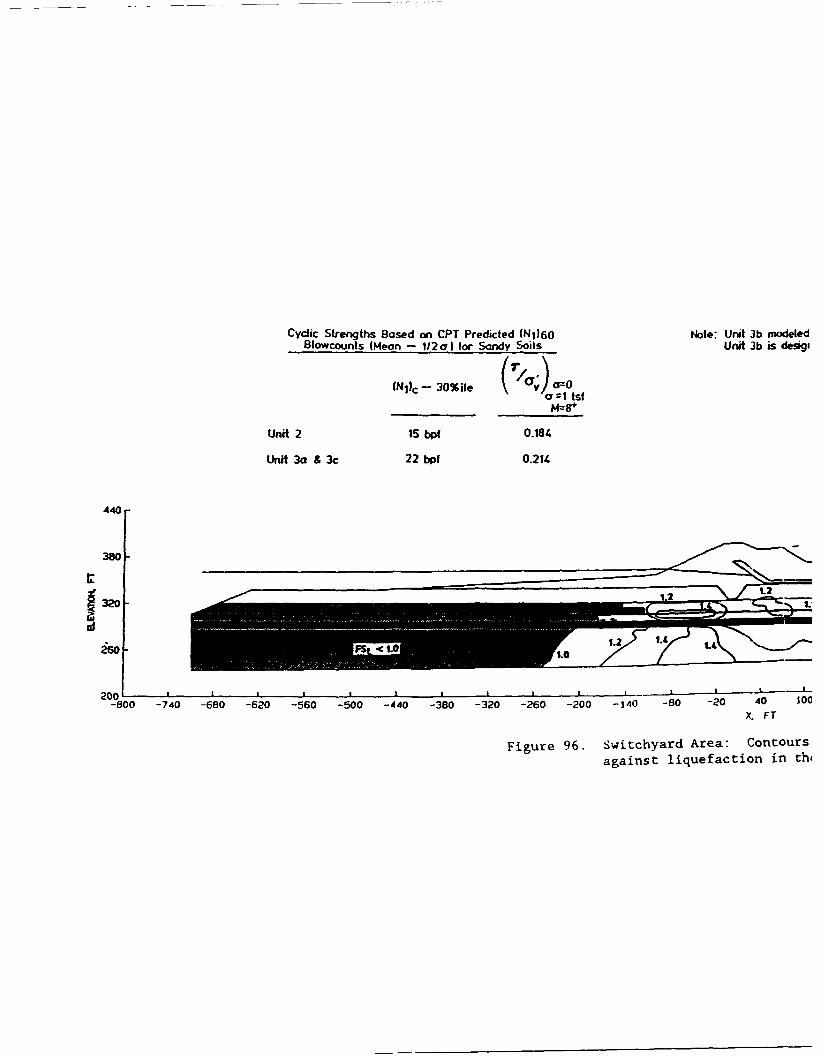
Cydic Strengths Based on CPT Predicted (NI)60 Note: Unit 3b modeledBlowcounts WMeon - 1/2a} for Sandy Soils Unit 3b is desg,
(N1)c - 30%ile a"ot o f
Unit 2 15 bpf 0.184
Unit 3a & 3c 22 bpf 0.214
440
380-
320 -S 2 1L2.
200 i-800 -740 -680 -620 -560 -500 -440 -380 -320 -;260 -200 -140 -80 -20 40 SOC
X. FT
Figure 96. Switchyard Area: Contoursagainst liquefaction in th,
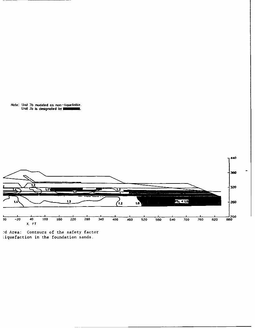
Note: Unit 3b modeled as non-liqetiobe.Unit 3b is designated by • .
440
-300
IL2
1.2-- J.2 10C.-
to -- 26.0
20030 -20 40 100 160 220 280 340 400 460 520 580 640 700 760 820 880
X. FT
:d Area: Contours of the safety factorLiquefaction in the foundation sands.
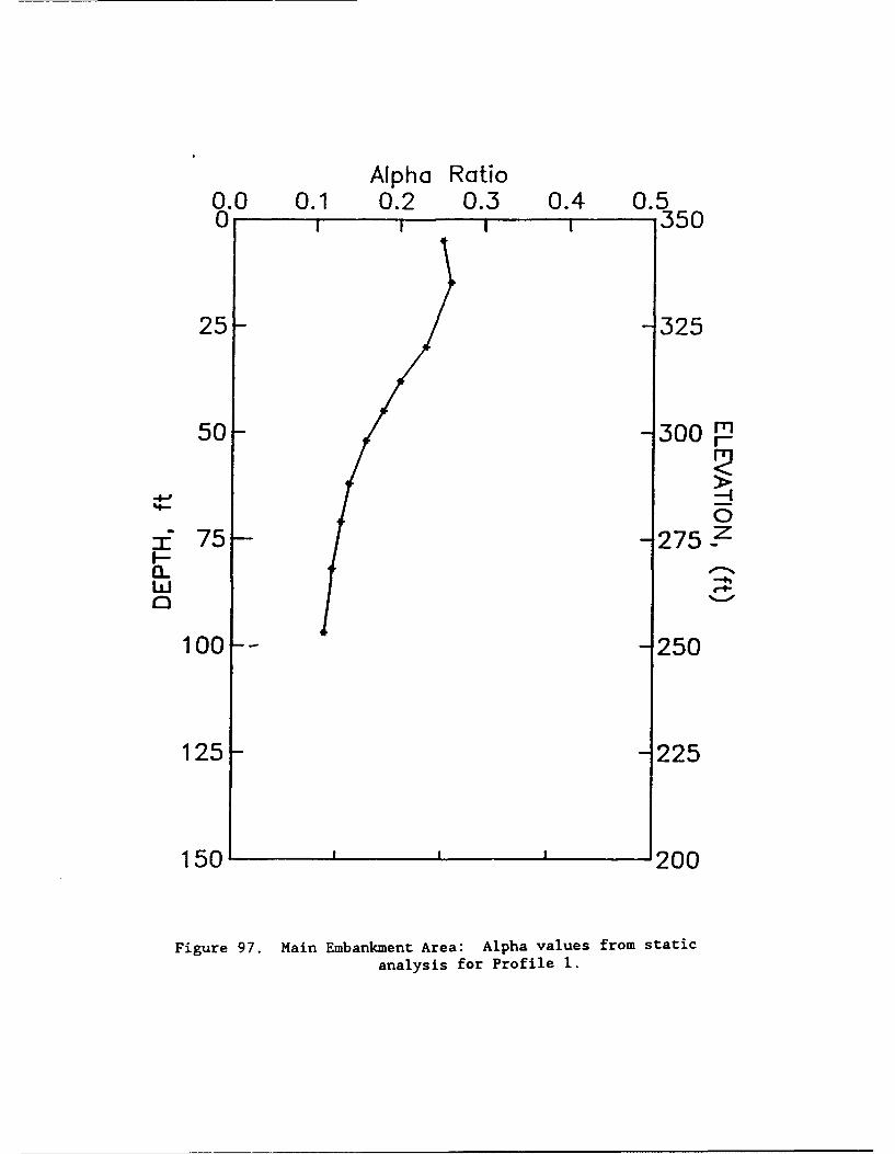
Alpha Ratio0.0 0.1 0.2 0.3 0.4 0.50 1 350
25- -325
50- - 300
'4 0
S75- - 2 7 5 zI--9° 1 1
100 -- -250
125- -225
150 200
Figure 97. Main Embankment Area: Alpha values from staticanalysis for Profile 1.
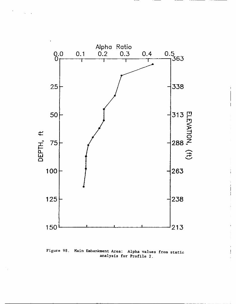
Alpha Ratio0.0 0.1 0.2 0.3 0.4 0.50 1 1 363
25- -338
50- -313
4- 0
n5 7 5 - - 288I--
100 -263
125- -238
150 '213
Figure 98. Main Embankment Area: Alpha values from staticanalysis for Profile 2.
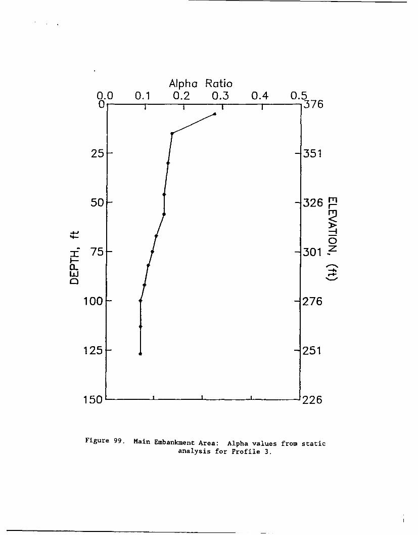
Alpha Ratio0.0 0.1 0.2 0.3 0.4 0.50 1 1 i 1 376
25- -351
50- -326 m
-4-J0
75- -301 zI--a
100 -276
125- -251
150 226
Figure 99. Main Embankment Area: Alpha values from staticanalysis for Profile 3.
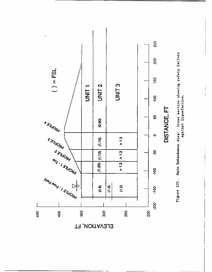
00
ICM
0 C0ocob
-- JClC)
0
o Cu
U) L
C- 0z z 0
zD W
A
0.J r9-
so_&o A C8
0 C
0 0ato 0 U) 0 0) 0
() m9 Cm
Id 'NOliVA3913
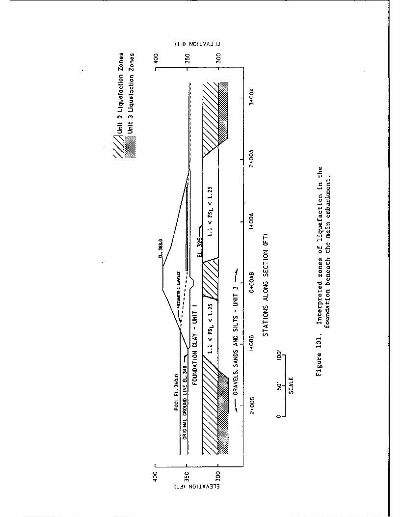
(1]) NOIIVA313
C c rn e0 0
000
+
44
I 0+
-44V 4
w ,0
0**
LA - 4) 4
-a3 ZL 0 (1
0* 0t:-1 4)4.0
0.4
z 4) 1
000
2.44
z + -40
C0 Ln b 0
-
V0 -U
mz * Uo 0
oz
0 t
(13) NOIIVA313
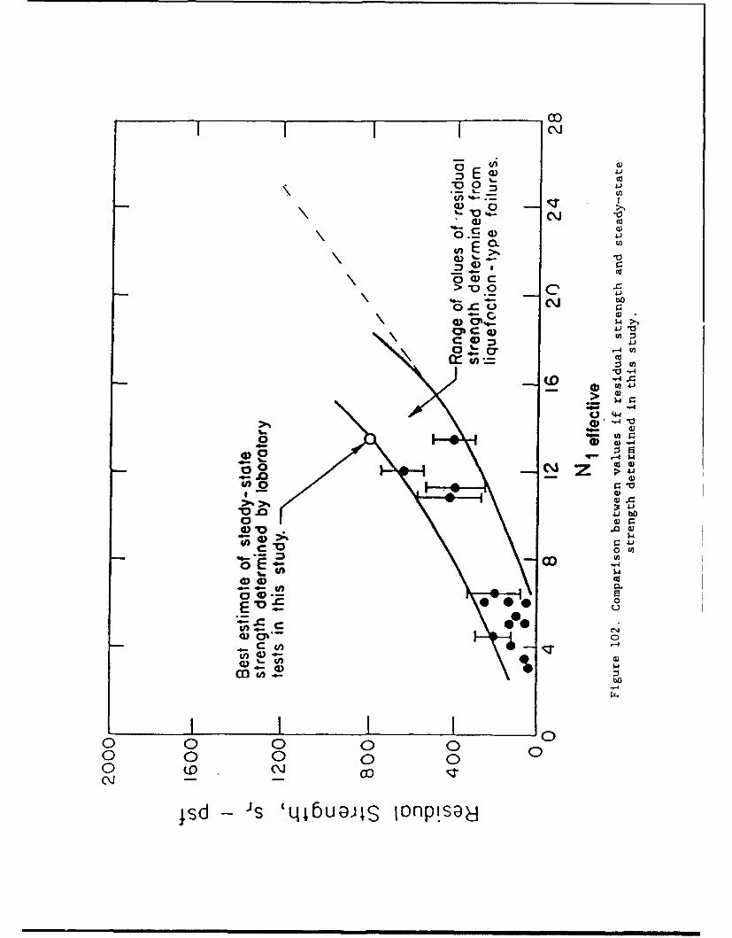
coI I IC~j
:9 G 04.2
CQ
bO
0'Coj
C 4.2
C)% a - 4 En
'4- 0d01 -4- -4
4.44
oo~ Z Cd44 -n )
"0 m 4.) bo
0 "
00S 00
0E -0~ 0
0
o o 0 0o o 0 0 0o 0 C l)co10
Isd ' s '14jbu~jj joflp!s@ý
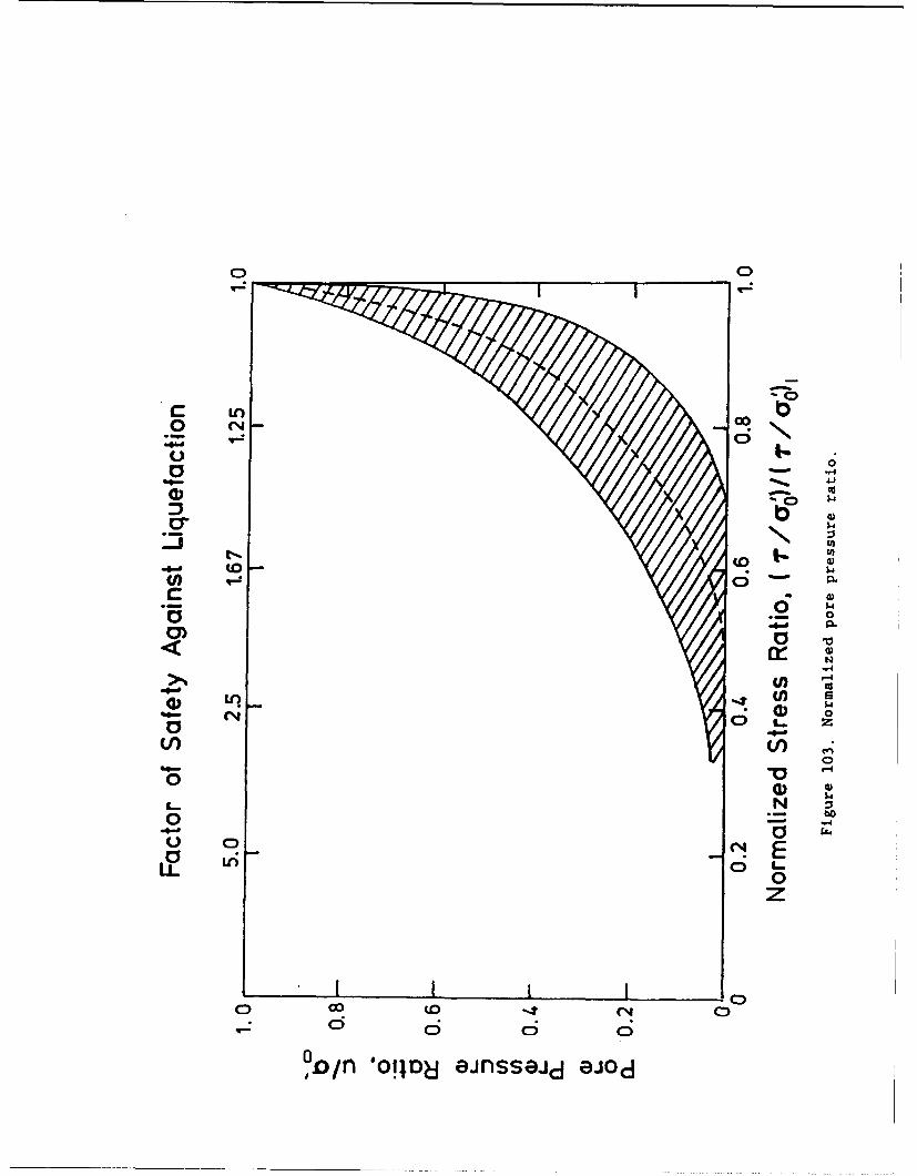
0 0*
C LA
0))
a-r-4
N
0-
C)
0
CDo) coC4Coi
O./ OI~ ansiiao
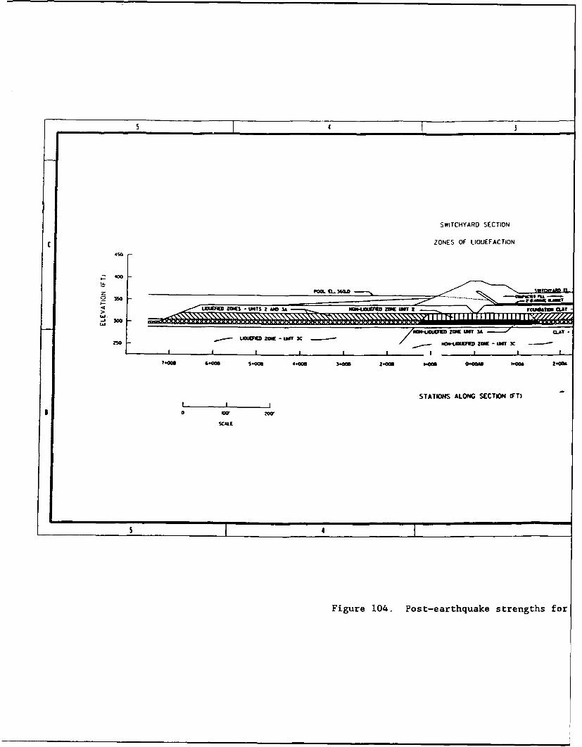
SWITCHYARD SECTION
c ZONES OF LIOUEFACTION
4i0
400
z FOOL 0.. MAo~ - T -TU FL_
> ___ FEmm ZONES UNWITS 2 AND U ~ N0IHJ=ZON UC liT 2 FU10 A
II I I I - I
1-008 6.011 06 S e 4-006 3-008 2.40101 6.001 0400111 ",006 240M
STATIONS ALONG SECTION (FT)
B ~ ~~0 0' 2
SCALE
Figure 104. Post-earthquake strengths for
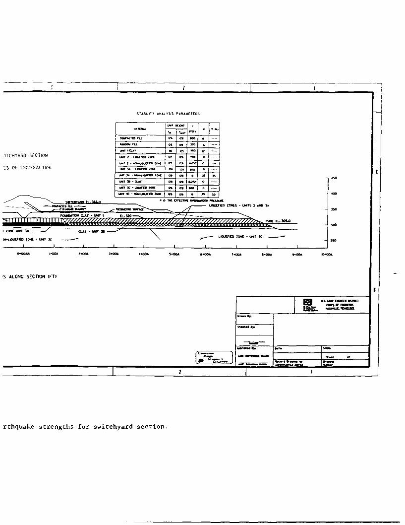
STABILITY ANALYSIS PARAMIETERS
OcWACTD VU. of no a ---
*ITCHT'ARD SECTION ukvTo~~ 2 a," ON ze -s a
LINT2 -W.-~0.,EDZW ro In m "£5 OF LIQUEFACTION MSTA-fZW 3. o33e ro Ca w -
ml 1 - CLAnWDw go 211 a" 0 T
uwr x-OA twnc z as weZI 0 -
wa x - aLnwrDZ@ [aa e as 0c " I-oA
WST3C-tWDZS [UIS aS AN 3A
L1~mn
)WOW ZOW - I" X. iaiL)FS2ED -O IWIT X -~.--- 2
IIIII I I
0-0011 I.<" 2.00* 3-004 4.001 5.00A 6.-00* ?-ODA 8.004 9.00A T0
'S ALONG SECTION (FT)
SWM DOW7 T67WLtwo% IF 00
_____________________
rthquake strengths for switchyard section.
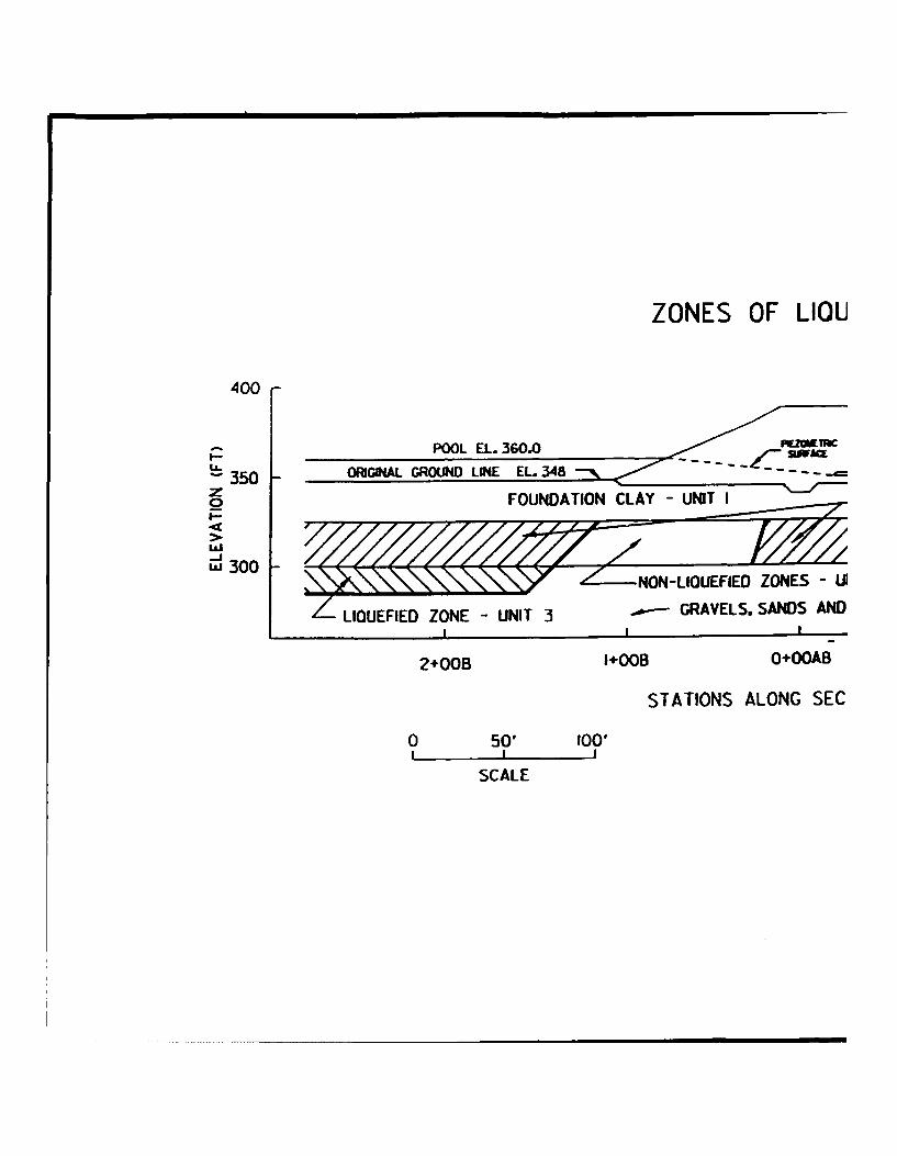
ZONES OF LIOU
400
POOL EL. 360.0 FIEZOMEC
350 ORICANAL GROUND LINE EL. 348
o FOUNDATION CLAY -UNIT I
w 300NO-LIOUEFIEO ZONES [A
LIOVEFIED ZONE -UNIT 3 GRAVELS. SANDS AND
2+0013 I+OOB O+OOAB
STATIONS ALONG SEC
050' 100,
SCALE
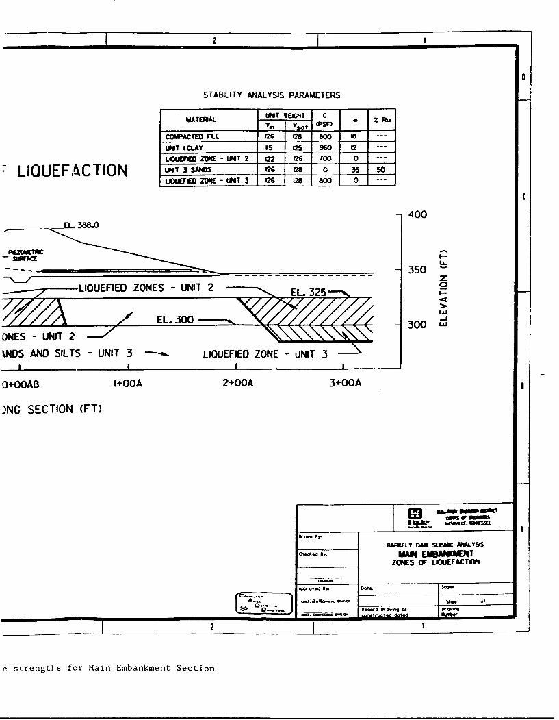
1 2 '
STABILITY ANALYSIS PARAMETERS
LINT WEIGHT C
'r. I y t PS:F)
COMPACTED FLL 126 028 800 is ---
LIT I CLAY as a2s 960 12 ---
LIOUEIFEWD ZONE - LIMIT 2 122 126 700 0 -'-
LIQUEFACTION ,Lu13s SAS26 I2 0 3 50LOMFEZONE - UNT 3 26 Ce 800 0 "_-
C
- 400EL 38&O
-- - - 350-LIOUEFIED ZONES - UNIT 2 aEL. 325
EL. 300 300
ONES - UNIT 2 ---- / 300
%NDS AND SILTS - UNIT 3 • LIOUEFIED ZONE - UNIT 3
0+OOAB I+OOA 2+OOA 3+OOA
)NG SECTION (FT)
BANEJY DAM SE&C AMLYSS
Owked or. MWt EIBAI5WITZONES OF LIUOEFACTON
ADwo d ey, DoteSo~
ou•.Soo ofNn o,4
e strengths for Main Embankment Section.

APPENDIX A:
SPT DATA PLOTS
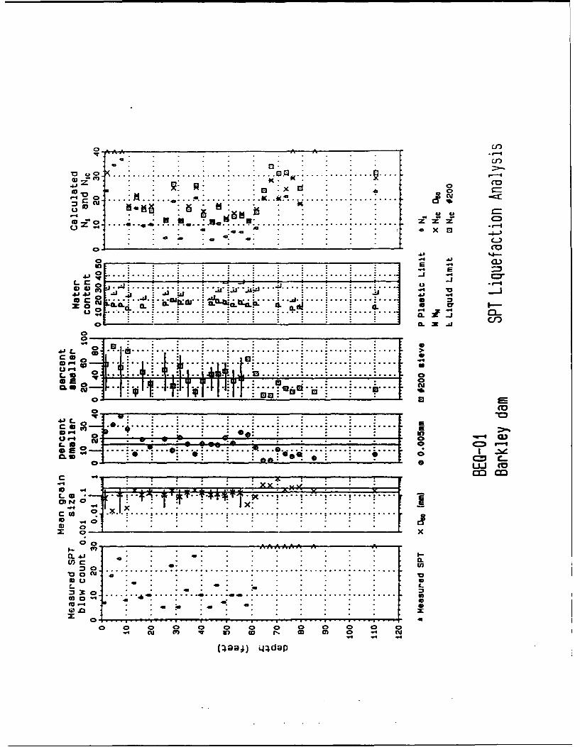
0 ___ __ __ __ __ __ __ ___ __ __ __ _-.___CC)
A .-uCt
...... ... .--
E 0
o..............,.................... ............... ...... J c-
0L C u: IL -0 .1) 0 ".......
oW " . . . ...... ...
. 0 ....... .... ... .... .... .... .... .
-. . ". . . . . ,
Coo o
. ... ."... ."u...
4 . . : . ....... ..... a
""t""0 : ...
0 4 . xe S
, .. . .. .. . . ......
i.41 -.. c. 4.
c.m -- • -•,-•• -,• ±"--. - -. .r' - . , ... ' " , "
". . . . . .. . - - . .
S... . . . . .•.........0 0
{Oc- • m (
•• .
0 0 0 0 0( 0 0 0 0 0 0 0 0- 4 ( U I ' ) 'q i n I- D r -. 0) 0 ) o .,4 ( Ul
(:•aa4) qjdap
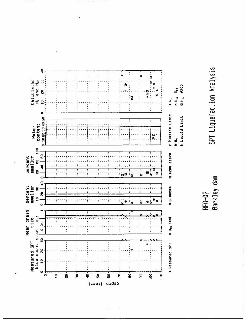
cJ)
o A , -. .L.
toU .. . .. .. . .x . .
m 0 . . . . . . . . . . . . . . . . . . . ... . . . . . .. . . .
:3 I........... . . . X
0 . . . .."o.' " (0 -. :- - -C:
CD,,
oo 4' 03
EU.* . €, 1.-
UU
00
S . .. - ..... .. ...
00. : 0: : :E o
0a.• : . : : : . . . . .. " . .. .
CL w .. . . . . . . . .JJL 0 . .
. ... ........ ."r ... .C .. . . . . . .. . . . .am o LY{1
CL .... . . .. .. ... ....
t n C .. . . .. . . . . . .. . . . . .. . . . .. .. . .. . .* a
ME
0 0 0A ," .0I-u M o o r'G () C
* . .. . .. . . .- i -if 0 ~ . . . . .. . .u " "
33:0
0 0 0 0 0 0 0 0 0 0 0 0.4 • • q • tid rI- a) (3)
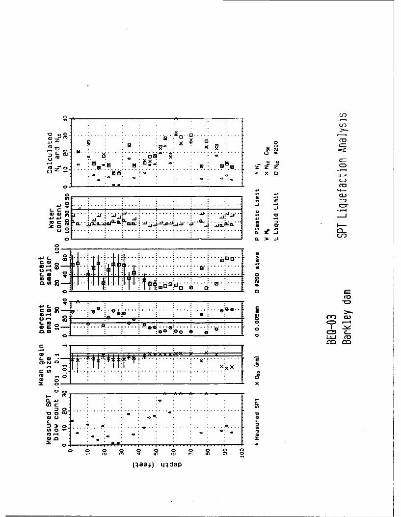
o co
"0 .. .. . . . . . . ..,.°.. . .. . .
w-• 0 .. . . .-. !-
a • • " " ." .s . " .. " -I--'
S= o -,. -., ,-,-,-.., -.•.,..,.,. .•.. ..-. - - - .- . . , ---° ' F ... " . .. : .. " .. "... ".. . : . . . . .1 E"'-u m on! :] : : :
L~to C =*1)
S. . . . . ... ..... . . . z.z-"
04
oiV: 1:•: - €_
4j .......... . .. . C, x4) 4) ... . ..
S o .. .. ..... :.. - 3
0. -
401 E
. :: . . . . . . . ..0::. t o .: .,,0 0. 00 0 0 % I
0*0
4()g P-1 in cr) LP
LU c
0 0
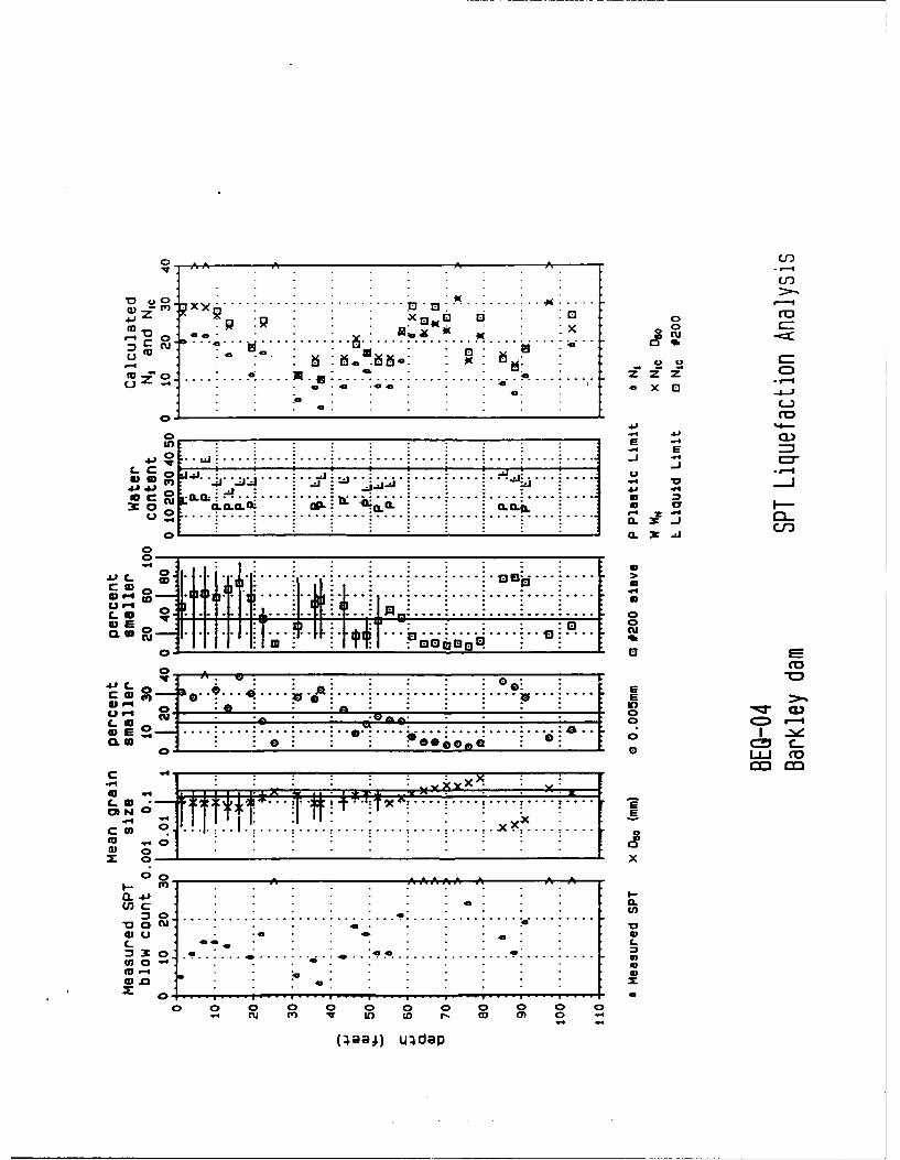
o "~ " . A A UJ)"3-
Ur)
u 42
.c ~ . . . ... • .
.40U
to .. > . . * .. .
* . * . . .. .
.Aj
-j r
L . . , 3 ... . ...I~a 31 I -1 C23"
L x 0J. ........ .".-. ._U
-r-- l
I _ _ _ _ _ ____ _ ,.,.,_ _._. ._ .. ,. ._• .. .. ..i ..•. ." _ .. .. _,
o00. - -JC.'
L 0 o . . .i. . . .i...... ... . ...i.... ......• .- ..... >e -: 0
c. u. . .. -,. .... c
___ __ __ _ "_L 0,. ............
•.48-IL xc
,- 9 ... .... . . . . . .- j C .... .a . •.
So . . . . . . . .. . .. . . . . . : . . . . . .. . 1.. . " . - . . - . .
S. .. . . .. . . . . . . . . . . ... . . . . ... ... . .. .. F1 . . . U
5 • -4- - .• .. . . .
0 . . • . . • . ..*. ..,. . . . . . . • . .. .. . | . . . | .. . .. .
00 0__ 0_____ ________ 0____ 0__CL o5)0 . C . .
0) uU)0 0 0 0 0 0 0 0 0 0 0 0
(984 .ad
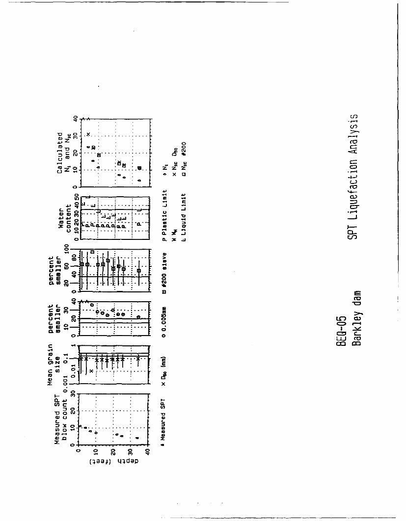
cT)
T)- 0 x ...
1-4u
CC
in aE -
=J ... .. . -i
41 A* -a*.IJ 4
3: 0 **c-m :4C 0 c
_ _ _ Cl)
0 cu4--14JL w c
0
au 0A0 LU(
0 .
LU c
c U ...............
0..-
U) c 0.
L
0 0 0 0 0 o
(;~)L~dap
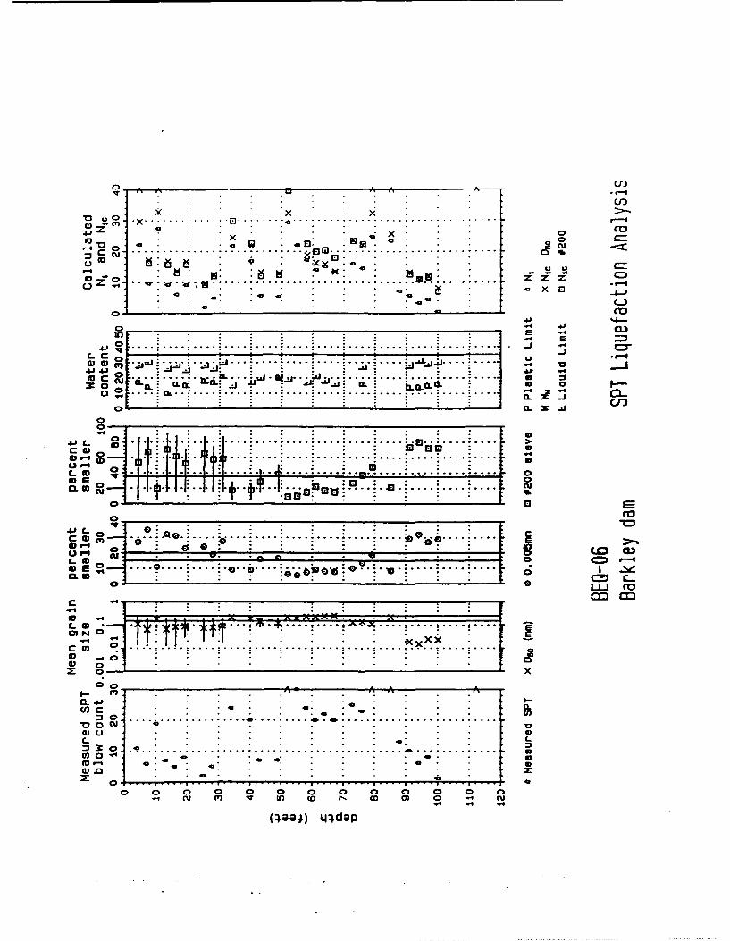
o A .A, A A - ,-
U:)
x~Io . x- x . ... . . .. .
C 8 . . . . . . . . . . . . . . . . . . 13", . . . . . . . . . . . . . . . . . . . . . "fU C=•• : * : :: .. : ::----
,. . ...... ... ,. . z X C_)
Q CO
o -
) . .... : .... ..... .... .... .... d " . .. : .... .41~in a. :- "W Wj .. L. "
o2
...... ...... .
0J O I o [
. .. -CO
Cr .
- ., . . . . . . . . .. . .I . . .. .... . . . . ....... .. .. ...
weN 0
CI ,,-- W . cu. 0.
1. 4-1.1 .. :1 .i . .
0
S.. .. .......
CL..0 -=) -
:0 C D.. .. . . . . .. .....
Eu.-' C. * w o . .
G n " ". . - . . . . ." " " rz o . -. ... . ... . .. . . . .. . .. . .. . . .0,.. . . . .
m a3
L ...... Q Q.. . 111 - •IIU ,- V ITT . 1 . . .. ... {
c 0 . . , . . . . , . . . . , . .. . . .. ..... . . . . .,. . . .. ,. . . . . . .
O x O 0 0 0 0 0 0 0 0 0 0
4) CU ILI ) 0 t E ) 0 I
C)~~(2 a~ .. . .. . . .... ....
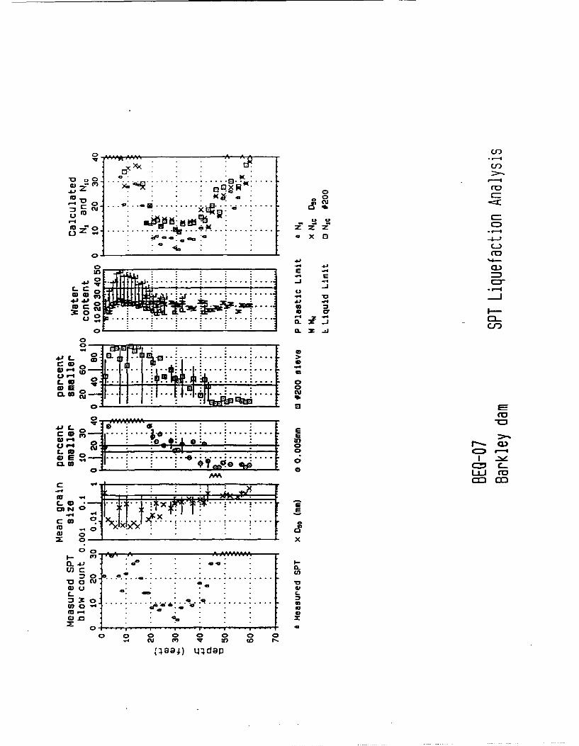
YOVOCiK
crC
to . -o
(-.-
x-J7 x-a
if)w;~ I.. A i .Lf... i...... .... . .. -
g 2m. . .:. . . . . .:. . ..... -,. : . C3: 0 CUVW O . c .
__ _ _ __ _ _ _ C3)
0 ___ ___ ___ ___ __
""C' 3. .
1 C-_.... .... ....
S.. . .. . . . .. . .:. . . .
C C-
0J o
g • ,• ix!• •'... .. .. .; ........ :.....0-
_ip :.. r C
OOo
4) • 0 .... i.... •... .i.... 0 .. .. i.... . .. o
LLA
50-F X . .V * a
L00l 0 0 0
c4 w
a)~ da
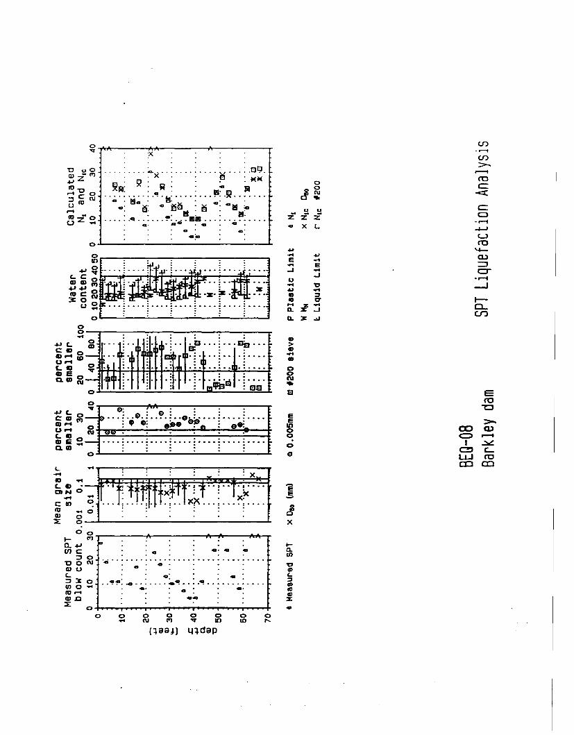
( A At A - L--
"0 . . . . ._ .. . . . . . . . _ E E?
Ci)X fu"D~~~~~~ uo. • 1 '
S. °: : o: ..,:° |•
0 mW).. q. .: mn.u...:..... z. -r I
L) 43 a Q• . a . t , X L, -.-
•~4 • 1•
,:a "a L -
.. . . 4.-
C)-.o ro:: : : : : - ." ,fJ
S.c -,C-
ID. •6 " " - "
40 Ccu
- -.i L " a.: : _E
0*
D '.j... .
I" .
*.C . . I-:30 co
to,,. . . a
S oo o
0) FE
0 0 0 0 0 0- 0=-x 03 ' I o r
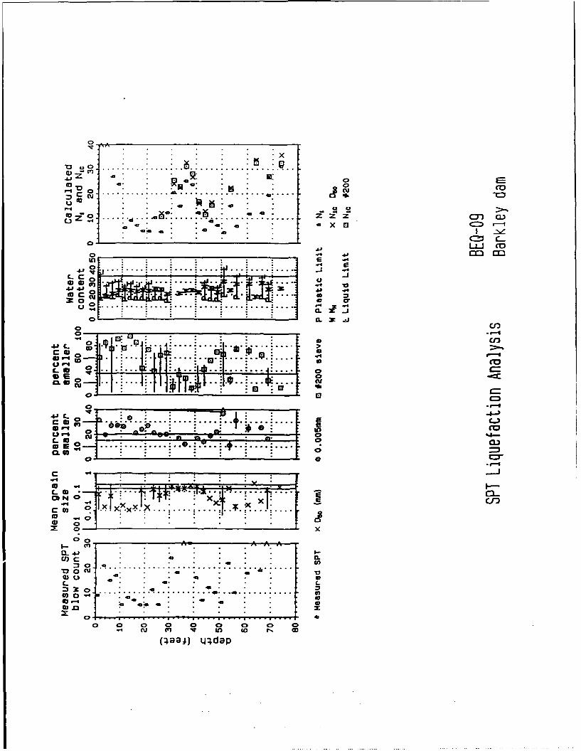
0 0
* . . . . .. .:.:S.: ... .. . .. . : ...
"0 10 0'cuZ) cu- eJ. . .......... ........ ....:' ' " .... "? 4
SZ ....... 4 • u..........•............ .... C C
LLJ co0~
a . . ......
14 CL
me -J
o.O4 o, -- .i
0 =,-0
U3
0-
I.! -- I
•oiO0 ,o=,,uu ,
ItTT0 CD
C 3 0 .. ..."... . ." CV a 1w -. "'No. " " " , ." 0
I .. . .. 4.. .. . .. uo-oo I1
w r0 . •u
0 0 0 0 0- 0
it :e I" -,
o;-
c U C! . .XX . X . . .. . ...
~00W. . . . a .?
0)0 a . . .
L 41:
.. .. .... .a 09) a4.. .: ... :--
0 0 0 0 0' 40, 0
fl88aj) LJ4dap
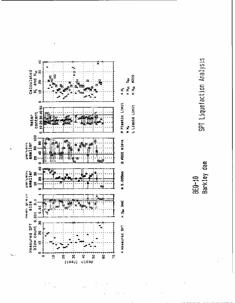
41 0 0 C2
'13 0
u toto *.6. Lei .1. W 1& 7- Z ZZ-C- 0. 4 . em .0 x 0
-4 CD
E_ c
30: 00)0) U3LC0* 1 0 ._C-JCD M
coo ..... ...... . c
00
_
aFEE
0M0
0 a ix
404~)N 0
(D .
w 0x
Q 0
cu *n tn w P(-taa,' q-,dO
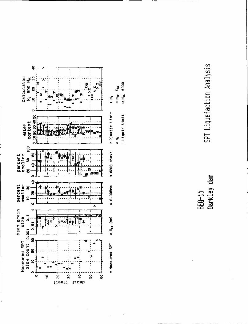
C3t
V ~OO
c .......... . cy 0I
m c M. , : * *mlq x :
00 x (l4-
%4 -
4JL~ .....
ii. I._____ __ 4
LU cu x~A~r39 II
aaU6
0 cuCL 0 cu Mt
CL
C;
c .4 .I .to C .. . . . .
00 . '' .
la o .u
0 0 0 0 0 0 0.4 cu (F) U') to
(;a) L14dap
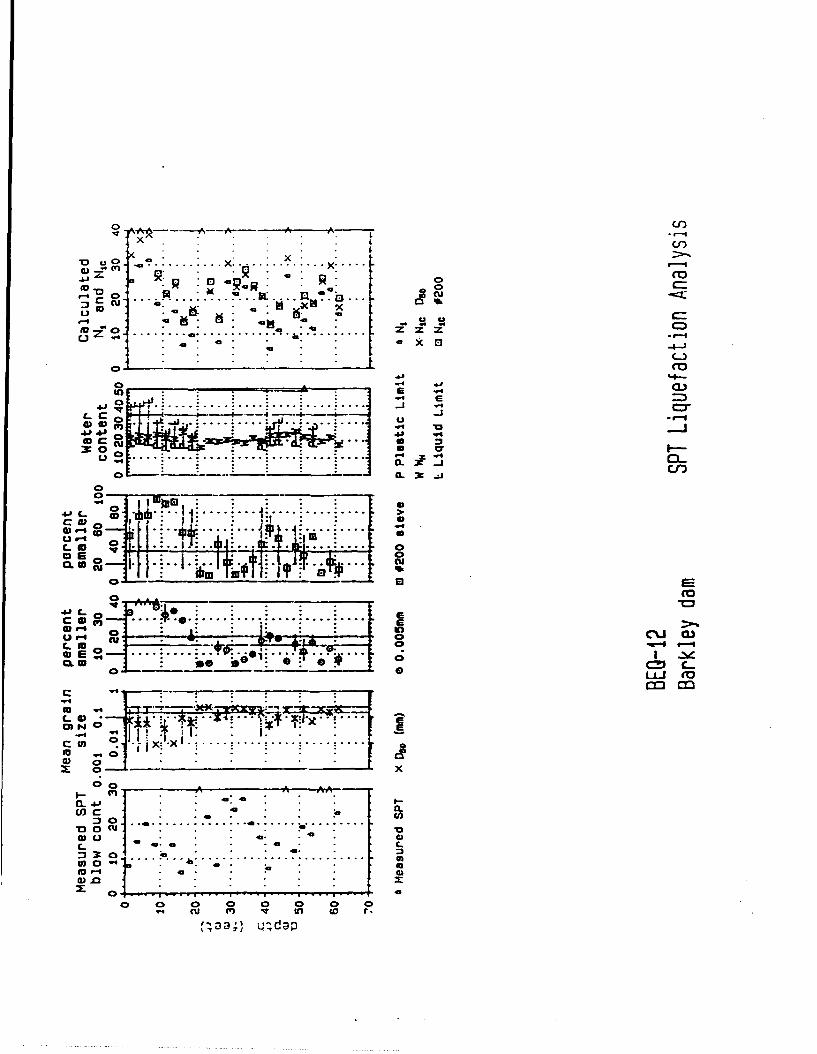
o ---- ~-A----~--A -cJ'I
Ax.U
•Ou - . -l , X ."x -m
0'-
0.......... -.. o..•.m a: .. .. '' '• *" . .'( . ....... ............ . .R. :. R -m -
,~j a.. Z Z •
-- -- • . . _ .:. e . . . - -. , . . . - . . -X . . . .l~a=4 .L o •,.. ....... .,•X~ El
C13
o.......... -fo C
.430 .4"
CU g
0o I 01 0 j
41~. C- ... .. ..
c00-.,P
~q :j'} -'d 0
C 0 cu
.6- -C-
13 - -
cc m
C;O . .x4 V.
a .-
cn c 40 . w
40 4m 43 (f
:3a~ Xa) . . . . . . . . .. . . .) 0 1 -b'- - .C
to --4a
Co -
S cu mq IT in W
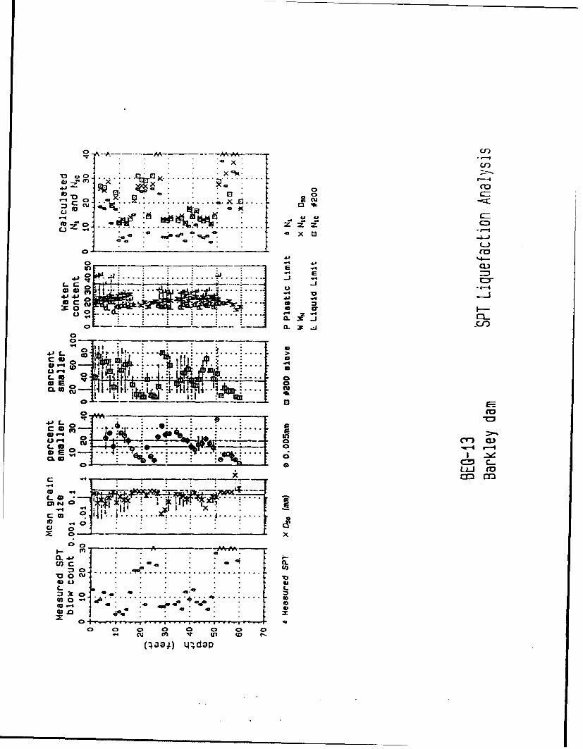
x.� ................. .
4 X a.•.... -Ca-
4Ca . . a a. "Eto "4-l.-!TT'- ' :•o
a aO
u ,4 !.. . :... :.... .:.... :.... . . .
to o ... , . .U'
------ - -- - -..-• -, n r-i----:.---,,--.-:--- -- .. 6-.
03 .- .. .............
c~~C 3c . .. . -:- -'
44 J L.
Al a
C- v
it.. I• .... • ...-iN.
"I NIa ' - c
~~ 0 . ..
03.4 CU M a
I: o--L- .r . . . ..m, 6
CL 020
•-Mo C•CS 1 , 3 J- (DA
_ _0 CM
. .•. ... . .... .. .....
C x
0 3 . ".
14 fi.... ..
Q I .......... . ....
0 0 0 0 0 0
{4a U C) q',dap
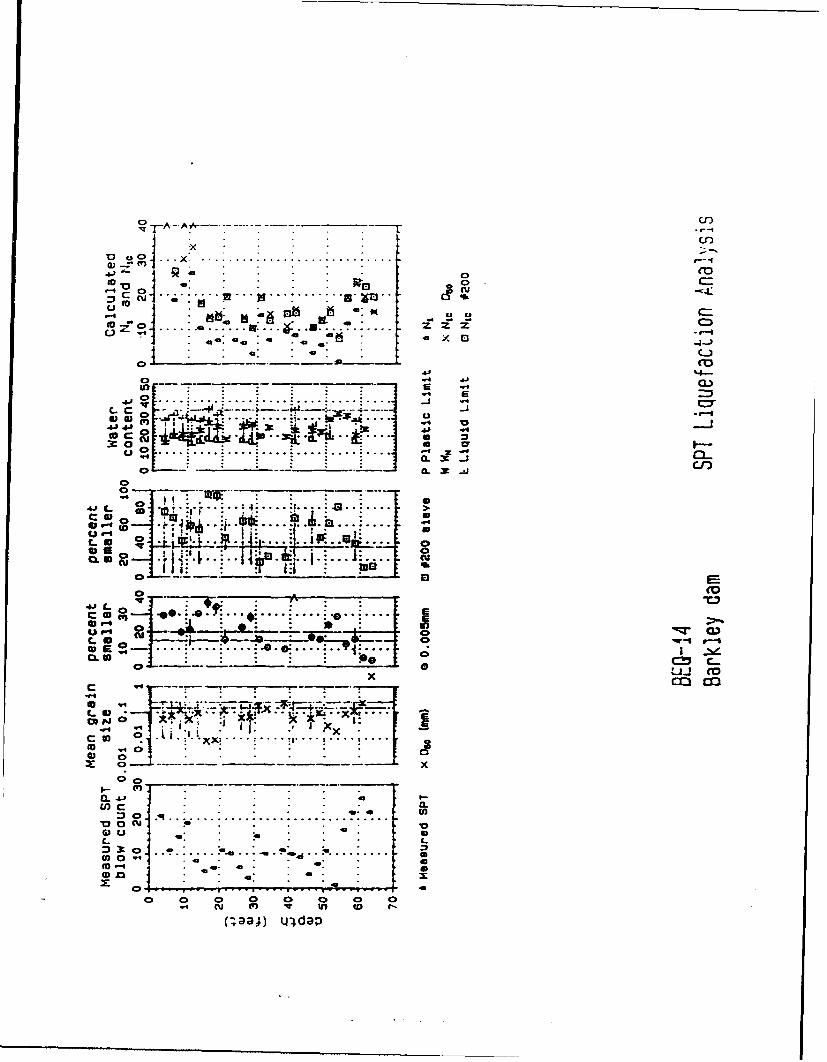
oT -A - A-A,--- c
A.. ____,'• -:...:- • C "nx
13~ 0
S. .... . ..... .......... ... . :r Z_
V- -; i,•. •..-.... .... .,...•.. ..... ... t
a.
0 or
o __.____: • . .4 d
i 4.3 0. "I
0. - ILl X :j Ln -' 1• E
o,- • _. _ .. _ .. _ .. _ _2_- .. ..... .x I
toU
:- : -Ow:
0 0 0..
(cu " "Eql .. .
Sa 0 ... " . .J . .. , .. ,. . . a .. .-..
Cnc ,", ., . . . . . aa L .D
O ) )...... : ..... . ....- .- ......
0. 41 4o - 1 . a
0 0 0 0 0 0 0 0
4 C•aa ] i dap
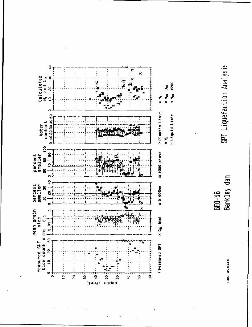
UU
I~
L 0 ........... ff11 . ex-_.f__ _ _
fo .0 i ... ...... ..... ...
a. .. .4 a .. ,.F --±
o : : : : : : - " . 1 o:x-i
00
0• --..- . .• . .• . .- - -- - -.-•• •-- - - -.. .. •"-
S .4. .... . ........ .
U4JL .. . .. M
C),
S• . . ,
r- II : : : "• , , : . .- : . . .• . . .... •... ....
WE • • p • • . .I .'I.m. .. .. . .. . r ... ... .
I10 •1
CI-" r • • -'.1.- - I-'
° " : ! ._ 0 !l " "" .... .... do.. .
S. . . .... .... -I
0~a . _ _
0 0
m F
L La 0 .. ......... -0
0 C
0 0 0 0 0 0 0 0 0 0 0
(;ae4) Lfldap
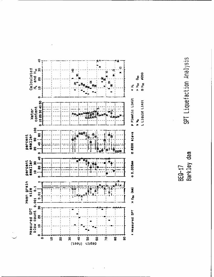
"0 ... .... . ... . . .. .. .. .. .
cu o . ..&) (K
0)
u 4 J
* . .. CA
.............4.ij
41 4 1 M
.to.CXJ(1
-I-..
:. i ... ji01,i
CL~~~.1 0. ..... ... c
. .) r- o.)
CL 0
LLJ to
)K- --- *
C- .0 .... ..... M
U) . . . .x X .
0 ) 0 U) .
.0 0 ------ A--,-7%
L. * O
:) 3 ... .... .... ...
0 0
(l~a4) q~dap
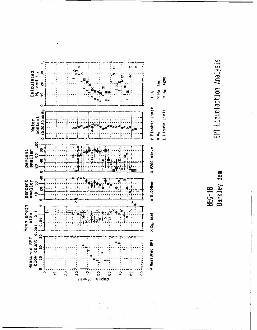
o .I Cf 0
xo.
ela
0~c "A-, m•............. - .. . . i 1,•f'
"0 to X -*
u 4 . 6-". . ... 9
43. .3
"o : : ' _: __la :_ _ ;= 4 : r-
z z4
o,. 4................... .,........... ,,.............. ...---• .. . .,- ---
L 0 ~
4J j .q ... ......... . ....... . _.
4- 4.--Sc . . : "... : :
o~~a. X. _a__ _ _ _ _ _ _ _
0 . .... ..... -
a . .. . .... .... .... ..... ... .- ,-In . . .. . . . " •- -"-- m :: .a : • ." .. . . . -• -- :: :", ,,.- '' . .. ,
CLC
0. . • . ' . " . ••'; : u
-- ]....:.... ...'"• :'[i " =..... •:;..... Lt-C
CA A LHC
"L 0 .---"-- ----- ,-j- ,.-
m . ......." D ... .... .... .......... .. .....
-o o . . .
S" ---- - A7"."--... .--- ~---'-- -- A: rA c
wa uh 0 . . . .. .. .
3o o
0 0C 00 0 0 0 404 l in ( ~ U CD r- w
I.-- ~ ~ ~ 48 ; t'4......- ;dm-aP A --. A -e-A --"
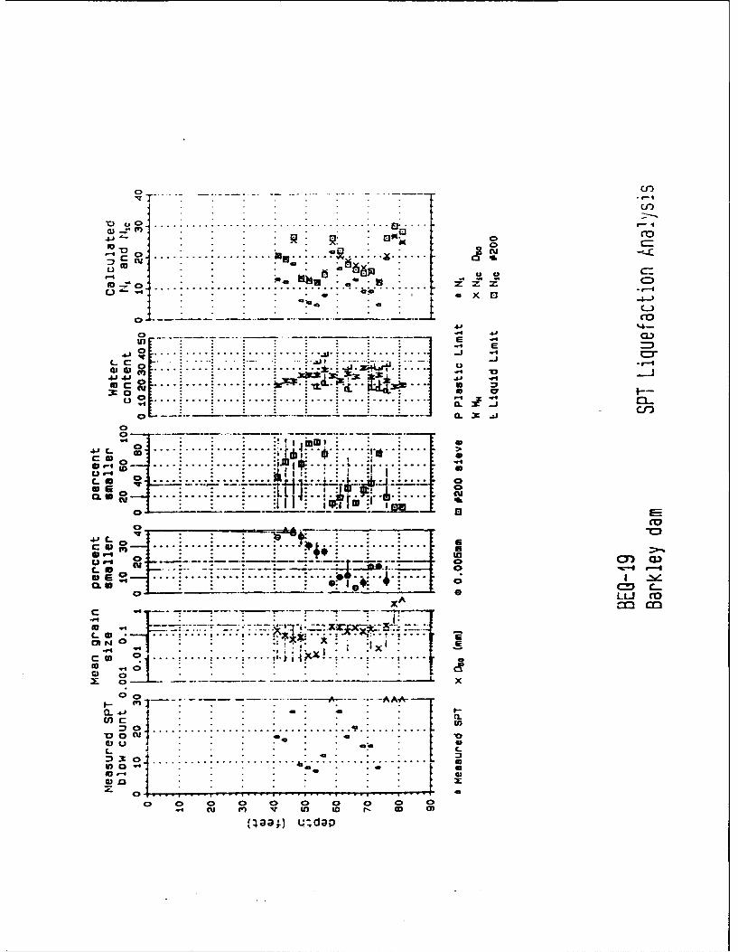
C.0
• _ o ...... ..... .. ...... ...... .... .......... -
c .. . ...o . . .X
DD cu ? 4
4J.8 .' . : . a.- .-'" • . -.• ---J400
C -.. . . .. . . . - . . . . . . . . . - . .0
0. , .... . .. ...... ..-U.; .... r,,, >X"- • -2 .Lk
3. 0 .:. .. : . . ...-.-. .
0 crr
-I• - _ _i_ IIo- . . .. . . . . . . . - - - -,, E....... .... : . ....... ..
W-f- go 0
0 . .... r
L0
411- 0. .. . . . .... ISE0 0 M.... .-.--- --A --- . -,-
a -- * . . . . . a . .v.. -"
. c'5i r- a3. .
C- a
0C 0im00f 0 0m 0-
o A LLJ C'OM: C-nS-.....
:IxI
So t ...l . ... .. ...... ..... ...... . .. ..... ].... -
0 0 ) 0 0 0 0 0 0 00
(CDa;) UUdap
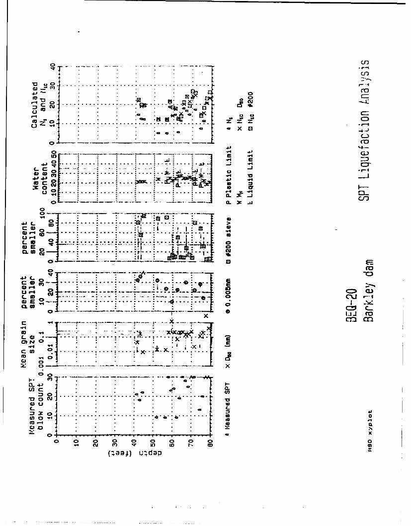
3 u C> . . . . . . . . . . . . .... . . . . . . . . . .
Ch 0> ro'U. .--- 0
0.. . . . > o_-,.• -. 4 . . . • • " ,• - • cu
. ...... . ... .. a
Ina
m --- -. 4 . . . .El I• . " • . 4 " g
S-a' .... ....................... ....-
o0 C -c--E - . " . - --.
-~3 -3..U
A0
4 0 ..... .........
F- O F - " -- w: " -' ' - ' - • -::,I : --" "... .- - -t
J~ WI
O I o . . .. . .. . S..i. . .. • • : -
.O.W E : :. _ • •. . -
€ 0 ,- C..•O...". . . .•, - -- , -- --- • a --
u ..... . .... ... ....... ...c . • J . . . .: . .:. . . :-- .:v--- : ... .00- -
C>
m ~-:.-
WI.: *c 0
2 ... . .' .
oo$C . .. a• e O..-
L 0
L. 0 . ........ ..... *... : ... . . -
O W . . . .. ... . .
-r44 . . . . " ..
•00" 0 00 0- 0 ......... 0.• X
WIC... ... .. .. ... .. .. I 'D • co r. . .. w o 0
(.aa)) uLdap
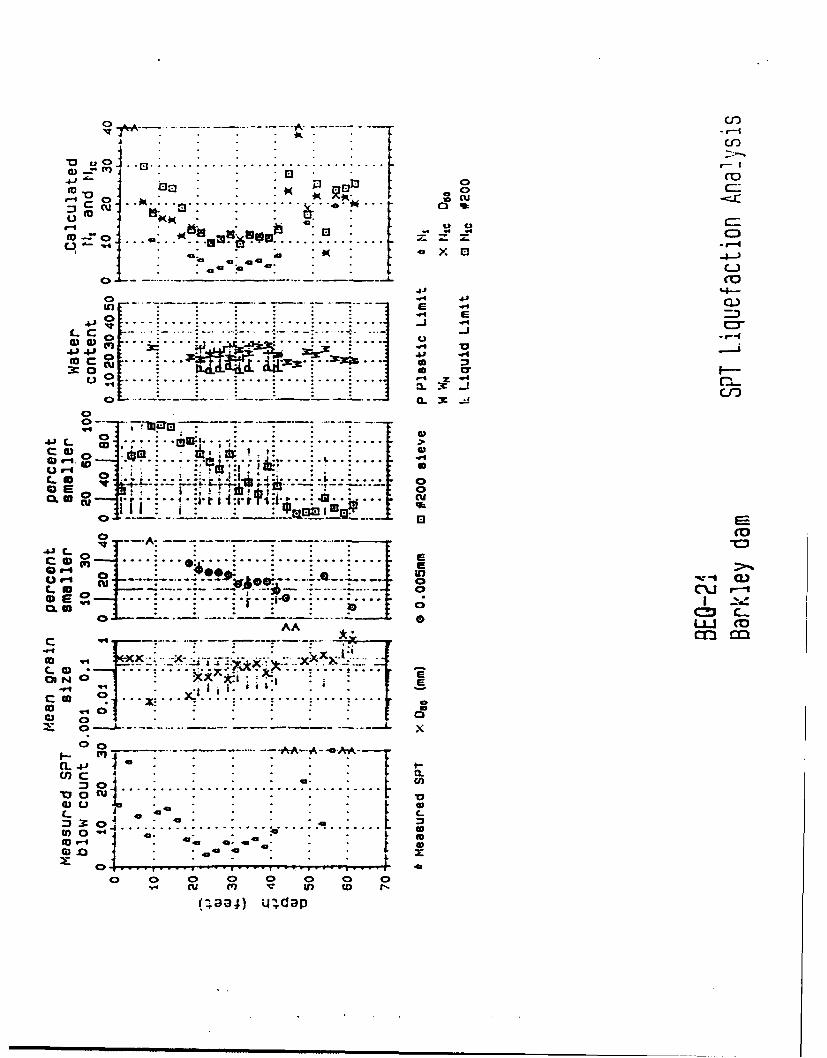
C) u..... ......... .... ......................
mn. "D-0Cer 4 c C> MK 3 ......... C~
CI o- . . . . -4 C)-
x 0
J .9
t -o -46 w
(L M
0
'I.4 -. .e ... . :. .
OL 47 0 4 .! . f. . .: ... c
C wID jj .. . .. . j E
Q I- ** :u
AA... L0 LU co
L0
(ti X ... X ~... 0CC. a. . . . .
(f0' a a I a
W.. 41 a
'4) CU a. D D
(;a34 u~a
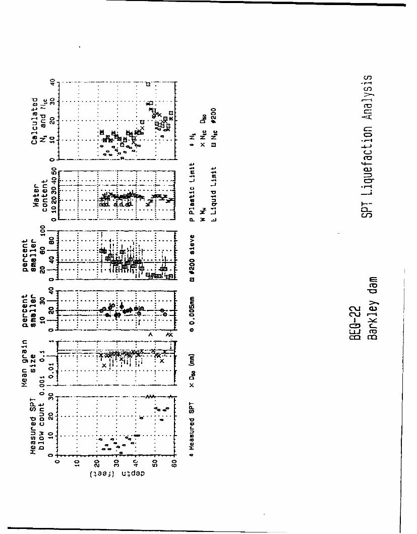
"~ o u O.. .---* 0
"D U o . . . . . :. . ... : - - . • " ... . C ? 4 k.•. .-'U 0 0
(O . ... ... .. V
aXOr
... r: : :3 CL:
...--- ... .... ..o -____i 43a
•0. .T . . . . . . . . .. . . . . . 4 -
w iY .... :....: I:I, . .:..
,' D "'"',... ........... ... o
4I=C .. 1 1 .. .a .j
L .. .. -.... .. ... .
U -G l .. .S. . . .:. . . .:. .
U- co041 01C) CD ,, - -] . . .... :......-- -:. -. : . .[
C- cu- CUc-. - .... ... 1
-L-, • j . .x-;" :"
. ..0. . l 3 '- ,t .1 0 . . . . . .. 2• .. :. . .
co
• )0 ¢u I .. .o o . ° . .• ~ S= ,
CM -
c o . " .. ,,-.•..
a)TO- - C3 a
U c4 o) "" t3 •Ua0 42aap01 uua
C)0 am Cr.
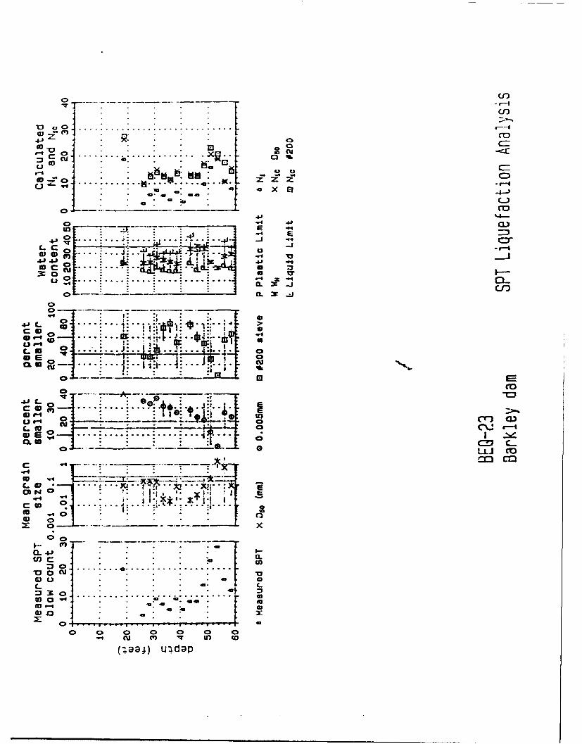
Cr)
"-'0 ciC . .. . . ...°,-
c cu - : * , "6a ... "*
o z 0 .- " C'
o L.- °"__.-_:____. ~Co)o . ... ... . -;--e.o -: ..
--- '
4 . . ... .
'44-&.
o to.. -
° .... ...... ..... .
--L -- :a: -:• , *
C CL .. .. . ---I . . .. •. .
E E
0300 o .0: : 14 : :
oj
L.L CT-
- w. ... .... ..
5 '= .4---- . .i. . . .i. . - - ., - E •
ou N0 : .. ; o
C- fa
C-iC)
L:J co
= ,, 4) ........ ,. . :•, . . .,.. i [
co mmr-- c " ....
En. a 0-..
0 C0
Q (0(9) O0• " • plQl l'lO • m 4m :aj m l l"l :
Co> 0 •>0
[qaaj) U•. dap
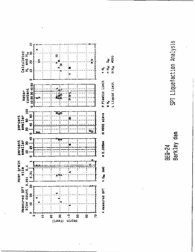
C)
• o . . . . . . .. . . ............... C3---UUU
.X El_o .. .* " - -- --- "---
.... .. .. 4 . . . .
C- -,0---- - - .- . . .,-,
' ... . 2. ... ".' ..... ...
0 L' :.. -- " .. " U I.--
0 C _ __" _
..3 :.......... .>... ..---.
1 C- o~I'o
C €' : .... ... ..... " .... . .". .
-• -. 3
C., r ~ '-.- ---. ._. -- , -- -... , ,.
C..5 .
CUI 0 ***
0 0N•,... .-
ut FE .... . . ... . .... ......
CO C=.
0 .... . . ..... .. ..
c . . . ...... '" . -oq ... . . . .... o
m• 1 -: 7-• -7 -o-
.4 aa ) .l CLd
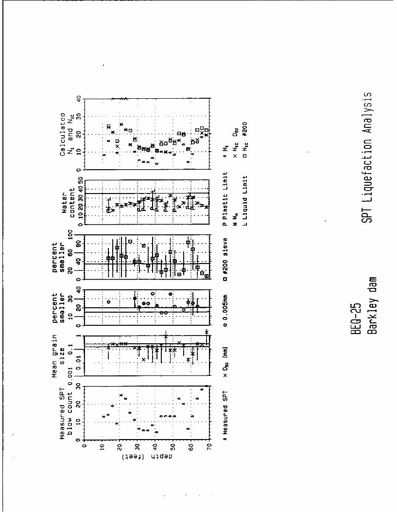
L1)
'0 . . ........ .. . . ..oC) Co
X0 000:D JI-I 0 4
0I.4. L ..u0 El.. X-o
, ), Z *. ... . ..... 4. .tl*•1, l
40
0-4
ICI
cM 0 -4
L) 3'-'
... I :Q :
a)-.* . . . . .
S.. .... ....... .. .. . I " i4 -
a) E 0 : " '
Q..- U) . 1 . T]
Q o . ..u .. .• . . .x . ai.. . ,L,.,- 0~ I0 .
m ×k
S0
0 0 0 0 0 0 0 0
cu U) mr- C a w r
L ) CD CrLdi
[La• G)T E
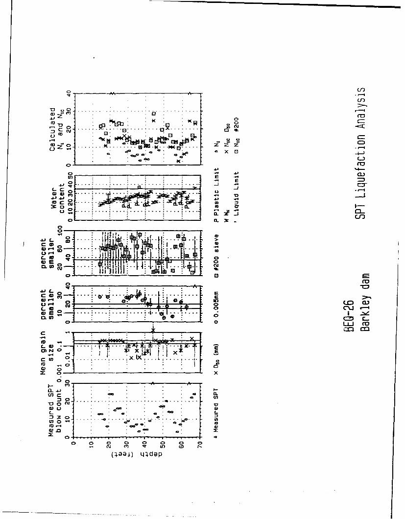
A
j C>co
uC c 13, El0*I as =
..... a -* a W - . .0
-
0)4 .a ýo .6. . x4-
o~w _____ 4D_____ _____ 4 -'j
or
OEE
4 J ....... ..... . C =
M -MI__ __
LU) - --.-
U ) 0....... . .
C) 0- X________O_
1 ocu cCLU) 0 : -
.00
W 0 .0 (JO .0
.0 .0 c
-,~ ~~ CMc,~ 0 C
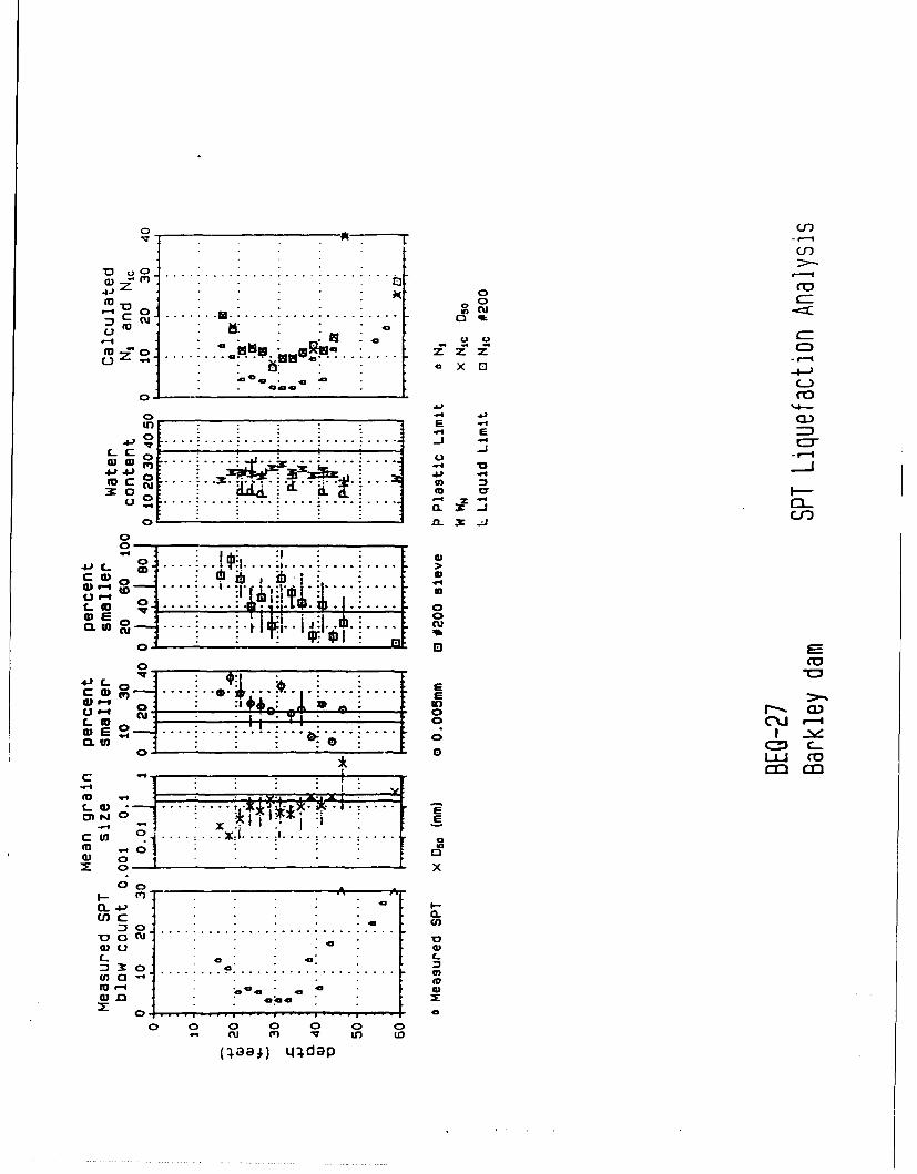
CO)' z0 .. ... ... . :.....:...... .. ...r
.o E or--
(a0
- .. .....L) XO x -)
0 .1 .0.0.D
o - (V a
--, .. .:.. *it... i . . ..... ::.....[0• j .. ,... .. 3. .C" 1 . .. I. .
. . ..- .... ... ............ ....... > "
0 di I.' A
0)U r= C
CL.. UP 0 .. .:. . # 1. 41.h ... I (
0 - 130 CID
4. -- 1q ,
EN l
C- 0
]O "
L- :
(- . ..C X I
• .ul a
.19 . x I '
0*x
0 C I
a) 0
:- 3: o . . . .. .. . . .
M 4-' . 42
0 0cu ~ to to
La j tC .0
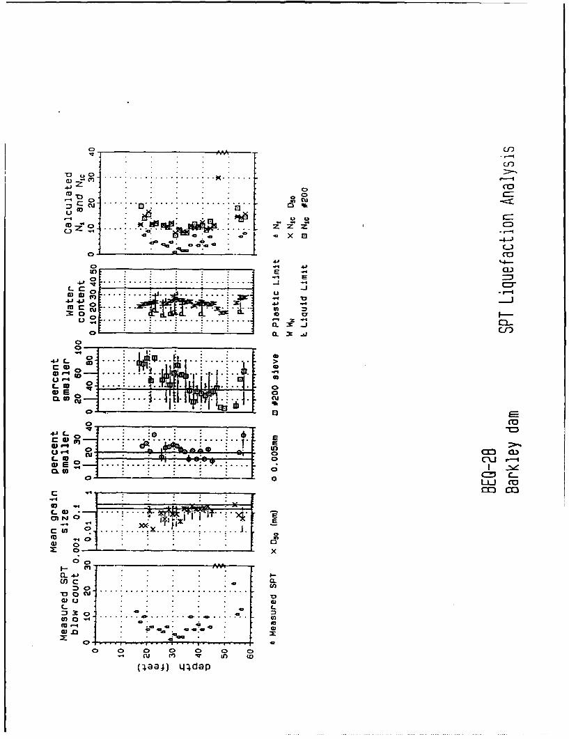
C) U)
0LCC)
El~ 0 lk
0 ........ W .-
.0 x o
45 '4-
W C)
-411CU0
0.w
L ___.........._!_It _1 _o
4J L 0 G
... ... .....
0. 0) - Nce...0 LMi CO
cu .4. !......
m -4-
a ClCL 0 .1.
C..
(fO. " i.0 62 P4
0 0 0 0 0Qcu vU 4L) toC
(;99a4) L14dap
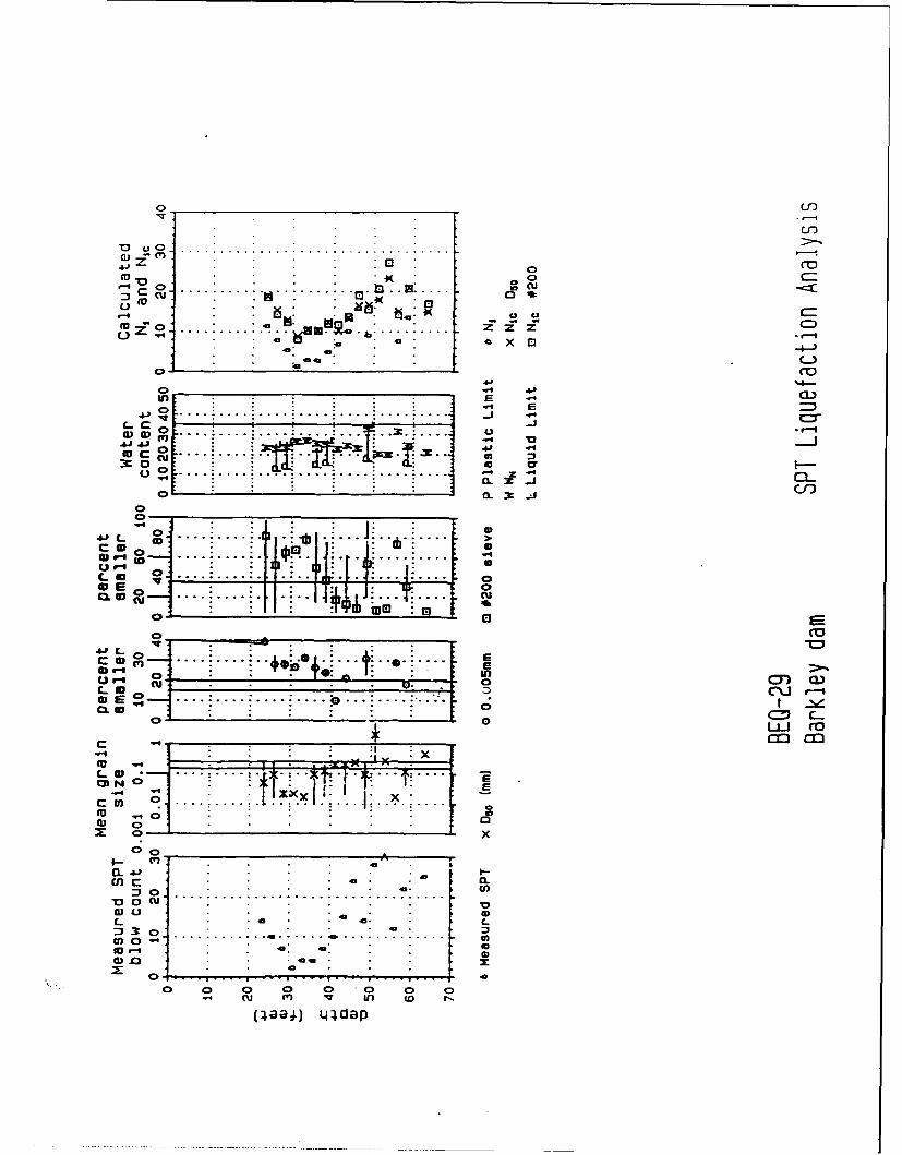
oo
ccu W"
r -q
9-'I
C)
r--t1
S. .• 0 *0 XO,0 : ... : .. :.. .. ... ..= ..... .. .z z0 CO
4'4
. - 4 CD
d) ID .... i.... i.......... .... M ...... ] • . ,• ••Lc C% 3cr .J ..1
0: 0
4J L
c ID
CD0
L, - ] . ..... .- i w0
I .... : ... . ..
oc
LW C-U r--
Cl. wm22i. *O, I-
CMcI x
L N . . . . . .1
c m U.... ......g
00
In c CL0
S.0 0 "'"
S0 ....................--.... --.................... t.C. r - • .• .•
0~ ~ ~ .. .. .. .
"'""0 0= 0 0• C) " O 0
,aa4) t0,dap
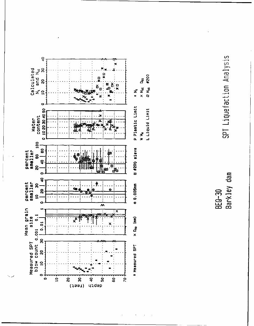
o ___ __ _,__ _-___ __ __ (f)C)f
.,,•I ~~A ...i.. .. i.. ..=.... ... 1 uu°r"D ,,- U . .... :.... :. -- : 4k--o.::
"" ... __ _ X E•
• o1 . :. .• :. E
C-)
o .-
0 . ..
C 0aI) di0).
4J 4 .J.
0. .... . .
5 0
I.- (a ... . . . cu
0 ... E .
L)r-I . D
iDA 0 ... IC
.4~~~~Z C Y -i) co v.(Aaak Lfd(a
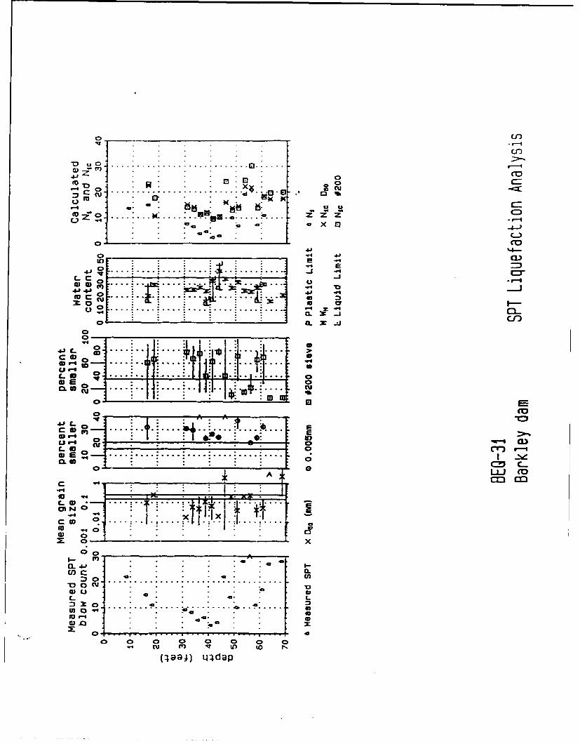
oo
© -o - o.O,_ o. . XU -.
a- 20
. C.)0., . ... .... ...... z.r•• .. :r Z-
o . . . . . . ..
40..
o cL C - -- --
V ..... ....o. w
. . . . . . . .. . . .
3: °o . . . ×L3c
LU -0 iio0.w
h, ~ ~ C) .... I•Iv... . ' ..... .... .. .... . .
0 .... _ _ _ _ _ _ _ _ _
(11• C:109 ... E . -
0 cu 1
CL fa CD aa..4 CID
a. 0 .... . . .C
Ow ci.. ... . .. . .. ... . 0
a)a
cna c
o o 000
U) C) C' ) D r.
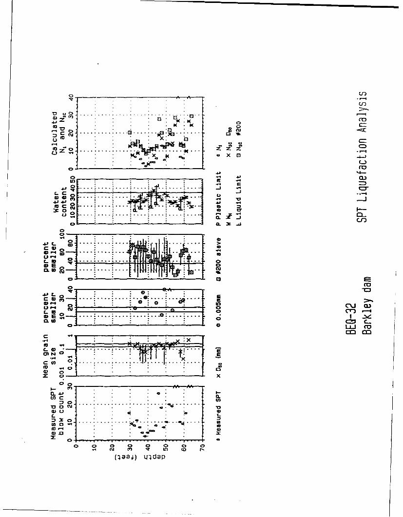
cn
.91
Ocn
Eoc
O ......... .... ... . .
eu-i . "~ i ., ..a
.. . . .. z __ J
S.....:.....;.... ;. ... ik . ... :.... o o:f -r ,
U -w 10XE
0 C"
04
,-0 . ... i .... .... .. . . ... ....
C- c4.Q, -
0
C) .... ... ....... .
L 0 0.. .
o...o 0,
I- to 40
C 0 .... *: .... ..
w 0E 0- a )0.
-0
C- a
CLw C_= -
033 m
co ~~ V4aa
a) 0
C-
-0 o au
a) . .
00 .. . . . . . a0a C)0 0 0 a 0 0
q cu w tn to fl(jaa4) tLn4d ap
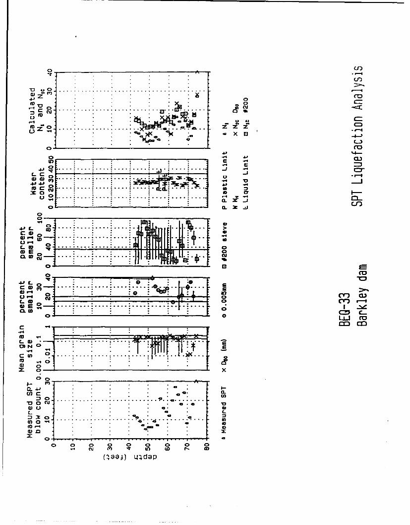
0 Cr, .
-LO
0 .......... .......... ..... r -*: 0, cro
u-4 0
o c,, T -..kC.)
L)' Is.
o- x a:
........ ...... 4jo . ,.. i• .""-o.i'.i. [ o .4
L. o 0 .... . ........
4JC~ .1to a CU
x 0
0. 3F
a. 39 r -
04*)
.............u ) 0- I ...... . . . . . . :'4b •
0 0 0 0 0 0 c
Ua)-3
LC 0
cm u
c U) ......... ..... . .
LA))
a) 4
0 .... .... ~
41 U
144da.
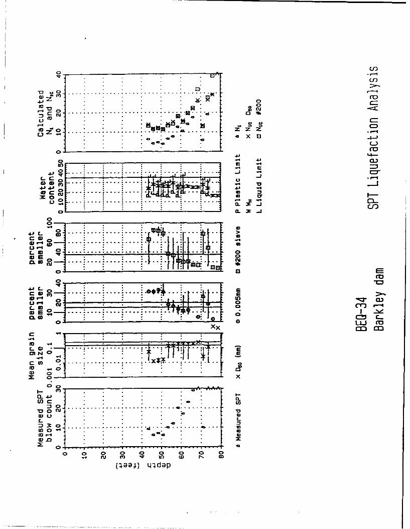
Co3
S........... ...... ..... : ..... ... . ...
* . . 0 o .
Q ~cucu .y -&•-
c~o: : a .•.. Z 7
0 .0. 240
04 E
"0 W4 V4
LZ C 0 ....
x . ..
o4 . ... . -•
L. ) .... .. or" = IC 30
* ,.1,,°
. . . . . . . .. .. . . .
NE 0
a.w , : : : : : •.o• t
oc
C au
. 1 .-.
CS :•w .. T. •
w - 0 . .. . . .. . . .. . . . . .i . . . . .. '*"' ' "0O)
rL
0 0 0 0 0 0 0 0
L aW C), dap
XX LM
I )....Ct1 .... x
z x
CL .1
=30 . .. .. .
0o40
0 0a 0 0 0ý 0cu C q W' ~ t to r% CD
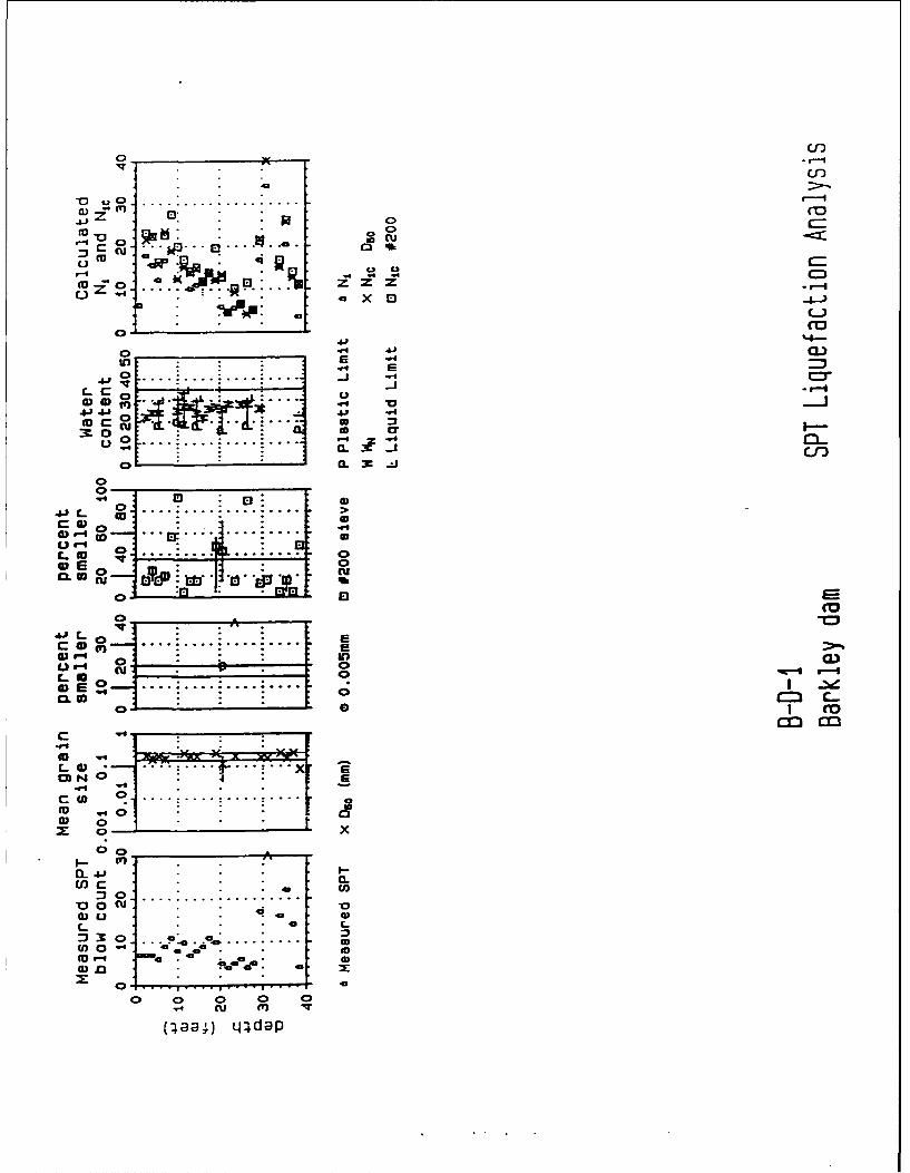
C)l
C=).0 l z z
43Cc x 04
ri~
C- a
c0~
a., 3r E
0 .4
411
0 a):
.1-WL 0
C. 0
L. goCD E
_ _ _ _ _ _ _ _ _ a,*1 :4110
-X10-
_ __ _ 4 ): . . . . : .
or_ -j . ... . . . ...-
a)
cr),
w 0 -. .. . ....
0 0 0 0004 CU (
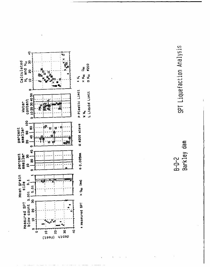
Ur)
o U ")
x CID
-w la0 c C
o 0 4 -
LI) S .. .
0)Z
o -.
. .. ..... ...... •.1 . ... .0
CL* w
.0 p . . . . . . . . . . . ...
to o .
0
CiL.
0--
S. o4
C--= 3 o ... ......E .. .
(paa4•) tp, dap
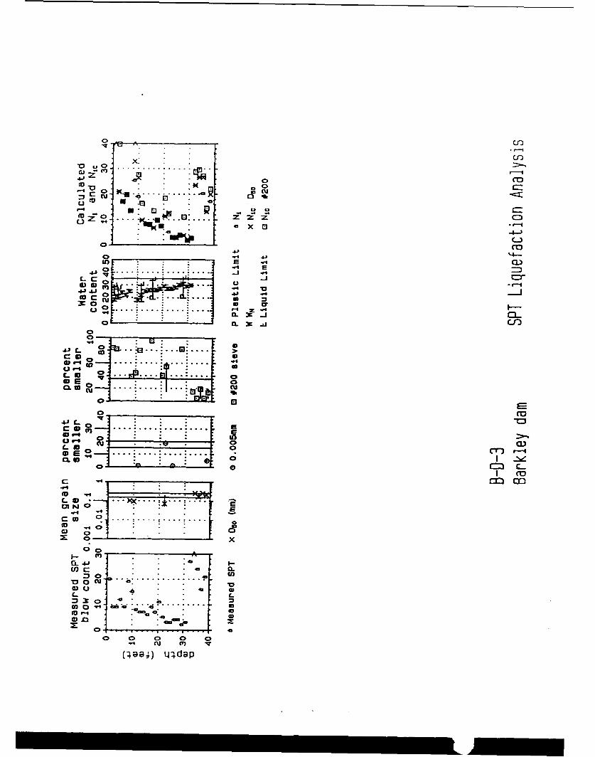
M 0
:or4 CU b . .:. . .... j: ....
'-U : • : -:-~ 4 .l-
CO)
E CDL -
•.•o ~r • • _ • -j 2 -
1 i , 1 a .
cu- . ." ....: ....•: " t •
mccr
..• o .... ... ... .... -1 o --I-l~a. * C 'I-.-
0
CD"Ur4 0
CL" W ..........
U r4 r (-r) ,---q
I CO
," ", . ..... ....-, ...... :.. .
'1 D ....UM X
0 mg..~ T
Cl • " "0
¢n ~ ~ ~ c on q,• , ";"" .....
(q•aa;) ql~dapI I I I II IIII0 0I "1
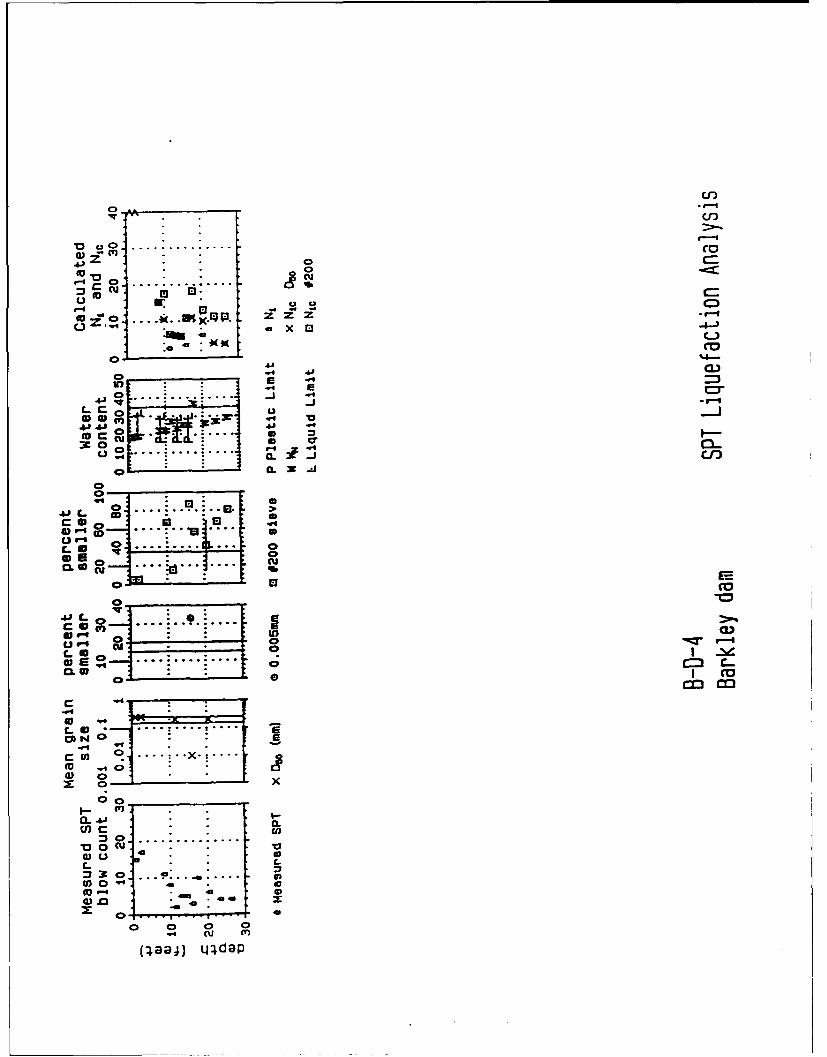
V .jOco
0 .
-X IEI CC)
CD.
mi U
COU cU
1 C- C4
.............cu
0- r
ONi Cu
* U)
o................
C-
LW o
Oý 400
0-a
cu enVO W . . V
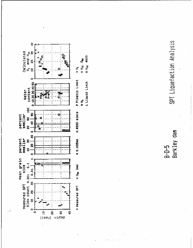
C-0
00 c co~
0. . *(C=
CZ) -r-4f
* . C-,
0 - 2
44
C3(W ... .. ..
4J.4 3: .&S
M4 .... . >
-4.I
U.-'
-- I - . . . . . .. .
r QCCD
S)E)
0L w I CO
C IY
LU) c C-L .. (
U) 0 4 4'00 4_
cnCr * .aI- . ) t 4dU)
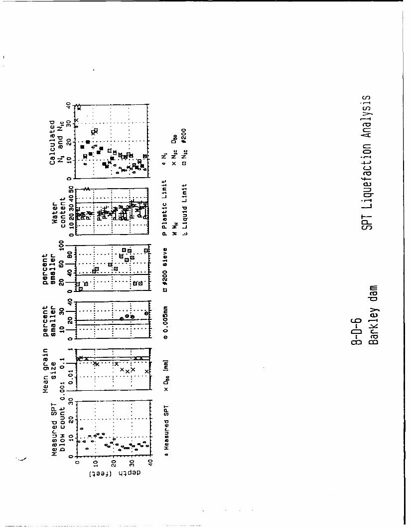
Cl)
""0_ CU0 0 4
C:c
z z z
41 41.4
0Ea
0c 0.
E3U
C- 0 cuQLc) r= -....
CL- w _ _ _ _;
I CoM 0
I.- ('2
0.co*
ajo a'
-f0 0a au
4Da
qq~dap
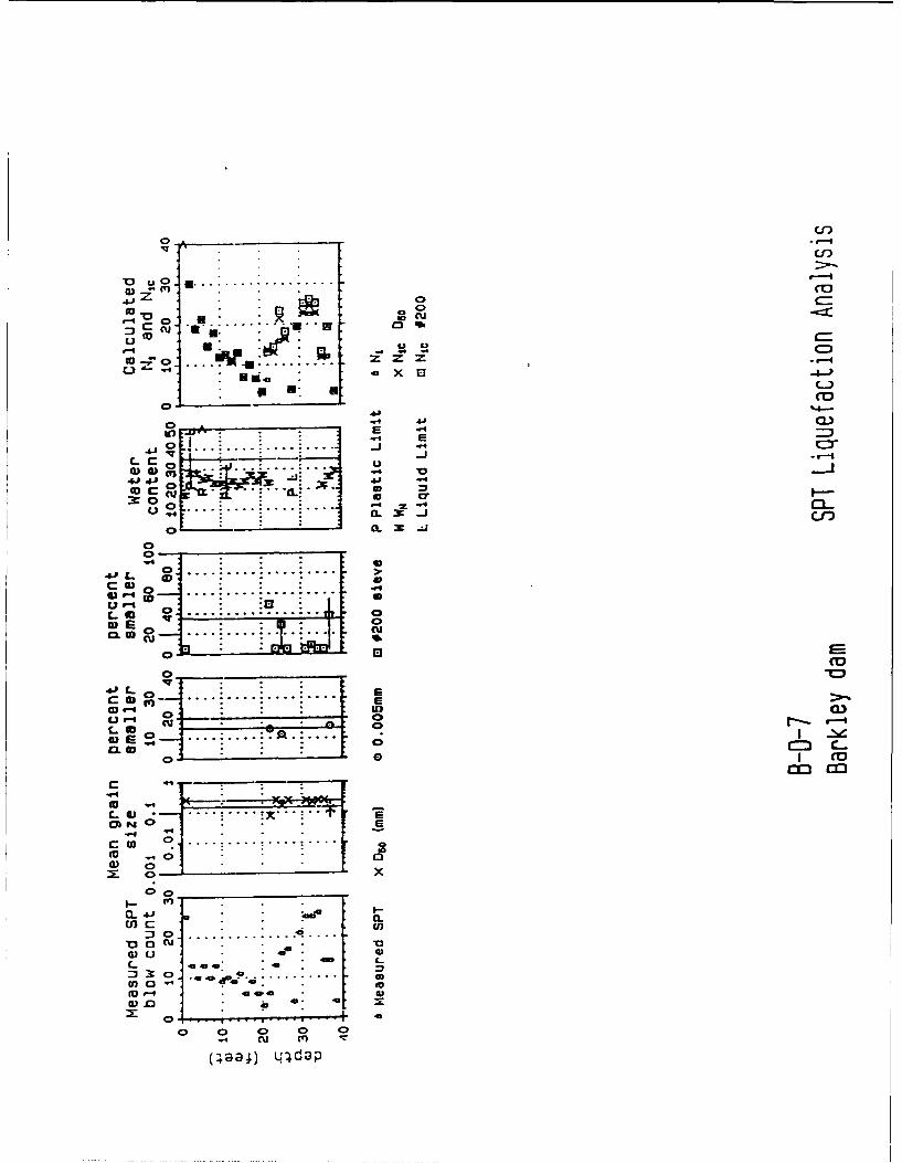
-c~ ........a)j M(
togv ý C>
COX
.a.)
C- -)
u 0-4 02
u o
CCC)
C.) 0-4
C-0Co
0 E~I co
4-ICM C .3
c 0w .. .. .. .. .
CU) x
CC
LU) u-. 4W
40 404
40
no 0 >-U)- . .
mn U *4 I -a
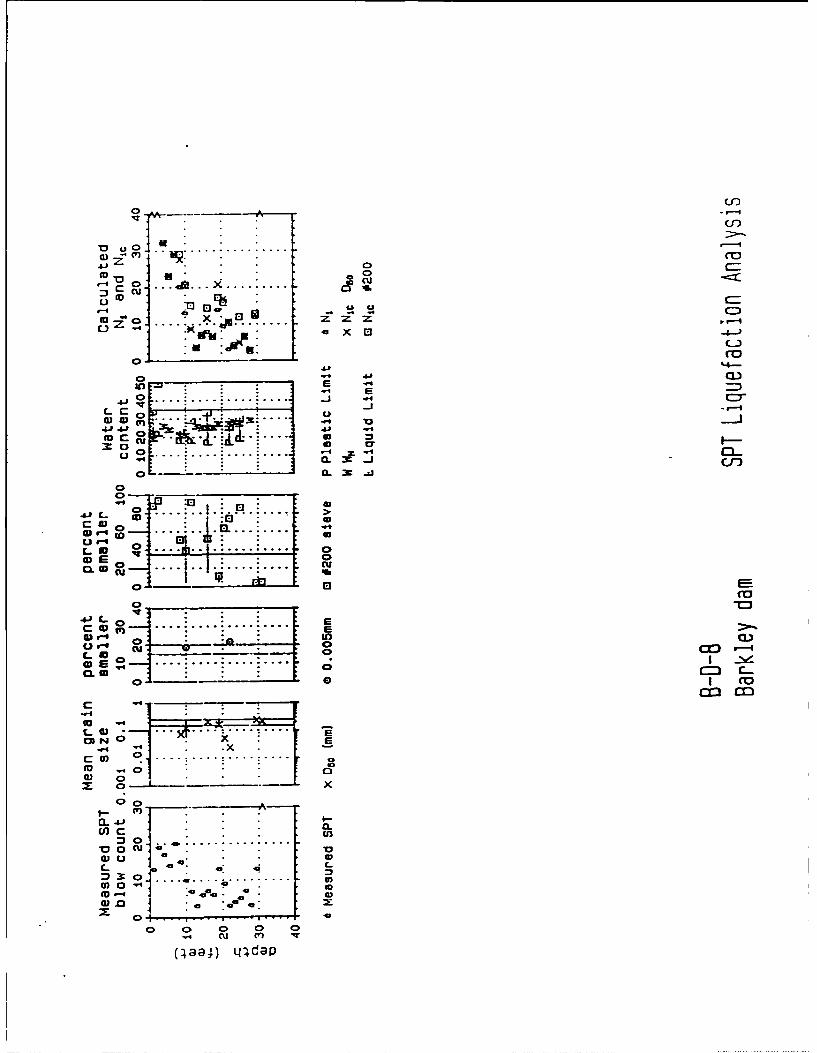
C,)
rI
- (V
u ID EL
0 .. . .. .. . .. . -
CL)o -E
E
4-1 41 40LUc0 0 t
WE.0 a.. . .. . .. .
0 .- 0E ... O
E E
41 C-
o 0 ___
0., w cm 0.
a~o o
on N ~.4 (U (YX
a)a4 0gda
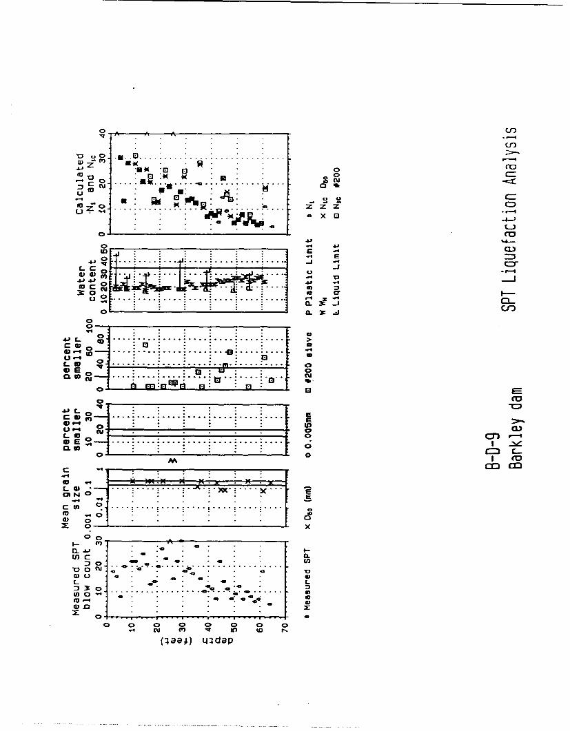
EM , 0 co
............. z. z.z4 " : . .......... .x. 0...
c_ o • . .: ! • "-I--.ac
• m • " i" ... . :. . . .... .. ...... u
x0
CO
,E .. 4 0
0 V-4L) P C-4 0-I-
L . . . . . . .. .. . . - . . . . .. ..
r.1v.
g o i -" ........ . . . .
° . i i ii i ..: .... ... 4hc --
v
CL w
I -- -- - - -- - - ... bc ..
Coo .,...-
0 ......... ...... ..... . . .... i..... • ..
0n 00
aatdp
0.400
U)0 ______________C
OINO-4 (4 . . j a4
.... .. ...
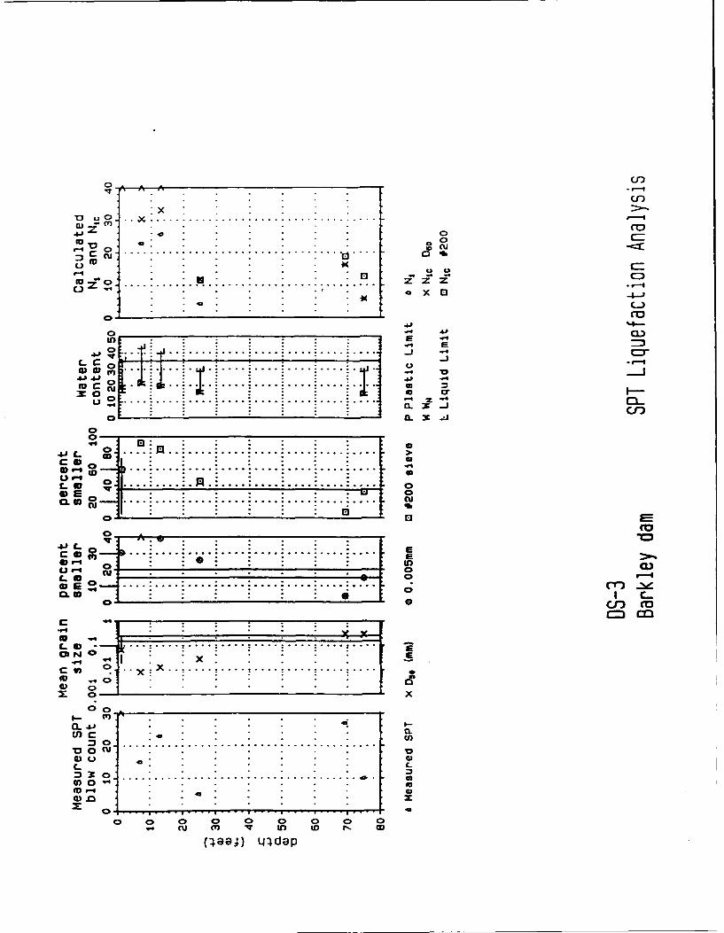
crnC)J
0 ................ rU
u tox
.,., ; .. .. . .. . ... ... ... ... - - .- € :
.. 0 4--m,,o . Z--
%-u-
* I'
o Co
-r :r " " ... . E .
S. ... . ... . .. . .
! 1
• .•! !..! 4:' .....
, u . . .... .... ....-4 I. -
C O - a - .
0 0
0 0'
0 . ............. ... :I. .
o to cd
a . . .
4.........CL .4 . .
0 C.0 co
to x x
00.
U)
. . . . . . . .
0) 0 0 0 0C
cu 4') M Zn D r- c
(,4aa;) tjqdap
APPENDIX B:
CPT DATA PLOTS
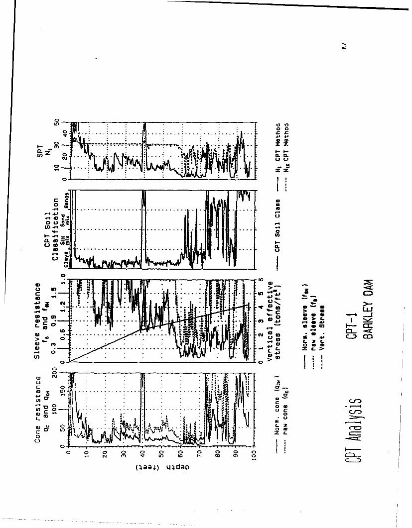
CJL14
00
..0 ... i ... .
C,....... ........
....
tt0.z 1,
CU
O)
10
C .!v
.94 ' . . . . . . . . . . . . . . . . . . .
40C.
U ) . . . . . . . . . . . . . . . . .U)l
0 00
0)I0-
ODS
LL
CO an -a __.
0 ..
21 C
0 ... .. c ot
a) 0 0 0 0 0 0o 0- Cu 0) ~fl an ~ CD O~c
(~~~84) 4Jde
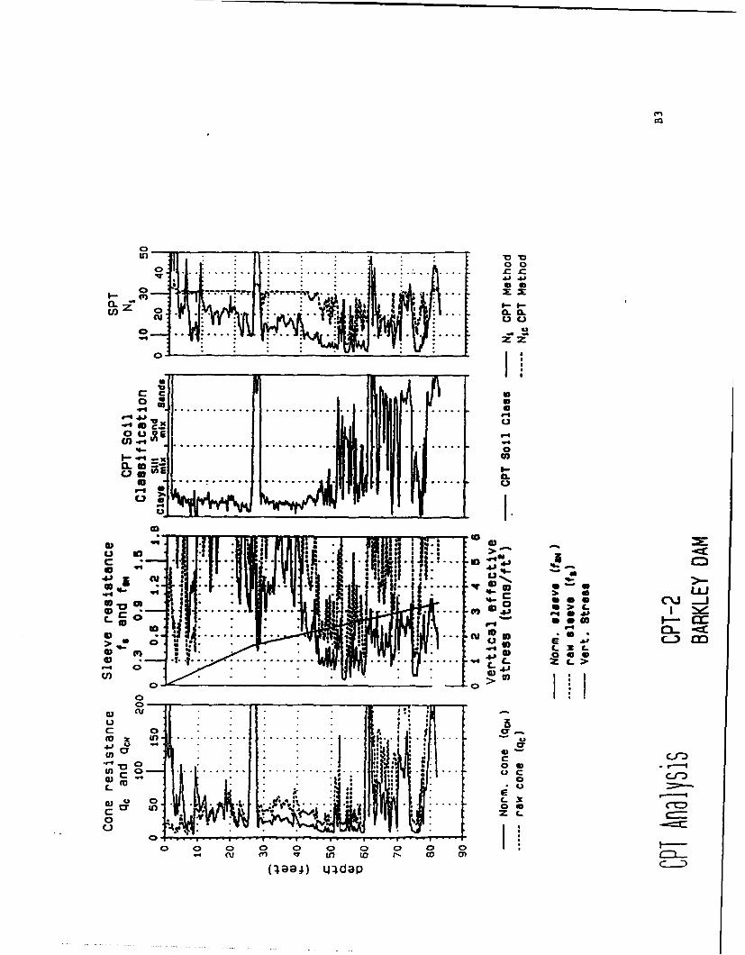
o. -- I---
z• o, C" a- ' , ,.
- ............ ........... . .
IDI
10 |U
coi40
. . .
(A - w .. . a
40 L.LJ
.-.... .... . .. ".
00 m:
f-I S
0 *0)
0)
"'zr' C o . -U'.cn .> .' i-c
0 0
0) .0. •. . . .. ......ci CU. . .
C 0 . '0 0: 0 0 C 0 C
ou oo o to to , o o
(:al e ) LP da P C-
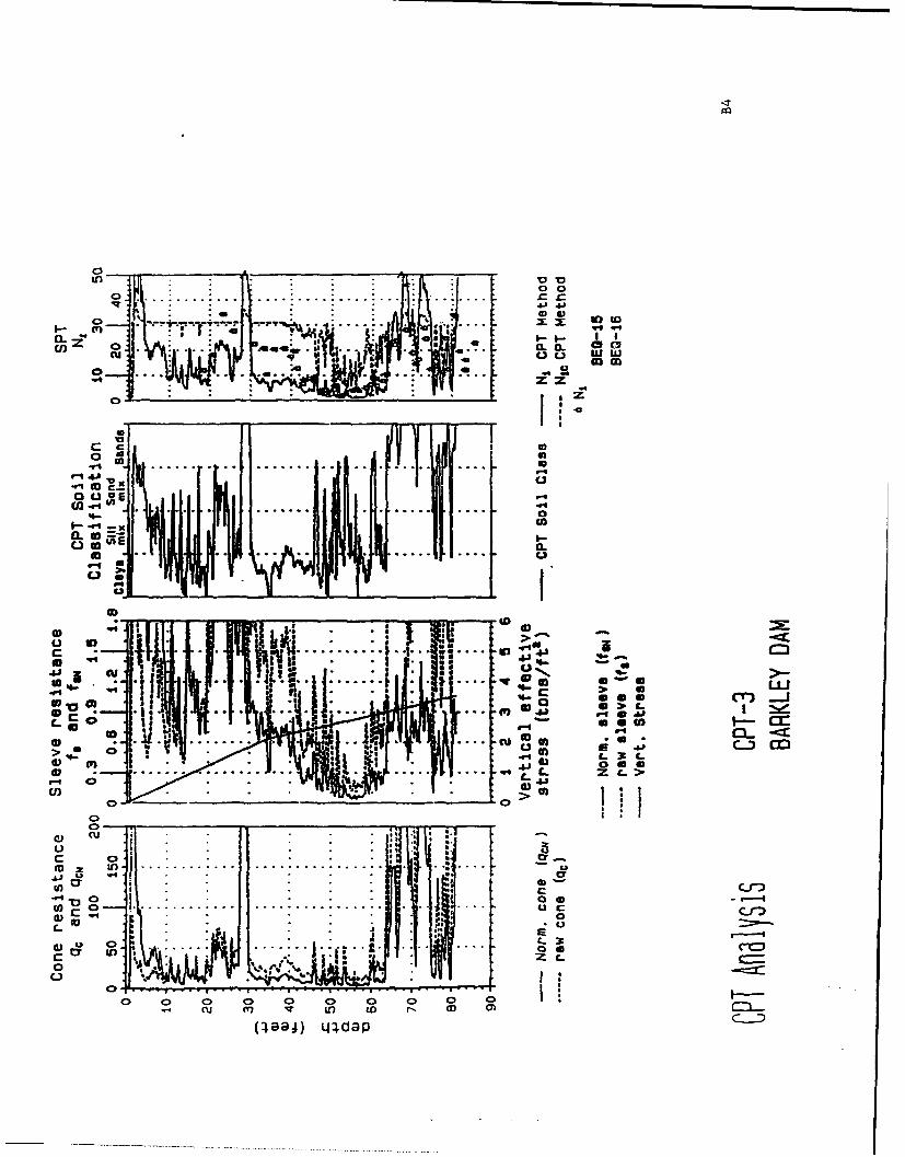
00 00 . .... .. .. . ..... ... .. ... ....
0- .. ... *•.•
.. . .a
o i ... L IL
o zo
. ..... .o
� • "•
- .. ....... . . .. . .. .
CO ..... .....C.) FA
t c. .o.. ..- ---.do 004 4) 6
C.) • ~ .. ...... . I4"t.....tI " ar1"4
uo i .In--
0!
0--al . ..i... I..0~~~~ ... c 0mC- -
..... U0*C-
w. t- 3 C0 0 0 0 11
-rC ()*-4n t r. CC)84 >Id
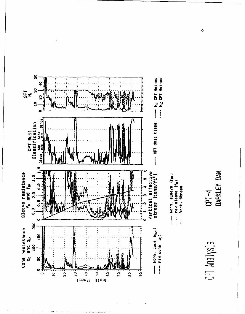
00n
I-". . .".fLJM1-4
. . . .... ... ...Z 7-
I ,
.= ..... ...... . .. . . . . . l; l . . ! . .
c_ .;. ...... . .... ..... ..... .. .rq.,, • , '
0~ 0CL E
P-In 0
: .. .... .... .......... W) , a •:
-r ff- 0
- -
C- • N. . ......... 1• I'"4
... ICU "_ w . 40
C--0
w41
ILiC)
00
CD cu
.0 . . . ...
(;)j 08a
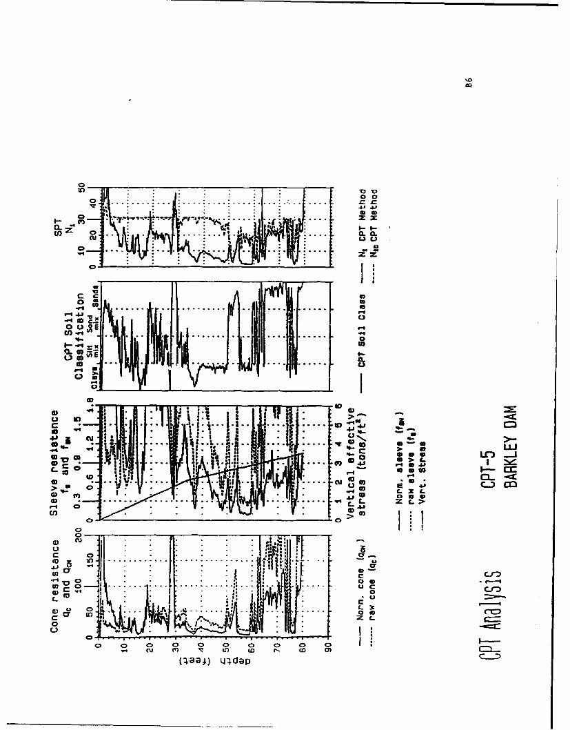
'%D
a0S. . . . . .... .
S... .. . . .° .... L C
.v.-'.-.-.-. . -.. . .. 4... •..... ... ....... .- r -
o i .... . ..... n ,'
I1 .. . .. 0 0L.1
00
o . . . .
41- ii >UL
c c .' .,3
m 41
to a C34-
4 .. ... >U V4C --4
ftC X- .rxI .
.. . ...... . . .
C- C.
an >. . a), z -0
c0.o I
u
73 .. ... . . . .
- 0 .
a) oo ------z.4> a 0 0 0 C
0 CD to -n
Paal w . -
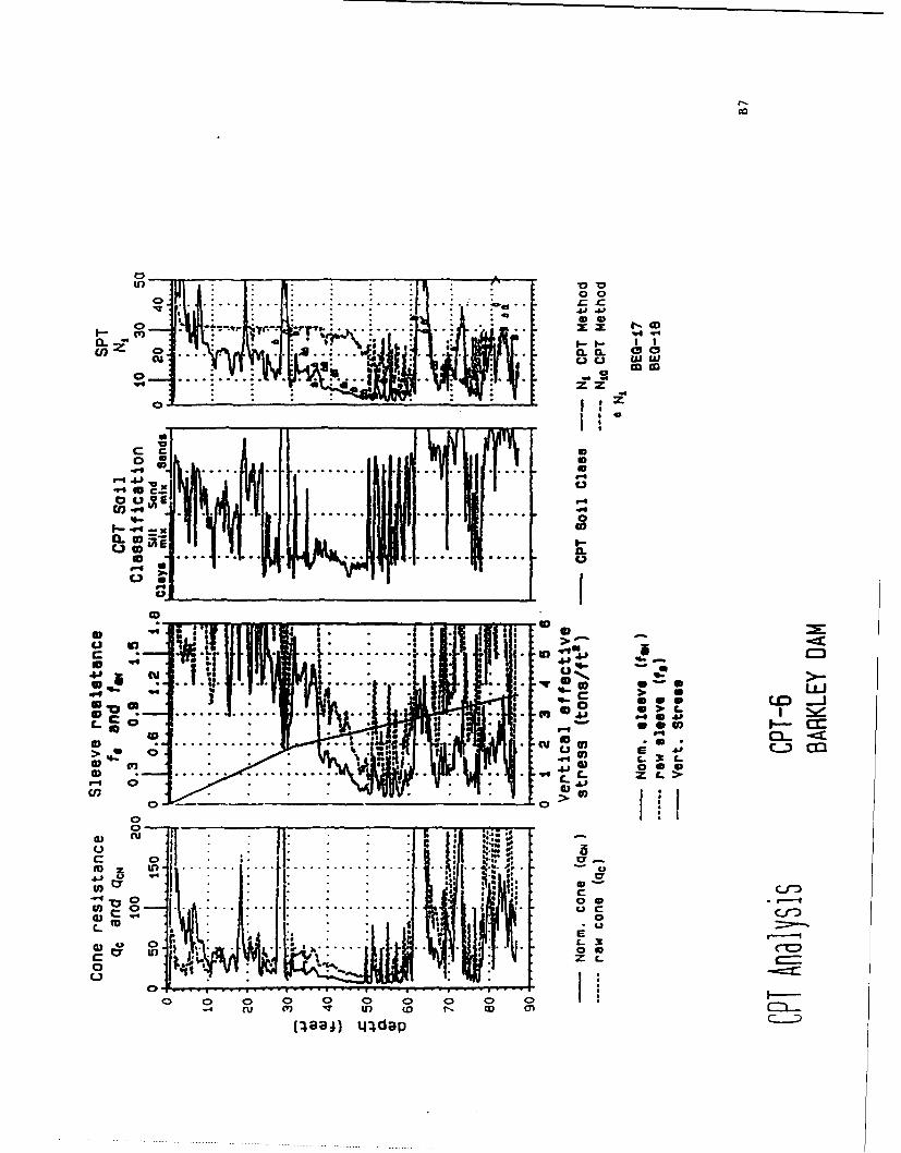
0 0
T. . .... .
.. . . ... . . . .. . . . ... .
M SI
Exr
. .. .. .4 J U
... .. .. C 3UaU:
0 4
40 0 0 -
0I a
>5* C. > R
Cl)0 0 r
0
U) 0Y 1 0
oo 000 0 C0 0 0 0.4 (U W)' ~ ) 4D ID Cf
(19a&) ~nde
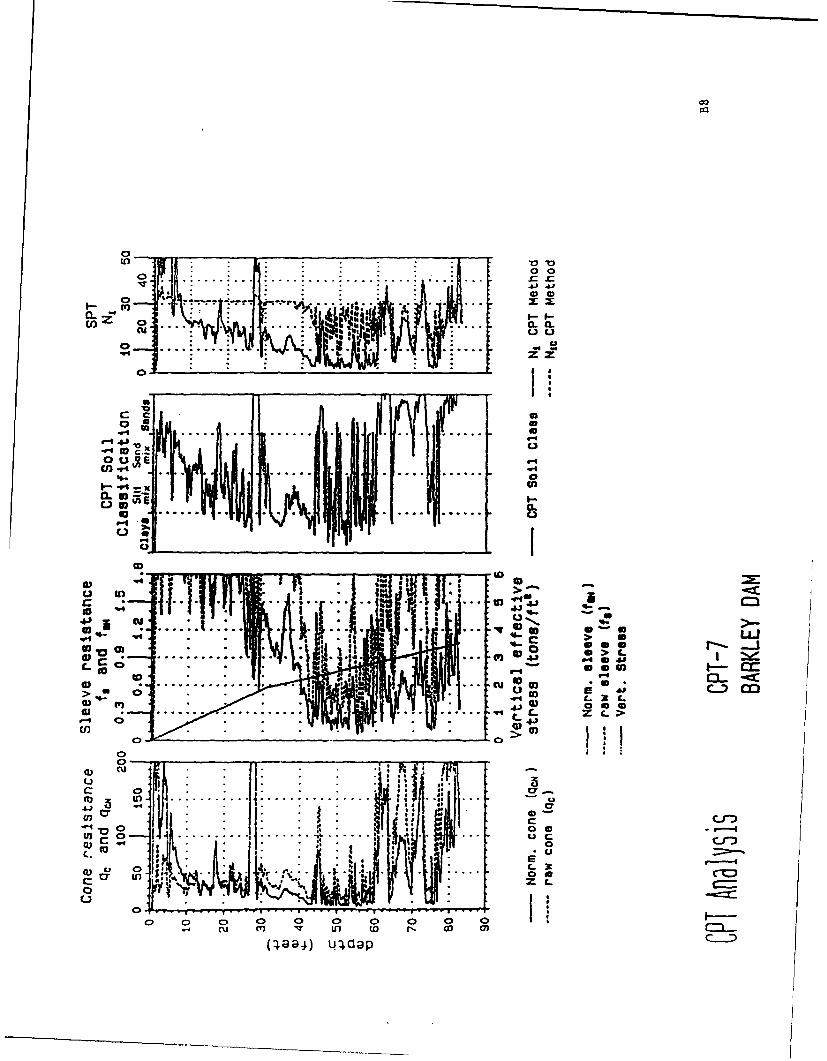
* 73
cc0 0
0.m Q . . . . . .. . . .C
.....
.1. . .. .
CU
C .) . .. . . .. . . .
a. 44 . w.
0 a.
10 .. . .. . . C3
o 2
U In3I.
0 ow
0 U)
0CD 0 0 0 0 a : ~C- >,
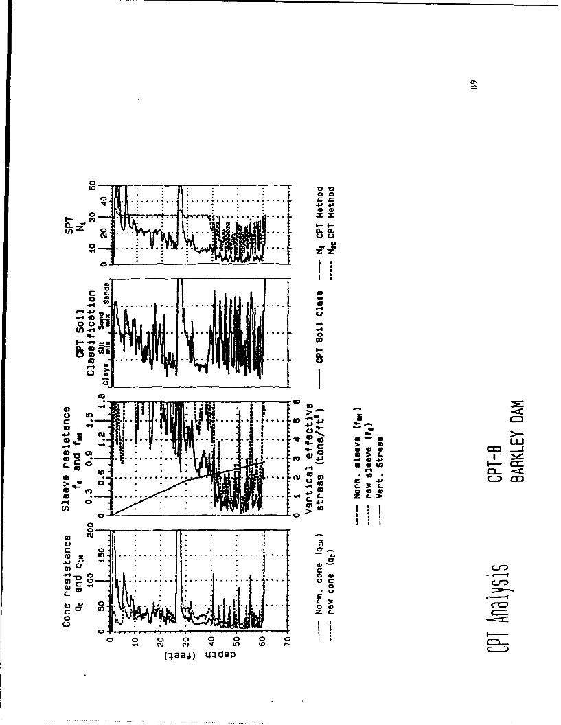
0 0'
azz
Cc
... .. .. ....
'-4
0
>- S4c
C.) %I,a4aL
Cc
. 4................. .4... cugow-7E41 0 a a
C,,0 4
0-0
C-a) L. 3 .
C-) , -kC
0~ ....C.) *- .r . .
__ __ __ __ __ _ __ __ __ __I
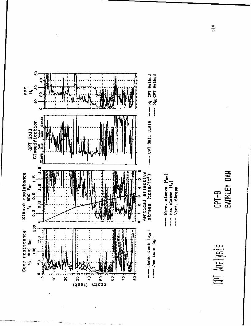
00
Z I;
I 11
oU l ""
m E. F.
QUIX
40) ft1 1 11>...0.%
V 0
o .4 -- i
o 41 c_.) c
c o
a)z cu '. :o
41 : .
40 j
C.) W.
o0 0) 0 0ý 0 0 00
(4aa4J L44dap
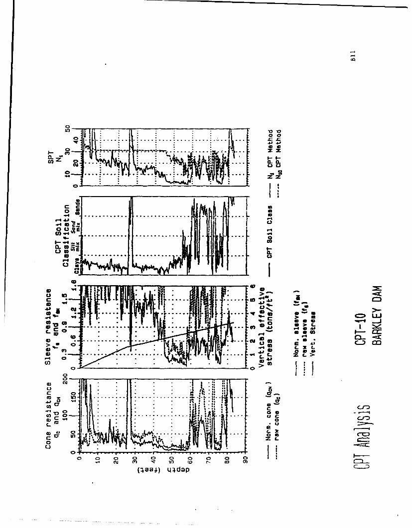
0 A_...._o, : : V.. ..: . :. . . . .. .. .. .: ..... . . ... .....
0 ... .. . . . ... ..... ..
_d_.. .. .lJi IY .. 0.0
-V4*0 C-
Eli | Y..: ::it :1,.-W .. . . . . .. . . . . . . ... .
40 .. . . ... ..... . . . ... ,. Q•1 :ca-
I"0£1)1
10 - -ca.
.... °u o° .. . . . . C-|
ill !allU, _ _ _ _ _ _ _ _ _ _
E 0 >
oI.
0-
0 C) ::) 0 C, <: ': :: (
L))
. ......... .....
a) iv(1 ~ ) CC)84 4ada
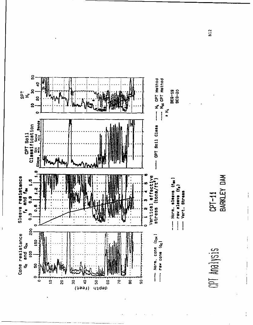
-4
0 00
41 4Jj
o go i
ql • •
cc a
Lo- E ._ J-
0 -In CL . • •"
o . . .. . .
C01
L ) . . . . >. ..... -- It
'4j
C . .. ... ! : >
* ... . . . . .... . ....... r
4.04
40 w• -!.. .. ...... . .. ° 00) 9) I" "
o . I . . . *. -o l- • * ,,:_I
C3 7- C. >
oil
. ........ .. o. ....
(U48)J) Ljrdap
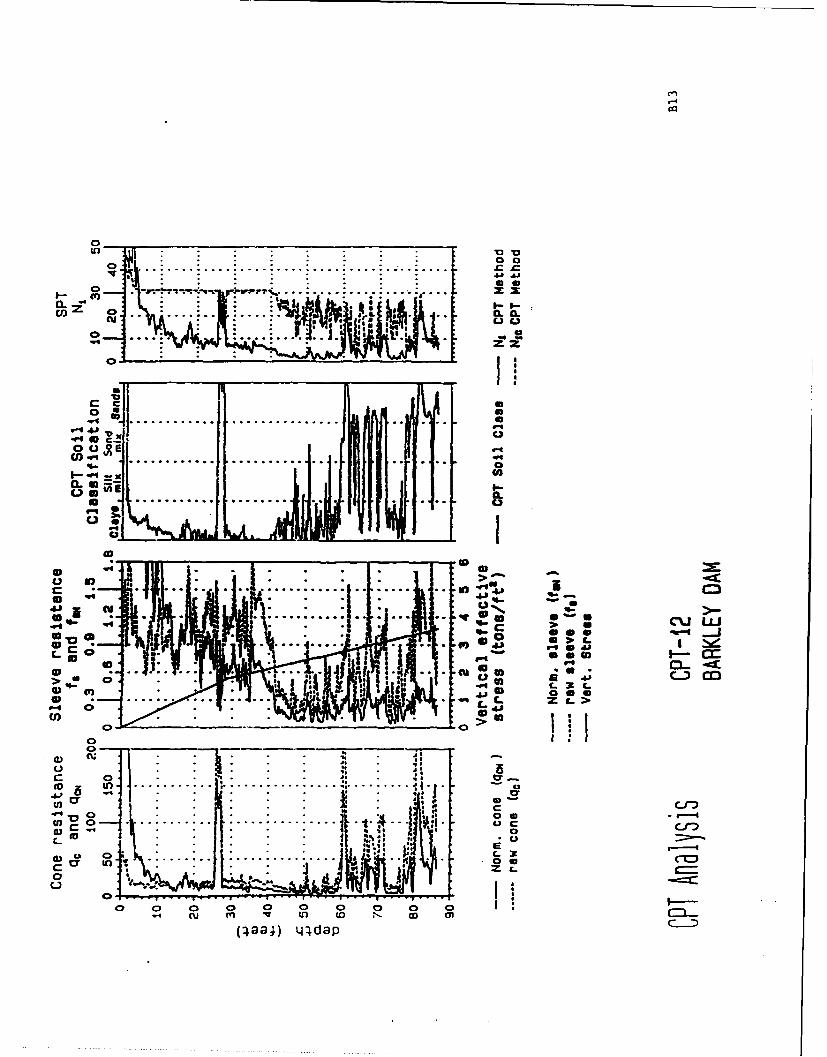
0 az
UI Q
041- .- .. . .. .......... ...
o . .... . .. ..... . . -we%. 0
sin40 . ............ .......... . .
ca-
S• . . .. . . . . ... : .... :.... : . : ... .. U3, • -
C). :_ =>
a ,* I . .vi L) , -
...... ..... .. s o
W4 F4 c cu LLIoam. -.- j
. .. . .. . . . 02
C '0 a
. •i C m
rq fa C-J L
. . . . . ow af 4
In 4
II i .......... .. .
L)
o
( oaa 0 0 0 0 0 0
.4 cu aW ) ~ L) CO N
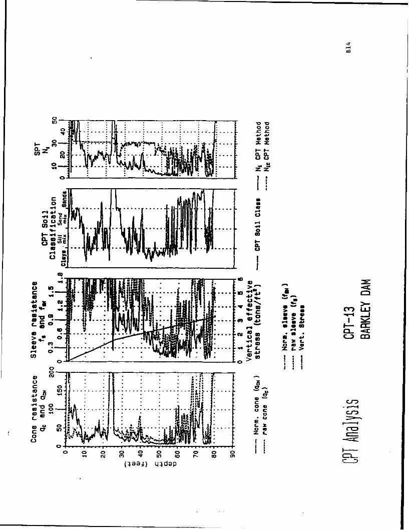
.. .......
U .) _ . .... :-.. .•m : , . ; :- -; ! - .... LIUQQ
• ,. .... ...... .0
W- r I .. . ... ....... ... .. .....a o- "-
""--- .vo.I x
roo- . L'f-- , , :-: [ox
r4 .. •j
'-tc- m L4L
S. .
C.a..
C) IY0L ~ 41 1.
S. ...... . .... . w
,>,., ! 0 0• 0. C -3
) "- C- 3d" c-o
.. . ...... Z
o I:-=::
o .cuo oooo
C),r " ,) ( r- () o
in,• ; ... .. .da. ..
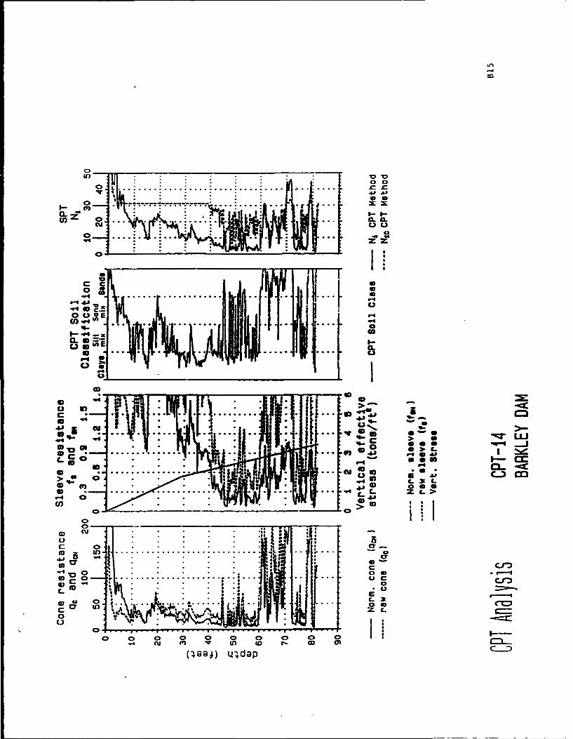
-4
0 0U.. ..... I
o .. .. . ..... ...... - .
0Ul
CL
. t. .... . 3
942
41 0
..... v [ A
0. 0 I -- c6) C-' a.
C.. x-P -O 0.aJ.:C- 41 - -- -
cn~ ... .. ii :,.., ~j . . .. " +
r- .. .. ,.. ,,., J.. . .. . . :•",' o u" )- I- :'
to 0 • .. .. ........ .............. ' '....• 0cy.
.06 -4O.. ZL4 cam .. - •
c on o ... ..... .... ... .. ... . .... . 0 a
005 C • •.. .. :• +. ,., .4. ll# I o
o 1 ..- "-
o 0 : D o 0--'---
cu tU(r ) (D t- D 0
(a a ) Lj4dap
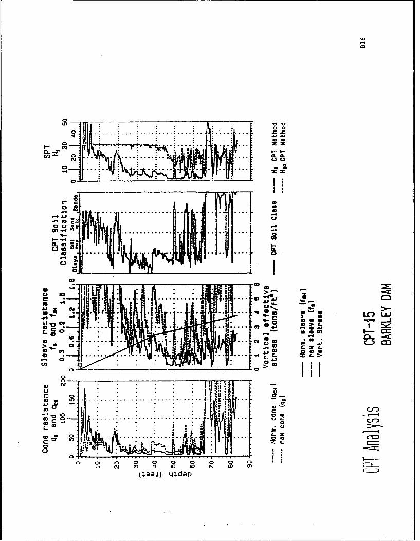
1.4
0. 0
cu 0-
0 4
-'o a -~ -I
q4
IL * li I-
q4................ .....
a i ... IV-a C
0-3
> m C.,--4 0 .:
0GD 01 0( 0 0 0 0 0V-4 Cu 41 D (0 f- ~ 0
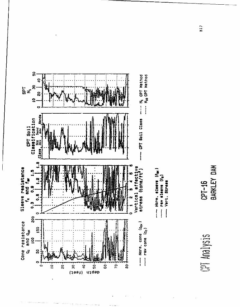
cc
cr
-a) 0 ,-:
o . . ................. .....
Wq .. ...--.%-.0
-vo
IDI0
to tj
f*0m """I -_J. I...... T,.-.~~~- bo , . .. -r.. .
~~~~c to !) C i .. .i•. .
EYq C-LL>
> U)ID 0
--3 . . . . c- c-1 Co-: 1>0
r-4 C;
(ol
0) c
0R X:
So . . . • l. ee Ur
0 0 . > C> Cm: v .;. •D ::- = .-..8a a o o oo-
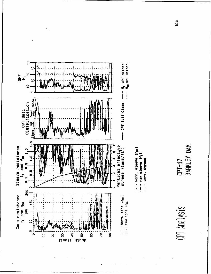
00r4
"0 '
cr) 6
C','
cc
o . .. i.. ... ..... ".....:. ... .. .. :.o oS ri "Sii " i i !=
V-4 4.1-.r4 40 V
.." : : : : : .... . . . . .... .... .
o ..
..... ..
CD'
I
"lp I" to"'q ID ME i
CI! ~~..~. ... fta > r- LIJ
1. 10. j.G3. .. : . 4J I Ne~
L- 0 40 --
0o .. . ..... . o.i.. ' cu dO C3 .T c
o 0 0 0 00 0 0 041"L" c
(cB8) 0)da
.• t . . . . . .... . . . . . . . . . . .
-" 0 c3"
...j ..... .... ....... ...L X
(:tag;) 144dap
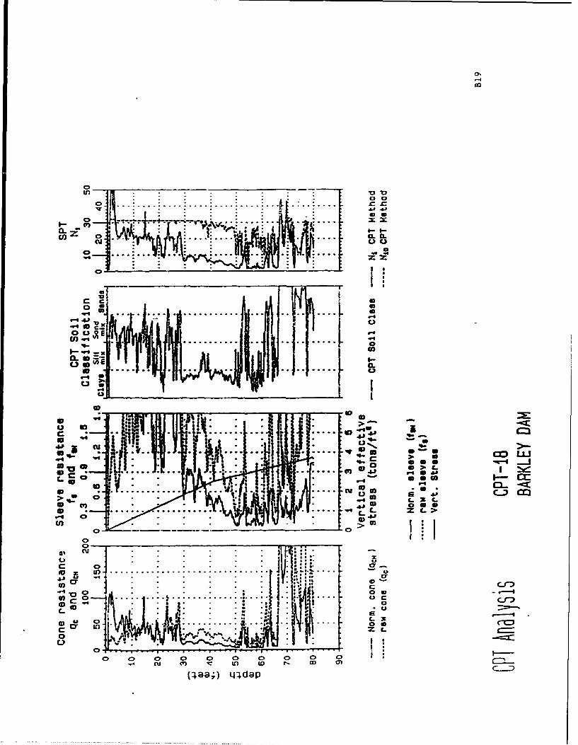
14
go
.. . .. . ... .... .... . ... . . -.. - .... . = J'
........... ........
- IJ 4-'
Ing ..... .. .. . .. .c
. .. . . .
S"
,-- , C I
.. . . .. . 0 : C- .
!'• :~.2 "go • ! J _
S . o
° . .. -
U U
° -C;C XC
0 a a0
, ' . J °K :
S: 0
"in . .. . .. .. .. . . . . . .... "
C~~ 0a1 0~qrI C)r
I S
c cr Lr e
. .. I Ij. !1[I'j,:-C • ;. ,e .. . Z L .,-
0o C > 0 0 0 Iu (V) ,,; to to a)
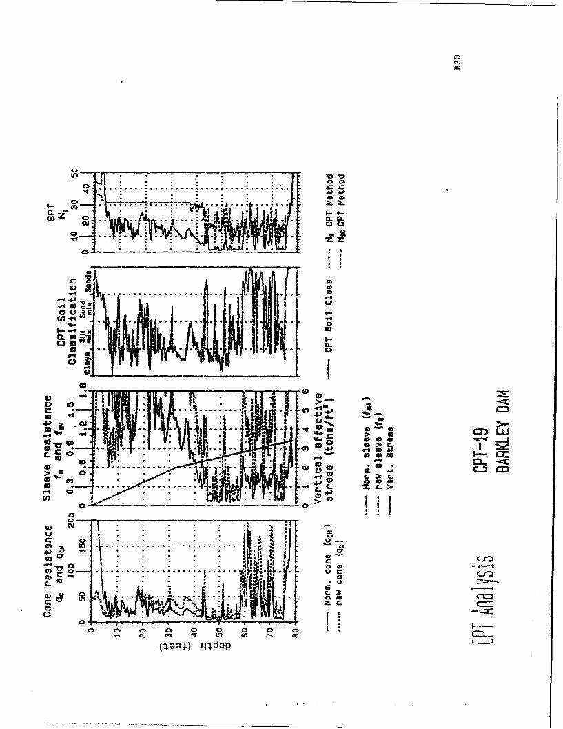
0C,4
0, 0
S ...... .. ... . . .. ... . .,
'"4 ZZ •
a. C.
cuU
0
Oo 'i n ........ .... '.... . ..
-'• • j iSa...
0 03
-. o o . o o o o . .WA-.- 0.
S.'•.) .' .aE
(•.aa~~CY L. l.dpc._.-
we Ie
.. .. . . ... u 4>- 0o -Z
m 1 41 ID 010C..C
o 1
0~~ 0
U()J Q - .....
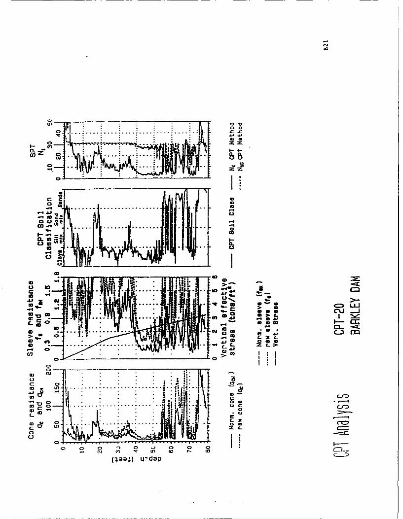
C',
•) . .. . ... IL UL
00 *0ou
- " " !
.-CO .. .; ..................
°L I.-1-
C3 0 I• .;. .- . " t ' . ....:'• ..... :'3•
-0 -&j ., is a :=)
0 to~l a ,L
""° Igoo 02c
z- W3 -'
...... ... .. ..... ..,.caC -- 4
60
. . °LJ ccc
CO t .. .... .. .. : " ...... '"..€
to'6-
( - to_ dp
L17 IIa
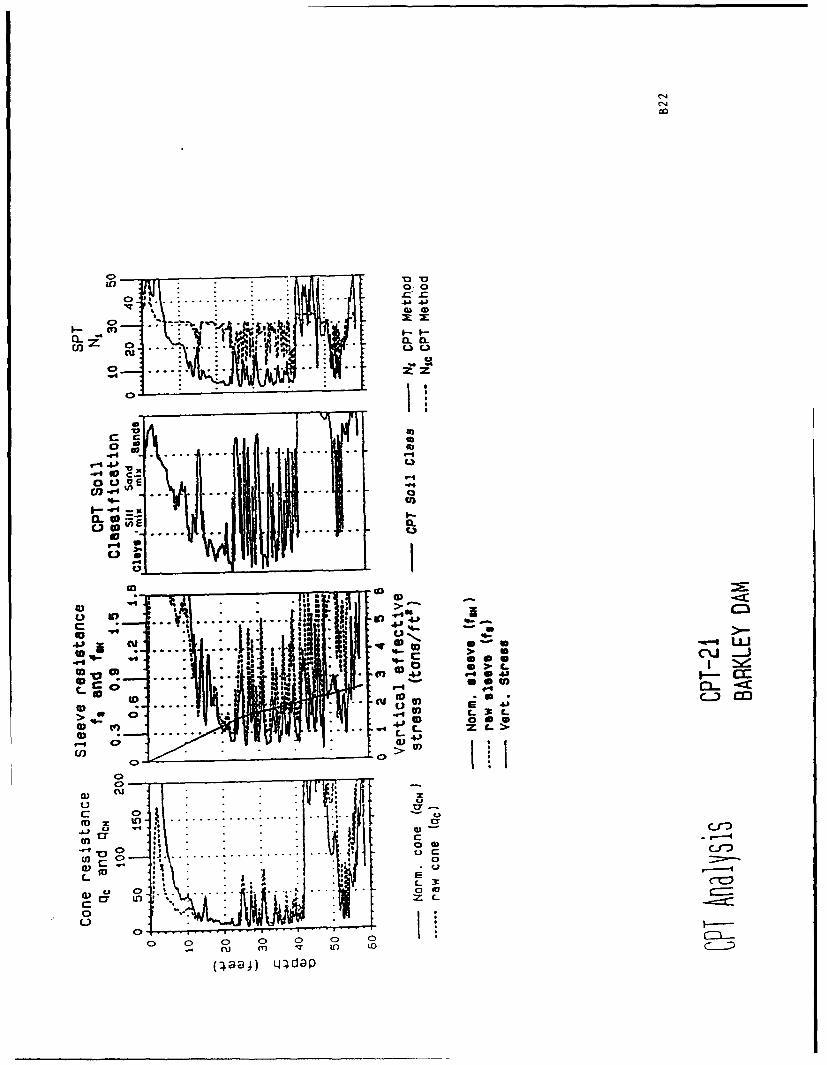
C14
"" " " 0 . 0
* . - !.
o r
, mm •rl. ... .. ....cu C.) U
o . . . .. ,
0 * . . . I
00
U)
-4 - x-.r--
to•° U
-- t
0.. . . t
4-, 1
so o) o>_o o
(41aC.) L,... U) ** ..... .... >*..:-
CU~1 'Co. ~Li
CD ID
C) MC Lo >
CL) CU
L *
C~
00
UL) (>
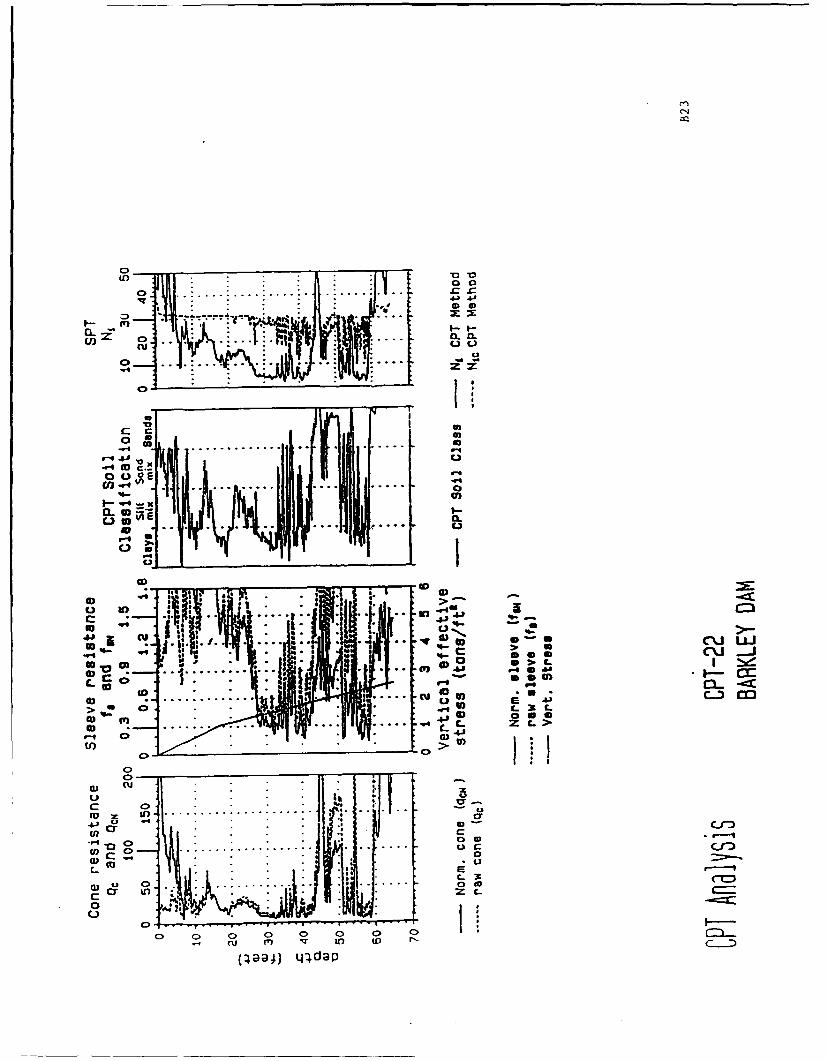
0 0
qtT
U)
9 - .f.[.... ....:o 1.. 0>- :• u- _ . " 'r. . ... ....: ..... cu _..
..... .... ... .. .
I-- -,- *
.. . . .++
CL 8on
o c . . .. :-1 -
a) w.4.
C,~
41
toa) a) {* 0 -!"Z ;14. m . :x.
S... .. cLLJ
Si, 4°-,t aSS.....-..(.*.
O~\. .. U
d) 4 1 ZL>0
o- to to o a o
(-) .r ) *i0 C.Pa)
0
c0 C
C 0 r*
. . . . .. . . . . . . .
rE X C-C)* ., 0
o r z
C> C> 0 0 0 0 0 0r"7cu 2n qq LO q
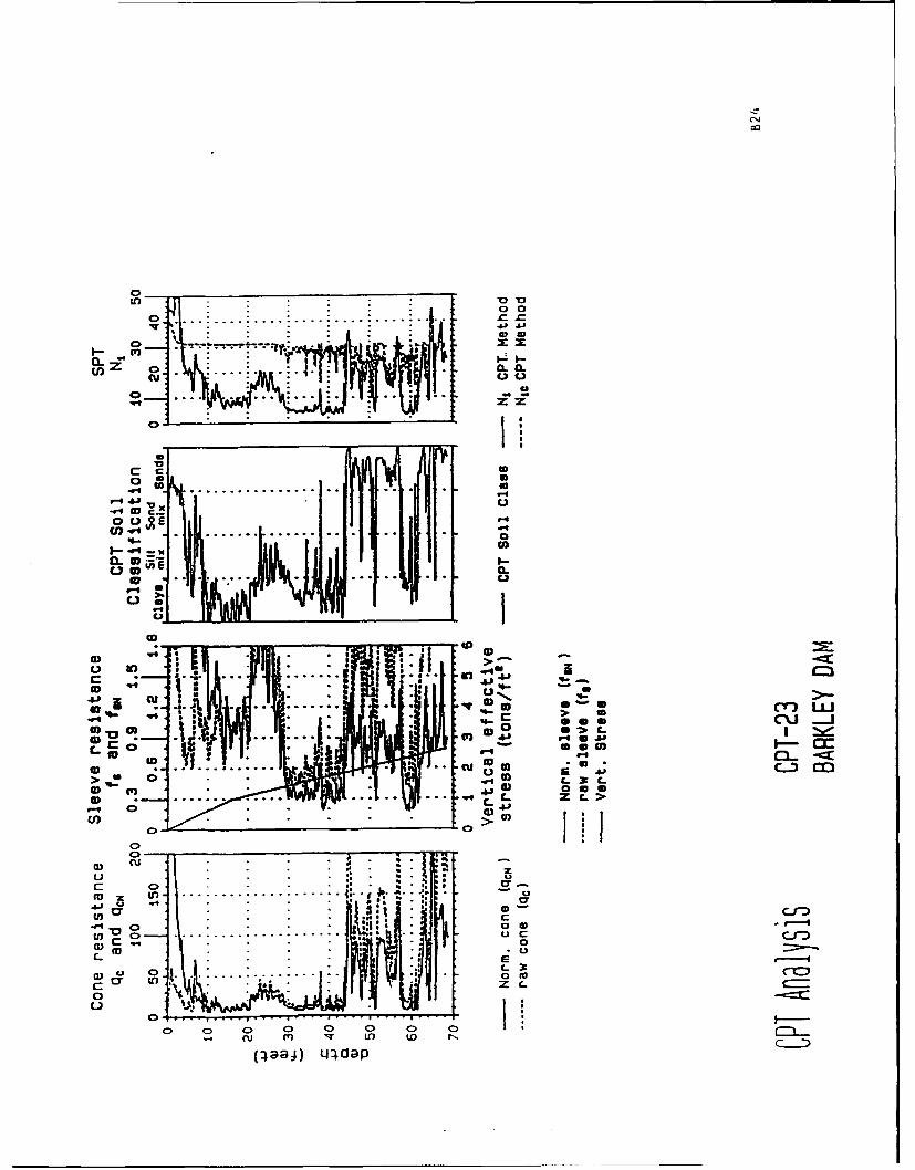
C.'J
01
Q0
Q ~< -......U) 0* 0.0.L
0
of . ... . . .. . .. .. . .I
x C3
xc w
0.
C.-
00
in 44
-- 1
41 %
.: -
44) 41 4
ICU tow c.:
o 00
0- r
a) cu .z
u U
0 0
a) LS OR C£flc0 m..u C..-C
C>
o 0 0D 0 0> 0CU m~ (T) t ) to
(paaj) I-40dap
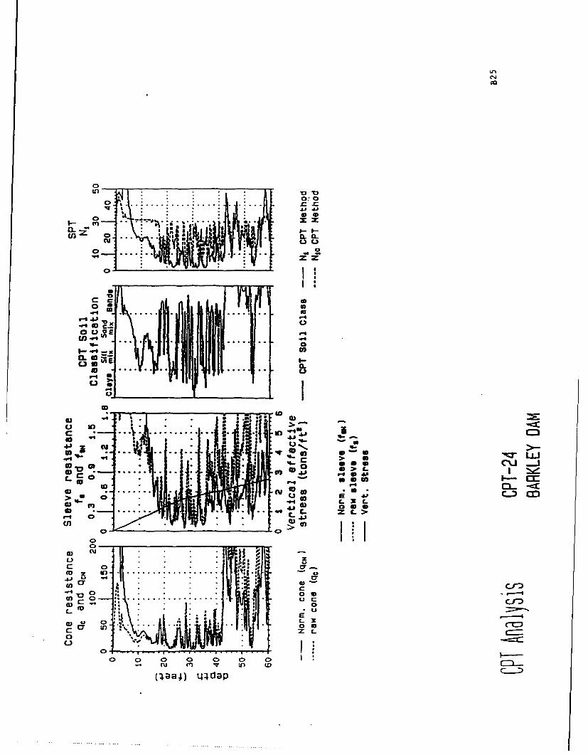
C,4
.044
0
6 0.'
, . . .I
~~.. . .. C3..- ,• , , ,-4- .S . .
U, IOo ,~ o . ., -
- > UL.-
S c.......... .. .... If4i 0I-
dl)0 1
Li-.l.I ">
•°' a " " " cJ.0 o> .
o. lf) ..... ......6j " :: li! i4. : . . L 3:m z •r . . .. .. ........... •|-
•'c o g.. ... :.. : ... : ,~t ,•l: " --0 0 .. -
r- •) .C> 0. go
CU C'r W)W)
o~ ot o o o (D ---
(paa;) LIpdap
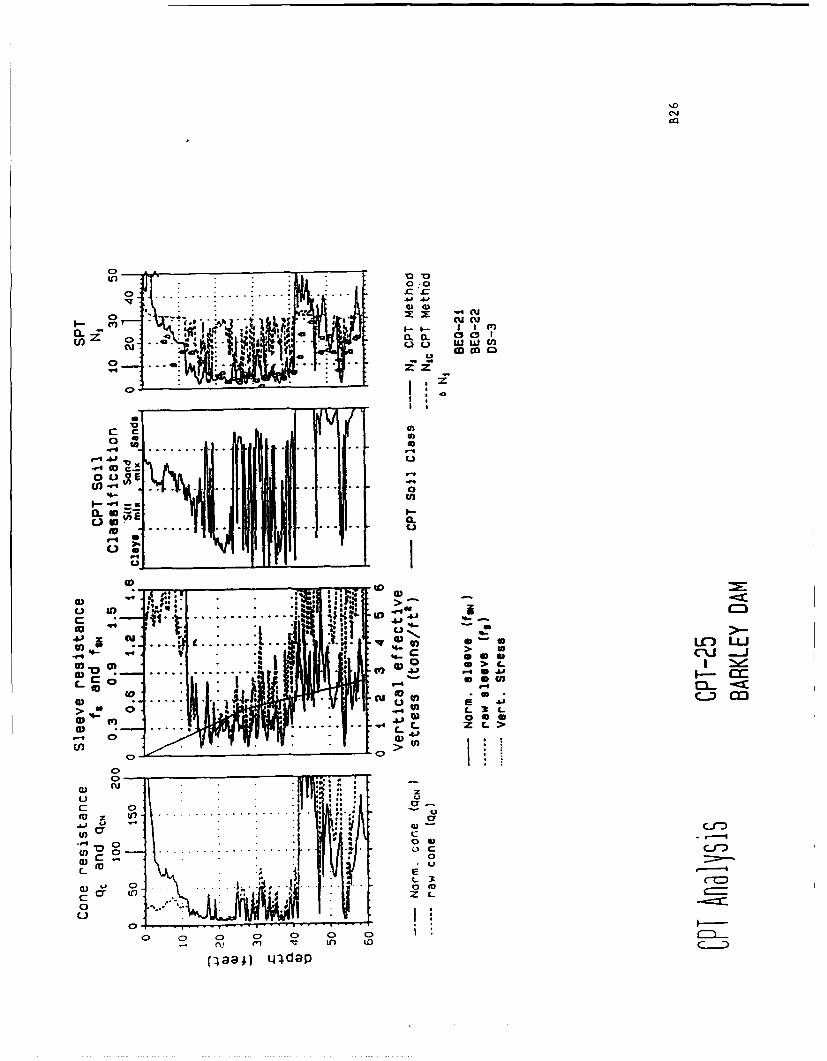
InD
o. .& .U
0~ mj
000-cu.
U c
0-.
0.. . . . . . . . .
9-4 to CU
U ) -r-
ID .. ... .. ( cJ O
.. W 7;'
4< >
1.3UU
> U00 . ID
. . . . . . .C) 0. 0(D -4 m 7 LA 1
(raa9 a)da
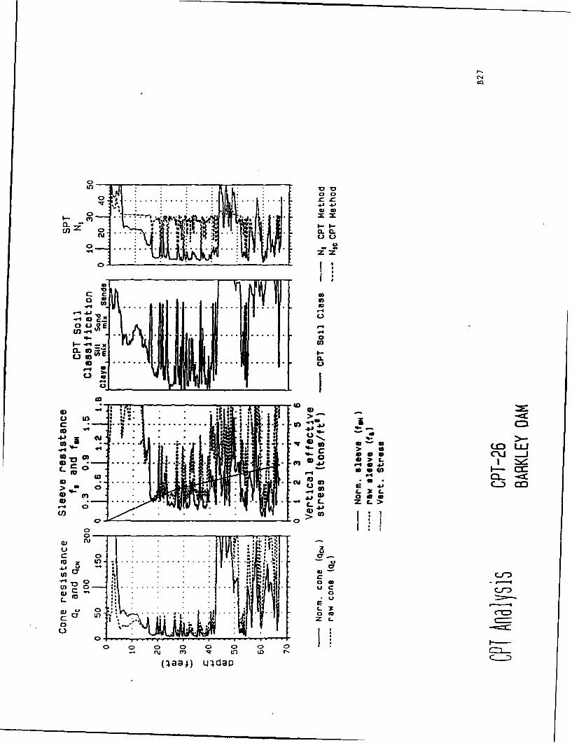
CJL)4
zz
co0 UXU
.- . . . .-@6 -U - -
a .-toviI.I- -eq -
40 . .. ..
to) in
C.....)r " ~to
LEO .L
to ýq C l -Cf... . . . . . t o . , * Z
ID ID~
.4) to
Vcuo -rto n . I.. . . .. . . . . .
(p84 Lj~da
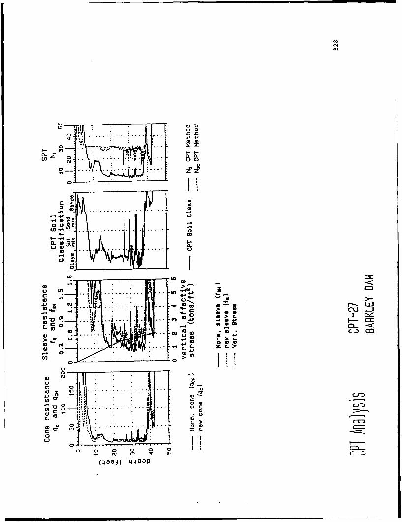
00
o 0
C , * . .... .. . .r
a. CLO
U) . ... . .... .
0 * .
0 0
'- .Ji ....4j.0 x.
0 I0 '0 . .. ... ,,' .. 4
0.. .........OC
ao. )
to0 C
- i -%
00 ' - fo-* ... " " "
c' .
r" .4 " .. ..S
rn's-.--'
..... . ... c u w :
> a C -4 toc X tS..U.. iP
°) c
0 .40 )i cla
-i z L.ni m>
(141
0-
tU) *.
0 0 :D
y 10..... .... . .... 0 0
60 ,..= L
L) C ..
( L9) udap
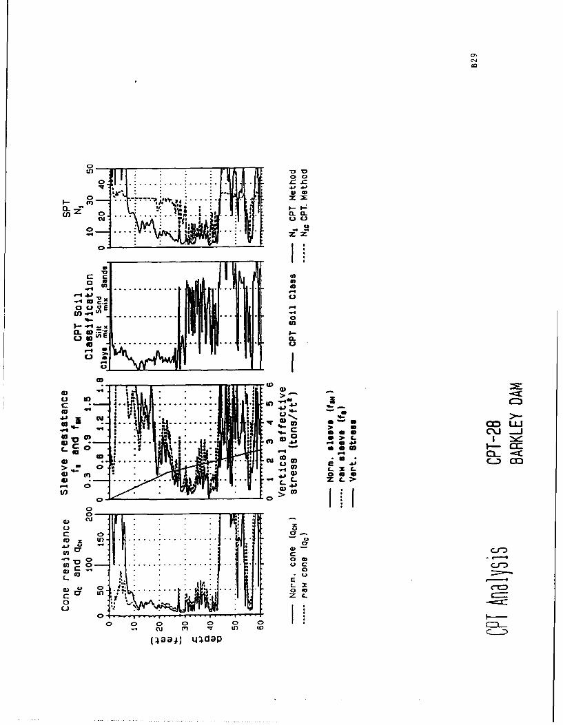
tn00
C)i r-Aj
"o M ..
S......... . ....
o ci'
,-
or ...rev .p
a. 4 .a. -I.-
... .
"•4
0. . .-. ID o
, O'SCcq 4- >0)
o -3
L0 Ar
C- C-'a z~ C--
W cr*c C ... . . . . .o
-.
Or
00
00
I . m .O t C .- I-- It~ d a P
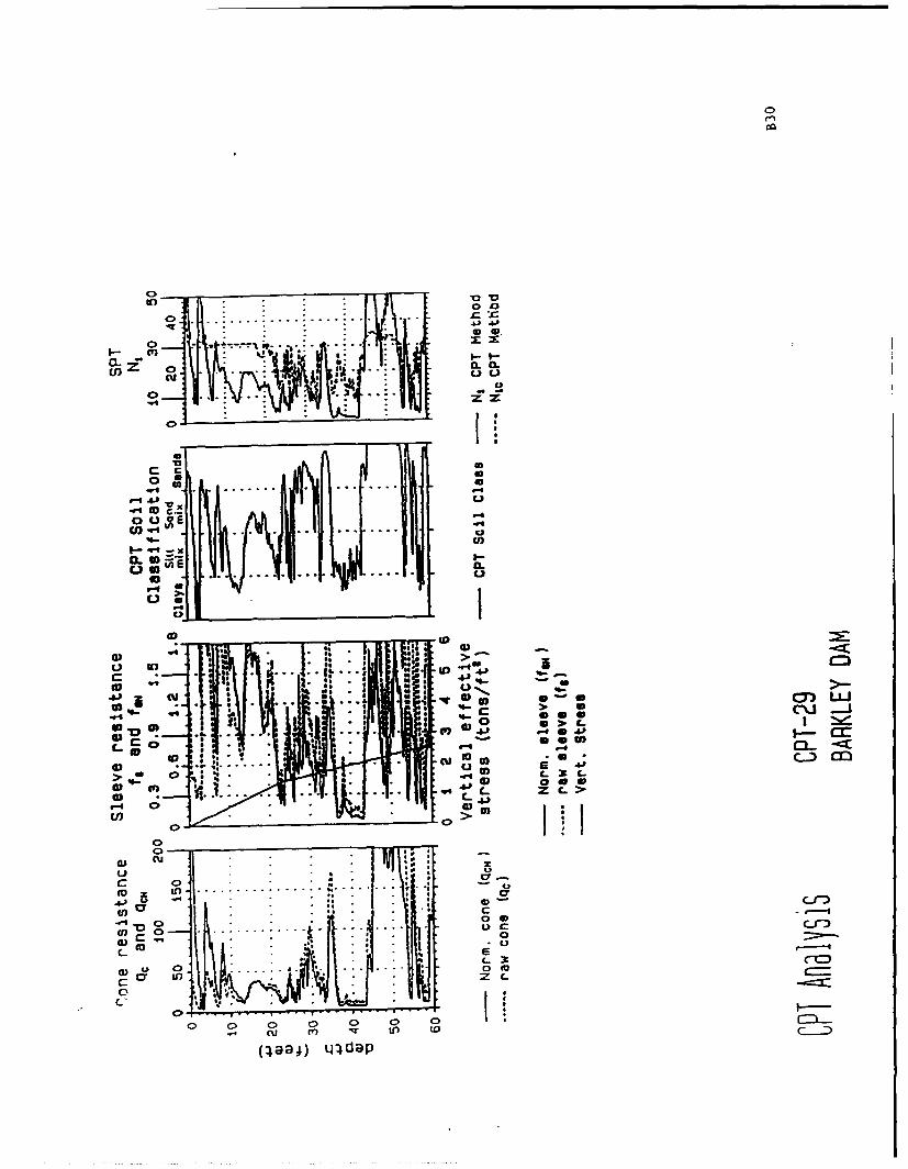
10 V
0
cc 0a
IL fa(i)
t.4 -r~ a
tto * D
C7 U
WI C *S *' 0) zo -
..... ..... ................. .... 8 -10 &PC-- 0)LL
> U) c- mL.
*0) 91
c . . . . . * . - e . .
U) c -. .*
0 0
X -I
0 0 0 0 C I.
r- u (* to* toW49& dJ a P
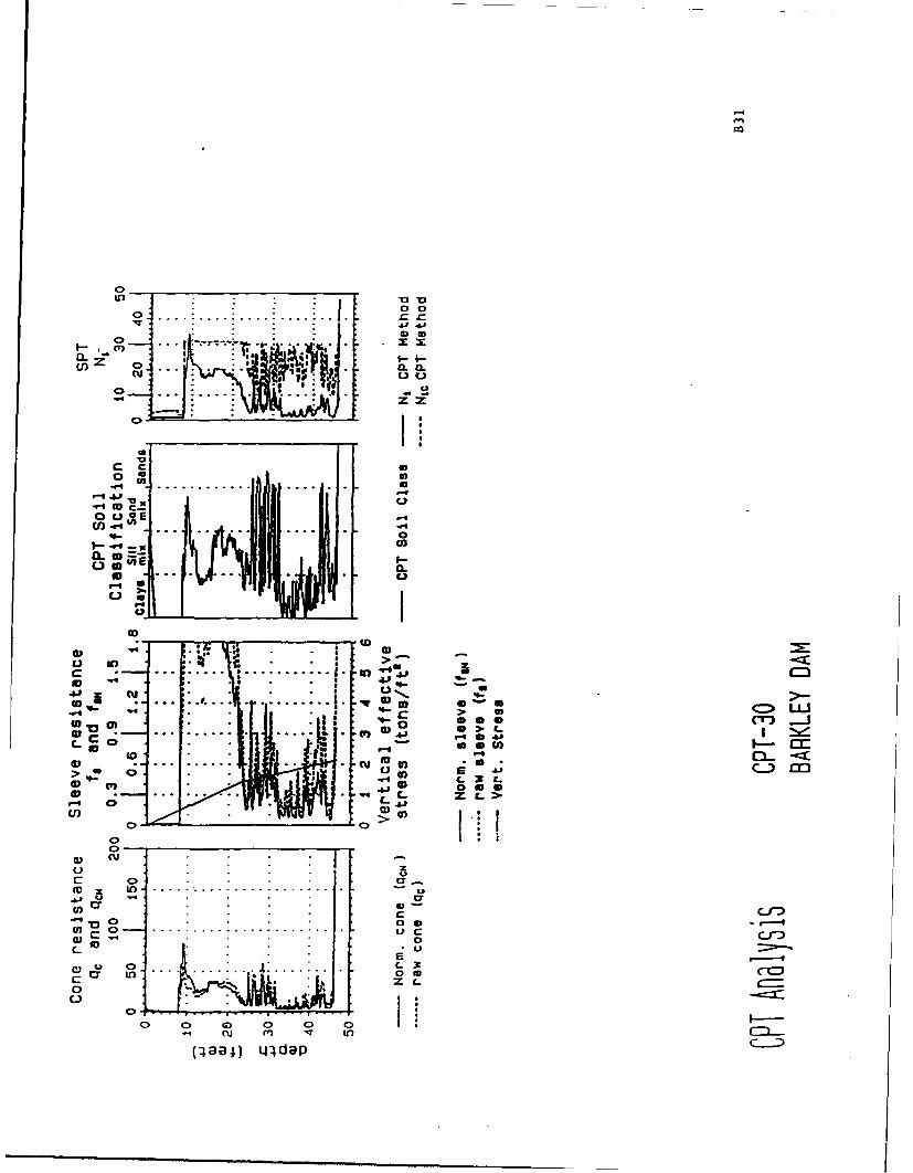
0.0.
zz
*v .) U
fa
.. .. .. ..-.
90 C.)0 UJJ
-- (
Ui IDC~ -
~LUa,. .1: ID
UU
03c 0 4 0 I
00-
4 'D 0U) 0 . ...... . . . . .
C- 3
cn 0Y L . . . . 0 . 0 Cr,)
In m n. t
C.)al .- . '
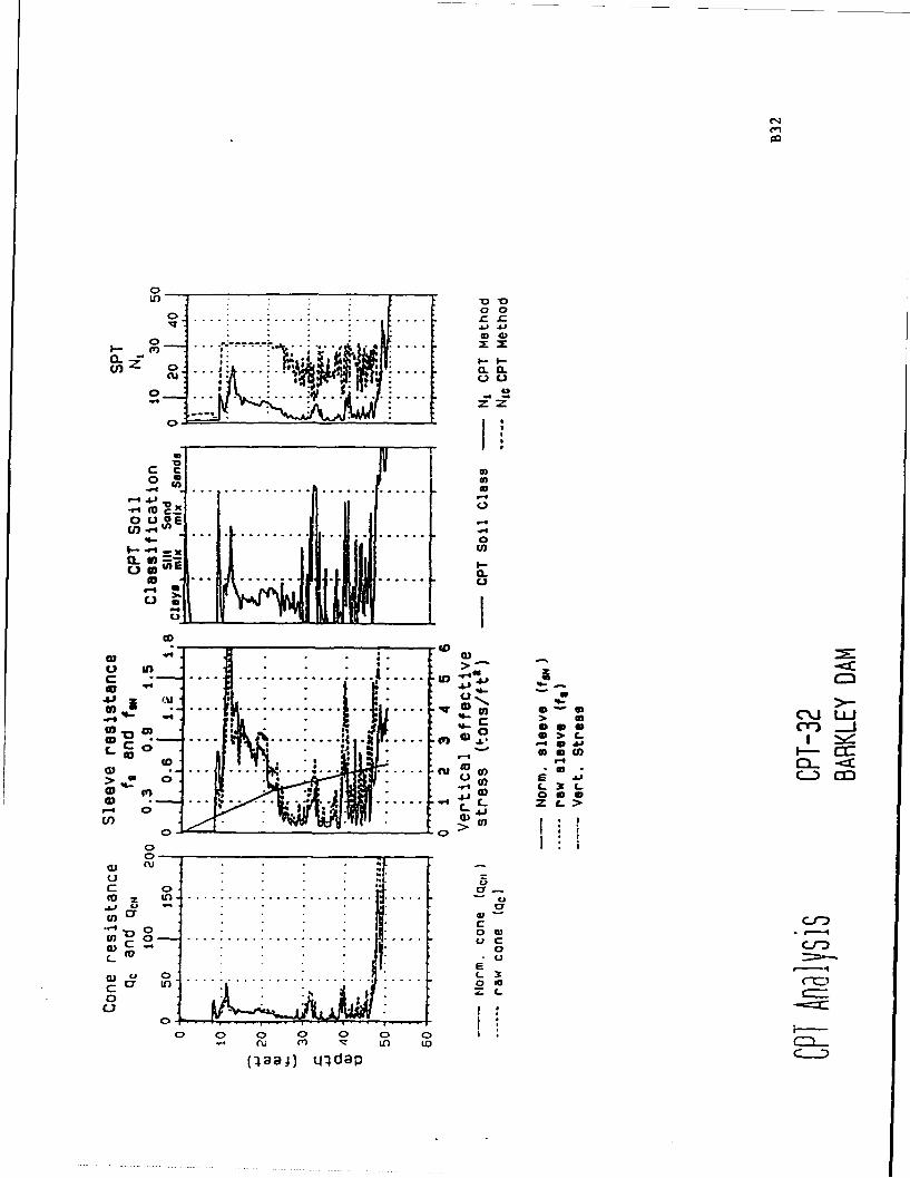
en
op
0 __
000
,- Ca .. - - o "
a- o" .
oU oo --'z zr
c a--4 ... . 40
0o UE -inf-I -4
0
I.- i- U)
... .. . . . 0
L)
c . .... • --.. -... .... . :.. .. f -r- o .. . . .. ID
a-I o°
C C>
. . . . .. .. . u
a..0)
>•)at}fl)a CO
S.. . . .
0f) > I- 3
(a in ........ 4 .... ())7S L-
4-P3 L
C0
U). "D C ..
Q) cu c0C-,.,
I E
Q) ................. ..... 040:
0 I0 2> C> C> 0 4
(laaj) LI-dap
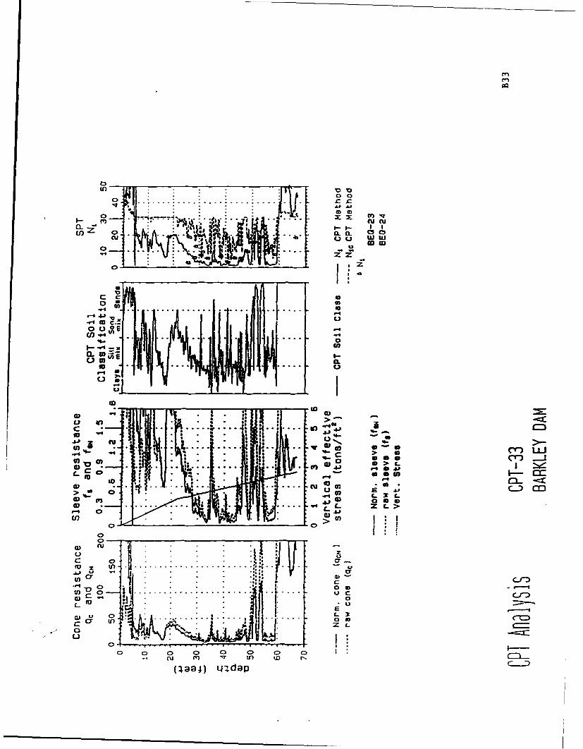
U.)
(D00
oa. a. -s
cu -b t.1.3
0 rig%W') ~iA&1
o .. U
a0
.- . . . . . . . .
.44-
0.r I-a! >.
41 -* &C-C-ýSU
to t Sa) C t ) -. ) c> a
0) G f-. 404
LD z C-C; L * vi'I :
...i;.... 4.- 0= -
or6
Ti ii CZ L
E.)
(-4aa4) LI~dap C
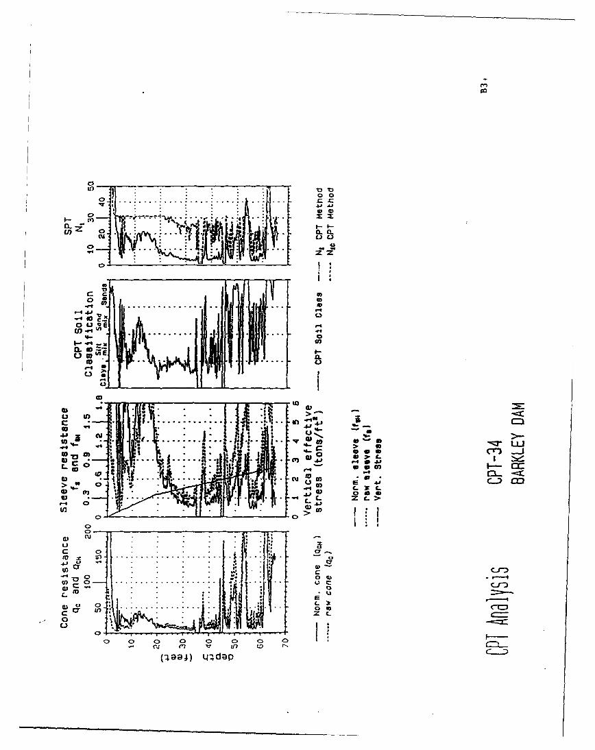
LOo
0 a
0~ .. ... .-0
CL0
. . ... . . . .
o .) ai P.4 Iz z
O. . .......... ....
0 L) CE
II (a
•) r4 ) .1 .... ... . c_
• , o ") •.'0 *
o gouu " 41C7
In -I . . r i0 0 iiL -- :0.•
_. 0 -. I
C>,
0 0 0 0 0 0 0 0
-) V~ " W D,,. i.,v 0r "O • 0 ,,
a),at Lda
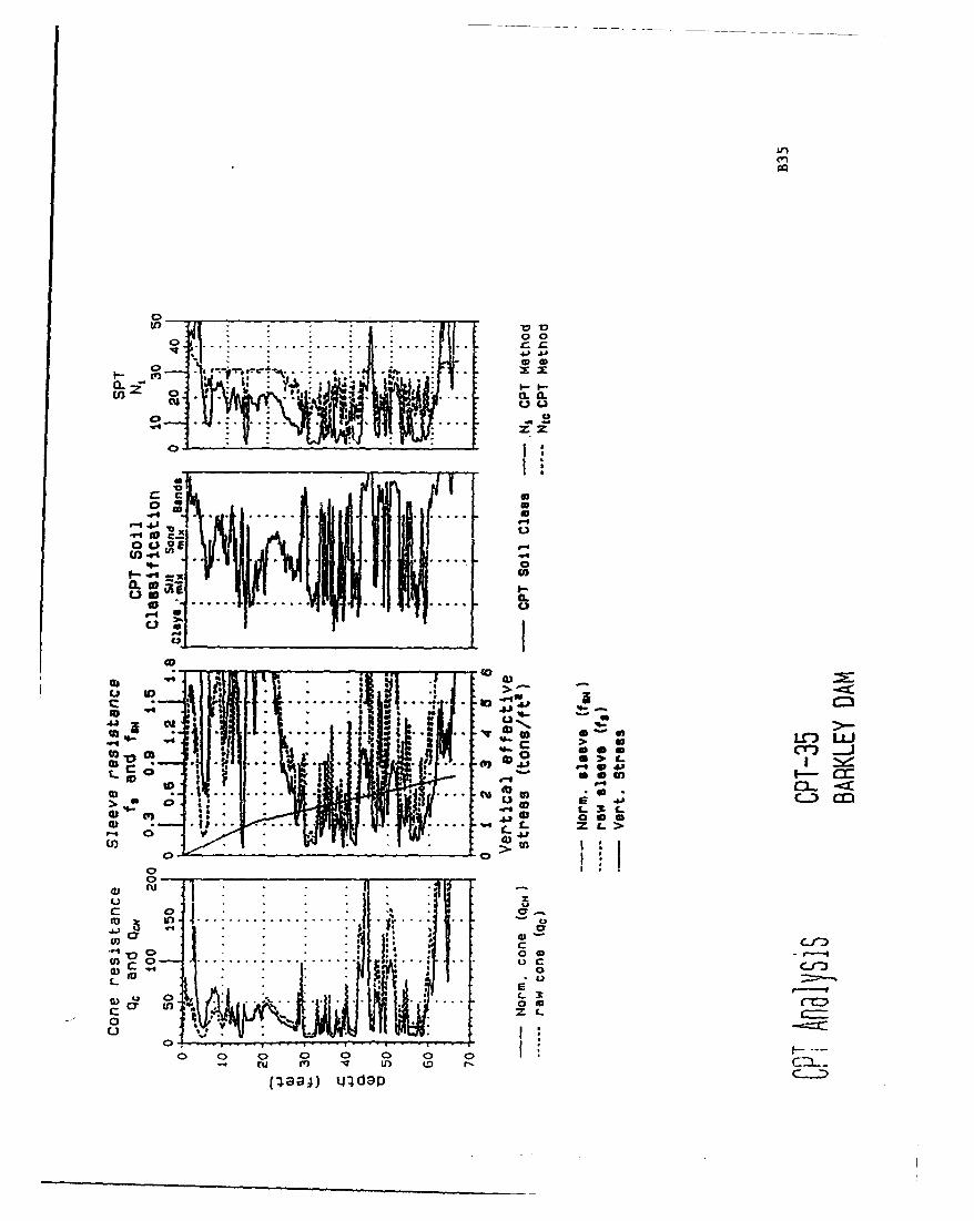
4-
117
U) 0 $et. 0.
o u U
40
40
. .. 1 . . . . .
I-3
00
_F a0n 0
0c1 z
n 0 0~ 1 0
cu
r-
- ) ~ I)flea4) tj"4d ap
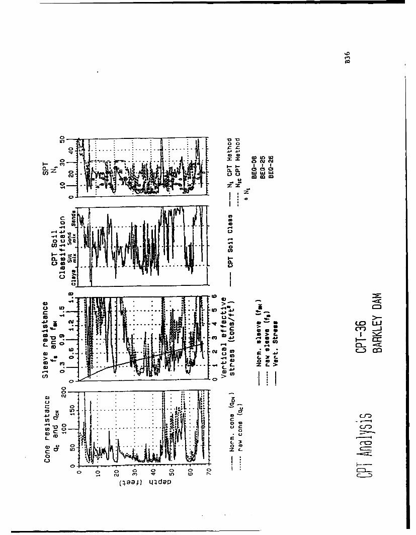
0~ ____
0 .. . . .. . 0 0 c
c ccc~
40 c
IL W
(U
CD W
-41
1.a a) cc..
CC3 j ** .3
> L. x CO-~0~ re %
.~ (W-j .44
44 >5 U)I~05 T
co Lo . . .. . .... .Z L
0 .
.. .. .. .. .0 0 H I00
ZL _
(;aal) Lrndap
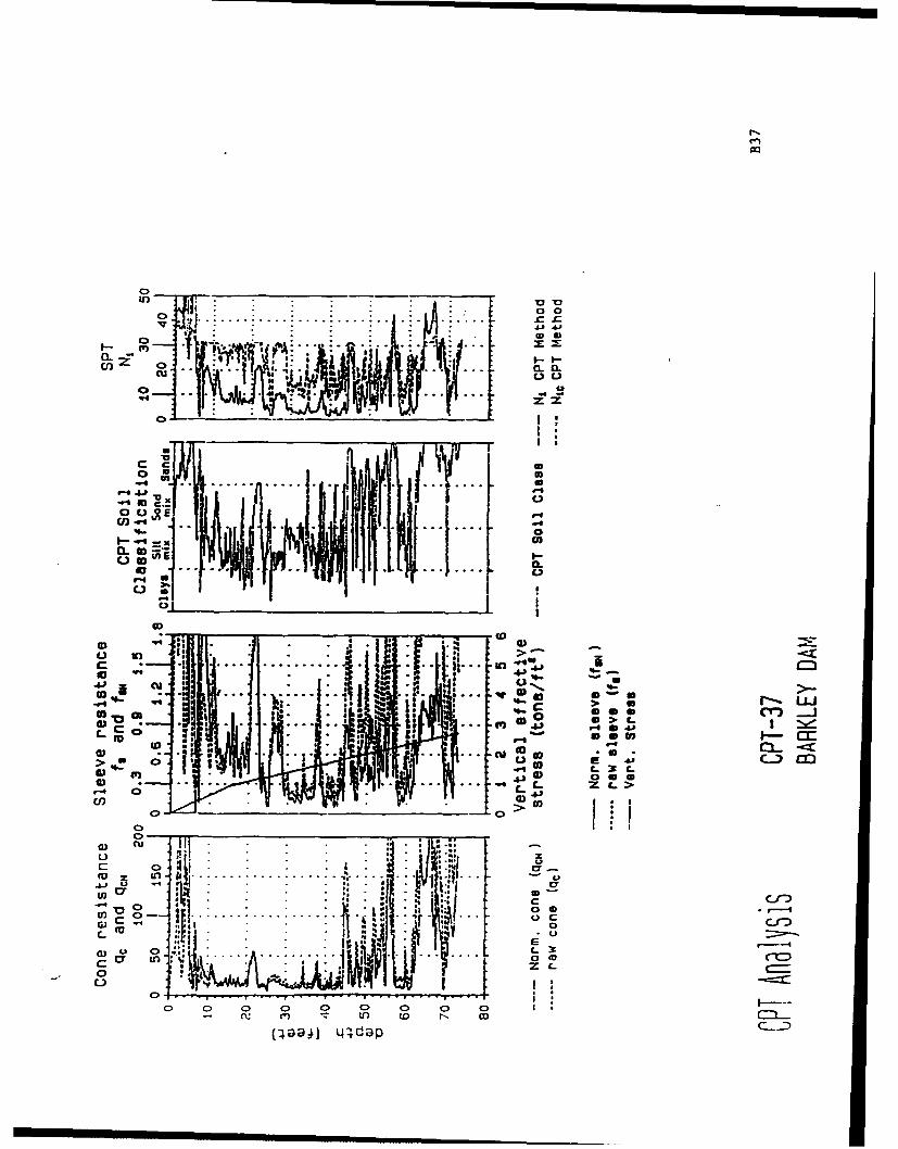
0~~~ 0__ _ __ _ _
z F-* .. 1
cu,
7- m
o - I
~~. . .. . ....... .... • •" '',' -, • w- --UJ
U .. 1k.I l U. )i.- rr
* C3
o, --E I d -n
C.
* * *t 0)O
'a "** ' . S.. ois
0 Up
°°°~ ~ ~ ~~~. ........ ....I .. i °c i .. . .
U to A >0 .. .. . .... .... . .
41.1
cm I oI
41 :1D .... ..
(_L._3C_) C-__ _
. 0 I I Ni
o 0 0 0II
(40)U.~
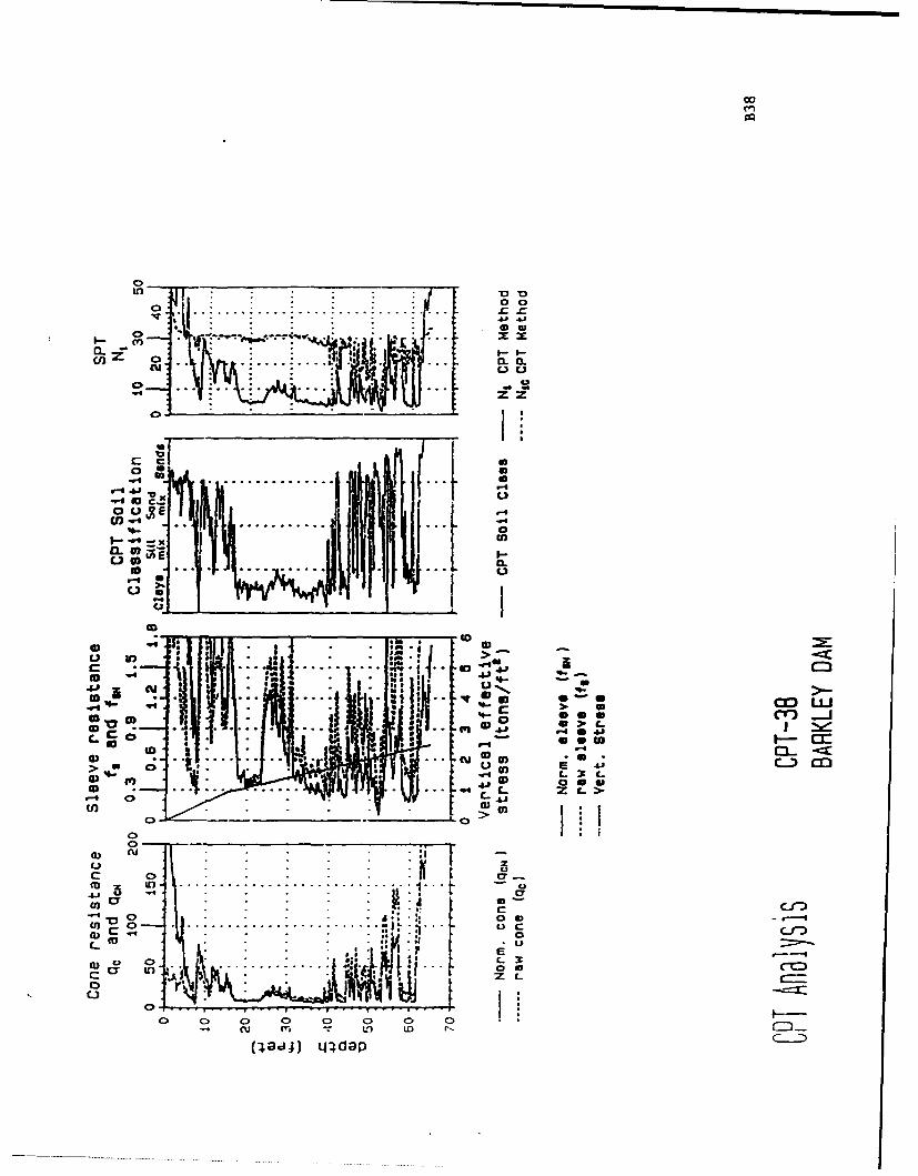
C0
0 0
cl- " 0.
-c I :.. ...... .-r o C.!_ _ __ _
o .•
ora ýl ...........
a,.. gi E x
C-.
... - .4 M.-It 41 ,• ' o• . .
tv o U
to 4
.u44 0 *41
O- :. 0-~U0 0 c
o.. cu . ... w
0 , 00- - Ca
V) CQ > to>C 0
rn 5 cfto1. 0 n - . ..... a
0
L3 _
0 0) 0 0) 0 0 C0 0 *_ -~4 cu ('r VL, ILD
(4acj) Lildap
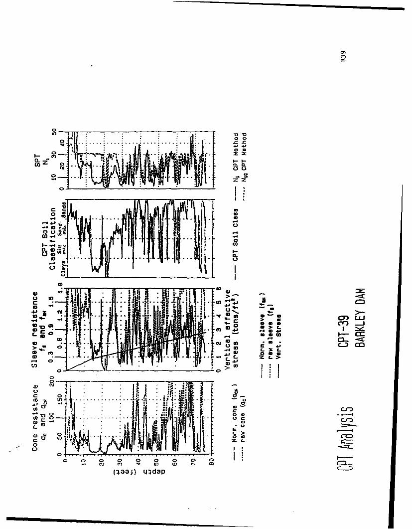
C0'
Ji4J
CLL
0 ;;
J0 C
C .)~~ C4to ...... ....
0)0
u ID00 C"m
a- a .1. I
X -.0 .. e: a
0 0 0 0 0 000 0C>() ~ , C I- C
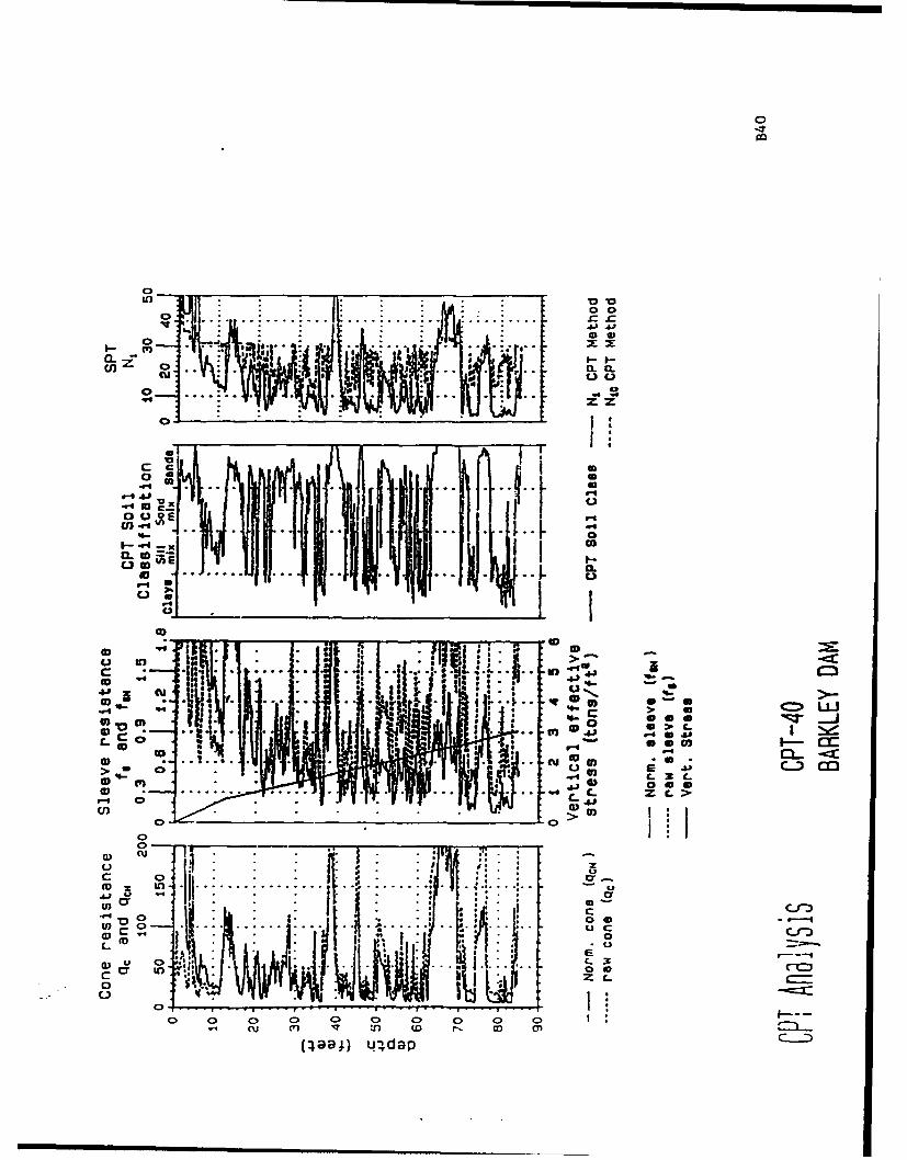
0 0
Cl) 0*L IL.
11.
CUD
C,,.3
-41
(3 ~ .. .. I__ _ _ _ _ _ _ _ _
W4ULIT CO
:6 cu to j) 6; -<C
h~41
U).0 a)._ IC) 0
C.,Y
U) 0 .. ..o u
C>C C) C> CJ > >
cu (n T CD r- ar) op -
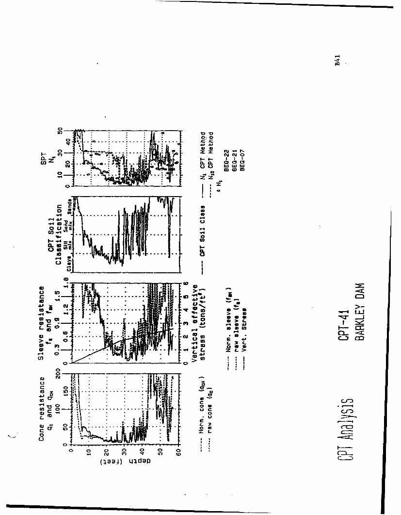
0I
IT) % 8 .
* . ... . ...
-ri . .. ............ .o- . .•
1Io
o . .. " I .. ...
WI- t ..l t l ! - -
<.•<''- '-I...... . '................ ..tiil it f .."U+ +. . - ,,
L (IJ
......... In 41 C
m "'.' rTT.. .
•,I : : : :!l+ili•_"- ~ ~ ~ ~ ~ 4 > .. 1IllW- C! 0•. . . . . . . . . . 1llt !"
-- 0i
i ! ''+"" "tw o . .V .iPL-_
OOScu o" . a0i
. ..-- * *
"> C; L)a 1C-)C M
(;aal) 41dap ca
-- -~~C i i- >i I III I iI I l
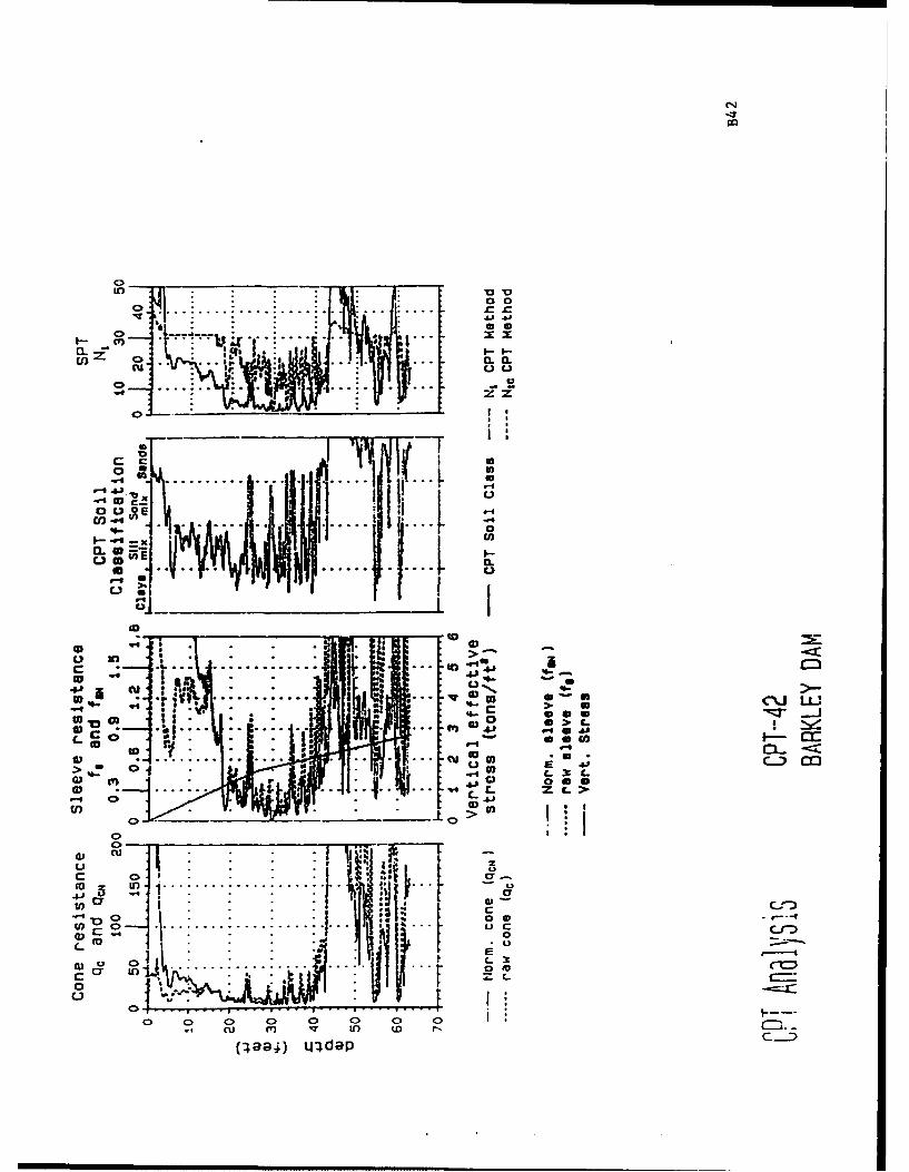
0 0_
Qt . . . . -J
to !
0 .. : .°. 0 0 C
-- :--. r " -: .... ..'-"
L-C) a n.
•5 o. ** :": , -I
on ...... 0)
U ID
0 . . . cca* .r..-
to to- -~ . .I
oam H ii e
"(a iý-s CC2)
.. "' CI•J"'- LC
.I 0. - . . .u ) L --I I. m € .. r) -a), .
0-
L z -. > -C>
to LO • ' t
( d.LP . . . . - 3
C> C> 0 0 0 0o 0C>-
CU c) Iq En Wf r
(p8g4) U:Jdap
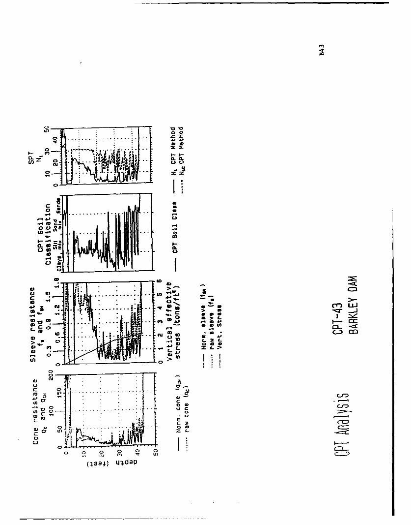
40V
00
r4 . .~ . . . . .
CL* 0 c.!4-
4-0 .v 0
0>Cc
*) -a 0 ! . . . . . . .0) C> - U
> t- .i C-
C; U))o.-3
004I i ..... .... ... 0a) WL
LI r. .
cn.
I .00
C', Uru0
paa1 . 'a
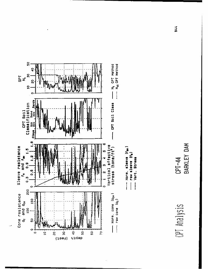
(0
co 100
0 0Ucn .0- 0 ... .. ...
- *:LD!)rL) .
U........ ................................r_ 4'1 .
IIl-
9-4L
4-4c~ 3- -c:c
goo 0)
di m. ... . -O C- >
En a) U)* .
CD cxj
0 4,
U) 0 - .. .. . .. . .w C.. . .*
I L 3_.. .. .. .... . . . .
L) .r -.)Z
0) 0> 0) C0 0 0 ir-. (j 'I * t* (0 rI~
(4aa;) LJidap
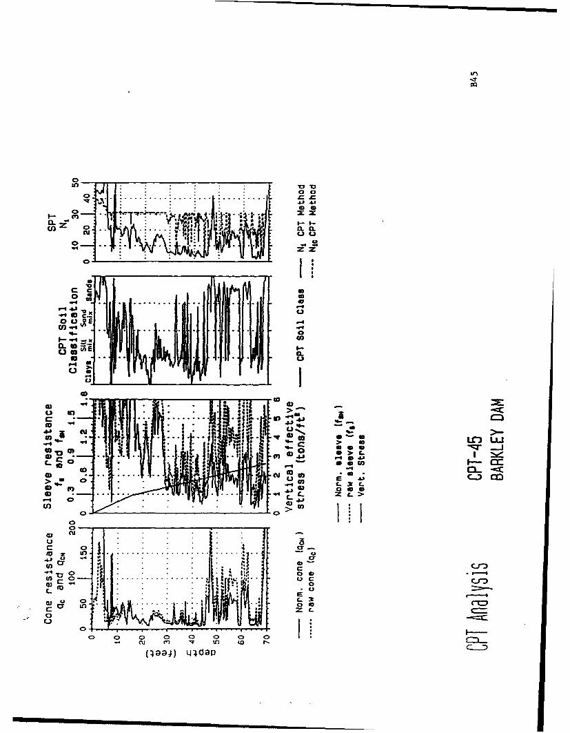
0 0r- =I
U)zz
CL 0
.... 0*.1.
010
.44 0
o- Vq - 4 . rCflu U) giC-
> .r 4 -; 0) f-3:
C a. 7CJ
c-to '~
Si IL X:.:0 0*qCr ML
u q, Jj to t 410~aa *q' - ea)I-
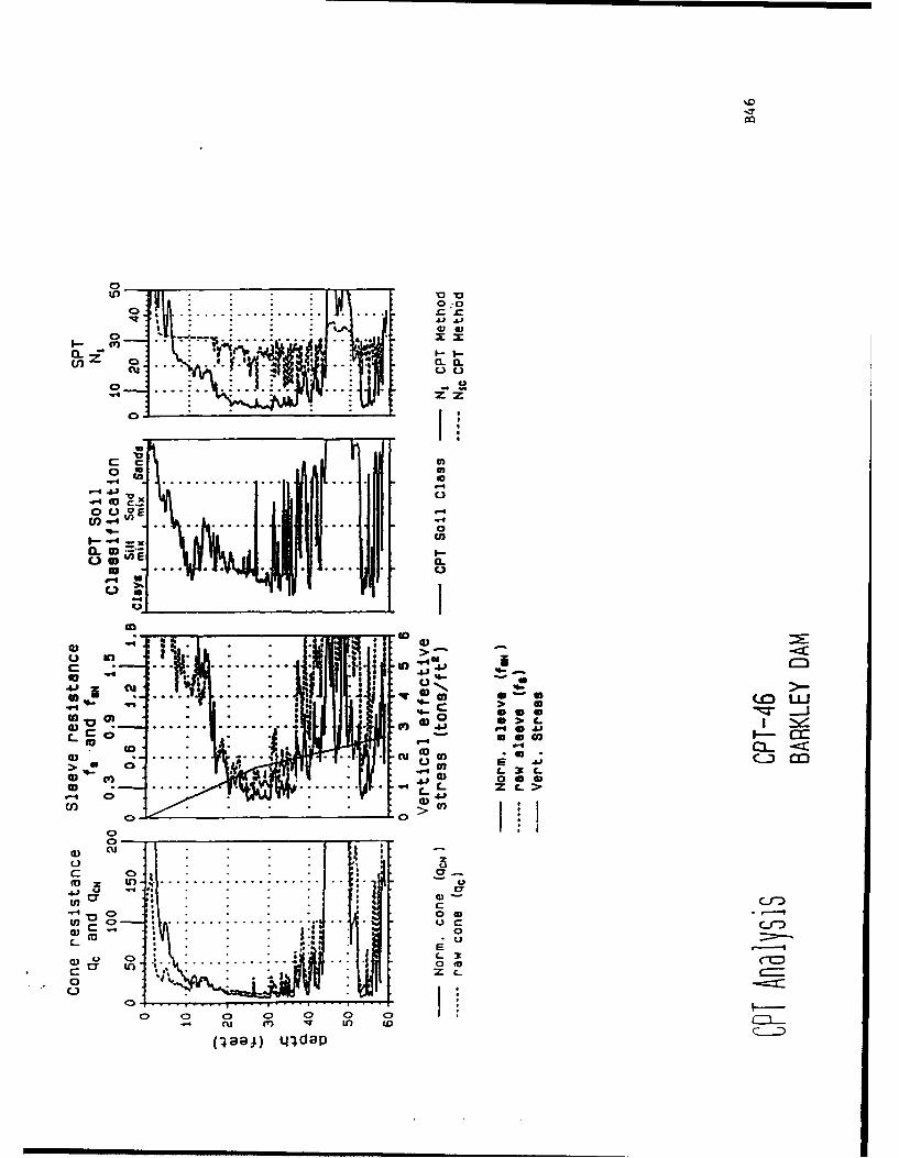
0--7
in z. . .. CL
.
0 Iw o. 0 0
*r . . . . . .. .. . ajI.
I- L) Ei ... U>S... ... .jIi
W CL
41 "~ uI1
"- c >
-U
qm 0 >0 CO.
a -C>0 . I - r
S.. .. . . ... *- CO 93 0 -
1: 11 --- 3C-
m 4 ( 0 a •
. 11
. . . . . . ... ... . C- ( L
0 0 0 030
I 0
f.464J
>* >
03 0 0y
.4.a95) L I )ap
CIl
llCD . .....3
ca0
P aaJ) 44d 3P
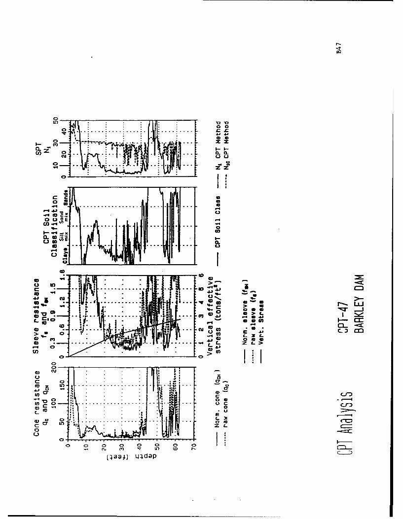
C)
0 0
oEUL
00.- .' . .. . . . .. .. ..
oL w* iI-w CD a
CD
c .. 04
..... CM.q* qf -~
La 94 - r
I %-
0- . uC) oaA-C>) q 0) E t
4) 0q ... l 0 a..-En C0
0
0 0 *
03 0> 0 0 5~~~ If t
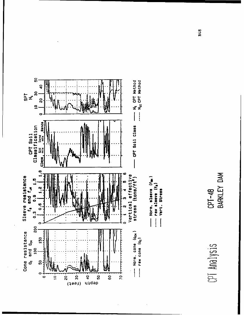
0 0
C111EL
Y
. . . . .. . . . . .
. . . ........... !-x -4
- 0 .... .C..
CD
4j x %A-
Ca 3a
4-44
0 r 4* w 0 43Ii
>14>
040
S0-t) .. .. ..
U)
0 C0f
L 39
C>
o 00 0 0 0 0 0)Cu LO (DD o -
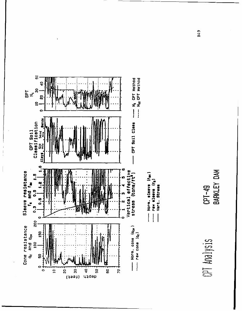
CL
UjJ0
40 . . .
q. I ZZ
so . .IL
44D)
a 1;
0mu. 6 . .: . I .. . . w4
C3- -dc
0I a
IL -
cn4.,
0 0 0 r-. * -*a4
.. .. .. .... c
0 40 =-:U L
0 C> 0 0 0 0ý 0 0
(pea4) tj4cdap
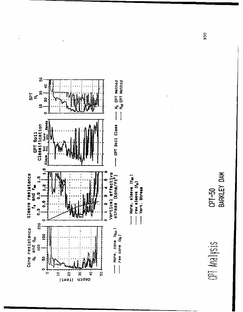
a00
asIin
o oiE :..
.. .. . ..... .. .. .
vC.0
=C=
co 0 0 ED 0 r3 -
o -. .... -. m->
0 N. q-•
. 9. , L1 J0-3 m. . . C
C- .... *-c- I
410 4
U) ID
00
U) .[t' . ........ ... ....... .
"0 - -... Q •)-•.-
8) Co m . S *
C 0 0 . 0 . 0
-* .m ...... . m mma c . >5
LEcD M
w~t4:tda.
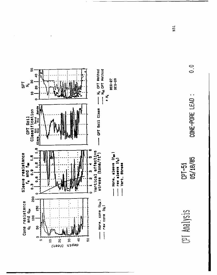
-. 4
C))
LfC)
S00
M m
0~
LUJ
.-ro . ... .. .. a:S41' , C.) -
oUgE .4-
4)-4 1
a II
IDD cut
r4 C M L.:0 10I
V-41 C;4 6S5 41L
40
cr
0 a.U) C) ..............
a) ................... . 0ou
o Q 0
(:Iaaj) wfldaP C-'
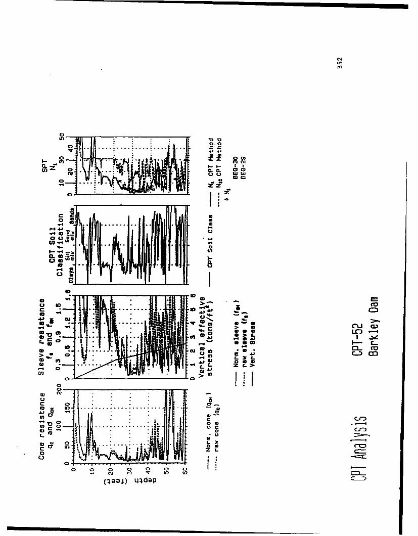
C z,
10
0 . weI--**~ 0
a-~ e1
a 20 . .I
.... .. cu I -4 2- c
t- x C-
c is 00.02-L
rn.
C>'o
in.: .... ...
a. .. . . ..-
c-4 I 0 go"
C z . L
0'C=C
ol t
q;aj tudap -D
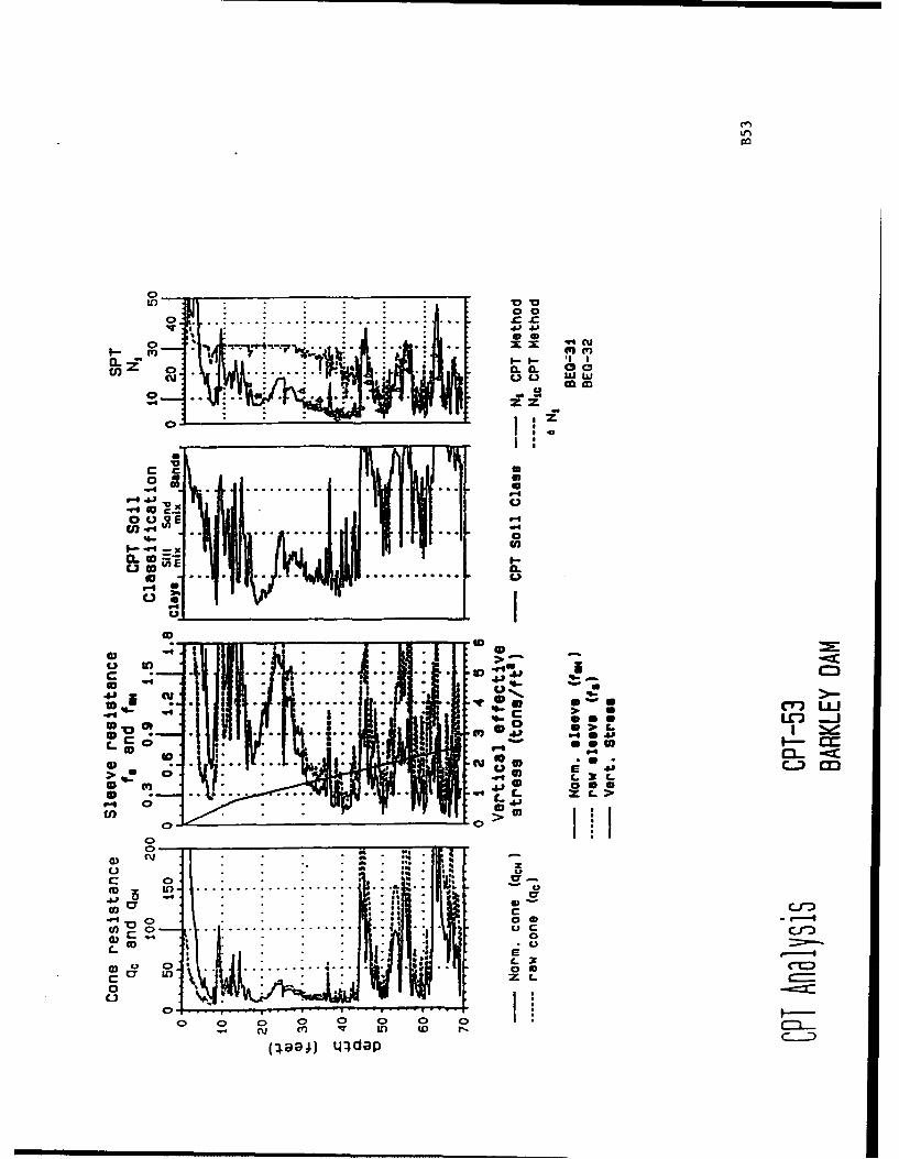
U3 ~ .
0. . 0
a~~~. .......
z.4 U
C3.aoc t
'7*
C.).
.. . . . ....C-)
0UU
IDI
to*. C=
w I cc
0u .0 6
0 -nAPV
o .- .- z 2
0'-
C
-7
mc?0
c o 0 0 0 0
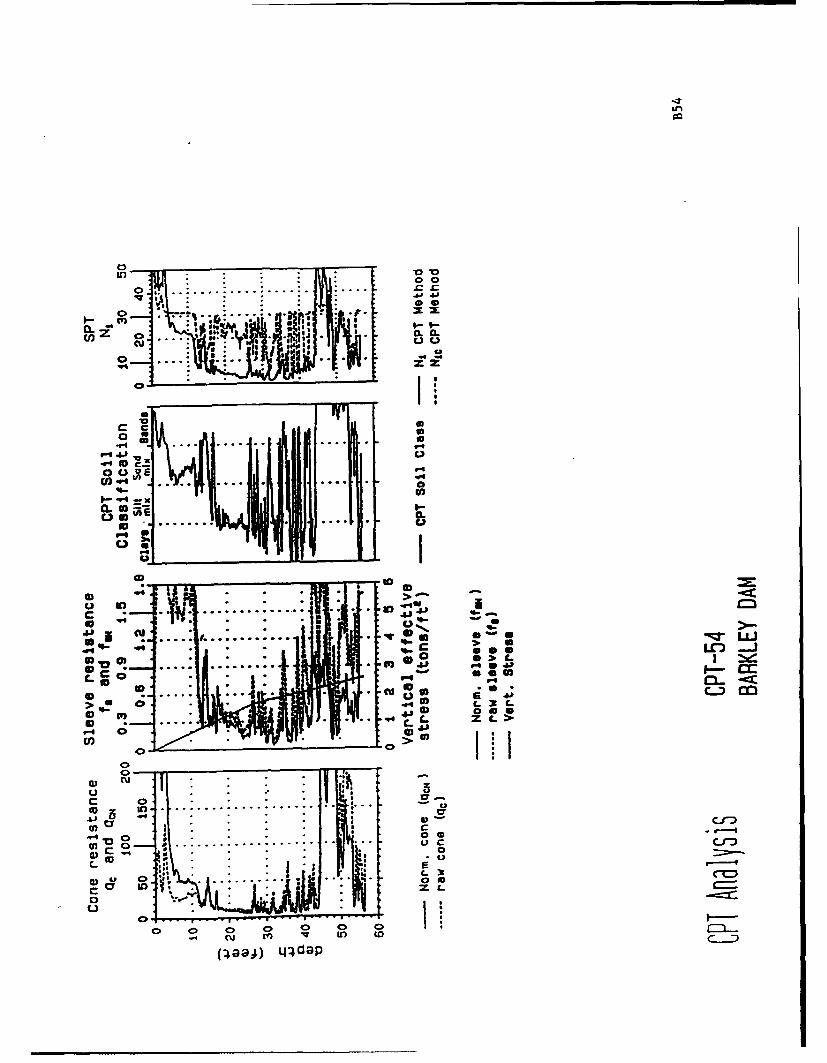
LM
00
46,.J 4,.0CV)U
7- IL rC---".LU• J -
I'inW
cc00
.r9 ,,. .... .... .. .I
o0 c.e V
000
L ts0 C! . . .. ..
L) _ . . ....... .
ID0 >
0 1 . ..3..- . .
. ) -) . ._.
. = ,; --- +
m .•o 1-.0...T-0 30 C.
V4:4- -cc
0
. Ur
go o I.n.. . .0
0~ I Z
o A
o 0 0 0 0 0 0 ,
•4 , u €V r Ir) t Do
(Peal.) qL.dap
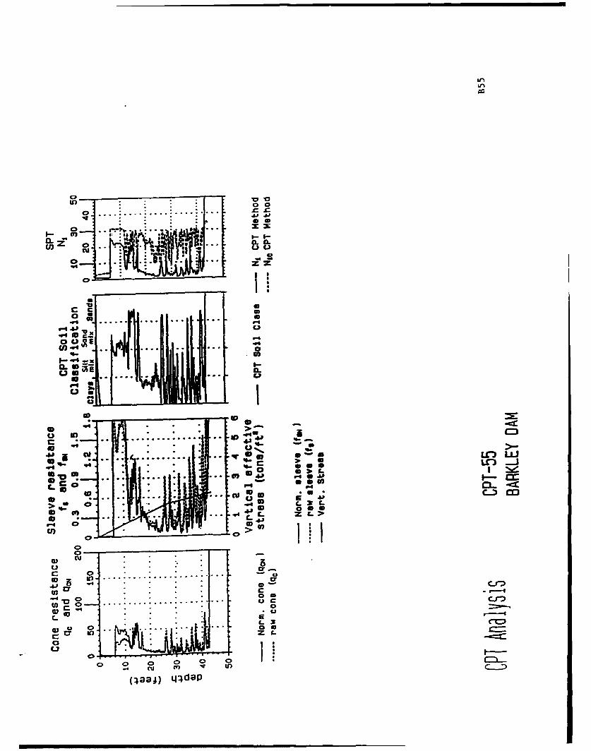
* ~V)
*~000j 414.
00
0 U
ccm
U >
a- .u(3)
doo-
Z-. 'CO =
- S-
10 .... C
* *0 a ~ S
- L-
0 .1 ** I'
paa; Q I>J
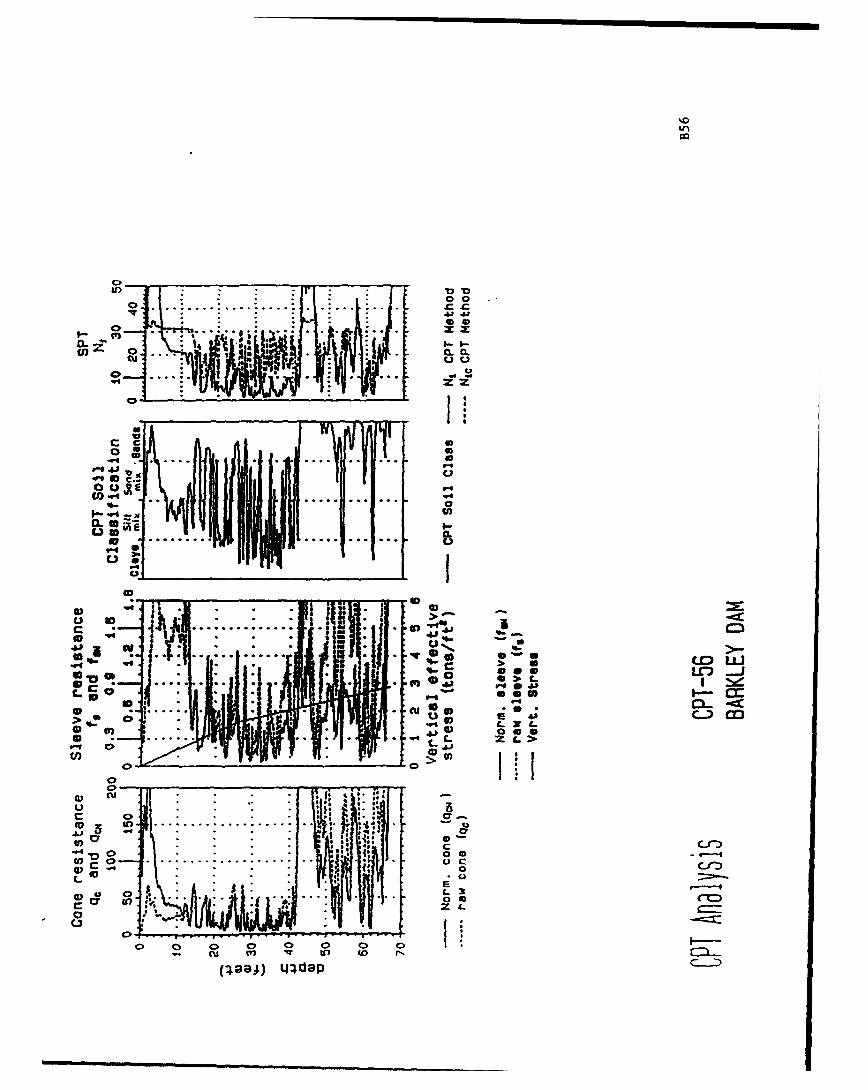
Lfn
0.0
Cu~A 441 0
CF)U-0L z
C L
lo.4
4,SC.3t
4j.-
aa
"0 :* C.
10C 0- :t. 40. .
> C; 0 l
41 L S l- >0C 4-AC.3 ' *
I *
u 1:v3 ~ U) 0 r-. I
(;9a~L Ifd
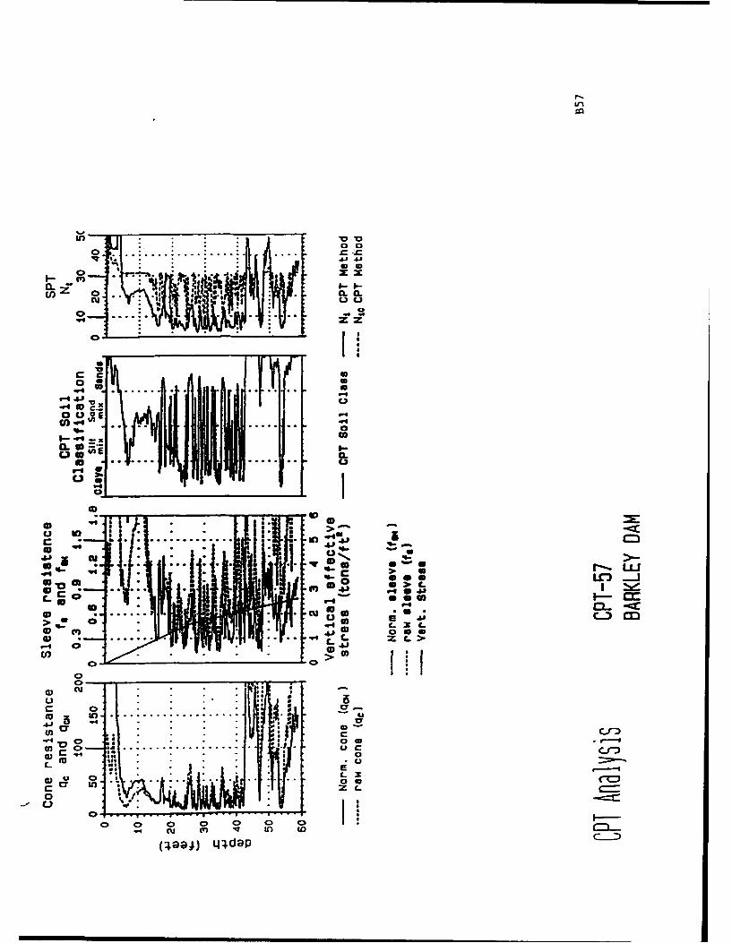
Lrn
100
0 0
cmmuCL - .- I.
Cc
to * U
U)U
I---
C ai
.40
cnI 0C *
o. o I'j0 - .4.-
o u M . . .. . - 20 **) 'c->
0 :
(0 40
**0v I.
0 0 0~ C>.C.-
(.488; ::~da - 0
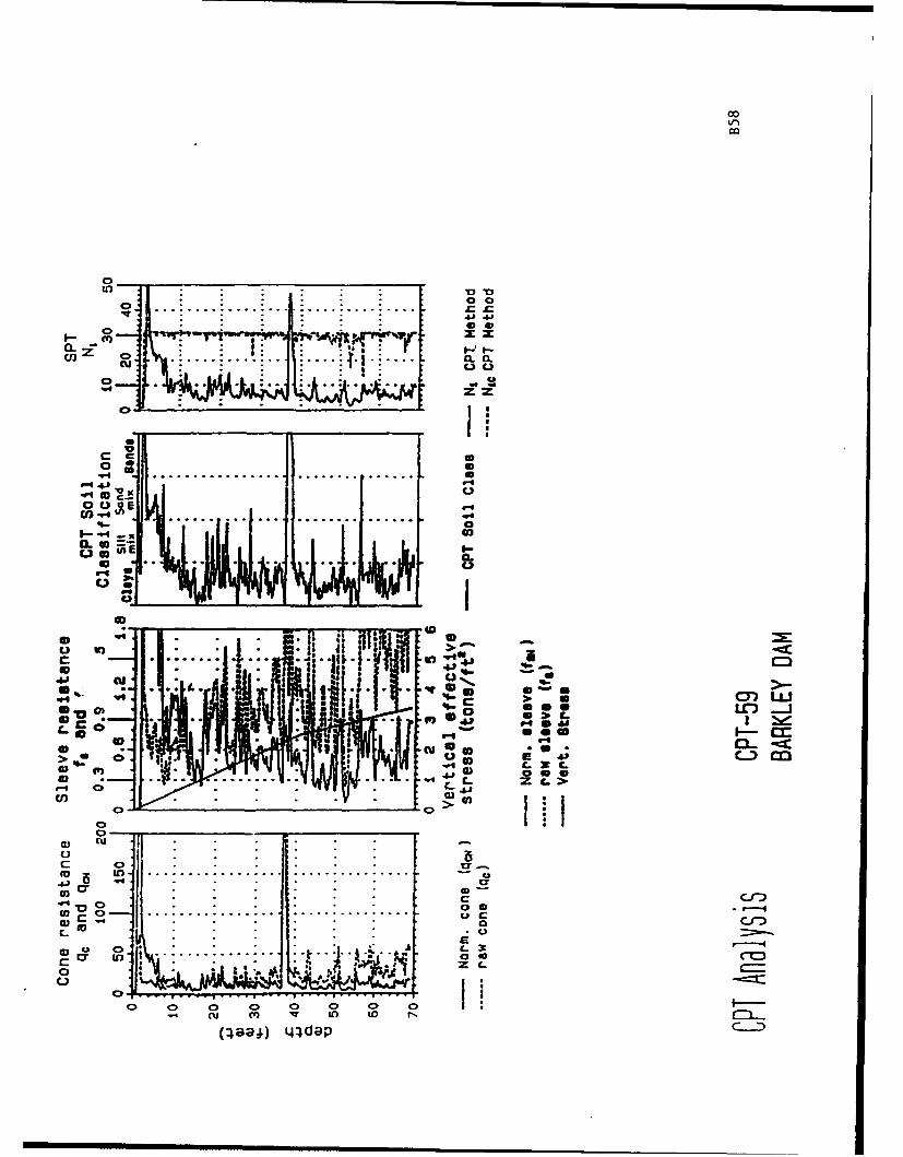
00
o I°
I o
o _•. ... ' ". .'' ." ... ".m
I '
cc . ..... ... ......... ........ ..... ..
U -r .......... . ... . ... . .101
"I .. ..... . ". " ... , " ..
.9.4 " ** " Uo
,, o . .... .,.
~4J 94J.91 U
O
.9..
0a=~ C. :I
u a.C; C-4
U)
S (4. ................ . u Co o •I---
I -n
-D 0' C
0-
c) . c . .
paa- ui C -5. a
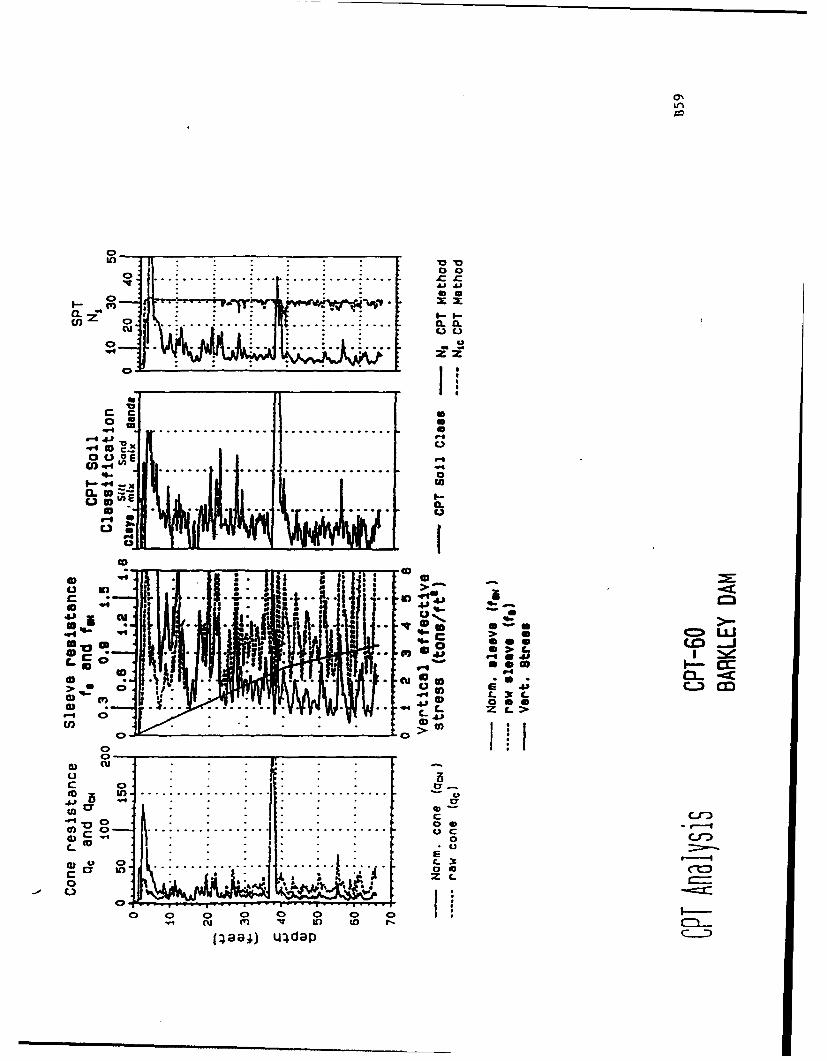
0'
40
cu'
0- •:0
04 . .. .... .... . . . .... ..
... . .. ...
o I
CL0 E
o U S
.40 *40
•.o U•E .
0.w I -
u01
o- . .o C
e9 t
C)CJ
S0 Z.C-CD _
""U a . . . . 2 -cc5 a-
S"4 . . . . Ii0~.. . ..C, >
0 0 • , '"a ) cu'. o o o o L0o is ..................... * L
'4 0 .
0n . .. . .... * 0
Co .... .. ... ... L 3
Li
c Sy inO
oco...............I .............C> oCJ
Ln I'V t
pa4 E~a
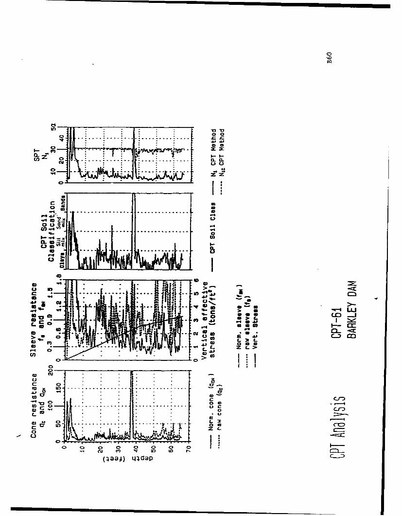
0 0
. .-- . . .
I0
on : .... .. '.. .... . .... i.... CL M
• a4m U
.. .. .. . ..... C.,
o C3~ -U -V4 . .. .. ..oo '4 - x It-.......... .... ................ 0
.,. .'-4,... , ..,......... ... Li)"- , uIDI
>0. K) >l
-- *0O ( o---
.... .... .. .... .1- "i0 C -
maw , -w
41 V4 o. I o o o l--
(•00) 4l
I0 I
10>10
U)........ .... ...... . . . . . . . .. u C
0 -0
C.)
C> 0C C-~ cu m' v Ln (D rN
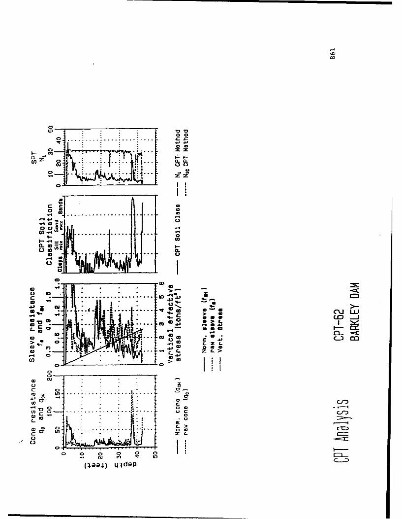
S0 0
c C ) o. . . . .. . .
°. . . .. . . . . . .. .
IV))
IU- z y CL o-
C2)L
C>
oo . a .......................x x
V-4
C-
.. .... ...... . . .. . -r 4• L
*00
r, .. *. ,.-" eo
--•••
o .... C)
.4-
° I
I.) °. o . - ---
.~I W g 1+** *CU, Li.)
>. 'Co LO I
C>.
- •
0
3S
0
.9 cc 41L 4OL>
S . .... .... .... ..
U ) C > . ... . 0 ( U U ) *
c 0 . U * 4 _
°- 0
CY j if ... . . c-
c 0 I_ '0
ZI
C) C 0 C> Lrn (n to
(4taO;) ij~dap
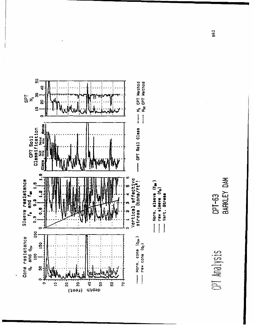
00
ILI I IL a. I I I
. .. ... . . o.
0 .-. 0-
.... . . .. ....... ..... u
o o . . .
o "__ _ _ _' H1
X!
co
6-4 1 4.1
.64 %- c m
o .. .. .01 o :o.
L >
, 0
• ,-1o o IT -.-
IS ' I "(En *) 4) (p 1
_L
w C--" - - 0
LL 3
C In .. . . .0 a ZL
Z S-
(I m~) da1p C--2D
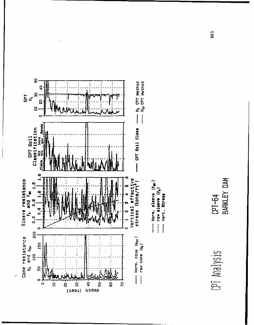
00
IT)
o C>•n . . .. . L.. . . . ...
. .. . . . . .-
ý') . ............... . .......... '...... . 1
- .'* - •Ca
o c-.
0.. -..". .£0 . .4-x U
a- . I.
*' C.L.
.. . .. . . .. .
C o o o. .. . ... q4pl 0!i 0 n
so .w**
0 0.6' 0 0 0 0 0u 0 0 w
(;)4 a 4da
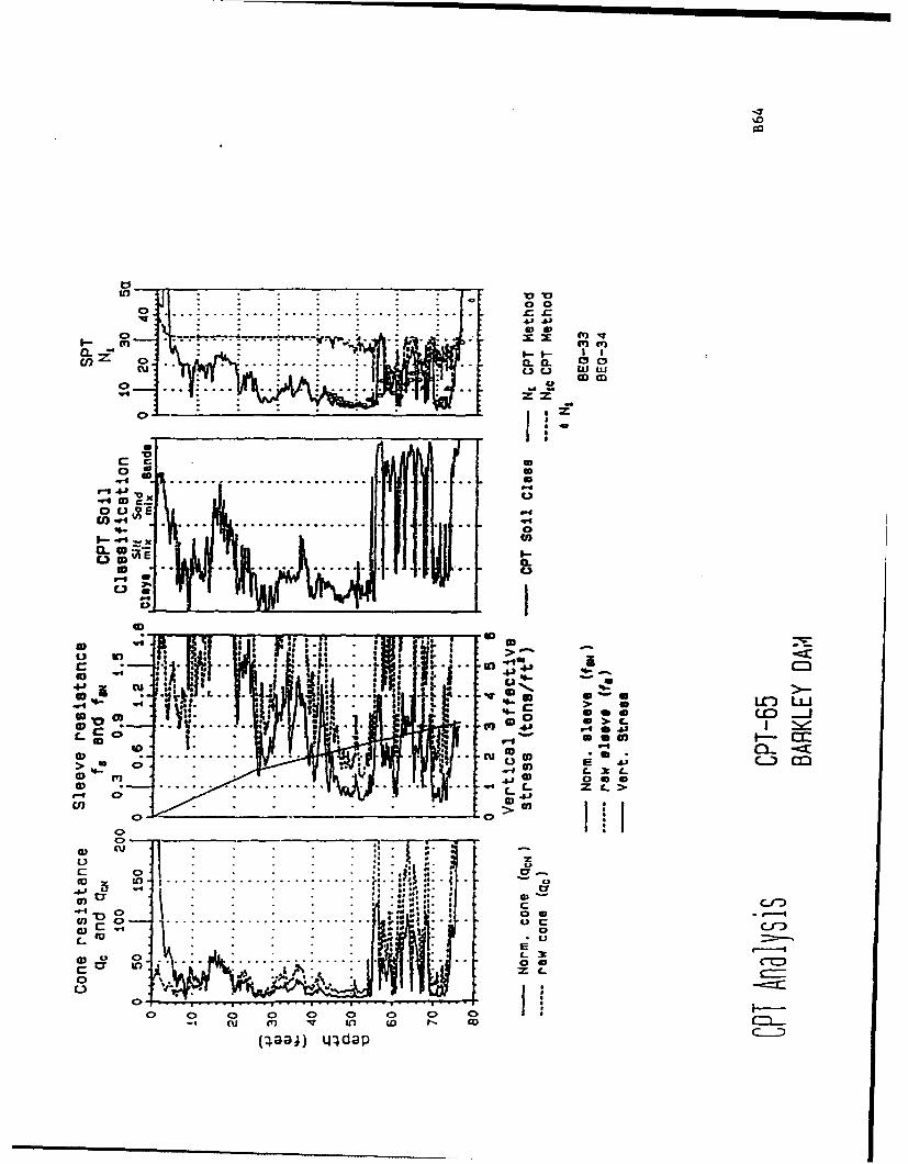
C0 0
Go o
00 tU) i..................................... ..... .
4- .. .. .. .. .. . .
.. . .. . .. . .. .
to, Ito 0
13,3T . .9)C
. ~ ~ I so.._
Ccc
0u 0
0 wrU. -- *(1) 0) X C
a)~aJ LJ) ) 0oD

APPENDIX C:
SPT lABORATORY DATA
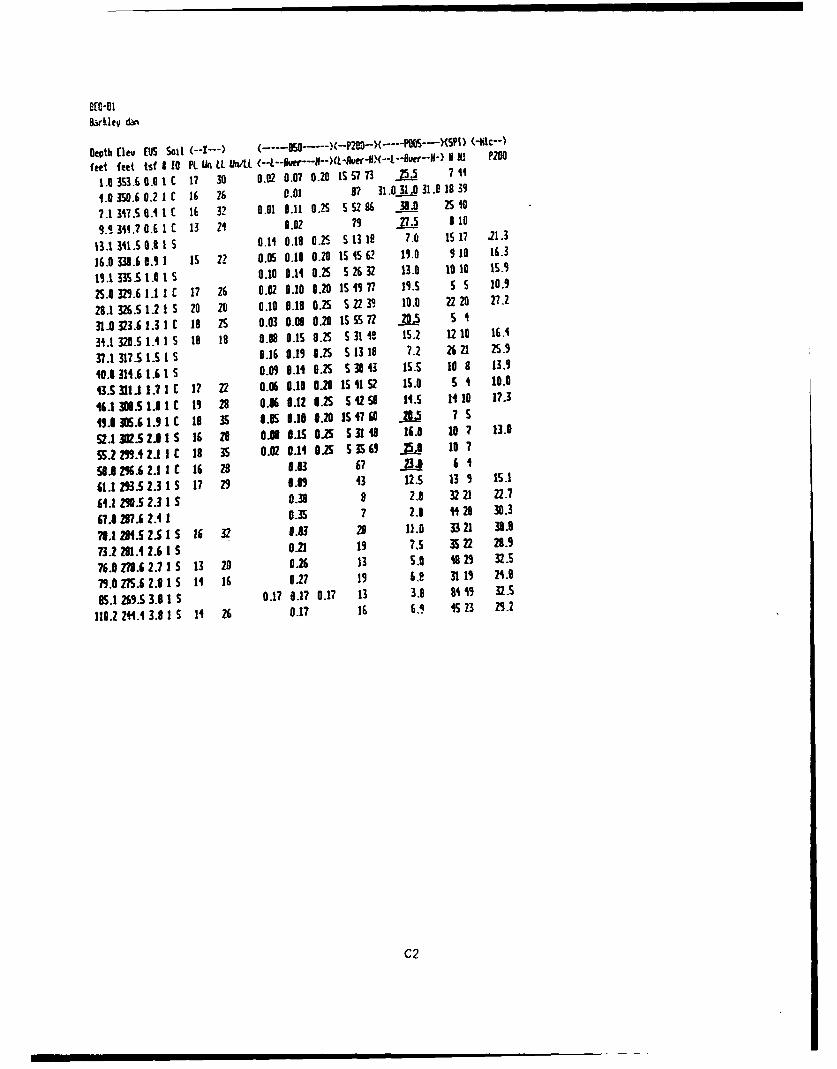
Barkley do
Depth lev US Soil (----) (-l •.. (-P29- . -SP1 ) (-,c-
feet feet tsf 1 10 PL Ik, LL Un/Lt - H NI P200
1.0 353.6 0.0 1 7 C 1 30 0.02 0.07 0.20 15 57 73 -P5 7? i
1.0 350.6 0.2 1 C 16 26 0.01 87 31031..0 31.0 1 939
7.1 317.5 0.41 Ic I6 32 0.01 0.11 0.2S 52 86 38.0 25s 0
91. 344.7 O. I C 13 24 0.02 79 27.5 8 10
13.1 341.5 0.815 0SI 0.19 0.25 S 13 19 7.0 IS 17 .21.3
16.0 338.6 0.9 1 1S 2? 0.05 0.10 0.20 is 4s 62 19.0 9 10 16.3
19.1 335.5 1.0 1 S 0.10 0.14 0.2S S 26 32 13.0 10 10 15.9
25.0 329.6 1.1 1 C 17 26 0.02 0.10 0.20 IS 49 77 11.5 5 5 10.9
28.1 326.5 1.2 1 S 20 20 0.10 0.18 0.25 5 223 10.0 22 20 27.2
31.0 323.6 1.3 1 C 18 25 0.03 0.08 0.20 IS 55 72 20. 5 i
3U.1 320.5 1.4 1 S 18 1 018 0.15 0.2S 5 31 19 15.2 12 10 16.1
37.1 317-5 1.5 I S 0.16 0.19 0.25 5 13 18 7.2 26 21 25.9
40.3 311.6 1.6 1 5 0.09 8.14 0.25 5 30 43 15.5 10 8 13.9
43.5311.1 1.7 1 C 17 22 0.06 0.10 0.20 15 41 52 15.0 5 1 10.0
46.1 308.s 1. 1 c 19 28 01.6 0.12 8.25 '2 SO2C 14.5 1419 17.3
"A9.Z05.6 1.9 1 E 18 35 0.85 0.18 0.20 151 47 0 LW 7 5
S2.1 302.S Z.IS 16 28 0 6.15 CIS 5 31 48 16.0 10 7 13.0
55.2 29.4 2.1 1 C 18 35 0.02 0.14 0.25 5 3569 Al 10 7
5.0296.6 2.11C 1 218 0.83 67 23. 61
61.1 293.5 2.3 1 5 17 29 0.09 43 12.5 13 9 15.1
64.1 290.5 2.3 1 S 0.38 8 2,0 3221 22.7
67.0 287.6 2.4 1 0.35 7 2.0 4 28 30.3
71,1 24.S 2.5S 16 32 0.83 29 11.0 33 21 38.0
73.2 281.4 2.6 Is 0.21 19 7.5 35 22 28.9
76.8 278.6 2.7 1 5 13 20 0.2 13 5.0 1829 32.5
79.0 275.6 2.8 1 5 1 6 1i 0.27 19 61. 3119 21.9
85.1 2569. 3.8 1 S 0.17 0.17 0.17 13 3.a 81 9q 32.5
110.2 241.1 3.8 1 5 11 26 0.17 16 6,, B5 23 29.2
C2
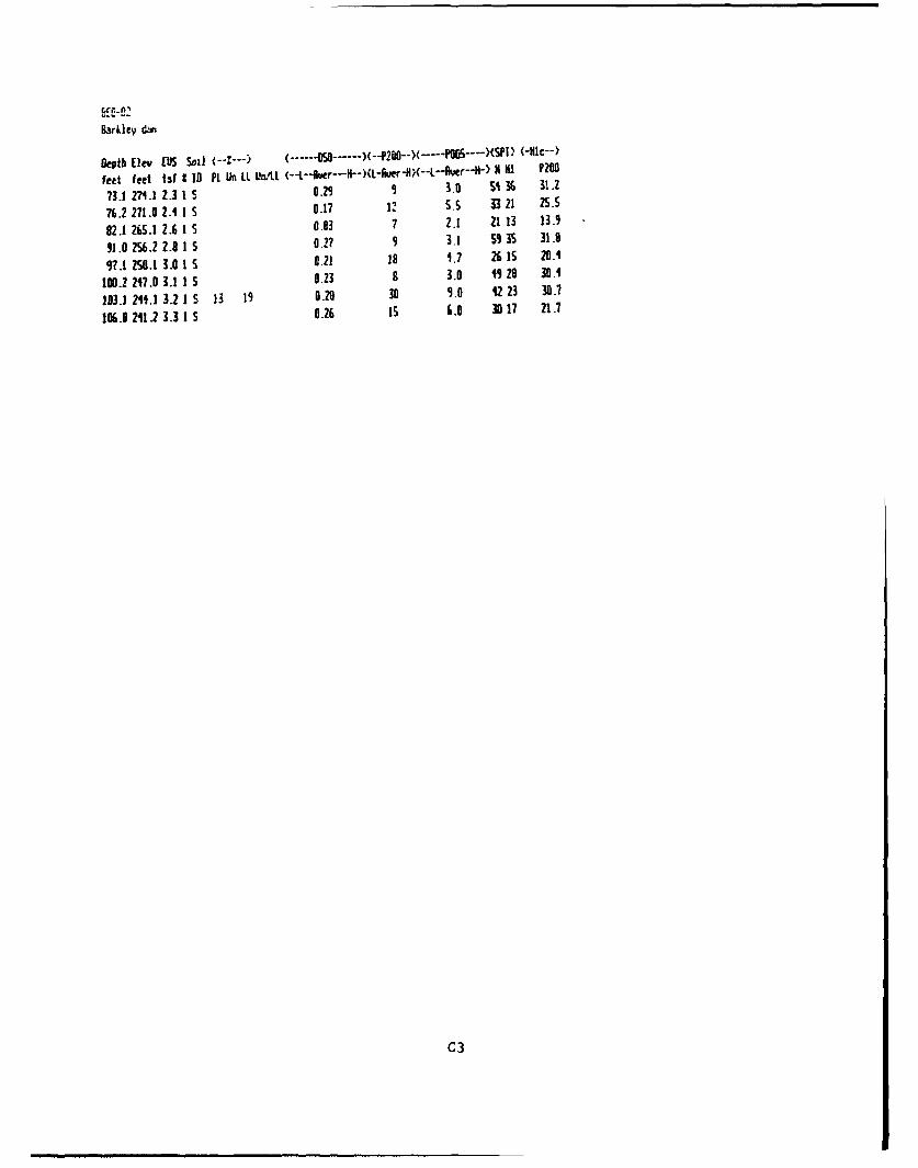
Barkley dan
Deoth [ICe [ So)l (--I--- (-..... -D ---- )(--P20 -- )( -. .i•- ..---- )(SI) (-Nlc--)
feet feet tsf 1 10 Pl. Un LL UnmLL (N-i-.er H--)(t-Auver-HXL-t-i r") HI P200
73.1 27M.1 2.3 1 S 0.29 9, 3.0 s 36 31z2
76.2 271.0 2.4 1 S 0.1? 12 S.S 33 21 2S.S
82.1 265.1 2.6 1 S 0.33 7 2.1 21 13 13.9
91.0 256i.2 Z.8 1 S 0.27 9 3.1 5S 3S 31.8
97.1 ZSo.! 3.0 1 S 8.21 18 1.7 26 is 20.1
I10.2 247.0 3.1 1 S 0.23 B 3.0 19 29 301
183.1 211.1 3.2 I S 13 19 0.20 30 9.0 2 23 30.1
106.0 211.2 3.3 1 S 0.26 is 6.0 30 17 21.7
C3
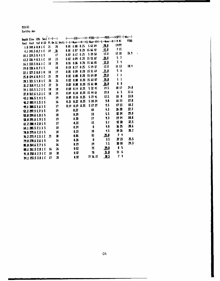
Depth lieu LIUS Soil (--Z--) (..-50 -- --)( --- . PeOSXSPI) (-HI--)
feet feet tsf I 10 Pl Un LI LM'LL (--L--u III---X*) I P200
1.0 3M8.6 0.0 tC 21 21 0.01 0.08 0.25 S 3 81 29.0 10)9
4.1 345.5 0.2 I 18 36 0.01 0.07 0.20 IS 66 92 12._0 ? 1s
10.1 339.5 0. 15 17 0.07 0.12 0.2 S 39 50 13.8 12 18 26.1
13.2 336A.0.S 1( 1t I 3 0.02 0.09 0.20 15 5592 28.0 S 7
16.1333.S0.61r 18 28 0.01 0.0 0.20 15 6695 3.0 3 1
19.0 3.6 0.7 1 S Is 0.10 0.17 0.25 5 19 32 12.0 11 13 18.4
22.1 327.5 0.8 I 18 19 0.05 0.09 0.20 15 516 4 21.0 5 6
25.0 2.6 0.9 1 c 21 28 0.02 0.08 0.20 15i 1 89 29.0 1 1
21.1 321.5 1.1 1 ( 20 26 0.02 0.08 0.20 15 63 87 26.0 1 1
31.2318.41.11C 22 31 0.82 0.0 8.20 IS 61 88 8 0
31.1 315.5 1.2 is 19 18 0.08 0.11 0.25 S 3215 11.5 19 17 21.8
37.0 312.6 1.3 1 C 18 21 0.04 0.10 0.20 15i 6 1 19.0 6 5 11.6
43.1 306.S 1.4 I S 19 0.09 9.16 015 521? 1 12.5 10 8 13.8
16.2 313.4 1.1 S 16 OM0.2 O1 0.25 18 24 9.0 16 13 17.8
"..1 .S 1.6 S 17 0.14 Oi9 0.25 5172Z? 11.5 1713 18.2
.2z15?. 1 .?5 11 0.22 10 4.3 2620 22.7
SJ 2"1 l.6 I 5 1 8s19 13 5.5 R 24 29.0
9.1291. 1.9 1 S 19 0.20 1? 9.3 11114 18.8
611 231 2.1 1 S 17 1.23 15 5.1 430 32.5
641 285.52.115 1 0.24 a 1.0 3625 29.6
701 27M.6 . 1S 18 0.23 10 1.5 39 26 30.2
76.2 273.52.1 C 21 30 8.6 55 sj 7 1
7911.271.62A 1S 16 326 8 3.5 37 23 253S
%A 2M4. 2.7 1 S 16 8.19 19 7.5 3 18 24.3
"1J261.s2.81c 16 26 8.02 73 291, 0 35
91.0 2M.6 .91 C 118 30 0.02 78 31.0 11 6
94.12S.53.81 17 29 0.02 77 ?677, 23 7 4
C4
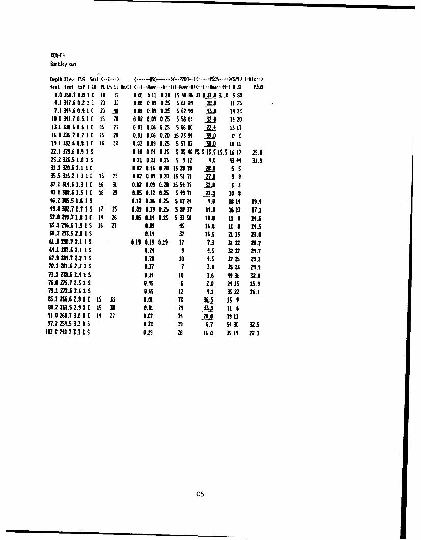
Barkiey dan
Depth lieu (US Soil (--Z----- (------ .... 0. .)--P200--X...-POOS--XSP1) (-Mic--)feet feet tsf 3 10 PL tUn LL Un/'d (--L--Aier-----)NL- er-HX--L--Ruer--N-) N HI P20M
1.0 3SO.?7 0.0 1 1 32 0.01 0.11 0.20 Is1i 88 31.0131 0 31.0 5504.1 3W7.0.2 1 C 20 3' 0.01 0.01 0.25 561 9 28.0 11257.I M1.6 0. 1 tC 20 10 0.01 0.09 0.2s S 62 0 43.0 11 23
10.0 31.7 0.5 1 c 15 28 0.02 0.09 0.25 S S 8M 32.0 11 2013.1 33.68.6 1 € IS 23 0.02 0.06 0.2S 5 66 80 22A 13 1716.0 335.? 8.7 1 C IS 28 0.01 0.06 0.20 15 73 1 39.J 0 019.1 332.6 0.1 1 C 16 22 0.02 0.01 0.25 557/93 NJ 10 1122.1 32.6 0., I S 0.10 0.14 1.25 S 35 16 15.5 15.5 1.5 16 17 25.82S.2 326.5 1. 1 S 0.Zl 0123 0.25 5 1 12 1.0 13 1 31.931.1 320.61.1 1 c 0.02 0616 6.20 15 27 ?1 .0 5 S535.5 316.2 1.3 1 2 IS V? O.O? 0.0 9 0.0020 is 51 71 27.0 9 937.1 314.6 1.3 1 C 16 31 0.02 0.01 0.20 i5s 77 ..32A 3 343.1 30. 1.5 1 C 19 21 8.05 6.126 1 5 5 "71 21.5 10846.23 .$ 1.6 1 6 0.12 6.16 0.25 517241 5.6 1314 19.141..3023 1.7 1 S 17 25 0.09 1.11 1.25 51137 11.6 1612 17.152.1 Z5.? 1I 1 C 14 26 0.5 6.11 65 53359 13.0 11 11.655.1 2 A 1.1 S 16 Z7 0..01 i 16.0 11 1 11.55R2I 3.5 2. 1 S 3.11 37 15.5 21 15 23.0a1A 210.? 2.11 S 3.15 6.11 0.11 17 7.3 31 22 23.264.1 2 .6 2.11 S 0.21 9 1.5 3222 21.767.A 20.7 2.2 1 S 0.23 10 1,5 37 S 29.370.1 2.6 2.3 1 S 0.37 7 3.0 3523 21.1?3.1278.6 2.4 1 S 3.34 10 3.6 " 31 32.87.0 ZS.7 2.S1 S 0.15 6 2.8 24 IS 15.979.1 22.62.6 1 S 0.5 12 .1 35 22 26.15.1266.6 2.8 1 C IS 33 0.01 78 36.5 155
88.2 263.5 2.1 C IS 30 0.01 79 33_5 11 611.0 260.7 3.0 I C Ii 27 0.02 71 -2.8 11117.2 251.5 3.2 1 S 0.28 19 6.7 Si 30 32.5
103.0 218.7 3.3 1 S 0.11 28 11.0 35 11 27.3
C5
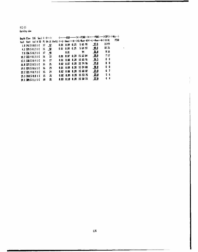
4-kle, da
Oepth lev (I£i Soi (..Z... (. O .)(-P20 0"X- 'OS- .... ) (-o--c----
feet feet tsf 1 10 P, UW Li UnI. (--.--.over-N)(L-,er-)(L-er-) --i P?[I 0
1.0 342.5 8.0 1IC 17 '2 0.01 0.09 0.25 S 65 5 17.0 11)99
4.1 339.5 0.2 1 C U6 5so 0.01 0.09 0..75 S 61 53 1.09 10 26
7.0 B33.5 0.2 1 ( 17 10 0.01 51 36.8 8 16
102 33.1 0.3 1 E 16 33 0.01 0.07 0.20 15 63 81 28.0 7 12
13.1 330. 0.S 1 C 16 27 0.01 0.08 0.20 15 6551 26.5 0 0
I6.0 327.50.S I E 16 26 0.02 0.07 0.20 151 M % 21.0 0 0
15.1 32.S0.6 1C 16 29 0.01 0.05 0.20 is5i80 M0. 0 0
22.2 321.4 0.7 1 C 15 21 0.02 0.08 0.20 15 60 2 25.0 6 7
2S.1 311.5 0.81( 15 25 0.02 0.05 0.28 15 S3 7S . 56
34.1 3f.S1.11C 1S 35 0.03 0.10 0.20 155873 22Z.J 1 1
c6
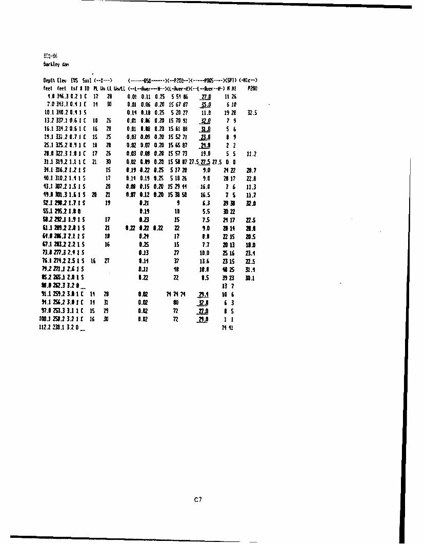
Barkley dan
Depth [leu EL'S Soil (--I --- 0 .... )(--) 200--.-- .... - )(SPI) (-RlC-)feet feet tsf I 10 PL Un UL UOn/L (--L--Bucr----X)(L-Auer-HX--L -Aver--H-) N HI P200
4.0 346.3 0.2 1 1 17 28 0.01 0.11 0.2S 5 51 86 27.9 11 267.0 3W3.3 0.1 1t l 30 0.01 0.06 0.20 15I 67V 35.0 6 10
10.1 340.2 0.1 1S 0.14 1.18 0.2S S 20 27 11.0 19 28 32.S13.2 337.1 0.6 1 ( 10 Z6 0.01 0.06 0.20 Is 70 91 32.0 7 916.1 334.2 0.6 1 C 16 28 0.01 0.08 0.20 Is 51 88 31.0 S 619.133r.20.71C 15 25 0.03 0.09 0.20 155,271 23.0 8 925.1 3.2 0.1 1 C 18 28 0.02 0.07 0.20 IS 687 21.9 2 228.0 2.3 1.0 I C 17 26 0.03 0.09 0.20 15 7 73 19.0 5 5 11.231- 3111 1.11C 21 30 0.02 0.0 0.20 1558 87 27.SV.5S Z7.S 0 034.1 3161 1.2 Is 15 0.19 0.22 0.25 5 1729 9.0 24 22 28.740.1 310.2 1.1 1 S 17 O.1 0.19 0.25 5 18 26 9.0 20 17 22.813.1 37.21. Is 20 0.98 0.1S 0.20 15 29 41 16.0 7 6 11.31.9 301.3 1.6 1 5 20 21 0R7 .12 0.20 15 3850 16.5 7 S 11.752.1 29621.71 5 1i 0.21 9 6.3 393 32.0SS.1 25.2 1.8 0.19 10 S.5 3 22L.2 2,2il S 17 0.23 15 7.5 2117 22.5
U 2859 2A 1s 21 0.2 2 0.22 22 9.0 20 14 21.061.3 25.3 2.1 S 1i 8.24 17 8.0 22 15 20.5U71 2 2 2.2 15 16 0.2S is ?7. 2913 18073.8 277.3 2.11 S 0.13 27 10.0 2S 16 23.476.1 2742 Z.5 I S 16 27 1.11 37 13.6 23 15 22.5?9.2 2?1 . 1 S oil 18 183. 1025 31.45.2 26S1 2 1I S 02 22 3.5 3923 30.1
08. 252.33.2 __ 13 ?9.1 252 3.11 C tH 29 0.02 17 1741 29. 10 6"11.1 256.2 1 . C 11 31 0.02 80 32.0 6317.0 253.3 3.11 15 29 0.02 72 27.0 8 5
100.1 250.2 3.2 1 f 16 30 0.02 72 29.0 1 1112.2 2389 3.2 0 __ 7411
C7
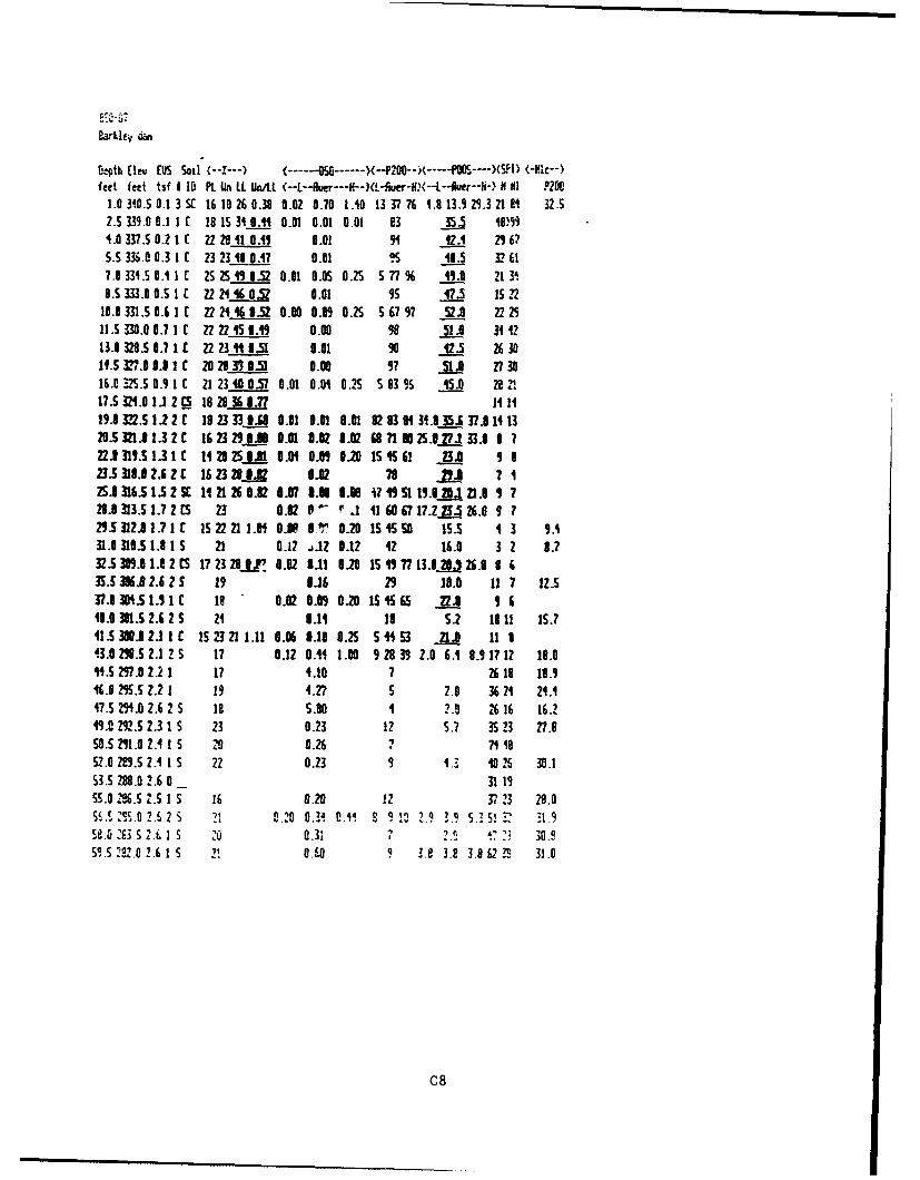
E-kle7ca3rkhtv din
Depth (cev (US Soil (--I---) (------S a - -P200-------S--)•I) (-Kic--)feet feet tsf 1 10 PL Un LL Un/LL (--L--Rver---N--)(L-,er-HX--L-",uer-l) N Ni P2l 0
1.0 310.5 01 3 SC 16 10 26 0.31 0.02 0.70 1.40 13 37 ?6 4.9 13.9 29.3 21 81 32.S2.S 339.0 0.1 1 18 IS31 9.41 0.01 0.01 0.01 E3 35.5 18,"mi.0 337.S 0.2 1 C 27 20 41 0.11 0.01 94 12.4 29675.5 336.0 0.3 1 C 23 23 1 0.47 0.01 Is 11.5 32 61?.8 334.S 0. I 25 25 0.52 0.01 0.05 0.25 S 77 % 1.0 21 31,'8.33.0.S 1 Z2 22 1 e0.2 0.01 I5 47.5 15 ,2
10.8 31.S 0.6 1 C 22 24 16 9.52 0.00 0.09 0.25 S 67 97 52.0 222511.S 330.0 0.7 1 C 22 22459.1 0.00 98 51.0 31?413.0 328.5 0.7 1 E 22 23 "4.51 0.01 90 12.5 26 3014.S 0• .8 1 C 20 2L33 .51 9.00 97 51.0 A Z 3016.0 32S.5 0.9 1 C 21 23 0 0.57 0.01 0.01 0.25 5 3 96 15.0 202117.S 241.03 2 LS 18 28-6 12.? 14 1119.8 22.5 1 2 C 18 23 33.59 0.01 0.01 0.01 82 93 94 3i.0]•5 37.0 14 1329.5 321.11.3 2 C 16 23 29.3M 0.01 0.02 9.02 8 71 125.0 j 33.0 1 722.1319.5 1.31t 14 20 2S11 0.01 8.09 0.20 IS 5561 2A.9 923.S 311. 2. 2 IC 16 23 239.02 0.02 798 W 72SJ 316.S 1.S 2 C 11 212690.2 0.07 .U 0.88 17 15 " 1 19.020 121. 9 ?28.9 313.5 1.7 2 CS 23 0.02 9 " .1 11 60 67 17.2• 26.9 1 729.S 12. 1.7 1 5 IS 22 21 1.91 O.N 8. 0.20 IS 45 SO IS. 4 3 9.131.0 310.5 1.8 1 S 21 0.12 J.12 0.12 42 16.0 3 2 8.732.-S 309 1.0 2 C 17 23 20_. 0.02 3.11 0.20 I5 11 77 13.82.,26.0 3 635.5 3968 A2.6 2 S 19 0.16 29 19.0 11 7 12.537.30. 1.S 1 C 1t 0.02 9.09 0.20 IS 4565 22.0 140.301.5 2.625 24 0.11 19 S.2 18 11 15.?4115 300.211 C 15 2321 1.11 0.06 9.10 0.25 54 53 &.0 11343.0 29•.S 2.1 2 5 17 0.12 0.11 1.009 928 39 2.0 6.1 8. 17 12 18.014.5 217.9 2.2 1 17 4.10 7 2619 18.146.0 215.5 2.2 1 19 4.27 5 2.0 36 21 21.147.5 2914.0 2.6 2 S 18 5.90 1 ?.a 26 16 16.249.0 2'925 2.3 1 S 23 0.23 12 5.? 3 23 27.950.5 291.0 2.4 1 S 2 0.26 7 711952.0 2n.5 2.4 1 S 22 0.23 9 1., 10 26 30.153.S5 288.0 2.6 0 _ 3111S5.0 16.52.S I55 16 0.20 12 37 23 29.0Si.l. sc, 0 2.6 2 S ?" 0.20 0.P 0.14 E i !2 2ý9 1.9 3.3 S1? 19S1. 23.5 2.6 1 IS 10 0.3; 1 . 1 .? 2 30.9S.5 201.0 Z.6 1 S Z! 0.0 9 3.8 3.8 3.6•2 • 31.0
C8
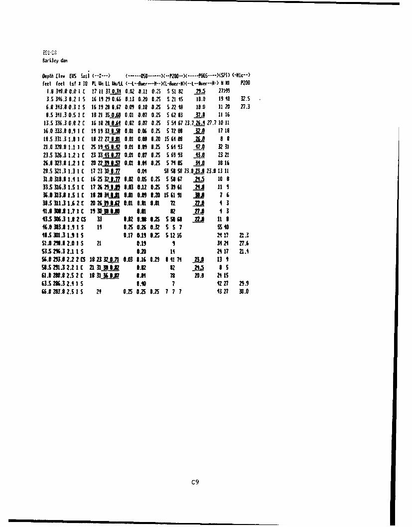
Depth [lev [US ail &---"--) S, .. ---- . .(--P200-)( -----P005-)(S{ ) (-Hlc--)feet feet tsf I 10 Pl Un LI Un/L. M--L--Rr---Il--)(t-Auer-H)(--L-Auer--) H HI P200
1.8 318.8 0.0 1 C 17 11 33 0.31 0.02 0.11 0.25 S S1 82 21.5 27)993.5 316.3 0.2 1 S 16 19 Z 0.66 0.13 0.20 O.2S 5"21 5 18.0 19 42 32.56.8 313.8 0.3 1 S 16 19 28 8.67 0.01 0.18 8.2 5 22 i8 18.0 11 20 27.38.5 311.3 8.5 I 18 21 35 0.60 0.01 0.07 8.2 56283 37.0 1116
13.5 336.3 0.8 2 C 16 18 28 3.64 0.8? 0.07 8.2S5 S5 67 23.7 26. 27.7 10 1116.0 333.8 0.9 1 C 19 19 330.58 0.01 0.06 0.5 S 72 88 32.8 17 1818.S 331.3 1.0 1 C 18 22 Z? I 0.81 0.01 8.20 IS61 88 26. 8 a 821.0 32H. 1.1I l1 25 115 1.42 0.01 0.01 8.25 561 3 7?.9 32 3123.5 326.3 1.2 1 C 23334433.77 0.01 0.07 .25 S 659 3 43.0 23 2126.8323.81.21C 2022 3Z3 57 0 O.M 3.6 025 S7185 3410 181629.5 321.3 1.3 1 1 17 233 3 .77 0.1 8 O S 23.0 Z3. Z3.0 13 1131.0 318.8 1.1 1 C 16 25 3287. 0.02 0.85 8.25 S 8 67 ZI.5 10 833.5 316.31 5 I C 17 2A 29 IJ 0.83 0.12 0.25 5 39 11 21. 11 13. 313J1 .S1C 1i 28 31j.J 0, 0.01 3.20 156 1 1 J. ? 638.5311.31 2 C 29 26-R 6.01 0.01 O.M 72 271 1 3l1.0 3MJ1.?1C 19 3 .k0L 0.61 82 Z?. 1 3U3 06.131.12CS 33 0.2 0.u8 0.25 59168 Z2A 11 846.0 03.8 1.9IS 1 s 19250168.32 S S 551 8
08.5 301.3 1.9 1 S 0.17 011 825 S 12I ,117 21.3
51.0 253.8 2.0 1 S 21 0.11 9 3124 27.653.5 2%.3 2.11 5 .20 1H 24 17 21.4S6.0 23.12.2 2 CS 19 23 32.71 9.03 0.16 0.21 8 111 23.0 13 158.5291.32.21C 2131- I 3.62 82 21.5 8 561.0 2U.I .S I 18313 .07 0.01 78 20.0 21 1563.5 236.3 2. 15 0.10 7 42 27 21.166.0 283.8 Z.S I S 21 0.25 0Z 0.25 7 7 7 43 .? 30.0
C9
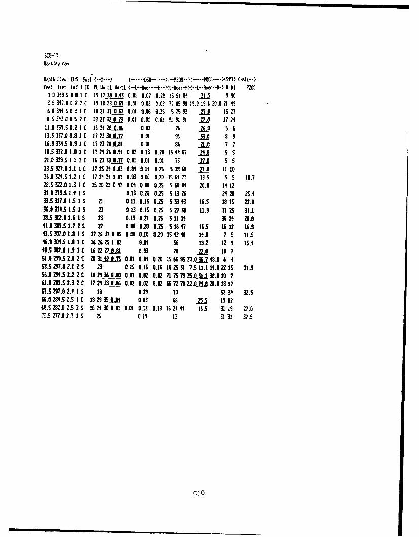
•p -ev EM• soil (--I --- • ---- ..... ---- .... )"2•; .. ,•..(SPT,{Xc-
fee, feet tsf l 1n PL Ui LL Un.L. (--L--fluer---H--.V.-fuer-..,--L--.,er--H-) H NI P2001.0 319.S 0.0 C 191738 0.43 0.01 0.07 0.20 !$61 84 31.5 9903.5 341.0 0.? 2 c 19 18 28 0. 6 0.01 0. 02 0.C2 ?7, 8so9 19.0 19.6 20.0 21 196.0 34.5 0.3 1 C 182131 0.67 0.01 0.06 0.2?S 51S3 27.0 1S28.5 312.0 0.5 2 C 19 23 32 0.73 0.01 0.01 0.01 9! 91 91 ?.w 17 24
11.0 339.S 0.7 1 C 16 21 28 0.86 0.02 76 26.0 S E13.5 337.0 0.8 1 C 17 23 30 0.7? 0.01 91 33.0 a 916.0 33.S 0.5 1 17 23 28 0.11 0.01 86 21.0 7 ?18.S 332.0 1.0 1 C 17 21 26 0.91 0.02 0.13 0.20 15 44 87 21.1 5 S21.0 329.5 1.1 1 C 16 23 30 0.77 0.01 0.01 0.01 73 7._0 S 53. I 3.0 1.1 1 C 17 25 24 1.03 0.04 0.14 0.2 5 53868 21 . 11 10
2E.0 32.51.21C 1721421.01 0.03 0.06 0.20 156I,1 19.S S 5 10.728.5 22.0 1.31C 15 20 21 0.57 0.01 0.08 0.S 5 68 84 20.0 11 1231.0 315.S 1.4 1 S 0.13 0.2 825 5 13 264 120 2 S.433.5 317. 1. L Is 21 0.11 8.15 0.2S 5 33 43 16.5 18 15 22.836.0 314.5 1.3 IS 23 0.13 0.15 0.25 S 27 30 11.9 31 25 31.18.S 312.0 1.6 1 23 0.15 021 0.25 5 11 14 30 24 21.0
11.3 309.51.7 25 22 0.K 0.20 0.2S 5 16 47 16.5 16 12 16.843.5s .0 1. 1 s 17 26 31 0.85 0.98 0.10 0.20 152 48 14.0 ? 5 11.546.8 31. 1 AIC 16 26 25 1.12 0.01 S6 18.7 12 5 15.48.S 302.0 1.5 1 C 16 22 27 8.08 0.03 70 72.0 10 751. 259.S 2.A 2 C 20 31 12 .713 0.01 0.01 0.20 IS 66 85 27.0 36.7 W. 6 453.5 29.8 2.1 z 5 23 0.15 O.15 0.16 1825 31 ?.S 11.1 11.0 22 15 21.55U02S1.52.22C 182930.6 0 1 .0I 0.32 0.02 71 A57525.031.1 38.010 761.0289.S2.32 C 172533306 0.02 0.02 0.02 66 7278 .024..1_._2..0181263.5 29.8 2.1 1 S 19 0.29 10 52 3 32.566.0 28.5 2.S I C 18 25 3 0.81 0.03 66 25.5 ! 12R.S 232.0 2.S 2 S 16 21 30 0.01 0.01 0.13 0.18 16 21 i, 16.5 31 19 27.07.5 277.0 2.7 1 5 2S 0.19 12 51 31 32.5
d1o
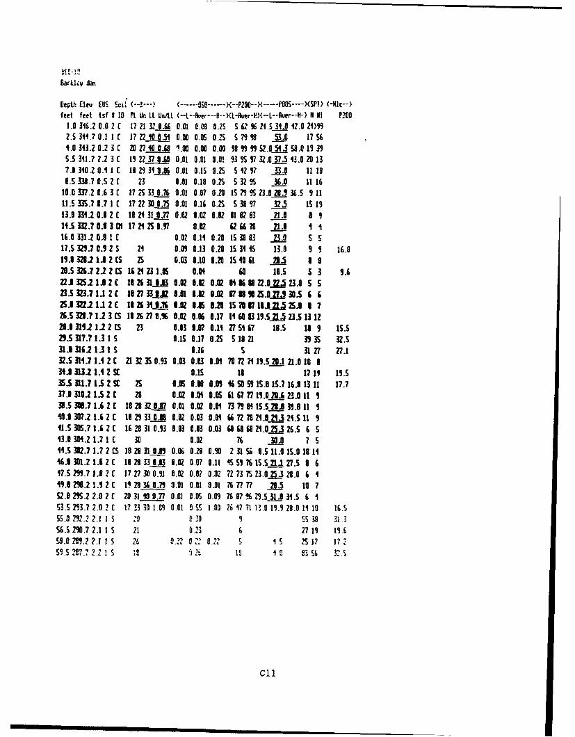
LatklIp d•.
Dept (Iev [US Sci! (--1---) (--i....-- P.--R- . .POOS----)(SPI> (-RC--)
feet feet tsf I ID PL. Ur LL Un/L (--L--Ruer--- ,--)(L-Auer-I)(--L--Auer--) HI H PZO01.0 346.2 0.0 2 C 172?1 31ý 0.(A 0.01 0.08 0.2S 5 62 9621.5 34.0 V2.0 21>5M2.5 341.7 0.1 1C I? 2210.54 0.00 O.OS 0.25S 7558 53.0 17564.0 343.2 03 I E 20 27 40 0.68 .00 0.00 0.00 58855 5S2.0 51.3 S.0 19 39S.S341.?2.23C 19 22 3780 0.01 0.01 0.0! 93 S 57 32.0 37.5 43.0 20137.9 340.2 0.1 1[ 18 2131 0.M 0.01 0.15 0.S S I2 57 33J. 11 1.5 338.7 0.5 2 C 23 0.01 0.18 0.2s 5 32 5 36.0 11 16
10.0 337.2 0.6 3 C 175 B80.76 0.01 0.07 0.10 IS 79 .023.82.536.S 91111.533S.70.71C 17 22 380.75 0.01 0.16 025 S3857 32.5 151913.0 331.. 0.8 2 18 21 31 0.77 0.02 0.02 0.02 81 V8V3 21. 8 914.5 332.7 08. 17212 50.7 0.02 6 667 s .1., I i16.0 331.2 0.8 1 C 0.02 0.11 020 1 538 0 2 1..0 S S17.5 325.7 0.5 2 S 21 0.09 8.13 0.20 IS 31 45 13.0 5 9 16.015.9 2.2 1I 2 CS 2S 0.03 0.10 0.20 15 40 61 20.5 8 829.5 326.2 2 CS 1621 231.9 8.01 60 18.5 5 3 5.622iJ32S 12C 1012631.83 0.02 8.02 0.02 8816822.0=23.0 5 S233.323.71122C 127t33.0 88.1 6.02 0.02 V8 IS 25.027.530.56 625.0221.2 1 012 t2530jA .8 3.15 3.28 15s 8370 1 .I .Z.258 .0 372.5 32.1.2 3 CS 1826 270.% 8.02 0.0 8.17 14 60 i 159.S s_ 23.S 13 1228. 152 112 CS 23 0.03 9O 0.11 27 56 67 18.5 10 5 15.529.s 317.? 1.3 1 S 0.15 9.17 0.25 518 21 393 S 32.531.13162 13 1 1 0.16 s 3127 27.132.5 311.7 1.12 C 21 32 35 0.53 0.03 0.03 0.01 70 ? 7 19.S 2.1 21.0 10 835.1 3132 1.4 2 SC O.s 10 17 14 195.35. 111.7 1 2 Sc 2S 0.05 8.0 0.085 46 SO 595.9 15.7 16.0 1311 17.737.1 310.2 1.5 2 C 28 0.02 0.84 OAS 61 67 77 15.0PAA 23.0 11 538.S 308.7 1.6 2 C 18 28 17 OR 0.01 0.82 0.01 73 75 84 15.5 28A 395.811 540.8 307.2 1.6 2 E 18 25 330. 0.02 0.03 0.01 66 72 ?7 Z1.8 21.3 21.5 11 511.5 30S.7 1.6 2 C 16 28 310.53 0.03 0.03 0.03 68 68 68 21.0 25.3 26.S5 6 543. 301.2 1.7 1 3 30 0.02 76 30.0 7 S41.5 302.7 1.7 2 C 18 28 931 3_ 0.06 0.28 0.90 2 31 S 0.S 11.0 IS.0 18 1I16.0 301.2 1.82 C 18 28 P _._3 0.02 0.07 0.11 4 l55 76 IS.51.1 27.S 8 617.5 2".7 1.8 2 C 1727 30 0.1 0.02 0.02 0.02 72 73 75 23.0 25.3 28.0 6 115. 2.2 1.9 2 C 1 28 3682.75 0.01 0.01 0.01 X 77 77 28.5 10 7S2.0 9.2 2.0 2 1 20 31 10 0.77 0.01 0.05 0.09 76 87 % 29.5 311.5 6 1S3 293.7 2.0 ? 173330 15.9 001 SS .00 261771 11.0 19.9 28.011 10 15.5S5.0 2921 2.1• Is 28 (.1'0 9 SS 38 31.35.5 250.7 2.1 1 S 21 013 6 27 15 15,6
n ... . .S • 17 1:S9.0 i 29.2 2.1 u 26 A2n Z_ a .22 1 1l1 17.a
2t527722 5 n1 G." SG 11 135 32
c 11
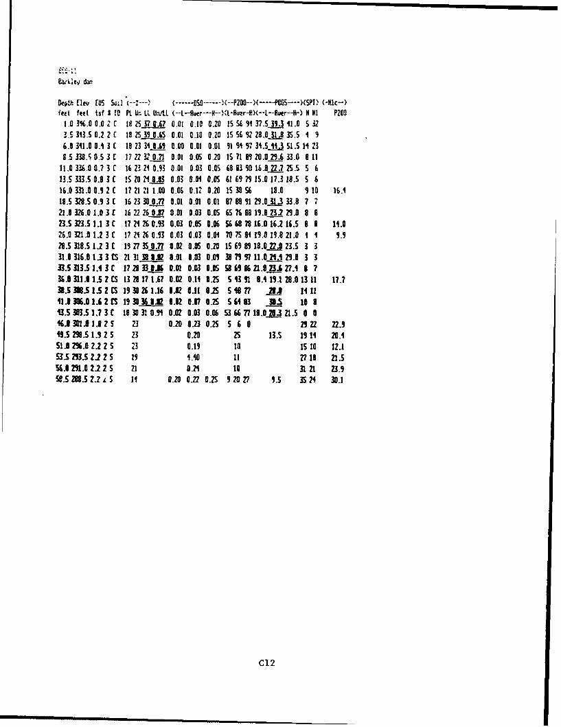
4-iley daf
Dep',.h lieu [US SO; (-.- , I ---- ..... ------.. ,,,--PZ0oo -)'( ----.. ---P S ... SPT, (-RIC--)
feet feet tsf I 10 PL Un LL Un%.LL (--L--Ruer---HK-- M-RIer-H)(--L--Ruer--N-) H Ni P2001.031%.00.0 LC 1 25376.67 0.01 0.10 0.20 155S 94 37.5 35.3 41.0 532M. 313.S 0.2 2 C 19 25 33 0.65 0.01 0.10 0.20 IS 5632 28.0 31.8 35.5 1 9
6.0 3P1.0 0.0 3 C 19 23 3 0.65 0.00 0.01 0.01 91 91 9s 34.5 11.3 51 .S 11 238.5 339. 0.5 3 C 17 22 32 0.71 0.01 0.05 0.20 157 1 89 20.0 23.6 33.0 9 11
11.0 336.0 0.7 3 C 16 23 2140.93 0.01 0.03 0.05 68 93 90 16.8 22.7 25.5 S 613.5 333.5 0.8 1 C 1S 20 21 0.33 0.03 0.01 0.05 61 69 9 15.0 17.3 18.5 5 616.0 331.0 0.9 2 C 17 21 2Z 1.00 0.06 0.2 0.20 15 38 56 18.0 9 10 16.118.5 328.5 0.9 3 C 16 23 30 0.77 0.01 0.01 0.01 87 88 31 23.0 31.3 33.8 7 721.8 326.0 1.0 3 1 16 22 26 O.R 0.01 0.03 0.05 65 76 98 19.8 23.2 23.0 8 823.S 323.S 1.1 3 C 17 21 6 0.93 0.03 0.05 0.06 566 8 78 16.0 16.2 16.5 8 8 14.026.0 321.01.23 C 1724126 0.3 0.03 0.03 0.01 70 750119.019.821.0 1 1 9.9
28.5 318.5 1.2 3 C 13 777 35 0.77 0.02 9.05 0.20 15 69 89 18.0..fJ 23.5 3 331.9 316.0 1.3 3 CS 21 31 38 .12 0.01 0.03 0.09 30 79 9? 11.0 21 23.90 3 333,S.313.S1.,l3,C 1728 33L 0.C1 0.030.05 59 69 86 Zf.023A 27.N 8 736.0 311.0 15 2 CS 13 28 17 1.67 0.02 0.14 0.25 5 43 91 8.4 19.1 28.0 13 11 17.73853N.851,52CS 1930261.16 0.02 0.11 0.25 51877 212 141141. 306.01.62 C5 159A36 .,2 0.02 8.07 0.25 56463 -9 18 8U3.503.S1.73C 1930310."1 0.02 0.03 0.06 5366 77 18.0 28.3 21.5 0 06J i301.I 2S 23 0.20 8.23 0.25S 5 6 8 2922 22.3
.5 298.5 1.9 2 S 23 0.20 25 13.S 19 14 20.451.0 23.0 2.2 2 5 243 0.13 10 15 10 12.153.59 3.5 22 2 S 19 4.40 11 77 18 21.5
6.i 291.0 222 S 21 0.24 10 31 21 23.958.5 M. 28 2 L S 1I 0.20 0.22 0.25 9 2027 9.5 35 24 30.1
C12

I.aiLieli dan
e.pth [leu [US Szi -- :---, ,- ..-. 50 . .-- P2-----X- -XFo0S---),SPD (-Nlc--)feet feet tsf 1 10 P. Un L1 L'./LL (--L-- Ner--I--)1L-Ruer-H)(--t--Aver--N-) HI P200
1.0 347.5 0.0 2 CS 18 21 1 0.52 0.01 0.07 0.20 15 S3 72 31.0 8 4i3.S 31S.0 0.2 2 1 20 23 2 0.55 O.00 0.06 8.2 5 75 94 37.01J. SO.S IS 316.0 32.5 0.3 2 1 9 2 '1 0.50 0.01 0.06 0.2 S 77 S '12.013.3 44.5 20 39.S 310.0 0.5 3 C 17 23 3 0.71t 0.0 1.01 0.01 0.01 93 S 97 33.036.8 40.5 11 19
11.0 337.S 0.6 3 " IS 21 2S 91 0.01 0.04 0.03 86 90 53 28.U32.3 38.S 11 1413.5 33S.0 0.7 3 1 17 21 31 3.67 0.01 0.01 0.01 5t K53 3M.0 31.3 35.5 1l 1716.0 332.5 0.3 2Z 17 5 290.1OA 0.01 0.05 0.20 15 S7 U 29.0-N 31.0 6 718.5 330.00.8 3 ES 16 2121 90.3 0.02 0.06 0.10 12 569i 318.5 19.1 21.0 9 1021.0 327.5 0.9 2 S 16 0.22 0.23 0.2S S 9 17 3.3 4.0 1.5 39 11 31.923.5 3250 1.0 1 S 20 0.21 0.25 025 S 7 9 1.5 22 22 23.926.0 322.S 1.1 3 SM 20 0.07 0.12 0.20 IS 38 53 11.3 13.7 17.2 9 8 11.228.5 320.0 1.1 2 S 21 0.08 0.180.25 5 22 18 12.1 27 25 31.231.0317.5 1.2 2 5 19 0.21 0.22 .25 S 3 10 3.8 41.1 1 24 22 24.133.5 315 1.3 z S 13 0.18 0.20 0.25 5 19 6.5 27 21 25.236.3 312.5 1.4 2 S 21 0.13 0.16 0.25 5 25 37 5.3 5.7 10.0 20 17 24.33.5 310. 1.12 S 16 20 218.93 0.02 0.18 3.25 32 I5 7.0 17.5 28.3 16 13 20.71.03/W.51.53C 191230312 03 O.M 5 U . 6 5262 7617.0..fl 22.3 7 6
43.S 05.1I1.6 3 r 19 2332 V.I 0.5 0.10 0.25 55 0 65 18.8 14 1116.1 302.5 1.7 2 5 23 0.16 0.20 0.25 512 21 5. 3521 31.848.5 39.3 1.8 S SC 18 25 26 0.54 0.04 0.08 0.12 20 15 6S 11. 16.7 21.0 12 9 15.651i 257.5 1.8 3 S5 25 2 0.23 0.06 0.16 0.28 14 365 6.3 12.9 18.5 19 153.5 255.0 2.1 3 N 18 22 28 078 006 0.07 0.07 51 52 5"715.0 16.721.017 12 18.55. 252.5 2.0 2 S 20" 0.20 0.20 0.21 1010 11 5.3 31 22 25.53.5 290.0 2.1 2 5 22 0.12 0.16 0.19 12 23 36 13.0 3323 B 3.161.0 2?.5 2.1 S 17 0.22 0.22 0.23 6 11 22 3.6 6.8 10.0 23 16 20.3
C13
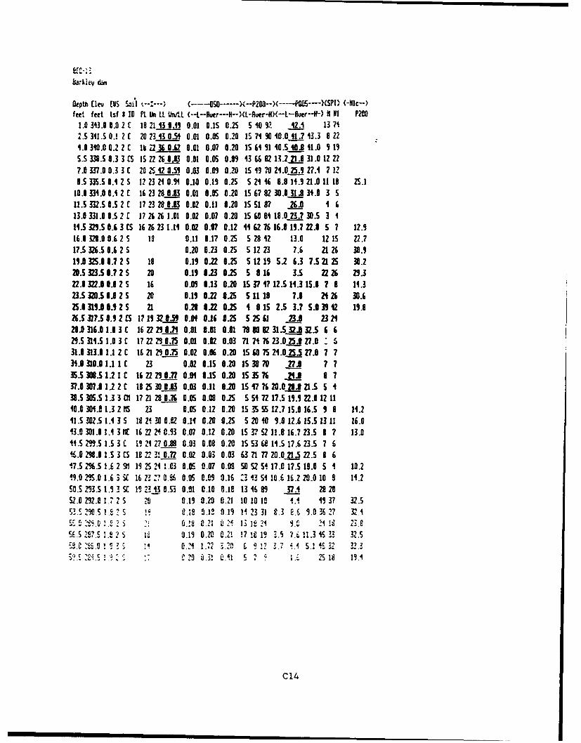
4&3rlty elan
Depth [lev [US sa1 ',--:---) (---- ----. )<--P200--) PO3----XSPD (-Hl¢)feet feet tsf I 10 Pft Un LL tLn/ti (--L--Ruer---H--)(L-Auer-I)--L--Pler-[H HI P200
1.0 343.0 0.0 2 ( 18 2113 0.15 0.01 0.15 0.25 5 40 92 V2.1 13 712.5341.50.S 2( 20 23130.54 0.01 0.OS 0.20 15 7419 .0 41.7] V.3 9221.0 340.0 0.42 c lb 2 36 0.12 0.01 0.07 0.20 1S 61 51 40.S•... U1.0 5 195.5 338.5 0.3 3 CS IS 22 26 0.83 0.01 0.85 0.09 13 66 82 IL2 21.8 31.0 12 227.8 337.0 0.3 3 C 020 2512 0.55 0.63 0.05 0.20 IS 519 21.0 25.9 27.1 7 120.S 335.5 0.4 2 S 12 23 21 0.51 0.10 0.15 0.25 S 21 %6 8.8 14.5 21.0 11 18 ZS.1
10.0 334.0 8.1 2 C 16 23 28 9 3 0.01 0.05 0.20 IS 67 82 30.031.8 31.0 3 511.5 32.50.5 2 C 17 23 28 B3 0.02 0.11 0.20 1S 5187 2.8 A 613.8 331.0 0.5 2 C 17 26 26 1.01 0.02 0.07 0.20 15 60 811.0 23.7 30.5 3 111.5 325.5 0.A 3 C5 16 26 23 1.14 0.02 0.07 0.12 44 62 6 16.8 15.7 22.0 5 7 12.516.0 328.0 0.6 2 5 13 0.11 0.17 0.25 S 28 2 13.0 12 15 22.717.5 326.S0.6 2 S 0.20 0.23 0.25 5 12 23 7.6 21 26 38.51SA 32S.0 0.7 2 S 18 0.15 0.22 0.25 5 12 15 51 6.3 7.S213 30.220.5323.5 . .? 2S 20 0.15 0.23 0.25 5 8 16 3.5 2226 29.322. 322.8 .3 2S 16 8.05 0.13 0.20 IS 37 47 12.5 14.3 15.3 7 8 14.323.5 326.5 1 8 2 S 20 0.15 0.22 0.215 11 18 7.8 24 26 30.625.1 19.0 A .5 2 S 21 0.23 3.22 0.21 1 8 IS 2.5 3.7 S.0 35 42 15.826.5 317.5 0.5 2 CS 1715 3 8.59 0.01 0.16 0.25 52561 23.8 23242J i316.0 1.0 3 C 16 22 25.71 0.01 0.61 0.01 ?8 89 82 31.]32 32.5 6 625.5 31.5 1.03( 172 ?2 25 0.75 0.01 0.02 0.03 71 ?1 7623.0 2?.0 " 531.3 313.0 1.1 2 C 16 21 290.75 0.02 0.06 0.20 IS6 0 ?5 21.02.5 27.8 7 734.0 310.11.1 1 C 23 0.02 0.15 0.20 is 1 70 27.8 7 735.53.0 1.21C 162229 OR70.87 0 .15 0.20 153S76 21 8 737.0 W.01.22C 1825390S3 3 0.03 0.11 3.20 15 47 76 20.028.0 21.5 538.5305.5 1.3 3 01 17 21 2q 0.76 0.85 0.00 0.25 S Si 72 17.5 15.5 22.0 12 1110.0 301.0 1.3 2 HS 2 0.85 0.12 0.20 !5 35 S 12.7 15.0 16.S 5 8 14.241. .S1.4 I3S ld 1213 0.82 0.11 0.20 0.25 520 0 9.0 12.6 15.13 11 16.013.0 301. 1.1 3 HC 16 22 21 0.53 0.07 0.12 0.20 153 V 7211.8 16.7 23.5 8 7 13.011.5 20,9.5 1.5 3 C 21 M ? 0.88 0.03 0.08 0.20 IS 53 11.5 17.6 23.5 7 6%.9 295.0 1.5L 3 CS 1 7! 03.2 0.02 0.03 0.03 63 71 77 20.0 21.5 22.5 9 617.5 2%.S 1.62 91 19 25 N 14.03 0.05 0.07 0.00 50 5252 17.0 17.5 19.0 5 1 10.219.0 259.0 1.6 3 SC 1623 Z? 0.,6 0.05 0.09 0.15 "3 4 3 51 10.6 16.2 20.0 10 9 11.250.S 3.S 1.9 SC 10, 27 .13..30.3 0.01 0.10 0.18 13 46 89 37. 28 20S2.0 292.0 1.7 2 S 29 0.19 0.20 0.21 10 100 .1 4 15 37 32.5S3.6 290.S 1.S ? S " 01.18 9.12 0.19 11 3 31 8.3 2.6 9.0 3 2? 32.1I"..r A .,•[ .' .. 2 S .. ri 5 ?' Q. 0.21 ý '. 1 13 2, 1.: 14 is 23.8
S.S 227.5 1.8 2S 10 9.15 0.20 0 !.2 71I 19 Z.5 7.u 11.3 is 13 32.S
ý,c C. P 7251 19.1
C14
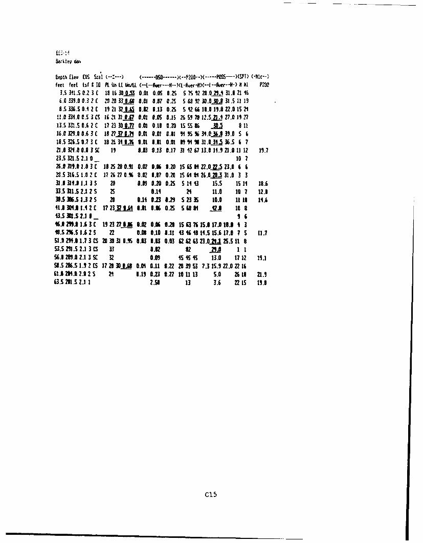
Depth [ieu (US ,-----) (--.. -050----- )(--P200-H(4.... >----) (---c-feet feet tsf 1 10 P1 (n Et. niLt, (--.--wer-H--)(L-Aher-H9(--|--er--N-) I hI P2,,1
.S N31. 0.2 3 ( 18 130053 0.01 .0S O.S S 0 .. S 92 28.0 2.A 31.0 211 4i. B39.0 0.3 2 C .19 .33 0_._0- 0.01 0.07 0.M 5 569 T 30.0 30.J 31.5 11 198.5 336.5 0.4 2 1 19 21 32 OA 0.02 0.13 0.25S 52 66 18.0 19.8 22.0 15 21!1. 0334.08 .5 3 (5 16 '1318.7 8.01 8.85 0.15 26 S9 79 12.52.c j 2.0 1213.5 33!.S 0.6 2 t 17 23 30177 0.01 0.10 020 15 856 30.5 9 1116.08.3290. 63C 1027L.71 0.01 0.01 0.81 "9S%5 34.036.039.0 S 618.525.6 0.7 S . C 18 26 3 1.76 0.01 0.01 0.01 89 *4A 9 31.0 34.5 36.5 6 723.0 321.0 0. 1 St 19 0.03 0.13 0.17 31 42 67 13.0 14.9 21.0 11 12 19.723.5 321.5 2.1 0 10 726.8 319.01.0 31t 18 25 290.91 0.02 0.16 0.20 I55 S IN2.0-V U.23.0 6 628.S 316.5 1.0 Z C 17 26 27 0.% 0.02 0.07 0.20 IS 15681 26.0 28.3 31.0 3 331.31 .M 1.1 3 S 20 0.09 0.20 0.25 S 143 15.S 15 11 18.633.S 3115 2.1 2 S 2S 8.14 24 11.0 10 7 12.03.5 30.5 1.3 275 28 0.14 3.23 019 5 2393 10.0 11 10 14.6ll3IM.91.42E 1723373.61 0.01 0.06 0.25 56801 Q.8 10 1
13.s IN.S 2.1 8 9646i.2"A91.63C 1923273.3 0.62 0.8 6 8 .20 600 1SS3751 .0118. 348.5 255.S 1.6 2 S 22 O.8 0.10 0.11 43 13 1481.5 15.6 17.0 ? 5 11.7S1.3291.91.73(C 2030319.10 0.03 0.03 0.03 6 62 263 23.0- 2411 .511 8
3.5291.5 2.13 C5 33 0.02 82 29.0 1 16.. 289.0 2.13 S( 32 0.09 151 51 5 13.0 17 12 19.1
58.528.51.92(5 1728305..._ 0.01 0.11 0.22 20939 7.31S.9 22.0 ZZ166 1.9 1. 2.0 2 S 2i 0.19 0.23 0.27 10 11 13 5.0 26 18 21.963.S 291.5 2.11 2.58 13 3.6 22 15 19.0
C15
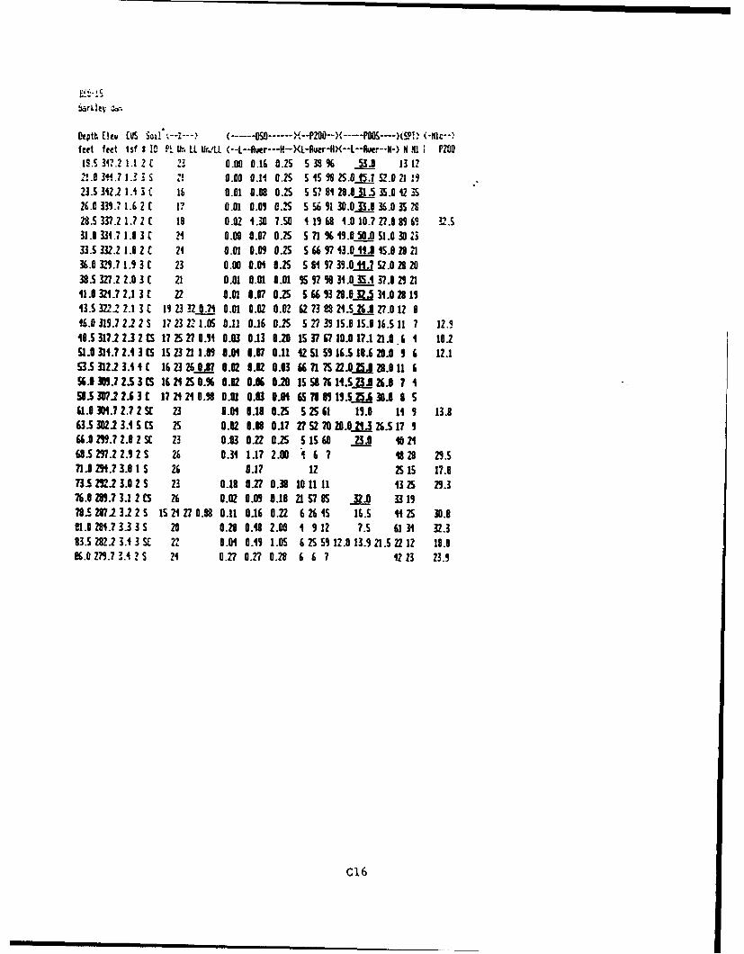
oepth E1ev [l U S•! -- (... -- 0 - -P20--- -P088----XS... (-a----}feet feet tsf S !2 P,. U. UL UrALL (--L--Auer---H-)(L-Auer-N<--L--liver--I-) N HI P2001M. 3W7.2 1.1 2 C 7 0.00 0.16 0U25 539 % 531 13 122!.1 311.1.3 S Z! 0.00 0.11 0. 5 51 98 2S.8 15.1 52.0 21 1923.5 3122 1.1 3 C 15 0.01 0.08 08 1 5 5? 81 28.0 31.5 35.0 Q 3526.0 339.7 1.6 2 c 1? 0.01 0.0 0CIS 5 591 30.0 33.0 36.0 3s 2828.5 337.2 1.? 2 c 18 0.02 1.30 7.50 119 68 1.0 10.7?27. 869 3,.S31.0 334.7 1.8 3 c 21 0.00 0.07 0.25 5 71% 19.0 501 51.0 30 2333.S M2.2 1.8 2 C 21 0.01 0.09 0.5 S 6 97 43.0 11i J15.828236.0 321.7 1.9 3 t 23 0.00 0.01 0.25 5 64 97 39.041.? 52.0 2 28038.5 .327 2.0 3 C 21 0.01 0.01 0.01 95 97 99 3.0 35.1 37.0 •22141.0 321.7 2.1 3 C 22 0.01 0.07 0.25 S 66 13 28.0 32 34.0 28 1113.5 322.2 2.1 312 19 23 32 0.71 0.01 0.02 0.0? 62 73823 21. 261 27.0 12 916.8 319.7 2., 2 S 17 23 22.OS 0.11 0.16 0.25 5.7 39 15.0 15.8 1W511 7 12.948.5 317.2 2.3 2 CS 173 2 2? 0.1 0.03 0.13 0.20 1537 57 10.0I1?.1721.01 6 19151.0 31. 2.1 3 1 5152321 1.81 0.01 07 0.11 1 5 1516.5518.28.0 9 6 12.153.5312.23.4,1t 1623203.87 0.02 O.32 0.03 66 71 7S22.0A5j 28.011 656.0301.7Z.S3CS 16212S0. 0.02 0.06 0.20 15 S 76 1l.5zVJ 26.0 7 1WS3.3071243C 17 2410.1 0C.1 0.03 U 657981 9.S AA 30.8 1 5
1.e0 31..7 2 SC 23 0.04 0.18 0.25 525 61 11.8 1H 9 13.863.5 302 13.1 5 CS 25 0.02 0.08 0.17 2? 52 70 28.0-Ztj 26.S 17 966.0 292.7 2.8 2 Sc 23 0.03 0.22 0.25 5 160 23.0 402163.52 .2 2.12 S 26 0.31 1.17 2.00 6 ? 7s 28 21.571.0 21.7 3.0 I S 2 0.17 12 215 I17.83.5212.2 3.0 2 2 3 0.18 0.2? 0.38 10 11 11 133 21.3
76.0 28.7 3.12 CS 26 0.02 0.01 0.18 215785 32.0 33 11?8.5 M.23122S 1521270.8 0.11 0.16 0.2 6 4265 16.S5" 21 30.881.0 28.7 3.3 3 S 20 0.28 0.18 2.00 1 9 12 7.S 61 34 32.383.5 2.2 3.1 3 SE 22 0.04 0.19 1.05 6 2S 59 12.0 13.9 21.5 22 12 18.096.0279.73.45 2 0.17 0.27 0.28 6 6 7 1223 23.9
C16
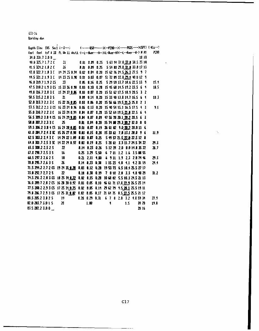
&3,rLle• d•-i
Depth F1tv ErUS Sa -.- --: ------. 5 . .. )-P0 -- .. .. (P) -~-.
feet feet tsf I Is Pt Un L Ur/LL (-L--dler---H--)L-fler-I)X--L--Ruer--H-) N MI P20034.0 331.73•.0 0 _ 181010.0 325.7 1.7 2 c 22 0.01 0.09 0.25 S 3 94 37.0 37.9 38. 5.' 2318L.5 32R. Z.82 A6 0.01 0.09 0.25 554 80 29.0 31.0 33.0 17 13
43.0 322.? 1.9 3 C 14 2 5 20.91 0.02 0.01 0.20 IS 2 76 21.5 26.5 27.S5 9 7W1.5 320.2 1.9 3 C 11232Z 0.90 0.01 0.03 0.07 SI 72 89 22.0 29.1 0.0 12 916.0 319.7 1.9 2 CS 23 0.05 0.16 0.25 5 29 S9 13.? 18.6 22.5 13 9 15.417.5 318.2 1.9 3 CS IS 23 26 0.50 0.03 0.10 0.20 15 iS 68 11.5 19.2 23.5 6 1 IO.S49.0 316.7 2.0 3 C I 212 0.85 0.03 0.07 0.20 IS S1 62 17.5 19.9 20.5 3 2S0.5 315.? 2.0 3 S 21 0.09 0.11 0.20 IS 33 18 13.0 11.7 16.5 6 1 10.352.0 313.7 2.1 3 C IS 22 26 0. 0.03 0.0 0.20 15 5 66 11.5.1-5 25.0 2 153.S 312.2 2.1 3 CS 16 3 21 0.% 0.05 0.13 0.20 IS 10 S4 15.1 165S 17.S 1 3 9.1SS.0 310.7 2.2 3 C 16 3 21 0.91 0.011 .07 0.20 15 52 61 19.S..LA 22.5 6 156.5 309.2 3.081S 1624298.03 0.01 0.07 0.09 17 S6 78 20 20.2 20.S 5 359.0 307.? 2.3 3 C 25 0.01 0.01 0.20 15 7 29.30. ?32.0 0 0$9.S 305.2 3.0 1 CS 1621 0 28 5 0.01 0.07 0.19 256182 9n80.7 28.011 661.0 0111.7 2. 3 SC 152 27 Z .9 0.03 0U5 0.20 153361 ?.113.1 20.0 9 & 11.962.5 303.2 2.4 3 C 1124221.09 0.03 0.07 0.25 S 19 S7 f1.5 ,l 22.512 864.0 301.7 2.S 3 S 11 22 210.93 0.03 0.19 0.25 S20 61 3.3 11.7 24.5 31 22 29.365.5 300.2 2.5 2 S 22 0.14 0.23 0.26 S1239 2.0 8.0 14.0 3S 22 26.767.0 298.7 2.5 3 S 16 0.25 3.29 S.50 6 7 11 1.2 1.6 3.S SS68.5 297.2 2.6 2 S 18 0.21 2.11 1.0D 6 911 1.9 2.3 2.8 74 16 29.370.0 29.7 2.6 3 S Oi 0.1 0.23 0.38 1 IS 23 1.0 1 4.2 31 1 21.171.5 24.2 2.7 2 CS 19 2 3S0.70 0.03 0.12 029 19 53 73 6.5 18.4 25.5 27 1773. 292.? 2.? 2 S 22 8.11 0.38 0.39 7 8 10 2.8 3.3 .0 48 29 31.274.5 291.2 2.8 3 C 19 25 310 .72 0.02 0.15 0.28 1060 82 5.S 18.3 21.S 21 1376.0 299.7 2.8 2 CS 16 28 30 0.92 0.03 0.05 0.10 1 61 71 17.0 22.9 26.5 23 1177.S 299.2 2.9 3 CS 17 25 31 0.725 0.02 LOS 0.11 29 6279 9.5 20.1 25.519 1179.0 286.7 2.9 3 C5 17 25 31 0.02 0.02 0.05 0.17 21 61 75 0.5 22.5 25.5 21 1290.5 285.2 3.0 2 S 19 0.28 0.29 0.31 6 7 8 2.0 3.2 4.0 59 31 27.982.0 283.7 3.01 S 20 1.80 1 1.S 31 20 19.983.S 282.2 3.0 0 28 16
C17
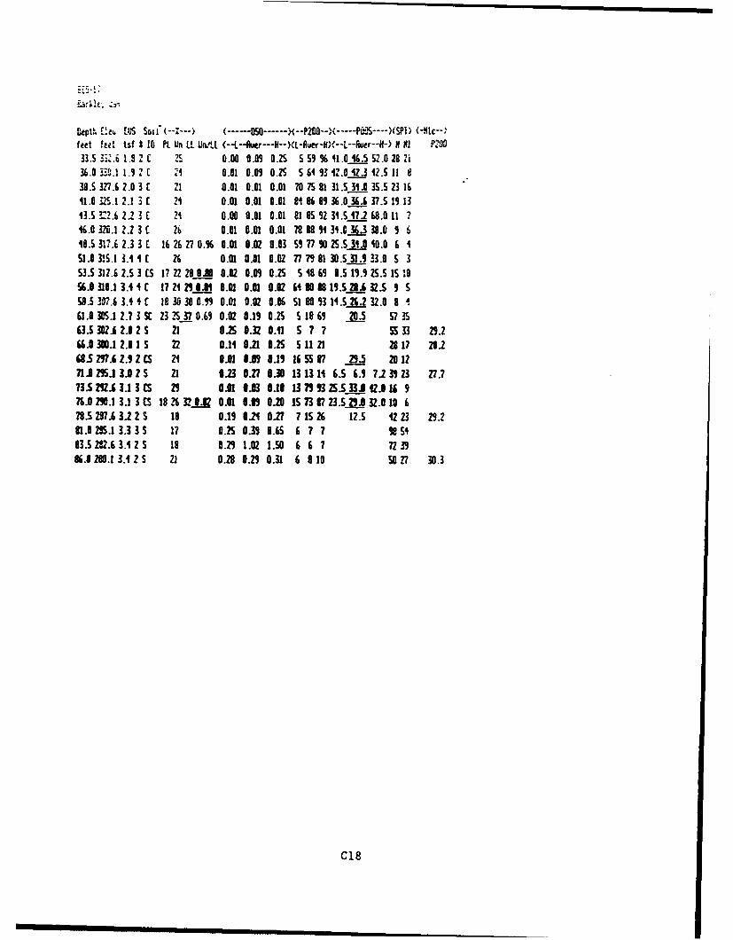
[!.ue [ Sod (--*- (------ -...--P200-- -- PtUBS -- )tSPI) (-Ntc--;feet feel, tsf 1 10 PL Ln LL UnA/L (--L--Owr---H--XL-R r-IV,--L--Ruer--fN-) H NJ P:9033.5S3..61.?2C ?s 0.00 0.09 U.S S5S9%11.064.557.0282i36.0 3 3C.1 1.9 2 1 21 0.01 0.09 0.25 S 61 931V.0 42.3 1V.5 11 838.5 37.6 2.0 3 C 21 0.01 0.01 0.01 70 75 81 31.5 31.0 35.5 23 1611.0 327.1 2.1 3 C 2 0.01 0.01 0.01 i 86989 36,091 37.5191343.5S M.62.2 3E 21 0.90 0.01 0.01 81 5 92 3.5 171 8.0 11 716.0 320.1 2.2 3 2h 0.01 0.01 0.01 70 88 91.W 36.3 38.0 9 618.5 31? 2.3 3. C 16 26270.% 0.01 0.02 .03 59 790 2S.5 1M.0 40.0 6 151.0 315.1 3.41 26 0.01 0.01 9.02 77 79 81 30.51,9 33.0 5 353.5 312.6 2.5 3(5 1722 20.0A 0.92 0.09 0.12 519 69 9.5 11.1 25.5 15.056.8310.1 3.14C 17 2?1 6.C1 0.01 0.01 0.02 61 80 81.52 . 32.5 9 558.5 707.6 3. C It 30.30 B." 0.01 0.02 0.06 51893 11.526.? 32.0 8 i61.0 3.1 2.73 S 23 237 0.69 0.02 0.19 0.2 5 18 69 20.5 S 3S63.5S3 A2.12S 21 025 0.32 0.11 5 ? 7 5533 29.266.0 300.1 2.8 1 5 22 0.14 0.21 0.25 511 21 28 17 2026829. Z.9 2 CS 21 0.81 6.81 8.11 165 5 21.5 127I J29S.13.025 21 0.3 .0.7 8.30 13131 6.5 6.9 71. 3 23 27.7?3. 292.6 3.1 3CS 29 0.01 6.03 6.18 1791 325.53J142.I16 976.0 290.1 3.1 3 3S 18 26 3260.2 0.01 0.09 0.20 15 73 7 23.5.l.0 32.0 10 678.5 2•7.6 312 S 18 0.19 021 0.27 7 15 26 1Z.5 23 29.231.0 29S.1 33. 3S 17 0.25 0.39 0.B5 6 7 7 92s583.522.6 3.425 18 0.29 1.02 1.50 6 6 7 72 1986.80 .13•.4 2S 21 0.29 0.29 0.31 6 0 10 5027 30.3
C18
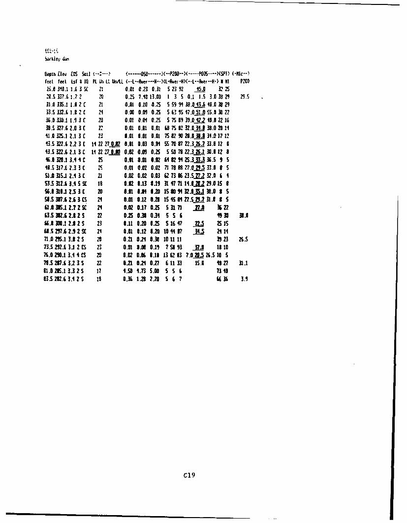
Depth ilev [tIS Sail -------- MO .---- )(--P2-- ----- PM .----. )(SPI) (-lWc--,feet feet jsf S 10 Pl. Uri L, UniLL (--L--9~er--NH--)(L-, ue;-H)(--L--over---) H H! P100
2N.1 310.1 1.6 3 sc Z 1 0.01 0.23 0.31 S 23 92 45.0 32 252,.5 337.6 1.7 2 7C 025 7.12 13.00 1 3 5 0.1 1.5 3.0 392Z9 29.S
31.0 33S.1 1.8 1 C Z! 0.01 0.10 0. 5 S59 91 38.0 13.6 18.0 38 2933.S 332.6 1.8 2 C 21 0.00 0.09 0.2 5 6 39V17.051.0 55.0 302?
36.0 330.1 1.1 3 C 2n 0.81 0.01 0.25 5 ?5 89 39.12.2 1.0 22 1639.5 327.6 2.0 3 C 2. 0.01 0.01 0.01 68 759 L32.0 3L. 38.0 20 11
41.0 325.1 2.1 3 C 231 0.01 1.01 0.01 75 02 90 28.0 v,. 34.0 17 12.3.S 322.6 2.2 36 112 2 .7 0.82 0.01 0.03 0.01 S ?0 V7 22.3 26.? 33.8 12 63.5 322.6 2.1 3 c 11 2227 0.1 0.02 0.09 025 5 SO 78 22.3W.. 38.0 12 8
46.0 320.1 3.4 1 25 ?0. 0.01 0.02 182 " 25.333. 33.5 518.5 317.6 2.3 3 C 2S 0.01 0.02 0.02 71 78 88 27.0 29.5 33.0 8 551.0 315.1 .1 3 C 21 0.02 0.02 0.03 62 73 86 23.5.27.2 32.0 6 153.5 312.6 3.1 5 SC 19 0.02 0.13 0.11 31 47 71 11.-W 229.0 15 856.0 310.1 2.5 3 c 20 oil 0.3m 0.20 1s 80 "132..•1 38.0 3 558.53N7.6 2.6 3 CS 24 3.01 0.12 1.20 15s 45 27.5 29.? 31.0 I s61305.1 .Z.?ZSC 21 0.02 0.17 0.25 53171 2? J 362263.S302.62A2s 22 0.25 0.30 0.31 5 5 6 1330 3".066.0 30.1 2.3 25 23 0.11 0.20 0.25 5 16 17 72.5 25 158.5 27.6 2.9 2 SE 21 0.01 0.12 0.20 10 87 34.5 114
71.0 295.1 3.0 2 5 20 0.21 0.21 0.30 10 11 11 3323 26.573.S 292.6 31 2 CS 23 0.01 0.08 0.13 753 93 37.0 1810
6.0 Z90.1 3.1 4 CS 2 0.02 0.06 0.18 13 28 3 7.020.5 26.S 10 S78.S27.6 3.2 3 S 22 0.21 024 027 61133 15.0 1827 31.121.0 2S5.1 3.3 2S 17 1.50e1.73 5.00 5 5 73 10
23.SMA.43A 2 S 19 0.36 128 2.20 S 6 7 66 36 3.9
C19
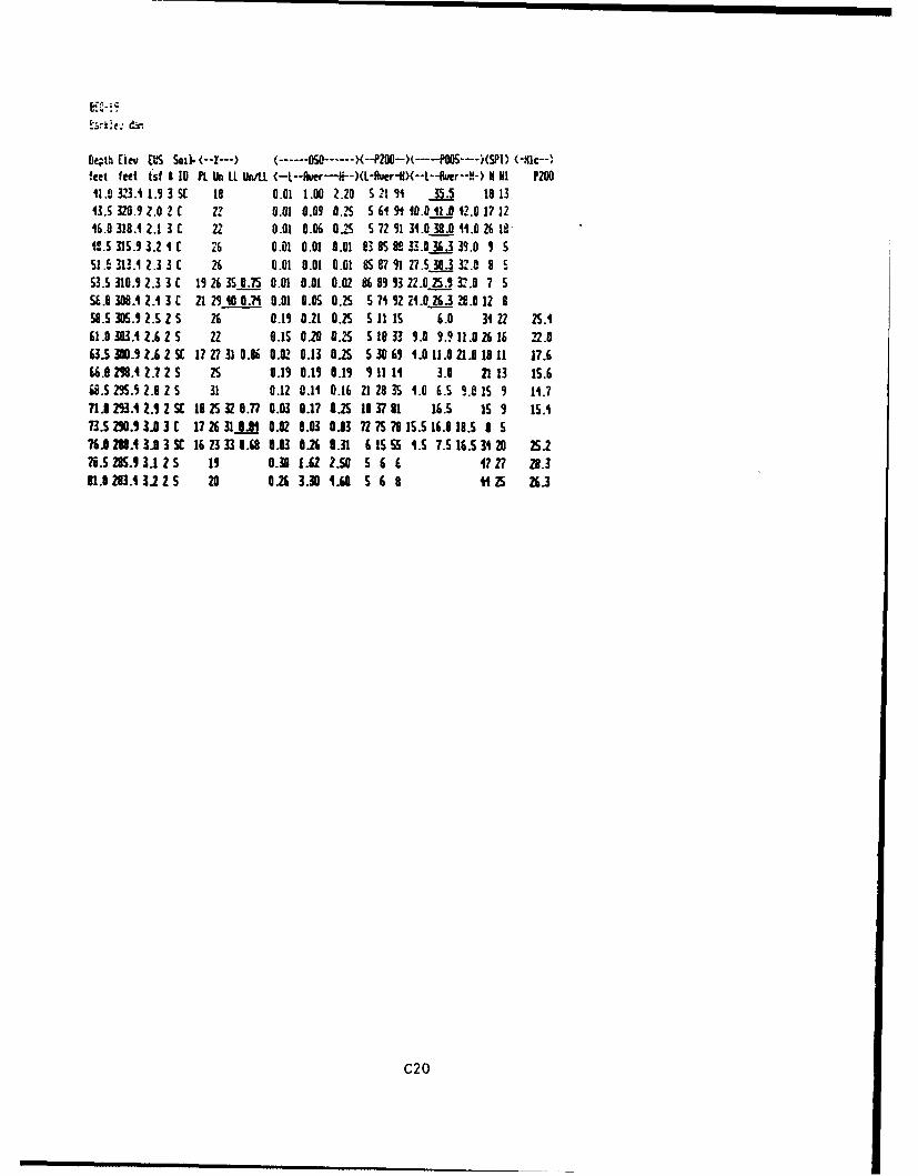
Er; . , aI IIII I
Oe;ot liev (LS Sol.. ---- 050------ )(--P200-x---POo ---- )(SP[) (-.I1c--,feet feet tsf 1 10 PL Un LL UrOnL (-L--Aver----f--)(L-9w'-f(--L--&,r--H-) H HI P20011.0 323.4 1.9 3 S 18 0.01 1.00 2.20 s 21 91 35.5 18 1313.s 320.9 2.0 2 C Z? 0.01 0.09 0.25 S 619 10.0 11.0 12.0 17 1216.0 318.1 2.1 3 C 22 0.01 0.06 0.2S 5 72 91 3.0 8.0 W.0 26 184l2.S 315.9 3.2 1 C 26 0.01 0.01 0.01 83 85 98 L.036 3 39.0 5 S51.6 313.1 2.3 3 C 26 0.01 0.01 0.1 S 879 1 27.S 30.3 32.0 a S53.5 310.9 2.3 3 C 19 26 35 .75 0.01 0.01 0.02 K 8 93 22.0 25._ 3:.0 7 5SE.0 308. 2. 3 C 21 29 0 0.7 0.01 0.05 0.25 S 71 92 Z1.026.3 2.0 12 B58.5 305.1 2.5 2 S 26 0.19 0.21 0.2 S 1115 6.0 31 22 2.161.• 3U.4 2.6•25 2 zz 0. 0.20 0.25 518 3 9.0 9.911. l 26 16 22.063.5 300.952.62 SE 17 27 31 0.86 0.02 0.13 0.25 5 30 69 1.0 11.0 21.8 18 11 17.666.0 29.8 .7 2 S 2S 0.19 0.19 0.19 9 11 11 3.0 21 13 15.6
.5 295.9 2.9 2 S 31 0.12 0.11 0.16 212 8 35 4.0 f6.5 S.0 15 9 14.771A 293.4 2.9 2 SC 18 25 32 0.77 0.03 0.17 0.2 10 37 81 16.5 is 5 15.173.5 290.9 3 3•C 17 26 311.M 0.02 0.03 0.03 72 ? 78 15.5 16.8 18.S I 576.6 M8. IJ 3 SC 16 23 33 0.68 0.50.26 031 6 15 SS 1.5 7.5 S.S 31 20 2S.271.S 25.9 3.1 25 19 0.30 I. 2.50 56 1 727 28.381i A A .3122S 20 0.2 3.30 1. S 56 8 25 26.3
C20
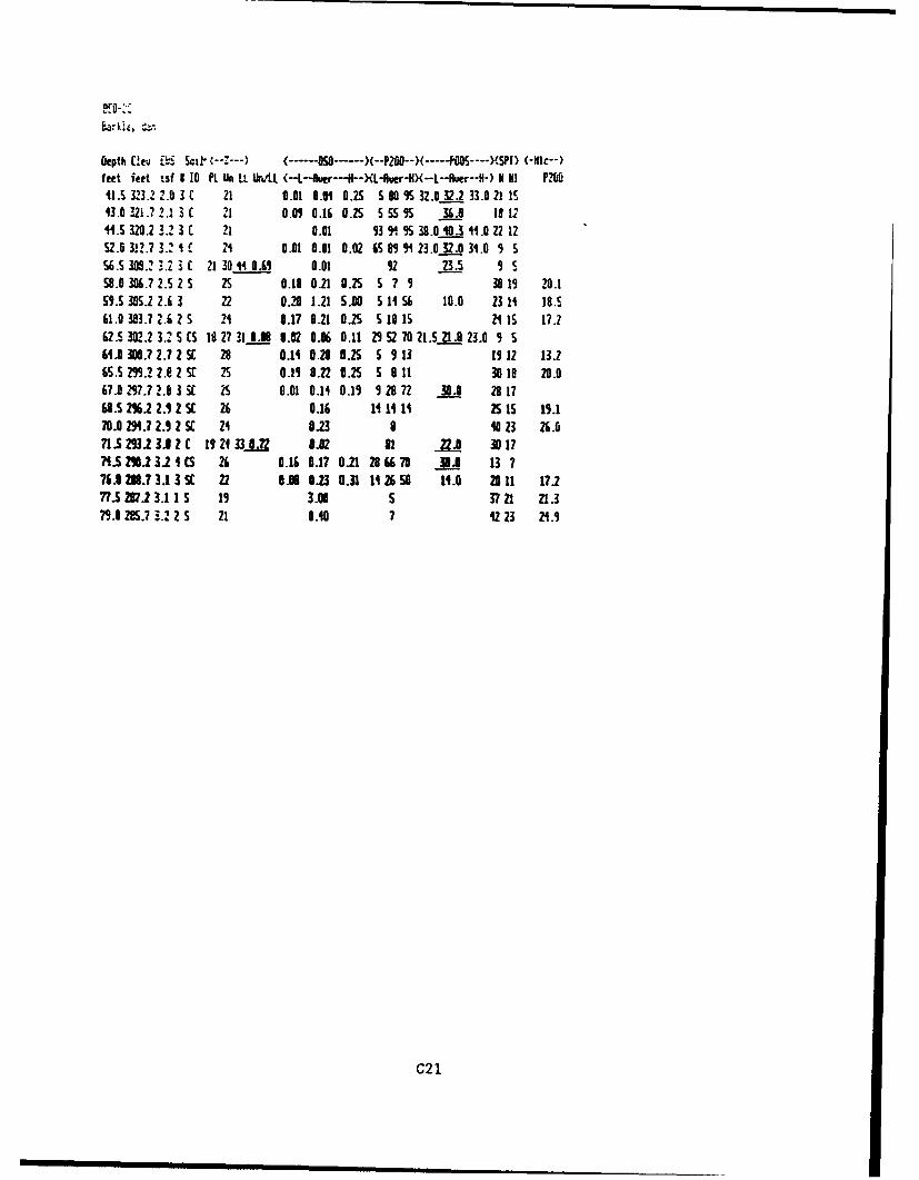
Depth (!eu .ts Scil (-- (-Z---0----•XSPI) (-lIc--)feeet feet tsf I 10 PL Wn LL UrsLL (-L--wer---H--)(L-Ruer-N --L--Ruer--H-) H MI Pm0m11.5 323.2 2.0 3 £ 21 0.01 0.01 0.25 5 80 9 32.0_.2 33.0 21 1S43.0 321.7 2.1 3 C 21 0.09 0.16 0.25 55595 36.0 s18 I.W.5 320.2 3.2 3 C 21 0.01 9314 95 .O8 0._3 11.0 22 1252.5 3,.?7 3.2 1 21 0.01 0.01 0.02 658 91 23.0 32.0 31.0 9 Si.S 308.2 3.21 3 C 21 30 " 0.61 0.01 92 23.5 9 S
58.0 30.7 2.5 2 S 5 0.18 0.21 0.25 5 ? 9 30 19 20.1S9.S 305.2 2.6 3 22 0.20 1.21 5.00 S11 56 10.0 23 11 18.561.0 303.7 2.6 25 21 0.17 9.21 015 S 10 15 21 is 17.262.S 302.2 3.2 S 5S 18 27 31 0.8 0.02 0.06 0.11 29 52 ?7 21.5 21.9 23.03 54.300.7 2.7 2 5( 28 0.14 0.20 025 s 9 13 19 12 13.2
65.5 23.2 2.e 2 5 IS 0.19 9.22 0.25 5 8 11 30 le 20.067.0 297.7 2.8 3SC 2 0.01 0.11 0.13 28 72 30.0 29 1768.5 21.2 2.1 2 SC 26 0.16 11 14 2 5 15 19.170.0 29.7 2.9 2 SE 21 0.23 8 40 23 26.071.s 291 3 2Z c 1921 33.L 0.02 11 .. 0 30 1774.S I.293.1 CS 26 0.16 0.17 021 2866 70 30.j 13 776.1288.73.1 3 S 22 0.0 1.23 0.31 1426 50 14.0 20 11 17.27?.S 287.2 3.1 1 S 19 3. S 37 21 21.37.0 225.73?,.2 2 S 21 0.40 7 2 23 21.9
C21
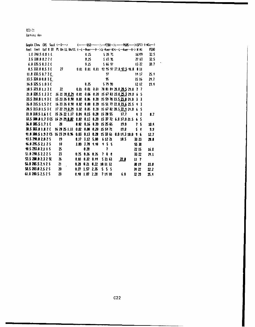
j~akl-V dam
Upth (eI 0U, Soli (--Z--- (-.... ----- . .-- P291--. .... POOS-...)(SF) (-Nl--)feet feet tsf 1 10 PL Un LL LK4/LL (--L--ver---,--)(L-Re;-IX--/--ur--H-) H MI P200
1 .1 34O.0.0 1 .25 S U 2.1 ?. 1)9 32.53.5 338.0 0.2 2 t 0.25 s65 951 27 63 32.56.0 35.S 0.3 2 C .2S S A 7 13 2Z 30.78.5 333.0 0.5 3 C 27 0.01 0.01 0.01 92 959 7 P.0 2.5 '.0.0 8 11
11. e33.S 0.73 C1 97 11 17 25.113.5 328.0 0.8 3 C 9S 15 16 24.716. 325.5 1.0 3 0.25 57 990 12 12 13.113.5 323.0 1.1 3 C 22 0.01 0.01 0.01 7s $I 81 '8.0 28.5 29.0 ? 721.0 320.S 1.3 3 C 16 2 28.7 0.01 0.06 0.20 15 67 83 23.025.3 29.0 6 523.S 318.8 1.4 3 C 152 3 26 0.50 0.02 0.06 0.20 15 59 ?O 23.S ZIJ 21.8 3 326.8 315.5 1.5 2 1 16 23 26 0.90 0.02 0.08 0.20 15 51 77 22.0 23.6 25.5 1 328.5 313.0 1.5 3 C 17 22 2 90.7 0.02 0.05 0.20 15 £7 82 20.5 22.A 21.0 6 531.8 310.5 1.6 I C 1S 26 22 1.17 0.01 9.15 0.20 15 28 55 17.7 4 3 8.733.S308J1.73C5 1621293.12 0.02 0.143 8.20 1537"72 6.017.021.5 6 536.J 30s.1.? 1C 28 8.02 0.16 0.20 15 2565S 19.0 ? 5 10.138.5 303.9 1.8 2 C 16 28 25 1.11 0.02 0.08 0.20 IS S4 71 19.0 5 1 9.941.8 300.S 1.9 2 CS 1623241 .% 0.03 0.13 8.28 IS 3361 8.0 11. 18.0 9 6 12.713.5 298.0 2.8 2 5 19 0.17 3.12 5.00 6 12 21 10.5 33 3 28.016.8 29.5 2.1 2 S 18 3.00 3.70 .10 1 5 5 SS 3
.5 293.0 2.1 1 5 25 0.20 7 22 15 16.051.8 290.5 2.2 2 5 23 0.2 0.26 0.26 ? 8 8 33 22 21.153.S 288.0 2.3 2 SC 26 0.03 0.32 0.41 5 216 3 22.A 11 756.0 285.5 2. 2 S 21 0.20 0.21 012 1011 12 Ja1l 23.0585 283.9 2.5 2 5 20 0.2? 1.57 2.35 5 S S 3 22 22.261.0 280.S 2.5 2 S 20 0.40 1.07 2.20 7 1113 6.0 32 20 25.1
C22
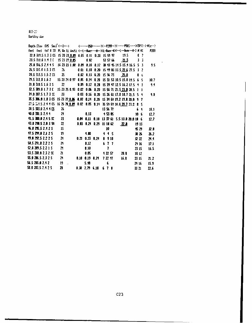
,•.rLie• •
Depth r, S Soil (--Z--- (- --050-- )(--P700--, .... -...)(SPI) (--I----
feet feet tsf 1 10 PL Un Li LI (--W--Ruer---iI--)(L-Aue-HX--L--Av'er-•- • If, PM022.6 319.S 1.3 3IS 1520230.0i O.OS 0.11 0.20 IS 5997 19.S 8 ?23.5 1.0 1.4C 1IS N 27 0.85 0.02 5S3 7 66 21.5 3 325.0 316.5 2.1 4 S 16 23 23 1.00 0.09 0.10 0.12 R8 13 15 11.S S1.1 16.S S 3 9.526.53 1S.0 1.5 3 S 26 0.01 0.10 0.20 IS 19 83 13.5 22.6 27.5 3 228.0 1I3.s 1.5 2 Is 25 0.02 0.13 0.20 I5 36 73 25.0 8 829.5 312.0 1.6 2 15 23 21 0.97 0.05 0.14 0.20 IS 31 53 10.5 IS.0 19.5 6 5 10.?31.0 310.S 1.6 3 5 2? 0.09 0.12 0.20 15 39 17 12.5 16.2 17.5 1 3 9.132.5 309.0 1.? 3 1 IS 23 S 0.93 O.R0 0. 0.20 IS 56 71 21.5 23. A28.5 I I31.0 30?.5 1.7 3 SE 23 0.03 0.16 0.20 IS 26 61 17.0 18. 21.5 5 1 9.035.5 3K.0 1.8 3 (S 15 23 273 IA 0.03 0.14 0.26 15 34 64 19.2 19.8 20.0 9 73?., L,.C 2.4 1 (5 16 25 .28 .9 002 0.V 5 0.14 35 59 69 1.0 20.7 23.0 9 S9.5 303.0 2.4 1IS 26 13 5677 6 1 10.1
40.0 301.S 2.4 4 21 0.13 1 5 3 10 6 12.741.5S 380.1 Z. t 23 0.61 0.11 0.18 13 3761 5.513.8 20.0 10 6 12.743.0 283.1 3 91 22 0.03 0.21 0.29 11182 IS 19 13
46 .A 5.S Z. Z S IS 10 1 29 32.047.5 2.8 2.1 2 19 1.0C 4 4 5 38 26 26.249.0 nz2.5 2.2 2 S 21 0.11 0.23 0.24 8 1 10 32 22 .1.450. 291.0 2. 225 21 0.12 6 ? 7 21 16 17.152.0 229.5 2.2 1 S 21 0.10 7 23 15 16.553.5 22.8 2.3 2 5t 21 0.85 1 22 57 20.0 18 1255.0 28.S 2.3 Z S 21 0.10 0.19 0.21 72 V7 16.0 23 IS 21.256.5 285 A2.4 2 19 5.10 6 2 16 15.92.0 283.5 2.4 125 20 0.30 2.19 6.10 6 7 8 33 21 22.6
C23
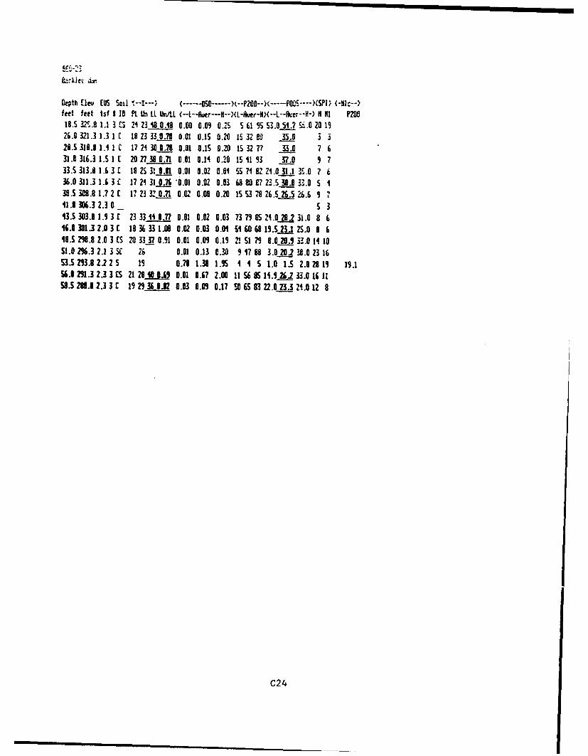
Depth ]rae [13 Scil ,------ (- o-050w )(..p20_.-...p0w5...},l) -- Hi--)feet feet tsf 110 PL Un LL Unt.L (--N--Aer---H--)(L-Aver-H)(--L--Aver--I-) H Hi P200
18.5 Z7.8 1.1 3 ES 24 23 Q 80.18 0.00 0.09 0.2S S 6i 9S 13.0 51.? S.0 20 19.26.0 321.3 1.3 1 C 18 23 33 0.79 0.01 0.1S 0.20 15 32' V 35.0_0 320.53 19.8 1.4 1 C 17 2 30 0.78 0.01 0.1S 0.20 IS 32 77 33.0 7 631.0 316.31.51 ( 20 27380.71 0.01 0.14 0.20 151193 37.0 9 733.5 313.6 1.6 3 E 18 ZS 31 0.81 0.01 0.02 0.01 S 71 82421.0 31.1 _ .3c .0 7 636.0 311.3 1.6 3£ 172131 0.76 0.01 0.02 0.03 68 80 ? 2.2.5 30.0 33.0 5 138.5 308.8 1.7 2 C 17 23 320.71 0.02 0.08 0.0 IS S3 78 26.5 26.5 26.6 9 '741.0 386.3 2.3 0 _ 5313.S 303.8 1.9 3 £ 23 33 11 0.77 0.01 0.02 0.03 73 79 OS 21.0 28.2 31.0 8 6
.0 301 .3 2.0 3C E 1•36 33 1.00 0.02 0.03 0.01 Si 60 68•1.S23.1 25.0 8 618.5 298.8 2.0 3 CS 20 33 37 0.,1 0.01 0.09 0.19 21, 57•9 8.0 20.9 32.0 14 1051.0 2%.3 2.1 3 5 26 0.01 0.13 0.30 9 17 88 3.0 20.2 38.0 23 16
3.5 293. 2.2 2 S 15 0.70 1.38 1.55 1 4 5 1.0 1.S 2.0 28 19 19.156.0291.3 2.3 3 C5 21 28080.69 0.01 0.67 2.00 11 56 OS1 .2562 33.0 16 1158.5288.12.33 £ 129_363 2 0.03 0.09 0.17 SO6S8322.082331.012 8
C24
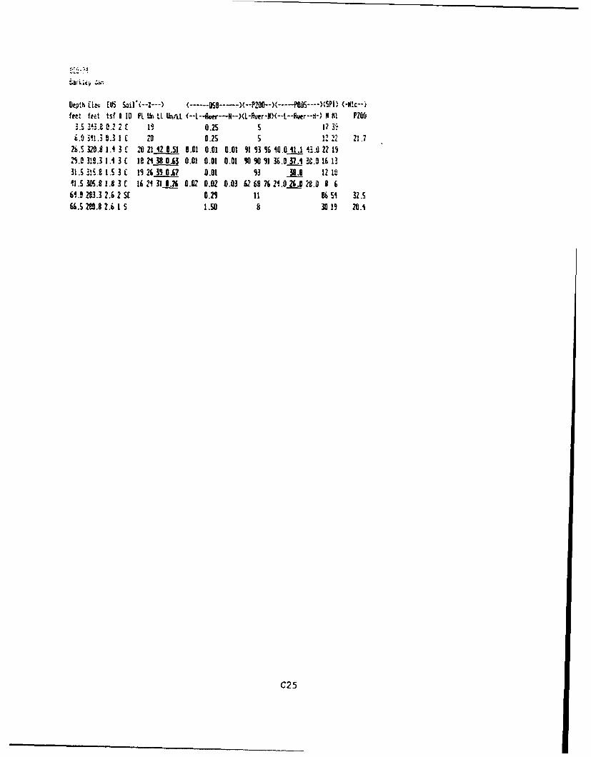
Depth GLe% [US Soil'(--Z---) (...0------. --P200--X-...-POOS...XSPi) (-1c--fee' fe-t tsf 1 10 PL Uri LL U,,in (--L--Ruer--*- X-L-Aver-fl)(--L--Rw.--e-) N K! P206
3.s-4. 0.2 19 0.2S s 17 3
i.9 311.3 9.3 1 C 0 0.25 5 112 1 .?
26.5, 30.8 1.4 3 Cc 0 221 Q 6.51 0.01 0.01 0.01 91 13 96 0.0 ill. .1.0 22 125.0 33.3 1.4 3 C 192138 0.63 0.01 0.01 0.01 905091 36.0 37.1 .0 16 1!31.S 331.1 1.53 3 C 1 265 .9 0.A 0.01 93 39.0 12 1i1,.1 3.8 1.8 3 C 16• 131 .76 0.02 0.02 0.03 62 65 76 2.. 2_.6J 29. 8 66l.7 2.3.3 2.6 2 S0 .25 it 351 s 32.s
6.s 20.8 Z.1 1 s ,so 8 30 19 20.1
C25
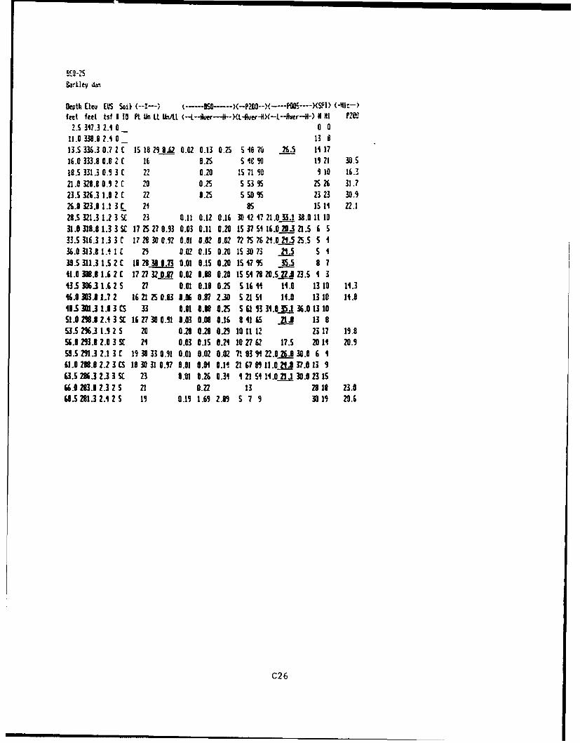
Carkity dm
Depth [leu [LS Soj) (--1--) (U5 Sa-i(--P20l--,-....p05---XSPI) (-N:--feet feet tsf 1 10 PL Un LL Ui.L {--N--8ur---I--XL-&,er-N)(--L--fler-H-) H1i FZ•
2.5 347.3 2.4 0 0 011.0 38.8 2. 0 _ 13 813.5 336.3 0.7 2£ 15 18 29 9.2 0.02 0.13 0.25 S 48 70 26.5 14 17
16.0 333.8 0.8 2 1i 0.25 S 4•8 90 1 21 30.S
18.5 331.3 0.9 3 C 22 0.2 S 1571 90 9 10 16.3
21.0 328.8 0.92t 20 0.25 5 53 9 25 26 31.723.5 326.3 1.0 2 C 22 0.25 5 50 95 23 23 30.926.0 323.8 1.1 3 C 24 as IS 1 22.128.5 321.3 1.2 3 SC 23 0.11 0.12 0.16 30 42 7 21.033.1 38.0 11 1031.0 318.8 1.3 3 C 725 27 0.93 0.03 0.11 0.20 15 31 5 16.020.3 21.5 6 5
33.5 316.3 1.1 3 C 17 28 30 0.9Z 0.81 0.02 0.02 72 ?S 75 24.021.5 25.S S I36.0313.8 1.41r 29 0.02 0.15 0.20 153073 21.5 5 4
38.5311.3 1.5 2 1 928 23 .73 0.01 0.15 0.20 IS 47 95 35.5 8 741.0 M19 1.6 2C 17 273? 0.37 0.02 0.08 0.20 15 54 78 20.5 22. 23.5 1 343.5 305.31.6 2 S 27 0.01 0.18 0.25 S 164 1H.0 13 10 11.346.0 313.31? 2 16 21 25 0.83 0.06 8.7 2.30 5 21 51 11.0 13 10 11.848.S 301.3 1.1 3 CS 33 0.01 0.08 0.25 5S 1 93 34.0 35.1 36. 13 1051.0 298.2.4 3 C 16 27 30 0.91 0.03 0.08 0.16 8 41 65 z1J 13 83.5 2%.3 1.9 2 S 28 0.28 0.26 82 10 112 23 17 19.86.8 293.8 2.0 3 S 24 0.03 0.15 0.24 10 27 62 17.5 20 14 28.9
58.5 291.3 2.1 3 C 1930 33 0.91 0.01 0.02 0.02 71 93 9 22.0 26.3 30.0 6 461.0 293.02.2 3 C 18 30 31 0.97 0.01 0.04 0.14 21 67 99 11.021. 37.0 13 9
63.5 286.3 .3 3 SE 23 0.01 0.26 0.31 1 21 51 !4.021.1 30.9 23 IS66.0 2.8 2.3 2 S 21 0.22 13 28 21 23.068.5 21.3 Z. 2 S 19 0.19 1.69 2.89 S 7 9 30 19 28.6
C26
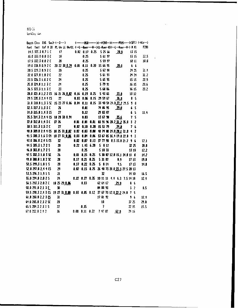
Depth [i ev [US Soi', (----) ( .----0 o-(-P0 -X--4t-,--)S? {-hc-)feet feet tsf I I PL Un LL Un/L. (----ukr----)L-Rver-H)(--L--Avcr---) H H1 P01.S 335.3 0. 1 C 17 0.02 0.17 0.25 S25 66 29.0 13 IS16.0 333.8 0.83 7 18 0.25 5 6197 13 is 2.517.5 332.3 0.8 2 C 20 0.25 5 59 9? 10 11 18.0190 330.8 0.9 2 C 20 22 3O 0.71 0.01 0.11 0.20 15 66 95 28.0 6 620.532.3 0.9 2 C 20 0.25 5 62 98 24 25 -1.122.0 327.0 1.0 2 C 22 0.25 56 1 93 24 24 31.223.5 326.3 1.0 2 C 24 0.25 55 95 151s 22.12S.0 321.8 1.1 3 C 21 U.2S 579 91 16 Is 23.626.S 323.3 1.1 3 C 23 0.25 5 68 86 165 is 23.228.0 321 1.2 2 CS 1621 26 0.02 0.16 019 025 5 13 65 23,.0 13 1229.5 320.3 2.4 4 CS 2 0.03 0.06 0.1S 29 59 67 26.0 8 S31.0 318.8 1.3 3 S 15 23 27 0.86 0.01 0.11 0.15 33 40 Si 21.0 27.7 2•.S 5 832.5 317.3 1.3 3 26 0.01 71 8695 2__.3 6 531.0 315.1 1.1 3 CS 27 0.12 29 83 7 6 5 11.135.5 1.3 2.41 iCS 18 28 30 0.91 0.03 13 67 98 25.6 7 537.0312.81.13C 3?26 8.01 0.81 0.01 83 91%28.2.12 35.0 3 238.5 31!3 1.5 2 C 27 0.02 0.10 0.20 IS51 79 21.3 7 640.0 309.8 2. I CS 18 25 31 0.2 0.02 6.03 6. 4 80 21.0423j 31.0 4 311.53 08.3 1.6 301 18 2? 31 3.X 0.03 0.04 0.06 53 67 85e1-.A 19.8 Z2.0 1 313.0 306. 2.1 5 CS 32 0.02 6.07 0.13 37 .7 9 8.S IS.8 21.2 9 6 12.1
.5 30S.3 1.72 S 20 0.22 1.43 6.20 5 9 12 32 25 28.0
16.0 303.01.7 2 5 20 0.25 5 10 33 1310 121.2V7.5 302.3 1.1 3 SE 26 0.01 0.15 .25 S 30 7 12.0 IS.1 34.011 0 11.ZW. 300.0 1.8 2 SC 28 0.17 0.21 0.25 31 8" 8.9 17 13 19.950.5s2z.3 1.s I S 2n .1? 022 0.25 5 I 1 1.5 17 13 11.052.0 297.8 2.4 1 (5 29 0.02 0.15 O.2S 26 0 323 ZO_._3327.529 1353.5 2%.3 1.9 1 5 21 32 14 10 16.555.0 294.3 2.0 2 S 21 012 0.27 0.35 10 11 11 4.4 6.3 7.5 11 10 12.16.5 253.3 2.0 2 ( 18 25 29 OJ6 0.03 62 6467 21.0 8 6
5S.C n1.8 2.1 3 t 30 M8 91M 3 3 2 8.559.5 20.3 2.1 3 CS 19 2? 31 9.98 0.03 O.OS 0.12 3" 67 73 12.0 22.2 24.0 7 501.0 M.8 2.2 3 ES 31 17 81 92 9 6 12.16.0 25.0 2.3 2 SC 20 10 372. 29.065.5 .72.3 2.3 ! S 22 0.35 7 22 1 IS.567.0 M2.8 2.4 2 36 0.00 0.11 0.22 7 1.78 ? 62.0 21 IS
C27
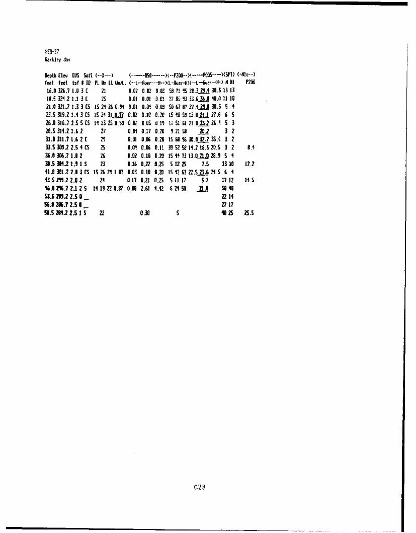
Barkley dan
Depth [lev ELS Sofl (--I---) (--. --- ---0 )(--PZOO-->(•---- POS .---- (-RIC--)feet feet tsf I I Pt Ln LL Un.LL (--L--•uer--- .--XL-Aver-lK--L--uer-') KIHB P20O
16.0 326.7 1.0 3 C 21 0.02 0.02 0.03 S8 7?1 995 .3L29.. 30.S 13 1318.5 324.2 1.1 3 C 25 0.01 0.01 0.02 77 869 3 33.6 36.8 0.0 11 1021.0 321.7 1.3 3 CS 15 21 26 0.91 0.01 0.01 0.08 SO 67 87 22.1 29.0 38.5 S 123.S 319.2 1.1 3 CS 15 21 31 0.7? 0.02 0.10 0.20 15 40 59 13.021.1 2?.6 6 526.0 316.7 2.5 S IS 11 23 25 0.90 0.02 O.OS 0.19 17 51 61 21.0 23.7 26.1 5 328.5 311.2 1.6 2 27 0.01 0.17 0.0 9 21 58O 20.2 3 231.0 311.7 1.6 2 £ 29 0.01 0.06 0.20 568 % 30.032. 3.5. 3 233.S 309.2 2.5 4 CS 2S 0.01 0.06 0.11 39 Q e 14.10.5 20.5 3 2 8.1
36.0 306.7 1.8 2 26 0.92 0.10 0.2.0 15 11 73 13.021.0 28.9 S I38.5 H0121.9 1 S 23 0.16 0.22 O0S 5 12 25 7.5 13 10 12.211.0 301.7 2.0 3 CS 15 26 1.07 0.031 0.10 Q0 15 26 3 22.S 23.6 21.S5 6 443.5 2".2 2.0 2 21 0.1? 0.21 0.25 5 11 17 5.2 17 1 11.54.1 296.7 2.1 2 S 11 19 22 0.87 0.08 2.61 .12 6 24 SO 21.80 58 10
53.5 21.2.5 0 22 1156.8 286.7 2.5 0 27 1758.52 .2 2.5 1 S 22 0.30 5 40 25 2S.5
C28
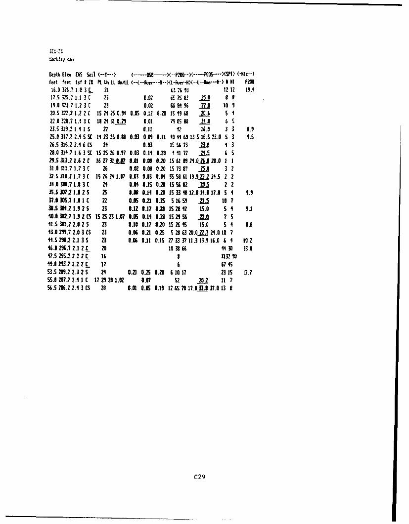
0Deth [Ieu [US Soil (-1---) (----0 .....--X--P200-- ... 05--)1) (.il--)feet feet isf 110 Pt. Lin LL UnAL (-L--Aker---N--XL-u•.-XI--L--tier') N I PM16.0 326.? 1.0 3 C 21 E3 76 13 12 12 19.117.5 3"S.2 1.1 3t 23 0.02 ES ?7S82 0 -Z5.0 c 819.0 323.7 1.2 3 C 23 0.02 9 al 96 27.0 10 920.5 32.2 1.2 2 ' !S 21 25 0."1 0.05 0.12 0.20 15 S. 9C9 20.6 5 122.0 3".7 1.1 3 E 13 21 3! 0.79 0.01 751 88 3e.Be .0 6 S23.5 319.21. 1.5 1 2 0.11 V2 16.0 3 3 8.125.0 317.7 2.4 5 St 14 23 26 0.83 0.03 0.09 0.11 iD 11 60 13.5 16.5 23.0 5 3 9.526.5 316.2 2.1 6(5 21 0.03 1C. 56 73 23.1 1 328.0 314.7 1.6 3 SC 15 2S 26 0.17 0.03 0.14 0.20 1 .1 72 21.5 6 S295.313.2 1.6 2 C 16 27 _31.. 0.01 0.3 8.20 156 1 •9 2.0L261. 28.0 1 131.0 311. I1.7 3 r 26 0.02 0.08 0.20 1S 73 87 25.0 3 232.5 310.2 1.7 3 C 15 26 21 1.07 0.03 0.03 0.01 55591 S 5. fi l .2 21.5 2 234.0 3M.7 1.0 3 C 21 0.01 8.15 0.20 1556 82 295 2 235.5 3W.7 1.8 2 S 25 O.A 0I 9.20 15 33 48 12.3 1.9 17.8 S. 1 1.937.1305.7 1.1 1 C 22 0.05 0.21 0.25 S 165 5 21.5 10 738.5 30411.9 2 5 23 0.12 0.17 0.29 IS28 42 15.0 S 9.140. 302.7 1.9 2 CS 525 23 1.7 .0 L OS .1 0.20 1S29 S6 21.0 7 S11.5 301.2 2.0 25 23 0.10 0.17 0.20 15 265 15.0 S 1 8.843.0 25.7 2.0 3 CS 23 0.05 0.21 0.25 c 28 63 20.0L2f.2 21.0 10 711.5 28.2 2.1 3 S 23 0.0 0.11 0.15 27 33 37 11.3 13.9 16.0 6 1 10.2
5.0 296.7 2.1 2C 20 1036 ( 1 3 13.017.5 295.2 2.2 2 _ 16 2 W132949.8 293.? 2. 2 C 17 6 67 1553.5 289.2 2.3 2 5 24 0.21 0.25 0.28 6 10 17 23 Is 17.7SS.O 287.7 2.4 1 ( 17 29 291.02 O.07 5. 20.2 11 756.5 286.2 2.4 3 CS 29 0.01 O.OS 0.11 1265 78 17.9 33.J 37.0 13 8
C29
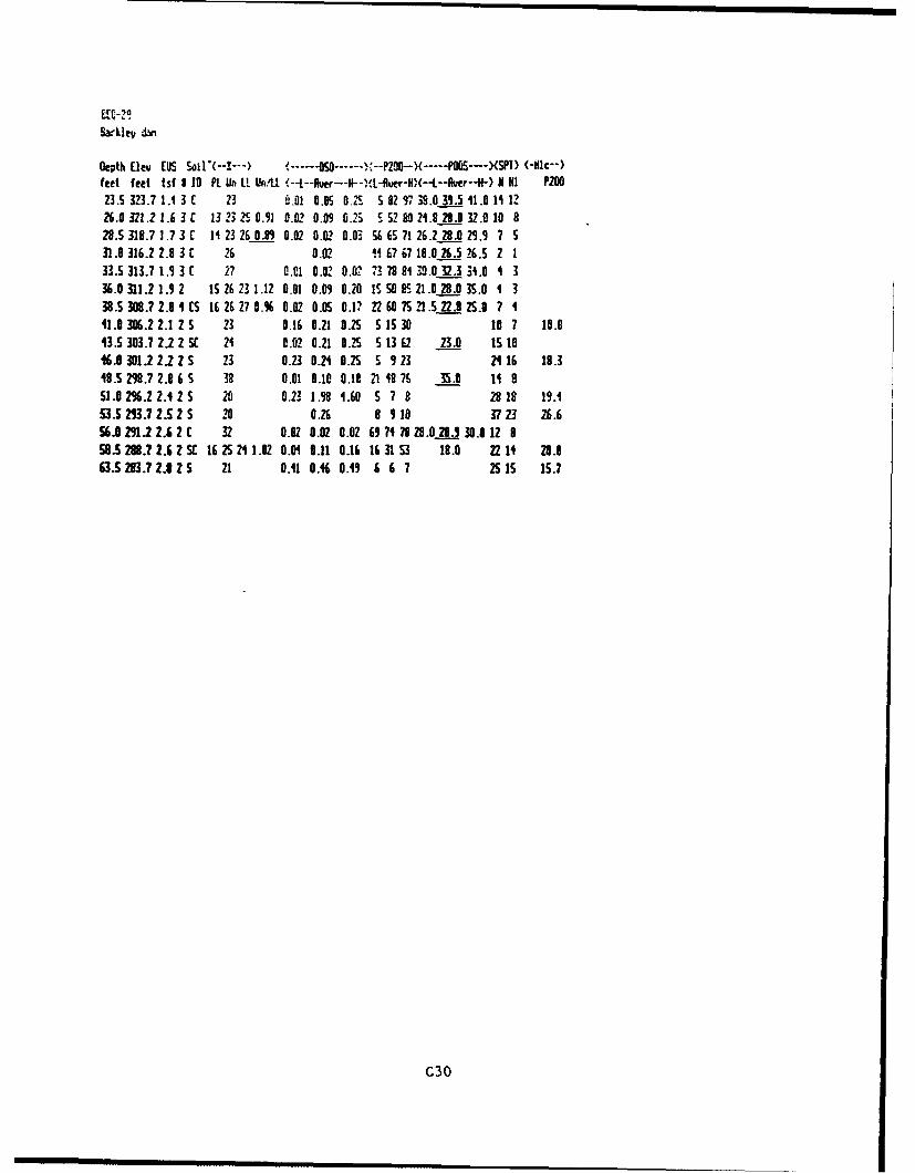
ERC-29.Barklev c~
Depth (1ev (US Soil*(--I---4 (------ . OSO ------ 0 --P2--)( ----- POOS---)(SPI) (-Nlc--)feet feet tsf 1 10 PL Lb LL Un/LL ,-4---Her--H--,L-ler-HX--L--Aer--) H III P20023.5 323.7 1.1 3 C 23 .01 0.05 012 5 82 97 39. 39.5 1.0 11 1223.0 32!.2 1.6 3£ 13 23 25 0.91 0.02 0.09 0.25 C 52 8024.8 28.0 32.O 10 828.5 318.7 1.7 3 1 1123 26 0.89 0.02 0.02 0.03 S CS 71 26.2 28.0 29.9 7 531.0 316.2 2.8 3 C 26 0.2 1i 67 67 18.0 26.5,26.5 2 1
33.5 313.7 1.9 3 1 27 0.11 0.02 0.02 73 78 81 39.0 32.33 .0 4 336.0 311.21.92 152623 1.12 0.01 0.09 0.20 IS50 SO 21 .0 28.0 3S.0 4 338.5 308.7 2.8 1 CS I6 26 27 0.3 0.02 O.0S 0.17 22•60 7S 21 .5 22.8 2S.0 7 141.0 306.2 2.1 2 5 23 0.16 0.21 0.5 515 30 10 7 10.843.5 303.7 2.2 2 SC 21 0.02 0.21 0.2S S 13 62 23.0 15 1046.0 301.2 2.22 S 23 0.23 0.21 OS 5 9 23 24 16 18.348.5 239.7 2.8 65 38 0.01 0.10 0.19 21 18 76 35.0 1H 951.0 23.2 2.4 2 S 20 0.23 1.98 1.60 5 7 8 28 18 19.153.5 233 25 2 S 20 0.26 8 9 31 37 23 26.656.0 291.2 2.6 2 C 32 0.02 0.02 0.02 69 74 78 28.0 29.3 38.012 I
.5 298.? 2.6 2 SC 16 2 21 1.02 0.04 0.11 0.16 16 31 53 18.0 22 14 20.863.53 .78.025 21 0.11 0.46 0.49 6 6 7 2515 15.7
C30
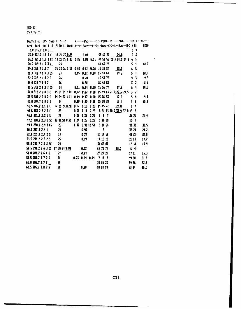
E.rkley dto
Oepth (1ev 1% Soil (--Z---) (---050----- 20O----- ... ----•S.... T>-c--)feet feet tsf 310 PL Un LL Un/Lt (--L--A er---N--XL-Ruer-H)(---Avr--H-) H II PKIN
1.0 346.7 2.8 0 _ 002S.0 .7 1.S 3 1121270.7. 0.01 2360 24.8 7 6
26.5 321.2 1.6 3 CS 11 21 250.35 O.06 0.09 0.11 451 S6 22.32I.0 21.0 6 523.0 315.7 1.7 3 23 6 S'7 72 5 I 10.029.S 318.2 1.7 2 15 23 U 0.87 0.03 0.12 0.20 15 3857 23_.1 - c31.0 316.7 1.8 3 CS 23 0.05 0.12 0.20 15 13 63 19.S 5 4 10.03.5 315.2 1.8 z 26 0.20 is 553 I 3 9.331.0 313.7 1.9 2 26 020 15i1 i83 3 2 L .635.5 312.2 1.5 3 S 21 0.11 0.11 0.20 15 56 77 17.5 6 1 1O.S37.0 310.7 2.6 36 152 211.01 0.02 6.87 0.20 5 19 63 21.0 Qf&. 21.5 3 23B.5 30.2 2.0 2 E 11 21 22 1.11 0.11 0.17 0.20 IS 36•53 17.0 5 1 5.810.0 307.7 2.8 s 21 0.18 0.19 0.20 15 20 30 12.1 9 6 10.841.5 30122.1 2 C 17 25 281. 0.02 0.13 0.20 IS 45 72 2 6 1
1.5 303.2 2.2 3 ( Z5 0.01 0.11 0.25 S S1 83 3.033.9 37.0 13 946.13011.7221 21 0.253 0.5 0.25 56 7 3121 21.117.S300.2 233Sc 3211510.71 0.24 0.25 0.25 5 0381 10 7"5 28.7 2.4 3 CS 25 0.32 5. 10.50 32656 5 2 3z.550.S 257.2 2.l 1 21 6.90 5 37 21 24.2SA. 255.7 2.4 2 S 17 0.27 12 11 16 19 31 32.553.5 251.2 2.5 2 S 25 0.19 14 15i1i 21 13 17.755 A25.7 2.5 15 29 31 62 87 12 8 13.9S6.5 251.2.6 3 IS 17 30 3 '.A 0.02 69 r 77 23.0 6 1.jl W.7 Z.6I S 24 11.1 2727 27 17 11 16.3
55.5 2.2 2.7 2 S 21 0.23 0.21 0.21 7 8 8 1 30 31.S61iJ 286.7 2.7 2 Is 10 15 20 55 36 32.562.5 285.2 2.8 Z S 20 0.60 10 1010 23 1 161
C31
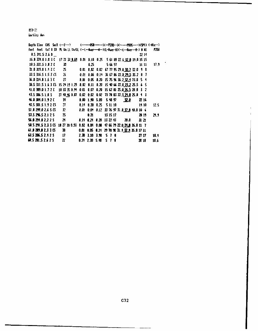
f,.re- ,
Depth [lev [US Soil c--!---. (------0S0-----X--P200-->(----P005--(SPI) (-NIc--)feet feet tsf 18 1 .. 10 LL Un/It (--LL--flur---P--)(L-Pi-r-NX--L--rM--l-) N I 72130
8.5 3M11 2.6 0 _ 2 1.16.0 331.0 1.0 3 C 1721313 L .5_ 0.01 0.10 025 5 61 89 22.6 32A3.0 151518.5 331.5 1.02 1 3-A 0.25 5 657 11 11 17.931.0319.0 11 3 C I5 0.01 0.02 0.02 67 77 95 .0 3._.? ?.0 1 933.5 316.5 1.5 3 CS 26 0.0! 0.06 0.11 3X 67 86 22.029.5 35.2 9 736.0 311.0 1.6 3 C 27 0.01 0.05 0.20 15 75 96 36.252.1 73.0 5 138.5 311.5 1.6 3 CS 15 21 !? 1.2 O.02 0.11 0.20 1510 622.02 32. 25.5 6 C,11.0 309.0 1.7 2 " 18 3 354 0.91 0.01 0.07 0.20 15 62 81 25.026.5 2.0 3 23.S 306.5 1.8 3 2r7 45 60.37 0.02 0.02 0.02 73 78 83 2'.23 21A 2S.0 1 3
U6.0 304.0 1.9 2 ( R. 0.0N 1.9 S.00 51 0 97 52. 22 1640.5 301.5 1., 2 £S 27 0.11 0.20 0.25 5 1 19 110 12.551.0 25".0 2.6S CS 32 0.01 0.01 0.12 33 76 97 31.0 37.0 10.0 10 bi
53.5 2%.5 2.1 2S 25 0.21 13 1517 2 1 24.3S6.0 25. A2.2 2 5 21 0.11 0.11 0.28 13 22 13 29.0 31 215.5 29%.5 2,3 3 (S 1027300.93 0.02 0.04 0.08 V6675• 2.01... A 26.0U11 71i 2. 23 3 CS5 30 0.01 0.5 0.11 29 70? 31.1lV 35.0 17 11
63.S 286. 2.4 2 5 17 2.38 3.10 3.10 5 7 8 27 17 118.68.521.5 2.6 2 5 22 0.21 2.30 5.10 5 7 3 28 18 18.6
C32
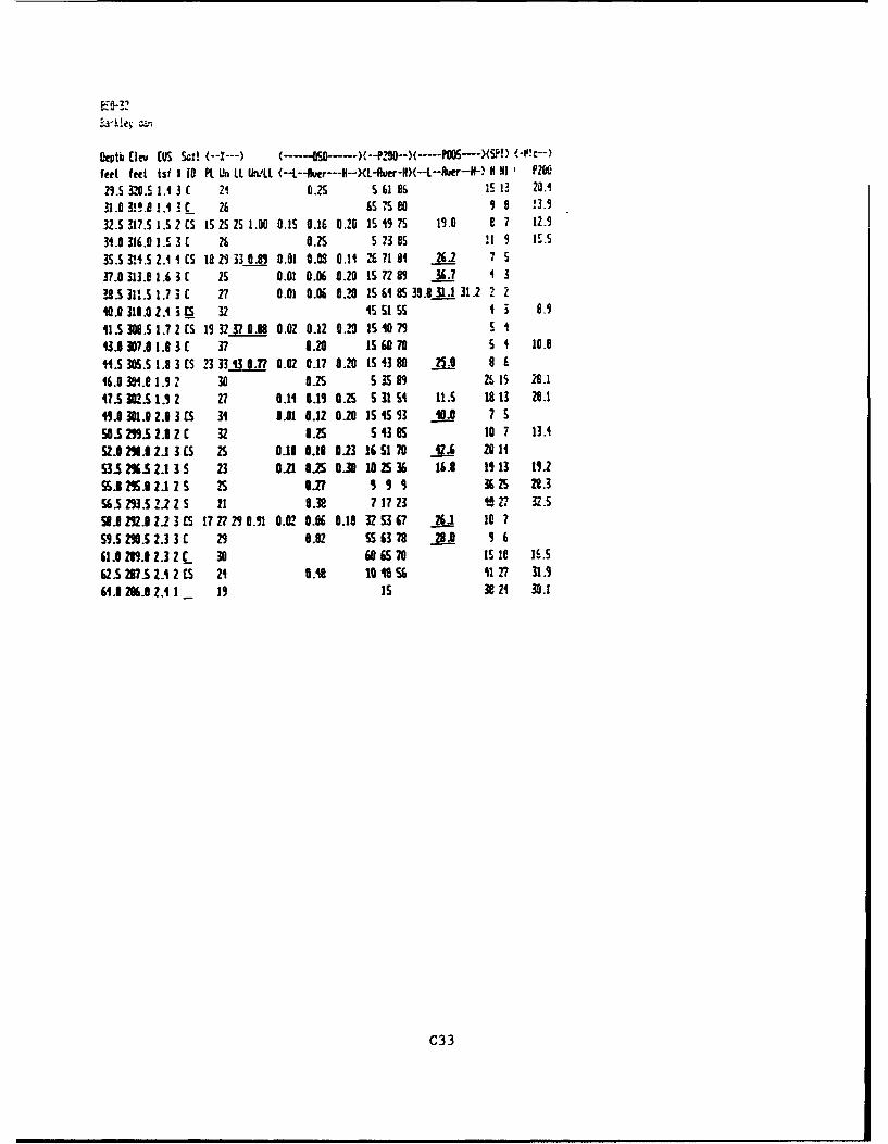
Depth Elev (US SG!! (- -) (---O0S0----)(--P20-)( . .P05---)(SP) (:")
feet feet isf 1 10 Pt Un IL UWLI. (--!--Awer---H--)(L-P.Fer-H)(--L--*p--i) H ' P206
23.5 320.5 1.1 3 C 2i os 5 619 es is 137 20.
31.0 3!1.8 1.4 3 ( 26 5 ' s0 9 9 13.9
32.5 317.5 1.5 2IS 152S25 1.00 0.15 16 0.20 1S497S 19.0 e 7 12.9
31.0 316.OlI.S 3 ( 26 0.25 5 7385 e1 9 I5.S
35.5 3R1.5 2. IS 19.133 B A 0.01 0.03 0.11 2 71 81 26.2 7
37.0 313.0 1.6 3 ( 25 0.01 0.06 0.20 IS 72 89 36.7 4 3
32.5 311.5 1.7 3 1 2? 0.01 0.06 0.2 1560 8S 39.8 31..1 31.2 2 2
i0.0 310.0 2.4 i Is 32 1 45155 1 3 8.9
l1.5 308.5 1.7 2 IS 1 32 3?0. 0.02 0.12 0.0 IS 40 79 c i
43.8 37.0 1.8 3 ( 37 0.20 158 170 5 4 10.0
1.5 305.5 1.8 3 (S 23 33 13 0.77 0.02 0.17 0.270 15 3 80 25.9 9 E
46.0 301.8 1.9 2 30 0.25 S 35 82 B is 28.1
47.5 30.s 1. 2 2? 1 0.10.15 0.25 531 5 11.5 18 13 20.1
19.04 31. 2.0 3 CS 3 0.01 0.12 0.20 15 15 93 4__ 7 S
58.S 25.5 2. ( 32 U.2S 5 I385 10 7 13.1
S. 2i8.12.1 3 CS 25 0.10 1.11 0.23 16 51 70 Zi 211
S3.S 2.S 2.1 3 S 23 0.21 6.S 0.30 1e 3 36 16.6 1913 19.2
55.0295.?2.125 25 9.2? 9 9 9 3625 22.3
56.S 293.5 2.2 2 S 21 0.32 7 17 23 0 "? 32.5
S 2A .1 2.2 3 IS 17 2 27 0.91 O.R2 5.0 0.10 32 53 67 26_ 1 10 ?
S9.S .S 2.3 3 C 29 6.02 556 3 ?8 2_.9 9 6
61. 22.1 2.3 2 C 30 60 8S 70 I510 l16.S62.s 21. Z. 2 IS 21 0.Ci 10 U56 l 27 31.9
64.8 206.0 2.1 1 19 is 38 z2 30.1
C33
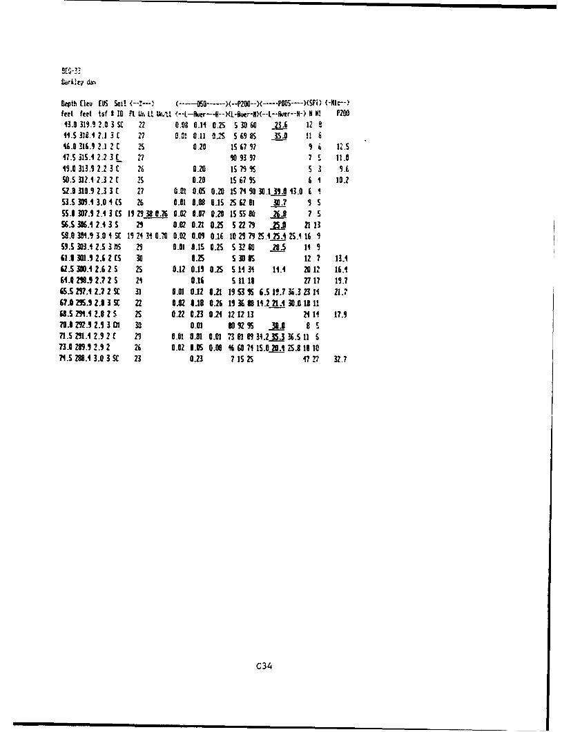
'•,rk~leV d
Depth (leu [US Sci! /--,._, (------ S.....-P20O--( . PODs ---- )(Spi) (-Klc*-)feet feet tsf 1 I0 PL WU Li. L N H--L-Aer---H--)(L- utr-N(--L--A er--H-) H H! P2t043.0 319.9 2.0 3 St 22 0.08 9.11 0.25 S 39 60 23.6 12 e11.5 318.1 2.1 3 C 27 0.0! 0.11 O.2S 569 8S 35.0 !! 646.0 316.9 2.1 2 C 7S 0.20 is 67 97 9 6 12.517.5 315.4 2.2 3 27 90 93 97 7 S 11.019.0 313.9 2.2 3 C 26 0.20 IS 79 95 5 3 9.6S0.5 312.1 2.3 ? C 25 0.20 IS 67 9S 6 1 10.252.0 310.9 2.3 3 C 27 0.01 0.05 0.20 IS M7 0 30.1 39.0 13.0 6 ¶S3.S 309.4 3.0 4 CS 26 0.01 0.08 9.15 2 62 1 30.7 9 5S55.0 307.9 2.4 3 CS 19 29 38 0.76 0.02 8.07 0.20 IS SS 80 26.8 7 S56.5 306. 2.4 3 S 29 0.02 0.21 0.25 52279 25J 211358.0 301.9 3.0 4 St 19 24 3 0.79 0.02 0.09 0.16 10 29 792 5.25.2514 25.1 1659.5 303.4 2.5 3 fS 79 0.01 0.15 0.25 5 32 80 28.5 14 961.0 301.1 2.6 2 CS 30 0.25 S 30 85 12 7 13.462.5 300.4 2.6 2 5 25 0.12 0.19 0.25 S 1H 31 11.4 20 12 16.164.0 299.9 2.7 2 5 21 0.16 S 11 18 27 17 19.765.5 297.1 2.7 2 s5 31 0.01 0.12 0.21 19 53 95 6.5 19.7 N.3 23 14 21.67.0 295.9 2.3 3 SC 22 0.02 0.18 0.26 19 36 88 141 21.1 30.0 18 1168.5 291.1 2.8 2 S 2S 0.22 0.23 0.24 1212 13 24 1 17.970.0 22.9 2.9 301 30 0.01 80 92 95 31 A S71.52 2q .4 2.9 2 2 9 0.01 0.01 0.01 73 81 9 34.2 .336 ,S 11 673.0 289.9 2.9 2 26 0.02 9.0S 0.0 16 60 71 15.0 20.1 25.8 18 10?.5 28.1 3.0 3 SC 23 0.23 7 1525 .7,7 32.7
C34
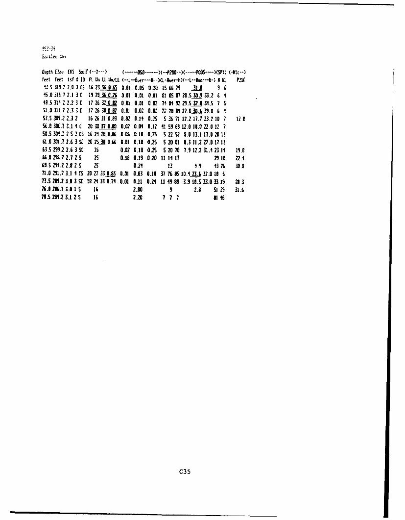
oelth n!eu cirs• Soir"(.. ( .. .. 50..... ---29 ---( ..- PODS--)(SP! -8M -
feet fee' tsf 1 10 PL U(, LL Un/it (--L--guer---l--)(L-Puer-N)(--L--Ruer--H-) NI ElI Pru("13.S 319.2 2.0 3 CS 16 23 36 0. 0.01 0.05 0.20 15 79 31.0 A 6li.0 3116.7 2.1 3 ( 19 28 36 0.76 0.01 0.01 0.01 81 85 87 28.S 30.1 33.2 1 11S.5 31W.2 2.2 3 17 26 32 0.02 0.01 0.01 0.02 79 81 2 29.5 3.8 31.5 7 SS!.0311.72.33t 1726300.97 0.01 0.02 0.02 72 70 89 27.0 30.6 39.0 6 13.5 309.2 .3 2 16 26 31 0.83 0.02 O.H 0.25 5 36 1 12.2 17.7 23.2 10 7 12.2
5E.C 30E.? 3.1 C 20 30 370.8 0. 2 0.01 0.12 a! 5 6112.0 18.0 22.0 12 758.5 304.2 2.5? 2 S 1621 228 0.06 0.06 0.19 0.25 52 52 8.0 13.1 17.0 20 1361.0301.72.635t 20 25380.06 0.01 0.18 0.25 52001 8.311.227.017!163.5 219.2 2.6 3 SE 26 0.02 0.18 0.25 S 20 70 7?. 12.2 31. 2311 1M.8WC.0 2%.? 2.7 2 S 25 0.18 0.19 0.20 11 1 17 2918 Z2.16,3".2 .2 2.3 2 S 25 0.21 23 1.9 13 26 30.871.0 291.7 3.1 4 (S 20 27 33 0.83 0.0! 0.03 0.10 37 76 5 10.1 23.6 32.0.10 673.5 28M.2 .0 3 S 18 21 33 0.71 0.01 0.11 0.24 11 19 88 3. 19.5 33.0 33 11 29.3?6.0 286.7 3.0 1 S 16 2.80 9 2.8 51 29 31.678.529.2 3.1 2 S 16 2.20 7 7 7 816
C35
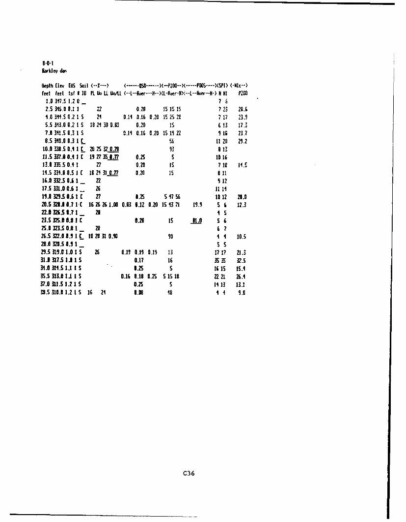
Sarkleu dam
Oepth [IeC [US Sail (--I-) (-.... 50-...-X-P0-- . POOS ---- XSPI) (-Nlc--)feet feet tsf I 10 Pk Lb U. Un/Lt (--t-fver---H--)(L-fiver-HRX--L--Auer--H-) N II P20O
1.0 347.S 1.2 0 _ 7 62.5 316.0 0.1 1 22 0.20 15 15 5 7 .13 2.64.0 314.5 0.2 1 S 24 0.14 0.16 0.20 15 25 2? E 17 23.9S.5 313.0 0.215 118 M 30 0.80 0.20 is ! 3 17.37.0 31.5 0.3 1 S 0.11 0.16 0.20 159122 9•1I 23.79.5 340.0 0.3 1 C -6 11 20 Z.2
10.0 338.50.S 1 C 20 25 32 0.798 93 171.5 337.0 0.4 1 C 19 27 35.7 0.25 S 10 16
13.8 335.5 0.4 1 27 0.20 is 710 14.C11.5 331.0 O.S 1 C 18 24 31 0.77 0.20 is a 1116.0 332.5 0.6 1 _ 22 5 1217.5 331.0 0.6 1 2_ 6 11 1411.0 329.50.6 1 C 27 0.2S S V17 10 12 20.020.5 328.0 0.7 ?1C 16 2 26 1.08 0.03 0.12 0.20 IS 13 71 19.9 5 6 12.322.8 3265. 0.7 1 __ 2 1523.5 325.0 8.8 1 c 0.20 1s 91.0 S 625.0 3235 0.8 1 __ 726.5 322.6 . 1 10 20 310.90 90 4 4 10.529.0320.50.91 S S29.S 319.0 1.0 1 S 26 0.19 0.19 0.15 13 17 17 21.331.9 317.5 1 A1 S 0.1? 16 35 5 32.531.0 311. 11 Is 0.25 5 1615 15.435.5 313.0 1.1 1 I.S0.16 0.18 0.25 1S 18 22 21 26.437.0 311.5 1.2 1 S 0.25 11 13 13.138.5 310.0 1.2 1 S 16 21 0.08 1s 4 1 9.9
C36
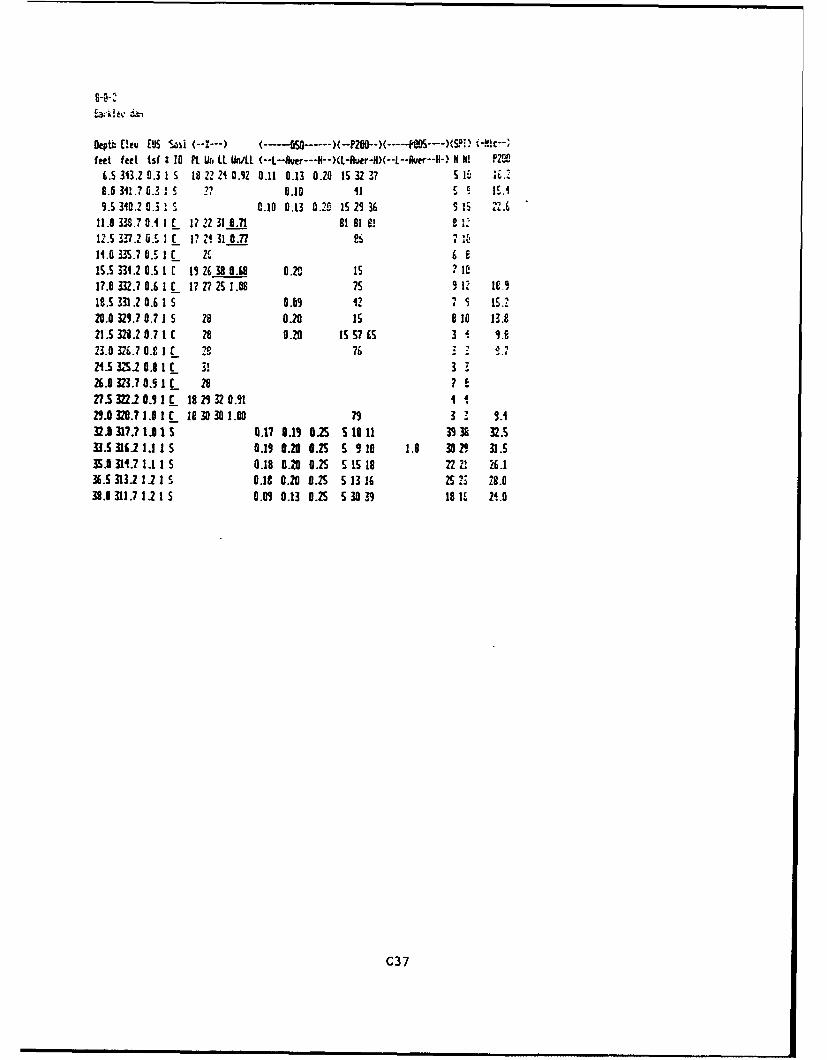
8-0-2
Oeptb [!eu [US Soil (--Z-- - -GO...)-PG-)------ M.D... )• Al -ic--;
feet feet tsf * 10 Fl Uri LL Un/LL (--L--iver---N--)(L-Rur-H)(--L--Rve--H-) H I1 P206.5 343.2 0.3 1 S 18 22 2710.92 0.11 0.13 0.20 IS 32 37 S 1 ;6."8.0 314.7 0.31 S 2? 0.10 41 S r c .A9.5 310.2 0.3 ci 0.10 0.13 0.20 IS 29 36 S 1; 22.6
11.0 3 ME. 8.1 I C 17 2231 0.71 81 81 8e 1 !,12.5 337.2 0&.r 16 17 1 31 0.77 es 7 , '11.0 33S.7 O.1 C 2C 6 81S.S 03.2 0.5 I C 19 263 8 0.68 020 is 7 1C17.0 332.7 0.6 1 C 17? 272 1.0 75 9 12 19.918.5 331.2 0.6 1 S 0.09 V2 I .15220.0 329.7 0.? 1 5 28 0.20 is a 10 13.821.5 328.2 0.7 1 C 28 070 is S? 1 S 3 . 9.823.0 326.7 0. I _ ? 76 0.,
21.5 332 0.8 1 C 3 33
26.0 323.7 0.9 1 c 28 727.5322120.11C 1829320.91 1129.0320.71.1 C 18383001.00 79 33 S.132. 317.7 1. A1 S 0.17 0.13 0.2S S 10 11 39 38 32.533.53 121.1 1 S 0.19 0.20 0.2S S 9 18 1.8 30M , 31.535.0 311.7 1.1 1 5 0.18 0.20 0.25 S5118 2 22 26.136.5 313.2 1.2 1 S 0.19 0.20 0.25 5 13 16 252 28.038.0 311.7 1.2 1 5 0.09 0.13 0.25 5 3039 18 1. 2..0
C37
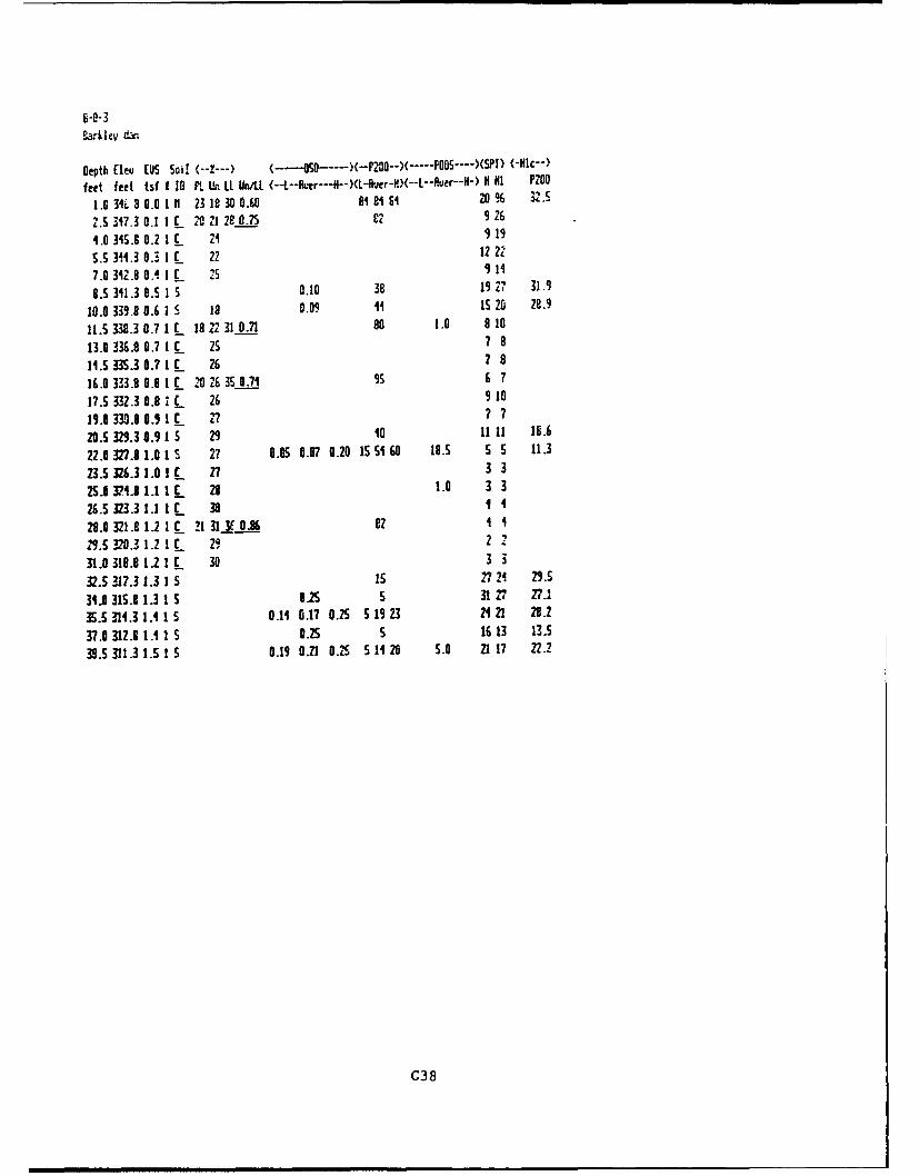
8-0-3
Depth cleu [US 'ji! ,--I---> (----050...X-P290--)( . pOS---- )(SPT) (-Hic--)
feet feet tsf t 10 ft Un LL UntLI K H--I P100
1.0 311 3 0.0 1 n 23 18 30 0.6 8181 20 6 32.s
..S W7.] 0.1 I 1 2021 2E0.75 e2 9C6
1.0 34S.9 0.2 1 -C L1 9 19
5.5 314.3 0.3 IC 22 12 2 2
7.0 312.8 0.4 i 1 25 9 1
8.5 341.3 0.5 I S 0.10 38 19 2? 31.9
10.0 339.8 0.6 1 S 18 0.09 11 15 20 28.9
11.5 33R.3 0.7 1 C 18 22 31 0.71 80 1.0 9 10
13.0 336.8 0.7 1 C zs 7 8
14.5 33.3 0.71 C 26 7 8
16.0 3733.8 0.8 1 2 •026 35 0.71 95 6 7
17.5 332.3 0.8 IC E 26 9 10
15.0 33.8 0.95 1 C 2 7 7
20.5 329.3 0.9 1 S 29 10 11 11 18.6
22.0 327.8 1.0 1 S 27 0.05 0.07 0.20 1551 60 18.5 5 5 11.3
23.5 326.3 1.0 1 C_ 27 3 3
25.34.8 1.1 1 E 28 1.0 3 3
26.5 323.3 1.1 1 c 38 4
28.0 321.8 1.2 1 C. 21 31M 0.-5 82 4 4
I9.SR0.3 1.2 2 c 249 22
31.0 318.8 1.2 1 C 30 3 3
32.5 317.3 1.3 1 S 15 27I1 2 9.S
31.0 315.8 1.3 15 02S 5 31 27 27.1
35.5 314.3 1.4 1 0.11 0.17 0.2 5 19 23 24 21 28.2
37.0 312.8 1.A Is 0.S S 16 13 13.5
38.5 311.3 1.5 I S 0.19 0.21 0.2 5 14 26 5.0 21 17 22.2
C38
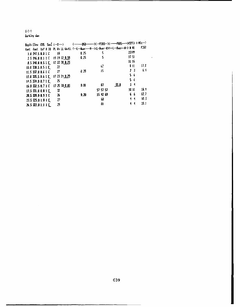
Barkley dw-
oeoth lEe [us Soil (--I- (-0 --- -SO . . -P0--)(...PfOS---)(ST) (-XNc--;
feet feet tsf I TO PL Li LL Un/L (--L--fluer---H--)(L- ver-H•-L-Aver-*H-) N K! PFN-
1.0 347.5 0.0 1 C 18 02
2.S 316.0 0.1 1 E 19 19 32 0.5_ 0.25 5 17 S5
8.5 310.0 0.S 1 ' 1722 30 0.73 11 16
io.0 33.50.5 .SI C_ 2 L2 1". 17.E
!I.S 337.0 0.6 i C 2? 0.20 is 2 3 CA
13.0 335.5 0.6 1 L 17 23 2, 0.79 S E
14.S 334.0 0.7 1 C 25 5 E
1 3.032.S 0.. 1 C 17 25 30 0.93 0.01 87 33.0 3 4
17.S 331.0 0.8 1 C 37 57 57 to 1! 16.1
20.S 320.0 0I.9 I 26 0.20 15 12 69 6 6 12.7
23.S 32S.0 1.0 1 C 27 68 1 1 10.3
26.5 322.0 1.1 1 C 29 8l 1 1 10.1
C39
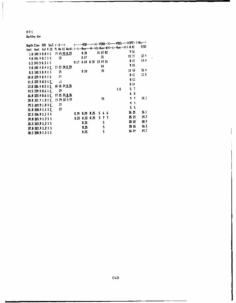
Barkley da
Depth [ICy (US Soil (-----) (. --S -XPZO)( P )(SPI, (-I1)c--
feet feet tsf : IO Pt Ln LL Un/LI R N•! PZGF
1.0 343.4 0.0 I ', 19 49 039 0.20 15 62 82 5 S1
1.0 345.4102 is .0 0.17 28 13 2 1
S.S 343.9 0.3 1 S 0.17 0.13 0.20 13 11 IS 8 2i 19.4
?.0 342.4 0.4 1 C 17 22 80.79 64 9 is
8.S 340.5 0.4 1 S 2S 0.10 39 11 16 26.
10.0 309.4 0.4 I S ?; 8 12 Z12.
11.5 33?.9 0.S 1 IC s 8 12
13.0 336. O.S I C 18 264 9.76 81
14.5 334.1 0.6 1 E 29 1.0 S 7
16.0 333.4 0.6 1 7 25 33 0.76 6
22.0 321.4 1.0 1C 1!29 L 0,.97 79 4 , 10.2
29.5 3195.9 1.0 1 C 27 4
31.0 318.1 1.1 1 C 27 5 5
32.5 316.5 1.1 1 S 0.1 0.21 0.25S 5 6 2625 26.1
34.0 315.1 1.2 1 S 0.23 0.23 0.25 S 7 7 25 23 24.7
35.5 313.5 1.2 1 S 0.2S S 20 18 19.1
37J 312.4 1.215 .25 5 18 16 16.2
38.5 310.5 1.3 1 S 0.25 S 161H 14.2
C40
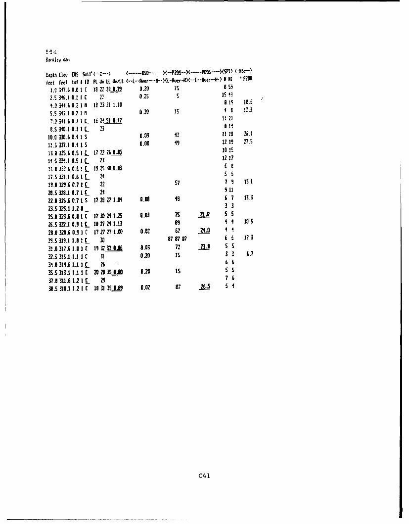
E-epth [ieu CLK Sail*(---- ............ 2O~)__po-•(PT -Hc-
feet feet tsf I 10 PL Un LL Un/LI (--L--RAr --- H--)(L-Aver-H)(--L--Auer--H-) N Ii i ' 00O
1.0 347.6 0.0 t C 182228 0.79 0.20 is 8 S9
2.5 341.1 0.1 1 C 0 .IS is 4.
i.0344.60.21 n 1823211.10 919 1i.a
S.5 3M3.1 0.2 1 f 0.20 IS 4 S 1-.3
?C B41.6 0.3 1 C 18 24--51 0.17 1
M.5 340.1 0.31 C 25 811
10.0 338.6 0.41 S 0.09 43 is i .l
11.S 337.1 0.1 IS 0.08 49 1219 27.5
13.0 3..60.5! 17 1 2 1 40.85 10 1E
W.S BI.1 O.S 1 C 23 12 17
U6.03M.60.6 ! C 19 X300.93 c I
17.5 3-1.1 0.61 C 24 5
19.0 329.60.7 1 C 22 57 79 IS.1
20.5 3298.1 0.7 1 c 24 5 11
22.0326.60.71 S 1722271.01 0.08 4i 6 7 13.3
.3.S 35.111.0 _ 33
25.1 M23.650. ! 173024 2S 0.03 75 21. 55
26.S 32.10. 1 1 182724 .13 99 4 4 1O.s
28.0320.60.9 1 C 17 27 V1.00 0.02 67 21.0 4 i
ZS.S 319.11.0 1 C 30 978787 6 L. 12.3
R, 317.5 1?.61. 1 9 12 -@A 0.03 72 23.0 S S
32.5 316.1 1.1 1 c 31 0.20 is 3 3 6.7
31.83114.6 1.1 1 76 26 -6-S.S313.11.11C 202835 IA 0.20 1s 55
37.0311.61.21C 29 7 "
38.5 310.11.21 c 18 1 350.•9 0.02 87 26.5 5 1
C4 1
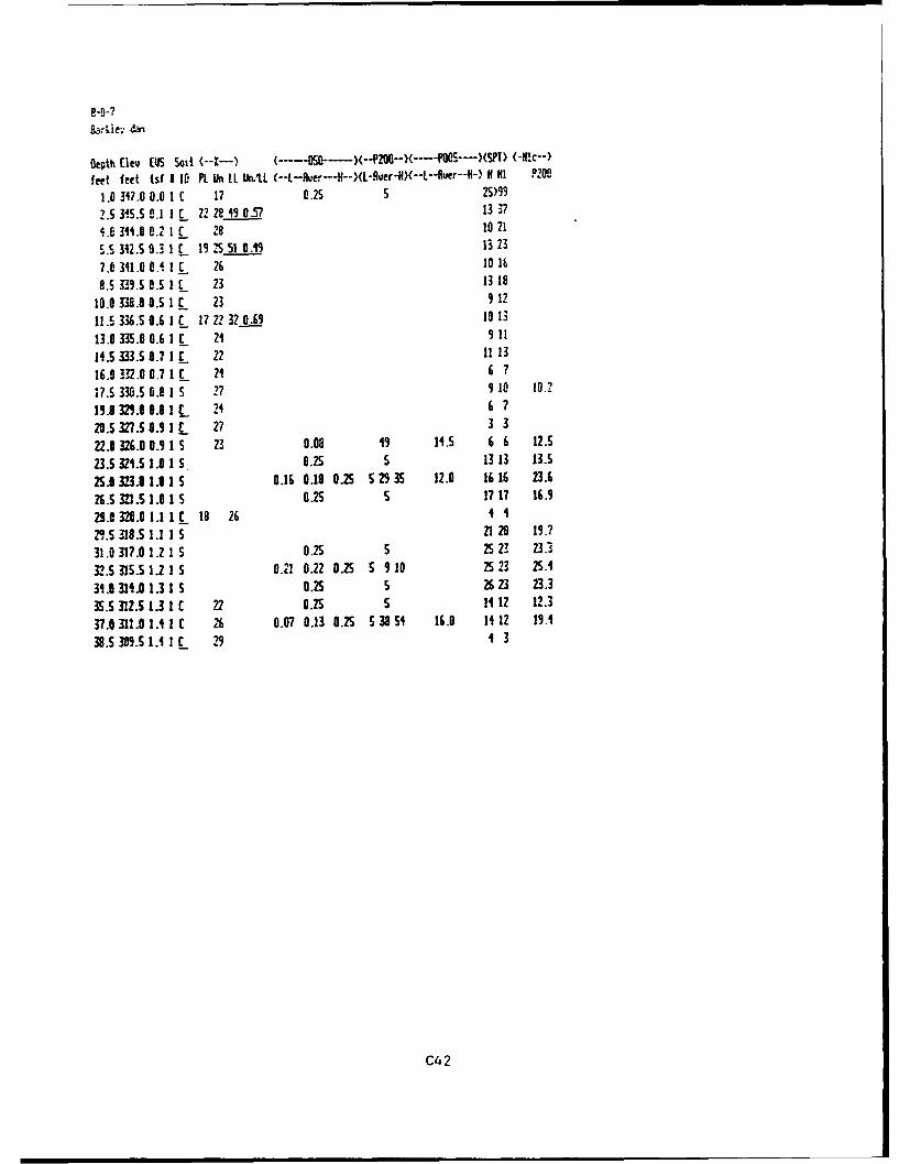
e-o-?
oepth Cleo [US Soil (--- --- ) (P20 ---- 0S)(S T) (-f~l--)feet feet tsf I 10 PL Un LI Un/LL -N- I P200
1.0 3M7.0 0.0 1 C 17 0.25 s 25)99
2.S 31S.S 0.1 I C 22 28 19 0.57 13 37
St. 3W4.0 0.2 1 c 28 10 21
5.5 342.5 0.3 1 195 51 0.9 1323
7.0 341.0 0.4 1 C 26 10 16
8.5 339.5 0.5 I E 23 13 18
10.0 330.0 0.5 1 £ 23 9 12
11.5 336.5 0.6 1 C 17 22 32 0.69 18 13
13.0 335.0 0.6 1 c 21 9 11
14.5 333.5 0.7 1 C 22 11 13
16.0 332.0 0.7 1 C 24 6 7
17.S 330.5 0.8 1 S 27 ,10 10.2
19.1 329.0 0.8 1 C 24 6 7
20.5 327.5 0.9 1 C 27 3 3
22.0 326.0 0.9 1 S 23 0.08 19 14.S 6 b 12.5
23.S 324.5 1.0 1 S 0.25 5 13 13 13.S
2S.0 323.0 1.0 1 5 0.16 0.18 0.25 5 29 35 12.0 16 16 23.6
26.5 3ZI.S 1.0 1 S 0.25 S 1717 16.9
29.0 320.01.11C 18 26 1 1
21.5 318.5 1.1 1 S 21 20 19.7
31.0 317.0 1.2 1 S 0.25 5 2S 23 23.3
32.5 315.5 11 1 S 0.21 0.22 025 5 9 10 25 23 5.4
31.8 311.0 1.3 15 0.25 5 26 23 23.3
35.5 312.5 1.3 1C 2 0.25 U 11 12 12.3
37.0 311.0 1.1 I C 26 0.07 0.13 0.2S S 38 S 16.0 14 12 19.1
38.5 309.5 1. I C 29 1 3
C42
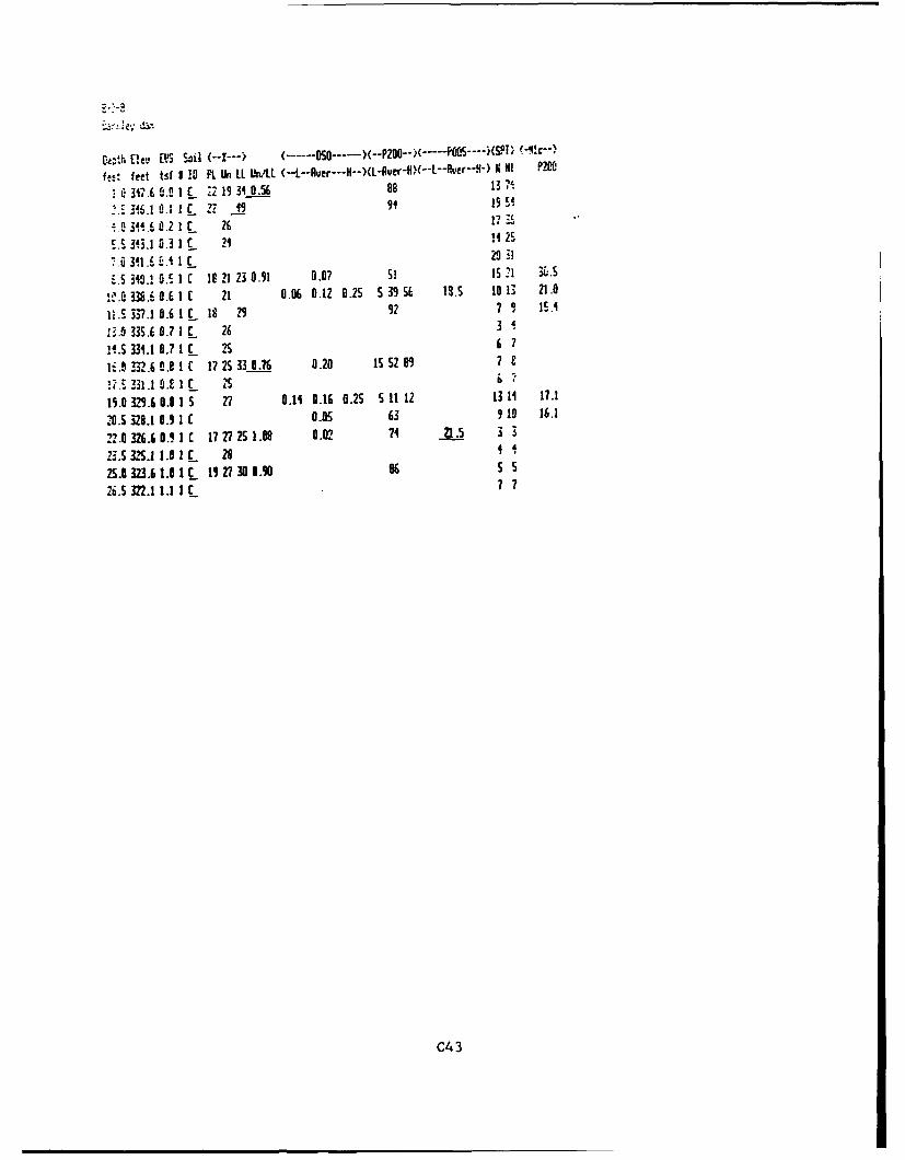
Otv US Soil (--I*--- -P---- .... ... )(S (-Ic..
f!!, feet tsf I to PL Un LL Un/L (-L--uer--- L eH)K HI P200
,0316 0.2 1.C 22 19 i30.56 88 13 ?.6.1.i, 0.1l 1. 1 .2: _.11 91 9•
-. e 3M4 .. 0 .2 1 26 17H 2
S.S 3413.1 .3 1 c 24 1125
7. 6 311.6 I.i I. 2031
_.S 34 0. 1 t. I C 19 21 23 0 .91 0.07 to 1 ,1 21. 0
9.- 3386.60. O.1 C 21 0.06 0.12 0.25 S3056 18.5 101" 21.0
I1.S 337.1 0.61t 1 t 0 02 7 0 12.1
A3. 335.6 0.7 1_C 26 34
!M.S 341.1 0.7 1c 2S 6?
1.0332.6 0.81 C 17 25 33 0.76 0.20 15 52 89 7
S .5 331 .1 51 1It 2510.0 3.9.6 9.31 S 27 0.14 0.16 0.25 5 11 12 13 11 17.1
20.5 328.1 0.5 1r 0.05 63 910 16.1
22.0 R26.6 0. f1C 1727 25 1.08 0.02 74 21.5 3 3
2.-.5 32.1 1.01 C 28 1 ,
2S.80M.6 1.0 1 1927130 0.9 5 5N.5 I 22.11.1 ? 77
C4 3
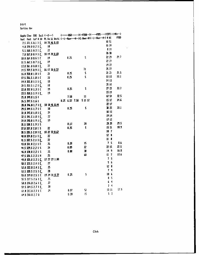
8-0-9
,4; klev da
Depth (lev [US Soil <--1--- (-- O0----)(--V200--- P-.)(5Pl' -llc--)
feet feet tsf I 10 PL Un Li Un/ti - -- )(L-fler-)&-LAuer"H) H HI P200
2.S 371.5 0.1 1 - 18 20 16 0.43 1 81
4.0 370.0 0.Z 1 1i 16 34
5.5 368.5 0.3 1 C 22 8 1
7.0 367.0 0.11 C 18 19 2$.0_.68 20 30
10.0 361.0 0.6 1 c 19 U.2S 5 22 29 29.7
I.S 362.S 0.7 1 _ 19 22 V
13.0 361.0 0.8 1 C 22 19 22
11.5 3S9.5 0.9 1 C_ 16 17 30 0.57 71 5 27
16.0 3S8.0 1.0 1 C 21 0.25 5 21 21 21.5
17.5 356.5 1.0 1 C 20 0.25 5 13 13 13.1
19.0 3SS.0 1.1 1 1 18 11 13
20.5 3S3.S 1.2 1 C 18 70 1E
22.0 352.8 1.3 1 C 19 0.25 5 27 23 23.7
23.S 350.5 1.4 1 C 19 23 19
2S.1 349.1 1.S 1 7.50 11 6754 32.5
2&.5 317.S 1.6 1 0.2 6.S3 7.50 511 12 15 12 11.6
28.1 M. 1.71C 18 181 0.44 22 17
29.S 34.5 1.7 1 C 1 0.5 5 30 23 Z3.1
31.1 343.0 1.8 1 C 21 19 13
32.S31.S 1.8 1 c 22 19 14
31.0..O . 1.9 1 t 19 17 12
35.5 338.5 1.9 1 S 0.13 28 2820 29.5
37. 337.0 2.815 22 0.25 S is 11 10.9
38.5 33.5 2.0 I 18 22 330.7 10 7
10.31.0 2.1 1 C 22 12 8
1.S 332.5 2.1 1 C 22 11 8
43.0 331.02 1 C 2S 0.20 15 7 5 8.6
W.5 329.5 2.2 1 S 24 0.09 32 22 1S 22.5
W.0 328.0 2.2 1 S 2S 0.08 38 1H 9 16.0
47.5 326.5 2.3 1 fl 25 60 11 7 13.6
19.0 325.0 2.3 1 C 17 27 27 1.00 7 S
50.5 323.S 2.4 1 c 27 9 6
S .A2M.0 2.4 1 C 2S 12 9
53.5 320.5 2.S 1 c 28 7 4
55.0 319.0 2.5 1C 19 24 310.77 0.2s 5 10 6
56.5 317.5 2.6 1 C 2S 8 S
S8.0 316.0 2.6 1 1 27 6 4
59.5 311.5 2.7 1 c 28 7 4
1.0 313.0 2.7 1 C 21 0.07 52 19 11 17.1
61.0 310.0..1#0 C'. 20 is S 3
C44
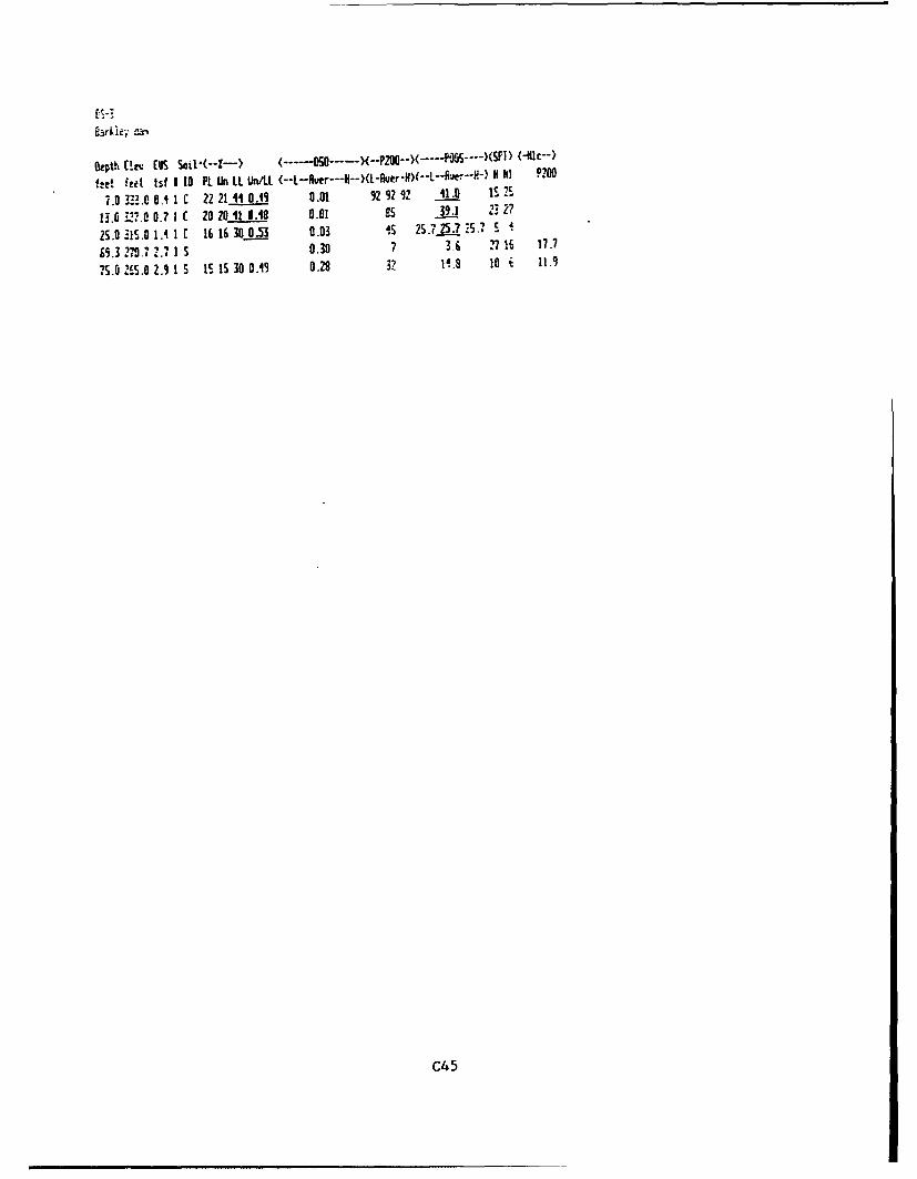
Depth• (Irv [US Soil'(--I--,) (...OO...>-P0-) ... P• .. }Sr}(•c-
feet feet tsf 1 0 PL Un LL Un/ML (--L-Ruer--- rH)- -I :') H h! P200
7.0 337.0 0.1 IC 22 21 011.1 9.01 92 92 5 011.0 IS 25
13.0 3:".0 0.7 1 C 20 201 0.48 0.01 E5 39.1 ,17?.7
2S.0 'IS.0 1.4 1 C 1616 3..•53 0.03 iS 25.7 ? 25.7 -___ '- S
69.3 2,.71 .? IS 0.30 ? 3.6 ? 17 i 1.7
,S.0 2S.0 2.1 S IS IS "0 0.19 0.28 32 11.8 10 - 111
C4 5
Waterways Experiment Stailon Cateloging-in-PublicatIon Data
Wahl, Ronald E.Seismic stability evaluation of Alben Barkley Lock and Dam Project.
Volume 4, Liquefaction susceptibility evaluation and post-earthquakestrength determination / by Ronald E. Wahl ... [et al.] ; prepared for USArmy Engineer District, Nashville.
346 p. : ill. ; 28 cm. - (Technical report ; GL-86-7 vol. 4)Includes bibliographical references.1. Dams - Kentucky -Earthquake effects. 2. Earthquake hazard
analysis. 3. Soil liquefaction. 4. Dam safety - Kentucky. I. Wahl,Ronald E. II. United States. Army. Corps of Engineers. Nashville Dis-trict. III. U.S. Army Engineer Waterways Experiment Station. IV. Title:Liquefaction susceptibility evaluation and post-earthquake strength deter-mination. V. Series: Technical report (U.S. Army Engineer WaterwaysExperiment Station) ; GL-86-7 vol. 4.TA7 W34 no.GL-86-7 vol.4