1

Activation-Based Recursive Self-Organizing Maps

A General Formulation and Empirical Results Kevin Hynna*, Mauri Kaipainen

Media Lab, University of Art and Design Helsinki,

Hämeentie 135 C FIN-00560 Helsinki, Finland

kevin.hynna@uiah.fi; mauri.kaipainen@uiah.fi

(+358 50) 583 3210; Fax: (+358 9) 7563 0555

We generalize a class of neural network models that extend the Kohonen self-organizing map

(SOM) algorithm into the sequential and temporal domain using recurrent connections.

Behaviour of the class of Activation-based Recursive Self-organizing Maps (ARSOM) is discussed

with respect to the choice of transfer function and parameter settings. By comparing

performances to existing benchmarks we demonstrate the robustness and systematicity of the

ARSOM models, thus opening the door to practical applications.

Keywords

recurrent neural networks, recursive algorithms, representing context, self-organizing maps,

sequential order

2

Activation-Based Recursive Self-Organizing Maps

A General Formulation and Empirical Results Introduction

In this paper we offer a general definition of a class of models, which we call Activation-based

Recursive Self-Organizing Maps (ARSOM), that extend the self-organizing map (SOM)

algorithm [14, 15] to the sequential or temporal domain by adding recurrent connections to the

map (or network) units. The SOM has been established as one of the most widely used

techniques for unsupervised data clustering, i.e., in the absence of any a priori given

classification. However, the SOM, as well as other popular artificial neural network architectures

such as the back-propagation algorithm [19, 20] for supervised learning of data, was designed

for data in which sequential order is insignificant, i.e., where the input elements are context-

independent. The applicability of the fundamentally atemporal SOM to tasks such as decision-

making and prediction in the context of preceding events is therefore limited.

A number of extensions to these basic architectures have been proposed to overcome this

limitation. Summaries of such attempts [2, 9, 12, 13, 23, 25] may be referred to for a more

complete view. However, within these attempts, an important distinction can be made between

the representation of time explicitly, giving time essentially a spatial representation, versus

representing time implicitly, “by the effect it has on processing” [5]. Explicit representations of

time, e.g., those implemented via a time window, treat time statically as another vector

dimension of the input. In contrast, implicit representations of time, e.g., those implemented

through recurrent connections which feed back the network’s own activation to itself, give the

network a memory of previous events which is, in principle, capable of dynamically

influencing subsequent processing. Thus with implicit representations of time the emphasis is

on memory as a procedure rather than memory as a data structure. The basic approach of using

recurrent connections to model temporal effects was first implemented within the back-

3

propagation paradigm by Jordan [7] and Elman [5], and was applied to the SOM by Kaipainen

et al. in the MuSeq model [9] and its extensions [10, 11]. The model of Voegtlin [25, 26] relies on

the same architecture.

At this point, a general class of Activation-based Recursive Self-Organizing Maps (ARSOM),

can be defined. ARSOMs use the activation state of the network itself as a time-delayed internal

input, which serves as the context with which incoming external input, or content, becomes

associated. However, following [26] we believe that an important feature of ARSOMs is that the

external (content) input connections and the internal (context) input connections are

implemented identically, both in the unit activation function and in the learning rules, thereby

allowing the learning algorithm to apply iteratively to its own results. It is this property which

distinguishes recursivity from mere recurrency.

Although there is much to admire in the formal analysis of stability in recursive models

given in [26], a large number of assumptions are made which severely restrict the applicability

of the results found therein. This paper is intended to complement that formal analysis. We

carry out a simulation-based exploration of the behaviour of a number of different transfer

functions under various parameter settings using the test paradigm described in [25].

Accordingly, external input is here restricted to a binary-valued one-dimensional data stream,

thereby focusing the investigation on context effects, and performance is measured by

comparing the depths of the representations of the units of a trained network. Good, stable-

performing ranges of parameter values are found for each of the transfer functions, even

outperforming the benchmark results presented in [25]. Our results suggest that the behaviour

of a network, i.e., a particular instantiation of a transfer function in terms of parameter settings,

can be adequately accounted for in terms of the shape of the instantiated transfer function. The

ability of all of the tested transfer functions to capture the probabilistic structure of the input data

sequences is taken to indicate that this property should not be viewed as the property of any

particular transfer function but rather is a property that is inherited by the entire class of

4

ARSOM models. Finally, effects of the neighbourhood radius parameter on overall performance

and the topological organization of the unit representations are also discussed.

Activation-Based Recursive Self-Organizing Maps

ARSOM models extend the SOM into the temporal domain by incorporating recurrent

connections between the units of the network into the algorithm. Basically, the original SOM

algorithm performs a topology preserving non-linear projection from some high-dimensional

input space, Rd, to some lower-dimensional output space, usually R2. The SOM consists of a set

of units (also referred to as nodes or neurons), W, organized on a regular low-dimensional grid.

Associated with each unit i is a weight vector wi = [wi1, wi2,..., wid], where d is the dimension of

the input vectors. During each training step a sample input data vector x(t) ∈ Rd is chosen from

the input space. Weight vectors of each of the units are compared to the input vector and the

closest or best matching unit (BMU) is calculated using some appropriate similarity measure

(e.g., Euclidean distance or dot product). The weights of the BMU and its neighbouring units on

the map unit are then updated towards the input vector, thus making them more similar to that

input data. Repeated samples from the input space are presented until some minimum error

criterion is reached (usually measured in terms of quantization error) or some pre-determined

number of input samples have been presented. Through this process the units of the SOM come

to approximate the probability density function of the input data. The units divide the higher-

dimensional input space into Voronoi cells, and hence the SOM algorithm also performs a form

of vector quantization on this space.

The SOM algorithm, however, is only a static quantizer in the sense that information about

the temporal order or sequence of the data inputs is not taken into account. A common method

for extending neural network techniques into the temporal domain is to add recurrent

connections to the network [5, 7]. This introduces the notion of context into the representations of

the network, thereby allowing the units of the map to learn to associate external input (content)

with the internal contexts in which they occur. ARSOM models extend the SOM by adding

recurrent connections to the units of the SOM.

5

In ARSOM models, just as with the generic SOM, associated with each unit i is a weight

vector wix = [wi1

x, wi2x,..., wid

x], where d is the dimension of the input vectors. However, with

ARSOM each unit is now also connected to every other unit in the network (including itself)

through another weight vector wiy = [wi1

y, wi2y,..., wim

y], where m is the number of units in the

network. We refer to wix as the content weight vector and wi

y as the context weight vector associated

with unit i. Although activation levels for units are not necessary in SOM, it is exactly the

distribution of activations across the network which is taken to represent context in ARSOM.

Unit responses (or activations) then are taken to be the product of a content response and a

context response, and the response of unit i in the network is given by :

yi(t) = (content responsei(t))(context responsei(t)) (1)

content responsei(t) = TF(D(x(t), wix ), α) (2)

context responsei(t) = TF(D(y(t-1), wiy), β) (3)

where x(t) is the external (content) input coming into the system at time t, y(t-1) is the recurrent

(context) input, i.e., the activation levels of the units, at time t-1, D is some similarity measure,

and TF is a transfer function that takes two inputs, the output of D and one of α ≥ 0 or β ≥ 0, free

parameters which we will refer to as the content parameter and the context parameter, respectively.

TF is a continuous valued monotonic function that maps onto the range [0, 1], with well-

matching units having values close to one. Note that in general the same function, TF, is used

in both the content response and the context response. Therefore, no distinction is made

between the incoming (feedforward) connections and recurrent (feedback) connections.

Training follows the standard SOM algorithm, only now we update both content weights and

context weights. If c is the index of the BMU, i.e, the unit maximizing response to input x(t) at

time step t:

yc(t) = maxi

{yi(t)} (4)

then the weights are updated according to the following update rules :

Δ wix = φ hci(t)(x(t)-wix) (5)

Δ wiy = ψ hci(t)(y(t-1)-wiy) (6)

6

where φ and ψ are learning rates, and hci is the neighbourhood function which is centred on

unit c and decreases with the distance between units i and c on the map grid. The

neighbourhood function, as usual with SOM, is taken to be the Gaussian:

hci(t) = exp

!d (rc , ri )2

2" ( t )2 (7)

Here rc and ri are the locations of units c and i with respect to the map grid, i.e., vectors in the

low-dimensional output space, d(rc, ri) is the distance between units i and c on the map grid and

σ(t) is a monotonically decreasing function that controls the width of the Gaussian. Although in

the standard SOM algorithm the learning rates also decrease monotonically during training, in

our implementation, the learning rates are kept constant (and equal to each other), and thus,

may be included as part of the neighbourhood function itself.

The above learning scheme is simply the original SOM algorithm applied to both content

and context weight vectors simultaneously. We can also note that, as we shall see below, in the

transfer functions under consideration, by setting the context parameter to 0, context plays no

role in the response function (1), and hence the models reduce to a standard SOM based on the

similarity measure of (2). In this sense, ARSOMs define a class of models that includes the SOM

as a special case.

To summarize our definition of the ARSOM class of models: we include in this class any

model that adds recurrent connections to the units of the SOM; uses an activation (or response)

function as given by (1), (2), and (3), where the transfer function (a) is continuous and

monotonic, (b) maps onto the range [0, 1], (c) is the same in both the content and the context

response functions, (d) takes as input the output of a similarity function and a free parameter, (e)

defines context similarity with respect to the activation levels of the units at the previous time

step, (f) includes the SOM as a special case; and which uses the learning scheme defined by (4),

(5), (6), and (7). As far as we are aware the only models that adhere to the above-mentioned

criteria are those found in [11] and [25, 26].

7

Experiment

Choice of Transfer Function

In this paper, we chose to explore the behaviour of four different transfer functions, which we

now motivate and compare to the transfer function found in [25]. Since the content response

function and the context response function are the same, in what follows we will refer to a

general transfer function of the form:

TF = F(D(v, w), ρ) (8)

where <v, w, ρ> is either <x(t), wix, α> or <y(t-1), wi

y, β>, depending on whether we are talking

about the content response function (2) or the context response function (3), respectively.

Specifying a transfer function involves specifying both a distance function and the form of the

transfer function itself.

Transfer Function Input Assumptions Binary-Valued 1-D

Data

TF1 (1 !

v ! w

2)"

|v| = |w| = 1

vi, wi ≥ 0

(1 ! abs(v ! w))

TF2 1

2(cos2!)

"+1( )

vi, wi ≥ 0

TF3 1

2cos 2! +1( )

"

vi, wi ≥ 0

TF4 1

2cos! +1( )

"

none

! (v,w) = (v " w)#

2

TF5 exp

(! " v!w 2 ) none

Table 1. Transfer functions TF1-TF4 used in simulations. TF5 is the transfer function used by[25]. Transfer functions TF1-TF3 place restrictions on the input data. Input to the transfer functions consists of two vectors, v and w, and a parameter ρ (see text). θ gives the angle between the two input vectors. Final column lists how the transfer functions were

extended to the one-dimensional case. abs is the absolute value function.

The first transfer function (TF1) is essentially the same as that used in the ROSOM model of [11],

minus the oscillatory component. Euclidean distance is used as the distance measure. In using

TF1, two assumptions are made about inputs. First, it is assumed that the input and weight

8

vectors have been normalized to unit length. Second, the components of the input and weight

vectors are assumed to all be greater than or equal to zero. Given two such vectors, their

Euclidean distance will fall in the range 0, 2[ ] , and therefore 2 in TF1 is just a normalizing

factor that ensures that the output maps into the interval [0, 1].

The two assumptions just mentioned however may not always be applicable or necessary.

Normalization to unit length, in particular, can be computationally expensive and it would be

nice if it could be avoided. In the present learning scheme, context is represented by the

distribution of activation across the units of the network, and hence context learning involves a

unit learning the scale-invariant pattern of activation of the network, with the actual magnitudes

of those activations playing little if any role. Thus, normalization of activation levels and context

weights would appear to be unnecessary. Whether or not the input vector components take

negative values is more problem domain specific in that it simply depends on whether it makes

sense to talk about negative-valued content or context input, as the case may be. With respect to

context, in our implementations the activation levels of the units (and hence the context weight

vectors) are always non-negative. If the vector components are all greater than or equal to zero,

then it follows that the angle between any two such vectors will lie in the interval 0,!

2

"

# $ %

& ' . The

above considerations led us to explore transfer functions based on the cosine measure of

similarity.

The second and third transfer functions, TF2 and TF3, transform the cosine function so that

the domain 0,!

2

"

# $ %

& ' maps into the range [0, 1]. The main difference is that TF2 preserves the

shape of the sigmoid with respect to the original domain (prior to the transformation) over the

parameter range. The fourth transfer function, TF4, is more general in that it makes no

restrictions on the input data. Note that even in the case in which the vector components of the

inputs are restricted to be non-negative (as with the current simulations) appropriate parameter

values can be found for TF4 which allow this function to (almost) cover the range [0, 1] (see

9

below). Again, the goal here was to explore how the shapes of the transfer functions affect

performance. Accordingly, the main motivation for including TF3 and TF4 was to explore more

varied transfer function shapes. The fifth transfer function, TF5, is that used in [25, 26]. We will

have more to say about it below.

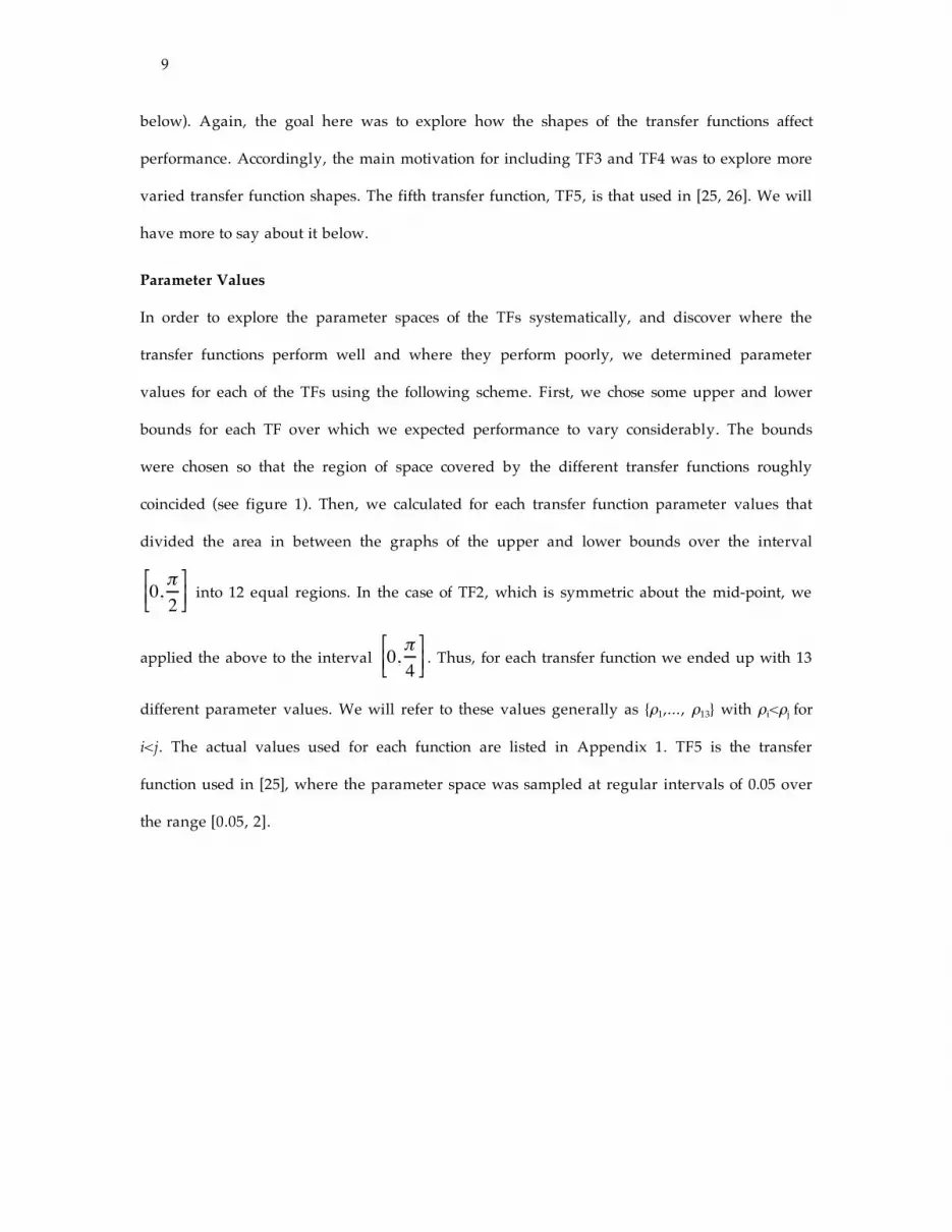
Parameter Values

In order to explore the parameter spaces of the TFs systematically, and discover where the

transfer functions perform well and where they perform poorly, we determined parameter

values for each of the TFs using the following scheme. First, we chose some upper and lower

bounds for each TF over which we expected performance to vary considerably. The bounds

were chosen so that the region of space covered by the different transfer functions roughly

coincided (see figure 1). Then, we calculated for each transfer function parameter values that

divided the area in between the graphs of the upper and lower bounds over the interval

0,!

2

"

# $ %

& ' into 12 equal regions. In the case of TF2, which is symmetric about the mid-point, we

applied the above to the interval 0,!

4

"

# $ %

& ' . Thus, for each transfer function we ended up with 13

different parameter values. We will refer to these values generally as {ρ1,..., ρ13} with ρi<ρj for

i<j. The actual values used for each function are listed in Appendix 1. TF5 is the transfer

function used in [25], where the parameter space was sampled at regular intervals of 0.05 over

the range [0.05, 2].

10

0 pi/4 pi/20

0.5

1

(a)

TF1

0 pi/4 pi/20

0.5

1

(b)

TF2

0 pi/4 pi/20

0.5

1

(c)

TF3

0 pi/4 pi/20

0.5

1

(d)

TF4

0 pi/4 pi/20

0.5

1

(e)

TF5

! = 0 to "/2

Figure 1. Graphs for the transfer functions listed in table 1. Simulations were carried out for 13 parameter values for each of TF1-TF4 (see text). TF5 is the transfer function used in [25]. θ is the angle between the input vectors v and w (cf.

equation 8).

Data and Training

We evaluated the above transfer functions, TF1-TF4, using the test paradigm presented in [25]

where the results of TF5 are compared with the Temporal Kohonen Map (TKM) model [4] and the

Recurrent SOM (RSOM) model [17, 23], thus providing benchmark results for comparison.

Accordingly, training and parameter settings were kept as similar as possible to those used

previously. The input data consisted of a binary sequence generated stochastically so that

transitions from ‘0’ to ‘1’ had a probability of 0.3 and transitions from ‘1’ to ‘0’ had a probability

of 0.4. Maps of 10 by 10 units were trained for 150 000 iterations. Both learning rates were kept

constant at 0.3, and the neighbourhood radius parameter σ decreased step-wise linearly from 5

to 0.25 over the course of the training. Weight components for both content and context weight

vectors were initialized randomly from a uniform distribution over the interval [0, 1].

For each of the four transfer functions TF1-TF4 we tested all thirteen values {ρ1, …, ρ13} of the

context parameter β crossed with five values {ρ3, ρ5, ρ7, ρ9, ρ11} for the content parameter α

giving us 65 conditions for each TF. Results were averaged over three separate trials of each

condition. We chose to explore only five out of the thirteen parameter values for content because

we did not expect to see much variation along the content parameter due to the relatively

simple nature of the content input, i.e., binary-valued and one-dimensional. However, in order

to accommodate the one-dimensionality of the input data we had to modify somewhat the

11

transfer functions. These fairly straightforward extensions to the one-dimensional case are listed

in table 1.

The simulations were carried out using the computing facilities of the Finnish Center for

Supercomputing (CSC), using MATLAB code developed in our lab based on the SOM Toolbox

for MATLAB [24] and SOM_PAK [16].

Results

To test the trained networks we used a performance measure based on the average context

length to which the units of a network respond. During testing, every time a unit responds (as

BMU) it will be responding to a certain (in principle infinite) context, namely the sequence that

has occurred prior to and including the most recent input. The intersection of all such contexts to

which any given unit has responded represents what the unit has selectively learned. We can

refer to this intersection of contexts as the receptive field of that unit. By comparing the lengths of

the receptive fields of the units of a network we get a measure of the average depth of the

representations of the entire network and it is this measure that we use to compare performance.

More formally, if Ri represents the receptive field of unit i in network W, ni represents the

length of the receptive field, and pi represents the probability of an occurrence of a context that

belongs to Ri, then the depth of the network is given by:

n_

= pii!W

" ni (9)

The receptive fields of a network (see, for ex., figure 5) represent a vector quantization of

context. The depth measure of equation (9) extends the standard measure of quantization error

to the sequential (and hence temporal) domain, and is taken in [25, 26] to be an indicator of

stability in learning.

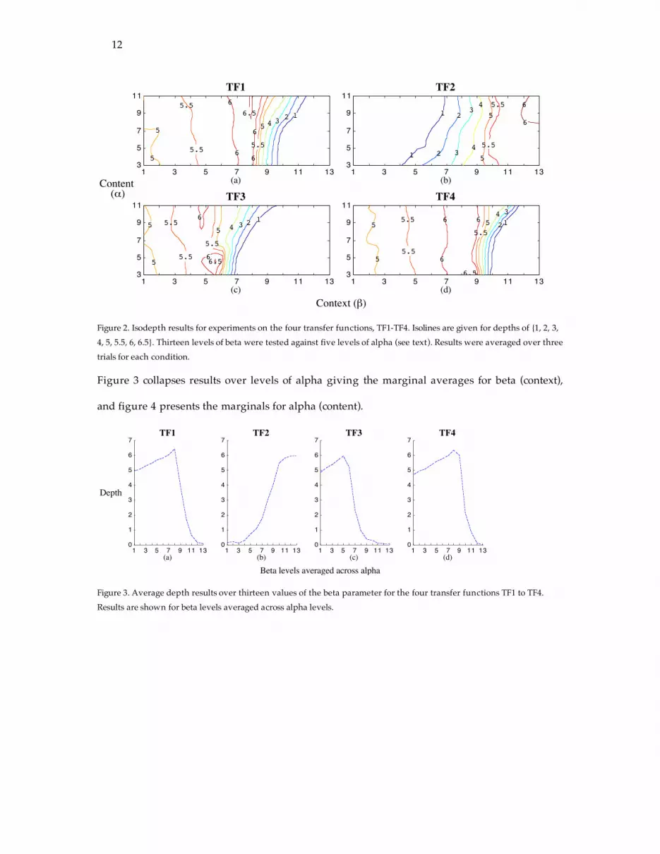
Figure 2 presents the average depth results of the four transfer functions across the content

(α) and context (β) parameter ranges.

12

1 3 5 7 9 11 133

5

7

9

11

(a)

TF1

5

5

5.5

5.5

6

6

6.5

6

6

5.5

5 432 1

1 3 5 7 9 11 133

5

7

9

11

(b)

TF2

1 2 3

1 234

5

5.5 6

6

4

5

5.5

1 3 5 7 9 11 133

5

7

9

11

(c)

TF3

5

5 5.5

5.5

6

6.56

5.5

5 4 3 2 1

1 3 5 7 9 11 133

5

7

9

11

(d)

TF4

5

55.5 6

5.56

6.5

6

5.5

54 3

21

Content (!)

Context (")

Figure 2. Isodepth results for experiments on the four transfer functions, TF1-TF4. Isolines are given for depths of {1, 2, 3, 4, 5, 5.5, 6, 6.5}. Thirteen levels of beta were tested against five levels of alpha (see text). Results were averaged over three trials for each condition.

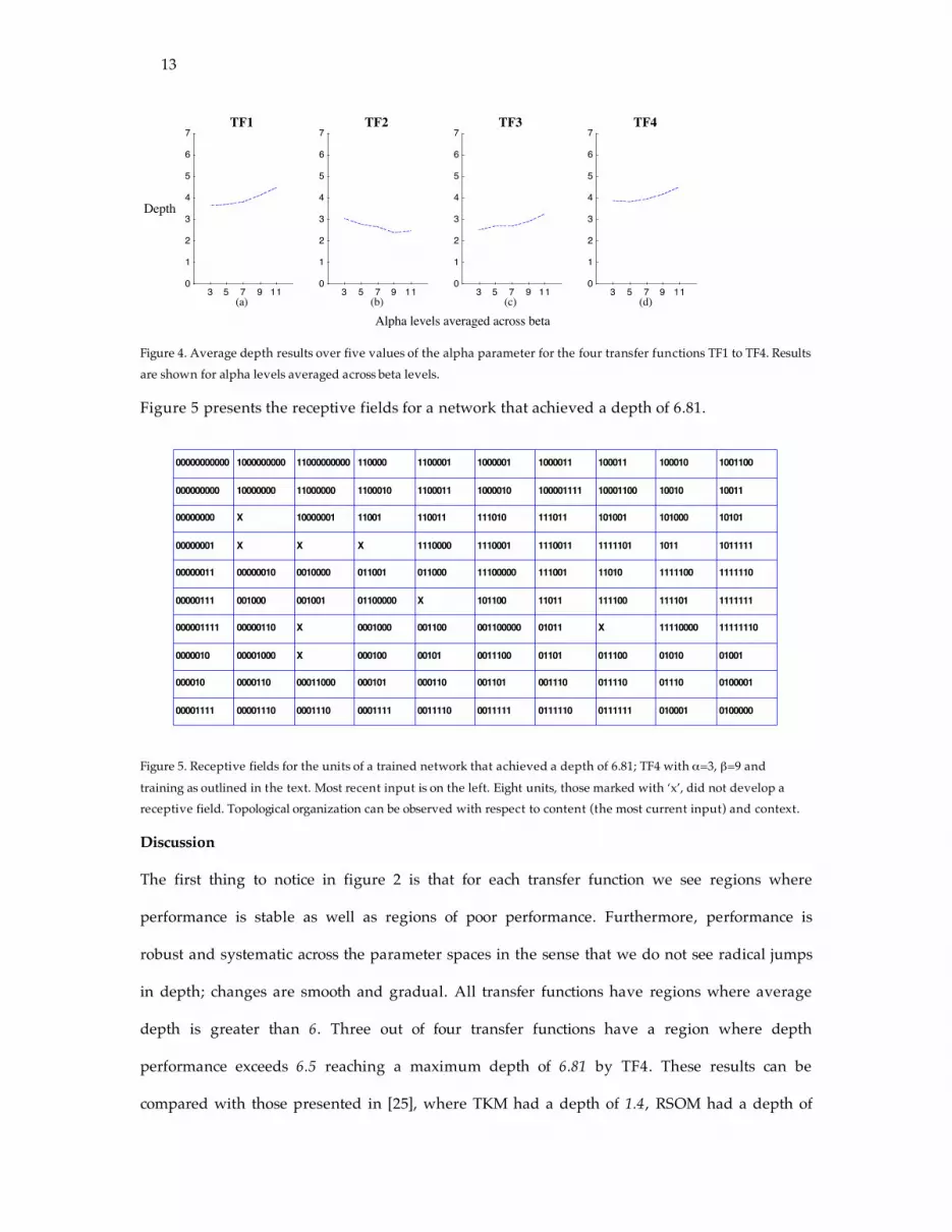
Figure 3 collapses results over levels of alpha giving the marginal averages for beta (context),

and figure 4 presents the marginals for alpha (content).

1 3 5 7 9 11 130

1

2

3

4

5

6

7

TF1

(a)1 3 5 7 9 11 13

0

1

2

3

4

5

6

7

TF2

(b)1 3 5 7 9 11 13

0

1

2

3

4

5

6

7

TF3

(c)1 3 5 7 9 11 13

0

1

2

3

4

5

6

7

TF4

(d)

Depth

Beta levels averaged across alpha

Figure 3. Average depth results over thirteen values of the beta parameter for the four transfer functions TF1 to TF4. Results are shown for beta levels averaged across alpha levels.

13

3 5 7 9 110

1

2

3

4

5

6

7

TF1

(a)3 5 7 9 11

0

1

2

3

4

5

6

7

TF2

(b)3 5 7 9 11

0

1

2

3

4

5

6

7

TF3

(c)3 5 7 9 11

0

1

2

3

4

5

6

7

TF4

(d)

Depth

Alpha levels averaged across beta

Figure 4. Average depth results over five values of the alpha parameter for the four transfer functions TF1 to TF4. Results are shown for alpha levels averaged across beta levels.

Figure 5 presents the receptive fields for a network that achieved a depth of 6.81.

00000000000

000000000

00000000

00000001

00000011

00000111

000001111

0000010

000010

00001111

1000000000

10000000

X

X

00000010

001000

00000110

00001000

0000110

00001110

11000000000

11000000

10000001

X

0010000

001001

X

X

00011000

0001110

110000

1100010

11001

X

011001

01100000

0001000

000100

000101

0001111

1100001

1100011

110011

1110000

011000

X

001100

00101

000110

0011110

1000001

1000010

111010

1110001

11100000

101100

001100000

0011100

001101

0011111

1000011

100001111

111011

1110011

111001

11011

01011

01101

001110

0111110

100011

10001100

101001

1111101

11010

111100

X

011100

011110

0111111

100010

10010

101000

1011

1111100

111101

11110000

01010

01110

010001

1001100

10011

10101

1011111

1111110

1111111

11111110

01001

0100001

0100000

Figure 5. Receptive fields for the units of a trained network that achieved a depth of 6.81; TF4 with α=3, β=9 and

training as outlined in the text. Most recent input is on the left. Eight units, those marked with ‘x’, did not develop a receptive field. Topological organization can be observed with respect to content (the most current input) and context.

Discussion

The first thing to notice in figure 2 is that for each transfer function we see regions where

performance is stable as well as regions of poor performance. Furthermore, performance is

robust and systematic across the parameter spaces in the sense that we do not see radical jumps

in depth; changes are smooth and gradual. All transfer functions have regions where average

depth is greater than 6. Three out of four transfer functions have a region where depth

performance exceeds 6.5 reaching a maximum depth of 6.81 by TF4. These results can be

compared with those presented in [25], where TKM had a depth of 1.4, RSOM had a depth of

14

5.8, while TF5 achieved a depth of 6.5. The theoretical maximum depth for 100 units is 7.08.

Our results thus exceed all previously reported results for SOM-based context quantizers.

Differences even of the magnitude 0.3 are quite significant since an increase in depth of 0.3 for

an optimal representation requires 20.3 ≈ 1.23 times more units, and hence represents a gain in

efficiency of about 23%.

As can be seen in figure 3, the context parameter β had a dramatic effect on performance. Note

that by setting β to 0, context effects are removed and all of the models behave as a static SOM,

being able to distinguish only between different (current) inputs; in this case there are only two,

‘0’ and ‘1’, and hence the expected depth value for β equal to 0 is 1. Although it was not

expected, it is clear from figure 4 that the content parameter α also affected performance. Notice

however, that the best-performing parameter settings of α are different from those of β for each

of the TFs. This can be attributed to the complexity of the data in the two cases, and

demonstrates that optimal parameter settings are highly data dependent. Since the isolines are

not parallel for any of the transfer functions in figure 2, these results also give evidence of

interaction effects between the content parameter and the context parameter. This is not very

surprising, however, since units are in effect learning a couple <content, context>.

To gain further insight into what makes for a good transfer function we can compare

performance with transfer function shape. Figure 6 presents the transfer function graphs of those

values of the context parameter β for which performance, as averaged over the content

parameter α, was good (depth > 5) and figure 7 shows the graphs of poor performing parameter

values of β (depth < 2).

15

0 pi/4 pi/20

0.5

1

(a)

TF1

0 pi/4 pi/20

0.5

1

(b)

TF2

0 pi/4 pi/20

0.5

1

(c)

TF3

0 pi/4 pi/20

0.5

1

(d)

TF4

! = 0 to "/2

Figure 6. Good performing transfer function graphs. Values of beta that achieved depth > 5. Results for beta were averaged over levels of alpha. θ is the angle between the input vectors v and w (cf. equation 8).

0 pi/4 pi/20

0.5

1

(a)

TF1

0 pi/4 pi/20

0.5

1

(b)

TF2

0 pi/4 pi/20

0.5

1

(c)

TF3

0 pi/4 pi/20

0.5

1

(d)

TF4

! = 0 to "/2

Figure 7. Poor peforming transfer function graphs. Values of beta that achieved depth < 2. Results for beta were averaged over levels of alpha. θ is the angle between the input vectors v and w (cf. equation 8).

As pointed out in [26], learning can be analyzed as a ‘moving target’ problem. The target in the

case of context learning is a set of stable weight vectors representing distributions of activation

over the network. Stability depends on whether the changes to the weights during learning

move faster than the changes to the activation distribution that result from those changing

weights. If so, then progressively longer sequences of context will be learned. This can be

related to transfer function shape by looking at the slope of the transfer function. If the transfer

function is too steep then a small change in the weights of units that fall in this steep interval

will have a large effect on their activations. What we often find with such TFs during training is

periods of relative stability and then sudden dramatic global reorganizations in the

representations of the units of the map. In other words, steepness makes the model sensitive to

small perturbations and as a result the units are unable to learn stable representations. Indeed,

16

the poor-performing transfer functions of figure 7 are all characterized by an interval in which

the slope is very steep.

However, this cannot be the entire story because the transfer functions of figure 6, those

which perform well, also have regions of steepness. Note that steepness in some interval of the

graph implies that there must be flatness in some other interval. The important factor affecting

performance is where those intervals of steepness and flatness occur. In particular, performance is

crucially dependent on the shape of the transfer function around θ = !

2. Recall that the context-

weight vector components were initialized to random values. Based then on the results of [18]

(see also [3]), where it was shown that two random-vectors in a high-dimensional space have a

very high probability of being close to orthogonal, if we assume that the distribution of

activation levels at the beginning of training can also be considered to be random, then the

context responses (and therefore total responses) for all of the units will begin around zero, i.e.,

with θ around !

2. If the transfer function is very flat at this end-point, then even if during

training units are updated towards the context inputs, the effect will only be minimal and

progressive learning will not occur. In other words, if the weight changes that occur during

learning have relatively insignificant effects then the model has an insufficient basis for

improved performance. This is, in effect, a bootstrapping problem.

We have therefore empirically discovered two criteria for good transfer functions: (1) they

cannot be too steep which would make the units too sensitive to small perturbations, and (2) they

cannot be too flat at the end-point or else the units will never be able to begin the learning process.

Notice however that the second criterion is dependent upon the fact that context activations

begin around zero, which, as we saw above, was a consequence of how the context weights

were initialized. This suggests that random initialization of context weights may not be

appropriate and if another form of initialization were implemented this problem of ‘flatness’ at

the end-point may be possible to avoid.

17

Figure 5 presented the receptive fields for a network that achieved a depth of 6.81. Notice

that as with the original SOM, topological organization can be observed across the network,

though in this case nearby units respond to both similar contents and contexts. Notice also that

the network has learned the statistical structure of the binary sequence, i.e., the units have

learned sequences that approach equi-probability given the transitional properties on which the

network was trained. In [25, 26] a property of optimal representations is derived according to

which ‘a [context] quantizer is optimal if it is not possible to find another quantizer closer to

equiprobability’, and this property is emphasized in contrasting TF5 against TKM and RSOM,

which do not have a tendency to develop equi-probable receptive fields. The fact that each of

the transfer functions TF1-TF4 demonstrated this tendency to develop equi-probable receptive

fields for units strongly suggests that this should be considered a property of ARSOM models in

general, rather than of any particular transfer function.

In addition to the property of developing equi-probable receptive fields, the topological

organization of the receptive fields of trained networks can be characterized with respect to two

other qualities: (1) the number of ‘dead’ neurons; and (2) the number of units (or neurons) that

share overlapping receptive fields (including as a special case units that have identical receptive

fields). Dead neurons are neurons that fail to develop a receptive field due to topological

constraints and are therefore never used. As with the SOM, the less convex the input data

manifold, the more dead neurons there will be. To use a popular analogy, in projecting from a

high-dimensional space to map units located in R2 we are, in effect, trying to ‘cover’ the higher-

dimensional data manifold with a two-dimensional elastic net. If regions of the data manifold

are not convex, then some of the net will fall outside of the data range (see [6], page 238, for a

nice illustration). In the case of context weight vectors, the input space that we are trying to

cover is the 100 dimensional data of unit activations, and so we expect there to be a large

number of non-convex regions (in such a high-dimensional space).

To illustrate the second case, the case of overlapping receptive fields, we first recall that the

receptive field of a unit represents the intersection of all the contexts to which that unit has

18

responded. If a unit has a receptive field of, say, 001 (where, as throughout, the most recent

input is on the left), then this implies that the unit has responded to contexts of the sort 0010+

and 0011+ where ‘+’ indicates some continuation of the context (possibly null). We can imagine

then two units, m1 and m2, which have as receptive fields 001 and 0011, respectively. This

implies that m1 has responded to contexts of the sort 0010+ and 0011+ and m2 has responded to

contexts of the sort 00110+ and 00111+, and thus both have responded to contexts of the sort

0011+. It is in this sense that their receptive fields overlap. It should be clear that these two

properties, (1) and (2), are distinct from the property of equi-probability mentioned above, and

therefore describe two other ways in which trained networks can be sub-optimal. As suggested

earlier, the property of equi-probability is inherent to the ARSOM architecture itself. Although,

clearly, properties of the input data manifold constrain the two other types of topological

differences, the locus for such differences between maps trained on the same data is not so

straightforward. One potential source for differences however is the neighbourhood radius

function, and thus we close this section with a discussion of neighbourhood radius parameter

effects on topological organization and performance.

The radius parameter controls to what extent neighbouring units on the map are updated

together, and thus affects the topological characteristics of the map. However, as we shall now

show, the concrete effect of the neighbourhood radius depends on the particular transfer

function used, as well as the α and β parameter settings. Recall that during training we

decreased the neighbourhood radius σ from 5 to 0.25.

Figure 8 presents the Gaussian neighbourhood function for various values of σ.

19

-5 -4 -3 -2 -1 0 1 2 3 4 50

0.1

0.2

0.3

! = 0.25

! = 0.5

! = 1

! = 5

0.3"hci

d(rc, r

i)

Figure 8: Neighbourhood radius function (equation (7)), a Gaussian centred on the BMU, for different values of the radius parameter σ with fixed learning rate of 0.3

Notice that towards the end of training, after σ values of about 0.3, only the weights of the BMU

are updated. Although going beyond this point continues to affect the representations of the

map, it is an open empirical question whether during training one should go beyond this point.

Naively, one might think that if performance is already stable at this point then the map is

structured and further training will only improve the representations of the map, but this turns

out to not exactly be the case.

1 3 5 7 9 11 13-3

-2

-1

0

1

2

3

4

5

6

7TF1

(a)1 3 5 7 9 11 13

-3

-2

-1

0

1

2

3

4

5

6

7TF2

(b)1 3 5 7 9 11 13

-3

-2

-1

0

1

2

3

4

5

6

7TF3

(c)1 3 5 7 9 11 13

-3

-2

-1

0

1

2

3

4

5

6

7TF4

(d)

Depth

Beta levels averaged across alpha

- - -

!!!!___

" = 0.25" = 0.5difference

Figure 9. Neighbourhood radius effects towards the end of training. Depth values have been calculated for networks at two different stages of training (for the same network), once for σ = 0.5, and then again at the end of training, σ = 0.25.

The differences are also marked. Values are shown for beta levels averaged across alpha levels for three experiments in 65 conditions.

Figure 9 shows the changes that occur to depth when σ goes from 0.5 to 0.25. In general, if

depth performance is poor when σ = 0.5, then further training decreases depth. However the

converse is not true. There are β values for which average depth is high (around 6) at σ = 0.5,

20

but drop significantly as σ goes to 0.25. What this shows is that if the depth measure is taken as

our measure of stability then we would have to say that there are parameter ranges of transfer

functions that are stable if learning stops with the radius parameter σ = 0.5, but become

unstable if learning continues to σ = 0.25. This seems counter-intuitive to the notion of stability

and suggests that the depth measure alone is not sufficient to capture the notion of stability, or,

at the very least, a distinction should be made between stability of learning, in the sense that

learning is progressive with respect to what has been learned previously, versus stability in

performance , as measured by the depth of the learned representations.

Conclusions

To summarize, an application using an ARSOM model is fully determined by:

(a) choice of transfer function

(b) parameter settings for content (α) and context (β)

(c) neighbourhood radius function implementation

(d) learning rates

(e) map size (i.e., number of units) and shape

(f) length of training

In the simulations of this paper, we have kept (d), (e), and (f) constant and investigated how

(a), (b), and (c) affect performance within the test paradigm of [25]. For each of the transfer

functions explored, parameter settings were discovered which led to good, stable performance,

outperforming all previously reported results for extensions of SOM-based models into the

temporal domain. It was shown that insight into the results could be gained by examining the

shape of the transfer function graphs. Performance was found to be highly dependent on the

slope of the transfer function. If the slope was too steep, the units of the network were too

sensitive to perturbations which led to instability in learning. If the slope was too flat at the zero

end-point, then the network was unable to initiate the learning process. Optimal parameter

settings were found to depend on the complexity of the data, varying dramatically in value

(and hence graph shape) for the content parameter as compared to the context parameter. The

21

neighbourhood radius function also affected performance, with the largest effect occurring at

parameter settings along the border between stability and instability for each transfer function.

All of the transfer functions developed representations which reflected the probabilistic structure

of the input data, suggesting that the ability to develop such representations is a property of

ARSOM models in general.

The ARSOM class of models represents a powerful extension of the SOM algorithm into the

temporal domain. In this paper, it has been demonstrated that the performance of such models

is robust and systematic. The simulation-based observations about the models’ performances

across a range of transfer functions and parameter settings complements the insights gained by

previous work [11, 25, 26] and encourages further research on practical implementations in

domains where context is necessary to disambiguate incoming information.

Acknowledgements

The study was part of the USIX-Interact project funded by Finnish National Technology Agency

(TEKES), ICL Invia Oyj, Sonera Oyj, Tecnomen Oyj, Lingsoft Oy, Gurusoft Oy, the Finnish

Association of the Deaf and the Arla Institute. We thank Thomas Voegtlin for comments and

clarifications concerning his papers.

22

References

1. E. Alhoniemi, J. Hollmén, O. Simula, J. Vesanto, Process Monitoring and Modeling

Using the Self-Organizing Map. Integrated Computer-Aided Engineering, 6(1): 3-14,

1999.

2. G. de A. Barreto, A.F.R Araujo,. Time in Self-Organizing Maps: An Overview of

Models. International Journal of Computer Research, Special Issue on Neural Networks:

Past, Present and Future, 10(2): 139-179, 2001.

3. E. Bingham, H. Mannila, Random projection in dimensionality reduction: Applications

to image and text data. Proceedings of the 7th ACM SIGKDD International Conference

on Knowledge Discovery and Data Mining (KDD-2001), August 26-29, 2001, San

Francisco, CA, USA, pp. 245-250, 2001.

4. G.J. Chappell, J.G. Taylor, The Temporal Kohonen Map. Neural Networks, Vol. 6, Iss 3,

441-445, 1993.

5. J. Elman, Finding structure in time. Cognitive Science 14, 179-211, 1990.

6. J. Hertz, A. Krogh, R. Palmer. Introduction to the theory of neural computation.

Reading, MA: A Lecture Notes volume in the Santa Fe Institute Studies in the Sciences

of Complexity, Perseus Books, 1991.

7. M. Jordan, Attractor Dynamics and parallellism in a connectionist sequential machine.

Hillsdale: Erlbaum, Proceedings of the Eight Annual Meeting of the Cognitive Science

Society, 1986.

8. M. Jordan, I. Serial order: A parallel processing approach. San Diego: University of

California, Center for Human Information Processing, ICS Report 8604, 1986.

9. M. Kaipainen, P. Papadopoulos, P. Karhu, MuSeq recurrent oscillatory self-organizing

map. Classification and entrainment of temporal feature spaces. Proceedings of WSOM

'97 Workshop on Self-Organizing Maps 1997, Espoo, Finland, 1997.

10. M. Kaipainen, P. Karhu, Bringing Knowing-When and Knowing-What Together.

Periodically Tuned Categorization and Category-Based Timing Modeled with the

23

Recurrent Oscillatory Self-Organizing Map (ROSOM). Minds and Machines 10: 203-229,

2000.

11. M. Kaipainen, T. Ilmonen, Period Detection and Representation by Recurrent

Oscillatory Self-Organizing Map. Neurocomputing (In press), 2003.

12. J. Kangas, Time-delayed self-organizing maps. Proc. IEEE Int. Conf. on Acoustics,

Speech and Signal Processing (ICSSP'91), 1990.

13. J. Kangas, On the Analysis of Pattern Sequences by Self-Organizing Maps. Espoo,

Finland: Doctoral thesis, Helsinki University of Technology, 1994.

14. T. Kohonen, Self-organized formation of topologically correct feature maps. Biological

Cybernetics 43:59-69, 1982.

15. T. Kohonen, Self-organizing Maps. Berlin: Springer-Verlag, 1995.

16. T. Kohonen, J. Hynninen, J. Kangas, J. Laaksonen, SOM_PAK. The Self-Organizing

Map Program Package. Version 3.1 (April 7, 1995). Helsinki University of Technology,

Laboratory of Computer and Information Science, 1995.

http://www.cis.hut.fi/research/som-research/nnrc-programs.shtml

17. T. Koskela, M. Varsta, J. Heikkonen, K. Kaski, Temporal Sequence Processing using

Recurrent SOM. Proc. 2nd Int. Conf. on Knowledge-Based Intelligent Engineering

Systems, Adelaide, Australia 1998, Vol. I, pp. 290-297, 1998.

18. S. Kaski, Dimensionality Reduction by Random Mapping: Fast Similarity Computation

for Clustering. Proc IJCNN'98 International Joint Conference on Neural Networks,

Anchorage, Alaska May 4-9, 1998.

19. J.L. McClelland, D.E. Rumelhart, the and Research PDP Group. Parallel Distributed

Processing: Explorations in the microstructure of cognition. 1. Foundations. Cambridge:

MIT Press, 1986.

20. J. McClelland, Rumelhart, L. E. D. the and Research PDP Group. Parallel Distributed

Processing: Explorations in the microstructure of cognition. 2. Psychological and

biological models. Cambridge: MIT Press, 1986.

24

21. U. Neisser, Cognition and Reality. Principles and implications of cognitive psychology.

San Fransisco: W. H. Freeman and company, 1976.

22. O. Simula, P. Vasara, J. Vesanto, R-R. Helminen, The Self-Organizing Map in Industry

Analysis. -L.C. Jain, V.R. Vemuri, (Eds.) Industrial Applications of Neural Networks.

CRC Press, 1999.

23. M. Varsta, Self Organizing Maps in Sequence Processing. Dissertation, Department of

Electrical and Communications Engineering, Helsinki University of Technology , 2002.

24. J. Vesanto, J. Himberg, E. Alhoniemi, J. Parhankangas, Som toolbox for matlab 5.

Helsinki University of Technology, Neural Networks Research Centre, Report A57,

2000. http://www.cis.hut.fi/projects/somtoolbox/

25. T. Voegtlin, Context Quantization and Contextual Self-Organizing Maps. Proc.

IJCNN'2000, vol.VI pp. 20-25, 2000.

26. T. Voegtlin, Recursive self-organizing maps. Neural Networks 15(8-9): 979-91, 2002.

Abbreviations

ARSOM, Activation-based recursive self-organizing map; BMU, best matching unit; SOM, self-

organizing map; TF, transfer function

Appendix 1 : Parameter Values Used in the Simulations

ρ1 ρ2 ρ3 ρ4 ρ5 ρ6 ρ7 ρ8 ρ9 ρ10 ρ11 ρ12 ρ13

TF1 0.333 0.408 0.492 0.587 0.696 0.823 0.972 1.148 1.362 1.627 1.962 2.401 3.000

TF2 0.125 0.231 0.357 0.508 0.693 0.924 1.217 1.598 2.109 2.818 3.844 5.414 8.000

TF3 0.250 0.317 0.396 0.490 0.603 0.741 0.911 1.126 1.402 1.767 2.264 2.964 4.000

TF4 2.000 2.312 2.660 3.050 3.492 3.999 4.588 5.280 6.108 7.115 8.364 9.946 12.000