acidification reversal in low mountain range streams of germany

Environ Monit Assess (2011) 174:65–89DOI 10.1007/s10661-010-1758-z

Acidification reversal in low mountain rangestreams of Germany

Carina Sucker · Klaus von Wilpert ·Heike Puhlmann

Received: 15 March 2010 / Accepted: 29 September 2010 / Published online: 14 November 2010© Springer Science+Business Media B.V. 2010

Abstract This study evaluates the acidificationstatus and trends in streams of forested mountainranges in Germany in consequence of reduced an-thropogenic deposition since the mid 1980s. Theanalysis is based on water quality data for 86 long-term monitored streams in the Ore Mountains,the Bavarian Forest, the Fichtelgebirge, the HarzMountains, the Spessart, the Black Forest, theThuringian Forest, and the Rheinisches Schiefer-gebirge of Germany and the Vosges of France.Within the observation period, which starts forthe individual streams between 1980 and 2001 andends between 1990 and 2009, trends in chemicalwater quality were calculated with the SeasonalMann Kendall Test. About 87% of the streamsshow significant (p < 0.05) negative trends insulfate. The general reduction in acid deposi-tion resulted in increased pH values (significantfor 66% of the streams) and subsequently de-creased base cation concentrations in the streamwater (for calcium significant in 58% and mag-

C. Sucker (B) · K. von Wilpert · H. PuhlmannForest Research Institute of Baden-Württemberg,Wonnhaldestr. 4, 791 00 Freiburg, Germanye-mail: [email protected]

K. von Wilperte-mail: [email protected]

H. Puhlmanne-mail: [email protected]

nesium 49% of the streams). Reaction productsof acidification such as aluminum (significant for50%) or manganese (significant for 69%) alsodecreased. Nitrate (52% with significant decrease)and chloride (38% with significant increase) haveless pronounced trends and more variable spatialpatterns. For the quotient of acidification, whichis the ratio of the sum of base cations and the sumof acid anions, no clear trend is observed: in 44%of the monitored streams values significantly de-creased and in 23% values significantly increased.A notable observation is the increasing DOC con-centration, which is significant for 55% of theobserved streams.

Keywords Water quality · Acidification ·Forested catchments · Deposition ·Germany

Introduction

Forested catchments are considered to guaran-tee a high quality of surface and drinking water,because disturbance of element budgets throughmanagement impacts is usually small there; hence,the contamination with nitrate and pesticides iscomparatively low (Gäth and Frede 1991). How-ever, forests are not per se guarantors for goodwater quality. Stream acidification is a prevalentproblem, particularly in catchments with bedrocks

66 Environ Monit Assess (2011) 174:65–89

poor in base content (Rhode et al. 1995). Ade-quate forestry can help to counteract effects ofpollutant deposition such as soil acidification andnitrogen saturation. Intensive forestry, as it ispracticed in some of our catchments, brings aboutproblems for the drinking water treatment suchas increased water turbidity, occurrence of herbi-cides and pesticides, or pulses of dissolved organiccarbon in the raw water (Sudbrack, personal com-munication). Ensuring a high drinking water qual-ity by adequate forest management is, therefore,of public and political concern.

Deposition history and present development

At the beginning of the twentieth century, acid de-position was predominantly restricted to the closevicinity of industrial and urban emission sources.With the overall trend of taller chimneys in the1950s, air pollutants were transported to higheratmospheric layers, and a mainly regional phe-nomenon became a large-scale global problem.Anthropogenic sulfur dioxide and nitrogen oxidesin the atmosphere acted as strong acids increasingthe natural acidity of rainwater. Since the early1980s, the “acid rain” phenomenon was associatedwith the observed extensive “forest dieback.” Inthe last two decades, the emission of acidifyingpollutants was reduced significantly as a result ofstringent air purification policy at national andEuropean level. Between 1990 and 2008, the emis-sions of oxidized sulfur compounds decreased by91%, of oxidized nitrogen by 52%, and of am-monia by 13% (UBA 2009). Regardless of thisobserved reduction, the nitrogen input, originat-ing in equal arts from fuel combustion (individualtraffic and power plants) and stock breeding inagriculture (von Wilpert 2007), presently remainsat a high level (Gauger et al. 2008; Meesenburget al. 2009; von Wilpert 2007). The total acidinput therefore still exceeds the receptiveness andthe buffer capacity of many forest systems (UBA2009; UNECE 2009; von Wilpert 2007).

Soil acidification

Frequently, the seepage water from forest ecosys-tems is subject to indirect strain caused by the

ongoing acidification of the soils. von Wilpert(2007) gives a concise overview on the causesand processes of soil acidification. Under naturalconditions, soil acidification is mainly caused byorganic acids (podsolisation) and is normally re-stricted to the upper 30 to 50 cm. Under theinfluence of stronger acids like sulfate or nitrate,acidification intensities can reach pH values sub-stantially below 5 and furthermore, can propa-gate into deeper soil horizons. As a consequence,cation acids like iron, manganese, aluminum, orheavy metal cations are mobilized and leachedfrom the soil zone (Bihl 2004). Wolff and Riek(1998) observed that, although acid depositionwas already decreasing by this time, the waterquality, with respect to pH, nitrogen, sulfate, andaluminum, in the German low mountain rangesgenerally did not show a positive development.The ongoing acidification leads to a leakage ofalkaline cations (sodium, magnesium, potassium),which affects root growth and activity and even-tually derogates the filter functions of the soil andthe plants (Jordi 2005).

Nitrogen saturation

Anthropogenic nitrogen input leads to a substan-tial increase of nitrogen availability. This causesnot only an increase in growth of almost all plantspecies but also a tendency towards nutrient im-balances. NO−

3 can leach from the rooting zone ifnitrogen saturation surpasses the uptake capacityof forest ecosystems (critical loads). The deposi-tion threshold above which NO−

3 leakage occurs isnot very sharp and largely depends on the individ-ual ecosystem characteristics. In most Europeancase studies, NO−

3 output occurs above a totalnitrogen input of between 10 and 25 kg ha−1 a−1

(Aber et al. 1989; Dise et al. 1998). In order toprotect the groundwater and drinking water qual-ity in the long run, the stabilization of the forestsoil systems is one of the most urgent needs (Bihl2004).

Adequate forestry

The endangered soil functions can be supportedby adapted forest management practices, e.g., tree

Environ Monit Assess (2011) 174:65–89 67

species selection, type of thinning, or type of for-est regeneration. As an example, the amount ofthe deposited substances depends on the directinput through precipitation and on the abilityof the trees to comb the air with their needlesand leaves. Numerous studies, e.g. Körner (1996),Hegg et al. (2004), Zirlewagen and von Wilpert(2002), have shown that element concentrationsbelow spruce are much higher than below beechstands. Low harvesting intensity and careful se-lection of tree species can lead to tighter elementcycles, thus decreasing acidification and leachingof base cations (Kreutzer 1994). Lenz et al. (1994)pointed out that element removal with harvestedwood biomass in the Fichtelgebirge Mountainsled to an acid load within the soil comparable tothe anthropogenic acid deposition. Additionally,liming or amelioration of soils can improve basesaturation. However, German legislation obligesforestry to preservation of soil and site qual-ity through adequate forest management only inrather fuzzy terms, such as the general rule thatforest must be replanted after harvest. The federalforest laws contain no specified technical direc-tives on how to optimize the water preservationfunction of forests through specific managementfeatures. Furthermore, while the principal mecha-nisms of silvicultural options for stabilizing forestecosystems and improving drinking water qualityare understood, a quantitative evaluation of theeffectiveness of the various possible managementpractices is rather difficult due to the complexinteractions between deposition, site/forest prop-erties and water/element fluxes.

Recent studies on trends in stream water quality

For several decades, surface water acidificationhas been recognized as a major environmentalproblem in many parts of Europe and NorthAmerica. Recent studies frequently providedevidence for (at least partial) recovery fromacidification in response to decreasing emissionsof acidifying pollutants (e.g., Davies et al. 2005;Evans et al. 2001a; Harriman et al. 2003; Kopáceket al. 1998, 2002; Majer et al. 2003; Skjelkvale et al.2005, 2007; Stoddard et al. 1999; Veselý et al.

2002). Evans et al. (2001a) found that in Europe,recovery of surface waters is most pronouncedin the Czech Republic and Slovakia, moderatein Scandinavia and the UK, and comparativelyweak in Germany. They observed wide-spreaddecreases in sulfate, base cations (particularly cal-cium), and aluminum and increases in acid neu-tralizing capacity and pH. Nitrate had a muchweaker and more varied pattern with no sig-nificant trend at 62% of the sites, decreases atsome sites in Scandinavia in the Czech Republic,Slovakia and Germany, and increases at somesites in Italy and the UK. Skjelkvale et al. (2005)also stated a largely varying extent of recoveryfrom acidification in Europe and North America,depending on a range of factors including themagnitude of deposition changes and catchmentcharacteristics. Most regions showed decreasingsulfate concentrations and improvement in atleast one indicator of chemical recovery (alka-linity, acid neutralizing capacity, or pH). Nitrateremained largely unchanged and dissolved or-ganic carbon increased significantly in half of theregions.

Numerous studies focus on the regional devel-opment of surface waters in Germany. A compre-hensive hydrochemical monitoring program foracidified surface waters is coordinated by theFederal Environmental Agency (UBA). Thismonitoring program includes 24 streams and ninelakes throughout Germany and, for some of them,more than 40 years of continuous measurementsare available (Schaumburg et al. 2008, 2010).Objectives of this monitoring program are (1)recording the degree of acidification and the ge-ographical distribution of acidified streams withinGermany, (2) documentation of changes in thechemical and biological status, (3) examinationof the effectiveness of actions taken for reduc-ing the sulfur and nitrogen emissions, and (4)specifying the demand and possible actions forfurther enhancement of chemical and biologicalwater quality. Regions with formerly very largesulfur and nitrogen deposits (e.g., Ore Mountains,Harz Mountains) responded to the drastic de-position reductions with a distinct improvementof their acidification status. Other regions whichwere less affected by pollutant deposition (e.g.,


Black Forest, Bavarian Forest) may, in the longrun, even attain a near-natural status unless otherincidents (e.g., forest die-back due to bark beetlesor wind throw) do not countervail this positivedevelopment (Schaumburg et al. 2010). Alewellet al. (2001) investigated nine streams in the HarzMountains, the Fichtelgebirge, the Bavarian For-est, the Spessart, and the Black Forest for the EUproject “Recover:2010” and considered observa-tions mainly from 1987/1988 to end of 1999s. Theyestimated element fluxes and budgets and as-sessed the biological recovery (microinvertebratesand diatom communities) in the investigatedstreams as response to two decades of decreasingacid deposition. Although Alewell et al. (2001) didnot observe a major acidification reversal, theyfound signs of improvement such as a decrease inthe level and frequency of extreme values of pH,acid neutralizing capacity, and aluminum concen-trations and generally (weakly) decreasing sulfateconcentrations. Nitrogen compounds in precipita-tion or stream water remained largely unchanged.Increasing base cation fluxes were interpretedas an indicator for an ongoing soil acidification.Ulrich et al. (2006) analyzed measurements (1993to 1999) from seven reservoirs and 22 tribu-taries in the Ore Mountains in eastern Germany.They assessed the response of the chemical waterquality to decreased acidic atmospheric deposi-tion and tried to quantify the influence of for-est soil liming on hydrochemical recovery. About85% of the waters showed a rapid reversal fromacidification, manifested by declining concentra-tions of protons, nitrate, sulfate, and reactive alu-minum. Lorz et al. (2003) investigated anotherstream in a limed forest catchment of the OreMountains and satisfactorily reproduced the maintrends (observation period 1993 to 1999) in pH,nitrate, sulfate, and aluminum concentrations us-ing a lumped-parameter model for groundwateracidification (MAGIC). Despite the regular ame-liorative liming of the catchment, calcium con-centrations slightly declined. Lorz et al. (2003)concluded that in general, the short-term effectsof ameliorative liming are low and recovery fromacidification can only take place over long-termperiods. Westermann (2000) analyzed 10 streamsin Rhineland-Palatinate for the years 1983 to 1999

and found slowly weakening acidification condi-tions (large sulfate decrease, slightly increasingpH, reduction of aluminum peaks) whereas ni-trate largely remained on a constant level. In-creasing calcium and magnesium concentrationsin the 1990s but possibly also the increasing con-centrations of dissolved organic carbon, were in-terpreted as liming effects. Significant changes insulfate, nitrate, calcium and aluminum were ob-served by Feger et al. (1995) in 85 streams in theBlack Forest between two repetitive inventoriesin 1984 and 1994. Besides deposition patterns,the pedological–geological conditions as well asthe vegetation mainly governed the stream waterchemistry.

The present study comprises the measurementsof the above-mentioned studies and expands thedatabase by including more recent data as well asdata from 34 (= 40% of the presented dataset)other streams. This comprehensive dataset gives abroad overview of the development of water qual-ity in streams of mountainous regions in Germany.The selected variables illustrate the main streamwater responses to changes in acid deposition,with sulfate, nitrate and chloride representing themajor acidifying anions, and pH value, aluminum,and manganese providing measures of stream wa-ter acidity and toxicity. In addition, concentra-tions of the base cations calcium and magnesiumwere considered as indicators of the depletionof the soils’ buffering capacity and/or increasedbase cation leaching from soils through high fluxesof mobile anions (NO−

3 , SO2−4 , Cl−). The hydro-

chemical dataset is complemented by a broad setof data on soil characteristics, geology, deposition,forest stand characteristics, forest management,and soil protective liming, which can be used toassess the effects of forest management optionsfor preservation of water quality under the givenenvironmental conditions.

Materials and methods

For the trend analyses, data were compiled for86 streams from various mountain ranges inGermany (Fig. 1). The streams cover a wide


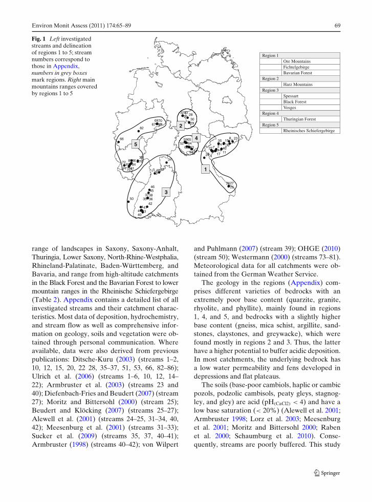
Fig. 1 Left investigatedstreams and delineationof regions 1 to 5; streamnumbers correspond tothose in Appendix,numbers in grey boxesmark regions. Right mainmountains ranges coveredby regions 1 to 5

Region 1 Ore MountainsFichtelgebirgeBavarian Forest

Region 2 Harz Mountains

Region 3 Spessart Black ForestVosges

Region 4 Thuringian Forest

Region 5 Rheinisches Schiefergebirge

98

76

54

3

21

86858483

82

81

7876

75

72

71

70696867

66 6564

6362

59

5453

52

50

4948

47

4645

4443

42

4140

38373635

34

333231

3029

28

272625

24

23

22

17

1514

1211

1

2

3

54

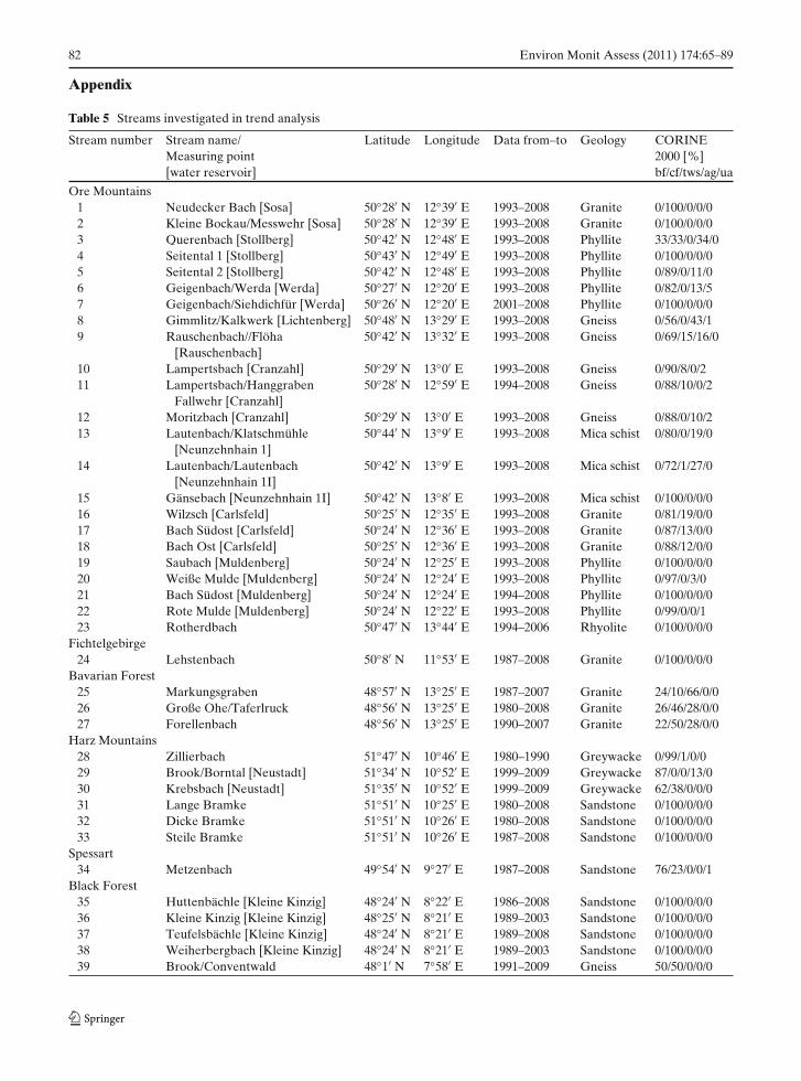
range of landscapes in Saxony, Saxony-Anhalt,Thuringia, Lower Saxony, North-Rhine-Westphalia,Rhineland-Palatinate, Baden-Württemberg, andBavaria, and range from high-altitude catchmentsin the Black Forest and the Bavarian Forest to lowermountain ranges in the Rheinische Schiefergebirge(Table 2). Appendix contains a detailed list of allinvestigated streams and their catchment charac-teristics. Most data of deposition, hydrochemistry,and stream flow as well as comprehensive infor-mation on geology, soils and vegetation were ob-tained through personal communication. Whereavailable, data were also derived from previouspublications: Ditsche-Kuru (2003) (streams 1–2,10, 12, 15, 20, 22 28, 35–37, 51, 53, 66, 82–86);Ulrich et al. (2006) (streams 1–6, 10, 12, 14–22); Armbruster et al. (2003) (streams 23 and40); Diefenbach-Fries and Beudert (2007) (stream27); Moritz and Bittersohl (2000) (stream 25);Beudert and Klöcking (2007) (streams 25–27);Alewell et al. (2001) (streams 24–25, 31–34, 40,42); Meesenburg et al. (2001) (streams 31–33);Sucker et al. (2009) (streams 35, 37, 40–41);Armbruster (1998) (streams 40–42); von Wilpert

and Puhlmann (2007) (stream 39); OHGE (2010)(stream 50); Westermann (2000) (streams 73–81).Meteorological data for all catchments were ob-tained from the German Weather Service.

The geology in the regions (Appendix) com-prises different varieties of bedrocks with anextremely poor base content (quarzite, granite,rhyolite, and phyllite), mainly found in regions1, 4, and 5, and bedrocks with a slightly higherbase content (gneiss, mica schist, argillite, sand-stones, claystones, and greywacke), which werefound mostly in regions 2 and 3. Thus, the latterhave a higher potential to buffer acidic deposition.In most catchments, the underlying bedrock hasa low water permeability and fens developed indepressions and flat plateaus.

The soils (base-poor cambiols, haplic or cambicpozols, podzolic cambisols, peaty gleys, stagnog-ley, and gley) are acid (pH(CaCl2) < 4) and have alow base saturation (< 20%) (Alewell et al. 2001;Armbruster 1998; Lorz et al. 2003; Meesenburget al. 2001; Moritz and Bittersohl 2000; Rabenet al. 2000; Schaumburg et al. 2010). Conse-quently, streams are poorly buffered. This study


considers exclusively catchments with a forestpercentage of at least 60% (Appendix). Norwayspruce (Picea abies) is the dominant forest tree,whilst beech (Fagus sylvatica) and other treespecies are of minor relevance. Landuse wasderived from CORINE landcover data (statusmapped for the year 2000). This was the onlylanduse information available for all catchments,although for some catchments, we had more de-tailed information on landuse and its temporalchanges. However, CORINE data also containsa landuse class “transitional woodland shrub”,which gives a hint as to structural changes in theforest cover, e.g. as a result of wind throw or barkbeetle infestation.

The streams were grouped into regions mainlyaccording to their geographic location (Fig. 1).In some cases, distant streams were grouped to-gether because of similar geological conditions(e.g. streams 25 to 27 grouped in region 1) orsimilar deposition patterns (stream 34 grouped inregion 3). The typical deposition regimes in theseregions were classified into deposition types ac-cording to Wellbrock et al. (2005), which is basedon the source and the total amount of atmosphericemissions from 1989 (Table 1). Wellbrock’s clas-sification constitutes a comprehensive assessmentof deposition patterns in Germany for a time whendeposition was at large still at a high level.

Deposition type 1 is characterized by mediumvalues for atmospheric deposition. In depositiontype 2, atmospheric input of potential acid and sul-fur was twice as high as in type 1. Nitrogen inputwas slightly above the German average but rela-tively low compared to sulfur deposition. Deposi-tion type 3 is characterized by low deposition ofsulfur, potential acid, and sodium compared with

the German average. Typical is a high percentageof reduced nitrogen of the total N input fromagricultural nitrogen emissions together with lowcalcium and magnesium deposition. Depositiontype 4 showed high sea-borne sodium and mag-nesium deposition with a high percentage of am-monia nitrogen of the total N deposition fromagricultural emissions. Deposition type 5 consistsof sites with extremely high depositions of sulfursubstances, nitrogen, and potential acid resultingfrom large nearby sources of emission (energyproduction, lignite combustion, livestock farming,and fertilization). Deposition type 6 is character-ized by low atmospheric deposition. Comparedto type 3, this type contains a greater amount ofoxidized nitrogen as well as a higher deposition ofcalcium, magnesium, and potassium.

Region 1 is located in southeast Germany andsurrounds the western BohemianBasin. It includes catchments in theOre Mountains (streams 1 to 23), inthe Fichtelgebirge (stream 24) and inthe Bavarian Forest (streams 25 to 27).Most catchments in the Ore Mountainsbelong to deposition type 5 and re-ceived extremely high depositions ofacidifying pollutants. Since the mid1980s, emissions of total inorganicsulfur were largely reduced in thesecatchments. Contrarily, nitrogen com-pounds decreased only slightly, andthey presently dominate the atmo-spheric input of acidity. Until ∼1995,alkaline emission components de-clined more than the acidic ones dueto insufficient flue gas desulfurization.

Table 1 Deposition typesaccording to Wellbrocket al. (2005)

Deposition Ntotal Potential acid SOx–Stype [kmol ha−1 yr−1] [kmol ha−1 yr−1] [kmol ha−1 yr−1]

1 2.63 5.50 2.962 2.41 9.57 7.163 2.92 5.32 2.534 2.92 5.32 2.535 4.02 19.75 15.826 2.07 4.56 2.55


This caused precipitation acidity torise five times above its level inWest Germany (Ulrich et al. 2006).The Fichtelgebirge is classified asWellbrock’s deposition type 2 withdeposition amounting to only halfof that in deposition type 1. TheBavarian Forest is strongly influencedby agricultural nitrogen emissionsand characterized by deposition type3. Accordingly, the deposit of totalinorganic S and N compounds hasdeclined only moderately since the1990s.

Region 2 is located in Central Germany, withcatchments in the southeast (streams28 to 30) and northwest (streams31 to 33) of the Harz Mountains.Atmospheric deposition in the catch-ments northwest of the Harz Moun-tains had been influenced by bothlong-range transport and by localsources due to the mining industry.The latter resulted in increased depo-sition rates during the last millennium.The smelting of sulfur containing oresemitted large amounts of sulfur, whichwere, in parts, deposited in the re-gion. Unlike Wellbrock et al. (2005)who classified these catchments intodeposition type 6 (low atmospheric in-put), our data (Alewell et al. 2001;Schaumburg et al. 2010) suggest a clas-sification into type 2 (high atmosphericinput). Since the mid 1980s, sulfatedeposition has decreased drastically.The formerly high nitrogen deposition(with a high percentage of ammonianitrogen) decreased only slightly. Thecatchments in the southeast of theHarz Mountains experienced low at-mospheric input in the past and ac-cordingly, are classified as depositiontype 6.

Region 3 is located in southwest Germany, inthe Spessart (stream 34), in the BlackForest (streams 35 to 49) and includes

one stream (no. 50) in the Vosges/France. Most of the catchments inthe Black Forest belong to depo-sition type 1 (medium atmosphericinput). Acid deposition decreased sub-stantially whereas nitrate depositionremained at a high level (von Wilpertet al. 2010). Some catchments in theBlack Forest as well as the Spessartcatchment belong to deposition type 6(low atmospheric input).

Region 4 groups the streams in the ThuringianForest (no. 51 to 65). This regionbelongs to deposition type 2, withhigher sulfur and potential acid de-position than German average. Until1990, most elements were depositedin the form of fly ashes. Since then,the emissions of total inorganic Sand N compounds have been reduceddramatically.

Region 5 is located in West Germany andsubsumes various catchments in theRheinische Schiefergebirge (streams66 to 86). This region is characterizedby deposition type 1. Sulfur depositionin this region originated mainly fromfossil fuels combustion in the heavilyindustrialized Ruhr Area at the north-ern edge of this region. N depositionis still comparatively high due to ex-tensive agriculture in the neighboringBenelux states.

For each catchment of the analyzed streams, thelong-term buffering capacity in the soil was as-sessed by the critical load values for acids pub-lished by UBA (2000). The concept of criticalloads combines soil chemical characteristics likebase saturation with an assessment of the long-term mobilization of base cations through weath-ering of primary minerals and leaching of basecations with seepage water. The maps of UBA(2000) give only rough estimates of the spatialpatterns of critical loads, and their value for lo-cal interpretations is rather limited. However,region-specific information on soil acidification


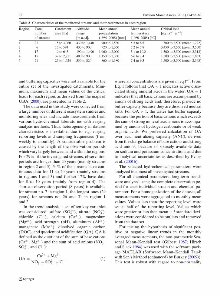
Table 2 Characteristics of the monitored streams and their catchments in each region

Region Total Catchment Altitude Mean annual Mean annual Critical loadnumber area [ha] range precipitation temperature [eq ha−1 yr−1]of streams [m a.s.l]. (1980–2008) [mm] (1980–2008) [◦C]

1 27 15 to 3,080 430 to 1,440 900 to 1,530 5.3 to 8.5 500 to 2,500 (mean 1,722)2 6 15 to 594 430 to 900 920 to 1,360 7.2 to 7.8 3,450 to 3,550 (mean 3,500)3 17 9 to 643 190 to 1,490 1,060 to 2,000 5.1 to 10.2 1,500 to 3,500 (mean 2,313)4 15 37 to 2,211 480 to 900 1,150 to 1,330 6.6 to 7.4 1,500 to 2,500 (mean 1,833)5 21 25 to 1,624 330 to 820 860 to 1,380 7.4 to 9.3 1,500 to 3,500 (mean 2,548)

and buffering capacities were not available for theentire set of the investigated catchments. Mini-mum, maximum and mean values of the criticalloads for each region, as derived from the maps ofUBA (2000), are presented in Table 2.

The data used in this study were collected froma large number of different ecosystem studies andmonitoring sites and include measurements fromvarious hydrochemical laboratories with varyinganalysis methods. Thus, heterogeneity in datasetcharacteristics is inevitable, due to e.g. varyingreporting levels and sampling frequencies (fromweekly to monthly). A considerable problem iscaused by the length of the observation periodswhich vary largely between and within the regions.For 29% of the investigated streams, observationperiods are longer than 20 years (mainly streamsin region 2 and 5), 54% of the streams have con-tinuous data for 11 to 20 years (mainly streamsin regions 1 and 3) and further 17% have datafor 8 to 10 years (mainly from region 4). Theshortest observation period (8 years) is availablefor stream no. 7 in region 1, the longest ones (29years) for streams no. 26 and 31 in region 1and 2.

In the trend analysis, a set of ten key variableswas considered: sulfate (SO2−

4 ), nitrate (NO−3 ),

chloride (Cl−), calcium (Ca2+), magnesium(Mg2+), acid strength (pH), aluminum (Al3+),manganese (Mn2+), dissolved organic carbon(DOC), and quotient of acidification (QA). QA isdefined as the quotient of the sum of base cations(Ca2+, Mg2+) and the sum of acid anions (NO−

3 ,SO2−

4 , and Cl−):

QA = Ca2+ + Mg2+

NO−3 + SO2−

4 + Cl−(1)

where all concentrations are given in eq l−1. FromEq. 1 follows that QA < 1 indicates active disso-ciated strong mineral acids in the water. QA = 1indicates that all basic cations are accompanied byanions of strong acids and, therefore, provide nobuffer capacity because they are dissolved neutralsalts. For QA > 1, the water has buffer capacitybecause the portion of basic cations which exceedsthe sum of strong mineral acid anions is accompa-nied by anions of hydrogen carbonate or of weakorganic acids. We preferred calculation of QAover acid neutralizing capacity (ANC), derivedfrom the charge balance of base cations and strongacid anions, because of sparsely available dataon sodium and potassium concentrations and dueto analytical uncertainties as described by Evanset al. (2001b).

The selected hydrochemical parameters wereanalyzed in almost all investigated streams.

For all chemical parameters, long-term trendswere analyzed using the complete observation pe-riod for each individual stream and chemical pa-rameter. For a homogenization of the dataset, allmeasurements were aggregated to monthly meanvalues. Values less than the reporting level wereset at half of the reporting level. Values whichwere greater or less than mean ± 3 standard devi-ations were considered to be outliers and removedfrom the data set.

For testing the hypothesis of significant pos-itive or negative linear trends in the monthlyaveraged measurements, the non-parametric Sea-sonal Mann–Kendall test (Gilbert 1987; Hirschand Slack 1984) was used with the software pack-age MATLAB (Software: Mann–Kendall Tau-bwith Sen’s Method (enhanced) by Burkey (2009)).This test is robust with regard to non-normality


as well as to missing or “less-than” values in thedatasets. This test groups data into monthly blocksto identify persistent long-term trends. The Z testwas used for accepting or rejecting the hypothesisof significant positive or negative trends. The levelof significance was set at p = 0.05.

Trend slopes were estimated according to themethod of Sen (1968), as individual slope �ci

for data pair {xij, xik} and the month i fori = 1..12

�ci =(xij − xik

)

( j − k)(2)

where, xij is the value for the month i of the yearj, and xik is the value for the month i of the year k,where j > k. From the set of individual slopes, �c,the median seasonal trend slope �C was derived.

Results and discussion

Observed trends

For the analyses of the medium to long-termtrends of the individual streams, the entire indi-vidual observation periods were used because weneed observation periods as long as possible for awell-defined trend recognition. In Fig. 2, the esti-mated median trend slopes, �C, for each chem-ical parameter are ranked over all investigatedstreams, from streams with low �C values tostreams with high �C values. Black bars markstreams with significant trend according to the Zstatistics; white bars mark streams without sig-nificant trend. This figure allows identifying gen-eral patterns of concentration changes across allinvestigated streams regardless of their belongingto a specific region.

Fig. 2 Ranked �C for allanalyzed streams; blackbars mark significantpositive or negativetrends (p < 0.05), whitebars mark nonsignificanttrends; QA quotient ofacidification


The estimated trends in our dataset confirma wide-spread recovery from acidification inresponse to decreasing emissions of acidifyingpollutants as reported in many recent studies.Significant decreases in stream water SO2−

4 con-centrations were observed in 87% of the streams.This complies with observations of Schaumburget al. (2008), who found significant negative SO2−

4trends for 86% of 28 investigated streams andlakes in Germany. The observation reflects thesteep reduction of sulfur deposition, although re-lease of sulfur stored in soils may have dampedthis response in some regions (Alewell et al. 2001;Prechtel et al. 2001). In comparison to SO2−

4 , ourdata on NO−

3 show only weak and more variabletrends with significant negative trends in 52% andsignificant positive trends in 25% of the moni-tored streams. Again, this complies with the re-sults of previous studies (e.g. Alewell et al. 2000,2001; Schaumburg et al. 2008; Westermann 2000).No clear trend could be found for chloride (Fig. 2),and streams had both significant positive (38%of the streams) and significant negative trends(29%). Chloride deposition originates from nat-ural (sea-spray in oceanic areas) and industrialsources (combustion of PVC, lignite powerplants). Due to the two different principle sourcesof Cl− depositions, Cl− concentrations vary withdistance to the sea but also to industrial re-gions and, therefore, have no clearly interpretablespatial pattern. The most important base cationsin aquatic systems, calcium and magnesium, aremobilized by weathering and cation exchange andrespond indirectly to the decreases in SO2−

4 andNO−

3 deposition. The reduced acid input led toa reduction of neutralizing processes in the soiland thereby reduced the release of base cationsto the stream water. Significant negative trendswere observed in 58% of the streams for Ca2+and 49% for Mg2+, whereas significant positivetrends were found in only 18% of the streamsfor Ca2+ and 17% for Mg2+. An integral mea-sure of stream acidification is the QA; it reflectsthe buffering capacity of the stream water. Noclear trend can currently be observed for QA,with 44% of all streams showing significant neg-ative trends and 23% showing significant positive

trends (Fig. 2). Other studies (Alewell et al. 2001;Evans et al. 2001a) used the acid neutralizingcapacity ANC for describing the status of streamacidification and found similar trends to those inour data. However, some studies (Schaumburget al. 2008; Ulrich et al. 2006; Westermann 2000)report slightly significant positive trends for ANCor alkalinity. The pH value characterizes the ac-tual acid strength in the water and is biologi-cally most relevant because aquatic biota havevery explicitly defined pH ranges favorable fortheir lives. In contrast to the QA, the pH valueshows a clear trend towards increasing values inalmost all streams (Fig. 2). Sixty-six percent of thestreams exhibit significant positive trends whilstonly 7% show significant negative trends. Posi-tive pH trends were also reported in Schaumburget al. (2008), where 52% of the streams and lakesshowed significant positive trends. Aluminum andmanganese leach from the soil zone as a result ofdeep soil acidification. Aluminum poses a severethread for aquatic organisms due to its highly toxiceffect (Baker and Schofield 1982; Driscoll et al.1980). High manganese concentration in the rawwater makes drinking water treatment cumber-some and costly, since the raw water needs tobe filtered and supplied with bases up to pH 9(Gray 2008). In consequence of widespread posi-tive trends in precipitation and stream water pH,significant negative trends in Al3+ have been ob-served in 50%, for Mn2+ in 69% of the inves-tigated streams. However, some of the streamsshowed increasing trends (18% for Al3+, 3% forMn2+). Decreasing Al3+ concentrations in sur-face waters of Germany were also reported byEvans et al. (2001a), Ulrich et al. (2006), andWestermann (2000), whereas Alewell et al. (2001)found no general negative trend. An indicatorof organic acidity is DOC. It is a broad clas-sification for organic molecules of varied originand composition in aquatic systems. The mainsource of DOC is leaching of decomposed organicmatter from soils into stream water. DOC is animportant source of carbon and energy for mi-croorganisms and thus plays an important role inmany chemical and photochemical reactions andtransformations. Increases in stream water DOC


concentrations occurred in most of the analyzedstreams (Fig. 2, 55% significant). Only 9% of thestreams showed significant negative trends.

Among all investigated streams, streams no. 3to 5 show the highest median changes in SO2−

4 ,NO−

3 , Ca2+, Mg2+, Al3+, and Mn2+. These streamsbelong to region 1, which received extremely highdeposition in the past, and furthermore, are influ-enced by abandoned interconnected drinkingwater wells and the influence of near-surfacegroundwater. Figure 2 also shows that the ob-served trends are highest for SO2−

4 , lower for Ca2+,Mg2+, Cl−, Al3+,and NO−

3 , and are small forMn2+.

Variation within and between regions

In order to provide information about the ab-solute level of the hydrochemical parameters andtheir variation within and between regions, the

median absolute values for each parameter ofall individual streams are summarized per regionas median, minimum and maximum values inTable 3. Thus, the mean regional characteristiccan be explained through predictors which are ac-tive in distinct regions, while the variation aroundthe median values provides an impression aboutthe potential which could be controlled, at leastpartially, by forest management. In order to allowfor an unbiased comparison between regions, thelength of time series considered was uniformlylimited to the period between 1999 and 2008,for which continuous measurements in almostall streams were available. In addition, Table 3summarizes in a second block (below the ab-solute concentrations) the identified trends foreach chemical parameter and each region. Themedian trend of a given chemical parameter fora specific region, �C*, is given together with thepercentage of streams with significant positive or

Table 3 Upper part: absolute concentrations (median,minimum, maximum), light/dark grey shading = lowest/highest values; lower part: median trends �C* withineach region (light/dark grey shading = highest/lowest

values), and percentage of streams with significant pos-itive/negative trends (light/dark grey shading = < 25%/> 75%)

Absolute conc. n median minimum maximum Parameter/Region 1 2 3 4 5 1 2 3 4 5 1 2 3 4 5 1 2 3 4 5

SO42- [µmolc l

-1] 27 5 16 15 17 430.79 497.38 88.07 312.32 229.03 54.14 221.20 49.14 174.90 80.99 1378.36 832.85 458.07 397.68 410.18

NO3- [µmolc l

-1] 27 5 16 15 21 70.96 55.00 27.82 81.69 57.12 17.74 48.63 4.76 41.05 31.45 391.91 121.01 91.69 119.35 180.63

Cl- [µmolc l-1] 27 5 16 15 8 121.30 87.45 43.72 111.42 136.81 16.93 80.73 19.18 73.34 105.78 1173.48 131.17 121.30 234.13 629.06

Ca2+ [µmolc l-1] 27 5 16 15 17 264.47 384.93 154.69 359.28 164.67 94.81 166.34 39.92 164.67 84.83 1047.90 603.79 474.05 499.00 414.17

Mg2+ [µmolc l-1] 27 5 16 15 17 246.81 361.99 63.27 106.95 172.77 41.14 144.06 10.61 65.82 115.18 740.44 389.76 246.81 255.04 436.03

QA [-] 27 6 8 13 8 0.75 0.96 1.08 0.80 0.79 0.41 0.89 0.50 0.65 0.43 1.54 1.38 2.89 1.83 1.15pH [-] 26 5 16 15 21 5.36 6.80 6.54 6.90 6.77 4.29 6.35 5.00 6.00 4.75 7.50 7.26 7.40 7.40 7.71

Al3+ [µmolc l-1] 26 5 15 15 17 44.67 2.11 5.56 5.23 28.35 3.22 2.06 1.67 1.78 4.67 308.23 12.23 31.25 35.58 85.45

Mn2+ [µmolc l-1] 27 3 15 8 12 5.90 0.18 0.22 0.50 2.71 0.15 0.11 0.09 0.04 0.25 45.14 0.36 2.44 2.57 6.13

DOC [mg l-1] 5 127 6 15 14 3.60 1.50 1.40 1.00 3.05 1.60 0.92 0.50 0.50 0.90 9.38 1.75 4.60 3.40 7.30

Trends n Δ C* Significant positive Significant negative

SO42- [µmolc l

-1yr-1] 27 6 17 15 17 -10.64 -6.17 -1.04 -7.81 -5.21 0 0 0 0 0 100 67 88 53 100

NO3- [µmolc l

-1yr-1] 27 6 17 14 21 -2.15 0.24 0 0.04 0.03 11 17 35 21 38 89 33 47 21 33

Cl- [µmolc l-1yr-1] 27 6 17 14 8 0.21 -2.52 0.12 2.12 -0.45 44 17 47 21 38 30 83 24 7 38

Ca2+ [µmolc l-1yr-1] 27 4 17 15 17 -8.83 -5.51 0 -16.22 0 15 0 18 0 41 85 75 41 40 41

Mg2+ [µmolc l-1yr-1] 27 4 17 13 17 -2.29 -3.04 0 -1.37 0.24 11 0 12 0 47 74 75 29 31 35

QA [yr-1] 4 127 7 9 7 -0.006 0.001 0.004 -0.011 -0.003 19 50 35 11 14 59 0 29 33 57

pH [yr-1] 626 17 15 21 0.021 0.024 0.005 0.000 0.030 85 83 47 33 76 0 0 18 13 5

Al3+ [µmolc l-1yr-1] 26 3 16 10 17 -2.51 -0.04 0.05 -0.03 -0.88 8 33 44 10 12 69 67 19 10 71

Mn2+ [µmolc l-1yr-1] 27 4 16 2 12 -0.22 -0.04 -0.02 -0.15 -0.03 7 0 0 0 0 78 100 63 50 50

DOC [mg l-1yr-1] 27 5 17 14 14 0.06 -0.01 0.01 0.03 0.08 59 0 24 71 86 4 40 18 0 7

Shadings for QA (quotient of acidification) and pH adverse. Absolute concentrations based on data from 1999 to 2008,trends based on data from entire individual measuring period for each stream


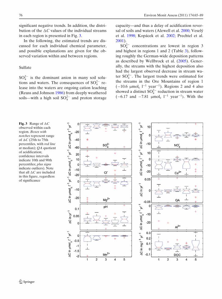
significant negative trends. In addition, the distri-bution of the �C values of the individual streamsin each region is presented in Fig. 3.

In the following, the estimated trends are dis-cussed for each individual chemical parameter,and possible explanations are given for the ob-served variation within and between regions.

Sulfate

SO2−4 is the dominant anion in many soil solu-

tions and waters. The consequences of SO2−4 re-

lease into the waters are ongoing cation leaching(Reuss and Johnson 1986) from deeply weatheredsoils—with a high soil SO2−

4 and proton storage

capacity—and thus a delay of acidification rever-sal of soils and waters (Alewell et al. 2000; Veselýet al. 1998; Kopácek et al. 2002; Prechtel et al.2001).

SO2−4 concentrations are lowest in region 3

and highest in regions 1 and 2 (Table 3), follow-ing roughly the German-wide deposition patternsas described by Wellbrock et al. (2005). Gener-ally, the streams with the highest deposition alsohad the largest observed decrease in stream wa-ter SO2−

4 . The largest trends were estimated forthe streams in the Ore Mountains of region 1(−10.6 μmolc l−1 year−1). Regions 2 and 4 alsoshowed a distinct SO2−

4 reduction in stream water(−6.17 and −7.81 μmolc l−1 year−1). With the

Fig. 3 Range of �Cobserved within eachregion. Boxes withnotches represent rangeof �C (25th to 75thpercentiles, with red lineat median); QA quotientof acidification;confidence intervalsindicate 10th and 90thpercentiles; plus signsindicate outliers). Notethat all �C are includedin this figure, regardlessof significance


exception of regions 3 and 5—where the deposi-tion level in the past was generally lower—in allregions observed SO2−

4 reductions in the streamwater amount to more than −6 μmolc l−1 year−1

(Table 3). By far the largest variation among theindividual streams can be observed in region 1(Fig. 3). Region 3, with the lowest deposition inthe past, exhibits both, small concentration trendsas well as a small variation between the variousstreams.

Nitrate

As for SO2−4 , NO−

3 concentrations are lowest inregion 3, whereas regions 4 and 1 show compar-atively high concentrations (Table 3). Trends arehighly variable within the same region (Fig. 3). Inregion 1, NO−

3 decrease was largest in catchmentswith comparatively large proportions of naturalgrassland and agricultural land (streams no. 3, 5, 8,9, 12, 14). In the 1970s, parts of these catchmentswere intensively used by agriculture connectedwith extensive use of organic and inorganic fer-tilizers as well as stock breeding. Consequently,NO−

3 concentration in surface water increaseddramatically until around 1979/1980 and remainedat a high level until 1992/1993 (Pütz et al. 2002).Since then, fertilizer use declined drastically, initi-ated by federal regulations of Saxony which cameinto effect in 1994. Another possible explanationfor decreasing trends in the Ore Mountains is ahigher N uptake as a result of extensive reforesta-tion and the continuous recovery and increasingvitality of damaged forests (Ulrich et al. 2006),which, according to Armbruster et al. (2003),could also explain the large NO−

3 decrease ofstream 23 (−8.87 μmolc l−1 year−1). Regardless ofthe landuse impact, the majority of streams in theOre Mountains and the Fichtelgebirge (region 1)show significant negative trends (Fig. 3). This canbe explained by the economic crash in this regionwhich followed the political changes in 1989, andwhich led to drastically reduced nitrogen deposi-tion. Contrarily to most other streams of region1, the streams in the Bavarian Forest (nos. 25to 27) exhibit large increases in NO−

3 concen-trations. Since 1993, these catchments have been

affected by extensive forest damage due to a se-vere bark beetle infestation (Alewell et al. 2001).Also, snow break can affect the NO−

3 trends. Thiscould be observed in stream no. 41, which showsamong all streams of region 3, the largest NO−

3increase (+0.84μmolc l−1 year−1, Appendix), re-sulting from wide-spread tree damage during thewinter season of 1996/1997 (Fink et al. 1999). Inregion 2, the streams 31–33 in the northwest ofthe Harz Mountains show decreases, in contrastto the southeast streams. Wright et al. (2001) men-tioned for these streams that the decreases are notexplained by changes in N deposition, climate ormanagement practices.

Chloride

By far the lowest concentrations of Cl− werefound in region 3. The highest concentrationswere observed in region 5, which can be explainedby the comparatively low distance to the NorthSea and, hence, larger sea-salt input. In regions1 and 4, increased concentration can neither beexplained by the vicinity to the sea nor by pri-mary Cl− content of the bedrock. There, themain factor is Cl− deposition from lignite com-bustion deposited with fly ashes (Kaufmann andNussbaumer 1999). Within these regions, chloridetrends showed a high degree of heterogeneity,with exception of region 3 (Fig. 3). De-icing saltsapplied to roads in winter can influence the con-centration additionally, as was reported for exam-ple for stream no. 23 (Armbruster et al. 2003).

Calcium and magnesium

Along with the reduction in particulate emis-sions, base cation deposition has been reducedin many forest ecosystems (Driscoll et al. 1989;Meesenburg et al. 1995). Temporal changes inthe leaching of the anions NO−

3 and SO2−4 have

strong effects on cation losses. As a consequenceof large reductions in SO2−

4 , concentrations ofCa2+ and Mg2+ in stream water generally de-creased in our study. The spatial patterns of Ca2+and Mg2+ concentrations resemble the depositionpatterns, but they are modified by the natural


base content of the soil and bedrock substrates.In region 2, the basic cation concentrations areover-proportionally high, because of the slightlymore carbonate-rich bedrocks, like greywackeand sandstones. This finding is supported by thecritical load values (Table 2), which are about27 to 51% higher in region 2 than in the otherregions. The comparatively high level of basiccations in regions 1 and 4 possibly originates fromfly ash resulting from lignite combustion. Largedecreases of base cation concentrations are ob-served in regions 1, 2, and 4 (Fig. 3, Table 3),which experienced a high deposition input in thepast. The largest variation among the individualstreams can be observed for Ca2+ and Mg2+ inregion 1. As for NO−

3 , the bark beetle-affectedstreams in the Bavarian Forest (streams 25 and27 in region 1) showed positive trends, contraryto most other streams of this region. Anotherexample for positive Ca2+ and Mg2+ trends canbe observed in streams 73 to 81 in region 5, whichWestermann (2000) argues to be effected by forestliming with dolomite rich in Mg2+. Alewell et al.(2001) investigated the base cation flux for sixstreams in Germany and found increasing net lossof base cations from all ecosystems, which theauthors interpreted as an effect of increased soilacidification.

QA

QA reflects the buffering capacity of the streamwater. Values of QA slightly lower than 1 (0.75–0.96) were observed in all regions expect forregion 3, where median QA was 1.08. This in-dicates that strong mineral acid anions dominatethe stream water chemistry. Large maxima ofQA values (1.2–2.9) point out that throughoutthe regions, some streams are well buffered, pos-sibly an buffering effect of deep aquifers. Ex-amination of individual regions reveals a highdegree of heterogeneity (Fig. 3). Region 4 showsthe largest variation of change in QA from thelargest significant negative trend for stream 57(−0.049 year−1) to the largest positive trend forstream 54 (+0.055 year−1). Only 44% of thestreams show significant trends. Region 1 displaysalso a high variation of QA trends with dominat-

ing negative trends, all other regions display lowvariety of QA trends around zero.

pH

Region 1 comprises the most acidified streamswith median pH values of slightly above 5. Allother regions have median pH values above 6.5(Table 3). Since the pH value partly depends onthe activity of Al3+, it follows only roughly thespatial pattern of strong acid anion concentrations(Table 3). The wide-spread pH increase can beexplained by reduced concentrations of strongmineral acids (particularly, sulfuric acid) and byreduced concentrations of “cation acids” (Al3+,Mn2+). Without exception, all streams in regions1 and 2 show increasing trends (Fig. 3), whereasin the other regions negative trends could be ob-served. The largest increase in stream water pHoccurred in region 5 (+0.03 year−1). The largestvariation among the individual streams can beobserved in region 5.

Aluminum and manganese

Since the leaching of anions is always connectedto cation leaching, the ongoing release of SO2−

4delays a reversal of stream water acidificationdue to leaching of Al3+ and Mn2+ (Alewell et al.2001). Al3+ and Mn2+ concentrations are lowestin region 2, and highest in region 1. The spatialpatterns of Al3+ and Mn2+ trends resemble thedeposition patterns. The decrease of Al3+ andMn2+ is following from reduced acidity which at-tenuates dissolution of bedrock minerals, favorsprecipitation of secondary mineral phases, andalters sorption exchange processes on organic andmineral surfaces (Ulrich et al. 2006). In compar-ison to Al3+ trends, Mn2+ trends are less pro-nounced. The largest reductions were observedin region 1 (−2.51 μmolc l−1 year−1 for Al3+,−0.22 μmolc l−1 year−1 for Mn2+; Fig. 3), whichreceived extremely high deposition input in thepast. All other regions experienced much lesspronounced decreases. A considerable number ofstreams even show significant positive trends inAl3+. However, the magnitude of this increaseis small compared with the decrease observed


in most other streams. The estimated increase ismainly caused by acid peaks which result fromintense rain fall or snow melt and subsequent fastsurface runoff.

Dissolved organic carbon (DOC)

The lowest DOC concentrations are observedin region 4, the highest in region 1. Significantincreases in stream water DOC concentrations oc-curred in most of the analyzed streams in regions1, 4, and 5 (Table 3, Fig. 3). The variation amongthe individual streams is largest in regions 1 and 5.Drains of moorland (data not presented) could ex-plain the higher increasing DOC concentrations inregion 1 (Ulrich et al. 2006). Westermann (2000)assumed that the microbial activity in most forestsoils of the catchments in region 5 has increasedduring the 1990s due to continuously improvingliving conditions since the 1980s (decreasing aciddeposition, extensive forest liming). Accordingly,the low DOC values at the beginning of the ob-servations could be interpreted as indicator forstrongly acidified soil conditions which favoredthe accumulation of thick raw humus layers on theforest floor, and which in the 1990s slowly startedregenerating.

Ecological impact of acidification

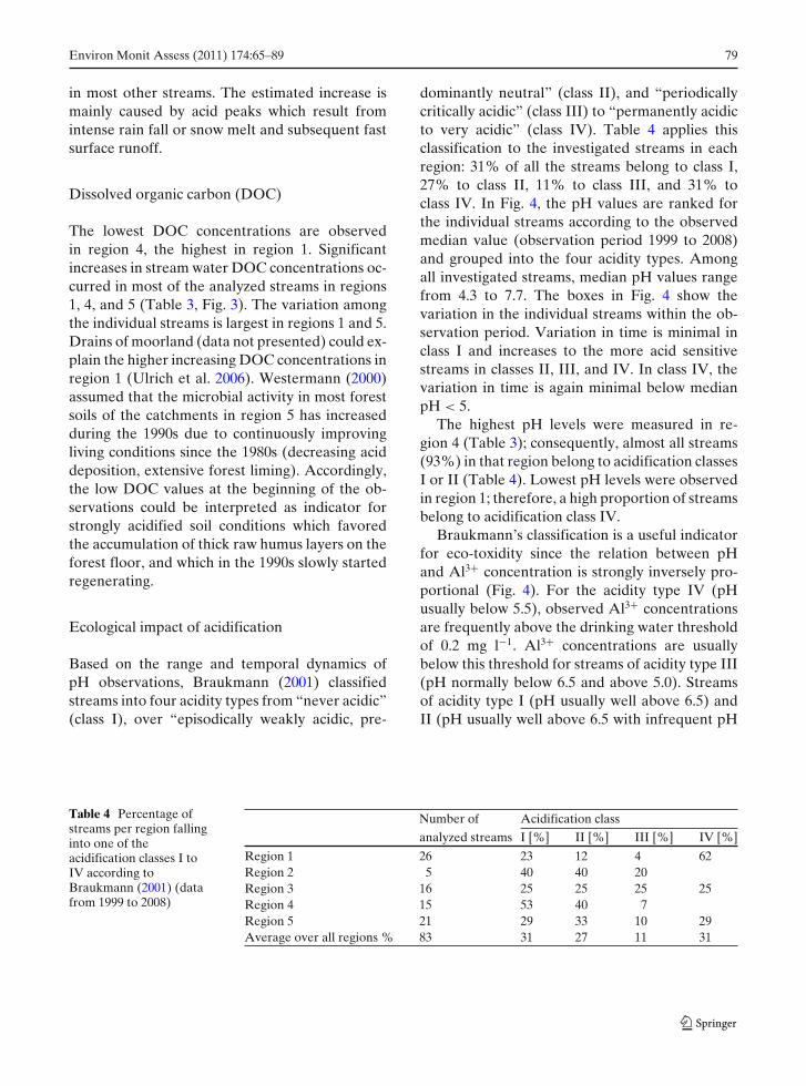
Based on the range and temporal dynamics ofpH observations, Braukmann (2001) classifiedstreams into four acidity types from “never acidic”(class I), over “episodically weakly acidic, pre-

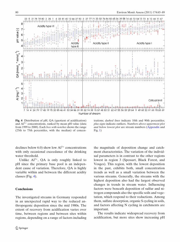
dominantly neutral” (class II), and “periodicallycritically acidic” (class III) to “permanently acidicto very acidic” (class IV). Table 4 applies thisclassification to the investigated streams in eachregion: 31% of all the streams belong to class I,27% to class II, 11% to class III, and 31% toclass IV. In Fig. 4, the pH values are ranked forthe individual streams according to the observedmedian value (observation period 1999 to 2008)and grouped into the four acidity types. Amongall investigated streams, median pH values rangefrom 4.3 to 7.7. The boxes in Fig. 4 show thevariation in the individual streams within the ob-servation period. Variation in time is minimal inclass I and increases to the more acid sensitivestreams in classes II, III, and IV. In class IV, thevariation in time is again minimal below medianpH < 5.

The highest pH levels were measured in re-gion 4 (Table 3); consequently, almost all streams(93%) in that region belong to acidification classesI or II (Table 4). Lowest pH levels were observedin region 1; therefore, a high proportion of streamsbelong to acidification class IV.

Braukmann’s classification is a useful indicatorfor eco-toxidity since the relation between pHand Al3+ concentration is strongly inversely pro-portional (Fig. 4). For the acidity type IV (pHusually below 5.5), observed Al3+ concentrationsare frequently above the drinking water thresholdof 0.2 mg l−1. Al3+ concentrations are usuallybelow this threshold for streams of acidity type III(pH normally below 6.5 and above 5.0). Streamsof acidity type I (pH usually well above 6.5) andII (pH usually well above 6.5 with infrequent pH

Table 4 Percentage ofstreams per region fallinginto one of theacidification classes I toIV according toBraukmann (2001) (datafrom 1999 to 2008)

Number of Acidification class

analyzed streams I [%] II [%] III [%] IV [%]

Region 1 26 23 12 4 62Region 2 5 40 40 20Region 3 16 25 25 25 25Region 4 15 53 40 7Region 5 21 29 33 10 29Average over all regions % 83 31 27 11 31


Fig. 4 Distribution of pH, QA (quotient of acidification)and Al3+ concentrations, ranked by mean pH value (datafrom 1999 to 2008). Each box with notches shows the range(25th to 75th percentiles, with the median) of concen-

trations; dashed lines indicate 10th and 90th percentiles;plus signs indicate outliers. Numbers above uppermost plotand below lowest plot are stream numbers (Appendix andFig. 1)

declines below 6.0) show low Al3+ concentrationswith only occasional exceedance of the drinkingwater threshold.

Unlike Al3+, QA is only roughly linked topH since the primary base pool is an indepen-dent cause of variation. Therefore, QA is highlyvariable within and between the different acidityclasses (Fig. 4).

Conclusions

The investigated streams in Germany respondedin an unexpected rapid way to the reduced an-thropogenic deposition since the mid 1980s. Theextent of recovery from acidification varies overtime, between regions and between sites withinregions, depending on a range of factors including

the magnitude of deposition change and catch-ment characteristics. The variation of the individ-ual parameters is in contrast to the other regionslowest in region 3 (Spessart, Black Forest, andVosges). This region, with the lowest depositionin the past, exhibits both, small concentrationtrends as well as a small variation between thevarious streams. Generally, the streams with thehighest deposition also had the largest observedchanges in trends in stream water. Influencingfactors were beneath deposition of sulfur and ni-trogen compounds also the specific soils and vege-tation, which respond to their reductions. Amongthem, sulfate desorption, organic S cycling in soils,and factors affecting N cycling in catchments areimportant.

The results indicate widespread recovery fromacidification, but more sites show increasing pH


than increasing QA. Indicators of the recovery ofstream water acidification were in detail:

• SO2−4 concentrations in stream water are de-

creasing steady in all regions• Trends in NO−

3 are highly variable, but slightlydecreasing

• QA and Cl−showed no clear trend• Steep increases were observed in pH values• Reduction of eco-toxical acidification prod-

ucts Al3+ and Mn2+

The processes responsible for the increased DOCconcentrations are complex and not entirely un-derstood (Porcal et al. 2009; Sucker and Krause2010). Freeman et al. (2001) and Harriman et al.(2003) emphasized that enhanced mineralizationthrough climate change and increasing tempera-ture would result in increased DOC release fromforest soils, especially in fens and bogs. Subsoilacidification seems to play a major role since themost positive DOC trends were found in regions1 (Fig. 3), which are characterized by low criticalload values (Table 2) and correspondingly, low pHvalues. Also, von Wilpert and Zirlewagen (2007)found in heavily acidified areas with podzol soiltypes that increasing DOC activity in seepage wa-ter was caused by the dissolution of organic matterfrom Bhs horizons through high proton activityin the soil solution. An increase of DOC releasefrom soils caused by soil acidification was alsoreported by Zech et al. (1994) for the BavarianForest. Lorz and Schneider (2003) and Grunewaldet al. (2004) hypothesized that soil protective lim-ing would result in DOC mobilization from soils.In the guidelines of liming procedure were organicwet sites explicitly excluded. Hildebrand (1991)and Hildebrand and Schack-Kirchner (2000) iden-tified the process of DOC mobilization in acidforest soils after forest liming to be a “reactionof neutralization where the stronger Fulvo acidsremove the weaker carbonic acid from its salt,the carbonate.” However, this reaction is lim-ited to the uppermost soil layers (Hildebrand andSchack-Kirchner 2000) due to the tendency oforganic acids for complexation, triggered thoughmulti-valent cations like Ca2+ and Al3+, whichcauses polymerization of organic acids in the sub-soil and eliminates them from the soil solution.Furthermore, the pH rises along the flow path

in the soil to values where fulvo acids are nomore dissociated. But the main objection againstthe hypothesis that soil protective liming wouldincrease DOC release from forest soils on the longrun is the fact that this process is limited in timeand must finish when the amount of carbonatedistributed with liming is exhausted by this neu-tralization reaction. Another argument against thehypothesis is the fact that DOC is rising in thewhole northern hemisphere since the 1990s. Thus,this process is very unlikely to play a key role inthe observed long-term increase of DOC release.

As a first step of this evaluation, in this papertrend analyses in the water quality of individualstreams are presented in a descriptive way, butan attempt is made to identify general patternsof chemical change at a region-wide scale. Forexplaining the observed trends in water quality,deposition, geology, and streamflow data as wellas information on forest management practices(liming) and natural disturbances (storms, barkbeetle infestation) are considered in more or lessexemplarily terms.

Acknowledgements We would like to thank allpersons who provided data to this study, namely frominstitutes in Bavaria: Büro für Angewandte HydrologieMünchen, Nationalparkverwaltung Bayerischer Wald,LfU (Bayrisches Landesamt für Umwelt); in Saxony:Landestalsperrenverwaltung des Freistaates Sachsen,Staatsbetrieb Sachsenforst, TU Dresden (Institut fürBodenkunde und Standortslehre); in Saxony-Anhalt:Talsperrenbetrieb Sachsen-Anhalt (AöR); in Thuringia:Thüringer Fernwasserversorgung; in Lower Saxony:Northwest German Forest Research Station; in North-Rhine-Westphalia: WSW Energie & Wasser AG, WAGNordeifel mbH, Wasserverband Aabachtalsperre; inRhineland-Palatinate: Stadtwerke Idar-Oberstein, SWTStadtwerke Trier Versorgungs-GmbH LUWG, Landesamtfür Umwelt, Wasserwirtschaft und GewerbeaufsichtRheinland-Pfalz; in Baden-Württemberg: ZweckverbandWasserversorgung Kleine Kinzig, LfU (Landesanstaltf. Umweltschutz Baden-Württemberg, KarlsruheAbt 4 Wasser), LUBW Landesanstalt für Umwelt,Messungen und Naturschutz Baden-Württemberg,Forstliche Versuchs- und Forschungsanstalt BW. Wekindly acknowledge also the help of H. Meesenburg(Department of Environmental Control, Forest ResearchInstitute of Lower Saxony), R. Sudbrack (ReferatWassergütebewirtschaftung, Landestalsperrenverwaltungdes Freistaates Sachsen), K.-H. Feger (Institute ofSoil Science and Site Ecology, Dresden Universityof Technology) and two anonymous reviewers forsubstantially improving the manuscript.


Appendix

Table 5 Streams investigated in trend analysis

Stream number Stream name/ Latitude Longitude Data from–to Geology CORINEMeasuring point 2000 [%][water reservoir] bf/cf/tws/ag/ua

Ore Mountains1 Neudecker Bach [Sosa] 50◦28′ N 12◦39′ E 1993–2008 Granite 0/100/0/0/02 Kleine Bockau/Messwehr [Sosa] 50◦28′ N 12◦39′ E 1993–2008 Granite 0/100/0/0/03 Querenbach [Stollberg] 50◦42′ N 12◦48′ E 1993–2008 Phyllite 33/33/0/34/04 Seitental 1 [Stollberg] 50◦43′ N 12◦49′ E 1993–2008 Phyllite 0/100/0/0/05 Seitental 2 [Stollberg] 50◦42′ N 12◦48′ E 1993–2008 Phyllite 0/89/0/11/06 Geigenbach/Werda [Werda] 50◦27′ N 12◦20′ E 1993–2008 Phyllite 0/82/0/13/57 Geigenbach/Siehdichfür [Werda] 50◦26′ N 12◦20′ E 2001–2008 Phyllite 0/100/0/0/08 Gimmlitz/Kalkwerk [Lichtenberg] 50◦48′ N 13◦29′ E 1993–2008 Gneiss 0/56/0/43/19 Rauschenbach//Flöha 50◦42′ N 13◦32′ E 1993–2008 Gneiss 0/69/15/16/0

[Rauschenbach]10 Lampertsbach [Cranzahl] 50◦29′ N 13◦0′ E 1993–2008 Gneiss 0/90/8/0/211 Lampertsbach/Hanggraben 50◦28′ N 12◦59′ E 1994–2008 Gneiss 0/88/10/0/2

Fallwehr [Cranzahl]12 Moritzbach [Cranzahl] 50◦29′ N 13◦0′ E 1993–2008 Gneiss 0/88/0/10/213 Lautenbach/Klatschmühle 50◦44′ N 13◦9′ E 1993–2008 Mica schist 0/80/0/19/0

[Neunzehnhain 1]14 Lautenbach/Lautenbach 50◦42′ N 13◦9′ E 1993–2008 Mica schist 0/72/1/27/0

[Neunzehnhain 1I]15 Gänsebach [Neunzehnhain 1I] 50◦42′ N 13◦8′ E 1993–2008 Mica schist 0/100/0/0/016 Wilzsch [Carlsfeld] 50◦25′ N 12◦35′ E 1993–2008 Granite 0/81/19/0/017 Bach Südost [Carlsfeld] 50◦24′ N 12◦36′ E 1993–2008 Granite 0/87/13/0/018 Bach Ost [Carlsfeld] 50◦25′ N 12◦36′ E 1993–2008 Granite 0/88/12/0/019 Saubach [Muldenberg] 50◦24′ N 12◦25′ E 1993–2008 Phyllite 0/100/0/0/020 Weiße Mulde [Muldenberg] 50◦24′ N 12◦24′ E 1993–2008 Phyllite 0/97/0/3/021 Bach Südost [Muldenberg] 50◦24′ N 12◦24′ E 1994–2008 Phyllite 0/100/0/0/022 Rote Mulde [Muldenberg] 50◦24′ N 12◦22′ E 1993–2008 Phyllite 0/99/0/0/123 Rotherdbach 50◦47′ N 13◦44′ E 1994–2006 Rhyolite 0/100/0/0/0

Fichtelgebirge24 Lehstenbach 50◦8′ N 11◦53′ E 1987–2008 Granite 0/100/0/0/0

Bavarian Forest25 Markungsgraben 48◦57′ N 13◦25′ E 1987–2007 Granite 24/10/66/0/026 Große Ohe/Taferlruck 48◦56′ N 13◦25′ E 1980–2008 Granite 26/46/28/0/027 Forellenbach 48◦56′ N 13◦25′ E 1990–2007 Granite 22/50/28/0/0

Harz Mountains28 Zillierbach 51◦47′ N 10◦46′ E 1980–1990 Greywacke 0/99/1/0/029 Brook/Borntal [Neustadt] 51◦34′ N 10◦52′ E 1999–2009 Greywacke 87/0/0/13/030 Krebsbach [Neustadt] 51◦35′ N 10◦52′ E 1999–2009 Greywacke 62/38/0/0/031 Lange Bramke 51◦51′ N 10◦25′ E 1980–2008 Sandstone 0/100/0/0/032 Dicke Bramke 51◦51′ N 10◦26′ E 1980–2008 Sandstone 0/100/0/0/033 Steile Bramke 51◦51′ N 10◦26′ E 1987–2008 Sandstone 0/100/0/0/0

Spessart34 Metzenbach 49◦54′ N 9◦27′ E 1987–2008 Sandstone 76/23/0/0/1

Black Forest35 Huttenbächle [Kleine Kinzig] 48◦24′ N 8◦22′ E 1986–2008 Sandstone 0/100/0/0/036 Kleine Kinzig [Kleine Kinzig] 48◦25′ N 8◦21′ E 1989–2003 Sandstone 0/100/0/0/037 Teufelsbächle [Kleine Kinzig] 48◦24′ N 8◦21′ E 1989–2008 Sandstone 0/100/0/0/038 Weiherbergbach [Kleine Kinzig] 48◦24′ N 8◦21′ E 1989–2003 Sandstone 0/100/0/0/039 Brook/Conventwald 48◦1′ N 7◦58′ E 1991–2009 Gneiss 50/50/0/0/0


Table 5 (continued)


40 ARINUS Brook S1 [Schluchsee] 47◦49′ N 8◦6′ E 1987–2007 Granite 0/100/0/0/041 ARINUS Brook S4 [Schluchsee] 47◦49′ N 8◦6′ E 1989–2007 Granite 0/100/0/0/042 ARINUS Brook V1 48◦3′ N 8◦21′ E 1988–1997 Sandstone 0/100/0/0/0

(Villingen)43 St.Wilhelmer Talbach 47◦53′ N 7◦59′ E 1987–2008 Gneiss 14/66/0/19/044 Zastlerbach 47◦54′ N 8◦1′ E 1993–2008 Gneiss 12/83/0/5/045 Kaltenbach 48◦37′ N 8◦24′ E 1986–2008 Sandstone 0/100/0/0/046 Dürreychbach 48◦45′ N 8◦27′ E 1987–2008 Sandstone 0/67/33/0/047 Goldersbach 47◦52′ N 8◦3′ E 1986–2008 Granite 0/99/0/1/048 Steinbach 49◦26′ N 8◦44′ E 1988–2008 Sandstone 18/82/0/0/049 Itterhof 49◦29′ N 9◦0′ E 1989–2005 Sandstone 56/44/0/0/0

Vosges (France)50 Strengbach 48◦12′ N 7◦11′ E 1985–2005 Granite 11/86/0/3/0

Thuringian Forest51 Apfelstädt 50◦46′ N 10◦37′ E 1995–2009 Molasse 0/100/0/0/0

[Tambach-Dietharz]52 Mittelwassergrund 50◦46′ N 10◦37′ E 1999–2009 Granite 0/94/6/0/0

[Tambach-Dietharz]53 Schwarza/Mündung 50◦29′ N 11◦2′ E 1995–2009 Argillite 0/82/0/15/3

[Scheibe-Alsbach]54 Brook/Lager 50◦29′ N 11◦5′ E 1999–2009 Sandstone 0/100/0/0/0

[Scheibe-Alsbach]55 Finstere Erle [Erletor] 50◦35′ N 10◦45′ E 1999–2009 Granite 19/81/0/0/056 Haselbach [Schmalwasser] 50◦45′ N 10◦39′ E 1999–2009 Granite 0/89/4/7/057 Schmalwasser [Schmalwasser] 50◦45′ N 10◦39′ E 1999–2009 Granite 0/91/9/0/058 Walsbach [Schmalwasser] 50◦45′ N 10◦39′ E 1999–2009 Granite 0/100/0/0/059 Schmalwasser/Mündung 50◦45′ N 10◦39′ E 1999–2009 Granite 0/90/5/5/0

[Schmalwasser]60 Gabelbach [Schönbrunn] 50◦34′ N 10◦53′ E 1999–2009 Argillite 17/83/0/0/061 Schleuse [Schönbrunn] 50◦34′ N 10◦52′ E 1999–2009 Granite 13/77/0/6/462 Tannenbach [Schönbrunn] 50◦33′ N 10◦54′ E 1999–2009 Granite 17/59/0/21/363 Trenkbach [Schönbrunn] 50◦34′ N 10◦52′ E 1999–2009 Granite 7/76/0/7/964 Silbergraben [Ohra] 50◦44′ N 10◦43′ E 1998–2009 Granite 0/97/0/0/365 Kernwasser [Ohra] 50◦45′ N 10◦41′ E 1998–2009 Granite 0/100/0/0/0

Rheinisches Schiefergebirge66 Saarscherbach/Stauwurzel 50◦38′ N 6◦18′ E 1998–2009 Phyllite 11/88/0/1/0

[Kall]67 Murmecke [Aabach] 51◦29′ N 8◦44′ E 1986–2008 Greywacke 31/56/0/11/268 Großer Aabach [Aabach] 51◦29′ N 8◦44′ E 1986–2008 Greywacke 21/52/0/24/369 Karpkebach [Aabach] 51◦30′ N 8◦46′ E 1986–2008 Greywacke 74/26/0/1/070 Kleiner Aabach [Aabach] 51◦29′ N 8◦45′ E 1986–2008 Greywacke 65/35/0/0/071 Riverisbach [Riveris] 49◦42′ N 6◦46′ E 1992–2009 Greywacke 53/42/0/2/072 Thielenbach [Riveris] 49◦42′ N 6◦47′ E 1992–2009 Greywacke 24/51/0/28/173 Ahringsbach 49◦55′ N 7◦13′ E 1983–2009 Argillite 27/73/0/0/074 Bleidenbach/Mündung 49◦39′ N 7◦5′ E 1984–2009 Argillite 55/46/0/0/075 Bleidenbach/Oberlauf 49◦39′ N 7◦4′ E 1982–2009 Quarzite 40/60/0/0/076 Ellerbach 49◦53′ N 7◦37′ E 1982–2009 Quarzite 26/27/51/0/077 Fischbach 49◦48′ N 7◦13′ E 1982–2009 Quarzite 11/89/0/0/078 Gräfenbach 49◦55′ N 7◦37′ E 1982–2009 Quarzite 26/67/7/0/079 Idarbach 49◦44′ N 7◦7′ E 1982–2009 Quarzite 14/82/4/0/080 Traunbach/Oberlauf 49◦43′ N 7◦7′ E 1982–2009 Quarzite 30/57/12/0/0


Table 5 (continued)


81 Traunbach/Börfink 49◦42′ N 7◦5′ E 1984–2009 Quarzite 47/44/5/3/082 Markbach [Kerspe] 51◦9′ N 7◦33′ E 1994–2008 Clay- and siltstone 8/92/0/0/083 Waldbach/Denkmal 49◦47′ N 7◦11′ E 1989–2009 Quarzite 26/64/10/1/0

[Steinbach]84 Waldbach/oberhalb 49◦47′ N 7◦10′ E 1991–2009 Quarzite 39/61/0/0/0

Denkmal [Steinbach]85 Bach ohne Namen 49◦47′ N 7◦11′ E 1985–2009 Quarzite 20/80/0/0/0

[Steinbach]86 Steinbach [Steinbach] 49◦47′ N 7◦11′ E 1989–2009 Quarzite 27/73/0/0/0

bf broad-leaved forest, cf coniferous forest, tws transitional woodland shrub; ag agricultural areas and natural grassland, uaurban areas

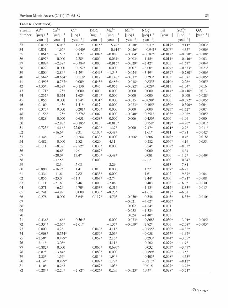
Table 6 �C for all analyzed streams

Stream Al3+ Ca2+ Cl− DOC Mg2+ Mn2+ NO−3 pH SO2−

4 QAnumber [μeq l−1 [μeq l−1 [μeq l−1 [mg l−1 [μeq l−1 [μeq l−1 [μeq l−1 [year−1] [μeq l−1 [year−1]

year−1] year−1] year−1] year−1] year−1] year−1] year−1] year−1]

1 −4.65* −12.8* 0.000 0.122* −6.17* −0.567* −2.15* 0.053* −22.1* −0.012*2 −7.39* −6.24* −0.282* 0.005 −3.09* −0.437* −3.00* 0.060* −9.58* −0.0053 −0.667* −25.0* 13.8* −0.018* −20.1* −0.733* −14.2* 0.028* −40.2* −0.006*4 −27.6* −25.0* −3.02* −0.012 −24.7* −1.97* −6.79* 0.018* −59.7* −0.0015 −18.2* −22.9* −3.22* −0.007 −22.3* −1.33* −8.44* 0.010* −40.4* −0.005*6 −4.59* −22.0* 7.44* 0.150* −6.58* −0.629* −1.23* 0.057* −16.0* −0.023*7 −2.25* −10.9* 26.3* 0.100 0.000 −0.582* −1.34* 0.020 −13.0* −0.017*8 0.111* −17.5* 0.705 0.030* −7.47* −0.076* −9.14* 0.014* −25.0* 0.006*9 0.278* −16.6* −3.29* 0.013 −9.40* −0.046* −9.68* 0.021* −17.4* 0.00010 −0.048 3.33* −0.403* 0.005 1.03 0.055* −6.33* 0.020* −2.43* 0.027*11 −0.222 13.3* 0.209 −0.021 2.74* −0.020 −5.36* 0.035* −5.52* 0.052*12 −1.49* −7.07* −0.513 0.150* −2.19* −0.050* −7.56* 0.061* −8.07* 0.00113 0.043 −4.51* 3.17* 0.006 −2.74* −0.036* −4.37* 0.012* −13.3* 0.00214 −0.074 −3.60* 14.4* 0.003 −5.48* 0.014 −5.03* 0.014* −13.4* −0.008*15 −0.188* −2.83* −0.769* 0.034* −1.37* −0.073* −3.23* 0.018* −6.02* −0.006*16 −3.50* −9.98* 0.000 0.274* −3.53* −0.312* −1.97* 0.030* −9.37* −0.021*17 −4.38* −7.98* 0.353* 0.056* −1.54* −0.330* −1.61* 0.023* −6.77* −0.015*18 −2.78* −6.65* 0.000 0.230* −1.37* −0.218* −1.45* 0.028* −5.44* −0.013*19 −3.34* −18.3* 17.3* 0.135* 0.000 0.319* −1.88* 0.025* −15.4* −0.027*20 −4.08* −9.98* 6.04* 0.134* −4.11* −0.728* −0.538* 0.059* −9.89* −0.030*21 −9.29* −12.8* 0.282* 0.133* −1.03* −0.546* −1.78* 0.021* −12.9* −0.011*22 −3.15* −8.83* 6.85* 0.178* −2.29* −0.659* −0.513* 0.070* −10.6* −0.016*23 −20.5* −13.1* 15.8* 0.131* −5.87* −0.364* −8.87* 0.010 −38.7* −0.00124 −1.22* −1.75* 4.80* 0.170* −0.686* −0.061* −1.05* 0.001 −5.21* −0.003*25 0.185 1.25* −0.353* 0.034* 0.343* 0.000 2.42* 0.000 −1.67* 0.006*26 −0.341* −0.651* 0.011 0.000 −0.010* 0.878* −1.93* 0.007*27 0.049 1.29* −0.049 0.067* 0.754* 0.001 5.92* 0.012* −1.37* −0.024*28 −4.99 2.68* 0.000 −0.455* 0.591 0.025* 0.000 −0.00429 −11.3* −0.125* 8.33 0.025* −58.3*30 −6.35* 0.017 3.23* 0.075* −3.8231 −0.051* −1.06* −0.355* −0.010 −0.592* −0.011* −0.107 0.002 −1.22* −0.00132 −0.043* −7.30* −3.36* 0.005 −7.12* −0.064* −6.89* 0.022* −8.53* 0.003*


Table 6 (continued)




33 0.016* −6.03* −1.67* −0.015* −5.49* −0.010* −2.37* 0.017* −9.11* 0.003*34 0.051 −1.66* −0.940* 0.017 −0.914* −0.026* −0.941* 0.007* −4.35* 0.006*35 0.061* −1.58* 0.027 −0.007* −0.008 −0.004* −0.582* −0.012* −0.390* −0.008*36 0.097* 0.000 2.28* 0.000 0.064* −0.003* −1.45* 0.011* −0.416* −0.00337 0.088* −2.38* −0.384* 0.000 −0.916* −0.029* −2.42* 0.005 −1.67* 0.004*38 0.022 0.000 0.157* 0.010 0.000 0.007 −3.00* 0.029* −0.833* 0.023*39 0.000 −2.84* −1.29* −0.049* −1.54* −0.024* −3.49* −0.039* −0.780* 0.006*40 −0.564* −0.664* 0.118* 0.012 −0.148* −0.017* 0.393* 0.005 −1.37* −0.005*41 −0.499* −0.767* 0.009 0.043* 0.486* −0.018* 0.835* 0.010* −2.26* 0.005*42 −3.55* −0.389 −0.150 0.045 −0.055 −0.082* 0.029* −0.013 −1.04* 0.01643 0.171* 1.75* 0.000 0.000 0.000 0.000 0.000 −0.014* −0.416* 0.01344 0.232* 0.624 1.62* 0.010* 0.000 0.000 0.000 0.000 0.000 −0.028*45 0.056 0.000 1.54* 0.031* 0.000 −0.015 −0.090* 0.000 −0.892* −0.005*46 −0.109 1.43* 1.41* 0.017 0.000 −0.073* −0.105* 0.050* −0.390* 0.00447 0.375* 0.000 0.201* 0.050* 0.000 0.000 0.000 0.023* −1.62* 0.00748 0.156* 1.25* 0.376* −0.007 0.000 −0.040* 0.251* 0.033* −2.08* 0.005*49 0.028 0.000 0.651 −0.038* 0.000 0.006 0.450* 0.000 −1.04 0.00050 −2.88* −0.185* 0.010 −0.813* 0.759* 0.012* −4.90* −0.001*51 0.723* −4.16* 22.0* 0.020* −1.37* 0.000 −2.17* −0.021* −12.2* −0.011*52 −16.6* 8.31 0.100* −5.48* 1.61* −0.011 −7.81 −0.042*53 −3.34* −1.25 −0.564 0.033* 0.000 −0.306* −0.806 0.040* −10.4* 0.018*54 0.482 0.000 2.82 −0.020 4.11 −0.282 0.050* −4.16 0.05555 −0.111 −8.32 −2.82* 0.033* 0.000 3.14* 0.038* −8.33*56 −16.6* −19.0 0.067* 0.000 0.000 −4.3457 −20.0* 13.4* 0.050* −5.48* 0.081 0.000 −11.2* −0.049*58 −17.5* 0.000 −2.22 0.000 0.34759 −18.3 −5.08 −2.29 −0.013 −7.8160 −0.890 −16.2* 1.41 0.013 0.000 1.27 0.067* −6.2561 −0.334 −11.6 2.82 0.033* 0.000 1.61 0.002 −9.37* −0.00462 0.056 −25.0 −11.3 0.067* −2.74 2.44* 0.000 −7.81* −0.00863 0.111 −21.6 8.46 0.000 −2.06 0.403 0.006 −16.0* −0.03064 0.371 −6.24 4.70* 0.033* −0.514 −1.13* 0.012* −8.33* −0.01565 −0.741 −4.99 0.000 0.033* −8.23* −1.61* −0.018* −6.0266 −0.278 0.000 5.64* 0.117* −4.70* −0.050* 0.346 0.045* −8.33* −0.010*67 −0.021 −4.62* −0.006*68 0.002 −4.84* 0.00169 −0.033 −1.32* 0.00370 0.024 −1.40* 0.00371 −0.436* −1.66* 0.564* 0.000 −0.073* 0.868* 0.030* −3.01* −0.005*72 −0.334* −2.66* −2.01* −1.37* −0.059* 2.82* 0.006 −2.08* −0.003*73 0.000 4.26 0.040* 4.11* −0.755* 0.030* −4.82*74 −0.908* 0.554* 0.050* 2.06* −0.038 0.057* −1.67*75 −2.50* 0.499* 0.057* 2.15* 0.293* 0.044* −3.55*76 −3.11* 3.08* 4.11* −0.202 0.079* −11.7*77 −0.882* 0.000 0.063* 0.686* 0.032 0.033* −3.47*78 −6.87* −3.84* 0.083* 0.000 −0.799* 0.028* −13.5*79 −2.83* 1.56* 0.014* 1.94* 0.403* 0.008* −4.53*80 −4.14* 0.499* 0.097* 1.79* −0.217* 0.044* −8.12*81 −1.10* −0.263 0.067* 1.03* −0.015 0.027* −3.23*82 −0.284* −2.20* −2.82* −0.026* 0.235 −0.023* 13.4* 0.028* −5.21*


Table 6 (continued)




83 0.209* −0.021* −1.41 0.230* −2.19* −0.018* 1.01* 0.031* −5.78* 0.00184 −1.44* −2.18* 0.504 0.135 −4.00* −0.205* 2.02* 0.125* −19.1* 0.020*85 0.056 −1.64* −7.47* 0.308* −3.81* −0.028 0.110 0.033* −15.5* −0.00786 0.549* 1.20* 11.7* 0.248* −0.806* −0.017 0.856* 0.026* −7.06* −0.002*

References

Aber, J. D., Nadelhoffer, K. J., Steuder, P., & Melillo, J. M.(1989). Nitrogen saturation in northern forest ecosys-tems. BioScience, 39, 378–386.

Alewell, C., Armbruster, M., Bittersohl, J., Evans, C. D.,Meesenburg, H., Moritz, K., et al. (2001). Are theresigns of aquatic recovery after two decades of re-duced acid deposition in the low mountain ranges ofGermany? Hydrology and Earth System Science, 5,367–378.

Alewell, C., Manderscheid, B., Bittersohl, J., &Meesenburg, H. (2000). Is acidification still anecological threat? Nature, 407, 856–857.

Armbruster, M. (1998). Zeitliche Dynamik der Wasser-und Elementflüsse in Waldökosystemen. FreiburgerBodenkundliche Abhandlungen, 38, 1–301.

Armbruster, M., Abiy, M., & Feger, K. H. (2003). The bio-geochemistry of two forested catchments in the BlackForest and the eastern Ore Mountains (Germany) -Effects of changing atmospheric inputs on soil solutionand streamwater chemistry. Biogeochemistry, 65, 341–368.

Baker, J. P., & Schofield, C. L. (1982). Aluminum toxicityto fish in acidic waters. Water Air Soil Pollution, 18,289–309.

Beudert, B., & Klöcking, B. (2007). Große Ohe: Impactof bark beetle infestation on the water and matterbudget of a forested catchment. In: H. Puhlmann, &R. Schwarze (Eds.), Forest hydrology – Results of re-search in Germany and Russia (pp. 41–63). Koblenz:Part I. IHP-HWRP-Berichte, H. 6.

Bihl, C. (2004). Erschließung und Einsatz mineralis-cher Sekundärrohstof fe im Bodenschutz im Wald.Deutsche Nationalbiliothek.

Braukmann, U. (2001). Stream acidification in SouthGermany – Chemical and biological assessment meth-ods and trends. Aquatic Ecology, 35, 207–232.

Burkey, J. (2009). Mann-Kendall Tau-b with Sen’sMethod (enhanced). Available online at http://www.mathworks.in/matlabcentral/fileexchange/11190. Ac-cessed on 19 July 2010.

Davies, J. J. L., Jenkins, A., Monteith, D. T., Evans, C. D.,& Cooper, D. M. (2005). Trends in surface waterchemistry of acidified UK Freshwaters, 1988–2002.Environmental Pollution, 137, 27–39.

Diefenbach-Fries, H., & Beudert, B. (2007). Report onnational ICP IM activities in Germany. Fifteen yearsof monitoring in the Forellenbach area—Using massbalances, bioindication, and modelling approachesto detect air pollution effects in a rapidly chang-ing ecosystem: Main results. In: S. Kleemola, & M.Forsius (Eds.), 16th Annual Report 2007 (pp. 63–81). UNECE ICP Integrated Monitoring. The FinnishEnvironment 26/2007, Finnish Environment Institute,Helsinki.

Dise, N., Matzner, E., & Gundersen, P. (1998). Nitrogenstatus of European forest ecosystems. Water Air SoilPollution, 105(1/2), 143–154.

Ditsche-Kuru, P. (2003). Wald in Wasserschutzgebi-eten von Trinkwassertalsperren - Zusammenfassungund Auswertung der ATT-Untersuchungsprogramme(p. 110) (unpublished report).

Driscoll, C. T., Bisogni, J. J., & Schofield, C. L. (1980).Effect of aluminum speciation on fish in diluteacidified waters. Nature, 248, 161–164.

Driscoll, C. T., Likens, G. E., Hedin, L. O., Eaton, J. S.,& Borman, F. H. (1989). Changes in the chemistry ofsurface waters. Environmental Science & Technology,23, 137–143.

Evans, C. D., Cullen, J. M., Alewell, C., Marchetto, A.,Moldan, F., Kopácek, J., et al. (2001a). Recovery fromacidification in European surface waters. Hydrologyand Earth System Science, 5, 283–297.

Evans, C. D., Harriman, R., Monteith, D. T., & Jenkins, A.(2001b). Assessing the suitability of acid neutralisingcapacity as a measure of long-term trends in acidicwaters based on two parallel datasets. Water Air SoilPollution, 130, 1541–1546.

Feger, K. H., Martin, D., & Zöttl, H. W. (1995). En-twicklung der Gewässerazidität im Schwarzwald - sinddepositionsbedingte Veränderungen erkennbar? DieNaturwissenschaften, 82, 420–423.

Fink, S., Feger, K. H., Gülpen, M., Armbruster, M., &Lorenz, K. (1999). Magnesium-Mangelvergilbung anFichte – Einfluss von frühsommerlicher Trockenheitund. Dolomit-Kalkung. FZKA-BWPLUS-Berichtsreihe 25. Available online at http://bwplus.fzk.de/berichte/SBer/PEF197001SBer.pdf. Accessed on26 July 2010.

Freeman, C., Evans, C. D., Monteith, D. T., Reynolds, B.,& Fenner, N. (2001). Export of organic carbon frompeat soils. Nature, 412, 785.

http://www.mathworks.in/matlabcentral/fileexchange/11190

http://www.mathworks.in/matlabcentral/fileexchange/11190

http://bwplus.fzk.de/berichte/SBer/PEF197001SBer.pdf

http://bwplus.fzk.de/berichte/SBer/PEF197001SBer.pdf


Gäth, S., & Frede, H. G. (1991). Einfluss der Land-nutzungsform auf die Nitratbelastung des Grund-wassers im Osthessischen Bergland. MitteilungenDeutsche Bodenkundliche Gesellschaft, 66, 943–946.

Gauger, T., Haenel, H.-D., Rösemann, C., Dämmgen, U.,Bleeker, A., Erisman, J. W., et al. (2008). NationalImplementation of the UNECE Convention on Long-range Transboundary Air Pollution (Effects) / Na-tionale Umsetzung UNECE-Luftreinhaltekonvention(Wirkungen): Part 1: Deposition Loads: Methods,modelling and mapping results, trends. BMU/UBA204 63 252. UBA-Texte 38/08 (1). ISSN 1862-4804.

Gilbert, R. O. (1987). Statistical methods for environmen-tal pollution monitoring. New York: Van NostrandReinhold Inc.

Gray, N. F. (2008). Drinking water quality: Problems andsolutions (2nd ed.). Cambridge University Press.

Grunewald, K., Scheithauer, J., Böhm, A., & Pavlik,D. (2004). Einzugsgebietsbewirtschaftung vonTrinkwassertalsperren im Erzgebirge unter demAspekt veränderter Huminstoffeinträge. In:Bronstert, et al. (Ed.), Forum für Hydrologie undWasserbewirtschaftung, Heft 05, Band 1, München.(pp. 265–272).

Harriman, R., Watt, A. W., Christie, A. E. G., Moore,D. W., McCartney, A. G., & Taylor, E. M. (2003).Quantifying the effects of forestry practices on the re-covery of upland streams and lochs from acidification.The Science of the Total Environment, 310, 101–111.

Hegg, C., Jeisy, M., & Waldner, P. (2004). Waldund Trinkwasser, Eine Literaturstudie. Eidg.Forschungsanstalt für Wald, Schnee und Landschaft,WSL, Birmensdorf.

Hildebrand, E. E. (1991). The influence of forestsite fertilisation on soil solution chemistry.Berichtsband des Seminars des ECE/FAO/ILO-Gemeinschaftsausschusses vom 26.-30.6.1990 inMünchen, über Schonung und Verbesserung desBodens als Grundlage nachhaltiger Forstwirtschaft(pp. 193–204). Bonn MELF.

Hildebrand, E. E., & Schack-Kirchner, H. (2000). Initialeffects of lime and rock powder application on soilsolution chemistry in a dystric cambisol - Results ofmodel experiments. Nutrient Cycling in Agroecosys-tems, 56, 69–78.

Hirsch, R. M., & Slack, J. R. (1984). A nonparametric trendtest for seasonal data with serial dependence. WaterResouces Research, 20(6), 727–732.

Jordi, B. (2005). Der Waldboden – ein optimaler Filter.WSL – Umwelt.

Kaufmann, H., & Nussbaumer, T. (1999). Bildung undEigenschaften von Chlorverbindungen bei Verbren-nung biogener Brennstoffe. Gefahrstof fe – Reinhal-tung der Luft, 59(7/8), 267–272.

Kopácek, J., Hejzlar, J., Stuchlík, E., Fott, J., & Vesely’, J.(1998). Reversibility of acidification of mountain lakesafter reduction in nitrogen and sulphur emissions inCentral Europe. Limnology Oceanography, 43, 357–361.

Kopácek, J., Stuchlík, E., Veselý, J., Schaumburg, J.,Anderson, I., Fott, J., et al. (2002). Hysteresis in re-

versal of Central European mountain lakes from at-mospheric acidification. Water Air Soil Pollution, 2,91–114, Focus.

Körner, J. (1996). Abflussbildung, Interflow undStoffbilanz im Schönbuch Waldgebiet (206 pp.).Institut und Museum für Geologie und Paläontologieder Universität Tübingen.

Kreutzer, K. (1994). Folgerungen aus der Höglwald-forschung. AFZ-Der Wald, 14, 769–774.

Lenz, R. J. M., Müller, A., & Erhard, M. (1994).Veränderungen der Säureneutralisationskapazitätnordostbayerischer Wälder. Forstarchiv, 65, 172–182.

Lorz, C., Hruška, J., & Krám, P. (2003). Modeling andmonitoring of long-term acidification in an uplandcatchment of the Western Ore Mountains, SE Ger-many, SE-Germany. The Science of the Total Environ-ment, 310, 153–161.

Lorz, C., & Schneider, B. (2003). Regenerierung einesversauerten Fließgewässers im Oberen Westerzge-birge. In: Freiburger Forstliche Forschung, Heft 49,137–151.

Majer, V., Cosby, B. J., Kopacek, J., & Veselý, J. (2003).Modelling reversibility of Central European moun-tain lakes from acidification: Part I – The Bohemianforest. Hydrology and Earth System Science, 7, 494–509.

Meesenburg, H., Eichhorn, J., & Meiwes, K. J. (2009).Atmospheric deposition and canopy interaction. In:R. Brumme, & P. K. Khanna (Eds.), Functioning andmanagement of European beech ecosystems. Ecologi-cal Studies (pp. 265–302). Berlin: Springer.

Meesenburg, H., Meiwes, K. J., & Rademacher, P. (1995).Long term trends in atmospheric deposition and seep-age output in northwest German forest ecosystems.Water Air Soil Pollution, 85, 611–616.

Meesenburg, H., Meiwes, K. J., Wagner, M., & Prenzel,J. (2001). Ecosystem effects after ameliorative limingof a catchment at the Harz mountains, Germany. In:W. J. Horst, et al. (Eds.), Plant nutrition - Food secu-rity and sustainability of agro-ecosystem (pp. 914–915).Netherlands: Kluver Academic Publishers.

Moritz, K., & Bittersohl, J. (2000). Turnover of nitrogenand acidfication in the small headwater catchmentMarkungsgraben. Silva Gabreta, 4, 63–70.

OHGE (2010). Observatoire Hydro-Géochimique del’Environnement. Available online at http://ohge.u-strasbg.fr/index.html. Accessed on 18 July 2010.

Porcal, P., Koprivnjak, J. F., Molot, L. A., & Dillon, P. J.(2009). Humic substances-part 7: The biogeochemistryof dissolved organic carbon and its interactions withclimate change. Environmental Science and PollutionResearch, 16, 714–726.

Prechtel, A., Alewell, C., Armbruster, M., Bittersohl, J.,Cullen, J. M., Evans, C. D., et al. (2001). Response ofsulphur dynamics in European catchments to decreas-ing sulphate deposition. Hydrology and Earth SystemScience, 5(3), 311–325.

Pütz, K., Reichelt, P., Sudbrack, R., & Friemel, M. (2002).Nitratbericht Sächsischer Trinkwassertalsperren– Bericht der Landestalsperrenverwaltung desFreistaates Sachsen zur Belastung der sächsischen

http://ohge.u-strasbg.fr/index.html

http://ohge.u-strasbg.fr/index.html


Talsperren mit Nitrat bis zum Jahre 2002.Pirna (pp. 55). Available online at http://www.smul.sachsen.de/de/wu/organisation/staatsbetriebe/ltv/downloads/nitratbericht2002_b.pdf. Accessed on 27July 2010.

Raben, G., Andreae, H., & Meyer-Heisig, M. (2000). Long-term acid load and its consequences in forest ecosys-tems of Saxony (Germany). Water Air Soil Pollution,122, 93–103.

Reuss, J. O., & Johnson, D. W. (1986). Acid depositionand the acidification of soils and waters. EcologicalStudies, 59, 199. New York: Springer.

Rhode, H., Grenfelt, P., Wisniewski, J., Ågren, C.,Bengtsson, G., Hultberg, H., et al. (1995). Acid Reign’95? In Conference summary statement from the 5thinternational conference on acidic deposition. Scienceand policy (pp. 1–15). Göteborg: Kluwer AcademicPublishers.

Schaumburg, J., Maetze, A., Lehmann, R., & Coring, E.(2010). Monitoringprogramm für versauerte Gewässerdurch Luftschadstoffe in der BundesrepublikDeutschland im Rahmen der ECE - Bericht derJahre 2007–2008; Bayerisches Landesamt für Umweltim Auftrag des Umweltbundesamtes, München(134 p.).

Schaumburg, J., Kifinger, B., Lehmann, R., Maetze, A.,Coring, E., Baltzer, S., et al. (2008). Monitoringpro-gramm für versauerte Gewässer durch Luftschadstoffein der Bundesrepublik Deutschland im Rahmen derECE. Bericht der Jahre 2005–2006, Bayerisches Lan-desamt für Umwelt im Auftrag des Umweltbunde-samtes, München (235 p).

Sen, P. K. (1968). Estimates of the regression coefficientbased on Kendall’s Tau. Journal of the American Sta-tistical Association, 63, 1379–1389.

Skjelkvale, B. L., Borg, H., Hindar, A., & Wilander, A.(2007). Large scale patterns of chemical recovery inlakes in Norway and Sweden: Importance of seasaltepisodes and changes in dissolved organic carbon. Ap-plied Geochemistry, 22(6), 1174–1180.

Skjelkvale, B. L., Stoddard, J. L., Jeffers, J. N. R., Tørseth,K., Høgasen, T., Bowman, J., et al. (2005). Regionalscale evidence for improvements in surface waterchemistry 1990–2001. Environmental Pollution, 137,165–176.

Stoddard, J. L., Jeffries, D. S., Lükewille, A., Clair, T. A.,Dillon, P. J., Driscoll, C. T., et al. (1999). Regionaltrends in aquatic recovery from acidification in NorthAmerica and Europe. Nature, 401, 575–578.

Sucker, C., & Krause, K. (2010). Increasing dissolvedorganic carbon concentrations in freshwaters: Whatis the actual driver? iForest 3: 106–108. Availableonline at http://www.sisef.it/iforest/show.php?id=546.Accessed on 25 July 2010.

Sucker, C., Puhlmann, H., Zirlewagen, D., Wilpert,K. V., & Feger, K. H. (2009). Bodenschutzkalkungenin Wäldern zur Verbesserung der Wasserqualität –Vergleichende Untersuchungen auf Einzugsgebietsebene.Hydrologie und Wasserbewirtschaftung, 4, 250–262.

UBA (= Umweltbundesamt) (2000). Bestim-mung und Kartierung der Critical Loads &

Levels für Deutschland. Available online athttp://www.umweltbundesamt.de/umweltbeobachtung/uid/mapping/karte_clmax_s.htm. Accessed on 25January 2010.

UBA (= Umweltbundesamt) (Ed.) (2009). Nationaltrend tables for the German atmospheric emissionreporting 1990–2008. Available online at http://www.umweltbundesamt.de/emissionen/archiv/EM_Entwicklung_in_D_Trendtabelle_LUFT_v2.1.2_EU-Submission_2010.xls.zip. Accessed on 6 July 2010.

Ulrich, K. U., Paul, L., & Meybohm, A. (2006). Responseof drinking-water reservoir ecosystems to decreasedacidic atmospheric deposition in SE Germany: Trendsof chemical reversal. Environmental Pollution, 141,42–53.

UNECE (2009). The condition of forests in Europe, 2009executive report, ICP forests and European com-mission, Hamburg and Brussels. Available online athttp://www.icp-forests.org/pdf/ER2005.pdf. Accessedon 6 July 2010.

Veselý, J., Hruška, J., Norton, S. A., & Johnson, C. E.(1998). Trends in the chemistry of acidified Bohemianlakes from 1984 to 1995: I. Major solutes. Water AirSoil Pollution, 108, 107–127.

Veselý, J., Majer, V., & Norton, S. A. (2002). Heteroge-neous response of central European streams to de-creased acidic atmospheric deposition. EnvironmentalPollution, 120, 275–281.

von Wilpert, K. (2007). Chemical deposition and seep-age water quality in forests. In: H. Puhlmann, & R.Schwarze (Eds.), Forest hydrology – Results of re-search in Germany and Russia (pp. 23–36). Koblenz:Part I. IHP-HWRP-Berichte, H. 6.

von Wilpert, K., & Puhlmann, H. (2007). Conventwald:Silvicultural management of seepage water quality.In: H. Puhlmann, & R. Schwarze (Eds.), Forest hydrol-ogy – results of research in Germany and Russia (pp.63–90). Koblenz: Part I. IHP-HWRP-Berichte, H. 6.

von Wilpert, K., Schäffer, J., Holzmann, S., Meining,S., Zirlewagen, D., & Augustin, N. (2010).Was Waldzustandserfassung und ForstlicheUmweltüberwachung bewirkt haben – Ableitungeines langfristigen Kalkungsprogramms. AFZ-DerWald, 3, 20–25.

von Wilpert, K., & Zirlewagen, D. (2007). Forestry Man-agement options to maintain sustainability – Elementbudgets at Level II sites in South – West Germany. In:J. Eichhorn (Ed.), Forests in a changing environment –Results of 20 years ICP forests monitoring (Vol. 142,pp. 170–179). Schriften aus der Forstlichen FakultätUniversität Göttingen.

Wellbrock, N., Riek, W., & Wolff, B. (2005). Characterisa-tion of and changes in the atmospheric deposition situ-ation in German forest ecosystems using multivariatestatistics. European Journal Forest Research, 124, 261–271.

Westermann, F. (2000). Versauerung von Fließgewässernin Rheinland-Pfalz. Untersuchungen von Bachober-läufen im Hunsrück 1983–1999 - Entwicklungen undTrends (113 pp.). Landesamt für Wasserwirtschaft -Bericht 206/00. Mainz.

http://www.smul.sachsen.de/de/wu/organisation/staatsbetriebe/ltv/downloads/nitratbericht2002_b.pdf



http://www.sisef.it/iforest/show.php?id=546

http://www.umweltbundesamt.de/umweltbeobachtung/uid/mapping/karte_clmax_s.htm

http://www.umweltbundesamt.de/umweltbeobachtung/uid/mapping/karte_clmax_s.htm

http://www.umweltbundesamt.de/emissionen/archiv/EM_Entwicklung_in_D_Trendtabelle_LUFT_v2.1.2_EU-Submission_2010.xls.zip




http://www.icp-forests.org/pdf/ER2005.pdf


Wolff, B., & Riek, W. (1998). Chemischer Waldboden-zustand in Deutschland, Ergebnisse der Bodenanaly-sen im Rahmen der BZE. Allgemeine Forst-Zeitschrift,Der Wald, 53(10), 503–506.

Wright, R. F., Alewell, C., Cullen, J., Evans, C. D.,Marchetto, A., Moldan, F., et al. (2001). Trendsin nitrogen deposition and leaching in acid-sensitivestreams in Europe. Hydrology and Earth SystemScience, 5, 299–310.

Zech, W., Guggenberger, G., & Schulten, H. R. (1994).Budgets and chemistry of dissolved organic carbon inforest soils: Effects of anthropogenic soil acidification.The Science of the Total Environment, 152, 49–62.

Zirlewagen, D., & von Wilpert, K. (2002). Was hatWaldbau mit Trinkwasservorsorge zu tun? Schriften-reihe Freiburger Forstliche Forschung, 18, 309–319.

acidification reversal in low mountain range streams of germany

Documents