the effect of acidification
TRANSCRIPT
THE EFFECT OF ACIDIFICATION ON EPILITHIC ALGAE IN THE LOCH ARD CATCHMENT
John Henri Kinross
Thesis submitted in fulfilment of the requirements of the Council for National Academic Awards for the degree of
Doctor of Philosophy
June, 1991
Napier Polytechnic of Edinburgh and
SOAFD Freshwater Fisheries Laboratory, Faskally, Pitlochry.
IA

To Graham

I hereby declare that: .
All the work presented in this thesis has been carried out by myself and that no part of this work has been -submitted in support of a degree validated by the CNAA or a University
ýý Kýý (Signed)
John H Kinross
I have received advice, help and encouragement from a large number of people in the course of this work.
I am indebted to my supervisors, Nick Christofi and Paul Read, for their support in initiating this research and for allowing me a free hand in conducting it. Their encouragement and guidance is much appreciated.
Thanks to, the Director and staff of SOAFD Freshwater Fisheries Laboratory, Faskally, Pitlochry, for permitting me to carry out the field work in their experimental area, particularly to Brian Morrison who proposed the initial survey in 1985, and to Ron Harriman who gave access to the chemical data from composite samplers. Thanks also to David Hay for continuous temperature records for some sites.
To Tony Bailey-Watts, Institute of Freshwater Ecology, Bush, Penicuik, my external super- visor, thanks for the useful discussions on methods and algal taxonomy.
The Solway River Purification Board, Rivers House, Dumfries, kindly gave me access to chemical data on the Loch Dee, Galloway, streams.
Thanks is due to the Forestry Commission for permitting access to sites within their forest areas at Loch Ard, Loch Rannoch and Galloway, and to the proprietors of Comer and Frenich farms in the L. Ard area.
Robin Henderson of Napier Polytechnic advised on statistical methods throughout the course of the work. I have been greatly assisted also by staff of the Computer Unit and of the Dunning Library, Napier Polytechnic.
During the development and construction of the PAR sensors and integrators I received assistance from members of staff at Napier Polytechnic. Thanks to the Department of Mechanical Engineering for machining the master for the sensor head, and to the Department of Applied Chemical Sciences Polymer Group for assistance with moulding the copies.
Ronnie Milne of ITE, Bush, Penicuik, give useful advice on light measurement and loaned two Kipp Solarimeters and integrators.
The PAR integrators and direct-reading meter were designed and built by John Gurney, of Edinburgh, as an exercise. I am deeply indebted to him for the time spent in this and for his assistance in the testing of the integrators.
Macam Photometrics Ltd., Kelvin Square, Livingston, calibrated the sensor and checked its spectral response.
Numerous members of staff at Napier Polytechnic have helped in some way through advice or generous loans of equipment.
I thank my wife, Alison, for her support both moral and financial during the period of this project.
Finally, thanks to Carol Robson for typing the manuscript throughout its many metamor- phoses.
in
Dedication
Declaration Acknowledgements Contents
List of Figures
List of Tables
Glossary of abbreviations Summary
1. INTRODUCTION
2. MATERIALS AND METHODS
2.1 Choice of Sites
2.2 Field Sampling
2.2.1 Sampling methods for algae 2.2.1.1 Natural substrates 2.2.1.2 Artificial substrates
2.2.2 Transport of samples 2.2.3 Water sampling 2.2.4 Temperature
2.2.5 Flow
2.2.6 Light
2.3 Laboratory methods 2.3.1 Microscopic examination of algal samples 2.3.2 Photography
2.3.3 Species identifications
2.3.4 Species abundance 2.4 Treatment of Samples
2.4.1 Biomass estimation 2.4.1.1 Pigment extraction 2.4.1.2 Ash-Free Dry Weight
2.4.1.3 Chlorophyll analysis 2.4.1.4 Carotenoid analysis
2.4.2 Surface area of substrates
Page i
ii
iv
vii xi
X111
xv
1
7 7 7
12
13
iv.

F=
2.5 Analysis of Water Samples 16
2.5.1 pH 2.5.2 Absorption measurements 2.5.3 Chemical analyses
2.6 Algal Growth Experiments 17
2.6.1 Media
2.6.2 Artificial Stream Channels
2.6.3 Measurement of Growth Rates
2.6.5 Static and semi-static culture 2.7 Statistical Methods 23
2.7.1 Recalculation of species and site values from CANOCO
3. RESULTS 24
3.1 Field Sampling 24
3.2 Environmental Data 31
3.3 Biomass 39
3.4 Channel Growth Experiments 48
3.4.1 Effect of pH on Growth Rate
3.4.2 Effect of Al on Growth Rate
3.4.3 Species composition on continued culture 3.4.4 Influence of Channel pH on Biomass
3.5 Tub Growth Experiments 83
3.6 Cultural Studies on Stigeocloniwn isolates 90
4. DISCUSSION 93
4.1 Characteristics of Sites 93
4.2 Sampling Methods for Species and Biomass 98
4.2.1 Species Identification Problems
4.2.2 Estimation of Biomass
4.3. Evidence of Seasonality 108
4.4 Species Diversity 113
4.4.1 Measures of Richness, Diversity and Evenness
4.4.2 Species Number in Each Sample as a Measure of Richness
4.5 Grouping of species by NASSOG BAS (Inverse Association Analysis) 125
V.
Page
4.6 Evidence for Community Differences between sites 143
4.6.1 Species Covariation
4.6.2 Species Association
4.6.3 Normal Association Analysis
4.6.4 Cluster Analysis
4.6.4.1 Choice of Method
4.6.4.2 Results
4.7 Species - Environment Relationships 167
4.7.1 Preliminary Considerations: choice of method 4.7.3 Canonical Correspondence Analysis
4.7.3.1 Use of CANOCO
4.7.3.2 Variables excluded from analysis by CANOCO
4.7.3.3 Transformation of variables 4.7.3.4 Results of analyses 4.7.3.5. Calibration using CANOCO
4.8 Algal Production 209
4.8.1 Methods for measuring production rates 4.8.2 Biomass
4.8.3 Production rates in laboratory studies 4.8.4 Growth rate measurements
5.0 CONCLUSIONS 219
6.0 RECOMMENDATIONS FOR FUTURE WORK 220
REFERENCES 223
APPENDIX 1 Species Descriptions 240
APPENDIX 2 Light Measurement 247
APPENDIX 3 Thermostat circuit 263
i
vi.
List of Figures
1. Map - location of sampling sites in the Loch Ard area. 2. Artificial stream apparatus: plan. 3. Growth rate during successive periods of exposure to media of differing pH of Hormid- -
ium subtile. 4. Growth rate during successive periods of exposure to media of differing pH of Gem-
inella 8 pm. 5. Growth rate during successive periods of exposure, to media of differing pH of
Stigeoclonium 5 pm. 6. Growth rate during successive periods, of exposure to media of differing pH of
Stigeoclonium 8 pm. 7. Growth rate during successive periods of exposure to media of differing pH of Drapar-
naldia sp. 8. Growth rate during successive periods of exposure to media of differing pH of
Mougeotia 8 pm. 9. Growth rate during successive periods of exposure to media of differing pH of Mougeo-
tia11pm. 10. Growth rate during successive periods of exposure to media of differing pH of Mougeo-
tia 17 pm. 11. Growth rate during successive periods of exposure to media of differing pH of Mougeo-
tia 22 pm. 12. Growth rate during successive periods of exposure to media of differing pH of Oedogo-
nium 6 pm. 13. Growth rate during successive periods of exposure to media of differing pH of Oedogo-
nium 15 pm. 14. Growth rate of filamentous algae in media of differing pH: Hormidium subtile; Geminella
8 pm.; Stigeoclonium 5 pm.; Stigeocloniwn 8 pm. 15. Growth rate of filamentous algae in media of differing pH: Mougeotia 8 pm.; Mougeotia
11 pm.; Mougeotia 17 pm.; Mougeotia 22 pm. 16. Growth rate of filamentous algae in media of differing pH: Draparnaldia sp.; Oedogonium
6 pm.; Oedogonium 15 pm. 17. Growth rate response of Hormidium subtile in media containing different levels of Si and
Al. 18. Growth rate response of Geminella 8 pm. in media containing different levels of Si and
Al. 19. Growth rate response of Stigeocloniwn 9e in media containing different levels of Si and
Al.
vii.
I 20. Growth rate response of Stigeocloniwn 10a in media containing different levels of Si
and Al. 21. Growth rate response of Draparnaldia sp. in media containing different levels of Si and
Al. 22. Growth rate response of Mougeotia 8 pm. in media containing different levels of Si and
Al. 23. Biomass developed on slides in channels, mean daily increment (a) Run 2, (b) Run 3. 24. Tub Growth Experiments (a) Influence of pH on biomass
(b) Effect of inhibition of diatom growth 25. (a) Seasonal variation in field temperature; individual values for all samples
(b) Relationship between mean field temperature and, time of sampling. 26. Plots of species abundance against annual week, with 2nd order regressions fitted
(99% C. I. ). 27. (a, b)Plots, regressions and 99% C. I. of species number in each sample with environ-
mental variables. 28. Plots, regressions (95% C. I. ) of means of range, for selected environmental variables. 29. Inverse Association Analysis - Species Association by NASSOC
(matrix A chi-squared and matrix A corrected chi-squared) 30. Inverse Association Analysis - Species Association by NASSOC
(matrix B chi-squared and matrix B corrected chi-squared) 31. Inverse Association Analysis - Species Association by NASSOC
(matrix C chi-squared and matrix C corrected chi-squared) 32. Inverse Association Analysis - Species Association by NASSOC
(subset 1 chi-squared and subset 2 chi-squared) 33. Inverse Association Analysis - Species Association by NASSOC
(subset 1 corrected chi-squared and subset 2 corrected chi-squared) 34. Inverse Association Analysis -. Species Association by NASSOC
(subset 3 chi-squared and subset 4 chi-squared) 35. Inverse Association Analysis - Species Association by NASSOC
(subset 3 corrected chi-squared and subset 4 corrected chi-squared) 36. Inverse Association Analysis - Species Association by NASSOC
(subset 5 chi-squared and subset 6 corrected chi-squared) 37. Inverse Association Analysis - Species Association by NASSOC
(subset 5 corrected chi-squared and subset 6 corrected chi-squared) 38. Inverse Association Analysis - Species Association by NASSOC
(subset 7 chi-squared and subset 8 chi-squared) 39. Inverse Association Analysis - Species Association by NASSOC
(subset 7 corrected chi-squared and subset 8 corrected chi-squared)
viii.
40. Inverse Association Analysis - Species Association by NASSOC
(subset 10 chi-squared and subset 11 chi-squared) 41. Inverse Association Analysis - Species Association by NASSOC
(subset 10 corrected chi-squared and subset 11 corrected chi-squared) 42. NASSOC Sampling Unit Associations: chi-squared on Presence-Absence data 43. NASSOC Sampling Unit Associations: corrected chi-squared on Presence-Absence
data 44. NASSOC Sampling Unit Associations: chi-squared on Presence-Absence data; rare
species deleted 45. NASSOC Sampling Unit Associations: corrected chi-shared on Presence-Absence
data, rare species deleted 46. NASSOC Sampling Unit Associations: subsets 1 and 2 compared 47. NASSOC Sampling Unit Associations: subsets 3 and 4 compared 48. NASSOC Sampling Unit Associations: subsets 5 and 6 compared 49. NASSOC Sampling Unit Associations: subsets 7 and 8 compared 50. NASSOC Sampling Unit Associations: subsets 10 and 11 compared 51. Cluster Analysis of Matrix B species data, Flexible stategy with ß= -0.25 ; Abundance
data 52. Cluster Analysis of Matrix B species data, Flexible stategy with ß= -0.25; Pooled p/a
data 53. a, b Plots of relative abundance of species against pH 54. a, b Plots of relative abundance of species against A2M 55. a, b Plots of relative abundance of species against Total Monomeric Al 56. CANOCO Biplot: DCCA on Matrix A abundance data 57. CANOCO Biplot: DCCA on Matrix A pooled p/a data 58. CANOCO Biplot: CCA on Matrix B abundance data 59. CANOCO Biplot: CCA on Matrix B pooled p/a data 60. CANOCO Biplot: DCCA on Matrix B abundance data
61. CANOCO Biplot: DCCA on Matrix B pooled p/a data
62. CANOCO Biplot: DCCA on Matrix C abundance data
63. CANOCO Biplot: DCCA on Matrix C pooled p/a data 64. Site Values on pH Vector, derived from (Detrended) Canonical Correspondence
Analyses 65. Species Values on pH Vector derived from Canonical Correspondence Analyses 66. Species Values on pH Vector derived from Detrended Canonical Correspondence
Analyses 67. Regression of Inferred pH Values of sites (using CANOCO) on mean measured pH:
Abundance data (a) L. Ard sites, matrix C data (b) Galloway and Rannoch sites
68. Regression of Inferred pH Values of sites (using CANOCO) on mean measured pH: Abundance data
ix.
69. Regression of Inferred pH Values of sites (using CANOCO) on mean measured pH: Abundance data (a) L. Ard sites, Matrix B data (b) Matrix A pH inferred from matrix B
70. Regression of Inferred pH Values of sites (using CANOCO) on mean measured pH: Pooled p/a data (a) Loch Ard sites, Matrix C (b) Matrix D, L. Ard sites
APPENDIX 2 71. Quantum-corrected absorption profiles of suspensions used in designing sensor re-
sponse curve 71. Circuit for direct reading PAR meter 73. Twin capacitor current integrator
74. Voltage Ramp current integrator
APPENDIX 3
75 Circuit for thermostat used in channel apparatus.
X
List of Tables
1. Physical characteristics of sampling sites 2. Recipes for synthetic streamwater media based on L. Ard bums
3. Comparison of artificial streamwater media used 4. Mean values of relative species abundance for each site, Matrix A
5. Mean values of relative species abundance for each site, Matrix B
6. Mean values of relative species abundance for each site, Matrix C
7. Values of pooled species presence-absence for each site, Matrix A
8. Values of pooled species presence-absence for each site, Matrix B 9. Values of pooled species presence-absence for each site, Matrix C
10. Mean values of environmental variables, Matrix A
11. Mean values of environmental variables, Matrix B
12. Mean values of environmental variables, Matrix C
13. Intercorrelations of environmental variables. Matrix C individual site/sample data
14. Mean values of biomass measures on different substrates, Matrix A 15. Mean values of biomass measures on different substrates, Matrix B 16. Mean values of biomass measures on different substrates, Matrix C
17. Correlations of biomass with environmental variables. Site-average values, Matrix C
18. Intercorrelations of biomass values. Site-average values, Matrix C.
19. Correlations of biomass with environmental variables. Individual site/sample
values, Matrix C
20. Intercorrelations of biomass values. Individual site-sample values, Matrix C
21(a-f). Growth Rates Analysis of Variance: pH manipulation experiments 22. Channel growth experiments; chemistry. pH experiments 23. Analysis of Variance on growth rate: Al/Si manipulation experiment 24. Channel growth experiments; chemistry. Al/Si manipulation experiment 25. Channel growth experiment: Final species composition, Run 2
26. Channel growth experiment: Final species composition, Run 3
27. Final channel biomass developed in pH experiments 28. Tub experiment 1. Final species composition 29. Tub experiment 2 (Germanium): Final species composition 30. Final biomass developed at different pH values
(a) Tub growth experiment 1 (b) Tub growth experiment 2 (Germanium)
31. Results of growth experiments on Stigeoclonium isolates 32. Comparison of pigment absorbances measured in acetone and methanol
xl.
33. Correlations between biomass estimates from slides 34. Seasonality of variables investigated by correlation with temperature 35. Species Richness, Diversity and Evenness
36. Correlations between measures of Species Richness, Diversity and Evenness for each
site with mean values of environmental variables: Matrix A, abundance 37. Correlations between measures of Species Richness, Diversity and Evenness for each
site with mean values of environmental variables: Matrix B, abundance 38. Correlations between measures of Species Richness, Diversity and Evenness for each
site with mean values of environmental variables: Matrix C, abundance 39. Correlations between measures of Species Richness, Diversity and Evenness for each
site with mean values of environmental variables: Matrix B, p/a 40. Species groups revealed by Inverse Association Analysis on matrices A, B and C
41. Inverse Association Analysis by NASSOC on subset pairs: Dates and Sampling Units
represented in each subset 42. Sampling Units Covariance matrix based on species (relative) abundance data
43. SU Associations by SPASSOC. BAS: Matrix A 44. SU Associations by SPASSOC. BAS: Matrix B 45. SU Associations by SPASSOC. BAS: Matrix C 46. Sampling sites, arranged in increasing order of mean pH, 1986-1988 47. Cluster Analysis Results
48. Length of Environmental Gradients, Matrix C 49. Correlations between relative species abundance and environmental variables in each
sample 50. Correlation Analysis of Total species number per sample with untransformed and Logo
environmental variables 51. Correlations between relative species" abundance and Logo transformed environ-
mental variables in each sample 52. Summary Statistics: Canonical Correspondence Analyses
53. Summary Statistics: Detrended Canonical Correspondence Analyses
54. Summary Statistics: Detrended Canonical Correspondence Analyses, omitting species 1
(Oscillatoria 1 pm) 55. Ranking of -species along axis 1 (High -> Low pH) APPENDIX 2
56 Linearity checks on PAR integrator (a) Correlations between Kipp and PAR integrator counts (b) Regression of PAR on Kipp count
X11.
Glossary of abbreviations and terms used
A= Optical Absorbance (Optical density units) at wavelength x nanometres A250 comp. Absorbance at 250 nm of composite (1 week) water samples AFDW Ash-Free Dry Weight (Weight loss on ignition at 550°C)
ALK Alkalinity
Al-TM Total Monomeric aluminium. Dissolved or complexed Al measured in catechol
violet assay, not subjected to passage over ion-exchange resin Al-NL Non-Labile aluminium. Dissolved Al complexed with organic or other ligands;
does not bind to ion exchange resin Al-L Labile aluminium; retained by ion exchange resin ANOVA ANalysis Of VAriance
CANOCOComputer program performing CANOnical COrespondence analysis (Ter Braak,
1988)
CCA Canonical Correspondence Analysis DCCA Detrended Canonical Correspondence Analysis. Detrending' is a means of
removing any 'arch' in the data along axis 2
DIC Dissolved Inorganic Carbon
Data form'
Species data is utilised in either 'abundance' (estimated relative abundance) or 'presence-absence' (p/a) form. For most applications mean abundance or 'pooled
p/a' is calculated HDPE High Density PolyEthylene
Matrix Species, biomass and environmental variables are measured in up to 15 sites, on up
to 35 occasions, to give a3 dimensional matrix, matrix C. Calculation of mean
species/biomass or environmental variable values yields a2 dimensional version. Division of the 3-D matrix along the 'occasions' dimension yields matrices A and B,
the earlier and later parts of the sampling programme. Matrix D consists of data collected in a preliminary survey in 1985 (Kinross, 1985)
NAA Normal Association Analysis, carried out by the program NASSOC. BAS
(Ludwig and Reynolds, 1988). Sampling Units are sorted into groups on the basis
of the species they contain. The X2 (chi-squared) value for each species pair in
turn is computed. Yate's corrected chi-squared is also available which corrects for bias due to rare species. Presence-absence data are used.
X111.
IAA Inverse Association Analysis - sorting of species into groups on the basis of their
presence or absence in different SUs. It is carried out using NASSOC. BAS on
an inverted data matrix. N Oi Collective term for gaseous oxides of nitrogen PAR Photosynthetically Available (or Active) Radiation. Light in the wavelength band
300-700 nm. Measured as quanta (photons); units are micromoles per square
metre per second (formerly microeinsteins per square metre per second). 1 mole
= 6.025 x 10¹³ photons PAR % Measured incident PAR expresssed as a percentage of that available in an 'open'
unshaded site, i. e. the reference site; burn 6
PAR. ABSAbsolute PAR - recalculated values of PAR at a site, in pmoles. m-2s''. Calculated
from product of measured incident PAR at the reference site and the mean PAR%
value for the secondary site
pH INST Instantaneous pH = pH measured in spot samples
pH COMP Composite pH = pH measured in composite samples RUN Experiment carried out to measure growth rate in channels. Runs 1-3 involved pH
manipulation, 4 and 5 involved different Al and Si concentrations SOAFD Scottish Office Agriculture and Fisheries Department Species Diversity
An expression of the degree to which a natural community is composed of different
species. It is composed of two components - Richness and Evenness (see section 4.4)
Richness - may be expressed-by the number of species in a sample (a) as a mean
value per site or (b) as the number of species found on each sampling occasion. Both versions have been examined in this study
SU Sampling Unit,, the term used in statistical ecology (e. g. Ludwig and Reynolds,
1988) to refer to a discrete division of the environment subjected to a sampling
procedure. It corresponds to a sampling site in this work TOC Total Organic Carbon
TON Total Oxidized Nitrogen (NO3 + NO2 )
VIF Variance Inflation Factor. One statistic provided by the output from the program CANOCO; VIF values greater than approximately 20 imply that the environ-
mental variable in question is highly correlated with others in the analysis. ,
xiv
A survey of epilithic filamentous algae was carried out at 15 sites on 10 streams with a range of mean pH from 4.37 to 6.67 in the Loch Ard area of the Trossachs, between 1986 and 1988. Monitoring of physical and chemical parameters was carried out in parallel. Photosynthetically Available Radiation (PAR) was measured using electronic integrators devel-
oped during the course of the study.
Samples of epilithic algae were taken from natural and artificial substrates (microscope slides) to determine the relative contribution of different species to the community structure. Taxa could not be identified to species level in most cases, and are described by genus and cell diameter. Forty-nine taxa were distinguished in the filamentous algal communities found. Relative abundance of taxa was estimated. The mean value of abundance was calculated for use in subsequent statistical analyses. As an alternative, presence-absence (p/a) on each occasion was scored, and a mean value (pooled
p/a) similarly calculated. Samples were taken also to determine algal biomass, as acetone or methanol extractable pigments (chlorophyll a and carotenoid) and ash-free dry weight (AFDW).
The community structure at the different sites was investigated using statistical ecology computer programs. Using Inverse Association Analysis and Canonical Correspondence Analysis, distinct species assemblages were found in
sites with mean pH values towards the extremes of the range encountered. Using Normal Association Analysis, Cluster Analysis and Canonical Correspondence Analysis, it was shown that sites are separable on the basis of the species they contain into groups related by mean pH. Using the results of Canonical Correspondence Analyses carried out by the
program CANOCO (Ter Braak, 1988) on one half of the data set, field pH may be inferred from the species data,
showing the indicator value of the community structure. In all analyses it was found that the pooled p/a data gave essentially the same result as the relative abundance data.
The effects of changes in the pH and Aluminium content of water on the growth rate of selected species of green algae was investigated using a laboratory-scale recirculating miniature artificial stream apparatus which allowed six variations to be tested at one time. Algae were grown attached to microscope slides. Growth rates were measured by counting cells in individual filaments over several successive time intervals. Mixed cultures of up to eight species were employed..
Species characteristic of the lower-pH streams such as Hormidium subtile, Geminella 8pm. , Stigeoclonium 5}un. and some species of Mougeotia have a pH optimum for growth rate between pH 4.5 and 5.5. Species characteristic of circumneutral streams, Draparnaldia sp. Stigeoclonium 8µm. and Oedogonaum species, have a pH optimum between
pH 5.0 and 6.0 or above. Hormidium subtile and Geminella 8}m. can grow at a reduced rate in a monomeric Aluminium
concentration of 200 pg 1.1 in which the majority of species tested are rapidly killed. Evidence was found for ecotypes with respect to pH in the genus Stigeoclonium.
Biomass in natural waters was positively correlated with pH in contrast to some previous reports. In mixed cultures in
the laboratory, the maximum biomass developed was in the range pH 4.5 to 5.5. around the pH optimum of the species present. At higher pH values (5.5 to 6.0) diatoms were predominant giving a brown-coloured periphyton layer which is less visually obtrusive than the bright green growth of the filamentous chlorophytes. Therefore anecdotal reports of an increased biomass upon acidification may reflect only a shift to more visible species. Inhibition of diatom growth by Germanium addition provided no evidence in favour of competition between diatoms and chlorophytes.
Differences in community structure and changes in biomass with pH in laboratory culture cannot be ascribed to changes in invertebrate grazing or heterotrophic microbial activity. It is concluded therefore that - differences between species in tolerance towards pH or associated water chemistry variables are sufficient to explain differences in algal community structure in the field.
XV.
1. INTRODUCTION
A trend towards the acidification of fresh waters has been noted in several regions of the
world over the last 20 years. This process is popularly ascribed to the effects of 'Acid Rain', but in reality acid precipitation is only one of a number of factors which predispose a catchment to acidifcation of its drainage water (Seip and Tollan, 1978).
The rainfall may be acidified beyond its natural acidity (due to dissolved C02) (Likens and Bormann, 1974) by SO2 and NO; derived both from natural sources and from the combustion of fossil fuels. In addition, particulate pollution from this latter source, 'dry deposition', can contribute acidity (Irwin, 1985). Salts in rainfall derived from sea-spray also contribute ultimately to the acidification of drainage water (Seip, 1980; Krug et al, 1985). t..
Catchments vary in their susceptibility to acid deposition. Soils, both mineral and organic, have the capacity to neutralize acidity (Bache, 1984; Edmunds and Coe, 1986). Catchments
with deep soils, especially of a neutral or alkaline nature, and with slight slope, allowing slow drainage, effectively neutralize precipitation (Bache, 1984; Edmunds and Coe, 1986; Hornung
et al, 1986). On the other hand catchments in upland areas with steep slopes, with exposed, slowly weathering bedrock and thin mainly peaty soils, are very susceptible to acidification (Bache, 1984).
Vegetation also influences soil acidity, and hence the pH of water passing through the soil. Trees may alter the precipitation pattern in a catchment and may, in addition, trap dry deposition (Mayer and Ulrich, 1974; Mayer, 1983). The growth of vegetation involves the
uptake of nutrient ions from the soil, resulting in a net increase in soil acidity, (Nilsson et al, 1982; Edmunds and Kinniburgh, 1986) the extent of which differs with species (Henderson
et al, 1977; Nilsson et al, 1982; Skeffington, 1983; Matzner and Ulrich, 1983; Hornung, 1985).
This process may be reversed when the vegetation dies back, or when a forest is cleared if the brushwood is left to decompose (Krug and Frink, 1983). However some plants such as ling (Calluna vulgaris) contain phenolic compounds which inhibit decomposition to such an extent that nutrients remain trapped in a layer of organic material, eventually forming acidic peat (Rosenqvist et al, 1980).
The rate of drainage through the soil also influences the acidity of drainage water. Prior to the
planting of trees in the past it has been the practice to plough and drain hill slopes, reducing the residence time of water in the soil. Channeling of flow through passages provided by tree roots may also occur (Bache, 1984). In addition, the drying out of previously saturated organic soils may cause acidification by the oxidation of sulphides (Van Dam, 1988).
1
In certain areas of the world sufficient of these predisposing conditions have been present to lead
to the acidification of fresh waters. This has been reported from areas of the Canadian Shield, Nova Scotia and the Adirondacks in North America (Davis et al, 1978; Harvey, 1980; Krug et al, 1985), large areas of Scandinavia (Seip and Tollan, 1978), and Wales (Stoner et al, 1984), Galloway (Wright et al, 1980) and Western Scotland (Harriman and Morrison, 1982; Harriman
and Wells, 1985) in Britain.
The most economically serious consequences of acidification are the deleterious effects on stocks
of salmonid fish indigenous to the nutrient-poor and highly oxygenated waters found in these
upland areas. The effects may be due to low pH alone or in combination with associated low Ca2+
and high Al concentrations. Invertebrates which form an important food source for these fish are
also adversely affected (Kinsman, 1984; Burton et al, 1985; Kullberg and Petersen, 1987).
It has been suggested that microbial degradation of organic material in fresh water is reduced by
acidification (Hendrey and Wright, 1975; Traaen, 1980; Allard and Moreau, 1985); more precisely, bacterial decomposers being progressively replaced by fungi which have a lower rate of mineralization (Overrein eta! , 1980). However this has been contested more recently (Ar-
nold et al, 1981).
Acidified streams and lakes are susceptible to'blooms' of attached green algae when compared with less acid streams (Hendrey, 1976; Kinsman, 1984; Stokes, 1981,1986; Turner et al, 1987)
which replace diatoms as a dominant group.
In the water column of lakes species changes occur among the phytoplankton, although there may not be any change in biomass (Molot eta!, 1990; Raddum et a1,1980). There is a shift towards
acidobiontic species of diatoms and chrysophytes, which have been utilized as indicators of lake
pH, allowing palaeoecological surveys of lake acidication to be carried out from sediment cores (Batterbee, 1984; Charles, 1985; Charles and Smol, 1988; Davis and Berge, 1980; Dixit and Dickman, 1986; Flower and B atterbee, 1983; Holmes eta!, 1989; Van Dam eta!, 1980; Van Dam, 1988).
Acidification induced changes in periphyton composition and biomass in streams and the littoral
zone of lakes are highly visible and may act as an early indicator of acidification (Turner et al, 1987) but there has been speculation as to the precise cause of biomass changes (Hall eta!, 1980; Stokes, 1981,1986).
2
The possibilities are:
(a) a direct effect of-pH favouring acidobiontic species; (b) removal of grazing organisms allowing unconstrained accumulation of particular spe- cies; (c) a decrease in the rate of decomposition of inactive algal biomass; (d) a decrease in competition from species which are inhibited by low pH (Stokes, 1986).
Algae form at least part of the diet of aquatic invertebrates (Eichenberger and Schlatter, 1978; Fulton, 1988; Hart, 1985; Hill and Knight, 1987,1988; Jacoby, 1987; Johnson, 1987; McAuliffe, 1984; Mason and Bryant, 1975; Peterson, 1987; Slack, 1936; Titmus and- Badcock, 1981; Yoshitake and Fukushima, 1985).
The abundance of invertebrate grazers in acidified streams is reduced (Arnold et al, 1981) and an inverse relationship between algal biomass and grazer abundance has been noted in experi- mentally manipulated systems including artificial acidification, invertebrate enhancement or exclusion by physical means or insecticide treatment (Eichenberger and Schlatter, 1978; McAuliffe, 1984; Yasuno et al, 1985; Jacoby, 1987; Feminella, 1989; Winterbourn, 1990). as well as by natural processes other than acidification (Lamberti and Resh, 1985b).
Selective grazing has been found to influence algal species composition (De Nicola et al, 1990; Hart, 1985; Hill and Knight, 1987; 1988; Jacoby, 1987; Pringle, 1985). Conversely, the quality of food represented by periphyton may limit the density of grazing invertebrates (Collier and Winterbourn, 1987) and invertebrates may be indirectly affected by pH decrease via conse- quent changes in decomposition rates (Hildrew et al, 1984).
Hendrey (1976) found that while algal cell numbers and biomass were higher at pH 4 than pH 6, the rate of carbon fixation was decreased, suggesting that the reason for biomass accrual might be reduced heterotrophic activity.. There appears to be as yet no evidence concerning competitive interaction between algal species.
A direct favouring of acidobiontic species is implicit in the use of diatoms and chrysophytes as biological indicators. However for the most part the indices used are based solely on correlations between species abundance and environmental factors in field studies, and have
not been checked experimentally (Gensemer, 1990a).
3
Possible routes for pH to influence algal species composition and productivity are numerous. There may be a direct effect of pH per se on the metabolic processes, with different species responding differently either in their ability to exclude hydrogen ions or through some aci- dobiontic species having metabolic processes adapted to low internal pH (Lane and Burris, 1981). -
Correlations between species abundance and pH may be due to concomitant effects upon metal concentrations, nutrients or light penetration.
Many metals are mobilized from sediments and catchments by low pH. ° The most important in terms of its abundance and effects is aluminium, which is known to be toxic to fish (Muniz
and Lievestad, 1980; Grahn, 1980; Robinson and Deano, 1986; Ormerod et al, 1987; Birchall
et al, 1989; Dietrich and Schlatter, 1989; Holtze and Hutchinson, 1989), and to increase drift
of macroinvertebrates (Weatherley et al, 1988). Heavy metals may also be solubilized and may reach toxic levels under particular local circumstances, as in the case of acidic mine drainage (Tease and Coler, 1984; Deniseger et al, 1986).
Toxicity to algae of aluminium (Helliwell et al, 1983; Campbell and Stokes, 1985; Folsom et al, 1986; Claesson and Torngvist, 1989; Pillsbury and Kingston, 1990) and other metals (McLean, 1974; Harding and Whitton, 1976; Say et al, 1977 a, b; Marshall and Mellinger, 1980; Say and Whitton, 1980; Leland and Carter, 1984; Peterson et al, 1984; Campbell and Stokes, 1985; Deniseger et al, 1986; Starodub et al, 1987; Luderitz and Nicklisch, 1989) has been demonstrated.
In the case of aluminium, effects on standing crops and possibly also on species composition of algae may be indirect due to complexation reactions. Aluminium may complex with phosphorus to form insoluble Al; PO4 precipitates, effectively, reducing phosphorus availa- bility (Minzoni, 1984; Nalewajko and Paul, 1985). It also complexes with silicon, which is
normally present in much higher concentrations than is phosphate, especially at higher pH. This may protect fish against the toxic effects of Al (Birchall et al, 1989) and will presumably have an ameliorating effect on other members of the biotic community.
Since the maximum solubility of Al is around pH 5.0 (Nordstrom and Ball, 1986), silicon complexation will be greatest around this pH or higher. However the toxicity of Al depends
upon the molecular species, monomeric aluminium being the most toxic and polymeric or complexed Al the least toxic (Helliwell et al, 1983; Miller and Andelman, 1987; Steinberg and Kuhnel, 1987; Gjessing et al, 1989; Tipping et al, 1989).
4
Monomeric Al is most abundant at low pH in the absence of complexing molecules, principally phosphorus, silicon and humic acids. At low pH in many catchments with a dense develop-
ment of peat in the organic A horizon, the drainage waters are stained brown with organic acids (humic and fulvic acids). These have a high ion exchange capacity and may complex with Al, releasing H* ions and forming a precipitate. Thus humics may act as buffers in natural waters (Henriksen et al, 1989; Johannessen, 1980) unless high levels of Al are released from
the mineral layers of the catchment (Turner et al, 1985), when they will acidify the water but
protect against the deleterious effects of Al (Robinson and Deano, 1986). On the other hand increased H` may reduce the toxicity of some metals by increasing competition for binding'
sites (Campbell and Stokes, 1985). Other metals may in fact be micronutrients and an increase in their availability may enhance algal growth (Eichenberger, 1979). Humic material can however also complex these metal ions and thus sequester essential minerals so that it shows inhibitory effects on algal growth (Jackson and Hecky, 1980). Phenolic compounds may inhibit microbial metabolism (Freeman et al, 1990).
The intense colour imparted by humics also reduces light penetration in lakes and may reduce the euphotic zone effectively limiting productivity. One consequence of acidification involv- ing increased aluminium leaching from the catchment is an increased clarity of lakes (Shearer
et al, 1989; O'Grady and Brown, 1989; which may account for some of the changes in algal composition and density observed (Turner et al, 1987).
Changes in the pH of water also influence the availability of inorganic carbon to aquatic plants. At high pH the buffering is provided by carbonate/bicarbonate and plants take up carbon for
photosynthetic fixation as HCO;. The source is large and therefore not limiting at pH values greater than 6, but below this HCO3 diminishes in importance and is replaced by dissolved CO2 (Turner et al, 1987). The concentration of CO2 in solution is limited by its rate of diffusion from the atmosphere and its solubility, which depends on temperature, pH and other solutes. Thus it may be- supposed that acidification might lead to dissolved inorganic carbon (DIC) limitation under conditions of light and nutrient sufficiency for periphyton and phytoplankton growth. Enhanced growth of periphyton in the riffle zones of acidified streams could reflect enhanced availability of dissolved CO2 because of turbulent mixing at the air-water interface.
The shift from HCO3 to CO2 based metabolism may be a major factor influencing the composition of algal communities, as some species are able to utilize only one of these sources (Raven and Beardall, 1981; Turner et al, 1987).
5
The interrelationship of the different biotic components of the ecosystem complicates any attempt to understand the effects of environmental factors such as increasing acidification.
Salmonid fish feed on aquatic invertebrates and terrestrial invertebrates which fall into the
water. The invertebrates are carnivores, algal grazers, detritus or filter feeders, 'utilising
native or allochthonous material.
In this investigation an assessment has been made of the influence of pH and related chemical
variables on total algal standing crop and species composition in the field, and on growth rates
of individual species in the laboratory.
The Trossachs area of the Scottish Highlands is one of the areas seriously affected by
acidification (Harriman and Morrison, 1982). Monitoring of water chemistry, fish and inver-
tebrate populations, has been carried out by the Scottish Office Agriculture and Fisheries
Department (SOAFD), Freshwater Fisheries Laboratory, Pitlochry, since 1975. The Loch
Ard catchment area contains a variety of streams spanning a range of mean pH values between
approximately 4.0 and 7.0. This is due to the fact that the area straddles the Highland
Boundary Fault,, with slowly weathering schists to the north-west and more easily weather- ing, thus 'more basic', rocks to the south-east of the fault line. Superimposed on this is a range
of degree and age of afforestation. Mean stream pH is inversely related to the age of trees in
the catchment (Harriman and Morrison, 1982; Ormerod et al, 1989), so that streams in the Loch Ard area may be expected to differ in pH in both space and time.
A preliminary survey of benthic algae in the Loch Ard catchment was carried out in 1985
(Kinross, 1985). This indicated that differences in species distribution existed between
streams of differing mean pH. The present work was carried out in order to refine these
observations and relate the distribution of species with their responses to experimental
manipulation of the growth conditions.
6
2. MATERIALS AND METHODS
2.1 CHOICE OF SITES
Sampling sites on each burn were chosen on the basis of both accessibility and suitability. In
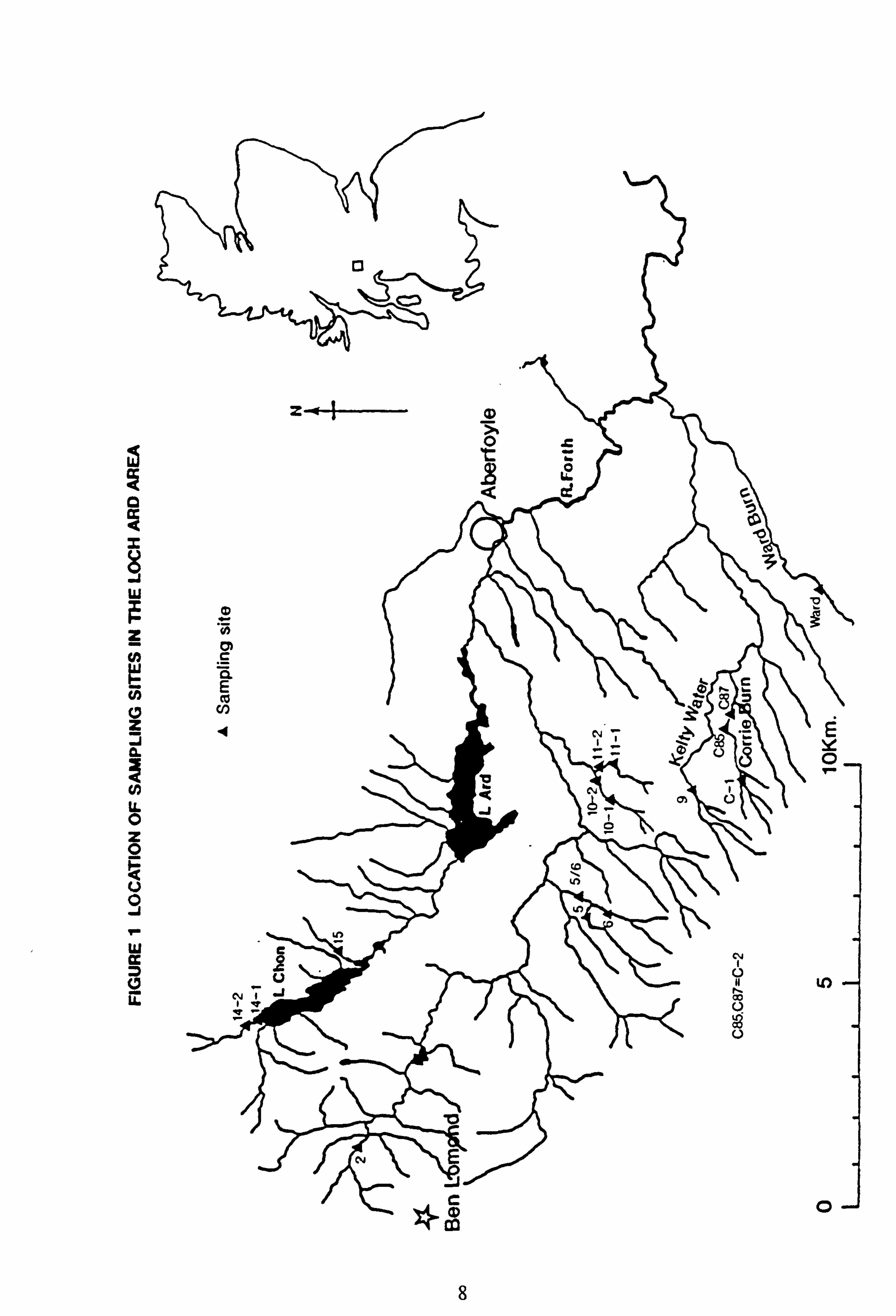
some cases reasonably open sites with good light availability are rare due to close planting of forestry, and the only open sites occur where the burn crosses a fire-break, pylon line or the line of the Loch Katrine aqueduct. The locations of the burns and sampling sites are indicated in Fig. 1.
Most sampling sites are near the staff gauges installed by the SOAFD Freshwater Fisheries Laboratory; these are situated on straight, level reaches as far as possible, which thus also normally provide good sites for the location of the artificial substrates. The Freshwater Fisheries laboratory has also situated its composite water samplers (sampling over a1 week period) at these points. Additional sites were chosen upstream on some burns (see Fig. 1).
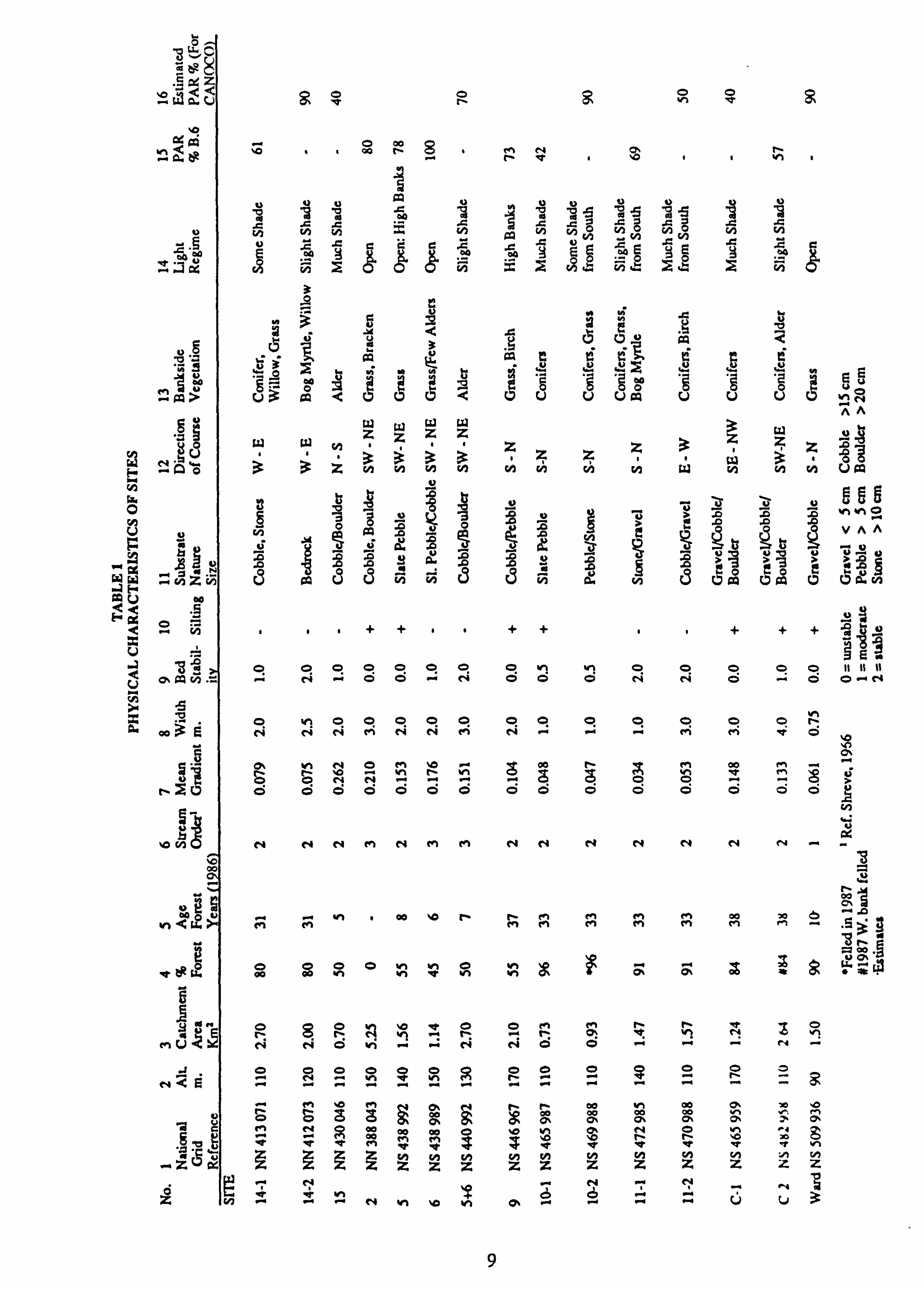
Characteristics of the burns and sites are shown in Table 1.
2.2 FIELD SAMPLING
Sampling was carried out in the Loch Ard area on a regular basis. Initially sampling was carried out every two weeks, but later approximately monthly. Samples of periphytic algae and stream water were collected and measurements made of temperature, staff gauge reading, and integrated incident light.
2.2.1 Sampling methods for algae
2.2.1.1 Natural Substrates Filamentous samples were taken by hand, either picked with fingers or as a fingernail scraping. Diatoms and other small, closely adhering periphyton were taken by brushing stones vigorously with a 25mm paintbrush and rinsing into a plastic tub. The brush was also used for taking filamentous samples underwater against the current.
For biomass estimation, stones were removed from the streams, put in labelled
polythene bags and transported to the laboratory. Stones were selected on the basis of size and shape in order to make extraction of pigments possible, and one was generally taken from both a region of fast and slow current.
7
T. W Q
t7 LL
A. f' m
Ir
pQ
xz ýttýca. Ü gv0 CD 0
'o
ýp .»O o0
- C<. C` t+ Q'4
vii 8 i
u y) (A u N1 w, to fA y CA y
Vf N c4 VI
gý gý C ßa0
p
Oe_0 E c4.00
E to
w :ý .7 OG ýi Vf 2ÖÖ Vý x V1 NQ . ̀ý wý' vý
.Qý G"Hü
53 J9 mý
c5 v .9
60 20 04 :3 bo ä , tÄ
"V y
Fy In 50 yU .0WW
vi"" 50 G
"' c5 avUv uoa UvUo ýN nn
.Z9wzZZZW
rý N ýv wy3333zzZz"3 z$
[.. . -" QO33Zc Vf Vf V) H Vf V! f/7 W Vl V! Vl U CD '~ u
3u '3 uu>o .o- v% v1 O
u1m>s _p . 0_Q . oO
ý+ ö ti xT
ý4ýýýý ýT Vüüüüýp^
W ýQ CO GJ ýQ ýUQ to vU ýQ ýQ UbQ3 FV 71 0. of G. ý CO =0 r3 0.
a bo0000000 Wi Vi o000ou iti n U Oý Wy^N ý+ OO-NC! O0NNÖÖ O^ N rr
äONOOOOOOOOOOOOn
00 EN e4 N t'1 NNMN- . -ý - t+1 ei le Ö
. .. ý hNO eM nhO 00 9m 0V ein
uÖÖNN---^SOO^O>
ný eý oööödöödodödöö h Wi fly
NO (A NNNMNMMNNNNNNN-
00 ä
N o0
ý7 ^- V1 . 00 "D NN en MMM OO 70 e^ Z Lo L. >MM N1 P1 MMMM en ^5 'g
A
9p
ýpýpo,
üä
iý k. 000 oa hO, h
In Oý + 0% 0%
oý
ii äk
VF
~ ~Eý VNN- Cý
-t; O; ýf v1 N
.0 vn
ý+ -N^
r1 U ýG NN C7 I- r+ N cV 00
AOOO0OO000O0Z
%0 ein ÖÖSO^ 00 00 ~ 00 A en
ü ö. 2fß ö oOO+ 0% 0% ä 0% aa
9 430 M en Z "0 r- r- 10 20 S
ZxzXzZZzzZZZZZZZZ
<<v, dd.. .. r7
Ze ."-N vý ýo ýn oý "" "" ". " "-" CJ U3
9
2.2.1.2 Artificial Substrates i. 15 cm square white glazed ceramic tiles were mounted in groups of three in
Dexion frames using 7mm plastic channel. The frames were securely anchored in the stream bed with Dexion stakes driven 0.5.1.0m into the bed. Tiles were sampled by removing the tile and either brushing off any growth from the glazed surface into a plastic bottle, or transporting the entire tile back to the laboratory for chlorophyll extraction.
ü. Glass microscope slides (76 x 26 mm) were mounted in pairs back-to-back in Perspex racks, holding 6 pairs in total. The racks were fastened to a building brick with silicone rubber cement and plastic-coated tying wire. Bricks were frequently dislodged in spates and the slides lost, so they were additionally anchored to the tile racks with tying wire. A Perspex strip held down with nylon 4BA screws retained the slides. Slides were removed from the racks and transported to the laboratory in polythene slide holders (Luckhams) full of stream water.
2.2.2 Transport of Samples
All field samples were transported to the laboratory packed in ice, and were kept on ice
until examined or extracted for pigment analysis, as appropriate.
2.2.3 Water Sampling
Samples of streamwater were taken at the sampling site in acid-washed 250m1 polyeth- ylene bottles which had been rinsed out with distilled water and again rinsed three times in the stream water before being filled. During warm weather the samples were kept in an ice-box until being returned to the laboratory. V
2.2.4 Temperature
Temperature was measured at each sampling site with a mercury-in-glass thermometer. In addition at certain sites a maximum-minimum thermometer was encased in a steel mesh sheath and attached to the tile rack. These were cheap, crude instruments so their
calibration was checked in the laboratory and appropriate corrections applied as
necessary.
10
2.2.5 Flow .
Staff gauges to measure the depth of water at relatively level reaches of the burns have been installed by the Freshwater Fisheries Laboratory at some sites. ' In addition the Forth River Purification Board had recently installed flumes on burns 9,10 and 11, with staff gauges alongside. These were read at the time of sampling: To obtain a value for volumetric flow a calculation based on mean width and bottom characteristics' must be made. This has not been done as the total volume of flow gives no direct indication of velocity at specific points. The staff gauge readings are thus used for within-stream comparisons only.
2.2.6 Light
Photosynthetically Active Radiation (PAR) was measured at selected sites, in rotation, by comparison with an 'open' site. The instruments used were home-made electronic integrators, and are fully described in Appendix 2. The sensors were designed to have a spectral response similar to the absorption pattern of some of the common filamentous algal species. Instantaneous measurements of PAR could be made with one of these sensors in conjunction with a modified voltmeter.
On site, the sensors were bolted to Dexion stakes in the stream bed, or to the tile racks. The ý top of the sensor was levelled with a spirit level, and located approximately 5 cm above 'normal' water level. The sensors were frequently submerged during floods and proved to be waterproof, but drifting vegetation occasionally interfered with a reading, which had to be discounted. Readings were a measure of integrated PAR between
visits. Corrections were applied to readings to take account of different times of reading between integrators, on the basis of a count-rate determined at time of sampling. ''-A further correction was necessary -. to relate the counts from each integrator to the reference instrument; these corrections were determined beforehand by simultaneous comparison of all instruments.
The results are expressed as a percentage of the PAR incident at the reference 'open' site at Burn 6. These are taken as the basis for comparing the light regimes at different sites. A conversion of the count of each instrument into PAR ( pmoles m-2 s'1) was also obtained by comparison with a direct reading meter (see Appendix 2).
11
2.3 LABORATORY METHODS
2.3.1 Microscopic examination of algal samples
Aliquots of each sample were removed and mounted under coverslips. Samples were examined live, without staining, using a Leitz Ortholux microscope equipped with phase-contrast. Cell dimensions were calculated by measurement against an eyepiece graticule. All
measurements of size were carried out with a x40 objective, x12.5 eyepiece, total
magnification x500.
2.3.2 Photography
Photographs were taken using a Leica 35mm camera back on the Leitz microscope. Kodak Ektachrome 200 ASA slide film was routinely used, processed by the Napier Polytechnic Photography Department. A light blue filter was used to compensate for the colour of the tungsten light. The
supply current to the lamp was kept constant to give consistent colour rendition.
2.3.3 Species identifications
The keys in Prescott (1970) and Starmach (1972) were used to identify algae to the genus level. Other keys used were in Randhawa (1959) and Ramanathan (1962). The criteria of Cox and Bold (1966) were applied to the identification of Stigeocloniwn
species. .
2.3.4 Species abundance
During examination of samples, the relative abundance in each sample of different taxa
was estimated following microscopic screening of the whole aliquot on the slide. Several aliquots were examined if the sample appeared heterogeneous.
The estimates of abundance rank taxa in 7 categories. These are, abundant; abundant/ common; common; common/frequent; frequent; frequent/rare; and rare. A species is
recorded as abundant if it appears to constitute more than approximately 30% of the total
algal volume present, and rare if it is present only once to a few times in the whole sub- sample. Between these categories there is obvious opportunity for uncertainty in the ranking of individual taxa due to the subjective nature of the ranking process, so the rank accorded may have an error of plus or minus one category.
12
2.4 TREATMENT OF SAMPLES
2.4.1 Biomass Estimation --
Two methods were used for biomass estimation. These were Pigment Extraction and Ash-Free Dry Weight (AFDW). Where possible both pigment extraction and Ash- Free Dry Weight analysis were carried out sequentially. Brushed samples from tiles were divided into aliquots, following sonication if necessary
with very concentrated filamentous samples. Replicate aliquots were filtered onto Whatman glass fibre-filter papers (type GF/C), an aliquot retained fresh for microscopic examination, and a further aliquot preserved in 6-3-1 (water : 95% alcohol : formalde- hyde) - preservative (Prescott, 1970).
2.4.1.1 Pigment extraction For chlorophyll analysis, extraction was carried out in 90% acetone saturated with MgCO3, overnight in a refrigerator. For carotenoid and chlorophyll analysis, MgCO3-saturated 90% methanol, at 55° for 1 hour (Foy, 1987) was used. Filters were frozen at -20°C during the earlier part of the investigation, but this was discontinued when it was found that some species give incomplete extraction fol- lowing freezing. The extractant was changed to 90% methanol after it was found that some unialgal
cultures'-gave very poor ' extraction in acetone (see Section 4.3).
Filters were immersed in the extractant without maceration (frozen filters were torn up and placed in the extractant). The contents of the tube were mixed by
periodic inversion. Slides were extracted by draining them briefly and then immersing in extractant in the Luckham's slide containers. Extraction of intact tiles and stones was carried out by placing them upside-down in a polythene sandwich box or similar container with a tight-fitting lid. Allowance
was made for the volume of water contained in the algal biomass by including a volume of 100% extractant equivalent to ten times the estimated water volume, along with sufficient 90% acetone (or methanol) saturated in MgCO3 to wet the top (i. e. formerly exposed) , surface of the tile or stone.
13
2.4.1.2 Ash-Free Dry Weight Determination Following extraction, filters and slides were removed from the containers - and dried in an oven at approximately 60°C to constant weight. They were then
subjected to incineration for 1 hour at 550°C in a muffle furnace before being re- weighed on a Stanton balance to determine -weight loss on ignition (AFDW).
Each weighing is estimated to be accurate to ±0.1 mg. To prevent loss of loose
material, filters and slides were weighed wrapped in Aluminium foil. Al melts at about 660°C and no loss of weight from Al foil at 550°C was found. GF/C filters (47mm diam. ) lose approximately 0.7mg on incineration at 550°C . They were not pre-ashed as this makes them brittle so they break up during filtration or pigment extraction. A subtraction of 0.7mg was made to accommodate this weight loss. In-
accuracy is estimated as ±0.2 mg. Slides treated in this way can then be mounted in Naphrax (Northern Biological Supplies) for diatom examination.
2.4.1.3 Chlorophyll analysis in pigment extracts. Extracts were centrifuged in stoppered tubes at 3,000 rpm for 20 minutes. Chlo-
rophyll-a was determined by the trichromatic method of Parsons and Strickland (1963).
Absorbance was measured at 750,663,645 and 630nm in 4cm glass cells against a 90% acetone or methanol blank. For the analysis of phaeophytin, acetone extracts were then acidified in the cell with 8 drops of 0.1N HC1 and A,, re-read. Afterl- 2 minutes the A., was read. These readings enable phaeophytin-a and chloro- phyll-a to be distinguished (Lorenzen, 1967).
Pigment yields per extract (slide or filter) were calculated from the following
equations: Trichromatic
chl-a(pg) = 11.64 (Aa; A,, ) + 2.16 (AMs -A, x) -0.1 (A630 A, 0 x Extract Volume, ml. 4 (path length) cm
(SCOR/UNESCO 1966) For Phaeophytin
chl-a(pg) = 26.73 [(Am3 A, 0 - (A A, 0 ]x Extract Volume, ml 4
phaeo-a(pg) = 26.73 [1.7 (A A�, ) - (AM; A, m) ]x Extract Volume, ml.
4 (Lorenzen, 1967)
Variations in the formulae necessary when using methanol are dealt with in Section 4.3 of the Discussion.
14
[In methanol the absorbance maximum is at 664 nm and is not shifted following
the conversion chlorophyll-a to phaeophytin-a. However the extract must either be acidified and then neutralized, or transferred to 90% acetone for
reading (Marker et al, 1980). ]
2.4.1.4 Carotenoid analysis Carotenoid is determined as 'microscopic pigment units' ( pspu) from methanol extracts (Foy, 1987). It is calculated using an extinction coefficient of 4 (Strickland et al , 1968).
Carotenoid = 4(A48O -A 750) x Extract volume, ml 4 (path length, cm) pspu
2.4.2 Surface area of substrates
Tiles measured 15 x 15cm, giving a total surface area of 225cm2. A strip measuring ap- proximately 3mm wide was not exposed up each side due to the plastic channel; this was compensated by the exposed vertical surfaces at the leading and trailing edges. Similarly the surface area of slide pairs was calculated as 20cm2, including the sides of the slide. The surface area of stones was estimated by wrapping the exposed upper surface with aluminium foil and estimating the area from the weight of foil (Naiman, 1983).
15
2.5 ANALYSIS OF WATER SAMPLES
2.5.1. pß
pH was measured to 0.01 pH unit with an Orion model 611 pH meter equipped with
a Ross combination electrode. The filling solution (3M KCl) was replaced before
reading a set of field samples. The pH was read in a stirred sample. When a steady
reading was obtained the sample was discarded and a fresh portion added, and the pH
reading was taken as soon as it stabilized. The stirrer was then stopped and a reading
taken of the unstirred sample. The samples were read at a temperature near to the field temperature at the time of sampling.
2.5.2 Absorption (optical density) measurements
The absorption of water samples was read at 400,350. and 250nm in quartz cuvettes in
a Unicam SP8.100 recording spectrophotometer. This instrument was also used to
obtain scans of chlorophyll extracts and cell suspensions, used in the design of the PAR
sensors. Absorption in the U. V. band is highly correlated with total organic carbon
concentration of water.
2.5.3 Chemical analyses ,
The following analyses were employed on field samples, and on synthetic stream water during growth experiments.
Calcium was determined by AAS in a nitrous oxide-air flame in a Perkin-Elmer Model
373 Atomic Absorbance Spectrophotometer. Phosphate was determined by the
stannous chloride method (APHA, 1985 ). Nitrate was determined by conversion to
nitrite by the spongy cadmium method, followed by assay of nitrite by reaction with
sulphanilamide (Elliott and Porter, 1971). This results in an estimate of Total Oxidised
Nitrogen (TON). Aluminium was determined by the catechol violet method (Seip et
al, 1984; Rogeberg and Henriksen, 1985). Fractionation into labile and non-labile Al is
carried out by passage over ion exchange resin (Driscoll, 1984). Silicon was deter-
mined by the oxalic acid-molybdate method (Parsons et al, 1984). In addition the
SOAFD Freshwater Fisheries Laboratory routinely monitors a range of determinands
in one-week composite samples. The full range of determinations includes pH, conduc-
tivity, Na', K', Cat , Mg', Mn2', Al, Fe, Si, SO42-, Cl', PO4'', and NO3, but is not
carried out on all samples.
16
2.6 ALGAL GROWTH EXPERIMENTS
2.6.1 Media
Initial growth experiments were carried out in Chu no. 10 medium (Nichols, 1973) and attempts to identify Stigeoclonium species employed medium BBMPTB12 (Cox and Bold, 1966).
For measurements of growth rates and experiments to determine changes in species composition, two new media were formulated based on chemical analysis of two of the Loch Ard streams (data from SOAFD, Pitlochry). Mean values over several years were used, with more frequent sampling in recent years the means may be biassed towards recent values.
Media were formulated using only the ions Na+, K'- Mgt+, Cat+, Al, Fe, Si, S04 2-, Ct" H', PO4ý, NO3, and Mn2+, slight discrepancies in the ion balance being attributed to organic acids (Cronan et al, 1978; Krug et at, 1985). No attempt was made to accommodate these in the media.
The recipes for media 'B9' and 'Corrie' are given in Table 2, and the concentrations of ions are compared with BBMPTB12 in Table 3.
Media are made up as concentrates (100 times) and diluted for use in glass-distilled water. Both media, especially 'Corrie', contain precipitates and have to be thoroughly
resuspended before aliquots are removed for dilution.
Manipulation of aluminium and silicate concentrations was carried out in Corrie medium. The amount of sodium silicate solution was reduced from 0.93 ml to 0.079ml per litre of concentrate, a decrease from 47 to 4 pM, to constitute treatment B. Treatment C had the total aluminium target level increased from 40 to 146 pgl-' (the same concentration as in B9 medium), although analysis showed that a higher final concentration was achieved in
practice. Treatment A was unmodified Corrie medium. The pH of A, B and C was maintained at 5.5, while treatment D was unmodified B9 medium at its 'natural' pH of 4.6.
17
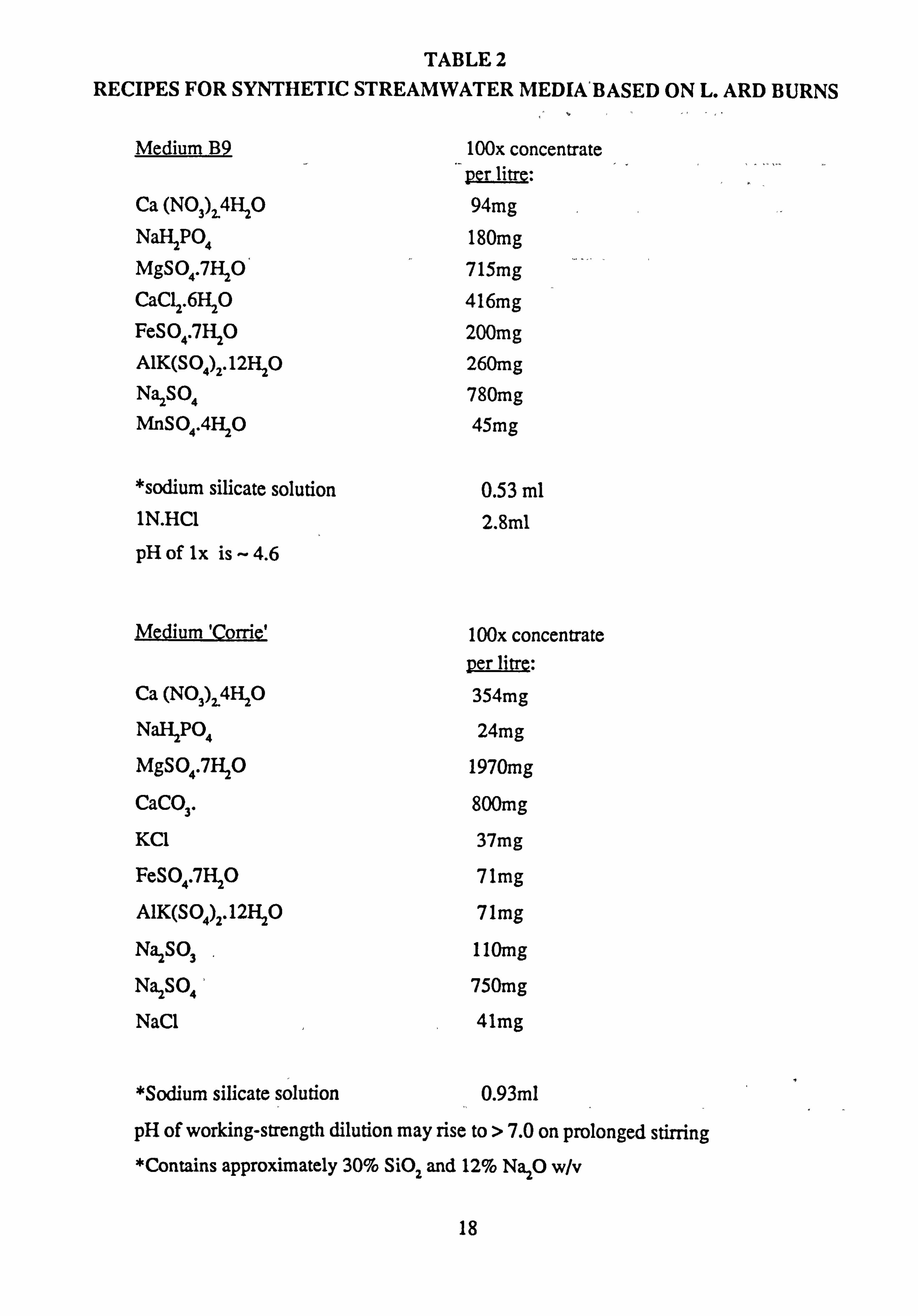
TABLE 2 RECIPES FOR SYNTHETIC STREAMWATER MEDIA`BASED ON L. ARD BURNS
Medium B9 100x concentrate per litre:
Ca (NO3)4_4H2O 94mg Nal ZPO4 180mg MgSO4.7H20' 715mg CaC12.6H20 416mg FeSO4.7H20 200mg A1K(SO4)2.12H20 260mg Na2SO4 780mg MnSO4.4H2O 45mg
*sodium silicate solution 0.53 ml 1N. HC1 2.8m1
pH of lx is-4.6
Medium 'Corrie' 100x concentrate per litre:
Ca (NO3)2.4H2O 354mg
NaH2PO4 24mg
MgSO4.7H2O 1970mg
CaCO3. 800mg
KC1 37mg
FeSO4.7H20 71mg
A1K(SO4)2.12H20 71mg
Na2SO3 110mg
Na2SO4 750mg
NaCl 41mg
*Sodium silicate solution 0.93m1
pH of working-strength dilution may rise to > 7.0 on prolonged stirring *Contains approximately 30% SiOZ and 12% Na20 w/v
18
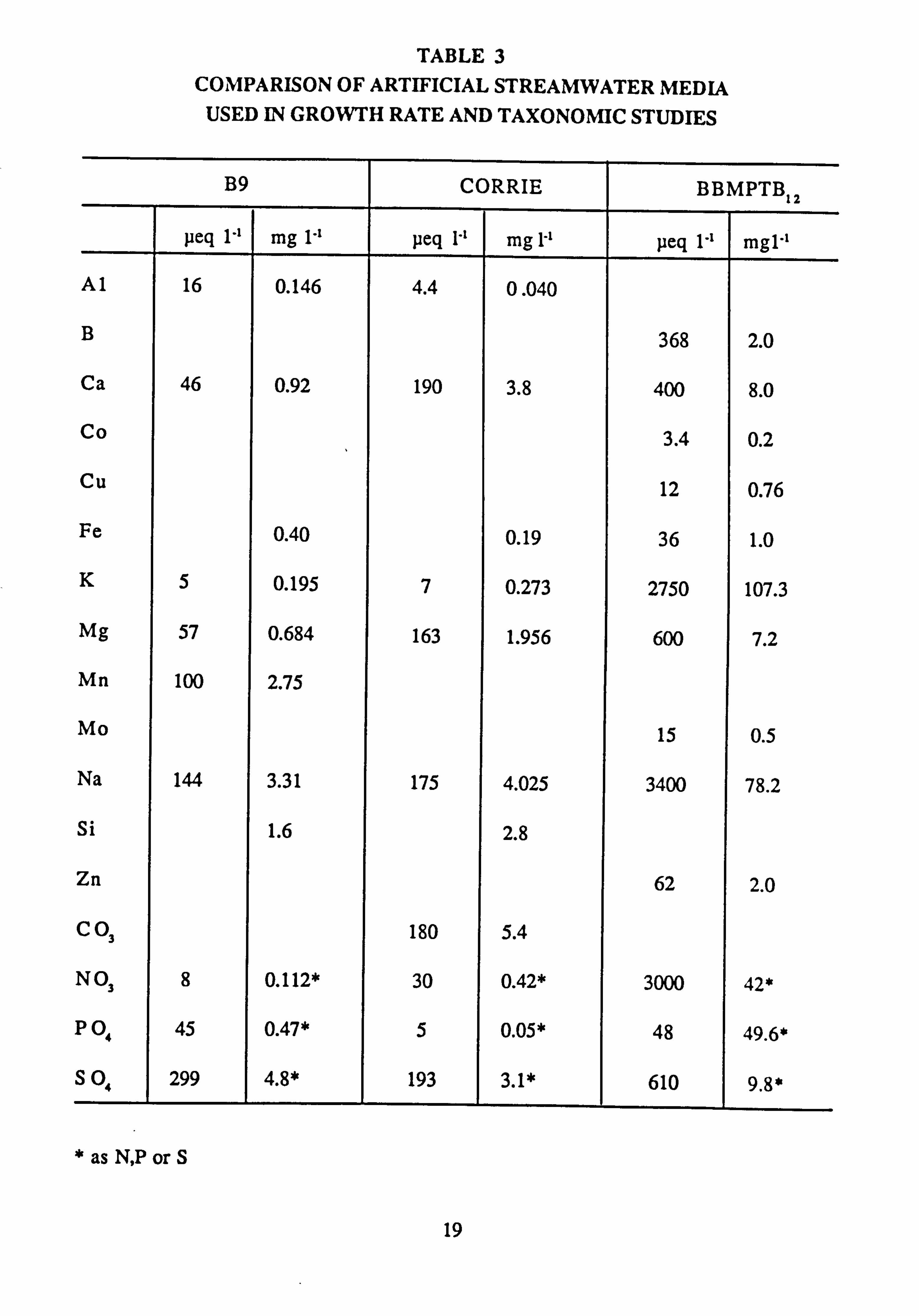
TABLE 3 COMPARISON OF ARTIFICIAL STREAMWATER MEDIA
USED IN GROWTH RATE AND TAXONOMIC STUDIES
B9 CORRIE BBMPTB12
peq 1-' mg 1-1 peq 1' mg 1-1 peq 1-1 mgl-'
Al 16 0.146 4.4 0.040
B 368 2.0
Ca 46 0.92 190 3.8 400 8.0
Co 3.4 0.2
Cu 12 0.76
Fe 0.40 0.19 36 1.0
K 5 0.195 7 0.273 2750 107.3
Mg 57 0.684 163 1.956 600 7.2
Mn 100 2.75
Mo 15 0.5
Na 144 3.31 175 4.025 3400 78.2
si 1.6 2.8
Zn 62 2.0
C O3 180 5.4
NO3 8 0.112* 30 0.42* 3000 42*
P 04 45 0.47* 5 0.05* 48 49.6*
S04 299 4.8* 193 3.1* 610 9.8*
* as N, P or S
19
a
a 0
zJ°
ac d an a I
W
H N J
C) -
U p
N
LI.
t Ö
20
2.6.2 Artificial stream channels
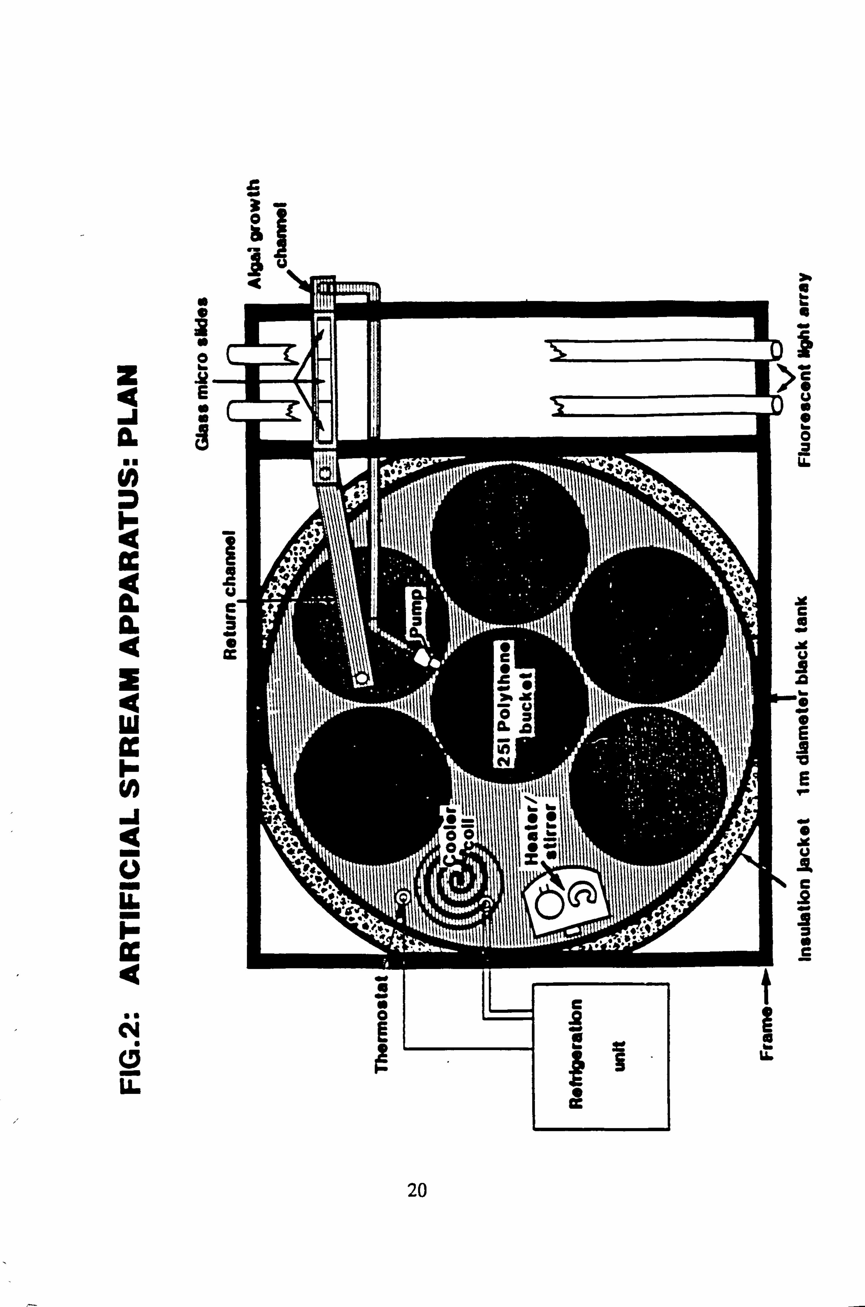
Periphytic algae were cultured in the laboratory under conditions approximating those in
the field, with control of water chemistry, temperature, flow rate and light regime. A plan of the apparatus used is shown in Fig. 2.
Artificial stream channels were constructed using clear Perspex sheet. Water is pumped in
at one end by means of a submersible aquarium pump (Aquaclear 200) in a 25 litre
polythene bucket, connected to the channel by 10mm i. d. silicone tubing. Filtered air is
pumped in by a Whisper 600 air pump at the same end of the channel via a perforated plastic pipe, so that the channel water is in equilibrium with the atmosphere in respect of dissolved
gases. The water leaves the channel at the other end via a 20mm tube and returns to the bucket via a channel constructed out of 40mm plastic electrical trunking. Six buckets are accommodated in a circular black PVC water tank, supported on a platform of galvanized Dexion and immersed to approximately two-thirds their depth in water. This is thermostati- cally contolled by means of a thermistor and associated circuitry (see Appendix 3)
connected to a Grant CZ2 dip cooler unit. Stirring is also provided in order to prevent icing
up of the cooling coils. During the course of this work a temperature of 10°C was employed, and manual checks reveal that the temperature varies by less than =0.25°C.
The submersible pumps are not fully insulated and it has been found that some generate a
potential of up to 60V between the stream water and ground, which causes problems when
using a pH electrode in the channels. The buckets are therefore grounded by means of
stainless steel rods dipping into the water. The Dexion frame of the apparatus, and the
submerged Dexion platform are also connected to ground.
Light is provided by two 40W cool white fluorescent tubes 40cm above the channels. The light regime used was 12h light : 12h dark, controlled by a time switch. Natural light is
excluded from the whole apparatus by enclosing it in a black polythene tent, and light from
the tubes is likewise excluded from the tank and buckets. To further minimise the
possibility of algal growth outwith the channels, the outside of the buckets and lids and the
return channels are painted black.
The buckets used are 25 litre food grade polythene (HDPE) brewing bins (Cumbria Brew
Bins). They were pre-treated to remove excess plasticiser which might be inhibitory to
algal growth (Hardwick and Cole, 1986) by twice steaming them full of distilled water at 100°C for 1 hour in an autoclave (higher temperatures result in shrinkage and distortion of
the HDPE).
21
Channel pH was controlled manually by addition of 0.2N H2S04. Growth experiments were carried out in pH-adjusted Corrie medium. This requires checking and adjustment about once every two days to maintain reasonable control of pH as the pH tends to rise with time especially at higher nominal pH values. In unadjusted Corrie medium, the pH may rise to over 7.0 on continued stirring. This may be due to the slow dissolution of Al
complexes or Al hydroxides (Tipping et al, 1989). The B9 medium on the other hand
gives an unadjusted pH of 4.6-4.7, which remains constant.
Algae were grown attached to slides which were held down on the bottom of the channels by Perspex grips. The slides were seeded from field samples. Some species readily generate zoospores, while others will regenerate from hormogonia; these proc- esses may be encouraged by a shift from a phosphate-depleted to a phosphate-enriched medium (Rosemarin, 1983). This was accomplished by placing slides in the bottom of a Pyrex tray, covered with 1 litre of B9 medium, which is high in PO4, as compared with Corrie (Table 3). Algae may be added directly to the medium, or in a 1mm mesh container suspended within it. Aeration and stirring were supplied by means of small airlift pumps constructed out of a Pasteur pipette and 10mm glass tubing, connected to an aquarium air pump (Whisper 600). After a period of settlement of 1-6 days (depending on the density required) the slides were removed, rinsed ` lightly, and transferred to other media.
2.6.3 Measurement of growth rates
Growth was measured by direct cell counting of individual plants (Rosemarin, 1983) at intervals of 2-4 days. This method can be used only at low algal densities and at an early phase of growth; 3 or 4 successive measurements may be made of each filament. Up to 4 main species were grown simultaneously on the same slide, and 3 slides were employed per channel.
2.6.4 Assessment of relative abundance
The relative abundance of species in channels was scored in the same manner as was used with field samples, allowing assessments to be made of the development and changes of dominance on prolonged culture.
2.6.5 Static and semi-static culture
Batch culture of isolates was carried out for the purpose of performing identifications (Cox and Bold, 1966) providing inocula or to test the effect of changes in the growth medium, in Ehrlenmeyer flasks or in 2 litre square plastic tubs (2Kg margarine tubs). If stirring or aeration was required an airlift pump was employed as described earlier. Incubation was carried out either in a waterbath illuminated from above or in an illuminated environmental chamber (Baird and Tatlock cooled incubator with side or bottom lighting).
22
2.7 STATISTICAL METHODS
Correlation and linear regression, manipulation of data and analysis of variance was carried out using MINITAB on a Prime 9955 mini computer.
Statistical ecology programs to carry out the analyses described by Ludwig and Reynolds (1988) are available on the disk supplied with the book and these were used to carry out Cluster Analysis, Normal Association Analysis and calculation of diversity indices.
Canonical Correspondence Analysis and its detrended form were carried out using the pro- gramme CANOCO (Ter Braak, 1988). SIGMAPLOT (Jandel Scientific) was used to prepare plots.
2.7.1 Recalculation of species and site values from CANOCO
The species and site values with respect to an environmental variable can be obtained by dropping a perpendicular to the arrow or its backwards extension from each species or site point in the ordination diagram (Ter Braak, 1987). This is more accurately carried out from the species coordinates and the coordinates of the head of the variable's arrow using the formula: -
fx'\ Cos9 Sing x y' -Sine Cosa
where tan 9= xV/yV (x, =x coordinate of the arrow head;
y� =y coordinate of the arrow head)
23
3. RESULTS
3.1 FIELD SAMPLING: SPECIES DATA
Forty-nine taxa of filamentous algae were distinguished in field samples. Descriptions and
some tentative identifications are presented on Appendix 1. Diatoms, desmids and unicellular
green algae were also found in samples but the data and analyses presented here are based
solely on filamentous algae.
The fifteen sampling sites were visited on up to thirty-five occasions. The species abundance data thus constitute a three-dimensional matrix (49 species, 15 sites, 35 sampling dates). The
matrix has been divided into two almost equal parts for comparative purposes. Some of the
sites were not sampled prior to sampling number 17 or 18, and thus the data obtained
subsequently are more complete. All sampling occasions up to no. 17 have been combined into Matrix A, and numbers 18 to 35 inclusive comprise Matrix B. The undivided matrix has
also been subjected to analyses, as Matrix C. The environmental and biomass data have been
divided along similar lines. The 3-dimensional matrices must be reduced to a 2-D form to
enable most statistical procedures to be carried out. This reduction was accomplished by
calculating the mean relative abundance of each species in each site, taking into account the
number of times each site was sampled. In the terminology of Ludwig and Reynolds (1988)
a site constitutes a 'Sampling Unit' (S. U. ).
The species data may also be used as presence-absence data in some statistical procedures. Conversion of the abundance data to presence-absence (p/a) was carried out in MINITAB by
converting all non-zero values to 1. This procedure was carried out in each of the 2-D
matrices. Conversion of the 3-D matrices was also carried out. If the mean (sum of all
presences divided by the number of samples taken) of the p/a data in the 3-D matrices is
calculated, a measure of relative abundance of species is obtained which is not dependent
upon estimates of relative abundance in each sample. The data obtained in this way, termed 'pooled p/a' have been used in the same analyses as the abundance data.
Species data matrices A, B and C in both mean abundance and pooled p/a form are shown in
Tables 4 to 9. The means have been multiplied by 100 to round up to whole numbers, as
required for analysis by the Ludwig and Reynolds (1988) programs.
24
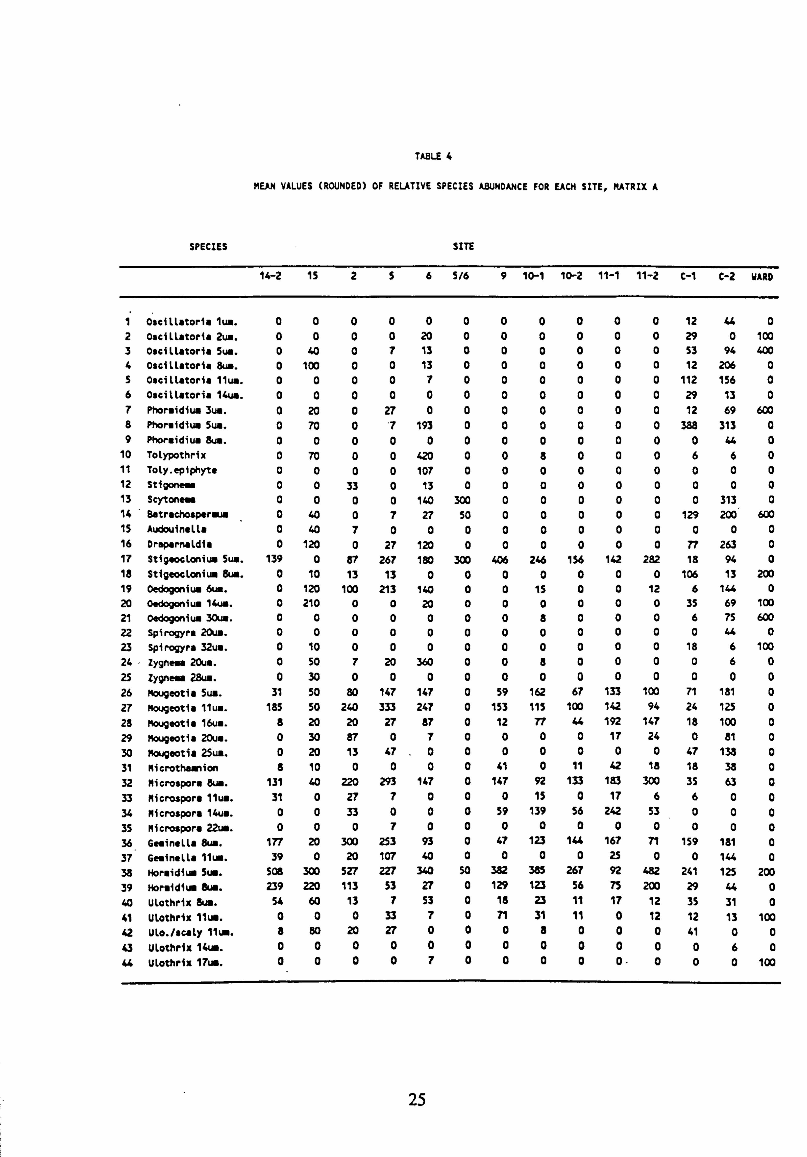
TABLE 4
MEAN VALUES (ROUNDED) OF RELATIVE SPECIES ABUNDANCE FOR EACH SITE, MATRIX A
SPECIES SITE
14-2 15 256 5/6 9 10-1 10-2 11-1 11-2 C-1 C-2 WARD
1 Oscitlatorin lu.. 0 0 0 0 0 0 0 0 0 0 0 12 44 0 2 Oscillatoria Zus. 0 0 0 0 20 0 0 0 0 0 0 29 0 100 3 Osciltatoria Sum. 0 40 0 7 13 0 0 0 0 0 0 53 94 400 4 Oscillatoria 8us. 0 100 0 0 13 0 0 0 0 0 0 12 206 0 S Osciltetoria llu.. 0 0 0 0 7 0 0 0 0 0 0 112 156 0
6 OscitLatoria 14u.. 0 0 0 0 0 0 0 0 0 0 0 29 13 0 7 Phorsidiun 3us. 0 20 0 27 0 0 0 0 0 0 0 12 69 600 8 Phor. idiun Sus. 0 70 0 7 193 0 0 0 0 0 0 388 313 0 9 Phorsidius Bus. 0 0 0 0 0 0 0 0 0 0 0 0 44 0
10 Tolypothrix 0 70 0 0 420 0 0 8 0 0 0 6 6 0 11 Toly. epiphyte 0 0 0 0 107 0 0 0 0 0 0 0 0 0 12 Stiltoner 0 0 33 0 13 0 0 0 0 0 0 0 0 0 13 Scytonesr 0 0 0 0 140 300 0 0 0 0 0 0 313 0 14 Batrachosperw 0 40 0 7 27 50 0 0 0 0 0 129 200 600 15 Audouinelts 0 40 7 0 0 0 0 0 0 0 0 0 0 0 16 Drsparnaldia 0 120 0 27 120 0 0 0 0 0 0 77 263 0 17 Stigeoctaniuw Sum. 139 0 87 267 180 300 406 246 156 142 282 18 94 0
18 Stigeoctoniun We. 0 10 13 13 0 0 0 0 0 0 0 106 13 200 19 Oedogoniuw 6us. 0 120 100 213 140 0 0 15 0 0 12 6 144 0 20 Oedogoniu. 14uw. 0 210 0 0 20 0 0 0 0 0 0 35 69 100 21 Oedogoniun 30un. 0 0 0 0 0 0 0 8 0 0 0 6 75 600 22 Spirogyra 20us. 0 0 0 0 0 0 0 0 0 0 0 0 44 0 23 Spirogyra 32u.. 0 10 0 0 0 0 0 0 0 0 0 18 6 100 24 Zygness 20u.. 0 50 7 20 360 0 0 8 0 0 0 0 6 0
25 Zygnen 28uw. 0 30 0 0 0 0 0 0 0 0 0 0 0 0 26 Mougeotia 5us. 31 50 80 147 147 0 59 162 67 133 100 71 181 0
27 Mougeotia 11us. 185 50 240 333 247 0 153 115 100 142 94 24 125 0
28 Mougeotia 16u.. 8 20 20 27 87 0 12 77 44 192 147 18 100 0
29 Mougeotis 20uu. 0 30 87 0 7 0 0 0 0 17 24 0 81 0
30 Mougeotia 25us. 0 20 13 47 .0 0 0 0 0 0 0 47 138 0 31 Microthasnion 8 10 0 0 0 0 41 0 11 42 18 18 38 0 32 Nitrospore 8us. 131 40 220 293 147 0 147 92 133 183 300 35 63 0
33 Nitrospore flue. 31 0 27 7 0 0 0 15 0 17 6 6 0 0 34 Microspora 14us. 0 0 33 0 0 0 59 139 56 242 53 0 0 0 35 Nitrospore 22uu. 0 0 0 7 0 0 0 0 0 0 0 0 0 0 36 Ge. inells 8uß. 177 20 300 253 93 0 47 123 144 167 71 159 181 0 37 Ge. inells 11ue. 39 0 20 107 40 0 0 0 0 25 0 0 144 0 38 Hor"idium Sum. 508 300 527 227 340 50 382 385 267 92 482 241 125 200
39 Morsidiuw 8um. 239 220 113 53 27 0 129 123 56 75 200 29 44 0 40 Ulothrix 8ue. 54 60 13 7 53 0 18 23 11 17 12 35 31 0 41 Ulothrix 11uß. 0 0 0 33 7 0 71 31 11 0 12 12 13 100 42 Ulo. /scaly 11ue. 8 80 20 27 0 0 0 8 0 0 0 41 0 0 43 Ulothrix l4ue. 0 0 0 0 0 0 0 0 0 0 0 0 6 0 44 Ulothrix 17um. 0 0 0 0 7 0 0 0 0 0. 0 0 0 100
25
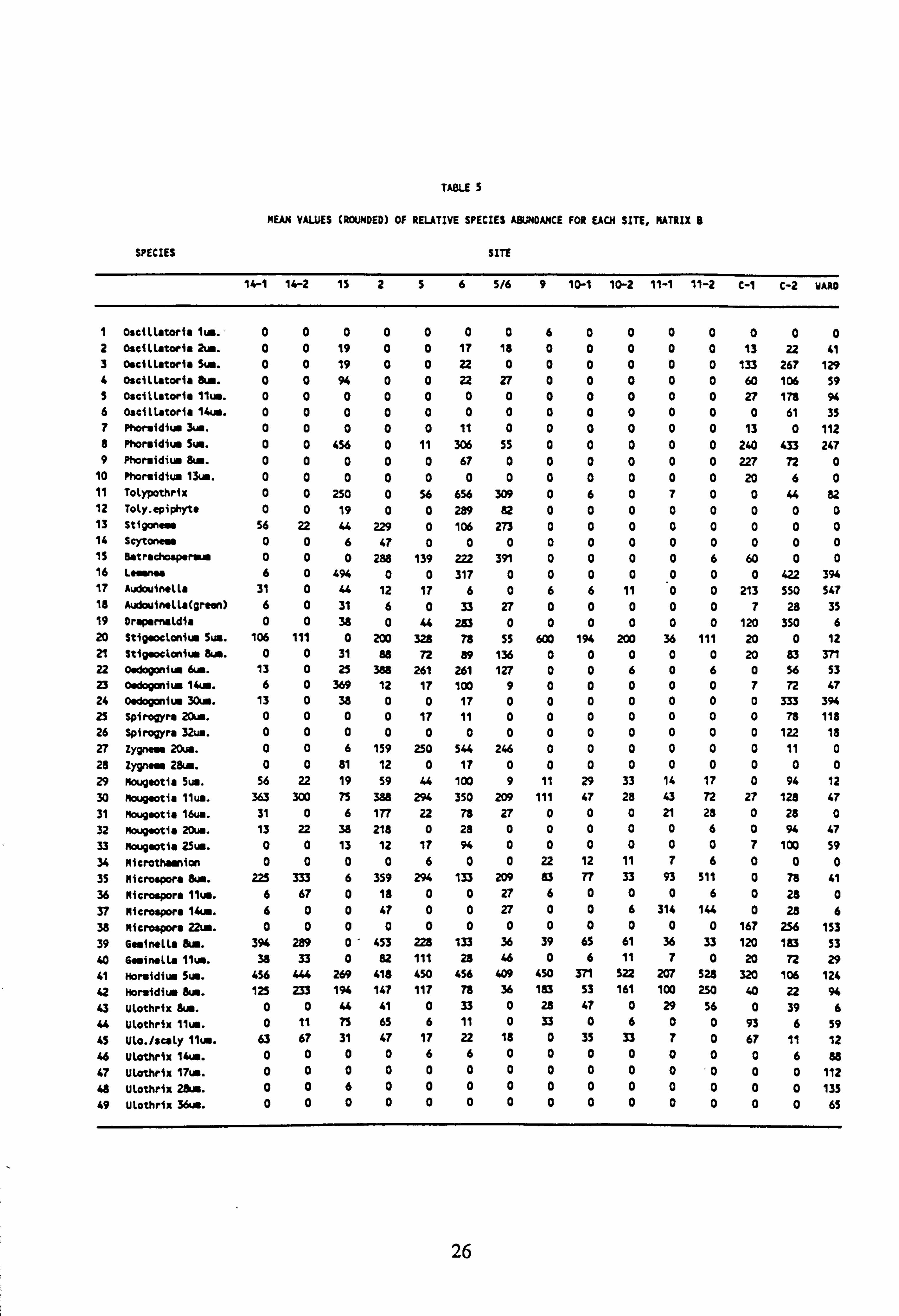
TABLE 5
MEAN VAUJES (ROUNDED) OF REUTIVE SPECIES ABUNDANCE FOR EACH SITE, MATRIX 8
SPECIES SITE
14-1 14-2 15 256 5/6 9 10-1 10-2 11-1 11-2 C-1 C-2 WARD
I Oseillatoris Zia. 0 0 0 0 0 0 0 6 0 0 0 0 0 0 0 2 Oseitlatoria 2um. 0 0 19 0 0 17 18 0 0 0 0 0 13 22 41 3 Osciltatoria 5pa. 0 0 19 0 0 22 0 0 0 0 0 0 133 267 129 4 Oscillatoria Bus. 0 0 94 0 0 22 27 0 0 0 0 0 60 106 59 5 Oscillatoria 11u.. 0 0 0 0 0 0 0 0 0 0 0 0 27 178 94 6 oseiltatoria 14u.. 0 0 0 0 0 0 0 0 0 0 0 0 0 61 3S 7 Phornidiua 3u.. 0 0 0 0 0 11 0 0 0 0 0 0 13 0 112 8 Phor. idiu. Sun. 0 0 456 0 11 306 55 0 0 0 0 0 240 433 247 9 PAornidiua 8ta. 0 0 0 0 0 67 0 0 0 0 0 0 227 72 0
10 Phorsldiuw 13u.. 0 0 0 0 0 0 0 0 0 0 0 0 20 6 0 11 Tolypothrix 0 0 250 0 56 656 309 0 6 0 7 0 0 44 82 12 Toly. epiphyts 0 0 19 0 0 289 82 0 0 0 0 0 0 0 0 13 Stlgonesa 56 22 44 229 0 106 273 0 0 0 0 0 0 0 0 14 Seytone s 0 0 6 47 0 0 0 0 0 0 0 0 0 0 0 15 Betrschosperum 0 0 0 288 139 222 391 0 0 0 0 6 60 0 0 16 Lesnaa 6 0 494 0 0 317 0 0 0 0 0 0 0 422 394 17 AudouinelLa 31 0 44 12 17 6 0 6 6 11 0 0 213 550 547 18 Audouin. lla(grsen) 6 0 31 6 0 33 27 0 0 0 0 0 7 28 35 19 Drap. rn. ldis 0 0 38 0 44 283 0 0 0 0 0 0 120 350 6 20 Stigsoctoniia Sun. 106 111 0 200 328 78 55 600 194 200 36 111 20 0 12 21 Sti9 octoniua 8uß. 0 0 31 88 72 89 136 0 0 0 0 0 20 83 371 22 0adogonim 6r. 13 0 25 388 261 261 127 0 0 6 0 6 0 56 53 23 0adog nim 14Aa. 6 0 369 12 17 100 9 0 0 0 0 0 7 72 47 24 0. dogoniua 30ua. 13 0 38 0 0 17 0 0 0 0 0 0 0 333 394 25 Spirogyra 20u.. 0 0 0 0 17 11 0 0 0 0 0 0 0 78 118 26 Spirogyra 32uw. 0 0 0 0 0 0 0 0 0 0 0 0 0 122 18 27 Zy9nar 20u.. 0 0 6 159 250 544 246 0 0 0 0 0 0 11 0 28 Zygnem 2&s. 0 0 81 12 0 17 0 0 0 0 0 0 0 0 0 29 Mougeotis 5uß. 56 22 19 59 44 100 9 11 29 33 14 17 0 94 12 30 Moug. ot1a 11w. 363 300 75 388 294 350 209 111 47 23 43 72 27 128 47 31 Mouyeotis 16uw. 31 0 6 177 22 78 27 0 0 0 21 28 0 28 0 32 Moupwtio 20u.. 13 22 38 218 0 28 0 0 0 0 0 6 0 94 47 33 soupaotis 25u.. 0 0 13 12 17 94 0 0 0 0 0 0 7 100 59
34 Microthrnion 0 0 0 0 6 0 0 22 12 11 7 6 0 0 0 35 Microspora 8uß. 225 333 6 359 294 133 209 83 77 33 93 511 0 78 41 36 Ric re llu.. 6 67 0 18 0 0 27 6 0 0 0 6 0 28 0 37 Microspore 14uß. 6 0 0 47 0 0 27 0 0 6 314 144 0 28 6 38 Microspore 22u.. 0 0 0 0 0 0 0 0 0 0 0 0 167 256 153 39 Gain*LLs 8ia. 394 289 0- 453 228 133 36 39 65 61 36 33 120 183 53 40 6winaLLa llua. 38 33 0 82 111 28 46 0 6 11 7 0 20 72 29 41 Mornidiua Sun. 456 444 269 418 450 456 409 450 371 522 207 528 320 106 124 42 Horsidiua 8uß. 125 233 194 147 117 78 36 183 53 161 100 250 40 22 94 43 Utothrix 8uß. 0 0 44 41 0 33 0 28 47 0 29 56 0 39 6 44 Utothrix 11uß. 0 11 75 65 6 11 0 33 0 6 0 0 93 6 59 45 Ulo. /scaly 11ua. 63 67 31 47 17 22 18 0 35 33 7 0 67 11 12 46 Ulothrix 14uß. 0 0 0 0 6 6 0 0 0 0 0 0 0 6 88 47 Ulothrix l7ua. 0 0 0 0 0 0 0 0 0 0 0 0 0 0 112 48 Utothrix 28uß. 0 0 6 0 0 0 0 0 0 0 0 0 0 0 135 49 Ulothrix 36ms. 0 0 0 0 0 0 0 0 0 0 0 0 0 0 65
26
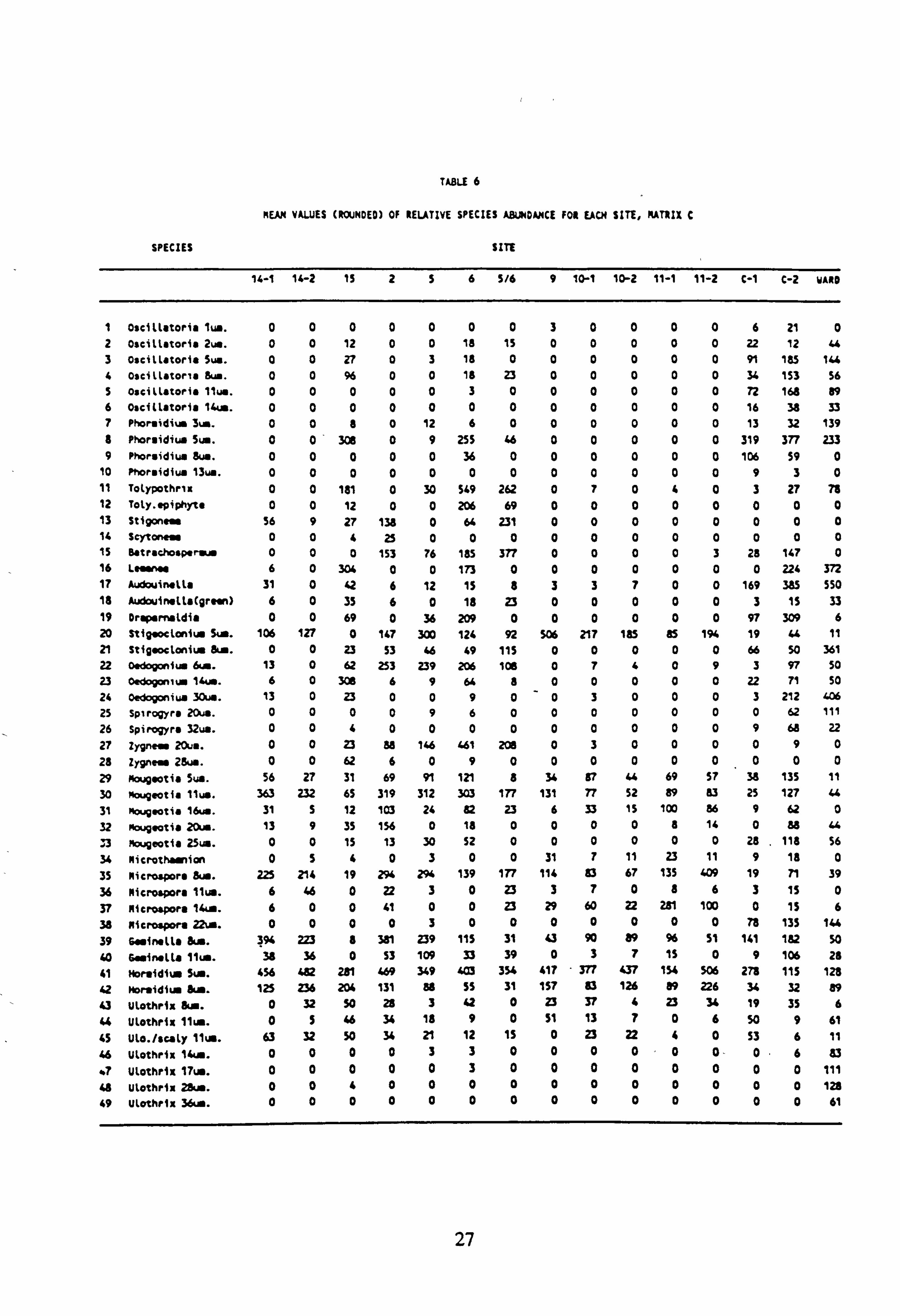
TABLE 6
MEAN VALUES (ROUNDED) Of RELATIVE SPECIES ABUNDANCE FOR EACH SITE, MATRIX C
SPECIES SITE
14-1 14-2 1i 256 5/6 9 10-1 10-2 11-1 11-2 C-1 C-2 YARD
I Oscillatoria lua. 0 0 0 0 0 0 0 3 0 0 0 0 6 21 0 2 Oscillatoria 2ua. 0 0 12 0 0 18 15 0 0 0 0 0 22 12 ý. t 3 osci(latoria Sun. 0 0 27 0 3 18 0 0 0 0 0 0 91 185 144 4 Oscillatoria 8uß. 0 0 % 0 0 18 23 0 0 0 0 0 34 153 56 5 oscillatoria 11w. 0 0 0 0 0 3 0 0 0 0 0 0 72 168 89 6 Oscittatoria 14M. 0 0 0 0 0 0 0 0 0 0 0 0 16 38 33 7 Phoraidium 3ua. 0 0 8 0 12 6 0 0 0 0 0 0 13 32 139 8 Phoraidiua Sum. 0 0 308 0 9 255 46 0 0 0 0 0 319 377 233 9 Phor, idiuw dw. 0 0 0 0 0 36 0 0 0 0 0 0 106 59 0
10 Phoraidiw 13ua. 0 0 0 0 0 0 0 0 0 0 0 0 9 3 0 11 Totypothri 0 0 181 0 30 S49 262 0 7 0 4 0 3 27 78 12 Toly. opiphyto 0 0 12 0 0 206 69 0 0 0 0 0 0 0 0 13 Stiyonaaa 56 9 27 138 0 64 231 0 0 0 0 0 0 0 0 14 Scytonasr 0 0 4 25 0 0 0 0 0 0 0 0 0 0 0 15 Batrachosperaua 0 0 0 153 76 185 377 0 0 0 0 3 28 147 0 16 Leaanw 6 0 304 0 0 173 0 0 0 0 0 0 0 224 372 17 Audouinalla 31 0 <2 6 12 15 8 3 3 7 0 0 169 385 550 18 Audouin. lla(gra. n) 6 0 35 6 0 18 23 0 0 0 0 0 3 1S 33 19 Draparnaldia 0 0 69 0 36 209 0 0 0 0 0 0 97 309 6 20 Stigaoclonium Sum. 106 127 0 147 300 124 92 506 217 185 85 194 19 4t 11 21 Sti; aoclonium &a. 0 0 23 53 46 49 113 0 0 0 0 0 66 SO 361 22 oadogoniua Eia. 13 0 62 253 239 206 108 0 7 f 0 9 3 97 50 23 Oedogom ua 14ua. 6 0 308 6 9 64 8 0 0 0 0 0 22 71 50 24 oedogoniuw 30uw. 13 0 23 0 0 9 0 0 3 0 0 0 3 212 406 25 Spirogyra 20w. 0 0 0 0 9 6 0 0 0 0 0 0 0 62 111 26 Spirogyra 32w. 0 0 4 0 0 0 0 0 0 0 0 0 9 68 22 27 Iygnew 20ua. 0 0 23 88 146 161 208 0 3 0 0 0 0 9 0 28 Iygnear 28ua. 0 0 62 6 0 9 0 0 0 0 0 0 0 0 0 29 Mougsotia Sum. 56 27 31 69 91 121 8 34 87 6t 69 57 38 135 11 30 Nougeotia 11w. 363 232 65 319 312 303 177 131 77 52 89 83 25 127 6G 31 nougwtia 16w. 31 S 12 103 24 82 23 6 33 15 100 86 9 62 0 32 Mougaotia 20ua. 13 9 35 156 0 18 0 0 0 0 8 14 0 88 u 3 Mougeotia 25ua. 0 0 15 13 30 52 0 0 0 0 0 0 28
. 118 56
34 Microthamian 0 5 4 0 3 0 0 31 7 11 23 11 9 18 0 35 Microspore 8ur. 225 214 19 294 294 139 177 114 83 67 135 609 19 71 39 36 Nicrospora Ilua. 6 46 0 22 3 0 23 3 7 0 8 6 3 15 0 37 Microspore 14Aa. 6 0 0 41 0 0 23 29 60 22 281 100 0 15 6 38 Microspora 22um. 0 0 0 0 3 0 0 0 0 0 0 0 78 135 1"
39 Gaainalla dis. 396 223 8 381 239 115 31 43 90 89 % 51 141 182 so
40 6. ainalla llia. 38 36 0 53 109 33 39 0 3 7 1S 0 9 106 28 41 tbraidia Sum. 456 482 281 469 349 40 354 417 377 437 154 $06 278 115 128
42 Horaidium S tin. 125 236 204 131 88 SS 31 1S7 83 126 89 226 34 32 89 43 Ulothrix 8ua. 0 32 SO 28 3 42 0 23 37 4 23 34 19 35 6 44 Ulothrix h um. 0 S 46 34 18 9 0 51 13 7 0 6 SO 9 61 45 Ulo. /scaly 11um. 63 32 SO 34 21 12 1S 0 23 22 4 0 53 6 11 46 Utothrix 1". 0 0 0 0 3 3 0 0 0 0 0 0- 0- 6 83
"7 Ulothrix Mo. 0 0 0 0 0 3 0 0 0 0 0 0 0 0 111
48 Ulothrix 26um. 0 0 4 0 0 0 0 0 0 0 0 0 0 0 128 49 Ulothrix 36um. 0 0 0 0 0 0 0 0 0 0 0 0 0 0 61
27
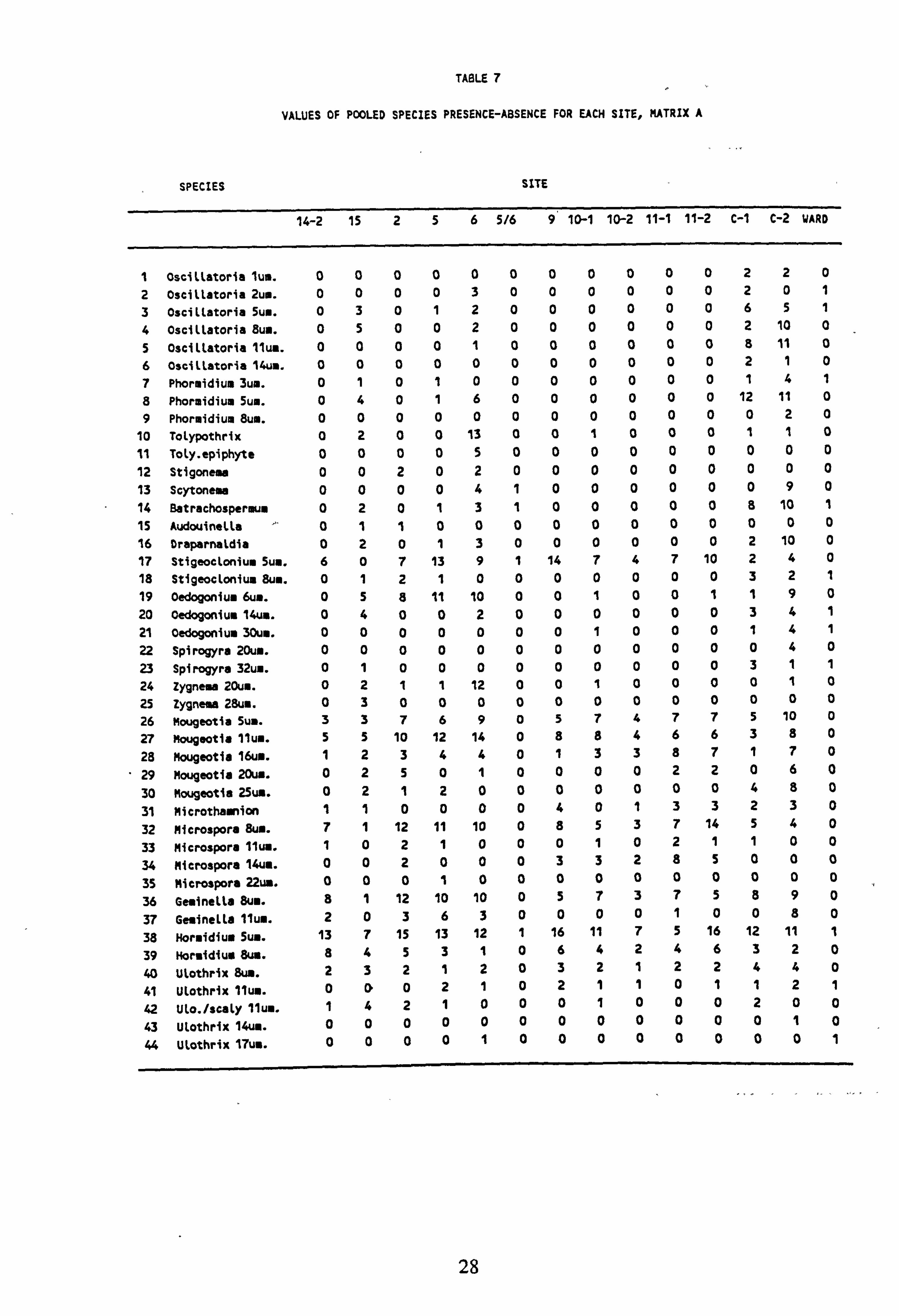
TABLE 7
VALUES OF POOLED SPECIES PRESENCE-ABSENCE FOR EACH SITE, MATRIX A
SPECIES SITE
14-2 15 256 5/6 9 10-1 10-2 11-1 11-2 C-1 C-2 WARD
I oscillatoria Zum. 0 0 0 0 0 0 0 0 0 0 0 2 2 0
2 Osciltatoria 2um. 0 0 0 0 3 0 0 0 0 0 0 2 0 1
3 Oscillatoria 5uN. 0 3 0 1 2 0 0 0 0 0 0 6 5 1
4 Oscillatoria aua. 0 5 0 0 2 0 0 0 0 0 0 2 10 0
5 Oscillatoria Ilum. 0 0 0 0 1 0 0 0 0 0 0 8 11 0
6 Oscillatoria 14un. 0 0 0 0 0 0 0 0 0 0 0 2 1 0
7 Phormidiua 3um. 0 1 0 1 0 0 0 0 0 0 0 1 4 1
8 Phormidium Sun. 0 4 0 1 6 0 0 0 0 0 0 12 11 0
9 Phormidium 8um. 0 0 0 0 0 0 0 0 0 0 0 0 2 0
10 Tolypothrix 0 2 0 0 13 0 0 1 0 0 0 1 1 0
11 Toly. epiphyte 0 0 0 0 5 0 0 0 0 0 0 0 0 0
12 Stigonema 0 0 2 0 2 0 0 0 0 0 0 0 0 0
13 Scytonema 0 0 0 0 4 1 0 0 0 0 0 0 9 0
14 Batrachospermua 0 2 0 1 3 1 0 0 0 0 0 8 10 1
15 Audouinella 0 1 1 0 0 0 0 0 0 0 0 0 0 0
16 Draparnaldia 0 2 0 1 3 0 0 0 0 0 0 2 10 0
17 Stigeoclonium Sun. 6 0 7 13 9 1 14 7 4 7 10 2 4 0
18 Stigeoclonium 8um. 0 1 2 1 0 0 0 0 0 0 0 3 2 1
19 Oedogonium 6um. 0 5 8 11 10 0 0 1 0 0 1 1 9 0
20 oedogonium 14um. 0 4 0 0 2 0 0 0 0 0 0 3 4 1
21 Oedogonium 30um. 0 0 0 0 0 0 0 1 0 0 0 1 4 1
22 Spirogyra 20um. 0 0 0 0 0 0 0 0 0 0 0 0 4 0
23 Spirogyra 32um. 0 1 0 0 0 0 0 0 0 0 0 3 1 1
24 Zygnema 20un. 0 2 1 1 12 0 0 1 0 0 0 0 1 0
25 Zygnema 28um. 0 3 0 0 0 0 0 0 0 0 0 0 0 0 26 Mougeotia 5u.. 3 3 7 6 9 0 5 7 4 7 7 5 10 0
27 Mougeotia 11um. 5 5 10 12 14 0 8 8 4 6 6 3 8 0
28 Mougeotia 16um. 1 2 3 4 4 0 1 3 3 8 7 1 7 0
29 Mougeotia 20un. 0 2 5 0 1 0 0 0 0 2 2 0 6 0
30 Mougeotia 25um. 0 2 1 2 0 0 0 0 0 0 0 4 8 0
31 Microthaanion 1 1 0 0 0 0 4 0 1 3 3 2 3 0
32 Microspora 8ua. 7 1 12 11 10 0 8 5 3 7 14 5 4 0
33 Microspora Ilum. 1 0 2 1 0 0 0 1 0 2 1 1 0 0
34 Microspora 14um. 0 0 2 0 0 0 3 3 2 8 5 0 0 0
35 Microspora 22u$. 0 0 0 1 0 0 0 0 0 0 0 0 0 0
36 Geminella 8uß. 8 1 12 10 10 0 5 7 3 7 5 8 9 0
37 Gesinella Ilum. 2 0 3 6 3 0 0 0 0 1 0 0 8 0
38 Mormidium Sun. 13 7 15 13 12 1 16 11 7 5 16 12 11 1
39 Mor. idiua Bum. 8 4 5 3 1 0 6 4 2 4 6 3 2 0
40 Ulothrix We. 2 3 2 1 2 0 3 2 1 2 2 4 4 0
41 Ulothrix Ilum. 0 0 0 2 1 0 2 1 1 0 1 1 2 1
42 Ulo. /scaly Ilum. 1 4 2 1 0 0 0 1 0 0 0 2 0 0
43 Ulothrix 14um. 0 0 0 0 0 0 0 0 0 0 0 0 1 0
44 Ulothrix 17uu. 0 0 0 0 1 0 0 0 0 0 0 0 0 1
28
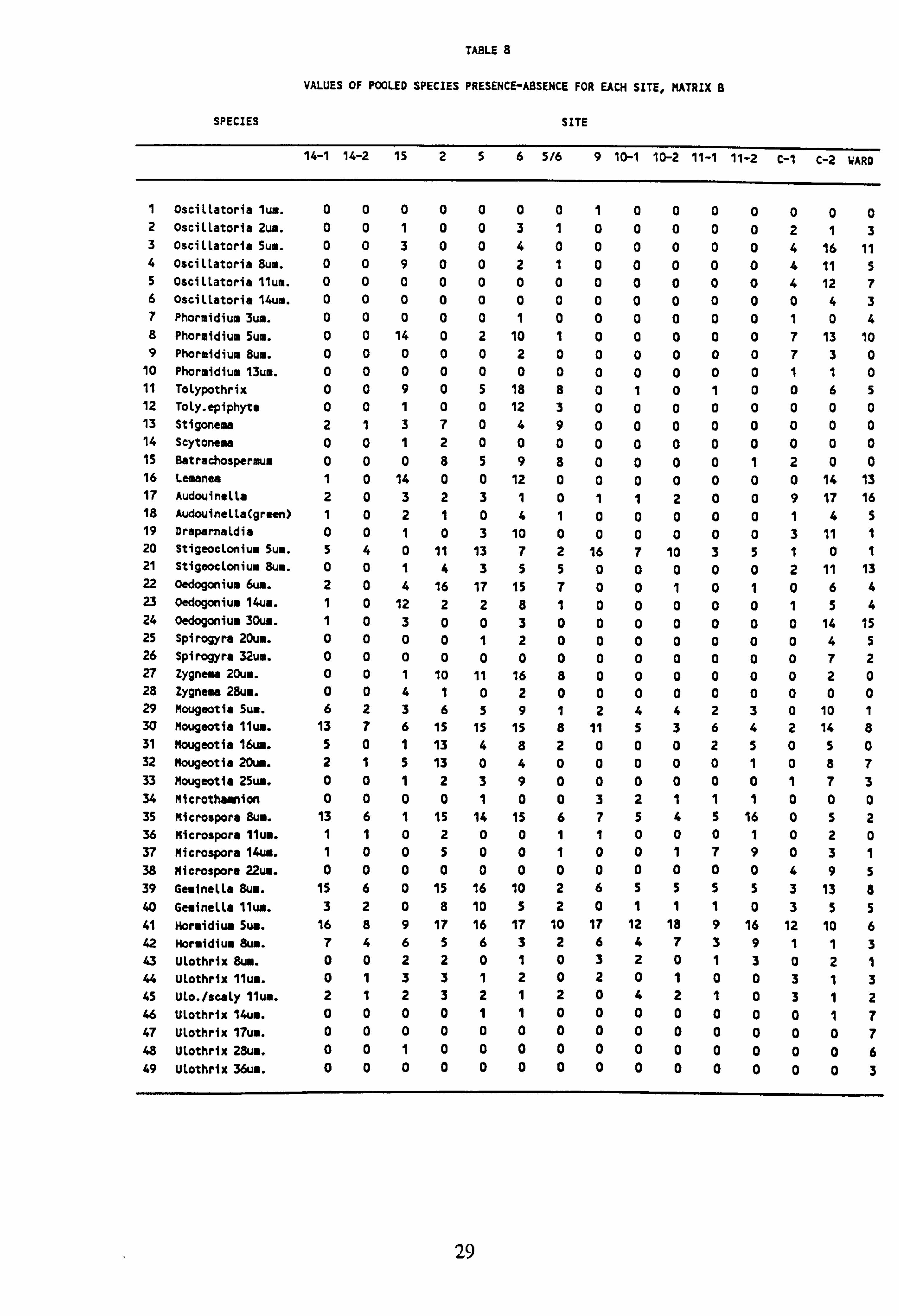
TABLE 8
VALUES OF POOLED SPECIES PRESENCE-ABSENCE FOR EACH SITE, MATRIX B
SPECIES SITE
14-1 14-2 15 256 5/6 9 10-1 10-2 11-1 11-2 C-1 C-2 WARD
1 Osciltatoria lug. 0 0 0 0 0 0 0 1 0 0 0 0 0 0 0 2 OsciLtatoria 2um. 0 0 1 0 0 3 1 0 0 0 0 0 2 1 3 3 Oscitlatoria sum. 0 0 3 0 0 4 0 0 0 0 0 0 4 16 11 4 Osciltatoria 8um. 0 0 9 0 0 2 1 0 0 0 0 0 4 11 5 5 Osciltatoria 11um. 0 0 0 0 0 0 0 0 0 0 0 0 4 12 7 6 Osciltatoria l4um. 0 0 0 0 0 0 0 0 0 0 0 0 0 4 3 7 Phormidium 3um. 0 0 0 0 0 1 0 0 0 0 0 0 1 0 4 8 Phormidium 5um. 0 0 14 0 2 10 1 0 0 0 0 0 7 13 10 9 Phormidium 8um. 0 0 0 0 0 2 0 0 0 0 0 0 7 3 0
10 Phormidium 13ue. 0 0 0 0 0 0 0 0 0 0 0 0 1 1 0 11 ToLypothrix 0 0 9 0 5 18 8 0 1 0 1 0 0 6 5 12 Toly. epiphyte 0 0 1 0 0 12 3 0 0 0 0 0 0 0 0 13 Stigonema 2 1 3 7 0 4 9 0 0 0 0 0 0 0 0 14 Scytonema 0 0 1 2 0 0 0 0 0 0 0 0 0 0 0 15 Batrachospermum 0 0 0 8 5 9 8 0 0 0 0 1 2 0 0 16 Lemanea 1 0 14 0 0 12 0 0 0 0 0 0 0 14 13 17 Audouinella 2 0 3 2 3 1 0 1 1 2 0 0 9 17 16 18 Audouinelta(green) 1 0 2 1 0 4 1 0 0 0 0 0 1 4 5 19 DraparnaLdia 0 0 1 0 3 10 0 0 0 0 0 0 3 11 1 20 Stigeoclonium sum. 5 4 0 11 13 7 2 16 7 10 3 5 1 0 1 21 Stigeoclonium Bum. 0 0 1 4 3 5 5 0 0 0 0 0 2 11 13 22 oedogonium 6um. 2 0 4 16 17 15 7 0 0 1 0 1 0 6 4 23 0edogonium 14um. 1 0 12 2 2 8 1 0 0 0 0 0 1 5 4 24 oedogonium 30um. 1 0 3 0 0 3 0 0 0 0 0 0 0 14 15 25 Spirogyra 20um. 0 0 0 0 1 2 0 0 0 0 0 0 0 4 5 26 Spirogyra 32um. 0 0 0 0 0 0 0 0 0 0 0 0 0 7 2 27 Zygnema 20um. 0 0 1 10 11 16 8 0 0 0 0 0 0 2 0 28 Zygnema 28um. 0 0 4 1 0 2 0 0 0 0 0 0 0 0 0 29 Mougeotia 5um. 6 2 3 6 5 9 1 2 4 4 2 3 0 10 1 30 Mougeotia Ilum. 13 7 6 15 15 15 8 11 5 3 6 4 2 14 8 31 Mougeotia l6um. 5 0 1 13 4 8 2 0 0 0 2 5 0 5 0 32 Mougeotia 20um. 2 1 5 13 0 4 0 0 0 0 0 1 0 8 7 33 Mougeotia 25um. 0 0 1 2 3 9 0 0 0 0 0 0 1 7 3 34 Microthamnion 0 0 0 0 1 0 0 3 2 1 1 1 0 0 0 35 Microspora Sum. 13 6 1 15 14 15 6 7 5 4 5 16 0 5 2 36 Microspora 11um. 1 1 0 2 0 0 1 1 0 0 0 1 0 2 0 37 Microspora 14um. 1 0 0 5 0 0 1 0 0 1 7 9 0 3 1 38 Microspora 22um. 0 0 0 0 0 0 0 0 0 0 0 0 4 9 5 39 Geminelta Sun. 15 6 0 15 16 10 2 6 5 5 5 5 3 13 8 40 GemineLta 11um. 3 2 0 8 10 5 2 0 1 1 1 0 3 5 5 41 Hormidium sun. 16 8 9 17 16 17 10 17 12 18 9 16 12 10 6 42 Hormidium 8um. 7 4 6 5 6 3 2 6 4 7 3 9 1 1 3 43 Ulothrix 8um. 0 0 2 2 0 1 0 3 2 0 1 3 0 2 1 44 ULothrix 11um. 0 1 3 3 1 2 0 2 0 1 0 0 3 1 3 45 ULo. /scaly 11um. 2 1 2 3 2 1 2 0 4 2 1 0 3 1 2 46 ULothrix 144Jm. 0 0 0 0 1 1 0 0 0 0 0 0 0 1 7 47 Ulothrix l7um. 0 0 0 0 0 0 0 0 0 0 0 0 0 0 7 48 Ulothrix 28ue. 0 0 1 0 0 0 0 0 0 0 0 0 0 0 6 49 Ulothrix 36um. 0 0 0 0 0 0 0 0 0 0 0 0 0 0 3
29
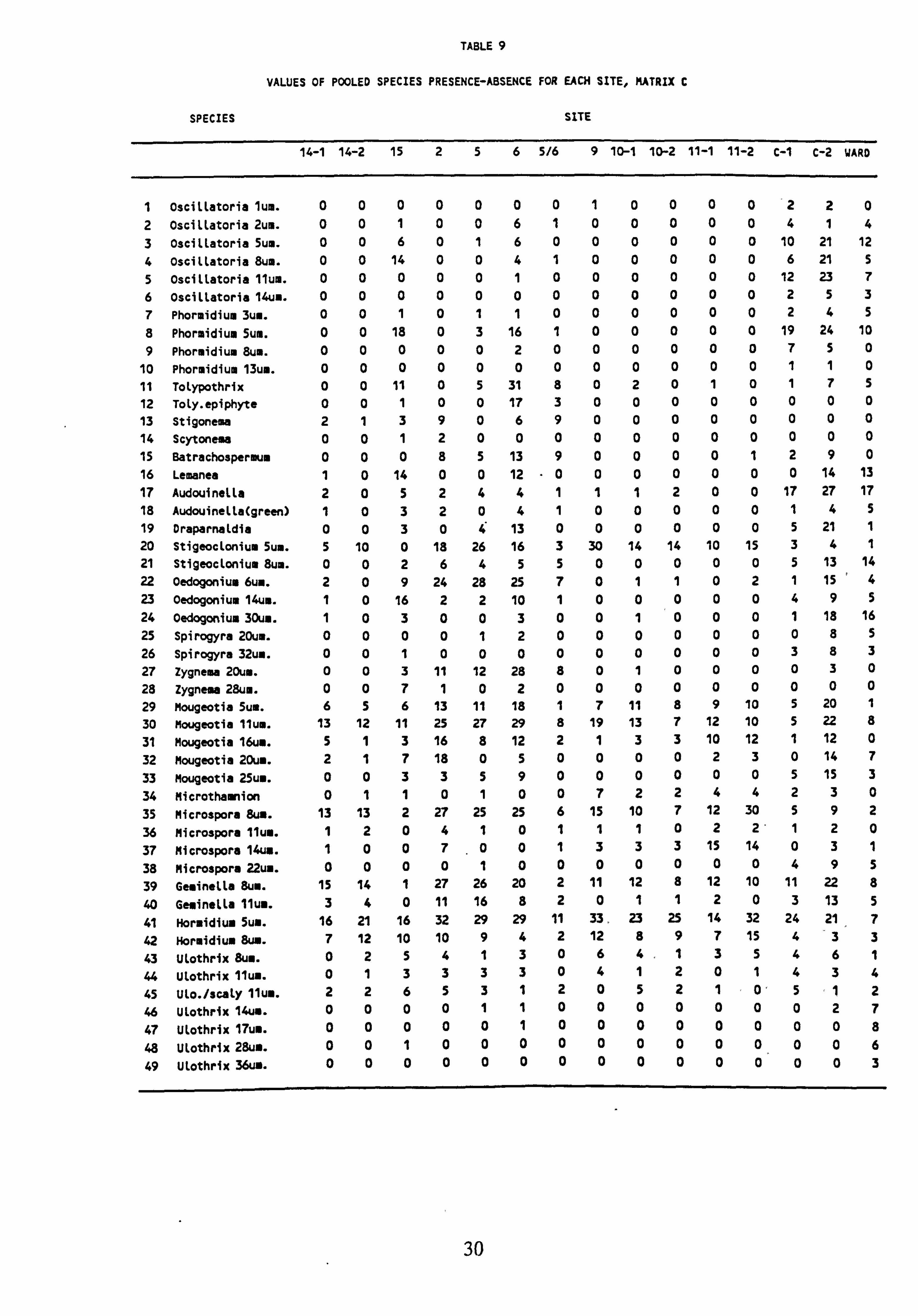
TABLE 9
VALUES OF POOLED SPECIES PRESENCE-ABSENCE FOR EACH SITE, MATRIX C
SPECIES SITE
14-1 14-2 15 2 5 6 5/6 9 10-1 10-2 11-1 11-2 c-1 C-2 WARD
1 oscillatoria Zum. 0 0 0 0 0 0 0 1 0 0 0 0 2 2 0 2 Oscillatoria 2um. 0 0 1 0 0 6 1 0 0 0 0 0 4 1 4 3 Oscillatoria 5um. 0 0 6 0 1 6 0 0 0 0 0 0 10 21 12 4 Oscillatoria sum. 0 0 14 0 0 4 1 0 0 0 0 0 6 21 5 5 Oscillatoria llum. 0 0 0 0 0 1 0 0 0 0 0 0 12 23 7 6 Oscillatoria 14ua. 0 0 0 0 0 0 0 0 0 0 0 0 2 5 3 7 Phormidium 3u.. 0 0 1 0 1 1 0 0 0 0 0 0 2 4 5
8 Phormidium 5um. 0 0 18 0 3 16 1 0 0 0 0 0 19 24 10
9 Phormidium Sun. 0 0 0 0 0 2 0 0 0 0 0 0 7 5 0
10 Phormidium 13um. 0 0 0 0 0 0 0 0 0 0 0 0 1 1 0
11 Tolypothrix 0 0 11 0 5 31 8 0 2 0 1 0 1 7 5
12 Toly. epiphyte 0 0 1 0 0 17 3 0 0 0 0 0 0 0 0 13 Stigonema 2 1 3 9 0 6 9 0 0 0 0 0 0 0 0 14 Scytonema 0 0 1 2 0 0 0 0 0 0 0 0 0 0 0 15 eatrachospermum 0 0 0 8 5 13 9 0 0 0 0 1 2 9 0 16 Lemanea 1 0 14 0 0 12 "0 0 0 0 0 0 0 14 13 17 AudouineLta 2 0 5 2 4 4 1 1 1 2 0 0 17 27 17 18 AudouineLta(green) 1 0 3 2 0 4 1 0 0 0 0 0 1 4 5 19 DraparnaLdia 0 0 3 0 4 13 0 0 0 0 0 0 5 21 1 20 Stigeoclonium 5um. 5 10 0 18 26 16 3 30 14 14 10 15 3 4 1 21 StigeocLonium sum. 0 0 2 6 4 5 5 0 0 0 0 0 5 13 14 22 Oedogonium 6uß. 2 0 9 24 28 25 7 0 1 1 0 2 1 15 4 23 Oedogonium 14um. 1 0 16 2 2 10 1 0 0 0 0 0 4 9 5 24 Oedogonium 30um. 1 0 3 0 0 3 0 0 1 0 0 0 1 18 16 25 Spirogyra 20um. 0 0 0 0 1 2 0 0 0 0 0 0 0 8 5 26 Spirogyra 32um. 0 0 1 0 0 0 0 0 0 0 0 0 3 8 3 27 Zygnema 20um. 0 0 3 11 12 28 8 0 1 0 0 0 0 3 0
28 Zygnema 28um. 0 0 7 1 0 2 0 0 0 0 0 0 0 0 0
29 Mougeotia 5um. 6 5 6 13 11 18 1 7 11 8 9 10 5 20 1
30 Mougeotia llum. 13 12 11 25 27 29 8 19 13 7 12 10 5 22 8
31 Mougeotia 16ue. 5 1 3 16 8 12 2 1 3 3 10 12 1 12 0
32 Mougeotia 20um. 2 1 7 18 0 5 0 0 0 0 2 3 0 14 7
33 Mougeotia 25um. 0 0 3 3 5 9 0 0 0 0 0 0 5 15 3
34 Microthamnion 0 1 1 0 1 0 0 7 2 2 4 4 2 3 0
35 Microspore sun. 13 13 2 27 25 25 6 15 10 7 12 30 5 9 2
36 Microspore llum. 1 2 0 4 1 0 1 1 1 0 2 2' 1 2 0
37 Microspora 14u.. 1 0 0 7 0 0 1 3 3 3 15 14 0 3 1
38 Microspore 22um. 0 0 0 0 1 0 0 0 0 0 0 0 4 9 5
39 Geminella Sun. 15 14 1 27 26 20 2 11 12 8 12 10 11 22 8
40 Geminella Ilum. 3 4 0 11 16 8 2 0 1 1 2 0 3 13 5
41 Hormidium Sum. 16 21 16 32 29 29 11 33. 23 25 14 32 24 21 7
42 Hormidium 8w. 7 12 10 10 9 4 2 12 8 9 7 15 4 3 3
43 ULothrix sun. 0 2 5 4 1 3 0 6 4 .1 3 5 4 6 1
44 ULothrix llue. 0 1 3 3 3 3 0 4 1 2 0 1 4 3 4
45 Ulo. /3caly llum. 2 2 6 5 3 1 2 0 5 2 1 0' 5 1 2
46 ULothrix 14uu. 0 0 0 0 1 1 0 0 0 0 0 0 0 2 7
47 ULothrix 17um. 0 0 0 0 0 1 0 0 0 0 0 0 0 0 8
48 ULothrix 28ua. 0 0 1 0 0 0 0 0 0 0 0 0 0 0 6
49 Utothrix 36um. 0 0 0 0 0 0 0 0 0 0 0 0 0 0 3
30
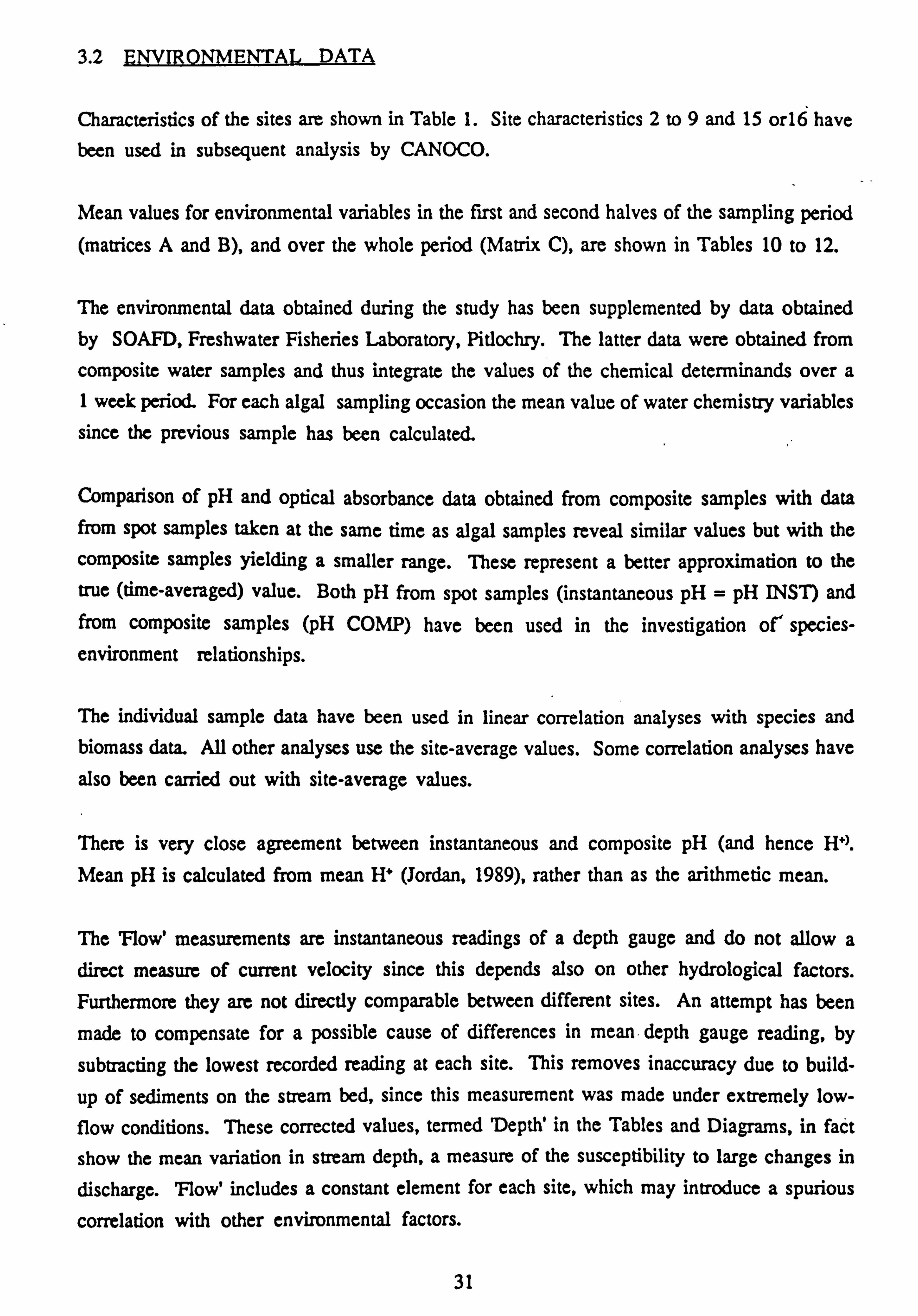
3.2 ENVIRONMENTAL DATA
Characteristics of the sites are shown in Table 1. Site characteristics 2 to 9 and 15 or16 have been used in subsequent analysis by CANOCO.
Mean values for environmental variables in the first and second halves of the sampling period (matrices A and B), and over the whole period (Matrix C), are shown in Tables 10 to 12.
The environmental data obtained during the study has been supplemented by data obtained by SOAFD, Freshwater Fisheries Laboratory, Pitlochry. The latter data were obtained from
composite water samples and thus integrate the values of the chemical determinands over a 1 week period. For each algal sampling occasion the mean value of water chemistry variables since the previous sample has been calculated.
Comparison of pH and optical absorbance data obtained from composite samples with data from spot samples taken at the same time as algal samples reveal similar values but with the composite samples yielding a smaller range. These represent a better approximation to the true (time-averaged) value. Both pH from spot samples (instantaneous pH = pH INST) and from composite samples (pH COMP) have been used in the investigation of" species- environment relationships.
The individual sample data have been used in linear correlation analyses with species and biomass data. All other analyses use the site-average values. Some correlation analyses have
also been carried out with site-average values.
There is very close agreement between instantaneous and composite pH (and hence H+).
Mean pH is calculated from mean H+ (Jordan, 1989), rather than as the arithmetic mean.
The 'Flow' measurements are instantaneous readings of a depth gauge and do not allow a direct measure of current velocity since this depends also on other hydrological factors.
Furthermore they are not directly comparable between different sites. An attempt has been
made to compensate for a possible cause of differences in mean, depth gauge reading, by
subtracting the lowest recorded reading at each site. This removes inaccuracy due to build-
up of sediments on the stream bed, since this measurement was made under extremely low-
flow conditions. These corrected values, termed Depth' in the Tables and Diagrams, in fact
show the mean variation in stream depth, a measure of the susceptibility to large changes in
discharge. 'Flow' includes a constant element for each site, which may introduce a spurious
correlation with other environmental factors.
31
Both 'Flow' and Depth' have been included in analyses in order to investigate this possibility.
Instantaneous temperature is liable to bias, as discussed in Section 4.4.2. The measurements of maximum and minimum temperatures are too few to be of value in statistical analyses.
Absorbance measurements have been used to infer values for Total Organic Carbon TOC) in
natural waters (Edwards and Cresser, 1987; Rees et al, 1989). These authors utilized absorbance at 350 nm, while others have used A350 as a close correlate with TOC (Karlsson
et al, 1987; Gjessing et al, 1989). The Freshwater Fisheries Laboratory have routinely measured A400 and A2% and this practice was continued in this work. Measurements of TOC
made in the L. Ard streams are highly correlated with . A250 (R. Harriman, pers. comm. ) A. is a measure of turbidity of the water and is positively correlated with A250 in field samples.
Mean (24 hour) Photosynthetically Available Radiation ( PAR) was measured over several time intervals at 8 sites, allowing calculation of a mean value for integrated PAR as a percentage of that available at the control 'open' site on Burn 6. These mean values have been assumed to remain constant over the whole sampling period. For analyses by CANOCO the percentages have been used, with estimated values for those sites not actually measured. For correlation analysis utilizing individual sample data, values of incident PAR immediately prior to the sampling, were calculated from the measured incident PAR at Bum 6 and the percentage values. The means of these values are shown in Tables 10-12 as 'absolute PAR' (= PAR ABS).
Measurements of PAR could not be carried out at all sites because of the limited number of instruments available (five) and the possibility of interference occurring at some sites. Therefore subjective estimates have been made in order to enable CANOCO to carry out analyses incorporating data on PAR. These however have not been used in correlation analyses (Table 13).
Values of Total Oxidised Nitrogen (TON) vary by up to a factor of 10. This can be largely
attributed to the very high values encountered in the Burn 10 and Corrie catchments following clearfelling of a section of forest.
Decomposition of litter and brushwood combined with a reduced uptake by plant cover may account for most of the increase, but some may also be due to the practice of treating the tree stumps with urea to promote microbial breakdown. Between other catchments mean TON
varies by less than a factor of three.
Mean Phosphate concentrations are around or below detectable limits in circumneutral waters and between 1 and 3 pegl-' in most of the acidic burns, but rise to 66 pegl-1 (mean) for Bum 9 in Table 10, and 14 in Table 11. This is a consequence of the fertilization of the catchment carried out by the Forestry Commission. Phosphate will continue to be leached out of the soil for several years after such treatment (Harriman, 1978).
32
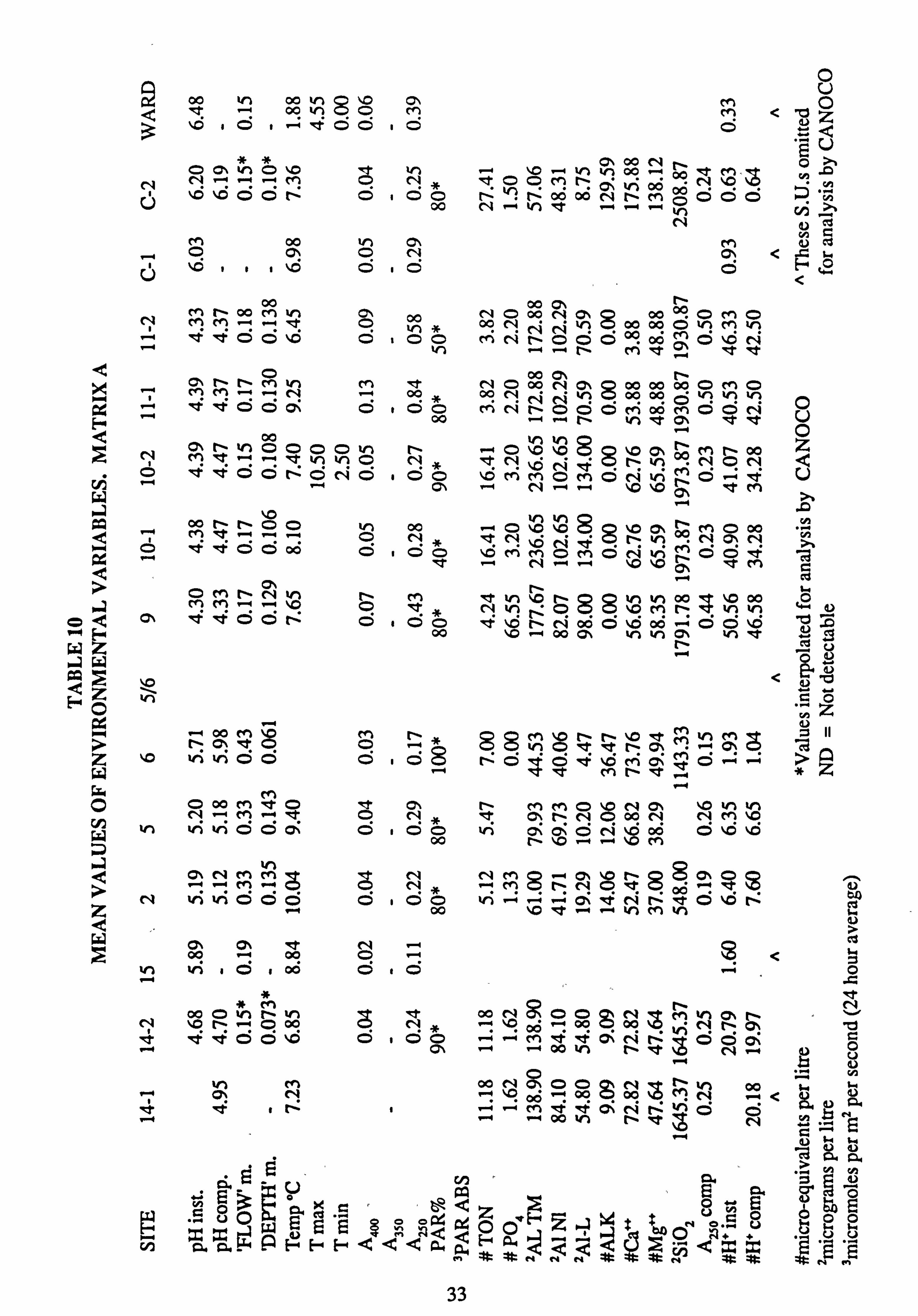
00 00 kil C-1
3 ö .ýv öö 1ö
Oo%W14 Oýo 1n N N --ý --ý "--ý M N
V ß'000N O 1 ö0 00
en 00 O Ö N
00 N
MN 00 M W-1 MM "--ý "-, d
Q\ O 00
- ^' ýt ßt00'0 Ö 14 1 i 00
iC O
WI) MM M 7' ºI
~ -4 N ýt ýi OO Oý
--4 O
0 lE O
00
N OWN n000 00 N M C 4 ýtOOn6 NÖ 1 ÖO
Ci I
00 NNÖO M ýf .- -4 -4
*n Q
00 N ä
O ýt ýt OO 00 Ö ,OO
OM[- Ntn N M
° Q Qý 'T R: 0C Ö I ÖO
.. E 00 wz aw
00 en
' M
fý C, tO z '. o 'n vý öö ö .cS
O -4 M IRT CD Ö N N
h *fl 000'. Ö i ÖÖ 00
-NMM0 0 N
N viv'i00 ÖC
09 09 yr vi 00 0 "0
iM M 00 c
N N
"' 0 000 0 q ÖÖ'. 0 '4 Ö ÖO
V-4 4 1-4
N 0-4
En
ýM Q' N
r-
M M O
N ON
00 00
. Ni
pip ýf en lqt OOMN %D N l-: oöo6IN Nn 006 OOÖ
CN O
00 Cý p (ON
°O O
cV Nw 00 0000 ÖO cM tq cnC-i Ö°OOÖMO"d N
NOO0 0000000000 MNNÖÖvOMOÖcn ÖÖN
r 00 NNONN MN-4 -O ý \oýOItM
'IT N \-6 (Ii 4 O'
SSn C\ r- 0" N O\ N
-MNOrO NT M
tri 00 ýM 00 N terry
ÖSS
et \G n
cV oö Ö ý6 oÖ -4 ý6 ÖÖ 00 O\ ' *A QN Yn It
N 1-4
SSM ýD lý NO C\
M V'1 O d: ý tý ýý Q)
lýÖ Öýt MCKme Ö14"--ý Mt en N le .. r
l- MMO ID N 0% %Z V1 'n lqt (: [- NO oO NNM \D vi cý OK Ö cN oö Ö
['ý ýo . -4 -M
wl M iý w"A- /1 a
O U
< -ý
ö
-
in m
0
O U O z
ca w w
< ub
"~z ý-y
II CQ
'1 ''. v vý v ý1M NO ýT ap
\O le -- kn en kn i2
.ý o
00 NCO0 ON r N M N OoO O tei
-nO C 000 ' 4 -4 o ýt tý 00 - " N -+ ý v
00 00OoN1 %fl oo a N 'i < i " "-+ "--4 cf fi Cý N r-: v ÖÖ 1.4 V" 00 V'1 N "T
9 y `ý . . ý
4. ö ö E'2 o
ye 03 , rr,, ý "~ UO o
.c cdz
OOW 5lf0ö +NO ý ý
uE W it dry O
G'i .. iU O
,. ý ~ýQ:
2 <2 U
33
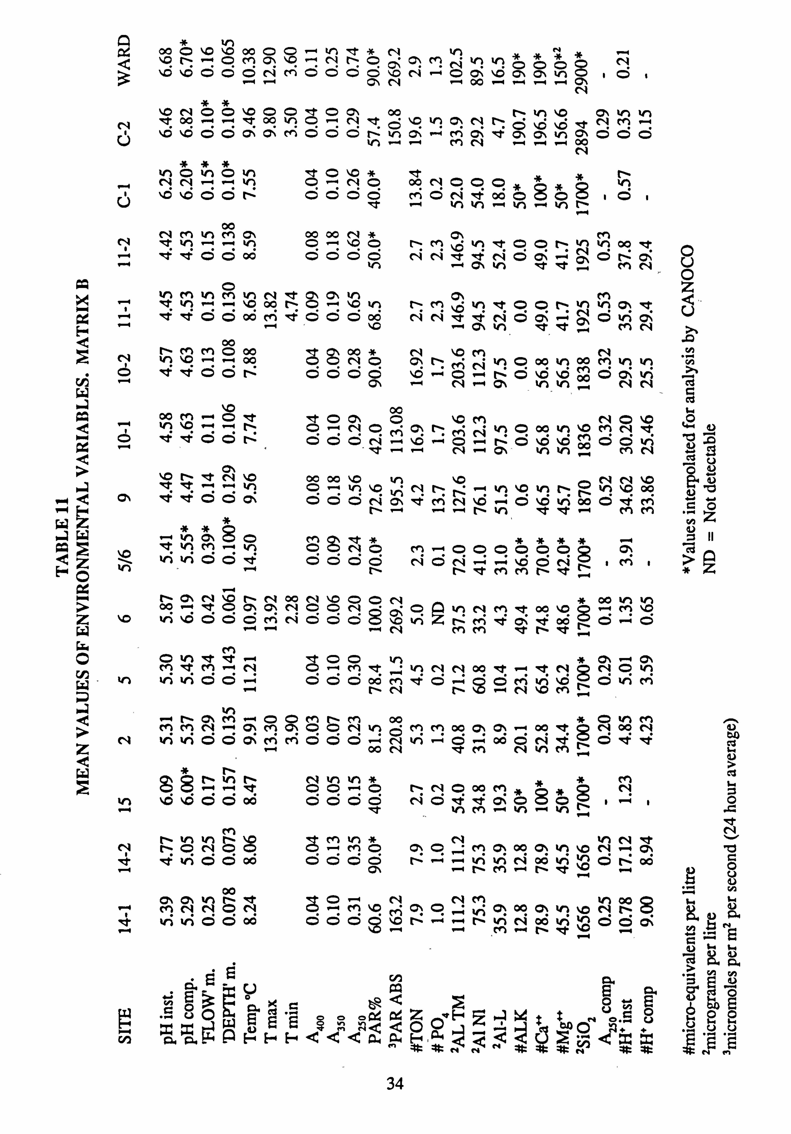
oo O ýD ýo 00 OO- to ItT *N W) N . -. t- OM ON ýO '-+ N I- O Cý Oý r! Cj In tt! 0N 3 \6 '000CNMÖÖOCNN-Oa, ýC Or C1Ö
\C NOO \0 OO It O ON oo tN Vn \C C\ tn ?n N ýt 09 rr -i 00 N Cl -14 N6 IO Ili Cý N I, ý O ,C et NM -1
ýO ýO OO Cý Oý C'i OOO in O, -M C\ ýt C5 QN in Q, OOO tn -4 -4 Cf) (14 -4 -4 -4 00
InCin0In Rt0'. o* Nt t- r, Cli Cli --ý 'i O-NO 00 N0aa*V! V ýOýpÖOn ÖÖÖOV C; 6C, 4 4°°OSa
i
00 N
NM try M Q\ 00 00 N* O\ M In "-" .I in O-'. G ONM Wi OON In in 00 It 116 0
-r 'tIt: t000o ÖÖ6 NN 'tNOcýNÖ N
. M
O Z in en in M to N It Q\ CN In p' M
" 0-4 1 r- C") . 16 In I: CR Cý rl: In 11 , 12, 'IT U C9 -+ i4 00oocri4 000ý NcVýý NC ýý6 in 0<
-4 ý - cq) C14 >% 00 .G
C`1 NMM 0 00 In 1 -+ 0
00 lF N '. O MN W A . . -4 00 OONO C7, r- MN In O oO vi oo M In W, CA
0 It d'00N OOOO ý, O-O-[NOýo"OO0 ý vi .ý ý 1.4 N- in i- N N Cd
p 110 00 cn ~-N 00
'I -I "I I-q 0NO Ci
Oý NMN Vý O CG W. ) ýO MN
4) 0.0 ý
Ö ýt I- 0©N ÖÖN -c- 0- [ýÖZ ý-d pMOÖI p + C ý7 --4 V-4 N- ON I/'1 ý -MN cd (ON \-O t- "Rt N \0 00 00 0 'n ti a V 0 'o , Cl S --ý in `0 in C- ln 0 Ö -1 u'
. "ý Gý 'Rttt©ÖO\ ÖÖÖNOýtt M"-+Ö'Cvnood'1 M 45 en V)
z W ýlW ** 0 cý ýt* ***r, II Z ýM--ýý O NO M"--X0000000 O; cý F it v100ý 000 NON .M M
ý
0 N ýM S'! l ~ Cý r-+ N O\ N '. O N 00
00 - NT O C'. O'. N N '. D OON* 00 in In OONO In NM 't o0 4D O- cM '. O
ýD vi \6 ÖÖÖ MC 'i6ci wi [: M4C7, : toÖCÖýÖ ^" 1 NMM ýt N v-
4+ M Q O v1 d- '0O 'n * 0\ - O\
M kT M- N -M _4 ºn NN 00 -Rt --ý NNON vý InIn00r:
--ý 666 o0M40 6 Min'. 0 0Inm
[ý NM te , r
N Qý M -+ OO MNM 00 lF ONM MMN C\ M C; OON %n MM 00 Q\ Q\ ý-+ 00 'It ON 00 N V Z
N hvi000ý ýM Ö0ÖooN'n Mod
6C4-4 ýqet C14 kn cn
OSýýý 00-
0N 000M ' ÖN p*
w-4 ýG ýÖÖ 00 ÖÖÖrio o'.
in in --+ NT in cn
0 C:
IRT N
N vl V'1 ýp eý M In *N in N 'Ct
0 0 " l- ONOO M Cý 0 O- MO O\ O0 in '. D N- CN b It ýhO0o4 000 1ýý+ r- M r- ýI V 0 -4 D -4 N
00 : -ý -
C'. C% vn 8 et MNNON
ýt O -+ NNM 00 p O-M\. oMC; O^; wi C: oOC\In '. oNt- O F, aý
4 In vi 66 06 000 '0 5- - t- M 00 in d0 0< "b in. -it 1-4 N
ä ä iy 0 > . ýi
H Vf
8a Q' ö
34
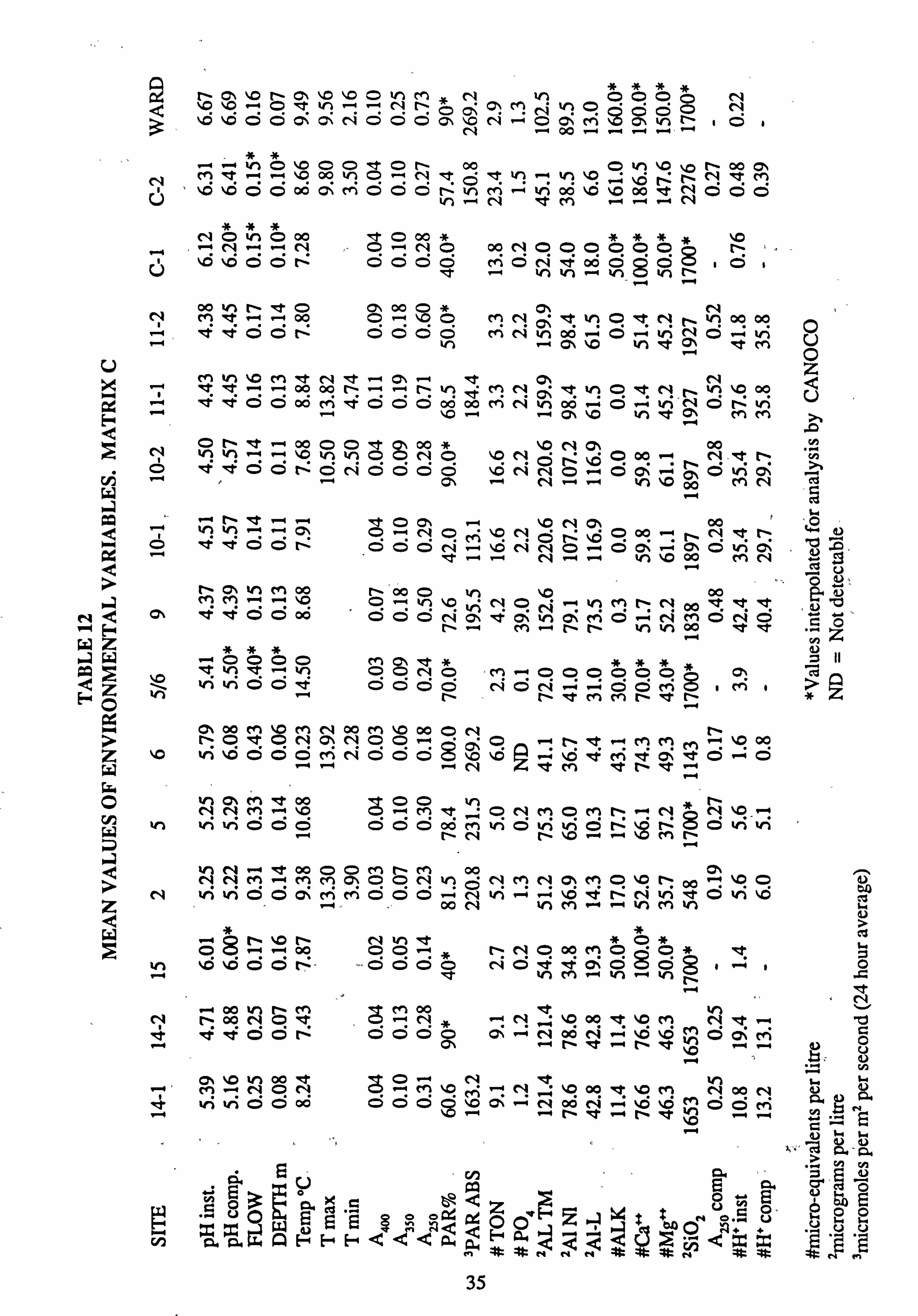
9N O" cN Q\ ,O 'O O 'r M* N W) OOO8N
< ýO 'D ý--ý O W, ý--ý ý--ý N I- O Oý Oý MN V'! OOQC? 0N 3 "Dý000'C'N000O\'0N'-0ONý\0C' NtOi
C14 00
. --ý --ý v1 Ö
\0 OO qt ON 00 0 yr ýo r- 00 CN NM Itt -- "O 00 Wn O-N 4t 'tt Vn- v', \O -4 "6 [.: I-Z N Rt M V' \G 110 OOooGNcri0ÖÖN N-InM OOoo NÖÖO
N0 to 0 00 'l 0 00 **** 'O ,.., 4 N--+-4 N 0-NO 00N000000p tý
ß\000N 0000 M0NIt000 aýÖ
0ov'1[- Ict O ON 000-x C' N N Met. -+. --goo 0-\00 MN"ttn0d; NNIn0000 p
vn - Oý \-O tra d' C' ýt M
M If \O M of N -4 Q\ -4 IIT O\ Nz X ýt rr "--ý 00 00 N --ý . --ý N in 'It lN It in 0 et NN In 'o 00 Ü
ÖÖOÖ M ýtÖÖÖo00M N in oKO MM
.G O [ý ýt 00 0 pý CA
Cý1 'f '( in V-1 0ON0
\ONýýý©00'--i N.
dtNN cn O etg00n6N000Ö ýNNO'+OOýý4 r- ÖviCý
C/j -+ -4 C' -N . --ý . -. in \0 op pMN W- cd
ýo C4 C\ 00 0
CD NO \0 N r. 5 ý6 O 00 N ', I: --4 NN Ö ÖÖ[- OÖÖr4"ý14D (VN- Ö Q\"-+QýÖv)C
. --4 . --i N -4 tn ýo 00 MN
> NC\vnMC0 n000 in ýo
ý00 °., a
a MCi -! -: ID 0 -4tn\DNON ý-- InM[-Nppýýtrt -0 yß 0 ©oö ÖÖCNa, 4Cýi'ý CK MÖ NMÖNÖ "'r r- 0 z wz
.aW. 0000 m to OONOM-OOOOOO * C; cC ¢Z N 'RT v? 'RT ý--ý tti ÖÖÖÖ NÖN14_; dÖM 1MI E-4C) N [- Ii'MMN q
C' 00 M ýD MN 00 c' '0 00 ON [, ý Olcý ONC'N00- O "--ý s "-+MMM'Oo0
Z V'ýýÖ(Z0CnNÖÖÖS\- ý Oýý. 4r 6.4M. 4 Cý t -4d
. -, . -, . -r N Itt M tt N 'I7 I"
G:. NNM-\
cn ýONMOM[-
"-+N' !
c- in inºn000 06600 i ©t 1iwi6NýMÖOýnv'1
NNN 'O
141 N- IRT 00 OOMNM 00 ON NNM -MMC'OON V NMNOýMO, DNpp BOO 0
N vnvý000ýcn MO00N W in
Mý t- C4til Mýwi ýM
z 00 .ý V
cl OSýýoýo ÖÖ[,
NOoOMÖO Ö*
ýt ý ýýÖÖn 0000 No44C\60hg ' -+ $0
't W) en ýt
N
00 V'l N0 OýN00
W) N N00
.ý -N`D00 '0 c4 Ný. -ý 4 14li66 ý ÖÖÖC ON --NNN\6 en6C--
Ö
Cý %0 in 00 -. fi -N0ý80MN r-+ N It IR OR ý7; ýD M NOON u0 MNO Cl a 4 viii 66 06 ö 66 s öos ^ ýNN ~+ýý ýÖÖý ab
44
dA V cý Hao C: 0-
35
Because of the bias introduced by these high values of PO43- and TON it is unlikely that
meaningful correlations between these variables and other variables (Table 13), biomass or species abundance data will be found. Nevertheless there appears to be a tendency for PO, 3-
to be higher in the more acidic waters (Table 12). This phenomenon has been noted previously (Nalewajko and_O'Mahony, 1988) although the opposite effect is also reported (Jansson et al, 1986).
Concentrations of total monomeric aluminium (Al-TM) are highest in the most acidified burns 9,10,11 and 14. Some differences are found between these sites in the proportion present as labile aluminium (A1-L), thought to represent the more toxic form (Helliwell et al, 1983; Folsom et al, 1986).
These differences may be due to the different amounts of humic material present in these burns; Burn 10 for example has the highest proportion (as well as the highest actual amount) of Al-L, and the lowest A2, in this acidified group of burns. Aluminium can complex with humic material (Steinberg and Kuhnel, 1987; Gjessing et al, 1989). Aluminium also com- plexes with phosphate (Minzoni, 1984; Nalewajko and Paul, 1985) so that some of the >79 pg 1-1 (approximately 9 peq 1) of non-labile aluminium may be in the form of an alumino- phosphorus complex. The water was not filtered before analysis so that the proportion of phosphate present in such complexes cannot be determined. Acidification of water may cause the release of aluminium from particulates (Tipping et al, 1989) and will thus release phosphate at the same time. Therefore complexed phosphate is not necessarily unavailable to algae. Alkalinity and the divalent cations Cat' and Mg-2' behave as would be expected, being highest in the sites with the highest mean pH.
Silicate concentrations are positively correlated with pH due to the pH dependence of silicate solubility. A limited amount of data is available for SiO2, so some interpolations have been
made to enable this variable to be included in analysis by CANOCO. The biological
significance of silicon results from its requirement by diatoms and its complexation reactions with aluminium, which can ameliorate its toxicity (Birchall et al, 1989).
Intercorrelations between environmental variables are of great importance in interpreting the influence of environment on species distributions. In Table 13 correlations between all pairs of variables is shown (Pearson's r), along with the number of paired observations (n) and the
p-value. There are 171 separate correlations in the table, so the appropriate level of signifi- cance is 0.5% (p = 0.005).
Those correlations with p<0.001 are most revealing about the relationships between the variables. The two measures of pH are strongly intercorrelated, but composite pH is usually found to give the higher correlation with other variables. pH is strongly correlated with
36
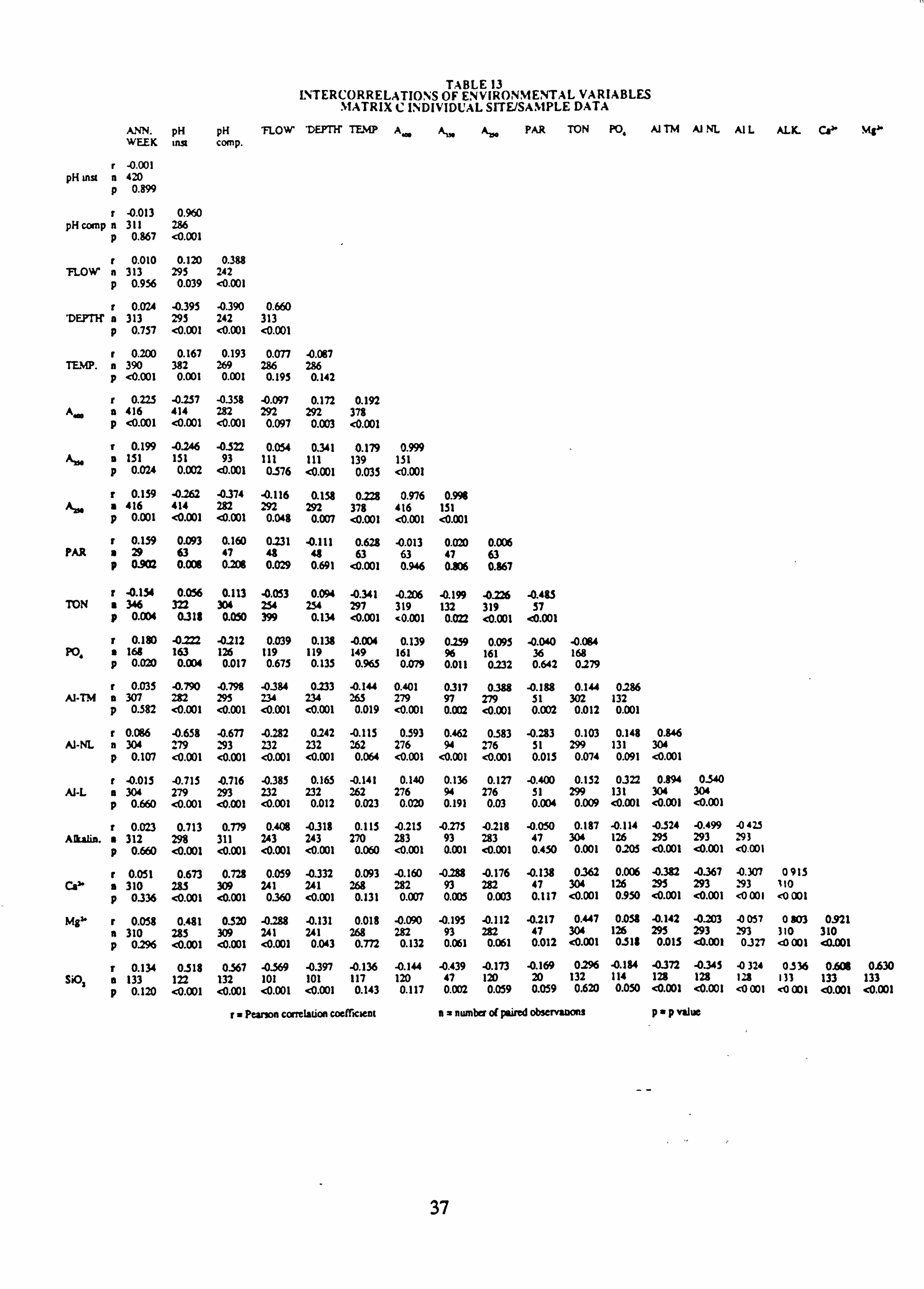
TABLE 13 LNTERCORRELATIO`S OF ENVIRONMENTAL VARIABLES
MATRIX C INDIVIDUAL SITE/SAMPLE DATA
ANN. PH pH 'FLOW 'DEPTH TEMP Ai, Aý Ab, PAR TON PO. Al TM Al NL Al L ALK. Ca" Mg" WEEK ina comp.
r -0.001 PH inst a 420
p 0.899
r -0.013 0.960 PH comp n 311 286
p 0.867 <0.001
r 0.010 0.120 0.388 FLOW n 313 295 242
p 0.956 0.039 <0.001
r 0.024 -0.395 . 0.390 0.660 'DEPTH' a 313 293 242 313
p 0.757 <0.001 <0.001 c0.001
r 0.200 0.167 0.193 0.077 . 0.097 TEMP. a 390 382 269 286 286
p <0.001 0.001 0.001 0.195 0.142
r 0.223 -0.257 -0.358 . 0.097 0.172 0.192 Aw a 416 414 282 292 292 378
p <0.001 <0.001 <0.001 0.097 0.003 c0.001
f 0.199 -0.246 -0.522 0.054 0.341 0.179 0.999 A,,, a 151 151 93 111 111 139 151
p 0.024 0.002 <0.001 0.576 <0.001 0.035 <0.001
r 0.159 -0262 -0.374 -0.116 0.158 0.228 0.976 0.996 Am a 416 414 282 292 292 378 416 151
p 0.001 <0.001 <0.001 0.048 0.007 <0.001 <0.001 <0.001
r 0.159 0.093 0.160 0.231 . 0.111 0.629 -0.013 0.020 0.006 PAR a 29 63 47 48 48 63 63 47 63
p 0.902 0.008 0.208 0.029 0.691 <0.001 0.946 0.806 0.867
r -0.154 0.056 0.113 -0.053 0.094 -0.341 -0.206 . 0.199 -0.226 -0.485 TON a 346 322 304 254 254 297 319 132 319 57
p 0.001 0.318 0.050 399 0.134 <0.001 <0.001 0.022 <0.001 <0.001
r 0.180 -0.222 -0212 0.039 0.138 -0.004 0.139 0139 0.095 . 0.040 -0.084 PO. a 168 163 126 119 119 149 161 96 161 36 168 p 0.020 0.004 0.017 0.675 0.135 0.965 0.079 0.011 0.232 0.642 0.279
r 0.035 . 0.790 . 0.798 -0384 0.233 -0.144 0.401 0.317 0.388 . 0.188 0.144 0.286 Al-7M a 307 282 295 234 234 265 279 97 279 51 302 132
p 0.582 <0.001 <0.001 <0.001 <0.001 0.019 <0.001 0.002 <0.001 0.002 0.012 0.001
r 0.086 -0.658 -0.677 . 0.282 0142 -0.115 0.593 0.462 0383 -0.283 0.103 0.148 0.846 Al-NL n 304 279 293 232 232 262 276 94 276 51 299 131 304
p 0.107 X0.001 c0.001 <0.001 <0.001 0.064 <0.001 <0.001 <0.001 0.015 0.074 0.091 <0.001
r -0.015 -0.715 -0.716 -0.385 0.165 -0.141 0.140 0.136 0.127 -0.400 0.152 0.322 0.894 0340 Al-L a 304 279 293 232 232 262 276 94 276 51 299 131 304 304
p 0.660 <0.001 <0.001 <0.001 0.012 0.023 0.020 0.191 0.03 0.004 0.009 c0.001 <0.001 <0.001
r 0.023 0.713 0.779 0.408 -0.318 0.113 -0.215 -0.275 -0.219 -0.050 0.187 -0.114 -0324 -0.499 -0 425 Alkalin. 312 298 311 243 243 270 283 93 283 47 304 126 295 293 293
p 0.660 <0.001 <0.001 N. 001 <0.001 0.060 <0.001 0.001 <0.001 0.450 0.001 0205 X0.001 <0.001 X0.001
r 0.051 0.673 0.728 0.059 -0.332 0.093 -0.160 -0.288 -0.176 -0.138 0.362 0.006 -0.382 -0.367 . 0.307 0 915 Ca" a 310 285 309 241 241 268 282 93 282 47 304 126 295 293 293 Ito
p 0.336 <0.001 <0.001 0360 N. 001 0.131 0.007 0.005 0.003 0.117 <0.001 0950 <0.001 <0.001 <0001 <0001
M8" r 0.058 0.481 0320 -0.288 -0.131 0.018 -0.090 . 0.195 . 0.112 -0.217 0.447 0.058 -0.142 -0.203 -0057 0303 0.921 a 310 285 309 241 241 268 282 93 282 47 304 126 295 293 293 310 310 p 0.296 <0.001 <0.001 c0.001 0.043 0.772 0.132 0.061 0.061 0.012 <0.001 0318 0.015 40.001 0.327 <0001 c0.001
r 0.134 0318 0.567 -0.569 -0.397 -0.136 -0.144 -0.439 -0.173 -0.169 0296 -0.184 -0.372 -0.345 -0324 0.536 0.606 0.630 Si03 a 133 122 132 101 101 117 120 47 120 20 132 114 128 128 128 133 133 133
p 0.120 <0.001 <O. 001 <0.001 <0.001 0.143 0.117 0.002 0.059 0.059 0.620 0.050 <0.001 <0.001 <0001 <0001 <0.001 <0.001
r- Paria carrelation coefficient n= number of paired observanom p"p value
37
alkalinity; Ca`+, Mg2'and SiO 2' and negatively with Aluminium. There is a weaker negative
correlation with absorbance measures. Both pH inst. and pH comp. are negatively correlated
with Depth', but show positive correlations, of which only pH comp. is significant, with 'Flow'. i This latter is surprising since it is a well-recorded phenomenon that pH is reduced during storm-induced increases in discharge (R. Harriman, pers. comm. ). It is likely that dif-
ferences in the depth of the gauges in the stream bed at different sites may obscure this
relationship in the data. When the correction of subtracting the lowest reading from the data
is applied, to produce the Depth' variable, a significant negative correlation results, which is
more in -accordance with expectation.
All measures of absorbance are strongly intercorrelated. They are also positively correlated with total monomeric and non-labile aluminium, but not with labile aluminium, which confirms the complexation of labile Al with humic material (Steinberg and Kuhnel, 1987; Gjessing et al, 1989). A weaker negative correlation exists between absorbance and alkalinity and between TON and A400 or A.. A weak correlation with annual week is found for A.
PAR is positively correlated with temperature, reflecting the causal relationship between them, and negatively correlated with TON. The latter could be due to nutrient uptake by terrestrial and aquatic plants during the growing season. The lack of any similar correlation with P04 3- seems surprising, but may be due to the presence of complexed PO43' which is not taken up by plants, or due to a superfluity of phosphate in some waters.
TON is positively correlated with Caz+, MgI and SiO2, higher levels of which are associated with the less acidic waters. This correlation could be biased slightly by the clearfelling operation in the Corrie catchment but since a similar clearfell was carried out at Burn 10, it may reflect catchment differences in the rate of litter breakdown, due to the different soil types
present.
PO43' is positively correlated with Al TM and particularly with Al-L, but not with non-labile Al (Al-NL). This is surprising in view of the known complexation reactions of PO4' with' aluminium, (Minzoni, 1984; Nalewajko and Paul, 1985). However the extreme values of P043- in Burn 9 resulting from fertilization may be responsible for this discrepancy.
Intercorrelations between the different forms of aluminium are high. The lowest is between labile and non-labile Al, implying that other variables are involved, e. g. through complexation
reactions, since there is not a simple proportionality relationship between these two forms.
Alkalinity being largely due to the availability of calcium and magnesium salts for neutralization reactions, is highly correlated with these two ions, and with pH. Due to the relationship between pH and silica solubility, this variable is also highly correlated with alkalinity, Cat` and M gz..
38
3.3 BIOMASS
Mean values for biomass estimates in matrices A, B and C are shown in Tables 14 to 16. Very few values are available in Matrix A and consequently no trends are discernible. Matrix B and Matrix C values are thus almost identical since the majority of data in Matrix C are also present in Matrix B.
Using any of the biomass measures on either slides or tiles, the highest biomass appears to be developed in the highest-pH sites. The situation is less clear-cut with biomass on stones, where high values of pigments are found in sites 6,9,10-2,11-2 and C-1 (carotenoid >2 pspu cm-2). The values at the remaining sites however are also high in comparison with values encountered on artificial substrates. This is presumably due to the sampling procedure used with stones, which involved selecting a stone with a dense growth and another with a low periphyton density. This presumably introduces bias in areal biomass estimates. The' minimum values for stone biomass (mean values of the minimum in each sample) shown in Table 16 are larger than the mean values on slides and tiles for most sites.
The relationship between environmental conditions and biomass is investigated further through correlation analysis (Tables 17,18), using Matrix C site-mean data. Only pH, 'Depth', alkalinity, calcium and H' show correlations significant at the 1% significance level. Al also shows correlations significant at the 5% level with AFDW on slides. All biomass measures on slides and pigments on tiles show high correlations with pH and Depth'. Pigment extracted from stones is not significantly correlated with any variable. Pigments are nega- tively correlated with Depth' which may be interpreted as meaning that where Depth' (= mean fluctuation in depth) is high, biomass may fail to accumulate, or may be more regularly washed away.
The highest correlations, of slide and tile pigments and slide AFDW with pH are positive suggesting that there is a decrease in biomass with a decrease in mean pH of a stream. Whether this relationship also applies where environmental variables fluctuate within each stream is investigated by calculating the correlations between variables and biomass determined in
each sample (Table 19). The correlations obtained are lower but because of the larger number of observation pairs in most cases, some are nevertheless significant at or below the 1% level (0.01<p<0.001).
The significant negative correlation of slide AFDW with annual week number implies a decline in biomass with time, and must be a consequence of particular environmental conditions occurring during the sampling programme, for example a large biomass accumu- lated early in the year being removed by spates later in the season rather than a true seasonality which would result in a non-linear relationship. There is a smaller, but significant positive correlation between stone chlorophyll-a and annual week. This may be spurious considering
39
the poor correlations found between stone biomass and other variables, and the low intercor-
relations existing between stone biomass and that on other substrates (Table 20).
Both instantaneous and composite pH are significantly positively correlated with slide and tile pigments, at the 1% significance level or lower. Some significant correlations betwen slide pigments and 'Flow', alkalinity, Caz+, Mgz' and silicate also occur. The largest correlations occur between tile pigments and silicate (r > 0.6). While it is tempting to see this as evidence that the growth of diatoms is enhanced by higher levels of silicate, the correlations could be
spurious since silicate has a correlation of 0.569 with composite pH. (The solubility of silicate is greater at higher pH). However the correlations between SiO
2 and slide pigments are lower, despite their high correlation with pH. There should be no difference between tile- and slide-derived biomass estimates in theory, and the results obtained suggest that extraneous or uncontrolled factors may be involved in the observed behaviour.
For example, the estimates of pigments from slides may be biased against some sites where abrasion by small stones was a particular problem, e. g. in sites 5,9,10-1,10-2 and C- 1. However, amongst the different biomass estimates (with the exception of chlorophyll-a and carotenoid estimates from the same sample) the highest correlations found are between tile and slide pigments.
It would appear from these results that while any extrapolation to a whole-stream estimate of areal biomass would be unsafe, the evidence is not in favour of the contention that an increase
of biomass occurs upon acidification. This is in agreement with the reports of Stokes (1981)
and Marker and Willoughby (1988). It contrasts with the reports of Hendrey (1976), Muller (1980) and many anecdotal accounts of the condition of acidified streams which may reflect the greater visual impact of filamentous green algae than of an equal biomass of diatoms or blue-green algae. Hendrey's (1976) findings of a higher biomass but lower productivity (by 14C incorporation) were interpreted as evidence for lower heterotrophic activity with decreased pH. However his results were obtained in artificial stream channels rather than in
natural streams subjected to fluctuating flows, and measurement was discontinued when sloughing of algae occurred. Muller's (1980) studies were of periphytic algae in enclosures of natural lakes, artificially acidified, where removal by current or abrasion would be minimal. Therefore these two reports are not necessarily at odds with field studies suggesting no negative correlation between pH and biomass.
The issue of whether biomass developed at different pH values is different in artificial conditions has been addressed also (see results of culture experiments in Sections 3.4.4 and 3.5).
40
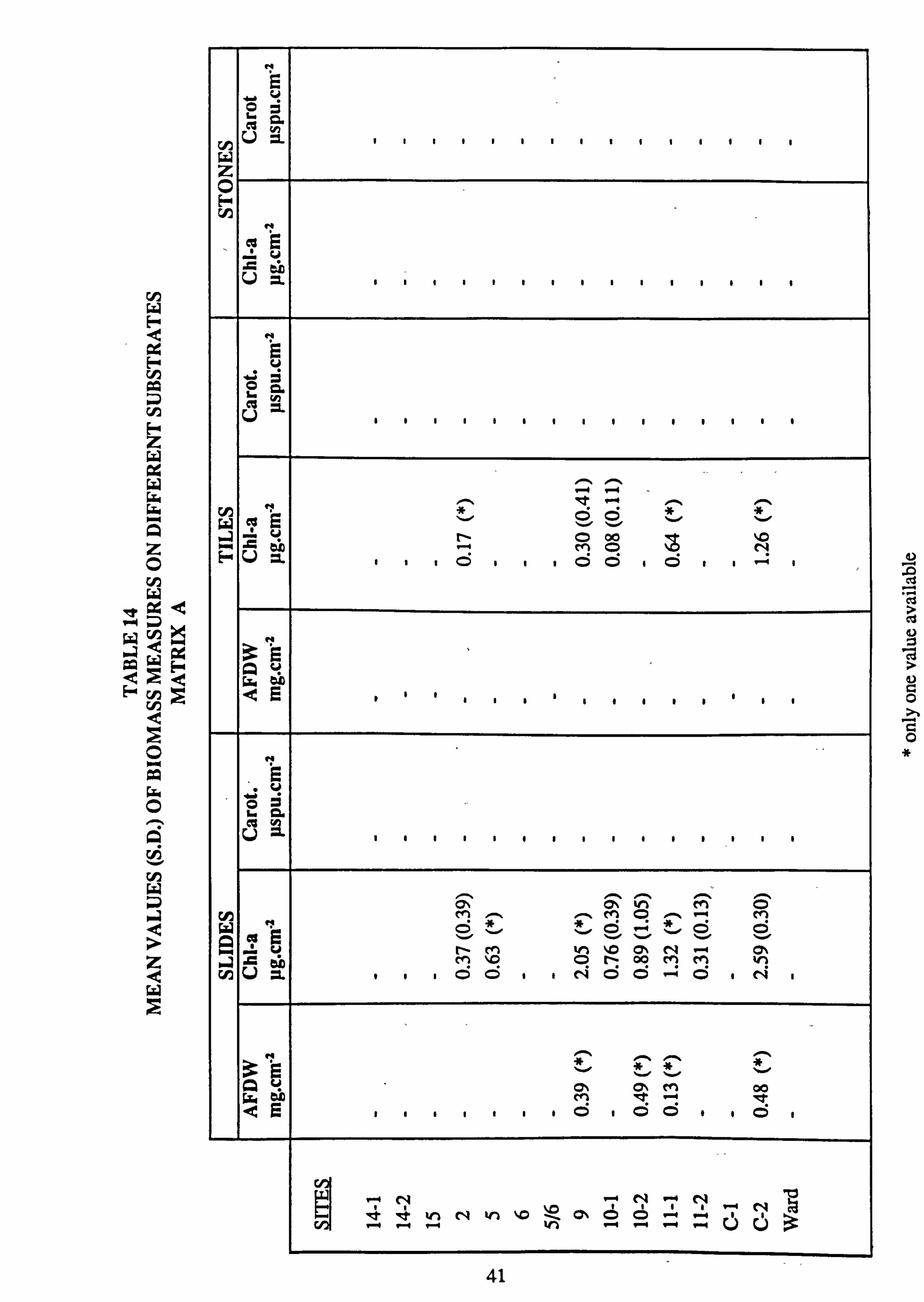
CA 94 ZD Gn F z
w w A z 0
ýä
aQ F
O
O
0 rii W
-
z Q w 1ý
Q
H
r
r. + V
cl U H 1 1 1 1 1 1 1 1 1 1 1 1 1 1
z 0 N
U Z 1 1 / 1 1 / 1 1 1 1 1 1 1 1
0 ö C.
y U
1 1 1 1 1 1 1 1 1 1 1 1 1 1
W u 00
0-M bD -4 M
Ö N
[ ý Cý U Z
1 1 Ö
1 1 1 Ö Ö
1 Ö
1 1 ý"ý
3 E Q u
E
1 1 ' ' 1 . 1 / 1 1 1 1 1 1 1
v C . a
U 1 1 1 1 1 1 1 1 1 1 1 1 1 1 1
Cý Cý In cn O con M M O - M W E O O v O OO
M .4
Z ob
M IO O [lý OO M Iti Vi U
. 1 1 0 0
1 1 N 0 0
- 0
1 cV
0% ON 00 Q E
1 1 1 1 1 1 1 ö
1 ö ö
1 1 ö
1
. -1 N N N F N vý ýO C7, Ö Ö -
- U N U
c a
aý
C13 cd aý
a 0
41
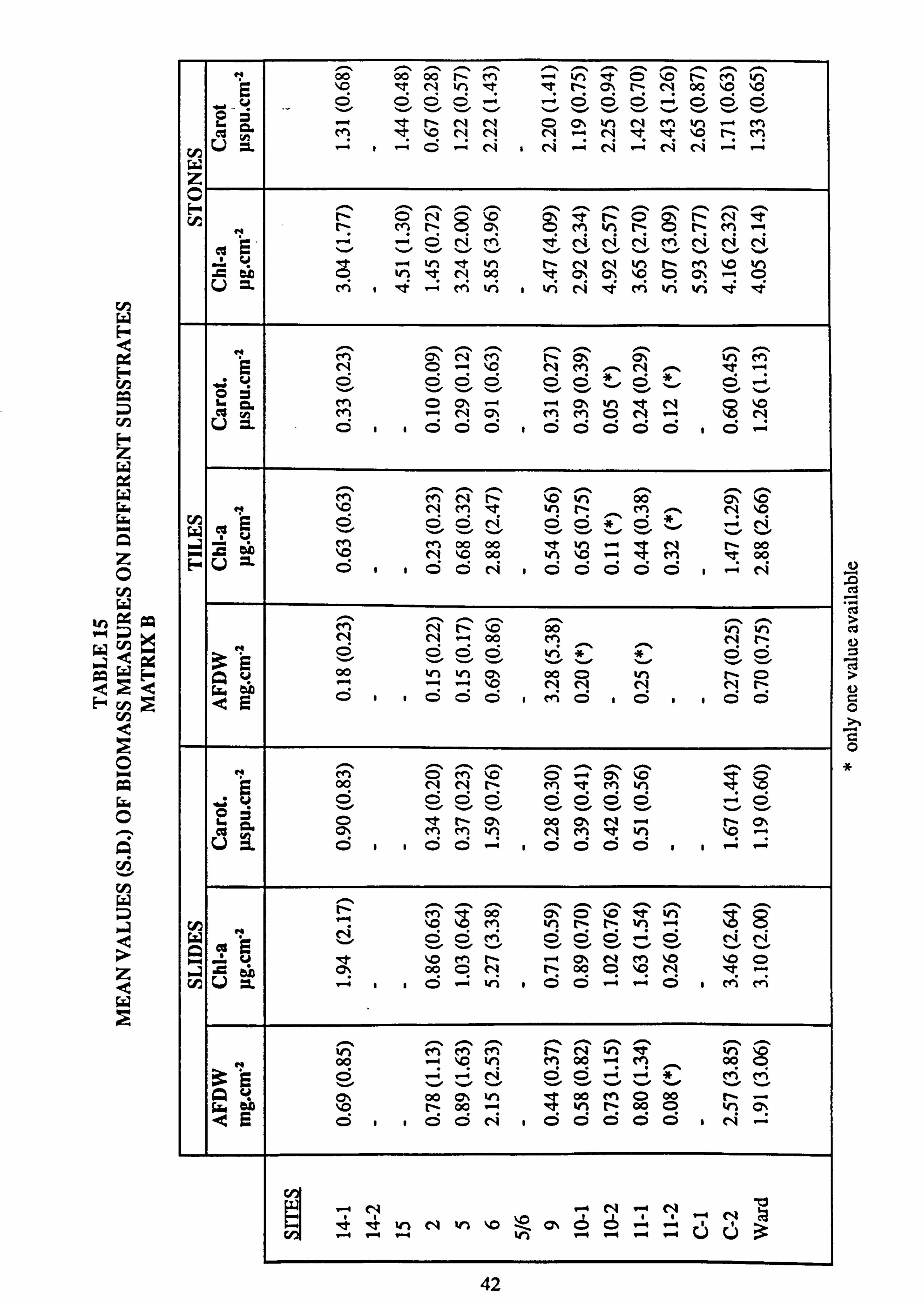
v, W F Q ß: F q
F- z w x w w w A
z 0 w
Q w QýQ F vý ý
Q 0 w w 0
C',
W
Q
z Q w
1-, 00 . -. 00 . -. 00 _ N .. M ^ - . -. in . -. 'RT . -. O . -. '. O ^ I- ^ M . -. V) E "O It N N ' n C N N 00 '. 0 '. O u Ö O O O v v o O O O O Ov
L v O ä
--ý ýt [- N N O ON in N M to r-+ M eC y M ýt IO N N N N: Y IC M
U Z - ' -+ Ö . (V i (V --ý (V - N N -+ -
Lrý
z c n N
O M
N C OO O
Cý O
N O -
Q'. N -
N M
ý' - N N N MM V1 [ I
O N M N N N M N N (V u rt - Lf ýi v1 [N N N tn N M 1.0 In
s bD O In N 00 It p'. OA '. G O C' - O U ý- M
--ý M wi . Vi (V q e-; vi h 4
~ M Qý N M n C' C' N M E N O q 'c N cn ý. N ^ t: h - O O O O O O O O v
O O L. M - N M in N - N ec
y ON M C 'D
U Z Ö Ö Ö Ö Ö Ö Ö Ö Ö Ö
M M N N ýo N 00 Ö'.
'. C N cM IRT In N M ^ N '. G C/1 W
E Ö ' ' N Ö O ^
1-0 ' 11 v
- M N
00 '. G
00 00
"T In
In so
- i--4
N M
N 00 00
E" U ö ö ö cli ö ö ö ö ö c-i
00 N11 N
' 00 N n
° ö ö ö v ^ *..
^ `. E
A u W) (ON 00 N r -+ 10 N
N N O O Ö vi Ö Ö Ö Ö
00 N ^ en ý-. N . -. N ^ - M ^
Itt In ...
Ö Ö Ö O Ö Ö Ö Ö 5 Ö v
1. O ct N ON 00 as N "-r I
N O' ca ON M M tn N M IRT V I 'O --ý
U ý O ý ý O O -+ ý O O O O ý ý ý r+
00 CS (D ýo
l qtt W)
con en te) r- t - in -4 W Cq O O v O O O O N N Q E O v º.. ý . 10 M [- - C'. N M I'D 1.0 O �a Z pp Oý 00 O N r- 00 O \O N "t "-+ V1 U Z --ý O vi a O O - "-+ c; I cn el;
M N M N OR O O 4 ^
00 rý E ..
v . -; . -
N Ö 5-
Ö .ý
"; I-I -;
'- * 5-
M v
cli . -
A V Oý 00 Cl. in 4 00 en O 00 N "-" (, z, ob '. D N 00 -4 In [N 00 O In Q; Q E Ö O Ö N Ö Ö Ö Ö Ö N "-
4 4 V', N v-) D ', 0 Cs Ö Ö "ý "=ý
'; N
N
.a
cd 0
N
0
0
42
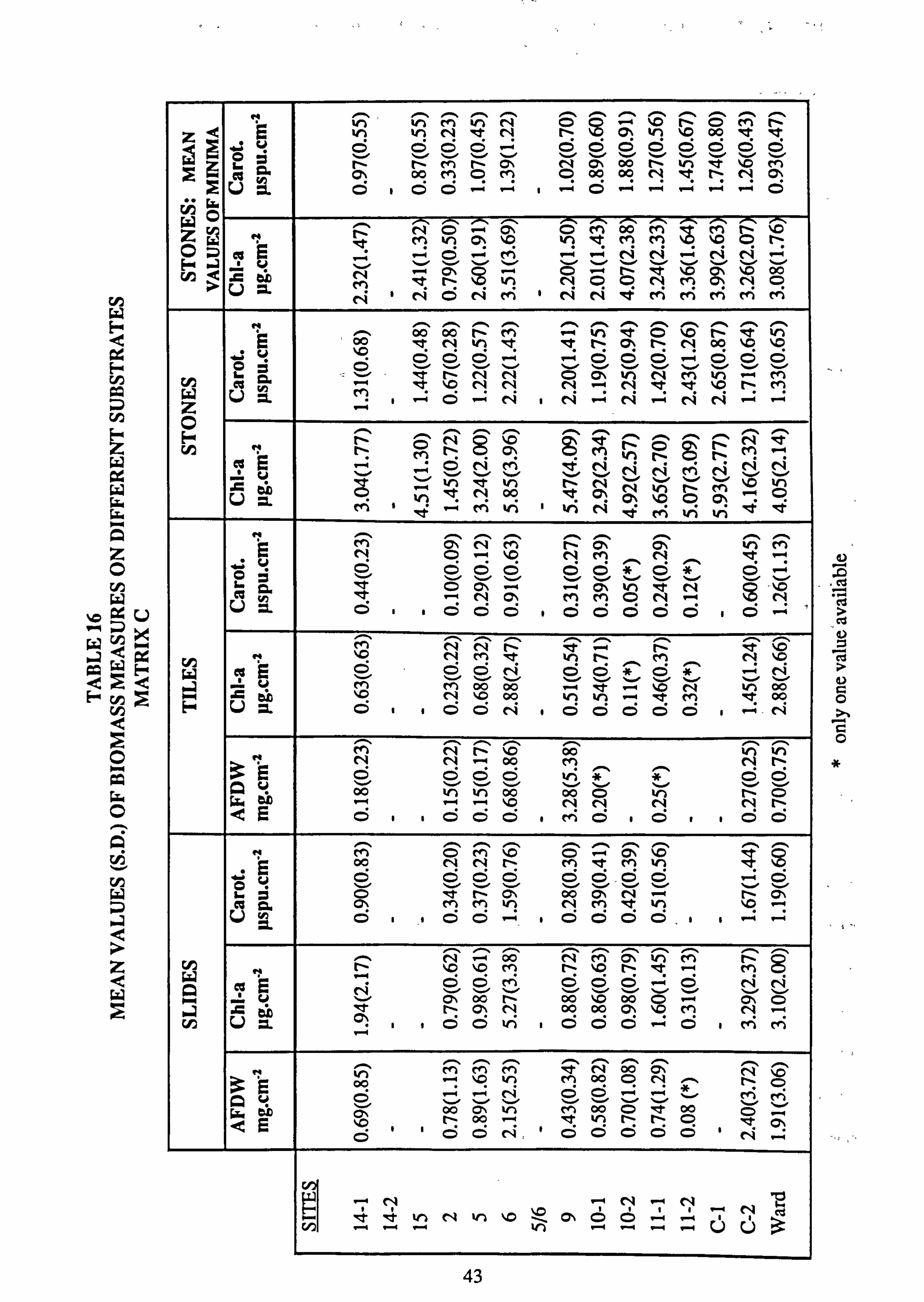
cn
ca CA
w a w w A z O w
Q Ix QýQ CIO
O
O
W
a
z w
p ^, ý
. -, w"I
^ en
. -% ý
^ . -. . -. p
. -. '. G
. -% N
. -. O . -.
M . -. N
z Q tn N V N
O1% V'1 00 't7 RT e ý+ v Ö Ö Ö Ö - Ö Ö Ö Ö Ö Ö Ö Ö
N N 00 i '. O 2 4- 1..
cc 4 [-
Qý N 00
M M
I O
ON M O
ON 00 cc
N N
N It
t N N
M C
iL U 'n Z Ö
. Ö Ö p
^ Ö Z N O
k - '. O M
' 00 M
M M
ýt ;
M ýC
N O
'. O t =
, it M n C; ý D ý O ß .., . -i Q - M -+ - N fV - N ei -4
.ý u ... .. ý v te 1-1 ý v I- N n p N r O
V pý "o O 00
M ýO v1 O N M O' N V =' Cj - N O N M I N N 't M M M M M
00 00 i M - v t Ö D N t n E 00 IRT N VII of IRT [N C tN N 00 '. O 10
C O O v v O O O v O O Ö h N
ä = - qt N N N O O'. M 117 ' M w Ri h -4 It 1.0 N N N N ýt `ti '. D N M U Z Ö --+ ri . cV cV "--ý cV C-1 --ý z 1-4
' S 1.0
!ý ! t- en [ ON O M wl N g N M "-" . v v N fV M N C'l C-4
N It N U =
O OR E O Ö
O, . cfl $ t+i V ' h N ýt M ýn V ýt
- E N Ö '0 N M N
0 C O O O O v O v C v O C\ -
- p -: N Q' M
M Ö N - '. D
N U ý. O . Ö Ö Ö . Ö Ö Ö Ö Ö O -
M N
r ýO M
ITt in
t": ^
M ^
N IIR
W of r O ' ' v O v v .ý
r-i . .
Z IO N 00 h -4 R: r -q ý M ý . 00
ID! o o h h - V 0 0 E-4 U Z O " O Ö N 0 Ö Ö Ö Ö Ö " N
N N 00
N N
I N N "-+ oo M N [N Q E O O O v v v O O O 00 ' -4 L=i u
"--4 '0 N N N N N
Q E Ö ' Ö Ö Ö M C 0 Ö " Ö Ö
00 N N N M tt M $( 8
u 0 0 0 0 ö ö .o o v ö
1. = O tt N (ON 00 O'. N --- N O' ß p O0 M M to N M "t N ýD I"
U � G O " . O O - " O O O O I . "4 "-; ,
N - 00 N M 11-3 M N OO N N '. O 1.0 M N '. G N MT - M G w ö ö v ö ö ö v ° v v N
N-e 00 00 o 00 0 N 0 $ a s ay IT
N C'.
N 00 o C M N -4 V1 U 5. C:
" ' O O ºn . O O O -4 O c" i
en en M M N 00 C14 \C) 3 09 ^; 0 O O
N r. N,
Q u O "-ý r-+ v N v
O O "-+ v --ý v M v
M
6T, 00 h ý cn 00 N 00 _ E
' tý o o -+
' ýt O Cý
O Ö N_ Ö Ö Ö Ö Ö $ cy , _.,
. _. --ý N
wl N vl ýc O, Ö Ö .1
N 1
C;
.0 c4
cil V
N
0
0 *
43
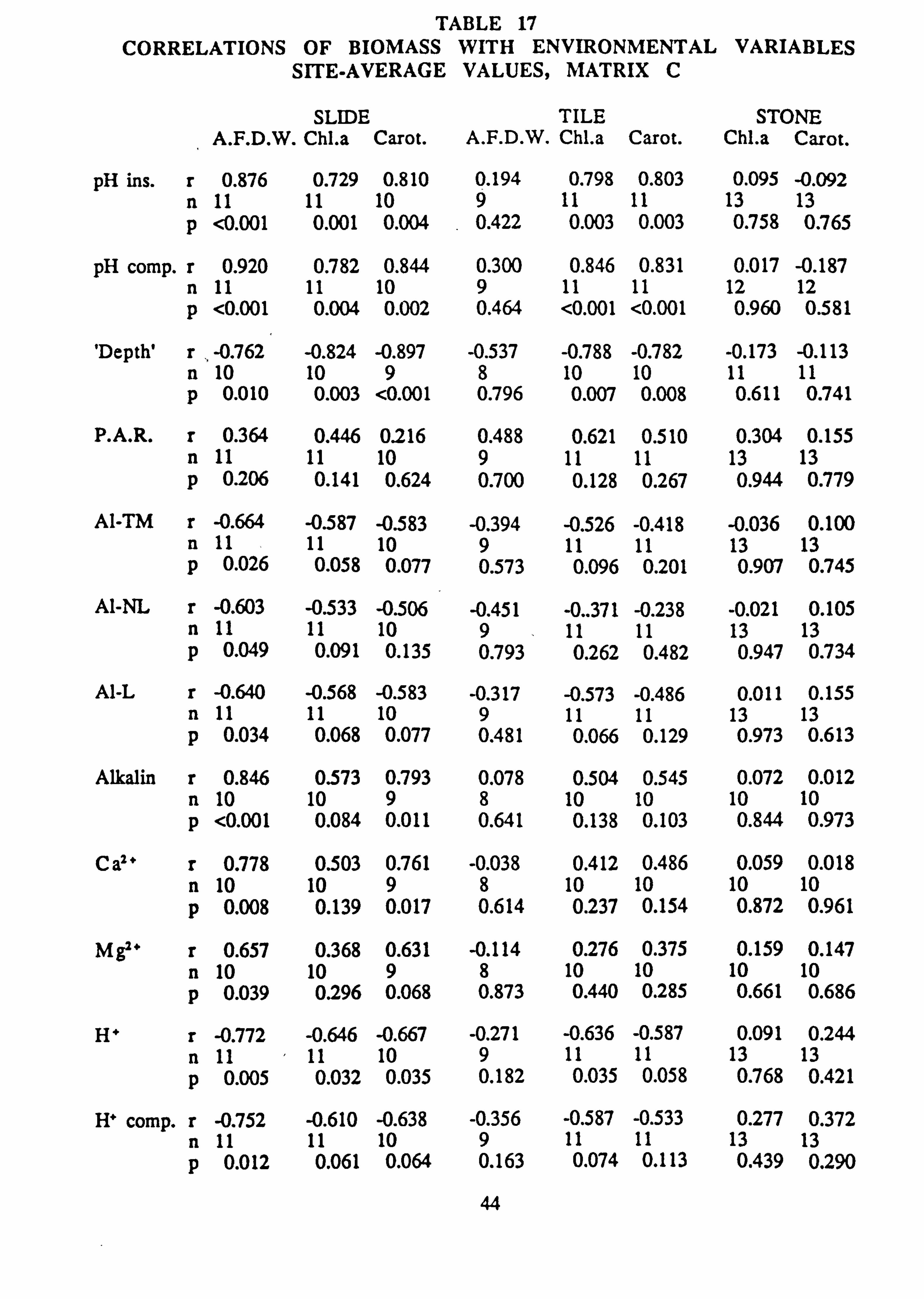
TABLE 17 CORRELATIONS OF BIOMASS WITH ENVIRONMENTAL VARIABLES
SITE-AVERAGE VALUES, MATRIX C
SLIDE TILE STONE A. F. D. W. Chl. a Carot. A. F. D. W. Chl. a Carot. Chl. a Carot.
pH ins. r 0.876 0.729 0.810 0.194 0.798 0.803 0.095 -0.092 n 11 11 10 9 11 11 13 13 p <0.001 0.001 0.004 0.422 0.003 0.003 0.758 0.765
pH comp. r 0.920 0.782 0.844 0.300 0.846 0.831 0.017 -0.187 n 11 11 10 9 11 11 12 12 p <0.001 0.004 0.002 0.464 <0.001 <0.001 0.960 0.581
'Depth' r , -0.762 -0.824 -0.897 -0.537 -0.788 -0.782 -0.173 -0.113 n 10 10 9 8 10 10 11 11 p 0.010 0.003 <0.001 0.796 0.007 0.008 0.611 0.741
P. A. R. r 0.364 0.446 0.216 0.488 0.621 0.510 0.304 0.155 n 11 11 10 9 11 11 13 13 p 0.206 0.141 0.624 0.700 0.128 0.267 0.944 0.779
Al-TM r -0.664 -0.587 -0.583 -0.394 -0.526 -0.418 -0.036 0.100 n 11 11 10 9 11 11 13 13 p 0.026 0.058 0.077 0.573 0.096 0.201 0.907 0.745
Al-NL r -0.603 -0.533 -0.506 -0.451 -0.. 371 -0.238 -0.021 0.105 n 11 11 10 9 11 11 13 13 p 0.049 0.091 0.135 0.793 0.262 0.482 0.947 0.734
Al-L r -0.640 -0.568 -0.583 -0.317 -0.573 -0.486 0.011 0.155 n 11 11 10 9 11 11 13 13 p 0.034 0.068 0.077 0.481 0.066 0.129 0.973 0.613
Alkalin r 0.846 0.573 0.793 0.078 0.504 0.545 0.072 0.012 n 10 10 9 8 10 10 10 10 p <0.001 0.084 0.011 0.641 0.138 0.103 0.844 0.973
C a2' r 0.778 0.503 0.761 -0.038 0.412 0.486 0.059 0.018 n 10 10 9 8 10 10 10 10 p 0.008 0.139 0.017 0.614 0.237 0.154 0.872 0.961
M g2' r 0.657 0.368 0.631 -0.114 0.276 0.375 0.159 0.147 n 10 10 9 8 10 10 10 10 p 0.039 0.296 0.068 0.873 0.440 0.285 0.661 0.686
H' r -0.772 -0.646 -0.667 -0.271 -0.636 -0.587 0.091 0.244 n 11 11 10 9 11 11 13 13 p 0.005 0.032 0.035 0.182 0.035 0.058 0.768 0.421
H' comp. r -0.752 -0.610 -0.638 -0.356 -0.587 -0.533 0.277 0.372 n 11 11 10 9 11 11 13 13 p 0.012 0.061 0.064 0.163 0.074 0.113 0.439 0.290
44
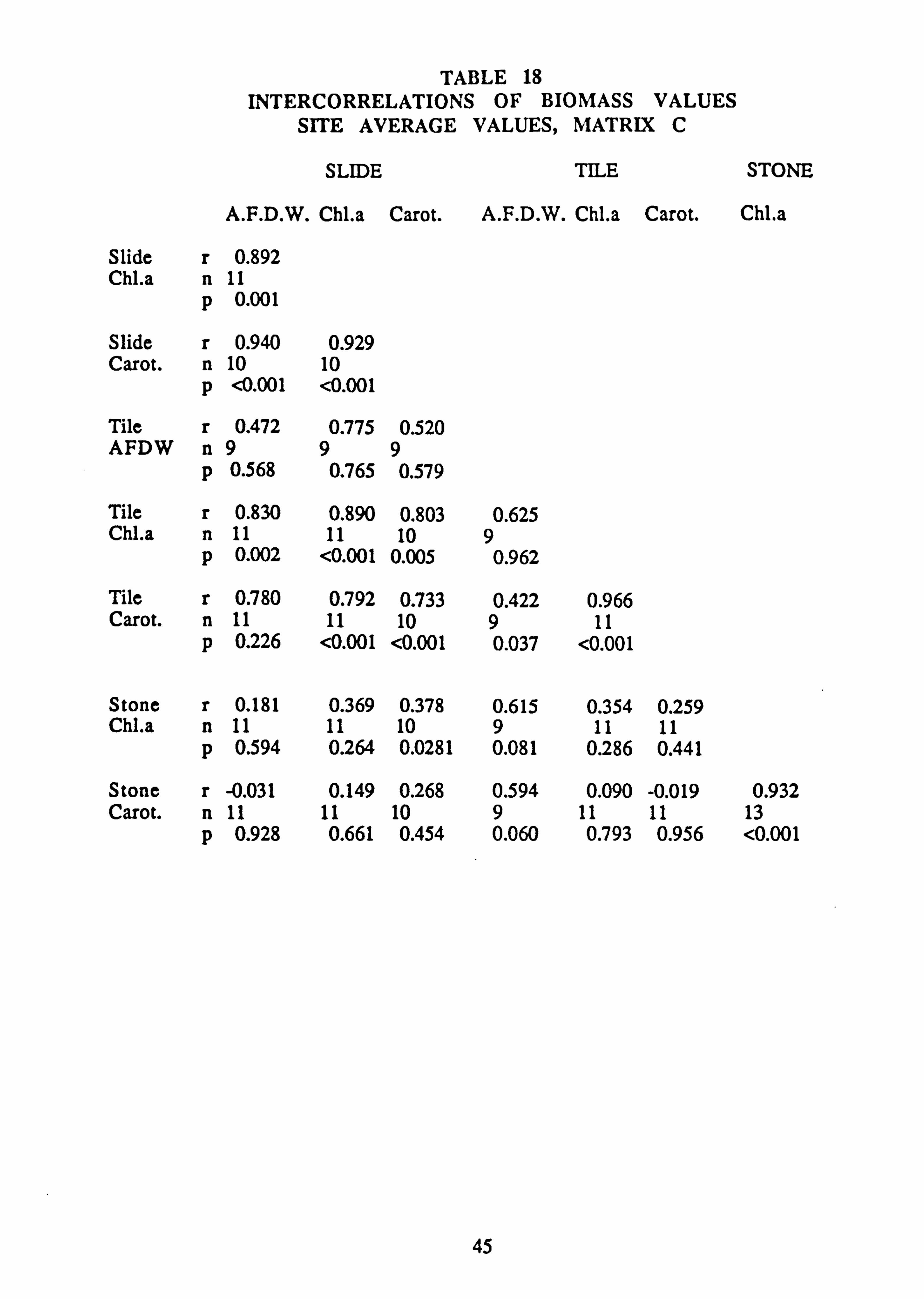
TABLE 18 INTERCORRELATIONS OF BIOMASS VALUES
SITE AVERAGE VALUES, MATRIX C
SLIDE TILE STONE
A. F. D. W. Chl. a Carot. A. F. D. W. Chl. a Carot. Chl. a
Slide r 0.892 Chl. a n 11
p 0.001
Slide r 0.940 0.929 Carot. n 10 10
p <0.001 <0.001
Tile r 0.472 0.775 0.520 AFDW n 9 9 9
p 0.568 0.765 0.579
Tile r 0.830 0.890 0.803 0.625 Chl. a n 11 11 10 9
p 0.002 <0.001 0.005 0.962
Tile r 0.780 0.792 0.733 0.422 0.966 Carot. n 11 11 10 9 11
p 0.226 <0.001 <0.001 0.037 <0.001
Stone r 0.181 0.369 0.378 0.615 0.354 0.259 Chl. a n 11 11 10 9 11 11
p 0.594 0.264 0.0281 0.081 0.286 0.441
Stone r -0.031 0.149 0.268 0.594 0.090 -0.019 0.932 Carot. n 11 11 10 9 11 11 13
p 0.928 0.661 0.454 0.060 0.793 0.956 <0.001
45
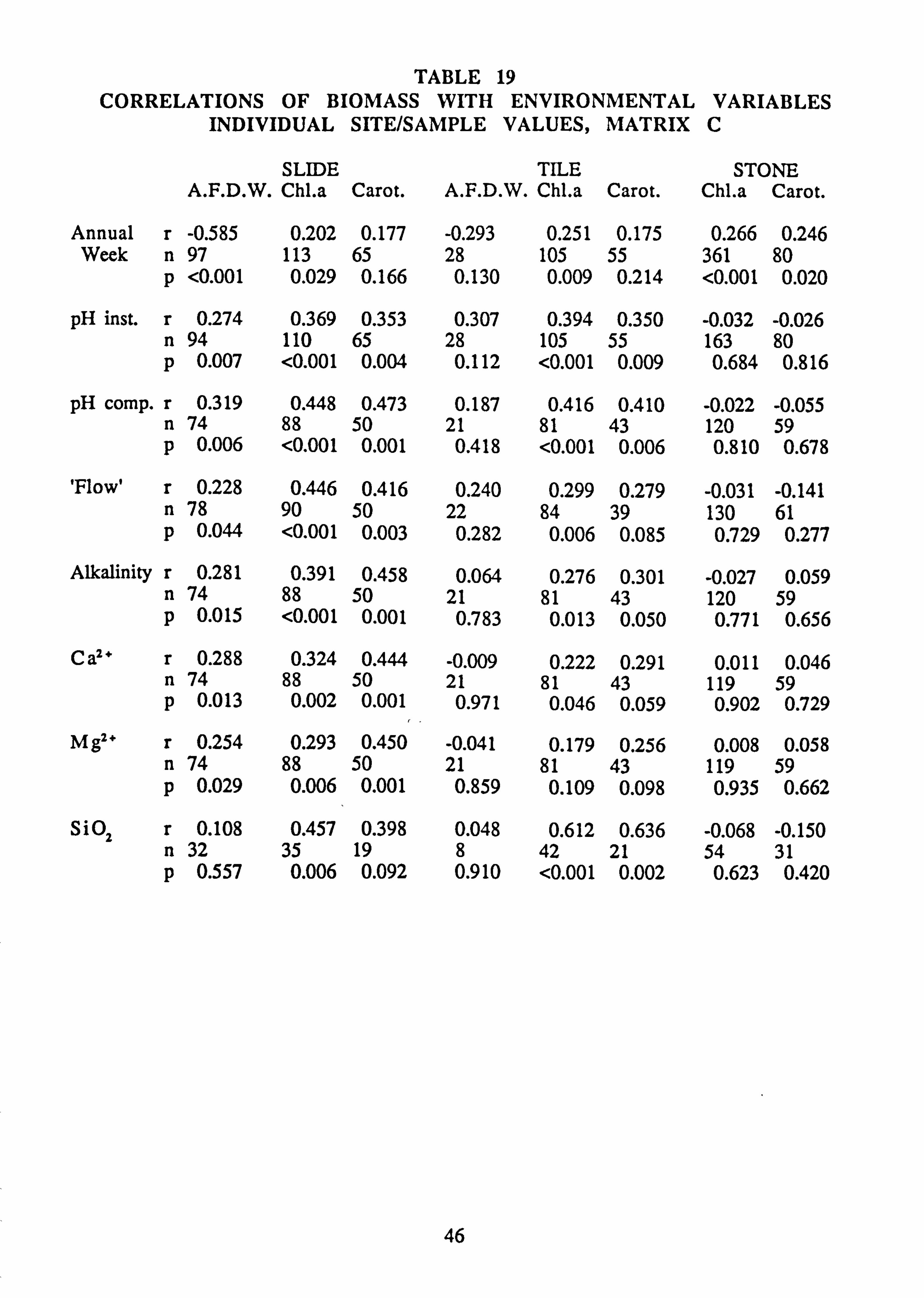
TABLE 19 CORRELATIONS OF BIOMASS WITH ENVIRONMENTAL VARIABLES
INDIVIDUAL SITE/SAMPLE VALUES, MATRIX C
SLIDE TILE STONE A. F. D. W. Chl. a Carot. A. F. D. W. Chl. a Carot. Chl. a Carot.
Annual r -0.585 0.202 0.177 -0.293 0.251 0.175 0.266 0.246 Week n 97 113 65 28 105 55 361 80
p <0.001 0.029 0.166 0.130 0.009 0.214 <0.001 0.020
pH inst. r 0.274 0.369 0.353 0.307 0.394 0.350 -0.032 -0.026 n 94 110 65 28 105 55 163 80 p 0.007 <0.001 0.004 0.112 <0.001 0.009 0.684 0.816
pH comp. r 0.319 0.448 0.473 0.187 0.416 0.410 -0.022 -0.055 n 74 88 50 21 81 43 120 59 p 0.006 <0.001 0.001 0.418 <0.001 0.006 0.810 0.678
'Flow' r 0.228 0.446 0.416 0.240 0.299 0.279 -0.031 -0.141 n 78 90 50 22 84 39 130 61 p 0.044 <0.001 0.003 0.282 0.006 0.085 0.729 0.277
Alkalinity r 0.281 0.391 0.458 0.064 0.276 0.301 -0.027 0.059 n 74 88 50 21 81 43 120 59 p 0.015 <0.001 0.001 0.783 0.013 0.050 0.771 0.656
CO* r 0.288 0.324 0.444 -0.009 0.222 0.291 0.011 0.046 n 74 88 50 21 81 43 119 59 p 0.013 0.002 0.001 0.971 0.046 0.059 0.902 0.729
mg 2+ r 0.254 0.293 0.450 -0.041 0.179 0.256 0.008 0.058 n 74 88 50 21 81 43 119 59 p 0.029 0.006 0.001 0.859 0.109 0.098 0.935 0.662
S'02 r 0.108 0.457 0.398 0.048 0.612 0.636 -0.068 -0.150 n 32 35 19 8 42 21 54 31 p 0.557 0.006 0.092 0.910 <0.001 0.002 0.623 0.420
46
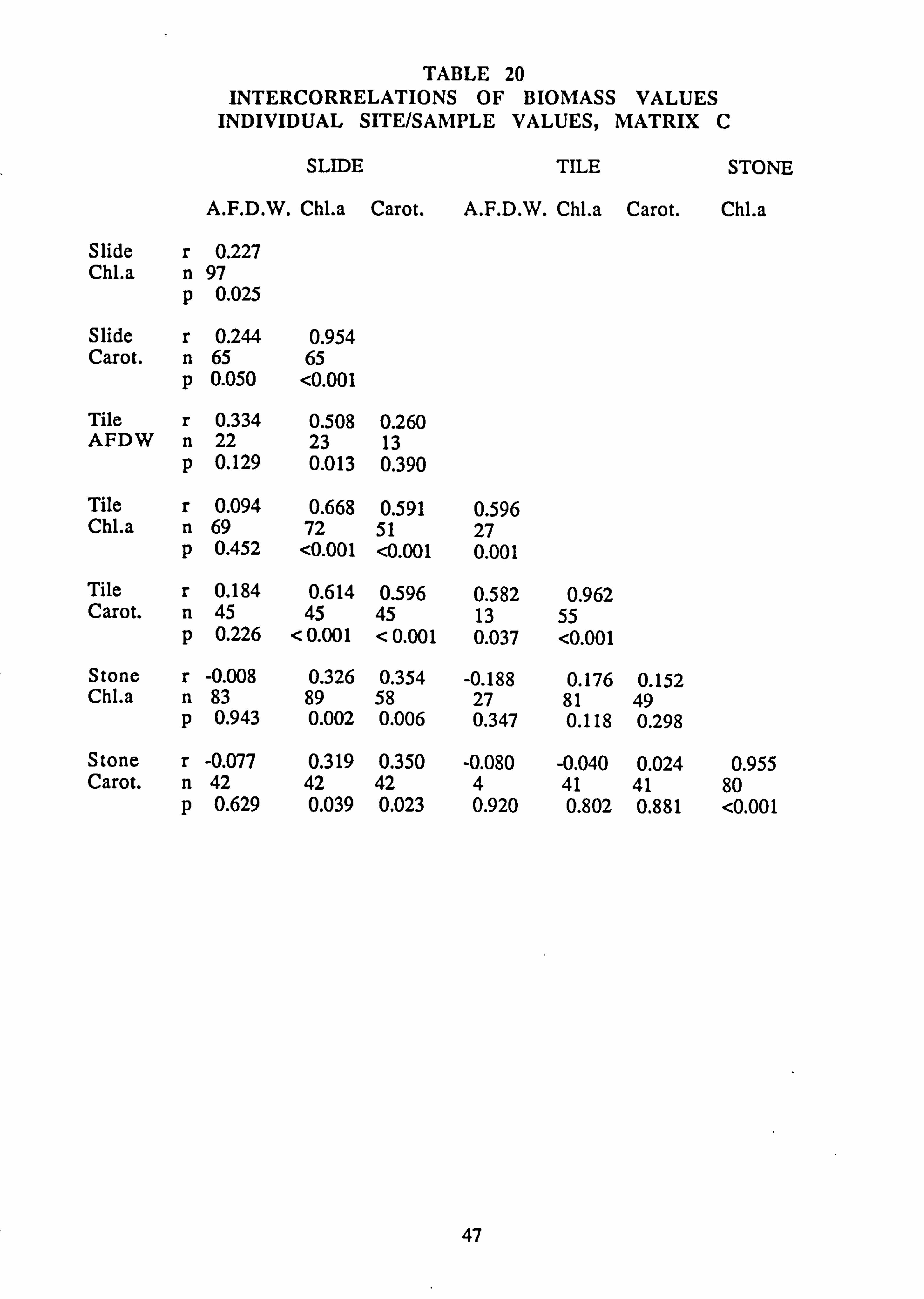
TABLE 20 INTERCORRELATIONS OF BIOMASS VALUES
INDIVIDUAL SITE/SAMPLE VALUES, MATRIX C
SLIDE TILE STONE
A. F. D. W. Chl. a Carot. A. F. D. W. Chl. a Carot. Chl. a
Slide r 0.227 Chl. a n 97
p 0.025
Slide r 0.244 0.954 Carot. n 65 65
p 0.050 <0.001
Tile r 0.334 0.508 0.260 AFDW n 22 23 13
p 0.129 0.013 0.390
Tile r 0.094 0.668 0.591 Chl. a n 69 72 51
p 0.452 <0.001 <0.001
Tile r 0.184 0.614 0.596 Carot. n 45 45 45
p 0.226 < 0.001 < 0.001
Stone r -0.008 0.326 0.354 Chl. a n 83 89 58
p 0.943 0.002 0.006
Stone r -0.077 0.319 0.350 Carot. n 42 42 42
p 0.629 0.039 0.023
0.596 27 0.001
0.582 0.962 13 55 0.037 <0.001
-0.188 0.176 0.152 27 81 49 0.347 0.118 0.298
-0.080 -0.040 0.024 0.955 4 41 41 80 0.920 0.802 0.881 <0.001
47
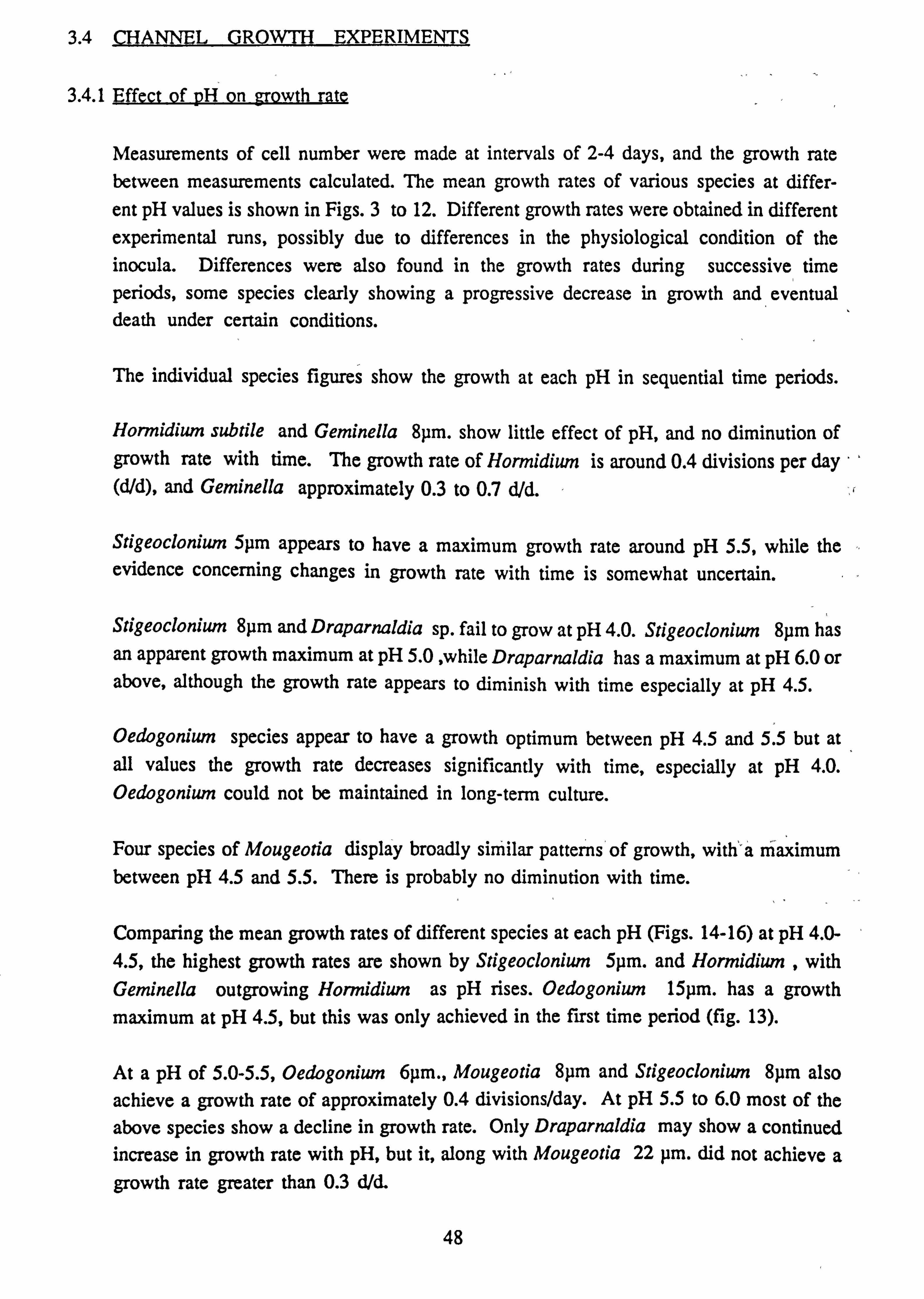
3.4 CHANNEL GROWTH EXPERIMENTS
3.4.1 Effect of pH on growth rate
Measurements of cell number were made at intervals of 2-4 days, and the growth rate between measurements calculated. The mean growth rates of various species at differ-
ent pH values is shown in Figs. 3 to 12. Different growth rates were obtained in different
experimental runs, possibly due to differences in the physiological condition of the inocula. Differences were also found in the growth rates during successive time periods, some species clearly showing a progressive decrease in growth and eventual death under certain conditions.
The individual species figures show the growth at each pH in sequential time periods.
Hormidium subtile and Geminella 8}ßm. show little effect of pH, and no diminution of growth rate with time. The growth rate of Hormidium is around 0.4 divisions per day (did), and Geminella approximately 0.3 to 0.7 d/d.
Stigeoclonium 5pm appears to have a maximum growth rate around pH 5.5, while the evidence concerning changes in growth rate with time is somewhat uncertain.
Stigeoclonium 8µm and Draparnaldia sp. fail to grow at pH 4.0. Stigeoclonium 8}ßm has an apparent growth maximum at pH 5.0 while Draparnaldia has a maximum at pH 6.0 or above, although the growth rate appears to diminish with time especially at pH 4.5.
Oedogonium species appear to have a growth optimum between pH 4.5 and 5.5 but at all values the growth rate decreases significantly with time, especially at pH 4.0. Oedogonium could not be maintained in long-term culture.
Four species of Mougeotia display broadly similar patterns of growth, with'a maximum between pH 4.5 and 5.5. There is probably no diminution with time.
Comparing the mean growth rates of different species at each pH (Figs. 14-16) at pH 4.0- 4.5, the highest growth rates are shown by Stigeoclonium 5pm. and Normidiom , with Geminella outgrowing Hormidiwn as pH rises. Oedogoniwn 15pm. has a growth maximum at pH 4.5, but this was only achieved in the first time period (fig. 13).
At a pH of 5.0-5.5, Oedogonium 6µm., Mougeotia 8pm and Stigeocloniwn 8pm also achieve a growth rate of approximately 0.4 divisions/day. At pH 5.5 to 6.0 most of the above species show a decline in growth rate. Only Draparnaldia may show a continued increase in growth rate with pH, but it, along with Mougeotia 22 pm. did not achieve a growth rate greater than 0.3 d/d.
48
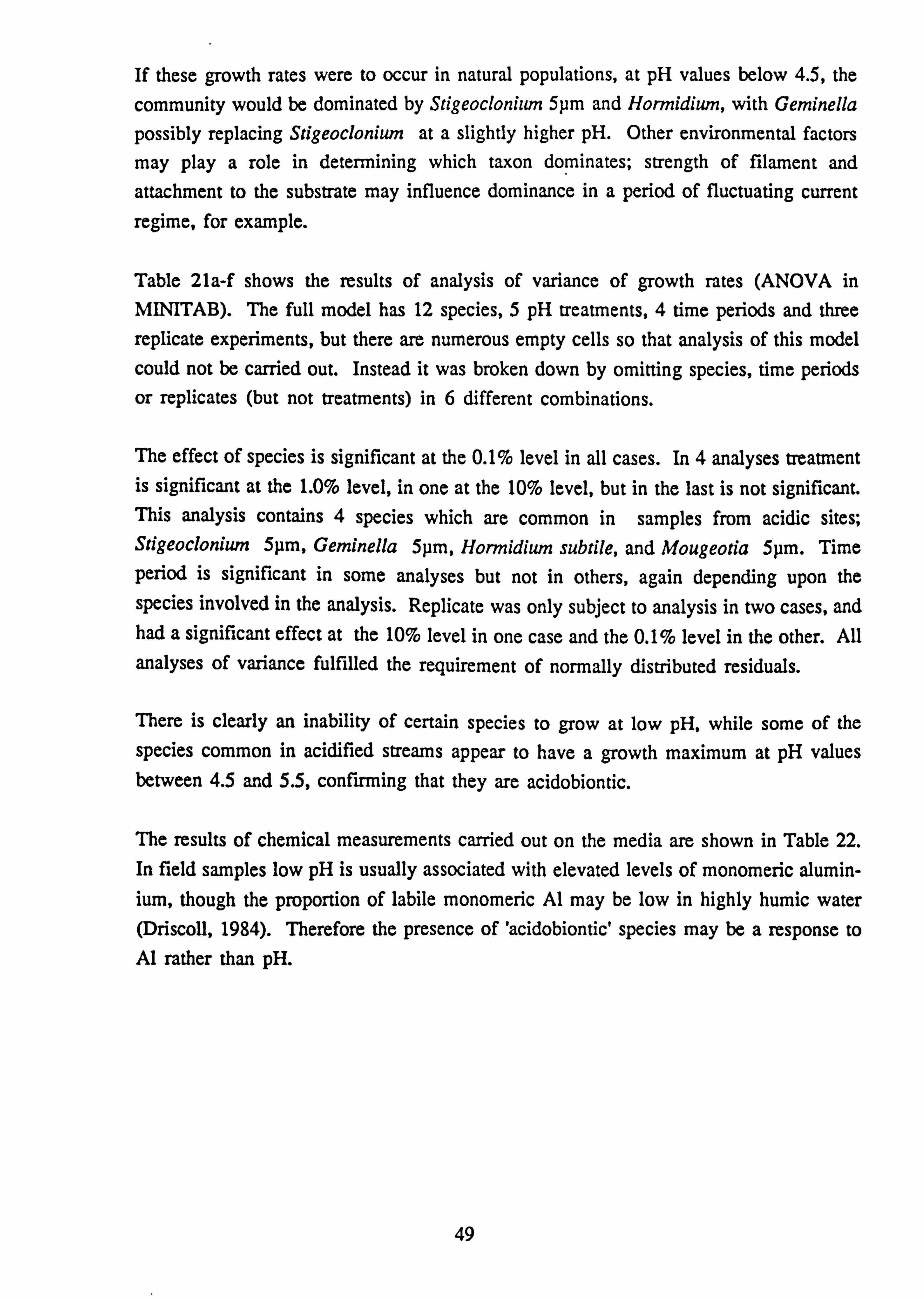
If these growth rates were to occur in natural populations, at pH values below 4.5, the
community would be dominated by Stigeoclonium 5pm and Normidiom, with Geminella
possibly replacing Stigeoclonium at a slightly higher pH. Other environmental factors
may play a role in determining which taxon dominates; strength of filament and attachment to the substrate may influence dominance in a period of fluctuating current regime, for example.
Table 2la-f shows the results of analysis of variance of growth rates (ANOVA in MINITAB). The full model has 12 species, 5 pH treatments, 4 time periods and three replicate experiments, but there are numerous empty cells so that analysis of this model could not be carried out. Instead it was broken down by omitting species, time periods or replicates (but not treatments) in 6 different combinations.
The effect of species is significant at the 0.1% level in all cases. In 4 analyses treatment is significant at the 1.0% level, in one at the 10% level, but in the last is not significant. This analysis contains 4 species which are common in samples from acidic sites; Stigeoclonium 5pm, Geminella 5pm, Hormidium subtile, and Mougeotia 5pm. Time period is significant in some analyses but not in others, again depending upon the species involved in the analysis. Replicate was only subject to analysis in two cases, and had a significant effect at the 10% level in one case and the 0.1% level in the other. All analyses of variance fulfilled the requirement of normally distributed residuals.
There is clearly an inability of certain species to grow at low pH, while some of the species common in acidified streams appear to have a growth maximum at pH values between 4.5 and 5.5, confirming that they are acidobiontic.
The results of chemical measurements carried out on the media are shown in Table 22. In field samples low pH is usually associated with elevated levels of monomeric alumin- ium, though the proportion of labile monomeric Al may be low in highly humic water (Driscoll, 1984). Therefore the presence of 'acidobiontic' species may be a response to Al rather than pH.
49
FIG. 3: GROWTH RATE DURING SUCCESSIVE PERIODS OF EXPOSURE TO MEDIA OF DIFFERENT pH, OF
Hormidium subtile
0.50
0.00
-0.50
0.50 rn
0.00
-0.50
0.50 A z 0.00 0 C2 -0.50
0.50
0.00 0
-0.50
0.50
0.00
-0.50
?ýýýý
ýýý
pH 4.0
pH 4.5
: 1ii I pH 5.0
1.10 5.24
: 1dI 1234
TIME PERIOD
EXPERIMENTAL RUN No. 1®2®3
50
pH 5.5
pH 6.0
FIG. 4: GROWTH RATE DURING SEQUENTIAL PERIODS OF EXPOSURE TO MEDIA OF DIFFERING pH, OF
Geminella 8lcm.
1.0
0.5
0.0
-0.5 1.0
0.5
0.0
-0.5 1.0
0.5
\ 0.0
Z O -0.5 I. 1.0
Q 0.5
E- 0.0
P. i x -0.5 E- 1.0
0.5
0.0
-n_5
1L
Al
mm
ýýý
: iIii I
: AII
pH 4.0
pH 4.5
pH 5.0
pH 5.5
pH 6.0
1234 TIME PERIOD
EXPERIMENTAL RUN No. 1®2®3
51

FIG. 5 : GROWTH RATE DURING SEQUENTIAL PERIODS
OF EXPOSURE TO MEDIA OF DIFFERING pH, OF
Stigeoclonium 5gm.
I. v
0.5
0.0 U
1.0 C)
0.5
0.0 co C)
pH 4.0
In J. v
0.5
U) 0.0 Z 0 C/1 1 r% 1.03 r-i I. V
0.5
0.0
t' I. U
0.5
0.0
pH 4.5
pH 5.0
pH 5.5
pH 6.0
1234 TIME PERIOD
EXPERIMENTAL RUN No. 1®2®3
52
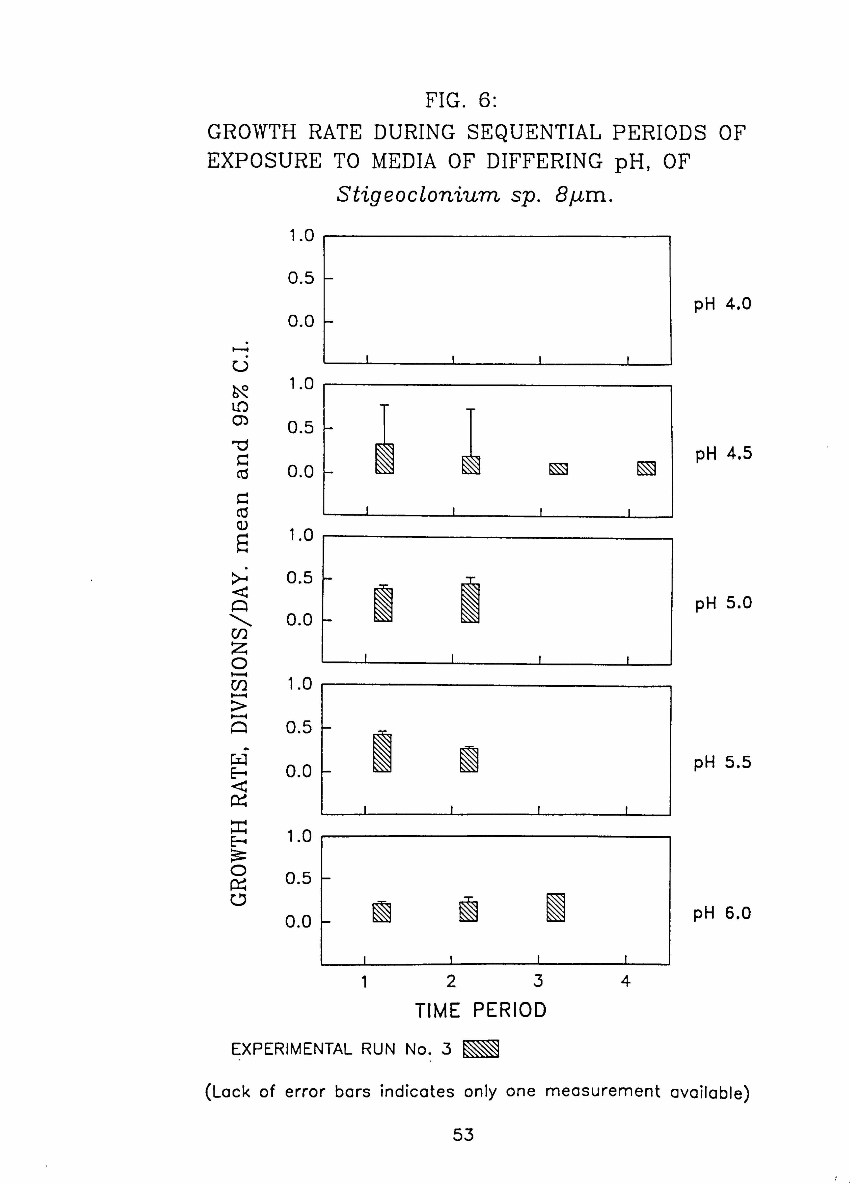
FIG. 6: GROWTH RATE DURING SEQUENTIAL PERIODS OF EXPOSURE TO MEDIA OF DIFFERING pH, OF
Stigeoclonium sp. 8t-cm.
1.0
0.5
0.0
-4 U
1.0
C) 0.5
Co 0.0
1.0
0.5
\ 0.0 U) z 0 U1 1.0
Q 0.5
F 0.0
Es 1.0
CD 0.5 CD
0.0
pH 4.0
pH 4.5
pH 5.0
pH 5.5
pH 6.0
1234
TIME PERIOD
EXPERIMENTAL RUN No. 3
(Lack of error bars indicates only one measurement available)
53
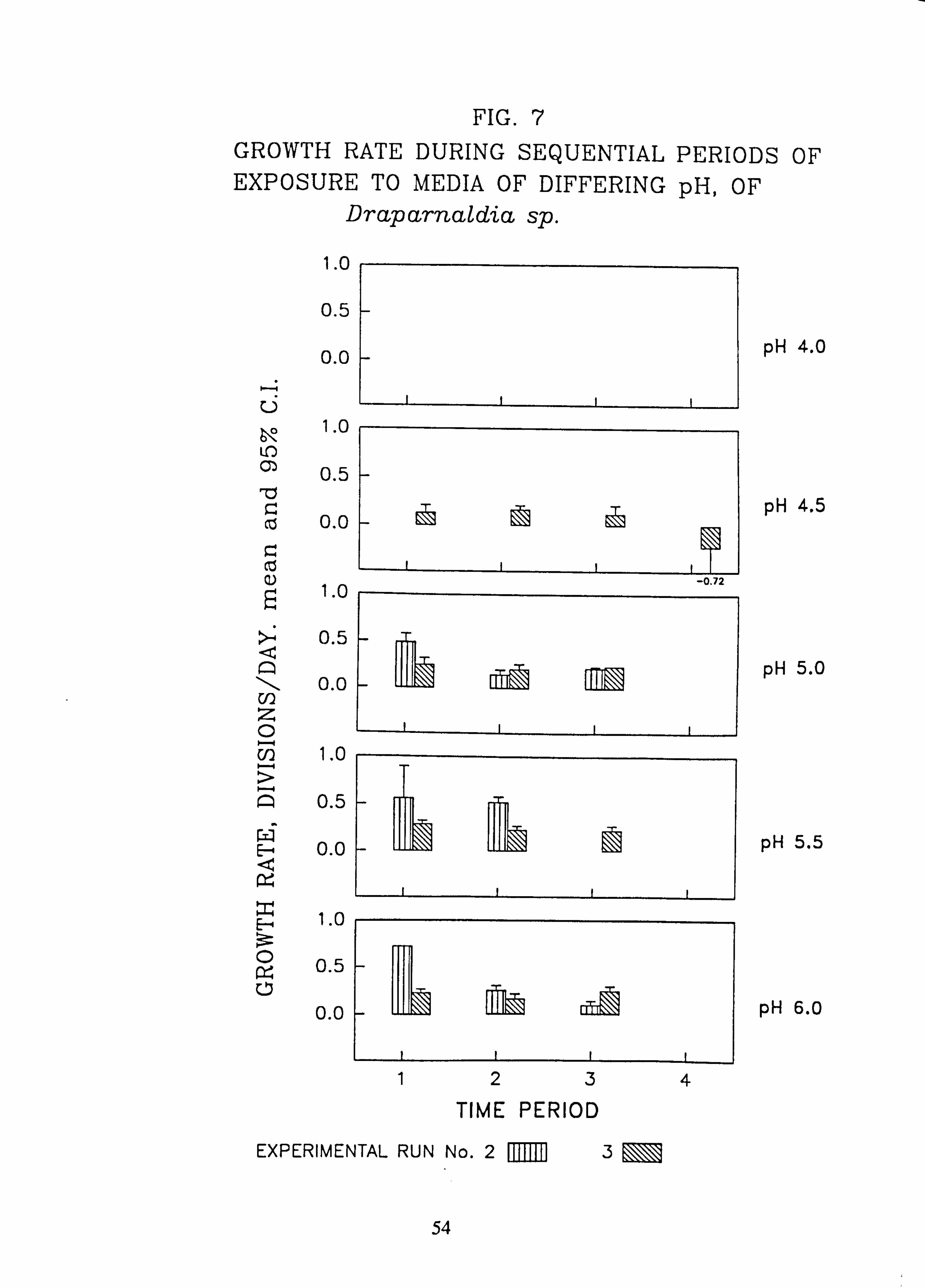
FIG. 7 GROWTH RATE DURING SEQUENTIAL PERIODS OF EXPOSURE TO MEDIA OF DIFFERING pH, OF
Draparnaldia sp. f1
i. v
0.5
0.0
U 1.0
0.5
0.0
a) 1.0
0.5
\ 0.0 U) z 0 U) 1.0 > Q 0.5
ril 0.0
1.0
0.5
0.0
-o.
pH 4.0
pH 4.5
pH 5.0
pH 5.5
1
06
A 1234
TIME PERIOD
EXPERIMENTAL RUN No. 2®3
pH 6.0
54
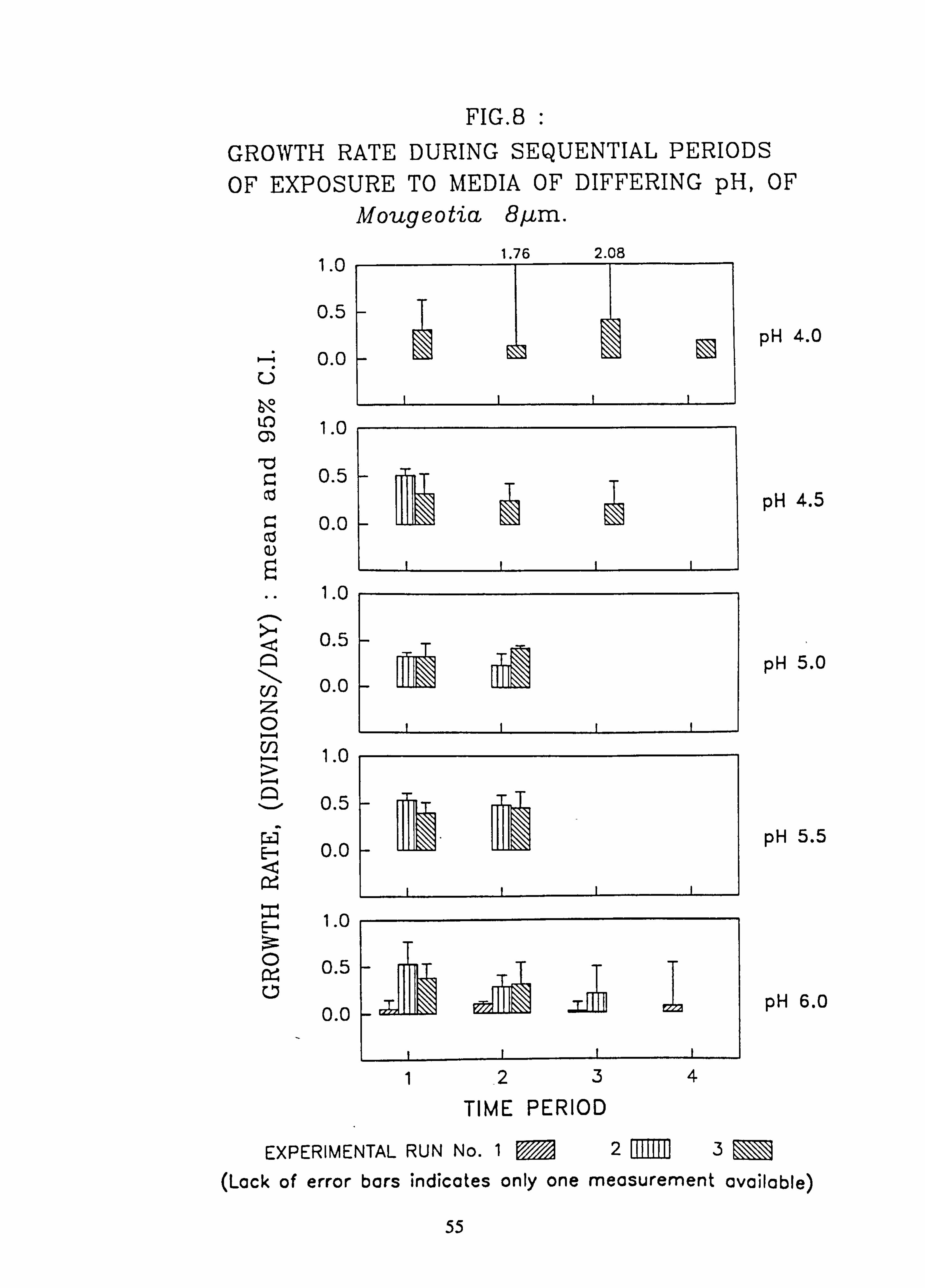
FIG. 8 GROWTH RATE DURING SEQUENTIAL PERIODS OF EXPOSURE TO MEDIA OF DIFFERING pH, OF
Mougeotia 8µm. 1.76 2.08
1.0
0.5
0.0 U
1.0
0.5
0.0 Q)
1.0
0.5
co 0.0 z 0 0-4 co 1.0
0.5
0.0
121.1 x 1.0 E-
0.5
0.0 : iA 1
pH 4.0
pH 4.5
pH 5.0
pH 5.5
pH 6.0
1234 TIME PERIOD
EXPERIMENTAL RUN No. 12®3 (Lack of error bars indicates only one measurement available)
55
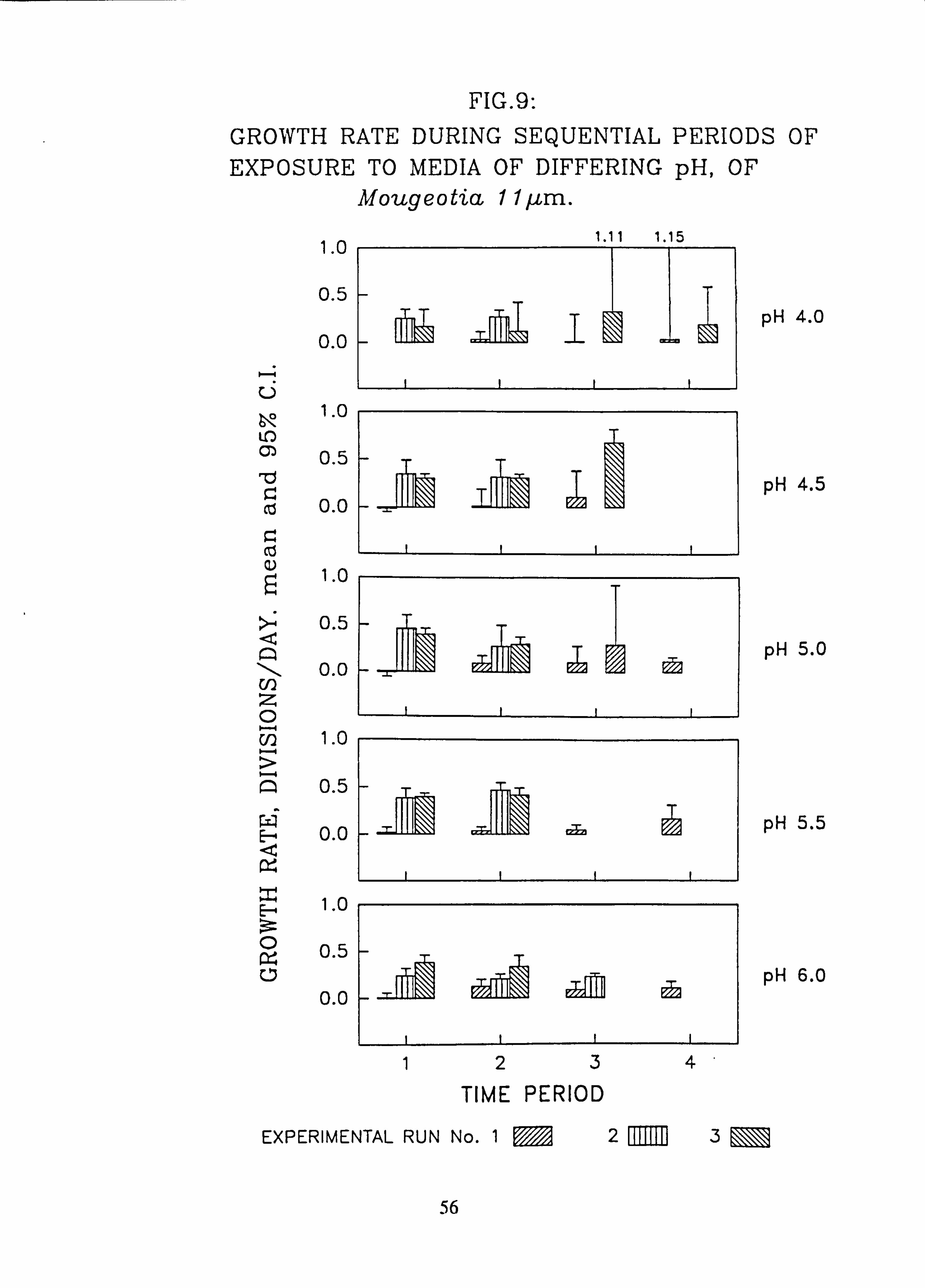
FIG. 9:
GROWTH RATE DURING SEQUENTIAL PERIODS OF EXPOSURE TO MEDIA OF DIFFERING pH, OF
Mougeotia 11/.. cm.
1.0
0.5
0.0
1-4 U
1.0
C) 0.5
Cli 0.0
Z, co
1.0
0.5
\ 0.0 U) z 0 CO 1.0
Q 0.5
E- 0.0
d P4 H 1.0
0 0.5
0.0
1.11 1.15
: ka :1a
IJJi
_ý
pH 4.0
pH 4.5
pH 5.0
pH 5.5
pH 6.0
1234
TIME PERIOD
EXPERIMENTAL RUN No. 1®2®3
56
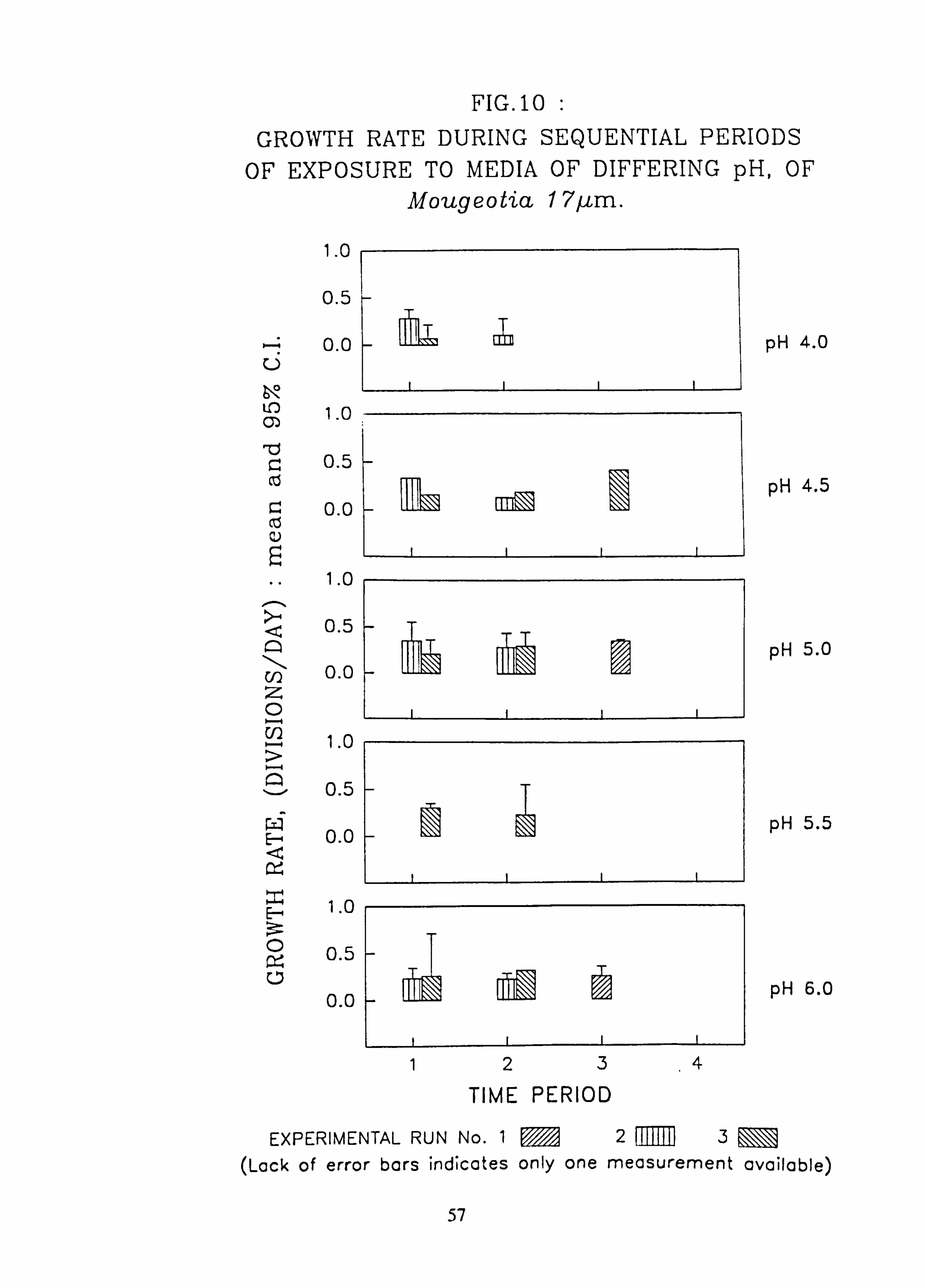
FIG. 10 : GROWTH RATE DURING SEQUENTIAL PERIODS
OF EXPOSURE TO MEDIA OF DIFFERING pH, OF Mougeotia 17,. cm.
1.0
0.5
H 0.0 U
1.0
0.5
0.0
1.0
0.5
0.0 2 0 Cf) 1.0
0.5
E- 0.0
1.0 E-
0.5
0.0
pH 4.0
pH 4.5
pH 5.0
pH 5.5
pH 6.0
123,4 TIME PERIOD
EXPERIMENTAL RUN No. 1®2®3 (Lack of error bars indicates only one measurement available)
57
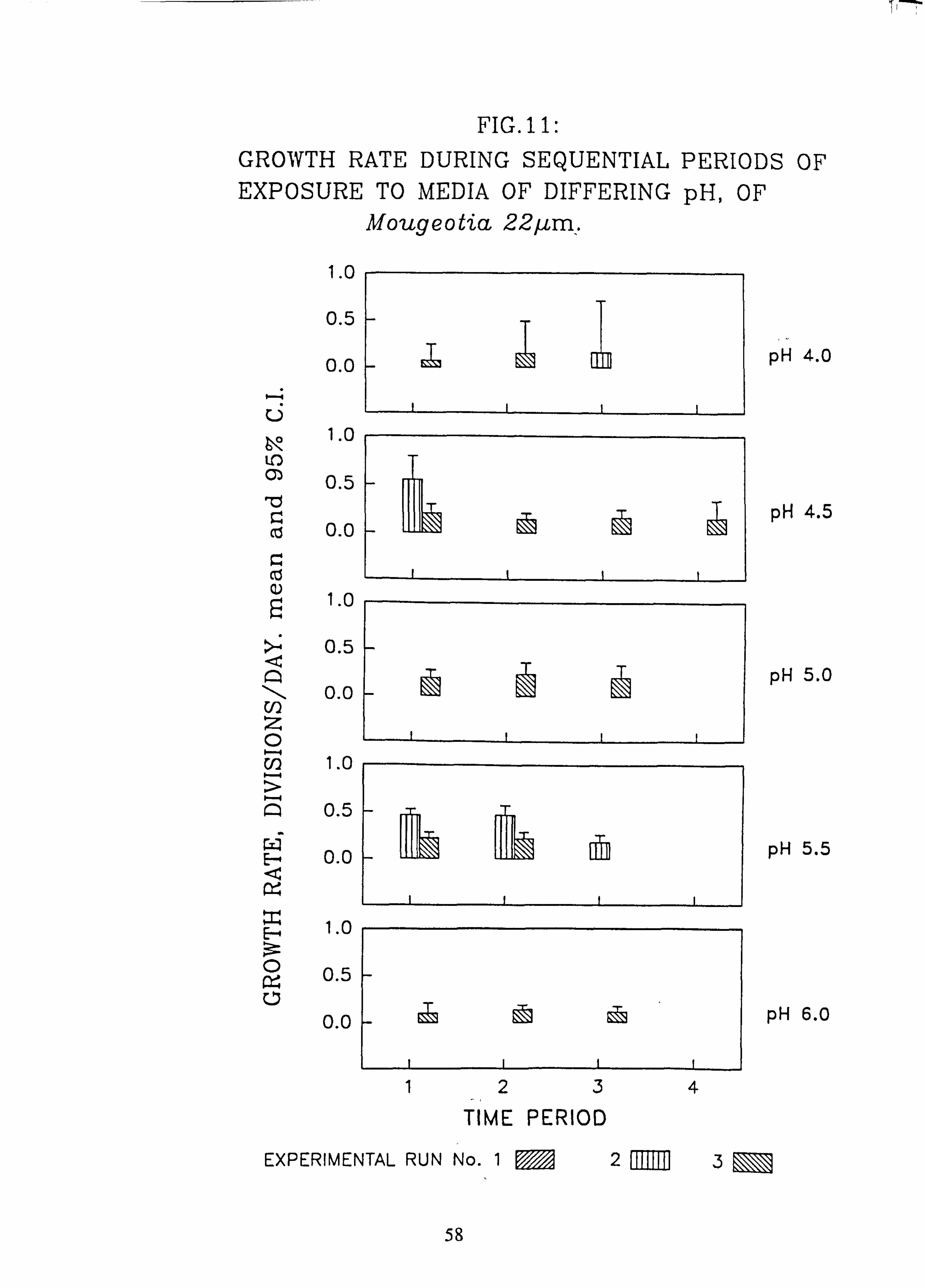
7i 7"
FIG. 11: GROWTH RATE DURING SEQUENTIAL PERIODS OF EXPOSURE TO MEDIA OF DIFFERING pH, OF
Mougeotia 22/-, cm. /1
I. V
0.5
0.0
U 1.0
0) 0.5
co 0.0
z CO
1.0
>ý 0.5
0.0 U) Z 0 co 1.0
0.5
E-y 0.0
E.., 1.0
0 0.5
0.0
pH 4.0
pH 4.5
pH 5.0
pH 5.5
- pH 6.0
1234 TIME PERIOD
EXPERIMENTAL RUN No. 1®2®3
58
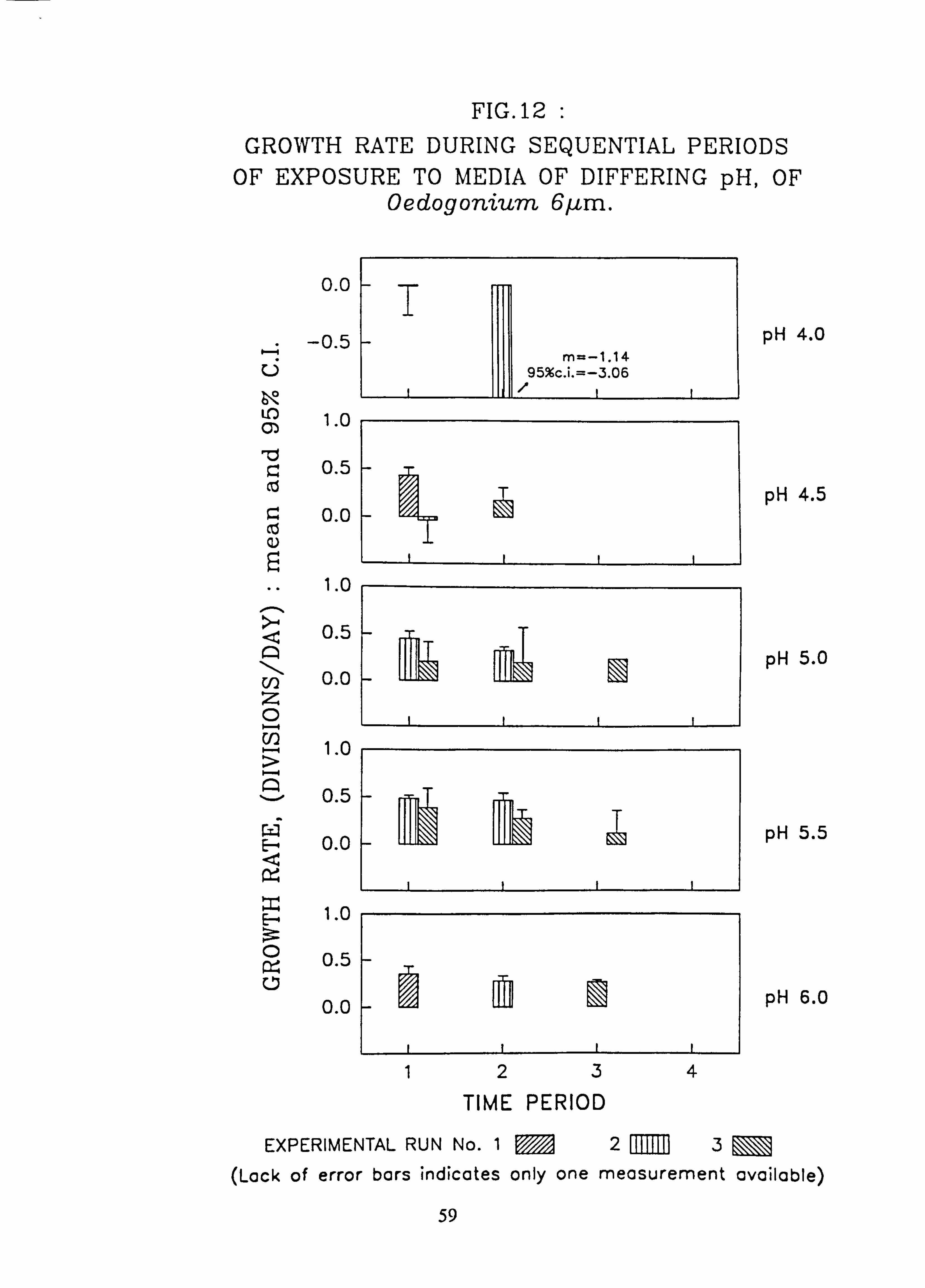
FIG. 12 : GROWTH RATE DURING SEQUENTIAL PERIODS
OF EXPOSURE TO MEDIA OF DIFFERING pH, OF Oedogonium 6/cm.
0.0
-0.5 L
t, Q ý 1.0
0.5
0.0 co a)
1.0
0.5
U) 0.0 z 0 CO 1.0
0.5
F 0.0
E- 1.0
0.5
0.0
r m=-1.14
95%c. i. =-3.06 ri
pH 4.0
pH 4.5
pH 5.0
pH 5.5
pH 6.0
1234 TIME PERIOD
EXPERIMENTAL RUN No. 1®2®3
(Lack of error bars indicates only one measurement available)
59
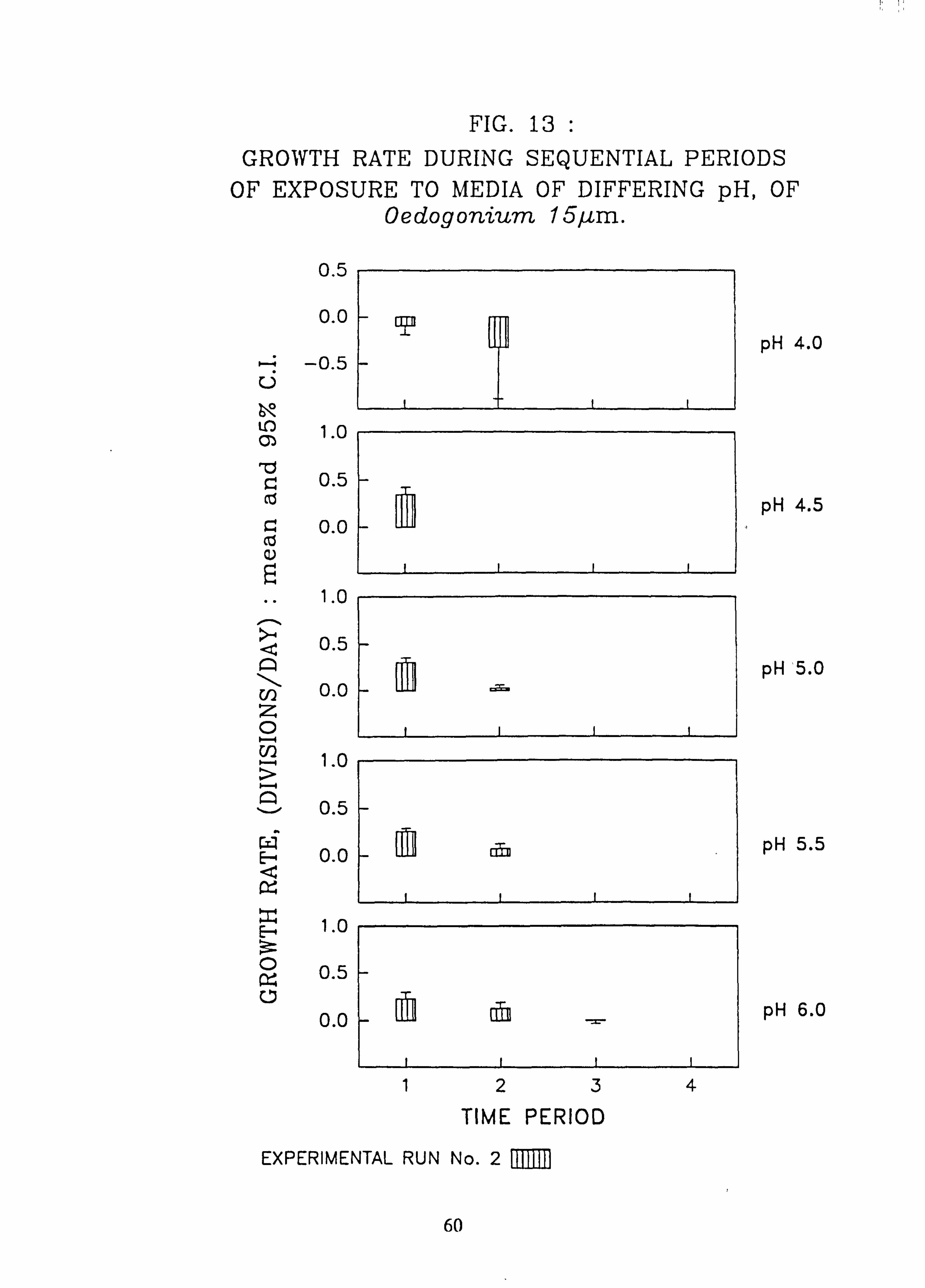
FIG. 13 : GROWTH RATE DURING SEQUENTIAL PERIODS
OF EXPOSURE TO MEDIA OF DIFFERING pH, OF Oedogon'ium 15/im.
0.5
0.0
H -0.5 C)
m 1.0
0.5
0.0 co a)
1.0
0.5
0.0 z 0 CO 1.0 Q 0.5
F 0.0
1.0 ýrz 0 0.5 0
0.0
OF
m
: -IM ah
pH 4.0
pH 4.5
pH '5.0
pH 5.5
pH 6.0
123 TIME PERIOD
EXPERIMENTAL RUN No. 2
4
60
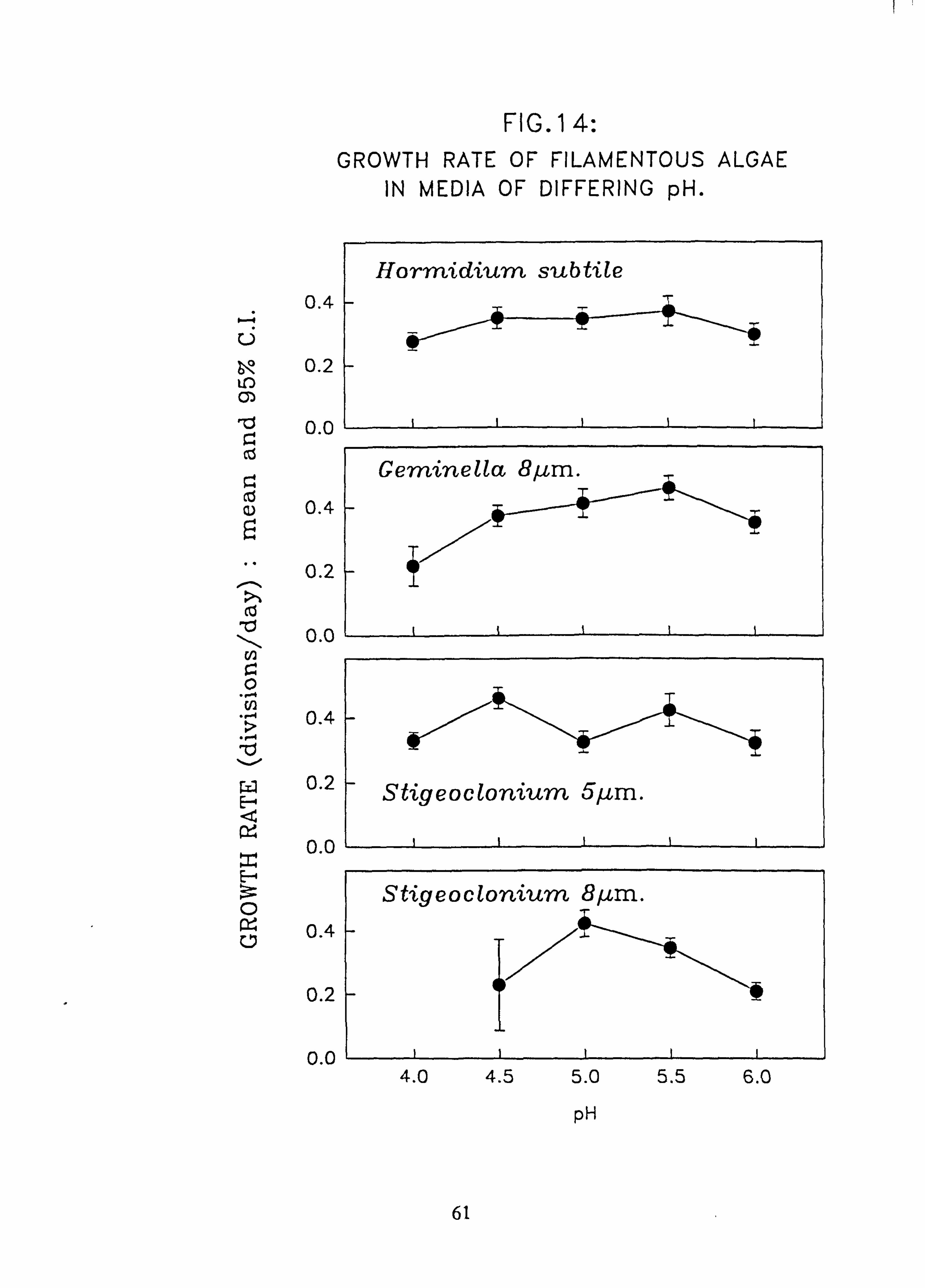
FIG. 1 4: GROWTH RATE OF FILAMENTOUS ALGAE
IN MEDIA OF DIFFERING pH.
0.4
U 0.2
0.0
czs
0.4
0.2
co 0.0
0
> 0.4
'b
0.2 E- :: 4
0.0
E-
0 0.4
0.2
0.0
Hormidium subtile
Geminella 8, um.
Stigeoclonium 5/Cm.
Stigeoclonium 8gm.
4.0 4.5 5.0
pH
5.5 6.0
61
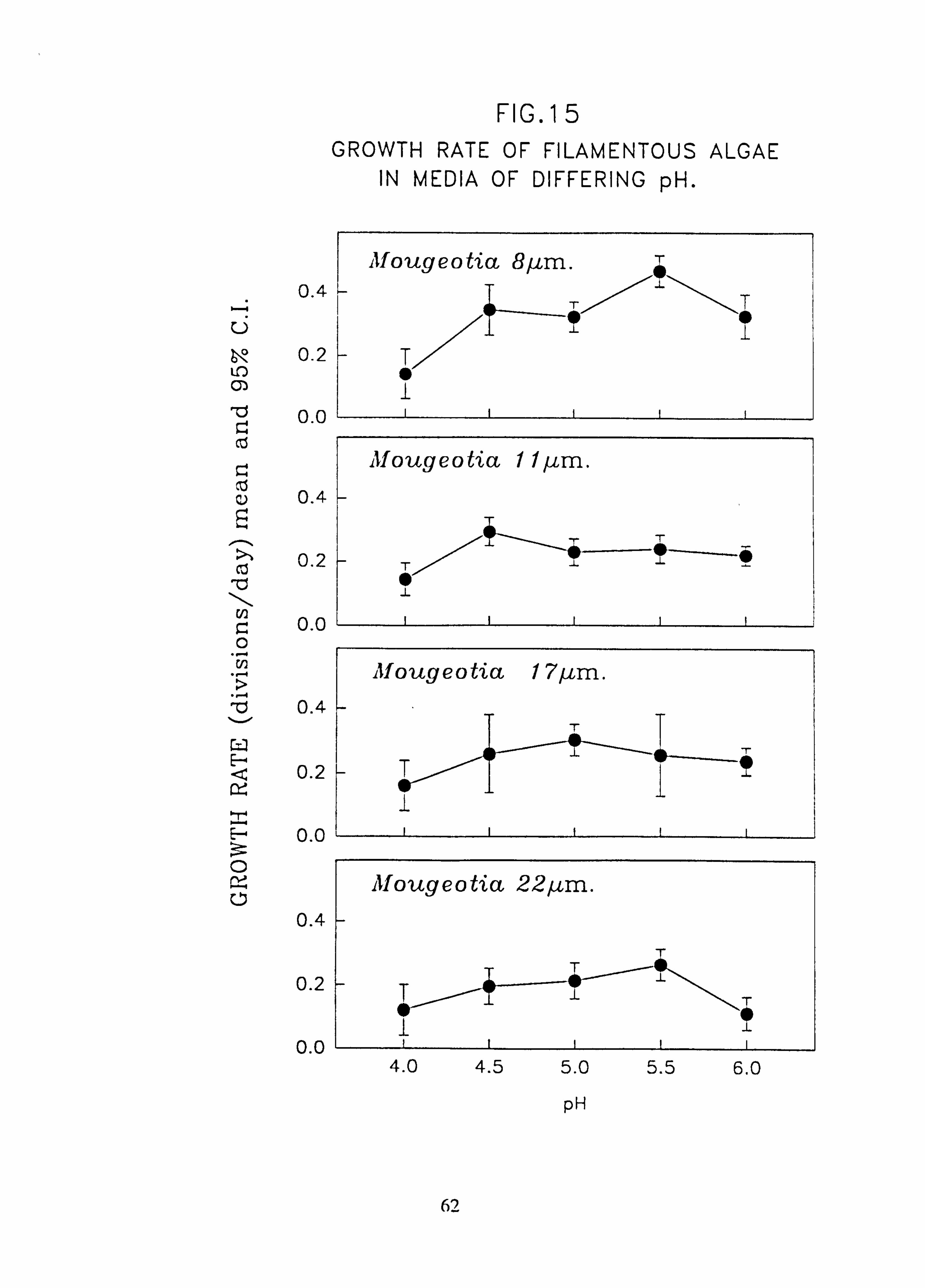
FIG. 15 GROWTH RATE OF FILAMENTOUS ALGAE
IN MEDIA OF DIFFERING pH.
U
býz 0.2 LO C)
00
co 0.4
0.2
0.0 0
'd 0.4
0.2 Q4
0.0
O
C, 0.4
0.2
0.4
Mougeotia 11 , um.
ýý
T
T/ l ýý
1
Mougeotia 17gm.
TT VH 1
1
T ý-l
T I
0.0
Mougeotia 22, am.
4.0 4.5 5.0
pH
5.5 6.0
62
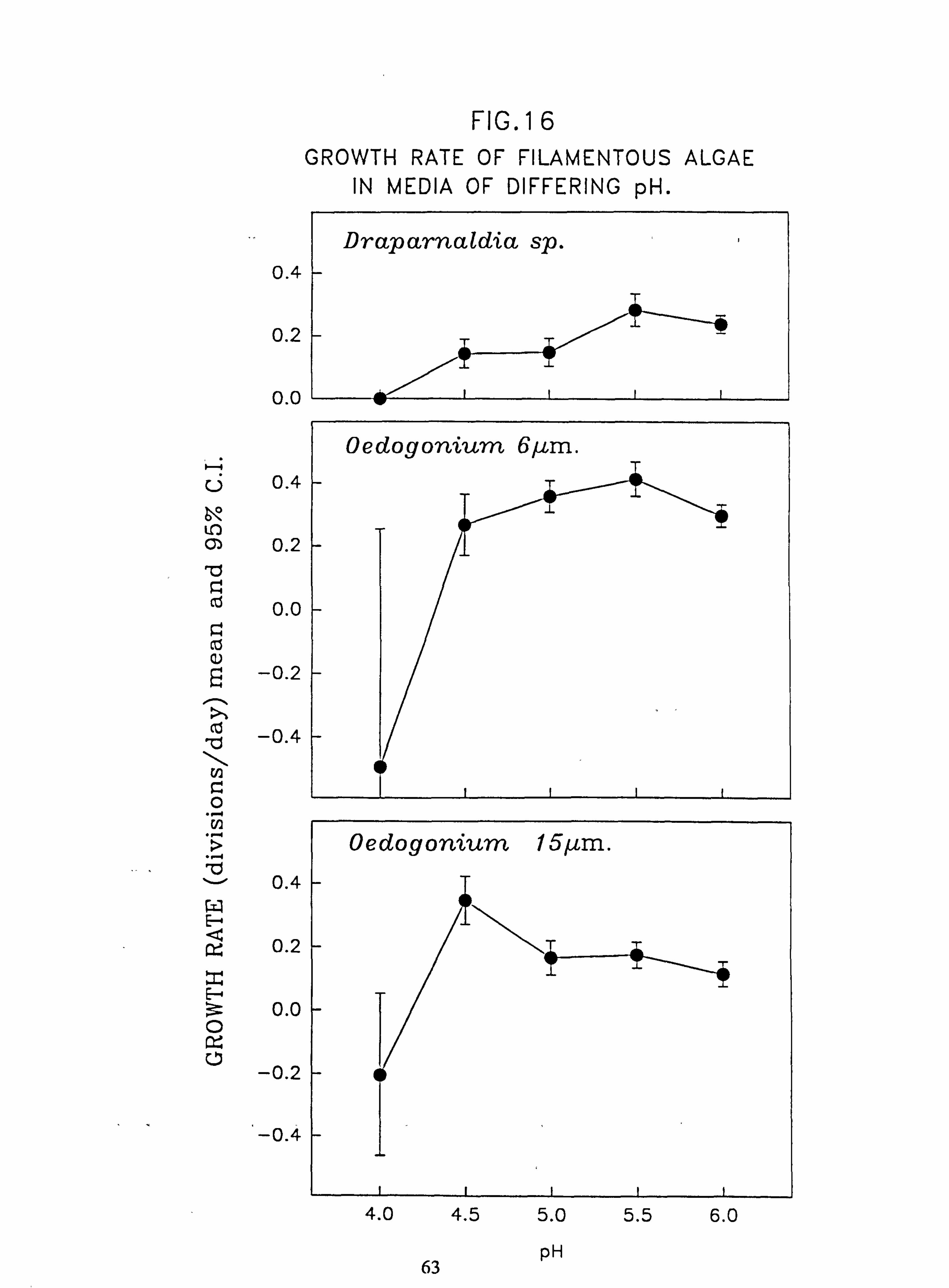
FIG. 1 6 GROWTH RATE OF FILAMENTOUS ALGAE
IN MEDIA OF DIFFERING pH.
0.4
0.2
0.0
Lj 0.4
C) 0.2
Cd 0.0
N
-0.2
co -0.4
U) 0
. r.
'd v 0.4
0.2
0.0 0
-0.2
-o.
Draparnatd'a sp.
Oedogonium 6gm.
pH 63
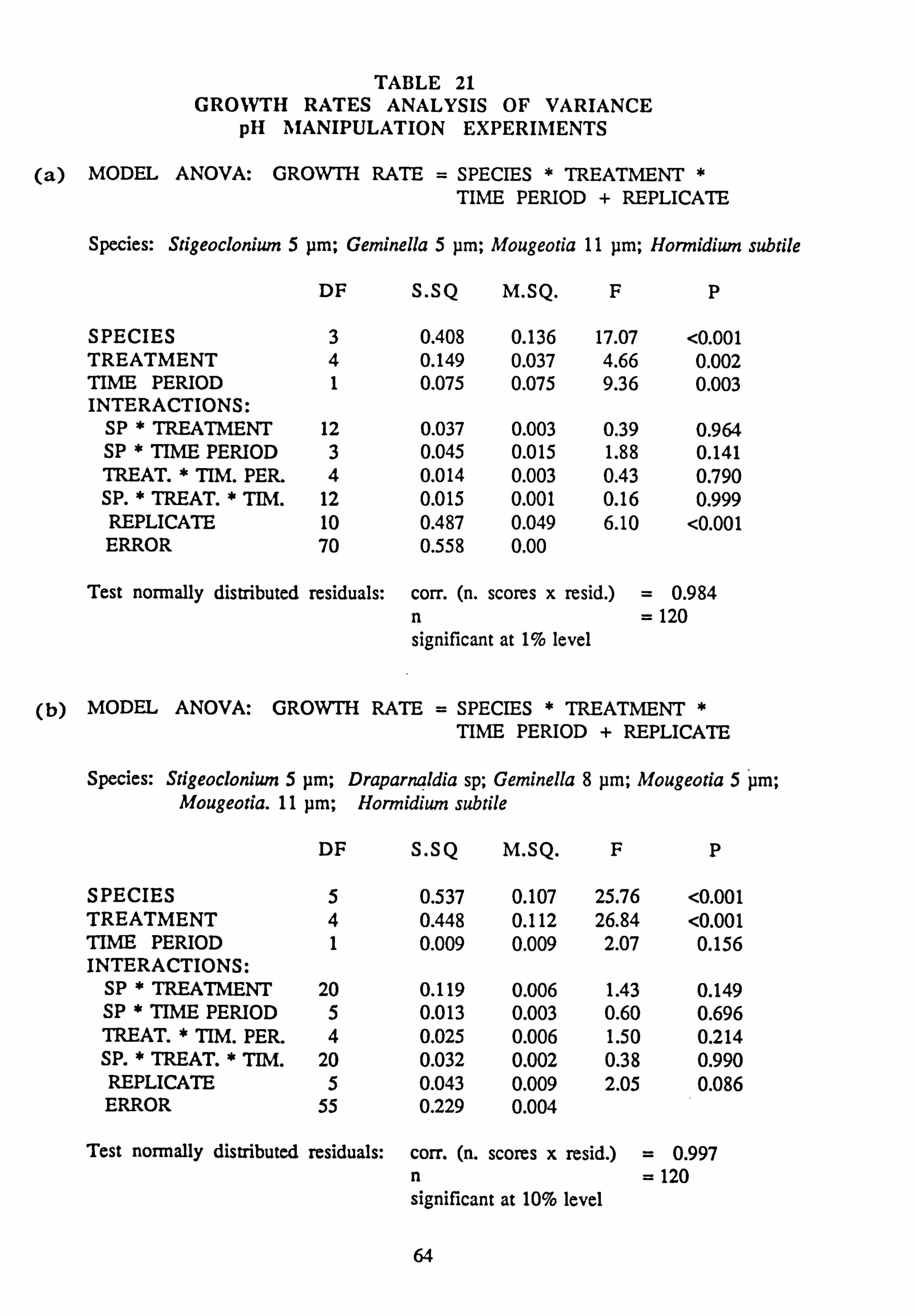
TABLE 21 GROWTH RATES ANALYSIS OF VARIANCE
pH MANIPULATION EXPERIMENTS
(a) MODEL ANOVA: GROWTH RATE = SPECIES * TREATMENT TIME PERIOD + REPLICATE
Species: Stigeoclonium 5 pm; Geminella 5 pm; Mougeotia 11 pm; Hormidium subtile
DF S. SQ M. SQ. F P
SPECIES 3 0.408 0.136 17.07 <0.001 TREATMENT 4 0.149 0.037 4.66 0.002 TIME PERIOD 1 0.075 0.075 9.36 0.003 INTERACTIONS:
SP * TREATMENT 12 0.037 0.003 0.39 0.964 SP * TIME PERIOD 3 0.045 0.015 1.88 0.141 TREAT. * TIM. PER. 4 0.014 0.003 0.43 0.790 SP. * TREAT. * TIM. 12 0.015 0.001 0.16 0.999 REPLICATE 10 0.487 0.049 6.10 <0.001 ERROR 70 0.558 0.00
Test normally distributed residuals: corr. (n. scores x resid. ) = 0.984 n = 120 significant at 1% level
(b) MODEL ANOVA: GROWTH RATE = SPECIES * TREATMENT * TIME PERIOD + REPLICATE
Species: Stigeocloniwn 5 pm; Draparnaldia sp; Geminella 8 pm; Mougeotia 5 pm; Mougeotia. 11 pm; Hormidium subtile
DF S. SQ M. SQ. F P
SPECIES 5 0.537 0.107 25.76 <0.001 TREATMENT 4 0.448 0.112 26.84 <0.001 TIME PERIOD 1 0.009 0.009 2.07 0.156 INTERACTIONS:
SP * TREATMENT 20 0.119 0.006 1.43 0.149 SP * TIME PERIOD 5 0.013 0.003 0.60 0.696 TREAT. * TIM. PER. 4 0.025 0.006 1.50 0.214 SP. * TREAT. * TIM. 20 0.032 0.002 0.38 0.990 REPLICATE 5 0.043 0.009 2.05 0.086 ERROR 55 0.229 0.004
Test normally distributed residuals: corr. (n. scores x resid. ) = 0.997 n = 120 significant at 10% le vel
64
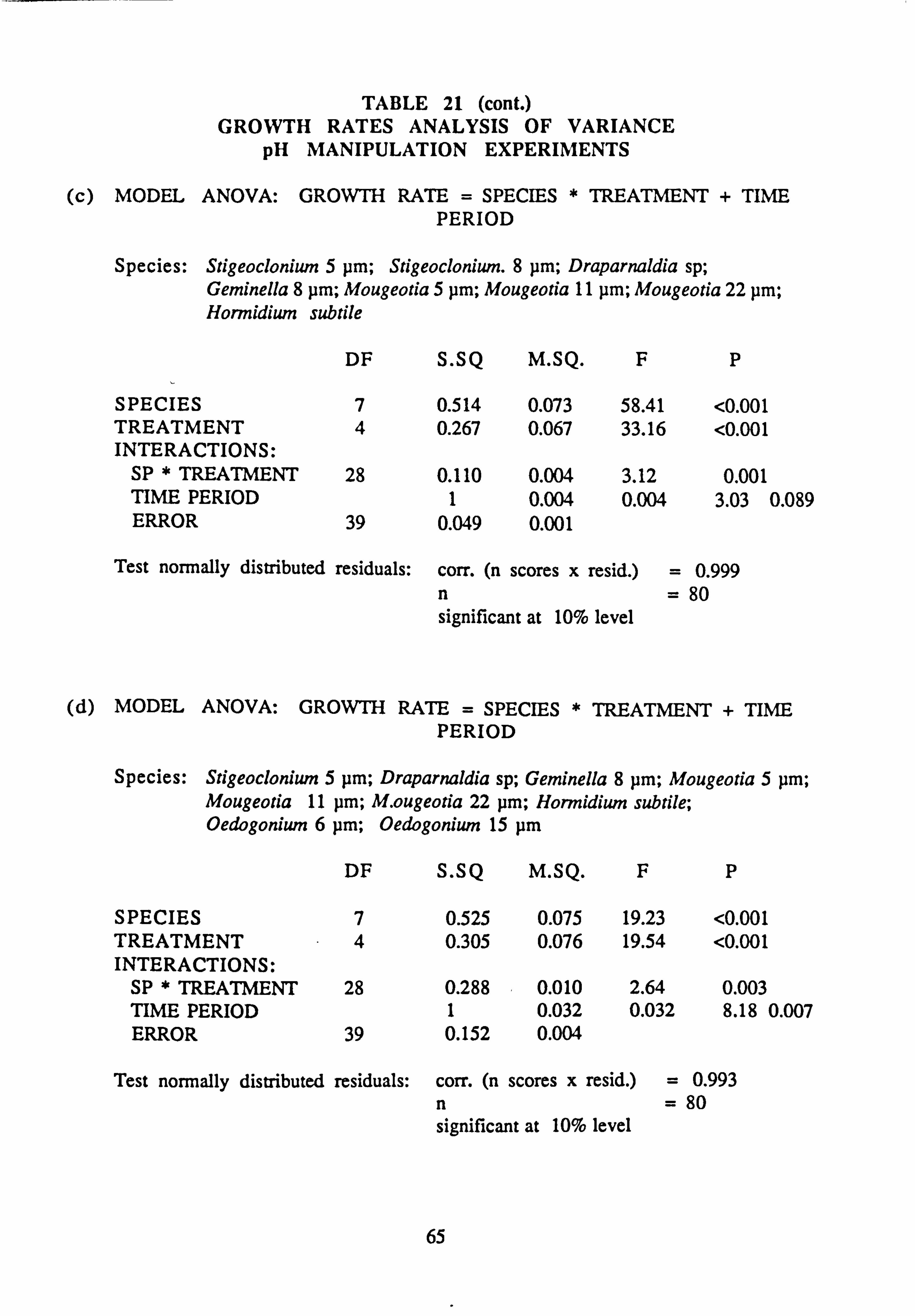
TABLE 21 (cont. ) GROWTH RATES ANALYSIS OF VARIANCE
pH MANIPULATION EXPERIMENTS
(c) MODEL ANOVA: GROWTH RATE = SPECIES * TREATMENT + TIME PERIOD
Species: Stigeoclonium 5 pm; Stigeoclonium. 8 pm; Draparnaldia sp; Geminella 8 pm; Mougeotia 5 pm; Mougeotia 11 pm; Mougeotia 22 pm; Hormidium subtile
DF S. SQ M. SQ. F P
SPECIES 7 0.514 0.073 58.41 <0.001 TREATMENT 4 0.267 0.067 33.16 <0.001 INTERACTIONS:
SP * TREATMENT 28 0.110 0.004 3.12 0.001 TIME PERIOD 1 0.004 0.004 3.03 0.089 ERROR 39 0.049 0.001
Test normally distributed residuals: corr. (n scores x resid. ) = 0.999 n = 80 significant at 10% level
(d) MODEL ANOVA: GROWTH RATE = SPECIES * TREATMENT + TIME PERIOD
Species: Stigeoclonium 5 pm; Draparnaldia sp; Geminella 8 pm; Mougeotia 5 pm; Mougeotia 11 pm; M. ougeotia 22 pm; Hormidium subtile; Oedogonium 6 pm; Oedogonium 15 pm
DF S. SQ M. SQ. F P
SPECIES 7 0.525 0.075 19.23 <0.001 TREATMENT 4 0.305 0.076 19.54 <0.001 INTERACTIONS:
SP * TREATMENT 28 0.288 0.010 2.64 0.003 TIME PERIOD 1 0.032 0.032 8.18 0.007 ERROR 39 0.152 0.004
Test normally distributed residuals: corr. (n scores x resid. ) = 0.993 n= 80 significant at 10% level
65
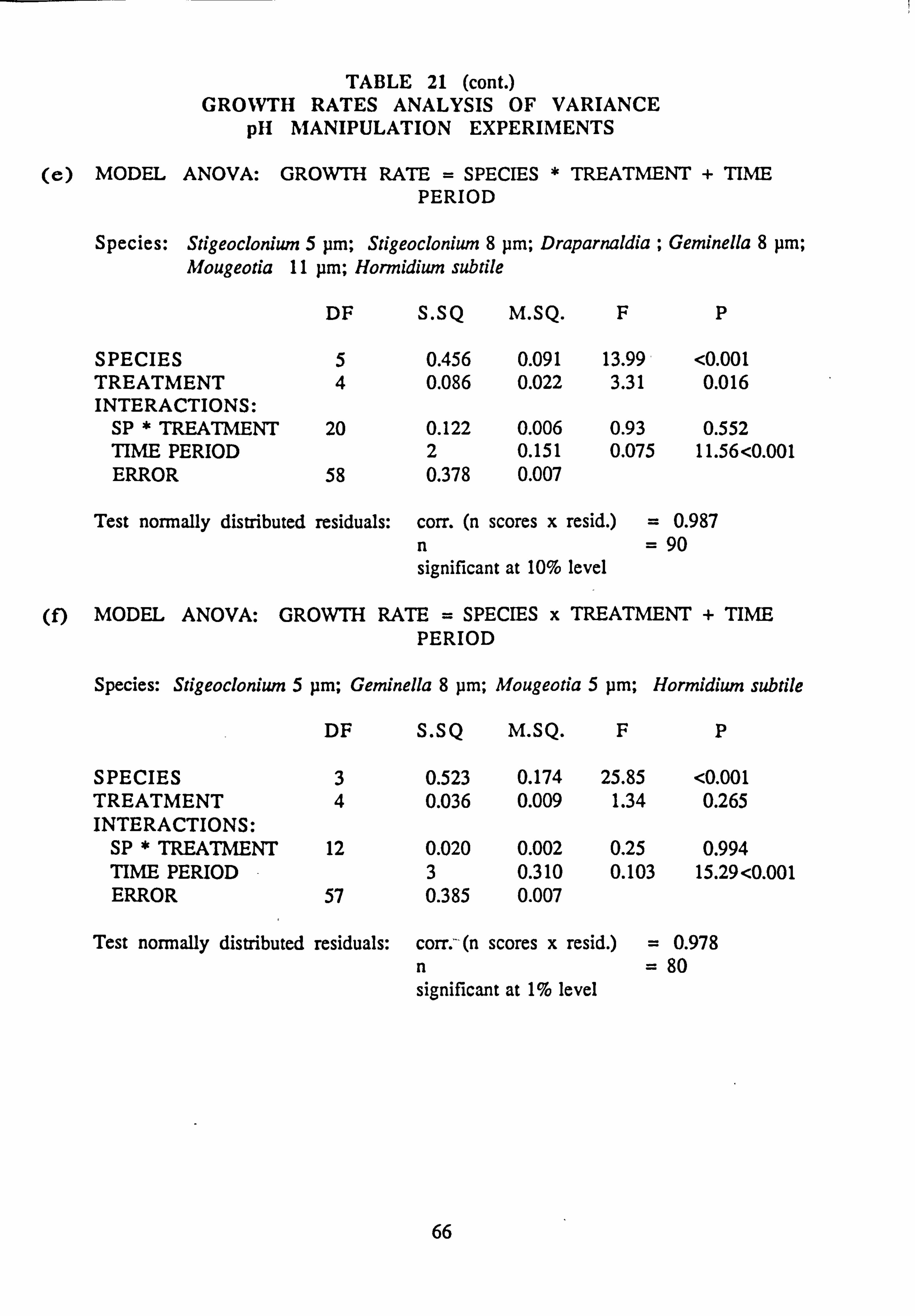
TABLE 21 (cont. ) GROWTH RATES ANALYSIS OF VARIANCE
pH MANIPULATION EXPERIMENTS
(e) MODEL ANOVA: GROWTH RATE = SPECIES * TREATMENT + TIME PERIOD
Species: Stigeocloniwn 5 pm; Stigeoclonium 8 pm; Draparnaldia ; Geminella 8 pm; Mougeotia 11 pm; Hormidium subtile
DF S. SQ M. SQ. F P
SPECIES 5 0.456 0.091 13.99 <0.001 TREATMENT 4 0.086 0.022 3.31 0.016 INTERACTIONS:
SP * TREATMENT 20 0.122 0.006 0.93 0.552 TIME PERIOD 2 0.151 0.075 11.56<0.001 ERROR 58 0.378 0.007
Test normally distributed residuals: corr. (n scores x resid. ) = 0.987 n= 90 significant at 10% level
(f) MODEL ANOVA: GROWTH RATE = SPECIES x TREATMENT + TIME PERIOD
Species: Stigeoclonium 5 pm; Geminella 8 pm; Mougeotia 5 pm; Hormidium subtile
DF S. SQ M. SQ. F P
SPECIES 3 0.523 0.174 25.85 <0.001 TREATMENT 4 0.036 0.009 1.34 0.265 INTERACTIONS:
SP * TREATMENT 12 0.020 0.002 0.25 0.994 TIME PERIOD 3 0.310 0.103 15.29<0.001 ERROR 57 0.385 0.007
Test normally distributed residuals: corr. (n scores x resid. ) = 0.978 n= 80 significant at 1% level
66
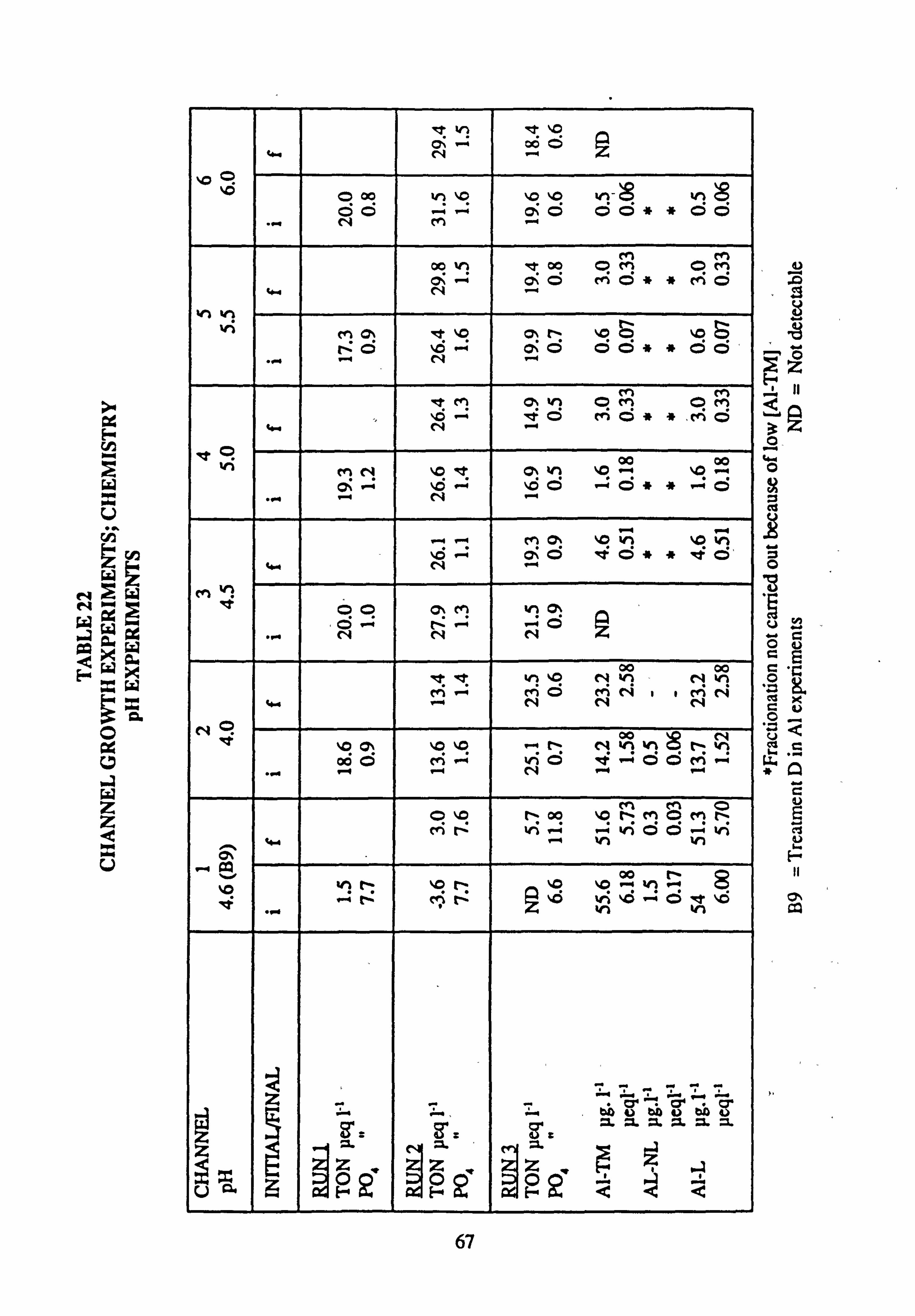
S CA om
U
ýWr NG Nä WW
as ýX EýW
C a a w z z Q x c)
Z W
GG W CL
W x a
le vý le ýlo oý, "4 oö Ö
c+. N
\p O
O 00 vs \O ýp
\D 'n- hO ÖÖ -c- 0; Ö ÖÖ IF * ÖCý
.. -. N M
00 In of clo OMO ri oý r-+ cý Ö r'i Ö** cri Ö
w N -4 hh
vi M c% lqt ýQ c% ['N ýO ýD
N1 ýÖ 00* " Öd'
et m O> V'1 OM0M
'D - OMO** , cM O w N -4
eO xn mN \O le
00 00 C% h %0 1--4 ýo "-m
.rp -i 0% 'D V1 ýc Vl \O 9-4 cý O ýt 0**'Ö'
w N -
OO C% cn vi 0%
... N N N
00 00 et ýt v-i ýD N M^ MÖMN
i' MN w - NNN
N ýp 00 h ýO0; 'CEO "-+N N h0 N 0ö0 cri "-+ nCG et "-+0©M-
O 'D N
to co NO r-en M [ý vi hÖÖ "-ý h
w vi vi CP%
ý Nth IlOC: %0 ýo v
Z to ü bo ü
to . ... , ci
z Ua .q Q cý Hd, E-cý Q
.o
3Q 0- 44
. 75
ýn 4. % /y
U
*Q
U
U F-
VM
1ý
67
3.4.2 Effect of Al on Growth Rate Three treatments based on Corrie mediuim were used, all at pH 5.5. Treatment A was unmodified, B had the silicate concentration reduced to approximately one-tenth, and C had, in addition, total aluminium input increased to equal that of medium B9. The
concentrations measured were found to differ from the target values (table 24). In
addition, the results of measurements made in parallel with the pH experiments, in B9,
are shown alongside, as treatment D. The Al experiments (Figs. 17-22 and Table 23) demonstrate the profound influence which total [Al] of approximately 200 pg 1-1 exerts on the growth rate of all species. Only Hormidium subtile andGeminella 8 pm. were able to grow under these conditions(treatment C), at a reduced growth rate. In contrast, in
the B9 medium (treatment D), other species including Mougeotia 5pm, Mougeotia 11µm and Stigeoclonium sp. grew readily.
Burn 9, the prototype for B9 medium, has a high mean P04 concentration, possibly due in part to fertilization of the catchment by the Forestry Commission (pers. comm. ). Nutrient leaching may continue for several years after such a treatment (Harriman, 1978).
The composition of the media with respect to important chemical parameters at the beginning and end of the growth measurements is shown in Table 24. Particularly
striking is the difference in growth rate between the two Stigeoclonium isolates, 9e and 10a, in treatment C. Stigeoclonium 9e originated in Burn 9, an acidified but humic
stream, also with high PO4 levels, both of which may ameliorate the effects of aluminium, while Stigeoclonium 10a was isolated from Burn 10, which has the highest mean Al con- centration, particularly as Al-L, of all sites (Tables 10-12).
During the earlier series of experiments on the effect of pH, the strain of Stigeoclonium
was not well defined, samples from Burn 14, Burn 9 and Bum 11 being mixed in some inocula. Therefore it is not certain which strain is represented in the graph of growth in
medium B9 (treatment D). The lower growth rate seen in B9 (0.3 to 0.6 d/d) in
comparison with treatments A and B must be compared with that obtained in the pH experiments at pH 4.5, i. e. approximately 0.45 d/d. One-way analysis of variance carried out on the pH experiments shows that the growth rate was not significantly different between pH 4.0, pH 4.5 (Corrie medium) and B9 at pH 4.6, so that the lower growth rate in D (Fig. 20) may be due to the pH difference between C and D. It may be that the different growth rates seen in different experimental runs on the effects of pH, on most species, may result from different sources of the algae used in the inocula.
The existence of ecotypes has been well documented, e. g. for Srigeoclonium, and may apply to some extent also for other species or genera. This means that exact conclusions cannot be drawn from these experiments about the extent of influence which pH and aluminium exert on the growth rate of a particular species. It would also blur the indicator values of species, for example in analyses by CANOCO.
68
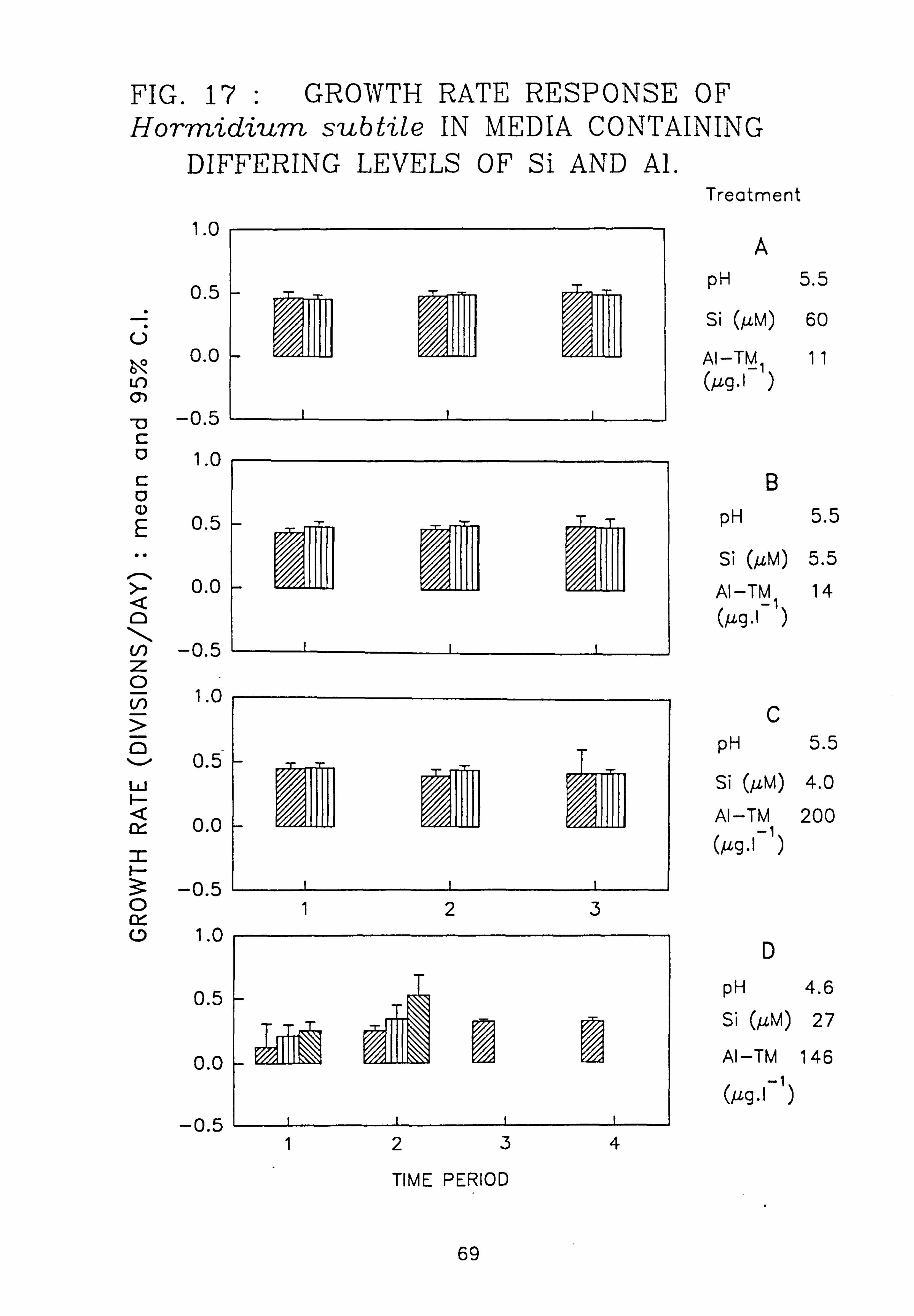
FIG. 17 : GROWTH RATE RESPONSE OF Hormidium subtile IN MEDIA CONTAINING
DIFFERING LEVELS OF Si AND Al. Treatment
I. U
0.5
U 0.0
rn -D -0.5 c ° 1.0 c 0 (D E 0.5
0.0
cn -0.5 z 0 1.0
ý 0.5 W F-
0.0
H
-0.5 0
cý 1.0
A
pH 5.5
Si (MM) 60
Al-TM1 11 (/ig. l )
123
0.5
0.0
-0.5
ýý 1234
TIME PERIOD
B pH 5.5
Si (AM) 5.5
Al-TM 14 (/hg., )
C pH 5.5
Si (MM) 4.0
Al --TM 200 (µ9"l_1)
D
pH 4.6
Si (MM) 27
Al-TM 146
(Ag. I_ 1)
69
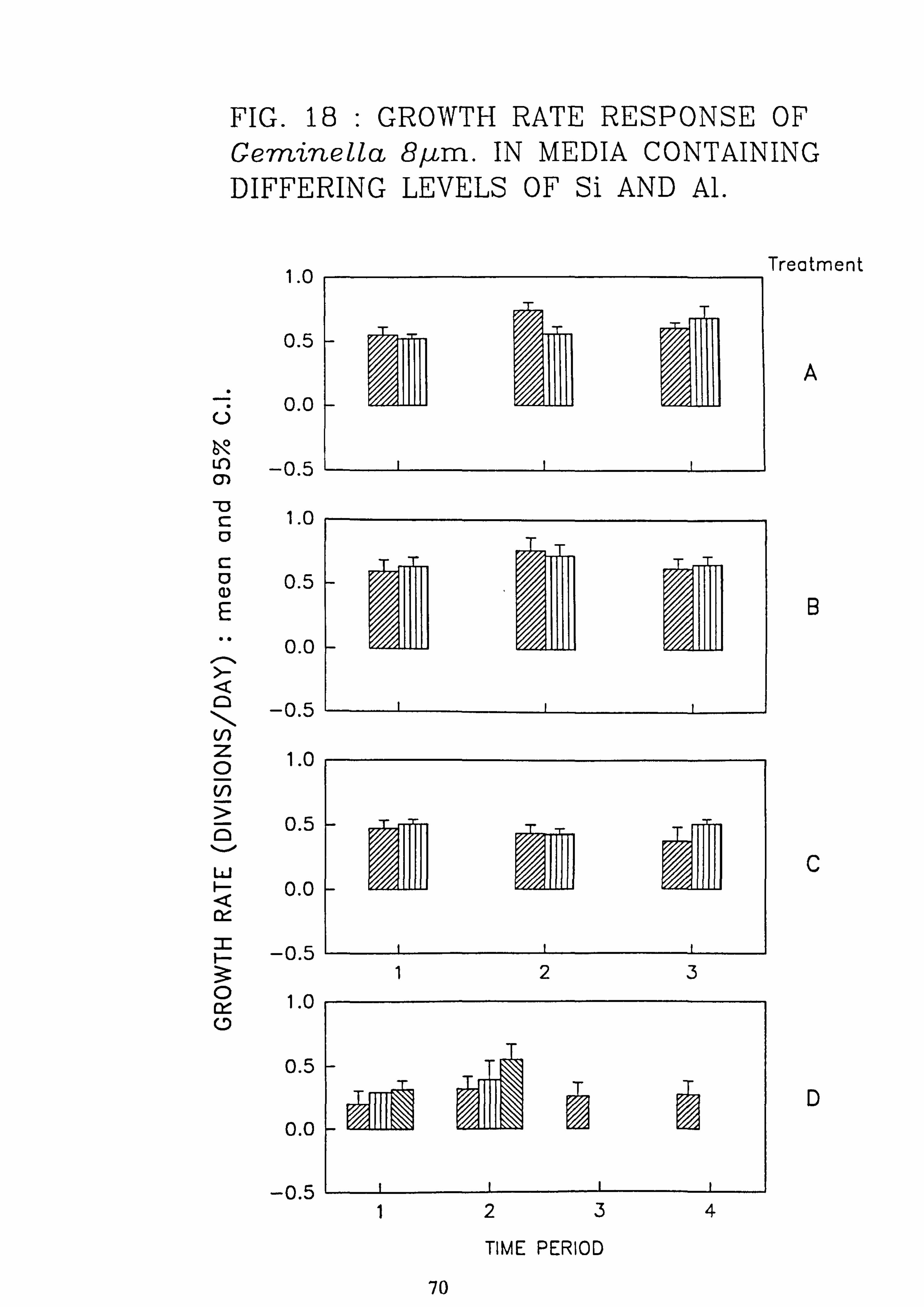
FIG. 18 : GROWTH RATE RESPONSE OF Gem'inella 81-, cm. IN MEDIA CONTAINING DIFFERING LEVELS OF Si AND Al.
1.0
0.5
0.0 U
ý -0.5
c 1.0 v c
0.5
E 0.0
° -0.5
Z 1.0 0
ö 0.5
0.0
-0.5
1.0
0.5
0.0
-0.5
Treatment
A
B
123
Irrr1thi I 1234
TIME PERIOD
70
C
D
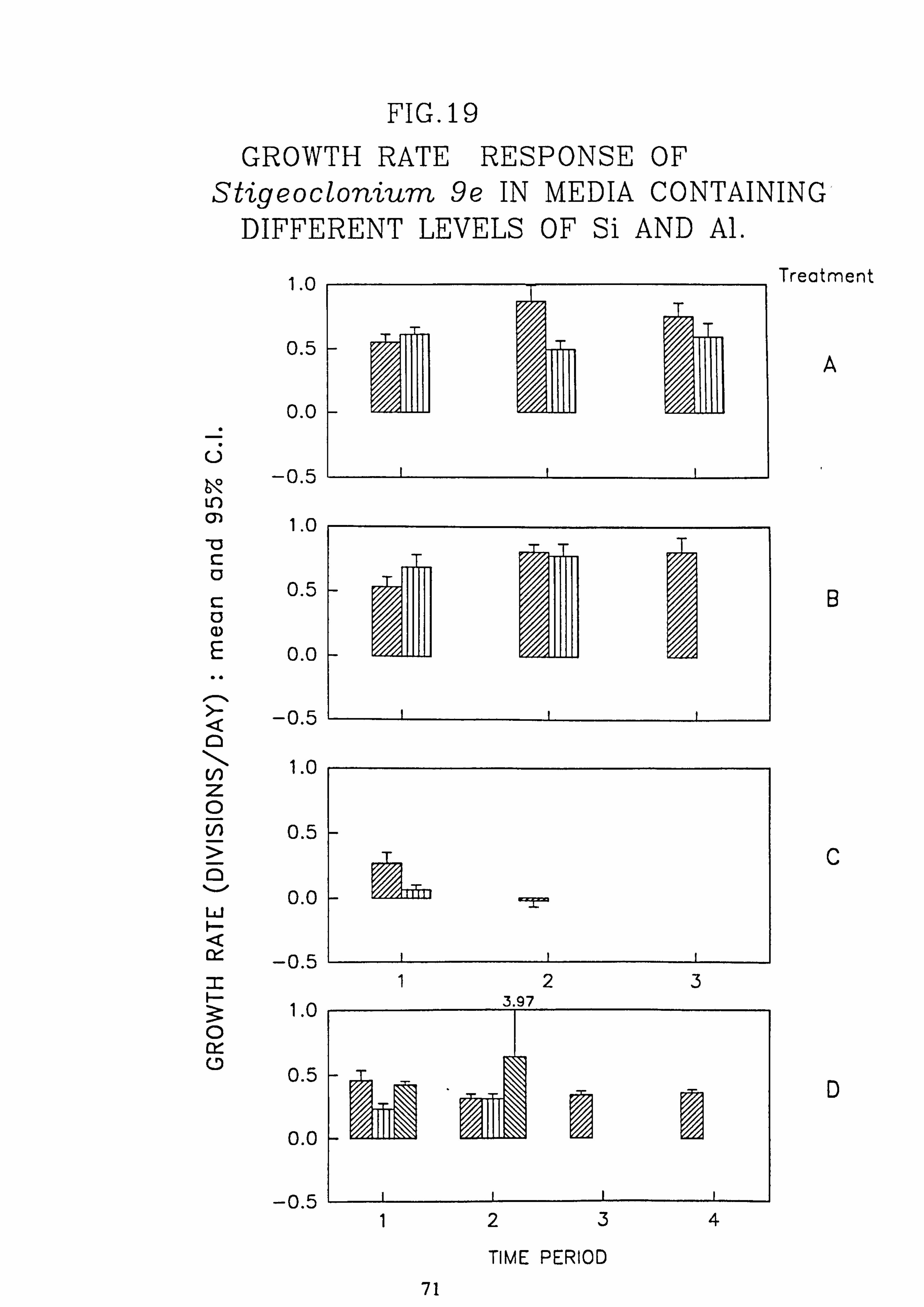
FIG. 19
GROWTH RATE RESPONSE OF Stigeoclonium 9e IN MEDIA CONTAINING
DIFFERENT LEVELS OF Si AND Al.
rN Treatment I. V
0.5
0.0
U
-nc;
A
L() O") n i. v
C 0 0.5 c 0 aý
0.0
-05
B
cL --- 0
11 I. V
z 0 N_ 0.5
0.0 w
_n
C
Z vv 123 1.0
O
0.5
0.0
_n c 1234
TIME PERIOD 71
D
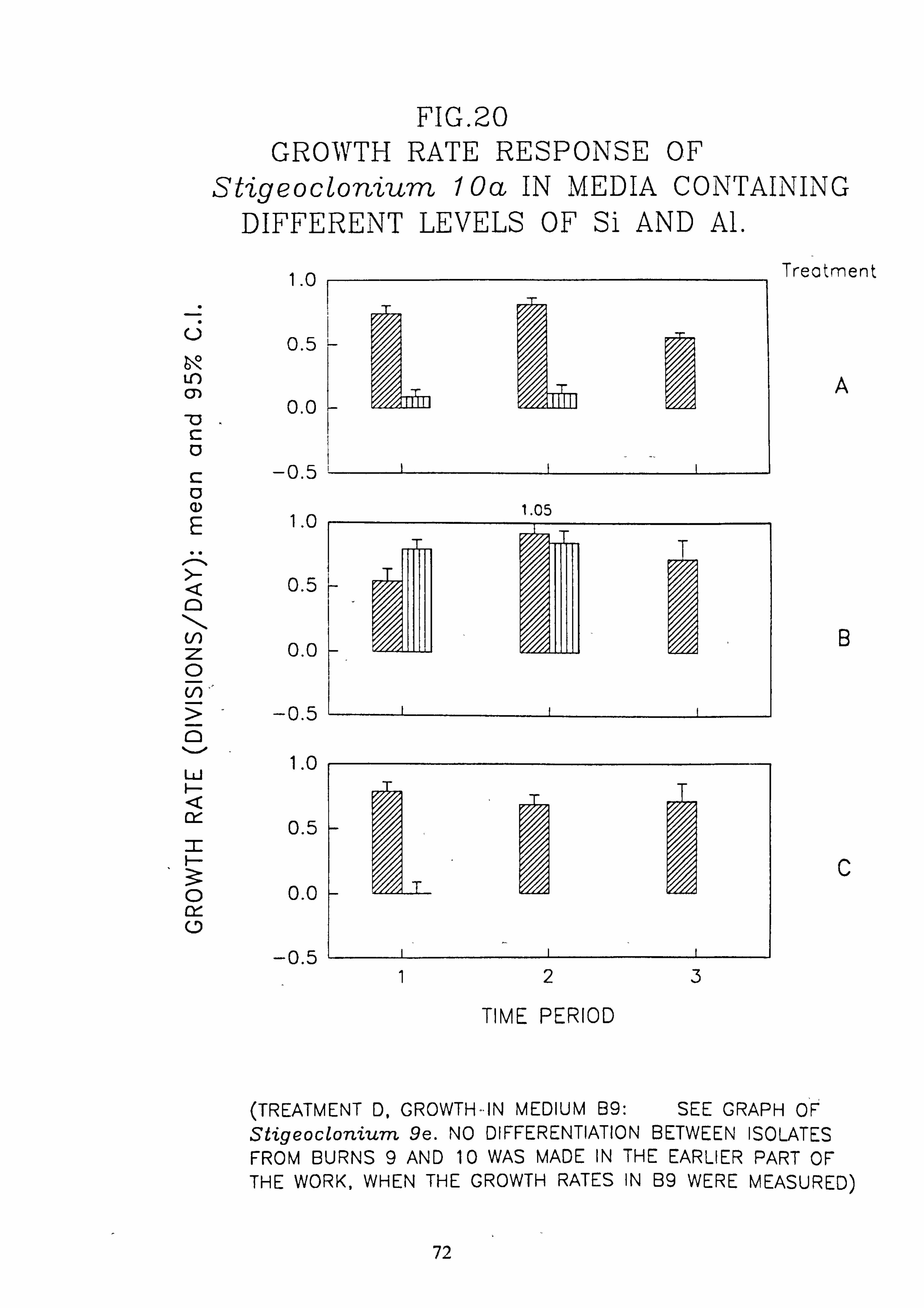
FIG. 20 GROWTH RATE RESPONSE OF
Stigeocton'ium 10a IN MEDIA CONTAINING DIFFERENT LEVELS OF Si AND Al.
Treatment i. v
U 0 In rn
C 0 C 0 N
E
Q 0
Cl) Z O_ (-I)_ > 0
w
Of 2 F- 3-1 0 ly- 0
0.5
0.0
-0.5 1.0
0.5
0.0
-0.5
1.0
0.5
0.0
-0.5
_ Li 1.05
123
TIME PERIOD
A
B
C
(TREATMENT D, GROWTH-IN MEDIUM B9: SEE GRAPH OF Stigeocloniurn 9e. NO DIFFERENTIATION BETWEEN ISOLATES FROM BURNS 9 AND 10 WAS MADE IN THE EARLIER PART OF THE WORK, WHEN THE GROWTH RATES IN B9 WERE MEASURED)
72
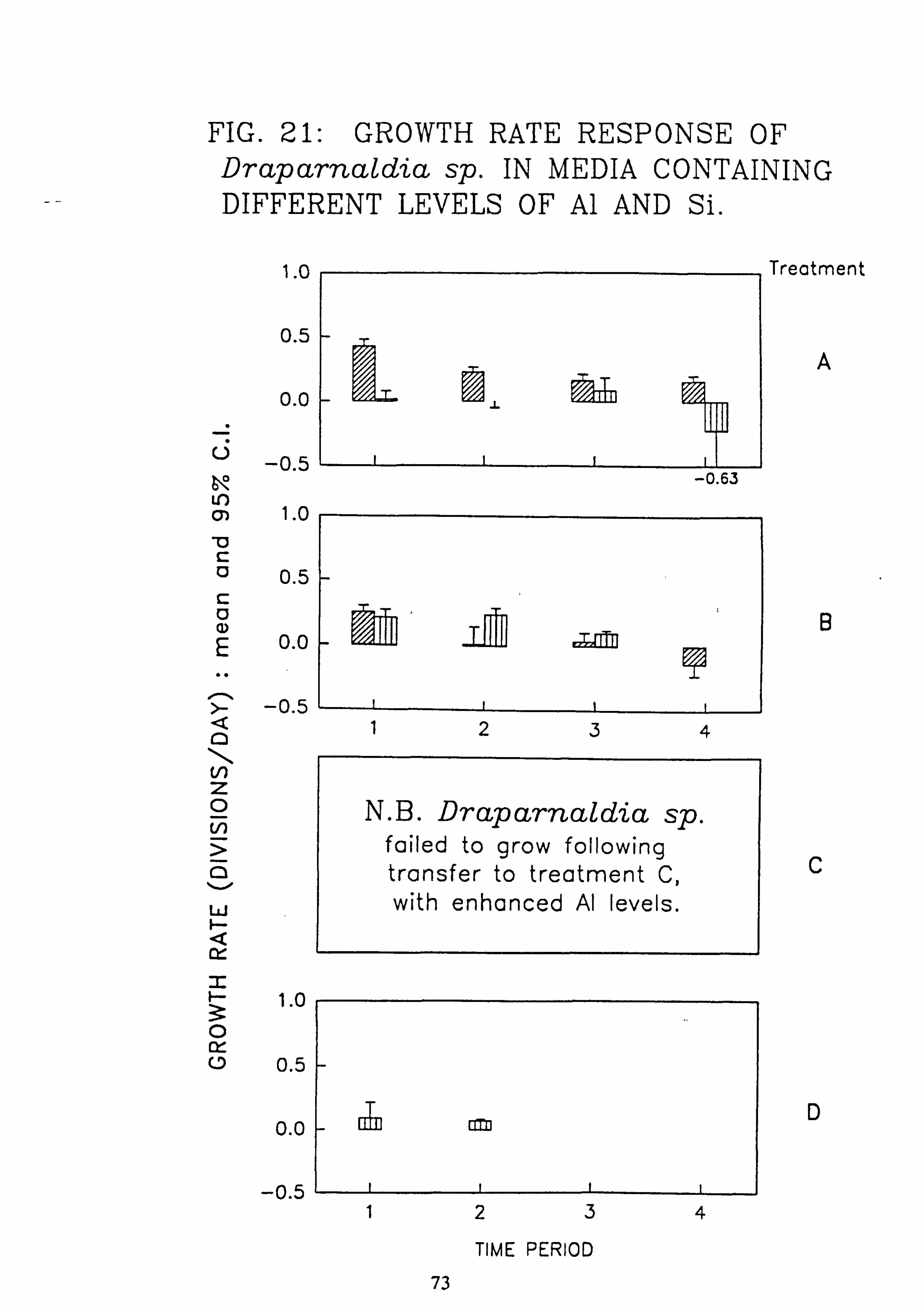
FIG. 21: GROWTH RATE RESPONSE OF Draparnaldia sp. IN MEDIA CONTAINING DIFFERENT LEVELS OF Al AND Si.
In Tran+mon1 I. v
0.5
0.0
V -0.5
11VVt111V11
A
-0.63 LO U7 I. U
-0 C
0.5 c 0 aý 0.0
, -- -0.5
B
Q1234 D
V)
z 0
Cl
W I
rY
C
I 4- ir
i. v 0
0 0.5
0.0
-0.5 1234
TIME PERIOD
73
D
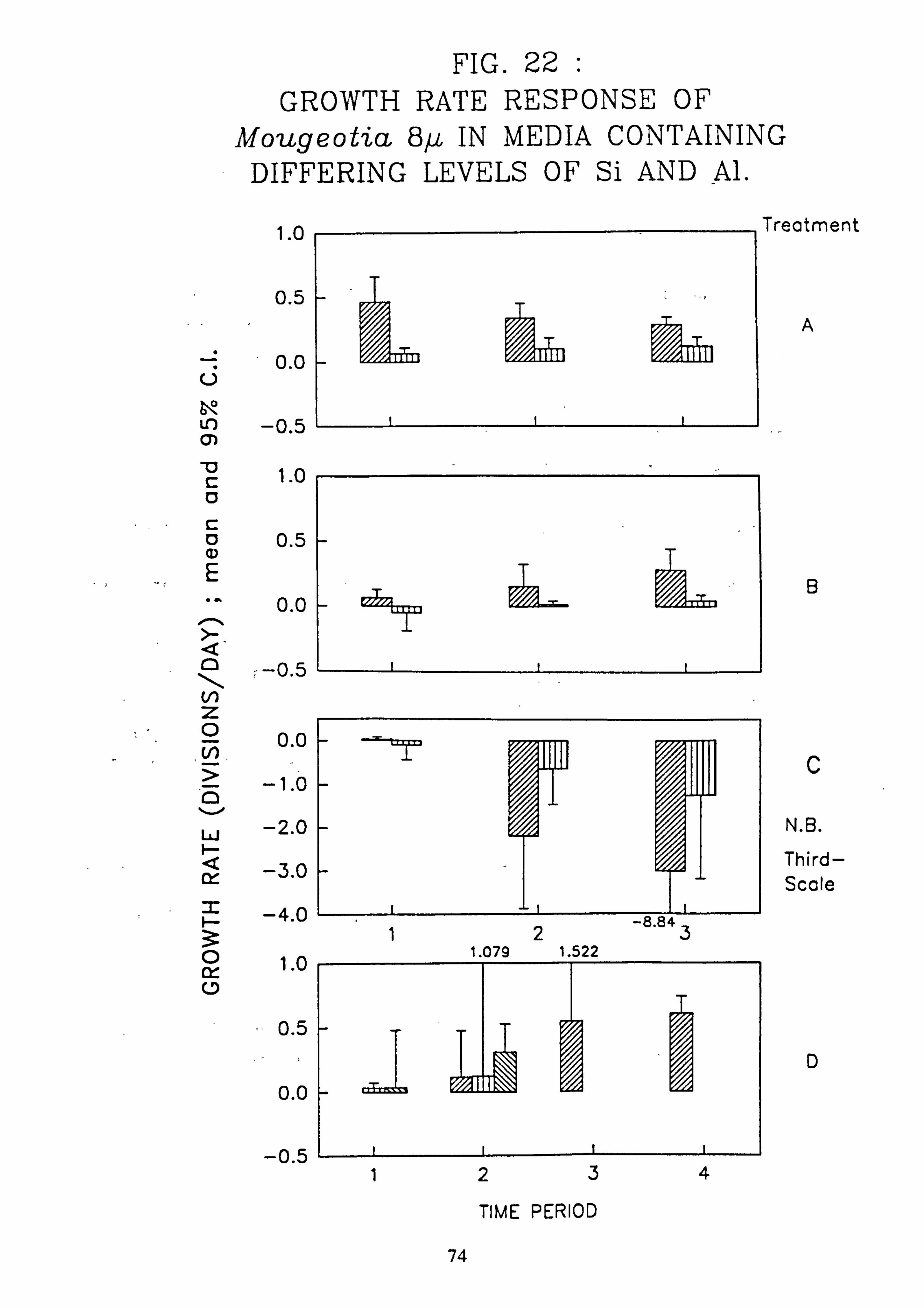
FIG. 22 GROWTH RATE RESPONSE OF
Mougeotia 8j. c IN MEDIA CONTAINING DIFFERING LEVELS OF Si AND Al.
.- TrPntmPnt I. U
0.5
0.0 U
Ln _nc
A
0)
Ü4n CLU D
C 0 0.5
E "w 0.0
Q-n-5
B
N z 0 0.0
-1.0
W -2.0 1-
-3.0
_An
C
N. B.
Third- Scale
-T. W 12 -8.843 1.079 1.522
1.0
0.5
0.0
_n c 1234
TIME PERIOD
74
D
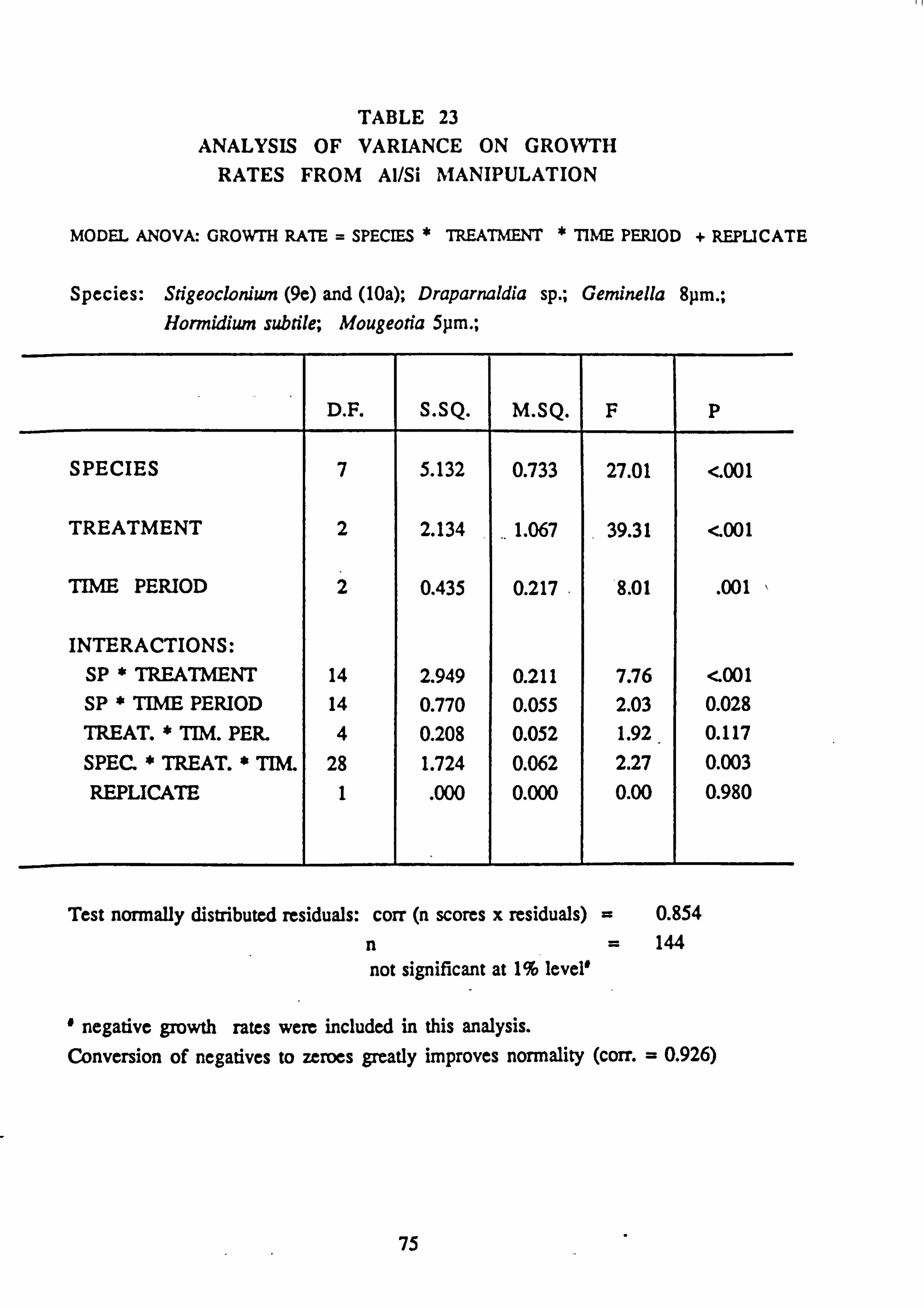
TABLE 23 ANALYSIS OF VARIANCE ON GROWTH
RATES FROM Al/Si MANIPULATION
MODEL ANOVA: GROWTH RATE = SPECIES * TREATMENT * TIME PERIOD + REPLICATE
Species: Stigeoclonium (9e) and (10a); Draparnaldia sp.; Geminella 8pm.; Hormidium subtile; Mougeotia 5pm.;
D. F. S. SQ. M. SQ. F P
SPECIES 7 5.132 0.733 27.01 <. 001
TREATMENT 2 2.134 1.067 39.31 <. 001
TIME PERIOD 2 0.435 0.217 8.01 . 001
INTERACTIONS: SP * TREATMENT 14 2.949 0.211 7.76 <. 001 SP * TIME PERIOD 14 0.770 0.055 2.03 0.028 TREAT. * TIM. PER. 4 0.208 0.052 1.92 0.117 SPEC. * TREAT. * TIM. 28 1.724 0.062 2.27 0.003
REPLICATE 1 . 000 0.000 0.00 0.980
Test normally distributed residuals: corr (n scores x residuals) = 0.854
n= 144
not significant at 1% level
' negative growth rates were included in this analysis. Conversion of negatives to zeroes greatly improves normality (corr. = 0.926)
75
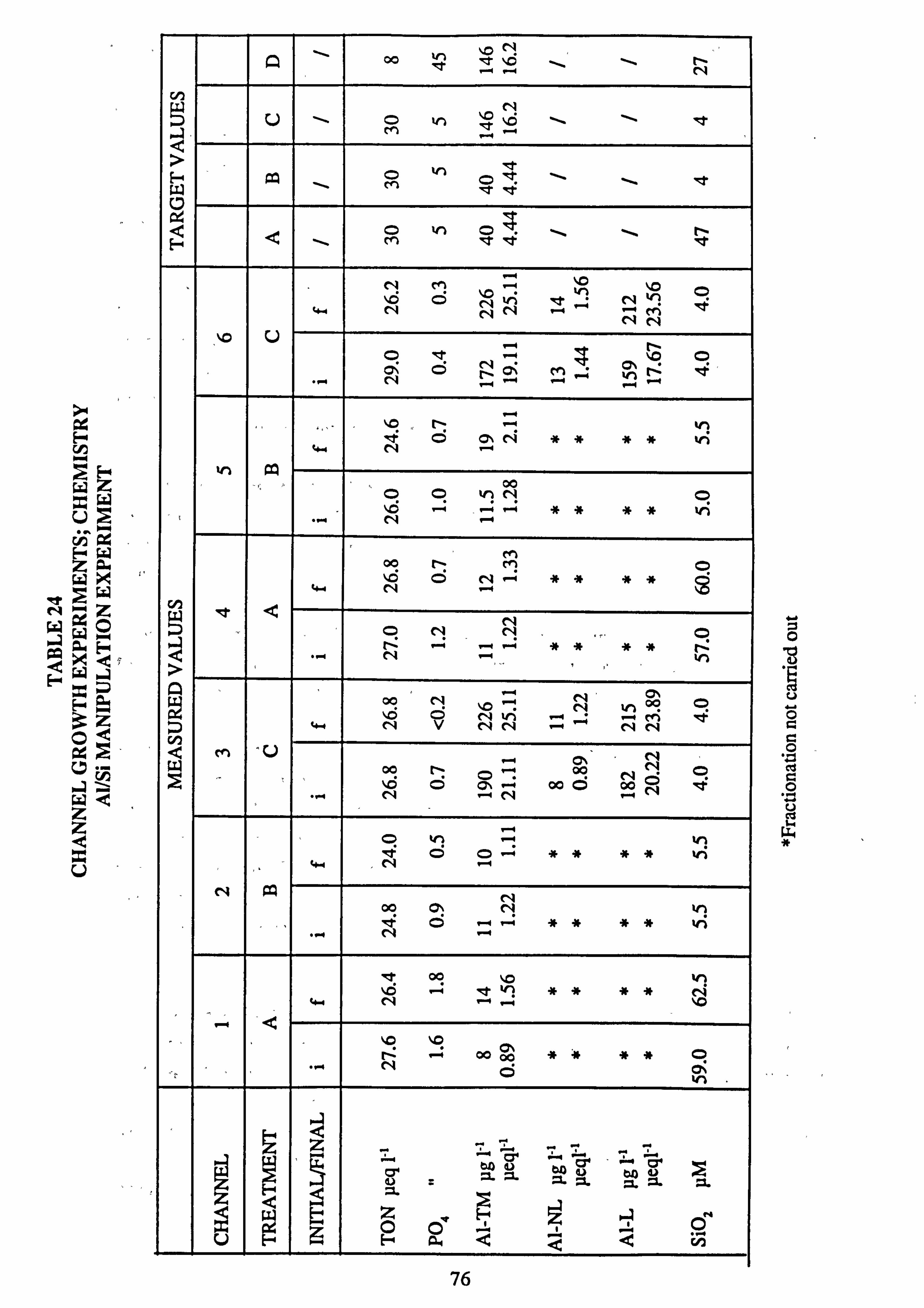
rg
CID
Hw wý
Nz
ýß"ofi HWär
öQ
.a te'
z
U
A N ýO
c N
in .4 110 -ý%
I M 1-4 -4
Q Q \ OM vi c. - N
N M - ýo
N O NN N
- ý NN
ýo U O ýt O
9-4
- O N tý 1 - ^" -- ýt
...
N O C\ N ** ** In w
to CQ 00
O O 'n N O
,., N -
M 00 N M O N O - "-ý ýF dF it ii p
w. ýD
Q
O N N
00 C14 "o N
tn 09 O N V NN
NN
m N N 00 N O
O "-: 00 N O N N 00 00 N
ý
O 041) -4 tn N O "-+ ýF 9F 9F dF 1ý
ý+r
N iYi N 00 Oý N to
.. r N -
00 ýp h "-ý 'ý? * ýt aF iF N
4-. 4 N P-+ . -- 1.0
'D \O oo 00 ** ** O
CFO
ý U ý F a Q ¢ ýC vý
a O
U
O O Q O
cd A O
U cý w
76
Nevertheless the general conclusions are clear: (a) species differ in their ability to grow
at pH values between 4.0 and 6.0; (b) they differ also in their ability to grow in the
presence of concentrations of Al which may be found in some acidified streams; and (c)
these differences in growth rates are related to the conditions pertaining in the streams in which the species are most abundant.
3.4.3 Species composition on continued culture The issue of whether the growth rates measured during the early phases of growth are maintained as the biomass develops cannot easily be determined for technical teasons. However a subjective estimate of relative species composition has been carried out on channel biomass in the same way as with field samples for Run 2, which was continued for 29 days (Table 25), and for Run 3, continued for 64 days (Table 26). These
populations are not naturally balanced as they were deliberately seeded with particular species; any others present were there as contaminants.
Considering the results of both experiments, at pH values below 5.0 Stigeoclonium 5µm
was dominant, together with Hormidium 5.5pm. At pH values above 5.0, Mougeotia 11µm becomes codominant with Stigeoclonium., while Hormidium declines slightly in
abundance.
Mougeotia 8µm, Mougeotia 17pm and Mougeotia 22pm are absent from pH 4.0. Mougeotia 22µm has a very patchy distribution and low abundance, surprising in view of its considerable contribution to the community in medium B9 in Run 3.
In run 3, two Stigeoclonium taxa, distinguished here by their main axis diameters, occur only at higher pH values. These may be separate ecotypes, adapted to a higher pH, or they may be morphological responses to the higher pH. In the early stages of its growth, Draparnaldia cannot be readily distinguished from Stigeoclonium, and indeed fails to develop main axis differentiation if the calcium concentration is below 1.7 mg 1-1 (Johnstone, 1978). Therefore the largest Stigeoclonium taxon may in fact be Draparnaldia.. Zygnema 20 pm is present at pH 4.0 and common at pH 4.5 but not at higher pH..
Pseudanabaena in these experiments is seen to occur at all pH values, including pH 4.0,
and is at a maximum at pH 5.0 although it is absent from B9 in Run 3. This cyanophyte
was largely ignored in field samples during the earlier phase of the sampling programme, but has repeatedly cropped up in cultures. In field samples it is quite difficult to score due to its small cell diameter (1.5 pm) and may be readily confused with other small cyanophytes. Many of the records of 'Oscillatoria 1 pm' probably refer to Pseudana- baena especially in Matrix B.
77
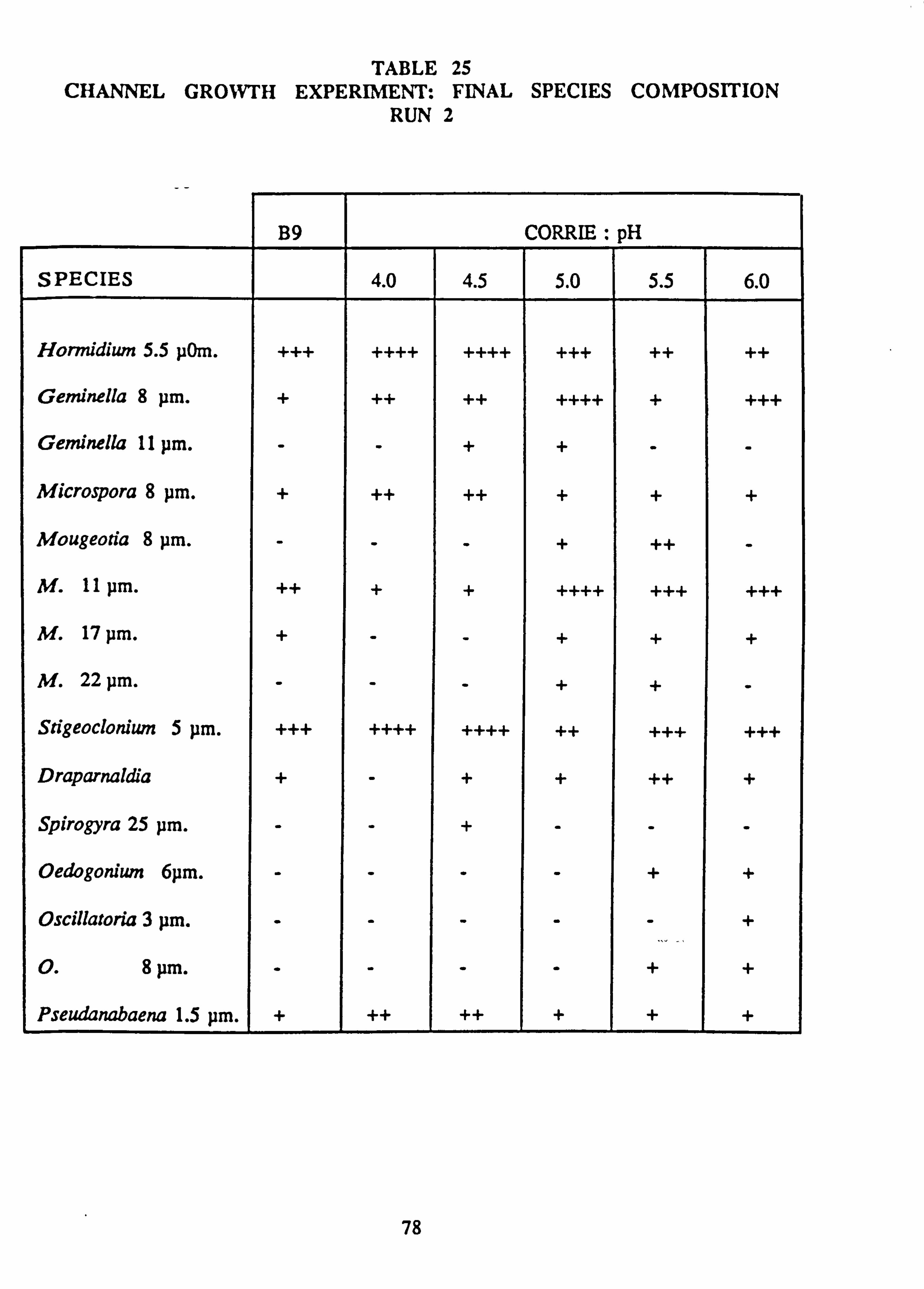
TABLE 25 CHANNEL GROWTH EXPERIMENT: FINAL SPECIES COMPOSITION
RUN 2
B9 CORRIE : pH
SPECIES 4.0 4.5 5.0 5.5 6.0
Hormidium 5.5 pOm. +++ ++++ ++++ +++ ++ ++
Geminella 8 pm. + ++ ++ ++++ + +++
Geminella 11 pm. - - + + - -
Microspora 8 pm. + ++ ++ + + +
Mougeotia 8 pm. - - - + ++ -
M. 11 pm. ++ + + ++++ +++ +++
M. 17 pm. + - - + + +
M. 22 pm. - - - + + -
Stigeoclonium 5 pm. +++ ++++ ++++ ++ +++ +++
Draparnaldia + - + + ++ +
Spirogyra 25 pm. - - + - - -
Oedogonium 6pm. - - - - + +
Oscillatoria 3 pm. - - - - - +
0.8 }gym. - - - - + +
Pseudanabaena 1.5 pm. + ++ ++ + + +
78
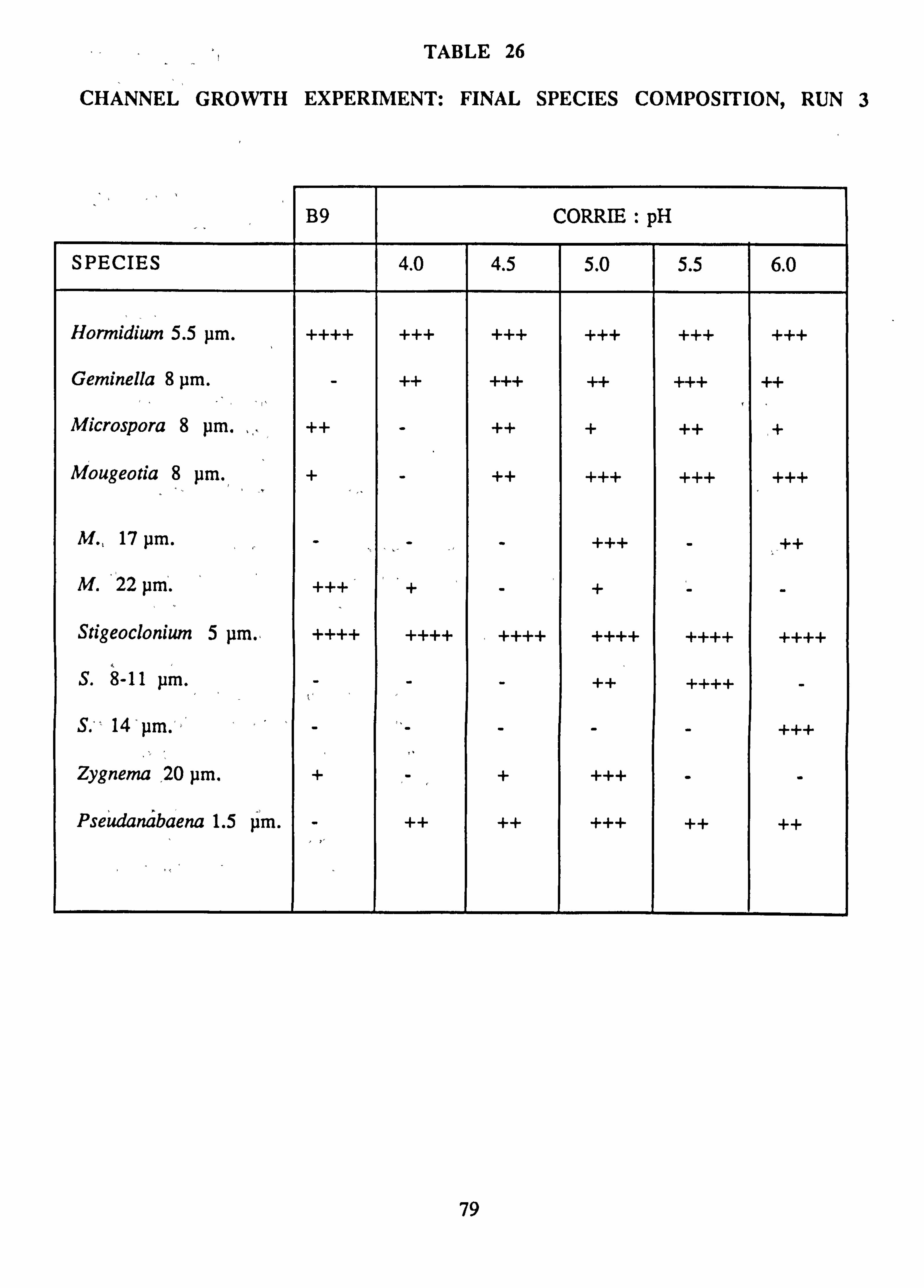
TABLE 26
CHANNEL GROWTH EXPERIMENT: FINAL SPECIES COMPOSITION, RUN 3
B9 CORRIE : pH
SPECIES 4.0 4.5 5.0 5.5 6.0
Hormidium 5.5 pm. ++++ +++ +++ +++ +++ +++
Geminella 8 pm. - ++ +++ ++ +++ ++
Microspora 8 pm. ++ - ++ + ++
Mougeotia 8 pm. + - ++ +++ +++ +++
M., 17 pm. - - - +++ - ++
M. ' 22 pm. +++ + - + - -
Stigeoclonium 5 pm., ++++ ++++ ++++ ++++ ++++ ++++
S. 8-11 pm. - - - ++ ++++ -
S. ° 14-pm. - - - - - +++
Zygnema , 20 pm. + + +++ - -
Pseudanäbaena 1.5 pm. - ++ ++ +++ ++ ++
79
3.4.4 Influence of Channel pH on Biomass
Biomass developed at different pH in channels after continued incubation is shown in
Fig. 23, expressed as mean daily increment in order to enable comparisons to be made between Runs 2 and 3, with the total biomass figures shown in Table 27.
Chlorophyll was at a maximum at pH 5.0 in Run 2 and pH 4.5 in Run 3. Carotenoid was at a maximum at pH 5.5 in Run 2, but in Run 3 there was very little change with pH, except that the lowest Chl. a value is found at pH 4.0
AFDW in Run 2 follows closely carotenoid, with a maximum at pH 5.5. In Run 3 AFDW
rises sharply from a low at pH 4.0 to a maximum at pH 5, with a slight drop thereafter.
In both runs, the chlorophyll maximum occurs at a lower pH (0.5 unit) than the carotenoid/AFDW maximum. This may reflect a different species composition at the different pHs, as green algae have a higher ratio of chlorophyll to dry weight than cyanophytes or diatoms. This result is also found in the tub growth experiments.
The results do not support the contention that biomass is greater at low pH. Rather, within the limits of the species composition of periphyton developed during these experiments, it shows that biomass is at a maximum around the middle of the pH range studied here. The maximum growth rate of many of these species also occurs around this pH, and it thus seems likely that it is pH preference which determines the accumu- lation of biomass. In these channels no grazing organisms were present, with the exception of some rotifers. Therefore if decreased invertebrate grazing were the cause of 'blooms' of green algae present in natural streams, no difference should have been
seen between the amounts of chlorophyll developed at different pH in the channels. On
the other hand, if reduced heterotrophic activity at low pH were the cause of (sup-
posed) biomass accumulation (Hendrey, 1976), the biomass ought to be at a maximum at pH 4, while this is clearly seen not to be the case.
The evidence from these experiments as well as from the field work, suggests that there is no consistent change in field biomass with pH, and that changes in species composi- tion are responsible for the apparent increase in algal abundance in acidified streams. While effects of pH on grazing and on microbial decomposition may occur, the major cause of species shifts is the differential effect of pH, aluminium and/or other environ- mental factors on the growth rate of algae.
80
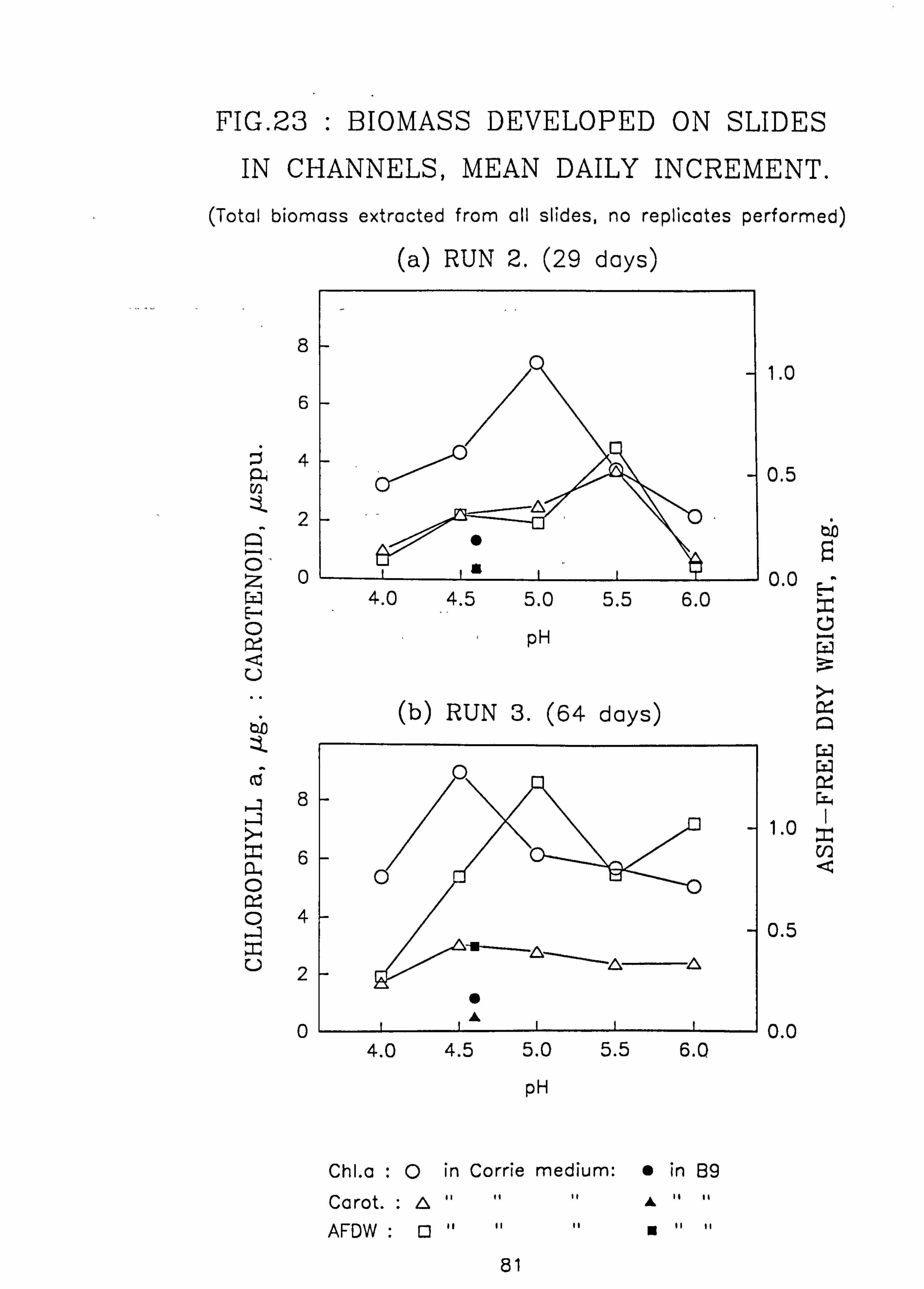
FIG. 23 : BIOMASS DEVELOPED ON SLIDES
IN CHANNELS, MEAN DAILY INCREMENT. (Total biomass extracted from all slides, no replicates performed)
(a) RUN 2. (29 days)
8
6
4
Z
E- CD
cd
ä6 0 tz o
U2
0
4.0 4.5 5.0 5.5 6.0
pH
(h) RTTN q (F, 4 Hn%/cz)
Chl. o :0 in Corrie medium: " in 89
Corot. :A if " AFDW :Q ýý 01
81
1.0
0.5
a0
0.0
x cý w
x Q
1. o x Q
5
0 4.0 4.5 5.0 5.5 6.0
pH
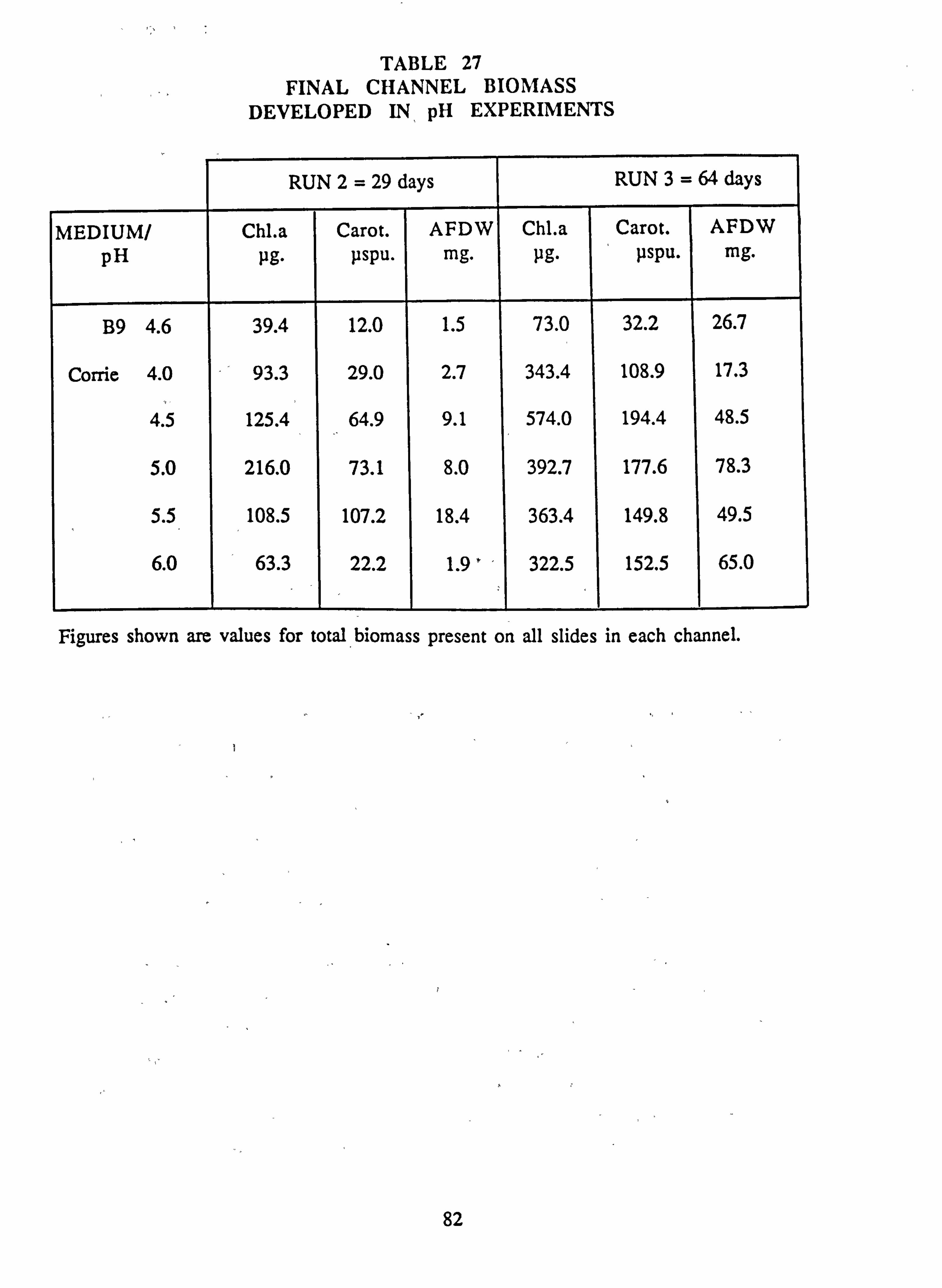
TABLE 27 FINAL CHANNEL BIOMASS
DEVELOPED IN, pH EXPERIMENTS
RUN 2= 29 days RUN 3= 64 days
MEDIUM/ Chl. a Carot. AFDW Chl. a Carot. AFDW
pH P9. pspu. Mg. pg. pspu. Mg.
B9 4.6 39.4 12.0 1.5 73.0 32.2 26.7
Corrie 4.0 93.3 29.0 2.7 343.4 108.9 17.3
4.5 125.4 64.9 9.1 574.0 194.4 48.5
5.0 216.0 73.1 8.0 392.7 177.6 78.3
5.5 108.5 107.2 18.4 363.4 149.8 49.5
6.0 63.3 22.2 1.9 322.5 152.5 65.0
Figures shown are values for total biomass present on all slides in each channel.
82
3.5 TUB GROWTH EXPERIMENTS
Preliminary experiments on the methodology of growth rate measurement were carried out in
tub growth experiments, with 21 of medium mixed by airlift pump (see Methods, Section
2.6.2). The primary reason for carrying out the tub growth experiments however was to
invesigate the effects of pH on biomass and relative species abundance. Two experiments
were run, the first using medium B9 and pH-adjusted Corrie, the second involving the
additional variable of the presence of Germanium, added to 5pg. 1-1 as Ge02 dissolved in
0.02N NaOH.
Final biomass developed at different pH in tub experiment 1 is shown in Fig. 24a and Table
30a. Carotenoid and AFDW show an increase with increasing pH. Chlorophyll is greatest at
pH 4.4-4.8. The biomass values have been expressed as biomass units per litre of medium
used, since batch replacement of the medium was practised over an extended period (201.
over 18 weeks).
The final species composition is shown in Table 28. At low pH, 4.0 to 4.4, Hormidium
dominates along with Mougeotia 11 pm and Stigeoclonium . Above pH 4.8 these species are
replaced by others, particularly Mougeotia 17}ßm and Pseudanabaena, with the species of Phormidiwn and Oscillatoria at pH values of 5.2 or above. Oedogonium 15 pm was present
at the start of the experiment but failed to survive in any of the treatments.
Diatoms were also present on the slides in these experiments but have not been enumerated. The difference in colour of the periphyton developed on the slides suggested however that
there might be a shift in the relative contribution of green algae and diatoms with a change in
pH, since the biomass developed below pH 5.2 was deep green in colour, while at higher pH
it was more brown. Such a shift in dominance might be due to different growth preferences of
individual species in both groups, or the increased prevalence of greens at lower pH might be
due to decreased competition from the diatoms, as suggested by Stokes (1981,1986).
The effect of removing the competition by diatoms was tested in the second experiment
involving growth of algae in 2 litre tubs, with and without the addition of 5 pg 1-1 germanium.
Ge is a competitive inhibitor of silicon uptake by diatoms and its use has been suggested as a
means of suppressing diatom growth in mixed cultures (Thomas and Dodson, 1974). Os-
trofsky and Bellmer (1987) however concluded that the effects of Ge were not uniform in
different cultural conditions, so that total suppression of diatom growth could not be relied
upon for productivity studies, although it is probably a useful tool in preventing the over-
83
growth of cultures of more slow-growing algae by diatoms. This is essentially what is required in the germanium tub experiment, the lessening of competition from diatoms. In fact very few
diatoms were present in the +Ge tubs at the end of the experiment and those seen were
probably the remnants of the original population before transfer to Ge.
The relative abundance of filamentous species at different pH, with and without Ge is shown
in Table 28. Hormidiwn 5.5 pm is seen to be fairly evenly spread across all treatments, in
comparison with tub experiment 1. Hormidium. 8 pm, as in the first experiment, was too
unevenly distributed for any valid conclusions to be drawn. Geminella 8 pm again achieved
its greatest abundance around the middle of the pH range, and appears to be somewhat
enhanced by the suppression of diatom growth in the +Ge treatments at pH 4.5 and 5.0. This
does not appear to occur consistently with any other species. Pseudanabaena had an unusual distribution, being common at pH 4.5 and 5.0 in the presence of Ge, and at pH 6.0 in its absence
Stigeoclonium in the Ge experiment grows better at pH values greater than 5.0, in contrast to
tub experiment 1. As with the channel experiments, this may be due to a different source of the inoculum.
No cyanophytes were present in the Ge experiment with the exception of Pseudanabaena,
which appears from all the results obtained in tub and channel experiments to be capable of
growth at pH values downto 4.4 . The lower pH limit would appear to be around pH 4.4, but
in the tub experiments upward drifts of pH occurred, and frequent manual readjustment to the
target pH with dilute H2SO4 was required. In consequence the pH values reported are target
values and not necessarily the mean values to which the algae were exposed.
One possibly significant difference between tub experiment 1 and the Ge experiment was the lack of temperature control during experiment 1, which is therefore thought to have been
exposed to an ambient temperature of 16°C, possibly more during the light ' period. One
consequence of this might be the growth of the Cyanophytes in this experiment. Cyanophytes
(= Cyanobacteria) are more tolerant of high temperatures than the eucaryotic algae (Brock,
1973) and even at modest temperatures may acquire a greater competitive edge.
A second consequence, which may be related to the first, concerns the poorer growth of Normidiom 5.5 pm at higher pH in experiment 1. This may be due to a reduced availability of D. I. C. to Hormidium. In nature this alga is most commonly found in riffles, usually in very
shallow, turbulent water or even subaerially at the edge of waterfalls and in splash zones,
possibly indicating a preference for high concentrations of dissolved CO2, and less readiness
84
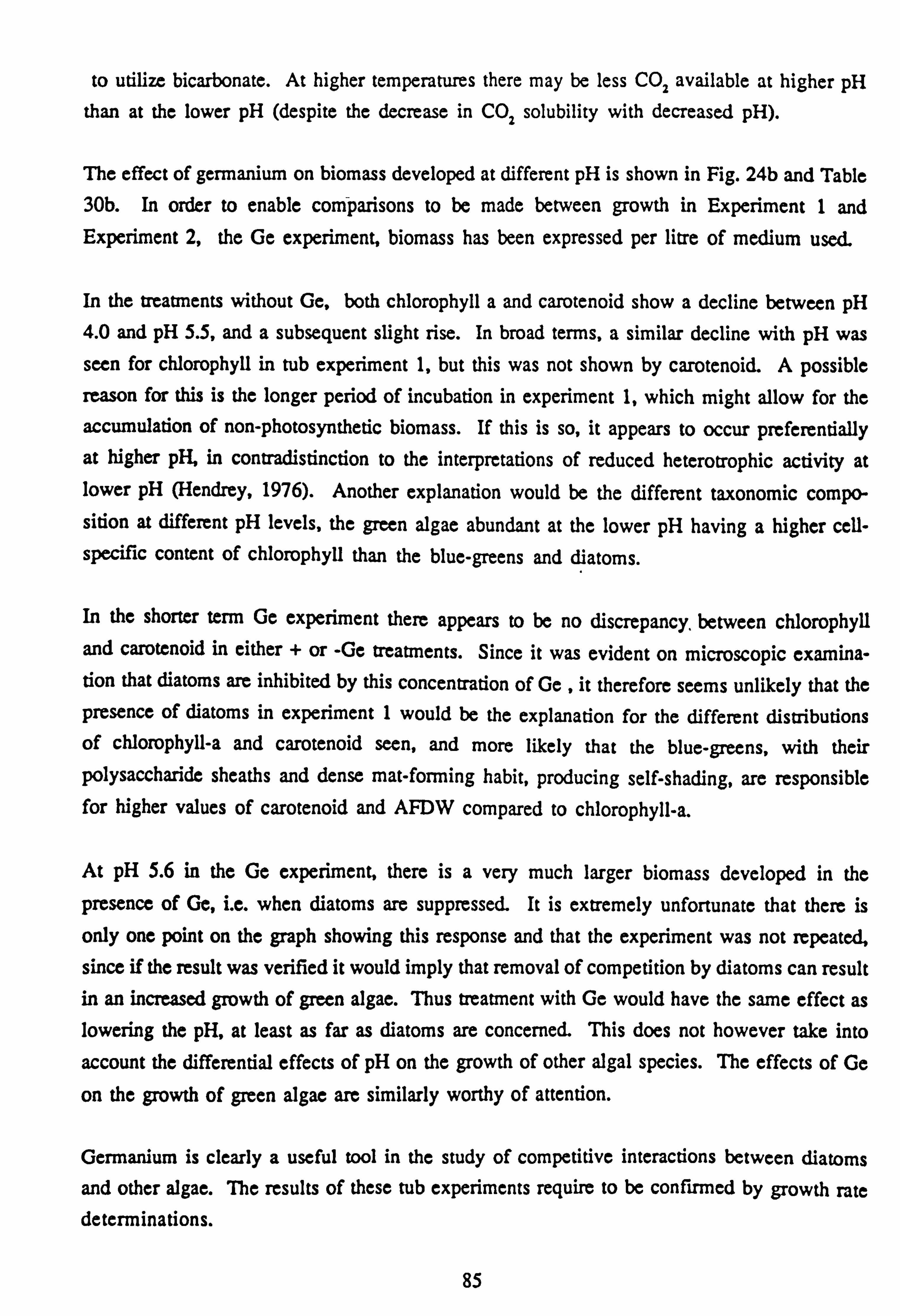
to utilize bicarbonate. At higher temperatures there may be less CO2 available at higher pH than at the lower pH (despite the decrease in CO2 solubility with decreased pH).
The effect of germanium on biomass developed at different pH is shown in Fig. 24b and Table 30b. In order to enable comparisons to be made between growth in Experiment 1 and Experiment 2, the Ge experiment, biomass has been expressed per litre of medium used.
In the treatments without Ge, both chlorophyll a and carotenoid show a decline between pH 4.0 and pH 5.5, and a subsequent slight rise. In broad terms, a similar decline with pH was seen for chlorophyll in tub experiment 1, but this was not shown by carotenoid. A possible reason for this is the longer period of incubation in experiment 1, which might allow for the accumulation of non-photosynthetic biomass. If this is so, it appears to occur preferentially at higher pH, in contradistinction to the interpretations of reduced heterotrophic activity at lower pH (Hendrey, 1976). Another explanation would be the different taxonomic compo- sition at different pH levels, the green algae abundant at the lower pH having a higher cell- specific content of chlorophyll than the blue-greens and diatoms.
In the shorter term Ge experiment there appears to be no discrepancy, between chlorophyll and carotenoid in either + or -Ge treatments. Since it was evident on microscopic examina- tion that diatoms are inhibited by this concentration of Ge , it therefore seems unlikely that the presence of diatoms in experiment 1 would be the explanation for the different distributions of chlorophyll-a and carotenoid seen, and more likely that the blue-greens, with their polysaccharide sheaths and dense mat-forming habit, producing self-shading, are responsible for higher values of carotenoid and AFDW compared to chlorophyll-a.
At pH 5.6 in the Go experiment, there is a very much larger biomass developed in the presence of Ge, i. e. when diatoms are suppressed. It is extremely unfortunate that there is
only one point on the graph showing this response and that the experiment was not repeated, since if the result was verified it would imply that removal of competition by diatoms can result in an increased growth of green algae. Thus treatment with Ge would have the same effect as lowering the pH, at least as far as diatoms are concerned. This does not however take into
account the differential effects of pH on the growth of other algal species. The effects of Ge
on the growth of green algae are similarly worthy of attention.
Germanium is clearly a useful tool in the study of competitive interactions between diatoms
and other algae. The results of these tub experiments require to be confirmed by growth rate determinations.
85
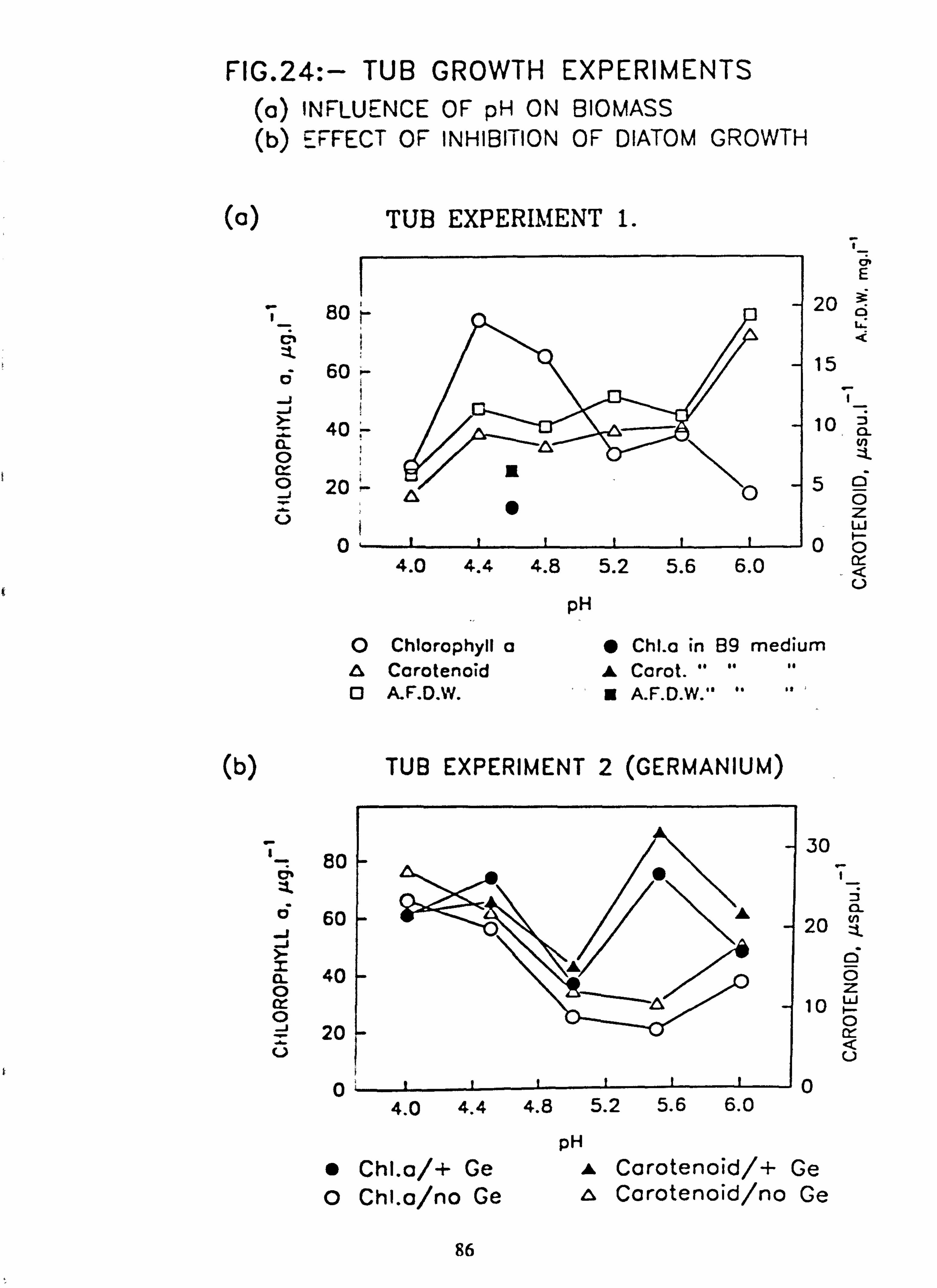
FIG. 24: - TUB GROWTH EXPERIMENTS (a) INFLUENCE OF pH ON BIOMASS (b) EFFECT OF INHIBITION OF DIATOM GROWTH
(a) TUB EXPERIMENT 1.
80 --
60 Ji
40 CL o G
20 V
0
0
4.0 4.4 4.8 5.2 5.6 6.0
pH
E 20 0
L. ä
15
10 ä
50 ö z w
0ö
C-)
O Chlorophyll a" Chl. a in 89 medium O Corotenoid f Corot. """ 0 A. F. D. W. A. F. D. W. " ""'
(b) TUB EXPERIMENT 2 (GERMANIUM)
80
° 60
40 cr- 0 J2 U
0
CL aN 0 z
0
v
0
pH " Chia/+ Ge A Carotenoid/+ Ge O Chl. a/no Ge o Carotenoid/no Ge
86
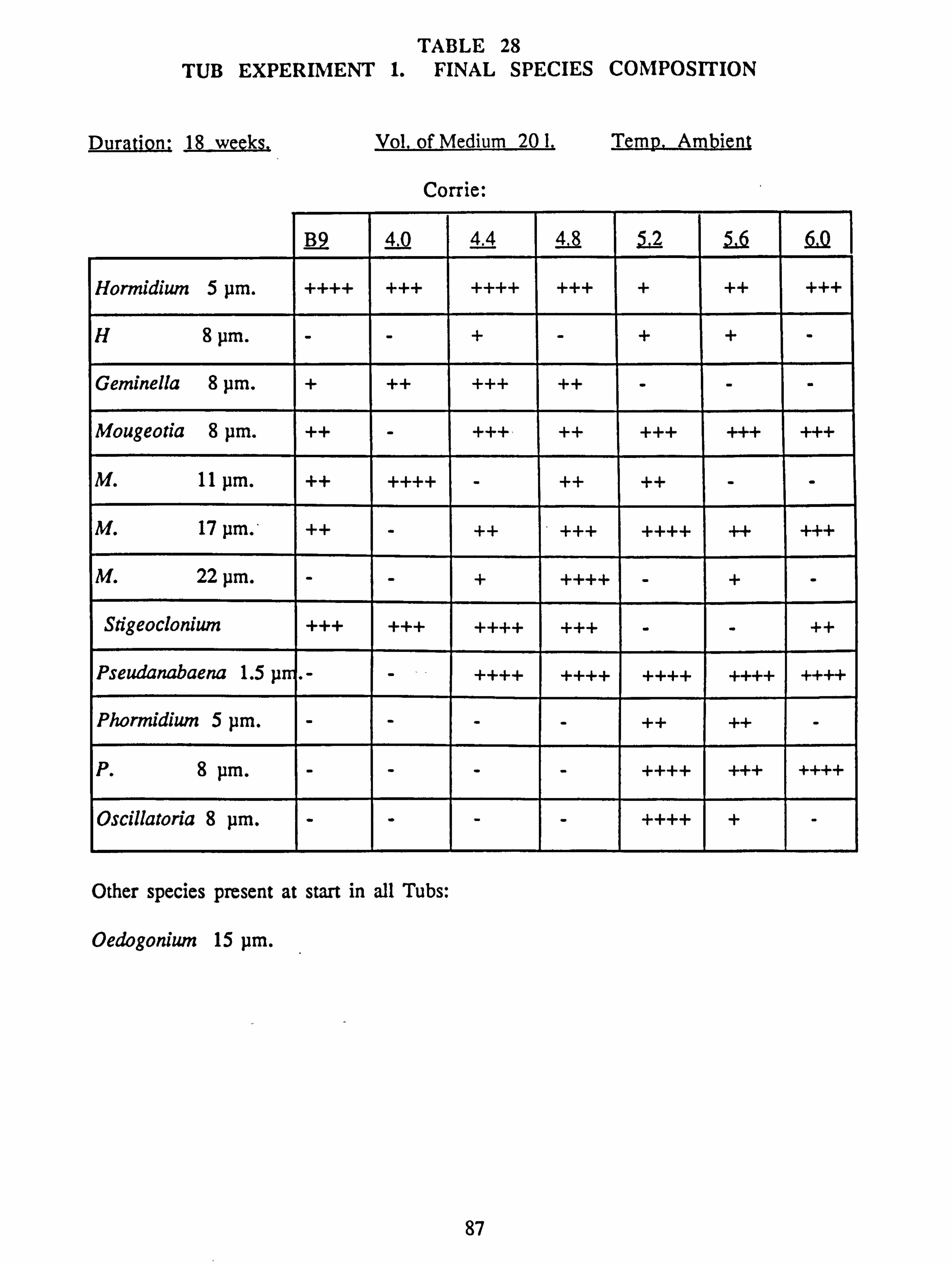
TABLE 28 TUB EXPERIMENT 1. FINAL SPECIES COMPOSITION
Duration: 18 weeks. Vol. of Medium 20 1. Temp. Ambient
Corrie:
B2 4_0 44 Al 12 5& UQ
Hormidium 5 pm. ++++ +++ ++++ +++ + ++ +++
H 8µm. - - + - + + -
Geminella 8 pm. + ++ +++ ++ - - -
Mougeotia 8 pm. ++ - +++ ++ +++ +++ +++
M. 11 pm. ++ ++++ - ++ ++ - -
M. 17 pm., ++ - ++ +++ ++++ ++ +++
M. 22 pm. - - + ++++ - + -
Stigeocloniwn +++ +++ ++++ +++ - - ++
Pseudanabaena 1.5 p .- - ++++ ++++ ++++ ++++ ++++
Phormidium 5 pm. - - - - ++ ++ -
P. 8 pm. - - - - ++++ +++ ++++
Oscillatoria 8 pm. - - - - ++++ + -
Other species present at start in all Tubs:
Oedogonium 15 pm.
87
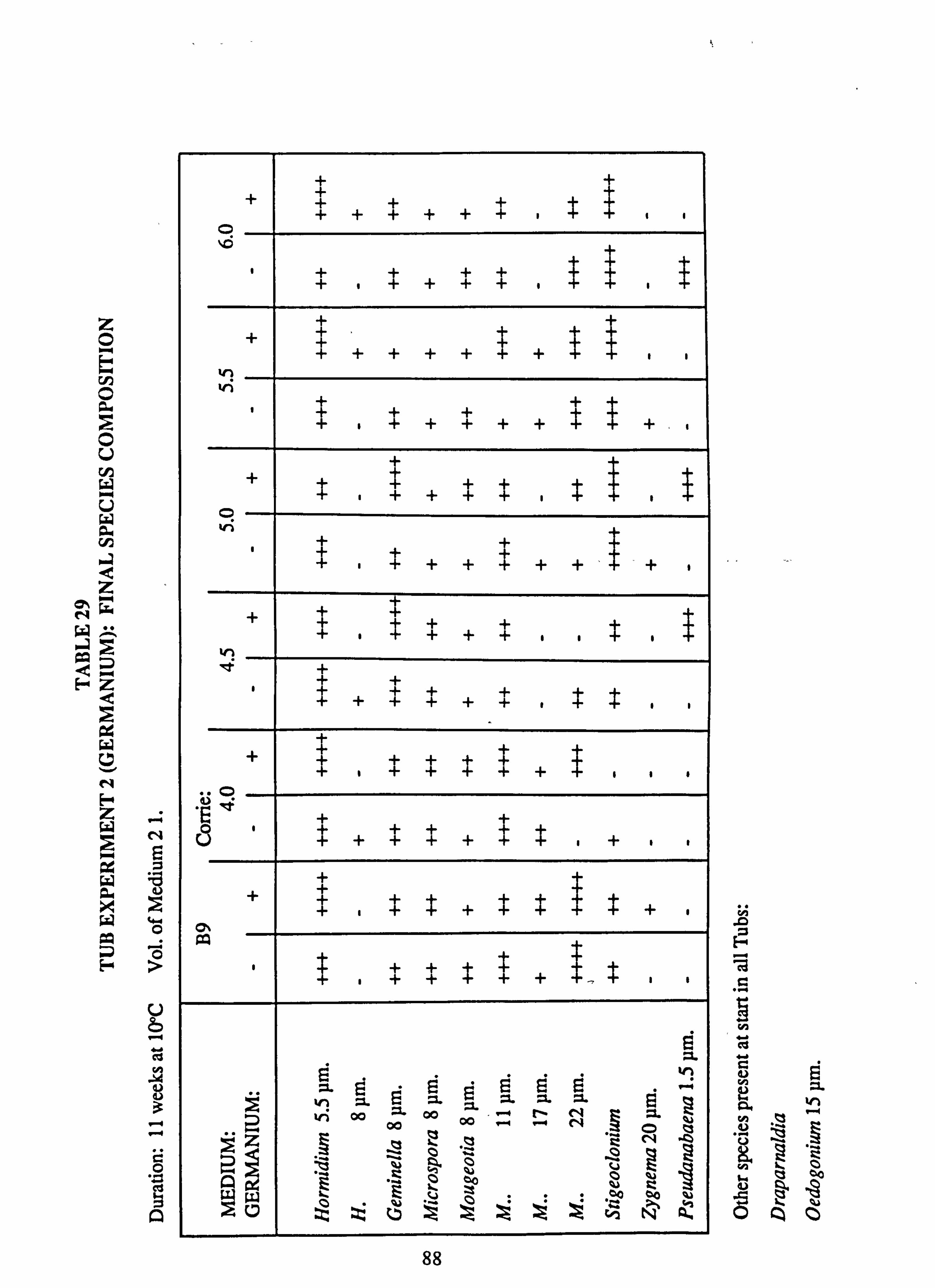
z 0
c7 F
cý N W
ßý Qý H
14 (V
u
c«, 0
r-: 0
U g
cqs H
0 U
0 .
+ + + +
+
+ + + , , ,
O IZ +
+ + +
+ +
.
+ + + + + +
vi + +
+ +
+ + + ,
In + + + + + +
+ +
+
Vi + +
+ + + +
+ + + -1- ,
O . ýt
V +
+ + +
+
+ + + + + ,
+ + + + +
Ei Ei E h ..,
V-3 00 00 00 00 N D
ý7 b q v
C7 ý V ý ý ý ý ý ý N 0. ý n
88
u
. iD
C7
h a+ Ce
4. i
a '^
C: QO
a4O
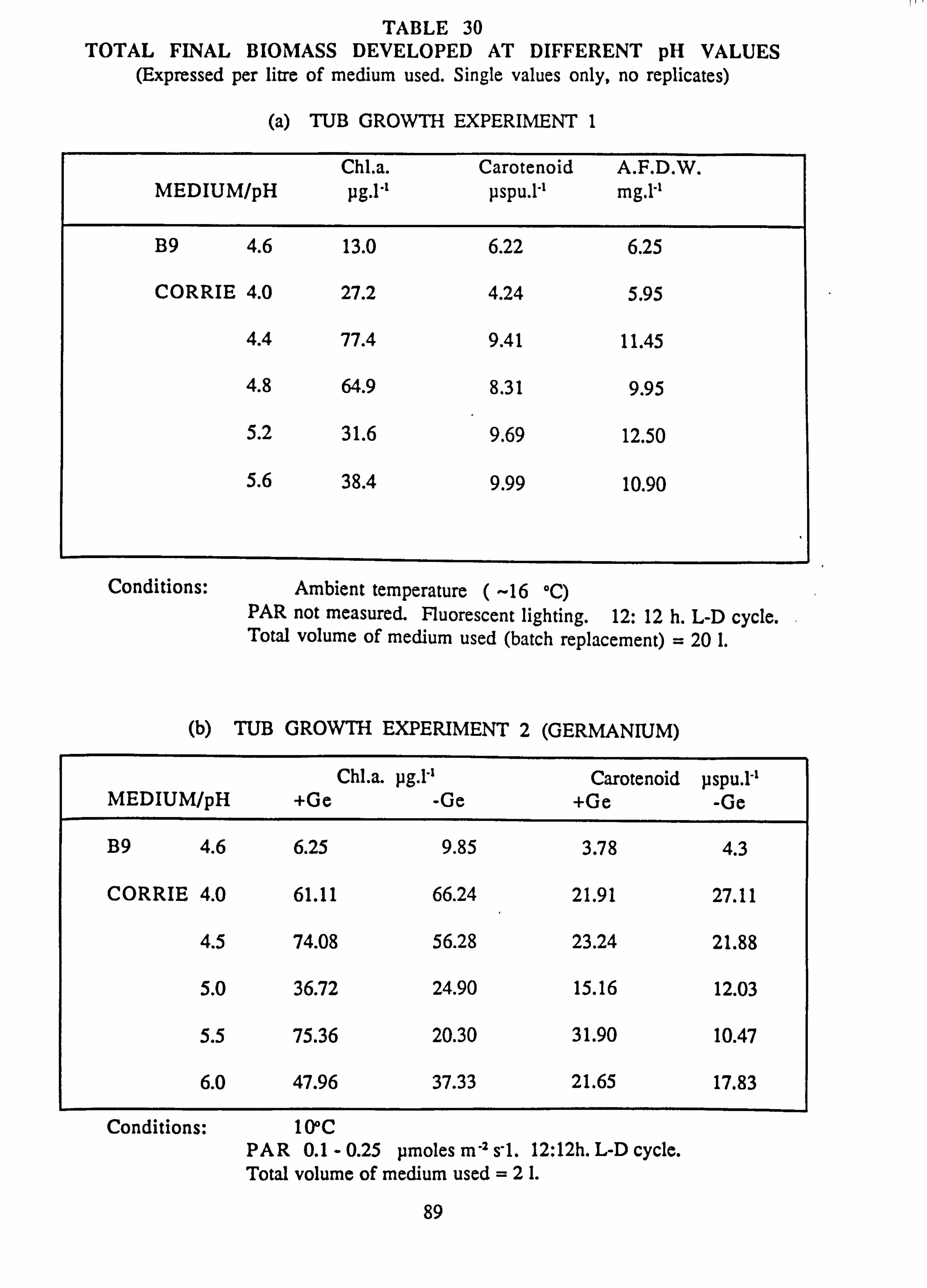
TABLE 30 TOTAL FINAL BIOMASS DEVELOPED AT DIFFERENT pH VALUES
(Expressed per litre of medium used. Single values only, no replicates)
(a) TUB GROWTH EXPERIMENT 1
MEDIUM/pH Chl. a. pg., ',
Carotenoid pspu. l''
A. F. D. W. mg. 1''
B9 4.6 13.0 6.22 6.25
CORRIE 4.0 27.2 4.24 5.95
4.4 77.4 9.41 11.45
4.8 64.9 8.31 9.95
5.2 31.6 9.69 12.50
5.6 38.4 9.99 10.90
Conditions: Ambient temperature ( -16 °C) PAR not measured. Fluorescent lighting. 12: 12 h. L-D cycle. Total volume of medium used (batch replacement) = 20 1.
(b) TUB GROWTH EXPERIMENT 2 (GERMANIUM)
MEDIUM/pH Chl. a.
+Ge pg. 1-'
-Ge Carotenoid
+Ge pspu. 1-'
-Ge
B9 4.6 6.25 9.85 3.78 4.3
CORRIE 4.0 61.11 66.24 21.91 27.11
4.5 74.08 56.28 23.24 21.88
5.0 36.72 24.90 15.16 12.03
5.5 75.36 20.30 31.90 10.47
6.0 47.96 37.33 21.65 17.83
Conditions: 10°C PAR 0.1 - 0.25 pmoles m'2 s'1.12: 12h. L-D cycle. Total volume of medium used =21.
89
3.6 CULTURAL STUDIES ON Stigeoclonitim ISOLATES
Stigeoclonium samples were isolated from the following sites: (1) Ward burn, sampled 15.6.88
(2) Burn 2, Subsample (f), sampled 14.6.88 (3) Burn 6, subsample (c), sampled 14.6.88 (4) Burn 10-2, subsample (a), sampled 14.6.88 (5) Burn 9, subsample (e), sampled 14.6.88
Tests were also conducted on Draparnaldia originally isolated from Burn 6.
Growth tests were carried out according to the procedure of Cox and Bold (1966) which involves growth in a flask with a slide half-immersed in the medium. The flasks were bubbled with filtered air, and exposed to 12: 12 hour light/dark illumination, 50 pmoles m-2s'1 at a temperature of 22°C. After a suitable period of incubation, slides were examined for
attachment and development of zoospores.
It was found that only one isolate, from the Ward burn, was able to grow and develop in the Cox and Bold medium. Adjustment of the pH of the BBMPTB12 medium was attempted in
order to circumvent this problem. Growth checks were made at pH 7.5 (the original pH of the medium), pH 6.0,5.0 and 4.5. Simultaneous growth checks were made in unmodified Come
and B9 media. The nutrient content of these media is compared in Table 3.
The results of the growth experiments are summarised in Table 31. The feature of major importance for taxonomy is the morphology of the basal system (Cox and Bold, 1966; Simons
et al, 1986). Continued examination of the development of isolates was curtailed by contami- nation by cyanophytes or cessation of growth of some isolates. Only isolates 9e and 10a were maintained in a viable condition and were used subsequently in channel growth experiments.
Based on the data obtained, the isolates correspond to the Simons et al (1986) description of S. tenue. Germination of the zoospore gives rise to a basal system consisting of initially a single filament, while the erect system grows more rapidly and gives rise to frequent branching. In older specimens a degree of branching of the basal system was seen but not on as extensive a scale as reported for S. farctum. The erect filaments seens were never as broad
as those reports for S. helveticwn, although. Simons et al (1986) reported some specimens only 5.4 to 10 pm in diameter.
90
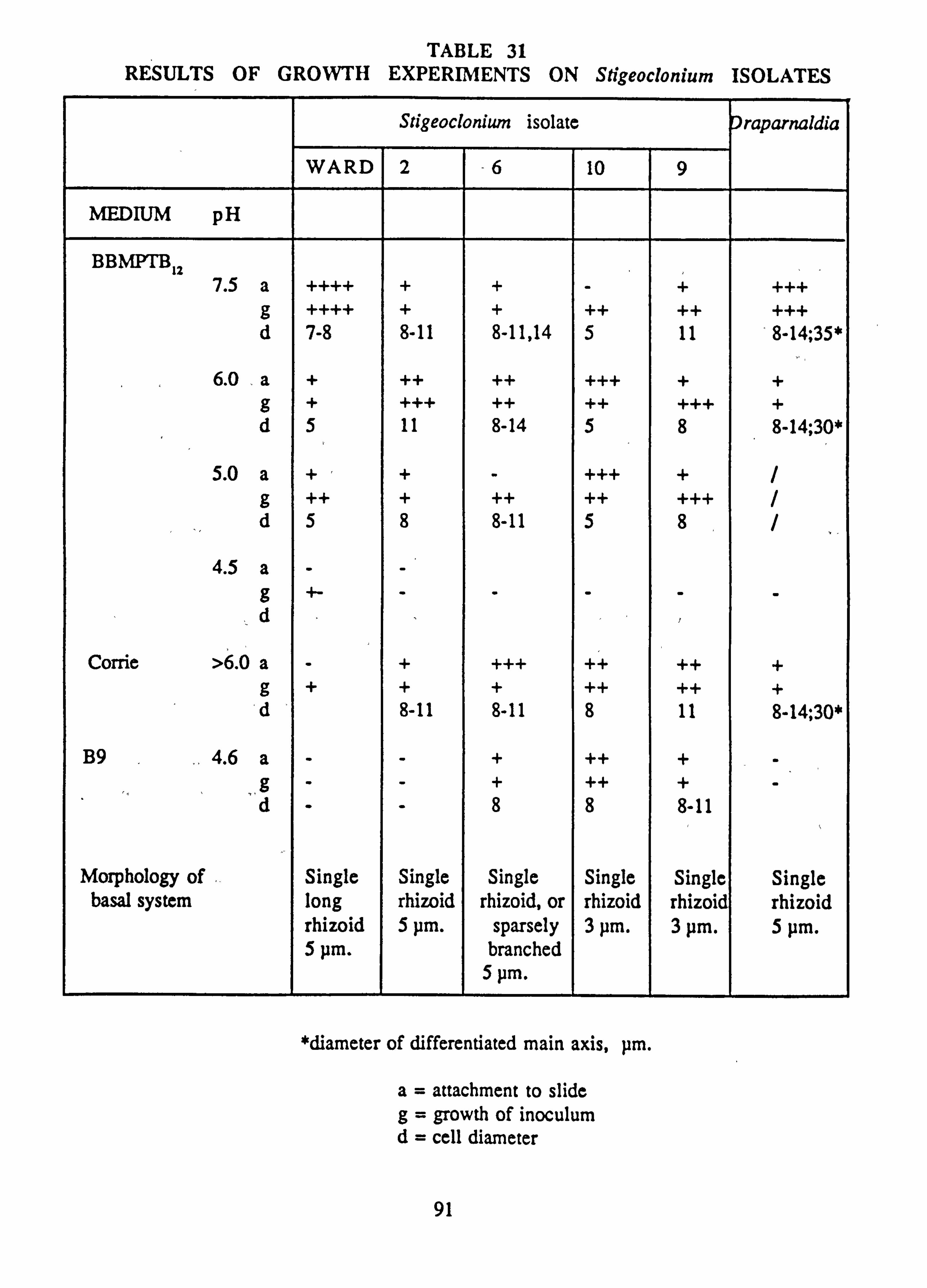
TABLE 31 RESULTS OF GROWTH EXPERIMENTS ON Stigeoclonium ISOLATES
Stigeoclonium isolate raparnaldia
WARD 2 -6 10 9
MEDIUM pH
BBMPTB12 7.5 a ++++ + + - + +++
g ++++ + + ++ ++ +++ d 7-8 8-11 8-11,14 5 11 8-14; 35*
6.0 a + ++ ++ +++ + + g + +++ ++ ++ +++ + d 5 11 8-14 5 8 8-14; 30*
5.0 a + + - +++ + / g ++ + ++ ++ +++ / d 5 8 8-11 5 8 /
4.5 a - - g +- - - - - - d
Corrie >6.0 a - + +++ ++ ++ + g + + + ++ ++ + d 8-11 8-11 8 11 8-14; 30*
B9 ..
4.6 a - - + ++ + - �g - - + ++ + -" d - - 8 8 8-11
Morphology of . Single Single Single Single Single Single basal system long rhizoid rhizoid, or rhizoid rhizoid rhizoid
rhizoid 5 pm. sparsely 3 pm. 3 pm. 5 pm. 5 pm. branched
5pm.
*diameter of differentiated main axis, pm.
a= attachment to slide g= growth of inoculum d= cell diameter
91
The Ward burn isolate is the broadest of those examined and is less similar to the others in its
morphology. The early development of Draparnaldia resembles that of the Stigeoclonium isolates, but its filament is much broader and it grows more slowly, as seen also in channel growth experiments. The main axis differentiation of Draparnaldia is reported to be sup- pressed if the concentration of calcium is less than 1.7 mg 1.1 (= 86 peq 1-1)( Johnstone, 1978) in which case it may be indistinguishable from some Stigeoclonium isolates.
Growth of Draparnaldia in BBMPTB12 or Corrie medium if continued long enough resulted in main axis differentiation. In modified B9 medium, with added calcium, growth was very poor and only at 200 peq 1-1 added Ca2+ was one example of main axis differentiation seen. Since the Ca2+ concentration in Corrie medium is 190 peq 1-' the other nutrients and minerals present must also influence the ability of Draparnaldia to undergo main axis differentiation.
In BBMPTBi2 and Corrie medium there is little likelihood of a healthy, adult plant of Stigeoclonium being confused with Draparnaldia..
The morphology of the Ward burn isolate sets it somewhat apart from the rest, and it may be
a variety of S. helveticum Vischer, rather than S. tenue . (C. Agardh. ) KUtzing. ,
Although it is concluded that most if not all of the isolates are S. tenue, there are clearly differences between them in their development, morphology, and pH optimum for growth.
Ecotypic variation has been previously recorded for Stigeoclonium (Francke and TenCate, 1980; Francke, 1982; Francke and Rhebergen, 1982). This means that identification to species is not necessarily sufficient for indicator organisms. If the types are morphologically distinguishable they may, be scored separately and the data used whether or not these, types belong, to different species. As a corollary, if two species are morphologically indistinguish-
able in field samples,, their indicator value is diminished. In either case it is important to check the growth characteristics of field isolates in laboratory conditions.
92
4.0 DISCUSSION
4.1 CHARACTERISTICS OF SITES
Because of the requirement of photosynthetic organisms for light, attempts were made when choosing sampling sites to find as open a location as possible. Nevertheless, with much of the
sampling area being under forestry, considerable differences between sites exist, as reflected in the measured values for PAR as a percentage of that at the reference site at burn 6. The
light sensors were mounted near water-level within the stream bed, but differences will occur at different points up, down and across the stream due to bank shading, etc. It is therefore
appropriate to treat the data obtained as a rough guide for comparisons between sites and not
as an indication of the general availability of light to the rest of the stream.
The degree of insolation however has an influence on the temperature of the stream water. If discharge, depth, altitude (hence air temperature; Webb and Walling, 1986), and substrate type are the same, a stream with an open course will have higher day time and lower night time
temperatures than a stream running within forest (Weatherley and Ormerod, 1990). It should be possible therefore to calibrate a given stream so that the temperature difference between
two points could be related to the amount of light incident on that reach of the stream (Wong
eta!, 1978).
Some differences are usually found between upstream and downstream sites on the same stream, i. e. on burns 10,11 and 14. The pairs of sites on these streams are a short distance
apart (about 400 m or less) and there are no major inflows of water between them.
The course of bum 14 between the upstream site 14-2 , and 14-1 downstream, is a mixture of
open course, a canalised section flowing over a bed of cobbles, and a series of cascades within
coniferous forest. Both sites lie within a pylon line clearing in the forest. The mean temperature difference between the two sites is + 0.18°C (Matrix B).
Prior to clearfelling, the entire course between 10-1 (upstream) and 10-2 was moderately to densely shaded by coniferous forest. The mean temperature difference is + 0.14 (Matrix B).
Between 11-1 (upper) and 11-2, the stream crosses a pylon line clearing, enters a narrow
gorge and reenters the forest where it plunges over a waterfall, dropping approximately 30 m. in total. The mean temperature difference is -0.06°C (Matrix B).
93
Burns 5 and 6 have a high mean temperature (about 11°C) as their courses are still relatively open. At site 5/6 some 200 m. below their confluence, the mean temperature has risen further
to 14.5°C. However 5/6 has been sampled less frequently than the main sites 5 and 6 and therefore the difference of 3.5°C may be biased. Nonetheless the trend is clear, and the
potential exists to exploit these temperature changes if it is desired to estimate the amount of PAR received by a given reach of a stream. Estimates of percentage incident PAR have been
made for sites 14-1,15,5/6,10-2,11-2, C-1 and Ward.
Besides light availability, sites differ in discharge characteristics and substrate type, which depend on the geological and topographical characteristics of the catchment. Soil and vegetation type also influence discharge and water chemistry. Burn 14 drains a predominantly forested catchment and runs within forest for part of its course. The major part of the course however is within broad clearings. The upper site, 14-2, has a substrate consisting of bedrock
which forms a series of cascades. The gradient of the stream is moderate so that considerable spates may occur, during which some smaller stones are mobilized. However, in the upper reaches of the stream, the tributaries show evidence of quite stable beds, having mosses attached to stones as small as 5 cm diameter. At the downstream site, 14-1, there was little
problem encountered with stones damaging slides, or of silting on the slides, although some problems with drifting vegetation occurred. The water is moderately humified, and has a mean pH around 5.0.
Burn 15 drains a steep, south-facing slope which was recently planted with conifers but has
considerable natural deciduous bankside trees. Its quality was previously good as it still retained a fish population at the time of the field work. Whether this will remain the case is
uncertain. The site is next to the public road, just downstream of a road bridge and is quite heavily shaded by bankside trees. The substrate type is quite large stones, approximately 15
cm. or more in size, since very large discharges of water occur during spates. There is little
evidence of silting occurring. No artificial substrates were used at this site. The water is very clear.
Burn 2 drains an almost totally treeless catchment, and is the control for the effects of afforestation within this group of burns utilized by the Freshwater Fisheries Laboratory, Pitlochry. It drains a large area on the north slopes of Ben Lomond and is subject to very large discharges during rainy weather. The substrate type is cobbles 20 cm or more in size, with some bedrock, but considerable deposition of silt and fine gravel also occurs during decreasing flows.
The potential for substrate movement and abrasion is therefore considerable. The water is
slightly humic, with quite low levels of Al, and supports the presence of fish, although the mean pH is only 5.3.
94
Burn 5, like 6, drains a large moorland catchment before entering a fairly young forest. The
substrate type is quite small pebbles of shale, with some bedrock. The shale is easily disturbed
during a spate and considerable abrasion and loss of slides was encountered at this site. There
is little vegetation shading the stream, but the banks at the side are quite high. This stream
supports few if any fish. Water quality parameters are similar to those of Burn 2.
Burn 6 has a more stable substrate type than 5. Shale is present but a larger proportion of the
substratum consists of cobble or boulder. Flow over these can be quite turbulent and some
mobilization and deposition of small stones can occur but losses of slides at this site were rare. There is little moss or liverwort growth apparent, which might signify an abrasion problem, but
some algal mats were of quite long-term duration, notably growths of Tolypothrix and some longer-lived Rhodophytes such as Lemanea and Batrachospermum were found.
Burn 5/6 shares some of the characteristics of its tributaries. The substrate type is fairly large
cobbles or boulders, implying that smaller stones are moved downstream during spates. However a considerable amount of Fontinalis moss grows in this stream, together with a semi-
permanent population of Batrachospermwn at the sampling site, showing that shading against
current and abrasion must occur. Fish occur in 5/6.
Burn 9 has one of the lowest mean pH values of all the streams. It drains a forested catchment
with deep peat deposits, and the water is highly humic. It is also subject to considerable spates during which small pebbles and stones are mobilized. This may be partly a consequence of forestry activities occurring upstream, where a ford is used by heavy machinery. Losses of
slides and breakage of tiles have occurred, as well as the more usual problem of abrasion. Siltation as such has not been a problem. The site lies on a straight reach lying between high
ground on either side. Midday values for PAR will be high as the course runs S-N, but shading during the earlier and later parts of the day reduce the total incident PAR to 70%. Mean values
of Al are similar to burn 14.
The burn 10 catchment lies wholly within the forested area. The substrate is mainly
pebble with a few cobbles. Considerable problems were encountered with abrasion and loss of slides, and siltation on tiles. During a dry period this burn was reduced to
virtually zero flow, much lower than any of the others. Its catchment area is one of the
smallest. The gradient between the two sites is very slight. Low light level was one of
the factors presumed to be reducing the amount of algal growth seen at sites 10-1 and
95
10-2. It remains to be seen what the effect of bankside clearance will be. Immediately
following clearfelling there was too much disturbance, sedimentation and obstruction by brushwood for any effect on algal growth to be manifest. Previously the only large develop-
ment of algal biomass which could be seen was of Hormidium sp. on stones below the
measuring , flume, where a constant splashing occurred. The water is quite low in humic
material (Au0 < 0.3) but has the highest recorded mean Total Monomeric Aluminium (Al-TM)
and Labile Aluminium (Al-L) concentrations. The mean pH is higher than that of burns 9 and 11, at about 4.6 in Matrix B.
The burn 11 catchment also lies totally within the forest, but the catchment characteristics are somewhat different from Burn 10. Burn 11 rises from a peaty bog and descends little before
site 11-1. In consequence the flow regime at this site is quite mild. The banks are peat, the substratum is boulder with small pebbles and gravel. The boulders and bedrock emerging downstream before the waterfall previously alluded to, support a luxuriant growth of moss and liverwort. There is usually little algal biomass found on either natural or artificial substrates. A fine deposit of organic material may usually be found on substrates. The A250 is high (mean > 0.6). The mean pH is marginally lower than burn 9 in Matrix B (1987-88). Al is lower than in burn 10. Al-L concentration is similar to that in burn 9.
Site 11-2 is subject to more abrasive discharges and breakage or loss of slides was encoun- tered upstream of the gauging flume. Downstream of the flume there was less abrasion but high current velocities occasionally caused losses. Low light levels due to shading by the trees growing within 2m of the bankside reduced the amount of algal biomass found in the stream, but high densities of algae and moss occurred on the apron of the flume, presumably because of the highly stable surface and the presence of a sediment trap upstream of the flume.
The Corrie burn lies wholly within the forest but has four tributary streams which straddle the Highland Boundary Fault. Measurement of pH in these tributary streams (Kinross, 1985)
showed a rise in pH from west to east. The acidified burn 9 (Kelty water) catchment lies
adjacent to that of the most westerly (lowest pH) tributary of the Corrie. The three most westerly tributaries unite upstream of the upper Corrie site (C-1). The fourth, highest pH, tributary joins the main stream about 200 m downstream of C-1. It however contributes a very small volume of flow to the burn.
The upper site is heavily shaded by coniferous forest approximately 30 years old. The
gradient upstream is quite steep and a great deal of abrasion takes place by sand and gravel during spates. Bricks with slides attached were regularly washed downstream and a tile rack
96
silted over. The substratum consists of cobble and boulder, deposits of finer material and some exposed bedrock. Moss occurs on some larger boulders. Fish occur in this stream. The
water is clear, with low levels of Al (Al-TM < 55 pgl4), and a mean pH (Matrix B) of 6.25). Possibly because of the current regime, large accumulations of biomass were not normal.
The downstream site C-2 changed location between 1986 and 1987 seasons because of severe erosion which shifted the course of the stream, burying a tile rack under 1 m. of gravel.
Some differences in algal taxa recorded may occur because of this change. A large protrusion of bedrock had previously supported a growth of Batrachospermwn , which was therefore
always recorded as being present at this site. Following the erosion the rock was covered and the site characteristics changed to a bed of stones < 10 cm diameter.
The post-1987 location was about 400 m downstream, at a bend with bedrock, boulder, pebble and gravel present. Loss of slides and tiles did not occur at this site but there was considerable deposition of fine silt and organic debris. The lower part of the catchment, between C-1 and C-2 sites, was undergoing a clearfelling operation during this period, along the eastern bank.
Around the post-1987 C-2 site clearfelling had already occurred, allowing greater light pene- tration (60% of burn 6) than would have existed previously, and greater than would have
existed at the pre-1987 location. The lower Corrie burn supports a fish population. The mean (Matrix B) pH is 6.5 (spot) to 6.8 (composite sample), approximately 0.2 units higher than at the C-1 site. The water is clear and levels of Al the lowest of all the streams sampled. Concentrations of silica are the highest found in those streams assayed. Bedrock supports a permanent population of Lemanea.
The Ward burn was chose as an alternative 'control' site to the Come burn when -it was feared
that the felling operations on the latter might cause problems. However the Ward burn is
considerably different from the Corrie. It has a mean pH which is slightly higher, but is a very much smaller stream arising in a boggy area and draining a forested, peaty catchment smaller in area to the Corrie. The total discharge of the Ward burn is therefore very much less. However the stream runs between steep narrow banks and high flows in spates cause bed instability. Loss of slides due to damage by stones and siltation of slides and tiles occurred. The water has a higher mean AU, than even Burn 11, but higher Al values than the Come burn. The substratum is a mixture of bedrock, cobbles and stones. A permanent colony of Lemanea is present on some of the bedrock.
97
4.2 SAMPLING METHODS FOR SPECIES AND BIOMASS
The highly heterogeneous nature of the environment found in the upland streams studied
presents particular difficulties in quantitative sampling.
Diatoms may be sampled from a determined area of substrate using special apparatus (Douglas, 1958) but larger filamentous algae have a markedly patchy distribution (Butcher,
1941) which could only be effectively sampled by very intensive quadrat methods. Such a
sampling programme would seriously limit the scope of the investigation while possibly contributing little in additional information (Fryer, 1987). In addition the enumeration of the
species present in such samples presents great practical difficulties as the sample cannot be
divided into aliquots for counting unless it is first homogenised or sonicated to break up clumps, which would destroy some of the characteristics necessary for identification e. g. in
the genera Tolypothriz, Stigeoclonium and Draparnaldia.
For this reason a very simple sampling procedure was adopted, the aim of which was to obtain representative samples of algal growth across the whole range of environmental niches, current regimes and substrate types found at a particular site on each' stream and to enable as wide a range of species to be detected as possible. A similar procedure was adopted by Jackson et al (1990), picking samples of representative growths and estimating percentage contribution to biovolume from replicate samples and by Say and Whitton (1980) and Morgan (1987). Frequent sampling of the same habitats may assist in the identification of difficult
specimens (Hillebrand, 1973).
Attention was directed to filamentous algae as these have been noted to apparently respond positively to acidification (Muller, 1980; Arnold et al, 1981; Stokes, 1981,1986) and were therefore considered as possible biological indicators. However their filamentous nature presents further difficulties in determining the quantity of each species in a sample. Because
of this difficulty and the additional problems of quantitative sampling already referred to, no
attempt was made to actually enumerate species abundance but rather to rank them in relative
abundance. Any attempt to use this data to determine species covariation or covariation between species and environmental variables must therefore be treated with caution.
The best measure for biomass is open to interpretation. Chlorophyll content is widely used but it varies with light intensity, nutrient availability, physiological state, and species. Carote-
noid has been advocated as 'a better correlate with algal volume (Foy, 1987) but this work was
carried out on an essentially unialgal population. Dry weight or ash-free dry weight has the disadvantage that it may include animal biomass and allochthonous material, as well as photo- synthetically inactive algal material and bacterial biomass in dense mats.
98
4.2.1 Species Identification Problems
Filamentous algae are notoriously difficult to identify to species level. Early workers dc-
scribed each variation found as a separate species, ignorant of the amount of phenotypic
variability shown by many. This situation is well illustrated in the genus Stigeoclonium,
as reported by Cox and Bold (1966).
The genus was originally described by Kützing (1853); in 1963 Islam reviewed the literature on the genus and noted reports of 100 different species, providing descriptions
of the morphology of a smaller number of species. However Cox and Bold (1966) found
that Stigeocloniwn species were polymorphic for many of the characteristics of the erect thallus utilised for identification by Islam (1963). They examined 100 isolates and reduced them to a list of 20 which were then cultured under standard conditions. They,
concluded that the morphology of the basal system was a more reliable attribute for
species identification, which allowed them to reduce the final list to six species (not
necessarily an exhaustive list however).
This methodology was extended by Simons et al (1986) who reduced to three species the examples of the genus found in the Netherlands. However it has not been adopted by all recent workers, e. g. Gibson and Whitton (1987).
Attempts to utilize the methods of Cox and Bold (1966) have failed in this study because only one out of four isolates tested was able to grow under the 'standard conditions' of Cox and Bold. It was found that the pH of the medium had to be reduced in order to allow growth of some isolates.
Polymorphism in Srigeoclonium may be due to genetic differences between populations where exotypes exist adapted to environmental variables, e. g. chloride (Francke and TenCate, 1980; Francke, 1982; Francke and Rhebergen, 1982), zinc (Harding and Whitton, 1976; Say and Whitton, 1980), or due to morphogenetic plasticity, as a response to environmental conditions, for example the formation of hairs in response to deficiency of PO43' or NO; (McLean and Benson-Evans, 1977; Whitton and Harding, 1978; Gibson and Whitton, 1987).
Other genera have been shown to exhibit ecotypic variation related to environmental
conditions, e. g. the response of Hormidium species to zinc (Say et al, 1977a; Say and Whitton, 1980).
99
The possible existence of strains differing in their tolerance to environmental variables, for example pH, reduces the likely value of such a taxon as an indicator organism, unless
the tolerance level is identified by laboratory tests for each population.
In view of the polymorphism of the erect thallus, field specimens cannot be readily identified to species. Indeed there is room for confusion of Stigeoclonium species with
the related genus Draparnaldia, which is also reported to be polymorphic. Draparnaldia
is reported to show Stigeoclonium - like morphology under conditions of low calcium
concentration (<1.7 mg/ml) (Johnstone, 1978 a, b; Van Beem and Simons, 1988)
Van Beem and Simons (1988) examined the growth of Draparnaldia mutabilis in
synthetic medium and concluded that herbarium specimens and fresh material collected . throughout the Netherlands could all be ascribed to the one species. They also report that some Stigeoclonium species show Draparnaldia -like growth in eutrophic waters,
and Johnstone (1978a) reports Cloniophora -like growth of Draparnaldia under
conditions of high nitrate concentration.
Even more confusingly, Cox and Bold report that S. helveticum exhibited many char-
acteristics of the genus Ulothrix .
This inability to ascribe a species name to a field specimen is likely to be common to
other genera, -especially if the observation of sexual reproductive structures is required, as in the Conjugales. For this reason genus names only are used here, plus an identifying characteristic, usually cell diameter, although this itself is variable between
close limits, e. g. in Mougeotia, or within much wider limits in the irregular tapering filaments of Oedogonium , and is not a valid taxonomic character in Zygnema (Miller
and Hoshaw, 1974).
As indicated above, confusion between genera is also a possibility. In particular, degenerate forms of Geminella 8 pm. and Microspora 8 pm. have been observed in this
study which resemble the described genus Binuclearia (Prescott, 1970). These always
occur in locations where Geminella and/or Microspora are frequent, and often occur in the same sample. Therefore it is doubtful whether Binuclearia occurs within the
Loch Ard area. However in some cases it may not be possible to decide whether a
particular filament is Geminella or Microspora. These filaments show contraction of
the chloroplast and thickening of the cell wall or sheath sometimes with a lamellate
appearance. The H-sections of the Microspora cell wall are not distinguishable under
these circumstances, and this may be the only feature which would make identification
possible.
100
Problems may also arise within the Cyanobacteria if only small pieces of filament, or hormogonia, of e. g. Tolypothrix occur in a sample. These may be erroneously ascribed to the
genus Lyngbya, but might equally be Plectonema or Scytonema if the mode of branching is
not evident. Similarly Oscillatoria may be confused with Phonnidium if motility is not observed.
Notwithstanding these problems some tentative identifications are presented with a description of each taxon in Appendix 1.
4.2.2 Estimation of Biomass
Spectrophotometric analysis of chlorophyll has been widely used as a convenient
method for estimating algal biomass, or biovolume. However there are uncertainties involved in the extraction processes; different workers using different organisms have
produced diametrically opposed recommendations as to method.
The recommendation of Strickland et al (1968) and Parsons et al (1984) is that 90%
acetone should be used as an extractant, MgCO3 should be used in the filtration, and that grinding or maceration of samples is helpful, while freezing filters leads to low extracta- bility.
Marker (1972), Holm-Hansen and Riemann (1978), and Marker et al (1980), recom- mended methanol due to the poor extraction of pigments from green and blue-green
algae by acetone, and report a loss of pigments due to storage of filters frozen in the presence of MgCO3, but found that grinding is not necessary if methanol is used as the
extractant. Sartory and Grobelaar (1984) found methanol or ethanol superior to acetone or
acetone/DMSO for the extraction of pigments from phytoplankton. However Hansson
(1988) found acetone superior to methanol when used with sediment samples, although 96% ethanol gave similar results to 90% acetone, and freeze-drying of the samples improved the yield. Wood (1985) found chloroform-methanol superior to all other
extractants with various algal samples.
Chlorophyll may be naturally degraded to phacon and this may be estimated from
the change in absorbance following acidifcati( s converts the remaining chloro-
phyll to phaeophytin, which has a lower extinction coefficient than chlorophyll. Thus
the phaeophytin content may be estimated from the change in the absorbance peak. If the
extract is in 90% acetone, the absorbance may simply be read at 663 nm before
acidification with HCI, and after at 665 nm (Marker, 1972) but in methanol the absorption
coefficient is pH-dependent, so that the extract requires to be neutralized following
conversion to phaeophytin (Marker, 1972,1977; Marker et al , 1980) making the
101
treatment of large numbers of samples more laborious.
For these reasons acetone was initially utilized as the extractant though without maceration of filters as my own findings were that this was not necessary (Kinross, 1985). However a variable degree of pigment extraction was evident with some of the field samples, and slides with cultured Hormidium sp. in particular were found to give very low extraction of chlorophyll-a, as judged by visible colour remaining in the algae after extraction. Also the estimation of phaeophytin in replicate samples was found to
give variable results, possibly due to an ineffective acidification procedure. For these reasons, 90% methanol, which effectively extracts a high percentage of chlorophyll-a from Hormidlum and other cultured species, was adopted instead of 90% acetone. The
estimation of phaeophytin was discontinued owing to the greater amount of work involved with methanol extracts (Marker, 1972). Chloroform-methanol extraction (Wood, 1985) was used unsuccessfully on Hormidium . Ethanol is reported to be as efficient as methanol (Jespersen and Christoffersen, 1987) and is less hazardous in use. The trichromatic method of Parsons and Strickland (1963) was used to calculate chlo- rophyll -a concentrations in both acetone and methanol extracts; transfer from one solvent to another by the method of Marker (1972) showed that there was effectively no difference in absorbance of extracts in the two solvents (Table 32).
It is concluded that chlorophyll-a may be calculated using the trichromatic equations from absorbances measured in either 90% acetone or 90% methanol. Carotenoid is
underestimated if calculated from A480 measured in 90% acetone. Foy (1987) showed that carotenoid measured in methanolic extracts of phytoplankton was a better estima- tor of algal biovolume than chlorophyll-a, though it should be noted that he was working with samples composed mainly of species of Oscillatoria (Cyanophyta).
These results appear to indicate that there is little overall difference in the suitability
of chlorophyll-a or carotenoid as an estimator of algal biomass. For theoretical reasons it inay,, bd: upposed that carotenoid might, as Foy (1987) finds, be more reliable, as the
specific conte chlorophyll varies with a cell's exposure to light and the nitrate
content of the medium (Round, 1973).
102
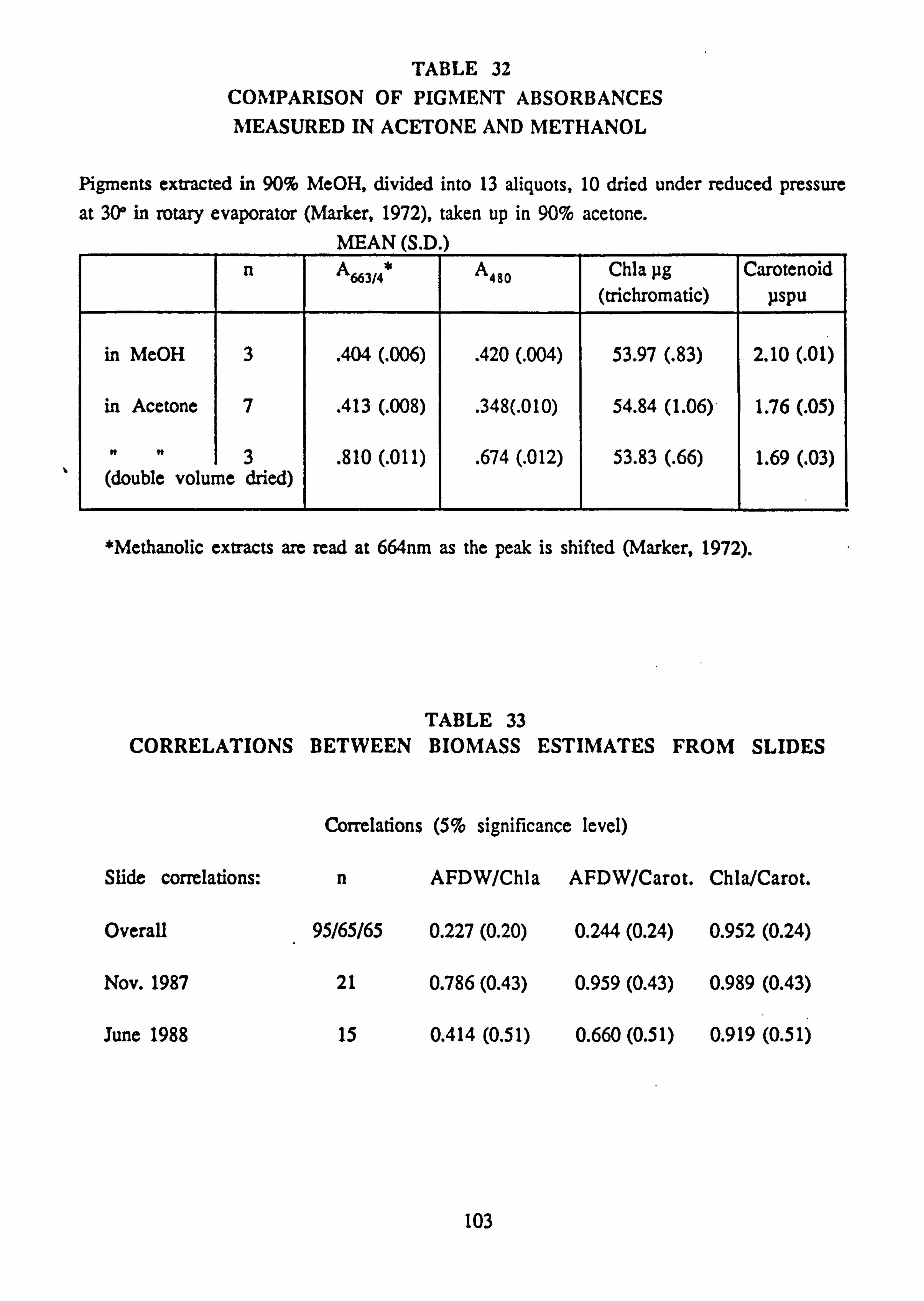
TABLE 32 COMPARISON OF PIGMENT ABSORBANCES MEASURED IN ACETONE AND METHANOL
Pigments extracted in 90% MeOH, divided into 13 aliquots, 10 dried under reduced pressure at 30° in rotary evaporator (Marker, 1972), taken up in 90% acetone.
MEAN (S. D. ) n A66314* A480 Chla pg
(trichromatic) Carotenoid
pspu
in MeOH 3 . 404 (. 006) . 420 (. 004) 53.97 (. 83) 2.10 (. 01)
in Acetone 7 . 413 (. 008) . 348(. 010) 54.84 (1.06) 1.76 (. 05)
3 . 810 (. 011) . 674 (. 012) 53.83 (. 66) 1.69 (. 03) (double volume dried)
*Methanolic extracts are read at 664nm as the peak is shifted (Marker, 1972).
TABLE 33 CORRELATIONS BETWEEN BIOMASS ESTIMATES FROM SLIDES
Correlations (5% significance level)
Slide correlations: n AFDW/Chla AFDW/Carot. Chla/Carot.
Overall 95/65/65 0.227 (0.20) 0.244 (0.24) 0.952 (0.24)
Nov. 1987 21 0.786 (0.43) 0.959 (0.43) 0.989 (0.43)
June 1988 15 0.414 (0.51) 0.660 (0.51) 0.919 (0.51)
103
Ash-free dry weight of lab-grown algae is the best measure of their biomass, notwith-
standing possible inaccuracies in measurement due to: (a) insufficient drying at 60°C
(b) uncertainty in weighing (c) loss of material after ashing
(d) increase in weight after drying and ashing by
uptake of atmospheric water vapour (e) loss of weight due to the presence of carbonates.
Inaccuracies due to a, c, d and e may be minimised by careful procedure, but the inherent
uncertainty in weighing, estimated as ±0. lmg, may form a considerable proportion of the
total AFDW in some cases. The accuracy of AFDW determination, in absolute terms, is also affected by the combustion temperature (Ridley-Thomas et al, 1989).
In the case of field samples, additional inaccuracy may result from the presence of
allochthonous material, detritus, animal or bacterial biomass, so that poor correlation of
pigments with AFDW may be expected. Selected sets of results from slides removed in
November 1987 and June 1988 show high and low correlations respectively between
AFDW and pigments, suggesting seasonal variation in the presence of such non-algal
material on the slides (Table 33). In such cases pigments may be the only suitable measures of algal biomass (Hillebrand, 1973).
The other parameter of algal abundance frequently measured is biovolume, but this
requires (a) cell counts and (b) measurements of critical cell dimensions enabling a
theoretical calculation to be made (Clarke et al, 1987). In this work no attempt has been
made to perform cell counts on field samples for practical and theoretical reasons (Hillebrand, 1973).
The habitat is extremely heterogeneous with respect to flow rate, exposure to light,
exposure to abrasion, supply and removal of dissolved gases, nutrients and waste
products. Hence it is not surprising that benthic algae have a very uneven distribu-
tion (Butcher, 1941; Round, 1981; Robinson, 1983; De Nicola and McIntyre, 1990
(a), (b)). This gives rise to errors in estimation of areal biomass which are usually larger than those due to errors in pigment measurement (Tett et al, 1975).
104
To estimate biomass present in streams, two strategies have been adopted. The first is
to sample natural substrates (stones) present in the streams, selecting two (within limits
of dimension set by the requirements of the extraction process) which represent the
range of periphyton density likely to occur at that site.
The second is to plant artificial substrates which are removed at intervals to sample the
periphyton. Two types of substrate were used: 15cm square glazed ceramic tiles, and
standard (2.6 x 7.2cm) microscope slides. The slides are fragile and thus frequently lost
during spates, and in addition sample a relatively small area (20cm2), but a larger number can be located at each site. The tiles sample a larger area (225cm 2) and are rarely lost in
spates, but a smaller number can be utilized at each site. In practice most sites had 3 tiles
and 6 slide pairs; some had 12 slide pairs.
These numbers are insufficient to truly sample the sites in a statistically valid way; as with the natural substrates they merely give an indication of biomass present. Most tiles when
sampled were 3 months old; the situation with slides is more complex due to frequent
losses. Slides were also more difficult to remove from the racks in times of high flow and so were more frequently omitted from the sampling routine at such times. The stones however had been present in the streams throughout: the age of their periphyton would depend on the time of the last spate which was sufficiently vigorous to scour them clean.
Artificial substrates require an initial colonization period, after which the biomass increases exponentially. Herder-Brouwer (1973) found a colonization phase of 10 days, followed by a growth phase up to approximately 40 days. Hamilton and Duthie (1984) found that colonization was logarithmic over a period of 25 days. Lamberti and Resh
(1985) found that tiles accurately reflected natural substrates in respect of chlorophyll-
a, bacterial and macroinvetebrate density after 28 days, and after 63 days in respect of
phaeophytin and AFDW, which would imply that the periphyton had reached a mature state. They recommend an exposure time of 1-2 months. By these estimates, exposure times of 3 months ought to permit the periphyton on tiles and slides to match that on
natural substrates.
Meier et al (1983) found variability between replicates of less than 8% with respect to
chlorophyll a on artificial substrates, the smallest areas used being approximately 2cm2
coverslips, at exposure times in excess of 10 days. Experience of the visually evident differences present on slides and tiles in the Loch Ard streams would suggest that
variability of biomass is in excess of this figure.
105
Measurement of chlorophyll-a extracted from 6 replicate slides exposed for 4 weeks in
an earlier study (Kinross, 1985) gave a mean of 7.42 pg. cm'2 and a s. d. of 1.17; the spread of values was 40% of the mean. Therefore the agreement between a limited number of replicates is not expected to be high.
The major advantages of using slides are that microscopic examination of closely
adherent periphyton is possible (some small adnate species were never found in
samples brushed off substrates but were noted on the slides) and that pigments and AFDW can be estimated by direct extraction followed by incineration of the growth on whole slide. The slide can finally be mounted for diatom examination.
Tiles have an advantage over stones in presenting a uniform smooth surface which can be thoroughly brushed or scraped clean; the white glaze helps in assessing when all periphyton has been removed. The colonized area is more readily calculated: the area lost at the edges where the plastic channel grips the tile is compensated by the leading
and trailing edges where periphyton can colonize the sides.
Extraction of whole tiles after brushing off the periphyton showed that very little biomass occurs on the underside or is left on the top surface after brushing. Slides however are colonized on both upper and lower surfaces, so slides are used in pairs, back-to-back, mounted horizontally. In the calculation of biomass per unit area, the area of both upper and lower slide surfaces has been considered together, as 20cm2.
When a high density of algal biomass has developed on the slides the effective surface area for photosynthetic biomass is only half this. There is therefore some ambiguity about the estimates of algal biomass on slides.
Artificial substrates have been criticised as aids to estimation of natural communities (Tippett, 1970), but most particularly in comparison with epiphytic communities. The
main problem appears to be that a long period of exposure is necessary for the
communities to resemble those present on natural substrates (Herder-Brouwer, 1973; Lamberti and Resh, 1985; Hamilton and Duthie, 1984). This may be because the even surfaces (which are a major advantage of artificial substrates) do not provide the optimum niches for rapid attachment and development of some species (Hamilton and Duthie, 1984). The main advantage is that the artificial substrates provide a uniform surface for colonization in all locations, enabling a comparison to be made between
streams with natural substrates of different geological nature (Castenholz, 1961; Klap-
wijk, 1978).
106
However in practice although the surface of the tiles may be uniform, the conditions in
which they are presented for colonization are difficult to match perfectly between
streams, because of constraints such as the ability to drive the anchoring stakes into the stream bed. This sometimes results in the rack not being aligned with the current. Indeed the pattern of flow in the bed may change with discharge, or may be altered per- manently due to bank erosion.
Robinson (1983) recommends replication of primary sampling to reduce variance in the results. The constraints just mentioned make it difficult to arrange multiple artificial substrates at each site, when so many sites are being monitored on a regular basis. Meier
et al (1983) found that after 10 days of colonization, variability of chlorophyll on coverslips was about 7% with three replicates. However the area sampled in this manner is so small that serious doubt exists whether the periphyton in the Loch Ard
streams would be adequately sampled. Colonization of surfaces such as slides and tiles occurs in an uneven manner, initial colonization occurring at the edges (Hamilton and Duthie, 1984; and personal observations). Thus after short colonization periods (less than 25 days, Hamilton and Duthie, 1984) the areal biomass will be dependent on the circumference : area ratio of the substrate.
This 'edge effect' may be due to the disruptive effect of the edge on current flow (De Nicola and McIntyre, 1990a), which might indicate that other interferences with flow may also affect the pattern of colonization on substrates, for example the racks used to retain the substrates. It may be that the stream used by Meier et al (1983) for their experiments had sufficient spatial homogeneity to ensure that replicate substrates at different points had essentially the same periphyton density. Nevertheless there is no assurance that the densities observed are truly representative of those on the natural substrates (Robinson, 1983).
Marker and Willoughby (1988) found that the biomass on natural substrates was pro- portional to the surface area. In this case stability and freedom from scouring may be the causative factors. On this basis the best comparative estimates of biomass may be
obtained from tethered tiles.
107
4.3 EVIDENCE OF SEASONALITY
Seasonal cycles in the values of environmental variables, species abundance, and biomass may be obscured rather than revealed by correlation analysis between them and a time variable, since correlation analysis presumes a linear relationship. Correlations calculated between
variables and annual week, squared annual week or square root annual week are low and not significant at 1% (not shown). A plot of temperature against annual week number shows a clear seasonal cycle (Fig. 25a). PAR shows a similar trend, also peaking about week 28. Absorbance data also shows a seasonal peak, around week 35, but with greater scatter of points.
If a seasonal cycle in species abundance or biomass exists it may be revealed via correlation
with temperature rather than with annual week.
Differences between mean temperature for different sites are largely an artefact due to
samples being taken in a regular sequence, as shown by a plot of mean site temperature against time of sampling (Fig. 25b). Therefore scatter in the temperature data may obscure the strength of correlations in the total data. Seasonality has been investigated by correlation analysis within individual site data sets and in the full data set (Table 34).
Significant correlations (at 1%) are rare. A large positive r value with PAR is to be expected. Some significant positive correlations with absorbance and negative with TON are also found. An increase in AuO indicates an increased concentration of humic material, which may occur in summer as a result of reduced dilution and release of humics due to cracking of peat beds
and increased microbial activity (Rees et al, 1989).
TON may decrease in summer as a result of increased nutrient uptake by periphyton. An increase in TON in winter occurs due to the breakdown of plant material at the end of the
growing season. The concentration of other chemical variables is liable to increase during low flow simply as a result of a decreased dilution.
Evidence for a seasonal trend in biomass is scarce. Only one significant correlation with temperature is found, for stone carotenoid in site 14-1. This is unexpected, but may be partly due to the scarcity of data for some biomass measures. Observation suggests that biomass is
reduced during autumn spates, but the evidence from measurements is against this during the
period of study. Observation again suggests that it is only very strong current and abrasion by
suspended material which reduces the quantity of periphyton, and if low-flow conditions occur during winter this 'seasonal' reduction may not take place.
108
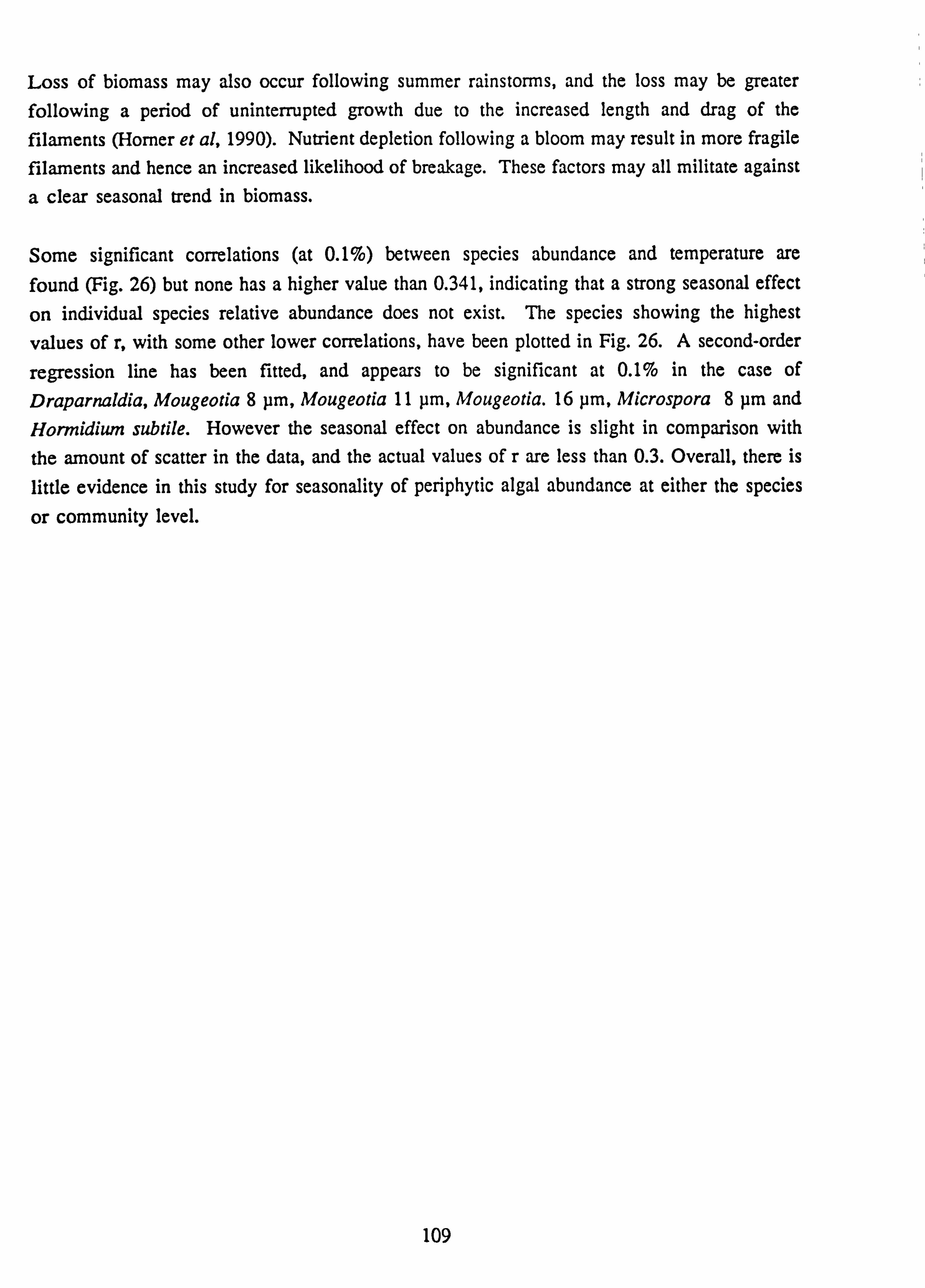
Loss of biomass may also occur following summer rainstorms, and the loss may be greater following a period of uninterrupted growth due to the increased length and drag of the filaments (Homer et al, 1990). Nutrient depletion following a bloom may result in more fragile
filaments and hence an increased likelihood of breakage. These factors may all militate against
a clear seasonal trend in biomass.
Some significant correlations (at 0.1%) between species abundance and temperature are found (Fig. 26) but none has a higher value than 0.341, indicating that a strong seasonal effect
on individual species relative abundance does not exist. The species showing the highest
values of r, with some other lower correlations, have been plotted in Fig. 26. A second-order
regression line has been fitted, and appears to be significant at 0.1% in the case of Draparnaldia, Mougeotia 8 pm, Mougeotia 11 pm, Mougeotia. 16 pm, Microspora 8 pm and Hormidiurn subtile. However the seasonal effect on abundance is slight in comparison with the amount of scatter in the data, and the actual values of r are less than 0.3. Overall, there is
little evidence in this study for seasonality of periphytic algal abundance at either the species
or community level.
109
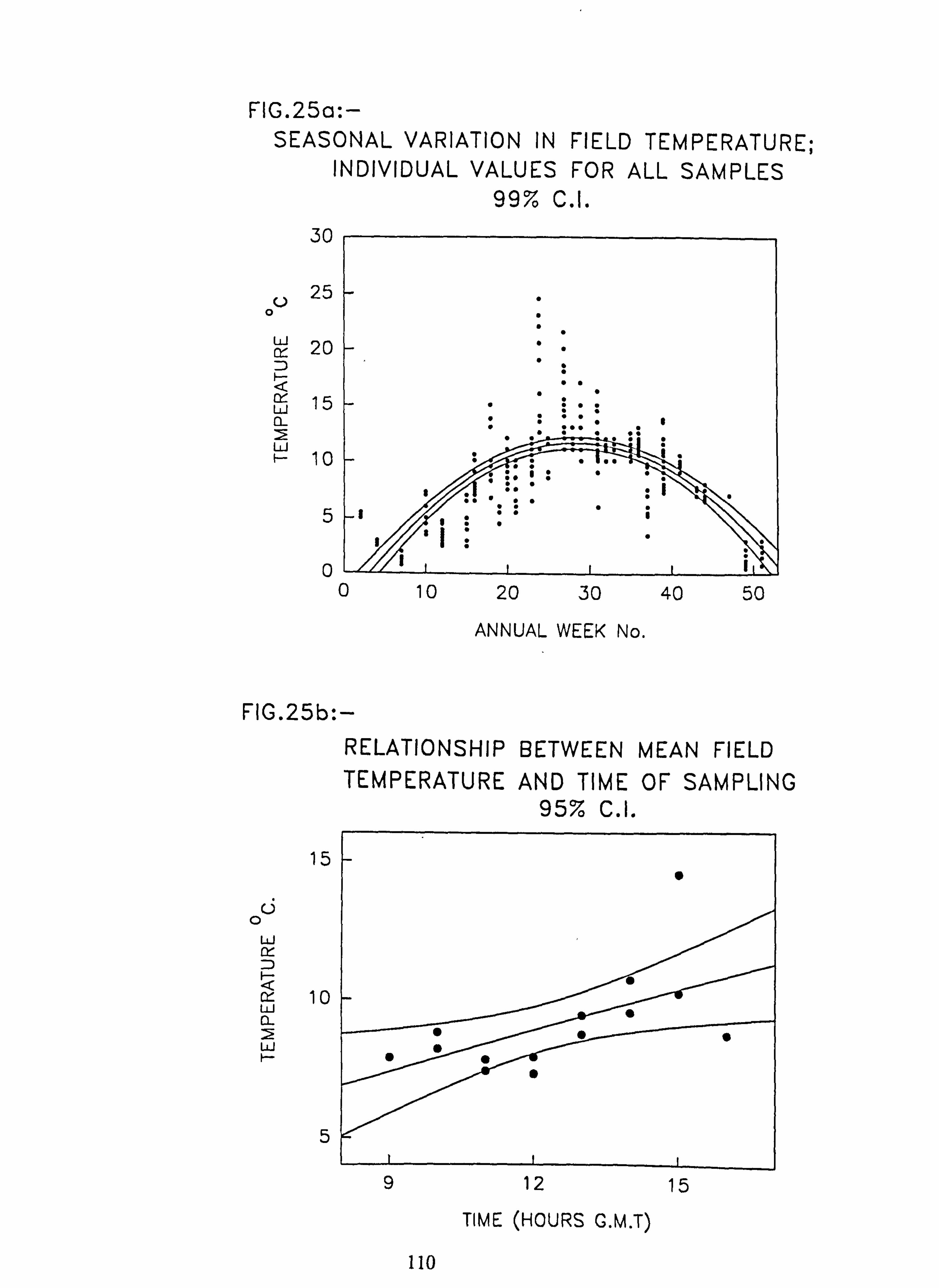
FIG. 25a: - SEASONAL VARIATION IN FIELD TEMPERATURE;
INDIVIDUAL VALUES FOR ALL SAMPLES 99% C. I.
30
25 0 W 20
15 Ww
10
5
0
. .
.
_ . . . .
..
. "
- . .. .
" . :
. "
" ...
"
S . . .
; " .
".
1 " 1
I
:' a
0 10 20 30 40 50
ANNUAL WEEK No.
FIG. 25b: - RELATIONSHIP BETWEEN MEAN FIELD TEMPERATURE AND TIME OF SAMPLING
95% C. I.
15
(3 0
w
10 a. w r
5
"
"
"
" "
9 12 15
TIME (HOURS G. M. T)
110
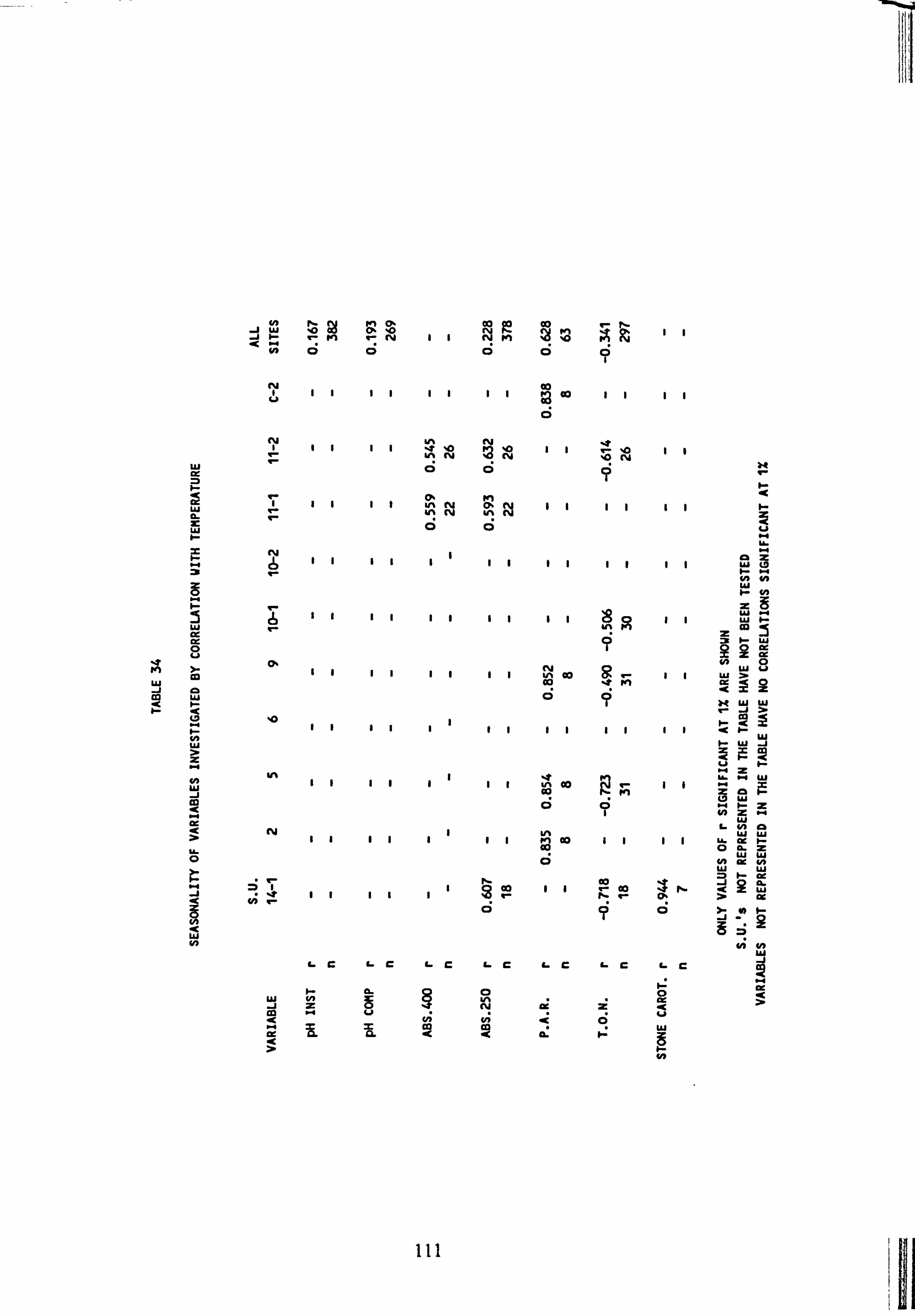
tH r M rN 11 NM ýO MN
1
N O O O O O
CY Co 1 1I 11 I1 Co 11 1
O
Al 1 1 11 IA N !2N 11 11 N
L O O F I- t W 1 1 11 v N 11 (I 11 Z 0 r4 N = Lii
Ö O u
= tV 1 I 11 11
x M 3
11 11 11 11 LU M NN L4i Iý Vf
-
g 1 1 1I 11 11 1I 11 'O m
e 1
ält L
P N 0 M m 1 1 I1 11 1I Co
9 1 LLI >
ui 1 I < r S
O J H
>
1 S 1 1I 1 11 1I 1I I1 <
5-- N W 1-ý
W WJ
Z ýQ ti b-
Cl) 1 I 11 11 i ~
W 11 v i Co 9
M I1 "+
Z X
J m O p
l 9 W
Z _ ~ N " -ý �g
N 1 L
tu ND ui LLA
> 1 1 11 1 1I M
a0 1I 11 Ö Cle Z LL a0
O N OC N ý.. 3 >- at J
I 11 r- L- i Z 'f I 1 I1 1 "O Co f. Co O. > L o c Nr
O Q O J
y Z Z L O W
N NN W
L C LC LC LC LC LC LC m
J I- 2
d r 8 O
Ö 1,2
> ýt
N O" Z
t
m º+ u u e ä s = d º > º- N
III
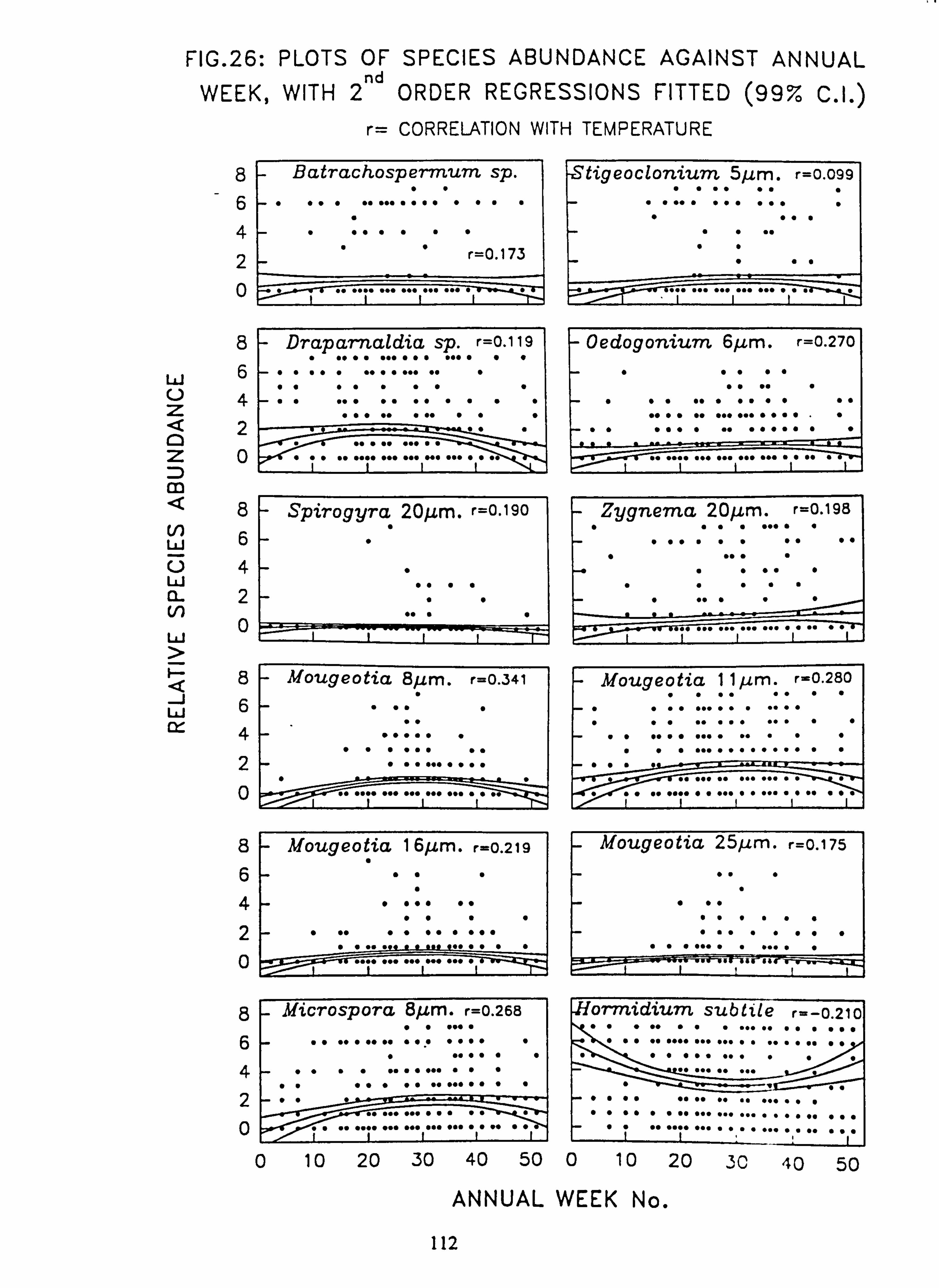
FIG. 26: PLOTS OF SPECIES ABUNDANCE AGAINST ANNUAL WEEK, WITH 2nd ORDER REGRESSIONS FITTED (99% C. I. )
r= CORRELATION WITH TEMPERATURE
8 6 4 2 0
W U Z
Z
m
W_ U Li a- (/)
w
I-
J W
- Batrachospermum sp.
.
r=0.173
"' "" ""I" """ """'""" ". " "
8
6
4 2
0
- Draparnaldia sp. r=o. i 19 . .. ".... .".... ...
-.... . .... ..
. .... ... ...
. ......... . """ "" """" .N N" N" ". " "0 00
8 6 4 2 0
Spirogyra 20Am. r=0.90
to :00
8
6
4
2
0
8 6 4 2 0
- Mougeotia 8µm. r=0.341
00 0000 000 ... 000 000 00 00
Mougeotia T r. 219
...
00.. of 0......... ..
0
8 6 4 2 0
_ Microspora 8Am. r=0.268
....... ....... ..
........... ... ......................
10 20 30 40 50 0 10 20 30 40 50
ANNUAL WEEK No.
112
Stigeoclonium 5p. m. r=0.099
... . ..
- Oedogoniurn 6f. cm. r=0.270 -.....
.... ............ ..
...... ........ . ..................
Zygnema 201im. r=0.198
- Mougeotia 1 1µm. r=0.280
. .... ... ... ..
............... . ..... ..... ... ...
..... 00 0.004 00... 00.. 004
ougeotia 25f. cm. r-0.175
...
00.... ..... ..
. Horrnidium subtile r=-0.21O ..... ............. . ................. ....... . . ........ ...
.... .... ... ...
.... .. 00 ... ... ... ...... ...
4.4. SPECIES DIVERSITY
The diversity of species which compose a community has been considered an indicator
of the degree of disturbance of an ecosystem; disturbance causing a reduction in the number and diversity of species (Stokes, 1986; Schindler, 1987; Rott and Pfister, 1988; Pontasch et al , 1989).
'Species diversity' is considered to consist of two components: richness and evenness (Ludwig and Reynolds, 1988). Species richness may be indicated by the total number of species in a sample, provided the sample size is uniform between sampling units (sites) (Ludwig and Reynolds, 1988). Indices which correct for different sample sizes have been proposed, but these are difficult to apply in a situation where an actual count is not taken, and overall the sample size is likely to even out when a large number of individual samples are combined to form the complete data matrix. Evenness expresses the degree to which the numbers of each species present are the same. Diversity indices attempt to combine the concepts of richness and evenness into a single index,
which makes the relative contribution of these two factors difficult to assess (Ludwig and Reynolds, 1988).
4.4.1 Measures of Richness. Diversity and Evenness
The program SPDIVERS. BAS (Ludwig and Reynolds, 1988) computes several indi-
ces for diversity and evenness. The authors recommend Hill's numbers Ni and N2 as measures of diversity, and the value E5 (modified Hill's ratio) as a measure of evenness, as it is independent of sample size.
Species number, diversity and evenness for the data matrices A, B, C and D are shown in Table 35.
Evenness is quite high and consistent, the values lying between 0.6 and 0.9 in A, B and C and 0.8 and 1.0 in matrix D, implying that the communities are not excessively dominated by a few species (potential values of E5 range from 0 to 1.25). In fact this
situation may stem from the sampling method and estimation of relative abundance, which has a similar effect to carrying out a log-transformation of true abundance data,
reducing the range of abundance values in matrix C to 0-550 (while pooled p/a data
range from 0 to 32), rather than over several logs.
113
The influence of environmental variables on richness, diversity and evenness has been
investigated by correlation analysis of site-mean abundance data for matrices A, B and C,
and using indices calculated on Matrix B pooled presence-absence data (Tables 36-39).
Variables showing no correlations significant at least at the 5% level have been excluded from the tables. Correlations with richness and diversity are highly significant for pH,
with higher correlations being obtained for pH from composite water samples. Similarly
the correlations with H' ion are higher with composite samples, and significant correla-
tions with AuO are found only with composite data. The composite sample values are
more likely to represent true means (time-averaged) of these variables.
Strong correlations are obtained also with aluminium and calcium concentrations, but
'Plow', Mgz+ and silicate give variable results in different matrices and therefore these
correlations must be considered less trustworthy. However if Matrix B is considered to contain the most complete data set, with all sites being sampled throughout its
duration, then silicate is seen to give strong correlations with richness and diversity,
significant at 1%. This is also seen in the 'unbiased' Matrix B pooled p/a data set (Table 39).
Evenness gives very low correlations with most variables, except in Matrix B (abun- dance data) where high correlations are found with 'Flow', aluminium and H.
A high correlation with richness or diversity implies an effect of the variable on the
number of species composing the community. A lowered diversity is considered to
indicate a stressed ecosystem. Therefore a decrease in pH (increased Hi, decrease in
alkalinity, or increase in concentration of aluminium species may constitute environ-
mental stress. However all these variables are strongly intercorrelated and thus it is not
possible to determine whether they each have some unique influence on richness and
diversity.
The strong negative correlations in Matrix B between forms of aluminium and evenness implies that the distribution of species abundances within the community is affected by
Al; at higher Al concentrations the abundance of some species is increased while that of
others is decreased.
114
As with all correlations, this cannot be taken as proof of a causative relationship since
many of the environmental variables are highly correlated with each other. Furthermore
the relationship between abundance of a species and a variable may not be straightfor-
ward; Lehman (1976) showed that a negative correlation between abundance of Dinobryon and phosphate concentration was not due to toxicity of phosphate to Dinobryon, as had been previously supposed, but was a result of its ability to scavenge
very low concentrations of phosphate. Thus it effectively outcompetes other algae
under these conditions, but is overgrown by faster growing algae under conditions of higher P04 concentration.
However, in view of the known toxic effects of Al on fish (Birchall et al, 1989; Dietrich
and Schlatter, 1989; Grahn, 1980; Holtze and Hutchinson, 1989), invertebrates
(Ormerod et al� 1987; Weatherley et al, 1988), and algae (Claesson and Tornqvist, 1989;
Folsom et al, 1986; Gensemer, 1990; Helliwell et al , 1983; Pillsbury and Kingston, 1990),
it is at least possible that the observed correlations may indicate selective toxicity of Al
towards some taxa.
4.4.2 Species Number in Each Sample as a Measure of Richness
Linear regression analysis has been carried out for species richness on the individual
data points obtained for total species number at each site on each sampling occasion, giving a total number of data points ranging from 29 (Al-1) to 412 (pH). The regressions have been plotted along with the 99% CI (Figs. 27a, b). The p-values of the regression
and correlation coefficient 'r' are shown for pH and A350. Many of the confidence intervals are fairly narrow indicating a high degree of reliability. Steep slopes indicating
a strong effect of the variable on species number are obtained for pH, H' (not shown), temperature, (labile) Aluminium, akalinity, Caz+, Mgt and SiO
2' Other variables either
have a shallow slope or a wide 99% C. I., which means that the slope is not significantly different from zero.
These correlated variables are all acidification-related, so that there is clearly a decrease
of richness and diversity with increasing acidity. It is less clear whether this decrease
can be related to ecosystem disturbance (Schindler 1987), since the conditions in each
burn have fluctuated naturally about the mean over several seasons. For the premise of
low species richness indicating a disturbed ecosystem to hold true, the intra-seasonal
range of e. g. pH, would have to be greater in low-mean pH burns.
115
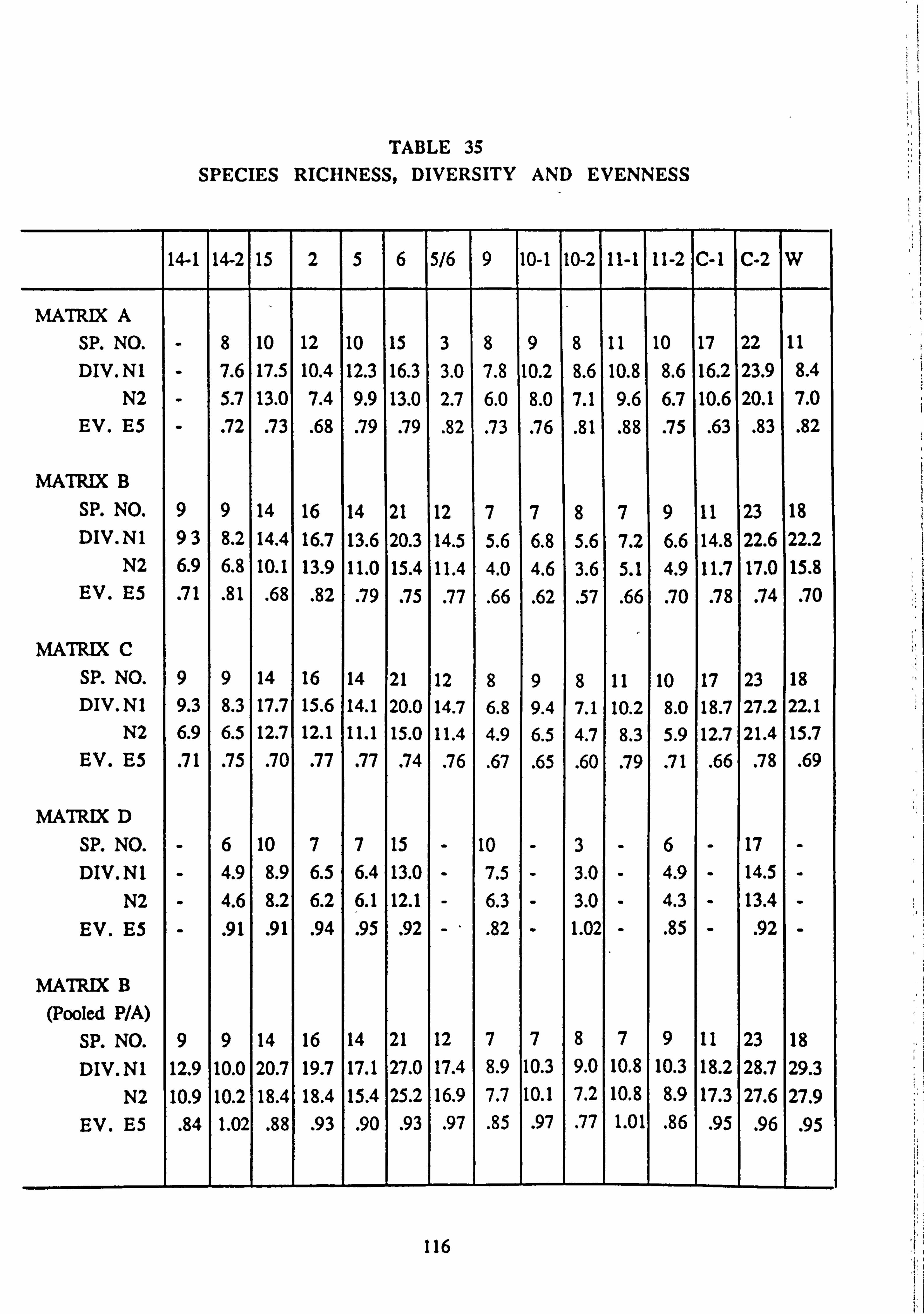
TABLE 35 SPECIES RICHNESS, DIVERSITY AND EVENNESS
14-1 14-2 15 2 5 6 5/6 9 10-1 10-2 11-1 11-2 C-1 C-2 W
MATRIX A SP. NO. - 8 10 12 10 15 3 8 9 8 11 10 17 22 11
DIV. Ni - 7.6 17.5 10.4 12.3 16.3 3.0 7.8 10.2 8.6 10.8 8.6 16.2 23.9 8.4 N2 - 5.7 13.0 7.4 9.9 13.0 2.7 6.0 8.0 7.1 9.6 6.7 10.6 20.1 7.0
EV. E5 - . 72 . 73 . 68 . 79 . 79 . 82 . 73 . 76 . 81 . 88 . 75 . 63 . 83 . 82
MATRIX B SP. NO. 9 9 14 16 14 21 12 7 7 8 79 11 23 18 DIV. Ni 93 8.2 14.4 16.7 13.6 20.3 14.5 5.6 6.8 5.6 7.2 6.6 14.8 22.6 22.2
N2 6.9 6.8 10.1 13.9 11.0 15.4 11.4 4.0 4.6 3.6 5.1 4.9 11.7 17.0 15.8 EV. E5 . 71 . 81 . 68 . 82 . 79 . 75 . 77 . 66 . 62 . 57 . 66 . 70 . 78 . 74 . 70
MATRIX C SP. NO. 9 9 14 16 14 21 12 8 9 8 11 10 17 23 18 DIV. Ni 9.3 8.3 17.7 15.6 14.1 20.0 14.7 6.8 9.4 7.1 10.2 8.0 18.7 27.2 22.1
N2 6.9 6.5 12.7 12.1 11.1 15.0 11.4 4.9 6.5 4.7 8.3 5.9 12.7 21.4 15.7 EV. E5 . 71 . 75 . 70 . 77 . 77 . 74 . 76 . 67 . 65 . 60 . 79 . 71 . 66 . 78 . 69
MATRIX D SP. NO. - 6 10 7 7 15 - 10 - 3 -6- 17 - DIV. N1 - 4.9 8.9 6.5 6.4 13.0 - 7.5 - 3.0 - 4.9 - 14.5 -
N2 - 4.6 8.2 6.2 6.1 12.1 - 6.3 - 3.0 - 4.3 - 13.4 - EV. E5 - . 91 . 91 . 94 . 95 . 92 -- . 82 - 1.02 - . 85 - . 92 -
MATRIX B (Pooled P/A)
SP. NO. 9 9 14 16 14 21 12 7 7 8 79 11 23 18 DIV. Ni 12.9 10.0 20.7 19.7 17.1 27.0 17.4 8.9 10.3 9.0 10.8 10.3 18.2 28.7 29.3
N2 10.9 10.2 18.4 18.4 15.4 25.2 16.9 7.7 10.1 7.2 10.8 8.9 17.3 27.6 27.9 EV. E5 . 84 1.02 . 88 . 93 . 90 . 93 . 97 . 85 . 97 . 77 1.01 . 86 . 95 . 96 . 95
116
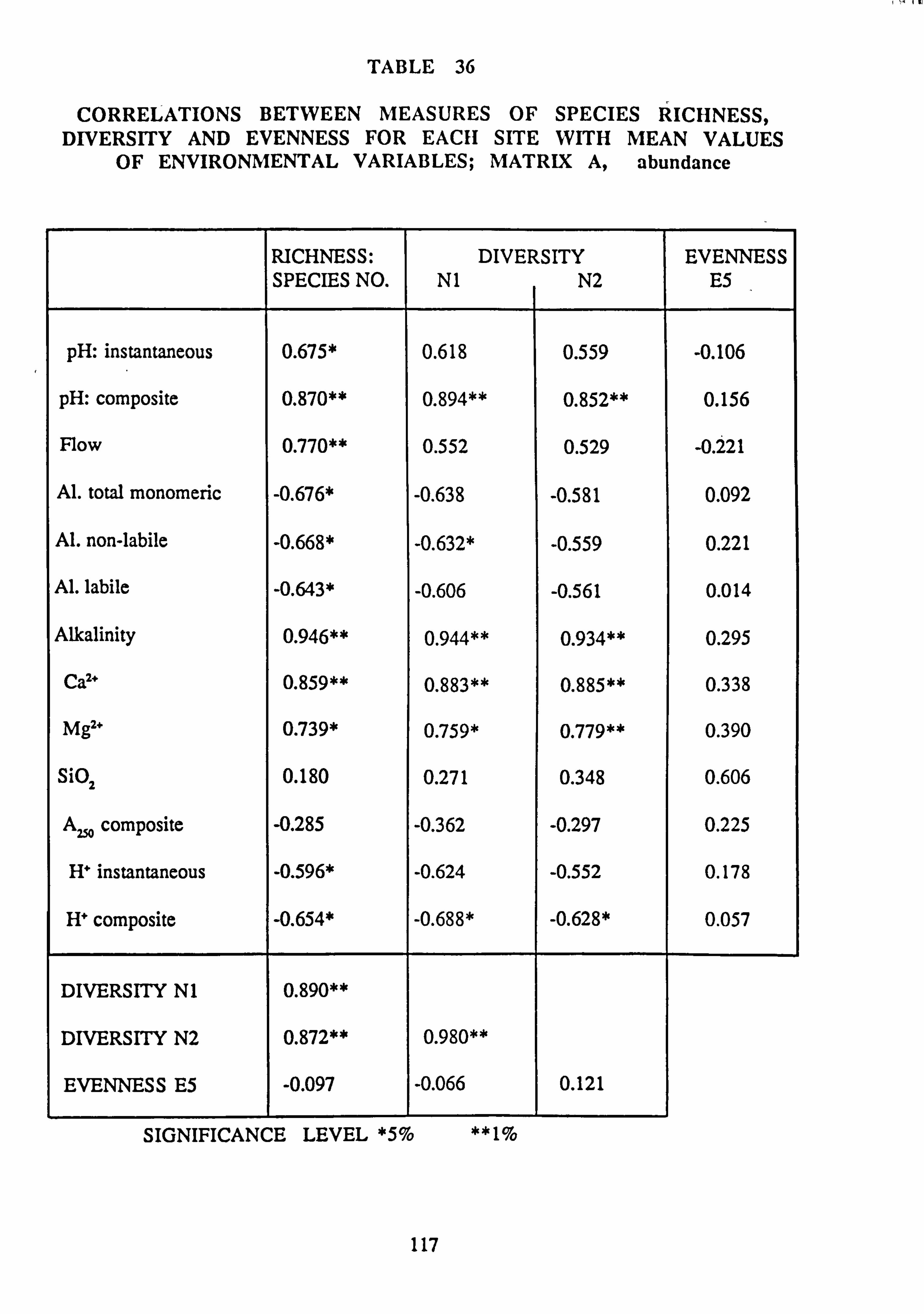
TABLE 36
CORRELATIONS BETWEEN MEASURES OF SPECIES RICHNESS, DIVERSITY AND EVENNESS FOR EACH SITE WITH MEAN VALUES
OF ENVIRONMENTAL VARIABLES; MATRIX A, abundance
RICHNESS: SPECIES NO.
DIVERSITY N1 N2
EVENNESS E5
pH: instantaneous 0.675* 0.618 0.559 -0.106
pH: composite 0.870** 0.894** 0.852** 0.156
Flow 0.770** 0.552 0.529 -0.221
Al. total monomeric -0.676* -0.638 -0.581 0.092
Al. non-labile -0.668* -0.632* -0.559 0.221
Al. labile -0.643* -0.606 -0.561 0.014
Alkalinity 0.946** 0.944** 0.934** 0.295
Cat' 0.859** 0.883** 0.885** 0.338
Mgz+ 0.739* 0.759* 0.779** 0.390
Si02 0.180 0.271 0.348 0.606
A. composite -0.285 -0.362 -0.297 0.225
H` instantaneous -0.596* -0.624 -0.552 0.178
H' composite -0.654* -0.688* -0.628* 0.057
DIVERSITY Ni 0.890**
DIVERSITY N2 0.872** 0.980**
EVENNESS E5 -0.097 -0.066 0.121
SIGNIFICANCE LEVEL *5% **J%
117
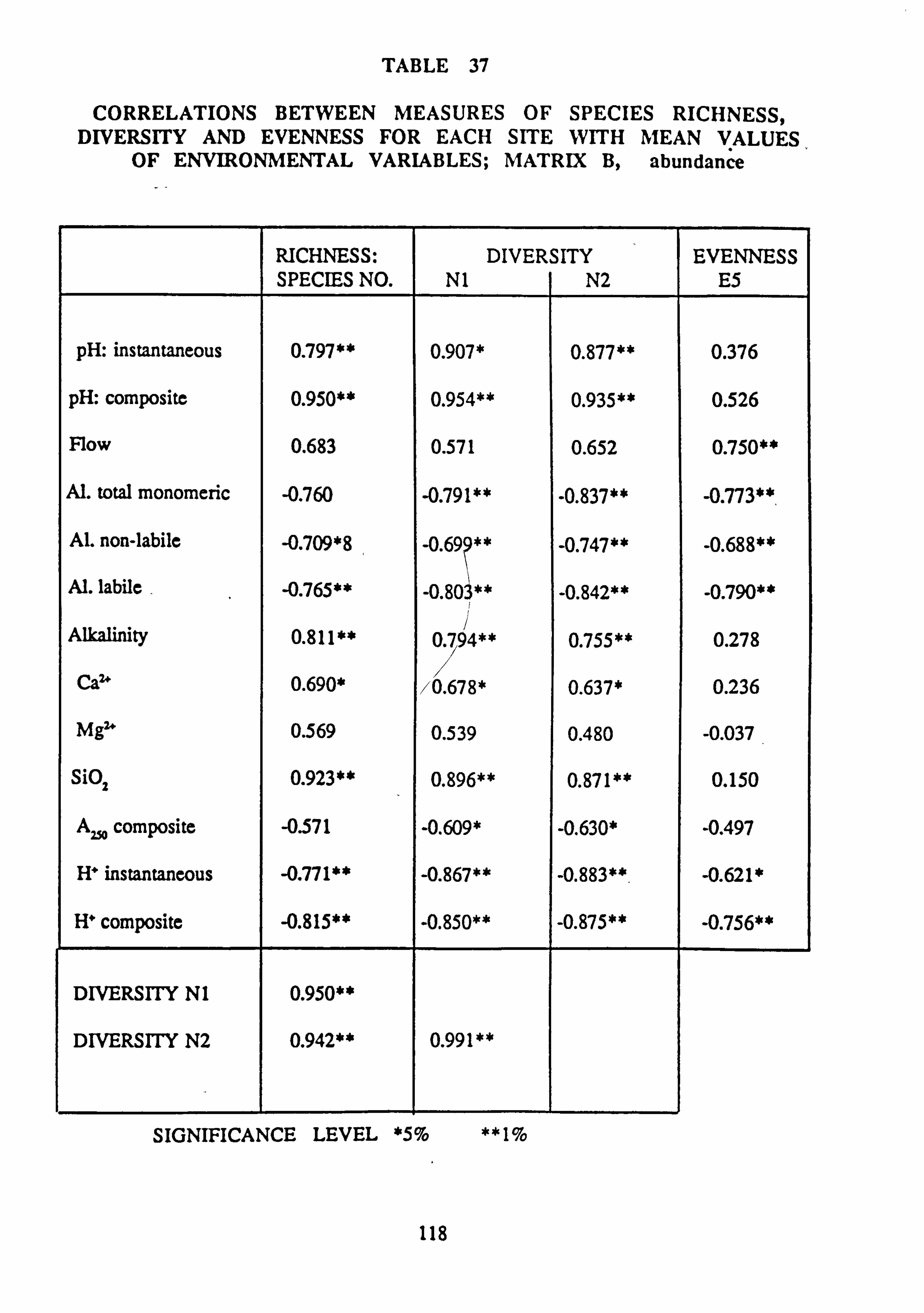
TABLE 37
CORRELATIONS BETWEEN MEASURES OF SPECIES RICHNESS, DIVERSITY AND EVENNESS FOR EACH SITE WITH MEAN VALUES
OF ENVIRONMENTAL VARIABLES; MATRIX B, abundance
RICHNESS: SPECIES NO.
DIVERSITY Ni N2
EVENNESS E5
pH: instantaneous 0.797** 0.907* 0.877** 0.376
pH: composite 0.950** 0.954** 0.935** 0.526
Flow 0.683 0.571 0.652 0.750**
Al. total monomeric -0.760 -0.791** -0.837** -0.773**.
Al. non-labile -0.709*8 -0.69 ** -0.747** -0.688** Al. labile -0.765** -0.80 ** -0.842** -0.790**
Alkalinity 0.811** 0.794** 0.755** 0.278
Cat' 0.690* /0.678* 0.637* 0.236
Mgr' 0.569 0.539 0.480 -0.037
SiO2 0.923** 0.896** 0.871** 0.150
A. composite -0.571 -0.609* -0.630* -0.497
H' instantaneous -0.771** -0.867** -0.883**. -0.621*
H' composite -0.815** -0.850** -0.875** -0.756**
DIVERSITY Ni 0.950**
DIVERSITY N2 0.942** 0.991**
SIGNIFICANCE LEVEL *5% **1%
118
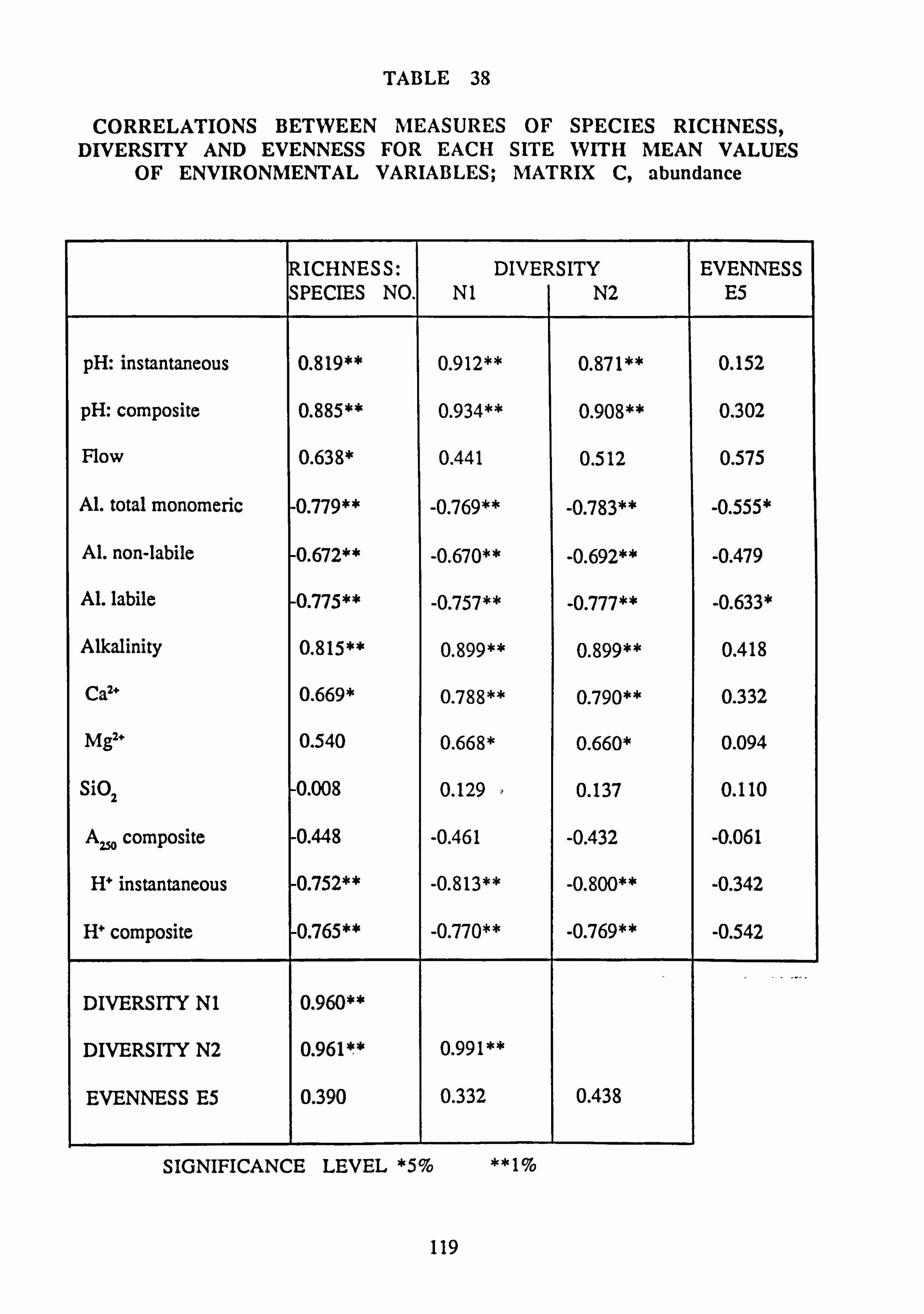
TABLE 38
CORRELATIONS BETWEEN MEASURES OF SPECIES RICHNESS, DIVERSITY AND EVENNESS FOR EACH SITE WITH MEAN VALUES
OF ENVIRONMENTAL VARIABLES; MATRIX C, abundance
RICHNESS: SPECIES NO.
DIVERSITY N1 N2
EVENNESS E5
pH: instantaneous 0.819** 0.912** 0.871** 0.152
pH: composite 0.885** 0.934** 0.908** 0.302
Flow 0.638* 0.441 0.512 0.575
Al. total monomeric 0.779** -0.769** -0.783** -0.555*
Al. non-labile 0.672** -0.670** -0.692** -0.479
Al. labile 0.775** -0.757** -0.777** -0.633*
Alkalinity 0.815** 0.899** 0.899** 0.418
CO* 0.669* 0.788** 0.790** 0.332
Mgt; 0.540 0.668* 0.660* 0.094
Si02 0.008 0.129 0.137 0.110
A250 composite 0.448 -0.461 -0.432 -0.061
H' instantaneous 0.752** -0.813** -0.800** -0.342
H+ composite 0.765** -0.770** -0.769** -0.542
DIVERSITY N1 0.960**
DIVERSITY N2 0.961** 0.991**
EVENNESS E5 0.390 0.332 0.438
SIGNIFICANCE LEVEL *5% **1%
119
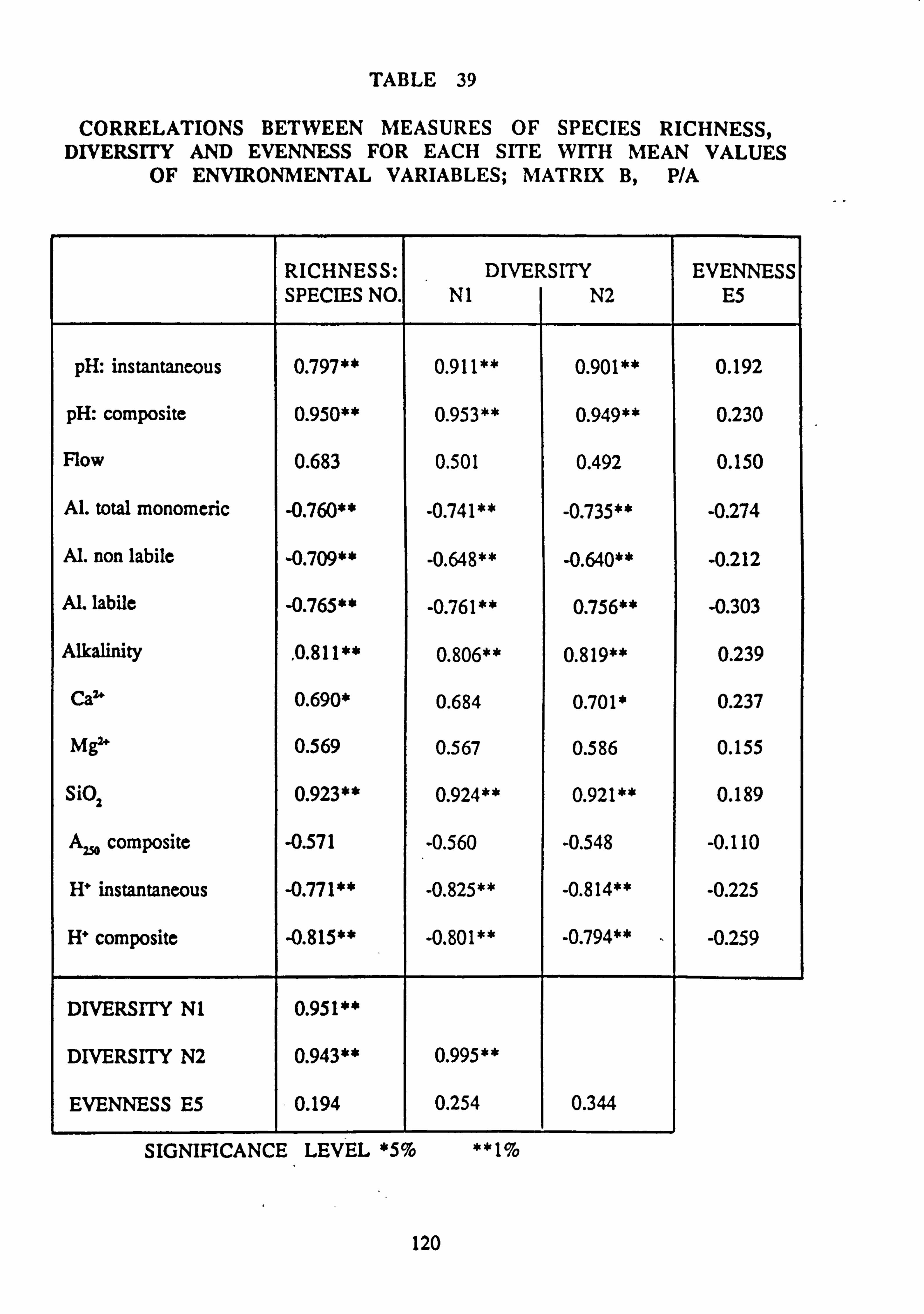
TABLE 39
CORRELATIONS BETWEEN MEASURES OF SPECIES RICHNESS, DIVERSITY AND EVENNESS FOR EACH SITE WITH MEAN VALUES
OF ENVIRONMENTAL VARIABLES; MATRIX B, P/A
RICHNESS: SPECIES NO.
DIVERSITY Nl N2
EVENNESS E5
pH: instantaneous 0.797** 0.911** 0.901** 0.192
pH: composite 0.950** 0.953** 0.949** 0.230
Flow 0.683 0.501 0.492 0.150
Al. total monomeric -0.760** -0.741** -0.735** -0.274
Al. non labile -0.709** -0.648** -0.640** -0.212
Al. labile -0.765** -0.761** 0.756** -0.303
Alkalinity , 0.811** 0.806** 0.819** 0.239
Cap' 0.690* 0.684 0.701* 0.237
MgU 0.569 0.567 0.586 0.155
SiO2 0.923** 0.924** 0.921** 0.189
A2% composite -0.571 -0.560 -0.548 -0.110
H' instantaneous -0.771** -0.825** -0.814** -0.225
H' composite -0.815** -0.801** -0.794** -0.259
DIVERSITY Ni 0.951 **
DIVERSITY N2 0.943** 0.995**
EVENNESS E5 0.194 0.254 0.344
SIGNIFICANCE LEVEL *5% **I%
120
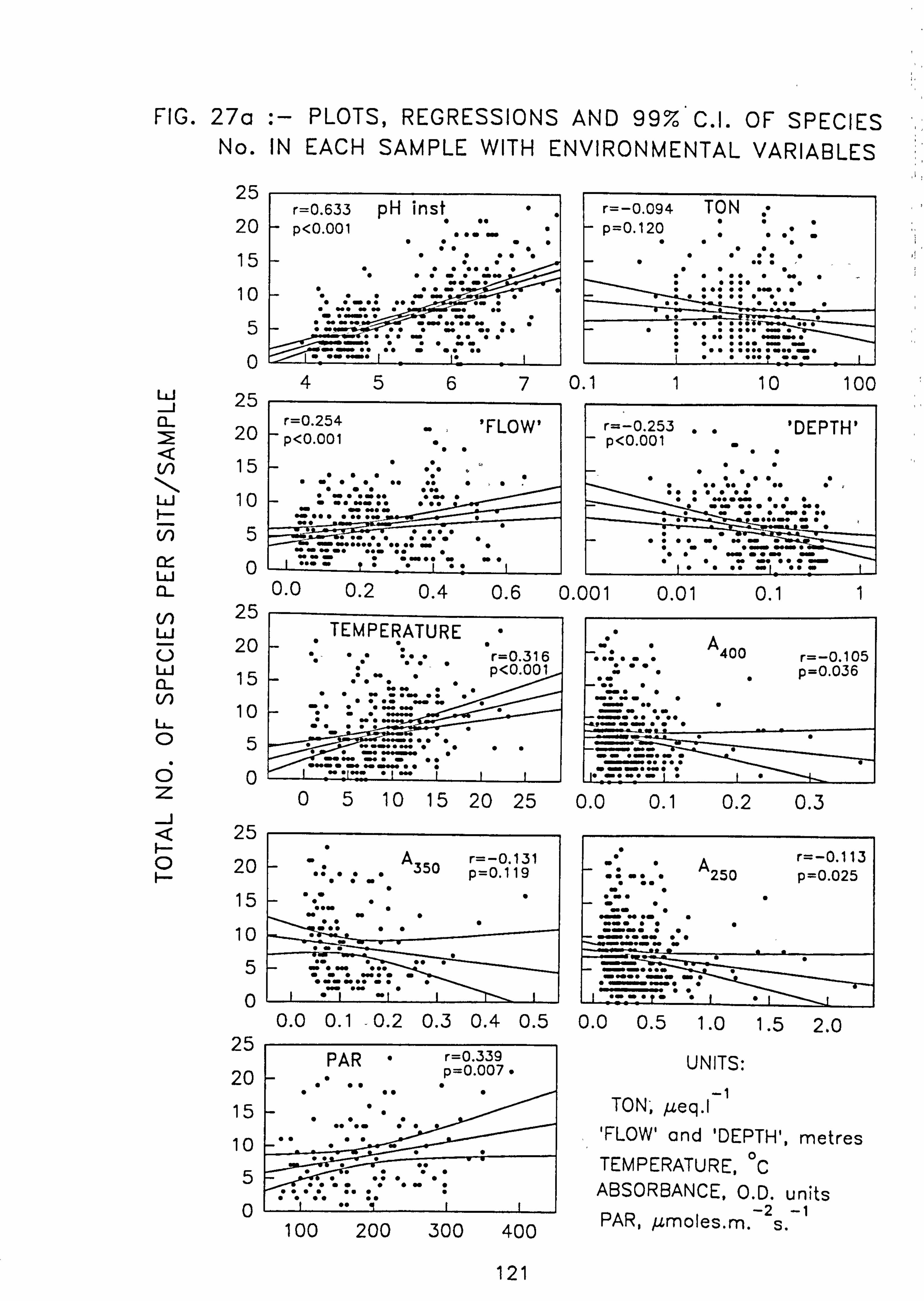
FIG. 27a :- PLOTS, REGRESSIONS AND 99% C. I. OF SPECIES No. IN EACH SAMPLE WITH ENVIRONMENTAL VARIABLES
25 r=0.633 pH inst r=-0.094 TON ; 20 p<0.001 *..: o ..: P=0.120 0.
:
". .
15 ...
10 ... -... .. . r. .
45670.1 1 10 100 Ld 25 IL r=0.254 'FLOW' r=-0.253 ." 'DEPTH' 20
p<0.001 p<0.001 Q N 15 6w .... 000 .
LLJ 10
rw »" r"_"r. """ w" +
to 5 ...... _: _. _"-_ _ 0 I-I
A r=-0.131 ": 350 P=0.119
ww "
"Y "Y
Lj. j
CL 0.0 0.2 0.4 0.6 0.001 0.01 0.1 1 NLJ
W 20 U w 15 N 10 Li- O5
Op Z J
F- O
05 10 15 20 25 0.0 0.1 0.2 0.3 25
20
15
10
5
0
25
20
15
10
5
0
.
0.0.0 400 r=-0.105 0.036
.
r=-0.113 ". -" " 250 p=0.025
Y
N'f
0.0 0.1 -0.2 0.3 0.4 0.5 0.0 0.5 1.0 1 .59. n
PAR " r=0.339 P=0.007 .
100 200 300 400
121
UNITS:
TON; µeq. l 'FLOW' and 'DEPTH', metres TEMPERATURE, 0C
ABSORBANCE, O. D. units PAR, µmoles. m. s. -1 -2
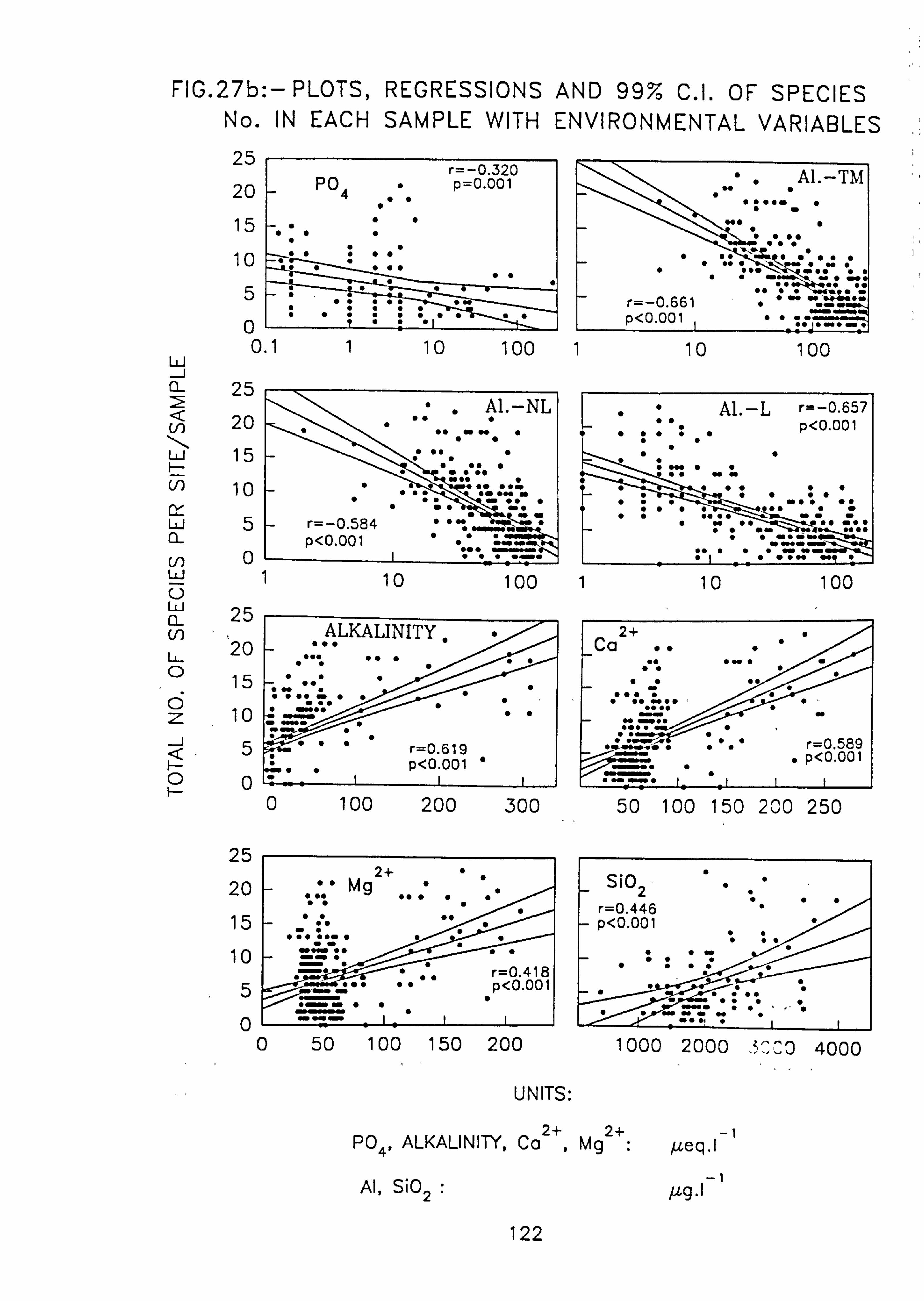
FIG. 27b: - PLOTS, REGRESSIONS AND 99% C. I. OF SPECIES No. IN EACH SAMPLE WITH ENVIRONMENTAL VARIABLES
r1 C Li
20
15
10
5
n 0.1 1 10 100 1 10 100
w J 25
A1. -NL A1. -L r=-0.657 2000 p .. »«. ". <0.001
w 15 ...
W5 r=-0.584 .. »' " .. «' ..
ý: s: " :..
....... .0.. .... Cl-
r, -en
w1 10 100 1 10 100 U
25 n' ALKALINITY. 2+ " .. Ca 20 ... .... .».
15 000 0
z 10 ...... ...
r=0.61 9'"' r=0.589 Q5
p<0 ;-
. 001 . p<0.001
. »_.
" AL-TM N"
" """"".
N". "
zý "
"N" ý"Y "N"
""Y"N 00 00 00
=-0 661 " "" : -: "" r . 001 `ý' P<0 .
~0 100 200 300 50 100 150 200 250
25
20
15
10
5
n
Si0 - 2 r=0.446 P<0 001 " .
" " vom' "
2+ " .. Mg
000 ein 0
0"Q r=0.418 ý-ý" "" p<0.001
0 50 100 150 200 1000 2000 . 3000 4000
UNITS:
P04, ALKALINITY, Cat+, Mgt+: peq. I
-1 Al, S102 : ug I
122
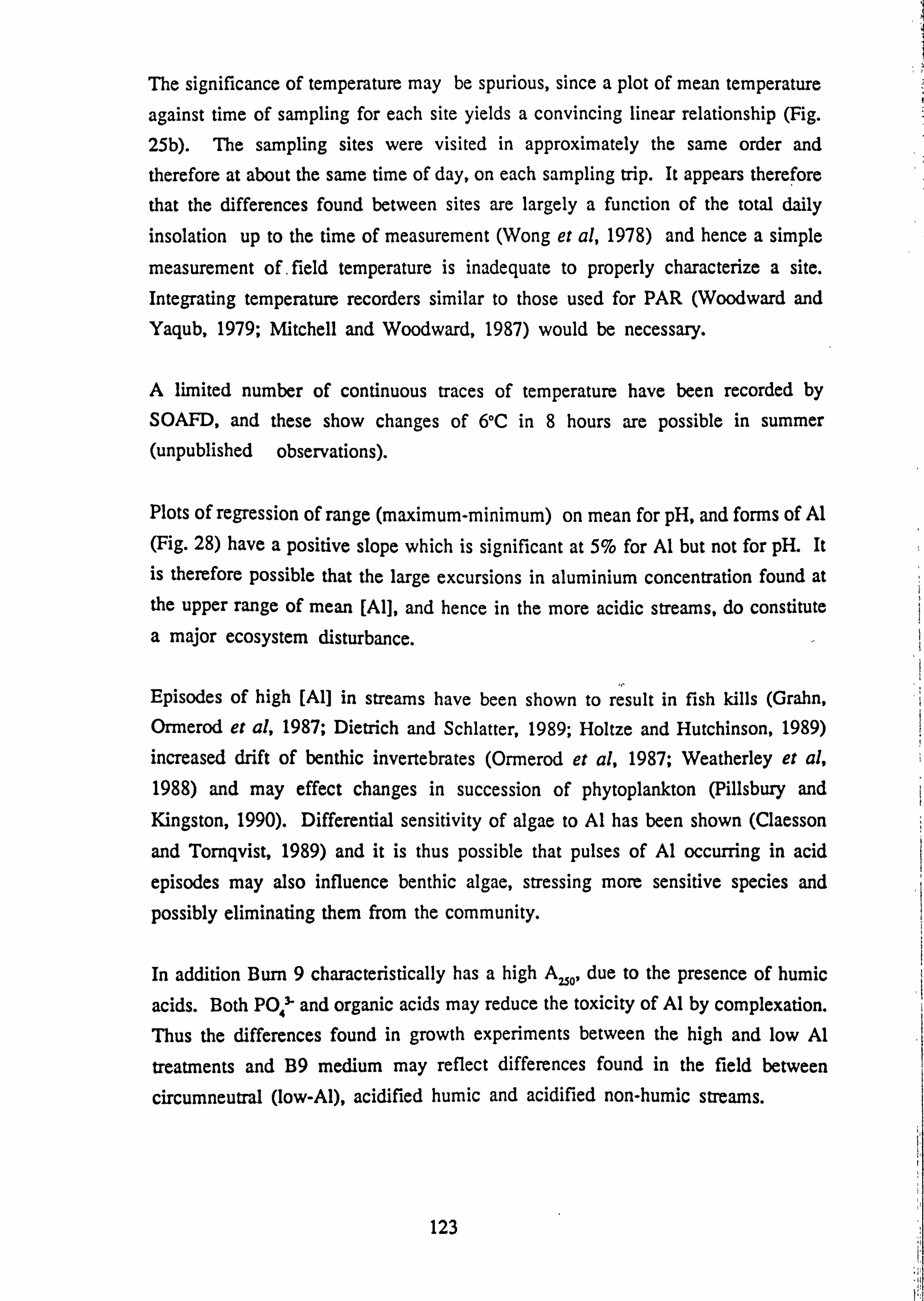
The significance of temperature may be spurious, since a plot of mean temperature
against time of sampling for each site yields a convincing linear relationship (Fig.
25b). The sampling sites were visited in approximately the same order and therefore at about the same time of day, on each sampling trip. It appears therefore
that the differences found between sites are largely a function of the total daily
insolation up to the time of measurement (Wong et al, 1978) and hence a simple
measurement of. field temperature is inadequate to properly characterize a site. Integrating temperature recorders similar to those used for PAR (Woodward and Yaqub, 1979; Mitchell and Woodward, 1987) would be necessary.
A limited number of continuous traces of temperature have been recorded by
SOAFD, and these show changes of 6°C in 8 hours are possible in summer (unpublished observations).
Plots of regression of range (maximum-minimum) on mean for pH, and forms of Al (Fig. 28) have a positive slope which is significant at 5% for Al but not for pH. It is therefore possible that the large excursions in aluminium concentration found at the upper range of mean [Al], and hence in the more acidic streams, do constitute a major ecosystem disturbance.
Episodes of high [Al] in streams have been shown to result in fish kills (Grahn, Ormerod et al, 1987; Dietrich and Schlatter, 1989; Holtze and Hutchinson, 1989) increased drift of benthic invertebrates (Ormerod et al, 1987; Weatherley et al, 1988) and may effect changes in succession of phytoplankton (Pillsbury and Kingston, 1990). Differential sensitivity of algae to Al has been shown (Claesson
and Tornqvist, 1989) and it is thus possible that pulses of Al occurring in acid
episodes may also influence benthic algae, stressing more sensitive species and
possibly eliminating them from the community.
In addition Burn 9 characteristically has a high Au0, due to the presence of humic
acids. Both PO43' and organic acids may reduce the toxicity of Al by complexation. Thus the differences found in growth experiments between the high and low Al
treatments and B9 medium may reflect differences found in the field between
circumneutral (low-Al), acidified humic and acidified non-humic streams.
123
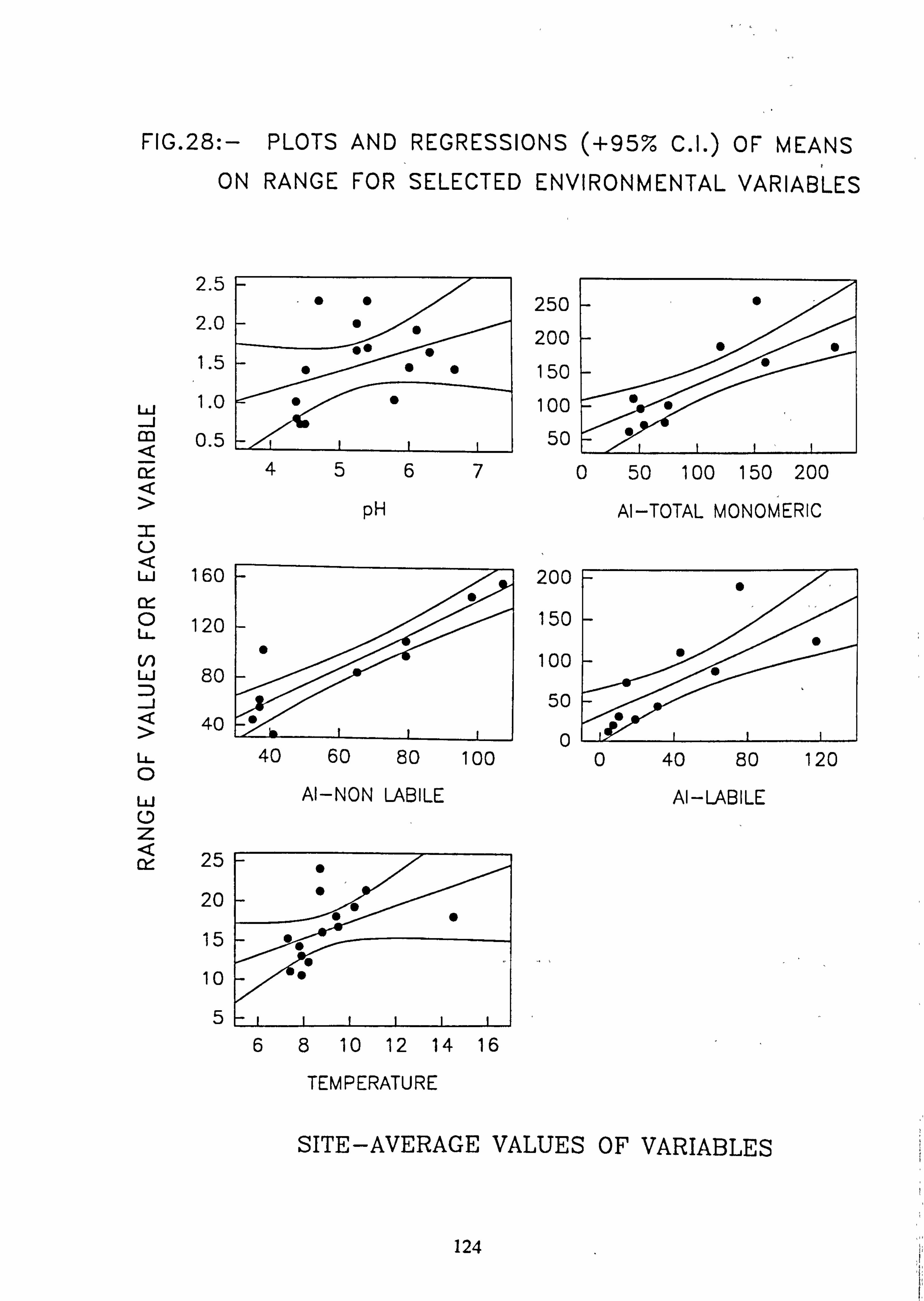
FIG. 28: - PLOTS AND REGRESSIONS (+95% C. I. ) OF MEANS
ON RANGE FOR SELECTED ENVIRONMENTAL VARIABLES
2.5
2.0
1.5
W 1.0 J
0.5
2 U w
160
cx 0 120
W 80
40
LL 0
W 0 Z
Of 25
20
15
10
S
S S S
4 5 6
pH
250
200
150
100
50
70 50 100 150 200
Al-TOTAL MONOMERIC
S
,. /
200
150
100
50
n
0 0
"
40 60 80 100 0
Al-NON LABILE
" S
0
40 80 120
Al-LABILE
9
5- 8 10 12 14 16
TEMPERATURE
SITE-AVERAGE VALUES OF VARIABLES
124
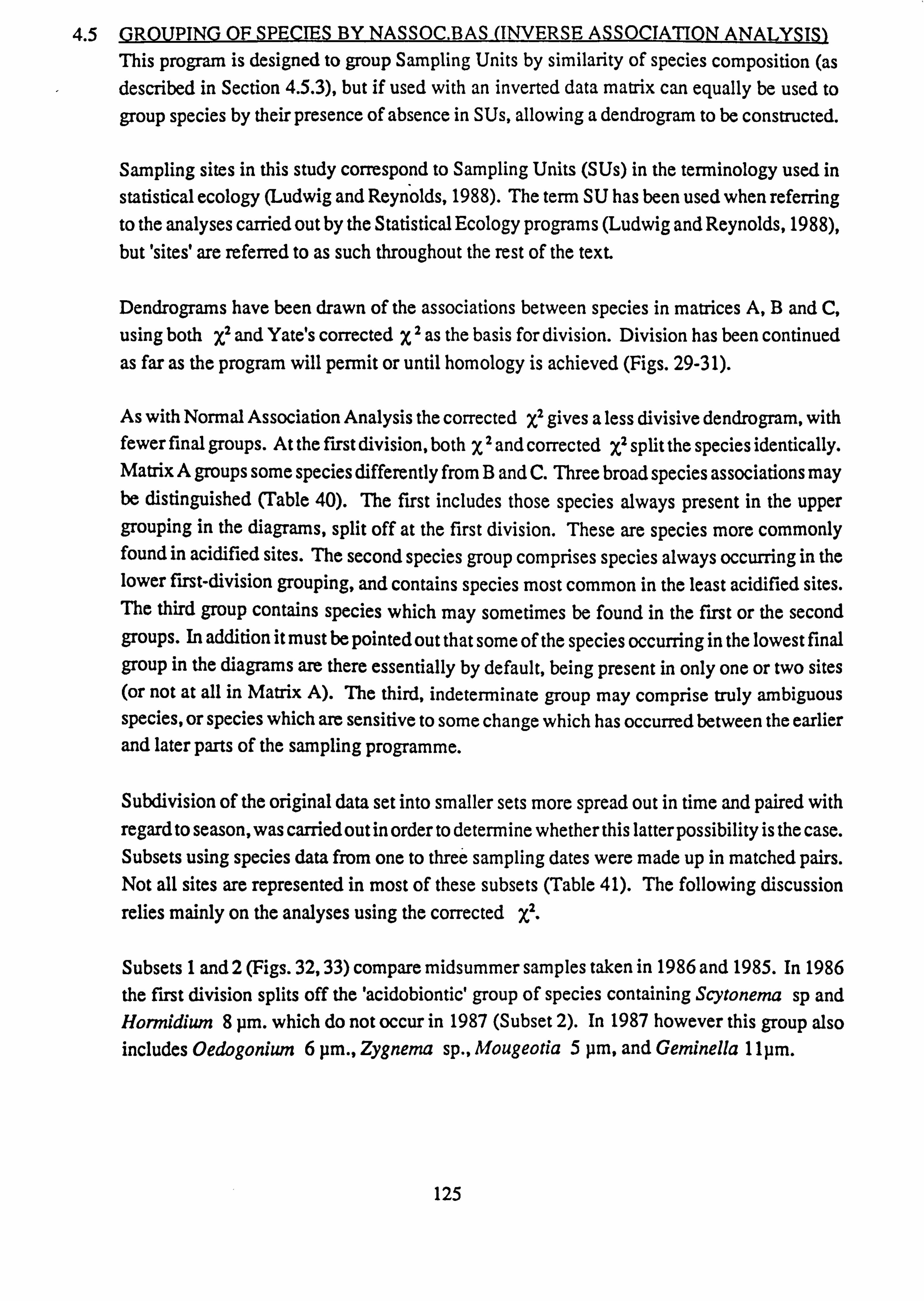
4.5 GROUPING OF SPECIES BY NASSOC. BAS (INVERSE ASSOCIATION ANALYSIS) This program is designed to group Sampling Units by similarity of species composition (as described in Section 4.5.3), but if used with an inverted data matrix can equally be used to group species by their presence of absence in SUs, allowing a dendrogram to be constructed.
Sampling sites in this study correspond to Sampling Units (SUs) in the terminology used in
statistical ecology (Ludwig and Reynolds, 1988). The term SU has been used when referring to the analyses carried out by the Statistical Ecology programs (Ludwig and Reynolds, 1988), but 'sites' are referred to as such throughout the rest of the text.
Dendrograms have been drawn of the associations between species in matrices A, B and C,
using both X2 and Yate's corrected X2 as the basis for division. Division has been continued as far as the program will permit or until homology is achieved (Figs. 29-31).
As with Normal Association Analysis the corrected x2 gives a less divisive dendrogram, with fewer final groups. At the first division, both x2 and corrected x2 split the species identically. Matrix A groups some species differently from B and C. Three broad species associations may be distinguished (Table 40). The first includes those species always present in the upper grouping in the diagrams, split off at the first division. These are species more commonly found in acidified sites. The second species group comprises species always occurring in the lower first-division grouping, and contains species most common in the least acidified sites. The third group contains species which may sometimes be found in the first or the second groups. In addition it must be pointed out that some of the species occurring in the lowest final
group in the diagrams are there essentially by default, being present in only one or two sites (or not at all in Matrix A). The third, indeterminate group may comprise truly ambiguous species, or species which are sensitive to some change which has occurred between the earlier and later parts of the sampling programme.
Subdivision of the original data set into smaller sets more spread out in time and paired with regard to season, was carried out in order to determine whether this latter possibility is the case. Subsets using species data from one to three sampling dates were made up in matched pairs. Not all sites are represented in most of these subsets (Table 41). The following discussion
relies mainly on the analyses using the corrected X2.
Subsets 1 and 2 (Figs. 32,33) compare midsummer samples taken in 1986 and 1985. In 1986
the first division splits off the 'acidobiontic' group of species containing Scytonema sp and Hormidium 8 pm. which do not occur in 1987 (Subset 2). In 1987 however this group also includes Oedogoniwn 6 pm., Zygnema sp., Mougeotia 5 pm, and Geminella 11 pm.
125
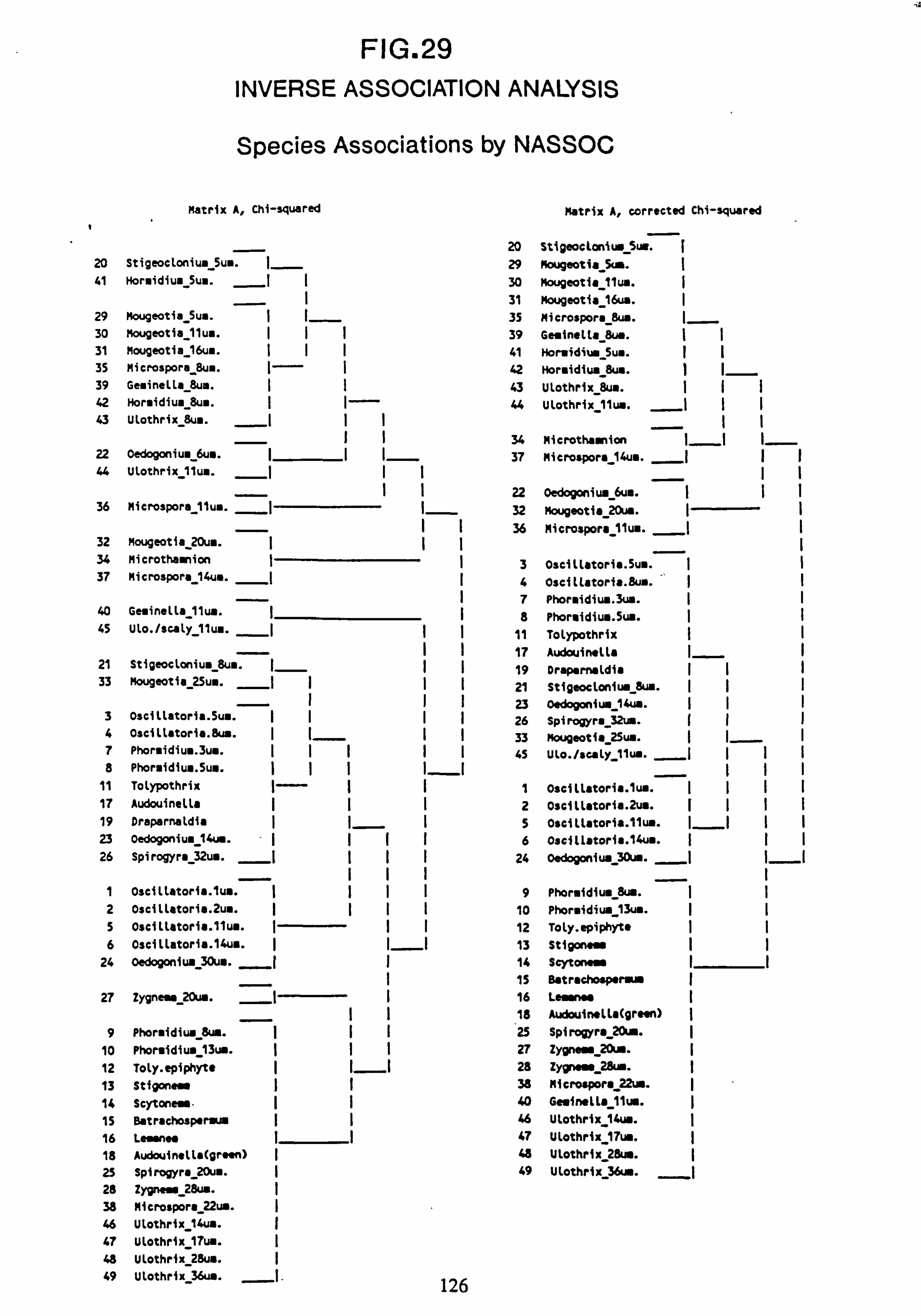
FIG. 29 INVERSE ASSOCIATION ANALYSIS
Species Associations by NASSOC
Matrix A, Chi-squared Matrix A, corrected Chi-squared
20 stigeoctoniu_ Sur. 20 Stigeocloniua 5u.. I 29 Mougeotia_Sca. 41 Horaidiua_5un. II 30 Mougeotio Ilu.. I
31 Mougeotia 16un. I 29 Mougeotia Sun. 35 Microspora 8w. 30 Mougeotia 11un. II I 39 Geninella aus. 31 Mougeotia 16u.. II I 41 Hornidiu. Su.. I 35 Microspora 8ua. 1 I 42 Horsidiw 8w. ý 39 Gesinella 8ua. I I 43 ULothrix 8u.. I 42 Horaidiua_8u". I 1 44 Ulothrix flue. 43 Ulothrix 8ua. I II
II 34 Microthaanion II 22 OedogoniuU 6u.. I II 37 Nitrospore 14ue. I 44 Ulothrix llua. II
22 Oedogoniw_6uu. I 36 Mierospora 11uß. ( I 32 Mougeotis 20w. I
36 Nitrospore 11w. I 32 Mougeotfs 20u.. I II 34 Microthannion I I3 Oscillatoria. 5ue. I 37 Nitrospore 14u.. I I4 OsciLLatorfa. 8w.
7 Phormidiw. 3ua. 40 Geainells 11w. I8 Phoreidiuw. 5w. I 45 Ulo. /scaly_llua. I II 11 Tolypothrix I
17 Audouinella I 21 Stigeoconium Bug. I II 19 Draparnaldia I 33 Mougeotia 25un. II II 21
_ Stigeoconiu. 8w. I
(( 23 u. Oedogoniuw 14 ( 3 Oscillatoria. Su.. II II 26 Spirogyra 32w. ((1 4 Osciltatoria. 8w. II (I 33 Mougeot4 25un. II 7 Phoraidiua. 3ua. II III 45 ULo. /s aLy_11w. I 8 Phor. idiua. Sun. II III
11 ToLypothrix ( III Oscillatoria. luw. I 17 Audouinella I II2 0scillatoria. 2w. ( 19 Draparnatdia I II5 OsciLtatoria. llw. (I 23 oedogoniua 14un. I III6 OscitLatoria. l4w. I 26 Spirogyra 32u.. ( II( 24
(II 0edogoniw 30un. III
1 OsclLtatoria. lu.. I III9 Phoraidiu. 8w. I 2 OsciLLatoria. 2un. I ((I 10 Phor. idiuw_13u.. 5 OsciLLatoria. llu.. I II 12 Toly. epiphyte I 6 OsciLLatoria. 14ua. I II 13 Stigoness I
24 oedogoniua_30ua. ( I 14 Scytonew 15 Betrachospernua I
27 Zygne. a20u.. I ( 16 Learn ( (I 18 Audouinella(green) I
9 Phoraidiw_dw. I I( 25 Spirogyra 20m. I
10 Phorsidius 13w. I II 27 Zygner20uU. I 12 Toly. epiphyte I II 28 Zygner28ua. 13 Stfgonees I I 38 Microspora22uu. I
14 Scytonear. I I 40 GesinotLa_lluL. 15 eatrachospenw I I 46 ULothrix_14ua. 16 Lemnos 47 ULathrix-17um. 18 Audouin. tta(green) I 48 Utothrix 28u.. 25 Spirogyra 20ua. I 49 ULothrix_3äa. I 28 Zygnme 28w. 38 Microspors22uw. I 46 ULothrix 14ui. I 47 ULothrix 17w. I 48 ULothrix 28uu. I 49 Utothrix 36u.. I. 126
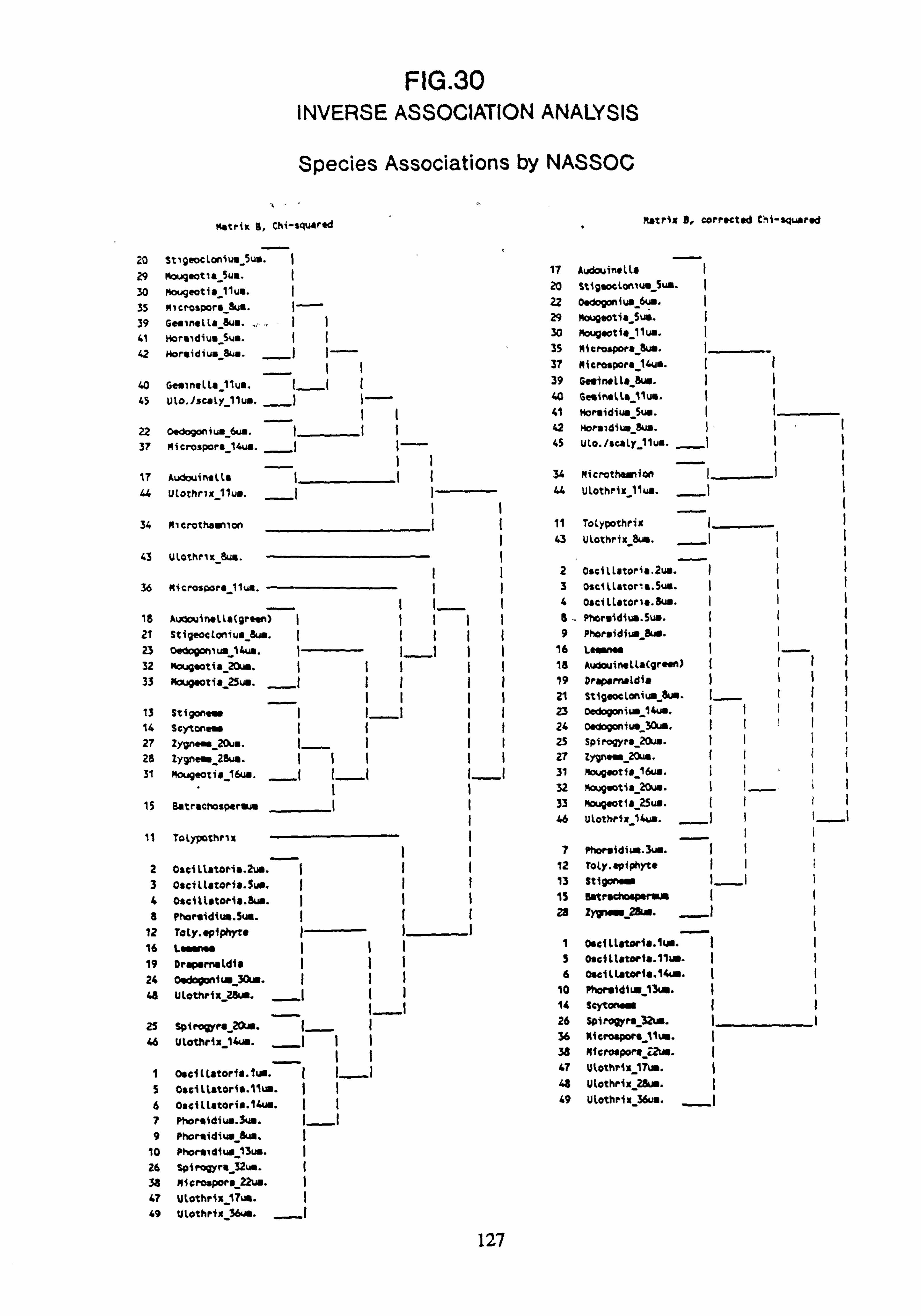
FIG. 30 INVERSE ASSOCIATION ANALYSIS
Species Associations by NASSOC
Matrix 5, Chi-squared Aatrix L. corrected C'mi-squared
20 stigeocloniua_Sua. I -r 29 Mougaot1a Sui. 17 Audouinalla I
30 Mougeotia_11ua. I 20 StiflaocLomuU Sua. I
35 Mle, OSpora_8W. I-ý 22 6us ado iw ' 39 Geainelta_8ua. 29 Mougaotia_Sum. I
41 Sua. rioriidiua 30 Mougootia_11ua. I
42 _
8ua. __)
)---- Noraidiua 35 Nitrospore Sua. _ 37 Microspora 14us. I
40 Gesinalla 11us. 39 Gesirwlla bua.
45 Uto. /scaly_11us. 40 Ge%inslls ilua. ( 41 Moraidiua_Sus. {
22 oedogoniu. bun. ý"f i1 42 nora, diua_5um. I
37 Mierospora_14w. 45 ulo. /suly�11ua. _lf {
17 I
AudouinaLts j I ( 34 Microthaanion
44 Utothrix_11us. ý(
( 4L Utothrix 11ua. _�-
34 Microthaamon II
11 Totypothrix ( 43 Ulothrix. 8w.
__{ {
43 Ulothr x_8w. (
iI2 Oscillatoria. 2us.
36 Microspors 11ua. 3 Oscillator s. Sua. I
( _4
I Oscillatona. 8us. 15 Auaouinalla(grasn) _ (((6,. Phoraidius. Sus. {!
21 Stigeoctoniua 8ua. { (((9 Phorpidiis_8us. 23 oedogoniu. 14us. (I
_j (I 16 Leasnaa
32 Mougaotia 20M. III II 1s Audouinella(9rern) ((
33 Nougaotis_25us. 19 Drapsrnaldis J
ý I 21 StigeocloniuS_aw. I___.
13 stiyonear I I, I 1I 23 Oedogiua 14w. If 14 Scytoneay (j fI 24 0adogonium 30w.
27 2ypne. a_20u.. (__ I I 25 Spirogyra-20w. I{
25 zyyne. a 2a,.. I1 I1 27 zyyn tow. ffJ 31 Mougeoti" 16uu. 31 MoUQaotio 16us. I
32 Mc gsotis 20ua. { __,
s
15 Batrachosperaw ( ( 33 Mougeotia 25us. 46 Ulothrix_14ua.
11 Totyyothrtix I 7 Phorsidiun. 3us. I{
2 0scillatoria. 2us. --I 12 toty. spiphyte I!
3 0acitlstoris. Sus. II f 13 Sti9onaas I___I
4 Oscillatoris. sus. ( { 15 6atrschoaperaw I
b Phoraidium. Sua. (( j 28 zyww &.. ý�+I
12 1oly. apipiºyte I _- 16 L. ea I( I I Oscitlatoria. lue.
19 Draparnaldis III 3 0acittatoM4. I1IS. I4
24 0adogoniua 3ßa. (() 6 oseillatoria. 1'sa. I
48 2&0. ___,
l I1 Utothrix 10 Phorsidiua 13uß. _ I I 14 Scyton. "
2S _
Spirogyra 20us. 26 Sp1rogyra_32. s. I1
46 Utothri: _14us. _ý)
II 36 Nicroapors 11uß. 38 Microspora 22um.
I oscillatoria. lus. ( (, w)
47 Ulothrix 17uw.
S 0sciltatoria. llum. 48 Utothrix 2&a.
6 Oscillatoris. l4ur. 49 Ulothrix_36us.
7 Phorsidiuw. 3ua. I__I
9 Phorsidiu. _Eus.
10 Phorsidiua 13us. I 26 Spirogyra 32uw. I
38 Microspor., 22us. I
47 Utothrix 17us. 49 Ulothrix 36uS.
127
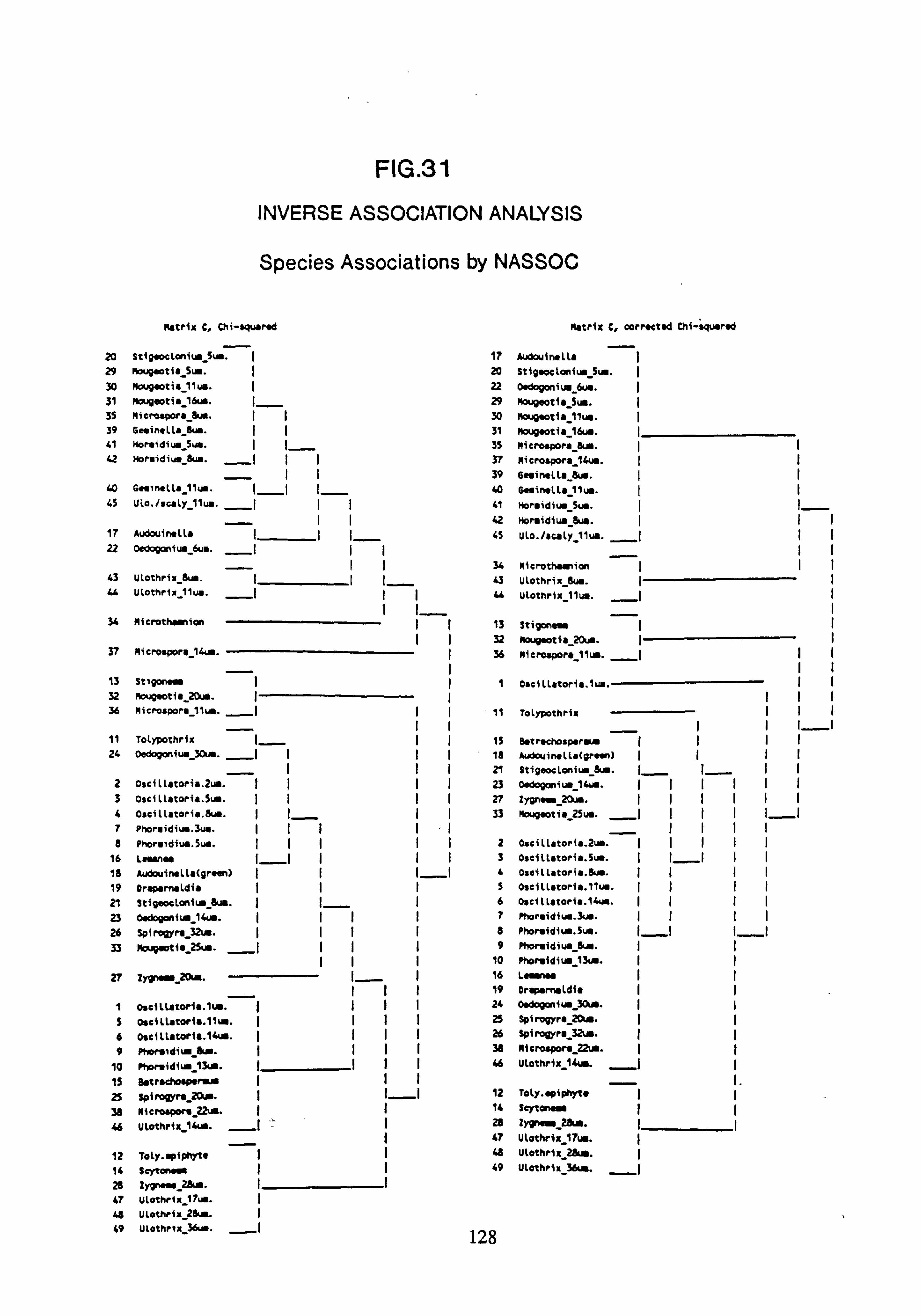
FIG. 31
20 29 30
31 35 39 <1
42
40 45
17 22
43 44
34
37
13 32 36
11 24
2
3
4 7 8
16 18 19 21 23 26
33
27 1
s 6 9
10 1S 25 38 46
12 14 28 47 48 49
INVERSE ASSOCIATION ANALYSIS
Species Associations by NASSOC
Matrix C, Chi-squared matrix C, corrected Chi-squared
Stipaocloniua Sum. I 17 Audouinalla Mouyeotia_Sua. I 20 StiyaocloniusSun.
_ Mougaotia llua. I 22 0sdogoiua6 _ .
Mou9eotia 16uw. 29 Moigeotia_ a. Microspora_8ua. II 30 Moupwtia 11u.. Gesinella 8w. II 31 Mougaotis 16w.
Moraidiw_5ua. I_ý 3S Microspora &A. Horaidiu.
_sua. _ III 37 Microspora 14uß.
I 39 Geainalla &a. Geainelta 11ua. I_I I_ 40 Guinalla 11ua. Ulo. /scaly_llua.
_ III 41 Hor. idiun Sua. I (__
42 Hornidiu. -8w. Audouinella II Iý 45 Ulo. /scaly 11w.
oedogoniua_6u.. ^- 34 Microthamion I
Ulothrix_bu.. I I__ 43 Ulothrix bw. I Ulothrix llu..
_ III 44 Ulothrix llun.
Microthaanion I I__
13 Stiganer I
32 Moupaotia20um. I Microspora 14uß. I 36
i Microspora_11..
_I
Stigor. II Oscillatoria, lua. Mougaotia 20um.
Nitrospore 11um. _
III 11 Tolypothrix I III
Totypothrix 15 _
Batrachosparu --I
0edogoniua 30um. _ _I
III 13 Audouinalla(gr«n) I
21 Stigeoclaniua-Eis. Oscillatoria. 2uw. IIII 23 0rdoganiua-14ua. I Oscillatoria. 5ua. II 27 Zypn. 20u. I
Oscillatoria. eua. I_ II 33 Mougaotia25u.. __I III I__I
Phoraidiua. 3w. IIII Phoraidiua. Sua. IIII2 Oscillatoria. 2um. I
Cannes I__I III3 Oscillatoria. Sua. I (__I Audouinalla(grean) II I__I 4 oscillatoria. 3uA. I
Draparnaldia IIIS Oscillatoria. llu.. I
Stigeocloniua-bus. I__ I6 Oscillatoria. l4ua. I 0adogoniua-14 a. III7 Phoraidiua. 3ua. I
SpiraVra_32un. IIIIe Phoraidiua. Sua. Moupaotia25ua.
_ _I III9 Phornidiu. Eis. I
10 Phorvidiua-13uß.
Zygs>"20a. I__ I 16 Lasxrw II 19
_ Draparnaldis I
0scillatoria. lua. IIII 24 0adogoniua_30um. I
Oscillatoria. llum. IIII 25 Spirogyra20un. I
Oscillatorla. 14ua. IIII 26 SPirogyr! 32um" I
Phorndiua_&a. iIII 38 Microapora22ua. I
Phornidiua-13um. III 46 Ulothrix 14uß, . ý)
eatrachosp'fsa III I. --
Spirogyra20um. I I_I 12 Toly. agiphyta I
Mierosyora 2'. . II 14 Sayto
Ulothris_14u0. ý IFI 28 Zygnasst2&m.
_ I 47 Ulothrix_17ur.
Toly. plphyta II 48 Ulothrix 2&a. I
Scytansw II 49 Ulothriti 36ua. ý+I
Zyg... 2eß.. I Ulothri: 17un. I
Ulot rix 2&a. I
Ulothri _36ua. ý _I 128

TABLE 40 SPE CIES GROUPS REVEALED BY INVERSE
ASSOCIATIO N ANALYSIS ON MATRICES A, B, AND C
'Acidobiontic' 2. Remnant 3. Indeterminate
Stigeoclonium 5 pm. Oscillatoria spp. Audouinella
Oedogonium 6 pm. * Phormidium spp. Mougeotia 20 pm.
Mougeotia 5 pm. * Tolypothrix Geminella 11 pm.
M. 11 pm. Epiphyte of Tolypothriz Ulothrix -sc. 11 pm.
M. 16 pm. * Stigonema sp.
Microthamnion * Scytonema sp.
Microspora 8 pm. Lemanea sp.
M. 14 pm. * Batrachospermum sp. Geminella 8 pm. * Audoulnella (green)
Hormidium 5 pm. Stigeoclonium 8 pm. H. 8 pm. * Draparnaldia sp. Ulothrix 8 pm. * Oedogonium 14 pm. U. 11 pm. * O. 30 pm.
Spirogyra spp.
Zygnema spp.
Mougeotia 25 pm.
Microspora 11 pm.
M. 22 pm.
Ulothrix 14 pm.
U. 17 pm.
U. 28 pm.
U. 36 pm.
*These species would be classified indeterminate taking the results of subset analyses into account
129
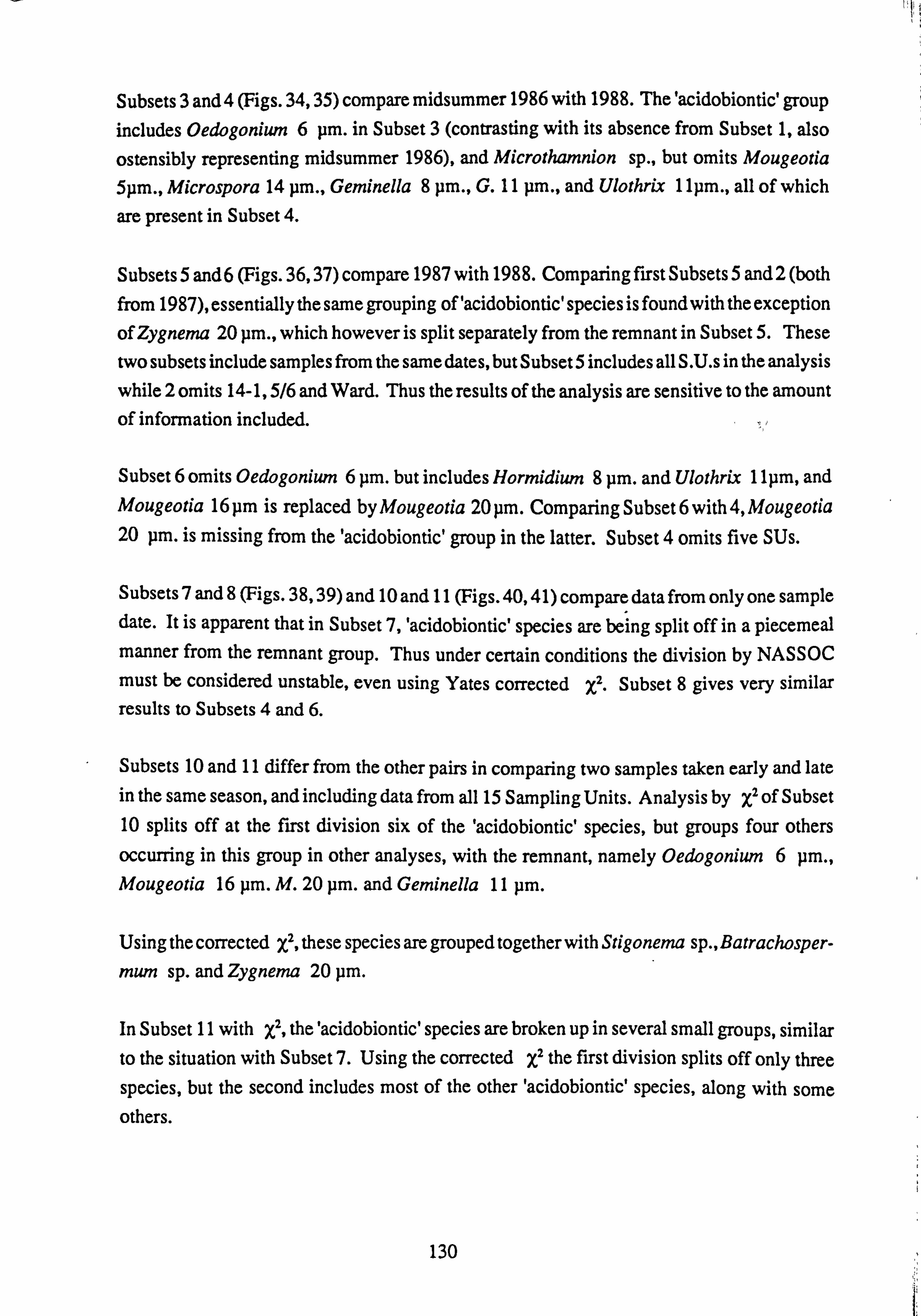
Subsets 3 and 4 (Figs. 34,35) compare midsummer 1986 with 1988. The'acidobiontic' group includes Oedogonium 6 pm. in Subset 3 (contrasting with its absence from Subset 1, also ostensibly representing midsummer 1986), and Microthamnion sp., but omits Mougeotia 5}ßm., Microspora 14 pm., Geminella 8 pm., G. 11 pm., and Ulothrix 11}ßm., all of which are present in Subset 4.
Subsets 5 and6 (Figs. 36,37) compare 1987 with 1988. Comparing first Subsets 5 and 2 (both from 1987), essentially the same grouping of 'acidobiontic'species is found with the exception of Zygnema 20 pm., which however is split separately from the remnant in Subset 5. These
two subsets include samples from the same dates, but Subset 5 includes all S. U. s in the analysis while 2 omits 14-1,5/6 and Ward. Thus the results of the analysis are sensitive to the amount of information included.
Subset 6 omits Oedogonium 6 pm. but includes Hormidium 8 pm. and Ulothrix 11pm, and Mougeotia 16 pm is replaced by Mougeotia 20 pm. Comparing Subset 6 with 4, Mougeotia 20 pm. is missing from the 'acidobiontic' group in the latter. Subset 4 omits five SUs.
Subsets 7 and 8 (Figs. 38,39) and 10 and 11 (Figs. 40,41) compare data from only one sample date. It is apparent that in Subset 7, 'acidobiontic' species are being split off in a piecemeal manner from the remnant group. Thus under certain conditions the division by NASSOC
must be considered unstable, even using Yates corrected X2. Subset 8 gives very similar results to Subsets 4 and 6.
Subsets 10 and 11 differ from the other pairs in comparing two samples taken early and late in the same season, and including data from all 15 Sampling Units. Analysis by x2 of Subset
10 splits off at the first division six of the 'acidobiontic' species, but groups four others
occurring in this group in other analyses, with the remnant, namely Oedogonium 6 pm., Mougeotia 16 pm. M. 20 pm. and Geminella 11 pm.
Using the corrected x2, these species are grouped together with Stigonema sp., Batrachosper-
mum sp. and Zygnema 20 pm.
In Subset 11 with x2, the'acidobiontic' species are broken up in several small groups, similar to the situation with Subset 7. Using the corrected x2 the first division splits off only three species, but the second includes most of the other 'acidobiontic' species, along with some others.
130
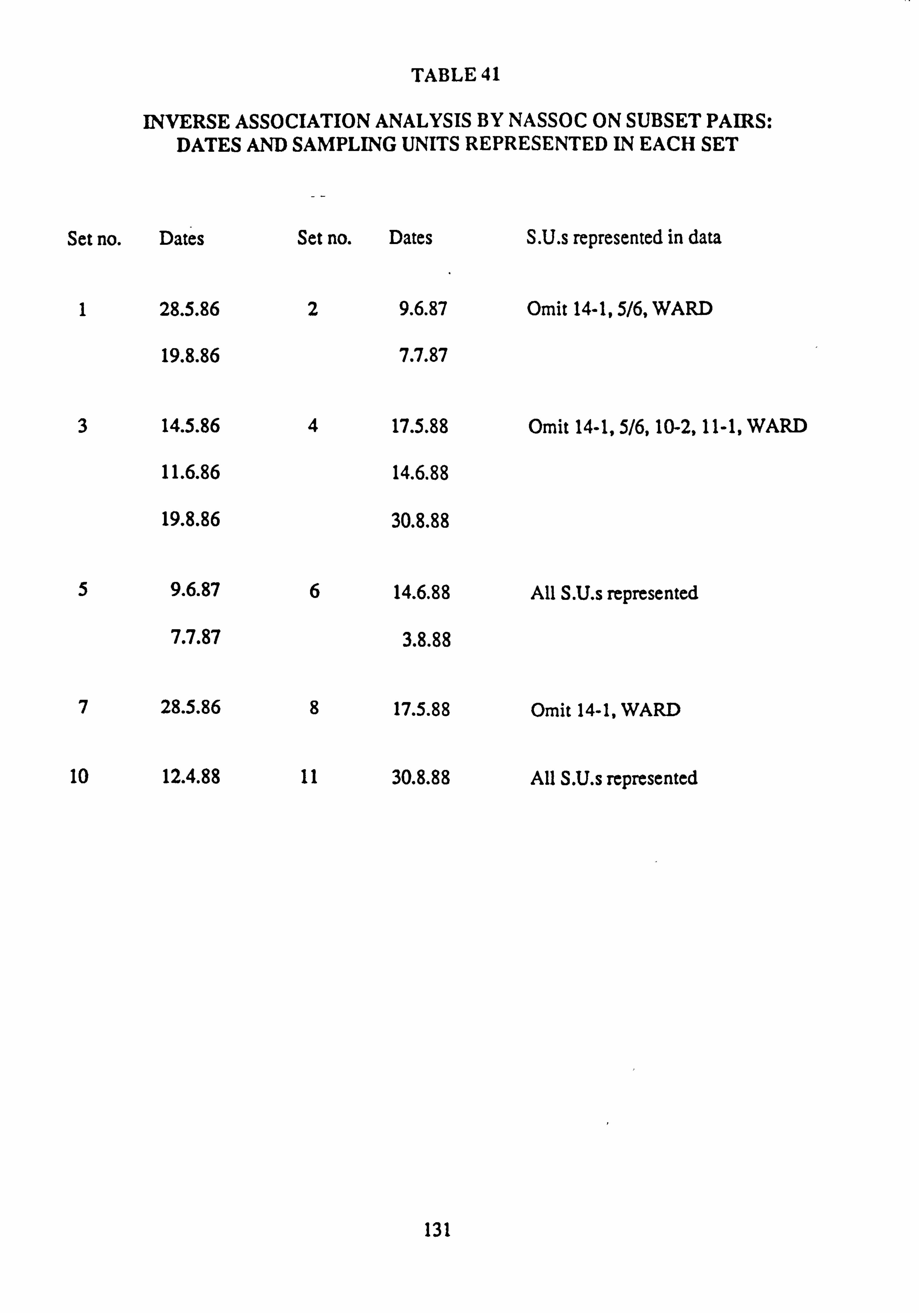
TABLE 41
INVERSE ASSOCIATION ANALYSIS BY NASSOC ON SUBSET PAIRS: DATES AND SAMPLING UNITS REPRESENTED IN EACH SET
Set no. Dates Set no. Dates S. U. s represented in data
1 28.5.86 2 9.6.87 Omit 14-1,5/6, WARD
19.8.86 7.7.87
3 14.5.86 4 17.5.88 Omit 14-1,5/6,10-2,11-1, WARD
11.6.86 14.6.88
19.8.86 30.8.88
5 9.6.87 6 14.6.88 All S. U. s represented
7.7.87 3.8.88
7 28.5.86 8 17.5.88 Omit 14-1, WARD
10 12.4.88 11 30.8.88 All S. U. s represented
131
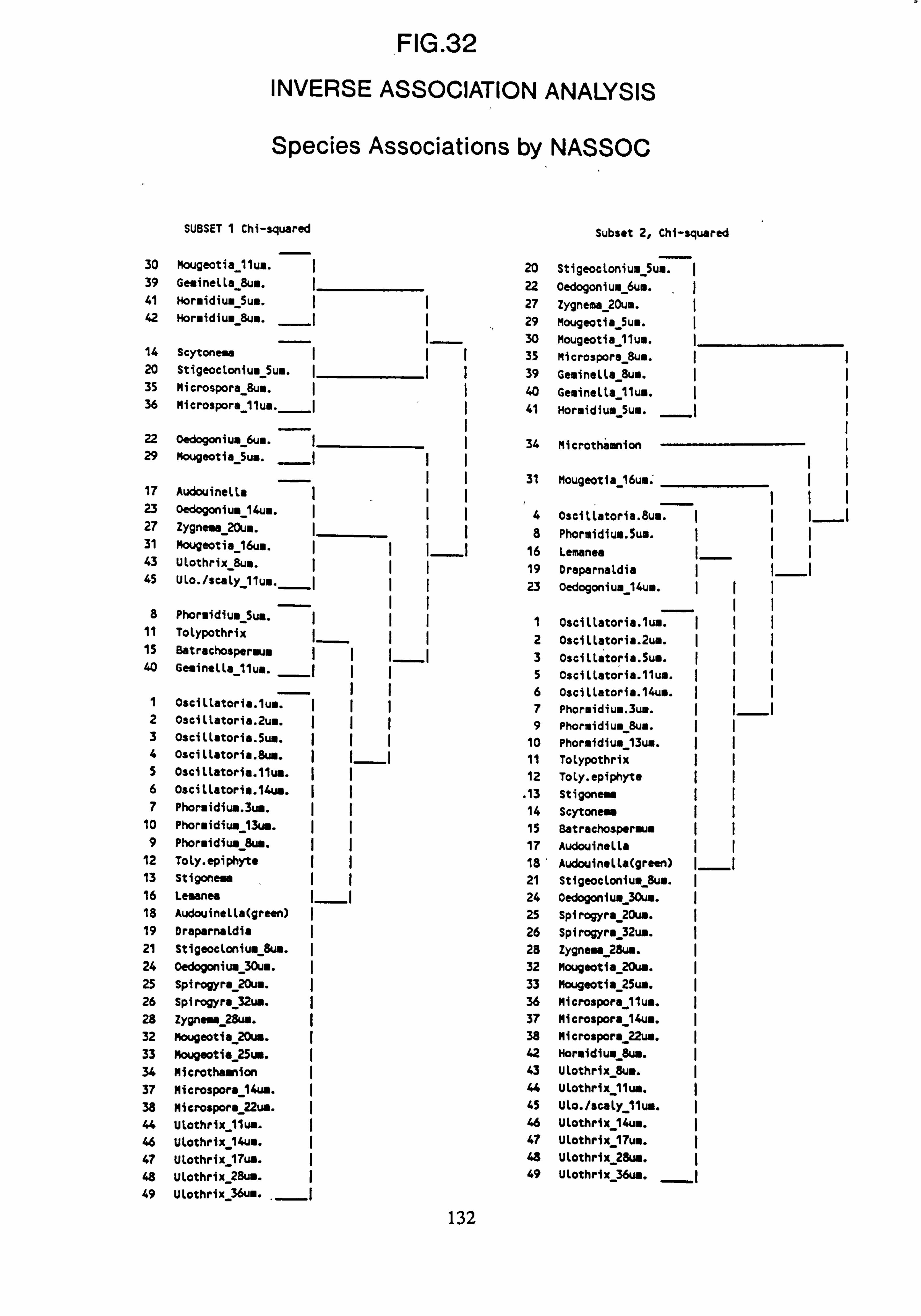
FIG. 32
INVERSE ASSOCIATION ANALYSIS
Species Associations by NASSOC
SUBSET 1 Chi-squared
30 Mougeotia 11un. 39 Ge. inellasum. 41 Horaidiu.
_5um. 42 Ftor. idiu. Bun.
14 Scytone. a 20 Stigeoclonium-5u.. 35 Microspora sun. 36 Microspora llua.
_
22 Oedogoniu. 6ua. 29 Mougeotis 5u..
17 Audouinella 23 Oedogoniua,
_14ua. 27 Zygne. a_20u.. 31 Mougeotia 16ua. 43 Ulothrix_8ua. 45 Ulo. /scaly_llun.
_
8 Phorsidiu. 5un. 11 ToLypothrix 15 Batrachosperoue 40 Ge. inella ilua.
1 Osciltatoria. lue. 2 Oscillatoria. 2u.. 3 0scillatoria. 5uw. 4 Osciltatoria. 8ua. 5 Oscillatoria. lluw. 6 0scitLatoria. 14uw. 7 Phor. idiuw. 3um.
10 Phor. idiua 13u.. 9 Phor. idius_8us.
12 Toly. epiphyte ý 13 Stigonear ý 16 Lesanea ý 18 Audouinelta(green) 19 Draparnaldia ý 21 Stigeocloniue 8ua. ý 24 Oedogoniu. 30u.. ý 25 Spirogyrs 20ua. ý 26 Spirogyra_32uM. ý 28 Zygneaa 28ua. ý 32 Mougeotia 20uw. 33 Mougeotia 25uw. ý 34 Microthaanion ý 37 Microspora_14um. 38 Microspors 22ua. 44 Ulothrix lluw. ý 46 Ulothrix_14uu. ý 47 Ulothrix 17uw. 48 ULothrix 28u.. 49 ULothrix 36uu. ý
Subset 2, Chi-squared
20 Stigeoctonius 5uß. 22 oedogonium 6us. 27 Zygnema 20us. 29 Mougeotia Su.. ý 30 Mougeotia 11us. ý 35 Microspore 8u.. ý 39 Gesinelta 8u.. ý 40 Gesinetta 11us. 41 Horsidius Sus. ý
34 Mierothaanion
31 Mougeotia 16us.
4 Oscillatoria. 8u.. ý 8 Phormidiuo. 5us. ý
16 Lemanea 19 Draparnaldis Iý 23 oedogonius 14uo.
1 Oscillatoria. lus. IIý 2 Oscillatoria. 2uo. IIý 3 Oscillatoria. Su.. 5 Oscillatoria. llua. 6 Oscillatoria. 14u.. ý 7 Phorsidiu.. 3us. 9 Phormidiu. Bus. ý
10 Phoraidiu. 13ue.
11 Tolypothrix ý 12 Toly. epiphyte 13 Stigonem 14 Scytonen 15 eatrachospersus 17 Audouinella 18 Audouinelta(green) ý 21 Stigeocloniu. 8u.. 24 Oedogoniu. 30uw. 25 Spirogyra 20us. ý 26 Spirogyra 32uw. 23 Zygne. e_28ua. 32 Mougeotis 20ua. ý 33 Mougeotia 25u.. ý 36 Microspors_llua. ý 37 Microspora 14ua. 38 Microspora22uw. 42 Hor"idium 8uß. I 43 Ulothrix sun. 44 Ulothrix 11uw. ý 45 Ulo. /scaly_llu.. ý 46 Ulothrix 14um. ý 47 Ulothrix_17u.. 48 Ulothrix_28uu.. ý 49 Ulothrix 36uw.
132
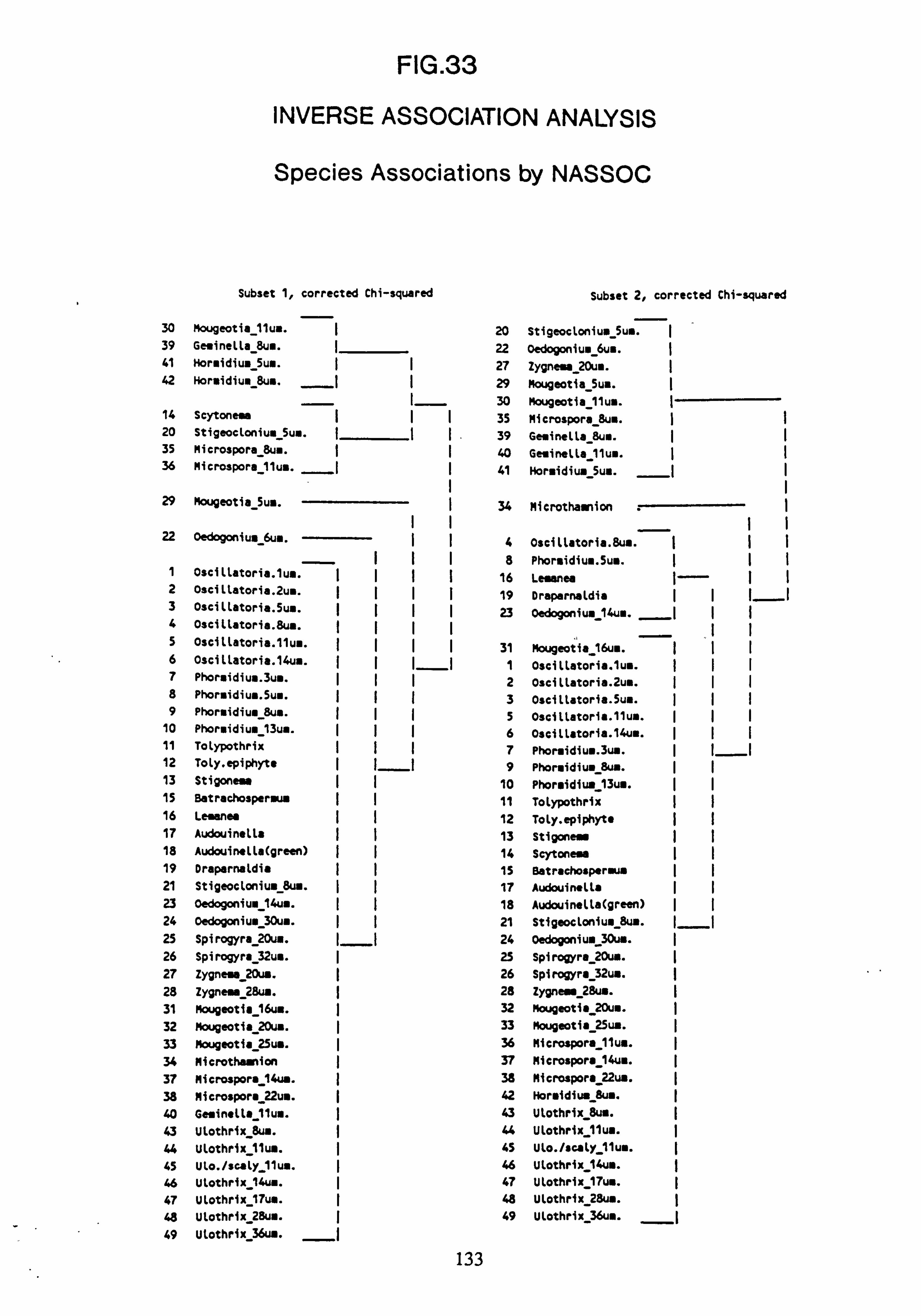
FIG. 33
INVERSE ASSOCIATION ANALYSIS
Species Associations by NASSOC
Subset 1, corrected Chi-squared
30 Mougeotia 11ue. 39 GenineLLa_Su". 41 Horaidiu.
_5u.. 42 Horaidiu. 8u..
14 Scytonem 20 Stigeocloniu. 5ua. 35 Microspora 8u.. 36 Microspora_11u..
_
29 Mougeotia 5u..
22 Oedocgoniu. 6u..
10 11 12 13 15 16 17 18 19 21 23 24 25 26 27 28 31 32 33 34 37 38 40 43 44 45 46 47 48 49
Oscillatoria. lue. OsciLtatoria. 2u.. 0scillatoria. 5ua. 0scittatoria. 8ua. Oscitlatoria. llua. Oscitlatoria. 14un. Phoreidiun. 3u.. Phoraidiua. Su.. Phoraidiu.
_8ua. Phoraidiu. _13ua.
Totypothrix Toly. epiphyts Stigonea.
Batrachospersru Leienea Audouinetla
AudouineLLa(green) Draparnaldia Stigeoctoniu. 8uu.
oedogoniu. 14u..
oedogoniu. 30un.
Spirogyra 20ua.
Spirogyra 32us.
Zygneae_20uw. Zygne. s 28uw.
Mougeotia 16u..
Mougeotia 20ua.
Mougeotia 25us.
Mi crothaani on Microspora 14ua.
Microspora_22ua. Ge. inetta_lluu.
Ulothrix 8ua.
ulothrix_llua. Ulo. /scaly llu..
Utothrix 14ua.
ULothrix_1Tua. Utothrix 28um.
Utothrix 36uw.
Subset 2, corrected Chi-squared
20 Stigeoclonium-5u.. 22 oedogonium
- 6u..
27 Zygnen 20ua. 29 Mougeotia 5u.. 30 Mougeotia llu.. 35 Microspora Su.. 39 Ge. inella 8u.. 40 Gesinella_11u.. 41 Hor. idium 5u..
34 Microthamnion
4 Osciltatoria. 8ua. ý 8 Phoraidiua. 5u".
16 leaanea 19 Draparnaldia 23 Oedogoniua_14ua. IIý
31 Mougeotia 16un. I Oscittatoria. lu.. ý 2 Osciltatoria. 2ua. ý 3 Oscittatoria. 5ua. 5 Oscitlatoria. llua.
6 Oscillatoria. 14u.. 7 Phoraidiu.. 3un. 9 Phoraidiua 8ua.
10 Phor. idiua_13u.. ý 11 Tolypothrix
12 Toly. epiphyto 13 Stigone. a 14 Scytone. a 15 Batrachosperaus
17 Audouinella 18 Audouinelta(green) 21 Stigeoctoniuu 8ua. ý 24 Oedogoniui. 30ua. 25 Spirogyra 20uw. ý 26 Spirogyra 32u.. 28 Zyyne. s 28ua. 32 Mougeotia_20uU. ý 33 Mouyeotia 25u.. ý 36 Microspora lluu. 37 Microspora 14ua. 38 Microspora_22uw. ý 42 Horaidiu.
_Su.. 43 Utothrix_8u.. ý 44 Ulothrix llu.. ý 45 Ulo. /scaly_llu.. ý 46 Ulothrix_14u". ý 47 Ulothrix 17u.. 48 Ulothrix 28u.. ý 49 Ulothrix 36u..
133
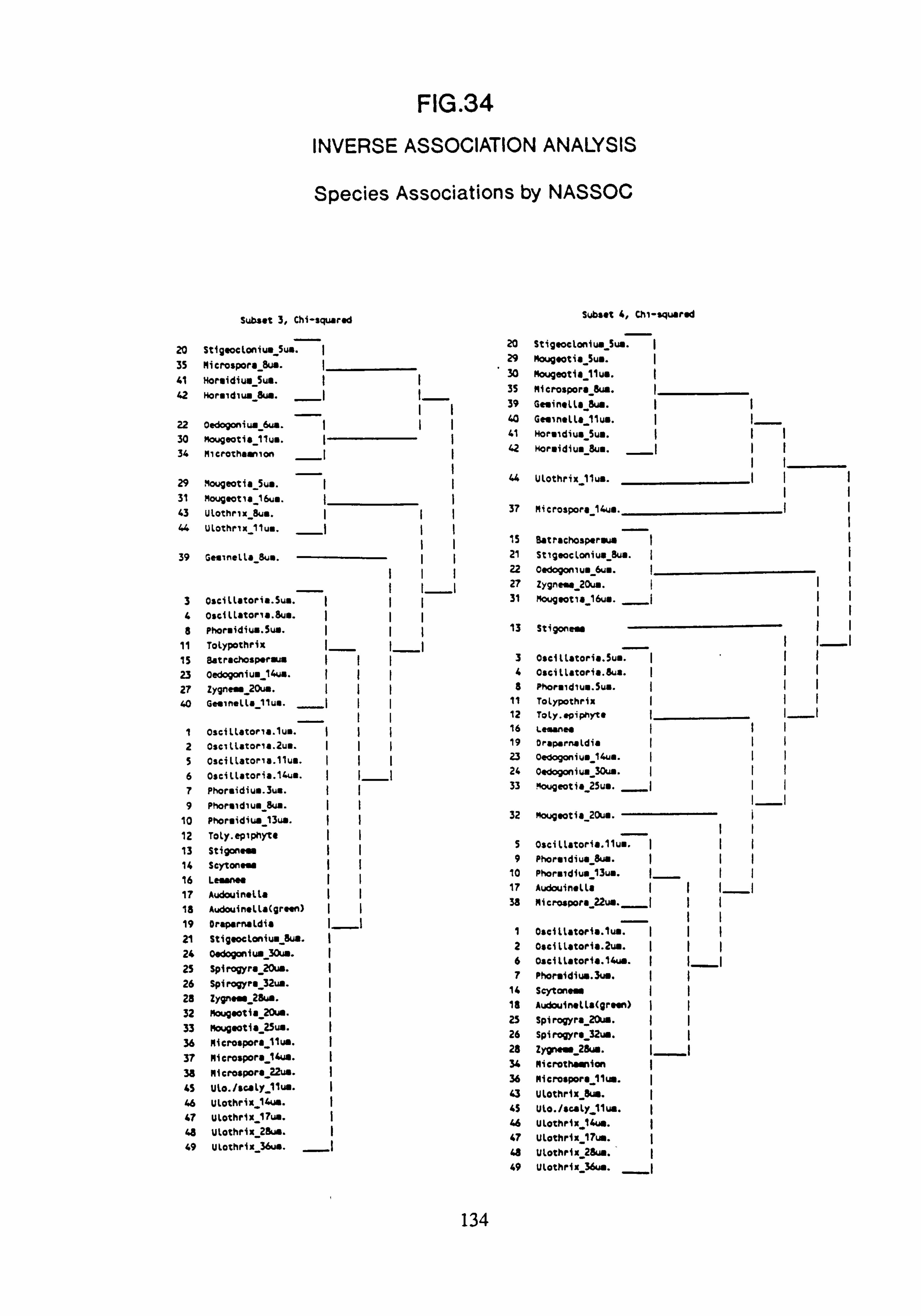
FIG. 34 INVERSE ASSOCIATION ANALYSIS
Species Associations by NASSOC
20 35 41 42
22 30 34
29 31 43 44
39
e
1s 23 n 40
1 2 S
6 7 9
10 12
13 14 16 17 1b 19 21 24 25 26 23 32 33 36 37
38
4s 46 47 48 49
Subset 3, Chi-squared Subset 4, Chi-squared
Stigeoclonium 5ua. I 20 Stigeocloniu. _Suw
I
Mierospors 8w. I 29 Mougootia_Su.. I
Horaidium Sui. 30 Mougeotia llua. I
Fbraidiu"8w. 35 Microspora Sue. 39 GenineLla Sua.
oni 6w . o- OI 40 Geainella 11ua. I I_
Mougege otia _11
ua .I 41 Moraidiua_Sua. III
Mierothsamon _I
42 _I
II Moraidiua-, Um. I
Mougeotia 5ua. I I 44 Ulothrix 11ua.
Mougeotla 16ua.
Ulothrix 8ua. I I 37 Microspora 14ua. I
Ulothr xllus. I I _ 15 Batrachosperaua
Geainella Sua. 21 Stigeocloniun_Bua. I
22 oedogomu. 6u . I _I
27 Zygner_20w.
oseillatoria. Sw. I 31 Mougsotie 16w.
Oscillatoria. 8u.. III Phoraidiw. Sua. III 13 Stigoneve Tolypothrix Batrachosperaun I 3 Oseiltatoria. Sua. I
Oedogonium-14un. III 1. Oscillatcria. aua. II
Zygnesr 2Oua. III 6 Phoraidiu.. Sua. II Geainella_11ua. 11 Tolypothrix II
12 Toly. piphyte IýýI
Oscillatoria. lua. 16 Lesanee I1I
oscittatoria. zua. 19 Oraparnaldia I
Oseillatoria. llua. I 23 oedogonius_14ua. I
Oseillatoria. 14us. I_I 24 Oedogoniue 30w. III
Phoraidiuo. 3un. I 33 ftpeotia 25ua. _I
Phoraidiua Sue. I I-I
Phoraidiua13ua. I 32 Mougaotia_20ua.
Toly. eplpnyte I _. II
S Oscillatoria. llua. I Stigonen I
9 Phoraidiue euw. II Seytone. I II 10
_ 13ua. Phoraidiua I A 17 _ ý
Audouinella (II I Audeu douin etta _ Audouinella(green) II 38 Microspora_22ua.
_I II
Drapernaldi" I_I I Osctllatoria. lw
Stigaoelonium Im. I 2 Oscillatoria. 2ua. III
oodogoniuw 30u.. 6 oscitlatoria. 14uw. II I
Spirogyra_20w. 7 _
Phoraidiuw. 3uw. II Spirogyra 32us.
14 Sogtoner I I Zygnom 2Sw.
18 Audouinalla(graen) II Mougaotia 20w. I
25 Spirogyra 20w. Moupsotia_25u .I 26 Spirogyra 32w. II Mierospora 11w. I
28 Zygneiw 2Ew. Microspora 1iw.
34 _
Microthareion Microspora22ua. I
36 6 Microspora 11w. Ulo. /tiny 11w. I
43 Ulothrix Ow. Ulothrix 16uw. I
4S Ulo. /scaly llua. Ulothrix iTw. I
46 Ulothrix 14un. Utothrix 26w.
47 Ulothrix 17w. Ulothrix_36w. is
_ Ulothrix 28w.
49 Ulothrix 36ua. _ýI
134
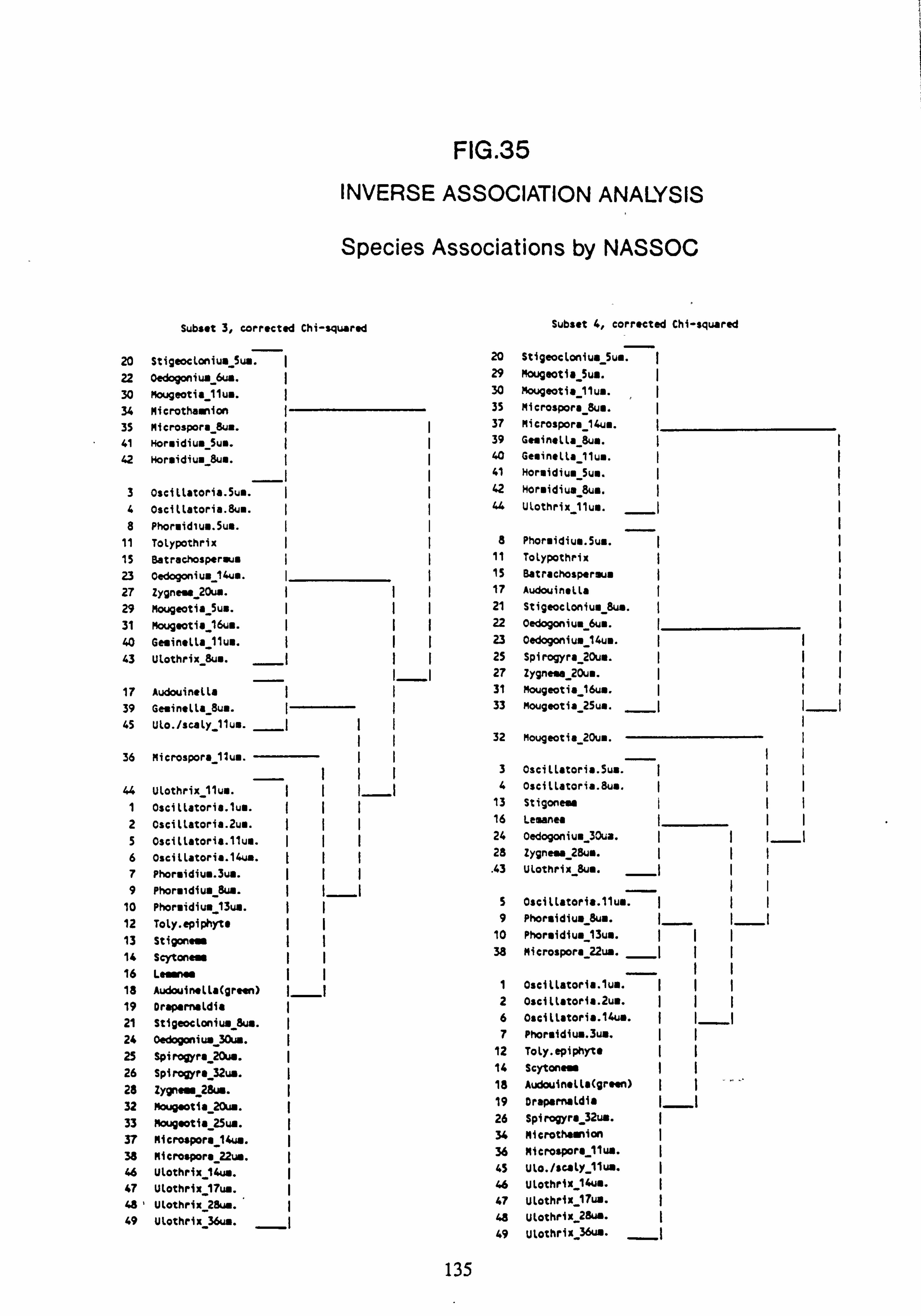
FIG. 35 INVERSE ASSOCIATION ANALYSIS
Species Associations by NASSOC
Subset 3, corrected Chi-squared Subset 4, corrected Chi-squared
20 Stigeoclonium-sum. I 20 Stigeocloniu. 5u.. I 22 Oedogoniua 6ua. 29 Mougeotia Sus. I
30 Mougeotia 11ua. { 30 mougeotia llua.
34 Microthasnion I 35 Microspore -
8uN. I
35 Microspora_8ua. II 37 Microspora_14u.. I
41 Horuidium-Sum. II 39 Ge. inella 8u.. {
42 Horaidium-Sum. 40 GeaineLLa llua. 41 Horsidiu. 5u.. I
3 OsciLtatoria. Su.. II 42 Hornidiua 8u.. 4 OscitLatoria. 8u.. II 44 Ulothrix 11u.. I
8 Phoruidiu". 5um. {
11 Tolypothrix I 8 Phorsidium. Su.. I
15 8atrachospermus 11 Tolypothrix I
23 Oedogoniuw 14ua. { 15 Batrachospermua {
27 Zygneus 20ua. II 17 AudouineLLa I
29 Mougeotia Sun. II 21 Stigeoclonium-8ua. I 31 Mougeoti" 16us. II ( 22 Oedogonium-bus. {
40 Ge. inetla llu.. II ( 23 Oedogonium 14u.. I
43 Ulothrix 8uu. I{ 25 Spirogyra 20us. 27 Zygne. e 20u.. I{
17 Audouinelta 31 Mougeotia 16u.. I
39 Ge. inelta 8ua. I{ 33 Mougeotia 25un. III
45 Ulo. /scaly_llus. III 32 Mougeotia 20ua. {
36 Microspora llua. II {{ 3 OsciLLatoria. Su.. I{{
44 Ulothrix lluu. I {_I 4 OsciLLatoria. 8us. I{
1 oscitLatoria. lu.. (I 13 Stigonesr II{
2 OsciLtatoria. 2uu. II 16 Lemanea {
5 OscitLatoria. llu.. III 24 0edogoniu 30ua. I
6 OsciLLatoria. 14ua. tI{ 28 Zygneaa 28u.. I{
7 Phoraidium. 3us. II . 43 ulothrix -8u..
I(
9 Phor. idium Sum. I{I {
10 Phor. idiu. 13uw. I S OscitLatoria. llue. I
12 Toly. epiphyt" II 9 Phorsidiu. 8u.. {{I
13 Stigonesxi 10 Phoraidiu. 13un. I
14 scytonew I 38 Mierospors22ua.
16 LesxmM II 18 Audouinella(green) II 1 OsclLLatoria. lui.
19 Draparnaldia 2 OscitLstoria. 2ua. I
21 Stigeoclaniua 8u.. I 6 OsciLL. toria. 14ui. I
24 -
Oedogoniu. 30u.. 7 Phoraidiuw. 3u1. I
25 Spirogyra-0u.. I 12 ToLy. epiphYte I
26 Spirogyra32u.. { 14 Scytones {
28 Zygneve 28u . 18 Audouinatla(green) I
32 Mougeotia20u.. 19 Drapernaldia
33 Mougeotia25uw. 26 spirogyra32uw.
37 Microspora 14w. 34 Microtha. nian I
38 Microspore22u.. I 36 Microspora_11un. I
46 Ulothrix 14w. I 45 Ulo. /suly_llua. I
47 Utothrix 17uw. I 46 Utothrix 14u". {
48 1 ULothrix 28u.. I 47 ULothrix 17us. I
49 ULothrix 36us. 48 Ulothrix_28uw. I _ 49 ULothrix 36u@. I
135
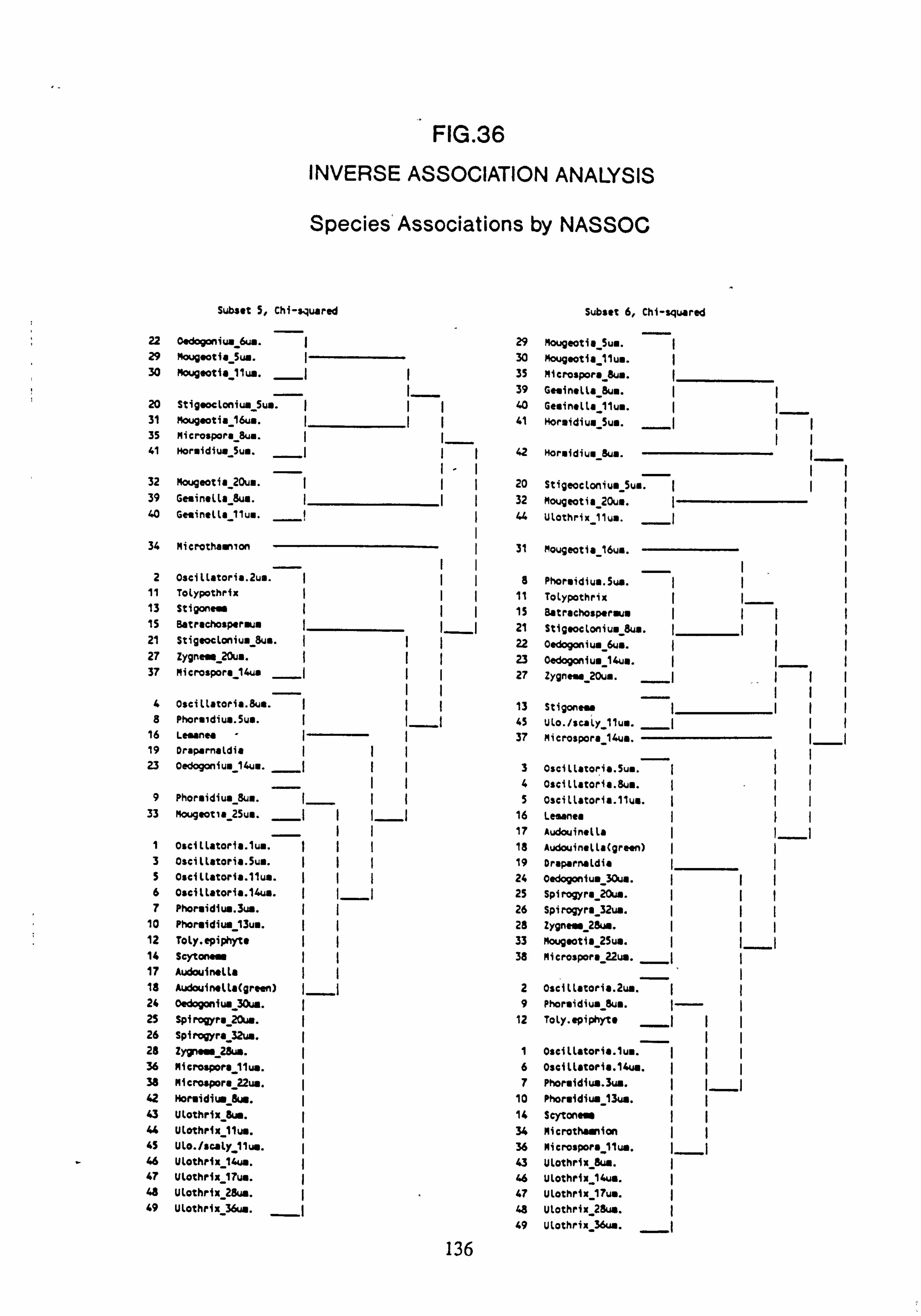
FIG. 36 INVERSE ASSOCIATION ANALYSIS
Species' Associations by NASSOC
Subset 5, Chi-squared
22 0sdogoniua 6uw. ý 29
29 Mougeotia Sun. ý 30 30 Mougeotia_11us. 35
39 20 Stigeocloniu.
_Sun_ 40
31 Mougeotia 16un. ý 41 35 Nicrospora Bun. 41 Moraidium 5ua. 42
32 Mougeotia 20us. 20 39 Geainella_8ue. ý 32 40 Geoinella ilua.
_I 4y
34 Microthannion ý 31
2 Oscitlatoria. 2uo. 11 Tolypothrix ýI 11 13 Stigoneve 1 ýý 15 15 Batrachospermum 21 21 Stigeoclonius 8ua. ý 22 27 Zygner 20un. 23 37 Microspora 14ua 27
4 OsciLtatoria. 8us. 13 8 Phoraidiua. 5ua. I I_ý 45
16 Leaanea I 37 19 Draparnaldia
23 Oedogoniu. 14un. 3 4
9 Phormidiua_8ua. 5
33 Mougeotia 25ua. 16
_ 17
1 Oscillatoria. lu.. 18 3 Oscillatoria. Sum. 19 5 OsciLLatoria. llu.. 24 6 OscitLatoria. 14us. 25 7 Phoraidiuw. 3us. 26
10 Phornidiu. _13u..
28 12 Toly. epiphyto 33 14 Scytonaoa ý 38 17 AudouinsLLa 18 Audouinella(green) 2 24 0edogoniuw 30us. 9 25 Spirogyra_20w. ý 12 26 Spirogyra 32u.. 28 Zygnomm 28ua. 1 36 Microspora 11uo. ý 6 38 Microspora_22u.. ý 7 42 Mornidiis_8ua. ý 10 43 Ulothrix 8u.. ý 14 44 ULothrix_llue. 34 45 Ulo. /scaly lluo. ý 36 46 Ulothrix_14un. ý 43 47 Ulothrix 17un. ý 46 48 ULothrix 28uw. ý 47 49 ULothrix 36uw. 48
49
136
Subset 6, Chi-squared
Mougeotis_Su.. Mougeotia llu.. Mi erospore-sum. Geuinella_8un. Gesinelta_Ilu.. Horsidiua Sum.
Nor. idiu Bun.
Stigeocloniua_5ua. Mougeotis 20ua. ULothrix 11ua.
Mougeotia 16ua.
I Phoraidiua. 5u.. I Totypothrix I I-
Batrachosparau. I
Stigoocloniua_8ua.
Oedogoniua bus. Oedoganium-14un. I I_ Zygness20um.
-I
Stigoneer II ULo. /scaly 11u.. Microspora 14un. I_I
I
Osciltatoria. Sua.
Oscillatoria. 8ua. I Oscillatoria. llua. I Lesanea IE AudouinetLa I I-1 Audcuin. LLa(gre. n) Draparnaldia
Oedogoniu. 30ua. I
Spirogyra20uw. I
Spirogyra-32u.. I
Zygneaa_2di.. I
Mougootia_25uo. I I-I
Microspora22uw. __I
Oscillatoria. 2uw. I Phoraidiua 9ua. ToLy. epiphyto
-I I OscitLatoria. lue. I OscitLatoria. 14u.. I
Pho ra idi uw. 3u.. II . __
I Phor. idiuw 13uw. scytonae. MicrotManion I Microspora lluw. I_ýI Ulothrix_8u.. ULothrix_14u.. Ulothrix_lluo. I Utothrix 26w. I ULothrix_36uw.
-I
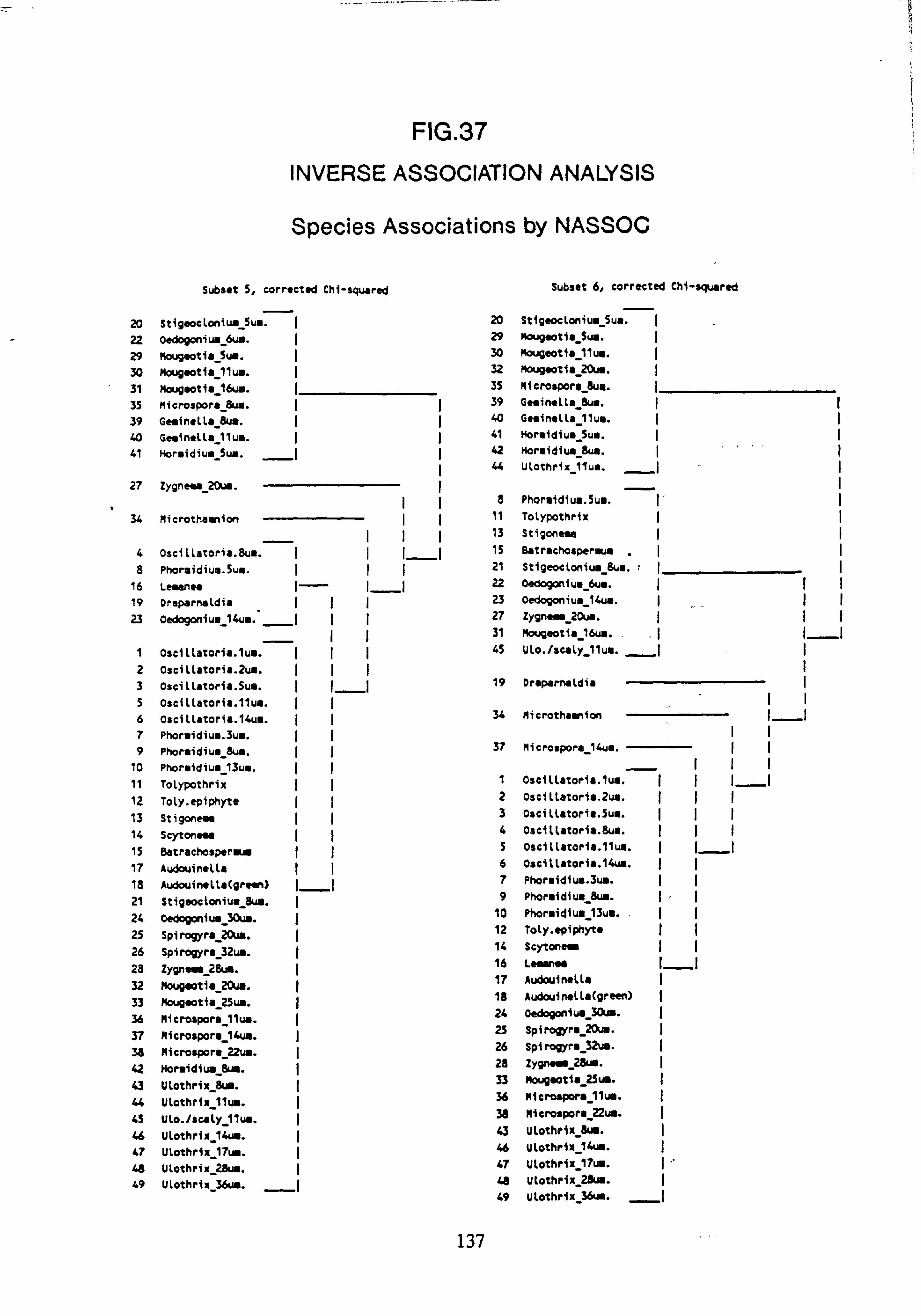
FIG. 37
INVERSE ASSOCIATION ANALYSIS
Species Associations by NASSOC
Subset 5, corrected Chi-squared Subset 6, corrected Chi-squared
20 Stigeoc1oniua_Sus. ý 20 Stigeoctonium-Sus.
22 Oedogoniu. _6uw.
29 Mougeotia Su.. I
29 Mougeotia SUN. 30 Mougeotia 11un. I
30 Mougeotia lluw. 32 Mougeotia 20u.. I 31 Mougeotia 16ua. 35 Microspora_8uu.
35 Microspora_&.. 39 Ge. inella_8u.. I
39 Ge. inella_8ui. I 40 Ge. inella_llu.. I
40 Geainella 11us. I 41 Hor. idiu. _SUN.
I
41 Horsidius_Sua. I ( 42 Morsidius_8ua. I 44 Utothriz flus. I
27 Zygne. a 20us. I 8 Phorsidius. Su.. I'
34 Microtha. tion I 11 Tolypothrix I 13 Stigoneve I
4 Oscillatoria. 8us. III 15 Batrachosperaua
8 Phoraidius. 5un. III 21 StigeocLonius_8ua.
16 Leaanea I- II 22 Oedogonius_6ua. I
19 Draparnaldia II 23 Oedogoniua_14ua. I
23 Oedoganiua_14un. (I 27 Zygne. a_20ua. 31 Mougeotia 16ui. III
1 OscitLatoria. lue. III 45 Ulo. /scaly_llua. I
2 Oscillatoria. 2ua. III 3 Oscillatoria. Sus. III 19 Draparnaldia
5 Oseillatoria. llun. II 6 Oseitlatoria. 14us. I 34 Mierothaanion II
7 Phorsidiu". 3ua. 9 Phorsidiuu 8u.. II 37 Microspora 14ua.
10 Phor. idiu. 13ua. II I
11 _
Tolypothrix II I 0sciltatoria. lue. IIII
12 ToLy. epiphyte 2 Osciltatoria. 2us. I
13 Stigoneme II 3 Oseitlatoria. 5u.. II
14 Scytoneaa I 4 Oscillatoria. 8ue. II
15 Batrschospersa I S osciltatoria. llua. III
17 Audouinella II 6 Oseillatoria. 14uw. II
18 Audouinelta(green) I 7 Phorsidiuw. 3uw. II
21 Stigeoctoniua 8u.. I 9 Phorsidiua 8u1. II
24 _
oedogoniu. 30u.. ý 10 Phor. idium 13ua. II
25 20w. I Spirogyra 12 Tolyepiphyts II
26 -
32ua. I Spirogyrs 14 Scytoner
28 _
Zygneýa 28uß. 16 Leaanea
32 Mougeotia 20u. 17 Audouinells I
33 Mougeotia 25u.. 18 Audouinella(green) I
36 Microspora lluw. I 24 Oedogoniw Sow. I
37 Mierospore 14uw. 25 Spirogyre_20u-. I
38 Microspora_22uw. ý 26 Spirogyra 32uw. I
42 &n. I Moraidiu. 28 Zygnesr 28ua. I
43 _
Ulothrix Bur. 33 Mougeotia_25um. I
44 Utothrix lluw. I 36 Mierospore 11um. I
45 _ Ulo. /scaly lluw. I 38 Mierospora 22w. I
46 14u.. ý Ulothrix 43 Ulothrix Sus. I
47 _
Ulothrix17u.. 46 Ulothrix 14u.. I
48 ULothrix 28u.. I 47 ULothrix 17uß. I
49 Ulothrix 36uw. 48 Ulothrix 2& .I 49 Ulothrix 36um.
137
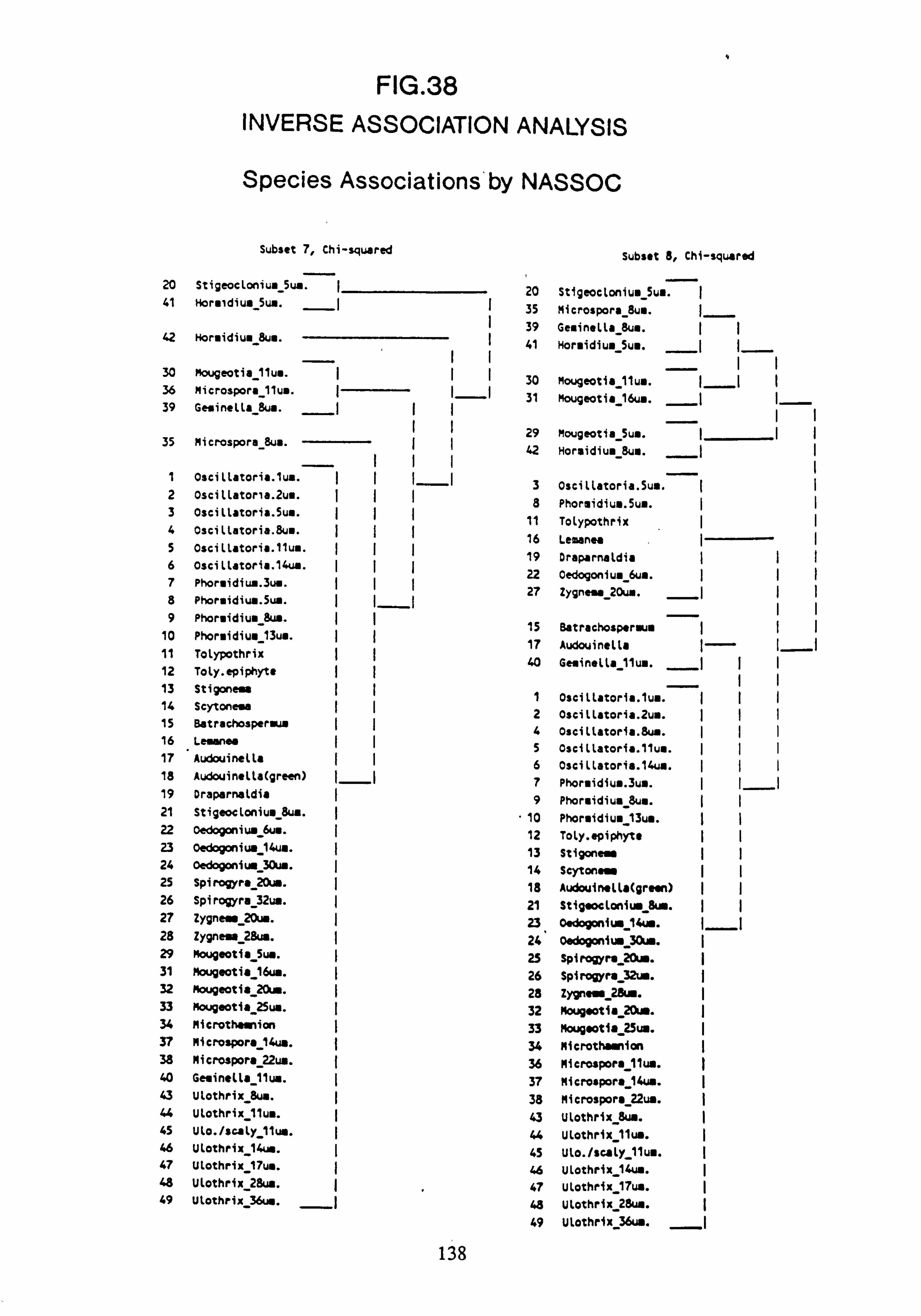
FIG. 38 INVERSE ASSOCIATION ANALYSIS
Species Associations'by NASSOC
Subset 7, Chi-squared
20 Stigeoclonium-5ua. 41 Hor. idius Sun. 1
42 Hor. idiu" 8uu.
30 Pougeotia 11ue. 36 Microspora ilu.. 39 Ge. ineLL& Su..
35 Microspora Su..
1 2 3
4 5 6 7 8 9
10 11 12 13 14 15 16 17
18
19 21
22
23 24 25 26
27
28
29 31 32 33 34 37
38
40 43 44
45 46 47 48 49
Oscillatoria. lus.
Oscillatoria. 2ue.
OsciLtatoria. Suu.
Oscillatoria. 8u..
Osciltatoria. llum
osciltatoria. l4w
Phoreidiua. 3un.
Phor. idiu.. 5ua.
Phoraidiua &u.
Phoriidium 13us.
ToLypothrix Toly. epiphyts Stigone. s Scytonesa Batrachospera . tesanoo Audouinella
Audouinelta(green Draparnatdia
Stigeoclonium-Bus
oedogoniua 6u..
Oedogoniua 14uu.
Oedogoniu. 30u..
Spirogyra-20u.. Spirogyra 32u..
Zygner20ua.
Zygnesa 28ua.
Mougeotia_Su.. Mougeatia 16uM.
nougeotio 20uß.
Mougootia 25uw.
Ni crothamnion NI crospore 14u..
Nicrospors 22u..
Gesinella_11ua.
Ulothrix_8uw. Ulothrix_llu.. Ulo. /scaly_llu..
Ulothrix_14u.. Ulothrix_17un. Ulothrix_28ui.
Ulothrix 36un.
i i ii
i i
iii iia
I. J
I.
iii ii ii iI ii ii ii
I) ii i I.
t i i i i i i i i i i i i i i i i i i i i
Subset 8, Chi-squared
20 stigeocloniu. 5u . ý 35 Mierospora 8u.. 39 Geuinella 8u.. ý 41 Hor. idiu. 5u..
30 Mougeotia 11u.. 31 Mougeotim 16u..
29 Mougeotia Su.. 42 Hormidium Suu.
3 8
11 16 19 22 27
15 17 40
1 2 4 5 6 7
9
10 12 13 14 18 21 23 24 25 26 28 32 33 34 36 37 38 43 44 45 46 47 48 49
Oscillatoria. Suu.
Phoraidiue. Sua.
ToLypothrix
Lemanea DraparnaLdia Oedogonium
- 6ua.
Zygnesa_20un.
Batrachosper. u. AudouineLta Geninella llu..
Oscillatoria. lua. Oscillstoria. 2un. oscillatoria. aw. Oscillatoria. llua, Oscillatoris. l4w,
Phoraidiua. 3ui.
Phoraidiua_8u.. Phoraidiu 13u". Toly. spiphyto Stigoner Scytoný Audouin. tLa(grean,
Stig. ocloniua 8u.,
Oadogonium_14u.. Oedogoniu.
_30ua. spirogyra-20m.
Spirogyrs 32u..
Zygnewa_2Qu.. Mougootia_20a. Mougootia 25u..
Microtha ion
Microspora Ilu..
Microspora 14u..
Microspors-22w.
Ulothrix 8u..
Ulothrix llu..
ULo. /scaly_llu..
ULothrix 14w.
ulothrix 17uw.
Ulothrix 2&u.
Ulothrix 36uw.
138
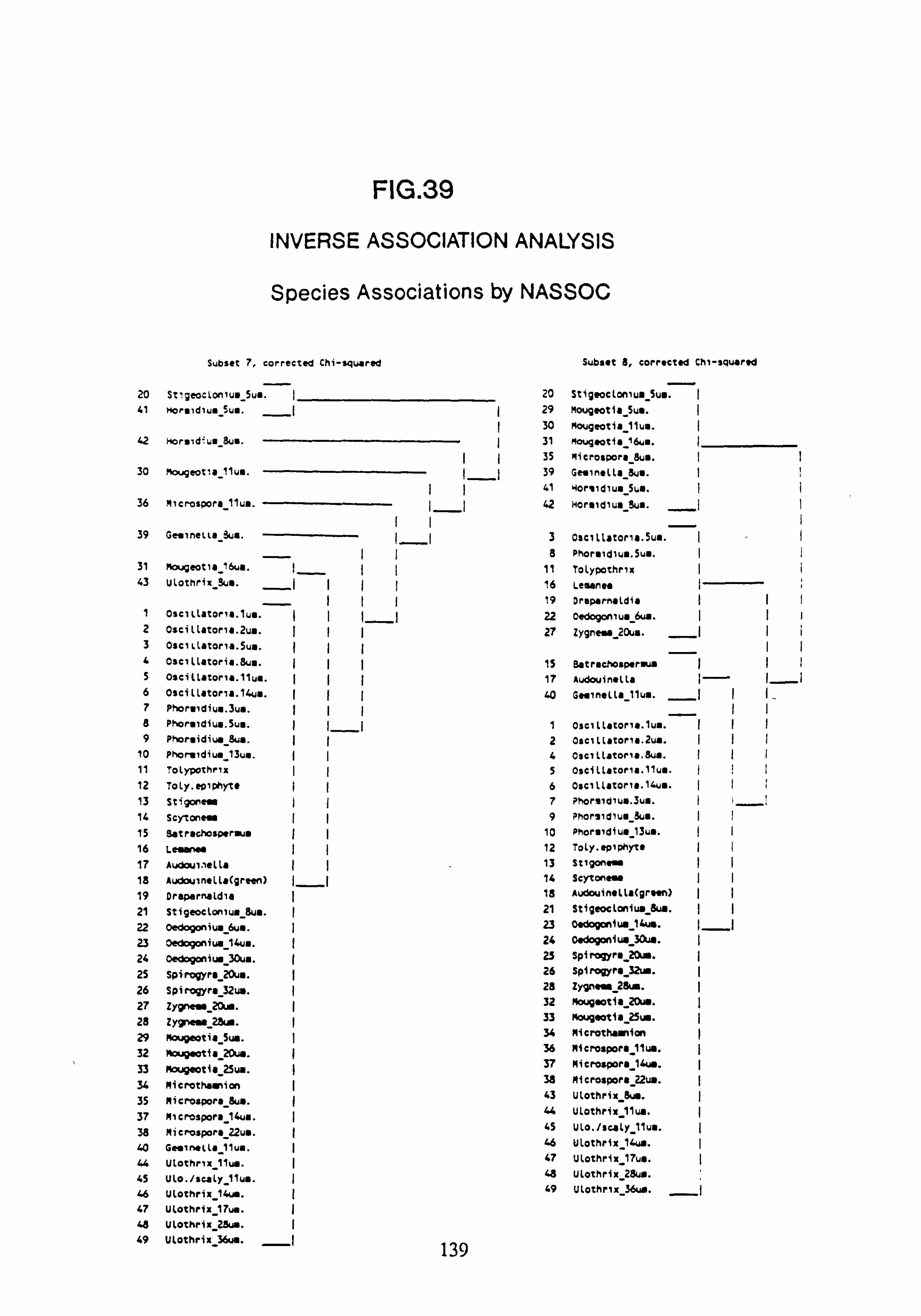
FIG. 39
INVERSE ASSOCIATION ANALYSIS
Species Associations by NASSOC
20 41
42
30
36
39
31 43
1
2 3 4 5 6 7 8 9
10 11 12 13 14 15 16 17 18 19 21 22 23 24 25 26 27 28 29 32 33 34 35 37 38 40 44 45 46 47 48 49
Subset 7, corrected Chi-squared
StigeocLoniun Sui.
NorIidlu" Sum.
Horsrd=uý aus. J II
mougeotla 11us. I_I II
Microspors 11us.
Gesinetu Sus. li_I JI
Motgeotia_ bus. Ulotnri: 9u..
__I I
OsciLL&torIa. lus. I I_I Oscillator, a. 2us. IJ osc1ktator, a. 5us. IIJ
Oseltlatoria. 8us. IIJ
Osci(Latoria. llus. II Oscitlatona. 14us. II
Phoraidius. 3us.
Phorsidius. 5us. I J_I Phorsidius $us. II
Phorsidius_13us. JJ
To(ypothrix I
Toly. ep'phyte
stigoness Scytoner I Satrachospersus I Lesanw II AudouineLLa AudouineLLa(green) Draparnald, a Stigeoctonius_Sus.
oedogonius_6ua.
Oedogonius_14us.
oedogonius 30us. J
Spirogyrs_20us. I
Spirogyra 32w. I
Zygrxss_20um. I
Zygness_2&a.
Mougeotis Sus. I
Mougsotia_20w. I
Mougeotia_25us.
Microthasnicn I
Microspora Bus. I
Microspors 1Gus.
Microspora_22us.
G.. in*tla 11us. I
Utothrix_11us. I
Uto. /sca(y_11w. I
Utothrix_14us. I
ULothri: 17us. I
Utothriýc 2ew. I
Utothri: 36.. 139
Subset 8, corrected Chi-squared
20 29 30 31 35 39 41 42
3 Oscillator, a. 5ua 8 Phoreidiu.. 5us.
11 Tolypothrix 16 Lemanee 19 Dreparne1dis 22 Oedogomum bw.
27 zygne. m20u .
15 Batrschospereua
17 Audouin. LLa
40 Gee, nella 11u..
1
2 4
5 6 7 9
10 12 13 14 1a 21 23 24 25 26 28 32 33 34 36 37 38 43 44 45 46 47 48 49
oscillatoria. lux.
OsC LLatona. 2us.
Oscillator a. 8ua.
Oscillator a. 11us
Oscillatoria. 14u"
Phoriidlua. 3u..
Phorsid, uo bus.
Phoraidiue 13us.
Toly. spiphytt Stigonw Scytoner
Audouin*Lta(grsen Stigeocloniua_Su.
Oadogoniua 14ua.
o. dogoniu. _30
.. Spirogyra 20ua.
Spirogyra_32ua. Zygn... 2&a.
Mouyaotia 20uS.
Mougeotia 25u..
Mi crotha. ion
Microspora ilu..
Microspor$ 16u..
Microspors 22us.
Utothrix_Suw.
Ulothrix_11us.
Ulo. /scaly llus.
ULothrix_14us.
ULothrix_17us.
Ulothrix_28u.
ULothrix 36ua.
StigeocLom um Sum I
Mougeotia Su.. I
Mougeotia 11u.. I
Mougeotis ibus.
Mierospora_8u..
Ge. inella Bus. I
Horiidiu. suw. I1
Horfidiu. ßu.. _I
i i i
ii
-i i i, ii
si
i ii
i i i i i i i i i i i i i i i
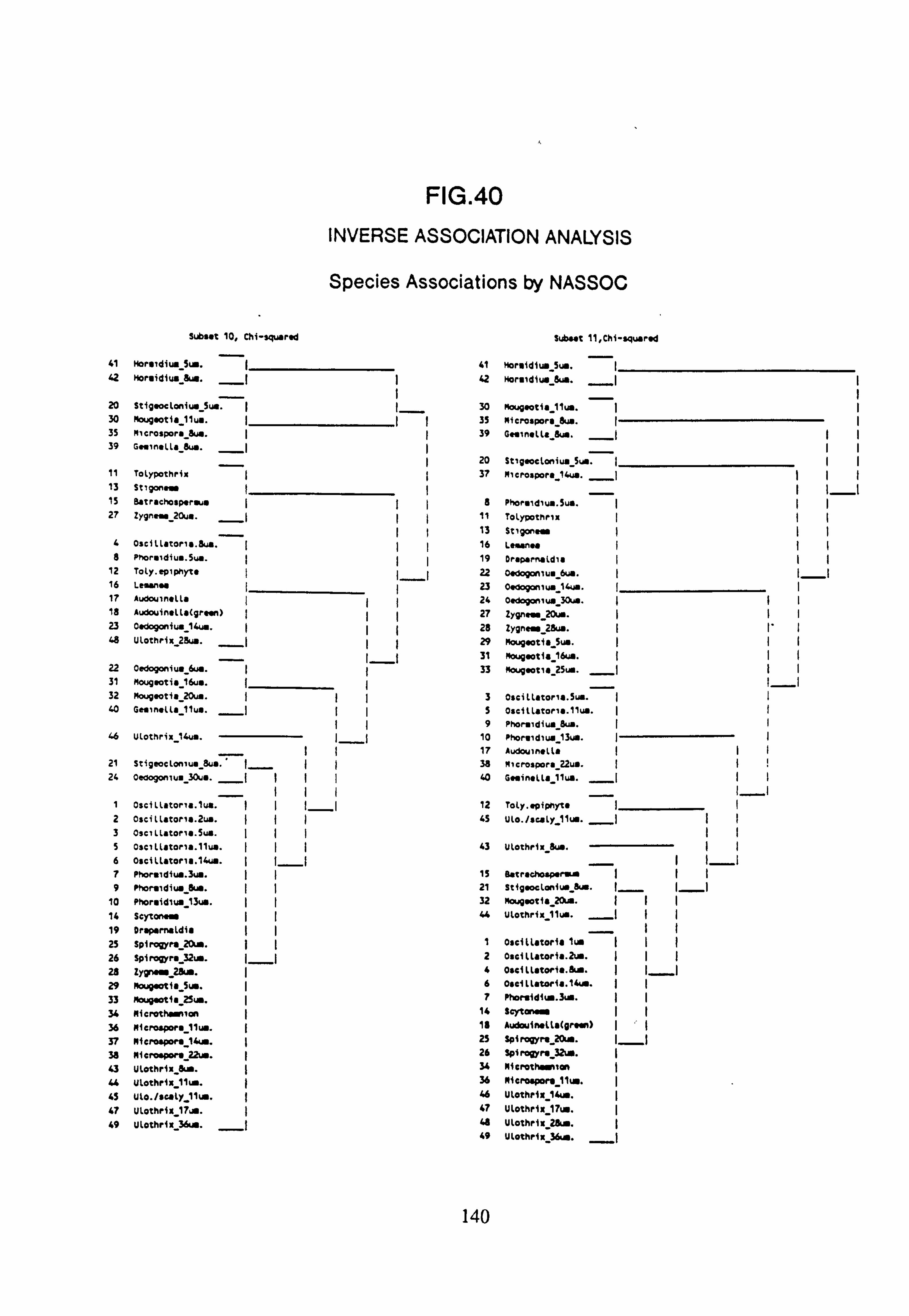
FIG. 40 INVERSE ASSOCIATION ANALYSIS
Species Associations by NASSOC
Subset 10, Chi-squared
41 Horsidiu. Sun. _ 42 Hor. idiw 8ß.
20 Stigeocloniw_Su.. 30 Mougeotia-ilu.. 35 Mhcrospors_8w. 39 GNlnslle 8w.
11 Tolypothrix 13 Stlgonesr 15 Betrschosperwa 27 2yynesr 20un.
_1
4 Oscilletone. 3u. 8 Phoruidiu.. 5uw.
12 Toly. epiphyte 16 Lemsn. s 17 AudouinsUs 18 Audouinell"(yrew) 23 Oedogoniu. 1Gw. 48 Utothrix 28ua.
22 Oedogonius 6uw. 31 Mougsotie 16u@. 32 Mougeotis20us. ý 40 Genn. lla ilu..
.6 Ulothrix 14u..
21 Stigeoclomua_8ua. - 24 Oeaogomu. 30ua.
1 Oscillatorna. luw. 2 Oscillatona. 2ua. 3 Oscillatona. Sua. 5 Oscillator a. 1luw. 6 Oscillator a. 14um. 7 Phortidium. 3u..
9 Phorndiua us. ý 10 Phoruidlum_13u/.
14 Scyton. ý 19 Oraparnaldis 25 Spiro'ra_20m. 26 Spiragyra_32ua. 23 Zygr Zan. ý 29 NougaotiaSun. ý 33 Mougwtia23ua. 34 Nicrothemnon ý 36 Nlcrospora_llu.. ý 37 Microspora_14a. ý 38 N1croapore 22uß. 43 Ulothris_&a. K Ulothrtx 11m. ý 4$ Uto. /scaly 11ua. ý 47 Ulothrix 17um. ý 49 Ulothrix 3&A.
_)
Sub"t 11, Chi-squared
41 Horuidiui Su.. 42 Hormidiua_Eus.
30 houg. otia 11ua. 3S hieroapora &a. 39 Ge. jnalla_bw.
20 St'paocLoniw_Su 37 Miarospora_14w.
_I
a Phorndiw. Sua.
11 Tolypot rix ý 13 Stlyoner 16 Le mnea 19 Drapornaldis 22 Oadogomus 6w. ý 23 0sdogoniu.
wl4A. 24 0edo" Ius 30ua.
27 Zygns. a_20uw. ý 28 Zygnear_2Eua. 29 Mouyaotia_Suw. 31 Noug. otia 16w. 33 nougaotia_2Suffi.
3 Oscillatoria. Sua. S Oseillatona. lluo. 9 Phornidiua &u.
10 Phorndiuw 13un. 17 Audouinllla 38 "Icrospora_22u . 40 G.. inalla llua.
12 Toly. epipnyt" 4S Ulo. /scaly_llu..
_ý
43 ULothrt: 8u..
15 eatr. ohosparaa I11 21 Stiy. ocLaniu. &a. 32 Mougsotia 20ia. 44 Ulothria 11 m.
I Ostillatoria 1uß 2 Oseillatoria. 2ua. 4 Osaillatoria. &a. I_1 6 O. eillatoria. IMa. 7 PAoraidiga. 3ua.
14 $cyto . 1" AudoUin. llafpr.. n) 25 spirogyra 20ia. 26 Spirogyra 32uß. ý 34 Mierotha. ion 36 Mitro. pora_I1um. 46 Ulothrit 14uß. ý 47 Ulothrit 17Ua. ý 48 Ulothrit 2&a. ý 49 Ulothrix 3&..
140
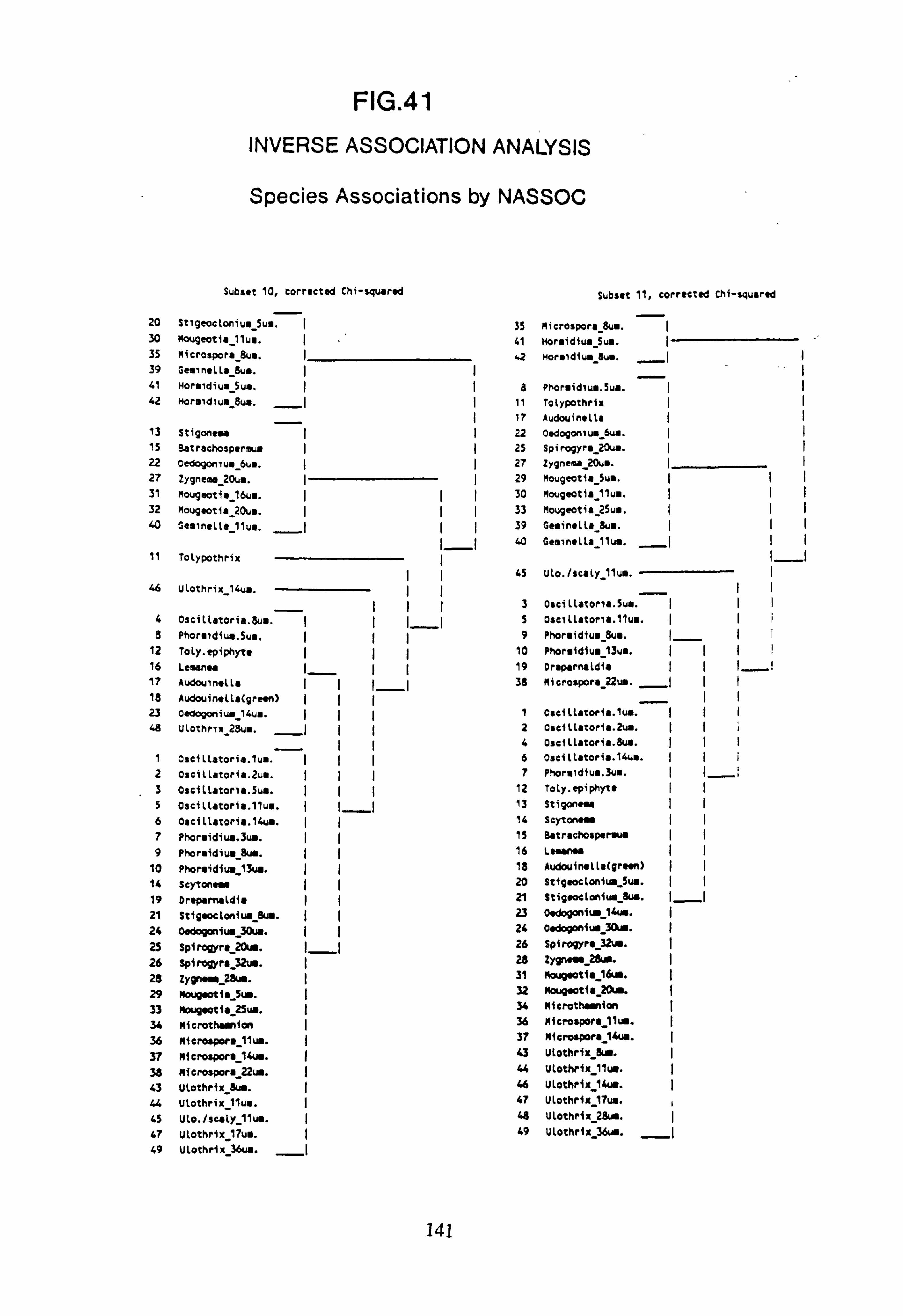
FIG. 41 INVERSE ASSOCIATION ANALYSIS
Species Associations by NASSOC
20 30 35 39 41 42
13 15 22 27 31 32 40
11
46
4 8
12
16
17
18
23
48
1 2 3 5 6 7 9
10 14 19 21 24 25 26 2$ 29 33 34 36 37 33 43 44 45 47 49
Subset 10, corrected Chi-squared
Stigeoclonium Su..
Mougwia llu;.
M1crospori 8u..
Ge. m@LL$_Buu. Horndiua_Sun. Horsidiuw 8u..
Stigone. a Batrachospenxu
Oedogom un_6u.. Zygnema 20ua.
Mougeotia 16u .
Mougeotia 20u.. Gesinelte llus.
Tolypothrix
ULothrix 14um.
OsciLLatoria. 8w.
Phoraidiui. 5um.
Toly. epiphyt" Lemanos
Audou n, LLa
Audouin*tLa(green)
Oedogoniu. _14un.
Ulothrix 28um.
Oscillatoria. lua. III Oscillatoria. 2u.. Oscillatoria. 5ua. I Oscillatoria. lluo. I I_I Osciltstoria. 1Lu.. I Phoraidiuw. 3uw. Phoraidiu. Sua. II Phoraidiu. 13un. I Scytonew I Dreparnaldis I Stigaocloniu.
_ew. II
oodogoniu. _30ua.
Spirogyra 20uß. I_I Spirogyra 32uw. I zyg+... 2&.. Moug. otia_5um. Mouyaotis 25uw. I
Mi crothasnion MicrosporI_11uo. I
Mierospors 1iu.. I
Microspora 22u.. I
Utothrix_&m. I
Ulothrix 11uu. I
Uto. /scaly_llu.. I
Ulothrix 17u.. I
Ulothrix_36uw. _I
Subset 11, corrected Chi-squared
35 nierospora suu. 1 41 Horiidius Suw. 42 Hor. idium-Sum.
�ýI
a
22 2s 27 29 30 33 39 40
45
3 S 9
10 19 38
1
2 4 6 7
12 13 14 15 16 18 20 21 23
24 26 28 31 32 34 36 37 43 44 46 47 48 49
Phoraidiua. Sua.
Tolypothrix
AudouinsLta I
Oedogontu. _6ua.
I
Spirogyra_20u.. I
Zygneia 2Ou..
Mougeotia Sua.
Mougeotia llua. I
Mougeotia 2Sua.
Gesinella Sum.
Geain. LLa llua. _I I__I
Ulo. /scaly llus.
Oseillatori.. Sua. I oseillaton .. 11ua. I Phoraidiua Sua. I_ 1
Phoraidiua_13ua. II
Dreparnaldia I Iý. I
Microspora 22u.. __1
I
Oscillatoria. lu.. I
Oscittatoria. 2ua. II
OsclLLatoria. Sun. I
OsclLt. toria. l4un. II
Phoraidiua. 3u.. I I__
Toty. epiphyto I
Stigone. a II
Seyton... II Batrachosperous II
Lamarles Audouin. LLa(green) StigoocLcniua_Su.. II Stig. ocloniua_aw. I_I
o. dogoniu. 14r. o. dogoniua_30ua. ý
Spirogyra_32um. Zygn. as_2&a. I
Mou9. otia 16uß. ý
Mouq. otia_20a. I Microtheanion ý Mierospors ilu.. I Mierospora 1: us. I Utothrix buy. I Utothrix_11uw. I Ulothrix_l4. I ULothrix llu.. Ulothrix 28uw. ULothrix 3&r.
141
Therefore reviewing all the results obtained using Inverse Association Analysis with subsets, a broad consensus appears about the existence of a group of species occurring in the more acidified sites, which may be considered acidobiontic. However it appears that the analysis is very sensitive to the quality of the data used. Inclusion of a large number of samples in the formation of the presence-absence matrix greatly improves the consistency of the results. It is also clear that the greater the number of sites included in the analysis the better the results will be since it is on the basis of the number of presences or absences of each species in sites that the x2 values are calculated.
In Normal Association Analysis the results are likely to be more robust since the divisions are on the basis of presence-absence of a sites in 49 different species, rather than onthe basis of each species in 15 (or less) sites in IAA.
142
4.6 - EVIDENCE FOR COMMUNITY DIFFERENCES BETWEEN SITES
The hypothesis that the abundances of different species are influenced by environmental factors is
implicit in the use of species diversity as an index of ecosystem disturbance. At the level of the individual species, each is considered to have an optimum range of values of any environmental
variable, within which it will achieve the greatest rate of increase, and hence the highest abundance. The abundances of this species in different locations may thus be taken as an indicator of the values
of that variable in each location. However species are influenced by more than one variable at a time
and thus one species may give uncertain information about a variable. Use of several species
simultaneously, or whole communities, is therefore likely to give a better indication of the likely
value of one (or more) environmental variables. For this to be valid, distinct communities of
organisms must be found to exist in sites which differ with regard to the environmental variable under
consideration.
Statistical methods of assessing the similarity between communities have been devised (reviewed in
Ludwig and Reynolds, 1988). The different approaches may be seen as means of assessing the degree of association between species (i. e. in communities) based on their (co-)occurrence in
different Sampling Units, or of association between SUs (sites, in this work) on the basis of the
species found in them. A series of tests is suggested by Ludwig and Reynolds (1988) for both
abundance and presence-absence data, to analyse interspecific relationships and subsequently to
classify the communities. Later stages in the testing, involving Correspondence Analysis, Polar
Ordination or Principal Components Analysis have not been utilized, Canonical Correspondence
Analysis by the Program CANOCO (Ter Braak, 1988) being preferred.
Abundance data may be used to test for covariance between species, with the recommendations that if species are not normally distributed the abundances should be ranked, and that the elimination of double-zero matches may be necessary. Species covariations may be calculated using the program SPCOVAR. BAS (Ludwig and Reynolds, 1988) but it does not include the option for the latter
manipulation. Instead therefore species covariation (correlation) was carried out in MINITAB using
a purpose-written macro to remove double-zero matches from each species pair in turn.
143
Presence-absence data may be used to compute indices of SU similiarity using the program SPASSOC. BAS (Ludwig and Reynolds, 1988). Presence-absence data are also used in Normal
Association Analysis, carried out by NASSOC. B AS (Ludwig and Reynolds, 1988), which classifies the sites by the algal communities they contain.
Community classification may also be carried out using Cluster Analysis by the program CLUSTER. BAS (Ludwig and Reynolds, 1988), using abundance data.
Both Normal Association Analysis and Cluster Analysis allow the construction of dendrograms
which graphically summarise the relationships between SUs and species, and are more readily interpretable than tables of numbers.
4.6.1 Species Covariation Similarity between sites has been investigated by calculation of correlations between mean species abundance values in pairs of sites (Table 42). Values of r shown are the Pearson
correlation coefficient in the upper half of the table, and Spearman ranked correlations in the lower half. This procedure is analogous to the calculation of species covariance. Double-zero
matches have been eliminated from both sets of calculations as recommended by Ludwig and Reynolds (1988). They also recommend the use of the Spearman correlation if the species abundances are not normally distributed as required for the validity of Pearson's correlation coefficient. Normal probability correlations carried out in MINITAB reveal that most species fail the test for normal distribution at the 1% level. Table 42 shows the correlations, the number of data points from which r was determined, and the value p (probability level) of the regression. With 105 separate correlations in each half, an appropriate level of significance is 0.5% (p < 0.005).
Considering the Spearman correlations, the majority of high values of r (> approx. 0.5) have
ap value of 0.005 or less and may thus be considered significantly different from zero. Large
positive correlations occur between sites 14-1,14-2,2,10-1 and 10-2; sites 15 and 6; sites 2, 5 and 11-2; sites 5,6, and 10-2; sites 6 and 5/6; and between most pairs of sites in the group 9,10-1,10-2,11-1 and 11-2, where the largest correlations occur. Lower but significant positive correlations occur between sites C-1 and C-2, and negative between sites Ward and 2,11-1 and 11-2.
The Pearson correlation yields higher values for these sites and includes a larger number of significant correlations, but must be considered less trustworthy as discussed above.
144
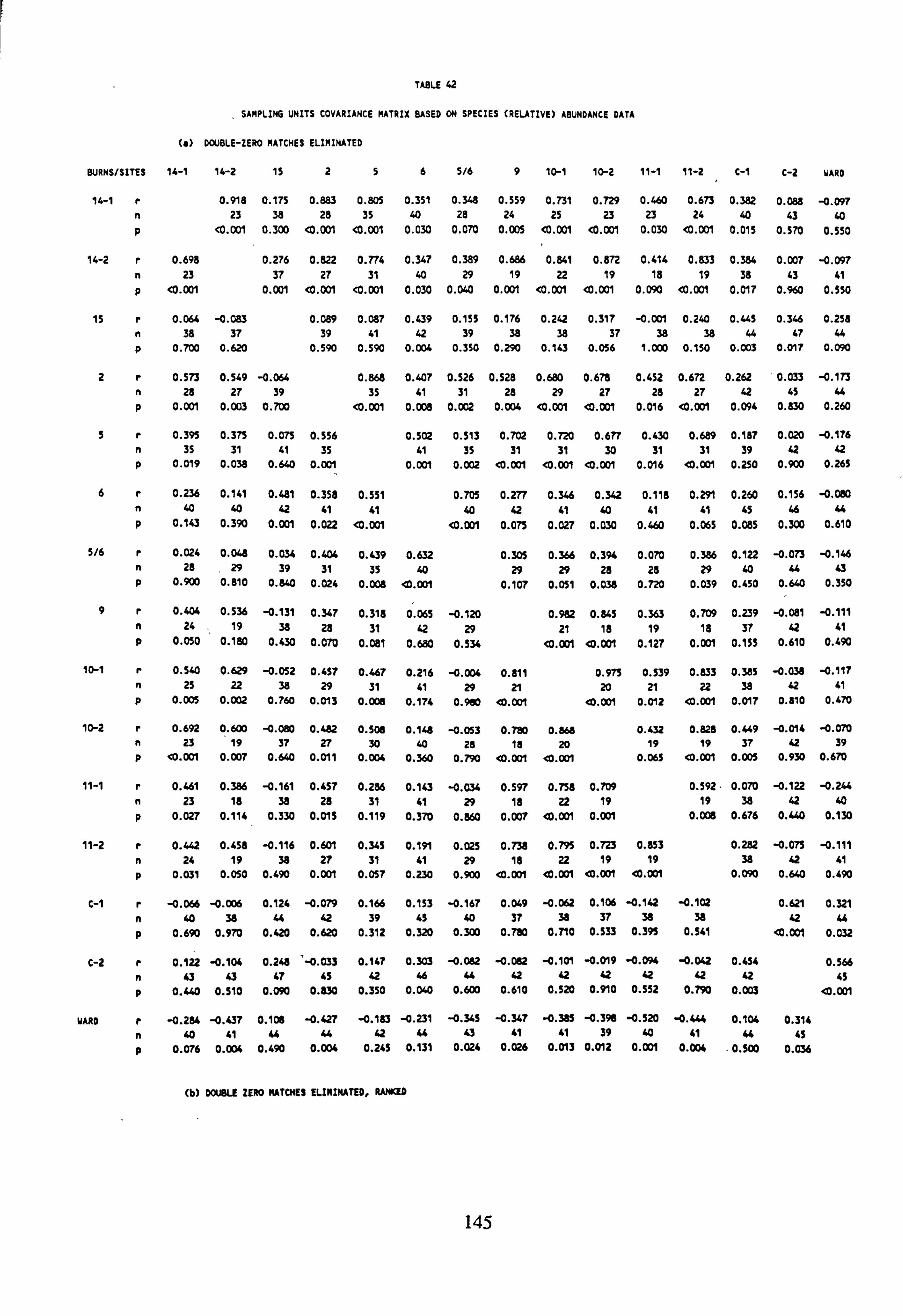
TABLE 42
SAMPLING UNITS COVARIANCE MAT RIX BASED ON SPECIES (RELATIVE) ABUNDANCE DA TA
(a) DOUBLE-ZERO MATCHES ELIMINATED
BURNS/SITES 14-1 14-2 15 2 5 6 5/6 9 10-1 10-2 11-1 11-2 C-1 C-2 WARD
14-1 r 0.918 0.175 0.883 0.805 0.351 0.348 0.559 0.731 0.729 0.460 0.673 0.382 0.088 -0.097 23 38 28 35 40 28 24 25 23 23 24 40 43 40
p <0.001 0.300 <0.001 10.001 0.030 0.070 0.005 <0.001 <0.001 0.030 <0.001 0.015 0.570 0.550
14-2 r 0.698 0.276 0.822 0.774 0.347 0.389 0.686 0.841 0.872 0.414 0.833 0.384 0.007 -0.097 n 23 37 27 31 40 29 19 22 19 18 19 38 43 41 p <0.001 0.001 <0.001 <0.001 0.030 0.040 0.001 <0.001 <0.001 0.090 <0.001 0.017 0.960 0.550
15 r 0.064 -0.083 0.089 0.087 0.439 0.155 0.176 0.242 0.317 -0.001 0.240 0.445 0.346 0.258 n 38 37 39 41 42 39 38 38 37 38 38 44 47 44 p 0.700 0.620 0.590 0.590 0.004 0.350 0.290 0.143 0.056 1.000 0.150 0.003 0.017 0.090
2 r 0.573 0.549 -0.064 0.868 0.407 0.526 0.528 0.680 0.678 0.452 0.672 0.262 ' 0.033 -0.173 n 28 27 39 35 41 31 28 29 27 28 27 42 45 44 p 0.001 0.003 0.700 <0.001 0.008 0.002 0.004 <0.001 <0.001 0.016 <0.001 0.094 0.830 0.260
5 r 0.395 0.375 0.075 0.556 0.502 0.513 0.702 0.720 0.677 0.430 0.689 0.187 0.020 -0.176 n 35 31 41 35 41 35 31 31 30 31 31 39 42 42 p 0.019 0.038 0.640 0.001 0.001 0.002 <0.001 <0.001 <0.001 0.016 <0.001 0.250 0.900 0.265
6 r 0.236 0.141 0.481 0.358 0.551 0.705 0.277 0.346 0.342 0.118 0.291 0.260 0.156 -0.080 n 40 40 42 41 41 40 42 41 40 41 41 45 46 K p 0.143 0.390 0.001 0.022 <0.001 <0.001 0.075 0.027 0.030 0.460 0.065 0.085 0.300 0.610
5/6 r 0.024 0.048 0.034 0.404 0.439 0.632 0.305 0.366 0.394 0.070 0.386 0.122 -0.073 -0.146 n 28 29 39 31 35 40 29 29 28 28 29 40 44 43 p 0.900 0.810 0.840 0.024 0.008 <0.001 0.107 0.051 0.038 0.720 0.039 0.450 0.640 0.350
9 r 0.404 0.536 -0.131 0.347 0.318 0.065 -0.120 0.982 0.845 0.363 0.709 0.239 -0.081 -0.111 n 24 19 38 28 31 42 29 21 18 19 18 37 42 41 p 0.050 0.180 0.430 0.070 0.081 0.680 0.534 <0.001 X0.001 0.127 0.001 0.155 0.610 0.490
10-1 r 0.540 0.629 -0.052 0.457 0.467 0.216 -0.004 0.811 0.975 0.539 0.833 0.385 -0.038 -0.117 n 25 22 38 29 31 41 29 21 20 21 22 38 42 41 p 0.005 0.002 0.760 0.013 0.008 0.174 0.960 <0.001 <O. 001 0.012 <0.001 0.017 0.810 0.470
10-2 r 0.692 0.600 -0.080 0.482 0.508 0.148 -0.053 0.780 0.868 0.432 0.828 0.449 -0.014 -0.070 n 23 19 37 27 30 40 28 18 20 19 19 37 42 39
p <0.001 0.007 0.640 0.011 0.004 0.360 0.790 <0.001 <0.001 0.065 <0.001 0.005 0.930 0.670
11-1 r 0.461 0.386 -0.161 0.457 0.286 0.143 -0.034 0.597 0.758 0.709 0.592 0.070 -0.122 -0.244 n 23 18 38 28 31 41 29 18 22 19 19 38 42 40 p 0.027 0.114 0.330 0.015 0.119 0.370 0.860 0.007 <0.001 0.001 0.008 0.676 0.440 0.130
11-2 r 0.442 0.458 -0.116 0.601 0.345 0.191 0.025 0.738 0.795 0.723 0.853 0.282 -0.075 -0.111 n 24 19 38 27 31 41 29 18 22 19 19 38 42 41 p 0.031 0.050 0.490 0.001 0.057 0.230 0.900 <0.001 <0.001 <0.001 <0.001 0.090 0.640 0.490
C-1 r -0.066 -0.006 0.124 -0.079 0.166 0.153 -0.167 0.049 -0.062 0.106 -0.142 -0.102 0.621 0.321 n 40 38 44 42 39 43 40 37 38 37 38 38 42 44 p 0.690 0.970 0.420 0.620 0.312 0.320 0.300 0.780 0.710 0.533 0.395 0.541 <0.001 0.032
C-2 r 0.122 -0.104 0.248 ' -0.033 0.147 0.303 -0.082 -0.082 -0.101 -0.019 -0.094 -0.042 0.454 0.566 n 43 43 47 4S 42 46 44 42 42 42 42 42 42 45
p 0.440 0.510 0.090 0.830 0.350 0.040 0.600 0.610 0.520 0.910 0.552 0.790 0.003 <0.001
WARD r -0.284 -0.437 0.108 -0.427 -0.183 -0.231 -0.345 -0.347 -0.385 -0.394 -0.520 -0.444 0.104 0.314 n 40 41 44 44 42 44 43 41 41 39 40 41 44 45
p 0.076 0.004 0.490 0.004 0.245 0.131 0.024 0.026 0.013 0.012 0.001 0.004 -0.500 0.036
(b) DOUBLE ZERO MATCHES ELIMINATED, RAIMCED
145
4.6.2 Species Association
Similarity between sites is also shown in Tables 43-45 compiled using the program SPASSOC. BAS (Ludwig and Reynolds, 1988), which computes similarity indices based on
species presence-absence. The tables show values of the Ochiai and Jaccard indices. Only
values occurring in site pairs showing a significant x2 value (> 3.84) have been included.
Significant values are seen to occur between upstream-downstream pairs of sites, and within
the group of sites which may be described as the most acidified, having the lowest mean pH
values (Table 46). These sites are on burns 2,5,9,10,11 and 14. The results taken with those
of species covariation therefore support the idea that such an 'acidified group' of sites does
exist. Comparison of the values of both indices in the three data matrices A, B and C show no
clear tendency for values to be higher in one matrix.
This analysis being based on p/a data is free of any criticism of bias due to estimation of relative
abundance.
4.6.3 Normal Association Analysis
The testing sequence suggested for presence-absence data matrices utilizes the program NASSOC. BAS to perform Normal Association Analysis. The first stage of the analysis involves the Variance Ratio test for significant association between multiple species, and all data sets used have passed this test. (Normal) Association Analysis determines a x2 value for
similarity between pairs of Sampling Units on the basis of the species they contain, and sorts the SUs into homologous groups using these xz values. Homology is achieved when no x2
value greater than 3.84 is found. If the procedure is carried out with an inverted data matrix
species may be sorted into groups on the basis of the SUs in which they occur. This procedure is referred to as Inverse Association Analysis (see Section 4.4.2).
The results of the analyses are shown in the form of dendrograms in Figs. 42 and 43. Ludwig
and Reynolds (1988) recommend removal of rare species from the data in order to minimise bias. This has been carried out in Figs. 44 and 45.
The analyses carried out with the uncorrected values ultimately result in a large number of
small groups of sites, while the corrected x2 gives only three groups. However the division
arising at the first cycle is almost identical in all matrices and utilizing both x2 and
146
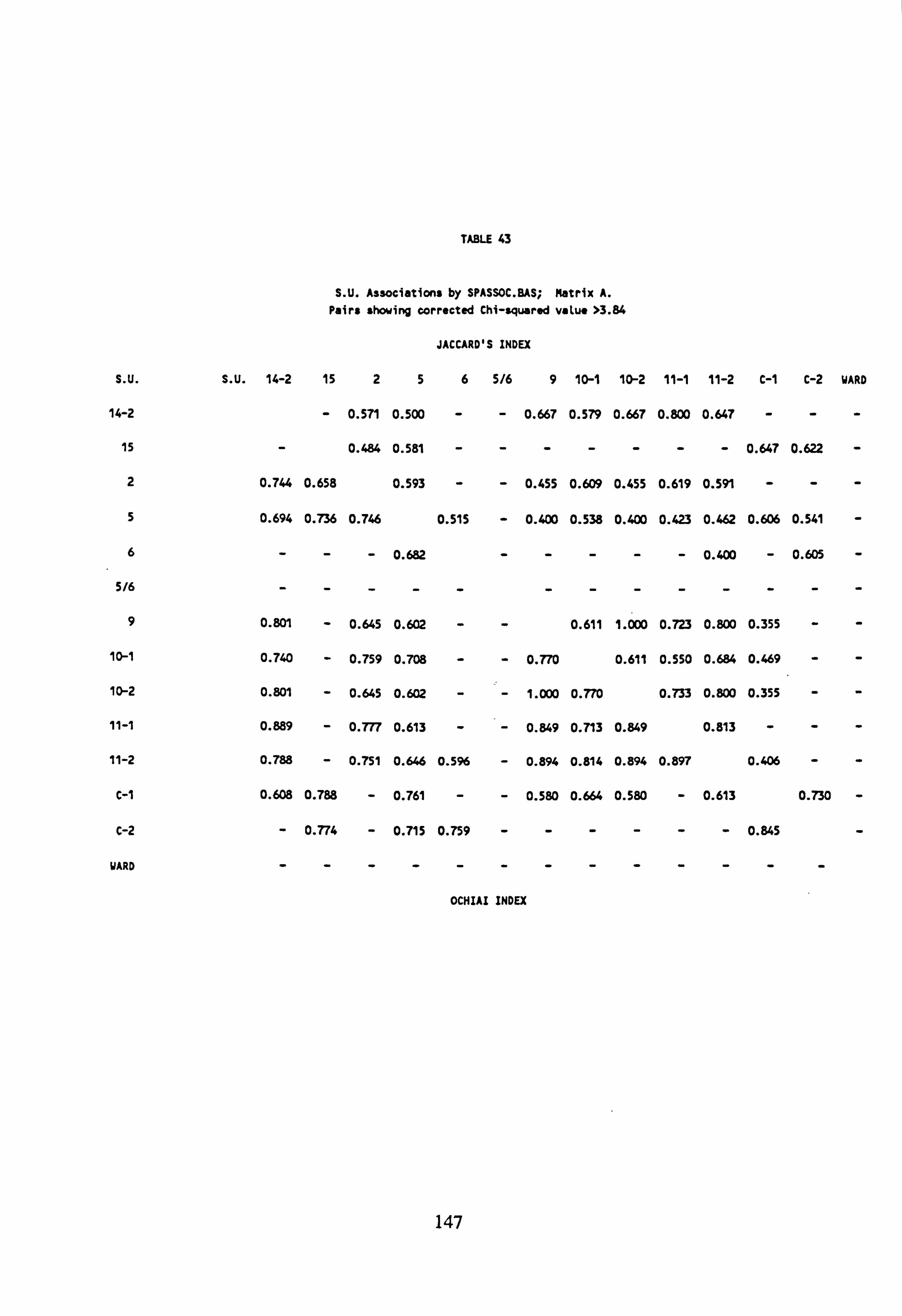
TABLE 43
S. U. Associations by SPASSOC. BAS; Matrix A. Pairs showing corrected Chi-squared value >3.84
JACCARD'S INDEX
S. U. S. U. 14-2 15 2 5 6 5/6 9 10-1 10-2 11-1 11-2 C-1 C-2 WARD
14-2 - 0.571 0.500 - - 0.667 0.579 0.667 0.800 0.647 - --
15 - 0.484 0.581 - -- - - - - 0.647 0.622 -
2 0.744 0.658 0.593 - - 0.455 0.609 0.455 0.619 0.591 - --
5 0.694 0.736 0.746 0.515 - 0.400 0.538 0.400 0.423 0.462 0.606 0.541 -
6 - - - 0.682 -- - - - 0.400 - 0.605 -
5/6 - - - - - - - - - - - --
9 0.801 - 0.645 0.602 - - 0.611 1.000 0.723 0.800 0.355 --
10-1 0.740 - 0.759 0.708 - - 0.770 0.611 0.550 0.684 0.469 --
10-2 0.801 - 0.645 0.602 - - 1.000 0.770 0.733 0.800 0.355 --
11-1 0.889 - 0.777 0.613 - - 0.849 0.713 0.849 0.813 - --
11-2 0.788 - 0.751 0.646 0.5% - 0.894 0.814 0.894 0.897 0.406 --
C-1 0.608 0.788 - 0.761 - - 0.580 0.664 0.580 - 0.613 0.730 -
C-2 - 0.774 - 0.715 0.759 -- - - - - 0.845 -
WARD
OCHIAI INDEX
147
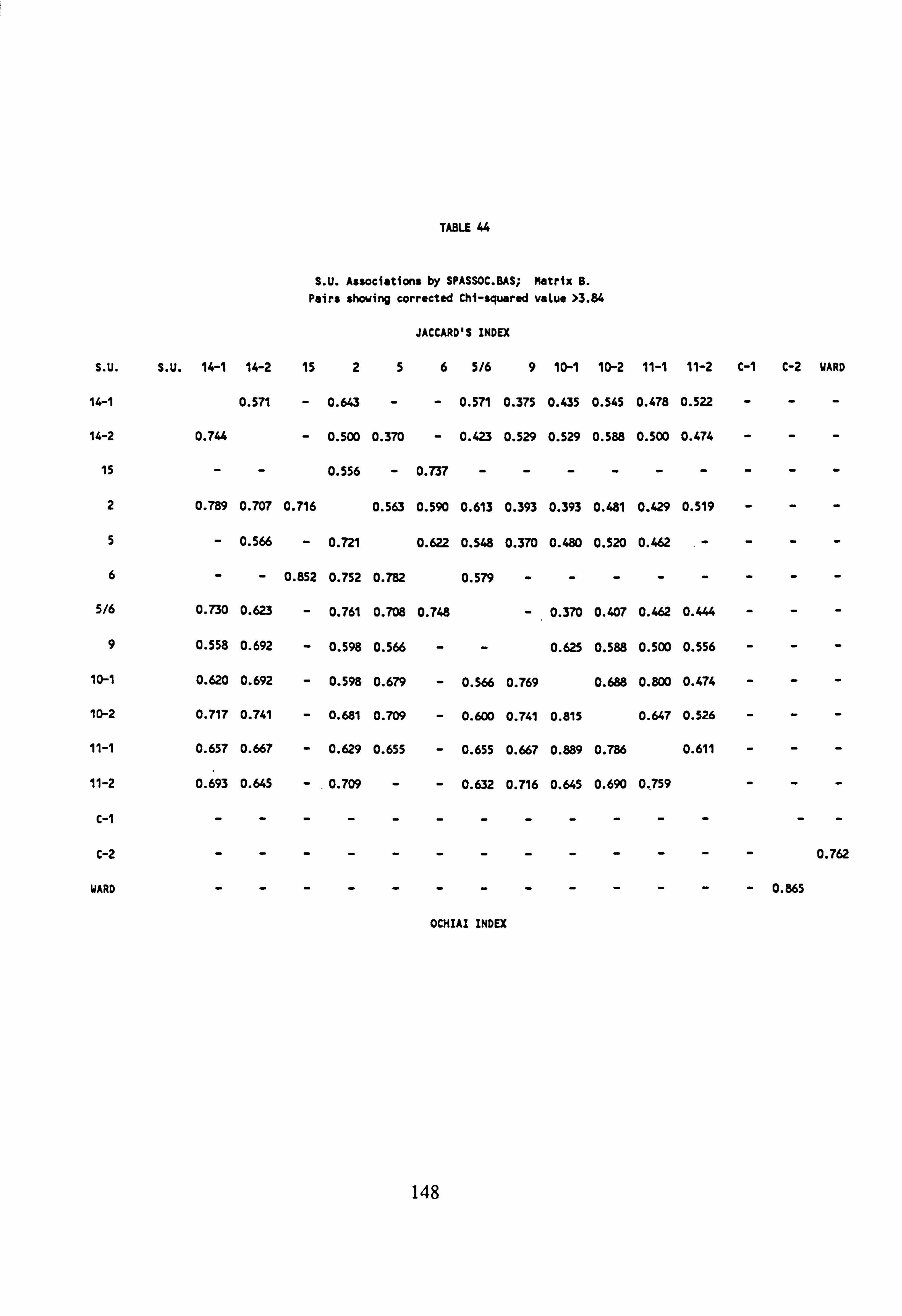
TABLE 44
S. U. Associations by SPASSOC. BAS; Matrix B. Pairs showing corrected Chi-squared value >3.84
JACCARD'S INDEX
S. U. S. U. 14-1 14-2 15 2 5 6 5/6 9 10-1 10-2 11-1 11-2 C-1 C-2 WARD
14-1 0.571 - 0.643 - - 0.571 0.375 0.435 0.545 0.478 0.522 ---
14-2 0.744 - 0.500 0.370 - 0.423 0.529 0.529 0.588 0.500 0.474 ---
15 - - 0.556 - 0.737 - - - - - ----
2 0.789 0.707 0.716 0.563 0.590 0.613 0.393 0.393 0.481 0.429 0.519 ---
5 - 0.566 - 0.721 0.622 0.548 0.370 0.480 0.520 0.462 ----
6 - - 0.852 0.752 0.782 0.579 - - - - ----
5/6 0.730 0.623 - 0.761 0.708 0.748 - 0.370 0.407 0.462 0.444 ---
9 0.558 0.692 - 0.598 0.566 - - 0.625 0.588 0.500 0.556 ---
10-1 0.620 0.692 - 0.598 0.679 - 0.566 0.769 0.688 0.800 0.474 ---
10-2 0.717 0.741 - 0.681 0.709 - 0.600 0.741 0.815 0.647 0.526 ---
11-1 0.657 0.667 - 0.629 0.655 - 0.655 0.667 0.889 0.786 0.611 ---
11-2 0.693 0.645 - 0.709 - - 0.632 0.716 0.645 0.690 0.759 ---
C-1 - - -- - - - - - - - ---
C-2 - - -- - - - - - - - --0.762
WARD - - -- - - - - - - - --0.865
OCHIAI INDEX
148
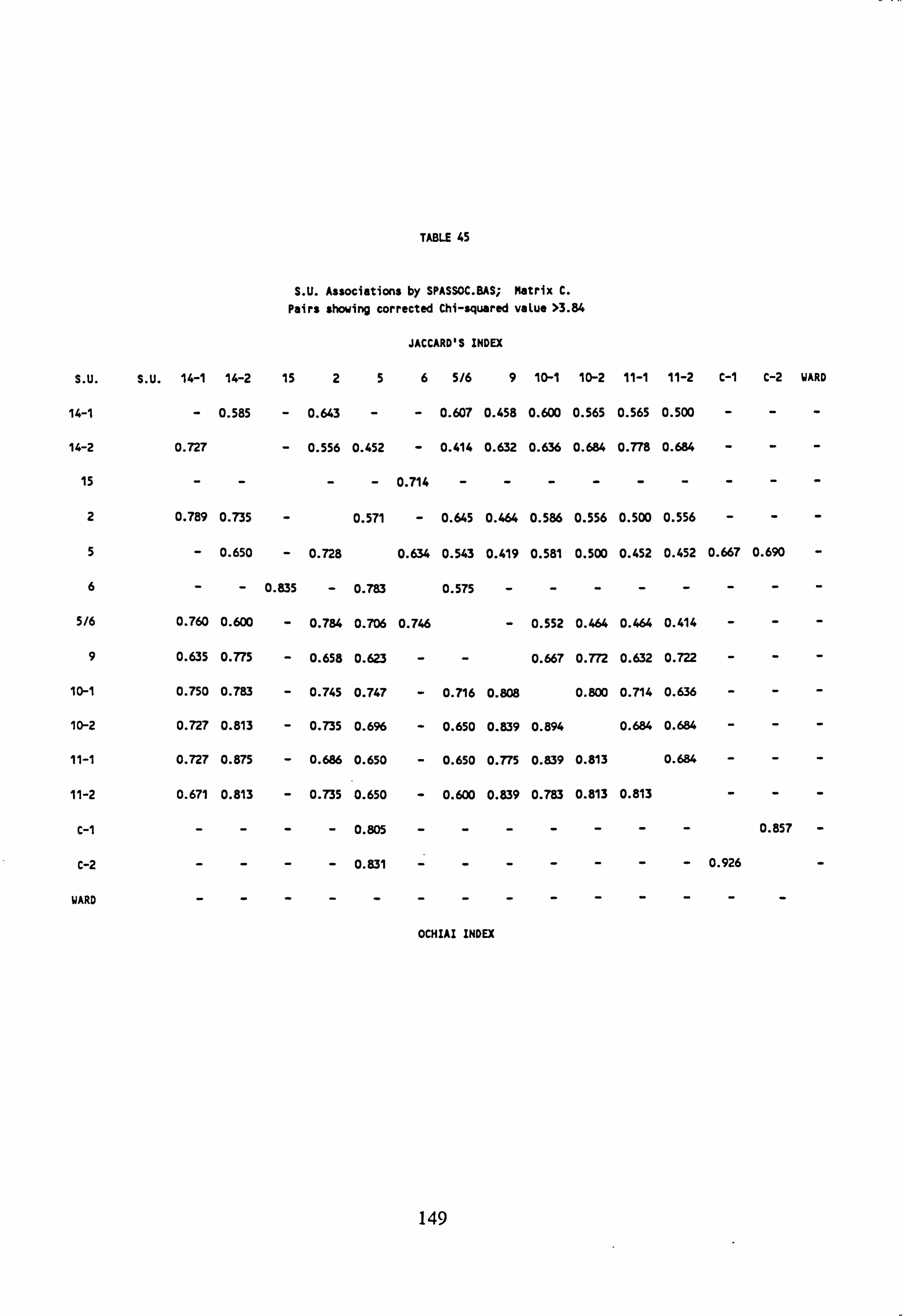
TABLE 45
S. U. Associations by SPASSOC. BAS; Matrix C.
Pairs showing corrected Chi-squared value >3.84
JACCARD'S INDEX
S. U. S. U. 14-1 14-2 15 2 5 6 5/6 9 10-1 10-2 11-1 11-2 C-1 C-2 WARD
14-1 - 0.585 - 0.643 - - 0.607 0.458 0.600 0.565 0.565 0.500 ---
14-2 0.727 - 0.556 0.452 - 0.414 0.632 0.636 0.684 0.778 0.684 ---
15 - - - - 0.714 - - - - - ----
2 0.789 0.735 - 0.571 - 0.645 0.464 0.586 0.556 0.500 0.556 ---
5 - 0.650 - 0.728 0.634 0.543 0.419 0.581 0.500 0.452 0.452 0.667 0.690 -
6 - - 0.835 - 0.783 0.575 - - - - ----
5/6 0.760 0.600 - 0.784 0.706 0.746 - 0.552 0.464 0.464 0.414 ---
9 0.635 0.775 - 0.658 0.623 - - 0.667 0.772 0.632 0.722 ---
10-1 0.750 0.783 - 0.745 0.747 - 0.716 0.808 0.800 0.714 0.636 ---
10-2 0.727 0.813 - 0.735 0.696 - 0.650 0.839 0.894 0.684 0.684 ---
11-1 0.727 0.875 - 0.686 0.650 - 0.650 0.775 0.839 0.813 0.684 ---
11-2 0.671 0.813 - 0.735 0.650 - 0.600 0.839 0.783 0.813 0.813 ---
C-1 - - -- 0.805 - - - - - - - 0.857 -
C-2 - - -- 0.831 - - - - - - - 0.926 -
WARD
OCHIAI INDEX
149
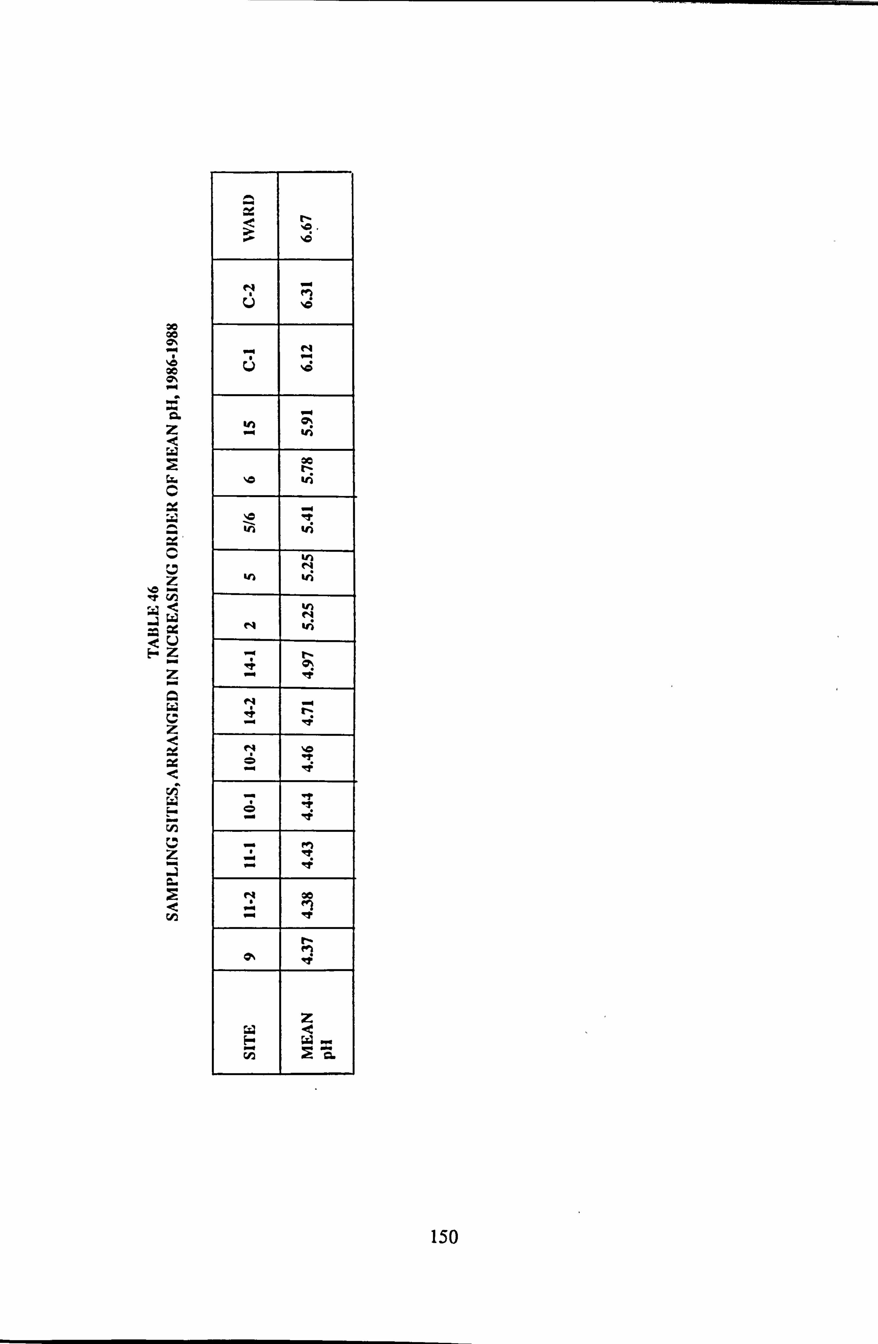
x 00
x
z a z < W i C'. C
x C
J
z b
FZ
z - C
L z x x
w Un u z
2
W
N
N
U Is
In
In ei ýA In
h N
N it
N ON
N-
fV NO
K i .r
nr 'ir
-M
N 00
N a , it
z FW=
vý ýa
150
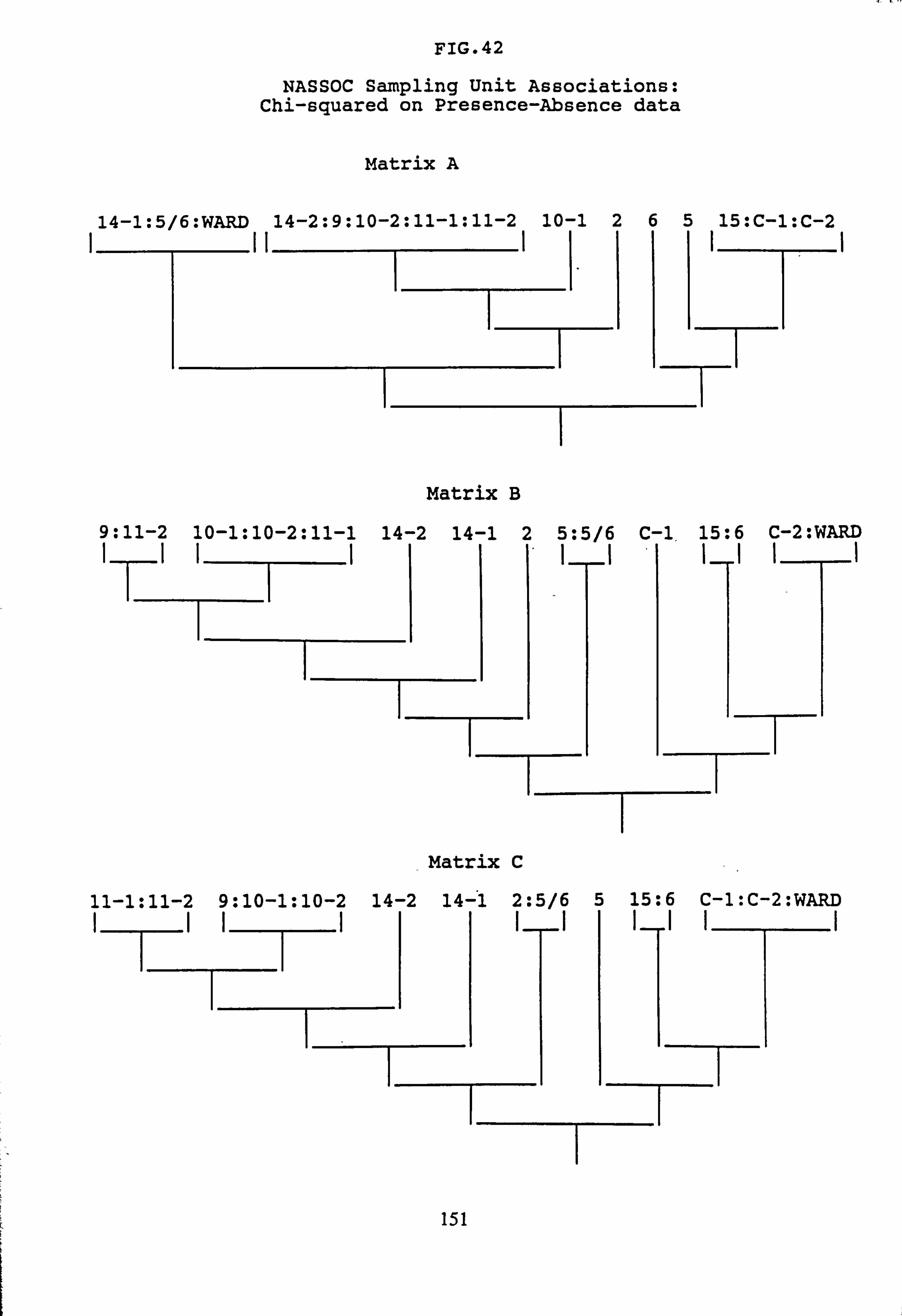
FIG. 42
NASSOC Sampling Unit Associations: Chi-squared on Presence-Absence data
Matrix A
14-1: 5/6: WARD 14-2: 9: 10-2: 11-1: 11-2 10-1 2
"1 I Matrix B
9: 11-2 10-1: 10-2: 11-1 14-2 14-1 2 5: 5/6 C-1,15: 6 C-2: WARD 1
Matrix C
11-1: 11-2 9: 10-1: 10-2 14-2 14-1 2: 5/6 1
rl 111111
i-mai
15: 6 C-1: C-2: WARD I
5 15: C-1: C-2
151
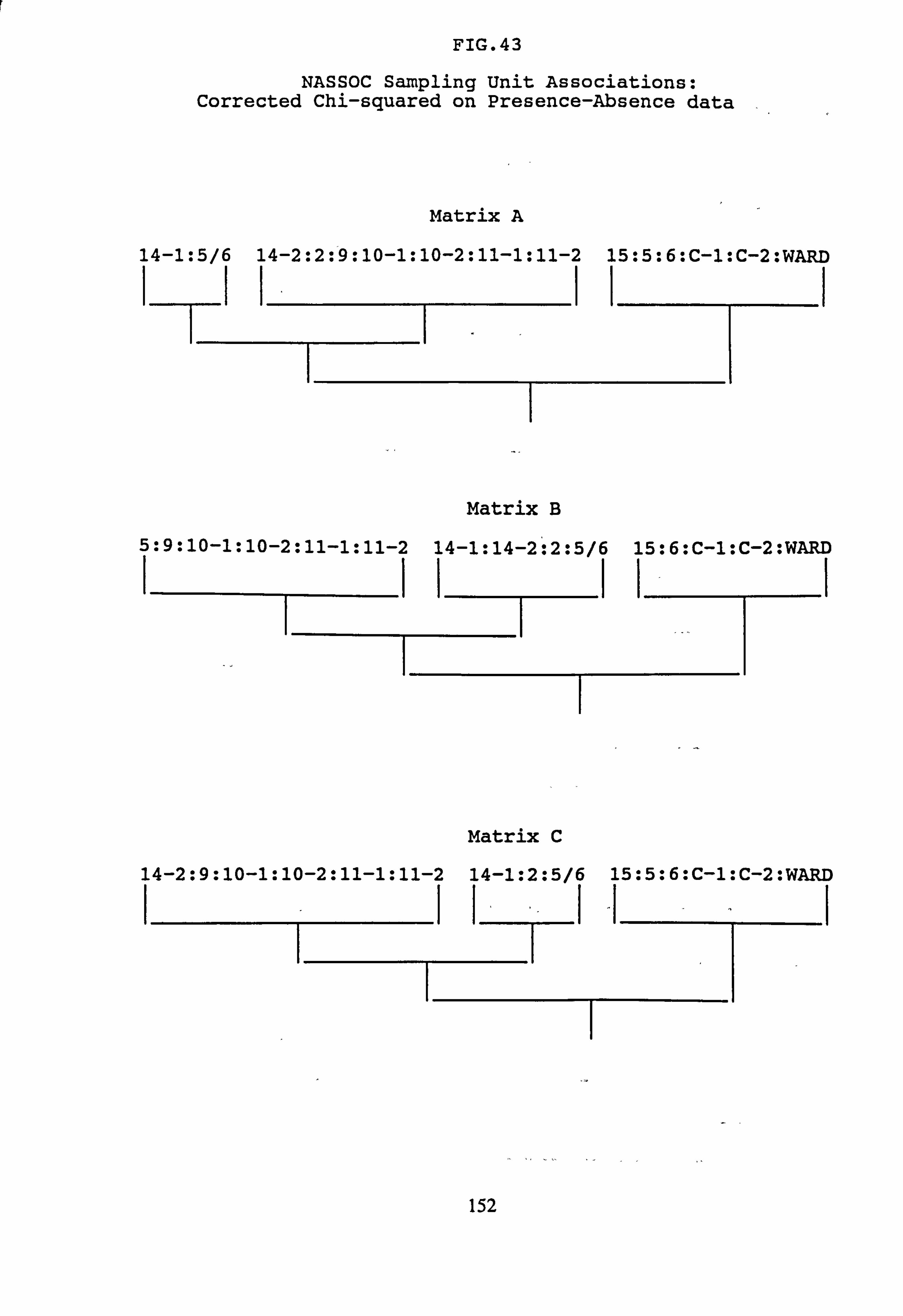
FIG. 43
NASSOC Sampling Unit Associations: Corrected Chi-squared on Presence-Absence data
Matrix A
14-1: 5/6 14-2: 2: 9: 10-1: 10-2: 11-1: 11-2 15: 5: 6: C-1: C-2: WARD IIIIII
7
Matrix B
5: 9: 10-1: 10-2: 11-1: 11-2 14-1: 14-2: 2: 5/6 15: 6: C-1: C-2: WARD IIIIII
Matrix C
14-2: 9: 10-1: 10-2: 11-1: 11-2 14-1: 2: 5/6 15: 5: 6: C-1: C-2: WARD
152
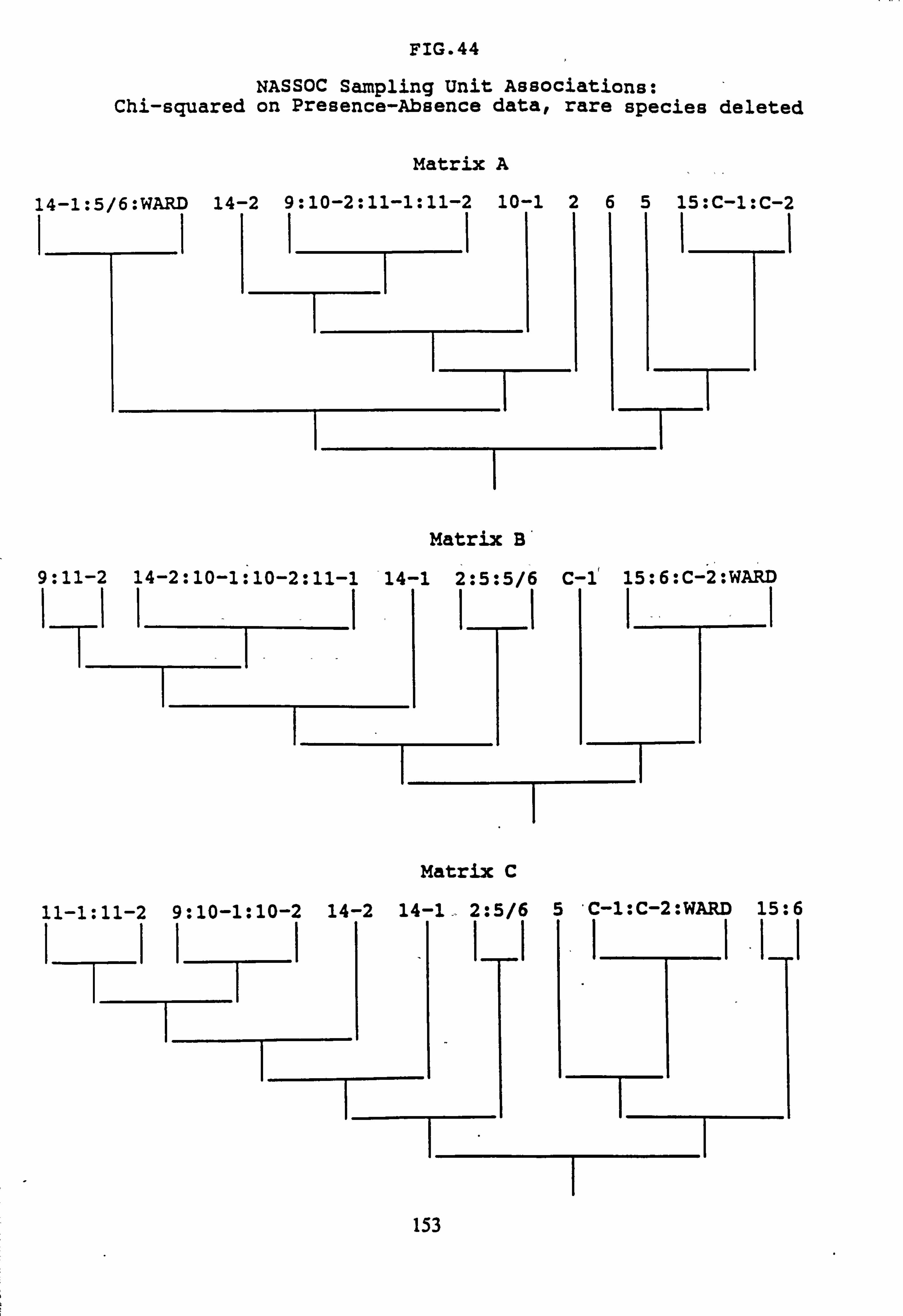
FIG. 44
NASSOC Sampling Unit Associations: Chi-squared on Presence-Absence data, rare species deleted
Matrix A
14-1 1
14 --1-
1
Matrix B
: 11-2 14-2: 10-1: 10-2: 11-1 14-1 2: 5: 5/6 C-1 15: IIIII I_
-T-
Matrix C
15: C-1: C-2 II
6: C-2: WARD
11-1: 11-2 9: 10-1: 10-2 14-2 14-1_. 2: 5/6 5 C-1: C-2: WARD 15: 6
: 5/6: WARD 14-2 9: 10-2: 11-1: 11-2 10-1
153
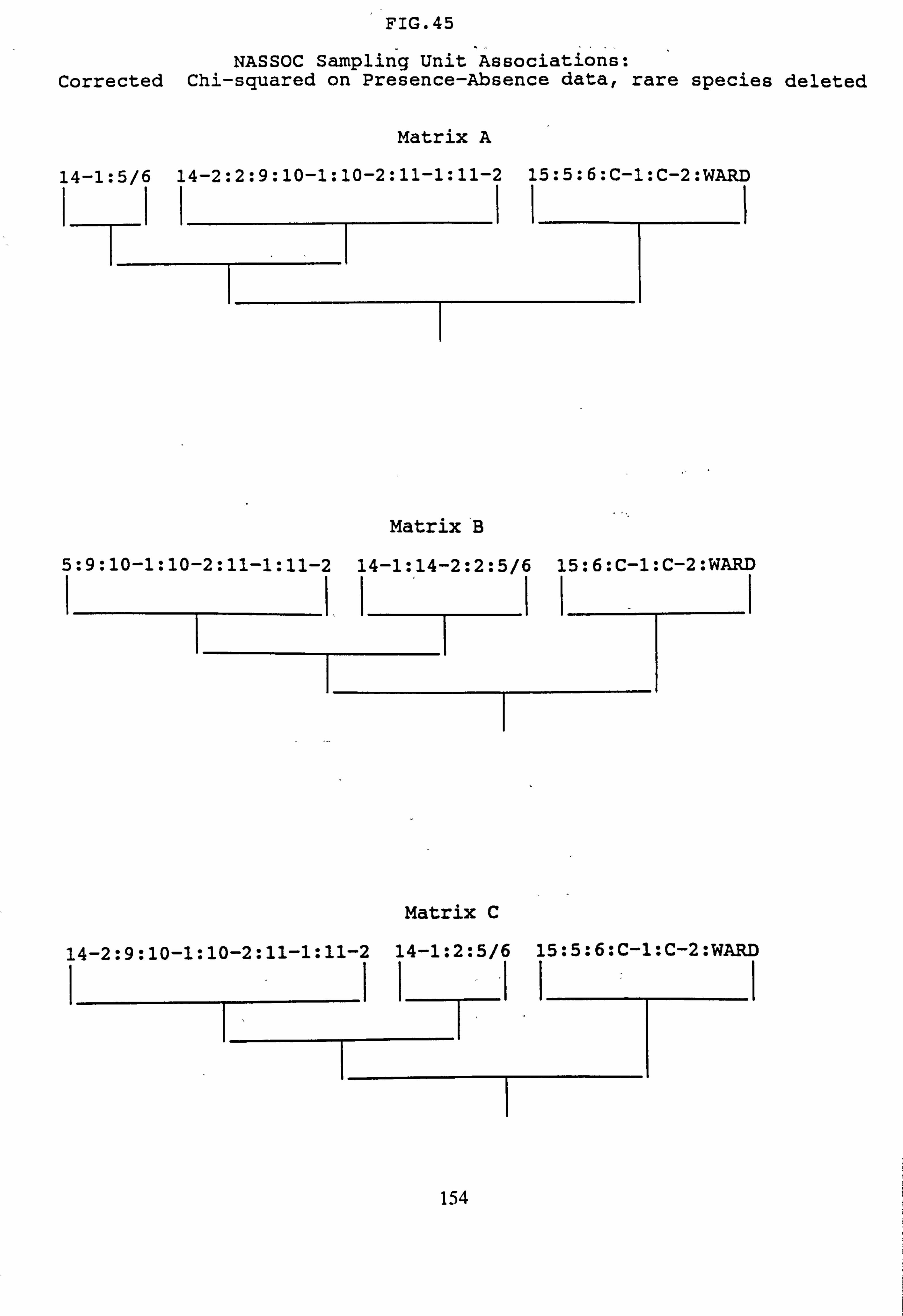
FIG. 45
NASSOC Sampling Unit Associations: Corrected Chi-squared on Presence-Absence data, rare species deleted
Matrix A
14-1: 5/6 14-2: 2: 9: 10-1: 10-2: 11-1: 11-2 15: 5: 6: C-1: C-2: WARD IIIII1
Matrix B
5: 9: 10-1: 10-2: 11-1: 11-2 14-1: 14-2: 2: 5/6 15: 6: C-1: C-2: WARD
Matrix C
14-2: 9: 10-1: 10-2: 11-1: 11-2 14-1: 2: 5/6 15: 5: 6: C-1: C-2: WARD IIIIII
154
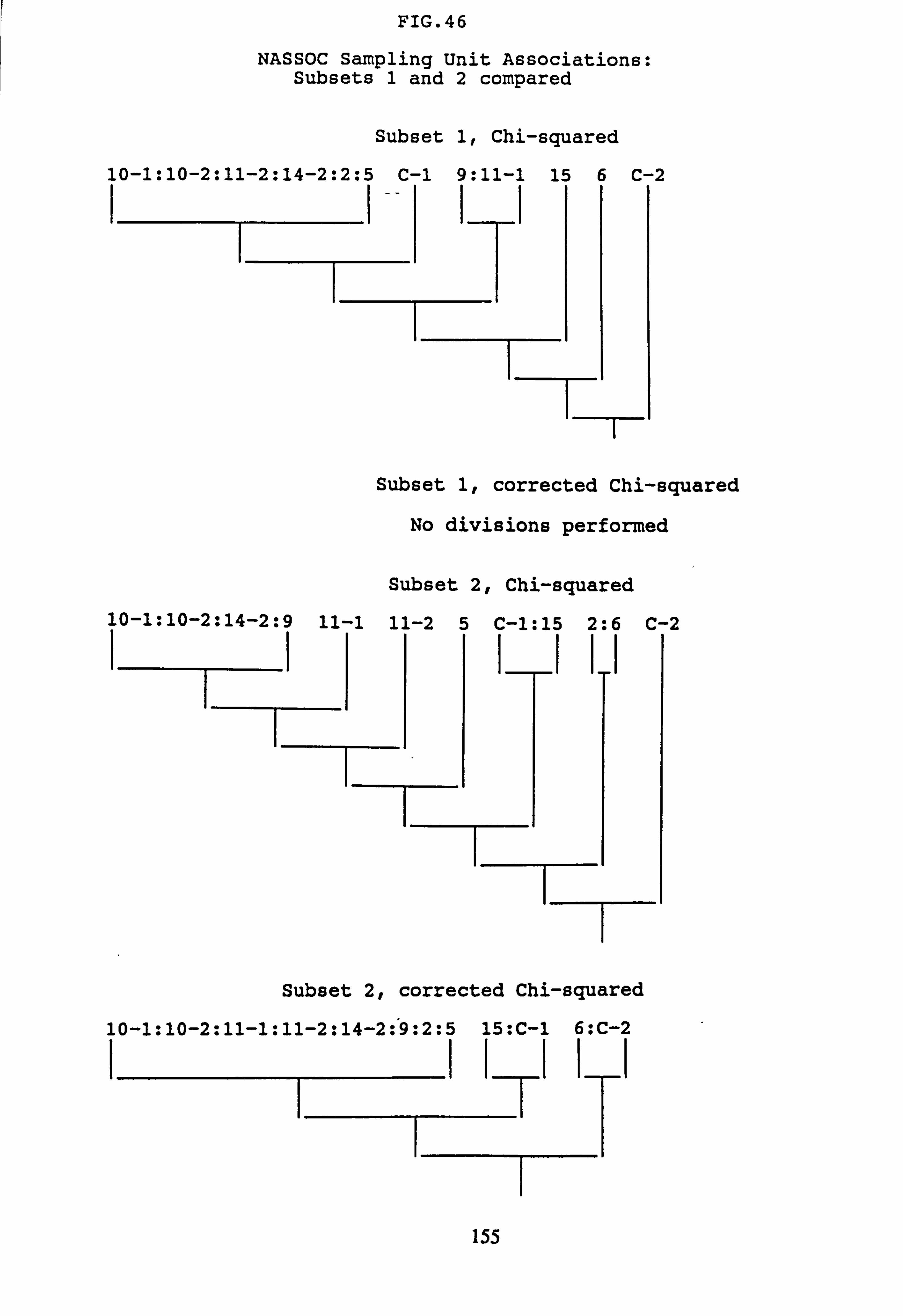
FIG. 46
NASSOC Sampling Unit Associations: Subsets 1 and 2 compared
Subset 1, Chi-squared
10-1: 10-2: 11-2: 14-2: 2: 5 C-1 9: 11-1 15 6 C-2
______" " _L
ýT Subset 1, corrected Chi-squared
No divisions performed
Subset 2, Chi-squared
10-1: 10-2: 14-2: 9 11-1 11-2 5 C-1: 15 2: 6 C-2 II(III
Subset 2, corrected Chi-squared
10-1: 10-2: 11-1: 11-2: 14-2: 9: 2: 5 15: C-1 6: C-2 II I_I II
155
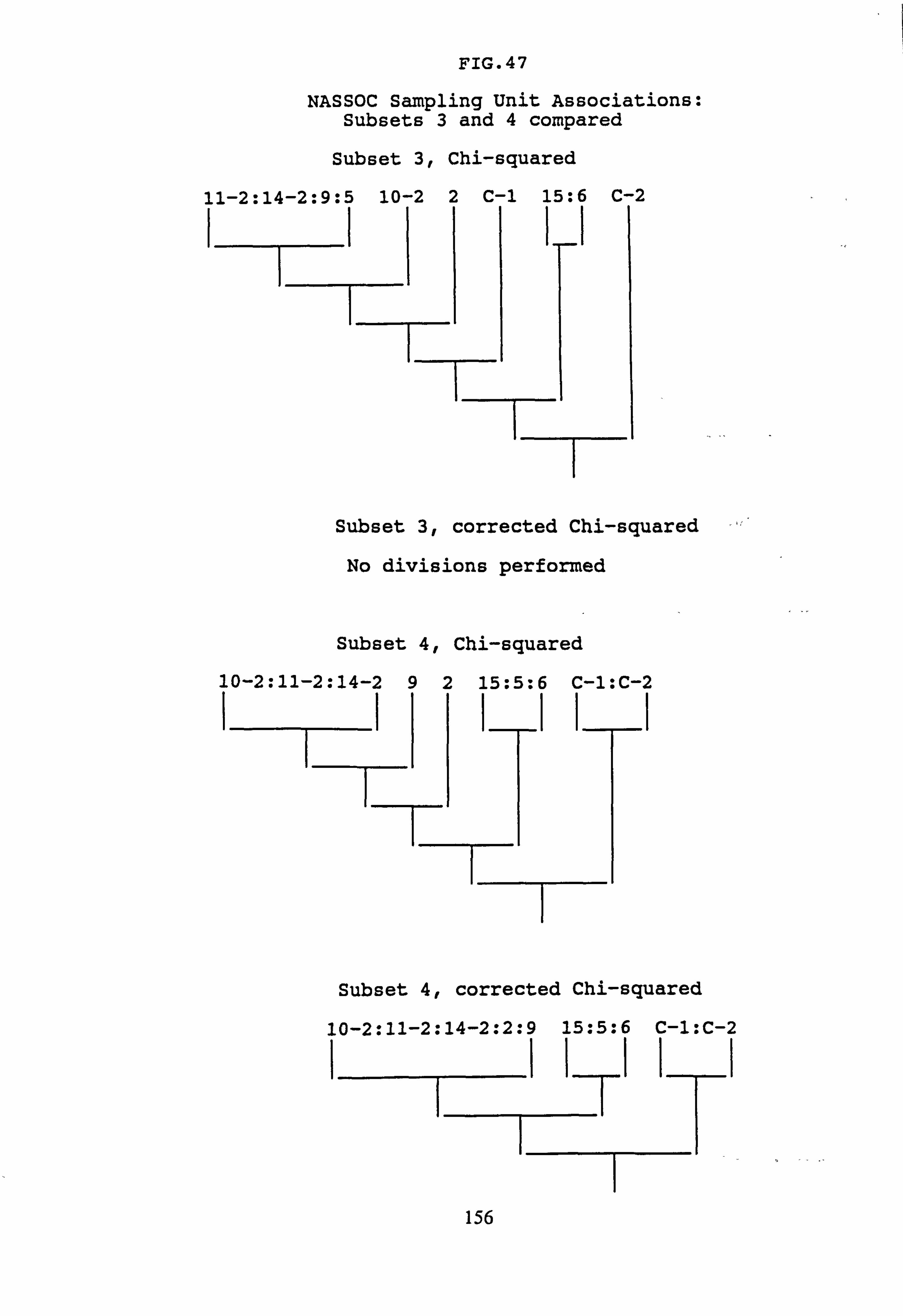
FIG. 47
NASSOC Sampling Unit Associations: Subsets 3 and 4 compared
Subset 3, Chi-squared
11-2: 14-2: 9: 5 10-2 2 C-1 15: 6 C-2 IIII
Subset 3, corrected Chi-squared
No divisions performed
Subset 4, Chi-squared
10-2: 11-2: 14-2 92 15: 5: 6 C-1: C-2 IIIIII
Subset 4, corrected Chi-squared
10-2: 11-2: 14-2: 2: 9 15: 5: 6 C-1: C-2 IIIIII
156
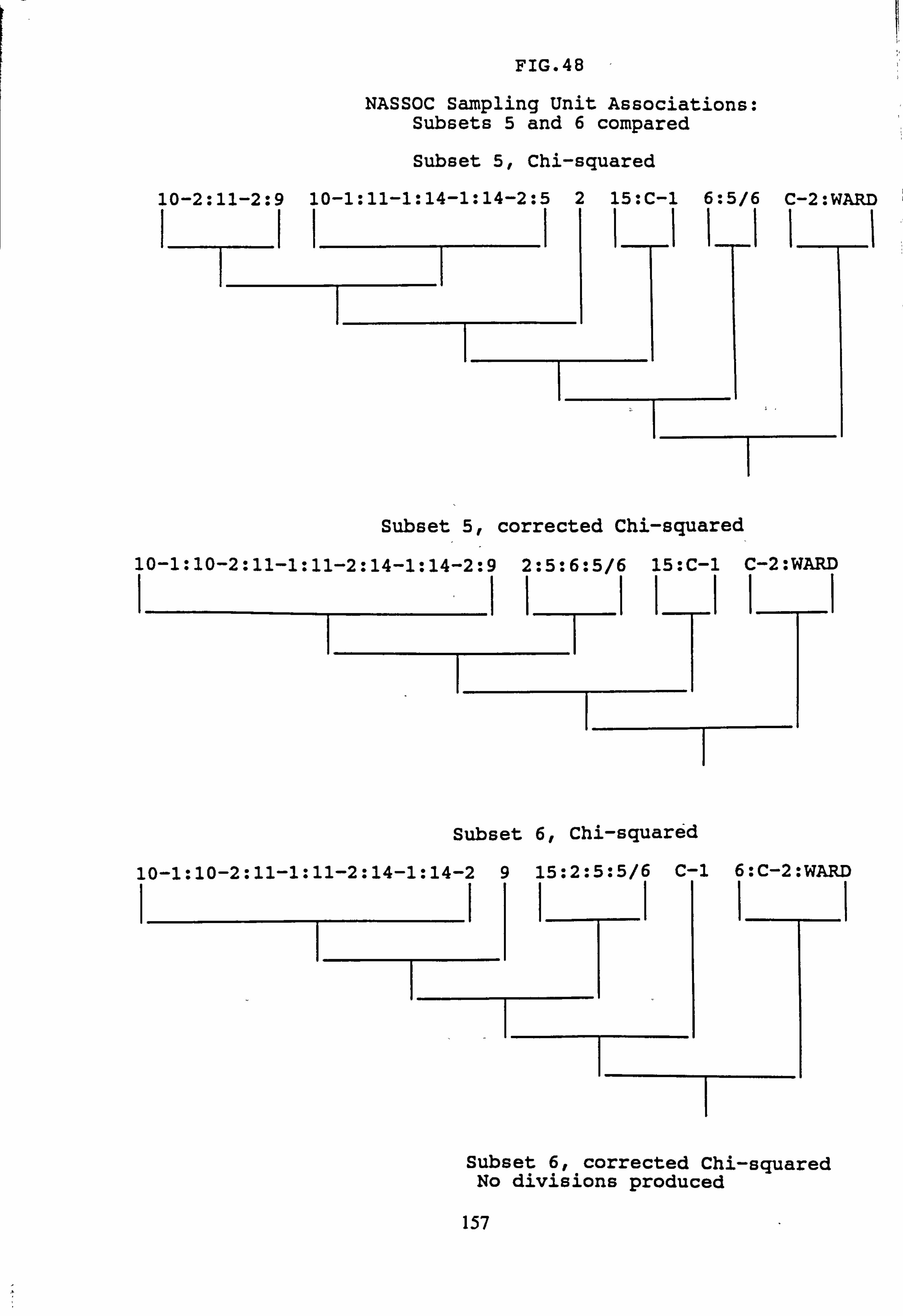
FIG. 48
NASSOC Sampling Unit Associations: Subsets 5 and 6 compared
Subset 5, Chi-squared
10-2: 11-2: 9 10-1: 11-1: 14-1: 14-2: 5 2 15: C-1 6: 5/6 C-2: WARD IIIIIIIIII
Subset 5, corrected Chi-squared
10-1: 10-2: 11-1: 11-2: 14-1: 14-2: 9 2: 5: 6: 5/6 15: C-1 C-2: WARD IIIIIIII
Subset 6, Chi-squared
10-1: 10-2: 11-1: 11-2: 14-1: 14-2 9 15: 2: 5: 5/6 C-1 6: C-2: WARD IIIIII
Subset 6, corrected Chi-squared No divisions produced
157
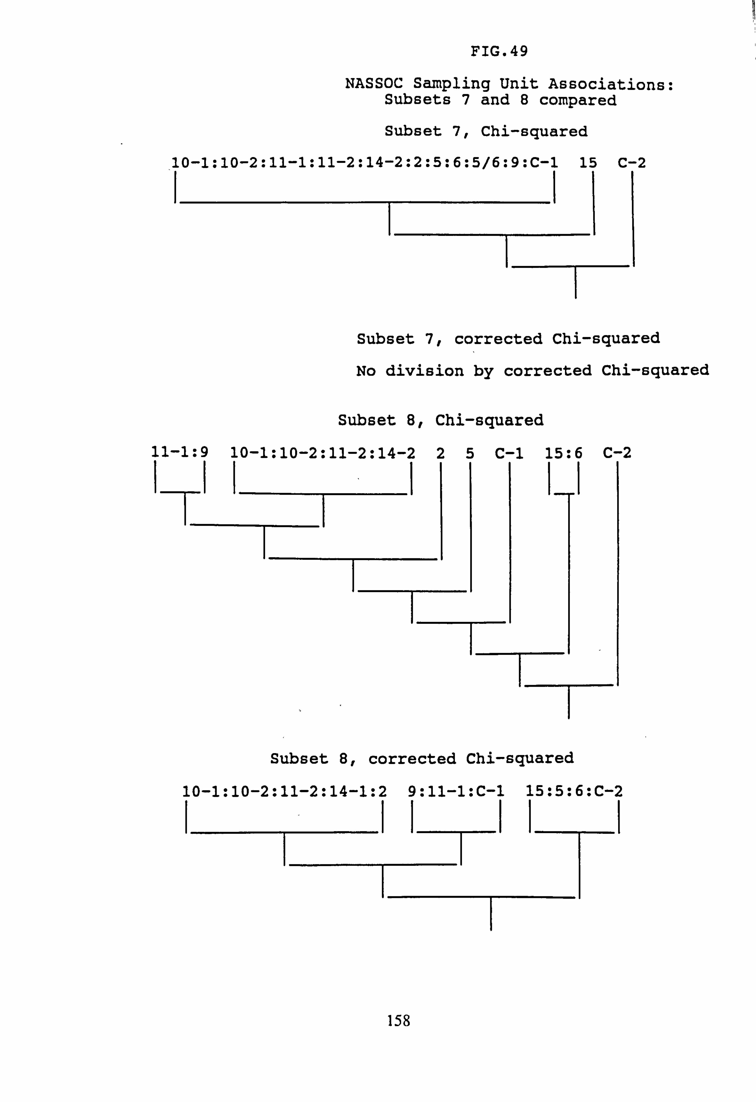
FIG. 49
NASSOC Sampling Unit Associations: Subsets 7 and 8 compared
Subset 7, Chi-squared
10-1: 10-2: 11-1: 11-2: 14-2: 2: 5: 6: 5/6: 9: C-1 15 C-2 II
Subset 7, corrected Chi-squared
No division by corrected Chi-squared
Subset 8, Chi-squared
11-1: 9 10-1: 10-2: 11-2: 14-2 25 C-1 15: 6 C-2 IIIIII
-T -T
Subset 8, corrected Chi-squared
10-1: 10-2: 11-2: 14-1: 2 9: 11-1: C-1 15: 5: 6: C-2 IIIIII
158
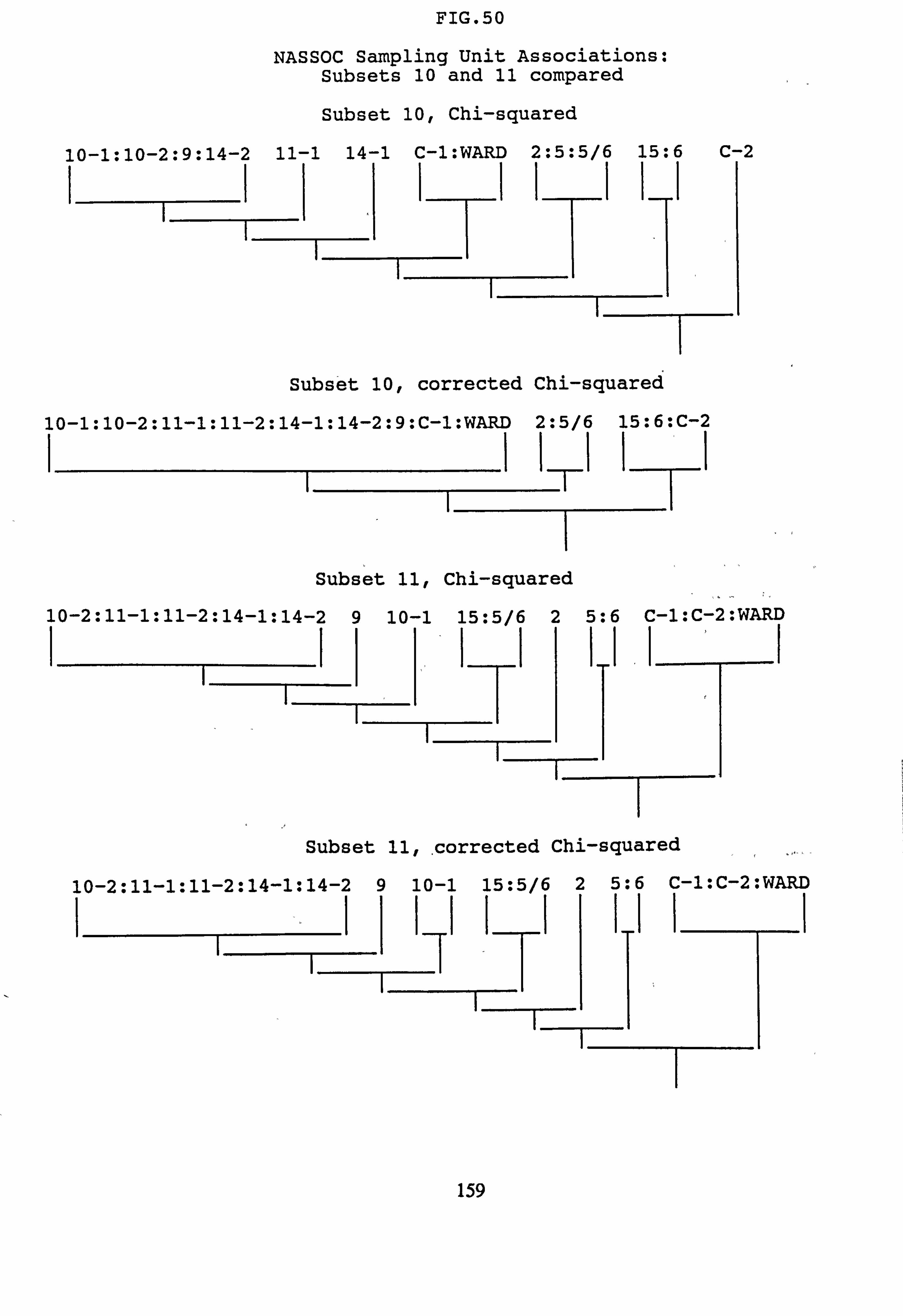
FIG. 50
NASSOC Sampling Unit Associations: Subsets 10 and 11 compared
Subset 10, Chi-squared
10-1: 10-2: 9: 14-2 11-1 14-1 C-1: WARD 2: 5: 5/6 15: 6 C-2 IIIIIIII
Subset 10, corrected Chi-squared
10-1: 10-2: 11-1: 11-2: 14-1: 14-2: 9: C-1: WARD 2: 5/6 15: 6: C-2 IIIIII
Subset 11, Chi-squared
10-2: 11-1: 11-2: 14-1: 14-2 9 10-1 15: 5/6 2 5: IIIII
C-1: C-2: WARD
Subset 11,. corrected Chi-squared
10-2: 11-1: 11-2: 14-1: 14-2 9 10-1 15: 5/6 2 5: 6 C-1: C-2: WARD
111I1 Ifs
159
corrected X2. It separates a group of sites which are characterised by having the highest mean
pH values (Table 46) from the others. These sites are Ward, C-1, C-2,15,6, and in some
analyses 5 also.
The second cycle divides the remaining sites into two groups, which may be interpreted as being a group of the lowest pH sites and an intermediate group, although the composition of
the latter is somewhat variable. It should be noted that these designations are at this stage
purely subjective, suggested by the observed distribution of mean pH shown in Table 46.
The data subsets used in Inverse Association Analysis (Section 4.4.2) were also subjected to
NAA (Figs. 46-50). Here also the least acidic sites tend to be separated off earliest in the
analysis but the results are much more variable. It is clear that the value of the analysis is
greatly enhanced if the data set is based on a larger number of samples.
An interesting feature seen in Figs. 41 and 42 is that the burn 5 site is associated with the least
acidic group in Matrix A, but with the most acidic group in Matrix B. If this is not simply a statistical aberration, it implies that burn 5 may be undergoing further acidification. In Figs. 43 and 44 however bum 5 is found to be associated with burns 2 and 5/6 which are intermediate in many of the analyses. It is also noteworthy that 14-1,5/6 and Ward form one group in
Matrix A, Figs 43 and 44, due to the paucity of samples. Thus insufficient or unevenly distributed data can bias the results.
4.6.4 Cluster Analysis
4.6.4.1 Choice of method The cluster analysis maybe carried out on several distance measures by several different
strategies; the CLUSTER. BAS program includes 10 distance measures and 4 strategies including a flexible strategy in which the analyst chooses the value of ß to be used in
the computation. Thus up to approximately 100 different cluster analyses may be
carried out on each data set. The results may be quite variable and it might be possible to choose an analysis to fit in with a number of different hypotheses. Some of the
clustering methods may be favoured a priori on theoretical grounds (Ludwig and Reynolds, 1988).
160
Ludwig and Reynolds recommend in particular the use of Percent Dissimilarity and Chord distance as they give less weight to the higher abundance groups. Also, Relative
Euclidean distances are preferable to Euclidean distance measures which may in some
circumstances give spurious results (Ludwig and Reynolds, 1988). Since the data
matrices are based on relative abundance measures rather than absolute numbers it may be questioned whether the use of Chord or P. D. is as advantageous in this case. The
cluster analyses were carried out using Mean Absolute Distance (a Euclidean measure), P. D., Chord and Relative Euclidean Distance, by both the group-average strategy and the flexible strategy with 0 ranging from +0.25 to -0.5.
Pinel-Alloul et al (1990) utilized aß value of -0.25 in order to minimise chaining. A ß value of -0.25 tends to be space conserving, i. e. not distorting the distances between S. U. s (Ludwig and Reynolds, 1988).
4.6.4.2 Results Most procedures produce clusters in which the circumneutral sites (burn 15, Corrie (upper and lower) and Ward burn) are separated from the acidic sites (burns 14,9,10and 11) with the remainder (bums 2,5,6,5/6) forming an intermediate group whose members might in some procedures be linked more closely with one of the other groups. In some cluster sets, burns 14 and 11-2 are attached more closely to burns 2 and 5, the more acidic of the intermediate group.
MAD frequently gives rise to chaining, in which clear groups are not formed but S. U. s are attached one at a time.
Intuitively an analysis might appear more valid if the upstream/downstream sites on the same burns are paired up early in the clustering. This is true in a large number of procedures for burns 14,10 and, slightly less frequently, 11. It might not be expected for the Corrie burn as the upper Corrie site (C-1) is situated above the confluence of a tributary which though small is nonetheless the least acidic of 4 feeder streams. It is also found that burns 2 and 5 are frequently paired up early in the clustering.
The performance of the different clustering procedures on the different data matrices is
compared in Table 47.
161
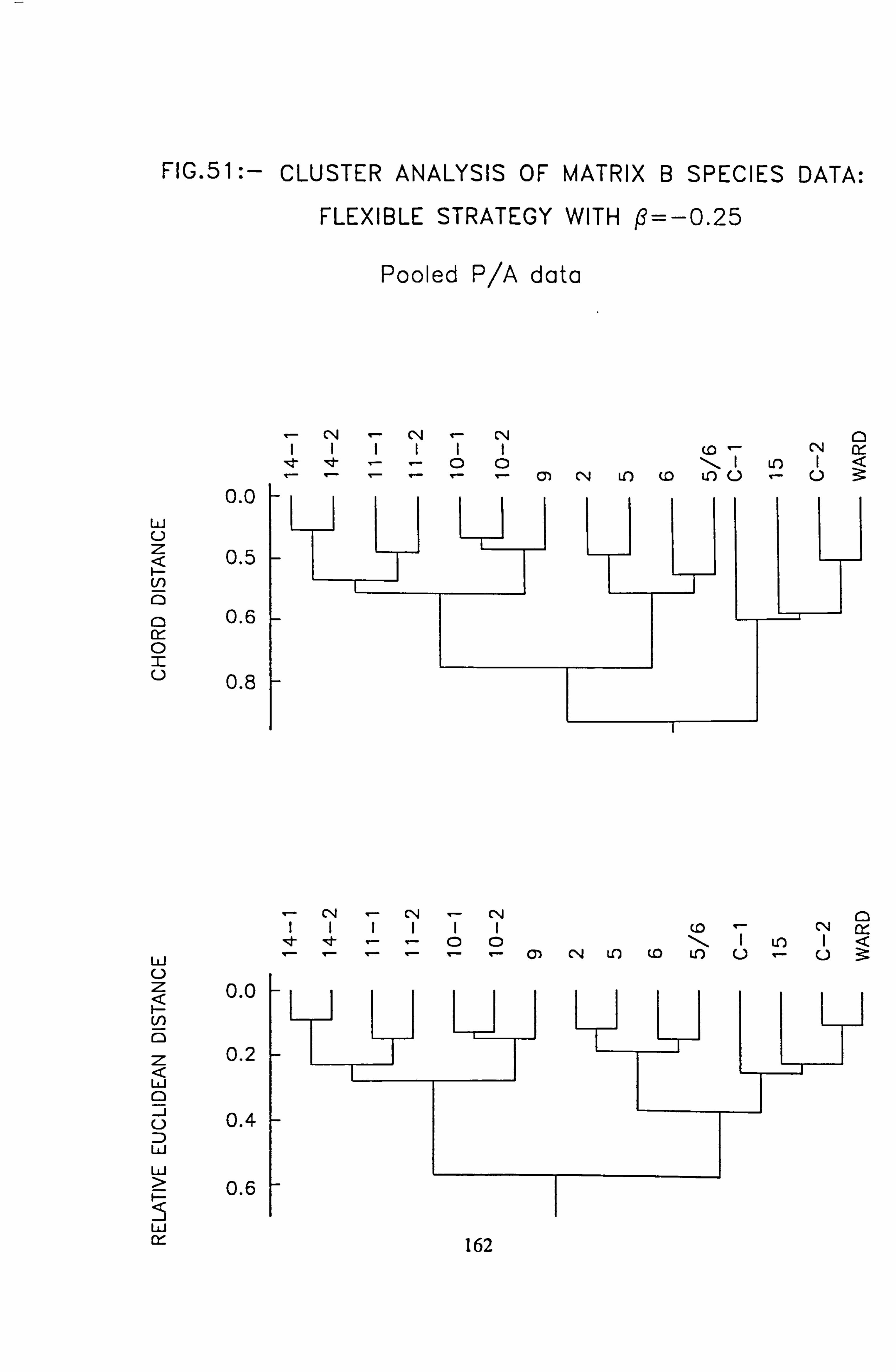
FIG. 51: - CLUSTER ANALYSIS OF MATRIX B SPECIES DATA:
FLEXIBLE STRATEGY WITH ß=-0.25
Pooled P/A data
0.0 w U Q 0.5
0 0.6
0 u 0.8
W U Z
N 0
Z
W
J U
W
W
0.0
0.2
0.4
0.6
"-NN "- Np iIOOI\I
i) Q r- r- "- "- "- N to cD LC) U, U
162
N r- NN0 (0 'N
00\I Lo U "-- "- "- "-- mN Lo W Lo 0
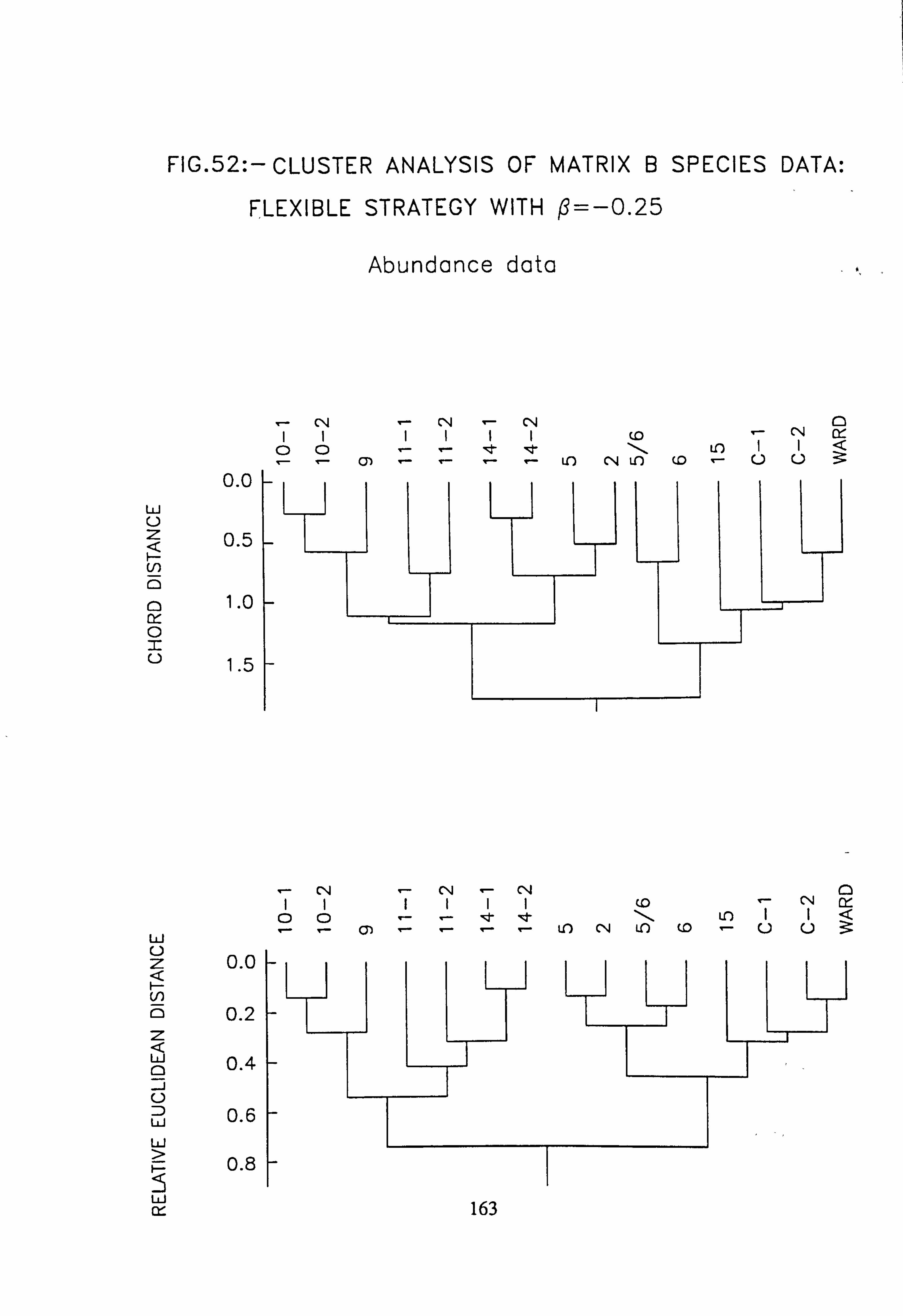
FIG. 52: - CLUSTER ANALYSIS OF MATRIX B SPECIES DATA:
FLEXIBLE STRATEGY WITH ß=-0.25
Abundance data
0.0 w U z 0.5 U,
0 1.0
0
1.5
w C) 0.0
V) o 0.2 z Q ö 0.4
v w 0.6
0.8
NN-N0 ÖÖii
LO UU< -- .- Qý r- "- r- U) N to CD
163
x
"- NN otý
NiIINUU
OO 0) "- ý- "- '- If) N tf) cD
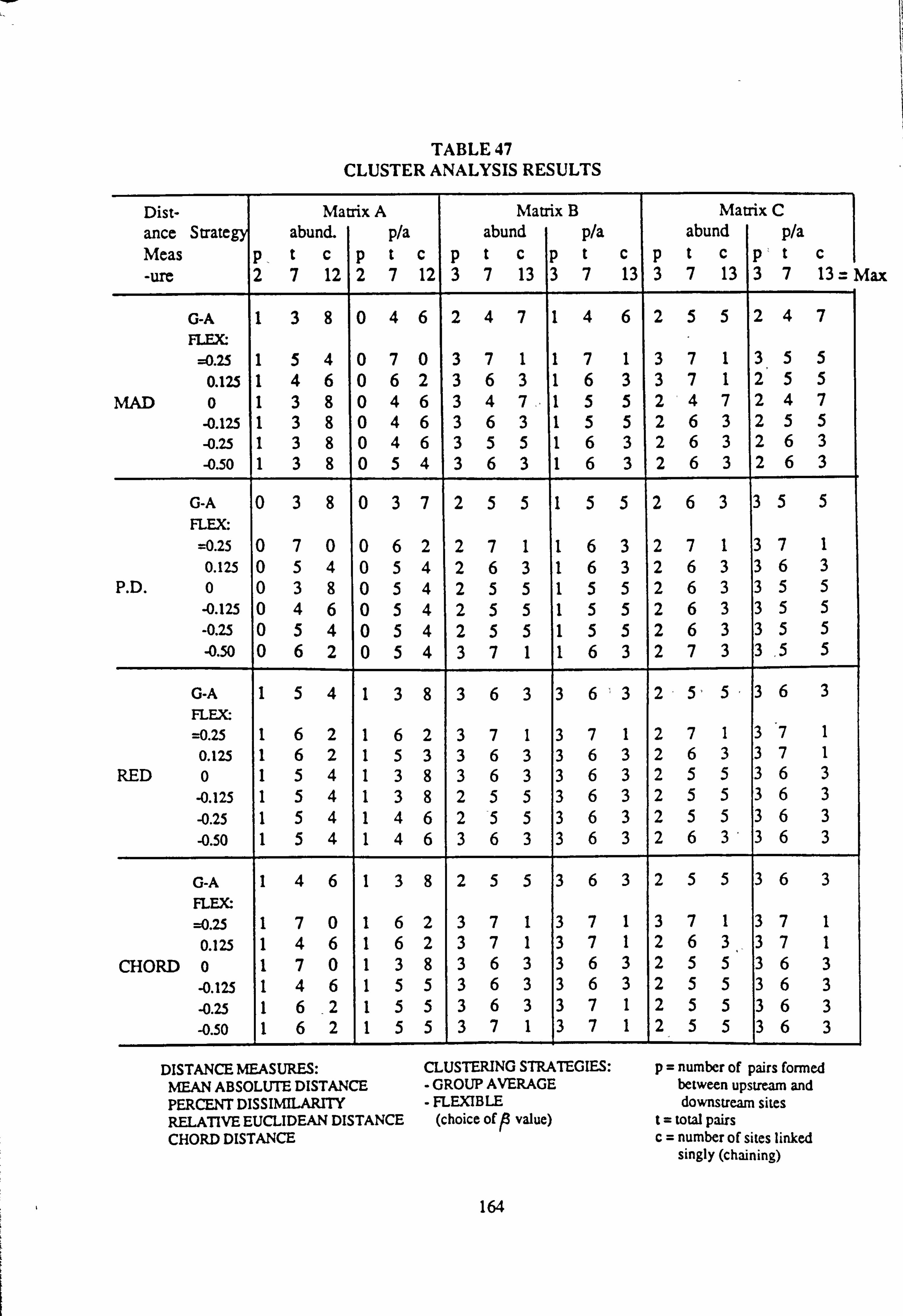
TABLE 47 CLUSTER ANALYSIS RESULTS
Dist- Matrix A Matrix B Matrix C
ance Strategy abund. p/a abu nd p/a abu nd p/a Meas p t c p t c p t cp t c p t c p t c -ure 2 7 12 2 7 12 3 7 13 3 7 13 3 7 13 3 7 13
G-A 1 3 8 0 4 6 2 4 7 1 4 6 2 5 5 2 4 7 FLEX:
=0.25 1 5 4 0 7 0 3 7 1 1 7 1 3 7 1 3 5 5 0.125 1 4 6 0 6 2 3 6 3 1 6 3 3 7 1 2 5 5
MAD 0 1 3 8 0 4 6 3 4 7 1 5 5 2 4 7 2 4 7
-0.125 1 3 8 0 4 6 3 6 3 1 5 5 2 6 3 2 5 5
-0.25 1 3 8 0 4 6 3 5 5 1 6 3 2 6 3 2 6 3
-0.50 1 3 8 0 5 4 3 6 3 1 6 3 2 6 3 2 6 3
G-A 0 3 8 0 3 7 2 5 5 1 5 5 2 6 3 3 5 5 FLEX:
=0.25 0 7 0 0 6 2 2 7 1 1 6 3 2 7 1 3 7 1 0.125 0 5 4 0 5 4 2 6 3 1 6 3 2 6 3 3 6 3
P. D. 0 0 3 8 0 5 4 2 5 5 1 5 5 2 6 3 3 5 5
-0.125 0 4 6 0 5 4 2 5 5 1 5 5 2 6 3 3 5 5
-0.25 0 5 4 0 5 4 2 5 5 1 5 5 2 6 3 3 5 5
-0.50 0 6 2 0 5 4 3 7 1 1 6 3 2 7 3 3 .5
5
G-A 1 5 4 1 3 8 3 6 3 3 6' 3 2 5 5 3 6 3 FLEX
=0.25 1 6 2 1 6 2 3 7 1 3 7 1 2 7 1 3 7 1 0.125 1 6 2 1 5 3 3 6 3 3 6 3 2 6 3 3 7 1
RED 0 1 5 4 1 3 8 3 6 3 3 6 3 2 5 5 3 6 3
-0.125 1 5 4 1 3 8 2 5 5 3 6 3 2 5 5 3 6 3
-0.25 1 5 4 1 4 6 2 5 5 3 6 3 2 5 5 3 6 3
-0.50 1 5 4 1 4 6 3 6 3 3 6 3 2 6 3 3 6 3
G-A 1 4 6 1 3 8 2 5 5 3 6 3 2 5 5 3 6 3 FLEX
=0.25 1 7 0 1 6 2 3 7 1 3 7 1 3 7 1 3 7 1 0.125 1 4 6 1 6 2 3 7 1 3 7 1 2 6 3 3 7 1
CHORD 0 1 7 0 1 3 8 3 6 3 3 6 3 2 5 5 3 6 3
-0.125 1 4 6 1 5 5 3 6 3 3 6 3 2 5 5 3 6 3
-0.25 1 6 -2
1 5 5 3 6 3 3 7 1 2 5 5 3 6 3
-0.50 1 6 2 1 5 5 3 7 1 3 7 1 2 5 5 3 6 3
DISTANCE MEASURES: MEAN ABSOLUTE DISTANCE PERCENT DISSIMILARITY RELATIVE EUCLIDEAN DISTANCE CHORD DISTANCE
CLUSTERING STRATEGIES:
- GROUP AVERAGE
- FLEXIBLE (choice of p value)
p= number of pairs formed between upstream and downstream sites
t= total pairs c= number of sites linked
singly (chaining)
dax
164
The first value'p' shows the number of pairings of upstream and downstream sites, e. g. 14-1 with 14-2. There are two such possible pairings in Matrix A and three in B and C.
Thus the higher the value in this column, the closer is the result to the expectation that
such sites should be similar.
The second value 't' shows the total number of pairs formed in the dendrogram. The third
value 'c' shows the number of sites which are attached by'chaining'. Thus t and c show the relative contribution of pairing and chaining.
The chaining phenomenon may be useful in that it shows a relative order of the sites, which is not apparent from highly paired dendrograms, since a cluster may be rotated
about the common stem. This information may then be used to order the sites in a dendrogram involving pairings. However different clustering procedures may result in
mutually exclusive interpretations of the interrelationship between sites.
The order of the sites shown in the cluster dendrograms (Figs. 51,52) has been drawn
up using evidence from chaining.
For a comparison of the relative virtues of different approaches, Matrix B data (the
second half of the time series) provides the most complete data set, as all sites were sampled during this period (not all on every occasion however). The data may be utilized in two ways (a) as a matrix based on the mean relative abundances of the taxa or (b) as
a matrix obtained by summing the presence/absence scores on each sampling occasion (giving a maximum score of 18 for any species in any site).
The Presence/Absence (p/a) data are found to give more consistent pairing of upstream- downstream sites than the abundance data. Figs. 51 and 52 shows a comparison of both
data sets clustered by the Flexible strategy, with ß= -0.25, using Chord distance and Relative Euclidean Distance.
This may be taken as some evidence for the superiority of the presence-absence form of the data. However the differences are very slight and it might not be correct to expect a very close pairing between 11-1 and 11-2 as the former is in a very open site with relatively slow-moving water and a heavy growth of mosses and liverworts, while the latter is heavily shaded by trees and lies downstream of a substantial waterfall, factors
which may result in some floral differences.
165
Therefore on the whole the results obtained using the pooled P/A data tend to support those obtained with relative abundance data, dividing the sites into a circumneutral set and an acidified set.
Intermediate between these are the sites on burns 2,5 and 6 which are attached to the
acidic set in the Chord Distance clusterings, and to the circumneutral set in RED
clustering.
These are burns which are at risk of acidification, being originally base-poor, moorland streams with low humic content. Burn 2 is still in this condition, with a very low
percentage of forest cover (about 100 m of bankside conifers), while the catchments of burns 5 and 6 are unforestedin their upper reaches, but with young coniferous plantation surrounding the sites and extending about half a mile upstream.
With the growth of the trees approaching canopy closure, the drainage water may be
expected to acidify further (Nilsson eta!, 1982; Nilsson, 1983) depending on the nature of the precipitation. Burns 2 and 6 currently still support the presence of fish, while burn 5 does not.
The composition of the algal flora therefore can be used to group the sites as shown by
correlations between sites in respect of their species composition (Species Covariation), by Species Association and Normal Association Analysis based on presence-absence data, and by Cluster Analysis based on both abundance and pooled P/A data, and this
grouping is related to the acidification status of the sites.
166
4.7 SPECIES-ENVIRONMENT RELATIONSHIPS
4.7.1 Preliminary Considerations: choice of method The type of analysis to be pursued depends on whether the relationship between species and environmental variables is best described by a linear or unimodel model. If the environmental gradient is short, a linear model may be appropriate (Ter Braak and Prentice, 1988).
The length of the environmental gradient formed by each of the variables measured is shown in Table 48. The majority exceed 3 S. D. and none is less than 2. The non-linear methods carried out by CANOCO are relevant if the gradient is more than 3 S. D. in length and should not be used if it is less than 1.5 (Ter Braak and Prentice, 1988).
To determine whether a linearmodel is appropriate for particular species, exploratory analyses were carried out. The Pearson correlation coefficient 'r' was calculated between individual
species and each environmental variable in turn (Table 49). The appropriate significance level depends on the number of correlations in the set. With 49 species and 16 variables, there are 784 correlations, so a strong correlation might be obtained purely by chance at a significance level less than 0.1%. At this level, the value of r which is significant depends on the number of data points on which each correlation is calculated: e. g. for pH a correlation is significant if it exceeds 0.165. Since the number of data points differ depending on the number of measurements made of each variable, the 0.1 % significance value of r for each is included in the table.
The possibility that transformation of the environmental data might yield larger correlation coefficients was considered. Inspection of the data points in plots of species abundance versus
environmental variables suggested that a Loglo or square root transformation might be
appropriate.
The effect of Log,, and square-root transformation of environmental variables was initially investigated through correlation analysis of total species number per sample with environ- mental variables (Table 50) as a larger number of data points is available than with individual
species.
Higher correlations are found with untransformed pH, alkalinity, Ca2', Mgt+, Si02, and with Logo transformed P04, Al-TM, Al-NL and Al-L.
167
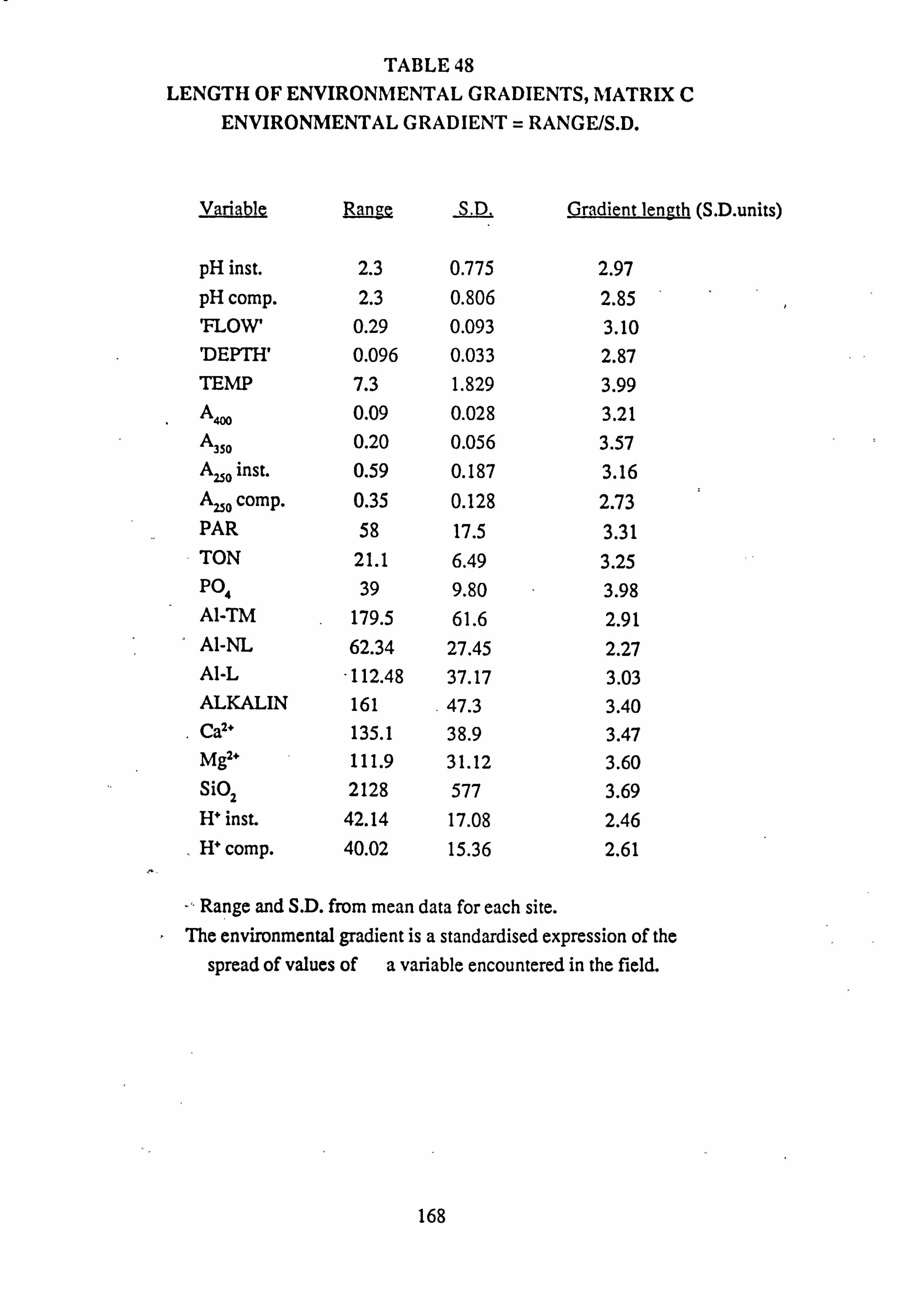
TABLE 48 LENGTH OF ENVIRONMENTAL GRADIENTS, MATRIX C
ENVIRONMENTAL GRADIENT = RANGE/S. D.
Variable Range S. D. Gradient length (S. D. units)
pH inst. 2.3 0.775 2.97
pH comp. 2.3 0.806 2.85 'FLOW 0.29 0.093 3.10 DEPTH' 0.096 0.033 2.87 TEMP 7.3 1.829 3.99 A 400 0.09 0.028 3.21 A350 0.20 0.056 3.57 A, 0 inst. 0.59 0.187 3.16 Au0 comp. 0.35 0.128 2.73 PAR 58 17.5 3.31 TON 21.1 6.49 3.25 P04 39 9.80 3.98 Al-TM 179.5 61.6 2.91 Al-NL 62.34 27.45 2.27 Al-L -112.48 37.17 3.03 ALKALIN 161 47.3 3.40 Caz+ 135.1 38.9 3.47 Mg2a 111.9 31.12 3.60 Si02 2128 577 3.69 If inst. 42.14 17.08 2.46 If comp. 40.02 15.36 2.61
r.
Range and S. D. from mean data for each site. The environmental gradient is a standardised expression of the
spread of values of a variable encountered in the field.
168
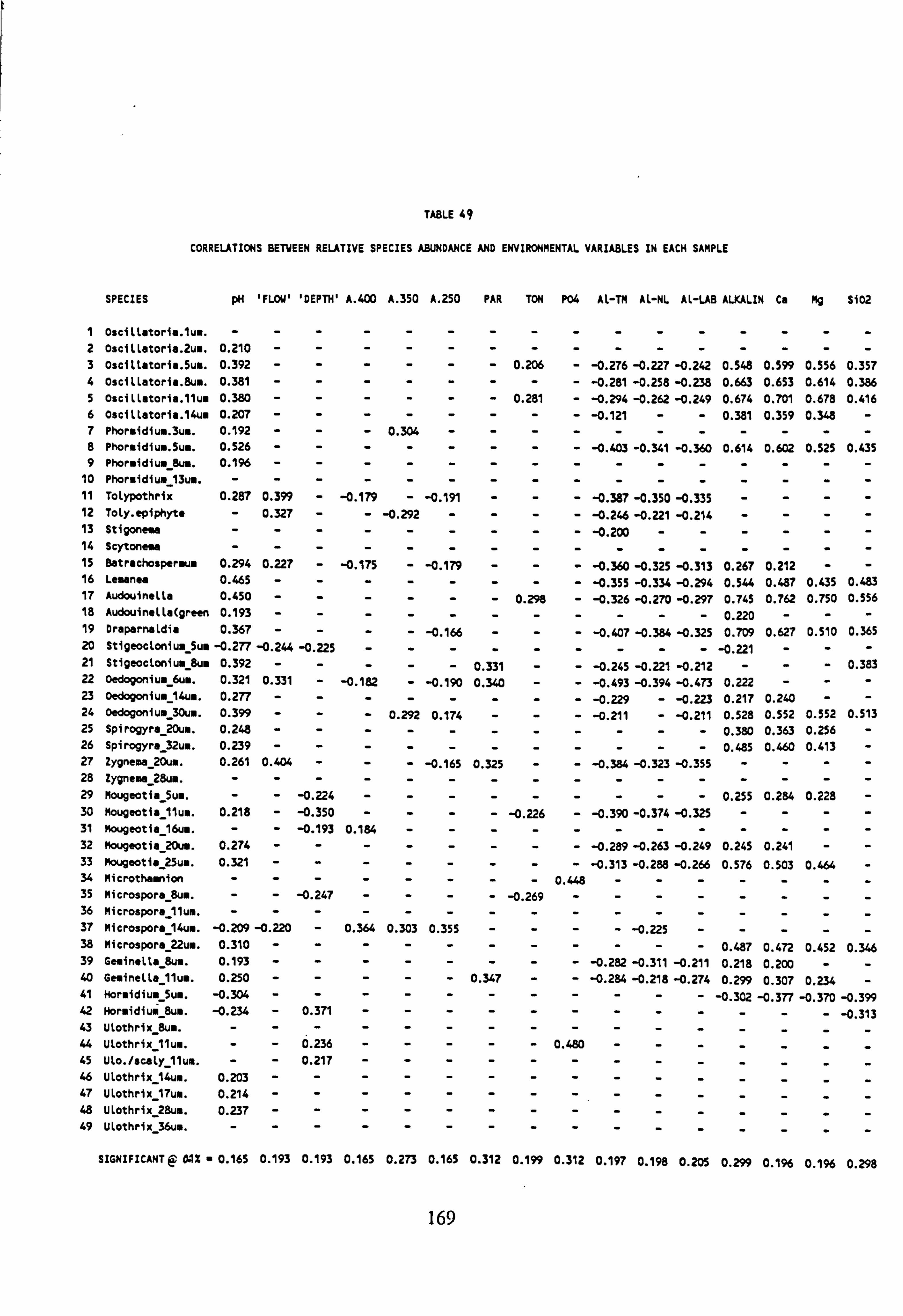
TABLE 49
CORRELATIONS BETWEEN RELATIVE SPECIES ABUNDANCE AND ENVIRONMENTAL VARIABLES IN EACH SAMPLE
SPECIES PH 'FLOW' 'DEPTH' A. 400 A. 350 A. 250 PAR TON P04 Al-TM AL-NL AL-UB ALKALIN Ca N9 SiO2
1 Oscillatorie. lu.. -------- 2 Oscillatorie. 2uu. 0.210 ------- 3 Oscillatoria. 5ua. 0.392 ------0.206 4 Oscillatoria. 8ua. 0.381 ------- 5 Oscillatoria. lluu 0.380 ------0.281 6 Oscillatoria. 14ua 0.207 ------- 7 Phoraidium. 3ua. 0.192 ---0.304 --- 8 Phoraidiua. Sua. 0.526 ------- 9 Phoraidiuiu_8ua. 0.196 -------
10 Phoraidiua_13ua. -------- 11 Tolypothrix 0.287 0.399 - -0.179 - -0.191 -- 12 Toly. epiphyte - 0.327 -- -0.292 --- 13 Stigoneae -------- 14 Scytoneae -------- 15 Batrechosperau. 0.294 0.227 - -0.175 - -0.179 -- 16 Leaenee 0.465 ------- 17 Audouinelle 0.450 ------0.298 18 Audouinella(green 0.193 ------- 19 Dreparnaldia 0.367 ---- -0.166 -- 20 Stigeocloniu. 5ue -0.277 -0.244 -0.225 ----- 21 Stigeocloniu. 8u. 0.392 -----0.331 - 22 Oedogoniue_6ua. 0.321 0.331 - -0.182 - -0.190 0.340 - 23 Oedogonium-14un. 0.277 ------- 24 Oedogonius 30us. 0.399 ---0.292 0.174 -- 25 Spirogyra 20ua. 0.248 ------- 26 Spirogyrs 32ua. 0.239 ------- 27 Zygnema 20ua. 0.261 0.404 --- -0.165 0.325 - 28 Zygnena 28u.. -------- 29 Mougeotia 5u.. -- -0.224 ----- 30 Mougeotia 11u.. 0.218 - -0.350 ---- -0.226 31 Mougeotie 16ua. -- -0.193 0.184 ---- 32 Mougeotia 20u.. 0.274 ------- 33 Mougeotia 25ua. 0.321 ------- 34 Microthaanion -------- 35 Microspora 8ua. -- -0.247 ---- -0.269 36 Nitrospore 11ua. -------- 37 Microspora 14ua. -0.209 -0.220 - 0.364 0.303 0.355 -- 38 Microspors 22uw. 0.310 ------- 39 Geninella_8ua. 0.193 ------- 40 Geainelle_llua. 0.250 -----0.347 - 41 Horaidiua_5ua. -0.304 ------- 42 Horaidiue8u.. -0.234 - 0.371 ----- 43 Ulothrix_8um. -------- 44 Ulothrix_11u.. --0.236 ----- 45 Ulo. /scaly_llum. --0.217 ----- 46 Ulothrix_14um. 0.203 ------- 47 Ulothrix_17um. 0.214 ------- 48 Ulothrix_28us. 0.237 ------- 49 Ulothrix 36ue. --------
- -0.276 -0.227 -0.242 0.548 0.599 0.556 0.357 - -0.281 -0.258 -0.238 0.663 0.653 0.614 0.386 - -0.294 -0.262 -0.249 0.674 0.701 0.678 0.416
- -0.121 -- 0.381 0.359 0.348 -
- -0.403 -0.341 -0.360 0.614 0.602 0.525 0.435
- -0.387 -0.350 -0.335 - - - - - -0.246 -0.221 -0.214 - - - - - -0.200 -- - - - -
- -0.360 -0.325 -0.313 0.267 0.212 - - - -0.355 -0.334 -0.294 0.544 0.487 0.435 0.483 - -0.326 -0.270 -0.297 0.745 0.762 0.750 0.556
---- 0.220 - - - - -0.407 -0.384 -0.325 0.709 0.627 0.510 0.365
---- -0.221 - - - - -0.245 -0.221 -0.212 - - - 0.383
- -0.493 -0.394 -0.473 0.222 - - -
- -0.229 - -0.223 0.217 0.240 - - - -0.211 - -0.211 0.528 0.552 0.552 0.513
---- 0.380 0.363 0.256 -
---- 0.485 0.460 0.413 -
- -0.384 -0.323 -0.355 - - - -
---- 0.255 0.284 0.228 - - -0.390 -0.374 -0.325 - - - -
- -0.289 -0.263 -0.249 0.245 0.241 - - - -0.313 -0.288 -0.266 0.576 0.503 0.464 -
0.448 --- - - - -
-- -0.225 - - - - - ---- 0.487 0.472 0.452 0.346 - -0.282 -0.311 -0.211 0.218 0.200 - - - -0.284 -0.218 -0.274 0.299 0.307 0.234 - ---- -0.302 -0.377 -0.370 -0.399 '-- - - - -0.313
0.480
SIGNIFICANT @ 09% " 0.165 0.193 0.193 0.165 0.273 0.165 0.312 0.199 0.312 0.197 0.198 0.205 0.299 0.196 0.196 0.298
169

TABLE 50 CORRELATION ANALYSIS OF TOTAL SPECIES NUMBER PER SAMPLE WITH UNTRANSFORMED AND LOG,, ENVIRONMENTAL VARIABLES
PF A' value of r (+/-) VARIABLE untransformed Loglo transformed significant at 0.1%
pH 0.633 # - 0.164
DEPTH' -0.253 -0.253 0.193
A 400 -0.105 -0.146 0.165
Also -0.131 -0.206 0.270
Au0 -0.113 -0.154 0.164
TON -0.038 -0.094 0.198
PO4 -0.094 -0.320 # 0.312
Al - T. M. -0.587 -0.661 # 0.196
Al - N. L. -0.527 -0.584 # 0.198
Al -L - 0.509 -0.657 # 0.205
Alkalinity 0.619 # 0.528 0.299
Ca" 0.589 # 0.525 0.196
Mg+' 0.418 # 0.313 0.196
Si02 0.446 0.205 0.298
PAR 0.260 0.251 0.312
# values exceeding the 0.1% significance level; the higher value of the pair is indicated
170
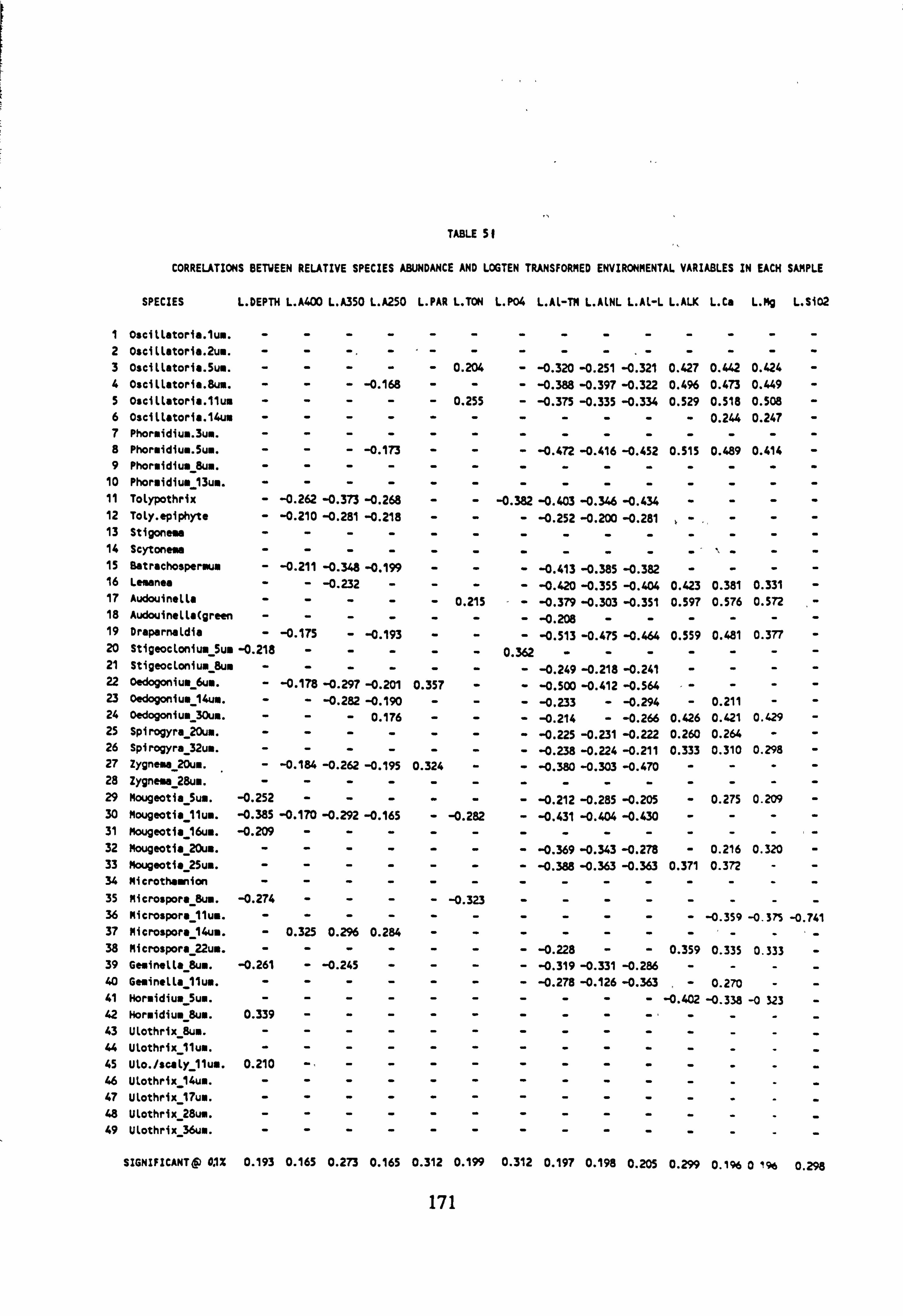
TABLE $
CORRELATIONS BETWEEN RELATIVE SPECIES ABUNDANCE AND LOGTEN TRANSFORMED ENVIRONMENTAL VARIABLES IN EACH SAMPLE
SPECIES L. DEPTH L. A400 L. A350 L. A250 L. PAR L. TON L. P04 L. AL-TM L. ALNL L. AL-L L. ALK L. Ca L. Mg L. Si02
1 Oscillatoria. lu.. ---- -- 2 Oscilletoria. 2un. 3 Oscillatoria. 5u.. ---- - 0.204 4 Oscilletoria. 8us. --- -0.168 -- 5 0scillatoria. llus ---- - 0.255 6 Oscillatoria. 14us ---- -- 7 Phoraidiua. 3us. ---- -- 8 Phoreidiu.. 5u.. --- -0.173 -- 9 Phoraidius_8u.. ---- --
10 Phoruidiua_13ua. ---- -- 11 Tolypothrix - -0.262 -0.373 -0.268 -- 12 Toly. epiphyte - -0.210 -0.281 -0.218 -- 13 Stigonesb ---- -- 14 Scytone. s ---- -- 15 eatrachospereum - -0.211 -0.348 -0.199 -- 16 Leaanea -- -0.232 - -- 17 Audouinella ---- - 0.215 18 Audouinella(9reen ---- -- 19 Drapernaldia - -0.175 - -0.193 -- 20 Stigeoclonium_5u. -0.218 --- -- 21 Stigeocloniun_8u. ---- -- 22 Oedogoniuu 6u.. - -0.178 -0.297 -0.201 0.357 - 23 Oedogoniu.
_14ua. -- -0.282 -0.190 -- 24 Oedogoniu. 30um. ---0.176 -- 25 Spirogyra_20um. ---- -- 26 Spirogyra-32u.. ---- -- 27 Zyynesb20u.. - -0.184 -0.262 -0.195 0.324 - 28 ZY9ne. a_28u.. ---- -- 29 Nougeotia 5u.. -0.252 --- -- 30 Mougeetia Ilu.. -0.385 -0.170 -0.292 -0.165 - -0.282 31 Mougeotia 16u.. -0.209 --- -- 32 Mougeotia 20u.. ---- -- 33 Mougeotia 25um. ---- -- 34 Nicrothemion ---- -- 35 Microspora 8u.. -0.274 --- - -0.323 36 Nicrospora 11u.. ---- -- 37 Microspora 14u.. - 0.325 0.296 0.284 -- 38 Microspora 22u.. ---- -- 39 Geeinella_8u.. -0.261 - -0.245 - -- 40 Geainella_llum. ---- -- 41 Mor. idiua_5un. ---- -- 42 Hor. idiu.
_8u.. 0.339 --- --
43 Ulothrix_8u.. ---- -- 44 Ulothrix_11u.. ---- -- 45 Ulo. /suly_llum. 0.210 -: -- -- 46 Ulothrix_14u.. ---- -- 47 Ulothrix_17u.. ---- -- 48 Ulothrix_28ue. ---- -- 49 Ulothrix 36um. ---- --
- -0.320 -0.251 -0.321 0.427 0.442 0.424 - - -0.388 -0.397 -0.322 0.496 0.473 0.449 - - -0.375 -0.335 -0.334 0.529 0.518 0.508 - ---- - 0.244 0.247 -
- -0.472 -0.416 -0.452 0.515 0.489 0.414 -
-0.382 -0.403 -0.346 -0.434 - - -- - -0.252 -0.200 -0.281 - - --
- -0.413 -0.385 -0.382 - - -- - -0.420 -0.355 -0.404 0.423 0.381 0.331 - - -0.379 -0.303 -0.351 0.597 0.576 0.572 -
- -0.208 -- - - -- - -0.513 -0.475 -0.464 0.559 0.481 0.377 -
0.362 --- - - -- - -0.249 -0.218 -0.241 - - -- - -0.500 -0.412 -0.564 - - -- - -0.233 - -0.294 - 0.211 -- - -0.214 - -0.266 0.426 0.421 0.429 -
- -0.225 -0.231 -0.222 0.260 0.264 -- - -0.238 -0.224 -0.211 0.333 0.310 0.298 - - -0.380 -0.303 -0.470 - -
- -0.212 -0.285 -0.205 - 0.275 0.209 - - -0.431 -0.404 -0.430 - - --
- -0.369 -0.343 -0.278 - 0.216 0.320 - - -0.388 -0.363 -0.363 0.371 0.372 --
---- - -0.359 -0.375 -0.741
- -0.228 -- 0.359 0.335 0.333 - - -0.319 -0.331 -0.286 - - -- - -0.278 -0.126 -0.363 ,-
0.270 -- ---- -0.402 -0.338 -0 323 -
SIGNIFICANT & 0.1% 0.193 0.165 0.273 0.165 0.312 0.199 0.312 0.197 0.198 0.205 0.299 0.1% 0 1% 0.298
171
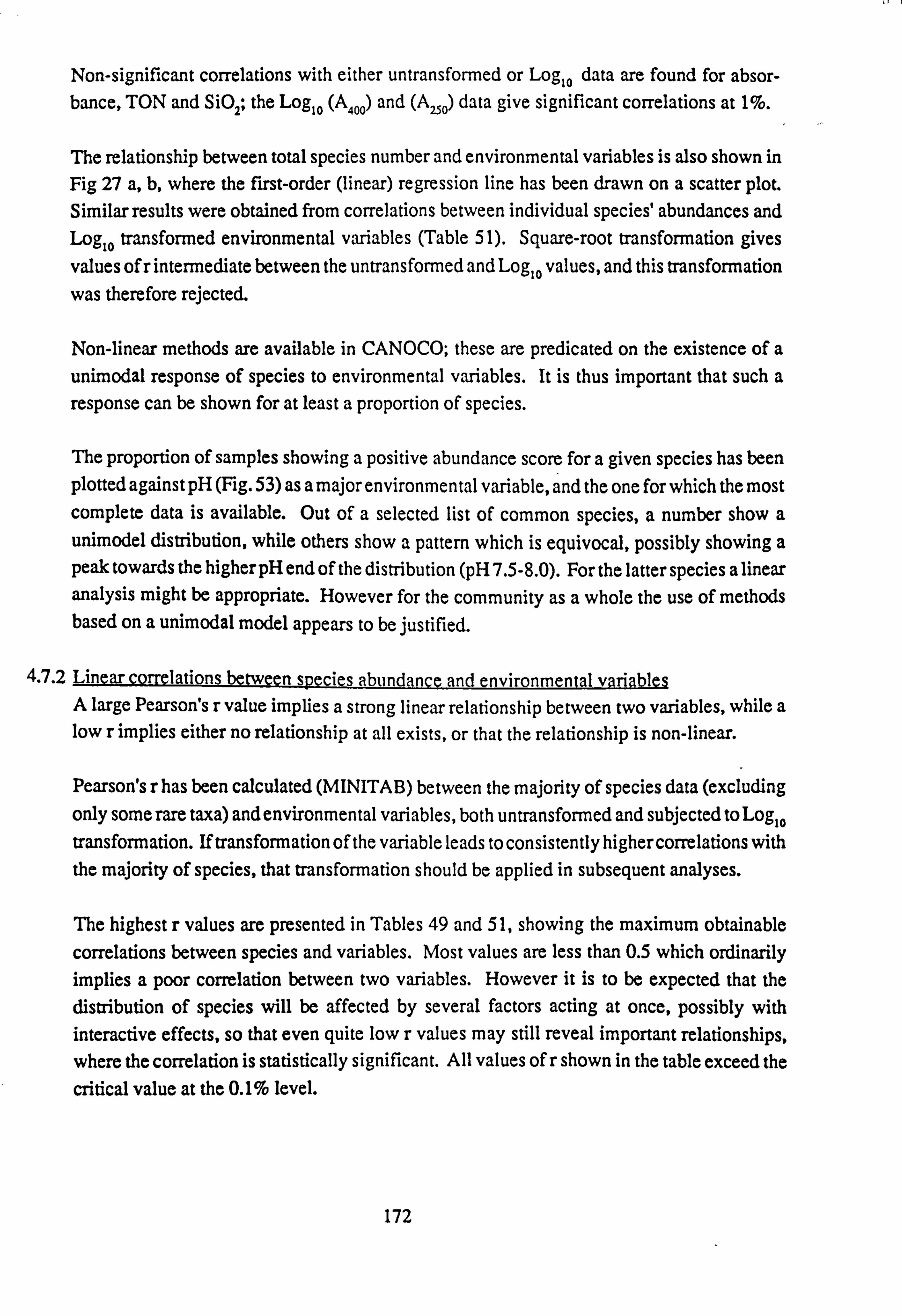
Non-significant correlations with either untransformed or Loglo data are found for absor- bance, TON and SiO2; the Loglo (A400) and (A250) data give significant correlations at 1%.
The relationship between total species number and environmental variables is also shown in Fig 27 a, b, where the first-order (linear) regression line has been drawn on a scatter plot. Similar results were obtained from correlations between individual species' abundances and Loglo transformed environmental variables (Table 51). Square-root transformation gives values of r intermediate between the untransformed and Loglo values, and this transformation was therefore rejected.
Non-linear methods are available in CANOCO; these are predicated on the existence of a unimodal response of species to environmental variables. It is thus important that such a response can be shown for at least a proportion of species.
The proportion of samples showing a positive abundance score for a given species has been
plotted against pH (Fig. 53) as a major environmental variable, and the one for which the most complete data is available. Out of a selected list of common species, a number show a unimodel distribution, while others show a pattern which is equivocal, possibly showing a peak towards the higher pH end of the distribution (pH 7.5-8.0). For the latter species a linear analysis might be appropriate. However for the community as a whole the use of methods based on a unimodal model appears to be justified.
4.7.2 Linear correlations between species abundance and environmental variables A large Pearson's r value implies a strong linear relationship between two variables, while a low r implies either no relationship at all exists, or that the relationship is non-linear.
Pearson's r has been calculated (MINITAB) between the majority of species data (excluding
only some rare taxa) and environmental variables, both untransformed and subjected to Loglo transformation. If transformation of the variable leads to consistently higher correlations with the majority of species, that transformation should be applied in subsequent analyses.
The highest r values are presented in Tables 49 and 51, showing the maximum obtainable correlations between species and variables. Most values are less than 0.5 which ordinarily implies a poor correlation between two variables. However it is to be expected that the distribution of species will be affected by several factors acting at once, possibly with interactive effects, so that even quite low r values may still reveal important relationships, where the correlation is statistically significant. All values of r shown in the table exceed the critical value at the 0.1% level.
172
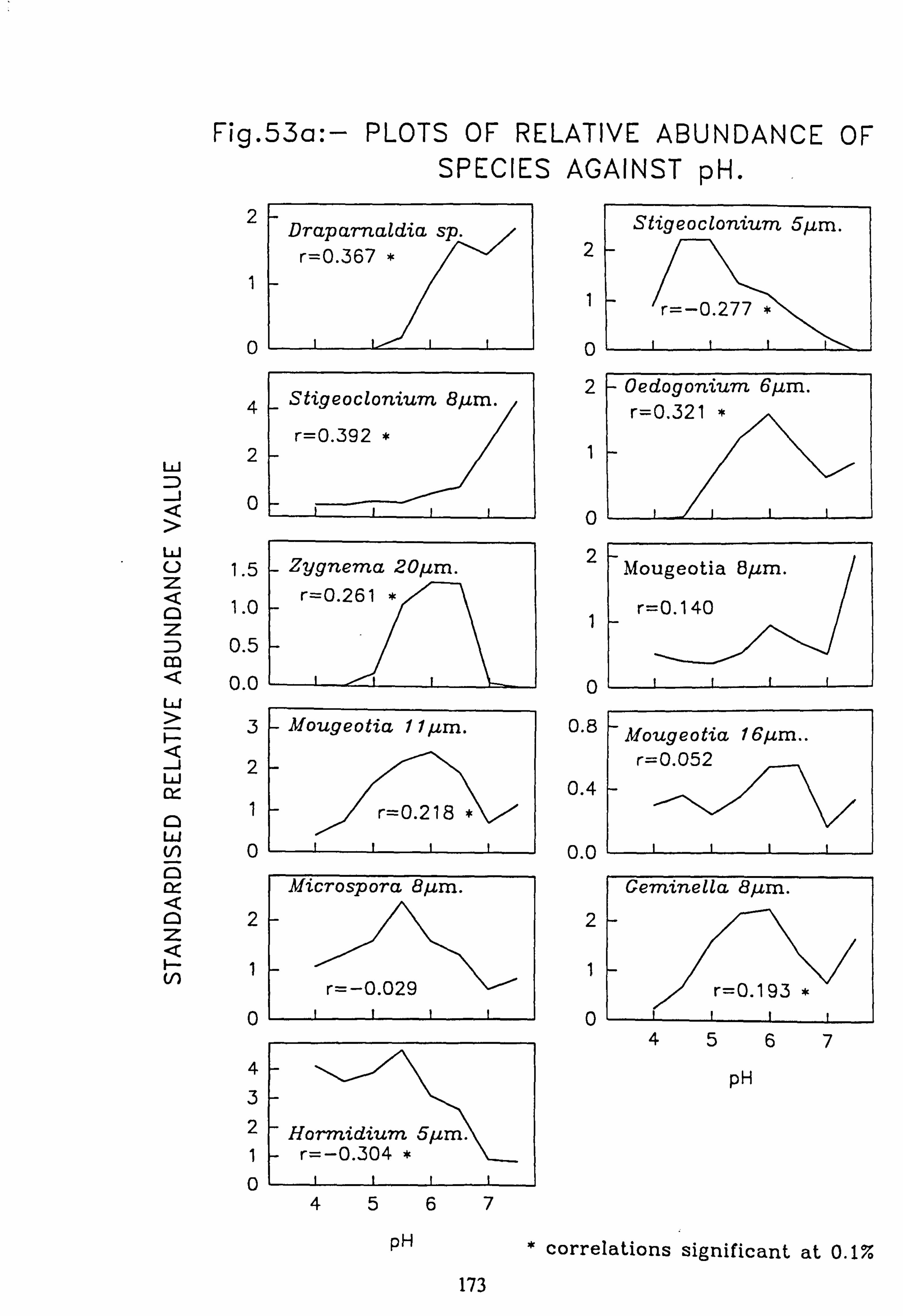
Fig. 53a: - PLOTS OF RELATIVE ABUNDANCE OF SPECIES AGAINST pH.
w
J
W U z
0 z Z) m W
J W cr-
a W (/') 0
0 z
2 Draparnaldia sp.
r=0.367 * %`
1
n
_ Stigeoclonium 8µm.
r=0.392 */
4
2
0
1.5
1.0
0.5
0.0
3
2
n
_ Zygnema 20/2m.
r=0.261 * z-"
- Mougeotia 11 ccm.
- r=0.218
Microspora 8µm.
r=-0.029
2
1
n
4 3
2
1
0
Horrnidi, u 5fcm. r=-0.304m
4 5 6 7
pH
2
1
0
2
Stigeoclonium 5µm.
r=-0.277 *
- Oedogonium 6µm. r=0.321 *
0 2
0 0.8
0.4
0.0
Mougeotia Bgm.
r=0.140
r r_ _ri
Mougeotia 16gm..
r=0.052
eminella 8J2m.
2
1
0 4 5 6 7
pH
* correlations significant at 0.1%
r=0.193
173
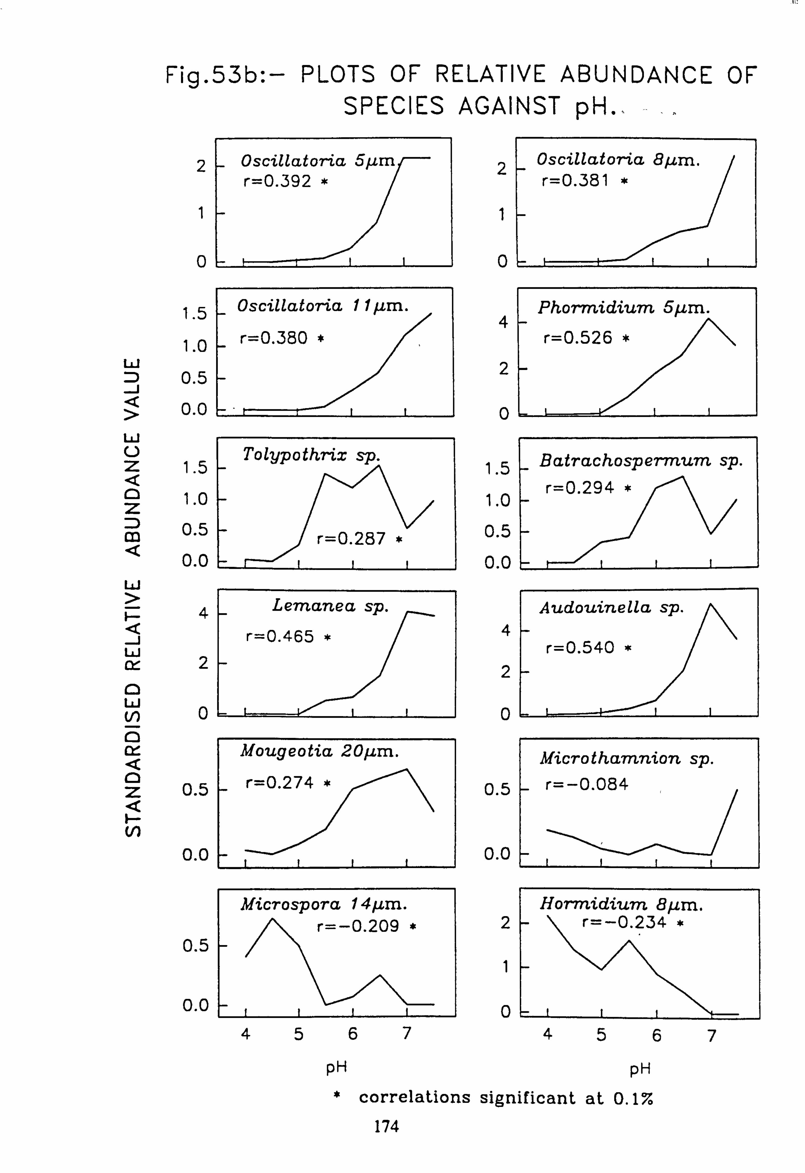
Fig. 53b: - PLOTS OF RELATIVE ABUNDANCE OF SPECIES AGAINST pH.
2
1
n
1.5
1.0 W D 0.5 J > 0.0 W U z 1.5
z 1.0
0.5 m Q 0.0 Li
4
J LLJ 2 0 W0 (! )
0
D z 0.5
F-
0.0
0.5
_ Oscillatoria 5, cm r=0.392 */
_ Oscillatoria 1 1µm.
_ r=0.380 *
Tolypothrix sp.
r=0.287
Lemanea sp.
r=0.465 *
Mougeotia 20ILm.
r=0.274
Microspora 141im. r=-0.209
2
1
n
4
2
1.5
1.0
0.5
0.0
4
2
0
0.5
0.0
_ Oscillatoria 8gm. r=0.381 *
Phormidiurn 5µm.
r=0.526 */
- Batrachospermum sp.
r=0.294 * /ý
Audouinella sp.
r=0.540
MicrothaTnnion sp. r=-0.084
0.0
2
1
0
Hormidium 8µm. -\ r=-0.234 *
45674567
pH pH * correlations significant at 0.1%
174
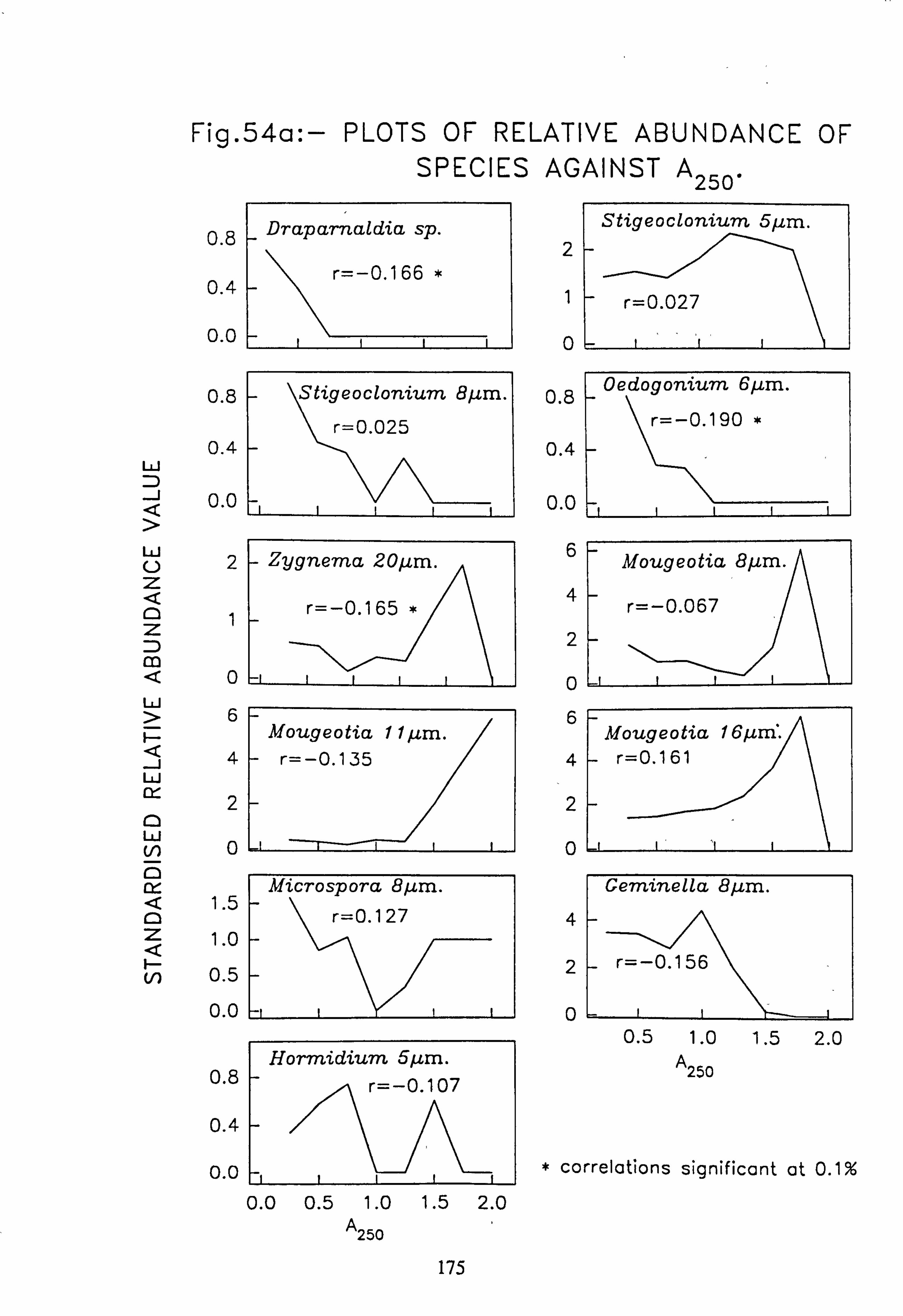
Fig. 54a: - PLOTS OF RELATIVE ABUNDANCE OF SPECIES AGAINST A250.
w J
w U
0 Z
m
w
J w
0 w (/) 0
0 Z
F-
0.8
0.4
0.0
0.8
0.4
0.0
L
1
0
6
4
2
n
1.5
1.0
0.5
0.0
Draparnaldia sp.
r=-0.166 *
tigeoclonium 8pm.
r=0.025
- Zygnema 20µm.
r=-0.165 *
Mougeotia 1 1µm.
- r=-0.135
Microspora 8µm.
r=0.127
0.0 0.5 1.0 1.5 2.0 A250
0.8 0.4
0.0
z
1 U
0.8
0.4
0.0
6
4
2
0
6
4
2
n
4
2
0
Stigeoclonium 5/um.
r=0.027
Oedogonium 6µm.
r=-0.190
Mougeotia 8µm.
r=-0.067
Mougeotia 16prr :
r=0.161 /
Ce7ninella 8µm.
A
r=-0.156
0.5 1.0 1.5 2.0 A250
* correlations significant at 0.1%
175
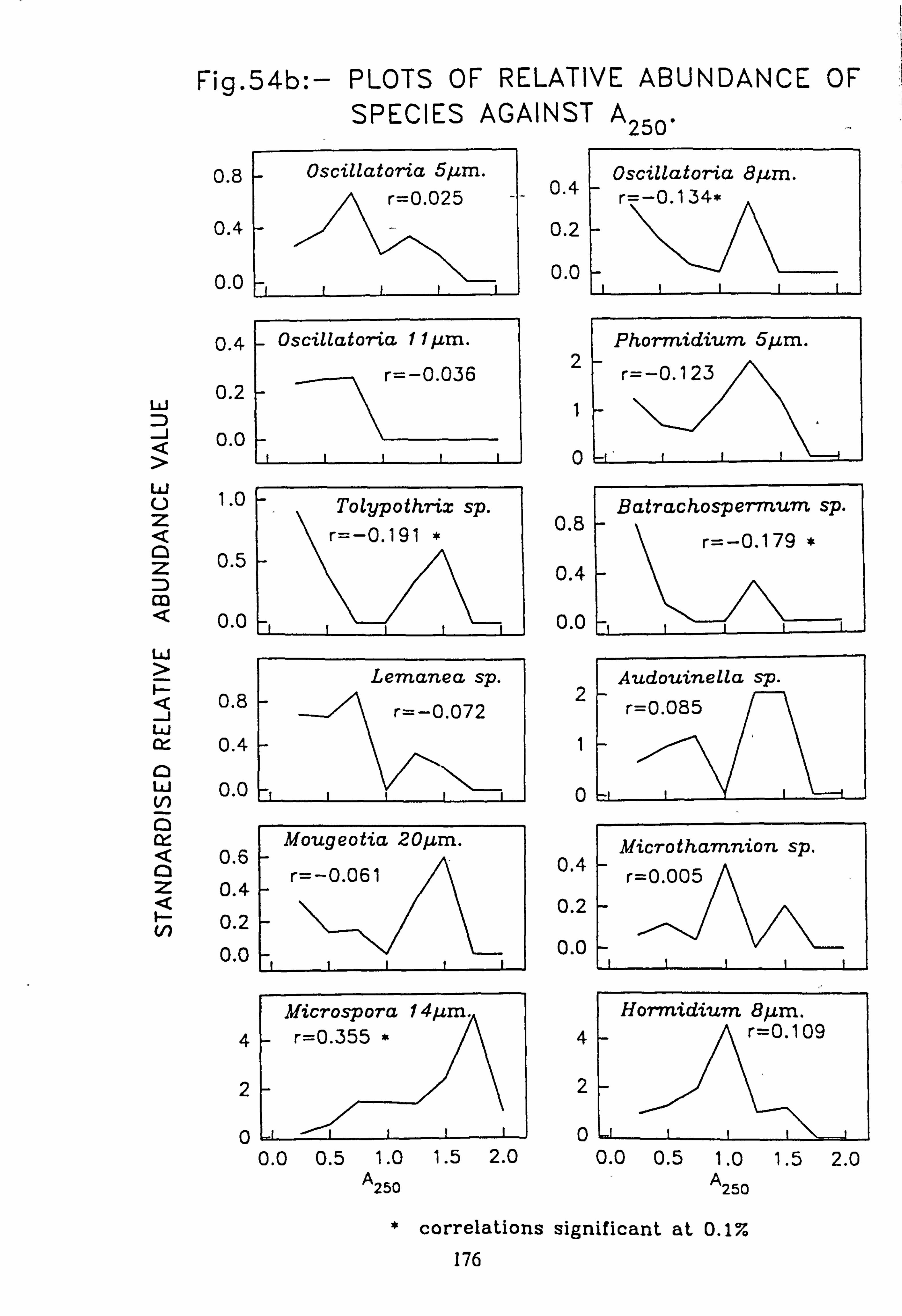
Fig. 54b: - PLOTS OF RELATIVE ABUNDANCE OF SPECIES AGAINST Also.
w J
w v z 0 z D
w
W cy-
a W (/') 0 cy-
0 z
F-
0.8
0.4
0.0
Oscillatoria 5jim.
r=0.025
0.4
0.2
0.0
Oscillatoria 1 1µm.
r=-0.036
1.0 Tolypothrix sp. r=-0.191 *
0.5
0.0
Lemanea sp.
r=-0.072 0.8
0.4
0.0
0.6
0.4
0.2
0.0
Mougeotia 20µm.
r=--0.061
Microspora 14µm r=0.355 */ 4
2
n
Oscillatoriac 8/2m. 0.4
r=-0.134* 0.2
0.0
Phormidiurn 5jcm.
r=--0.123 /\ 2
1
0
Batrachospermum sp.
r=-0.179 * 0.8
0.4
0.0
2 Audouinelld sp.
r=0.085 I-
1
0
Microtharanion sp.
r-0.005 0.4
0.2
0.0
4
2
0
Hormidium 8µm. A r=0.109
0.0 0.5 1.0 1.5 2.0 0.0 0.5 1.0 1.5 2.0 A250 A250
* correlations significant at 0.1% 176
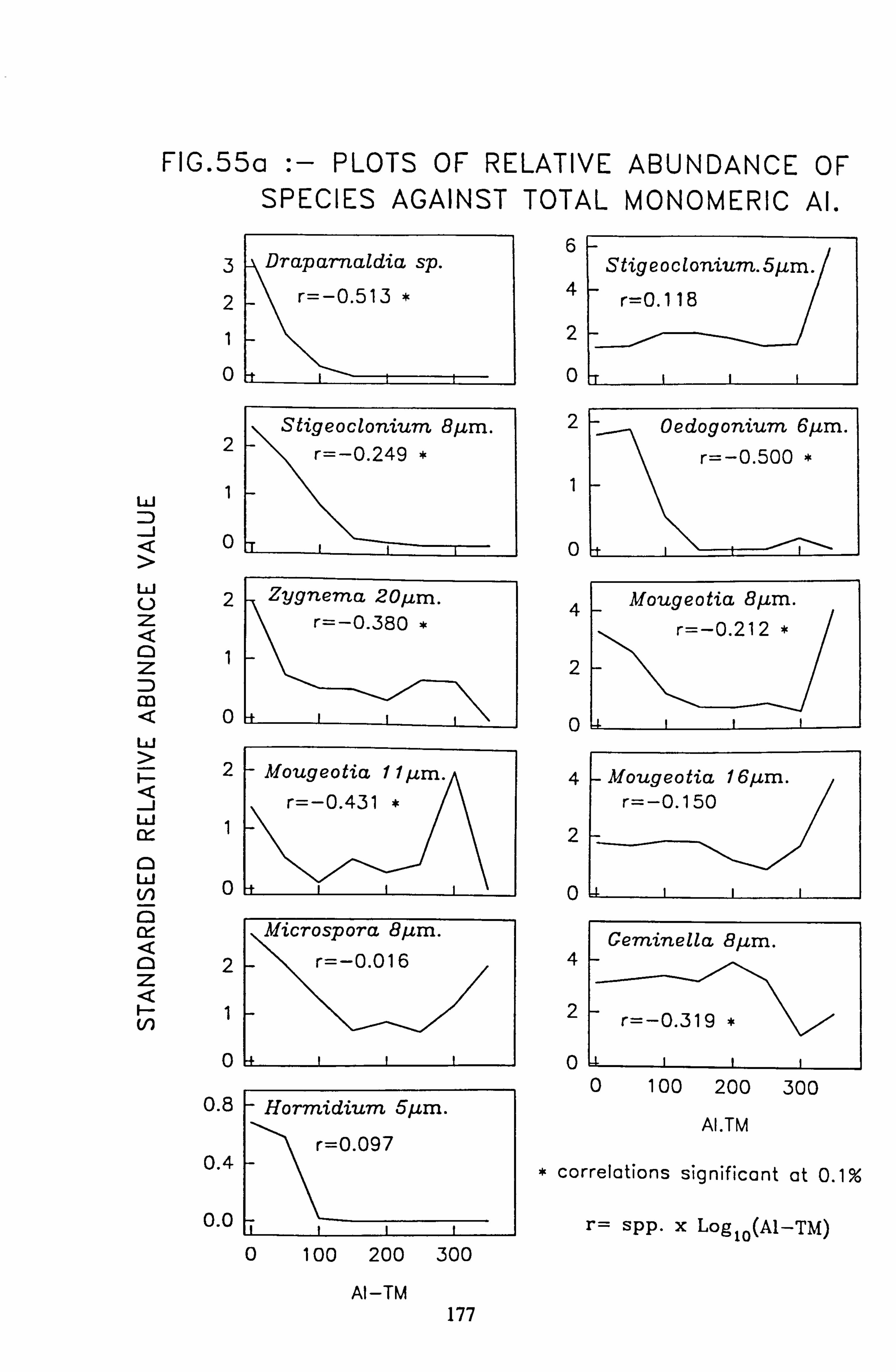
FIG. 55a :- PLOTS OF RELATIVE ABUNDANCE OF SPECIES AGAINST TOTAL MONOMERIC Al.
3
2
1
0
2
w1
J0
W2 U Z
Z
m Q0
w
F= 2
w CY- 0 W (A O
0 Of
02 Z
ý-- 1
0 0.8
0.4
0.0
6
4
2
0
Stigeocloniurn 8/2m.
r=-0.249 *
Zygnema 20µm. r=-0.380 *
- Mougeotia 1112m.
r=-0.431 */
Microspord 8/um.
r=-0.016
Horrnidium 5p m.
r=0.097
0 100 200 300
Al -TM 177
2
1
0
4
2
0
4
2
0
4
2
Oedogoniurrt 6/ß, m.
r=-0.500 *
Mougeotia 8fcm.
r=-0.212
Mougeotia 16µm. r=-0.150
Ceminella 8µm.
-7r=--(0.319
OL 0 100 200 300
AI. TM
* correlations significant at 0.1%
r= spp. x Log 10(A1-TM)
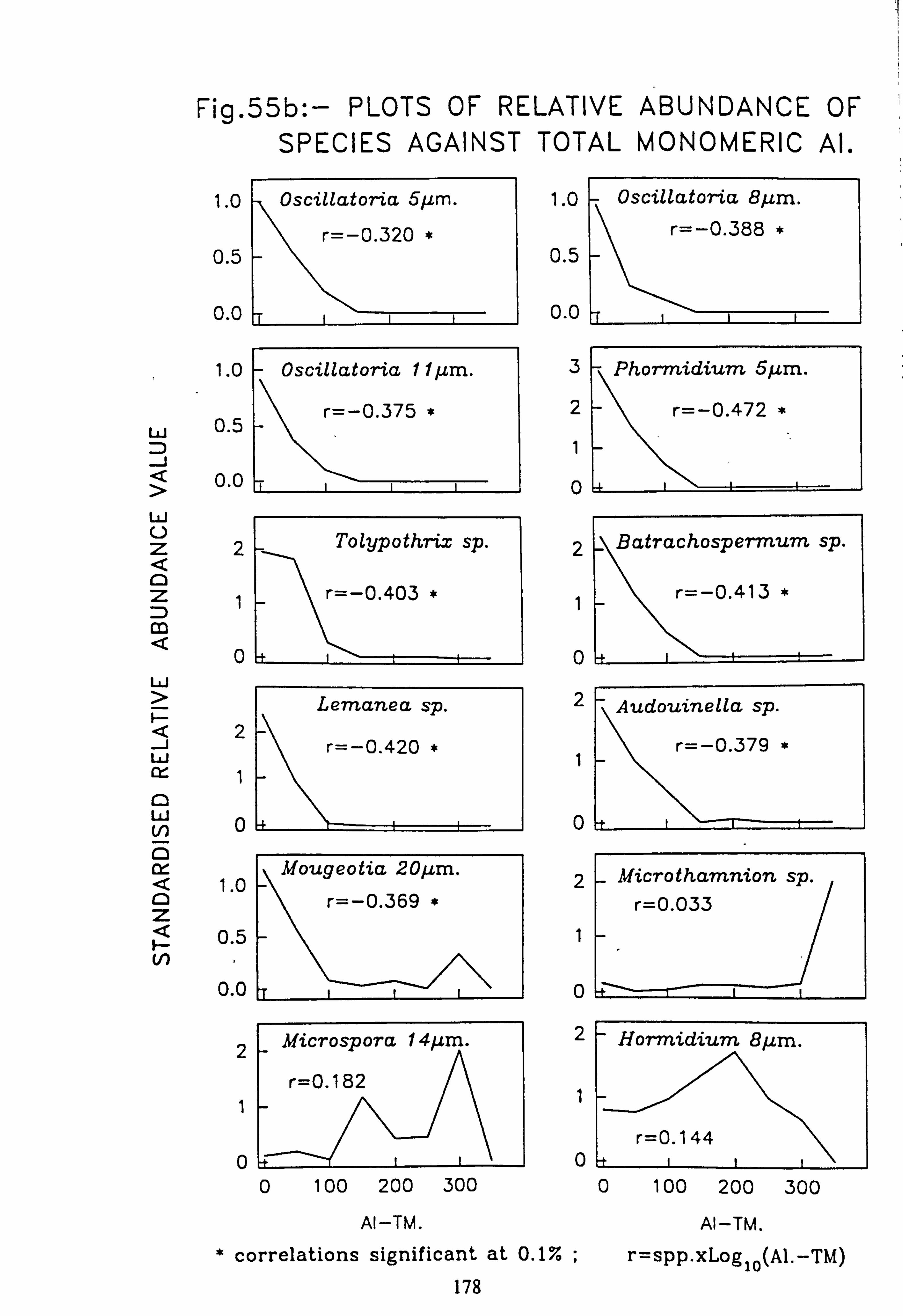
Fig. 55b: - PLOTS OF RELATIVE ABUNDANCE OF SPECIES AGAINST TOTAL MONOMERIC Al.
W
J
W U Z
Z
m
W
E- J W
0 W V) 0 cy- 0 Z
F- N
1.0
0.5
0.0
1.0
0.5
0.0
1.0
0.5
0.0
3
2
1
0
Tolypothrix sp.
r=-0.403 *
z
i
0 Lemanea sp.
r=-0.420 * 2
1
0
1.0
0.5
0.0
z
1
0
Mougeotia 201im.
r=-0.369 *
2
1
0
2
\BatrachosPerrni2rn. sp.
r=-0.413 *
Audouinella sp.
r=-0.379 1
0
z
1
o! z
1
0
_ Micro thamnion sp.
r=0.033
Hormidium 8ILm.
r=0.144
0 100 200 300 0
Al-TM.
* correlations significant at 0.1%
178
100 200 300
AI-TM.
r=spp. xLoglo(A1. -TM)
A linear relationship between a species and an environmental variable means that there
should be a steady increase (or decrease) in abundance of that species with an increase of
the variable over the range of values of the variable encountered.
The actual distribution patterns of selected species with respect to environmental variables has been investigated by plotting abundance against values of the variable. The values of
variables have been grouped in bands and the species abundancies within each band
summed, then standardized by dividing by the number of observations of that value of the
variable.
Plots have been prepared in this way of species distribution against pH, A250 and total
monomeric aluminium (Figs. 53-55). No transformation of variables was carried out before constructing these plots, as the sole purpose was to obtain an idea of the nature of the relationship, and transformation would not have altered the basic shape of the curve obtained. Pearsons' r is shown on each plot.
Those species showing a unimodal distribution should not also have a large r with that variable; those with a large r value should show a maximum abundance towards one end of the variable's distribution. By and large the results are in accordance with this expecta- tion, implying that important information about the relationships between species and environment may be obtained by both linear analyses and those based on a unimodal distribution model.
4.7.3 Canonical Correspondence Analysis (Ter Braak, 1988) 4.7.3.1 Use of CANOCO
This is a direct gradient method, as opposed to indirect gradient methods such as PCA in which species data are used to construct ordination axes which may then be tested for correlations with environmental variables. In CCA the environmental variables are involved in the construction of the ordination diagram from the start.
The results of CCA (and Detrended CCA) may be exhibited in a biplot, where the
species values, site values and environmental variables are present in the same ordination diagram, enabling inferences to be drawn about the relationships existing between species, sites and environmental factors. The lengths of the environmental factors' arrows indicate the relative importance of the factors in explaining the
variance in the species data (Ter Braak and Prentice, 1988).
179
Arrows which are almost parallel indicate that these environmental factors may be highly correlated and thus each will have no unique contribution to the ordination. All but one could be removed from the analysis without affecting the ordination. The
presence of a Variance Inflation Factor (VIF) greater than 20 in the CANOCO output also indicates a high degree of intercorrelation. However there is nothing to indicate
which in a set of intercorrelated variables are actually responsible for the community composition.
The ordination diagram is not hampered by high correlations between species or between environmental variables (Ter Braak, 1987).
The final analyses selected have been carried out on the three matrices and both
abundance and pooled P/A data sets using as far as possible the same conditions and variables, with the restriction that in the case of Matrix A only 8 variables can be
subjected to a canonical analysis, as opposed to 13 for B and C (2 less than the number of sites). The results are shown in Figs. 56-63.
The robustness of the ordinations obtained can be investigated by comparing matrices A, B and C as both abundance and pooled presence-absence data. The abundance data
should contain more information but are based on estimated relative abundance; the pooled presence/absence data ought to be free of any bias due to estimation. Both types of data however will span a much narrower range of values than would true abundance data based on counts of cell number.
Bias may be introduced by the presence of rare species (Ter Braak, 1988) at the edge of the species distribution and a correction can be introduced in CANOCO by downweight- ing rare species. The effect of this downweighting was found to be minimal in
presence-absence data Matrix B, but applied to the abundance data it reduced the spread of the species sites and environmental variables along Axis 2. Downweighting of rare species has therefore been applied to all the ordinations shown, in order to make them comparable. The choice of environmental factors to be included in the ordination was made on the basis of the statistics shown in the summary tables (Tables 52-54). Removal
of factors was carried out systematically to produce low VIFs as values greater than 20 indicate a high degree of intercorrelation between variables, also evident from the correlation matrix (Ter Braak, 1988).
180
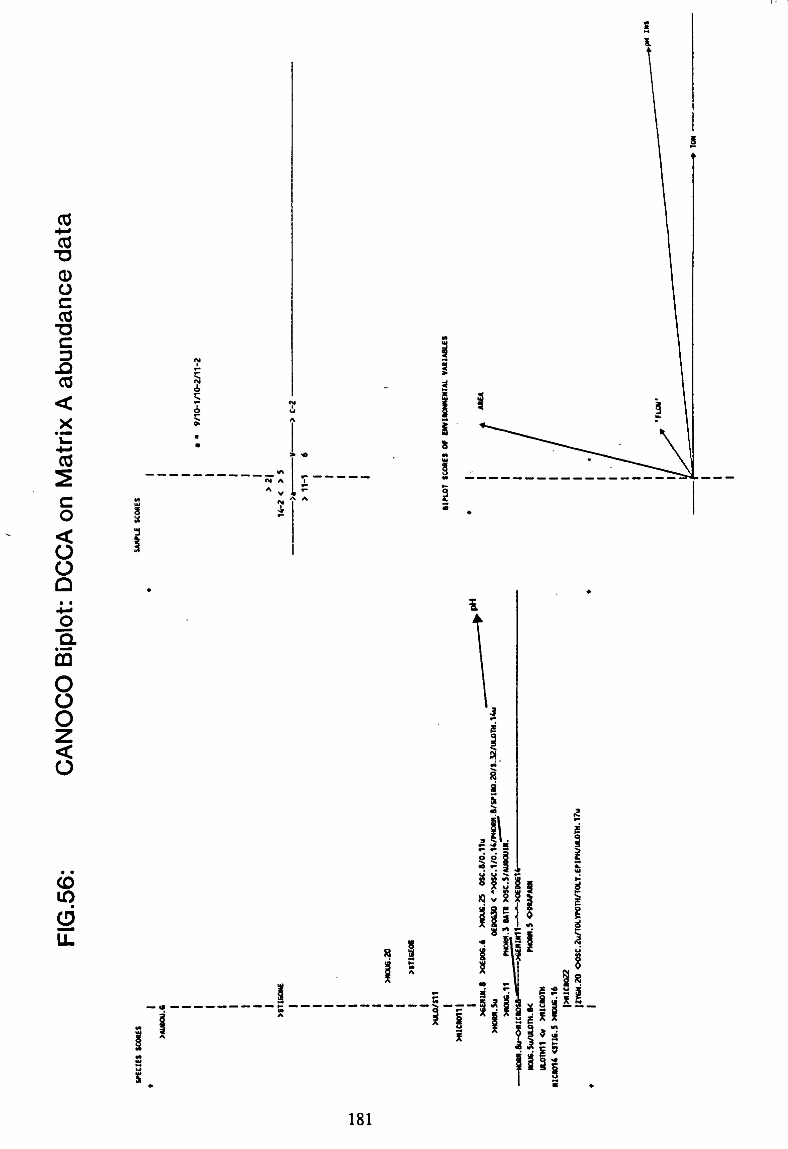
a) U
ü
(13
X _ .L
0
U U
0 n.
0 0 0 z V
LL
6N
PA
t
Ayr
NAA
1 W
g u WN J
a Wsp
ýl M ..
H
O
pýW
Nf
- -------- ---------- --jý g-
iA 11 9
2
181
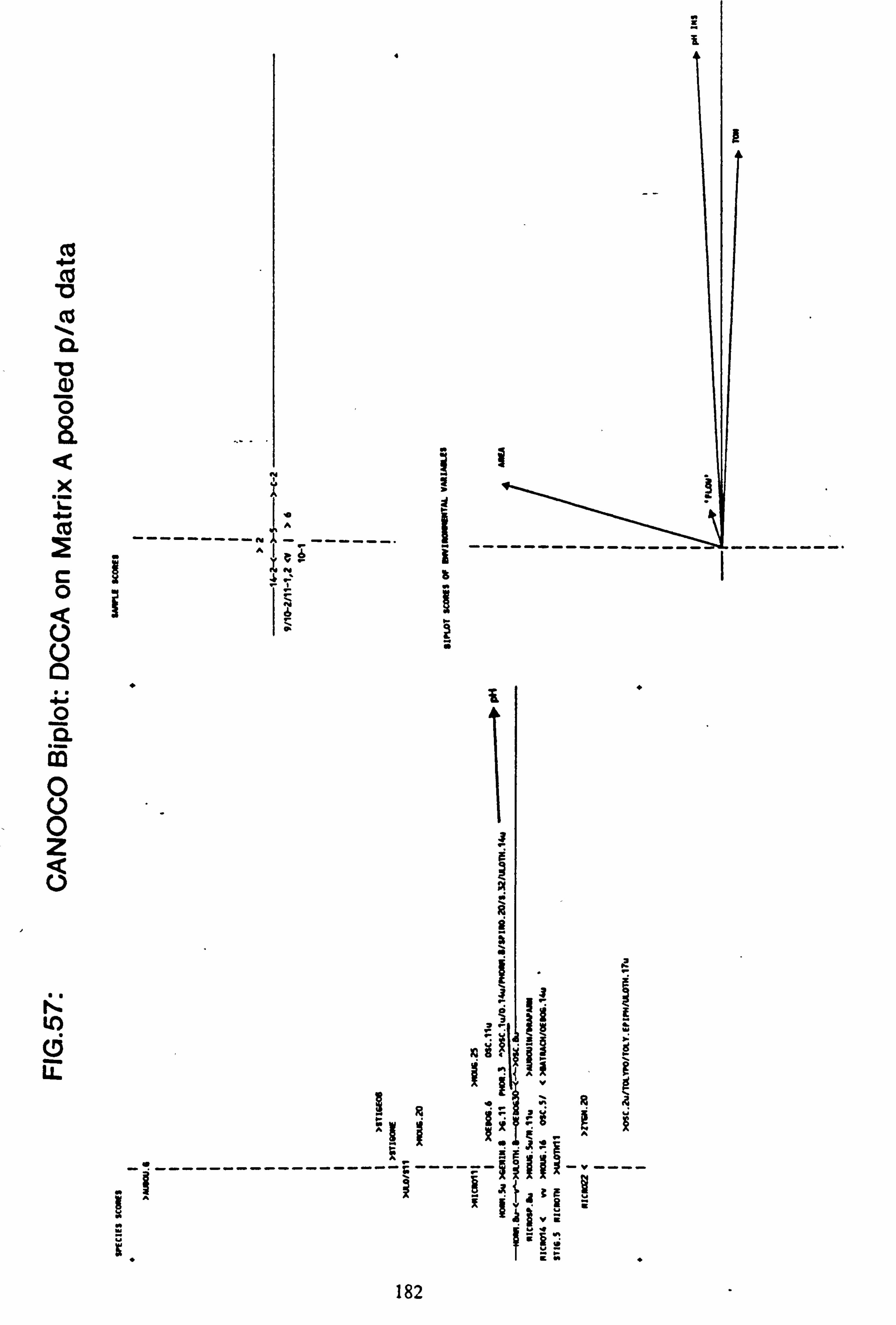
4-0 cu
0
co
a. G) O
x
cc
0
U U 0
0 ä C13 0 U 0 Z
to
LL
4
n X A
I P
.
w
f
w
Hg
i
i
3
eM N
g
ä
I W!
-°-------------------------
182
.
13
0-- 9 ý
s -v
u
Vt
ur
tM ý
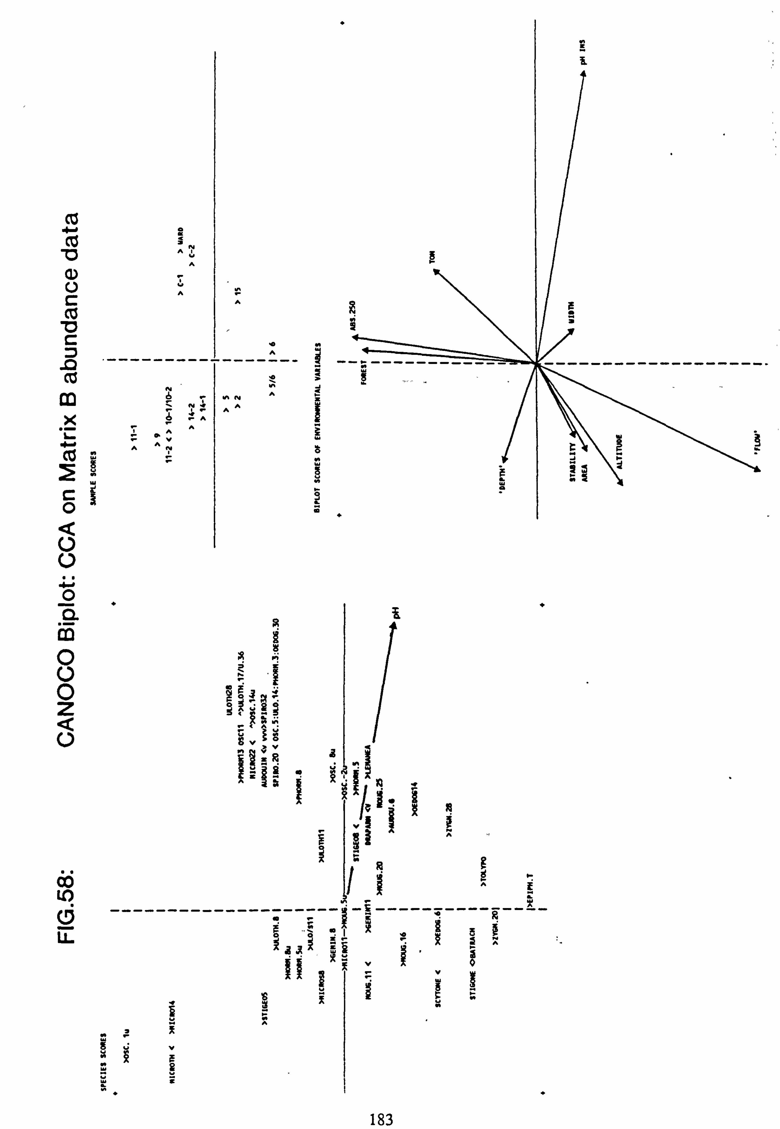
U
td V C
cu m x
r. 0
0
0 V 0 CL m 0 V 0 z U
Co to C_7 LL
e s a AN Y
A
Y
A
IV b
b sý 1
pA A
A AN
.
N
A ý
t
'O M
d j
N J A ý NN
AA
> i W
M W e O V N
H
L
O
M
M
o'ý g ý1
ANN r y
<AN ýO
v v
~ v_
.ý 7C 5
--------------------
Öi A y
ä
1J V
i-C
W g W
i
N q
I
Au A
R
sA Vö
V
C A
183
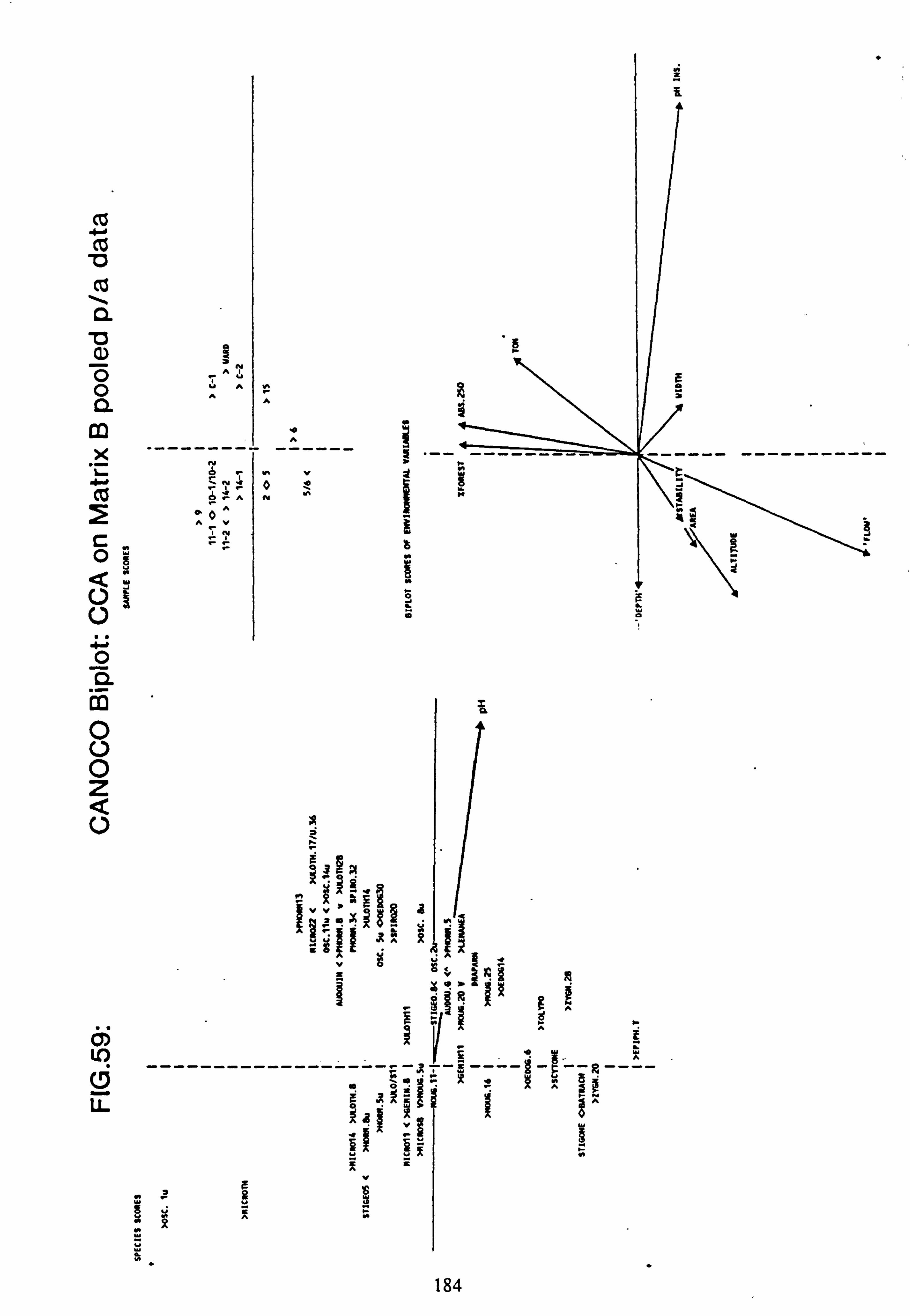
C'0 td
Ü
0.
O 0 Q
m x
.L
U 0 Q m 0 0 0 Z U
LC)
LL
A
YAN
A
M
--------------
.N0 býANN
PA
A0V 1N
O
m
33ý? I
v! O
Xýý» üN
8z
A«F
--------------------------=-R---
WV
xR,. «
184
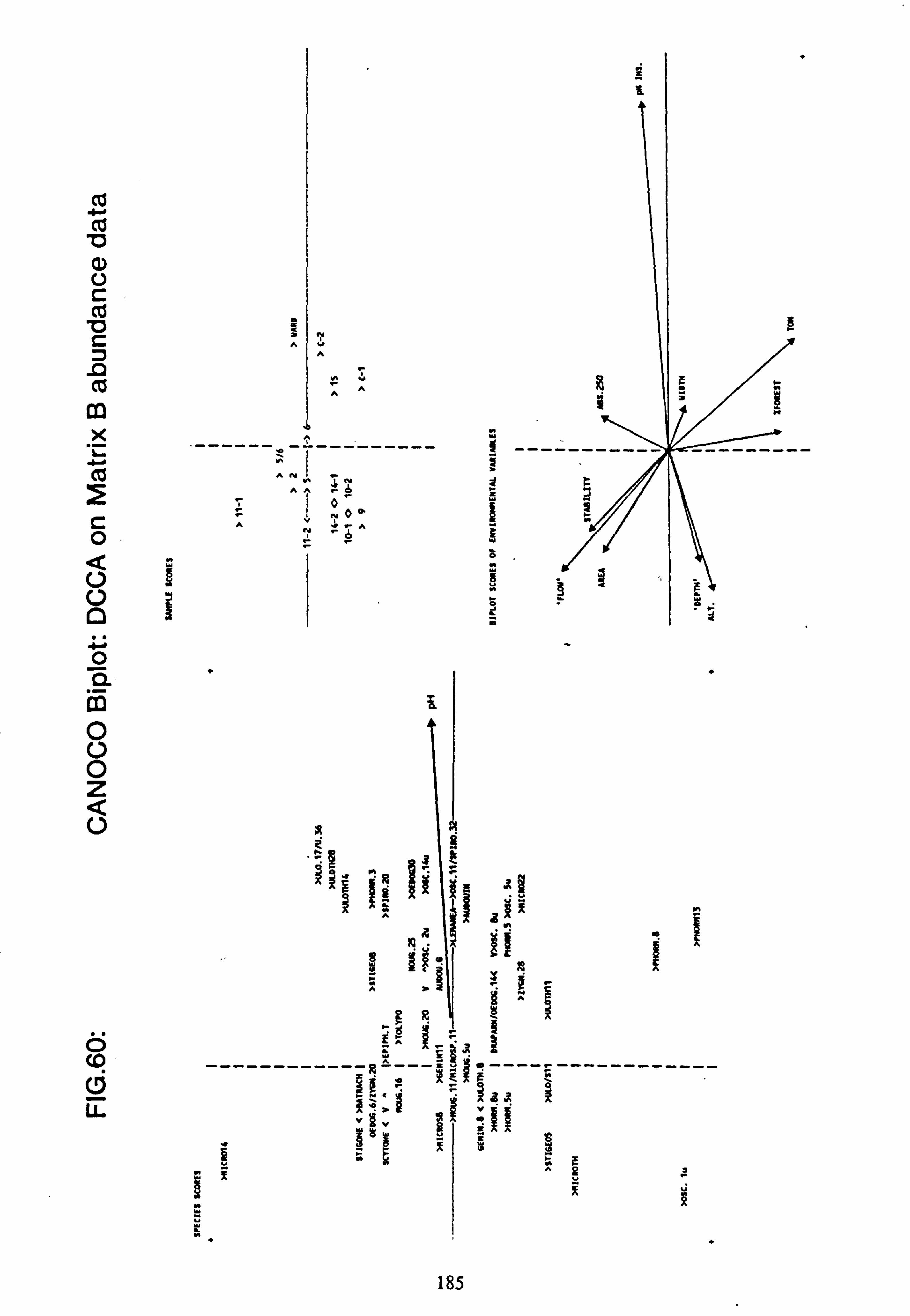
U
as
C
.D as
x
C 0
U U
0 CL m 0 0 0 Z
U
ö cG c0 U-
e s a A
N ü
A
NY
AA
----- =---------
AN yý b
AA
o
oll,
AV A
WqJ
i
I- r z Wcz
i
W
MWs
O
M
r O J
O
s n
2 »
g ß ý
e n ýr
W
= ýýN
----- ------ - -R - ý Ic -- ----------- i
^
N"
ý 7C
+
185
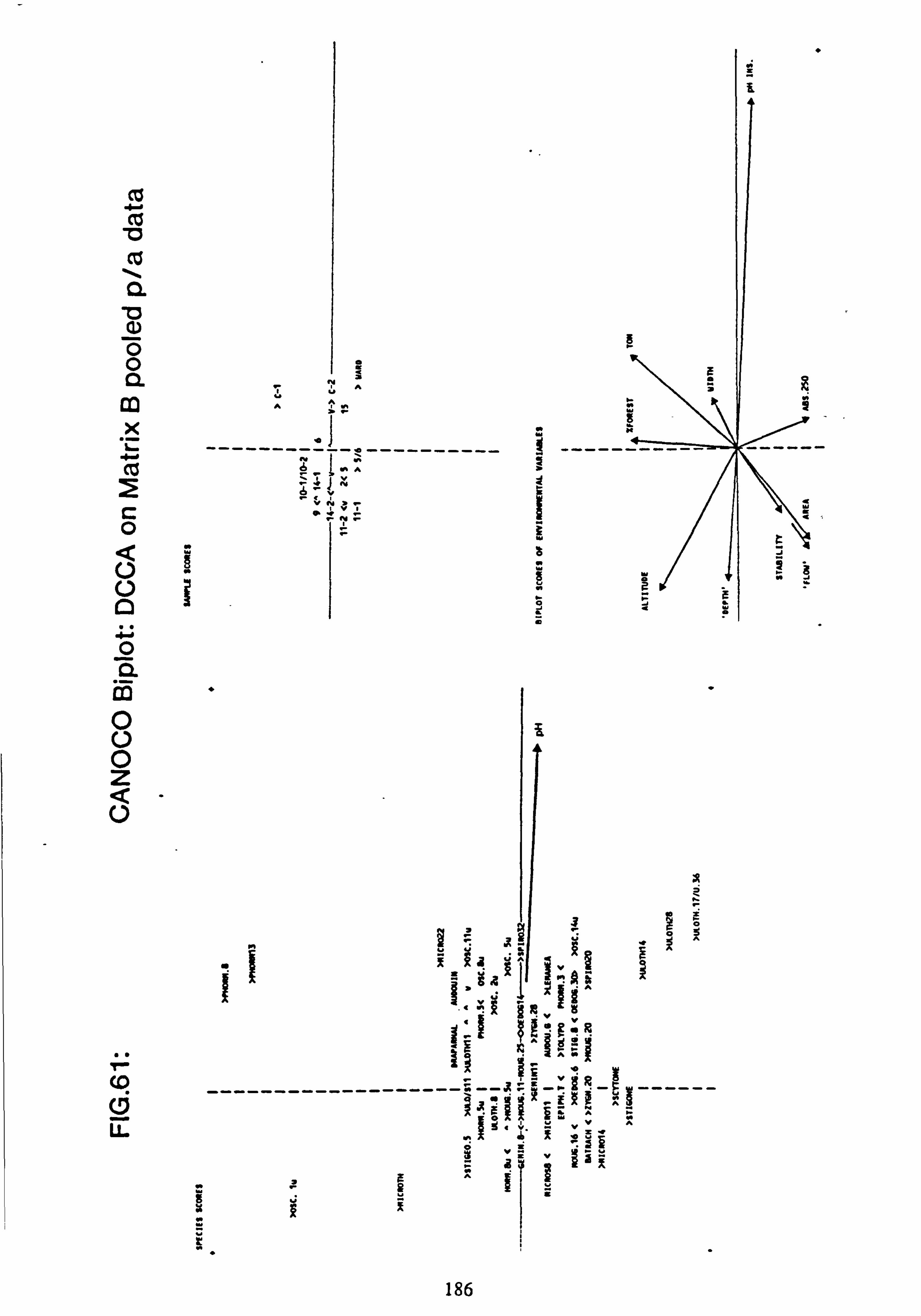
to 4-0
cu
cu
0.
a) O 0 CL co x
cu
0
U U
0 Q. m 0 U 0 z
U
c
U-
ä
II
I r
S s 7
Ms
O
wH
-... -=
a
I W`
O w
W G
w
f
ö
JE a ä ýyA
AAM
NM
_'NA \rv
ÖýV r<
VN1r PvVý
rNr
w W`p
U M
i
3ýö
---------------------- = -A R-
------
Mvyýü
wgv
i
0
Ne
j
etý- Je
MJ
186
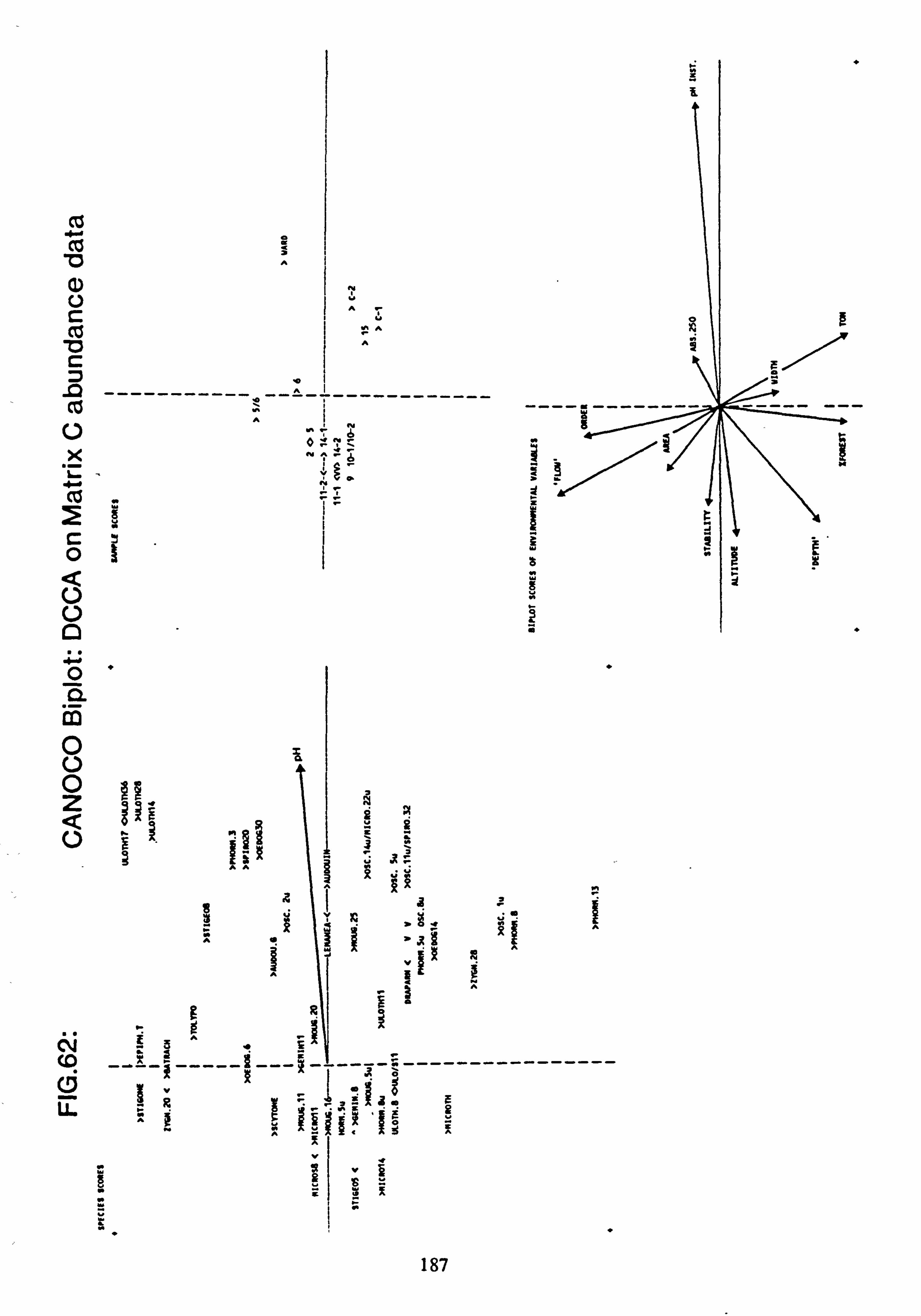
Co C13
VA
U Y
A C Y
V A
M 'O I
N
ü A
Ný b 1
X NA
NP -
w
1
v
0
U U
0 Q. m 0
0 Z Q 0 YE 3
Y
ýý _ý
W
ei
O
AxY ý+ 3zz
öA
FgRý CV
--X - ----1--- ---- --------------- cJ
a3eg
V g_
"' jw
187
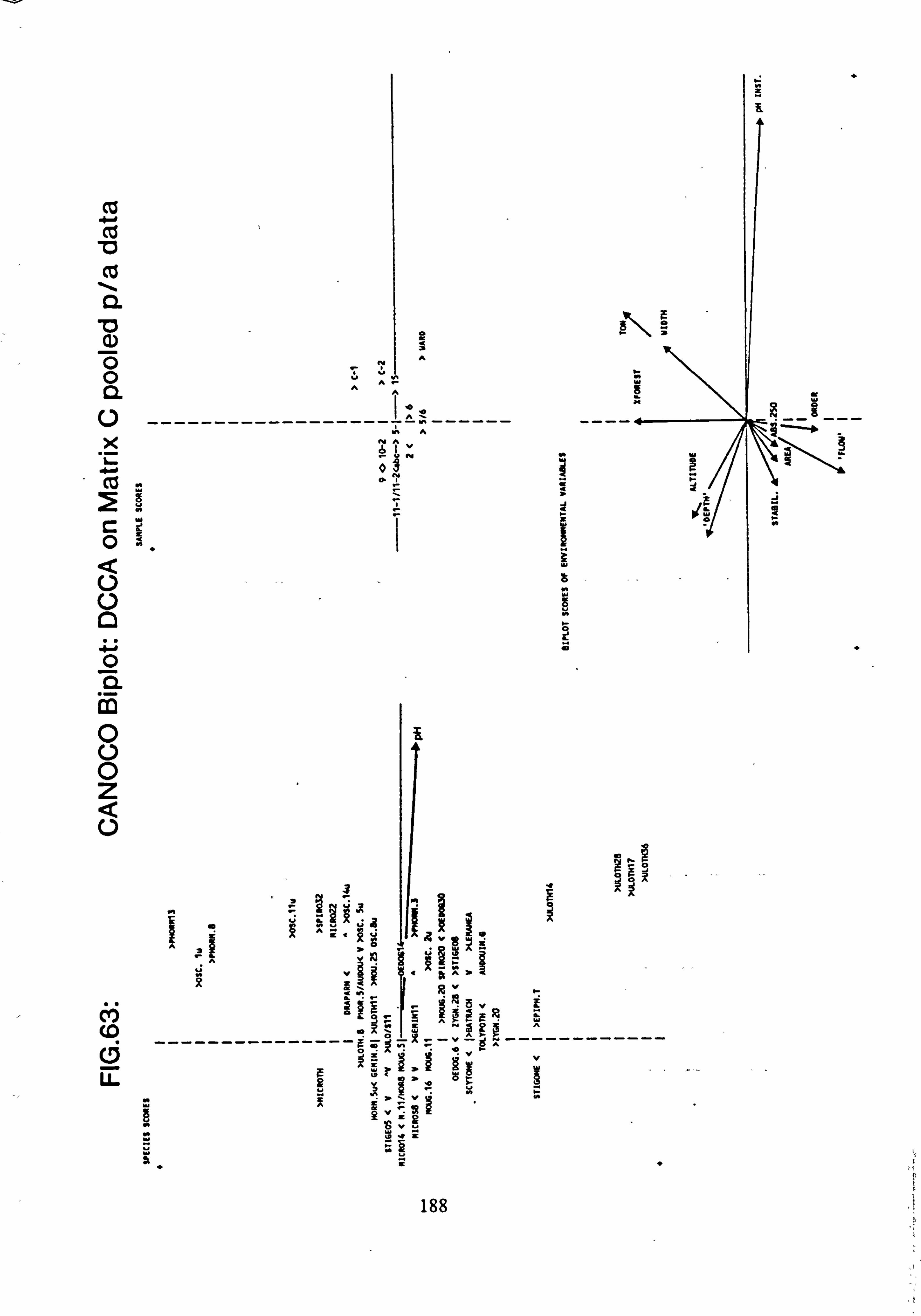
cu tz
cu
a
O 0 a U
cu 2 C 0
U U
0 a m 0 U 0 Z U
CY) co 0 U-
o
ry A
YN Ar
AA
_ MA
bf" ýwN
0
g
J 6
i
w i
C s
1 s W[
W
S N Wi
O V N
f O J L
O
ýR
Rv< "'pwss ývF
ü! !ýOZA
g yý g! ' ýC
MN
w 'ö vu 1s wöwS
Wy
"i
188
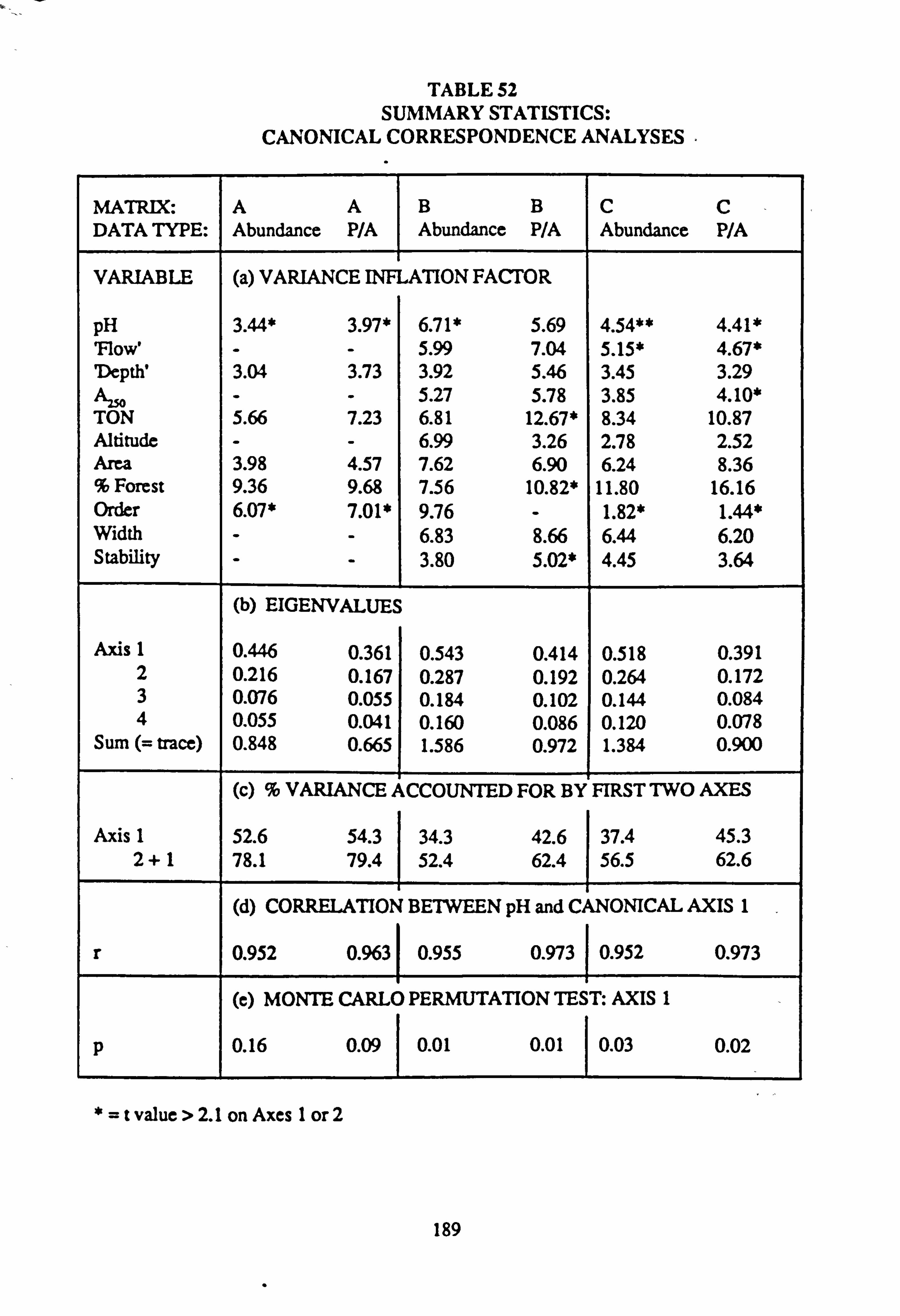
TABLE 52 SUMMARY STATISTICS:
CANONICAL CORRESPONDENCE ANALYSES
MATRIX: A A B B C C DATA TYPE: Abundance P/A Abundance P/A Abundance P/A
VARIABLE (a) VARIANCE INF LATION FACTOR
pH 3.44* 3.97* 6.71* 5.69 4.54** 4.41* 'Flow' - - 5.99 7.04 5.15* 4.67* 'Depth' 3.04 3.73 3.92 5.46 3.45 3.29 A250 - - 5.27 5.78 3.85 4.10* TON 5.66 7.23 6.81 12.67* 8.34 10.87 Altitude - - 6.99 3.26 2.78 2.52 Area 3.98 4.57 7.62 6.90 6.24 8.36 % Forest 9.36 9.68 7.56 10.82* 11.80 16.16 Order 6.07* 7.01* 9.76 - 1.82* 1.44* Width - - 6.83 8.66 6.44 6.20 Stability - - 3.80 5.02* 4.45 3.64
(b) EIGENVALUES
Axis 1 0.446 0.361 0.543 0.414 0.518 0.391 2 0.216 0.167 0.287 0.192 0.264 0.172 3 0.076 0.055 0.184 0.102 0.144 0.084 4 0.055 0.041 0.160 0.086 0.120 0.078
Sum (= trace) 0.848 0.665 1.586 0.972 1.384 0.900
(c) % VARIANCE A CCOUNTED FOR BY FIRST TWO AXES
Axis 1 52.6 54.3 34.3 42.6 37.4 45.3 2+1 78.1 79.4 52.4 62.4 56.5 62.6
(d) CORRELATION BETWEEN pH and CANONICAL AXIS 1
r 0.952 0.963 0.955 0.973 0.952 0.973
(e) MONTE CARLO PERMUTATION TES T: AXIS 1
p 0.16 0.09 0.01 0.01 0.03 0.02
*=t value > 2.1 on Axes 1 or 2
189
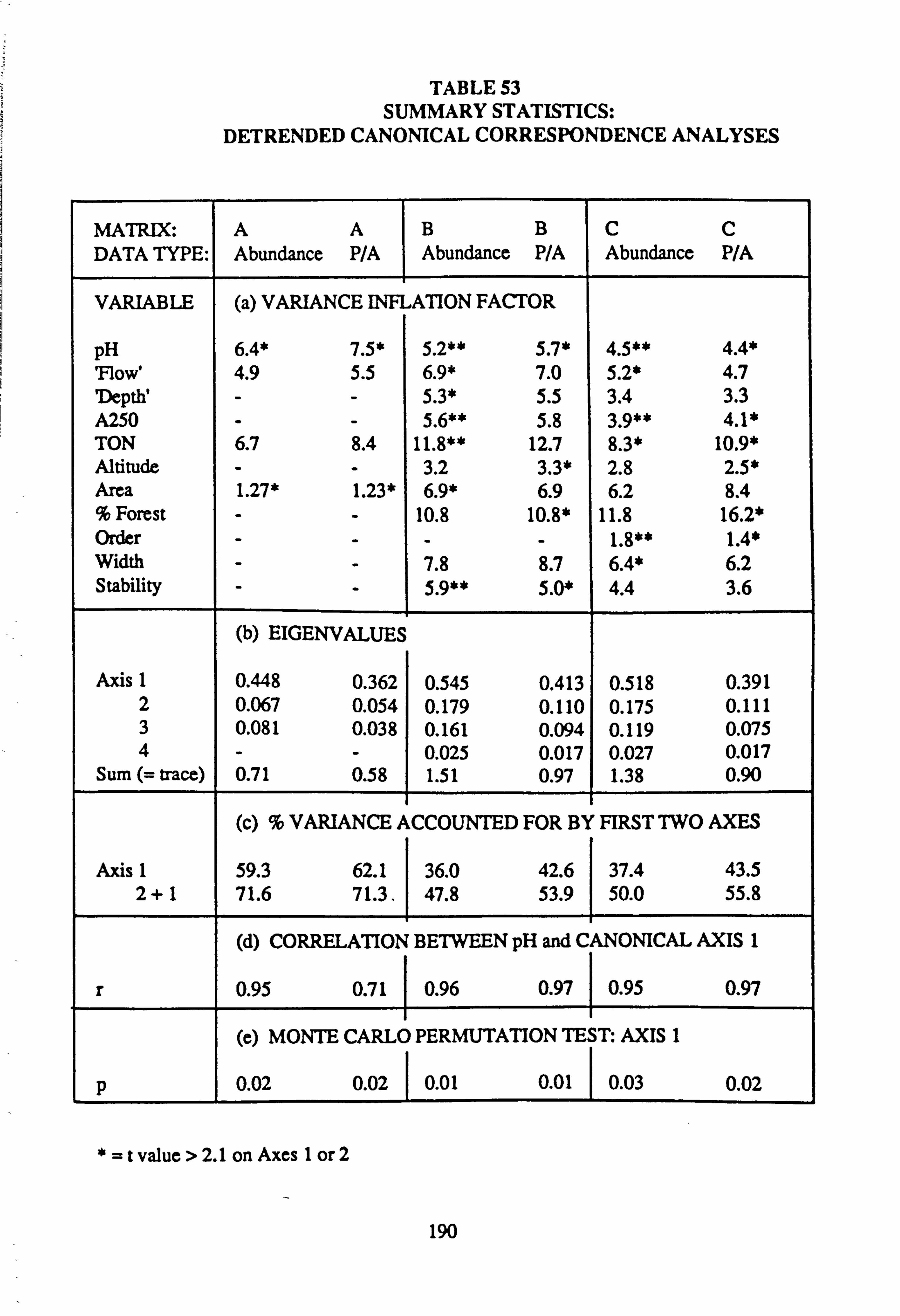
TABLE 53 SUMMARY STATISTICS:
DETRENDED CANONICAL CORRESPONDENCE ANALYSES
MATRIX: A A B B C C DATA TYPE: Abundance P/A Abundance P/A Abundance P/A
VARIABLE (a) VARIANCE INFL ATION FACTOR
pH 6.4* 7.5* 5.2** 5.7* 4.5** 4.4* 'Flow' 4.9 5.5 6.9* 7.0 5.2* 4.7 Depth' - - 5.3* 5.5 3.4 3.3 A250 - - 5.6** 5.8 3.9** 4.1* TON 6.7 8.4 11.8** 12.7 8.3* 10.9* Altitude - - 3.2 3.3* 2.8 2.5* Area 1.27* 1.23* 6.9* 6.9 6.2 8.4 % Forest - - 10.8 10.8* 11.8 16.2* Order - - - - 1.8** 1.4* Width - - 7.8 8.7 6.4* 6.2 Stability - - 5.9** 5.0* 4.4 3.6
(b) EIGENVALUES
Axis 1 0.448 0.362 0.545 0.413 0.518 0.391 2 0.067 0.054 0.179 0.110 0.175 0.111 3 0.081 0.038 0.161 0.094 0.119 0.075 4 - - 0.025 0.017 0.027 0.017
Sum (= trace) 0.71 0.58 1.51 0.97 1.38 0.90
(c) % VARIANCE A CCOUNTED FOR BY FIRST TWO AXES
Axis 1 59.3 62.1 36.0 42.6 37.4 43.5 2+1 71.6 71.3. 47.8 53.9 50.0 55.8
(d) CORRELATION BETWEEN pH and CANONICAL AXIS 1
r 0.95 0.71 0.96 0.97 0.95 0.97
(e) MONTE CARLO PERMUTATION TE ST: AXIS 1
p 0.02 0.02 0.01 0.01 0.03 0.02
*=t value > 2.1 on Axes 1 or 2
190
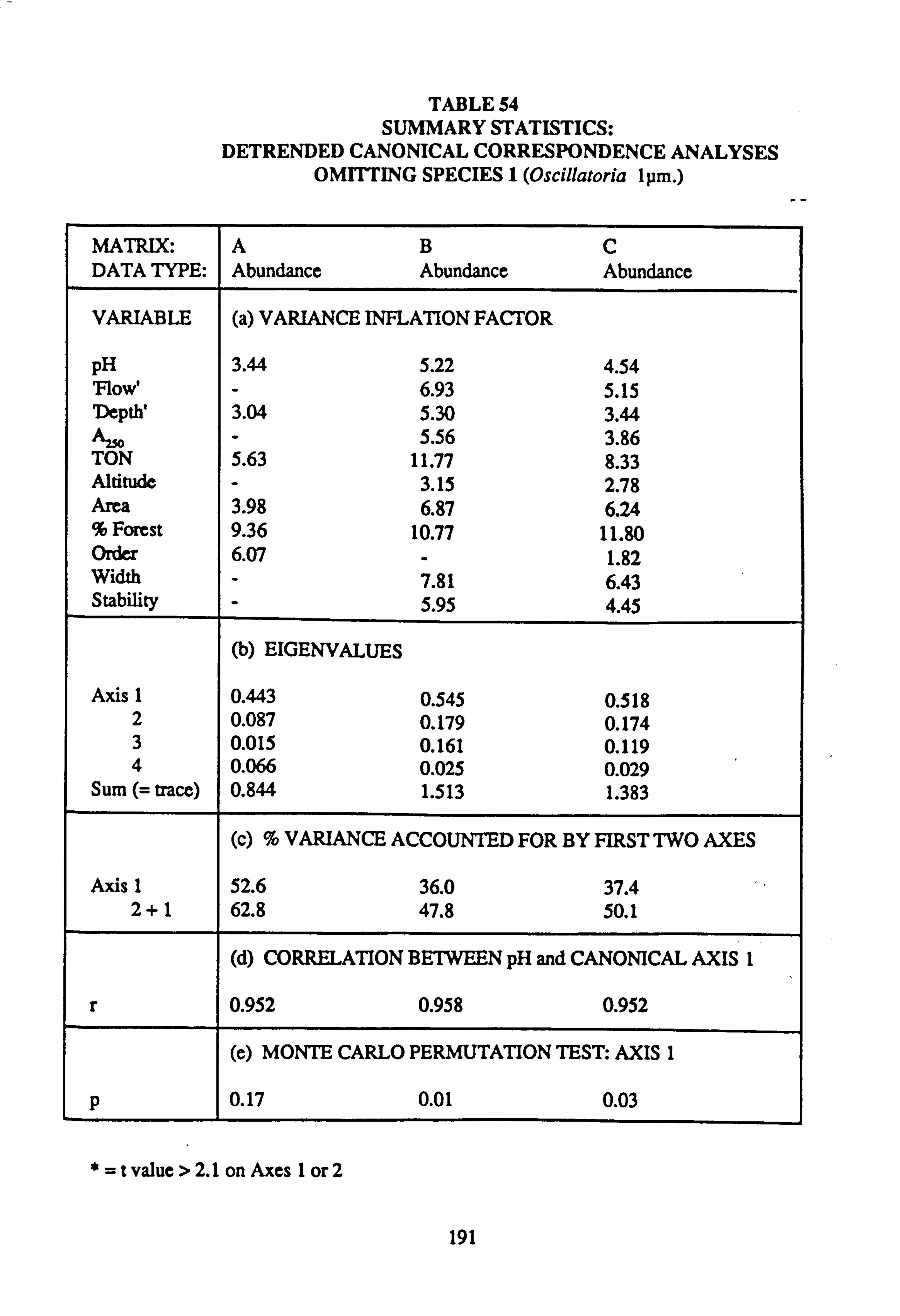
TABLE 54 SUMMARY STATISTICS:
DETRENDED CANONICAL CORRESPONDENCE ANALYSES OMITTING SPECIES 1(Oscillatoria 1µm. )
MATRIX: A B C DATA TYPE: Abundance Abundance Abundance
VARIABLE (a) VARIANCE INFLATION FACTOR
pH 3.44 5.22 4.54 'Flow' - 6.93 5.15 Depth' 3.04 5.30 3.44 A250 - 5.56 3.86 TON 5.63 11.77 8.33 Altitude - 3.15 2.78 Area 3.98 6.87 6.24 % Forest 9.36 10.77 11.80 Order 6.07 - 1.82 Width - 7.81 6.43 Stability - 5.95 4.45
(b) EIGENVALUES
Axis 1 0.443 0.545 0.518 2 0.087 0.179 0.174 3 0.015 0.161 0.119 4 0.066 0.025 0.029
Sum (= trace) 0.844 1.513 1.383
(c) % VARIANCE ACCOUNTED FOR BY FIRST TWO AXES
Axis 1 52.6 36.0 37.4 2+1 62.8 47.8 50.1
(d) CORRELATION BETWEEN pH and CANONICAL AXIS I
r 0.952 0.958 0.952
(e) MONTE CARLO PERMUTATION TEST: AXIS 1
p 0.17 0.01 0.03
*=t value > 2.1 on Axes 1 or 2
191
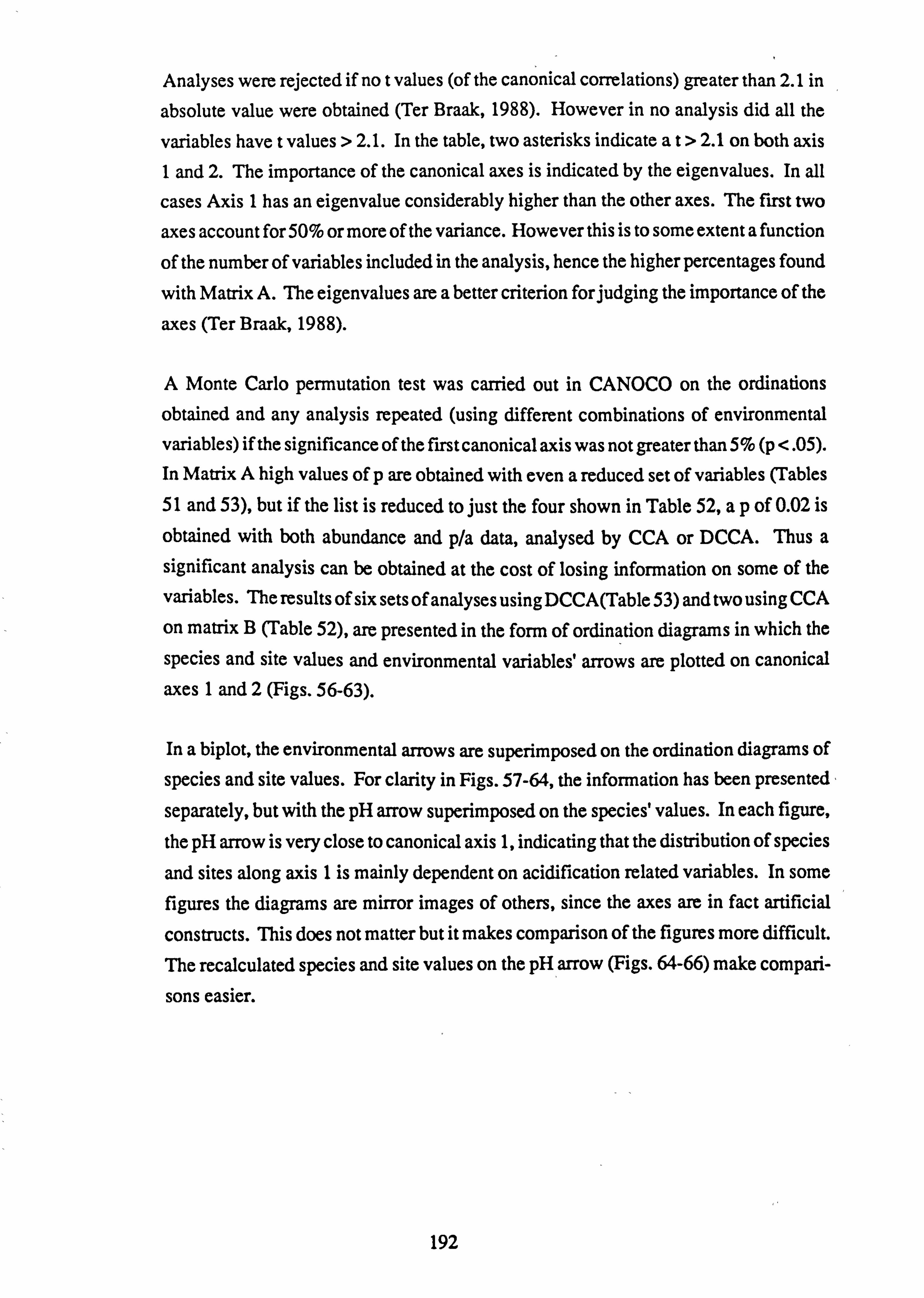
Analyses were rejected if no t values (of the canonical correlations) greater than 2.1 in
absolute value were obtained (Ter Braak, 1988). However in no analysis did all the
variables have t values > 2.1. In the table, two asterisks indicate at>2.1 on both axis 1 and 2. The importance of the canonical axes is indicated by the eigenvalues. In all
cases Axis 1 has an eigenvalue considerably higher than the other axes. The first two
axes account for 50% or more of the variance. However this is to some extent a function
of the number of variables included in the analysis, hence the higher percentages found
with Matrix A. The eigenvalues are a better criterion for judging the importance of the
axes (Ter Braak, 1988).
A Monte Carlo permutation test was carried out in CANOCO on the ordinations
obtained and any analysis repeated (using different combinations of environmental variables) if the significance of the first canonical axis was not greater than 5% (p <. 05). In Matrix A high values of p are obtained with even a reduced set of variables (Tables 51 and 53), but if the list is reduced to just the four shown in Table 52, ap of 0.02 is
obtained with both abundance and p/a data, analysed by CCA or DCCA. Thus a significant analysis can be obtained at the cost of losing information on some of the
variables. The results of six sets of analyses using DCCA(Table 53) and two using CCA
on matrix B (Table 52), are presented in the form of ordination diagrams in which the
species and site values and environmental variables' arrows are plotted on canonical axes 1 and 2 (Figs. 56-63).
In a biplot, the environmental arrows are superimposed on the ordination diagrams of
species and site values. For clarity in Figs. 57-64, the information has been presented
separately, but with the pH arrow superimposed on the species' values. In each figure,
the pH arrow is very close to canonical axis 1, indicating that the distribution of species
and sites along axis 1 is mainly dependent on acidification related variables. In some figures the diagrams are mirror images of others, since the axes are in fact artificial
constructs. This does not matter but it makes comparison of the figures more difficult.
The recalculated species and site values on the pH arrow (Figs. 64-66) make compari-
sons easier.
192
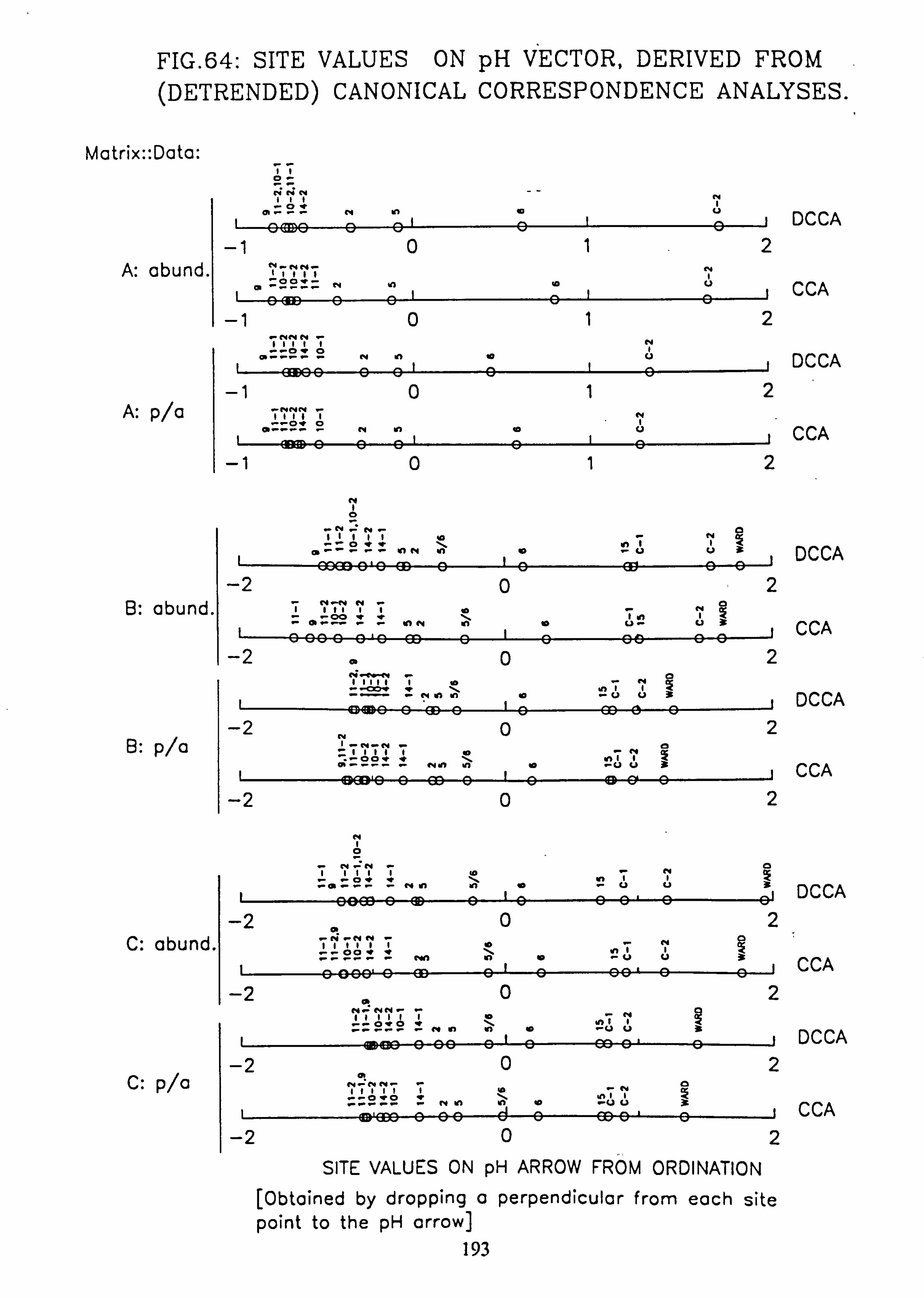
FIG. 64: SITE VALUES ON pH VECTOR, DERIVED FROM (DETRENDED) CANONICAL CORRESPONDENCE ANALYSES.
Matrix:: Data: ö ^
NNN 111 N
O
o ý e 1
eI DCCA
-1 m
0 1 2 A b d "-""- t4 : un a .
11111 ^ýýýý
N 1q
e ' 10
V
e CCA
-1 0 1 2 NN N ; N
1
DCCA
-1
e 6
0 6
1 2 A / N : p a ý N N
' In m CCA
-1 -e e RBS 6
0 e
1 2
B: abund.
B: p/a
C: abund.
C: p/a
N
0 N^N O
11111 io N -r 1
pl in Ni eamo-O ®
tl 1 ( 0 6
-2 6 0
0 1
2 C4 --N N- O
N
-a °-° ßf1 N
L
n tl
I cä .
n- U3
-2 0000 9 6 a) 6 6
0 ee 0
2 a 11111 el I\
N in
6gA tl n1
-UU 9
3
6
-2 06®6
0 a
2 N 1 -N-N - O
^-ööv p- Nn i
lo -u v 3
"' ' 1 s 6
-2 96® 6 6
0 ®
2
N
O
N. N N O
-a-N in n
^ e
19 U
6 6- U e el
-2
99WC ® v 0 2
a MNN
1111 01.
tl n ü
Nn tl 916
. e q,
0 A-- --
3 0
-2
00 00 0® 0 2
a Nr NN- a
9 n = g -- N in ® 6ee
tl 6I 6---
VV )6 =
3 9
-2
ß g 0 2
at NýNN7 N
O
0.0 rNn
ee '
In tl
e
ýV V
69 e
;
.2
O EIDO e
0 2
SITE VALUES ON pH ARROW FROM ORDINATION [Obtained by dropping a perpendicular from each site point to the pH arrow]
193
DCCA
CCA
DCCA
CCA
DCCA
CCA
DCCA
CCA
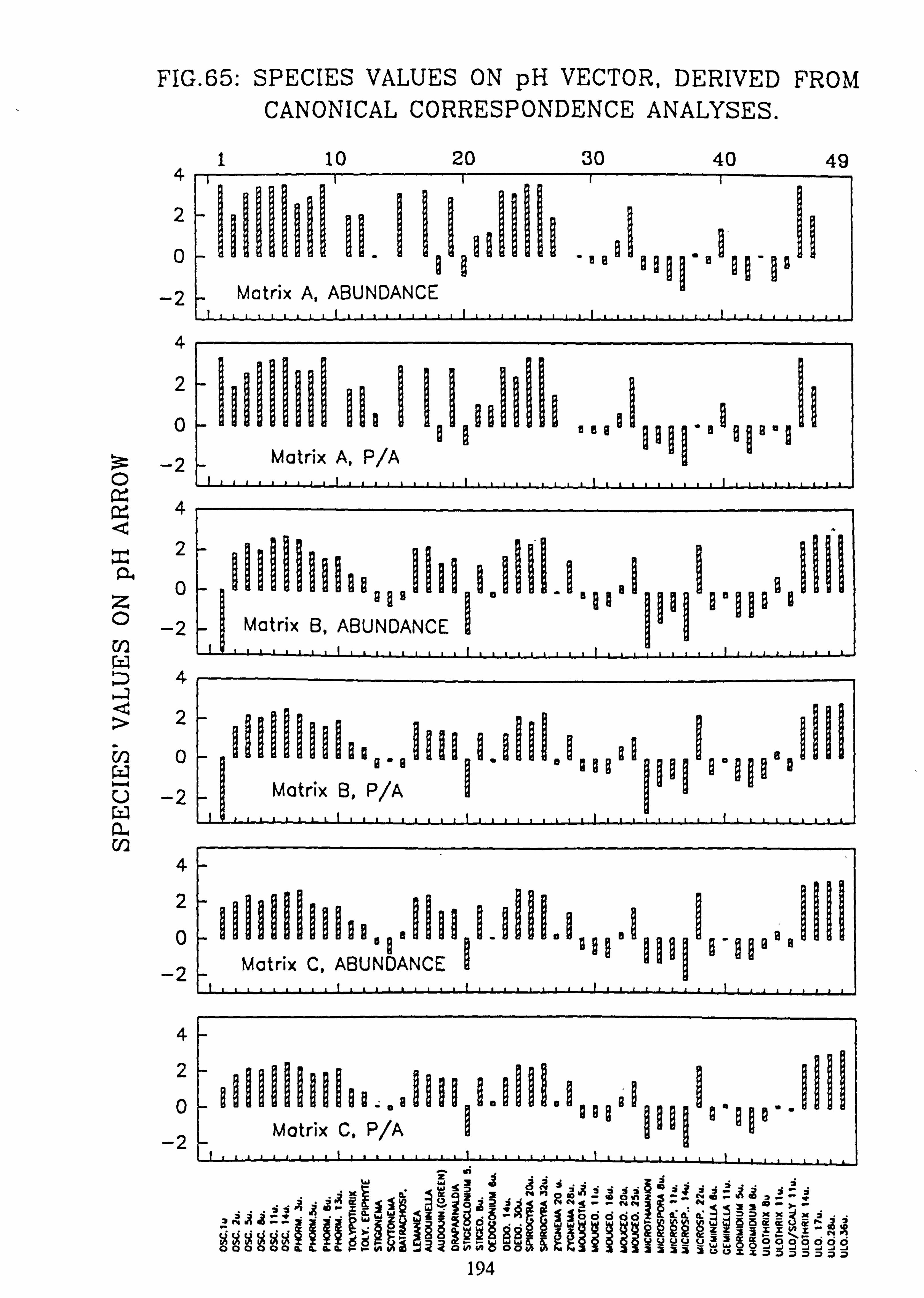
FIG. 65: SPECIES VALUES ON pH VECTOR, DERIVED FROM CANONICAL CORRESPONDENCE ANALYSES.
4
2
0
-2
4
2
0
ý -2 0
4
x2
z0 o
-2 U) W 4
v1 0
o -2
U)
1 10 20 30 40 49
Matrix A, ABUNDANCE eee8A
., lý p! , I, 'IiIllI ..., ý�sl. Dille Matrix A,
ll g 11le II1a1 jB I9II
. IILI
.Ia Bi'I ý9 1l11 'Il as II
II. I
Matrix B, ABUNDANCE
3111111i11o,. A Iiesl1.1lll. o,,, aoý'oIBB. ae,., 4111
Matrix 8, P/
4
2
0
-2
O ýýý ee8
Matrix C, ABUNDANCE
4
2
0
-2 I IIIIIIiEIaa. qI
I l3'1.99f0. fue°I1IIII°. p1o.. 9I
II
Matrix C. P
in
'fix 3ý 3 ýý 40A tön Z °=3Neýaýý ^--^
WWZ >> xxx
ýý -4 g93-- ß
DS
& Z< 9ddddý
e do e§ §-as&ý'iA
ii CK UM" d-
ýj`ylYV UU Ui WO OZ
ý ýOOOOJO
000 009h. 4dNNmNNpO .55 33331VV2 2>>>> j77
194
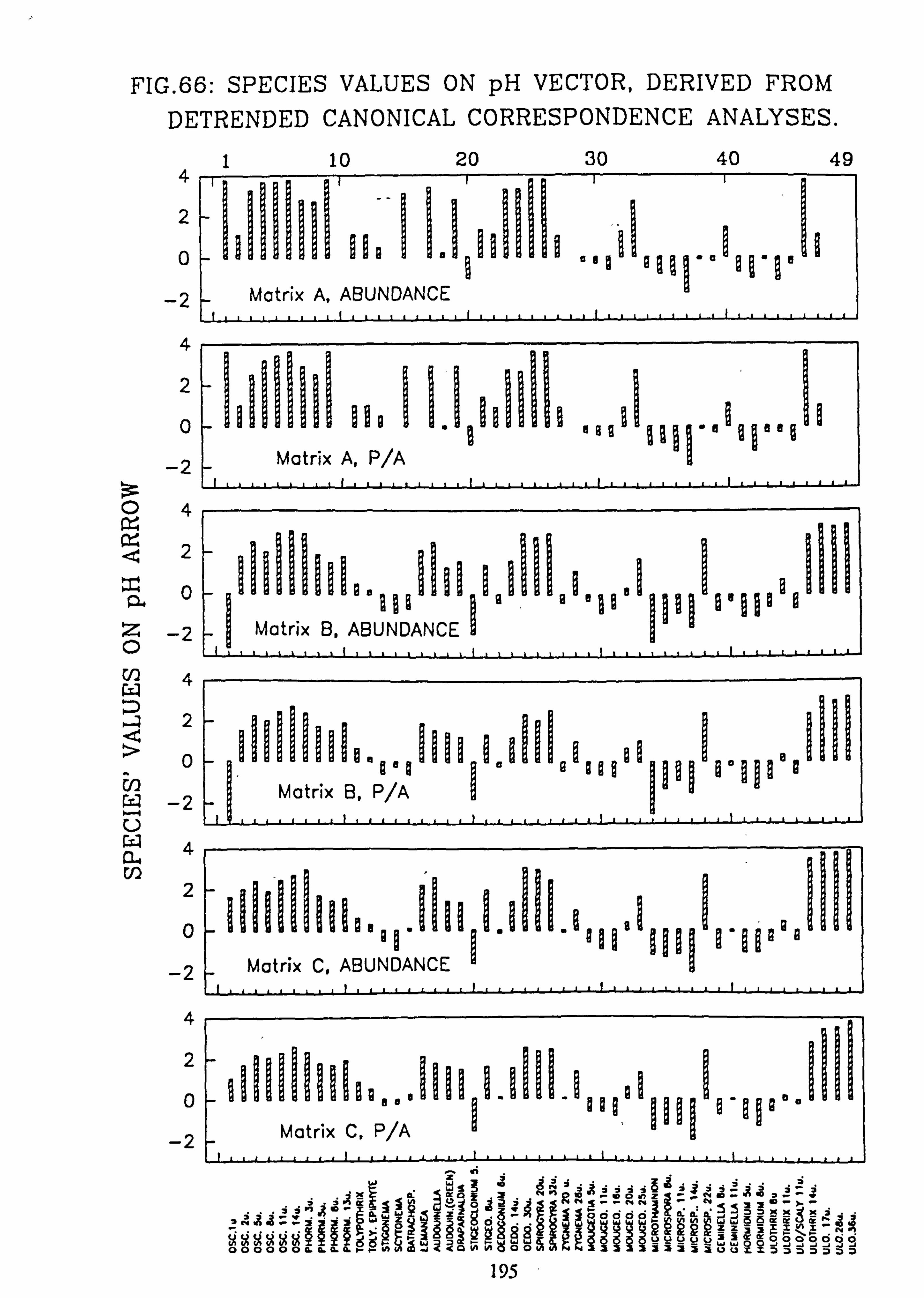
FIG. 66: SPECIES VALUES ON pH VECTOR, DERIVED FROM
DETRENDED CANONICAL CORRESPONDENCE ANALYSES.
4
2
0
4
2
0
-2
04
d2
Z -2 O w4
. ý.
a 2
w -2
w4
-2
1 10 20 30 40 49
Matrix A, ABUNDANCE
1 .a of l1eýl.. ie
ß,. a§9 91I &ýý8ý8 190 ý I. IhflH
Matrix A, P/A
111111
,I §II, I,
I Matrix
B, ABUNDANCE o III II II Ei.
a. a EI IB ý. ýI6IýBoI BBI p Ie I
Io. ýý1. a
6I II
Matrix B, P/A I9
Matrix C, ABUNDANCE
P/A Matrix C,
7 td ö=
Z^ýö i
er-ö - ^r
iOi_ in =_ 6(ý
` 11 ioööocp {p[ý d Hp§ d(1
WiäRK ä^^3
Q Cv {J
KKK31CN
`yý `yý' _
U_ U_ U_ U 0000000 OOOOÖÖ gL CL. CL CL
ýmJ 2< C
VI NO5Z3322i1uui i»»> J7
195
4.7.3.2 Variables excluded from analysis by CANOCO Some variables were excluded from the analysis because of insufficient data or other reasons for considering them unreliable as discussed below. (a) 'Flow' is the depth gauge reading on site. It takes no account of the other hydrological factors which determine the current velocity and thus is not strictly
comparable between sites. Furthermore alterations in the stream beds have occurred
since the installation of the gauges so that the zero mark lies beneath the stream bed in
some cases. The 'Flow' data was therefore adjusted by subtracting from each the
minimum reading encountered, giving the variable 'Depth', which is thus the mean fluctuation in water depth.
(b) Temperature was measured on site during sampling. The measured temperature is influenced by time of day, being related to insolation. The same order of site visitation was used on most occasions, so that the time of sampling each site can be predicted within an hour or two. It is found that when the mean temperature is plotted against G. M. T.,
a reasonable straight-line regression is obtained (Fig. 25b), implying that the spot- measured temperature is not a reliable measure of real differences between sites. Measurements of maximum and minimum temperature were too infrequent to be of value. (c) PAR was measured only at certain sites as insufficient instruments were available and some sites were considered too public to leave an unattended instrument for several weeks. The instruments were furthermore not available during the earlier part of the investigation. Therefore although calculated values of PAR have been used in Pearson correlation analysis there were insufficient sites with measured'percent of open' values to enable PAR to be usefully included in CANOCO. (d) Measurements of silica were carried out relatively infrequently and therefore mean values are not available for some sites. (e) Phosphate is to a lesser extent subject to the same problem, as the distribution of values for P04 is biased because analyses were carried out by SOAFD more frequently following fertilization of the catchment by the Forestry Commission. (f) Variables such as alkalinity, Cat;, Mg2`, Al and absorbance had to be dropped from
many of the analyses because of their contribution to high VIFs. These are clearly a priori and as implied in these analyses, acidification-related variables. However one variable is able to represent the whole group in terms of the effects of acidification on species distribution. This role has been allotted to pH, but several other variables might equally well have been chosen. For practical purposes however pH is a good choice; it is more easily measured than the others and hence more data are available, and it is a direct measure of the changes implicit in the term 'acidification'.
196
4.7.3.3 Transformation of variables Loglo transformation is indicated for forms of Al (see section 4.6.1), but these have been
excluded on the basis of high intercorrelation with pH, so no transformations have been
applied to data for analysis by CANOCO.
4.7.3.4 Results of analyses In all analyses pH is highly correlated with Canonical axis 1 (Tables 52-54) and in
consequence the arrow lies very close to axis 1 in the biplot. The pH arrow is the longest
one in the biplot and thus the most important variable in explaining the distribution of
species (Ter Braak and Prentice, 1988).
The second important fact to emerge from an inspection of the biplots is that the distribution of the sites along the pH arrow is in all cases virtually identical to the order
of sites in Table 46, where they are ranked by mean pH, and to the groupings carried out by CLUSTER. BAS (abundance data) and NASSOC. BAS (presence-absence data).
This is shown more clearly in Fig. 64 where the site values on the pH vector have been
recalculated and plotted along a single axis, for all matrix and data combinations. The
distribution, clearly separating the acidic burns 9,10,11 and 14 from the circumneutral Ward, Corrie, 6 and 15, is in fact remarkably stable and was obtained also in analyses
where other variables were included, contributing to VIFs exceeding 100. These
variables contribute little additional information to the ordination but they do not upset the canonical coordinates (Ter Braak, 1988). Differences in the distribution of species
on the diagrams have however been detected and it is for this reason that a common set
of variables has been employed as far as possible in comparing the six matrix/data
combinations (Tables 52,53).
The results of these analyses may be most readily compared by consulting Figs. 65 and 66, where the recalculated species values on the pH arrow have been plotted for all
matrix/data analysis combinations. In these figures the recalculated species values are
presented as a bar chart with the species in the same order to facilitate comparison of
the patterns. The value (height of the bar) represents the position on the pH arrow
occupied by each species. This is the weighted average of the species occurrence with
respect to pH. The value is thus a function of the mean pH at which a given species is
found - the mode of the Gaussian distribution curve.
197
The species values may thus be used as indicator values for inferring environmental pH. Species which occur towards the extremities of the ordination carry more predictive weight, so that in the case of pH, it is the highest and lowest species values which are of the greatest importance. The downweighting of rare species is advisable to prevent rare species, which by chance may fall towards the outside of the ordination, from biasing the
result.
The species' values shown in Figs. 65 and 66 are very similar in different matrices and data forms, with the notable exception of 'Oscillatoria 1 pm' (species 1). This may be due to a tendency to overlook its occurrence in films of organic material prevalent in
some of the more acidic streams during the earlier part of the investigation. The finding
of an (apparent) cyanophyte in these waters was unexpected (Brock, 1973). Another
problem is that these dimensions are near the limits of resolution in field samples which were normally examined at x500 magnification, and this size class may therefore encompass several taxa.
The analyses were re-run with the option allowed in CANOCO for giving zero weight to this species, but apart from the effects on species 1, there was very little difference in the values of the summary statistics (Table 54) and in the configuration of the ordination diagrams (not shown).
Acidification has been noted to result in changes in algal communities in lakes and streams. Both in planktonic and benthic communities, reduction in pH is found to result in a decrease in abundance of diatoms and Rhodophytes and a progressive replacement by blue-greens and then filamentous green algae (Muller, 1980; Morling et al, 1985; Stokes, 1986; Marker and Willoughby, 1988; Findlay and Kasian, 1990; Havens and Heath, 1990). These changes are found whether acidification occurs 'naturally', i. e. as a slow process due to catchment acidification, or artificially in the course of experimen- tal manipulation. While some workers find an increase in biomass on acidification (Hendrey, 1976; Muller, 1980; Mulholland et al , 1986), others find no change (Arnold
eta! , 1981; Howell eta! al, 199Molot eta! al, 199or even a decrease (Nalewajko and O'Mahony, 1989).
Schindler (1987) concluded that stress, including acidification, does not lead to changes in production, nutrient cycling or decomposition, but does cause changes in species com- position which are thus better indicators of disturbance. Marker and Willoughby (1988)
concluded that the increased biomass reported in acidified streams is more apparent than real, due to the different types of algae present.
198
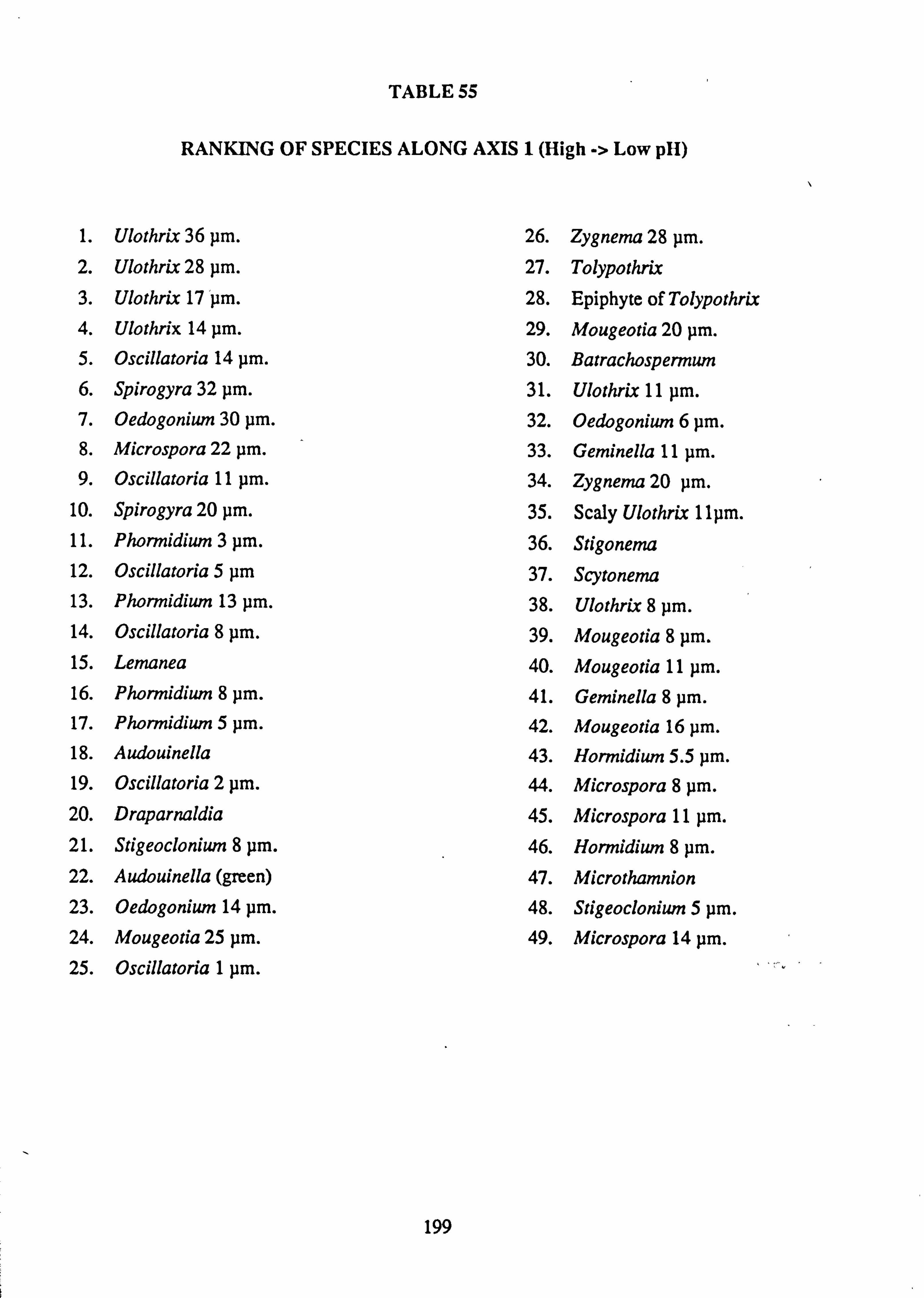
TABLE 55
RANKING OF SPECIES ALONG AXIS 1 (High -> Low pH)
1. Ulothrix 36 pm. 26. Zygnema 28 pm. 2. Ulothriz 28 pm. 27. Tolypothrix
3. Ulothrix 17 pm. 28. Epiphyte of Tolypothrix 4. Ulothrix 14 pm. 29. Mougeotia 20 pm. 5. Oscillatoria 14 pm. 30. Batrachospermum 6. Spirogyra 32 pm. 31. Ulothrix 11 pm. 7. Oedogonium 30 pm. 32. Oedogonium 6 pm. 8. Microspora 22 pm. 33. Geminella 11 pm. 9. Oscillatoria 11 pm. 34. Zygnema 20 pm.
10. Spirogyra 20 pm. 35. Scaly Ulothrix 11pm. 11. Phormidium 3 pm. 36. Stigonema 12. Oscillatoria 5 pm 37. Scytonema 13. Phormidium 13 pm. 38. Ulothrix 8 pm. 14. Oscillatoria 8 pm. 39. Mougeotia 8 pm. 15. Lemanea 40. Mougeotia 11 pm. 16. Phormidium 8 pm. 41. Geminella 8 pm. 17. Phormidium 5 pm. 42. Mougeotia 16 pm. 18. Audouinella 43. Hormidium 5.5 pm. 19. Oscillatoria 2 pm. 44. Microspora 8 pm. 20. Draparnaldia 45. Microspora 11 pm. 21. Stigeoclonium 8 pm. 46. Hormidium 8 pm. 22. Audouinella (green) 47. Microthamnion 23. Oedogonium 14 pm. 48. Stigeoclonium 5 pm. 24. Mougeotia 25 pm. 49. Microspora 14 pm. 25. Oscillatoria 1 pm.
199
There is a greater degree of agreement about the algae most favoured by acidification. Filamentous greens come progressively to dominate below pH 6.0 (Hargreaves et al, 1975; Muller, 1980; Turner eta!, 1987; Marker and Willoughby, 1988; Howell et al, 1990; Jackson et al, 1990). The genus Mougeotia is particularly prevalent as periphyton in the littoral zone of lakes, or forming free-floating masses of meta- phyton, leading to the speculation that either light penetration or DIC concentration limits its development in deeper water (Turner et al, 1987). Zygnema (or Zygogo-
niwn) is also reported to occur under these circumstances (Jackson et al, 1990). In
streams the availability of light or DIC may impose less of a limitation on algal growth.
Marker and Willoughby (1988) found in natural streams of differing pH that at circumneutral pH the filamentous genera Ulothrix, Rhodochorton (= Audouinella), Batrachospermum and Lemanea were common, but at lower pH the Rhodophytes
were replaced by blue-greens and Hormidium subtile. In contrast, Mulholland et al (1986) found that Rhodochorton was present at a site with median pH 4.5. In highly
acidified water (e. g. affected by mine drainage), filamentous greens including Hormidium sp. and some resistant diatoms may be found, down to pH values below 3.0 (Hargreaves et al, 1975).
Most of these results accord with the distribution of species with pH found in the L.
Ard streams (e. g. Fig. 63), except thatAudouinella/Rhodochorton is found predomi- nantly in the higher-pH sites (Fig. 53b) and in association with other'circumneutral'
species (Figs. 29-40). However it has been recorded in every stream apart from Burn
11 on at least one occasion (Tables 4-9).
The ranking of species with respect to pH can be derived from CCA analysis. In an analysis where the pH arrow is very close to axis 1, e. g. Fig. 63, the order of species along axis 1 given in the CANOCO output will be effectively the ranking of species
with respect to pH (Table 55). This ranking does not lend support to the observation
of Havens and Heath (1990) that acidification leads to a shift towards larger-diameter
species. Rather the opposite trend appears in the L. Ard streams. This difference may be accounted for by changes in grazing pressure during the 23-day experimental
acidification and aluminium spiking experiment of Havens and Heath (1990), in in-
lake polyethylene mesocosms.
200
Sensitive zooplankton may be very rapidly eliminated by such manipulations leading to
a community dominated by forms too small to exploit the larger algae, leaving them at
a competitive advantage. These zooplankton species do not exist in lotic environments
and in any case a longer-term acidification will permit the establishment of a stable algal
community which may not be the same as a replacement community following
ecosystem disturbance.
If the change in algal species which occurs on acidification is due to a rapid development
of species tolerant of the new conditions, i. e. able to exploit a resource left vacant by intolerant species, it is more likely to result in a community dominated by small cell forms, as the maximum specific growth rate is inversely related to cell diameter (Raven
and Geider, 1988). Therefore if a change in species composition is due to a shift in
grazing pressure, a population of larger cells is likely to result in the short term, but if
grazing is not important prior to acidification, the post-acidification population should consist of smaller algal cells. The final, steady-state condition however will depend on the pH-sensitivity of growth rate in the species comprising the community and their
relative ability to exploit other resources such as TON, P04, light and DIC, which may be limiting.
It is evident from Figs. 56-63 that a great deal of variation in species abundance also exists along canonical axis 2, which is closely related to the variables % Forest, Auo, Stream Order, Area or TON, in some analyses.
It is possible that the distribution of cyanophytes may be influenced by the TON
concentration. In Figs. 60-63 Phormidium 8 pm and Phormidium 13 pm are closely
associated with the head of the TON arrow (high concentration), while Scytonema,
Stigonema and Tolypothrix lie towards to other end (low TON). The latter three species form heterocysts while Phormidium spp. do not.
No other clear candidates for relationships between particular species and environ-
mental variables can be seen in these analyses. A larger data set would be necessary to
enable the effects of multiple environmental variables to be disentangled.
201
Canonical Correspondence Analysis is thus seen to give important and consistent information about the influence of environmental variables on the distribution of filamentous algal taxa. The most important environmental gradient is one associated with acidification. The ultimate test of the validity of the relationship revealed however is whether the information can be used to reconstruct site pH values from the species data (calibration).
4.7.3.5 Calibration using CANOCO Inferring environmental values from species data (calibration) by CANOCO is de-
scribed by Ter Braak (1988). An analysis is carried out using a calibration set of data,
with both species and environmental data included. It is necessary only to include one' environmental variable, the 'variable-of-interest', in this process. The samples for
which environmental variable values are to be inferred are included in the species data
only, and are thus passive samples in the analysis.
Mean values of pH are inferred from the CANOCO output of the analysis according to, the formula: -
inferred pH =Z+ SX/ C
where Z is the mean and S is the standard deviation of pH values for the calibration sites, C is the canonical coefficient for pH, and Xis the sample score on axis 1, which are all given in the CANOCO output (Ter Braak, 1988).
This procedure has been carried out using Matrix C as the calibration data set and species data collected on four occasions in the Loch Dee catchment, Galloway, and on two occasions in the Loch Rannoch area. The values of pH inferred for the original data
set (Matrix C, abundance data) have been plotted against the measured values in Fig. 67a, and the inferred and measured values for the Galloway and Rannoch data in Fig. 67b. The regression shown in Fig. 67a, lies very close to the ideal, which is the diagonal in this graph. However the Galloway and Rannoch data yield a much less significant regression, and the slope is well removed from the ideal.
A similar analysis has been carried out on the two halves of of the L. Ard data set, using matrix B as the calibration set (Figs. 68,69). Using abundance data the autoregression (Fig. 68a) of the matrix B data is poorer than that obtained with matrix C, but with pooled p/a data an almost identical fit is found. The inferred pH values in matrix A however bear a less close relationship to measured values, although they are closer than the fit obtained with the Galloway/Rannoch data.
202
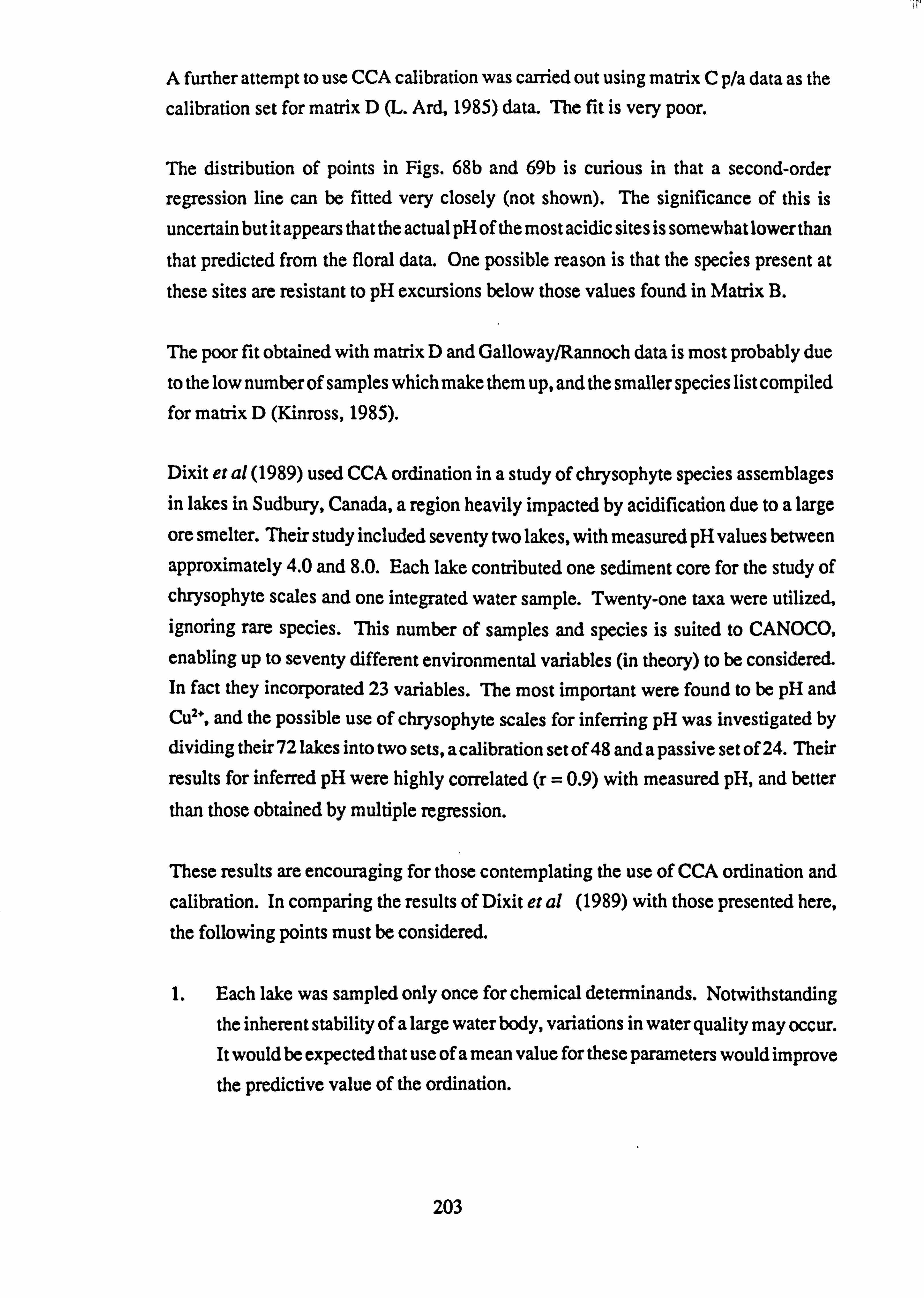
A further attempt to use CCA calibration was carried out using matrix C p/a data as the
calibration set for matrix D (L. Ard, 1985) data. The fit is very poor.
The distribution of points in Figs. 68b and 69b is curious in that a second-order
regression line can be fitted very closely (not shown). The significance of this is
uncertain but it appears that the actual pH of the most acidic sites is somewhat lower than
that predicted from the floral data. One possible reason is that the species present at these sites are resistant to pH excursions below those values found in Matrix B.
The poor fit obtained with matrix D and Galloway/Rannoch data is most probably due
to the low number of samples which make them up, and the smaller species list compiled for matrix D (Kinross, 1985).
Dixit et al (1989) used CCA ordination in a study of chrysophyte species assemblages in lakes in Sudbury, Canada, a region heavily impacted by acidification due to a large
ore smelter. Their study included seventy two lakes, with measured pH values between
approximately 4.0 and 8.0. Each lake contributed one sediment core for the study of chrysophyte scales and one integrated water sample. Twenty-one taxa were utilized, ignoring rare species. This number of samples and species is suited to CANOCO,
enabling up to seventy different environmental variables (in theory) to be considered. In fact they incorporated 23 variables. The most important were found to be pH and Cue+, and the possible use of chrysophyte scales for inferring pH was investigated by dividing their 72 lakes into two sets, a calibration set of 48 and a passive set of 24. Their
results for inferred pH were highly correlated (r = 0.9) with measured pH, and better
than those obtained by multiple regression.
These results are encouraging for those contemplating the use of CCA ordination and
calibration. In comparing the results of Dixit et al (1989) with those presented here,
the following points must be considered.
Each lake was sampled only once for chemical determinands. Notwithstanding
the inherent stability of a large water body, variations in water quality may occur. It would be expected that use of a mean value for these parameters would improve
the predictive value of the ordination.
203
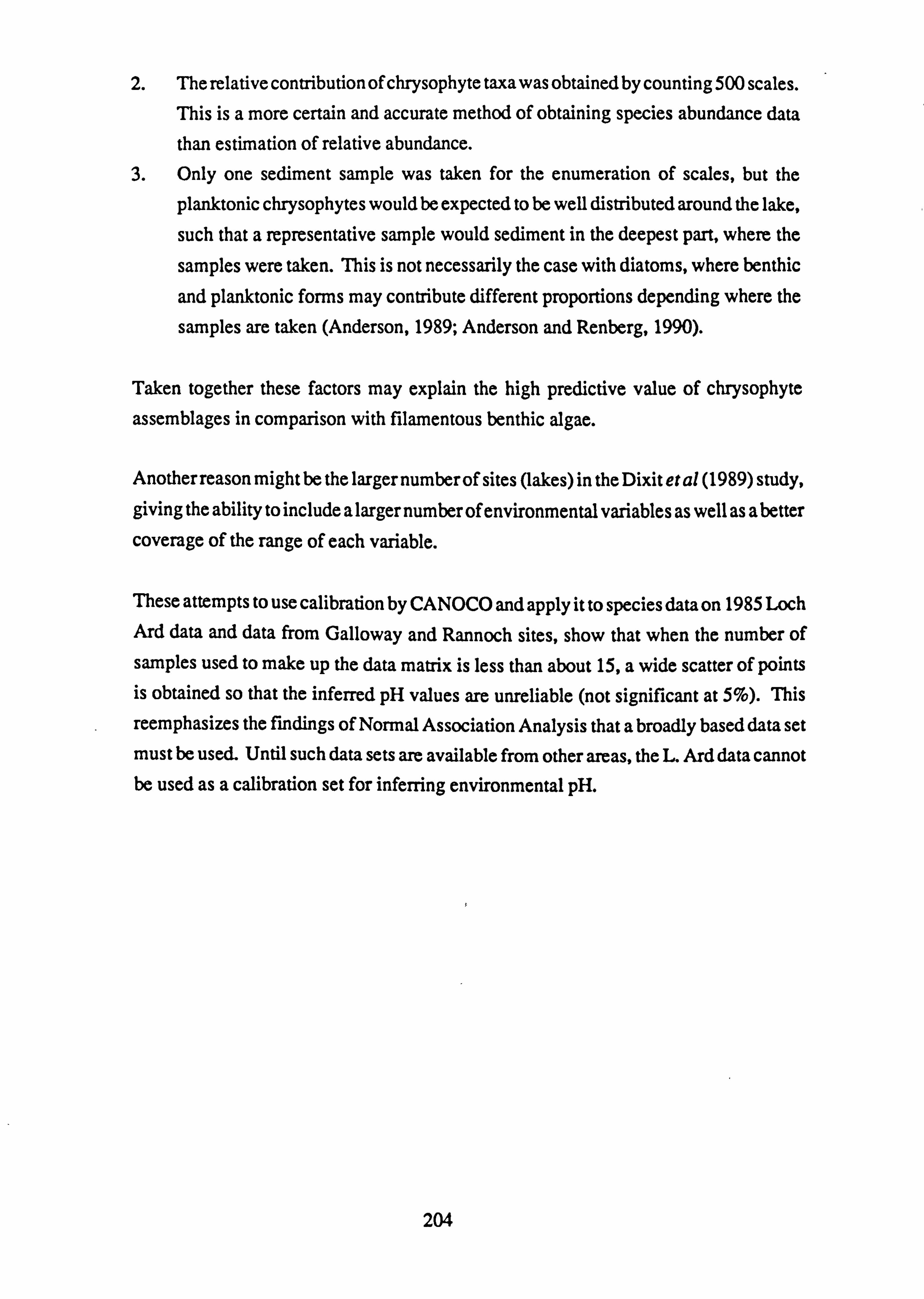
2. The relative contribution of chrysophyte taxa was obtained by counting 500 scales. This is a more certain and accurate method of obtaining species abundance data
than estimation of relative abundance. 3. Only one sediment sample was taken for the enumeration of scales, but the
planktonic chrysophytes would be expected to be well distributed around the lake,
such that a representative sample would sediment in the deepest part, where the
samples were taken. This is not necessarily the case with diatoms, where benthic
and planktonic forms may contribute different proportions depending where the
samples are taken (Anderson, 1989; Anderson and Renberg, 1990).
Taken together these factors may explain the high predictive value of chrysophyte
assemblages in comparison with filamentous benthic algae.
Another reason might be the larger number of sites (lakes) in the Dixit et al (1989) study, giving the ability to include a larger number of environmental variables as well as abetter coverage of the range of each variable.
These attempts to use calibration by CANOCO and apply it to species data on 1985 Loch Ard data and data from Galloway and Rannoch sites, show that when the number of samples used to make up the data matrix is less than about 15, a wide scatter of points is obtained so that the inferred pH values are unreliable (not significant at 5%). This
reemphasizes the findings of Normal Association Analysis that a broadly based data set must be used. Until such data sets are available from other areas, the L. Ard data cannot be used as a calibration set for inferring environmental pH.
204
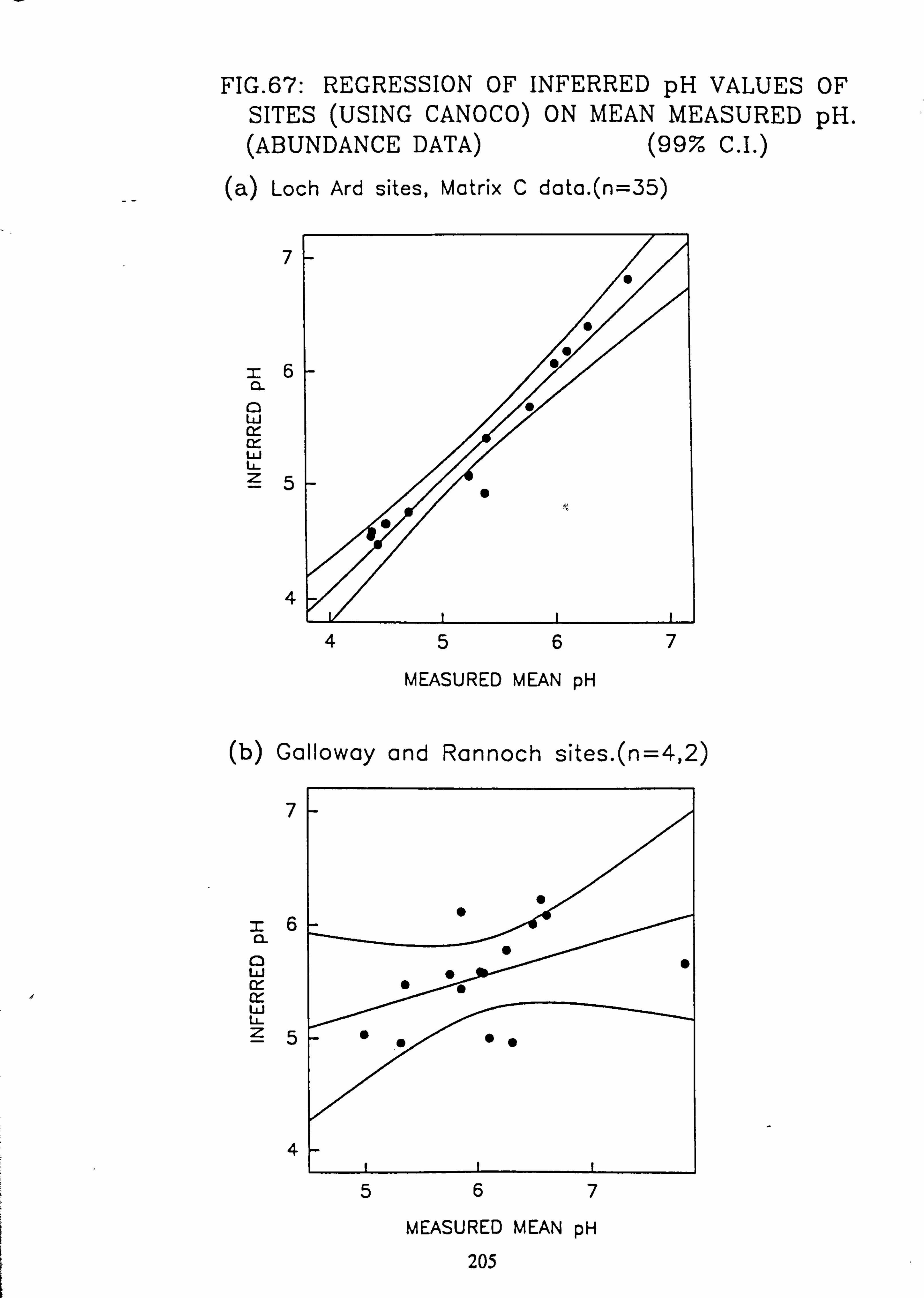
FIG. 67: REGRESSION OF INFERRED pH VALUES OF SITES (USING CANOCO) ON MEAN MEASURED pH. (ABUNDANCE DATA) (99% C. I. )
(a) Loch Ard sites, Matrix C data. (n=35)
I
"
z6 a
Q W Of
W LL- z5
0
0
A
s
4567
MEASURED MEAN pH
(b) Galloway and Rannoch sites. (n=4,2)
7
= CL
0 W
ix Li U- z5
. 7 "
" "
"
567
MEASURED MEAN pH 205
FIG. 68: REGRESSION OF INFERRED pH VALUES OF SITES (USING CANOCO) ON MEAN MEASURED pH.
ABUNDANCE DATA (99% C. I. )
(a) L. Ard sites, Matrix B data (n=18) --
7
z6 0 a w Of x w LL-
z5
0
0
0
4
0
0
4567
MEASURED MEAN pH
(b) Matrix A data. (n=17) pH inferred from matrix B data
7
=6 CL
0
0 W
W Li z5
0
4
4567
MEASURED MEAN pH 206
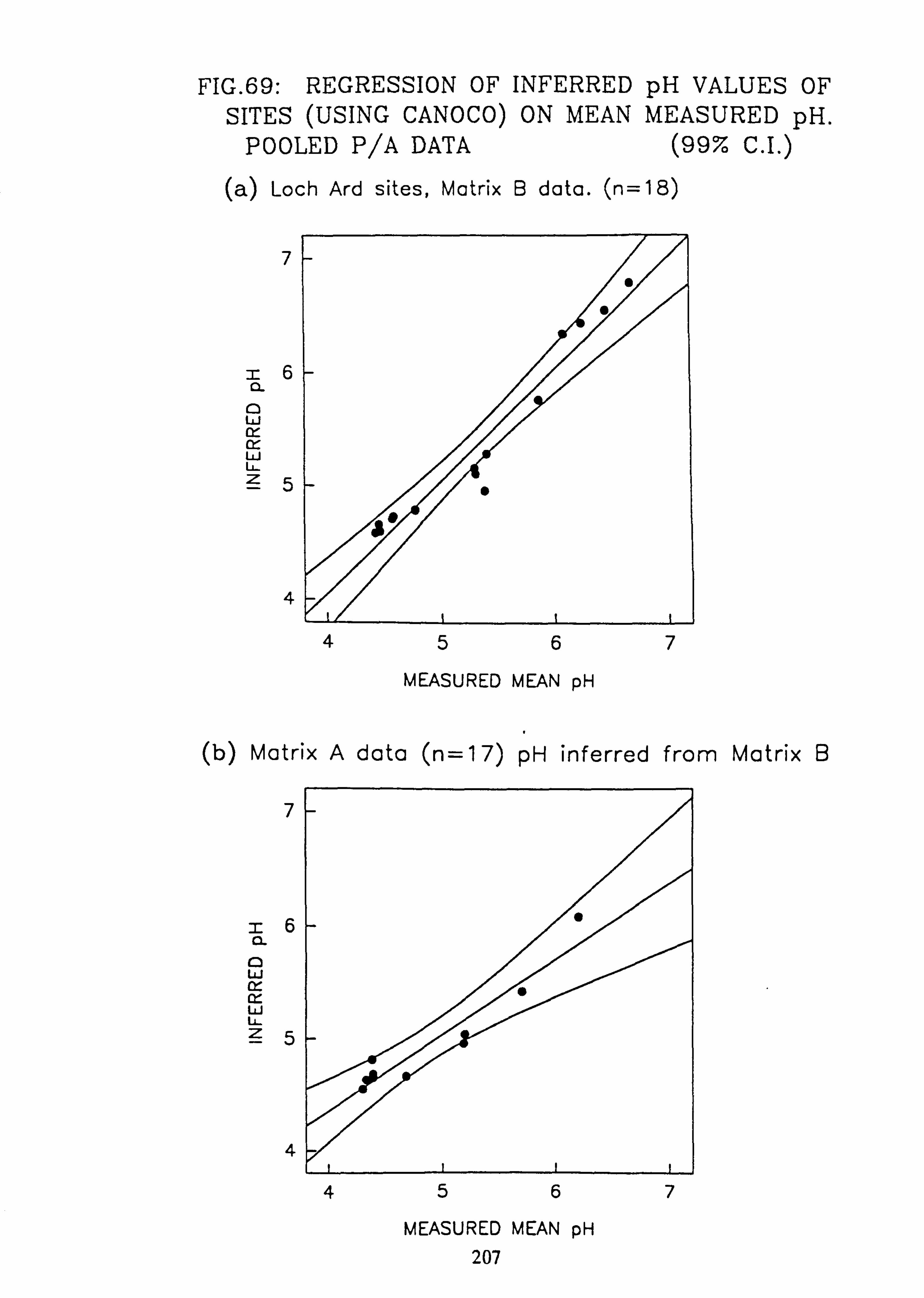
FIG. 69: REGRESSION OF INFERRED pH VALUES OF SITES (USING CANOCO) ON MEAN MEASURED pH.
POOLED P/A DATA (99% C. I. )
(a) Loch Ard sites, Matrix B data. (n=18)
7 0
i6 a
0 Li cr- cr W L- z5 0
4
4567
MEASURED MEAN pH
(b) Matrix A data (n=17) pH inferred from Matrix B
7
= CL
0
0 W
W li. z5
S
4
4567
MEASURED MEAN pH 207
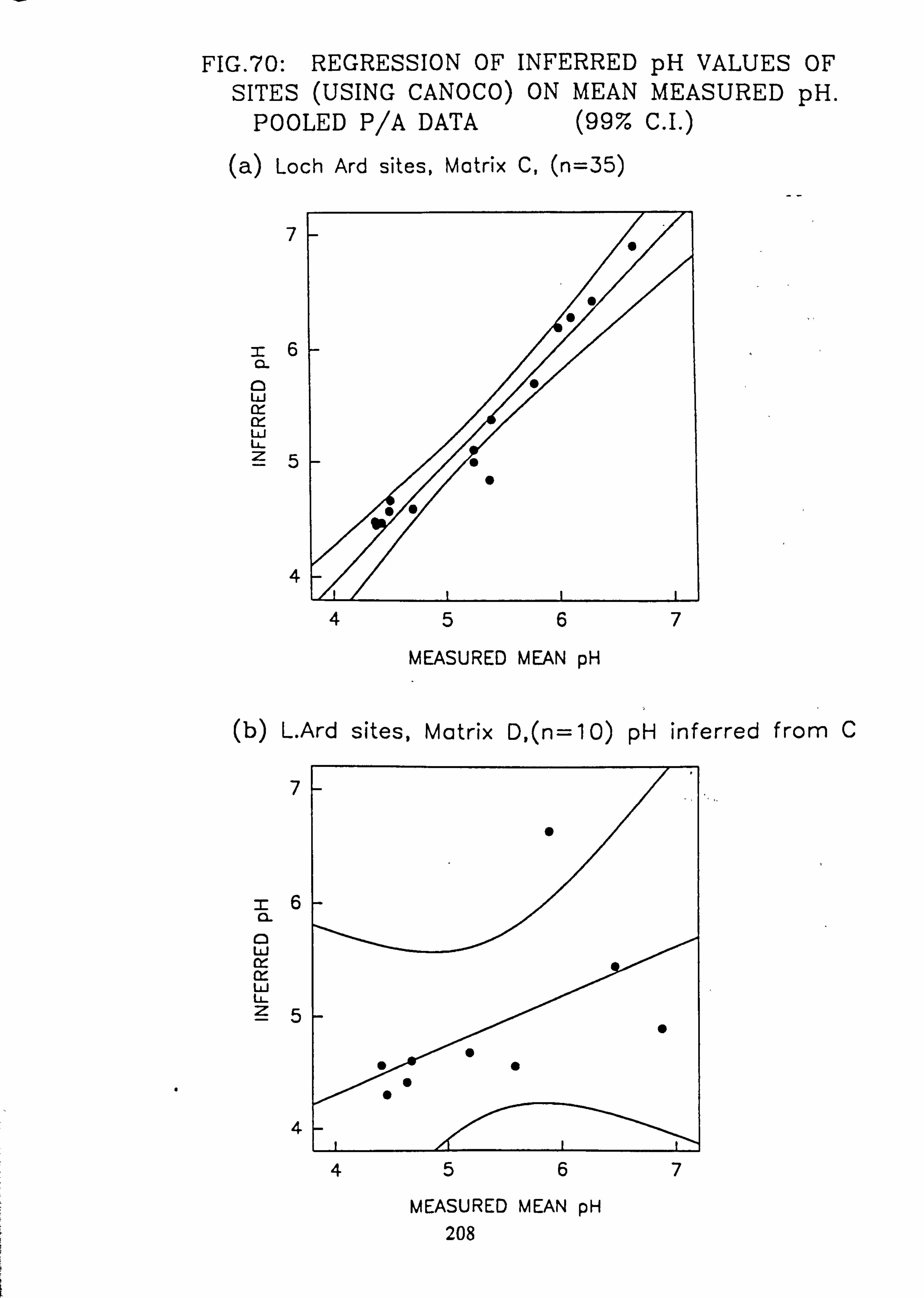
FIG. 70: REGRESSION OF INFERRED pH VALUES OF SITES (USING CANOCO) ON MEAN MEASURED pH.
POOLED P/A DATA (99% C. I. )
(a) Loch Ard sites, Matrix C, (n=35)
i
= CL
0
0 w Of it w w z5
0
A
56
MEASURED MEAN pH
(b) L. Ard sites, Matrix D, (n=10) pH inferred from C
7
I
= CL
0 W cy-
m W LL. z5
0 S
" S
" A
456
MEASURED MEAN pH 208
4.8 ALGAL PRODUCTION
4.8.1 Methods for measuring production rates
In the measurement of production rates both in the field and laboratory, several methods are
possible. The assimilation of carbon may be measured as uptake of IT from bicarbonate, from
flux of dissolved inorganic carbon (Turner eta!, 1983) or as changes in pH consequent on the
uptake of CO2 from the water (Wright and Mills, 1967). Production of 02 can be measured,
either by Winkler assay or by use of a dissolved oxygen meter, by comparing values upstream
and downstream, or diurnal changes at one station (Odum, 1956). Rate of biomass increase
may also be measured as change in photosynthetic pigment yield or AFDW per unit area over
a time interval. Unfortunately all these methods have limitations which render them less
useful in environments such as the L. Ard streams.
The14C methodology may be used in the laboratory or in respiration chambers in the field
(Bott et a1,1978; Duthie and Hamilton, 1983; Turner et a1,1983; Mulholland et a1,1986) but it relies on the presence of bicarbonate ion in the water. At the pH values prevalent in many of the L. Ard streams (pH 4-5) the bicarbonate would be dissociated and might be lost as CO2
(Schindler et al, 1972).
Diurnal changes in pH as a consequence of CO2 uptake during the day have been noted (Morgan, 1985; Wright and Mills, 1967. This phenomenon has been detected in streams in
Galloway which are susceptible to acidification, but only at pH values in excess of 6.0
(Solway River Purification Board, unpublished observations), where the buffering is largely
due to carbonate/bicarbonate (Ulrich, 1983 b). The equations for calculating carbon uptake from pH depend upon there being no other buffer system operating (Kelly et al, 1983).
Morgan (1985) found the pH in an acidic lake raised from about 4.5 to 8 by photosynthetic
activity enhanced by cultural eutrophication. Nutrient-poor running waters may be too well
aerated for such pH increases to occur, and may in addition have a considerable accrual of CO2
from groundwater percolation (Seip and Tollan, 1978, Reuss and Johnson, 1985).
209
Methods of estimating production from upstream/downstream oxygen concentration have been devised (Odum, 1956, Kelly et a1,1983) but these are again workable only in situations
where the flow conditions are such that the exchange of gases between the water and the
atmosphere can be calculated (which is not the case in rapidly flowing, shallow turbulent
streams (McConnell and Sigler, 1959)) or in situations where exchange can be controlled or eliminated (Edelmann and Wuhrmann, 1978; Tease et al, 1983, Tease and Coler, 1984,
Gallegos and Scheibe, 1986).
Measurement of changes in DIC have been utilized in acidified lakes (Turner eta!, 1987) but
would be more difficult to apply in running water, for the reasons just given.
4.8.2 Biomass In the absence of direct measurements of primary production, the standing crop of primary producers may be taken as an indicator of production rate in this field.
An increased algal standing crop has been reported in acidified water (Hendrey, 1976; Muller, 1980; Mulholland et al, 1986). The cause has been questioned. Stokes (1986) lists four
possibilities, decreased grazing by acid-sensitive invertebrates being one. Removal of grazing pressure by factors other than acidification has been shown to result in an increased periphyton biomass (Eichenberger and Schlatter, 1978; McAuliffe, 1984; Yasuno et al, 1985; Jacoby, 1987; Feminella, 1989; Winterbourn, 1990). Decreased decomposition as a result of acidification is also proposed as a cause of the reported biomass increase. The other two possibilities are a shift towards dominance by acidobiontic algal species and a decrease in
competition between species.
If such an increase upon acidification is real then productivity cannot be compared between
acidified and non-acidified streams. Biomass in acidified streams will reflect the primary
productivity more closely, without the necessity of considering loss factors.
The relationship between biomass and environmental variables has been investigated by
calculating Pearson's correlation coefficient, r, between variables and different measures of biomass. This has been carried out using both mean values for each sampling site, when the
appropriate significance level is 5%, and individual values from all sites on all occasions, when the appropriate significance level is 0.1-1% (Tables 17,19). The results show a high degree
of variability but tend to support the view that acidification does not result in an increase in
algal biomass, indeed they suggest that the opposite is the case. The reasons for this however
are uncertain.
210
4.8.3 Production rates in laboratory studies Estimation of rate of increase of biomass in the field is complicated by sampling difficulties, in particular the difficulty of providing replicates in view of the patchy distribution of benthic
algae (Butcher, 1941; De Nicola and McIntyre, 1990) and of the high probability of loss of biomass and/or substrates with changes in discharge between visits.
This is not a problem in the laboratory but there remains the difficulty of obtaining an even colonization of artificial substrates such that the reproducibility between replicates is
acceptable (Meier et al, 1983). This was found in preliminary trials to be too serious a difficulty to make this method feasible.
Instead the method of Rosemarin (1983) was employed, in which the growth of individual filaments is followed over a time course by direct counting of cell number. This has the advantage of allowing the use of mixed cultures, allowing a great deal of information to be
gathered in one experiment, but with the limitation that only fairly low filament densities and short filament lengths can be used. Thus the growth rates obtained may not be relevant under conditions of high biomass.
Changes in average cell length may lead to inaccuracies in the growth rates obtained. Some species appear to show synchrony of cell division through several generations; Hormidium subtile and Geminella 8 pm. are most frequently found in filaments of 4,8,16,32 or 64 cells under the conditions employed. Thus it is necessary to obtain counts from a large number of filaments over several time intervals to even out the consequence of a sudden doubling of cell number in a given filament. Growth might also be measured by increase in the length of filaments; however this could not be done directly under the microscope due to the tortuous nature of many of the filaments, which also rules out photography of a microscope field as a means of obtaining material for measurement, as only a small proportion of the filaments will be in focus at any time. The use of a drawing tube might make measurement of filament length
possible, but at the cost of a reduced number of possible observations.
Despite possible inaccuracies or limitations of the cell-counting method, it does have some advantage over short term measures of production such as are obtained by measurement of14C uptake. Knoechel and De Noyelles (1980) found that short-term bioassays tend to overesti- mate the accrual of biomass because they neglect possible extracellular release fo fixed
carbon. On the other hand 14C labelling followed by track autoradiography (Knoechel and Kalff, 1976) offers the opportunity of simultaneous measurement of uptake rates of different
species in mixed culture if the culture conditions, particularly pH, permit its use.
211
For production measurement by "C uptake, or by pH measurement or 02 production, the algae
must be enclosed in apparatus which restricts exchange with the atmosphere while permitting
a current regime to that obtained in the open channels to be maintained. An attempt was made
to grow algae attached to a slide (removed from a channel after a growth rate experiment) in
a chemostat jar with a stirrer and 02 electrode. It was found that the condition of the algae deteriorated steadily so that repetition of 02 measurements could not be relied upon. The
culture conditions were evidently not suitable in the long term, so short term measures carried
out under these conditions could not have been related to the growth rate measurements carried
out over 1-2 weeks. Further work on this problem would be necessary to enable measurements
of 02, DIC or pH to be utilized.
If it can be shown that the short-term measurements are reliable and can be related to long-term
growth rates, then the micro-methods described by Brammer and Hogberg (1980), Wetzel et
al (1984), and Brammer (1988), utilizing samples of plant material enclosed in a Cartesian
diver, may permit rapid assessments to be made of the effects of environmental variables on
photosynthesis in different species.
4.7.4 Growth rate measurements
The results obtained from the statistical analyses of field data all suggest a relationship between
community structure and acidification-related environmental variables. However there is no way of determining from these which of the many intercorrelated variables are actually
responsible for the observed species distribution.
The thesis that pH and/or Al are the determining factors was investigated by experimental
manipulation of the growth conditions of algal isolates from natural populations. The
temperature, light regime, current velocity and DIC levels were held constant, allowing
aspects of water chemistry to be independently manipulated.
In the first series of experiments pH was adjusted by addition of dilute H2SO4. Additional
sulphate was thus added, raising the initial concentration of 193 peq 1'1 to between 270
peq Y' and 350 peq 1-', depending upon the target pH of the medium (6.0 to 4.0 respectively). The initial and final values of TON, P04, and, for run 3, Aluminium concentrations are shown in Table 22.
212
In the second series of experiments, the pH was held constant at 5.5 and the proportions of Al
and Si were varied. Treatment A consisted of 'Come' medium adjusted to pH 5.5, B was a
modified medium with Si reduced from 6.0 to 5.5 pM in order to test the thesis that the high
[Si] in'Corrie' protects against the effects of Al, and treatment C had the concentration of Al
raised from 40 to 146 pg 1' in addition to the decreased Si concentration. The actual
concentrations of Al, Si and the major nutrients N and P were measured at the beginning and
end of the experiments. Two experimental runs were performed, using different species. In
each run, three pairs of channels were used with the three treatments.
Comparison can also be made for some species with growth measurements made previously in the acidic medium B9, with a pH of 4.6. Si and Al concentrations were 27 pM and 146 pg 1'' respectively. N and P concentrations in B9 differ markedly from Corrie; B9 is N-
limited whereas Corrie is P-limited. Differences in the ability of some species to grow in these
media may be due to the complexation of phosphate with Al in B9.
The reduction of Si concentration is accompanied by a decrease in the concentration of Na`
from 175 to 168 peq 1.1 (by calculation) but readjustment of pH by addition of NaOH causes the final measured Na concentration to increase from 220 peq 1.1 in A to 240 in B and 400 in C. Similarly, increasing Al concentration results in an increase in Cl' from 240 to 252 peq 1.1. As a consequence of pH adjustment the sulphate concentration in the pH 4 channel is 80 peq 1' higher than the 270 peq 1'' in the pH 6 channel. Table 24 shows the initial and final values of TON, P04, Si and Al concentration in these experiments.
The changes in Na', SO41' and Cl' which accompany the experimental treatments cannot be
formally excluded from a role in influencing growth rates and species distribution, but are
probably of minor or secondary importance in view of the relatively high starting concentra-
tions of these ions.
Growth rates of algae are potentially affected by light, temperature, nutrients and the supply
of inorganic carbon. These factors are interrelated. If growth is limited by the availability of
one resource, the others may have their effects modified or even negated (Raven and Geider,
1988). This has led to reports of different resources limiting productivity in aquatic systems. Light levels have been implicated in an increased biomass in acidified lakes, supposedly due
to greater light penetration as the humic waters become clearer (Effler eta!, 1985; Shearer et
al, 1989; O'Grady and Brown, 1989).
213
In shallow, lotic environments with similar water chemistry, light penetration may not be
limiting but shading may cause light limitation of growth (De Nicola and McIntyre, 1990a).
Measured levels of PAR at some sites were as low as 40% of those at open sites, while other
unmeasured locations on some streams would undoubtedly be even lower due to shading by
vegetation. However the levels of PAR supplied to the growth channels was approximately 25 pmoles m-2s'' during the pH experiments and 40 pmoles M-2 s" during the Al/Si
experiments, approximately 3% and 6% of normal daylight levels (summer). At these levels
some algae might be expected to be light limited (Tailing, 1957).
Different species associations occur under different insolation conditions (Steinman and McIntyre, 1986; O'Grady and Brown, 1989), implying a differential effect of light on the
growth of different species.
Differences in current velocity may also affect growth rates, taxonomic composition and biomass accrual, although these effects are secondary to any differences in nutrient concen-
tration or PAR (McIntyre, 1968; Homer and Welch, 1981; Homer et al, 198 3,1990; De Nicola
and McIntyre, 1990a, b).
Current velocity in the channels varies between 11 and 25 cm. s'', depending on biomass,
compared with values between 0 and approximately 100 cm. s-1 in the field. Current velocities between about 15 and 50 cm. s-1 appear to enhance the development of periphytic biomass
(Homer and Welch, 1981; Homer et al, 1983). This may be due in part to increased exchange
of nutrients and waste materials, compared to the rates possible solely by diffusion across the
boundary layer (Patrick, 1968; Bothwell, 1989).
Furthermore if the water surface is disturbed the rate of dissolution of CO2 from the
atmosphere will be increased. In acidic waters the amount of dissolved CO2 may limit primary
productivity (Wetzel eta!, 1984; Mulholland et a1,1986; Turner et al, 1987). An increased
supply of DIC has been found to enhance primary productivity under such circumstances (McIntyre and Phinney, 1965; Dickman, 1973).
214
The design of the channels is such that an adequate supply of DIC should be available; since
air is pumped into the water flow at the head of the channel it is expected that the water in the
channel will be saturated with respect to atmospheric CO2. However it was not possible to
check DIC levels in the different channels and hence any differential effect of pH on the
availability of DIC is unknown. Likewise in the field, the levels of DIC available are unknown.
Lerman and Stumm (1989) report that lakes are near equilibrium with atmospheric CO2.
Flowing water should be even closer to equilibrium (although periphytic algae in a shallow
body of water may disturb this). The available DIC is therefore largely dependent on the
alkalinity of the water (Lerman and Stumm, 1989) and should therefore be less at lower pH
values. Below pH 5.6 essentially all DIC is in the form of dissolved CO2 (Stumm and Morgan,
1981).
At low light levels (20-90 pmoles m'2s'' PAR) the primary productivity rates of periphyton
are similar at different current velocities (De Nicola and McIntyre, 1990). It appears likely
therefore that light may be a limiting resource in the channels and that current is immaterial.
However if nutrients are limiting, e. g. available P04 less than 0.1 pg 1-1 (0.01 peq. V), PAR
changes may have no effect on growth rates (Bothwell, 1988). Bothwell (1988) also found that
when P04 was not limiting temperature had a strong influence on growth rates.
Coesel and Wardenaar (1990) found that species of planktonic desmid were temperature- limited for growth below 15°C, but at higher temperatures light became the limiting factor
(levels tested were between 8 and 150 pmoles m'2s'1). Therefore at 10°C, the standard
temperature used in the experiments described in this work, light may not actually be limiting,
even at 25 pmoles. m'2s'1.
10°C is a realistic temperature for growth of the algae studied as field temperatures were between 5 and 15°C for most of the year, going as low as 1°C only in low-flow conditions in
winter, and reaching 22°C during similar conditions in strong summer sunlight. However a
constant temperature is not a realistic environmental condition. In the field, temperature may
vary by up to 8°C diurnally, which differentially affects the rates of photosynthesis and
respiration (Round, 1973; Davison, 1991).
215
Kelly et al (1983) found no effect of temperature on the rate of photosynthesis in the field.
Light harvesting is not sensitive to temperature (Raven and Geider, 1988) but growth rate may be affected, each species having an optimum temperature for growth (Patrick, 1968; Davison,
1991). At temperatures above and below this, the net photosynthetic rate declines. Tempera-
ture may influence the availability of DIC at pH values below 5.6 due to its effect on the
solubility of gases.
In comparison with medium B9, Corrie medium is strongly P043- limited, hence the transfer
of old cultures into B9 medium to encourage zoosporogenesis (cf. Reynolds, 1950). Never-
theless, at 50 pg 1'' P04 P, the concentration is high enough that differences in current velocity
may be more important, because of diffusional constraints (Homer and Welch, 1981).
Although the same amount of PO43' was supplied in all the variations of Come medium used, its availability may be affected by complexation with metals, principally Al and Fe (Minzoni,
1984; Nalewajko and Paul, 1985; Nalewajko and O'Mahony, 1988). Liberation of metals and
phosphate from these complexes may occur if the pH is lowered (Nalewajko and O'Mahony,
1988).
Assay of nutrients, Al (and Si) was carried out on the channel media at the beginning and end
of growth experiments, but the samples were not filtered prior to assay so that particulate
complexes would not have been excluded. In some analyses levels of Al were found to rise
with time implying a slow release from complexation (Tables 22,24) P043' concentrations
also rose with time in some media which had not yet been inoculated (data not shown), but
where algae were present uptake might mask any such release. Precipitates could remain un- disturbed at the bottom of the medium bucket despite the presence of the circulation pump,
and would therefore only slowly release their component ions into solution.
Nalewajko and O'Mahony (1988) found that phosphate released from complexes in natural
water in response to acid shock emanate principally from particles greater than 0.45 pm in
size, therefore filtration is necessary if it is desired to discriminate between total and soluble P043- in field samples as well as in culture media.
216
However simple measurement of dissolved phosphate concentration is not enough to indicate
whether algal growth in a body of water is limited by F availability (Nyholm and Lyngby,
1988).
Differences in nutrient availability may lead to differences in taxonomic composition (Lehman, 1976; Evenson et al, 1981; Carrick and Lowe, 1989; Bothwell, 1989).
Unfortunately phosphate concentrations in Come medium and in many field samples, are at the limits of detectability by the assay method used. Therefore it is uncertain whether any
variation in P043' availability with pH is occurring. Jansson et al (1986) found that lake water
acidification resulted in lower PO43' concentrations because of reduced input from the catch-
ment, possibly owing to the formation of Al-PO4 complexes in the soil. It is therefore not
possible to state unequivocally what the effects of acidification will have on P04 3-concentra-
tions in the field.
Of all these factors, DIC and P043- are the ones most likely to be influenced by the major
variable, pH. Since the algae are allowed to settle on the slides in a phosphate-replete medium before transfer to the channels and many species are known to exhibit luxury uptake of nutrients, they are unlikely to be phosphate-starved at the outset, at least. Furthermore the cell density is very low at the stage when growth measurements can be made but will develop into
a biomass many hundreds of times denser if allow to grow on, indicating no nutrient limitation. The mean daily increment of biomass in Runs 2 and 3 (Fig. 23) is similar, although the period of growth was twice as long in Run 3, again indicating that growth was not impaired by a depletion of nutrients up to at least 64 days.
While it is most probable that DIC levels are the same at all pH values below 5.6 and may be
very similar at all pH values, these levels were not measured and therefore no definitive
statement can be made. Therefore pH itself or an associated change in Al level is probably the
major variable affecting growth rate in the pH experiments (runs 1-3).
Measured concentrations of aluminium in Run 3 fall short of the recipe values; in B9 the value is 52-56 compared to the target 146 pg 1'1 and at pH 4, the Come medium has only 14-23 instead
of 40, while at higher pH it is less than 5 pg V (Table 22). The difference with pH is probably due to the dissociation of complexes.
217
In Runs 4 and 5, the Al/Si manipulation experiments, reducing the Si concentration (treatment
B) results in no significant difference in growth rate from treatment A, but increasing the Al
concentration to approximately 200 pg 1-' (treatment C) causes a marked decrease in growth
rate in all species tested except for Hormidium subtile and Geminella 8 pm.
In Run 4 the Al concentration in treatment C overshoots the target, while treatments A and
B fall short of the target values. Because Si equivalence has been reduced below that of Al
in treatment B, this cannot be ascribed to coprecipitation of Al with Si in treatment A. There
is therefore effectively no difference between treatments A and B (apart from a slightly lower
P043 concentration) and correspondingly no differences in growth rate are found.
Treatment A ought to have a similar concentration of Al-TM to Channel 5 (pH 5.5) in Run
3, while it clearly does not (Tables 22 and 24). Two factors which may be involved in this are
the variability found in the results of the catechol violet assay for Al, for which no reason could
be found, and the fact that different batches of 100 x concentrated medium were used in these
experiments. These results emphasize the need for measurements to be made of major
chemical variables such as Al in growth experiments, rather than a reliance on speciation
calculations (Gensemer, 1990) and the need for alternative assays for low levels of Al and
P043 .
In summary, the following factors may limit the applicability of the experimentally derived
growth rate data to the field situation:
(a) Low PAR levels and constant light-dark cycle.
(b) Current velocity restricted to 10-20 cm. s-1, compared to <10-100 cm. s'' in the field
(c) Constant temperature
(d) Unknown DIC concentration both in channels and in the field.
218
5. CONCLUSIONS
Filamentous algal communities present difficulties in quantitative sampling and enumeration because of their patchy distribution and filamentous nature. It has been demonstrated that these difficulties may be overcome by taking samples from all available habitat types within a sample site and scoring taxa for their relative contributions to the community. By taking multiple samples over a period, the data may be aggregated into a semi- quantitative form suitable for statistical treatments. As an alternative, to avoid possible bias in the estimation of relative abundance, the data may be
expressed as presence or absence in each sample before being pooled.
Using the data in these forms, Inverse Association Analysis revealed the presence of distinct
communities in streams with mean pH values towards the extremes of the range encountered. Normal Association Analysis and Cluster Analysis showed that sites can be divided, on the basis of their community structure, into groups which are related by their mean pH values. Canonical Correspondence Analysis confirms both of these findings and furthermore enables the ordinations of species and sites to be related directly to environmental variables. It is found that pH, acting as a marker for all acidification-related variables, has the greatest influence on the ordinations amongst those variables tested. The data set was subdivided chronologically for these analyses to test the internal consistency of the data. Substantially the same results were found, whether the whole data
set, or the earlier or later half of the data set was used, in either the relative abundance or pooled presence/absence form.
The Canonical Correspondence Analysis program CANOCO (TerBraak, 1988) can also be used to infer field pH from community data. This was done for the earlier half of the data set, using the later half as a training set, and the results showed a close correspondence between the observed and predicted mean pH values. This analysis confirms that community structure may be used as an environmental indicator.
These statistical procedures cannot discriminate between the different variables which are closely correlated with pH as potential causes of the distribution of taxa. Therefore measurements were made of the growth rates of isolates of several algal taxa, to determine the independent influences of pH and aluminium. Measurement by direct counting of cell numbers in individual filaments is feasible
only on attached, non-motile taxa at an early stage of growth on sparsely settled substrata. It was found that the optimum growth rate of the algae tested varied within the pH range tested ( pH 4.0 to 6.0). Species characteristic of the more acidified sites (Hormidium subtile , Mougeotia 11pm., Mougeotia 17pm., and Stigeoclonium 5pm. ) had higher growth rates (0.2-04 divisions/day) between pH 4.0 and 4.5 than species which are found in circumneutral sites (Draparnaldia sp. and Stigeoclonium 8pm. ) which grow much more slowly or not at all at pH 4.0-4.5. Oedogonium
species die below pH 4.5, but show growth rate optima at higher pH values which do not reflect their distribution in the field (Table 55), possibly because , in contrast to other species, they died rapidly in culture.
The effect of 200pg. 1'' of total aluminium, most of which was in the toxic labile form, was to cause
219
a rapid decline in growth rate inmost species, apart from Hormidium subtile, Geminella 8pm. and one of two Stigeoclonium 5µm. isolates (in one replicate only). Taken together with the effects of pH on these species, the results explain why they have a similar ranking with respect to pH in the field. The growth rate of the Stigeoclonium isolate in that replicate which grew -was the highest
recorded, which may explain its place in the pH ranking, at a lower-pH position than Hormidiwn
and Geminella.
In separate attempts to culture Stigeoclonium isolates for taxonomic studies, it was found that isolates from different streams were ecotypes with respect to pH, which may prejudice the use of these taxa for predictive purposes.
In contrast to some previous reports (Hendrey, 1976; Muller, 1980; Mulholland et al, 1986), but in
accordance with other work on naturally acidified streams (Stokes, 1981; Marker and Willoughby, 1988), biomass measured in natural streams was not higher in low pH waters. In laboratory
measurement it was found that the maximum biomass was developed around the pH optimum of the species present as revealed by the growth rate experiments. Differences in the ratio of chlorophyll- a to other biomass measures probably reflect the composition of the periphyton, with green algae contributing relatively more chlorophyll-a.
It can be concluded that differences in the species composition of populations at different pH in the experimental channels can be ascribed solely to species preference for pH or associated chemical factors, since no invertebrate grazing occurred, and heterotrophic activity can be presumed not to be reduced by low pH (in contrast to the reports by Hendrey (1976) and Muller (1980)) because biomass was not found to be greater at low pH. Thus while such factors undoubtedly play some role in determining biomass and species abundance in the field, it is not necessary to invoke them in order to explain why changes in taxonomic composition occur on acidification.
6. RECOMMENDATIONS FOR FUTURE WORK
Filamentous algae have not been extensively utilized as biological indicators, unlike diatoms (Patrick, 1973; Davis and Berge, 1980; Van Dam et al., 1980; Flower and Battarbee, 1983; Batterbee, 1984; Charles, 1985; Dixit and Dickman, 1986; Charles and Smol, 1988; Keithan et al, 1988; Anderson, 1989; Holmes et al, 1989; Eloranta, 1990). Nevertheless they possess some advantages in the study of acidification, being present at pH values where diatoms are rare, although they do not permit palaeoecological surveys to be carried out.
In order for the best value to be made of indicator species, a good understanding of their autecology is required. This is rarely the case in the use of diatoms (see however Gensemer and Kilham, 1984)
where the indicator value of a species is often determined solely from correlation analyses (Gensemer, 1990). In all algal groups therefore it would be advantageous to determine the growth rate of species under different environmental conditions.
The experiments described illustrate a method for determining growth rate in different environ- mental conditions which is suitable for some algal groups under some circumstances. The results
220
obtained show the effect of pH on growth and show that aluminium concentrations also differen-
tially affect algae. The measurements require to be extended however for a more complete
understanding of the autecology of these species. In particular different temperatures and higher
intensities of PAR should be employed and growth measurements made at higher cell densities.
The contribution of diatoms has been largely ignored in these studies. Nevertheless the potential exists to examine the growth of non-motile species. The Germanium inhibition technique has been
demonstrated to be a useful tool for examining the interaction of different algal groups and could be employed in the channel apparatus to permit the detailed analysis of the effects of competition between diatoms and green algae. Diatoms were present in many of the field samples and in some
of the cultural studies also. Samples have been preserved for analysis, which could be related to future work.
In autecological studies serious consideration must be given to the possibility of ecotypic variation. Two problems arise. In the fast, morphological variability is such that species cannot be positively identified, as in the genus Siigeocloniwn (Cox and Bold, 1966). In the second, varieties of a species may occur which are specifically adapted to a particular environmental condition, so that this species
cannot have any indicator value for that variable, a situation which also arises with Stigeoclonium
species (Francke and TenCate, 1980; Francke, 1982; Francke and Rhebergen, 1982).
Under these circumstances it is extremely important to compare the autecology of different isolates
of a'species', to determine whether such ecotypes exist. Polymorphisms are common in natural populations and it is important to know whether the indicator value is compromised. Clonal,
unialgal cultures should be used as inocula, even if mixed species are used in growth measurements.
A third type of variability can arise which however may not pose a problem in practice. If
morphological variation in a character occurs in response to an environmental variable, that
character may be utilized as an indicator. Thus if two types can be distinguished, one always
associated with, say, pH below 5.0, the two types may simply be scored as separate taxa for indicator
purposes.
The method of relating species occurrence in the field to environmental variables employed in this
study was determined by the particular sampling problems associated with filamentous algae. In
essence it involved taking a large number of separate samples, spread out in time in order to build
up a frequency table for the different taxa. Conventionally, where counts of species abundance can be carried out, the procedure would be to take one large sample (albeit with several subsamples) from each site and to perform a detailed count on it (e. g. Dixit eta!, 1989). Taking samples across a period of time has advantages in enabling difficult specimens to be identified (Hillebrand, 1973) but has the obvious drawback in being expensive in time. It might be possible to reduce the time
required to a few consecutive weeks or months by taking multiple simultaneous samples, perhaps using a larger reach of a stream to maximise the chances of including rarer species and obtaining multiple records of the more common ones.
221
The use of CANOCO for analysing and interpreting species-environment interactions is likely to become more prevalent, as it posesses major theoretical and practical advantages over rival methods such as PCA and correlation analysis (Gauch and Whittaker, 1981; Ter Braak, 1986; Dixit et al, 1989; Varis et al, 1989). This study was not initiated with the application of CANOCO in mind as it became available only in 1988, and therefore there are some deficiencies in the data used with CANOCO. Future studies should be carried out considering the requirements of CANOCO. In
particular it must be considered that a canonical analysis can be carried out only using a number of environmental variables which is two less than the number of sites. Therefore as large a number of sites as possible should be sampled. Also the quality of the environmental data is important. CANOCO cannot analyse data sets with missing values, so it is necessary to ensure that all variables are measured at all sites, otherwise estimates must be inserted which inevitably reduce the quality of the analysis.
The measurements of PAR carried out in this study were of necessity limited to a few isolated sites, which restricts the value of this variable in the CANOCO analysis. Since PAR is a variable of major importance in the growth of algae it would be preferable to measure it at all sites throughout a study. This would require the use of a large number of instruments which, considering also the public access to some sites, would need to be cheaper than those developed for this study. The instrument described by Newman (1985) would appear to satisfy these criteria.
Mean site temperature cannot be adequately measured by spot-sampling with a thermometer, as revealed in the results (Fig. 25b). A better means of recording mean temperature is thus necessary, using either data loggers or the instrument described by Woodward and Yaqub (1979).
If the community composition is truly a reflection of the environmental regime, then changes with time, for example of mean pH in the L. Ard streams, ought to result in predictable changes in the relative abundance of algal species. Sampling these sites at some later time, using the same techniques, would reveal whether this was the case, by permitting pH values inferred from the species data to be compared with pH measured contemporaneously.
It is also important that the conclusions reached on the basis of the Loch Ard sites should be checked by using comparable species data from streams in other areas, with a wider range of mean pH values, or in areas with different geological, topographical and rainfall characteristics.
Finally, if the findings of laboratory studies on the autecology of algal species are to be successfully used in interpreting the species values derived from the application of statistical procedures such as CANOCO to natural populations, measurements of growth rate should be carried out in situ in
natural streams, with measurement of the relevant environmental variables carried out simultane- ously and preferably continuously. The techniques for measuring growth rates described here could be applied also in a situation where a field laboratory can be employed.
222
Allard, M. and Moreau, G. 1985. Short-term effect on the metabolism of lotic benthic communities following experimental acidification. Can. J. Fish. Aquat. Sci. 42(10). 1676-1680.
Anderson, N. J. 1989. A whole-basin diatom accumulation rate for a small eutrophic lake in
Northern Ireland and its palaeoecological implications. Journal of Ecology. 77.926-946.
Anderson, N. J. and Renberg, I. 1990. A palaeolimnological assessment of diatom productivity
responses to lake acidification. In Conference Abstracts: International Conference on acidic Deposition, Its Nature and Impacts, Glasgow, 1990. Royal Society of Edinburgh.
APHA. 1985. Standard methods for the analysis of water and waste water. American Public Health
Association.
Arnold, D. E., Bender, P. M., Hale, A. B. and Light, R. W. 1981. Studies on infertile, acidic Pennsylvania streams and their benthic communities. In R. Singer (Ed. ). Effects of Acidic
Precipitation on Benthos. North American Benthological Society.
Bache, B. W. 1984. Soil-water interactions. Phil. Trans. Roy. Soc. Lond. B. 305.393-407.
Batterbee, R. W. 1984. Diatom analysis and the acidification of lakes. Phil. Trans. Roy. Soc.
London. B. 305.451-477.
Biggs, W. W., Edison, A. R., Eastin, J. D., Brown, K. W., Maranville, J. W. and Clegg, M. D. 1971.
Photosynthesis light sensor and meter. Ecology. 52.125.231.
Birchall, J. D., Exley, C., Chappell, J. S., Phillips, M. J. 1989. Acute toxicity of aluminium to fish
eliminated in silicon-rich acid waters. Nature 338.146-148.
Bothwell, M. L. 1988. Growth rate responses of lotic periphytic diatoms to experimental
phosphorus enrichment: The influence of temperature and light. Can. J. Fish. Aquat. Sci. 45.
261-270.
Bothwell, M. L. 1989. Phosphorus-limited growth dynamics of lotic periphytic diatom communi-
ties: Areal biomass and cellular growth rate responses. Can. J. Fish. Aquat. Sci. 46,1293-
1301.
Bott, T. L., Brock, J. T., Cushing, C. E., Gregory, S. V., King, D. and Petersen, R. C. 1978. A
comparison of methods for measuring primary productivity and community respiration in
streams. Hydrobiologia. 60(1). 3-12.
Brammer, E. S. and Hogberg, F. 1980. Illumination of Cartesian divers -a micromethod for
measuring photosynthesis. Arch. Hydrobiol. 89(1/2). 33-42.
Brammer, E. S. 1988. Light utilization efficiency as a function of stored C02 in leaves of some
acidotolerant aquatic macrophytes. Verh. Internat. Verein. Limnol. 23.1934-1939.
Brock, T. 1973. Lower pH limit for the existence of blue-green algae: evolutionary and ecological implications. Science. 179.480-483.
223
Burton, T. M., Stanford, R. M. and Allan, J. W. 1985. Acidification effects on stream biota and
organic matter processing. Can. J. Fish. Aquat. Sci. 42.669-675.
Butcher, R. W. 1941. Problems of distribution of sessile algae in running water. Verh. Internat.
Verein. Limnol. 10.98-103.
Campbell P. G. C. and Stokes, P. M. 1985 Acidification and toxicity of metals to aquatic biota.
Can. J. Fish. Aquat. Sci. 42. (12) 2034-2049
Carrick, H. J. and Lowe, R. L. 1989. Benthic algal responses to N and P enrichment along a pH
gradient. Hydrobiologia. 179.119-127.
Castenholz, R. W. 1961. An evaluation of a submerged glass method of estimating production of
attached algae. Verh. Internat. Verein. Limnol. 14.155-159.
Charles, D. F. 1985. Relationships between surface sediment diatom assemblages and lakewater
characteristics in Adirondack lakes. Ecology. 66(3). 994-1011.
Charles, D. F. and Smol, J. P. 1988. New methods for using diatoms and chrysophytes to infer past
pH of low-alkalinity lakes. Limnol. Oceanogr. 33(6 pt 2). 1451-1462.
Claesson, A. and Torngvist, L. 1989. The toxicity of aluminium to two acido-tolerant green algae. Water Research. 22(8). 977-983.
Clarke, R. T., Marker, A. F. H. and Rother, J. A. 1987. The estimation of the mean and variance of
algal cell volume from critical measurements. Freshwater Biology. 17.117-128.
Coesel, P. F. M. and Wardenaar, K. 1990. Growth responses of planktonic desmid species in a temperature-light gradient. Freshwater Biology. 23.551-560.
Collier, K. J. and Winterbourn, M. J. 1987. Faunal and chemical dynamics of some acid and alkaline New Zealand streams. Freshwater Biology. 18.227-240.
Cox, E. R. and Bold, H. C. 1966. Taxonomic investigations of Stigeoclonium. Phycological
Studies. VII. Sept. 15.
Cronan, C. S., Reimers, W. A., Reynolds, R. C., and Lang, G. E. 1978. Forest floor leaching: contri- butions from mineral, organic and carbonic acids in New Hampshire subalpine forests.
Science. 200.309-311. Davis R. B., Smith, M. O., Bailey, J. H. and Norton, S. A. 1978. Acidification of Maine (USA) lakes
by acidic preciptation. Verh. Internat. Verein. Limnol. 20.532-537.
Davis, R. B. and Berge, F. 1980. Diatom stratigraphy and inferred pH. 270-27 1. In Drablos, D.
and Tollan, A. (Eds. ) Proc. Internat. Conf. Ecol. Impact Acid Precip. Sandefjord, Norway.
Davison, I. R. 1991. Minireview. Environmental effects on algal photosynthesis: Temperature. J.
Phycol. 27.2-8.
De Nicola, D. M., McIntyre, C. D., Lamberti, G. A., Gregory, S. V. and Ashkenas, L. R. 1990.
Temporal patterns of grazer-periphyton interactions in laboratory streams. Freshwater
Biology. 23.475-489.
224
De Nicola, D. M. and McIntyre, C. D. 1990. (a) Effects of substrate relief on the distribution of periphyton in laboratory streams I. Hydrology. J. Phycol. 26.624-633.
(b) Effects of substrate relief on the distribution of
periphyton in laboratory streams II. Interactions with irradiance. J. Phycol. 26.634-641.
Deniseger, J., Austin, A. and Lucey, W. P. 1986. Periphyton communities in a pristine mountain
stream above and below heavy metal mining operations. Freshwater Biology. 16.209-218.
Dickman, M. 1973. Changes in periphytic algae following bicarbonate additions to a small stream. J. Fish. Res. Bd. Can. 30(12). 1882-1884.
Dickson, W. 1980. Properties of acidified waters. In Drablos, D. and Tollan, A. (Eds. ). Proc.
Internat. Conf. Ecol. Impact Acid Precipitation. Sandefjord, Norway.
Dietrich, D. and Schlatter, C. 1989. Aluminium toxicity to rainbow trout at low pH. Aquatic
Toxicology. 15(3). 197-212.
Dixit, S. S. andDickman, M. D. 1986. Correlations of surface sediment diatoms with the present lake
water pH in 28 Algoma lakes, Ontario, Canada. Hydrobiologia. 131.133-143.
Dixit, S. S., Dixit, A. S. and Smol, J. P. 1989. Relationship between chrysophyte assemblages and
environmental variables in seventy-two Sudbury lakes as examined by canonical correspon- dence analysis (CCA). Can. J. Fish. Aquat. Sci. 46,1667-1676.
Douglas, B. 1958. The ecology of attached diatoms and other algae in a small stony stream. J. Ecol.
46.295-322. Driscoll. C. T. 1984. A procedure for the fractionation of aqueous aluminium in dilute acidic waters.
Internat. J. Environ. Anal. Chem. 16.267-283.
Duthie, H. C. and Hamilton, P. B. 1983. Studies on periphyton community dynamics of acidic
streams using track autoradiography. In Wetzel, R. G. (Ed. ). Ch. 23. Periphyton of Freshwater
Ecosystems, Dr. W. Junk Publishers, The Hague.
Edelmann, W. and Wuhrmann, K. 1978. Energy balance of running water systems. Verh. Internat.
Verein Limnol. 20.1800-1805.
Edmunds, W. M. and Coe, K. 1986. Geochemical aspects of acid rain. J. Geolog. Soc. Lond. 143.
619-620. Edmunds, W. M. and Kinniburgh. D. G. 1986. The susceptibility of UK groundwaters to acidic
deposition. J. Geolog. Soc. London. 143.707-720.
Edwards, A. C. and Cresser, M. S. 1987. Relationships between ultraviolet absorbance and total
organic carbon in two upland catchments. Water Research. 21(1). 49-56.
Effler, S. W., Schafron, G. C. and Driscoll, C. T. 1985. Partitioning light attenuation in an acidic lake. Can. J. Fish. Aquat. Sci. 42(11). 1707-1711.
Eichenberger, E. 1979. The study of eutrophication of algal benthos by essential metals in artificial rivers. In Ravera, 0. (Ed. ). Biological Aspects of Freshwater Pollution. C. E. C. Pergamon, Oxford.
225
Eichenberger, E. and Schlatter, A. Effects of herbivorous insects on the production of benthic algal
vegetation in outdoor channels. Verh. Internat. Verein. Limnol. 20.1806-1810.
Elliott, R. J. and Porter, A. G. 1971. A rapid cadmium reduction method for the determination of
nitrate in bacon and curing brines. Analyst. Lond. 96.522-527.
Eloranta, P. 1990. Periphytic diatoms in the Acidification Project lakes. pp. 985-994 in
Kauppi er al (Eds. ) Acidification in Finland. Springer-Verlag, Berlin.
Evenson, W. E., Rushforth, S. R., Brotherson, J. D. and Fungladda, N. 1981. The effects of selected
physical and chemical factors on attached diatoms in the Uintah Basin of Utah, USA.
Hydrobiologia. 83.325-330.
Feminella, J. W., Power, M. E. and Resh, V. H. 1989. Periphyton responses to invertebrate grazing
and riparian canopy in three northern California coastal streams. Findlay, D. L. and Kasian, S. E. M. 1990. Phytoplankton communities of lakes experimentally
acidified with sulfuric and nitric acids. Can. J. Fish. Aquat. Sci. 47.1378-1386.
Flower, R. J. and Batterbee, R. W. 1983. Diatom evidence for recent acidification of two Scottish
lochs. Nature. 305.130-133. Folsom, B. R, Popescu, N. A. and Wood, J. M. 1986. Comparative study of aluminium and copper
transport and toxicity in an acid-tolerant freshwater green alga. Environmental Science and Technology. 20(6). 616-620.
Foy, R. H. 1987. A comparison of chlorophyll a and carotenoid concentrations as indicators of algal
volume. Freshwater Biology. 17(2). 237-250.
Francke, J. A. and TenCate, H. J. 1980. Ecotypic differentiation in response to nutritional factors
in the genus Stigeocloniwn. Br. Phycol. J. 15.343-355.
Francke, J. A. 1982. Morphological plasticity and ecological range in three Stigeoclonium species (Chlorophyceae, Chaetophorales). Br. Phycol. J. 17.117-133.
Francke, J. A. and Rhebergen, L. J. 1982. Euryhaline ecotypes in some species 'of Stigeocloniwn
Kutz. Br. Phycol. J. 17.135-145.
Freeman, C., Lock, M. A., Marxsen, J. and Jones, S. E. 1990. Inhibitory effects of high molecular
weight dissolved organic matter upon metabolic processes in biofilms from contrasting rivers
and streams. Freshwater Biology. 24.159-166.
Fryer, G. 1987. Quantitative and qualitative: numbers and reality in the study of living organisms. Freshwater Biology. 17.177-189.
Fulton III, R. S. 1988. Grazing on filamentous algae by herbivorous zooplankton. Freshwat. Biol.
20.263-271.
Gallegos, C. L. and Schiebe, F. R. 1986. A device for the continuous measurement of algal
photosynthetic response to light. Water Research. 20(4). 509-516.
Gauch, H. G. and Whittaker, R. H. 1981. Hierarchical classification of community data. J. Ecol. 69.
537-557.
226
Gensemer, R. W. and Kilham, S. S. 1984. Growth rates of five freshwater algae in well-buffered
acidic media. Can. J. Fish. Aquat. Sci. 41.1240-1243.
Gensemer, R. W. 1990a. Role of aluminium and growth rate on changes in cell size and silica content
of silica-limited populations of Asterionella ralfsii var americana (Bacillariophyceae). J.
Phycol. 26.250-258.
Gensemer, R. W. 1990b. Aluminium chemistry in an artificial culture system: implications for
metal ion bioavailability estimates. p. 396. In Conference Abstracts: International Confer-
ence on Acidic Deposition, Its Nature and Impacts, Glasgow 1990. Royal Society of Edinburgh.
Gibson, M. T. and Whitton, B. A. 1987. Hairs, phosphatase activity and environmental chemistry in Stigeocloniwn, Chaetophora and Draparnaldia (Chaetophorales). Br. Phycol. J. 22.11-
22.
Gjessing, E. T., Riise, G., Petersen, R. C. and Andruchow, E. 1989. Bioavailability of aluminium in the presence of humic substances at low and moderate pH. The Science of the Total
Environment. 81/82.683-690. Grahn, O. 1980. Fish kills in two moderately acid lakes due to high aluminium concentration. 310-
311. In Drablos, D. and Tollan, A. (Eds. ). Proc. Internat. Conf. Ecol. Impact Acid precipi- tation. Sandefjord, Norway.
Hall, R. J., Likens, G. E., Fiance, S. B. and Hendrey, G. R. 1980. Experimental acidification of a
stream in the Hubbard Brook Experimental Forest, New Hampshire. Ecology. 61.976-989.
Hamilton, P. B. and Duthie, H. C. 1984. Periphyton colonization of rock surfaces in a boreal forest
stream studied by scanning electron microscopy and track autoradiography. J. Phycol. 20.
525-532.
Hansson, L: A. 1988. Chlorophyll-a determination of periphyton on sediments: identification of
problems and recommendation of method. Freshwater Biology. 20.347-352.
Harding, J. P. C. and Whitton, B. A. 1976. Resistance to zinc of Stigeoclonium tenue in the field and
the laboratory. Br. Phycol. J. 11.417-426.
Hardwick, R. and Cole, R. 1986. Plastics that kill plants. New Scientist. 30 Jan. 1986.38-40.
Hargreaves, J. W., Lloyd, E. J. H. and Whitton, B. A. 1975. Chemistry and vegetation of highly acidic
streams. Freshwater Biology. 5.563-576.
Harriman, R. 1978. Nutrient leaching from fertilized forest watersheds in Scotland. J. Appl. Ecol.
15.933-942. Harriman, R. and Morrison, B. R. S. 1982. Ecology of streams draining forested and non-forested
catchments in an area of central Scotland subject to acid precipitation. Hydrobiologia. 88.251 263.
Harriman, R. and Wells, D. E. 1985. Causes and effects of surface water acidification in Scotland. Wat. Poll. Control. 215-224.
227
Hart, D. D. 1985. Grazing insects mediate algal interactions in a stream benthic community. Oikos.
44.40-46.
Harvey, H. H. 1980. Widespread and diverse changes in the biota of North American lakes and
rivers coincident with acidification. 93-98. In Drablos, D. and Tollan, A. (Eds. ). Proc.
Internat. Conf. Ecol. Impact Acid Precipitation. Sandefjord, Norway.
Havens, K. E. and Heath, R. T. 1990. Phytoplankton succession during acidification with and
without increasing aluminium levels. Environmental Pollution. 68.129-145.
Helliwell, S., Batley, G. E., Florence, T. M. and Lumsden, B. G. 1983. Speciation and toxicity of
aluminium in a model fresh water. Environ. Technol. Letters. 4.141-144.
Henderson, G. S., Harris, W. F., Todd, D. E. Jr. and Grizzard, T. 1977. Quantity and chemistry of
throughfall as influenced by forest-type and season. J. Ecol. 65.365-374.
Hendrey, G. R. and Wright, R. F. 1975. Acid precipitation in Norway: effects on aquatic fauna. 192-
207. In Elder, F. and Matheson, D. (Eds. ). First speciality symposium on atmospheric
contributions to the chemistry of lake waters. Internat. Assoc. GreatLakes Research, 28 Sept. - 1 Oct. 1975, Orillia, Ontario.
Hendrey, G. R. 1976. Effect of pH on the growth of periphytic algae in artificial stream channels. SNSF Project IR25/76. Oslo -
As.
Henriksen, A., Wathne, B. M., Rogeberg, E. J. S. and Braake, D. F. 1989. The role of stream
substrates in aluminium mobility and acid neutralization. Water Research. 22(8). 1069-1073.
Herder-Brouwer, S. J. 1973. - The development of periphyton on artificial substrates. Hydrobiol.
Bull. 9.81-86. Hildrew, A. G., Townsend, C. R., Francis, J. and Finch, K. 1984. Cellulolytic decomposition in
streams of contrasting pH and its relationship with invertebrate community structure. Freshwater Biology. 14.323-328.
Hill, W. R. and Knight, A. W. 1987. Experimental analysis of the grazing interaction between a
mayfly and stream algae. Ecology. 68(6). 1955-1965.
Hill, W. R. and Knight, A. W. 1988. Concurrent grazing effects of two stream insects on periphyton. Limnol. Oceanogr. 33(1). 15-26.
Hillebrand, H. 1973. Ecological investigations on filamentous algae. Hydrobiol. Bull. 9.25-27.
Holmes, R. W., Whiting, M. C. and Stoddard, J. L. 1989. Changes in diatom-inferred pH and acid
neutralizing capacity in a dilute, high elevation, Sierra Nevada lake since A. D. 1825. Fresh-
water Biology. 21.295-310.
Holm-Hansen, 0. and Riemann, B. 1978. Chlorophyll a determination: improvements in
methodology. Oikos. 30.438-447.
Holtze, K. E. and Hutchinson, N. J. 1989. Lethality of low pH and Al to early life stages of six fish
species inhabiting Precambrian Shield waters in Ontario. Can. J. Fish. Aquat. Sci. 46.1188-
1202.
228
Horner, R. R. and Welch, E. B. 1981. Stream periphyton development in relation to current velocity
and nutrients. Can. J. Fish. Aquat. Sci. 38.449-457.
Horner, R. R., Welch, E. B. and Veenstra, R. B. 1983. Development of nuisance periphytic algae in
laboratory streams in relation to enrichment and velocity. Chapter 16, In Wetzel, R. G.
Periphyton of Freshwater Ecosystems. 16. Dr W Junk, Publishers, The Hague.
Horner, R. R., Welch, E. B., Seeley, M. R. and Jacoby, J. M. 1990. Responses of periphyton to
changes in current velocity, suspended sediment and phosphorus concentration. Freshwater
Biology. 24.215-232.
Hornung, M. 1985. Acidification of soils by trees and forests. Soil Use and Management. 1(1).
24-28.
Hornung, M., Adamson, J. K., Reynolds, B. and Stevens, P. A. 1986. Influence of mineral weathering
and catchment hydrology on drainage water chemistry in three upland sites in England and Wales. J. Geol. Soc. Lond. 143.627-634.
Howell, E. T., Turner, M. A., France, P. L., Jackson, M. B. and Stokes, P. M. 1990. Comparison of Zyg-
nematacean (Chlorophyta) algae in the metaphyton of two acidic lakes. Can. J. Fish. Aquat. Sci.
47. (6) 1085-1092.
Islam, A. K. M. N. 1963. Nova Hedwigia. 10. Revision of the genus Stigeoclonium. J. Cramer,
Weinheim (ref. In Cox and Bold. 1966).
Jackson, M. B., Vandermeer, E. M., Lester, N., Booth, J. A., Molot, L. and Gray, I. M. 1990. Effects
of neutralization and early reacidification on filamentous algae and macrophytes in Bowland
Lake. Can. J. Fish. Aquat. Sci. 47.432-439.
Jackson, T. A. and Heckey, R. E. 1980. Depression of primary production by humic matter in lake
and reservoir waters of the boreal forest zone. Can. J. Fish. Aquat. Sci. 37.2300-2317
Jacoby, J. M. 1987. Alterations in periphyton characteristics due to grazing in a Cascade foothill
stream. Freshwater Biology. 18.495-508.
Jansson, M., Persson, G. and Broberg, 0.1986. Phosphorus in acidified lakes: the example of Lake
Gärdsjön, Sweden. Hydrobiologia. 139.81-96.
Jespersen, A. -M. and Christoffersen, K. 1987. Measurements of chlorophyll-a from phytoplank-
ton using ethanol as extraction solvent. Arch. Hydrobiol. 109(3). 445-454.
Johannessen, M. 1980. Aluminium, a buffer in acidic waters. p. 222. In Drablos, D. and Tollan,
A. (Eds. ) Proc. Internat. Conf. Impact Acid Precip., Sandefjord, Norway.
Johnson, R. K. 1987. Seasonal variation in diet of Chironomus plumosus (L. ) and C. anthracinus. Zett. (Diptera: Chironomidae) in mesotrophic Lake Erken. Freshwater Biology. 17.525-532
Johnstone, I. M. 1978. (a) Phenotypic plasticity in Draparnaldia (Chaetophoraceae).
I: Effects of the chemical environment. J. Phycol. 14.302-308.
(b) Phenotypic plasticity in Draparnaldia (Chaetophoraceae).
II: The physical environment and conclusions. Am. J. Bot. 65.608-614.
229
Jordan, C. 1989. Technical note: The mean pH of mixed fresh waters. Water Research. 23(10).
1331-1334
Karlsson, S., Hakanson, K. and Allard, B. 1987. Simultaneous dissolution of organic acids in
sequential leaching of sediment bound trace metals. J. Environ. Sci. Health. A22(6). 549-562.
Keithan, E. D., Lowe, R. L. and De Yoe, H. R. 1988. Benthic diatom distribution in a Pennsylvania
stream: role of pH and nutrients. J. Phycol. 24.581-585.
Kelly, M. G., Thyssen, N. and Moeslund, B. 1983. Light and the annual variation of oxygen and
carbon-based measurements of productivity in a macrophyte-dominated river. Limnol.
Oceanogr. 503-515.
Kinross, J. 1985. The algal flora of acidified streams. MSc thesis, Napier Polytechnic.
Kinsman, D. J. J. 1984. Ecological effects of deposited S and N compounds: effects on aquatic biota.
Phil. Trans. R. Soc. Lond. B. 305.479-485.
Kirk, J. T. O. 1983. Light and photosynthesis in aquatic ecosystems. Cambridge University Press,
Cambridge.
Klapwijk, S. P. 1978. Saprobiological evaluation of Dutch ditches using benthic algae on artificial
substrates. Verh. Internat. Verein. Limnol. 20.1811-1815.
Knoechel, R. and DeNoyelles, F. Jr. 1980. Analysis of the response of hypolimnetic phytoplank-
ton in continuous culture to increased light or phosphorus using track autoradiography. Can.
J. Fish. Aquat. Sci. 37.434-441.
Knoechel, R. and Kalff, J. 1976. Track autoradiography: a method for the determination of
phytoplankton species productivity. Limnol. Oceanogr. 21(4). 590-596.
Krug, E. C. and Frink, C. R. 1983. Acid rain on acid soil: a new perspective. Science. 221.520-525.
Krug, E. C., Isaacson, P. J. and Frink, C. R. 1985. Appraisal of some current hypotheses describing
acidification of watersheds. J. of Air Poll. Control Assoc. 35(2). 109-114.
Kullberg, A. and Petersen, R. C. 1987. Dissolved organic carbon, seston and macroinvertebrate drift in an acidified and limed humic stream. Freshwater Biology. 17.553-564.
Kützing, F. T. 1853. Tabulae Phycologicae. M. Nordhausen.
Lamberti, G. A. and Resh, V. H. 1985. Comparability of introduced tiles and natural substrates for
sampling lotic bacteria, algae and macroinvertebrates. Freshwater Biology 15.21-30.
Lane, A. E. and Burris, J. E. 1981. Effects of environmental pH on the internal pH of Chlorella
pyrenoidosa, Scenedesmus quadricauda and Euglena mutabilis. Plant Physiology. 6$(2).
439-442.
Lehman, J. T. 1976. Ecological and nutritional studies onDinobryon Ehrenb.: seasonal periodicity
and the phosphate toxicity problem. Limnol. Oceanogr. 21.646-658.
Leland, H. V. and Carter, J. L. 1984. Effects of copper on species composition of periphyton in a Sierra Nevada, California, stream. Freshwater Biology. 14.281-296.
230
Lerman, A. and Stumm, W. 1989. CO2 storage and alkalinity trends in lakes. Water Research. 23(2).
139-146.
Likens, G. E. and Bormann, F. H. 1974. Acid rain: a serious regional environmental problem.
Science. 184.1176-1179.
Lorenzen, C. J. 1967. Determination of chlorophyll and pheo-pigments: spectrophotometric
equations. Limnol. Oceanogr. 12.343-346.
Luderitz, V. and Nicklisch, A. 1989. The effect of pH on copper toxicity to blue-green algae. Int.
Revue Ges. Hydrobiol. 74(3). 283-291.
Ludwig, J. A. and Reynolds, J. F. 1988. Statistical ecology -a primer on methods and computing. John Wiley and Sons, New York, Chichester, Brisbane, Toronto, Singapore.
McAuliffe, J. R. 1984. Resource depression by a stream herbivore: effects on distributions and
abundances of other grazers. Oikos. 42.327-333.
McConnell, W. J. and Sigler, W. F. 1959. Chlorophyll and productivity in a mountain river. Limnol.
Oceanogr. 4,335-351.
McCree, K. J. 1976. Practical applications of action spectra. 461-465 In Smith, H. (Ed. ). Light
and Plant Development.. Butterworths, London.
McIntyre, C. D. and Phinney, H. K. 1965. Laboratory studies of periphyton production and
community metabolism in lotic environments. Ecological Monographs. 35.237-258.
McIntyre, C. D. 1968. Structural characteristics of benthic algal communities in laboratory streams. Ecology. 49.520-537.
McLaughlin, N. B. and Allan, J. R. 1976. An inexpensive radiant energy integrator. J. of Physics
E: Scientific Instruments. 9.651-653.
McLean, R. O. 1974. The tolerance of Stigeoclonium tenue Kutz. to heavy metals in South Wales.
Br. Phycol. J. 9.91-95.
McLean, R. O. and Benson-Evans, K. 1977. Water chemistry and growth form variations in
Stigeocloniwn tenue Kütz. British Phycological Journal. 12.83-88.
Marker, A. F. H. 1972. The use of acetone and methanol in the estimation of chlorophyll in the
presence of phaeophytin. Freshwater Biology. 2.361-385.
Marker, A. F. H. 1977. Some problems arising from the estimation of chlorophyll a and pheophytin
a in methanol. Limnol. Oceanogr. 22(3). 578-579.
Marker, A. F. H., Nusch, E. A., Rai, H. and Riemann, B. 1980. The measurement of photosynthetic
pigments in freshwaters and standardization of methods: conclusions and recommendations. Arch. Hydrobiol. Bull. 14.91-106.
Marker, A. F. H. and Willoughby, L. G. 1988. Epilithic and epiphytic algae in streams of contrasting
pH and hardness. 312-325. In Round, F. E. (Ed. ) Algae and the aquatic environment. Biopress Ltd, Bristol.
231
Marshall, J. S. and Mellinger, D. L. 1980. Dynamics of cadmium-stressed plankton communities. Can. J. Fish. Aquat. Sci. 37.403-414.
Mason, C. F. and Bryant, R. J. 1975. Periphyton production and grazing by chironomids in Alderfen
Broad, Norfolk. Freshwater Biology. 5.271-277.
Matzner, E. and Ulrich, B. 1983. The turnover of protons by mineralization and ion uptake in a beech (Fagus silvatica ) and a Norway spruce ecosystem. 93-103. In Ulrich, B., Pankrath,
J. and Riedel, D. (Eds. ). Effects of accumulation of air pollutants in forest ecosystems.
Mayer, R. and Ulrich, B. 1974. Conclusions on the filtering action of forests from ecosystem
analysis. Oecologia Plantarum. 9.157-168.
Mayer, R. 1983. Interactions of forest canopies with atmospheric constituents: aluminium and heavy metals. In Ulrich, B. and Pankrath, J. (Eds. ) Effects of accumulation of air pollutants in forest systems. D. Riedel Publishing Company, Dordrecht, Holland.
Meier, P. G., O'Connor, D. and Dilks, D. 1983. Artificial substrata for reducing periphytic
variability on replicated samples. Chapter 34. In Periphyton of Freshwater Ecosystems.
Wetzel, R. G. (Ed. ). Developments in Hydrobiology. 17. Dr W Junk, The Hague.
Miller, J. R. and Andelman, J. B. 1987. Speciation of aluminium in an acidic mountain stream. Water Research. 21(8). 999-1005.
Miller, R. D. and Hoshaw, R. W. 1974. Cell width as a taxonomic character with special reference
to Zygnema circumcarinatum Czurda. Br. Phycol. J. 9.145-148.
Minzoni, F. 1984. Effects of aluminium on different forms of phosphorus and freshwater plankton. Environmental Technology Letters. 5.425-432.
Mitchell, P. L. and Woodward, F. I. 1987. Instrument for measuring temperature, photosyntheti-
cally active radiation and daylength, and its use in the measurement of daylength and
temperature in coppice. J. Appl. Ecol. 24.239-249.
Molot, L. A., Heintsch, L. and Nicholls, K. H. 1990. Response of phytoplankton in acidic lakes in
Ontario to whole-lake neutralization. Can. J. Fish. Aquat. Sci. 47.422-431.
Morgan, M. D. 1985. Photosynthetically elevated pH in acid waters with high nutrient content and its significance for the zooplankton community. Hydrobiologia. 128.239-247.
Morgan, M. D. 1987. Impact of nutrient enrichment and alkalinization on periphyton communities in the New Jersey Pine Barrens. Hydrobiologia. 144.233-241.
Morling, G., Forsberg, C., and Wetzel, R. 1985. Lake Änketjärn :a non-acidified lake in an acidi- feed region. Oikos. 44.324-330
Mulholland, P. J., Elwood, J. W., Palumbo, A. V. and Stevenson, R. J. 1986. Effect of stream
acidification on periphyton composition, chlorophyll and productivity. Can. J. Fish. Aquat.
Sci. 43.1846-1858.
Muller, P. 1980. Effects of artificial acidification on the growth of periphyton. Can. J. Fish. Aquat. Sci. 37.355-363.
232
Muniz, I. P. and Lievestad, H. 1980. Toxic effects of aluminium on the brown trout, Salmo trutta.,
L. 320-321. In Drablos, D. and Tollan, A. (Eds. ). Proc. Internat. Conf. Ecol. Impact Acid
Precip., Sandefjord, Norway.
Naiman, R. J. 1983. The annual pattern and spatial distribution of aquatic oxygen metabolism in
boreal forest watersheds. Ecol. Monographs. 53(1). 73-94.
Nalewajko, C. and Paul, B. 1985. Effects of manipulations of aluminium concentrations and pH on
- phosphate uptake and photosynthesis of planktonic communities in two Precambrian Shield
lakes. Can. J. Fish. Aquat. Sci. 42(12). 1946-53.
Nalewajko, C. and O'Mahony, M. A. 1988. Effects of acid pH shock on phosphate concentrations
and microbial phosphate uptake in an acidifying and a circumneutral lake. Can. J. Fish. Aquat.
Sci. 45.254-260.
Newman, S. M. 1985. Low-cost integrators for measuring the transmissivity of complex canopies
to photosynthetically active radiation. Agricultural and Forest Meteorology. 35.243-254.
Nichols, H. W. 1973. Growth Media - Freshwater. Chapter 1 In Stein, J. R. (Ed. ). Handbook of
Phycological Methods: culture methods and growth measurements. Cambridge University
Press, Cambridge.
Nilsson, S. I., Miller, H. G. and Miller, J. D. 1982. Forest growth as a possible cause of soil and water
acidification: an examination of the concepts. Oikos. 39.40-49.
Nilsson, S. I. 1983. Effects on soil chemistry as a consequence of proton input. In U1rich, B. and
Pankrath, J. (Eds. ) Effects of accumulation of air pollutants in forest ecosystems. pp. 105-111
D. Riedel Publishing Company, Dordrecht, Holland.
Nordstrom, D. K. and Ball, J. W. 1986. The geochemical behaviour of aluminium in acidified surface
waters. Science. 232. (4746) 54-56.
Nyholm, N. and Lyngby, J. E. 1988. Algal bioassays in eutrophication research -a discussion in the
framework of a mathematical analysis. Water Research. 22(10). 1293-1300.
Odum, H. T. 1956. Primary production in flowing waters. Limnol. Oceanogr. 1.102-117.
O'Grady, K. and Brown, L. M. 1989. Growth inhibition by high light intensities in algae from lakes
undergoing acidification. Hydrobiologia. 184.201-208.
Ormerod, S. J., Boole, P., McCahon, C. P., Weatherley, N. S., Pascoe, D. and Edwards, R. W. 1987.
Short-term experimental acidification of a Welsh stream: comparing the biological effects of
hydrogen ions and aluminium. Freshwater Biology. 17(2). 341-356.
Ormerod, SJ., Donald, A. P. and Brown, S. J. 1989. The influence of plantation forestry on the pH
and aluminium concentration of upland Welsh streams: a re-examination. Environmental
Pollution. 62.47-62.
Ostrofsky, M. L. and Bellmer, A. E. 1987. The response of AsrerionellaFormosa to germanium: implications for the germanium-inhibition technique for estimating diatom contribution to
community productivity. Freshwater Biology. 17.547.552.
233
Overrein, L. N., Seip, H. M. and Tollan, A. 1980. Acid precipitation - effects on forest and fish. Final report of the SNSF-Project 1972-1980. Oslo-As.
Parsons, T. R. and Strickland, J. D. 1963. Discussion of spectrophotometric determination of marine
plant pigments with revised equations for ascertaining chlorophylls. J. Marine Research 21.
155-163'
Parsons, T. R., Maita, Y. and Lalli, C. M. 1984. A manual of chemical and biological methods for
seawater analysis. Pergamon, Oxford.
Patrick, R. 1968. Some effects of temperature on freshwater algae. 161-185. In Krenkel, P. A. and Parker, F. L. (Eds. ). Biological Aspects of Thermal Pollution. Vanderbilt University Press,
Portland, Oregon.
Patrick, R. 1973. Use of algae, especially diatoms in the assessment of water quality. 76-95. In
Cairns and Dickson (Eds. ). Biological methods for the assessment of water quality. ASTM
STP 528. American Society for Testing and Materials.
Peterson, C. G. 1987. Gut passage and insect grazer selectivity of lotic diatoms. Freshwater Biology. 18.455-460.
Peterson, H. G., Healey, F. P. and Wagemann, R. 1984. Metal toxicity to algae: a highly pH- dependent phenomenon. Can. J. Fish. Aquat. Sci. 41.974-979.
Pillsbury, R. W. and Kingston, J. C. 1990. The pH-independent effect of aluminium on cultures of
phytoplankton from an acidic Wisconsin lake. Hydrobiologia. 194.225-233.
Pinel-Alloul, B., Methot, G., Verrault, G. and Vigneault, Y. 1990. Phytoplankton in Quebec
lakes: variation with lake morphometry, and with natural and anthropogenic acidification. Can. J. Fish. Aquat. Sci. 47.1047-1057.
Pontasch, K. W., Smith, E. P. and Cairns J. Jr., 1989. Diversity indices, community comparison indices and canonical discriminant analysis: interpreting the results of multispecies toxicity
tests.
Prescott, G. 1970. How to Know the Freshwater Algae. Pictured Key Series. Wm. C. Brown Co.,
Dubuque, Iowa.
Pringle, C. M. 1985. Effects of Chironomid (Insecta: Diptera) tube-building activities on stream diatom communities. J. Phycol. 21.185-194.
Raddum, G. G., Hobaek, A., Lotusland, E. R. and Johnsen, T. 1980. Phytoplankton and zooplankton in acidified lakes in south Norway. In Drablos, D. and Tollan, A. (Eds. ). Proc. Internat.
Conf. Ecol. Impact Acid Precip. Sandefjord, Norway.
Ramanathan, K. R. 1962. Ulotrichales. Indian Council of Agricultural Research, New Delhi.
Randhawa, M. S. 1959. Zygnemaceae. Indian Council of Agricultural Research, New Delhi.
Raven, J. A. and Beardall, J. 1981. Carbon dioxide as the exogenous inorganic carbon source for Batrachospermum and Lemanea. Br. Phycol. J. 16.165-175.
234
Raven, J. A. and Geider, R. J. 1988. Temperature and algal growth. New Phytologist. 110.441.461.
Rees, R. M., Parker-Jervis, F. and Cresser, M. S. 1989. Soil effects on water chemistry in three
adjacent upland streams at Glendye in northeast Scotland. Water Research. 23(4). 511-517.
Reuss, J. O. and Johnson, D. W. 1985. Effect of soil processes on the acidification of water by acid deposition. J. Environ. Quality. 14(1). 26-31.
Reynolds, N. 1950. Methods of culturing epiphytic algae. New Phytologist. 49.155-162.
Ridley-Thomas, C. I., Austin, A., Lucey, W. P. and Clark, M. J. R. 1989. Variability in the
determination of ash-free dry weight for periphyton communities: a call fora standard method. Water Research. 23(6). 667-670.
Robinson, G. 1983. Methology: the key to understanding periphyton. Chapter 20. In Wetzel, R. G.
(Ed. ). Periphyton of Freshwater Ecosystems. Dr. W. Junk, The Hague.
Robinson, J. W. and Deano, P. M. 1986. Acid rain: the effects of pH, aluminium and leaf
decomposition products on fish survival. International Laboratory. Sept. 1986. p. 14.
Rogeberg, E. J. S. and Henriksen, A. 1985. An automatic method for fractionation and determination
of aluminium species in fresh waters. Vatten. 41.15-24.
Rosemarin, A. S. 1983. Direct examination of growing filaments to determine phosphate growth kinetics in Cladophora glomerata Kutz. and Stigeoclonium tenue (Agardh) Kutz. Chapter
15 In Wetzel, R. G. (Ed. ). Periphyton of Freshwater Ecosystems. Dr. W. Junk, The Hague.
Rosenqvist, I. Th., Jorgensen, P. and Rueslatten H. 1980. The importance of natural H' production for acidity in soil and water. In Drablos, D. and Tollan, A. (Eds. ). Proc. Internat. Conf.
Impact Acid Precip. Sandefjord, Norway.
Rott, E. and Pfister, P. 1988. Natural epilithic algal communities in fast-flowing mountain streams
and rivers and some man-induced changes. Verh. Internat. Verein Limnol. 23.1320-1324.
Round, F. E. 1973. The Biology of the Algae. 2nd edition. Edward Arnold, London.
Round, F. E. 1981. The Ecology of Algae. Cambridge University Press, Cambridge.
Saffell, R. A., Campbell, G. S. and Campbell, E. C. 1979. An improved micropower counting
integrator. Agricultural Meteorology. 20.393-396. Sartory, D. P. and Grobbelaar, J. U. 1984. Extraction of chlorophyll a from freshwater phytoplank-
ton for spectrophotometric analysis. Hydrobiologia. 114.177-187.
Say, P. J., Diaz, B. M. and Whitton, B. A. 1977. (a) Influence of zinc on lotic plants. (I).
Tolerance of Hormidiwn species to zinc. Freshwater Biology. 7.357-376.
(b) (II) Environmental effects on toxicity of
zinc to Hormidiwn rivulare. Freshwater Biology. 7.377-384.
Say, P. J. and Whitton, B. A. 1980. Changes in flora down a stream showing a zinc gradient. Hydrobiologia. 76.255-262.
235
Schindler, D. W., Schmidt, R. V. and Reid, R. 1972. Acidification and bubbling as an alternative
to filtration in determining phytoplankton production by the "C method. J. Fish. Res. Board.
Can. 29.1626-1631.
Schindler, D. W. 1987. Detecting ecosystem responses to anthropogenic stress. Can. J. Fish. Aquat.
Sci. 44(Suppl. 1). 6-25.
SCORJUNESCO. 1966. Working Group on Photosynthetic Pigments. Monographs on Oceano-
graphic Methodology, UNESCO, 1966.
Seip, H. M. and Tollan, A. 1978. Acid precipitation and other possible sources for acidification of
rivers and lakes. The Science of the Total Environment. 10.253.270.
Seip, H. M. 1980. Acidification of freshwaters - sources and mechanisms. pp. 358-3661n Drablos,
D. and Tollan, A. (Eds. ) Proc. Internat. Conf. Impact Acid Precip., Sandefjord, Norway.
Seip, H. M., Muller, L. and Naas, A. 1984. Aluminium speciation: comparison of two spectro-
photometric analytical methods and observed concentrations in some acidic aquatic systems
in southern Norway. Water, Air, Soil Pollution. 23.81-95.
Shearer, J. A., Fee, E. J., De Bruyn, E. R. and De Clercq, D. R. 1989. Phytoplankton primary
production and light attenuation responses to the experimental acidification of a small
Canadian Shield lake. Can. J. Fish. Aquat. Sci. 44(Suppl. 1). 83-90.
Shreve, R. L. 1966. Statistical law of stream numbers. Journal of Geology. 74.17-37.
Simons, J., van Beem, A. P. and de Vries, P. J. R. 1986. Morphology of the prostrate thallus of
Stigeoclonium (Chlorophyceae, Chaetophorales) and its taxonomic implications. Phycolo-
gia. 25.210-220.
Skeffington, R. A. (1983). Soil properties under three species of tree in southern England in relation
to acid deposition in throughfall. 291-23 1. In Ulrich, B. and Pankrath, J. (Eds. ). Effects of
Accumulation of Air Pollutants in Forest Ecosystems. D. Reidel Publishing Company.
Slack, H. D. 1936. The food of Caddis fly (Trichoptera) larvae. J. Animal Ecology. 51. (1)105-115
Starmach, K. 1972. Flora Slodkowodna Polski (the Algal Flora of Poland). Tom 10. Chlorophyta
III. In Starmach, K. and Sieminska, J. Panstwowe Wydawnicto Naukowe. Warszawa,
Krakow.
Starodub, M. E., Wong, P. T. S.. Mayfield, C. I. and Chau, Y. K. 1987. Influence of complexation and
pH on individual and combined heavy metal toxicity to a freshwater green alga. Can. J. Fish.
Aquat. Sci. 44.1173-1180.
Steinberg, C. and Kuhnel, W. 1987. Influence of cation acids on dissolved humic substances under
acidified conditions. Water Research. 21(1). 95-98.
Steinman, A. D. and McIntyre, C. D. 1986. Effects of current velocity and light energy on the
structure of periphyton assemblages in laboratory streams. J. Phycol. 22.352-361.
236
Stokes, P. M. 1981. Benthic algal communities in acid lakes. 119-138 In Singer, R. (Ed. ). Effects
of Acid Precipitation on Benthos. North American Benthological Society, Hamilton, New
York.
Stokes, P. M. 1986. Ecological effects of acidification on primary producers in aquatic systems. Water, Air and Soil Pollution. 30(1/2). 421-438.
Stoner, J. H., Gee, A. S. and Wade, K. R. 1984. The effects of acidification on the ecology of streams
in the Upper Tywi Catchment in West Wales. Environmental Pollution (Series A). 35.125-
157.
Strickland, J. D. H. et al. 1968. Spectrophotometric determination of chlorophylls and total
carotenoids. Fish. Res. Bd. Can. Bull. 167.185-192.
Stumm, W. and Morgan, J. J. 1981. Aquatic Chemistry, an introduction emphasizing chemical
equilibria in natural waters. John Wiley and Sons, New York, Chichester, Brisbane, Toronto.
Tailing, J. F. 1957. Photosynthetic characteristics of some freshwater plankton diatoms in relation
to underwater radiation. New Phytologist. 56.29-50.
Tease, B., Hartman, E. and Coler, R. A. 1983. An in situ method to compare the potential for
periphyton productivity of lotic habitats. Water Research. 17.589-591.
Tease, B. and Coler, R. A. 1984. The effect of mineral acids and aluminium from coal leachate on
substrate periphyton composition and productivity. J. Freshwat. Ecol. 2(5). 459-467.
Ter Braak, C. J. F. 1986. Canonical correspondence analysis: a new eigenvector technique for
multivariate direct gradient analysis. Ecology. 67. (5) 1167-1179.
Ter Braak, CJ. F. 1987. The analysis of vegetation - environment relationships by canonical
correspondence analysis. Vegetatio. 69.69-77.
Ter Braak, C. J. F. and Prentice, I. C. 1988. A theory of gradient analysis. Advances in Ecological
Research. 18.271-317.
Ter Braak, C. J. F. 1988. CANOCO -A Fortran program for Canonical Qgmmunity ordination by
[partial] [detrended] [canonical] correspondence analysis, principal components analysis and
redundancy analysis (version 2.1). Agricultural Mathematics Group, Box 100,6700 AC
Wageningen, The Netherlands.
Tett, P., Kelly, M. G. and Hornberger, G. M. 1975. A method for the spectrophotometric
measurement of chlorophyll a and pheophytin a in benthic microalgae. Limnol. Oceanogr. 20.
887-896.
Thomas, W. H. and Dodson, A. N. 1974. Inhibition of diatom photosynthesis by germanic acid:
separation of diatom productivity from total marine primary productivity. Marine Biology.
27.11-19.
Tippett, R. 1970. Artificial substrates as a method of studying populations of benthic micro-algae in fresh water. Br. Phycol. J. 5(2). 187-199.
237
Tipping, E., Ohnstad, M. and Woof, C. 1989. Adsorption of aluminium by stream particulates. Environmental Pollution. 57.85-96.
Titmus, G. and Badcock, R. M. 1981. Distribution and feeding of larval Chronomidae in a gravel-
pit lake. Freshwater Biology. 11.263-271.
Traaen, T. S. 1980. Effects of acidity on decomposition of organic matter in aquatic environments.
p. 340 In Drablos, D. and Tollan, A. (Eds. ). Proc. Internat. Conf. Ecol. Impact Acid Precip.,
Sandefjord, Norway.
Turner, M. A., Schindler, D. W. and Graham, R. W. 1983. Photosynthesis - irradiance relationships
of epilithic algae measured in the laboratory and in situ. Chapter 11 In Wetzel, R. G. (Ed. ).
Periphyton of Freshwater Ecosystems.
Turner, M. A., Jackson, M. B., Finlay, D. L., Graham, R. W., De Bruyn, E. R. and Vandermeer, E. M.
1987. Early responses of periphyton to experimental lake acidification. Can. J. Fish Aquat.
S ci. 44 (S uppl. 1). 135-149.
Turner, R. S., Johnson, A. H. and D. Wang. 1985. Biogeochemistry of aluminium in McDonalds
Branch Watershed, New Jersey Pine Barrens. J. Environ. Qual. 14(3). 314-323.
Ulrich, B. 1983. (a) A concept of forest ecosystem stability and of acid deposition as a driving force
for destabilization. 1-29.
(b) Soil acidity and its relations to acid deposition. 127-146.
In Ulrich, B. and Pankrath, J. (Eds. ). Effects of Accumulation of Air Pollutants in Forest
Ecosystems. D. Reidel Publishing Company.
van Beem, A. P. and Simons, J. 1988. Growth and morphology of Draparnaldia mutabilis (Chlorophyceae, Chaetophorales) in synthetic medium. Br. Phycol. J. 23.143-151.
van Dam, H., Suurmond, G. and Ter Braak, C. 1980. Impact of acid precipitation on diatoms and
chemistry of Dutch moorland pools. 298. In Drablos, D. and Tollan, A. (Eds. ). Proc.
Internat. Conf. Ecol. Impact Acid Precip., Sandefjord, Norway.
van Dam, H. 1988. Acidification of three moorland pools in the Netherlands by acid precipitation
and extreme drought over seven decades. Freshwater Biology. 20.157-176.
Vans, 0., Sirvio, H. and Kettunen, J. 1989. Multivariate analysis of lake phytoplankton and
environmental factors. Arch. Hydrobiol. 117(2). 163-175.
Weatherley, N. S., Ormerod, SJ., Thomas, S. P. and Edwards, R. W. 1988. The response of
macroinvertebrates to experimental episodes of low pH with different forms of aluminium, during a natural spate. Hydrobiologia. 169.225-232.
Weatherley, N. S. and Ormerod, SJ. 1990. Forests and the temperature of upland streams in Wales:
a modelling exploration of the biological effects. Freshwater Biology. 24.109-122.
238
Webb, B. W. and Walling, D. E. 1986. Spatial variation of water temperature characteristics and
behaviour in a Devon river system. Freshwater Biology. 16.585-608.
West, G. S. 1904. The British Freshwater Algae. Cambridge University Press.
Wetzel, R. G., Brammer, E. S. and Forsberg, C. 1984. Photosynthesis of submersed macrophytes in
acidified lakes. 1. Carbon fluxes and recycling of CO2 in Juncus bulbosus. Aquatic Botany.
19.329-342.
Winterbourn, MJ. 1990. Interactions among nutrients, algae and invertebrates in a New Zealand
mountain stream. Freshwater Biology. 23.463-474.
Whitton, B. A. and Harding, J. P. C. 1978. Influence of nutrient deficiency on hair formation in
Stigeoclonium. Br. Phycol. J. 13.65-68.
Wong, S. L., Clark, B., Kirby, M. and Kosciuw, R. F. 1978. Water temperature fluctuations and
seasonal periodicity of Cladophora and Potamogeton in shallow rivers.
Wood, L. W. 1985. Chloroform-methanol extraction of chlorophyll a. Can. J. Fish. Aquat. Sci. 42.
38-43.
Woodward, F. I. and Yaqub, M. 1979. Integrator and sensors for measuring photosynthetically
active radiation and temperature in the field. J. Applied Ecology. 16.545-552.
Wright, J. C. and Mills, I. K. Productivity studies on the Madison river, Yellowstone National Park.
Limnol. Oceanogr. 12.568-577.
Wright, R. F., Harriman, R., Henriksen, A., Morrison, B. and Caines, L. A. 1980. Acid lakes and
streams in the Galloway area, south-western Scotland. 248. In Drablos, D. and Tollan, A.
(Eds. ). Proc. Internat. Conf. Ecol. Impact Acid Precip., Sandefjord, Norway.
Yasuno, M., Sugaya, Y. and Iwakuma, T. 1985. Effects of insecticides on the benthic community
in a model stream. Environmental Pollution (Series A). 38.31-43.
Yoshitake, S. and Fukushima, H. 1985. Interrelations between epilithic or drifting algae and algae
contained in the digestive tracts of some aquatic insects. Verh. Internat. Verein. Limnol. 22.
2838-2844.
239
I
Taxon no. Cyanobacteria: Oscillatoriaceae 1 'Oscillatoria '1 pm diameter
Little detail of this species is discernable in field samples, but it may be Pseudanabaena
sp. which has been found to grow in cultures, as a frequently significant contaminant of other algae. This has been found to grow in experimental conditions of low pH (4.0)
and high [Al] (200 pg11 at pH 5.5). Motility has not be observed. In field samples this 'taxon' probably includes several species.
2-6 Oscillatoria species These are cyanophytes growing as long straight filaments, showing no branching or heteocyst formation. They may occur as dense mats, like Phormidium spp. but more frequently are found intermingled with other algae, more dispersed than Phormidium
as their distinguishing feature is the possession of motility. This however is not always exhibited during examination so that a degree of uncertainty may exist between Oscillatoria and Phormidiwn in certain cases. West (1904) concluded that the genus Phormidium may serve as a receptacle for species which cannot be strictly referred to Lyngbya and Oscillatoria.
Varieties encountered have been somewhat arbitrarily divided into size groups as 2,5, 8,11 and 14 pm. diameter. Variations in colour are also found but these have not been
taken into account.
7-10 Phormidium species These filamentous cyanophytes are non-motile and possess a thin sheath (not always visible). They are usually found in almost unialgal dense mats, sometimes with a mixture of other species, especially Oscillatoria. They have been divided into the size groups 3,4-5,8 and 13 pm diameter, taking no account of colour, as this can vary within a mat due to the effects of self-shading.
11 Tolypothrix This is a filamentous cyanophyte, approximately 11 pm. diameter within a dense sheath which becomes dark brown with age. The alga exhibits false branching, with a heterocyst always being found at the point of branching. Hormogonia may be formed composed of a small number of cells separated from others within the sheath. Isolated portions of the filament may therefore be readily confused with species of Lyngbya, if the false branching is not seen. The cells may be turquoise in young filaments but tend to turn brown with age.
240
12 In its most reliable location (Bum 6) Tolypothrix frequently possesses an epiphyte, a
greyish cyanophyte filament approximately 3 pm diameter and greyish in colour, with
no sheath or cell differentiation visible. This may be Chamaesiphon sp.
13 Stigonema
This cyanophyte is composed of cells closely appressed into a multiseriate filament, with
small branches emerging from it initiually as small knobs or swellings. The colour is
dark green, frequently appearing black. It is more frequently found in damp, aerial locations than actually under water. It may form dense 'mossy' expanses beside
waterfalls, etc.
14 Scyronema
This is a sheathed filamentous cyanophyte similar to Tolypothrix but having a different
form of false branching, two false branches emerging from the sheath at the same point. Again if this feature is not seen the sample may be ascribed to the wrong genus.
Rhodophyta
15 Batrachospermum
This is a large alga. It maybe readily seen with the naked eye and its form is visible with
a hand lens or low power microscopy. The colour may be dark brown or deep turquoise The main axis of the plant is composed of many layers of cells with whorls of branches
emerging at intervals giving a beaded appearance. The plant is invested in mucilage,
making the gathering of samples quite difficult. It has not proved possible to grow this
alga in the simple inorganic media used in this study.
16 Lemanea
Another Rhodophyte, this is also large enough to be readily seen with the naked eye. It
grows firmly attached to rocky substrata in locations exposed to permanent rapid
currents. The thallus is multiseriate, tough and wiry, greyish in colour, tapering towards
the tip with swellings (nodes) at intervals.
241
17,18 Audouinella (Rhodochorton) This Rhodophyte frequently forms a short pinkish turf on stones in fairly fast-flowing
water. The filaments are branches, blunt-ended, with cells approximately 17 pm in diameter and a pinkish coloured chloroplast distributed around the periphery of the cell. Less frequently a variation is found in which the chloroplast is greyish or grey-green. This may not be a separate species.
Chlorophyceae: Chaetophorales
19 Draparnaldia This chaetophoracean has a main axis of cell approximately 50 pm. diameter with branches arising at intervals composed of narrower cells. These branches are subdi-
vided to give a tufted appearance. The terminal cells are usually drawn out into a long
colourless hair. The chloroplast is a parietal band, fimbriate in the large cells of the main
axis.
20,21 Stigeoclonium This chaetophoracean resembles Draparnaldia in the shape of the chloroplast and the possession of terminal hairs but shows no main axis differentiation and branching tends to be simple. There are numerous problems in the identification of Stigeoclonium
species but for operational purposes two types have been recognized. The first has filaments composed of cells approximately 5-7-(8) pm in diameter, while the second has cells 8-14 pm in diameter.
Oedogoniales
22-24 Oedogonium species The cells are slightly tapered so that the entire, unbranched, filament becomes wider with distance from the holdfast. Bulbous, oogonial cells may also be found and the cell walls bear ring-like scars due to the method of cell division. In some cases the narrowest filaments (approximately 6 pm diameter) may show little tapering and confusion is
possible with other genera. Three size classes have been distinguished; 6 pm, 15 pm and 30 pm. There is the possibility of overlap between the 15 pm class and the other two due to the tapering nature of the filaments so these are purely operational taxa. In culture these taxa have been observed to produce zoospores, settle on substrata and grow for several days but have not continued to grow indefinitely.
242
Zygnemataceae: Zygnemales 25,26 Spirogyra species
These have been found entangled with other vegetation rather than actually attached to the substratum and have not been observed in culture. The cells are cylindrical, the filaments long, uniform in diameter and with clearly visible spiral band chloroplasts. Two size classes were found in L. Ard samples; diameters approximately 20 and 32 pm. They are not very common in these samples.
27,28 Zygnema species These are usually distinctive, being broad (approximately 20 pm or 28 pm diameter) filaments, with twin stellate chloroplasts, dark green under the microscope but the mass of filaments appearing almost brown to the naked eye. Cell diameter is reported to be an unreliable taxonomic feature in this genus (Miller and Hoshaw, 1974). A morphological variant was rarely encountered in L. Ard samples, and from other areas, in which the chloroplast is a parietal ribbon or band, the full length of the cell, but filling approximately 50% of the circumference so that it appeared similar to Mougeotia
or Ulothrix spp. That it was actually Zygnema was revealed when a filament was discovered with normal Zygnema morphology at one end but the aberrant form at the
other. There were no pyrenoids visible in the aberrant chloroplast.
29-33 Mougeotia species Mougeotia species have an axial band chloroplast with several pyrenoids. The criterion for species identification rests on the morphology of the zygospore so that it is not possible to determine the species of most field specimens. The filaments are essentially unbranched but occasional short branches can be found in taxa 30-33, originating at a Y-shaped cell. The lateral outgrowth may have a somewhat irregular appearance and sometimes appears to be functioning as an additional holdfast cell. In culture Mougeotia
species were not observed to develop from spores but from hormogonia. One end of the filament appeared to develop the ability to attach to the substratum, and in the case of the narrowest cell type, (5-)8 pm diameter, the basal cell was almost always found to form a recurved hook-like structure. Larger taxa attach by means of a cell with irregular
outline as described above. The operational taxa are:
29 = 5-8 p m. possibly M. viridis (KUtz. ) Wittr. (may include other species also) 30= 11pm 31 = 14-17 pm. possibly M. capucina (Bory) Agardh. 32 = 20-22 pm. 33 = 25-28 pm.
243
Taxon 29 has a chloroplast with a very clear, non-granular appearance, unlike the others. Taxon 31 frequently has cytoplasm tinged purple, indicating M. capucina. The identifications are after Randhawa (1959).
(haetophorales) 34 Microthamnion
This is a microscopic branched filament, with cells approximately 3 pm. in diameter,
branching frequently but with short branches, the terminal cells blunt with a single
parietal chloroplast occupying approximately half the cell's circumference. The whole plant has not been found, in this study, to be more than 1 mm. in length. Its taxonomic
relationships are uncertain but it is classified as a Chaetophoracean by Prescott (1970).
Microsporales 35-38 Microspora
Microspora species are unbranched filaments, some at least having the capability in
culture to attach to surfaces by a specialized basal cell, following zoospore germination. In field samples however they are almost always found entangled in mosses and liverworts and their original point of attachment is not discernible. Their distribution is therefore practically limited to those waters where mosses and liverworts are plentiful. The cells are encased in walls composed of H-shaped segments, and in the species found, these segments may normally be distinguished under the microscope. However
senescent plants show a degenerate morphology in which the chloroplast, normally a plate or complex network filling the cell, becomes contracted and the wall material becomes swollen and hyaline. The H-segments may be invisible, making the morphol- ogy of the filament similar to that described for Binuclearia, as discussed in section 4. As Geminella spp. may also undergo degenerative changes to somewhat resemble Binuclearia there is a possibility of confusing Microspora and Geminella species. This is primarily a problem with the 8 pm wide taxa of these two genera. The taxa of Microspora recognized in this study are:
taxon 35 - Microspora 8 pm. diameter; possibly M. tumidula. Hazen
36 - Microspora 1 pm. diameter 37 - Microspora 14 pm. diameter 38 - M. icrospora 22 pm. diameter.
244
Ulotrichales
39,40 Geminella species This genus is distinguished by the possession of a mucilage sheath, described as wide (Prescott, 1970), but in the two examples found in the Loch Ard area the sheath is
relatively narrow. Apart from the possession of this sheath the filaments resemble Ulothrix species, but
the cell walls are very indistinct so that the appearance is of Ulotrichoid chloroplasts
strung together in a clear refractile tube. Some species of Ulothrix are reported to possess narrow sheaths (Ramanathan, 1962) but none of these appear to resemble the species described here.
In nutrient depleted conditions the cells may become widely separated within a clear matrix. In this form they resemble algae of the genus Binuclearia. The two taxa distinguished have cell diameters (6)-8 pm. and 10-11p m. With these dimensions both
would belong to the species B. tectorum KUtzing (Ramanathan, 1962).
However as this morphology is only found in senscent samples (e. g. old cultures or field
samples gathered in summer) I am reluctant to ascribe any samples to the genus Binuclearia and have adopted the working designations Geminella 8 pm. and 'G. 11p m. They may be size variants of the same species.
41,42 Normidiom species Two taxa are recognized, modal cell diameters approximately 5.5 pm. and 8 pm. They have long filaments of cylindrical cells, not usually constricted at cross-walls. Taxon 41
ranges from 5 to 7 pm. diameter and taxon 42 ranges from 7 to 9 pm., so there is a degree
of overlap and if only one is present in a sample it may not be possible to unequivocally
ascribe it to the 'correct' taxon. These are operational taxa and may both belong to the
same species. The cells are 1-2 times as long as broad, occasionally longer. The cell wall is thin, with no sheath. The chloroplast is a parietal disc, covering about half the circumference and 50-100% of the cell length. Frequently two chloroplasts per cell are found, especially in the longer cells (longer than 2 cell diameters).
In a nutrient depleted culture this form of the chloroplast is easily seen, but in a fresh
culture or in nutrient sufficient conditions in field samples the chloroplast is enlarged and may appear more Ulotrichoid. In nutrient depleted conditions the cytoplasm is also seen to be more granular in appearance and the cells tend to be longer.
245
43-49 Ulothrix species These taxa have cylindrical cells forming long unbranched filaments. The chloroplast is a parietal ring, which is incomplete in the smaller taxa, covering about half the
circumference and the full length of the cell. There is thus a great deal of overlap possible with the Hormidium species described previously. Taxa ascribed to the genus Ulothrix have the following descriptions and dimensions:
43 8 pm. diameter, may not be a separate species from 42, and is distinguished only by
appearing'more Ulotrichoid'.
44 10 pm. diameter. Similar in appearance to the last taxon, but larger. The chloroplast
occupies the full length of the cell. 45 10-11 pm. diameter, with walls frequently bearing plates of thickened material, often
coloured deep brown so that the cell contents are obscured. The form of the chloroplast is similar to the previous taxon. This is believed to be Hormidiwn crenulatum Kutzing,
as described by Ramanathan (1962). The operational designation 'UlothrLx 10 Pm.
scaly' has been retained in figures and tables. 46 14 pm. diameter, chloroplast a complete ring. 47 17 pm. diameter, chloroplast a complete ring. 48 25-30 pm. diameter, chloroplast a complete ring. 49 36 pm. diameter, chloroplast a complete ring.
The last four taxa are uncommon in the L. Ard samples.
246
The electronic circuits desscribed in this appendix were developed and built by John Gurney, of Edinburgh. Full circuit diagrams of the integrators are therefore not provided here, being his
intellectual property, but the direct-reading meter circuit is shown with his permission. (a) Sensor design (b) Instantaneous PAR measurement (c) Integrator design (d) Integrator construction (e) Sensor calibration (f) Integrator calibration.
(a) Sensor design In measuring Photosynthetically Available Radiation (PAR) it must be borne in mind that this is only a fraction of the available light energy supplied in sunlight, since plants respond to light between 300 and 700 nm. with a peak in the blue and a peak in the red region. It is therefore
not appropriate to measure total energy available, for example with a solarimeter, and even comparisons between two sites may not be possible with such an instrument if the light quality is different, for example because of a forest canopy.
To accurately measure PAR a sensor should have the same sensitivity response as the action spectrum of photosynthesis in the plants it is desired to study. Furthermore measurement
should be in units of photons rather than energy, since photosynthetic reactions start by the
capture of photons, which elicit the same response no matter the energy which they contain.
Barrier-layer semiconductor devices can be used as sensors. Silicon photocells have been
widely used as they provide an output which is proportional to the numberof quanta of incident
light. However they require to have a large surface area, and are therefore expensive, in order to provide enough electrical output to be measureable.
An alternative is the photodiode, which will provide a small amount of power in response to light, but which can also be reverse-biased and will then provide an output current proportional to incident light (expressed as quanta) which can be amplified.
247
The spectral response of photodiodes and photocells does not match the action spectrum of
plants, and filters must be used to correct this. Commercially available sensors are designed
to two different response shapes. A quantum sensor is designed to give a flat response between 300 and 700 nm and to have a sharp cut off below 300 and above 700. A PAR sensor is designed to show a biomodal response with a peak at 400 nm and another about 620 nm, the actual shape of which is a match for the mean of action spectra for photosynthesis in 22
land plants (McCree, 1973).
Such a sensor may not therefore accurately mirror the response of an individual species, and there may be an even greater discrepancy with aquatic plants and single-celled or filamentous
forms. It was therefore decided to base the design response around some of those species
of fresh-water algae being studied. Since filamentous green algae were the main focus of the
experimental work, these were chosen as the models for sensor response. The ideal basis for
designing a sensor is the photosynthetic action spectrum, but in cases where this is not
available, for practical purposes the absorbance spectrum of a cell suspension can be
substituted (Kirk, 1983).
The absorbance spectrum of Geminella 8 pm. was measured in a Unicam SP8001 double-
beam recording spectrophotometer according to the recommendations of Kirk (1983). The
filaments were sonicated to yield a cell suspension and measured with a diffuser between the
suspension and the photocell to correct for light scattering, against a blank with a similar diffuser. The diffusers were dense white acrylic which showed very little differential
absorbance with wavelength. Use of two diffusers in the double-beam machine ensured that
this would cancel out in any case.
The spectra of suspensions of other species were measured at a later date. The Geminella
results were used for the sensor design. The absorbance curve of the algae was found to be
close to that of chlorophyll extracts, with a pronounced dip between the two absorbance peaks,
confirming the need to design a better sensor response than one based on McCree (1973) (Fig.
71). 1
The basis for the sensor is the BPW21 photodiode (Radio Spares) which is designed to have
a spectral response similar to the human eye and incorporates a Schott glass filter. The
response was modified by the use of a Kodak Wratten CC20M and a Cinemoid 71A acetate filter. These were chosen on the basis of the calculated product of the proportional transmission at 10-20 nm intervals and the proportional response of the photodiode. Matches
between the resultant sensitivity profile and the design criterion were checked by trial and error using transmission data for different filters.
248
The response profile of the final sensor was tested by Macam Photometrics Ltd., Livingston,
and found to match the calculated pattern (Fig. 71c). This is not an exact match for the
Geminella absorbance spectrum due to a miscalculation of filter transmittance made early in the design process, but is reasonably close and in any case must also serve to measure light
reaching other species. It is likely that the match would be less good for diatoms, Rhodophytes
and blue-green algae.
The diode and filters are mounted beneath a white acrylic diffuser (dense white Perspex) in a
sensor head based on the design of Biggs et al (1971). This is designed to cosine-correct the
response of the photosensor; at high angles of incidence little light is absorbed via the side of
the diffuser disc, but as the angle decreases this proportion increases. When the light becomes
horizontal to the plane of the sensor head, the rim of the head cuts off the beam completely. The design was modified slightly by angling the annular trough around the sensor and incorporating drain holes for field use, so that rainwater would not accumulate and cause
inaccuracy by reflection.
The heads were cast in epoxy resin with black pigment and an inert filler. Calcium carbonate
or iron powder were used as fillers. The iron has the advantage that it renders the casting
conductive and thus it can be connected to the screen around the photodiode lead, improving
the screening against R. F. interference. This is considered a potential problem in the field
because of thunderstorms and particularly because some sites lie beneath high voltage power lines which can discharge to earth in some atmospheric conditions.
Slight shrinkage of the casting occurs during setting, and the hardened castings were hand.
dressed back to the design dimensions. The Perspex diffuser discs were glued in position and
the top surface levelled with the rim of the head. The filters were mounted dry between the
diffuser and the photodiode, and the diode anchored in position with epoxy cement. The diode
leads were then soldered on and the central cavity sealed with silicone rubber. Finally a base
section of epoxy resin of the same composition as the head was cast over the inverted head. The
completed heads were glued to a small acrylic plate which could be bolted to the Dexion tile
racks in the field.
249
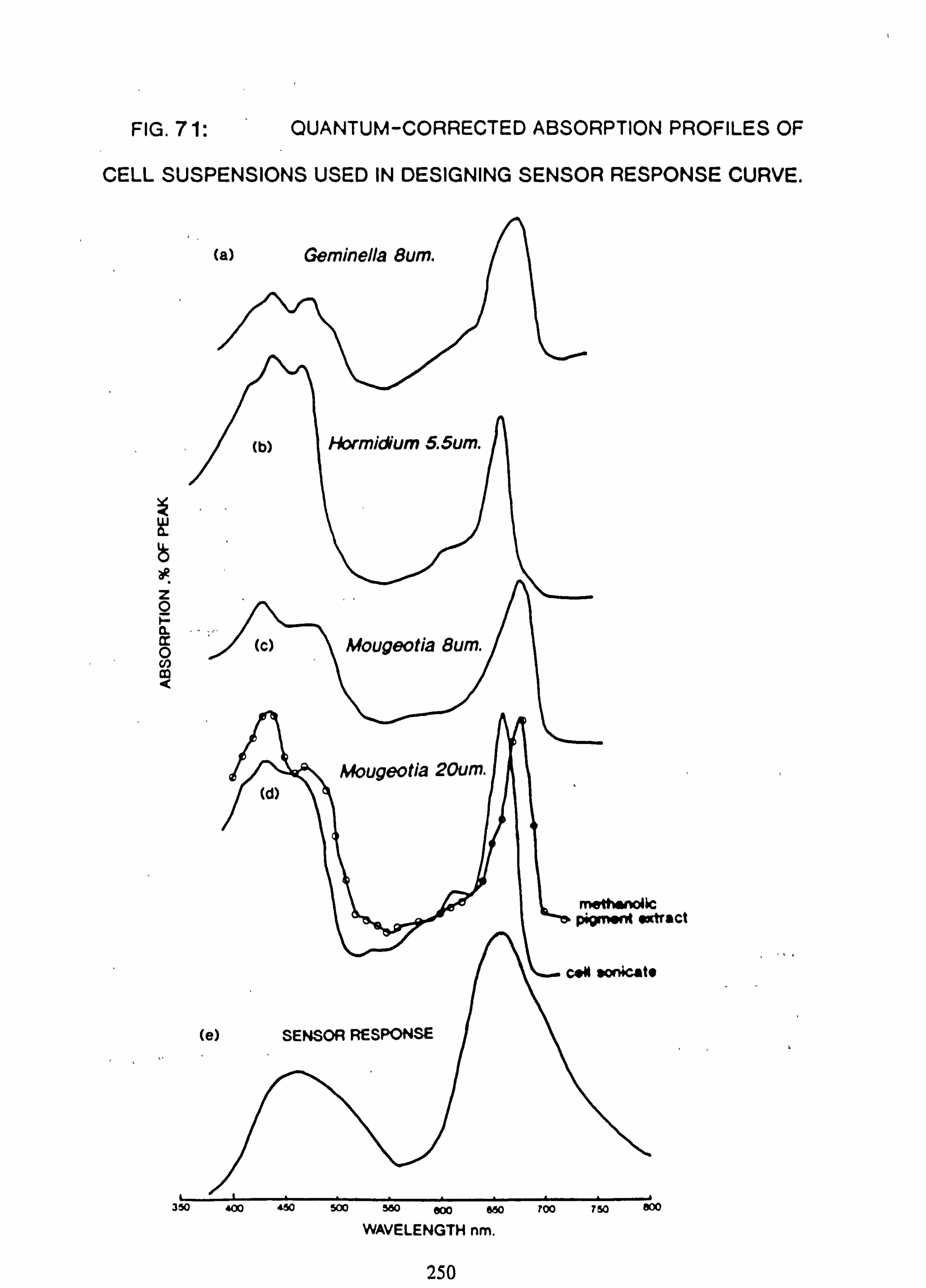
FIG. 71: QUANTUM-CORRECTED ABSORPTION PROFILES OF
CELL SUSPENSIONS USED IN DESIGNING SENSOR RESPONSE CURVE.
ca) Geminella Bum.
z 0 I. - a 0 m
mrttwnoüc pigmKnt sxtract
*# sonic. t"
(e) SENSOR RESPONSE
330 400 450 500 560 800 660 700 730 Soo
WAVELENGTH nm.
250
(c) Mougeotia 8um.
fib) Instantaneous measure of PAR The sensor head can be used with a modified voltmeter to measure instantaneous incidence
of PAR. The calibration was carried out at 660 nm by Macam Photometrics Ltd, in energy units and a correction applied to convert to quantum units.
Comparison of readings taken with this instrument in daylight and simultaneous readings with a Skye PAR meter (SKP 200) show that the Skye instrument gives approximately 25% higher
values (pmoles m: -2s: ') in daylight, 60% higher in fluorescent light, but similar values in
tungsten light.
The circuitry used for direct reading is shown in Fig. 72.
(o) Integrator Design
The integration of measured Photosynthetically Available Radiation is desirable in ecological
surveys for the comparison of field sites which may be subjected to different degrees of insolation at different times of the day. PAR may be detected using a photodiode and suitable filters. Integration may be achieved in three different ways: (i) by sampling intensity at frequent intervals and storing the information in a data logger (ii) by electronic integration, resulting in a'count' (iii) by chemical integration.
Use of data loggers may be limited by their high cost, especially on sites which may be
susceptible to accidental damage or interference. Chemical integration (Newman, 1985) may be the cheapest option if a large number of sites are to be monitored. For a modest number
of sites, independent electronic integrators may be the best option. We describe two circuits
which can be built for less than £65 each (1988 prices), which are weatherpoof, unaffected by temperature, will integrate linearly down to 0.1% of normal daylight levels, and may be
left unattended for months at a time.
Two different electronic integrator circuits were built. The first is a modification of the instrument reported by McLaughlin and Allan (1976). Their instrument uses a reverse-biased
photodiode which supplies a current dependent on the light intensity to a capacitor. The
capäcitor is charged up to a pre-set voltage at which point the capacitor is grounded by a relay and a pulse sent to an electromechanical counter.
251
They employed a range switch to bring in different value capacitors in order to cover a range of light intensities. This would cause problems in an instrument left unattended for long
periods as a low-value capacitor would lead to count rates which were in excess of the performance of the counter while the large-value electrolytic capacitors they employed for the high light intensities would give inaccurate counts at low light intensity because of the high leakage rate inherent to these capacitors. Our modification minimises these problems by the
use of polycarbonate capacitors which have a very low leakage rate.
Another protential problem arises at high count rates where a capacitor may not be fully discharged in the short time taken by the relay to change from one state to the other, thus leading to an overestimate of PAR. Also, under these conditions, loss of charge may occur due
to the diode being disconnected from the capacitor during switching ('dead' time). We have
minimised these problems by employing two capacitors which are charged and discharged
alternately. The diode is thus only disconnected very briefly and we believe that minimal loss
of charge occurs. Each capacitor has as long to discharge as to charge. Capacitor values and trigger point potential were chosen to give, in conjunction with the sensor characteristics, a
count rate at maximum natural light intensity which was well within the switching capacity of the electromechanical counter.
The device is shown in block diagram form in Fig. 73. Two latching relays switch input and
output to the two integrating capacitors alternately. The capacitor voltage is fed to a voltage follower which has an input impedance in excess of 1010 ohms. Current leakage of the stored charge is thus negligible. The output of this voltage follower is fed to a comparator with a trigger point settable by a potential divider at around 4.5 v. When the trigger point is reached, a pulse is sent to the bistable latch. The two outputs of the bistable go high alternately with successive pulses. They are connected to monostables MI and M2 which produce a discrete
pulse each driving a transistor and feeding the integrating current to one side or the other of the integrating capacitor relays. One of these relay lines is also connected to the electrome- chanical counter which thus registers a count each time a full cycle is completed.
The op-amps (voltage follower, latches and comparator) are supplied with a regulated 6v from
a 15 v battery pack. The voltage regulator incorporates temperature compensation so that the trigger point is not influenced by ambient temperature, making burial in the ground (e. g. Woodward and Yaqub, 1979) unnecessary. Tests performed at -18°C to approximately 40°C
revealed no detectable effect on count rate, although the instrument was not exposed to the lowest temperatures for sufficient time for the battery pack to reach this temperature.
252
The relays and counter are powered directly from the battery pack. Their operating range is from approximately 10 v to 15 v so that the cells can be run down to 1.0 v or less each before
the instrument will fail. At this point the op. amps are still being supplied with a regulated 6
v. Another consequence of powering the relays and counter directly is that no power surges occur in the regulated line. A large decoupling capacitor is incorporated in the 15 v line.
Use of CMOS circuitry has reduced the power consumption to 90-1,000 pA depending on count rate. A battery pack of Duracell AA cells has operated for approximately 1 year in field
use.
The second design of integrator (Fig. 74) was initially built in order to check the behaviour
of the photodiodes in reverse-bias mode as opposed to open circuit, as the manufacturers data
refers to open circuit current being linear with light intensity. The design also incorporates
temperature compensation of the trigger point by floating zero and bears some similarity to the instrument described by Saffell et al (1979).
The sensor is connected via a polarity reverse solid state switch to a current-voltage converter I. C. The diode is thus in open circuit mode. The voltage output is proportional to the current input. This voltage is fed in turn to an integrator op-amp. The integrator produces a rising or falling voltage ramp, according to the polarity of the voltage input. The height of the ramp is controlled by a Schmitt trigger set for ±3.6 v. Thus when the ramp reaches + 3.6 v the Schmitt trigger changes state. This causes the polarity sensor to drive a bistable from one state to the other which in turn reverses the polarity of the photodiode and thus reverses the direction of the ramp. The voltage then falls to -3.6 v, when the polarity is reversed once again and the cycle is completed.
It was found that the pulse rate had to be divided by 10 since the calculator used to accumulate the count was unable to operate at frequencies in excess of 1 Hz. The divider output is fed
to CMOS analogue switches which send alternate signals to the' 1' and'+' switches (buttons)
of a cheap digital calculator.
It is necessary to include additional circuitry with battery-operated calculators to prevent the auto-off facility turning the display off and thus losing the count at low light levels, e. g. at night. An alternative is to use a solar-powered calculator, and connect it to a single dry cell instead of the solar power pack. The integrator operates on a regulated i6v supplied from
two 9v packs.
253
This integrator operates at a higher frequency than the first design. P. D. measured at the Schmitt trigger shows a symmetrical saw-tooth profile above and below the zero line. Temperature effects on supply voltage will cause the zero line to shift but the waveform will be unaffected since both the +6v and the -6 v supplies will be shifted in the same direction by the same amount.
(d) Instrument construction Exposure to adverse climatic conditions was taken into account in constructing the integrators. Burial in the ground was adopted by Woodward and Yaqub (1979) as a protection against temperature extremes and would probably reduce the likelihood of some other types of damage
but was considered impractical in many of the sites at Loch Ard. Therefore the instrument had
to be insensitive to temperatures from below zero to possibly over 40'C, for as shown in
preliminary tests these temperatures could be achieved in strong sunlight with an unshaded integrator box. It was found that some mercury-wetted relays used with the integrators would
not operate at elevated temperatures, and these had to be changed. As a further precaution,
metal shades were constructed to cover the instruments, which gave protection against rain also. The circuitry was enclosed in R. F. screened ABS boxes (Radio Spares) since it was anticipated that interference could occur due to electrical storms or proximity to pylon lines.
Switches, counter displays and battery test jack sockets were mounted through the box and thus further protection was required. The ABS box was enclosed in a polyethylene sandwich box
and screwed to a wooden board along with the solar shade. The board could then be mounted vertically on Dexion stakes. The ABS box was earthed through the stakes and the earth screen on the diode lead also grounded.
.. The boxes could not be hermetically sealed, since the diurnal temperature fluctuations would lead to a 50% expansion in the volume of air contained, which could lead to the collapse of the boxes, or the possible entry of water through a leaking diode cable, during cold weather. Instead the boxes were deliberately vented through the jack sockets used for battery testing,
via a vial of silica gel which could be replaced each time the instrument was visited. A second vial was sealed inside the box. In practice it was found that leakage of air did occur and the
vial inside also required to be changed occasionally.
If necessary in very adverse conditions the mechanical counters can be read through the lid of the sandwich box.
254
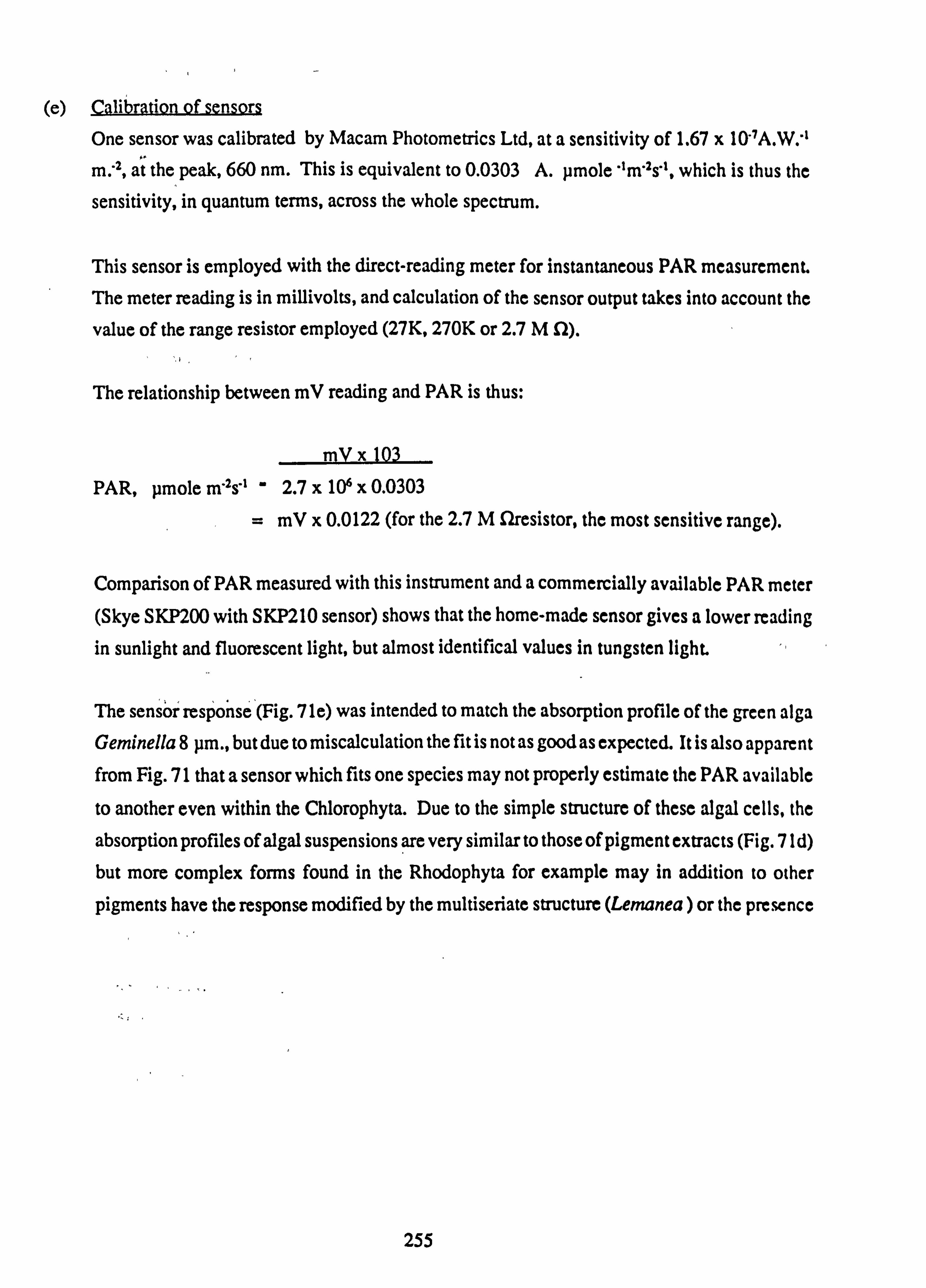
(e) Calibration of sensors One sensor was calibrated by Macam Photometrics Ltd, at a sensitivity of 1.67 x 10'1A. W. ''
m: 2, at the peak, 660 nm. This is equivalent to 0.0303 A. pmole "m'2s'1. which is thus the
sensitivity, in quantum terms, across the whole spectrum.
This sensor is employed with the direct-reading meter for instantaneous PAR measurement. The meter reading is in millivolts, and calculation of the sensor output takes into account the
value of the range resistor employed (27K, 270K or 2.7 M S2).
The relationship between mV reading and PAR is thus:
mV x 103
PAR, pmole m'2s"l - 2.7 x 106 x 0.0303
= mV x 0.0122 (for the 2.7 M flresistor, the most sensitive range).
Comparison of PAR measured with this instrument and a commercially available PAR meter (Skye SKP200 with SKP210 sensor) shows that the home-made sensor gives a lower reading in sunlight and fluorescent light, but almost identifical values in tungsten light.
The sensor response (Fig. 71e) was intended to match the absorption profile of the green alga Geminella 8 pm., but due to miscalculation the fit is not as good as expected. It is also apparent from Fig. 71 that a sensor which fits one species may not properly estimate the PAR available
to another even within the Chlorophyta. Due to the simple structure of these algal cells, the absorption profiles of algal suspensions are very similar to those of pigment extracts (Fig. 71 d)
but more complex forms found in the Rhodophyta for example may in addition to other
pigments have the response modified by the multiseriate structure (Lemanea) or the presence
255
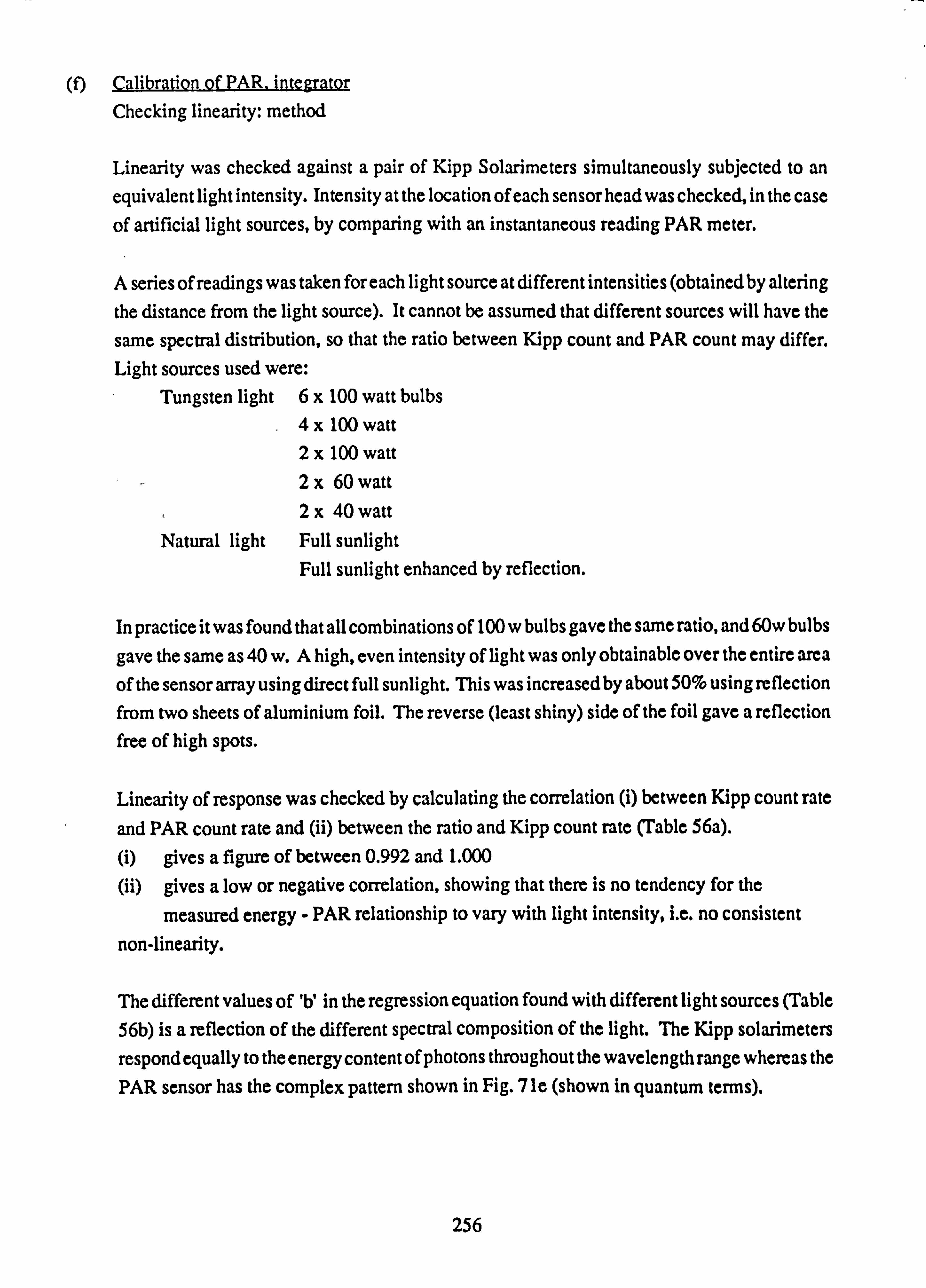
(f) Calibration of PAR. integrator Checking linearity: method
Linearity was checked against a pair of Kipp Solarimeters simultaneously subjected to an equivalent light intensity. Intensity at the location of each sensor head was checked, in the case of artificial light sources, by comparing with an instantaneous reading PAR meter.
A series of readings was taken for each light source at different intensities (obtained by altering the distance from the light source). It cannot be assumed that different sources will have the
same spectral distribution, so that the ratio between Kipp count and PAR count may differ. Light sources used were:
Tungsten light 6x 100 watt bulbs 4x 100 watt 2x 100 watt 2x 60 watt 2x 40 watt
Natural light Full sunlight Full sunlight enhanced by reflection.
In practice it was found that all combinations of 100 w bulbs gave the same ratio, and 60w bulbs
gave the same as 40 w. A high, even intensity of light was only obtainable over the entire area
of the sensor array using direct full sunlight. This was increased by about 50% using reflection from two sheets of aluminium foil. The reverse (least shiny) side of the foil gave a reflection free of high spots.
Linearity of response was checked by calculating the correlation (i) between Kipp count rate
and PAR count rate and (ii) between the ratio and Kipp count rate (Table 56a).
(i) gives a figure of between 0.992 and 1.000
(ii) gives a low or negative correlation, showing that there is no tendency for the
measured energy - PAR relationship to vary with light intensity, i. e. no consistent
non-linearity.
The different values of 'b' in the regression equation found with different light sources (Table 56b) is a reflection of the different spectral composition of the light. The Kipp solarimeters
respond equally to the energy content of photons throughout the wavelength range whereas the PAR sensor has the complex pattern shown in Fig. 71e (shown in quantum terms).
256
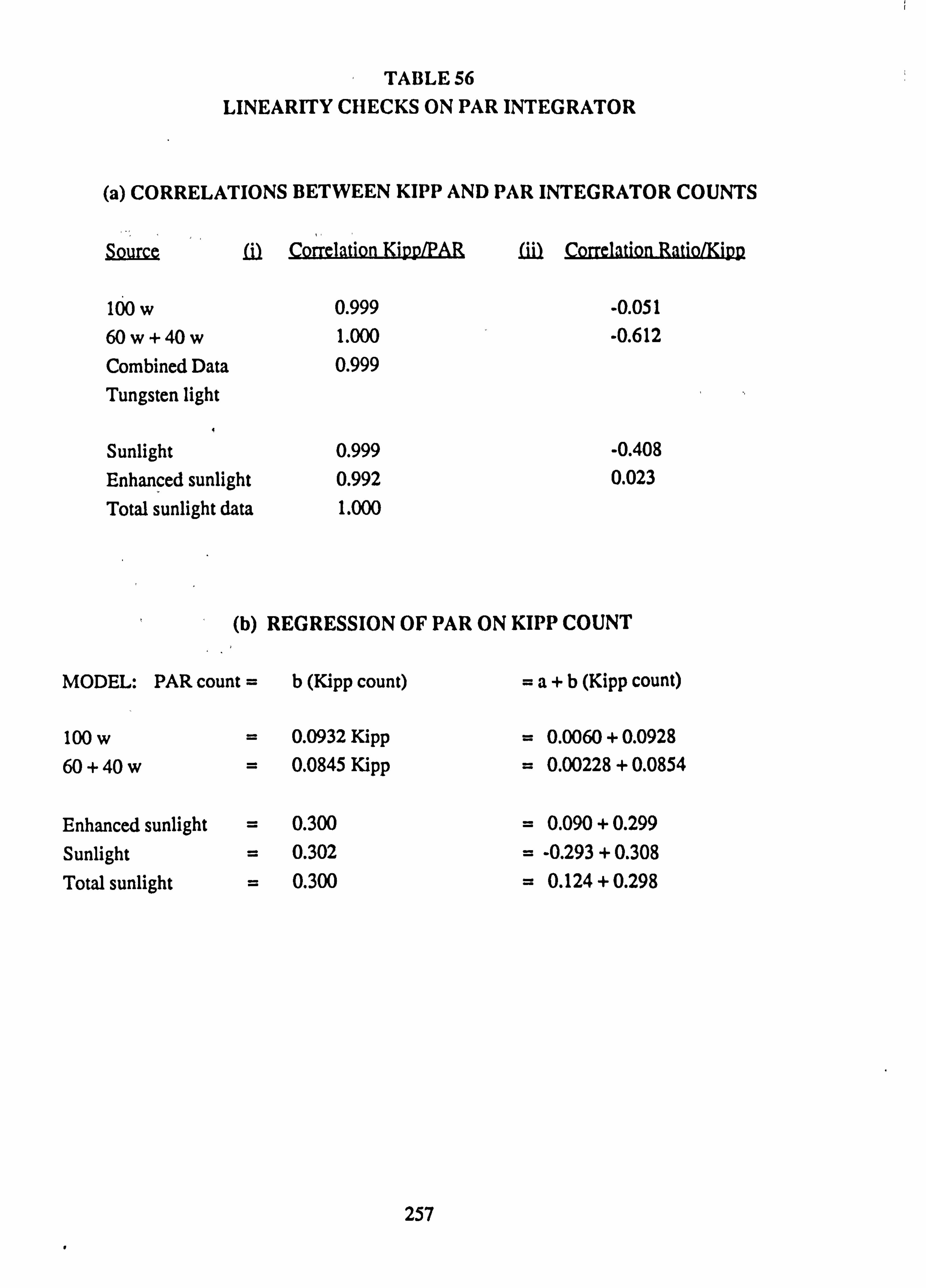
TABLE 56 LINEARITY CHECKS ON PAR INTEGRATOR
(a) CORRELATIONS BETWEEN KIPP AND PAR INTEGRATOR COUNTS
Source Ü Correlation Kipp/PAR Correlation Ratio/Kipp
100 w 0.999 -0.051 60 w+ 40 w 1.000 -0.612 Combined Data 0.999
Tungsten light
Sunlight 0.999 -0.408 Enhanced sunlight 0.992 0.023 Total sunlight data 1.000
(b) REGRESSION OF PAR ON KIPP COUNT
MODEL: PAR count =b (Kipp count) =a+b (Kipp count)
100 w 60+40w
= 0.0932 Kipp
= 0.0845 Kipp = 0.0060 + 0.0928
= 0.00228 + 0.0854
Enhanced sunlight Sunlight Total sunlight
= 0.300
= 0.302 0.300
= 0.090 + 0.299
_ -0.293 + 0.308
= 0.124 + 0.298
257
The lack of consistency in the'a' term found in the second form of the regression suggests that
there is little or no dark current effect or loss of stored charge from the integrator capacitors (leakage), nor any similar flaw in the Delta-T devices integrator (Type MV 1) used with the Kipps.
This testing was carried out on the twin-capacitor instrument. Linearity checks were also
made on the ramp integrator, and all integrators were checked together prior to field
deployment by exposing them on the Polytechnic roof with all sensors set at the same level,
so that no shadows could interfere with the light reaching any instrument. The results of these
tests were also used to calculate a factor to relate the counts obtained on the different
instruments. (The rate is adjustable by varying the preset voltage value at the Schmitt trigger,
but cannot be perfectly matched between instruments over a long period).
Some variability in the value of this factor was found as the calibration was carried out in
winter, with low angles of incidence and low intensity of natural light. This indicates some
variation in the cosine correction provided by the different sensor heads, due to slight differences in manufacturing tolerance. There was less variability when all heads were tilted
towards the south, and in practice throughout the year the error due to this flaw would be quite
small, although it has not been estimated.
Calculation of a factor relating the integrator count of the reference instrument to an absolute
value of PAR was carried out by comparing the integrated count with an instantaneous reading
under artificial light.
258
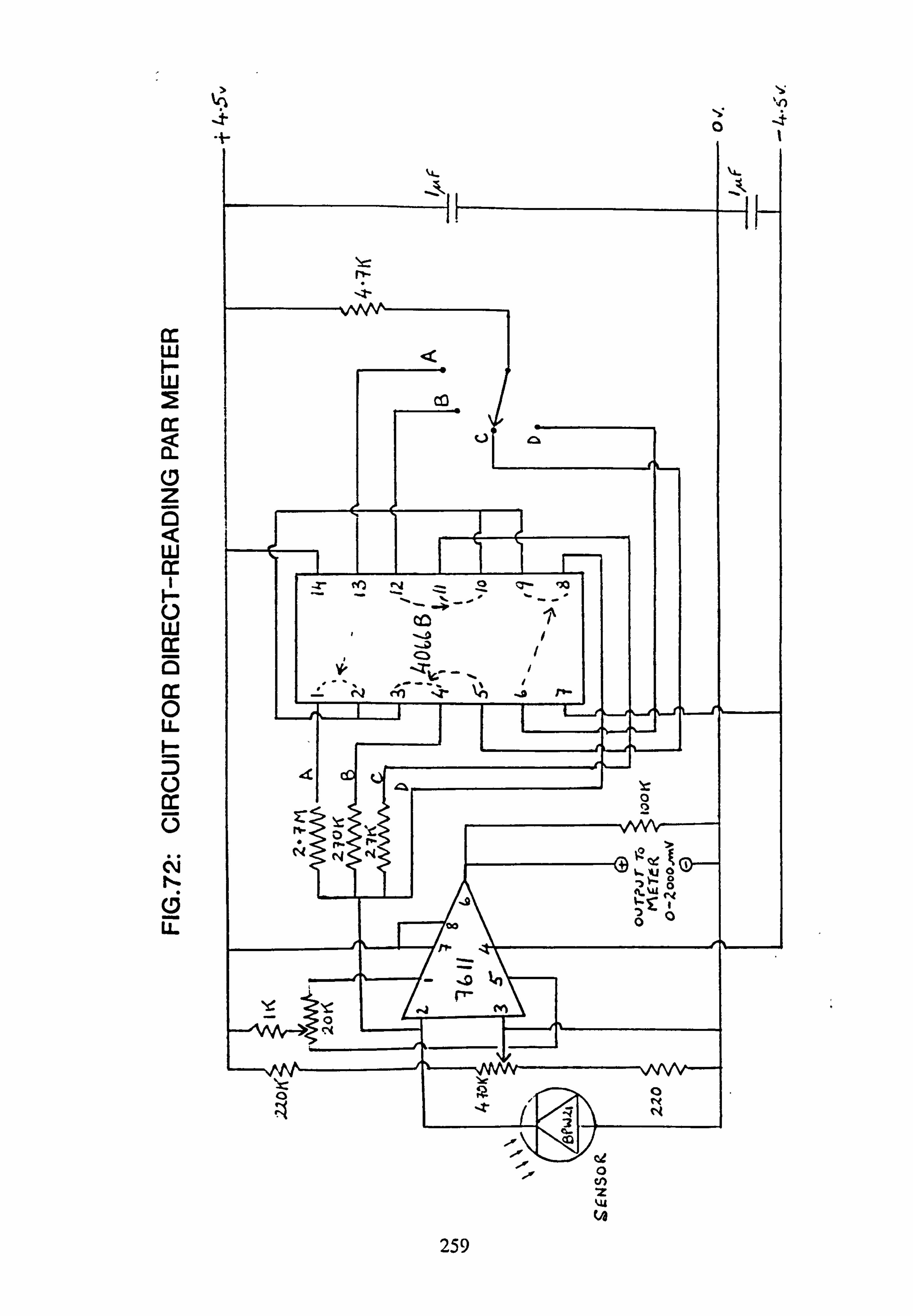
cc W h- w 2 cc ä
0 z
W cc
U W
cc 0 U- F- U cc V
CV N. C_3 LL
. {-
lir O 0
tu (4
Oý
259
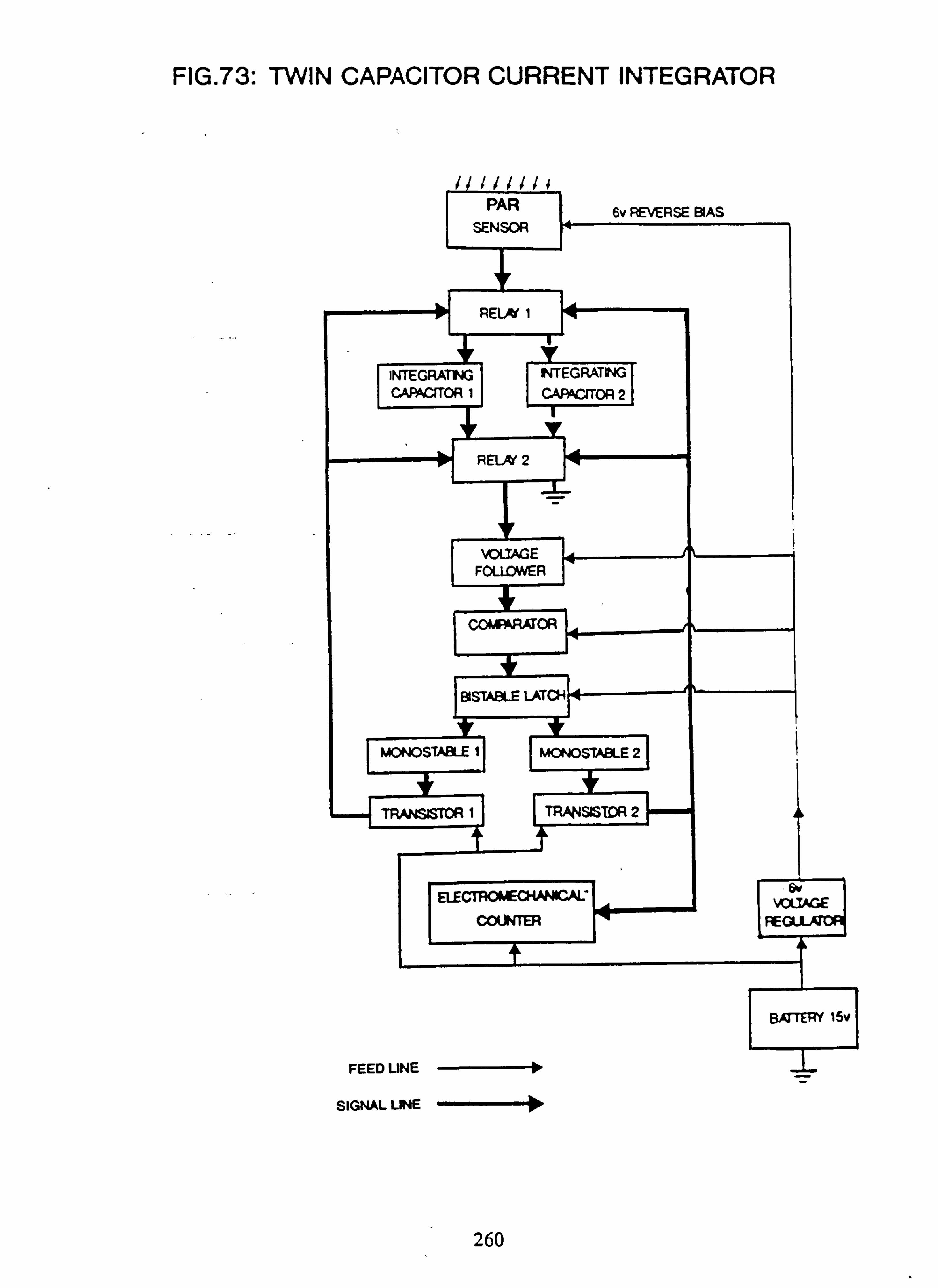
FIG. 73: TWIN CAPACITOR CURRENT INTEGRATOR
Iii'i PAR
SENSOR
RELM 1
6v REVERSE BIAS
INTEGRATING INTEGRATING CAP kWOR 1 CAPAC TOR 2
RELN 2
VOLTAGE FOLLOWER
CO AAOA
81STASLE LATCH f---'
MONOSTA13LE 1 MONOSTA8LE 2
TRANSISTOR 1II TRANSISTDR 2
II COUNTER
k--
IREGULAX BATTERY 15v
FEED UNE
SIGNAL LINE
260
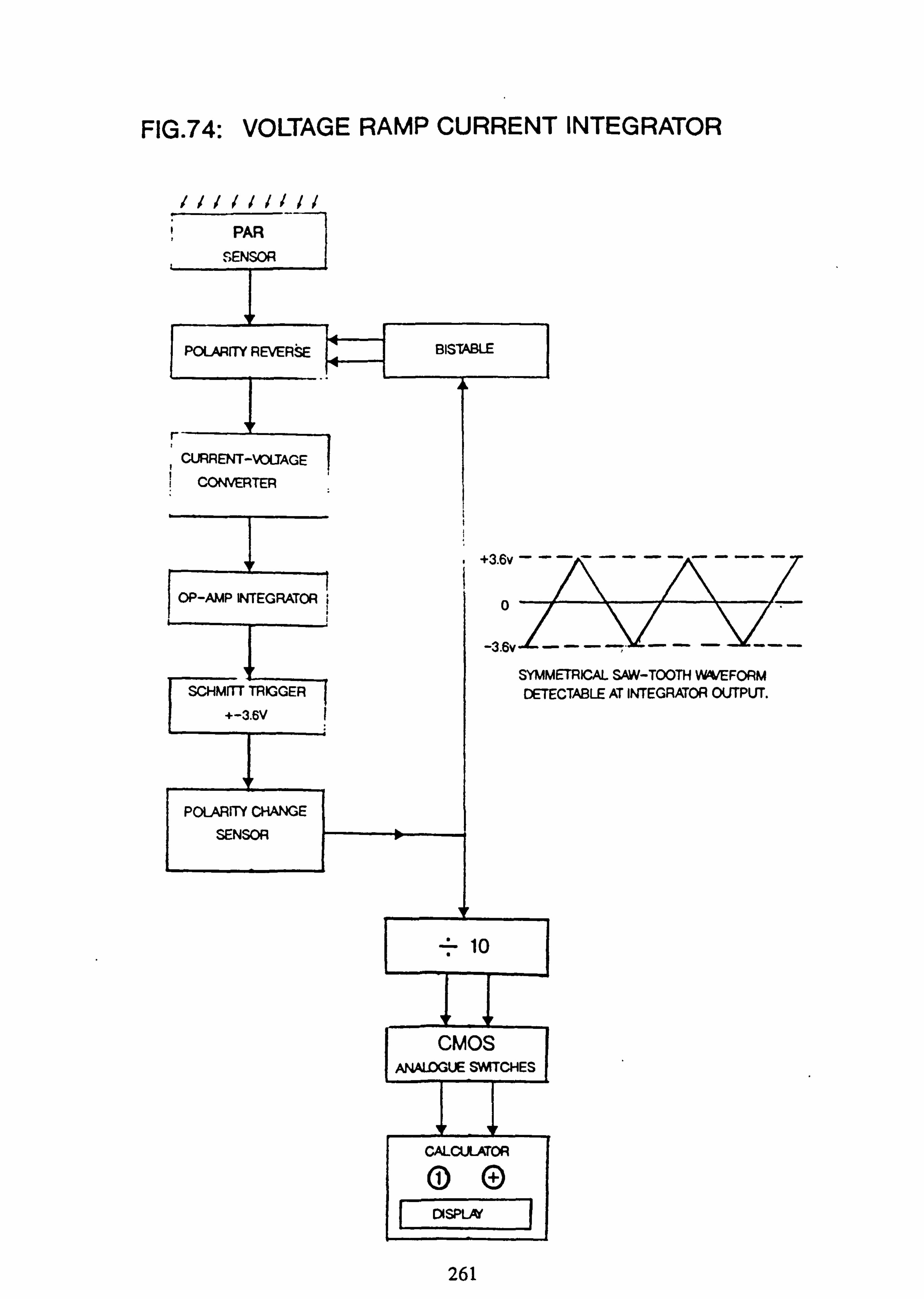
FIG. 74: VOLTAGE RAMP CURRENT INTEGRATOR
I /I <<! lll PAR
SENSOR
POLARITY REVERSE ITI BISTABLE
r CURRENT-VOLTAGE
CONVERTER
OP-AMP INTEGRATOR 0AA
SYMMETRICAL SAW-TOOTH WOVEFORM SCHMITT TRIGGER DETECTABLE AT INTEGRATOR OUTPUT.
+-3.6V I
POLARITY CHANGE
SENSOR
10
I CMOS ANALOGUE SWTCHES
CALCULATOR @O
DISPLN
261

262
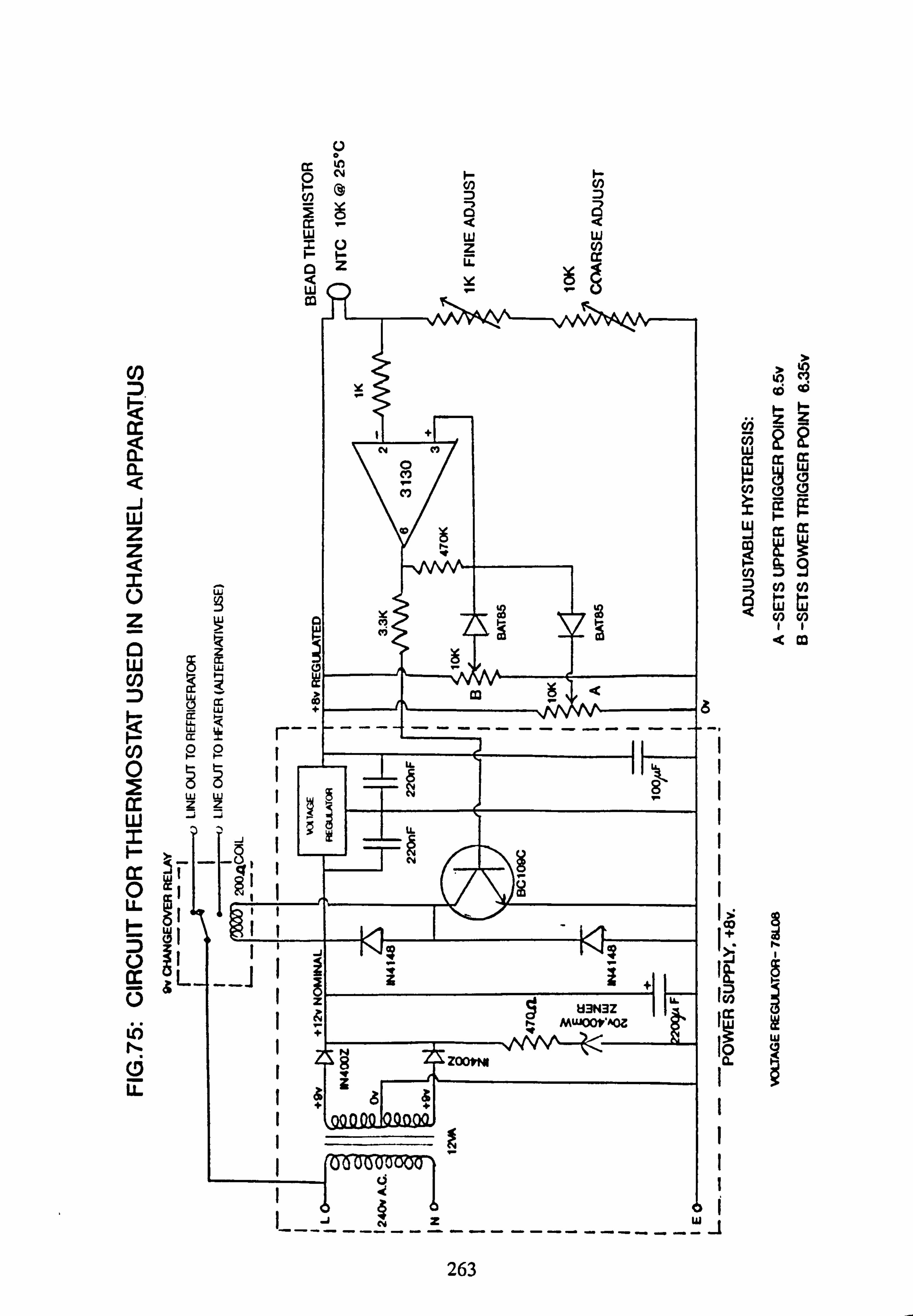
a
J W z z I U Z
13 W U) D
0 2 cc w 2
0 LL H 5 U
U
to ti U LL
W LL q
OO O
OO w
JJ
ýI I
L --ý
U C
c 0 Cl)
N I- Cl) D
N
0 Q aa ~
w
Z z
Id
cc
Y ý m
N 0
ri ri
M w
}
Q
c
W
S2
m Y ý
rx
Q ý
IV) a, y ýs is
D "Ilý
co (j)
14
co U)
M,
mýab
LL
LL N i
J
IJ
z LL U3N3Z 'CO
MUu001'AOZ I
zoott* Iä
+ I
.J UJ
W
263