accelerating similarly structured data lisa wu
TRANSCRIPT
Accelerating Similarly Structured Data
Lisa Wu
Submitted in partial fulfillment of the
requirements for the degree
of Doctor of Philosophy
in the Graduate School of Arts and Sciences
COLUMBIA UNIVERSITY
2014

c©2014
Lisa Wu
All Rights Reserved

ABSTRACT
Accelerating Similarly Structured Data
Lisa Wu
The failure of Dennard scaling [Bohr, 2007] and the rapid growth of data produced and
consumed daily [NetApp, 2012] have made mitigating the dark silicon phenomena [Es-
maeilzadeh et al., 2011] and providing fast computation for processing large volumes and
expansive variety of data while consuming minimal energy the utmost important challenges
for modern computer architecture. This thesis introduces the concept that grouping data
structures that are previously defined in software and processing them with an accelerator
can significantly improve the application performance and energy efficiency.
To measure the potential performance benefits of this hypothesis, this research starts
out by examining the cache impacts on accelerating commonly used data structures and its
applicability to popular benchmarks. We found that accelerating similarly structured data
can provide substantial benefits, however, most popular benchmark suites do not contain
shared acceleration targets and therefore cannot obtain significant performance or energy
improvements via a handful of accelerators. To further examine this hypothesis in an envi-
ronment where the common data structures are widely used, we choose to target database
application domain, using tables and columns as the similarly structured data, accelerating
the processing of such data, and evaluate the performance and energy efficiency. Given
that data partitioning is widely used for database applications to improve cache locality,
we architect and design a streaming data partitioning accelerator to assess the feasibility of
big data acceleration. The results show that we are able to achieve an order of magnitude
improvement in partitioning performance and energy. To improve upon the present ad-hoc
communications between accelerators and general-purpose processors [Vo et al., 2013], we
also architect and evaluate a streaming framework that can be used for the data parti-
tioner and other streaming accelerators alike. The streaming framework can provide at
least 5GB/s per stream per thread using software control, and is able to elegantly handle
interrupts and context switches using a simple save/restore. As a final evaluation of this
hypothesis, we architect a class of domain-specific database processors, or Database Pro-
cessing Units (DPUs), to further improve the performance and energy efficiency of database
applications. As a case study, we design and implement one DPU, called Q100, to execute
industry standard analytic database queries. Despite Q100’s sensitivity to communication
bandwidth on-chip and off-chip, we find that the low-power configuration of Q100 is able
to provide three orders of magnitude in energy efficiency over a state of the art software
Database Management System (DBMS), while the high-performance configuration is able
to outperform the same DBMS by 70X.
Based on these experiments, we conclude that grouping similarly structured data and
processing it with accelerators vastly improve application performance and energy efficiency
for a given application domain. This is primarily due to the fact that creating specialized
encapsulated instruction and data accesses and datapaths allows us to mitigate unnecessary
data movement, take advantage of data and pipeline parallelism, and consequently provide
substantial energy savings while obtaining significant performance gains.
Table of Contents
List of Figures iv
List of Tables vii
1 Introduction 1
1.1 Architectural Challenges . . . . . . . . . . . . . . . . . . . . . . . . . . . . . 2
1.2 Accelerating Memory Operations . . . . . . . . . . . . . . . . . . . . . . . . 3
1.3 Big Data Acceleration . . . . . . . . . . . . . . . . . . . . . . . . . . . . . . 4
1.4 Contributions . . . . . . . . . . . . . . . . . . . . . . . . . . . . . . . . . . . 5
1.5 Thesis Outline . . . . . . . . . . . . . . . . . . . . . . . . . . . . . . . . . . 6
2 Cache Impacts of Datatype Acceleration 7
2.1 Architecture of ADPs . . . . . . . . . . . . . . . . . . . . . . . . . . . . . . 7
2.2 Evaluation of ADPs . . . . . . . . . . . . . . . . . . . . . . . . . . . . . . . 8
2.2.1 Instruction Delivery . . . . . . . . . . . . . . . . . . . . . . . . . . . 9
2.2.2 Data Delivery . . . . . . . . . . . . . . . . . . . . . . . . . . . . . . . 12
2.3 Summary of Findings on ADPs . . . . . . . . . . . . . . . . . . . . . . . . . 15
3 Acceleration Targets 17
3.1 Profiling of Benchmark Suites . . . . . . . . . . . . . . . . . . . . . . . . . . 17
3.2 Results and Analysis . . . . . . . . . . . . . . . . . . . . . . . . . . . . . . . 18
3.3 Summary of Findings on Acceleration Targets . . . . . . . . . . . . . . . . . 19
i
4 Hardware Accelerated Range Partitioning 21
4.1 Data Partitioning is Important . . . . . . . . . . . . . . . . . . . . . . . . . 22
4.2 Partitioning Background . . . . . . . . . . . . . . . . . . . . . . . . . . . . . 23
4.3 Software Partitioning Evaluation . . . . . . . . . . . . . . . . . . . . . . . . 26
4.4 HARP Accelerator . . . . . . . . . . . . . . . . . . . . . . . . . . . . . . . . 29
4.4.1 Instruction Set Architecture . . . . . . . . . . . . . . . . . . . . . . . 29
4.4.2 Microarchitecture . . . . . . . . . . . . . . . . . . . . . . . . . . . . . 30
4.5 Evaluation Methodology . . . . . . . . . . . . . . . . . . . . . . . . . . . . . 31
4.6 Evaluation Results . . . . . . . . . . . . . . . . . . . . . . . . . . . . . . . . 32
4.7 Design Space Exploration . . . . . . . . . . . . . . . . . . . . . . . . . . . . 36
4.8 Summary of Findings on HARP . . . . . . . . . . . . . . . . . . . . . . . . . 39
5 A Hardware-Software Streaming Framework 40
5.1 HARP System Integration . . . . . . . . . . . . . . . . . . . . . . . . . . . . 41
5.2 Streaming Framework . . . . . . . . . . . . . . . . . . . . . . . . . . . . . . 42
5.2.1 Instruction Set Architecture . . . . . . . . . . . . . . . . . . . . . . . 43
5.2.2 Microarchitecture . . . . . . . . . . . . . . . . . . . . . . . . . . . . . 44
5.3 Evaluation Methodology . . . . . . . . . . . . . . . . . . . . . . . . . . . . . 45
5.4 Evaluation Results . . . . . . . . . . . . . . . . . . . . . . . . . . . . . . . . 46
5.5 Summary of Findings on Streaming Framework . . . . . . . . . . . . . . . . 47
6 Q100: A First DPU 48
6.1 Q100 Instruction Set Architecture . . . . . . . . . . . . . . . . . . . . . . . 49
6.2 Q100 Microarchitecture . . . . . . . . . . . . . . . . . . . . . . . . . . . . . 52
6.3 Q100 Tile Mix Design Space Exploration . . . . . . . . . . . . . . . . . . . 56
6.4 Q100 Communication Needs . . . . . . . . . . . . . . . . . . . . . . . . . . . 59
6.4.1 On-chip bandwidth constraints. . . . . . . . . . . . . . . . . . . . . . 60
6.4.2 Off-chip bandwidth constraints. . . . . . . . . . . . . . . . . . . . . . 63
6.4.3 Performance impact of communication resources. . . . . . . . . . . . 63
6.4.4 Area and power impact of communication resources. . . . . . . . . . 65
6.4.5 Intermediate storage discussion. . . . . . . . . . . . . . . . . . . . . . 66
ii
6.5 Q100 Evaluation . . . . . . . . . . . . . . . . . . . . . . . . . . . . . . . . . 66
6.5.1 Methodology . . . . . . . . . . . . . . . . . . . . . . . . . . . . . . . 66
6.5.2 Performance . . . . . . . . . . . . . . . . . . . . . . . . . . . . . . . 67
6.5.3 Energy . . . . . . . . . . . . . . . . . . . . . . . . . . . . . . . . . . . 71
6.5.4 Scalability . . . . . . . . . . . . . . . . . . . . . . . . . . . . . . . . . 71
6.6 Summary of Findings on DPU . . . . . . . . . . . . . . . . . . . . . . . . . 73
7 Related Work 74
8 Conclusions 78
Bibliography 80
iii
List of Figures
2.1 ADI Impacts on Instruction Fetch . . . . . . . . . . . . . . . . . . . . . . . 10
2.2 Instruction Fetch Energy Breakdown . . . . . . . . . . . . . . . . . . . . . . 10
2.3 Instruction Access Time Breakdown . . . . . . . . . . . . . . . . . . . . . . 11
2.4 L1 Data Store Configurations . . . . . . . . . . . . . . . . . . . . . . . . . . 12
2.5 ADI Impacts on Data Delivery . . . . . . . . . . . . . . . . . . . . . . . . . 13
2.6 Data Delivery Energy Breakdown . . . . . . . . . . . . . . . . . . . . . . . . 13
2.7 Data Access Time Breakdown . . . . . . . . . . . . . . . . . . . . . . . . . . 14
2.8 Example PARSER code snippet using hash table ADIs . . . . . . . . . . . . 16
3.1 Potential Speedup with Various Granular Acceleration Targets . . . . . . . 19
4.1 Partitioning Example . . . . . . . . . . . . . . . . . . . . . . . . . . . . . . . 23
4.2 Partitioned-Join Example . . . . . . . . . . . . . . . . . . . . . . . . . . . . 24
4.3 Join Execution Time with respect to TPC-H Query Execution Time . . . . 25
4.4 A Partitioning Microbenchmark Pseudocode . . . . . . . . . . . . . . . . . . 26
4.5 Partition Function Kernel Code . . . . . . . . . . . . . . . . . . . . . . . . . 26
4.6 Multi-threaded Software Partitioning Performance . . . . . . . . . . . . . . 29
4.7 HARP Microarchitecture Block Diagram . . . . . . . . . . . . . . . . . . . . 31
4.8 HARP vs. Software Partitioning Performance . . . . . . . . . . . . . . . . . 33
4.9 HARP vs. Software Partitioning Energy . . . . . . . . . . . . . . . . . . . . 33
4.10 HARP Skew Analysis . . . . . . . . . . . . . . . . . . . . . . . . . . . . . . 33
4.11 HARP Performance Sensitivity to Partitioning Factor . . . . . . . . . . . . 36
4.12 HARP Area Sensitivity to Partitioning Factor . . . . . . . . . . . . . . . . . 36
iv
4.13 HARP Power Sensitivity to Partitioning Factor . . . . . . . . . . . . . . . . 36
4.14 HARP Performance Sensitivity to Key and Record Widths . . . . . . . . . 37
4.15 HARP Area Sensitivity to Key and Record Widths . . . . . . . . . . . . . . 37
4.16 HARP Power Sensitivity to Key and Record Widths . . . . . . . . . . . . . 37
4.17 Coping with Fixed Partition Size . . . . . . . . . . . . . . . . . . . . . . . . 38
4.18 Coping with Fixed Record Width . . . . . . . . . . . . . . . . . . . . . . . . 38
5.1 An Integrated HARP System Block Diagram . . . . . . . . . . . . . . . . . 42
5.2 HARP Integration with Existing Software Synchronization . . . . . . . . . . 42
5.3 Streaming Framework Datapath . . . . . . . . . . . . . . . . . . . . . . . . 44
5.4 Streaming Framework Performance . . . . . . . . . . . . . . . . . . . . . . . 46
6.1 An Example Query Spatial Instruction Representation . . . . . . . . . . . . 50
6.2 An Example Query Directed Graph and Temporal Instruction Representation 51
6.3 Aggregator Sensitivity Study . . . . . . . . . . . . . . . . . . . . . . . . . . 57
6.4 ALU Sensitivity Study . . . . . . . . . . . . . . . . . . . . . . . . . . . . . . 57
6.5 Sorter Sensitivity Study . . . . . . . . . . . . . . . . . . . . . . . . . . . . . 57
6.6 Three Q100 Designs Performance and Power . . . . . . . . . . . . . . . . . 59
6.7 LowPower Design Connection Count Heat Map . . . . . . . . . . . . . . . . 60
6.8 Pareto Design Connection Count Heat Map . . . . . . . . . . . . . . . . . . 60
6.9 HighPerf Design Connection Count Heat Map . . . . . . . . . . . . . . . . . 60
6.10 LowPower Design Connection Bandwidth Heat Map . . . . . . . . . . . . . 61
6.11 Pareto Design Connection Bandwidth Heat Map . . . . . . . . . . . . . . . 61
6.12 HighPerf Design Connection Bandwidth Heat Map . . . . . . . . . . . . . . 61
6.13 NoC Bandwidth Sensitivity Study . . . . . . . . . . . . . . . . . . . . . . . 61
6.14 TPC-H Query Read Memory Bandwidth Demands . . . . . . . . . . . . . . 62
6.15 TPC-H Query Write Memory Bandwidth Demands . . . . . . . . . . . . . . 62
6.16 Memory Read Bandwidth Sensitivity Study . . . . . . . . . . . . . . . . . . 64
6.17 Memory Write Bandwidth Sensitivity Study . . . . . . . . . . . . . . . . . . 64
6.18 Q100 Performance Slowdown with Memory and NoC Bandwidth Limits . . 65
6.19 Q100 Performance vs. Software . . . . . . . . . . . . . . . . . . . . . . . . . 68
v
6.20 Q100 Energy vs. Software . . . . . . . . . . . . . . . . . . . . . . . . . . . . 68
6.21 Q100 Performance Efficiency as Parallelism Increases . . . . . . . . . . . . . 69
6.22 Q100 Performance Speedup Breakdown by Source . . . . . . . . . . . . . . 70
6.23 Q100 Performance with Large Data Sets . . . . . . . . . . . . . . . . . . . . 71
6.24 Q100 Energy with Large Data Sets . . . . . . . . . . . . . . . . . . . . . . . 71
6.25 Q100 Small and Large Data Set Scaling Comparison . . . . . . . . . . . . . 72
vi
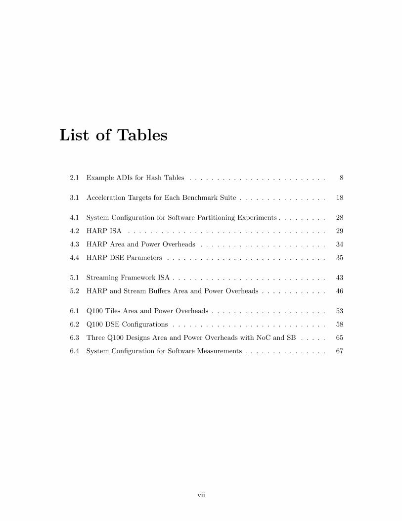
List of Tables
2.1 Example ADIs for Hash Tables . . . . . . . . . . . . . . . . . . . . . . . . . 8
3.1 Acceleration Targets for Each Benchmark Suite . . . . . . . . . . . . . . . . 18
4.1 System Configuration for Software Partitioning Experiments . . . . . . . . . 28
4.2 HARP ISA . . . . . . . . . . . . . . . . . . . . . . . . . . . . . . . . . . . . 29
4.3 HARP Area and Power Overheads . . . . . . . . . . . . . . . . . . . . . . . 34
4.4 HARP DSE Parameters . . . . . . . . . . . . . . . . . . . . . . . . . . . . . 35
5.1 Streaming Framework ISA . . . . . . . . . . . . . . . . . . . . . . . . . . . . 43
5.2 HARP and Stream Buffers Area and Power Overheads . . . . . . . . . . . . 46
6.1 Q100 Tiles Area and Power Overheads . . . . . . . . . . . . . . . . . . . . . 53
6.2 Q100 DSE Configurations . . . . . . . . . . . . . . . . . . . . . . . . . . . . 58
6.3 Three Q100 Designs Area and Power Overheads with NoC and SB . . . . . 65
6.4 System Configuration for Software Measurements . . . . . . . . . . . . . . . 67
vii
Acknowledgments
I am extremely thankful for the support, guidance, and friendship of my advisor Martha
Kim throughout my years at Columbia. Martha taught me how to persevere through
problems that seem impossible to solve; she taught me how to be meticulous in my work;
she taught me how to face challenges when I feel defeated. She was a constant in helping
me mature technically, academically, professionally, and also personally. I would not be
able to complete this journey without her understanding of me having to spend (a small
but not nonexistent) part of my time battling with a part-time job. Martha’s motivation,
enthusiasm, and her outstanding ability to distill research questions and present insights
have been invaluable. She pushed me to greater success with her patience and perfectionism
in our work.
I am also grateful for Ken Ross’s excellent instruction on databases, his sharing his ex-
tensive knowledge in the field, and his guidance on the project that became the culmination
of my thesis. Many thanks for Simha Sethumadhavan’s time and feedback on my work and
his generosity to let me use his compute resources.
I have been very fortunate to have Doug Carmean and Joel Emer as my long time
mentors and advocates, both at work and at school. I am extremely grateful for their
support, guidance, encouragement, hard questions, and insightful feedback on my research
and at Intel. I would also like to thank George Chrysos for his understanding and support
while I worked part-time to complete my degree.
Many thanks to John Demme and Melanie Kambadur for their support and friendship;
I have learned a great deal from them and thoroughly enjoyed their company in and outside
of the fish bowl.
Last but not least, I am tremendously thankful for the support of my family. My parents’
many fasting and praying sessions, their encouragement, and their love have got me through
viii

days and nights of success and defeat. My brother Leo’s “tough” love when I really needed
a kick in the butt have allowed me to carry on.
ix

To Adonai Elohai.
x
CHAPTER 1. INTRODUCTION 1
Chapter 1
Introduction
Harvard Business Review recently published an article on Big Data that lead with a piece
of artwork by Tamar Cohen titled “You can’t manage what you don’t measure” [McAfee
and Brynjolfsson, 2012]. It goes on to describe big data analytics as not just important for
business, but essential. The article emphasized the analyses must process large volumes of
a wide variety, and at real-time or nearly real-time velocity. With the big data technology
and services market forecast to grow from $3.2B in 2010 to $16.9B in 2015 [IDC Research,
2012], and 2.6 exabytes of data created each day [McAfee and Brynjolfsson, 2012], it is
imperative for the research community to develop machines that can keep up with this data
deluge.
However, the architecture community is facing challenges that require radical microar-
chitectural innovations to deliver performance gains while adhering to the required power
constraints. These challenges are: (1) failure of Dennard scaling and dark silicon projections
leave us with no clear path to exploit more transistors on die without violating the power
envelope, (2) utilizing multiple simple cores (i.e. multicore architecture) can provide some
parallel performance gain with energy efficiency but the gain is limited by Amdahl’s law
and the scaling is not sustainable, (3) creating application-specific integrated circuits, or
ASICs, may not be cost effective if the specialization target is not broadly reused/applicable
to provide substantial performance benefits, and (4) the accelerator interfaces to general
purpose processors are ad-hoc and difficult to program.
CHAPTER 1. INTRODUCTION 2
1.1 Architectural Challenges
More than thirty years ago, Dennard et. al. from the IBM T. J. Waston Research Cen-
ter published a paper detailing MOSFET scaling rules stating that with each technology
generation, the devices got smaller, faster, and consumed less power [Bohr, 2007]. This is
commensurate with Moore’s law stating that the transistors on integrated circuits doubled
approximately every two years, along with processing speed and memory capacity. These
technology trends were followed by the semiconductor industry through the 1990’s improv-
ing transistor density by 2X every 3 years, and increasing transistor count by 2X every 18
months. More recently, however, voltage scaling, a key component in the MOSFET scaling,
has reached a limit where the voltage and frequency scaling are no longer possible, as the
sub-threshold leakage is not just a tiny contributor to total chip logic power consumption
any more. The transistor counts are still doubling on die, but they can not all operate at
full speed without substantial cooling systems, and the fraction of a chip that can run at full
speed is getting exponentially worse with each process generation [Venkatesh et al., 2010];
this is known as the utilization wall. Together with dark silicon projections [Esmaeilzadeh
and others, 2011], it is shown that only 7.9X average speedup is possible over the next
five technology generations with only 79% of the chip fully operational at 22nm, and less
than 50% of the chip fully operational at 8nm. This phenomenon leaves the community to
explore solutions alongside of either trading area for power to utilize multicore architecture
to provide more parallel performance for less power, or using specialization to allow the
same number of transistors to provide more application performance for less power.
In theory, parallel processing on multicore chips can match historic performance gains
while meeting modern power budgets, but as recent studies show, this requires near-perfect
application parallelization [Hill and Marty, 2008]. In practice, such parallelization is often
unachievable: most algorithms have inherently serial portions and require synchronization
in their parallel portions. Furthermore, parallel software requires drastic changes to how
software is written, tested, and debugged. Multicore scaling is also not sustainable as
increased number of cores put more pressure on memory bandwidth and necessitate the
support and management of increased number of outstanding memory requests [Cascaval
and others, 2010].
CHAPTER 1. INTRODUCTION 3
Creating ASICs is another solution for computational power and performance efficiency
because it removes unnecessary hardware for general computation while delivering excep-
tional performance via specialized control paths and execution units. However, given the
cost associated with designing, verifying, and deploying an accelerator, it is uneconomical
and impractical to produce a custom chip for every application. Hence, a particular opera-
tion only becomes a feasible and realistic acceleration target when it is used across a range
of applications.
Furthermore, hardware accelerators, such as graphics coprocessors, cryptographic ac-
celerators [Wu et al., 2001], or network processors [Franke et al., 2010; Carli et al., 2009],
provide custom-caliber efficiency in a general-purpose setting for their target domain, but
often have awkward, ad hoc interfaces that make them difficult to use and impede software
portability [Vo et al., 2013]. Therefore, it is important to carefully choose the accelera-
tion targets and their interface to general-purpose processors to provide high-performance,
energy-efficient computation in a form palatable to software.
1.2 Accelerating Memory Operations
Before a suitable acceleration target can be chosen, we want to understand where most of the
energy is spent when doing an operation in the computer system. [Dally et al., 2008] found
that in one RISC processor, each arithmetic operation consumes only 10 pJ but reading the
two operands from the data cache for that particular operation required 107 pJ each, and
writing the result back required another 121 pJ . This shows us that data supply energy
dominates the execution of this arithmetic instruction by an order of magnitude compared
to the actual computation. If we can reduce the data movement of an operation, we can in
turn reduce the energy consumed. In this thesis, we architect accelerators that accelerate
memory operations by specializing memory subsystems to provide energy efficiency for
computations that require lots of data movement. We also opt for acceleration targets that
are widely applicable, or coarse-grained enough to provide performance improvement for
important workloads.
CHAPTER 1. INTRODUCTION 4
The spectrum of accelerators available today ranges from coarse-grain off-load engines
such as GPUs to fine-grain instruction set extensions such as SSE. By encapsulating data
and algorithms richer than the usual fine-grained arithmetic, memory, and control-transfer
instructions, accelerating datatypes that are already defined in software provides ample
implementation optimization opportunities in the form of an already familiar programming
interface. Architects have made heroic efforts to quickly execute streams of fine-grained in-
structions, but their hands have been tied by the narrow scope of program information that
conventional ISAs afford to hardware. Good software programming practice has long en-
couraged the use of carefully written, well-optimized libraries over manual implementations
of everything; datatype acceleration simply supply such libraries in a new form.
1.3 Big Data Acceleration
Datatypes manipulated in relational database applications are mostly tables, rows, and
columns. These similarly structured data have long been the software optimization explo-
ration focus of the Database Management System (DBMS) software community. Examples
include using column stores [Idreos et al., 2012; Lamb et al., 2012; SAP Sybase IQ, 2013;
Kx Systems, 2013; Abadi et al., 2009; Stonebraker et al., 2005]. pipelining operations either
in rows or columns [Abadi et al., 2007; Boncz et al., 2005], and vectorizing operations across
entries within a column [Zukowski and Boncz, 2012], to take advantage of commodity server
hardware.
We propose applying those same techniques, but in hardware, to construct a domain-
specific processor for databases. Just as conventional DBMSs operate on data in logical
entities of tables and columns, our processor manipulates these same data primitives. Like
DBMSs use software pipelining between relational operators to reduce intermediate results
we too can exploit pipelining between relational operators implemented in hardware to in-
crease throughput and reduce query completion time. In light of the SIMD instruction
set advances in general purpose CPUs in the last decade, DBMSs also vectorize their im-
plementations of many operators to exploit data parallelism. Our hardware does not use
CHAPTER 1. INTRODUCTION 5
vectorized instructions, but exploits data parallelism by processing multiple streams of data,
corresponding to tables and columns, at once.
This thesis claims that grouping similarly structured data and processing them together
provides performance and energy efficiency. As a case study, we use tables and columns as
the similarly structured data, and architect specialized hardware control and datapaths to
accelerate the processing of read-only analytic database workloads. This class of database
domain-specific processors, called DPUs, are analogous to GPUs. Whereas GPUs target
graphics applications, DPUs target relational database workloads.
1.4 Contributions
The contributions of this thesis are as follows:
• A preliminary study on the analysis of cache impacts on datatype acceleration using
sparse vectors and hash tables to assess the potential performance and energy savings
of datatype acceleration.
• A preliminary study of acceleration targets using popular benchmark suites to assess
the applicability of datatype acceleration.
• The architecture and design of a data partitioning accelerator, to assess the feasibility
of big data acceleration.
• The architecture of a high-bandwidth, hardware-software streaming framework that
transfers data to and from a streaming accelerator and integrates seamlessly with
existing hardware and software.
• An energy-efficient DPU instruction set architecture for processing data-analytic work-
loads, with instructions that both closely match standard relational primitives and are
good fits for hardware acceleration.
• A proof-of-concept DPU design, called Q100, that reveals the many opportunities,
pitfalls, tradeoffs, and overheads one can expect to encounter when designing small
accelerators to process big data.
CHAPTER 1. INTRODUCTION 6
1.5 Thesis Outline
In the next two chapters, we present the preliminary studies exploring the benefits and chal-
lenges of datatype acceleration and choosing appropriate acceleration targets. Chapters 4
and 5 describe the architecture and design of an accelerator for an important database
operation, data partitioning, and its communications to and from the general processor.
Chapters 6 and 7 detail a DPU instruction set architecture, microarchitecture, implementa-
tion, and evaluation of the proof of concept DPU, Q100. Chapters 8 and 9 examine related
work and conclude.
CHAPTER 2. CACHE IMPACTS OF DATATYPE ACCELERATION 7
Chapter 2
Cache Impacts of Datatype
Acceleration
In this preliminary experiment, we consider predefined software data structures, or datatypes,
as acceleration targets and examine the cache impacts of doing so. We supplement general-
purpose processors with abstract datatype processors (ADPs) to deliver custom hardware
performance. ADPs implement abstract datatype instructions (ADIs) that expose to hard-
ware high-level types such as hash tables, XML DOMs, relational database tables, and
others common to software.
2.1 Architecture of ADPs
ADIs are instructions that express hardware-accelerated operations on data structures. Ta-
ble 2.1 shows example ADIs for a hash table accelerator. The scope and behavior of a
typical ADI resembles that of a method in an object-oriented setting: ADIs create, query,
modify, and destroy complex datatypes, operations that might otherwise be coded in 10s or
100s of conventional instructions. Multiple studies in a range of domains conclude that the
quality of interaction across an application’s data structures is a significant determinant of
performance [Jung et al., 2011; Liu and Rus, 2009; Williams et al., 2007]. Because ADIs
encapsulate data structures as well as the algorithms that act on them, they can be imple-
mented using specialized datapaths coupled to special-purpose storage structures that can
CHAPTER 2. CACHE IMPACTS OF DATATYPE ACCELERATION 8
Table 2.1: Example Abstract Datatype Instructions for Hash Tables
ADI Description
new id Create a table; return its ID in register id
put id, key, val Associate val with key in table id
get val, id, key Return value val associated with key in table id
remove id Delete hash table with the given ID
be considerably more efficient than the general-purpose alternative. While there has been
a great deal of research on specialized datapaths and computation, few researchers have
considered specializing the memory system. For this study, we focus our exploration on a
hash table accelerator with specialized storage (HashTab) and a sparse vector accelerator
with specialized storage (SparseVec).
As with other instruction set extensions, we assume a compiler will generate binaries
that include ADIs where appropriate. When an ADI-enhanced processor encounters an
ADI, the instruction and its operand values are sent to the appropriate ADP for execution.
For example, operations on hash tables would be dispatched to the hash table ADP; op-
erations on priority queues would be dispatched to the priority queue ADP. While ADIs
can be executed in either a parallel or serial environment, we only consider single-threaded
execution here.
2.2 Evaluation of ADPs
In this experiment, we quantify the impact of ADIs on instruction and data delivery to the
processing core via the memory hierarchy. We examine two contemporary, performance-
critical, serial applications that are not obviously amenable to parallelization: support
vector machines and natural language parsing.
• Machine learning classification is used in domains ranging from spam filtering to cancer
diagnosis. We use libsvm [Chang and Lin, 2001], a popular support vector machine
library that forms the core of many classification, recognition, and recommendation
CHAPTER 2. CACHE IMPACTS OF DATATYPE ACCELERATION 9
engines. In particular, we used libsvm to train a SVM for multi-label scene classi-
fication [Boutell et al., 2004]. The training data set consists of 1211 photographs of
outdoor scenes belonging to six potentially overlapping classes, beach, sunset, field,
fall foliage, mountain or urban. We target the sparse vector type with an ADP with
specialized instructions for insertion, deletion, and dot product operations on sparse
vectors.
• Parsing is a notoriously serial bottleneck in natural language processing applications.
For this study, we selected an open source statistical parser developed by Michael
Collins [Collins, 1999]. We trained the parser using annotated English text from the
Penn Treebank Project [University of Pennsylvania, 1995] and parsed a selection of
sentences from the Wall Street Journal. For this application we target hash tables,
assuming ADI support for operations such as table lookup and insertion. An example
code snippet of the PARSER benchmark and its corresponding ADI version is shown
in Figure 2.8.
We instrument these two applications using Pin [Intel Corporation, 2011], and feed
the dynamic instruction and data reference streams to a memory system simulator. We
then combine the output access counts with CACTI’s [HP Labs, 2011] characterization of
the access time and energy of each structure to compute the total time and energy spent
fetching instructions and data. We evaluate a design space of fifty-four cache configurations
for ADI-enhanced and ADI-free instruction streams. We consider direct-mapped and 2-way
L1 caches of capacity 2 KB to 512 KB (each with 32 B lines), and unified L2 caches (each
with 64 B lines) of sizes 1 MB (4-way), 2 MB (8-way), and 4 MB (8-way). We keep main
memory capacity fixed at 1 GB.
2.2.1 Instruction Delivery
First, we compare the instruction fetch behavior of an ADI-equipped processor to its ADI-
free counterpart. We characterize the hierarchy by total energy consumed, dynamic and
leakage, over all levels of the hierarchy; and total time spent accessing the memory system.
CHAPTER 2. CACHE IMPACTS OF DATATYPE ACCELERATION 10
0.0
0.1
0.2
0.3
0.4
0.5
0 10 20 30 Access Time (s)
Parser
0.0
0.1
0.2
0.3
0.4
0.5
0 10 20 30
Fetc
h En
ergy
(J)
Access Time (s)
SVM
Baseline
With ADIs
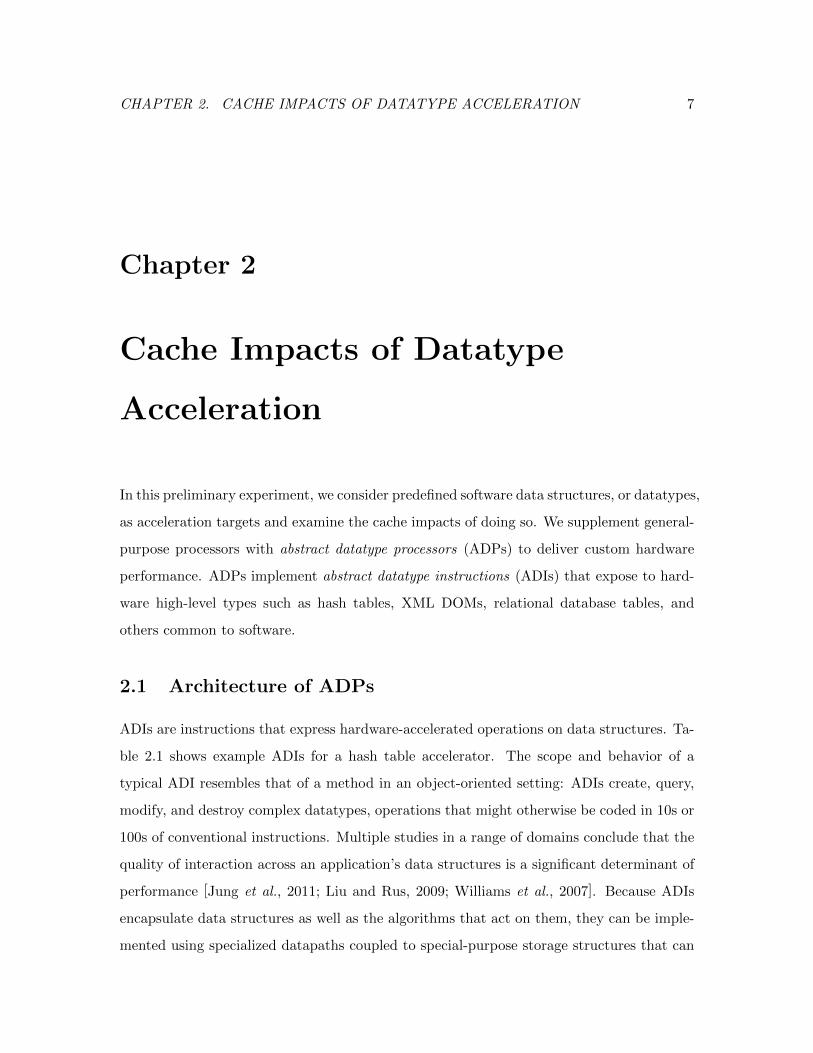
Figure 2.1: The scatter plots show instruction fetch performance and energy tradeoffs across a design space
of 54 cache configurations. ADIs reduce time and energy an average of 21% and 19% respectively relative
to ADI-free baselines for Parser and an average of 48% and 44% for SVM.
0
0.1
0.2
0.3
0.4
0.5
2K+4
M
ADI 2
K+4M
2K+1
M
ADI 2
K+1M
4K+1
M
ADI 4
K+1M
16K+
1M
ADI 1
6K+1
M
Fetc
h En
ergy
(J)
Parser
Mem Dynamic Mem Static L2 Dynamic L2 Static L1I Dynamic L1I Static
0
0.1
0.2
0.3
0.4
0.5
2K+4
M
ADI 2
K+4M
2K+1
M
ADI 2
K+1M
4K+1
M
ADI 4
K+1M
Fetc
h En
ergy
(J)
SVM
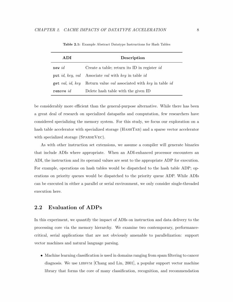
Figure 2.2: The bar charts display the breakdown of instruction fetch energy for each Pareto optimal cache
configuration. For all but one cache configuration (16K+1M for Parser), L2 dynamic energy dominates as
workload instruction footprint fits into the L2 capacity.
Figures 2.1– 2.3 show the results of our instruction fetch experiments for SVM and Parser
benchmarks. The scatter plots in Figure 2.1 graph the total instruction fetch energy against
the total instruction fetch time. Here, the diamonds show the instruction cache behavior
for ADI-free programs; the circles show the change in efficiency with the addition of ADIs.
Of the two programs, SVM shows the greatest improvement, confirming the importance of
the sparse vector dot product in the execution of this benchmark. The Parser benchmark
CHAPTER 2. CACHE IMPACTS OF DATATYPE ACCELERATION 11
0
10
20
2K+4
M
ADI 2
K+4M
2K+1
M
ADI 2
K+1M
4K+1
M
ADI 4
K+1M
16K+
1M
ADI 1
6K+1
M Ac
cess
Tim
e (s
)
Parser
0
10
20
30 2K
+4M
ADI 2
K+4M
2K+1
M
ADI 2
K+1M
4K+1
M
ADI 4
K+1M
Acce
ss T
ime
(s)
SVM Mem L2 L1
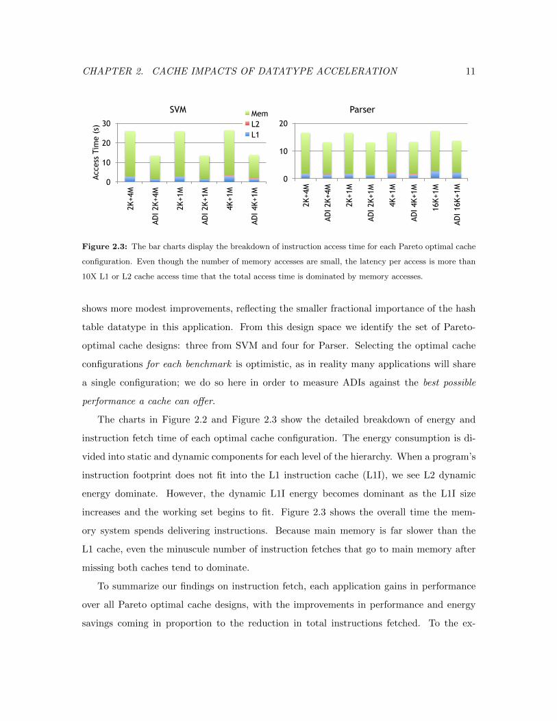
Figure 2.3: The bar charts display the breakdown of instruction access time for each Pareto optimal cache
configuration. Even though the number of memory accesses are small, the latency per access is more than
10X L1 or L2 cache access time that the total access time is dominated by memory accesses.
shows more modest improvements, reflecting the smaller fractional importance of the hash
table datatype in this application. From this design space we identify the set of Pareto-
optimal cache designs: three from SVM and four for Parser. Selecting the optimal cache
configurations for each benchmark is optimistic, as in reality many applications will share
a single configuration; we do so here in order to measure ADIs against the best possible
performance a cache can offer.
The charts in Figure 2.2 and Figure 2.3 show the detailed breakdown of energy and
instruction fetch time of each optimal cache configuration. The energy consumption is di-
vided into static and dynamic components for each level of the hierarchy. When a program’s
instruction footprint does not fit into the L1 instruction cache (L1I), we see L2 dynamic
energy dominate. However, the dynamic L1I energy becomes dominant as the L1I size
increases and the working set begins to fit. Figure 2.3 shows the overall time the mem-
ory system spends delivering instructions. Because main memory is far slower than the
L1 cache, even the minuscule number of instruction fetches that go to main memory after
missing both caches tend to dominate.
To summarize our findings on instruction fetch, each application gains in performance
over all Pareto optimal cache designs, with the improvements in performance and energy
savings coming in proportion to the reduction in total instructions fetched. To the ex-
CHAPTER 2. CACHE IMPACTS OF DATATYPE ACCELERATION 12
tend instruction fetch consumes time and energy, these results suggest that changing the
instruction encoding can reap important benefits, regardless of application domain.
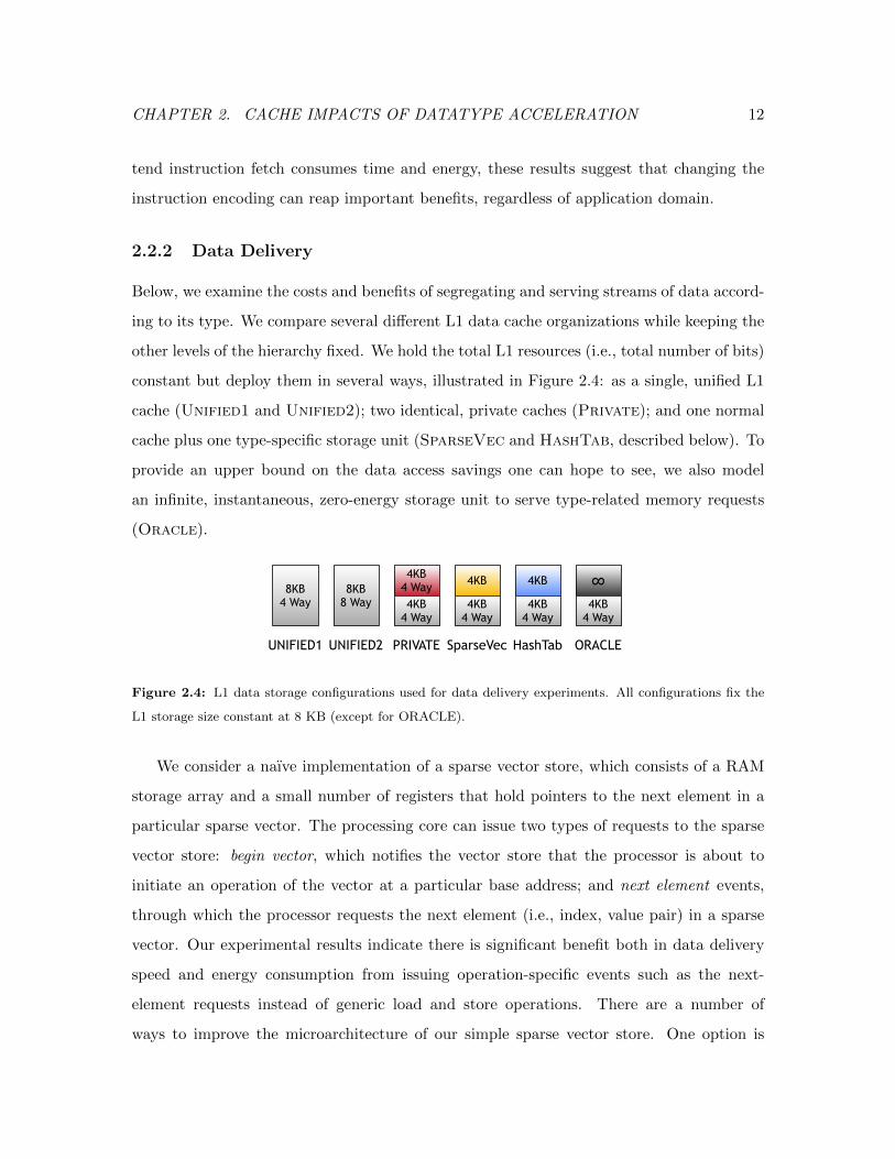
2.2.2 Data Delivery
Below, we examine the costs and benefits of segregating and serving streams of data accord-
ing to its type. We compare several different L1 data cache organizations while keeping the
other levels of the hierarchy fixed. We hold the total L1 resources (i.e., total number of bits)
constant but deploy them in several ways, illustrated in Figure 2.4: as a single, unified L1
cache (Unified1 and Unified2); two identical, private caches (Private); and one normal
cache plus one type-specific storage unit (SparseVec and HashTab, described below). To
provide an upper bound on the data access savings one can hope to see, we also model
an infinite, instantaneous, zero-energy storage unit to serve type-related memory requests
(Oracle).
8KB4 Way
8KB8 Way
4KB4 Way4KB
4 Way
4KB
4KB4 Way
4KB
4KB4 Way
!4KB
4 Way
UNIFIED1 UNIFIED2 PRIVATE SparseVec HashTab ORACLE
Figure 2.4: L1 data storage configurations used for data delivery experiments. All configurations fix the
L1 storage size constant at 8 KB (except for ORACLE).
We consider a naıve implementation of a sparse vector store, which consists of a RAM
storage array and a small number of registers that hold pointers to the next element in a
particular sparse vector. The processing core can issue two types of requests to the sparse
vector store: begin vector, which notifies the vector store that the processor is about to
initiate an operation of the vector at a particular base address; and next element events,
through which the processor requests the next element (i.e., index, value pair) in a sparse
vector. Our experimental results indicate there is significant benefit both in data delivery
speed and energy consumption from issuing operation-specific events such as the next-
element requests instead of generic load and store operations. There are a number of
ways to improve the microarchitecture of our simple sparse vector store. One option is
CHAPTER 2. CACHE IMPACTS OF DATATYPE ACCELERATION 13
1.2
1.4
1.6
1.8
2
2.2
2.4
5 6 7 8 9 10
Acce
ss E
nerg
y (J
)
Access Time (s)
SVM
1.5
2
2.5
3
6 7 8 9 10 11 12 Access Time (s)
Parser
UNIFIED1 UNIFIED2 PRIVATE SparseVec/HashTab ORACLE
Figure 2.5: The scatter plots show data delivery performance and energy tradeoffs across a design space.
HashTab reduced access time by up to 38% and energy by up to 33%. SparseVec reduced access time by
up to 20% and energy by up to 9%.
0
1
2
3 U
NIF
IED
1
UN
IFIE
D2
PRIV
ATE
Has
hTab
ORA
CLE
Acce
ss E
nerg
y (J
)
Parser
HashTab
0
1
2
3
UN
IFIE
D1
UN
IFIE
D2
PRIV
ATE
Spar
seVe
c
ORA
CLE
Acce
ss E
nerg
y (J
)
SVM Mem L2 L1 Private$ SparseVec
Figure 2.6: The bar charts display the breakdown of data access energy by memory structure for each
circled configuration from Figure 2.5.
prefetching. The SparseVec knows the processor is doing a dot product operation and
thus always knows what the processor will request next. Even a simple prefetch algorithm
can be expected to reduce data delivery time.
We evaluate the Parser benchmark in a similar manner to SVM. Instead of a Sparse-
Vec, we employ a type-specific storage for hash tables, HashTab. Similar to the Sparse-
Vec, the HashTab at its core is simply a RAM array whose total capacity is partitioned
into two regions: the first caches portions of the table backbone; the second caches table
elements themselves. As with SparseVec there is ample room for microarchitects to opti-

CHAPTER 2. CACHE IMPACTS OF DATATYPE ACCELERATION 14
0
2
4
6
8
10
12
UN
IFIE
D1
UN
IFIE
D2
PRIV
ATE
Has
hTab
ORA
CLE
Acce
ss T
ime
(s)
Parser
HashTab
0
2
4
6
8
10
12
UN
IFIE
D1
UN
IFIE
D2
PRIV
ATE
Spar
seVe
c
ORA
CLE
Acce
ss T
ime
(s)
SVM Mem L2 L1 Private$ SparseVec
Figure 2.7: The bar charts display the breakdown of access time by memory structure for each circled
configuration from Figure 2.5.
mize the implementation of this storage structure, employing aggressive datapaths or more
sophisticated storage structures such as CAMs. Other research, particularly from the net-
working domain, has outlined microarchitectural techniques to support efficient associative
lookups in hardware [Zane and Narlikar, 2003; Carli et al., 2009].
The scatter plots in Figure 2.5 plot the Pareto optimal energy-performance curves for
the four generic cache organizations (Unified1, Unified2, Private, Oracle) plus the
type-specific stores (SparseVec and HashTab). In this case we see that the specialized
store is a vast improvement over the general purpose stores, nearly matching ideal storage
properties. Specialized storage structures, SparseVec and HashTab, showed 13–19.7%
and 35.1–38% performance gains for SVM and Parser respectively while reducing energy by
5.9–8.6% and 28.9–33.1% respectively. The Private configuration is less complex to design
but gained at most 7.9% and 5.9% while costing 1.4% and 1.7% more energy for SVM and
Parser respectively.
Both the energy and runtime breakdowns in Figures 2.6 and 2.7 indicate that the spe-
cialized hash table store operates as a near-perfect cache. It reduces L2 pressure, which in
turn reduces trips to memory, where most of the time and energy costs lie. In both cases,
datatype-specific management policies were able to outperform equivalent-capacity general
purpose caches, regardless of cache configuration. This is because the generic cache has no
knowledge of the semantics of a hash table or a sparse vector. In contrast, the specialized
CHAPTER 2. CACHE IMPACTS OF DATATYPE ACCELERATION 15
cache only caches the desired entries or structures, effectively increasing the capacity of the
storage.
2.3 Summary of Findings on ADPs
Datatype acceleration marries high-level datatypes with processor architecture—an unusu-
ally large range of abstraction—to solve a pressing problem: how to improve the energy
efficiency of large-scale computation. Our experiments found such specialization can im-
prove instruction and data delivery energy by 27% and 38% respectively. The impact on the
overall system will depend on the relative importance of instruction and data delivery, which
varies between embedded systems [Dally et al., 2008] and high-performance cores [Natara-
jan et al., 2003]. This study show that data structures, or datatypes, represent suitable
acceleration targets with significant performance and energy potential gains. By aligning
specialized hardware with common programming constructs, datatype specialization can
improve both energy and performance efficiency while providing programmability.
CHAPTER 2. CACHE IMPACTS OF DATATYPE ACCELERATION 16
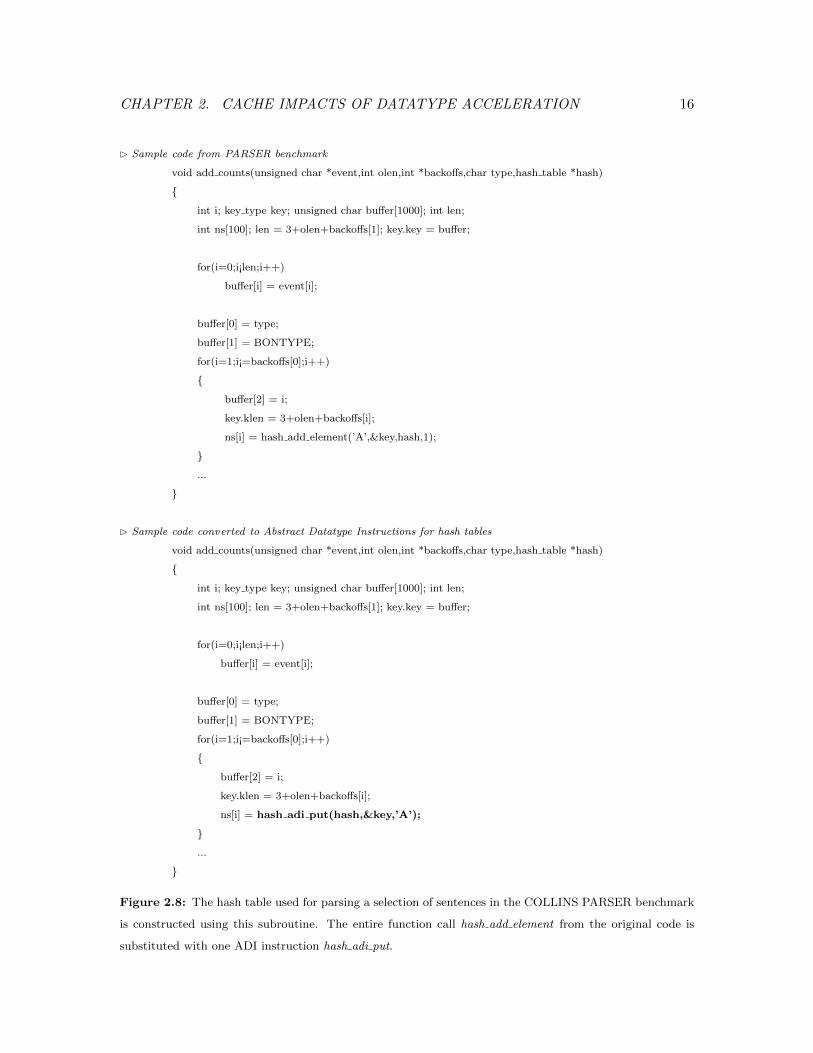
B Sample code from PARSER benchmark
void add counts(unsigned char *event,int olen,int *backoffs,char type,hash table *hash)
{
int i; key type key; unsigned char buffer[1000]; int len;
int ns[100]; len = 3+olen+backoffs[1]; key.key = buffer;
for(i=0;i¡len;i++)
buffer[i] = event[i];
buffer[0] = type;
buffer[1] = BONTYPE;
for(i=1;i¡=backoffs[0];i++)
{
buffer[2] = i;
key.klen = 3+olen+backoffs[i];
ns[i] = hash add element(’A’,&key,hash,1);
}
...
}
B Sample code converted to Abstract Datatype Instructions for hash tables
void add counts(unsigned char *event,int olen,int *backoffs,char type,hash table *hash)
{
int i; key type key; unsigned char buffer[1000]; int len;
int ns[100]; len = 3+olen+backoffs[1]; key.key = buffer;
for(i=0;i¡len;i++)
buffer[i] = event[i];
buffer[0] = type;
buffer[1] = BONTYPE;
for(i=1;i¡=backoffs[0];i++)
{
buffer[2] = i;
key.klen = 3+olen+backoffs[i];
ns[i] = hash adi put(hash,&key,’A’);
}
...
}
Figure 2.8: The hash table used for parsing a selection of sentences in the COLLINS PARSER benchmark
is constructed using this subroutine. The entire function call hash add element from the original code is
substituted with one ADI instruction hash adi put.
CHAPTER 3. ACCELERATION TARGETS 17
Chapter 3
Acceleration Targets
From the previous experiments, we found that datatype acceleration can be effective but
the workloads may or may not utilize the datatypes. We perform another preliminary study
and examine a wide range of industry standard benchmarks, assessing the potential of sev-
eral acceleration targets within them. Depending on the language used for a particular
application, there exists various granular data containers or data structures that can po-
tentially be suitable acceleration targets. We start out looking at the smallest predefined
data containers, such as standard library method calls for specific datatypes.
In order to isolate and group similar data containers, we profile popular benchmark
suites and answer the following three questions:
• Do the benchmarks exhibit any common functionality at or above the function/method
call level?
• What impact does the language or programming environment have on the potential
acceleration of a suite of applications?
• How many unique accelerators would be required to see benefits across a particular
benchmark suite? Does this change across suites and source programming languages?
3.1 Profiling of Benchmark Suites
To explore these questions, we profile four benchmark suites: SPEC2006 (C) [Standard Per-
formance Evaluation Corporation, 2006], SPECJVM (Java) [Standard Performance Evalua-
CHAPTER 3. ACCELERATION TARGETS 18
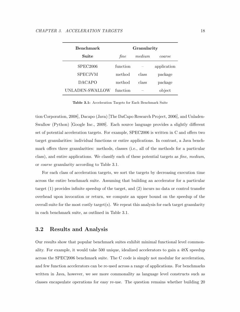
Benchmark Granularity
Suite fine medium coarse
SPEC2006 function – application
SPECJVM method class package
DACAPO method class package
UNLADEN-SWALLOW function – object
Table 3.1: Acceleration Targets for Each Benchmark Suite
tion Corporation, 2008], Dacapo (Java) [The DaCapo Research Project, 2006], and Unladen-
Swallow (Python) [Google Inc., 2009]. Each source language provides a slightly different
set of potential acceleration targets. For example, SPEC2006 is written in C and offers two
target granularities: individual functions or entire applications. In contrast, a Java bench-
mark offers three granularities: methods, classes (i.e., all of the methods for a particular
class), and entire applications. We classify each of these potential targets as fine, medium,
or coarse granularity according to Table 3.1.
For each class of acceleration targets, we sort the targets by decreasing execution time
across the entire benchmark suite. Assuming that building an accelerator for a particular
target (1) provides infinite speedup of the target, and (2) incurs no data or control transfer
overhead upon invocation or return, we compute an upper bound on the speedup of the
overall suite for the most costly target(s). We repeat this analysis for each target granularity
in each benchmark suite, as outlined in Table 3.1.
3.2 Results and Analysis
Our results show that popular benchmark suites exhibit minimal functional level common-
ality. For example, it would take 500 unique, idealized accelerators to gain a 48X speedup
across the SPEC2006 benchmark suite. The C code is simply not modular for acceleration,
and few function accelerators can be re-used across a range of applications. For benchmarks
written in Java, however, we see more commonality as language level constructs such as
classes encapsulate operations for easy re-use. The question remains whether building 20
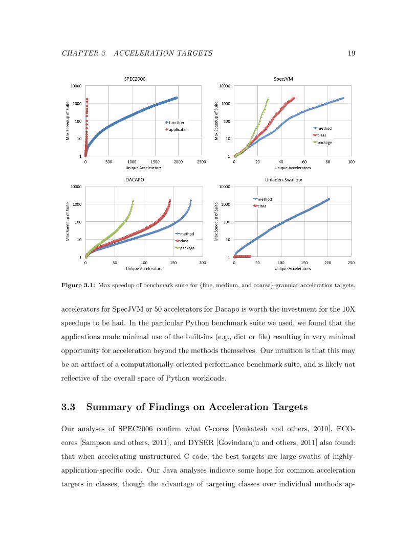
CHAPTER 3. ACCELERATION TARGETS 19
Figure 3.1: Max speedup of benchmark suite for {fine, medium, and coarse}-granular acceleration targets.
accelerators for SpecJVM or 50 accelerators for Dacapo is worth the investment for the 10X
speedups to be had. In the particular Python benchmark suite we used, we found that the
applications made minimal use of the built-ins (e.g., dict or file) resulting in very minimal
opportunity for acceleration beyond the methods themselves. Our intuition is that this may
be an artifact of a computationally-oriented performance benchmark suite, and is likely not
reflective of the overall space of Python workloads.
3.3 Summary of Findings on Acceleration Targets
Our analyses of SPEC2006 confirm what C-cores [Venkatesh and others, 2010], ECO-
cores [Sampson and others, 2011], and DYSER [Govindaraju and others, 2011] also found:
that when accelerating unstructured C code, the best targets are large swaths of highly-
application-specific code. Our Java analyses indicate some hope for common acceleration
targets in classes, though the advantage of targeting classes over individual methods ap-
CHAPTER 3. ACCELERATION TARGETS 20
pears modest. Across the board, our data show that filling dark silicon with specialized
accelerators will require systems containing tens or even hundreds of accelerators. In partic-
ular, popular benchmark suites, containing a collection of kernels attempting to represent a
wide range of application characteristics, do not contain suitable acceleration targets. This
conclusion points us to choose acceleration targets carefully in order to realize the potential
performance and energy efficiency gains while offset the cost of designing unique circuitries.
CHAPTER 4. HARDWARE ACCELERATED RANGE PARTITIONING 21
Chapter 4
Hardware Accelerated Range
Partitioning
The preliminary studies up to this point show that datatype acceleration is still a good idea,
but needs to be implemented in an environment where the targeted data containers/struc-
tures are widely used. We choose to focus on the database application domain, specifically,
analytic relational databases. We target relational databases for the following four rea-
sons: (1) relational databases process structured datatypes, namely columns and tables,
so we would expect to see benefits similar to the conclusion of our first preliminary study
in Chapter 2; (2) relational databases are well established and accepted by the database
community, so building hardware for such standard is broadly-applicable; (3) relational
database applications are compute-bound, and there is potential for performance improve-
ment; and (4) relational database applications are ubiquitous and increasingly important
as evidenced by the fact that Oracle, Microsoft, and IBM build and support commercial
relational databases.
Relational database applications being compute-bound are evidenced by the following
observations. Servers running Bing, Hotmail, and Cosmos (Microsoft’s search, email, and
parallel data analysis engines, respectively) show 67%–97% processor utilization but only
2%–6% memory bandwidth utilization under stress testing [Kozyrakis et al., 2010]. Google’s
BigTable and Content Analyzer (large data storage and semantic analysis, respectively)
CHAPTER 4. HARDWARE ACCELERATED RANGE PARTITIONING 22
show fewer than 10 K/msec last level cache misses, which represents just a couple of percent
of the total available memory bandwidth [Tang et al., 2011]. These observations clearly show
that despite the relative scarcity of memory pins, these large data workloads do not saturate
the available bandwidth and are largely compute-bound.
In this chapter, we explore targeted deployment of hardware accelerators to improve
the throughput and energy efficiency of large-scale data processing in relational databases.
In particular, data partitioning is a critical operation for manipulating large data sets. It
is often the limiting factor in database performance and represents a significant fraction of
the overall runtime of large data queries.
We start by providing some background on data partitioning, then we describe a hard-
ware accelerator for a specific type of partitioning algorithm called range partitioning. We
present the evaluation of the hardware accelerated range partitioner, or HARP, and show
that HARP provides an order of magnitude improvement in partitioning performance and
energy compared to a state-of-the-art software implementation.
4.1 Data Partitioning is Important
Databases are designed to manage large quantities of data, allowing users to query and
update the information they contain. The database community has been developing algo-
rithms to support fast or even real-time queries over relational databases, and, as data sizes
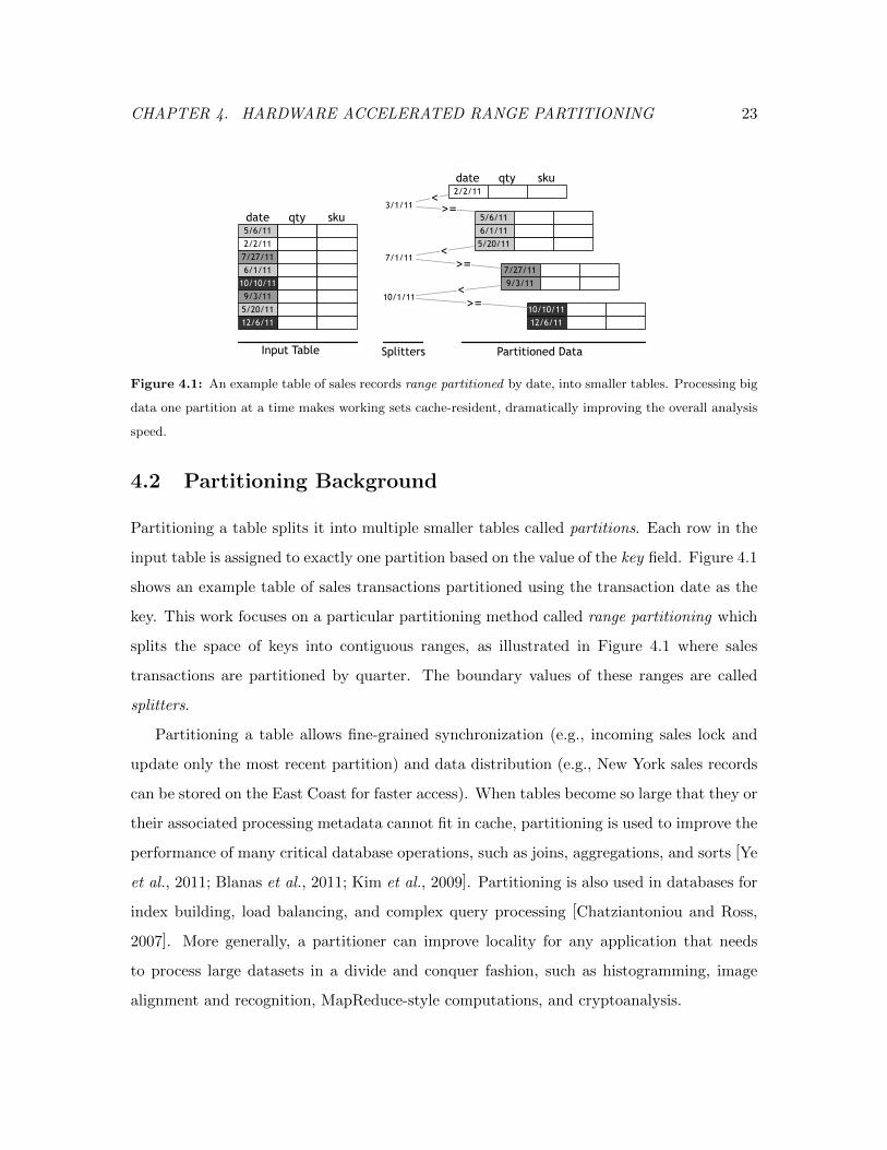
grow, they increasingly opt to partition the data for faster subsequent processing. As illus-
trated in the small example in Figure 4.1, partitioning assigns each record in a large table to
a smaller table based on the value of a particular field in the record, such as the transaction
date in Figure 4.1. Partitioning enables the resulting partitions to be processed indepen-
dently and more efficiently (i.e., in parallel and with better cache locality). Partitioning
is used in virtually all modern database systems including Oracle Database 11g [Oracle,
2013], IBM DB2 [IBM, 2013a], and Microsoft SQL Server 2012 [Microsoft, 2012] to improve
performance, manageability, and availability in the face of big data, and the partitioning
step itself has become a key determinant of query processing performance.
CHAPTER 4. HARDWARE ACCELERATED RANGE PARTITIONING 23
5/6/11
2/2/11
7/27/11
6/1/11
10/10/11
9/3/11
5/20/11
12/6/11
5/6/11
2/2/11
7/27/11
5/20/11
12/6/11
9/3/11
10/10/11
6/1/11
date qty sku
date qty sku
3/1/11
Input Table Partitioned DataSplitters
7/1/11
10/1/11
<
<
<>=
>=
>=
Figure 4.1: An example table of sales records range partitioned by date, into smaller tables. Processing big
data one partition at a time makes working sets cache-resident, dramatically improving the overall analysis
speed.
4.2 Partitioning Background
Partitioning a table splits it into multiple smaller tables called partitions. Each row in the
input table is assigned to exactly one partition based on the value of the key field. Figure 4.1
shows an example table of sales transactions partitioned using the transaction date as the
key. This work focuses on a particular partitioning method called range partitioning which
splits the space of keys into contiguous ranges, as illustrated in Figure 4.1 where sales
transactions are partitioned by quarter. The boundary values of these ranges are called
splitters.
Partitioning a table allows fine-grained synchronization (e.g., incoming sales lock and
update only the most recent partition) and data distribution (e.g., New York sales records
can be stored on the East Coast for faster access). When tables become so large that they or
their associated processing metadata cannot fit in cache, partitioning is used to improve the
performance of many critical database operations, such as joins, aggregations, and sorts [Ye
et al., 2011; Blanas et al., 2011; Kim et al., 2009]. Partitioning is also used in databases for
index building, load balancing, and complex query processing [Chatziantoniou and Ross,
2007]. More generally, a partitioner can improve locality for any application that needs
to process large datasets in a divide and conquer fashion, such as histogramming, image
alignment and recognition, MapReduce-style computations, and cryptoanalysis.
CHAPTER 4. HARDWARE ACCELERATED RANGE PARTITIONING 24
SALES
WEATHER
partition(SALES)
join(1)partition(WEATHER)
join(2) join(3) join(4)
join(SALES,WEATHER)
SALES_1
SALES_2
SALES_3
SALES_4
WEATHER_1
WEATHER_2
WEATHER_3
WEATHER_4
Without partitioning, even smaller
table exceeds cache capacity,
consequently lookups thrash and
the join operation is slow.
After partitioning, small table
partitions are cache resident,
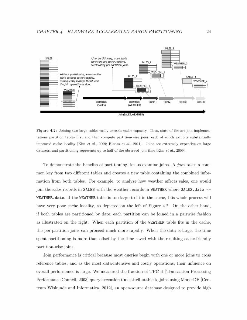
accelerating per-partition joins.
Figure 4.2: Joining two large tables easily exceeds cache capacity. Thus, state of the art join implemen-
tations partition tables first and then compute partition-wise joins, each of which exhibits substantially
improved cache locality [Kim et al., 2009; Blanas et al., 2011]. Joins are extremely expensive on large
datasets, and partitioning represents up to half of the observed join time [Kim et al., 2009].
To demonstrate the benefits of partitioning, let us examine joins. A join takes a com-
mon key from two different tables and creates a new table containing the combined infor-
mation from both tables. For example, to analyze how weather affects sales, one would
join the sales records in SALES with the weather records in WEATHER where SALES.date ==
WEATHER.date. If the WEATHER table is too large to fit in the cache, this whole process will
have very poor cache locality, as depicted on the left of Figure 4.2. On the other hand,
if both tables are partitioned by date, each partition can be joined in a pairwise fashion
as illustrated on the right. When each partition of the WEATHER table fits in the cache,
the per-partition joins can proceed much more rapidly. When the data is large, the time
spent partitioning is more than offset by the time saved with the resulting cache-friendly
partition-wise joins.
Join performance is critical because most queries begin with one or more joins to cross
reference tables, and as the most data-intensive and costly operations, their influence on
overall performance is large. We measured the fraction of TPC-H [Transaction Processing
Performance Council, 2003] query execution time attributable to joins using MonetDB [Cen-
trum Wiskunde and Informatica, 2012], an open-source database designed to provide high
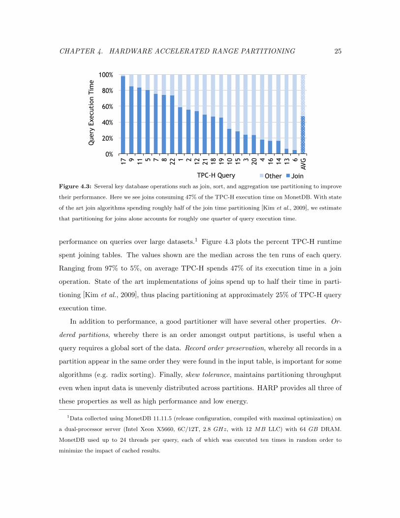
CHAPTER 4. HARDWARE ACCELERATED RANGE PARTITIONING 25
0%
20%
40%
60%
80%
100%
17 9 11 5 7 8 22 1 2 12
21
18
19
10
15 3 20 4 16
14
13 6
AVG
Que
ry E
xecu
tion
Tim
e
TPC-H Query Other Join Figure 4.3: Several key database operations such as join, sort, and aggregation use partitioning to improve
their performance. Here we see joins consuming 47% of the TPC-H execution time on MonetDB. With state
of the art join algorithms spending roughly half of the join time partitioning [Kim et al., 2009], we estimate
that partitioning for joins alone accounts for roughly one quarter of query execution time.
performance on queries over large datasets.1 Figure 4.3 plots the percent TPC-H runtime
spent joining tables. The values shown are the median across the ten runs of each query.
Ranging from 97% to 5%, on average TPC-H spends 47% of its execution time in a join
operation. State of the art implementations of joins spend up to half their time in parti-
tioning [Kim et al., 2009], thus placing partitioning at approximately 25% of TPC-H query
execution time.
In addition to performance, a good partitioner will have several other properties. Or-
dered partitions, whereby there is an order amongst output partitions, is useful when a
query requires a global sort of the data. Record order preservation, whereby all records in a
partition appear in the same order they were found in the input table, is important for some
algorithms (e.g. radix sorting). Finally, skew tolerance, maintains partitioning throughput
even when input data is unevenly distributed across partitions. HARP provides all three of
these properties as well as high performance and low energy.
1Data collected using MonetDB 11.11.5 (release configuration, compiled with maximal optimization) on
a dual-processor server (Intel Xeon X5660, 6C/12T, 2.8 GHz, with 12 MB LLC) with 64 GB DRAM.
MonetDB used up to 24 threads per query, each of which was executed ten times in random order to
minimize the impact of cached results.
CHAPTER 4. HARDWARE ACCELERATED RANGE PARTITIONING 26
NumRecs← 108 . Alloc. and init. input
in← malloc(NumRecs ·RecSize)
for r = 0..(NumRecs− 1) do
in[r]← RandomRec()
end for
for p = 0..(NumParts− 1) do . Alloc. output
out[p]← malloc(NumRecs ·RecSize)
end for
for i = 0..NumRecs do . Partitioning inner loop
r ← in[i]
p← PartitionFunction(r)
∗(out[p])← r
out[p]← out[p] + RecSize
end for
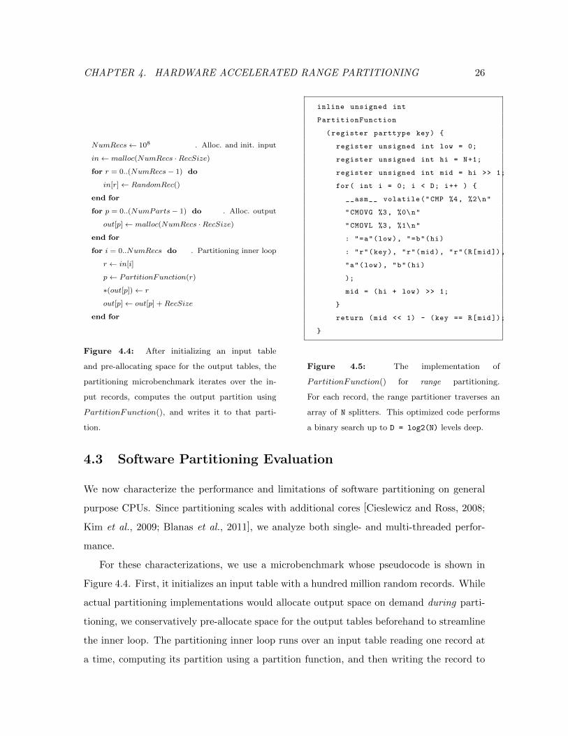
Figure 4.4: After initializing an input table
and pre-allocating space for the output tables, the
partitioning microbenchmark iterates over the in-
put records, computes the output partition using
PartitionFunction(), and writes it to that parti-
tion.
inline unsigned int
PartitionFunction
(register parttype key) {
register unsigned int low = 0;
register unsigned int hi = N+1;
register unsigned int mid = hi >> 1;
for( int i = 0; i < D; i++ ) {
__asm__ volatile("CMP %4, %2\n"
"CMOVG %3, %0\n"
"CMOVL %3, %1\n"
: "=a"(low), "=b"(hi)
: "r"(key), "r"(mid), "r"(R[mid]),
"a"(low), "b"(hi)
);
mid = (hi + low) >> 1;
}
return (mid << 1) - (key == R[mid ]);
}
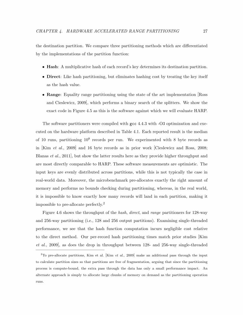
Figure 4.5: The implementation of
PartitionFunction() for range partitioning.
For each record, the range partitioner traverses an
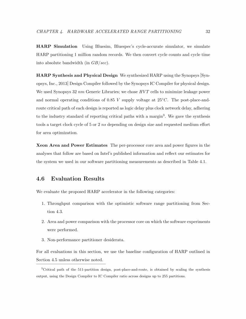
array of N splitters. This optimized code performs
a binary search up to D = log2(N) levels deep.
4.3 Software Partitioning Evaluation
We now characterize the performance and limitations of software partitioning on general
purpose CPUs. Since partitioning scales with additional cores [Cieslewicz and Ross, 2008;
Kim et al., 2009; Blanas et al., 2011], we analyze both single- and multi-threaded perfor-
mance.
For these characterizations, we use a microbenchmark whose pseudocode is shown in
Figure 4.4. First, it initializes an input table with a hundred million random records. While
actual partitioning implementations would allocate output space on demand during parti-
tioning, we conservatively pre-allocate space for the output tables beforehand to streamline
the inner loop. The partitioning inner loop runs over an input table reading one record at
a time, computing its partition using a partition function, and then writing the record to
CHAPTER 4. HARDWARE ACCELERATED RANGE PARTITIONING 27
the destination partition. We compare three partitioning methods which are differentiated
by the implementations of the partition function:
• Hash: A multiplicative hash of each record’s key determines its destination partition.
• Direct: Like hash partitioning, but eliminates hashing cost by treating the key itself
as the hash value.
• Range: Equality range partitioning using the state of the art implementation [Ross
and Cieslewicz, 2009], which performs a binary search of the splitters. We show the
exact code in Figure 4.5 as this is the software against which we will evaluate HARP.
The software partitioners were compiled with gcc 4.4.3 with -O3 optimization and exe-
cuted on the hardware platform described in Table 4.1. Each reported result is the median
of 10 runs, partitioning 108 records per run. We experimented with 8 byte records as
in [Kim et al., 2009] and 16 byte records as in prior work [Cieslewicz and Ross, 2008;
Blanas et al., 2011], but show the latter results here as they provide higher throughput and
are most directly comparable to HARP. These software measurements are optimistic. The
input keys are evenly distributed across partitions, while this is not typically the case in
real-world data. Moreover, the microbenchmark pre-allocates exactly the right amount of
memory and performs no bounds checking during partitioning, whereas, in the real world,
it is impossible to know exactly how many records will land in each partition, making it
impossible to pre-allocate perfectly.2
Figure 4.6 shows the throughput of the hash, direct, and range partitioners for 128-way
and 256-way partitioning (i.e., 128 and 256 output partitions). Examining single-threaded
performance, we see that the hash function computation incurs negligible cost relative
to the direct method. Our per-record hash partitioning times match prior studies [Kim
et al., 2009], as does the drop in throughput between 128- and 256-way single-threaded
2To pre-allocate partitions, Kim et al. [Kim et al., 2009] make an additional pass through the input
to calculate partition sizes so that partitions are free of fragmentation, arguing that since the partitioning
process is compute-bound, the extra pass through the data has only a small performance impact. An
alternate approach is simply to allocate large chunks of memory on demand as the partitioning operation
runs.
CHAPTER 4. HARDWARE ACCELERATED RANGE PARTITIONING 28
System Configuration
Chip 2X Intel E5620
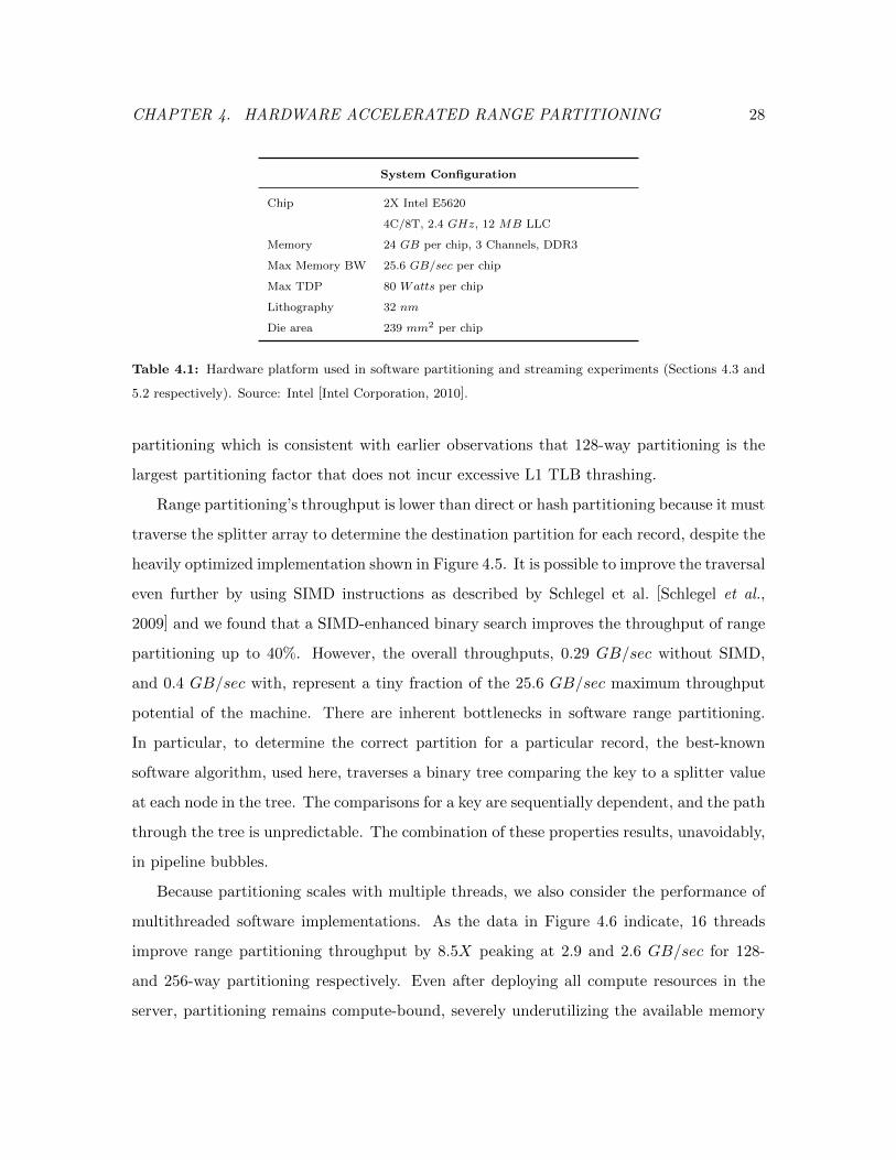
4C/8T, 2.4 GHz, 12 MB LLC
Memory 24 GB per chip, 3 Channels, DDR3
Max Memory BW 25.6 GB/sec per chip
Max TDP 80 Watts per chip
Lithography 32 nm
Die area 239 mm2 per chip
Table 4.1: Hardware platform used in software partitioning and streaming experiments (Sections 4.3 and
5.2 respectively). Source: Intel [Intel Corporation, 2010].
partitioning which is consistent with earlier observations that 128-way partitioning is the
largest partitioning factor that does not incur excessive L1 TLB thrashing.
Range partitioning’s throughput is lower than direct or hash partitioning because it must
traverse the splitter array to determine the destination partition for each record, despite the
heavily optimized implementation shown in Figure 4.5. It is possible to improve the traversal
even further by using SIMD instructions as described by Schlegel et al. [Schlegel et al.,
2009] and we found that a SIMD-enhanced binary search improves the throughput of range
partitioning up to 40%. However, the overall throughputs, 0.29 GB/sec without SIMD,
and 0.4 GB/sec with, represent a tiny fraction of the 25.6 GB/sec maximum throughput
potential of the machine. There are inherent bottlenecks in software range partitioning.
In particular, to determine the correct partition for a particular record, the best-known
software algorithm, used here, traverses a binary tree comparing the key to a splitter value
at each node in the tree. The comparisons for a key are sequentially dependent, and the path
through the tree is unpredictable. The combination of these properties results, unavoidably,
in pipeline bubbles.
Because partitioning scales with multiple threads, we also consider the performance of
multithreaded software implementations. As the data in Figure 4.6 indicate, 16 threads
improve range partitioning throughput by 8.5X peaking at 2.9 and 2.6 GB/sec for 128-
and 256-way partitioning respectively. Even after deploying all compute resources in the
server, partitioning remains compute-bound, severely underutilizing the available memory
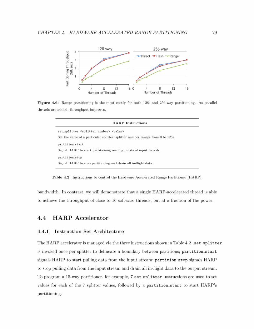
CHAPTER 4. HARDWARE ACCELERATED RANGE PARTITIONING 29
0 4 8 12 16 Number of Threads
256 way
Direct Hash Range
1
2
3
4
0 4 8 12 16
Part
itio
ning
Thr
ough
put
(G
B/se
c)
Number of Threads
128 way
Figure 4.6: Range partitioning is the most costly for both 128- and 256-way partitioning. As parallel
threads are added, throughput improves.
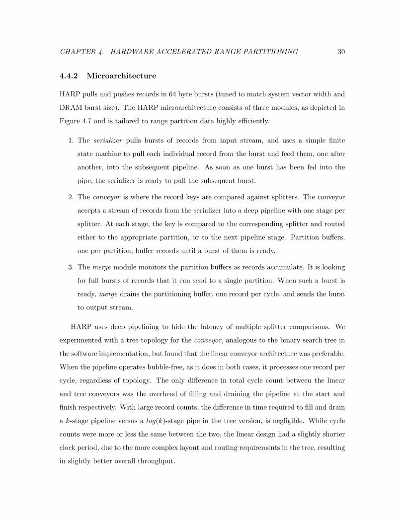
HARP Instructions
set splitter <splitter number> <value>
Set the value of a particular splitter (splitter number ranges from 0 to 126).
partition start
Signal HARP to start partitioning reading bursts of input records.
partition stop
Signal HARP to stop partitioning and drain all in-flight data.
Table 4.2: Instructions to control the Hardware Accelerated Range Partitioner (HARP).
bandwidth. In contrast, we will demonstrate that a single HARP-accelerated thread is able
to achieve the throughput of close to 16 software threads, but at a fraction of the power.
4.4 HARP Accelerator
4.4.1 Instruction Set Architecture
The HARP accelerator is managed via the three instructions shown in Table 4.2. set splitter
is invoked once per splitter to delineate a boundary between partitions; partition start
signals HARP to start pulling data from the input stream; partition stop signals HARP
to stop pulling data from the input stream and drain all in-flight data to the output stream.
To program a 15-way partitioner, for example, 7 set splitter instructions are used to set
values for each of the 7 splitter values, followed by a partition start to start HARP’s
partitioning.
CHAPTER 4. HARDWARE ACCELERATED RANGE PARTITIONING 30
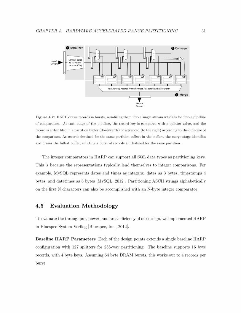
4.4.2 Microarchitecture
HARP pulls and pushes records in 64 byte bursts (tuned to match system vector width and
DRAM burst size). The HARP microarchitecture consists of three modules, as depicted in
Figure 4.7 and is tailored to range partition data highly efficiently.
1. The serializer pulls bursts of records from input stream, and uses a simple finite
state machine to pull each individual record from the burst and feed them, one after
another, into the subsequent pipeline. As soon as one burst has been fed into the
pipe, the serializer is ready to pull the subsequent burst.
2. The conveyor is where the record keys are compared against splitters. The conveyor
accepts a stream of records from the serializer into a deep pipeline with one stage per
splitter. At each stage, the key is compared to the corresponding splitter and routed
either to the appropriate partition, or to the next pipeline stage. Partition buffers,
one per partition, buffer records until a burst of them is ready.
3. The merge module monitors the partition buffers as records accumulate. It is looking
for full bursts of records that it can send to a single partition. When such a burst is
ready, merge drains the partitioning buffer, one record per cycle, and sends the burst
to output stream.
HARP uses deep pipelining to hide the latency of multiple splitter comparisons. We
experimented with a tree topology for the conveyor, analogous to the binary search tree in
the software implementation, but found that the linear conveyor architecture was preferable.
When the pipeline operates bubble-free, as it does in both cases, it processes one record per
cycle, regardless of topology. The only difference in total cycle count between the linear
and tree conveyors was the overhead of filling and draining the pipeline at the start and
finish respectively. With large record counts, the difference in time required to fill and drain
a k-stage pipeline versus a log(k)-stage pipe in the tree version, is negligible. While cycle
counts were more or less the same between the two, the linear design had a slightly shorter
clock period, due to the more complex layout and routing requirements in the tree, resulting
in slightly better overall throughput.
CHAPTER 4. HARDWARE ACCELERATED RANGE PARTITIONING 31
<
=
<
=
<
=
Serializer
Convert burstto stream ofrecords (FSM)
1 Conveyor2
Merge3
WE WE WE WE WE WE
Pull burst of records from the most full partition buffer (FSM)
WE WE WE WE WE WE WE
Input Stream
OutputStream
Figure 4.7: HARP draws records in bursts, serializing them into a single stream which is fed into a pipeline
of comparators. At each stage of the pipeline, the record key is compared with a splitter value, and the
record is either filed in a partition buffer (downwards) or advanced (to the right) according to the outcome of
the comparison. As records destined for the same partition collect in the buffers, the merge stage identifies
and drains the fullest buffer, emitting a burst of records all destined for the same partition.
The integer comparators in HARP can support all SQL data types as partitioning keys.
This is because the representations typically lend themselves to integer comparisons. For
example, MySQL represents dates and times as integers: dates as 3 bytes, timestamps 4
bytes, and datetimes as 8 bytes [MySQL, 2012]. Partitioning ASCII strings alphabetically
on the first N characters can also be accomplished with an N-byte integer comparator.
4.5 Evaluation Methodology
To evaluate the throughput, power, and area efficiency of our design, we implemented HARP
in Bluespec System Verilog [Bluespec, Inc., 2012].
Baseline HARP Parameters Each of the design points extends a single baseline HARP
configuration with 127 splitters for 255-way partitioning. The baseline supports 16 byte
records, with 4 byte keys. Assuming 64 byte DRAM bursts, this works out to 4 records per
burst.
CHAPTER 4. HARDWARE ACCELERATED RANGE PARTITIONING 32
HARP Simulation Using Bluesim, Bluespec’s cycle-accurate simulator, we simulate
HARP partitioning 1 million random records. We then convert cycle counts and cycle time
into absolute bandwidth (in GB/sec).
HARP Synthesis and Physical Design We synthesized HARP using the Synopsys [Syn-
opsys, Inc., 2013] Design Compiler followed by the Synopsys IC Compiler for physical design.
We used Synopsys 32 nm Generic Libraries; we chose HVT cells to minimize leakage power
and normal operating conditions of 0.85 V supply voltage at 25◦C. The post-place-and-
route critical path of each design is reported as logic delay plus clock network delay, adhering
to the industry standard of reporting critical paths with a margin3. We gave the synthesis
tools a target clock cycle of 5 or 2 ns depending on design size and requested medium effort
for area optimization.
Xeon Area and Power Estimates The per-processor core area and power figures in the
analyses that follow are based on Intel’s published information and reflect our estimates for
the system we used in our software partitioning measurements as described in Table 4.1.
4.6 Evaluation Results
We evaluate the proposed HARP accelerator in the following categories:
1. Throughput comparison with the optimistic software range partitioning from Sec-
tion 4.3.
2. Area and power comparison with the processor core on which the software experiments
were performed.
3. Non-performance partitioner desiderata.
For all evaluations in this section, we use the baseline configuration of HARP outlined in
Section 4.5 unless otherwise noted.
3Critical path of the 511-partition design, post-place-and-route, is obtained by scaling the synthesis
output, using the Design Compiler to IC Compiler ratio across designs up to 255 partitions.
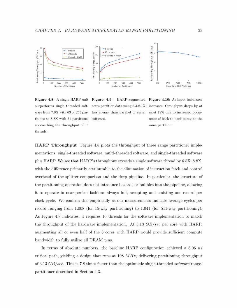
CHAPTER 4. HARDWARE ACCELERATED RANGE PARTITIONING 33
2
4
6
8
0 100 200 300 400 500
Part
itio
ning
Thr
ough
put
(GB/
sec)
Number of Partitions
1 thread 16 threads 1 thread + HARP
Figure 4.8: A single HARP unit
outperforms single threaded soft-
ware from 7.8X with 63 or 255 par-
titions to 8.8X with 31 partitions,
approaching the throughput of 16
threads.
5
10
15
20
0 100 200 300 400 500
Part
itio
ning
Ene
rgy
(J/G
B)
Number of Partitions
1 thread
16 threads
1 thread + HARP
Figure 4.9: HARP-augmented
cores partition data using 6.3-8.7X
less energy than parallel or serial
software.
1
2
3
4
0% 25% 50% 75% 100%
Part
itio
ning
Thr
ough
put
(GB/
sec)
Records in Hot Partition
Figure 4.10: As input imbalance
increases, throughput drops by at
most 19% due to increased occur-
rence of back-to-back bursts to the
same partition.
HARP Throughput Figure 4.8 plots the throughput of three range partitioner imple-
mentations: single-threaded software, multi-threaded software, and single-threaded software
plus HARP. We see that HARP’s throughput exceeds a single software thread by 6.5X–8.8X,
with the difference primarily attributable to the elimination of instruction fetch and control
overhead of the splitter comparison and the deep pipeline. In particular, the structure of
the partitioning operation does not introduce hazards or bubbles into the pipeline, allowing
it to operate in near-perfect fashion: always full, accepting and emitting one record per
clock cycle. We confirm this empirically as our measurements indicate average cycles per
record ranging from 1.008 (for 15-way partitioning) to 1.041 (for 511-way partitioning).
As Figure 4.8 indicates, it requires 16 threads for the software implementation to match
the throughput of the hardware implementation. At 3.13 GB/sec per core with HARP,
augmenting all or even half of the 8 cores with HARP would provide sufficient compute
bandwidth to fully utilize all DRAM pins.
In terms of absolute numbers, the baseline HARP configuration achieved a 5.06 ns
critical path, yielding a design that runs at 198 MHz, delivering partitioning throughput
of 3.13 GB/sec. This is 7.8 times faster than the optimistic single-threaded software range-
partitioner described in Section 4.3.
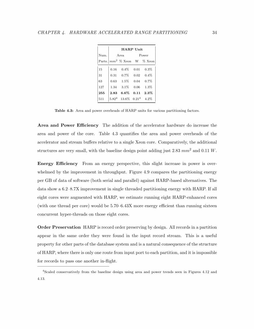
CHAPTER 4. HARDWARE ACCELERATED RANGE PARTITIONING 34
HARP Unit
Num. Area Power
Parts. mm2 % Xeon W % Xeon
15 0.16 0.4% 0.01 0.3%
31 0.31 0.7% 0.02 0.4%
63 0.63 1.5% 0.04 0.7%
127 1.34 3.1% 0.06 1.3%
255 2.83 6.6% 0.11 2.3%
511 5.824 13.6% 0.214 4.2%
Table 4.3: Area and power overheads of HARP units for various partitioning factors.
Area and Power Efficiency The addition of the accelerator hardware do increase the
area and power of the core. Table 4.3 quantifies the area and power overheads of the
accelerator and stream buffers relative to a single Xeon core. Comparatively, the additional
structures are very small, with the baseline design point adding just 2.83 mm2 and 0.11 W .
Energy Efficiency From an energy perspective, this slight increase in power is over-
whelmed by the improvement in throughput. Figure 4.9 compares the partitioning energy
per GB of data of software (both serial and parallel) against HARP-based alternatives. The
data show a 6.2–8.7X improvement in single threaded partitioning energy with HARP. If all
eight cores were augmented with HARP, we estimate running eight HARP-enhanced cores
(with one thread per core) would be 5.70–6.43X more energy efficient than running sixteen
concurrent hyper-threads on those eight cores.
Order Preservation HARP is record order preserving by design. All records in a partition
appear in the same order they were found in the input record stream. This is a useful
property for other parts of the database system and is a natural consequence of the structure
of HARP, where there is only one route from input port to each partition, and it is impossible
for records to pass one another in-flight.
4Scaled conservatively from the baseline design using area and power trends seen in Figures 4.12 and
4.13.

CHAPTER 4. HARDWARE ACCELERATED RANGE PARTITIONING 35
HARP Design Space Configurations
# Splitters 7 15 31 63 127 255
# Partitions 15 31 63 127 255 511
Key Width (Bytes) 4 8 16
Record Width (Bytes) 4 8 16
Table 4.4: Parameters for HARP design space exploration with baseline configuration highlighted.
Skew Tolerance We evaluate HARP’s skew tolerance by measuring the throughput (i.e.,
cycles/record) on synthetically unbalanced record sets. In this experiment, we varied the
record distribution from optimal, where records were uniformly distributed across all par-
titions, to pessimal, where all records are sent to a single partition. Figure 4.10 shows the
gentle degradation in throughput as one partition receives an increasingly large share of
records.
This mild degradation is due to the design of the merge module. Recall that this
stage identifies which partition has the most records ready and drains them from that
partition’s buffer to send as a single burst back to memory. Back-to-back drains of the
same partition require an additional cycle in the merge, which rarely happens, when records
are distributed across partitions. If there are B records per DRAM burst, draining two
different partition buffers back-to-back takes 2B cycles. However, when skew increases, the
frequency of back-to-back drains of the same partition increases, resulting in an average of
B + 1 cycles per burst rather than B. Thus, the throughput of the merge module varies
between 1B cycles/record in the best case to 1
B+1 in the worst case. Note that this tolerance
is independent of many factors including the number of splitters, the size of the keys, or
the size of the table being partitioned.
The baseline HARP design supports four records per burst resulting in a 25% degrada-
tion in throughput between best- and worst-case skew. This is very close to the degradation
seen experimentally in Figure 4.10, where throughput sinks from 3.13 GB/sec with no skew
to 2.53 GB/sec in the worst-case.
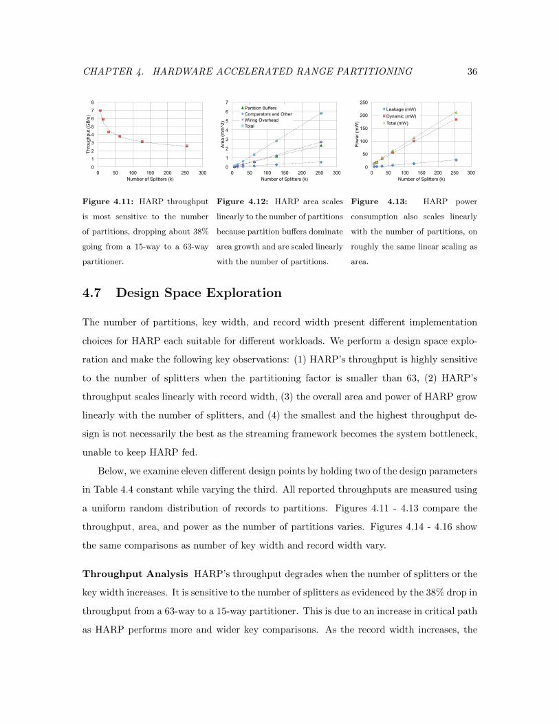
CHAPTER 4. HARDWARE ACCELERATED RANGE PARTITIONING 36
0
1
2
3
4
5
6
7
8
0 50 100 150 200 250 300
Thro
ughp
ut (G
B/s
)
Number of Splitters (k)
Figure 4.11: HARP throughput
is most sensitive to the number
of partitions, dropping about 38%
going from a 15-way to a 63-way
partitioner.
0
1
2
3
4
5
6
7
0 50 100 150 200 250 300
Are
a (m
m^2
)
Number of Splitters (k)
Partition Buffers Comparators and Other Wiring Overhead Total
Figure 4.12: HARP area scales
linearly to the number of partitions
because partition buffers dominate
area growth and are scaled linearly
with the number of partitions.
0
50
100
150
200
250
0 50 100 150 200 250 300
Pow
er (m
W)
Number of Splitters (k)
Leakage (mW) Dynamic (mW) Total (mW)
Figure 4.13: HARP power
consumption also scales linearly
with the number of partitions, on
roughly the same linear scaling as
area.
4.7 Design Space Exploration
The number of partitions, key width, and record width present different implementation
choices for HARP each suitable for different workloads. We perform a design space explo-
ration and make the following key observations: (1) HARP’s throughput is highly sensitive
to the number of splitters when the partitioning factor is smaller than 63, (2) HARP’s
throughput scales linearly with record width, (3) the overall area and power of HARP grow
linearly with the number of splitters, and (4) the smallest and the highest throughput de-
sign is not necessarily the best as the streaming framework becomes the system bottleneck,
unable to keep HARP fed.
Below, we examine eleven different design points by holding two of the design parameters
in Table 4.4 constant while varying the third. All reported throughputs are measured using
a uniform random distribution of records to partitions. Figures 4.11 - 4.13 compare the
throughput, area, and power as the number of partitions varies. Figures 4.14 - 4.16 show
the same comparisons as number of key width and record width vary.
Throughput Analysis HARP’s throughput degrades when the number of splitters or the
key width increases. It is sensitive to the number of splitters as evidenced by the 38% drop in
throughput from a 63-way to a 15-way partitioner. This is due to an increase in critical path
as HARP performs more and wider key comparisons. As the record width increases, the
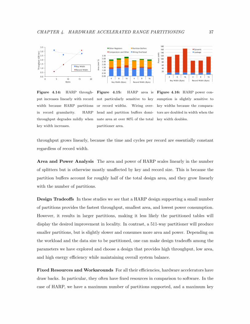
CHAPTER 4. HARDWARE ACCELERATED RANGE PARTITIONING 37
0.0
0.5
1.0
1.5
2.0
2.5
3.0
3.5
0 5 10 15 20
Thro
ughp
ut (
GB/
sec)
Bytes
Key Width
Record Width
Figure 4.14: HARP through-
put increases linearly with record
width because HARP partitions
in record granularity. HARP
throughput degrades mildly when
key width increases.
0.00
0.50
1.00
1.50
2.00
2.50
3.00
3.50
4 8 16 4 8 16
Key Width (Byte) Record Width (Byte)
Area
(m
m^2
)
Other Registers Partition Buffers
Comparators and Other Wiring Overhead
Figure 4.15: HARP area is
not particularly sensitive to key
or record widths. Wiring over-
head and partition buffers domi-
nate area at over 80% of the total
partitioner area.
20
40
60
80
100
120
140
160
180
4 8 16 4 8 16
Key Width (Byte) Record Width (Byte)
Pow
er (
mW
)
Dynamic Leakage
Figure 4.16: HARP power con-
sumption is slightly sensitive to
key widths because the compara-
tors are doubled in width when the
key width doubles.
throughput grows linearly, because the time and cycles per record are essentially constant
regardless of record width.
Area and Power Analysis The area and power of HARP scales linearly in the number
of splitters but is otherwise mostly unaffected by key and record size. This is because the
partition buffers account for roughly half of the total design area, and they grow linearly
with the number of partitions.
Design Tradeoffs In these studies we see that a HARP design supporting a small number
of partitions provides the fastest throughput, smallest area, and lowest power consumption.
However, it results in larger partitions, making it less likely the partitioned tables will
display the desired improvement in locality. In contrast, a 511-way partitioner will produce
smaller partitions, but is slightly slower and consumes more area and power. Depending on
the workload and the data size to be partitioned, one can make design tradeoffs among the
parameters we have explored and choose a design that provides high throughput, low area,
and high energy efficiency while maintaining overall system balance.
Fixed Resources and Workarounds For all their efficiencies, hardware accelerators have
draw backs. In particular, they often have fixed resources in comparison to software. In the
case of HARP, we have a maximum number of partitions supported, and a maximum key
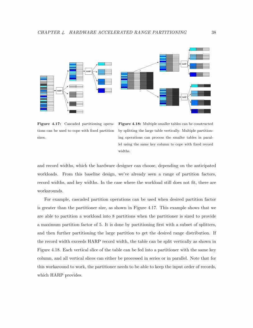
CHAPTER 4. HARDWARE ACCELERATED RANGE PARTITIONING 38
HARP
HARP
Figure 4.17: Cascaded partitioning opera-
tions can be used to cope with fixed partition
sizes.
HARP
HARP
Figure 4.18: Multiple smaller tables can be constructed
by splitting the large table vertically. Multiple partition-
ing operations can process the smaller tables in paral-
lel using the same key column to cope with fixed record
widths.
and record widths, which the hardware designer can choose, depending on the anticipated
workloads. From this baseline design, we’ve already seen a range of partition factors,
record widths, and key widths. In the case where the workload still does not fit, there are
workarounds.
For example, cascaded partition operations can be used when desired partition factor
is greater than the partitioner size, as shown in Figure 4.17. This example shows that we
are able to partition a workload into 8 partitions when the partitioner is sized to provide
a maximum partition factor of 5. It is done by partitioning first with a subset of splitters,
and then further partitioning the large partition to get the desired range distribution. If
the record width exceeds HARP record width, the table can be split vertically as shown in
Figure 4.18. Each vertical slice of the table can be fed into a partitioner with the same key
column, and all vertical slices can either be processed in series or in parallel. Note that for
this workaround to work, the partitioner needs to be able to keep the input order of records,
which HARP provides.
CHAPTER 4. HARDWARE ACCELERATED RANGE PARTITIONING 39
4.8 Summary of Findings on HARP
We presented the design and implementation of HARP, a hardware accelerated range parti-
tioner. HARP is able to provide a compute bandwidth of at least 7.8 times a very efficient
software algorithm running on an aggressive Xeon core, with just 6.9% of the area and
4.3% of the power. Processing data with accelerators such as HARP can alleviate serial
performance bottlenecks in the application and can free up resources on the server to do
other useful work.
This experiment corroborates our findings on datatype acceleration that when the accel-
eration target is carefully chosen, it can provide substantial performance gains and energy
savings across a domain of applications that employ such datatypes. In the case of HARP,
processing columns of data together using specialized control and datapaths achieved an
order of magnitude efficiency compared to same algorithm implemented in software.
However, as mentioned in the introduction of this thesis, most accelerators have ad-hoc
communication infrastructure to and from the general purpose processors and the interfaces
are often difficult to program. We will look at how to integrate a streaming accelerator such
as HARP into an existing general processor system next.
CHAPTER 5. A HARDWARE-SOFTWARE STREAMING FRAMEWORK 40
Chapter 5
A Hardware-Software Streaming
Framework
Accelerators are integrated into a system with one or more general processors in various
fashions. These integration choices often depend on the acceleration target granularity
and workload characteristics. For example, GPUs are integrated with a general processor
system as offload engines via device drivers and high-bandwidth PCIe [PCI-SIG, 2011] or
HyperTransport [HyperTransport Consortium, 2009] buses. The accelerator, in this case,
communicates with the general purpose processor using indirect access through a bus or
some type of interconnect. GPUs and the general processor(s) usually do not share memory
or address space, but there are proposals that allow either the appearance of a shared
coherent memory [Kelm et al., 2009] or a partially coherent memory [Saha and others, 2009;
Wang et al., 2007]. ISA extensions and math co-processors are examples of a much more
tightly-coupled integration model. In this model, the accelerator is tightly integrated into
the general purpose processor, often times on the same physical die, and share the same
main memory and use the same address space.
In designing an integration model for an accelerator like HARP, we consider the fact
that partitioning is often an auxiliary function that is not specific to any single operation
or query. Partitioned-joins, partitioned-sorts, and partitioned-aggregations are some of the
example operations that HARP can help accelerate. This necessitates frequent and fast
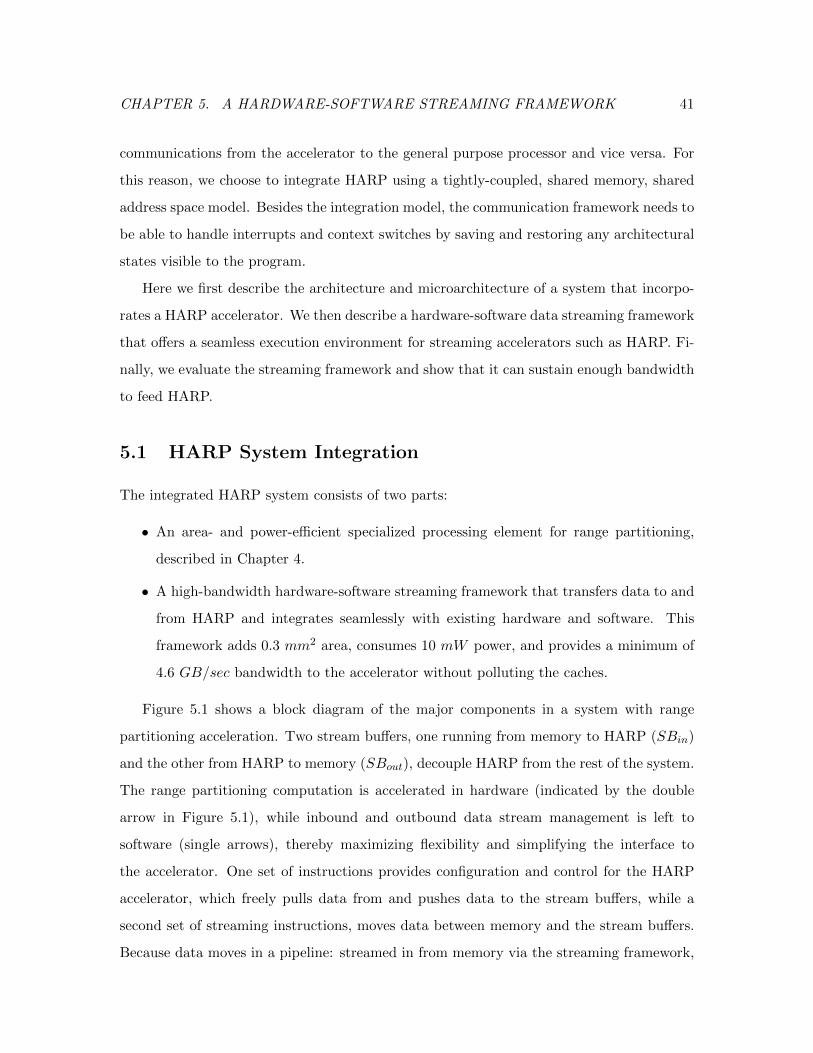
CHAPTER 5. A HARDWARE-SOFTWARE STREAMING FRAMEWORK 41
communications from the accelerator to the general purpose processor and vice versa. For
this reason, we choose to integrate HARP using a tightly-coupled, shared memory, shared
address space model. Besides the integration model, the communication framework needs to
be able to handle interrupts and context switches by saving and restoring any architectural
states visible to the program.
Here we first describe the architecture and microarchitecture of a system that incorpo-
rates a HARP accelerator. We then describe a hardware-software data streaming framework
that offers a seamless execution environment for streaming accelerators such as HARP. Fi-
nally, we evaluate the streaming framework and show that it can sustain enough bandwidth
to feed HARP.
5.1 HARP System Integration
The integrated HARP system consists of two parts:
• An area- and power-efficient specialized processing element for range partitioning,
described in Chapter 4.
• A high-bandwidth hardware-software streaming framework that transfers data to and
from HARP and integrates seamlessly with existing hardware and software. This
framework adds 0.3 mm2 area, consumes 10 mW power, and provides a minimum of
4.6 GB/sec bandwidth to the accelerator without polluting the caches.
Figure 5.1 shows a block diagram of the major components in a system with range
partitioning acceleration. Two stream buffers, one running from memory to HARP (SBin)
and the other from HARP to memory (SBout), decouple HARP from the rest of the system.
The range partitioning computation is accelerated in hardware (indicated by the double
arrow in Figure 5.1), while inbound and outbound data stream management is left to
software (single arrows), thereby maximizing flexibility and simplifying the interface to
the accelerator. One set of instructions provides configuration and control for the HARP
accelerator, which freely pulls data from and pushes data to the stream buffers, while a
second set of streaming instructions, moves data between memory and the stream buffers.
Because data moves in a pipeline: streamed in from memory via the streaming framework,
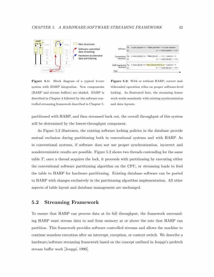
CHAPTER 5. A HARDWARE-SOFTWARE STREAMING FRAMEWORK 42
SBin
SBout
HARP(Fig 10)
Core
L1
Memory Controller
Memory
SBin
SBout
HARP(Fig 10)
Core
L1
New structures
Hardware-accelerateddata partitioningL2 L2
Software controlleddata streaming
Figure 5.1: Block diagram of a typical 2-core
system with HARP integration. New components
(HARP and stream buffers) are shaded. HARP is
described in Chapter 4 followed by the software con-
trolled streaming framework described in Chapter 5.
SoftwareLock acquire Table partition Lock release
Lock acquire
ConventionalHardware
Lock.{ld,st} Table.{ld,st} ... Lock.st
Lock.{ld,st}
HARP AugmentedHardware
Lock.{ld,st} Table.{sbload,sbstore}... Lock.st
Lock.{ld,st}
Time
T0
T1
T0T1
T0T1
Figure 5.2: With or without HARP, correct mul-
tithreaded operation relies on proper software-level
locking. As illustrated here, the streaming frame-
work works seamlessly with existing synchronization
and data layouts.
partitioned with HARP, and then streamed back out, the overall throughput of this system
will be determined by the lowest-throughput component.
As Figure 5.2 illustrates, the existing software locking policies in the database provide
mutual exclusion during partitioning both in conventional systems and with HARP. As
in conventional systems, if software does not use proper synchronization, incorrect and
nondeterministic results are possible. Figure 5.2 shows two threads contending for the same
table T ; once a thread acquires the lock, it proceeds with partitioning by executing either
the conventional software partitioning algorithm on the CPU, or streaming loads to feed
the table to HARP for hardware partitioning. Existing database software can be ported
to HARP with changes exclusively in the partitioning algorithm implementation. All other
aspects of table layout and database management are unchanged.
5.2 Streaming Framework
To ensure that HARP can process data at its full throughput, the framework surround-
ing HARP must stream data to and from memory at or above the rate that HARP can
partition. This framework provides software controlled streams and allows the machine to
continue seamless execution after an interrupt, exception, or context switch. We describe a
hardware/software streaming framework based on the concept outlined in Jouppi’s prefetch
stream buffer work [Jouppi, 1990].
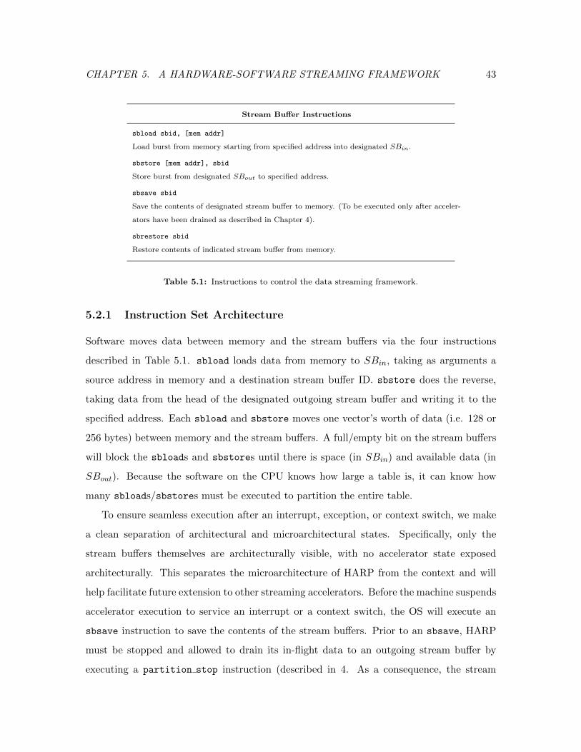
CHAPTER 5. A HARDWARE-SOFTWARE STREAMING FRAMEWORK 43
Stream Buffer Instructions
sbload sbid, [mem addr]
Load burst from memory starting from specified address into designated SBin.
sbstore [mem addr], sbid
Store burst from designated SBout to specified address.
sbsave sbid
Save the contents of designated stream buffer to memory. (To be executed only after acceler-
ators have been drained as described in Chapter 4).
sbrestore sbid
Restore contents of indicated stream buffer from memory.
Table 5.1: Instructions to control the data streaming framework.
5.2.1 Instruction Set Architecture
Software moves data between memory and the stream buffers via the four instructions
described in Table 5.1. sbload loads data from memory to SBin, taking as arguments a
source address in memory and a destination stream buffer ID. sbstore does the reverse,
taking data from the head of the designated outgoing stream buffer and writing it to the
specified address. Each sbload and sbstore moves one vector’s worth of data (i.e. 128 or
256 bytes) between memory and the stream buffers. A full/empty bit on the stream buffers
will block the sbloads and sbstores until there is space (in SBin) and available data (in
SBout). Because the software on the CPU knows how large a table is, it can know how
many sbloads/sbstores must be executed to partition the entire table.
To ensure seamless execution after an interrupt, exception, or context switch, we make
a clean separation of architectural and microarchitectural states. Specifically, only the
stream buffers themselves are architecturally visible, with no accelerator state exposed
architecturally. This separates the microarchitecture of HARP from the context and will
help facilitate future extension to other streaming accelerators. Before the machine suspends
accelerator execution to service an interrupt or a context switch, the OS will execute an
sbsave instruction to save the contents of the stream buffers. Prior to an sbsave, HARP
must be stopped and allowed to drain its in-flight data to an outgoing stream buffer by
executing a partition stop instruction (described in 4. As a consequence, the stream
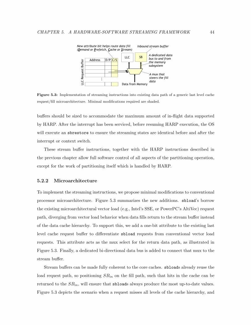
CHAPTER 5. A HARDWARE-SOFTWARE STREAMING FRAMEWORK 44
LLC R
equest B
uff
er Address D/P C/S
Data from Memory
LLC
A mux that
steers the fill
data
A dedicated data
bus to and from
the memory
subsystem
Inbound stream buffer
...
New attribute bit helps route data fill
(Demand or Prefetch, Cache or Stream)
SB
Figure 5.3: Implementation of streaming instructions into existing data path of a generic last level cache
request/fill microarchitecture. Minimal modifications required are shaded.
buffers should be sized to accommodate the maximum amount of in-flight data supported
by HARP. After the interrupt has been serviced, before resuming HARP execution, the OS
will execute an sbrestore to ensure the streaming states are identical before and after the
interrupt or context switch.
These stream buffer instructions, together with the HARP instructions described in
the previous chapter allow full software control of all aspects of the partitioning operation,
except for the work of partitioning itself which is handled by HARP.
5.2.2 Microarchitecture
To implement the streaming instructions, we propose minimal modifications to conventional
processor microarchitecture. Figure 5.3 summarizes the new additions. sbload’s borrow
the existing microarchitectural vector load (e.g., Intel’s SSE, or PowerPC’s AltiVec) request
path, diverging from vector load behavior when data fills return to the stream buffer instead
of the data cache hierarchy. To support this, we add a one-bit attribute to the existing last
level cache request buffer to differentiate sbload requests from conventional vector load
requests. This attribute acts as the mux select for the return data path, as illustrated in
Figure 5.3. Finally, a dedicated bi-directional data bus is added to connect that mux to the
stream buffer.
Stream buffers can be made fully coherent to the core caches. sbloads already reuse the
load request path, so positioning SBin on the fill path, such that hits in the cache can be
returned to the SBin, will ensure that sbloads always produce the most up-to-date values.
Figure 5.3 depicts the scenario when a request misses all levels of the cache hierarchy, and
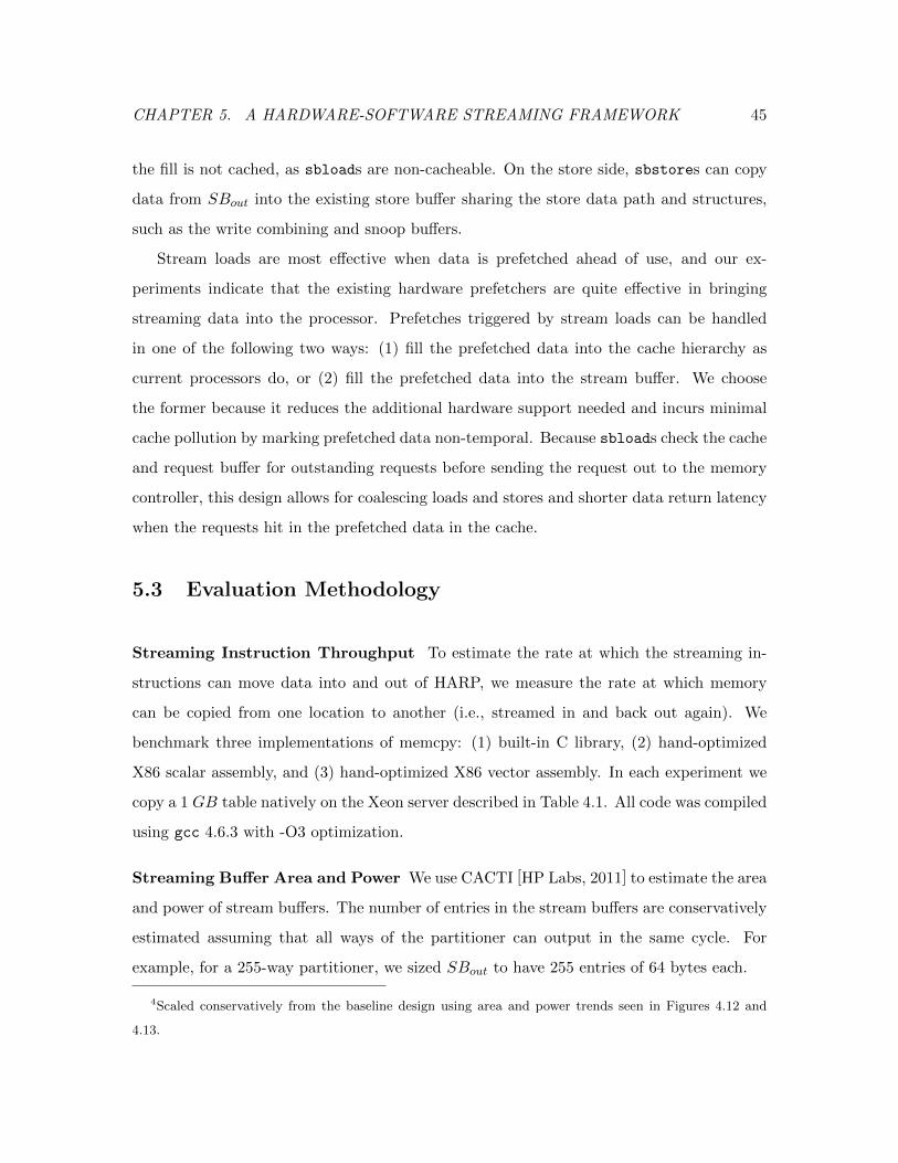
CHAPTER 5. A HARDWARE-SOFTWARE STREAMING FRAMEWORK 45
the fill is not cached, as sbloads are non-cacheable. On the store side, sbstores can copy
data from SBout into the existing store buffer sharing the store data path and structures,
such as the write combining and snoop buffers.
Stream loads are most effective when data is prefetched ahead of use, and our ex-
periments indicate that the existing hardware prefetchers are quite effective in bringing
streaming data into the processor. Prefetches triggered by stream loads can be handled
in one of the following two ways: (1) fill the prefetched data into the cache hierarchy as
current processors do, or (2) fill the prefetched data into the stream buffer. We choose
the former because it reduces the additional hardware support needed and incurs minimal
cache pollution by marking prefetched data non-temporal. Because sbloads check the cache
and request buffer for outstanding requests before sending the request out to the memory
controller, this design allows for coalescing loads and stores and shorter data return latency
when the requests hit in the prefetched data in the cache.
5.3 Evaluation Methodology
Streaming Instruction Throughput To estimate the rate at which the streaming in-
structions can move data into and out of HARP, we measure the rate at which memory
can be copied from one location to another (i.e., streamed in and back out again). We
benchmark three implementations of memcpy: (1) built-in C library, (2) hand-optimized
X86 scalar assembly, and (3) hand-optimized X86 vector assembly. In each experiment we
copy a 1 GB table natively on the Xeon server described in Table 4.1. All code was compiled
using gcc 4.6.3 with -O3 optimization.
Streaming Buffer Area and Power We use CACTI [HP Labs, 2011] to estimate the area
and power of stream buffers. The number of entries in the stream buffers are conservatively
estimated assuming that all ways of the partitioner can output in the same cycle. For
example, for a 255-way partitioner, we sized SBout to have 255 entries of 64 bytes each.
4Scaled conservatively from the baseline design using area and power trends seen in Figures 4.12 and
4.13.
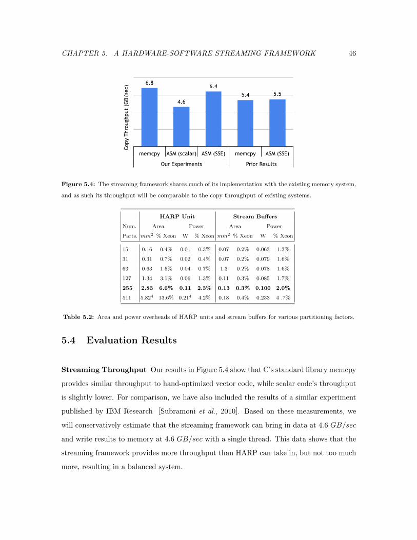
CHAPTER 5. A HARDWARE-SOFTWARE STREAMING FRAMEWORK 46
6.8
4.6
6.4
5.4 5.5
memcpy ASM (scalar) ASM (SSE) memcpy ASM (SSE)
Our Experiments Prior Results
Copy
Thr
ough
put
(GB/
sec)
Figure 5.4: The streaming framework shares much of its implementation with the existing memory system,
and as such its throughput will be comparable to the copy throughput of existing systems.
HARP Unit Stream Buffers
Num. Area Power Area Power
Parts. mm2 % Xeon W % Xeon mm2 % Xeon W % Xeon
15 0.16 0.4% 0.01 0.3% 0.07 0.2% 0.063 1.3%
31 0.31 0.7% 0.02 0.4% 0.07 0.2% 0.079 1.6%
63 0.63 1.5% 0.04 0.7% 1.3 0.2% 0.078 1.6%
127 1.34 3.1% 0.06 1.3% 0.11 0.3% 0.085 1.7%
255 2.83 6.6% 0.11 2.3% 0.13 0.3% 0.100 2.0%
511 5.824 13.6% 0.214 4.2% 0.18 0.4% 0.233 4 .7%
Table 5.2: Area and power overheads of HARP units and stream buffers for various partitioning factors.
5.4 Evaluation Results
Streaming Throughput Our results in Figure 5.4 show that C’s standard library memcpy
provides similar throughput to hand-optimized vector code, while scalar code’s throughput
is slightly lower. For comparison, we have also included the results of a similar experiment
published by IBM Research [Subramoni et al., 2010]. Based on these measurements, we
will conservatively estimate that the streaming framework can bring in data at 4.6 GB/sec
and write results to memory at 4.6 GB/sec with a single thread. This data shows that the
streaming framework provides more throughput than HARP can take in, but not too much
more, resulting in a balanced system.
CHAPTER 5. A HARDWARE-SOFTWARE STREAMING FRAMEWORK 47
Area and Power Efficiency Because the stream buffers are sized according to the accel-
erators they serve, we quantify their area and power overheads for each HARP partitioning
factor we consider in Table 5.2. The proposed streaming framework adds 0.3 mm2 area,
consumes 10 mW power for a baseline HARP configuration. Together, HARP and the SBs
add just 6.9% area and 4.3% power of a Xeon core, while delivering 7.8X performance gain
over single-threaded software.
5.5 Summary of Findings on Streaming Framework
We have described a HARP system that provide seamless execution of streaming accelera-
tors in modern computer systems and exceptional throughput and power efficiency advan-
tages over software. These benefits are necessary to address the ever increasing demands of
big data processing. This proposed framework can be utilized for other database process-
ing accelerators such as specialized aggregators, joiners, sorters, and so on, setting forth a
flexible yet modular data-centric acceleration framework.
CHAPTER 6. Q100: A FIRST DPU 48
Chapter 6
Q100: A First DPU
The design and evaluation in Chapters 4 and 5 showed promising results for the HARP
accelerator, allowing us to extend the ASIC concept to a collection of tiles, that perform
other database operations. Our vision is a class of domain-specific database processors that
can efficiently handle database applications called Database Processing Units, or DPUs.
Instead of processing only part of a relational database query, DPUs would process entire
queries to take advantage of the fact that the data needed to compute that query is already
moved from main memory into the accelerator, and therefore reduce data movement for
intermediate results by pipelining relational operations one after another.
To further evaluate our hypothesis that grouping and processing datatypes used for rela-
tional database applications, namely columns and tables, we are able to provide substantial
efficiency using specialized hardware, we architect, design, and evaluate a first DPU, called
Q100. The Q100 is a performance and energy efficient data analysis accelerator. It contains
a collection of heterogeneous ASIC tiles that process relational tables and columns quickly
and energy-efficiently. The architecture uses coarse grained instructions that manipulate
streams of data, thereby maximizing pipeline and data parallelism, and minimizing the need
to time multiplex the accelerator tiles and spill intermediate results to memory. We explore
a Q100 design space of 150 configurations, selecting three for further analysis: a small,
power-conscious implementation, a high-performance implementation, and a balanced de-
sign that maximizes performance per Watt. We then demonstrate that the power-conscious
Q100 handles the TPC-H queries with three orders of magnitude less energy than a state of
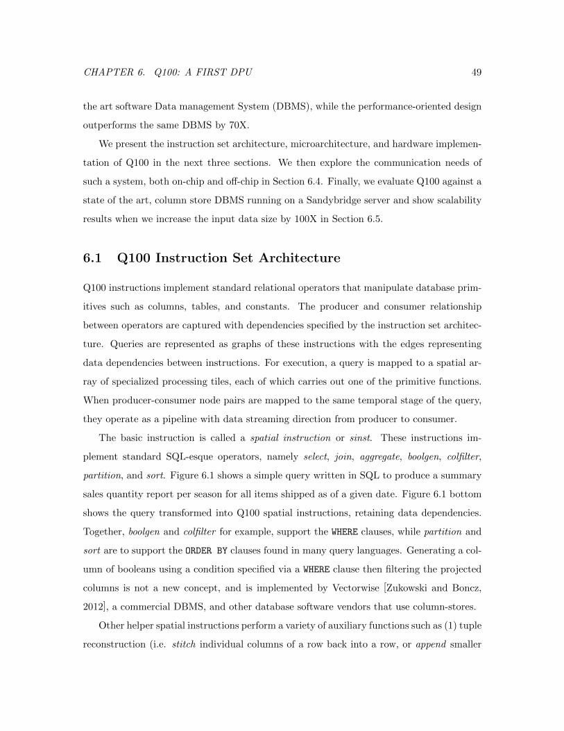
CHAPTER 6. Q100: A FIRST DPU 49
the art software Data management System (DBMS), while the performance-oriented design
outperforms the same DBMS by 70X.
We present the instruction set architecture, microarchitecture, and hardware implemen-
tation of Q100 in the next three sections. We then explore the communication needs of
such a system, both on-chip and off-chip in Section 6.4. Finally, we evaluate Q100 against a
state of the art, column store DBMS running on a Sandybridge server and show scalability
results when we increase the input data size by 100X in Section 6.5.
6.1 Q100 Instruction Set Architecture
Q100 instructions implement standard relational operators that manipulate database prim-
itives such as columns, tables, and constants. The producer and consumer relationship
between operators are captured with dependencies specified by the instruction set architec-
ture. Queries are represented as graphs of these instructions with the edges representing
data dependencies between instructions. For execution, a query is mapped to a spatial ar-
ray of specialized processing tiles, each of which carries out one of the primitive functions.
When producer-consumer node pairs are mapped to the same temporal stage of the query,
they operate as a pipeline with data streaming direction from producer to consumer.
The basic instruction is called a spatial instruction or sinst. These instructions im-
plement standard SQL-esque operators, namely select, join, aggregate, boolgen, colfilter,
partition, and sort. Figure 6.1 shows a simple query written in SQL to produce a summary
sales quantity report per season for all items shipped as of a given date. Figure 6.1 bottom
shows the query transformed into Q100 spatial instructions, retaining data dependencies.
Together, boolgen and colfilter for example, support the WHERE clauses, while partition and
sort are to support the ORDER BY clauses found in many query languages. Generating a col-
umn of booleans using a condition specified via a WHERE clause then filtering the projected
columns is not a new concept, and is implemented by Vectorwise [Zukowski and Boncz,
2012], a commercial DBMS, and other database software vendors that use column-stores.
Other helper spatial instructions perform a variety of auxiliary functions such as (1) tuple
reconstruction (i.e. stitch individual columns of a row back into a row, or append smaller
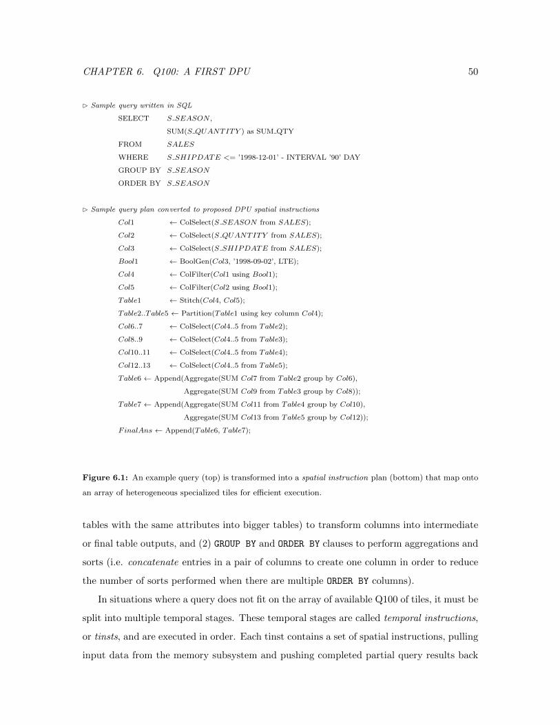
CHAPTER 6. Q100: A FIRST DPU 50
B Sample query written in SQL
SELECT S SEASON ,
SUM(S QUANTITY ) as SUM QTY
FROM SALES
WHERE S SHIPDATE <= ’1998-12-01’ - INTERVAL ’90’ DAY
GROUP BY S SEASON
ORDER BY S SEASON
B Sample query plan converted to proposed DPU spatial instructions
Col1 ← ColSelect(S SEASON from SALES);
Col2 ← ColSelect(S QUANTITY from SALES);
Col3 ← ColSelect(S SHIPDATE from SALES);
Bool1 ← BoolGen(Col3, ’1998-09-02’, LTE);
Col4 ← ColFilter(Col1 using Bool1);
Col5 ← ColFilter(Col2 using Bool1);
Table1 ← Stitch(Col4, Col5);
Table2..Table5 ← Partition(Table1 using key column Col4);
Col6..7 ← ColSelect(Col4..5 from Table2);
Col8..9 ← ColSelect(Col4..5 from Table3);
Col10..11 ← ColSelect(Col4..5 from Table4);
Col12..13 ← ColSelect(Col4..5 from Table5);
Table6 ← Append(Aggregate(SUM Col7 from Table2 group by Col6),
Aggregate(SUM Col9 from Table3 group by Col8));
Table7 ← Append(Aggregate(SUM Col11 from Table4 group by Col10),
Aggregate(SUM Col13 from Table5 group by Col12));
FinalAns ← Append(Table6, Table7);
Figure 6.1: An example query (top) is transformed into a spatial instruction plan (bottom) that map onto
an array of heterogeneous specialized tiles for efficient execution.
tables with the same attributes into bigger tables) to transform columns into intermediate
or final table outputs, and (2) GROUP BY and ORDER BY clauses to perform aggregations and
sorts (i.e. concatenate entries in a pair of columns to create one column in order to reduce
the number of sorts performed when there are multiple ORDER BY columns).
In situations where a query does not fit on the array of available Q100 of tiles, it must be
split into multiple temporal stages. These temporal stages are called temporal instructions,
or tinsts, and are executed in order. Each tinst contains a set of spatial instructions, pulling
input data from the memory subsystem and pushing completed partial query results back
CHAPTER 6. Q100: A FIRST DPU 51
(a) Unrestricted Graph of Spatial Instructions
(b) Resource Profile
(c) Resource-Aware Temporal Instructions
4 ColSelect 2 ColFilter 2 BoolGen 1 Stitch 1 Part 2 Aggregator 2 Appender
SALES
BoolGen
Col3
Col2
Col1
ColSelect
ColSelect
ColFilter
ColFilter
Bool1
Stitch
Col4
Col5
Table1
Agg
Agg
Agg
Agg
Parti-tion
Table2
Table4
Table5
Append
FinalAnswer
Table6
Table7
Append
Append
ColSelect
ColSelectCol
Select
ColSelectCol
Select
ColSelectCol
Select
ColSelectCol
Select
Col6
Col7
Col8
Col9
Col10
Col11
Col12
Col13
Temporal Instruction #1
Temporal Instruction #2
Temporal Instruction #3
Table3
Figure 6.2: The example query from Figure 6.1 is mapped onto a directed graph with nodes as relational
operators and edges as data dependencies. Given a set of Q100 resources, the graph is broken into three
temporal instructions that are executed in sequence, one after another.
to the memory subsystem. Figure 6.2 walks through how a graph representation of spatial
instructions, implementing the example query from Figure 6.1, is mapped onto available spe-
cialized processing tiles. Figure 6.2 (a) shows the entire query as one graph with each shape
representing a different primitive and edges representing producer-consumer relationships
(i.e., data dependencies). Figure 6.2 (b) shows an example array of specialized hardware
CHAPTER 6. Q100: A FIRST DPU 52
tiles, or a resource profile, for a particular Q100 configuration. Figure 6.2 (c) depicts how
the query must to be broken into three temporal instructions, because the resource profile
does not have enough column selectors, column filters, aggregators, or appenders at each
stage.
This instruction set architecture is energy efficient because it closely matches building
blocks of our target domain, while simultaneously encapsulating operations that can be
implemented very efficiently in hardware. Spatial instructions are executed in a dataflow-
esque style seen in dataflow machines in the 80’s [Gurd et al., 1985; Dennis, 1991], in the
90’s [Hicks et al., 1993], and more recently [Swanson et al., 2007; Gebhart et al., 2009;
Parashar et al., 2013], eliminating complex issue and control logic, exposing parallelism,
and passing data dependencies directly from producer to consumer. All of these features
provide performance benefit and energy savings.
6.2 Q100 Microarchitecture
The Q100 contains eleven types of hardware tile corresponding to the eleven operators in
the ISA. As in the ISA, we break the discussion into core functional tiles and auxiliary
helper tiles. The facts and figures of this section are summarized in Table 6.1, while the
text that follows focuses on the design choices and tradeoffs. The slowest tile determines the
clock cycle of the Q100. As Table 6.1 indicates, the partitioner limits the Q100 frequency
to 315 MHz.
Methodology. Each tile has been implemented in Verilog and synthesized, placed, and
routed using Synopsys 32nm Generic Libraries1 with the Synopsys [Synopsys, Inc., 2013]
Design and IC Compilers to produce timing, area, and power numbers. We report the
post-place-and-route critical path of each design as logic delay plus clock network delay,
adhering to the industry standard of reporting critical paths with a margin.
1Normal operating conditions (1.25V supply voltage at 25◦C) with high threshold voltage to minimize
leakage.
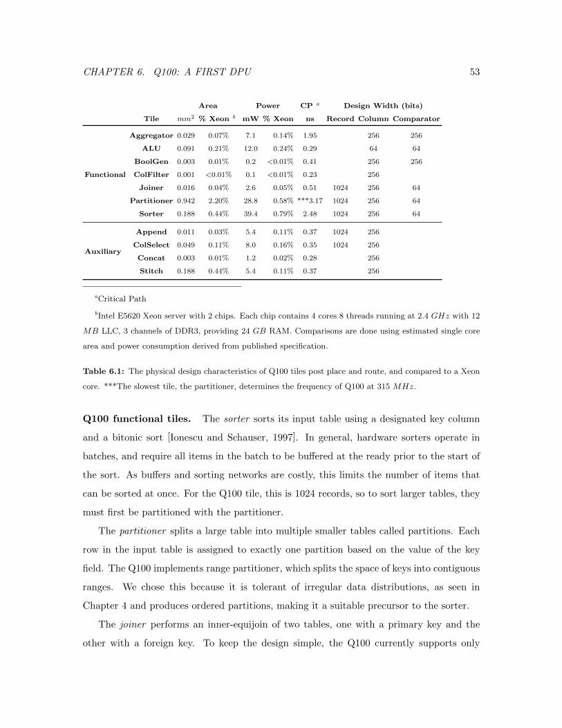
CHAPTER 6. Q100: A FIRST DPU 53
Area Power CP a Design Width (bits)
Tile mm2 % Xeon b mW % Xeon ns Record Column Comparator
Functional
Aggregator 0.029 0.07% 7.1 0.14% 1.95 256 256
ALU 0.091 0.21% 12.0 0.24% 0.29 64 64
BoolGen 0.003 0.01% 0.2 <0.01% 0.41 256 256
ColFilter 0.001 <0.01% 0.1 <0.01% 0.23 256
Joiner 0.016 0.04% 2.6 0.05% 0.51 1024 256 64
Partitioner 0.942 2.20% 28.8 0.58% ***3.17 1024 256 64
Sorter 0.188 0.44% 39.4 0.79% 2.48 1024 256 64
Auxiliary
Append 0.011 0.03% 5.4 0.11% 0.37 1024 256
ColSelect 0.049 0.11% 8.0 0.16% 0.35 1024 256
Concat 0.003 0.01% 1.2 0.02% 0.28 256
Stitch 0.188 0.44% 5.4 0.11% 0.37 256
aCritical Path
bIntel E5620 Xeon server with 2 chips. Each chip contains 4 cores 8 threads running at 2.4 GHz with 12
MB LLC, 3 channels of DDR3, providing 24 GB RAM. Comparisons are done using estimated single core
area and power consumption derived from published specification.
Table 6.1: The physical design characteristics of Q100 tiles post place and route, and compared to a Xeon
core. ***The slowest tile, the partitioner, determines the frequency of Q100 at 315 MHz.
Q100 functional tiles. The sorter sorts its input table using a designated key column
and a bitonic sort [Ionescu and Schauser, 1997]. In general, hardware sorters operate in
batches, and require all items in the batch to be buffered at the ready prior to the start of
the sort. As buffers and sorting networks are costly, this limits the number of items that
can be sorted at once. For the Q100 tile, this is 1024 records, so to sort larger tables, they
must first be partitioned with the partitioner.
The partitioner splits a large table into multiple smaller tables called partitions. Each
row in the input table is assigned to exactly one partition based on the value of the key
field. The Q100 implements range partitioner, which splits the space of keys into contiguous
ranges. We chose this because it is tolerant of irregular data distributions, as seen in
Chapter 4 and produces ordered partitions, making it a suitable precursor to the sorter.
The joiner performs an inner-equijoin of two tables, one with a primary key and the
other with a foreign key. To keep the design simple, the Q100 currently supports only
CHAPTER 6. Q100: A FIRST DPU 54
inner-equijoins. It is by far the most common type of join, though extending the joiner to
support other types (e.g., outer-joins) would not increase its area or power substantially.
The ALU tile performs arithmetic and logical operations on two input columns, pro-
ducing one output column. It supports all arithmetic and logical operations found in SQL
(i.e., ADD, SUB, MUL, DIV, AND, OR, and NOT) as well as constant multiplication
and division. We use these latter operations to work around the current lack of a floating
point unit in the Q100. In its place, we multiply any SQL decimal data type by a large
constant, apply the integer arithmetic, finally divide the result by the original scaling fac-
tor, effectively using fixed point to support single precision floating point arithmetic, as
most domain-specific accelerators have done. SQL does not specify precision requirements
for floating point calculations and most commercial DBMS supports either single-precision
floating point and/or double-precision floating point calculations.
The boolean generator compares an input column with either a constant or a second
input column, producing a column of boolean values. Using just two hardware comparators,
the tile provides all six comparisons used in SQL (i.e. EQ, NEQ, LTE, LT, GT, GTE). While
this tile could have been combined with the ALU, offering two tiles a la carte leaves more
flexibility when allocating tile resources. The boolean generator is often paired with the
column filter (described next) with no need for an ALU. It is also often used in a chain or
tree to form complex predicates, again not always in 1-to-1 correspondence with ALUs.
The column filter takes in a column of booleans (from a boolean generator) and a
second data column. It outputs the same data column but dropping all rows where the
corresponding bool is false.
Finally the aggregator takes in the column to be aggregated and a “group by” column
whose values determine which entries in the first column to aggregate. For example, if the
query sums purchases by zipcode, the data column are the purchase totals while the group-
by is the zipcode. The tile requires that both input columns arrive sorted on the group-by
column so that the tile can simply compare consecutive group-by values to determine where
to close each aggregation. This decision has tradeoffs. A hash-based implementation might
not require pre-sorting, but it would require a buffer of unknown size to maintain the partial
CHAPTER 6. Q100: A FIRST DPU 55
aggregation results for each group. The Q100 aggregator supports all aggregation operations
in the SQL spec, namely MAX, MIN, COUNT, SUM, and AVG.
Q100 auxiliary tiles. The column selector extracts a column from a table, and the
column stitcher does the inverse, taking multiple input columns (up to a maximum total
width) and producing a table. This operation often precedes partitions and sorts where
queries frequently require column A sorted according to the values in column B. The col-
umn concatenator concatenates corresponding entries in two input columns to produce one
output column. This can cut down on sorts and partitions when a query requires sorting
or grouping on more than one attribute (i.e., column). Finally, the table appender appends
two tables with the same schema. This is often used to combine the results of per-partition
computations.
Modifications to TPC-H due to tile limitations. The design parameters such as
record, column, key, and comparator widths are generally sized conservatively. However,
we encountered a small number of situations where we had to modify the layout of an
underlying table or adjust the operation, though never the semantics, of a query. When a
column width exceeds the 32 byte maximum column width the Q100 can support, we divide
the wide column vertically into smaller ones of no more than 32 bytes and process them
in parallel. Out of 8 tables and 61 columns in TPC-H, just 10 were split in this fashion.
Similarly, because the Q100 does not currently support regular expression matching, as with
the SQL LIKE keyword, the query is converted to use as many WHERE EQ clauses as required.
These are all minor side effects of the current Q100 design and may not be required in future
implementations.
Coping with fixed hardware. Most Q100 tiles are agnostic to the number of records
they process. The sorter is the exception. To sort a table that has more than what the
hardware has provisioned (in the case of the Q100, it is 1024 records), a partitioner needs to
be used first to partition the records into chunks that are smaller than what the sorter can
take in. The partitioned chunks are then fed into the sorters for sorting. The sorted records
can then be appended to form a sorted table if necessary. From the hardware perspective,
CHAPTER 6. Q100: A FIRST DPU 56
Q100 can implement an exception handler that raises an exception when the number of
input records to the sorter exceeds 1024, and leave it to software to reschedule the query
with appropriate number of partitioners followed by sorters and re-execute the query. The
scheduler needs to be able to schedule the partitioning and sorting operations based on
dynamic data size. With respect to fixed datapath widths, we employ the same techniques
and workarounds described for the partitioner in Chapter 4.
6.3 Q100 Tile Mix Design Space Exploration
To understand the relative utility of each type of tile, and the tradeoffs amongst them, we
explore a wide design space of different sets of Q100 tiles. We start with a sensitivity analysis
of TPC-H performance, evaluating each type of tile in isolation to bound the maximum
number of useful tiles of each type. We then carry out a complete design space exploration
considering multiple tiles at once, from which we understand the power performance shape
of the Q100 space and select three configurations (i.e., tile mixtures) for further analysis.
Methodology. We have developed a functional and timing Q100 simulator in C++.
The function and throughput of each tile have been validated against simulations of the
corresponding Verilog. As we do not yet have a compiler for the Q100, we have manually
implemented each TPC-H query in the Q100 ISA. Using the simulator, we have confirmed
that the Q100 query implementations produce the same results as the SQL versions running
on MonetDB [Centrum Wiskunde and Informatica, 2012]. Given a query and a Q100 config-
uration, a scheduling algorithm, that uses a data-aware algorithm to minimize intermediate
results, schedules each query into a sequence of temporal instructions. The simulator pro-
duces cycle counts, which we convert to wall clock time using a Q100 frequency of 315 MHz.
Tile count sensitivity. To understand how sensitive Q100 is to the number of each type
of tile, say aggregators, we simulate a range of Q100 configurations, sweeping the number
aggregators, while holding all other types of tiles at sufficiently high counts so as not to limit
performance. Figure 6.3 shows how the runtime of each TPC-H varies with the number of
aggregators in the design. Having run this experiment for each of the eleven types of tile,
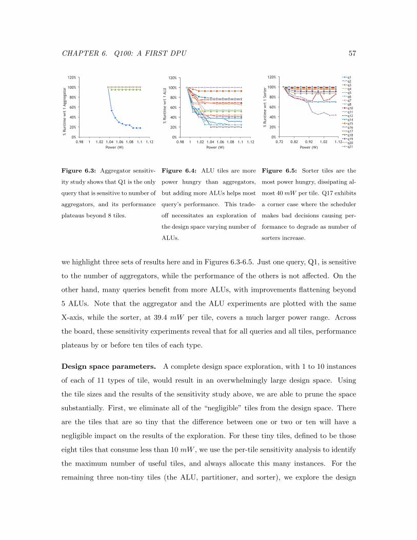
CHAPTER 6. Q100: A FIRST DPU 57
0%
20%
40%
60%
80%
100%
120%
0.98 1 1.02 1.04 1.06 1.08 1.1 1.12
% Ru
ntim
e w
rt 1
Agg
rega
tor
Power (W)
Figure 6.3: Aggregator sensitiv-
ity study shows that Q1 is the only
query that is sensitive to number of
aggregators, and its performance
plateaus beyond 8 tiles.
0%
20%
40%
60%
80%
100%
120%
0.98 1 1.02 1.04 1.06 1.08 1.1 1.12
% Ru
ntim
e w
rt 1
ALU
Power (W)
Figure 6.4: ALU tiles are more
power hungry than aggregators,
but adding more ALUs helps most
query’s performance. This trade-
off necessitates an exploration of
the design space varying number of
ALUs.
0%
20%
40%
60%
80%
100%
120%
0.72 0.82 0.92 1.02 1.12
% Ru
ntim
e w
rt 1
Sor
ter
Power (W)
q1 q2 q3 q4 q5 q6 q7 q8 q10 q11 q12 q14 q15 q16 q17 q18 q19 q20 q21
Figure 6.5: Sorter tiles are the
most power hungry, dissipating al-
most 40 mW per tile. Q17 exhibits
a corner case where the scheduler
makes bad decisions causing per-
formance to degrade as number of
sorters increase.
we highlight three sets of results here and in Figures 6.3-6.5. Just one query, Q1, is sensitive
to the number of aggregators, while the performance of the others is not affected. On the
other hand, many queries benefit from more ALUs, with improvements flattening beyond
5 ALUs. Note that the aggregator and the ALU experiments are plotted with the same
X-axis, while the sorter, at 39.4 mW per tile, covers a much larger power range. Across
the board, these sensitivity experiments reveal that for all queries and all tiles, performance
plateaus by or before ten tiles of each type.
Design space parameters. A complete design space exploration, with 1 to 10 instances
of each of 11 types of tile, would result in an overwhelmingly large design space. Using
the tile sizes and the results of the sensitivity study above, we are able to prune the space
substantially. First, we eliminate all of the “negligible” tiles from the design space. There
are the tiles that are so tiny that the difference between one or two or ten will have a
negligible impact on the results of the exploration. For these tiny tiles, defined to be those
eight tiles that consume less than 10 mW , we use the per-tile sensitivity analysis to identify
the maximum number of useful tiles, and always allocate this many instances. For the
remaining three non-tiny tiles (the ALU, partitioner, and sorter), we explore the design
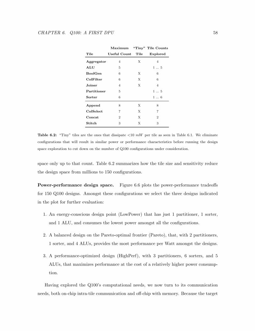
CHAPTER 6. Q100: A FIRST DPU 58
Maximum “Tiny” Tile Counts
Tile Useful Count Tile Explored
Aggregator 4 X 4
ALU 5 1 ... 5
BoolGen 6 X 6
ColFilter 6 X 6
Joiner 4 X 4
Partitioner 5 1 ... 5
Sorter 6 1 ... 6
Append 8 X 8
ColSelect 7 X 7
Concat 2 X 2
Stitch 3 X 3
Table 6.2: “Tiny” tiles are the ones that dissipate <10 mW per tile as seen in Table 6.1. We eliminate
configurations that will result in similar power or performance characteristics before running the design
space exploration to cut down on the number of Q100 configurations under consideration.
space only up to that count. Table 6.2 summarizes how the tile size and sensitivity reduce
the design space from millions to 150 configurations.
Power-performance design space. Figure 6.6 plots the power-performance tradeoffs
for 150 Q100 designs. Amongst these configurations we select the three designs indicated
in the plot for further evaluation:
1. An energy-conscious design point (LowPower) that has just 1 partitioner, 1 sorter,
and 1 ALU, and consumes the lowest power amongst all the configurations.
2. A balanced design on the Pareto-optimal frontier (Pareto), that, with 2 partitioners,
1 sorter, and 4 ALUs, provides the most performance per Watt amongst the designs.
3. A performance-optimized design (HighPerf), with 3 partitioners, 6 sorters, and 5
ALUs, that maximizes performance at the cost of a relatively higher power consump-
tion.
Having explored the Q100’s computational needs, we now turn to its communication
needs, both on-chip intra-tile communication and off-chip with memory. Because the target
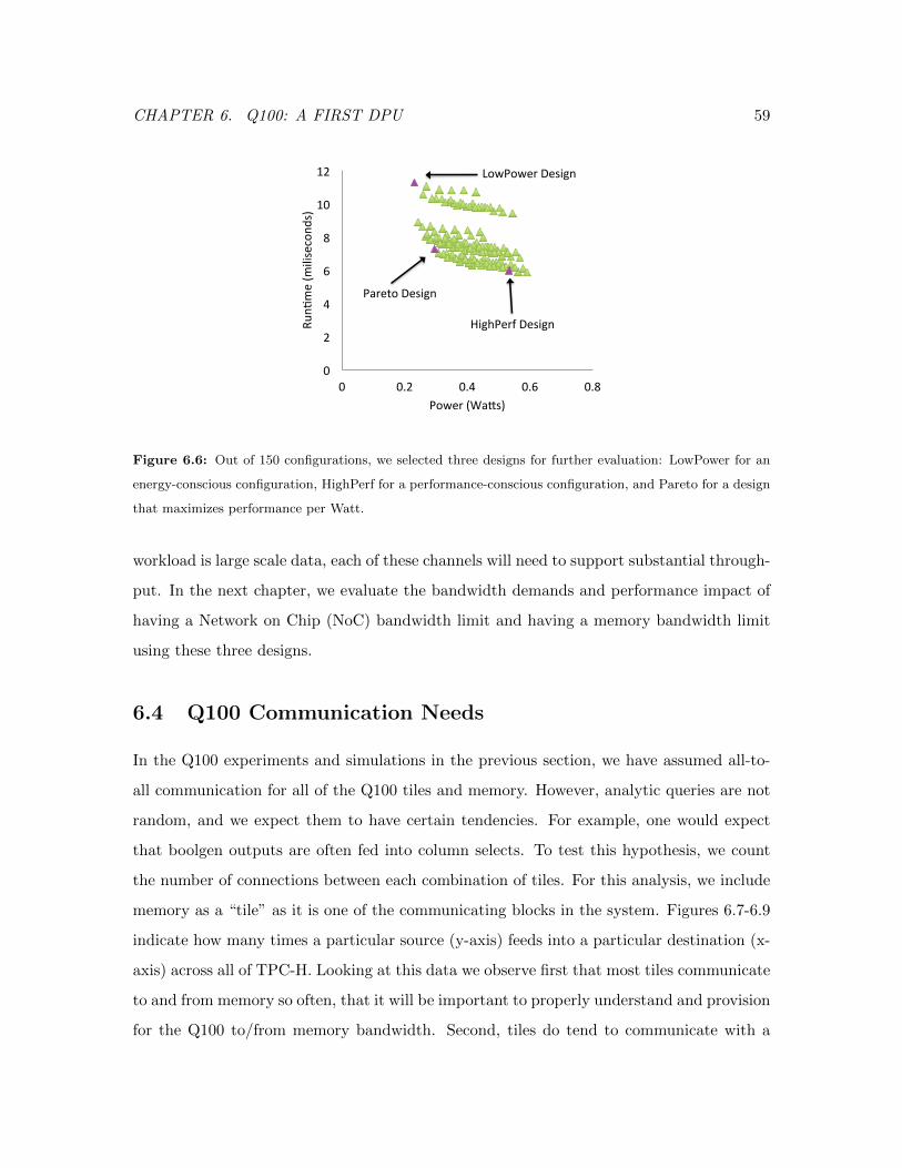
CHAPTER 6. Q100: A FIRST DPU 59
0
2
4
6
8
10
12
0 0.2 0.4 0.6 0.8
Run,
me (m
ilisecond
s)
Power (Wa<s)
Pareto Design
HighPerf Design
LowPower Design
Figure 6.6: Out of 150 configurations, we selected three designs for further evaluation: LowPower for an
energy-conscious configuration, HighPerf for a performance-conscious configuration, and Pareto for a design
that maximizes performance per Watt.
workload is large scale data, each of these channels will need to support substantial through-
put. In the next chapter, we evaluate the bandwidth demands and performance impact of
having a Network on Chip (NoC) bandwidth limit and having a memory bandwidth limit
using these three designs.
6.4 Q100 Communication Needs
In the Q100 experiments and simulations in the previous section, we have assumed all-to-
all communication for all of the Q100 tiles and memory. However, analytic queries are not
random, and we expect them to have certain tendencies. For example, one would expect
that boolgen outputs are often fed into column selects. To test this hypothesis, we count
the number of connections between each combination of tiles. For this analysis, we include
memory as a “tile” as it is one of the communicating blocks in the system. Figures 6.7-6.9
indicate how many times a particular source (y-axis) feeds into a particular destination (x-
axis) across all of TPC-H. Looking at this data we observe first that most tiles communicate
to and from memory so often, that it will be important to properly understand and provision
for the Q100 to/from memory bandwidth. Second, tiles do tend to communicate with a
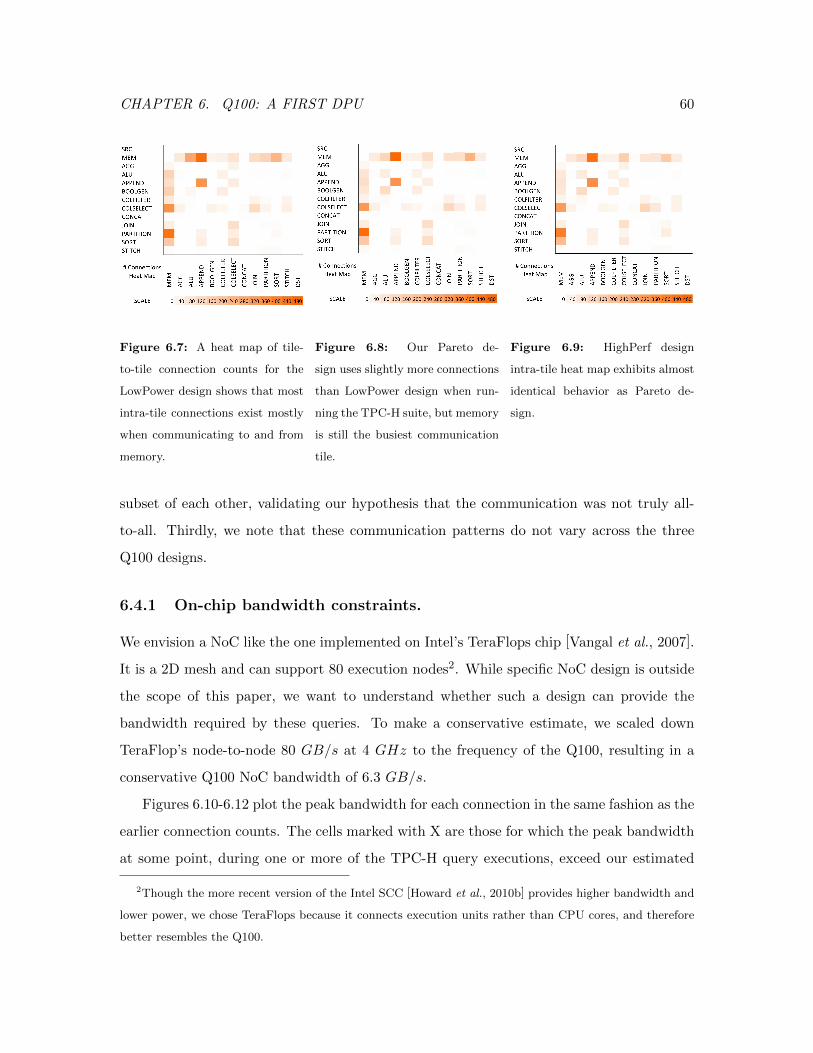
CHAPTER 6. Q100: A FIRST DPU 60
Figure 6.7: A heat map of tile-
to-tile connection counts for the
LowPower design shows that most
intra-tile connections exist mostly
when communicating to and from
memory.
Figure 6.8: Our Pareto de-
sign uses slightly more connections
than LowPower design when run-
ning the TPC-H suite, but memory
is still the busiest communication
tile.
Figure 6.9: HighPerf design
intra-tile heat map exhibits almost
identical behavior as Pareto de-
sign.
subset of each other, validating our hypothesis that the communication was not truly all-
to-all. Thirdly, we note that these communication patterns do not vary across the three
Q100 designs.
6.4.1 On-chip bandwidth constraints.
We envision a NoC like the one implemented on Intel’s TeraFlops chip [Vangal et al., 2007].
It is a 2D mesh and can support 80 execution nodes2. While specific NoC design is outside
the scope of this paper, we want to understand whether such a design can provide the
bandwidth required by these queries. To make a conservative estimate, we scaled down
TeraFlop’s node-to-node 80 GB/s at 4 GHz to the frequency of the Q100, resulting in a
conservative Q100 NoC bandwidth of 6.3 GB/s.
Figures 6.10-6.12 plot the peak bandwidth for each connection in the same fashion as the
earlier connection counts. The cells marked with X are those for which the peak bandwidth
at some point, during one or more of the TPC-H query executions, exceed our estimated
2Though the more recent version of the Intel SCC [Howard et al., 2010b] provides higher bandwidth and
lower power, we chose TeraFlops because it connects execution units rather than CPU cores, and therefore
better resembles the Q100.
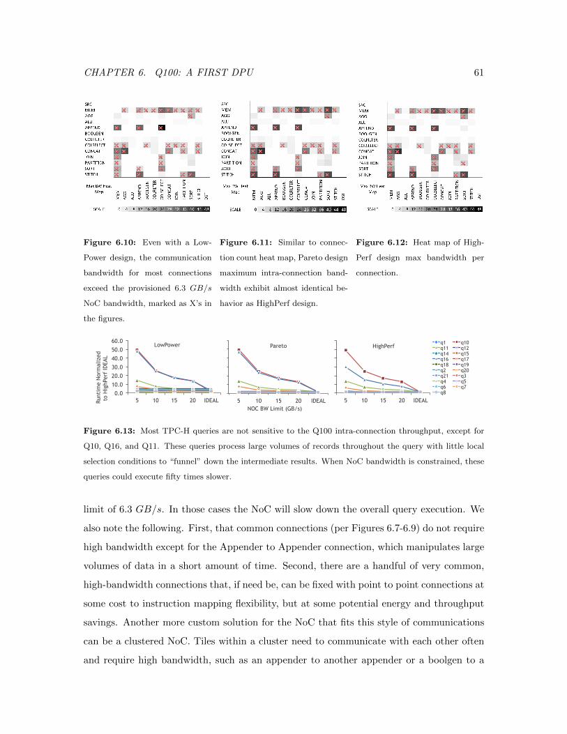
CHAPTER 6. Q100: A FIRST DPU 61
Figure 6.10: Even with a Low-
Power design, the communication
bandwidth for most connections
exceed the provisioned 6.3 GB/s
NoC bandwidth, marked as X’s in
the figures.
Figure 6.11: Similar to connec-
tion count heat map, Pareto design
maximum intra-connection band-
width exhibit almost identical be-
havior as HighPerf design.
Figure 6.12: Heat map of High-
Perf design max bandwidth per
connection.
0.0
10.0
20.0
30.0
40.0
50.0
60.0
5 10 15 20 IDEAL Run
tim
e N
orm
aliz
ed
to H
ighP
erf
IDEA
L
LowPower q1 q10 q11 q12 q14 q15 q16 q17 q18 q19 q2 q20 q21 5 10 15 20 IDEAL
NOC BW Limit (GB/s)
Pareto q1 q10 q11 q12 q14 q15 q16 q17 q18 q19 q2 q20 q21
5 10 15 20 IDEAL
HighPerf q1 q10 q11 q12 q14 q15 q16 q17 q18 q19 q2 q20 q21 q3 q4 q5 q6 q7 q8
Figure 6.13: Most TPC-H queries are not sensitive to the Q100 intra-connection throughput, except for
Q10, Q16, and Q11. These queries process large volumes of records throughout the query with little local
selection conditions to “funnel” down the intermediate results. When NoC bandwidth is constrained, these
queries could execute fifty times slower.
limit of 6.3 GB/s. In those cases the NoC will slow down the overall query execution. We
also note the following. First, that common connections (per Figures 6.7-6.9) do not require
high bandwidth except for the Appender to Appender connection, which manipulates large
volumes of data in a short amount of time. Second, there are a handful of very common,
high-bandwidth connections that, if need be, can be fixed with point to point connections at
some cost to instruction mapping flexibility, but at some potential energy and throughput
savings. Another more custom solution for the NoC that fits this style of communications
can be a clustered NoC. Tiles within a cluster need to communicate with each other often
and require high bandwidth, such as an appender to another appender or a boolgen to a
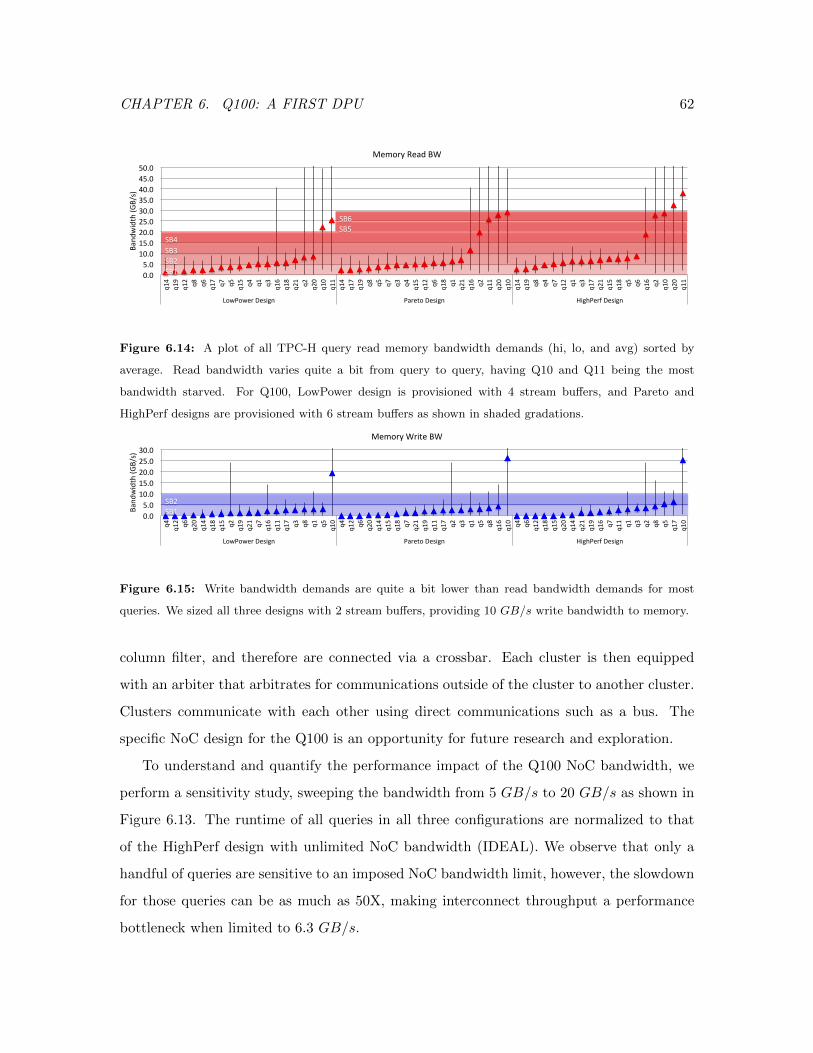
CHAPTER 6. Q100: A FIRST DPU 62
0.0 5.0 10.0 15.0 20.0 25.0 30.0 35.0 40.0 45.0 50.0
q14
q19
q12 q8
q6
q17 q7
q5
q15 q4
q1
q3
q16
q18
q21 q2
q20
q10
q11
q14
q17
q19 q8
q5
q7
q3
q4
q15
q12 q6
q18 q1
q21
q16 q2
q11
q20
q10
q14
q19 q8
q4
q7
q12 q1
q3
q17
q21
q15
q18 q5
q6
q16 q2
q10
q20
q11
LowPower Design Pareto Design HighPerf Design
Band
width (G
B/s)
Memory Read BW
SB1 SB2 SB3 SB4
SB5 SB6
Figure 6.14: A plot of all TPC-H query read memory bandwidth demands (hi, lo, and avg) sorted by
average. Read bandwidth varies quite a bit from query to query, having Q10 and Q11 being the most
bandwidth starved. For Q100, LowPower design is provisioned with 4 stream buffers, and Pareto and
HighPerf designs are provisioned with 6 stream buffers as shown in shaded gradations.
0.0 5.0 10.0 15.0 20.0 25.0 30.0
q4
q12 q6
q20
q14
q18
q15 q2
q19
q21 q7
q16
q11
q17 q3
q8
q1
q5
q10 q4
q12 q6
q20
q14
q15
q18 q7
q21
q19
q11
q17 q2
q3
q1
q5
q8
q16
q10 q4
q6
q12
q18
q15
q20
q14
q21
q19
q16 q7
q11 q1
q3
q2
q8
q5
q17
q10
LowPower Design Pareto Design HighPerf Design
Band
width (G
B/s)
Memory Write BW
SB1 SB2
Figure 6.15: Write bandwidth demands are quite a bit lower than read bandwidth demands for most
queries. We sized all three designs with 2 stream buffers, providing 10 GB/s write bandwidth to memory.
column filter, and therefore are connected via a crossbar. Each cluster is then equipped
with an arbiter that arbitrates for communications outside of the cluster to another cluster.
Clusters communicate with each other using direct communications such as a bus. The
specific NoC design for the Q100 is an opportunity for future research and exploration.
To understand and quantify the performance impact of the Q100 NoC bandwidth, we
perform a sensitivity study, sweeping the bandwidth from 5 GB/s to 20 GB/s as shown in
Figure 6.13. The runtime of all queries in all three configurations are normalized to that
of the HighPerf design with unlimited NoC bandwidth (IDEAL). We observe that only a
handful of queries are sensitive to an imposed NoC bandwidth limit, however, the slowdown
for those queries can be as much as 50X, making interconnect throughput a performance
bottleneck when limited to 6.3 GB/s.
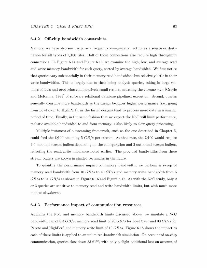
CHAPTER 6. Q100: A FIRST DPU 63
6.4.2 Off-chip bandwidth constraints.
Memory, we have also seen, is a very frequent communicator, acting as a source or desti-
nation for all types of Q100 tiles. Half of those connections also require high throughput
connections. In Figure 6.14 and Figure 6.15, we examine the high, low, and average read
and write memory bandwidth for each query, sorted by average bandwidth. We first notice
that queries vary substantially in their memory read bandwidths but relatively little in their
write bandwidths. This is largely due to their being analytic queries, taking in large vol-
umes of data and producing comparatively small results, matching the volcano style [Graefe
and McKenna, 1993] of software relational database pipelined execution. Second, queries
generally consume more bandwidth as the design becomes higher performance (i.e., going
from LowPower to HighPerf), as the faster designs tend to process more data in a smaller
period of time. Finally, in the same fashion that we expect the NoC will limit performance,
realistic available bandwidth to and from memory is also likely to slow query processing.
Multiple instances of a streaming framework, such as the one described in Chapter 5,
could feed the Q100 assuming 5 GB/s per stream. At that rate, the Q100 would require
4-6 inbound stream buffers depending on the configuration and 2 outbound stream buffers,
reflecting the read/write imbalance noted earlier. The provided bandwidths from these
stream buffers are shown in shaded rectangles in the figure.
To quantify the performance impact of memory bandwidth, we perform a sweep of
memory read bandwidth from 10 GB/s to 40 GB/s and memory write bandwidth from 5
GB/s to 20 GB/s as shown in Figure 6.16 and Figure 6.17. As with the NoC study, only 2
or 3 queries are sensitive to memory read and write bandwidth limits, but with much more
modest slowdowns.
6.4.3 Performance impact of communication resources.
Applying the NoC and memory bandwidth limits discussed above, we simulate a NoC
bandwidth cap of 6.3 GB/s, memory read limit of 20 GB/s for LowPower and 30 GB/s for
Pareto and HighPerf, and memory write limit of 10 GB/s. Figure 6.18 shows the impact as
each of these limits is applied to an unlimited-bandwidth simulation. On account of on-chip
communication, queries slow down 33-61%, with only a slight additional loss on account of
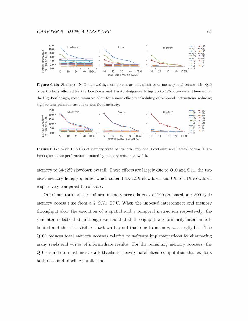
CHAPTER 6. Q100: A FIRST DPU 64
0.0
2.0
4.0
6.0
8.0
10.0
12.0
10 20 30 40 IDEAL Runt
ime
Nor
mal
ized
to
Hig
hPer
f ID
EAL
LowPower q1 q10 q11 q12 q14 q15 q16 q17 q18 q19 q2 q20 q21 10 20 30 40 IDEAL
MEM Read BW Limit (GB/s)
Pareto q1 q10 q11 q12 q14 q15 q16 q17 q18 q19 q2 q20 q21
10 20 30 40 IDEAL
HighPerf q1 q10 q11 q12 q14 q15 q16 q17 q18 q19 q2 q20 q21 q3 q4 q5 q6 q7 q8
Figure 6.16: Similar to NoC bandwidth, most queries are not sensitive to memory read bandwidth. Q16
is particularly affected for the LowPower and Pareto designs suffering up to 12X slowdown. However, in
the HighPerf design, more resources allow for a more efficient scheduling of temporal instructions, reducing
high-volume communications to and from memory.
0.0
5.0
10.0
15.0
20.0
25.0
5 10 15 20 IDEAL Run
tim
e N
orm
aliz
ed
to H
ighP
erf
IDEA
L
LowPower q1 q10 q11 q12 q14 q15 q16 q17 q18 q19 q2 q20 q21 5 10 15 20 IDEAL
MEM Write BW Limit (GB/s)
Pareto q1 q10 q11 q12 q14 q15 q16 q17 q18 q19 q2 q20 q21
5 10 15 20 IDEAL
HighPerf q1 q10 q11 q12 q14 q15 q16 q17 q18 q19 q2 q20 q21 q3 q4 q5 q6 q7 q8
Figure 6.17: With 10 GB/s of memory write bandwidth, only one (LowPower and Pareto) or two (High-
Perf) queries are performance- limited by memory write bandwidth.
memory to 34-62% slowdown overall. These effects are largely due to Q10 and Q11, the two
most memory hungry queries, which suffer 1.4X-1.5X slowdown and 6X to 11X slowdown
respectively compared to software.
Our simulator models a uniform memory access latency of 160 ns, based on a 300 cycle
memory access time from a 2 GHz CPU. When the imposed interconnect and memory
throughput slow the execution of a spatial and a temporal instruction respectively, the
simulator reflects that, although we found that throughput was primarily interconnect-
limited and thus the visible slowdown beyond that due to memory was negligible. The
Q100 reduces total memory accesses relative to software implementations by eliminating
many reads and writes of intermediate results. For the remaining memory accesses, the
Q100 is able to mask most stalls thanks to heavily parallelized computation that exploits
both data and pipeline parallelism.

CHAPTER 6. Q100: A FIRST DPU 65
0
0.5
1
1.5
2
2.5
3
LowPower Pareto HighPerf
Runt
ime
Nor
mal
ized
to
Hig
hPer
f Id
eal
Ideal
+ NocBW Limit
+ MemBW + NoCBW Limit
Figure 6.18: From the bandwidth heat maps plotted earlier, we see that Q100 was demanding a lot more
NoC bandwidth than provisioned. Here, we plotted runtime with respect to no bandwidth limit penalties,
and see a large slowdown at 30-60%, a caution for future implementations to design sufficient bandwidth for
intra-tile connections.
Area Power
Tiles NoC SBs Total Total Tiles NoC SBs Total Total
mm2 mm2 mm2 mm2 % Xeon W W W W % Xeon
LowPower 1.890 0.567 0.520 2.978 7.0% 0.238 0.071 0.400 0.710 14.2%
Pareto 3.107 0.932 0.780 4.819 11.3% 0.303 0.091 0.600 0.994 19.9%
HighPerf 5.080 1.524 0.780 7.384 17.3% 0.541 0.162 0.600 1.303 26.1%
Table 6.3: Area and power of the three Q100 configurations, broken down by tile, on chip interconnect,
and stream buffers.
6.4.4 Area and power impact of communication resources.
Starting with the area and power for the tiles in each Q100 design (based on Chapter 6
Table 6.1), we add the additional area and power due to the NoC and stream buffers.
Table 6.3 lists the area of the three design points broken down by tile, NoC, and stream
buffers. We add an extra 30% area and power to the Q100 designs for the NoC, based on
the characteristics of the TeraFlops implementation [Vangal et al., 2007]. For the stream
buffers, we add 0.13 mm2 and 0.1 Watts for each stream buffer based on the results from
Chapter 5 Table 5.2. In sum, the Q100 remains quite small, with the large, HighPerf
configuration including NoC and stream buffers taking 17.3% area and 26.1% power of a
single Xeon core.
CHAPTER 6. Q100: A FIRST DPU 66
6.4.5 Intermediate storage discussion.
To handle the spills and fills in between the execution of temporal instructions, an interme-
diate storage that is smaller and faster than memory, such as a scratch pad that is explicitly
managed by the Q100 device, can be implemented. It is conceivable that if an intermediate
storage is available, and provides sufficient bandwidth to and from the Q100 device, it can
be used to provide better performance and energy efficiency than communicating directly
to and from memory. The intermediate storage does not need to be sized for the entirety
of all intermediate results as space can be reused and reclaimed once the data is consumed.
It, however, needs to be sized so that it is large enough to hold the partial results while the
device frees up from executing the last data element of the previous temporal instruction.
This may not be feasible in the beginning of the query execution as large amount of data
needs to be read in before any filtering or local selection conditions can be executed. The
addition of an intermediate storage, the sizing, and the management of such storage present
another opportunity for future research and exploration.
6.5 Q100 Evaluation
Taking what we have learned about the Q100 system, it’s ISA, it’s implementation, commu-
nication both internal and external, we now compare our three configurations, LowPower,
Pareto, and HighPerf, with conventional software DBMS. This evaluation takes on three
parts: initial power and performance benchmarking for the TPC-H queries as executed on a
conventional DBMS+CPU system, comparison of Q100’s execution of TPC-H to that sys-
tem’s, and finally an evaluation of how a Q100, designed for one scale of database handles
the same queries over a database 100 times larger.
6.5.1 Methodology
We measure the performance and energy consumption of MonetDB 11.11.5 running on the
Xeon server described in Table 6.4 and executing the set of TPC-H queries. Each reported
result is the average of five runs during which we measured the elapsed time and the energy
consumption. For the latter we used Intel’s Running Average Power Limit (RAPL) energy
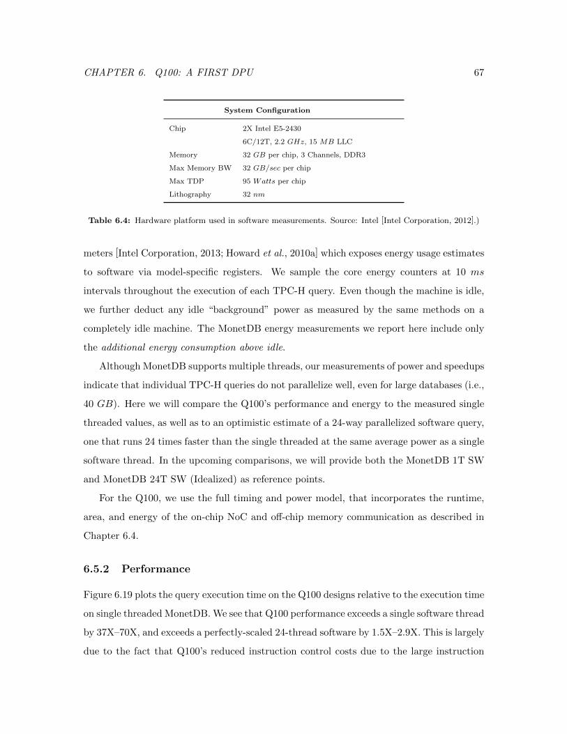
CHAPTER 6. Q100: A FIRST DPU 67
System Configuration
Chip 2X Intel E5-2430
6C/12T, 2.2 GHz, 15 MB LLC
Memory 32 GB per chip, 3 Channels, DDR3
Max Memory BW 32 GB/sec per chip
Max TDP 95 Watts per chip
Lithography 32 nm
Table 6.4: Hardware platform used in software measurements. Source: Intel [Intel Corporation, 2012].)
meters [Intel Corporation, 2013; Howard et al., 2010a] which exposes energy usage estimates
to software via model-specific registers. We sample the core energy counters at 10 ms
intervals throughout the execution of each TPC-H query. Even though the machine is idle,
we further deduct any idle “background” power as measured by the same methods on a
completely idle machine. The MonetDB energy measurements we report here include only
the additional energy consumption above idle.
Although MonetDB supports multiple threads, our measurements of power and speedups
indicate that individual TPC-H queries do not parallelize well, even for large databases (i.e.,
40 GB). Here we will compare the Q100’s performance and energy to the measured single
threaded values, as well as to an optimistic estimate of a 24-way parallelized software query,
one that runs 24 times faster than the single threaded at the same average power as a single
software thread. In the upcoming comparisons, we will provide both the MonetDB 1T SW
and MonetDB 24T SW (Idealized) as reference points.
For the Q100, we use the full timing and power model, that incorporates the runtime,
area, and energy of the on-chip NoC and off-chip memory communication as described in
Chapter 6.4.
6.5.2 Performance
Figure 6.19 plots the query execution time on the Q100 designs relative to the execution time
on single threaded MonetDB. We see that Q100 performance exceeds a single software thread
by 37X–70X, and exceeds a perfectly-scaled 24-thread software by 1.5X–2.9X. This is largely
due to the fact that Q100’s reduced instruction control costs due to the large instruction
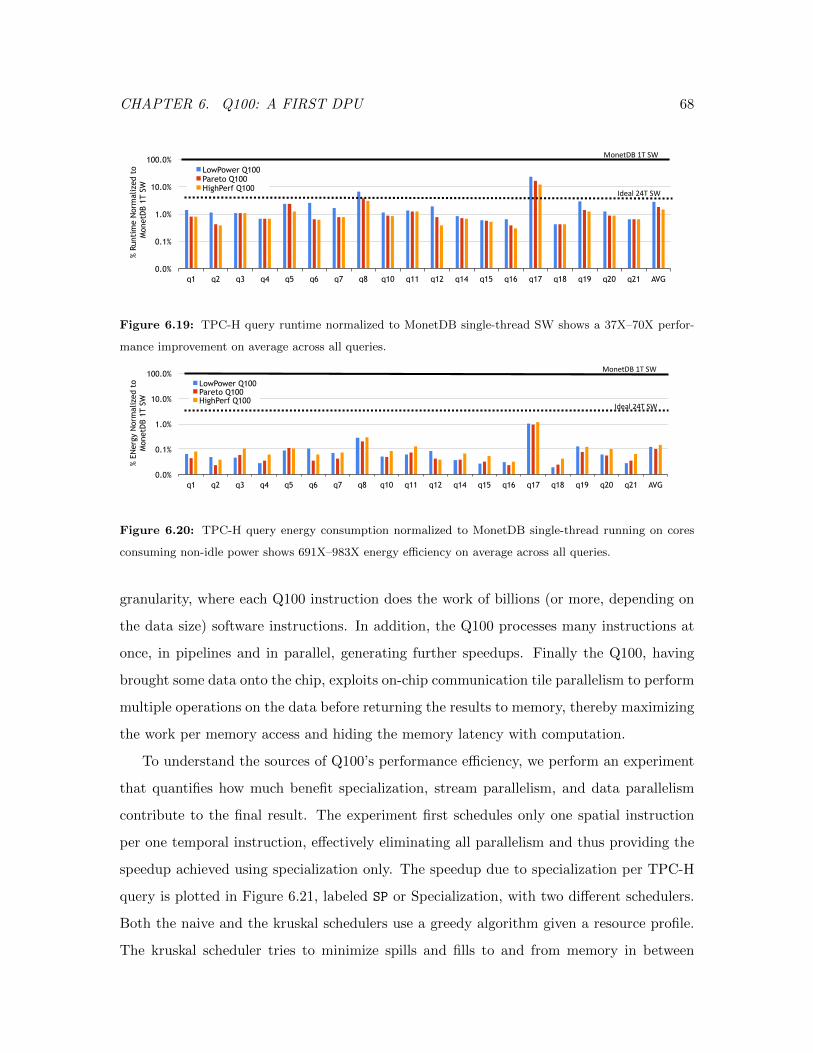
CHAPTER 6. Q100: A FIRST DPU 68
0.0%
0.1%
1.0%
10.0%
100.0%
q1 q2 q3 q4 q5 q6 q7 q8 q10 q11 q12 q14 q15 q16 q17 q18 q19 q20 q21 AVG
% Ru
ntim
e N
orm
aliz
ed t
o
Mon
etD
B 1T
SW
LowPower Q100 Pareto Q100 HighPerf Q100
MonetDB 1T SW
Ideal 24T SW
Figure 6.19: TPC-H query runtime normalized to MonetDB single-thread SW shows a 37X–70X perfor-
mance improvement on average across all queries.
0.0%
0.1%
1.0%
10.0%
100.0%
q1 q2 q3 q4 q5 q6 q7 q8 q10 q11 q12 q14 q15 q16 q17 q18 q19 q20 q21 AVG
% EN
ergy
Nor
mal
ized
to
Mon
etD
B 1T
SW
LowPower Q100 Pareto Q100 HighPerf Q100
MonetDB 1T SW
Ideal 24T SW
Figure 6.20: TPC-H query energy consumption normalized to MonetDB single-thread running on cores
consuming non-idle power shows 691X–983X energy efficiency on average across all queries.
granularity, where each Q100 instruction does the work of billions (or more, depending on
the data size) software instructions. In addition, the Q100 processes many instructions at
once, in pipelines and in parallel, generating further speedups. Finally the Q100, having
brought some data onto the chip, exploits on-chip communication tile parallelism to perform
multiple operations on the data before returning the results to memory, thereby maximizing
the work per memory access and hiding the memory latency with computation.
To understand the sources of Q100’s performance efficiency, we perform an experiment
that quantifies how much benefit specialization, stream parallelism, and data parallelism
contribute to the final result. The experiment first schedules only one spatial instruction
per one temporal instruction, effectively eliminating all parallelism and thus providing the
speedup achieved using specialization only. The speedup due to specialization per TPC-H
query is plotted in Figure 6.21, labeled SP or Specialization, with two different schedulers.
Both the naive and the kruskal schedulers use a greedy algorithm given a resource profile.
The kruskal scheduler tries to minimize spills and fills to and from memory in between
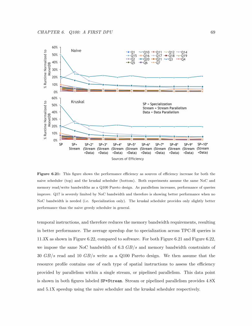
CHAPTER 6. Q100: A FIRST DPU 69
0%
10%
20%
30%
40%
50%
60% %
Runt
ime
Nor
mal
ized
to
Mon
etD
B Naive Q1 Q10 Q11 Q12 Q14
Q15 Q16 Q17 Q18 Q19 Q2 Q20 Q21 Q3 Q4 Q5 Q6 Q7
0%
10%
20%
30%
40%
50%
60%
% Ru
ntim
e N
orm
aliz
ed t
o M
onet
DB
Sources of Efficiency
Kruskal
SP SP+ Stream
SP+2* (Stream +Data)
SP+3* (Stream +Data)
SP+5* (Stream +Data)
SP+6* (Stream +Data)
SP+7* (Stream +Data)
SP+8* (Stream +Data)
SP+9* (Stream +Data)
SP+10* (Stream +Data)
SP+4* (Stream +Data)
SP = Specialization Stream = Stream Parallelism Data = Data Parallelism
Figure 6.21: This figure shows the performance efficiency as sources of efficiency increase for both the
naive scheduler (top) and the kruskal scheduler (bottom). Both experiments assume the same NoC and
memory read/write bandwidths as a Q100 Pareto design. As parallelism increases, performance of queries
improve. Q17 is severely limited by NoC bandwidth and therefore is showing better performance when no
NoC bandwidth is needed (i.e. Specialization only). The kruskal scheduler provides only slightly better
performance than the naive greedy scheduler in general.
temporal instructions, and therefore reduces the memory bandwidth requirements, resulting
in better performance. The average speedup due to specialization across TPC-H queries is
11.3X as shown in Figure 6.22, compared to software. For both Figure 6.21 and Figure 6.22,
we impose the same NoC bandwidth of 6.3 GB/s and memory bandwidth constraints of
30 GB/s read and 10 GB/s write as a Q100 Pareto design. We then assume that the
resource profile contains one of each type of spatial instructions to assess the efficiency
provided by parallelism within a single stream, or pipelined parallelism. This data point
is shown in both figures labeled SP+Stream. Stream or pipelined parallelism provides 4.8X
and 5.1X speedup using the naive scheduler and the kruskal scheduler respectively.
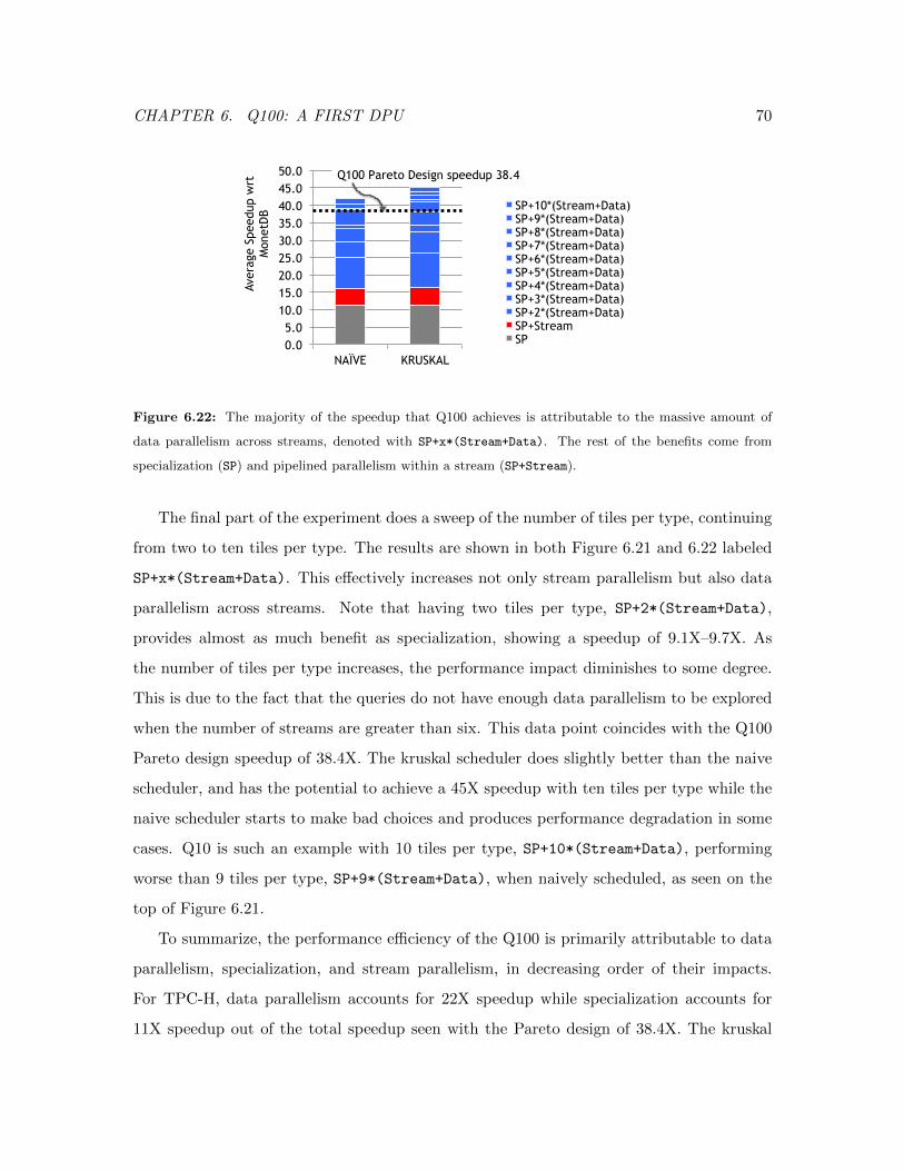
CHAPTER 6. Q100: A FIRST DPU 70
0.0 5.0
10.0 15.0 20.0 25.0 30.0 35.0 40.0 45.0 50.0
NAÏVE KRUSKAL
Aver
age
Spee
dup
wrt
M
onet
DB SP+10*(Stream+Data)
SP+9*(Stream+Data) SP+8*(Stream+Data) SP+7*(Stream+Data) SP+6*(Stream+Data) SP+5*(Stream+Data) SP+4*(Stream+Data) SP+3*(Stream+Data) SP+2*(Stream+Data) SP+Stream SP
Q100 Pareto Design speedup 38.4
Figure 6.22: The majority of the speedup that Q100 achieves is attributable to the massive amount of
data parallelism across streams, denoted with SP+x*(Stream+Data). The rest of the benefits come from
specialization (SP) and pipelined parallelism within a stream (SP+Stream).
The final part of the experiment does a sweep of the number of tiles per type, continuing
from two to ten tiles per type. The results are shown in both Figure 6.21 and 6.22 labeled
SP+x*(Stream+Data). This effectively increases not only stream parallelism but also data
parallelism across streams. Note that having two tiles per type, SP+2*(Stream+Data),
provides almost as much benefit as specialization, showing a speedup of 9.1X–9.7X. As
the number of tiles per type increases, the performance impact diminishes to some degree.
This is due to the fact that the queries do not have enough data parallelism to be explored
when the number of streams are greater than six. This data point coincides with the Q100
Pareto design speedup of 38.4X. The kruskal scheduler does slightly better than the naive
scheduler, and has the potential to achieve a 45X speedup with ten tiles per type while the
naive scheduler starts to make bad choices and produces performance degradation in some
cases. Q10 is such an example with 10 tiles per type, SP+10*(Stream+Data), performing
worse than 9 tiles per type, SP+9*(Stream+Data), when naively scheduled, as seen on the
top of Figure 6.21.
To summarize, the performance efficiency of the Q100 is primarily attributable to data
parallelism, specialization, and stream parallelism, in decreasing order of their impacts.
For TPC-H, data parallelism accounts for 22X speedup while specialization accounts for
11X speedup out of the total speedup seen with the Pareto design of 38.4X. The kruskal
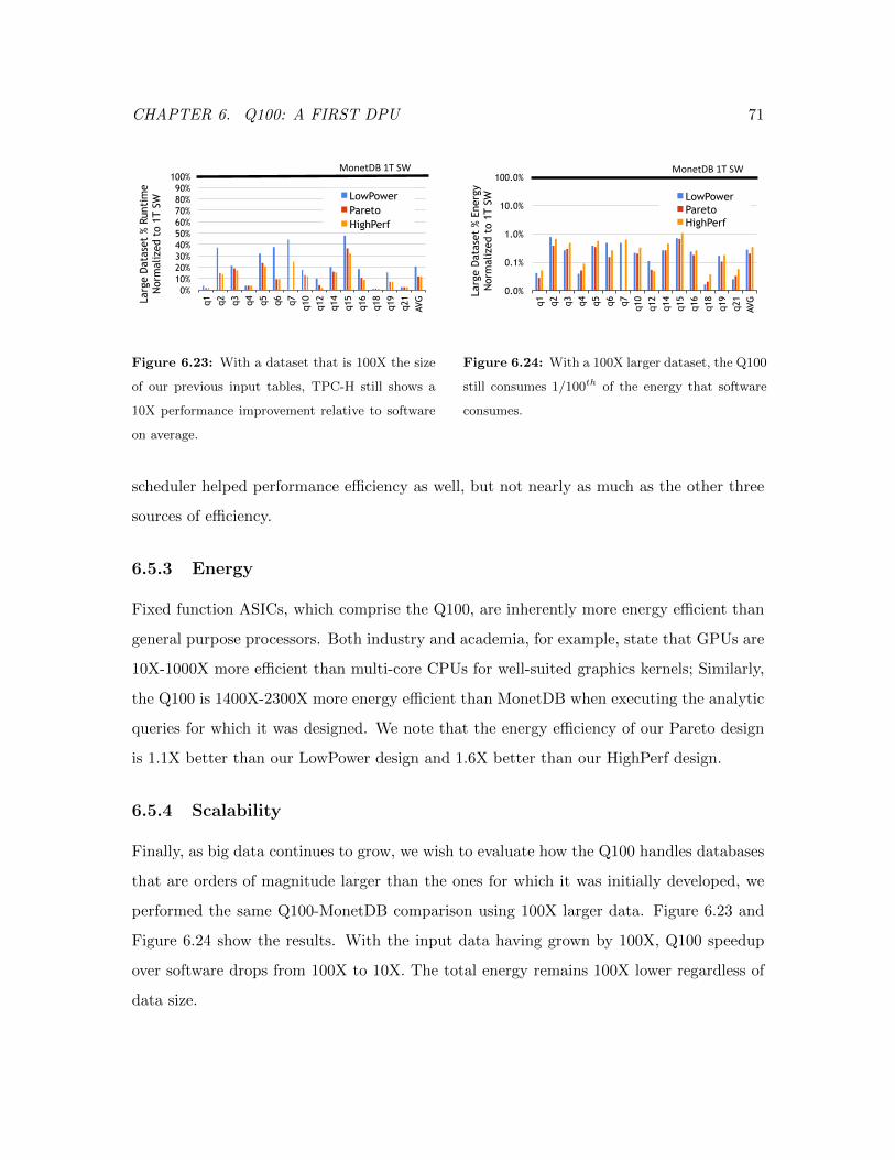
CHAPTER 6. Q100: A FIRST DPU 71
0% 10% 20% 30% 40% 50% 60% 70% 80% 90%
100%
q1
q2
q3
q4
q5
q6
q7
q10
q12
q14
q15
q16
q18
q19
q21
AVG
Larg
e D
atas
et %
Run
tim
e N
orm
aliz
ed t
o 1T
SW
LowPower Pareto HighPerf
MonetDB 1T SW
Figure 6.23: With a dataset that is 100X the size
of our previous input tables, TPC-H still shows a
10X performance improvement relative to software
on average.
0.0%
0.1%
1.0%
10.0%
100.0%
q1
q2
q3
q4
q5
q6
q7
q10
q12
q14
q15
q16
q18
q19
q21
AVG
Larg
e D
atas
et %
Ene
rgy
Nor
mal
ized
to
1T S
W
LowPower Pareto HighPerf
MonetDB 1T SW
Figure 6.24: With a 100X larger dataset, the Q100
still consumes 1/100th of the energy that software
consumes.
scheduler helped performance efficiency as well, but not nearly as much as the other three
sources of efficiency.
6.5.3 Energy
Fixed function ASICs, which comprise the Q100, are inherently more energy efficient than
general purpose processors. Both industry and academia, for example, state that GPUs are
10X-1000X more efficient than multi-core CPUs for well-suited graphics kernels; Similarly,
the Q100 is 1400X-2300X more energy efficient than MonetDB when executing the analytic
queries for which it was designed. We note that the energy efficiency of our Pareto design
is 1.1X better than our LowPower design and 1.6X better than our HighPerf design.
6.5.4 Scalability
Finally, as big data continues to grow, we wish to evaluate how the Q100 handles databases
that are orders of magnitude larger than the ones for which it was initially developed, we
performed the same Q100-MonetDB comparison using 100X larger data. Figure 6.23 and
Figure 6.24 show the results. With the input data having grown by 100X, Q100 speedup
over software drops from 100X to 10X. The total energy remains 100X lower regardless of
data size.
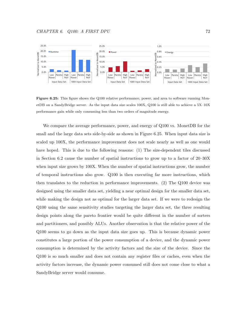
CHAPTER 6. Q100: A FIRST DPU 72
0.0%
5.0%
10.0%
15.0%
20.0%
25.0%
Low Power
Pareto High Perf
Low Power
Pareto High Perf
Input Data Set 100X Input Data Set
Nor
mal
ized
to
Mon
etD
B Runtime
0.0%
5.0%
10.0%
15.0%
20.0%
25.0%
Low Power
Pareto High Perf
Low Power
Pareto High Perf
Input Data Set 100X Input Data Set
Nor
mal
ized
to
Mon
etD
B Power
0.0%
0.2%
0.4%
0.6%
0.8%
1.0%
Low Power
Pareto High Perf
Low Power
Pareto High Perf
Input Data Set 100X Input Data Set
Nor
mal
ized
to
Mon
etD
B Energy
Figure 6.25: This figure shows the Q100 relative performance, power, and area to software running Mon-
etDB on a SandyBridge server. As the input data size scales 100X, Q100 is still able to achieve a 5X–10X
performance gain while only consuming less than two orders of magnitude energy.
We compare the average performance, power, and energy of Q100 vs. MonetDB for the
small and the large data sets side-by-side as shown in Figure 6.25. When input data size is
scaled up 100X, the performance improvement does not scale nearly as well as one would
have hoped. This is due to the following reasons: (1) The size-dependent tiles discussed
in Section 6.2 cause the number of spatial instructions to grow up to a factor of 20–30X
when input size grows by 100X. When the number of spatial instructions grow, the number
of temporal instructions also grow. Q100 is then executing far more instructions, which
then translates to the reduction in performance improvements. (2) The Q100 device was
designed using the smaller data set, yielding a near optimal design for the smaller data set,
while making the design not as optimal for the larger data set. If we were to redesign the
Q100 using the same sensitivity studies targeting the larger data set, the three resulting
design points along the pareto frontier would be quite different in the number of sorters
and partitioners, and possibly ALUs. Another observation is that the relative power of the
Q100 seems to go down as the input data size goes up. This is because dynamic power
constitutes a large portion of the power consumption of a device, and the dynamic power
consumption is determined by the activity factors and the size of the device. Since the
Q100 is so much smaller and does not contain any register files or caches, even when the
activity factors increase, the dynamic power consumed still does not come close to what a
SandyBridge server would consume.
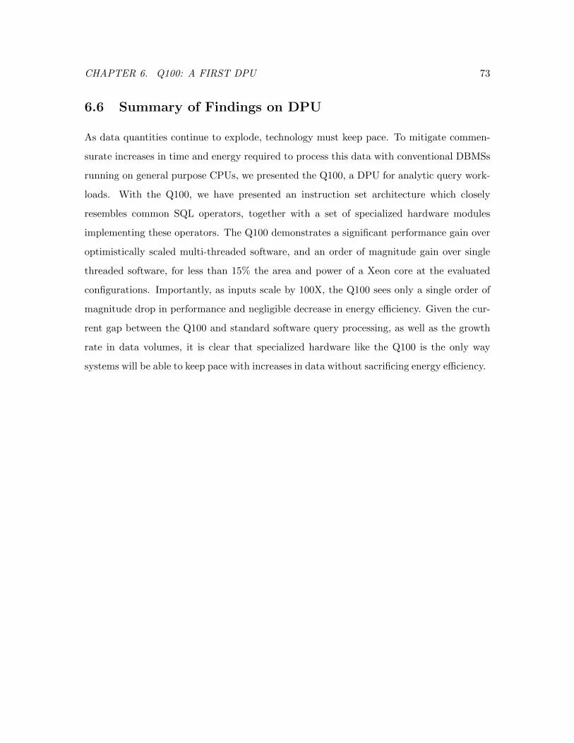
CHAPTER 6. Q100: A FIRST DPU 73
6.6 Summary of Findings on DPU
As data quantities continue to explode, technology must keep pace. To mitigate commen-
surate increases in time and energy required to process this data with conventional DBMSs
running on general purpose CPUs, we presented the Q100, a DPU for analytic query work-
loads. With the Q100, we have presented an instruction set architecture which closely
resembles common SQL operators, together with a set of specialized hardware modules
implementing these operators. The Q100 demonstrates a significant performance gain over
optimistically scaled multi-threaded software, and an order of magnitude gain over single
threaded software, for less than 15% the area and power of a Xeon core at the evaluated
configurations. Importantly, as inputs scale by 100X, the Q100 sees only a single order of
magnitude drop in performance and negligible decrease in energy efficiency. Given the cur-
rent gap between the Q100 and standard software query processing, as well as the growth
rate in data volumes, it is clear that specialized hardware like the Q100 is the only way
systems will be able to keep pace with increases in data without sacrificing energy efficiency.
CHAPTER 7. RELATED WORK 74
Chapter 7
Related Work
Specialization is a topic of great interest in the research community. Here, we place our
work in context with other accelerators, separating them into categories according to their
acceleration granularity, parallelism granularity, streaming properties, and communication
with the host processor. We then compare and contrast our work with the most related
database acceleration techniques to date.
Acceleration granularity. A program consists of two main parts, the algorithmic part
and the data structures. Regardless of granularity, most existing accelerators focus on algo-
rithmic acceleration. On one end of the spectrum, there is instruction specific acceleration.
These accelerators do work for on the order of less than ten conventional x86 assembly
instructions. Examples include Intel’s SSE instruction set, PowerPC’s AltiVec, and the
Visual Instruction Set for UltraSparc. On the other end of the spectrum, there is domain
or application specific acceleration. These accelerators do work for a set of domain specific
algorithms or entire applications. Stanford’s convolution engine [Qadeer et al., 2013] targets
image processing kernels and stencil computations, [Salapura et al., 2012] uses specialization
to speed up regular expression matching in queries, [Hameed and others, 2010] accelerates
H.264 video encoders, and perhaps the most visible and among the most successful, GPUs,
such as Nvidia’s GeForce [NVIDIA, 2013] and AMD/ATI’s Radeon [AMD/ATI, 2013], tar-
get graphics applications. In contrast, we focus on accelerating data structure operations.
In terms of granularity, this is going to fall somewhere in the middle of the spectrum. Each
CHAPTER 7. RELATED WORK 75
of these datatype accelerators does work on the order of tens to hundreds conventional x86
assembly instructions. Abstract Datatype Instructions, described in Chapter 2, use hash
tables and sparse vectors as our acceleration targets. Datatype acceleration leverages exist-
ing software container interfaces already familiar to programmers and to provide compute
efficiency and programmability. HARP and Q100 described in Chapter 4 and 6 are con-
sidered domain-specific accelerators for relational databases, but the underlying principle
employs datatype acceleration, where the datatypes correspond to tables and columns.
Parallelism granularity. Instruction specific accelerators take advantage of fine-grained
parallelism using SIMD or vector processing to exploit data element parallelism within a
instruction. At a slightly coarser granularity, there is stream parallelism, or pipelined par-
allelism, that can either be implicitly implemented in hardware as Q100 and most pipelined
architecture have done, or explicitly controlled via software as Merrimac [Dally et al., 2003]
has demonstrated, using software pipelining and explicit control to overlap data transfer
operations with compute operations. Task parallelism is fairly coarse grained and requires
software controlled synchronization, which can be expensive and cumbersome; examples
include SARC [Ramirez et al., 2010] and Rigel [Kelm et al., 2009]. Most domain-specific
accelerators mentioned previously, including the Q100, take advantage of a combination of
SIMD parallelism, pipelined parallelism, and data parallelism across streams. There are
also recent work that are parallelism agnostic, such as Conservation Cores [Venkatesh et
al., 2010] that compiles a program into regions of “hot” codes and synthesize the “hot”
codes into functional blocks for execution, or DySER [Govindaraju and others, 2011] that
compiles a program into phases and map the phases into functional blocks for execution.
Spatially Programmed Streaming Accelerators. The Q100 has a streaming property
that produces and consumes data as a stream of elements. The data is used for a short
period of time, and all the elements go through the same set of computations that are well
defined. This streaming property lends itself to spatially programmed processing elements,
processing one element as soon as input data is ready. In the case of the Q100, each
data column is consumed as an input stream, processed through a relational operator, or a
functional tile, and each intermediate result is produced as an output stream that is then
CHAPTER 7. RELATED WORK 76
consumed immediately by the next relational operator. This streaming property is shared by
RSVP [Ciricescu et al., 2003], with the configuration of the processing elements determined
at compile time, and utilizes input and output stream “buffers”. The specific streaming
mechanism differs from our proposed streaming framework in that they fetch data using
dedicated vector streaming units and manage streams via interlocked FIFO queues. RSVP
also differs from our approach in that they implement a set of computations specifically for
vector and media processing, in contrast to our set of relational database operators. Finally,
RSVP’s processing elements are reconfigurable, contain register files and intermediate local
stores, and they operate on vector data elements as opposed to data column or data table
elements. Other streaming and reconfigurable accelerators include PipeRench [Goldstein
et al., 1999] and more recently Triggered Instructions [Parashar et al., 2013], which is
also spatially programmed. Our approach differ from these that our functional units, or
processing elements, are not homogeneous and are statically programmed spatially and
temporally.
Accelerator communication with the host processor. HARP is integrated with
the host processor in a tightly-coupled fashion, borrowing existing load/store datapaths of
the core to communicate to the host memory subsystems. DySER is similar in that it also
utilizes the CPU as a load/store engine to feed the DySER blocks. Conservation Cores is
similar in that it communicates directly to and from the CPU data cache, however, our
approach slightly differs in that we use non-temporal loads and therefore do not pollute the
data cache unnecessarily. Q100, on the other hand, is integrated with the host processor in
an indirect fashion through an interconnect, most similar to a GPU.
Hardware acceleration of databases. Database machines were developed by the
database community in the early 1980s as specialized hardware for database workloads.
These efforts largely failed, primarily because commodity CPUs were improving so rapidly
at the time, and hardware design was slow and expensive [Boral and DeWitt, 1983]. The
architectures proposed at that time targeted a different set of challenges than those we face
today, namely dark silicon, the utilization wall, the power wall, etc.. While hardware de-
sign remains quite costly, high computing requirements of data-intensive workloads, limited
CHAPTER 7. RELATED WORK 77
single-threaded performance gains, increases in specialized hardware, aggressive efficiency
targets, and the data deluge have spurred us and others to revisit this approach.
Much more recently, a flurry of projects accelerates queries by compiling them down
to FPGAs, such as LINQits [Chung et al., 2013], Teradata [Teradata Corporation, 2013],
and [Muller and Teubner, 2010]. Industry appliances using Xeon servers combined with
FPGAs such as the IBM Netezza [IBM, 2013b] also show promising performance and energy
efficiency. Whereas we have designed a domain specific circuit, these projects produce query-
specific circuits, a different point in the specialization space. Other have investigated using
existing accelerators, such as network processors [Gold et al., 2005] or GPUs [Govindaraju
et al., 2005] to speed relational operators. Our work is similar in that we too accelerate
database queries and relational operators, but differs in the overall strategy and specific
hardware platform.
CHAPTER 8. CONCLUSIONS 78
Chapter 8
Conclusions
In this thesis, we present a hypothesis that grouping similarly structured data and processing
them with specialized hardware provides significant performance and energy efficiency.
To evaluate this hypothesis, we start with preliminary experiments to assess if datatype
acceleration is indeed a worthwhile idea. We perform experiments to assess the poten-
tial performance gain by accelerating commonly used datatypes such as hash tables and
sparse vectors. We find that by raising the level of abstraction and giving hardware more
information about the software structures used in the applications, datatype acceleration
provides performance while reducing energy. In order to further examine our hypothesis,
we survey a range of popular benchmark suites and use varied granular data containers to
assess potential acceleration targets. We find that these popular benchmark suites often do
not contain shared or common datatypes, and therefore require a large number of unique
accelerators in order to see substantial performance benefits.
Given our findings from the preliminary experiments, we choose to target domain-specific
applications for datatype acceleration, in particular, we target read-only analytic relational
database workloads. This is motivated by the massive increase in volume of data produced
and consumed daily and the need to process them quickly and energy efficiently. We envision
a class of database domain-specific processors, or DPUs, that are composed of collections of
relational operation accelerators. As a feasibility study, we architect and design a hardware
data partitioner, HARP, that achieved an order of magnitude better performance and energy
efficiency than a state-of-the-art software DBMS running on a Xeon server, at just a fraction
CHAPTER 8. CONCLUSIONS 79
of a Xeon core area and power. This is primarily due to the inherent performance inefficiency
of even the best-known software algorithm, which traverses a binary tree comparing key
values at each node in the tree. The comparisons are sequentially dependent, and the
path through the tree is unpredictable. HARP’s microarchitecture takes advantage of a
specialized hardware pipeline of comparators, allowing sequential comparisons for a single
record, yet also allowing pipeline parallelization across records, eliminating pipeline bubbles
seen in the software algorithm.
We also architect a streaming framework that allows a tightly-coupled integration of
HARP and other streaming accelerators to communicate with the general purpose proces-
sor core seamlessly. We perform experiments to show that a single thread can stream data
into and out of the accelerator using software control and sustain the bandwidth demands
at roughly 5 GB/s. For accelerators that demand more bandwidth, multiple stream buffers
can be implemented without too much extra cost. We design the input and output stream
buffers to be architecturally visible as to provide a clear boundary delineating the accel-
erator microarchitecture states from the general processor microarchitecture states. With
simple save/restore instructions, the accelerator can handle interrupts and context switches
through the saving and restoring of stream buffer entries.
Finally, as a proof of concept, we architect and design the first DPU, Q100, that con-
sists of 11 unique relational operation accelerators, or tiles. We present the instruction set
architecture of Q100, which contains spatial instructions that are mapped onto underlying
relational operators, processing data elements from columns, one per cycle in a pipelined,
streaming fashion. Each query is mapped onto a directed graph of spatial instructions and
can be executed at once if there is no resource constraints. Given a set of resources, or
a hardware configuration, the spatial instructions are further mapped onto a sequential
set of temporal instructions that are executed in order. We walk through the design and
evaluation of three Q100 designs, namely a LowPower configuration that provides the best
power efficiency, a HighPerf configuration that provides the best performance, and a Pareto
configuration that provides the maximum performance per Watt. We evaluate these de-
signs on their on-chip and off-chip interconnect bandwidth demands and find that TPC-H
is particularly sensitive to the NoC bandwidth, and slightly sensitive to the memory band-
CHAPTER 8. CONCLUSIONS 80
width. We compare the efficiency of Q100 and find that all three designs perform an order
of magnitude better than a state-of-the-art DBMS running on a Sandybridge server, and
up to three orders of magnitude more energy efficient. This efficiency gain holds even when
we scale the input data size by 100X.
We summarize that datatype acceleration provides (1) better application throughput
and compute efficiency, in turn reduces time for execution and reduces energy consump-
tion, (2) lower register energy consumption, because temporary storage or pipeline registers
in a specialized datapath can be sized for structured data and reduce rapid and frequent
data movement in and out of registers; furthermore, it reduces general purpose register con-
tentions, (3) lower cache energy consumption, because managing similarly structured data
by using specialized control and specialized storage, we avoid unnecessary tag lookups, TLB
accesses, and cache pollution, and (4) better memory bandwidth utilization for compute-
bound workloads as it resolves the imbalance between compute bottleneck and memory
underutilization by speeding up compute to match memory throughput.
We conclude that accelerating similarly structured data does provide significant per-
formance and energy efficiency in the case for database acceleration. We believe that this
finding is significant in helping the architecture community to face the big data era with
memory subsystem specialization and encourage the community to look for other applica-
tion domains where this hypothesis may apply.
BIBLIOGRAPHY 81
Bibliography
[Abadi et al., 2007] D. J. Abadi, D. S. Myers, D. J. DeWitt, and S. R. Madden. Material-
ization strategies in a column-oriented dbms. In ICDE, 2007.
[Abadi et al., 2009] D. J. Abadi, P. A. Boncz, and S. Harizopoulos. Column-oriented
database systems. VLDB, August 2009.
[AMD/ATI, 2013] AMD/ATI. AMD Radeon Graphics Cards, 2013. http://www.amd.com/
us/products/graphics/Pages/graphics.aspx.
[Blanas et al., 2011] Spyros Blanas, Yinan Li, and Jignesh M. Patel. Design and evaluation
of main memory hash join algorithms for multi-core CPUs. In SIGMOD, 2011.
[Bluespec, Inc., 2012] Bluespec, Inc. Bluespec Core Technology, 2012. http://www.
bluespec.com.
[Bohr, 2007] Mark Bohr. A 30 year retrospective on dennard’s mosfet scaling paper. IEEE
Solid-State Circuits Newsletter, 12(1):11–13, winter 2007.
[Boncz et al., 2005] P. A. Boncz, M. Zukowski, and N. Nes. Monetdb/x100: Hyper-
pipelining query execution. In CIDR, 2005.
[Boral and DeWitt, 1983] Haran Boral and David J. DeWitt. Database machines: an idea
whose time has passed? In IWDM, 1983.
[Boutell et al., 2004] Matthew R. Boutell, Jiebo Luo, Xipeng Shen, and Christopher M.
Brown. Learning multi-label scene classification. Pattern Recognition, 37(9):1757–1771,
2004.
BIBLIOGRAPHY 82
[Carli et al., 2009] Lorenzo De Carli, Yi Pan, Amit Kumar, Cristian Estan, and
Karthikeyan Sankaralingam. Plug: Flexible lookup modules for rapid deployment of
new protocols in high-speed routers. In SIGCOMM, August 2009.
[Cascaval and others, 2010] Calin Cascaval et al. A taxonomy of accelerator architectures
and their programming models. IBM Journal of Research and Development, 54(5):1–10,
2010.
[Centrum Wiskunde and Informatica, 2012] Centrum Wiskunde and Informatica, 2012.
http://www.monetdb.org.
[Chang and Lin, 2001] Chih-Chung Chang and Chih-Jen Lin. LIBSVM: a library for
support vector machines, 2001. Software available at http://www.csie.ntu.edu.tw/
~cjlin/libsvm.
[Chatziantoniou and Ross, 2007] Damianos Chatziantoniou and Kenneth A. Ross. Parti-
tioned optimization of complex queries. Information Systems (IS), 32(2):248–282, 2007.
[Chung et al., 2013] E. S. Chung, J. D. Davis, and J. Lee. Linqits: Big data on little clients.
In ISCA, 2013.
[Cieslewicz and Ross, 2008] John Cieslewicz and Kenneth A. Ross. Data partitioning on
chip multiprocessors. In DaMoN, 2008.
[Ciricescu et al., 2003] Silviu Ciricescu, Ray Essick, Brian Lucas, Phil May, Kent Moat, Jim
Norris, Michael Schuette, and Ali Saidi. The reconfigurable streaming vector processor
(RSVPTM). In MICRO, 2003.
[Collins, 1999] Michael Collins. Head-Driven Statistical Models for Natural Language Pars-
ing. PhD thesis, University of Pennsylvania, 1999.
[Dally et al., 2003] W. J. Dally, P. Hanrahan, M. Erez, and T. J. Knight. Merrimac: Super-
computing with streams. In Proceedings of the ACM/IEEE SC2003 Conference, Novem-
ber 2003.
BIBLIOGRAPHY 83
[Dally et al., 2008] William J. Dally, James Balfour, David Black-Shaffer, James Chen,
R. Curtis Harting, Vishal Parikh, Jongsoo Park, and David Sheffield. Efficient embedded
computing. IEEE Computer, 41(7):27–32, July 2008.
[Dennis, 1991] J. B. Dennis. Advanced topics in data-flow computing. Prentice-Hall, 1991.
[Esmaeilzadeh and others, 2011] Hadi Esmaeilzadeh et al. Dark silicon and the end of
multicore scaling. In ISCA, pages 365–376, 2011.
[Esmaeilzadeh et al., 2011] H. Esmaeilzadeh, E. Blem, R. St. Amant, K. Sankaralingam,
and D. Burger. Dark silicon and the end of multicore scaling. In ISCA, pages 365–376,
2011.
[Franke et al., 2010] H Franke, J Xenidis, C Basso, B Bass, S Woodward, J Brown, and
C Johnson. Introduction to the wire-speed processor and architecture. IBM Journal of
Research and Development, 54(1):3:1–3:11, 2010.
[Gebhart et al., 2009] M. Gebhart, B. A. Maher, K. E. Coons, J. Diamond, P. Gratz,
M. Marino, N. Ranganathan, B. Robatmili, A. Smith, J. Burrill, S. W. Keckler, D. Burger,
and K. S. McKinley. An evaluation of the TRIPS computer system. In ASPLOS, 2009.
[Gold et al., 2005] B. Gold, A. Ailamaki, L. Huston, and B. Falsafi. Accelerating database
operators using a network processor. In DaMoN, 2005.
[Goldstein et al., 1999] Seth Copen Goldstein, Herman Schmit, Matthew Moe, Mihai
Budiu, Srihari Cadambi, R. Reed Taylor, and Ronald Laufer. PipeRench: a co/pro-
cessor for streaming multimedia acceleration. In ISCA, 1999.
[Google Inc., 2009] Google Inc. Unladen Swallow Benchmark Suite, 2009. http://code.
google.com/p/unladen-swallow/wiki/Benchmarks.
[Govindaraju and others, 2011] Venkatraman Govindaraju et al. Dynamically specialized
datapaths for energy efficient computing. In HPCA, pages 503–514, 2011.
[Govindaraju et al., 2005] N. K. Govindaraju, B. Lloyd, W. Wang, M. Lin, and
D. Manocha. Fast computation of database operations using graphics processors. In
SIGGRAPH, 2005.
BIBLIOGRAPHY 84
[Graefe and McKenna, 1993] G. Graefe and W. J. McKenna. The volcano optimizer gen-
erator: Extensivility and efficient search. In ICDE, 1993.
[Gurd et al., 1985] J.R. Gurd, C. C. Kirkham, and I. Watson. The manchester prototype
dataflow computer. Communications of the ACM, 1985.
[Hameed and others, 2010] Rehan Hameed et al. Understanding sources of inefficiency in
general-purpose chips. In ISCA, pages 37–47, June 2010.
[Hicks et al., 1993] J. Hicks, D. Chiou, B. S. Ang, and Arvind. Performance studies of ld
on the monsoon dataflow system. 1993.
[Hill and Marty, 2008] Mark D. Hill and Michael R. Marty. Amdahl’s law in the multicore
era. IEEE Computer, 41(7):33–38, July 2008.
[Howard et al., 2010a] D. Howard, E. Gorbatov, U. R. Hanebutte, R. Khanna, and C. Le.
Rapl: memory power estimateion and capping. In ISLPED, 2010.
[Howard et al., 2010b] Jason Howard, Saurabh Dighe, Yatin Hoskote, Sriram R. Vangal,
David Finan, Gregory Ruhl, David Jenkins, Howard Wilson, Nitin Borkar, Gerhard
Schrom, Fabric Pailet, Shailendra Jain, Tiju Jacob, Satish Yada, Sraven Marella, Praveen
Salihundam, Vasantha Erraguntla, Michael Konow, Michael Riepen, Guido Droege, Joerg
Lindemann, Matthias Gries, Thomas Apel, Kersten Henriss, Tor Lund-Larsen, Sebastian
Steibl, Shekhar Borkar, Vivek De, Rob F. Van der Wijngaart, and Timothy G. Mattson.
A 48-core IA-32 message-passing processor with DVFS in 45nm CMOS. In ISSCC, pages
108–109, 2010.
[HP Labs, 2011] HP Labs. CACTI 4.0 (web-based), 2011. http://www.hpl.hp.com/
research/cacti/.
[HyperTransport Consortium, 2009] HyperTransport Consortium. HyperTransport. http:
//www.hypertransport.org/, 2009.
[IBM, 2013a] IBM. DB2 Partitioning Features, 2013. http://www.ibm.com/
developerworks/data/library/techarticle/dm-0608mcinerney.
BIBLIOGRAPHY 85
[IBM, 2013b] IBM. IBM Netezza Data Warehouse Appliance, 2013. http://www-01.ibm.
com/software/data/netezza/.
[IDC Research, 2012] IDC Research. IDC’s most recent worldwide Big Data technology
and services market forecast, 2012. http://www.idc.com/getdoc.jsp?containerId=
prUS23355112.
[Idreos et al., 2012] S. Idreos, F. Groffen, N. Nes, S. Manegold, K. S. Mullender, and M. L.
Kersten. Monetdb: Two decades of research in column-oriented database architectures.
Data Engineering Bulletin, 2012.
[Intel Corporation, 2010] Intel Corporation. Intel R© Xeon R© Processor E5620, 2010. http:
//ark.intel.com/products/47925.
[Intel Corporation, 2011] Intel Corporation. Pin - a dynamic binary in-
strumentation tool. http://software.intel.com/en-us/articles/
pin-a-dynamic-binary-instrumentation-tool, 2011.
[Intel Corporation, 2012] Intel Corporation. Intel Xeon Processor E5-2430, 2012. http://
ark.intel.com/products/64616/Intel-Xeon-Processor-E5-2430--(15M-Cache-2_
20-GHz-7_20-GTs-Intel-QPI).
[Intel Corporation, 2013] Intel Corporation. Intel 64 R©and IA-32 architectures software de-
veloper’s manual, 2013. http://download.intel.com/products/processor/manual/
253669.pdf.
[Ionescu and Schauser, 1997] M. F. Ionescu and K. E. Schauser. Optimizing parallel bitonic
sort. In IPDPS, 1997.
[Jouppi, 1990] N. P. Jouppi. Improvind direct-mapped cache performance by the addition
of a small fully-associative cache and prefetch buffers. In ISCA, 1990.
[Jung et al., 2011] Changhee Jung, Silvius Rus, Brian P. Railing, Nathan Clark, and San-
tosh Pande. Brainy: effective selection of data structures. In PLDI, pages 86–97, 2011.
BIBLIOGRAPHY 86
[Kelm et al., 2009] John H. Kelm, Daniel R. Johnson, Matthew R. Johnson, Neal C. Crago
an William Tuohy, Ageel Mahesri, Steven S. Lumetta, Matthew I. Frank, and Sanjay J.
Patel. Rigel: An architecture and scalable programming interface for a 1000-core ac-
celerator. In Proceedings of the 36th Annual International Symposium on Computer
Architecture (ISCA). ACM, 2009.
[Kim et al., 2009] Changkyu Kim, Eric Sedlar, Jatin Chhugani, Tim Kaldewey, Anthony D.
Nguyen, Andrea Di Blas, Victor W. Lee, Nadathur Satish, and Pradeep Dubey. Sort
vs. hash revisited: Fast join implementation on modern multi-core CPUs. PVLDB,
2(2):1378–1389, 2009.
[Kozyrakis et al., 2010] C. Kozyrakis, A. Kansal, S. Sankar, and K. Vaid. Server engineering
insights for large-scale online services. IEEE Micro, 30(4), July/August 2010.
[Kx Systems, 2013] Kx Systems. Kx High-Performance Database. http://kx.com/
_papers/Kx_White_Paper-2013-02c.pdf, 2013.
[Lamb et al., 2012] A. Lamb, M. Fuller, R. Varadarajan, N. Tran, B. Vandiver, L. Doshi,
and C. Bear. The vertica analytic database: C-store 7 years later. In VLDB, 2012.
[Liu and Rus, 2009] Lixia Liu and Silvius Rus. Perflint: A context sensitive performance
advisor for C++ programs. In CGO, pages 265–274, 2009.
[McAfee and Brynjolfsson, 2012] A. McAfee and E. Brynjolfsson. Big Data: The manage-
ment revolution. Harvard Business Review, October 2012.
[Microsoft, 2012] Microsoft. Microsoft SQL Server 2012, 2012. http://technet.
microsoft.com/en-us/sqlserver/ff898410.
[Muller and Teubner, 2010] R. Muller and J. Teubner. FPGAs: A new point in the database
design space, 2010. EDBT Tutorial.
[MySQL, 2012] MySQL. Date and time datatype representation, 2012. http://dev.
mysql.com/doc/internals/en/date-and-time-data-type-representation.html.
BIBLIOGRAPHY 87
[Natarajan et al., 2003] Karthik Natarajan, Heather Hanson, Stephen W. Keckler,
Charles R. Moore, and Doug Burger. Microprocessor pipeline energy analysis. In
ISLPED, pages 282–287, 2003.
[NetApp, 2012] NetApp. Where is your data? [Infographic], 2012. https://twitter.com/
NetApp/status/205677239600283648/photo/1/large.
[NVIDIA, 2013] NVIDIA. NVIDIA GeForce Graphics Processors, 2013. http://www.
nvidia.com/object/geforce_family.html.
[Oracle, 2013] Oracle. Oracle Database 11g: Partitioning, 2013. http://www.oracle.com/
technetwork/database/options/partitioning/index.html.
[Parashar et al., 2013] A. Parashar, M. Pellauer, M. Adler, B. Ahsan, N. Crago, D. Lustig,
V. Pavlov, A. Zhai, M. Gambhir, A. Jaleel, R. Allmon, R. Rayess, and J. Emer. Triggered
instructions: A control paradigm for spatially-programmed architectures. In ISCA, 2013.
[PCI-SIG, 2011] PCI-SIG. PCI Express 4.0. http://www.pcisig.com/specifications/
pciexpress/, 2011.
[Qadeer et al., 2013] W. Qadeer, R. Hameed, O. Shacham, P. Venkatesan, C. Kozyrakis,
and M. A. Horowitz. Convolution engine: Balancing efficiency and flexibility in specialized
computing. In ISCA, 2013.
[Ramirez et al., 2010] A. Ramirez, F. Cabarcas, B. Juurlink, M. Alvarez, F. Sanchez,
A. Azevedo, C. Meenderinck, C. Ciobanu, S. Isaza, and G. Gaydaduiev. The sarc archi-
tecture. IEEE Micro, 2010.
[Ross and Cieslewicz, 2009] Kenneth A. Ross and John Cieslewicz. Optimal splitters for
database partitioning with size bounds. In ICDT, pages 98–110, 2009.
[Saha and others, 2009] Bratin Saha et al. Programming model for a heterogeneous x86
platform. In Proceedings of the 2009 ACM SIGPLAN Conference on Programming Lan-
guage Design and Implementation (PLDI). ACM, 2009.
[Salapura et al., 2012] V. Salapura, T. Karkhanis, P. Nagpurkar, and J. Moreira. Acceler-
ating business analytics applications. In HPCA, 2012.
BIBLIOGRAPHY 88
[Sampson and others, 2011] Jack Sampson et al. Efficient complex operators for irregular
codes. In Proceedings of the 17th International Symposium on High Performance Com-
puter Architeture (HPCA), pages 491–502. ACM, Feb 2011.
[SAP Sybase IQ, 2013] SAP Sybase IQ. Sybase IQ Analytics Server. http://www.sybase.
com/products/archivedproducts/sybaseiq, 2013.
[Schlegel et al., 2009] Benjamin Schlegel, Rainer Gemulla, and Wolfgang Lehner. k-ary
search on modern processors. In DaMoN, 2009.
[Standard Performance Evaluation Corporation, 2006] Standard Performance Evaluation
Corporation. Spec2006 Benchmark Suite, 2006. http://www.spec.org/cpu2006/.
[Standard Performance Evaluation Corporation, 2008] Standard Performance Evaluation
Corporation. SpecJVM2008 Benchmark Suite, 2008. http://www.spec.org/jvm2008/.
[Stonebraker et al., 2005] M. Stonebraker, D. J. Abadi, A. Batkin, X. Chen, M. Cherniack,
M. Ferreira, E. Lau, A. Lin, S. Madden, E. O’Neil, P. O’Neil, A. Rasin, N. Tran, and
S. Zdonik. C-store: a column-oriented dbms. In VLDB, 2005.
[Subramoni et al., 2010] H. Subramoni, F. Petrini, V. Agarwal, and D. Pasetto. Intra-socket
and inter-socket communication in multi-core systems. IEEE Computer Architecture
Letters, 9:13–16, January 2010.
[Swanson et al., 2007] S. Swanson, A. Schwerin, M. Mercaldi, A. Petersen, A. Putnam,
K. Michelson, M. Oskin, and S. J. Eggers. The wavescalar architecture. ACM Trans.
Comp. Syst., 2007.
[Synopsys, Inc., 2013] Synopsys, Inc. 32/28nm Generic Library for IC Design, Design Com-
piler, IC Compiler, 2013. http://www.synopsys.com.
[Tang et al., 2011] L. Tang, J. Mars, N. Vachharajani, R. Hundt, and M. L. Soffa. The
impact of memory subsystem resource sharing on datacenter applications. In ISCA,
2011.
[Teradata Corporation, 2013] Teradata Corporation. Teradata Data Warehousing, 2013.
http://www.teradata.com.
BIBLIOGRAPHY 89
[The DaCapo Research Project, 2006] The DaCapo Research Project. The DaCapo Bench-
mark Suite, 2006. http://dacapobench.org/.
[Transaction Processing Performance Council, 2003] Transaction Processing Performance
Council, 2003. http://www.tpc.org/tpch/default.asp.
[University of Pennsylvania, 1995] University of Pennsylvania. The Penn treebank project.
Online http://www.cis.upenn.edu/~treebank, 1995.
[Vangal et al., 2007] S. Vangal, J. Howard, G. Ruhl, S. Dighe, H. Wilson, J. Tschanz, D. Fi-
nan, P. Iyer, A. Singh, T. Jacob, S. Jain, S. Venkataraman, Y. Hoskote, and N. Borkar.
An 80-tile 1.28TFLOPS network-on-chip in 65nm CMOS. In ISSCC, February 2007.
[Venkatesh and others, 2010] Ganesh Venkatesh et al. Conservation cores: reducing the
energy of mature computations. In ASPLOS, pages 205–218, March 2010.
[Venkatesh et al., 2010] Ganesh Venkatesh, Jack Sampson, Nathan Goulding, Saturnino
Garcia, Vladyslav Bryksin, Jose Lugo-Martinez, Steven Swanson, and Michael Bedford
Taylor. Conservation cores: Reducing the energy of mature computations. In ASPLOS,
pages 205–218, Pittsburgh, Pennsylvania, March 2010.
[Vo et al., 2013] H Vo, Yunsup Lee, Andrew Waterman, and Krste Asanovic. A case for
OS-friendly hardware accelerators. WIVOSCA workshop, 2013.
[Wang et al., 2007] Perry H. Wang, Jamison D. Collins, Gautham N. Chinya, Hong Jiang,
Xinmin Tian, Milind Girkar, Nick Y. Yang, Guei-Yuan Lueh, and Hong Wang. EXOCHI:
architecture and programming environment for a heterogeneous multi-core multithreaded
system. In Proceedings of the 2007 ACM SIGPLAN conference on Programming language
design and implementation (PLDI). ACM, 2007.
[Williams et al., 2007] Samuel Williams, Leonid Oliker, Richard Vuduc, John Shalf,
Katherine Yelick, and James Demmel. Optimization of sparse matrix-vector multipli-
cation on emerging multicore platforms. pages 1–12, 2007.
[Wu et al., 2001] Lisa Wu, Chris Weaver, and Todd Austin. Cryptomaniac: a fast flexible
architecture for secure communication. In ISCA, June 2001.
BIBLIOGRAPHY 90
[Ye et al., 2011] Y. Ye, K. A. Ross, and N. Vesdapunt. Scalable aggregation on multicore
processors. In DaMoN, 2011.
[Zane and Narlikar, 2003] F Zane and G Narlikar. CoolCAMs: Power-efficient TCAMs for
forwarding engines. In Joint Conference of the IEEE Computer and Communications
Societies, pages 42–52, July 2003.
[Zukowski and Boncz, 2012] M. Zukowski and P. Boncz. Vectorwise: Beyond column stores.
Data Engineering Bulletin, 2012.