arX

iv:1

412.

8384

v1 [

gr-q

c] 2

9 D

ec 2

014

Free-flight experiments in LISA Pathfinder

M Armanoa, H Audleyb, G Augerc, J Bairdn, P Binetruyc, M Bornb,

D Bortoluzzid, N Brandte, A Bursit, M Calenof , A Cavallerig,

A Cesarinig, M Cruiseh, C Cutleru, K Danzmannb, I Diepholzb,

R Dolesig, N Dunbari, L Ferraiolij, V Ferronig, E Fitzsimonse,

M Freschia, J Gallegosa, C Garcıa Marirrodrigaf , R Gerndte,

LI Gesak, F Gibertk, D Giardinij, R Giusterig, C Grimanil,

I Harrisonm, G Heinzelb, M Hewitsonb, D Hollingtonn, M Huellerg,

J Hueslerf , H Inchauspec, O Jennrichf , P Jetzero, B Johlanderf ,

N Karnesisk, B Kauneb, N Korsakovab, C Killowp, I Llorok,

R Maarschalkerweerdm, S Maddenf , P Maghamis, D Mancej,

V Martınk, F Martin-Porquerasa, I Mateosk, P McNamaraf ,

J Mendesm, L Mendesa, A Moronit, M Nofrariask, S Paczkowskib,

M Perreur-Lloydp, A Petiteauc, P Pivatog, E Plagnolc, P Pratc,

U Ragnitf , J Ramos-Castroqr, J Reicheb, J A Romera Perezf ,

D Robertsonp, H Rozemeijerf , G Russanog, P Sarrat, A Schleichere,

J Slutskys, C F Sopuertak, T Sumnern, D Texiera, J Thorpes,

C Trenkeli, H B Tug, D Vetrugnog, S Vitaleg, G Wannerb, H Wardp,

S Waschken, P Wassn, D Wealthyi, S Weng, W Weberg, A Wittchenb,

C Zanonid, T Zieglere, P Zweifelj

a European Space Astronomy Centre, European Space Agency, Villanueva de la Canada,28692 Madrid, Spainb Albert-Einstein-Institut, Max-Planck-Institut fur Gravitationsphysik und UniversitatHannover, 30167 Hannover, Germanyc APC UMR7164, Universite Paris Diderot, Paris, Franced Department of Industrial Engineering, University of Trento, via Sommarive 9, 38123 Trento,and Trento Institute for Fundamental Physics and Application / INFNe Airbus Defence and Space, Claude-Dornier-Strasse, 88090 Immenstaad, Germanyf European Space Technology Centre, European Space Agency, Keplerlaan 1, 2200 AGNoordwijk, The Netherlandsg Dipartimento di Fisica, Universita di Trento and Trento Institute for Fundamental Physicsand Application / INFN, 38123 Povo, Trento, Italyh Department of Physics and Astronomy, University of Birmingham, Birmingham, UKi Airbus Defence and Space, Gunnels Wood Road, Stevenage, Hertfordshire, SG1 2AS, UKj Institut fur Geophysik, ETH Zurich, Sonneggstrasse 5, CH-8092, Zurich, Switzerlandk Institut de Ciencies de l’Espai (CSIC-IEEC), Campus UAB, Facultat de Ciencies, 08193Bellaterra, Spainl Istituto di Fisica, Universita degli Studi di Urbino/ INFN Urbino (PU), Italym European Space Operations Centre, European Space Agency, 64293 Darmstadt, Germanyn The Blackett Laboratory, Imperial College London, UKo Physik Institut, Universitat Zurich, Winterthurerstrasse 190, CH-8057 Zurich, Switzerlandp SUPA, Institute for Gravitational Research, School of Physics and Astronomy, University ofGlasgow, Glasgow, G12 8QQ, UKq Department d’Enginyeria Electronica, Universitat Politecnica de Catalunya, 08034Barcelona, Spain

r Institut d’Estudis Espacials de Catalunya (IEEC), C/ Gran Capita 2-4, 08034 Barcelona,Spains NASA Goddard Space Flight Center, 8800 Greenbelt Road, Greenbelt, MD 20771, USAt CGS S.p.A, Compagnia Generale per lo Spazio, Via Gallarate, 150 - 20151 Milano, Italyt NASA Jet Propulsion Laboratory, 4800 Oak Grove Drive, Pasadena, CA 91109

E-mail: james.i.thorpe@nasa.gov

Abstract. The LISA Pathfinder mission will demonstrate the technology of drag-free testmasses for use as inertial references in future space-based gravitational wave detectors. Toaccomplish this, the Pathfinder spacecraft will perform drag-free flight about a test mass whilemeasuring the acceleration of this primary test mass relative to a second reference test mass.Because the reference test mass is contained within the same spacecraft, it is necessary to applyforces on it to maintain its position and attitude relative to the spacecraft. These forces are apotential source of acceleration noise in the LISA Pathfinder system that are not present in thefull LISA configuration. While LISA Pathfinder has been designed to meet it’s primary missionrequirements in the presence of this noise, recent estimates suggest that the on-orbit performancemay be limited by this ‘suspension noise’. The drift-mode or free-flight experiments provide anopportunity to mitigate this noise source and further characterize the underlying disturbancesthat are of interest to the designers of LISA-like instruments. This article provides a high-leveloverview of these experiments and the methods under development to analyze the resultingdata.

1. Introduction

The basic operating principle of an interferometric gravitational-wave detector is themeasurement of fluctuations in space-time curvature via the exchange of photons between pairsof geodesic-tracking references separated by large baselines [1]. A key challenge for implementingsuch a detector is the development of an object whose worldline approximates a geodesic – aninertial particle. The LISA Pathfinder (LPF) mission [2] will validate the technology of drag-free test masses for use as inertial references in a future space-based gravitational wave detectorsuch as the Laser Interferometer Space Antenna (LISA).

The technique of drag-free flight for disturbance reduction [3, 4] can be briefly summarizedas follows. A reference or ‘test’ mass is placed inside a hollow housing within the host spacecraft(SC). On orbit, the test mass is allowed to float freely inside the housing while a sensor systemmonitors the position and attitude of the test mass relative to the SC. This information is usedby a control system which commands the SC to follow the orbit of the test mass. In doing so, theSC isolates the test mass from external disturbances. By actuating the SC rather than the testmass (as is done in a traditional inertial guidance system) to maintain the relative position andattitude, the test mass is isolated from noise associated with the actuation itself. The remainingresidual acceleration noise of the test mass results from forces local to the SC as well as externalforces that are not absorbed by the SC (e.g. magnetic). In practice, the “accelerometer”(feedback to the test mass) and “drag-free” (feedback to the SC) techniques are combined into ahybrid system where the feedback can be routed differently depending on the kinematic degreeof freedom (DoF) and frequency band. For the LISA application, it is sufficient to have drag-freeflight only along the linear DoF and only in the frequency band of desired sensitivity. This isanalogous to the pendulum suspensions used for ground-based gravitational wave detectors thatprovide approximate free-fall in one DoF for frequencies sufficiently far above the resonancefrequency.

In the LPF implementation [5], two 46mm cubic Au-Pt test masses are contained in a singleSC. One of the test masses is designated as the reference test mass (RTM) and the SC performsdrag free flight along one linear DoF while controlling the remaining five DoFs (three angular

and two linear) with an electrostatic suspension system. The second or non-reference test mass(NTM) is located ∼ 38 cm away from the primary test mass along the drag-free axis and isused as a witness to assess the residual acceleration of the RTM. An interferometric metrologysystem [6], monitors relative displacements between the RTM and NTM with a precision of∼ 10 pm/

√Hz in the measurement band 0.1mHz < f < 100mHz

A key difference between the LPF configuration and the LISA configuration is that theLISA acceleration measurement is made between test masses on separate spacecraft whereas theLPF acceleration measurement is made between two test masses on the same spacecraft. Asa result, the LPF NTM must be electrostatically suspended along the sensitive DoF becausethe SC cannot simultaneously follow the trajectories of both the RTM and NTM along thesame DoF. This suspension force has a noise component which represents a disturbance in theLPF measurement that is not present in LISA-like configurations. With all noise sources at thedesign requirement levels for LPF, this residual suspension noise contribution is not a significantcontribution to the overall measured differential acceleration noise in the LISA measurementband (see Figure 1a). The dominating term over this band are various types of spurious forceson the test masses, precisely the phenomena of interest to the designers of future gravitationalwave instruments.

10-4

10-3

10-2

10-1

100

101

102

TotalDirect

Forces

Electrostatic

Suspension

Thr

uste

rs

Posi

tion S

ensi

ng

Sta

r

Tra

cker

Angle

Sensin

g

(a) Design Requirements

10-4

10-3

10-2

10-1

100

101

102

Total Posi

tion S

ensi

ng

Direct

Forces

ElectrostaticSuspension

Star

Tracker

Requirements

(b) Current Best Estimate

Figure 1: Breakdown of noise sources for measurement of acceleration of the reference test massrelative to the non-reference test mass along the sensitive DoF. The left panel shows the designrequirement levels whereas the right panel shows the current best estimates based on groundtest campaigns of flight hardware and system modeling. See [5] for more detail.

Figure 1b shows the current best estimate (CBE) for the differential acceleration noise inLPF. As would be expected from a conservative set of design requirements, the CBE levelsfor all terms are lower than the corresponding ones for the requirements. However, suspensionnoise is now expected to play a significant role in the measurement band. This expectation issupported by stringent limits placed on the magnitudes of unknown or unmodeled forces on theLPF inertial sensor using torsion pendulums [7, 8].

To be clear, LPF performance at either the requirement or CBE level would accomplish thegoal of validating drag-free flight as a technique for realizing inertial reference sensors for LISA-like observatories. Nevertheless, a direct measurement of the forces acting on the test masseswould provide additional valuable information to the designers of such observatories.

2. Free-Flight Experiments

The electrostatic suspension of the NTM in LPF is needed to counteract forces in the NTM-SCsystem that differ from those in the RTM-SC system, which are suppressed by the drag-freecontrol loop. These include disturbance forces that are local to the test masses, such as residualgas disturbances, thermal disturbances, electrostatic forces, magnetic forces, etc. In addition,the static gravitational gradient differs at the RTM and NTM location, leading to a constantbias in the force that must be applied to the NTM along the sensitive axis. Although thisbias will be minimized through the use of compensation masses designed based on pre-flightgravitational models, it is expected that residual gravitational accelerations along the sensitiveDoF will be on the order of 10−10 m/s2. This sets the amplitude, and consequently the noise, ofthe required suspension force.

In the drift mode or free-flight experiment, the compensation of the static field experienced bythe NTM is performed with a series of discrete ‘kicks’ rather than with a continuously-appliedforce. Between the kicks, the electrostatic actuation of the NTM along the sensitive DoF isturned off, allowing the NTM to drift under the influence of the constant forces. In principle,this ‘kick control’ strategy could be employed on all DoFs of the NTM, which would suppressactuation noise from other DoFs from leaking into the sensitive DoF. In practice, this actuationcross-talk is expected to be sufficiently small that kick control is only required along the sensitiveDoF.

2.1. The LTP Drift Mode Experiment

The drift mode controller designed for the LISA Test Package (LTP)[9] fixes both the length ofthe drift period (∼ 350 s) and the duration of the kicks (∼ 1 s). A Kalman-filter based observertracks the motion of the NTM during the free flight and estimates the impulse required tomaintain the NTM position. The amplitude of the subsequent kick is adjusted to deliver thisimpulse and the process is repeated. Figure 2a shows the displacement of the RTM relative tothe NTM for a segment of simulated data from the LTP drift mode. It consists of a series ofrepeated quasi-parabolic flights (the trajectory of the NTM is not a true parabola due to theinfluence of other force terms such as a linear spring term that couples the NTM to the SC)with a duration of 350 s. Figure 2b shows the corresponding acceleration of the RTM relativeto the NTM, which shows a series of discrete kicks separated by nearly constant accelerationduring the free flight segments.

Time [s]0 500 1000 1500 2000

RT

M-N

TM

Dis

pla

cem

ent

[u

m]

0

1

2

3

4

5

6

(a) RTM-NTM Relative Position

Time [s]0 500 1000 1500 2000

RT

M-N

TM

Acc

eler

atio

n [

nm

/s2 ]

-20

0

20

40

60

80

100

120

140

160

180

(b) RTM-NTM Relative Acceleration

Figure 2: Example data for a LTP drift-mode simulation. The left panel shows the displacementof the RTM relative to the NTM whereas the right panel shows the acceleration.

2.2. A proposed ST7-DRS Free-Flight Experiment

An alternative drift-mode control design has recently been develop for possible use with theNASA-provided payload known as the Disturbance Reduction System (DRS)1. The ST7 designis based on a modified dead-band controller, where the dynamical state of the system determinesthe control mode. The two-dimensional phase space of NTM position and NTM velocity is usedto describe the system state and a region centered around the nominal position and zero velocityis designated as the dead band. So long as the NTM position and velocity remain in this deadband region, no suspension control is applied along the sensitive DoF. When the NTM statedrifts out of this deadband region, a suspension controller is engaged and remains on untilthe NTM state re-enters the dead-band region. The resulting trajectory of the NTM is morecomplex than that of the LTP drift mode experiment. In general, the duration of the free-flightsegments vary from segment to segment. A 300 ks simulation yielded an approximately normaldistribution of free-flights with a mean duration of ∼ 357 s and a standard deviation of ∼ 14 s.While at first glance, this irregularity in the free flight durations might seem to be disadvantage,it has a potential advantage for data analysis because the few long segments can be used toestimate spectral information at lower frequencies. Additionally, unlike the LTP design, theDRS control design automatically adjusts to changes in the static gravity gradient and is robustto fairly significant changes. This means that the controller would not have to be re-optimizedin-flight as the residual gravity gradient changes, for example due to fuel consumption.

2.3. Laboratory Experiments

Torsion pendulums with a LPF-like test mass suspended as a torsion member have been usedto measure the small forces relevant to the free-fall purity in LISA and LPF. In this section,we describe an implementation of free-flight experiments in a torsion pendulum facility locatedat the University of Trento. The torsion pendulum consists of a hollow replica of the LISAPathfinder test mass, suspended by a thin silica torsion fiber, and hangs inside a GravitationalReference Sensor (GRS) prototype [8]. The sensitive degree of freedom is Φ, the rotation aroundthe z-axis. A breadboard version of the front-end electronic chain provides torque authority of∼ 200 fN · m by applying desired actuation voltages acrossa diagonal pair of electrodes. Tosimulate a large DC acceleration, the pendulum can be rotated by an angle ∆Φ with respect tothe inertial sensor, such that a DC torque NDC = − Γ · ∆Φ is required to keep it centered. Thisis analogous to the bias on the NTM suspension in LPF. Unlike LPF, the bias for the torsionpendulum can be tuned by adjusting ∆Φ.

The equation of motion for the torsional degree of freedom for the test-mass is

IΦ = −Iω20Φ− I

τΦ +N(t) (1)

where I is the moment of inertia, ω0 =√

ΓI= 2π

T0is the pendulum resonance angular frequency

(and T0 the period), Γ is the pendulum rotational elastic constant and τ is the energy decaytime. It is possible to soften electrostatically the pendulum by applying DC constant voltagesto lengthen the pendulum period from roughly 465 s, without applied fields, to as much asT0 ≈ 830 s, to allow flight times comparable to those foreseen for LPF, Tfly = 350 s.

The pendulum torque sensitivity is around 1 fN · m/√Hz at 1mHz, corresponding to an

equivalent acceleration of 50 fm/s2√Hz, and thus near the LPF noise specification. The

pendulum can thus allow a quantitatively significant test of the free-fall mode and our analysisalgorithms, with real data exhibiting gaps as well as the large dynamic range needed in free-fallmode, and thus readout and dynamic system linearity challenges. The on-ground experiment

1 the DRS is part of NASA’s Space Technology 7 (ST7) mission

will also allow more flexibility to explore different control strategies, by varying flight and impulsetime or control points, and different dynamic configurations made possible by having a variablestiffness.

Our free-fall test consists of three measurements. The first is the pendulum backgroundtorque noise level in absence of any applied force, which can be performed by rotating thependulum such that the test mass is centered without applied torques. The measured angulardisplacement is then converted into torque

Nm = IΦ + ΓΦ +I

τΦ (2)

In the second experiment, the pendulum is rotated by a large angle with respect to the GRSto simulate a large DC acceleration. In the current configuration, a rotation angle ΦEQ ≈ 2mradrequires a DC torque of roughly 13 pN · m to keep the test mass centered, a differential forceof roughly 1.3 nN (with electrostatic softening of the pendulum, this gives ΦEQ ≈ 5.3mrad, seeFigure 3b). The measured angular displacement is again converted into torque using (2) and thecontribution from the noisy electrostatic actuation produces an excess in noise power relative tothe first configuration.

(a) Torsion-pendulum apparatus (b) Free-flight displacement data

Figure 3: Example data from a torsion pendulum facility used to simulate LPF free-flightexperiments. The displacement timeseries is for an experiment performed with free-flight timesTfly = 90 s and 250 s and angular set points Φcontrol = 0, −1, −2.5mrad.

In the final measurement, the pendulum rotation of the second experiment is maintained buta free-fall control scheme is employed to control the position of the TM. Torque impulses areapplied periodically with a duty cycle χ, with average amplitude Nkick ≈ −ΓΦEQ/χ. The free-fall torque noise can then be measured and compared with both the background and continuous-actuation cases.

The pendulum dynamics in between two impulses is a free oscillation around the equilibriumpoint. The torsional spring is small and positive, in contrast to the small negative springexpected in orbit. Because the stiffnesses are small and the flight time relatively short, 350 s

flight compared to the 830 s free-oscillation period, the motion is similar to a parabolic flight inboth cases.

The motion is periodically forced, by the impulses applied, to come back to a single initialposition with a chosen velocity, to allow a periodic flight. To do that, a control scheme isimplemented, where an observer estimates the pendulum position and velocity before eachimpulse with least squares fitting of the pendulum rotation data. Then a controller estimates theimpulse intensity needed to reach the ideal initial point for the next cycle, using the pendulumdynamic constants and the flight and impulse times. We can also vary Φcontrol, the averageposition of the mass during the free flight, to change the actuation level.

Example preliminary data are shown in Figure 3b, with flight times of 90 and 250 s, usingpendulum periods of 482 and 830 s, respectively, employing also different controller set points.The controller has been successfully employed with a variety of control configurations. The nextstep is that of debugging and understanding the torque noise in our on-ground free-fall modeland beginning to test our flight data analysis algorithms on the experimental data.

3. Data Analysis Challenge

At their core, the goals of the LPF drift mode experiments are the same as those conducted inthe standard science mode: measurement of the spectrum of the acceleration of the RTM relativeto the NTM and estimation of system parameters such as the gravity gradients, stiffness terms,etc. The general analysis strategy for LPF experiments begins with models of the expectedacceleration that are parametrized by relevant system parameters. Fitting these models to thedata provides estimates of the system parameters and the fit residuals can be used to estimatethe relative test mass acceleration.

The drift mode data poses two unique challenges to this approach. The first is the presenceof the kicks, which represent a high-noise configuration of the NTM and can’t be used forspectral estimation. Consequently, they must be excised in some way. The second is the sizeof the free-flight signals relative to the noise levels of interest. In displacement, the free flightshave an amplitude of ∼ 10µm, compared with a displacement sensitivity of 7 pm/

√Hz. In

acceleration, the force bias on the NTM is equivalent to an acceleration of 10−10 m/s2, comparedwith expected noise levels of ∼ 10−14 m/s2/

√Hz. Residuals in fitting the free-flight terms caused

by small parameter or model errors can significantly impact the resulting estimate of the relativeacceleration between the NTM and RTM. The effect of such residuals is exacerbated by thepresence of the data gaps around the excised kicks, to which we now turn our attention.

After the ‘deterministic’ portion of the free-flight data has been removed, the next step isto estimate the spectrum of the residuals. The data from individual free-flights is well suitedto this purpose and standard spectral estimation techniques can be applied. Unfortunately,the minimum Fourier frequency at which the spectrum can be estimated is determined by thelength of the free flight segments. For the ∼ 350 s flights for the LTP experiment, this limits theestimation to f > 3mHz. To move to the lower end of the LTP band (1mHz) and to the fullLISA band (0.1mHz), requires combining data from successive flights. Since the portions of dataduring the kicks cannot be used, this amounts to the not-uncommon problem of estimating theunderlying spectrum in the presence of gaps. The most common technique for estimating spectrain unevenly-sampled timeseries is the Lomb-Scargle method [10, 11, 12], which is a mainstay inastronomical data analysis. However, Lomb Scargle is not ideally suited to the LPF free-flightproblem because the data gaps are regular and periodic and the dynamic range of the spectrais larger than the typical simple power-law spectra encountered in astrophysics.

The general effect of data gaps is to introduce systematic biases into the estimated spectrumof the underlying continuous process. The precise nature of this bias depends both on thecharacteristics of the gaps (their duration, number, and grouping) as well as on the spectrumof the signal. The primary effect on LPF free-flight data is to ‘fill in the bucket’ in the LPF

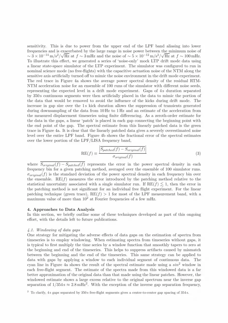
sensitivity. This is due to power from the upper end of the LPF band aliasing into lowerfrequencies and is exacerbated by the large range in noise power between the minimum noise of∼ 3× 10−14 m/s2/

√Hz at f ∼ 3mHz and the noise of ∼ 5× 10−12 m/s2/

√Hz at f ∼ 100mHz.

To illustrate this effect, we generated a series of ‘noise-only’ mock LTP drift mode data usinga linear state-space simulator of the LTP experiment. The simulator was configured to run innominal science mode (no free-flights) with the capacitive actuation noise of the NTM along thesensitive axis artificially turned off to mimic the noise environment in the drift mode experiment.The red trace in Figure 4a shows the average power spectral density of the residual RTM-NTM acceleration noise for an ensemble of 100 runs of the simulator with different noise seeds,representing the expected level in a drift mode experiment. Gaps of 4 s duration separatedby 350 s continuous segments were then artificially placed in the data to mimic the portion ofthe data that would be removed to avoid the influence of the kicks during drift mode. Theincrease in gap size over the 1 s kick duration allows the suppression of transients generatedduring downsampling of the data from 10Hz to 1Hz and an estimate of the acceleration fromthe measured displacement timeseries using finite differencing. As a zeroth-order estimate forthe data in the gaps, a linear ‘patch’ is placed in each gap connecting the beginning point withthe end point of the gap. The spectral estimate from this linearly patched data is the greentrace in Figure 4a. It is clear that the linearly patched data gives a severely overestimated noiselevel over the entire LPF band. Figure 4b shows the fractional error of the spectral estimatesover the lower portion of the LPF/LISA frequency band,

RE(f) ≡

∣

∣

∣Spatched(f)− Soriginal(f)

∣

∣

∣

σoriginal(f)(3)

where Soriginal(f)− Spatched(f) represents the error in the power spectral density in eachfrequency bin for a given patching method, averaged over the ensemble of 100 simulator runs.σoriginal(f) is the standard deviation of the power spectral density in each frequency bin overthe ensemble. RE(f) measures the error introduced by the patching method relative to thestatistical uncertainty associated with a single simulator run. If RE(f) . 1, then the error inthe patching method is not significant for an individual free flight experiment. For the linearpatching technique (green trace), RE(f) > 1 for most of the LPF measurement band, with amaximum value of more than 102 at Fourier frequencies of a few mHz.

4. Approaches to Data Analysis

In this section, we briefly outline some of these techniques developed as part of this ongoingeffort, with the details left to future publications.

4.1. Windowing of data gaps

One strategy for mitigating the adverse effects of data gaps on the estimation of spectra fromtimeseries is to employ windowing. When estimating spectra from timeseries without gaps, itis typical to first multiply the time series by a window function that smoothly tapers to zero atthe beginning and end of the timeseries. This helps to suppress artifacts caused by mismatchbetween the beginning and the end of the timeseries. This same strategy can be applied todata with gaps by applying a window to each individual segment of continuous data. Thecyan line in Figure 4a shows the result of the spectral estimate made using a sin2 window ineach free-flight segment. The estimate of the spectra made from this windowed data is a farbetter approximation of the original data than that made using the linear patches. However, thewindowed estimate shows a large excess relative to the original spectrum near the inverse gapseparation of 1/354 s ≈ 2.8mHz2. With the exception of the inverse gap separation frequency,

2 To clarify, 4 s gaps separated by 350 s free-flight segments gives a center-to-center gap spacing of 354 s.

Frequency [Hz]10-6 10-5 10-4 10-3 10-2 10-1d

iffe

rnti

al a

ccel

erat

ion

[m

s-2

Hz-1

/2]

10-15

10-14

10-13

10-12

original datalinear patchingCG patchingwindowing

(a) Ensemble-averaged noise spectral densities

Frequency [Hz]10-6 10-5 10-4 10-3 10-2 10-1

RE

[]

10-2

10-1

100

101

102

103

linear patchingCG patchingwindowing

(b) Relative Error

Figure 4: Comparison of methods for spectral estimation of RTM acceleration relative to NTMwith data gaps of 4 s duration separated by 350s free-flight segments. A linear state-spacesimulator of LTP was used to generate an ensemble of 100 noise realizations of LTP sciencemode data with no electrostatic suspension noise and data gaps were artificially inserted allowingfor the comparison of the estimated power spectral densities with and without gaps. The leftplot shows the power spectral densities of the original signal (red), the linearly-patched signal(green), the Constrained-Gaussian patched signal (dashed blue), and the power spectral densityestimated with the window method (dashed cyan). The right plot shows the relative error asdefined in (3) between the power spectral density estimated with gaps and that without gapsfor the three approaches.

RE(f) < 1 for most of the LPF measurement band.To better compare the original acceleration noise power spectrum to the one recovered using

the window method, fits were made to both versions of the power spectral density from eachsimulator run. The model was a four-component power law3,

Smod(f) = P−6 · f−6 + P−2 · f−2 + P0 · f0 + P4 · f+4, (4)

where f is the Fourier frequency and P−6,−2,0,+4 are the amplitudes of the four components.Figures 5a - 5d show histograms of the best-fit amplitudes for the spectral model over theensemble of 100 simulator runs for both the original data (red) and the windowed method(cyan). Table 1 lists the mean and standard deviations for the ensemble of noise realizations foreach of the four component amplitudes. As a rough measure of the statistical equivalenceof the distributions of the best-fit coefficients to the original and recovered power spectraldensities, we compute the difference between the means normalized by the quadrature sumof the deviations. The window method produces significant bias in the P−2 and P0 coefficients(3.5 and 6 sigma, respectively) and slight bias (0.9 sigma, or a p-value of 36%) in the P+4

coefficient. The recovered P−6 coefficient is consistent but is not well-determined in the fits toeither the original or recovered data.

4.2. Constrained-Gaussian Gap Patching

Another approach to dealing with data gaps and the difficulties they cause with estimatingspectra is to fill the gaps with fabricated data. While the fabricated data in these patches willnecessarily bias the spectral estimate, if the gaps are not too numerous and the patch data

3 Note that the fit was performed on the power spectral density where as Figures 1a, 1b, and 4a plot the amplitude

spectral density. As a result the spectral indices are a factor of two greater.

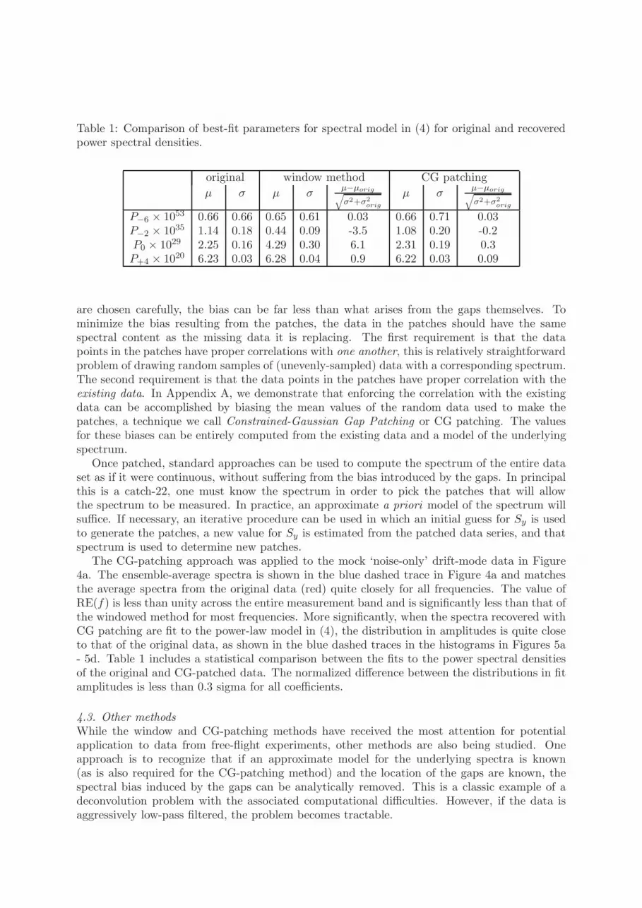
Table 1: Comparison of best-fit parameters for spectral model in (4) for original and recoveredpower spectral densities.

original window method CG patching

µ σ µ σµ−µorig

√

σ2+σ2orig

µ σµ−µorig

√

σ2+σ2orig

P−6 × 1053 0.66 0.66 0.65 0.61 0.03 0.66 0.71 0.03P−2 × 1035 1.14 0.18 0.44 0.09 -3.5 1.08 0.20 -0.2P0 × 1029 2.25 0.16 4.29 0.30 6.1 2.31 0.19 0.3P+4 × 1020 6.23 0.03 6.28 0.04 0.9 6.22 0.03 0.09

are chosen carefully, the bias can be far less than what arises from the gaps themselves. Tominimize the bias resulting from the patches, the data in the patches should have the samespectral content as the missing data it is replacing. The first requirement is that the datapoints in the patches have proper correlations with one another, this is relatively straightforwardproblem of drawing random samples of (unevenly-sampled) data with a corresponding spectrum.The second requirement is that the data points in the patches have proper correlation with theexisting data. In Appendix A, we demonstrate that enforcing the correlation with the existingdata can be accomplished by biasing the mean values of the random data used to make thepatches, a technique we call Constrained-Gaussian Gap Patching or CG patching. The valuesfor these biases can be entirely computed from the existing data and a model of the underlyingspectrum.

Once patched, standard approaches can be used to compute the spectrum of the entire dataset as if it were continuous, without suffering from the bias introduced by the gaps. In principalthis is a catch-22, one must know the spectrum in order to pick the patches that will allowthe spectrum to be measured. In practice, an approximate a priori model of the spectrum willsuffice. If necessary, an iterative procedure can be used in which an initial guess for Sy is usedto generate the patches, a new value for Sy is estimated from the patched data series, and thatspectrum is used to determine new patches.

The CG-patching approach was applied to the mock ‘noise-only’ drift-mode data in Figure4a. The ensemble-average spectra is shown in the blue dashed trace in Figure 4a and matchesthe average spectra from the original data (red) quite closely for all frequencies. The value ofRE(f) is less than unity across the entire measurement band and is significantly less than that ofthe windowed method for most frequencies. More significantly, when the spectra recovered withCG patching are fit to the power-law model in (4), the distribution in amplitudes is quite closeto that of the original data, as shown in the blue dashed traces in the histograms in Figures 5a- 5d. Table 1 includes a statistical comparison between the fits to the power spectral densitiesof the original and CG-patched data. The normalized difference between the distributions in fitamplitudes is less than 0.3 sigma for all coefficients.

4.3. Other methods

While the window and CG-patching methods have received the most attention for potentialapplication to data from free-flight experiments, other methods are also being studied. Oneapproach is to recognize that if an approximate model for the underlying spectra is known(as is also required for the CG-patching method) and the location of the gaps are known, thespectral bias induced by the gaps can be analytically removed. This is a classic example of adeconvolution problem with the associated computational difficulties. However, if the data isaggressively low-pass filtered, the problem becomes tractable.

P-6

x 1053 [m2 s-4 Hz5] 0 0.5 1 1.5 2 2.5 3 3.5 4

cou

nts

0

5

10

15

20

25

30

35

40

45

50 originalwindowedCG patched

(a) f−6 component

P-2

x 1035 [m2 s-4]0 0.2 0.4 0.6 0.8 1 1.2 1.4 1.6

cou

nts

0

10

20

30

40

50

60originalwindowedCG patched

(b) f−2 component

P0 x 1029 [m2 s-4 Hz-1]

1 1.5 2 2.5 3 3.5 4 4.5

cou

nts

0

10

20

30

40

50

60

70 originalwindowedCG patched

(c) f0 component

P4 x 1020 [m2 s-4 Hz-5]

6 6.05 6.1 6.15 6.2 6.25 6.3 6.35 6.4

cou

nts

0

5

10

15

20

25

30

35 originalwindowedCG patched

(d) f+4 component

Figure 5: Histograms of power-law amplitudes in a four-component fit to the spectrum of RTMacceleration relative to the NTM for the original data (red) and as recovered in the presenceof gaps using the window method (cyan) and the Constrained Gaussian patching method (bluedashed). For each of the 100 simulator runs, a power spectrum was generated and fit using aleast-squares algorithm to a four-component power law with indices -6,-2,0, and +4 as describedin (4). The plots show the distribution of best-fit parameters over the ensemble of 100 simulatorruns. For the case of the windowed method, the noise spike around 2.8mHz was de-weighted tominimize it’s bias on the fit.

An altogether unique approach is to consider only the data in the free-flights themselves andperform time-domain fits on the free-flight trajectories. Each of these fits will have parameterssuch as residual gravity gradient that are the same as those for the first stage, explained atthe beginning of Section 3, of the methods outlined above. However, there will also be somevariation in these parameters between successive flights that is caused by low-frequency (Fourierfrequencies lower than the inverse free-flight time) acceleration noise in the system. By analyzingthe variation in parameters recovered from fits to a series of free-flight trajectories, an estimateof acceleration noise at Fourier frequencies below the inverse free-flight frequency can be madewithout the need to deal with data gaps.

5. Conclusions

The free fight experiments planned for LPF will provide an opportunity to gather data thatis even more representative of a full-scale LISA like instrument than the standard LPF sciencemode. This improvement will allow for better characterization of the small forces that ultimately

limit the performance of LPF, LISA, and other future instruments requiring low-disturbanceenvironments such as advanced geodesy or fundamental physics missions. The challenges inextracting this information from the free-flight data are significant, but progress in overcomingthem is being made with a number of independent techniques. The challenge of estimatingthe relative RTM/NTM acceleration noise in the presence of data gaps has been successfullyaddressed by a number of techniques with the current limitation being the ability to combinethis with accurate removal of the deterministic free-flight signal. It is fully expected that theremaining challenges will be resolved in time for launch and operations.

Appendix A: Generating Constrained-Gaussian Patches

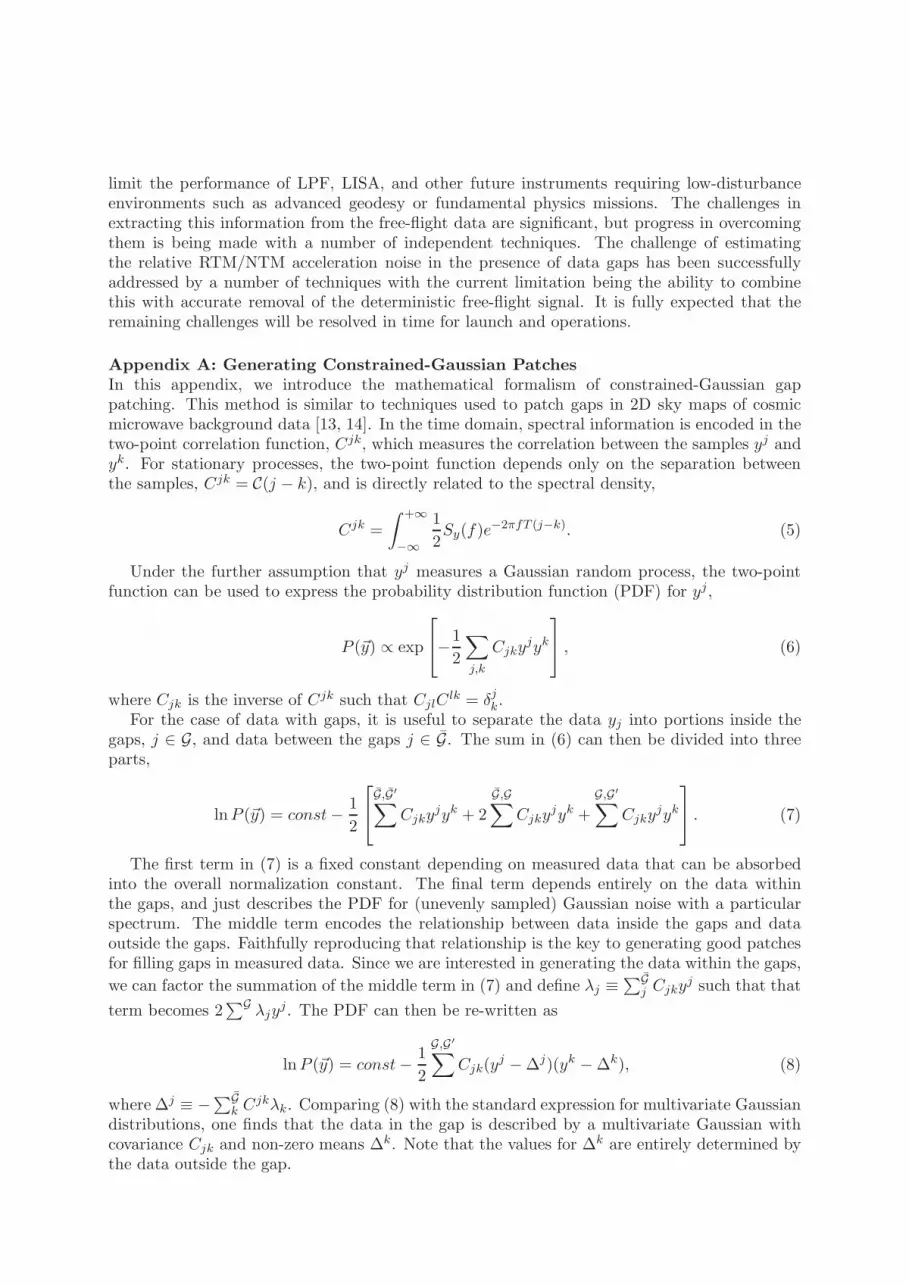
In this appendix, we introduce the mathematical formalism of constrained-Gaussian gappatching. This method is similar to techniques used to patch gaps in 2D sky maps of cosmicmicrowave background data [13, 14]. In the time domain, spectral information is encoded in thetwo-point correlation function, Cjk, which measures the correlation between the samples yj andyk. For stationary processes, the two-point function depends only on the separation betweenthe samples, Cjk = C(j − k), and is directly related to the spectral density,

Cjk =

∫ +∞

−∞

1

2Sy(f)e

−2πfT (j−k). (5)

Under the further assumption that yj measures a Gaussian random process, the two-pointfunction can be used to express the probability distribution function (PDF) for yj,

P (~y) ∝ exp

−1

2

∑

j,k

Cjkyjyk

, (6)

where Cjk is the inverse of Cjk such that CjlClk = δjk.

For the case of data with gaps, it is useful to separate the data yj into portions inside thegaps, j ∈ G, and data between the gaps j ∈ G. The sum in (6) can then be divided into threeparts,

lnP (~y) = const− 1

2

G,G′

∑

Cjkyjyk + 2

G,G∑

Cjkyjyk +

G,G′

∑

Cjkyjyk

. (7)

The first term in (7) is a fixed constant depending on measured data that can be absorbedinto the overall normalization constant. The final term depends entirely on the data withinthe gaps, and just describes the PDF for (unevenly sampled) Gaussian noise with a particularspectrum. The middle term encodes the relationship between data inside the gaps and dataoutside the gaps. Faithfully reproducing that relationship is the key to generating good patchesfor filling gaps in measured data. Since we are interested in generating the data within the gaps,

we can factor the summation of the middle term in (7) and define λj ≡∑G

j Cjkyj such that that

term becomes 2∑G λjy

j. The PDF can then be re-written as

lnP (~y) = const− 1

2

G,G′

∑

Cjk(yj −∆j)(yk −∆k), (8)

where ∆j ≡ −∑G

k Cjkλk. Comparing (8) with the standard expression for multivariate Gaussian

distributions, one finds that the data in the gap is described by a multivariate Gaussian withcovariance Cjk and non-zero means ∆k. Note that the values for ∆k are entirely determined bythe data outside the gap.

The prescription for Constrained Gaussian Gap Filling is thus as follows: make a guess forspectral density Sy(f) describing the data; compute an estimated two-point correlation function,Cjk; compute the ∆k for each point on the gap based on the data outside the gap and theestimated Cjk, draw data from a multivariate Gaussian distribution with covariance Cjk andmean ∆k.

References[1] Bondi H, Pirani F A E and Robinson I 1959 Royal Society of London Proceedings Series A 251 519–533[2] Armano M and et al 2009 Class. Quant. Grav. 26

[3] Lange B 1964 AIAA Journal 2 1590–1606 URL http://dx.doi.org/10.2514/3.55086

[4] deBra D B 1997 Classical and Quantum Gravity 14 1549 URLhttp://stacks.iop.org/0264-9381/14/i=6/a=026

[5] Antonucci F, Armano M, Audley H, Auger G, Benedetti M, Binetruy P, Boatella C, Bogenstahl J, BortoluzziD, Bosetti P, Brandt N, Caleno M, Cavalleri A, Cesa M, Chmeissani M, Ciani G, Conchillo A, Congedo G,Cristofolini I, Cruise M, Danzmann K, Marchi F D, Diaz-Aguilo M, Diepholz I, Dixon G, Dolesi R, DunbarN, Fauste J, Ferraioli L, Fertin D, Fichter W, Fitzsimons E, Freschi M, Marin A G, Marirrodriga C G,Gerndt R, Gesa L, Giardini D, Gibert F, Grimani C, Grynagier A, Guillaume B, Cervantes F G, HarrisonI, Heinzel G, Hewitson M, Hollington D, Hough J, Hoyland D, Hueller M, Huesler J, Jeannin O, JennrichO, Jetzer P, Johlander B, Killow C, Llamas X, Lloro I, Lobo A, Maarschalkerweerd R, Madden S, ManceD, Mateos I, McNamara P W, Mendes J, Mitchell E, Monsky A, Nicolini D, Nicolodi D, Nofrarias M,Pedersen F, Perreur-Lloyd M, Perreca A, Plagnol E, Prat P, Racca G D, Rais B, Ramos-Castro J, ReicheJ, Perez J A R, Robertson D, Rozemeijer H, Sanjuan J, Schleicher A, Schulte M, Shaul D, Stagnaro L,Strandmoe S, Steier F, Sumner T J, Taylor A, Texier D, Trenkel C, Tombolato D, Vitale S, Wanner G,Ward H, Waschke S, Wass P, Weber W J and Zweifel P 2011 Classical and Quantum Gravity 28 094002URL http://stacks.iop.org/0264-9381/28/i=9/a=094002

[6] Audley H, Danzmann K, Marin A G, Heinzel G, Monsky A, Nofrarias M, Steier F, Gerardi D, GerndtR, Hechenblaikner G, Johann U, Luetzow-Wentzky P, Wand V, Antonucci F, Armano M, Auger G,Benedetti M, Binetruy P, Boatella C, Bogenstahl J, Bortoluzzi D, Bosetti P, Caleno M, Cavalleri A, CesaM, Chmeissani M, Ciani G, Conchillo A, Congedo G, Cristofolini I, Cruise M, Marchi F D, Diaz-AguiloM, Diepholz I, Dixon G, Dolesi R, Fauste J, Ferraioli L, Fertin D, Fichter W, Fitzsimons E, Freschi M,Marirrodriga C G, Gesa L, Gibert F, Giardini D, Grimani C, Grynagier A, Guillaume B, Cervantes F G,Harrison I, Hewitson M, Hollington D, Hough J, Hoyland D, Hueller M, Huesler J, Jeannin O, Jennrich O,Jetzer P, Johlander B, Killow C, Llamas X, Lloro I, Lobo A, Maarschalkerweerd R, Madden S, Mance D,Mateos I, McNamara P W, Mendes J, Mitchell E, Nicolini D, Nicolodi D, Pedersen F, Perreur-Lloyd M,Perreca A, Plagnol E, Prat P, Racca G D, Rais B, Ramos-Castro J, Reiche J, Perez J A R, Robertson D,Rozemeijer H, Sanjuan J, Schulte M, Shaul D, Stagnaro L, Strandmoe S, Sumner T J, Taylor A, Texier D,Trenkel C, Tombolato D, Vitale S, Wanner G, Ward H, Waschke S, Wass P, Weber W J and Zweifel P 2011Classical and Quantum Gravity 28 094003 URL http://stacks.iop.org/0264-9381/28/i=9/a=094003

[7] Carbone L, Ciani G, Dolesi R, Hueller M, Tombolato D, Vitale S, Weber W J and Cavalleri A 2007 Phys.

Rev. D 75(4) 042001 URL http://link.aps.org/doi/10.1103/PhysRevD.75.042001

[8] Cavalleri A, Ciani G, Dolesi R, Hueller M, Nicolodi D, Tombolato D, Wass P J, We-ber W J, Vitale S and Carbone L 2009 Classical and Quantum Gravity 26 094012 URLhttp://stacks.iop.org/0264-9381/26/i=9/a=094012

[9] Grynagier A 2010 The drift mode for LISA Pathfinder, control description Tech. Rep. S2-iFR-TN-3005Universitat Stuttgart

[10] Lomb N R 1976 Astrophysics and Space Science 39 447–462[11] Scargle J D 1982 The Astrophysical Journal 263 835–853[12] Press W H and Rybicki G B 1989 The Astrophysical Journal 338 277–280[13] Hoffman Y and Ribak E 1991 The Astrophysical Journal 380 L5–L8[14] Bucher M and Louis T 2012 Monthly Notices of the Royal Astronomical Society 424 1694–1713