Citation: Malvermi, R.; Gonzalez, S.;

Antonacci, F.; Sarti, A.; Corradi, R. A

Statistical Approach to Violin

Evaluation. Appl. Sci. 2022, 12, 7313.

https://doi.org/10.3390/

app12147313

Academic Editors: Mariana Domnica

Stanciu, Voichit,a Bucur and Mircea

Mihalcica

Received: 26 June 2022

Accepted: 19 July 2022

Published: 21 July 2022

Publisher’s Note: MDPI stays neutral

with regard to jurisdictional claims in

published maps and institutional affil-

iations.

Copyright: © 2022 by the authors.

Licensee MDPI, Basel, Switzerland.

This article is an open access article

distributed under the terms and

conditions of the Creative Commons

Attribution (CC BY) license (https://

creativecommons.org/licenses/by/

4.0/).

applied sciences

Article

A Statistical Approach to Violin EvaluationRaffaele Malvermi 1,* , Sebastian Gonzalez 1, Fabio Antonacci 1, Augusto Sarti 1 and Roberto Corradi 2

1 Department of Electronics, Information and Bioengineering, Politecnico di Milano, 20133 Milano, Italy;tsuresuregusa@gmail.com (S.G.); fabio.antonacci@polimi.it (F.A.); augusto.sarti@polimi.it (A.S.)

2 Department of Mechanical Engineering, Politecnico di Milano, 20156 Milano, Italy; roberto.corradi@polimi.it* Correspondence: raffaele.malvermi@polimi.it

Featured Application: Physics-informed quality assessment of a stringed musical instrument.

Abstract: Comparing violins requires competence and involves both subjective and objective evalua-tions. In this manuscript, vibration tests were performed on a set of 25 violins, both historical andnew. The resulting bridge admittances were modeled in the low and mid-frequency ranges througha set of objective features. Once projected into the new representation, the bridge admittances ofthree historical violins made by Stradivari and a famous reproduction revealed high similarity. PCAhighlighted the importance of signature mode frequencies, bridge hill behavior, and signature modeamplitudes in distinguishing different violins.

Keywords: musical acoustics; bridge admittance; feature-based

1. Introduction

Assessing the quality of a violin is an extremely difficult matter. There are no objectivedescriptors that can separate a “good” violin from a “great” one and yet some instrumentscan reach prices up in the millions. Even professional musicians have trouble distinguishingold from new violins, and their preference does not necessarily correlate with the price ofthe instrument [1–3]. At the end of the day, it comes down to the subjective preference ofthe player. Having an objective measure to support the evaluation of an instrument couldhelp instrument makers and musicians in the search for the perfect match between violinistand violin.

The bridge admittance could be such a simple objective tool to qualify an instrument.This is the frequency response function (FRF) measured at the bridge on the plane per-pendicular to the strings. The measurement is performed by means of an instrumentedhammer and an accelerometer, located at opposites on the bridge. It is a good estimator ofthe vibrational behavior of the instrument soundbox from whence the sound of the violincomes from. It is fast to perform and the equipment needed is relatively cheap, at least fora scientific lab if not for the luthier’s workshop [4,5].

FRFs have in fact been used for a long time as descriptors of the violin in the liter-ature [6,7]. It has even been stated, without hard evidence though, that the quality ofthe violin correlates with some spectral features of the bridge admittance. In particular,the presence of the so-called bridge hill has been hailed as a mark of quality. Accordingto [7], this bridge hill is “a hump [sic] between 2 and 3 kHz in their frequency responses”.Despite the importance of this feature, the lack of a scientifically grounded definition makesits use in research questionable.

Our objective in this article is to produce physically informed and objectively measur-able features from the bridge admittance that allow one to compare, and maybe eventuallydiscriminate, good violins from great ones. At the very least, have a standard way ofcomparing them beyond the mere visual inspection, which seems to be the preferred wayin the state of the art [5].

Appl. Sci. 2022, 12, 7313. https://doi.org/10.3390/app12147313 https://www.mdpi.com/journal/applsci

Appl. Sci. 2022, 12, 7313 2 of 14

To compare different FRFs one needs to understand their physical provenance. Wood-house [8] divides the signal into three separate regions. In the low range, the influence ofthe individual modes of the instrument is clearly visible in the signal as peaks. Eventually,as the frequency of the modes becomes higher, the damping factor makes the peaks blendtogether and a clear identification of the modes is not possible: these are the transitionalmodes. At high frequency, in fact, the mode overlap becomes greater, and even smalldifferences cause a great variability of the mode shapes between instruments. Although themodes still determine the behavior of the FRF, analytical approaches to model it becomesprogressively less effective [9].

Different instruments have different resonance frequencies. These differences aredue to material and geometric variation between the instruments [10]. Therefore, a directcomparison in the frequency domain is not immediately applicable. If two instrumentshave the same FRFs but shifted in a few Hertz, does that make them more similar than apair of FRFs where the modes are at the same frequency but their amplitude is completelydifferent? Developing a way to answer those kinds of questions is the aim of this article.

Following the separation highlighted by Woodhouse, one can consider different mod-els for each frequency range of the FRF. Modal approaches are revealed as powerfulreconstructions of the individual (also denoted as “signature”) and transitional modes.Indeed, the bridge can be interpreted as a filter coupling strings and violin soundbox suchthat its admittance can be seen as the filter transfer function [11]. Accordingly, the funda-mental properties of modes, i.e., frequency, amplitude, and damping ratio, can be usedto define the poles and zeros of such filter. From the signal processing perspective, thismethodology can be applied not only in the analysis stage [12] but also in the synthesis ofvirtual or altered instrument timbre starting from measured admittances [13–15].

Although they can fit a large portion inside acoustic instrument admittances, thesemodels are not able to interpret relevant high-frequency components. At the same time, theycould need a large number of modes to reach good accuracy [13]. The same considerationshold for Euclidean distances computed even on a small set of signature mode features.These showed to better quantify the similarity between FRFs if compared to point measures,e.g., mean square error (MSE), which are evaluated in the frequency domain directly [16].However, the same metric fails when differences occur mainly at high frequency.

In this work, we propose an extension of the multidimensional feature space proposedin [16] based on both modal parameters and energy-based descriptors, found to be morerepresentative for the mid-range [9]. In this new representation, a more informativeEuclidean distance can be measured to assess the similarity between FRFs in the low andmid-frequency ranges. The features adopted here are objectively defined, in contrast toe.g., the bridge hill, and could be used to study the perceptual relevance of particularelements of the FRF through virtual sound synthesis.

2. Materials and Methods2.1. Violins

The selection of violins under study counts twenty-five instruments with varying agesand styles of making. Thirteen of these belong to the permanent collection of instrumentsawarded in the “Antonio Stradivari International Triennial Competitions of Stringed instru-ment making” [17]. The competition, held in the city of Cremona since 1976, embraces bothCremonese and international competitors. A jury of experts selects the winner according tostylistic and technical evaluations. The winner of each contest is acquired by the museumand kept in its permanent collection. Among the remaining samples, there are nine modernviolins that were kindly offered by violin makers during the Mondo Musica 2020 expositionand three historical violins made by Stradivari in the 18th century. For all the instruments,the owners provided consent for the usage of the results in an anonymous fashion. For thisreason, and for the ease of reading, we will denote all the violins made within the 20thand 21st centuries with M1–M22 (modern) while we will refer to the historical ones asH1–H3. It is noteworthy that one of the modern violins (i.e., M22) was made by a famous

Appl. Sci. 2022, 12, 7313 3 of 14

international violin maker with the aim of reproducing the outline of one of the measuredhistorical violins (i.e., H3). The acoustic similarity of the violins was confirmed by the actualowner of both instruments, who happens to be an internationally acclaimed violin player.Although dissimilarities between violins rely often on subtle details and even two replicasof the same violin could easily differ in their sound [3], the presence of the pair M22–H3 inaddition to a group of violins belonging to the same author, i.e., to Stradivari, still could beused to assess the soundness of the proposed metric. Indeed, common trends are expectedto be observed once the bridge admittances are projected into the feature representation.

2.2. Vibration Tests

The bridge admittances were measured by means of hammer impact testing. A struc-ture made of wood and rubber bands was built to approximate free boundary conditionsduring the test. Four rubber bands were used for the suspension of the instrument, lettingthe sample hang in a vertical position and minimizing the contact surface [18,19]. In partic-ular, two rubber bands were placed at the bottom of the violin while the remaining twosupported its soundbox from the upper corners. In this configuration, the resting positionof the hammer is vertical after the hit, avoiding the occurrence of accidental secondarystrikes during the acquisition. A dynamometric hammer with light tip (086E80, by PCBPiezotronics) and a uniaxial accelerometer (352A12, by PCB Piezotronics) were used togenerate an impulsive excitation and measure the harmonic response, respectively. Impactswere applied on one edge of the bridge while the accelerometer was placed on the oppositeside. For each measurement, six time-domain signals of two seconds sampled at 48 kHzwere acquired. FRFs were then estimated following the definition of the H1 estimator toreduce noise caused by the instrumentation [20]. The magnitudes of the resulting FRFs arerepresented in dB scale, with a reference value equal to 1 m s−1 N−1.

2.3. Low-Frequency Features

The signature modes of a violin typically cover the violin response in the low-frequencyrange, which can reach 800 Hz for the complete soundbox [21]. Thanks to the low modaldensity encountered in this region, analytical approximations based on modal superpositioncan be used [22]. Therefore, let us model a given bridge admittance Hij(ω) as a linearcombination of modal contributions, namely

Hij(ω) ∼N

∑r=1

ΦriΦrj

ω2r + 2jωξrωr −ω2 , ω ∈ [ωmin, ωmid], (1)

where i and j refer to the excitation and measurement points at the bridge corners, N is thenumber of signature modes considered, Φri and Φrj correspond to the mode shape of moder evaluated at the two points observed, ωr is the natural frequency and ξr is the dampingratio associated to mode r, respectively.

The model was defined using as features the frequency fr = ωr/2π, amplitudepr = |Hij(ωr)| and Q factor qr = 1/2ξr of N = 4 signature modes among the ones presentedin the literature [21], namely: (i) the Helmholtz mode A0 (features f1, p1, q1); (ii) the C BoutsRhomboidal mode CBR ( f2, p2, q2); (iii) the Corpus mode B1− ( f3, p3, q3); (iv) the Bodymode B1+ ( f4, p4, q4). The choice was made on the basis of two main considerations. Onthe one hand, the selected modes proved to be consistent over frequency throughout theset of bridge admittances analyzed while mode switching occurred frequently for theexcluded ones. As an example, the second air mode A1 was found either between CBRand B1− or between B1− and B1+, making its identification impossible for a simple peakfinding algorithm. On the other hand, these modes are also well-known by the violin makercommunity [8,23].

The frequency range in which the reconstruction shows a good agreement with themeasurement has ωmin = 2π fmin with fmin = 230 Hz as lower limit to exclude irrelevantinformation before the A0 mode and, as upper limit, ωmid = 2π fmid with fmid equal to the

Appl. Sci. 2022, 12, 7313 4 of 14

frequency of the first antiresonance (i.e., minimum in the FRF magnitude) after the B1+mode. This antiresonance was taken as a reference since it was found in all the FRFs understudy. It is worth noticing that when ω matches ωr,

|Hij(ωr)| ∼ΦriΦrj

2ξrω2r

, (2)

thus making Equation (1) completely recovered from the knowledge of the mode frequen-cies, amplitudes and corresponding damping ratios.

Finally, a total of twelve low-frequency descriptors are included in the definition ofthe feature space. We will denote the features related to signature mode frequencies as thevector f = [ f1, f2, f3, f4], the features related to signature mode amplitudes as the vectorp = [p1, p2, p3, p4] and the features related to damping as the vector of corresponding Qfactors q = [q1, q2, q3, q4]. If f is extracted directly from the measured signal by meansof available peak finding algorithms, p and q must be tuned such that the model takesinto account the correlation between modes, even though this was found to be low. Theestimates for these two subsets of features are thus obtained rewriting Equation (1) as afunction of p and q and setting up a least-square measurement fitting problem as

minp,q∈R+

∣∣∣∣∣∣∣∣ |Hij(ω)| −∣∣∣∣ 4

∑r=1

ω2r pr

qr(ω2r −ω2) + jωωr

∣∣∣∣ ∣∣∣∣∣∣∣∣22, (3)

with ω ∈ [ωmin, ωmid] and ωr = 2π fr. The minimization was solved iteratively using thesimplex algorithm. The peak amplitudes extracted from the signal were provided as initialvalues for p while a guess for q was computed by means of the half-power bandwidthmethod [24].

2.4. Mid-Frequency Features

To define a set of features modeling the FRF at higher frequencies, we took inspirationfrom statistical approaches to the subject [9]. We chose to represent the energy distributionof a given bridge admittance Hij(ω) by computing its relative power (RP) as

RP(ω) =P(ω)

Ptot=

∫ ωωmin|Hij(ω)|2 dω∫ ωmax

ωmin|Hij(ω)|2 dω

, (4)

where P(ω) is the cumulative power and Ptot is the total power of the signal, i.e., computedwithin the range [2π fmin, 2π fmax] with fmin = 230 Hz and fmax = 4500 Hz. In the frequencyinterval considered, RP(ω) ranges between 0 and 1.

The slope of this descriptor is characterized by “bumps” where the correspondingbridge admittance exhibits high-energy components (see Figure 1b as an example). Inparticular, two main slope changes typically occur in violin bridge admittances after500–600 Hz and between 2 and 3 kHz. The first relevant increase in the RP value, encoun-tered at low frequencies, quantifies the amount of energy of the signature modes. Indeed,the RP curve starts to flatten at the frequency of mode B1+. Starting from the antiresonanceafter mode B1+, the RP shows a different growth rate for each violin in the dataset. Here,the RP curve exhibits a characteristic S-shape strongly correlated to a high-energy region inthe corresponding bridge admittance.

To obtain a compact description of this behavior in the mid-frequency range, beingit the interval between ωmid and ωmax, we modelled the RP curve by means of a sigmoidfunction with tunable curvature based on [25], namely

σ(ω, ω∗, k∗) =ω− k∗ω

k∗ − 2k∗|ω|+ 1where ω =

ω−ω∗

∆ω, (5)

Appl. Sci. 2022, 12, 7313 5 of 14

ω∗ is the center frequency of the sigmoid, k∗ the control parameter for its curvature and∆ω = min(|ω∗ − ωmid|, |ωmax − ω∗|) such that the domain of the sigmoid is symmetricwith respect to ω∗. To better fit the RP values at the extremes of the mid-frequency range,the output of the function σ(ω, ω∗, k∗) is scaled and shifted leading to

σ′(ω, ωmid, ω∗, k∗) = σ(ω, ω∗, k∗)RP(ω∗ + ∆ω)− RPmid

σmax − σmin+ |RPmid − σmin|,

RPmid = RP(ωmid),

σmax = max(σ(ω, ωmid, ω∗, k∗)),

σmin = min(σ(ω, ωmid, ω∗, k∗)).

(6)

The fitting was performed by searching for the values of ω∗, k∗ such that the MSEbetween the measured RP and the predicted sigmoid has its minimum. The minimizationwas carried out iteratively using the simplex algorithm. Interestingly enough, the valuesfound for k∗ at the end of the optimization follow a Gaussian distribution centered around−0.7. Two outliers were detected, with k∗ equal to −0.25 and −0.05.

The advantage of this representation is that the resulting optimal sigmoid model canbe easily projected back to the frequency-magnitude space by computing its derivativewith respect to ω. We thus decided to use the parameters of Equation (6) as features for themid-frequency range.

Along with these features, we added two additional descriptors to the set. On theone hand, we took the MSE between the measured RP and the sigmoid fit as a metricof the fitting accuracy. We will denote it as the “area difference” ∆A for its geometricinterpretation (see Figure 1b). On the other hand, we considered the slope khigh of thelinear fit in the range [4000, 4500] Hz since the sigmoid model fails at explaining the lineardecrease in the magnitude encountered in FRFs at very high frequency. Table 1 summarizesthe final set of low and mid-frequency features defined to reconstruct a bridge admittance.

Table 1. Summary of the low and mid-frequency features defined.

Name Description

Signature mode frequencies

f1 Frequency of the first signature mode (Helmoltz mode, A0)

f2 Frequency of the second signature mode (C Bouts Rhomboidal mode, CBR)

f3 Frequency of the third signature mode (Corpus mode, B1−)

f4 Frequency of the fourth signature mode (Body mode, B1+)

Signature mode amplitudes

p1 Amplitude of the first signature mode (Helmoltz mode, A0)

p2 Amplitude of the second signature mode (C Bouts Rhomboidal mode, CBR)

p3 Amplitude of the third signature mode (Corpus mode, B1−)

p4 Amplitude of the fourth signature mode (Body mode, B1+)

Signature mode damping

q1 Q Factor of the first signature mode (Helmoltz mode, A0)

q2 Q Factor of the second signature mode (C Bouts Rhomboidal mode, CBR)

q3 Q Factor of the third signature mode (Corpus mode, B1−)

q4 Q Factor of the fourth signature mode (Body mode, B1+)

Appl. Sci. 2022, 12, 7313 6 of 14

Table 1. Cont.

Name Description

Mid-frequency

ωmid Frequency of the first antiresonance after mode B1+

RPmid Relative power of the signature modes, RPmid = RP(ωmid)

ω∗ Sigmoid center frequency

RP∗ Relative power center value, RP∗ = RP(ω∗)

k∗ Relative power curvature

∆A Area difference, ∆A = MSE(RP(ω), σ′(ω, ωmid, ω∗, k∗))

khigh Slope of the linear fit at high frequency

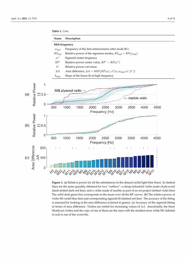
Figure 1. (a) Relative power for all the admittances in the dataset (solid light blue lines). In dashedlines are the same quantity obtained for two “outliers”: a cheap industrial violin made of plywood(dash-dotted dark red line), and a violin made of marble as part of an art project (dotted violet line).The solid dark green line corresponds to the mean over all the RP curves. (b) The relative power ofviolin M1 (solid blue line) and corresponding sigmoid fit (dashed red line). The accuracy of the fittingis assessed by looking at the area difference (colored in green). (c) Accuracy of the sigmoid fittingin terms of area difference. Violins are sorted for increasing values of ∆A. Anecdotally, the threeStradivari violins and the copy of one of them are the ones with the smallest error while M1 (labeledin red) is one of the worst fits.

Appl. Sci. 2022, 12, 7313 7 of 14

2.5. Feature-Based Reconstruction

Given the models for the different components of the bridge admittance inEquations (1) and (6), its magnitude can be reconstructed starting from the correspondingvalues of low and mid-frequency features as

∣∣Hij(ω)∣∣ ∼ ∣∣∣∣∣ 4

∑r=1

ΦriΦrj

ω2r + 2jωξrωr −ω2

∣∣∣∣∣+ Cδσ′(ω, ωmid,ω∗, k∗)

δω, ω ∈ [ωmin, ωmax], (7)

where C is a constant found through iterative optimization such that the MSE between thesecond term of Equation (7) and

∣∣Hij(ω)∣∣ is minimized around ω = ω∗.

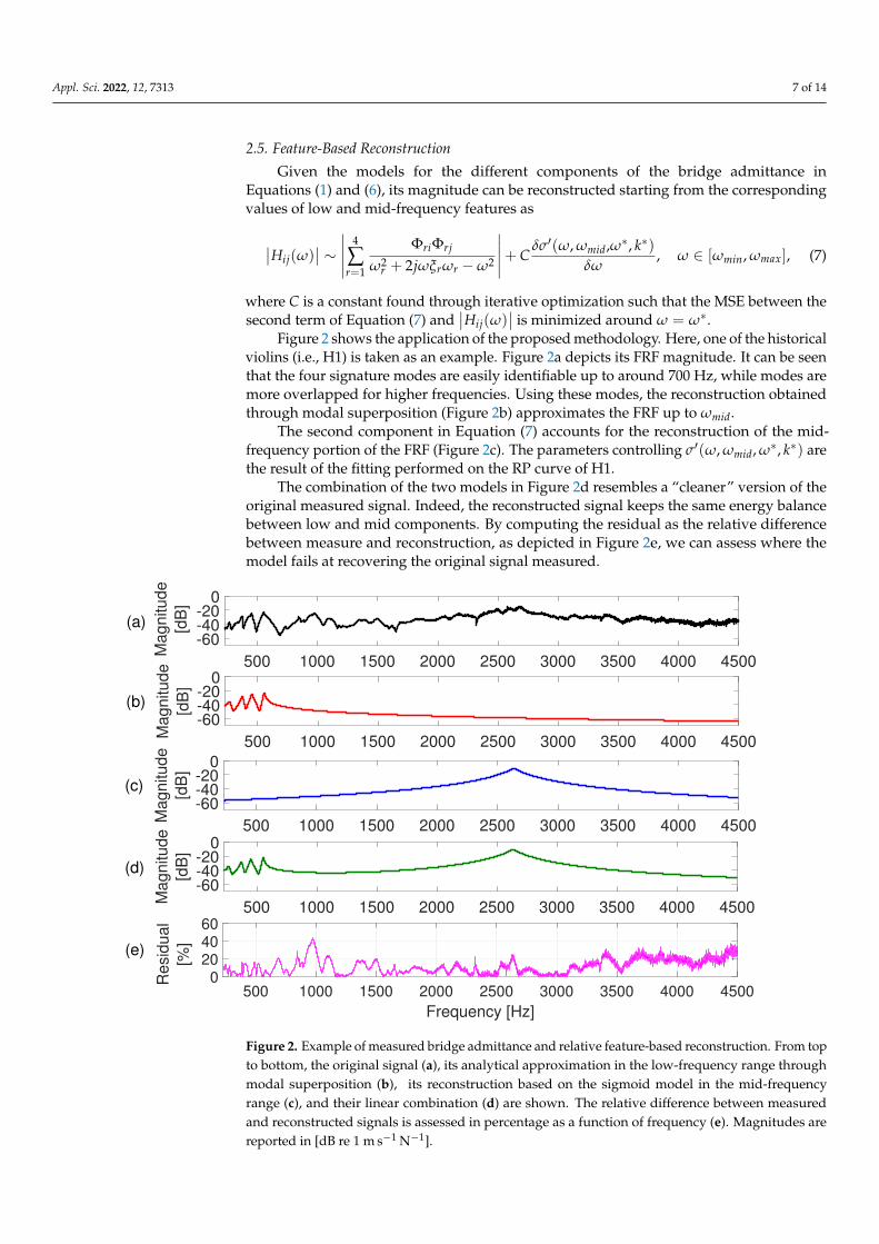
Figure 2 shows the application of the proposed methodology. Here, one of the historicalviolins (i.e., H1) is taken as an example. Figure 2a depicts its FRF magnitude. It can be seenthat the four signature modes are easily identifiable up to around 700 Hz, while modes aremore overlapped for higher frequencies. Using these modes, the reconstruction obtainedthrough modal superposition (Figure 2b) approximates the FRF up to ωmid.

The second component in Equation (7) accounts for the reconstruction of the mid-frequency portion of the FRF (Figure 2c). The parameters controlling σ′(ω, ωmid, ω∗, k∗) arethe result of the fitting performed on the RP curve of H1.

The combination of the two models in Figure 2d resembles a “cleaner” version of theoriginal measured signal. Indeed, the reconstructed signal keeps the same energy balancebetween low and mid components. By computing the residual as the relative differencebetween measure and reconstruction, as depicted in Figure 2e, we can assess where themodel fails at recovering the original signal measured.

500 1000 1500 2000 2500 3000 3500 4000 4500

-60-40-20

0

Magnitude

[dB

]

500 1000 1500 2000 2500 3000 3500 4000 4500

-60-40-20

0

Magnitude

[dB

]

500 1000 1500 2000 2500 3000 3500 4000 4500

-60-40-20

0

Magnitude

[dB

]

500 1000 1500 2000 2500 3000 3500 4000 4500

Frequency [Hz]

0204060

Resid

ual

[%]

500 1000 1500 2000 2500 3000 3500 4000 4500

-60-40-20

0

Magnitude

[dB

]

(c)

(d)

(e)

(b)

(a)

Figure 2. Example of measured bridge admittance and relative feature-based reconstruction. From topto bottom, the original signal (a), its analytical approximation in the low-frequency range throughmodal superposition (b), its reconstruction based on the sigmoid model in the mid-frequencyrange (c), and their linear combination (d) are shown. The relative difference between measuredand reconstructed signals is assessed in percentage as a function of frequency (e). Magnitudes arereported in [dB re 1 m s−1 N−1].

Appl. Sci. 2022, 12, 7313 8 of 14

In the specific case of H1, the reconstructed signature modes resemble the originalones and the residual oscillates around 5% close to antiresonance frequencies. A relevantincrease of the residual up to 40% is then encountered around 1 kHz. The frequency spancharacterized by large values of the residuals covers the portion of FRF dominated bytransitional modes. For a subset of FRFs in the dataset, transitional modes exhibit lowmode overlapping and modal superposition may model the FRF better than the proposedenergy-based model. However, a common trend was not found throughout the dataset andfurther research is needed to improve the model within this frequency range.

In the case of H1, the proposed reconstruction is also able to model the region of theFRF between 1500 and 3000 Hz. Here, the residual stabilizes between 5% and 10% exceptfor spikes corresponding to the presence of peaks or deeps in this portion of the spectrum,which cannot be recognized however as individual modes.

Finally, the reconstruction fails at explaining the trend of the admittance for higherfrequencies, i.e., between 4000 and 4500 Hz. In this range, the FRF exhibits a more lineartrend, and the residual reaches values around 20%. The feature khigh has been indeedintroduced to overcome this lack of information, defined as the slope of the linear fit limitedto the high frequency range mentioned.

3. Results3.1. Relative Power Analysis

We focus only on the analysis of the estimated RP curves. Indeed, an in-depth discus-sion of the low-frequency features is already presented in [16].

Figure 1a shows, in terms of relative power, all the violins in the dataset (solid lightblue lines) along with two violins that can be considered as “outliers”: on one hand anindustrial violin made of plywood (dash-dotted dark red line), and on the other, a violinentirely made of marble, except for the bridge and tailpiece (dotted violet line). It can benoticed that all the RP curves are concentrated in the middle between the two outliers.By computing the mean over all the RP curves in the dataset (dark green solid line),a sigmoidal trend can be observed. Moreover, the largest variation among the RP curvescan be observed between 2000 and 3000 Hz if the standard deviation is evaluated as afunction of frequency. In this frequency interval, the center of the sigmoid occurs for all theviolins in the dataset.

Concerning the clearly different behavior of the outliers, as we said the major differencebetween them and the other violins is the material used for these instruments. Despitebeing shifted in the frequency axis, the shape of the RP curves still follows a sigmoidaltrend. In the case of plywood, its specific stiffness (i.e., the ratio between the Young’smodulus, being it the constant describing the material stiffness, and the density) is farsmaller than typical spruce wood, as well as being less anisotropic [26]. For marble it is thecontrary: the material is far stiffer and denser than spruce. Both violins have roughly thesame geometric characteristics, in terms of dimensions, arching, and thickness profile, sowe can interpret the difference in the RP curves to their vastly different materials. Althougha sigmoidal behavior can be seen for the averaged RP, the accuracy of the actual fittingvaries from one violin to another. As an example, Figure 1b shows one of the worst sigmoidfits obtained (i.e., violin M1). It can be seen that the sigmoid curve (dashed red line) failsat approximating the measured RP (solid blue line). This may be due to the irregular andbumpy behavior of the RP curve, especially in the frequency range where the sigmoidis centered.

To have a measure of the “regularity” of the energy distribution, we computed thearea difference ∆A (Figure 1b, colored in green) throughout the dataset. Figure 1c lists allthe resulting values, in ascending order. Anecdotally, the four violins characterized by thelowest values are H3, H2, M22, and H1. These are the three Stradivari violins present in thedataset and a fine modern copy of one of them used by a professional musician. Conversely,the poor fit already observed for M1 corresponds to one of the highest values of ∆A. Forthe ease of reading, the label of M1 is colored in red in Figure 1c.

Appl. Sci. 2022, 12, 7313 9 of 14

From the analysis of the RP curves and the features related, we can conclude thatthe sigmoid is able to model the majority of the RP curves in the dataset, especially theStradivari violins.

3.2. Violin Clustering

Given the features defined in Sections 2.3 and 2.4, the resulting feature space consid-ered has thus 19 dimensions, leading to a feature matrix in RM×19, where M = 25. Z-scorenormalization [27] has been applied over each feature vector inside the feature matrix toequalize values within a common scale. Once normalized, an Euclidean distance can becomputed over the feature vectors characterizing each pair of admittances, leading to adistance matrix D ∈ RM×M. Notice that all the features have the same relative importanceto define our distance. In perceptual terms this could not hold, as some features can have afar larger influence than others. However, further studies are needed in this sense to definea “perceptual distance” between instruments.

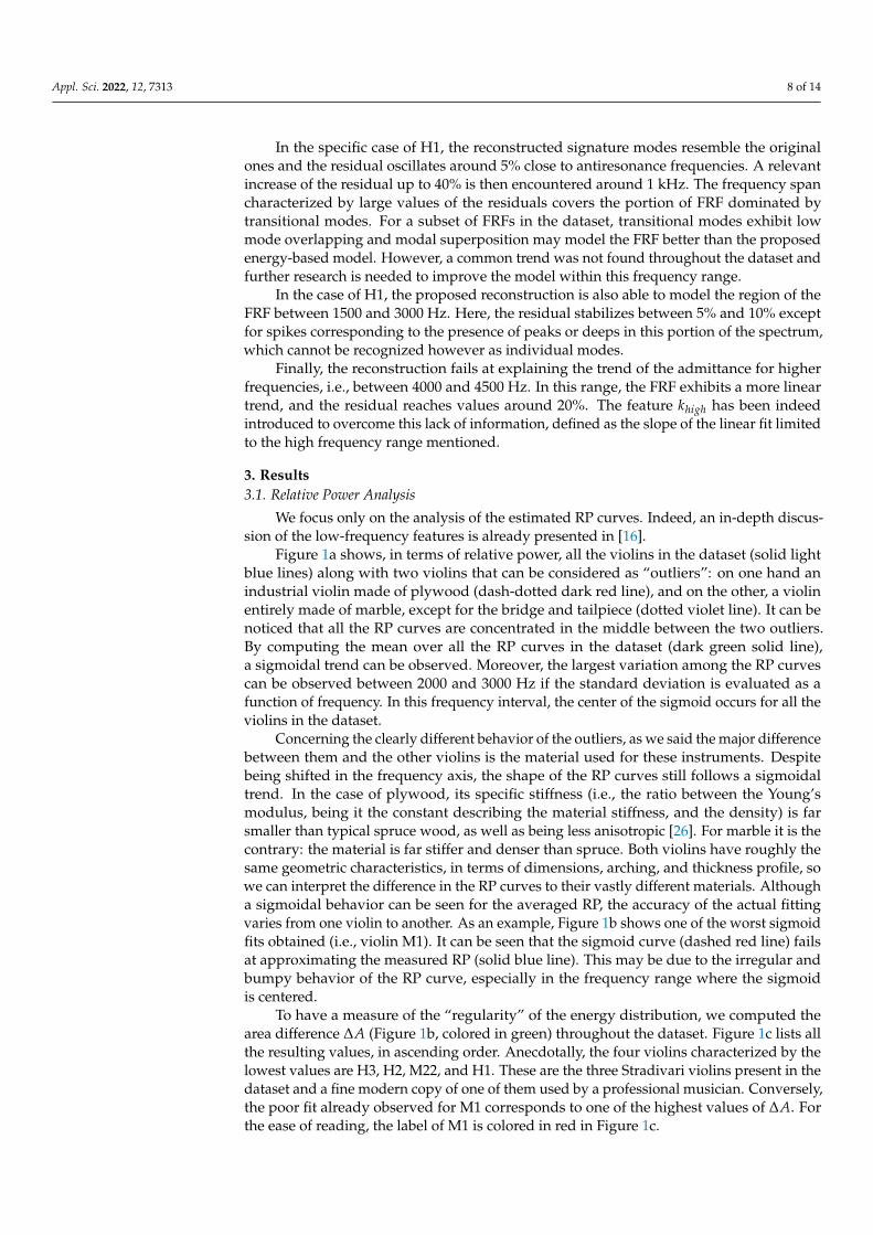
Figure 3a shows the distance matrix D, with the elements sorted following the hierar-chy of a dendrogram [28]. The dendrogram is computed iteratively using farthest neighborclustering to define the hierarchical relations [29]. In this way, similar violins (i.e., pairs ofinstruments with a small distance) are clustered together.

We decided to cut the dendrogram at a value of the farthest neighbor distance equalto 50 (vertical cyan line) as the link between H3, M22 and the remaining Stradivari vio-lins occurs at around 48. As a result, four clusters with varying sizes can be observed:(i) M17-M13-M18-M5-M16-M3-M8-M6-M7, (ii) M12-M14-M4-M1-M19-M11-M20-M10-M9,(iii) M21-M15, and (iv) H1-M2-H2-H3.

It is noteworthy that the distance between M22 and H1 is lower than the one assessedbetween M22 and its model H3. The similarity between M22 and H3 was already confirmedup to 1400 Hz in [16] (referred to as “V1” and “Strad” ), where the first ten peaks werechosen as features. To investigate which features the similarity between M22 and H1 mostlyrelies on, we visually compare the bridge admittance of the three violins.

Figure 3b shows the three FRFs overlapped. Looking at the low-frequency range,the modes of M22 (dash-dotted blue line) resemble both those of its original H3 (dotted redline) and H1 (dashed yellow line). In terms of Euclidean distances, the distance computedconsidering only the low-frequency features yields comparable values: 7.72 between M22and H1, and 8.92 between M22 and H3. However, a huge difference can be observed atmid frequencies, where H3 is characterized by a high-energy region centered at a lowerfrequency (1632 Hz against 2402 Hz for M22 and 2634 Hz for H1) and more limited inamplitude with respect to M22 and H1 (−24.2 dB against −16 dB for M22 and −14.9 dBfor H1). Due to this difference, the proposed similarity metric varies greatly between thetwo pairs of violins: 9.51 between M22 and H1, 17.88 between M22 and H3.

The same considerations can be inferred more clearly by inspecting the correspondingfeature-based reconstructions in Figure 3c. In particular, the reconstruction of the high-energy region better highlights its position and width and thus makes the visual comparisonbetween different instruments much easier.

Appl. Sci. 2022, 12, 7313 10 of 14

20406080

Fa

rthe

st N

eig

hbor

Dis

tance

Dend

rog

ram

M2M

17M

13M

18M5M

16M3M

8M

6M

7M

12M

14M4M

1M

19M

11M

20M

10M9M

21M

15 H1M

22 H2

H3

M2M17M13M18

M5M16

M3M8M6M7

M12M14

M4M1

M19M11M20M10

M9M21M15

H1M22

H2H3 0

10

20

30

40

50

60

70

80

90

Euclid

ea

n D

ista

nce

(a)

500 1000 2000 3000 4000

Frequency [Hz]

-60

-40

-20

0

Ma

gn

itu

de

[dB

]

500 1000 2000 3000 4000

Frequency [Hz]

-60

-40

-20

0

Ma

gn

itu

de

[dB

]

M22 H3 H1

(b)

(c)

Figure 3. (a) Euclidean distance matrix, with elements sorted following the dendrogram hierarchy.In this way, similar violins cluster together (colored in red). Four clusters are obtained by cutting thedendrogram at a farthest neighbor distance equal to 50 (vertical cyan line). (b) The bridge admittanceof M22 (dash-dotted blue line) compared to those of H3 (dotted red line) and H1 (dashed yellowline), and (c) corresponding reconstructions from the feature space. Magnitudes are reported in[dB re 1 m s−1 N−1]. The similarity between these violins leads to the cluster at the bottom-rightcorner of the distance matrix. The comparison of the three reconstructions highlights the differentsimilarities: the signature modes of M22 are similar to those of both H3 and H1 while its mid-rangeresembles more that of H1.

3.3. Correlation between Features and PCA

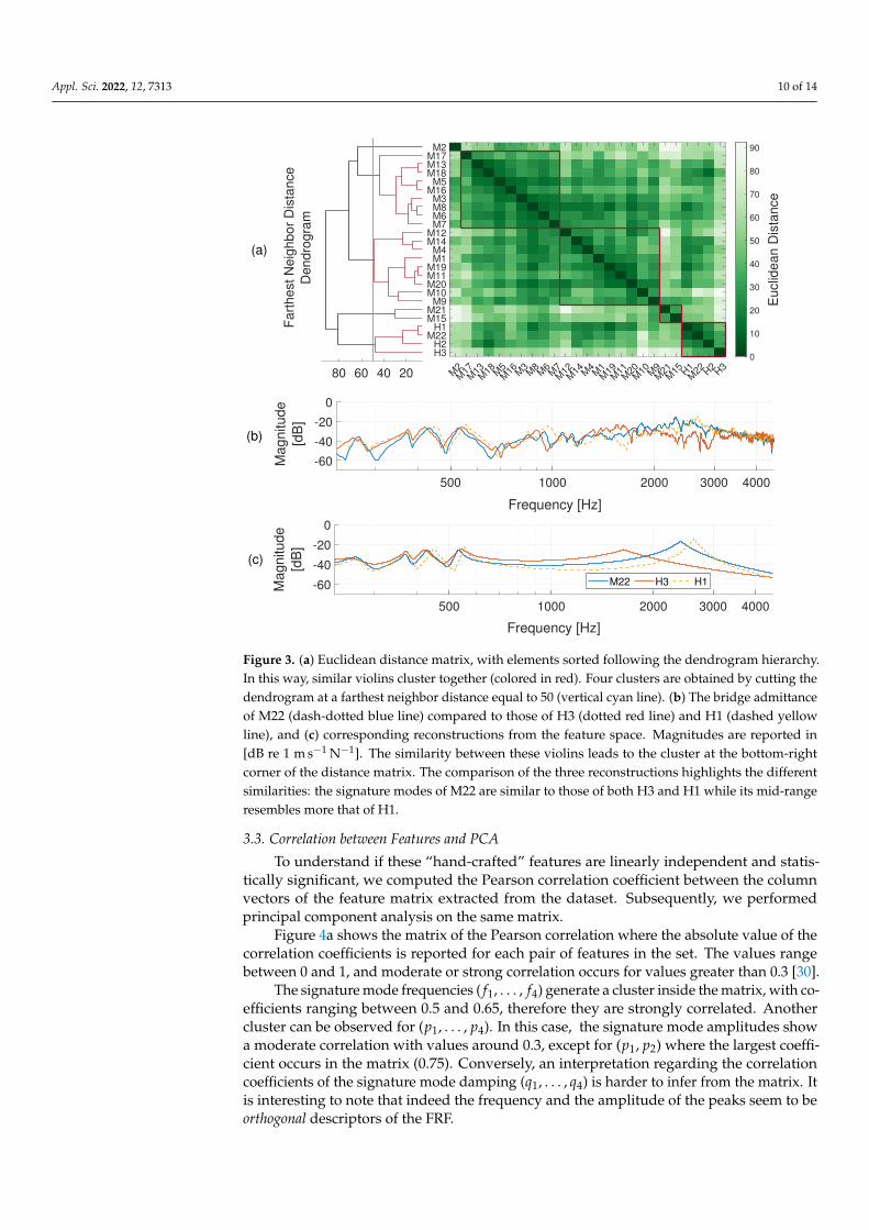
To understand if these “hand-crafted” features are linearly independent and statis-tically significant, we computed the Pearson correlation coefficient between the columnvectors of the feature matrix extracted from the dataset. Subsequently, we performedprincipal component analysis on the same matrix.

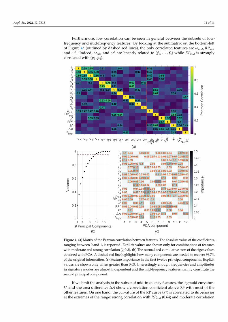
Figure 4a shows the matrix of the Pearson correlation where the absolute value of thecorrelation coefficients is reported for each pair of features in the set. The values rangebetween 0 and 1, and moderate or strong correlation occurs for values greater than 0.3 [30].

The signature mode frequencies ( f1, . . . , f4) generate a cluster inside the matrix, with co-efficients ranging between 0.5 and 0.65, therefore they are strongly correlated. Anothercluster can be observed for (p1, . . . , p4). In this case, the signature mode amplitudes showa moderate correlation with values around 0.3, except for (p1, p2) where the largest coeffi-cient occurs in the matrix (0.75). Conversely, an interpretation regarding the correlationcoefficients of the signature mode damping (q1, . . . , q4) is harder to infer from the matrix. Itis interesting to note that indeed the frequency and the amplitude of the peaks seem to beorthogonal descriptors of the FRF.

Appl. Sci. 2022, 12, 7313 11 of 14

Furthermore, low correlation can be seen in general between the subsets of low-frequency and mid-frequency features. By looking at the submatrix on the bottom-leftof Figure 4a (outlined by dashed red lines), the only correlated features are ωmid, RPmidand ω∗. Indeed, ωmid and ω∗ are linearly related to ( f1, . . . , f4) while RPmid is stronglycorrelated with (p3, p4).

1

0.58

0.65

0.31

0.4

0.39

0.58

1

0.55

0.53

0.35

0.32

0.42

0.65

0.55

1

0.56

0.3

0.41

0.42

0.53

0.53

0.56

1

0.46

0.35

0.31

0.3

1

0.75

0.3

0.63

0.47

0.75

1

0.31

0.68

0.35

0.41

0.3

0.31

1

0.34

0.42

0.56

0.36

0.4

0.34

1

0.64

0.34

1

0.32

0.47

0.63

0.68

0.32

1

0.37

0.32

0.42

0.37

1

0.47

1

0.39

0.42

0.42

0.46

1

0.36

0.56

0.64

1

0.64

0.32

0.53

0.35

1

0.57

0.52

0.57

1

0.4

0.34

0.36

0.64

1

0.36

0.43

0.36

0.32

0.52

0.4

0.36

1

0.47

0.43

1

f 1 f 2 f 3 f 4 p 1 p 2 p 3 p 4 q 1 q 2 q 3 q 4m

id

RP m

id*

RP* k* A

k high

f1

f2

f3

f4

p1

p2

p3

p4

q1

q2

q3

q4

midRP

mid*

RP*k*A

khigh 0

0.2

0.4

0.6

0.8

1

Pears

on C

orr

ela

tion

(a)

1 4 8 12 16

# Principal Components

0

0.2

0.4

0.6

0.8

1

Variance

0.1

0.09

0.12

0.08

0.09

0.07

0.05

0.05

0.06

0.08

0.06

0.05

0.06

0.05

0.07

0.05

0.06

0.06

0.06

0.08

0.09

0.11

0.08

0.05

0.05

0.13

0.14

0.05

0.08

0.14

0.07

0.05

0.05

0.06

0.1

0.03

0.09

0.06

0.05

0.05

0.07

0.11

0.08

0.14

0.06

0.05

0.07

0.05

0.09

0.18

0.17

0.13

0.07

0.06

0.03

0.03

0.05

0.03

0.09

0.05

0.1

0.09

0.06

0.08

0.09

0.12

0.06

0.03

0.03

0.05

0.11

0.23

0.06

0.03

0.08

0.17

0.04

0.03

0.05

0.03

0.05

0.04

0.05

0.04

0.13

0.04

0.03

0.14

0.06

0.03

0.03

0.09

0.13

0.04

0.07

0.04

0.14

0.05

0.03

0.03

0.03

0.09

0.1

0.05

0.18

0.08

0.03

0.07

0.1

0.07

0.09

0.08

0.04

0.11

0.04

0.08

0.1

0.08

0.07

0.12

0.08

0.03

0.08

0.06

0.09

0.09

0.08

0.03

0.06

0.05

0.06

0.05

0.04

0.06

0.12

0.07

0.03

0.06

0.03

0.04

0.05

0.05

0.08

0.06

0.12

0.17

0.03

0.04

0.03

0.04

0.03

0.03

0.04

0.03

0.04

0.03

0.03

0.03

0.03

0.03

0.03

0.04

1 2 3 4 5 6 7 8 9 10 11 12PCA component

f1

f2

f3

f4

p1

p2

p3

p4

q1

q2

q3

q4

midRP

mid*

RP*k*A

khigh 0

0.05

0.1

0.15

0.2

0.25

0.3

0.35

0.4

0.45

0.5

Import

ance

(b) (c)

Figure 4. (a) Matrix of the Pearson correlation between features. The absolute value of the coefficients,ranging between 0 and 1, is reported. Explicit values are shown only for combinations of featureswith moderate and strong correlation (≥0.3). (b) The normalized cumulative sum of the eigenvaluesobtained with PCA. A dashed red line highlights how many components are needed to recover 96.7%of the original information. (c) Feature importance in the first twelve principal components. Explicitvalues are shown only when greater than 0.05. Interestingly enough, frequencies and amplitudesin signature modes are almost independent and the mid-frequency features mainly constitute thesecond principal component.

If we limit the analysis to the subset of mid-frequency features, the sigmoid curvaturek∗ and the area difference ∆A show a correlation coefficient above 0.3 with most of theother features. On one hand, the curvature of the RP curve (k∗) is correlated to its behaviorat the extremes of the range: strong correlation with RPmid (0.64) and moderate correlation

Appl. Sci. 2022, 12, 7313 12 of 14

with khigh (0.43), ωmid (0.36), and ∆A (0.36). On the other hand, strong correlation can beobserved between ∆A and features characterizing the central part of the sigmoid: ω∗ (0.52),RP∗ (0.4), k∗ (0.36), and RPmid (0.32). As a consequence, one could infer an estimate for k∗

starting from (ωmid, RPmid, khigh, ∆A) and for ∆A given (ω∗, RP∗, k∗, RPmid).Figure 4b shows the cumulative sum of the eigenvalues obtained with PCA. The

cumulative function is normalized such that the eigenvalues sum to 1. Twelve principalcomponents out of nineteen account for 96.7% of the total variance of the set.

Figure 4c shows the absolute value of the coefficients for the first twelve principalcomponents. We normalized the resulting values such that the sum is equal to 1 foreach component.

Although no clear patterns can be observed inside the matrix, it can be noticed thatsome features contribute more than others. Indeed, frequencies ( f1, . . . , f4) dominate thefirst principal component, with values greater than 0.08. Additionally, the amplitudes(p1, . . . , p4) show noticeable values in the most informative components (1 and 3). Con-versely, the damping features (q1, . . . , q4) start occurring later inside the PCA vectors (onlyafter the third). Interestingly enough, the mid-frequency features occur in the first twoprincipal components. We can thus conclude that the mid-frequency features are as statisti-cally significant as modal frequencies and amplitudes in defining an FRF. To the best of ourknowledge this is the first result showing such objective relevance of the mid range features.

4. Discussion

The features we have defined to compare violins have three advantages with respect tothe literature: (a) they are objectively defined and they can be easily computed from any FRF.(b) They can be used to roughly reconstruct the FRF signal with just a handful of parameters.This could be extremely useful in virtual analog simulations of instruments [13], as anexample. (c) They provide a reduced dimensional representation of the FRF whence anobjective distance metric can be computed. Hitherto in the literature, this comparison hasbeen purely visual and subjective.

One of these features, i.e., the degree to which the high power spectrum approximatesa sigmoid function, has been found to anecdotally correlate with the subjective quality ofthe instruments: three Stradivari and one bench copy of one of them have the lowest valuesfor this feature. The copy of the Stradivari is in possession of a renowned professionalmusician, and he states that both violins have a very similar sound.

We have also found that these quality violins live in a “Goldilocks zone” for relativepower. That Goldilocks zone seems to depend on the material of the instrument: if thematerial is too soft, the instrument has no tone, as the cheap violin shows. If the materialis too stiff, as in the case of the marble violin, there is no body to the sound and it lacksprojection. Studying in depth how design and material parameters influence the shape ofthe relative power may give valuable insights in how to craft a quality instrument.

Once the bridge admittances are projected into the feature representation, one canassess the similarity between different instruments by simply computing a Euclideandistance. Additionally, in this case, the three Stradivari and the modern copy have beenfound to cluster together.

If compared to the feature representation presented in [16], the extension of therepresentation to the mid-frequency range led to a more informative similarity metric.Indeed, the new Euclidean distance highlighted that the bench copy is more similar toanother Stradivari violin rather than its original. By comparing the reconstructed FRFs, it isclear that the difference relies on the frame of the signal related to the so-called bridge hill.

This evidence, together with the importance of the mid-frequency features highlightedby PCA, may suggest that not only the shape and the material used for the violin soundboxbut also its interaction with the other components (i.e., the bridge) play a crucial role indefining the characteristics of the instrument. Studying the impact of the violin setup (e.g.,tuning of the bridge and the tailpiece) on these features may give a new tool to violinmakers and musicians to design the violin sound from a vibrational standpoint.

Appl. Sci. 2022, 12, 7313 13 of 14

One limitation is that our model does not consider the transitional modes between 700and 1200 Hz, but they could be easily included. Our own research does show, however,that at least for the top plate [10], the higher modes are highly correlated with the lowmodes so its inclusion should not change the clustering or the definition of the distancematrix. To overcome this limitation, a possible extension of the current feature set couldbe envisioned through the definition of additional descriptors derived from the RP curve.These new features could deal with transitional modes separately from the mid-frequencyrange, as a simpler alternative to mode fitting.

In its current version, the feature representation proposed allows the comparisonbetween different instruments only in terms of vibration. Indeed, how much these featuresare relevant from a perceptual point of view and how they should be “prioritized” while de-signing a musical instrument are still open questions. However, the proposed methodologycould be used to synthesize a variety of “virtual” violins to assess the perceptual weightsof the features through listening tests [31]. Since most of the features presented here seemto be possible to predict from the material and geometric parameters of the instrument [32],the dream of having a virtual workbench where one can sonically design an instrument tooptimize perception is one step closer.

Author Contributions: R.M. performed the vibration tests; R.M., S.G. and F.A. designed the featurerepresentation and analyzed the data; R.M. and S.G. wrote the paper; A.S. and R.C. supervised thework. All authors have revised the manuscript. All authors have read and agreed to the publishedversion of the manuscript.

Funding: This research received no external funding.

Institutional Review Board Statement: Not applicable.

Informed Consent Statement: Not applicable.

Data Availability Statement: The data presented in this study are available on request from thecorresponding author. The data are not publicly available due to privacy restrictions.

Acknowledgments: The authors would like to thank the “Fondazione Stradivari—Museo del Violino”and the curator of the museum M◦ F. Cacciatori for offering some of the instruments of the collectionand all the participants who joined the measurement campaign during Mondo Musica 2020.

Conflicts of Interest: The authors declare no conflict of interest.

AbbreviationsThe following abbreviations are used in this manuscript:

FRF Frequency Response FunctionMSE Mean Square ErrorRP Relative PowerPCA Principal Component Analysis

References1. Fritz, C.; Curtin, J.; Poitevineau, J.; Tao, F.C. Listener evaluations of new and Old Italian violins. Proc. Natl. Acad. Sci. USA 2017,

114, 5395–5400. [CrossRef] [PubMed]2. Fritz, C.; Curtin, J.; Poitevineau, J.; Morrel-Samuels, P.; Tao, F.C. Player preferences among new and old violins. Proc. Natl. Acad.

Sci. USA 2012, 109, 760–763. [CrossRef]3. Rozzi, C.A.; Voltini, A.; Antonacci, F.; Nucci, M.; Grassi, M. A listening experiment comparing the timbre of two Stradivari with

other violins. J. Acoust. Soc. Am. 2022, 151, 443–450. [CrossRef] [PubMed]4. Rau, M.; Abel, J.S.; Smith, J.O., III. Contact sensor processing for acoustic instrument recording using a modal architecture. In

Proceedings of the International Conference of Digital Audio Effects, Aveiro, Portugal, 4–8 September 2018.5. Gough, C. Acoustic characterisation of string instruments by internal cavity measurements. J. Acoust. Soc. Am. 2021,

150, 1922–1933. [CrossRef] [PubMed]6. Woodhouse, J. On the “bridge hill” of the violin. Acta Acust. United Acust. 2005, 91, 155–165.7. Durup, F.; Jansson, E.V. The quest of the violin bridge-hill. Acta Acust. United Acust. 2005, 91, 206–213.8. Woodhouse, J. Body vibration of the violin–What can a maker expect to control. Catgut Acoust. Soc. J. 2002, 4, 43–49.

Appl. Sci. 2022, 12, 7313 14 of 14

9. Woodhouse, J. The acoustics of the violin: A review. Rep. Prog. Phys. 2014, 77, 115901. [CrossRef]10. Gonzalez, S.; Salvi, D.; Baeza, D.; Antonacci, F.; Sarti, A. A data-driven approach to violin making. Sci. Rep. 2021, 11, 1–9.11. Bissinger, G. The violin bridge as filter. J. Acoust. Soc. Am. 2006, 120, 482–491. [CrossRef]12. Rau, M. Measurements and analysis of acoustic guitars during various stages of their construction. J. Acoust. Soc. Am. 2021,

149, A25–A25. [CrossRef]13. Rau, M.; Abel, J.S.; James, D.; Smith III, J.O. Electric-to-acoustic pickup processing for string instruments: An experimental study

of the guitar with a hexaphonic pickup. J. Acoust. Soc. Am. 2021, 150, 385–397. [CrossRef] [PubMed]14. Maestre Gómez, E.; Scavone, G.P.; Smith, J.O. Digital modeling of bridge driving-point admittance from measurements

on violin-family instruments. In Proceedings of the Stockholm Music Acoustics Conference 2013, Stockholm, Sweden,30 July–3 August 2013; Bresin, R., Askenfelt, A., Eds.; Logos Verlag: Berlin, Germany, 2013; pp. 101–108.

15. Woodhouse, J.; Langley, R. Interpreting the Input Admittance of Violins and Guitars. Acta Acust. United Acust. 2012, 98, 611–628.[CrossRef]

16. Malvermi, R.; Gonzalez, S.; Quintavalla, M.; Antonacci, F.; Sarti, A.; Torres, J.A.; Corradi, R. Feature-based representation forviolin bridge admittances. In Proceedings of the “Advances in Acoustics, Noise and Vibration—2021” the 27th InternationalCongress on Sound and Vibration, Online, 11–16 July 2021.

17. The Permanent Collection of Contemporary Violinmaking. Available online: https://www.museodelviolino.org/en/museo/percorso-museale/sala-8-il-concorso-triennale-di-liuteria-contemporanea/ (accessed on 12 May 2022).

18. Vasques, C.; Rodrigues, J.D. Vibration and Structural Acoustics Analysis: Current Research and Related Technologies; Springer Science& Business Media: Berlin/Heidelberg, Germany, 2011.

19. Kiesel, T.; Langer, P.; Marburg, S. Numerical Study on the Effect of Gravity on Modal Analysis of Thin-Walled Structures. ActaAcust. United Acust. 2019, 105, 545–554. [CrossRef]

20. Schwarz, B.J.; Richardson, M.H. Experimental modal analysis. CSI Reliab. Week 1999, 35, 1–12.21. Gough, C.E. A violin shell model: Vibrational modes and acoustics. J. Acoust. Soc. Am. 2015, 137, 1210–1225. [CrossRef]22. Meirovitch, L. Fundamentals of Vibrations; McGraw-Hill Higher Education, McGraw-Hill: New York, NY, USA, 2001.23. Curtin, J. Scent of a violin. STRAD 2009, 120, 30–33.24. Chopra, A.K. Dynamics of Structures: Theory and Applications to Earthquake Engineering; Pearson: London, UK, 2006.25. Normalized Tunable Sigmoid Function. Available online: https://dhemery.github.io/DHE-Modules/technical/sigmoid/

(accessed on 22 May 2022).26. Ross, R.J. Wood handbook: Wood as an engineering material. In USDA Forest Service, Forest Products Laboratory, General Technical

Report FPL-GTR-190, 2010: 509 p. 1 v; U.S. Department of Agriculture, Forest Service, Forest Products Laboratory: Madison, WI,USA, 2010; Volume 190. [CrossRef]

27. Jain, A.; Nandakumar, K.; Ross, A. Score normalization in multimodal biometric system. Pattern Recognit. 2005, 38, 2270–2285.[CrossRef]

28. Gruvaeus, G.; Wainer, H. Two additions to hierarchical cluster analysis. Br. J. Math. Stat. Psychol. 1972, 25, 200–206. [CrossRef]29. Defays, D. An efficient algorithm for a complete link method. Comput. J. 1977, 20, 364–366. [CrossRef]30. Cohen, J. Statistical Power Analysis for the Behavioral Sciences; Routledge: London, UK, 2013.31. Fritz, C.; Cross, I.; Moore, B.C.; Woodhouse, J. Perceptual thresholds for detecting modifications applied to the acoustical

properties of a violin. J. Acoust. Soc. Am. 2007, 122, 3640–3650. [CrossRef] [PubMed]32. Badiane, D.G.; Malvermi, R.; Gonzalez, S.; Antonacci, F.; Sarti, A. On the Prediction of the Frequency Response of a Wooden Plate

from Its Mechanical Parameters. In Proceedings of the ICASSP 2022–2022 IEEE International Conference on Acoustics, Speechand Signal Processing (ICASSP), Singapore, 22–27 May 2022; pp. 461–465. [CrossRef]