A space-time approach in digital image correlation:Movie-DIC

Gilles Besnarda,b, Sandra Guerardb,c, Stephane Rouxb,∗, Francois Hildb

aCEA, DAM, DIF, F-91297 Arpajon, FrancebLMT-Cachan, ENS Cachan / CNRS / UPMC / UniverSud Paris61 avenue du President Wilson, F-94235 Cachan Cedex, France

cnow at Laboratoire de Biomecanique, Arts et Metiers ParisTech, ENSAM / CNRS,151 boulevard de l’Hopital, F-75013 Paris, France

Abstract

A new method is proposed to estimate arbitrary velocity fields from a time se-

ries of images acquired by a single camera. This approach, here focused on a

single spatial plus a time dimension, is specialized to the decomposition of the

velocity field over rectangular shaped (finite-element) bilinear shape functions.

It is therefore assumed that the velocity field is essentially aligned along one di-

rection. The use of a time sequence over which the velocity is assumed to have

a smooth temporal change allows one to use elements whose spatial extension

is much smaller than in traditional digital image correlation based on succes-

sive image pairs. This method is first qualified by using synthetic numerical

test cases, and then applied to a dynamic tensile test performed on a tanta-

lum specimen. Improvements with respect to classical digital image correlation

techniques are observed in terms of spatial resolution.

Keywords: Digital image correlation, displacement field, strain field, strain

rate field, velocity field, video.

∗Corresponding authorEmail address: stephane.roux@lmt.ens-cachan.fr (Stephane Roux)

Preprint submitted to Elsevier August 19, 2010

hal-0

0521

203,

ver

sion

1 -

26 S

ep 2

010

Author manuscript, published in "Optics and Lasers in Engineering 49 (2011) 71-81" DOI : 10.1016/j.optlaseng.2010.08.012

1. Introduction

In Solid Mechanics, digital imaging is used to detect and measure the motion

and deformation of objects. From these observations follow various evaluation

procedures of mechanical parameters [1]. To achieve this goal, different optical

techniques are used [2]. Among them, Digital Image Correlation (DIC) is ap-

pealing thanks to its versatility in terms of scales ranging from nanoscopic [3, 4]

to macroscopic [5, 6] observations with essentially the same type of algorithms.

DIC always involves a compromise between spatial resolution and uncer-

tainty [7, 8]. As the technique exploits the comparison of zones of interest, or

elements between a deformed and a reference image, the information is carried

by the pixels contained in those regions. A key characteristic is thus, β, the

number of pixels per kinematic degree of freedom. On the one hand, low un-

certainties call for a large β (i.e., large elements), but the description of the

displacement will be coarse, and hence maybe unsuited to capture rapidly vary-

ing displacement fields. The resulting systematic error may be prohibitive for

a specific application. On the other hand, small elements may be more flexible

to account for a complex displacement field, but as the information content,

or β, is small, large uncertainties will result. This trade-off has to be solved

for every application, depending on the “complexity” of the expected displace-

ment field. However, one may have access to a large number of pictures thanks

to camcorders or high-speed cameras. Traditionally, 2D-DIC operates on image

pairs [9, 10, 11], and hence a long temporal series is of little use. On the contrary,

if the overall displacement over the entire time sequence is large, one may have

to break the analysis into time intervals which are finally “chained” to obtain

the entire displacement field. When updating the reference picture [12], this

procedure involves cumulative errors that are prejudicial to the displacement

uncertainty.

The principle of the proposed approach is to extend to the time domain the

regularization strategy used spatially. If the velocity field evolves smoothly in

time, the above discussion about the β parameter may be readily applicable to

2

hal-0

0521

203,

ver

sion

1 -

26 S

ep 2

010

include the time dimension. Thus, for the same β value, small elements along the

space direction(s) may still offer a good accuracy provided a sufficient number of

images is considered along the time axis for each element. This temporal series

may be used to compensate for the poor quality of each individual image.

Some approaches post-process a posteriori the measured velocity fields to ex-

tract, say, the coherent part of the latter [13] or to filter the measured data [14].

The objective of the present work is to propose an a priori approach in which

a space-time decomposition is sought. The main advantage of the proposed

method is the large number of pictures used that may allow one to reach the

same uncertainty level with a small amount of spatial information, counter-

balanced by a large amount of temporal data.

Sequences of images can be obtained from standard movies. To benefit

from the large number of images, a temporal regularization is called for. For

instance, one may seek for a steady-state velocity fields [15], or in the present

case velocity fields that are decomposed over a set of piece-wise linear fields

in space and time. This type of description is developed in the same spirit as

global approaches [16, 17], and in particular to finite-element based correlation

algorithms whereby the displacement field is described by finite element shape

functions of the space variables [8, 18].

Along those lines different strategies can be considered. The direct transpo-

sition of DIC is to search for displacement fields in space and time simultane-

ously. This route is not followed here since the sought fields are velocities and

strain rates. It is well known that (time or space) derivatives will increase the

noise level, and thus the displacement-formulated strategy may reveal unreli-

able. Therefore, the choice was made to focus directly on the velocity field as

the main unknown to the problem. It will be shown that in spite of the fact

that this velocity is the time derivative of displacement, good performances will

be reached.

In the present case, a 2D approach is developed, namely, 1D in space and

1D in time. It is referred to as DIC applied to analyze movies (or Movie-

DIC). The paper is organized as follows. First, the principle of the method is

3

hal-0

0521

203,

ver

sion

1 -

26 S

ep 2

010

described. Then, artificial pictures are generated and the technique is carried

out to determine a priori performances. Last, the spatiotemporal approach is

applied to analyze the kinematics of a sample in a split Hopkinson pressure bar

test.

2. Principle of the spatiotemporal analysis

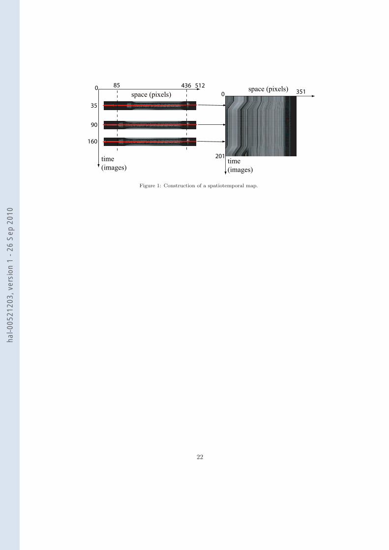
The first step of the analysis consists in creating the so-called spatiotem-

poral map. For each picture, where x, y are the image coordinates, taken at

several instants of time t, the gray level for a particular (chosen) position (x, y)

is represented as a function of time t. Therefore, for a fixed y coordinate a se-

quence of images becomes an f(x, t) map. The stacking principle is depicted in

Figure 1. The restriction to a single spatial coordinate (y being fixed) is suited

for problems where the velocity is essentially along the x axis.

The measurement technique is based upon the conservation of the bright-

ness [19, 20]. The advection of the texture by a velocity field v (along the x-axis)

is expressed as

f(x + vdt, t + dt) = f(x, t) (1)

where the increment dt corresponds to one time interval between successive

images (i.e. a “time pixel”). The aim is to estimate the velocity field v(x, t) by

using the brightness conservation. Minimization of the quadratic difference τ

over space and time is used

τ =∫

x

∫

t

[f(x, t)− f(x + v(x, t)dt, t + dt)]2 dxdt (2)

The velocity field is decomposed over a basis of functions φ and ϕ as follows

v(x, t) =∑

i,j

aijφi(x)ϕj(t) (3)

In the present case, finite-element shape functions are chosen, and their sim-

plest form is adopted, namely, a piece-wise bi-linear description of the velocity

field. However, it is conceivable to consider other sets of either continuous

functions [15] or even discontinuous functions [21, 22].

4

hal-0

0521

203,

ver

sion

1 -

26 S

ep 2

010

The proposed scheme is to solve this non-linear problem iteratively by a

progressive adjustment of the velocity to the tangent linearized problem. The

initialization of the unknown velocity field is here chosen to be equal to zero,

v0(x, t) = 0. However, if a predetermination of the velocity field is available, it

is straightforward to include it at this stage. The velocity v(n+1)(x, t) at step

n + 1 of this iterative scheme is determined from the Taylor expansion of the

objective functional

τ =∫

x

∫

t

[f(x(n), t− dt)− f,x(x, t)(v(n+1) − v(n))dt− f(x, t)]2 dxdt (4)

with f,x(x, t) = ∂f(x, t)/∂x. In this expression x(n) is a short hand notation for

the value x′ such that x′+v(n)(x′, t−dt)dt = x. Note that the above expression

is a specific choice out of many equivalent ones that differ only through second

order terms. The advantage of this particular form is that the correction field

is multiplied by f,x(x, t), which may be computed once for all iterations. This

will ease the computational work as shown in the following.

One difficulty of the above approach, in particular for low quality images, is

the use of a space derivative that may render the procedure sensitive to noise.

A filtering of the images may be used. Note that in this case, the band filtering

used in space and time should be adjusted so that their bounds are in proportion

of the mean velocity.

The decomposition (3) is introduced in Equation (4) and minimization with

respect to aij leads to a linear system∑

i,j

(∫

x

∫

t

[φi(x)φk(x)ϕj(t)ϕl(t)f2

,x(x, t)]

dxdt

)a(n+1)ij

=∑

i,j

(∫

x

∫

t

[φi(x)φk(x)ϕj(t)ϕl(t)f2

,x(x, t)]

dxdt

)a(n)ij

+∫

x

∫

t

(φk(x)ϕl(t)f,x(x, t)(f(x(n), t− dt)− f(x, t))) dxdt

(5)

This elementary step is written in compact form as

Mijkla(n+1)ij = B

(n)kl (6)

The reason for the specific choice made in Equation (4) is now clear, namely,

matrix M is computed once for all at the first iteration, and it does not depend

5

hal-0

0521

203,

ver

sion

1 -

26 S

ep 2

010

on the current evaluation of the velocity field. However the second member, B

is dependent on v(n), but its evaluation is much less demanding computationally

than M. At each step, the “deformed” image f(x + v(n)dt, t + dt) is corrected

by using the velocity field estimate at the previous step in order to compute the

second member. By inverting (6), the unknown degrees of freedom a(n+1)ij are

obtained, and thus the corresponding velocity field is estimated. Convergence,

based on a measure of the norm of a(n+1) − a(n), is reached in a few iterations

(typically less than 10). By integrating the velocity field with respect to time,

the displacement and thereafter the strain fields are obtained.

In order to validate the approach, the objective function is considered. Its

value, normalized by the image size (nx × nt),

R =√

τ/(nxnt) (7)

gives the mean gray level difference of the matching of f(x, t) with f(x, t + dt)

using the measured velocity field. It is thus a global measure of the quality.

Moreover, because τ is a space-time integral of the square of a residual field,

δ ≡ 1∆|f(x, t)− v(x, t)dtf,x(x, t)− f(x, t + dt)| (8)

which gives the local contribution of each pixel to the global residual. To make

this density dimensionless, it is rescaled by the dynamic range of the original

image line ∆ = max[f(., t = 0)]−min[f(., t = 0)].

The algorithm will be checked below against test cases for which the velocity

field will be known exactly. In those cases, two quality indicators are introduced,

namely, the systematic error η and the corresponding standard uncertainty σ

η =1

nxnt

nx∑

i=1

nt∑

j=1

(Apreij −Ameas

ij )

σ =

√√√√ 1nxnt

nx∑

i=1

nt∑

j=1

(Apreij −Ameas

ij )2(9)

where Apre is the prescribed value and Ameas its measured counterpart. The

quantities Ai will denote velocity, displacement, strain or strain rate data.

6

hal-0

0521

203,

ver

sion

1 -

26 S

ep 2

010

The directly measured quantity is the velocity field v. From the latter, the

longitudinal strain rate Dxx is computed as

Dxx(x, t) =∂v

∂x(x, t) (10)

which, from the present choice of basis for the velocity (i.e., linear in space and

time), is a piecewise constant function in x, and piecewise linear and continuous

in time. The derivation is performed by centered finite differences.

From the velocity field it is also possible to compute the displacement field

(trajectories) from an explicit time integration, and sub-pixel linear interpola-

tion of the velocity, which is an exact result because of the choice of the shape

function

x(t) = x0(t = 0) +∫ t

0

v(x(t′), t′) dt′ (11)

The velocity field is computed on the entire space-time domain. In the sequel,

in order to use a Fourier-based filtering of the spatio-temporal image, it is useful

to extrapolate the observed domain to a larger domain. For instance elements

that are not present over the space interval at the initial time, t0, may enter the

observed scene at a later time, t1. In this case, when needed, we assume that

a constant velocity was followed in the time interval [t0; t1]. This conventional

procedure allows to minimize edge effects for the Fourier filtering, yet it is to be

underlined that the extrapolated domain is removed after filtering, and hence

this ad hoc extrapolation procedure has a very low impact on the measurement

over the observed scene. If instead a zero padding is used, edge effects are

observed to be detrimental to the quality of the determined velocity field.

The corresponding longitudinal strain εxx is expressed as

εxx(x, t) =∂u

∂x(x, t) (12)

The derivation is carried out by a centered finite differences scheme.

3. A priori analyses

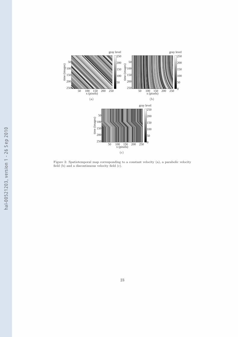
The three maps shown in Figure 2 are artificially generated so that the

correlation length of the first line was approximately equal to 3 pixels. The

7

hal-0

0521

203,

ver

sion

1 -

26 S

ep 2

010

size of each map is equal to 256 × 256 pixels because a wide range of mesh

sizes 2i pixels (i = 3 . . . 7 along the time dimension, and i = 1 . . . 7 along the

space dimension) are used, with a reasonable computation time (e.g., 8×8-pixel

elements require less than twenty seconds of computation time on a standard

PC). Moreover, small mesh sizes along the time dimension are not considered

except for the discontinuous map because in practice the aim of this method

is to use many time steps to compensate for the small amount of information

along the space dimension.

As mentioned in Section 2, images may be filtered in Fourier space, but this

operation has its principal axes along the space and time directions, and hence it

is unsuited to the spatio-temporal maps. The chosen strategy was first to correct

this map. The evaluation of the velocity field allows for the trajectories to be

determined, and hence for each point (x, t) one may trace back the trajectory

going through this point up to the origin of time (x0(x, t), 0). The “corrected”

map g(x, t) is built so that g(x0(x, t), t) = f(x, t). By hypothesis, g(x, t) should

be time invariant (and equal to f(x, 0)). In this transformation, the boundary of

the domain becomes more or less lozenge shaped (a lozenge would be obtained

for a uniform and constant velocity field). This corrected map g is embedded in a

larger rectangle and the missing information is completed using (conventionally)

a constant velocity as explained in the previous section. A low pass Gaussian

filter is applied over the g field and the inverse transformation g → f is applied to

restore back the original domain shape. The extrapolated data is thus removed.

The standard deviation of the Gaussian filter is equal to 1 pixel for all the

studied cases.

3.1. Constant velocity

In this first case, the prescribed velocity is constant and equal to (1+√

5)/4 ≈0.81 pixel per image. This specific number, half the golden mean, is chosen be-

cause it induces sub-pixel components of the displacements that are close to a

uniform distribution (i.e., the standard deviation of the sub-pixel component

distribution is 0.290 to be compared with 1/√

12 ≈ 0.289 for a uniform dis-

8

hal-0

0521

203,

ver

sion

1 -

26 S

ep 2

010

tribution). The spatiotemporal map corresponding to this case is shown in

Figure 2(a). In the present case a bilinear gray level interpolation is used. Fur-

ther, it is worth noting that the measurement basis contains the studied velocity

field.

The present case is a typical baseline analysis in classical DIC techniques [23,

8]. It allows one to check the implemented algorithms. Let us first consider the

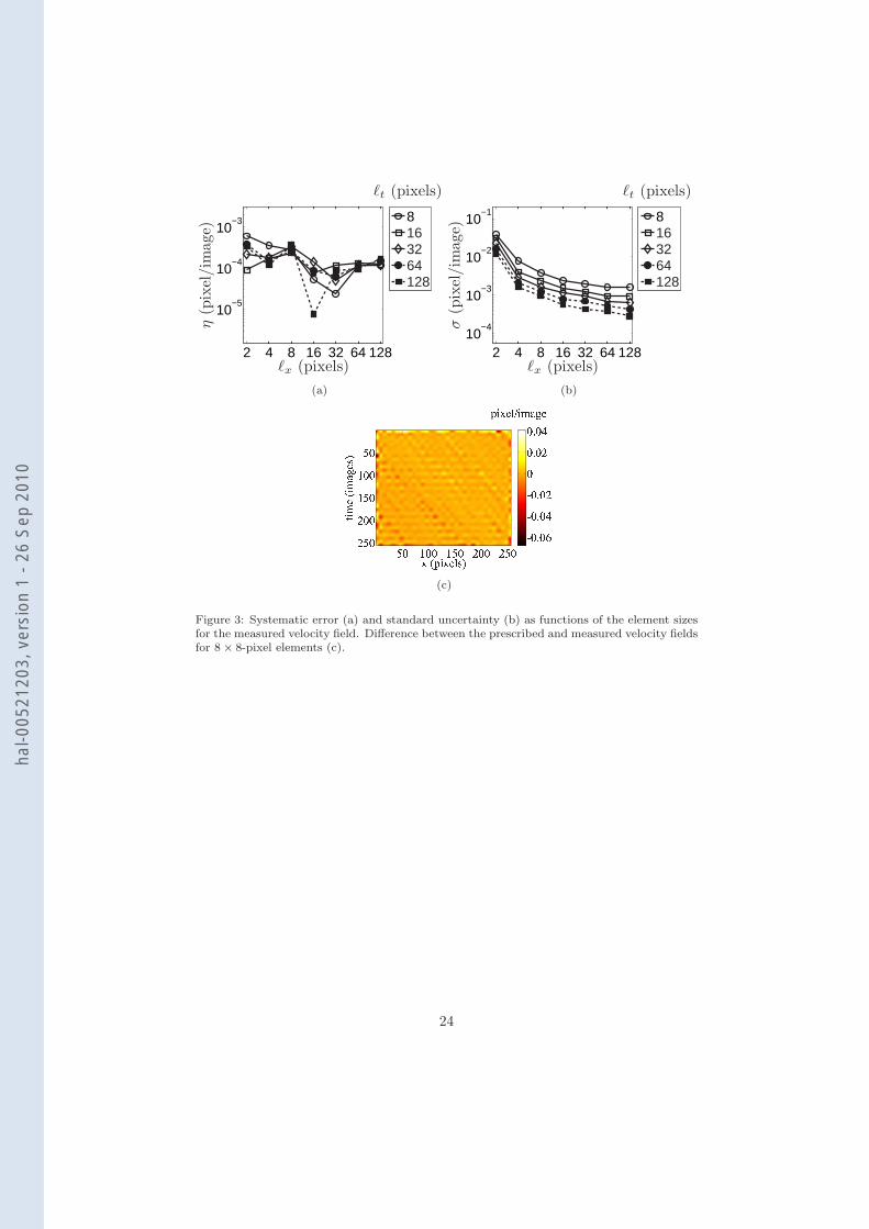
velocity field. The only parameters are the sizes `x and `t of the spatial and

temporal discretizations. The systematic error and the standard uncertainty are

shown in Figure 3(a) and Figure 3(b). A decrease of the standard uncertainty

is observed with increasing element sizes, be it spatial or temporal. The larger

the element, the larger the number of data (i.e., pixels), the more accurate the

measured velocity. Differences between the prescribed and measured velocity

fields for 8× 8-pixel elements are shown in Figure 3(c).

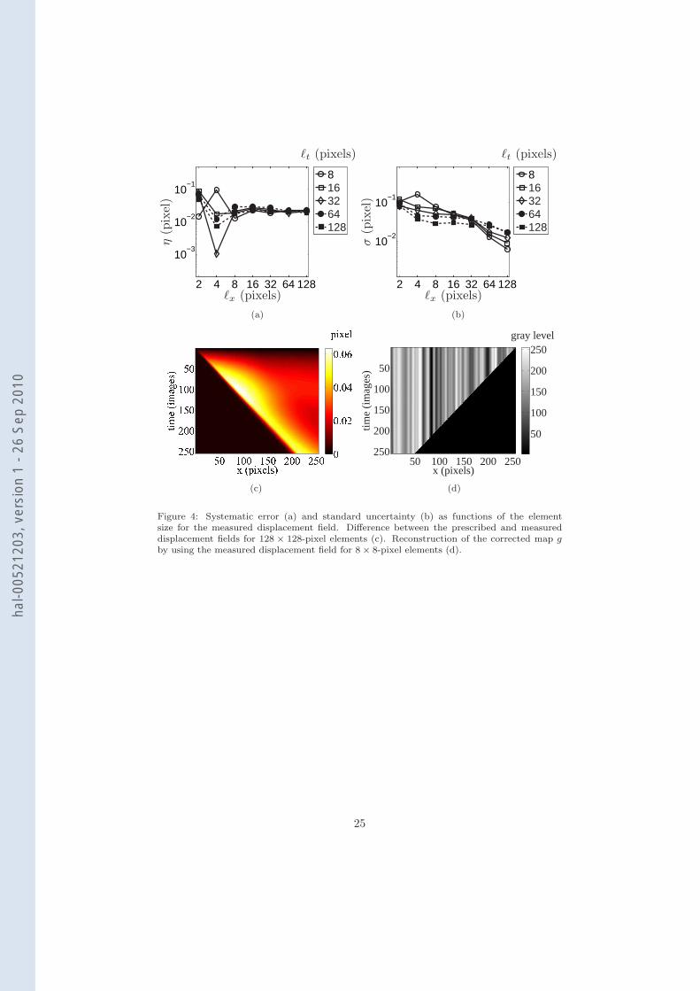
The second studied quantity is the displacement field for which the system-

atic error and the standard uncertainty are given in Figure 4(a) and Figure 4(b).

A decrease of the uncertainty is observed when the element size increases, while

the systematic error is approximately constant. Differences between the pre-

scribed and measured displacement fields are shown in Figure 4(c) for the largest

element size, 128× 128-pixel. The shape of the map is due to the fact that the

displacement of the first line of the map is followed. The values of the displace-

ment field are ranging from 0 and 256 pixels, whereas the velocity level is close

to 0.809 pixel per image. The values of the measured displacement fields are in

good agreement with the prescribed ones.

A good way of estimating the quality of the displacement field determination

is to construct the corrected spatiotemporal map, g, where the effect of the

estimated velocity is removed (the one used for the Fourier filtering). The

result is shown in Figure 4(d) for a small element size, 8 × 8-pixel. For larger

element size, no difference can be perceived with bare eyes. The spatial position

is corrected from the beginning to the end. The particular shape of the map is

caused by the fact that there is no information outside the bounds of the image.

Therefore, the repositioning cannot be performed at these locations.

9

hal-0

0521

203,

ver

sion

1 -

26 S

ep 2

010

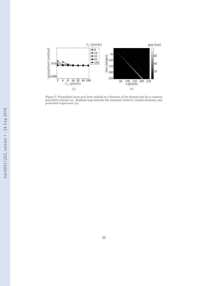
For real applications, the actual velocity field is unknown. Thus the quality

evaluation that is used is the residual, f(x, t)−f(x+v(x, t)dt, t+dt), computed

from the estimated velocity field. Figure 5(a) shows the normalized mean resid-

ual for different element sizes and Figure 5(b) the residual map for a particular

element size (8× 8 pixels). In that case, the residuals are virtually constant for

all element sizes, and the higher values are located close to the left edge of the

map, presumably because of an imperfect extrapolation procedure. It is to be

noted that edges are always a weak point in DIC analyses based on a similar

methodology.

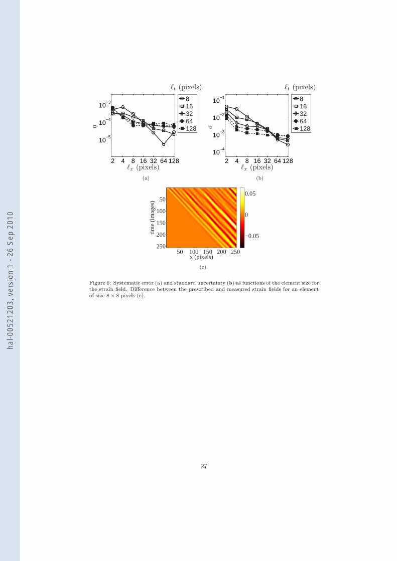
In many situations, the end user of the measurements is more interested

in strain and/or strain rate fields than in the displacement or velocity fields.

The latter are interpreted in terms of mechanical behavior, whereas the former

include rigid body components that are usually not useful to understand or cap-

ture the true mechanical response of a system under investigation. However, the

strain or strain rate fields require spatial derivations that amplify the noise level.

The systematic error and standard uncertainty of the strain fields are shown in

Figure 6(a) and Figure 6(b). In this particular case, the prescribed strain field

is equal to zero. Figure 6(c) shows the difference between the prescribed and

measured strain fields for elements of size 8 × 8 pixels. This field is similar to

the displacement field and the effect of derivation is observed.

In order to validate the benefit of the proposed approach with respect to

classical tools, the test case with a constant velocity field is an appropriate

example. A classical tool would ignore the time dimension and thus it consists

in analyzing two consecutive lines. These lines are partitioned into intervals (i.e.,

“Zone Of Interest”, or ZOI), over which the mean displacement is searched for,

independently for each interval. It is to be emphasized that such a “classical”

tool is seldom used in one space dimension. However, there is no limitation in

this respect. No convergence was obtained for ZOI sizes smaller than 8 pixels.

For this size (`x = 8 pixels) up to 32 pixels, the displacement field uncertainty

decreased from 0.023 to 0.006 pixel. This uncertainty is always worse than the

one obtained in the spatio-temporal framework.

10

hal-0

0521

203,

ver

sion

1 -

26 S

ep 2

010

A global one dimensional DIC approach is also performed. It is based on a

continuous kinematic basis (linearly varying displacement field) over a partition

of the line into 1D-elements, or intervals as in the previous case. This treatment

is similar to the spatio-temporal approach at the exception of the incorpora-

tion of time in the kinematics. The prescription of a continuous displacement

(here equivalent to velocity since only two consecutive lines are considered) field

helped significantly the convergence since elements as small a size of 3 pixels

could be handled without convergence problems. For `x = 4 pixels, the uncer-

tainty was observed to amount to 0.042 pixel. In the same range as above, from

`x = 8 to 32 pixels, the uncertainty decreased from 0.020 down to 0.005 pixel.

Thus continuity revealed useful to reduce the uncertainty level, yet at a level

higher than the proposed spatio-temporal approach.

As a last comparison with classical approaches, the maximum displacement

that would allow for convergence is evaluated. It was found that for velocities as

large as about 1.5 times the correlation length, the computation converged. This

allows one to consider velocities as large as 6 pixels per time step. Being able

to handle such large displacements without any special initialization is another

benefit of the proposed method.

To summarize, the time regularization that is proposed herein allows one to

extend considerably the range of convergence of the DIC algorithm. Moreover,

it reduces the uncertainty level. Note that the rather large level of uncertainty

as compared to traditional DIC is due to the fact that in one dimension the

number of pixels used to determine a kinematic degree of freedom is small

compared with 2D approaches.

3.2. Parabolic velocity field

The expression of the velocity field in this second test case reads

u =at2x2

2562(13)

with a = (1 +√

5)/4 ≈ 0.81 pixel per image. In that case, the degree of

the prescribed velocity is higher than that of the measurement basis. Thus

11

hal-0

0521

203,

ver

sion

1 -

26 S

ep 2

010

systematic bias due to the projector error on the discretization basis is expected

to penalize large element discretizations.

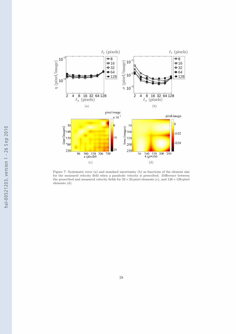
Figure 2(b) shows the spatiotemporal map corresponding to the chosen ve-

locity field. First, the systematic error and the standard uncertainty for the

measured velocity field are analyzed as functions of the element size in Fig-

ure 7(a) and Figure 7(b). When the discretization becomes too crude, the two

quantities increase because the measurement basis is not rich enough to capture

a parabolic field. For instance, for an element size equal to 128×128 pixels (Fig-

ure 7(d)), the difference between the prescribed and measured velocity fields is

less satisfactory than for sizes 32 × 32 pixels (Figure 7(c)) even though fewer

degrees of freedom are measured in the first case.

Moreover, the difference clearly shows the underlying mesh (made of four

elements in the first case), and its maximum is located on the edges and in

the middle of the elements. However, even for a large element size, the map is

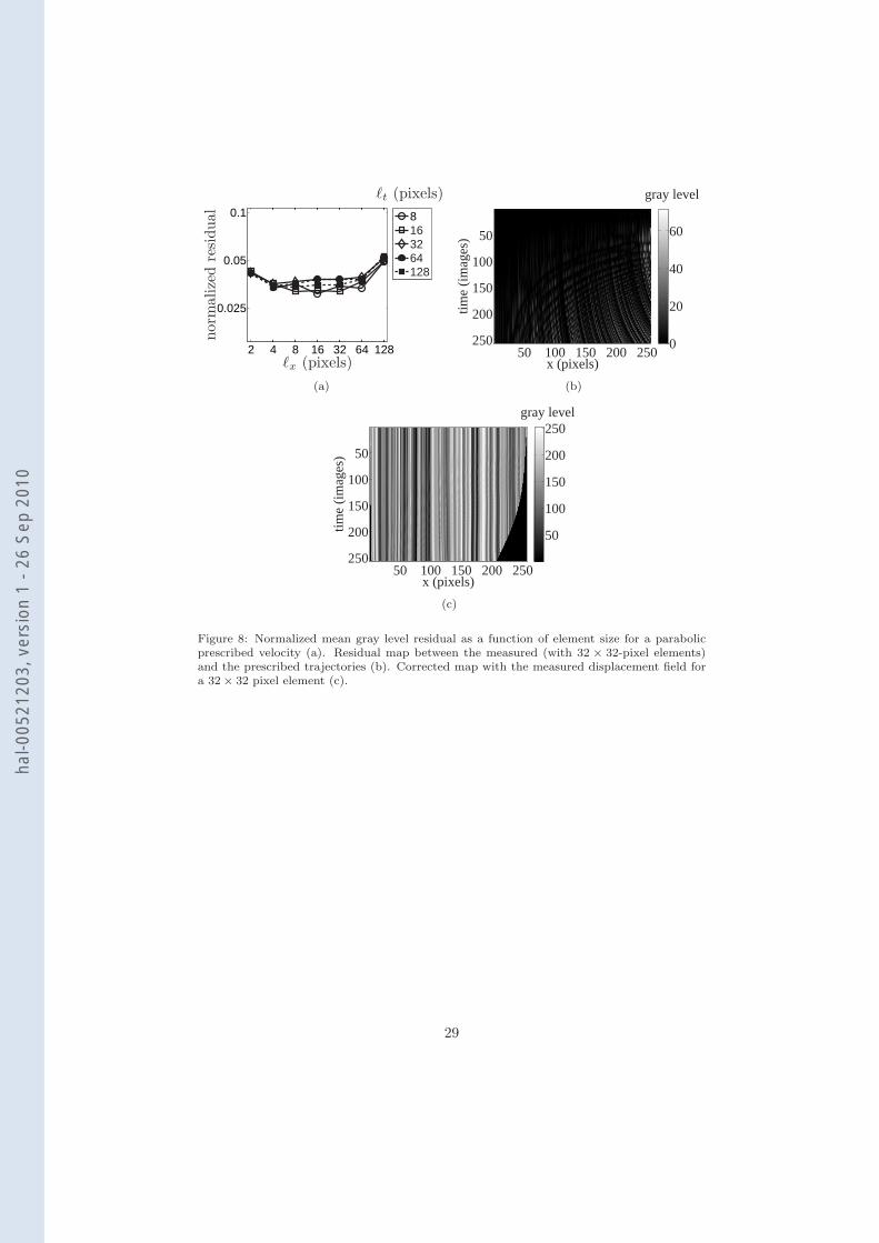
reconstructed accurately as can be seen on Figure 8(c). Although the description

of the velocity is poor, the mean trend is well captured. The gray level residuals

as functions of the element size are shown in Figure 8(a) and the difference

between the measured (with 32× 32-pixel elements) and prescribed trajectories

are shown in Figure 8(b). In this case too, the residuals are approximatively

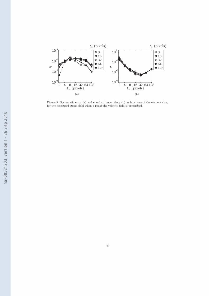
identical for tested element sizes. Figure 9(a) and Figure 9(b) show the change

of the strain error and uncertainty for different element sizes. The optimum size

is observed to be 32 × 32 pixels in the present case. (Note however that this

optimum size is dependent on the observed velocity field.)

3.3. Discontinuous velocity

In this last synthetic example, the prescribed velocity field is discontinuous.

For times 1 to 100, and 141 to 256, the velocity is equal to 0. In between,

the velocity is constant and equal to v = (1 +√

5)/4 pixel per image. The

spatiotemporal map is shown in Figure 2(c).

The same analysis as previously shown is carried out. However, the conclu-

sions are not the same. The change of the systematic error and the standard

12

hal-0

0521

203,

ver

sion

1 -

26 S

ep 2

010

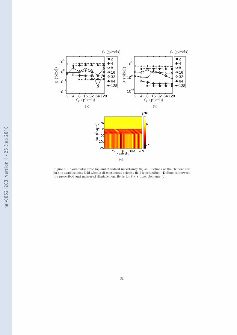
uncertainty (Figure 10(a) and Figure 10(b)) for the displacement fields with the

element size shows that both quantities reach a minimum for a small spatial

size, typically 2 × 32 pixels or 4 × 16 pixels, along the direction transverse to

the discontinuity.

Moreover, the differences shown in Figure 10(c) for the displacement fields

provide an additional information because they give exactly the position and

intensity of the perturbations associated with the chosen measurement basis.

From Figure 10(c) it is concluded that the error is the most important exactly

where the discontinuity is located and not near the edges.

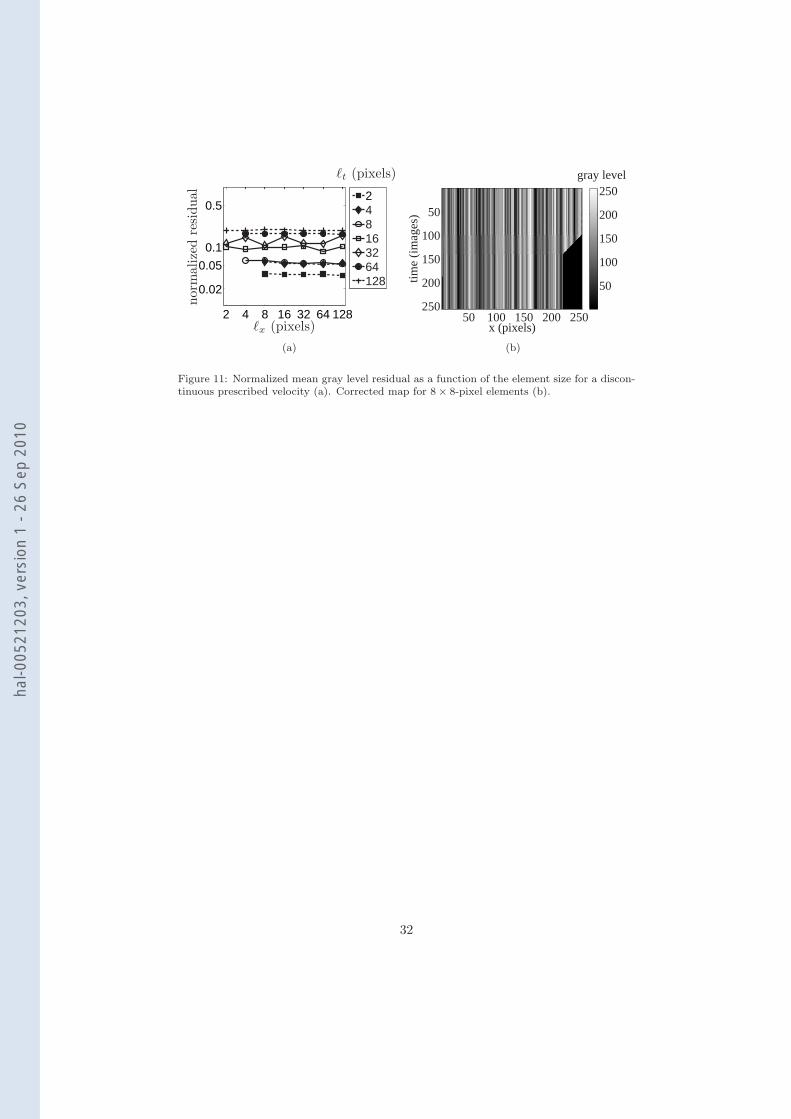
The gray level residuals are shown in Figure 11(a). The residual decreases

when the element size along the time dimension decreases too. The minimum

value is reached for a size equal to 4 × 128 pixels. Over the discontinuity line,

the difference between the prescribed and measured displacement leads to a

systematic error, which is partially corrected by the second discontinuity seen

in the corrected image. However, this incomplete correction induces a non-

vanishing strain field, which in reality does not exist.

Unlike the other tested maps, the image is not completely corrected by

using the displacement field (Figure 11(b)). A solution is to use enriched shape

functions as in eXtended Finite Element techniques [24]. This second solution

is implemented in DIC techniques when only two pictures are analyzed [22].

4. Application to a tensile test

In this last part, a real experimental case is studied. A cylinder-shaped

tantalum specimen is subjected to a tensile test in split Hopkinson pressure

bars [25, 26, 27, 28]. In the present case, out-of-plane displacements remain

small so that no correction procedure is used [29]. The spatiotemporal map is

shown in Figure 1, whose size is 201×351 pixels in space and time, respectively.

A pixel represents a size equal to 165 µm and the frame rate is equal to 30,000

fps.

The sample is first subjected to a tensile pulse followed by a quiescent period

when the loading wave has traveled out of the specimen. Wave reflection at the

13

hal-0

0521

203,

ver

sion

1 -

26 S

ep 2

010

end of the bar, leads to a second tensile pulse episode. During the second pulse,

failure occurs through a localized necking instability.

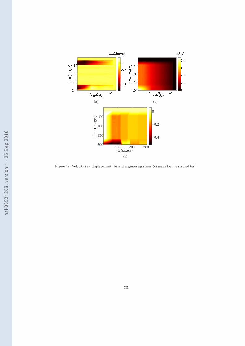
First, at a given position (Figure 1), the corresponding velocity, displace-

ment and strain maps are given in Figures 12(a), 12(b) and 12(c), respectively,

for 4× 64-pixel elements. This size is chosen by using the results of Section 3.3.

The present approach is also compared with a Q4-DIC code in which a spatial

piece-wise bilinear (Q4 finite element) kinematics is implemented [8]. In that

case, a series of 2D displacement fields are obtained for different instances of

time. For the spatiotemporal analysis, 40 maps are generated for the tantalum

sample corresponding to several vertical positions. For each of them, a compu-

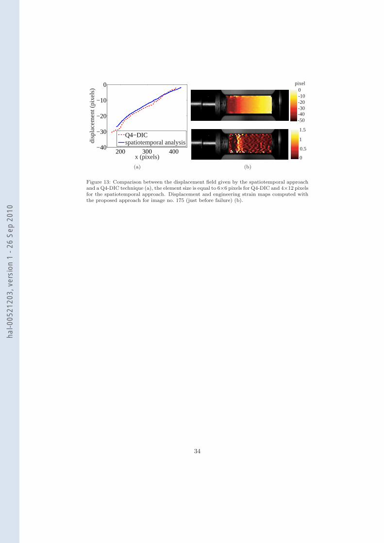
tation is carried out independently. The displacement field for image no. 35 is

computed by using both techniques as shown in Figure 13(a). A good alignment

of the camera with the sample axis allows for the present analysis. In terms of

transverse displacements that may violate the 1D-approach, they were measured

with Q4-DIC. The average transverse displacement is estimated to amount to

about 0.02 pixel, and hence a 1D approach is legitimate. More precisely, the

displacement field given by Q4-DIC is the average of the lines where it is mea-

surable (i.e., over 18 pixels). For the spatiotemporal approach, it is exactly the

same operation, although an interpolation is not needed since the displacement

field is directly computed for each line. A good agreement between the two

techniques is observed. Beyond position 350 pixels, noise is observed because of

the small element size (i.e., 6× 6 pixels) chosen for the Q4-DIC approach. An-

other advantage of the spatiotemporal approach is its tolerance to large values

of the displacement field.

When cumulated, a small velocity level may eventually induce large dis-

placements that are difficult to estimate by using standard DIC techniques.

This explains why the displacement field for the image corresponding to time

no. 175 is measurable with the spatiotemporal approach (Figure 13(b)). For

this picture, necking is very important and the engineering strain field is more

suited to see the exact position and intensity of this phenomenon. Moreover,

even if the result is shown for a given time, it is possible to obtain the same field

14

hal-0

0521

203,

ver

sion

1 -

26 S

ep 2

010

at different times and consequently to follow the growth of necking. This result

shows that localized phenomena can be captured with a spatial resolution that

is smaller than that allowed by classical 2D-DIC techniques [30, 31, 32].

To compare the present results with previous studies, gray level residuals are

shown in Figure 14(a), for different element sizes, and the difference between

the computed and measured trajectories is given in Figure 14(b). The levels of

the residuals are higher than those for the discontinuous velocity field. This is

partly due to the acquisition noise of the images, and presumably also to the

second discontinuity along the space dimension. However, even though higher

than in artificial cases, the overall level is sufficiently low to allow us to deem

the present results trustworthy.

5. Conclusion

A novel approach was developed to determine velocity fields based on the

global registration of a series of digital images. The velocity field is decomposed

onto a basis of continuous functions using Q4P1-shape spatiotemporal functions.

Displacement, strain and strain rate fields are subsequently estimated.

The performance of the algorithm is tested on several test maps in order

to evaluate the reliability of the estimation, which is shown to allow for either

an excellent accuracy for continuous velocity fields, or reasonable estimates for

discontinuous velocities. In the latter case, it is shown that the space/time dis-

cretization has to be adapted to properly capture the specific features of the

velocity field. Last, this method is used to analyze a tantalum specimen sub-

jected to a tensile test in Hopkinson bars where the performance of the technique

is compared with a finite element based DIC approach. A good agreement be-

tween both techniques is observed.

The space-time approach is particularly suited to experiments in which small

resolution pictures obtained by, say, camcorders or high speed cameras, yield a

large amount of images. This is for instance the case of split Hopkinson pressure

bar experiments. The time regularization proposed herein enables for the use of

fine spatial discretizations with reasonable uncertainty levels to capture localized

15

hal-0

0521

203,

ver

sion

1 -

26 S

ep 2

010

phenomena such as necking. It is an alternative to local 2D-DIC approaches [30,

31, 32] and an extension of Q4-DIC [8]. Discontinuous enrichments such as those

proposed for a Q4-DIC scheme [33] may be added in the future.

The generalization to 2D spatial discretizations, or 3D discretizations cou-

pled with 1D time discretizations is currently investigated. The output will

then be 3D and 4D velocity fields that can be used, for instance, to identify or

validate the parameters of constitutive equations.

Acknowledgements

The authors wish to thank Nicolas Granier of CEA Valduc for providing the

pictures of the experiment analyzed herein.

References

[1] S. Avril, M. Bonnet, A.-S. Bretelle, M. Grediac, F. Hild, P. Ienny, F. La-

tourte, D. Lemosse, S. Pagano, E. Pagnacco and F. Pierron, “Overview of

identification methods of mechanical parameters based on full-field measure-

ments,” Exp. Mech. 48, [4], 381-402 (2008).

[2] P. K. Rastogi, edt.,Photomechanics, (Springer, Berlin (Germany), 2000), 77.

[3] I. Chasiotis (edt.), “Special issue on nanoscale measurements in Mechanics,”

Exp. Mech. 47, [1], (2007).

[4] K. Han, M. Ciccotti and S. Roux, Measuring Nanoscale Stress Intensity

Factors with an Atomic Force Microscope, EuroPhys. Lett. 89 [6] (2010)

66003.

[5] M. A. Sutton, J.-J. Orteu and H. Schreier, Image correlation for shape,

motion and deformation measurements: Basic Concepts, Theory and Appli-

cations, (Springer, New York, NY (USA), 2009).

[6] M. Kuntz, M. Jolin, J. Bastien, F. Perez and F. Hild, “Digital image cor-

relation analysis of crack behavior in a reinforced concrete beam during a

load test,” Canad. J. Civil Eng. 33, 1418-1425 (2006).

16

hal-0

0521

203,

ver

sion

1 -

26 S

ep 2

010

[7] S. Bergonnier, F. Hild and S. Roux, “Digital image correlation used for

mechanical tests on crimped glass wool samples,” J. Strain Analysis 40,

185-197 (2005).

[8] G. Besnard, F. Hild and S. Roux, “Finite-element displacement fields anal-

ysis from digital images: Application to Portevin-Le Chatelier bands,” Exp.

Mech. 46, 789-803 (2006).

[9] P. J. Burt, C. Yen and X. Xu, Local correlation measures for motion analysis:

a comparative study, Proceedings IEEE Conf. on Pattern Recognition and

Image Processing , (1982), 269-274.

[10] M. A. Sutton, W. J. Wolters, W. H. Peters, W. F. Ranson and S. R.

McNeill, Determination of Displacements Using an Improved Digital Corre-

lation Method, Im. Vis. Comp. 1 [3] (1983) 133-139.

[11] M. A. Sutton, S. R. McNeill, J. D. Helm and Y. J. Chao, “Advances in Two-

Dimensional and Three-Dimensional Computer Vision,” in Photomechanics,

P. K. Rastogi, edt., (Springer, Berlin (Germany), 2000), 323-372.

[12] F. Hild, B. Raka, M. Baudequin, S. Roux and F. Cantelaube, “Multi-Scale

Displacement Field Measurements of Compressed Mineral Wool Samples by

Digital Image Correlation,” Appl. Optics. IP 41, [32], 6815-6828 (2002).

[13] C. Py, E. de Langre, B. Moulia and P. Hemon, “Measurement of wind-

induced motion of crop canopies from digital video images,” Agric. Forest

Meteorol. 130, 223-236 (2005).

[14] L. B. Fore, A. T. Tung, J. R. Buchanan and J. W. Welch, “Nonlinear

temporal filtering of time-resolved digital particle image velocimetry data,”

Exp. Fluids. 39, 22-31 (2005).

[15] S. Bergonnier, F. Hild and S. Roux, “Analyse d’une cinematique station-

naire heterogene,” Revue Comp. Mat. Av. 13, [3], 293-302 (2003).

17

hal-0

0521

203,

ver

sion

1 -

26 S

ep 2

010

[16] E. P. Simoncelli, “Bayesian Multi-Scale Differential Optical Flow,” in

Handbook of Computer Vision and Applications, B. Jahne, H. Haussecker

and P. Geissler, eds., (Academic Press, 1999), pp. 297-422.

[17] B. Wagne, S. Roux and F. Hild, “Spectral Approach to Displacement Eval-

uation From Image Analysis,” Eur. Phys. J. AP. 17, 247-252 (2002).

[18] S. Roux, F. Hild, P. Viot and D. Bernard, “Three dimensional image cor-

relation from X-Ray computed tomography of solid foam,” Comp. Part A.

39, [8], 1253-1265 (2008).

[19] C. Fennema and W. Thompson, “Velocity determination in scenes contain-

ing several moving objects,” Comput. Graph. Im. Proc. 9, 301-315 (1979).

[20] B. K. P. Horn and B. G. Schunck, “Determining optical flow,” Artificial

Intelligence. 17, 185-203 (1981).

[21] J. Rethore, S. Roux and F. Hild, “From pictures to extended finite elements:

Extended digital image correlation (X-DIC),” C. R. Mecanique. 335, 131-

137 (2007).

[22] Rethore, F. Hild and S. Roux, “Shear-band capturing using a multiscale

extended digital image correlation technique,” Comp. Meth. Appl. Mech.

Eng. 196, [49-52], 5016-5030 (2007).

[23] M. A. Sutton, S. R. McNeill, J. Jang and M. Babai, “Effects of subpixel

image restoration on digital correlation error estimates,” Opt. Eng. 27, [10],

870-877 (1988).

[24] N. Moes, J. Dolbow and T. Belytschko, “A finite element method for crack

growth without remeshing,” Int. J. Num. Meth. Eng. 46, [1], 133-150 (1999).

[25] D. Hopkinson, “A Method of Measuring the Pressure Produced in the Det-

onation of High Explosives or by the Impact of Bullets,” Phil. Trans. Roy.

Soc. A 213 437 (1914).

18

hal-0

0521

203,

ver

sion

1 -

26 S

ep 2

010

[26] H. Kolsky, Stress Waves in Solids, (Dover Publications, New York (USA),

1963).

[27] J. Harding, E. O. Wood and J. D. Campbell, “Tensile testing of materials

at impact rates of strain,” J. Mech. Eng. Sci. 2, 88-96 (1960).

[28] J. E. Field, S. M. Walley, W. G. Proud, H. T. Goldrein and C. R. Siviour,

“Review of experimental techniques for high rate deformation and shock

studies,” Int. J. Impact Eng. 30, 725-775 (2004).

[29] M. A. Sutton, J. H. Yan, V. Tiwari, H. W. Schreier and J.-J. Orteu, “The

Effect of Out of Plane Motion on 2D and 3D Digital Image Correlation

Measurements,” Opt. Lasers Eng. 46 746-757 (2008).

[30] B. Wattrisse, A. Chrysochoos, J. M. Muracciole and M. Nemoz-Gaillard,

Analysis of strain localisation during tensile test by digital image correlation,

Exp. Mech. 41 [1] (2001) 29-39.

[31] P. Schlosser, D. Favier, H. Louche and L. Orgeas, Experimental character-

ization of NiTi SMAs thermomechanical behaviour using temperature and

strain full-field measurements, Adv. Sci. Tech. 59 (2008) 140-149.

[32] S.-H. Tung, M.-H. Shih and J.-C. Kuo, Application of digital image corre-

lation for anisotropic plastic deformation during tension testing, Opt. Lasers

Eng. 48 [5] (2010) 636-641.

[33] J. Rethore, G. Besnard, G. Vivier, F. Hild and S. Roux, Experimental

investigation of localized phenomena using Digital Image Correlation, Phil.

Mag. 88 [28-29] (2008) 3339-3355.

19

hal-0

0521

203,

ver

sion

1 -

26 S

ep 2

010

List of Figures

1 Construction of a spatiotemporal map. . . . . . . . . . . . . . . 22

2 Spatiotemporal map corresponding to a constant velocity (a), a

parabolic velocity field (b) and a discontinuous velocity field (c). 23

3 Systematic error (a) and standard uncertainty (b) as functions

of the element sizes for the measured velocity field. Difference

between the prescribed and measured velocity fields for 8 × 8-

pixel elements (c). . . . . . . . . . . . . . . . . . . . . . . . . . . 24

4 Systematic error (a) and standard uncertainty (b) as functions

of the element size for the measured displacement field. Differ-

ence between the prescribed and measured displacement fields

for 128× 128-pixel elements (c). Reconstruction of the corrected

map g by using the measured displacement field for 8 × 8-pixel

elements (d). . . . . . . . . . . . . . . . . . . . . . . . . . . . . . 25

5 Normalized mean gray level residual as a function of the element

size for a constant prescribed velocity (a). Residual map between

the measured (with 8 × 8-pixel elements) and prescribed trajec-

tories (b). . . . . . . . . . . . . . . . . . . . . . . . . . . . . . . 26

6 Systematic error (a) and standard uncertainty (b) as functions

of the element size for the strain field. Difference between the

prescribed and measured strain fields for an element of size 8× 8

pixels (c). . . . . . . . . . . . . . . . . . . . . . . . . . . . . . . 27

7 Systematic error (a) and standard uncertainty (b) as functions of

the element size for the measured velocity field when a parabolic

velocity is prescribed. Difference between the prescribed and

measured velocity fields for 32× 32-pixel elements (c), and 128×128-pixel elements (d). . . . . . . . . . . . . . . . . . . . . . . . 28

20

hal-0

0521

203,

ver

sion

1 -

26 S

ep 2

010

8 Normalized mean gray level residual as a function of element size

for a parabolic prescribed velocity (a). Residual map between

the measured (with 32 × 32-pixel elements) and the prescribed

trajectories (b). Corrected map with the measured displacement

field for a 32× 32 pixel element (c). . . . . . . . . . . . . . . . . 29

9 Systematic error (a) and standard uncertainty (b) as functions of

the element size, for the measured strain field when a parabolic

velocity field is prescribed. . . . . . . . . . . . . . . . . . . . . . 30

10 Systematic error (a) and standard uncertainty (b) as functions of

the element size for the displacement field when a discontinuous

velocity field is prescribed. Difference between the prescribed and

measured displacement fields for 8× 8-pixel elements (c). . . . . 31

11 Normalized mean gray level residual as a function of the element

size for a discontinuous prescribed velocity (a). Corrected map

for 8× 8-pixel elements (b). . . . . . . . . . . . . . . . . . . . . 32

12 Velocity (a), displacement (b) and engineering strain (c) maps

for the studied test. . . . . . . . . . . . . . . . . . . . . . . . . . 33

13 Comparison between the displacement field given by the spa-

tiotemporal approach and a Q4-DIC technique (a), the element

size is equal to 6× 6 pixels for Q4-DIC and 4× 12 pixels for the

spatiotemporal approach. Displacement and engineering strain

maps computed with the proposed approach for image no. 175

(just before failure) (b). . . . . . . . . . . . . . . . . . . . . . . . 34

14 Normalized mean gray level residual as function of element size

for the real application (a). Difference between the real and re-

constructed spatiotemporal maps (b). The latter is reconstructed

with the measured velocities (4× 20-pixel elements). . . . . . . 35

21

hal-0

0521

203,

ver

sion

1 -

26 S

ep 2

010

space (pixels)

time

(images)

time

(images)

space (pixels)0

0

201

351

35

90

160

51285 436

Figure 1: Construction of a spatiotemporal map.

22

hal-0

0521

203,

ver

sion

1 -

26 S

ep 2

010

x (pixels)

time

(im

ages

)

gray level

50 100 150 200 250

50

100

150

200

250

50

100

150

200

250

(a)

x (pixels)

time

(im

ages

)

gray level

50 100 150 200 250

50

100

150

200

250 0

50

100

150

200

250

(b)

x (pixels)

time

(im

ages

)

gray level

50 100 150 200 250

50

100

150

200

250 0

50

100

150

200

250

(c)

Figure 2: Spatiotemporal map corresponding to a constant velocity (a), a parabolic velocityfield (b) and a discontinuous velocity field (c).

23

hal-0

0521

203,

ver

sion

1 -

26 S

ep 2

010

2 4 8 16 32 64 128

10−5

10−4

10−3

`x (pixels)

η(p

ixel

/im

age)

`t (pixels)

8163264128

(a)

2 4 8 16 32 64 12810

−4

10−3

10−2

10−1

`x (pixels)

σ(p

ixel

/im

age)

`t (pixels)

8163264128

(b)

����������� ���

��������������

��� ����� � �!� "#��� "$���

����%���� ���"#���"$��� & ��'(��)

& ��'(�#*& ��'(�#"���'(��"��'(��*

�$�+���-, ��.0/21#�

(c)

Figure 3: Systematic error (a) and standard uncertainty (b) as functions of the element sizesfor the measured velocity field. Difference between the prescribed and measured velocity fieldsfor 8× 8-pixel elements (c).

24

hal-0

0521

203,

ver

sion

1 -

26 S

ep 2

010

2 4 8 16 32 64 128

10−3

10−2

10−1

`x (pixels)

η(p

ixel

)`t (pixels)

8163264128

(a)

2 4 8 16 32 64 128

10−2

10−1

`x (pixels)

σ(p

ixel

)

`t (pixels)

8163264128

(b)

����������� ���

��������������

��� ����� � ��� !��� !��"�

����#����$���!���!%��� �

�'&(�"!

�'&(�")

�'&(�+*�%�,���

(c)

x (pixels)

time

(im

ages

)

gray level

50 100 150 200 250

50

100

150

200

250

50

100

150

200

250

(d)

Figure 4: Systematic error (a) and standard uncertainty (b) as functions of the elementsize for the measured displacement field. Difference between the prescribed and measureddisplacement fields for 128 × 128-pixel elements (c). Reconstruction of the corrected map gby using the measured displacement field for 8× 8-pixel elements (d).

25

hal-0

0521

203,

ver

sion

1 -

26 S

ep 2

010

2 4 8 16 32 64 128

0.005

0.01

`x (pixels)

norm

ali

zed

resi

dual

`t (pixels)

8163264128

(a)

x (pixels)

time

(im

ages

)

gray level

50 100 150 200 250

50

100

150

200

250

20

40

60

(b)

Figure 5: Normalized mean gray level residual as a function of the element size for a constantprescribed velocity (a). Residual map between the measured (with 8× 8-pixel elements) andprescribed trajectories (b).

26

hal-0

0521

203,

ver

sion

1 -

26 S

ep 2

010

2 4 8 16 32 64 128

10−5

10−4

10−3

`x (pixels)

η`t (pixels)

8163264128

(a)

2 4 8 16 32 64 12810

−4

10−3

10−2

10−1

`x (pixels)

σ

`t (pixels)

8163264128

(b)

x (pixels)

time

(im

ages

)

50 100 150 200 250

50

100

150

200

250

−0.05

0

0.05

(c)

Figure 6: Systematic error (a) and standard uncertainty (b) as functions of the element size forthe strain field. Difference between the prescribed and measured strain fields for an elementof size 8× 8 pixels (c).

27

hal-0

0521

203,

ver

sion

1 -

26 S

ep 2

010

2 4 8 16 32 64 128

10−3

10−2

`x (pixels)

η(p

ixel

/im

age)

`t (pixels)

8163264128

(a)

2 4 8 16 32 64 128

10−3

10−2

10−1

`x (pixels)

σ(p

ixel

/im

age)

`t (pixels)

8163264128

(b)

��������������

��������������

��� ����� ����� ��� !�"�

�"�������#�"� ��� !�"� �

���

�

� �$�!%'&�!�(����*)+��,.-�/0�

(c)

����������� ���

��������������

��� ����� � �!� "#��� "$���

����%���� ���"#���"$���

& ��'(��)& ��'(��"

��$���$��+* �-,/.102�

(d)

Figure 7: Systematic error (a) and standard uncertainty (b) as functions of the element sizefor the measured velocity field when a parabolic velocity is prescribed. Difference betweenthe prescribed and measured velocity fields for 32× 32-pixel elements (c), and 128× 128-pixelelements (d).

28

hal-0

0521

203,

ver

sion

1 -

26 S

ep 2

010

2 4 8 16 32 64 128

0.025

0.05

0.1

`x (pixels)

norm

ali

zed

resi

dual

`t (pixels)

8163264128

(a)

x (pixels)

time

(im

ages

)

gray level

50 100 150 200 250

50

100

150

200

250 0

20

40

60

(b)

x (pixels)

time

(im

ages

)

gray level

50 100 150 200 250

50

100

150

200

250

50

100

150

200

250

(c)

Figure 8: Normalized mean gray level residual as a function of element size for a parabolicprescribed velocity (a). Residual map between the measured (with 32 × 32-pixel elements)and the prescribed trajectories (b). Corrected map with the measured displacement field fora 32× 32 pixel element (c).

29

hal-0

0521

203,

ver

sion

1 -

26 S

ep 2

010

2 4 8 16 32 64 12810

−5

10−4

10−3

10−2

`x (pixels)

η`t (pixels)

8163264128

(a)

2 4 8 16 32 64 12810

−3

10−2

10−1

100

`x (pixels)

σ

`t (pixels)

8163264128

(b)

Figure 9: Systematic error (a) and standard uncertainty (b) as functions of the element size,for the measured strain field when a parabolic velocity field is prescribed.

30

hal-0

0521

203,

ver

sion

1 -

26 S

ep 2

010

2 4 8 16 32 64 12810

−2

10−1

100

101

`x (pixels)

η(p

ixel

)`t (pixels)

248163264128

(a)

2 4 8 16 32 64 12810

−1

100

101

`x (pixels)

σ(p

ixel

)

`t (pixels)

248163264128

(b)

��������������

��������������

��� ����� ��� � !"�#�

� ��$������ �!���!%� � &

!

&�

�

�%�'����

(c)

Figure 10: Systematic error (a) and standard uncertainty (b) as functions of the element sizefor the displacement field when a discontinuous velocity field is prescribed. Difference betweenthe prescribed and measured displacement fields for 8× 8-pixel elements (c).

31

hal-0

0521

203,

ver

sion

1 -

26 S

ep 2

010

2 4 8 16 32 64 128

0.02

0.05

0.1

0.5

`x (pixels)

norm

ali

zed

resi

dual

`t (pixels)

248163264128

(a)

x (pixels)

time

(im

ages

)

gray level

50 100 150 200 250

50

100

150

200

250

50

100

150

200

250

(b)

Figure 11: Normalized mean gray level residual as a function of the element size for a discon-tinuous prescribed velocity (a). Corrected map for 8× 8-pixel elements (b).

32

hal-0

0521

203,

ver

sion

1 -

26 S

ep 2

010

��������������

��������������

����� ����� � �!�

" ��#���� " �����

$ �&% "$ �$ �'% "�

�������)(*�,+.-0/��

(a)

����������� ���

��������������

����� ����� !�!�

" �

�#�!�

� " �

��!� �

��

$�

%!�

&'��(�)��*

(b)

x (pixels)

time

(im

ages

)

100 200 300

50

100

150

200

−0.4

−0.2

0

(c)

Figure 12: Velocity (a), displacement (b) and engineering strain (c) maps for the studied test.

33

hal-0

0521

203,

ver

sion

1 -

26 S

ep 2

010

200 300 400−40

−30

−20

−10

0

x (pixels)

disp

lace

men

t (pi

xels

)

Q4−DICspatiotemporal analysis

(a)

-10

-50-40-30-20

0

0

0.5

1

1.5

pixel

(b)

Figure 13: Comparison between the displacement field given by the spatiotemporal approachand a Q4-DIC technique (a), the element size is equal to 6×6 pixels for Q4-DIC and 4×12 pixelsfor the spatiotemporal approach. Displacement and engineering strain maps computed withthe proposed approach for image no. 175 (just before failure) (b).

34

hal-0

0521

203,

ver

sion

1 -

26 S

ep 2

010

8 16 32 64 128

0.06

0.1

0.2

`x (pixels)

norm

ali

zed

resi

dual

`t (pixels)

24816

(a)

x (pixels)

time

(im

ages

)

gray level

100 200 300

50

100

150

200 0

50

100

(b)

Figure 14: Normalized mean gray level residual as function of element size for the real ap-plication (a). Difference between the real and reconstructed spatiotemporal maps (b). Thelatter is reconstructed with the measured velocities (4× 20-pixel elements).

35

hal-0

0521

203,

ver

sion

1 -

26 S

ep 2

010