HD28.MA14no.

96

Dewey

A Scaling Algorithm for

Multicommodity Flow Problems

byRina R. Schneur

James B. Orlin

WP #3808-95 April 1995

A SCALING ALGORITHM FOR MULTICOMMODITY

FLOW PROBLEMS

Rina R. Schneur

PTCG Inc.

Burlington, Massachusetts

James B. Orlin

Massachusetts Instittite of Technology

Cambridge, Massachusetts

i/ASSAOHUSSrrS INSTITUTE

OF TECHNOLOGY

MAY 3 1995

LIBRARIES

Abstract

We present a penalty-based algorithm that solves the multicommodity flow problem as a

sequence of a fmite number of scaling phases. In the 8-scaling phase the algorithm determines an e-

optimal solution, that is, one in which complementary slackness conditions are satisfied to within 8.

We analyze the performance of the algorithm from both the theoretical and practical perspectives.

1. Introduction

Multicommodity flow problems arise whenever commodities, vehicles, or messages are to

be shipped or transmitted simultaneously from certain origins to certain destinations along arcs of

an underlying network. These problems find applications in the study of urban traffic, railway

systems, logistics, communication systems, and many other areas as well (see for example Ali et.

al. [1984], Schneur [1991], Ahuja, Magnanti and Oriin [1993]). The multicommodity flow problem

is a generalization of the single commodity network flow problem in which different commodities

share a common network, and interact with each other typically through common capacity

constraints. In the absence of any interaction among the commodities, the problem can be solved as

separate single commodity flow problems. The interaction between the commodities, however,

requires one to solve all the single commodity problems concurrently and, therefore, makes

multicommodity flow problems much more difficult to solve than the corresponding set of single

commodity problems.

Linear multicommodity flow problems can be formulated as linear programs and solved by

the simplex algorithm or by interior point methods. The best time bound for linear programming

problems is due to Vaidya [1989]. Many applications of multicommodity flow problems, however,

lead to linear programs which are too large to solve by a direct application of linear programming

software. Researchers have therefore developed specialized adaptations of linear programming

algorithms which exploit the special structure and the sparsity inherent in multicommodity network

flow problems. Three "classical" approaches to multicommodity flow problems are price-directive

decomposition, resource-directive decomposition, and partitioning. These approaches are all based

on the simplex method. Assad [1978], Kennington [1978], and Ali, Helgason, Kennington and Lall

[1980] review these methods and their computational performance. Recent research has focused

mainly on the development of interior point methods, the development of parallel algorithms, and

the solution of large-scale problems. Examples of interior point algorithms may be found m Choi

and Goldfarb [1989], and Bertsimas and Oriin [1991]. Multicommodity flow problems reveal

inherent parallelism. Choi and Goldfarb [1989] as well as Pinar and Zenios [1990] exploited this

characteristic in their parallel algorithms. The latter uses linear and quadratic penalty functions.

In this paper we present a scaling-based approximation algorithm. A solution x is called e-

optimal if it is possible to perturb some cost coefficients or capacity constraints by at most e units

so that the solution x is optimal for the perturbed problem. The scaling approach may be

summarized as follows. Let P(A) be a problem which is different by at most A from the original

problem P. Start by solving P(A) for a sufficiently large A, such that P(A) is relatively easy to solve.

Then, lise the solution to P(A) to solve P(A/F) for some scalmg factor F>1, and modify A to be A/F.

Keep iterating until the value ofA is sufficiently small. Edmonds and Karp [1972] and Dinic [1973]

developed the first scaling algorithms for the minimum cost single commodity network flow

problem. Gabow [1985] showed the application of scaling to several problems, including the

shortest path, matching and maximum flow problems. Scaling algorithms which use the idea of s-

optimality are theoretically the most efficient algorithms for various network flow problems.

Prominent among these are single commodity network flow problems such as minimum cost flow

(Goldberg and Tarjan [1987], Ahuja, Goldberg, Orlin and Tarjan [1992|, and Orlin [1988]) and

maximum flow (Ahuja, Orlin and Tarjan [1989]) In this paper we develop a cost scaling algorithm

approach to solve multicommodity network flow problems. Other researchers have developed e-

optimal algorithms (the traditional notion) for multicommodity flow problems. Such approximation

algorithms are described and analyzed in the papers by Grigoriadis and Khachiyan [1991], Klein,

Agrawal, Ravi, and Rao [1990], Leighton et. al. [1991], Klein, Plotkin, Stein, and Tardos [1990],

Shahrokhi and Matula [1990]. The last two focus on the maximum concurrent flow problem which

is a special case of the multicommodity flow problem. In all these cases the focus of the research

has been on obtaining good worst case bounds. Our research focuses more on computational

performance in practice.

Our algorithm is simple, and yet robust. It solves the multicommodity flow problem as a

sequence of penalty problems, each of which is constructed by relaxing the capacity constraints and

adding a term for theh violation to the objective flinction. (For detailed description of penalty

methods see Fiacco and McCormick [1968].) Each penalty problem is solved to s-optimality using

a network-based scaling algorithm. Since the parameters of real-world multicommodity problems,

such as cost and capacity, are typically approximate in practice, the algorithm presented here often

finds an optimal solution up to the accuracy of the data. The main component of the algorithm

consists ofmoving flow around cycles. Thus, the algorithm focuses on cycles rather than on paths.

The efficiency of the algorithm is a result of usmg the scaling approach and of exploiting

the network structure of the problem. In subsequent sections we present convergence results and

prove that the algorithm has some interesting theoretical characteristics. The computational testing

provides insight into the behavior of the algorithm and shows that the algorithm is quite efficient

and worthy of fiirther consideration. The computational results also reveal that in some cases the

theoretical bounds are observed in practice, while in other cases the bounds are much more

conservative than the practical performance. The testing shows that the run time of the algorithm is

competitive with the run time of recent algorithms for large scale multicommodity flow problems.

These algorithms by Bamhart [1993], Bamhart and Sheffi [1993], and Farvolden, Powell and

Lustig [1993] are based on dual ascent methods, the primal-dual approach and partitioning method

respectively.

The general fi-amework of our algorithm can be used to solve different types of

multicommodity flow problems. A variation of it also be used for various network flow problems

with side constraints of which the muhicommodity flow problem is a special case (see Schneur

[1991]). In this paper we focus on the algorithm for the minimum cost multicommodity flow

problem. In the next section, we apply a penalty method to the multicommodity flow problem, and

formulate it as a penalty problem. We also present in this section a detailed description of the

algorithm. In Section 3, we develop the optimality conditions for the penalty problem, and in

Section 4, we introduce and prove some of its theoretical properties. Numerical results are

presented in Section 5, and in Section 6 we briefly discuss possible extensions of our algorithm to

other network flow problems and make some concluding remarks.

2. The Scaling Algorithm for the Penalty Problem

We consider linear multicommodity flow problems on directed networks. For each

commodity there is an associated vector of supply/demand. We observe that a multicommodity

flow problem on an undirected network with multiple sources and multiple sinks for each

commodity can be transformed to a single source-single sink multicommodity flow problem on a

directed network. This can be done by adding a super-source and a super-sink node for each

commodity. The super-source node is connected to each supply node of that commodity with an

outgoing arc from the super-source node whose capacity equals the supply at the node and whose

cost is zero. Similar arcs are added from each demand node of that commodity to the super-sink

node. The capacity of each such arc equals the demand at the node and its cost is zero. Henceforth,

we consider only cases in which there is a single source node and a single sink node for each

commodity.

Let N be a set of n nodes and A be a set of m directed arcs, which together form a network

G=(N,A). There are K commodities sharing the capacity Uy of each arc (ij) in the network. For each

commodity k there is a required flow of b units from its source node s(k) to its smk node t(k). The

cost of a unit flow of commodity k on arc (ij) is clj and the amount of flow is denoted as xlj • Let

dl* be the flow balance of commodity k at node i. Thus, d!'= b if i=s(k); d!' = -b if i=t(k); and

d!' =0 otherwise.

Using these notations, the minimum-cost multicommodity flow problem[MM] may be

formulated as follows:

(1)

Vi6N,Vk=l,...,K (2)

[MM]

Min

In order to formulate the multicommodity flow problem using a penalty function method,

we relax the capacity bundle constraints and add a penalty function term of their violation to the

objective function.

K

Let eij (x) = max{0,(^ xlj- uy)} be the amount by which the total flow on arc (ij) exceeds

k = l

its capacity. A quadratic penalty fiinction with a penalty parameter p is associated with each

violated capacity constraint and a penalty term p(eij(x)) is added to the objective function.

The resulting penalty problem [PMM(p)] is:

Mm(f^(x)= X i^4x^+ Zp(e,Mf ) (5)

Z4-Z4-^' VieN,Vk=l,...,K (2)

p

s.t.

J:{l.j)tA jtj))tA

4>0 V(ij)eA,Vk=l,...,K (4)

After relaxing the bundle constraints, the remaining constraints in [PMM(p)] decompose

into the constraints ofK single commodity flow problems. The objective flmction, however, is non-

separable and nonlinear. Hence, we eliminate the complicating constraints, but introduce nonlinear

(convex) and non-separable terms into the objective function.

A sequence of solutions to the penalty problem with an increasing penalty parameter

converges to the optimal solution of the original problem as long as the penalty parameter increases

without bound (Avriel [1976] and Luenberger [1984]). Penalty methods using the Hessian to solve

the penalty problems may fail when the penalty parameter is too large because the Hessian is ill-

conditioned (Avriel [1976]). We present a scaling algorithm which utilizes the special network

structure of the penalty problem and does not require the computation of the Hessian. The

algorithm finds an approximately optimal solution to the penalty problem and successively

improves the quality of the solution at each iteration.

kLet Q denote an undirected cycle of commodity k. Since G=(N,A) is a directed network

but Q is an undirected cycle, not all the arcs in (^ follow the same direction. When we send flow

around a cycle we send it in a particular direction. We call the arcs that follow that direction

forward arcs and the arcs that are opposite to the direction of the flow backward arcs. To send 5

units of flow around Q is to increase the flow on each forward arc of Q*' by 5 units and to decrease

the flow on each backward arc of Q'' by 8 units. We refer to this flow as a b-flow around Q*' and

denote it as y(6, Q ). The cost of a 5-flow around Q*' is the net change in the objective function fp

obtained by sending the flow around the cycle. That is, it is fp(x+ y(5, Q"")) - fp(x). If fp(x+ y(8, Q*'))

- fp(x) < 0, we refer to Q as a negative cost h-cycle with respect to fp(x), and we refer to y(6, Q ) as

a negative cost d-flow with respect to fp(x). In order to detect these cycles, we build a residual

network (also called the b-residual netM'ork) which is constructed as follows. Let arc (ij)' represent

an arc from node i to node j in the residual network. For each arc (ij) of the original network we

potentially have two oppositely directed arcs in the residual network: ^t forward arc (ij)' whose

cost represents increasing the flow on arc (ij) by 5 units; the backward arc (j,i)' whose cost

represents decreasing the flow on arc (ij) by 6 units; the backward arc (],ii is included in the 5-

residual network of commodity k only if we can decrease the flow of commodity k on arc (ij) by 5

units, that is, if x!) > 6 . Using our notations (c is the cost vector, x is the flow and e is the excess of

flow), we can write the cost of each arc on the 5-residuaI network as follows.

-*The cost of each forward arc (iJ) on the residual network for commodity k, c,j , is the net

change in fp obtained by increasing the flow on arc (iJ) by 6 units. That is:

~* - ^*d = c*5 + p(26e,(x)+ 6')

keK

and

\/{i,j)eA:eoix)>0 (6)

V(/,7)e^:-5<Xx*-M,<0 (7)

-*= c*5 V(/,7)€^:Xx^M,<-5 (8)

The cost of each backward arc (j,i) on the residual network for commodity k, Cj, is the net change

in fp obtained by decreasing the flow on arc (ij) by 6 units. That is:

~* - „*c, = -c*5 + p(-2de,j(x) + 6') yiJ,i)eA:e,{x)>d (9)

c*, = -4 5 - p(e,j(x)/ \fU,i)^A:0<eJx)<6 (10)

and

-c*5 ^U,i)eA:J^4-u,<0 (11)

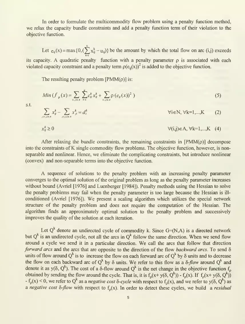
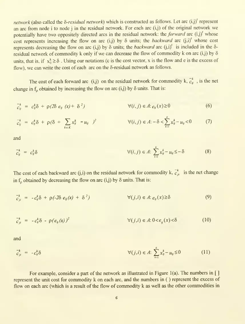
For example, consider a part of the network as illustrated in Figure 1(a). The numbers in [ ]

represent the unit cost for commodity k on each arc, and the numbers in ( ) represent the excess of

flow on each arc (which is a result of the flow of commodity k as well as the other commodities in

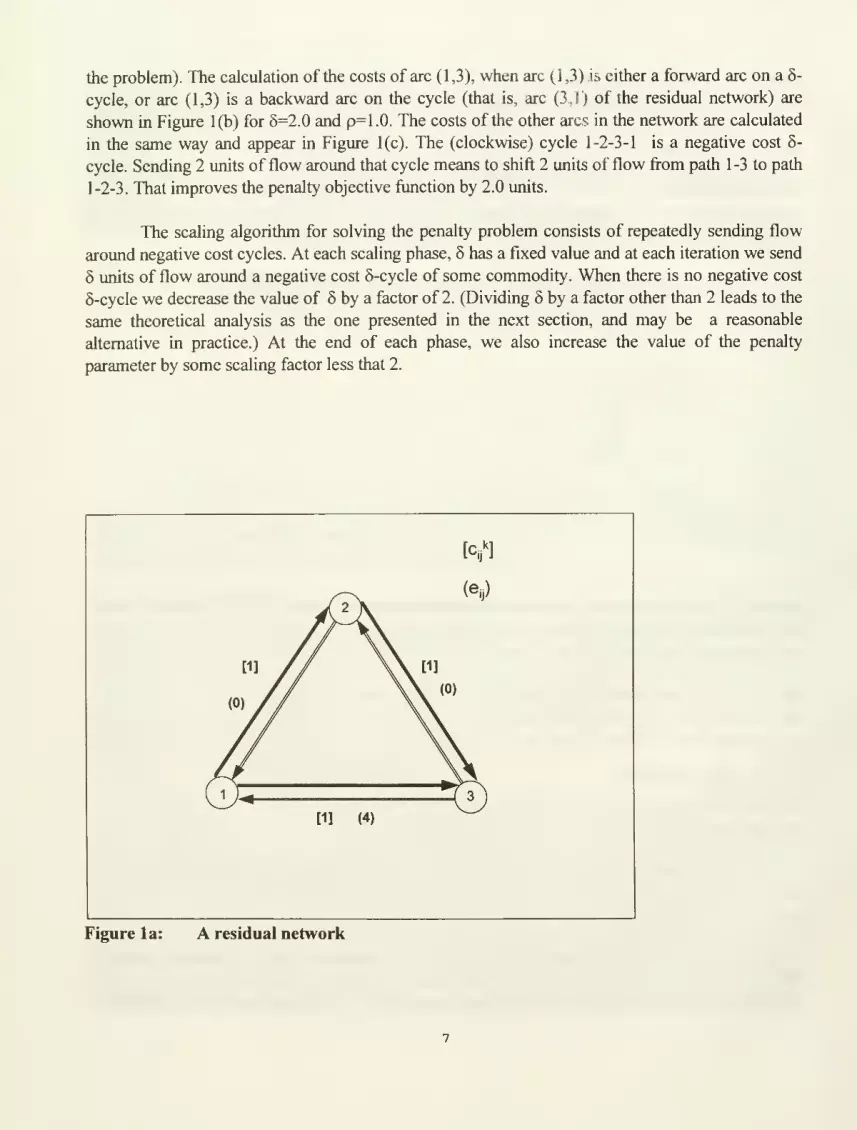
the problem). The calculation of the costs of arc (1,3), when arc (1,3) is either a forward arc on a 5-

cycle, or arc (1,3) is a backward arc on the cycle (that is, arc (3J ) of the residual network) are

shown in Figure 1(b) for 6=2.0 and p=1.0. The costs of the other arcs in the network are calculated

in the same way and appear in Figure 1(c). The (clockwise) cycle 1-2-3-1 is a negative cost 6-

cycle. Sending 2 units of flow around that cycle means to shift 2 units of flow from path 1 -3 to path

1-2-3. That improves the penalty objective ftinction by 2.0 units.

The scaling algorithm for solving the penalty problem consists of repeatedly sending flow

around negative cost cycles. At each scaling phase, 5 has a fixed value and at each iteration we send

5 units of flow around a negative cost 5-cycle of some commodity. When there is no negative cost

6-cycle we decrease the value of 6 by a factor of 2. (Dividing 6 by a factor other than 2 leads to the

same theoretical analysis as the one presented in the next section, and may be a reasonable

alternative in practice.) At the end of each phase, we also increase the value of the penalty

parameter by some scaling factor less that 2.

8 = 2.0

p= 1.0

2 + 16 + 4 = 22

-2 -16 + 4 = -14

Figure lb: Calculating the cost of the residual arcs

Figure Ic: A negative cost 5-cycIe

We say that a flow x is (b,p)-optimal for the penalty version of the muhicommodity flow

problem if x is a feasible flow for the penalty problem and there is no negative cost 5-cycle with

respect to the function fp. We present the following Theorem here since it helps to understand the

motivation behind our algorithm. We prove it in the next section.

Theorem 1:

A flow X is optimal for PMM(p) if and only if x is (8,p)-optimal for all sufficiently small

positive values of 5.

The scaling algorithm for the penalty problem can be viewed as a nonlinear programming

algorithm in which the step size at each phase is fixed at a value of 5. We try to find a "direction" (a

vector of flow modifications) such that by moving 6 units in this direction the penalty objective

fiinction decreases. When we can not find an improving direction with a step size 5, we decrease

the step size to 5/2. An alternative approach, in which we first detect the improving direction and

then determine the step size, is described in Schneur [1991]. In the remainder of this section we

outline the scaling algorithm.

The scaling algorithm for the minimum cost multicommodity flow problem may be

described in the general form of a scaling algorithm as follows.

Given:

cjj= cost ofunit flow on arc (ij) for commodity k

Ujj= capacity of arc (iJ)

b = amount of supply/demand of commodity k.

Objective:

Find a minimum cost flow which satisfies the flow requirements for each commodity

without violating the capacity constraints.

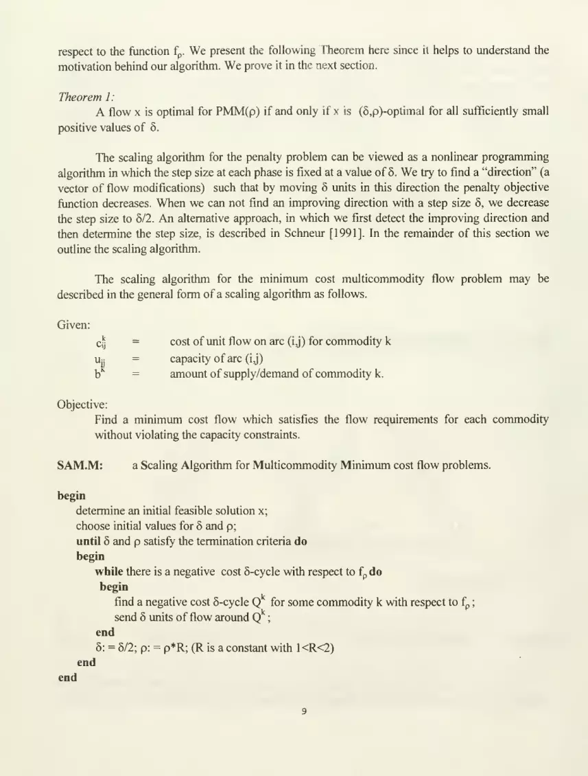
SAM.M: a Scaling Algorithm for Multicommodity Minimum cost flow problems.

begin

determine an initial feasible solution x;

choose initial values for 5 and p;

until 5 and p satisfy the termination criteria do

begin

while there is a negative cost 5-cycle with respect to fp do

begin

find a negative cost 5-cycle Q for some commodity k with respect to fp

;

send 5 units of flow around Q ;

end

5: = 5/2; p: = p*R; (R is a constant with 1<R<2)

end

end

We now discuss some practical issues related to the various elements of the

algorithm.

Initial solution:

An initial solution may be any solution which satisfies the supply/demand constraints. For

example, one can satisfy the supply/demand of each commodity by sending b units on the shortest

path from s(k) to t(k). We henceforth assume that we initialize the solution in this way.

Parameter setting:

In our implementation we let the initial value of 5 be the size of the largest demand rounded

up to the nearest power of 2, i.e., 5o:= 2 °^

, where B = max{b : k=l,...,K}. Since 5 is halved at

each successive scaling phase, within [log b1 additional phases 5=1, a fact needed in the

subsequent analysis. The best initial penalty parameter value and its modification rate, R, may be

empirically determined. Observe that 5 and p are modified simultaneously. For theoretical purposes

which are discussed later, we need 5*p to decrease by a constant factor in each phase. Since 5

decreases by a factor of 2 at each phase, we require that R < 2. We have found Po=0.3 and

R€[1.6,1.7] to be good choices for the problems that we have tested.

Termination rulesfor the algorithm:

The termination criteria of the algorithm depend on the values of 5 and p. (In cases in which

the dual solution is obtained, the criteria may also depend on the value of the duality gap.) The final

values of 5 and p are chosen to ensure that 5 is "sufficiently" small and p is "sufficiently" large. In

practice, one may bound the penalty parameter value from above in order to help maintain

numerical stability or to ensure faster termination of the algorithm. We let p^ denote our upper

bound on p.

For each solution to the penalty problem, we also derive a solution to the dual of the

penalty problem. The duality gap is the difference between the value of the penalty objective

fiinction and the value of this dual solution. We refer to this dual solution and this duality gap as the

induced dual solution and the induced duality gap, respectively. We describe these terms in details

in Section 4. The induced duality gap may be used in the termination criteria.

Let GAP be the current value of the induced duality gap, and let g and 8 be small positive

values set by the user. Then, the algorithm terminates when one of the following conditions is

satisfied:

i) 6*p < e or

ii) GAP < g and p = Py.

The values of 6*p and the duality gap indicate how close the solution is to optimality. The lower

bounds on those values provide the user the option of terminating with a pre-specified level of

solution quality.

10

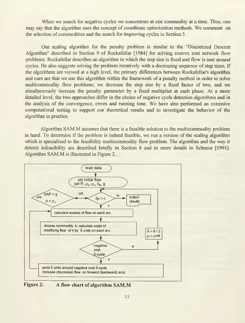
When we search for negative cycles we concentrate at one commodity at a time. Thus, one

may say that the algorithm uses the concept of coordinate optimization methods. We comment on

the selection of commodities and the search for improving cycles in Section 5.

Our scaling algorithm for the penalty problem is similar to the "Discretized Descent

Algorithm" described in Section 9 of Rockafellar [1984] for solving convex cost network flow

problems. Rockafellar describes an algorithm in which the step size is fixed and flow is sent around

cycles. He also suggests solving the problem iteratively with a decreasing sequence of step sizes. If

the algorithms are viewed at a high level, the primary differences between Rockafellar's algorithm

and ours are that we use this algorithm within the fi-amework of a penalty method in order to solve

multicommodity flow problems; we decrease the step size by a fixed factor of two, and wesimultaneously increase the penalty parameter by a fixed multiplier at each phase. At a more

detailed level, the two approaches differ in the choice of negative cycle detection algorithms and in

the analysis of the convergence, errors and running time. We have also performed an extensive

computational testing to support our theoretical results and to investigate the behavior of the

algorithm in practice.

Algorithm SAM.M assumes that there is a feasible solution to the multicommodity problem

in hand. To determine if the problem is indeed feasible, we run a version of the scaling algorithm

which is specialized to the feasibility multicommodity flow problem. The algorithm and the way it

detects infeasibility are described briefly in Section 6 and in more details in Schneur [1991].

Algorithm SAM.M is illustrated in Figure 2.

calculate excess of flow on each arc

choose commodity k; calculate costs of

modifying flow of k by 6 units on each arc 5 = 5/2

p = p*R

send 5 units around negative cost 5-cycle

increase (decrease) flow on forward (backward) arcs

Figure 2: A flow chart of algorithm SAM.M

11

We have developed also an optimal-shift version of the scaling algorithm (Schneur [1991]).

The algorithm is motivated by Frank-Wolfe gradient-based algorithm for quadratic programming

(Frank and Wolfe [1956]). Among other problems, Frank-Wolfe algorithm is used to solve traffic

equilibrium multicommodity flow problems (Sheffi [1976]). The optimal-shift algorithm may be

viewed as a network-based scaling version of Frank-Wolfe algorithm. While in algorithm SAM.Mwe first determine the step size and then look for an improving direction, the optimal-shift scaling

algorithm is more similar to conventional nonlinear algorithms. First the direction of improvement

is determined. Then, the optimal step size along this direction is calculated. A direction of

improvement is found by detecting a negative cost cycle in the residual network of each

commodity. The costs of the residual network of commodity k represent the derivative of the

penalty objective fianction with respect to the flow of that commodity on each arc. This is a

different residual network than the one used in algorithm SAM.M. Once a negative cycle is

detected, we shift the optimal amount of flow around it, i.e., the amount which results in the

maximum improvement of the penalty objective fianction. The optimal amount is the amount which

drives the cycle derivative cost to zero. The optimal amount to shift on a cycle can be calculated

using a binary search technique.

3. Optimality Conditions

The optimality conditions for the penalty problem are derived from the Kuhn-Tucker

optimality conditions for nonlinear programming. Since the objective function is convex and the

constraints are linear, the Kuhn-Tucker conditions are sufficient for optimality (see, for example,

Avriel [1976]).

For a general nonlinear programming problem {min f(x): q(x)=0, x> 0}, the Kuhn-Tucker

optimality conditions for a feasible solution x are (A denotes derivative):

x(^x(f) -^ \'^x(^)= and Ax(/) + ^iAx(q)> (12)

for some vector |i.

Applied to a feasible solution for the penalty problem [PMM(p)], the optimality conditions

for each arc (ij) and commodity k are:

xUcl + 2pey(x) + ^i* - ^])= and c* + 2pe,j(x) + ^f - [i' > (13)

for some values of j^, and jJ.* .

Let * be the reduced cost of arc (iJ) and commodity k which is defmed as

e* = cj + 2peo(x) + ^' - ^; . (14)

The optimality conditions for a feasible solution x may now be written as

xfj > => e* = (15)

and

12

xfj= => G* > 0. (16)

The optimality conditions indicate that in the optimal solution, flow is assigned only to arcs whose

reduced costs equal 0.

Lemma 1:

Let X be a (5,p)-optimai solution to the penalty problem. Then, there exists a vector \x. of

simplex multipliers, such that the following conditions hold:

X* > 5 => -6p < e* < 5p (17)

and

4 < 6 => -5p < e*. (18)

Proof:

Let us define a cost vector h as follows. For each forward arc (ij)' of the 5-residual network

for commodity k:

A* = c,; + 2pe.j(x) + 5p (19)

and for each backward arc (j,i)^ of the 5-residual network of commodity k:

A* = -c* - 2pe,(x) + 6p . (20)

We first claim that there is no negative cost cycle within the 5-residual network for commodity k

with respect to h''. To see this claim, let y denote a unit flow around some cycle Q in the 5-residual

network for commodity k, and consider [fp(x + 5y) - fp(x)] along that cycle. The contribution fi-om

each forward arc (iJ)' to [fp (x + 5y) - fp (x)] is at most 5 c* + 25p gy (x) + d^p which equals 5 /?*.

The contribution from each backward arc (],[)' to [fp(x+6y)-fp(x)] is at most

-6 c-j - 25p ey (x)+d^p which equals 5/j * . (These contributions are achieved when eij(x) > and

eij(x+6y) > 0; in all other cases the contribution is smaller.) By the (6,p)-optimality of x, [fp (x + 5y)

-fp(x)]>O.Thus, Ss/2,; >fp(x + 6y)-fp(x) >Oand X h^ >0.

Let |i* denote the negative of the length of the shortest path from the source node of

commodity k to node i with respect to the arc costs /j*

. We assume without loss of generality that

the original network is strongly connected, and hence the residual network for each commodity is

strongly connected. Given that and the fact that there is no negative cost cycle, |i * is well-defined.

By the optimality conditions for the shortest path problem (see, for example, Ahuja, Magnanti and

Orlm [1993]) it follows that for each arc (ij)'

;,* + ^if- ^; > (21)

and thus

4 + 2pe,j(x) + 5p+^,* -p* >0. (22)

Using the definition in (14), it follows fi-om (22) that 0* > - 5p for each arc (i j)*^ in the 5-residual

network for commodity k. When at* < 5 arc (ij)^ is the only residual arc between i and j, and thus

the condition in (18) is proved. Moreover, if jc,* > 6 , then both (ij)^ and Q,i)' are in the 5-residual

13

network, and thus *, = - 6 * ^ -Sp .It follows that for arcs where x* > 5 , -8p < 6 * < 5p and

thus the condition is (17) is proved as well.

We have shown in Lemma 1 that at the end of each 5p-phase, when there are no negative

cost 6-cycles, we can bound the violation of the optimality condition by 5p. That is, the algorithm

finds an s-optimal solution to the penalty problem with E=5p. When the flow values are multiples

of 6 (in the algorithm, for example, this occurs when the demand of each commodity is integral and

5 =1/2" for some integer n) the 6-residual network is the same as the residual network. In Lemma1 we can replace the conditions in (1 7)-(l 8) by

4 > => -6p < 0* < 5p (23)

and

X* = => -5p < 0*. (24)

Corollary I:

Suppose that x is a (6,p)-optimal solution and xj is a multiple of 6 for all ij,k . Then there

exists a marginal cost vector p with |/?*| < 5p for all ij,k such that x is an optimal flow for the

penalty problem with the cost vector c replace by c+p.

Proof:

The Kuhn-Tucker conditions are satisfied by x if c in (23)-(24) is replaced by c+p, where p, k If

is defined as follows. For arc (ij) and commodity k for which Xy >0 as in (23), p,j = -0 y. For arc

(ij) and commodity k for which Xy = as in (24), p* = -min{0, * }. In each case, |p*| < 5p,

and the Kuhn-Tucker conditions are satisfied for vector \i.

We are now ready to prove Theorem 1. Recall the Theorem as stated in the previous

section.

Theorem 1:

A flow X is optimal for the penalty problem PMM(p) if and only if x is (5,p)-optimal for all

sufficiently small positive values of 6.

Proof:

By the definition of a (5,p)-optimal solution, if x is not (5,p)-optimal for some positive

value of 5 , then x is infeasible or there is a cost-improving 5-cycle. In either case, x is not optimal

for the penalty problem, and thus the only //part of the theorem is true. Suppose conversely that x is

(5,p)-optimal for all positive values of 5. Let the vectors h, \i and be defined as in the proof of

Lemma 1, but with the value 6=0. The same proof shows that the optimality conditions are satisfied

by and \i , and with 5=0 it shows that x is optimal. Thus, the //part of the theorem is true as well.

14

4. The Lagrangian Dual and Performance Analysis

In this section, we provide worst case performance for algorithm SAM.M. In Section 4.1 we

focus on deviation from optimality. In Section 4.2 we focus on worst case time complexity. To

simplify the analysis, we assume that the supply/demand values are integral for all the

commodities. We start with 5 = 2 '°s ^' and for the sake of the analysis, we assume that the

algorithms runs at least until 5 < 1 . The following lemma shows that under these assumptions all

the flows are multiples of 6 in the phases where 5<1, and therefore the optimality conditions in

(23)-(24) are satisfied.

Lemma 2:

a) If a flow X* is a multiple of 5 at the beginning of a 5-scaling phase, then it is a multiple of 5'

during any subsequent 5'-scaling phase of the algorithm.

b) The flows during the algorithm are integral multiples of 5 on all for which the initial flow is 0.

c) When 5<1 , all the arc flows are integral multiples of 5.

Proof:

a) Suppose that x* is the flow at the beginning of a 5-scaling phase, and it is an integral multiple

of 5. Let >'* be the flow after one additional phase. If flow is sent on (ij) , then 5 units of flow are

sent and >'* is also an integral multiple of 5. If 6 is halved, then ;^* is also an integral multiple of the

revised 5. Thus once the flow on (ij)'' is an integral multiple of 5, it continues to be an integral

multiple of 5 at all subsequent phases.

b) Part (a) shows that once a flow is an integral multiple of 5, it remains an integral multiple of 5

for the rest of algorithm. Therefore all arcs (iJ)'' whose initial flow is have flows that are integral

multiple of 5.

c) Since we start the algorithm with 5 = T°^ and halve the value of 5 at each phase, after

[logSl phases we have 5=1. Since the supply/demand values are integers, the same argument as in

part (a) shows that all the arc flows are integral at each phase. So when 6=1, all flows are integral

multiple of 5. Using the results in (a), we conclude that at any subsequent phase when 5<1, all the

flows are multiples of 6.

4. 1 The Lagrangian dual and the duality gap

Let ay be the slack variable of the bundle capacity constraint of arc (iJ). The penalty

problem (2),(4),(5) may be rewritten as:

[PMM(p)]

s.t.

E 4- Z 4 = d1 Vi€N,Vk=l,...,K (2)

15

l;^* + a, - e,j = u,j V(ij)eA (25)

i.i

e^>0,a*>0 V(ij)eA (26)

4>0 V(iJ)eA,Vk=l,...,K (4)

Constraints (25) are derived from the definitions of Cy and CTy. Let Xy be the dual variables

of constraints (25), and let H(c,p,x,A.) be defined as follows:

Hie, p,x,X)= S 2^44 + S P(e//)' + Hh (L4+<yu-eu-t^-j) (27)

We now relax constraints (25) and obtain the Lagrangian relaxation:

[LPMM(p,X)]

v(c,p,>.) = Min {H(c,p,xA)} (28)

Z 4 - Z 4 = df Vi€N, Vk=l,...,K (2)

s.t.

;:(ij)ev< ;:(y;)€y(

e^>0,(j*>0 V(io)€A (26)

xfj>0 V(iJ)€A,Vk=l,...,K (4)

The Lagrangian dual problem can be formulated as:

[LDPMM(p)]

MaxUv(c,p,X)J (29)

The problem LPMM(p,X,) is separable with respect to the variables CT,e and x. For each

fixed value of >., the solution to [LPMM(p,A,)] is therefore determined as follows:

* Gy is chosen to minimize Z ^ij^ij subject to ay > 0. Thus, ay is set to if A.y > 0, and it

can be arbitrarily large if A,y < 0. Consequently, if A.y < for some arc (ij), then v(c,p,X,) = -

co;

* Cy is chosen to minimize X (p(^\}f -^ij^ij) subject to Cy > 0. Thus, Cy is chosen such that

ey(2pey - >,y) = 0. That is, either Cy = 0, or Cy = X,y/2p;

16

* X* is chosen to minimize 2^ z^icy + hj) subject to (2),(4). Thus, x* is the flow resulting'-'

i=i {,.1)1*

from sending the demand of each commodity along the shortest path from its source to its

sink, with respect to the costs (cj + X,j)

.

Note that for each fixed value of X, the time required to determine the value of the Lagrangian

objective fimction is (at most) the time required to solve K shortest path problems.

Let X be a solution to the penalty problem PMM(p) and let e be the vector of excess

generated by x. Associated with the primal solution (x,e) is a dual solution (A,°,e'',x°,a°), determined

as follows:

* X°: = 2pe;

* e := e;

* CT° is the slack variable of the capacity bundle constraint;

* x° is the flow which results from sending each commodity along the shortest path from its

source to its sink with respect to the costs (c + 2pe).

We have selected X° to be a vector such that the optimal choice of e" is e" = X,°/2p = e. Also

x° is the flow which results from sending each commodity along the shortest path with respect to

the costs (c + X°). In addition, the slack variables may be positive only for arcs with a zero excess,

and therefore X,°ct° = 2pea° = 0. Thus, (e°,x°,a°) = (e,x°,CT°) solves the Lagrangian problem

[LPMM(p,X°)]. We refer to this associated dual solution as the induced dual solution.

The value of the induced dual solution v(c,p,>-°) can be calculated as:

v(c,p,r)= Z(Z4 + 2pe,>1 -P(e,y -2pe,M,; (30)

The value of the primal solution z(c,x,p) is:

z{c,x,9)= Z(l]4 4+P(^i,)') (31){.i.JliA *.l

Thus, we can calculate the induced duality gap GAP(c,p) as:

GAP(c.p) = z(c,x,p) - v^c.p.r; (32)

The Lagrangian dual defined here is only one way to defme the dual problem. In addition

there are various methods to solve that problem (e.g. subgradient method). Here we present a very

simple and fast method for computing a dual solution. The method appears to be very good in

practice (see the results of Section 5), and is usefiil in proving bounds. We next give some bounds

on the size of the induced duality gap. This allows us to use the value of the induced duality gap as

a possible termination criterion and for performance analysis.

17

Theorem 2:

Ifx=x* is an optimal solution to the penalty problem PMM(p), then the induced duality gap

is zero.

Proof:

Let X be a feasible solution to PMM(p) and let (X°,e°,x°,a°) be the induced dual solution. In

general x° ?t x (x is any feasible solution to the penalty problem). However, when x is the optimal

solution x*. the optimality conditions (23)-(24) hold with 6=0. For each commodity the optimality

conditions become the same as the conditions for the shortest path problem with costs c+2pe. Thus

in this case x° = x*. By substituting 2] jc* -uij by Cy in (30) we get v(c,p,A,°) = z(c,x*,p), and so

the duality gap is zero.

In the next Theorem we develop an upper bound on the value of the induced duality gap for

any (5,p)-optimal solution.

Theorem 3:

Suppose that y is a (5,p)-optimal solution determined by the algorithm when 5<1. Then the

value of the induced duality gap is at most 26pnD, where D= 2j^* is the sum of all the demands.

Proof:

Let y be a (6,p)-optimal solution to the penalty problem for some value of 6 which is at

most 1, and let e* and a* denote the excess and slack vectors associated with y, respectively. Let

X* = 2pe,j. Let (>,*,w,e*,a*) denote the induced dual solution. We now want to evaluate

H(c,p,y,X*)-H(c,p,w,X*).

Let 6 and \x be vectors chosen as in the proof of Lemma 1. Thus 0y = c* + Xij + M, - M-^ for

all arcs (ij) . Moreover, by Lemma 1,

yl> => -5p < 0* < 6p

and

yl= => -6p < 0*

.

The effect of including the dual variables term ^ ^ yl i^'! ~ 1^*) ^ the objective function is

only a constant which is equal to /)*|i,(4)for each commodity, where t(k) is the sink node of

commodity k. This is because the flow of each commodity can be decomposed into paths from s(k)

to t(k) (s(k) is the source node of commodity k) , b'' |^*(A)=0, and the dual variable terms at all other

nodes cancel out. Thus the value H(c,p,y,>,*) is equal to

and therefore

(33)

18

*^ - ,p,w,X*)= Zl]e*(>'*-w*) (34)H(c,p,y,X )-H(cU.j)iA t=]

< Zl][Sp(>^*)-5p(wJ)]•J'

t l&pnb" <25p«D

The second to last inequality follows from the fact that for each commodity k, the flow in y (and

also in w) may be written as the sum of at most b units of flow on paths, each of which has fewer

than n arcs, (in fact, one may restrict attention to the case in which the flow is b units along a

single path.)

4.2 Worst Case Computational Analysis

In order to derive a worst case bound, we limit the negative cycle search in the algorithm to

6-cycles whose mean cost is at most -5 p. The mean cost of each cycle is greater than -5 p if and

only if adding 5^p units to the cost of each arc results in no negative cost cycle. Since we always

send 5 units of flow around a cycle, one way to avoid detecting cycles whose mean cost is greater

than -5^p (and thus limit the search to cycles whose mean cost is at most -5 p) is to add 5p to the

unit cost of each arc. When we replace the unit cost vector c by c+6p the bound on the optimality

condition violation in Lemma 1 becomes 25p. Also, in Corollary 1 the (5,p)-optimal solution is

optimal for costs c+p where |p|< 25p. As a result, the bound on the induced duality gap in

Theorem 3 becomes 45pnD.

Lemma 3:

Suppose that we limit the search in the algorithm to 5-cycles whose mean is at most -5 p.

Then the improvement in the objective ftmction after each iteration is at least 25 p.

Proof:

When 5 units are sent around a cycle Q whose mean cost is at most -5 p, the improvement

in the objective ftinction which equals the total cost of that cycle is at least 5 p|Q|, where |Q| is the

number of arcs in the cycle. Since there are at least two arcs in each cycle, the improvement after

each 6-shift is at least 25 p.

Theorem 4:

When we limit the search m the algorithm to 6-cycles whose mean is at most -5 p, the

number of negative cost cycles found in each phase is at most 2nD/6.

Proof:

From the results of Theorem 3 modified to the case when the mean cost of each cycle is at

most -5^p, we get that the bound on the induced duality gap is at most 46pnD. Since the

improvement per sending flow around a negative 5-cycle is at least 25 p, the number of negative

cost cycles detected in each phase is bounded by 45pnD/25 p = 2nD/6.

19

Let 4 be a lower bound on the value of 6. Then the bound on the total number of negative

cycles throughout the algorithm is 2nD/^ = 0(nD/ ^).

Schneur [1991] presents a more detailed analysis of the bounds on the number of

algorithmic operations. Under some (not very limiting) assumptions, we can show that the number

of operations performed by algorithm SAM.M is 0(n mK It, ). Note, however, that this bound and

the bound of Theorem 4 are not as good as the ones given by Klein, Plotkin, Stein, and Tardos

[1990].

5. Computational Results

We have performed extensive computational tests and have analyzed algorithm SAM.M on

a variety of problem instances. These tests have included the investigation of different

implementation ideas and the testing of the sensitivity of the algorithm to various data parameters,

such as the number of arcs, the number of commodities, and the congestion in the network. Wehave also compared the practical behavior of the algorithm, as observed in the computational tests,

with the theoretical characteristics and bounds we have derived. These results are presented in

Schneur[1991].

In this paper, we focus on results which highlight certain features of the algorithm, and

provide some insight regarding its bottleneck operations and practical convergence . We also report

and discuss running time results.

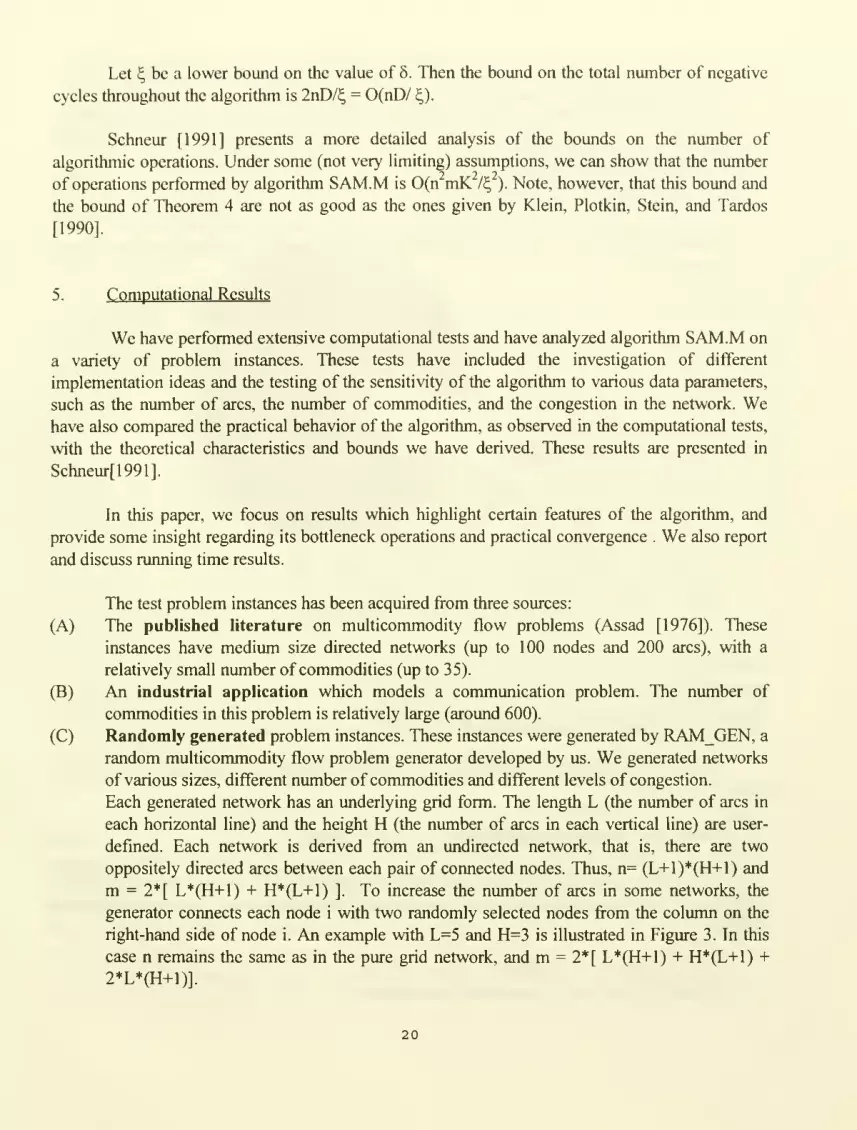
The test problem instances has been acquired from three sources:

(A) The published literature on multicommodity flow problems (Assad [1976]). These

instances have medium size directed networks (up to 100 nodes and 200 arcs), with a

relatively small number of commodities (up to 35).

(B) An industrial application which models a communication problem. The number of

commodities in this problem is relatively large (around 600).

(C) Randomly generated problem instances. These instances were generated by RAMGEN, a

random multicommodity flow problem generator developed by us. We generated networks

of various sizes, different number of commodities eind different levels of congestion.

Each generated network has an underlying grid form. The length L (the number of arcs in

each horizontal line) and the height H (the number of arcs in each vertical line) are user-

defmed. Each network is derived from an undirected network, that is, there are two

oppositely directed arcs between each pair of connected nodes. Thus, n= (L+1)*(H+1) and

m = 2*[ L*(H+I) + H*(L+1) ]. To increase the number of arcs in some networks, the

generator connects each node i with two randomly selected nodes from the column on the

right-hand side of node i. An example with L=5 and H=3 is illusfrated in Figure 3. In this

case n remains the same as in the pure grid network, and m = 2*[ L*(H+1) + H*(L+1) +

2*L*(H+1)].

20

The cost on each arc is randomly chosen from a uniform distribution between 0.0 and a

user-defined parameter Cn,ax.

The user sets the number of commodities, denoted as K. Then, the generator randomly

selects K source-sink pairs. The source and smk nodes can be unrestricted, or else limited

only to the boundary nodes of the grid.

The demand for each commodity is randomly chosen from a uniform distribution between

0.0 and a user-defined parameter Bn,^^-

The capacity on each arc is randomly selected from a uniform distribution between bounds

which depend on the size of the network, the number of commodities and the demand

values.

Figure 3: A network generated by RAM_GEN

A detailed description of the problem instances from all three sources is given in

Schneur[1991].

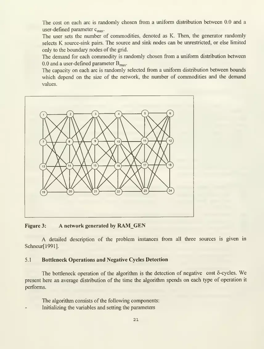
5.1 Bottleneck Operations and Negative Cycles Detection

The bottleneck operation of the algorithm is the detection of negative cost 5-cycles. Wepresent here an average distribution of the time the algorithm spends on each type of operation it

performs.

The algorithm consists of the following components:

Initializing the variables and setting the parameters

21

Calculating the costs of the residual arcs at the beginning of each phase

Searching for a negative cost cycle until one is detected (successful iterations)

Searching for a negative cost cycle and concluding that no such cycle exists (an

unsuccessful iteration which occurs once at the end of each phase)

Modifying the flow, the excess and cost of each arc at each iteration, when 5 units are sent

around a negative cost cycle.

^^^^^^^^H

these cycles may become negative, and if so are used in subsequent iterations. As long as there is a

negative cycle in C we do not search for another negative cost cycle. The collection C uses a data

structure that enables a fast update of the cycles' cost. Storing these cycles and updating their cost

is time consuming, but the saving in overall cycles detection time more than compensates for this

computational expense. In fact, in our computational testing about 50% of all negative cycles used

for shifting flow^ were fi^om the collection C, while managing the collection added only about 3% to

the running time cycles. Moreover, we limit our search only to "sufficiently negative" cycles in

order to eliminate the detection of negative cost cycles with very small absolute cost, and improve

the theoretical convergence of the algorithm (as shown in Section 4). Since a cycle corresponds to a

particular commodity, we need to choose a commodity at each iteration. The order in which

commodities are considered does not influence the theoretical worst case performance of the

algorithm. It does affect, however, the performance of the algorithm in practice. Empirical results

show that scanning the commodities in a cyclic order and detecting one cycle for each commodity

provides a faster convergence than searching for all negative cycles for one commodity and then

moving to the next one (Schneur [1991]).

5.2 Practical convergence

In any approximation algorithm, there are various ways of evaluating the quality of the

solution. In general, one would want an algorithm based on a scaling and penalty function method

to have the following properties:

(1) As the penalty parameter increases and the scaling parameter decreases, the flow cost

^ ^(cj Xy) associated with the algorithm's solution converges to the cost of the optimal

solution to the original problem.

(2) As the penalty parameter increases and the scaling parameter decreases, the penalty cost

(excess cost) converges to zero, and thus the total cost (flow cost + excess cost) converges

to the cost of the optimal solution to the original problem.

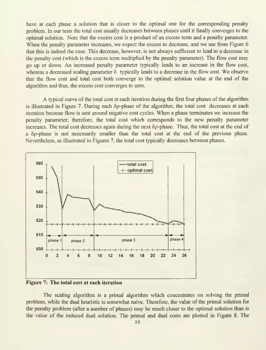
(3) As the penalty parameter increases, the value of the maximum excess (max^ij^ eij(x))

converges to zero.

In our computational testing, we found the above properties to be typical to the behavior of

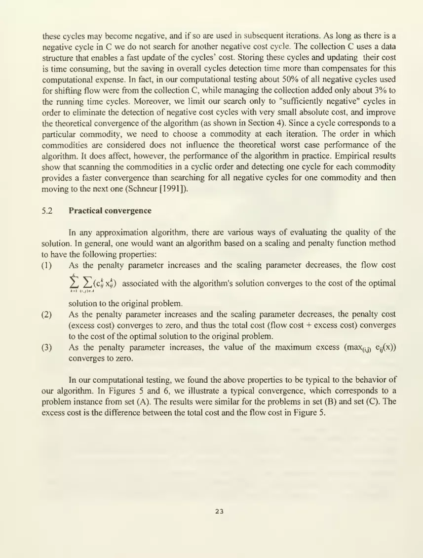
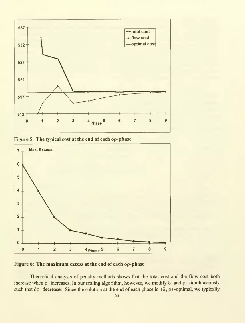
our algorithm. In Figures 5 and 6, we illustrate a typical convergence, which corresponds to a

problem instance from set (A). The results were similar for the problems in set (B) and set (C). The

excess cost is the difference between the total cost and the flow cost in Figure 5.

23

537 T

532

527

522

517

512

total cost

-flow cost

-optimal cost

4 5Phase

Figure 5: The typical cost at the end of each 5p-phase

7 ,

have at each phase a solution that is closer to the optimal one for the corresponding penalty

problem. In our tests the total cost usually decreases between phases until it finally converges to the

optimal solution. Note that the excess cost is a product of an excess term and a penalty parameter.

When the penalty parameter increases, we expect the excess to decrease, and we see from Figure 6

that this is indeed the case. This decrease, however, is not always sufficient to lead to a decrease in

the penalty cost (which is the excess term multiplied by the penalty parameter). The flow cost may

go up or down. An increased penalty parameter typically leads to an increase in the flow cost,

whereas a decreased scaling parameter 5 typically leads to a decrease in the flow cost. We observe

that the flow cost and total cost both converge to the optimal solution value at the end of the

algorithm and thus, the excess cost converges to zero.

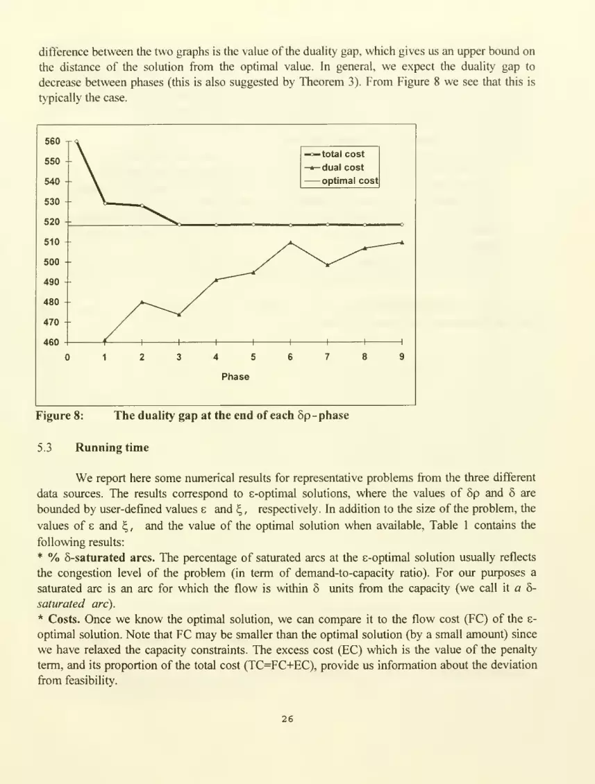
A typical curve of the total cost at each iteration during the fu-st four phases of the algorithm

is illustrated in Figure 7. During each 5p-phase of the algorithm, the total cost decreases at each

iteration because flow is sent around negative cost cycles. When a phase terminates we increase the

penalty parameter; therefore, the total cost which corresponds to the new penalty parameter

increases. The total cost decreases again during the next 6p-phase. Thus, the total cost at the end of

a 5p-phase is not necessarily smaller than the total cost at the end of the previous phase.

Nevertheless, as illustrated in Figures 7, the total cost typically decreases between phases.

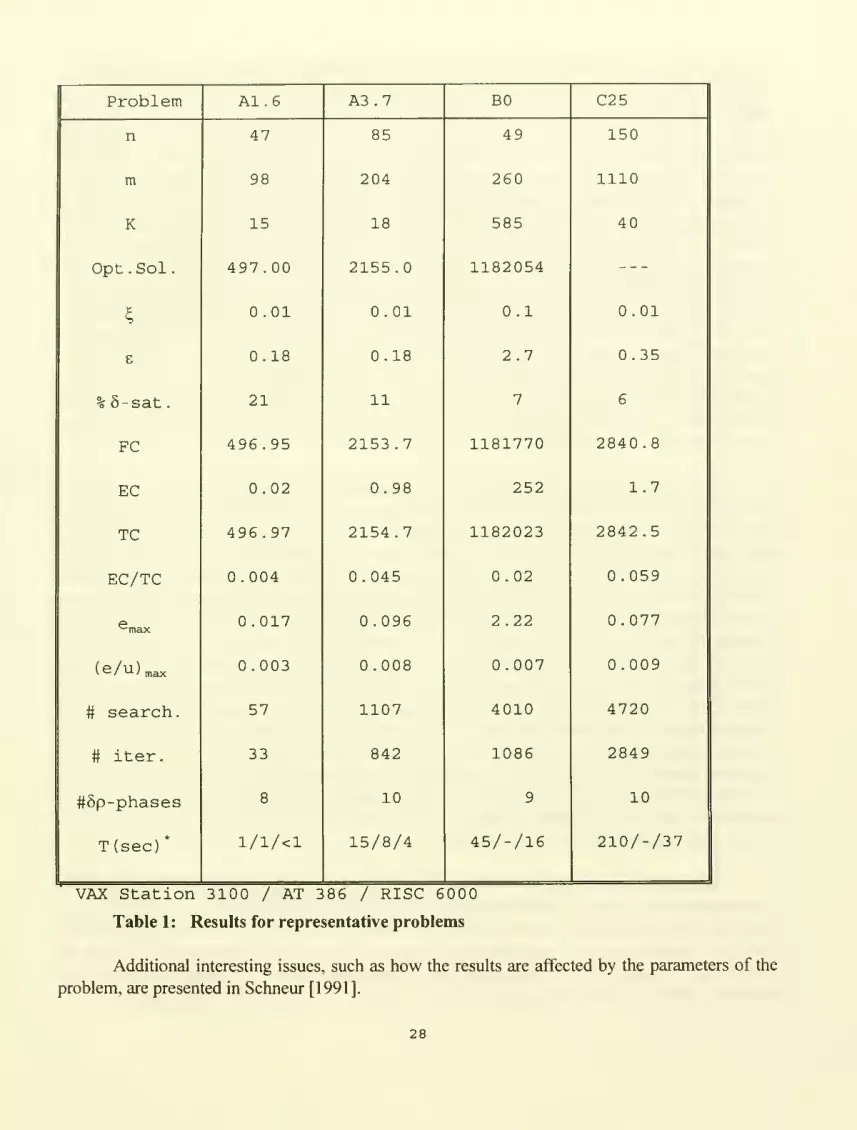
difference between the two graphs is the value of the duality gap, which gives us an upper bound on

the distance of the solution from the optimal value. In general, we expect the duality gap to

decrease between phases (this is also suggested by Theorem 3). From Figure 8 we see that this is

typically the case.

—>- total cost

-*-dual cost

optimal cost

Figure 8: The duality gap at the end of each 5p - phase

5.3 Running time

We report here some numerical results for representative problems from the three different

data sources. The results correspond to s-optimal solutions, where the values of 6p and 6 are

bounded by user-defined values 8 and t,, respectively. In addition to the size of the problem, the

values of e and £, , and the value of the optimal solution when available, Table 1 contains the

following results:

* % 6-saturated arcs. The percentage of saturated arcs at the 8-optimal solution usually reflects

the congestion level of the problem (in term of demand-to-capacity ratio). For our purposes a

saturated arc is an arc for which the flow is within 5 units from the capacity (we call it a 6-

saturated arc).

* Costs. Once we know the optimal solution, we can compare it to the flow cost (FC) of the s-

optimal solution. Note that FC may be smaller than the optimal solution (by a small amount) since

we have relaxed the capacity constraints. The excess cost (EC) which is the value of the penalty

term, and its proportion of the total cost (TC=FC+EC), provide us information about the deviation

from feasibility.

26

* Maximum excess. The maximum value of the excess (e^ax) and the maximum excess-to-capacity

ratio ((e/u)n,ax) represent the maximum violation of the capacity constraints.

* # of searches. The number of times we search for a negative cost cycle is highly correlated to the

number of operations required to find the reported solution. This is because the search for negative

cycles is the primary time-consuming operation in the algorithm (Figure 8).

* # of iterations. This is the number of flow shifts around negative cost cycles.

* # of phases. The number of 6p-phases performed.

* Running time. The computational testing was performed in three environments:

1. A UNIX-based VAX Station 3100, model 30. The algorithm was coded using the 'C

compiler of the Athena project at the Massachusetts Institute of Technology. Running times

were measured by the 'time( )' function of the utilities library 'sys/times.h'.

2. A DOS-based PC IBM compatible, AT 386/ 33 Mhz. The algorithm was coded using

Borland's 'Turbo C Running times were measured by the 'timeQ' function in the utility

library 'time.h'.

3. An IBM RISC 6000, model 530. The algorithm was coded in 'C. Running times were

measured by the 'time( )' ftmction in the utility library 'time.h'.

Due to memory (RAM) limitations, we could not test the problems from data set B and

some problems in data set C on the AT 386.

27

Problem

In order to evaluate the performance of the algorithm in terms of running time, we

compared it to other algorithms for the same set of problem instances. To the best of our

knowledge, there is no single set of problem instances which has been widely used for testing other

multicommodity flow algorithms. A quite popular (and available) set of problems was that used

initially by Assad (our set A). The algorithms for multicommodity flow problems with the

theoretical performance are based on more general algorithms for linear programming. Among the

"classical" decomposition and partitioning algorithms, Assad found price-directive decomposition

(Dantzig-Wolfe) to have the best performance in practice, at least for his data set (Assad [1976]). Aprimal-dual network algorithm [PDN] for large-scale multicommodity flow problems has been

developed by Bamhart [1988] and has been tested using Assad's test problems. A primal

partitioning algorithm based on price directive decomposition [PPLP] (Farvolden and Powell

[1991] and Farvolden, Powell and Lustig [1993]), aiming to solve large-scale problems in the Less-

than Truck-Load industry, has been tested on Assad's problems as well. This algorithm has also

outperformed general purpose LP algorithms (MINOS and OBI). We compare our algorithm (as

restricted to Assad's problem instances) with the corresponding results for PDN, PPLP, and a

Dantzig-Wolfe (DW) implementation by Bamhart[1988]. These comparisons provide some sense

for the relative computational performance of the algorithm. They are, however, limited in scope

and do not provide a complete picture.

The algorithms DW and PDN have been programmed in VAX FORTRAN 4.5 and have

been tested on a VAX Station II. PPLP has been programmed in FORTRAN 77 and tested on a

Micro VAX Israel (Farvolden and Powell [1991]). The VAX was the common computational

environment used by all algorithms. We need, however, to interpret our results based on the

performance of the different VAX computational environments. According to performance

comparison tables provided by Digital, the CPU performance of the VAX Station 3100 is 2.8 times

higher than the CPU performance of the Micro VAX II, and the performance of the VAX Station II

is at least as high as the one for the Micro VAX II. Therefore, the results for algorithm SAM.M on

the VAX Station 3100 in Table 2 and Figure 9 are multiplied by 2.8. In addition, we provide the

running time of algorithm SAM.M on the PC AT 386/33 Mhz. A special implementation of the

algorithm on the PC AT 386 has led to further improvement in the running time of the algorithm.

The only means of comparison between the PC or RISC 6000 and the other computers are MIPS

(Million Instructions Per Second), which is the most common means of comparison in the

computer industry. The PC AT 386/33 Mhz has about the same value of MIPS as the Micro VAXII (around 5 MIPS), and the RISC is about 7 times faster (34.5 MIPS). We feel, however, that the

comparison with the VAX Station 3100 is a more accurate one, and therefore the other results in

Table 2 are reported only for future comparisons.

This running time evaluation is approximate, and it is used only to provide a sense of the

performance of our scaling algorithm relative to other recent algorithms and more traditional ones.

There may be other factors which influence the running time, such as the amount of available

RAM, the compiler and the programming language. In general, FORTRAN compilers may be

better than 'C compilers, but we do not have information about the specific compilers. The

compiler optimizer has not been used for SAM.M, DW or PDN but may have been used for PPLP.

29

In addition, the other algorithms have found an optimal solution in the cases reported here, while

the solutions found by algorithm SAM.M violate the capacity constraints by up to 0.2%- 1.0%.

While such violations may be acceptable in most applications, it may give our algorithm an unfair

advantage.

The running time for the different algorithms are reported in Table 2 and illustrated in

Figure 9a,b. All the problems in set Al have 47 nodes and 98 arcs, and all the problems in set A3

have 85 nodes and 204 arcs. The total running time for all the problems is 83 seconds for algorithm

DW, 85 seconds for algorithm PDN, 42 seconds for algorithm PPLP, 39 for the VAXimplementation of algorithm SAM.M (after it is multiplied by 2.8), and 10 seconds for the PC

implementation of algorithm SAM.M. The running time on the RISC 6000 was less than 1 second

for all the instances.

p

10

9

8

7

6

T 5

4

3

2

1

SAM.M-PC

dsam.m-vaxHpplpDpdndw

A1.1 A1.2 A1.3 A1.4 A1.5 A1.6

Figure 9(a): Comparison of running time for set Al

35

30

251-

20

15

10

5|-

/ 71 SAM.M-PC

dsam.m-vaxHpplpDpdndw

A3.2 A3.5 A3.6

Figure 9(b): Comparison of running time for set A3

31

6. Extensions and Summary

We have presented in this paper a simple and yet robust algorithm for multicommodity flow

problems. The algorithm consists of solving a sequence of penalty problems by repeatedly sending

flow around negative cost cycles. Two parameter control the solution process: the penalty

parameter p which specifies the cost of a unit penalty function for violating the capacity constraints,

and the scaling parameter S which govern the amount of flow sent around cycles. These parameters

also control the maximum deviation fi-om optimality at the end of each phase of the algorithm.

We have analyzed our algorithm from both theoretical and practical perspectives. The

computational results seem not only to support the theoretical properties we have derived, but also

to demonstrate that our algorithm has merit for solving multicommodity flow problems of various

types and sizes.

This paper focus on the scaling algorithm for minimum cost multicommodity flow

problems. The general scheme, however, can be used to solve other types of multicommodity flow

problems as well as network flow problem with side constraints of which the multicommodity

problem is a special case. For example, the feasibility multicommodityflow problem is similar to

the minimum cost multicommodity problem, except that all the unit flow costs are zero. As a result

the penalty terms are the only components of the objective fiinctions and the penalty parameter has

no influence on the solution of the penalty problem and can be arbitrarily set to 1 . Thus, only one

penalty problem needs to be solved with a decreasing scaling parameter. The feasibility scaling

algorithm may also be used as a subroutine in an algorithm which solves the maximum concurrent

flow problem. This problem is a special case of multicommodity flow problems in which we need

to send commodities along a capacitated network. In order to be "fair" to all commodities, the same

ratio of each commodity's demand should be sent, and the objective is to maximize this ratio

(Shahrokhi and Matula [1990]). Observe that for each fixed ratio in the maximum concurrent flow

problem we can solve a feasibility problem to determine if this ratio is feasible. Thus, we can apply

a binary search to determine the maximum feasible ratio, where a feasibility problem is solved at

each iteration by algorithm. A detailed description and analysis of all these algorithms may be

found in Schneur[1991].

Acknowledgment

Many thanks to Cham Aggarwal and Hitendra Wadhwa for all their usefial comments, and to

Prof Cindy Bamhart for providing us with data sets. Part of this work has been done under

contract #ONR:N000 14-94- 1-0099.

32

References

Ahuja, R.K., A.V. Goldberg, J.B. Orlin, and R.E. Tarjan. 1992. Finding Minimum-Cost Flows by

Double Scaling. Math. Programming 53, 243-266.

Ahuja, R.K., T.L. Magnanti, and J.B. Orlin. 1993. Network Flows - Theory, Algorithms, and

Applications. Prentice-Hall, Inc., Englewood Cliffs, NJ.

Ahuja, R.K., J.B. Orlin, and R.E. Tarjan. 1989. Improved Time Bounds for the Maximum Flow

Problem. SIAMJ. on Computing 18, 939-954.

Ali, I., D. Bamett, K. Farhangian, J. Kennington, B. Patty, B. Shetty, B. McCarl, and P. Wong.

1984. Multicommodity Network Problems: Applications and Computations. HE Trans. 16, 127-

134.

Ali, A., R. Helgason, J. Kennington, and H. Lall. 1980. Computational Comparison Among Three

Multicommodity Network Flow Algorithms. Opns. Res. 28, 995-1000.

Assad, A.A. 1976. Multicommodity Network Flows - Computational Experience. Working Paper

OR-058-76, Operations Res. Center, M.I.T., Cambridge, MA.

Assad, A.A. 1978. Multicommodity Network Flows - a Survey. Networks 8, 37-91.

Avriel, M. 1976. Nonlinear Programming: Analysis and Methods. Prentice-Hall, Inc., Englewood

Cliffs, NJ.

Bamhart, C. 1988. A Network-Based Primal-Dual Solution Methodology for the Multicommodity

network Flow Problem. PhD Thesis, Department of Civil Engineering, Massachusetts Institute of

Technology, Cambridge, MA.

Bamhart, C. 1993. Dual-Ascent Methods for Large-Scale Multicommodity Flow Problems. Naval

Res. Log Quart. 40, 305-324.

Bamhart, C, and Y. Sheffi. 1993. A Network-Based Primal-Dual Heuristic for the Solution of

Multicommodity Network Flow Problems. Trans. Sci. 27(2), 102-1 17.

Bertsimas, D., and J.B. Orlin. 1991. A Technique for Speeding Up the Solution of the Lagrangean

Dual. Working Paper No. 3278-91, Sloan School of Management, Massachusetts Institute of

Technology, Cambridge, MA.

33

Choi, I.e., and D. Goldfarb. 1989. Solving Multicommodity Network Flow Problems by an

Interior Point Method. In Proc. ofthe SLAM Workshop on Large-Scale Numerical Optimization, T.

Coleman and Q. Li (eds.)

Dinic. E.A. 1973. The Method of Scaling and Transportation Problems. Issledovaniya po

Diskretnoi Matematike, Science, Moscow (Russian).

Edmonds, J., and R.M. Karp. 1972. Theoretical Improvements in Algorithmic Efficiency for

Network Flow Problems. J. oftheACM 19, 248-264.

Fiacco, A.V. and G.P. McCormick. 1968. Nonlinear Programming: Sequential Unconstrained

Minimization Techniques. John-Wiley & Sons, New-York.

Farvolden, J.M., and W.B. Powell. 1990. A Primal Partitioning Solution for Multicommodity

Network Flow Problems. Working Paper #90-04, Department of Industrial Engineering, University

of Toronto, Toronto, Canada.

Farvolden, J.M., W.B. Powell, and I.J. Lustig. 1993. A Primal Partitioning Solution for the Arc-

Chain Formulation of a Multicommodity Network Flow Problem. Opns. Res. 41(4), 669-693.

Ford, L.R., and D.R. Fulkerson. 1962. Flows in Networks. Princeton University Press, Princeton,

NJ.

Frank, M., and P. Wolfe. 1956. An Algorithm for Quadratic Programming. Naval Res. Log. Quart.

3,95-110.

Gabow, H. 1985. Scaling Algorithms for Network Problems. J. ofComput. Sys. Sci. 31, 148-168.

Goldberg, A.V., and R.E. Tarjan. 1987. Solving Minimum Cost Flow Problems by Successive

Approximation. Proc. ofthe 1 9th ACM Symp. on the Theory ofComp., 7-18.

Grigoriadis, M.D., and L.G. Khachiyan. 1991. Fast Approximation Schemes for Convex Programs

with Many Blocks and Coupling Constraints. Technical Report DCS-TR-273, Department of

Computer Science, Rutgers Univ., New Brunswick, NJ.

Kennington, J.L. 1978. A Survey of Line£ir Cost Multicommodity Network Flows. Opns. Res. 26,

209-236.

Klein, P., A. Agrawal, R. Ravi, and S. Rao. 1990. Approximation Through Multicommodity Flow.

In Proc. ofthe 31st Annual Symp. on Foundations ofComputer Science, 726-727.

Klein, P., S.A. Plotkin, C. Stein, and E. Tardos. 1990. Fast Approximation Algorithms for the Unit

Capacity Concurrent Flow Problem with Application to Routing and Finding Sparse Cuts. In Proc.

34

of the 22nd Annual ACM Symp. on Theory of Computing, 310-321 Also Technical Report 961,

School of Operations Research and Industrial Engineering, Cornell Univ., NY, 1991.

Leighton, T., F. Makedon, S. Plotkin, C. Stein, E. Tardos, and S. Tragoudas. 1991. Fast

Approximation Algorithms for Multicommodity Flow Problems. In Proc. ofthe 23rd AnnualACMSymp. on Theory ofComputing, 101-111.

Luenberger, D.G. 1984. Linear and Nonlinear Programming. Addison-Wesley, reading, MA.

Orlin, J.B. 1988. A Faster Strongly Polynomial Minimum Cost Flow Algorithm. Proc. of the 20th

ACM Symp. on the Theory ofComp., 377-387.

Pinar, M.C., and S.A. Zenios. 1990. Parallel Decomposition of Multicommodity Network Flows

Using Smooth Penalty Functions. Report 90-12-06, Decision Sciences Department, The Wharton

School, Univ. of Pennsylvania, Philadelphia, PA.

Plotkin, S., D.B. Shmoys, and E. Tardos. 1991. Fast Approximation Algorithms for Packing and

Covering Problems. In Proc. ofthe 32ndAnnual Symp. on Foundations ofComputer Science.

Rockafellar, R.T. 1984. Network Flows and Monotropic Optimization. John Wiley an Sons, NewYork, 420-425.

Schneur, R. 1991. Scaling Algorithms for Multicommodity Flow Problems and Network Flow

Problems with Side Constraints. PhD Thesis, MIT, Cambridge, MA.

Shahrokhi F., and D.W. Matula. 1990. The Maximum Concurrent Flow Problem. J. oftheACM 37,

318-334.

Sheffi, Y. 1976. Urban Transportation Networks: Equilibrium Analysis with Mathematical

Programming Methods. Prentice-Hall Inc., New-Jersey.

Vaidya, P.M. 1989. Speeding Up Linear Programming Using Fast Matrix Multiplication. In Proc.

Ofthe 30th Annual Symp. On Foundations ofComputer Sci., 332-337.

35

> -

D J D i 'D

Date Due

MIT LIBBABIES ,., ,1.1 M uinll II

3 9080 00922 4467