superlinear convergence of the affine scaling algorithm
TRANSCRIPT

Mathematical Programming 75 (1996) 77-110
Superlinear convergence of the affine scaling algorithm
T. Tsuchiya a,*, R.D.C. Montei ro b'l a The Institute of Statistical Mathematics, 4-6-7 Minami-Azabu, Minato-Ku, Tokyo 106, Japan
b School of h~dustriaI and Systems Engineering, Georgia h~stitute of Technology, Atlanta, GA 30332, USA
Received 4 March 1993; revised manuscript received 27 February 1996
Abstract
In this paper we show that a variant of the long-step affine scaling algorithm (with variable stepsizes) is two-step superlinearly convergent when applied to general linear programming (LP) problems. Superlinear convergence of the sequence of dual estimates is also established. For homogeneous LP problems having the origin as the unique optimal solution, we also show that 2 is a sharp upper bound on the (fixed) stepsize that provably guarantees that the sequence of primal iterates converge to the optimal solution along a unique direction of approach. Since the point to which the sequence of dual estimates converge depend on the direction of approach of the sequence of primal iterates, this result gives a plausible (but not accurate) theoretical explanation for why ~ is a sharp upper bound on the (fixed) stepsize that guarantees the convergence of the dual estimates.
Keywords: Interior point algorithms: Affine scaling algorithm; Linear programming; Superlinear convergence; Global convergence
1. Introduct ion
The affine scaling ( A S ) a lgor i thm, introduced by Dikin [6] in 1967, is one o f the
s implest and most efficient interior point a lgor i thms for solving linear p rog ramming
* Corresponding author. E-mail: [email protected]. The work of this author was based on research supported by the Overseas Research Scholars of the Ministry of Education, Science and Culture of Japan, 1992.
I The work of this author was based on research supported by the National Science Foundation (NSF) under grant DDM-9109404 and the Office of Naval Research (ONR) under grant N00014-93-1-0234. This work was done while the second author was a faculty member of the Systems and Industrial Engineering Department at the University of Arizona.
0025-5610 Copyright (E) 1996 The Mathematical Programming Society, Inc. Published by Elsevier Science B.V. Pll S0025-56 10(96)00025-1

78 Z Z~uchiya, R.D.C. Monteiro/Mathematical Programming 75 (1996) 77-110
(LP) problems. Because of its theoretical and practical importance, there are a number of papers which study its global and local convergence [4,6-8,12,16,25,26,28-31 ] as well as its continuous trajectories [3,16,32]. For computational experiments and imple- mentation issues related to the AS algorithm, we refer the reader to [ 1,2,5,18,21,22].
Recently, Dikin [8] and Tsuchiya and Muramatsu [29] proved global convergence of the long-step version of the AS algorithm [31] for degenerate LP problems. This long- step version is the one in which the next iterate is determined by taking a fixed fi'action A ~ (0, I) of the whole step to the boundary of the feasible region. Assuming that A = �89 Dikin [8] showed the sequence of primal iterates converges to a point lying in
the relative interior of the optimal face and that the sequence of dual estimates converges
to the analytic center of the dual optimal face. Independently, Tsuchiya and Muramatsu [29] obtained an analogous result under the less restrictive condition that A ~< 3" They also demonstrated that the asymptotic reduction rate of the objective function value is
exactly 1 - A, under the same assumption that A ~< 3" A simplified and self-contained proof of these results can be found in the recent survey by Monteiro, Tsuchiya and
Wang [ 19]. In this paper we focus our attention on the asymptotic convergence properties of the
long-step AS algorithm with variable stepsizes &. Specifically, we develop a variant which is two-step superlinearly convergent by properly choosing the sequence of step- sizes {Ak}. The algorithm is based on a centrality measure in the space of the "small" variables. When this measure is small, we show that, asymptotically, it is possible to take stepsizes sufficiently close to 1 to force the reduction rate of the objective function value as close to 0 as desired without loosing too much centrality. At the next step, if
1 necessary, we select the stepsize At = 5 to recover the centrality of the iterate. This paper is organized as follows. In Section 2, we introduce basic assumptions,
terminology and notation. The long-step AS algorithm and some of its basic properties
are also reviewed. The main content of the paper is given in Sections 3, 4 and 5. The main result obtained
in Section 3 is somewhat independent of (though related to) the results of Sections 4 and 5. It deals with the case of the AS algorithm applied to a homogeneous LP problem with the origin as the unique optimal solution. In this case, we show that, when the sequence of stepsizes {At} satisfies lira infk~ ~ At > 3' the direction of approach of the primal iterates towards the (unique) optimal solution always oscillates. This result contrasts with the case where At = A ~< ~ for all k ~> 0, for which it is shown that the direction of approach is unique. Since the point to which the sequence of dual estimates converges depends on the direction of approach of the sequence of primal iterates, this
2 is a sharp result gives a plausible (but not accurate) theoretical explanation for why _g upper bound on the (fixed) stepsize A that provably guarantees the convergence of the dual estimates. Specific examples illustrating that 3 is indeed sharp in the above sense were given by Tsuchiya and Muramatsu [29] and Hall and Vanderbei [ 13].
The above result is obtained by observing that the sequence of points obtained by conically projecting the sequence of the AS iterates for the homogeneous problem onto a constant-cost hyperplane (that is, a hyperplane where the objective function is constant)

T. Tsuchiya, R.D.C. Monteiro/Mathematical Programming 75 (1996) 77-110 79
is exactly the sequence obtained by applying Newton's method (with variable stepsizes)
to the optimization problem defining the analytic center of the polyhedron determined
by the intersection of the constant-cost hyperplane with the feasible (conical) region
of the homogeneous problem. In conjunction with this, we also show that the projected I for all k > / 0 . sequence converges quadratically to the analytic center when 2tk = ,~ =
This result suggests that the AS iteration with/~k = �89 can be used as a kind of centering
step to keep the iterate "well-centered". In Section 4, we show that the relation established in Section 3 between the AS
algorithm for the homogeneous problem and Newton's method for the analytic center
problem can be used to analyze the sequence of AS iterates for general LP problems.
Close to a constant-cost face, it is possible to approximate the original problem by
a homogeneous problem in the sense that the AS directions at a point x for the two
problems asymptotically approach each other as x approaches the face. Hence, near
a constant-cost face, the iterates generated by the AS algorithm applied to a general
problem behave very much like the ones generated by the AS algorithm applied to a
homogeneous problem. The analysis of Section 4 forms the basis for the development
of the superlinear AS algorithm presented in Section 5. We show in Section 5 that the new variant of the AS algorithm, whose sequence of
stepsizes asymptotically alternate between ,~ = �89 and ,Ik ~ 1, is two-step superlinearly
convergent with Q-order 1 + p with respect to the sequence of objective function values,
where p is any a priori chosen constant in the interval (0, �89 Superlinear convergence
of the sequences of primal iterates and dual estimates to a point in the relative interior
of the optimal face and to the analytic center of the dual optimal face, respectively, with
R-order 1 + p is also shown. Finally, we give some remarks in Section 6.
The following notation is used throughout our paper. We denote the vector of all ones
by e. Its dimension is always clear from the context. The symbols R n, R~ and R~_+
denote the n-dimensional Euclidean space, the nonnegative orthant of N" and the positive
orthant of IR n, respectively. The set of all m x n matrices with real entries is denoted
by R ' ' x ' . I f J is a finite index set then ]J[ denotes its cardinality, that is the number
of elements of J. For J C_ {l . . . . . n} and w E R ", we let wj denote the subvector
[Wi]ieJ; moreover, if E is an m x n matrix then Ej denotes the m x ]J] submatrix of E corresponding to J. For a vector w E R", we let max(w) denote the largest
component of w, diag(w) denote the diagonal matrix whose i-th diagonal element is wi for i = l . . . . . n and w -1 denote the vector [ d i a g ( w ) ] - l e whenever it is well-defined.
The Euclidean norm, the l-norm and the c~-norm are denoted by I1" 11, II' I1~ and I1' I1~, respectively. The superscript T denotes transpose.
To avoid introducing several constants throughout the paper, we use the following
notation. Given functions gl (x) and g2(x) which are defined for points on a set E,
we say that g l ( x ) = O ( g 2 ( x ) ) for every x E E if there exists some constant M such
that ]]g~(x)ll ~< Mllg2(x)l[ for every x E E. When the conditions g l (x ) = (.Q(g2(x))
for every x E E and g2(x) = O ( g l ( x ) ) for every x E E hold then we simply write
gl (x) ~ g2(x) for every x E E.

80 Z Tsuchiya, R.D.C. Monteiro/Mathematical Programming 75 (1996) 77-110
2. Affine sealing algorithm
In this section, we state the main terminology and assumptions used throughout our paper and describe the AS algorithm. We also review some basic properties of the AS algorithm that are needed in the subsequent sections.
Consider the following LP problem
minimizex c'r.r ( l )
subject to A x = b, x ) O,
and its associated dual problem
maximize(~. ,~ bTy (2)
subject to A-r y + s = c, s >l O,
where A E R m• c, x , s E R" and b, y E R m. We next introduce some notation and definitions which will be used throughout
our paper. Given a point x E IR", let B (x ) - {i : x~ ~ 0} and N ( x ) - {i : xi = 0}. Clearly, ( N ( x ) , B ( x ) ) determines a partition of { l . . . . . n}. Associated with any specific
partition ( N , B ) of {1 . . . . . n}, we let
790 = {x E R" : A x = b, XN = 0},
79~ - {x E 79N :x8 /> 0},
79~+ - {x E 79N x B > 0},
738 = { ( y , s ) E IR" x I R " : A T y + s = c , s8 = 0 } ,
73~ ~ { ( y , S ) ~ 73B : SN ~ 0},
73~+ - { ( y , s ) E 738 : sN > o}.
(3)
(4)
(5)
(6)
(7)
(8)
When N = 0, we denote the sets PN, 79~ and 79~+ by 7 9, 79+ and P++, respectively. The sets 79+ and 79++ are the sets of feasible solutions and strictly feasible solutions
of problem (1) . Similarly, when B = 0, we denote the sets De, D~ and D~ + by D, 73 + and 73 ++, respectively. 73+ and 73++ are the sets of feasible solutions and strictly
feasible solutions of problem (2). A constant-cost f ace of an LP problem is a nonempty face of the feasible polyhedron
over which the objective function is constant. Every nonempty face 5 t- of 79+ is uniquely determined by a partition ( N , B ) in the sense that 79~ = 5 r" and 79++ 5 / 0. Every partition (N, B) which is uniquely associated with a constant-cost face of (1) is called
a constant-cost partition. If ( N , B ) is a constant-cost partition then the constant value of the objective function cVx over 7'~ is denoted by VN. The partition associated with
the optimal face of ( 1 ) is referred to as the optimal partition.
The following result can be easily shown.

T Tsuchiya, R.D.C. Monteiro/Mathematical Programming 75 (1996) 77-110 81
Lemma 2.1. The following statements hold:
(a) ( N, B) is a constant-cost partition if and only if 7)~ + ~/ 0 and 738 4 0; (b) i f ( N, B) is a constant-cost partition then cTx -- VN = yTNxN for any x E 7 ~ and
(y,g) ~ DB.
We impose the following assumptions throughout this paper.
Assumption 1. Rank(A) = m.
Assumption 2. The objective function cTx is not constant over the feasible region of
problem ( 1 ).
Assumption 3. Problem ( l ) has an interior feasible solution, that is 7 :'++ 4= 0,
Assumption 4. Problem ( 1 ) has an optimal solution.
We now introduce important functions which are used in the description and analysis of the AS algorithm. For every x C R'.~.+, let
y ( x ) = ( A X 2 A T ) - I AX2c,
s ( x ) =- c - A T y ( x ) ,
d ( x ) = X2s(x ) = X[ I - X A T ( A X 2 A T ) - I AX]Xc,
(9a)
(9b)
(9c)
where X ~ diag(x). Note that Assumption 1 implies that the inverse of AX2A T exists for every x > 0. The quantities ( y ( x ) , s ( x ) ) and d ( x ) are the dual estimate and the AS
direction associated with the point x, respectively. For the purpose of future reference, we note that (9c) implies
X - l d ( x ) = X s ( x ) . (10)
Lemma 2.2. The following statements hold:
(a) for any (y, ~) E 73, d ( x ) is the (unique) optimal solution of
maximized gTd-- �89 2
subject to Ad = O; (11)
(b) tf (N, B) is a constant-cost partition then there exists a constant Co > 0 such
that
f lX~'ds(x)[ I ~ CoI[X~'I[IIXNIIIIXN~dN(X) II VX > O.
Proof. The proof of (a) is straightforward. The proof of (b) is given in Monteiro et al. [19, Lemma 3.6]. []

82 T. Tsuchiya. R.D.C. Monteiro/Mathematical Programming 75 (1996) 77-110
We are ready to describe the AS algorithm. For a good motivation of the method, we refer the reader to Dikin [6], Barnes [4], Vanderbei, Meketon and Freedman [31] and Vanderbei and Lagarias [30].
Algor i thm 1 (Affine Scaling Algorithm) Step O. Assume x ~ E 79 e ~ is available. Set k := 0.
Step 1. Choose At E (0, 1 ), and let
d t = d ( x k ) ,
X t = d iag (x t ) ,
xk+l = .rt _ At dk" m a x ( ( X t ) - ~ d t)
Step 2. k := k + l and return to Step 1.
(12a)
(12b)
(12c)
We note that Assumptions 1-4 imply that, for every x C 79++, the direction d ( x )
must have at least one positive component so that m a x ( X - l d ( x ) ) > 0. Hence, the expression which determines x t+l in the AS algorithm is well-defined. Observe also that if 3.k were equal to 1, the iterate x k+l would lie in the boundary of the feasible
region. Thus, since we choose &- E (0, I ), x k~l is ensured to be a point in 79++. The following basic result whose proof can be found in Vanderbei and Lagarias [30,
p. 118] or in Monteiro et al. [19, Proposition 2.8] will be needed later on.
Proposi t ion 2.3, For any full row rank matrix A E R rex" and any vector c E N ~, the
set { ( y ( x ) , s ( x ) ) : x > 0} is bounded, where ( y ( x ) , s ( x ) ) is defined in (9).
We next summarize the main results that have been proved for the AS algorithm. Proofs of these results can be found in Tsuchiya and Muramatsu [29] and in the survey paper by Monteiro et al. [ 19]. The results below are stated in more general terms than they have been stated originally to accommodate the needs of the current paper. But
their proofs follow along the same lines pursued in the above two references. Let {x k}
denote the sequence of iterates generated by Algorithm 1 and let {(yk, sk)} denote the sequence of dual estimates defined as (y t , s t) = (y ( x t ) , s(.r k) ) for all k ~> 0.
Proposi t ion 2.4. The Jbllowing statements hold: (a) the sequence {x k} converges to some point x* E 79-t-;
(b) there exists M > 0 such that IIx t - x * l l <~ M( cTxt - c T x * ) for all k >~ 0; (c) the sequence { ( y k s t) } is bounded.
I f in addition, we have lira inf t~ ~ At > 0 then: (d) ( N . , B . ) = ( N ( x * ) , B(x* ) ) is a constant-cost partition, or equivalently, the
smallest face containing x*, namely 79~ , is a constant-cost face; ( e) every accumulation point (y*, s*) of { (y t , s t) } is in DB. (hence, X ' s* = 0).

T. Tsuchiya, R.D.C. Monteiro/Mathematical Programming 75 (1996) 77-110 83
The analytic center of the optimal face of problem (2) is the (unique) point defined as
(ya,~,) =argmax{ ~ logsj: (y,s)CD-~}, j E Nopt
(13)
where (Nopt, Bopt) denotes the optimal partition of (1).
Proposition 2.5. I f the sequence {Ak} satisfies Ak ~ ~ for all k >>. 0 and lira inf'k~ ~ ak > O, then the following statements hold:
(a) {x ~} converges to a point x* lying in the relative interior of the optimal face of. ( 1 ) (hence, ( N . , B. ) =- ( N(x* ), B (x*) ) is the optimal partition of ( 1 ) ) ;
(b) {(yk,s~)} converges to (33a,ga); (C) l im~_~ ~ k T k XN. SN./(C X -- cTx *) = e/IN.I; (d) for any (~, g) C DB., we have
k ~ c T x k - - c T x * JN.I -argmax logxj : gTN. XN. = I , XN. > 0 . (14) J
Remark. Statement (d) is not explicitly stated in [19] and [29]; however, the first equality in (d) follows immediately from (b) and (c), while the second one follows
by verifying that (~)-~/IN, I satisfies the optimality condition for the optimization problem in (14) (see Lemma 4.7).
3. Asymptotic behavior of the AS algorithm for a homogeneous problem
It was shown in the original version of Tsuchiya and Muramatsu [29] that the sequence of dual estimates { (yk, s k) } converges to the analytic center (.~a, ga) of the dual optimal face whenever ,~k = A C (0, 5) for all k ) 0 (see Proposition 2.5(b)) .
2 Later, Tsuchiya and Muramatsu [29] pointed out that their result holds even for )t~ = ~. Furthermore, they [29] and Hall and Vanderbei [ 13] gave specific examples showing that the bound ~ on the (fixed) stepsize is tight with respect to the property that l i m k - ~ ( y k , s k) = (.9~,g"). In this section, we give a plausible explanation for the tightness of the bound _2
3" 2 Specifically, we show for any homogeneous LP problem that 5 is a sharp upper bound
on the fixed stepsize that provably guarantees that the sequence {x k} converges to the optimal solution along a unique direction of approach. For an arbitrary LP problem and for A ~< 5' the uniqueness of the direction of approach of {x k} follows as a consequence of Proposition 2.5(c) and Lemma 4.9. The main result of this section shows that the direction of approach of {x ~} towards the optimal solution is not unique, whenever the
2 sequence of stepsizes {ak} satisfies l i m i n f ~ ,~k > _~ (e.g., ak = A > 32- for all k ~> 0), the LP problem is homogeneous and 0 is its unique optimal solution.

84 77 Z~uchiya, R.D.C. Monteiro/Mathematical Programming 75 (1996) 77-110
Since the accumulation points of the sequence {(yt , sk)} are determined by the set of directions of approach of {x k} (this fact can be proved by using similar arguments as in Adler and Monteiro [ 3, Theorem 4.1 ] ), the above result gives a plausible theoretical explanation for why ~ is a tight bound on the (fixed) stepsize that guarantees the convergence of {(yk, st)} to the analytic center (35 a, g"). This explanation is not accurate though since existence of two or more directions of approach of {x k} does not imply (but is likely to result in) nonconvergence of the sequence {(yk, st)}.
The main observation used in this section is that the sequence of points {r k} obtained by conically projecting {x k} onto a constant-cost hyperplane (that is, a hyperplane where the objective function is constant) is exactly the sequence obtained by applying Newton's method with a sequence of variable stepsizes {~'k} to the optimization problem defining the analytic center, say r*, of the polyhedron determined by the intersection of the constant-cost hyperplane with the feasible (conical) region of the homogeneous problem. One important consequence of this observation is that the sequence {r k} converges quadratically to r* when .hi = ,~ = �89 for all k /> 0. This result suggests that
1 the AS iteration with At = 2 can be used as a kind of centering step to keep the iterates "well-centered". Another important consequence is that when At = .,l > _-} for all k ~> 0, the corresponding sequence of Newton stepsizes {~'t} satisfies lira infk~or r~. > 2 from which nonconvergence of the sequence {r k} easily follows.
The following homogeneous problem is considered in this section. Given a vector E R p and a subspace H _C RP, the problem is to
minimize {gT2 : 2 E H, ~ >/0}. (15)
Define
H ++ = {2 c H : S: > 0},
H ++ = {2 E H ++ �9 ([.T~ > 0 } , >
H ++ - {.~ ~ H ++ : c'T~ = 1 }.
Throughout this section we assume that H ++ ~ 0, or equivalently, H~ -+ g 0. The AS direction at a point ~ E H ++ is the (unique) solution d(.~) of the problem
maximize {cTd-- �89 " .~ E W } , (16)
where X ~ diag(2). One of our goals in this section is to give the relationship between the direction d(2)
and the Newton direction at the point r = ff/gT2 C H +~ with respect to the following maximization problem:
P
maximize { ~ l o g r i : r C H++}. (17) i=1
Given r E Hi ~+, the Newton direction of (17) at r is the (unique) solution ~7(r) of the problem

T. Tsuchiya, R,D.C. Monteiro/Mathematical PJvgramming 75 (1996) 77-110 85
maximize { ( r - I ) T ( - - r / ) - I T~-2 . 7r/ t~ r/ r / E H, t~T7 "] = 0 } , (18)
where R = diag(r) and the variable ~7 belongs to R p. With this z/(r) , one iteration of the Newton method with a unit stepsize at the point r k is written as r ~+1 = r k - rl(rk).
The proof of the following result is straightforward.
L e m m a 3.1. Assume that H ++ ~ ~. Then, the following statements are equivalent:
(a) ~ = 0 is the unique optimal solution of (15);
(b) Hi ~+ is nonempty and bounded;
(c) problem (17) has a (unique) optimal solution.
The optimal solution of (17), when it exists, is denoted by r*. The following result
plays an important role in several parts of the paper.
L e m m a 3.2. The following statements hold:
(a) the function r ~ ~7(r) is continuous on H~-+;
(b) f o r r E H~ +, rl(r) ~ 0 if and only if r is not the optimal solution of ( 17);
(c) i f the optimal solution r* o f (17) exists then
Ilr - r* - ~ ( r ) I I lim sup < ~ ,
. . . . . . "EHi '+ 11 r -- r*][ 2
11~7(r) ll l imsup - - - 1 . . . . . . . c - i " IIr - r*ll
(19)
( 2 0 )
Proof. The proof of (a) and (b) are straightforward. Relation (19) is a standard
property of Newton methods and it holds whenever some reduced Hessian (see Fletcher
[ 11, p. 260] ) of the objective function of (17) is nonsingular at r*. This last property
follows due to the fact that the (full) Hessian of ~iP=l logri is negative definite at r*.
Relation (20) follows as an immediate consequence of (19). []
L e m m a 3.3. Assume that {r k} C H { + is a sequence detemzined by the recurrence
relation r ~+l = r k --rkrl( rk), where {'rk} is a sequence o f scalars such that lim i n f ~ rk > 2. Then
(i) r k = r* holds f o r all k sufficiently large (this can happen only if r* exists), or
(ii) {r k} can not converge to a point in H ++.
Proof. Assume that (i) does not hold. We will show that (ii) must hold. Indeed, in view of Lemma 3.2(b), we know that if r k~ = r* for some k0 then r k = r* for all
k > k0. Since we are assuming that (i) does not hold, we conclude that r k -7' r* for all
k/> 0. To show that (ii) holds, assume for contradiction that {r k} converges to a point r ~ E H ++. The relation r k+l = r k - rkz/(r k) and the fact that lim inI'k~oo rk > 2 imply
that limk~oo r / ( r k) = 0. By (a) and (b) of Lemma 3.2, we conclude that r ~176 = r*, and hence that l i m k ~ r k = r*. Using the relation r k+l = r k - rkrl(r k) and Lemma 3.2(c),
we obtain

86 T. Tsuchiya. R.D. C Monteiro/Mathematical Programming 75 (1996) 77-110
II ? + ~ - r*ll II - (r~ - 1)r /(r k) + (r ~ - r* - ,(r~))ll lira inf - lira inf k ~ 11 rk - r*ll k - ~ II " k - r*II
>/ l iminf (rk - 1)[[r/(r~) ]1 - I 1 ( ? - r * - , 7 ( ? ) ) II
= liminf(r~ - 1) > 1. k ~ o o
Hence, we conclude that II ra+~ - r*l l > ][r ~ - r*ll for every k sufficiently large, which contradicts the fact that {r k} converges to r*. []
Given a point .~" E H> +, we define
~(27) = R-~d( .~ - ) . FT~. -
r(27) - ~ T ~ - '
where X = diag(.t).
(21)
(22)
Lemma 3.4.
~*d(27) -- II;?- 'd(~)[[2 eT~(~) = 1,
Ii~'-~d(~)ll-< II~ell,
r /(r(~:)) = - - r ( Z ) +
where R(.~) = diag(r(.~)).
The fol lowing relations hold f o r every ~ E H>+:
,7 (~-) "~ d(.~) - R(.~) - e +
IIX'-'d(~) II 2 1 1 ~ 1 2 J '
(23)
(24)
(25)
(26)
Proof. Let ~ C- H~ + be given. Since d(.2) is a solution of (16), we have
6 - X-2d(27) C H • d(27) E H, (27)
where H i denotes the orthogonal complement of H. Multiplying the first relation in
(27) on the left by d(27) T and using the second relation, we obtain (23). Multiplying
the first relation in (27) on the left by 27T and using the fact that 27 C H, we obtain
~vy, = e T ( f ( - l d ( 2 7 ) ) , which is equivalent to (24), due to (21). Using (23) and the
Cauchy-Schwarz inequality, we obtain
I1~-'d(27) I/2 = ( ~ ) T ( ~ - ' d ( m ) ) ~ 112<111~-'d(m)II,
which clearly implies (25). It remains to show (26). To simplify notation, let r - r(~:).
Since ~7(r) is the unique optimal solution of (18), the first equality in relation (26)
follows once we show that - r + d(~) / l lR-Ld(~ . ) ] l 2 satisfies the optimality condition
for (18) , that is, ~7 = - r + d ( . ~ ) / l l R - l d ( x ) f satisfies
- r - I - R - 2 ~ T E H • ~TEH, 8Tr /=0 , (28)

T. Tsuchiya, R.D.C. Monteiro/Mathematical Programming 75 (1996) 77-110 87 where R c = {3.c: A E R} and R = diag(r). Indeed, relations (22) and (27) imply
( = - r - I - R-2 - - r 4- 112_~d(~)112 ) 112_1d(~)112
(sTY) 2,~-2d(2) H_L = E + R c .
l l2 - 'd (y) II 2
Since H is a subspace, 2 E H and ,'](2) ~ H, we conclude that
d(~) .~ d(~) - r + - - - + EH.
112-~d(~)ll 2 aY~ 112-td(~)lle
Using (22) and (23), we obtain
d(.~) _ (gTr , 8Td(.~) "~ 6"T(--F 4- [[,~-ij(.,~)[[2)= - -[[z~._loT(~f)ll2//
=_(, 112-~d(~)ll 2
Hence, the first equality in (26) follows. The second equality in (26) follows from (21) and (22). []
Given a point 2 r H> + and a scalar A E (0, 1 ), let
O(~) = I1,~(~)11: m a x ( ~ ( 2 ) ) '
a ~*(a) = ~ - d(~).
max(2-1d( .~))
(29)
(30)
Lemma 3.5. Let 2 E HE + and a > 0 be such that 2+(h) E H+> +. Then, the following relations hold:
1 1 ~ I1~(~)II ~ 0(~) ~ ~,
a0(~) r (~+(a) ) = r(2)
1 - ag(~)
(31)
(32)
q ( r ( 2 ) ) . (33)
Proof. Let 2 + =.~+(,~). Using (21), (23), (29) and (30), we obtain
~T~q-=?'l" ~._ max(2-1d(2))'~ 07(2) =?Tk 1 - (gV2) max( ,~_ld(2))
=~?T~ 1 max( f i (2 ) ) J
and hence (31) follows. The first and second inequalities in (32) follow from (24) and (29). Since ~ and 2 + are in H ++, relation (31) imply that I - 3 .0 (~ ) > 0, from which

88 Z Tsuchiya, R.D.C Monteiro/Mathematical Programming 75 (1996) 77-110
the third inequality in (32) follows. We next show (33). Using (30), (21) and (29) ,
we obtain
( ) ( ) A )(-laT(.~) = 2 e m a x ( a ( ~ ) ) a ( ~ ) ~ + = ) ( e - m a x ( ~ _ ~ d ( 2 ) )
) II'~(-~) II 2 /
This relation together with (31) yield
~+ ~'[e - (a0(~) / l l~( .~) I[ 2) 5(~)] r ( 2 +) =
FT~-~ = ~T~( 1 - 20(2) )
_ R ( 2 ) [ e - (aO(.~)/ll~(~) 11 =) ~(.~)] I - ~(~)
( ) = r ( ~ ) - A0(.~) R(.~) - e + 1 - a 0 ( . ~ ) II,~(-~) I I Z /
where R ( 2 ) = d i ag ( r (~ ) ) . Combining the last relation with (26), we obtain (33). []
In the remaining part of this section, we let {.~} and {Ak} denote the sequence of iterates and stepsizes for the AS algorithm applied to problem (15) and define ~ _ r(2k) = ff~/sX.~l, for all k ~ 0. When /lk = A C (3 ' 1) for all k >7 0, the following result shows that {~:k} can not converge to ~ = 0 along a unique direction of approach.
Theorem 3.6. Assume that {At} C_ (3 ' 1) satisfies lim infk~oo hk > ~ and that {Yc k} C_ + + H> . Then, the following statements hold: (a) limk~ooE'x~ k = 0 (hence, if 0 is the unique optimal solution of (15) then
limk~oo ~:k = 0) ; (b) {?k} does not converge (i.e., {?k} has at least two accumulation points), or
?k = r* for all k sufficiently large.
++ ~7~k Proof. Since, by assumption, {2 k} C H> , we have > 0 for all k ~> 0. Moreover, (32) and the assumption that Ak > 3 imply that lira infk~oo A~0(.~: k) > 0. Since, by (31) , we have ~?Xyck+l = ~Xs:k(1 -- AJ)(x k)), we conclude that limk~oo E'T2 k = 0. We
next show (b). If/~k = r* holds for some k = k0, then, we see, in view of (33) and the fact that ~k = r* implies fik = el[N[ due to (26), that ~k = r* holds for all k ~> k0. Now we deal with the case where ~k ~ r* for all k. Assume for contradiction that {?k}
converges to some point /:oo. It follows from relation (33) that
~k+1 = ~k Ak0(x~) r/(~ k) Vk/> 0. (34) 1 - a ~ ( ~ k)
This relation together with the fact that {?k} converges and liminfk~oo Aj,0(~: k) > 0
imply that
lira "r/(~ k) = 0. (35) k ~ o o

T. Tsuchiya, R.D. C. Monteiro /Mathematical Programming 75 (1996) 77-110 89
By (26), we have
( / ~ ) - l r / ( F k ) = --e + - - Vk >~ 0, (36) II~kll 2
where ~k = fi(x k) and /~k = diag(Fk). We now consider two cases: 1. ~oo > 0 and 2.
7 ~176 ~ 0, and show that both of them are not possible. Consider first case 1. In this case,
it follows from (35) and (36) that
~k lira = e, (37)
k-oo II~kll2
and hence, in view of (29), we obtain
lira 0(2k) - I = l~m max = 1. k~cx~ k
2 This relation together with the assumption that lim infk~c~ Ak > .~ yield
AkO(2 k) & lim - lira - - > 2 .
,~--oo 1 - akO( .~ k) k ~ 1 - Ak
Hence, in view of Lernma 3.3, we conclude that F k can not converge to a point F ~176 > 0. This shows that case 1 can not occur. We now consider case 2 in which /:oo ~ 0. Let
Z = {i : ?i ~176 = 0}. It is shown in Lemma 3.7 below that limk~oo [ ( /~k)- l r / (?k)] z = --e, and hence that rlz(? k) > 0 for every k sufficiently large. This observation together
with (34) clearly imply that f~+J > ~ for every k sufficiently large, a conclusion that
contradicts the fact that 0 = ?~o = limk~oo ~ . []
Note that the assumption {2 k} C_ H ++ in Theorem 3.6 is automatically satisfied if
2 = 0 is the unique optimal solution of problem (15).
We next state and prove the result that was needed in proof of Theorem 3.6.
L e m m a 3.7. Let a sequence {r k} C Hi ~+ and an index set Z c {1 . . . . . p} be given such that limk~oo rkz = 0. Then, limk~oo [ ( Rk) - Ir l ( rk) ] z = --e, where R k = diag(rk).
Proof. Let 2 be an arbitrary point in H> ++ and ft. be a full row rank matrix such that Null(riO = H. Then, it is easy to see that d (2 ) = ~zg(s where g(2) _= ~ - fiJ(fi~2fi~T)-lfi, k~2g. Hence, we obtain
2-~d(2) Ri(x) ~(~) - e v ~ - U ~ = R ( x ) ~ ( x ) , ( 3 8 )
where R(2) = d i a g ( r ( 2 ) ) . By Proposition 2.3, there exists a constant Lo > 0 such that Jig(2) ]] ~< L0 for all 2 > 0. This observation together with (38) imply
[]fiz(2)[] ~<Lollrz(2)]] V 2 E H ++. (39)

90 Z K~uchiya, R.D.C. Monteiro/Mathematical Programming 75 (1996) 77-110
Let {2 k} be a sequence such that r(2 k) = r k (for example, 2 k = r k for every k). From
(39) and the assumption that lim~. . . . . r~ = 0, we conclude that l im~_~t~z(~ /`) = 0.
Using this observation together with (24) and (26), we obtain
tTz ( . { ~ ) ) l i m [ ( R ~ ) - l r / ( r k ) ] z = lim - e + - - = - e .
k ~ k - ~ !l~(x-~)ll 2 []
We close this section with a result showing Ihat the sequence {?k} converges quadrat- i for all k>~0. ically to r* whene;er r* exists and 3.k = A =
Theorem 3.8. I f r* exists and ,~k = �89 Jbr all k >~ 0 then {?k} converges quadratically
to r*.
Proof. Assume that r* exists and that Ak = ~ for all k ) 0. We first show that {?k} converges to r*. Indeed, by Lemma 3.1 and the fact that r * exists, we conclude that
2 = 0 is the unique optimal solution of (15). By Proposition 2.5(a), it follows that
x* l- limk_oo 2k = 0 and. and hence that N, - N(x*) = {1 . . . . . p}. Hence, if ,4
is a full row rank matrix such that H = Null(,4) then, by Proposition 2.5(d) with
(.~, g) = (0, ?), we conclude that
l i m /:k = lira = a r g n a a x log Xj " z~,- _-- 0 , c T x ---- 1, 2 > 0 = r*, k ~ c ~ k~cr ~ " j=l
where the last equality follows from the definition of r*. It remains to show that {?k}
converges quadratically to r*. In view of (34), quadratic convergence follows once we
show that
& 0 ( Z )
1 - & g ( ~ k ) - 1 + O(ll ( k)ll). ( 4 0 )
First observe that (29) and (36) imply that
) 0 ( Z ) - a - x = m a x [/~kll 2 1 = m a x ( ( k k ) - r ~ ( ~ ) ) = O ( ~ ( ? ' ) ) .
Using the fact that hk = �89 1or all k I> 0, it is now easy to see that the above relation
implies (40). []
I would yield It is easily seen that any other fixed stepsize ,~ E (0, ~) such that h r
only linear convergence of the sequence {?~} to r*. Hence, the above result shows that a = �89 is the best stepsize as far as the speed of convergence of the sequence {?k} to r*
is concerned.

T. Tsuchiya, R.D.C Monteiro/Mathematical Programming 75 (1996) 77-110 91
4. Technical results
In this section, we show that the relation between the conical projection of the AS sequence {2 k} for the homogeneous problem (15) and the Newton iterates for the analytic center problem (17) carries over to the context of general LP problems. The main idea is to approximate the original LP problem by a homogeneous LP problem near a constant-cost face in the sense that the AS directions at a feasible point x for the two problems approach each other as x approaches the constant-cost face. We can then apply the techniques developed in the previous section to the approximate homogeneous problem and thereby obtain conclusions about the AS sequence {x ~} for the original LP problem. The results of this section are rather technical but they form the basis for the development of the superlinearly convergent algorithm of Section 5.
Associated with a given constant-cost partition ( N , B ) , there is a homogeneous LP problem defined in the xu-space. Near the face 79~, the AS direction associated with this homogeneous problem provides a good approximation of dN(x) as we will see below in Lemma 4.3. To motivate and introduce the homogeneous LP problem associated with (N, B), consider the following problem
minimize.~ CTNXN + C~X8
subject to ANXN + ABXB = b, XN >/ O, (41)
obtained by removing the constraint xB ) 0 from (1). The homogeneous LP problem is obtained by eliminating x8 from the above problem as follows. Let (y, g) E 738 be given and note that b E Range(AB) since 79~ :/(~. Due to Lemma 2.1(b), problem (41) can be written as
minimizex sTNx N
subject to ANXN c Range(AB), XN >>- O, (42)
which is the homogeneous problem associated with (N, B). This problem can be iden- tified as a problmn of the form (15) by letting c = SN, x = XN and H = ~,v -- {~ E R ]NI : AN.~ E Range(A~)}. The corresponding problems (16), (17) and (18) in this case become:
1 maximizedu g~& - ~llX.~'a~lJ 2
subject to ANdN C Range(AB), (43)
maximize,.~ Y~iEN log ri
subject to ANrN E Range(AB)
gTNr N = 1, rN > 0 ,
(44)
and
92 T. Tsuchiya, R.D.C. Monteiro/Mathematical Programming 75 (1996) 77-110
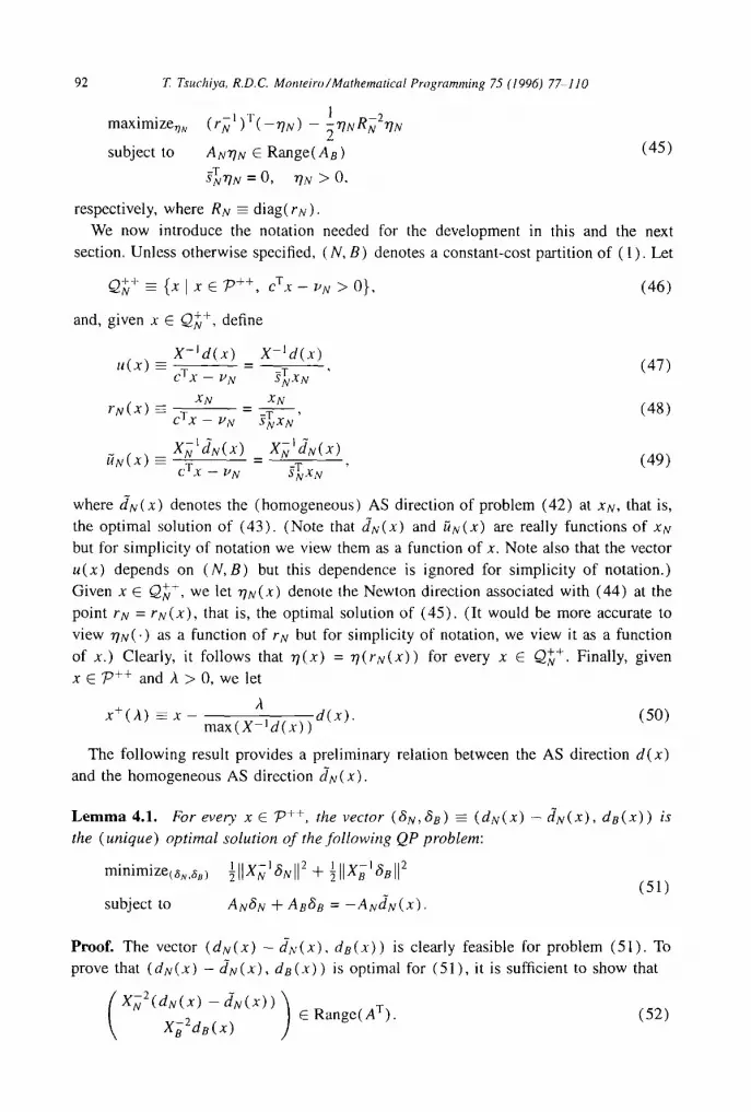
maximiz%~, ( ru 1 )Y(_rlN ) _ ~riNRN.rlN
subject to ANON E Range(AB) (45)
sTT]N ---- 0, 7"IN > 0,
respectively, where RN =-- diag(rN). We now introduce the notation needed ['or the development in this and the next
section. Unless otherwise specified, (N, B) denotes a constant-cost partition of ( I ) . Let
Q~-b ~ {X IX ~ "7")++ cTx __ PN > 0}, (46)
and, given x E Q~v ~, define
X-ld(x) X- ld(x) u(x) = = (47)
cT x -- PN STNXN
XN XN rN(x) = --cTx -- "N - f f x~' (48)
~tN(X ) ~ XN I J N ( x ) X N l d N ( X ) cT"~ ~ t-'--'~ -- sT NxN ' (49)
where du (x ) denotes the (homogeneous) AS direction of problem (42) at XN, that is, the optimal solution of (43). (Note that dN(X) and fin(X) are really functions of XN but for simplicity of notation we view them as a function of x. Note also that the vector u(x) depends on (N,B) but this dependence is ignored for simplicity of notation.) Given x E Q~+, we let ~TN(X) denote the Newton direction associated with (44) at the point rN = rN(X), that is, the optimal solution of (45). (It would be more accurate to
view r/N(') as a function of rN but for simplicity of notation, we view it as a function of x.) Clearly, it follows that "q(x) = r l ( rN(x ) ) for every x E Q++. Finally, given x E 7 -9++ and A > 0, we let
A x+(h) = - x - max(X_ld(x) )d(x). (50)
The following result provides a preliminary relation between the AS direction d(x) and the homogeneous AS direction do(x).
L e m m a 4.1. For eyeD' x C ~++, the vector (SS,tiB) ~ (dN(x ) -- t in(X), dB(x) ) is the (unique) optimal solution of the Jbllowing QP problem:
minimize(,~u,,~.) I[IXN16NI] 2 q- IlIXBI6Bll2 (51)
subject to ANtiS + AB69 = --ANdN(X).
Proof. The vector (tin(x) --dN(X). dB(x)) is clearly feasible for problem (51). To prove that (du(x) --dN (x) , dB (x) ) is optimal for (51), it is sufficient to show that
( XN2(dN(x) -- dN(X) ) ) X~2 d8 ( x) E Range(AT). (52)

T. Tsuchiya, R.D.C. Monteiro/Mathematical Programming 7.5 (1996) 77-110 93
Fix some (y,g) C Dn 5/0. Since gn = 0, dN(X) solves (43) and, by Lemrna 2.2(a), d ( x ) solves (11), we have
_ X ~ 2 d B ( x ) E Range(AT). (54)
Combining (53) and (54), we obtain (52). []
The following technical lemma is well-known and is used in the proof of next result.
Lemma 4.2. Let F E g{P xq be given. Then, there exists a constant CI = CI ( F ) with
the following property.: f o r any f C R v such that the system Fw = f is feasible and any
z E R q, there ~ is t s a solution ~, o f Fw = f such that
I 1 ~ - z l l <<. c~llf - Fzll
Lemma 4.3. The following statements hold:
(a) Ilun(x)[I = O(l lg~al l IIXNII I l u N i x ) l [ ) f o r a l l x E Q~v+; (b) [[~gix) -- uNix)l[ = OiIIX~tII2IIXN]I2HUN(X)[[) for all x G Q~v + such that
l lx~ ~ II IIXN]I is sufficiently small.
Proof. The proof of (a) follows immediately from (47) and Lemma 2.2(b). We next
show (b). Fix x > 0. Since ANdNiX) ~ Range(An) and A n d e ( x ) = - -ANdNix) , it follows from Lemma 4.2 that there exists riB(x) such that
Andn(x) =--ANdN(X), Ildn(x) - d n i x ) l l ~ C2] tdN(X) - dgix)]] , (55)
where C2 is a constant independent of x. Using the second relation in (55), we obtain
IIX~' ( d n i x ) - dn(x) ) t[ ~< IIX~ * [I I l d n ( x ) - dBiX)I[
~< c211x~Xll Ildg( x ) -- dN( X) [I
<. c211x~'ll IIXNll l i s a ' a N ( x ) - XN~dNiX) II �9 (56)
The first relation in (55) implies that (6N,&B) = (O, dB(X) ) is feasible to problem (51), and hence, by Lemma 4.1, we obtain
IIX~'dn ix)II 2 + IIX; ' (aNix) - dNix ) ) l l 2 <~ IIX~ ldB (x) II 2. i57)
Thus, we obtain
IIX~ ~ (dNix) - & i x ) ) l l 2 ~< IIX~ ~& ix)II 2 - IIX~dn ix)II 2
= [ X ~ l ( d n ( x ) + d n ( x ) ) ] T [ x ~ l ( d n ( x ) - dn(x ) ) ]
<~ I lX~( dn(x) + & ( x ) ) ll IIX~' i & i x ) - d n ( x ) ) ] l . (58)

94 T. Tsuchiya, R.D.C. Monteiro/Mathematical Programnting 75 (1996) 77-110
Combining this last relation with (56), we obtain
Hx?-,, ~ (aN(.,..) - t iN(X)) I I <~ C211XB j II IIXNII IIX~' (dB(x) + & ( x ) ) l l c: llX;'rl ppXNII {211XBIdB(x)ll + IIX~l(dB(-r) - d B ( x ) ) l l }
<~ 2C~IIXB ~ II IIXNII IIX~'dB(x)H "~ ~, - I + c211x~' II 2 IIXNII'HX~ t i N ( X ) - - x/v ldN(x) l l ,
from which we conclude that
IIx;,~ (dN(x) - & ( x ) ) l l ~< 4C211X~'II I[XNI[ IIX~'dB(x)l l ,
whenever C~IIXB 1 II 2 IIXNII 2 ~< ~ The last relation together with (a) imply
I IX ; , ~ ( dN(X) -- tiN( X ) )[[ = 0 ( l l X / ' I! 2 II XN II-' ! lX~ ' dN( x)ll )"
After dividing both sides of this relation by cTx -- VN, we obtain the desired result.
Lemma 4.4. The fol lowing relations hold:
e'r~v(x) : 1 Vx r Q~+,
and
[]
(59 )
l e f u N ( x ) -- 11 = (,.9( ]]X~ l I]IIXNII211.N(X)H), (60)
f o r every x r Q~+ with IIx~ ~ II I/XNI/ su/ficiently small.
Proof. Relation (59) is an immediate consequence of (24). Using (59) and Lemma 4.3, we obtain
leTuN(X) -- 1[ = leT(uN(X) -- fiN(x))]
~< Ileil I I .N(x) - ~,,~(x)]l
= o( II gB-l II 2 II XN II 2 II l t N ( X ) l l ) '
for every x ~ Q,~+ with IIx~ 1 ]1 IIXNII sufficiently small. []
L e m m a 4.5. The fol lowing relations hold:
cTx +(A) VN=(I - -A0(X)) (CTX--UN) Vx~79++ , (61)
and
( tgN(X) ) AO(x) RN(X) - - e + - - (62) rN(X+(A) ) = rN(X) l - aO(x) Ilu(x) II 2 '
f o r every x E Q[v + and A > 0 such that x+(,~) e Q++, where RN(X) = d iag ( rN(x ) )
and
II"(x) II 2 O(x) - (63)
max(u(x) )"

72 Tsuchiya, R.D.C. Monteiro/Mathematical Programming 75 (1996) 77-110 95
Proof. The proof of (61) is similar to the proof of (31) and uses the fact that cTd (x ) =
iiX-~d(x) ]]2 Also, the proof of (62) tollows along the same line as the proof of (33).
We omit the details. []
The next lemma is the main result of this section. It generalizes relation (33) of
Lemma 3.5 to the context of general LP problems.
Lemma 4.6. We have:
,~O(x) rN(X + ( /~) ) = rN(X) (37N(-r) + RN( X) hN(X) ),
1 - A O ( x )
where ( UN(X) )
h N ( x ) = --e + 11,4x)ll---- ~ RN'(X)'qN(X) -=O(IIX~IIZlIXNII2),
for every x E Q}+ such that IIx~ III IIXNll is sufficiently small.
(64)
(65)
Proof. First note that (59) and Lemma 4.3 imply that
II~N(X)II ~ ~ IluN(X)II ~ II~N(X)II ~ ~ (66)
for every x C Q~+ with ]]X~ -I ]111XNII sufficiently small. Due to relation (26), we have
R~I(X)~N(X) = R~i(X)~N(rN(X)) = -e +
and hence,
u u ( x ) ~N(X) hN(X) - - - -
l l . (x)l l 2 l l~ (x ) l l 2 _ ~N(X) ( l l~N(x)l l 2
ll~N(X) II 2 \ llu(x)112 Thus, we obtain
~u(x)
[IhN(X) H
HaN(X)H 2'
HN(X ) -- ~N(X)
1 + ilu(x)ll 2
I ]I~N(X)II 2 --llu(x)]121 [IUN(X) --ON(X)I I + II~N(x) 11 [tu(x)II 2 $1u(x) II 2
llu,(x)ll2 + II/~N(X) -UN(X)ll [ll;~.(x)ll + IlUN(X)[I] Hs (x)l[ IlUN(x) II 2
IlUN( X) - ;-.,;~( x) II + Iluu(x) l?
II.;~(x) II 2 II~N(X) - UN(X)ll + 11,TN(x)[lllu•(x)ll 2 II~N(x)ll IlUg(X)[[ 2
+2llUN(X) - aN(x) LluN(x)II 2
(67)
Now, using (66) and Lenuna 4.3, it is easy to see that each one of the terms m the right hand side of the above expression is (9(]IX~ 1112NXNII 2) for every x C Q~v '~ with
(68)

96 T. Tsuch(va, R.D.C Monteiro/Mathematical Programming 75 (1996) 77-110
IIS~ll IIXNII sufficiently small. Hence, (65) follows. Relation (64) is an immediate consequence of (62) and (65). []
A natural question to be asked is: for which constant-cost partitions (N,B) does problem (44) have an optimal solution? The following result shows that the optimal partition is the only one. Recall that (9",~V ') denotes the analytic center of the dual optimal face, that is, the point defined in (13).
Lemma 4.7. Let (N, B) be a constant-cost partition. Then, problem (44) has an optimal solution if and only if ( N, B) is the optimal partition of ( 1 ), in which case ( s~v ) - j / I NI is the (unique) optimal solution of (44).
Proof. If r~, is the optimal solution of (44) then by considering the optimality conditions of (44), we can easily show that
( ( r*N)o I/[N[ ) E Range(AT) + Rc. (69)
Hence, 79 ++ ,=' ~. Due to the assumption that (N, B) is a constant-cost partition, we have 7:'~ + ~ 0. Hence, we conclude that (N, B) is the optimal partition of (1). Conversely, by considering the optimality conditions of (13), we can easily verify that (~v)-~/Igl, where (g~)- i =_ [diag(g~v)]-le, satisfies the optimality conditions of (44) with gN = g~,. We omit the details of the proof. []
Lemma 4.8. Let (N, B) be a constant-cost partition and assume that {ak} C 1t~ ++, {.~k} C 7 ~++ and {(yk ~k)} C_ 79 are sequences satisf3'ing the following conditions:
(a) {~v/otk} is bounded; (b) lim~:~()f~g~v)/ce~ = aN > 0. where X~ = diag(~r and aN is some Igl-
dimensional vector; (c) l imk_~ ~ = 0 and {gkN} is bounded.
Then, ( N, B) is the optimal partition of ( 1 ) and we have:
lira (~t g~)=(y ,~) , (70) k ~ ~ -
lira x~./cek = ( , . ~ m ) - l a N , (71) k ~ oc,
where So = diag(gN) and
(9, s) = argmax{ Z a j l o g s . / "(.y,s) E D~ +}. (72) j G N
In particular, if aN is a positive multiple of the vector of all ones then (~, ~) is equal to the analytic center (y~,g~) defined in (13).
Proof. Since (N ,B) defines a constant-cost face, we have 7 :'++ :~ 0. Hence, to show that (N, B) is the optimal partition of (1) and that (70) holds, it is sufficient to show

T. Tsuchiy& R.D. C. Monteiro /Mathematical Programmb~g 75 (1996) 77-110 97
that any accumulation point (~, g) of (9 k, ~k) satisfies the optimality condition for (72), namely
(y, g) E D~ +, (73)
ANSNl aN C Range(Ae), (74)
where SN = diag(.7/v). Indeed, let K be an infinite index set such that limke~:(y k, g~) = (~,g). Using (c) and the assumption that {(.~ ~k)} C D, we conclude (y,~) C DB. Moreover, (a) and (b) imply that SO > 0 and that
lim 2ku = S N I a N . (75) kEK; i~" k
Thus, we conclude that (73) holds. Since 79++ ~ ~, we have b E Range(Ag). This observation together with the fact that {2k} C_ 79 ++ imply
AN(YCk) ~ Range(AB). (76) \o:~/ ,
Relation (74) now follows immediately fiom (75) and (76). The limit (71) is an immediate consequence of (70) and (b). []
Lemma 4.9. Let ( N, B) be a consmnt-cost partition attd let {.~k} C_ Q}+ be a sequence such that {ru(2k)} is bounded and l i m k ~ II(X~) -1 II ]IXkNI[ = 0. The,, the following statements are equivalent:
(a) l i m ~ U N ( 2 k) = e/INI; (b) l i m k ~ II(R~N)-Jr/N(2~)I] = 0, where R k N =- diag(rN(xk)) ; (c) ( N, B) is the optimal partition of ( 1 ) and l i m ~ r N ( 2 k) = ( g~N ) - I / I N],
in which case, limk--.~ (y(.~k), s (2k) ) = (9% ga).
Proof. From Lemma 4.3 and the assumption that l imk__,oo 11 (2~) - ill I I 2kNll = 0, it fol- lows that
lim UN(Y~ ~) = e/IN[ "r lim ~m(~ k) -- e/lNI. (77) k ~ o o k ~ o o
Due to relations (26) and (59), we have
--e + ~(~k) 112 2 2 eTUN('YCk) 1 II(R~)-'r/N(~k)IIZ= } } , 7 ~ = INL- ~ p ~ - 2 + [[aN(.~k)ll2
1 = INI ilaN(~)112, (78)
Using the fact that eT~TN(2 ~') = 1, it is easy to see that l i m k ~ H~N(.i k) II = l / ~ v / ~ if and only if limk--,o~ fiN(YC k) = el[N[. This observation together with (77) and (78) immediately imply the equivalence of (a) and (b). The proof of the implication (c) (b) follows immediately from (a) and (b) of Lemma 3.2 and Lemma 4.7. It remains to show the implication (a) ~ (c). Indeed, assume that (a) holds and let cek -= cT~: k -- uu

98 "E Tsuchiya, R,D. C. Monteiro/Mathematical Programnmtg 75 (1996) 77-110
and (.yk,.~k) _= (y( .~k) ,s(2k)) for all k ) 0. We will show that the sequences {.~k},
{(.gk, ~k)} and {cek) satisfy conditions (a), (b) and (c) of Lemma 4.8 with a~v = e/lgl- Since by assumption {rN(2k)} is bounded and rN(2 t) = Y:~v/C~k for every k, condition (a) of Lemma 4.8 holds. Condition (a) implies that (b) of Lemma 4.8 with aN = e / IN[
is satisfied since
u ( 2 k ) R~s (2~) 2k~ k . . . . . . (79)
cT-~k -- PN OLk
Clearly, { ( y k ~ ) } is bounded in view of Proposition 2.3. Hence, to show that condition (c) of Lemma 4.8 bolds, it is sufficient to prove that limk--,~ Y~ = 0. Indeed, first
observe that (a), the assumption that lim~._~ II ( 2 ~ ) - t II H2~vll = 0 and Lemma 4.3(a) imply that {u(~ -k) } is bounded. Using this observation, the fact that ~k = (_9(112~,11) and (79), we obtain
I1~11 <~ 1](2w = ,~11(2w II,,(?)ll ~< o(11(2~)-'[[ 112~,11),
which, together with the assumption that l i m k ~ 11(2w II II 2~ II = o, clearly imply that l i m k ~ ~ = 0. Using Lemma 4.8, we conclude that (c) holds and l i n l k ~ ( y ( 2 k ) , s ( 2 k) ) = ( y" , ~" ) . []
We observe that it is possible to give a direct proof of the implication (b) ~ (c) by using Lemma 3.7, Lenuna 3.2(b) and Lemma 4.7. The proof given above shows instead the implication (a) =:> (c) via Lemma 4.8, which is simpler in the sense that it does not need the machinery introduced in the Section 2 and in the first part of this section.
It also illustrates a basic principle that has been used in the convergence analysis of the AS algorithm (see Tsuchiya and Muramatsu [29] or Monteiro et al. [ 19, Theorem 4.3]).
5. A superlinearly convergent affine scaling algorithm
In this section we present a variant of Algorithm I which is globally and two- step superlinearly convergent. After we state the algorithm, its global convergence and superlinear convergence are proved.
To describe the variant of Algorithm 1 that will be studied in this section, we assume that two constants p and q are given such that
p , q E (0, 1), p < q (80) q + 2
Examples of constants satisfying these conditions are: p = 0.3 and q = 0.95. Observe I that p can be chosen as close as to 5 as it is desired. For the purpose of future reference,
we note that (80) implies that
2 ( q - p) >q. (81) l + p

T. Tsuchiya, R.D.C Monteiro/Mathematical Programming 75 (1996) 77-110 99
The following variant of Algorithm 1 will be shown later to converge two-step super- linearly with order at least 1 + p < 4 3"
Algor i thm SLA
Step O. Assume that constants p and q satisfying (80) and a point x ~ E P++ are given. Set k := 0.
Step 1. Compute d k =_ d ( x k) according to (9c) and let
Nk = {i" x~ <~ [ e T [ ( x k ) - I d k ] 11/2}, (82a)
O'k=eT((X~uk)--ldku~ ), (82b)
~ (eTuNk(xk))2 o-~ - IN~-I (82c)
e k = . [N~I [l(xk)_~dkll2 ilu(x~.)ll2
Step 2. If
,~ < o-~, (83)
then (Predictor step)
,~k = max(0.5 , 1 - o-['.) (84)
else (Corrector step)
,~k = 0.5.
d k Step 3. x k+l = x k - Ak (85)
max( (X k ) - ldk) '
Step 4. k := k + 1 and return to Step 1.
The first expression for ek is the one that should be used to compute it. The second one is used during the analysis of the algorithm and is a consequence of (47) . It is easy to see that term within the square root of the first or second expression for ek is nonnegative so that e~ is well-defined.
The basic procedure is to alternate the choice of the stepsize between Ak = 0.5 and ak ~ 1. Since Algorithm SLA is a variant of Algorithm 1 in which ak >_- �89 for all
k/> 0, we conclude that it satisfies all the statements ( a ) - ( e ) of Proposition 2.4. As in Section 2, we denote the limit point of the sequence {x k} by x* and let ( N . , B . ) =
( N ( x * ) , B (x*) ). By Proposition 2.4 (d) , ( N . , B. ) is a constant-cost partition. Recall that the constant value of cTx over the face 7 ~+. is denoted by ~'N.. Clearly, ~'N, = cTx *. Throughout this section, the function u( . ) refers to the one associated with the partition ( N , , B. ) and the following notation is used: u k = u (x k),/~k = Ux, (X k), rk . N . = rN* ( x k ) '
R k. = d i a g ( r k ), k . r lN .=r lN . (xk ) , (yk, s k ) = ( y ( x k ) , s ( x k ) ) , f o r a l l k > ~ O . The global convergence analysis of Algorithm SLA is much simpler than its super-
linear convergence analysis and is obtained in Theorem 5.3. So we next explain the underlying idea behind the superlinear convergence analysis of Algorithm SLA. It is

100 7: Tsuchiya, R.D.C Monteiro/Mathematical Programm#zg 75 (1996) 77-110
shown in Proposition 5.1 that crk ,--, cTx ~ - PN. and IIx~,. II = O(c Tx~- ~'N. ) from which it is easy to conclude that Nk = Nopt for all k sufficiently large, where (gopt, Bopt) denotes the optimal partition of (1). Moreover, Lemma 5.2 shows that ek is a measure of centrality for the "small" variables x k the ones that dictate the speed of convergence g . ~
of the (or, any interior point) algorithm. When the measure of centrality ek is small, a
predictor step with stepsize ,~x asymptotically approaching 1 is taken. The behavior of the predictor steps is analyzed in Lemma 5.5; the main conclusion is that the measure of progress cTx -- VN. is reduced at a superlinear rate while the centrality measure "slowly" deteriorates. At the next step, if the the small variables are not well-centered (i.e., the
test (83) fails), then a corrector step is taken with stepsize At = �89 The effect of this step is analyzed in Lemma 5.6; the main conclusion is that c T x - ut~'. is reduced at a linear rate while the centrality measure is improved at a quadratic rate. Lemma 5.7 shows that, asymptotically, one corrector step suffices to recover the centrality of the small variables and hence that a predictor step is taken in every two steps of Algorithm SLA. Using these conclusions, it is now easy to prove the superlinear convergence of Algorithm SLA (see Theorem 5.10).
Some basic properties of Algorithm SLA which follows almost immediately from the
analysis of Section 4 are given in the following result.
L e m m a 5.1. The fol lowing statements hold:
(a) the sequences {uk}, {tT~. } and {r~m. } are bounded;
(b) {II(XL)-'H IIX~-.ll}. {llu~,. - ~ . [ [ } . {11,4.11}, {eTu~N. -- l} and {ll&.ll} con- verge to 0 according to:
II ( x k ) - ' II IIX%. II = O(c T:~* - , ,N.). (86)
I1,~. - ,~ . II = o ( ( c T x * - ,,N. )2), (87)
l e t u p . - - II = O ( ( c T x ~ - ,,,,,.)~-), (88)
Ilu~. II = o (c T x~ - PN. ) , (89)
IIsw II = O((c Txk - PN. )2). (90)
(c) Nt = N, f o r all k sufficiently large and the following relations hold:
lim o-k - 1, (91) k ~ o o (CTX k -- PN. )
lim o-k = 0. (92) k---* oo
Proof. By Proposition 2.4(b) and the fact that X~v, = 0, we have
k [[Xu. [[ ~ [[Y k -- X*[] = ( ~ ( c T x k -- PN. )" ( 9 3 )
Clearly, this implies that {rkN.} is bounded and that (86) holds, since l imk~o~x~. = X* s. > 0. By (47) and ( I 0 ) , we have

Z Tsuchiya, R.D.C. Monteipv/Mathemat ical Programming 75 (1996) 77-110 I Ol
Xk s k u ~ - (94)
c T x k - - l.,N. '
from which we conclude that u~. = k k RN. SN.. This fact together with Proposition 2.4(c) and the fact that k {ro . } is bounded imply that {u~. } is also bounded. Due to Lemma 4.3, Lemma 4.4, the fact that {u~.} is bounded and (86), we conclude that (87),
(88) and (89) hold. Clearly, (87) and (89) imply that {u ~} and { ~ . } are bounded.
Relation (90) follows immediately from (89), (94) and the fact that l i m k ~ x~. > 0. It remains to show (c). Let ~-~ = e T ( ( X k ) - l d ~) = ( xk )Ts k. Using (88), (89) and
(94), we obtain
lim "rk = lim e'r u k = 1 k---*oc~ c T x k -- I.'N. k--*c'x3
and hence, that
lim ~-~ = 0. (95) k~oo
These two relations together with (93) imply that
x~i = O(c~rx k - VN. ) <~ O ( r k ) ~ v ~ ,
for aH i C N, and k sufficiently large. Moreover, (95) and the fact that limk--.oo -~B. =
X* B, > 0 imply that x~ > v ~ for all i C B. and k sufficiently large. From these two observations and (82a), we conclude that Nk = N, for all k sufficiently large. Relation
(92) follows immediately from (91), which in turn is an immediate consequence of (88) and the fact that crk/ (cTx k - -PN. ) = eTu~k = eTu~N, for all k sufficiently large. []
Remark. From the previous lemma, it immediately follows that O-k ~ cTx ~ -- VN.. This means that any quantity appearing in the analysis below whose order is CO(o-k) is also (.9(cTx k -- UN. ) and vice versa.
L e m m a 5.2.
III (R~N.)- '~7~, . II - ekl : CO(o-k). (96)
Proof. Due to relations (26) and (59), we have (see (78))
1 I I ( R k N . ) - ~ , ~ . I I 2 = IN*I i i ~ , l l 2
Define
(97)
1 (eTukN')2 Vk >~ O. (98) ,bk - II~N. ii 2 ii,kll 2
Using the inequality (or - 5,) 2 <~ [a 2 - y2[ for cr > 0 and y > 0, relation (97) and
Lemma 5.1(c), we obtain for every k sufficiently large that

102 T. Tsuchiya, R.D.C, Monteiro/Mathematical Programming 75 (1996) 77-110
2 )_, k l12
( eTG ' )2 I I (G )-1 = IN.I i1.~112 . ~ X . II 2
~< 14'k[-
It remains to show that I&~[ = (.9(o-~). Indeed, using a bounding scheme similar to the one in (68) together with (66) , Lemma 4.3 and Lemma 4.4, it is easy to see that
14,~ I = co( I I ( xL ) - ' II 2 llX,~, ll~).
This relation together with (86) and (91) imply I&k[ = O(o-~). []
The next result establishes global convergence of Algorithm SLA.
T he o rem 5.3. ( N., B. ) is the optimal partition of (1), or equivalently, x* lies in the
relative interior of the optimal face of ( 1 ).
Proof. If the condition ek < o-~, is satisfied for finitely many indices k, the result follows 1 lot all k sufficiently large. Assume now from Proposition 2.5 since, in this case, cr~ =
that the set /C of all indices k satisfying et < cry, is infinite. By (92) and the definition of ]C, we have litn~.e~ et = 0, and hence, in view of Lemma 5.2, we conclude that
lim~eK: II (RkN.) -1 ,,,k 'IN. I[ = 0. Using the equivalence between (b) and (c) of Lemma 4.9, we conclude that ( N . , B. ) is the optimal partition of ( 1 ). []
We now focus our attention on the superlinear convergence analysis of Algorithm
SLA. We start with the following technical result.
L e m m a 5.4. Consider the function O(x) defined in (63) with N = N. and let Ok =- O(x k) for all k ) O. For all k sujficiently large, we have:
IO[ ~ II ~< ll(R~v )-~ * - - . T I N . II + o ( , ~ . ) , ( 9 9 )
where Oh = O(x k) for all k.
Proof. By (89) and (88) , we have max(u k) = max(u~+, ) for every k sufficiently large.
This observation together with (63), (65), (86) and (91) imply
0k71 _ max (u~ . ) ii.kll 2 - max(e + (R~v)-I~7~. + hN.(Xk)),
where hN. (x k) = O( [I (Xw -111211X~N. 112) ~< O(o'~). Hence, we obtain
_ - , k O ( o ' ~ ) [ ] 10; I 11 ~< II(R~v.)- 'G. II + HhN.(-?)II ~< I I ( G . ) *TN. 11 + �9
To simplify our presentation, we introduce the following set of indices:
K,p = {k : a predictor step is taken at the kth iteration}.

Z Tsuchiya, R.D.C. Monwiro/Mathematical Programming 75 (1996) 77-110 103
In the remaining part of this section, we use r~v. to denote the point ( ~ . ) - ~ / I N . I . By Lemma 4.7 and Theorem 5.3, we know that r~v. is the (unique) optimal solution of
problem (44) with N = N. . The main result about the predictor steps is given next.
Lemma 5.5. For every k E ICe, we have:
(a) I I G . - r k , ll = O ( o - q ) ; ( b ) Ok+ 1 ,----' ( c T x k+l - - P N . ) ~.o ( c T x k -- p N . ) I + P ,,-,., O-~+P;
..k+l * ,',',r ( q - p ) / ( l + p ) ' ~ and hence, .A+x �9 (C) I N . - - rN. [1 = t.2kO-k+ 1 , . lim~c/Cp i N . - - rN. [[ = O.
Proof. Observe that (83) implies that ek = 0 ( o -q) for all k E ICe. Using this observa- tion, Lemma 5.2, (92) and the fact that q < 1, we obtain that
II(R~v.--1 k ) TIN. II = O ( O ' q ) V k E ICp sufficiently large, ( 1 0 0 )
and hence, l i m k ~ II(R~.) - ]~k 'IN. II = 0. It then follows from Lemma 4.9 that
l i m ~ r~. = r*N.. This observation together with Lemma 3.2(c) imply
]]r~r - r~v * - TIkN, II = O(l lrkN. - r~v * l ib , ( 1 0 1 )
II?N. * ~ R k - ' - ~ II~N. II ~ N. rN. II H( ) , ~ . 1 1 . (102)
for all k C ICp sufficiently large. Statement (a) now follows from relations ( I00 ) and (102). We next show (b) . By (61) , we have c t x k+l -- PN. = (1 -- 2tkOk)(cTx k -- PN.) for all k ~> 0. In view of (91) , (b) follows once we show that
1 - AkOk "~ ~ Vk E ICe sufficiently large. (103)
Using (100) , Lemma 5.4, (92) and the fact that q < 2, we conclude that
[0k - 11 = O ( o -q) Vk E ]Cp sufficiently large. (I})4)
Using this observation and the fact that, by (84) and (92) , we have ak = 1 -- o'~ for all
k E ICp sufficiently large, we obtain
l( 1 -- a k O k ) -- ~ 1 = I(1 - a k 0 k ) - (1 - a , ) l = AklOk -- II = o ( ~ g ) .
Using (92) , the fact that, by (80) , q > p, and the above relation, we conclude that 1 - akOk "-' ~ , and hence (b) follows. It remains to show (c). By (64) , we have
AkOk ( k RkN h N . ( X k ) ) (105) rk+N. 1 -~ r~. 1 ~ Z O k TIN* -~ "
Moreover, by (65) , (86) and (91) , we have
hN.(X k) =O(ll(Xw 2) ~ O( (cTxk-- pN.)2 ) ~ 0(0"2). (106)
Using relations ( 101 ), (102) , ( 103 ), (105) and (106) , Lemma 5.1 (a) and statements (a) and (b) , we obtain that, for all k E ICe sufficiently large,

104
rk+l ~. - % 11 =
<<.
7:. Tsuchiya, R.D.C. Monteiro/Mathematical Programming 75 (1996) 77-110
(rN" ( ) "~kOk Rk h N . ( x k ) k �9 k AkOk I ~ k O. -- rN. -- "ON. ) -- I -- .,~kOk 1 -- ,)tkO k
. 12akOk-- I I , &0k [ I r k . - rN. - - T]kN. II + i ~ 1 ~ IIT]N.I[ + l - A~0~
IIrN.--tN. ) ~<o(11,.% _ r L l l 2 ) + o ( k ~ , . . II + o ( ~ - p )
q-t,. e~_(q-t,)/(~+r)). [] (107) O ( a k ) ~ V\Uk.+l
I[R* N. II Ilhm (x ~) II
The main result about the corrector steps is as follows.
L e m m a 5.6. Assume that 1C is an infinite index set such that limkE~: rkN. = r*u. and Ak = �89 for all k E IC. Then, the following statements hold:
(a) limkEK(cTx k+l -- P N , ) / ( c T x k -- b'N.) = t ;
(b) lim,~K: o'k+l/o-k = �89
( c ) lira,+ ' * rN. II O(llr~. * 112+~r~) . foreven 'kcE- - - = - - i N . .
(hence, limkEr r~ +l = r~v" ).
Proof. The assumption limkcjc r~. = r}. implies that lilnkc~ II (R~,)-lT]k. 1] ---- 0, which together with (92) and Lemma 5.4 imply limkc~ 0k = 1. This relation together with the assumption that Ak = �89 for all k E KS imply
lim 1 - akOk = �89 ( 1 0 8 ) kE~
This in turn implies (a), due to (61). Statement (b) follows immediately from (a) and (91). We next prove (c). Since limkE~: r ~x. =rx.,* Lemma 3.2(c) implies that
l i ra. - r~v. - T]~N. II = co( IlrkN. -- rYv. 112).
l id , . - * ~ ~ rN. II I I~LI I I I (R%.) - '~J , . I I .
(~o9)
(11o)
hold for every k E/C sufficiently large. Hence, by Lemma 5.4, we have
1 0 ~ - l l - - O ( l l ( R % , ) - ' ~ . I I +o-~)~ = O C i l r % . - r ~ . l l * + o-z.), ( 1 1 1 )
for every k E K: sufficiently large. Using relations (108), (109), (110) and (111), 1 for all k E K:, we obtain by Lemmas 4.6 and 5.1(b) and the assumption that & =
using an argument similar to (105), (106) and (107) that
. 1 2 & 0 k - I I &Ok lira** 1 - r L I I <~ lira. - rN, -- T]kN, II + f~-A~-k I1~.11 + 1 --~Ok Itgk'[k I[hN" (xk)ll
O( l l r ~ . - % II 2) + o (10 , - ~11[r~N, - - r*N. II) + O(O 'b
<~ O( l l r%. -- r:,,. II 2 + ~,~),
for every k E /C sufficiently large. []

Z Tsuchiya, R.D.C. Monte iro/Mathemat ical Programming 75 (1996) 77-110 105
The next result shows that, asymptotically, a predictor step must occur at every two
steps as long as the set KS̀ O is infinite�9
Lemma 5.7. For every k sufficiently large, the following implication holds:
kEKSe , k + l ~ K S ` o =:~ k+2EKS`O. (112)
Proof. Let KS~ _= {k �9 k E KZ`O, k + 1 ~/C`o}. In view of Lemma 5.5(c), it follows that
the set KS = {k + 1 : k C KS~} satisfies the assumption of Lemma 5.6. Hence, it follows from (b) and (c) of Lemma 5.6 that
k+2 * k+l .* rN. rN. II O( [12 + 2 , - - = rN. - - 1 N. O'k+ I ) Vk E KS`O, (113)
o'k+2 ~ O-kH Vk C KS~,, (114)
�9 k + 2 _ r * and lamkcx:;, ru. N. [[ = 0. Hence, in view of Lemma 3.2(c) , we have
r.k+2 * k+2 ( R k • - 1 k+2 t II U. rN. II ~ ~ (115) - [inN. II N'. ) 9~N'. Vk ~ KS`O.
Using Lemma 5.2, (115) , (113) , (114) and Lemma 5.5(c) , we obtain
( R k + 2 ) - l _ k + 2 II ek+2 ~- N. t i N . II + O ( O ' k + 2 )
k+2 �9 <~ (.9( ru. -- ru. II + ok+2)
<~ O( k+l �9 2 r N . -- r N . 112 + O'k+l + O'k+2)
r,-,z 2 ( q - - p ) / ( l + p ) 2 ~tO'k+ l + O'k+l + O'k+2)
for every k E KS~, where s - m i n { 2 ( q - p ) / ( l + p ) , 1}. By (81), we have s > q. This
observation together with the above relation imply that ek+2 < crq+2, or equivalently, k + 2 ~ KS,o, for every k C KS~o sufficiently large. []
The next result shows that the set KS̀ O is infinite. In view of the Lemma 5.7, this clearly implies that, asymptotically, a predictor step occurs at every two steps of Algorithm SLA.
Lemma 5.8. The set KSp is infinite.
Proof. Assume for contradiction that there exists an integer k0 such that k ~ ICe for every k >~ k0. By Proposition 2.5(c) , we have
lira k lim k k T k biN. = XN, S N. / (C X -- VN.) = e / l N . I. k ~ o o k~ex~
This relation together with Lernma 5.1 (a) and Lemma 4.9 imply that limk--oo r~. = r* N . ' Hence, it follows that the assumptions of Lemma 5.6 are satisfied with KS = {k : k ~> k0}. By using statements (b) and (c) of this lemma, we conclude that limk~oo crk/o-k+l = 2 and that, for some constant L0 > 0,
uk+l * "~ I l tN. - - F N . ]l ~ L0(l]r~. - r~r ]l 2 + o-~,) Vk/> k0. (116)
106 77 77vuchiya. R.D.C. Monteiro/Marhematical Programming 75 (1 996) 77-110
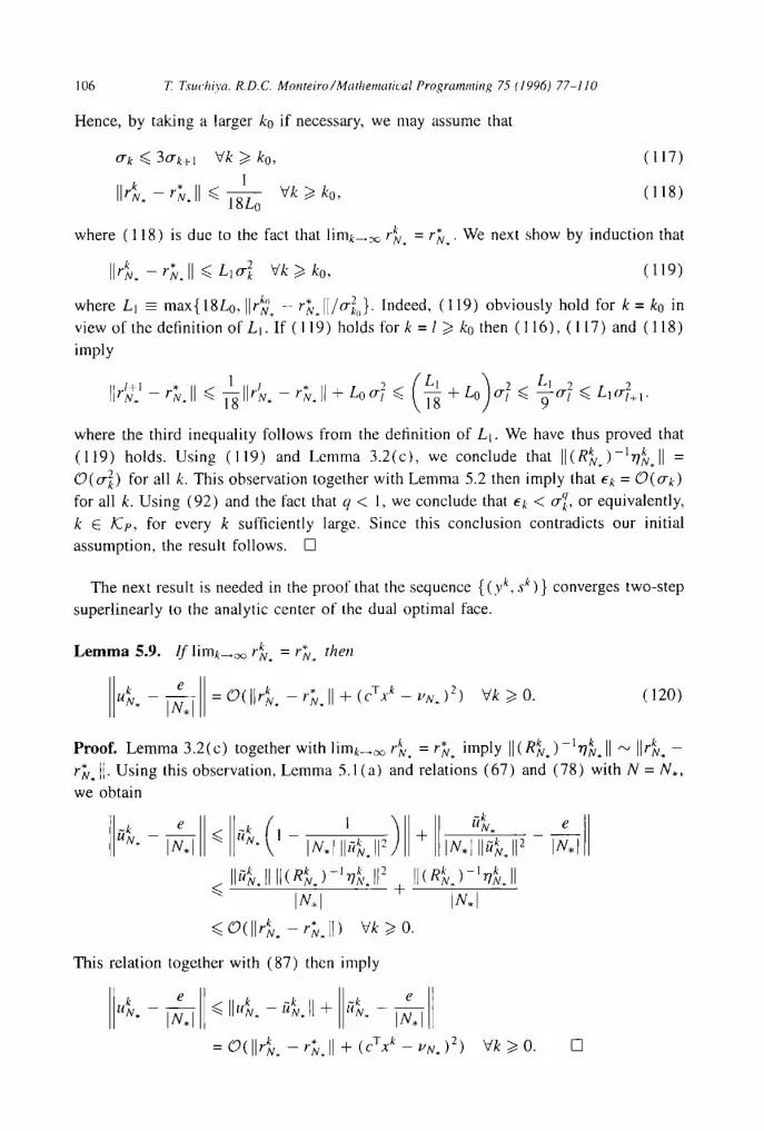
Hence, by taking a larger k0 if necessary, we may assume that
o'k <~ 3crk~l Vk >-ko, (117)
1 IIr~. - & . l l -< 18g~ vk > k0, (118)
where (118) is due to the fact that limk_.m rkN. =rN.'* We next show by induction that
Ilrk.--r~v. II ~ Llcr~ gk~>ko, (119)
where LI -= max{18Lo k,~ _ r* [[rN. N. /rrT.~} Indeed, (119) obviously hold for k = k0 in view of the definition of Li. If (119) holds for k = l ~> k0 then (116), (117) and (118) imply
-- rN. II <~ II N. -- 'N. ll + Lo~T <~ + Lo cr~ <<. cr~ <~ L,oT+ ,.
where the third inequality follows from the definition of Ll. We have thus proved that
(119) holds. Using (119) and Lemma 3.2(c), we conclude that II(R~,~) -ln~,. II = Cg(cr~) for all k. This observation together with Lemma 5.2 then imply that ek = O(o-k)
q for all k. Using (92) and the fact that q < 1, we conclude that ek < o- k, or equivalently, k E KTp, for every k sufficiently large. Since this conclusion contradicts our initial assumption, the result follows. []
The next result is needed in the proof that the sequence { (yk, S k ) } converges two-step superlinearly to the analytic center of the dual optimal face.
L e m m a 5 . 9 . / f limk~oo rkN. = r*N. then
u~, IN.le --O(llr~,---r*N. I I - t - ( cTxk - -UN. ) 2) gk ) O. (120)
Proof. Lemma 3.2(c) together with limk~oo r~,. = r~v . imply I1(R~.)-%%.11 ~ II&. - r~, tl- Using this observation, Lemma 5.1 (a) and relations (67) and (78) with N = N. ,
we obtain
G. e G . ( I ) - ~TT ~< 1 i N . r IIG. ii 2
IIG [I II(G )-l_k ,,x [I(RkN )-~,7~,.11 ~< . . ' / X . rt + .
Im, I IX.I ~ O(llG. - &,[l) V k > 0
This relation together with (87) then imply
e G . - ~ -<IIG.-G.II+ G . -
rk .* =o(11 u. - - 'g . II + (d xk - ~'N.) 2)
/?N. e
+ IN*I I1~.112 IN.I
Vk>~0. []

Z Tsuchiya, R.D.C. Monteilv/Mathematical Programming 75 (1996) 77-1 I0 1 0 7
The next result establishes the two-step superlinear convergence of Algorithm SLA.
T h e o r e m 5.10. Algorithm SLA has the following properties: (a) the sequence {cTx t } converges 2-step supeHinearly to the optimal value VN. =
cTx * with Q-order at least 1 + p, namely
c T 3 . - k + 2 _ I.,N. lim sup (121)
~--.oo (c Tx~ - uU.) l+r' < oC;
(b) the sequence {x k} converges 2-step superlinearly with R-order at least I + p m
a point lying in the relative interior of the optimal face of problem ( l ); (c) the sequence {(yk, st)} converges 2-step superlinearly with R-order at least
1 + p to the analytic center of the optimal face of the dual problem (2), that is,
the point ( ~a, ~a ) defined in (13).
P r o o f . It follows from Lemma 5.7 that if k is sufficiently large then either k C Ice or k + 1 E iCe. This fact together with Lemma 5.5(b) clearly imply (a). By Proposition 2.4(b), we know that I[x k - x*ll = O ( c l x k - ~N . ) and hence, in view of (a), it
follows that {x ~} converges 2-step superlinearly to x* with R-order at least 1 + p. We �9 . ~a = 0 next show (c) From (a) and (90), it follows that that {s~ } converges t o . B .
two-step superlinearly with R-order at least 1 + p. We next analyze the convergence of {s~v.}. From (a) and (c) of Lemma 5.5 and Lemma 5.7, it is easy to see that tl"~N. -- % II = O ( ( c T x k -- ~N. ) ' ) , where t = ( q - p ) / ( 1 + p ) . Using this observation,
* - a -- I the relation rN. = (SN.) (> 0) and Lemma 5.9, we obtain
[[ s~v. ~,a ( R k a-tu~ ( R*)-I e - S N . II = N.~ N. I g , I
L l k . e
~< H(R~,.)-'II I/V.] +
= 0 u . - - + rN --rN.
II(R~.)-Ie- ( R * ) -1e l i
IN.J
(122)
(123)
(124)
(125)
(126)
= O( Plr~. - , ' ~ . II + ( e T x k -- ~N. )2)
= O ( ( c r x k - VN. ) ' ) .
This clearly implies that {SkN, } converges to ~ N. two-step superlinearly with R-order at least l + p . []
6. C o n c l u d i n g r e m a r k s
In this paper we have demonstrated that a variant of the long-step AS algorithm is 4 two-step superlinearly convergent with Q(R)-order as close to g as desired. Practical
eff• of this algorithm is not known at this moment, but the results of this paper

108 T. Tsuchiya, R.D.C. Monteiro/Mathematical Programming 75 (1996) 77-110
may suggest possible ways to implement the AS algorithm more reliably and efficiently, We believe that the analysis of this paper is important from the theoretical point of view since it shows that the AS aIgorithm with certain stepsizes is also able to keep the sequence of iterates well-centered, at least asymptotically. This is in some sense an unexpected result in view of the (pure) steepest descent nature of the AS algorithm.
One interesting research problem is to improve the order of convergence of the algorithm of Section 5. It would also be interesting to develop a variant of the AS algorithm with convergence order equal to any number less than or equal to two, a property which many primal-dual algorithms (e.g. [33] and [17]) and the Iri and Imai's algorithm [27] have been shown to have.
We believe that our analysis can be directly applied to the long-step variant of Karmarkar's algorithm [15] presented in [20]. It seems possible to show that this variant of Karmarkar's algorithm enjoys superlinear convergence without sacrificing its polynomial complexity by properly choosing the sequence of stepsizes according to the
ideas suggested in this paper. Another algorithm whose analysis could benefit from the techniques in this paper
is Todd's low complexity algorithm [231. During the predictor steps, his algorithm moves along the AS direction with stepsize tess than �89 (namely �89 of the step to the boundary of the largest inscribed ellipsoid). Since the AS step with Ak ~< �89 works as a kind of corrector step, it seems possible to show that Todd's algorithm may not need any corrector step asymptotically (cf. [24]). Moreover, it seems possible to apply our analysis to show that a variant of Todd's algorithm is superlinearly convergent without sacrificing its polynomial complexity.
Acknowledgment
This research was carried out while the first author was visiting the Center for Research on Parallel Computation and the Department of Computational and Applied Mathematics of Rice University, Houston, USA from March of 1992 to February of 1993. He thanks his host Prof. J.E. Dennis and the colleagues there for providing the excellent research environment during his stay at Rice University.
Part of this research was supported by the National Science Foundation (NSF) under grant DDM-9109404 and the Office of Naval Research (ONR) under grant N00014- 93-1-0234. The second author thanks NSF and ONR for the financial support received during the completion of this work.
The first author also thanks the second author for having arranged and supported a trip with his NSF grant to visit the University of Arizona in the summer of 1992 where this research was initiated. He also thanks the University of Arizona 1or the congenial scientific atmosphere that it provided.

T. Tsuchiya, R.D.C. Monteiro/Mathematical Programming 75 (1996) 77-110 109
References
[ I ] I. Adler, N.K. Karmarkar, M.G.C. Resende and G. Veiga, "Data structures and programming techniques for the implementation of Karmarkar's algorithm," ORSA Journal on Computing 1 (1989) 84-106.
[2] 1. Adler, N.K. Karmarkar, M.G.C. Resende and G. Veiga, "An implementation of Karmarkar's algorithm for linear programming," Mathematical Programming 44 (1989) 297-335. (Errata in Mathematical Programming 50 ( 1991 ) 415.)
13] I. Adler and R.D.C. Monteiro, "Limiting behavior of the affine scaling continuous trajectories for linear prograrnming problems," Mathematical Programming 50 ( 1991 ) 29-51.
14] E.R. Barnes, "'A varia6on on Karmarkar's algorithm for solving linear programming problerns," Mathematical Programming 36 (1986) 174-182.
15] Y.-C. Cheng, D.J. Houck, J.-M. Liu, M.S. Meketon, L. Slutsman, R,J. Vanderbei and P. Wang, "The AT&T KORBX System", AT&T Technical Journal 68 (3) (1989) 7-19.
16] I.I. Dikin, "Iterative solution of problems of linear and quadratic programming," Doklady Akademii Nauk SSSR 174 (1967) 747-748. (Translated in: Soviet Mathematics Doklady 8 (1967) 674-675.)
[7] I.I. Dikin, "On the convergence of an iterative process," Upravlyaemye Sistemi 12 (1974) 54-60 (In Russian).
I81 I.I. Dikin, "The convergence of dual variables," Technical Report Siberian Energy Institute (lrkutsk, Russia, December 1991 ).
191 1.I. Dikin, "Determination of the interior point of one system of linear inequalities," Kibernetica and System Analysis 1 (1992).
110] I.I. Dikin and V.I. Zorkaltsev, lterative Solutions of Mathematical Programming Problems (Nauka, Novosibirsk, USSR, 1980).
[ 11 j R. Fletcher, Practical Methods of Optimization, 2nd edition (Wiley, New York, 1987). [ 12] C.C. Gonzaga, "'Convergence of the large step primal affine-scaling algorithm for primal nondegenerate
linear progr,~ns," Technical Report, ES-230/90, Dept. of Systems Engineering and Computer Science, COPPE Federal University of Rio de Janeiro (Rio de Janeiro, Brazil, Sept. 1990).
[ 13] L.A. Hall and R.J. Vanderbei, "Two-thirds is sharp for affine scaling," Operations Research Letters 13 (1993) 197-201.
[ 14] A.J. Hoffman, "On approximate solutions of systems of linear inequalities," Journal of Research of the National Bureau of Standards 49 (1952) 263-265.
[ 15 ] N.K. Karmarkar, "A new polynomial-time algorithm for linear programming," Combinatorica 4 (1984) 373-395.
[ 16] N. Megiddo and M. Shub, "Boundary behavior of interior point algorithms in linear programming," Mathematics of Operations Research 14 (1989) 97-114.
[ 17] S. Mehrotra, "Quadratic convergence in a primal-dual method," Mathematics of Operations Research 18 (1993) 741-751.
[ 18] C.L. Monma and A.J. Morton, "Computational experience with the dual affine variant of Karmarkar's method for linear programming," Operations Research Letters 6 (1987) 261-267.
[ 19] R.D.C. Monteiro and T. Tsuchiya and Y. Wang, "A simplified global convelgence proof of the affine scaling algorithm," Annals of Operations Research 47 (1993) 443-482.
120] M. Muramatsu and T. Tsucttiya, "Convergence analysis of the projective scaling algorithm based on a long-step homogeneous affine scaling algorithm," Mathematical Programming 72 (1996) 291-305.
121] M.G.C. Resende and G. Veiga, "'An efficient implementation of a network interior point method," in: D.S. Johnson and C.C. McGeoch, eds., Network Flows and Match#tg: First DIMACS hnplementation Challenge, DIMACS Series on Discrete Mathematics and Theoretical Computer Science, Vol. 12 (American Mathematical Society,, 1993) pp. 299-348.
[ 22] L. Sinha and B. Freedman and N. Karmarkar and A. Putcha and K. Ramakrishnan, "Overseas network planning," Proc. Third Internat. Network Planning Sysmposium - Ne~,orks'86 ( IEEE Communications Society, held on June 1-6, 1986, Tarpon Springs, FL, 1986) 121 124.
[23] M. Todd, "A low complexity interior-point algorithm for linear programming," SIAM Journal on Optimization 2 (1992) 198-209.
[ 24 ] M. Todd and J.-P. Vial, "Todd's complexity inter/or-point algorithm is a predictor-corrector path-following algorithm," Operations Research Letters 11 (1992) 199-207.
[ 251 P. Tseng and Z.Q. Luo, "On the convergence of the affine-scaling algorithm," Mathematical Programming 56 (1992) 301-319.

110 T. Tsuchiya, RD.C. Monteiro/Mathematical Programming 75 (1996) 77-110
[26] T. Tsuchiya, ~'Global convergence of the affine-scaling methods for degenerate linear programming problems," Mathematical Programming 52 ( 1991 ) 377-404.
127] T. Tsuchiya, "Quadratic convelgence of lfi and Imai's method for degenerate linear programming problems," &mnral ~f Optimization The~)p 3, and Applications 87 (3) (1995) 703-726.
[281 T. Tsuchiya. "'Global convergence property of the affine scaling method for primal degenerate linear programming problems," Mathematics of Operations Research 17 (3) (1992) 527-557.
[29] T. Tsuchiya and M. Muramatsu, "Global convergence of a long-step altine scaling algorithm for degenerate linear programming problems," SIAM ,hmrnal on Optimization 5 (3) ( 1995 ) 525-551.
[301 R.J. Vanderbei and J.C. Lagarias. "1.1. Dikin's convergence result for the affine-scaling algorithm," Contempora O" Mathematics 114 (1990) 109-119.
[31 I R.J. Vanderbei, M.S. Meketon and B.A. Freedman, "A modification of Karmarkar's linear programming algorithm," Algorithmica 1 (4) (1986) 395-407.
[32] C. Witzgall, P.T. Boggs and RD. Domich, "On the convergence behavior of trajectories for linear programming," Contempom O, Mathemtuics 114 (1990) 109-119.
133] Y. Ye, O. Gfiler, R.A. Tapia and Y. Zhang, "A quadratically convergent O( x/~L)-iteration algorithm for linear programming," Mathematical Prt)gramming 59 (1993) 151-162.