PERTURBATION ANALYSIS OF FRACTIONAL

AFFINE MATRIX EQUATIONS

M.M. Konstantinov∗ P.Hr. Petkov† V. Angelova‡

D.W. Gu

Control Systems ResearchDepartment of Engineering

Leicester UniversityLeicester LE1 7RH

UK

Report No: 98–12 August 1998

Abstract

Local and non-local perturbation bounds for general fractional affinematrix algebraic equations are derived using the technique of Lyapunovmajorants and fixed point principles.

Keywords. Perturbation analysis, fractional affine matrix equations,discrete-time algebraic matrix Riccati equations.

AMS Subject classification. Primary 93B35, Secondary 93C73.

∗On leave from the University of Architecture & Civil Engineering, 1 Hr. SmirnenskiBlvd., 1421 Sofia, Bulgaria (mmk fte@uacg.acad.bg)†On leave from the Department of Automatics, Technical University of Sofia, 1756

Sofia, Bulgaria (php@mbox.digsys.bg)‡On leave from the Institute of Information Technologies, Bulgarian Academy of Sci-

ences, Akad. G. Bonchev Str., Bl. 2, 1113 Sofia, Bulgaria (vangelova@iit.acad.bg)

1

1 Introduction and notations

In this paper we present a complete perturbation analysis of a general frac-tional affine matrix equation (FAME) of the form F1 +F2F

−13 F4 = 0, where

Fi are matrix affine operators in the unknown matrix X. We also considersymmetric FAME, particular cases of which are the discrete-time Riccatiequations, arising in the optimal control and filtering (including H∞ controland filtering) of discrete-time systems. A detailed treatment of general sym-metric FAME will be published elsewhere. For FAME with one fractionalaffine term (as in the discrete-time Riccati equations) the Lyapunov majo-rant h(ρ,∆), see [2] is either a quadratic function or a fractional polynomialfunction with quadratic nominator and affine denominator in ρ, where ρis an upper bound for the perturbation δX in the solution and ∆ is thevector of norms of perturbations in the data. Hence the fundamental alge-braic equation ρ = h(ρ,∆) for determining the perturbation in the solutionδX ≤ ρ(∆) is quadratic, which simplifies the results. In case when there arer > 1 fractional affine terms the fundamental equation is of degree r+ 1 > 2and its treatment is more subtle.

Each fractional affine term in a FAME includes the inversion of a matrix,depending on the solution. Thus in general the equation is not defined overthe whole space of matrix arguments. This significantly complicates theestablishing of existence theorems for the solution. Unfortunately, little isknown in this area for general FAME.

In what follows we use the following notations: Fm×n – the space ofm× n matrices over the field of real (F = R) or complex (F = C) numbers;Fm = Fm×1; R+ = [0,∞); A> = [aji] and AH = [aji] – the transpose and thecomplex conjugate transpose of the matrix A = [aij ]; vec(A) ∈ Fmn – thecolumn-wise vector representation of the matrix A ∈ Fm×n; A⊗B = [aijB]– the Kronecker product of the matrices A and B; ‖ · ‖2 – the Euclideannorm in Fm or the spectral (or 2-) norm in Fm×n; ‖.‖F – the Frobenius (orF-) norm in Fm×n. We write A B if aij ≤ bij . The notation ‘:=’ standsfor ‘equal by definition’.

2 Problem statement

Consider the general FAME

F (X,P ) := F1(X,P1) + F2(X,P2)F−13 (X,P3)F4(X,P4) = 0, (1)

where X ∈ Fm×n is the unknown matrix. The function

F (·, P ) : Fm×n → Fp×q

is a fractional affine matrix operator, depending on the matrix collectionP = (P1, P2, P3, P4) and

Fi(·, Pi) : Fm×n → Fpi×qi

2

are affine operators,

Fi(X,Pi) := Ci +

ri∑k=1

AikXBik, (2)

depending on the matrix collections

Pi := (Ci, Ai1, Bi1, . . . , Ai,ri , Bi,ri) , i = 1, 2, 3, 4.

HereCi ∈ Fpi×qi , Aik ∈ Fpi×m, Bik ∈ Fn×qi

are given matrix coefficients. It is assumed that mn = pq := l and

p1 = p2 = p, p3 = p4 = s, q1 = q4 = q, q2 = q3 = s.

The matrix (2ri + 1)-tuple Pi depends on piqi + ri(mpi + nqi) parameters –the elements of the matrices Ci, Aik and Bik.

The most general case of FAME

F1(X,P1) +

r∑j=1

F2j(X,P2j)F−13j (X,P3j)F4j(X,P4j)

includes r ≥ 1 fractional affine terms F2jF−13j F4j . It may be treated by the

technique, presented below. However, in this case the Lyapunov majorantis more complicated and its treatment requires the solution of an algebraicequation of (r0 + 1)-th degree, where r0 ≤ r is the number of differentoperators F3j . By further simplifications this case may also be reduced tothe solution of a quadratic equation.

Denote byFZ(X,P ) : Fr×t → Fp×q

the partial Frechet derivative of F in the corresponding r×tmatrix argument

Z ∈ P := C1, A11, B11, . . . , C4, . . . , A4,r4 , B4,r4 , (3)

computed at the point (X,P ).Our main assumption is that equation (1) has a solution X, such that

the linear operator

FX := FX(X,P ) : Fm×n → Fp×q

is invertible (we remind thatmn = pq and hence the matrix spaces Fm×n andFp×q are isomorphic)1. Then according to the implicit function theorem (see[3, 1]) the solution X is isolated, i.e., there exists ε > 0 such that equation

1The problems of existence and uniqueness of the solution of FAME are of independentinterest but they are not the subject of the present work.

3

(1) has no other solution X with ‖X − X‖ < ε. The matrix F3(X, P3)is invertible in an open neighbourhood of the pair (X,P3) and hence thefunctions F3(·, ·) and F (·, ·) are correctly defined and even analytic in someneighbourhoods of (X,P3) and (X,P ), respectively.

The perturbation problem for equation (1) is stated as follows. Let thematrices from P be perturbed as

Ci 7→ Ci + δCi, Aik 7→ Aik + δAik, Bik 7→ Bik + δBik

(if some of the above matrices are not perturbed then the correspondingperturbations are assumed to be zero). Denote by P + δP the perturbedcollection P , in which each matrix Z ∈ P is replaced by Z + δZ. Then theperturbed equation is

F (Y, P + δP ) = 0. (4)

In general some of the coefficient matrices from P may not be perturbed.For instance, some of the matrices Ci may be zero, or some Aik or Bik maybe unit matrices as in the symmetric FAME, discussed below. To treat suchcases we shall need some more notations. Denote by

P∗ := Z1, Z2, . . . , Zr ⊂ P

the set of all matrices from P, which are perturbed, and let χ∗ : P → 0, 1be the characterstic function of the subset P∗, i.e.,

χ∗(Z) =

1 if Z ∈ P∗,0 if Z ∈ P\P∗.

If e.g. the FAME in Fn×n is

C1 +A1X +XB2(In +X)−1A4X = 0

then

P = C1, A1, In; 0, In, B2; In, In, In; 0, A4, In,P∗ = C1, A1, B2, A4.

Since the operator FX is invertible, equation (4) has an unique isolatedsolution Y = X + δX in the neighbourhood of X if the perturbation δP issufficiently small. Moreover, in this case the elements of δX are analyticalfunctions of the elements of δP .

Denote by

∆0 :=[∆0

1,∆02,∆

03, . . . ,∆

04+2(r1+r2+r3)

, . . . ,∆0ν−1,∆

0ν

]>(5)

:=[δC1 , δA11 , δB11 , . . . , δC4 , . . . , δA4,r4

, δB4,r4

]>∈ Rν+

4

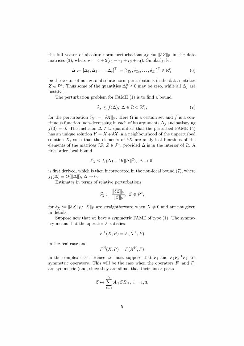
the full vector of absolute norm perturbations δZ := ‖δZ‖F in the datamatrices (3), where ν := 4 + 2(r1 + r2 + r3 + r4). Similarly, let

∆ := [∆1,∆2, . . . ,∆r]> := [δZ1 , δZ2 , . . . , δZr ]> ∈ Rr+ (6)

be the vector of non-zero absolute norm perturbations in the data matricesZ ∈ P∗. Thus some of the quantities ∆0

i ≥ 0 may be zero, while all ∆j arepositive.

The perturbation problem for FAME (1) is to find a bound

δX ≤ f(∆), ∆ ∈ Ω ⊂ Rr+, (7)

for the perturbation δX := ‖δX‖F. Here Ω is a certain set and f is a con-tinuous function, non-decreasing in each of its arguments ∆j and satisgyingf(0) = 0. The inclusion ∆ ∈ Ω quarantees that the perturbed FAME (4)has an unique solution Y = X + δX in a neighbourhood of the unperturbedsolution X, such that the elements of δX are analytical functions of theelements of the matrices δZ, Z ∈ P∗, provided ∆ is in the interior of Ω. Afirst order local bound

δX ≤ f1(∆) +O(‖∆‖2), ∆→ 0,

is first derived, which is then incorporated in the non-local bound (7), wheref1(∆) = O(‖∆‖), ∆→ 0.

Estimates in terms of relative perturbations

δ′Z :=‖δZ‖F‖Z‖F

, Z ∈ P∗,

for δ′X := ‖δX‖F/‖X‖F are straightforward when X 6= 0 and are not givenin details.

Suppose now that we have a symmetric FAME of type (1). The symme-try means that the operator F satisfies

F>(X,P ) = F (X>, P )

in the real case andFH(X,P ) = F (XH, P )

in the complex case. Hence we must suppose that F1 and F2F−13 F4 are

symmetric operators. This will be the case when the operators F1 and F3

are symmetric (and, since they are affine, that their linear parts

Z 7→ri∑k=1

AikZBik, i = 1, 3,

5

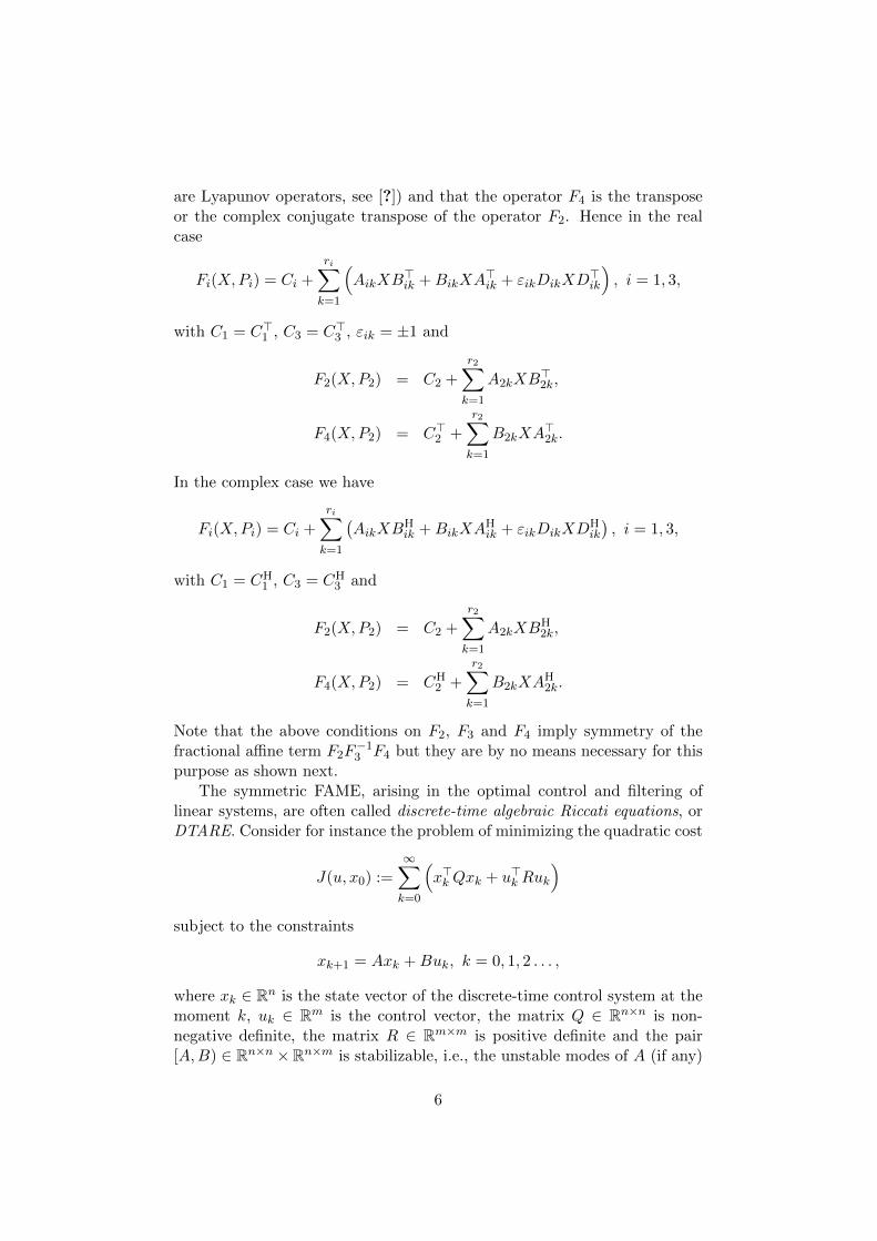
are Lyapunov operators, see [?]) and that the operator F4 is the transposeor the complex conjugate transpose of the operator F2. Hence in the realcase

Fi(X,Pi) = Ci +

ri∑k=1

(AikXB

>ik +BikXA

>ik + εikDikXD

>ik

), i = 1, 3,

with C1 = C>1 , C3 = C>3 , εik = ±1 and

F2(X,P2) = C2 +

r2∑k=1

A2kXB>2k,

F4(X,P2) = C>2 +

r2∑k=1

B2kXA>2k.

In the complex case we have

Fi(X,Pi) = Ci +

ri∑k=1

(AikXB

Hik +BikXA

Hik + εikDikXD

Hik

), i = 1, 3,

with C1 = CH1 , C3 = CH

3 and

F2(X,P2) = C2 +

r2∑k=1

A2kXBH2k,

F4(X,P2) = CH2 +

r2∑k=1

B2kXAH2k.

Note that the above conditions on F2, F3 and F4 imply symmetry of thefractional affine term F2F

−13 F4 but they are by no means necessary for this

purpose as shown next.The symmetric FAME, arising in the optimal control and filtering of

linear systems, are often called discrete-time algebraic Riccati equations, orDTARE. Consider for instance the problem of minimizing the quadratic cost

J(u, x0) :=

∞∑k=0

(x>k Qxk + u>k Ruk

)subject to the constraints

xk+1 = Axk +Buk, k = 0, 1, 2 . . . ,

where xk ∈ Rn is the state vector of the discrete-time control system at themoment k, uk ∈ Rm is the control vector, the matrix Q ∈ Rn×n is non-negative definite, the matrix R ∈ Rm×m is positive definite and the pair[A,B) ∈ Rn×n ×Rn×m is stabilizable, i.e., the unstable modes of A (if any)

6

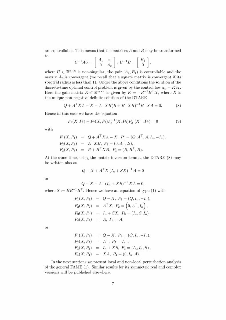
are controllable. This means that the matrices A and B may be transformedto

U−1AU =

[A1 ×0 A2

], U−1B =

[B1

0

],

where U ∈ Rn×n is non-singular, the pair [A1, B1) is controllable and thematrix A2 is convergent (we recall that a square matrix is convergent if itsspectral radius is less than 1). Under the above conditions the solution of thediscrete-time optimal control problem is given by the control law uk = Kxk.Here the gain matrix K ∈ Rm×n is given by K = −R−1B>X, where X isthe unique non-negative definite solution of the DTARE

Q+A>XA−X −A>XB(R+B>XB)−1B>XA = 0. (8)

Hence in this case we have the equation

F1(X,P1) + F2(X,P2)F−13 (X,P3)F

>2 (X>, P2) = 0 (9)

with

F1(X,P1) = Q+A>XA−X, P1 = (Q,A>, A, In,−In),

F2(X,P2) = A>XB, P2 = (0, A>, B),

F3(X,P3) = R+B>XB, P3 = (R,B>, B).

At the same time, using the matrix inversion lemma, the DTARE (8) maybe written also as

Q−X +A>X (In + SX)−1A = 0

orQ−X +A> (In +XS)−1XA = 0,

where S := BR−1B>. Hence we have an equation of type (1) with

F1(X,P1) = Q−X, P1 = (Q, In,−In),

F2(X,P2) = A>X, P2 =(

0, A>, In

),

F3(X,P3) = In + SX, P3 = (In, S, In) ,

F4(X,P4) = A, P4 = A,

or

F1(X,P1) = Q−X, P1 = (Q, In,−In),

F2(X,P2) = A>, P2 = A>,

F3(X,P3) = In +XS, P3 = (In, In, S) ,

F4(X,P4) = XA, P4 = (0, In, A).

In the next sections we present local and non-local perturbation analysisof the general FAME (1). Similar results for its symmetric real and complexversions will be published elsewhere.

7

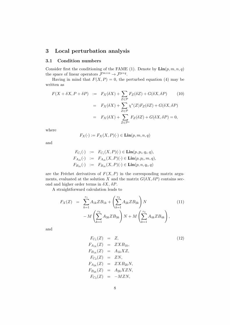
3 Local perturbation analysis

3.1 Condition numbers

Consider first the conditioning of the FAME (1). Denote by Lin(p,m, n, q)the space of linear operators Fm×n → Fp×q.

Having in mind that F (X,P ) = 0, the perturbed equation (4) may bewritten as

F (X + δX, P + δP ) := FX(δX) +∑Z∈P

FZ(δZ) +G(δX, δP ) (10)

= FX(δX) +∑Z∈P

χ∗(Z)FZ(δZ) +G(δX, δP )

= FX(δX) +∑Z∈P∗

FZ(δZ) +G(δX, δP ) = 0,

whereFX(·) := FX(X,P )(·) ∈ Lin(p,m, n, q)

and

FCi(·) := FCi(X,P )(·) ∈ Lin(p, pi, qi, q),

FAik(·) := FAik

(X,P )(·) ∈ Lin(p, pi,m, q),

FBik(·) := FBik

(X,P )(·) ∈ Lin(p, n, qi, q)

are the Frechet derivatives of F (X,P ) in the corresponding matrix argu-ments, evaluated at the solution X and the matrix G(δX, δP ) contains sec-ond and higher order terms in δX, δP .

A straightforward calculation leads to

FX(Z) =

r1∑k=1

A1kZB1k +

(r2∑k=1

A2kZB2k

)N (11)

−M

(r3∑k=1

A3kZB3k

)N +M

(r4∑k=1

A4kZB4k

),

and

FC1(Z) = Z, (12)

FA1k(Z) = ZXB1k,

FB1k(Z) = A1kXZ,

FC2(Z) = ZN,

FA2k(Z) = ZXB2kN,

FB2k(Z) = A2kXZN,

FC3(Z) = −MZN,

8

FA3k(Z) = −MZXB3kN,

FB3k(Z) = −MA3kXZN,

FC4(Z) = MZ,

FA4k(Z) = MZXB4k,

FB4k(Z) = MA4kXZ,

where

M := F2(X,P )F−13 (X,P ), (13)

N := F−13 (X,P )F4(X,P ).

Since the operator FX(.) is invertible we get

δX = −∑Z∈P∗

F−1X FZ(δZ)− F−1X (G(δX, δP )). (14)

The relation (14) gives

δX ≤∑Z∈P∗

KZδZ +O(‖∆‖2), ∆→ 0, (15)

where the quantities

KZ :=∥∥F−1X FZ

∥∥ , Z ∈ P∗, (16)

are the absolute individual condition numbers [5] of FALE (1). Here ‖.‖ isthe induced norm in the corresponding space Lin of linear operators.

If X 6= 0 an estimate in terms of relative perturbations is

δ′X :=‖δX‖F‖X‖F

≤∑Z∈P∗

kZδ′Z +O(‖∆‖2), ∆→ 0,

where the scalars

kZ := KZ‖Z‖F‖X‖F

, Z ∈ P∗,

are the relative condition numbers with respect to perturbations in the ma-trix coefficients Z ∈ P∗.

The calculation of the condition numbers KZ is staightforward. De-note by LZ ∈ Fpq×rt the matrix representation of the operator FZ(·) ∈Lin(p, r, t, q). We have

LX =

r1∑k=1

B>1k ⊗A1k +

r2∑k=1

(B2kN)> ⊗A2k (17)

−r3∑k=1

(B3kN)> ⊗ (MA3k) +

r4∑k=1

B>4k ⊗ (MA4k),

9

and

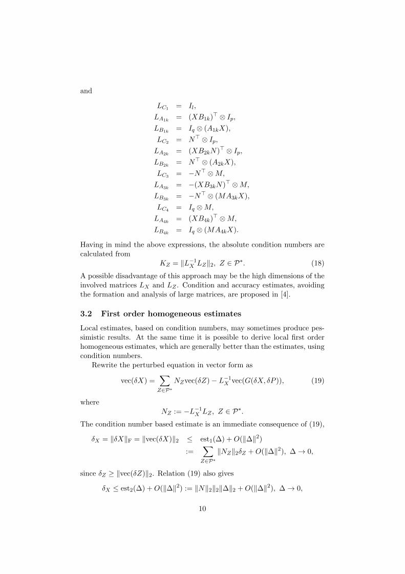
LC1 = Il,

LA1k= (XB1k)

> ⊗ Ip,LB1k

= Iq ⊗ (A1kX),

LC2 = N> ⊗ Ip,LA2k

= (XB2kN)> ⊗ Ip,LB2k

= N> ⊗ (A2kX),

LC3 = −N> ⊗M,

LA3k= −(XB3kN)> ⊗M,

LB3k= −N> ⊗ (MA3kX),

LC4 = Iq ⊗M,

LA4k= (XB4k)

> ⊗M,

LB4k= Iq ⊗ (MA4kX).

Having in mind the above expressions, the absolute condition numbers arecalculated from

KZ = ‖L−1X LZ‖2, Z ∈ P∗. (18)

A possible disadvantage of this approach may be the high dimensions of theinvolved matrices LX and LZ . Condition and accuracy estimates, avoidingthe formation and analysis of large matrices, are proposed in [4].

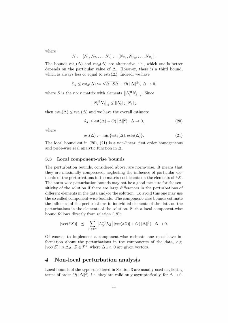
3.2 First order homogeneous estimates

Local estimates, based on condition numbers, may sometimes produce pes-simistic results. At the same time it is possible to derive local first orderhomogeneous estimates, which are generally better than the estimates, usingcondition numbers.

Rewrite the perturbed equation in vector form as

vec(δX) =∑Z∈P∗

NZvec(δZ)− L−1X vec(G(δX, δP )), (19)

whereNZ := −L−1X LZ , Z ∈ P∗.

The condition number based estimate is an immediate consequence of (19),

δX = ‖δX‖F = ‖vec(δX)‖2 ≤ est1(∆) +O(‖∆‖2):=

∑Z∈P∗

‖NZ‖2δZ +O(‖∆‖2), ∆→ 0,

since δZ ≥ ‖vec(δZ)‖2. Relation (19) also gives

δX ≤ est2(∆) +O(‖∆‖2) := ‖N‖2‖2‖∆‖2 +O(‖∆‖2), ∆→ 0,

10

whereN := [N1, N2, . . . , Nr] := [NZ1 , NZ2 , . . . , NZr ] .

The bounds est1(∆) and est2(∆) are alternative, i.e., which one is betterdepends on the particular value of ∆. However, there is a third bound,which is always less or equal to est1(∆). Indeed, we have

δX ≤ est3(∆) :=√

∆>S∆ +O(‖∆‖2), ∆→ 0,

where S is the r × r matrix with elements∥∥NH

i Nj

∥∥2. Since∥∥NH

i Nj

∥∥2≤ ‖Ni‖2‖Nj‖2

then est3(∆) ≤ est1(∆) and we have the overall estimate

δX ≤ est(∆) +O(‖∆‖2), ∆→ 0, (20)

whereest(∆) := minest2(∆), est3(∆). (21)

The local bound est in (20), (21) is a non-linear, first order homogeneousand piece-wise real analytic function in ∆.

3.3 Local component-wise bounds

The perturbation bounds, considered above, are norm-wise. It means thatthey are maximally compressed, neglecting the influence of particular ele-ments of the perturbations in the matrix coefficients on the elements of δX.The norm-wise perturbation bounds may not be a good measure for the sen-sitivity of the solution if there are large differences in the perturbations ofdifferent elements in the data and/or the solution. To avoid this one may usethe so called component-wise bounds. The component-wise bounds estimatethe influence of the perturbations in individual elements of the data on theperturbations in the elements of the solution. Such a local component-wisebound follows directly from relation (19):

|vec(δX)| ∑Z∈P∗

∣∣L−1X LZ∣∣ |vec(δZ)|+O(‖∆‖2), ∆→ 0.

Of course, to implement a component-wise estimate one must have in-formation about the perturbations in the components of the data, e.g.|vec(Z)| ∆Z , Z ∈ P∗, where ∆Z 0 are given vectors.

4 Non-local perturbation analysis

Local bounds of the type considered in Section 3 are usually used neglectingterms of order O(‖∆‖2), i.e. they are valid only asymptotically, for ∆→ 0.

11

Unfortunately, it is usually impossible to say, having a small but a finite per-turbation ∆, whether the neglected terms are indeed negligible. We can noteven claim that the magnitude of the neglected terms is less, or of the orderof magnitude of the local bound. Even for simple linear equations the localbound may always underestimate the actual perturbation in the solution fora class perturbations in the data. Moreover, for some critical values of theperturbations in the coefficient matrices the solution may not exist (or maygo to infinity when these critical values are approached). Nevertheless, evenin such cases the local estimates will still produce a ‘bound’ for a very largeor even for a non-existing solution which surely is not desirable.

The disadvantages of the local estimates may be overcome using thetechniques of non-linear perturbation analysis. As a result we get a domainΩ ⊂ Rr+ and a non-linear function f : Ω → R+ such that δX ≤ f(∆)for all ∆ ∈ Ω as described in the end of Section 2. In connection withthis we would like to emphasize two important issues. First, the inclusion∆ ∈ Ω guarantees that the perturbed equation has an unique solution ina neighbourhood of the unperturbed solution (this is an independent andessential point). And second, the estimate δX ≤ f(∆) is rigorous, i.e., theinequality always holds true for perturbations with ∆ ∈ Ω, which is not thecase with the local bounds. Unfortunately, the non-local bound may notexist or may be pessimistic in some cases.

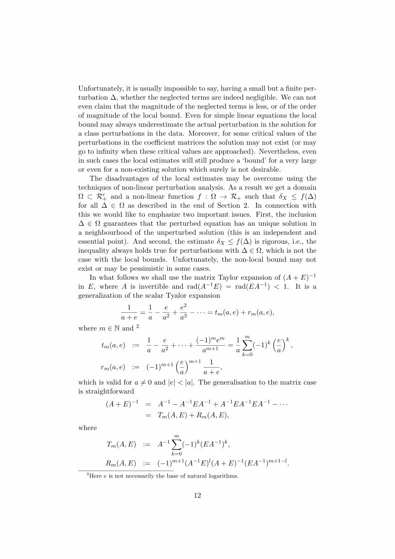
In what follows we shall use the matrix Taylor expansion of (A + E)−1

in E, where A is invertible and rad(A−1E) = rad(EA−1) < 1. It is ageneralization of the scalar Tyalor expansion

1

a+ e=

1

a− e

a2+e2

a3− · · · = tm(a, e) + rm(a, e),

where m ∈ N and 2

tm(a, e) :=1

a− e

a2+ · · ·+ (−1)mem

am+1=

1

a

m∑k=0

(−1)k( ea

)k,

rm(a, e) := (−1)m+1( ea

)m+1 1

a+ e,

which is valid for a 6= 0 and |e| < |a|. The generalisation to the matrix caseis straightforward

(A+ E)−1 = A−1 −A−1EA−1 +A−1EA−1EA−1 − · · ·= Tm(A,E) +Rm(A,E),

where

Tm(A,E) := A−1m∑k=0

(−1)k(EA−1)k,

Rm(A,E) := (−1)m+1(A−1E)l(A+ E)−1(EA−1)m+1−l.

2Here e is not necessarily the base of natural logarithms.

12

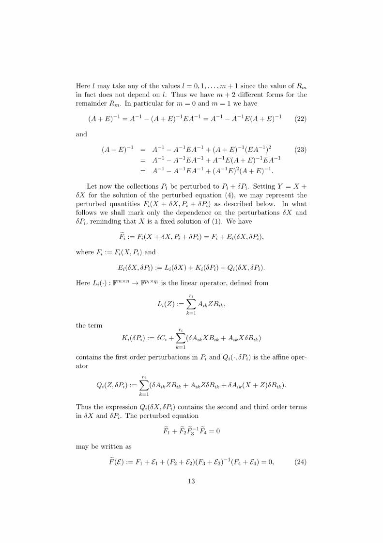
Here l may take any of the values l = 0, 1, . . . ,m+ 1 since the value of Rmin fact does not depend on l. Thus we have m + 2 different forms for theremainder Rm. In particular for m = 0 and m = 1 we have

(A+ E)−1 = A−1 − (A+ E)−1EA−1 = A−1 −A−1E(A+ E)−1 (22)

and

(A+ E)−1 = A−1 −A−1EA−1 + (A+ E)−1(EA−1)2 (23)

= A−1 −A−1EA−1 +A−1E(A+ E)−1EA−1

= A−1 −A−1EA−1 + (A−1E)2(A+ E)−1.

Let now the collections Pi be perturbed to Pi + δPi. Setting Y = X +δX for the solution of the perturbed equation (4), we may represent theperturbed quantities Fi(X + δX, Pi + δPi) as described below. In whatfollows we shall mark only the dependence on the perturbations δX andδPi, reminding that X is a fixed solution of (1). We have

Fi := Fi(X + δX, Pi + δPi) = Fi + Ei(δX, δPi),

where Fi := Fi(X,Pi) and

Ei(δX, δPi) := Li(δX) +Ki(δPi) +Qi(δX, δPi).

Here Li(·) : Fm×n → Fpi×qi is the linear operator, defined from

Li(Z) :=

ri∑k=1

AikZBik,

the term

Ki(δPi) := δCi +

ri∑k=1

(δAikXBik +AikXδBik)

contains the first order perturbations in Pi and Qi(·, δPi) is the affine oper-ator

Qi(Z, δPi) :=

ri∑k=1

(δAikZBik +AikZδBik + δAik(X + Z)δBik).

Thus the expression Qi(δX, δPi) contains the second and third order termsin δX and δPi. The perturbed equation

F1 + F2F−13 F4 = 0

may be written as

F (E) := F1 + E1 + (F2 + E2)(F3 + E3)−1(F4 + E4) = 0, (24)

13

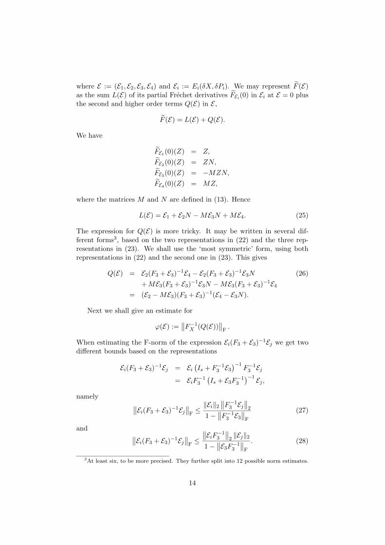
where E := (E1, E2, E3, E4) and Ei := Ei(δX, δPi). We may represent F (E)as the sum L(E) of its partial Frechet derivatives FEi(0) in Ei at E = 0 plusthe second and higher order terms Q(E) in E ,

F (E) = L(E) +Q(E).

We have

FE1(0)(Z) = Z,

FE2(0)(Z) = ZN,

FE3(0)(Z) = −MZN,

FE4(0)(Z) = MZ,

where the matrices M and N are defined in (13). Hence

L(E) = E1 + E2N −ME3N +ME4. (25)

The expression for Q(E) is more tricky. It may be written in several dif-ferent forms3, based on the two representations in (22) and the three rep-resentations in (23). We shall use the ‘most symmetric’ form, using bothrepresentations in (22) and the second one in (23). This gives

Q(E) = E2(F3 + E3)−1E4 − E2(F3 + E3)−1E3N (26)

+ME3(F3 + E3)−1E3N −ME3(F3 + E3)−1E4= (E2 −ME3)(F3 + E3)−1(E4 − E3N).

Next we shall give an estimate for

ϕ(E) :=∥∥F−1X (Q(E))

∥∥F.

When estimating the F-norm of the expression Ei(F3 + E3)−1Ej we get twodifferent bounds based on the representations

Ei(F3 + E3)−1Ej = Ei(Is + F−13 E3

)−1F−13 Ej

= EiF−13

(Is + E3F−13

)−1 Ej ,namely ∥∥Ei(F3 + E3)−1Ej

∥∥F≤‖Ei‖2

∥∥F−13 Ej∥∥2

1−∥∥F−13 E3

∥∥F

(27)

and ∥∥Ei(F3 + E3)−1Ej∥∥F≤∥∥EiF−13

∥∥2‖Ej‖2

1−∥∥E3F−13

∥∥F

. (28)

3At least six, to be more precised. They further split into 12 possible norm estimates.

14

In order to have equal denominators we must choose the first (27) or thesecond (28) option in all four terms in the first equality in (26). Let fordefiniteness choose the first option (27). Then we have

ϕ(E) ≤∥∥L−1X ∥∥2 ‖E2‖2

∥∥F−13 E4∥∥2

1−∥∥F−13 E3

∥∥F

(29)

+∥∥∥L−1X (

N> ⊗ Ip)∥∥∥

2

‖E2‖2∥∥F−13 E3

∥∥2

1−∥∥F−13 E3

∥∥F

+∥∥L−1X (Iq ⊗M)

∥∥2

‖E3‖2∥∥F−13 E4

∥∥2

1−∥∥F−13 E3

∥∥F

+∥∥∥L−1X (N> ⊗M)

∥∥∥2

‖E3‖2∥∥F−13 E3

∥∥2

1−∥∥F−13 E3

∥∥F

.

Using the second equality in (26) we also get

ϕ(E) ≤∥∥L−1X ∥∥2 ‖E2 −ME3‖2

∥∥F−13 (E4 − E3N)∥∥2

1−∥∥F−13 E3

∥∥F

. (30)

If we choose the option (28) we have

ϕ(E) ≤∥∥L−1X ∥∥2

∥∥E2F−13

∥∥2‖E4‖2

1−∥∥E3F−13

∥∥F

(31)

+∥∥∥L−1X (

N> ⊗ Ip)∥∥∥

2

∥∥E2F−13

∥∥2‖E3‖2

1−∥∥E3F−13

∥∥F

+∥∥L−1X (Iq ⊗M)

∥∥2

∥∥E3F−13

∥∥2‖E4‖2

1−∥∥E3F−13

∥∥F

+∥∥∥L−1X (N> ⊗M)

∥∥∥2

∥∥E3F−13

∥∥2‖E3‖2

1−∥∥E3F−13

∥∥F

.

and

ϕ(E) ≤∥∥L−1X ∥∥2 ‖(E2 −ME3)F−13 ‖2 ‖E4 − E3N‖2

1−∥∥E3F−13

∥∥F

. (32)

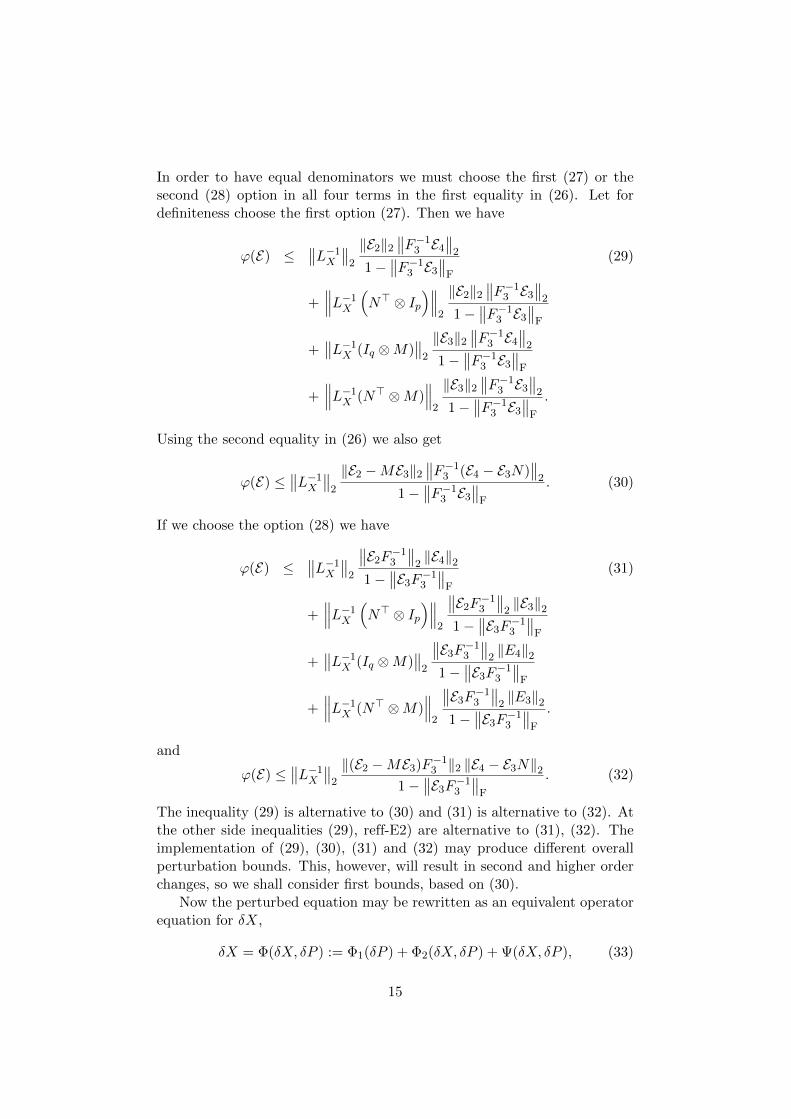
The inequality (29) is alternative to (30) and (31) is alternative to (32). Atthe other side inequalities (29), reff-E2) are alternative to (31), (32). Theimplementation of (29), (30), (31) and (32) may produce different overallperturbation bounds. This, however, will result in second and higher orderchanges, so we shall consider first bounds, based on (30).

Now the perturbed equation may be rewritten as an equivalent operatorequation for δX,

δX = Φ(δX, δP ) := Φ1(δP ) + Φ2(δX, δP ) + Ψ(δX, δP ), (33)

15

where

Φ1(δP ) := −F−1X (K1(δP1) +K2(δP2)N (34)

−MK3(δP3)N +MK4(δP4)),

Φ2(Z, δP ) := −F−1X (Q1(Z, δP1) +Q2(Z, δP2)N

−MQ3(Z, δP3)N +MQ4(Z, δP4)),

Ψ(Z, δP ) := −F−1X ((E2(Z, δP2)−ME3(Z, δP3))

×(F3 + E3(Z, δP3))−1(E4(Z, δP4)− E3(Z, δP3)N)).

Let ‖Z‖F ≤ ρ. After some computations we get

‖E2(Z, δP2)−ME3(Z, δP3)‖2 ≤ α2(∆) + β2(∆)ρ, (35)∥∥F−13 E3(Z, δP3)∥∥F≤ α3(∆) + β3(∆)ρ,∥∥F−13 (E4(Z, δP4)− E3(Z, δP3)N)

∥∥2≤ α4(∆) + β4(∆)ρ,

where, for i = 2, 3, 4,

αi(∆) := αi1(∆) + αi2(∆), (36)

βi(∆) := βi0(∆) + βi1(∆) + βi2(∆).

The quantities

αij(∆) = O(‖∆‖j); βik(∆) = O(‖∆‖k), ∆→ 0,

are determined as follows.Case i = 2:

α21(∆) := δC2 +

r2∑k=1

(‖XB2k‖2δA2k+ ‖A2kX‖2δB2k

) (37)

+ ‖M‖2δC3 +

r3∑k=1

(‖M‖2‖XB3k‖2δA3k+ ‖MA3kX‖2δB3k

),

α22(∆) := ‖X‖2β22(∆),

β20(∆) :=

∥∥∥∥∥r2∑k=1

B>2k ⊗A2k −r3∑k=1

B>3k ⊗ (MA3k)

∥∥∥∥∥2

,

β21(∆) :=

r2∑k=1

(‖B2k‖2δA2k+ ‖A2k‖2δB2k

)

+

r3∑k=1

(‖M‖2‖B3k‖2δA3k+ ‖MA3k‖2δB3k

),

β22(∆) :=

r2∑k=1

δA2kδB2k

+ ‖M‖2r3∑k=1

δA3kδB3k

.

16

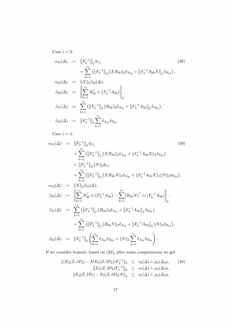
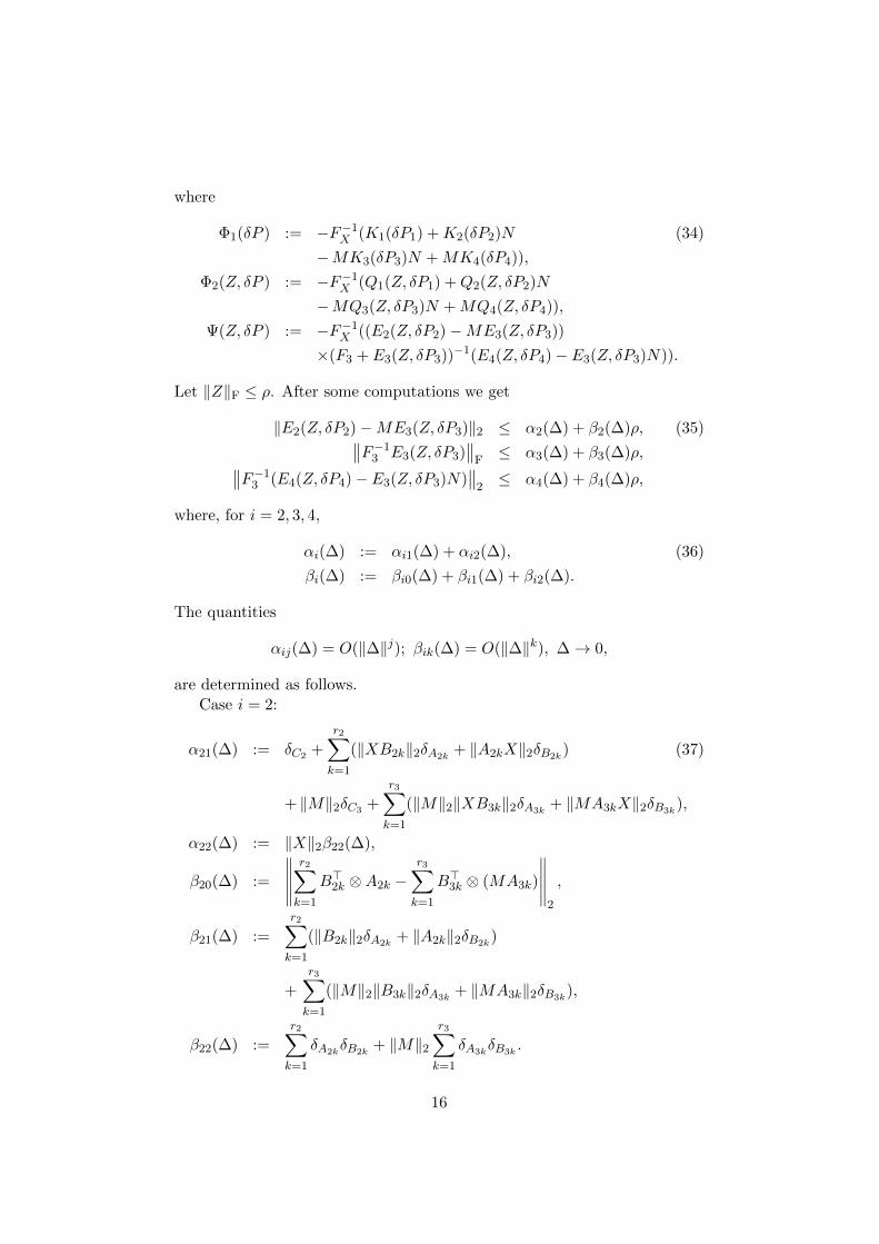
Case i = 3:

α31(∆) :=∥∥F−13

∥∥2δC3 (38)

+

r3∑k=1

(∥∥F−13

∥∥2‖XB3k‖2δA3k

+∥∥F−13 A3kX

∥∥2δB3k

),

α32(∆) := ‖X‖2β32(∆),

β30(∆) :=

∥∥∥∥∥r3∑k=1

B>3k ⊗(F−13 A3k

)∥∥∥∥∥2

,

β31(∆) :=

r3∑k=1

(∥∥F−13

∥∥2‖B3k‖2δA3k

+∥∥F−13 A3k

∥∥2δB3k

),

β32(∆) :=∥∥F−13

∥∥2

r3∑k=1

δA3kδB3k

.

Case i = 4:

α41(∆) :=∥∥F−13

∥∥2δC4 (39)

+

r4∑k=1

(∥∥F−13

∥∥2‖XB4k‖2δA4k

+ ‖F−13 A4kX‖2δB4k

)+∥∥F−13

∥∥2‖N‖2δC3

+

r3∑k=1

(∥∥F−13

∥∥2‖XB3kN‖2δA3k

+ ‖F−13 A3kX‖2‖N‖2δB3k

),

α42(∆) := ‖X‖2β42(∆),

β40(∆) :=

∥∥∥∥∥r4∑k=1

B>4k ⊗(F−13 A4k

)−

r3∑k=1

(B3kN)> ⊗ (F−13 A3k)

∥∥∥∥∥2

,

β41(∆) :=

r4∑k=1

(∥∥F−13

∥∥2‖B4k‖2δA4k

+∥∥F−13 A4k

∥∥2δB4k

)+

r3∑k=1

(∥∥F−13

∥∥2‖B3kN‖2δA3k

+∥∥F−13 A3k

∥∥2‖N‖2δB3k

),

β42(∆) :=∥∥F−13

∥∥2

(r4∑k=1

δA4kδB4k

+ ‖N‖2r3∑k=1

δA3kδB3k

).

If we consider bounds, based on (32), after some computations we get

‖(E2(Z, δP2)−ME3(Z, δP3))F−13 ‖2 ≤ ν2(∆) + µ2(∆)ρ, (40)∥∥E3(Z, δP3)F−13

∥∥F≤ ν3(∆) + µ3(∆)ρ,

‖E4(Z, δP4)− E3(Z, δP3)N‖2 ≤ ν4(∆) + µ4(∆)ρ,

17

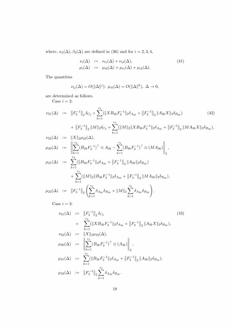
where, α3(∆), β3(∆) are defined in (36) and for i = 2, 3, 4,

νi(∆) := νi1(∆) + νi2(∆), (41)

µi(∆) := µi0(∆) + µi1(∆) + µi2(∆).

The quantities

νij(∆) = O(‖∆‖j); µik(∆) = O(‖∆‖k), ∆→ 0,

are determined as follows.Case i = 2:

ν21(∆) :=∥∥F−13

∥∥2δC2 +

r2∑k=1

(‖XB2kF−13 ‖2δA2k

+∥∥F−13

∥∥2‖A2kX‖2δB2k

) (42)

+∥∥F−13

∥∥2‖M‖2δC3 +

r3∑k=1

(‖M‖2‖XB3kF−13 ‖2δA3k

+∥∥F−13

∥∥2‖MA3kX‖2δB3k

),

ν22(∆) := ‖X‖2µ22(∆),

µ20(∆) :=

∥∥∥∥∥r2∑k=1

(B2kF−13 )> ⊗A2k −

r3∑k=1

(B3kF−13 )> ⊗ (MA3k)

∥∥∥∥∥2

,

µ21(∆) :=

r2∑k=1

(‖B2kF−13 ‖2δA2k

+∥∥F−13

∥∥2‖A2k‖2δB2k

)

+

r3∑k=1

(‖M‖2‖B3kF−13 ‖2δA3k

+∥∥F−13

∥∥2‖MA3k‖2δB3k

),

µ22(∆) :=∥∥F−13

∥∥2

(r2∑k=1

δA2kδB2k

+ ‖M‖2r3∑k=1

δA3kδB3k

).

Case i = 3:

ν31(∆) :=∥∥F−13

∥∥2δC3 (43)

+

r3∑k=1

(‖XB3kF−13 ‖2δA3k

+∥∥F−13

∥∥2‖A3kX‖2δB3k

),

ν32(∆) := ‖X‖2µ32(∆),

µ30(∆) :=

∥∥∥∥∥r3∑k=1

(B3kF−13 )> ⊗ (A3k)

∥∥∥∥∥2

,

µ31(∆) :=

r3∑k=1

(‖B3kF−13 ‖2δA3k

+∥∥F−13

∥∥2‖A3k‖2δB3k

),

µ32(∆) :=∥∥F−13

∥∥2

r3∑k=1

δA3kδB3k

.

18

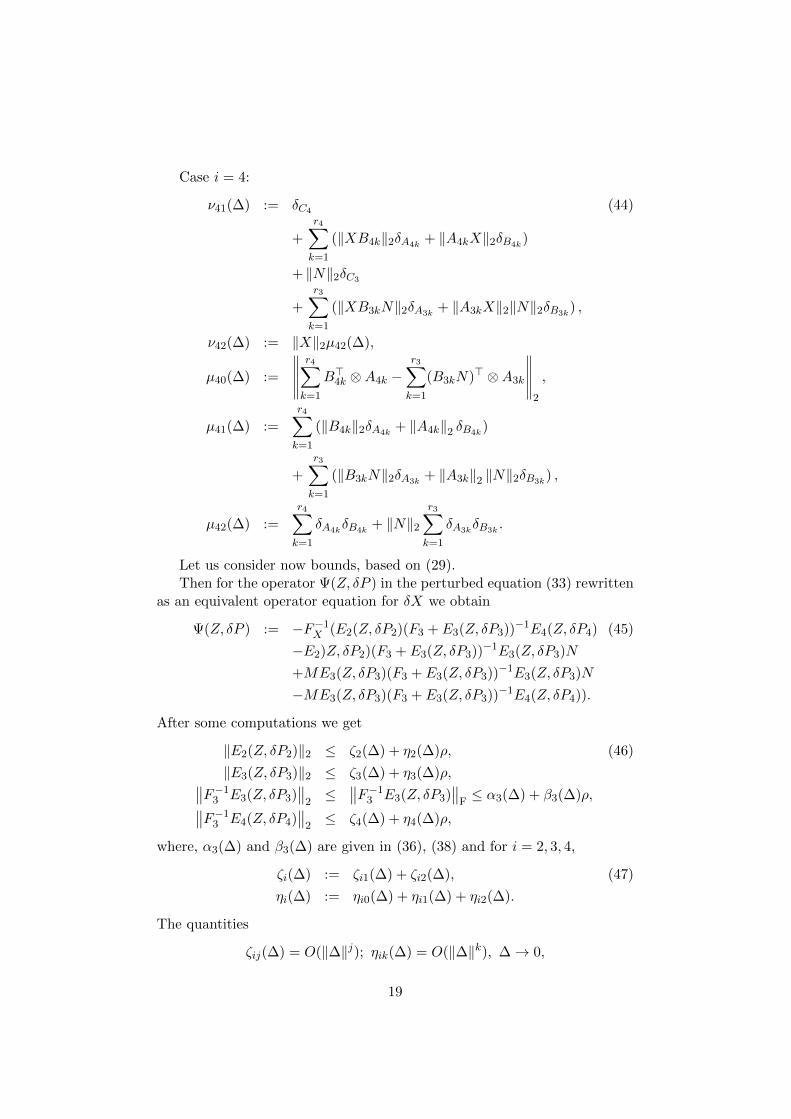
Case i = 4:

ν41(∆) := δC4 (44)

+

r4∑k=1

(‖XB4k‖2δA4k+ ‖A4kX‖2δB4k

)

+ ‖N‖2δC3

+

r3∑k=1

(‖XB3kN‖2δA3k+ ‖A3kX‖2‖N‖2δB3k

) ,

ν42(∆) := ‖X‖2µ42(∆),

µ40(∆) :=

∥∥∥∥∥r4∑k=1

B>4k ⊗A4k −r3∑k=1

(B3kN)> ⊗A3k

∥∥∥∥∥2

,

µ41(∆) :=

r4∑k=1

(‖B4k‖2δA4k+ ‖A4k‖2 δB4k

)

+

r3∑k=1

(‖B3kN‖2δA3k+ ‖A3k‖2 ‖N‖2δB3k

) ,

µ42(∆) :=

r4∑k=1

δA4kδB4k

+ ‖N‖2r3∑k=1

δA3kδB3k

.

Let us consider now bounds, based on (29).Then for the operator Ψ(Z, δP ) in the perturbed equation (33) rewritten

as an equivalent operator equation for δX we obtain

Ψ(Z, δP ) := −F−1X (E2(Z, δP2)(F3 + E3(Z, δP3))−1E4(Z, δP4) (45)

−E2)Z, δP2)(F3 + E3(Z, δP3))−1E3(Z, δP3)N

+ME3(Z, δP3)(F3 + E3(Z, δP3))−1E3(Z, δP3)N

−ME3(Z, δP3)(F3 + E3(Z, δP3))−1E4(Z, δP4)).

After some computations we get

‖E2(Z, δP2)‖2 ≤ ζ2(∆) + η2(∆)ρ, (46)

‖E3(Z, δP3)‖2 ≤ ζ3(∆) + η3(∆)ρ,∥∥F−13 E3(Z, δP3)∥∥2≤

∥∥F−13 E3(Z, δP3)∥∥F≤ α3(∆) + β3(∆)ρ,∥∥F−13 E4(Z, δP4)

∥∥2≤ ζ4(∆) + η4(∆)ρ,

where, α3(∆) and β3(∆) are given in (36), (38) and for i = 2, 3, 4,

ζi(∆) := ζi1(∆) + ζi2(∆), (47)

ηi(∆) := ηi0(∆) + ηi1(∆) + ηi2(∆).

The quantities

ζij(∆) = O(‖∆‖j); ηik(∆) = O(‖∆‖k), ∆→ 0,

19

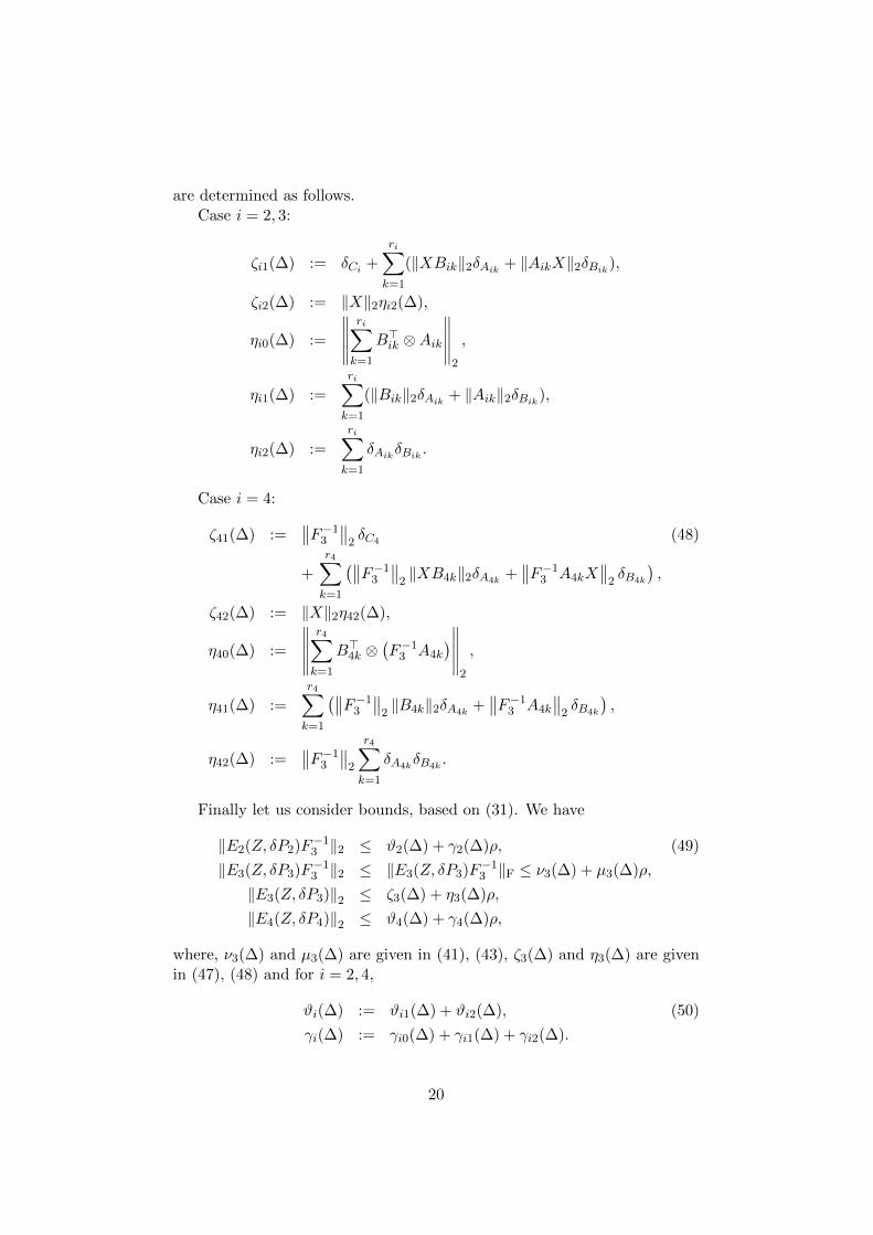
are determined as follows.Case i = 2, 3:

ζi1(∆) := δCi +

ri∑k=1

(‖XBik‖2δAik+ ‖AikX‖2δBik

),

ζi2(∆) := ‖X‖2ηi2(∆),

ηi0(∆) :=

∥∥∥∥∥ri∑k=1

B>ik ⊗Aik

∥∥∥∥∥2

,

ηi1(∆) :=

ri∑k=1

(‖Bik‖2δAik+ ‖Aik‖2δBik

),

ηi2(∆) :=

ri∑k=1

δAikδBik

.

Case i = 4:

ζ41(∆) :=∥∥F−13

∥∥2δC4 (48)

+

r4∑k=1

(∥∥F−13

∥∥2‖XB4k‖2δA4k

+∥∥F−13 A4kX

∥∥2δB4k

),

ζ42(∆) := ‖X‖2η42(∆),

η40(∆) :=

∥∥∥∥∥r4∑k=1

B>4k ⊗(F−13 A4k

)∥∥∥∥∥2

,

η41(∆) :=

r4∑k=1

(∥∥F−13

∥∥2‖B4k‖2δA4k

+∥∥F−13 A4k

∥∥2δB4k

),

η42(∆) :=∥∥F−13

∥∥2

r4∑k=1

δA4kδB4k

.

Finally let us consider bounds, based on (31). We have

‖E2(Z, δP2)F−13 ‖2 ≤ ϑ2(∆) + γ2(∆)ρ, (49)

‖E3(Z, δP3)F−13 ‖2 ≤ ‖E3(Z, δP3)F

−13 ‖F ≤ ν3(∆) + µ3(∆)ρ,

‖E3(Z, δP3)‖2 ≤ ζ3(∆) + η3(∆)ρ,

‖E4(Z, δP4)‖2 ≤ ϑ4(∆) + γ4(∆)ρ,

where, ν3(∆) and µ3(∆) are given in (41), (43), ζ3(∆) and η3(∆) are givenin (47), (48) and for i = 2, 4,

ϑi(∆) := ϑi1(∆) + ϑi2(∆), (50)

γi(∆) := γi0(∆) + γi1(∆) + γi2(∆).

20

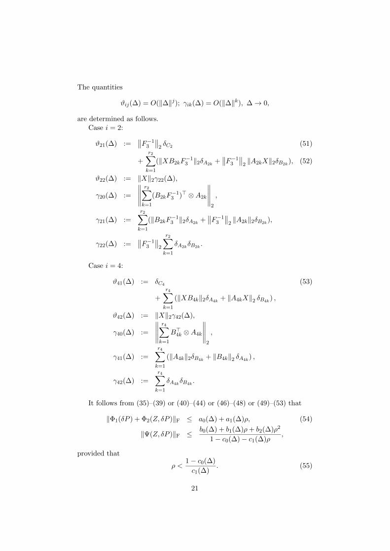
The quantities

ϑij(∆) = O(‖∆‖j); γik(∆) = O(‖∆‖k), ∆→ 0,

are determined as follows.Case i = 2:

ϑ21(∆) :=∥∥F−13

∥∥2δC2 (51)

+

r2∑k=1

(‖XB2kF−13 ‖2δA2k

+∥∥F−13

∥∥2‖A2kX‖2δB2k

), (52)

ϑ22(∆) := ‖X‖2γ22(∆),

γ20(∆) :=

∥∥∥∥∥r2∑k=1

(B2kF−13 )> ⊗A2k

∥∥∥∥∥2

,

γ21(∆) :=

r2∑k=1

(‖B2kF−13 ‖2δA2k

+∥∥F−13

∥∥2‖A2k‖2δB2k

),

γ22(∆) :=∥∥F−13

∥∥2

r2∑k=1

δA2kδB2k

.

Case i = 4:

ϑ41(∆) := δC4 (53)

+

r4∑k=1

(‖XB4k‖2δA4k+ ‖A4kX‖2 δB4k

) ,

ϑ42(∆) := ‖X‖2γ42(∆),

γ40(∆) :=

∥∥∥∥∥r4∑k=1

B>4k ⊗A4k

∥∥∥∥∥2

,

γ41(∆) :=

r4∑k=1

(‖A4k‖2δB4k+ ‖B4k‖2 δA4k

) ,

γ42(∆) :=

r4∑k=1

δA4kδB4k

.

It follows from (35)–(39) or (40)–(44) or (46)–(48) or (49)–(53) that

‖Φ1(δP ) + Φ2(Z, δP )‖F ≤ a0(∆) + a1(∆)ρ, (54)

‖Ψ(Z, δP )‖F ≤ b0(∆) + b1(∆)ρ+ b2(∆)ρ2

1− c0(∆)− c1(∆)ρ,

provided that

ρ <1− c0(∆)

c1(∆). (55)

21

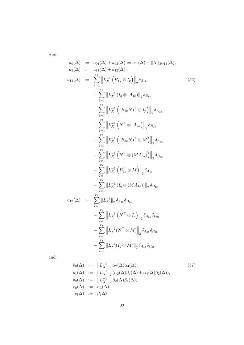
Here

a0(∆) := a01(∆) + a02(∆) := est(∆) + ‖X‖2a12(∆),

a1(∆) := a11(∆) + a12(∆),

a11(∆) :=

r1∑k=1

∥∥∥L−1X (B>1k ⊗ Ip

)∥∥∥2δA1k

(56)

+

r1∑k=1

∥∥L−1X (Iq ⊗ A1k)∥∥2δB1k

+

r2∑k=1

∥∥∥L−1X ((B2kN)> ⊗ Ip

)∥∥∥2δA2k

+

r2∑k=1

∥∥∥L−1X (N> ⊗ A2k

)∥∥∥2δB2k

+

r3∑k=1

∥∥∥L−1X ((B3kN)> ⊗M

)∥∥∥2δA3k

+

r3∑k=1

∥∥∥L−1X (N> ⊗ (MA3k)

)∥∥∥2δB3k

+

r4∑k=1

∥∥∥L−1X (B>4k ⊗M

)∥∥∥2δA4k

+

r4∑k=1

∥∥L−1X (Iq ⊗ (MA4k))∥∥2δB4k

,

a12(∆) :=

r1∑k=1

∥∥L−1X ∥∥2 δA1kδB1k

+

r2∑k=1

∥∥∥L−1X (N> ⊗ Ip

)∥∥∥2δA2k

δB2k

+

r3∑k=1

∥∥∥L−1X (N> ⊗M)∥∥∥2δA3k

δB3k

+

r4∑k=1

∥∥L−1X (Iq ⊗M)∥∥2δA4k

δB4k

and

b0(∆) :=∥∥L−1X ∥∥2 α2(∆)α4(∆), (57)

b1(∆) :=∥∥L−1X ∥∥2 (α2(∆)β4(∆) + α4(∆)β2(∆)),

b2(∆) :=∥∥L−1X ∥∥2 β2(∆)β4(∆),

c0(∆) := α3(∆),

c1∆) := β3∆)

22

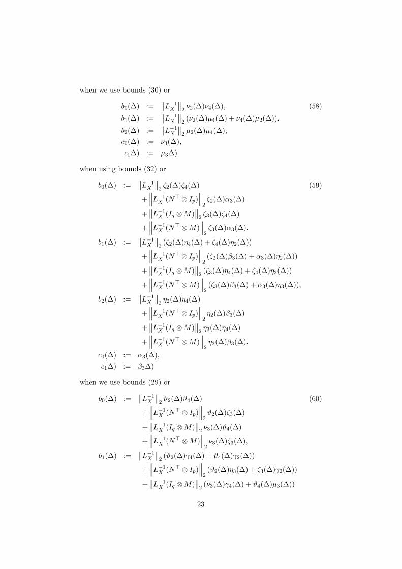
when we use bounds (30) or

b0(∆) :=∥∥L−1X ∥∥2 ν2(∆)ν4(∆), (58)

b1(∆) :=∥∥L−1X ∥∥2 (ν2(∆)µ4(∆) + ν4(∆)µ2(∆)),

b2(∆) :=∥∥L−1X ∥∥2 µ2(∆)µ4(∆),

c0(∆) := ν3(∆),

c1∆) := µ3∆)

when using bounds (32) or

b0(∆) :=∥∥L−1X ∥∥2 ζ2(∆)ζ4(∆) (59)

+∥∥∥L−1X (N> ⊗ Ip)

∥∥∥2ζ2(∆)α3(∆)

+∥∥L−1X (Iq ⊗M)

∥∥2ζ3(∆)ζ4(∆)

+∥∥∥L−1X (N> ⊗M)

∥∥∥2ζ3(∆)α3(∆),

b1(∆) :=∥∥L−1X ∥∥2 (ζ2(∆)η4(∆) + ζ4(∆)η2(∆))

+∥∥∥L−1X (N> ⊗ Ip)

∥∥∥2

(ζ2(∆)β3(∆) + α3(∆)η2(∆))

+∥∥L−1X (Iq ⊗M)

∥∥2

(ζ3(∆)η4(∆) + ζ4(∆)η3(∆))

+∥∥∥L−1X (N> ⊗M)

∥∥∥2

(ζ3(∆)β3(∆) + α3(∆)η3(∆)),

b2(∆) :=∥∥L−1X ∥∥2 η2(∆)η4(∆)

+∥∥∥L−1X (N> ⊗ Ip)

∥∥∥2η2(∆)β3(∆)

+∥∥L−1X (Iq ⊗M)

∥∥2η3(∆)η4(∆)

+∥∥∥L−1X (N> ⊗M)

∥∥∥2η3(∆)β3(∆),

c0(∆) := α3(∆),

c1∆) := β3∆)

when we use bounds (29) or

b0(∆) :=∥∥L−1X ∥∥2 ϑ2(∆)ϑ4(∆) (60)

+∥∥∥L−1X (N> ⊗ Ip)

∥∥∥2ϑ2(∆)ζ3(∆)

+∥∥L−1X (Iq ⊗M)

∥∥2ν3(∆)ϑ4(∆)

+∥∥∥L−1X (N> ⊗M)

∥∥∥2ν3(∆)ζ3(∆),

b1(∆) :=∥∥L−1X ∥∥2 (ϑ2(∆)γ4(∆) + ϑ4(∆)γ2(∆))

+∥∥∥L−1X (N> ⊗ Ip)

∥∥∥2

(ϑ2(∆)η3(∆) + ζ3(∆)γ2(∆))

+∥∥L−1X (Iq ⊗M)

∥∥2

(ν3(∆)γ4(∆) + ϑ4(∆)µ3(∆))

23

+∥∥∥L−1X (N> ⊗M)

∥∥∥2

(ν3(∆)η3(∆) + ζ3(∆)µ3(∆)),

b2(∆) :=∥∥L−1X ∥∥2 γ2(∆)γ4(∆)

+∥∥∥L−1X (N> ⊗ Ip)

∥∥∥2γ2(∆)η3(∆)

+∥∥L−1X (Iq ⊗M)

∥∥2µ3(∆)γ4(∆)

+∥∥∥L−1X (N> ⊗M)

∥∥∥2η3(∆)µ3(∆),

c0(∆) := ν3(∆),

c1(∆) := µ3(∆)

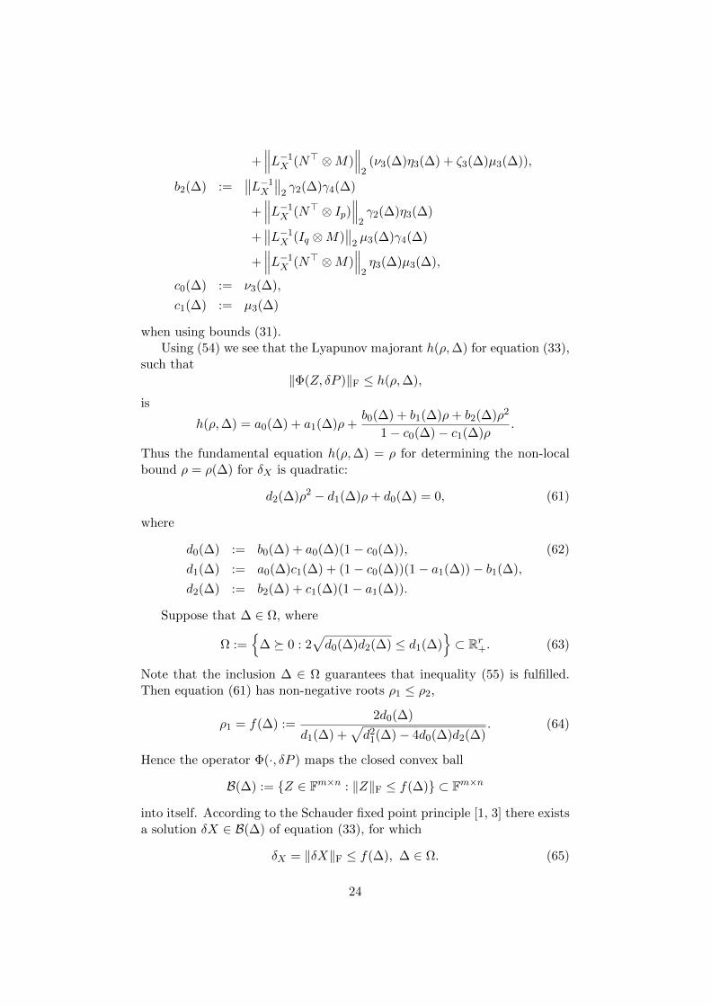
when using bounds (31).Using (54) we see that the Lyapunov majorant h(ρ,∆) for equation (33),

such that‖Φ(Z, δP )‖F ≤ h(ρ,∆),

is

h(ρ,∆) = a0(∆) + a1(∆)ρ+b0(∆) + b1(∆)ρ+ b2(∆)ρ2

1− c0(∆)− c1(∆)ρ.

Thus the fundamental equation h(ρ,∆) = ρ for determining the non-localbound ρ = ρ(∆) for δX is quadratic:

d2(∆)ρ2 − d1(∆)ρ+ d0(∆) = 0, (61)

where

d0(∆) := b0(∆) + a0(∆)(1− c0(∆)), (62)

d1(∆) := a0(∆)c1(∆) + (1− c0(∆))(1− a1(∆))− b1(∆),

d2(∆) := b2(∆) + c1(∆)(1− a1(∆)).

Suppose that ∆ ∈ Ω, where

Ω :=

∆ 0 : 2√d0(∆)d2(∆) ≤ d1(∆)

⊂ Rr+. (63)

Note that the inclusion ∆ ∈ Ω guarantees that inequality (55) is fulfilled.Then equation (61) has non-negative roots ρ1 ≤ ρ2,

ρ1 = f(∆) :=2d0(∆)

d1(∆) +√d21(∆)− 4d0(∆)d2(∆)

. (64)

Hence the operator Φ(·, δP ) maps the closed convex ball

B(∆) := Z ∈ Fm×n : ‖Z‖F ≤ f(∆) ⊂ Fm×n

into itself. According to the Schauder fixed point principle [1, 3] there existsa solution δX ∈ B(∆) of equation (33), for which

δX = ‖δX‖F ≤ f(∆), ∆ ∈ Ω. (65)

24

If ∆ ∈ Ω1, where

Ω1 :=

∆ 0 : 2√d0(∆)d2(∆) < d1(∆)

⊂ Ω,

then ρ1 < ρ2 and the operator Φ(·,∆) is a contraction on B(∆). Hence thesolution δX, for which the estimate (65) holds true, is unique. This meansthat the perturbed equation has an isolated solution Y = X + δX, wherethe elements of δX are analytical functions of the elements of δP .

As a result of the non-local perturbation analysis, presented above, wehave the perturbation bound (65), (64), (63), where the involved quantitiesare determined via the relations (36) – (39), (41) – (44), (47) – (48), (50) –(53), (56), (57) and (62).

References

[1] L. Kantorovich and G. Akilov. Functional Analysis in Normed Spaces.Nauka, Moscow, 1977. In Russian.

[2] M.M. Konstantinov, P.H. Petkov, D.W. Gu, and I. Postlethwaite. Per-turbation analysis in finite dimensional spaces. Technical Report 96–18,Dept. of Engineering, Leicester Univ., Leicester, UK, 1996.

[3] J. Ortega and W. Rheinboldt. Iterative Solution of Nonlinear Equationsin Several Variables. Academic Press, New York, 1970.

[4] P.H. Petkov, M.M. Konstantinov, and V. Mehrmann. DGRSVX andDMSRIC: Fortan 77 subroutines for solving continuous-time matrix alge-braic Riccati equations with condition and accuracy estimates. TechnicalReport SFB393/98-16, Fak. fur Mathematik, TU Chemnitz, Chemnitz,Germany, 1998.

[5] J.R. Rice. A theory of condition. SIAM J. Numer. Anal., 3:287–310,1966.

25