a robust finite element method for darcy--stokes flow

A ROBUST FINITE ELEMENT METHOD FORDARCY–STOKES FLOW∗

KENT ANDRE MARDAL† , XUE-CHENG TAI‡ , AND RAGNAR WINTHER§

SIAM J. NUMER. ANAL. c© 2002 Society for Industrial and Applied MathematicsVol. 40, No. 5, pp. 1605–1631

Abstract. Finite element methods for a family of systems of singular perturbation problems of asaddle point structure are discussed. The system is approximately a linear Stokes problem when theperturbation parameter is large, while it degenerates to a mixed formulation of Poisson’s equationas the perturbation parameter tends to zero. It is established, basically by numerical experiments,that most of the proposed finite element methods for Stokes problem or the mixed Poisson’s systemare not well behaved uniformly in the perturbation parameter. This is used as the motivation forintroducing a new “robust” finite element which exhibits this property.

Key words. singular perturbation problems, Darcy–Stokes flow, nonconforming finite elements,uniform error estimates

AMS subject classifications. 65N12, 65N15, 65N30

PII. S0036142901383910

1. Introduction. Let Ω ⊂ R2 be a bounded and connected polygonal domainwith boundary ∂Ω. In this paper we shall consider finite element methods for thefollowing singular perturbation problem:

(I − ε2∆)u− grad p = f in Ω,divu = g in Ω,

u = 0 on ∂Ω.(1.1)

Here ε ∈ (0, 1] is a parameter, while∆ = diag(∆,∆) is the Laplace operator on vectorfields. The vector field f and scalar field g represent the data. The problem (1.1)admits only a solution if the function g has mean value zero on Ω and “the pressure” pis determined only up to addition of a constant.

We note that when ε is not too small, and g = 0, this problem is simply a stan-dard Stokes problem but with an additional nonharmful lower order term. However,if f = 0 and ε approaches zero, then the model problem formally tends to a mixed for-mulation of the Poisson equation with homogeneous Neumann boundary conditions.

When ε = 0 the first equation in (1.1) has the form of Darcy’s law for flow ina homogeneous porous medium, where u is a volume averaged velocity. In fact, thesystem (1.1) can be regarded as a macroscopic model for flow in an “almost porousmedia,” where u and p represent volume averaged velocity and pressure, respectively.The zero order velocity term in the first equation of (1.1) then typically representsa Stokes drag. An attempt to derive Darcy’s law from volume averaged Stokes flowis, for example, discussed in [16]. Generalizations of the system (1.1) have also beenproposed in the modeling of macrosegregation formation in binary alloy solidification;

∗Received by the editors January 22, 2001; accepted for publication (in revised form) April 23,2002; published electronically October 31, 2002. This research was supported in part by the ResearchCouncil of Norway under grants 128224/431, 133755/441, and 135420/431.

http://www.siam.org/journals/sinum/40-5/38391.html†Department of Informatics, University of Oslo, P.O. Box 1080 Blindern, 0316 Oslo, Norway

([email protected]).‡Department of Mathematics, University of Bergen, Johannes Brunsgt. 12, 5007 Bergen, Norway

([email protected]).§Department of Informatics and Department of Mathematics, University of Oslo, P.O. Box 1080

Blindern, 0316 Oslo, Norway ([email protected]).

1605

https://www.researchgate.net/publication/216756664_Flow_in_Porous_Media_I_A_Theoretical_Derivation_of_Darcy's_Law?el=1_x_8&enrichId=rgreq-42293891-f79c-4286-843a-409b4c655889&enrichSource=Y292ZXJQYWdlOzMwMDY2NzY0O0FTOjk5NzA5MjQ3MDMzMzU3QDE0MDA3ODM5NDU4MjE=

1606 K. A. MARDAL, X.-C. TAI, AND R. WINTHER

cf. [13]. Systems of the form (1.1) may also arise from time discretizations of theNavier–Stokes equation, where the parameter ε corresponds to the square root of thetime step; cf. [4]. However, the study of such time discretizations is not the motivationfor the present paper.

The purpose of the present paper is to discuss a finite element method for themodel problem (1.1) with convergence properties that are uniform with respect tothe perturbation parameter ε. In section 2 we will introduce some notations anddiscuss various properties of the model (1.1). Discretizations of the model problemby the finite element method is described in section 3. In particular, we will statestability conditions which are uniform with respect to the parameter ε and show, bynumerical experiments, that the standard discretizations, proposed either for ε = 1 orε = 0, do not satisfy these stability conditions. A new nonconforming finite elementdiscretization is then proposed in section 4. We show that this new discretizationis uniformly stable, and, as a consequence, we establish in section 5 error estimateswhich are uniform in ε under the assumption that proper regularity estimates hold forthe solution. In section 6 we then study the asymptotic smoothness of the solutionof (1.1) as ε tends to zero. Based on these regularity results we show that, for fixeddata f and g, a uniform O(h1/2) error estimate in a suitable energy norm can bederived.

In the final section of this paper we study an elliptic system which formally is ageneralization of (1.1). This system is given by

(I − ε2∆)u− δ−2 grad(divu− g) = f in Ω,u = 0 on ∂Ω,

(1.2)

where ε, δ ∈ (0, 1]. By introducing p = δ−2(divu−g) this system can be alternativelywritten on the mixed form

(I − ε2∆)u− grad p = f in Ω,divu− δ2p = g in Ω,

u = 0 on ∂Ω.(1.3)

Note that this system also has meaning when δ = 0, and in this case the systemreduces to (1.1).

The symmetric and positive definite system (1.2) is discretized by a straightfor-ward finite element approach, utilizing the new nonconforming velocity space con-structed earlier in this paper; i.e., the mixed system (1.3) is not introduced in thediscretization. We show, by numerical experiments and theory, that under the as-sumption of sufficiently regular solutions we obtain error estimates which are uniformboth in ε and δ.

2. Preliminaries. We will use Hm = Hm(Ω) to denote the Sobolev space ofscalar functions on Ω with m derivatives in L2 = L2(Ω), with norm ‖ · ‖m. Further-more, the notation ‖·‖m,K is used to indicate that the norm is defined with respect toa domain K different from Ω. The seminorm derived from the partial derivatives oforder equal m is denoted | · |m, i.e., | · |2m = ‖ · ‖2

m−‖ · ‖2m−1. The space Hm

0 = Hm0 (Ω)

will denote the closure in Hm of C∞0 (Ω). The dual space of Hm

0 with respect to theL2 inner product will be denoted by H−m. Furthermore, L2

0 will denote the space ofL2 functions with mean value zero. A space written in boldface denotes a 2-vectorvalued analogue of the corresponding scalar space. The notation (·, ·) is used to denotethe L2 inner product on scalar, vector, and matrix valued functions.

https://www.researchgate.net/publication/2503961_Iterative_Techniques_for_Time_Dependent_Stokes_Problems?el=1_x_8&enrichId=rgreq-42293891-f79c-4286-843a-409b4c655889&enrichSource=Y292ZXJQYWdlOzMwMDY2NzY0O0FTOjk5NzA5MjQ3MDMzMzU3QDE0MDA3ODM5NDU4MjE=

https://www.researchgate.net/publication/267477558_A_mathematical_model_of_macrosegregation_formation_in_binary_alloy_solidification?el=1_x_8&enrichId=rgreq-42293891-f79c-4286-843a-409b4c655889&enrichSource=Y292ZXJQYWdlOzMwMDY2NzY0O0FTOjk5NzA5MjQ3MDMzMzU3QDE0MDA3ODM5NDU4MjE=

ROBUST FINITE ELEMENTS FOR DARCY–STOKES FLOW 1607

Below we shall encounter the intersection and sum of Hilbert spaces. We thereforerecall the basic definitions of these concepts. If X and Y are Hilbert spaces, bothcontinuously contained in some larger Hilbert spaces, then the intersection X ∩Y andthe sum X + Y are themselves Hilbert spaces with the norms

‖z‖X∩Y = (‖z‖2X + ‖z‖2

Y )1/2

and

‖z‖X+Y = infz=x+y

x∈X, y∈Y

(‖x‖2X + ‖y‖2

Y )1/2.

Furthermore, if X ∩Y is dense in both X and Y , then (X ∩Y )∗ = X∗+Y ∗. We referthe reader to [3, Chapter 2] for these results.

If q is a scalar field, then grad q will denote the gradient of q, while div v denotesthe divergence of a vector field v. We shall also use the differential operators

curl q =

(−∂q/∂x2

∂q/∂x1

)and rotv = ∂v1/∂x2 − ∂v2/∂x1.

Note that, due to Green’s theorem, these definitions lead to the following “integrationby parts formula”:∫

Ω

curl q · v dx =

∫Ω

q rotv dx+

∫∂Ω

q(v · t) dτ,(2.1)

where t is the unit tangent vector in the counterclockwise direction on ∂Ω, and τ isthe arclength.

The gradient of a vector field v is denoted Dv; i.e., Dv is the 2× 2 matrix withelements

(Dv)i,j = ∂vi/∂xj , 1 ≤ i, j ≤ 2.

Hence, for any u ∈ H2 and v ∈ H10 we have

−(∆u,v) = (Du,Dv) ≡∫

Ω

Du : Dv dx,

where the colon denotes the scalar product of matrix fields. Recall also the identity

∆ = graddiv− curl rot,(2.2)

which can be verified by a direct computation. As a consequence, we obtain theidentity

(Du,Dv) = (divu,div v) + (rotu, rotv) ∀u ∈ H1, v ∈ H10 .(2.3)

In addition to the function spaces introduced above we will also use the spaceH(div) = H(div; Ω) consisting of all vector fields in L2 with divergence in L2, i.e.,

H(div) = v ∈ L2 : div v ∈ L2.Similarly,

H(rot) = v ∈ L2 : rotv ∈ L2,


and the norms of these spaces are denoted by ‖·‖div and ‖·‖rot, respectively. Further-more, H0(div) is the closed subspace of H(div) consisting of functions with vanishingnormal components on the boundary; i.e.,

H0(div) = v ∈ H(div) : v · n = 0 on ∂Ω,where n is the unit outward normal vector.

Throughout this paper aε(·, ·) : H1 ×H1 → R will denote the bilinear form

aε(u,v) = (u,v) + ε2(Du,Dv).

A weak formulation of problem (1.1) is given by the following:Find (u, p) ∈ H1

0 × L20 such that

aε(u,v) + (p,div v) = (f ,v) ∀v ∈ H10 ,

(divu, q) = (g, q) ∀q ∈ L20.

(2.4)

Here we assume that data (f , g) is given in H−1 × L20.

The problem (2.4) has a unique solution (u, p) ∈ H10 × L2

0. This follows fromstandard results for Stokes problem; cf., for example, [11]. However, the bound on(u, p) ∈ H1

0 × L20 will degenerate as ε tends to zero. In fact, for the reduced prob-

lem (2.4) with ε = 0 the space H10 ×L2

0 is not a proper function space for the solution.However, the theory developed in [6] can be applied in this case if we seek (u, p) eitherin H0(div)×L2

0 or in L2 × (H1 ∩L20), and with data (f , g) in the proper dual spaces.

These results are, in fact, consequences of standard results for the Poisson equation.The fact that the regularity of the solution is changed when ε becomes zero

strongly suggests that ε-dependent norms and function spaces are required in order toobtain stability estimates independent of ε. Furthermore, since the reduced problemis well posed for two completely different choices of function spaces, this indicates thatthere are at least two different choices of ε-dependent norms. In the present paperwe will study the problem (1.1) with respect to an ε-dependent norm which reducesto the norm in H0(div)× L2

0 when ε = 0. Our goal is to derive discretizations whichare uniformly stable with respect to ε in this norm. This appears to be the properchoice if we want to study discretizations which also can be generalized to nonmixedapproximations of elliptic problems of the form (1.2).

Remark. When we refer to the reduced system corresponding to (1.1) we refer tothe system (1.1) with ε = 0 and the boundary condition u = 0 replaced by u ·n = 0.This system has a weak formulation given by (2.4) but with the solution space H1

0

replaced by H0(div).The space H0(div) ∩ ε ·H1

0 , with norm ||| · |||ε given by

|||v|||2ε = ‖v‖20 + ‖div v‖2

0 + ε2‖Dv‖20,

is equal to H10 as a set for ε > 0 but equal to H0(div) for ε = 0. The system (2.4)

can alternatively be written as the system

Aε

(up

)=

(fg

),

where the coefficient operator Aε is given by

Aε =

(I − ε2∆ −grad

div 0

).(2.5)

https://www.researchgate.net/publication/202243110_Finite_Element_Methods_for_Navier_Stokes_Equations?el=1_x_8&enrichId=rgreq-42293891-f79c-4286-843a-409b4c655889&enrichSource=Y292ZXJQYWdlOzMwMDY2NzY0O0FTOjk5NzA5MjQ3MDMzMzU3QDE0MDA3ODM5NDU4MjE=


Let Xε be the product space (H0(div) ∩ ε ·H10 )×L2

0 and X∗ε the corresponding

dual space with respect to the L2 inner product. This space can also be expressed as

X∗ε = (H−1(rot) + ε−1H−1)× L2

0.

Here the + sign has the interpretation as the sum of Hilbert spaces, and the spaceH−1(rot) is given by

H−1(rot) = v ∈ H−1 : rotv ∈ H−1.

The operator Aε can be seen to be an isomorphism mapping Xε into X∗ε . Further-

more, the corresponding operator norms

||Aε||L(Xε,X∗ε ) and ||A−1

ε ||L(X∗ε ,Xε)

are independent of ε. In fact, with the definitions above, this is also true for ε ∈ [0, 1];i.e., the endpoint ε = 0 can be included.

The uniform boundedness of Aε is straightforward to check from the definitionsabove, while the uniform boundedness of the inverse can be verified from the twoBrezzi conditions; cf. [6]. For the present problem these conditions read as follows:

There are constants α0, β0 > 0, independent of ε, such that

supv∈H0(div)∩ε·H1

0

(q,div v)

|||v|||ε ≥ α0‖q‖0 ∀q ∈ L20(2.6)

and

aε(v,v) ≥ β0|||v|||2ε ∀v ∈ Z,(2.7)

where Z = v ∈ H10 : div v = 0.

Since it is well known (cf., for example, [11, Chapter 1, Corollary 2.4]) thatcondition (2.6) holds for ε = 1, it also holds for all ε ∈ [0, 1] with the same constant α0.Furthermore, condition (2.7) holds trivially with β0 = 1 for ε ∈ [0, 1].

3. Uniformly stable discretizations. The purpose of this section is to discussfinite element discretizations of the system (1.1). In particular, we shall be interestedin discretizations which are stable uniformly in the parameter ε ∈ (0, 1].

Let Vh ⊂ H10 and Qh ⊂ L2

0 be finite element spaces, where h ∈ (0, 1] is adiscretization parameter. The weak formulation (2.4) leads to the following corre-sponding finite element discretization:

Find (uh, ph) ∈ Vh ×Qh such that

aε(uh,v) + (ph,div v) = (f ,v) ∀v ∈ Vh,(divuh, q) = (g, q) ∀q ∈ Qh.

(3.1)

Remark. Below we shall also encounter several examples of nonconforming ap-proximations of (2.4), i.e., the space Vh H1

0 . In all these examples the bilinearform aε(·, ·) is understood to be the sum of the corresponding integrals over eachelement. No extra jump terms are added. The same remark applies to the energynorm, ||| · |||ε.

The discretization (3.1) is stable in the sense of [6] if proper discrete analogues ofthe conditions (2.6) and (2.7) hold. These conditions are the following.

https://www.researchgate.net/publication/225625854_A_stable_finite_element_for_Stokes_equation_Calcolo?el=1_x_8&enrichId=rgreq-42293891-f79c-4286-843a-409b4c655889&enrichSource=Y292ZXJQYWdlOzMwMDY2NzY0O0FTOjk5NzA5MjQ3MDMzMzU3QDE0MDA3ODM5NDU4MjE=




Stability conditions. The discretization (3.1) is said to be uniformly stable if thereexist constants α, β > 0, independent of ε and h, such that

supv∈Vh

(q,div v)

|||v|||ε ≥ α‖q‖0 ∀q ∈ Qh(3.2)

and

aε(v,v) ≥ β|||v|||2ε ∀v ∈ Zh,(3.3)

where Zh = v ∈ Vh : (div v, q) = 0 ∀q ∈ Qh.For the case ε = 1, or more precisely for ε bounded away from zero, the second

condition is obvious. In this case there are several choices of pairs of finite elementspaces which satisfy (3.2) with α independent of h. We mention, for example, the Minielement proposed in [1] or the P2 − P0 element; i.e., we choose continuous quadraticvelocities for Vh and the corresponding space of piecewise constants for Qh; cf. [10].For a general review of stable Stokes elements we refer the reader to [8].

However, most of these spaces do not lead to discretizations which are stableuniformly in ε. The main reason for this is that when ε approaches zero the secondcondition is no longer obvious. In fact, for the reduced problem with ε = 0 thecondition (3.3) requires

‖v‖20 ≥ β‖v‖2

div ∀v ∈ Zh.

Hence, we must have

‖div v‖0 ≤ c‖v‖0 ∀v ∈ Zh(3.4)

for a suitable constant c independent of h, and this condition does not hold for thecommon conforming stable Stokes elements.

Example 3.1. We consider the problem (1.1) with Ω taken as the unit square.The domain is triangulated by first dividing it into h× h squares. Then, each squareis divided into two triangles by the diagonal with a negative slope. The system is thendiscretized using the P2−P0 element with respect to this triangulation; i.e., Vh ⊂ H1

0

consists of piecewise quadratic functions, while Qh ⊂ L20 is the space of discontinuous

piecewise constants. This discretization is known to be stable when ε > 0 is fixed;cf. [10]. However, our purpose here is to investigate how the convergence behaves asε becomes small.

We consider the system (1.1) with the function g chosen to be identical zero,while f = u− ε2∆u− grad p, where u = curl sin2(πx1) sin

2(πx2) and p = sin(πx1).Hence, in this example the solution is independent of ε.

In Table 3.1 we have computed the relative L2 error in the velocity u; i.e., e(h) =‖u − uh‖0/‖u‖0 for different values of ε and h. A third order Gauss–Legendre rule(cf. [17]) was used here, and in all the other examples of this section, to perform thenecessary integrations. For each fixed ε the convergence rate with respect to h, γis estimated by assuming e(h) = chγ and by computing a least squares fit to thislog-linear relation.

When ε = 1 the convergence seems to be at least quadratic with respect to h inthis case. However, the convergence deteriorates as ε becomes smaller, and for ε = 0there is no convergence.

Table 3.2 is based on the corresponding relative errors in the energy norm, i.e.,the norm ||| · |||ε for velocity and the L2 norm for pressure. For simplicity only theestimated convergence rates are given.


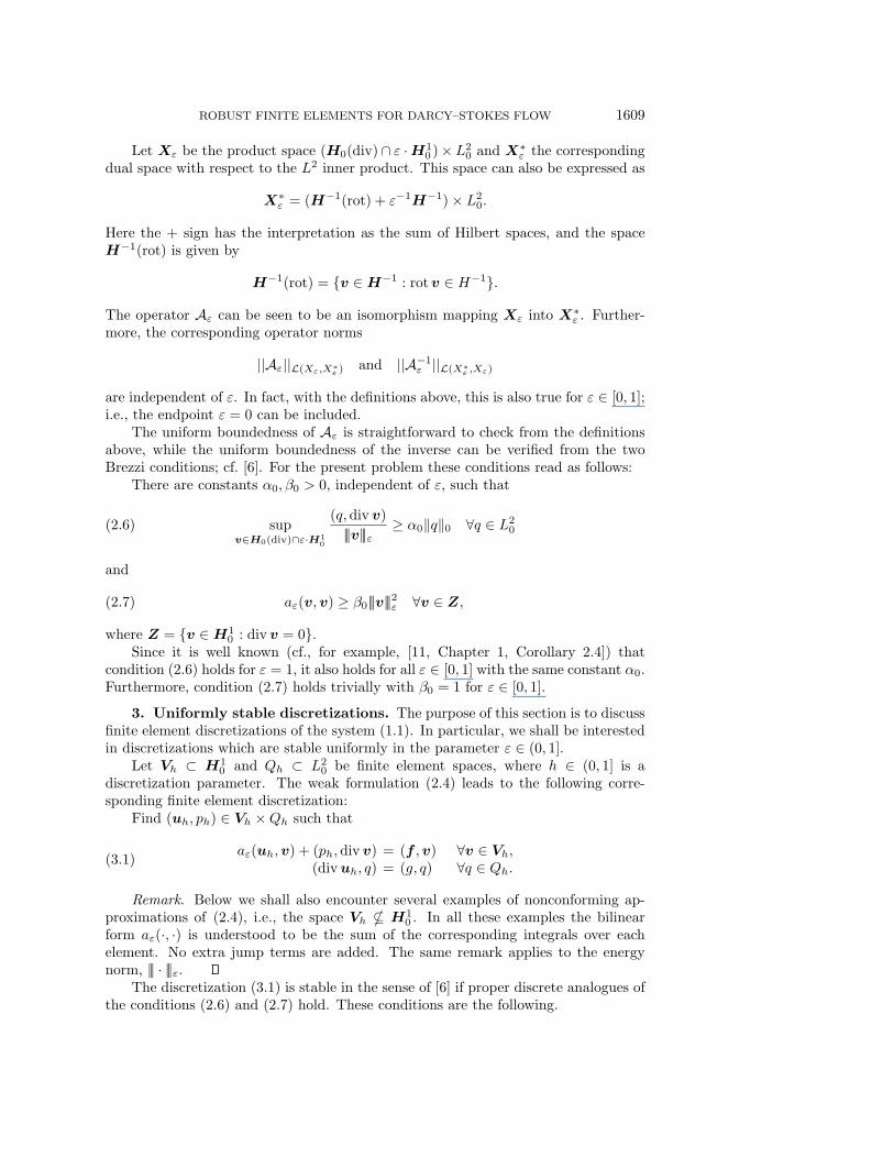
Table 3.1The relative L2 error in velocity obtained by the P2 − P0 element.

ε\ h 2−2 2−3 2−4 2−5 2−6 Rate

1 3.84e-2 4.75e-3 6.41e-4 1.04e-4 2.11e-5 2.72

2−2 6.15e-2 1.73e-2 4.65e-3 1.20e-3 3.05e-4 1.92

2−4 4.55e-1 2.10e-1 6.78e-2 1.86e-2 4.79e-3 1.67

2−8 9.31e-1 9.68e-1 9.43e-1 8.14e-1 5.32e-1 0.19

0 9.35e-1 9.84e-1 1.00 1.01 1.02 -0.03

Table 3.2Estimated convergence rates for the velocity and pressure, measured in the energy norm, for

the P2 − P0 element.

ε 1 2−2 2−4 2−8 0

rate, velocity 1.84 1.01 0.70 -0.79 -1.03

rate, pressure 1.06 1.01 1.09 0.13 -0.20

These results indicate a similar degenerate behavior with respect to ε. In fact,when ε = 0 the norm, |||uh|||ε, seems to grow like h−1 as h approaches zero. Thismust be due to the fact that only the projection of divuh into piecewise constants iscontrolled by the method in this case.

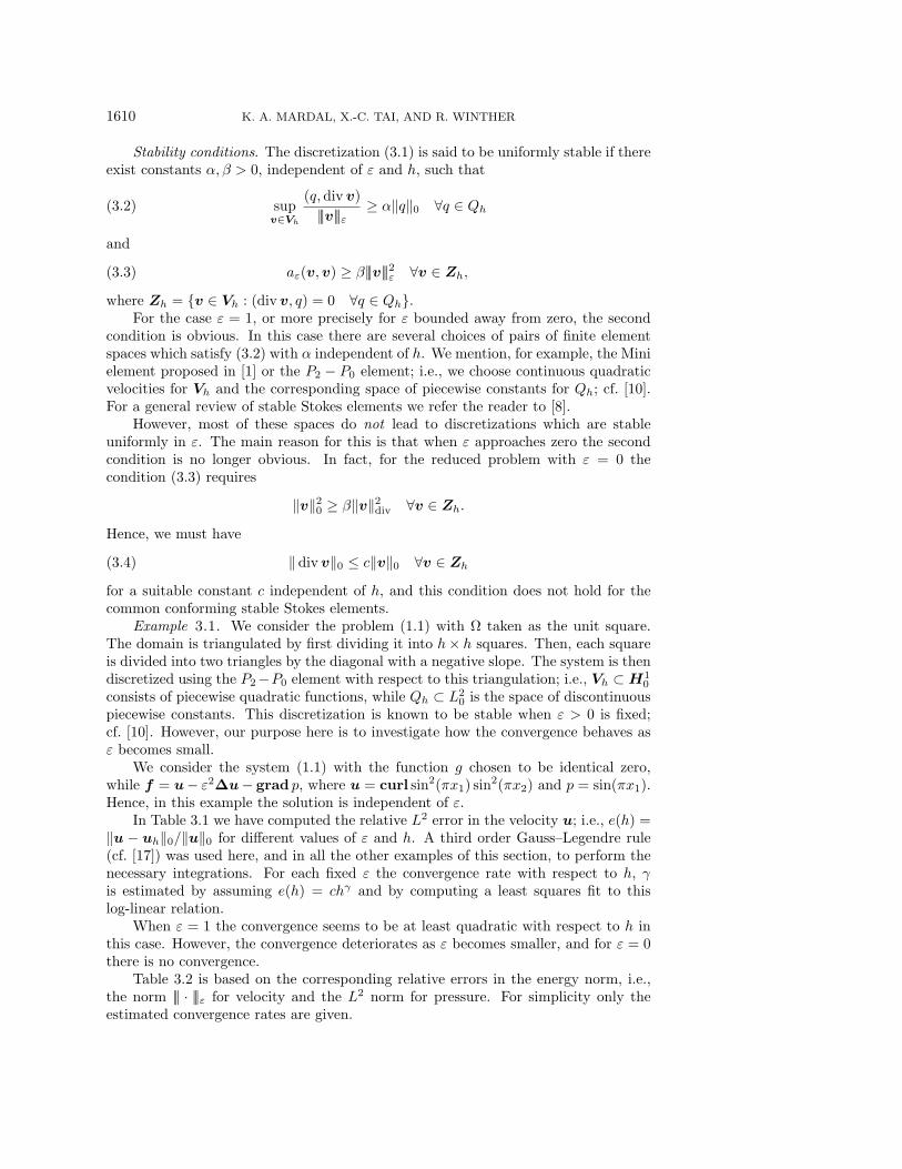
Example 3.2. We repeat the experiment above but with the difference that weuse the nonconforming Crouzeix–Raviart element instead of the P2 −P0 element; i.e.,Vh consists of piecewise linear vector fields which are continuous at the midpoint ofeach edge of the triangulation, while Qh ⊂ L2

0 is the space of piecewise constants. Itis well known that for any fixed ε > 0 this element leads to a stable discretization;cf. [10].

In Table 3.3 we have again computed the relative L2 error in the velocity u fordifferent values of ε and h.

Table 3.3The relative L2 error in velocity obtained by the nonconforming Crouzeix–Raviart element.

ε\ h 2−2 2−3 2−4 2−5 2−6 Rate

1 1.83e-1 4.89e-2 1.26e-2 3.19e-3 8.02e-4 1.96

2−2 2.19e-1 6.89e-2 1.91e-2 4.96e-3 1.26e-3 1.87

2−4 6.42e-1 3.86e-1 1.53e-1 4.58-2 1.21-3 1.45

2−8 9.51e-1 1.00 1.01 9.43e-1 7.44e-1 0.08

0 9.53e-1 1.01 1.04 1.05 1.06 -0.04

The L2 convergence appears to be quadratic when ε is large. However, also inthis case the convergence deteriorates as ε decreases, and for the reduced problem,with ε = 0, the observed values for the relative error is monotonically increasing.

The corresponding estimates of the convergence rates in the energy norm decreasesfrom approximately linear convergence to no convergence as is shown by Table 3.4.

In fact, the divergence of the Crouzeix–Raviart element in the case ε = 0 isnot surprising. Since the divergence-free vector fields in this case can be realized asthe curl operator applied to the corresponding Morley space, this behavior of theCrouzeix–Raviart element is closely tied to the divergence of the Morley element forthe Poisson equation; cf. [14].


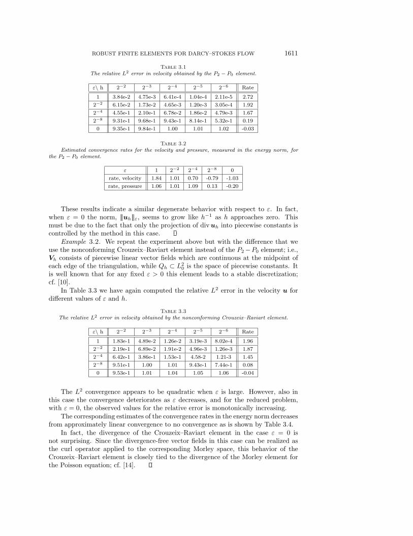
Table 3.4Estimated convergence rates for the velocity and pressure, measured in the energy norm, for

the Crouzeix–Raviart element.

ε 1 2−2 2−4 2−8 0

rate, velocity 0.98 0.97 0.74 0.03 -0.03

rate, pressure 1.00 0.93 0.98 0.12 -0.03

The two examples above show that the P2 − P0 element and the nonconformingCrouzeix–Raviart element, which both are known to be stable for ε = 1, fail to givemethods which converge uniformly in ε. The divergence of the P2 − P0 element forε = 0 is basically due to the fact that the estimate (3.4) does not hold, and thereforethe method is unstable, while the divergence of the Crouzeix–Raviart method is causedby the inconsistency of the method.

Example 3.3. We repeat the experiment above once more, but this time thesystem (1.1) is discretized by using the Mini element; i.e., Vh ⊂ H1

0 consists of linearcombinations of piecewise linear functions and cubic bubble functions with support ona single triangle, while Qh ⊂ L2

0 is the space of continuous piecewise linear functions.In Table 3.5 we have computed the relative error in the velocity, with respect to

the energy norm ||| · |||ε, for different values of ε and h.

Table 3.5The relative error in velocity, measured in the energy norm, for the Mini element.

ε\ h 2−2 2−3 2−4 2−5 2−6 Rate

1 3.01 1.65 8.42e-1 4.22e-1 2.11e-1 0.96

2−2 2.70 1.55 7.80e-1 3.90e-1 1.95e-1 0.96

2−4 3.71 1.67 7.89e-1 3.87e-1 1.92e-1 1.07

2−8 7.32 4.28 2.79 1.64 6.51e-1 0.84

0 7.44 4.76 3.70 3.39 3.30 0.28

When ε = 1 the convergence seems to be linear with respect to h. This agreeswith the theoretical results given in [1]. The convergence deteriorates as ε becomessmaller, and for ε = 0 there seems to be essentially no convergence in the energynorm.

An interesting observation can be made for the Mini element if we consider thecorresponding errors for the pressure p. In Table 3.6 we study the relative error givenby ‖p− ph‖0/‖p‖0.

Table 3.6The relative L2 error in the pressure obtained by the Mini element.

ε\h 2−2 2−3 2−4 2−5 2−6 Rate

1 8.78 2.81 8.85e-1 2.95e-1 1.02e-1 1.61

2−2 6.09e-1 1.84e-1 5.62e-2 1.85e-2 6.40e-3 1.64

2−4 6.08e-2 1.51e-2 3.88e-3 1.21e-3 4.07e-4 1.81

2−8 3.58e-2 9.93e-3 2.34e-3 4.10e-4 6.00e-5 2.30

0 3.59e-2 1.02e-2 2.75e-3 7.23e-4 1.87e-4 1.90

The surprising observation is that for the pressure the convergence seems to beuniform with respect to ε. In fact, the convergence rate seems to improve as ε tends


to zero, and for ε small the convergence with respect to h appears to be quadratic.This is a striking difference to what we observed in Examples 3.1 and 3.2. In boththese cases the error in the pressure diverges as ε tend to zero; cf. Tables 3.2 and 3.4.

What we have observed here is not special to the present example. The Minielement leads to a discretization which is uniformly stable with respect to ε in aproper ε-dependent norm different from ||| · |||ε. If we define the solution space Xε by

Xε = (L2 ∩ ε ·H10 )× ((H1 ∩ L2

0) + ε−1 · L2),(3.5)

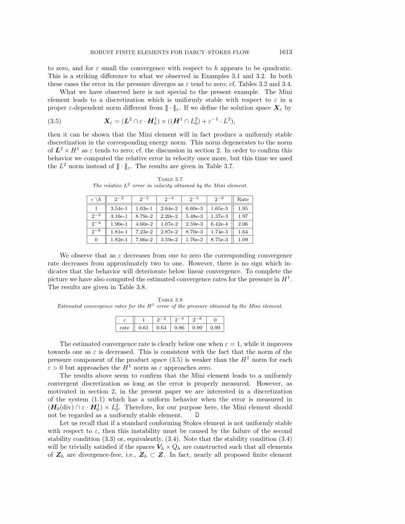
then it can be shown that the Mini element will in fact produce a uniformly stablediscretization in the corresponding energy norm. This norm degenerates to the normof L2 ×H1 as ε tends to zero; cf. the discussion in section 2. In order to confirm thisbehavior we computed the relative error in velocity once more, but this time we usedthe L2 norm instead of ||| · |||ε. The results are given in Table 3.7.

Table 3.7The relative L2 error in velocity obtained by the Mini element.

ε \h 2−2 2−3 2−4 2−5 2−6 Rate

1 3.54e-1 1.03e-1 2.64e-2 6.60e-3 1.65e-3 1.95

2−2 3.16e-1 8.79e-2 2.20e-2 5.48e-3 1.37e-3 1.97

2−4 1.90e-1 4.60e-2 1.07e-2 2.59e-3 6.42e-4 2.06

2−8 1.81e-1 7.23e-2 2.87e-2 8.70e-3 1.74e-3 1.64

0 1.82e-1 7.66e-2 3.59e-2 1.76e-2 8.75e-3 1.09

We observe that as ε decreases from one to zero the corresponding convergencerate decreases from approximately two to one. However, there is no sign which in-dicates that the behavior will deteriorate below linear convergence. To complete thepicture we have also computed the estimated convergence rates for the pressure in H1.The results are given in Table 3.8.

Table 3.8Estimated convergence rates for the H1 error of the pressure obtained by the Mini element.

ε 1 2−2 2−4 2−8 0

rate 0.61 0.64 0.86 0.99 0.99

The estimated convergence rate is clearly below one when ε = 1, while it improvestowards one as ε is decreased. This is consistent with the fact that the norm of thepressure component of the product space (3.5) is weaker than the H1 norm for eachε > 0 but approaches the H1 norm as ε approaches zero.

The results above seem to confirm that the Mini element leads to a uniformlyconvergent discretization as long as the error is properly measured. However, asmotivated in section 2, in the present paper we are interested in a discretizationof the system (1.1) which has a uniform behavior when the error is measured in(H0(div) ∩ ε · H1

0 ) × L20. Therefore, for our purpose here, the Mini element should

not be regarded as a uniformly stable element.Let us recall that if a standard conforming Stokes element is not uniformly stable

with respect to ε, then this instability must be caused by the failure of the secondstability condition (3.3) or, equivalently, (3.4). Note that the stability condition (3.4)will be trivially satisfied if the spaces Vh ×Qh are constructed such that all elementsof Zh are divergence-free, i.e., Zh ⊂ Z. In fact, nearly all proposed finite element


methods for the reduced problem will have this property. This is, for example, truefor the Raviart–Thomas spaces (cf. [15]) and for the Brezzi–Douglas–Marini spacesof [7]. However, in all these cases the spaces Vh will be only a subspace of H0(div)and not of H1

0 , due to the fact that only the normal components of the elements of Vh

are required to be continuous across element edges. It is therefore not clear that thesespaces will be useful for problems of the form (1.1) with ε > 0.

Example 3.4. We repeat the calculation done in the three examples above, butnow we use the lowest order Raviart–Thomas space for the discretization. Hence, forε = 0 we will expect to obtain linear convergence with respect to h. On the otherhand, for ε > 0 the method is nonconforming and there seems to be no reason toexpect that the method is convergent in this case. In Table 3.9 we have computedthe estimated convergence rates with respect to h for the relative L2 errors of thevelocity u and the pressure p for different values of ε.

Table 3.9Estimated convergence rates for the L2 errors of the velocity and pressure for the Raviart–

Thomas element.

ε 1 2−2 2−4 2−8 0

rate, velocity -0.07 -0.07 0.28 0.97 0.97

rate, pressure -0.04 0.08 0.86 1.01 1.01

As expected, the method appears to be divergent for ε > 0.

4. A robust nonconforming finite element space. The four examples pre-sented above illustrate that none of the standard elements proposed for the case ε = 1or ε = 0 will lead to a discretization of the problem (1.1) with uniform convergenceproperties with respect to ε, when the error is measured in the norm of the space(H0(div)∩ε ·H1

0 )×L20. The purpose of the rest of this paper is therefore to construct

and analyze a new finite element space which has this property.

4.1. The finite element space. In order to describe the new finite elementspace we will first define the proper polynomial space, or shape functions, on a giventriangle. Let T ⊂ R2 be a triangle and consider the polynomial space of vector fieldson T given by

V (T ) = v ∈ P23 : div v ∈ P0, (v · n)|e ∈ P1 ∀e ∈ E(T ).

Here Pk denotes the set of polynomials of degree k and E(T ) denotes the set of theedges of T . Furthermore, n is the unit normal vector on the edge e. Below we will alsouse t to denote the unit tangent vector on e, while τ denotes the arc length along e.

The space P23 is a vector space of dimension 20. Furthermore, the conditions

div v ∈ P0 and (v · n)|e ∈ P1 ∀e ∈ E(T )

represent at most 11 linearly independent constraints on this space. Therefore wemust have

dimV (T ) ≥ 9.

In fact, we shall show that dimV (T ) = 9.Lemma 4.1. The space V (T ) is a linear space of dimension nine. Furthermore,

an element v ∈ V (T ) is uniquely determined by the following degrees of freedom:


• ∫e(v · n)τk dτ , k = 0, 1, for all e ∈ E(T ).

• ∫e(v · t) dτ for all e ∈ E(T ).

Proof. Since V (T ) is a vector space of dimension ≥ 9 it is enough to show thatelements of V (T ) are uniquely determined by the given nine degrees of freedom.Assume that v ∈ V (T ) with all the degrees of freedom equal zero. In particular, thisimplies that

(v · n)|∂T ≡ 0.

As a consequence of this ∫T

div v dx =

∫∂T

v · n dτ = 0.

Hence, since div v ∈ P0, we conclude that v is divergence-free.However, since v ∈ P2

3 is divergence-free we must have v = curlw for a suitablescalar function w ∈ P4. Furthermore, since

(gradw · t)|e = (v · n)|e = 0

for each edge e, we conclude that gradw ·t ≡ 0 on ∂T . Since w is uniquely determinedonly up to a constant, we can therefore assume that w ≡ 0 on ∂T .

Hence, w is of the form w = pb, where p ∈ P1 and b is the cubic bubble functionwith respect to T ; i.e., b = λ1λ2λ3, where λi(x) are the barycentric coordinates of xwith respect to the three corners of T . In particular, ∂b

∂n |e does not change sign on e.Furthermore,

∂w

∂n

∣∣∣∣∂T

= p∂b

∂n

∣∣∣∣∂T

and ∫e

p∂b

∂ndτ =

∫e

∂w

∂ndτ =

∫e

v · t dτ = 0 ∀e ∈ E(T ).

We can therefore conclude that p has a root in the interior of e. However, if p ∈ P1

with a root in the interior of each edge of T , then p ≡ w ≡ 0.Let Th be a shape regular family of triangulations of Ω, where h is the maximal

diameter. Furthermore, let Eh be the set of edges of Th. Define a finite element spaceof vector fields Vh, associated with the triangulation Th, as all functions v ∈ Vh suchthat

• v|T ∈ V (T ) for all T ∈ Th,• ∫

e(v · n)τk dτ is continuous for k = 0, 1 for all e ∈ Eh,

• ∫e(v · t) dτ is continuous for all e ∈ Eh.

Here we assume that v is extended to be zero outside Ω; i.e., if e is an edge on theboundary of Ω, then we require∫

e

(v · n)τk dτ = 0, k = 0, 1, and

∫e

(v · t) dτ = 0.

It follows from Lemma 4.1 that any function v ∈ Vh is uniquely determined by thetwo lowest order moments of v ·n and by the mean value of v · t for all interior edges;cf. Figure 4.1.


Fig. 4.1. The degrees of freedom of the new nonconforming element.

If v ∈ Vh, then the normal component v · n is continuous for all interior edges.Therefore, Vh ⊂ H0(div). However, the tangential component of v is not continuous;only the mean value with respect to each edge is continuous. Therefore, Vh H1

0 . Inaddition to the space Vh we let Qh ⊂ L2

0 denote the space of scalar piecewise constantswith respect to the triangulation Th.

In the rest of this paper Vh and Qh will always refer to the finite element spacesjust introduced. The corresponding nonconforming finite element approximation ofthe system (1.1) is defined by the system (3.1).

4.2. Properties of the new finite element space. It follows from the defini-tion of Vh that divVh ⊂ Qh. Hence, if we define Zh ⊂ Vh as the weakly divergence-free elements of Vh, i.e.,

Zh = v ∈ Vh : (div v, q) = 0 ∀q ∈ Qh,then these elements are in fact divergence-free.

Remark. It can be seen that

Zh = curlWh,(4.1)

where Wh is an associated nonconforming H2-element. Locally, on each triangle,Wh consists of all P4 polynomials which reduce to a quadratic on each edge. Inaddition, Wh ⊂ H1

0 and the average of the normal derivatives of functions in Wh

are continuous on each edge. The finite element space Wh is precisely describedand analyzed in [14]. The identity (4.1) was actually the main motivation for theconstruction of the space Vh. More precisely, the spaces Wh, Vh, and Qh are relatedsuch that the sequence

0 −−−−→ Wh/Rcurl−−−−→ Vh

div−−−−→ Qh −−−−→ 0

is exact. In particular, divVh = Qh.Define an interpolation operator Πh : H1

0 → Vh by∫e

(Πhv · n)τk dτ =

∫e

(v · n)τk dτ, k = 0, 1,∫e

(Πhv · t) dτ =

∫e

(v · t) dτ

for all e ∈ Eh. In addition, let Ph : L20 → Qh be the L2 projection. From the definition

of the operator Πh we easily verify the commutativity property

divΠhv = Ph div v ∀v ∈ H10 .(4.2)


In fact, for all T ∈ Th∫T

divΠhv dx =

∫∂T

(Πhv · n) dτ =

∫∂T

(v · n) dτ =

∫T

div v dx,

and hence (4.2) follows.Since Qh is the space of piecewise constants the L2 projection Ph onto Qh satisfies

‖w − Phw‖0 ≤ ch‖w‖1(4.3)

for all w ∈ H1 ∩ L20, where c > 0 is independent of h and w. The operator Πh

is well defined on H10 , it is locally defined on each triangle, and it preserves linear

functions locally. Furthermore, the polynomial space V (T ) is invariant under affinePiola transformations. More precisely, let T ∈ Th and let φ(x) = Bx+ c be an affinemap of T onto a reference triangle T . Then the Piola transform, v → v, where

v(x) = (detB)−1Bv(x), x = φ(x),

maps V (T ) onto V (T ). Therefore, approximation estimates for the operator Πh canbe derived from standard scaling arguments utilizing the shape regularity of Th. Inparticular, there exists a constant c > 0, independent of h, such that

‖Πhv‖div ≤ ‖Πhv‖1,h ≤ c‖v‖1.(4.4)

In addition, from the Bramble–Hilbert lemma, using the fact thatΠh preserves linearslocally, we can further conclude that

‖Πhv − v‖j,h ≤ chk−j |v|k for 0 ≤ j ≤ 1 ≤ k ≤ 2(4.5)

and for all v ∈ H10 ∩Hk. Here ‖ · ‖j,h denotes the piecewise Hj-norm

‖v‖2j,h =

∑T∈Th

‖v‖2j,T .

In fact, if T is a reference triangle, and Π : H1(T ) → V (T ) the correspondinginterpolation operator, then for all v ∈ H1(T )

‖Πv‖0,T ≤ c1‖v‖0,∂T ≤ c2‖v‖1/2

0,T‖v‖1/2

1,T,

where c1 and c2 depend only on T . Hence, from a scaling argument we also obtainthe low order estimate

‖Πhv − v‖0 ≤ ch1/2‖v‖1/20 ‖v‖1/2

1(4.6)

for all v ∈ H10 .

Next we will verify the stability conditions (3.2) and (3.3) for the product spaceVh × Qh. However, due to the fact that we are considering a nonconforming finiteelement approximation of the system (1.1), where Vh H1

0 , the norm ||| · |||ε has tobe properly modified. For each v ∈ Vh we define

|||v|||2ε,h = ‖v‖2div + ε2

∑T∈Th

‖Dv‖20,T .


Note that for ε = 0 this norm is simply equal to ‖·‖div, while for ε = 1 it is equivalent,uniformly in h, to the piecewise H1-norm ‖ · ‖1,h.Lemma 4.2. There exists a constant α1 > 0, independent of h, such that

supv∈Vh

(q,div v)

‖v‖1,h≥ α1‖q‖0 ∀q ∈ Qh.

Proof. This follows by a standard argument from the properties of the interpo-lation operator Πh and the corresponding continuous result (2.6). In fact, since forany v ∈ H1

0 and q ∈ Qh we have

(q,divΠhv) = (q,div v)

and

‖Πhv‖1,h ≤ c1‖v‖1,

we can take α1 = α0/c1.The following uniform stability result is an immediate consequence of the previous

lemma.Theorem 4.1. The pair of spaces (Vh, Qh) satisfies the uniform stability condi-

tions (3.2) and (3.3) but with the norm ||| · |||ε replaced by ||| · |||ε,h.Proof. The norms ||| · |||1,h and ‖ · ‖1,h are equivalent on Vh, and ||| · |||ε,h decreases

as ε decreases. It follows from Lemma 4.2 that condition (3.2) holds. Since Zh ⊂ Zthe second condition (3.3) holds with β = 1.

5. Error estimates for smooth solutions. Since our new finite element space(Vh, Qh) satisfies the proper stability conditions (3.2) and (3.3), uniformly with re-spect to ε, it seems probable that the corresponding finite element method will in facthave uniform convergence properties. In the present section we shall investigate thisquestion under the assumption that the solution (u, p) of the continuous problem issufficiently smooth, while the effect of the ε-dependent boundary layers will be takeninto account in the next section.

We will start the discussion here with a numerical example which is completelysimilar to Examples 3.1–3.3.

Example 5.1. We redo the computations done in Examples 3.1–3.3, but this timewe use the finite element spaces constructed above. In all the numerical examples withthe new element we used a fifth order Gauss–Legendre method (cf. [17]) as integrationrule.

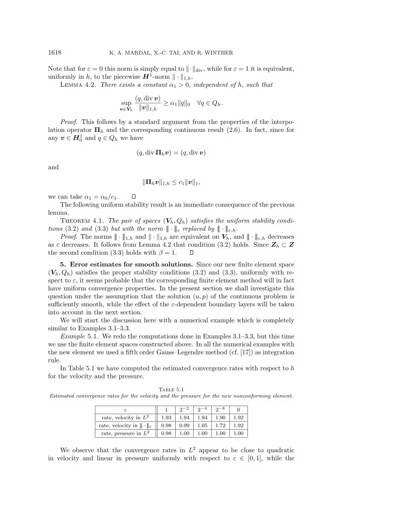
In Table 5.1 we have computed the estimated convergence rates with respect to hfor the velocity and the pressure.

Table 5.1Estimated convergence rates for the velocity and the pressure for the new nonconforming element.

ε 1 2−2 2−4 2−8 0

rate, velocity in L2 1.93 1.94 1.94 1.90 1.92

rate, velocity in ||| · |||ε 0.98 0.99 1.05 1.72 1.92

rate, pressure in L2 0.98 1.00 1.00 1.00 1.00

We observe that the convergence rates in L2 appear to be close to quadraticin velocity and linear in pressure uniformly with respect to ε ∈ [0, 1], while the


2 3 4 5 610

−4

10−3

10−2

10−1

100

101

P2−P

0MiniNew elementCrouzeix−Raviart

2 3 4 5 610

−4

10−3

10−2

10−1

100

101

102

103

Fig. 5.1. The errors in velocity, measured in the L2 norm and the energy norm, as functionsof σ = − log(h)/ log(2).

convergence in the energy norm appears to be at least linear for each ε > 0. In fact,as ε approaches zero the convergence rate tends to two. This improved convergenceis partly due to the fact that the exact solution u is divergence-free in this case.

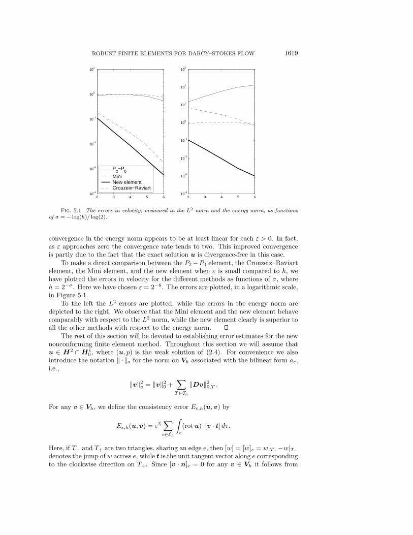
To make a direct comparison between the P2 −P0 element, the Crouzeix–Raviartelement, the Mini element, and the new element when ε is small compared to h, wehave plotted the errors in velocity for the different methods as functions of σ, whereh = 2−σ. Here we have chosen ε = 2−8. The errors are plotted, in a logarithmic scale,in Figure 5.1.

To the left the L2 errors are plotted, while the errors in the energy norm aredepicted to the right. We observe that the Mini element and the new element behavecomparably with respect to the L2 norm, while the new element clearly is superior toall the other methods with respect to the energy norm.

The rest of this section will be devoted to establishing error estimates for the newnonconforming finite element method. Throughout this section we will assume thatu ∈ H2 ∩ H1

0 , where (u, p) is the weak solution of (2.4). For convenience we alsointroduce the notation ‖ · ‖a for the norm on Vh associated with the bilinear form aε,i.e.,

‖v‖2a = ‖v‖2

0 +∑T∈Th

‖Dv‖20,T .

For any v ∈ Vh, we define the consistency error Eε,h(u,v) by

Eε,h(u,v) = ε2∑e∈Eh

∫e

(rotu) [v · t] dτ.

Here, if T− and T+ are two triangles, sharing an edge e, then [w] = [w]e = w|T+−w|T−

denotes the jump of w across e, while t is the unit tangent vector along e correspondingto the clockwise direction on T+. Since [v · n]e = 0 for any v ∈ Vh it follows from


(2.2) and Green’s theorem, in particular from (2.1), that

aε(u,v) + (p,div v) = (f ,v) + Eε,h(u,v) ∀v ∈ Vh,(divu, q) = (g, q) ∀q ∈ L2

0,(5.1)

where the term Eε,h appears due to the fact that Vh H10 .

In the error analysis below we will need proper estimates on the consistencyerror Eε,h. The following bounds are therefore useful.Lemma 5.1. If u ∈ H2 ∩H1

0 , then

supv∈Vh

|Eε,h(u,v)|‖v‖a ≤ c ε

h‖ rotu‖1,

h1/2‖ rotu‖1/21 ‖ rotu‖1/2

0 ,

where c > 0 is independent of ε and h.Proof. Let e ∈ Eh and v ∈ H1

0 +Vh. Since the mean value with respect to e of v ·tis zero, it follows from a standard scaling argument (cf., for example, [5, section 8.3]or [14, section 4] for similar arguments) that for any φ ∈ H1

∫eφ[v · t]dτ ≤ infλ,µ∈R ‖φ− λ‖0,e‖[v · t− µ]‖0,e

≤

ch|φ|1,Ωe(|v|1,T− + |v|1,T+),

ch1/2|φ|1/21,Ωe‖φ‖1/2

0,Ωe(|v|1,T− + |v|1,T+

).

(5.2)

Here T− and T+ denote the two triangles meeting the edge e and Ωe = T−∪T+. Since

|Eε,h(u,v)| ≤ ε2∑e∈Eh

∣∣∣∣∫e

(rotu) [v · t] dτ∣∣∣∣ ,

the desired estimate follows by applying the estimate (5.2) with φ = rotu, summingover all edges, and using the fact that∑

e∈Eh

|v|21,T ≤ ε−2aε(v,v).

Let (uh, ph) ∈ Vh ×Qh be the approximation of (u, p) derived from the discretesystem (3.1). From (3.1) and (5.1) we obtain

aε(u− uh,v) + (p− ph,div v) = Eε,h(u,v)(5.3)

for all v ∈ Vh. Furthermore,

divuh = Ph divu = divΠhu.

Therefore, taking v = Πhu− uh in (5.3) we obtain

aε(u− uh,Πhu− uh) = Eε,h(u,Πhu− uh).

Since aε is an inner product we further have

‖Πhu− uh‖2a ≤ ‖u−Πhu‖2

a + 2aε(u− uh,Πhu− uh)

≤ ‖u−Πhu‖2a + 2Eε,h(u,Πhu− uh).


Hence, we conclude that

‖u− uh‖a ≤ 2

(‖u−Πhu‖a + sup

v∈Vh

|Eε,h(u,v)|‖v‖a

).(5.4)

From this basic bound we easily derive the following error estimate.Theorem 5.1. If u ∈ H2 ∩H1

0 and p ∈ H1 ∩ L20, then the following estimates

hold:

‖u− uh‖0 + ε‖ rot(u− uh)‖0 ≤ c(h2 + εh)‖u‖2,

‖div(u− uh)‖0 ≤ ch‖divu‖1,

‖p− ph‖0 ≤ ch(‖p‖1 + (ε+ h)‖u‖2).

Here c > 0 is a constant independent of ε and h.Remark. Here, and below, the differential operators D and rot, applied to vector

fields in Vh, are defined locally on each triangle of the triangulation Th.Proof. The first estimate is a direct consequence of (4.5), (5.4), and Lemma 5.1.

The second estimate follows from the bound (4.3) and the fact that divuh = Ph divu.In order to establish the third estimate we first observe that (4.3) implies that

‖p− Php‖0 ≤ ch‖p‖1.(5.5)

Hence, it remains only to estimate Php − ph. However, from the modified inf-supcondition (3.2) (cf. Theorem 4.1) we obtain

‖Php− ph‖0 ≤ α−1 supv∈Vh

(Php− ph,div v)

|||v|||ε,h .

Furthermore, for any v ∈ Vh we have

(Php− ph,div v) = (p− ph,div v)

= −aε(u− uh,v) + Eε,h(u,v),

which implies that

|(Php− ph,div v)| ≤(‖u− uh‖a + sup

v∈Vh


)|||v|||ε,h

or

‖Php− ph‖0 ≤ α−1

(‖u− uh‖a + sup

v∈Vh


).(5.6)

From the previous estimates we therefore obtain

‖Php− ph‖0 ≤ c(h2 + εh)‖u‖2,

and together with (5.5) this establishes the desired estimate on the error ‖p −ph‖0.

Remark. As an alternative to the estimates given in Theorem 5.1 we can alsoobtain

‖u− uh‖0 + ε‖ rot(u− uh)‖0 ≤ ch(‖u‖1 + ε‖u‖2)(5.7)


and

‖p− ph‖0 ≤ ch(‖p‖1 + ‖u‖1 + ε‖u‖2).(5.8)

These modifications are obtained if we use the estimate

‖u−Πhu‖0 ≤ ch‖u‖1,

obtained from (4.5), in (5.4) instead of the corresponding quadratic estimate. Even ifthe modified estimates are weaker for uniformly smooth solutions, they are sometimespreferable for more singular solutions.

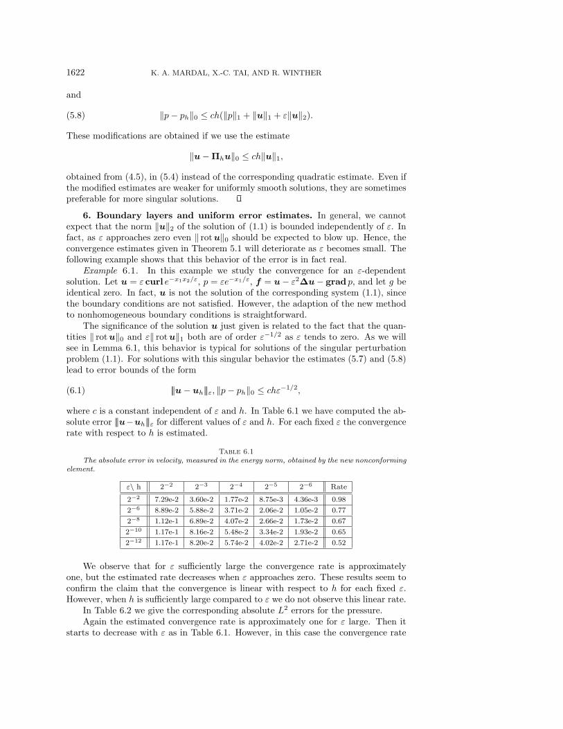
6. Boundary layers and uniform error estimates. In general, we cannotexpect that the norm ‖u‖2 of the solution of (1.1) is bounded independently of ε. Infact, as ε approaches zero even ‖ rotu‖0 should be expected to blow up. Hence, theconvergence estimates given in Theorem 5.1 will deteriorate as ε becomes small. Thefollowing example shows that this behavior of the error is in fact real.

Example 6.1. In this example we study the convergence for an ε-dependentsolution. Let u = ε curl e−x1x2/ε, p = εe−x1/ε, f = u− ε2∆u− grad p, and let g beidentical zero. In fact, u is not the solution of the corresponding system (1.1), sincethe boundary conditions are not satisfied. However, the adaption of the new methodto nonhomogeneous boundary conditions is straightforward.

The significance of the solution u just given is related to the fact that the quan-tities ‖ rotu‖0 and ε‖ rotu‖1 both are of order ε−1/2 as ε tends to zero. As we willsee in Lemma 6.1, this behavior is typical for solutions of the singular perturbationproblem (1.1). For solutions with this singular behavior the estimates (5.7) and (5.8)lead to error bounds of the form

|||u− uh|||ε, ‖p− ph‖0 ≤ chε−1/2,(6.1)

where c is a constant independent of ε and h. In Table 6.1 we have computed the ab-solute error |||u−uh|||ε for different values of ε and h. For each fixed ε the convergencerate with respect to h is estimated.

Table 6.1The absolute error in velocity, measured in the energy norm, obtained by the new nonconforming

element.

ε\ h 2−2 2−3 2−4 2−5 2−6 Rate

2−2 7.29e-2 3.60e-2 1.77e-2 8.75e-3 4.36e-3 0.98

2−6 8.89e-2 5.88e-2 3.71e-2 2.06e-2 1.05e-2 0.77

2−8 1.12e-1 6.89e-2 4.07e-2 2.66e-2 1.73e-2 0.67

2−10 1.17e-1 8.16e-2 5.48e-2 3.34e-2 1.93e-2 0.65

2−12 1.17e-1 8.20e-2 5.74e-2 4.02e-2 2.71e-2 0.52

We observe that for ε sufficiently large the convergence rate is approximatelyone, but the estimated rate decreases when ε approaches zero. These results seem toconfirm the claim that the convergence is linear with respect to h for each fixed ε.However, when h is sufficiently large compared to ε we do not observe this linear rate.

In Table 6.2 we give the corresponding absolute L2 errors for the pressure.Again the estimated convergence rate is approximately one for ε large. Then it

starts to decrease with ε as in Table 6.1. However, in this case the convergence rate


Table 6.2The absolute L2 error in the pressure obtained by the new nonconforming element.

ε\ h 2−2 2−3 2−4 2−5 2−6 Rate

2−2 2.32e-2 1.11e-2 5.36e-3 2.64e-3 1.31e-3 1.04

2−6 9.00e-3 5.33e-3 2.62e-3 1.15e-3 4.61e-4 1.07

2−8 5.28e-3 3.24e-3 2.18e-3 1.23e-3 5.97e-4 0.77

2−10 4.93e-3 2.54e-3 1.33e-3 7.93e-4 5.32e-4 0.81

2−12 4.92e-3 2.51e-3 1.24e-3 6.22e-4 3.27e-4 0.98

increases roughly back to one when ε is superclose to zero. We will comment on thisphenomenon for the error of the pressure at the end of this section.

The estimate (6.1) does not imply uniform convergence with respect to ε for ournew finite element method. However, as a consequence of the theory below, we willobtain an improved estimate of the form

|||u− uh|||ε, ‖p− ph‖0 ≤ cmin(h1/2, hε−1/2)(6.2)

for solutions with a singular behavior similar to the solution u studied here. Notethat this is in fact consistent with the results of Tables 6.1 and 6.2, where we neverobserve a convergence rate below a half.

The main purpose of this section is to establish error estimates which are uniformwith respect to the perturbation parameter ε. We shall show a uniform O(h1/2) errorestimate in the energy norm. We observe that if g ∈ H1 ∩L2

0, then it follows directlyfrom Theorem 5.1 that

‖div(u− uh)‖0 ≤ c h‖g‖1,(6.3)

where the constant c is independent of ε and h. Hence, we have uniform linearconvergence for the error of the divergence. In contrast to this, the remaining partof the error will be affected by boundary layers as ε becomes small. However, thefollowing uniform convergence estimate will be derived.Theorem 6.1. If f ∈ H(rot) and g ∈ H1

+, then there is a constant c, independentof f , g, ε, and h, such that

‖u− uh‖0 + ε‖ rot(u− uh)‖0 + ‖p− ph‖0 ≤ c h1/2(‖f‖rot + ‖g‖1,+).

Here the Sobolev space H1+ is a space contained in H1, with an associated norm,

‖ · ‖1,+, slightly stronger than ‖ · ‖1. This space will be precisely defined below.The derivation of the uniform error estimate above will depend heavily on cer-

tain regularity estimates for the solution of the system (1.1). For example, we shallestimate the blowup of ‖ rotu‖1 as ε approaches zero. We shall therefore first derivethese regularity estimates.

For convenience of the reader we repeat the system (1.1):

(I − ε2∆)u− grad p = f in Ω,divu = g in Ω,

u = 0 on ∂Ω.(6.4)

We also repeat that the domain Ω is a polygonal domain in R2. In fact, in thediscussion of this section we shall assume that Ω in addition is convex. If ε ∈ (0, 1],


f ∈ L2, and g = 0, then the corresponding weak solution admits the additionalregularity that (u, p) ∈ (H1

0 ×L20)∩ (H2×H1). This regularity result follows directly

from the result for the corresponding Stokes problem on a convex domain which canbe found in [12, Corollary 7.3.3.5]. In fact, the same regularity holds for g = 0 if werestrict the data g to the space H1

+.In order to define this space let x1, x2, . . . , xN ∈ ∂Ω denote the vertices of Ω. The

space H1+ is given by

H1+ =

g ∈ H1 ∩ L2

0 :

∫Ω

|g(x)|2|x− xj |2 dx < ∞, j = 1, 2, . . . , N

,

with associated norm

‖g‖21,+ = ‖g‖2

1 +

N∑j=1

∫Ω

|g(x)|2|x− xj |2 dx.

Hence, functions in H1+ vanish weakly at each vertex of Ω.

It is established in [2] that

div(H2 ∩H10 ) = H1

+.

Furthermore, the divergence operator has a bounded right inverse,R : H1+ → H2∩H1

0 ;i.e., divRg = g for all g ∈ H1

+ and

‖Rg‖2 ≤ c‖g‖1,+.

Note that if (u, p) solves (6.4), then (u − Rg, p) solves a corresponding problemwith g = 0. From the result in the case g = 0 we can therefore conclude that(u, p) ∈ (H1

0 × L20) ∩ (H2 ×H1) for any (f , g) ∈ L2 ×H1

+.The following result gives an upper bound for the blowup of the norm ‖ rotu‖1

as ε tends to zero.Lemma 6.1. Assume that f ∈ H(rot), g ∈ H1

+, and let (u, p) be the correspond-ing solution of (6.4). There exists a constant c > 0, independent of ε, f and g, suchthat

ε1/2‖ rotu‖0 + ε3/2‖ rotu‖1 ≤ c (‖ rotf‖0 + ‖g‖1,+).(6.5)

Proof. We first construct a function u ∈ H2 ∩H10 such that

div u = g and rot∆u = 0.(6.6)

In fact, the function u can be constructed by defining

u = Rg + curlψ,

with ψ ∈ H20 being the weak solution of the biharmonic equation

∆2ψ = rot∆Rg in Ω,

ψ =∂ψ

∂n= 0 on ∂Ω.

We observe that, since Rg ∈ H2, the right-hand side is in H−1. Therefore, fromthe regularity of solutions of the biharmonic equation on convex domains (cf. [12,


Theorem 7.2.2.3]), we have that ψ ∈ H3, and ‖ψ‖3 ≤ c‖ rot∆Rg‖−1. Hence, u ∈H2 ∩H1

0 , and

‖u‖2 ≤ c ‖g‖1,+.(6.7)

Furthermore, clearly div u = divRg = g, and for any µ ∈ C∞0 we have

(∆u, curlµ) = (∆Rg, curlµ)− (∆ψ,∆µ) = 0.

Hence, the second property in (6.6) also holds.Define v = u− u. Then (v, p) ∈ (H1

0 × L20) ∩ (H2 ×H1) is the weak solution of

the problem

(I − ε2∆)v − grad p = f in Ω,div v = 0 in Ω,

v = 0 on ∂Ω,(6.8)

where f = f + ε2∆u− u. Clearly, f ∈ L2. In fact, f ∈ H(rot), since

rot f = rotf − rot u.

Furthermore, there is a constant c, independent of ε, f and g, such that

‖ rot f‖0 ≤ c (‖ rotf‖0 + ‖g‖1,+).(6.9)

Since v ∈ L2 and div v = 0 there exists φ ∈ H1, uniquely determined up to a constant,such that v = curlφ [11, Theorem I.3.1]. Hence, since v ∈ H2 ∩H1

0 , we can chooseφ ∈ H3 ∩H2

0 . In fact, by applying the rot operator, as a map from L2 to H−1, to thefirst equation of (6.8) we obtain

−∆φ+ ε2∆2φ = rot f in Ω,

φ =∂φ

∂n= 0 on ∂Ω.

The function φ is uniquely determined by this problem. This singular perturbationproblem was in fact studied in [14], where it was established that [14, Lemma 5.1]

ε1/2‖φ‖2 + ε3/2‖φ‖3 ≤ c‖ rot f‖0,

and as a consequence

ε1/2‖ rotv‖0 + ε3/2‖ rotv‖1 ≤ c‖ rot f‖0.

Therefore, since u = v + u, (6.7) and (6.9) imply

ε1/2‖ rotu‖0 + ε3/2‖ rotu‖1 ≤ c‖ rot f‖0 + ε1/2(‖ rot u‖0 + ε‖ rot u‖1)

≤ c(‖ rotf‖0 + ‖g‖1,+).

This completes the proof.In addition to the ε-dependent bound on the solution (u, p) of (6.4) derived above,

we shall also need convergence estimates on how fast these solutions converge to thesolution of the reduced system.


The reduced system corresponding to (6.4) is of the form

u0 − grad p0 = f in Ω,divu0 = g in Ω,u0 · n = 0 on ∂Ω.

(6.10)

A precise weak formulation of this system is given by the following:Find (u0, p0) ∈ H0(div)× L2

0 such that

(u0,v) + (p0,div v) = (f ,v) ∀v ∈ H0(div),(divu0, q) = (g, q) ∀q ∈ L2

0.(6.11)

If (f , g) ∈ H−1(rot) × L20, then this system admits a unique solution. In fact, if

f ∈ H(rot), then u0 ∈ H(rot) with rotu0 = rotf . Therefore,

u0 ∈ H0(div) ∩H(rot),

and hence (cf. [11, Proposition 3.1, Chapter 1]) u0 ∈ H1. As a consequence, p0 ∈H1. Furthermore, the corresponding solution map is continuous; i.e., there exists aconstant c, independent of f and g, such that

‖u0‖1 + ‖p0‖1 ≤ c (‖f‖rot + ‖g‖0).(6.12)

Lemma 6.2. Assume that f ∈ H(rot), g ∈ H1+, and let (u, p) be the correspond-

ing solution of (6.4). There exists a constant c > 0, independent of ε, f and g, suchthat

‖u− u0‖0 + ‖p− p0‖1 ≤ c ε1/2(‖f‖rot + ‖g‖1,+).

Proof. It follows from (2.2), the weak formulation of (6.4), and Green’s theoremthat for any v ∈ H1 ∩H0(div) the solution (u, p) satisfies

(u,v) + ε2(divu,div v) + ε2(rotu, rotv) + ε2

∫∂Ω

(rotu)(v · t)dτ+ (p,div v) = (f ,v).

By subtracting from this the first equation of (6.11), we obtain

(u− u0,v) + ε2(rotu, rotv) + ε2

∫∂Ω

(rotu)(v · t)dτ = 0

for any v ∈ H1 ∩H0(div) with div v = 0. Hence, if we take v = u−u0, and observethat rotu0 = rotf and div(u− u0) = 0, we derive the identity

‖u− u0‖20 + ε2‖ rotu‖2

0 = ε2

∫∂Ω

(rotu)(u0 · t)dτ + ε2(rotu, rotf),

which immediately leads to the bound

‖u− u0‖20 +

ε2

2‖ rotu‖2

0 ≤ ε2 ‖ rotf‖20 + ε2

∫∂Ω

(rotu)(u0 · t)dτ.(6.13)

In order to estimate the boundary integral we note that it follows from Lemma 6.1and [12, Theorem 1.5.1.10] that

‖ rotu‖0,∂Ω ≤ c‖ rotu‖1/20 ‖ rotu‖1/2

1 ≤ cε−1 (‖ rotf‖0 + ‖g‖1,+).


Together with the estimate (6.12) this leads to

ε2

∫∂Ω

(rotu)(u0 · t)dτ ≤ ε2‖ rotu‖0,∂Ω‖u0‖1

≤ c ε(‖f‖2rot + ‖g‖2

1,+).

Hence, the estimate

‖u− u0‖0 + ε2‖ rotu‖20 ≤ c ε1/2(‖f‖rot + ‖g‖1,+)(6.14)

follows.The estimate for ‖p− p0‖1 is now a direct consequence of the identity

grad(p− p0) = u− u0 − ε2∆u

= u− u0 + ε2(curl rotu− grad g)

and the previously established bounds. In fact, it follows from Lemma 6.1 and (6.14)that

‖grad(p− p0)‖0 ≤ ‖u− u0‖0 + ε2(‖ rotu‖1 + ‖g‖1)

≤ c ε1/2(‖f‖rot + ‖g‖1,+).

Since p−p0 ∈ L20, an application of the Poincare inequality completes the proof.

The regularity bounds derived above will now be used to prove the uniform con-vergence estimates.

Proof of Theorem 6.1. Recall that since u ∈ H10 it follows from [11, Proposi-

tion 3.1, Chapter 1] that

‖u‖1 ≤ c(‖divu‖0 + ‖ rotu‖0).

Furthermore, by the standard H2-regularity for solutions of the Poisson equation onconvex domains, and (2.2), we obtain

‖u‖2 ≤ c‖∆u‖0 ≤ c(‖divu‖1 + ‖ rotu‖1).

Hence, from the estimates given in Lemmas 6.1 and 6.2 we conclude that

ε2‖u‖2 + ε‖u‖1 + ‖u− u0‖0 + ‖p− p0‖1 ≤ cε1/2(‖f‖rot + ‖g‖1,+).(6.15)

The desired estimate on the velocity error will be derived from (5.4). We will firstestablish the interpolation estimate

‖u−Πhu‖0 + ε‖D(u−Πhu)‖1 ≤ c h1/2(‖f‖rot + ‖g‖1,+).(6.16)

From (4.6), (6.12), and (6.15) we have

‖u−Πhu‖0 ≤ ‖(I −Πh)(u− u0)‖0 + ‖u0 −Πhu0‖0

≤ ch1/2 (‖u− u0‖1/20 ‖u− u0‖1/2

1 + h1/2 ‖u0‖1)

≤ ch1/2(‖f‖rot + ‖g‖1,+).


Furthermore, from (4.4), (4.5), and (6.15),

ε‖D(u−Πhu)‖0 ≤ cε‖u‖1/21 ‖u−Πhu‖1/2

1 ≤ cεh1/2‖u‖1/21 ‖u‖1/2

2

≤ ch1/2(‖f‖rot + ‖g‖1,+).

The estimate (6.16) is therefore verified.

Similarly, since ‖u‖1/21 ‖u‖1/2

2 ≤ cε−1(‖f‖rot+‖g‖1,+), we obtain from Lemma 5.1that

supv∈Vh

|Eε,h(u,v)|‖v‖a ≤ ch1/2(‖f‖rot + ‖g‖1,+).(6.17)

However, by combining (5.4), (6.3), (6.16), and (6.17), this implies

‖u− uh‖0 + ε‖ rot(u− uh)‖0 ≤ ch1/2(‖f‖rot + ‖g‖1,+).(6.18)

In order to establish the estimate for the ‖p− ph‖0 note that (4.3) and (6.15) imply

‖Php− p‖0 ≤ ch‖p‖1 ≤ ch(‖f‖rot + ‖g‖1,+).

Finally, by (5.6), (6.17), and (6.18),

‖Php− ph‖0 ≤ ch1/2(‖f‖rot + ‖g‖1,+).

This completes the proof of Theorem 6.1.Remark. Even if Lemma 6.2 states that ‖p‖1 is uniformly bounded with respect

to ε, we are not able to prove that ‖p − ph‖0 converges linearly in h uniformly in ε.The convergence rate is polluted by the blowup of u. This seems to agree with whatwe observed in Example 6.1; cf. Table 6.2.

7. An associated elliptic system. In this section we shall study the ellipticsystem (1.2) given by

(I − ε2∆)u− δ−2 grad(divu− g) = f in Ω,u = 0 on ∂Ω,

(7.1)

where ε, δ ∈ (0, 1]. Recall that by introducing p = δ−2 divu this system can bealternatively written on the mixed form (1.3). Hence, as δ approaches zero the systemformally reduces to (1.1).

The system (7.1) will be discretized by a standard finite element approach; i.e.,the mixed system (1.3) is not introduced in the discretization. Let the bilinearform bε,δ(·, ·) be defined by

bε,δ(u,v) = aε(u,v) + δ−2(divu,div v)

= (u,v) + ε2(Du,Dv) + δ−2(divu,div v).

For a given finite element space Vh, the corresponding standard finite element dis-cretization of (7.1) is given by the following:

Find a uh ∈ Vh such that

bε,δ(uh,v) = (f ,v) + δ−2(g,div v) ∀v ∈ Vh.(7.2)


Our purpose here is to discuss this discretization when the finite element space Vh

is the space introduced in section 4. Since this space is not a subspace of H10 this

will lead to a nonconforming discretization of the system (7.1). However, before weanalyze this discretization, we will present some numerical experiments based on thesystem (7.1).

Example 7.1. In all the examples presented in this section we consider the sys-tem (7.1) with u = curl sin2(πx1) sin

2(πx2), g = 0, and f = u − ε2∆u. Hence, thesolution is independent of ε and δ.

We consider the problem (7.1) with Ω taken as the unit square. The domain istriangulated as described in Example 3.1. The system is then discretized by solvingthe system (7.2), where the space Vh is the standard space of continuous piecewiselinear functions with respect to this triangulation.

In the present example we have used ε = 1, while δ and h vary. In Table 7.1 wehave computed the relative error in the L2 norm for different values of δ and h.

Table 7.1The relative L2 error using piecewise linear elements, ε = 1.

δ\h 2−2 2−3 2−4 2−5 2−6 Rate

1.00 3.87e-1 1.32e-1 3.69e-2 9.52e-3 2.39e-3 1.85

0.10 9.19e-1 7.28e-1 4.34e-1 1.88e-1 6.20e-2 0.97

0.01 1.00 9.96e-1 9.82e-1 9.32e-1 7.88e-1 0.08

As expected we observe approximately quadratic convergence with respect to hfor δ = 1. However, the convergence clearly deteriorates as δ tends to zero.

Example 7.2. We repeat the experiment above, but we extend the finite elementspace and use the corresponding velocity space of the Mini element instead of thepiecewise linear space. It is interesting to note that the L2 convergence deteriorates,as δ gets small, also in this case, in contrast to what we have observed in Table 3.7.The relative L2 error is given in Table 7.2.

Table 7.2The relative L2 error using the Mini element, ε = 1.

δ\h 2−2 2−3 2−4 2−5 2−6 Rate

1.00 3.80e-1 1.30e-1 3.62e-2 9.34e-3 2.35e-3 1.85

0.10 9.19e-1 7.28e-1 4.34e-1 1.88e-1 6.20e-2 0.97

0.01 9.99e-1 9.96e-1 9.82e-1 9.33e-1 7.88e-1 0.08

We observe that the results are almost identical to the ones we obtained in thepiecewise linear case. Hence, the extra bubble functions have almost no effect. Ofcourse, the main reason for the difference between the results given here, for δ small,and the results given in Example 3.3, where δ = 0, is that the second equation ofthe mixed method used previously implicitly introduces a reduced integration in thedivergence term.

Example 7.3. We repeat the experiment above once more, but this time we usethe new nonconforming element. In Table 7.3 we have computed the relative errorin the energy norm, i.e., the norm generated by the form bε,δ, for different values ofδ and h.

In contrast to the other examples above, in this case the convergence seems to belinear with respect to h, uniformly in δ. We also observe that the errors are almost


Table 7.3The relative error in energy norm for the new nonconforming element, ε = 1.

δ\h 2−2 2−3 2−4 2−5 2−6 Rate

1.00 1.84 9.83e-1 4.98e-1 2.50e-1 1.25e-1 0.97

0.10 1.83 9.66e-1 4.87e-1 2.44e-1 1.22e-1 0.98

0.01 1.83 9.66e-1 4.87e-1 2.44e-1 1.22e-1 0.98

Table 7.4The relative error in energy norm for the new nonconforming element, ε = 0.01.

δ\h 2−2 2−3 2−4 2−5 2−6 Rate

1.00 1.04e-1 3.23e-2 8.94e-3 2.21e-3 5.29e-4 1.91

0.10 1.04e-1 3.23e-2 8.94e-3 2.21e-3 5.29e-4 1.91

0.01 1.04e-1 3.23e-2 8.94e-3 2.21e-3 5.29e-4 1.91

independent of δ.Next, we reduce ε and take ε = 0.01 and redo the experiment. The results are

given in Table 7.4.We observe that to the given accuracy the numerical solution is independent

of δ, clearly indicating that the numerical solutions are close to a pure curl fieldindependent of δ, which is precisely the form of the exact solution in this case. Asimilar observation is done if we take ε = 0.

The numerical experiments just presented indicate that the nonconforming spaceVh, introduced in section 4 above, is well suited for problem (7.1). We will give a par-tial theoretical justification for this claim by deriving a generalization of Theorem 5.1.

We assume throughout this section that u ∈ H2 ∩H10 . Let ‖ · ‖b be the energy

norm associated with the system (7.1), i.e.,

‖v‖2b = bε,δ(v,v).

It is a straightforward consequence of the second Strang lemma (cf. [9, Theorem 4.2.2])that there exists a c > 0, independent of ε, h and u, such that

‖u− uh‖2b ≤ ‖u−Πhu‖2

b + c supv∈Vh

|Eε,h(u,v)|2‖v‖2

b

,(7.3)

where the inconsistency error Eε,h is introduced in section 5. However, since ‖v‖b ≥‖v‖a, the inconsistency term can be bounded as in Lemma 5.1. Furthermore, (4.5)implies

‖u−Πhu‖a ≤ c(h2 + εh)‖u‖2.

As a consequence of the fact that divΠhu = Ph divu, it is also true that

‖div(u− uh)‖20 = ‖div(u−Πhu)‖2

0 + ‖div(Πhu− uh)‖20.

Thus, we can conclude from (7.3) that

‖u− uh‖2a + δ−2‖(I − Ph) divu‖2

0 + δ−2‖div(Πhu− uh)‖20

≤ c(h2 + εh)2‖u‖22 + δ−2‖(I − Ph) divu‖2

0.


We therefore have established the following convergence result.Theorem 7.1. If u ∈ H2 ∩H1

0 , then

‖u− uh‖0 + ε‖ rot(u− uh)‖0 + δ−1‖div(Πhu− uh)‖0 ≤ c(h2 + εh)‖u‖2.

Here c > 0 is a constant independent of ε, δ, and h.Note that from this result we can conclude that if ε and h are fixed, and δ

approaches zero, then divuh converges in L2 to Ph divu. Furthermore, the divergenceof the error can be controlled by this estimate since

‖div(u− uh)‖0 ≤ ‖(I − Ph) divu‖0 + ‖div(Πhu− uh)‖0

≤ ch‖divu‖1 + cδ(ε2 + hε)‖u‖2.

Of course, exactly as for the problem (1.1) we can argue that, in general cases, thenorm ‖u‖2 will not remain bounded as ε and δ approach zero. Hence, ideally wewould like to generalize the results of section 6 to the problem (7.1). However, thisdiscussion is outside the scope of this paper.

Acknowledgments. The authors are grateful to Professors D.N. Arnold, R.S.Falk, and Z. Cai for many useful discussions.

REFERENCES

[1] D.N. Arnold, F. Brezzi, and M. Fortin, A stable finite element method for the Stokesequations, Calcolo, 21 (1984), pp. 337–344.

[2] D.N. Arnold, L.R. Scott, and M. Vogelius, Regular inversion of the divergence operatorwith Dirichlet boundary conditions on a polygon, Ann. Scuola Norm. Sup. Pisa Cl. Sci. (4),15 (1988), pp. 169–192.

[3] J. Bergh and J. Lofstrom, Interpolation Spaces, Springer-Verlag, Berlin, New York, 1976.[4] J.H. Bramble and J.E. Pasciak, Iterative techniques for time dependent Stokes problem,

Comput. Math. Appl., 33 (1997), pp. 13–30.[5] S.C. Brenner and L.R. Scott, The Mathematical Theory of Finite Element Methods,

Springer-Verlag, New York, 1994.[6] F. Brezzi, On the existence, uniqueness and approximation of saddle–point problems arising

from Lagrangian multipliers, Rev. Francaise Automat. Informat. Recherche OperationelleSer. Rouge Anal. Numer., 8 (1974), pp. 129–151.

[7] F. Brezzi, J. Douglas, and L.D. Marini, Two families of mixed finite elements for secondorder elliptic problems, Numer. Math., 47 (1985), pp. 217–235.

[8] F. Brezzi and M. Fortin, Mixed and Hybrid Finite Element Methods, Springer-Verlag, NewYork, 1991.

[9] P.G. Ciarlet, The Finite Element Method for Elliptic Problems, North–Holland, Amsterdam,1978.

[10] M. Crouzeix and P.A. Raviart, Conforming and non–conforming finite element methodsfor solving the stationary Stokes equations, Rev. Francaise Automat. Informat. RechercheOperationelle Ser. Rouge Anal. Numer., 7 (1973), pp. 33–76.

[11] V. Girault and P.-A. Raviart, Finite Element Methods for Navier–Stokes Equations,Springer-Verlag, Berlin, 1986.

[12] P. Grisvard, Elliptic Problems on Nonsmooth Domains, Monogr. Stud. Math. 24, Pitman,Boston, 1985.

[13] E. Haug, T. Rusten, and H. Thevik, A mathematical model for macrosegregation forma-tion in binary alloy solidification, in Numerical Methods and Software Tools in IndustrialMathematics, M. Dæhlen and A. Tveito, eds., Birkhauser, Boston, 1997.

[14] T.K. Nilssen, X-C. Tai, and R. Winther, A robust nonconforming H2–element, Math.Comp., 70 (2000), pp. 489–505.

[15] P.A. Raviart and J.M. Thomas, A mixed finite element method for second order ellipticproblems, in Mathematical Aspects of Finite Element Methods, Lecture Notes in Math.606, Springer-Verlag, Berlin, 1977.

[16] S. Whitaker, Flow in porous media I: A theoretical derivation of Darcy’s law, Transp. PorousMedia, 1 (1986), pp. 3–25.

[17] O.C. Zienkiewicz and R.L. Taylor, The Finite Element Method, Butterworth-Heinemann,Oxford, UK, 2000.

a robust finite element method for darcy--stokes flow

Documents