vorticity-velocity-pressure formulation for stokes problem

MATHEMATICS OF COMPUTATIONVolume 73, Number 248, Pages 1673–1697S 0025-5718(03)01615-6Article electronically published on October 27, 2003

VORTICITY-VELOCITY-PRESSURE FORMULATIONFOR STOKES PROBLEM

M. AMARA, E. CHACON VERA, AND D. TRUJILLO

Abstract. We propose a three-field formulation for efficiently solving a two-dimensional Stokes problem in the case of nonstandard boundary conditions.More specifically, we consider the case where the pressure and either normal ortangential components of the velocity are prescribed at some given parts of theboundary. The proposed computational methodology consists in reformulatingthe considered boundary value problem via a mixed-type formulation wherethe pressure and the vorticity are the principal unknowns while the velocityis the Lagrange multiplier. The obtained formulation is then discretized anda convergence analysis is performed. A priori error estimates are established,and some numerical results are presented to highlight the perfomance of theproposed computational methodology.

1. Introduction

We consider in this work the stationary Stokes equations with nonstandardboundary conditions in a bounded domain Ω ⊂ R2, with a polygonal boundaryΓ = ∂Ω. Ω is assumed to be on one side of the boundary Γ. The velocity fieldu = (u1, u2)t and the pressure p satisfy

−ν∆u +∇p = f in Ω,div u = 0 in Ω,

where ν > 0 is the kinematic viscosity of the fluid and f is the density of externalforces. Our aim is to adopt a three-field formulation involving the velocity, thepressure and the vorticity. This approach is based on a mixed formulation where theprincipal unknowns are the pressure and the vorticity and the Lagrange multiplieris the velocity. A discrete model associated to this formulation by conforming finiteelements is not appropriate due to the lake of coercivity of the discrete formulation.Specifically, the pressure is not well defined if we do not use compatible discretespaces for the pressure and the velocity. We propose to add a stabilization term inthe discrete mixed formulation to restore the coercivity of the form and therefore thewell posedness of the discrete problem. This stabilization form consists of the jumpsof the discrete vorticity and pressure on the internal edges of the triangulation. Thisidea has already been used in [12], among other works. We prove that the method isunconditionally convergent in the sense that it does not require additional regularityassumptions. We present in this paper the case where finite elements of degree 1are used. The description of the general case of finite elements of degree k can be

Received by the editor January 10, 2002 and, in revised form, March 5, 2003.2000 Mathematics Subject Classification. Primary 65N12; Secondary 35Q30.

c©2003 American Mathematical Society

1673

License or copyright restrictions may apply to redistribution; see http://www.ams.org/journal-terms-of-use

1674 M. AMARA, E. CHACON VERA, AND D. TRUJILLO

found in [3]. We prove that the method is optimal in terms of finite elements, i.e.,we obtain an O(hk) error estimate when we use finite elements of degree k.

The numerical results presented in this paper demonstrate the efficiency of themethod by using only simple finite elements (continuous, piecewise of degree 1 forthe velocity and constant discontinuous for the pressure and the vorticity). Thismethod can be easily extended to the three-dimensional case. The extension to theNavier-Stokes case is still under investigation.

Throughout this paper, we adopt the following nomenclature and assumptions:For any 2D vector field v = (v1, v2)t, we use the divergence and scalar rotationaloperators div v = ∂1v1 + ∂2v2 and curl v = ∂1v2 − ∂2v1, and the vector rotationalof any scalar field φ, curlφ = (∂2φ,−∂1φ)t.

Finally, we recall that for any 2D vector field v, the identity∇ div v−curl curl v= ∆v is satisfied.

We suppose that Γ is formed by three open and disjoint subsets Γ1,Γ2,Γ3 suchthat Γ = Γ1 ∪ Γ2 ∪ Γ3. Each of the Γi itself might be formed by a set of linearsegments, and we denote by ci the vertices of Ω and by αi the openings of theangles of Ω at each of the ci. We assume αi < 2 π for each i, and we denote byaj , for j = 1, . . . , l, the nonconvex corners of Ω, i.e., the corners where αj > π. Wealso assume that there are no nonconvex corners at the intersection of Γ1 ∪ Γ2 andΓ3.

Introduce the scalar vorticity ω = curl u, the outward normal vector n and thetangent vector t to the boundary Γ. Given vector data u0,a,b and scalar data p0,ω0, we consider the following boundary conditions:

u · n = u0 · n, u · t = u0 · t on Γ1,u · t = a · t, p = p0 on Γ2,u · n = b · n, ω = ω0 on Γ3,

together with a compatibility condition for these boundary data, that is, there existsat least one incompressible velocity field which satisfies them, i.e., there exists afunction U0 ∈ L2(Ω) with curl U0 ∈ L2(Ω) such that

div U0 = 0 in Ω and

U0 = u0 on Γ1,U0 · t = a · t on Γ2,U0 · n = b · n on Γ3.

Therefore, we will work with homogeneous boundary conditions, i.e., u0 =0 on Γ1, a = 0 on Γ2 and b = 0 on Γ3.

To illustrate the above boundary conditions we can consider a pipe flow problemwhere we impose simultaneously this family of boundary conditions (see [7]):

Boundary Conditions Duct flow applicationΓ1 u = 0 or u = u0 No-slip or injection velocity

Γ2 u · t = a · t, p = p0Pressure condition at tube exit withan unknown velocity distribution

Γ3 u · n = b · n, ω = ω0 Jet

Since a Dirichlet boundary condition for the vorticity is imposed, we formulatethe problem in terms of the velocity field u, the vorticity ω and the pressure p. Weuse a modified pressure p ' 1

ν p and a modified body force f ' 1ν f . We are now


VORTICITY-VELOCITY-PRESSURE FORMULATION FOR STOKES PROBLEM 1675

ready to state the following three-field problem:

(1.1)

curlω +∇p = f in Ω,ω = curl u in Ω,div u = 0 in Ω,

(1.2)

u · n = 0, u · t = 0 on Γ1,u · t = 0, p = p0 on Γ2,u · n = 0, ω = ω0 on Γ3.

The remainder of this paper is organized as follows: In Section 2, we introduce thefunction spaces and derive the variational formulation corresponding to the aboveproblem. In Section 3 we discretize the problem using finite elements of degree1. Section 4 is devoted to the analysis of the discrete problem. The convergenceanalysis is performed and error estimates are established. Finally, in Section 5,numerical simulations are presented to illustrate the performance of the proposedapproach.

2. Functional framework and variational formulation

First, we introduce the following space [13]:

Definition 1. Let Γa,Γb be a partition of the boundary Γ = ∂Ω, i.e., Γa ∩ Γb = ∅and Γa ∪ Γb = Γ. Let γ0 : H1(Ω) → H1/2(Γ) be the trace operator. We defineH

1/200 (Γa), the set of traces on Γ that are equal to 0 on Γb, i.e.,

H1/200 (Γa) = γ0ϕ, ϕ ∈ H1(Ω); γ0ϕ = 0 on Γb.

We denote by H−1/200 (Γa) the dual space of H1/2

00 (Γa).

We denote by ∂n = n · ∇ the normal derivative and by ∂t = t · ∇ the tangentialderivative along the boundary Γ.

We consider the following Hilbert spaces:

(2.1)L2(Ω) = L2(Ω)× L2(Ω),X = L2(Ω)× L2

0(Ω) when |Γ2| = 0,X = L2(Ω) when |Γ2| > 0,

where L20(Ω) = q ∈ L2(Ω);

∫Ωq dΩ = 0. We denote by ‖ · ‖0,Ω the L2-norm in Ω

and endow X with the following norm:

‖τ‖X = (‖θ‖20,Ω + ‖q‖20,Ω)1/2

for τ = (θ, q) ∈ X. We also consider the Hilbert space H(div, curl; Ω) of square inte-grable vector fields on Ω whose divergence and rotation are also square integrable:

H(div, curl; Ω) = v ∈ L2(Ω); div v ∈ L2(Ω), curl v ∈ L2(Ω).Let M be the closed subspace of H(div, curl; Ω) defined by

(2.2) M = v ∈ H(div, curl; Ω); v · n|Γ1∪Γ3 = v · t|Γ1∪Γ2 = 0.The boundary condition v · n|Γ1∪Γ3 = 0 is to be understood in the weak sense,

i.e.,

v · n ∈ H− 12 (Γ) and 〈v · n, µ〉 = 0 ∀µ ∈ H

1200(Γ1 ∪ Γ3).

A similar weak sense is given for the boundary condition v · t|Γ1∪Γ2 = 0.



The spaces H(div, curl; Ω) and M are both equipped with the norm

‖v‖M = (‖v‖20,Ω + ‖ div v‖20,Ω + ‖ curl v‖20,Ω)1/2,

and we also consider the semi-norm

|v|M = (‖ div v‖20,Ω + ‖ curlv‖20,Ω)1/2.

The following results will be useful:

Lemma 1. There exists s ∈ ]1/2, 1] such that M is continuously imbedded in Hs(Ω).

Proof. We have M ⊂M1, where

M1 = v ∈ H(div, curl; Ω); v · n = 0 on Γ1 ∪ Γ3 , v · t = 0 on Γ2.For v ∈ M1 fixed, let ϕ be the solution of the problem −∆ϕ = div v in Ω,

ϕ = 0 on Γ1 ∪ Γ2,∂nϕ = 0 on Γ3.

For each of the nonconvex corners aj of Ω, we can introduce a fixed neighborhoodUj (as small as needed) of aj such that Uj ∩ Uj′ = ∅ for each j 6= j′, with j, j′ =1, . . . , l. Moreover, as we do not have any of the nonconvex corners in (Γ2 ∪ Γ1)∩Γ3,then, following [11], the solution ϕ can be written as the sum of a regular partϕr ∈ H2(Ω) and a linear combination

∑kj=1 λj Sj , where the λj are real constants,

Sj ∈ H1+sj (Ω) with compact support in Uj , and the sj are real numbers such that1/2 < sj < π/αj . Therefore, we find that ϕ ∈ H1+sdiv(Ω) for some positive numbersdiv ∈ ]1/2, 1]. In addition, there is a constant C such that

‖ϕ‖1+sdiv,Ω ≤ C‖ div v‖0,Ω.

Next, we set w = v + ∇ϕ. Since div w = 0, there exists a function ξ ∈ H1(Ω)such that w = curlξ. Moreover, using the fact that ϕ is constant on Γ1 ∪ Γ2 andassuming now v ∈M, we have

curlξ · t = ∂nξ = v · t +∇ϕ · t = 0, on Γ1 ∪ Γ2.

Then, ξ satisfies the following problem for the Laplace operator: −∆ξ = curl v in Ω,∂nξ = 0 on Γ1 ∪ Γ2,∂tξ = 0 on Γ3.

Again, using the regularity results for the Laplacian operator, we find that ξ ∈H1+srot(Ω) for some positive number srot ∈ ]1/2, 1], and

‖ξ‖1+srot,Ω ≤ C‖ curl v‖0,Ω.Hence, we obtain

v = −∇ϕ+ curlξ,

and then v ∈ Hs(Ω) for s = minsdiv, srot ∈ ]1/2, 1] with

‖v‖s,Ω ≤ ‖∇ϕ‖s,Ω + ‖curlξ‖s,Ω ≤ C |v|M ≤ C ‖v‖M.

Corollary 2. Any v ∈ M satisfies v · n ∈ L2(Γ) and v · t ∈ L2(Γ).



Hypothesis. We assume throughout this paper that the set

(2.3) K = v ∈M; div v = curl v = 0 a.e. in Ω

satisfies

(2.4) K = 0.

Remark 1. If v ∈ K, then there is a function ψ ∈ H1(Ω)/R such that v = curlψand ∆ψ = 0 a.e. in Ω. Furthermore, ∂nψ = ∂tψ = 0 on Γ1, ∂tψ = 0 on Γ3 and∂nψ = 0 on Γ2. If |Γ1| > 0, then Holmgrem’s uniqueness theorem insures thatψ = 0, and then v = 0. If |Γ1| = 0 and Γ3 has only one connected component, wehave also ψ = 0, and then v = 0. In these two cases, assumption (2.4) is verified.In the other cases, i.e., when |Γ1| = 0 and Γ3 has m + 1 components with m ≥ 1,the set K has a finite dimension equal to m and we can characterize a basis of K.We can work in this framework but with the space M/K.

Lemma 3. Under assumption (2.4), the semi-norm | · |M is equivalent to the norm‖ · ‖M in M.

Proof. The proof uses a compactness argument. We suppose that the semi-norm| · |M is not equivalent to the norm ‖ · ‖M in M. Then, for each integer n ∈ N∗ thereexists a sequence (vn)n of elements of M such that

‖vn‖0,Ω = 1 and |vn|M <1n.

We then have ‖vn‖M < 2. Using Lemma 1, we deduce that the sequence (vn)nis bounded in Hs(Ω) with s ∈ ]1/2, 1]. Therefore, there exists a subsequence of(vn)n, still denoted the same, weakly convergent in Hs(Ω) and strongly convergentin L2(Ω) to some v. Moreover, v ∈ M and div v = curl v = 0 a.e. in Ω. From hy-pothesis (2.4), we deduce that v = 0. On the other hand, as the sequence convergesstrongly in L2(Ω) to v, then ‖v‖0,Ω = 1. The latter result contradicts v = 0.

In order to define the trace of the elements of the space H = θ ∈ L2(Ω); ∆θ ∈H−1(Ω), we prove the following lemma.

Lemma 4. Set Q = H10 (Ω) ∩H2(Ω) and consider the space Y defined by

Y = µ ∈ L2(Γ); ∃ϕ ∈ Q, µ = ∂nϕ a.e. in Γ.

For all functions θ ∈ H, the trace γ0(θ) is defined on the dual space Y ′.

Proof. The space Y is normed by

‖µ‖Y = Infϕ∈Q, ∂nϕ=µ |ϕ|2,Ω.

Using [11], we can define a continuous linear operator γ0 from H to Y ′ such that

∀θ ∈ D(Ω), γ0(θ) = θ|Γ

and

∀θ ∈ H, ∀ϕ ∈ Q,∫

Ω

θ∆ϕdx − 〈∆θ, ϕ〉−1,1,Ω = 〈γ0(θ), ∂nϕ〉Y ′,Y .



Throughout this section, we will denote by (·, ·) the scalar product in L2(Ω),by 〈·, ·〉 the duality in the space M and by 〈·, ·〉Γi the scalar product in L2(Γi) fori = 2, 3. We assume that f belongs to L2(Ω) and, for the sake of simplicity, we takep0 ∈ L2(Γ) and ω0 ∈ L2(Γ). We can take, of course, weaker conditions for p0 andω0. Using integration by parts, one can derive the following variational formulationfor problem (1.1)-(1.2):

(2.5)

Find σ = (ω, p) ∈ X and u ∈M such that(ω, curl v)− (p, div v) = F (v), ∀v ∈M,(ω, θ)− (θ, curl u) = 0, ∀θ ∈ L2(Ω),(q, div u) = 0, ∀q ∈ L2(Ω),

where F ∈M′ is given by

F (v) = (f ,v) + 〈ω0,v · t〉Γ3 − 〈p0,v · n〉Γ2 , ∀v ∈ M.By adding the second equation of (2.5) to the third one, we obtain

(ω, θ)− (θ, curl u) + (q, div u) = 0, ∀τ = (θ, q) ∈ X,(ω, curl v)− (p, div v) = F (v), ∀v ∈M.

Now we consider the bilinear forms a : X × X → R and b : X ×M → R definedfor all σ = (ω, p), τ = (θ, q) ∈ X and v ∈ M by

(2.6) a(σ, τ) = (ω, θ) and b(τ,v) = −(θ, curl v) + (q, div v).

We then obtain the following saddle point formulation associated to problem (1.1)-(1.2):

(2.7)

Find (σ,u) ∈ X×M such thata(σ, τ) + b(τ,u) = 0, ∀τ ∈ X,b(σ,v) = −F (v), ∀v ∈M.

We denote by V the kernel of b, i.e.,

V = τ ∈ X; b(τ,v) = 0, ∀v ∈ M.We remark that if τ = (θ, q) ∈ V, then we have curlθ +∇q = 0. So, we deduce

that ∆θ = ∆q = 0 a.e. in Ω. Hence, using Lemma 4, we can define the traces of θand q on the boundary Γ as elements of Y ′. We take µ ∈ Y with µ = 0 on Γ1 ∪ Γ2

and consider a function ϕ ∈ Q such that ∂nϕ = µ on Γ. Then, for v = curlϕ, wehave v · n = 0 a.e. on Γ, v · t = −µ a.e. on Γ, v ∈ M and div v = 0. From thedefinition of V, we deduce that∫

Ω

θ curl vdx = −∫

Ω

θ∆ϕdx = −〈γ0(θ), µ〉 = 0.

Since µ = 0 on Γ1 ∪ Γ2, the previous equality can be written as follows:

γ0(θ) = 0 on Γ3 in the sense of Y ′.

Similarly, we establish that γ0(q) = 0 on Γ2 (in the sense of Y ′). Then, we havethe following characterization:

V = τ = (θ, q) ∈ X; curlθ +∇q = 0 a.e. in Ω, “q = 0 on Γ2”, “θ = 0 on Γ3”.Therefore, when τ = (θ, q) ∈ V, then q ∈ Z, where Z is given by

Z = q ∈ L20(Ω); ∆q = 0 a.e. in Ω if |Γ2| = 0,

Z = q ∈ L2(Ω); ∆q = 0 a.e. in Ω, q = 0 on Γ2 if |Γ2| > 0.



We recall that there exists a positive constant C, depending only on Ω, suchthat,

(2.8) ‖q‖0,Ω ≤ C‖∇q‖−1,Ω, ∀q ∈ L20(Ω),

where ‖.‖−1,Ω denotes the norm of H−1(Ω), the dual space of H10 (Ω). When |Γ2| =

0, the inequality (2.8) is true for every q ∈ Z. This result remains valid when|Γ2| > 0. This property is stated by the following lemma:

Lemma 5. There is a positive constant C, depending only on Ω, such that

(2.9) ‖q‖0,Ω ≤ C‖∇q‖−1,Ω, ∀q ∈ Z.

Proof. Suppose that, when |Γ2| > 0, (2.9) does not hold. Then, there is a sequence(qn)n of elements of Z such that

‖qn‖0,Ω > n‖∇qn‖−1,Ω

for all n ∈ N. Let qn =1

‖qn‖0,Ωqn; then ‖qn‖0,Ω = 1 and

1n> ‖∇qn‖−1,Ω.

This inequality implies that (∇qn)n goes to 0 in H−1(Ω). Hence, there exists asubsequence of (qn)n, still denoted the same, weakly convergent in L2(Ω) to someq ∈ Z. We introduce qn ∈ L2

0(Ω) by qn = qn− 1|Ω|∫

ΩqndΩ. This sequence converges

weakly in L2(Ω) to q ∈ L20(Ω) given by q = q − 1

|Ω|∫

Ω qdΩ. Moreover, there is aconstant C > 0 such that

‖qn‖0,Ω ≤ C‖∇qn‖−1,Ω = C‖∇qn‖−1,Ω ≤C

n.

Therefore, (qn)n tends strongly to 0 in L2(Ω). Moreover, since (qn)n convergesweakly to q in L2(Ω), we obtain that (qn)n tends to q = 1

|Ω|∫

Ω qdΩ strongly inL2(Ω). Finally, using the fact that q ∈ Z and |Γ2| > 0, we have necessarily q = 0.On the other hand, we have ‖qn‖0,Ω = 1 for every n. Then ‖q‖0,Ω = 1, whichcontradicts q = 0.

Corollary 6. We have

(2.10) ‖τ‖X ≤ (1 + C2)12 ‖θ‖0,Ω, ∀τ = (θ, q) ∈ V,

where the constant C is given by Lemma 5.

Proof. For all τ = (θ, q) ∈ V we have curlθ +∇q = 0. Therefore, it follows fromLemma 5 that

‖q‖0,Ω ≤ C‖∇q‖−1,Ω = C‖curlθ‖−1,Ω ≤ C‖θ‖0,Ω.

Hence,‖τ‖2X = ‖θ‖20,Ω + ‖q‖20,Ω ≤ (1 + C2)‖θ‖20,Ω.

Theorem 7. Let f ∈ L2(Ω), p0 ∈ L2(Γ) and ω0 ∈ L2(Γ). Then, the saddle pointproblem (2.7) admits a unique solution σ = (ω, p) ∈ X and u ∈M satisfying

(2.11)

curlω +∇p = f in L2(Ω),ω = curl u in L2(Ω),div u = 0 in L2(Ω),



and

(2.12)

u · n = 0 a.e. on Γ1, u · t = 0 a.e. on Γ1,p = p0 a.e. on Γ2, u · t = 0 a.e. on Γ2,u · n = 0 a.e. on Γ3, ω = ω0 a.e. on Γ3.

Proof. First, one can easily verify that the forms a and b (see (2.6)) are bilinear andcontinuous. Second, the existence and uniqueness of the solution of problem (2.7)is then established once we prove that a is V-elliptic and b satisfies the “inf-sup”condition [10]. The coercivity of a on V is a consequence of Corollary 6. Next, wecheck the “inf-sup” condition on b. For a given v ∈ M, we set τ = (− curl v, div v) ∈X. Then,

b(τ,v) = ‖τ‖2X = ‖ curl v‖20,Ω + ‖ div v‖20,Ωand

supτ∈X

b(τ,v)‖τ‖X

≥ b(τ ,v)‖τ‖X

= ‖τ‖X = |v|M.

Hence, the “inf-sup” condition is satisfied. Therefore, we conclude the existenceand uniqueness of a pair (σ,u) ∈ X×M, with σ = (ω, p), that is a solution of (2.7).In addition, one can easily verify that (ω, p,u) satisfies (2.11) by simply using in(2.7) τ = (θ, η) ∈ D2(Ω) and v ∈ D2(Ω). The normal and tangential boundaryconditions for the solution u are satisfied because u ∈ M. We only have to checkthe boundary data for the pressure on Γ2 and vorticity on Γ3. Since f ∈ L2(Ω),by applying the differential operators curl and div to the first equation of (2.11),we obtain that both ∆ω and ∆p belong to H−1(Ω). Therefore, using Lemma 4,the traces of ω and p are defined in Y ′. Let µ be an element of Y such that µ = 0on Γ1 ∪ Γ2. Taking ϕ in Q with ∂nϕ = µ on Γ, the function v = curlϕ satisfiesv · n = 0 a.e. on Γ and v · t = −µ a.e. on Γ. Consequently, v ∈ M and div v = 0.Choosing v as test function in (2.7), we obtain∫

Ω

ω curl v dx =∫

Ω

f · v dx +∫

Γ3

ω0 v · t dσ.

On the other hand, we also have∫Ω

f · curlϕdx = 〈curl f , ϕ〉−1,1,Ω

and curl f = −∆ω. Therefore, we obtain

〈γ0ω, µ〉Y ′,Y =∫

Γ3

ω0µdσ,

i.e., γ0ω = ω0 on Γ3 in the sense of Y ′. Similarly, one can also prove that γ0p = p0

on Γ2 in the sense of Y ′.

3. The discrete problem

Let (Th)h be a regular family of triangulations of Ω. For each triangle K, wedenote by hK its diameter, and by |K| its area. We associate to each triangulationTh the following sets:

• Eh is the set of the internal edges.• F ih is the set of the edges which belong to the part Γi of the boundary

(i = 1, 2, 3).• Ch = Eh ∪ F1

h ∪ F2h ∪ F3

h. Ch is the set of all the edges of Th.



We assume that if an edge e belongs to Γ, then it belongs entirely to one of theF ih, i.e., e ⊂ Γi. For each edge e ∈ Eh, there exist two triangles K and K ′ in Thsuch that e = ∂K ∩ ∂K ′. We denote by he the length of each edge e and we seth = max

K∈ThhK . Moreover, since (Th)h is a regular family of triangulations, there is a

constant c > 0, independent of h, such that

(3.1) ∀h > 0, ∀K ∈ Th , ∀e ⊂ ∂K hK ≤ che.For every l ∈ N and K ∈ Th we denote by Pl(K) the space of the polynomial

functions defined on K of degree less than or equal to l, and by Pl(K) the spacePl(K)× Pl(K). We introduce the following discrete spaces:

Lh = qh ∈ L2(Ω); qh|K ∈ P0(K) ∀K ∈ Th,Xh = Lh × Lh ∩ X,Mh = vh ∈ (C0(Ω))2; vh|K ∈ P1(K) ∀K ∈ Th ∩M,

= vh ∈M; vh|K ∈ P1(K) ∀K ∈ Th.

(3.2)

The discrete formulation for the saddle point problem (2.7) is given by

(3.3)

Find (σh,uh) ∈ Xh×Mh such thata(σh, τh) + b(τh,uh) = 0 ∀τh ∈ Xh,b(σh,vh) = −F (vh) ∀vh ∈Mh,

with σh = (ωh, ph). We recall that the bilinear forms a and b and the linear formF are given by

(3.4)a(σh, τh) = (ωh, θh),b(τh,vh) = −(θh, curl vh) + (qh, div vh),F (vh) = (f ,vh) + 〈ω0,vh · t〉Γ3 − 〈p0,vh · n〉Γ2 ,

where σh = (ωh, ph) ∈ Xh, τh = (θh, qh) ∈ Xh and vh ∈Mh.The choice of the spaces Xh and Mh allows the bilinear form b to inherit the

inf-sup condition satisfied in the continuous case. Indeed, for vh ∈ Mh and τh =(− curl vh, div vh) ∈ Xh, we have

b(τh,vh) = ‖τh‖2X = ‖ curl vh‖20,Ω + ‖ div vh‖20,Ω = |vh|2M.Hence,

supτh∈Xh

b(τh,vh)‖τh‖X

≥ b(τh,vh)‖τh‖X

= ‖τh‖X = |vh|M.

This shows that the discrete “inf-sup” condition holds.In order to follow the standard analysis (see for example [10]), we need to obtain

the coercivity of a on the discrete kernel

Vh = τh ∈ Xh; b(τh,vh) = 0 ∀vh ∈Mh.It is clear that we do not have Vh ⊂ V. Hence, the coercivity of the form

a on Vh is not a consequence of Corollary 6. In fact, one can prove that a isnot coercive on Vh. Indeed, analyzing the uniqueness of the solution of problem(3.3) leads to a solution for F = 0. In this case, we have b(σh,uh) = 0. Thus,a(σh, σh) = 0. Due to the expression of a, it follows that a(σh, τh) = 0, ∀τh ∈ Xh.Hence, using the inf-sup condition, we deduce that uh = 0. Moreover, we have(ph, div vh) = 0, ∀vh ∈ Mh. Unfortunately, this does not imply that ph = 0.Therefore, the homogeneous problem (3.3) admits nontrivial solutions, and so a isnot coercive on Vh. To restore the coercivity, one needs to modify the bilinear form



and not the spaces in order to preserve the uniform “inf-sup” condition satisfiedby the bilinear form b. To do this, we adopt the approach developed in [1] and [2]and tailor it to our problem. First, we observe that the proof of Lemma 5 leansessentially on the fact that curl θ + ∇q = 0. This crucial property is no longervalid at the discrete level. One can only estimate the norm ‖curl θ +∇q‖−1,Ω interms of the jumps across the edges of the elements. However, we will see that thisproperty is enough for our objective.

For a given edge e ∈ Eh, we have e = ∂K ∩ ∂K ′ for some K 6= K ′ ∈ Th. Let nKeand tKe be the outward normal and tangent vectors to the edge e with respect tothe triangle K. Then nKe + nK

′

e = tKe + tK′

e = 0 on e. Also, for any edge e ∈ F ihwith i = 1, 2, 3, we have e ⊂ ∂K for some K ∈ Th. To simplify the notation, we letne = nKe and te = tKe be the outward normal and tangent vectors to the edge ewith respect to the triangle K.

Definition 2. For τh = (θh, qh) ∈ Xh, we define the jump [τh]e across an edge e ofTh as follows:

(3.5)

• e ∈ Eh and e = ∂K ∩ ∂K ′, [τh]e = (θKh − θK′

h ) tKe − (qKh − qK′

h ) nKe ,• e ∈ F1

h and e ⊂ ∂K, [τh]e = 0,• e ∈ F2

h and e ⊂ ∂K, [τh]e = −qKh ne,• e ∈ F3

h and e ⊂ ∂K, [τh]e = θK te.

We also define the jumps [θh]e and [qh]e across any edge e of Th as follows:

(3.6)

• e ∈ Eh and e = ∂K ∩ ∂K ′, [θh]e = (θKh − θK′

h ), [qh]e = (qK′

h − qKh ),• e ∈ F1

h and e ⊂ ∂K, [θh]e = 0, [qh]e = 0,• e ∈ F2

h and e ⊂ ∂K, [θh]e = 0, [qh]e = −qKh ,• e ∈ F3

h and e ⊂ ∂K, [θh]e = θK , [qh]e = 0,

For every e ∈ Ch, we have

(3.7) [τh]e = [θh]e tKe + [qh]e nKe .

We consider the symmetric bilinear form Ah : Xh × Xh → R given by

(3.8) Ah(δh, τh) =∑e∈Ch

he ([δh]e, [τh]e)e, ∀δh, τh ∈ Xh

and the associated semi-norm on Xh defined by

(3.9) |τh|h =√Ah(τh, τh) = (

∑e∈Ch

he ‖[τh]e‖20, e)12 , ∀τh ∈ Xh.

Using the Cauchy-Schwarz inequality, we have

|Ah(δh, τh)| ≤ |δh|h |τh|h, ∀δh, τh ∈ Xh.Moreover,

Ah(τh, τh) = |τh|2h , ∀τh ∈ Xh.We also observe that(3.10)([δh]e, [τh]e)e = ([ρh]e, [θh]e)e + ([rh]e, [qh]e)e, ∀δh = (ρh, rh), τh = (θh, qh) ∈ Xh.

Next, we consider the linear form Gh : Xh → R given by

Gh(τh) = −∑e∈F2

h

he (p0 ne, [τh]e)e +∑e∈F3

h

he (ω0 te, [τh]e)e, ∀τh = (θh, qh) ∈ Xh,



which also satisfies

(3.11) Gh(τh) = −∑e∈F2

h

he (p0 , [qh]e)e +∑e∈F3

h

he (ω0 , [θh]e)e.

Remark 2. The jumps are constant on the edges.

For a positive fixed parameter βh > 0, we define the stabilized bilinear formah : Xh × Xh → R given by

ah(δh, τh) = a(δh, τh) + βhAh(δh, τh) ∀δh, τh ∈ Xh.

The discrete problem (3.3) is then modified as follows:

(3.12)

Find (σh,uh) ∈ Xh×Mh with σh = (ωh, ph) such thatah(σh, τh) + b(τh,uh) = βhGh(τh), ∀τh ∈ Xh,b(σh,vh) = −F (vh), ∀vh ∈ Mh.

We note that for βh = 0, problem (3.12) is reduced to problem (3.3). Moreover, wehave

Theorem 8. For any βh > 0, problem (3.12) admits a unique solution.

Proof. To establish the uniqueness of the solution, we consider problem (3.12) withF = 0 and Gh = 0. It follows that b(σh,uh) = 0. Then, ah(σh, σh) = 0, whichgives ωh = 0 and Ah(σh, σh) = |σh|2h = 0.

Then for e ∈ Ch, ‖[σh]e‖0, e = 0, i.e., for all e ∈ Eh ‖[σh]e‖0, e = ‖[ph]e‖0, e = 0and for all e ∈ F2

h ‖[σh]e‖0, e = ‖ph‖0, e = 0. We deduce then that ph = 0.We get from b(τh,uh) = 0 ∀τh ∈ Xh and the “inf-sup” condition that uh = 0.

This proves the uniqueness. Moreover, because of the linearity of problem (3.12),we deduce the existence of the solution.

The bilinear form Ah gives the Vh coercivity of the new form ah. This coercivityis not a priori uniform, i.e., the constant of ellipticity can depend on h. We studythis coercivity and also the continuity of Ah in the following results. The form Ghis introduced to preserve the consistency. We first focus on the coercivity of ah.With this purpose we first exhibit a useful representation for b and some bounds.From now on, we denote by C, C′ positive constants that do not depend on h.

Proposition 9. For τh ∈ Xh and v ∈M, we have

(3.13) b(τh,v) = −∑e∈Ch

([τh]e,v)e.

Proof. For any τh = (θh, qh) ∈ Xh and v ∈ M, we have

b(τh,v) = −(θh, curl v) + (qh, div v)

= −∑

K∈Th(θh, curl v)K − (qh, div v)K

=∑

K∈Th(θh tKe − qh nKe ,v)∂K

= −∑

e∈Ch([τh]e,v)e.



Corollary 10. There is a positive constant C, independent of h, such that:

(3.14)

• |b(τh,v)| ≤ C|τh|h∑e∈Ch

h−1e ‖v‖

20,e

12 , ∀τh ∈ Xh,v ∈ M,

• |b(τh,v)| ≤ C|τh|h|v|1,Ω, ∀τh ∈ Vh,v ∈ M ∩H1(Ω),• ‖curl θh +∇qh‖−1 ≤ C|τh|h, ∀τh = (θh, qh) ∈ Vh.

Proof. The first estimate is an immediate consequence of Proposition 9. Considernow τh = (θh, qh) ∈ Vh and v ∈M∩H1(Ω). For any vh ∈Mh, we have b(τh,vh) = 0.Then, using Proposition 9, we deduce that

|b(τh,v − vh)| =

∣∣∣∣∣∑e∈Ch

([τh]e,v − vh)e

∣∣∣∣∣≤∑e∈Ch

‖[τh]e‖0,e ‖v − vh‖0,e

≤ |τh|h

∑e∈Ch

1he‖v − vh‖20,e

12

.

Now, for v ∈ M ∩H1(Ω) and vh ∈ Mh (see for example [4] among others), wehave ∑

e∈Ch

1he‖v − vh‖20,e

12

≤ C|v|1,Ω

and the second relation of (3.14) is satisfied. In addition, by definition

‖curl θh +∇qh‖−1,Ω = supv∈H1

0(Ω)

|b(τh,v)||v|1,Ω

≤ C|τh|h.

The following corollary ensures the coercivity of the bilinear form ah.

Corollary 11. There is a positive constant C, independent of h, such that

(3.15) ‖qh‖0,Ω ≤ C (|τh|h + ‖θh‖0,Ω), ∀τh = (θh, qh) ∈ Vh.

Proof. Consider τh = (θh, qh) ∈ Vh and qh = qh − 1|Ω|∫

Ω qhdΩ. Then, qh ∈ L20(Ω).

Moreover, using (2.8), we deduce that

C ‖qh‖0,Ω ≤ ‖∇qh‖−1,Ω = ‖∇qh‖−1,Ω ≤ ‖curlθh‖−1,Ω .

Hence, it follows that

C ‖qh‖0,Ω ≤ ‖θh‖0,Ω ≤ C′ (|τh|h + ‖θh‖0,Ω).

In the case where |Γ2| = 0 we have qh = qh, and therefore the proof is achieved.In the case where |Γ2| > 0, we consider a function w ∈ M ∩ H1(Ω) such that∫

Ω div wdΩ = 1. Then, we have

1|Ω|

∣∣∣∣∫Ω

qhdΩ∣∣∣∣ =

∣∣∣∣∫Ω

(qh − qh) div wdΩ∣∣∣∣

=∣∣∣∣b(τh,w) +

∫Ω

θh curl wdΩ−∫

Ω

qh div wdΩ∣∣∣∣

≤ |b(τh,w)|+‖θh‖20,Ω + ‖qh‖20,Ω

12 |w|M .



Moreover, using (3.14), we obtain

|b(τh,w)| ≤ C|τh|h|w|1,Ω.

It follows that

1|Ω|

∣∣∣∣∫Ω

qhdΩ∣∣∣∣ ≤ C ‖θh‖20,Ω + ‖qh‖20,Ω + |τh|2h

12 |w|1,Ω

≤ C‖θh‖20,Ω + |τh|2h

12 |w|1,Ω.

The proof is then achieved using

‖qh‖0,Ω ≤ ‖qh‖0,Ω +1√|Ω|

∣∣∣∣∫Ω

qhdΩ∣∣∣∣ .

Remark 3. Corollary 11 states the coercivity of the bilinear form ah on the discretekernel Vh. Indeed, for τh = (θh, qh) ∈ Vh, we have

ah(τh, τh) = ‖θh‖20,Ω + βh|τh|2h≥ 1

2 ‖θh‖20,Ω + min 1

2 , βh‖θh‖20,Ω + |τh|2h

≥ 1

2 ‖θh‖20,Ω + min 1

2C ,βhC ‖qh‖20,Ω.

We note that the constant of coercivity depends on βh, since we have

(3.16) ah(τh, τh) ≥ min12,

12C

,βhC‖τh‖2X ∀τh ∈ Vh.

Next, we prove the continuity of the form Ah on Xh×Xh in order to deduce thecontinuity of the form ah. This property will be used later in order to prove theconsistency of the new terms added to the formulation.

Proposition 12. For µ ∈ Πe∈Ch

L2(e) such that:

• µ = 0 on e, if e ⊂ Γ1,• µ.t =0 on e, if e ⊂ Γ2,• µ.n =0 on e, if e ⊂ Γ3,

there is a function Φh ∈ M ∩H1(Ω) such that

(3.17)

• b(τh,Φh) = −∑e∈Ch

([τh]e, µ)e,

• |Φh|1,Ω ≤ C∑e∈Ch

1he‖µ‖20,e

12

,

for all τh = (θh, qh) ∈ Xh.

Proof. We consider the function Φh satisfying

• Φh |K∈ P2(K), ∀K ∈ Th,• Φh(S) = 0, ∀S vertex of Th,•∫e

Φhdσ =∫e

µdσ, ∀e edge of Th.



Similarly to the proof of Proposition 9, we have

b(τh,Φh) = −(θh, curl Φh) + (qh, div Φh)= −

∑e∈Ch

([τh]e,Φh)e

= −∑e∈Ch

([τh]e, µ)e,

for τh = (θh, qh) ∈ Xh. Then, it follows that

|b(τh,Φh)| ≤ |τh|h

∑e∈Ch

1he‖µ‖20,e

12

.

Finally, from the classical inverse inequalities, we have the existence of two positiveconstants c0 and c1, independent of h, such that

c0 |Φh|1,K ≤ ∑e⊂∂K

1he‖µ‖20,e

12

≤ c1 |Φh|1,K , ∀K ∈ Th.

Therefore, we conclude the proof by setting τh = Φh.

Corollary 13. For τh ∈ Xh, there is a function Φh ∈M ∩H1(Ω) satisfying

b(δh,Φh) = Ah(δh, τh) ∀δh ∈ Xh and |Φh|1,Ω ≤ C|τh|h.In addition, if we write τh = (θh, qh), we have

(3.18) |τh|h ≤ C‖θh‖20,Ω + ‖qh‖20,Ω

12

= C ‖τh‖X .

Proof. We apply Proposition 12 for µ ∈ Πe∈Ch

L2(e) given by

µ |e= −he[τh]e.

It follows that for δh ∈ Xh, we have

Ah(δh, τh) =∑e∈Ch

he([δh]e, [τh]e)e

= −∑e∈Ch

([δh]e, µ)e

= b(δh,Φh).

Then,

|τh|2h = b(τh,Φh) = −(θh, curl Φh) + (qh, div Φh)

≤‖θh‖20,Ω + ‖qh‖20,Ω

12 |Φh|M ≤ C ‖τh‖X |Φh|1,Ω ≤ C ‖τh‖X |τh|h.

The a priori estimate (3.18) is then established. Consequently, the bilinear formAh is continuous on Xh × Xh.

Next, we define the L2-projections of the functions p0 and ω0 as follows:p0h ∈ L2(Γ2) and ∀e ∈ F2

h,p0h |e ∈ P0(e), (p0 − p0h , yh)K = 0, ∀yh ∈ P0(e)m,(3.19) ω0h ∈ L2(Γ3) and ∀e ∈ F3

h,ω0h |e ∈ P0(e), (ω0 − ω0h , yh)K = 0, ∀yh ∈ P0(e).(3.20)



We are now ready to establish the consistency of the additional terms in the for-mulation. We have

Proposition 14. Let σ = (ω, p) be the solution of the continuous problem (2.7).There is a constant C > 0, independent of h, such that for a given τh ∈ Xh andδh ∈ Xh we have(3.21)

|Ah(δh, τh)−Gh(τh)| ≤ C|τh|h ‖σ − δh‖X + h ‖f‖0,Ω

+√h ‖p0 − p0h‖0,Γ2

+√h ‖ω0 − ω0h‖0,Γ3

.

Proof. Similarly to Corollary 13, for given τh = (θh, qh) ∈ Xh and δh = (ρh, rh) ∈Xh , we consider the function Φh associated to τh. Then, we have

Ah(δh, τh) = b(δh,Φh) and |Φh|1,Ω ≤ C|τh|h.

Furthermore, we have

Ah(δh, τh)−Gh(τh) = b(δh − σ,Φh)− F (Φh)−Gh(τh)

with F (vh) = (f ,vh) + 〈ω0,vh · t〉Γ3 − 〈p0,vh · n〉Γ2 and

Gh(τh) = −∑e∈F2

h

he (p0 , [qh]e)e +∑e∈F3

h

he (ω0 , [θh]e)e

= −∑e∈F2

h

he (p0h , [qh]e)e +∑e∈F3

h

he (ω0h , [θh]e)e

= −∑e∈F2

h

(p0h ,Φh.ne)e +∑e∈F3

h

(ω0h ,Φh.te)e

= −〈p0h ,Φh · n〉Γ2 + 〈ω0h ,Φh · t〉Γ3 .

It follows that

|F (Φh) +Gh(τh)| = |(f ,Φh)− 〈p0 − p0h ,Φh · n〉Γ2 + 〈ω0 − ω0h ,Φh · t〉Γ3 |≤ ‖f‖0,Ω ‖Φh‖0,Ω + ‖p0 − p0h‖0,Γ2

‖Φh‖0,Γ2

+ ‖ω0 − ω0h‖0,Γ3‖Φh‖0,Γ3

.

Using classical inverse inequalities and the fact that the function Φh vanishes ateach vertex of Th, we deduce that

‖Φh‖0,Ω ≤ Ch |Φh|1,Ω ≤ C′h|τh|h and ‖Φh‖0,Γ ≤ C√h |Φh|1,Ω ≤ C′

√h|τh|h.

Moreover, we have

|b(δh − σ,Φh)| ≤ C ‖Φh‖M ‖σ − δh‖X≤ C|τh|h ‖σ − δh‖X ,

which achieves the proof of this proposition.

Remark 4. We note that if δh is a good approximation of σ, the added termsintroduce an error which is of the same order as the one expected when using finiteelement methods.



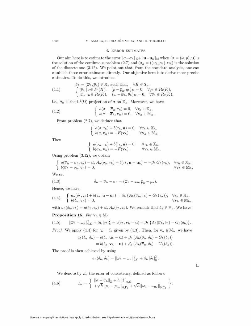
4. Error estimates

Our aim here is to estimate the error ‖σ−σh‖X+‖u−uh‖M when (σ = (ω, p),u) isthe solution of the continuous problem (2.7) and (σh = ((ωh, ph),uh) is the solutionof the discrete one (3.12). We point out that, from the standard analysis, one canestablish these error estimates directly. Our objective here is to derive more preciseestimates. To do this, we introduce

(4.1)σh = (ωh, ph) ∈ Xh such that, ∀K ∈ Th,ph |K∈ P0(K), (p− ph, qh)K = 0, ∀qh ∈ P0(K),ωh |K∈ P0(K), (ω − ωh, θh)K = 0, ∀θh ∈ P0(K),

i.e., σh is the L2(Ω) projection of σ on Xh. Moreover, we have

(4.2)a(σ − σh, τh) = 0, ∀τh ∈ Xh,b(σ − σh,vh) = 0, ∀vh ∈Mh.

From problem (2.7), we deduce thata(σ, τh) + b(τh,u) = 0, ∀τh ∈ Xh,b(σ,vh) = −F (vh), ∀vh ∈Mh.

Then a(σh, τh) + b(τh,u) = 0, ∀τh ∈ Xh,b(σh,vh) = −F (vh), ∀vh ∈Mh.

Using problem (3.12), we obtaina(σh − σh, τh)− βhAh(σh, τh) + b(τh,u− uh) = −βhGh(τh), ∀τh ∈ Xh,b(σh − σh,vh) = 0, ∀vh ∈Mh.

We set

(4.3) δh = σh − σh = (ωh − ωh, ph − ph).

Hence, we have

(4.4)ah(δh, τh) + b(τh,u− uh) = βh Ah(σh, τh)−Gh(τh), ∀τh ∈ Xh,b(δh,vh) = 0, ∀vh ∈Mh,

with ah(δh, τh) = a(δh, τh) + βhAh(δh, τh). We remark that δh ∈ Vh. We have

Proposition 15. For vh ∈Mh

(4.5) ‖ωh − ωh‖20,Ω + βh |δh|2h = b(δh,vh − u) + βh Ah(σh, δh)−Gh(δh).

Proof. We apply (4.4) for τh = δh given by (4.3). Then, for vh ∈ Mh, we have

ah(δh, δh) = b(δh,uh − u) + βh (Ah(σh, δh)−Gh(δh))

= b(δh,vh − u) + βh (Ah(σh, δh)−Gh(δh)).

The proof is then achieved by using

ah(δh, δh) = ‖ωh − ωh‖20,Ω + βh |δh|2h .

We denote by Ec the error of consistency, defined as follows:

(4.6) Ec = ‖σ − σh‖X + h ‖f‖0,Ω

+√h ‖p0 − p0h‖0,Γ2

+√h ‖ω0 − ω0h‖0,Γ3

.



Then, from Lemma 14, we have the existence of a constant C > 0, independent ofh, such that

|Ah(σh, δh)−Gh(δh)| ≤ CEc|δh|h .We also have from definition (2.6) that

|b(δh,vh − u)| ≤ |u− vh|M ‖δh‖X .Hence we deduce from Proposition 15 and these two previous estimates the followingfirst error estimate:

Lemma 16. We set βh = min(1, βh) and denote the error on σ by

(4.7) Eh(σ) = ‖ωh − ωh‖0,Ω +√βh ‖ph − ph‖0,Ω +

√βh |δh|h .

Then, there is a constant C > 0, independent of h, such that for vh ∈Mh, we have

(4.8) Eh(σ) ≤ C√βh

|u− vh|M + C√βhEc.

Proof. Relation (3.15) gives the following inequality:

‖ph − ph‖0,Ω ≤ C (|δh|h + ‖ωh − ωh‖0,Ω).

Then, we have

‖ωh − ωh‖0,Ω +√βh |δh|h ≥

√βh ‖ωh − ωh‖0,Ω + |δh|h

≥ C√βh ‖δh‖X .

Using (4.5), we deduce that

‖ωh − ωh‖20,Ω + βh |δh|2h + βh ‖δh‖2X

≤ C |b(δh,vh − u)|+ Cβh |Ah(σh, δh)−Gh(δh)| .

Proposition 17. There is a constant C > 0, independent of h, such that forvh ∈Mh we have the following error estimate:

(4.9) |u− uh|M ≤ CEc + max(1,√βh)Eh(σ) + |u− vh|M.

Proof. For vh ∈ Mh we define

τh = (− curl(uh − vh), div (uh − vh)) ∈ Xh.Hence, we have

b(τh,uh − vh) = |uh−vh|2M = ‖τh‖2Xand

b(τh,uh − vh) = b(τh,uh − u) + b(τh,u− vh).Using (4.4), we deduce that

b(τh,u− uh) = βh Ah(σh, τh)−Gh(τh) − ah(δh, τh),

which implies that

|b(τh,u− uh)| ≤ βh |Ah(σh, τh)−Gh(τh)|+‖ωh − ωh‖0,Ω‖ curl(uh − vh)‖0,Ω + βh |δh|h |τh|h .

Moreover, since (3.18) states that

|τh|h ≤ C‖τh‖X



and since|b(τh,u− vh)| ≤ |uh−vh|M|u− vh|M,

it follows that

|u− uh|M

≤ Cβh |Ah(σh, τh)−Gh(τh)||τh|h

+ ‖ωh − ωh‖0,Ω + βh |δh|h + |u− vh|M.

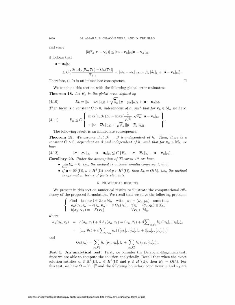
Therefore, (4.9) is an immediate consequence. We conclude this section with the following global error estimates:

Theorem 18. Let Eh be the global error defined by

(4.10) Eh = ‖ω − ωh‖0,Ω +√βh ‖p− ph‖0,Ω + |u− uh|M.

Then there is a constant C > 0, independent of h, such that for vh ∈ Mh we have

(4.11) Eh ≤ C

max(1, βh)Ec + max(

1√βh,√βh)|u− vh|M

+‖ω − ωh‖0,Ω +√βh ‖p− ph‖0,Ω

.

The following result is an immediate consequence:

Theorem 19. We assume that βh = β is independent of h. Then, there is aconstant C > 0, dependent on β and independent of h, such that for vh ∈ Mh wehave

(4.12) ‖σ − σh‖X + |u− uh|M ≤ C Ec + ‖σ − σh‖X + |u− vh|M .Corollary 20. Under the assumption of Theorem 19, we have

• limh→0

Eh = 0, i.e., the method is unconditionally convergent, and

• if u ∈ H2(Ω), ω ∈ H1(Ω) and p ∈ H1(Ω), then Eh = O(h), i.e., the methodis optimal in terms of finite elements.

5. Numerical results

We present in this section numerical results to illustrate the computational effi-ciency of the proposed formulation. We recall that we solve the following problem:

Find (σh,uh) ∈ Xh×Mh with σh = (ωh, ph) such thatah(σh, τh) + b(τh,uh) = β Gh(τh), ∀τh = (θh, qh) ∈ Xh,b(σh,vh) = −F (vh), ∀vh ∈Mh.

where

ah(σh, τh) = a(σh, τh) + β Ah(σh, τh) = (ωh, θh) + β∑

e∈Chhe ([σh]e, [τh]e)e

= (ωh, θh) + β∑

e∈Chhe( ([ωh]e, [θh]e)e + ([ph]e, [qh]e)e)

andGh(τh) =

∑e∈F2

h

he (p0, [qh]e)e +∑e∈F3

h

he (ω0, [θh]e)e.

Test 1: An analytical test. First, we consider the Bercovier-Engelman test,since we are able to compute the solution analytically. Recall that when the exactsolution satisfies u ∈ H2(Ω), ω ∈ H1(Ω) and p ∈ H1(Ω), then Eh = O(h). Forthis test, we have Ω = ]0, 1[2 and the following boundary conditions: p and u2 are



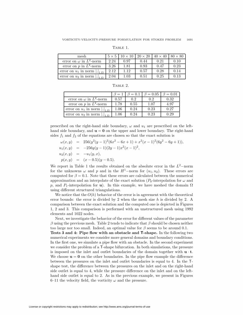
Table 1.

mesh 5× 5 10× 10 20× 20 40× 40 80× 80error on ω in L2-norm 2.24 0.97 0.44 0.21 0.10error on p in L2-norm 3.26 1.81 0.93 0.47 0.23

error on u1 in norm |.|1,Ω 2.12 1.12 0.57 0.28 0.14error on u2 in norm |.|1,Ω 2.04 1.03 0.51 0.25 0.13

Table 2.

β = 1 β = 0.1 β = 0.05 β = 0.01error on ω in L2-norm 0.57 0.2 0.2 0.32error on p in L2-norm 1.78 0.55 1.07 4.97

error on u1 in norm |.|1,Ω 1.06 0.24 0.23 0.27error on u2 in norm |.|1,Ω 1.06 0.24 0.23 0.29

prescribed on the right-hand side boundary, ω and u1 are prescribed on the left-hand side boundary, and u = 0 on the upper and lower boundary. The right-handsides f1 and f2 of the equations are chosen so that the exact solution is

ω(x, y) = 256(y2(y − 1)2(6x2 − 6x+ 1) + x2(x− 1)2(6y2 − 6y + 1)),u1(x, y) = −256y(y− 1)(2y − 1)x2(x− 1)2,

u2(x, y) = −u1(y, x),p(x, y) = (x− 0.5)(y − 0.5).

We report in Table 1 the results obtained on the absolute error in the L2−normfor the unknowns ω and p and in the H1−norm for (u1, u2). These errors arecomputed for β = 0.1. Note that these errors are calculated between the numericalapproximation and an interpolate of the exact solution (P0-interpolation for ω andp, and P1-interpolation for u). In this example, we have meshed the domain Ωusing different structured triangulations.

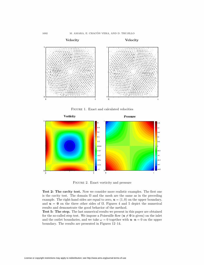
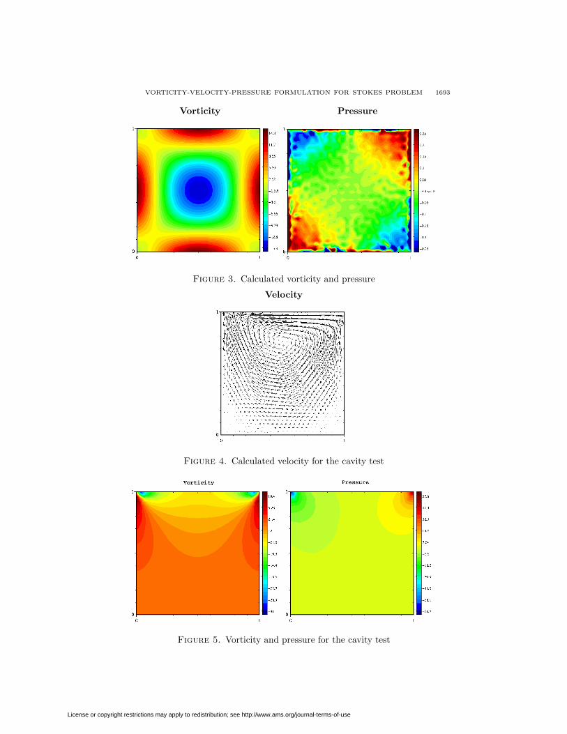
We notice that the O(h) behavior of the error is in agreement with the theoreticalerror bounds: the error is divided by 2 when the mesh size h is divided by 2. Acomparison between the exact solution and the computed one is depicted in Figures1, 2 and 3. This comparison is performed with an unstructured mesh using 1992elements and 1022 nodes.

Next, we investigate the behavior of the error for different values of the parameterβ using the previous mesh. Table 2 tends to indicate that β should be chosen neithertoo large nor too small. Indeed, an optimal value for β seems to be around 0.1.Tests 3 and 4: Pipe flow with an obstacle and T-shape. In the following twonumerical experiments we consider more general domains and boundary conditions.In the first one, we simulate a pipe flow with an obstacle. In the second experimentwe consider the problem of a T-shape bifurcation. In both simulations, the pressureis imposed on the inlet and outlet boundaries of the domain together with u · t.We choose u = 0 on the other boundaries. In the pipe flow example the differencebetween the pressures on the inlet and outlet boundaries is equal to 4. In the T-shape test, the difference between the pressures on the inlet and on the right-handside outlet is equal to 4, while the pressure difference on the inlet and on the left-hand side outlet is equal to 2. As in the previous example, we present in Figures6–11 the velocity field, the vorticity ω and the pressure.



Velocity Velocity

Figure 1. Exact and calculated velocities

Figure 2. Exact vorticity and pressure

Test 2: The cavity test. Now we consider more realistic examples. The first oneis the cavity test. The domain Ω and the mesh are the same as in the precedingexample. The right-hand sides are equal to zero, u = (1, 0) on the upper boundary,and u = 0 on the three other sides of Ω. Figures 4 and 5 depict the numericalresults and demonstrate the good behavior of the method.Test 5: The step. The last numerical results we present in this paper are obtainedfor the so-called step test. We impose a Poiseuille flow (u 6= 0 is given) on the inletand the outlet boundaries, and we take ω = 0 together with u ·n = 0 on the upperboundary. The results are presented in Figures 12–14.



Vorticity Pressure

Figure 3. Calculated vorticity and pressure

Velocity

Figure 4. Calculated velocity for the cavity test

Figure 5. Vorticity and pressure for the cavity test



mesh : 1506 triangles and 819 nodes

Velocity

Figure 6. Calculated velocity for the pipe flow test

Vorticity

Figure 7. Calculated vorticity for the pipe flow test

Pressure

Figure 8. Calculated pressure for the pipe flow test



mesh: 3150 triangles and 1696 nodes

Velocity

Figure 9. Calculated velocity for the T-shape test

Vorticity

Figure 10. Calculated vorticity for the T-shape test

Pressure

Figure 11. Calculated pressure for the T-shape test



Velocity

Figure 12. Calculated velocity for the step test

Vorticity

Figure 13. Calculated vorticity for the step test

Pressure

Figure 14. Calculated pressure for the step test



References

[1] Amara, M. and Bernardi, C., Convergence of a finite element discretization of the Navier-Stokes equations in vorticity and stream function formulation, Mathematical Modelling andNumerical Analysis, vol. 33, n. 5, pp. 1033-1056 (1999). MR 2000k:65200

[2] Amara, M. and El Dabaghi, F., An optimal C0 finite element algorithm for the 2D bihar-monic problem: Theoretical analysis and numerical results, Numerische Mathematik, vol. 90,n. 1, pp. 19-46 (2001). MR 2002h:65172

[3] Amara, M., Chacon Vera, E. and Trujillo, D., Stokes equations with non standard boundaryconditions, Prpubli. du Labo. de Math. Appli. de Pau, n. 13, (2001).

[4] Bernardi, C. and Girault, V., A local regularization operator for triangular and quadrilateralfinite elements, SIAM J. Numer. Anal., vol. 35, n. 5, pp. 1893-1916 (1998). MR 99g:65107

[5] Bernardi, C., Girault, V. and Maday, Y., Mixed spectral element approximation of the Navier–Stokes equation in the stream function and vorticity formulation, IMA, J. of Numer. Anal,12, pp. 564-608, 1992. MR 93i:65113

[6] Costabel, M., A remark on the regularity of solutions of Maxwell’s equations on Lipschitzdomains, Mathematical Methods in the Applied Sciences, vol. 12, 365-368 (1990). MR91c:35028

[7] Conca, C., Pares, C., Pironneau, O. and Thiriet, M., Navier-Stokes equations with imposedpressure and velocity fluxes, International Journal for Numerical Methods in Fluids, vol. 20,267-287 (1995). MR 96d:76019

[8] Dubois, F., Salaun M. and Salmon S., Discrete harmonics for stream function-vorticity Stokesproblem, Numer. Math., vol. 92, 711–742 (2002). MR 2003h:76088

[9] John, F., Partial Differential Equations, Applied Mathematical Sciences, 1. Springer-Verlag,(1978). MR 80f:35001

[10] Girault, V. and Raviart, P.-A., Finite Element Methods for the Navier-Stokes Equations.Theory and Algorithms, Springer-Verlag, (1986). MR 88b:65129

[11] Grisvard, P., Elliptic Problems in Nonsmooth Domains, Pitman, (1985). MR 86m:35044

[12] Hughes, T. and Franca, L., A new finite element formulation for computational fluid dy-namics. VII. The Stokes problem with various well-posed boundary conditions: Symetricformulations that converge for all velocity/pressure space, Comput. Methods in Appl. Mech.and Eng., 65, 85–96, (1987). MR 89j:76015g

[13] Lions, J.L. and Magenes, E., Problemes aux limites non homogenes et applications, vol 1,Dunod, Paris (1969). MR 40:512

IPRA-LMA, Universite de Pau, 64000 Pau, France

E-mail address: [email protected]

IPRA-LMA, Universite de Pau, 64000 Pau, France


Departamento de Ecuaciones Diferenciales y Analisis, Universidad de Sevilla, 41080

Sevilla, Spain



http://www.ams.org/mathscinet-getitem?mr=2000k:65200

http://www.ams.org/mathscinet-getitem?mr=2002h:65172

http://www.ams.org/mathscinet-getitem?mr=99g:65107

http://www.ams.org/mathscinet-getitem?mr=93i:65113

http://www.ams.org/mathscinet-getitem?mr=91c:35028

http://www.ams.org/mathscinet-getitem?mr=96d:76019

http://www.ams.org/mathscinet-getitem?mr=2003h:76088

http://www.ams.org/mathscinet-getitem?mr=80f:35001

http://www.ams.org/mathscinet-getitem?mr=88b:65129

http://www.ams.org/mathscinet-getitem?mr=86m:35044

http://www.ams.org/mathscinet-getitem?mr=89j:76015g

http://www.ams.org/mathscinet-getitem?mr=40:512

vorticity-velocity-pressure formulation for stokes problem

Documents