a redefinition of jupiter's rotation period

JOURNAL OF GEOPHYSICAL RESEARCH, VOL. 102, NO. A10, PAGES 22,033-22,041, OCTOBER 1, 1997

A redefinition of Jupiter's rotation period

Charles A. Higgins, Thomas D. Carr, Francisco Reyes, Wes B. Greenman, and George R. Lebo Astronomy Department, University of Florida, Gainesville

Abstract. We measured the rotation period of Jupiter's inner magnetosphere with precision previously unattainable, using 35 years of observations of the Jovian decametric radiation at the University of Florida Radio Observatory at frequencies between 18 and 22.2 MHz. The new rotation period is the weighted mean of 13 independent 24-year average determinations. Each of these was found by measuring the drift of the histogram of occurrence probability versus System III (1965) central meridian longitude over an interval of approximately 24 years. The measured drift was used to correct the System III (1965) period to obtain the new value. Our weighted mean is 9 hours 55 min 29.6854 s, with a standard deviation of the weighted mean (a) of 0.0035 s. This new rotation period is 7.4a shorter than that of the System III (1965), indicating that the latter is in need of revision. Our measurements indicate an upper limit of about 4 ms/year on any possible Jovian rotation period drift.

1. Introduction

Since Jupiter does not have a solid surface, no fixed visible feature can be used for making precise measurements of its rotation period from Earth. The famil- iar spots are the tops of clouds that drift through the atmosphere at variable speeds in response to the vio- lent Jovian winds. Marth [1875] and Williams [1896] were prominent among the earlier astronomers who attempted to determine a nonvarying Jovian rotation period value accurately by averaging many measurements calculated from successive transit times of particular cloud tops across the central meridian. The corresponding central meridian longitude (CML) systems were designated as System I, for cloud tops at equatorial latitudes, and System II, for temperate zone cloud tops. Further attempts by optical astronomers to determine a unique rotation period value that might be attributed to a stable rotating interior continued, without success, until about 35 years ago. This situation changed, however, after the discoveries of radio emissions from relatively fixed sources on Jupiter. This paper follows a long series of papers based on radio measurements of Jupiter's rotation period that began in 1956. The measurement presented here is by far the most precise that has been made by any means.

The Jovian decametric radiation was discovered by Burke and Franklin [1955] at a frequency of about 20

Copyright 1997 by the American Geophysical Uniou.

Paper number 97JA02090. 0148-0227/97/97JA-02090509.00

MHz. This nonthermal radiation was the first discov-

ered planetary radiation, and it provided the first ev- idence of a Jovian magnetic field [Gardner and $hain, 1958; Cart, 1959]. The first observation of the Jovian nonthermal continuum radiation that occurs at decime-

ter and shorter wavelengths (i.e., at frequencies of hun- dreds and thousands of megahertz) was made by Mayer et al. [1958]. By the mid-1960s it was definitely established that this new component was synchrotron radiation, and there was no longer any question that Jupiter had a magnetic field.

$hain [1956] was the first to obtain a measurement of the Jovian rotation period from decametric observations. He found that the emission occurrence probability tends to vary periodically in time, and by measuring this periodicity he obtained a rotation period value. Subsequently, decametric radio rotation period measurements were made by several groups, including ours at the University of Florida. In each of these measurements, histograms of occurrence probability versus System II CML for two or more apparitions were plotted. From the observed rate of CML drift in the main

peak (source A) the corrected value of the rotation period, Pc, was calculated by means of the formula

1 1 AA -1

Pc-[po 360 At] ' (1) Po is the initially assumed rotation period, and AA is the observed CML drift (in degrees) of the source A peak over the time interval At between the midtimes of the initial and final apparitions.

These radio measurements became more accurate as

the number of years that elapsed between the first and

22,033

22,034 HIGGINS ET AL' JUPITER'S ROTATION PERIOD

last of such histograms was increased. By 1962 the measurements were in sufIiciently close agreement that the International Astronomical Union (IAU) adopted the so-called "System III (1957.0)" Jovian longitude system for radio observations [Douglas, 1960]. It was based on an assumed rotation period of 9 hours 55 min 29.37 s, the weighted mean of the radio measurements [Burke et al., 1962]. Following the identification of the Jo- vian synchrotron radiation, it, too, was used for rotation period measurements. The most precise of these early synchrotron measurements was that of Roberts and Komesaro• [1965]. Their value did not differ significantly from the decametric-determined System III (1957.0) value.

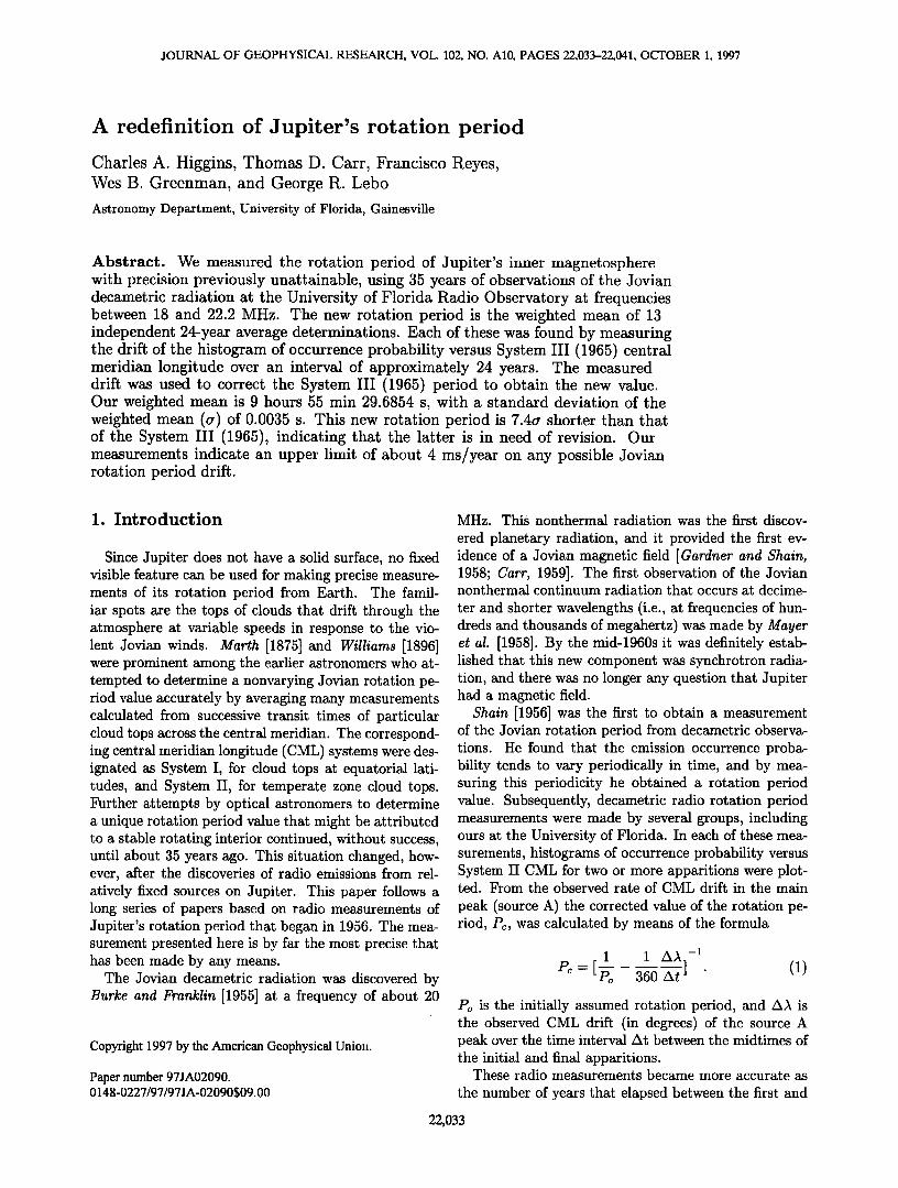
During the mid-1960s, several reports stated that the measured average decametric rotation period had shifted rather abruptly by a substantial fraction of a second. This effect was subsequently explained by Gulkis and Cart [1966] and Cart et al. [1970]. It was demonstrated that the midlongitude of the main peak of the probability of occurrence histogram for a given apparition depends on the mean Jovicentric declination of Earth, DE, during the apparition. DE is also referred to as the Jovian sub-Earth latitude; its period of variation is 11.9 years (i.e., Jupiter's orbital period), and its average value over successive apparitions varies between about -3ø.3 and +3ø.3. This effect is well illustrated in

Figure 1, in which the CML of the source A peak (the most probable CML for detecting emission) at 18 MHz is plotted versus time. The average of DE over each apparition is also plotted versus time for comparison. It is apparent from Figure I that a large error in the average rotation period value can be introduced if the mean Dr values during the two apparitions of a widely separated pair differ appreciably. It is also clear that if the measurements are made only from pairs of apparitions having middates separated by approximately 12 years, so that the two DE values are nearly the same, the error largely disappears. Cart [1972] incorporated this improvement into the measurement procedure and obtained a mean of 9 hours 55 min 29.74 s 4- 0.04 s from

eight measured 12-year averaged rotation period values. After several years of new data had become available, May et al. [1979] were able to make 26 such individual 12-year average rotation period determinations, the weighted mean of which was 9 hours 55 min 29.689 s.

Meanwhile, Duncan [1971] employed a somewhat different method, which is seemingly less affected by variations in Dr. He used the CML position of the leading edge of source A, which has been shown to be nearly independent of DE [Cart et al., 1970]. He determined the storm commencement times and then made a su-

perimposed epoch spectral analysis to arrive at the rotation period. His last published value was 9 hours 55 min 29.70 s 4- 0.05 s. By the mid-1970s it had become apparent from measurements made with both the decametric and synchrotron radiation components that the System III (1957.0) rotation period was in need of

280

27O

• 26O

-o 250

o - 240

230

22O

1955

Declination Effect

.... i .... i .... i .... i .... i .... i .... i .... t

, , , i .... I .... i .... I .... i , , , , I , , , , I , , , ,

1960 1965 1970 1975 1980 1985 1990 1995 Year

Figure 1. Longitudinal positions of the peak occurrence probabilities for each apparition of source A at 18 MHz, plotted as a function of time. Note the 12-year oscillation in the source location, and also note that the phase of the occurrence probability curve matches that of the DE curve plotted below for reference. The change in the DE curve is caused by Jupiter's orbital motion with respect to Earth.

revision. Accordingly, Riddle and Warwick [1976] com- puted the weighted average of the decametric measurements of Duncan [1971], Cart [1972], and Kaiser and Alexander [1972] and the synchrotron radiation determination of Berge [1974], obtaining the value 9 hours 55 min 29.71 s. Defined as the System III (1965) Jovian rotation period, it was subsequently adopted by the IAU. Since that time the only published new Jovian rotation period measurements of which we are aware are the May et al. [1979] calculation at the University of Florida, a new synchrotron radiation determination by Komesaroff et al. [1980], which was in good agreement with the earlier synchrotron measurement, and the report by Higgins et al. [1996] on the results presented here.

In this paper we report on a new measurement of the rotational period of the inner Jovian magnetosphere that is clearly of unprecedented precision. This result is determined from decametric observations made at three

frequencies from the University of Florida Radio Obser- vatory from 1957 to 1994 and over a part of this time span from the Maipu Radio Astronomy Observatory in Chile. We present a detailed description of our method, which we believe is the most precise method available and which, with continuing observations, should provide increasing precision in the future. A tabulation of our separate determinations, which will be of value in future searches for a true radio rotation period change, is included. It is demonstrated that the currently accepted IAU standard System III (1965) period is in need of revision. The prospect for the future detection of long-term variations in the magnetic field is discussed.

HIGGINS ET AL.: JUPITER'S ROTATION PERIOD 22,035

2. Observations and Initial Data

Reduction

The observations span 35 apparitions of Jupiter from 1957 to 1994. Most of the observations were made at the

University of Florida Radio Observatory using nearly identical equipment for all the observations. The re- mainder (10 apparitions from 1960-1964 and 1972-1976) were made jointly by University of Florida and Univer- sity of Chile personnel at the Maipu Radio Astronomy Observatory near Santiago, Chile. The Florida observations were made at 18, 20, and 22.2 MHz, with receiver bandwidths of 6 kHz. The observations in Chile were

made at 18 and 22.2 MHz with the same bandwidth.

This is the best spectral region to observe, because there is increased ionospheric absorption and interference at lower frequencies and much lower probabilities of emission at higher frequencies. A separate antenna of relatively low gain, usually a five-element tracking yagi antenna, was used for each frequency channel. Al- though our antennas have relatively low gain, they are appropriate for rotation period measurements, because the weaker Jovian component has a much more variable CML distribution. The receiver outputs, along with appropriate time marks, were pen recorded on analog strip charts having a recording time constant of about I s.

All the Jovian decametric activity is in the form of sporadic bursts, often occurring in the form of intense storms having well-defined beginnings and end- ings. There is also a great deal of more isolated activity, however, that consists of scattered small groups of bursts. The probability of occurrence of activity over given intervals of time (or CML) is defined as the ratio of the total activity time to the total time of effective observing. The effective observing time is the total time during which interference was sufficiently low that any activity of greater intensity than our detection thresh- old could have been detected, or actually was detected. For our relatively low sensitivity observations at single frequencies the histograms of occurrence probability versus CML usually display three broad peaks. The earliest (i.e., the one having the lowest CML) is known as source Io-B. The last and least probable is source Io-C, and the middle and most probable is the super- position of sources Io-A and non-Io-A [see Cart et al., 1983]. The Io-reiated ones are active only when Io is within certain narrow sectors of its orbit about Jupiter, while the non-Io-A activity is completely independent of Io. However, non-Io-A is strongly dependent on De. It nearly disappears during apparitions in which De is near its minimum value (slightly less than -3 ø ) and ex- hibits a higher occurrence probability than any of the other sources when De is positive.

In reducing the data from a given night of observations the strip chart for each frequency channel was inspected, and the start and end times of the overall observing period were recorded. The start and end times of periods of interference that were sufficiently intense

to obscure weak Jovian bursts were also noted. Observ-

ing periods were terminated at the start of each interference interval and then restarted at the conclusion of

the interference. The overall observing period remain- ing after the deletion of intervals of severe interference is referred to as the effective observing period. Each effective observing period was subsequently inspected for Jupiter activity. Jovian activity was considered to be continuous for as long as there was at least one burst in each successive 5-min interval with no gaps in the data larger than 15 min. If there was such a gap, a new observing period was begun.

After an entire apparition of such strip chart record- ings had been read for a given frequency, all the starting and ending times of the effective observing periods (in UT) and all the starting and ending times of Jupiter activity were converted into Jovian CML values by using an ephemeris program. Although the time resolution for reducing the data was 5-min, these 5-min readings were then binned into 5 ø CML intervals. For each 5 ̧

CML interval from 0 ø to 360 ø the occurrence probability was calculated by taking the ratio of the number in the activity bin to that in the observing bin. Then the 72 occurrence probability values for 5 ø CML intervals were smoothed to obtain 144 probability values for 2.5 ø intervals. Finally, the histogram of occurrence probability was plotted as a function of CML in the 2.5 ø intervals. Similar histograms were created for all three frequency channels for each apparition used in this study.

3. Rotation Period Calculations 3.1. Cross-Correlation Method of Drift

Measurement

A total of 24 independent measurements of the 24- year or 12-year average values of the Jovian rotation period were made, and the final result is their weighted mean. Each measurement was obtained from a pair of histograms of occurrence probability versus CML for which the middates were separated by approximately 12 or 24 years. Such separations were chosen in order that the average values of Ds for the two apparitions in a pair would be nearly equal. Equation (1) was used to calculate a corrected value of the rotation period, Pc, from the two histograms for each pair of apparitions. Since System III (1965) was used in specifying CML for the histograms, the initially assumed period Po in equation (1) is simply the System III (1965) period. The elapsed time from the midtime of the first apparition in the pair to that of the second apparition is At. The CML drift, AA, was calculated from the cross- correlation function for the histogram pair (as was done in the May et al. [1979] paper). A simple formula for the value of the cross-correlation function r for a 2.5 ø

CML shift AL of the second histogram with respect to the first is given by

n

r(AL) - 1 Z[f• (Li)- f•][f2(Li + AL)- f2] (2) T/,171 t7 2 .

22,036 HIGGINS ET AL.' JUPITER'S ROTATION PERIOD

where n = 144, Li is the CML value designating the CML bin, fl (Li) represents the histogram for the first apparition, f•.(Li+AL) represents the second histogram,

_ _

fl and f•. are the average values of the occurrence probabilities for the two histograms, and (Yl and •. are the

_

standard deviations of the means of fl (Li) - fl and f•.(L• + AL) - f•., respectively.

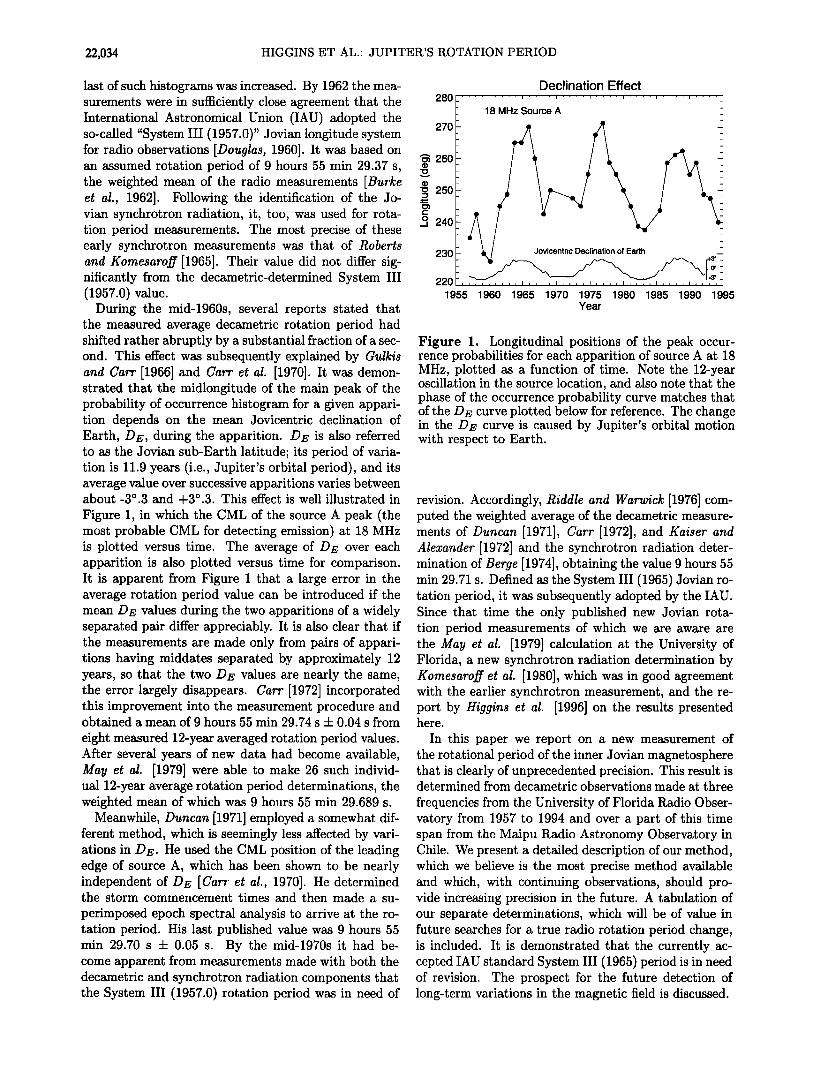
The value of AL that maximizes r(AL) represents an estimate of the CML drift of the second histogram with respect to the first, to the nearest 2.5 ø interval. The drift was then determined to a precision of about 0.1 ø by finding the CML value at the maximum of a fourth-order polynomial fit to the peak of the correlation function between 4-30 ø . This more precise estimate of the drift is the value used for A• in equation (1). The method is illustrated in Figure 2. Figures 2a and 2b represent the two histograms for single-frequency observations made during apparitions separated by about 24 years, and Figure 2c is their cross-correlation function with the indicated CML shift. This procedure was employed for all the other same-observatory, same- frequency apparition pairs that are separated by 12 or 24 years. None of the data sets for a given observatory, apparition, and frequency were used more than once.

3.2. Method of Weighting and Averaging of Individual Measurements

A separate rotation period value was calculated from the data of each same-observatory, same-frequency apparition pair. The proper weighting of these initial values was of primary importance because of the variabil- ity of the quality of observing conditions, the perfor- mance of equipment and personnel, and the amount of Jovian activity. Subsequent averaging was done in stages. In the first stage the period values determined at the two or three frequencies at each of the observato- ries for each apparition pair were combined into a single value by taking their weighted average. This was necessary because they could not separately be counted as completely independent measurements in the final standard deviation determination. In the second stage the weighted averages and standard deviations of the first- stage values were calculated separately for the 24-year and 12-year apparition pairs (the latter included Chile as well as Florida data). The decision whether to average the inherently less precise 12-year weighted mean with the 24-year weighted mean was deferred until it could be ascertained whether so doing would lead to an appreciable increase in precision.

0.4

.(3 0.2 (!3

..• 0 0.1

ß o.o,

•_•

o

Cross Correlation Technique

_ (a) 1963 sou• - 30 60 90 120 150 180 210 240 270 300 330

_ (b)1987 _

source A

Central Meridian Longitude (deg)

Cross Correlation

(:D ß

0

.

-180 -150 -120 -90 -60 -30 0 30 60 90 120 150 180

Longitude Shift (deg)

Figure 2. Data used for a single rotation period measurement. (a) Histogram of occurrence probability versus CML at 22 MHz for the 1963 apparition. The peaks commonly known as sources A, B, and C are labeled. (b) Same type of histogram for the 1987 apparition. (c) Smoothed plot of the cross correlation of the two histograms as a function of the shift of the later one with respect to the earlier one. The maximum correlation, which is based on a polynomial fit to the curve between +30ø(heavy dashed curve), is 0.975 and occurs at a longitude shift of -6ø.8. From Higgins et al. [1996]

HIGGINS ET AL.' JUPITER'S ROTATION PERIOD 22,037

3.2.1. First Stage To each single rotation period measurement, pj, obtained from one observatory for one apparition pair at one frequency we assign a statistical weight wj given by

- (3) where rj is the cross-correlation coefficient for the two histograms (defined as the value of the correlation function at its peak) and {a)j is the geometrical mean of the total activity times during the two apparitions (i.e., the effective activity time). The reason for this choice for the weighting factor is that on the one hand, the expected rms uncertainty due to statistical fluctuations is inversely proportional to the square root of the effective activity time, and on the other hand, the value of rj is a direct measure of the similarity of the two histograms. If all factors affecting histogram quality were highly fa- vorable, the two histograms should be nearly identical, and rj would be nearly 1.0. Otherwise, rj would be less than 1.0 by an amount depending on the combined degree of histogram dissimilarity.

The first-stage average rotation period /•k and its weight Wk are determined from all the individual rotation periods pj, and their corresponding weights wj for each of the frequency channels at one observatory for a given apparition pair are given by

E7=l pj , wj N , W• - • w• (4)

where N indicates the number of frequency channels used (3, 2, or 1). The formula for W• was used because we assigned equal confidence for each frequency-based rotation period.

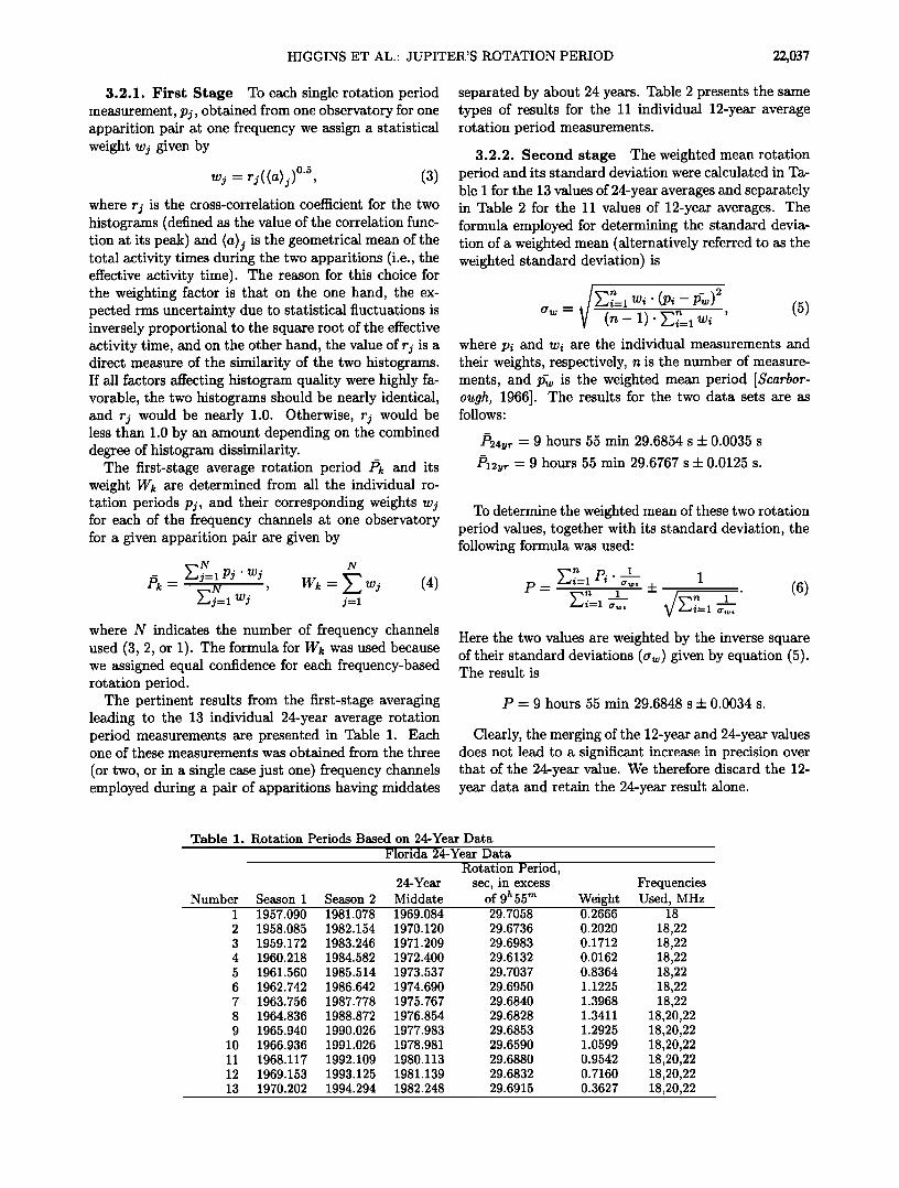
The pertinent results from the first-stage averaging leading to the 13 individual 24-year average rotation period measurements are presented in Table 1. Each one of these measurements was obtained from the three

(or two, or in a single case just one) frequency channels employed during a pair of apparitions having middates

separated by about 24 years. Table 2 presents the same types of results for the 11 individual 12-year average rotation period measurements.

3.2.2. Second stage The weighted mean rotation period and its standard deviation were calculated in Ta- ble I for the 13 values of 24-year averages and separately in Table 2 for the 11 values of 12-year averages. The formula employed for determining the standard deviation of a weighted mean (alternatively referred to as the weighted standard deviation) is

n_--I Wi ' (Pi - iffw) 2 aw - (n- 1) Y•i•l wi ' (5) where Pi and wi are the individual measurements and their weights, respectively, n is the number of measurements, and iffw is the weighted mean period [Scarbor- ough, 1966]. The results for the two data sets are as follows:

P24yr - 9 hours 55 min 29.6854 s q- 0.0035 s _

P12yr - 9 hours 55 min 29.6767 s q- 0.0125 s.

To determine the weighted mean of these two rotation period values, together with its standard deviation, the following formula was used:

p__ Ein_--I Pi' 1__ 1 . (6) En 1 v/En 1 i--1 •,,: i--1

Here the two values are weighted by the inverse square of their standard deviations (aw) given by equation (5). The result is

P - 9 hours 55 min 29.6848 s q- 0.0034 s.

Clearly, the merging of the 12-year and 24-year values does not lead to a significant increase in precision over that of the 24-year value. We therefore discard the 12- year data and retain the 24-year result alone.

Table 1. Rotation Periods Based on 24-Year Data

Number Season 1 Season 2

Florida 24-Year Data

Rotation Period, 24-Year sec, in excess Middate of 9 h 55 m Weight

Frequencies Used, MHz

1 1957.090 1981.078 2 1958.085 1982.154 3 1959.172 1983.246 4 1960.218 1984.582

5 1961.560 1985.514

6 1962.742 1986.642 7 1963.756 1987.778 8 1964.836 1988.872 9 1965.940 1990.026

10 1966.936 1991.026 11 1968.117 1992.109 12 1969.153 1993.125 13 1970.202 1994.294

1969.084 29.7058 0.2666 1970.120 29.6736 0.2020 1971.209 29.6983 0.1712 1972.400 29.6132 0.0162 1973.537 29.7037 0.8364 1974.690 29.6950 1.1225 1975.767 29.6840 1.3968 1976.854 29.6828 1.3411 1977.983 29.6853 1.2925 1978.981 29.6590 1.0599 1980.113 29.6880 0.9542 1981.139 29.6832 0.7160 1982.248 29.6915 0.3627

18

18,22 18,22 18,22 18,22 18,22 18,22

18,20,22 18,20,22 18,20,22 18,20,22 18,20,22 18,20,22


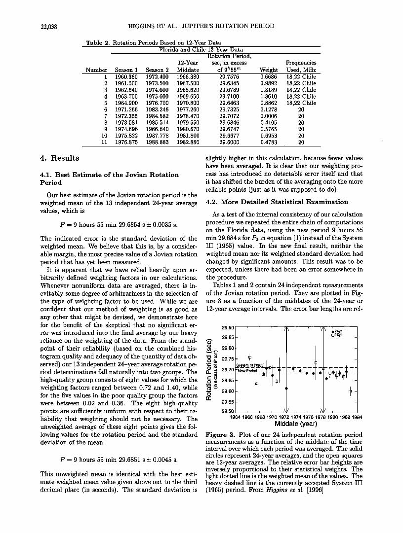
Table 2. Rotation Periods Based on 12-Year Data Florida and Chile 12-Year Data

Number Season 1 Season 2

Rotation Period, 12-Year sec, in excess Frequencies Middate of 9 h55 " Weight Used, MHz

I 1960.360 1972.400 2 1961.500 1973.500 3 1962.640 1974.600

4 1963.700 1975.600 5 1964.900 1976.700 6 1971.266 1983.246 7 1972.355 1984.582 8 1973.581 1985.514 9 1974.696 1986.640

10 1975.822 1987.778 11 1976.875 1988.883

1966.380 29.7576 0.6686 18,22 Chile 1967.500 29.6345 0.9892 18,22 Chile 1968.620 29.6789 1.3139 18,22 Chile 1969.650 29.7100 1.3610 18,22 Chile 1970.800 29.6463 0.8862 18,22 Chile 1977.260 29.7325 0.1278 20 1978.470 29.7072 0.0006 20 1979.550 29.6846 0.4105 20 1980.670 29.6747 0.5765 20 1981.800 29.6677 0.6953 20 1982.880 29.6000 0.4783 20

4. Results

4.1. Best Estimate of the Jovian Rotation

Period

Our best estimate of the Jovian rotation period is the weighted mean of the 13 independent 24-year average values, which is

P - 9 hours 55 min 29.6854 s 4, 0.0035 s.

The indicated error is the standard deviation of the

weighted mean. We believe that this is, by a consider- able margin, the most precise value of a Jovian rotation period that has yet been measured.

It is apparent that we have relied heavily upon ar- bitrarily defined weighting factors in our calculations. Whenever nonuniform data are averaged, there is in- evitably some degree of arbitrariness in the selection of the type of weighting factor to be used. While we are confident that our method of weighting is as good as any other that might be devised, we demonstrate here for the benefit of the skeptical that no significant error was introduced into the final average by our heavy reliance on the weighting of the data. From the stand- point of their reliability (based on the combined histogram quality and adequacy of the quantity of data observed) our 13 independent 24-year average rotation period determinations fall naturally into two groups. The high-quality group consists of eight values for which the weighting factors ranged between 0.72 and 1.40, while for the five values in the poor quality group the factors were between 0.02 and 0.36. The eight high-quality points are sufficiently uniform with respect to their reliability that weighting should not be necessary. The unweighted average of these eight points gives the following values for the rotation period and the standard deviation of the mean:

P - 9 hours 55 min 29.6851 s 4- 0.0045 s.

This unweighted mean is identical with the best estimate weighted mean value given above out to the third decimal place (in seconds). The standard deviation is

slightly higher in this calculation, because fewer values have been averaged. It is clear that our weighting pro- cess has introduced no detectable error itself and that

it has shifted the burden of the averaging onto the more reliable points (just as it was supposed to do).

4.2. More Detailed Statistical Examination

As a test of the internal consistency of our calculation procedure we repeated the entire chain of computations on the Florida data, using the new period 9 hours 55 min 29.684 s for P0 in equation (1) instead of the System III (1965) value. In the new final result, neither the weighted mean nor its weighted standard deviation had changed by significant amounts. This result was to be expected, unless there had been an error somewhere in the procedure.

Tables i and 2 contain 24 independent measurements of the Jovian rotation period. They are plotted in Fig- ure 3 as a function of the middates of the 24-year or 12-year average intervals. The error bar lengths are rel-

29.90

29.85

29.80

29.75

29.70

29.60

_ [] 12yr _

_

_

.... "-' "-"' "-' ø '-' -

29.55 - -

29.50 1964 1966 1968 1970 1972 1974 1976 1978 1980 1982 1984

Middate (year)

Figure 3. Plot of our 24 independent rotation period measurements as a function of the middate of the time

interval over which each period was averaged. The solid circles represent 24-year averages, and the open squares are 12-year averages. The relative error bar heights are inversely proportional to their statistical weights. The light dotted line is the weighted mean of the values. The heavy dashed line is the currently accepted System III (1965) period. From Higgins et al. [1996]

HIGGINS ET AL. JUPITER'S ROTATION PERIOD 22,039

ative and are made inversely proportional to their statistical weights (described in section 3). The two points with off-scale error bars carry negligible weight because of abnormally short observing seasons in combination with very low rates of Jovian activity (because of low values of Dr). The light dotted line is the weighted mean of the plotted points, and the heavy dashed line represents the System III (1965) rotation period.

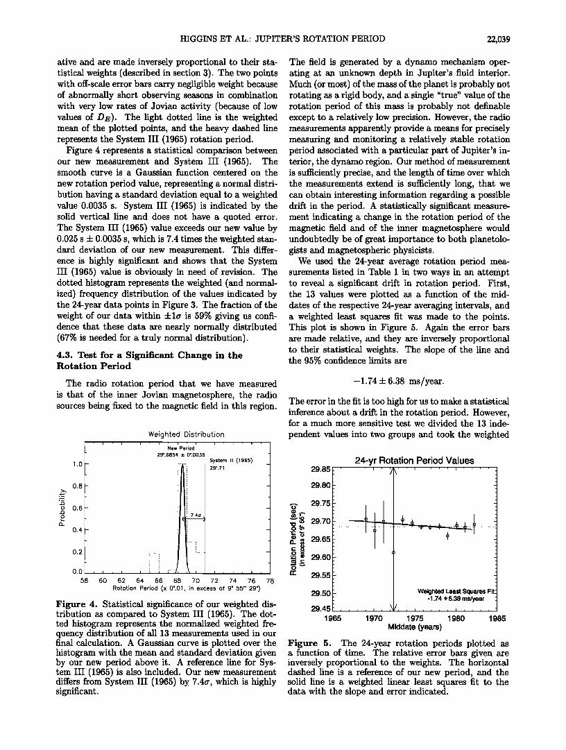
Figure 4 represents a statistical comparison between our new measurement and System III (1965). The smooth curve is a Gaussian function centered on the

new rotation period value, representing a normal distribution having a standard deviation equal to a weighted value 0.0035 s. System III (1965) is indicated by the solid vertical line and does not have a quoted error. The System III (1965) value exceeds our new value by 0.025 s + 0.0035 s, which is 7.4 times the weighted standard deviation of our new measurement. This differ-

ence is highly significant and shows that the System III (1965) value is obviously in need of revision. The dotted histogram represents the weighted (and normalized) frequency distribution of the values indicated by the 24-year data points in Figure 3. The fraction of the weight of our data within +la is 59% giving us confidence that these data are nearly normally distributed (67% is needed for a truly normal distribution).

4.3. Test for a Significant Change in the Rotation Period

The radio rotation period that we have measured is that of the inner Jovian magnetosphere, the radio sources being fixed to the magnetic field in this region.

Weighted Distribution i , i i , i , i , i , i , i , i ,

New Period

29'.6854 ñ 0'.0035

System III (1965)

i : ! :

: i .

i / : 7.4• :

i : .

:

, i ..... • , i ; i ;"' I I , I , I ,

1.0

0.8

0.6

0.4

0.2

0.0

58 60 62 64 66 68 70 72 74 76 78

Rototion Period (x 0".01, in excess of 9 h 55"' 29")

Figure 4. Statistical significance of our weighted distribution as compared to System III (1965). The dotted histogram represents the normalized weighted frequency distribution of all 13 measurements used in our final calculation. A Gaussian curve is plotted over the histogram with the mean and standard deviation given by our new period above it. A reference line for Sys- tem III (1965) is also included. Our new measurement differs from System III (1965) by 7.4a, which is highly significant.

The field is generated by a dynamo mechanism oper- ating at an unknown depth in Jupiter's fluid interior. Much (or most) of the mass of the planet is probably not rotating as a rigid body, and a single "true" value of the rotation period of this mass is probably not definable except to a relatively low precision. However, the radio measurements apparently provide a means for precisely measuring and monitoring a relatively stable rotation period associated with a particular part of Jupiter's interior, the dynamo region. Our method of measurement is sufficiently precise, and the length of time over which the measurements extend is sufficiently long, that we can obtain interesting information regarding a possible drift in the period. A statistically significant measurement indicating a change in the rotation period of the magnetic field and of the inner magnetosphere would undoubtedly be of great importance to both planerolo- gists and magnetospheric physicists.

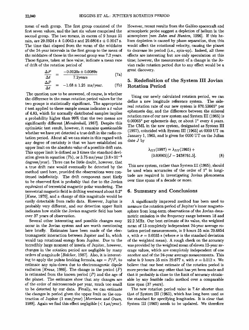
We used the 24-year average rotation period measurements listed in Table I in two ways in an attempt to reveal a significant drift in rotation period. First, the 13 values were plotted as a function of the middates of the respective 24-year averaging intervals, and a weighted least squares fit was made to the points. This plot is shown in Figure 5. Again the error bars are made relative, and they are inversely proportional to their statistical weights. The slope of the line and the 95% confidence limits are

-1.74 + 6.38 ms/year.

The error in the fit is too high for us to make a statistical inference about a drift in the rotation period. However, for a much more sensitive test we divided the 13 inde-

pendent values into two groups and took the weighted

29.85

29.80

•, 29.75

.o.,o 29.70 Oo•

n • 29.65

= e 29.60

n' 29.55

29.50

29.45 , ,

1965

24-yr Rotation Period Values .... ,. :/\.. , ,

1970

Weighted Least Squares Fit -1.74 -t-6.38 ms/year

I , , i .... i ....

1975 1980 1985

Middate (years)

Figure 5. The 24-year rotation periods plotted as a function of time. The relative error bars given are inversely proportional to the weights. The horizontal dashed line is a reference of our new period, and the solid line is a weighted linear least squares fit to the data with the slope and error indicated.


mean of each group. The first group consisted of the first seven values, and the last six values comprised the second group. The two means, in excess of 9 hours 55 min, are 29.6924 s + 0.0043 s and 29.6804 s + 0.0047 s. The time that elapsed from the mean of the middates of the 24-year intervals in the first group to the mean of the middates of those in the second group was 7.2 years. These figures, taken at face value, indicate a mean rate of drift of the rotation period of

Ap -0.0120s + 0.0089s = (7a)

At 7.2years AP

= -1.68 + 1.25 ms/year. (7b) At

The question now to be answered, of course, is whether the difference in the mean rotation period values for the two groups is statistically significant. The appropriate t test applied to these sample means indicates a t value of 4.83, which for normally distributed samples implies a probability higher than 99% that the two means are significantly different [Mendenhall, 1987]. Despite this optimistic test result, however, it remains questionable whether we have yet detected a true drift in the radio rotation period. About all we can state in this regard with any degree of certainty is that we have established an upper limit on the absolute value of a possible drift rate. This upper limit is defined as 3 times the standard deviation given in equation (7b), or 3.75 ms/year (3.8x 10 -5 degrees/year). There can be little doubt, however, that a true drift rate would eventually be detected by the method used here, provided the observations were continued indefinitely. The drift component most likely to be observed first is probably that due to the Jovian equivalent of terrestrial magnetic polar wandering. The terrestrial magnetic field is drifting westward about 0.2 ø [Kane, 1976], and a change of this magnitude would be easily detectable from radio data. However, Jupiter is probably very different, and our detection upper limit indicates how stable the Jovian magnetic field has been over 37 years of observation.

Several other interesting and possible changes may occur in the Jovian system and are worth mentioning here briefly. Estimates have been made of the electromagnetic interaction between Jupiter and Io, which would tap rotational energy from Jupiter. Due to the incredibly large moment of interia of Jupiter, however, changes in the rotation period are negligible by many orders of magnitude [Belcher, 1987]. Also, it is interesting to apply the pulsar braking formula, age - P/t b, to estimate any spin-down due to electromagnetic dipole radiation [Kraus, 1986]. The change in the period (/5) is estimated from the known period (P) and the age of the planet. The estimates show that any changes are of the order of microseconds per year, much too small to be detected by our data. Finally, we can estimate the changes in period given the upper limit on the con- traction of Jupiter (1 mm/year) [Morrison and Owen, 1988]. Again we find this effect negligible (< 1/•s/year).

However, recent results from the Galileo spacecraft and atmospheric probe suggest a depletion of helium in the atmosphere [von Zahn and Hunten, 1996]. If this helium depletion is caused by phase separation, then this would affect the rotational velocity, causing the planet to decrease its period (i.e., spin-up). Indeed, all these effects are interesting but are only speculation at this time; however, the measurement of a change in the Jo- vian radio rotation period due to any effect would be a great discovery.

5. Redefinition of the System III Jovian Rotation Period

Using our newly calculated rotation period, we can define a new longitude reference system. The sidereal rotation rate of our new system is 8?0.53665 ø per ephemeris day, and the difference between the sidereal rotation rate of our new system and System III (1965) is 0.00065 ø per ephemeris day, or about 1 ø every 4 years. The CML in the new system, designated as System III (1997), coincided with System III (1965) at 0000 UT on January 1, 1965, and is given for 0000 UT on the Julian date J by

,kH•(1997) -- AH•(1965) +

(0.00065)[J- 2438761.5]. (8)

This new system, rather than System III (1965), should be used when accuracies of the order of 1 ø in longitude are required in investigating Jovian phenomena over time spans of a decade or more.

6. Summary and Conclusions

A significantly improved method has been used to measure the rotation period of Jupiter's inner magnetosphere from long-term observations of the Jovian decametric emission in the frequency range between 18 and 22.2 MHz. Our best estimate of its value, the weighted mean of 13 completely independent 24-year average rotation period measurements, is 9 hours 55 min 29.6854 s, with a = 0.0035 s (where a is the standard deviation of the weighted mean). A rough check on the accuracy was provided by the weighted mean of eleven 12-year average values, which are completely independent of one another and of the 24-year average measurements. This value is 9 hours 55 min 29.677 s, with • = 0.012 s. We believe that our best estimate of the rotation period is more precise than any other that has yet been made and that it probably is close to the limit of accuracy obtain- able by any feasible radio method over a comparable time span (37 years).

The new rotation period value is 7.4• shorter than that of System III (1965), which has long been used as the standard for specifying longitudes. It is clear that System III (1965) needs to be updated. We therefore

HIGGINS ET AL.: JUPITER'S ROTATION PERIOD 22,041

propose System III (1997), which is based on our estimate of the rotation period. A Jovian feature that is stationary in System III (1997) longitude would drift toward higher System III (1965) longitudes at the rate of about 1 ø every 4 years.

We attempted to detect a true drift in rotation period over the 37-year span, i.e., one that is of planetary rather than statistical origin. We found only a marginal result that the Jovian period may have changed slightly over our span of observations. We establish an upper limit of about 4 ms/year on any possible drift. There is little doubt that a continuation of the Jovian decamet-

ric monitoring program would eventually reveal such a drift. However, we do not expect a revised or improved measurement in the foreseeable future.

Acknowledgments. The authors thank the observers over the years who have contributed to the collection of data used in this investigation. This research at the University of Florida Radio Observatory currently receives support from NSF grant AST 94-06501. One of us (C.A.H.) was supported under NASA grants NAS5-31207 and NAS5-30960.

The Editor thanks M.D. Desch and another referee for

their assistance in evaluating this paper.

References

Belcher, J. W., The Jupiter-Io connection: An Alfv•n engine in space, Science, 238, 170-176, 1987.

Berge, G. L., The position and Stokes parameters in the in- tegrated 21-centimeter radio emission of Jupiter and their variation with epoch and central meridian longitude, As- frophys. J. 191,775-784, 1974.

Burke, B. F., and K. L. Franklin, Observations of a variable radio source associated with the planet Jupiter, J. Geophys. Res., 60, 213-217, 1955.

Burke, B. F., A. G. Smith, H. J. Smith, and J. W. Warwick (Eds.), Commission 40 (radio astronomy), in Proceedings IA U Symposium No. 12, URSI Symp., vol. 1, Inform. Bull. 8, Int. Astron. Union, London, England, 1962.

Carr, T. D., Radio frequency emission from the planet Jupiter, Astron. J., 6•, 39-41, 1959.

Carr, T. D., Jupiter's decametric rotation period and the source A emission beam, Phys. Earth Planet. Inter., 6, 21-28, 1972.

Carr, T. D., and M.D. Desch, and J. K. Alexander, Phe- nomenology of magnetospheric radio emissions, in Physics of the Jovian Magnetosphere, edited by A. J. Dessler, chap. 7, pp. 226-284, Cambridge Univ. Press, New York, 1983.

Carr, T. D., A. G. Smith, F. F. Donivan, and H. I. Register, The twelve-year periodicities of the decametric radiation of Jupiter, Radio Sci., 5, 495-503, 1970.

Douglas, J. N., A uniform statistical analysis of Jovian de- cameter radiation, 1950-1960, Astron. J., 65, 487-488, 1960.

Duncan, R. A., Jupiter's rotation, Planet. Space Sci., 19, 391-398, 1971.

Gardner, F. F., and C. A. Shain, Further observations of radio emission from the planet Jupiter, Aust. J. Phys., 11, 55-69, 1958.

Gulkis, S., and T. D. Carr, Radio rotation period of Jupiter, Science, 15•, 257-259, 1966.

Higgins, C. A., T. D. Carr, and F. Reyes, A new determination of Jupiter's radio rotation period, Geophys. Res. Left., 23, 2653-2656, 1996.

Kaiser, M. L., and J. K. Alexander, The Jovian decametric rotation period, Astrophys. Left., 12, 215-217, 1972.

Kane, R. P., Geomagnetic field variations, Space Sci. Rev., 18, 413-540, 1976.

Komesaroff, M. M., P.M. McCulloch, G. L. Berge, and M. J. Klein, The position angle of Jupiter's linearly polar- ized synchrotron emission: Observations extending over 16 years, Mon. Not. R. Astron. Soc., 193, 745-759, 1980.

Kraus, J. D., Radio Astronomy, 2nd ed., Cygnus-Quasar, Powell, Ohio, 1986.

Marth, A., Ephemeris for physical observations of Jupiter, Mon. Not. R. Astron. Soc., 35, 112, 1875.

May, J., T. D. Cart, and M.D. Desch, Decametric radio measurements of Jupiter's rotation period, Icarus, •0, 87- 93, 1979.

Mayer, C. H., T. P. McCullough, and R. M. Sloanaker, Measurements of planetary radiation at centimeter wavelengths, Proc. IRE., •6, 260-266, 1958.

Mendenhall, W., Introduction to Probability and Statistics, PWS-Kent, Boston, Mass., 1987.

Morrison, D. and T. Owen, The Planetary System, Addison- Wesley, Reading, MA, 1988.

Riddle, A. C., and J. W. Warwick, Redefinition of System III longitude, Icarus, 27, 457-459, 1976.

Roberts, J. A., and M. M. Komesaroff, Observations of Jupiter's radio spectrum and polarization in the range from 6 to 100 cm, Icarus, •, 127-156, 1965.

Scarborough, J. R., Numerical Mathematical Analysis, Johns Hopkins Univ. Press, Baltimore, Md., 1966.

Shain, C. A., 18.3 Mc/s radiation from Jupiter, Aust. J. Phys., 9, 61-73, 1956.

von Zahn, U., and D. M. Hunten, The helium mass fraction in Jupiter's atmosphere, Science, 272, 849-851, 1996.

Williams, A. S., On the drift of the surface material of Jupiter in different latitudes, Mon. Not. R. Astron. Soc., LVI, 143-151, 1896.

T. D. Carr, W. B. Greenman, C. A. Higgins, G. R. Lebo, and F. Reyes, Astronomy Department, Univer- sity of Florida, P.O. Box 112055, Gainesville, FL 32611. (e-mail: [email protected]; [email protected]; hig- [email protected]; [email protected]; [email protected])

(Received February 13, 1997; revised July 1, 1997; accepted July 18, 1997.)

a redefinition of jupiter's rotation period

Documents