Texts in Computational Scienceand Engineering 6EditorsTimothy J. BarthMichael GriebelDavid E. KeyesRisto M. NieminenDirk RooseTamar Schlick

Hans Petter Langtangen

A Primer on ScientificProgramming with Python

123

2nd Edition

Hans Petter Langtangen

Simula Research LaboratoryMartin Linges vei 171325 Lysaker, FornebuNorwayhpl@simula.no

ISSN 1611-0994ISBN 978-3-642-18365-2 e-ISBN 978-3-642-18366-9DOI 10.1007/978-3-642-18366-9Springer DordrechtHeidelberg London New York

Library of Congress Control Number:

Mathematics Subject Classification (2000): 26-01, 34A05, 34A30, 34A34, 39-01, 40-01, 65D15, 65D25,65D30, 68-01, 68N01, 68N19, 68N30, 70-01, 92D25, 97-04, 97U50

© Springer-Verlag Berlin HeidelberThis work is subject to copyright. All rights are reserved, whether the whole or part of the material isconcerned, specifically the rights of translation, reprinting, reuse of illustrations, recitation, broadcasting,reproduction on microfilm or in any other way, and storage in data banks. Duplication of this publicationor parts thereof is permitted only under the provisions of the German Copyright Law of September 9,1965, in its current version, and permission for use must always be obtained from Springer. Violations areliable to prosecution under the German Copyright Law.The use of general descriptive names, registered names, trademarks, etc. in this publication does not imply,even in the absence of a specific statement, that such names are exempt from the relevant protective lawsand regulations and therefore free for general use.

Cover design: deblik, Berlin

Printed on acid-free paper

Springer is part of Springer Science+Business Media (www.springer.com)

On leave from:

Department of InformaticsUniversity of OsloP.O. Box 1080 Blindern0316 Oslo, Norwayhttp://folk.uio.no/hpl

2011925575

g 2009, 2011

Preface

The aim of this book is to teach computer programming using examplesfrom mathematics and the natural sciences. We have chosen to use thePython programming language because it combines remarkable powerwith very clean, simple, and compact syntax. Python is easy to learnand very well suited for an introduction to computer programming.Python is also quite similar to Matlab and a good language for doingmathematical computing. It is easy to combine Python with compiledlanguages, like Fortran, C, and C++, which are widely used languagesfor scientific computations. A seamless integration of Python with Javais offered by a special version of Python called Jython.

The examples in this book integrate programming with applica-tions to mathematics, physics, biology, and finance. The reader is ex-pected to have knowledge of basic one-variable calculus as taught inmathematics-intensive programs in high schools. It is certainly an ad-vantage to take a university calculus course in parallel, preferably con-taining both classical and numerical aspects of calculus. Although notstrictly required, a background in high school physics makes many ofthe examples more meaningful.

Many introductory programming books are quite compact and focuson listing functionality of a programming language. However, learningto program is learning how to think as a programmer. This book has itsmain focus on the thinking process, or equivalently: programming as aproblem solving technique. That is why most of the pages are devotedto case studies in programming, where we define a problem and explainhow to create the corresponding program. New constructions and pro-gramming styles (what we could call theory) is also usually introducedvia examples. Special attention is paid to verification of programs andto finding errors. These topics are very demanding for mathematicalsoftware, because the unavoidable numerical approximation errors arepossibly mixed with programming mistakes.

v

vi Preface

By studying the many examples in the book, I hope readers willlearn how to think right and thereby write programs in a quicker andmore reliable way. Remember, nobody can learn programming by justreading – one has to solve a large amount of exercises hands on. Thebook is therefore full of exercises of various types: modifications ofexisting examples, completely new problems, or debugging of givenprograms.

To work with this book, I recommend to use Python version 2.7(although version 2.6 will work for most of the material). For Chap-ters 5–9 and Appendices A–E you also need the NumPy, Matplotlib,SciTools packages. There is a web page associated with this book,http://www.simula.no/intro-programming, which lists the software youneed and explains briefly how to install it. On this page, you will alsofind all the files associated with the program examples in this book.Download book-examples.tar.gz, store this file in some folder of yourchoice, and unpack it using WinZip on Windows or the command tar

xzf book-examples.tar.gz on Linux and Mac. This unpacking yields afolder src with subfolders for the various chapters in the book.

Python version 2 or 3? A common problem among Python program-mers is to choose between version 2 or 3, which at the time of this writ-ing means choosing between version 2.7 and 3.1. The general recom-mendation is to go for version 3, but programs are then not compatiblewith version 2 and vice versa. There is still a problem that much usefulmathematical software in Python has not yet been ported to version3. Therefore, scientific computing with Python still goes mostly withversion 2. A widely used strategy for software developers who wantto write Python code that works with both versions, is to develop forv2.7, which is very close to v3.1, and then use the ranslation tool 2to3to automatically translate the code to version 3.1.

When using v2.7, one should employ the newest syntax and mod-ules that make the differences beween version 2 and 3 very small. Thisstrategy is adopted in the present book. Only two differences betweenversion 2 and 3 are expected to be significant for the programs inthe book: a/b implies float division in version 3 if a and b are inte-gers, and print ’Hello’ in version 2 must be turned into a functioncall print(’Hello’) in version 3. None of these differences should leadto any annoying problems when future readers study the book’s v2.7examples, but program in version 3. Anyway, running 2to3 on the ex-ample files generates the corresponding version 3 code.

Contents. Chapter 1 introduces variables, objects, modules, and textformatting through examples concerning evaluation of mathematicalformulas. Chapter 2 presents programming with while and for loopsas well as with lists, including nested lists. The next chapter dealswith two other fundamental concepts in programming: functions and

Preface vii

if-else tests. Successful further reading of the book demands thatChapters 1–3 are digested.

How to read data into programs and deal with errors in input are thesubjects of Chapter 4. Chapter 5 introduces arrays and array comput-ing (including vectorization) and how this is used for plotting y = f(x)curves and making animation of curves. Many of the examples in thefirst five chapters are strongly related. Typically, formulas from the firstchapter are used to produce tables of numbers in the second chapter.Then the formulas are encapsulated in functions in the third chapter.In the next chapter, the input to the functions are fetched from thecommand line, or from a question-answer dialog with the user, andvalidity checks of the input are added. The formulas are then shownas graphs in Chapter 5. After having studied Chapters 1- 5, the readershould have enough knowledge of programming to solve mathematicalproblems by “Matlab-style” programming.

Chapter 6 explains how to work with files and text data. Classprogramming, including user-defined types for mathematical compu-tations (with overloaded operators), is introduced in Chapter 7. Chap-ter 8 deals with random numbers and statistical computing with appli-cations to games and random walks. Object-oriented programming, inthe meaning of class hierarchies and inheritance, is the subject of Chap-ter 9. The key examples here deal with building toolkits for numericaldifferentiation and integration as well as graphics.

Appendix A introduces mathematical modeling, using sequences anddifference equations. We also treat sound as a sequence. Only program-ming concepts from Chapters 1–5 are used in this appendix, the aimbeing to consolidate basic programming knowledge and apply it tomathematical problems. Some important mathematical topics are in-troduced via difference equations in a simple way: Newton’s method,Taylor series, inverse functions, and dynamical systems.

Appendix B deals with functions on a mesh, numerical differenti-ation, and numerical integration. A simple introduction to ordinarydifferential equations and their numerical treatment is provided in Ap-pendix C. Appendix D shows how a complete project in physics can besolved by mathematical modeling, numerical methods, and program-ming elements from Chapters 1–5. This project is a good example onproblem solving in computational science, where it is necessary to in-tegrate physics, mathematics, numerics, and computer science.

How to create software for solving systems of ordinary differentialequations, primarily using classes and object-oriented programming,is the subject of Appendix E. The material in this appendix bringstogether many of the programming concepts from Chapters 1–9 in amathematical setting and ends up with a flexible and general tool forsolving differential equations.

viii Preface

Appendix F is devoted to the art of debugging, and in fact problemsolving in general, while Appendix G deals with various more advancedtechnical topics.

Most of the examples and exercises in this book are quite com-pact and limited. However, many of the exercises are related, and to-gether they form larger projects in science, for example on FourierSeries (3.7, 4.18–4.20, 5.29, 5.30), Taylor series (3.21, 5.20, 5.27, A.16,A.17, 7.23), falling objects (E.5, E.6, E.7, E.25, E.26), oscillatory popu-lation growth (A.21, A.22, 6.25, 7.34, 7.35), analysis of web data (6.22,6.28–6.30), graphics and animation (9.20–9.23), optimization and fi-nance (A.23, 8.42, 8.43), statistics and probability (4.24–4.26, 8.22–8.24), hazard games (8.8–8.13), random walk and statistical physics(8.33–8.40), noisy data analysis (8.44–8.48), numerical methods (5.13,5.14, 7.9, A.12, 7.22, 9.16–9.18, E.15–E.23), building a calculus cal-culator (7.36, 7.37, 9.24, 9.25), and creating a toolkit for simulatingvibrating engineering systems (E.30–E.37).

Chapters 1–9 and Appendix E have, from 2007, formed the core of anintroductory first-semester course on scientific programming, INF1100,at the University of Oslo (see below).

Changes to the First Edition. Besides numerous corrections of mis-prints, the second edition features a major reorganization of severalchapters. Chapter 2 in the first edition, Basic Constructions, was acomprehensive chapter, both with respect to length and topics. Thischapter has therefore been split in two for the second edition: a newChapter 2 Loops and Lists and a new Chapter 3 Functions and Branch-ing. A new Chapter 2.1.4 explicitly explains how to implement a sum-mation expression by a loop, and later examples present alternativeimplementations.

All text and program files that used the getopt module to parsecommand-line options in the first edition now make use of the simplerand more flexible argparse module (new in Python v2.7/3.1).

The material on curve plotting in Chapter 5 has been thoroughlyrevised. Now we give an introduction to plotting with Matplotlib as wellas SciTools/Easyviz. Both tools are very similar from a syntax pointof view. Much of the more detailed information on Easyviz plotting inthe first edition has been removed, and the reader is directed to theonline manuals for more details.

While the first edition almost exclusively used “star import” for con-venience (e.g., from numpy import * and from scitools.std import *),the second edition tries to adhere to the standard import numpy as

np. However, in mathematical formulas that are to work with scalarand array variables, we do not want an explicit prefix. Avoiding thenamespace prefixes is important for making formulas as close to themathematical notation as possible as well as for making the transition

Preface ix

from or to Matlab smooth. The two import styles have different meritsand applications. The choice of style in various examples is carefullythought through in the second edition.

Chapter 5 in the first edition, Sequences and Difference Equations,has now become Appendix A since the material is primarily aboutmathematical modeling, and no new basic programming concepts areintroduced.

Chapter 6 in the first edition, Files, Strings, and Dictionaries, hasbeen substantially revised. Now, Chapter 6.4, on downloading and in-terpreting data from web pages, have completely new examples. Manyof the exercises in this chapter are also reworked to fit with the newexamples.

The material on differential equations in chapters on classes (Ch. 7and 9 in the first edition) has been extracted, reworked, slightly ex-panded, and placed in Appendix E. This restructuring allows a moreflexible treatment of differential equations, and parts of this impor-tant topic can be addressed right after Chapter 3, if desired. Also, thechanges make readers of Chapters 7 and 9 less disturbed with moredifficult mathematical subjects.

To distinguish between Python’s random module and the one innumpy, we have in Chapter 8 changed practice compared with the firstedition. Now random always refers to Python’s random module, whilethe random module in numpy is normally invoked as np.random (or oc-casionally as numpy.random). The associated software has been revisedsimilarly.

Acknowledgments. First, I want to express my thanks to Aslak Tveitofor his enthusiastic role in the initiation of this book project and forwriting Appendices B and C about numerical methods. Without Aslakthere would be no book. Another key contributor is Ilmar Wilbers. Hisextensive efforts with assisting the book project and help establishingthe associated course (INF1100) at the University of Oslo are greatlyappreciated. Without Ilmar and his solutions to numerous technicalproblems the book would never have been completed. Johannes H. Ringalso deserves a special acknowledgment for the development of theEasyviz graphics tool, which is much used throughout this book, andfor his careful maintenance and support of software associated withthis book.

Several people have helped to make substantial improvements ofthe text, the exercises, and the associated software infrastructure.The author is thankful to Ingrid Eide, Arve Knudsen, Tobias Vi-darssønn Langhoff, Solveig Masvie, Hakon Møller, Mathias Nedrebø,Marit Sandstad, Lars Storjord, Fredrik Heffer Valdmanis, and TorkilVederhus for their contributions. Hakon Adler is greatly acknowledgedfor his careful reading of various versions of the manuscript. The pro-

x Preface

fessors Fred Espen Bent, Ørnulf Borgan, Geir Dahl, Knut Mørken, andGeir Pedersen have contributed with many exciting exercises from var-ious application fields. Great thanks also go to Jan Olav Langseth forcreating the cover image.

This book and the associated course are parts of a comprehensivereform at the University of Oslo, called Computers in Science Edu-cation. The goal of the reform is to integrate computer programmingand simulation in all bachelor courses in natural science where mathe-matical models are used. The present book lays the foundation for themodern computerized problem solving technique to be applied in latercourses. It has been extremely inspiring to work with the driving forcesbehind this reform, in particular the professors Morten Hjorth–Jensen,Anders Malthe–Sørenssen, Knut Mørken, and Arnt Inge Vistnes.

The excellent assistance from the Springer and le-tex teams, consist-ing of Martin Peters, Thanh-Ha Le Thi, Ruth Allewelt, Peggy Glauch-Ruge, Nadja Kroke, Thomas Schmidt, and Patrick Waltemate, is highlyappreciated, and ensured a smooth and rapid production of both thefirst and the second edition of this book.

Oslo, February 2011 Hans Petter Langtangen

Contents

1 Computing with Formulas . . . . . . . . . . . . . . . . . . . . . . . . . 11.1 The First Programming Encounter: A Formula . . . . . . . 1

1.1.1 Using a Program as a Calculator . . . . . . . . . . . . . 21.1.2 About Programs and Programming . . . . . . . . . . . 21.1.3 Tools for Writing Programs . . . . . . . . . . . . . . . . . . 31.1.4 Using Idle to Write the Program . . . . . . . . . . . . . . 41.1.5 How to Run the Program . . . . . . . . . . . . . . . . . . . . 71.1.6 Verifying the Result . . . . . . . . . . . . . . . . . . . . . . . . . 81.1.7 Using Variables . . . . . . . . . . . . . . . . . . . . . . . . . . . . . 81.1.8 Names of Variables . . . . . . . . . . . . . . . . . . . . . . . . . . 91.1.9 Reserved Words in Python . . . . . . . . . . . . . . . . . . . 101.1.10 Comments . . . . . . . . . . . . . . . . . . . . . . . . . . . . . . . . . 101.1.11 Formatting Text and Numbers . . . . . . . . . . . . . . . 11

1.2 Computer Science Glossary . . . . . . . . . . . . . . . . . . . . . . . . . 141.3 Another Formula: Celsius-Fahrenheit Conversion . . . . . . 19

1.3.1 Potential Error: Integer Division . . . . . . . . . . . . . . 191.3.2 Objects in Python . . . . . . . . . . . . . . . . . . . . . . . . . . 201.3.3 Avoiding Integer Division . . . . . . . . . . . . . . . . . . . . 211.3.4 Arithmetic Operators and Precedence . . . . . . . . . 22

1.4 Evaluating Standard Mathematical Functions . . . . . . . . . 221.4.1 Example: Using the Square Root Function . . . . . 231.4.2 Example: Using More Mathematical Functions . 251.4.3 A First Glimpse of Round-Off Errors . . . . . . . . . . 25

1.5 Interactive Computing . . . . . . . . . . . . . . . . . . . . . . . . . . . . . 261.5.1 Calculating with Formulas in the Interactive

Shell . . . . . . . . . . . . . . . . . . . . . . . . . . . . . . . . . . . . . . 271.5.2 Type Conversion . . . . . . . . . . . . . . . . . . . . . . . . . . . . 281.5.3 IPython . . . . . . . . . . . . . . . . . . . . . . . . . . . . . . . . . . . 29

1.6 Complex Numbers . . . . . . . . . . . . . . . . . . . . . . . . . . . . . . . . 31

xi

xii Contents

1.6.1 Complex Arithmetics in Python . . . . . . . . . . . . . . 321.6.2 Complex Functions in Python . . . . . . . . . . . . . . . . 331.6.3 Unified Treatment of Complex and Real

Functions . . . . . . . . . . . . . . . . . . . . . . . . . . . . . . . . . . 331.7 Summary . . . . . . . . . . . . . . . . . . . . . . . . . . . . . . . . . . . . . . . . 35

1.7.1 Chapter Topics . . . . . . . . . . . . . . . . . . . . . . . . . . . . . 351.7.2 Summarizing Example: Trajectory of a Ball . . . . 381.7.3 About Typesetting Conventions in This Book . . 40

1.8 Exercises . . . . . . . . . . . . . . . . . . . . . . . . . . . . . . . . . . . . . . . . . 41

2 Loops and Lists . . . . . . . . . . . . . . . . . . . . . . . . . . . . . . . . . . . . 512.1 While Loops . . . . . . . . . . . . . . . . . . . . . . . . . . . . . . . . . . . . . . 51

2.1.1 A Naive Solution . . . . . . . . . . . . . . . . . . . . . . . . . . . 512.1.2 While Loops . . . . . . . . . . . . . . . . . . . . . . . . . . . . . . . 522.1.3 Boolean Expressions . . . . . . . . . . . . . . . . . . . . . . . . 542.1.4 Loop Implementation of a Sum . . . . . . . . . . . . . . . 56

2.2 Lists . . . . . . . . . . . . . . . . . . . . . . . . . . . . . . . . . . . . . . . . . . . . . 572.2.1 Basic List Operations . . . . . . . . . . . . . . . . . . . . . . . 582.2.2 For Loops . . . . . . . . . . . . . . . . . . . . . . . . . . . . . . . . . . 60

2.3 Alternative Implementations with Lists and Loops . . . . 622.3.1 While Loop Implementation of a For Loop . . . . . 622.3.2 The Range Construction . . . . . . . . . . . . . . . . . . . . . 622.3.3 For Loops with List Indices . . . . . . . . . . . . . . . . . . 632.3.4 Changing List Elements . . . . . . . . . . . . . . . . . . . . . 652.3.5 List Comprehension . . . . . . . . . . . . . . . . . . . . . . . . . 652.3.6 Traversing Multiple Lists Simultaneously . . . . . . 66

2.4 Nested Lists . . . . . . . . . . . . . . . . . . . . . . . . . . . . . . . . . . . . . . 662.4.1 A Table as a List of Rows or Columns . . . . . . . . . 672.4.2 Printing Objects . . . . . . . . . . . . . . . . . . . . . . . . . . . . 682.4.3 Extracting Sublists . . . . . . . . . . . . . . . . . . . . . . . . . . 692.4.4 Traversing Nested Lists . . . . . . . . . . . . . . . . . . . . . . 71

2.5 Tuples . . . . . . . . . . . . . . . . . . . . . . . . . . . . . . . . . . . . . . . . . . . 732.6 Summary . . . . . . . . . . . . . . . . . . . . . . . . . . . . . . . . . . . . . . . . 74

2.6.1 Chapter Topics . . . . . . . . . . . . . . . . . . . . . . . . . . . . . 742.6.2 Summarizing Example: Analyzing List Data . . . 772.6.3 How to Find More Python Information . . . . . . . . 80

2.7 Exercises . . . . . . . . . . . . . . . . . . . . . . . . . . . . . . . . . . . . . . . . . 81

3 Functions and Branching . . . . . . . . . . . . . . . . . . . . . . . . . . 913.1 Functions . . . . . . . . . . . . . . . . . . . . . . . . . . . . . . . . . . . . . . . . 91

3.1.1 Functions of One Variable . . . . . . . . . . . . . . . . . . . 913.1.2 Local and Global Variables . . . . . . . . . . . . . . . . . . . 933.1.3 Multiple Arguments . . . . . . . . . . . . . . . . . . . . . . . . . 953.1.4 Multiple Return Values . . . . . . . . . . . . . . . . . . . . . . 973.1.5 Functions with No Return Values . . . . . . . . . . . . . 99

Contents xiii

3.1.6 Keyword Arguments . . . . . . . . . . . . . . . . . . . . . . . . 1003.1.7 Doc Strings . . . . . . . . . . . . . . . . . . . . . . . . . . . . . . . . 1033.1.8 Function Input and Output . . . . . . . . . . . . . . . . . . 1043.1.9 Functions as Arguments to Functions . . . . . . . . . 1043.1.10 The Main Program . . . . . . . . . . . . . . . . . . . . . . . . . 1063.1.11 Lambda Functions . . . . . . . . . . . . . . . . . . . . . . . . . . 107

3.2 Branching . . . . . . . . . . . . . . . . . . . . . . . . . . . . . . . . . . . . . . . . 1083.2.1 If-Else Blocks . . . . . . . . . . . . . . . . . . . . . . . . . . . . . . 1083.2.2 Inline If Tests . . . . . . . . . . . . . . . . . . . . . . . . . . . . . . 110

3.3 Summary . . . . . . . . . . . . . . . . . . . . . . . . . . . . . . . . . . . . . . . . 1113.3.1 Chapter Topics . . . . . . . . . . . . . . . . . . . . . . . . . . . . . 1113.3.2 Summarizing Example: Numerical Integration . . 113

3.4 Exercises . . . . . . . . . . . . . . . . . . . . . . . . . . . . . . . . . . . . . . . . . 116

4 Input Data and Error Handling . . . . . . . . . . . . . . . . . . . 1294.1 Asking Questions and Reading Answers . . . . . . . . . . . . . . 130

4.1.1 Reading Keyboard Input . . . . . . . . . . . . . . . . . . . . 1304.1.2 The Magic “eval” Function . . . . . . . . . . . . . . . . . . . 1314.1.3 The Magic “exec” Function . . . . . . . . . . . . . . . . . . . 1354.1.4 Turning String Expressions into Functions . . . . . 136

4.2 Reading from the Command Line . . . . . . . . . . . . . . . . . . . 1374.2.1 Providing Input on the Command Line . . . . . . . . 1374.2.2 A Variable Number of Command-Line

Arguments . . . . . . . . . . . . . . . . . . . . . . . . . . . . . . . . . 1384.2.3 More on Command-Line Arguments . . . . . . . . . . . 1394.2.4 Option–Value Pairs on the Command Line . . . . . 140

4.3 Handling Errors . . . . . . . . . . . . . . . . . . . . . . . . . . . . . . . . . . . 1424.3.1 Exception Handling . . . . . . . . . . . . . . . . . . . . . . . . . 1434.3.2 Raising Exceptions . . . . . . . . . . . . . . . . . . . . . . . . . . 146

4.4 A Glimpse of Graphical User Interfaces . . . . . . . . . . . . . . 1484.5 Making Modules . . . . . . . . . . . . . . . . . . . . . . . . . . . . . . . . . . 151

4.5.1 Example: Compund Interest Formulas . . . . . . . . . 1524.5.2 Collecting Functions in a Module File . . . . . . . . . 1534.5.3 Using Modules . . . . . . . . . . . . . . . . . . . . . . . . . . . . . 157

4.6 Summary . . . . . . . . . . . . . . . . . . . . . . . . . . . . . . . . . . . . . . . . 1594.6.1 Chapter Topics . . . . . . . . . . . . . . . . . . . . . . . . . . . . . 1594.6.2 Summarizing Example: Bisection Root Finding . 162

4.7 Exercises . . . . . . . . . . . . . . . . . . . . . . . . . . . . . . . . . . . . . . . . . 170

5 Array Computing and Curve Plotting . . . . . . . . . . . . 1775.1 Vectors . . . . . . . . . . . . . . . . . . . . . . . . . . . . . . . . . . . . . . . . . . 178

5.1.1 The Vector Concept . . . . . . . . . . . . . . . . . . . . . . . . . 1785.1.2 Mathematical Operations on Vectors . . . . . . . . . . 1795.1.3 Vector Arithmetics and Vector Functions . . . . . . 181

5.2 Arrays in Python Programs . . . . . . . . . . . . . . . . . . . . . . . . 183

xiv Contents

5.2.1 Using Lists for Collecting Function Data . . . . . . . 1835.2.2 Basics of Numerical Python Arrays . . . . . . . . . . . 1845.2.3 Computing Coordinates and Function Values . . . 1855.2.4 Vectorization . . . . . . . . . . . . . . . . . . . . . . . . . . . . . . . 186

5.3 Curve Plotting . . . . . . . . . . . . . . . . . . . . . . . . . . . . . . . . . . . . 1885.3.1 Matplotlib; Pylab . . . . . . . . . . . . . . . . . . . . . . . . . . . 1885.3.2 Matplotlib; Pyplot . . . . . . . . . . . . . . . . . . . . . . . . . . 1925.3.3 SciTools and Easyviz . . . . . . . . . . . . . . . . . . . . . . . . 1945.3.4 Making Animations . . . . . . . . . . . . . . . . . . . . . . . . . 1995.3.5 Curves in Pure Text . . . . . . . . . . . . . . . . . . . . . . . . 203

5.4 Plotting Difficulties . . . . . . . . . . . . . . . . . . . . . . . . . . . . . . . . 2045.4.1 Piecewisely Defined Functions . . . . . . . . . . . . . . . . 2055.4.2 Rapidly Varying Functions . . . . . . . . . . . . . . . . . . . 2105.4.3 Vectorizing StringFunction Objects . . . . . . . . . . . 211

5.5 More on Numerical Python Arrays . . . . . . . . . . . . . . . . . . 2125.5.1 Copying Arrays . . . . . . . . . . . . . . . . . . . . . . . . . . . . . 2125.5.2 In-Place Arithmetics . . . . . . . . . . . . . . . . . . . . . . . . 2135.5.3 Allocating Arrays . . . . . . . . . . . . . . . . . . . . . . . . . . . 2145.5.4 Generalized Indexing . . . . . . . . . . . . . . . . . . . . . . . . 2145.5.5 Testing for the Array Type . . . . . . . . . . . . . . . . . . 2155.5.6 Compact Syntax for Array Generation. . . . . . . . . 2165.5.7 Shape Manipulation . . . . . . . . . . . . . . . . . . . . . . . . . 216

5.6 Higher-Dimensional Arrays . . . . . . . . . . . . . . . . . . . . . . . . . 2175.6.1 Matrices and Arrays . . . . . . . . . . . . . . . . . . . . . . . . 2175.6.2 Two-Dimensional Numerical Python Arrays . . . . 2185.6.3 Array Computing . . . . . . . . . . . . . . . . . . . . . . . . . . . 2205.6.4 Two-Dimensional Arrays and Functions of Two

Variables . . . . . . . . . . . . . . . . . . . . . . . . . . . . . . . . . . 2215.6.5 Matrix Objects . . . . . . . . . . . . . . . . . . . . . . . . . . . . . 222

5.7 Summary . . . . . . . . . . . . . . . . . . . . . . . . . . . . . . . . . . . . . . . . 2235.7.1 Chapter Topics . . . . . . . . . . . . . . . . . . . . . . . . . . . . . 2235.7.2 Summarizing Example: Animating a Function . . 224

5.8 Exercises . . . . . . . . . . . . . . . . . . . . . . . . . . . . . . . . . . . . . . . . . 229

6 Files, Strings, and Dictionaries . . . . . . . . . . . . . . . . . . . . 2436.1 Reading Data from File . . . . . . . . . . . . . . . . . . . . . . . . . . . . 243

6.1.1 Reading a File Line by Line . . . . . . . . . . . . . . . . . . 2446.1.2 Reading a Mixture of Text and Numbers . . . . . . 2476.1.3 What Is a File, Really? . . . . . . . . . . . . . . . . . . . . . . 248

6.2 Dictionaries . . . . . . . . . . . . . . . . . . . . . . . . . . . . . . . . . . . . . . 2526.2.1 Making Dictionaries . . . . . . . . . . . . . . . . . . . . . . . . . 2526.2.2 Dictionary Operations . . . . . . . . . . . . . . . . . . . . . . . 2536.2.3 Example: Polynomials as Dictionaries . . . . . . . . . 2546.2.4 Example: File Data in Dictionaries . . . . . . . . . . . . 2566.2.5 Example: File Data in Nested Dictionaries . . . . . 257

Contents xv

6.2.6 Example: Comparing Stock Prices . . . . . . . . . . . . 2626.3 Strings . . . . . . . . . . . . . . . . . . . . . . . . . . . . . . . . . . . . . . . . . . . 266

6.3.1 Common Operations on Strings . . . . . . . . . . . . . . . 2666.3.2 Example: Reading Pairs of Numbers . . . . . . . . . . 2706.3.3 Example: Reading Coordinates . . . . . . . . . . . . . . . 272

6.4 Reading Data from Web Pages . . . . . . . . . . . . . . . . . . . . . . 2746.4.1 About Web Pages . . . . . . . . . . . . . . . . . . . . . . . . . . . 2746.4.2 How to Access Web Pages in Programs . . . . . . . . 2766.4.3 Example: Reading Pure Text Files . . . . . . . . . . . . 2776.4.4 Example: Extracting Data from an HTML Page 278

6.5 Writing Data to File . . . . . . . . . . . . . . . . . . . . . . . . . . . . . . . 2796.5.1 Example: Writing a Table to File . . . . . . . . . . . . . 2806.5.2 Standard Input and Output as File Objects . . . . 2816.5.3 Reading and Writing Spreadsheet Files . . . . . . . . 284

6.6 Summary . . . . . . . . . . . . . . . . . . . . . . . . . . . . . . . . . . . . . . . . 2896.6.1 Chapter Topics . . . . . . . . . . . . . . . . . . . . . . . . . . . . . 2896.6.2 Summarizing Example: A File Database . . . . . . . 291

6.7 Exercises . . . . . . . . . . . . . . . . . . . . . . . . . . . . . . . . . . . . . . . . . 294

7 Introduction to Classes . . . . . . . . . . . . . . . . . . . . . . . . . . . . 3057.1 Simple Function Classes . . . . . . . . . . . . . . . . . . . . . . . . . . . . 306

7.1.1 Problem: Functions with Parameters . . . . . . . . . . 3067.1.2 Representing a Function as a Class . . . . . . . . . . . . 3087.1.3 Another Function Class Example . . . . . . . . . . . . . 3147.1.4 Alternative Function Class Implementations . . . . 3157.1.5 Making Classes Without the Class Construct . . . 317

7.2 More Examples on Classes . . . . . . . . . . . . . . . . . . . . . . . . . 3207.2.1 Bank Accounts . . . . . . . . . . . . . . . . . . . . . . . . . . . . . 3207.2.2 Phone Book . . . . . . . . . . . . . . . . . . . . . . . . . . . . . . . . 3227.2.3 A Circle . . . . . . . . . . . . . . . . . . . . . . . . . . . . . . . . . . . 323

7.3 Special Methods . . . . . . . . . . . . . . . . . . . . . . . . . . . . . . . . . . 3247.3.1 The Call Special Method . . . . . . . . . . . . . . . . . . . . 3257.3.2 Example: Automagic Differentiation . . . . . . . . . . . 3257.3.3 Example: Automagic Integration . . . . . . . . . . . . . . 3287.3.4 Turning an Instance into a String . . . . . . . . . . . . . 3307.3.5 Example: Phone Book with Special Methods . . . 3317.3.6 Adding Objects . . . . . . . . . . . . . . . . . . . . . . . . . . . . . 3337.3.7 Example: Class for Polynomials . . . . . . . . . . . . . . . 3337.3.8 Arithmetic Operations and Other Special

Methods . . . . . . . . . . . . . . . . . . . . . . . . . . . . . . . . . . . 3377.3.9 Special Methods for String Conversion . . . . . . . . . 338

7.4 Example: Class for Vectors in the Plane . . . . . . . . . . . . . . 3407.4.1 Some Mathematical Operations on Vectors . . . . . 3407.4.2 Implementation . . . . . . . . . . . . . . . . . . . . . . . . . . . . . 3407.4.3 Usage . . . . . . . . . . . . . . . . . . . . . . . . . . . . . . . . . . . . . 342

xvi Contents

7.5 Example: Class for Complex Numbers . . . . . . . . . . . . . . . 3437.5.1 Implementation . . . . . . . . . . . . . . . . . . . . . . . . . . . . . 3447.5.2 Illegal Operations . . . . . . . . . . . . . . . . . . . . . . . . . . . 3457.5.3 Mixing Complex and Real Numbers . . . . . . . . . . . 3467.5.4 Special Methods for “Right” Operands . . . . . . . . . 3487.5.5 Inspecting Instances . . . . . . . . . . . . . . . . . . . . . . . . . 350

7.6 Static Methods and Attributes . . . . . . . . . . . . . . . . . . . . . . 3517.7 Summary . . . . . . . . . . . . . . . . . . . . . . . . . . . . . . . . . . . . . . . . 352

7.7.1 Chapter Topics . . . . . . . . . . . . . . . . . . . . . . . . . . . . . 3527.7.2 Summarizing Example: Interval Arithmetics . . . . 353

7.8 Exercises . . . . . . . . . . . . . . . . . . . . . . . . . . . . . . . . . . . . . . . . . 359

8 Random Numbers and Simple Games . . . . . . . . . . . . 3758.1 Drawing Random Numbers . . . . . . . . . . . . . . . . . . . . . . . . . 376

8.1.1 The Seed . . . . . . . . . . . . . . . . . . . . . . . . . . . . . . . . . . 3768.1.2 Uniformly Distributed Random Numbers . . . . . . 3778.1.3 Visualizing the Distribution . . . . . . . . . . . . . . . . . . 3788.1.4 Vectorized Drawing of Random Numbers . . . . . . 3798.1.5 Computing the Mean and Standard Deviation . . 3808.1.6 The Gaussian or Normal Distribution . . . . . . . . . 381

8.2 Drawing Integers . . . . . . . . . . . . . . . . . . . . . . . . . . . . . . . . . . 3828.2.1 Random Integer Functions . . . . . . . . . . . . . . . . . . . 3838.2.2 Example: Throwing a Die . . . . . . . . . . . . . . . . . . . . 3848.2.3 Drawing a Random Element from a List . . . . . . . 3858.2.4 Example: Drawing Cards from a Deck . . . . . . . . . 3858.2.5 Example: Class Implementation of a Deck . . . . . 387

8.3 Computing Probabilities . . . . . . . . . . . . . . . . . . . . . . . . . . . 3908.3.1 Principles of Monte Carlo Simulation . . . . . . . . . . 3908.3.2 Example: Throwing Dice . . . . . . . . . . . . . . . . . . . . . 3918.3.3 Example: Drawing Balls from a Hat . . . . . . . . . . . 3938.3.4 Example: Policies for Limiting Population

Growth . . . . . . . . . . . . . . . . . . . . . . . . . . . . . . . . . . . . 3958.4 Simple Games . . . . . . . . . . . . . . . . . . . . . . . . . . . . . . . . . . . . 398

8.4.1 Guessing a Number . . . . . . . . . . . . . . . . . . . . . . . . . 3988.4.2 Rolling Two Dice . . . . . . . . . . . . . . . . . . . . . . . . . . . 398

8.5 Monte Carlo Integration . . . . . . . . . . . . . . . . . . . . . . . . . . . 4018.5.1 Standard Monte Carlo Integration . . . . . . . . . . . . 4018.5.2 Area Computing by Throwing Random Points . . 404

8.6 Random Walk in One Space Dimension . . . . . . . . . . . . . . 4068.6.1 Basic Implementation . . . . . . . . . . . . . . . . . . . . . . . 4068.6.2 Visualization . . . . . . . . . . . . . . . . . . . . . . . . . . . . . . . 4078.6.3 Random Walk as a Difference Equation . . . . . . . . 4088.6.4 Computing Statistics of the Particle Positions . . 4088.6.5 Vectorized Implementation . . . . . . . . . . . . . . . . . . . 409

8.7 Random Walk in Two Space Dimensions . . . . . . . . . . . . . 411

Contents xvii

8.7.1 Basic Implementation . . . . . . . . . . . . . . . . . . . . . . . 4118.7.2 Vectorized Implementation . . . . . . . . . . . . . . . . . . . 413

8.8 Summary . . . . . . . . . . . . . . . . . . . . . . . . . . . . . . . . . . . . . . . . 4148.8.1 Chapter Topics . . . . . . . . . . . . . . . . . . . . . . . . . . . . . 4148.8.2 Summarizing Example: Random Growth . . . . . . . 415

8.9 Exercises . . . . . . . . . . . . . . . . . . . . . . . . . . . . . . . . . . . . . . . . . 421

9 Object-Oriented Programming . . . . . . . . . . . . . . . . . . . . 4379.1 Inheritance and Class Hierarchies . . . . . . . . . . . . . . . . . . . 437

9.1.1 A Class for Straight Lines . . . . . . . . . . . . . . . . . . . . 4389.1.2 A First Try on a Class for Parabolas . . . . . . . . . . 4399.1.3 A Class for Parabolas Using Inheritance . . . . . . . 4399.1.4 Checking the Class Type . . . . . . . . . . . . . . . . . . . . 4419.1.5 Attribute versus Inheritance . . . . . . . . . . . . . . . . . . 4429.1.6 Extending versus Restricting Functionality . . . . . 4439.1.7 Superclass for Defining an Interface . . . . . . . . . . . 444

9.2 Class Hierarchy for Numerical Differentiation . . . . . . . . . 4469.2.1 Classes for Differentiation . . . . . . . . . . . . . . . . . . . . 4479.2.2 A Flexible Main Program . . . . . . . . . . . . . . . . . . . . 4509.2.3 Extensions . . . . . . . . . . . . . . . . . . . . . . . . . . . . . . . . . 4519.2.4 Alternative Implementation via Functions . . . . . . 4549.2.5 Alternative Implementation via Functional

Programming . . . . . . . . . . . . . . . . . . . . . . . . . . . . . . 4559.2.6 Alternative Implementation via a Single Class . . 456

9.3 Class Hierarchy for Numerical Integration . . . . . . . . . . . . 4589.3.1 Numerical Integration Methods . . . . . . . . . . . . . . . 4589.3.2 Classes for Integration . . . . . . . . . . . . . . . . . . . . . . . 4599.3.3 Using the Class Hierarchy . . . . . . . . . . . . . . . . . . . . 4639.3.4 About Object-Oriented Programming . . . . . . . . . 466

9.4 Class Hierarchy for Geometric Shapes . . . . . . . . . . . . . . . 4679.4.1 Using the Class Hierarchy . . . . . . . . . . . . . . . . . . . . 4679.4.2 Overall Design of the Class Hierarchy . . . . . . . . . 4699.4.3 The Drawing Tool . . . . . . . . . . . . . . . . . . . . . . . . . . 4709.4.4 Implementation of Shape Classes . . . . . . . . . . . . . 4729.4.5 Scaling, Translating, and Rotating a Figure . . . . 476

9.5 Summary . . . . . . . . . . . . . . . . . . . . . . . . . . . . . . . . . . . . . . . . 4809.5.1 Chapter Topics . . . . . . . . . . . . . . . . . . . . . . . . . . . . . 4809.5.2 Summarizing Example: Input Data Reader . . . . . 482

9.6 Exercises . . . . . . . . . . . . . . . . . . . . . . . . . . . . . . . . . . . . . . . . . 488

A Sequences and Difference Equations . . . . . . . . . . . . . . 497A.1 Mathematical Models Based on Difference Equations . . 498

A.1.1 Interest Rates . . . . . . . . . . . . . . . . . . . . . . . . . . . . . . 499A.1.2 The Factorial as a Difference Equation . . . . . . . . 501A.1.3 Fibonacci Numbers . . . . . . . . . . . . . . . . . . . . . . . . . 502

xviii Contents

A.1.4 Growth of a Population . . . . . . . . . . . . . . . . . . . . . . 503A.1.5 Logistic Growth . . . . . . . . . . . . . . . . . . . . . . . . . . . . 504A.1.6 Payback of a Loan . . . . . . . . . . . . . . . . . . . . . . . . . . 506A.1.7 Taylor Series as a Difference Equation . . . . . . . . . 507A.1.8 Making a Living from a Fortune . . . . . . . . . . . . . . 508A.1.9 Newton’s Method . . . . . . . . . . . . . . . . . . . . . . . . . . . 509A.1.10 The Inverse of a Function . . . . . . . . . . . . . . . . . . . . 513

A.2 Programming with Sound . . . . . . . . . . . . . . . . . . . . . . . . . . 515A.2.1 Writing Sound to File . . . . . . . . . . . . . . . . . . . . . . . 515A.2.2 Reading Sound from File . . . . . . . . . . . . . . . . . . . . 516A.2.3 Playing Many Notes . . . . . . . . . . . . . . . . . . . . . . . . 517A.2.4 Music of a Sequence . . . . . . . . . . . . . . . . . . . . . . . . . 518

A.3 Exercises . . . . . . . . . . . . . . . . . . . . . . . . . . . . . . . . . . . . . . . . . 521

B Introduction to Discrete Calculus . . . . . . . . . . . . . . . . . 529B.1 Discrete Functions . . . . . . . . . . . . . . . . . . . . . . . . . . . . . . . . 529

B.1.1 The Sine Function . . . . . . . . . . . . . . . . . . . . . . . . . . 530B.1.2 Interpolation . . . . . . . . . . . . . . . . . . . . . . . . . . . . . . . 532B.1.3 Evaluating the Approximation . . . . . . . . . . . . . . . . 532B.1.4 Generalization . . . . . . . . . . . . . . . . . . . . . . . . . . . . . . 533

B.2 Differentiation Becomes Finite Differences . . . . . . . . . . . . 535B.2.1 Differentiating the Sine Function. . . . . . . . . . . . . . 536B.2.2 Differences on a Mesh . . . . . . . . . . . . . . . . . . . . . . . 536B.2.3 Generalization . . . . . . . . . . . . . . . . . . . . . . . . . . . . . . 538

B.3 Integration Becomes Summation . . . . . . . . . . . . . . . . . . . . 539B.3.1 Dividing into Subintervals . . . . . . . . . . . . . . . . . . . 540B.3.2 Integration on Subintervals . . . . . . . . . . . . . . . . . . 541B.3.3 Adding the Subintervals . . . . . . . . . . . . . . . . . . . . . 542B.3.4 Generalization . . . . . . . . . . . . . . . . . . . . . . . . . . . . . . 543

B.4 Taylor Series . . . . . . . . . . . . . . . . . . . . . . . . . . . . . . . . . . . . . 545B.4.1 Approximating Functions Close to One Point . . . 545B.4.2 Approximating the Exponential Function . . . . . . 545B.4.3 More Accurate Expansions . . . . . . . . . . . . . . . . . . . 546B.4.4 Accuracy of the Approximation . . . . . . . . . . . . . . . 548B.4.5 Derivatives Revisited . . . . . . . . . . . . . . . . . . . . . . . . 550B.4.6 More Accurate Difference Approximations . . . . . 551B.4.7 Second-Order Derivatives . . . . . . . . . . . . . . . . . . . . 553

B.5 Exercises . . . . . . . . . . . . . . . . . . . . . . . . . . . . . . . . . . . . . . . . . 555

C Introduction to Differential Equations . . . . . . . . . . . . 561C.1 The Simplest Case . . . . . . . . . . . . . . . . . . . . . . . . . . . . . . . . 562C.2 Exponential Growth . . . . . . . . . . . . . . . . . . . . . . . . . . . . . . . 564C.3 Logistic Growth . . . . . . . . . . . . . . . . . . . . . . . . . . . . . . . . . . . 569C.4 A Simple Pendulum . . . . . . . . . . . . . . . . . . . . . . . . . . . . . . . 570C.5 A Model for the Spread of a Disease . . . . . . . . . . . . . . . . . 573

Contents xix

C.6 Exercises . . . . . . . . . . . . . . . . . . . . . . . . . . . . . . . . . . . . . . . . . 575

D A Complete Differential Equation Project . . . . . . . . 577D.1 About the Problem: Motion and Forces in Physics . . . . . 577

D.1.1 The Physical Problem . . . . . . . . . . . . . . . . . . . . . . . 577D.1.2 The Computational Algorithm . . . . . . . . . . . . . . . 580D.1.3 Derivation of the Mathematical Model . . . . . . . . . 580D.1.4 Derivation of the Algorithm . . . . . . . . . . . . . . . . . . 583

D.2 Program Development and Testing . . . . . . . . . . . . . . . . . . 584D.2.1 Implementation . . . . . . . . . . . . . . . . . . . . . . . . . . . . . 584D.2.2 Callback Functionality . . . . . . . . . . . . . . . . . . . . . . . 587D.2.3 Making a Module . . . . . . . . . . . . . . . . . . . . . . . . . . . 588D.2.4 Verification . . . . . . . . . . . . . . . . . . . . . . . . . . . . . . . . 589

D.3 Visualization . . . . . . . . . . . . . . . . . . . . . . . . . . . . . . . . . . . . . 591D.3.1 Simultaneous Computation and Plotting . . . . . . . 591D.3.2 Some Applications . . . . . . . . . . . . . . . . . . . . . . . . . . 594D.3.3 Remark on Choosing ∆t . . . . . . . . . . . . . . . . . . . . . 594D.3.4 Comparing Several Quantities in Subplots . . . . . 595D.3.5 Comparing Approximate and Exact Solutions . . 596D.3.6 Evolution of the Error as ∆t Decreases . . . . . . . . 597

D.4 Exercises . . . . . . . . . . . . . . . . . . . . . . . . . . . . . . . . . . . . . . . . . 601

E Programming of Differential Equations . . . . . . . . . . . 603E.1 Scalar Ordinary Differential Equations . . . . . . . . . . . . . . . 604

E.1.1 Examples on Right-Hand-Side Functions . . . . . . . 604E.1.2 The Forward Euler Scheme . . . . . . . . . . . . . . . . . . 606E.1.3 Function Implementation . . . . . . . . . . . . . . . . . . . . 607E.1.4 Verifying the Implementation. . . . . . . . . . . . . . . . . 607E.1.5 Switching Numerical Method . . . . . . . . . . . . . . . . . 608E.1.6 Class Implementation . . . . . . . . . . . . . . . . . . . . . . . 609E.1.7 Example: Logistic Growth . . . . . . . . . . . . . . . . . . . 612

E.2 Systems of Ordinary Differential Equations . . . . . . . . . . . 613E.2.1 Mathematical Problem . . . . . . . . . . . . . . . . . . . . . . 614E.2.2 Example of a System of ODEs . . . . . . . . . . . . . . . . 615E.2.3 From Scalar ODE Code to Systems . . . . . . . . . . . 616E.2.4 Numerical Methods . . . . . . . . . . . . . . . . . . . . . . . . . 619E.2.5 The ODE Solver Class Hierarchy . . . . . . . . . . . . . 621E.2.6 The Backward Euler Method . . . . . . . . . . . . . . . . . 623E.2.7 Application 1: u′ = u . . . . . . . . . . . . . . . . . . . . . . . . 626E.2.8 Application 2: The Logistic Equation . . . . . . . . . . 627E.2.9 Application 3: An Oscillating System . . . . . . . . . . 629E.2.10 Application 4: The Trajectory of a Ball . . . . . . . . 631

E.3 Exercises . . . . . . . . . . . . . . . . . . . . . . . . . . . . . . . . . . . . . . . . . 633

F Debugging . . . . . . . . . . . . . . . . . . . . . . . . . . . . . . . . . . . . . . . . . 655F.1 Using a Debugger . . . . . . . . . . . . . . . . . . . . . . . . . . . . . . . . . 655

xx Contents

F.2 How to Debug . . . . . . . . . . . . . . . . . . . . . . . . . . . . . . . . . . . . 658F.2.1 A Recipe for Program Writing and Debugging . . 658F.2.2 Application of the Recipe . . . . . . . . . . . . . . . . . . . . 660

G Technical Topics . . . . . . . . . . . . . . . . . . . . . . . . . . . . . . . . . . . 673G.1 Different Ways of Running Python Programs . . . . . . . . . 673

G.1.1 Executing Python Programs in IPython . . . . . . . 673G.1.2 Executing Python Programs on Unix . . . . . . . . . . 673G.1.3 Executing Python Programs on Windows . . . . . . 675G.1.4 Executing Python Programs on Macintosh . . . . . 677G.1.5 Making a Complete Stand-Alone Executable . . . 677

G.2 Integer and Float Division . . . . . . . . . . . . . . . . . . . . . . . . . . 677G.3 Visualizing a Program with Lumpy . . . . . . . . . . . . . . . . . . 678G.4 Doing Operating System Tasks in Python . . . . . . . . . . . . 681G.5 Variable Number of Function Arguments . . . . . . . . . . . . . 683

G.5.1 Variable Number of Positional Arguments . . . . . 683G.5.2 Variable Number of Keyword Arguments . . . . . . 686

G.6 Evaluating Program Efficiency . . . . . . . . . . . . . . . . . . . . . . 688G.6.1 Making Time Measurements . . . . . . . . . . . . . . . . . 688G.6.2 Profiling Python Programs . . . . . . . . . . . . . . . . . . . 690

Bibliography . . . . . . . . . . . . . . . . . . . . . . . . . . . . . . . . . . . . . . . . . . . 693

Index . . . . . . . . . . . . . . . . . . . . . . . . . . . . . . . . . . . . . . . . . . . . . . . . . . 695

List of Exercises

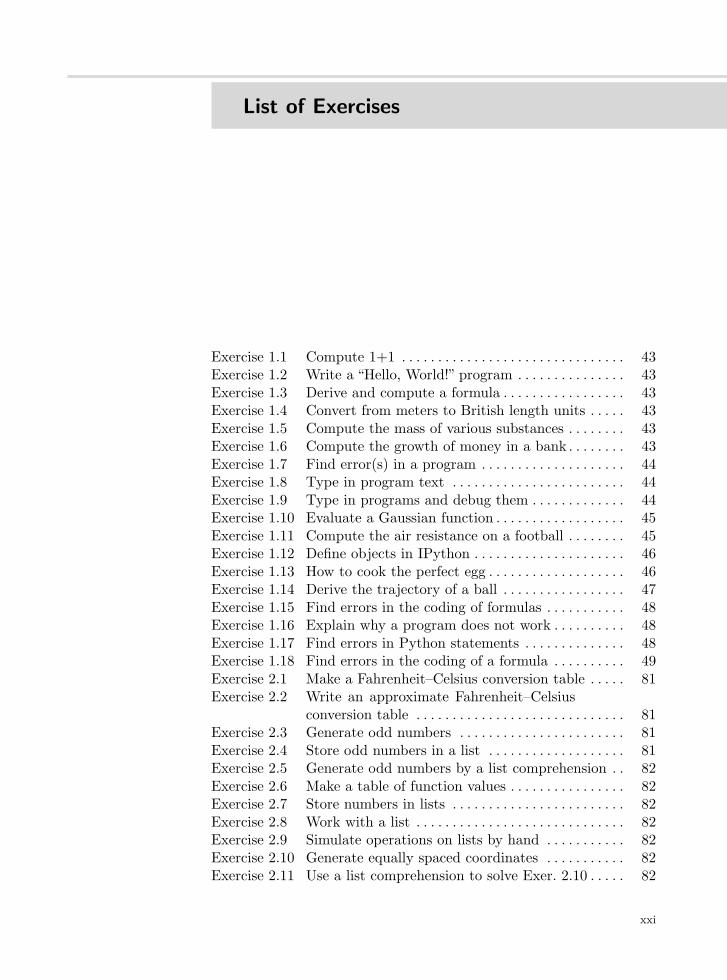
Exercise 1.1 Compute 1+1 . . . . . . . . . . . . . . . . . . . . . . . . . . . . . . . 43Exercise 1.2 Write a “Hello, World!” program . . . . . . . . . . . . . . . 43Exercise 1.3 Derive and compute a formula . . . . . . . . . . . . . . . . . 43Exercise 1.4 Convert from meters to British length units . . . . . 43Exercise 1.5 Compute the mass of various substances . . . . . . . . 43Exercise 1.6 Compute the growth of money in a bank . . . . . . . . 43Exercise 1.7 Find error(s) in a program . . . . . . . . . . . . . . . . . . . . 44Exercise 1.8 Type in program text . . . . . . . . . . . . . . . . . . . . . . . . 44Exercise 1.9 Type in programs and debug them . . . . . . . . . . . . . 44Exercise 1.10 Evaluate a Gaussian function . . . . . . . . . . . . . . . . . . 45Exercise 1.11 Compute the air resistance on a football . . . . . . . . 45Exercise 1.12 Define objects in IPython . . . . . . . . . . . . . . . . . . . . . 46Exercise 1.13 How to cook the perfect egg . . . . . . . . . . . . . . . . . . . 46Exercise 1.14 Derive the trajectory of a ball . . . . . . . . . . . . . . . . . 47Exercise 1.15 Find errors in the coding of formulas . . . . . . . . . . . 48Exercise 1.16 Explain why a program does not work . . . . . . . . . . 48Exercise 1.17 Find errors in Python statements . . . . . . . . . . . . . . 48Exercise 1.18 Find errors in the coding of a formula . . . . . . . . . . 49Exercise 2.1 Make a Fahrenheit–Celsius conversion table . . . . . 81Exercise 2.2 Write an approximate Fahrenheit–Celsius

conversion table . . . . . . . . . . . . . . . . . . . . . . . . . . . . . 81Exercise 2.3 Generate odd numbers . . . . . . . . . . . . . . . . . . . . . . . 81Exercise 2.4 Store odd numbers in a list . . . . . . . . . . . . . . . . . . . 81Exercise 2.5 Generate odd numbers by a list comprehension . . 82Exercise 2.6 Make a table of function values . . . . . . . . . . . . . . . . 82Exercise 2.7 Store numbers in lists . . . . . . . . . . . . . . . . . . . . . . . . 82Exercise 2.8 Work with a list . . . . . . . . . . . . . . . . . . . . . . . . . . . . . 82Exercise 2.9 Simulate operations on lists by hand . . . . . . . . . . . 82Exercise 2.10 Generate equally spaced coordinates . . . . . . . . . . . 82Exercise 2.11 Use a list comprehension to solve Exer. 2.10 . . . . . 82

xxi

xxii List of Exercises

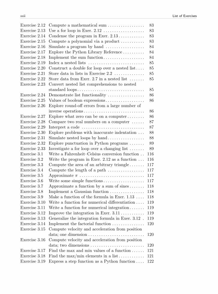
Exercise 2.12 Compute a mathematical sum . . . . . . . . . . . . . . . . . 83Exercise 2.13 Use a for loop in Exer. 2.12 . . . . . . . . . . . . . . . . . . . 83Exercise 2.14 Condense the program in Exer. 2.13 . . . . . . . . . . . . 83Exercise 2.15 Compute a polynomial via a product . . . . . . . . . . . 83Exercise 2.16 Simulate a program by hand . . . . . . . . . . . . . . . . . . 84Exercise 2.17 Explore the Python Library Reference . . . . . . . . . . 84Exercise 2.18 Implement the sum function . . . . . . . . . . . . . . . . . . . 84Exercise 2.19 Index a nested lists . . . . . . . . . . . . . . . . . . . . . . . . . . 85Exercise 2.20 Construct a double for loop over a nested list . . . . 85Exercise 2.21 Store data in lists in Exercise 2.2 . . . . . . . . . . . . . . 85Exercise 2.22 Store data from Exer. 2.7 in a nested list . . . . . . . 85Exercise 2.23 Convert nested list comprehensions to nested

standard loops . . . . . . . . . . . . . . . . . . . . . . . . . . . . . . . 85Exercise 2.24 Demonstrate list functionality . . . . . . . . . . . . . . . . . 86Exercise 2.25 Values of boolean expressions . . . . . . . . . . . . . . . . . . 86Exercise 2.26 Explore round-off errors from a large number of

inverse operations . . . . . . . . . . . . . . . . . . . . . . . . . . . . 86Exercise 2.27 Explore what zero can be on a computer . . . . . . . . 86Exercise 2.28 Compare two real numbers on a computer . . . . . . 87Exercise 2.29 Interpret a code . . . . . . . . . . . . . . . . . . . . . . . . . . . . . 87Exercise 2.30 Explore problems with inaccurate indentation . . . 88Exercise 2.31 Simulate nested loops by hand . . . . . . . . . . . . . . . . . 88Exercise 2.32 Explore punctuation in Python programs . . . . . . . 89Exercise 2.33 Investigate a for loop over a changing list . . . . . . . 89Exercise 3.1 Write a Fahrenheit–Celsius conversion function . . 116Exercise 3.2 Write the program in Exer. 2.12 as a function . . . 116Exercise 3.3 Compute the area of an arbitrary triangle . . . . . . . 117Exercise 3.4 Compute the length of a path . . . . . . . . . . . . . . . . . 117Exercise 3.5 Approximate π . . . . . . . . . . . . . . . . . . . . . . . . . . . . . . 117Exercise 3.6 Write some simple functions . . . . . . . . . . . . . . . . . . . 117Exercise 3.7 Approximate a function by a sum of sines . . . . . . . 118Exercise 3.8 Implement a Gaussian function . . . . . . . . . . . . . . . . 118Exercise 3.9 Make a function of the formula in Exer. 1.13 . . . . 118Exercise 3.10 Write a function for numerical differentiation . . . . 119Exercise 3.11 Write a function for numerical integration . . . . . . . 119Exercise 3.12 Improve the integration in Exer. 3.11 . . . . . . . . . . . 119Exercise 3.13 Generalize the integration formula in Exer. 3.12 . 119Exercise 3.14 Implement the factorial function . . . . . . . . . . . . . . . 120Exercise 3.15 Compute velocity and acceleration from position

data; one dimension . . . . . . . . . . . . . . . . . . . . . . . . . . 120Exercise 3.16 Compute velocity and acceleration from position

data; two dimensions . . . . . . . . . . . . . . . . . . . . . . . . . 120Exercise 3.17 Find the max and min values of a function . . . . . . 121Exercise 3.18 Find the max/min elements in a list . . . . . . . . . . . . 121Exercise 3.19 Express a step function as a Python function . . . . 122

List of Exercises xxiii

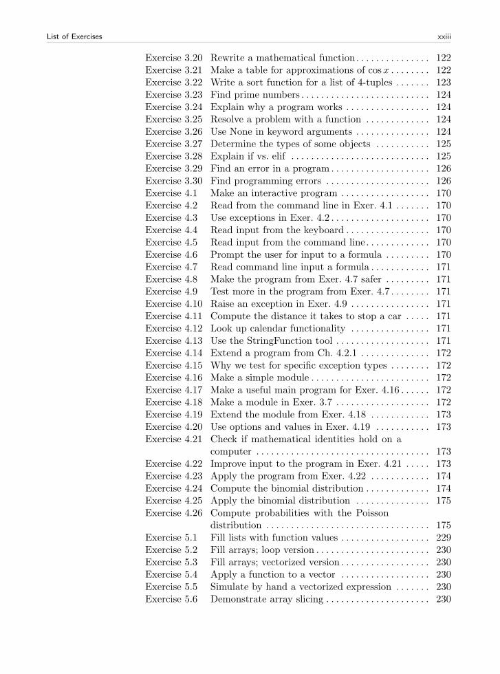
Exercise 3.20 Rewrite a mathematical function . . . . . . . . . . . . . . . 122Exercise 3.21 Make a table for approximations of cosx . . . . . . . . 122Exercise 3.22 Write a sort function for a list of 4-tuples . . . . . . . 123Exercise 3.23 Find prime numbers . . . . . . . . . . . . . . . . . . . . . . . . . . 124Exercise 3.24 Explain why a program works . . . . . . . . . . . . . . . . . 124Exercise 3.25 Resolve a problem with a function . . . . . . . . . . . . . 124Exercise 3.26 Use None in keyword arguments . . . . . . . . . . . . . . . 124Exercise 3.27 Determine the types of some objects . . . . . . . . . . . 125Exercise 3.28 Explain if vs. elif . . . . . . . . . . . . . . . . . . . . . . . . . . . . 125Exercise 3.29 Find an error in a program . . . . . . . . . . . . . . . . . . . . 126Exercise 3.30 Find programming errors . . . . . . . . . . . . . . . . . . . . . 126Exercise 4.1 Make an interactive program . . . . . . . . . . . . . . . . . . 170Exercise 4.2 Read from the command line in Exer. 4.1 . . . . . . . 170Exercise 4.3 Use exceptions in Exer. 4.2 . . . . . . . . . . . . . . . . . . . . 170Exercise 4.4 Read input from the keyboard . . . . . . . . . . . . . . . . . 170Exercise 4.5 Read input from the command line . . . . . . . . . . . . . 170Exercise 4.6 Prompt the user for input to a formula . . . . . . . . . 170Exercise 4.7 Read command line input a formula . . . . . . . . . . . . 171Exercise 4.8 Make the program from Exer. 4.7 safer . . . . . . . . . 171Exercise 4.9 Test more in the program from Exer. 4.7 . . . . . . . . 171Exercise 4.10 Raise an exception in Exer. 4.9 . . . . . . . . . . . . . . . . 171Exercise 4.11 Compute the distance it takes to stop a car . . . . . 171Exercise 4.12 Look up calendar functionality . . . . . . . . . . . . . . . . 171Exercise 4.13 Use the StringFunction tool . . . . . . . . . . . . . . . . . . . 171Exercise 4.14 Extend a program from Ch. 4.2.1 . . . . . . . . . . . . . . 172Exercise 4.15 Why we test for specific exception types . . . . . . . . 172Exercise 4.16 Make a simple module . . . . . . . . . . . . . . . . . . . . . . . . 172Exercise 4.17 Make a useful main program for Exer. 4.16 . . . . . . 172Exercise 4.18 Make a module in Exer. 3.7 . . . . . . . . . . . . . . . . . . . 172Exercise 4.19 Extend the module from Exer. 4.18 . . . . . . . . . . . . 173Exercise 4.20 Use options and values in Exer. 4.19 . . . . . . . . . . . 173Exercise 4.21 Check if mathematical identities hold on a

computer . . . . . . . . . . . . . . . . . . . . . . . . . . . . . . . . . . . 173Exercise 4.22 Improve input to the program in Exer. 4.21 . . . . . 173Exercise 4.23 Apply the program from Exer. 4.22 . . . . . . . . . . . . 174Exercise 4.24 Compute the binomial distribution . . . . . . . . . . . . . 174Exercise 4.25 Apply the binomial distribution . . . . . . . . . . . . . . . 175Exercise 4.26 Compute probabilities with the Poisson

distribution . . . . . . . . . . . . . . . . . . . . . . . . . . . . . . . . . 175Exercise 5.1 Fill lists with function values . . . . . . . . . . . . . . . . . . 229Exercise 5.2 Fill arrays; loop version . . . . . . . . . . . . . . . . . . . . . . . 230Exercise 5.3 Fill arrays; vectorized version . . . . . . . . . . . . . . . . . . 230Exercise 5.4 Apply a function to a vector . . . . . . . . . . . . . . . . . . 230Exercise 5.5 Simulate by hand a vectorized expression . . . . . . . 230Exercise 5.6 Demonstrate array slicing . . . . . . . . . . . . . . . . . . . . . 230

xxiv List of Exercises

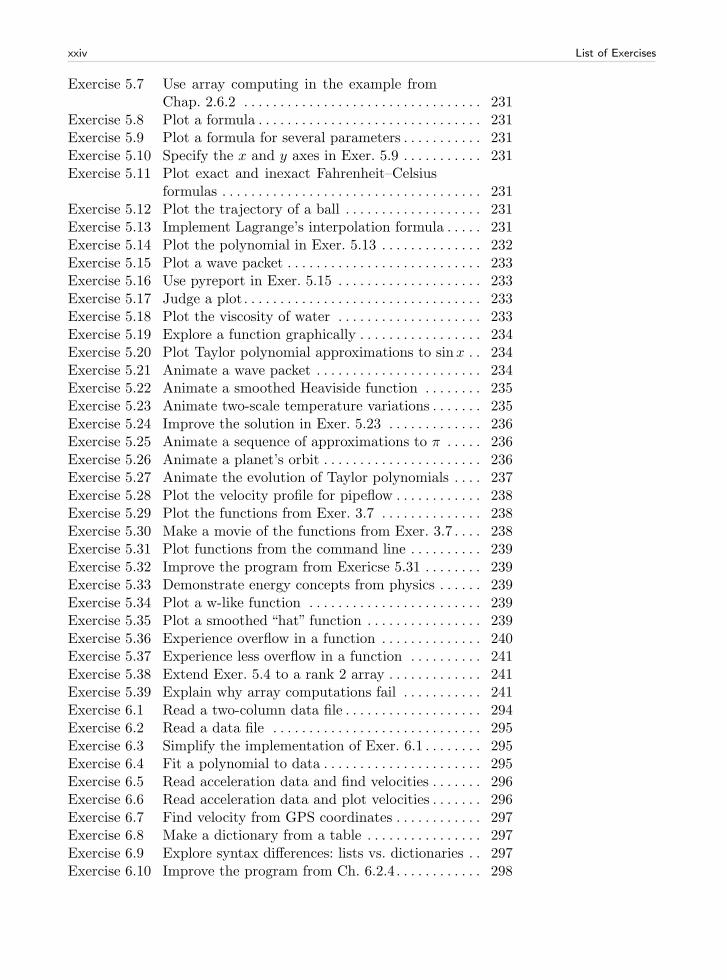
Exercise 5.7 Use array computing in the example fromChap. 2.6.2 . . . . . . . . . . . . . . . . . . . . . . . . . . . . . . . . . 231

Exercise 5.8 Plot a formula . . . . . . . . . . . . . . . . . . . . . . . . . . . . . . . 231Exercise 5.9 Plot a formula for several parameters . . . . . . . . . . . 231Exercise 5.10 Specify the x and y axes in Exer. 5.9 . . . . . . . . . . . 231Exercise 5.11 Plot exact and inexact Fahrenheit–Celsius

formulas . . . . . . . . . . . . . . . . . . . . . . . . . . . . . . . . . . . . 231Exercise 5.12 Plot the trajectory of a ball . . . . . . . . . . . . . . . . . . . 231Exercise 5.13 Implement Lagrange’s interpolation formula . . . . . 231Exercise 5.14 Plot the polynomial in Exer. 5.13 . . . . . . . . . . . . . . 232Exercise 5.15 Plot a wave packet . . . . . . . . . . . . . . . . . . . . . . . . . . . 233Exercise 5.16 Use pyreport in Exer. 5.15 . . . . . . . . . . . . . . . . . . . . 233Exercise 5.17 Judge a plot . . . . . . . . . . . . . . . . . . . . . . . . . . . . . . . . . 233Exercise 5.18 Plot the viscosity of water . . . . . . . . . . . . . . . . . . . . 233Exercise 5.19 Explore a function graphically . . . . . . . . . . . . . . . . . 234Exercise 5.20 Plot Taylor polynomial approximations to sinx . . 234Exercise 5.21 Animate a wave packet . . . . . . . . . . . . . . . . . . . . . . . 234Exercise 5.22 Animate a smoothed Heaviside function . . . . . . . . 235Exercise 5.23 Animate two-scale temperature variations . . . . . . . 235Exercise 5.24 Improve the solution in Exer. 5.23 . . . . . . . . . . . . . 236Exercise 5.25 Animate a sequence of approximations to π . . . . . 236Exercise 5.26 Animate a planet’s orbit . . . . . . . . . . . . . . . . . . . . . . 236Exercise 5.27 Animate the evolution of Taylor polynomials . . . . 237Exercise 5.28 Plot the velocity profile for pipeflow . . . . . . . . . . . . 238Exercise 5.29 Plot the functions from Exer. 3.7 . . . . . . . . . . . . . . 238Exercise 5.30 Make a movie of the functions from Exer. 3.7 . . . . 238Exercise 5.31 Plot functions from the command line . . . . . . . . . . 239Exercise 5.32 Improve the program from Exericse 5.31 . . . . . . . . 239Exercise 5.33 Demonstrate energy concepts from physics . . . . . . 239Exercise 5.34 Plot a w-like function . . . . . . . . . . . . . . . . . . . . . . . . 239Exercise 5.35 Plot a smoothed “hat” function . . . . . . . . . . . . . . . . 239Exercise 5.36 Experience overflow in a function . . . . . . . . . . . . . . 240Exercise 5.37 Experience less overflow in a function . . . . . . . . . . 241Exercise 5.38 Extend Exer. 5.4 to a rank 2 array . . . . . . . . . . . . . 241Exercise 5.39 Explain why array computations fail . . . . . . . . . . . 241Exercise 6.1 Read a two-column data file . . . . . . . . . . . . . . . . . . . 294Exercise 6.2 Read a data file . . . . . . . . . . . . . . . . . . . . . . . . . . . . . 295Exercise 6.3 Simplify the implementation of Exer. 6.1 . . . . . . . . 295Exercise 6.4 Fit a polynomial to data . . . . . . . . . . . . . . . . . . . . . . 295Exercise 6.5 Read acceleration data and find velocities . . . . . . . 296Exercise 6.6 Read acceleration data and plot velocities . . . . . . . 296Exercise 6.7 Find velocity from GPS coordinates . . . . . . . . . . . . 297Exercise 6.8 Make a dictionary from a table . . . . . . . . . . . . . . . . 297Exercise 6.9 Explore syntax differences: lists vs. dictionaries . . 297Exercise 6.10 Improve the program from Ch. 6.2.4 . . . . . . . . . . . . 298

List of Exercises xxv

Exercise 6.11 Interpret output from a program . . . . . . . . . . . . . . . 298Exercise 6.12 Make a dictionary . . . . . . . . . . . . . . . . . . . . . . . . . . . . 298Exercise 6.13 Make a nested dictionary . . . . . . . . . . . . . . . . . . . . . 298Exercise 6.14 Make a nested dictionary from a file . . . . . . . . . . . . 299Exercise 6.15 Compute the area of a triangle . . . . . . . . . . . . . . . . 299Exercise 6.16 Compare data structures for polynomials . . . . . . . 299Exercise 6.17 Compute the derivative of a polynomial . . . . . . . . 299Exercise 6.18 Generalize the program from Ch. 6.2.6 . . . . . . . . . 300Exercise 6.19 Write function data to file . . . . . . . . . . . . . . . . . . . . 300Exercise 6.20 Specify functions on the command line . . . . . . . . . 300Exercise 6.21 Interpret function specifications . . . . . . . . . . . . . . . . 301Exercise 6.22 Compare average temperatures in cities . . . . . . . . . 301Exercise 6.23 Try Word or OpenOffice to write a program . . . . . 302Exercise 6.24 Evaluate objects in a boolean context . . . . . . . . . . 302Exercise 6.25 Generate an HTML report . . . . . . . . . . . . . . . . . . . . 303Exercise 6.26 Fit a polynomial to experimental data . . . . . . . . . . 303Exercise 6.27 Generate an HTML report with figures . . . . . . . . . 304Exercise 6.28 Extract information from a weather page . . . . . . . 304Exercise 6.29 Compare alternative weather forecasts . . . . . . . . . . 304Exercise 6.30 Improve the output in Exercise 6.29 . . . . . . . . . . . . 304Exercise 7.1 Make a function class . . . . . . . . . . . . . . . . . . . . . . . . 359Exercise 7.2 Make a very simple class . . . . . . . . . . . . . . . . . . . . . . 359Exercise 7.3 Extend the class from Ch. 7.2.1 . . . . . . . . . . . . . . . . 359Exercise 7.4 Make classes for a rectangle and a triangle . . . . . . 360Exercise 7.5 Make a class for straight lines . . . . . . . . . . . . . . . . . 360Exercise 7.6 Improve the constructor in Exer. 7.5 . . . . . . . . . . . 360Exercise 7.7 Make a class for quadratic functions . . . . . . . . . . . . 360Exercise 7.8 Make a class for linear springs . . . . . . . . . . . . . . . . . 361Exercise 7.9 Implement code from Exer. 5.13 as a class . . . . . . 361Exercise 7.10 A very simple “Hello, World!” class . . . . . . . . . . . . . 361Exercise 7.11 Use special methods in Exer. 7.1 . . . . . . . . . . . . . . . 361Exercise 7.12 Make a class for nonlinear springs . . . . . . . . . . . . . . 361Exercise 7.13 Extend the class from Ch. 7.2.1 . . . . . . . . . . . . . . . . 362Exercise 7.14 Implement a class for numerical differentation . . . 362Exercise 7.15 Verify a program. . . . . . . . . . . . . . . . . . . . . . . . . . . . . 363Exercise 7.16 Test methods for numerical differentation . . . . . . . 363Exercise 7.17 Modify a class for numerical differentiation . . . . . . 363Exercise 7.18 Make a class for summation of series . . . . . . . . . . . 364Exercise 7.19 Apply the differentiation class from Ch. 7.3.2 . . . . 364Exercise 7.20 Use classes for computing inverse functions . . . . . . 364Exercise 7.21 Vectorize a class for numerical integration . . . . . . . 365Exercise 7.22 Speed up repeated integral calculations . . . . . . . . . 365Exercise 7.23 Apply a polynomial class . . . . . . . . . . . . . . . . . . . . . 366Exercise 7.24 Find a bug in a class for polynomials . . . . . . . . . . . 366Exercise 7.25 Subtraction of polynomials . . . . . . . . . . . . . . . . . . . . 366

xxvi List of Exercises

Exercise 7.26 Represent a polynomial by an array . . . . . . . . . . . . 367Exercise 7.27 Vectorize a class for polynomials . . . . . . . . . . . . . . . 367Exercise 7.28 Use a dict to hold polynomial coefficients; add . . . 367Exercise 7.29 Use a dict to hold polynomial coefficients; mul . . . 367Exercise 7.30 Extend class Vec2D to work with lists/tuples . . . . 368Exercise 7.31 Extend class Vec2D to 3D vectors . . . . . . . . . . . . . . 368Exercise 7.32 Use NumPy arrays in class Vec2D . . . . . . . . . . . . . 368Exercise 7.33 Use classes in the program from Ch. 6.6.2 . . . . . . . 369Exercise 7.34 Use a class in Exer. 6.25 . . . . . . . . . . . . . . . . . . . . . . 369Exercise 7.35 Apply the class from Exer. 7.34 interactively . . . . 370Exercise 7.36 Find local and global extrema of a function . . . . . 370Exercise 7.37 Improve the accuracy in Exer. 7.36 . . . . . . . . . . . . . 372Exercise 7.38 Find the optimal production for a company . . . . . 372Exercise 7.39 Extend the program from Exer. 7.38 . . . . . . . . . . . 373Exercise 7.40 Model the economy of fishing . . . . . . . . . . . . . . . . . . 374Exercise 8.1 Flip a coin N times . . . . . . . . . . . . . . . . . . . . . . . . . . 421Exercise 8.2 Compute a probability . . . . . . . . . . . . . . . . . . . . . . . . 421Exercise 8.3 Choose random colors . . . . . . . . . . . . . . . . . . . . . . . . 421Exercise 8.4 Draw balls from a hat . . . . . . . . . . . . . . . . . . . . . . . . 422Exercise 8.5 Probabilities of rolling dice . . . . . . . . . . . . . . . . . . . . 422Exercise 8.6 Estimate the probability in a dice game . . . . . . . . . 422Exercise 8.7 Compute the probability of hands of cards . . . . . . 422Exercise 8.8 Decide if a dice game is fair . . . . . . . . . . . . . . . . . . . 422Exercise 8.9 Adjust the game in Exer. 8.8 . . . . . . . . . . . . . . . . . . 422Exercise 8.10 Compare two playing strategies . . . . . . . . . . . . . . . . 423Exercise 8.11 Solve Exercise 8.10 with different no. of dice . . . . . 423Exercise 8.12 Extend Exercise 8.11 . . . . . . . . . . . . . . . . . . . . . . . . . 423Exercise 8.13 Investigate the winning chances of some games . . 423Exercise 8.14 Probabilities of throwing two dice . . . . . . . . . . . . . . 424Exercise 8.15 Play with vectorized boolean expressions . . . . . . . . 424Exercise 8.16 Vectorize the program from Exer. 8.1 . . . . . . . . . . . 424Exercise 8.17 Vectorize the code in Exer. 8.2 . . . . . . . . . . . . . . . . 424Exercise 8.18 Throw dice and compute a small probability . . . . 425Exercise 8.19 Difference equation for random numbers . . . . . . . . 425Exercise 8.20 Make a class for drawing balls from a hat . . . . . . . 425Exercise 8.21 Independent vs. dependent random numbers . . . . 426Exercise 8.22 Compute the probability of flipping a coin . . . . . . 426Exercise 8.23 Extend Exer. 8.22 . . . . . . . . . . . . . . . . . . . . . . . . . . . . 426Exercise 8.24 Simulate the problems in Exer. 4.25 . . . . . . . . . . . . 427Exercise 8.25 Simulate a poker game . . . . . . . . . . . . . . . . . . . . . . . 427Exercise 8.26 Write a non-vectorized version of a code . . . . . . . . 427Exercise 8.27 Estimate growth in a simulation model . . . . . . . . . 427Exercise 8.28 Investigate guessing strategies for Ch. 8.4.1 . . . . . 428Exercise 8.29 Make a vectorized solution to Exer. 8.8 . . . . . . . . . 428Exercise 8.30 Compute π by a Monte Carlo method . . . . . . . . . . 428

List of Exercises xxvii

Exercise 8.31 Do a variant of Exer. 8.30 . . . . . . . . . . . . . . . . . . . . . 428Exercise 8.32 Compute π by a random sum . . . . . . . . . . . . . . . . . 428Exercise 8.33 1D random walk with drift . . . . . . . . . . . . . . . . . . . . 429Exercise 8.34 1D random walk until a point is hit . . . . . . . . . . . . 429Exercise 8.35 Make a class for 2D random walk . . . . . . . . . . . . . . 429Exercise 8.36 Vectorize the class code from Exer. 8.35 . . . . . . . . 430Exercise 8.37 2D random walk with walls; scalar version . . . . . . 430Exercise 8.38 2D random walk with walls; vectorized version . . 430Exercise 8.39 Simulate the mixture of gas molecules . . . . . . . . . . 430Exercise 8.40 Simulate the mixture of gas molecules . . . . . . . . . . 431Exercise 8.41 Guess beer brands . . . . . . . . . . . . . . . . . . . . . . . . . . . 431Exercise 8.42 Simulate stock prices . . . . . . . . . . . . . . . . . . . . . . . . . 431Exercise 8.43 Compute with option prices in finance . . . . . . . . . . 432Exercise 8.44 Compute velocity and acceleration . . . . . . . . . . . . . 433Exercise 8.45 Numerical differentiation of noisy signals . . . . . . . . 434Exercise 8.46 Model the noise in the data in Exer. 8.44 . . . . . . . 434Exercise 8.47 Reduce the noise in Exer. 8.44 . . . . . . . . . . . . . . . . . 435Exercise 8.48 Make a class for differentiating noisy data . . . . . . . 435Exercise 8.49 Find the expected waiting time in traffic lights . . 436Exercise 9.1 Demonstrate the magic of inheritance . . . . . . . . . . 488Exercise 9.2 Inherit from classes in Ch. 9.1 . . . . . . . . . . . . . . . . . 488Exercise 9.3 Inherit more from classes in Ch. 9.1 . . . . . . . . . . . . 488Exercise 9.4 Reverse the class hierarchy from Ch. 9.1 . . . . . . . . 488Exercise 9.5 Make circle a subclass of an ellipse . . . . . . . . . . . . . 489Exercise 9.6 Make super- and subclass for a point . . . . . . . . . . . 489Exercise 9.7 Modify a function class by subclassing . . . . . . . . . . 489Exercise 9.8 Explore the accuracy of difference formulas . . . . . . 490Exercise 9.9 Implement a subclass . . . . . . . . . . . . . . . . . . . . . . . . . 490Exercise 9.10 Make classes for numerical differentiation . . . . . . . 490Exercise 9.11 Implement a new subclass for differentiation . . . . . 490Exercise 9.12 Understand if a class can be used recursively . . . . 490Exercise 9.13 Represent people by a class hierarchy . . . . . . . . . . . 491Exercise 9.14 Add a new class in a class hierarchy . . . . . . . . . . . . 492Exercise 9.15 Change the user interface of a class hierarchy . . . . 492Exercise 9.16 Compute convergence rates of numerical

integration methods . . . . . . . . . . . . . . . . . . . . . . . . . . 492Exercise 9.17 Add common functionality in a class hierarchy . . 493Exercise 9.18 Make a class hierarchy for root finding . . . . . . . . . . 493Exercise 9.19 Make a class for drawing an arrow . . . . . . . . . . . . . 494Exercise 9.20 Make a class for drawing a person . . . . . . . . . . . . . . 494Exercise 9.21 Animate a person with waving hands . . . . . . . . . . . 495Exercise 9.22 Make a class for drawing a car . . . . . . . . . . . . . . . . . 495Exercise 9.23 Make a car roll . . . . . . . . . . . . . . . . . . . . . . . . . . . . . . 495Exercise 9.24 Make a calculus calculator class . . . . . . . . . . . . . . . . 495Exercise 9.25 Extend Exer. 9.24 . . . . . . . . . . . . . . . . . . . . . . . . . . . . 496

xxviii List of Exercises

Exercise A.1 Determine the limit of a sequence . . . . . . . . . . . . . . 521Exercise A.2 Determine the limit of a sequence . . . . . . . . . . . . . . 521Exercise A.3 Experience convergence problems . . . . . . . . . . . . . . 521Exercise A.4 Convergence of sequences with π as limit . . . . . . . 521Exercise A.5 Reduce memory usage of difference equations . . . . 522Exercise A.6 Development of a loan over N months . . . . . . . . . . 522Exercise A.7 Solve a system of difference equations . . . . . . . . . . 522Exercise A.8 Extend the model (A.26)–(A.27) . . . . . . . . . . . . . . . 522Exercise A.9 Experiment with the program from Exer. A.8 . . . 522Exercise A.10 Change index in a difference equation . . . . . . . . . . 523Exercise A.11 Construct time points from dates . . . . . . . . . . . . . . 523Exercise A.12 Solve nonlinear equations by Newton’s method . . 523Exercise A.13 Visualize the convergence of Newton’s method . . . 524Exercise A.14 Implement the Secant method . . . . . . . . . . . . . . . . . 524Exercise A.15 Test different methods for root finding . . . . . . . . . . 525Exercise A.16 Difference equations for computing sin x . . . . . . . . 525Exercise A.17 Difference equations for computing cos x . . . . . . . . 525Exercise A.18 Make a guitar-like sound . . . . . . . . . . . . . . . . . . . . . . 526Exercise A.19 Damp the bass in a sound file . . . . . . . . . . . . . . . . . 526Exercise A.20 Damp the treble in a sound file . . . . . . . . . . . . . . . . 527Exercise A.21 Demonstrate oscillatory solutions of (A.13) . . . . . . 527Exercise A.22 Improve the program from Exer. A.21 . . . . . . . . . . 527Exercise A.23 Simulate the price of wheat . . . . . . . . . . . . . . . . . . . 528Exercise B.1 Interpolate a discrete function . . . . . . . . . . . . . . . . . 555Exercise B.2 Study a function for different parameter values . . 555Exercise B.3 Study a function and its derivative . . . . . . . . . . . . . 556Exercise B.4 Use the Trapezoidal method . . . . . . . . . . . . . . . . . . . 556Exercise B.5 Compute a sequence of integrals . . . . . . . . . . . . . . . 557Exercise B.6 Use the Trapezoidal method . . . . . . . . . . . . . . . . . . . 557Exercise B.7 Trigonometric integrals . . . . . . . . . . . . . . . . . . . . . . . 558Exercise B.8 Plot functions and their derivatives . . . . . . . . . . . . 559Exercise B.9 Use the Trapezoidal method . . . . . . . . . . . . . . . . . . . 559Exercise C.1 Solve a nonhomogeneous linear ODE . . . . . . . . . . . 575Exercise C.2 Solve a nonlinear ODE . . . . . . . . . . . . . . . . . . . . . . . 575Exercise C.3 Solve an ODE for y(x) . . . . . . . . . . . . . . . . . . . . . . . 575Exercise C.4 Experience instability of an ODE . . . . . . . . . . . . . . 576Exercise C.5 Solve an ODE for the arc length . . . . . . . . . . . . . . . 576Exercise C.6 Solve an ODE with time-varying growth . . . . . . . . 576Exercise D.1 Use a w function with a step . . . . . . . . . . . . . . . . . . 601Exercise D.2 Make a callback function in Exercise D.1 . . . . . . . . 601Exercise D.3 Improve input to the simulation program . . . . . . . 601Exercise E.1 Solve a simple ODE in two ways . . . . . . . . . . . . . . . 633Exercise E.2 Use the ODESolver hierarchy to solve a simple

ODE . . . . . . . . . . . . . . . . . . . . . . . . . . . . . . . . . . . . . . . 634Exercise E.3 Solve an ODE for emptying a tank . . . . . . . . . . . . . 634

List of Exercises xxix

Exercise E.4 Logistic growth with time-varying carryingcapacity . . . . . . . . . . . . . . . . . . . . . . . . . . . . . . . . . . . . 634

Exercise E.5 Simulate a falling or rising body in a fluid . . . . . . . 635Exercise E.6 Check the solution’s limit in Exer. E.5 . . . . . . . . . . 636Exercise E.7 Visualize the different forces in Exer. E.5 . . . . . . . 636Exercise E.8 Solve an ODE until constant solution . . . . . . . . . . . 636Exercise E.9 Use classes in Exer. E.8 . . . . . . . . . . . . . . . . . . . . . . . 637Exercise E.10 Scale away parameters in Exer. E.8 . . . . . . . . . . . . 637Exercise E.11 Use the 4th-order Runge-Kutta on (C.32) . . . . . . . 638Exercise E.12 Compare ODE methods . . . . . . . . . . . . . . . . . . . . . . 638Exercise E.13 Compare ODE methods . . . . . . . . . . . . . . . . . . . . . . 638Exercise E.14 Solve two coupled ODEs for radioactive decay . . . 638Exercise E.15 Code a 2nd-order Runge-Kutta method; function 639Exercise E.16 Code a 2nd-order Runge-Kutta method; class . . . 639Exercise E.17 Make an ODESolver subclass for Heun’s method . 639Exercise E.18 Make an ODESolver subclass for the Midpoint

method . . . . . . . . . . . . . . . . . . . . . . . . . . . . . . . . . . . . . 639Exercise E.19 Make an ODESolver subclass for an Adams-

Bashforth method . . . . . . . . . . . . . . . . . . . . . . . . . . . . 640Exercise E.20 Implement the iterated Midpoint method;

function . . . . . . . . . . . . . . . . . . . . . . . . . . . . . . . . . . . . 640Exercise E.21 Implement the iterated Midpoint method; class . . 640Exercise E.22 Make an ODESolver subclass for the iterated

Midpoint method . . . . . . . . . . . . . . . . . . . . . . . . . . . . 640Exercise E.23 Study convergence of numerical methods for

ODEs . . . . . . . . . . . . . . . . . . . . . . . . . . . . . . . . . . . . . . 641Exercise E.24 Solve an ODE specified on the command line . . . . 641Exercise E.25 Find the body’s position in Exer. E.5 . . . . . . . . . . . 641Exercise E.26 Add the effect of air resistance on a ball . . . . . . . . 642Exercise E.27 Solve an ODE system for an electric circuit . . . . . 642Exercise E.28 Compare methods for solving (E.73)–(E.74) . . . . . 643Exercise E.29 Explore predator-prey population interactions . . . 643Exercise E.30 Formulate a 2nd-order ODE as a system . . . . . . . . 644Exercise E.31 Solve the system in Exer. E.30 in a special case . . 645Exercise E.32 Enhance the code from Exer. E.31 . . . . . . . . . . . . . 646Exercise E.33 Make a tool for analyzing oscillatory solutions . . . 648Exercise E.34 Replace functions by class in Exer. E.32 . . . . . . . . 648Exercise E.35 Allow flexible choice of functions in Exer. E.34 . . 652Exercise E.36 Use the modules from Exer. E.34 and E.35 . . . . . . 652Exercise E.37 Use the modules from Exer. E.34 and E.35 . . . . . . 653

Computing with Formulas 1

Our first examples on computer programming involve programs thatevaluate mathematical formulas. You will learn how to write and runa Python program, how to work with variables, how to compute withmathematical functions such as ex and sin x, and how to use Pythonfor interactive calculations.

We assume that you are somewhat familiar with computers so thatyou know what files and folders1 are, how you move between folders,how you change file and folder names, and how you write text and saveit in a file.

All the program examples associated with this chapter can be foundas files in the folder src/formulas. We refer to the preface for how todownload the folder tree src containing all the program files for thisbook.

1.1 The First Programming Encounter: A Formula

The first formula we shall consider concerns the vertical motion of aball thrown up in the air. From Newton’s second law of motion one canset up a mathematical model for the motion of the ball and find thatthe vertical position of the ball, called y, varies with time t accordingto the following formula2:

y(t) = v0t−1

2gt2 . (1.1)

1 Another frequent word for folder is directory.2 This formula neglects air resistance, which is usually small unless v0 is large – seeExercise 1.11.

1

2 1 Computing with Formulas

Here, v0 is the initial velocity of the ball, g is the acceleration of gravity,and t is time. Observe that the y axis is chosen such that the ball startsat y = 0 when t = 0.

To get an overview of the time it takes for the ball to move upwardsand return to y = 0 again, we can look for solutions to the equationy = 0:

v0t−1

2gt2 = t(v0 −

1

2gt) = 0 ⇒ t = 0 or t = 2v0/g .

That is, the ball returns after 2v0/g seconds, and it is therefore rea-sonable to restrict the interest of (1.1) to t ∈ [0, 2v0/g].

1.1.1 Using a Program as a Calculator

Our first program will evaluate (1.1) for a specific choice of v0, g, andt. Choosing v0 = 5 m/s and g = 9.81 m/s2 makes the ball come backafter t = 2v0/g ≈ 1 s. This means that we are basically interested inthe time interval [0, 1]. Say we want to compute the height of the ballat time t = 0.6 s. From (1.1) we have

y = 5 · 0.6− 1

2· 9.81 · 0.62

This arithmetic expression can be evaluated and its value can beprinted by a very simple one-line Python program:

print 5*0.6 - 0.5*9.81*0.6**2

The four standard arithmetic operators are written as +, -, *, and/ in Python and most other computer languages. The exponentiationemploys a double asterisk notation in Python, e.g., 0.62 is written as0.6**2.

Our task now is to create the program and run it, and this will bedescribed next.

1.1.2 About Programs and Programming

A computer program is just a sequence of instructions to the computer,written in a computer language. Most computer languages look some-what similar to English, but they are very much simpler. The numberof words and associated instructions is very limited, so to perform acomplicated operation we must combine a large number of differenttypes of instructions. The program text, containing the sequence ofinstructions, is stored in one or more files. The computer can only doexactly what the program tells the computer to do.

1.1 The First Programming Encounter: A Formula 3

Another perception of the word “program” is a file that can be run(“double-clicked”) to perform a task. Sometimes this is a file with tex-tual instructions (which is the case with Python), and sometimes thisfile is a translation of all the program text to a more efficient andcomputer-friendly language that is quite difficult to read for a human.All the programs in this chapter consist of short text stored in a singlefile. Other programs that you have used frequently, for instance Fire-fox or Internet Explorer for reading web pages, consist of program textdistributed over a large number of files, written by a large number ofpeople over many years. One single file contains the machine-efficienttranslation of the whole program, and this is normally the file thatyou “double-click” on when starting the program. In general, the word“program” means either this single file or the collection of files withtextual instructions.

Programming is obviously about writing programs, but this processis more than writing the correct instructions in a file. First, we mustunderstand how a problem can be solved by giving a sequence of in-structions to the computer. This is usually the most difficult thing withprogramming. Second, we must express this sequence of instructionscorrectly in a computer language and store the corresponding text in afile (the program). Third, we must run the program, check the validityof the results, and usually enter a fourth phase where errors in the pro-gram must be found and corrected. Mastering this process requires alot of training, which implies making a large number of programs (ex-ercises in this book, for instance) and getting the programs to work.

1.1.3 Tools for Writing Programs

Since programs consist of plain text, we need to write this text with thehelp of another program that can store the text in a file. You have mostlikely extensive experience with writing text on a computer, but forwriting your own programs you need special programs, called editors ,which preserve exactly the characters you type. The widespread wordprocessors, Microsoft Word being a primary example3, are aimed atproducing nice-looking reports. These programs format the text andare not good tools for writing your own programs, even though they cansave the document in a pure text format. Spaces are often important inPython programs, and editors for plain text give you complete controlof the spaces and all other characters in the program file.

3 Other examples are OpenOffice, TextEdit, iWork Pages, and BBEdit. Chapter 6.1.3gives some insight into why such programs are not suitable for writing your ownPython programs.

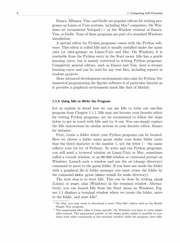
4 1 Computing with Formulas

Emacs, XEmacs, Vim, and Gedit are popular editors for writing pro-grams on Linux or Unix systems, including Mac4 computers. On Win-dows we recommend Notepad++ or the Window versions of Emacs,Vim, or Gedit. None of these programs are part of a standard Windowsinstallation.

A special editor for Python programs comes with the Python soft-ware. This editor is called Idle and is usually installed under the nameidle (or idle-python) on Linux/Unix and Mac. On Windows, it isreachable from the Python entry in the Start menu. Idle has a gentlelearning curve, but is mainly restricted to writing Python programs.Completely general editors, such as Emacs and Vim, have a steeperlearning curve and can be used for any text files, including reports instudent projects.

More advanced development environments also exist for Python. Fornumerical programming the Spyder software is of particular interest asit provides a graphical environment much like that of Matlab.

1.1.4 Using Idle to Write the Program

Let us explain in detail how we can use Idle to write our one-lineprogram from Chapter 1.1.1. Idle may not become your favorite editorfor writing Python programs, yet we recommend to follow the stepsbelow to get in touch with Idle and try it out. You can simply replacethe Idle instructions by similar actions in your favorite editor, Emacsfor instance.

First, create a folder where your Python programs can be located.Here we choose a folder name py1st under your home folder (notethat the third character is the number 1, not the letter l – the namereflects your 1st try of Python). To write and run Python programs,you will need a terminal window on Linux/Unix or Mac, sometimescalled a console window, or an MS-DOS window or command prompt onWindows. Launch such a window and use the cd (change directory)command to move to the py1st folder. If you have not made the folderwith a graphical file & folder manager you must create the folder bythe command mkdir py1st (mkdir stands for make directory).

The next step is to start Idle. This can be done by writing idle&

(Linux) or start idle (Windows) in the terminal window. Alterna-tively, you can launch Idle from the Start menu on Windows. Fig-ure 1.1 displays a terminal window where we create the folder, moveto the folder, and start Idle5.

4 On Mac, you may want to download a more “Mac-like” editor such as the ReallySimple Text program.

5 The ampersand after idle is Linux specific. On Windows you have to write start

idle instead. The ampersand postfix or the start prefix makes it possible to con-tinue with other commands in the terminal window while the program, here Idle,

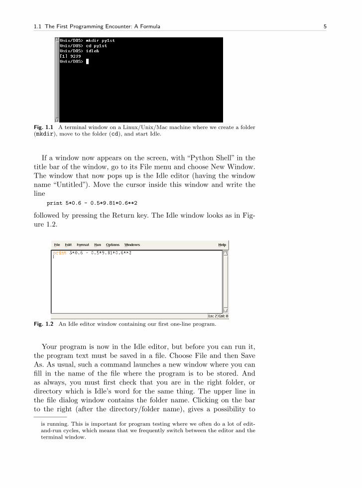
1.1 The First Programming Encounter: A Formula 5

Fig. 1.1 A terminal window on a Linux/Unix/Mac machine where we create a folder(mkdir), move to the folder (cd), and start Idle.

If a window now appears on the screen, with “Python Shell” in thetitle bar of the window, go to its File menu and choose New Window.The window that now pops up is the Idle editor (having the windowname “Untitled”). Move the cursor inside this window and write theline

print 5*0.6 - 0.5*9.81*0.6**2

followed by pressing the Return key. The Idle window looks as in Fig-ure 1.2.

Fig. 1.2 An Idle editor window containing our first one-line program.

Your program is now in the Idle editor, but before you can run it,the program text must be saved in a file. Choose File and then SaveAs. As usual, such a command launches a new window where you canfill in the name of the file where the program is to be stored. Andas always, you must first check that you are in the right folder, ordirectory which is Idle’s word for the same thing. The upper line inthe file dialog window contains the folder name. Clicking on the barto the right (after the directory/folder name), gives a possibility to

is running. This is important for program testing where we often do a lot of edit-and-run cycles, which means that we frequently switch between the editor and theterminal window.

6 1 Computing with Formulas

move upwards in the folder hierarchy, and clicking on the folder iconto the right of the bar, moves just one folder upwards. To go downin the folder tree, you simply double-click a folder icon in the mainwindow of this dialog. You must now navigate to the py1st folder underyour home folder. If you started Idle from the terminal window, thereis no need to navigate and change folder. Simply fill in the name ofthe program. Any name will do, but we suggest that you choose thename ball_numbers.py because this name is compatible with what weuse later in this book. The file extension .py is common for Pythonprograms, but not strictly required6.

Press the Save button and move back to the terminal window. Makesure you have a new file ball_numbers.py here, by running the com-mand ls (on Linux/Unix and Mac) or dir (on Windows). The outputshould be a text containing the name of the program file. You can nowjump to the paragraph “How to Run the Program”, but it might be agood idea to read the warning below first.

Warning About Typing Program Text. Even though a program is justa text, there is one major difference between a text in a program anda text intended to be read by a human. When a human reads a text,she or he is able to understand the message of the text even if the textis not perfectly precise or if there are grammar errors. If our one-lineprogram was expressed as

write 5*0.6 - 0.5*9.81*0.6^2

most humans would interpret write and print as the same thing, andmany would also interpret 6^2 as 62. In the Python language, however,write is a grammar error and 6^2 means an operation very differentfrom the exponentiation 6**2. Our communication with a computerthrough a program must be perfectly precise without a single grammarerror7. The computer will only do exactly what we tell it to do. Anyerror in the program, however small, may affect the program. There isa chance that we will never notice it, but most often an error causesthe program to stop or produce wrong results. The conclusion is thatcomputers have a much more pedantic attitude to language than what(most) humans have.

Now you understand why any program text must be carefully typed,paying attention to the correctness of every character. If you try outprogram texts from this book, make sure that you type them in exactlyas you see them in the book. Blanks, for instance, are often importantin Python, so it is a good habit to always count them and type them

6 Some editors, like Emacs, have many features that make it easier to write Pythonprograms, but these features will not be automatically available unless the programfile has a .py extension.

7 “Programming demands significantly higher standard of accuracy. Things don’tsimply have to make sense to another human being, they must make sense to acomputer.” –Donald Knuth [4, p. 18], computer scientist, 1938-.

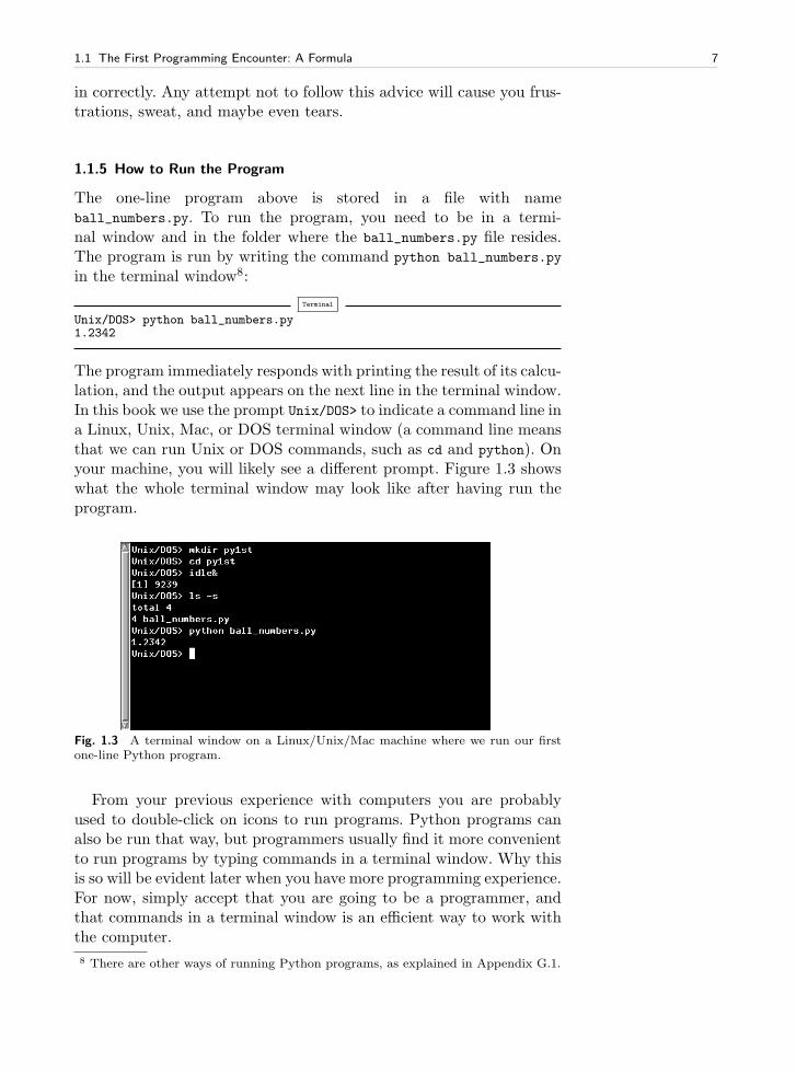
1.1 The First Programming Encounter: A Formula 7

in correctly. Any attempt not to follow this advice will cause you frus-trations, sweat, and maybe even tears.

1.1.5 How to Run the Program

The one-line program above is stored in a file with nameball_numbers.py. To run the program, you need to be in a termi-nal window and in the folder where the ball_numbers.py file resides.The program is run by writing the command python ball_numbers.py

in the terminal window8:

Terminal

Unix/DOS> python ball_numbers.py1.2342

The program immediately responds with printing the result of its calcu-lation, and the output appears on the next line in the terminal window.In this book we use the prompt Unix/DOS> to indicate a command line ina Linux, Unix, Mac, or DOS terminal window (a command line meansthat we can run Unix or DOS commands, such as cd and python). Onyour machine, you will likely see a different prompt. Figure 1.3 showswhat the whole terminal window may look like after having run theprogram.

Fig. 1.3 A terminal window on a Linux/Unix/Mac machine where we run our firstone-line Python program.

From your previous experience with computers you are probablyused to double-click on icons to run programs. Python programs canalso be run that way, but programmers usually find it more convenientto run programs by typing commands in a terminal window. Why thisis so will be evident later when you have more programming experience.For now, simply accept that you are going to be a programmer, andthat commands in a terminal window is an efficient way to work withthe computer.

8 There are other ways of running Python programs, as explained in Appendix G.1.

8 1 Computing with Formulas

Suppose you want to evaluate (1.1) for v0 = 1 and t = 0.1. This iseasy: move the cursor to the Idle editor window, edit the program textto

print 1*0.1 - 0.5*9.81*0.1**2

Save the file, move back to the terminal window and run the programas before:

Terminal

Unix/DOS> python ball_numbers.py0.05095

We see that the result of the calculation has changed, as expected.

1.1.6 Verifying the Result

We should always carefully control that the output of a computer pro-gram is correct. You will experience that in most of the cases, at leastuntil you are an experienced programmer, the output is wrong, andyou have to search for errors. In the present application we can simplyuse a calculator to control the program. Setting t = 0.6 and v0 = 5 inthe formula, the calculator confirms that 1.2342 is the correct solutionto our mathematical problem.

1.1.7 Using Variables

When we want to evaluate y(t) for many values of t, we must modify thet value at two places in our program. Changing another parameter, likev0, is in principle straightforward, but in practice it is easy to modifythe wrong number. Such modifications would be simpler to performif we express our formula in terms of variables, i.e., symbols, ratherthan numerical values. Most programming languages, Python included,have variables similar to the concept of variables in mathematics. Thismeans that we can define v0, g, t, and y as variables in the program,initialize the former three with numerical values, and combine thesethree variables to the desired right-hand side expression in (1.1), andassign the result to the variable y.

The alternative version of our program, where we use variables, maybe written as this text:

v0 = 5g = 9.81t = 0.6y = v0*t - 0.5*g*t**2print y

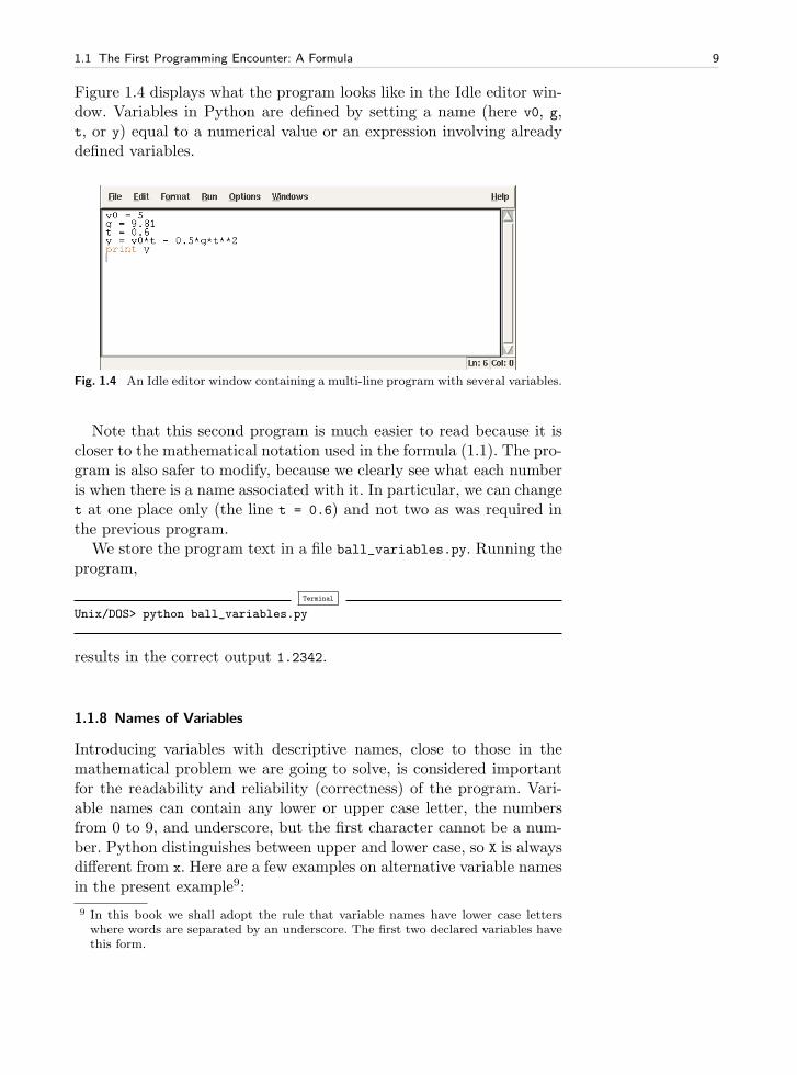
1.1 The First Programming Encounter: A Formula 9

Figure 1.4 displays what the program looks like in the Idle editor win-dow. Variables in Python are defined by setting a name (here v0, g,t, or y) equal to a numerical value or an expression involving alreadydefined variables.

Fig. 1.4 An Idle editor window containing a multi-line program with several variables.

Note that this second program is much easier to read because it iscloser to the mathematical notation used in the formula (1.1). The pro-gram is also safer to modify, because we clearly see what each numberis when there is a name associated with it. In particular, we can changet at one place only (the line t = 0.6) and not two as was required inthe previous program.

We store the program text in a file ball_variables.py. Running theprogram,

Terminal

Unix/DOS> python ball_variables.py

results in the correct output 1.2342.

1.1.8 Names of Variables

Introducing variables with descriptive names, close to those in themathematical problem we are going to solve, is considered importantfor the readability and reliability (correctness) of the program. Vari-able names can contain any lower or upper case letter, the numbersfrom 0 to 9, and underscore, but the first character cannot be a num-ber. Python distinguishes between upper and lower case, so X is alwaysdifferent from x. Here are a few examples on alternative variable namesin the present example9:

9 In this book we shall adopt the rule that variable names have lower case letterswhere words are separated by an underscore. The first two declared variables havethis form.

10 1 Computing with Formulas

initial_velocity = 5acceleration_of_gravity = 9.81TIME = 0.6VerticalPositionOfBall = initial_velocity*TIME - \

0.5*acceleration_of_gravity*TIME**2print VerticalPositionOfBall

With such long variables names, the code for evaluating the formulabecomes so long that we have decided to break it into two lines. Thisis done by a backslash at the very end of the line (make sure there areno blanks after the backslash!).

We note that even if this latter version of the program containsvariables that are defined precisely by their names, the program isharder to read than the one with variables v0, g, t, and y0.

The rule of thumb is to use the same variable names as those ap-pearing in a precise mathematical description of the problem to besolved by the program. For all variables where there is no associatedprecise mathematical description and symbol, one must use descriptivevariable names which explain the purpose of the variable. For example,if a problem description introduces the symbol D for a force due to airresistance, one applies a variable D also in the program. However, if theproblem description does not define any symbol for this force, one mustapply a descriptive name, such as air_resistance, resistance_force,or drag_force.

1.1.9 Reserved Words in Python

Certain words are reserved in Python because they are used to build upthe Python language. These reserved words cannot be used as variablenames: and, as, assert, break, class, continue, def, del, elif, else,except, False, finally, for, from, global, if, import, in, is, lambda,None, nonlocal, not, or, pass, raise, return, True, try, with, while, andyield. You may, for instance, add an underscore at the end to turn areserved word into a variable name. See Exercise 1.17 for examples onlegal and illegal variable names.

1.1.10 Comments

Along with the program statements it is often informative to providesome comments in a natural human language to explain the idea behindthe statements. Comments in Python start with the # character, andeverything after this character on a line is ignored when the program isrun. Here is an example of our program with explanatory comments:

1.1 The First Programming Encounter: A Formula 11

# Program for computing the height of a ball in vertical motion.v0 = 5 # initial velocityg = 9.81 # acceleration of gravityt = 0.6 # timey = v0*t - 0.5*g*t**2 # vertical positionprint y

This program and the initial version on page 8 are identical when runon the computer, but for a human the latter is easier to understandbecause of the comments.

Good comments together with well-chosen variable names are nec-essary for any program longer than a few lines, because otherwise theprogram becomes difficult to understand, both for the programmer andothers. It requires some practice to write really instructive comments.Never repeat with words what the program statements already clearlyexpress. Use instead comments to provide important information thatis not obvious from the code, for example, what mathematical variablenames mean, what variables are used for, and general ideas that liebehind a forthcoming set of statements.

1.1.11 Formatting Text and Numbers

Instead of just printing the numerical value of y in our introductoryprogram, we now want to write a more informative text, typically some-thing like

At t=0.6 s, the height of the ball is 1.23 m.

where we also have control of the number of digits (here y is accurateup to centimeters only).

Such output from the program is accomplished by a print state-ment where we use something often known as printf formatting10.For a newcomer to programming, the syntax of printf formatting maylook awkward, but it is quite easy to learn and very convenient andflexible to work with. The sample output above is produced by thisstatement:

print ’At t=%g s, the height of the ball is %.2f m.’ % (t, y)

Let us explain this line in detail. The print statement now prints astring: everything that is enclosed in quotes (either single: ’, or dou-ble: ") denotes a string in Python. The string above is formatted usingprintf syntax. This means that the string has various “slots”, start-ing with a percentage sign, here %g and %.2f, where variables in theprogram can be put in. We have two “slots” in the present case, andconsequently two variables must be put into the slots. The relevant

10 This formatting was originally introduced by a function printf in the C program-ming language.

12 1 Computing with Formulas

syntax is to list the variables inside standard parentheses after thestring, separated from the string by a percentage sign. The first vari-able, t, goes into the first “slot”. This “slot” has a format specification%g, where the percentage sign marks the slot and the following char-acter, g, is a format specification. The g that a real number is to bewritten as compactly as possible. The next variable, y, goes into thesecond “slot”. The format specification here is .2f, which means a realnumber written with two digits after comma. The f in the .2f formatstands for float, a short form for floating-point number, which is theterm used for a real number on a computer.

For completeness we present the whole program, where text andnumbers are mixed in the output:

v0 = 5g = 9.81t = 0.6y = v0*t - 0.5*g*t**2print ’At t=%g s, the height of the ball is %.2f m.’ % (t, y)

You can find the program in the file ball_output1.py in thesrc/formulas folder.

There are many more ways to specify formats. For example, e writesa number in scientific notation, i.e., with a number between 1 and 10followed by a power of 10, as in 1.2432 · 10−3. On a computer such anumber is written in the form 1.2432e-03. Capital E in the exponentis also possible, just replace e by E, with the result 1.2432E-03.

For decimal notation we use the letter f, as in %f, and the outputnumber then appears with digits before and/or after a comma, e.g.,0.0012432 instead of 1.2432E-03. With the g format, the output willuse scientific notation for large or small numbers and decimal notationotherwise. This format is normally what gives most compact output ofa real number. A lower case g leads to lower case e in scientific notation,while upper case G implies E instead of e in the exponent.

One can also specify the format as 10.4f or 14.6E, meaning in thefirst case that a float is written in decimal notation with four decimalsin a field of width equal to 10 characters, and in the second case a floatwritten in scientific notation with six decimals in a field of width 14characters.

Here is a list of some important printf format specifications11:

%s a string%d an integer%0xd an integer padded with x leading zeros%f decimal notation with six decimals%e compact scientific notation, e in the exponent%E compact scientific notation, E in the exponent%g compact decimal or scientific notation (with e)

11 For a complete specification of the possible printf-style format strings, follow thelink from the item “printf-style formatting” in the index of the Python LibraryReference.

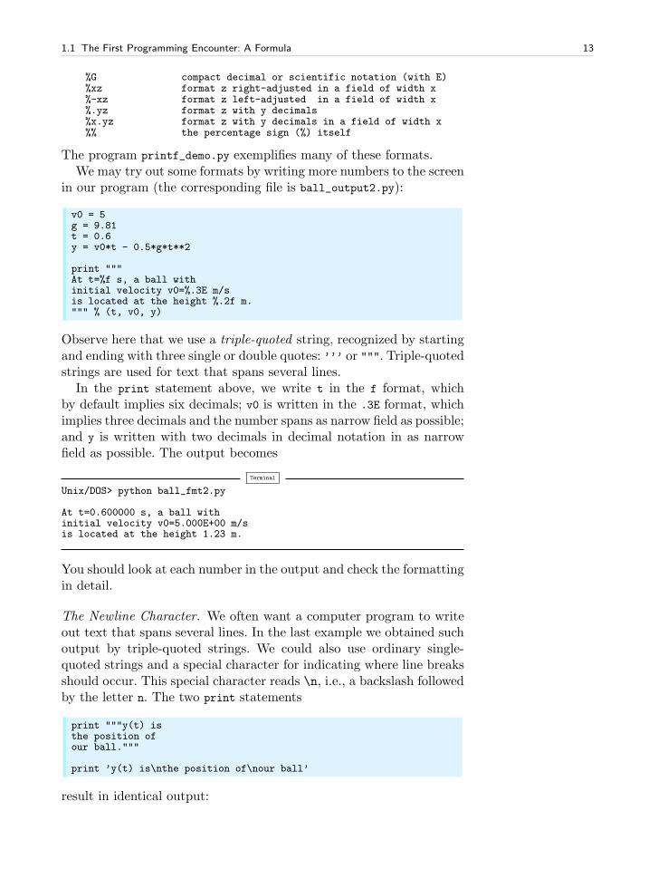
1.1 The First Programming Encounter: A Formula 13

%G compact decimal or scientific notation (with E)%xz format z right-adjusted in a field of width x%-xz format z left-adjusted in a field of width x%.yz format z with y decimals%x.yz format z with y decimals in a field of width x%% the percentage sign (%) itself

The program printf_demo.py exemplifies many of these formats.We may try out some formats by writing more numbers to the screen

in our program (the corresponding file is ball_output2.py):

v0 = 5g = 9.81t = 0.6y = v0*t - 0.5*g*t**2

print """At t=%f s, a ball withinitial velocity v0=%.3E m/sis located at the height %.2f m.""" % (t, v0, y)

Observe here that we use a triple-quoted string, recognized by startingand ending with three single or double quotes: ’’’ or """. Triple-quotedstrings are used for text that spans several lines.

In the print statement above, we write t in the f format, whichby default implies six decimals; v0 is written in the .3E format, whichimplies three decimals and the number spans as narrow field as possible;and y is written with two decimals in decimal notation in as narrowfield as possible. The output becomes

Terminal

Unix/DOS> python ball_fmt2.py

At t=0.600000 s, a ball withinitial velocity v0=5.000E+00 m/sis located at the height 1.23 m.

You should look at each number in the output and check the formattingin detail.

The Newline Character. We often want a computer program to writeout text that spans several lines. In the last example we obtained suchoutput by triple-quoted strings. We could also use ordinary single-quoted strings and a special character for indicating where line breaksshould occur. This special character reads \n, i.e., a backslash followedby the letter n. The two print statements

print """y(t) isthe position ofour ball."""

print ’y(t) is\nthe position of\nour ball’

result in identical output:

14 1 Computing with Formulas

y(t) isthe position ofour ball.

1.2 Computer Science Glossary

It is now time to pick up some important words that programmersuse when they talk about programming: algorithm, application, as-signment, blanks (whitespace), bug, code, code segment, code snippet,debug, debugging, execute, executable, implement, implementation, in-put, library, operating system, output, statement, syntax, user, verify,and verification.These words are frequently used in English in lots of contexts, yet theyhave a precise meaning in computer science.

Program and code are interchangeable terms. A code/program seg-ment is a collection of consecutive statements from a program. Anotherterm with similar meaning is code snippet. Many also use the word ap-plication in the same meaning as program and code. A related term issource code, which is the same as the text that constitutes the program.You find the source code of a program in one or more text files12.

We talk about running a program, or equivalently executing a pro-gram or executing a file. The file we execute is the file in which theprogram text is stored. This file is often called an executable or anapplication. The program text may appear in many files, but the ex-ecutable is just the single file that starts the whole program when werun that file. Running a file can be done in several ways, for instance,by double-clicking the file icon, by writing the filename in a terminalwindow, or by giving the filename to some program. This latter tech-nique is what we have used so far in this book: we feed the filename tothe program python. That is, we execute a Python program by execut-ing another program python, which interprets the text in our Pythonprogram file.

The term library is widely used for a collection of generally usefulprogram pieces that can be applied in many different contexts. Hav-ing access to good libraries means that you do not need to programcode snippets that others have already programmed (most probablein a better way!). There are huge numbers of Python libraries. InPython terminology, the libraries are composed of modules and pack-ages. Chapter 1.4 gives a first glimpse of the math module, which con-tains a set of standard mathematical functions for sinx, cosx, lnx, ex,sinhx, sin−1 x, etc. Later, you will meet many other useful modules.

12 Note that text files normally have the extension .txt, while program files have anextension related to the programming language, e.g., .py for Python programs. Thecontent of a .py file is, nevertheless, plain text as in a .txt file.

1.2 Computer Science Glossary 15

Packages are just collections of modules. The standard Python dis-tribution comes with a large number of modules and packages, butyou can download many more from the Internet, see in particularwww.python.org/pypi. Very often, when you encounter a programmingtask that is likely to occur in many other contexts, you can find aPython module where the job is already done. To mention just oneexample, say you need to compute how many days there are betweentwo dates. This is a non-trivial task that lots of other programmersmust have faced, so it is not a big surprise that Python comes with amodule datetime to do calculations with dates.

The recipe for what the computer is supposed to do in a program iscalled algorithm. In the examples in the first couple of chapters in thisbook, the algorithms are so simple that we can hardly distinguish themfrom the program text itself, but later in the book we will carefully setup an algorithm before attempting to implement it in a program. Thisis useful when the algorithm is much more compact than the resultingprogram code. The algorithm in the current example consists of threesteps:

1. initialize the variables v0, g, and t with numerical values,2. evaluate y according to the formula (1.1),3. print the y value to the screen.

The Python program is very close to this text, but some less expe-rienced programmers may want to write the tasks in English beforetranslating them to Python.

The implementation of an algorithm is the process of writing andtesting a program. The testing phase is also known as verification: Af-ter the program text is written we need to verify that the programworks correctly. This is a very important step that will receive sub-stantial attention in the present book. Mathematical software producenumbers, and it is normally quite a challenging task to verify that thenumbers are correct.

An error in a program is known as a bug13, and the process of lo-cating and removing bugs is called debugging. Many look at debuggingas the most difficult and challenging part of computer programming.

Programs are built of statements. There are many types of state-ments:

v0 = 3

is an assignment statement, while

13 In the very early days of computing, computers were built of a large number oftubes, which glowed and gave off heat. The heat attracted bugs, which causedshort circuits. “Debugging” meant shutting down the computer and cleaning outthe dead bugs.

16 1 Computing with Formulas

print y

is a print statement. It is common to have one statement on eachline, but it is possible to write multiple statements on one line if thestatements are separated by semi-colon. Here is an example:

v0 = 3; g = 9.81; t = 0.6y = v0*t - 0.5*g*t**2print y

Although most newcomers to computer programming will think theyunderstand the meaning of the lines in the above program, it is im-portant to be aware of some major differences between notation in acomputer program and notation in mathematics. When you see theequality sign “=” in mathematics, it has a certain interpretation as anequation (x+2 = 5) or a definition (f(x) = x2+1). In a computer pro-gram, however, the equality sign has a quite different meaning, and it iscalled an assignment. The right-hand side of an assignment contains anexpression, which is a combination of values, variables, and operators.When the expression is evaluated, it results in a value that the variableon the left-hand side will refer to. We often say that the right-hand sidevalue is assigned to the variable on the left-hand side. In the currentcontext it means that we in the first line assign the number 3 to thevariable v0, 9.81 to g, and 0.6 to t. In the next line, the right-hand sideexpression v0*t - 0.5*g*t**2 is first evaluated, and the result is thenassigned to the y variable.

Consider the assignment statement

y = y + 3

This statement is mathematically false, but in a program it just meansthat we evaluate the right-hand side expression and assign its value tothe variable y. That is, we first take the current value of y and add 3.The value of this operation is assigned to y. The old value of y is thenlost.

You may think of the = as an arrow, y <- y+3, rather than an equalitysign, to illustrate that the value to the right of the arrow is stored inthe variable to the left of the arrow14. An example will illustrate theprinciple of assignment to a variable:

y = 3print yy = y + 4print yy = y*yprint y

14 The R (or S or S-PLUS) programming languages for statistical computing actuallyuse an arrow, while other languages such as Algol, Simula, and Pascal use := toexplicitly state that we are not dealing with a mathematical equality.

1.2 Computer Science Glossary 17

Running this program results in three numbers: 3, 7, 49. Go throughthe program and convince yourself that you understand what the resultof each statement becomes.

A computer program must have correct syntax , meaning that thetext in the program must follow the strict rules of the computer lan-guage for constructing statements. For example, the syntax of the printstatement is the word print, followed by one or more spaces, followedby an expression of what we want to print (a Python variable, textenclosed in quotes, a number, for instance). Computers are very pickyabout syntax! For instance, a human having read all the previous pagesmay easily understand what this program does,

myvar = 5.2prinnt Myvar

but the computer will find two errors in the last line: prinnt is anunknown instruction and Myvar is an undefined variable. Only the firsterror is reported (a syntax error), because Python stops the programonce an error is found. All errors that Python finds are easy to remove.The difficulty with programming is to remove the rest of the errors,such as errors in formulas or the sequence of operations.

Blanks may or may not be important in Python programs. In Chap-ter 2.1.2 you will see that blanks are in some occasions essential fora correct program. Around = or arithmetic operators, however, blanksdo not matter. We could hence write our program from Chapter 1.1.7as

v0=3;g=9.81;t=0.6;y=v0*t-0.5*g*t**2;print y

This is not a good idea because blanks are essential for easy readingof a program code, and easy reading is essential for finding errors, andfinding errors is the difficult part of programming. The recommendedlayout in Python programs specifies one blank around =, +, and -, andno blanks around *, /, and **. Note that the blank after print is es-sential: print is a command in Python and printy is not recognizedas any valid command. (Python would look at printy as an undefinedvariable.) Computer scientists often use the term whitespace when re-ferring to a blank15.

When we interact with computer programs, we usually provide someinformation to the program and get some information out. It is commonto use the term input data, or just input , for the information thatmust be known on beforehand. The result from a program is similarlyreferred to as output data, or just output . In our example, v0, g, and

15 More precisely, blank is the character produced by the space bar on the keyboard,while whitespace denotes any character(s) that, if printed, do not print ink on thepaper: a blank, a tabulator character (produced by backslash followed by t), or anewline character (produced by backslash followed by n). The newline character isexplained on page 13.

18 1 Computing with Formulas

t constitute input, while y is output. All input data must be assignedvalues in the program before the output can be computed. Input datacan be explicitly initialized in the program, as we do in the presentexample, or the data can be provided by user through keyboard typingwhile the program is running, as we explain in Chapter 4. Output datacan be printed in the terminal window, as in the current example,displayed as graphics on the screen, as done in Chapter 5, or stored ina file for later access, as explained in Chapter 6.

The word user usually has a special meaning in computer science:It means a human interacting with a program. You are a user of atext editor for writing Python programs, and you are a user of yourown programs. When you write programs, it is difficult to imagine howother users will interact with the program. Maybe they provide wronginput or misinterpret the output. Making user-friendly programs is verychallenging and depends heavily on the target audience of users. Theauthor had the average reader of the book in mind as a typical userwhen developing programs for this book.

A central part of a computer is the operating system. This is actu-ally a collection of programs that manages the hardware and softwareresources on the computer. There are three major operating systemstoday: Windows, Macintosh (called Mac for short), and Unix. Sev-eral versions of Windows have appeared since the 1990s: Windows 95,98, 2000, ME, XP, and Vista. Unix was invented already in 1970 andcomes in many different versions. Nowadays, two open source imple-mentations of Unix, Linux and Free BSD Unix, are most common. Thelatter forms the core of the Mac OS X operating system on Macintoshmachines, while Linux exists in slightly different flavors: Red Hat, De-bian, Ubuntu, and Suse to mention the most important distributions.We will use the term Unix in this book as a synonym for all the operat-ing systems that inherit from classical Unix, such as Solaris, Free BSD,Mac OS X, and any Linux variant. Note that this use of Unix also in-cludes Macintosh machines, but only newer machines as the older onesrun an Apple-specific Mac operating system. As a computer user andreader of this book, you should know exactly which operating systemyou have. In particular, Mac users must know if their operating systemis Unix-based or not.

The user’s interaction with the operation system is through a set ofprograms. The most widely used of these enable viewing the contentsof folders or starting other programs. To interact with the operatingsystem, as a user, you can either issue commands in a terminal windowor use graphical programs. For example, for viewing the file contentsof a folder you can run the command ls in a Unix terminal windowor dir in a DOS (Windows) terminal window. The graphical alterna-tives are many, some of the most common are Windows Explorer onWindows, Nautilus and Konqueror on Unix, and Finder on Mac. To

1.3 Another Formula: Celsius-Fahrenheit Conversion 19

start a program, it is common to double-click on a file icon or writethe program’s name in a terminal window.

1.3 Another Formula: Celsius-Fahrenheit Conversion

Our next example involves the formula for converting temperaturemeasured in Celsius degrees to the corresponding value in Fahrenheitdegrees:

F =9

5C + 32 (1.2)

In this formula, C is the amount of degrees in Celsius, and F is thecorresponding temperature measured in Fahrenheit. Our goal now isto write a computer program which can compute F from (1.2) whenC is known.

1.3.1 Potential Error: Integer Division

Straightforward Coding of the Formula. A straightforward attempt atcoding the formula (1.2) goes as follows16:

C = 21F = (9/5)*C + 32print F

When run, this program prints the value 53. You can find the programin the file c2f_v1.py17 in the src/formulas folder – as all other programsfrom this chapter.

Verifying the Results. Testing the correctness is easy in this case sincewe can evaluate the formula on a calculator: 9

5 · 21+ 32 is 69.8, not 53.What is wrong? The formula in the program looks correct!

Float and Integer Division. The error in our program above is oneof the most common errors in mathematical software and is not at allobvious for a newcomer to programming. In many computer languages,there are two types of divisions: float division and integer division.Float division is what you know from mathematics: 9/5 becomes 1.8in decimal notation.

Integer division a/b with integers (whole numbers) a and b resultsin an integer that is truncated (or mathematically, “rounded down”).

16 The parentheses around 9/5 are not strictly needed, i.e., (9/5)*C is computation-ally identical to 9/5*C, but parentheses remove any doubt that 9/5*C could mean9/(5*C). Chapter 1.3.4 has more information on this topic.

17 The v1 part of the name stands for “version 1”. Throughout this book, we will oftendevelop several trial versions of a program, but remove the version number in thefinal version of the program.

20 1 Computing with Formulas

More precisely, the result is the largest integer c such that bc ≤ a. Thisimplies that 9/5 becomes 1 since 1 · 5 = 5 ≤ 9 while 2 · 5 = 10 > 9.Another example is 1/5, which becomes 0 since 0 ·5 ≤ 1 (and 1 ·5 > 1).Yet another example is 16/6, which results in 2 (try 2 · 6 and 3 · 6 toconvince yourself). Many computer languages, including Fortran, C,C++, Java, and Python, interpret a division operation a/b as integerdivision if both operands a and b are integers. If either a or b is a real(floating-point) number, a/b implies the standard mathematical floatdivision.

The problem with our program is the coding of the formula (9/5)*C

+ 32. This formula is evaluated as follows. First, 9/5 is calculated. Since9 and 5 are interpreted by Python as integers (whole numbers), 9/5 isa division between two integers, and Python chooses by default integerdivision, which results in 1. Then 1 is multiplied by C, which equals 21,resulting in 21. Finally, 21 and 32 are added with 53 as result.

We shall very soon present a correct version of the temperatureconversion program, but first it may be advantageous to introduce afrequently used word in Python programming: object.

1.3.2 Objects in Python

When we write

C = 21

Python interprets the number 21 on the right-hand side of the assign-ment as an integer and creates an int (for integer) object holding thevalue 21. The variable C acts as a name for this int object. Similarly, ifwe write C = 21.0, Python recognizes 21.0 as a real number and there-fore creates a float (for floating-point) object holding the value 21.0and lets C be a name for this object. In fact, any assignment statementhas the form of a variable name on the left-hand side and an object onthe right-hand side. One may say that Python programming is aboutsolving a problem by defining and changing objects.

At this stage, you do not need to know what an object really is,just think of an int object as a collection, say a storage box, withsome information about an integer number. This information is storedsomewhere in the computer’s memory, and with the name C the pro-gram gets access to this information. The fundamental issue right nowis that 21 and 21.0 are identical numbers in mathematics, while in aPython program 21 gives rise to an int object and 21.0 to a float

object.There are lots of different object types in Python, and you will later

learn how to create your own customized objects. Some objects containa lot of data, not just an integer or a real number. For example, whenwe write

1.3 Another Formula: Celsius-Fahrenheit Conversion 21

print ’A text with an integer %d and a float %f’ % (2, 2.0)

a str (string) object, without a name, is first made of the text betweenthe quotes and then this str object is printed. We can alternatively dothis in two steps:

s = ’A text with an integer %d and a float %f’ % (2, 2.0)print s

1.3.3 Avoiding Integer Division

As a quite general rule of thumb, one should avoid integer divisionin mathematical formulas18. There are several ways to do this, as wedescribe in Appendix G.2. The simplest remedy in Python is to inserta statement that simply turns off integer division. A more widely ap-plicable method, also in other programming languages than Python,is to enforce one of the operands to be a float object. In the currentexample, there are several ways to do this:

F = (9.0/5)*C + 32F = (9/5.0)*C + 32F = float(C)*9/5 + 32

In the first two lines, one of the operands is written as a decimal num-ber, implying a float object and hence float division. In the last line,float(C)*9 means float times int, which results in a float object, andfloat division is guaranteed.

A related construction,

F = float(C)*(9/5) + 32

does not work correctly, because 9/5 is evaluated by integer division,yielding 1, before being multiplied by a float representation of C (seenext section for how compound arithmetic operations are calculated).In other words, the formula reads F=C+32, which is wrong.

We now understand why the first version of the program does notwork and what the remedy is. A correct program is

C = 21F = (9.0/5)*C + 32print F

Instead of 9.0 we may just write 9. (the dot implies a float interpre-tation of the number). The program is available in the file c2f.py. Tryto run it – and observe that the output becomes 69.8, which is correct.

18 Some mathematical algorithms do make use of integer division, but in those casesyou should use a double forward slash, //, as division operator, because this isPython’s way of explicitly indicating integer division.

22 1 Computing with Formulas

Comment. We could easily have run into problems in our very firstprograms if we instead of writing the formula 1

2gt2 as 0.5*g*t**2 wrote

(1/2)*g*t**2. Explain the problem!

1.3.4 Arithmetic Operators and Precedence

Formulas in Python programs are usually evaluated in the same wayas we would evaluate them mathematically. Python proceeds from leftto right, term by term in an expression (terms are separated by plusor minus). In each term, power operations such as ab, coded as a**b,has precedence over multiplication and division. As in mathematics, wecan use parentheses to dictate the way a formula is evaluated. Beloware two illustrations of these principles.

5/9+2*a**4/2: First 5/9 is evaluated (as integer division, giving 0as result), then a4 (a**4) is evaluated, then 2 is multiplied with a4,that result is divided by 2, and the answer is added to the result ofthe first term. The answer is therefore a**4.

5/(9+2)*a**(4/2): First 59+2 is evaluated (as integer division, yield-

ing 0), then 4/2 is computed (as integer division, yielding 2), thena**2 is calculated, and that number is multiplied by the result of5/(9+2). The answer is thus always zero.

As evident from these two examples, it is easy to unintentionally getinteger division in formulas. Although integer division can be turnedoff in Python, we think it is important to be strongly aware of theinteger division concept and to develop good programming habits toavoid it. The reason is that this concept appears in so many commoncomputer languages that it is better to learn as early as possible howto deal with the problem rather than using a Python-specific featureto remove the problem.

1.4 Evaluating Standard Mathematical Functions

Mathematical formulas frequently involve functions such as sin, cos,tan, sinh, cosh, exp, log, etc. On a pocket calculator you have spe-cial buttons for such functions. Similarly, in a program you also haveready-made functionality for evaluating these types of mathematicalfunctions. One could in principle write one’s own program for evaluat-ing, e.g., the sin(x) function, but how to do this in an efficient way isa non-trivial topic. Experts have worked on this problem for decadesand implemented their best recipes in pieces of software that we shouldreuse. This section tells you how to reach sin, cos, and similar functionsin a Python context.

1.4 Evaluating Standard Mathematical Functions 23

1.4.1 Example: Using the Square Root Function

Problem. Consider the vertical motion of a ball in (1.1) on page 1. Wenow ask the question: How long time does it take for the ball to reachthe height yc? The answer is straightforward to derive. When y = ycwe have

yc = v0t−1

2gt2 .

We recognize that this equation is a quadratic equation which we mustsolve with respect to t. Rearranging,

1

2gt2 − v0t+ yc = 0,

and using the well-known formula for the two solutions of a quadraticequation, we find

t1 =

(

v0 −√

v20 − 2gyc

)

/g, t2 =

(

v0 +√

v20 − 2gyc

)

/g . (1.3)

There are two solutions because the ball reaches the height yc on itsway up (t = t1) and on its way down (t = t2 > t1).

The Program. To evaluate the expressions for t1 and t2 from (1.3)in a computer program, we need access to the square root function.In Python, the square root function and lots of other mathematicalfunctions, such as sin, cos, sinh, exp, and log, are available in a modulecalled math. We must first import the module before we can use it,that is, we must write import math. Thereafter, to take the square rootof a variable a, we can write math.sqrt(a). This is demonstrated in aprogram for computing t1 and t2:

v0 = 5g = 9.81yc = 0.2import matht1 = (v0 - math.sqrt(v0**2 - 2*g*yc))/gt2 = (v0 + math.sqrt(v0**2 - 2*g*yc))/gprint ’At t=%g s and %g s, the height is %g m.’ % (t1, t2, yc)

The output from this program becomesAt t=0.0417064 s and 0.977662 s, the height is 0.2 m.

You can find the program as the file ball_yc.py in the src/formulas

folder.

Two Ways of Importing a Module. The standard way to import amodule, say math, is to write

import math

and then access individual functions in the module with the modulename as prefix as in

24 1 Computing with Formulas

x = math.sqrt(y)

People working with mathematical functions often find math.sqrt(y)

less pleasing than just sqrt(y). Fortunately, there is an alternative im-port syntax that allows us to skip the module name prefix. This alter-native syntax has the form “from module import function”. A specificexample is

from math import sqrt

Now we can work with sqrt directly, without the math. prefix. Morethan one function can be imported:

from math import sqrt, exp, log, sin

Sometimes one just writes

from math import *

to import all functions in the math module. This includes sin, cos, tan,asin, acos, atan, sinh, cosh, tanh, exp, log (base e), log10 (base 10),sqrt, as well as the famous numbers e and pi. Importing all functionsfrom a module, using the asterisk (*) syntax, is convenient, but thismay result in a lot of extra names in the program that are not used.It is in general recommended not to import more functions than thosethat are really used in the program19.

With a from math import sqrt statement we can write the formulasfor the roots in a more pleasing way:

t1 = (v0 - sqrt(v0**2 - 2*g*yc))/gt2 = (v0 + sqrt(v0**2 - 2*g*yc))/g

Import with New Names. Imported modules and functions can be givennew names in the import statement, e.g.,

import math as m# m is now the name of the math modulev = m.sin(m.pi)

from math import log as lnv = ln(5)

from math import sin as s, cos as c, log as lnv = s(x)*c(x) + ln(x)

In Python, everything is an object, and variables refer to objects, sonew variables may refer to modules and functions as well as numbersand strings. The examples above on new names can also be coded byintroducing new variables explicitly:

19 Nevertheless, of convenience we often use the from module import * syntax in thisbook.

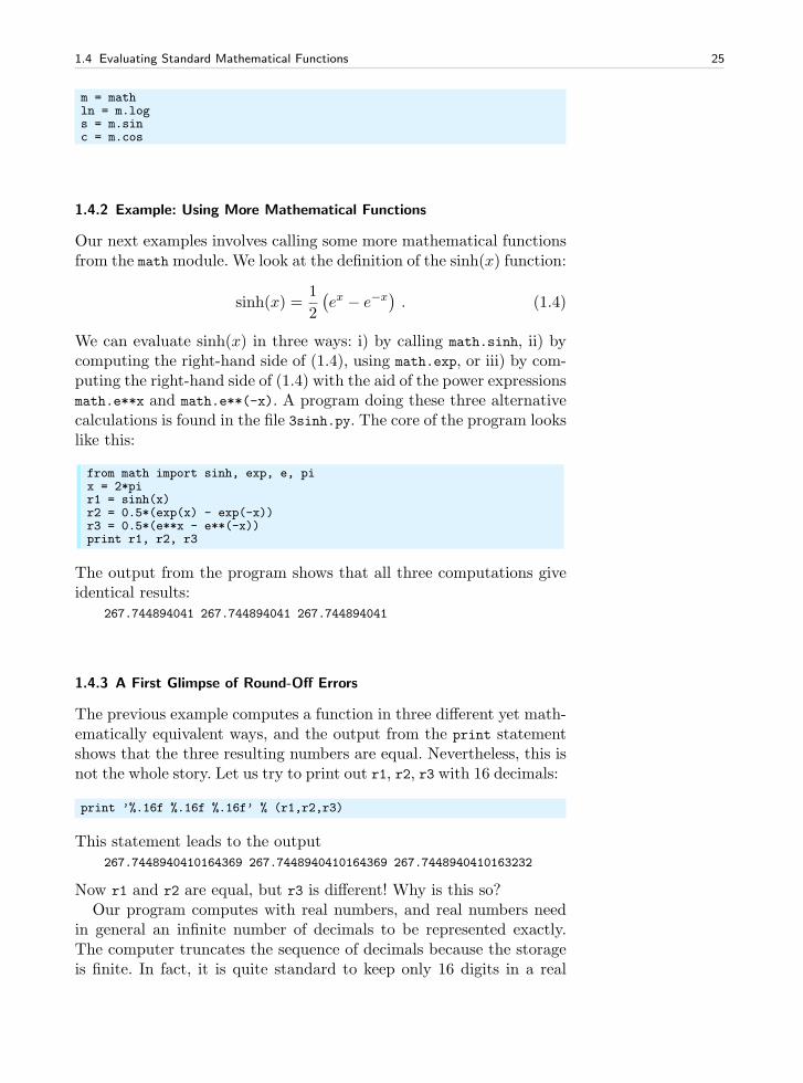
1.4 Evaluating Standard Mathematical Functions 25

m = mathln = m.logs = m.sinc = m.cos

1.4.2 Example: Using More Mathematical Functions

Our next examples involves calling some more mathematical functionsfrom the math module. We look at the definition of the sinh(x) function:

sinh(x) =1

2

(

ex − e−x)

. (1.4)

We can evaluate sinh(x) in three ways: i) by calling math.sinh, ii) bycomputing the right-hand side of (1.4), using math.exp, or iii) by com-puting the right-hand side of (1.4) with the aid of the power expressionsmath.e**x and math.e**(-x). A program doing these three alternativecalculations is found in the file 3sinh.py. The core of the program lookslike this:

from math import sinh, exp, e, pix = 2*pir1 = sinh(x)r2 = 0.5*(exp(x) - exp(-x))r3 = 0.5*(e**x - e**(-x))print r1, r2, r3

The output from the program shows that all three computations giveidentical results:

267.744894041 267.744894041 267.744894041

1.4.3 A First Glimpse of Round-Off Errors

The previous example computes a function in three different yet math-ematically equivalent ways, and the output from the print statementshows that the three resulting numbers are equal. Nevertheless, this isnot the whole story. Let us try to print out r1, r2, r3 with 16 decimals:

print ’%.16f %.16f %.16f’ % (r1,r2,r3)

This statement leads to the output267.7448940410164369 267.7448940410164369 267.7448940410163232

Now r1 and r2 are equal, but r3 is different! Why is this so?Our program computes with real numbers, and real numbers need

in general an infinite number of decimals to be represented exactly.The computer truncates the sequence of decimals because the storageis finite. In fact, it is quite standard to keep only 16 digits in a real

26 1 Computing with Formulas

number on a computer. Exactly how this truncation is done is notexplained in this book20. For now the purpose is to notify the readerthat real numbers on a computer often have a small error. Only a fewreal numbers can be represented exactly with 16 digits, the rest of thereal numbers are only approximations.

For this reason, most arithmetic operations involve inaccurate realnumbers, resulting in inaccurate calculations. Think of the followingtwo calculations: 1/49 · 49 and 1/51 · 51. Both expressions are identicalto 1, but when we perform the calculations in Python,

print ’%.16f %.16f’ % (1/49.0*49, 1/51.0*51)

the result becomes0.9999999999999999 1.0000000000000000

The reason why we do not get exactly 1.0 as answer in the first case, isbecause 1/49 is not correctly represented in the computer. Also 1/51has an inexact representation, but the error does not propagate to thefinal answer.

To summarize, errors21 in floating-point numbers may propagatethrough mathematical calculations and result in answers that are onlyapproximations to the exact underlying mathematical values. The er-rors in the answers are commonly known as round-off errors. As soonas you use Python interactively as explained in the next section, youwill encounter round-off errors quite often.

Python has a special module decimal which allows real numbers tobe represented with adjustable accuracy so that round-off errors canbe made as small as desired. However, we will hardly use this module22

because approximations implied by many mathematical methods ap-plied throughout this book normally lead to (much) larger errors thanthose caused by round-off.

1.5 Interactive Computing

A particular convenient feature of Python is the ability to executestatements and evaluate expressions interactively. The environmentswhere you work interactively with programming are commonly knownas Python shells. The simplest Python shell is invoked by just typingpython at the command line in a terminal window. Some messagesabout Python are written out together with a prompt >>>, after whichyou can issue commands. Let us try to use the interactive shell as acalculator. Type in 3*4.5-0.5 and then press the Return key to seePython’s response to this expression:

20 Instead, you can search for “floating point number” on wikipedia.org.21 Exercise 2.27 on page 86 estimates the size of the errors.22 See the last paragraph of Chapter 3.1.9 for an example.

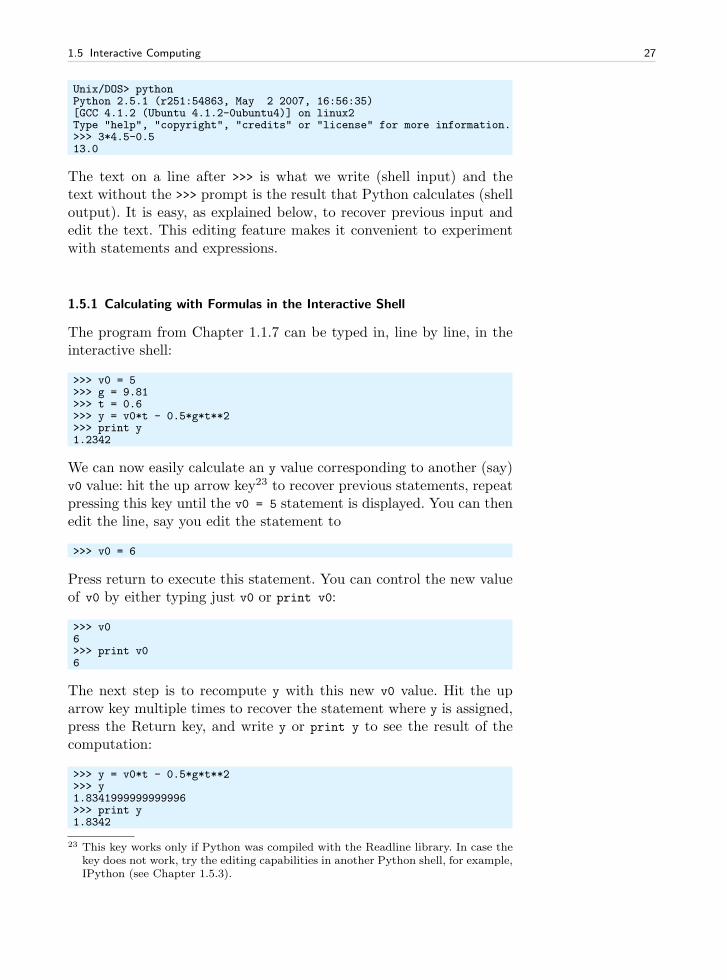
1.5 Interactive Computing 27

Unix/DOS> pythonPython 2.5.1 (r251:54863, May 2 2007, 16:56:35)[GCC 4.1.2 (Ubuntu 4.1.2-0ubuntu4)] on linux2Type "help", "copyright", "credits" or "license" for more information.>>> 3*4.5-0.513.0

The text on a line after >>> is what we write (shell input) and thetext without the >>> prompt is the result that Python calculates (shelloutput). It is easy, as explained below, to recover previous input andedit the text. This editing feature makes it convenient to experimentwith statements and expressions.

1.5.1 Calculating with Formulas in the Interactive Shell

The program from Chapter 1.1.7 can be typed in, line by line, in theinteractive shell:

>>> v0 = 5>>> g = 9.81>>> t = 0.6>>> y = v0*t - 0.5*g*t**2>>> print y1.2342

We can now easily calculate an y value corresponding to another (say)v0 value: hit the up arrow key23 to recover previous statements, repeatpressing this key until the v0 = 5 statement is displayed. You can thenedit the line, say you edit the statement to

>>> v0 = 6

Press return to execute this statement. You can control the new valueof v0 by either typing just v0 or print v0:

>>> v06>>> print v06

The next step is to recompute y with this new v0 value. Hit the uparrow key multiple times to recover the statement where y is assigned,press the Return key, and write y or print y to see the result of thecomputation:

>>> y = v0*t - 0.5*g*t**2>>> y1.8341999999999996>>> print y1.8342

23 This key works only if Python was compiled with the Readline library. In case thekey does not work, try the editing capabilities in another Python shell, for example,IPython (see Chapter 1.5.3).

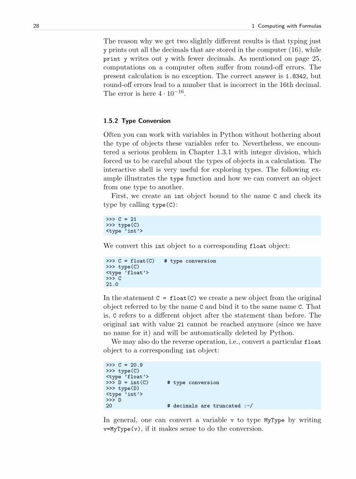
28 1 Computing with Formulas

The reason why we get two slightly different results is that typing justy prints out all the decimals that are stored in the computer (16), whileprint y writes out y with fewer decimals. As mentioned on page 25,computations on a computer often suffer from round-off errors. Thepresent calculation is no exception. The correct answer is 1.8342, butround-off errors lead to a number that is incorrect in the 16th decimal.The error is here 4 · 10−16.

1.5.2 Type Conversion

Often you can work with variables in Python without bothering aboutthe type of objects these variables refer to. Nevertheless, we encoun-tered a serious problem in Chapter 1.3.1 with integer division, whichforced us to be careful about the types of objects in a calculation. Theinteractive shell is very useful for exploring types. The following ex-ample illustrates the type function and how we can convert an objectfrom one type to another.

First, we create an int object bound to the name C and check itstype by calling type(C):

>>> C = 21>>> type(C)<type ’int’>

We convert this int object to a corresponding float object:

>>> C = float(C) # type conversion>>> type(C)<type ’float’>>>> C21.0

In the statement C = float(C) we create a new object from the originalobject referred to by the name C and bind it to the same name C. Thatis, C refers to a different object after the statement than before. Theoriginal int with value 21 cannot be reached anymore (since we haveno name for it) and will be automatically deleted by Python.

We may also do the reverse operation, i.e., convert a particular floatobject to a corresponding int object:

>>> C = 20.9>>> type(C)<type ’float’>>>> D = int(C) # type conversion>>> type(D)<type ’int’>>>> D20 # decimals are truncated :-/

In general, one can convert a variable v to type MyType by writingv=MyType(v), if it makes sense to do the conversion.

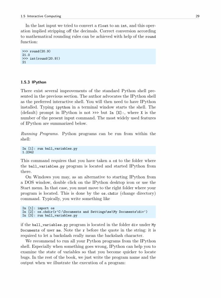
1.5 Interactive Computing 29

In the last input we tried to convert a float to an int, and this oper-ation implied stripping off the decimals. Correct conversion accordingto mathematical rounding rules can be achieved with help of the round

function:

>>> round(20.9)21.0>>> int(round(20.9))21

1.5.3 IPython

There exist several improvements of the standard Python shell pre-sented in the previous section. The author advocates the IPython shellas the preferred interactive shell. You will then need to have IPythoninstalled. Typing ipython in a terminal window starts the shell. The(default) prompt in IPython is not >>> but In [X]:, where X is thenumber of the present input command. The most widely used featuresof IPython are summarized below.

Running Programs. Python programs can be run from within theshell:

In [1]: run ball_variables.py1.2342

This command requires that you have taken a cd to the folder wherethe ball_variables.py program is located and started IPython fromthere.

On Windows you may, as an alternative to starting IPython froma DOS window, double click on the IPython desktop icon or use theStart menu. In that case, you must move to the right folder where yourprogram is located. This is done by the os.chdir (change directory)command. Typically, you write something like

In [1]: import osIn [2]: os.chdir(r’C:\Documents and Settings\me\My Documents\div’)In [3]: run ball_variables.py

if the ball_variables.py program is located in the folder div under MyDocuments of user me. Note the r before the quote in the string: it isrequired to let a backslash really mean the backslash character.

We recommend to run all your Python programs from the IPythonshell. Especially when something goes wrong, IPython can help you toexamine the state of variables so that you become quicker to locatebugs. In the rest of the book, we just write the program name and theoutput when we illustrate the execution of a program:

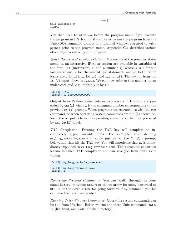
30 1 Computing with Formulas

Terminal

ball_variables.py1.2342

You then need to write run before the program name if you executethe program in IPython, or if you prefer to run the program from theUnix/DOS command prompt in a terminal window, you need to writepython prior to the program name. Appendix G.1 describes variousother ways to run a Python program.

Quick Recovery of Previous Output. The results of the previous state-ments in an interactive IPython session are available in variables ofthe form _iX (underscore, i, and a number X), where X is 1 for thelast statement, 2 for the second last statement, and so forth. Shortforms are _ for _i1, __ for _i2, and ___ for _i3. The output from theIn [1] input above is 1.2342. We can now refer to this number by anunderscore and, e.g., multiply it by 10:

In [2]: _*10Out[2]: 12.341999999999999

Output from Python statements or expressions in IPython are pre-ceded by Out[X] where X is the command number corresponding to theprevious In [X] prompt. When programs are executed, as with the runcommand, or when operating system commands are run (as shown be-low), the output is from the operating system and then not precededby any Out[X] label.

TAB Completion. Pressing the TAB key will complete an in-completely typed variable name. For example, after definingmy_long_variable_name = 4, write just my at the In [4]: promptbelow, and then hit the TAB key. You will experience that my is imme-diately expanded to my_long_variable_name. This automatic expansionfeature is called TAB completion and can save you from quite sometyping.

In [3]: my_long_variable_name = 4

In [4]: my_long_variable_nameOut[4]: 4

Recovering Previous Commands. You can “walk” through the com-mand history by typing Ctrl-p or the up arrow for going backward orCtrl-n or the down arrow for going forward. Any command you hitcan be edited and re-executed.

Running Unix/Windows Commands. Operating system commands canbe run from IPython. Below we run the three Unix commands date,ls (list files), and mkdir (make directory):

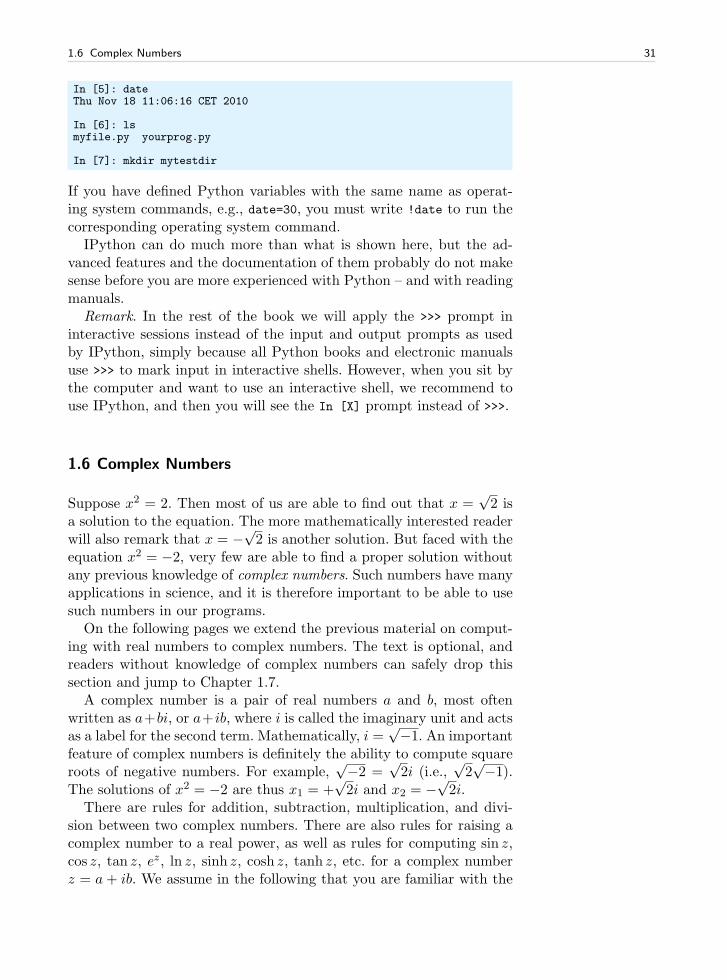
1.6 Complex Numbers 31

In [5]: dateThu Nov 18 11:06:16 CET 2010

In [6]: lsmyfile.py yourprog.py

In [7]: mkdir mytestdir

If you have defined Python variables with the same name as operat-ing system commands, e.g., date=30, you must write !date to run thecorresponding operating system command.

IPython can do much more than what is shown here, but the ad-vanced features and the documentation of them probably do not makesense before you are more experienced with Python – and with readingmanuals.

Remark. In the rest of the book we will apply the >>> prompt ininteractive sessions instead of the input and output prompts as usedby IPython, simply because all Python books and electronic manualsuse >>> to mark input in interactive shells. However, when you sit bythe computer and want to use an interactive shell, we recommend touse IPython, and then you will see the In [X] prompt instead of >>>.

1.6 Complex Numbers

Suppose x2 = 2. Then most of us are able to find out that x =√2 is

a solution to the equation. The more mathematically interested readerwill also remark that x = −

√2 is another solution. But faced with the

equation x2 = −2, very few are able to find a proper solution withoutany previous knowledge of complex numbers. Such numbers have manyapplications in science, and it is therefore important to be able to usesuch numbers in our programs.

On the following pages we extend the previous material on comput-ing with real numbers to complex numbers. The text is optional, andreaders without knowledge of complex numbers can safely drop thissection and jump to Chapter 1.7.

A complex number is a pair of real numbers a and b, most oftenwritten as a+bi, or a+ib, where i is called the imaginary unit and actsas a label for the second term. Mathematically, i =

√−1. An important

feature of complex numbers is definitely the ability to compute squareroots of negative numbers. For example,

√−2 =

√2i (i.e.,

√2√−1).

The solutions of x2 = −2 are thus x1 = +√2i and x2 = −

√2i.

There are rules for addition, subtraction, multiplication, and divi-sion between two complex numbers. There are also rules for raising acomplex number to a real power, as well as rules for computing sin z,cos z, tan z, ez, ln z, sinh z, cosh z, tanh z, etc. for a complex numberz = a+ ib. We assume in the following that you are familiar with the

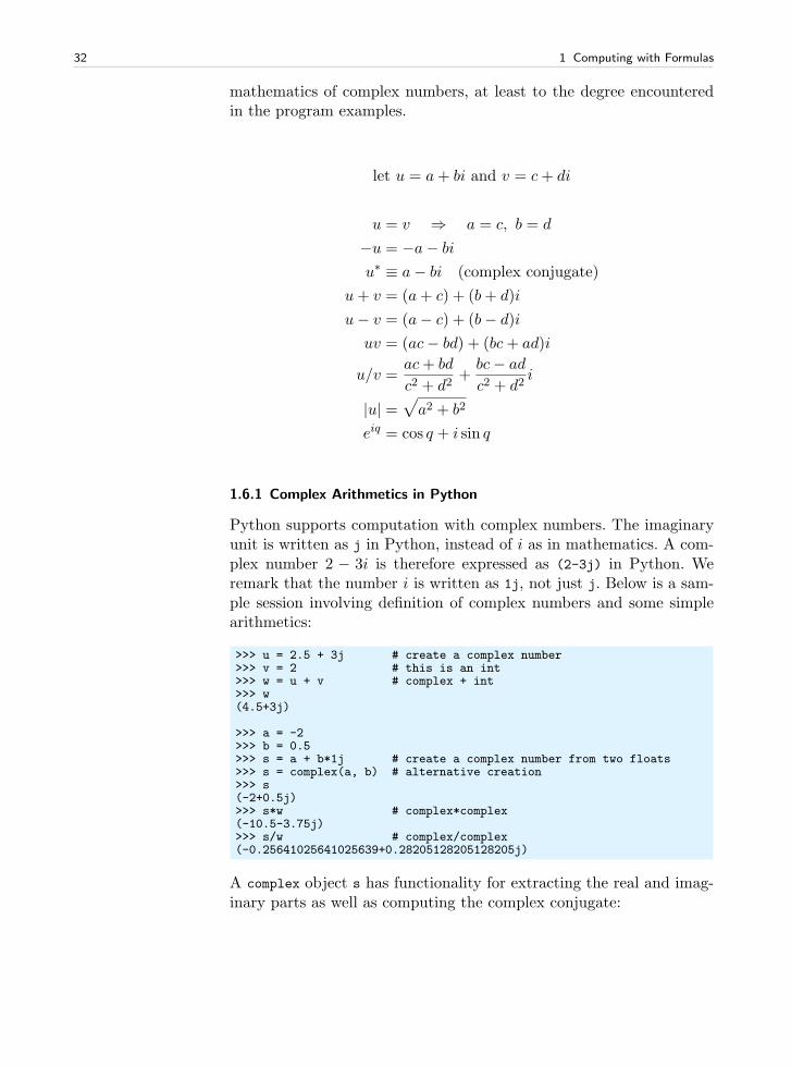
32 1 Computing with Formulas

mathematics of complex numbers, at least to the degree encounteredin the program examples.

let u = a+ bi and v = c+ di

u = v ⇒ a = c, b = d

−u = −a− bi

u∗ ≡ a− bi (complex conjugate)

u+ v = (a+ c) + (b+ d)i

u− v = (a− c) + (b− d)i

uv = (ac− bd) + (bc+ ad)i

u/v =ac+ bd

c2 + d2+

bc− ad

c2 + d2i

|u| =√

a2 + b2

eiq = cos q + i sin q

1.6.1 Complex Arithmetics in Python

Python supports computation with complex numbers. The imaginaryunit is written as j in Python, instead of i as in mathematics. A com-plex number 2 − 3i is therefore expressed as (2-3j) in Python. Weremark that the number i is written as 1j, not just j. Below is a sam-ple session involving definition of complex numbers and some simplearithmetics:

>>> u = 2.5 + 3j # create a complex number>>> v = 2 # this is an int>>> w = u + v # complex + int>>> w(4.5+3j)

>>> a = -2>>> b = 0.5>>> s = a + b*1j # create a complex number from two floats>>> s = complex(a, b) # alternative creation>>> s(-2+0.5j)>>> s*w # complex*complex(-10.5-3.75j)>>> s/w # complex/complex(-0.25641025641025639+0.28205128205128205j)

A complex object s has functionality for extracting the real and imag-inary parts as well as computing the complex conjugate:

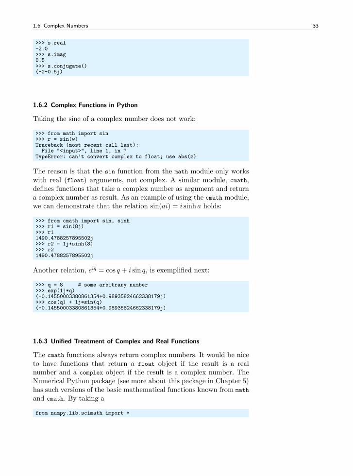
1.6 Complex Numbers 33

>>> s.real-2.0>>> s.imag0.5>>> s.conjugate()(-2-0.5j)

1.6.2 Complex Functions in Python

Taking the sine of a complex number does not work:

>>> from math import sin>>> r = sin(w)Traceback (most recent call last):File "<input>", line 1, in ?

TypeError: can’t convert complex to float; use abs(z)

The reason is that the sin function from the math module only workswith real (float) arguments, not complex. A similar module, cmath,defines functions that take a complex number as argument and returna complex number as result. As an example of using the cmath module,we can demonstrate that the relation sin(ai) = i sinh a holds:

>>> from cmath import sin, sinh>>> r1 = sin(8j)>>> r11490.4788257895502j>>> r2 = 1j*sinh(8)>>> r21490.4788257895502j

Another relation, eiq = cos q + i sin q, is exemplified next:

>>> q = 8 # some arbitrary number>>> exp(1j*q)(-0.14550003380861354+0.98935824662338179j)>>> cos(q) + 1j*sin(q)(-0.14550003380861354+0.98935824662338179j)

1.6.3 Unified Treatment of Complex and Real Functions

The cmath functions always return complex numbers. It would be niceto have functions that return a float object if the result is a realnumber and a complex object if the result is a complex number. TheNumerical Python package (see more about this package in Chapter 5)has such versions of the basic mathematical functions known from math

and cmath. By taking a

from numpy.lib.scimath import *

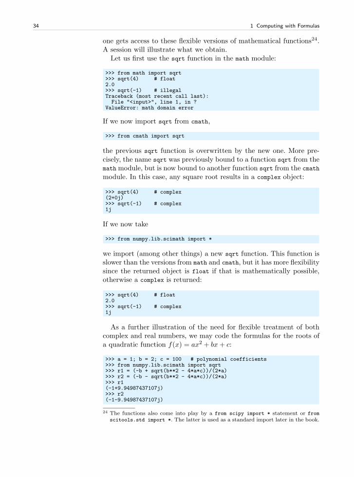
34 1 Computing with Formulas

one gets access to these flexible versions of mathematical functions24.A session will illustrate what we obtain.

Let us first use the sqrt function in the math module:

>>> from math import sqrt>>> sqrt(4) # float2.0>>> sqrt(-1) # illegalTraceback (most recent call last):File "<input>", line 1, in ?

ValueError: math domain error

If we now import sqrt from cmath,

>>> from cmath import sqrt

the previous sqrt function is overwritten by the new one. More pre-cisely, the name sqrt was previously bound to a function sqrt from themath module, but is now bound to another function sqrt from the cmathmodule. In this case, any square root results in a complex object:

>>> sqrt(4) # complex(2+0j)>>> sqrt(-1) # complex1j

If we now take

>>> from numpy.lib.scimath import *

we import (among other things) a new sqrt function. This function isslower than the versions from math and cmath, but it has more flexibilitysince the returned object is float if that is mathematically possible,otherwise a complex is returned:

>>> sqrt(4) # float2.0>>> sqrt(-1) # complex1j

As a further illustration of the need for flexible treatment of bothcomplex and real numbers, we may code the formulas for the roots ofa quadratic function f(x) = ax2 + bx+ c:

>>> a = 1; b = 2; c = 100 # polynomial coefficients>>> from numpy.lib.scimath import sqrt>>> r1 = (-b + sqrt(b**2 - 4*a*c))/(2*a)>>> r2 = (-b - sqrt(b**2 - 4*a*c))/(2*a)>>> r1(-1+9.94987437107j)>>> r2(-1-9.94987437107j)

24 The functions also come into play by a from scipy import * statement or from

scitools.std import *. The latter is used as a standard import later in the book.

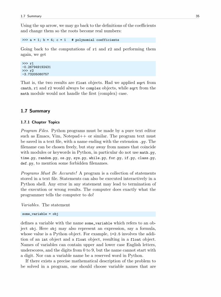
1.7 Summary 35

Using the up arrow, we may go back to the definitions of the coefficientsand change them so the roots become real numbers:

>>> a = 1; b = 4; c = 1 # polynomial coefficients

Going back to the computations of r1 and r2 and performing themagain, we get

>>> r1-0.267949192431>>> r2-3.73205080757

That is, the two results are float objects. Had we applied sqrt fromcmath, r1 and r2 would always be complex objects, while sqrt from themath module would not handle the first (complex) case.

1.7 Summary

1.7.1 Chapter Topics

Program Files. Python programs must be made by a pure text editorsuch as Emacs, Vim, Notepad++ or similar. The program text mustbe saved in a text file, with a name ending with the extension .py. Thefilename can be chosen freely, but stay away from names that coincidewith modules or keywords in Python, in particular do not use math.py,time.py, random.py, os.py, sys.py, while.py, for.py, if.py, class.py,def.py, to mention some forbidden filenames.

Programs Must Be Accurate! A program is a collection of statementsstored in a text file. Statements can also be executed interactively in aPython shell. Any error in any statement may lead to termination ofthe execution or wrong results. The computer does exactly what theprogrammer tells the computer to do!

Variables. The statement

some_variable = obj

defines a variable with the name some_variable which refers to an ob-ject obj. Here obj may also represent an expression, say a formula,whose value is a Python object. For example, 1+2.5 involves the addi-tion of an int object and a float object, resulting in a float object.Names of variables can contain upper and lower case English letters,underscores, and the digits from 0 to 9, but the name cannot start witha digit. Nor can a variable name be a reserved word in Python.

If there exists a precise mathematical description of the problem tobe solved in a program, one should choose variable names that are

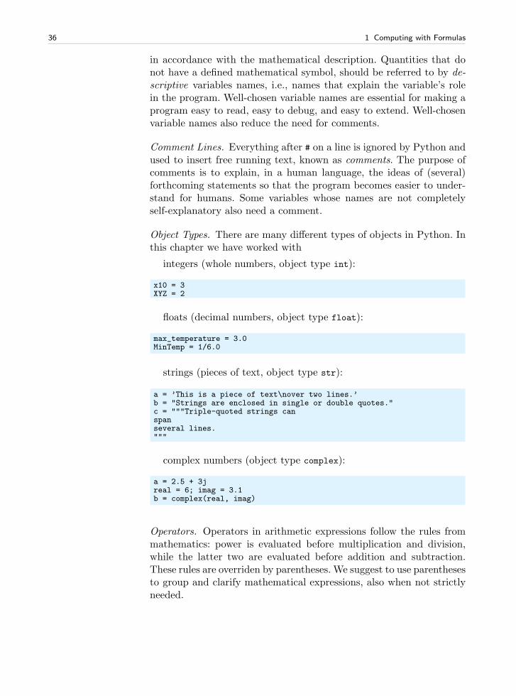
36 1 Computing with Formulas

in accordance with the mathematical description. Quantities that donot have a defined mathematical symbol, should be referred to by de-scriptive variables names, i.e., names that explain the variable’s rolein the program. Well-chosen variable names are essential for making aprogram easy to read, easy to debug, and easy to extend. Well-chosenvariable names also reduce the need for comments.

Comment Lines. Everything after # on a line is ignored by Python andused to insert free running text, known as comments. The purpose ofcomments is to explain, in a human language, the ideas of (several)forthcoming statements so that the program becomes easier to under-stand for humans. Some variables whose names are not completelyself-explanatory also need a comment.

Object Types. There are many different types of objects in Python. Inthis chapter we have worked with

integers (whole numbers, object type int):

x10 = 3XYZ = 2

floats (decimal numbers, object type float):

max_temperature = 3.0MinTemp = 1/6.0

strings (pieces of text, object type str):

a = ’This is a piece of text\nover two lines.’b = "Strings are enclosed in single or double quotes."c = """Triple-quoted strings canspanseveral lines."""

complex numbers (object type complex):

a = 2.5 + 3jreal = 6; imag = 3.1b = complex(real, imag)

Operators. Operators in arithmetic expressions follow the rules frommathematics: power is evaluated before multiplication and division,while the latter two are evaluated before addition and subtraction.These rules are overriden by parentheses. We suggest to use parenthesesto group and clarify mathematical expressions, also when not strictlyneeded.

1.7 Summary 37

-t**2*g/2-(t**2)*(g/2) # equivalent-t**(2*g)/2 # a different formula!

a = 5.0; b = 5.0; c = 5.0a/b + c + a*c # yields 31.0a/(b + c) + a*c # yields 25.5a/(b + c + a)*c # yields 1.6666666666666665

Particular attention must be paid to coding fractions, since the divisionoperator / often needs extra parentheses that are not necessary in themathematical notation for fractions (compare a

b+c with a/(b+c) anda/b+c).

Common Mathematical Functions. The math module contains commonmathematical functions for real numbers. Modules must be importedbefore they can be used:

import matha = math.sin(math.pi*1.5)

or

from math import *a = sin(pi*1.5)

or

from math import sin, pia = sin(pi*1.5)

Print. To print the result of calculations in a Python program to aterminal window, we apply the print command, i.e., the word print

followed by a string enclosed in quotes, or just a variable:

print "A string enclosed in double quotes"print a

Several objects can be printed in one statement if the objects are sep-arated by commas. A space will then appear between the output ofeach object:

>>> a = 5.0; b = -5.0; c = 1.9856; d = 33>>> print ’a is’, a, ’b is’, b, ’c and d are’, c, da is 5.0 b is -5.0 c and d are 1.9856 33

The printf syntax enables full control of the formatting of real numbersand integers:

>>> print ’a=%g, b=%12.4E, c=%.2f, d=%5d’ % (a, b, c, d)a=5, b= -5.0000E+00, c=1.99, d= 33

Here, a, b, and c are of type float and formatted as compactly aspossible (%g for a), in scientific notation with 4 decimals in a field of

38 1 Computing with Formulas

width 12 (%12.4E for b), and in decimal notation with two decimals inas compact field as possible (%.2f for c). The variable d is an integer(int) written in a field of width 5 characters (%5d).

Integer Division. A common error in mathematical computations isto divide two integers, because this results in integer division. Anynumber written without decimals is treated as an integer. To avoidinteger division, ensure that every division involves at least one realnumber, e.g., 9/5 is written as 9.0/5, 9./5, 9/5., or 9/5.0.

Complex Numbers. Values of complex numbers are written as (X+Yj),where X is the value of the real part and Y is the value of the imaginarypart. One example is (4-0.2j). If the real and imaginary parts areavailable as variables r and i, a complex number can be created bycomplex(r, i).

The cmath module must be used instead of math if the argumentis a complex variable. The numpy package offers similar mathematicalfunctions, but with a unified treatment of real and complex variables.

Terminology. Some Python and computer science terms briefly coveredin this chapter are

object: anything that a variable (name) can refer to25 (number,string, function, module, ...)

variable: name of an object statement: an instruction to the computer, usually written on aline in a Python program (multiple statements on a line must beseparated by semicolons)

expression: a combination of numbers, text, variables, and operatorsthat results in a new object, when being evaluated

assignment: a statement binding an evaluated expression (object)to a variable (name)

algorithm: detailed recipe for how to solve a problem by program-ming

code: program text (or synonym for program) implementation: same as code executable: the file we run to start the program verification: providing evidence that the program works correctly debugging: locating and correcting errors in a program

1.7.2 Summarizing Example: Trajectory of a Ball

Problem. The formula (1.1) computes the height of a ball in verticalmotion. What if we throw the ball with an initial velocity having an

25 But objects can exist without being bound to a name: print ’Hello!’ first makesa string object of the text in quotes and then the contents of this string object,without a name, is printed.

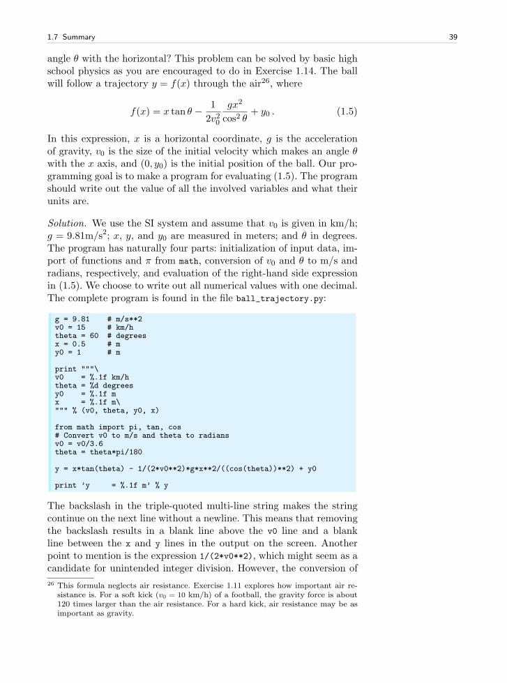
1.7 Summary 39

angle θ with the horizontal? This problem can be solved by basic highschool physics as you are encouraged to do in Exercise 1.14. The ballwill follow a trajectory y = f(x) through the air26, where

f(x) = x tan θ − 1

2v20

gx2

cos2 θ+ y0 . (1.5)

In this expression, x is a horizontal coordinate, g is the accelerationof gravity, v0 is the size of the initial velocity which makes an angle θwith the x axis, and (0, y0) is the initial position of the ball. Our pro-gramming goal is to make a program for evaluating (1.5). The programshould write out the value of all the involved variables and what theirunits are.

Solution. We use the SI system and assume that v0 is given in km/h;g = 9.81m/s2; x, y, and y0 are measured in meters; and θ in degrees.The program has naturally four parts: initialization of input data, im-port of functions and π from math, conversion of v0 and θ to m/s andradians, respectively, and evaluation of the right-hand side expressionin (1.5). We choose to write out all numerical values with one decimal.The complete program is found in the file ball_trajectory.py:

g = 9.81 # m/s**2v0 = 15 # km/htheta = 60 # degreesx = 0.5 # my0 = 1 # m

print """\v0 = %.1f km/htheta = %d degreesy0 = %.1f mx = %.1f m\""" % (v0, theta, y0, x)

from math import pi, tan, cos# Convert v0 to m/s and theta to radiansv0 = v0/3.6theta = theta*pi/180

y = x*tan(theta) - 1/(2*v0**2)*g*x**2/((cos(theta))**2) + y0

print ’y = %.1f m’ % y

The backslash in the triple-quoted multi-line string makes the stringcontinue on the next line without a newline. This means that removingthe backslash results in a blank line above the v0 line and a blankline between the x and y lines in the output on the screen. Anotherpoint to mention is the expression 1/(2*v0**2), which might seem as acandidate for unintended integer division. However, the conversion of

26 This formula neglects air resistance. Exercise 1.11 explores how important air re-sistance is. For a soft kick (v0 = 10 km/h) of a football, the gravity force is about120 times larger than the air resistance. For a hard kick, air resistance may be asimportant as gravity.

40 1 Computing with Formulas

v0 to m/s involves a division by 3.6, which results in v0 being float,and therefore 2*v0**2 being float. The rest of the program should beself-explanatory at this stage in the book.

We can execute the program in IPython or an ordinary terminalwindow and watch the output:

Terminal

ball_trajectory.pyv0 = 15.0 km/htheta = 60 degreesy0 = 1.0 mx = 0.5 my = 1.6 m

1.7.3 About Typesetting Conventions in This Book

This version of the book applies different design elements for differenttypes of “computer text”. Complete programs and parts of programs(snippets) are typeset with a light blue background. A snippet lookslike this:

a = sqrt(4*p + c)print ’a =’, a

A complete program has an additional vertical line to the left:

C = 21F = (9.0/5)*C + 32print F

As a reader of this book, you may wonder if a code shown is a completeprogram you can try out or if it is just a part of a program (a snippet) sothat you need to add surrounding statements (e.g., import statements)to try the code out yourself. The appearance of a vertical line to theleft or not will then quickly tell you what type of code you see.

An interactive Python session is typeset as

>>> from math import *>>> p = 1; c = -1.5>>> a = sqrt(4*p + c)

Running a program, say ball_yc.py, in the terminal window, followedby some possible output is typeset as27

Terminal

ball_yc.pyAt t=0.0417064 s and 0.977662 s, the height is 0.2 m.

27 Recall from Chapter 1.5.3 that we just write the program name. A real executiondemands prefixing the program name by python in a DOS/Unix terminal window,or by run if you run the program from an interactive IPython session. We referto Appendix G.1 for more complete information on running Python programs indifferent ways.

1.8 Exercises 41

Sometimes just the output from a program is shown, and this outputappears as plain “computer text”:

h = 0.2order=0, error=0.221403order=1, error=0.0214028order=2, error=0.00140276order=3, error=6.94248e-05order=4, error=2.75816e-06

Files containing data are shown in a similar way in this book:

date Oslo London Berlin Paris Rome Helsinki01.05 18 21.2 20.2 13.7 15.8 1501.06 21 13.2 14.9 18 24 2001.07 13 14 16 25 26.2 14.5

1.8 Exercises

What Does It Mean to Solve an Exercise?

The solution to most of the exercises in this book is a Python program.To produce the solution, you first need understand the problem andwhat the program is supposed to do, and then you need to understandhow to translate the problem description into a series of Python state-ments. Equally important is the verification (testing) of the program.A complete solution to a programming exercises therefore consists oftwo parts: the program text and a demonstration that the programworks correctly. Some simple programs, like the ones in the first twoexercises below, have so simple output that the verification can just beto run the program and record the output.

In cases where the correctness of the output is not obvious, it isnecessary to provide information together with the output to “prove”that the result is correct. This can be a calculation done separatelyon a calculator, or one can apply the program to a special simple testwith known results. The requirement is to provide evidence that theprogram works as intended.

The sample run of the program to check its correctness can be in-serted at the end of the program as a triple-quoted string28. The con-tents of the string can be text from the run in the terminal window, cutand pasted to the program file by the aid of the mouse. Alternatively,one can run the program and direct the output to a file29:

28 Alternatively, the output lines can be inserted as comments, but using a multi-linestring requires less typing. (Technically, a string object is created, but not assignedto any name or used for anything in the program – but for a human the text in thestring contains useful information.)

29 The redirection to files does not work if the program is run inside IPython. In aDOS terminal window you may also choose to redirect output to a file, because cutand paste between the DOS window and the program window does not work bydefault unless you right-click the top bar, choose Properties and tick off Quick EditMode.

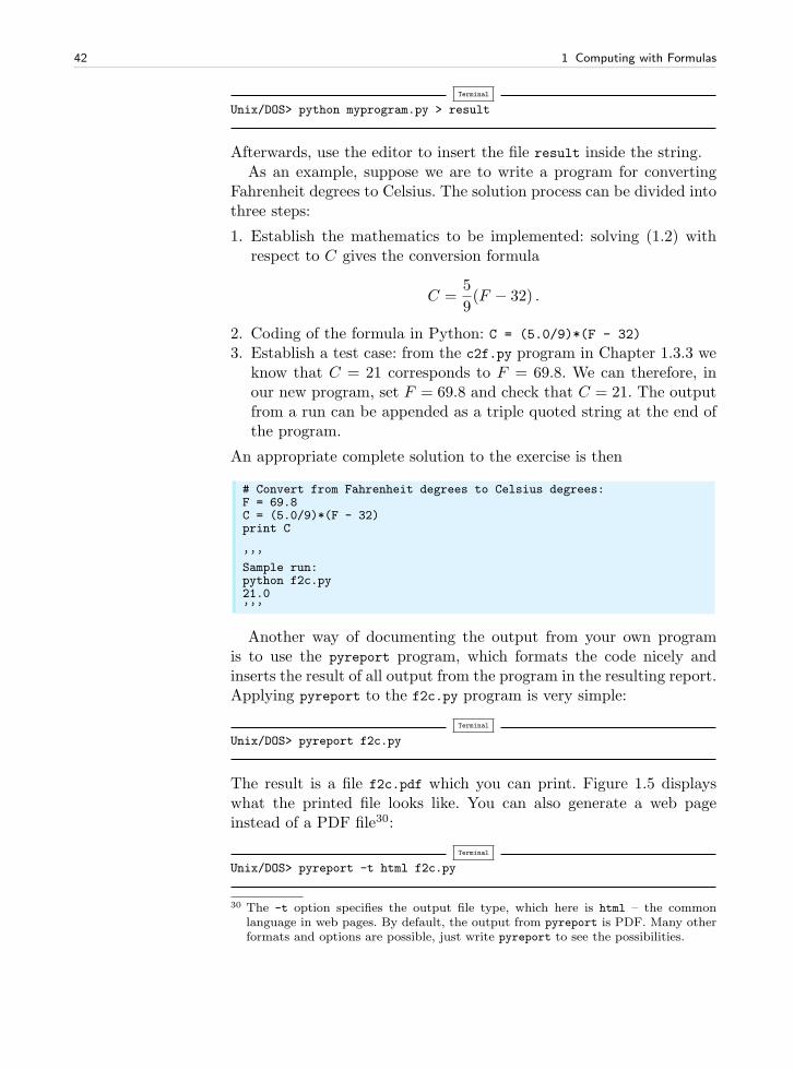
42 1 Computing with Formulas

Terminal

Unix/DOS> python myprogram.py > result

Afterwards, use the editor to insert the file result inside the string.As an example, suppose we are to write a program for converting

Fahrenheit degrees to Celsius. The solution process can be divided intothree steps:

1. Establish the mathematics to be implemented: solving (1.2) withrespect to C gives the conversion formula

C =5

9(F − 32) .

2. Coding of the formula in Python: C = (5.0/9)*(F - 32)

3. Establish a test case: from the c2f.py program in Chapter 1.3.3 weknow that C = 21 corresponds to F = 69.8. We can therefore, inour new program, set F = 69.8 and check that C = 21. The outputfrom a run can be appended as a triple quoted string at the end ofthe program.

An appropriate complete solution to the exercise is then

# Convert from Fahrenheit degrees to Celsius degrees:F = 69.8C = (5.0/9)*(F - 32)print C

’’’Sample run:python f2c.py21.0’’’

Another way of documenting the output from your own programis to use the pyreport program, which formats the code nicely andinserts the result of all output from the program in the resulting report.Applying pyreport to the f2c.py program is very simple:

Terminal

Unix/DOS> pyreport f2c.py

The result is a file f2c.pdf which you can print. Figure 1.5 displayswhat the printed file looks like. You can also generate a web pageinstead of a PDF file30:

Terminal

Unix/DOS> pyreport -t html f2c.py

30 The -t option specifies the output file type, which here is html – the commonlanguage in web pages. By default, the output from pyreport is PDF. Many otherformats and options are possible, just write pyreport to see the possibilities.

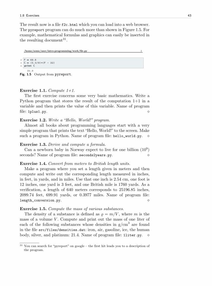
1.8 Exercises 43

The result now is a file f2c.html which you can load into a web browser.The pyreport program can do much more than shown in Figure 1.5. Forexample, mathematical formulas and graphics can easily be inserted inthe resulting document31.

/home/some/user/intro-programming/work/f2c.py 1

2 F = 69.8

3 C = (5.0/9)*(F - 32)

4 p r i n t C

21.0

Fig. 1.5 Output from pyreport.

Exercise 1.1. Compute 1+1.The first exercise concerns some very basic mathematics. Write a

Python program that stores the result of the computation 1+1 in avariable and then prints the value of this variable. Name of programfile: 1plus1.py. ⋄

Exercise 1.2. Write a “Hello, World!” program.Almost all books about programming languages start with a very

simple program that prints the text“Hello, World!” to the screen. Makesuch a program in Python. Name of program file: hello_world.py. ⋄

Exercise 1.3. Derive and compute a formula.Can a newborn baby in Norway expect to live for one billion (109)

seconds? Name of program file: seconds2years.py. ⋄

Exercise 1.4. Convert from meters to British length units.Make a program where you set a length given in meters and then

compute and write out the corresponding length measured in inches,in feet, in yards, and in miles. Use that one inch is 2.54 cm, one foot is12 inches, one yard is 3 feet, and one British mile is 1760 yards. As averification, a length of 640 meters corresponds to 25196.85 inches,2099.74 feet, 699.91 yards, or 0.3977 miles. Name of program file:length_conversion.py. ⋄

Exercise 1.5. Compute the mass of various substances.The density of a substance is defined as = m/V , where m is the

mass of a volume V . Compute and print out the mass of one liter ofeach of the following substances whose densities in g/cm3 are foundin the file src/files/densities.dat: iron, air, gasoline, ice, the humanbody, silver, and platinum: 21.4. Name of program file: 1liter.py. ⋄

31 You can search for “pyreport” on google – the first hit leads you to a description ofthe program.

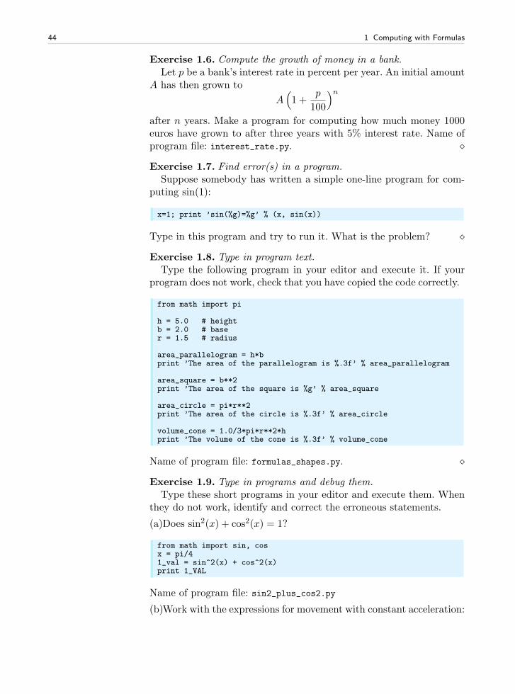
44 1 Computing with Formulas

Exercise 1.6. Compute the growth of money in a bank.Let p be a bank’s interest rate in percent per year. An initial amount

A has then grown to

A(

1 +p

100

)n

after n years. Make a program for computing how much money 1000euros have grown to after three years with 5% interest rate. Name ofprogram file: interest_rate.py. ⋄

Exercise 1.7. Find error(s) in a program.Suppose somebody has written a simple one-line program for com-

puting sin(1):

x=1; print ’sin(%g)=%g’ % (x, sin(x))

Type in this program and try to run it. What is the problem? ⋄

Exercise 1.8. Type in program text.Type the following program in your editor and execute it. If your

program does not work, check that you have copied the code correctly.

from math import pi

h = 5.0 # heightb = 2.0 # baser = 1.5 # radius

area_parallelogram = h*bprint ’The area of the parallelogram is %.3f’ % area_parallelogram

area_square = b**2print ’The area of the square is %g’ % area_square

area_circle = pi*r**2print ’The area of the circle is %.3f’ % area_circle

volume_cone = 1.0/3*pi*r**2*hprint ’The volume of the cone is %.3f’ % volume_cone

Name of program file: formulas_shapes.py. ⋄

Exercise 1.9. Type in programs and debug them.Type these short programs in your editor and execute them. When

they do not work, identify and correct the erroneous statements.

(a)Does sin2(x) + cos2(x) = 1?

from math import sin, cosx = pi/41_val = sin^2(x) + cos^2(x)print 1_VAL

Name of program file: sin2_plus_cos2.py

(b)Work with the expressions for movement with constant acceleration:

1.8 Exercises 45

v0 = 3 m/st = 1 sa = 2 m/s**2s = v0*t + 1/2 a*t**2print s

Name of program file: acceleration.py

(c)Verify these equations:

(a+ b)2 = a2 + 2ab+ b2

(a− b)2 = a2 − 2ab+ b2

a = 3,3 b = 5,3a2 = a**2b2 = b**2

eq1_sum = a2 + 2ab + b2eq2_sum = a2 - 2ab + b2

eq1_pow = (a + b)**2eq2_pow = (a - b)**2

print ’First equation: %g = %g’, % (eq1_sum, eq1_pow)print ’Second equation: %h = %h’, % (eq2_pow, eq2_pow)

Name of program file: a_pm_b_sqr.py ⋄Exercise 1.10. Evaluate a Gaussian function.

The bell-shaped Gaussian function,

f(x) =1√2π s

exp

[

−1

2

(

x−m

s

)2]

, (1.6)

is one of the most widely used functions in science and technol-ogy32. The parameters m and s are real numbers, where s must begreater than zero. Make a program for evaluating this function whenm = 0, s = 2, and x = 1. Verify the program’s result by compar-ing with hand calculations on a calculator. Name of program file:Gaussian_function1.py. ⋄Exercise 1.11. Compute the air resistance on a football.

The drag force, due to air resistance, on an object can be expressedas

Fd =1

2CDAV

2, (1.7)

where is the density of the air, V is the velocity of the object, A isthe cross-sectional area (normal to the velocity direction), and CD is

32 The function is named after Carl Friedrich Gauss, 1777–1855, who was a Germanmathematician and scientist, now considered as one of the greatest scientists of alltime. He contributed to many fields, including number theory, statistics, mathemat-ical analysis, differential geometry, geodesy, electrostatics, astronomy, and optics.Gauss introduced the function (1.6) when he analyzed probabilities related to as-tronomical data.

46 1 Computing with Formulas

the drag coefficient, which depends heavily on the shape of the objectand the roughness of the surface.

The gravity force on an object with mass m is Fg = mg, whereg = 9.81ms−2.

We can use the formulas for Fd and Fg to study the importance ofair resistance versus gravity when kicking a football. The density of airis = 1.2 kg m−3. We have A = πa2 for any ball with radius a. For afootball a = 11 cm. The mass of a football is 0.43 kg, CD can be takenas 0.2.

Make a program that computes the drag force and the gravity forceon a football. Write out the forces with one decimal in units of Newton(N = kgm/s2). Also print the ratio of the drag force and the gravityforce. Define CD, , A, V , m, g, Fd, and Fg as variables, and put acomment with the corresponding unit. Use the program to calculatethe forces on the ball for a hard kick, V = 120 km/h and for a softkick, V = 10 km/h (it is easy to mix inconsistent units, so make sureyou compute with V expressed in m/s). Name of program file: kick.py.⋄

Exercise 1.12. Define objects in IPython.Start ipython and give the following command, which will save the

interactive session to a file mysession.log:

In [1]: %logstart -r -o mysession.log

Thereafter, define an integer, a real number, and a string in IPython.Apply the type function to check that each object has the right type.Print the three objects using printf syntax. Finally, type logoff to endthe recording of the interactive session:

In [8]: %logoff

Leave IPython and restart it as ipython -logplay mysession.log onthe command line. IPython will now re-execute the input statementsin the logfile mysession.log so that you get back the variables youdeclared. Print out the variables to demonstrate this fact. ⋄

Exercise 1.13. How to cook the perfect egg.As an egg cooks, the proteins first denature and then coagulate.

When the temperature exceeds a critical point, reactions begin andproceed faster as the temperature increases. In the egg white the pro-teins start to coagulate for temperatures above 63 C, while in the yolkthe proteins start to coagulate for temperatures above 70 C. For a softboiled egg, the white needs to have been heated long enough to coag-ulate at a temperature above 63 C, but the yolk should not be heatedabove 70 C. For a hard boiled egg, the center of the yolk should beallowed to reach 70 C.

1.8 Exercises 47

The following formula expresses the time t it takes (in seconds) forthe center of the yolk to reach the temperature Ty (in Celsius degrees):

t =M2/3cρ1/3

Kπ2(4π/3)2/3ln

[

0.76To − Tw

Ty − Tw

]

. (1.8)

Here, M , ρ, c, and K are properties of the egg: M is the mass,ρ is the density, c is the specific heat capacity, and K is thermalconductivity. Relevant values are M = 47 g for a small egg andM = 67 g for a large egg, ρ = 1.038 g cm−3, c = 3.7 J g−1K−1, andK = 5.4 ·10−3 Wcm−1 K−1. Furthermore, Tw is the temperature (in Cdegrees) of the boiling water, and To is the original temperature (in Cdegrees) of the egg before being put in the water. Implement the for-mula in a program, set Tw = 100 C and Ty = 70 C, and compute t for alarge egg taken from the fridge (To = 4 C) and from room temperature(To = 20 C). Name of program file: egg.py. ⋄

Exercise 1.14. Derive the trajectory of a ball.The purpose of this exercise is to explain how Equation (1.5) for the

trajectory of a ball arises from basic physics. There is no programmingin this exercise, just physics and mathematics.

The motion of the ball is governed by Newton’s second law:

Fx = max (1.9)

Fy = may (1.10)

where Fx and Fy are the sum of forces in the x and y directions,respectively, ax and ay are the accelerations of the ball in the x and ydirections, and m is the mass of the ball. Let (x(t), y(t)) be the positionof the ball, i.e., the horisontal and vertical coordinate of the ball at timet. There are well-known relations between acceleration, velocity, andposition: the acceleration is the time derivative of the velocity, and thevelocity is the time derivative of the position. Therefore we have that

ax =d2x

dt2, (1.11)

ay =d2y

dt2. (1.12)

If we assume that gravity is the only important force on the ball, Fx = 0and Fy = −mg.

Integrate the two components of Newton’s second law twice. Use theinitial conditions on velocity and position,

48 1 Computing with Formulas

d

dtx(0) = v0 cos θ, (1.13)

d

dty(0) = v0 sin θ, (1.14)

x(0) = 0, (1.15)

y(0) = y0, (1.16)

to determine the four integration constants. Write up the final expres-sions for x(t) and y(t). Show that if θ = π/2, i.e., the motion is purelyvertical, we get the formula (1.1) for the y position. Also show that ifwe eliminate t, we end up with the relation (1.5) between the x and ycoordinates of the ball. You may read more about this type of motionin a physics book, e.g., [6]. ⋄

Exercise 1.15. Find errors in the coding of formulas.Some versions of our program for calculating the formula (1.2) are

listed below. Determine which versions that will not work correctly andexplain why in each case.

C = 21; F = 9/5*C + 32; print FC = 21.0; F = (9/5)*C + 32; print FC = 21.0; F = 9*C/5 + 32; print FC = 21.0; F = 9.*(C/5.0) + 32; print FC = 21.0; F = 9.0*C/5.0 + 32; print FC = 21; F = 9*C/5 + 32; print FC = 21.0; F = (1/5)*9*C + 32; print FC = 21; F = (1./5)*9*C + 32; print F

⋄

Exercise 1.16. Explain why a program does not work.Find out why the following program does not work:

C = A + BA = 3B = 2print C

⋄

Exercise 1.17. Find errors in Python statements.Try the following statements in an interactive Python shell. Explain

why some statements fail and correct the errors.1a = 2a1 = bx = 2y = X + 4 # is it 6?from Math import tanprint tan(pi)pi = "3.14159’print tan(pi)c = 4**3**2**3_ = ((c-78564)/c + 32))discount = 12%AMOUNT = 120.-amount = 120$address = hpl@simula.no

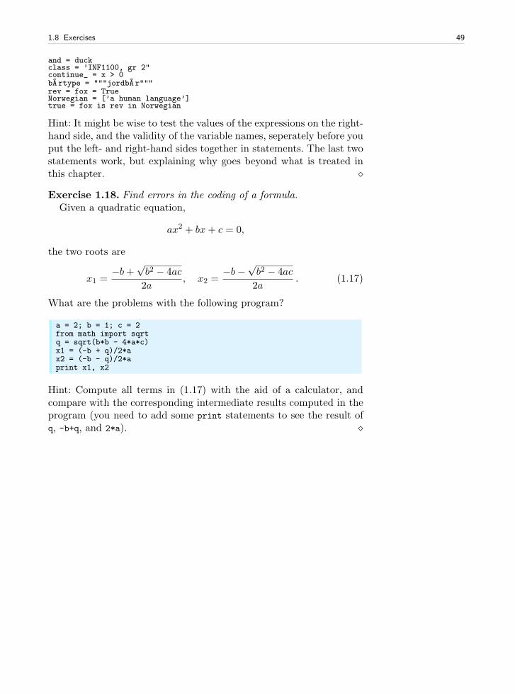
1.8 Exercises 49

and = duckclass = ’INF1100, gr 2"continue_ = x > 0b~Artype = """jordb~Ar"""rev = fox = TrueNorwegian = [’a human language’]true = fox is rev in Norwegian

Hint: It might be wise to test the values of the expressions on the right-hand side, and the validity of the variable names, seperately before youput the left- and right-hand sides together in statements. The last twostatements work, but explaining why goes beyond what is treated inthis chapter. ⋄

Exercise 1.18. Find errors in the coding of a formula.Given a quadratic equation,

ax2 + bx+ c = 0,

the two roots are

x1 =−b+

√b2 − 4ac

2a, x2 =

−b−√b2 − 4ac

2a. (1.17)

What are the problems with the following program?

a = 2; b = 1; c = 2from math import sqrtq = sqrt(b*b - 4*a*c)x1 = (-b + q)/2*ax2 = (-b - q)/2*aprint x1, x2

Hint: Compute all terms in (1.17) with the aid of a calculator, andcompare with the corresponding intermediate results computed in theprogram (you need to add some print statements to see the result ofq, -b+q, and 2*a). ⋄

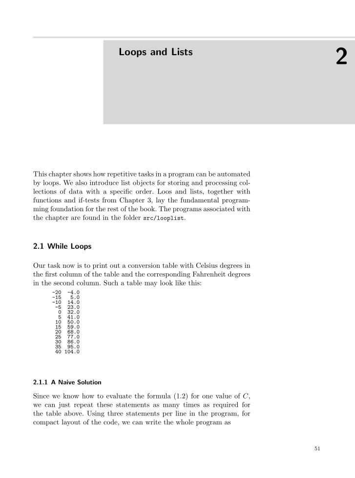
Loops and Lists 2

This chapter shows how repetitive tasks in a program can be automatedby loops. We also introduce list objects for storing and processing col-lections of data with a specific order. Loos and lists, together withfunctions and if-tests from Chapter 3, lay the fundamental program-ming foundation for the rest of the book. The programs associated withthe chapter are found in the folder src/looplist.

2.1 While Loops

Our task now is to print out a conversion table with Celsius degrees inthe first column of the table and the corresponding Fahrenheit degreesin the second column. Such a table may look like this:

-20 -4.0-15 5.0-10 14.0-5 23.00 32.05 41.010 50.015 59.020 68.025 77.030 86.035 95.040 104.0

2.1.1 A Naive Solution

Since we know how to evaluate the formula (1.2) for one value of C,we can just repeat these statements as many times as required forthe table above. Using three statements per line in the program, forcompact layout of the code, we can write the whole program as

51

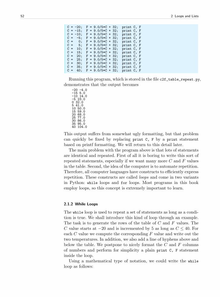
52 2 Loops and Lists

C = -20; F = 9.0/5*C + 32; print C, FC = -15; F = 9.0/5*C + 32; print C, FC = -10; F = 9.0/5*C + 32; print C, FC = -5; F = 9.0/5*C + 32; print C, FC = 0; F = 9.0/5*C + 32; print C, FC = 5; F = 9.0/5*C + 32; print C, FC = 10; F = 9.0/5*C + 32; print C, FC = 15; F = 9.0/5*C + 32; print C, FC = 20; F = 9.0/5*C + 32; print C, FC = 25; F = 9.0/5*C + 32; print C, FC = 30; F = 9.0/5*C + 32; print C, FC = 35; F = 9.0/5*C + 32; print C, FC = 40; F = 9.0/5*C + 32; print C, F

Running this program, which is stored in the file c2f_table_repeat.py,demonstrates that the output becomes

-20 -4.0-15 5.0-10 14.0-5 23.00 32.05 41.010 50.015 59.020 68.025 77.030 86.035 95.040 104.0

This output suffers from somewhat ugly formatting, but that problemcan quickly be fixed by replacing print C, F by a print statementbased on printf formatting. We will return to this detail later.

The main problem with the program above is that lots of statementsare identical and repeated. First of all it is boring to write this sort ofrepeated statements, especially if we want many more C and F valuesin the table. Second, the idea of the computer is to automate repetition.Therefore, all computer languages have constructs to efficiently expressrepetition. These constructs are called loops and come in two variantsin Python: while loops and for loops. Most programs in this bookemploy loops, so this concept is extremely important to learn.

2.1.2 While Loops

The while loop is used to repeat a set of statements as long as a condi-tion is true. We shall introduce this kind of loop through an example.The task is to generate the rows of the table of C and F values. TheC value starts at −20 and is incremented by 5 as long as C ≤ 40. Foreach C value we compute the corresponding F value and write out thetwo temperatures. In addition, we also add a line of hyphens above andbelow the table. We postpone to nicely format the C and F columnsof numbers and perform for simplicity a plain print C, F statementinside the loop.

Using a mathematical type of notation, we could write the while

loop as follows:

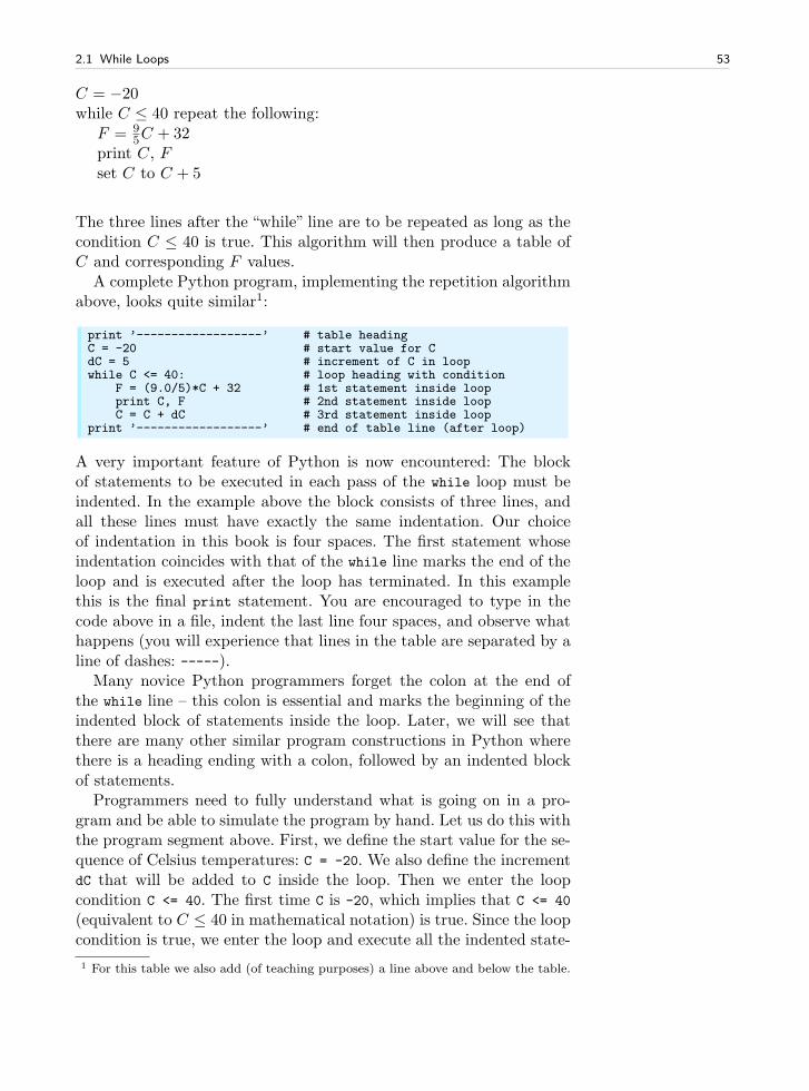
2.1 While Loops 53

C = −20while C ≤ 40 repeat the following:

F = 95C + 32

print C, Fset C to C + 5

The three lines after the “while” line are to be repeated as long as thecondition C ≤ 40 is true. This algorithm will then produce a table ofC and corresponding F values.

A complete Python program, implementing the repetition algorithmabove, looks quite similar1:

print ’------------------’ # table headingC = -20 # start value for CdC = 5 # increment of C in loopwhile C <= 40: # loop heading with condition

F = (9.0/5)*C + 32 # 1st statement inside loopprint C, F # 2nd statement inside loopC = C + dC # 3rd statement inside loop

print ’------------------’ # end of table line (after loop)

A very important feature of Python is now encountered: The blockof statements to be executed in each pass of the while loop must beindented. In the example above the block consists of three lines, andall these lines must have exactly the same indentation. Our choiceof indentation in this book is four spaces. The first statement whoseindentation coincides with that of the while line marks the end of theloop and is executed after the loop has terminated. In this examplethis is the final print statement. You are encouraged to type in thecode above in a file, indent the last line four spaces, and observe whathappens (you will experience that lines in the table are separated by aline of dashes: -----).

Many novice Python programmers forget the colon at the end ofthe while line – this colon is essential and marks the beginning of theindented block of statements inside the loop. Later, we will see thatthere are many other similar program constructions in Python wherethere is a heading ending with a colon, followed by an indented blockof statements.

Programmers need to fully understand what is going on in a pro-gram and be able to simulate the program by hand. Let us do this withthe program segment above. First, we define the start value for the se-quence of Celsius temperatures: C = -20. We also define the incrementdC that will be added to C inside the loop. Then we enter the loopcondition C <= 40. The first time C is -20, which implies that C <= 40

(equivalent to C ≤ 40 in mathematical notation) is true. Since the loopcondition is true, we enter the loop and execute all the indented state-

1 For this table we also add (of teaching purposes) a line above and below the table.

54 2 Loops and Lists

ments. That is, we compute F corresponding to the current C value,print the temperatures, and increment C by dC.

Thereafter, we enter the second pass in the loop. First we check thecondition: C is -15 and C <= 40 is still true. We execute the statementsin the indented loop block, C becomes -10, this is still less than or equalto 40, so we enter the loop block again. This procedure is repeated untilC is updated from 40 to 45 in the final statement in the loop block.When we then test the condition, C <= 40, this condition is no longertrue, and the loop is terminated. We proceed with the next statementthat has the same indentation as the while statement, which is thefinal print statement in this example.

Newcomers to programming are sometimes confused by statementslike

C = C + dC

This line looks erroneous from a mathematical viewpoint, but the state-ment is perfectly valid computer code, because we first evaluate theexpression on the right-hand side of the equality sign and then let thevariable on the left-hand side refer to the result of this evaluation. Inour case, C and dC are two different int objects. The operation C+dC

results in a new int object, which in the assignment C = C+dC is boundto the name C. Before this assignment, C was already bound to a int

object, and this object is automatically destroyed when C is bound toa new object and there are no other names (variables) referring to thisprevious object2.

Since incrementing the value of a variable is frequently done in com-puter programs, there is a special short-hand notation for this andrelated operations:

C += dC # equivalent to C = C + dCC -= dC # equivalent to C = C - dCC *= dC # equivalent to C = C*dCC /= dC # equivalent to C = C/dC

2.1.3 Boolean Expressions

In our first example on a while loop, we worked with a condition C <=

40, which evaluates to either true or false, written as True or False inPython. Other comparisons are also useful:

C == 40 # C equals 40C != 40 # C does not equal 40C >= 40 # C is greater than or equal to 40C > 40 # C is greater than 40C < 40 # C is less than 40

2 If you did not get the last point here, just relax and continue reading.

2.1 While Loops 55

Not only comparisons between numbers can be used as conditions inwhile loops: Any expression that has a boolean (True or False) valuecan be used. Such expressions are known as logical or boolean expres-sions.

The keyword not can be inserted in front of the boolean expression tochange the value from True to False or from False to True. To evaluatenot C == 40, we first evaluate C == 40, for C = 1 this is False, and thennot turns the value into True. On the opposite, if C == 40 is True, not C

== 40 becomes False. Mathematically it is easier to read C != 40 thannot C == 40, but these two boolean expressions are equivalent.

Boolean expressions can be combined with and and or to form newcompound boolean expressions, as in

while x > 0 and y <= 1:print x, y

If cond1 and cond2 are two boolean expressions with values True orFalse, the compound boolean expression cond1 and cond2 is True ifboth cond1 and cond2 are True. On the other hand, cond1 or cond2 isTrue if at least one of the conditions, cond1 or cond2, is True3

Here are some more examples from an interactive session where wejust evaluate the boolean expressions themselves without using themin loop conditions:

>>> x = 0; y = 1.2>>> x >= 0 and y < 1False>>> x >= 0 or y < 1True>>> x > 0 or y > 1True>>> x > 0 or not y > 1False>>> -1 < x <= 0 # -1 < x and x <= 0True>>> not (x > 0 or y > 0)False

In the last sample expression, not applies to the value of the booleanexpression inside the parentheses: x>0 is False, y>0 is True, so the com-bined expression with or is True, and not turns this value to False.

The common4 boolean values in Python are True, False, 0 (false),and any integer different from zero (true). To see such values in action,we recommend to do Exercises 2.29 and 2.25.

3 In Python, cond1 and cond2 or cond1 or cond2 returns one of the operands andnot just True or False values as in most other computer languages. The operandscond1 or cond2 can be expressions or objects. In case of expressions, these are firstevaluated to an object before the compound boolean expression is evaluated. Forexample, (5+1) or -1 evaluates to 6 (the second operand is not evaluated whenthe first one is True), and (5+1) and -1 evaluates to -1.

4 All objects in Python can in fact be evaluated in a boolean context, and all areTrue except False, zero numbers, and empty strings, lists, and dictionaries. SeeExercise 6.24 for more details.

56 2 Loops and Lists

Erroneous thinking about boolean expressions is one of the mostcommon sources of errors in computer programs, so you should becareful every time you encounter a boolean expression and check thatit is correctly stated.

2.1.4 Loop Implementation of a Sum

Summations frequently appear in mathematics. For instance, the sinefunction can be calculated as a polynomial:

sin(x) ≈ x− x3

3!+

x5

5!− x7

7!+ · · · , (2.1)

where 3! = 3 ·2 ·1, 5! = 5 ·4 ·3 ·2 ·1, etc., are factorials. The expressionk! = k(k − 1)(k − 2) · · · 2 · 1 can be computed by math.factorial(k).

An infinite number of terms are needed on the right-hand side of(2.1) for the equality sign to hold. With a finite number of terms,we obtain an approximation to sin(x), which is well suited for beingcalculated in a program since only powers and the basic four arithmeticoperations are involved. Say we want to compute the right-hand sideof (2.1) for powers up to N = 25. Writing out and implementing eachone of these terms is a tedious job that can easily be automated by aloop.

Computation of the sum in (2.1) by a while loop in Python, makesuse of (i) a counter k that runs through odd numbers from 1 up to somegiven maximum power N, and (ii) a summation variable, say s, whichaccumulates the terms, one at a time. The purpose of each pass of theloop is to compute a new term and add it to s. Since the sign of eachterm alternates, we introduce a variable sign that changes between −1and 1 in each pass of the loop.

The previous paragraph can be precisely expressed by this piece ofPython code:

x = 1.2 # assign some valueN = 25 # maximum power in sumk = 1s = xsign = 1.0import math

while k < N:sign = - signk = k + 2term = sign*x**k/math.factorial(k)s = s + term

print ’sin(%g) = %g (approximation with %d terms)’ % (x, s, N)

The best way to understand such a program is to simulate it by hand.That is, we go through the statements, one by one, and write down ona piece of paper what the state of each variable is.

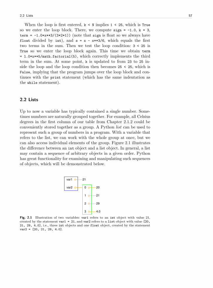
2.2 Lists 57

When the loop is first entered, k < N implies 1 < 25, which is True

so we enter the loop block. There, we compute sign = -1.0, k = 3,term = -1.0*x**3/(3*2*1)) (note that sign is float so we always havefloat divided by int), and s = x - x**3/6, which equals the firsttwo terms in the sum. Then we test the loop condition: 3 < 25 isTrue so we enter the loop block again. This time we obtain term

= 1.0*x**5/math.factorial(5), which correctly implements the thirdterm in the sum. At some point, k is updated to from 23 to 25 in-side the loop and the loop condition then becomes 25 < 25, which isFalse, implying that the program jumps over the loop block and con-tinues with the print statement (which has the same indentation asthe while statement).

2.2 Lists

Up to now a variable has typically contained a single number. Some-times numbers are naturally grouped together. For example, all Celsiusdegrees in the first column of our table from Chapter 2.1.2 could beconveniently stored together as a group. A Python list can be used torepresent such a group of numbers in a program. With a variable thatrefers to the list, we can work with the whole group at once, but wecan also access individual elements of the group. Figure 2.1 illustratesthe difference between an int object and a list object. In general, a listmay contain a sequence of arbitrary objects in a given order. Pythonhas great functionality for examining and manipulating such sequencesof objects, which will be demonstrated below.

var1 21

var2 0 20

1 21

2 29

3 4.0

Fig. 2.1 Illustration of two variables: var1 refers to an int object with value 21,created by the statement var1 = 21, and var2 refers to a list object with value [20,

21, 29, 4.0], i.e., three int objects and one float object, created by the statementvar2 = [20, 21, 29, 4.0].

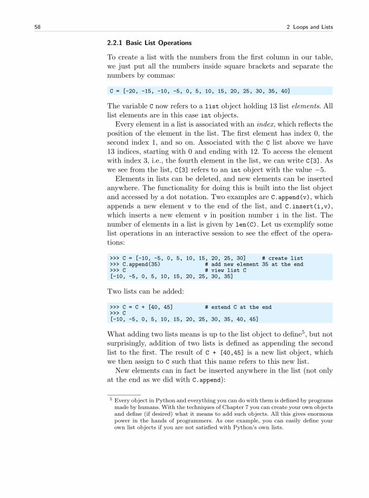
58 2 Loops and Lists

2.2.1 Basic List Operations

To create a list with the numbers from the first column in our table,we just put all the numbers inside square brackets and separate thenumbers by commas:

C = [-20, -15, -10, -5, 0, 5, 10, 15, 20, 25, 30, 35, 40]

The variable C now refers to a list object holding 13 list elements. Alllist elements are in this case int objects.

Every element in a list is associated with an index, which reflects theposition of the element in the list. The first element has index 0, thesecond index 1, and so on. Associated with the C list above we have13 indices, starting with 0 and ending with 12. To access the elementwith index 3, i.e., the fourth element in the list, we can write C[3]. Aswe see from the list, C[3] refers to an int object with the value −5.

Elements in lists can be deleted, and new elements can be insertedanywhere. The functionality for doing this is built into the list objectand accessed by a dot notation. Two examples are C.append(v), whichappends a new element v to the end of the list, and C.insert(i,v),which inserts a new element v in position number i in the list. Thenumber of elements in a list is given by len(C). Let us exemplify somelist operations in an interactive session to see the effect of the opera-tions:

>>> C = [-10, -5, 0, 5, 10, 15, 20, 25, 30] # create list>>> C.append(35) # add new element 35 at the end>>> C # view list C[-10, -5, 0, 5, 10, 15, 20, 25, 30, 35]

Two lists can be added:

>>> C = C + [40, 45] # extend C at the end>>> C[-10, -5, 0, 5, 10, 15, 20, 25, 30, 35, 40, 45]

What adding two lists means is up to the list object to define5, but notsurprisingly, addition of two lists is defined as appending the secondlist to the first. The result of C + [40,45] is a new list object, whichwe then assign to C such that this name refers to this new list.

New elements can in fact be inserted anywhere in the list (not onlyat the end as we did with C.append):

5 Every object in Python and everything you can do with them is defined by programsmade by humans. With the techniques of Chapter 7 you can create your own objectsand define (if desired) what it means to add such objects. All this gives enormouspower in the hands of programmers. As one example, you can easily define yourown list objects if you are not satisfied with Python’s own lists.

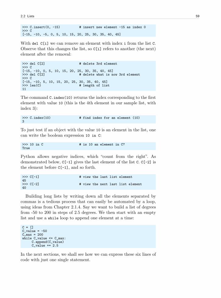
2.2 Lists 59

>>> C.insert(0, -15) # insert new element -15 as index 0>>> C[-15, -10, -5, 0, 5, 10, 15, 20, 25, 30, 35, 40, 45]

With del C[i] we can remove an element with index i from the list C.Observe that this changes the list, so C[i] refers to another (the next)element after the removal:

>>> del C[2] # delete 3rd element>>> C[-15, -10, 0, 5, 10, 15, 20, 25, 30, 35, 40, 45]>>> del C[2] # delete what is now 3rd element>>> C[-15, -10, 5, 10, 15, 20, 25, 30, 35, 40, 45]>>> len(C) # length of list11

The command C.index(10) returns the index corresponding to the firstelement with value 10 (this is the 4th element in our sample list, withindex 3):

>>> C.index(10) # find index for an element (10)3

To just test if an object with the value 10 is an element in the list, onecan write the boolean expression 10 in C:

>>> 10 in C # is 10 an element in C?True

Python allows negative indices, which “count from the right”. Asdemonstrated below, C[-1] gives the last element of the list C. C[-2] isthe element before C[-1], and so forth.

>>> C[-1] # view the last list element45>>> C[-2] # view the next last list element40

Building long lists by writing down all the elements separated bycommas is a tedious process that can easily be automated by a loop,using ideas from Chapter 2.1.4. Say we want to build a list of degreesfrom -50 to 200 in steps of 2.5 degrees. We then start with an emptylist and use a while loop to append one element at a time:

C = []C_value = -50C_max = 200while C_value <= C_max:

C.append(C_value)C_value += 2.5

In the next sections, we shall see how we can express these six lines ofcode with just one single statement.

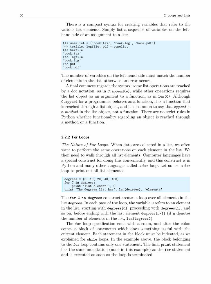
60 2 Loops and Lists

There is a compact syntax for creating variables that refer to thevarious list elements. Simply list a sequence of variables on the left-hand side of an assignment to a list:

>>> somelist = [’book.tex’, ’book.log’, ’book.pdf’]>>> texfile, logfile, pdf = somelist>>> texfile’book.tex’>>> logfile’book.log’>>> pdf’book.pdf’

The number of variables on the left-hand side must match the numberof elements in the list, otherwise an error occurs.

A final comment regards the syntax: some list operations are reachedby a dot notation, as in C.append(e), while other operations requiresthe list object as an argument to a function, as in len(C). AlthoughC.append for a programmer behaves as a function, it is a function thatis reached through a list object, and it is common to say that append isa method in the list object, not a function. There are no strict rules inPython whether functionality regarding an object is reached througha method or a function.

2.2.2 For Loops

The Nature of For Loops. When data are collected in a list, we oftenwant to perform the same operations on each element in the list. Wethen need to walk through all list elements. Computer languages havea special construct for doing this conveniently, and this construct is inPython and many other languages called a for loop. Let us use a for

loop to print out all list elements:

degrees = [0, 10, 20, 40, 100]for C in degrees:

print ’list element:’, Cprint ’The degrees list has’, len(degrees), ’elements’

The for C in degrees construct creates a loop over all elements in thelist degrees. In each pass of the loop, the variable C refers to an elementin the list, starting with degrees[0], proceeding with degrees[1], andso on, before ending with the last element degrees[n-1] (if n denotesthe number of elements in the list, len(degrees)).

The for loop specification ends with a colon, and after the coloncomes a block of statements which does something useful with thecurrent element. Each statement in the block must be indented, as weexplained for while loops. In the example above, the block belongingto the for loop contains only one statement. The final print statementhas the same indentation (none in this example) as the for statementand is executed as soon as the loop is terminated.

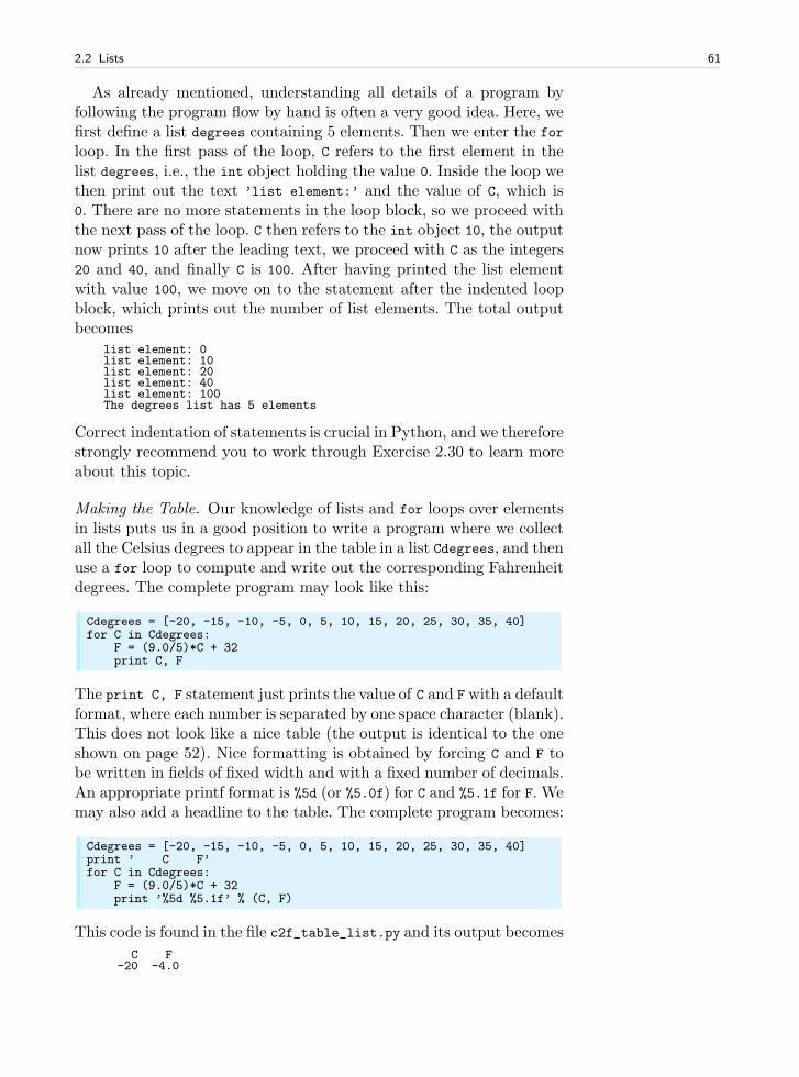
2.2 Lists 61

As already mentioned, understanding all details of a program byfollowing the program flow by hand is often a very good idea. Here, wefirst define a list degrees containing 5 elements. Then we enter the for

loop. In the first pass of the loop, C refers to the first element in thelist degrees, i.e., the int object holding the value 0. Inside the loop wethen print out the text ’list element:’ and the value of C, which is0. There are no more statements in the loop block, so we proceed withthe next pass of the loop. C then refers to the int object 10, the outputnow prints 10 after the leading text, we proceed with C as the integers20 and 40, and finally C is 100. After having printed the list elementwith value 100, we move on to the statement after the indented loopblock, which prints out the number of list elements. The total outputbecomes

list element: 0list element: 10list element: 20list element: 40list element: 100The degrees list has 5 elements

Correct indentation of statements is crucial in Python, and we thereforestrongly recommend you to work through Exercise 2.30 to learn moreabout this topic.

Making the Table. Our knowledge of lists and for loops over elementsin lists puts us in a good position to write a program where we collectall the Celsius degrees to appear in the table in a list Cdegrees, and thenuse a for loop to compute and write out the corresponding Fahrenheitdegrees. The complete program may look like this:

Cdegrees = [-20, -15, -10, -5, 0, 5, 10, 15, 20, 25, 30, 35, 40]for C in Cdegrees:

F = (9.0/5)*C + 32print C, F

The print C, F statement just prints the value of C and F with a defaultformat, where each number is separated by one space character (blank).This does not look like a nice table (the output is identical to the oneshown on page 52). Nice formatting is obtained by forcing C and F tobe written in fields of fixed width and with a fixed number of decimals.An appropriate printf format is %5d (or %5.0f) for C and %5.1f for F. Wemay also add a headline to the table. The complete program becomes:

Cdegrees = [-20, -15, -10, -5, 0, 5, 10, 15, 20, 25, 30, 35, 40]print ’ C F’for C in Cdegrees:

F = (9.0/5)*C + 32print ’%5d %5.1f’ % (C, F)

This code is found in the file c2f_table_list.py and its output becomes

C F-20 -4.0

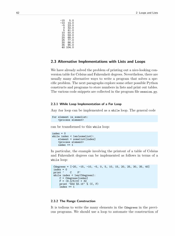
62 2 Loops and Lists

-15 5.0-10 14.0-5 23.00 32.05 41.010 50.015 59.020 68.025 77.030 86.035 95.040 104.0

2.3 Alternative Implementations with Lists and Loops

We have already solved the problem of printing out a nice-looking con-version table for Celsius and Fahrenheit degrees. Nevertheless, there areusually many alternative ways to write a program that solves a spe-cific problem. The next paragraphs explore some other possible Pythonconstructs and programs to store numbers in lists and print out tables.The various code snippets are collected in the program file session.py.

2.3.1 While Loop Implementation of a For Loop

Any for loop can be implemented as a while loop. The general code

for element in somelist:<process element>

can be transformed to this while loop:

index = 0while index < len(somelist):

element = somelist[index]<process element>index += 1

In particular, the example involving the printout of a table of Celsiusand Fahrenheit degrees can be implemented as follows in terms of awhile loop:

Cdegrees = [-20, -15, -10, -5, 0, 5, 10, 15, 20, 25, 30, 35, 40]index = 0print ’ C F’while index < len(Cdegrees):

C = Cdegrees[index]F = (9.0/5)*C + 32print ’%5d %5.1f’ % (C, F)index += 1

2.3.2 The Range Construction

It is tedious to write the many elements in the Cdegrees in the previ-ous programs. We should use a loop to automate the construction of

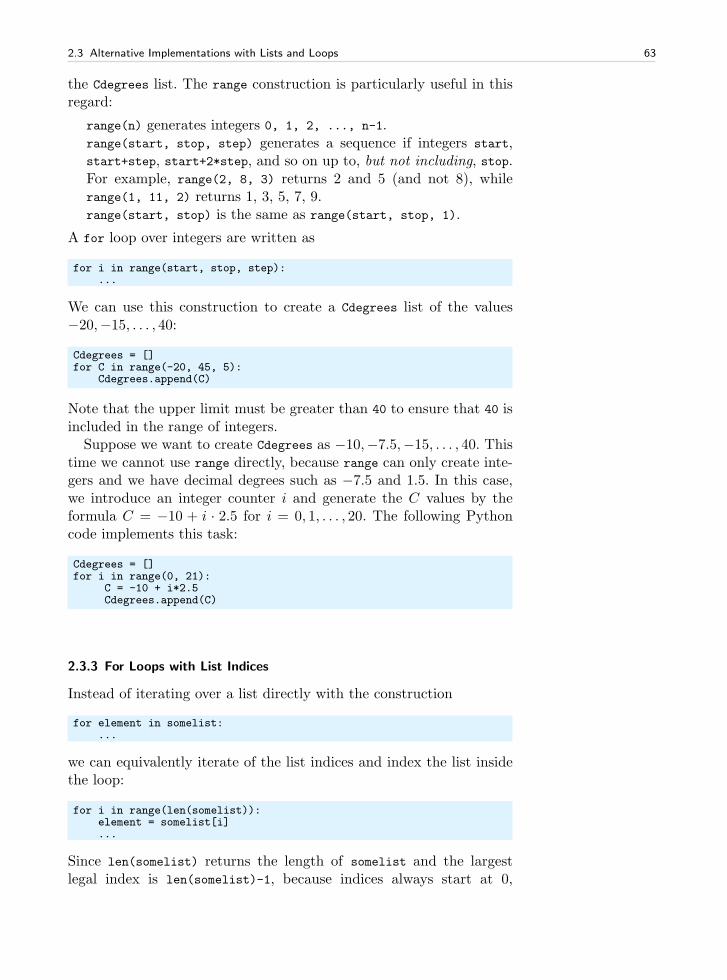
2.3 Alternative Implementations with Lists and Loops 63

the Cdegrees list. The range construction is particularly useful in thisregard:

range(n) generates integers 0, 1, 2, ..., n-1. range(start, stop, step) generates a sequence if integers start,start+step, start+2*step, and so on up to, but not including, stop.For example, range(2, 8, 3) returns 2 and 5 (and not 8), whilerange(1, 11, 2) returns 1, 3, 5, 7, 9.

range(start, stop) is the same as range(start, stop, 1).

A for loop over integers are written as

for i in range(start, stop, step):...

We can use this construction to create a Cdegrees list of the values−20,−15, . . . , 40:

Cdegrees = []for C in range(-20, 45, 5):

Cdegrees.append(C)

Note that the upper limit must be greater than 40 to ensure that 40 isincluded in the range of integers.

Suppose we want to create Cdegrees as −10,−7.5,−15, . . . , 40. Thistime we cannot use range directly, because range can only create inte-gers and we have decimal degrees such as −7.5 and 1.5. In this case,we introduce an integer counter i and generate the C values by theformula C = −10 + i · 2.5 for i = 0, 1, . . . , 20. The following Pythoncode implements this task:

Cdegrees = []for i in range(0, 21):

C = -10 + i*2.5Cdegrees.append(C)

2.3.3 For Loops with List Indices

Instead of iterating over a list directly with the construction

for element in somelist:...

we can equivalently iterate of the list indices and index the list insidethe loop:

for i in range(len(somelist)):element = somelist[i]...

Since len(somelist) returns the length of somelist and the largestlegal index is len(somelist)-1, because indices always start at 0,

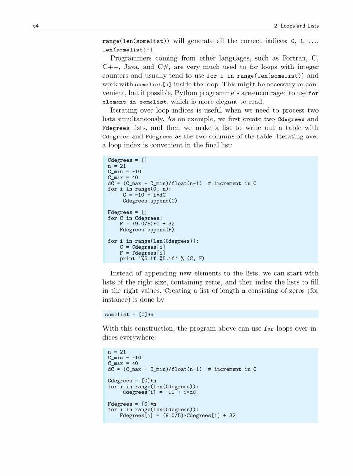
64 2 Loops and Lists

range(len(somelist)) will generate all the correct indices: 0, 1, . . .,len(somelist)-1.

Programmers coming from other languages, such as Fortran, C,C++, Java, and C#, are very much used to for loops with integercounters and usually tend to use for i in range(len(somelist)) andwork with somelist[i] inside the loop. This might be necessary or con-venient, but if possible, Python programmers are encouraged to use forelement in somelist, which is more elegant to read.

Iterating over loop indices is useful when we need to process twolists simultaneously. As an example, we first create two Cdegrees andFdegrees lists, and then we make a list to write out a table withCdegrees and Fdegrees as the two columns of the table. Iterating overa loop index is convenient in the final list:

Cdegrees = []n = 21C_min = -10C_max = 40dC = (C_max - C_min)/float(n-1) # increment in Cfor i in range(0, n):

C = -10 + i*dCCdegrees.append(C)

Fdegrees = []for C in Cdegrees:

F = (9.0/5)*C + 32Fdegrees.append(F)

for i in range(len(Cdegrees)):C = Cdegrees[i]F = Fdegrees[i]print ’%5.1f %5.1f’ % (C, F)

Instead of appending new elements to the lists, we can start withlists of the right size, containing zeros, and then index the lists to fillin the right values. Creating a list of length n consisting of zeros (forinstance) is done by

somelist = [0]*n

With this construction, the program above can use for loops over in-dices everywhere:

n = 21C_min = -10C_max = 40dC = (C_max - C_min)/float(n-1) # increment in C

Cdegrees = [0]*nfor i in range(len(Cdegrees)):

Cdegrees[i] = -10 + i*dC

Fdegrees = [0]*nfor i in range(len(Cdegrees)):

Fdegrees[i] = (9.0/5)*Cdegrees[i] + 32

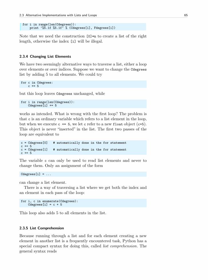
2.3 Alternative Implementations with Lists and Loops 65

for i in range(len(Cdegrees)):print ’%5.1f %5.1f’ % (Cdegrees[i], Fdegrees[i])

Note that we need the construction [0]*n to create a list of the rightlength, otherwise the index [i] will be illegal.

2.3.4 Changing List Elements

We have two seemingly alternative ways to traverse a list, either a loopover elements or over indices. Suppose we want to change the Cdegrees

list by adding 5 to all elements. We could try

for c in Cdegrees:c += 5

but this loop leaves Cdegrees unchanged, while

for i in range(len(Cdegrees)):Cdegrees[i] += 5

works as intended. What is wrong with the first loop? The problem isthat c is an ordinary variable which refers to a list element in the loop,but when we execute c += 5, we let c refer to a new float object (c+5).This object is never “inserted” in the list. The first two passes of theloop are equivalent to

c = Cdegrees[0] # automatically done in the for statementc += 5c = Cdegrees[1] # automatically done in the for statementc += 5

The variable c can only be used to read list elements and never tochange them. Only an assignment of the form

Cdegrees[i] = ...

can change a list element.There is a way of traversing a list where we get both the index and

an element in each pass of the loop:

for i, c in enumerate(Cdegrees):Cdegrees[i] = c + 5

This loop also adds 5 to all elements in the list.

2.3.5 List Comprehension

Because running through a list and for each element creating a newelement in another list is a frequently encountered task, Python has aspecial compact syntax for doing this, called list comprehension. Thegeneral syntax reads

66 2 Loops and Lists

newlist = [E(e) for e in list]

where E(e) represents an expression involving element e. Here are threeexamples:

Cdegrees = [-5 + i*0.5 for i in range(n)]Fdegrees = [(9.0/5)*C + 32 for C in Cdegrees]C_plus_5 = [C+5 for C in Cdegrees]

List comprehensions are recognized as a for loop inside square bracketsand will be frequently examplified thoughout the book.

2.3.6 Traversing Multiple Lists Simultaneously

We may use the Cdegrees and Fdegrees lists to make a table. To thisend, we need to traverse both arrays. The for element in list con-struction is not suitable in this case, since it extracts elements fromone list only. A solution is to use a for loop over the integer indices sothat we can index both lists:

for i in range(len(Cdegrees)):print ’%5d %5.1f’ % (Cdegrees[i], Fdegrees[i])

It happens quite frequently that two or more lists need to be traversedsimultaneously. As an alternative to the loop over indices, Python offersa special nice syntax that can be sketched as

for e1, e2, e3, ... in zip(list1, list2, list3, ...):# work with element e1 from list1, element e2 from list2,# element e3 from list3, etc.

The zip function turns n lists (list1, list2, list3, ...) into one listof n-tuples, where each n-tuple (e1,e2,e3,...) has its first element (e1)from the first list (list1), the second element (e2) from the second list(list2), and so forth. The loop stops when the end of the shortest listis reached. In our specific case of iterating over the two lists Cdegrees

and Fdegrees, we can use the zip function:

for C, F in zip(Cdegrees, Fdegrees):print ’%5d %5.1f’ % (C, F)

It is considered more“Pythonic”to iterate over list elements, here C andF, rather than over list indices as in the for i in range(len(Cdegrees))

construction.

2.4 Nested Lists

Nested lists are list objects where the elements in the lists can be liststhemselves. A couple of examples will motivate for nested lists andillustrate the basic operations on such lists.

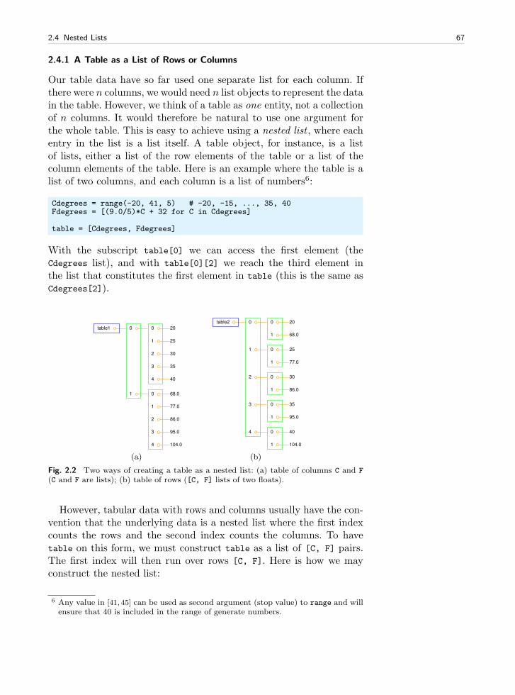
2.4 Nested Lists 67

2.4.1 A Table as a List of Rows or Columns

Our table data have so far used one separate list for each column. Ifthere were n columns, we would need n list objects to represent the datain the table. However, we think of a table as one entity, not a collectionof n columns. It would therefore be natural to use one argument forthe whole table. This is easy to achieve using a nested list , where eachentry in the list is a list itself. A table object, for instance, is a listof lists, either a list of the row elements of the table or a list of thecolumn elements of the table. Here is an example where the table is alist of two columns, and each column is a list of numbers6:

Cdegrees = range(-20, 41, 5) # -20, -15, ..., 35, 40Fdegrees = [(9.0/5)*C + 32 for C in Cdegrees]

table = [Cdegrees, Fdegrees]

With the subscript table[0] we can access the first element (theCdegrees list), and with table[0][2] we reach the third element inthe list that constitutes the first element in table (this is the same asCdegrees[2]).

table1 0 0 20

1 25

2 30

3 35

4 40

1 0 68.0

1 77.0

2 86.0

3 95.0

4 104.0

(a)

table2 0 0 20

1 68.0

1 0 25

1 77.0

2 0 30

1 86.0

3 0 35

1 95.0

4 0 40

1 104.0

(b)

Fig. 2.2 Two ways of creating a table as a nested list: (a) table of columns C and F

(C and F are lists); (b) table of rows ([C, F] lists of two floats).

However, tabular data with rows and columns usually have the con-vention that the underlying data is a nested list where the first indexcounts the rows and the second index counts the columns. To havetable on this form, we must construct table as a list of [C, F] pairs.The first index will then run over rows [C, F]. Here is how we mayconstruct the nested list:

6 Any value in [41, 45] can be used as second argument (stop value) to range and willensure that 40 is included in the range of generate numbers.

68 2 Loops and Lists

table = []for C, F in zip(Cdegrees, Fdegrees):

table.append([C, F])

We may shorten this code segment by introducing a list comprehen-sion:

table = [[C, F] for C, F in zip(Cdegrees, Fdegrees)]

This construction loops through pairs C and F, and for each pass in theloop we create a list element [C, F].

The subscript table[1] refers to the second element in table, whichis a [C, F] pair, while table[1][0] is the C value and table[1][1] isthe F value. Figure 2.2 illustrates both a list of columns and a list ofpairs. Using this figure, you can realize that the first index looks upthe “main list”, while the second index looks up the “sublist”.

2.4.2 Printing Objects

Modules for Pretty Print of Objects. We may write print table to im-mediately view the nested list table from the previous section. In fact,any Python object obj can be printed to the screen by the commandprint obj. The output is usually one line, and this line may becomevery long if the list has many elements. For example, a long list likeour table variable, demands a quite long line when printed.

[[-20, -4.0], [-15, 5.0], [-10, 14.0], ............., [40, 104.0]]

Splitting the output over several shorter lines makes the layout nicerand more readable. The pprint module offers a “pretty print” function-ality for this purpose. The usage of pprint looks like

import pprintpprint.pprint(table)

and the corresponding output becomes

[[-20, -4.0],[-15, 5.0],[-10, 14.0],[-5, 23.0],[0, 32.0],[5, 41.0],[10, 50.0],[15, 59.0],[20, 68.0],[25, 77.0],[30, 86.0],[35, 95.0],[40, 104.0]]

With this book comes a slightly modified pprint module havingthe name scitools.pprint2. This module allows full format con-trol of the printing of the float objects in lists by specifying

2.4 Nested Lists 69

scitools.pprint2.float_format as a printf format string. The fol-lowing example demonstrates how the output format of real numberscan be changed:

>>> import pprint, scitools.pprint2>>> somelist = [15.8, [0.2, 1.7]]>>> pprint.pprint(somelist)[15.800000000000001, [0.20000000000000001, 1.7]]>>> scitools.pprint2.pprint(somelist)[15.8, [0.2, 1.7]]>>> # default output is ’%g’, change this to>>> scitools.pprint2.float_format = ’%.2e’>>> scitools.pprint2.pprint(somelist)[1.58e+01, [2.00e-01, 1.70e+00]]

As can be seen from this session, the pprint module writes floating-point numbers with a lot of digits, in fact so many that we explicitlysee the round-off errors. Many find this type of output is annoying andthat the default output from the scitools.pprint2 module is more likeone would desire and expect.

The pprint and scitools.pprint2 modules also have a functionpformat, which works as the pprint function, but it returns a prettyformatted string rather than printing the string:

s = pprint.pformat(somelist)print s

This last print statement prints the same as pprint.pprint(somelist).

Manual Printing. Many will argue that tabular data such as thosestored in the nested table list are not printed in a particularly prettyway by the pprint module. One would rather expect pretty output tobe a table with two nicely aligned columns. To produce such outputwe need to code the formatting manually. This is quite easy: We loopover each row, extract the two elements C and F in each row, and printthese in fixed-width fields using the printf syntax. The code goes asfollows:

for C, F in table:print ’%5d %5.1f’ % (C, F)

2.4.3 Extracting Sublists

Python has a nice syntax for extracting parts of a list structure. Suchparts are known as sublists or slices :

A[i:] is the sublist starting with index i in A and continuing to theend of A:

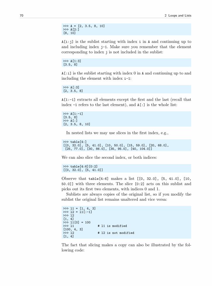
70 2 Loops and Lists

>>> A = [2, 3.5, 8, 10]>>> A[2:][8, 10]

A[i:j] is the sublist starting with index i in A and continuing up toand including index j-1. Make sure you remember that the elementcorresponding to index j is not included in the sublist:

>>> A[1:3][3.5, 8]

A[:i] is the sublist starting with index 0 in A and continuing up to andincluding the element with index i-1:

>>> A[:3][2, 3.5, 8]

A[1:-1] extracts all elements except the first and the last (recall thatindex -1 refers to the last element), and A[:] is the whole list:

>>> A[1:-1][3.5, 8]>>> A[:][2, 3.5, 8, 10]

In nested lists we may use slices in the first index, e.g.,

>>> table[4:][[0, 32.0], [5, 41.0], [10, 50.0], [15, 59.0], [20, 68.0],[25, 77.0], [30, 86.0], [35, 95.0], [40, 104.0]]

We can also slice the second index, or both indices:

>>> table[4:6][0:2][[0, 32.0], [5, 41.0]]

Observe that table[4:6] makes a list [[0, 32.0], [5, 41.0], [10,

50.0]] with three elements. The slice [0:2] acts on this sublist andpicks out its first two elements, with indices 0 and 1.

Sublists are always copies of the original list, so if you modify thesublist the original list remains unaltered and vice versa:

>>> l1 = [1, 4, 3]>>> l2 = l1[:-1]>>> l2[1, 4]>>> l1[0] = 100>>> l1 # l1 is modified[100, 4, 3]>>> l2 # l2 is not modified[1, 4]

The fact that slicing makes a copy can also be illustrated by the fol-lowing code:

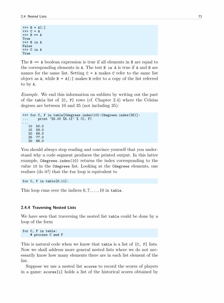
2.4 Nested Lists 71

>>> B = A[:]>>> C = A>>> B == ATrue>>> B is AFalse>>> C is ATrue

The B == A boolean expression is true if all elements in B are equal tothe corresponding elements in A. The test B is A is true if A and B arenames for the same list. Setting C = A makes C refer to the same listobject as A, while B = A[:] makes B refer to a copy of the list referredto by A.

Example. We end this information on sublists by writing out the partof the table list of [C, F] rows (cf. Chapter 2.4) where the Celsiusdegrees are between 10 and 35 (not including 35):

>>> for C, F in table[Cdegrees.index(10):Cdegrees.index(35)]:... print ’%5.0f %5.1f’ % (C, F)...

10 50.015 59.020 68.025 77.030 86.0

You should always stop reading and convince yourself that you under-stand why a code segment produces the printed output. In this latterexample, Cdegrees.index(10) returns the index corresponding to thevalue 10 in the Cdegrees list. Looking at the Cdegrees elements, onerealizes (do it!) that the for loop is equivalent to

for C, F in table[6:11]:

This loop runs over the indices 6, 7, . . . , 10 in table.

2.4.4 Traversing Nested Lists

We have seen that traversing the nested list table could be done by aloop of the form

for C, F in table:# process C and F

This is natural code when we know that table is a list of [C, F] lists.Now we shall address more general nested lists where we do not nec-essarily know how many elements there are in each list element of thelist.

Suppose we use a nested list scores to record the scores of playersin a game: scores[i] holds a list of the historical scores obtained by

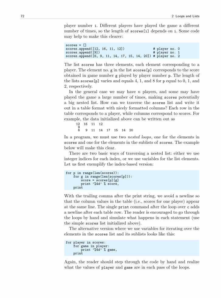
72 2 Loops and Lists

player number i. Different players have played the game a differentnumber of times, so the length of scores[i] depends on i. Some codemay help to make this clearer:

scores = []scores.append([12, 16, 11, 12]) # player no. 0scores.append([9]) # player no. 1scores.append([6, 9, 11, 14, 17, 15, 14, 20]) # player no. 2

The list scores has three elements, each element corresponding to aplayer. The element no. g in the list scores[p] corresponds to the scoreobtained in game number g played by player number p. The length ofthe lists scores[p] varies and equals 4, 1, and 8 for p equal to 0, 1, and2, respectively.

In the general case we may have n players, and some may haveplayed the game a large number of times, making scores potentiallya big nested list. How can we traverse the scores list and write itout in a table format with nicely formatted columns? Each row in thetable corresponds to a player, while columns correspond to scores. Forexample, the data initialized above can be written out as

12 16 11 1296 9 11 14 17 15 14 20

In a program, we must use two nested loops , one for the elements inscores and one for the elements in the sublists of scores. The examplebelow will make this clear.

There are two basic ways of traversing a nested list: either we useinteger indices for each index, or we use variables for the list elements.Let us first exemplify the index-based version:

for p in range(len(scores)):for g in range(len(scores[p])):

score = scores[p][g]print ’%4d’ % score,

print

With the trailing comma after the print string, we avoid a newline sothat the column values in the table (i.e., scores for one player) appearat the same line. The single print command after the loop over c addsa newline after each table row. The reader is encouraged to go throughthe loops by hand and simulate what happens in each statement (usethe simple scores list initialized above).

The alternative version where we use variables for iterating over theelements in the scores list and its sublists looks like this:

for player in scores:for game in player:

print ’%4d’ % game,print

Again, the reader should step through the code by hand and realizewhat the values of player and game are in each pass of the loops.

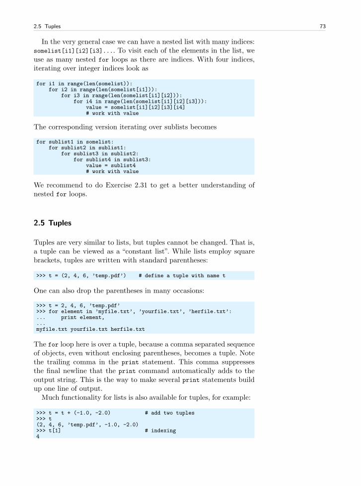
2.5 Tuples 73

In the very general case we can have a nested list with many indices:somelist[i1][i2][i3].... To visit each of the elements in the list, weuse as many nested for loops as there are indices. With four indices,iterating over integer indices look as

for i1 in range(len(somelist)):for i2 in range(len(somelist[i1])):

for i3 in range(len(somelist[i1][i2])):for i4 in range(len(somelist[i1][i2][i3])):

value = somelist[i1][i2][i3][i4]# work with value

The corresponding version iterating over sublists becomes

for sublist1 in somelist:for sublist2 in sublist1:

for sublist3 in sublist2:for sublist4 in sublist3:

value = sublist4# work with value

We recommend to do Exercise 2.31 to get a better understanding ofnested for loops.

2.5 Tuples

Tuples are very similar to lists, but tuples cannot be changed. That is,a tuple can be viewed as a “constant list”. While lists employ squarebrackets, tuples are written with standard parentheses:

>>> t = (2, 4, 6, ’temp.pdf’) # define a tuple with name t

One can also drop the parentheses in many occasions:

>>> t = 2, 4, 6, ’temp.pdf’>>> for element in ’myfile.txt’, ’yourfile.txt’, ’herfile.txt’:... print element,...myfile.txt yourfile.txt herfile.txt

The for loop here is over a tuple, because a comma separated sequenceof objects, even without enclosing parentheses, becomes a tuple. Notethe trailing comma in the print statement. This comma suppressesthe final newline that the print command automatically adds to theoutput string. This is the way to make several print statements buildup one line of output.

Much functionality for lists is also available for tuples, for example:

>>> t = t + (-1.0, -2.0) # add two tuples>>> t(2, 4, 6, ’temp.pdf’, -1.0, -2.0)>>> t[1] # indexing4

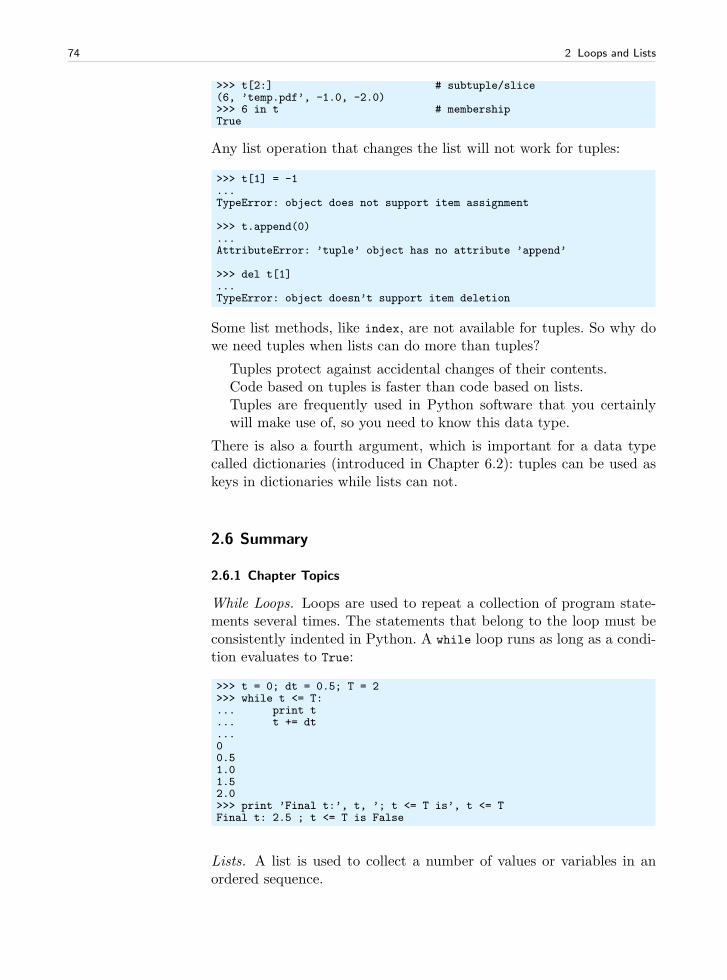
74 2 Loops and Lists

>>> t[2:] # subtuple/slice(6, ’temp.pdf’, -1.0, -2.0)>>> 6 in t # membershipTrue

Any list operation that changes the list will not work for tuples:

>>> t[1] = -1...TypeError: object does not support item assignment

>>> t.append(0)...AttributeError: ’tuple’ object has no attribute ’append’

>>> del t[1]...TypeError: object doesn’t support item deletion

Some list methods, like index, are not available for tuples. So why dowe need tuples when lists can do more than tuples?

Tuples protect against accidental changes of their contents. Code based on tuples is faster than code based on lists. Tuples are frequently used in Python software that you certainlywill make use of, so you need to know this data type.

There is also a fourth argument, which is important for a data typecalled dictionaries (introduced in Chapter 6.2): tuples can be used askeys in dictionaries while lists can not.

2.6 Summary

2.6.1 Chapter Topics

While Loops. Loops are used to repeat a collection of program state-ments several times. The statements that belong to the loop must beconsistently indented in Python. A while loop runs as long as a condi-tion evaluates to True:

>>> t = 0; dt = 0.5; T = 2>>> while t <= T:... print t... t += dt...00.51.01.52.0>>> print ’Final t:’, t, ’; t <= T is’, t <= TFinal t: 2.5 ; t <= T is False

Lists. A list is used to collect a number of values or variables in anordered sequence.

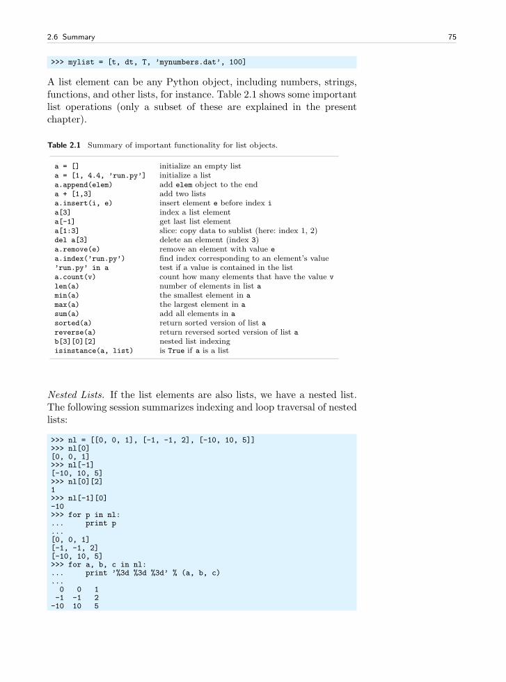
2.6 Summary 75

>>> mylist = [t, dt, T, ’mynumbers.dat’, 100]

A list element can be any Python object, including numbers, strings,functions, and other lists, for instance. Table 2.1 shows some importantlist operations (only a subset of these are explained in the presentchapter).

Table 2.1 Summary of important functionality for list objects.

a = [] initialize an empty lista = [1, 4.4, ’run.py’] initialize a lista.append(elem) add elem object to the enda + [1,3] add two listsa.insert(i, e) insert element e before index i

a[3] index a list elementa[-1] get last list elementa[1:3] slice: copy data to sublist (here: index 1, 2)del a[3] delete an element (index 3)a.remove(e) remove an element with value e

a.index(’run.py’) find index corresponding to an element’s value’run.py’ in a test if a value is contained in the lista.count(v) count how many elements that have the value v

len(a) number of elements in list amin(a) the smallest element in a

max(a) the largest element in a

sum(a) add all elements in a

sorted(a) return sorted version of list areverse(a) return reversed sorted version of list ab[3][0][2] nested list indexingisinstance(a, list) is True if a is a list

Nested Lists. If the list elements are also lists, we have a nested list.The following session summarizes indexing and loop traversal of nestedlists:

>>> nl = [[0, 0, 1], [-1, -1, 2], [-10, 10, 5]]>>> nl[0][0, 0, 1]>>> nl[-1][-10, 10, 5]>>> nl[0][2]1>>> nl[-1][0]-10>>> for p in nl:... print p...[0, 0, 1][-1, -1, 2][-10, 10, 5]>>> for a, b, c in nl:... print ’%3d %3d %3d’ % (a, b, c)...0 0 1-1 -1 2-10 10 5

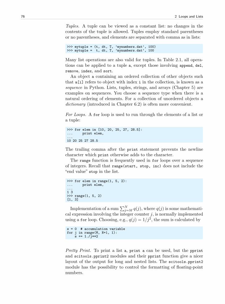
76 2 Loops and Lists

Tuples. A tuple can be viewed as a constant list: no changes in thecontents of the tuple is allowed. Tuples employ standard parenthesesor no parentheses, and elements are separated with comma as in lists:

>>> mytuple = (t, dt, T, ’mynumbers.dat’, 100)>>> mytuple = t, dt, T, ’mynumbers.dat’, 100

Many list operations are also valid for tuples. In Table 2.1, all opera-tions can be applied to a tuple a, except those involving append, del,remove, index, and sort.

An object a containing an ordered collection of other objects suchthat a[i] refers to object with index i in the collection, is known as asequence in Python. Lists, tuples, strings, and arrays (Chapter 5) areexamples on sequences. You choose a sequence type when there is anatural ordering of elements. For a collection of unordered objects adictionary (introduced in Chapter 6.2) is often more convenient.

For Loops. A for loop is used to run through the elements of a list ora tuple:

>>> for elem in [10, 20, 25, 27, 28.5]:... print elem,...10 20 25 27 28.5

The trailing comma after the print statement prevents the newlinecharacter which print otherwise adds to the character.

The range function is frequently used in for loops over a sequenceof integers. Recall that range(start, stop, inc) does not include the“end value” stop in the list.

>>> for elem in range(1, 5, 2):... print elem,...1 3>>> range(1, 5, 2)[1, 3]

Implementation of a sum∑N

j=M q(j), where q(j) is some mathemati-cal expression involving the integer counter j, is normally implementedusing a for loop. Choosing, e.g., q(j) = 1/j2, the sum is calculated by

s = 0 # accumulation variablefor j in range(M, N+1, 1):

s += 1./j**2

Pretty Print. To print a list a, print a can be used, but the pprint

and scitools.pprint2 modules and their pprint function give a nicerlayout of the output for long and nested lists. The scitools.pprint2

module has the possibility to control the formatting of floating-pointnumbers.

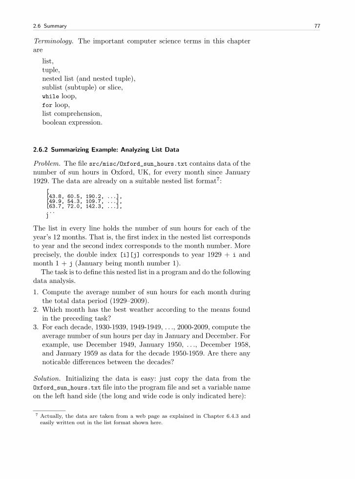
2.6 Summary 77

Terminology. The important computer science terms in this chapterare

list, tuple, nested list (and nested tuple), sublist (subtuple) or slice, while loop, for loop, list comprehension, boolean expression.

2.6.2 Summarizing Example: Analyzing List Data

Problem. The file src/misc/Oxford_sun_hours.txt contains data of thenumber of sun hours in Oxford, UK, for every month since January1929. The data are already on a suitable nested list format7:

[[43.8, 60.5, 190.2, ...],[49.9, 54.3, 109.7, ...],[63.7, 72.0, 142.3, ...],...]

The list in every line holds the number of sun hours for each of theyear’s 12 months. That is, the first index in the nested list correspondsto year and the second index corresponds to the month number. Moreprecisely, the double index [i][j] corresponds to year 1929 + i andmonth 1 + j (January being month number 1).

The task is to define this nested list in a program and do the followingdata analysis.

1. Compute the average number of sun hours for each month duringthe total data period (1929–2009).

2. Which month has the best weather according to the means foundin the preceding task?

3. For each decade, 1930-1939, 1949-1949, . . ., 2000-2009, compute theaverage number of sun hours per day in January and December. Forexample, use December 1949, January 1950, . . ., December 1958,and January 1959 as data for the decade 1950-1959. Are there anynoticable differences between the decades?

Solution. Initializing the data is easy: just copy the data from theOxford_sun_hours.txt file into the program file and set a variable nameon the left hand side (the long and wide code is only indicated here):

7 Actually, the data are taken from a web page as explained in Chapter 6.4.3 andeasily written out in the list format shown here.

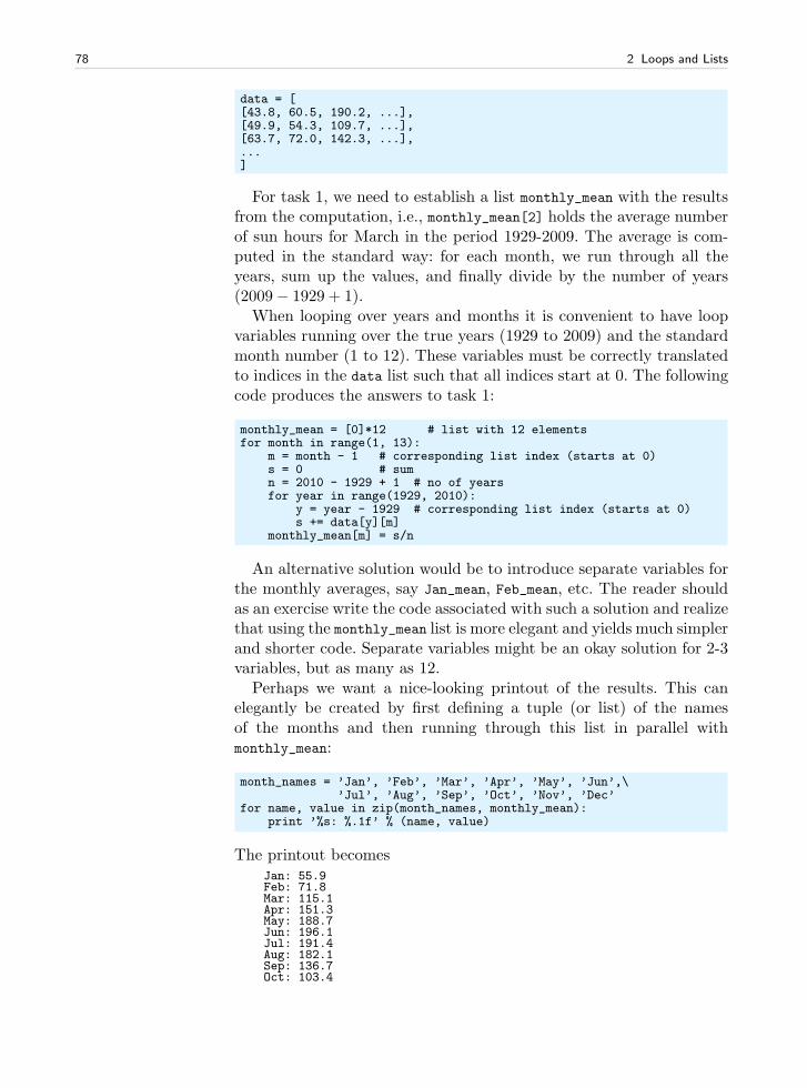
78 2 Loops and Lists

data = [[43.8, 60.5, 190.2, ...],[49.9, 54.3, 109.7, ...],[63.7, 72.0, 142.3, ...],...]

For task 1, we need to establish a list monthly_mean with the resultsfrom the computation, i.e., monthly_mean[2] holds the average numberof sun hours for March in the period 1929-2009. The average is com-puted in the standard way: for each month, we run through all theyears, sum up the values, and finally divide by the number of years(2009− 1929 + 1).

When looping over years and months it is convenient to have loopvariables running over the true years (1929 to 2009) and the standardmonth number (1 to 12). These variables must be correctly translatedto indices in the data list such that all indices start at 0. The followingcode produces the answers to task 1:

monthly_mean = [0]*12 # list with 12 elementsfor month in range(1, 13):

m = month - 1 # corresponding list index (starts at 0)s = 0 # sumn = 2010 - 1929 + 1 # no of yearsfor year in range(1929, 2010):

y = year - 1929 # corresponding list index (starts at 0)s += data[y][m]

monthly_mean[m] = s/n

An alternative solution would be to introduce separate variables forthe monthly averages, say Jan_mean, Feb_mean, etc. The reader shouldas an exercise write the code associated with such a solution and realizethat using the monthly_mean list is more elegant and yields much simplerand shorter code. Separate variables might be an okay solution for 2-3variables, but as many as 12.

Perhaps we want a nice-looking printout of the results. This canelegantly be created by first defining a tuple (or list) of the namesof the months and then running through this list in parallel withmonthly_mean:

month_names = ’Jan’, ’Feb’, ’Mar’, ’Apr’, ’May’, ’Jun’,\’Jul’, ’Aug’, ’Sep’, ’Oct’, ’Nov’, ’Dec’

for name, value in zip(month_names, monthly_mean):print ’%s: %.1f’ % (name, value)

The printout becomesJan: 55.9Feb: 71.8Mar: 115.1Apr: 151.3May: 188.7Jun: 196.1Jul: 191.4Aug: 182.1Sep: 136.7Oct: 103.4

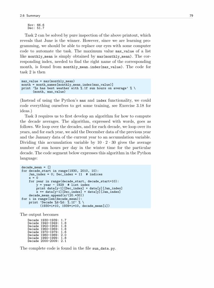
2.6 Summary 79

Nov: 66.6Dec: 51.7

Task 2 can be solved by pure inspection of the above printout, whichreveals that June is the winner. However, since we are learning pro-gramming, we should be able to replace our eyes with some computercode to automate the task. The maximum value max_value of a listlike monthly_mean is simply obtained by max(monthly_mean). The cor-responding index, needed to find the right name of the correspondingmonth, is found from monthly_mean.index(max_value). The code fortask 2 is then

max_value = max(monthly_mean)month = month_names[monthly_mean.index(max_value)]print ’%s has best weather with %.1f sun hours on average’ % \

(month, max_value)

(Instead of using the Python’s max and index functionality, we couldcode everything ourselves to get some training, see Exercise 3.18 forideas.)

Task 3 requires us to first develop an algorithm for how to computethe decade averages. The algorithm, expressed with words, goes asfollows. We loop over the decades, and for each decade, we loop over itsyears, and for each year, we add the December data of the previous yearand the January data of the current year to an accumulation variable.Dividing this accumulation variable by 10 · 2 · 30 gives the averagenumber of sun hours per day in the winter time for the particulardecade. The code segment below expresses this algorithm in the Pythonlanguage:

decade_mean = []for decade_start in range(1930, 2010, 10):

Jan_index = 0; Dec_index = 11 # indicess = 0for year in range(decade_start, decade_start+10):

y = year - 1929 # list indexprint data[y-1][Dec_index] + data[y][Jan_index]s += data[y-1][Dec_index] + data[y][Jan_index]

decade_mean.append(s/(20.*30))for i in range(len(decade_mean)):

print ’Decade %d-%d: %.1f’ % \(1930+i*10, 1939+i*10, decade_mean[i])

The output becomesDecade 1930-1939: 1.7Decade 1940-1949: 1.8Decade 1950-1959: 1.8Decade 1960-1969: 1.8Decade 1970-1979: 1.6Decade 1980-1989: 2.0Decade 1990-1999: 1.8Decade 2000-2009: 2.1

The complete code is found in the file sun_data.py.

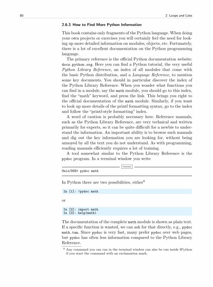
80 2 Loops and Lists

2.6.3 How to Find More Python Information

This book contains only fragments of the Python language. When doingyour own projects or exercises you will certainly feel the need for look-ing up more detailed information on modules, objects, etc. Fortunately,there is a lot of excellent documentation on the Python programminglanguage.

The primary reference is the official Python documentation website:docs.python.org. Here you can find a Python tutorial, the very usefulPython Library Reference, an index of all modules that come withthe basic Python distribution, and a Language Reference, to mentionsome key documents. You should in particular discover the index ofthe Python Library Reference. When you wonder what functions youcan find in a module, say the math module, you should go to this index,find the “math” keyword, and press the link. This brings you right tothe official documentation of the math module. Similarly, if you wantto look up more details of the printf formatting syntax, go to the indexand follow the “printf-style formatting” index.

A word of caution is probably necessary here. Reference manuals,such as the Python Library Reference, are very technical and writtenprimarily for experts, so it can be quite difficult for a newbie to under-stand the information. An important ability is to browse such manualsand dig out the key information you are looking for, without beingannoyed by all the text you do not understand. As with programming,reading manuals efficiently requires a lot of training.

A tool somewhat similar to the Python Library Reference is thepydoc program. In a terminal window you write

Terminal

Unix/DOS> pydoc math

In Python there are two possibilities, either8

In [1]: !pydoc math

or

In [2]: import mathIn [3]: help(math)

The documentation of the complete math module is shown as plain text.If a specific function is wanted, we can ask for that directly, e.g., pydocmath.tan. Since pydoc is very fast, many prefer pydoc over web pages,but pydoc has often less information compared to the Python LibraryReference.

8 Any command you can run in the terminal window can also be run inside IPythonif you start the command with an exclamation mark.

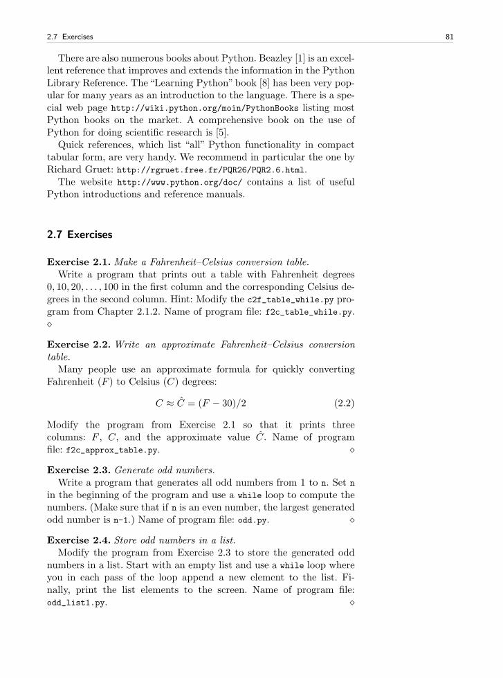
2.7 Exercises 81

There are also numerous books about Python. Beazley [1] is an excel-lent reference that improves and extends the information in the PythonLibrary Reference. The “Learning Python”book [8] has been very pop-ular for many years as an introduction to the language. There is a spe-cial web page http://wiki.python.org/moin/PythonBooks listing mostPython books on the market. A comprehensive book on the use ofPython for doing scientific research is [5].

Quick references, which list “all” Python functionality in compacttabular form, are very handy. We recommend in particular the one byRichard Gruet: http://rgruet.free.fr/PQR26/PQR2.6.html.

The website http://www.python.org/doc/ contains a list of usefulPython introductions and reference manuals.

2.7 Exercises

Exercise 2.1. Make a Fahrenheit–Celsius conversion table.Write a program that prints out a table with Fahrenheit degrees

0, 10, 20, . . . , 100 in the first column and the corresponding Celsius de-grees in the second column. Hint: Modify the c2f_table_while.py pro-gram from Chapter 2.1.2. Name of program file: f2c_table_while.py.⋄

Exercise 2.2. Write an approximate Fahrenheit–Celsius conversiontable.

Many people use an approximate formula for quickly convertingFahrenheit (F ) to Celsius (C) degrees:

C ≈ C = (F − 30)/2 (2.2)

Modify the program from Exercise 2.1 so that it prints threecolumns: F , C, and the approximate value C. Name of programfile: f2c_approx_table.py. ⋄

Exercise 2.3. Generate odd numbers.Write a program that generates all odd numbers from 1 to n. Set n

in the beginning of the program and use a while loop to compute thenumbers. (Make sure that if n is an even number, the largest generatedodd number is n-1.) Name of program file: odd.py. ⋄

Exercise 2.4. Store odd numbers in a list.Modify the program from Exercise 2.3 to store the generated odd

numbers in a list. Start with an empty list and use a while loop whereyou in each pass of the loop append a new element to the list. Fi-nally, print the list elements to the screen. Name of program file:odd_list1.py. ⋄

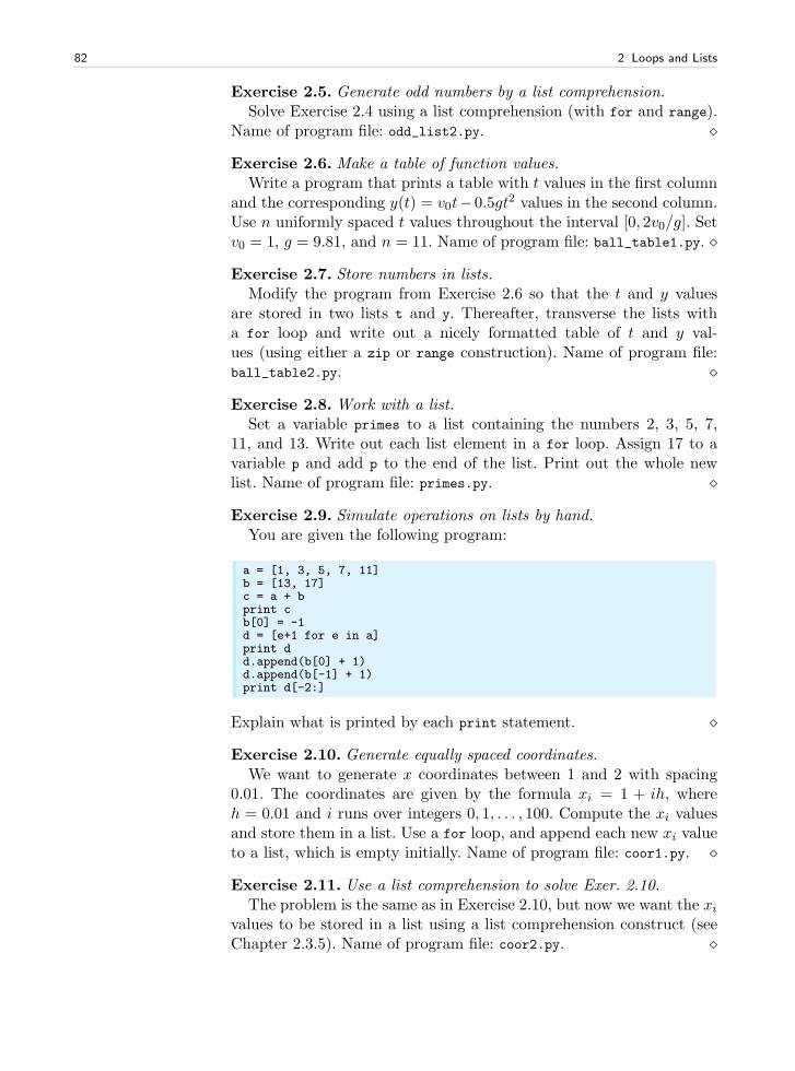
82 2 Loops and Lists

Exercise 2.5. Generate odd numbers by a list comprehension.Solve Exercise 2.4 using a list comprehension (with for and range).

Name of program file: odd_list2.py. ⋄

Exercise 2.6. Make a table of function values.Write a program that prints a table with t values in the first column

and the corresponding y(t) = v0t−0.5gt2 values in the second column.Use n uniformly spaced t values throughout the interval [0, 2v0/g]. Setv0 = 1, g = 9.81, and n = 11. Name of program file: ball_table1.py. ⋄

Exercise 2.7. Store numbers in lists.Modify the program from Exercise 2.6 so that the t and y values

are stored in two lists t and y. Thereafter, transverse the lists witha for loop and write out a nicely formatted table of t and y val-ues (using either a zip or range construction). Name of program file:ball_table2.py. ⋄

Exercise 2.8. Work with a list.Set a variable primes to a list containing the numbers 2, 3, 5, 7,

11, and 13. Write out each list element in a for loop. Assign 17 to avariable p and add p to the end of the list. Print out the whole newlist. Name of program file: primes.py. ⋄

Exercise 2.9. Simulate operations on lists by hand.You are given the following program:

a = [1, 3, 5, 7, 11]b = [13, 17]c = a + bprint cb[0] = -1d = [e+1 for e in a]print dd.append(b[0] + 1)d.append(b[-1] + 1)print d[-2:]

Explain what is printed by each print statement. ⋄

Exercise 2.10. Generate equally spaced coordinates.We want to generate x coordinates between 1 and 2 with spacing

0.01. The coordinates are given by the formula xi = 1 + ih, whereh = 0.01 and i runs over integers 0, 1, . . . , 100. Compute the xi valuesand store them in a list. Use a for loop, and append each new xi valueto a list, which is empty initially. Name of program file: coor1.py. ⋄

Exercise 2.11. Use a list comprehension to solve Exer. 2.10.The problem is the same as in Exercise 2.10, but now we want the xi

values to be stored in a list using a list comprehension construct (seeChapter 2.3.5). Name of program file: coor2.py. ⋄

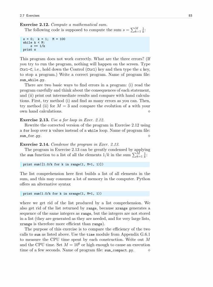
2.7 Exercises 83

Exercise 2.12. Compute a mathematical sum.The following code is supposed to compute the sum s =

∑Mk=1

1k :

s = 0; k = 1; M = 100while k < M:

s += 1/kprint s

This program does not work correctly. What are the three errors? (Ifyou try to run the program, nothing will happen on the screen. TypeCtrl-C, i.e., hold down the Control (Ctrl) key and then type the c key,to stop a program.) Write a correct program. Name of program file:sum_while.py.

There are two basic ways to find errors in a program: (i) read theprogram carefully and think about the consequences of each statement,and (ii) print out intermediate results and compare with hand calcula-tions. First, try method (i) and find as many errors as you can. Then,try method (ii) for M = 3 and compare the evolution of s with yourown hand calculations. ⋄

Exercise 2.13. Use a for loop in Exer. 2.12.Rewrite the corrected version of the program in Exercise 2.12 using

a for loop over k values instead of a while loop. Name of program file:sum_for.py. ⋄

Exercise 2.14. Condense the program in Exer. 2.13.The program in Exercise 2.13 can be greatly condensed by applying

the sum function to a list of all the elements 1/k in the sum∑M

k=11k :

print sum([1.0/k for k in range(1, M+1, 1)])

The list comprehension here first builds a list of all elements in thesum, and this may consume a lot of memory in the computer. Pythonoffers an alternative syntax

print sum(1.0/k for k in xrange(1, M+1, 1))

where we get rid of the list produced by a list comprehension. Wealso get rid of the list returned by range, because xrange generates asequence of the same integers as range, but the integers are not storedin a list (they are generated as they are needed, and for very large lists,xrange is therefore more efficient than range).

The purpose of this exercise is to compare the efficiency of the twocalls to sum as listed above. Use the time module from Appendix G.6.1to measure the CPU time spent by each construction. Write out Mand the CPU time. Set M = 106 or high enough to cause an executiontime of a few seconds. Name of program file: sum_compact.py. ⋄

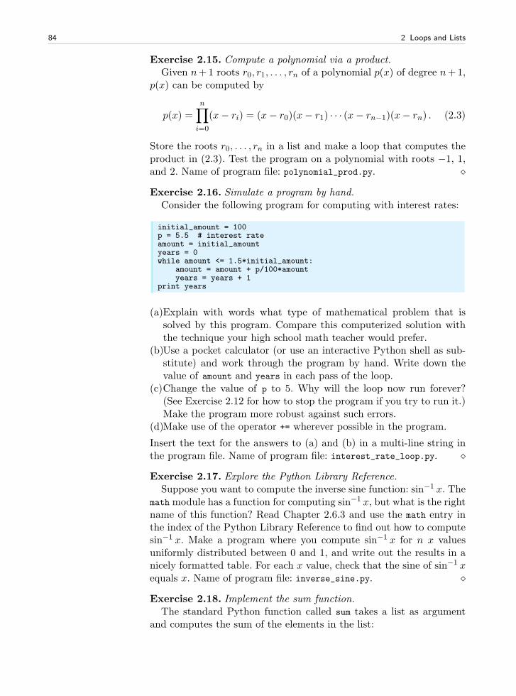
84 2 Loops and Lists

Exercise 2.15. Compute a polynomial via a product.Given n+1 roots r0, r1, . . . , rn of a polynomial p(x) of degree n+1,

p(x) can be computed by

p(x) =

n∏

i=0

(x− ri) = (x− r0)(x− r1) · · · (x− rn−1)(x− rn) . (2.3)

Store the roots r0, . . . , rn in a list and make a loop that computes theproduct in (2.3). Test the program on a polynomial with roots −1, 1,and 2. Name of program file: polynomial_prod.py. ⋄

Exercise 2.16. Simulate a program by hand.Consider the following program for computing with interest rates:

initial_amount = 100p = 5.5 # interest rateamount = initial_amountyears = 0while amount <= 1.5*initial_amount:

amount = amount + p/100*amountyears = years + 1

print years

(a)Explain with words what type of mathematical problem that issolved by this program. Compare this computerized solution withthe technique your high school math teacher would prefer.

(b)Use a pocket calculator (or use an interactive Python shell as sub-stitute) and work through the program by hand. Write down thevalue of amount and years in each pass of the loop.

(c)Change the value of p to 5. Why will the loop now run forever?(See Exercise 2.12 for how to stop the program if you try to run it.)Make the program more robust against such errors.

(d)Make use of the operator += wherever possible in the program.

Insert the text for the answers to (a) and (b) in a multi-line string inthe program file. Name of program file: interest_rate_loop.py. ⋄

Exercise 2.17. Explore the Python Library Reference.Suppose you want to compute the inverse sine function: sin−1 x. The

math module has a function for computing sin−1 x, but what is the rightname of this function? Read Chapter 2.6.3 and use the math entry inthe index of the Python Library Reference to find out how to computesin−1 x. Make a program where you compute sin−1 x for n x valuesuniformly distributed between 0 and 1, and write out the results in anicely formatted table. For each x value, check that the sine of sin−1 xequals x. Name of program file: inverse_sine.py. ⋄

Exercise 2.18. Implement the sum function.The standard Python function called sum takes a list as argument

and computes the sum of the elements in the list:

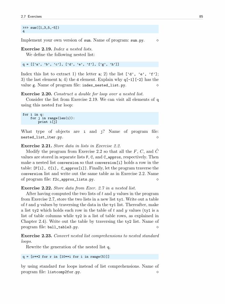
2.7 Exercises 85

>>> sum([1,3,5,-5])4

Implement your own version of sum. Name of program: sum.py. ⋄

Exercise 2.19. Index a nested lists.We define the following nested list:

q = [[’a’, ’b’, ’c’], [’d’, ’e’, ’f’], [’g’, ’h’]]

Index this list to extract 1) the letter a; 2) the list [’d’, ’e’, ’f’];3) the last element h; 4) the d element. Explain why q[-1][-2] has thevalue g. Name of program file: index_nested_list.py. ⋄

Exercise 2.20. Construct a double for loop over a nested list.Consider the list from Exercise 2.19. We can visit all elements of q

using this nested for loop:

for i in q:for j in range(len(i)):

print i[j]

What type of objects are i and j? Name of program file:nested_list_iter.py. ⋄

Exercise 2.21. Store data in lists in Exercise 2.2.Modify the program from Exercise 2.2 so that all the F , C, and C

values are stored in separate lists F, C, and C_approx, respectively. Thenmake a nested list conversion so that conversion[i] holds a row in thetable: [F[i], C[i], C_approx[i]]. Finally, let the program traverse theconversion list and write out the same table as in Exercise 2.2. Nameof program file: f2c_approx_lists.py. ⋄

Exercise 2.22. Store data from Exer. 2.7 in a nested list.After having computed the two lists of t and y values in the program

from Exercise 2.7, store the two lists in a new list ty1. Write out a tableof t and y values by traversing the data in the ty1 list. Thereafter, makea list ty2 which holds each row in the table of t and y values (ty1 is alist of table columns while ty2 is a list of table rows, as explained inChapter 2.4). Write out the table by traversing the ty2 list. Name ofprogram file: ball_table3.py. ⋄

Exercise 2.23. Convert nested list comprehensions to nested standardloops.

Rewrite the generation of the nested list q,

q = [r**2 for r in [10**i for i in range(5)]]

by using standard for loops instead of list comprehensions. Name ofprogram file: listcomp2for.py. ⋄

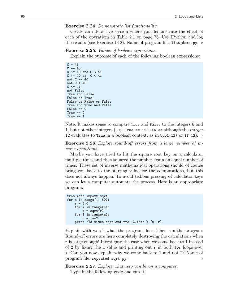
86 2 Loops and Lists

Exercise 2.24. Demonstrate list functionality.Create an interactive session where you demonstrate the effect of

each of the operations in Table 2.1 on page 75. Use IPython and logthe results (see Exercise 1.12). Name of program file: list_demo.py. ⋄Exercise 2.25. Values of boolean expressions.

Explain the outcome of each of the following boolean expressions:

C = 41C == 40C != 40 and C < 41C != 40 or C < 41not C == 40not C > 40C <= 41not FalseTrue and FalseFalse or TrueFalse or False or FalseTrue and True and FalseFalse == 0True == 0True == 1

Note: It makes sense to compare True and False to the integers 0 and1, but not other integers (e.g., True == 12 is False although the integer12 evaluates to True in a boolean context, as in bool(12) or if 12). ⋄Exercise 2.26. Explore round-off errors from a large number of in-verse operations.

Maybe you have tried to hit the square root key on a calculatormultiple times and then squared the number again an equal number oftimes. These set of inverse mathematical operations should of coursebring you back to the starting value for the computations, but thisdoes not always happen. To avoid tedious pressing of calculator keyswe can let a computer automate the process. Here is an appropriateprogram:

from math import sqrtfor n in range(1, 60):

r = 2.0for i in range(n):

r = sqrt(r)for i in range(n):

r = r**2print ’%d times sqrt and **2: %.16f’ % (n, r)

Explain with words what the program does. Then run the program.Round-off errors are here completely destroying the calculations whenn is large enough! Investigate the case when we come back to 1 insteadof 2 by fixing the n value and printing out r in both for loops overi. Can you now explain why we come back to 1 and not 2? Name ofprogram file: repeated_sqrt.py. ⋄Exercise 2.27. Explore what zero can be on a computer.

Type in the following code and run it:

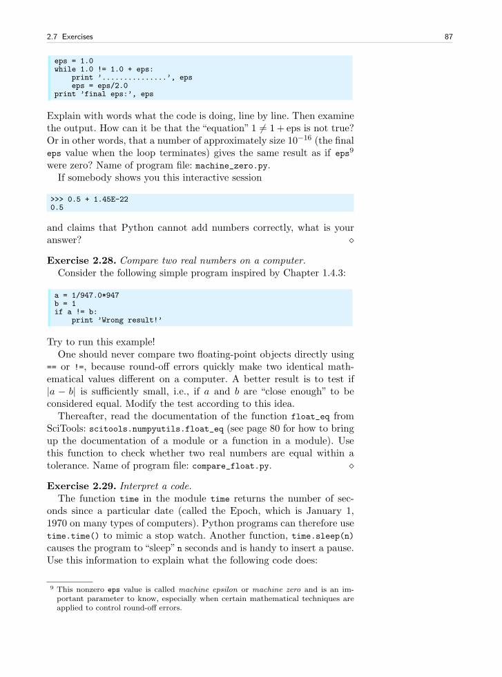
2.7 Exercises 87

eps = 1.0while 1.0 != 1.0 + eps:

print ’...............’, epseps = eps/2.0

print ’final eps:’, eps

Explain with words what the code is doing, line by line. Then examinethe output. How can it be that the “equation” 1 6= 1+ eps is not true?Or in other words, that a number of approximately size 10−16 (the finaleps value when the loop terminates) gives the same result as if eps9

were zero? Name of program file: machine_zero.py.If somebody shows you this interactive session

>>> 0.5 + 1.45E-220.5

and claims that Python cannot add numbers correctly, what is youranswer? ⋄

Exercise 2.28. Compare two real numbers on a computer.Consider the following simple program inspired by Chapter 1.4.3:

a = 1/947.0*947b = 1if a != b:

print ’Wrong result!’

Try to run this example!One should never compare two floating-point objects directly using

== or !=, because round-off errors quickly make two identical math-ematical values different on a computer. A better result is to test if|a − b| is sufficiently small, i.e., if a and b are “close enough” to beconsidered equal. Modify the test according to this idea.

Thereafter, read the documentation of the function float_eq fromSciTools: scitools.numpyutils.float_eq (see page 80 for how to bringup the documentation of a module or a function in a module). Usethis function to check whether two real numbers are equal within atolerance. Name of program file: compare_float.py. ⋄

Exercise 2.29. Interpret a code.The function time in the module time returns the number of sec-

onds since a particular date (called the Epoch, which is January 1,1970 on many types of computers). Python programs can therefore usetime.time() to mimic a stop watch. Another function, time.sleep(n)causes the program to “sleep” n seconds and is handy to insert a pause.Use this information to explain what the following code does:

9 This nonzero eps value is called machine epsilon or machine zero and is an im-portant parameter to know, especially when certain mathematical techniques areapplied to control round-off errors.

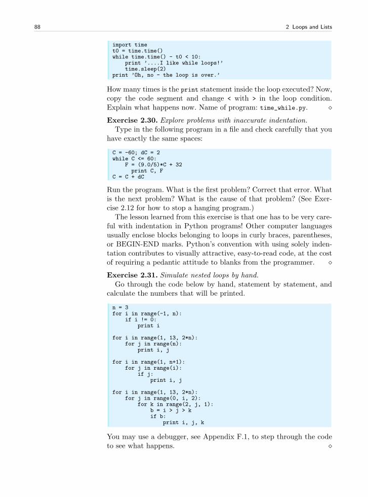
88 2 Loops and Lists

import timet0 = time.time()while time.time() - t0 < 10:

print ’....I like while loops!’time.sleep(2)

print ’Oh, no - the loop is over.’

How many times is the print statement inside the loop executed? Now,copy the code segment and change < with > in the loop condition.Explain what happens now. Name of program: time_while.py. ⋄Exercise 2.30. Explore problems with inaccurate indentation.

Type in the following program in a file and check carefully that youhave exactly the same spaces:

C = -60; dC = 2while C <= 60:

F = (9.0/5)*C + 32print C, F

C = C + dC

Run the program. What is the first problem? Correct that error. Whatis the next problem? What is the cause of that problem? (See Exer-cise 2.12 for how to stop a hanging program.)

The lesson learned from this exercise is that one has to be very care-ful with indentation in Python programs! Other computer languagesusually enclose blocks belonging to loops in curly braces, parentheses,or BEGIN-END marks. Python’s convention with using solely inden-tation contributes to visually attractive, easy-to-read code, at the costof requiring a pedantic attitude to blanks from the programmer. ⋄Exercise 2.31. Simulate nested loops by hand.

Go through the code below by hand, statement by statement, andcalculate the numbers that will be printed.

n = 3for i in range(-1, n):

if i != 0:print i

for i in range(1, 13, 2*n):for j in range(n):

print i, j

for i in range(1, n+1):for j in range(i):

if j:print i, j

for i in range(1, 13, 2*n):for j in range(0, i, 2):

for k in range(2, j, 1):b = i > j > kif b:

print i, j, k

You may use a debugger, see Appendix F.1, to step through the codeto see what happens. ⋄

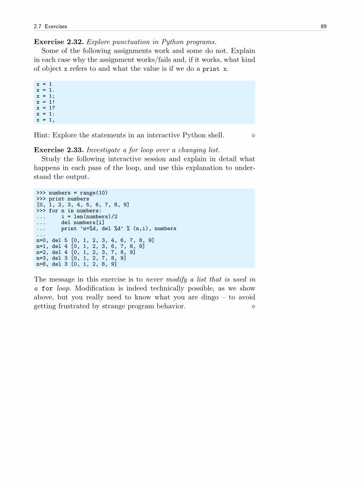
2.7 Exercises 89

Exercise 2.32. Explore punctuation in Python programs.Some of the following assignments work and some do not. Explain

in each case why the assignment works/fails and, if it works, what kindof object x refers to and what the value is if we do a print x.

x = 1x = 1.x = 1;x = 1!x = 1?x = 1:x = 1,

Hint: Explore the statements in an interactive Python shell. ⋄

Exercise 2.33. Investigate a for loop over a changing list.Study the following interactive session and explain in detail what

happens in each pass of the loop, and use this explanation to under-stand the output.

>>> numbers = range(10)>>> print numbers[0, 1, 2, 3, 4, 5, 6, 7, 8, 9]>>> for n in numbers:... i = len(numbers)/2... del numbers[i]... print ’n=%d, del %d’ % (n,i), numbers...n=0, del 5 [0, 1, 2, 3, 4, 6, 7, 8, 9]n=1, del 4 [0, 1, 2, 3, 6, 7, 8, 9]n=2, del 4 [0, 1, 2, 3, 7, 8, 9]n=3, del 3 [0, 1, 2, 7, 8, 9]n=8, del 3 [0, 1, 2, 8, 9]

The message in this exercise is to never modify a list that is used ina for loop. Modification is indeed technically possible, as we showabove, but you really need to know what you are dingo – to avoidgetting frustrated by strange program behavior. ⋄

Functions and Branching 3

This chapter introduces two fundamental and extremely useful con-cepts in programming: user-defined functions and branching of pro-gram flow, the latter often referred to as “if tests”. The programsassociated with the chapter are found in src/funcif.

3.1 Functions

In a computer language like Python, the term function means morethan just a mathematical function. A function is a collection of state-ments that you can execute wherever and whenever you want in theprogram. You may send variables to the function to influence what isgetting computed by statements in the function, and the function mayreturn new objects. In particular, functions help to avoid duplicatingcode snippets by putting all similar snippets in a common place. Thisstrategy saves typing and makes it easier to change the program later.Functions are also often used to just split a long program into smaller,more managable pieces, so the program and your own thinking about itbecome clearer. Python comes with lots of functions (math.sqrt, range,and len are examples we have met so far). This section outlines howyou can define your own functions.

3.1.1 Functions of One Variable

Let us start with making a Python function that evaluates a math-ematical function, more precisely the function F (C) defined in (1.2):F (C) = 9

5C + 32. The corresponding Python function must take C asargument and return the value F (C). The code for this looks like

91

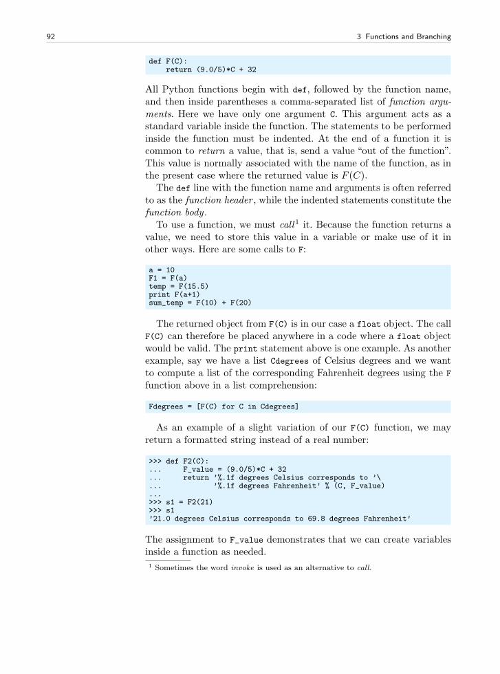
92 3 Functions and Branching

def F(C):return (9.0/5)*C + 32

All Python functions begin with def, followed by the function name,and then inside parentheses a comma-separated list of function argu-ments. Here we have only one argument C. This argument acts as astandard variable inside the function. The statements to be performedinside the function must be indented. At the end of a function it iscommon to return a value, that is, send a value “out of the function”.This value is normally associated with the name of the function, as inthe present case where the returned value is F (C).

The def line with the function name and arguments is often referredto as the function header , while the indented statements constitute thefunction body .

To use a function, we must call1 it. Because the function returns avalue, we need to store this value in a variable or make use of it inother ways. Here are some calls to F:

a = 10F1 = F(a)temp = F(15.5)print F(a+1)sum_temp = F(10) + F(20)

The returned object from F(C) is in our case a float object. The callF(C) can therefore be placed anywhere in a code where a float objectwould be valid. The print statement above is one example. As anotherexample, say we have a list Cdegrees of Celsius degrees and we wantto compute a list of the corresponding Fahrenheit degrees using the F

function above in a list comprehension:

Fdegrees = [F(C) for C in Cdegrees]

As an example of a slight variation of our F(C) function, we mayreturn a formatted string instead of a real number:

>>> def F2(C):... F_value = (9.0/5)*C + 32... return ’%.1f degrees Celsius corresponds to ’\... ’%.1f degrees Fahrenheit’ % (C, F_value)...>>> s1 = F2(21)>>> s1’21.0 degrees Celsius corresponds to 69.8 degrees Fahrenheit’

The assignment to F_value demonstrates that we can create variablesinside a function as needed.

1 Sometimes the word invoke is used as an alternative to call.

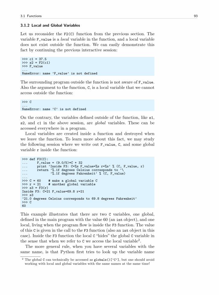
3.1 Functions 93

3.1.2 Local and Global Variables

Let us reconsider the F2(C) function from the previous section. Thevariable F_value is a local variable in the function, and a local variabledoes not exist outside the function. We can easily demonstrate thisfact by continuing the previous interactive session:

>>> c1 = 37.5>>> s2 = F2(c1)>>> F_value...NameError: name ’F_value’ is not defined

The surrounding program outside the function is not aware of F_value.Also the argument to the function, C, is a local variable that we cannotaccess outside the function:

>>> C...NameError: name ’C’ is not defined

On the contrary, the variables defined outside of the function, like s1,s2, and c1 in the above session, are global variables. These can beaccessed everywhere in a program.

Local variables are created inside a function and destroyed whenwe leave the function. To learn more about this fact, we may studythe following session where we write out F_value, C, and some globalvariable r inside the function:

>>> def F3(C):... F_value = (9.0/5)*C + 32... print ’Inside F3: C=%s F_value=%s r=%s’ % (C, F_value, r)... return ’%.1f degrees Celsius corresponds to ’\... ’%.1f degrees Fahrenheit’ % (C, F_value)...>>> C = 60 # make a global variable C>>> r = 21 # another global variable>>> s3 = F3(r)Inside F3: C=21 F_value=69.8 r=21>>> s3’21.0 degrees Celsius corresponds to 69.8 degrees Fahrenheit’>>> C60

This example illustrates that there are two C variables, one global,defined in the main program with the value 60 (an int object), and onelocal, living when the program flow is inside the F3 function. The valueof this C is given in the call to the F3 function (also an int object in thiscase). Inside the F3 function the local C “hides” the global C variable inthe sense that when we refer to C we access the local variable2.

The more general rule, when you have several variables with thesame name, is that Python first tries to look up the variable name

2 The global C can technically be accessed as globals()[’C’], but one should avoidworking with local and global variables with the same names at the same time!

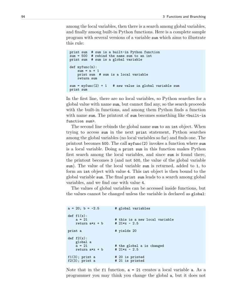
94 3 Functions and Branching

among the local variables, then there is a search among global variables,and finally among built-in Python functions. Here is a complete sampleprogram with several versions of a variable sum which aims to illustratethis rule:

print sum # sum is a built-in Python functionsum = 500 # rebind the name sum to an intprint sum # sum is a global variable

def myfunc(n):sum = n + 1print sum # sum is a local variablereturn sum

sum = myfunc(2) + 1 # new value in global variable sumprint sum

In the first line, there are no local variables, so Python searches for aglobal value with name sum, but cannot find any, so the search proceedswith the built-in functions, and among them Python finds a functionwith name sum. The printout of sum becomes something like <built-in

function sum>.The second line rebinds the global name sum to an int object. When

trying to access sum in the next print statement, Python searchesamong the global variables (no local variables so far) and finds one. Theprintout becomes 500. The call myfunc(2) invokes a function where sum

is a local variable. Doing a print sum in this function makes Pythonfirst search among the local variables, and since sum is found there,the printout becomes 3 (and not 500, the value of the global variablesum). The value of the local variable sum is returned, added to 1, toform an int object with value 4. This int object is then bound to theglobal variable sum. The final print sum leads to a search among globalvariables, and we find one with value 4.

The values of global variables can be accessed inside functions, butthe values cannot be changed unless the variable is declared as global:

a = 20; b = -2.5 # global variables

def f1(x):a = 21 # this is a new local variablereturn a*x + b # 21*x - 2.5

print a # yields 20

def f2(x):global aa = 21 # the global a is changedreturn a*x + b # 21*x - 2.5

f1(3); print a # 20 is printedf2(3); print a # 21 is printed

Note that in the f1 function, a = 21 creates a local variable a. As aprogrammer you may think you change the global a, but it does not

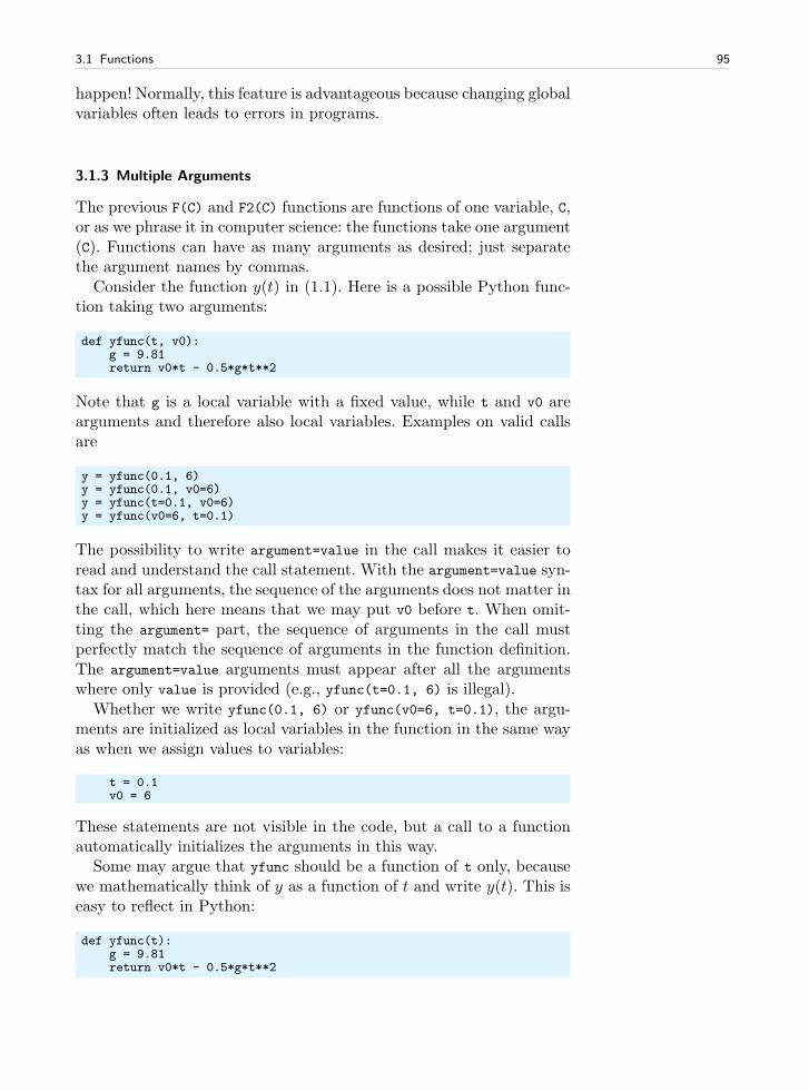
3.1 Functions 95

happen! Normally, this feature is advantageous because changing globalvariables often leads to errors in programs.

3.1.3 Multiple Arguments

The previous F(C) and F2(C) functions are functions of one variable, C,or as we phrase it in computer science: the functions take one argument(C). Functions can have as many arguments as desired; just separatethe argument names by commas.

Consider the function y(t) in (1.1). Here is a possible Python func-tion taking two arguments:

def yfunc(t, v0):g = 9.81return v0*t - 0.5*g*t**2

Note that g is a local variable with a fixed value, while t and v0 arearguments and therefore also local variables. Examples on valid callsare

y = yfunc(0.1, 6)y = yfunc(0.1, v0=6)y = yfunc(t=0.1, v0=6)y = yfunc(v0=6, t=0.1)

The possibility to write argument=value in the call makes it easier toread and understand the call statement. With the argument=value syn-tax for all arguments, the sequence of the arguments does not matter inthe call, which here means that we may put v0 before t. When omit-ting the argument= part, the sequence of arguments in the call mustperfectly match the sequence of arguments in the function definition.The argument=value arguments must appear after all the argumentswhere only value is provided (e.g., yfunc(t=0.1, 6) is illegal).

Whether we write yfunc(0.1, 6) or yfunc(v0=6, t=0.1), the argu-ments are initialized as local variables in the function in the same wayas when we assign values to variables:

t = 0.1v0 = 6

These statements are not visible in the code, but a call to a functionautomatically initializes the arguments in this way.

Some may argue that yfunc should be a function of t only, becausewe mathematically think of y as a function of t and write y(t). This iseasy to reflect in Python:

def yfunc(t):g = 9.81return v0*t - 0.5*g*t**2

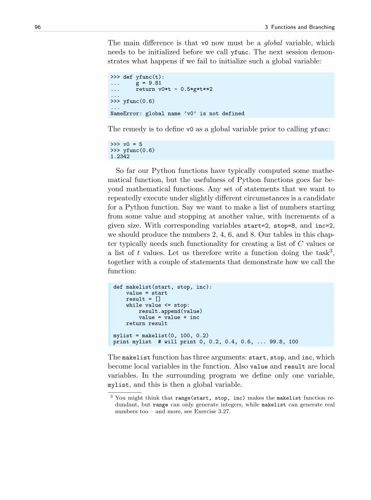
96 3 Functions and Branching

The main difference is that v0 now must be a global variable, whichneeds to be initialized before we call yfunc. The next session demon-strates what happens if we fail to initialize such a global variable:

>>> def yfunc(t):... g = 9.81... return v0*t - 0.5*g*t**2...>>> yfunc(0.6)...NameError: global name ’v0’ is not defined

The remedy is to define v0 as a global variable prior to calling yfunc:

>>> v0 = 5>>> yfunc(0.6)1.2342

So far our Python functions have typically computed some mathe-matical function, but the usefulness of Python functions goes far be-yond mathematical functions. Any set of statements that we want torepeatedly execute under slightly different circumstances is a candidatefor a Python function. Say we want to make a list of numbers startingfrom some value and stopping at another value, with increments of agiven size. With corresponding variables start=2, stop=8, and inc=2,we should produce the numbers 2, 4, 6, and 8. Our tables in this chap-ter typically needs such functionality for creating a list of C values ora list of t values. Let us therefore write a function doing the task3,together with a couple of statements that demonstrate how we call thefunction:

def makelist(start, stop, inc):value = startresult = []while value <= stop:

result.append(value)value = value + inc

return result

mylist = makelist(0, 100, 0.2)print mylist # will print 0, 0.2, 0.4, 0.6, ... 99.8, 100

The makelist function has three arguments: start, stop, and inc, whichbecome local variables in the function. Also value and result are localvariables. In the surrounding program we define only one variable,mylist, and this is then a global variable.

3 You might think that range(start, stop, inc) makes the makelist function re-dundant, but range can only generate integers, while makelist can generate realnumbers too – and more, see Exercise 3.27.

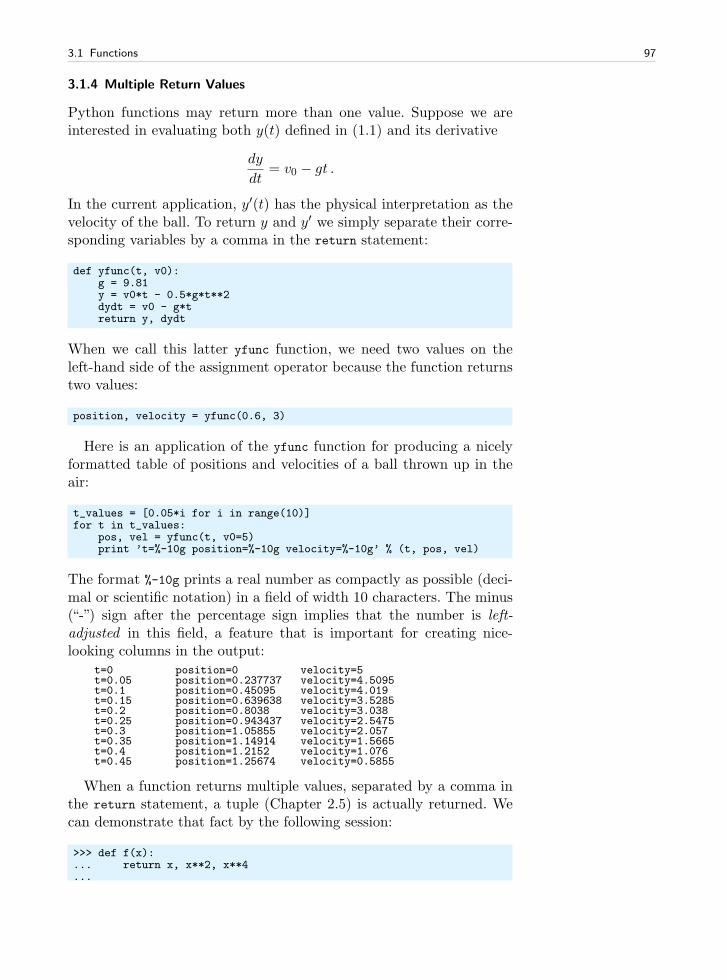
3.1 Functions 97

3.1.4 Multiple Return Values

Python functions may return more than one value. Suppose we areinterested in evaluating both y(t) defined in (1.1) and its derivative

dy

dt= v0 − gt .

In the current application, y′(t) has the physical interpretation as thevelocity of the ball. To return y and y′ we simply separate their corre-sponding variables by a comma in the return statement:

def yfunc(t, v0):g = 9.81y = v0*t - 0.5*g*t**2dydt = v0 - g*treturn y, dydt

When we call this latter yfunc function, we need two values on theleft-hand side of the assignment operator because the function returnstwo values:

position, velocity = yfunc(0.6, 3)

Here is an application of the yfunc function for producing a nicelyformatted table of positions and velocities of a ball thrown up in theair:

t_values = [0.05*i for i in range(10)]for t in t_values:

pos, vel = yfunc(t, v0=5)print ’t=%-10g position=%-10g velocity=%-10g’ % (t, pos, vel)

The format %-10g prints a real number as compactly as possible (deci-mal or scientific notation) in a field of width 10 characters. The minus(“-”) sign after the percentage sign implies that the number is left-adjusted in this field, a feature that is important for creating nice-looking columns in the output:

t=0 position=0 velocity=5t=0.05 position=0.237737 velocity=4.5095t=0.1 position=0.45095 velocity=4.019t=0.15 position=0.639638 velocity=3.5285t=0.2 position=0.8038 velocity=3.038t=0.25 position=0.943437 velocity=2.5475t=0.3 position=1.05855 velocity=2.057t=0.35 position=1.14914 velocity=1.5665t=0.4 position=1.2152 velocity=1.076t=0.45 position=1.25674 velocity=0.5855

When a function returns multiple values, separated by a comma inthe return statement, a tuple (Chapter 2.5) is actually returned. Wecan demonstrate that fact by the following session:

>>> def f(x):... return x, x**2, x**4...

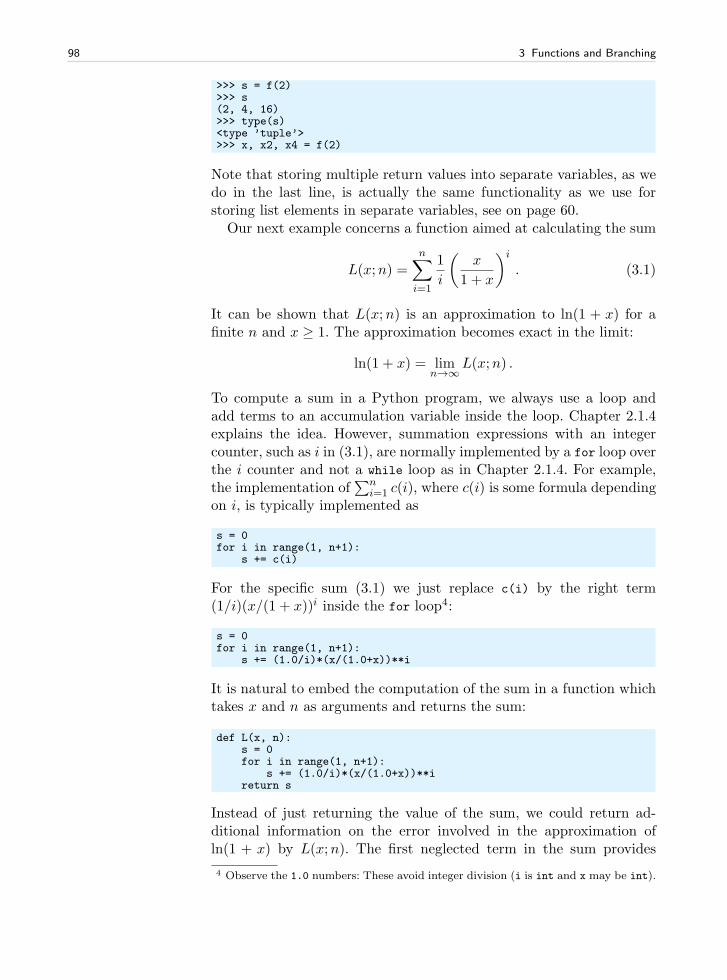
98 3 Functions and Branching

>>> s = f(2)>>> s(2, 4, 16)>>> type(s)<type ’tuple’>>>> x, x2, x4 = f(2)

Note that storing multiple return values into separate variables, as wedo in the last line, is actually the same functionality as we use forstoring list elements in separate variables, see on page 60.

Our next example concerns a function aimed at calculating the sum

L(x;n) =n∑

i=1

1

i

(

x

1 + x

)i

. (3.1)

It can be shown that L(x;n) is an approximation to ln(1 + x) for afinite n and x ≥ 1. The approximation becomes exact in the limit:

ln(1 + x) = limn→∞

L(x;n) .

To compute a sum in a Python program, we always use a loop andadd terms to an accumulation variable inside the loop. Chapter 2.1.4explains the idea. However, summation expressions with an integercounter, such as i in (3.1), are normally implemented by a for loop overthe i counter and not a while loop as in Chapter 2.1.4. For example,the implementation of

∑ni=1 c(i), where c(i) is some formula depending

on i, is typically implemented as

s = 0for i in range(1, n+1):

s += c(i)

For the specific sum (3.1) we just replace c(i) by the right term(1/i)(x/(1 + x))i inside the for loop4:

s = 0for i in range(1, n+1):

s += (1.0/i)*(x/(1.0+x))**i

It is natural to embed the computation of the sum in a function whichtakes x and n as arguments and returns the sum:

def L(x, n):s = 0for i in range(1, n+1):

s += (1.0/i)*(x/(1.0+x))**ireturn s

Instead of just returning the value of the sum, we could return ad-ditional information on the error involved in the approximation ofln(1 + x) by L(x;n). The first neglected term in the sum provides

4 Observe the 1.0 numbers: These avoid integer division (i is int and x may be int).

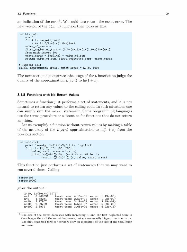
3.1 Functions 99

an indication of the error5. We could also return the exact error. Thenew version of the L(x, n) function then looks as this:

def L(x, n):s = 0for i in range(1, n+1):

s += (1.0/i)*(x/(1.0+x))**ivalue_of_sum = sfirst_neglected_term = (1.0/(n+1))*(x/(1.0+x))**(n+1)from math import logexact_error = log(1+x) - value_of_sumreturn value_of_sum, first_neglected_term, exact_error

# Typical callvalue, approximate_error, exact_error = L2(x, 100)

The next section demonstrates the usage of the L function to judge thequality of the approximation L(x;n) to ln(1 + x).

3.1.5 Functions with No Return Values

Sometimes a function just performs a set of statements, and it is notnatural to return any values to the calling code. In such situations onecan simply skip the return statement. Some programming languagesuse the terms procedure or subroutine for functions that do not returnanything.

Let us exemplify a function without return values by making a tableof the accuracy of the L(x;n) approximation to ln(1 + x) from theprevious section:

def table(x):print ’\nx=%g, ln(1+x)=%g’ % (x, log(1+x))for n in [1, 2, 10, 100, 500]:

value, next, error = L(x, n)print ’n=%-4d %-10g (next term: %8.2e ’\

’error: %8.2e)’ % (n, value, next, error)

This function just performs a set of statements that we may want torun several times. Calling

table(10)table(1000)

gives the output :

x=10, ln(1+x)=2.3979n=1 0.909091 (next term: 4.13e-01 error: 1.49e+00)n=2 1.32231 (next term: 2.50e-01 error: 1.08e+00)n=10 2.17907 (next term: 3.19e-02 error: 2.19e-01)n=100 2.39789 (next term: 6.53e-07 error: 6.59e-06)n=500 2.3979 (next term: 3.65e-24 error: 6.22e-15)

5 The size of the terms decreases with increasing n, and the first neglected term isthen bigger than all the remaining terms, but not necessarily bigger than their sum.The first neglected term is therefore only an indication of the size of the total errorwe make.

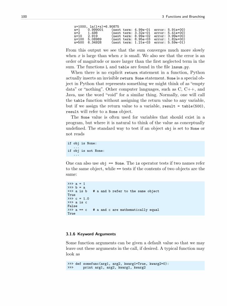
100 3 Functions and Branching

x=1000, ln(1+x)=6.90875n=1 0.999001 (next term: 4.99e-01 error: 5.91e+00)n=2 1.498 (next term: 3.32e-01 error: 5.41e+00)n=10 2.919 (next term: 8.99e-02 error: 3.99e+00)n=100 5.08989 (next term: 8.95e-03 error: 1.82e+00)n=500 6.34928 (next term: 1.21e-03 error: 5.59e-01)

From this output we see that the sum converges much more slowlywhen x is large than when x is small. We also see that the error is anorder of magnitude or more larger than the first neglected term in thesum. The functions L and table are found in the file lnsum.py.

When there is no explicit return statement in a function, Pythonactually inserts an invisible return None statement. None is a special ob-ject in Python that represents something we might think of as “emptydata” or “nothing”. Other computer languages, such as C, C++, andJava, use the word “void” for a similar thing. Normally, one will callthe table function without assigning the return value to any variable,but if we assign the return value to a variable, result = table(500),result will refer to a None object.

The None value is often used for variables that should exist in aprogram, but where it is natural to think of the value as conceptuallyundefined. The standard way to test if an object obj is set to None ornot reads

if obj is None:...

if obj is not None:...

One can also use obj == None. The is operator tests if two names referto the same object, while == tests if the contents of two objects are thesame:

>>> a = 1>>> b = a>>> a is b # a and b refer to the same objectTrue>>> c = 1.0>>> a is cFalse>>> a == c # a and c are mathematically equalTrue

3.1.6 Keyword Arguments

Some function arguments can be given a default value so that we mayleave out these arguments in the call, if desired. A typical function maylook as

>>> def somefunc(arg1, arg2, kwarg1=True, kwarg2=0):>>> print arg1, arg2, kwarg1, kwarg2

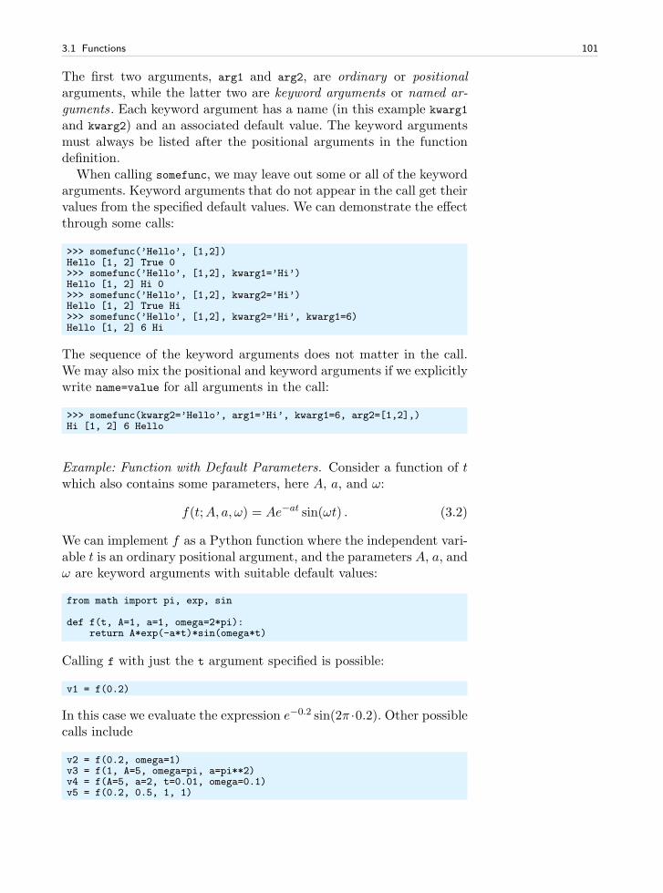
3.1 Functions 101

The first two arguments, arg1 and arg2, are ordinary or positionalarguments, while the latter two are keyword arguments or named ar-guments . Each keyword argument has a name (in this example kwarg1

and kwarg2) and an associated default value. The keyword argumentsmust always be listed after the positional arguments in the functiondefinition.

When calling somefunc, we may leave out some or all of the keywordarguments. Keyword arguments that do not appear in the call get theirvalues from the specified default values. We can demonstrate the effectthrough some calls:

>>> somefunc(’Hello’, [1,2])Hello [1, 2] True 0>>> somefunc(’Hello’, [1,2], kwarg1=’Hi’)Hello [1, 2] Hi 0>>> somefunc(’Hello’, [1,2], kwarg2=’Hi’)Hello [1, 2] True Hi>>> somefunc(’Hello’, [1,2], kwarg2=’Hi’, kwarg1=6)Hello [1, 2] 6 Hi

The sequence of the keyword arguments does not matter in the call.We may also mix the positional and keyword arguments if we explicitlywrite name=value for all arguments in the call:

>>> somefunc(kwarg2=’Hello’, arg1=’Hi’, kwarg1=6, arg2=[1,2],)Hi [1, 2] 6 Hello

Example: Function with Default Parameters. Consider a function of twhich also contains some parameters, here A, a, and ω:

f(t;A, a, ω) = Ae−at sin(ωt) . (3.2)

We can implement f as a Python function where the independent vari-able t is an ordinary positional argument, and the parameters A, a, andω are keyword arguments with suitable default values:

from math import pi, exp, sin

def f(t, A=1, a=1, omega=2*pi):return A*exp(-a*t)*sin(omega*t)

Calling f with just the t argument specified is possible:

v1 = f(0.2)

In this case we evaluate the expression e−0.2 sin(2π ·0.2). Other possiblecalls include

v2 = f(0.2, omega=1)v3 = f(1, A=5, omega=pi, a=pi**2)v4 = f(A=5, a=2, t=0.01, omega=0.1)v5 = f(0.2, 0.5, 1, 1)

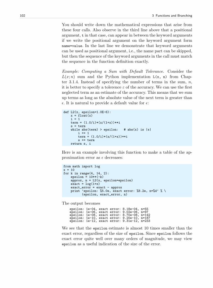
102 3 Functions and Branching

You should write down the mathematical expressions that arise fromthese four calls. Also observe in the third line above that a positionalargument, t in that case, can appear in between the keyword argumentsif we write the positional argument on the keyword argument formname=value. In the last line we demonstrate that keyword argumentscan be used as positional argument, i.e., the name part can be skipped,but then the sequence of the keyword arguments in the call must matchthe sequence in the function definition exactly.

Example: Computing a Sum with Default Tolerance. Consider theL(x;n) sum and the Python implementation L(x, n) from Chap-ter 3.1.4. Instead of specifying the number of terms in the sum, n,it is better to specify a tolerence ε of the accuracy. We can use the firstneglected term as an estimate of the accuracy. This means that we sumup terms as long as the absolute value of the next term is greater thanǫ. It is natural to provide a default value for ǫ:

def L2(x, epsilon=1.0E-6):x = float(x)i = 1term = (1.0/i)*(x/(1+x))**is = termwhile abs(term) > epsilon: # abs(x) is |x|

i += 1term = (1.0/i)*(x/(1+x))**is += term

return s, i

Here is an example involving this function to make a table of the ap-proximation error as ǫ decreases:

from math import logx = 10for k in range(4, 14, 2):

epsilon = 10**(-k)approx, n = L2(x, epsilon=epsilon)exact = log(1+x)exact_error = exact - approxprint ’epsilon: %5.0e, exact error: %8.2e, n=%d’ % \

(epsilon, exact_error, n)

The output becomesepsilon: 1e-04, exact error: 8.18e-04, n=55epsilon: 1e-06, exact error: 9.02e-06, n=97epsilon: 1e-08, exact error: 8.70e-08, n=142epsilon: 1e-10, exact error: 9.20e-10, n=187epsilon: 1e-12, exact error: 9.31e-12, n=233

We see that the epsilon estimate is almost 10 times smaller than theexact error, regardless of the size of epsilon. Since epsilon follows theexact error quite well over many orders of magnitude, we may viewepsilon as a useful indication of the size of the error.

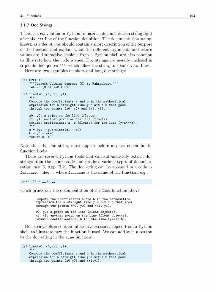
3.1 Functions 103

3.1.7 Doc Strings

There is a convention in Python to insert a documentation string rightafter the def line of the function definition. The documentation string,known as a doc string, should contain a short description of the purposeof the function and explain what the different arguments and returnvalues are. Interactive sessions from a Python shell are also commonto illustrate how the code is used. Doc strings are usually enclosed intriple double quotes """, which allow the string to span several lines.

Here are two examples on short and long doc strings:

def C2F(C):"""Convert Celsius degrees (C) to Fahrenheit."""return (9.0/5)*C + 32

def line(x0, y0, x1, y1):"""Compute the coefficients a and b in the mathematicalexpression for a straight line y = a*x + b that goesthrough two points (x0, y0) and (x1, y1).

x0, y0: a point on the line (floats).x1, y1: another point on the line (floats).return: coefficients a, b (floats) for the line (y=a*x+b)."""a = (y1 - y0)/float(x1 - x0)b = y0 - a*x0return a, b

Note that the doc string must appear before any statement in thefunction body.

There are several Python tools that can automatically extract docstrings from the source code and produce various types of documen-tation, see [5, App. B.2]. The doc string can be accessed in a code asfuncname.__doc__, where funcname is the name of the function, e.g.,

print line.__doc__

which prints out the documentation of the line function above:

Compute the coefficients a and b in the mathematicalexpression for a straight line y = a*x + b that goesthrough two points (x0, y0) and (x1, y1).

x0, y0: a point on the line (float objects).x1, y1: another point on the line (float objects).return: coefficients a, b for the line (y=a*x+b).

Doc strings often contain interactive sessions, copied from a Pythonshell, to illustrate how the function is used. We can add such a sessionto the doc string in the line function:

def line(x0, y0, x1, y1):"""Compute the coefficients a and b in the mathematicalexpression for a straight line y = a*x + b that goesthrough two points (x0,y0) and (x1,y1).

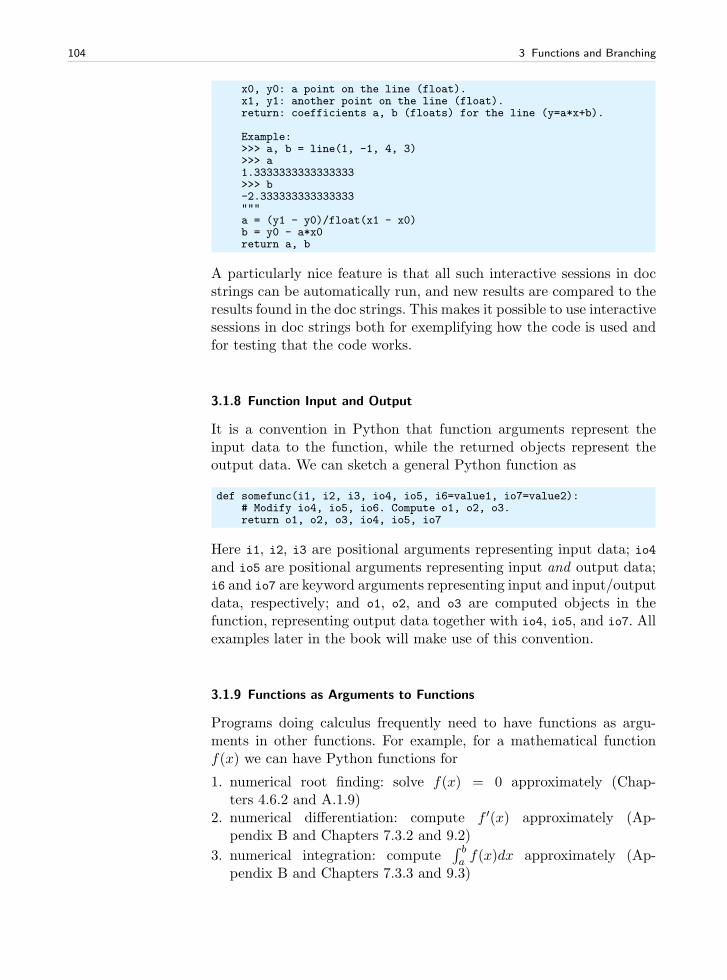
104 3 Functions and Branching

x0, y0: a point on the line (float).x1, y1: another point on the line (float).return: coefficients a, b (floats) for the line (y=a*x+b).

Example:>>> a, b = line(1, -1, 4, 3)>>> a1.3333333333333333>>> b-2.333333333333333"""a = (y1 - y0)/float(x1 - x0)b = y0 - a*x0return a, b

A particularly nice feature is that all such interactive sessions in docstrings can be automatically run, and new results are compared to theresults found in the doc strings. This makes it possible to use interactivesessions in doc strings both for exemplifying how the code is used andfor testing that the code works.

3.1.8 Function Input and Output

It is a convention in Python that function arguments represent theinput data to the function, while the returned objects represent theoutput data. We can sketch a general Python function as

def somefunc(i1, i2, i3, io4, io5, i6=value1, io7=value2):# Modify io4, io5, io6. Compute o1, o2, o3.return o1, o2, o3, io4, io5, io7

Here i1, i2, i3 are positional arguments representing input data; io4and io5 are positional arguments representing input and output data;i6 and io7 are keyword arguments representing input and input/outputdata, respectively; and o1, o2, and o3 are computed objects in thefunction, representing output data together with io4, io5, and io7. Allexamples later in the book will make use of this convention.

3.1.9 Functions as Arguments to Functions

Programs doing calculus frequently need to have functions as argu-ments in other functions. For example, for a mathematical functionf(x) we can have Python functions for

1. numerical root finding: solve f(x) = 0 approximately (Chap-ters 4.6.2 and A.1.9)

2. numerical differentiation: compute f ′(x) approximately (Ap-pendix B and Chapters 7.3.2 and 9.2)

3. numerical integration: compute∫ ba f(x)dx approximately (Ap-

pendix B and Chapters 7.3.3 and 9.3)

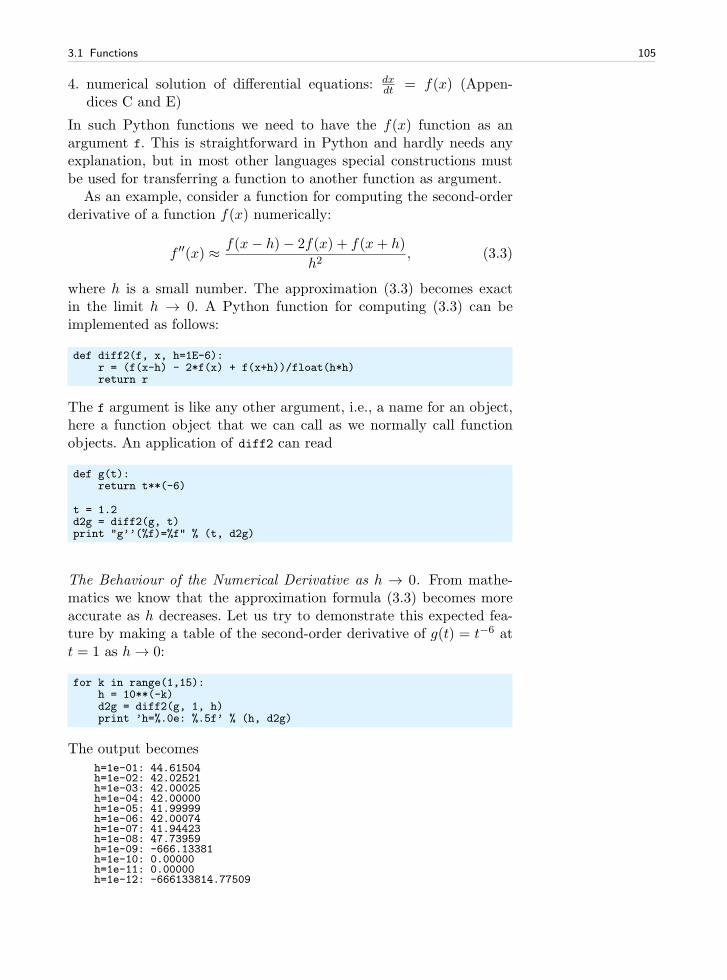
3.1 Functions 105

4. numerical solution of differential equations: dxdt = f(x) (Appen-

dices C and E)

In such Python functions we need to have the f(x) function as anargument f. This is straightforward in Python and hardly needs anyexplanation, but in most other languages special constructions mustbe used for transferring a function to another function as argument.

As an example, consider a function for computing the second-orderderivative of a function f(x) numerically:

f ′′(x) ≈ f(x− h)− 2f(x) + f(x+ h)

h2, (3.3)

where h is a small number. The approximation (3.3) becomes exactin the limit h → 0. A Python function for computing (3.3) can beimplemented as follows:

def diff2(f, x, h=1E-6):r = (f(x-h) - 2*f(x) + f(x+h))/float(h*h)return r

The f argument is like any other argument, i.e., a name for an object,here a function object that we can call as we normally call functionobjects. An application of diff2 can read

def g(t):return t**(-6)

t = 1.2d2g = diff2(g, t)print "g’’(%f)=%f" % (t, d2g)

The Behaviour of the Numerical Derivative as h → 0. From mathe-matics we know that the approximation formula (3.3) becomes moreaccurate as h decreases. Let us try to demonstrate this expected fea-ture by making a table of the second-order derivative of g(t) = t−6 att = 1 as h→ 0:

for k in range(1,15):h = 10**(-k)d2g = diff2(g, 1, h)print ’h=%.0e: %.5f’ % (h, d2g)

The output becomesh=1e-01: 44.61504h=1e-02: 42.02521h=1e-03: 42.00025h=1e-04: 42.00000h=1e-05: 41.99999h=1e-06: 42.00074h=1e-07: 41.94423h=1e-08: 47.73959h=1e-09: -666.13381h=1e-10: 0.00000h=1e-11: 0.00000h=1e-12: -666133814.77509

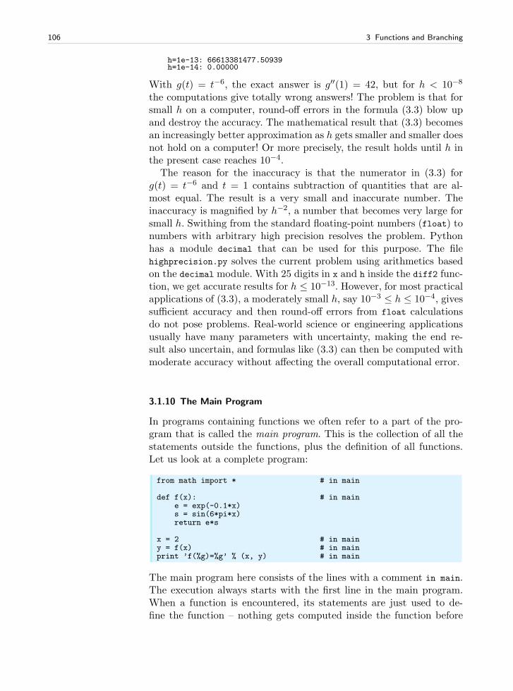
106 3 Functions and Branching

h=1e-13: 66613381477.50939h=1e-14: 0.00000

With g(t) = t−6, the exact answer is g′′(1) = 42, but for h < 10−8

the computations give totally wrong answers! The problem is that forsmall h on a computer, round-off errors in the formula (3.3) blow upand destroy the accuracy. The mathematical result that (3.3) becomesan increasingly better approximation as h gets smaller and smaller doesnot hold on a computer! Or more precisely, the result holds until h inthe present case reaches 10−4.

The reason for the inaccuracy is that the numerator in (3.3) forg(t) = t−6 and t = 1 contains subtraction of quantities that are al-most equal. The result is a very small and inaccurate number. Theinaccuracy is magnified by h−2, a number that becomes very large forsmall h. Swithing from the standard floating-point numbers (float) tonumbers with arbitrary high precision resolves the problem. Pythonhas a module decimal that can be used for this purpose. The filehighprecision.py solves the current problem using arithmetics basedon the decimal module. With 25 digits in x and h inside the diff2 func-tion, we get accurate results for h ≤ 10−13. However, for most practicalapplications of (3.3), a moderately small h, say 10−3 ≤ h ≤ 10−4, givessufficient accuracy and then round-off errors from float calculationsdo not pose problems. Real-world science or engineering applicationsusually have many parameters with uncertainty, making the end re-sult also uncertain, and formulas like (3.3) can then be computed withmoderate accuracy without affecting the overall computational error.

3.1.10 The Main Program

In programs containing functions we often refer to a part of the pro-gram that is called the main program. This is the collection of all thestatements outside the functions, plus the definition of all functions.Let us look at a complete program:

from math import * # in main

def f(x): # in maine = exp(-0.1*x)s = sin(6*pi*x)return e*s

x = 2 # in mainy = f(x) # in mainprint ’f(%g)=%g’ % (x, y) # in main

The main program here consists of the lines with a comment in main.The execution always starts with the first line in the main program.When a function is encountered, its statements are just used to de-fine the function – nothing gets computed inside the function before

3.1 Functions 107

we explicitly call the function, either from the main program or fromanother function. All variables initialized in the main program becomeglobal variables (see Chapter 3.1.2).

The program flow in the program above goes as follows:

1. Import functions from the math module,2. define a function f(x),3. define x,4. call f and execute the function body,5. define y as the value returned from f,6. print the string.

In point 4, we jump to the f function and execute the statement in-side that function for the first time. Then we jump back to the mainprogram and assign the float object returned from f to the y variable.

Readers who are uncertain about the program flow and the jumpsbetween the main program and functions should learn to use a debug-ger, see Appendix F.1.

3.1.11 Lambda Functions

There is a quick one-line construction of functions that is sometimesconvenient:

f = lambda x: x**2 + 4

This so-called lambda function is equivalent to writing

def f(x):return x**2 + 4

In general,

def g(arg1, arg2, arg3, ...):return expression

can be written as

g = lambda arg1, arg2, arg3, ...: expression

Lambda functions are usually used to quickly define a function asargument to another function. Consider, as an example, the diff2 func-tion from Chapter 3.1.9. In the example from that chapter we want todifferentiate g(t) = t−6 twice and first make a Python function g(t)

and then send this g to diff2 as argument. We can skip the step withdefining the g(t) function and instead insert a lambda function as thef argument in the call to diff2:

108 3 Functions and Branching

d2 = diff2(lambda t: t**(-6), 1, h=1E-4)

Because lambda functions can be defined “on the fly” and thereby savetyping of a separate function with def and an intended block, lambdafunctions are popular among many programmers.

Lambda functions may also take keyword arguments. For example,

d2 = diff2(lambda t, A=1, a=0.5: -a*2*t*A*exp(-a*t**2), 1.2)

3.2 Branching

The flow of computer programs often needs to branch. That is, if acondition is met, we do one thing, and if not, we do another thing. Asimple example is a function defined as

f(x) =

sin x, 0 ≤ x ≤ π0, otherwise

(3.4)

In a Python implementation of this function we need to test on thevalue of x, which can be done as displayed below:

def f(x):if 0 <= x <= pi:

value = sin(x)else:

value = 0return value

3.2.1 If-Else Blocks

The general structure of an if-else test isif condition:

<block of statements, executed if condition is True>else:

<block of statements, executed if condition is False>

When condition evaluates to true, the program flow branches into thefirst block of statements. If condition is False, the program flow jumpsto the second block of statements, after the else: line. As with while

and for loops, the block of statements are indented. Here is anotherexample:

if C < -273.15:print ’%g degrees Celsius is non-physical!’ % Cprint ’The Fahrenheit temperature will not be computed.’

else:F = 9.0/5*C + 32print F

print ’end of program’

3.2 Branching 109

The two print statements in the if block are executed if and only ifC < -273.15 evaluates to True. Otherwise, we jump over the first twoprint statements and carry out the computation and printing of F. Theprintout of end of program will be performed regardless of the outcomeof the if test since this statement is not indented and hence neither apart of the if block nor the else block.

The else part of an if test can be skipped, if desired:

if condition:<block of statements>

<next statement>

For example,

if C < -273.15:print ’%s degrees Celsius is non-physical!’ % C

F = 9.0/5*C + 32

In this case the computation of F will always be carried out, since thestatement is not indented and hence not a part of the if block.

With the keyword elif, short for else if, we can have several mu-tually exclusive if tests, which allows for multiple branching of theprogram flow:

if condition1:<block of statements>

elif condition2:<block of statements>

elif condition3:<block of statements>

else:<block of statements>

<next statement>

The last else part can be skipped if it is not needed. To illustratemultiple branching we will implement a “hat” function, which is widelyused in advanced computer simulations in science and industry. Oneexample of a “hat” function is

N(x) =

0, x < 0x, 0 ≤ x < 12− x, 1 ≤ x < 20, x ≥ 2

(3.5)

The solid line in Figure 5.9 on page 208 illustrates the shape of thisfunction. The Python implementation associated with (3.5) needs mul-tiple if branches:

def N(x):if x < 0:

return 0.0elif 0 <= x < 1:

return xelif 1 <= x < 2:

110 3 Functions and Branching

return 2 - xelif x >= 2:

return 0.0

This code corresponds directly to the mathematical specification,which is a sound strategy that usually leads to fewer errors in pro-grams. We could mention that there is another way of constructingthis if test that results in shorter code:

def N(x):if 0 <= x < 1:

return xelif 1 <= x < 2:

return 2 - xelse:

return 0

As a part of learning to program, understanding this latter samplecode is important, but we recommend the former solution because ofits direct similarity with the mathematical definition of the function.

A popular programming rule is to avoid multiple return statementsin a function – there should only be one return at the end. We can dothat in the N function by introducing a local variable, assigning valuesto this variable in the blocks and returning the variable at the end.However, we do not think an extra variable and an extra line make agreat improvement in such a short function. Nevertheless, in long andcomplicated functions the rule can be helpful.

3.2.2 Inline If Tests

A variable is often assigned a value that depends on a boolean expres-sion. This can be coded using a common if-else test:

if condition:a = value1

else:a = value2

Because this construction is often needed, Python provides a one-linesyntax for the four lines above:

a = (value1 if condition else value2)

The parentheses are not required, but recommended style. One exam-ple is

def f(x):return (sin(x) if 0 <= x <= 2*pi else 0)

Since the inline if test is an expression with a value, it can be usedin lambda functions:

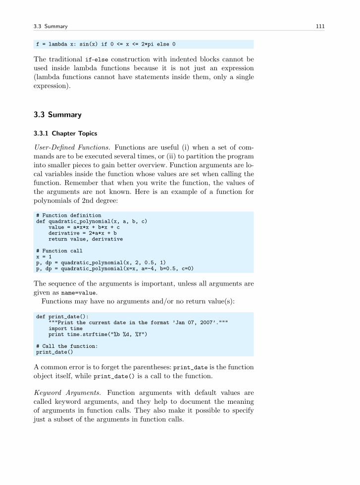
3.3 Summary 111

f = lambda x: sin(x) if 0 <= x <= 2*pi else 0

The traditional if-else construction with indented blocks cannot beused inside lambda functions because it is not just an expression(lambda functions cannot have statements inside them, only a singleexpression).

3.3 Summary

3.3.1 Chapter Topics

User-Defined Functions. Functions are useful (i) when a set of com-mands are to be executed several times, or (ii) to partition the programinto smaller pieces to gain better overview. Function arguments are lo-cal variables inside the function whose values are set when calling thefunction. Remember that when you write the function, the values ofthe arguments are not known. Here is an example of a function forpolynomials of 2nd degree:

# Function definitiondef quadratic_polynomial(x, a, b, c)

value = a*x*x + b*x + cderivative = 2*a*x + breturn value, derivative

# Function callx = 1p, dp = quadratic_polynomial(x, 2, 0.5, 1)p, dp = quadratic_polynomial(x=x, a=-4, b=0.5, c=0)

The sequence of the arguments is important, unless all arguments aregiven as name=value.

Functions may have no arguments and/or no return value(s):

def print_date():"""Print the current date in the format ’Jan 07, 2007’."""import timeprint time.strftime("%b %d, %Y")

# Call the function:print_date()

A common error is to forget the parentheses: print_date is the functionobject itself, while print_date() is a call to the function.

Keyword Arguments. Function arguments with default values arecalled keyword arguments, and they help to document the meaningof arguments in function calls. They also make it possible to specifyjust a subset of the arguments in function calls.

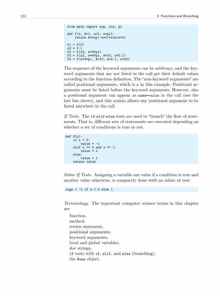
112 3 Functions and Branching

from math import exp, sin, pi

def f(x, A=1, a=1, w=pi):return A*exp(-a*x)*sin(w*x)

f1 = f(0)x2 = 0.1f2 = f(x2, w=2*pi)f3 = f(x2, w=4*pi, A=10, a=0.1)f4 = f(w=4*pi, A=10, a=0.1, x=x2)

The sequence of the keyword arguments can be arbitrary, and the key-word arguments that are not listed in the call get their default valuesaccording to the function definition. The “non-keyword arguments” arecalled positional arguments, which is x in this example. Positional ar-guments must be listed before the keyword arguments. However, alsoa positional argument can appear as name=value in the call (see thelast line above), and this syntax allows any positional argument to belisted anywhere in the call.

If Tests. The if-elif-else tests are used to “branch” the flow of state-ments. That is, different sets of statements are executed depending onwhether a set of conditions is true or not.

def f(x):if x < 0:

value = -1elif x >= 0 and x <= 1:

value = xelse:

value = 1return value

Inline If Tests. Assigning a variable one value if a condition is true andanother value otherwise, is compactly done with an inline if test:

sign = -1 if a < 0 else 1

Terminology. The important computer science terms in this chapterare

function, method, return statement, positional arguments, keyword arguments, local and global variables, doc strings, if tests with if, elif, and else (branching), the None object.

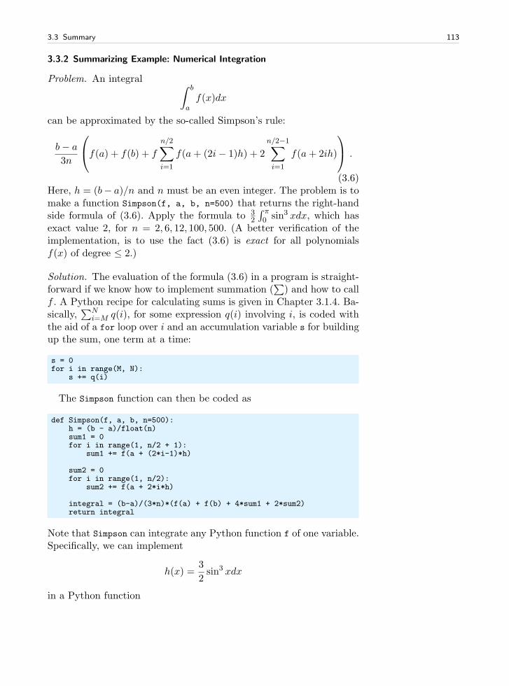
3.3 Summary 113

3.3.2 Summarizing Example: Numerical Integration

Problem. An integral∫ b

af(x)dx

can be approximated by the so-called Simpson’s rule:

b− a

3n

f(a) + f(b) + f

n/2∑

i=1

f(a+ (2i− 1)h) + 2

n/2−1∑

i=1

f(a+ 2ih)

.

(3.6)Here, h = (b− a)/n and n must be an even integer. The problem is tomake a function Simpson(f, a, b, n=500) that returns the right-handside formula of (3.6). Apply the formula to 3

2

∫ π0 sin3 xdx, which has

exact value 2, for n = 2, 6, 12, 100, 500. (A better verification of theimplementation, is to use the fact (3.6) is exact for all polynomialsf(x) of degree ≤ 2.)

Solution. The evaluation of the formula (3.6) in a program is straight-forward if we know how to implement summation (

∑

) and how to callf . A Python recipe for calculating sums is given in Chapter 3.1.4. Ba-sically,

∑Ni=M q(i), for some expression q(i) involving i, is coded with

the aid of a for loop over i and an accumulation variable s for buildingup the sum, one term at a time:

s = 0for i in range(M, N):

s += q(i)

The Simpson function can then be coded as

def Simpson(f, a, b, n=500):h = (b - a)/float(n)sum1 = 0for i in range(1, n/2 + 1):

sum1 += f(a + (2*i-1)*h)

sum2 = 0for i in range(1, n/2):

sum2 += f(a + 2*i*h)

integral = (b-a)/(3*n)*(f(a) + f(b) + 4*sum1 + 2*sum2)return integral

Note that Simpson can integrate any Python function f of one variable.Specifically, we can implement

h(x) =3

2sin3 xdx

in a Python function

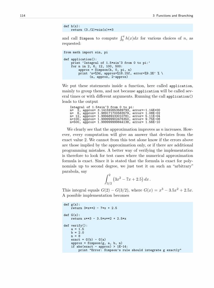
114 3 Functions and Branching

def h(x):return (3./2)*sin(x)**3

and call Simpson to compute∫ π0 h(x)dx for various choices of n, as

requested:

from math import sin, pi

def application():print ’Integral of 1.5*sin^3 from 0 to pi:’for n in 2, 6, 12, 100, 500:

approx = Simpson(h, 0, pi, n)print ’n=%3d, approx=%18.15f, error=%9.2E’ % \

(n, approx, 2-approx)

We put these statements inside a function, here called application,mainly to group them, and not because application will be called sev-eral times or with different arguments. Running the call application()leads to the output

Integral of 1.5*sin^3 from 0 to pi:n= 2, approx= 3.141592653589793, error=-1.14E+00n= 6, approx= 1.989171700583579, error= 1.08E-02n= 12, approx= 1.999489233010781, error= 5.11E-04n=100, approx= 1.999999902476350, error= 9.75E-08n=500, approx= 1.999999999844138, error= 1.56E-10

We clearly see that the approximation improves as n increases. How-ever, every computation will give an answer that deviates from theexact value 2. We cannot from this test alone know if the errors aboveare those implied by the approximation only, or if there are additionalprogramming mistakes. A better way of verifying the implementationis therefore to look for test cases where the numerical approximationformula is exact. Since it is stated that the formula is exact for poly-nomials up to second degree, we just test it on such an “arbitrary”parabola, say

∫ 2

3/2

(

3x2 − 7x+ 2.5)

dx .

This integral equals G(2) − G(3/2), where G(x) = x3 − 3.5x2 + 2.5x.A possible implementation becomes

def g(x):return 3*x**2 - 7*x + 2.5

def G(x):return x**3 - 3.5*x**2 + 2.5*x

def verify():a = 1.5b = 2.0n = 8exact = G(b) - G(a)approx = Simpson(g, a, b, n)if abs(exact - approx) > 1E-14:

print "Error: Simpson’s rule should integrate g exactly"

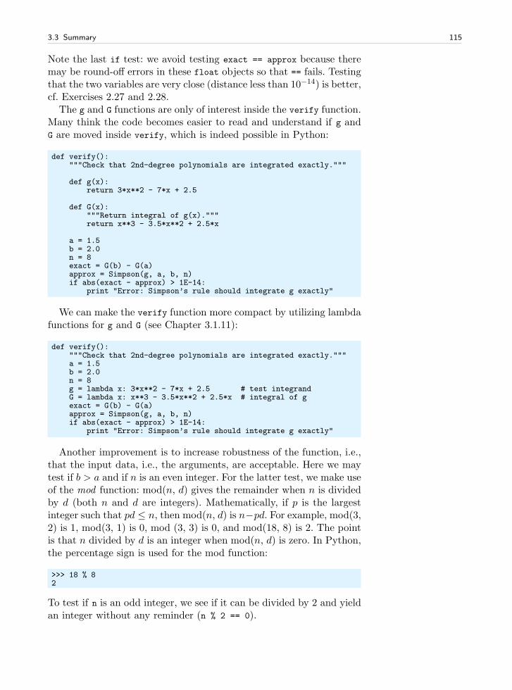
3.3 Summary 115

Note the last if test: we avoid testing exact == approx because theremay be round-off errors in these float objects so that == fails. Testingthat the two variables are very close (distance less than 10−14) is better,cf. Exercises 2.27 and 2.28.

The g and G functions are only of interest inside the verify function.Many think the code becomes easier to read and understand if g andG are moved inside verify, which is indeed possible in Python:

def verify():"""Check that 2nd-degree polynomials are integrated exactly."""

def g(x):return 3*x**2 - 7*x + 2.5

def G(x):"""Return integral of g(x)."""return x**3 - 3.5*x**2 + 2.5*x

a = 1.5b = 2.0n = 8exact = G(b) - G(a)approx = Simpson(g, a, b, n)if abs(exact - approx) > 1E-14:

print "Error: Simpson’s rule should integrate g exactly"

We can make the verify function more compact by utilizing lambdafunctions for g and G (see Chapter 3.1.11):

def verify():"""Check that 2nd-degree polynomials are integrated exactly."""a = 1.5b = 2.0n = 8g = lambda x: 3*x**2 - 7*x + 2.5 # test integrandG = lambda x: x**3 - 3.5*x**2 + 2.5*x # integral of gexact = G(b) - G(a)approx = Simpson(g, a, b, n)if abs(exact - approx) > 1E-14:

print "Error: Simpson’s rule should integrate g exactly"

Another improvement is to increase robustness of the function, i.e.,that the input data, i.e., the arguments, are acceptable. Here we maytest if b > a and if n is an even integer. For the latter test, we make useof the mod function: mod(n, d) gives the remainder when n is dividedby d (both n and d are integers). Mathematically, if p is the largestinteger such that pd ≤ n, then mod(n, d) is n−pd. For example, mod(3,2) is 1, mod(3, 1) is 0, mod (3, 3) is 0, and mod(18, 8) is 2. The pointis that n divided by d is an integer when mod(n, d) is zero. In Python,the percentage sign is used for the mod function:

>>> 18 % 82

To test if n is an odd integer, we see if it can be divided by 2 and yieldan integer without any reminder (n % 2 == 0).

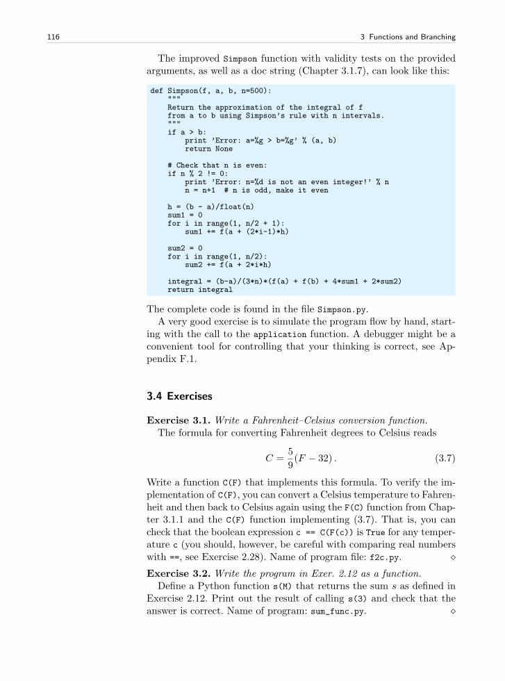
116 3 Functions and Branching

The improved Simpson function with validity tests on the providedarguments, as well as a doc string (Chapter 3.1.7), can look like this:

def Simpson(f, a, b, n=500):"""Return the approximation of the integral of ffrom a to b using Simpson’s rule with n intervals."""if a > b:

print ’Error: a=%g > b=%g’ % (a, b)return None

# Check that n is even:if n % 2 != 0:

print ’Error: n=%d is not an even integer!’ % nn = n+1 # n is odd, make it even

h = (b - a)/float(n)sum1 = 0for i in range(1, n/2 + 1):

sum1 += f(a + (2*i-1)*h)

sum2 = 0for i in range(1, n/2):

sum2 += f(a + 2*i*h)

integral = (b-a)/(3*n)*(f(a) + f(b) + 4*sum1 + 2*sum2)return integral

The complete code is found in the file Simpson.py.A very good exercise is to simulate the program flow by hand, start-

ing with the call to the application function. A debugger might be aconvenient tool for controlling that your thinking is correct, see Ap-pendix F.1.

3.4 Exercises

Exercise 3.1. Write a Fahrenheit–Celsius conversion function.The formula for converting Fahrenheit degrees to Celsius reads

C =5

9(F − 32) . (3.7)

Write a function C(F) that implements this formula. To verify the im-plementation of C(F), you can convert a Celsius temperature to Fahren-heit and then back to Celsius again using the F(C) function from Chap-ter 3.1.1 and the C(F) function implementing (3.7). That is, you cancheck that the boolean expression c == C(F(c)) is True for any temper-ature c (you should, however, be careful with comparing real numberswith ==, see Exercise 2.28). Name of program file: f2c.py. ⋄Exercise 3.2. Write the program in Exer. 2.12 as a function.

Define a Python function s(M) that returns the sum s as defined inExercise 2.12. Print out the result of calling s(3) and check that theanswer is correct. Name of program: sum_func.py. ⋄

3.4 Exercises 117

Exercise 3.3. Compute the area of an arbitrary triangle.An arbitrary triangle can be described by the coordinates of its three

vertices: (x1, y1), (x2, y2), (x3, y3), numbered in a counterclockwise di-rection. The area of the triangle is given by the formula

A =1

2|x2y3 − x3y2 − x1y3 + x3y1 + x1y2 − x2y1| . (3.8)

Write a function area(vertices) that returns the area of a trianglewhose vertices are specified by the argument vertices, which is anested list of the vertex coordinates. For example, vertices can be[[0,0], [1,0], [0,2]] if the three corners of the triangle have coordi-nates (0, 0), (1, 0), and (0, 2). Test the area function on a triangle withknown area. Name of program file: area_triangle.py. ⋄Exercise 3.4. Compute the length of a path.

Some object is moving along a path in the plane. At n points oftime we have recorded the corresponding (x, y) positions of the object:(x0, y0), (x1, y2), . . ., (xn−1, yn−1). The total length L of the path from(x0, y0) to (xn−1, yn−1) is the sum of all the individual line segments((xi−1, yi−1) to (xi, yi), i = 1, . . . , n− 1):

L =

n−1∑

i=1

√

(xi − xi−1)2 + (yi − yi−1)2 . (3.9)

Make a function pathlength(x, y) for computing L according tothe formula. The arguments x and y hold all the x0, . . . , xn−1 andy0, . . . , yn−1 coordinates, respectively. Test the function on a triangu-lar path with the four points (1, 1), (2, 1), (1, 2), and (1, 1). Name ofprogram file: pathlength.py. ⋄Exercise 3.5. Approximate π.

The value of π equals the circumference of a circle with radius 1/2.Suppose we approximate the circumference by a polygon through N+1points on the circle. The length of this polygon can be found using thepathlength function from Exercise 3.4. Compute N + 1 points (xi, yi)along a circle with radius 1/2 according to the formulas

xi =1

2cos(2πi/N), yi =

1

2sin(2πi/N), i = 0, . . . , N .

Call the pathlength function and write out the error in the approx-imation of π for N = 2k, k = 2, 3, . . . , 10. Name of program file:pi_approx.py. ⋄Exercise 3.6. Write some simple functions.

Write three functions:

1. hw1, which takes no arguments and returns the string ’Hello,

World!’

118 3 Functions and Branching

2. hw2, which takes no arguments and returns nothing, but the string’Hello, World!’ is printed in the terminal window

3. hw3, which takes two string arguments and prints these two argu-ments separated by a comma.

Use the following main program to test the three functions:

print hw1()hw2()hw3(’Hello ’, ’World!’)

Name of program: hw_func.py. ⋄

Exercise 3.7. Approximate a function by a sum of sines.We consider the piecewise constant function

f(t) =

1, 0 < t < T/2,0, t = T/2,−1, T/2 < t < T

(3.10)

Sketch this function on a piece of paper. One can approximate f(t) bythe sum

S(t;n) =4

π

n∑

i=1

1

2i− 1sin

(

2(2i− 1)πt

T

)

. (3.11)

It can be shown that S(t;n)→ f(t) as n→∞.Write a Python function S(t, n, T) for returning the value of

S(t;n). Also write a Python f(t, T) for computing f(t). Write outtabular information showing how the error f(t) − S(t;n) varies withn and t for the case where n = 1, 3, 5, 10, 30, 100 and t = αT , withT = 2π, and α = 0.01, 0.25, 0.49. Make a sketch of f(t) and mark the tpoints in the table. Use the table to comment on how the quality of theapproximation depends on α and n. Name of program file: sinesum1.py.

Remark. A sum of sine and/or cosine functions, as in (3.11), is called aFourier series . Approximating a function by a Fourier series is a veryimportant technique in science and technology. Exercise 5.29 asks forvisualization of how well S(t;n) approximates f(t) for some values ofn. ⋄

Exercise 3.8. Implement a Gaussian function.Make a Python function gauss(x, m=0, s=1) for computing the

Gaussian function (1.6) on page 45. Call gauss and print out the resultfor x equal to −5,−4.9,−4.8, . . . , 4.8, 4.9, 5, using default values for m

and s. Name of program file: Gaussian_function2.py. ⋄

Exercise 3.9. Make a function of the formula in Exer. 1.13.Implement the formula (1.8) from Exercise 1.13 in a Python function

with three arguments: egg(M, To=20, Ty=70). The parameters ρ, K, c,and Tw can be set as local (constant) variables inside the function. Let

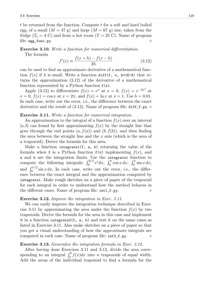
3.4 Exercises 119

t be returned from the function. Compute t for a soft and hard boiledegg, of a small (M = 47 g) and large (M = 67 g) size, taken from thefridge (To = 4 C) and from a hot room (T = 25 C). Name of programfile: egg_func.py. ⋄

Exercise 3.10. Write a function for numerical differentiation.The formula

f ′(x) ≈ f(x+ h)− f(x− h)

2h(3.12)

can be used to find an approximate derivative of a mathematical func-tion f(x) if h is small. Write a function diff(f, x, h=1E-6) that re-turns the approximation (3.12) of the derivative of a mathematicalfunction represented by a Python function f(x).

Apply (3.12) to differentiate f(x) = ex at x = 0, f(x) = e−2x2

atx = 0, f(x) = cosx at x = 2π, and f(x) = lnx at x = 1. Use h = 0.01.In each case, write out the error, i.e., the difference between the exactderivative and the result of (3.12). Name of program file: diff_f.py. ⋄

Exercise 3.11. Write a function for numerical integration.An approximation to the integral of a function f(x) over an interval

[a, b] can found by first approximating f(x) by the straight line thatgoes through the end points (a, f(a)) and (b, f(b)), and then findingthe area between the straight line and the x axis (which is the area ofa trapezoid). Derive the formula for this area.

Make a function integrate1(f, a, b) returning the value of theformula when f is a Python function f(x) implementing f(x), anda and b are the integration limits. Use the integrate1 function tocompute the following integrals:

∫ ln 30 exdx,

∫ π0 cosx dx,

∫ π0 sinx dx,

and∫ π/20 sinx dx, In each case, write out the error, i.e., the differ-

ence between the exact integral and the approximation computed byintegrate1. Make rough sketches on a piece of paper of the trapezoidfor each integral in order to understand how the method behaves inthe different cases. Name of program file: int1_f.py. ⋄

Exercise 3.12. Improve the integration in Exer. 3.11.We can easily improve the integration technique described in Exer-

cise 3.11 by approximating the area under the function f(x) by twotrapezoids. Derive the formula for the area in this case and implementit in a function integrate2(f, a, b) and test it on the same cases aslisted in Exercise 3.11. Also make sketches on a piece of paper so thatyou get a visual understanding of how the approximate integrals arecomputed in each case. Name of program file: int2_f.py. ⋄

Exercise 3.13. Generalize the integration formula in Exer. 3.12.After having done Exercises 3.11 and 3.12, divide the area corre-

sponding to an integral∫ ba f(x)dx into n trapezoids of equal width.

Add the areas of the individual trapezoid to find a formula for the

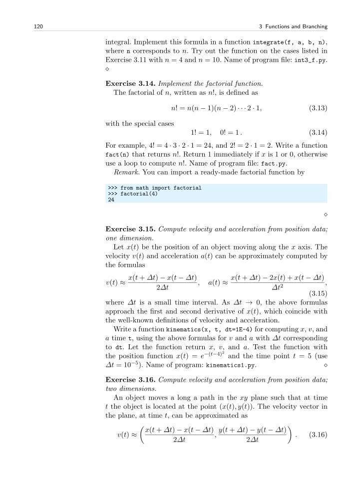
120 3 Functions and Branching

integral. Implement this formula in a function integrate(f, a, b, n),where n corresponds to n. Try out the function on the cases listed inExercise 3.11 with n = 4 and n = 10. Name of program file: int3_f.py.⋄

Exercise 3.14. Implement the factorial function.The factorial of n, written as n!, is defined as

n! = n(n− 1)(n− 2) · · · 2 · 1, (3.13)

with the special cases1! = 1, 0! = 1 . (3.14)

For example, 4! = 4 · 3 · 2 · 1 = 24, and 2! = 2 · 1 = 2. Write a functionfact(n) that returns n!. Return 1 immediately if x is 1 or 0, otherwiseuse a loop to compute n!. Name of program file: fact.py.

Remark. You can import a ready-made factorial function by

>>> from math import factorial>>> factorial(4)24

⋄

Exercise 3.15. Compute velocity and acceleration from position data;one dimension.

Let x(t) be the position of an object moving along the x axis. Thevelocity v(t) and acceleration a(t) can be approximately computed bythe formulas

v(t) ≈ x(t+∆t)− x(t−∆t)

2∆t, a(t) ≈ x(t+∆t)− 2x(t) + x(t−∆t)

∆t2,

(3.15)where ∆t is a small time interval. As ∆t → 0, the above formulasapproach the first and second derivative of x(t), which coincide withthe well-known definitions of velocity and acceleration.

Write a function kinematics(x, t, dt=1E-4) for computing x, v, anda time t, using the above formulas for v and a with ∆t correspondingto dt. Let the function return x, v, and a. Test the function withthe position function x(t) = e−(t−4)2 and the time point t = 5 (use∆t = 10−5). Name of program: kinematics1.py. ⋄

Exercise 3.16. Compute velocity and acceleration from position data;two dimensions.

An object moves a long a path in the xy plane such that at timet the object is located at the point (x(t), y(t)). The velocity vector inthe plane, at time t, can be approximated as

v(t) ≈(

x(t+∆t)− x(t−∆t)

2∆t,y(t+∆t)− y(t−∆t)

2∆t

)

. (3.16)

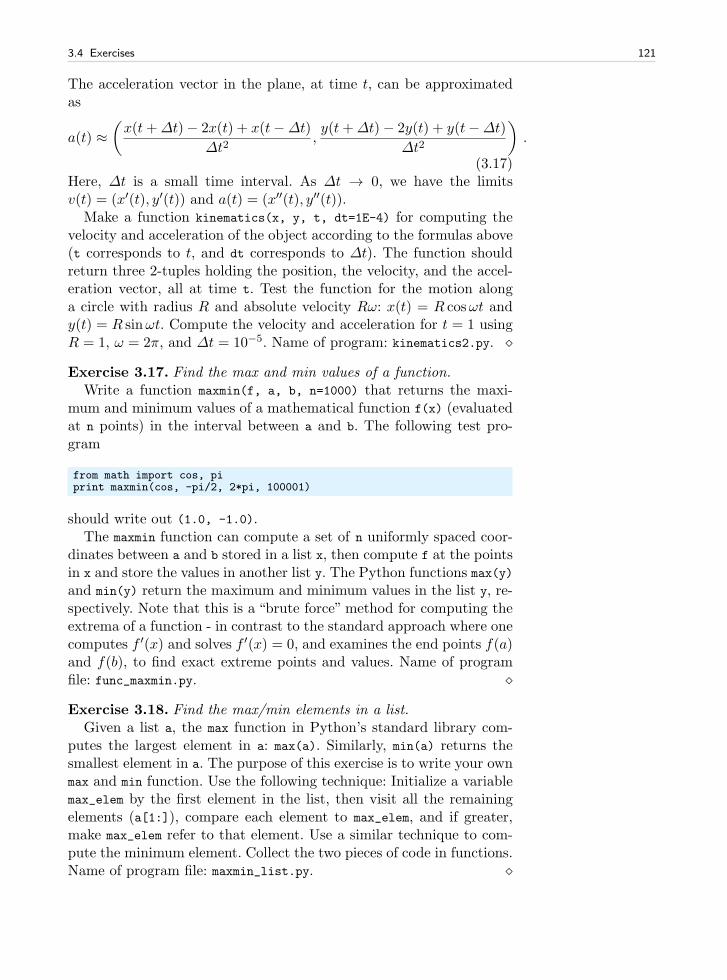
3.4 Exercises 121

The acceleration vector in the plane, at time t, can be approximatedas

a(t) ≈(

x(t+∆t)− 2x(t) + x(t−∆t)

∆t2,y(t+∆t)− 2y(t) + y(t−∆t)

∆t2

)

.

(3.17)Here, ∆t is a small time interval. As ∆t → 0, we have the limitsv(t) = (x′(t), y′(t)) and a(t) = (x′′(t), y′′(t)).

Make a function kinematics(x, y, t, dt=1E-4) for computing thevelocity and acceleration of the object according to the formulas above(t corresponds to t, and dt corresponds to ∆t). The function shouldreturn three 2-tuples holding the position, the velocity, and the accel-eration vector, all at time t. Test the function for the motion alonga circle with radius R and absolute velocity Rω: x(t) = R cosωt andy(t) = R sinωt. Compute the velocity and acceleration for t = 1 usingR = 1, ω = 2π, and ∆t = 10−5. Name of program: kinematics2.py. ⋄

Exercise 3.17. Find the max and min values of a function.Write a function maxmin(f, a, b, n=1000) that returns the maxi-

mum and minimum values of a mathematical function f(x) (evaluatedat n points) in the interval between a and b. The following test pro-gram

from math import cos, piprint maxmin(cos, -pi/2, 2*pi, 100001)

should write out (1.0, -1.0).The maxmin function can compute a set of n uniformly spaced coor-

dinates between a and b stored in a list x, then compute f at the pointsin x and store the values in another list y. The Python functions max(y)and min(y) return the maximum and minimum values in the list y, re-spectively. Note that this is a “brute force” method for computing theextrema of a function - in contrast to the standard approach where onecomputes f ′(x) and solves f ′(x) = 0, and examines the end points f(a)and f(b), to find exact extreme points and values. Name of programfile: func_maxmin.py. ⋄

Exercise 3.18. Find the max/min elements in a list.Given a list a, the max function in Python’s standard library com-

putes the largest element in a: max(a). Similarly, min(a) returns thesmallest element in a. The purpose of this exercise is to write your ownmax and min function. Use the following technique: Initialize a variablemax_elem by the first element in the list, then visit all the remainingelements (a[1:]), compare each element to max_elem, and if greater,make max_elem refer to that element. Use a similar technique to com-pute the minimum element. Collect the two pieces of code in functions.Name of program file: maxmin_list.py. ⋄

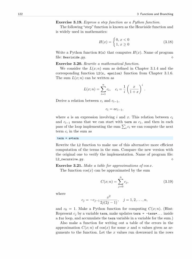
122 3 Functions and Branching

Exercise 3.19. Express a step function as a Python function.The following“step” function is known as the Heaviside function and

is widely used in mathematics:

H(x) =

0, x < 01, x ≥ 0

(3.18)

Write a Python function H(x) that computes H(x). Name of programfile: Heaviside.py. ⋄Exercise 3.20. Rewrite a mathematical function.

We consider the L(x;n) sum as defined in Chapter 3.1.4 and thecorresponding function L2(x, epsilon) function from Chapter 3.1.6.The sum L(x;n) can be written as

L(x;n) =

n∑

i=1

ci, ci =1

i

(

x

1 + x

)i

.

Derive a relation between ci and ci−1,

ci = aci−1,

where a is an expression involving i and x. This relation between ciand ci−1 means that we can start with term as c1, and then in eachpass of the loop implementing the sum

∑

i ci we can compute the nextterm ci in the sum as

term = a*term

Rewrite the L2 function to make use of this alternative more efficientcomputation of the terms in the sum. Compare the new version withthe original one to verify the implementation. Name of program file:L2_recursive.py. ⋄Exercise 3.21. Make a table for approximations of cosx.

The function cos(x) can be approximated by the sum

C(x;n) =

n∑

j=0

cj, (3.19)

where

cj = −cj−1x2

2j(2j − 1), j = 1, 2, . . . , n,

and c0 = 1. Make a Python function for computing C(x;n). (Hint:Represent cj by a variable term, make updates term = -term*... insidea for loop, and accumulate the term variable in a variable for the sum.)

Also make a function for writing out a table of the errors in theapproximation C(x;n) of cos(x) for some x and n values given as ar-guments to the function. Let the x values run downward in the rows

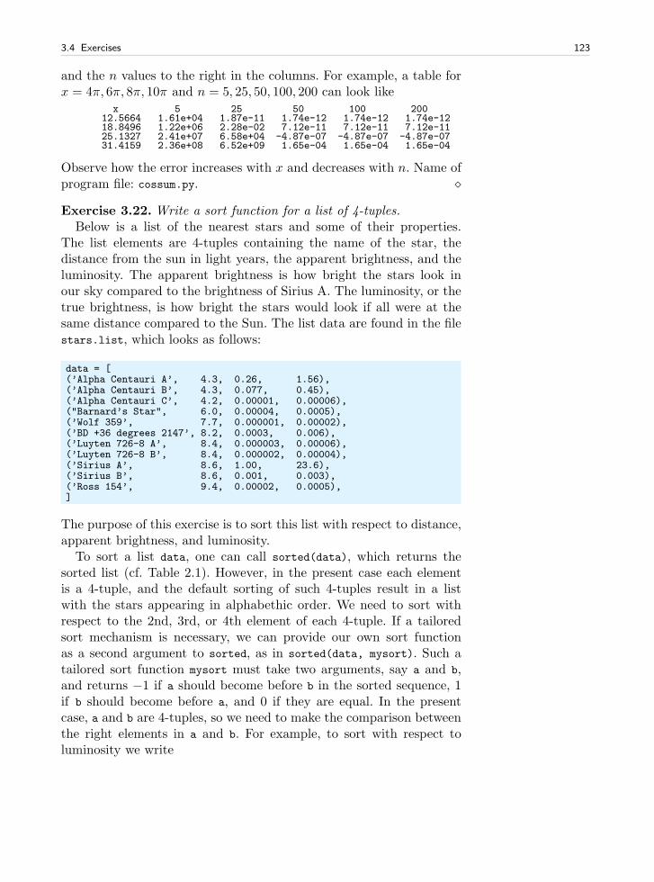
3.4 Exercises 123

and the n values to the right in the columns. For example, a table forx = 4π, 6π, 8π, 10π and n = 5, 25, 50, 100, 200 can look like

x 5 25 50 100 20012.5664 1.61e+04 1.87e-11 1.74e-12 1.74e-12 1.74e-1218.8496 1.22e+06 2.28e-02 7.12e-11 7.12e-11 7.12e-1125.1327 2.41e+07 6.58e+04 -4.87e-07 -4.87e-07 -4.87e-0731.4159 2.36e+08 6.52e+09 1.65e-04 1.65e-04 1.65e-04

Observe how the error increases with x and decreases with n. Name ofprogram file: cossum.py. ⋄

Exercise 3.22. Write a sort function for a list of 4-tuples.Below is a list of the nearest stars and some of their properties.

The list elements are 4-tuples containing the name of the star, thedistance from the sun in light years, the apparent brightness, and theluminosity. The apparent brightness is how bright the stars look inour sky compared to the brightness of Sirius A. The luminosity, or thetrue brightness, is how bright the stars would look if all were at thesame distance compared to the Sun. The list data are found in the filestars.list, which looks as follows:

data = [(’Alpha Centauri A’, 4.3, 0.26, 1.56),(’Alpha Centauri B’, 4.3, 0.077, 0.45),(’Alpha Centauri C’, 4.2, 0.00001, 0.00006),("Barnard’s Star", 6.0, 0.00004, 0.0005),(’Wolf 359’, 7.7, 0.000001, 0.00002),(’BD +36 degrees 2147’, 8.2, 0.0003, 0.006),(’Luyten 726-8 A’, 8.4, 0.000003, 0.00006),(’Luyten 726-8 B’, 8.4, 0.000002, 0.00004),(’Sirius A’, 8.6, 1.00, 23.6),(’Sirius B’, 8.6, 0.001, 0.003),(’Ross 154’, 9.4, 0.00002, 0.0005),]

The purpose of this exercise is to sort this list with respect to distance,apparent brightness, and luminosity.

To sort a list data, one can call sorted(data), which returns thesorted list (cf. Table 2.1). However, in the present case each elementis a 4-tuple, and the default sorting of such 4-tuples result in a listwith the stars appearing in alphabethic order. We need to sort withrespect to the 2nd, 3rd, or 4th element of each 4-tuple. If a tailoredsort mechanism is necessary, we can provide our own sort functionas a second argument to sorted, as in sorted(data, mysort). Such atailored sort function mysort must take two arguments, say a and b,and returns −1 if a should become before b in the sorted sequence, 1if b should become before a, and 0 if they are equal. In the presentcase, a and b are 4-tuples, so we need to make the comparison betweenthe right elements in a and b. For example, to sort with respect toluminosity we write

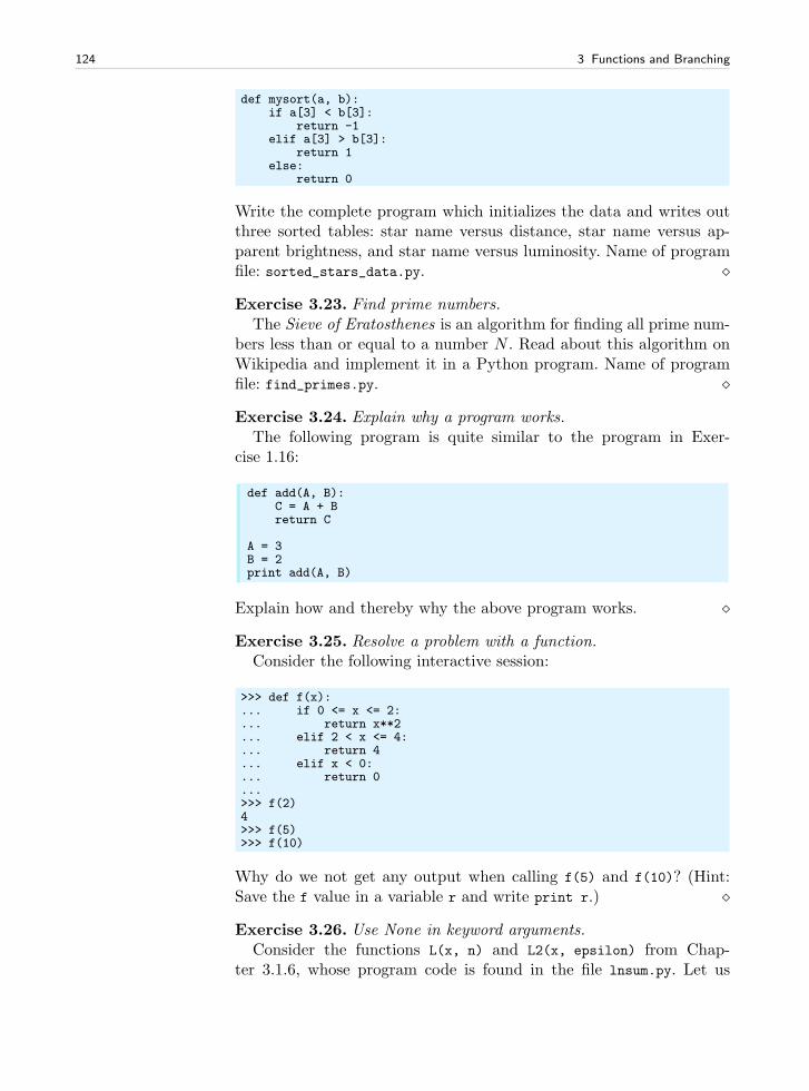
124 3 Functions and Branching

def mysort(a, b):if a[3] < b[3]:

return -1elif a[3] > b[3]:

return 1else:

return 0

Write the complete program which initializes the data and writes outthree sorted tables: star name versus distance, star name versus ap-parent brightness, and star name versus luminosity. Name of programfile: sorted_stars_data.py. ⋄

Exercise 3.23. Find prime numbers.The Sieve of Eratosthenes is an algorithm for finding all prime num-

bers less than or equal to a number N . Read about this algorithm onWikipedia and implement it in a Python program. Name of programfile: find_primes.py. ⋄

Exercise 3.24. Explain why a program works.The following program is quite similar to the program in Exer-

cise 1.16:

def add(A, B):C = A + Breturn C

A = 3B = 2print add(A, B)

Explain how and thereby why the above program works. ⋄

Exercise 3.25. Resolve a problem with a function.Consider the following interactive session:

>>> def f(x):... if 0 <= x <= 2:... return x**2... elif 2 < x <= 4:... return 4... elif x < 0:... return 0...>>> f(2)4>>> f(5)>>> f(10)

Why do we not get any output when calling f(5) and f(10)? (Hint:Save the f value in a variable r and write print r.) ⋄

Exercise 3.26. Use None in keyword arguments.Consider the functions L(x, n) and L2(x, epsilon) from Chap-

ter 3.1.6, whose program code is found in the file lnsum.py. Let us

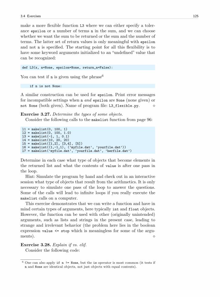
3.4 Exercises 125

make a more flexible function L3 where we can either specify a toler-ance epsilon or a number of terms n in the sum, and we can choosewhether we want the sum to be returned or the sum and the number ofterms. The latter set of return values is only meaningful with epsilon

and not n is specified. The starting point for all this flexibility is tohave some keyword arguments initialized to an “undefined” value thatcan be recognized:

def L3(x, n=None, epsilon=None, return_n=False):

You can test if n is given using the phrase6

if n is not None:

A similar construction can be used for epsilon. Print error messagesfor incompatible settings when n and epsilon are None (none given) ornot None (both given). Name of program file: L3_flexible.py. ⋄

Exercise 3.27. Determine the types of some objects.Consider the following calls to the makelist function from page 96:

l1 = makelist(0, 100, 1)l2 = makelist(0, 100, 1.0)l3 = makelist(-1, 1, 0.1)l4 = makelist(10, 20, 20)l5 = makelist([1,2], [3,4], [5])l6 = makelist((1,-1,1), (’myfile.dat’, ’yourfile.dat’))l7 = makelist(’myfile.dat’, ’yourfile.dat’, ’herfile.dat’)

Determine in each case what type of objects that become elements inthe returned list and what the contents of value is after one pass inthe loop.

Hint: Simulate the program by hand and check out in an interactivesession what type of objects that result from the arithmetics. It is onlynecessary to simulate one pass of the loop to answer the questions.Some of the calls will lead to infinite loops if you really execute themakelist calls on a computer.

This exercise demonstrates that we can write a function and have inmind certain types of arguments, here typically int and float objects.However, the function can be used with other (originally unintended)arguments, such as lists and strings in the present case, leading tostrange and irrelevant behavior (the problem here lies in the booleanexpression value <= stop which is meaningless for some of the argu-ments). ⋄

Exercise 3.28. Explain if vs. elif.Consider the following code:

6 One can also apply if n != None, but the is operator is most common (it tests ifn and None are identical objects, not just objects with equal contents).

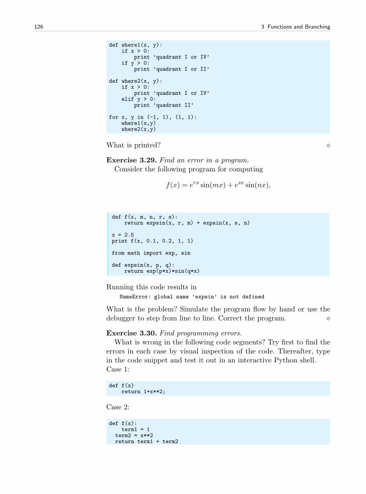
126 3 Functions and Branching

def where1(x, y):if x > 0:

print ’quadrant I or IV’if y > 0:

print ’quadrant I or II’

def where2(x, y):if x > 0:

print ’quadrant I or IV’elif y > 0:

print ’quadrant II’

for x, y in (-1, 1), (1, 1):where1(x,y)where2(x,y)

What is printed? ⋄

Exercise 3.29. Find an error in a program.Consider the following program for computing

f(x) = erx sin(mx) + esx sin(nx),

def f(x, m, n, r, s):return expsin(x, r, m) + expsin(x, s, n)

x = 2.5print f(x, 0.1, 0.2, 1, 1)

from math import exp, sin

def expsin(x, p, q):return exp(p*x)*sin(q*x)

Running this code results inNameError: global name ’expsin’ is not defined

What is the problem? Simulate the program flow by hand or use thedebugger to step from line to line. Correct the program. ⋄

Exercise 3.30. Find programming errors.What is wrong in the following code segments? Try first to find the

errors in each case by visual inspection of the code. Thereafter, typein the code snippet and test it out in an interactive Python shell.Case 1:

def f(x)return 1+x**2;

Case 2:

def f(x):term1 = 1

term2 = x**2return term1 + term2

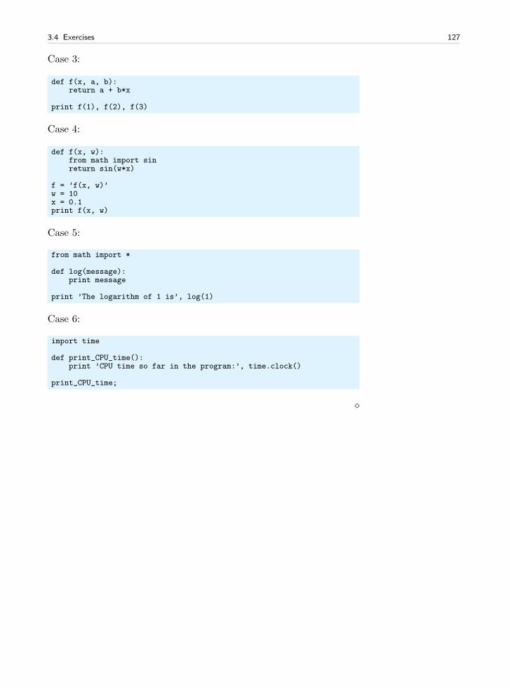
3.4 Exercises 127

Case 3:

def f(x, a, b):return a + b*x

print f(1), f(2), f(3)

Case 4:

def f(x, w):from math import sinreturn sin(w*x)

f = ’f(x, w)’w = 10x = 0.1print f(x, w)

Case 5:

from math import *

def log(message):print message

print ’The logarithm of 1 is’, log(1)

Case 6:

import time

def print_CPU_time():print ’CPU time so far in the program:’, time.clock()

print_CPU_time;

⋄

Input Data and Error Handling 4

Recall our first program for evaluating the formula (1.2) on page 19 inChapter 1:

C = 21F = (9/5)*C + 32print F

In this program, C is input data in the sense that C must be knownbefore the program can perform the calculation of F. The results pro-duced by the program, here F, constitute the output data.

Input data can be hardcoded in the program as we do above. Thatis, we explicitly set variables to specific values (C = 21). This program-ming style may be suitable for small programs. In general, however, itis considered good practice to let a user of the program provide inputdata when the program is running. There is then no need to modifythe program itself when a new set of input data is to be explored1.

This chapter starts with describing three different ways of readingdata into a program: (i) letting the user answer questions in a dialog inthe terminal window (Chapter 4.1), (ii) letting the user provide inputon the command line (Chapter 4.2), and (iii) letting the user writeinput data in a graphical interface (Chapter 4.4). A fourth method isto read data from a file, but this topic is left for Chapter 6.

Even if your program works perfectly, wrong input data from theuser may cause the program to produce wrong answers or even crash.Checking that the input data are correct is important, and Chapter 4.3tells you how to do this with so-called exceptions.

The Python programming environment is organized as a big col-lection of modules. Organizing your own Python software in terms of

1 Programmers know that any modification of the source code has a danger of intro-ducing errors, so it is a good rule to change as little as possible in a program thatworks.

129

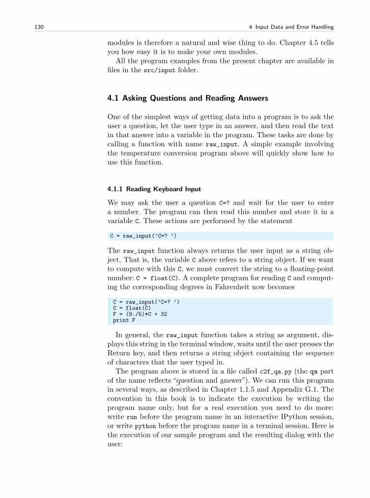
130 4 Input Data and Error Handling

modules is therefore a natural and wise thing to do. Chapter 4.5 tellsyou how easy it is to make your own modules.

All the program examples from the present chapter are available infiles in the src/input folder.

4.1 Asking Questions and Reading Answers

One of the simplest ways of getting data into a program is to ask theuser a question, let the user type in an answer, and then read the textin that answer into a variable in the program. These tasks are done bycalling a function with name raw_input. A simple example involvingthe temperature conversion program above will quickly show how touse this function.

4.1.1 Reading Keyboard Input

We may ask the user a question C=? and wait for the user to entera number. The program can then read this number and store it in avariable C. These actions are performed by the statement

C = raw_input(’C=? ’)

The raw_input function always returns the user input as a string ob-ject. That is, the variable C above refers to a string object. If we wantto compute with this C, we must convert the string to a floating-pointnumber: C = float(C). A complete program for reading C and comput-ing the corresponding degrees in Fahrenheit now becomes

C = raw_input(’C=? ’)C = float(C)F = (9./5)*C + 32print F

In general, the raw_input function takes a string as argument, dis-plays this string in the terminal window, waits until the user presses theReturn key, and then returns a string object containing the sequenceof characters that the user typed in.

The program above is stored in a file called c2f_qa.py (the qa partof the name reflects “question and answer”). We can run this programin several ways, as described in Chapter 1.1.5 and Appendix G.1. Theconvention in this book is to indicate the execution by writing theprogram name only, but for a real execution you need to do more:write run before the program name in an interactive IPython session,or write python before the program name in a terminal session. Here isthe execution of our sample program and the resulting dialog with theuser:

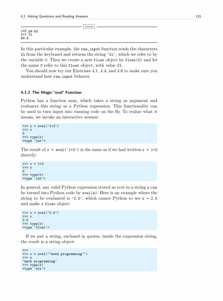
4.1 Asking Questions and Reading Answers 131

Terminal

c2f_qa.pyC=? 2169.8

In this particular example, the raw_input function reads the characters21 from the keyboard and returns the string ’21’, which we refer to bythe variable C. Then we create a new float object by float(C) and letthe name C refer to this float object, with value 21.

You should now try out Exercises 4.1, 4.4, and 4.6 to make sure youunderstand how raw_input behaves.

4.1.2 The Magic “eval” Function

Python has a function eval, which takes a string as argument andevaluates this string as a Python expression. This functionality canbe used to turn input into running code on the fly. To realize what itmeans, we invoke an interactive session:

>>> r = eval(’1+2’)>>> r3>>> type(r)<type ’int’>

The result of r = eval(’1+2’) is the same as if we had written r = 1+2

directly:

>>> r = 1+2>>> r3>>> type(r)<type ’int’>

In general, any valid Python expression stored as text in a string s canbe turned into Python code by eval(s). Here is an example where thestring to be evaluated is ’2.5’, which causes Python to see r = 2.5

and make a float object:

>>> r = eval(’2.5’)>>> r2.5>>> type(r)<type ’float’>

If we put a string, enclosed in quotes, inside the expression string,the result is a string object:

>>>>>> r = eval(’"math programming"’)>>> r’math programming’>>> type(r)<type ’str’>

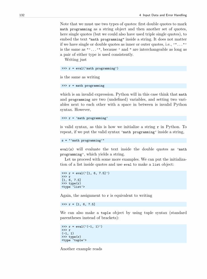
132 4 Input Data and Error Handling

Note that we must use two types of quotes: first double quotes to markmath programming as a string object and then another set of quotes,here single quotes (but we could also have used triple single quotes), toembed the text "math programming" inside a string. It does not matterif we have single or double quotes as inner or outer quotes, i.e., ’"..."’is the same as "’...’", because ’ and " are interchangeable as long asa pair of either type is used consistently.

Writing just

>>> r = eval(’math programming’)

is the same as writing

>>> r = math programming

which is an invalid expression. Python will in this case think that mathand programming are two (undefined) variables, and setting two vari-ables next to each other with a space in between is invalid Pythonsyntax. However,

>>> r = ’math programming’

is valid syntax, as this is how we initialize a string r in Python. Torepeat, if we put the valid syntax ’math programming’ inside a string,

s = "’math programming’"

eval(s) will evaluate the text inside the double quotes as ’math

programming’, which yields a string.Let us proceed with some more examples. We can put the initializa-

tion of a list inside quotes and use eval to make a list object:

>>> r = eval(’[1, 6, 7.5]’)>>> r[1, 6, 7.5]>>> type(r)<type ’list’>

Again, the assignment to r is equivalent to writing

>>> r = [1, 6, 7.5]

We can also make a tuple object by using tuple syntax (standardparentheses instead of brackets):

>>> r = eval(’(-1, 1)’)>>> r(-1, 1)>>> type(r)<type ’tuple’>

Another example reads

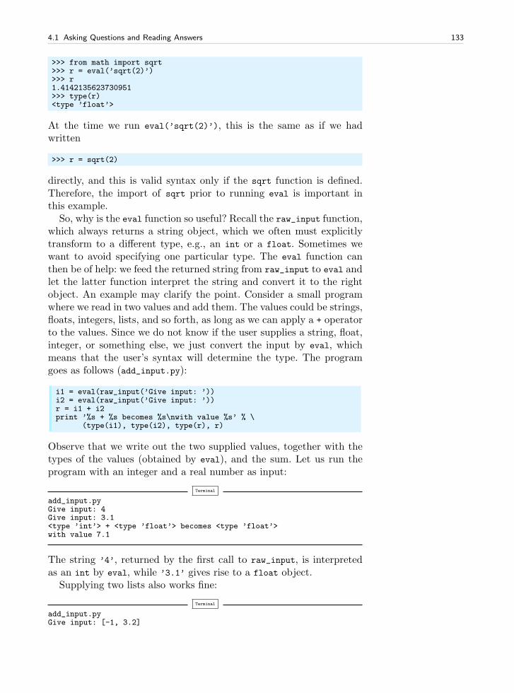
4.1 Asking Questions and Reading Answers 133

>>> from math import sqrt>>> r = eval(’sqrt(2)’)>>> r1.4142135623730951>>> type(r)<type ’float’>

At the time we run eval(’sqrt(2)’), this is the same as if we hadwritten

>>> r = sqrt(2)

directly, and this is valid syntax only if the sqrt function is defined.Therefore, the import of sqrt prior to running eval is important inthis example.

So, why is the eval function so useful? Recall the raw_input function,which always returns a string object, which we often must explicitlytransform to a different type, e.g., an int or a float. Sometimes wewant to avoid specifying one particular type. The eval function canthen be of help: we feed the returned string from raw_input to eval andlet the latter function interpret the string and convert it to the rightobject. An example may clarify the point. Consider a small programwhere we read in two values and add them. The values could be strings,floats, integers, lists, and so forth, as long as we can apply a + operatorto the values. Since we do not know if the user supplies a string, float,integer, or something else, we just convert the input by eval, whichmeans that the user’s syntax will determine the type. The programgoes as follows (add_input.py):

i1 = eval(raw_input(’Give input: ’))i2 = eval(raw_input(’Give input: ’))r = i1 + i2print ’%s + %s becomes %s\nwith value %s’ % \

(type(i1), type(i2), type(r), r)

Observe that we write out the two supplied values, together with thetypes of the values (obtained by eval), and the sum. Let us run theprogram with an integer and a real number as input:

Terminal

add_input.pyGive input: 4Give input: 3.1<type ’int’> + <type ’float’> becomes <type ’float’>with value 7.1

The string ’4’, returned by the first call to raw_input, is interpretedas an int by eval, while ’3.1’ gives rise to a float object.

Supplying two lists also works fine:

Terminal

add_input.pyGive input: [-1, 3.2]

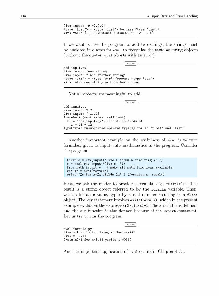
134 4 Input Data and Error Handling

Give input: [9,-2,0,0]<type ’list’> + <type ’list’> becomes <type ’list’>with value [-1, 3.2000000000000002, 9, -2, 0, 0]

If we want to use the program to add two strings, the strings mustbe enclosed in quotes for eval to recognize the texts as string objects(without the quotes, eval aborts with an error):

Terminal

add_input.pyGive input: ’one string’Give input: " and another string"<type ’str’> + <type ’str’> becomes <type ’str’>with value one string and another string

Not all objects are meaningful to add:

Terminal

add_input.pyGive input: 3.2Give input: [-1,10]Traceback (most recent call last):File "add_input.py", line 3, in <module>r = i1 + i2

TypeError: unsupported operand type(s) for +: ’float’ and ’list’

Another important example on the usefulness of eval is to turnformulas, given as input, into mathematics in the program. Considerthe program

formula = raw_input(’Give a formula involving x: ’)x = eval(raw_input(’Give x: ’))from math import * # make all math functions availableresult = eval(formula)print ’%s for x=%g yields %g’ % (formula, x, result)

First, we ask the reader to provide a formula, e.g., 2*sin(x)+1. Theresult is a string object referred to by the formula variable. Then,we ask for an x value, typically a real number resulting in a float

object. The key statement involves eval(formula), which in the presentexample evaluates the expression 2*sin(x)+1. The x variable is defined,and the sin function is also defined because of the import statement.Let us try to run the program:

Terminal

eval_formula.pyGive a formula involving x: 2*sin(x)+1Give x: 3.142*sin(x)+1 for x=3.14 yields 1.00319

Another important application of eval occurs in Chapter 4.2.1.

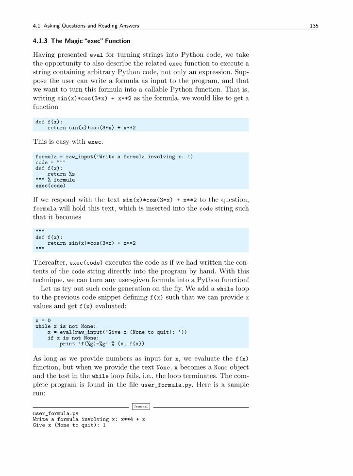
4.1 Asking Questions and Reading Answers 135

4.1.3 The Magic “exec”Function

Having presented eval for turning strings into Python code, we takethe opportunity to also describe the related exec function to execute astring containing arbitrary Python code, not only an expression. Sup-pose the user can write a formula as input to the program, and thatwe want to turn this formula into a callable Python function. That is,writing sin(x)*cos(3*x) + x**2 as the formula, we would like to get afunction

def f(x):return sin(x)*cos(3*x) + x**2

This is easy with exec:

formula = raw_input(’Write a formula involving x: ’)code = """def f(x):

return %s""" % formulaexec(code)

If we respond with the text sin(x)*cos(3*x) + x**2 to the question,formula will hold this text, which is inserted into the code string suchthat it becomes

"""def f(x):

return sin(x)*cos(3*x) + x**2"""

Thereafter, exec(code) executes the code as if we had written the con-tents of the code string directly into the program by hand. With thistechnique, we can turn any user-given formula into a Python function!

Let us try out such code generation on the fly. We add a while loopto the previous code snippet defining f(x) such that we can provide x

values and get f(x) evaluated:

x = 0while x is not None:

x = eval(raw_input(’Give x (None to quit): ’))if x is not None:

print ’f(%g)=%g’ % (x, f(x))

As long as we provide numbers as input for x, we evaluate the f(x)

function, but when we provide the text None, x becomes a None objectand the test in the while loop fails, i.e., the loop terminates. The com-plete program is found in the file user_formula.py. Here is a samplerun:

Terminal

user_formula.pyWrite a formula involving x: x**4 + xGive x (None to quit): 1

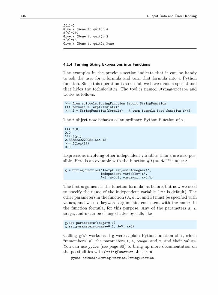
136 4 Input Data and Error Handling

f(1)=2Give x (None to quit): 4f(4)=260Give x (None to quit): 2f(2)=18Give x (None to quit): None

4.1.4 Turning String Expressions into Functions

The examples in the previous section indicate that it can be handyto ask the user for a formula and turn that formula into a Pythonfunction. Since this operation is so useful, we have made a special toolthat hides the technicalities. The tool is named StringFunction andworks as follows:

>>> from scitools.StringFunction import StringFunction>>> formula = ’exp(x)*sin(x)’>>> f = StringFunction(formula) # turn formula into function f(x)

The f object now behaves as an ordinary Python function of x:

>>> f(0)0.0>>> f(pi)2.8338239229952166e-15>>> f(log(1))0.0

Expressions involving other independent variables than x are also pos-sible. Here is an example with the function g(t) = Ae−at sin(ωx):

g = StringFunction(’A*exp(-a*t)*sin(omega*x)’,independent_variable=’t’,A=1, a=0.1, omega=pi, x=0.5)

The first argument is the function formula, as before, but now we needto specify the name of the independent variable (’x’ is default). Theother parameters in the function (A, a, ω, and x) must be specified withvalues, and we use keyword arguments, consistent with the names inthe function formula, for this purpose. Any of the parameters A, a,omega, and x can be changed later by calls like

g.set_parameters(omega=0.1)g.set_parameters(omega=0.1, A=5, x=0)

Calling g(t) works as if g were a plain Python function of t, which“remembers” all the parameters A, a, omega, and x, and their values.You can use pydoc (see page 80) to bring up more documentation onthe possibilities with StringFunction. Just run

pydoc scitools.StringFunction.StringFunction

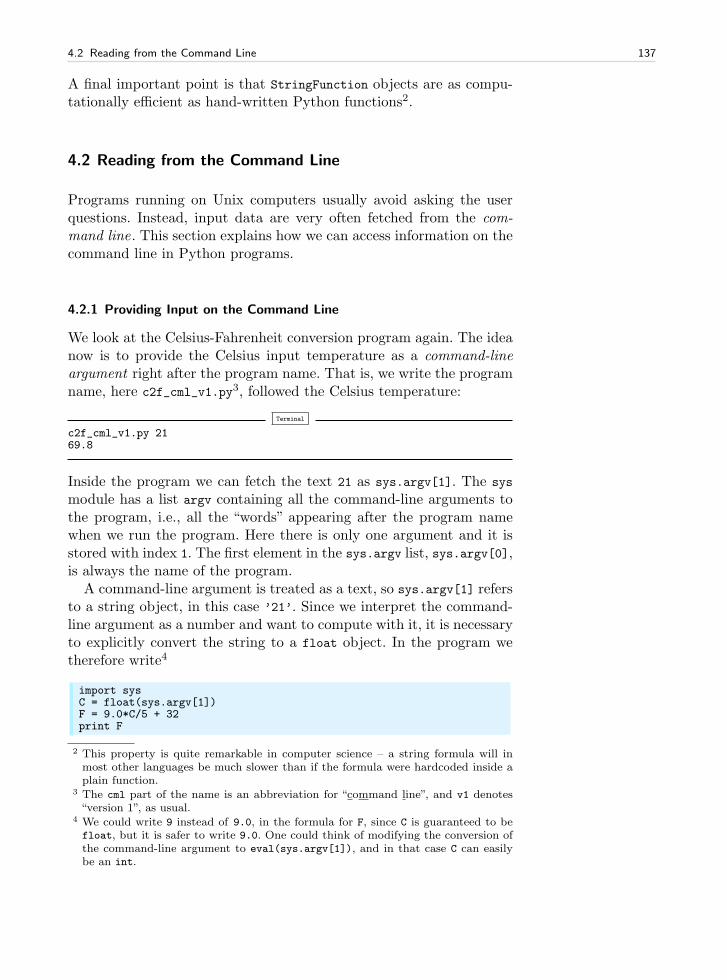
4.2 Reading from the Command Line 137

A final important point is that StringFunction objects are as compu-tationally efficient as hand-written Python functions2.

4.2 Reading from the Command Line

Programs running on Unix computers usually avoid asking the userquestions. Instead, input data are very often fetched from the com-mand line. This section explains how we can access information on thecommand line in Python programs.

4.2.1 Providing Input on the Command Line

We look at the Celsius-Fahrenheit conversion program again. The ideanow is to provide the Celsius input temperature as a command-lineargument right after the program name. That is, we write the programname, here c2f_cml_v1.py3, followed the Celsius temperature:

Terminal

c2f_cml_v1.py 2169.8

Inside the program we can fetch the text 21 as sys.argv[1]. The sys

module has a list argv containing all the command-line arguments tothe program, i.e., all the “words” appearing after the program namewhen we run the program. Here there is only one argument and it isstored with index 1. The first element in the sys.argv list, sys.argv[0],is always the name of the program.

A command-line argument is treated as a text, so sys.argv[1] refersto a string object, in this case ’21’. Since we interpret the command-line argument as a number and want to compute with it, it is necessaryto explicitly convert the string to a float object. In the program wetherefore write4

import sysC = float(sys.argv[1])F = 9.0*C/5 + 32print F

2 This property is quite remarkable in computer science – a string formula will inmost other languages be much slower than if the formula were hardcoded inside aplain function.

3 The cml part of the name is an abbreviation for “command line”, and v1 denotes“version 1”, as usual.

4 We could write 9 instead of 9.0, in the formula for F, since C is guaranteed to befloat, but it is safer to write 9.0. One could think of modifying the conversion ofthe command-line argument to eval(sys.argv[1]), and in that case C can easilybe an int.

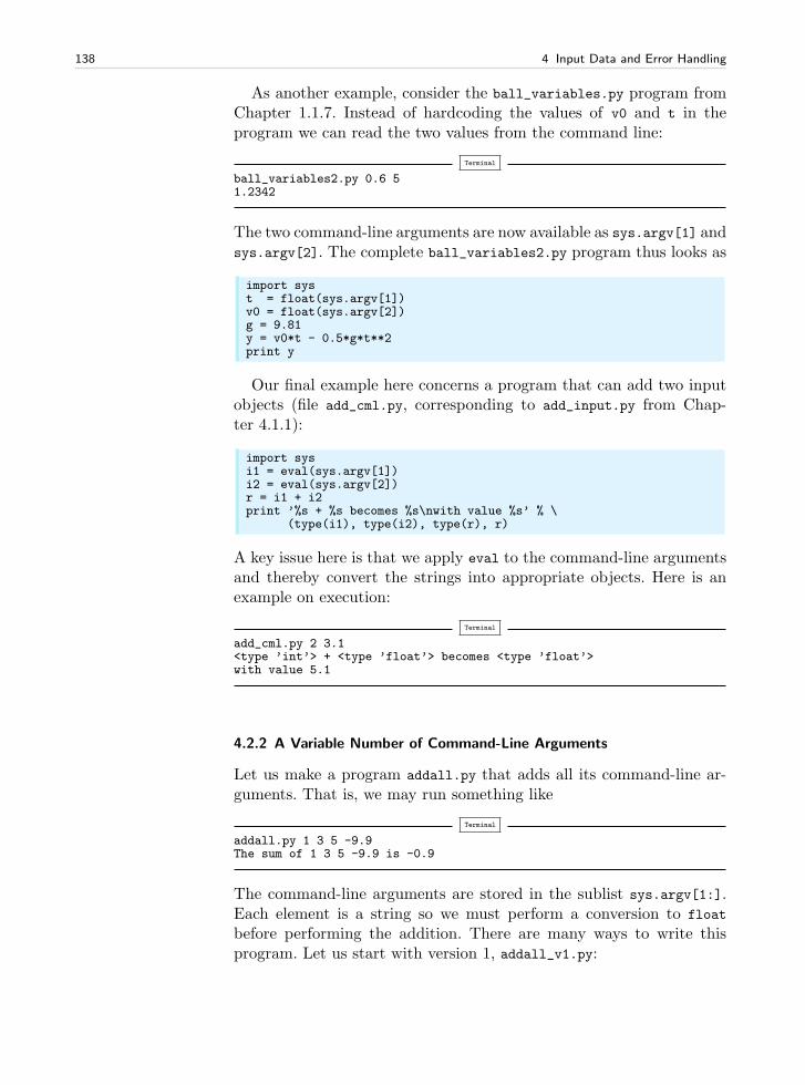
138 4 Input Data and Error Handling

As another example, consider the ball_variables.py program fromChapter 1.1.7. Instead of hardcoding the values of v0 and t in theprogram we can read the two values from the command line:

Terminal

ball_variables2.py 0.6 51.2342

The two command-line arguments are now available as sys.argv[1] andsys.argv[2]. The complete ball_variables2.py program thus looks as

import syst = float(sys.argv[1])v0 = float(sys.argv[2])g = 9.81y = v0*t - 0.5*g*t**2print y

Our final example here concerns a program that can add two inputobjects (file add_cml.py, corresponding to add_input.py from Chap-ter 4.1.1):

import sysi1 = eval(sys.argv[1])i2 = eval(sys.argv[2])r = i1 + i2print ’%s + %s becomes %s\nwith value %s’ % \

(type(i1), type(i2), type(r), r)

A key issue here is that we apply eval to the command-line argumentsand thereby convert the strings into appropriate objects. Here is anexample on execution:

Terminal

add_cml.py 2 3.1<type ’int’> + <type ’float’> becomes <type ’float’>with value 5.1

4.2.2 A Variable Number of Command-Line Arguments

Let us make a program addall.py that adds all its command-line ar-guments. That is, we may run something like

Terminal

addall.py 1 3 5 -9.9The sum of 1 3 5 -9.9 is -0.9

The command-line arguments are stored in the sublist sys.argv[1:].Each element is a string so we must perform a conversion to float

before performing the addition. There are many ways to write thisprogram. Let us start with version 1, addall_v1.py:

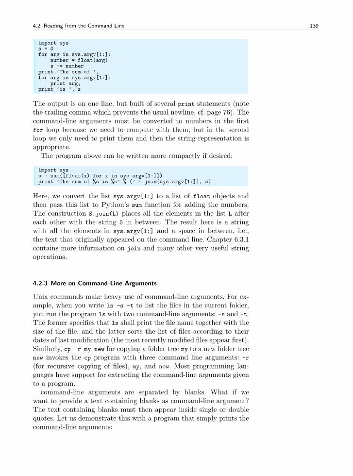
4.2 Reading from the Command Line 139

import syss = 0for arg in sys.argv[1:]:

number = float(arg)s += number

print ’The sum of ’,for arg in sys.argv[1:]:

print arg,print ’is ’, s

The output is on one line, but built of several print statements (notethe trailing comma which prevents the usual newline, cf. page 76). Thecommand-line arguments must be converted to numbers in the firstfor loop because we need to compute with them, but in the secondloop we only need to print them and then the string representation isappropriate.

The program above can be written more compactly if desired:

import syss = sum([float(x) for x in sys.argv[1:]])print ’The sum of %s is %s’ % (’ ’.join(sys.argv[1:]), s)

Here, we convert the list sys.argv[1:] to a list of float objects andthen pass this list to Python’s sum function for adding the numbers.The construction S.join(L) places all the elements in the list L aftereach other with the string S in between. The result here is a stringwith all the elements in sys.argv[1:] and a space in between, i.e.,the text that originally appeared on the command line. Chapter 6.3.1contains more information on join and many other very useful stringoperations.

4.2.3 More on Command-Line Arguments

Unix commands make heavy use of command-line arguments. For ex-ample, when you write ls -s -t to list the files in the current folder,you run the program ls with two command-line arguments: -s and -t.The former specifies that ls shall print the file name together with thesize of the file, and the latter sorts the list of files according to theirdates of last modification (the most recently modified files appear first).Similarly, cp -r my new for copying a folder tree my to a new folder treenew invokes the cp program with three command line arguments: -r(for recursive copying of files), my, and new. Most programming lan-guages have support for extracting the command-line arguments givento a program.

command-line arguments are separated by blanks. What if wewant to provide a text containing blanks as command-line argument?The text containing blanks must then appear inside single or doublequotes. Let us demonstrate this with a program that simply prints thecommand-line arguments:

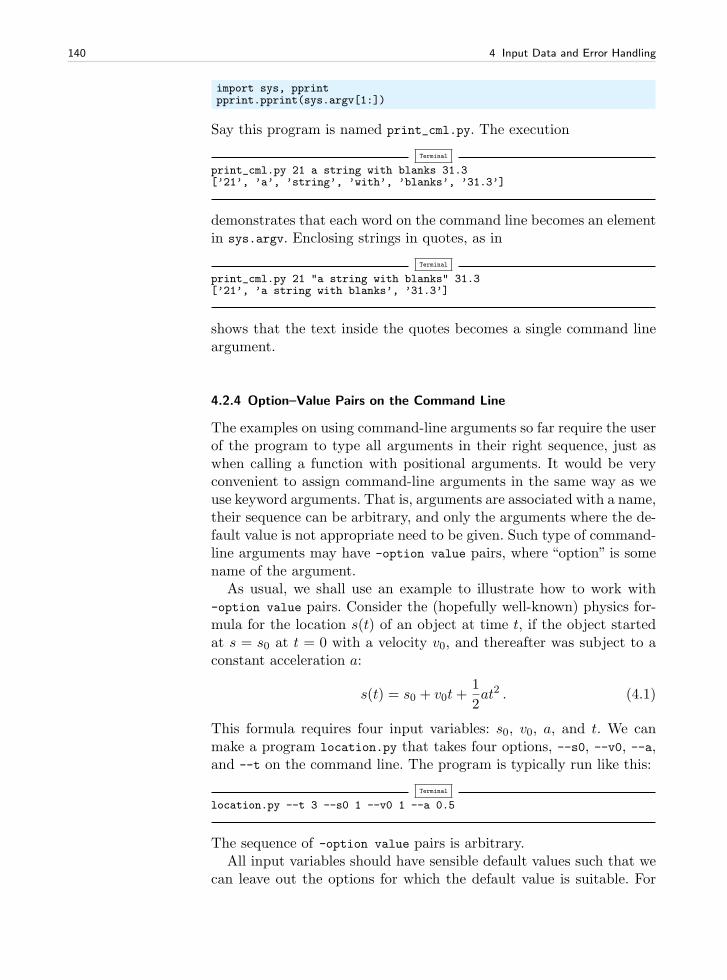
140 4 Input Data and Error Handling

import sys, pprintpprint.pprint(sys.argv[1:])

Say this program is named print_cml.py. The execution

Terminal

print_cml.py 21 a string with blanks 31.3[’21’, ’a’, ’string’, ’with’, ’blanks’, ’31.3’]

demonstrates that each word on the command line becomes an elementin sys.argv. Enclosing strings in quotes, as in

Terminal

print_cml.py 21 "a string with blanks" 31.3[’21’, ’a string with blanks’, ’31.3’]

shows that the text inside the quotes becomes a single command lineargument.

4.2.4 Option–Value Pairs on the Command Line

The examples on using command-line arguments so far require the userof the program to type all arguments in their right sequence, just aswhen calling a function with positional arguments. It would be veryconvenient to assign command-line arguments in the same way as weuse keyword arguments. That is, arguments are associated with a name,their sequence can be arbitrary, and only the arguments where the de-fault value is not appropriate need to be given. Such type of command-line arguments may have -option value pairs, where “option” is somename of the argument.

As usual, we shall use an example to illustrate how to work with-option value pairs. Consider the (hopefully well-known) physics for-mula for the location s(t) of an object at time t, if the object startedat s = s0 at t = 0 with a velocity v0, and thereafter was subject to aconstant acceleration a:

s(t) = s0 + v0t+1

2at2 . (4.1)

This formula requires four input variables: s0, v0, a, and t. We canmake a program location.py that takes four options, --s0, --v0, --a,and --t on the command line. The program is typically run like this:

Terminal

location.py --t 3 --s0 1 --v0 1 --a 0.5

The sequence of -option value pairs is arbitrary.All input variables should have sensible default values such that we

can leave out the options for which the default value is suitable. For

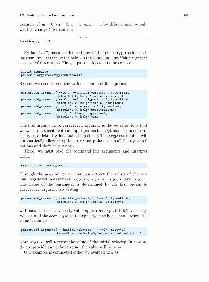
4.2 Reading from the Command Line 141

example, if s0 = 0, v0 = 0, a = 1, and t = 1 by default, and we onlywant to change t, we can run

Terminal

location.py --t 3

Python (v2.7) has a flexible and powerful module argparse for read-ing (parsing) -option value pairs on the command line. Using argparse

consists of three steps. First, a parser object must be created:

import argparseparser = argparse.ArgumentParser()

Second, we need to add the various command-line options,

parser.add_argument(’--v0’, ’--initial_velocity’, type=float,default=0.0, help=’initial velocity’)

parser.add_argument(’--s0’, ’--initial_position’, type=float,default=0.0, help=’initial position’)

parser.add_argument(’--a’, ’--acceleration’, type=float,default=1.0, help=’acceleration’)

parser.add_argument(’--t’, ’--time’, type=float,default=1.0, help=’time’)

The first arguments to parser.add_argument is the set of options thatwe want to associate with an input parameter. Optional arguments arethe type, a default value, and a help string. The argparse module willautomatically allow an option -h or -help that prints all the registeredoptions and their help strings.

Third, we must read the command line arguments and interpretthem:

args = parser.parse_args()

Through the args object we now can extract the values of the var-ious registered parameters: args.v0, args.s0, args.a, and args.t.The name of the parameter is determined by the first option toparser.add_argument, so writing

parser.add_argument(’--initial_velocity’, ’--v0’, type=float,default=0.0, help=’initial velocity’)

will make the initial velocity value appear as args.initial_velocity.We can add the dest keyword to explicitly specify the name where thevalue is stored:

parser.add_argument(’--initial_velocity’, ’--v0’, dest=’V0’,type=float, default=0, help=’initial velocity’)

Now, args.V0 will retrieve the value of the initial velocity. In case wedo not provide any default value, the value will be None.

Our example is completed either by evaluating s as

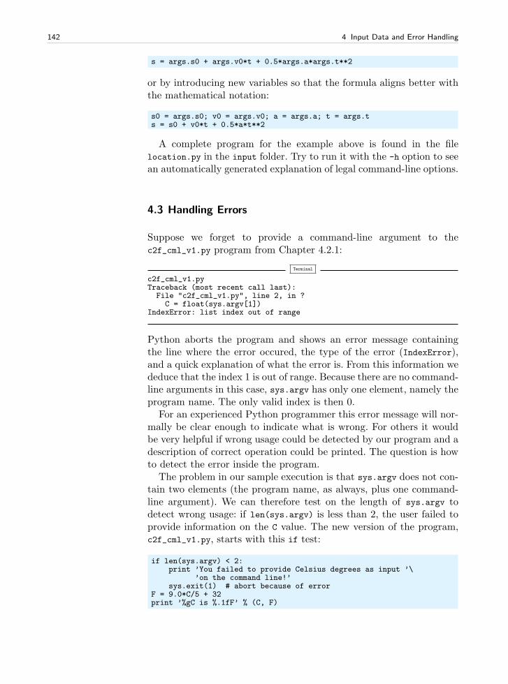
142 4 Input Data and Error Handling

s = args.s0 + args.v0*t + 0.5*args.a*args.t**2

or by introducing new variables so that the formula aligns better withthe mathematical notation:

s0 = args.s0; v0 = args.v0; a = args.a; t = args.ts = s0 + v0*t + 0.5*a*t**2

A complete program for the example above is found in the filelocation.py in the input folder. Try to run it with the -h option to seean automatically generated explanation of legal command-line options.

4.3 Handling Errors

Suppose we forget to provide a command-line argument to thec2f_cml_v1.py program from Chapter 4.2.1:

Terminal

c2f_cml_v1.pyTraceback (most recent call last):File "c2f_cml_v1.py", line 2, in ?C = float(sys.argv[1])

IndexError: list index out of range

Python aborts the program and shows an error message containingthe line where the error occured, the type of the error (IndexError),and a quick explanation of what the error is. From this information wededuce that the index 1 is out of range. Because there are no command-line arguments in this case, sys.argv has only one element, namely theprogram name. The only valid index is then 0.

For an experienced Python programmer this error message will nor-mally be clear enough to indicate what is wrong. For others it wouldbe very helpful if wrong usage could be detected by our program and adescription of correct operation could be printed. The question is howto detect the error inside the program.

The problem in our sample execution is that sys.argv does not con-tain two elements (the program name, as always, plus one command-line argument). We can therefore test on the length of sys.argv todetect wrong usage: if len(sys.argv) is less than 2, the user failed toprovide information on the C value. The new version of the program,c2f_cml_v1.py, starts with this if test:

if len(sys.argv) < 2:print ’You failed to provide Celsius degrees as input ’\

’on the command line!’sys.exit(1) # abort because of error

F = 9.0*C/5 + 32print ’%gC is %.1fF’ % (C, F)

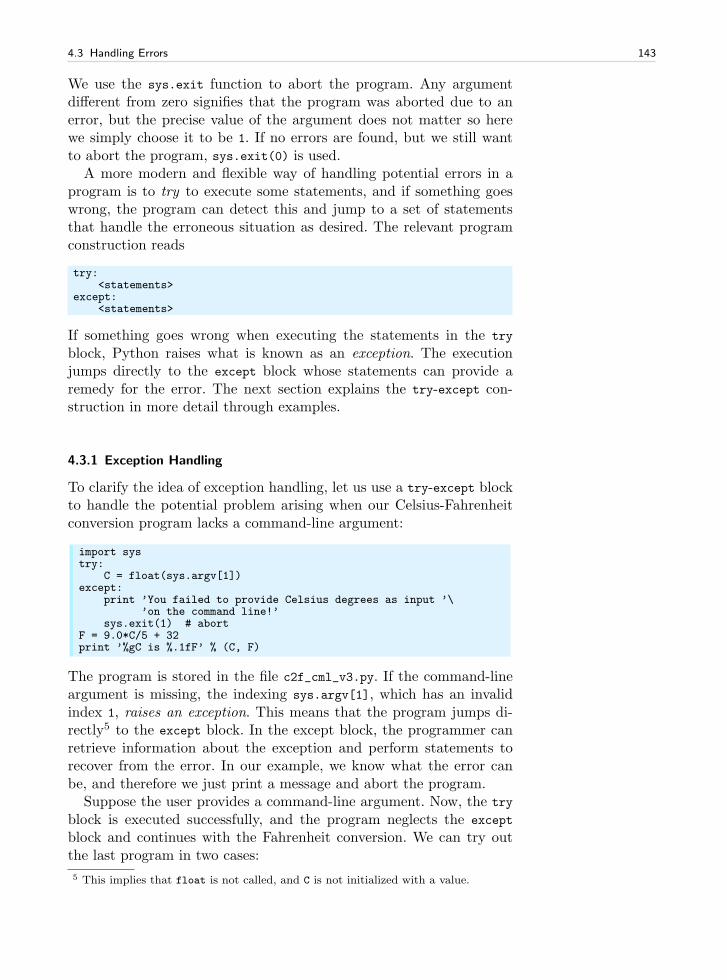
4.3 Handling Errors 143

We use the sys.exit function to abort the program. Any argumentdifferent from zero signifies that the program was aborted due to anerror, but the precise value of the argument does not matter so herewe simply choose it to be 1. If no errors are found, but we still wantto abort the program, sys.exit(0) is used.

A more modern and flexible way of handling potential errors in aprogram is to try to execute some statements, and if something goeswrong, the program can detect this and jump to a set of statementsthat handle the erroneous situation as desired. The relevant programconstruction reads

try:<statements>

except:<statements>

If something goes wrong when executing the statements in the try

block, Python raises what is known as an exception. The executionjumps directly to the except block whose statements can provide aremedy for the error. The next section explains the try-except con-struction in more detail through examples.

4.3.1 Exception Handling

To clarify the idea of exception handling, let us use a try-except blockto handle the potential problem arising when our Celsius-Fahrenheitconversion program lacks a command-line argument:

import systry:

C = float(sys.argv[1])except:

print ’You failed to provide Celsius degrees as input ’\’on the command line!’

sys.exit(1) # abortF = 9.0*C/5 + 32print ’%gC is %.1fF’ % (C, F)

The program is stored in the file c2f_cml_v3.py. If the command-lineargument is missing, the indexing sys.argv[1], which has an invalidindex 1, raises an exception. This means that the program jumps di-rectly5 to the except block. In the except block, the programmer canretrieve information about the exception and perform statements torecover from the error. In our example, we know what the error canbe, and therefore we just print a message and abort the program.

Suppose the user provides a command-line argument. Now, the try

block is executed successfully, and the program neglects the except

block and continues with the Fahrenheit conversion. We can try outthe last program in two cases:

5 This implies that float is not called, and C is not initialized with a value.

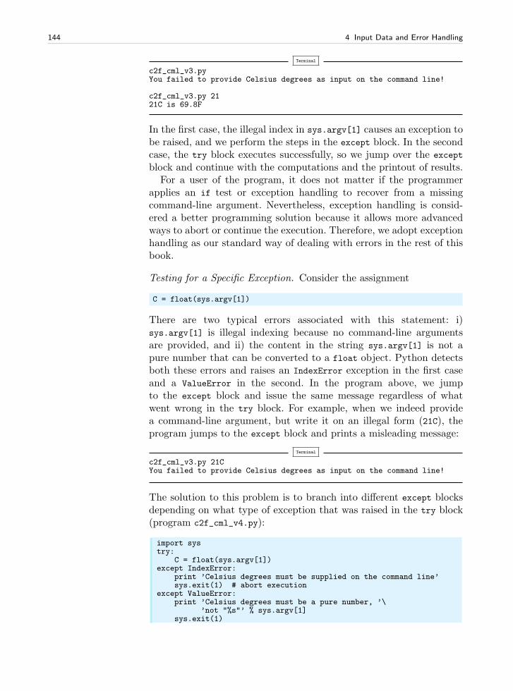
144 4 Input Data and Error Handling

Terminal

c2f_cml_v3.pyYou failed to provide Celsius degrees as input on the command line!

c2f_cml_v3.py 2121C is 69.8F

In the first case, the illegal index in sys.argv[1] causes an exception tobe raised, and we perform the steps in the except block. In the secondcase, the try block executes successfully, so we jump over the except

block and continue with the computations and the printout of results.For a user of the program, it does not matter if the programmer

applies an if test or exception handling to recover from a missingcommand-line argument. Nevertheless, exception handling is consid-ered a better programming solution because it allows more advancedways to abort or continue the execution. Therefore, we adopt exceptionhandling as our standard way of dealing with errors in the rest of thisbook.

Testing for a Specific Exception. Consider the assignment

C = float(sys.argv[1])

There are two typical errors associated with this statement: i)sys.argv[1] is illegal indexing because no command-line argumentsare provided, and ii) the content in the string sys.argv[1] is not apure number that can be converted to a float object. Python detectsboth these errors and raises an IndexError exception in the first caseand a ValueError in the second. In the program above, we jumpto the except block and issue the same message regardless of whatwent wrong in the try block. For example, when we indeed providea command-line argument, but write it on an illegal form (21C), theprogram jumps to the except block and prints a misleading message:

Terminal

c2f_cml_v3.py 21CYou failed to provide Celsius degrees as input on the command line!

The solution to this problem is to branch into different except blocksdepending on what type of exception that was raised in the try block(program c2f_cml_v4.py):

import systry:

C = float(sys.argv[1])except IndexError:

print ’Celsius degrees must be supplied on the command line’sys.exit(1) # abort execution

except ValueError:print ’Celsius degrees must be a pure number, ’\

’not "%s"’ % sys.argv[1]sys.exit(1)

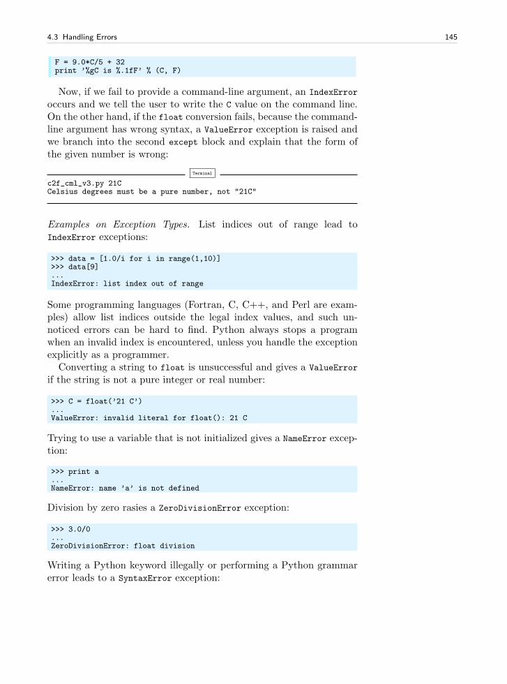
4.3 Handling Errors 145

F = 9.0*C/5 + 32print ’%gC is %.1fF’ % (C, F)

Now, if we fail to provide a command-line argument, an IndexError

occurs and we tell the user to write the C value on the command line.On the other hand, if the float conversion fails, because the command-line argument has wrong syntax, a ValueError exception is raised andwe branch into the second except block and explain that the form ofthe given number is wrong:

Terminal

c2f_cml_v3.py 21CCelsius degrees must be a pure number, not "21C"

Examples on Exception Types. List indices out of range lead toIndexError exceptions:

>>> data = [1.0/i for i in range(1,10)]>>> data[9]...IndexError: list index out of range

Some programming languages (Fortran, C, C++, and Perl are exam-ples) allow list indices outside the legal index values, and such un-noticed errors can be hard to find. Python always stops a programwhen an invalid index is encountered, unless you handle the exceptionexplicitly as a programmer.

Converting a string to float is unsuccessful and gives a ValueError

if the string is not a pure integer or real number:

>>> C = float(’21 C’)...ValueError: invalid literal for float(): 21 C

Trying to use a variable that is not initialized gives a NameError excep-tion:

>>> print a...NameError: name ’a’ is not defined

Division by zero rasies a ZeroDivisionError exception:

>>> 3.0/0...ZeroDivisionError: float division

Writing a Python keyword illegally or performing a Python grammarerror leads to a SyntaxError exception:

146 4 Input Data and Error Handling

>>> forr d in data:...

forr d in data:^

SyntaxError: invalid syntax

What if we try to multiply a string by a number?

>>> ’a string’*3.14...TypeError: can’t multiply sequence by non-int of type ’float’

The TypeError exception is raised because the object types involved inthe multiplication are wrong (str and float).

Digression. It might come as a surprise, but multiplication of a stringand a number is legal if the number is an integer. The multiplicationmeans that the string should be repeated the specified number of times.The same rule also applies to lists:

>>> ’--’*10 # ten double dashes = 20 dashes’--------------------’>>> n = 4>>> [1, 2, 3]*n[1, 2, 3, 1, 2, 3, 1, 2, 3, 1, 2, 3]>>> [0]*n[0, 0, 0, 0]

The latter construction is handy when we want to create a list of n

elements and later assign specific values to each element in a for loop.

4.3.2 Raising Exceptions

When an error occurs in your program, you may either print a mes-sage and use sys.exit(1) to abort the program, or you may raise anexception. The latter task is easy. You just write raise E(message),where E can be a known exception type in Python and message is astring explaining what is wrong. Most often E means ValueError if thevalue of some variable is illegal, or TypeError if the type of a variableis wrong. You can also define your own exception types. An exceptioncan be raised from any location in a program.

Example. In the program c2f_cml_v4.py from page 144 we show howwe can test for different exceptions and abort the program. Sometimeswe see that an exception may happen, but if it happens, we want a moreprecise error message to help the user. This can be done by raising anew exception in an except block and provide the desired exceptiontype and message.

Another application of raising exceptions with tailored error mes-sages arises when input data are invalid. The code below illustrateshow to raise exceptions in various cases.

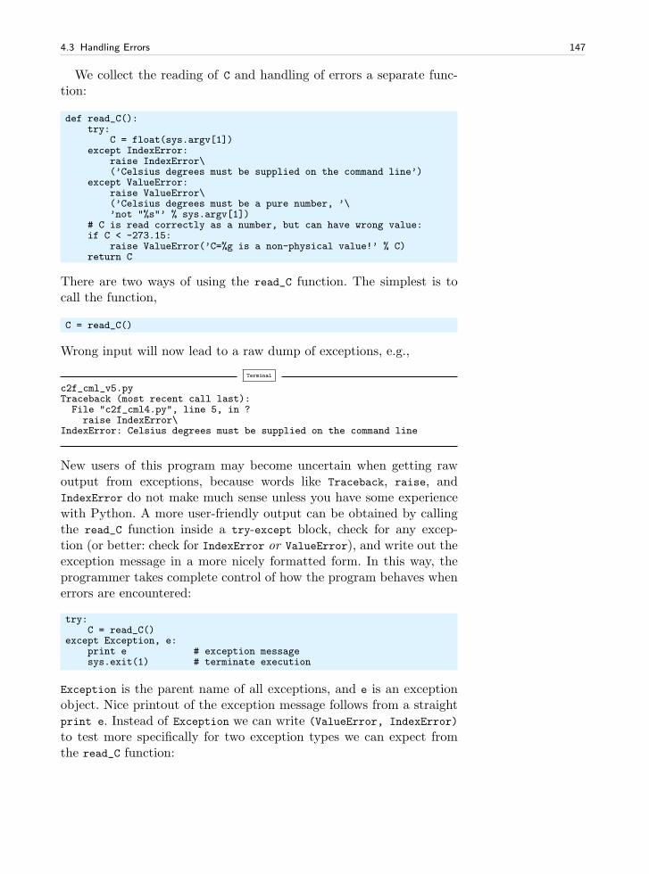
4.3 Handling Errors 147

We collect the reading of C and handling of errors a separate func-tion:

def read_C():try:

C = float(sys.argv[1])except IndexError:

raise IndexError\(’Celsius degrees must be supplied on the command line’)

except ValueError:raise ValueError\(’Celsius degrees must be a pure number, ’\’not "%s"’ % sys.argv[1])

# C is read correctly as a number, but can have wrong value:if C < -273.15:

raise ValueError(’C=%g is a non-physical value!’ % C)return C

There are two ways of using the read_C function. The simplest is tocall the function,

C = read_C()

Wrong input will now lead to a raw dump of exceptions, e.g.,

Terminal

c2f_cml_v5.pyTraceback (most recent call last):File "c2f_cml4.py", line 5, in ?raise IndexError\

IndexError: Celsius degrees must be supplied on the command line

New users of this program may become uncertain when getting rawoutput from exceptions, because words like Traceback, raise, andIndexError do not make much sense unless you have some experiencewith Python. A more user-friendly output can be obtained by callingthe read_C function inside a try-except block, check for any excep-tion (or better: check for IndexError or ValueError), and write out theexception message in a more nicely formatted form. In this way, theprogrammer takes complete control of how the program behaves whenerrors are encountered:

try:C = read_C()

except Exception, e:print e # exception messagesys.exit(1) # terminate execution

Exception is the parent name of all exceptions, and e is an exceptionobject. Nice printout of the exception message follows from a straightprint e. Instead of Exception we can write (ValueError, IndexError)

to test more specifically for two exception types we can expect fromthe read_C function:

148 4 Input Data and Error Handling

try:C = read_C()

except (ValueError, IndexError), e:print e # exception messagesys.exit(1) # terminate execution

After the try-except block above, we can continue with computing F =

9*C/5 + 32 and print out F. The complete program is found in the filec2f_cml.py. We may now test the program’s behavior when the inputis wrong and right:

Terminal

c2f_cml.pyCelsius degrees must be supplied on the command line

c2f_cml.py 21CCelsius degrees must be a pure number, not "21C"

c2f_cml.py -500C=-500 is a non-physical value!

c2f_cml.py 2121C is 69.8F

This program deals with wrong input, writes an informative message,and terminates the execution without annoying behavior.

Scattered if tests with sys.exit calls are considered a bad program-ming style compared to the use of nested exception handling as illus-trated above. You should abort execution in the main program only,not inside functions. The reason is that the functions can be re-usedin other occasions where the error can be dealt with differently. Forinstance, one may avoid abortion by using some suitable default data.

The programming style illustrated above is considered the best wayof dealing with errors, so we suggest that you hereafter apply exceptionsfor handling potential errors in the programs you make, simply becausethis is what experienced programmers expect from your codes.

4.4 A Glimpse of Graphical User Interfaces

Maybe you find it somewhat strange that the usage of the programswe have made so far in this book – and the programs we will make inthe rest of the book – are less graphical and intuitive than the com-puter programs you are used to from school or entertainment. Thoseprograms are operated through some self-explaning graphics, and mostof the things you want to do involve pointing with the mouse, clickingon graphical elements on the screen, and maybe filling in some textfields. The programs in this book, on the other hand, are run from thecommand line in a terminal window or inside IPython, and input isalso given here in form of plain text.

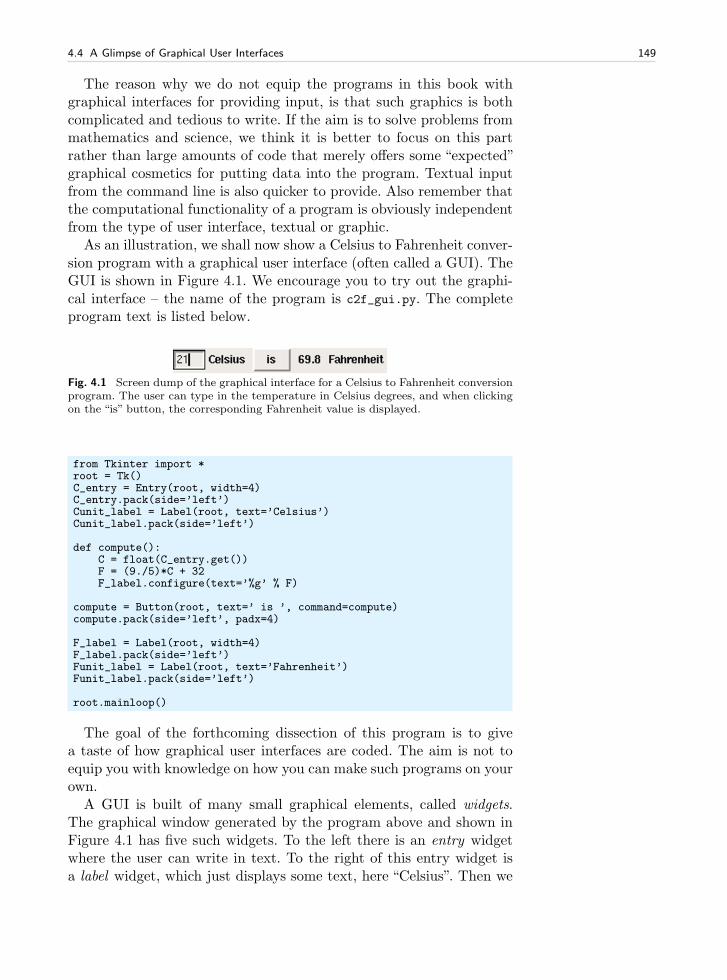
4.4 A Glimpse of Graphical User Interfaces 149

The reason why we do not equip the programs in this book withgraphical interfaces for providing input, is that such graphics is bothcomplicated and tedious to write. If the aim is to solve problems frommathematics and science, we think it is better to focus on this partrather than large amounts of code that merely offers some “expected”graphical cosmetics for putting data into the program. Textual inputfrom the command line is also quicker to provide. Also remember thatthe computational functionality of a program is obviously independentfrom the type of user interface, textual or graphic.

As an illustration, we shall now show a Celsius to Fahrenheit conver-sion program with a graphical user interface (often called a GUI). TheGUI is shown in Figure 4.1. We encourage you to try out the graphi-cal interface – the name of the program is c2f_gui.py. The completeprogram text is listed below.

Fig. 4.1 Screen dump of the graphical interface for a Celsius to Fahrenheit conversionprogram. The user can type in the temperature in Celsius degrees, and when clickingon the “is” button, the corresponding Fahrenheit value is displayed.

from Tkinter import *root = Tk()C_entry = Entry(root, width=4)C_entry.pack(side=’left’)Cunit_label = Label(root, text=’Celsius’)Cunit_label.pack(side=’left’)

def compute():C = float(C_entry.get())F = (9./5)*C + 32F_label.configure(text=’%g’ % F)

compute = Button(root, text=’ is ’, command=compute)compute.pack(side=’left’, padx=4)

F_label = Label(root, width=4)F_label.pack(side=’left’)Funit_label = Label(root, text=’Fahrenheit’)Funit_label.pack(side=’left’)

root.mainloop()

The goal of the forthcoming dissection of this program is to givea taste of how graphical user interfaces are coded. The aim is not toequip you with knowledge on how you can make such programs on yourown.

A GUI is built of many small graphical elements, called widgets.The graphical window generated by the program above and shown inFigure 4.1 has five such widgets. To the left there is an entry widgetwhere the user can write in text. To the right of this entry widget isa label widget, which just displays some text, here “Celsius”. Then we

150 4 Input Data and Error Handling

have a button widget, which when being clicked leads to computationsin the program. The result of these computations is displayed as textin a label widget to the right of the button widget. Finally, to theright of this result text we have another label widget displaying thetext “Fahrenheit”. The program must construct each widget and packit correctly into the complete window. In the present case, all widgetsare packed from left to right.

The first statement in the program imports functionality from theGUI toolkit Tkinter to construct widgets. First, we need to make aroot widget that holds the complete window with all the other widgets.This root widget is of type Tk. The first entry widget is then made andreferred to by a variable C_entry. This widget is an object of typeEntry, provided by the Tkinter module. Widgets constructions followthe syntax

variable_name = Widget_type(parent_widget, option1, option2, ...)variable_name.pack(side=’left’)

When creating a widget, we must bind it to a parent widget, which isthe graphical element in which this new widget is to be packed. Ourwidgets in the present program have the root widget as parent widget.Various widgets have different types of options that we can set. Forexample, the Entry widget has a possibility for setting the width of thetext field, here width=4 means that the text field is 4 characters wide.The pack statement is important to remember – without it, the widgetremains invisible.

The other widgets are constructed in similar ways. The next fun-damental feature of our program is how computations are tied to theevent of clicking the button “is”. The Button widget has naturally atext, but more important, it binds the button to a function compute

through the command=compute option. This means that when the userclicks the button “is”, the function compute is called. Inside the compute

function we first fetch the Celsius value from the C_entry widget, usingthis widget’s get function, then we transform this string (everythingtyped in by the user is interpreted as text and stored in strings) to afloat before we compute the corresponding Fahrenheit value. Finally,we can update (“configure”) the text in the Label widget F_label witha new text, namely the computed degrees in Fahrenheit.

A program with a GUI behaves differently from the programs weconstruct in this book. First, all the statements are executed from topto bottom, as in all our other programs, but these statements just con-struct the GUI and define functions. No computations are performed.Then the program enters a so-called event loop: root.mainloop(). Thisis an infinite loop that “listens” to user events, such as moving themouse, clicking the mouse, typing characters on the keyboard, etc.When an event is recorded, the program starts performing associated

4.5 Making Modules 151

actions. In the present case, the program waits for only one event:clicking the button “is”. As soon as we click on the button, the compute

function is called and the program starts doing mathematical work.The GUI will appear on the screen until we destroy the window byclick on the X up in the corner of the window decoration. More com-plicated GUIs will normally have a special “Quit” button to terminatethe event loop.

In all GUI programs, we must first create a hierarchy of widgets tobuild up all elements of the user interface. Then the program enters anevent loop and waits for user events. Lots of such events are registeredas actions in the program when creating the widgets, so when the userclicks on buttons, move the mouse into certain areas, etc., functions inthe program are called and “things happen”.

Many books explain how to make GUIs in Python programs, see forinstance [2, 3, 5, 7].

4.5 Making Modules

Sometimes you want to reuse a function from an old program in a newprogram. The simplest way to do this is to copy and paste the old sourcecode into the new program. However, this is not good programmingpractice, because you then over time end up with multiple identicalversions of the same function. When you want to improve the functionor correct a bug, you need to remember to do the same update in allfiles with a copy of the function, and in real life most programmersfail to do so. You easily end up with a mess of different versions withdifferent quality of basically the same code. Therefore, a golden rule ofprogramming is to have one and only one version of a piece of code.All programs that want to use this piece of code must access one andonly one place where the source code is kept. This principle is easy toimplement if we create a module containing the code we want to reuselater in different programs.

You learned already in Chapter 1 how to import functions fromPython modules. Now you will learn how to make your own modules.There is hardly anything to learn, because you just collect all the func-tions that constitute the module in one file, say with name mymodule.py.This file is automatically a module, with name mymodule, and you canimport functions from this module in the standard way. Let us makeeverything clear in detail by looking at an example.

152 4 Input Data and Error Handling

4.5.1 Example: Compund Interest Formulas

The classical formula for the growth of money in a bank reads6

A = A0

(

1 +p

360 · 100)n

, (4.2)

where A0 is the initial amount of money, and A is the present amountafter n days with p percent annual interest rate. Equation (4.2) involvesfour parameters: A, A0, p, and n. We may solve for any of these, giventhe other three:

A0 = A(

1 +p

360 · 100)−n

, (4.3)

n =ln A

A0

ln(

1 + p360·100

) , (4.4)

p = 360 · 100(

(

A

A0

)1/n

− 1

)

(4.5)

Suppose we have implemented (4.2)–(4.5) in four functions:

from math import log as ln

def present_amount(A0, p, n):return A0*(1 + p/(360.0*100))**n

def initial_amount(A, p, n):return A*(1 + p/(360.0*100))**(-n)

def days(A0, A, p):return ln(A/A0)/ln(1 + p/(360.0*100))

def annual_rate(A0, A, n):return 360*100*((A/A0)**(1.0/n) - 1)

We want to make these functions available in a module, say withname interest, so that we can import functions and compute withthem in a program. For example,

from interest import daysA0 = 1; A = 2; p = 5n = days(A0, 2, p)years = n/365.0print ’Money has doubled after %.1f years’ % years

How to make the interest module is described next.

6 The formula applies the so-called Actual/360 convention where the rate per dayis computed as p/360, while n counts the actual number of days the money is inthe bank. See “Day count convention” in Wikipedia for detailed information andpage 500 for a Python module for computing the number of days between two dates.

4.5 Making Modules 153

4.5.2 Collecting Functions in a Module File

To make a module of the four functions present_amount,initial_amount, days, and annual_rate, we simply open an emptyfile in a text editor and copy the program code for all the four func-tions over to this file. This file is then automatically a Python moduleprovided we save the file under any valid filename. The extension mustbe .py, but the module name is only the base part of the filename. Inour case, the filename interest.py implies a module name interest.To use the annual_rate function in another program we simply write,in that program file,

from interest import annual_rate

or we can write

from interest import *

to import all four functions, or we can write

import interest

and access individual functions as interest.annual_rate and so forth.

Test Block. It is recommended to only have functions and not anystatements outside functions in a module7. However, Python allows aspecial construction to let the file act both as a module with functiondefinitions only and as an ordinary program that we can run, i.e., withstatements that apply the functions and possibly write output. Thistwo-fold “magic” consists of putting the application part after an if

test of the form

if __name__ == ’__main__’:<block of statements>

The __name__ variable is automatically defined in any module andequals the module name if the module file is imported in another pro-gram, or __name__ equals the string ’__main__’ if the module file isrun as a program. This implies that the <block of statements> part isexecuted if and only if we run the module file as a program. We shallrefer to <block of statements> as the test block of a module.

Often, when modules are created from an ordinary program, theoriginal main program is used as test block. The new module file thenworks as the old program, but with the new possibility of being im-ported in other programs. Let us write a little main program for testingthe interest module. The idea is that we assign compatible values to

7 The module file is executed from top to bottom during the import. With functiondefinitions only in the module file, there will be no calculations or output from theimport, just definitions of functions. This is the desirable behavior.

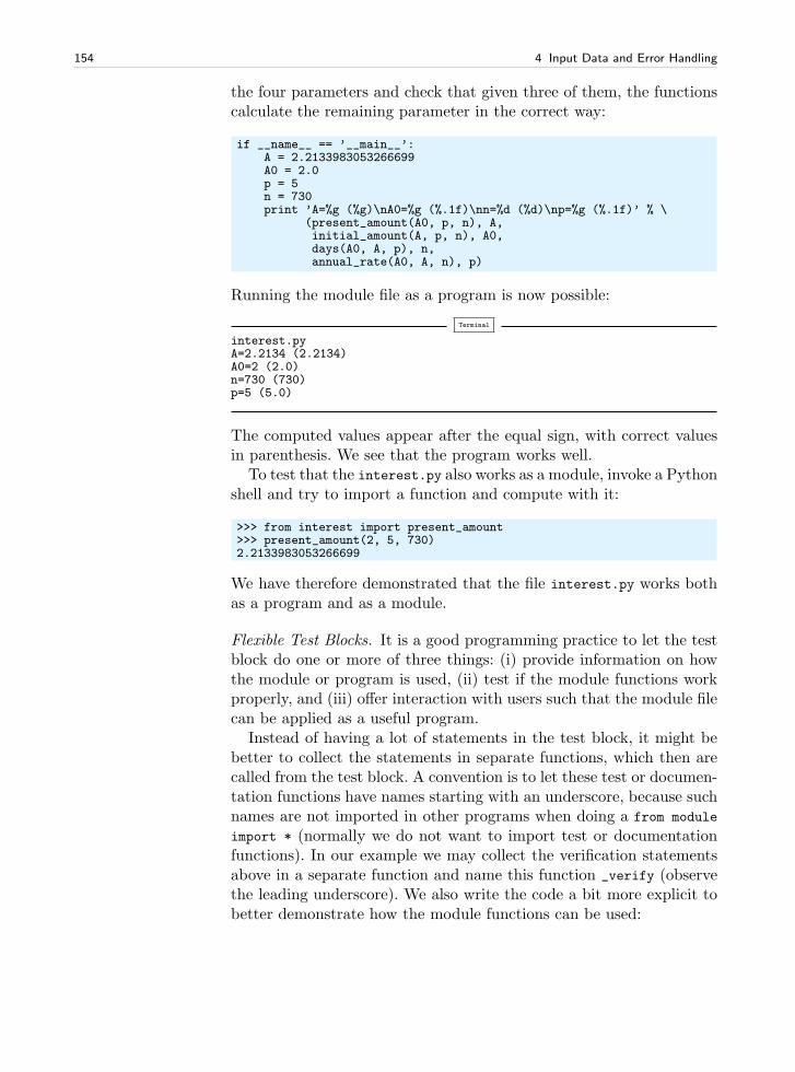
154 4 Input Data and Error Handling

the four parameters and check that given three of them, the functionscalculate the remaining parameter in the correct way:

if __name__ == ’__main__’:A = 2.2133983053266699A0 = 2.0p = 5n = 730print ’A=%g (%g)\nA0=%g (%.1f)\nn=%d (%d)\np=%g (%.1f)’ % \

(present_amount(A0, p, n), A,initial_amount(A, p, n), A0,days(A0, A, p), n,annual_rate(A0, A, n), p)

Running the module file as a program is now possible:

Terminal

interest.pyA=2.2134 (2.2134)A0=2 (2.0)n=730 (730)p=5 (5.0)

The computed values appear after the equal sign, with correct valuesin parenthesis. We see that the program works well.

To test that the interest.py also works as a module, invoke a Pythonshell and try to import a function and compute with it:

>>> from interest import present_amount>>> present_amount(2, 5, 730)2.2133983053266699

We have therefore demonstrated that the file interest.py works bothas a program and as a module.

Flexible Test Blocks. It is a good programming practice to let the testblock do one or more of three things: (i) provide information on howthe module or program is used, (ii) test if the module functions workproperly, and (iii) offer interaction with users such that the module filecan be applied as a useful program.

Instead of having a lot of statements in the test block, it might bebetter to collect the statements in separate functions, which then arecalled from the test block. A convention is to let these test or documen-tation functions have names starting with an underscore, because suchnames are not imported in other programs when doing a from module

import * (normally we do not want to import test or documentationfunctions). In our example we may collect the verification statementsabove in a separate function and name this function _verify (observethe leading underscore). We also write the code a bit more explicit tobetter demonstrate how the module functions can be used:

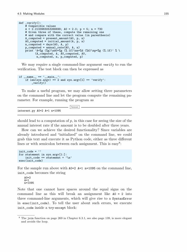
4.5 Making Modules 155

def _verify():# Compatible valuesA = 2.2133983053266699; A0 = 2.0; p = 5; n = 730# Given three of these, compute the remaining one# and compare with the correct value (in parenthesis)A_computed = present_amount(A0, p, n)A0_computed = initial_amount(A, p, n)n_computed = days(A0, A, p)p_computed = annual_rate(A0, A, n)print ’A=%g (%g)\nA0=%g (%.1f)\nn=%d (%d)\np=%g (%.1f)’ % \

(A_computed, A, A0_computed, A0,n_computed, n, p_computed, p)

We may require a single command-line argument verify to run theverification. The test block can then be expressed as

if __name__ == ’__main__’:if len(sys.argv) == 2 and sys.argv[1] == ’verify’:

_verify()

To make a useful program, we may allow setting three parameterson the command line and let the program compute the remaining pa-rameter. For example, running the program as

Terminal

interest.py A0=2 A=1 n=1095

should lead to a computation of p, in this case for seeing the size of theannual interest rate if the amount is to be doubled after three years.

How can we achieve the desired functionality? Since variables arealready introduced and “initialized” on the command line, we couldgrab this text and execute it as Python code, either as three differentlines or with semicolon between each assignment. This is easy8:

init_code = ’’for statement in sys.argv[1:]:

init_code += statement + ’\n’exec(init_code)

For the sample run above with A0=2 A=1 n=1095 on the command line,init_code becomes the string

A0=2A=1n=1095

Note that one cannot have spaces around the equal signs on thecommand line as this will break an assignment like A0 = 2 intothree command-line arguments, which will give rise to a SyntaxError

in exec(init_code). To tell the user about such errors, we executeinit_code inside a try-except block:

8 The join function on page 269 in Chapter 6.3.1, see also page 139, is more elegantand avoids the loop.

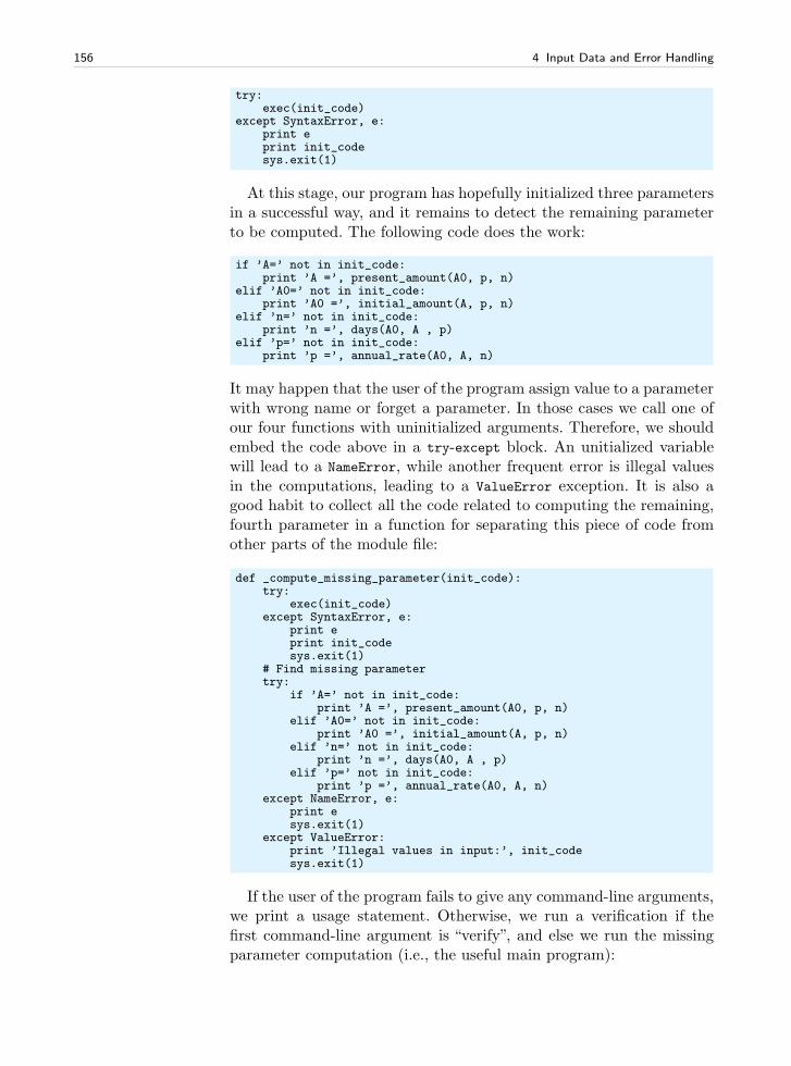
156 4 Input Data and Error Handling

try:exec(init_code)

except SyntaxError, e:print eprint init_codesys.exit(1)

At this stage, our program has hopefully initialized three parametersin a successful way, and it remains to detect the remaining parameterto be computed. The following code does the work:

if ’A=’ not in init_code:print ’A =’, present_amount(A0, p, n)

elif ’A0=’ not in init_code:print ’A0 =’, initial_amount(A, p, n)

elif ’n=’ not in init_code:print ’n =’, days(A0, A , p)

elif ’p=’ not in init_code:print ’p =’, annual_rate(A0, A, n)

It may happen that the user of the program assign value to a parameterwith wrong name or forget a parameter. In those cases we call one ofour four functions with uninitialized arguments. Therefore, we shouldembed the code above in a try-except block. An unitialized variablewill lead to a NameError, while another frequent error is illegal valuesin the computations, leading to a ValueError exception. It is also agood habit to collect all the code related to computing the remaining,fourth parameter in a function for separating this piece of code fromother parts of the module file:

def _compute_missing_parameter(init_code):try:

exec(init_code)except SyntaxError, e:

print eprint init_codesys.exit(1)

# Find missing parametertry:

if ’A=’ not in init_code:print ’A =’, present_amount(A0, p, n)

elif ’A0=’ not in init_code:print ’A0 =’, initial_amount(A, p, n)

elif ’n=’ not in init_code:print ’n =’, days(A0, A , p)

elif ’p=’ not in init_code:print ’p =’, annual_rate(A0, A, n)

except NameError, e:print esys.exit(1)

except ValueError:print ’Illegal values in input:’, init_codesys.exit(1)

If the user of the program fails to give any command-line arguments,we print a usage statement. Otherwise, we run a verification if thefirst command-line argument is “verify”, and else we run the missingparameter computation (i.e., the useful main program):

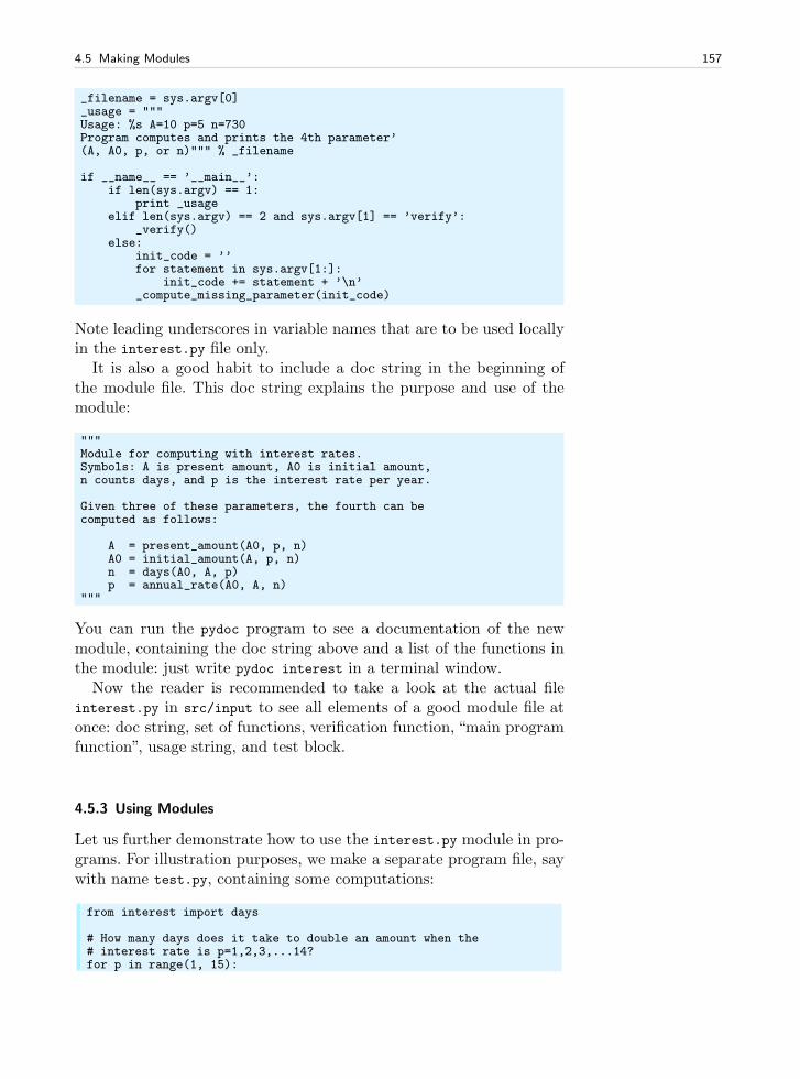
4.5 Making Modules 157

_filename = sys.argv[0]_usage = """Usage: %s A=10 p=5 n=730Program computes and prints the 4th parameter’(A, A0, p, or n)""" % _filename

if __name__ == ’__main__’:if len(sys.argv) == 1:

print _usageelif len(sys.argv) == 2 and sys.argv[1] == ’verify’:

_verify()else:

init_code = ’’for statement in sys.argv[1:]:

init_code += statement + ’\n’_compute_missing_parameter(init_code)

Note leading underscores in variable names that are to be used locallyin the interest.py file only.

It is also a good habit to include a doc string in the beginning ofthe module file. This doc string explains the purpose and use of themodule:

"""Module for computing with interest rates.Symbols: A is present amount, A0 is initial amount,n counts days, and p is the interest rate per year.

Given three of these parameters, the fourth can becomputed as follows:

A = present_amount(A0, p, n)A0 = initial_amount(A, p, n)n = days(A0, A, p)p = annual_rate(A0, A, n)

"""

You can run the pydoc program to see a documentation of the newmodule, containing the doc string above and a list of the functions inthe module: just write pydoc interest in a terminal window.

Now the reader is recommended to take a look at the actual fileinterest.py in src/input to see all elements of a good module file atonce: doc string, set of functions, verification function, “main programfunction”, usage string, and test block.

4.5.3 Using Modules

Let us further demonstrate how to use the interest.py module in pro-grams. For illustration purposes, we make a separate program file, saywith name test.py, containing some computations:

from interest import days

# How many days does it take to double an amount when the# interest rate is p=1,2,3,...14?for p in range(1, 15):

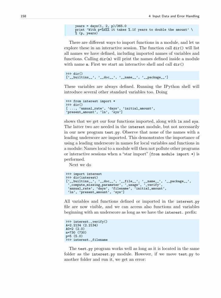
158 4 Input Data and Error Handling

years = days(1, 2, p)/365.0print ’With p=%d%% it takes %.1f years to double the amount’ \% (p, years)

There are different ways to import functions in a module, and let usexplore these in an interactive session. The function call dir() will listall names we have defined, including imported names of variables andfunctions. Calling dir(m) will print the names defined inside a modulewith name m. First we start an interactive shell and call dir()

>>> dir()[’__builtins__’, ’__doc__’, ’__name__’, ’__package__’]

These variables are always defined. Running the IPython shell willintroduce several other standard variables too. Doing

>>> from interest import *>>> dir()[ ..., ’annual_rate’, ’days’, ’initial_amount’,’present_amount’, ’ln’, ’sys’]

shows that we get our four functions imported, along with ln and sys.The latter two are needed in the interest module, but not necessarilyin our new program test.py. Observe that none of the names with aleading underscore are imported. This demonstrates the importance ofusing a leading underscore in names for local variables and functions ina module: Names local to a module will then not pollute other programsor interactive sessions when a “star import” (from module import *) isperformed.

Next we do

>>> import interest>>> dir(interest)[’__builtins__’, ’__doc__’, ’__file__’, ’__name__’, ’__package__’,’_compute_missing_parameter’, ’_usage’, ’_verify’,’annual_rate’, ’days’, ’filename’, ’initial_amount’,’ln’, ’present_amount’, ’sys’]

All variables and functions defined or imported in the interest.py

file are now visible, and we can access also functions and variablesbeginning with an underscore as long as we have the interest. prefix:

>>> interest._verify()A=2.2134 (2.2134)A0=2 (2.0)n=730 (730)p=5 (5.0)>>> interest._filename

The test.py program works well as long as it is located in the samefolder as the interest.py module. However, if we move test.py toanother folder and run it, we get an error:

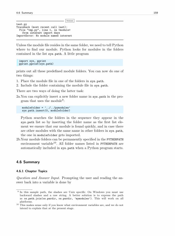
4.6 Summary 159

Terminal

test.pyTraceback (most recent call last):File "tmp.py", line 1, in <module>from interest import days

ImportError: No module named interest

Unless the module file resides in the same folder, we need to tell Pythonwhere to find our module. Python looks for modules in the folderscontained in the list sys.path. A little program

import sys, pprintpprint.pprint(sys.path)

prints out all these predefined module folders. You can now do one oftwo things:

1. Place the module file in one of the folders in sys.path.2. Include the folder containing the module file in sys.path.

There are two ways of doing the latter task:

2a.You can explicitly insert a new folder name in sys.path in the pro-gram that uses the module9:

modulefolder = ’../../pymodules’sys.path.insert(0, modulefolder)

Python searches the folders in the sequence they appear in thesys.path list so by inserting the folder name as the first list ele-ment we ensure that our module is found quickly, and in case thereare other modules with the same name in other folders in sys.path,the one in modulefolder gets imported.

2b.Your module folders can be permanently specified in the PYTHONPATHenvironment variable10. All folder names listed in PYTHONPATH areautomatically included in sys.path when a Python program starts.

4.6 Summary

4.6.1 Chapter Topics

Question and Answer Input. Prompting the user and reading the an-swer back into a variable is done by

9 In this sample path, the slashes are Unix specific. On Windows you must usebackward slashes and a raw string. A better solution is to express the pathas os.path.join(os.pardir, os.pardir, ’mymodules’). This will work on allplatforms.

10 This makes sense only if you know what environment variables are, and we do notintend to explain that at the present stage.

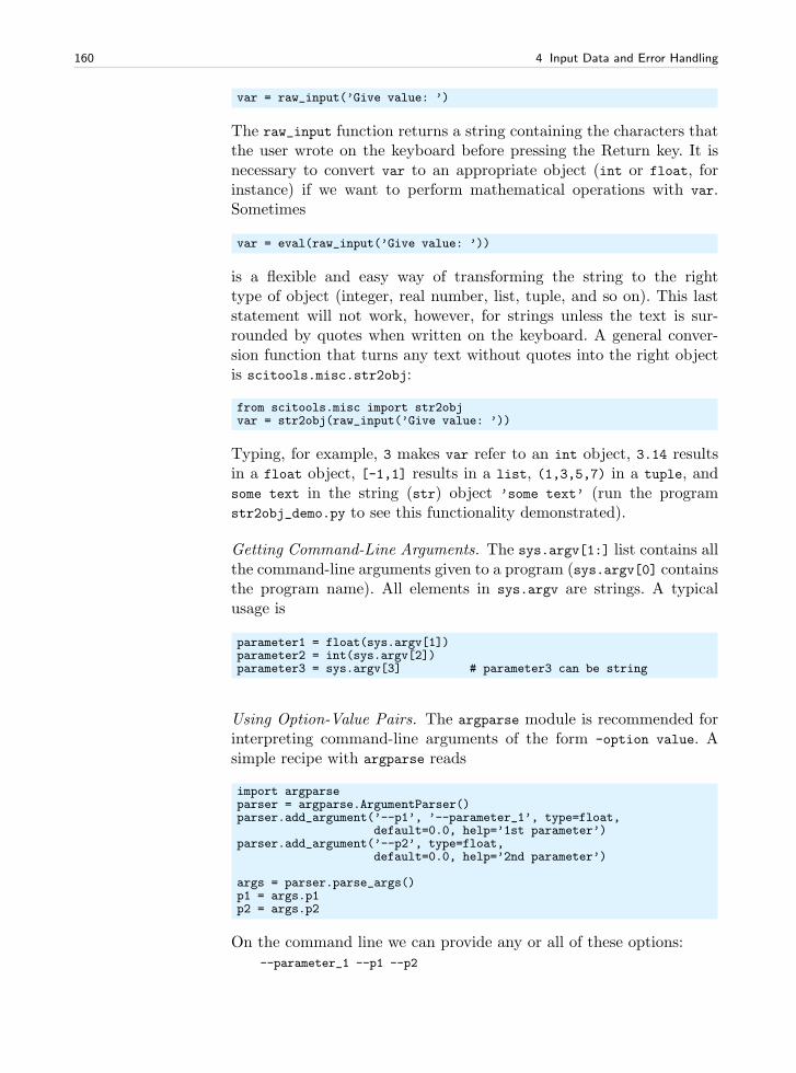
160 4 Input Data and Error Handling

var = raw_input(’Give value: ’)

The raw_input function returns a string containing the characters thatthe user wrote on the keyboard before pressing the Return key. It isnecessary to convert var to an appropriate object (int or float, forinstance) if we want to perform mathematical operations with var.Sometimes

var = eval(raw_input(’Give value: ’))

is a flexible and easy way of transforming the string to the righttype of object (integer, real number, list, tuple, and so on). This laststatement will not work, however, for strings unless the text is sur-rounded by quotes when written on the keyboard. A general conver-sion function that turns any text without quotes into the right objectis scitools.misc.str2obj:

from scitools.misc import str2objvar = str2obj(raw_input(’Give value: ’))

Typing, for example, 3 makes var refer to an int object, 3.14 resultsin a float object, [-1,1] results in a list, (1,3,5,7) in a tuple, andsome text in the string (str) object ’some text’ (run the programstr2obj_demo.py to see this functionality demonstrated).

Getting Command-Line Arguments. The sys.argv[1:] list contains allthe command-line arguments given to a program (sys.argv[0] containsthe program name). All elements in sys.argv are strings. A typicalusage is

parameter1 = float(sys.argv[1])parameter2 = int(sys.argv[2])parameter3 = sys.argv[3] # parameter3 can be string

Using Option-Value Pairs. The argparse module is recommended forinterpreting command-line arguments of the form -option value. Asimple recipe with argparse reads

import argparseparser = argparse.ArgumentParser()parser.add_argument(’--p1’, ’--parameter_1’, type=float,

default=0.0, help=’1st parameter’)parser.add_argument(’--p2’, type=float,

default=0.0, help=’2nd parameter’)

args = parser.parse_args()p1 = args.p1p2 = args.p2

On the command line we can provide any or all of these options:--parameter_1 --p1 --p2

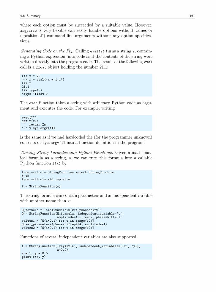
4.6 Summary 161

where each option must be succeeded by a suitable value. However,argparse is very flexible can easily handle options without values or(“positional”) command-line arguments without any option specifica-tions.

Generating Code on the Fly. Calling eval(s) turns a string s, contain-ing a Python expression, into code as if the contents of the string werewritten directly into the program code. The result of the following eval

call is a float object holding the number 21.1:

>>> x = 20>>> r = eval(’x + 1.1’)>>> r21.1>>> type(r)<type ’float’>

The exec function takes a string with arbitrary Python code as argu-ment and executes the code. For example, writing

exec("""def f(x):

return %s""" % sys.argv[1])

is the same as if we had hardcoded the (for the programmer unknown)contents of sys.argv[1] into a function definition in the program.

Turning String Formulas into Python Functions. Given a mathemat-ical formula as a string, s, we can turn this formula into a callablePython function f(x) by

from scitools.StringFunction import StringFunction# orfrom scitools.std import *

f = StringFunction(s)

The string formula can contain parameters and an independent variablewith another name than x:

Q_formula = ’amplitude*sin(w*t-phaseshift)’Q = StringFunction(Q_formula, independent_variable=’t’,

amplitude=1.5, w=pi, phaseshift=0)values1 = [Q(i*0.1) for t in range(10)]Q.set_parameters(phaseshift=pi/4, amplitude=1)values2 = [Q(i*0.1) for t in range(10)]

Functions of several independent variables are also supported:

f = StringFunction(’x+y**2+A’, independent_variables=(’x’, ’y’),A=0.2)

x = 1; y = 0.5print f(x, y)

162 4 Input Data and Error Handling

Handling Exceptions. Testing for potential errors is done withtry-except blocks:

try:<statements>

except ExceptionType1:<provide a remedy for ExceptionType1 errors>

except ExceptionType2, ExceptionType3, ExceptionType4:<provide a remedy for three other types of errors>

except:<provide a remedy for any other errors>

...

The most common exception types are NameError for an undefinedvariable, TypeError for an illegal value in an operation, and IndexError

for a list index out of bounds.

Raising Exceptions. When some error is encountered in a program, theprogrammer can raise an exception:

if z < 0:raise ValueError(’z=%s is negative - cannot do log(z)’ % z)

r = log(z)

Modules. A module is created by putting a set of functions in a file. Thefilename (minus the required extension .py) is the name of the module.Other programs can import the module only if it resides in the samefolder or in a folder contained in the sys.path list (see Chapter 4.5.3for how to deal with this potential problem). Optionally, the modulefile can have a special if construct at the end, called test block, whichtests the module or demonstrates its usage. The test block does notget executed when the module is imported in another program, onlywhen the module file is run as a program.

4.6.2 Summarizing Example: Bisection Root Finding

Problem. The summarizing example of this chapter concerns the im-plementation of the Bisection method for solving nonlinear equationsof the form f(x) = 0 with respect to x. For example, the equation

x = 1 + sinx

can be cast to the form f(x) = 0 if we move all terms to the left-hand side and define f(x) = x − 1 − sinx. We say that x is a root ofthe equation f(x) = 0 if x is a solution of this equation. Nonlinearequations f(x) = 0 can have zero, one, many, or infinitely many roots.

Numerical methods for computing roots normally lead to approxi-mate results only, i.e., f(x) is not made exactly zero, but very close tozero. More precisely, an approximate root x fulfills |f(x)| ≤ ǫ, where ǫ

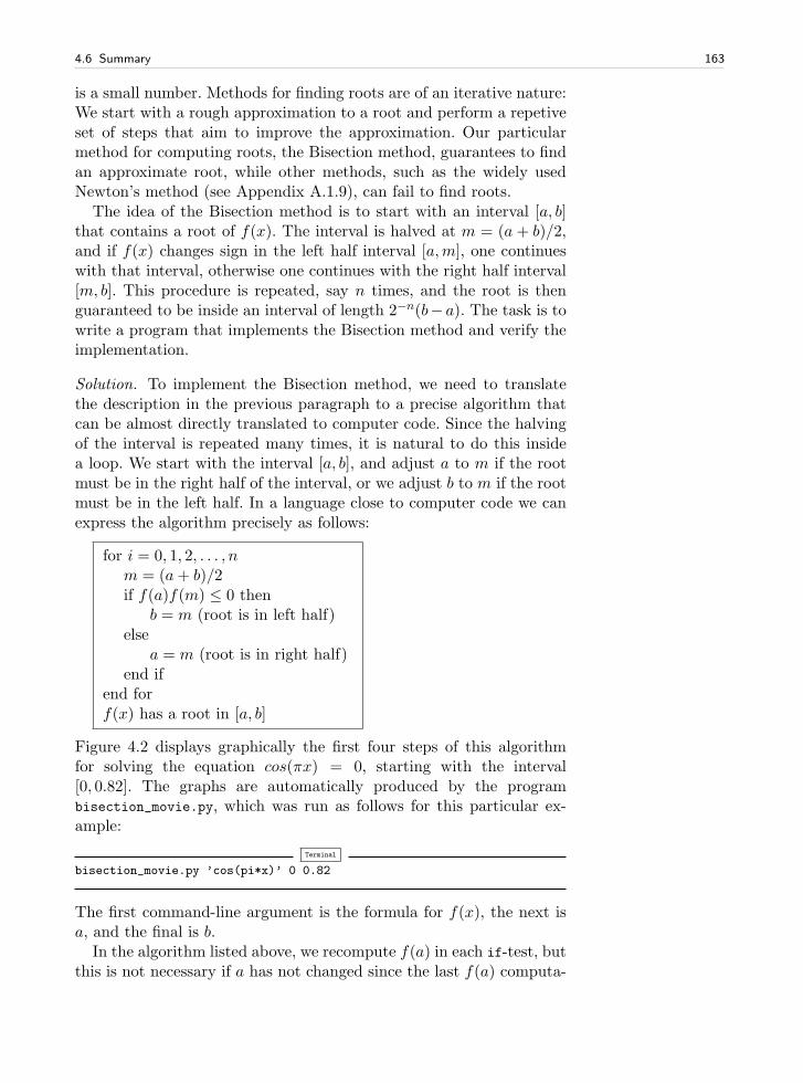
4.6 Summary 163

is a small number. Methods for finding roots are of an iterative nature:We start with a rough approximation to a root and perform a repetiveset of steps that aim to improve the approximation. Our particularmethod for computing roots, the Bisection method, guarantees to findan approximate root, while other methods, such as the widely usedNewton’s method (see Appendix A.1.9), can fail to find roots.

The idea of the Bisection method is to start with an interval [a, b]that contains a root of f(x). The interval is halved at m = (a + b)/2,and if f(x) changes sign in the left half interval [a,m], one continueswith that interval, otherwise one continues with the right half interval[m, b]. This procedure is repeated, say n times, and the root is thenguaranteed to be inside an interval of length 2−n(b− a). The task is towrite a program that implements the Bisection method and verify theimplementation.

Solution. To implement the Bisection method, we need to translatethe description in the previous paragraph to a precise algorithm thatcan be almost directly translated to computer code. Since the halvingof the interval is repeated many times, it is natural to do this insidea loop. We start with the interval [a, b], and adjust a to m if the rootmust be in the right half of the interval, or we adjust b to m if the rootmust be in the left half. In a language close to computer code we canexpress the algorithm precisely as follows:

for i = 0, 1, 2, . . . , nm = (a+ b)/2if f(a)f(m) ≤ 0 then

b = m (root is in left half)else

a = m (root is in right half)end if

end forf(x) has a root in [a, b]

Figure 4.2 displays graphically the first four steps of this algorithmfor solving the equation cos(πx) = 0, starting with the interval[0, 0.82]. The graphs are automatically produced by the programbisection_movie.py, which was run as follows for this particular ex-ample:

Terminal

bisection_movie.py ’cos(pi*x)’ 0 0.82

The first command-line argument is the formula for f(x), the next isa, and the final is b.

In the algorithm listed above, we recompute f(a) in each if-test, butthis is not necessary if a has not changed since the last f(a) computa-

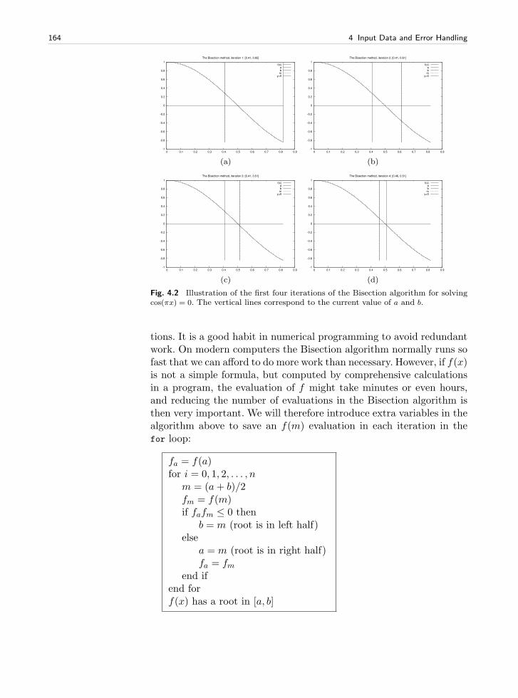
164 4 Input Data and Error Handling

-1

-0.8

-0.6

-0.4

-0.2

0

0.2

0.4

0.6

0.8

1

0 0.1 0.2 0.3 0.4 0.5 0.6 0.7 0.8 0.9

The Bisection method, iteration 1: [0.41, 0.82]

f(x)abm

y=0

(a)

-1

-0.8

-0.6

-0.4

-0.2

0

0.2

0.4

0.6

0.8

1

0 0.1 0.2 0.3 0.4 0.5 0.6 0.7 0.8 0.9

The Bisection method, iteration 2: [0.41, 0.61]

f(x)abm

y=0

(b)

-1

-0.8

-0.6

-0.4

-0.2

0

0.2

0.4

0.6

0.8

1

0 0.1 0.2 0.3 0.4 0.5 0.6 0.7 0.8 0.9

The Bisection method, iteration 3: [0.41, 0.51]

f(x)abm

y=0

(c)

-1

-0.8

-0.6

-0.4

-0.2

0

0.2

0.4

0.6

0.8

1

0 0.1 0.2 0.3 0.4 0.5 0.6 0.7 0.8 0.9

The Bisection method, iteration 4: [0.46, 0.51]

f(x)abm

y=0

(d)

Fig. 4.2 Illustration of the first four iterations of the Bisection algorithm for solvingcos(πx) = 0. The vertical lines correspond to the current value of a and b.

tions. It is a good habit in numerical programming to avoid redundantwork. On modern computers the Bisection algorithm normally runs sofast that we can afford to do more work than necessary. However, if f(x)is not a simple formula, but computed by comprehensive calculationsin a program, the evaluation of f might take minutes or even hours,and reducing the number of evaluations in the Bisection algorithm isthen very important. We will therefore introduce extra variables in thealgorithm above to save an f(m) evaluation in each iteration in thefor loop:

fa = f(a)for i = 0, 1, 2, . . . , n

m = (a+ b)/2fm = f(m)if fafm ≤ 0 then

b = m (root is in left half)else

a = m (root is in right half)fa = fm

end ifend forf(x) has a root in [a, b]

4.6 Summary 165

To execute the algorithm above, we need to specify n. Say we wantto be sure that the root lies in an interval of maximum extent ǫ. Aftern iterations the length of our current interval is 2−n(b − a), if [a, b] isthe initial interval. The current interval is sufficiently small if

2−n(b− a) = ǫ,

which implies

n = − ln ǫ− ln(b− a)

ln 2. (4.6)

Instead of calculating this n, we may simply stop the iterations whenthe length of the current interval is less than ǫ. The loop is then nat-urally implemented as a while loop testing on whether b − a ≤ ǫ. Tomake the algorithm more foolproof, we also insert a test to ensure thatf(x) really changes sign in the initial interval11.

Our final version of the Bisection algorithm now becomes

fa = f(a)if faf(b) > 0 then

error: f does not change sign in [a, b]end ifi = 0 (iteration counter)while b− a > ǫ:

i← i+ 1m = (a+ b)/2fm = f(m)if fafm ≤ 0 then

b = m (root is in left half)else

a = m (root is in right half)fa = fm

end ifend whileif x is the real root, |x−m| < ǫ

This is the algorithm we aim to implement in a Python program.A direct translation of the previous algorithm to a Python program

should be quite a simple process:

eps = 1E-5a, b = 0, 10

fa = f(a)if fa*f(b) > 0:

print ’f(x) does not change sign in [%g,%g].’ % (a, b)sys.exit(1)

11 This guarantees a root in [a, b]. However, f(a)f(b) < 0 is not a necessary conditionif there is an even number of roots in the initial interval.

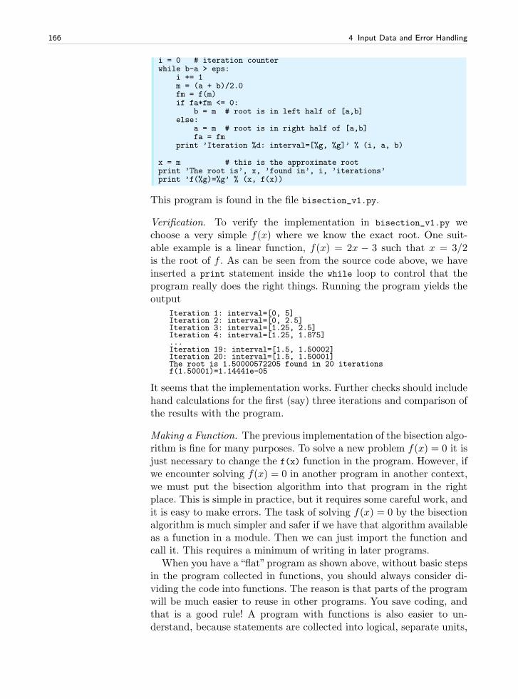
166 4 Input Data and Error Handling

i = 0 # iteration counterwhile b-a > eps:

i += 1m = (a + b)/2.0fm = f(m)if fa*fm <= 0:

b = m # root is in left half of [a,b]else:

a = m # root is in right half of [a,b]fa = fm

print ’Iteration %d: interval=[%g, %g]’ % (i, a, b)

x = m # this is the approximate rootprint ’The root is’, x, ’found in’, i, ’iterations’print ’f(%g)=%g’ % (x, f(x))

This program is found in the file bisection_v1.py.

Verification. To verify the implementation in bisection_v1.py wechoose a very simple f(x) where we know the exact root. One suit-able example is a linear function, f(x) = 2x − 3 such that x = 3/2is the root of f . As can be seen from the source code above, we haveinserted a print statement inside the while loop to control that theprogram really does the right things. Running the program yields theoutput

Iteration 1: interval=[0, 5]Iteration 2: interval=[0, 2.5]Iteration 3: interval=[1.25, 2.5]Iteration 4: interval=[1.25, 1.875]...Iteration 19: interval=[1.5, 1.50002]Iteration 20: interval=[1.5, 1.50001]The root is 1.50000572205 found in 20 iterationsf(1.50001)=1.14441e-05

It seems that the implementation works. Further checks should includehand calculations for the first (say) three iterations and comparison ofthe results with the program.

Making a Function. The previous implementation of the bisection algo-rithm is fine for many purposes. To solve a new problem f(x) = 0 it isjust necessary to change the f(x) function in the program. However, ifwe encounter solving f(x) = 0 in another program in another context,we must put the bisection algorithm into that program in the rightplace. This is simple in practice, but it requires some careful work, andit is easy to make errors. The task of solving f(x) = 0 by the bisectionalgorithm is much simpler and safer if we have that algorithm availableas a function in a module. Then we can just import the function andcall it. This requires a minimum of writing in later programs.

When you have a“flat”program as shown above, without basic stepsin the program collected in functions, you should always consider di-viding the code into functions. The reason is that parts of the programwill be much easier to reuse in other programs. You save coding, andthat is a good rule! A program with functions is also easier to un-derstand, because statements are collected into logical, separate units,

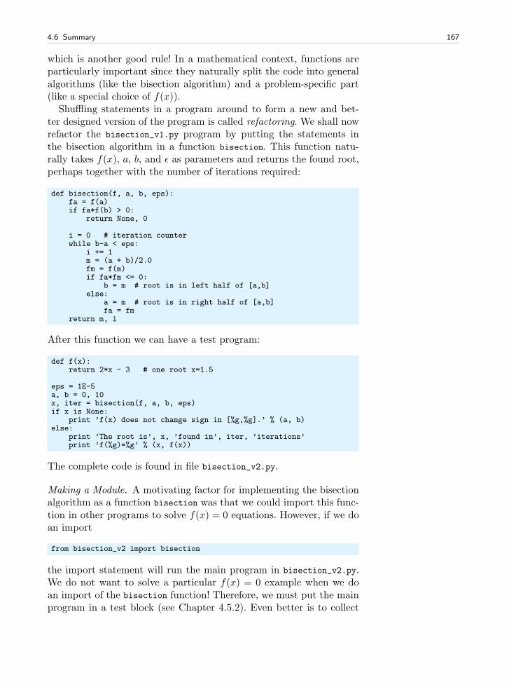
4.6 Summary 167

which is another good rule! In a mathematical context, functions areparticularly important since they naturally split the code into generalalgorithms (like the bisection algorithm) and a problem-specific part(like a special choice of f(x)).

Shuffling statements in a program around to form a new and bet-ter designed version of the program is called refactoring. We shall nowrefactor the bisection_v1.py program by putting the statements inthe bisection algorithm in a function bisection. This function natu-rally takes f(x), a, b, and ǫ as parameters and returns the found root,perhaps together with the number of iterations required:

def bisection(f, a, b, eps):fa = f(a)if fa*f(b) > 0:

return None, 0

i = 0 # iteration counterwhile b-a < eps:

i += 1m = (a + b)/2.0fm = f(m)if fa*fm <= 0:

b = m # root is in left half of [a,b]else:

a = m # root is in right half of [a,b]fa = fm

return m, i

After this function we can have a test program:

def f(x):return 2*x - 3 # one root x=1.5

eps = 1E-5a, b = 0, 10x, iter = bisection(f, a, b, eps)if x is None:

print ’f(x) does not change sign in [%g,%g].’ % (a, b)else:

print ’The root is’, x, ’found in’, iter, ’iterations’print ’f(%g)=%g’ % (x, f(x))

The complete code is found in file bisection_v2.py.

Making a Module. A motivating factor for implementing the bisectionalgorithm as a function bisection was that we could import this func-tion in other programs to solve f(x) = 0 equations. However, if we doan import

from bisection_v2 import bisection

the import statement will run the main program in bisection_v2.py.We do not want to solve a particular f(x) = 0 example when we doan import of the bisection function! Therefore, we must put the mainprogram in a test block (see Chapter 4.5.2). Even better is to collect

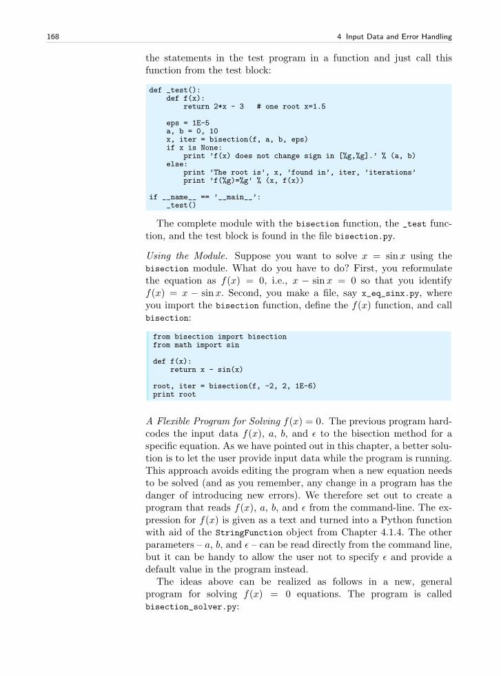
168 4 Input Data and Error Handling

the statements in the test program in a function and just call thisfunction from the test block:

def _test():def f(x):

return 2*x - 3 # one root x=1.5

eps = 1E-5a, b = 0, 10x, iter = bisection(f, a, b, eps)if x is None:

print ’f(x) does not change sign in [%g,%g].’ % (a, b)else:

print ’The root is’, x, ’found in’, iter, ’iterations’print ’f(%g)=%g’ % (x, f(x))

if __name__ == ’__main__’:_test()

The complete module with the bisection function, the _test func-tion, and the test block is found in the file bisection.py.

Using the Module. Suppose you want to solve x = sinx using thebisection module. What do you have to do? First, you reformulatethe equation as f(x) = 0, i.e., x − sin x = 0 so that you identifyf(x) = x − sinx. Second, you make a file, say x_eq_sinx.py, whereyou import the bisection function, define the f(x) function, and callbisection:

from bisection import bisectionfrom math import sin

def f(x):return x - sin(x)

root, iter = bisection(f, -2, 2, 1E-6)print root

A Flexible Program for Solving f(x) = 0. The previous program hard-codes the input data f(x), a, b, and ǫ to the bisection method for aspecific equation. As we have pointed out in this chapter, a better solu-tion is to let the user provide input data while the program is running.This approach avoids editing the program when a new equation needsto be solved (and as you remember, any change in a program has thedanger of introducing new errors). We therefore set out to create aprogram that reads f(x), a, b, and ǫ from the command-line. The ex-pression for f(x) is given as a text and turned into a Python functionwith aid of the StringFunction object from Chapter 4.1.4. The otherparameters – a, b, and ǫ – can be read directly from the command line,but it can be handy to allow the user not to specify ǫ and provide adefault value in the program instead.

The ideas above can be realized as follows in a new, generalprogram for solving f(x) = 0 equations. The program is calledbisection_solver.py:

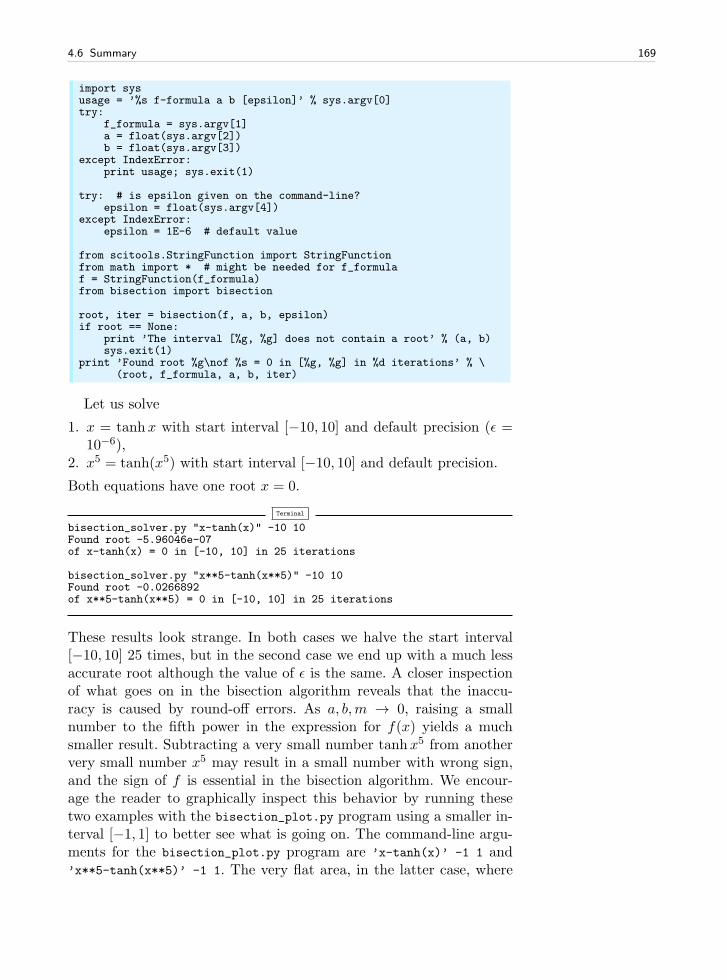
4.6 Summary 169

import sysusage = ’%s f-formula a b [epsilon]’ % sys.argv[0]try:

f_formula = sys.argv[1]a = float(sys.argv[2])b = float(sys.argv[3])

except IndexError:print usage; sys.exit(1)

try: # is epsilon given on the command-line?epsilon = float(sys.argv[4])

except IndexError:epsilon = 1E-6 # default value

from scitools.StringFunction import StringFunctionfrom math import * # might be needed for f_formulaf = StringFunction(f_formula)from bisection import bisection

root, iter = bisection(f, a, b, epsilon)if root == None:

print ’The interval [%g, %g] does not contain a root’ % (a, b)sys.exit(1)

print ’Found root %g\nof %s = 0 in [%g, %g] in %d iterations’ % \(root, f_formula, a, b, iter)

Let us solve

1. x = tanhx with start interval [−10, 10] and default precision (ǫ =10−6),

2. x5 = tanh(x5) with start interval [−10, 10] and default precision.

Both equations have one root x = 0.

Terminal

bisection_solver.py "x-tanh(x)" -10 10Found root -5.96046e-07of x-tanh(x) = 0 in [-10, 10] in 25 iterations

bisection_solver.py "x**5-tanh(x**5)" -10 10Found root -0.0266892of x**5-tanh(x**5) = 0 in [-10, 10] in 25 iterations

These results look strange. In both cases we halve the start interval[−10, 10] 25 times, but in the second case we end up with a much lessaccurate root although the value of ǫ is the same. A closer inspectionof what goes on in the bisection algorithm reveals that the inaccu-racy is caused by round-off errors. As a, b,m → 0, raising a smallnumber to the fifth power in the expression for f(x) yields a muchsmaller result. Subtracting a very small number tanhx5 from anothervery small number x5 may result in a small number with wrong sign,and the sign of f is essential in the bisection algorithm. We encour-age the reader to graphically inspect this behavior by running thesetwo examples with the bisection_plot.py program using a smaller in-terval [−1, 1] to better see what is going on. The command-line argu-ments for the bisection_plot.py program are ’x-tanh(x)’ -1 1 and’x**5-tanh(x**5)’ -1 1. The very flat area, in the latter case, where

170 4 Input Data and Error Handling

f(x) ≈ 0 for x ∈ [−1/2, 1/2] illustrates well that it is difficult to locatean exact root.

4.7 Exercises

Exercise 4.1. Make an interactive program.Make a program that (i) asks the user for a temperature in Fahren-

heit degrees and reads the number; (ii) computes the correspodningtemperature in Celsius degrees; and (iii) prints out the temperature inthe Celsius scale. Name of program file: f2c_qa.py. ⋄Exercise 4.2. Read from the command line in Exer. 4.1.

Modify the program from Exercise 4.1 such that the Fahrenheittemperature is read from the command line. Name of program file:f2c_cml.py. ⋄Exercise 4.3. Use exceptions in Exer. 4.2.

Extend the program from Exercise 4.2 with a try-except block tohandle the potential error that the Fahrenheit temperature is missingon the command line. Name of program file: f2c_cml_exc.py. ⋄Exercise 4.4. Read input from the keyboard.

Make a program that asks for input from the user, apply eval tothis input, and print out the type of the resulting object and its value.Test the program by providing five types of input: an integer, a realnumber, a complex number, a list, and a tuple. Name of program file:objects_qa.py. ⋄Exercise 4.5. Read input from the command line.

Let a program store the result of applying the eval function to thefirst command-line argument. Print out the resulting object and itstype. Run the program with different input: an integer, a real number,a list, and a tuple. (On Unix systems you need to surround the tupleexpressions in quotes on the command line to avoid error message fromthe Unix shell.) Try the string "this is a string" as a command-line argument. Why does this string cause problems and what is theremedy? Name of program file: objects_cml.py. ⋄Exercise 4.6. Prompt the user for input to a formula.

Consider the simplest program for evaluting the formula y(t) = v0t−0.5gt2:

v0 = 3; g = 9.81; t = 0.6y = v0*t - 0.5*g*t**2print y

Modify this code so that the program asks the user questions t=? andv0=?, and then gets t and v0 from the user’s input through the key-board. Name of program file: ball_qa.py. ⋄

4.7 Exercises 171

Exercise 4.7. Read command line input a formula.Modify the program listed in Exercise 4.6 such that v0 and t are

read from the command line. Name of program file: ball_cml.py. ⋄

Exercise 4.8. Make the program from Exer. 4.7 safer.The program from Exercise 4.7 reads input from the command

line. Extend that program with exception handling such that miss-ing command-line arguments are detected. In the except IndexError

block, use the raw_input function to ask the user for missing inputdata. Name of program file: ball_cml_qa.py. ⋄

Exercise 4.9. Test more in the program from Exer. 4.7.Test if the t value read in the program from Exercise 4.7 lies between

0 and 2v0/g. If not, print a message and abort execution. Name ofprogram file: ball_cml_errorcheck.py. ⋄

Exercise 4.10. Raise an exception in Exer. 4.9.Instead of printing an error message and aborting the program ex-

plicitly, raise a ValueError exception in the if test on legal t values inthe program from Exercise 4.9. Include the legal interval for t in theexception message. Name of program file: ball_cml_ValueError.py. ⋄

Exercise 4.11. Compute the distance it takes to stop a car.A car driver, driving at velocity v0, suddenly puts on the brake.

What braking distance d is needed to stop the car? One can derive,from basic physics, that

d =1

2

v20µg

. (4.7)

Make a program for computing d in (4.7) when the initial car velocityv0 and the friction coefficient µ are given on the command line. Run theprogram for two cases: v0 = 120 and v0 = 50 km/h, both with µ = 0.3(µ is dimensionless). (Remember to convert the velocity from km/h tom/s before inserting the value in the formula!) Name of program file:stopping_length.py. ⋄

Exercise 4.12. Look up calendar functionality.The purpose of this exercise is to make a program which takes a

date, consisting of year (4 digits), month (2 digits), and day (1-31) onthe command line and prints the corresponding name of the weekday(Monday, Tuesday, etc.). Python has a module calendar, which youmust look up in the Python Library Reference (see Chapter 2.6.3), forcalculating the weekday of a date. Name of program file: weekday.py.⋄

Exercise 4.13. Use the StringFunction tool.Make the program user_formula.py from Chapter 4.1.3 shorter by

using the convenient StringFunction tool from Chapter 4.1.4. Name ofprogram file: user_formula2.py. ⋄

172 4 Input Data and Error Handling

Exercise 4.14. Extend a program from Ch. 4.2.1.How can you modify the add_cml.py program from the end of Chap-

ter 4.1.2 such that it accepts input like sqrt(2) and sin(1.2)? In thiscase the output should be

<type ’float’> + <type ’float’> becomes <type ’float’>with value 2.34625264834

(Hint: Mathematical functions like sqrt and sin must be defined in theprogram before using eval. Furthermore, Unix (bash) does not like theparentheses on the command line so you need to put quotes aroundthe command-line arguments.) Name of program file: add2.py. ⋄

Exercise 4.15. Why we test for specific exception types.The simplest way of writing a try-except block is to test for any

exception, for example,

try:C = float(sys.arg[1])

except:print ’C must be provided as command-line argument’sys.exit(1)

Write the above statements in a program and test the program. Whatis the problem?

The fact that a user can forget to supply a command-line argumentwhen running the program was the original reason for using a try block.Find out what kind of exception that is relevant for this error and testfor this specific exception and re-run the program. What is the problemnow? Correct the program. Name of program file: cml_exception.py. ⋄

Exercise 4.16. Make a simple module.Make six conversion functions between temperatures in Celsius,

Kelvin, and Fahrenheit: C2F, F2C, C2K, K2C, F2K, and K2F. Collect thesefunctions in a module convert_temp. Make some sample calls to thefunctions from an interactive Python shell. Name of program file:convert_temp.py. ⋄

Exercise 4.17. Make a useful main program for Exer. 4.16.Extend the module made in Exercise 4.16 with a main program in

the test block. This main program should read the first command-line argument as a numerical value of a temperature and the secondargument as a temperature scale: C, K, or F. Write out the temperaturein the other two scales. For example, if 21.3 C is given on the commandline, the output should be 70.34 F 294.45 K. Name of program file:convert_temp2.py. ⋄

Exercise 4.18. Make a module in Exer. 3.7.Collect the f and S functions in the program from Exercise 3.7 in a

separate file such that this file becomes a module. Put the statements

4.7 Exercises 173

making the table (i.e., the main program from Exercise 3.7) in a sepa-rate function table(n_values, alpha_values, T), and call this functiononly if the module file is run as a program (i.e., call table from a testblock, see Chapter 4.5.2). Name of program file: sinesum2.py. ⋄Exercise 4.19. Extend the module from Exer. 4.18.

Extend the program from Exercise 4.18 such that T and a seriesof n and α values are read from the command line. The extendedprogram should import the table function from the module sinesum2

(and not copy any code from the module file). Name of program file:sinesum3.py. ⋄Exercise 4.20. Use options and values in Exer. 4.19.

Let the input to the program in Exercise 4.19 be option-value pairsof the type -n, -alpha, and -T, with sensible default values for thesequantities set in the program. Apply the argparse module to read thecommand-line arguments. Name of program file: sinesum4.py. ⋄Exercise 4.21. Check if mathematical identities hold on a computer.

Because of round-off errors, it could happen that a mathematicalrule like (ab)3 = a3b3 does not hold (exactly) on a computer. The ideaof this exercise is to check such identities for a large number of randomnumbers. We can make random numbers using the random module inPython:

import randoma = random.uniform(A, B)b = random.uniform(A, B)

Here, a and b will be random numbers which are always larger than orequal to A and smaller than B.

Make a program that reads the number of tests to be performedfrom the command line. Set A and B to fixed values (say -100 and 100).Perform the test in a loop. Inside the loop, draw random numbers a andb and test if the two mathematical expressions (a*b)**3 and a**3*b**3

are equivalent. Count the number of failures of equivalence and writeout the percentage of failures at the end of the program.

Duplicate the code segment outlined above to also com-pare the expressions a/b and 1/(b/a). Name of program file:math_identities_failures.py. ⋄Exercise 4.22. Improve input to the program in Exer. 4.21.

The purpose of this exercise is to extend the program from Exer-cise 4.21 to handle a large number of mathematical identities. Makea function equal(expr1, expr2, A, B, n=500) which tests if the math-ematical expressions expr1 and expr2, given as strings and involvingnumbers a and b, are exactly equal (eval(expr1) == eval(expr2)) for nrandom choices of numbers a and b in the interval between A and B. Re-turn the percentage of failures. Make a module with the equal function

174 4 Input Data and Error Handling

and a test block which feeds the equal function with arguments readfrom the command line. Run the module file as a program to test thetwo identities from Exercise 4.21. Also test the identities ea+b = eaeb

and ln ab = b ln a (take a from math import * in the module file so thatmathematical functions like exp and log are defined). Name of programfile: math_identities_failures_cml.py. ⋄

Exercise 4.23. Apply the program from Exer. 4.22.Import the equal function from the module made in Exercise 4.22

and test the three identities from Exercise 4.21 in addition to the fol-lowing identities:

a− b and −(b− a) a/b and 1/(b/a) (ab)4 and a4b4

(a+ b)2 and a2 + 2ab+ b2

(a+ b)(a− b) and a2 − b2

ea+b and eaeb

ln ab and b ln a ln ab and ln a+ ln b ab and eln a+ln b

1/(1/a+ 1/b) and ab/(a+ b) a(sin2 b+ cos2 b) and a sinh(a+ b) and (eaeb − e−ae−b)/2 tan(a+ b) and sin(a+ b)/ cos(a+ b) sin(a+ b) and sin a cos b+ sin b cos a

Store all the expressions in a list of 2-tuples, where each 2-tuple con-tains two mathematically equivalent expressions as strings which canbe sent to the eval function. Make a nicely formatted table with a pairof equivalent expressions at each line followed by the failure rate. Tryout A=0 and B=1 as well as A=-1E+7 and B=1E+7. Does the failure rateseem to depend on the magnitude of the numbers a and b? Name ofprogram file: math_identities_failures_table.py.

Remark. Exercise 4.21 can be solved by a simple program, but if youwant to check 17 identities the present exercise demonstrates how im-portant it is to be able to automate the process via the equal functionand two nested loops over a list of equivalent expressions. ⋄

Exercise 4.24. Compute the binomial distribution.Consider an uncertain event where there are two outcomes only,

typically success or failure. Flipping a coin is an example: The outcomeis uncertain and of two types, either head (can be considered as success)or tail (failure). Throwing a die can be another example, if (e.g.) gettinga six is considered success and all other outcomes represent failure. Letthe probability of success be p and that of failure 1−p. If we perform nexperiments, where the outcome of each experiment does not depend

4.7 Exercises 175

on the outcome of previous experiments, the probability of gettingsuccess x times (and failure n− x times) is given by

B(x, n, p) =n!

x!(n− x)!px(1− p)n−x . (4.8)

This formula (4.8) is called the binomial distribution. The expressionx! is the factorial of x as defined in Exercise 3.14. Implement (4.8) in afunction binomial(x, n, p). Make a module containing this binomial

function. Include a test block at the end of the module file. Name ofprogram file: binomial_distribution.py. ⋄

Exercise 4.25. Apply the binomial distribution.Use the module from Exercise 4.24 to make a program for solving

the problems below.

1. What is the probability of getting two heads when flipping a coinfive times?This probability corresponds to n = 5 events, where the success ofan event means getting head, which has probability p = 1/2, andwe look for x = 2 successes.

2. What is the probability of getting four ones in a row when throwinga die?This probability corresponds to n = 4 events, success is getting oneand has probability p = 1/6, and we look for x = 4 successful events.

3. Suppose cross country skiers typically experience one ski break inone out of 120 competitions. Hence, the probability of breaking a skican be set to p = 1/120. What is the probability b that a skier willexperience a ski break during five competitions in a world champi-onship?This question is a bit more demanding than the other two. We arelooking for the probability of 1, 2, 3, 4 or 5 ski breaks, so it is simplerto ask for the probability c of not breaking a ski, and then computeb = 1− c. Define “success” as breaking a ski. We then look for x = 0successes out of n = 5 trials, with p = 1/120 for each trial. Computeb.

Name of program file: binomial_problems.py. ⋄

Exercise 4.26. Compute probabilities with the Poisson distribution.Suppose that over a period of tm time units, a particular uncertain

event happens (on average) νtm times. The probability that there willbe x such events in a time period t is approximately given by theformula

P (x, t, ν) =(νt)x

x!e−νt . (4.9)

176 4 Input Data and Error Handling

This formula is known as the Poisson distribution12. An importantassumption is that all events are independent of each other and thatthe probability of experiencing an event does not change significantlyover time.

Implement (4.9) in a function Poisson(x, t, nu), and make a pro-gram that reads x, t, and ν from the command line and writes out theprobability P (x, t, ν). Use this program to solve the problems below.

1. Suppose you are waiting for a taxi in a certain street at night. Onaverage, 5 taxis pass this street every hour at this time of the night.What is the probability of not getting a taxi after having waited 30minutes?Since we have 5 events in a time period of tm = 1 hour, νtm = ν = 5.The sought probability is then P (0, 1/2, 5). Compute this number.What is the probability of having to wait two hours for a taxi?If 8 people need two taxis, that is the probability that two taxisarrive in a period of 20 minutes?

2. In a certain location, 10 earthquakes have been recorded duringthe last 50 years. What is the probability of experiencing exactlythree earthquakes over a period of 10 years in this erea? What isthe probability that a visitor for one week does not experience anyearthquake?With 10 events over 50 years we have νtm = ν ·50 years = 10 events,which imples ν = 1/5 event per year. The answer to the first ques-tion of having x = 3 events in a period of t = 10 years is givendirectly by (4.9). The second question asks for x = 0 events ina time period of 1 week, i.e., t = 1/52 years, so the answer isP (0, 1/52, 1/5).

3. Suppose that you count the number of misprints in the first versionsof the reports you write and that this number shows an average ofsix misprints per page. What is the probability that a reader of afirst draft of one of your reports reads six pages without hitting amisprint?Assuming that the Poisson distribution can be applied to this prob-lem, we have “time” tm as 1 page and ν · 1 = 6, i.e., ν = 6 events(misprints) per page. The probability of no events in a “period” ofsix pages is P (0, 6, 6).

⋄

12 It can be shown that (4.9) arises from (4.8) when the probability p of experiencingthe event in a small time interval t/n is p = νt/n and we let n → ∞.

Array Computing and Curve Plotting 5

Lists are introduced in Chapter 2 to store “tabular data” in a con-venient way. An array is an object that is very similar to a list, butless flexible and computationally much more efficient. When using thecomputer to perform mathematical calculations, we often end up witha huge amount of numbers and associated arithmetic operations. Stor-ing numbers in lists may in such contexts lead to slow programs, whilearrays can make the programs run much faster. This may not be veryimportant for the mathematical problems in this book, since most ofthe programs usually finish execution within a few seconds. Never-theless, in more advanced applications of mathematics, especially theapplications met in industry and science, computer programs may runfor weeks and months. Any clever idea that reduces the execution timeto days or hours is therefore paramount1.

This chapter gives a brief introduction to arrays – how they arecreated and what they can be used for. Array computing usually endsup with a lot of numbers. It may be very hard to understand what thesenumbers mean by just looking at them. Since the human is a visualanimal, a good way to understand numbers is to visualize them. In thischapter we concentrate on visualizing curves that reflect functions ofone variable, e.g., curves of the form y = f(x). A synonym for curveis graph, and the image of curves on the screen is often called a plot.We will use arrays to store the information about points along thecurve. It is fair to say that array computing demands visualization andvisualization demands arrays.

1 Many may argue that programmers of mathematical software have traditionallypaid too much attention to efficiency and smart program constructs. The resultingsoftware often becomes very hard to maintain and extend. In this book we advo-cate a focus on clear, well-designed, and easy-to-understand programs that workcorrectly. Optimization for speed should always come as a second step in programdevelopment.

177

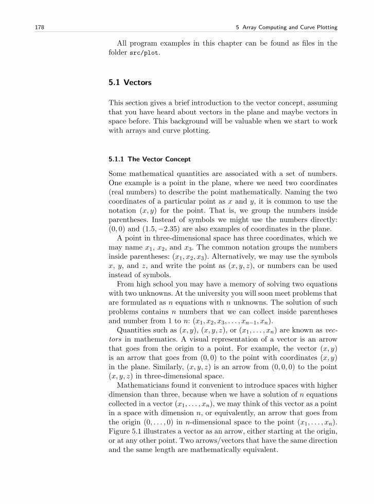
178 5 Array Computing and Curve Plotting

All program examples in this chapter can be found as files in thefolder src/plot.

5.1 Vectors

This section gives a brief introduction to the vector concept, assumingthat you have heard about vectors in the plane and maybe vectors inspace before. This background will be valuable when we start to workwith arrays and curve plotting.

5.1.1 The Vector Concept

Some mathematical quantities are associated with a set of numbers.One example is a point in the plane, where we need two coordinates(real numbers) to describe the point mathematically. Naming the twocoordinates of a particular point as x and y, it is common to use thenotation (x, y) for the point. That is, we group the numbers insideparentheses. Instead of symbols we might use the numbers directly:(0, 0) and (1.5,−2.35) are also examples of coordinates in the plane.

A point in three-dimensional space has three coordinates, which wemay name x1, x2, and x3. The common notation groups the numbersinside parentheses: (x1, x2, x3). Alternatively, we may use the symbolsx, y, and z, and write the point as (x, y, z), or numbers can be usedinstead of symbols.

From high school you may have a memory of solving two equationswith two unknowns. At the university you will soon meet problems thatare formulated as n equations with n unknowns. The solution of suchproblems contains n numbers that we can collect inside parenthesesand number from 1 to n: (x1, x2, x3, . . . , xn−1, xn).

Quantities such as (x, y), (x, y, z), or (x1, . . . , xn) are known as vec-tors in mathematics. A visual representation of a vector is an arrowthat goes from the origin to a point. For example, the vector (x, y)is an arrow that goes from (0, 0) to the point with coordinates (x, y)in the plane. Similarly, (x, y, z) is an arrow from (0, 0, 0) to the point(x, y, z) in three-dimensional space.

Mathematicians found it convenient to introduce spaces with higherdimension than three, because when we have a solution of n equationscollected in a vector (x1, . . . , xn), we may think of this vector as a pointin a space with dimension n, or equivalently, an arrow that goes fromthe origin (0, . . . , 0) in n-dimensional space to the point (x1, . . . , xn).Figure 5.1 illustrates a vector as an arrow, either starting at the origin,or at any other point. Two arrows/vectors that have the same directionand the same length are mathematically equivalent.

5.1 Vectors 179

-1

0

1

2

3

4

-1 0 1 2 3 4

vector (2,3)

vector (2,3)

Fig. 5.1 A vector (2, 3) visualized in the standard way as an arrow from the originto the point (2, 3), and mathematically equivalently, as an arrow from (1, 1

2) (or any

point (a, b)) to (3, 3 1

2) (or (a+ 2, b+ 3)).

We say that (x1, . . . , xn) is an n-vector or a vector with n compo-nents. Each of the numbers x1, x2, . . . is a component or an element.We refer to the first component (or element), the second component(or element), and so forth.

A Python program may use a list or tuple to represent a vector:

v1 = [x, y] # list of variablesv2 = (-1, 2) # tuple of numbersv3 = (x1, x2, x3) # tuple of variablesfrom math import expv4 = [exp(-i*0.1) for i in range(150)]

While v1 and v2 are vectors in the plane and v3 is a vector in three-dimensional space, v4 is a vector in a 150-dimensional space, consistingof 150 values of the exponentional function. Since Python lists andtuples have 0 as the first index, we may also in mathematics write thevector (x1, x2) as (x0, x1). This is not at all common in mathematics,but makes the distance from a mathematical description of a problemto its solution in Python shorter.

It is impossible to visually demonstrate how a space with 150 dimen-sions looks like. Going from the plane to three-dimensional space givesa rough feeling of what it means to add a dimension, but if we forgetabout the idea of a visual perception of space, the mathematics is verysimple: Going from a 4-dimensional vector to a 5-dimensional vector isjust as easy as adding an element to a list of symbols or numbers.

5.1.2 Mathematical Operations on Vectors

Since vectors can be viewed as arrows having a length and a direction,vectors are extremely useful in geometry and physics. The velocity ofa car has a magnitude and a direction, so has the acceleration, and

180 5 Array Computing and Curve Plotting

the position of a car is a point2 which is also a vector. An edge of atriangle can be viewed as a line (arrow) with a direction and length.

In geometric and physical applications of vectors, mathematical op-erations on vectors are important. We shall exemplify some of the mostimportant operations on vectors below. The goal is not to teach com-putations with vectors, but more to illustrate that such computationsare defined by mathematical rules3. Given two vectors, (u1, u2) and(v1, v2), we can add these vectors according to the rule:

(u1, u2) + (v1, v2) = (u1 + v1, u2 + v2) . (5.1)

We can also subtract two vectors using a similar rule:

(u1, u2)− (v1, v2) = (u1 − v1, u2 − v2) . (5.2)

A vector can be multiplied by a number. This number, called a below,is usually denoted as a scalar :

a · (v1, v2) = (av1, av2) . (5.3)

The inner product, also called dot product, or scalar product, of twovectors is a number4:

(u1, u2) · (v1, v2) = u1v1 + u2v2 . (5.4)

There is also a cross product defined for 2-vectors or 3-vectors, but wedo not list the cross product formula here.The length of a vector is defined by

||(v1, v2)|| =√

(v1, v2) · (v1, v2) =√

v21 + v22 . (5.5)

The same mathematical operations apply to n-dimensional vectorsas well. Instead of counting indices from 1, as we usually do in mathe-matics, we now count from 0, as in Python. The addition and subtrac-tion of two vectors with n components (or elements) read

(u0, . . . , un−1) + (v0, . . . , vn−1) = (u0 + v0, . . . , un−1 + vn−1), (5.6)

(u0, . . . , un−1)− (v0, . . . , vn−1) = (u0 − v0, . . . , un−1 − vn−1) .(5.7)

2 A car is of course not a mathematical point, but when studying the acceleration ofa car, it suffices to view it as a point. In other occasions, e.g., when simulating acar crash on a computer, the car may be modeled by a large number (say 106) ofconnected points.

3 You might recall many of the formulas here from high school mathematics orphysics. The really new thing in this chapter is that we show how rules for vectorsin the plane and in space can easily be extended to vectors in n-dimensional space.

4 From high school mathematics and physics you might recall that the inner or dotproduct also can be expressed as the product of the lengths of the two vectorsmultiplied by the cosine of the angle between them. We will not make use of thisformula.

5.1 Vectors 181

Multiplication of a scalar a and a vector (v0, . . . , vn−1) equals

(av0, . . . , avn−1) . (5.8)

The inner or dot product of two n-vectors is defined as

(u0, . . . , un−1) · (v0, . . . , vn−1) = u0v0 + · · ·+ un−1vn−1 =

n−1∑

j=0

ujvj .

(5.9)Finally, the length ||v|| of an n-vector v = (v0, . . . , vn−1) is

√

(v0, . . . , vn−1) · (v0, . . . , vn−1) =(

v20 + v21 + · · ·+ v2n−1

)1

2

=

n−1∑

j=0

v2j

1

2

. (5.10)

5.1.3 Vector Arithmetics and Vector Functions

In addition to the operations on vectors in Chapter 5.1.2, which youmight recall from high school mathematics, we can define other oper-ations on vectors. This is very useful for speeding up programs. Un-fortunately, the forthcoming vector operations are hardly treated intextbooks on mathematics, yet these operations play a significant rolein mathematical software, especially in computing environment suchas Matlab, Octave, Python, and R.

Applying a mathematical function of one variable, f(x), to a vectoris defined as a vector where f is applied to each element. Let v =(v0, . . . , vn−1) be a vector. Then

f(v) = (f(v0), . . . , f(vn−1)) .

For example, the sine of v is

sin(v) = (sin(v0), . . . , sin(vn−1)) .

It follows that squaring a vector, or the more general operation ofraising the vector to a power, can be defined as applying the operationto each element:

vb = (vb0, . . . , vbn−1) .

Another operation between two vectors that arises in computer pro-gramming of mathematics is the “asterisk” multiplication, defined as

u ∗ v = (u0v0, u1v1, . . . , un−1vn−1) . (5.11)

Adding a scalar to a vector or array can be defined as adding the scalarto each component. If a is a scalar and v a vector, we have

182 5 Array Computing and Curve Plotting

a+ v = (a+ v0, . . . , a+ vn−1) .

A compound vector expression may look like

v2 ∗ cos(v) ∗ ev + 2 . (5.12)

How do we calculate this expression? We use the normal rules of math-ematics, working our way, term by term, from left to right, payingattention to the fact that powers are evaluated before multiplicationsand divisions, which are evaluated prior to addition and subtraction.First we calculate v2, which results in a vector we may call u. Then wecalculate cos(v) and call the result p. Then we multiply u ∗ p to get avector which we may call w. The next step is to evaluate ev, call theresult q, followed by the multiplication w∗q, whose result is stored as r.Then we add r+2 to get the final result. It might be more convenientto list these operations after each other:

1. u = v2

2. p = cos(v)3. w = u ∗ p4. q = ev

5. r = w ∗ q6. s = r + 2

Writing out the vectors u, w, p, q, and r in terms of a general vectorv = (v0, . . . , vn−1) (do it!) shows that the result of the expression (5.12)is the vector

(v20 cos(v0)ev0 + 2, . . . , v2n−1 cos(vn−1)e

vn−1 + 2) .

That is, component no. i in the result vector equals the number arisingfrom applying the formula (5.12) to vi, where the * multiplication isordinary multiplication between two numbers.

We can, alternatively, introduce the function

f(x) = x2 cos(x)ex + 2

and use the result that f(v) means applying f to each element in v.The result is the same as in the vector expression (5.12).

In Python programming it is important for speed (and conveniencetoo) that we can apply functions of one variable, like f(x), to vectors.What this means mathematically is something we have tried to explainin this subsection. Doing Exercises 5.4 and 5.5 may help to grasp theideas of vector computing, and with more programming experience youwill hopefully discover that vector computing is very useful. It is notnecessary to have a thorough understanding of vector computing inorder to proceed with the next sections.

5.2 Arrays in Python Programs 183

Arrays are used to represent vectors in a program, but one can domore with arrays than with vectors. Until Chapter 5.6 it suffices tothink of arrays as the same as vectors in a program.

5.2 Arrays in Python Programs

This section introduces array programming in Python, but first wecreate some lists and show how arrays differ from lists.

5.2.1 Using Lists for Collecting Function Data

Suppose we have a function f(x) and want to evaluate this functionat a number of x points x0, x1, . . . , xn−1. We could collect the n pairs(xi, f(xi)) in a list, or we could collect all the xi values, for i = 0, . . . , n−1, in a list and all the associated f(xi) values in another list. We learnedhow to create such lists in Chapter 2, but as a review, we present therelevant program statements in an interactive session:

>>> def f(x):... return x**3 # sample function...>>> n = 5 # no of points along the x axis>>> dx = 1.0/(n-1) # spacing between x points in [0,1]>>> xlist = [i*dx for i in range(n)]>>> ylist = [f(x) for x in xlist]>>> pairs = [[x, y] for x, y in zip(xlist, ylist)]

Here we have used list comprehensions for achieving compact code.Make sure that you understand what is going on in these list compre-hensions (you are encouraged to write the same code using standardfor loops and appending new list elements in each pass of the loops).

The list elements consist of objects of the same type: any elementin pairs is a list of two float objects, while any element in xlist orylist is a float. Lists are more flexible than that, because an elementcan be an object of any type, e.g.,

mylist = [2, 6.0, ’tmp.ps’, [0,1]]

Here mylist holds an int, a float, a string, and a list. This combinationof diverse object types makes up what is known as heterogeneous lists.We can also easily remove elements from a list or add new elementsanywhere in the list. This flexibility of lists is in general convenientto have as a programmer, but in cases where the elements are of thesame type and the number of elements is fixed, arrays can be usedinstead. The benefits of arrays are faster computations, less memorydemands, and extensive support for mathematical operations on the

184 5 Array Computing and Curve Plotting

data. Because of greater efficiency and mathematical convenience, ar-rays will be used to a large extent in this book. The great use of arraysis also prominent in other programming environments such as Matlab,Octave, and R, for instance. Lists will be our choice instead of arrayswhen we need the flexibility of adding or removing elements or whenthe elements may be of different object types.

5.2.2 Basics of Numerical Python Arrays

An array object can be viewed as a variant of a list, but with thefollowing assumptions and features:

All elements must be of the same type, preferably integer, real, orcomplex numbers, for efficient numerical computing and storage.

The number of elements must be known5 when the array is created. Arrays are not part of standard Python6 – one needs an additionalpackage called Numerical Python, often abbreviated as NumPy.The Python name of the package, to be used in import statements,is numpy.

With numpy, a wide range of mathematical operations can be donedirectly on complete arrays, thereby removing the need for loopsover array elements. This is commonly called vectorization and maycause a dramatic speed-up of Python programs. Vectorization makesuse of the vector computing concepts from Chapter 5.1.3.

Arrays with one index are often called vectors. Arrays with twoindices are used as an efficient data structure for tables, instead oflists of lists. Arrays can also have three or more indices.

The following text lists some important functionality of NumPy ar-rays. A more comprehensive treatment is found in the excellent NumPyTutorial, NumPy User Guide, NumPy Reference, Guide to NumPy, andNumPy for Matlab Users, all found at scipy.org.

The standard import statement for Numerical Python reads

import numpy as np

To convert a list r to an array, we use the array function from numpy:

a = np.array(r)

To create a new array of length n, filled with zeros, we write

a = np.zeros(n)

The array elements are of a type that corresponds to Python’s float

type. A second argument to np.zeros can be used to specify other

5 The number of elements can be changed, at a substantial computational cost.6 Actually, there is an object type called array in standard Python, but this datatype is not so efficient for mathematical computations.

5.2 Arrays in Python Programs 185

element types, e.g., int. Arrays with more than one index are treatedin Chapter 5.6.

Often one wants an array to have n elements with uniformly dis-tributed values in an interval [p, q]. The numpy function linspace createssuch arrays:

a = np.linspace(p, q, n)

Array elements are accessed by square brackets as for lists: a[i].Slices also work as for lists, for example, a[1:-1] picks out all elementsexcept the first and the last, but contrary to lists, a[1:-1] is not a copyof the data in a. Hence,

b = a[1:-1]b[2] = 0.1

will also change a[3] to 0.1. A slice a[i:j:s] picks out the elementsstarting with index i and stepping s indices at the time up to, but notincluding, j. Omitting i implies i=0, and omitting j implies j=n if n isthe number of elements in the array. For example, a[0:-1:2] picks outevery two elements up to, but not including, the last element, whilea[::4] picks out every four elements in the whole array.

5.2.3 Computing Coordinates and Function Values

With these basic operations at hand, we can continue the session fromthe previous section and make arrays out of the lists xlist and ylist:

>>> import numpy as np>>> x2 = np.array(xlist) # turn list xlist into array x2>>> y2 = np.array(ylist)>>> x2array([ 0. , 0.25, 0.5 , 0.75, 1. ])>>> y2array([ 0. , 0.015625, 0.125 , 0.421875, 1. ])

Instead of first making a list and then converting the list to an array,we can compute the arrays directly. The equally spaced coordinates inx2 are naturally computed by the np.linspace function. The y2 arraycan be created by np.zeros, to ensure that y2 has the right length7

len(x2), and then we can run a for loop to fill in all elements in y2

with f values:

>>> n = len(xlist)>>> x2 = np.linspace(0, 1, n)>>> y2 = np.zeros(n)>>> for i in xrange(n):... y2[i] = f(x2[i])...

7 This is referred to as allocating the array, and means that a part of the computer’smemory is marked for being occupied by this array.

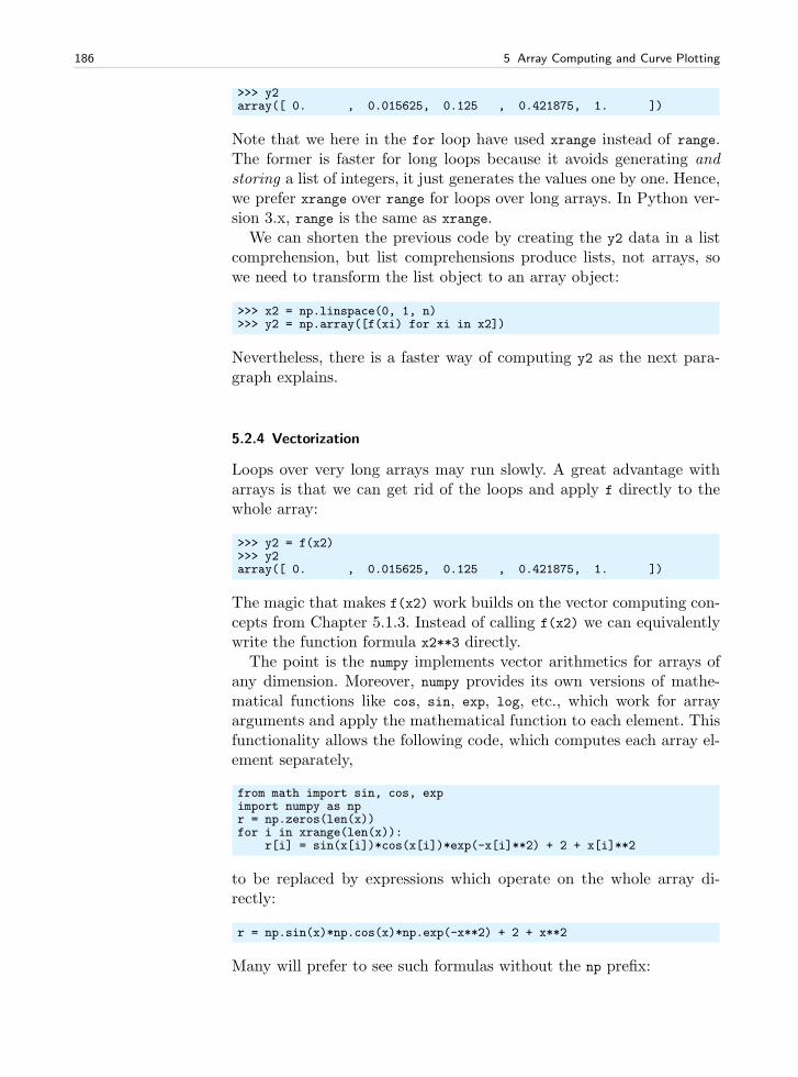
186 5 Array Computing and Curve Plotting

>>> y2array([ 0. , 0.015625, 0.125 , 0.421875, 1. ])

Note that we here in the for loop have used xrange instead of range.The former is faster for long loops because it avoids generating andstoring a list of integers, it just generates the values one by one. Hence,we prefer xrange over range for loops over long arrays. In Python ver-sion 3.x, range is the same as xrange.

We can shorten the previous code by creating the y2 data in a listcomprehension, but list comprehensions produce lists, not arrays, sowe need to transform the list object to an array object:

>>> x2 = np.linspace(0, 1, n)>>> y2 = np.array([f(xi) for xi in x2])

Nevertheless, there is a faster way of computing y2 as the next para-graph explains.

5.2.4 Vectorization

Loops over very long arrays may run slowly. A great advantage witharrays is that we can get rid of the loops and apply f directly to thewhole array:

>>> y2 = f(x2)>>> y2array([ 0. , 0.015625, 0.125 , 0.421875, 1. ])

The magic that makes f(x2) work builds on the vector computing con-cepts from Chapter 5.1.3. Instead of calling f(x2) we can equivalentlywrite the function formula x2**3 directly.

The point is the numpy implements vector arithmetics for arrays ofany dimension. Moreover, numpy provides its own versions of mathe-matical functions like cos, sin, exp, log, etc., which work for arrayarguments and apply the mathematical function to each element. Thisfunctionality allows the following code, which computes each array el-ement separately,

from math import sin, cos, expimport numpy as npr = np.zeros(len(x))for i in xrange(len(x)):

r[i] = sin(x[i])*cos(x[i])*exp(-x[i]**2) + 2 + x[i]**2

to be replaced by expressions which operate on the whole array di-rectly:

r = np.sin(x)*np.cos(x)*np.exp(-x**2) + 2 + x**2

Many will prefer to see such formulas without the np prefix:

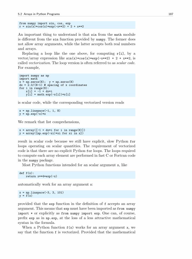
5.2 Arrays in Python Programs 187

from numpy import sin, cos, expr = sin(x)*cos(x)*exp(-x**2) + 2 + x**2

An important thing to understand is that sin from the math moduleis different from the sin function provided by numpy. The former doesnot allow array arguments, while the latter accepts both real numbersand arrays.

Replacing a loop like the one above, for computing r[i], by avector/array expression like sin(x)*cos(x)*exp(-x**2) + 2 + x**2, iscalled vectorization. The loop version is often referred to as scalar code.For example,

import numpy as npimport mathx = np.zeros(N); y = np.zeros(N)dx = 2.0/(N-1) # spacing of x coordinatesfor i in range(N):

x[i] = -1 + dx*iy[i] = math.exp(-x[i])*x[i]

is scalar code, while the corresponding vectorized version reads

x = np.linspace(-1, 1, N)y = np.exp(-x)*x

We remark that list comprehensions,

x = array([-1 + dx*i for i in range(N)])y = array([np.exp(-xi)*xi for xi in x])

result in scalar code because we still have explicit, slow Python for

loops operating on scalar quantities. The requirement of vectorizedcode is that there are no explicit Python for loops. The loops requiredto compute each array element are performed in fast C or Fortran codein the numpy package.

Most Python functions intended for an scalar argument x, like

def f(x):return x**4*exp(-x)

automatically work for an array argument x:

x = np.linspace(-3, 3, 101)y = f(x)

provided that the exp function in the definition of f accepts an arrayargument. This means that expmust have been imported as from numpy

import * or explicitly as from numpy import exp. One can, of course,prefix exp as in np.exp, at the loss of a less attractive mathematicalsyntax in the formula.

When a Python function f(x) works for an array argument x, wesay that the function f is vectorized. Provided that the mathematical

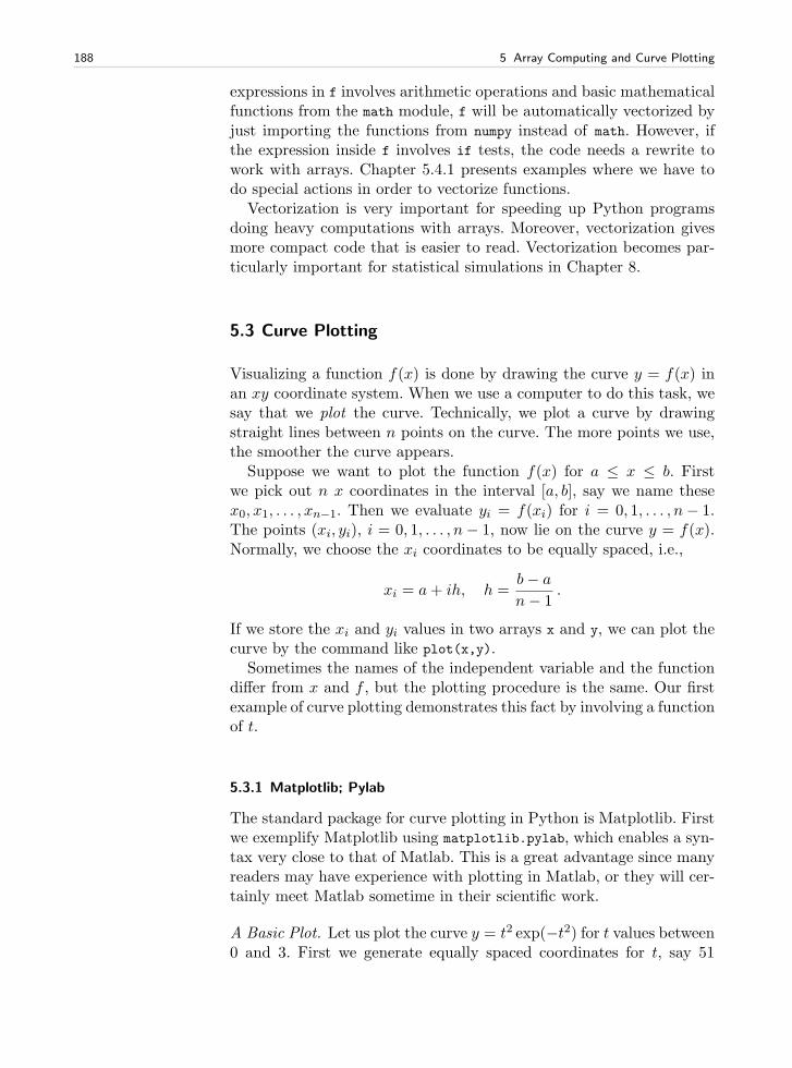
188 5 Array Computing and Curve Plotting

expressions in f involves arithmetic operations and basic mathematicalfunctions from the math module, f will be automatically vectorized byjust importing the functions from numpy instead of math. However, ifthe expression inside f involves if tests, the code needs a rewrite towork with arrays. Chapter 5.4.1 presents examples where we have todo special actions in order to vectorize functions.

Vectorization is very important for speeding up Python programsdoing heavy computations with arrays. Moreover, vectorization givesmore compact code that is easier to read. Vectorization becomes par-ticularly important for statistical simulations in Chapter 8.

5.3 Curve Plotting

Visualizing a function f(x) is done by drawing the curve y = f(x) inan xy coordinate system. When we use a computer to do this task, wesay that we plot the curve. Technically, we plot a curve by drawingstraight lines between n points on the curve. The more points we use,the smoother the curve appears.

Suppose we want to plot the function f(x) for a ≤ x ≤ b. Firstwe pick out n x coordinates in the interval [a, b], say we name thesex0, x1, . . . , xn−1. Then we evaluate yi = f(xi) for i = 0, 1, . . . , n− 1.The points (xi, yi), i = 0, 1, . . . , n− 1, now lie on the curve y = f(x).Normally, we choose the xi coordinates to be equally spaced, i.e.,

xi = a+ ih, h =b− a

n− 1.

If we store the xi and yi values in two arrays x and y, we can plot thecurve by the command like plot(x,y).

Sometimes the names of the independent variable and the functiondiffer from x and f , but the plotting procedure is the same. Our firstexample of curve plotting demonstrates this fact by involving a functionof t.

5.3.1 Matplotlib; Pylab

The standard package for curve plotting in Python is Matplotlib. Firstwe exemplify Matplotlib using matplotlib.pylab, which enables a syn-tax very close to that of Matlab. This is a great advantage since manyreaders may have experience with plotting in Matlab, or they will cer-tainly meet Matlab sometime in their scientific work.

A Basic Plot. Let us plot the curve y = t2 exp(−t2) for t values between0 and 3. First we generate equally spaced coordinates for t, say 51

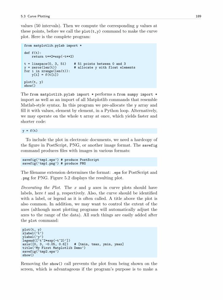
5.3 Curve Plotting 189

values (50 intervals). Then we compute the corresponding y values atthese points, before we call the plot(t,y) command to make the curveplot. Here is the complete program:

from matplotlib.pylab import *

def f(t):return t**2*exp(-t**2)

t = linspace(0, 3, 51) # 51 points between 0 and 3y = zeros(len(t)) # allocate y with float elementsfor i in xrange(len(t)):

y[i] = f(t[i])

plot(t, y)show()

The from matplotlib.pylab import * performs a from numpy import *

import as well as an import of all Matplotlib commands that resembleMatlab-style syntax. In this program we pre-allocate the y array andfill it with values, element by element, in a Python loop. Alternatively,we may operate on the whole t array at once, which yields faster andshorter code:

y = f(t)

To include the plot in electronic documents, we need a hardcopy ofthe figure in PostScript, PNG, or another image format. The savefig

command produces files with images in various formats:

savefig(’tmp1.eps’) # produce PostScriptsavefig(’tmp1.png’) # produce PNG

The filename extension determines the format: .eps for PostScript and.png for PNG. Figure 5.2 displays the resulting plot.

Decorating the Plot. The x and y axes in curve plots should havelabels, here t and y, respectively. Also, the curve should be identifiedwith a label, or legend as it is often called. A title above the plot isalso common. In addition, we may want to control the extent of theaxes (although most plotting programs will automatically adjust theaxes to the range of the data). All such things are easily added afterthe plot command:

plot(t, y)xlabel(’t’)ylabel(’y’)legend([’t^2*exp(-t^2)’])axis([0, 3, -0.05, 0.6]) # [tmin, tmax, ymin, ymax]title(’My First Matplotlib Demo’)savefig(’tmp2.eps’)show()

Removing the show() call prevents the plot from being shown on thescreen, which is advantageous if the program’s purpose is to make a

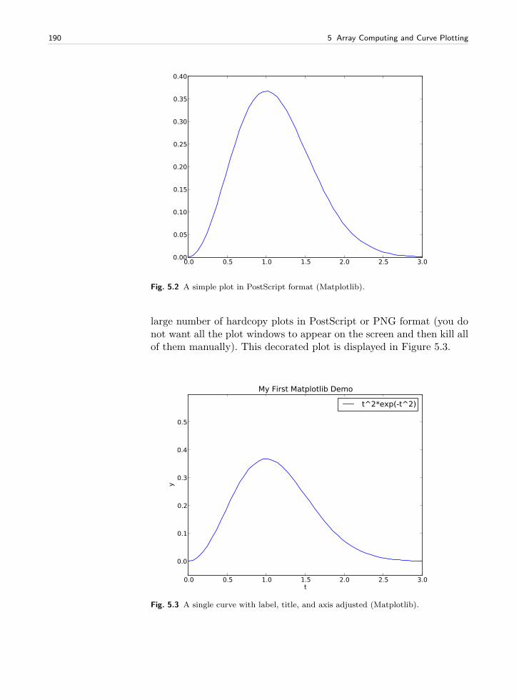
190 5 Array Computing and Curve Plotting

0.0 0.5 1.0 1.5 2.0 2.5 3.00.00

0.05

0.10

0.15

0.20

0.25

0.30

0.35

0.40

Fig. 5.2 A simple plot in PostScript format (Matplotlib).

large number of hardcopy plots in PostScript or PNG format (you donot want all the plot windows to appear on the screen and then kill allof them manually). This decorated plot is displayed in Figure 5.3.

0.0 0.5 1.0 1.5 2.0 2.5 3.0t

0.0

0.1

0.2

0.3

0.4

0.5

y

My First Matplotlib Demo

t^2*exp(-t^2)

Fig. 5.3 A single curve with label, title, and axis adjusted (Matplotlib).

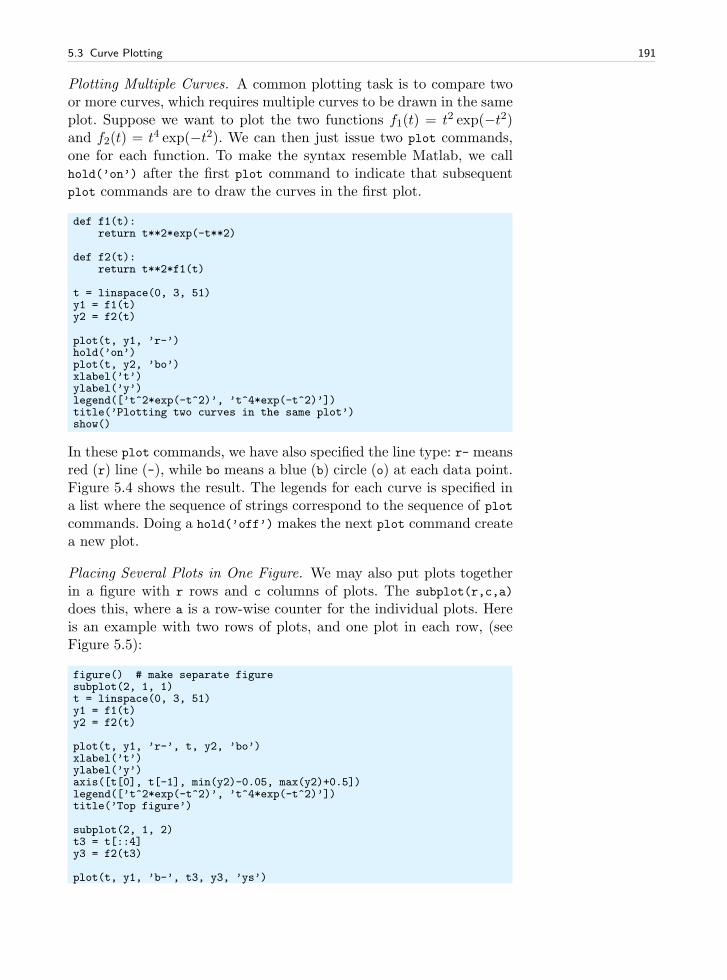
5.3 Curve Plotting 191

Plotting Multiple Curves. A common plotting task is to compare twoor more curves, which requires multiple curves to be drawn in the sameplot. Suppose we want to plot the two functions f1(t) = t2 exp(−t2)and f2(t) = t4 exp(−t2). We can then just issue two plot commands,one for each function. To make the syntax resemble Matlab, we callhold(’on’) after the first plot command to indicate that subsequentplot commands are to draw the curves in the first plot.

def f1(t):return t**2*exp(-t**2)

def f2(t):return t**2*f1(t)

t = linspace(0, 3, 51)y1 = f1(t)y2 = f2(t)

plot(t, y1, ’r-’)hold(’on’)plot(t, y2, ’bo’)xlabel(’t’)ylabel(’y’)legend([’t^2*exp(-t^2)’, ’t^4*exp(-t^2)’])title(’Plotting two curves in the same plot’)show()

In these plot commands, we have also specified the line type: r- meansred (r) line (-), while bo means a blue (b) circle (o) at each data point.Figure 5.4 shows the result. The legends for each curve is specified ina list where the sequence of strings correspond to the sequence of plotcommands. Doing a hold(’off’) makes the next plot command createa new plot.

Placing Several Plots in One Figure. We may also put plots togetherin a figure with r rows and c columns of plots. The subplot(r,c,a)

does this, where a is a row-wise counter for the individual plots. Hereis an example with two rows of plots, and one plot in each row, (seeFigure 5.5):

figure() # make separate figuresubplot(2, 1, 1)t = linspace(0, 3, 51)y1 = f1(t)y2 = f2(t)

plot(t, y1, ’r-’, t, y2, ’bo’)xlabel(’t’)ylabel(’y’)axis([t[0], t[-1], min(y2)-0.05, max(y2)+0.5])legend([’t^2*exp(-t^2)’, ’t^4*exp(-t^2)’])title(’Top figure’)

subplot(2, 1, 2)t3 = t[::4]y3 = f2(t3)

plot(t, y1, ’b-’, t3, y3, ’ys’)

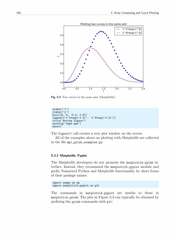
192 5 Array Computing and Curve Plotting

0.0 0.5 1.0 1.5 2.0 2.5 3.0t

0.0

0.1

0.2

0.3

0.4

0.5

y

Plotting two curves in the same plot

t^2*exp(-t^2)t^4*exp(-t^2)

Fig. 5.4 Two curves in the same plot (Matplotlib).

xlabel(’t’)ylabel(’y’)axis([0, 4, -0.2, 0.6])legend([’t^2*exp(-t^2)’, ’t^4*exp(-t^2)’])title(’Bottom figure’)savefig(’tmp4.eps’)show()

The figure() call creates a new plot window on the screen.All of the examples above on plotting with Matplotlib are collected

in the file mpl_pylab_examples.py.

5.3.2 Matplotlib; Pyplot

The Matplotlib developers do not promote the matplotlib.pylab in-terface. Instead, they recommend the matplotlib.pyplot module andprefix Numerical Python and Matplotlib functionality by short formsof their package names:

import numpy as npimport matplotlib.pyplot as plt

The commands in matplotlib.pyplot are similar to those inmatplotlib.pylab. The plot in Figure 5.3 can typically be obtained byprefixing the pylab commands with plt:

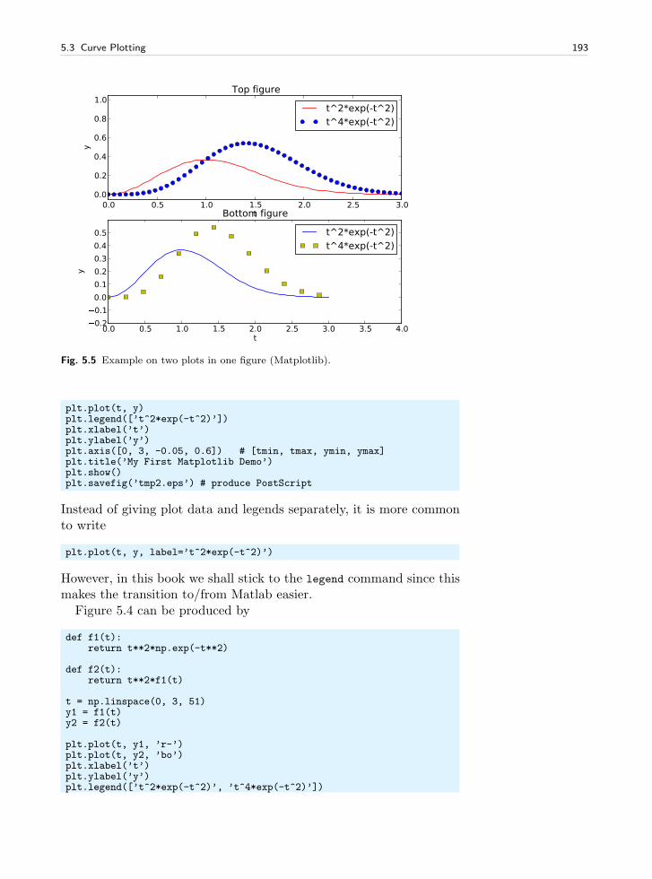
5.3 Curve Plotting 193

0.0 0.5 1.0 1.5 2.0 2.5 3.0t

0.0

0.2

0.4

0.6

0.8

1.0

yTop figure

t^2*exp(-t^2)t^4*exp(-t^2)

0.0 0.5 1.0 1.5 2.0 2.5 3.0 3.5 4.0t

0.2

0.1

0.0

0.1

0.2

0.3

0.4

0.5

y

Bottom figure

t^2*exp(-t^2)t^4*exp(-t^2)

Fig. 5.5 Example on two plots in one figure (Matplotlib).

plt.plot(t, y)plt.legend([’t^2*exp(-t^2)’])plt.xlabel(’t’)plt.ylabel(’y’)plt.axis([0, 3, -0.05, 0.6]) # [tmin, tmax, ymin, ymax]plt.title(’My First Matplotlib Demo’)plt.show()plt.savefig(’tmp2.eps’) # produce PostScript

Instead of giving plot data and legends separately, it is more commonto write

plt.plot(t, y, label=’t^2*exp(-t^2)’)

However, in this book we shall stick to the legend command since thismakes the transition to/from Matlab easier.

Figure 5.4 can be produced by

def f1(t):return t**2*np.exp(-t**2)

def f2(t):return t**2*f1(t)

t = np.linspace(0, 3, 51)y1 = f1(t)y2 = f2(t)

plt.plot(t, y1, ’r-’)plt.plot(t, y2, ’bo’)plt.xlabel(’t’)plt.ylabel(’y’)plt.legend([’t^2*exp(-t^2)’, ’t^4*exp(-t^2)’])

194 5 Array Computing and Curve Plotting

plt.title(’Plotting two curves in the same plot’)plt.savefig(’tmp3.eps’)plt.show()

Putting multiple plots in a figure follows the same set-up with subplot

as shown for pylab, except that commands are prefixed by plt. Thecomplete example, along with the codes listed above, are found in thefile mpl_pyplot_examples.py.

Once you have created a basic plot, there are numerous possibilitiesfor fine-tuning the figure, i.e., adjusting tickmarks on the axis, insertingtext, etc. The Matplotlib website is full of instructive examples on whatyou can do with this excellent package.

5.3.3 SciTools and Easyviz

Although Matplotlib has recently evolved to be the de facto standardfor curve plotting in Python, there are several other alternative pack-ages, especially if we also consider plotting of 2D/3D scalar and vectorfields. Python has interfaces to many leading visualization packages:Matlab, Gnuplot, Grace, OpenDX, and VTK. Even basic plotting withthese packages has very different syntax, and deciding which packageand syntax to go with was and still is a challenge. As a response to thischallenge, Easyviz was created to provide a common uniform interfaceto all the mentioned visualization packages (including Matplotlib). Thesyntax of this interface was made very close to that of Matlab, sincemost scientists and engineers have experience with Matlab or mostprobably will be using it in some context8.

Easyviz is part of the SciTools package, which consists of a setof Python tools building on Numerical Python, ScientificPython, thecomprehensive SciPy environment, and other packages for scientificcomputing with Python. SciTools contains in particular software re-lated to the book [5] and the present text. Installation is straightfor-ward (just run python setup.py install, if you have downloaded thesource code, or do THIS IS WRONG COMMAND - use ptex2tex: sudo

apt-get install python-scitools on Debian-based systems such asUbuntu Linux).

Importing SciTools and Easyviz. A standard import of SciTools is

from scitools.std import *

The advantage of this statement is that it, with a minimum of typing,imports a lot of useful modules for numerical Python programming:Easyviz, all of numpy (from numpy import *), all of scipy (from scipy

8 In general, the Python syntax used in the examples in this book is constructed toease the transition to and from Matlab.

5.3 Curve Plotting 195

import *) if available, all of scitools.numpyutils (some conveniencefunctions extending numpy), numpy.lib.scimath (see Chapter 1.6.3),StringFunction tool (see Chapter 4.1.4), plus commonly applied mod-ules such as sys, os, and math. The imported standard mathematicalfunctions (sqrt, sin, asin, exp, etc.) work with arrays and deal trans-parently with real and complex input/output (as the correspondingMatlab functions).

The downside of the “star import” from scitools.std is twofold.First, it fills up your program or interactive session with the names ofseveral hundred functions. Second, when using a particular function,you do not know the package it comes from. Both problems are solvedby doing an import of the type used in Chapter 5.3.2:

import scitools.std as stimport numpy as np

All of the SciTools and Easyviz functions must then be prefixed byst. Although the numpy functions are available through the st prefix,we recommend to use the np prefix to clearly see where functionalitycomes from.

Importing scitools.std might be a comprehensive process, espe-cially if scipy is available, and consequently take some time. A moreminimalistic and faster import for plotting with Easyviz is

from scitools.easyviz import *from numpy import *

or

import scitools.easyviz as evimport numpy as np

The Easyviz plotting functions must then be prefixed by ev.Since the Easyviz syntax for plotting is very close to that of Matlab,

it is also close to the syntax of Matplotlib. This will be demonstrated inthe forthcoming examples. The advantage of using Easyviz is that theunderlying plotting package, used to create the graphics and known asa backend , can trivially be replaced by another package. If users of yourPython software have not installed a particular visualization package,the software can still be used with another alternative (which mightbe considerably easier to install). By default, Easyviz now employsMatplotlib for plotting. Other popular alternatives are Gnuplot andMatlab. For 2D/3D scalar and vector fields, VTK is a popular backendfor Easyviz.

We shall next redo the curve plotting examples from Chapter 5.3.1using Easyviz syntax.

A Basic Plot. Plotting the curve y = t2 exp(−t2) for t ∈ [0, 3], using51 equally spaced points (50 intervals) is performed by like this:

196 5 Array Computing and Curve Plotting

from scitools.std import *

def f(t):return t**2*exp(-t**2)

t = linspace(0, 3, 51)y = f(t)plot(t, y)

To save the plot in a file, either in PostScript or PNG format, we usethe savefig function, which takes the filename as argument:

savefig(’tmp1.eps’) # produce PostScriptsavefig(’tmp1.png’) # produce PNG

The filename extension determines the format: .ps or .eps forPostScript, and .png for PNG. A synonym for the savefig func-tion is hardcopy.

On some platforms, some backends may result in a plot that is shownin just a fraction of a second on the screen before the plot windowdisappears (using the Gnuplot backend on Windows machines, or usingthe Matplotlib backend, constitute two examples). To make the windowstay on the screen, add

raw_input(’Press the Return key to quit: ’)

at the end of the program. The plot window is killed when the programterminates, and this satement postpones the termination until the userhits the Return key.

Decorating the Plot. Let us plot the same curve, but now with a legend,a plot title, labels on the axes, and specified ranges of the axes:

from scitools.std import *

def f(t):return t**2*exp(-t**2)

t = linspace(0, 3, 51)y = f(t)plot(t, y)xlabel(’t’)ylabel(’y’)legend(’t^2*exp(-t^2)’)axis([0, 3, -0.05, 0.6]) # [tmin, tmax, ymin, ymax]title(’My First Easyviz Demo’)

Easyviz has also introduced a more ”Pythonic”plot command whereall the plot properties can be set at once through keyword arguments:

plot(t, y,xlabel=’t’,ylabel=’y’,legend=’t^2*exp(-t^2)’,axis=[0, 3, -0.05, 0.6],title=’My First Easyviz Demo’,

5.3 Curve Plotting 197

savefig=’tmp1.eps’, # or hardcopy=’tmp1.eps’show=True)

With show=False one can avoid the plot window on the screen andjust make the hardcopy.

Note that we in the curve legend write t square as t^2 (LATEX style)rather than t**2 (program style). Whichever form you choose is upto you, but the LATEX form sometimes looks better in some plottingprograms (Matplotlib and Gnuplot are two examples).

Plotting Multiple Curves. Next we want to compare the two functionsf1(t) = t2 exp(−t2) and f2(t) = t4 exp(−t2). Writing two plot com-mands after each other makes two separate plots. To make the secondcurve appear together with the first one, we need to issue a hold(’on’)

call after the first plot command. All subsequent plot commands willthen draw curves in the same plot, until hold(’off’) is called.

from scitools.std import *

def f1(t):return t**2*exp(-t**2)

def f2(t):return t**2*f1(t)

t = linspace(0, 3, 51)y1 = f1(t)y2 = f2(t)

plot(t, y1)hold(’on’)plot(t, y2)

xlabel(’t’)ylabel(’y’)legend(’t^2*exp(-t^2)’, ’t^4*exp(-t^2)’)title(’Plotting two curves in the same plot’)savefig(’tmp3.eps’)

The sequence of the multiple legends is such that the first legend cor-responds to the first curve, the second legend to the second curve, andso forth.

Instead of separate calls to plot and the use of hold(’on’), we cando everything at once and just send several curves to plot:

plot(t, y1, t, y2, xlabel=’t’, ylabel=’y’,legend=(’t^2*exp(-t^2)’, ’t^4*exp(-t^2)’),title=’Plotting two curves in the same plot’,savefig=’tmp3.eps’)

Throughout this book, we very often make use of this type of compactplot command, which also only requires an import of the form from

scitools.std import plot.

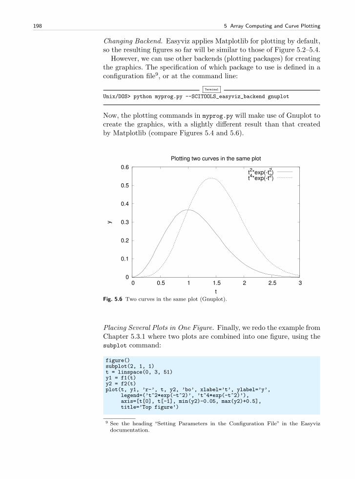
198 5 Array Computing and Curve Plotting

Changing Backend. Easyviz applies Matplotlib for plotting by default,so the resulting figures so far will be similar to those of Figure 5.2–5.4.

However, we can use other backends (plotting packages) for creatingthe graphics. The specification of which package to use is defined in aconfiguration file9, or at the command line:

Terminal

Unix/DOS> python myprog.py --SCITOOLS_easyviz_backend gnuplot

Now, the plotting commands in myprog.py will make use of Gnuplot tocreate the graphics, with a slightly different result than that createdby Matplotlib (compare Figures 5.4 and 5.6).

0

0.1

0.2

0.3

0.4

0.5

0.6

0 0.5 1 1.5 2 2.5 3

y

t

Plotting two curves in the same plot

t2*exp(-t

2)

t4*exp(-t

2)

Fig. 5.6 Two curves in the same plot (Gnuplot).

Placing Several Plots in One Figure. Finally, we redo the example fromChapter 5.3.1 where two plots are combined into one figure, using thesubplot command:

figure()subplot(2, 1, 1)t = linspace(0, 3, 51)y1 = f1(t)y2 = f2(t)plot(t, y1, ’r-’, t, y2, ’bo’, xlabel=’t’, ylabel=’y’,

legend=(’t^2*exp(-t^2)’, ’t^4*exp(-t^2)’),axis=[t[0], t[-1], min(y2)-0.05, max(y2)+0.5],title=’Top figure’)

9 See the heading “Setting Parameters in the Configuration File” in the Easyvizdocumentation.

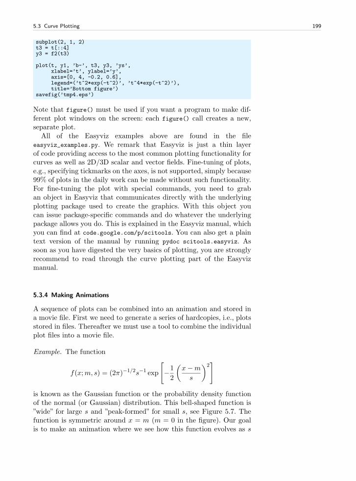
5.3 Curve Plotting 199

subplot(2, 1, 2)t3 = t[::4]y3 = f2(t3)

plot(t, y1, ’b-’, t3, y3, ’ys’,xlabel=’t’, ylabel=’y’,axis=[0, 4, -0.2, 0.6],legend=(’t^2*exp(-t^2)’, ’t^4*exp(-t^2)’),title=’Bottom figure’)

savefig(’tmp4.eps’)

Note that figure() must be used if you want a program to make dif-ferent plot windows on the screen: each figure() call creates a new,separate plot.

All of the Easyviz examples above are found in the fileeasyviz_examples.py. We remark that Easyviz is just a thin layerof code providing access to the most common plotting functionality forcurves as well as 2D/3D scalar and vector fields. Fine-tuning of plots,e.g., specifying tickmarks on the axes, is not supported, simply because99% of plots in the daily work can be made without such functionality.For fine-tuning the plot with special commands, you need to graban object in Easyviz that communicates directly with the underlyingplotting package used to create the graphics. With this object youcan issue package-specific commands and do whatever the underlyingpackage allows you do. This is explained in the Easyviz manual, whichyou can find at code.google.com/p/scitools. You can also get a plaintext version of the manual by running pydoc scitools.easyviz. Assoon as you have digested the very basics of plotting, you are stronglyrecommend to read through the curve plotting part of the Easyvizmanual.

5.3.4 Making Animations

A sequence of plots can be combined into an animation and stored ina movie file. First we need to generate a series of hardcopies, i.e., plotsstored in files. Thereafter we must use a tool to combine the individualplot files into a movie file.

Example. The function

f(x;m, s) = (2π)−1/2s−1 exp

[

−1

2

(

x−m

s

)2]

is known as the Gaussian function or the probability density functionof the normal (or Gaussian) distribution. This bell-shaped function is”wide” for large s and ”peak-formed” for small s, see Figure 5.7. Thefunction is symmetric around x = m (m = 0 in the figure). Our goalis to make an animation where we see how this function evolves as s

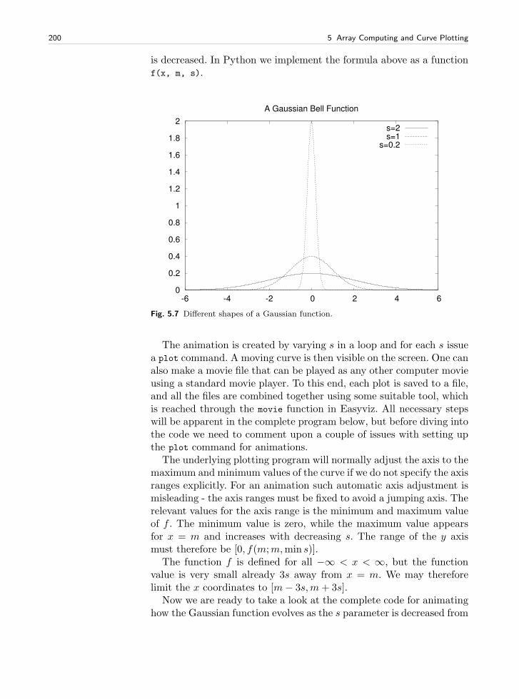
200 5 Array Computing and Curve Plotting

is decreased. In Python we implement the formula above as a functionf(x, m, s).

0

0.2

0.4

0.6

0.8

1

1.2

1.4

1.6

1.8

2

-6 -4 -2 0 2 4 6

A Gaussian Bell Function

s=2s=1

s=0.2

Fig. 5.7 Different shapes of a Gaussian function.

The animation is created by varying s in a loop and for each s issuea plot command. A moving curve is then visible on the screen. One canalso make a movie file that can be played as any other computer movieusing a standard movie player. To this end, each plot is saved to a file,and all the files are combined together using some suitable tool, whichis reached through the movie function in Easyviz. All necessary stepswill be apparent in the complete program below, but before diving intothe code we need to comment upon a couple of issues with setting upthe plot command for animations.

The underlying plotting program will normally adjust the axis to themaximum and minimum values of the curve if we do not specify the axisranges explicitly. For an animation such automatic axis adjustment ismisleading - the axis ranges must be fixed to avoid a jumping axis. Therelevant values for the axis range is the minimum and maximum valueof f . The minimum value is zero, while the maximum value appearsfor x = m and increases with decreasing s. The range of the y axismust therefore be [0, f(m;m,min s)].

The function f is defined for all −∞ < x < ∞, but the functionvalue is very small already 3s away from x = m. We may thereforelimit the x coordinates to [m− 3s,m+ 3s].

Now we are ready to take a look at the complete code for animatinghow the Gaussian function evolves as the s parameter is decreased from

5.3 Curve Plotting 201

2 to 0.2. We employ Easyviz for plotting, but you can equally well useMatplotlib for creating the individual frames of the movie.

from scitools.std import *import time

def f(x, m, s):return (1.0/(sqrt(2*pi)*s))*exp(-0.5*((x-m)/s)**2)

m = 0s_start = 2s_stop = 0.2s_values = linspace(s_start, s_stop, 30)x = linspace(m -3*s_start, m + 3*s_start, 1000)# f is max for x=m; smaller s gives larger max valuemax_f = f(m, m, s_stop)

# Show the movie on the screen# and make hardcopies of frames simultaneously.

counter = 0for s in s_values:

y = f(x, m, s)plot(x, y, axis=[x[0], x[-1], -0.1, max_f],

xlabel=’x’, ylabel=’f’, legend=’s=%4.2f’ % s,savefig=’tmp%04d.png’ % counter)

counter += 1#time.sleep(0.2) # can insert a pause to control movie speed

# Make movie file the simplest possible way:movie(’tmp*.png’)

Note that the s values are decreasing (linspace handles this auto-matically if the start value is greater than the stop value). Also notethat we, simply because we think it is visually more attractive, let they axis go from -0.1 although the f function is always greater than zero.

Remarks on Filenames. For each frame (plot) in the movie we store theplot in a file. The different files need different names and an easy wayof referring to the set of files in right order. We therefore suggest to usefilenames of the form tmp0001.png, tmp0002.png, tmp0003.png, etc. Theprintf format 04d pads the integers with zeros such that 1 becomes0001, 13 becomes 0013 and so on. The expression tmp*.png will nowexpand (by an alphabetic sort) to a list of all files in proper order.Without the padding with zeros, i.e., names of the form tmp1.png,tmp2.png, ..., tmp12.png, etc., the alphabetic order will give a wrongsequence of frames in the movie. For instance, tmp12.png will appearbefore tmp2.png.

Note that the names of plot files specified when making hardopiesmust be consistent with the specification of names in the call to theEasyviz movie function. Typically, one applies a Unix wildcard notationin the call to movie, say plotfile*.eps, where the asterisk will matchany set of characters. When specifying hardcopies, we must then usea filename that is consistent with plotfile*.eps, that is, the filename

202 5 Array Computing and Curve Plotting

must start with plotfile and end with .eps, but in between these twoparts we are free to construct (e.g.) a frame number padded with zeros.

We recommend to always remove previously generated plot files be-fore a new set of files is made. Otherwise, the movie may get old andnew files mixed up. The following Python code removes all files of theform tmp*.png:

import glob, osfor filename in glob.glob(’tmp*.png’):

os.remove(filename)

These code lines should be inserted at the beginning of the code exam-ple above. Alternatively, one may store all plotfiles in a subfolder andlater delete the subfolder. Here is a suitable code segment10:

import shutil, ossubdir = ’temp’ # subfolder name for plot filesif os.path.isdir(subdir): # does the subfolder already exist?

shutil.rmtree(subdir) # delete the whole folderos.mkdir(subdir) # make new subfolderos.chdir(subdir) # move to subfolder# ... perform all the plotting, make movie ...os.chdir(os.pardir) # optional: move up to parent folder

Movie Formats. Having a set of (e.g.) tmp*.png files, one can simplygenerate a movie by a movie(’tmp*.png’) call. The movie function gen-erates a movie file called movie.avi (AVI format), movie.mpeg (MPEGformat), or movie.gif (animated GIF format) in the current workingdirectory. The movie format depends on the encoders found on yourmachine.

You can get complete control of the movie format and the nameof the movie file by supplying more arguments to the movie function.First, let us generate an animated GIF file called tmpmovie.gif:

movie(’tmp_*.eps’, encoder=’convert’, fps=2,output_file=’tmpmovie.gif’)

The generation of animated GIF images applies the convert programfrom the ImageMagick suite. This program must of course be installedon the machine. The argument fps stands for frames per second so herethe speed of the movie is slow in that there is a delay of half a secondbetween each frame (image file). To view the animated GIF file, onecan use the animate program (also from ImageMagick) and give themovie file as command-line argument. One can alternatively put theGIF file in a web page in an IMG tag such that a browser automaticallydisplays the movie.

An AVI movie can be generated by the call

10 Python and many other languages use the word directory instead of folder. Con-sequently, the name of functions dealing with folders have a name with dir for“directory”.

5.3 Curve Plotting 203

movie(’tmp_*.eps’, encoder=’ffmpeg’, fps=4,output_file=’tmpmovie1.avi’,

Alternatively, we may generate an MPEG movie using the ppmtompeg

encoder from the Netpbm suite of image manipulation tools:

movie(’tmp_*.eps’, encoder=’ppmtompeg’, fps=24,output_file=’tmpmovie2.mpeg’,

The ppmtompeg supports only a few (high) frame rates.The next sample call to movie uses the Mencoder tool and spec-

ifies some additional arguments (video codec, video bitrate, and thequantization scale):

movie(’tmp_*.eps’, encoder=’mencoder’, fps=24,output_file=’tmpmovie.mpeg’,vcodec=’mpeg2video’, vbitrate=2400, qscale=4)

Note that even if you prefer to make the individual plot files byMatplotlib, Matlab, or whatever, the movie command from Easyviz isstill handy to make a movie file out of the individual plot files. All youneed to do is from scitools.std import movie and call movie with theright specification of plot file names.

Playing movie files can be done by a lot of programs. Windows MediaPlayer is a default choice on Windows machines. On Unix, a variety oftools are available. For animated GIF files the animate program fromthe ImageMagick suite is suitable, or one can simply show the file ina web page with the HTML command <img src="tmpmovie.gif">. AVIand MPEG files can be played by, for example, the mplayer, vlc, ortotem programs.

5.3.5 Curves in Pure Text

Sometimes it can be desirable to show a graph in pure ASCII text,e.g., as part of a trial run of a program included in the program itself(cf. the introduction to Chapter 1.8), or a graph can be handy in adoc string. For such purposes we have slightly extended a module byImri Goldberg (aplotter.py) and included it as a module in SciTools.Running pydoc on scitools.aplotter describes the capabilities of thistype of primitive plotting. Here we just give an example of what it cando:

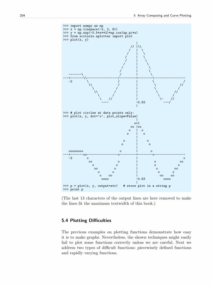
204 5 Array Computing and Curve Plotting

>>> import numpy as np>>> x = np.linspace(-2, 2, 81)>>> y = np.exp(-0.5*x**2)*np.cos(np.pi*x)>>> from scitools.aplotter import plot>>> plot(x, y)

|// |\\/ | \/ | \/ | \/ | \/ | \/ | \/ | \

-------\ / | \---+-------\\-----------------/---------+--------\-----------------

-2 \ / | \ /\\ / | \ //\ / | \ /\\ / | \ //\ / | \ /\ // | \- //---- -0.63 ---/

|

>>> # plot circles at data points only:>>> plot(x, y, dot=’o’, plot_slope=False)

|o+1

oo |ooo | oo | o

|o | oo | o

|oooooooo o | o

---+-------oo-----------------o---------+--------o------------------2 o | o

oo o | o ooo o | o ooo o | o ooo o | o oo oo | oo oooooo -0.63 oooo

|>>> p = plot(x, y, output=str) # store plot in a string p>>> print p

(The last 13 characters of the output lines are here removed to makethe lines fit the maximum textwidth of this book.)

5.4 Plotting Difficulties

The previous examples on plotting functions demonstrate how easyit is to make graphs. Nevertheless, the shown techniques might easilyfail to plot some functions correctly unless we are careful. Next weaddress two types of difficult functions: piecewisely defined functionsand rapidly varying functions.

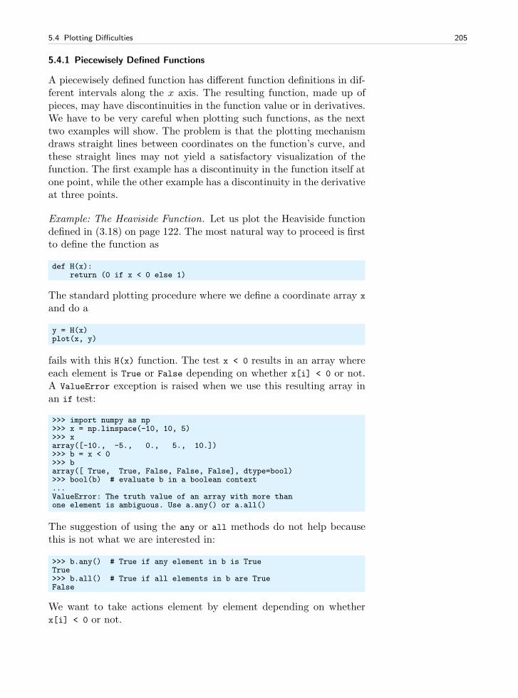
5.4 Plotting Difficulties 205

5.4.1 Piecewisely Defined Functions

A piecewisely defined function has different function definitions in dif-ferent intervals along the x axis. The resulting function, made up ofpieces, may have discontinuities in the function value or in derivatives.We have to be very careful when plotting such functions, as the nexttwo examples will show. The problem is that the plotting mechanismdraws straight lines between coordinates on the function’s curve, andthese straight lines may not yield a satisfactory visualization of thefunction. The first example has a discontinuity in the function itself atone point, while the other example has a discontinuity in the derivativeat three points.

Example: The Heaviside Function. Let us plot the Heaviside functiondefined in (3.18) on page 122. The most natural way to proceed is firstto define the function as

def H(x):return (0 if x < 0 else 1)

The standard plotting procedure where we define a coordinate array x

and do a

y = H(x)plot(x, y)

fails with this H(x) function. The test x < 0 results in an array whereeach element is True or False depending on whether x[i] < 0 or not.A ValueError exception is raised when we use this resulting array inan if test:

>>> import numpy as np>>> x = np.linspace(-10, 10, 5)>>> xarray([-10., -5., 0., 5., 10.])>>> b = x < 0>>> barray([ True, True, False, False, False], dtype=bool)>>> bool(b) # evaluate b in a boolean context...ValueError: The truth value of an array with more thanone element is ambiguous. Use a.any() or a.all()

The suggestion of using the any or all methods do not help becausethis is not what we are interested in:

>>> b.any() # True if any element in b is TrueTrue>>> b.all() # True if all elements in b are TrueFalse

We want to take actions element by element depending on whetherx[i] < 0 or not.

206 5 Array Computing and Curve Plotting

There are three ways to find a remedy to our problems with theif x < 0 test: (i) we can write an explicit loop for computing the ele-ments, (ii) we can use a tool for automatically vectorize H(x), or (iii)we can manually vectorize the H(x) function. All three methods will beillustrated next.

Loop. The following function works well for arrays if we insert a simpleloop over the array elements (such that H(x) operates on scalars only):

def H_loop(x):r = np.zeros(len(x))for i in xrange(len(x)):

r[i] = H(x[i])return r

x = np.linspace(-5, 5, 6)y = H_loop(x)

This H_loop version of H is sufficient for plotting the Heaviside function.The next paragraph explains other ways of making versions of H(x) thatwork for array arguments.

Automatic Vectorization. Numerical Python contains a method forautomatically vectorizing a Python function that works with scalars(pure numbers) as arguments:

import numpy as npH_vec = np.vectorize(H)

The H_vec(x) function will now work with vector/array arguments x.Unfortunately, such automatically vectorized functions are often asslow as the explicit loop shown above.

Manual Vectorization. (Note: This topic is considered advanced.) Toallow array arguments in our Heaviside function and get the increasedspeed that one associates with vectorization, we have to rewrite theH function completely. The mathematics must now be expressed byfunctions from the Numerical Python library. In general, this type ofrewrite is non-trivial and requires knowledge of and experience withthe library. Fortunately, functions of the form

def f(x):if condition:

x = <expression1>else:

x = <expression2>return x

can in general be vectorized quite simply as

def f_vectorized(x):x1 = <expression1>x2 = <expression2>return np.where(condition, x1, x2)

5.4 Plotting Difficulties 207

The np.where function returns an array of the same length ascondition, whose element no. i equals x1[i] if condition[i] isTrue, and x2[i] otherwise. With Python loops we can express thisprinciple as

r = np.zeros(len(condition)) # array returned from np.where(...)for i in xrange(condition):

r[i] = x1[i] if condition[i] else x2[i]

The x1 and x2 variables can be pure numbers or arrays of the samelength as x.

In our case we can use the np.where function as follows:

def Hv(x):return np.where(x < 0, 0.0, 1.0)

Plotting the Heaviside Function. Since the Heaviside function consistsof two flat lines, one may think that we do not need many points alongthe x axis to describe the curve. Let us try with nine points:

x = np.linspace(-10, 10, 9)from scitools.std import plotplot(x, Hv(x), axis=[x[0], x[-1], -0.1, 1.1])

However, so few x points are not able to describe the jump from 0 to 1at x = 0, as shown by the solid line in Figure 5.8a. Using more points,say 50 between −10 and 10,

x2 = np.linspace(-10, 10, 50)plot(x, Hv(x), ’r’, x2, Hv(x2), ’b’,

legend=(’5 points’, ’50 points’),axis=[x[0], x[-1], -0.1, 1.1])

makes the curve look better. However, the step is still not strictlyvertical. More points will improve the situation. Nevertheless, the bestis to draw two flat lines directly: from (−10, 0) to (0, 0), then to (0, 1)and then to (10, 1):

plot([-10, 0, 0, 10], [0, 0, 1, 1],axis=[x[0], x[-1], -0.1, 1.1])

The result is shown in Figure 5.8b.Some will argue that the plot of H(x) should not contain the vertical

line from (0, 0) to (0, 1), but only two horizontal lines. To make such aplot, we must draw two distinct curves, one for each horizontal line:

plot([-10,0], [0,0], ’r-’, [0,10], [1,1], ’r-’,axis=[x[0], x[-1], -0.1, 1.1])

Observe that we must specify the same line style for both lines (curves),otherwise they would by default get different color on the screen and

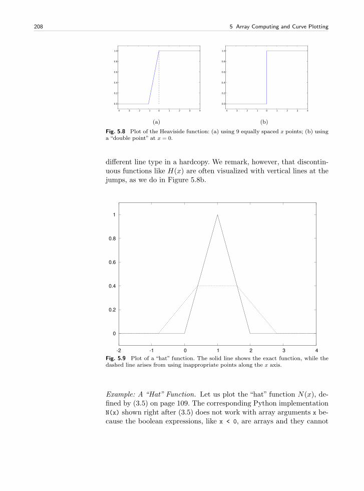
208 5 Array Computing and Curve Plotting

4 3 2 1 0 1 2 3 4

0.0

0.2

0.4

0.6

0.8

1.0

(a)

4 3 2 1 0 1 2 3 4

0.0

0.2

0.4

0.6

0.8

1.0

(b)

Fig. 5.8 Plot of the Heaviside function: (a) using 9 equally spaced x points; (b) usinga “double point” at x = 0.

different line type in a hardcopy. We remark, however, that discontin-uous functions like H(x) are often visualized with vertical lines at thejumps, as we do in Figure 5.8b.

0

0.2

0.4

0.6

0.8

1

-2 -1 0 1 2 3 4

Fig. 5.9 Plot of a “hat” function. The solid line shows the exact function, while thedashed line arises from using inappropriate points along the x axis.

Example: A “Hat” Function. Let us plot the “hat” function N(x), de-fined by (3.5) on page 109. The corresponding Python implementationN(x) shown right after (3.5) does not work with array arguments x be-cause the boolean expressions, like x < 0, are arrays and they cannot

5.4 Plotting Difficulties 209

yield a single True or False value for the if tests. The simplest solutionis to use vectorize, as explained for the Heaviside function above11:

N_vec = vectorize(N)

A manual rewrite, yielding a faster vectorized function, is more de-manding than for the Heaviside function because we now have multiplebranches in the if test. One attempt may be12

def Nv(x):r = np.where(x < 0, 0.0, x)r = np.where(0 <= x < 1, x, r)r = np.where(1 <= x < 2, 2-x, r)r = np.where(x >= 2, 0.0, r)return r

However, the condition like 0 <= x < 1, which is equivalent to 0 <=

x and x < 1, does not work because the and operator does not workwith array arguments. All operators in Python (+, -, and, or, etc.)are available as pure functions in a module operator (operator.add,operator.sub, operator.and_, operator.or_13, etc.). A working Nv func-tion must apply operator.and_ instead:

def Nv(x):r = np.where(x < 0, 0.0, x)import operatorcondition = operator.and_(0 <= x, x < 1)r = np.where(condition, x, r)condition = operator.and_(1 <= x, x < 2)r = np.where(condition, 2-x, r)r = np.where(x >= 2, 0.0, r)return r

A second, alternative rewrite is to use boolean expressions in indices:

def Nv(x):r = x.copy() # avoid modifying x in-placer[x < 0.0] = 0.0condition = operator.and_(0 <= x, x < 1)r[condition] = x[condition]condition = operator.and_(1 <= x, x < 2)r[condition] = 2-x[condition]r[x >= 2] = 0.0return r

Now to the computation of coordinate arrays for the plotting. Wemay use an explicit loop over all array elements, or the N_vec function,or the Nv function. An approach without thinking about vectorizationtoo much could be

11 It is important that N(x) return float and not int values, otherwise the vectorizedversion will produce int values and hence be incorrect.

12 This is again advanced material.13 Recall that and and or are reserved keywords, see page 10, so a module or program

cannot have variables or functions with these names. To circumvent this problem,the convention is to add a trailing underscore to the name.

210 5 Array Computing and Curve Plotting

x = np.linspace(-2, 4, 6)plot(x, N_vec(x), ’r’, axis=[x[0], x[-1], -0.1, 1.1])

This results in the dashed line in Figure 5.9. What is the problem?The problem lies in the computation of the x vector, which does notcontain the points x = 1 and x = 2 where the function makes significantchanges. The result is that the “hat” is “flattened”. Making an x vectorwith all critical points in the function definitions, x = 0, 1, 2, providesthe necessary remedy, either

x = np.linspace(-2, 4, 7)

or the simple

x = [-2, 0, 1, 2, 4]

Any of these x alternatives and a plot(x, N_vec(x)) will result in thesolid line in Figure 5.9, which is the correct visualization of the N(x)function.

5.4.2 Rapidly Varying Functions

Let us now visualize the function f(x) = sin(1/x), using 10 and 1000points:

def f(x):return sin(1.0/x)

from scitools.std import linspace, plotx1 = linspace(-1, 1, 10)x2 = linspace(-1, 1, 1000)plot(x1, f(x1), label=’%d points’ % len(x))plot(x2, f(x2), label=’%d points’ % len(x))

The two plots are shown in Figure 5.10. Using only 10 points gives acompletely wrong picture of this function, because the function oscil-lates faster and faster as we approach the origin. With 1000 points weget an impression of these oscillations, but the accuracy of the plot inthe vicinity of the origin is still poor. A plot with 100000 points hasbetter accuracy, in principle, but the extermely fast oscillations nearthe origin just drowns in black ink (you can try it out yourself).

Another problem with the f(x) = sin(1/x) function is that it is easyto define an x vector containing x = 0, such that we get division byzero. Mathematically, the f(x) function has a singularity at x = 0: itis difficult to define f(0), so one should exclude this point from thefunction definition and work with a domain x ∈ [−1,−ǫ] ∪ [ǫ, 1], withǫ chosen small.

The lesson learned from these examples is clear. You must investigatethe function to be visualized and make sure that you use an appropriate

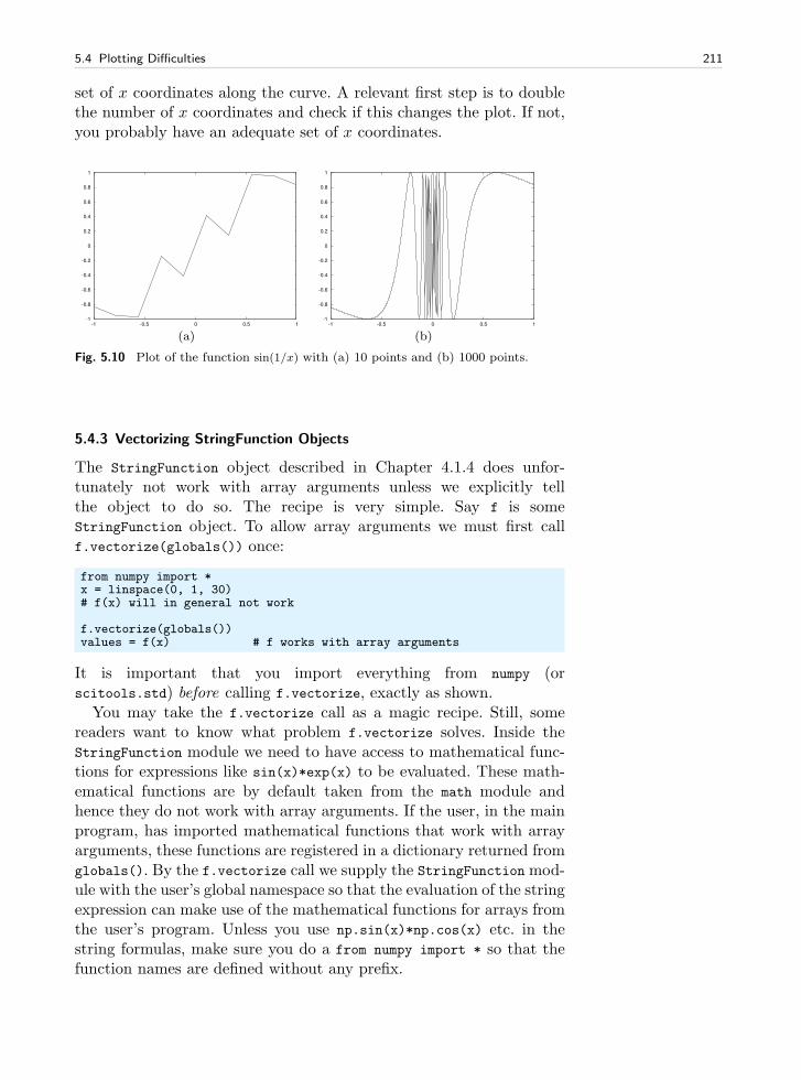
5.4 Plotting Difficulties 211

set of x coordinates along the curve. A relevant first step is to doublethe number of x coordinates and check if this changes the plot. If not,you probably have an adequate set of x coordinates.

-1

-0.8

-0.6

-0.4

-0.2

0

0.2

0.4

0.6

0.8

1

-1 -0.5 0 0.5 1

(a)

-1

-0.8

-0.6

-0.4

-0.2

0

0.2

0.4

0.6

0.8

1

-1 -0.5 0 0.5 1

(b)

Fig. 5.10 Plot of the function sin(1/x) with (a) 10 points and (b) 1000 points.

5.4.3 Vectorizing StringFunction Objects

The StringFunction object described in Chapter 4.1.4 does unfor-tunately not work with array arguments unless we explicitly tellthe object to do so. The recipe is very simple. Say f is someStringFunction object. To allow array arguments we must first callf.vectorize(globals()) once:

from numpy import *x = linspace(0, 1, 30)# f(x) will in general not work

f.vectorize(globals())values = f(x) # f works with array arguments

It is important that you import everything from numpy (orscitools.std) before calling f.vectorize, exactly as shown.

You may take the f.vectorize call as a magic recipe. Still, somereaders want to know what problem f.vectorize solves. Inside theStringFunction module we need to have access to mathematical func-tions for expressions like sin(x)*exp(x) to be evaluated. These math-ematical functions are by default taken from the math module andhence they do not work with array arguments. If the user, in the mainprogram, has imported mathematical functions that work with arrayarguments, these functions are registered in a dictionary returned fromglobals(). By the f.vectorize call we supply the StringFunction mod-ule with the user’s global namespace so that the evaluation of the stringexpression can make use of the mathematical functions for arrays fromthe user’s program. Unless you use np.sin(x)*np.cos(x) etc. in thestring formulas, make sure you do a from numpy import * so that thefunction names are defined without any prefix.

212 5 Array Computing and Curve Plotting

Even after calling f.vectorize(globals()), a StringFunction objectmay face problems with vectorization. One example is a piecewise con-stant function as specified by a string expression ’1 if x > 2 else 0’.One remedy is to use the vectorized version of an if test: ’where(x >

2, 1, 0)’. For an average user of the program this construct is not atall obvious so a more user-friendly solution is to apply vectorize fromnumpy:

f = vectorize(f) # vectorize a StringFunction f

The line above is therefore the most general (but also the slowest) wayof vectorizing a StringFunction object. After that call, f is no more aStringFunction object, but f behaves as a (vectorized) function. Thevectorize tool from numpy can be used to allow any Python functiontaking scalar arguments to also accept array arguments.

To get better speed, one can use vectorize(f) only in the case theformula in f contains an inline if test (e.g., recoginzed by the string ’

else ’ inside the formula). Otherwise, we use f.vectorize. The formulain f is obtained by str(f) so we can test

if ’ else ’ in str(f):f = vectorize(f)

else:f.vectorize(globals())

5.5 More on Numerical Python Arrays

This section lists some more advanced but useful operations with Nu-merical Python arrays.

5.5.1 Copying Arrays

Let x be an array. The statement a = x makes a refer to the same arrayas x. Changing a will then also affect x:

>>> import numpy as np>>> x = np.array([1, 2, 3.5])>>> a = x>>> a[-1] = 3 # this changes x[-1] too!>>> xarray([ 1., 2., 3.])

Changing a without changing x requires a to be a copy of x:

>>> a = x.copy()>>> a[-1] = 9>>> aarray([ 1., 2., 9.])>>> xarray([ 1., 2., 3.])

5.5 More on Numerical Python Arrays 213

5.5.2 In-Place Arithmetics

Let a and b be two arrays of the same shape. The expression a += b

means a = a + b, but this is not the complete story. In the statementa = a + b, the sum a + b is first computed, yielding a new array, andthen the name a is bound to this new array. The old array a is lostunless there are other names assigned to this array. In the statementa += b, elements of b are added directly into the elements of a (inmemory). There is no hidden intermediate array as in a = a + b. Thisimplies that a += b is more efficient than a = a + b since Python avoidsmaking an extra array. We say that the operators +=, *=, and so on,perform in-place arithmetics in arrays.

Consider the compound array expression

a = (3*x**4 + 2*x + 4)/(x + 1)

The computation actually goes as follows with seven hidden arrays forstoring intermediate results:

1. r1 = x**4

2. r2 = 3*r1

3. r3 = 2*x

4. r4 = r2 + r3

5. r5 = r4 + 4

6. r6 = x + 1

7. r7 = r5/r6

8. a = r7

With in-place arithmetics we can get away with creating three newarrays, at a cost of a significantly less readable code:

a = x.copy()a **= 4a *= 3a += 2*xa += 4a /= x + 1

The three extra arrays in this series of statement arise from copying x,and computing the right-hand sides 2*x and x+1.

Quite often in computational science and engineering, a huge num-ber of arithmetics is performed on very large arrays, and then savingmemory and array allocation time by doing in-place arithmetics is im-portant.

The mix of assignment and in-place arithmetics makes it easy tomake unintended changes of more than one array. For example, thiscode changes x:

a = xa += y

since a refers to the same array as x and the change of a is done in-place.

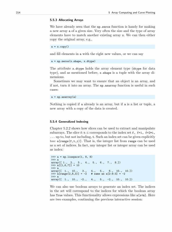
214 5 Array Computing and Curve Plotting

5.5.3 Allocating Arrays

We have already seen that the np.zeros function is handy for makinga new array a of a given size. Very often the size and the type of arrayelements have to match another existing array x. We can then eithercopy the original array, e.g.,

a = x.copy()

and fill elements in a with the right new values, or we can say

a = np.zeros(x.shape, x.dtype)

The attribute x.dtype holds the array element type (dtype for datatype), and as mentioned before, x.shape is a tuple with the array di-mensions.

Sometimes we may want to ensure that an object is an array, andif not, turn it into an array. The np.asarray function is useful in suchcases:

a = np.asarray(a)

Nothing is copied if a already is an array, but if a is a list or tuple, anew array with a copy of the data is created.

5.5.4 Generalized Indexing

Chapter 5.2.2 shows how slices can be used to extract and manipulatesubarrays. The slice f:t:i corresponds to the index set f, f+i, f+2*i,

... up to, but not including, t. Such an index set can be given explicitlytoo: a[range(f,t,i)]. That is, the integer list from range can be usedas a set of indices. In fact, any integer list or integer array can be usedas index:

>>> a = np.linspace(1, 8, 8)>>> aarray([ 1., 2., 3., 4., 5., 6., 7., 8.])>>> a[[1,6,7]] = 10>>> aarray([ 1., 10., 3., 4., 5., 6., 10., 10.])>>> a[range(2,8,3)] = -2 # same as a[2:8:3] = -2>>> aarray([ 1., 10., -2., 4., 5., -2., 10., 10.])

We can also use boolean arrays to generate an index set. The indicesin the set will correspond to the indices for which the boolean arrayhas True values. This functionality allows expressions like a[x<m]. Hereare two examples, continuing the previous interactive session:

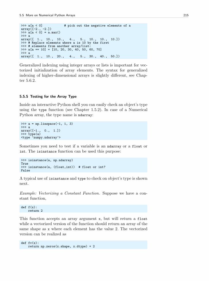
5.5 More on Numerical Python Arrays 215

>>> a[a < 0] # pick out the negative elements of aarray([-2., -2.])>>> a[a < 0] = a.max()>>> aarray([ 1., 10., 10., 4., 5., 10., 10., 10.])>>> # Replace elements where a is 10 by the first>>> # elements from another array/list:>>> a[a == 10] = [10, 20, 30, 40, 50, 60, 70]>>> aarray([ 1., 10., 20., 4., 5., 30., 40., 50.])

Generalized indexing using integer arrays or lists is important for vec-torized initialization of array elements. The syntax for generalizedindexing of higher-dimensional arrays is slightly different, see Chap-ter 5.6.2.

5.5.5 Testing for the Array Type

Inside an interactive Python shell you can easily check an object’s typeusing the type function (see Chapter 1.5.2). In case of a NumericalPython array, the type name is ndarray:

>>> a = np.linspace(-1, 1, 3)>>> aarray([-1., 0., 1.])>>> type(a)<type ’numpy.ndarray’>

Sometimes you need to test if a variable is an ndarray or a float orint. The isinstance function can be used this purpose:

>>> isinstance(a, np.ndarray)True>>> isinstance(a, (float,int)) # float or int?False

A typical use of isinstance and type to check on object’s type is shownnext.

Example: Vectorizing a Constant Function. Suppose we have a con-stant function,

def f(x):return 2

This function accepts an array argument x, but will return a float

while a vectorized version of the function should return an array of thesame shape as x where each element has the value 2. The vectorizedversion can be realized as

def fv(x):return np.zeros(x.shape, x.dtype) + 2

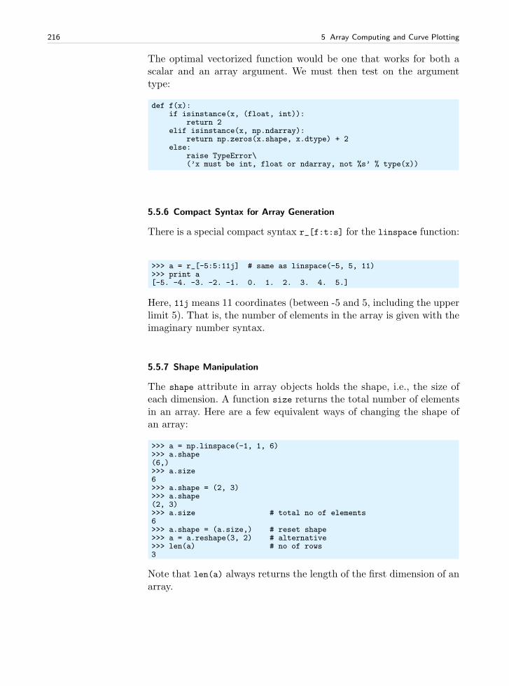
216 5 Array Computing and Curve Plotting

The optimal vectorized function would be one that works for both ascalar and an array argument. We must then test on the argumenttype:

def f(x):if isinstance(x, (float, int)):

return 2elif isinstance(x, np.ndarray):

return np.zeros(x.shape, x.dtype) + 2else:

raise TypeError\(’x must be int, float or ndarray, not %s’ % type(x))

5.5.6 Compact Syntax for Array Generation

There is a special compact syntax r_[f:t:s] for the linspace function:

>>> a = r_[-5:5:11j] # same as linspace(-5, 5, 11)>>> print a[-5. -4. -3. -2. -1. 0. 1. 2. 3. 4. 5.]

Here, 11j means 11 coordinates (between -5 and 5, including the upperlimit 5). That is, the number of elements in the array is given with theimaginary number syntax.

5.5.7 Shape Manipulation

The shape attribute in array objects holds the shape, i.e., the size ofeach dimension. A function size returns the total number of elementsin an array. Here are a few equivalent ways of changing the shape ofan array:

>>> a = np.linspace(-1, 1, 6)>>> a.shape(6,)>>> a.size6>>> a.shape = (2, 3)>>> a.shape(2, 3)>>> a.size # total no of elements6>>> a.shape = (a.size,) # reset shape>>> a = a.reshape(3, 2) # alternative>>> len(a) # no of rows3

Note that len(a) always returns the length of the first dimension of anarray.

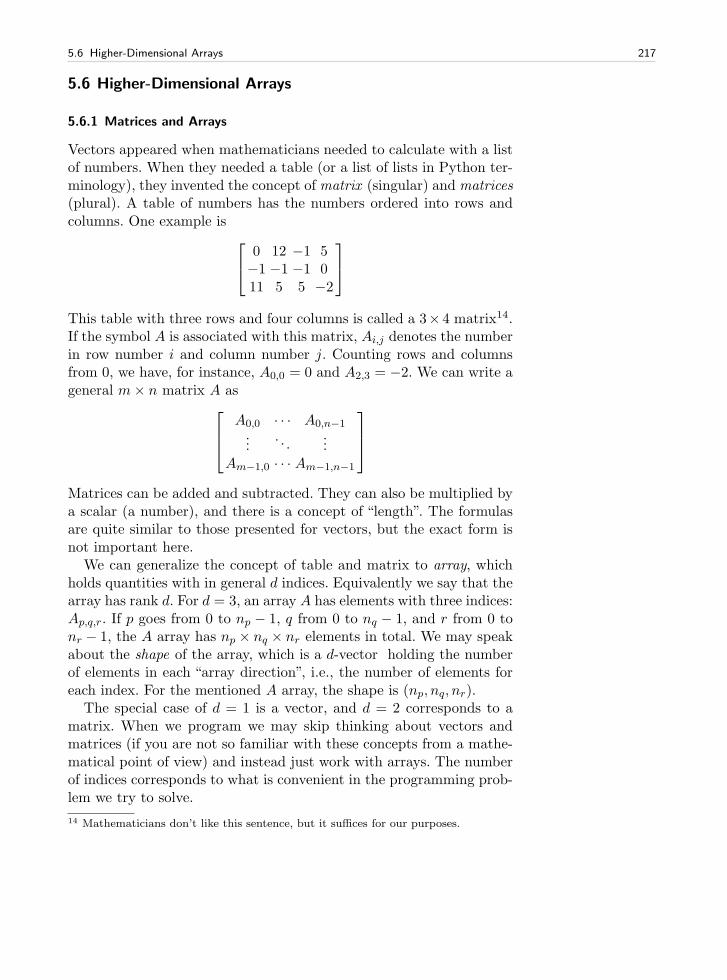
5.6 Higher-Dimensional Arrays 217

5.6 Higher-Dimensional Arrays

5.6.1 Matrices and Arrays

Vectors appeared when mathematicians needed to calculate with a listof numbers. When they needed a table (or a list of lists in Python ter-minology), they invented the concept of matrix (singular) and matrices(plural). A table of numbers has the numbers ordered into rows andcolumns. One example is

0 12 −1 5−1 −1 −1 011 5 5 −2

This table with three rows and four columns is called a 3× 4 matrix14.If the symbol A is associated with this matrix, Ai,j denotes the numberin row number i and column number j. Counting rows and columnsfrom 0, we have, for instance, A0,0 = 0 and A2,3 = −2. We can write ageneral m× n matrix A as

A0,0 · · · A0,n−1...

. . ....

Am−1,0 · · · Am−1,n−1

Matrices can be added and subtracted. They can also be multiplied bya scalar (a number), and there is a concept of “length”. The formulasare quite similar to those presented for vectors, but the exact form isnot important here.

We can generalize the concept of table and matrix to array, whichholds quantities with in general d indices. Equivalently we say that thearray has rank d. For d = 3, an array A has elements with three indices:Ap,q,r. If p goes from 0 to np − 1, q from 0 to nq − 1, and r from 0 tonr − 1, the A array has np × nq × nr elements in total. We may speakabout the shape of the array, which is a d-vector holding the numberof elements in each “array direction”, i.e., the number of elements foreach index. For the mentioned A array, the shape is (np, nq, nr).

The special case of d = 1 is a vector, and d = 2 corresponds to amatrix. When we program we may skip thinking about vectors andmatrices (if you are not so familiar with these concepts from a mathe-matical point of view) and instead just work with arrays. The numberof indices corresponds to what is convenient in the programming prob-lem we try to solve.

14 Mathematicians don’t like this sentence, but it suffices for our purposes.

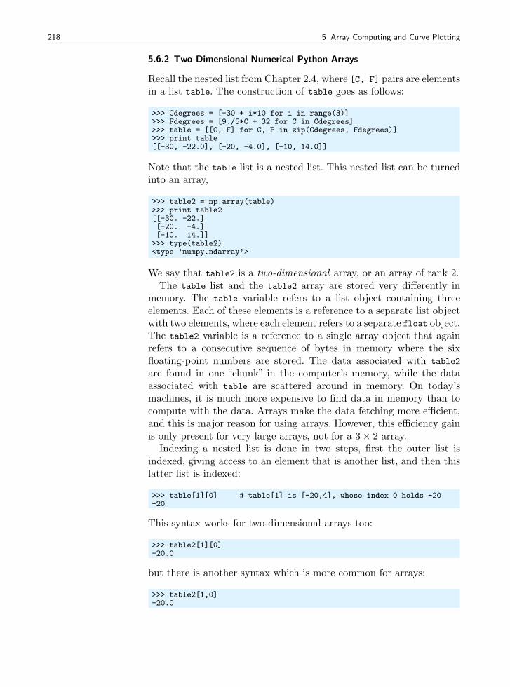
218 5 Array Computing and Curve Plotting

5.6.2 Two-Dimensional Numerical Python Arrays

Recall the nested list from Chapter 2.4, where [C, F] pairs are elementsin a list table. The construction of table goes as follows:

>>> Cdegrees = [-30 + i*10 for i in range(3)]>>> Fdegrees = [9./5*C + 32 for C in Cdegrees]>>> table = [[C, F] for C, F in zip(Cdegrees, Fdegrees)]>>> print table[[-30, -22.0], [-20, -4.0], [-10, 14.0]]

Note that the table list is a nested list. This nested list can be turnedinto an array,

>>> table2 = np.array(table)>>> print table2[[-30. -22.][-20. -4.][-10. 14.]]>>> type(table2)<type ’numpy.ndarray’>

We say that table2 is a two-dimensional array, or an array of rank 2.The table list and the table2 array are stored very differently in

memory. The table variable refers to a list object containing threeelements. Each of these elements is a reference to a separate list objectwith two elements, where each element refers to a separate float object.The table2 variable is a reference to a single array object that againrefers to a consecutive sequence of bytes in memory where the sixfloating-point numbers are stored. The data associated with table2

are found in one “chunk” in the computer’s memory, while the dataassociated with table are scattered around in memory. On today’smachines, it is much more expensive to find data in memory than tocompute with the data. Arrays make the data fetching more efficient,and this is major reason for using arrays. However, this efficiency gainis only present for very large arrays, not for a 3× 2 array.

Indexing a nested list is done in two steps, first the outer list isindexed, giving access to an element that is another list, and then thislatter list is indexed:

>>> table[1][0] # table[1] is [-20,4], whose index 0 holds -20-20

This syntax works for two-dimensional arrays too:

>>> table2[1][0]-20.0

but there is another syntax which is more common for arrays:

>>> table2[1,0]-20.0

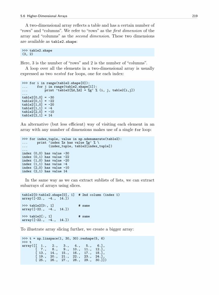
5.6 Higher-Dimensional Arrays 219

A two-dimensional array reflects a table and has a certain number of“rows” and “columns”. We refer to “rows” as the first dimension of thearray and “columns” as the second dimension. These two dimensionsare available as table2.shape:

>>> table2.shape(3, 2)

Here, 3 is the number of “rows” and 2 is the number of “columns”.A loop over all the elements in a two-dimensional array is usually

expressed as two nested for loops, one for each index:

>>> for i in range(table2.shape[0]):... for j in range(table2.shape[1]):... print ’table2[%d,%d] = %g’ % (i, j, table2[i,j])...table2[0,0] = -30table2[0,1] = -22table2[1,0] = -20table2[1,1] = -4table2[2,0] = -10table2[2,1] = 14

An alternative (but less efficient) way of visiting each element in anarray with any number of dimensions makes use of a single for loop:

>>> for index_tuple, value in np.ndenumerate(table2):... print ’index %s has value %g’ % \... (index_tuple, table2[index_tuple])...index (0,0) has value -30index (0,1) has value -22index (1,0) has value -20index (1,1) has value -4index (2,0) has value -10index (2,1) has value 14

In the same way as we can extract sublists of lists, we can extractsubarrays of arrays using slices.

table2[0:table2.shape[0], 1] # 2nd column (index 1)array([-22., -4., 14.])

>>> table2[0:, 1] # samearray([-22., -4., 14.])

>>> table2[:, 1] # samearray([-22., -4., 14.])

To illustrate array slicing further, we create a bigger array:

>>> t = np.linspace(1, 30, 30).reshape(5, 6)>>> tarray([[ 1., 2., 3., 4., 5., 6.],

[ 7., 8., 9., 10., 11., 12.],[ 13., 14., 15., 16., 17., 18.],[ 19., 20., 21., 22., 23., 24.],[ 25., 26., 27., 28., 29., 30.]])

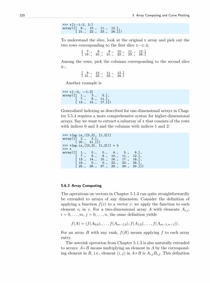
220 5 Array Computing and Curve Plotting

>>> t[1:-1:2, 2:]array([[ 9., 10., 11., 12.],

[ 21., 22., 23., 24.]])

To understand the slice, look at the original t array and pick out thetwo rows corresponding to the first slice 1:-1:2,

[ 7., 8., 9., 10., 11., 12.][ 19., 20., 21., 22., 23., 24.]

Among the rows, pick the columns corresponding to the second slice2:,

[ 9., 10., 11., 12.][ 21., 22., 23., 24.]

Another example is

>>> t[:-2, :-1:2]array([[ 1., 3., 5.],

[ 7., 9., 11.],[ 13., 15., 17.]])

Generalized indexing as described for one-dimensional arrays in Chap-ter 5.5.4 requires a more comprehensive syntax for higher-dimensionalarrays. Say we want to extract a subarray of t that consists of the rowswith indices 0 and 3 and the columns with indices 1 and 2:

>>> t[np.ix_([0,3], [1,2])]array([[ 2., 3.],

[ 20., 21.]])>>> t[np.ix_([0,3], [1,2])] = 0>>> tarray([[ 1., 0., 0., 4., 5., 6.],

[ 7., 8., 9., 10., 11., 12.],[ 13., 14., 15., 16., 17., 18.],[ 19., 0., 0., 22., 23., 24.],[ 25., 26., 27., 28., 29., 30.]])

5.6.3 Array Computing

The operations on vectors in Chapter 5.1.3 can quite straightforwardlybe extended to arrays of any dimension. Consider the definition ofapplying a function f(v) to a vector v: we apply the function to eachelement vi in v. For a two-dimensional array A with elements Ai,j ,i = 0, . . . ,m, j = 0, . . . , n, the same definition yields

f(A) = (f(A0,0), . . . , f(Am−1,0), f(A1,0), . . . , f(Am−1,n−1)) .

For an array B with any rank, f(B) means applying f to each arrayentry.

The asterisk operation from Chapter 5.1.3 is also naturally extendedto arrays: A∗B means multiplying an element in A by the correspond-ing element in B, i.e., element (i, j) in A∗B is Ai,jBi,j . This definition

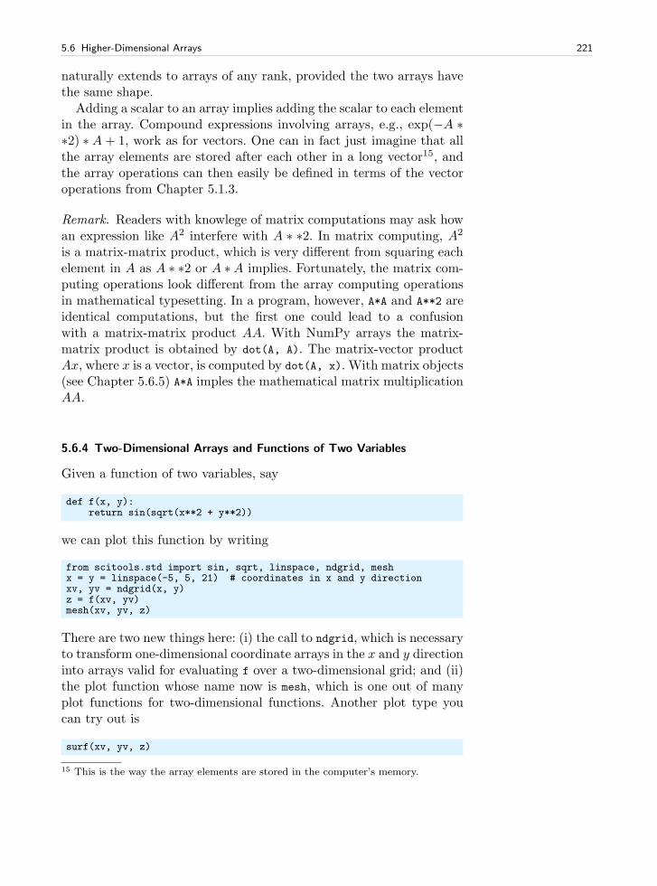
5.6 Higher-Dimensional Arrays 221

naturally extends to arrays of any rank, provided the two arrays havethe same shape.

Adding a scalar to an array implies adding the scalar to each elementin the array. Compound expressions involving arrays, e.g., exp(−A ∗∗2) ∗ A + 1, work as for vectors. One can in fact just imagine that allthe array elements are stored after each other in a long vector15, andthe array operations can then easily be defined in terms of the vectoroperations from Chapter 5.1.3.

Remark. Readers with knowlege of matrix computations may ask howan expression like A2 interfere with A ∗ ∗2. In matrix computing, A2

is a matrix-matrix product, which is very different from squaring eachelement in A as A ∗ ∗2 or A ∗A implies. Fortunately, the matrix com-puting operations look different from the array computing operationsin mathematical typesetting. In a program, however, A*A and A**2 areidentical computations, but the first one could lead to a confusionwith a matrix-matrix product AA. With NumPy arrays the matrix-matrix product is obtained by dot(A, A). The matrix-vector productAx, where x is a vector, is computed by dot(A, x). With matrix objects(see Chapter 5.6.5) A*A imples the mathematical matrix multiplicationAA.

5.6.4 Two-Dimensional Arrays and Functions of Two Variables

Given a function of two variables, say

def f(x, y):return sin(sqrt(x**2 + y**2))

we can plot this function by writing

from scitools.std import sin, sqrt, linspace, ndgrid, meshx = y = linspace(-5, 5, 21) # coordinates in x and y directionxv, yv = ndgrid(x, y)z = f(xv, yv)mesh(xv, yv, z)

There are two new things here: (i) the call to ndgrid, which is necessaryto transform one-dimensional coordinate arrays in the x and y directioninto arrays valid for evaluating f over a two-dimensional grid; and (ii)the plot function whose name now is mesh, which is one out of manyplot functions for two-dimensional functions. Another plot type youcan try out is

surf(xv, yv, z)

15 This is the way the array elements are stored in the computer’s memory.

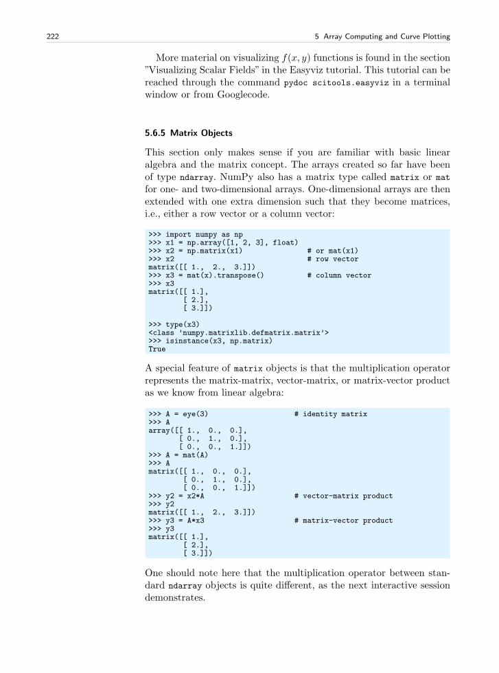
222 5 Array Computing and Curve Plotting

More material on visualizing f(x, y) functions is found in the section”Visualizing Scalar Fields” in the Easyviz tutorial. This tutorial can bereached through the command pydoc scitools.easyviz in a terminalwindow or from Googlecode.

5.6.5 Matrix Objects

This section only makes sense if you are familiar with basic linearalgebra and the matrix concept. The arrays created so far have beenof type ndarray. NumPy also has a matrix type called matrix or mat

for one- and two-dimensional arrays. One-dimensional arrays are thenextended with one extra dimension such that they become matrices,i.e., either a row vector or a column vector:

>>> import numpy as np>>> x1 = np.array([1, 2, 3], float)>>> x2 = np.matrix(x1) # or mat(x1)>>> x2 # row vectormatrix([[ 1., 2., 3.]])>>> x3 = mat(x).transpose() # column vector>>> x3matrix([[ 1.],

[ 2.],[ 3.]])

>>> type(x3)<class ’numpy.matrixlib.defmatrix.matrix’>>>> isinstance(x3, np.matrix)True

A special feature of matrix objects is that the multiplication operatorrepresents the matrix-matrix, vector-matrix, or matrix-vector productas we know from linear algebra:

>>> A = eye(3) # identity matrix>>> Aarray([[ 1., 0., 0.],

[ 0., 1., 0.],[ 0., 0., 1.]])

>>> A = mat(A)>>> Amatrix([[ 1., 0., 0.],

[ 0., 1., 0.],[ 0., 0., 1.]])

>>> y2 = x2*A # vector-matrix product>>> y2matrix([[ 1., 2., 3.]])>>> y3 = A*x3 # matrix-vector product>>> y3matrix([[ 1.],

[ 2.],[ 3.]])

One should note here that the multiplication operator between stan-dard ndarray objects is quite different, as the next interactive sessiondemonstrates.

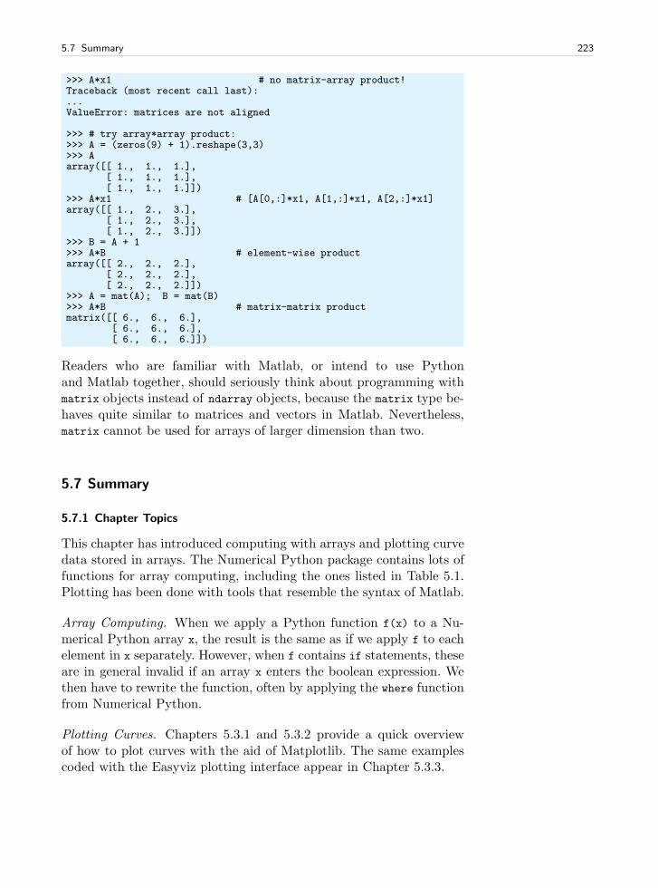
5.7 Summary 223

>>> A*x1 # no matrix-array product!Traceback (most recent call last):...ValueError: matrices are not aligned

>>> # try array*array product:>>> A = (zeros(9) + 1).reshape(3,3)>>> Aarray([[ 1., 1., 1.],

[ 1., 1., 1.],[ 1., 1., 1.]])

>>> A*x1 # [A[0,:]*x1, A[1,:]*x1, A[2,:]*x1]array([[ 1., 2., 3.],

[ 1., 2., 3.],[ 1., 2., 3.]])

>>> B = A + 1>>> A*B # element-wise productarray([[ 2., 2., 2.],

[ 2., 2., 2.],[ 2., 2., 2.]])

>>> A = mat(A); B = mat(B)>>> A*B # matrix-matrix productmatrix([[ 6., 6., 6.],

[ 6., 6., 6.],[ 6., 6., 6.]])

Readers who are familiar with Matlab, or intend to use Pythonand Matlab together, should seriously think about programming withmatrix objects instead of ndarray objects, because the matrix type be-haves quite similar to matrices and vectors in Matlab. Nevertheless,matrix cannot be used for arrays of larger dimension than two.

5.7 Summary

5.7.1 Chapter Topics

This chapter has introduced computing with arrays and plotting curvedata stored in arrays. The Numerical Python package contains lots offunctions for array computing, including the ones listed in Table 5.1.Plotting has been done with tools that resemble the syntax of Matlab.

Array Computing. When we apply a Python function f(x) to a Nu-merical Python array x, the result is the same as if we apply f to eachelement in x separately. However, when f contains if statements, theseare in general invalid if an array x enters the boolean expression. Wethen have to rewrite the function, often by applying the where functionfrom Numerical Python.

Plotting Curves. Chapters 5.3.1 and 5.3.2 provide a quick overviewof how to plot curves with the aid of Matplotlib. The same examplescoded with the Easyviz plotting interface appear in Chapter 5.3.3.

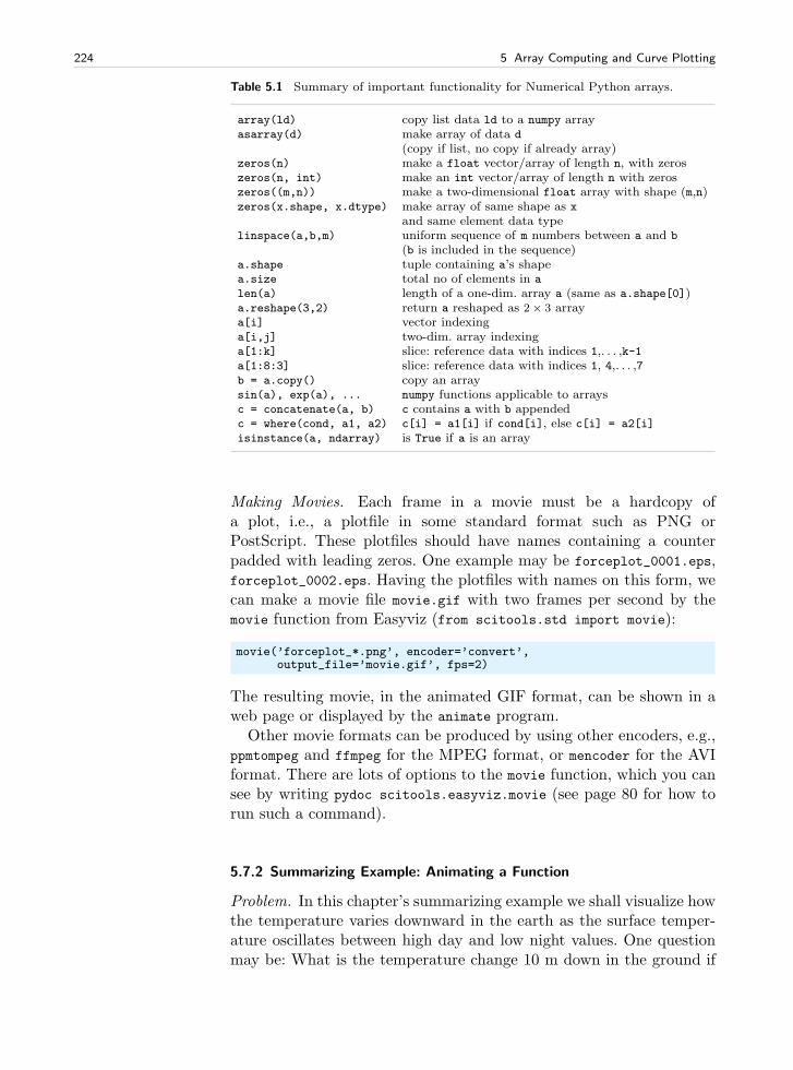
224 5 Array Computing and Curve Plotting

Table 5.1 Summary of important functionality for Numerical Python arrays.

array(ld) copy list data ld to a numpy arrayasarray(d) make array of data d

(copy if list, no copy if already array)zeros(n) make a float vector/array of length n, with zeroszeros(n, int) make an int vector/array of length n with zeroszeros((m,n)) make a two-dimensional float array with shape (m,n)zeros(x.shape, x.dtype) make array of same shape as x

and same element data typelinspace(a,b,m) uniform sequence of m numbers between a and b

(b is included in the sequence)a.shape tuple containing a’s shapea.size total no of elements in a

len(a) length of a one-dim. array a (same as a.shape[0])a.reshape(3,2) return a reshaped as 2× 3 arraya[i] vector indexinga[i,j] two-dim. array indexinga[1:k] slice: reference data with indices 1,. . . ,k-1a[1:8:3] slice: reference data with indices 1, 4,. . . ,7b = a.copy() copy an arraysin(a), exp(a), ... numpy functions applicable to arraysc = concatenate(a, b) c contains a with b appendedc = where(cond, a1, a2) c[i] = a1[i] if cond[i], else c[i] = a2[i]

isinstance(a, ndarray) is True if a is an array

Making Movies. Each frame in a movie must be a hardcopy ofa plot, i.e., a plotfile in some standard format such as PNG orPostScript. These plotfiles should have names containing a counterpadded with leading zeros. One example may be forceplot_0001.eps,forceplot_0002.eps. Having the plotfiles with names on this form, wecan make a movie file movie.gif with two frames per second by themovie function from Easyviz (from scitools.std import movie):

movie(’forceplot_*.png’, encoder=’convert’,output_file=’movie.gif’, fps=2)

The resulting movie, in the animated GIF format, can be shown in aweb page or displayed by the animate program.

Other movie formats can be produced by using other encoders, e.g.,ppmtompeg and ffmpeg for the MPEG format, or mencoder for the AVIformat. There are lots of options to the movie function, which you cansee by writing pydoc scitools.easyviz.movie (see page 80 for how torun such a command).

5.7.2 Summarizing Example: Animating a Function

Problem. In this chapter’s summarizing example we shall visualize howthe temperature varies downward in the earth as the surface temper-ature oscillates between high day and low night values. One questionmay be: What is the temperature change 10 m down in the ground if

5.7 Summary 225

the surface temperature varies between 2 C in the night and 15 C inthe day?

Let the z axis point downwards, towards the center of the earth,and let z = 0 correspond to the earth’s surface. The temperature atsome depth z in the ground at time t is denoted by T (z, t). If thesurface temperature has a periodic variation around some mean valueT0, according to

T (0, t) = T0 +A cos(ωt),

one can find, from a mathematical model for heat conduction, that thetemperature at an arbitrary depth is

T (z, t) = T0 +Ae−az cos(ωt− az), a =

√

ω

2k. (5.13)

The parameter k reflects the ground’s ability to conduct heat (k iscalled the thermal diffusivity or the heat conduction coefficient).

The task is to make an animation of how the temperature profile inthe ground, i.e., T as a function of z, varies in time. Let ω correspondto a time period of 24 hours. The mean temperature T0 is taken as10 C, and the maximum variation A is assumed to be 10 C. The heatconduction coefficient k may be set as 1 mm2/s (which is 10−6 m2/sin proper SI units).

Solution. To animate T (z, t) in time, we need to make a loop overpoints in time, and in each pass in the loop we must make a hardcopyof the plot of T as a function of z. The files with the hardcopies canthen be combined to a movie. The algorithm becomes

for ti = i∆t, i = 0, 1, 2 . . . , n:plot the curve y(z) = T (z, ti)make hardcopy (store the plot in a file)

combine all the plot files into a movie

It can be wise to make a general animate function where we justfeed in some f(x, t) function and make all the plot files. If animate hasarguments for setting the labels on the axis and the extent of the yaxis, we can easily use animate also for a function T (z, t) (we just usez as the name for the x axis and T as the name for the y axis in theplot). Recall that it is important to fix the extent of the y axis in aplot when we make animations, otherwise most plotting programs willautomatically fit the extent of the axis to the current data, and thetickmarks on the y axis will jump up and down during the movie. Theresult is a wrong visual impression of the function.

The names of the plot files must have a common stem appended withsome frame number, and the frame number should have a fixed numberof digits, such as 0001, 0002, etc. (if not, the sequence of the plot files

226 5 Array Computing and Curve Plotting

will not be correct when we specify the collection of files with an aster-isk for the frame numbers, e.g., as in tmp*.png). We therefore includean argument to animate for setting the name stem of the plot files.By default, the stem is tmp_, resulting in the filenames tmp_0000.png,tmp_0001.png, tmp_0002.png, and so forth. Other convenient argumentsfor the animate function are the initial time in the plot, the time lag∆t between the plot frames, and the coordinates along the x axis. Theanimate function then takes the form

def animate(tmax, dt, x, function, ymin, ymax, t0=0,xlabel=’x’, ylabel=’y’, hardcopy_stem=’tmp_’):

t = t0counter = 0while t <= tmax:

y = function(x, t)plot(x, y,

axis=[x[0], x[-1], ymin, ymax],title=’time=%2d h’ % (t/3600.0),xlabel=xlabel, ylabel=ylabel,hardcopy=hardcopy_stem + ’%04d.png’ % counter)

t += dtcounter += 1

The T (z, t) function is easy to implement, but we need to decidewhether the parameters A, ω, T0, and k shall be arguments to thePython implementation of T (z, t) or if they shall be global variables.Since the animate function expects that the function to be plotted hasonly two arguments, we must implement T (z, t) as T(z,t) in Pythonand let the other parameters be global variables (Chapters 7.1.1 and7.1.2 explain this problem in more detail and present a better imple-mentation). The T(z,t) implementation then reads

def T(z, t):# T0, A, k, and omega are global variablesa = sqrt(omega/(2*k))return T0 + A*exp(-a*z)*cos(omega*t - a*z)

Suppose we plot T (z, t) at n points for z ∈ [0, D]. We make suchplots for t ∈ [0, tmax] with a time lag ∆t between the them. The framesin the movie are now made by

# set T0, A, k, omega, D, n, tmax, dtz = linspace(0, D, n)animate(tmax, dt, z, T, T0-A, T0+A, 0, ’z’, ’T’)

We have here set the extent of the y axis in the plot as [T0−A, T0+A],which is in accordance with the T (z, t) function.

The call to animate above creates a set of files with names of theform tmp_*.png. The animation is then created by a call

movie(’tmp_*.png’, encoder=’convert’, fps=2,output_file=’tmp_heatwave.gif’)

It now remains to assign proper values to all the global variablesin the program: n, D, T0, A, omega, dt, tmax, and k. The oscillation

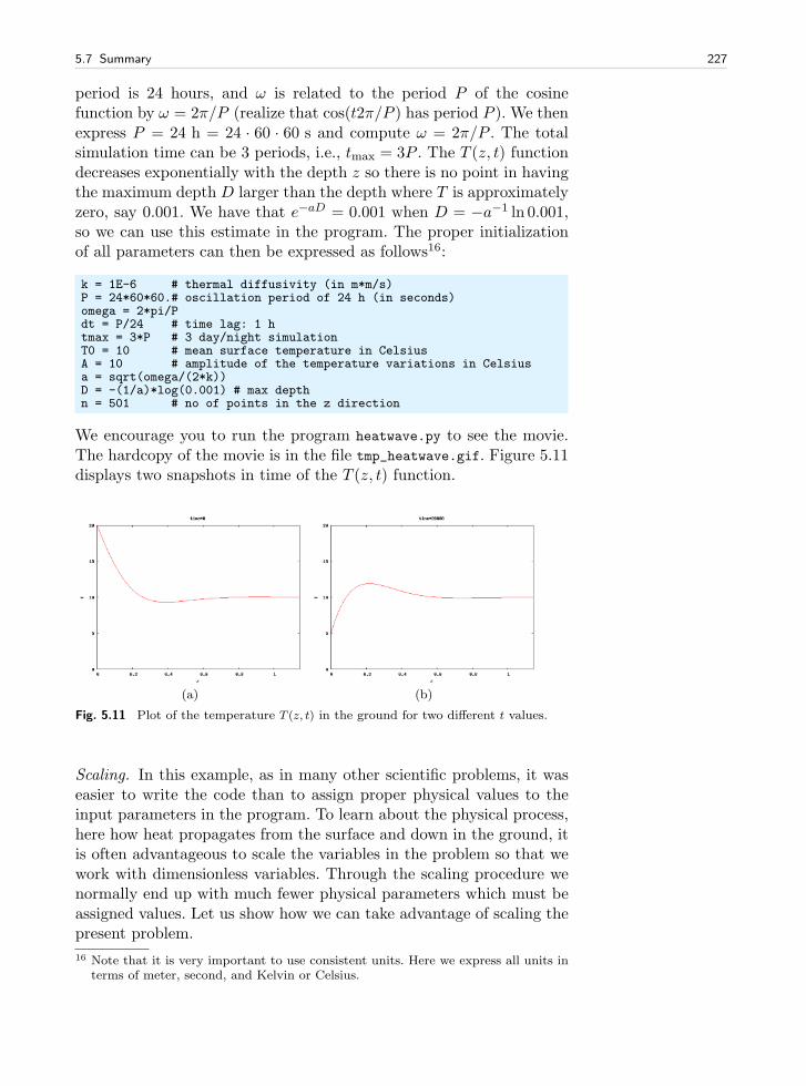
5.7 Summary 227

period is 24 hours, and ω is related to the period P of the cosinefunction by ω = 2π/P (realize that cos(t2π/P ) has period P ). We thenexpress P = 24 h = 24 · 60 · 60 s and compute ω = 2π/P . The totalsimulation time can be 3 periods, i.e., tmax = 3P . The T (z, t) functiondecreases exponentially with the depth z so there is no point in havingthe maximum depth D larger than the depth where T is approximatelyzero, say 0.001. We have that e−aD = 0.001 when D = −a−1 ln 0.001,so we can use this estimate in the program. The proper initializationof all parameters can then be expressed as follows16:

k = 1E-6 # thermal diffusivity (in m*m/s)P = 24*60*60.# oscillation period of 24 h (in seconds)omega = 2*pi/Pdt = P/24 # time lag: 1 htmax = 3*P # 3 day/night simulationT0 = 10 # mean surface temperature in CelsiusA = 10 # amplitude of the temperature variations in Celsiusa = sqrt(omega/(2*k))D = -(1/a)*log(0.001) # max depthn = 501 # no of points in the z direction

We encourage you to run the program heatwave.py to see the movie.The hardcopy of the movie is in the file tmp_heatwave.gif. Figure 5.11displays two snapshots in time of the T (z, t) function.

(a) (b)

Fig. 5.11 Plot of the temperature T (z, t) in the ground for two different t values.

Scaling. In this example, as in many other scientific problems, it waseasier to write the code than to assign proper physical values to theinput parameters in the program. To learn about the physical process,here how heat propagates from the surface and down in the ground, itis often advantageous to scale the variables in the problem so that wework with dimensionless variables. Through the scaling procedure wenormally end up with much fewer physical parameters which must beassigned values. Let us show how we can take advantage of scaling thepresent problem.

16 Note that it is very important to use consistent units. Here we express all units interms of meter, second, and Kelvin or Celsius.

228 5 Array Computing and Curve Plotting

Consider a variable x in a problem with some dimension. The ideaof scaling is to introduce a new variable x = x/xc, where xc is a char-acteristic size of x. Since x and xc have the same dimension, the di-mension cancels in x such that x is dimensionless. Choosing xc to bethe expected maximum value of x, ensures that x ≤ 1, which is usuallyconsidered a good idea. That is, we try to have all dimensionless vari-ables varying between zero and one. For example, we can introducea dimensionless z coordinate: z = z/D, and now z ∈ [0, 1]. Doing aproper scaling of a problem is challenging so for now it is sufficient tojust follow the steps below - and not worry why we choose a certainscaling.

In the present problem we introduce these dimensionless variables:

z = z/D

T =T − T0

At = ωt

We now insert z = zD and t = t/ω in the expression for T (z, t) andget

T = T0 +Ae−bz cos(t− bz), b = aD

or

T (z, t) =T − T0

A= e−bz cos(t− bz) .

We see that T depends on only one dimensionless parameter b in addi-tion to the independent dimensionless variables z and t. It is commonpractice at this stage of the scaling to just drop the bars and write

T (z, t) = e−bz cos(t− bz) . (5.14)

This function is much simpler to plot than the one with lots of physicalparameters, because now we know that T varies between −1 and 1, tvaries between 0 and 2π for one period, and z varies between 0 and 1.The scaled temperature has only one “free” parameter b. That is, theshape of the graph is completely determined by b.

In our previous movie example, we used specific values for D, ω, andk, which then implies a certain b = D

√

ω/(2k) (≈ 6.9). However, wecan now run different b values and see the effect on the heat propa-gation. Different b values will in our problems imply different periodsof the surface temperature variation and/or different heat conductionvalues in the ground’s composition of rocks. Note that doubling ω andk leaves the same b – it is only the fraction ω/k that influences thevalue of b.

We can reuse the animate function also in the scaled case, but weneed to make a new T (z, t) function and, e.g., a main program whereb can be read from the command line:

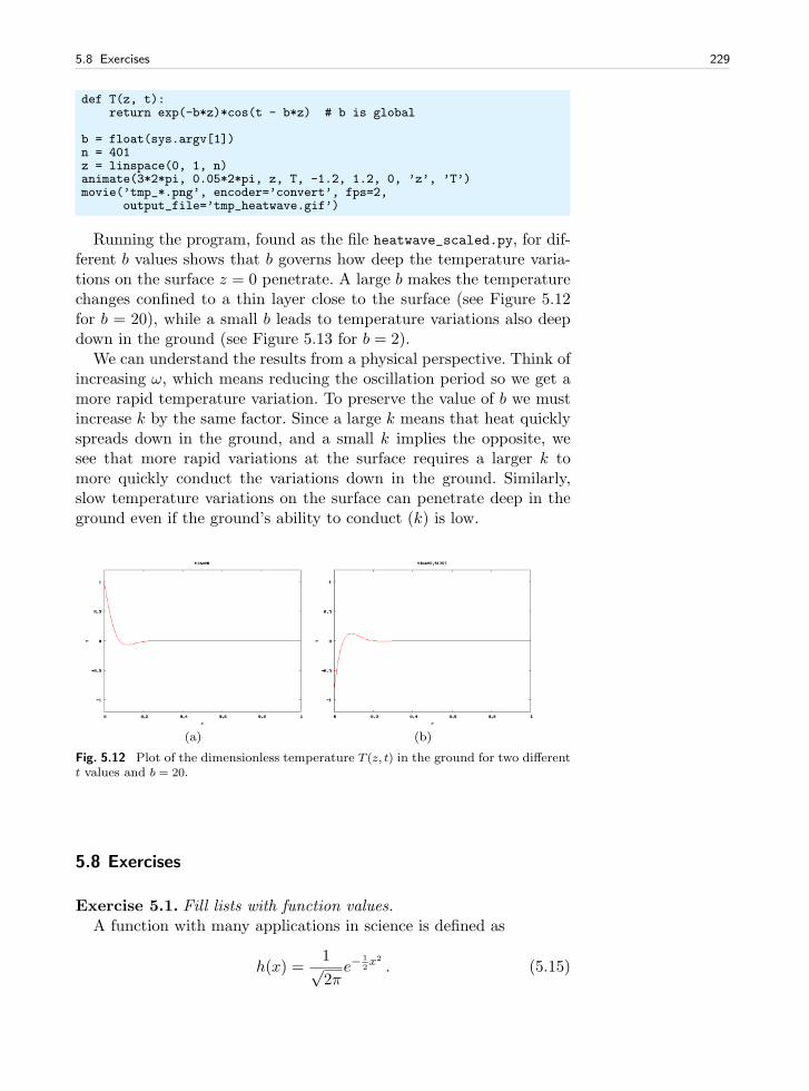
5.8 Exercises 229

def T(z, t):return exp(-b*z)*cos(t - b*z) # b is global

b = float(sys.argv[1])n = 401z = linspace(0, 1, n)animate(3*2*pi, 0.05*2*pi, z, T, -1.2, 1.2, 0, ’z’, ’T’)movie(’tmp_*.png’, encoder=’convert’, fps=2,

output_file=’tmp_heatwave.gif’)

Running the program, found as the file heatwave_scaled.py, for dif-ferent b values shows that b governs how deep the temperature varia-tions on the surface z = 0 penetrate. A large b makes the temperaturechanges confined to a thin layer close to the surface (see Figure 5.12for b = 20), while a small b leads to temperature variations also deepdown in the ground (see Figure 5.13 for b = 2).

We can understand the results from a physical perspective. Think ofincreasing ω, which means reducing the oscillation period so we get amore rapid temperature variation. To preserve the value of b we mustincrease k by the same factor. Since a large k means that heat quicklyspreads down in the ground, and a small k implies the opposite, wesee that more rapid variations at the surface requires a larger k tomore quickly conduct the variations down in the ground. Similarly,slow temperature variations on the surface can penetrate deep in theground even if the ground’s ability to conduct (k) is low.

(a) (b)

Fig. 5.12 Plot of the dimensionless temperature T (z, t) in the ground for two differentt values and b = 20.

5.8 Exercises

Exercise 5.1. Fill lists with function values.A function with many applications in science is defined as

h(x) =1√2π

e−1

2x2

. (5.15)

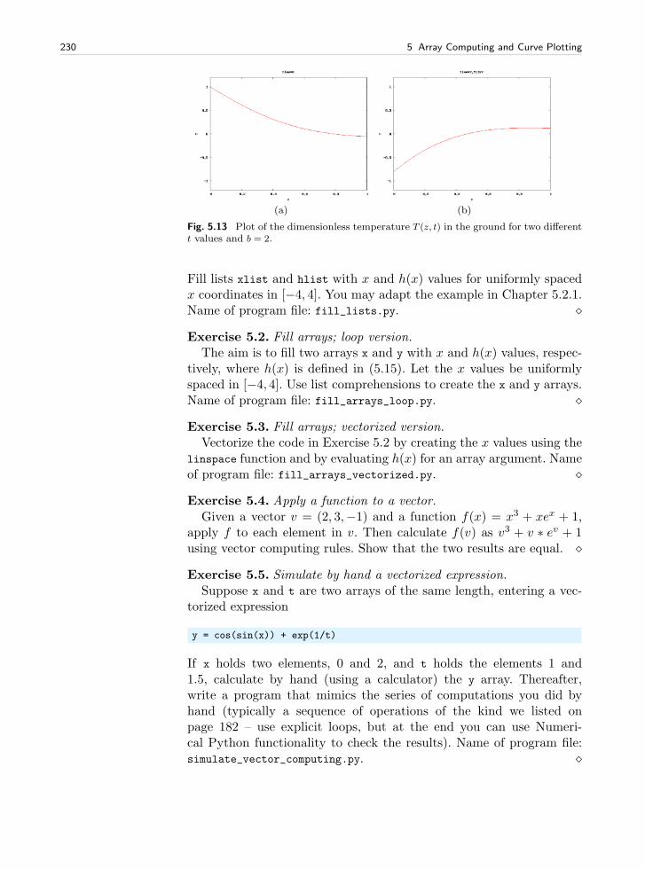
230 5 Array Computing and Curve Plotting

(a) (b)

Fig. 5.13 Plot of the dimensionless temperature T (z, t) in the ground for two differentt values and b = 2.

Fill lists xlist and hlist with x and h(x) values for uniformly spacedx coordinates in [−4, 4]. You may adapt the example in Chapter 5.2.1.Name of program file: fill_lists.py. ⋄

Exercise 5.2. Fill arrays; loop version.The aim is to fill two arrays x and y with x and h(x) values, respec-

tively, where h(x) is defined in (5.15). Let the x values be uniformlyspaced in [−4, 4]. Use list comprehensions to create the x and y arrays.Name of program file: fill_arrays_loop.py. ⋄

Exercise 5.3. Fill arrays; vectorized version.Vectorize the code in Exercise 5.2 by creating the x values using the

linspace function and by evaluating h(x) for an array argument. Nameof program file: fill_arrays_vectorized.py. ⋄

Exercise 5.4. Apply a function to a vector.Given a vector v = (2, 3,−1) and a function f(x) = x3 + xex + 1,

apply f to each element in v. Then calculate f(v) as v3 + v ∗ ev + 1using vector computing rules. Show that the two results are equal. ⋄

Exercise 5.5. Simulate by hand a vectorized expression.Suppose x and t are two arrays of the same length, entering a vec-

torized expression

y = cos(sin(x)) + exp(1/t)

If x holds two elements, 0 and 2, and t holds the elements 1 and1.5, calculate by hand (using a calculator) the y array. Thereafter,write a program that mimics the series of computations you did byhand (typically a sequence of operations of the kind we listed onpage 182 – use explicit loops, but at the end you can use Numeri-cal Python functionality to check the results). Name of program file:simulate_vector_computing.py. ⋄

5.8 Exercises 231

Exercise 5.6. Demonstrate array slicing.Create an array w with values 0, 0.1, 0.2, . . . , 3. Write out w[:],

w[:-2], w[::5], w[2:-2:6]. Convince yourself in each case that youunderstand which elements of the array that are printed. Name of pro-gram file: slicing.py. ⋄

Exercise 5.7. Use array computing in the example from Chap. 2.6.2.The data analysis problem in Chapter 2.6.2 is solved by list oper-

ations. Convert the list to a two-dimensional array and perform thethree tasks using array operations. There should be no explicit loopsin this Python program. Name of program file: sun_data_vec.py. ⋄

Exercise 5.8. Plot a formula.Make a plot of the function y(t) = v0t−0.5gt2 for v0 = 10, g = 9.81,

and t ∈ [0, 2v0/g]. The label on the x axis should be ’time (s)’ andthe label on the y axis should be ’height (m)’. Name of program file:plot_ball1.py. ⋄

Exercise 5.9. Plot a formula for several parameters.Make a program that reads a set of v0 values from the command

line and plots the corresponding curves y(t) = v0t− 0.5gt2 in the samefigure (set g = 9.81). Let t ∈ [0, 2v0/g] for each curve, which impliesthat you need a different vector of t coordinates for each curve. Nameof program file: plot_ball2.py. ⋄

Exercise 5.10. Specify the x and y axes in Exer. 5.9.Extend the program from Exercises 5.9 such that the minimum and

maximum x and y values are computed, and use the extreme valuesto specify the extent of the x and y axes. Add some space above theheighest curve. Name of program file: plot_ball3.py. ⋄

Exercise 5.11. Plot exact and inexact Fahrenheit–Celsius formulas.Exercise 2.2 introduces a simple rule to quickly compute the Celsius

temperature from the Fahreheit degrees: C = (F−30)/2. Compare thiscurve against the exact curve C = (F − 32)5/9 in a plot. Let F varybetween −20 and 120. Name of program file: f2c_shortcut_plot.py. ⋄

Exercise 5.12. Plot the trajectory of a ball.The formula for the trajectory of a ball is given in (1.5) on page 39.

In a program, first read the input data y0, θ, and v0 from the commandline. Then plot the trajectory y = f(x) for y ≥ 0. Name of programfile: plot_trajectory.py. ⋄

Exercise 5.13. Implement Lagrange’s interpolation formula.Imagine we have n+1measurements of some quantity y that depends

on x: (x0, y0), (x1, y1), . . . , (xn, yn). We may think of y as a function ofx and ask what y is at some arbitrary point x not coinciding with anyof the x0, . . . , xn. This problem is known as interpolation. One way to

232 5 Array Computing and Curve Plotting

solve this problem is to fit a continuous function that goes through allthe n + 1 points and then evaluate this function for any desired x. Acandidate for such a function is the polynomial of degree n that goesthrough all the points. This polynomial can be written

pL(x) =

n∑

k=0

ykLk(x), (5.16)

where

Lk(x) =

n∏

i=0,i6=k

x− xixk − xj

.

The∏

notation corresponds to∑

, but the terms are multiplied, e.g.,

n∏

i=0,i 6=k

xi = x0x1 · · · xk−1xk+1 · · · xn .

The polynomial pL(x) is known as Lagrange’s interpolation formula,and the points (x0, y0), . . . , (xn, yn) are called interpolation points.

Make a function Lagrange(x, points) that evaluates pL at the pointx, given n+ 1 interpolation points as a two-dimensional array points,such that points[i,0] is the x coordinate of point number i andpoints[i,1] is the corresponding y coordinate.

To verify the program, we observe that Lk(xk) = 1 and thatLk(xi) = 0 for i 6= k, implying that pL(xk) = yk. Write a functionverify(points) that computes |pL(xk) − yk| at all the interpolationpoints and checks that the value is approximately zero. Call verifywith 5 equally spaced points along the curve y = sin(x) for x ∈ [0, π].Then evaluate pL(x) for an x in the middle of two interpolation pointsand compare the value of pL(x) with the exact one: sin(x). Name ofprogram file: Lagrange_polynomial1.py. ⋄

Exercise 5.14. Plot the polynomial in Exer. 5.13.Unfortunately, the polynomial pL(x) defined and implemented in

Exercise 5.13 can exhibit some undesired oscillatory behavior whichwe shall explore graphically.

Write a function graph(f, xmin, xmax, n, resolution=1001) forplotting pL(x) in the case the points come from the Python functionf(x) for x equally spaced between xmin and xmax. The parameter nin the formula (5.16) is given as a list n, i.e., we can provide severalvalues of n and get all the corresponding polynomials pL(x) displayedin the same plot. Also show the n + 1 given interpolation points assmall circles in the same plot as the pL(x) curves. The final argumentresolution is the number of points used to plot pL(x). (If only thegiven n + 1 points are used to plot pL(x), we just get straight lines

5.8 Exercises 233

between these points, and we cannot see how pL(x) behaves betweenthe points. This behavior is of particular interest.)

Call the graph function with f(x) = |x|, for x ∈ [−2, 2], andn = 2, 4, 6, 10. Observe from the plot that pL always goes throughthe given points, but as the number of points increases, pL oscillatesmore and more between the points, and the approximation of pL tothe curve f(x) = |x| becomes poorer. Call the graph function to makean additional plot of pL corresponding to n = 13 and n = 20, andobserve how the amplitude of the oscillations increases with increasingn. Much research has historically been focused on methods that do notresult in such strange oscillations when fitting a polynomial to a set ofpoints.

Name of program file: Lagrange_polynomial2.py. ⋄

Exercise 5.15. Plot a wave packet.The function

f(x, t) = e−(x−3t)2 sin (3π(x− t)) (5.17)

describes for a fixed value of t a wave localized in space. Make a pro-gram that visualizes this function as a function of x on the interval[−4, 4] when t = 0. Name of program file: plot_wavepacket.py. ⋄

Exercise 5.16. Use pyreport in Exer. 5.15.Use pyreport (see Chapter 1.8) in Exercise 5.15 to generate a nice

report in HTML and PDF format. To get the plot inserted in thereport, you must call show() after the plot instruction. If you applyEasyviz for plotting, you need to use the version of pyreport that comeswith SciTools (that version is automatically installed when you installSciTools). Name of program file: pyreport_wavepacket.py. ⋄

Exercise 5.17. Judge a plot.Assume you have the following program for plotting a parabola:

import numpy as npx = np.linspace(0, 2, 20)y = x*(2 - x)import matplotlib.pyplot as pltplt.plot(x, y)plt.show()

Then you switch to the function cos(18πx) by altering the computationof y to y = cos(18*pi*x). Judge the resulting plot. Is it correct? Displaythe cos(18πx) function with 1000 points in the same plot. Name ofprogram file: judge_plot.py. ⋄

Exercise 5.18. Plot the viscosity of water.The viscosity of water, µ, varies with the temperature T (in Kelvin)

according toµ(T ) = A · 10B/(T−C), (5.18)

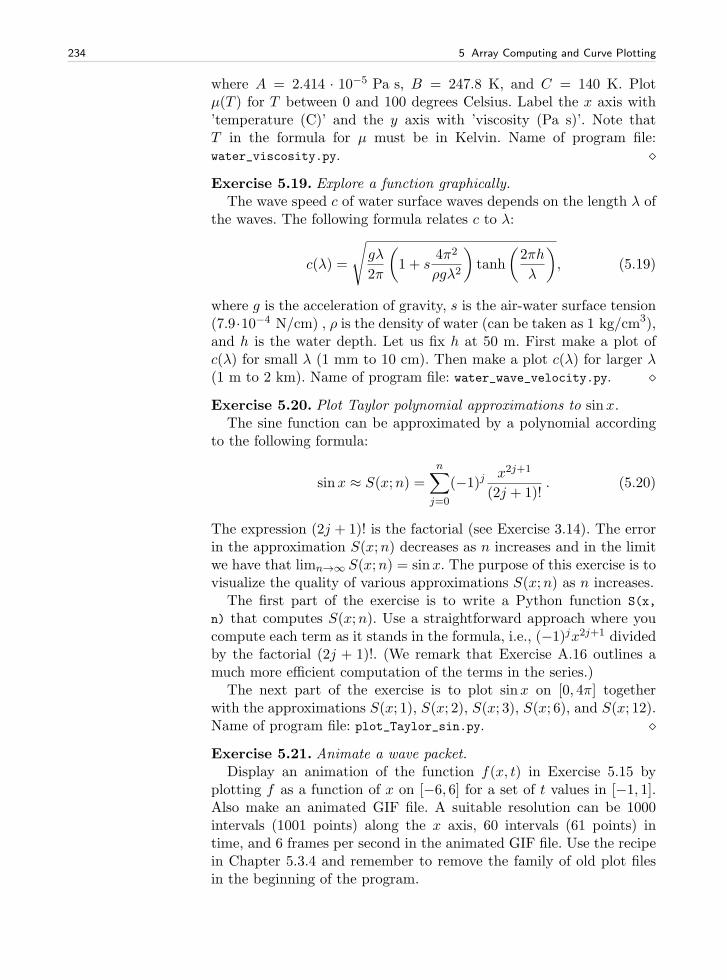
234 5 Array Computing and Curve Plotting

where A = 2.414 · 10−5 Pa s, B = 247.8 K, and C = 140 K. Plotµ(T ) for T between 0 and 100 degrees Celsius. Label the x axis with’temperature (C)’ and the y axis with ’viscosity (Pa s)’. Note thatT in the formula for µ must be in Kelvin. Name of program file:water_viscosity.py. ⋄

Exercise 5.19. Explore a function graphically.The wave speed c of water surface waves depends on the length λ of

the waves. The following formula relates c to λ:

c(λ) =

√

gλ

2π

(

1 + s4π2

ρgλ2

)

tanh

(

2πh

λ

)

, (5.19)

where g is the acceleration of gravity, s is the air-water surface tension(7.9·10−4 N/cm) , ρ is the density of water (can be taken as 1 kg/cm3),and h is the water depth. Let us fix h at 50 m. First make a plot ofc(λ) for small λ (1 mm to 10 cm). Then make a plot c(λ) for larger λ(1 m to 2 km). Name of program file: water_wave_velocity.py. ⋄

Exercise 5.20. Plot Taylor polynomial approximations to sinx.The sine function can be approximated by a polynomial according

to the following formula:

sinx ≈ S(x;n) =

n∑

j=0

(−1)j x2j+1

(2j + 1)!. (5.20)

The expression (2j + 1)! is the factorial (see Exercise 3.14). The errorin the approximation S(x;n) decreases as n increases and in the limitwe have that limn→∞ S(x;n) = sinx. The purpose of this exercise is tovisualize the quality of various approximations S(x;n) as n increases.

The first part of the exercise is to write a Python function S(x,

n) that computes S(x;n). Use a straightforward approach where youcompute each term as it stands in the formula, i.e., (−1)jx2j+1 dividedby the factorial (2j + 1)!. (We remark that Exercise A.16 outlines amuch more efficient computation of the terms in the series.)

The next part of the exercise is to plot sinx on [0, 4π] togetherwith the approximations S(x; 1), S(x; 2), S(x; 3), S(x; 6), and S(x; 12).Name of program file: plot_Taylor_sin.py. ⋄

Exercise 5.21. Animate a wave packet.Display an animation of the function f(x, t) in Exercise 5.15 by

plotting f as a function of x on [−6, 6] for a set of t values in [−1, 1].Also make an animated GIF file. A suitable resolution can be 1000intervals (1001 points) along the x axis, 60 intervals (61 points) intime, and 6 frames per second in the animated GIF file. Use the recipein Chapter 5.3.4 and remember to remove the family of old plot filesin the beginning of the program.

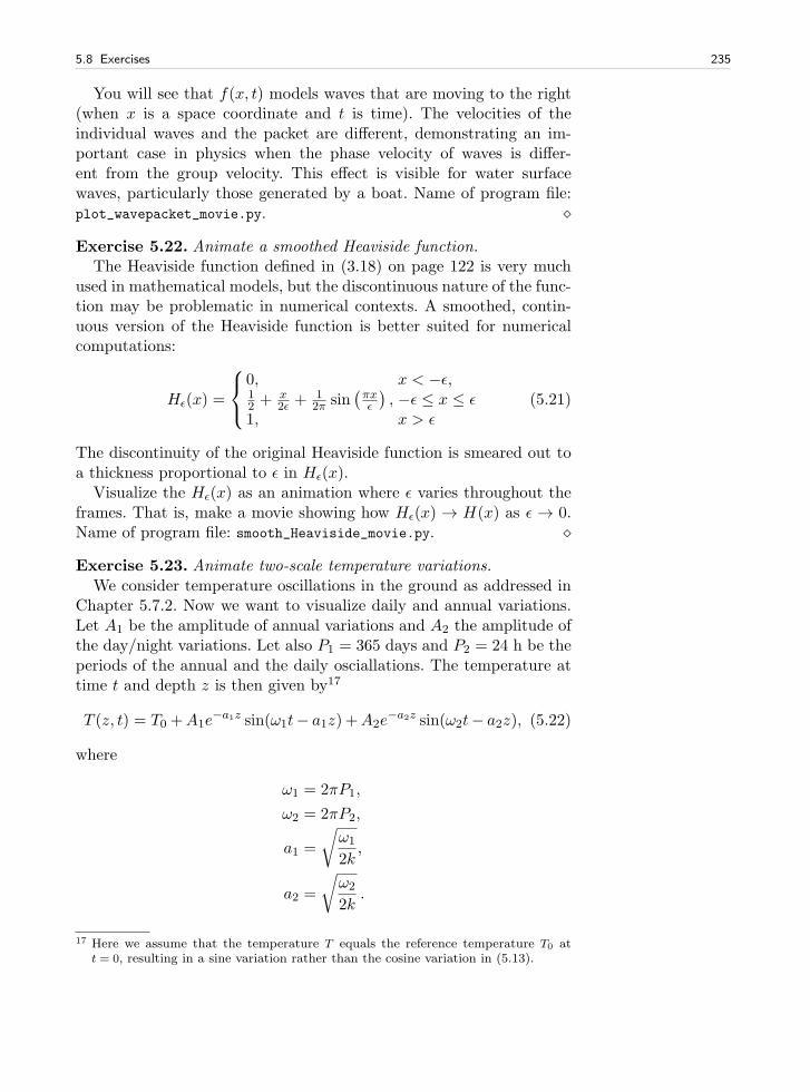
5.8 Exercises 235

You will see that f(x, t) models waves that are moving to the right(when x is a space coordinate and t is time). The velocities of theindividual waves and the packet are different, demonstrating an im-portant case in physics when the phase velocity of waves is differ-ent from the group velocity. This effect is visible for water surfacewaves, particularly those generated by a boat. Name of program file:plot_wavepacket_movie.py. ⋄

Exercise 5.22. Animate a smoothed Heaviside function.The Heaviside function defined in (3.18) on page 122 is very much

used in mathematical models, but the discontinuous nature of the func-tion may be problematic in numerical contexts. A smoothed, contin-uous version of the Heaviside function is better suited for numericalcomputations:

Hǫ(x) =

0, x < −ǫ,12 + x

2ǫ +12π sin

(

πxǫ

)

, −ǫ ≤ x ≤ ǫ1, x > ǫ

(5.21)

The discontinuity of the original Heaviside function is smeared out toa thickness proportional to ǫ in Hǫ(x).

Visualize the Hǫ(x) as an animation where ǫ varies throughout theframes. That is, make a movie showing how Hǫ(x) → H(x) as ǫ → 0.Name of program file: smooth_Heaviside_movie.py. ⋄

Exercise 5.23. Animate two-scale temperature variations.We consider temperature oscillations in the ground as addressed in

Chapter 5.7.2. Now we want to visualize daily and annual variations.Let A1 be the amplitude of annual variations and A2 the amplitude ofthe day/night variations. Let also P1 = 365 days and P2 = 24 h be theperiods of the annual and the daily osciallations. The temperature attime t and depth z is then given by17

T (z, t) = T0 +A1e−a1z sin(ω1t− a1z) +A2e

−a2z sin(ω2t− a2z), (5.22)

where

ω1 = 2πP1,

ω2 = 2πP2,

a1 =

√

ω1

2k,

a2 =

√

ω2

2k.

17 Here we assume that the temperature T equals the reference temperature T0 att = 0, resulting in a sine variation rather than the cosine variation in (5.13).

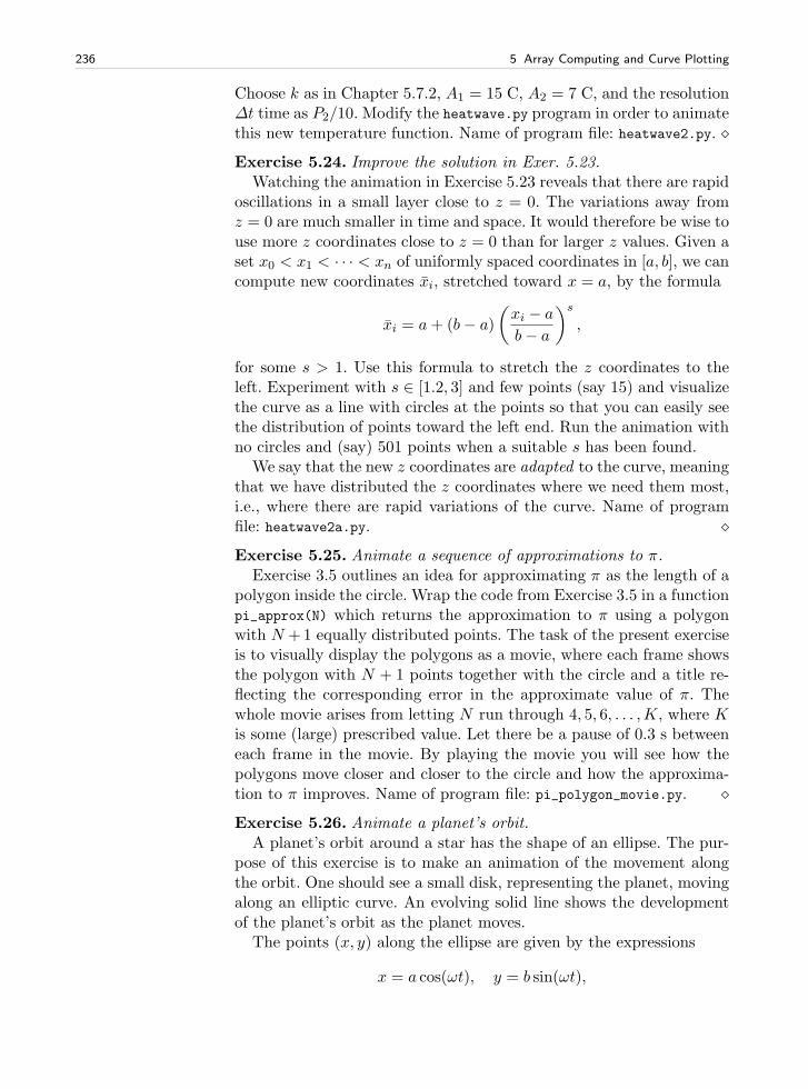
236 5 Array Computing and Curve Plotting

Choose k as in Chapter 5.7.2, A1 = 15 C, A2 = 7 C, and the resolution∆t time as P2/10. Modify the heatwave.py program in order to animatethis new temperature function. Name of program file: heatwave2.py. ⋄Exercise 5.24. Improve the solution in Exer. 5.23.

Watching the animation in Exercise 5.23 reveals that there are rapidoscillations in a small layer close to z = 0. The variations away fromz = 0 are much smaller in time and space. It would therefore be wise touse more z coordinates close to z = 0 than for larger z values. Given aset x0 < x1 < · · · < xn of uniformly spaced coordinates in [a, b], we cancompute new coordinates xi, stretched toward x = a, by the formula

xi = a+ (b− a)

(

xi − a

b− a

)s

,

for some s > 1. Use this formula to stretch the z coordinates to theleft. Experiment with s ∈ [1.2, 3] and few points (say 15) and visualizethe curve as a line with circles at the points so that you can easily seethe distribution of points toward the left end. Run the animation withno circles and (say) 501 points when a suitable s has been found.

We say that the new z coordinates are adapted to the curve, meaningthat we have distributed the z coordinates where we need them most,i.e., where there are rapid variations of the curve. Name of programfile: heatwave2a.py. ⋄Exercise 5.25. Animate a sequence of approximations to π.

Exercise 3.5 outlines an idea for approximating π as the length of apolygon inside the circle. Wrap the code from Exercise 3.5 in a functionpi_approx(N) which returns the approximation to π using a polygonwith N +1 equally distributed points. The task of the present exerciseis to visually display the polygons as a movie, where each frame showsthe polygon with N + 1 points together with the circle and a title re-flecting the corresponding error in the approximate value of π. Thewhole movie arises from letting N run through 4, 5, 6, . . . ,K, where Kis some (large) prescribed value. Let there be a pause of 0.3 s betweeneach frame in the movie. By playing the movie you will see how thepolygons move closer and closer to the circle and how the approxima-tion to π improves. Name of program file: pi_polygon_movie.py. ⋄Exercise 5.26. Animate a planet’s orbit.

A planet’s orbit around a star has the shape of an ellipse. The pur-pose of this exercise is to make an animation of the movement alongthe orbit. One should see a small disk, representing the planet, movingalong an elliptic curve. An evolving solid line shows the developmentof the planet’s orbit as the planet moves.

The points (x, y) along the ellipse are given by the expressions

x = a cos(ωt), y = b sin(ωt),

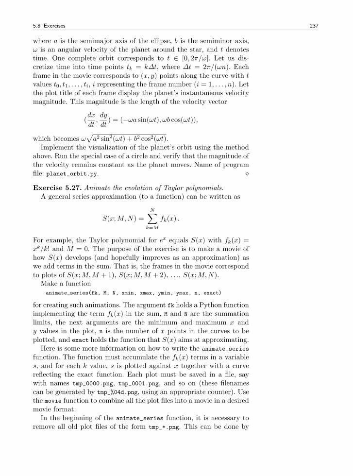
5.8 Exercises 237

where a is the semimajor axis of the ellipse, b is the semiminor axis,ω is an angular velocity of the planet around the star, and t denotestime. One complete orbit corresponds to t ∈ [0, 2π/ω]. Let us dis-cretize time into time points tk = k∆t, where ∆t = 2π/(ωn). Eachframe in the movie corresponds to (x, y) points along the curve with tvalues t0, t1, . . . , ti, i representing the frame number (i = 1, . . . , n). Letthe plot title of each frame display the planet’s instantaneous velocitymagnitude. This magnitude is the length of the velocity vector

(dx

dt,dy

dt) = (−ωa sin(ωt), ωb cos(ωt)),

which becomes ω√

a2 sin2(ωt) + b2 cos2(ωt).Implement the visualization of the planet’s orbit using the method

above. Run the special case of a circle and verify that the magnitude ofthe velocity remains constant as the planet moves. Name of programfile: planet_orbit.py. ⋄

Exercise 5.27. Animate the evolution of Taylor polynomials.A general series approximation (to a function) can be written as

S(x;M,N) =N∑

k=M

fk(x) .

For example, the Taylor polynomial for ex equals S(x) with fk(x) =xk/k! and M = 0. The purpose of the exercise is to make a movie ofhow S(x) develops (and hopefully improves as an approximation) aswe add terms in the sum. That is, the frames in the movie correspondto plots of S(x;M,M + 1), S(x;M,M + 2), . . ., S(x;M,N).

Make a functionanimate_series(fk, M, N, xmin, xmax, ymin, ymax, n, exact)

for creating such animations. The argument fk holds a Python functionimplementing the term fk(x) in the sum, M and N are the summationlimits, the next arguments are the minimum and maximum x andy values in the plot, n is the number of x points in the curves to beplotted, and exact holds the function that S(x) aims at approximating.

Here is some more information on how to write the animate_series

function. The function must accumulate the fk(x) terms in a variables, and for each k value, s is plotted against x together with a curvereflecting the exact function. Each plot must be saved in a file, saywith names tmp_0000.png, tmp_0001.png, and so on (these filenamescan be generated by tmp_%04d.png, using an appropriate counter). Usethe movie function to combine all the plot files into a movie in a desiredmovie format.

In the beginning of the animate_series function, it is necessary toremove all old plot files of the form tmp_*.png. This can be done by

238 5 Array Computing and Curve Plotting

the glob module and the os.remove function as exemplified in Chap-ter 5.3.4.

Test the animate_series function in two cases:

1. The Taylor series for sinx, where fk(x) = (−1)kx2k+1/(2k + 1)!,and x ∈ [0, 13π], M = 0, N = 40, y ∈ [−2, 2].

2. The Taylor series for e−x, where fk(x) = (−x)k/k!, and x ∈ [0, 15],M = 0, N = 30, y ∈ [−0.5, 1.4].

Name of program file: animate_Taylor_series.py. ⋄

Exercise 5.28. Plot the velocity profile for pipeflow.A fluid that flows through a (very long) pipe has zero velocity on

the pipe wall and a maximum velocity along the centerline of the pipe.The velocity v varies through the pipe cross section according to thefollowing formula:

v(r) =

(

β

2µ0

)1/n n

n+ 1

(

R1+1/n − r1+1/n)

, (5.23)

where R is the radius of the pipe, β is the pressure gradient (the forcethat drives the flow through the pipe), µ0 is a viscosity coefficient(small for air, larger for water and even larger for toothpaste), n is areal number reflecting the viscous properties of the fluid (n = 1 forwater and air, n < 1 for many modern plastic materials), and r is aradial coordinate that measures the distance from the centerline (r = 0is the centerline, r = R is the pipe wall).

Make a function that evaluates v(r). Plot v(r) as a function ofr ∈ [0, R], with R = 1, β = 0.02, µ = 0.02, and n = 0.1. There-after, make an animation of how the v(r) curves varies as n goes from1 and down to 0.01. Because the maximum value of v(r) decreasesrapidly as n decreases, each curve can be normalized by its v(0) valuesuch that the maximum value is always unity. Name of program file:plot_velocity_pipeflow.py. ⋄

Exercise 5.29. Plot the functions from Exer. 3.7.Exercise 3.7 defines the approximation S(t;n) to a function f(t).

Plot S(t; 1), S(t; 3), S(t; 20), S(t; 200), and the exact f(t) function inthe same plot. Use T = 2π. Name of program file: sinesum1_plot.py. ⋄

Exercise 5.30. Make a movie of the functions from Exer. 3.7.First perform Exercise 5.29. A natural next step is to animate the

evolution of S(t;n) as n increases. Create such an animation and ob-serve how the discontinuity in f(t) is poorly approximated by S(t;n),even when n grows large (plot f(t) in each frame). This is a well-knowndeficiency, called Gibb’s phenomenon, when approximating discontin-uous functions by sine or cosine (Fourier) series. Name of program file:sinesum1_movie.py. ⋄

5.8 Exercises 239

Exercise 5.31. Plot functions from the command line.For quickly getting a plot a function f(x) for x ∈ [xmin, xmax] it

could be nice to a have a program that takes the minimum amount ofinformation from the command line and produces a plot on the screenand a hardcopy tmp.eps. The usage of the program goes as follows:

Terminal

plotf.py "f(x)" xmin xmax

A specific example is

Terminal

plotf.py "exp(-0.2*x)*sin(2*pi*x)" 0 4*pi

Hint: Make x coordinates from the second and third command-linearguments and then use eval (or StringFunction from Chapters 4.1.4and 5.4.3) on the first first argument. Try to write as short programas possible (we leave it to Exercise 5.32 to test for valid input). Nameof program file: plotf_v1.py. ⋄Exercise 5.32. Improve the program from Exericse 5.31.

Equip the program from Exericse 5.31 with tests on valid inputon the command line. Also allow an optional fourth command-lineargument for the number of points along the function curve. Set thisnumber to 501 if it is not given. Name of program file: plotf.py. ⋄Exercise 5.33. Demonstrate energy concepts from physics.

The vertical position y(t) of a ball thrown upward is given byy(t) = v0t − 0.5gt2, where g is the acceleration of gravity and v0 isthe velocity at t = 0. Two important physical quantities in this con-text are the potential energy, obtained by doing work against gravity,and the kinetic energy, arising from motion. The potential energy isdefined as P = mgy, where m is the mass of the ball. The kinetic en-ergy is defined as K = 1

2mv2, where v is the velocity of the ball, relatedto y by v(t) = y′(t). Plot P (t) and K(t) in the same plot, along withtheir sum P +K. Let t ∈ [0, 2v0/g]. Read m and v0 from the commandline. Run the program with various choices of m and v0 and observethat P + K is always constant in this motion. In fact, it turns outthat P +K is constant for a large class of motions, and this is a veryimportant result in physics. Name of program file: energy_physics.py.⋄Exercise 5.34. Plot a w-like function.

Define mathematically a function that looks like the ’w’ character.Plot this function. Name of program file: plot_w.py. ⋄Exercise 5.35. Plot a smoothed “hat” function.

The “hat” function N(x) defined by (3.5) on page 109 has a discon-tinuity in the derivative at x = 1. Suppose we want to “round” this

240 5 Array Computing and Curve Plotting

function such that it looks smooth around x = 1. To this end, replacethe straight lines in the vicinity of x = 1 by a (small) cubic curve

y = a(x− 1)3 + b(x− 1)2 + c(x− 1) + d,

for x ∈ [1 − ǫ, 1 + ǫ], where a, b, c, and d are parameters that mustbe adjusted in order for the cubic curve to match the value and thederivative of the function N(x). The new rounded functions has thespecification

N(x) =

0, x < 0x, 0 ≤ x < 1− ǫa1(x− 1)3 + b(x− 1) + c(x− 1) + d1, 1− ǫ ≤ x < 1,a2(x− 1)3 + b(x− 1) + c(x− 1) + d2, 1 ≤ x < 1 + ǫ,2− x, 1 + ǫ ≤ x < 20, x ≥ 2

(5.24)with a1 = 1

3ǫ−2, a2 = −a1, d1 = 1 − ǫ + a1ǫ

3, d2 = 1 − ǫ − a2ǫ3, and

b = c = 0. Plot this function. (Hint: Be careful with the choice of xcoordinates!) Name of program file: plot_hat.py. ⋄

Exercise 5.36. Experience overflow in a function.When an object (ball, car, airplane) moves through the air, there is

a very, very thin layer of air close to the object’s surface where the airvelocity varies dramatically18, from the same value as the velocity ofthe object at the object’s surface to zero a few centimeters away. Thechange in velocity is quite abrupt and can be modeled by the functiion

v(x) =1− ex/µ

1− e1/µ,

where x = 1 is the object’s surface, and x = 0 is some distance awaywhere one cannot notice any wind velocity v because of the passingobject (v = 0). The vind velocity coincides with the velocity of theobject at x = 1, here set to v = 1. The parameter µ is very smalland related to the viscosity of air. With a small value of µ, it becomesdifficult to calculate v(x) on a computer.

Make a function v(x, mu=1E-6, exp=math.exp) for calculating theformula for v(x) using exp as a possibly user-given exponentional func-tion. Let the v function return the nominator and denominator in theformula as well as the fraction (result). Call the v function for various xvalues between 0 and 1 in a for loop, let mu be 1E-3, and have an innerfor loop over two different exp functions: math.exp and numpy.exp. Theoutput will demonstrate how the denominator is subject to overflowand how difficult it is to calculate this function on a computer.

18 This layer is called a boundary layer. The physics in the boundary layer is veryimportant for air resistance and cooling/heating of objects.

5.8 Exercises 241

Also plot v(x) for µ = 1, 0.01, 0.001 on [0, 1] using 10,000points to see what the function looks like. Name of program file:boundary_layer_func1.py. ⋄

Exercise 5.37. Experience less overflow in a function.In the program from Exercise 5.36, convert x and eps to a higher

presicion representation of real numbers, with the aid of the NumPytype float96:

import numpyx = numpy.float96(x); mu = numpy.float96(e)

Call the v function with these type of variables observe how much“bet-ter” results we get with float96 compared the standard float value(which is float64 – the number reflects the number of bits in the ma-chine’s representation of a real number). Also call the v function with x

and mu as float32 variables and report how the function now behaves.Name of program file: boundary_layer_func2.py. ⋄

Exercise 5.38. Extend Exer. 5.4 to a rank 2 array.Let A be the two-dimensional array

0 12 −1−1 −1 −111 5 5

Apply the function f from Exercise 5.4 to each element in A. Thencalculate the result of the array expression A ∗ ∗3 + A ∗ eA + 1, anddemonstrate that the end result of the two methods are the same. ⋄

Exercise 5.39. Explain why array computations fail.The following loop computes the array y from x:

>>> import numpy as np>>> x = np.linspace(0, 1, 3)>>> y = np.zeros(len(x))>>> for i in range(len(x)):... y[i] = x[i] + 4

However, the alternative loop

>>> for xi, yi in zip(x, y):... yi = xi + 5

leaves y unchanged. Why? Explain in detail what happens in each passof this loop and write down the contents of xi, yi, x, and y as the loopprogresses. ⋄

Files, Strings, and Dictionaries 6

Files are used for permanent storage of information on a computer.From previous computer experience you are hopefully used to save in-formation to files and open the files at a later time for inspection again.The present chapter tells you how Python programs can access informa-tion in files (Chapter 6.1) and also create new files (Chapter 6.5). Thechapter builds on programming concepts introduced in Chapters 1–5.

Since files often contain structured information that one wants tomap to objects in a running program, there is a need for flexible objectswhere various kinds of other objects can be stored. Dictionaries are veryhandy for this purpose and are described in Chapter 6.2.

Information in files often appear as pure text, so to interpret andextract data from files it is sometimes necessary to carry out sophisti-cated operations on the text. Python strings have many methods forperforming such operations, and the most important functionality isdescribed in Chapter 6.3.

The World Wide Web is full of information and scientific data thatmay be useful to access from a program. Chapter 6.4 tells you how toread web pages from a program and interpret the contents using stringoperations.

The folder src/files contains all the program example files referredto in the present chapter.

6.1 Reading Data from File

Suppose we have recorded some measurements in a file data1.txt, lo-cated in the src/files folder. The goal of our first example of readingfiles is to read the measurement values in data1.txt, find the averagevalue, and print it out in the terminal window.

243

244 6 Files, Strings, and Dictionaries

Before trying to let a program read a file, we must know the file for-mat, i.e., what the contents of the file looks like, because the structureof the text in the file greatly influences the set of statements neededto read the file. We therefore start with viewing the contents of thefile data1.txt. To this end, load the file into a text editor or viewer1.What we see is a column with numbers:

21.818.119232617.8

Our task is to read this column of numbers into a list in the programand compute the average of the list items.

6.1.1 Reading a File Line by Line

To read a file, we first need to open the file. This action creates a fileobject, here stored in the variable infile:

infile = open(’data1.txt’, ’r’)

The second argument to the open function, the string ’r’, tells thatwe want to open the file for reading. We shall later see that a filecan be opened for writing instead, by providing ’w’ as the secondargument. After the file is read, one should close the file object withinfile.close().

For Loop over Lines. We can read the contents of the file in variousways. The basic recipe for reading the file line by line applies a for

loop like this:

for line in infile:# do something with line

The line variable is a string holding the current line in the file. Thefor loop over lines in a file has the same syntax as when we go througha list. Just think of the file object infile as a collection of elements,here lines in a file, and the for loop visits these elements in sequencesuch that the line variable refers to one line at a time. If somethingseemingly goes wrong in such a loop over lines in a file, it is useful todo a print line inside the loop.

Instead of reading one line at a time, we can load all lines into a listof strings (lines) by

1 You can use emacs, vim, more, or less on Unix and Mac. On Windows, WordPadis appropriate, or the type command in a DOS window. Word processors such asOpenOffice or Microsoft Word can also be used.

6.1 Reading Data from File 245

lines = infile.readlines()

This statement is equivalent to

lines = []for line in infile:

lines.append(line)

or the list comprehension:

lines = [line for line in infile]

In the present example, we load the file into the list lines. The nexttask is to compute the average of the numbers in the file. Trying astraightforward sum of all numbers on all lines,

mean = 0for number in lines:

mean = mean + numbermean = mean/len(lines)

gives an error message:

TypeError: unsupported operand type(s) for +: ’int’ and ’str’

The reason is that lines holds each line (number) as a string, not afloat or int that we can add to other numbers. A fix is to converteach line to a float:

mean = 0for line in lines:

number = float(line)mean = mean + number

mean = mean/len(lines)

This code snippet works fine. The complete code can be found in thefile files/mean1.py.

Summing up a list of numbers is often done in numerical programs,so Python has a special function sum for performing this task. However,sum must in the present case operate on a list of floats, not strings.We can use a list comprehension to turn all elements in lines intocorresponding float objects:

mean = sum([float(line) for line in lines])/len(lines)

An alternative implementation is to load the lines into a list of float

objects directly. Using this strategy, the complete program (found infile mean2.py) takes the form

infile = open(’data1.txt’, ’r’)numbers = [float(line) for line in infile.readlines()]infile.close()mean = sum(numbers)/len(numbers)print mean

246 6 Files, Strings, and Dictionaries

A newcomer to programming might find it confusing to see thatone problem is solved by many alternative sets of statements, but thisis the very nature of programming. A clever programmer will judgeseveral alternative solutions to a programming task and choose onethat is either particularly compact, easy to understand, and/or easy toextend later. We therefore present more examples on how to read thedata1.txt file and compute with the data.

While Loop over Lines. The call infile.readline() returns a stringcontaining the text at the current line. A new infile.readline() willread the next line. When infile.readline() returns an empty string,the end of the file is reached and we must stop further reading. The fol-lowing while loop reads the file line by line using infile.readline():

while True:line = infile.readline()if not line:

break# process line

This is perhaps a somewhat strange loop, but it is a well-establishedway of reading a file in Python (especially in older codes). The shownwhile loop runs forever since the condition is always True. However,inside the loop we test if line is False, and it is False when we reachthe end of the file, because line then becomes an empty string, whichin Python evaluates to False. When line is False, the break statementbreaks the loop and makes the program flow jump to the first statementafter the while block.

Computing the average of the numbers in the data1.txt file can nowbe done in yet another way:

infile = open(’data1.txt’, ’r’)mean = 0n = 0while True:

line = infile.readline()if not line:

breakmean += float(line)n += 1

mean = mean/float(n)

Reading a File into a String. The call infile.read() reads the wholefile and returns the text as a string object. The following interactivesession illustrates the use and result of infile.read():

>>> infile = open(’data1.txt’, ’r’)>>> filestr = infile.read()>>> filestr’21.8\n18.1\n19\n23\n26\n17.8\n’>>> print filestr21.8

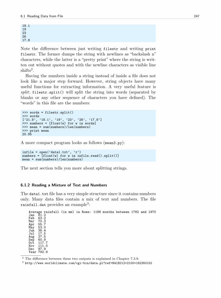
6.1 Reading Data from File 247

18.119232617.8

Note the difference between just writing filestr and writing print

filestr. The former dumps the string with newlines as “backslash n”characters, while the latter is a “pretty print” where the string is writ-ten out without quotes and with the newline characters as visible lineshifts2.

Having the numbers inside a string instead of inside a file does notlook like a major step forward. However, string objects have manyuseful functions for extracting information. A very useful feature issplit : filestr.split() will split the string into words (separated byblanks or any other sequence of characters you have defined). The“words” in this file are the numbers:

>>> words = filestr.split()>>> words[’21.8’, ’18.1’, ’19’, ’23’, ’26’, ’17.8’]>>> numbers = [float(w) for w in words]>>> mean = sum(numbers)/len(numbers)>>> print mean20.95

A more compact program looks as follows (mean3.py):

infile = open(’data1.txt’, ’r’)numbers = [float(w) for w in infile.read().split()]mean = sum(numbers)/len(numbers)

The next section tells you more about splitting strings.

6.1.2 Reading a Mixture of Text and Numbers

The data1.txt file has a very simple structure since it contains numbersonly. Many data files contain a mix of text and numbers. The filerainfall.dat provides an example3:

Average rainfall (in mm) in Rome: 1188 months between 1782 and 1970Jan 81.2Feb 63.2Mar 70.3Apr 55.7May 53.0Jun 36.4Jul 17.5Aug 27.5Sep 60.9Oct 117.7Nov 111.0Dec 97.9Year 792.9

2 The difference between these two outputs is explained in Chapter 7.3.9.3 http://www.worldclimate.com/cgi-bin/data.pl?ref=N41E012+2100+1623501G1

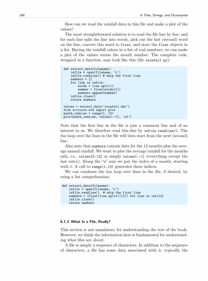
248 6 Files, Strings, and Dictionaries

How can we read the rainfall data in this file and make a plot of thevalues?

The most straightforward solution is to read the file line by line, andfor each line split the line into words, pick out the last (second) wordon the line, convert this word to float, and store the float objects ina list. Having the rainfall values in a list of real numbers, we can makea plot of the values versus the month number. The complete code,wrapped in a function, may look like this (file rainfall.py):

def extract_data(filename):infile = open(filename, ’r’)infile.readline() # skip the first linenumbers = []for line in infile:

words = line.split()number = float(words[1])numbers.append(number)

infile.close()return numbers

values = extract_data(’rainfall.dat’)from scitools.std import plotmonth_indices = range(1, 13)plot(month_indices, values[:-1], ’o2’)

Note that the first line in the file is just a comment line and of nointerest to us. We therefore read this line by infile.readline(). Thefor loop over the lines in the file will then start from the next (second)line.

Also note that numbers contain data for the 12 months plus the aver-age annual rainfall. We want to plot the average rainfall for the monthsonly, i.e., values[0:12] or simply values[:-1] (everything except thelast entry). Along the “x” axis we put the index of a month, startingwith 1. A call to range(1,13) generates these indices.

We can condense the for loop over lines in the file, if desired, byusing a list comprehension:

def extract_data(filename):infile = open(filename, ’r’)infile.readline() # skip the first linenumbers = [float(line.split()[1]) for line in infile]infile.close()return numbers

6.1.3 What Is a File, Really?

This section is not mandatory for understanding the rest of the book.However, we think the information here is fundamental for understand-ing what files are about.

A file is simply a sequence of characters. In addition to the sequenceof characters, a file has some data associated with it, typically the

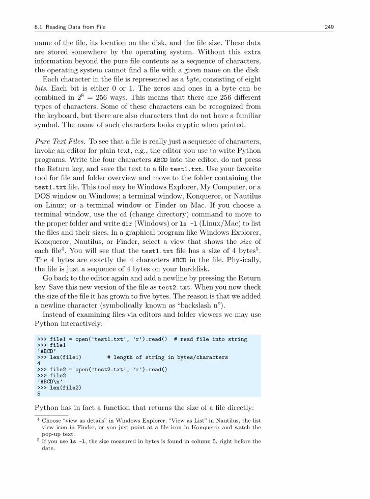
6.1 Reading Data from File 249

name of the file, its location on the disk, and the file size. These dataare stored somewhere by the operating system. Without this extrainformation beyond the pure file contents as a sequence of characters,the operating system cannot find a file with a given name on the disk.

Each character in the file is represented as a byte, consisting of eightbits. Each bit is either 0 or 1. The zeros and ones in a byte can becombined in 28 = 256 ways. This means that there are 256 differenttypes of characters. Some of these characters can be recognized fromthe keyboard, but there are also characters that do not have a familiarsymbol. The name of such characters looks cryptic when printed.

Pure Text Files. To see that a file is really just a sequence of characters,invoke an editor for plain text, e.g., the editor you use to write Pythonprograms. Write the four characters ABCD into the editor, do not pressthe Return key, and save the text to a file test1.txt. Use your favoritetool for file and folder overview and move to the folder containing thetest1.txt file. This tool may be Windows Explorer, My Computer, or aDOS window on Windows; a terminal window, Konqueror, or Nautiluson Linux; or a terminal window or Finder on Mac. If you choose aterminal window, use the cd (change directory) command to move tothe proper folder and write dir (Windows) or ls -l (Linux/Mac) to listthe files and their sizes. In a graphical program like Windows Explorer,Konqueror, Nautilus, or Finder, select a view that shows the size ofeach file4. You will see that the test1.txt file has a size of 4 bytes5.The 4 bytes are exactly the 4 characters ABCD in the file. Physically,the file is just a sequence of 4 bytes on your harddisk.

Go back to the editor again and add a newline by pressing the Returnkey. Save this new version of the file as test2.txt. When you now checkthe size of the file it has grown to five bytes. The reason is that we addeda newline character (symbolically known as “backslash n”).

Instead of examining files via editors and folder viewers we may usePython interactively:

>>> file1 = open(’test1.txt’, ’r’).read() # read file into string>>> file1’ABCD’>>> len(file1) # length of string in bytes/characters4>>> file2 = open(’test2.txt’, ’r’).read()>>> file2’ABCD\n’>>> len(file2)5

Python has in fact a function that returns the size of a file directly:

4 Choose “view as details” in Windows Explorer, “View as List” in Nautilus, the listview icon in Finder, or you just point at a file icon in Konqueror and watch thepop-up text.

5 If you use ls -l, the size measured in bytes is found in column 5, right before thedate.

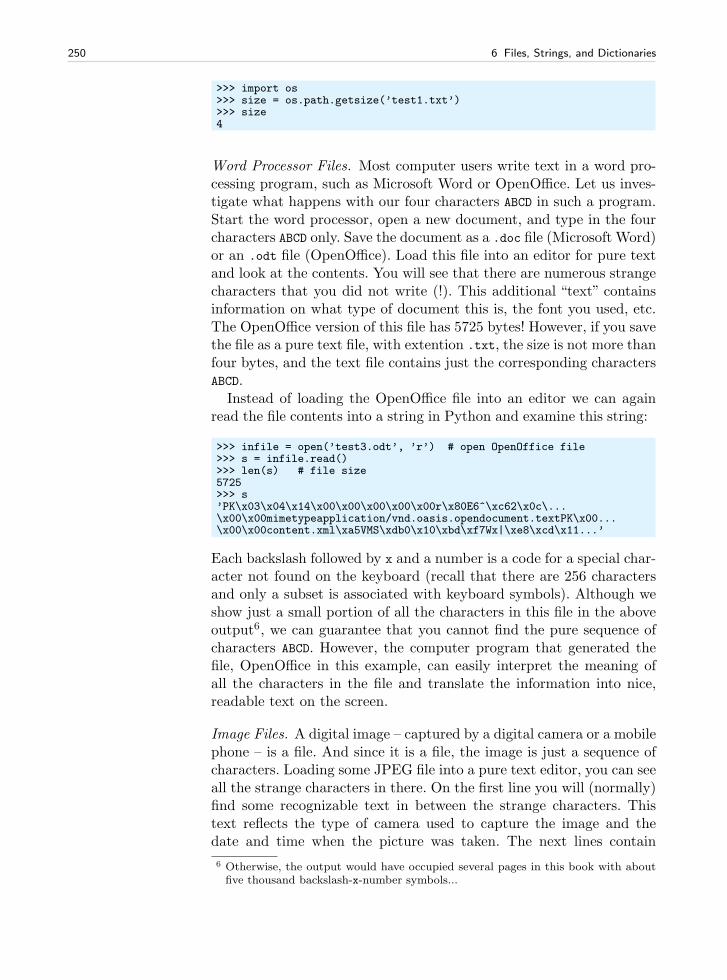
250 6 Files, Strings, and Dictionaries

>>> import os>>> size = os.path.getsize(’test1.txt’)>>> size4

Word Processor Files. Most computer users write text in a word pro-cessing program, such as Microsoft Word or OpenOffice. Let us inves-tigate what happens with our four characters ABCD in such a program.Start the word processor, open a new document, and type in the fourcharacters ABCD only. Save the document as a .doc file (Microsoft Word)or an .odt file (OpenOffice). Load this file into an editor for pure textand look at the contents. You will see that there are numerous strangecharacters that you did not write (!). This additional “text” containsinformation on what type of document this is, the font you used, etc.The OpenOffice version of this file has 5725 bytes! However, if you savethe file as a pure text file, with extention .txt, the size is not more thanfour bytes, and the text file contains just the corresponding charactersABCD.

Instead of loading the OpenOffice file into an editor we can againread the file contents into a string in Python and examine this string:

>>> infile = open(’test3.odt’, ’r’) # open OpenOffice file>>> s = infile.read()>>> len(s) # file size5725>>> s’PK\x03\x04\x14\x00\x00\x00\x00\x00r\x80E6^\xc62\x0c\...\x00\x00mimetypeapplication/vnd.oasis.opendocument.textPK\x00...\x00\x00content.xml\xa5VMS\xdb0\x10\xbd\xf7Wx|\xe8\xcd\x11...’

Each backslash followed by x and a number is a code for a special char-acter not found on the keyboard (recall that there are 256 charactersand only a subset is associated with keyboard symbols). Although weshow just a small portion of all the characters in this file in the aboveoutput6, we can guarantee that you cannot find the pure sequence ofcharacters ABCD. However, the computer program that generated thefile, OpenOffice in this example, can easily interpret the meaning ofall the characters in the file and translate the information into nice,readable text on the screen.

Image Files. A digital image – captured by a digital camera or a mobilephone – is a file. And since it is a file, the image is just a sequence ofcharacters. Loading some JPEG file into a pure text editor, you can seeall the strange characters in there. On the first line you will (normally)find some recognizable text in between the strange characters. Thistext reflects the type of camera used to capture the image and thedate and time when the picture was taken. The next lines contain

6 Otherwise, the output would have occupied several pages in this book with aboutfive thousand backslash-x-number symbols...

6.1 Reading Data from File 251

more information about the image. Thereafter, the file contains a set ofnumbers representing the image. The basic representation of an imageis a set of m × n pixels, where each pixel has a color represented as acombination of 256 values of red, green, and blue, which can be storedas three bytes (resulting in 2563 color values). A 6 megapixel camerawill then need to store 3 × 6 · 106 = 18 megabytes for one picture.The JPEG file contains only a couple of megabytes. The reason isthat JPEG is a compressed file format, produced by applying a smarttechnique that can throw away pixel information in the original picturesuch that the human eye hardly can detect the inferior quality.

A video is just a sequence of images, and therefore a video is also astream of bytes. If the change from one video frame (image) to the nextis small, one can use smart methods to compress the image informationin time. Such compression is particularly important for videos since thefile sizes soon get too large for being transferred over the Internet. Asmall video file occasionally has bad visual quality, caused by too muchcompression.

Music Files. An MP3 file is much like a JPEG file: First, there is someinformation about the music (artist, title, album, etc.), and then comesthe music itself as a stream of bytes. A typical MP3 file has a size ofsomething like five million bytes7, i.e., five megabytes (5 Mb). On a 2GbMP3 player you can then store roughly 2, 000, 000, 000/5, 000, 000 =400 MP3 files. MP3 is, like JPEG, a compressed format. The completedata of a song on a CD (the WAV file) contains about ten times asmany bytes. As for pictures, the idea is that one can throw away a lotof bytes in an intelligent way, such that the human ear hardly detectsthe difference between a compressed and uncompressed version of themusic file.

PDF Files. Looking at a PDF file in a pure text editor shows that thefile contains some readable text mixed with some unreadable charac-ters. It is not possible for a human to look at the stream of bytes anddeduce the text in the document8. A PDF file reader can easily inter-pret the contents of the file and display the text in a human-readableform on the screen.

Remarks. We have repeated many times that a file is just a stream ofbytes. A human can interpret (read) the stream of bytes if it makessense in a human language – or a computer language (provided thehuman is a programmer). When the series of bytes does not make

7 The exact size depends on the complexity of the music, the length of the track, andthe MP3 resolution.

8 From the assumption that there are always some strange people doing strangethings, there might be somebody out there who – with a lot of training – caninterpret the pure PDF code with the eyes.

252 6 Files, Strings, and Dictionaries

sense to any human, a computer program must be used to interpretthe sequence of characters.

Think of a report. When you write the report as pure text in a texteditor, the resulting file contains just the characters you typed in fromthe keyboard. On the other hand, if you applied a word processor likeMicrosoft Word or OpenOffice, the report file contains a large numberof extra bytes describing properties of the formatting of the text. Thisstream of extra bytes does not make sense to a human, and a computerprogram is required to interpret the file content and display it in a formthat a human can understand. Behind the sequence of bytes in the filethere are strict rules telling what the series of bytes means. Theserules reflect the file format. When the rules or file format is publiclydocumented, a programmer can use this documentation to make herown program for interpreting the file contents9. It happens, though,that secret file formats are used, which require certain programs fromcertain companies to interpret the files.

6.2 Dictionaries

So far in the book we have stored information in various types of ob-jects, such as numbers, strings, list, and arrays. A dictionary is a veryflexible object for storing various kind of information, and in particularwhen reading files. It is therefore time to introduce the dictionary type.

A list is a collection of objects indexed by an integer going from 0 tothe number of elements minus one. Instead of looking up an elementthrough an integer index, it can be more handy to use a text. Roughlyspeaking, a list where the index can be a text is called a dictionaryin Python. Other computer languages use other names for the samething: HashMap, hash, associative array, or map.

6.2.1 Making Dictionaries

Suppose we need to store the temperatures from three cities: Oslo,London, and Paris. For this purpose we can use a list,

temps = [13, 15.4, 17.5]

but then we need to remember the sequence of cities, e.g., that index0 corresponds to Oslo, index 1 to London, and index 2 to Paris. Thatis, the London temperature is obtained as temps[1]. A dictionary withthe city name as index is more convenient, because this allows us to

9 Interpreting such files is much more complicated than our examples on readinghuman-readable files in this book.

6.2 Dictionaries 253

write temps[’London’] to look up the temperature in London. Such adictionary is created by one of the following two statements

temps = ’Oslo’: 13, ’London’: 15.4, ’Paris’: 17.5# ortemps = dict(Oslo=13, London=15.4, Paris=17.5)

Additional text-value pairs can be added when desired. We can, forinstance, write

temps[’Madrid’] = 26.0

The temps dictionary has now four text-value pairs, and a print temps

yields

’Oslo’: 13, ’London’: 15.4, ’Paris’: 17.5, ’Madrid’: 26.0

6.2.2 Dictionary Operations

The string “indices” in a dictionary are called keys. To loop over thekeys in a dictionary d, one writes for key in d: and works with key

and the corresponding value d[key] inside the loop. We may apply thistechnique to write out the temperatures in the temps dictionary fromthe previous paragraph:

>>> for city in temps:... print ’The temperature in %s is %g’ % (city, temps[city])...The temperature in Paris is 17.5The temperature in Oslo is 13The temperature in London is 15.4The temperature in Madrid is 26

We can check if a key is present in a dictionary by the syntax if key

in d:

>>> if ’Berlin’ in temps:... print ’Berlin:’, temps[’Berlin’]... else:... print ’No temperature data for Berlin’...No temperature data for Berlin

Writing key in d yields a standard boolean expression, e.g.,

>>> ’Oslo’ in tempsTrue

The keys and values can be extracted as lists from a dictionary:

>>> temps.keys()[’Paris’, ’Oslo’, ’London’, ’Madrid’]>>> temps.values()[17.5, 13, 15.4, 26.0]

254 6 Files, Strings, and Dictionaries

An important feature of the keys method in dictionaries is that theorder of the returned list of keys is unpredictable. If you need to traversethe keys in a certain order, you can sort the keys. A loop over the keysin the temps dictionary in alphabetic order is written as

>>> for city in sorted(temps):... print city...LondonMadridOsloParis

Python also has a special dictionary type, called OrderedDict, foundin the collections module. This dictionary remembers the order ofkey-value pairs as they were created. A for loop over an OrderedDict

object will always visit the keys in this particular order.A key-value pair can be removed by del d[key]:

>>> del temps[’Oslo’]>>> temps’Paris’: 17.5, ’London’: 15.4, ’Madrid’: 26.0>>> len(temps) # no of key-value pairs in dictionary3

Sometimes we need to take a copy of a dictionary:

>>> temps_copy = temps.copy()>>> del temps_copy[’Paris’] # this does not affect temps>>> temps_copy’London’: 15.4, ’Madrid’: 26.0>>> temps’Paris’: 17.5, ’London’: 15.4, ’Madrid’: 26.0

Note that if two variables refer to the same dictionary and we changethe contents of the dictionary through either of the variables, thechange will be seen in both variables:

>>> t1 = temps>>> t1[’Stockholm’] = 10.0 # change t1>>> temps # temps is also changed’Stockholm’: 10.0, ’Paris’: 17.5, ’London’: 15.4, ’Madrid’: 26.0

To avoid that temps is affected by adding a new key-value pair to t1,t1 must be a copy of temps.

6.2.3 Example: Polynomials as Dictionaries

The keys in a dictionary are not restricted to be strings. In fact, anyPython object whose contents cannot be changed can be used as key10.

10 Such objects are known as immutable data types and consist of int, float, complex,str, and tuple. Lists and dictionaries can change their contents and are calledmutable objects. These cannot be used as keys in dictionaries. If you desire a listas key, use a tuple instead.

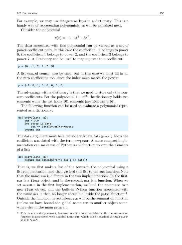
6.2 Dictionaries 255

For example, we may use integers as keys in a dictionary. This is ahandy way of representing polynomials, as will be explained next.

Consider the polynomial

p(x) = −1 + x2 + 3x7 .

The data associated with this polynomial can be viewed as a set ofpower-coefficient pairs, in this case the coefficient −1 belongs to power0, the coefficient 1 belongs to power 2, and the coefficient 3 belongs topower 7. A dictionary can be used to map a power to a coefficient:

p = 0: -1, 2: 1, 7: 3

A list can, of course, also be used, but in this case we must fill in allthe zero coefficients too, since the index must match the power:

p = [-1, 0, 1, 0, 0, 0, 0, 3]

The advantage with a dictionary is that we need to store only the non-zero coefficients. For the polynomial 1 + x100 the dictionary holds twoelements while the list holds 101 elements (see Exercise 6.16).

The following function can be used to evaluate a polynomial repre-sented as a dictionary:

def poly1(data, x):sum = 0.0for power in data:

sum += data[power]*x**powerreturn sum

The data argument must be a dictionary where data[power] holds thecoefficient associated with the term x**power. A more compact imple-mentation can make use of Python’s sum function to sum the elementsof a list:

def poly1(data, x):return sum([data[p]*x**p for p in data])

That is, we first make a list of the terms in the polynomial using alist comprehension, and then we feed this list to the sum function. Notethat the name sum is different in the two implementations: In the first,sum is a float object, and in the second, sum is a function. When weset sum=0.0 in the first implementation, we bind the name sum to anew float object, and the built-in Python function associated withthe name sum is then no longer accessible inside the poly1 function11.Outside the function, nevertheless, sum will be the summation function(unless we have bound the global name sum to another object some-where else in the main program.

11 This is not strictly correct, because sum is a local variable while the summationfunction is associated with a global name sum, which can be reached through glob-

als()[’sum’].

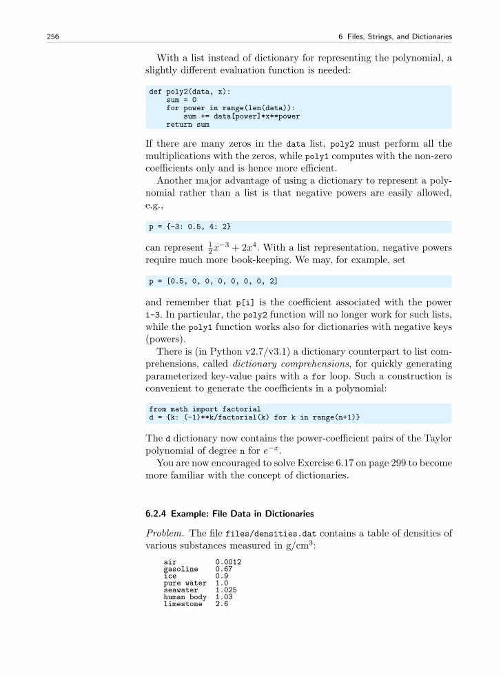
256 6 Files, Strings, and Dictionaries

With a list instead of dictionary for representing the polynomial, aslightly different evaluation function is needed:

def poly2(data, x):sum = 0for power in range(len(data)):

sum += data[power]*x**powerreturn sum

If there are many zeros in the data list, poly2 must perform all themultiplications with the zeros, while poly1 computes with the non-zerocoefficients only and is hence more efficient.

Another major advantage of using a dictionary to represent a poly-nomial rather than a list is that negative powers are easily allowed,e.g.,

p = -3: 0.5, 4: 2

can represent 12x

−3 + 2x4. With a list representation, negative powersrequire much more book-keeping. We may, for example, set

p = [0.5, 0, 0, 0, 0, 0, 0, 2]

and remember that p[i] is the coefficient associated with the poweri-3. In particular, the poly2 function will no longer work for such lists,while the poly1 function works also for dictionaries with negative keys(powers).

There is (in Python v2.7/v3.1) a dictionary counterpart to list com-prehensions, called dictionary comprehensions, for quickly generatingparameterized key-value pairs with a for loop. Such a construction isconvenient to generate the coefficients in a polynomial:

from math import factoriald = k: (-1)**k/factorial(k) for k in range(n+1)

The d dictionary now contains the power-coefficient pairs of the Taylorpolynomial of degree n for e−x.

You are now encouraged to solve Exercise 6.17 on page 299 to becomemore familiar with the concept of dictionaries.

6.2.4 Example: File Data in Dictionaries

Problem. The file files/densities.dat contains a table of densities ofvarious substances measured in g/cm3:

air 0.0012gasoline 0.67ice 0.9pure water 1.0seawater 1.025human body 1.03limestone 2.6

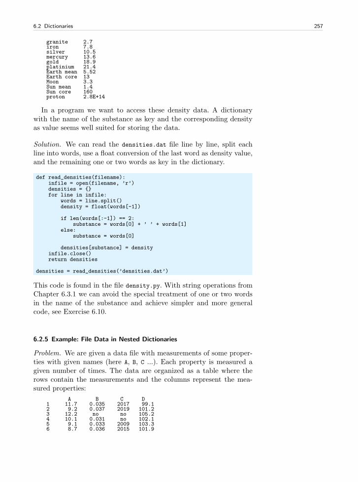
6.2 Dictionaries 257

granite 2.7iron 7.8silver 10.5mercury 13.6gold 18.9platinium 21.4Earth mean 5.52Earth core 13Moon 3.3Sun mean 1.4Sun core 160proton 2.8E+14

In a program we want to access these density data. A dictionarywith the name of the substance as key and the corresponding densityas value seems well suited for storing the data.

Solution. We can read the densities.dat file line by line, split eachline into words, use a float conversion of the last word as density value,and the remaining one or two words as key in the dictionary.

def read_densities(filename):infile = open(filename, ’r’)densities = for line in infile:

words = line.split()density = float(words[-1])

if len(words[:-1]) == 2:substance = words[0] + ’ ’ + words[1]

else:substance = words[0]

densities[substance] = densityinfile.close()return densities

densities = read_densities(’densities.dat’)

This code is found in the file density.py. With string operations fromChapter 6.3.1 we can avoid the special treatment of one or two wordsin the name of the substance and achieve simpler and more generalcode, see Exercise 6.10.

6.2.5 Example: File Data in Nested Dictionaries

Problem. We are given a data file with measurements of some proper-ties with given names (here A, B, C ...). Each property is measured agiven number of times. The data are organized as a table where therows contain the measurements and the columns represent the mea-sured properties:

A B C D1 11.7 0.035 2017 99.12 9.2 0.037 2019 101.23 12.2 no no 105.24 10.1 0.031 no 102.15 9.1 0.033 2009 103.36 8.7 0.036 2015 101.9

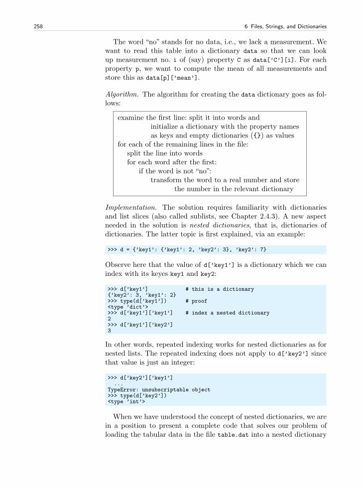
258 6 Files, Strings, and Dictionaries

The word “no” stands for no data, i.e., we lack a measurement. Wewant to read this table into a dictionary data so that we can lookup measurement no. i of (say) property C as data[’C’][i]. For eachproperty p, we want to compute the mean of all measurements andstore this as data[p][’mean’].

Algorithm. The algorithm for creating the data dictionary goes as fol-lows:

examine the first line: split it into words andinitialize a dictionary with the property namesas keys and empty dictionaries () as values

for each of the remaining lines in the file:split the line into wordsfor each word after the first:

if the word is not “no”:transform the word to a real number and store

the number in the relevant dictionary

Implementation. The solution requires familiarity with dictionariesand list slices (also called sublists, see Chapter 2.4.3). A new aspectneeded in the solution is nested dictionaries, that is, dictionaries ofdictionaries. The latter topic is first explained, via an example:

>>> d = ’key1’: ’key1’: 2, ’key2’: 3, ’key2’: 7

Observe here that the value of d[’key1’] is a dictionary which we canindex with its keyes key1 and key2:

>>> d[’key1’] # this is a dictionary’key2’: 3, ’key1’: 2>>> type(d[’key1’]) # proof<type ’dict’>>>> d[’key1’][’key1’] # index a nested dictionary2>>> d[’key1’][’key2’]3

In other words, repeated indexing works for nested dictionaries as fornested lists. The repeated indexing does not apply to d[’key2’] sincethat value is just an integer:

>>> d[’key2’][’key1’]...

TypeError: unsubscriptable object>>> type(d[’key2’])<type ’int’>

When we have understood the concept of nested dictionaries, we arein a position to present a complete code that solves our problem ofloading the tabular data in the file table.dat into a nested dictionary

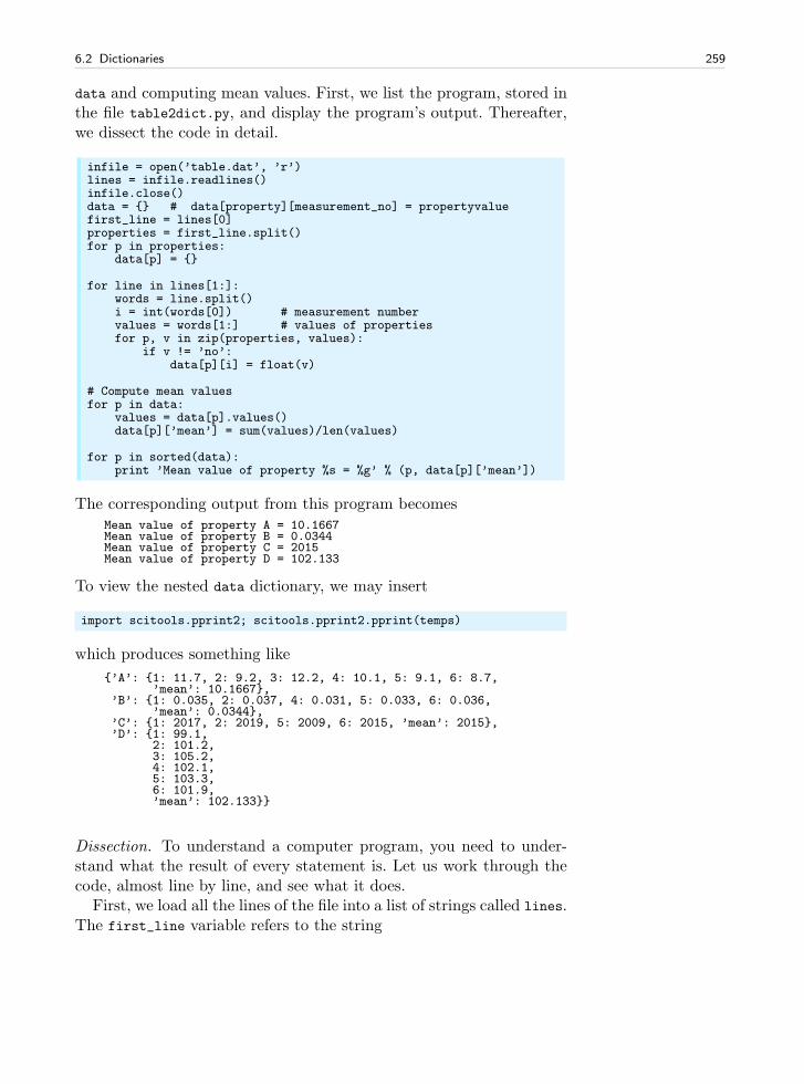
6.2 Dictionaries 259

data and computing mean values. First, we list the program, stored inthe file table2dict.py, and display the program’s output. Thereafter,we dissect the code in detail.

infile = open(’table.dat’, ’r’)lines = infile.readlines()infile.close()data = # data[property][measurement_no] = propertyvaluefirst_line = lines[0]properties = first_line.split()for p in properties:

data[p] =

for line in lines[1:]:words = line.split()i = int(words[0]) # measurement numbervalues = words[1:] # values of propertiesfor p, v in zip(properties, values):

if v != ’no’:data[p][i] = float(v)

# Compute mean valuesfor p in data:

values = data[p].values()data[p][’mean’] = sum(values)/len(values)

for p in sorted(data):print ’Mean value of property %s = %g’ % (p, data[p][’mean’])

The corresponding output from this program becomesMean value of property A = 10.1667Mean value of property B = 0.0344Mean value of property C = 2015Mean value of property D = 102.133

To view the nested data dictionary, we may insert

import scitools.pprint2; scitools.pprint2.pprint(temps)

which produces something like

’A’: 1: 11.7, 2: 9.2, 3: 12.2, 4: 10.1, 5: 9.1, 6: 8.7,’mean’: 10.1667,

’B’: 1: 0.035, 2: 0.037, 4: 0.031, 5: 0.033, 6: 0.036,’mean’: 0.0344,

’C’: 1: 2017, 2: 2019, 5: 2009, 6: 2015, ’mean’: 2015,’D’: 1: 99.1,

2: 101.2,3: 105.2,4: 102.1,5: 103.3,6: 101.9,’mean’: 102.133

Dissection. To understand a computer program, you need to under-stand what the result of every statement is. Let us work through thecode, almost line by line, and see what it does.

First, we load all the lines of the file into a list of strings called lines.The first_line variable refers to the string

260 6 Files, Strings, and Dictionaries

’ A B C D’

We split this line into a list of words, called properties, which thencontains

[’A’, ’B’, ’C’, ’D’]

With each of these property names we associate a dictionary with themeasurement number as key and the property value as value, but firstwe must create these “inner” dictionaries as empty before we can addthe measurements:

for p in properties:data[p] =

The first pass in the for loop picks out the string

’1 11.7 0.035 2017 99.1’

as the line variable. We split this line into words, the first word(words[0]) is the measurement number, while the rest words[1:] isa list of property values, here named values. To pair up the rightproperties and values, we loop over the properties and values listssimultaneously:

for p, v in zip(properties, values):if v != ’no’:

data[p][i] = float(v)

Recall that some values may be missing and we drop to record thatvalue12. Because the values list contains strings (words) read from thefile, we need to explicitly transform each string to a float numberbefore we can compute with the values.

After the for line in lines[1:] loop, we have a dictionary data

of dictionaries where all the property values are stored for each mea-surement number and property name. Figure 6.1 shows a graphicalrepresentation of the data dictionary.

It remains to compute the average values. For each property namep, i.e., key in the data dictionary, we can extract the recorded valuesas the list data[p].values() and simply send this list to Python’s sum

function and divide by the number of measured values for this property,i.e., the length of the list:

for p in data:values = data[p].values()data[p][’mean’] = sum(values)/len(values)

Alternatively, we can write an explicit loop to compute the average:

12 We could, alternatively, set the value to None.

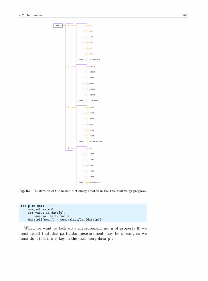
6.2 Dictionaries 261

data ’A’ 1 11.7

2 9.2

3 12.2

4 10.1

5 9.1

6 8.7

’mean’ 8.71428571429

’C’ 1 2017.0

2 2019.0

3 None

4 None

5 2009.0

6 2015.0

’mean’ 1151.42857143

’B’ 1 0.035

2 0.037

3 None

4 0.031

5 0.033

6 0.036

’mean’ 0.0245714285714

’D’ 1 99.1

2 101.2

3 105.2

4 102.1

5 103.3

6 101.9

’mean’ 87.5428571429

Fig. 6.1 Illustration of the nested dictionary created in the table2dict.py program.

for p in data:sum_values = 0for value in data[p]:

sum_values += valuedata[p][’mean’] = sum_values/len(data[p])

When we want to look up a measurement no. n of property B, wemust recall that this particular measurement may be missing so wemust do a test if n is key in the dictionary data[p]:

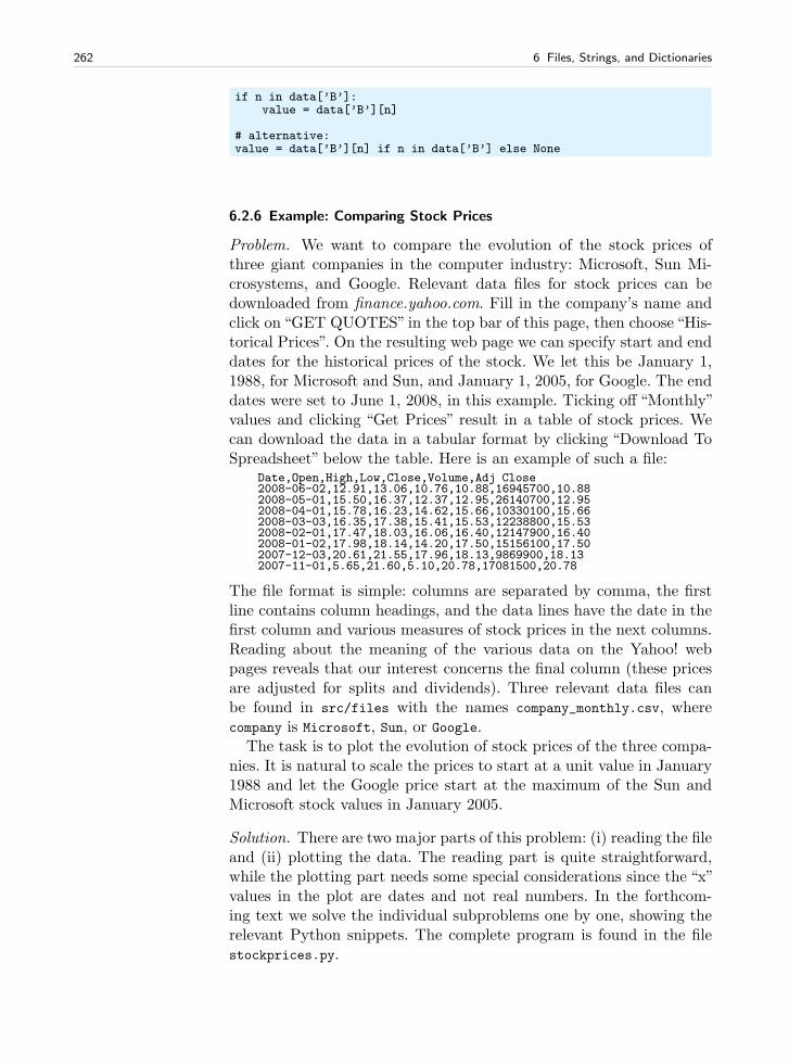
262 6 Files, Strings, and Dictionaries

if n in data[’B’]:value = data[’B’][n]

# alternative:value = data[’B’][n] if n in data[’B’] else None

6.2.6 Example: Comparing Stock Prices

Problem. We want to compare the evolution of the stock prices ofthree giant companies in the computer industry: Microsoft, Sun Mi-crosystems, and Google. Relevant data files for stock prices can bedownloaded from finance.yahoo.com. Fill in the company’s name andclick on “GET QUOTES” in the top bar of this page, then choose “His-torical Prices”. On the resulting web page we can specify start and enddates for the historical prices of the stock. We let this be January 1,1988, for Microsoft and Sun, and January 1, 2005, for Google. The enddates were set to June 1, 2008, in this example. Ticking off “Monthly”values and clicking “Get Prices” result in a table of stock prices. Wecan download the data in a tabular format by clicking “Download ToSpreadsheet” below the table. Here is an example of such a file:

Date,Open,High,Low,Close,Volume,Adj Close2008-06-02,12.91,13.06,10.76,10.88,16945700,10.882008-05-01,15.50,16.37,12.37,12.95,26140700,12.952008-04-01,15.78,16.23,14.62,15.66,10330100,15.662008-03-03,16.35,17.38,15.41,15.53,12238800,15.532008-02-01,17.47,18.03,16.06,16.40,12147900,16.402008-01-02,17.98,18.14,14.20,17.50,15156100,17.502007-12-03,20.61,21.55,17.96,18.13,9869900,18.132007-11-01,5.65,21.60,5.10,20.78,17081500,20.78

The file format is simple: columns are separated by comma, the firstline contains column headings, and the data lines have the date in thefirst column and various measures of stock prices in the next columns.Reading about the meaning of the various data on the Yahoo! webpages reveals that our interest concerns the final column (these pricesare adjusted for splits and dividends). Three relevant data files canbe found in src/files with the names company_monthly.csv, wherecompany is Microsoft, Sun, or Google.

The task is to plot the evolution of stock prices of the three compa-nies. It is natural to scale the prices to start at a unit value in January1988 and let the Google price start at the maximum of the Sun andMicrosoft stock values in January 2005.

Solution. There are two major parts of this problem: (i) reading the fileand (ii) plotting the data. The reading part is quite straightforward,while the plotting part needs some special considerations since the “x”values in the plot are dates and not real numbers. In the forthcom-ing text we solve the individual subproblems one by one, showing therelevant Python snippets. The complete program is found in the filestockprices.py.

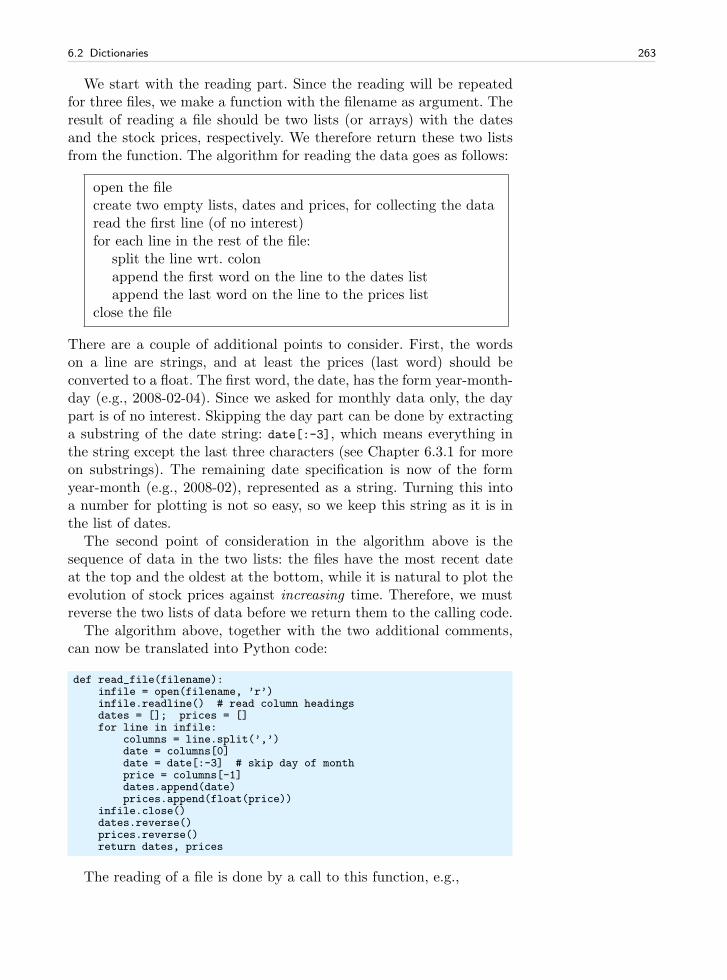
6.2 Dictionaries 263

We start with the reading part. Since the reading will be repeatedfor three files, we make a function with the filename as argument. Theresult of reading a file should be two lists (or arrays) with the datesand the stock prices, respectively. We therefore return these two listsfrom the function. The algorithm for reading the data goes as follows:

open the filecreate two empty lists, dates and prices, for collecting the dataread the first line (of no interest)for each line in the rest of the file:

split the line wrt. colonappend the first word on the line to the dates listappend the last word on the line to the prices list

close the file

There are a couple of additional points to consider. First, the wordson a line are strings, and at least the prices (last word) should beconverted to a float. The first word, the date, has the form year-month-day (e.g., 2008-02-04). Since we asked for monthly data only, the daypart is of no interest. Skipping the day part can be done by extractinga substring of the date string: date[:-3], which means everything inthe string except the last three characters (see Chapter 6.3.1 for moreon substrings). The remaining date specification is now of the formyear-month (e.g., 2008-02), represented as a string. Turning this intoa number for plotting is not so easy, so we keep this string as it is inthe list of dates.

The second point of consideration in the algorithm above is thesequence of data in the two lists: the files have the most recent dateat the top and the oldest at the bottom, while it is natural to plot theevolution of stock prices against increasing time. Therefore, we mustreverse the two lists of data before we return them to the calling code.

The algorithm above, together with the two additional comments,can now be translated into Python code:

def read_file(filename):infile = open(filename, ’r’)infile.readline() # read column headingsdates = []; prices = []for line in infile:

columns = line.split(’,’)date = columns[0]date = date[:-3] # skip day of monthprice = columns[-1]dates.append(date)prices.append(float(price))

infile.close()dates.reverse()prices.reverse()return dates, prices

The reading of a file is done by a call to this function, e.g.,

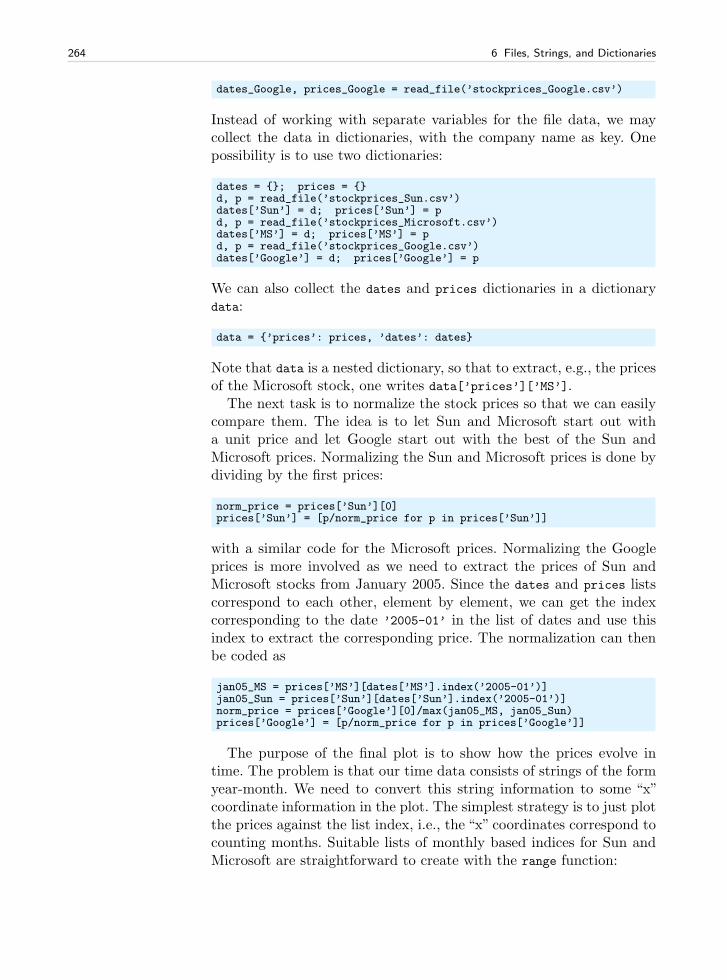
264 6 Files, Strings, and Dictionaries

dates_Google, prices_Google = read_file(’stockprices_Google.csv’)

Instead of working with separate variables for the file data, we maycollect the data in dictionaries, with the company name as key. Onepossibility is to use two dictionaries:

dates = ; prices = d, p = read_file(’stockprices_Sun.csv’)dates[’Sun’] = d; prices[’Sun’] = pd, p = read_file(’stockprices_Microsoft.csv’)dates[’MS’] = d; prices[’MS’] = pd, p = read_file(’stockprices_Google.csv’)dates[’Google’] = d; prices[’Google’] = p

We can also collect the dates and prices dictionaries in a dictionarydata:

data = ’prices’: prices, ’dates’: dates

Note that data is a nested dictionary, so that to extract, e.g., the pricesof the Microsoft stock, one writes data[’prices’][’MS’].

The next task is to normalize the stock prices so that we can easilycompare them. The idea is to let Sun and Microsoft start out witha unit price and let Google start out with the best of the Sun andMicrosoft prices. Normalizing the Sun and Microsoft prices is done bydividing by the first prices:

norm_price = prices[’Sun’][0]prices[’Sun’] = [p/norm_price for p in prices[’Sun’]]

with a similar code for the Microsoft prices. Normalizing the Googleprices is more involved as we need to extract the prices of Sun andMicrosoft stocks from January 2005. Since the dates and prices listscorrespond to each other, element by element, we can get the indexcorresponding to the date ’2005-01’ in the list of dates and use thisindex to extract the corresponding price. The normalization can thenbe coded as

jan05_MS = prices[’MS’][dates[’MS’].index(’2005-01’)]jan05_Sun = prices[’Sun’][dates[’Sun’].index(’2005-01’)]norm_price = prices[’Google’][0]/max(jan05_MS, jan05_Sun)prices[’Google’] = [p/norm_price for p in prices[’Google’]]

The purpose of the final plot is to show how the prices evolve intime. The problem is that our time data consists of strings of the formyear-month. We need to convert this string information to some “x”coordinate information in the plot. The simplest strategy is to just plotthe prices against the list index, i.e., the “x” coordinates correspond tocounting months. Suitable lists of monthly based indices for Sun andMicrosoft are straightforward to create with the range function:

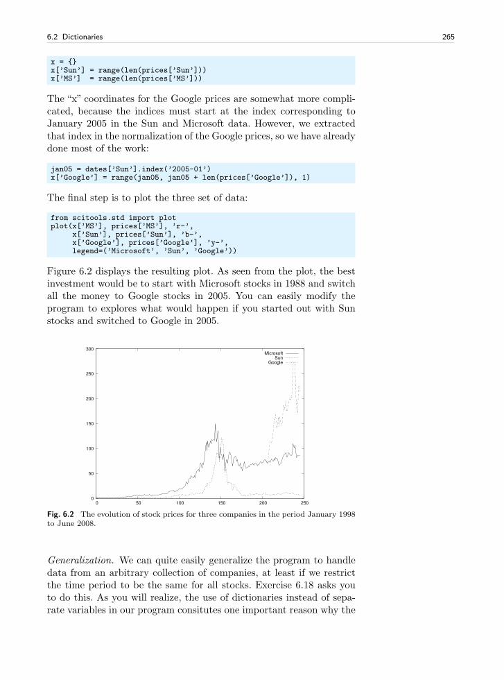
6.2 Dictionaries 265

x = x[’Sun’] = range(len(prices[’Sun’]))x[’MS’] = range(len(prices[’MS’]))

The “x” coordinates for the Google prices are somewhat more compli-cated, because the indices must start at the index corresponding toJanuary 2005 in the Sun and Microsoft data. However, we extractedthat index in the normalization of the Google prices, so we have alreadydone most of the work:

jan05 = dates[’Sun’].index(’2005-01’)x[’Google’] = range(jan05, jan05 + len(prices[’Google’]), 1)

The final step is to plot the three set of data:

from scitools.std import plotplot(x[’MS’], prices[’MS’], ’r-’,

x[’Sun’], prices[’Sun’], ’b-’,x[’Google’], prices[’Google’], ’y-’,legend=(’Microsoft’, ’Sun’, ’Google’))

Figure 6.2 displays the resulting plot. As seen from the plot, the bestinvestment would be to start with Microsoft stocks in 1988 and switchall the money to Google stocks in 2005. You can easily modify theprogram to explores what would happen if you started out with Sunstocks and switched to Google in 2005.

0

50

100

150

200

250

300

0 50 100 150 200 250

MicrosoftSun

Google

Fig. 6.2 The evolution of stock prices for three companies in the period January 1998to June 2008.

Generalization. We can quite easily generalize the program to handledata from an arbitrary collection of companies, at least if we restrictthe time period to be the same for all stocks. Exercise 6.18 asks youto do this. As you will realize, the use of dictionaries instead of sepa-rate variables in our program consitutes one important reason why the

266 6 Files, Strings, and Dictionaries

program becomes easy to extend. Avoiding different time periods fordifferent price data also makes the generalized program simpler thanthe one we developed above.

6.3 Strings

Many programs need to manipulate text. For example, when we readthe contents of a file into a string or list of strings (lines), we may wantto change parts of the text in the string(s) – and maybe write out themodified text to a new file. So far in this chapter we have convertedparts of the text to numbers and computed with the numbers. Now itis time to learn how to manipulate the text strings themselves.

6.3.1 Common Operations on Strings

Python has a rich set of operations on string objects. Some of the mostcommon operations are listed below.

Substring Specification. The expression s[i:j] extracts the substringstarting with character number i and ending with character numberj-1 (similarly to lists, 0 is the index of the first character):

>>> s = ’Berlin: 18.4 C at 4 pm’>>> s[8:] # from index 8 to the end of the string’18.4 C at 4 pm’>>> s[8:12] # index 8, 9, 10 and 11 (not 12!)’18.4’

A negative upper index counts, as usual, from the right such that s[-1]is the last element, s[-2] is the next last element, and so on.

>>> s[8:-1]’18.4 C at 4 p’>>> s[8:-8]’18.4 C’

Searching for Substrings. The call s.find(s1) returns the index wherethe substring s1 first appears in s. If the substring is not found, -1 isreturned.

>>> s.find(’Berlin’) # where does ’Berlin’ start?0>>> s.find(’pm’)20>>> s.find(’Oslo’) # not found-1

Sometimes the aim is to just check if a string is contained in anotherstring, and then we can use the syntax:

6.3 Strings 267

>>> ’Berlin’ in s:True>>> ’Oslo’ in s:False

Here is a typical use of the latter construction in an if test:

>>> if ’C’ in s:... print ’C found’... else:... print ’no C’...C found

Two other convenient methods for checking if a string starts with orends with a specified string are startswith and endswith:

>>> s.startswith(’Berlin’)True>>> s.endswith(’am’)False

Substitution. The call s.replace(s1, s2) replaces substring s1 by s2

everywhere in s:

>>> s.replace(’ ’, ’_’)’Berlin:_18.4_C__at_4_pm’>>> s.replace(’Berlin’, ’Bonn’)’Bonn: 18.4 C at 4 pm’

A variant of the last example, where several string operations are puttogether, consists of replacing the text before the first colon13:

>>> s.replace(s[:s.find(’:’)], ’Bonn’)’Bonn: 18.4 C at 4 pm’

String Splitting. The call s.split() splits the string s into words sep-arated by whitespace (space, tabulator, or newline):

>>> s.split()[’Berlin:’, ’18.4’, ’C’, ’at’, ’4’, ’pm’]

Splitting a string s into words separated by a text t can be done bys.split(t). For example, we may split with respect to colon:

>>> s.split(’:’)[’Berlin’, ’ 18.4 C at 4 pm’]

We know that s contains a city name, a colon, a temperature, and thenC:

13 Take a “break” and convince yourself that you understand how we specify thesubstring to be replaced.

268 6 Files, Strings, and Dictionaries

>>> s = ’Berlin: 18.4 C at 4 pm’

With s.splitlines(), a multi-line string is split into lines (very usefulwhen a file has been read into a string and we want a list of lines):

>>> t = ’1st line\n2nd line\n3rd line’>>> print t1st line2nd line3rd line>>> t.splitlines()[’1st line’, ’2nd line’, ’3rd line’]

Upper and Lower Case. s.lower() transforms all characters to theirlower case equivalents, and s.upper() performs a similar transforma-tion to upper case letters:

>>> s.lower()’berlin: 18.4 c at 4 pm’>>> s.upper()’BERLIN: 18.4 C AT 4 PM’

Strings Are Constant. A string cannot be changed, i.e., any changealways results in a new string. Replacement of a character is not pos-sible:

>>> s[18] = 5...TypeError: ’str’ object does not support item assignment

If we want to replace s[18], a new string must be constructed, forexample by keeping the substrings on either side of s[18] and insertinga ’5’ in between:

>>> s[:18] + ’5’ + s[19:]’Berlin: 18.4 C at 5 pm’

Strings with Digits Only. One can easily test whether a string containsdigits only or not:

>>> ’214’.isdigit()True>>> ’ 214 ’.isdigit()False>>> ’2.14’.isdigit()False

Whitespace. We can also check if a string contains spaces only by call-ing the isspace method. More precisely, isspace tests for whitespace,which means the space character, newline, or the TAB character:

6.3 Strings 269

>>> ’ ’.isspace() # blanksTrue>>> ’ \n’.isspace() # newlineTrue>>> ’ \t ’.isspace() # TABTrue>>> ’’.isspace() # empty stringFalse

The isspace is handy for testing for blank lines in files. An alternativeis to strip first and then test for an empty string:

>>> line = ’ \n’>>> empty.strip() == ’’True

Stripping off leading and/or trailing spaces in a string is sometimesuseful:

>>> s = ’ text with leading/trailing space \n’>>> s.strip()’text with leading/trailing space’>>> s.lstrip() # left strip’text with leading/trailing space \n’>>> s.rstrip() # right strip’ text with leading/trailing space’

Joining Strings. The opposite of the split method is join, which joinselements in a list of strings with a specified delimiter in between. Thatis, the following two types of statements are inverse operations:

t = delimiter.join(words)words = t.split(delimiter)

An example on using join may be

>>> strings = [’Newton’, ’Secant’, ’Bisection’]>>> t = ’, ’.join(strings)>>> t’Newton, Secant, Bisection’

As an illustration of the usefulness of split and join, we want toremove the first two words on a line. This task can be done by firstsplitting the line into words and then joining the words of interest:

>>> line = ’This is a line of words separated by space’>>> words = line.split()>>> line2 = ’ ’.join(words[2:])>>> line2’a line of words separated by space’

There are many more methods in string objects. All methods aredescribed in the Python Library Reference, see “string methods” in theindex.

270 6 Files, Strings, and Dictionaries

6.3.2 Example: Reading Pairs of Numbers

Problem. Suppose we have a file consisting of pairs of real numbers, i.e.,text of the form (a, b), where a and b are real numbers. This notationfor a pair of numbers is often used for points in the plane, vectors inthe plane, and complex numbers. A sample file may look as follows:

(1.3,0) (-1,2) (3,-1.5)(0,1) (1,0) (1,1)(0,-0.01) (10.5,-1) (2.5,-2.5)

The file can be found as read_pairs1.dat. Our task is to read thistext into a nested list pairs such that pairs[i] holds the pair withindex i, and this pair is a tuple of two float objects. We assume thatthere are no blanks inside the parentheses of a pair of numbers (werely on a split operation which would otherwise not work).

Solution. To solve this programming problem, we can read in the fileline by line; for each line: split the line into words (i.e., split withrespect to whitespace); for each word: strip off the parentheses, splitwith respect to comma, and convert the resulting two words to floats.Our brief algorithm can be almost directly translated to Python code:

lines = open(’read_pairs1.dat’, ’r’).readlines()

pairs = [] # list of (n1, n2) pairs of numbersfor line in lines:

words = line.split()for word in words:

word = word[1:-1] # strip off parenthesisn1, n2 = word.split(’,’)n1 = float(n1); n2 = float(n2)pair = (n1, n2)pairs.append(pair) # add 2-tuple to last row

This code is available in the file read_pairs1.py. Figure 6.3 shows asnapshot of the state of the variables in the program after havingtreated the first line. You should explain each line in the programto yourself, and compare your understanding with the figure.

The output from the program becomes

[(1.3, 0.0),(-1.0, 2.0),(3.0, -1.5),(0.0, 1.0),(1.0, 0.0),(1.0, 1.0),(0.0, -0.01),(10.5, -1.0),(2.5, -2.5)]

We remark that our solution to this programming problem reliesheavily on the fact that spaces inside the parentheses are not allowed.If spaces were allowed, the simple split to obtain the pairs on a line aswords would not work. What can we then do?

We can first strip off all blanks on a line, and then observe that thepairs are separated by the text ’)(’. The first and last pair on a line

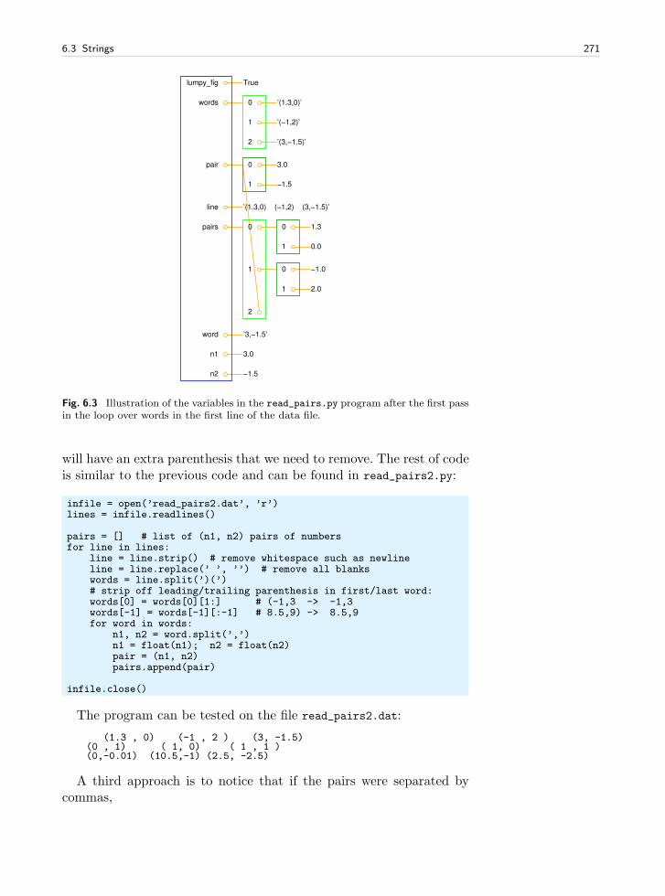
6.3 Strings 271

lumpy_fig True

words 0 ’(1.3,0)’

1 ’(−1,2)’

2 ’(3,−1.5)’

pair 0 3.0

1 −1.5

line ’(1.3,0) (−1,2) (3,−1.5)’

pairs 0 0 1.3

1 0.0

1 0 −1.0

1 2.0

2

word ’3,−1.5’

n1 3.0

n2 −1.5

Fig. 6.3 Illustration of the variables in the read_pairs.py program after the first passin the loop over words in the first line of the data file.

will have an extra parenthesis that we need to remove. The rest of codeis similar to the previous code and can be found in read_pairs2.py:

infile = open(’read_pairs2.dat’, ’r’)lines = infile.readlines()

pairs = [] # list of (n1, n2) pairs of numbersfor line in lines:

line = line.strip() # remove whitespace such as newlineline = line.replace(’ ’, ’’) # remove all blankswords = line.split(’)(’)# strip off leading/trailing parenthesis in first/last word:words[0] = words[0][1:] # (-1,3 -> -1,3words[-1] = words[-1][:-1] # 8.5,9) -> 8.5,9for word in words:

n1, n2 = word.split(’,’)n1 = float(n1); n2 = float(n2)pair = (n1, n2)pairs.append(pair)

infile.close()

The program can be tested on the file read_pairs2.dat:

(1.3 , 0) (-1 , 2 ) (3, -1.5)(0 , 1) ( 1, 0) ( 1 , 1 )(0,-0.01) (10.5,-1) (2.5, -2.5)

A third approach is to notice that if the pairs were separated bycommas,

272 6 Files, Strings, and Dictionaries

(1, 3.0), (-1, 2), (3, -1.5)(0, 1), (1, 0), (1, 1)

the file text is very close to the Python syntax of a list of 2-tuples. Byadding enclosing brackets, plus a comma at the end of each line,

[(1, 3.0), (-1, 2), (3, -1.5),(0, 1), (1, 0), (1, 1),]

we have a string to which we can apply eval to get the pairs listdirectly. Here is the code doing this (program read_pairs3.py):

infile = open(’read_pairs3.dat’, ’r’)listtext = ’[’for line in infile:

# add line, without newline (line[:-1]), with a trailing comma:listtext += line[:-1] + ’, ’

infile.close()listtext = listtext + ’]’pairs = eval(listtext)

In general, it is a good idea to construct file formats that are as closeas possible to valid Python syntax such that one can take advantageof the eval or exec functions to turn text into “live objects”.

6.3.3 Example: Reading Coordinates

Problem. Suppose we have a file with coordinates (x, y, z) in three-dimensional space. The file format looks as follows:

x=-1.345 y= 0.1112 z= 9.1928x=-1.231 y=-0.1251 z= 1001.2x= 0.100 y= 1.4344E+6 z=-1.0100x= 0.200 y= 0.0012 z=-1.3423E+4x= 1.5E+5 y=-0.7666 z= 1027

The goal is to read this file and create a list with (x,y,z) 3-tuples,and thereafter convert the nested list to a two-dimensional array withwhich we can compute.

Note that there is sometimes a space between the = signs and thefollowing number and sometimes not. Splitting with respect to spaceand extracting every second word is therefore not an option. We shallpresent three solutions.

Solution 1: Substring Extraction. The file format looks very regularwith the x=, y=, and z= texts starting in the same columns at every line.By counting characters, we realize that the x= text starts in column 2,the y= text starts in column 16, while the z= text starts in column 31.Introducing

x_start = 2y_start = 16z_start = 31

the three numbers in a line string are obtained as the substrings

6.3 Strings 273

x = line[x_start+2:y_start]y = line[y_start+2:z_start]z = line[z_start+2:]

The following code, found in file file2coor_v1.py, creates the coor

array with shape (n, 3), where n is the number of (x, y, z) coordinates.

infile = open(’xyz.dat’, ’r’)coor = [] # list of (x,y,z) tuplesfor line in infile:

x_start = 2y_start = 16z_start = 31x = line[x_start+2:y_start]y = line[y_start+2:z_start]z = line[z_start+2:]print ’debug: x="%s", y="%s", z="%s"’ % (x,y,z)coor.append((float(x), float(y), float(z)))

infile.close()

import numpy as npcoor = np.array(coor)print coor.shape, coor

The print statement inside the loop is always wise to include whendoing string manipulations, simply because counting indices for sub-string limits quickly leads to errors. Running the program, the outputfrom the loop looks like this

debug: x="-1.345 ", y=" 0.1112 ", z=" 9.1928"

for the first line in the file. The double quotes show the exact extent ofthe extracted coordinates. Note that the last quote appears on the nextline. This is because line has a newline at the end (this newline must bethere to define the end of the line), and the substring line[z_start:]

contains the newline at the of line. Writing line[z_start:-1] wouldleave the newline out of the z coordinate. However, this has no effectin practice since we transform the substrings to float, and an extranewline or other blanks make no harm.

The coor object at the end of the program has the value

[[ -1.34500000e+00 1.11200000e-01 9.19280000e+00][ -1.23100000e+00 -1.25100000e-01 1.00120000e+03][ 1.00000000e-01 1.43440000e+06 -1.01000000e+00][ 2.00000000e-01 1.20000000e-03 -1.34230000e+04][ 1.50000000e+05 -7.66600000e-01 1.02700000e+03]]

Solution 2: String Search. One problem with the solution approachabove is that the program will not work if the file format is subject toa change in the column positions of x=, y=, or z=. Instead of hardcodingnumbers for the column positions, we can use the find method in stringobjects to locate these column positions:

x_start = line.find(’x=’)y_start = line.find(’y=’)z_start = line.find(’z=’)

274 6 Files, Strings, and Dictionaries

The rest of the code is similar to the complete program listed above,and the complete code is stored in the file file2coor_v2.py.

Solution 3: String Split. String splitting is a powerful tool, also in thepresent case. Let us split with respect to the equal sign. The first linein the file then gives us the words

[’x’, ’-1.345 y’, ’ 0.1112 z’, ’ 9.1928’]

We throw away the first word, and strip off the last character in thenext word. The final word can be used as is. The complete program isfound in the file file2coor_v3.py and looks like

infile = open(’xyz.dat’, ’r’)coor = [] # list of (x,y,z) tuplesfor line in infile:

words = line.split(’=’)x = float(words[1][:-1])y = float(words[2][:-1])z = float(words[3])coor.append((x, y, z))

infile.close()

import numpy as npcoor = np.array(coor)print coor.shape, coor

More sophisticated examples of string operations appear in Chap-ter 6.4.4.

6.4 Reading Data from Web Pages

Python has a module urllib which makes it possible to read data froma web page as easily as we can read data from an ordinary file14. Beforewe do this, a few concepts from the Internet world must be touched.

6.4.1 About Web Pages

Web pages are viewed with a web browser. There are many browsers:Firefox, Internet Explorer, Safari, Opera, and Google Chrome to men-tion the most famous. Any web page you visit is associated with anaddress, usually something like

http://www.some.where.net/some/file.html

This type of web address is called a URL (which stands for Uniform Re-source Locator15). The graphics you see in a web browser, i.e., the web

14 In principle this is true, but in practice the text in web pages tend to be much morecomplicated than the text in the files we have treated so far.

15 Another term is URI (Uniform Resource Identifier), which is replacing URL intechnical documentation. We stick to URL, however, in this book because Python’stools for accessing resources on the Internet have url as part of module and functionnames.

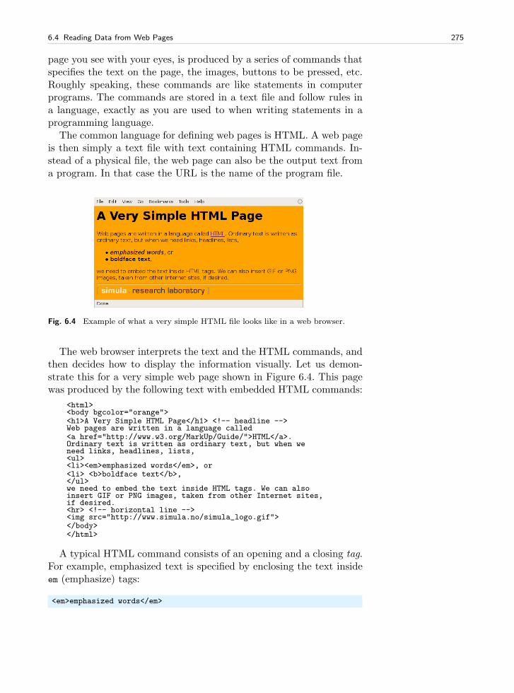
6.4 Reading Data from Web Pages 275

page you see with your eyes, is produced by a series of commands thatspecifies the text on the page, the images, buttons to be pressed, etc.Roughly speaking, these commands are like statements in computerprograms. The commands are stored in a text file and follow rules ina language, exactly as you are used to when writing statements in aprogramming language.

The common language for defining web pages is HTML. A web pageis then simply a text file with text containing HTML commands. In-stead of a physical file, the web page can also be the output text froma program. In that case the URL is the name of the program file.

Fig. 6.4 Example of what a very simple HTML file looks like in a web browser.

The web browser interprets the text and the HTML commands, andthen decides how to display the information visually. Let us demon-strate this for a very simple web page shown in Figure 6.4. This pagewas produced by the following text with embedded HTML commands:

<html><body bgcolor="orange"><h1>A Very Simple HTML Page</h1> <!-- headline -->Web pages are written in a language called<a href="http://www.w3.org/MarkUp/Guide/">HTML</a>.Ordinary text is written as ordinary text, but when weneed links, headlines, lists,<ul><li><em>emphasized words</em>, or<li> <b>boldface text</b>,</ul>we need to embed the text inside HTML tags. We can alsoinsert GIF or PNG images, taken from other Internet sites,if desired.<hr> <!-- horizontal line --><img src="http://www.simula.no/simula_logo.gif"></body></html>

A typical HTML command consists of an opening and a closing tag.For example, emphasized text is specified by enclosing the text insideem (emphasize) tags:

<em>emphasized words</em>

276 6 Files, Strings, and Dictionaries

The opening tag is enclosed in less than and greater than signs, whilethe closing tag has an additional forward slash before the tag name.

In the HTML file we see an opening and closing html tag around thewhole text in the file. Similarly, there is a pair of body tags, where thefirst one also has a parameter bgcolor which can be used to specify abackground color in the web page. Section headlines are specified byenclosing the headline text inside h1 tags. Subsection headlines apply h2

tags, which results in a smaller font compared with h1 tags. Commentsappear inside <!- and ->. Links to other web pages are written insidea tags, with an argument href for the link’s web address. Lists applythe ul (unordered list) tag, while each item is written with just anopening tag li (list item), but no closing tag is necessary. Images arealso specified with just an opening tag having name img, and the imagefile is given as a file name or URL of a file, enclosed in double quotes,as the src parameter.

The ultra-quick HTML course in the previous paragraphs gives aglimpse of how web pages can be constructed. One can either write theHTML file by hand in a pure text editor, or one can use programs suchas Dream Weaver to help design the page graphically in a user-friendlyenvironment, and then the program can automatically generate theright HTML syntax in files.

6.4.2 How to Access Web Pages in Programs

Why is it useful to know some HTML and how web pages are con-structed? The reason is that the web is full of information that we canget access to through programs and use in new contexts. What we canget access to is not the visual web page you see, but the underlyingHTML file. The information you see on the screen appear in text formin the HTML file, and by extracting text, we can get hold of the text’sinformation in a program.

Given the URL as a string stored in a variable, there are two waysof accessing the HTML text in a Python program:

1. Download the HTML file and store it as a local file with a givenname, say webpage.html:

import urlliburl = ’http://www.simula.no/research/scientific/cbc’urllib.urlretrieve(url, filename=’webpage.html’)

2. Open the HTML file as a file-like object:

infile = urllib.urlopen(url)

This infile object has methods such as read, readline, and readlines.

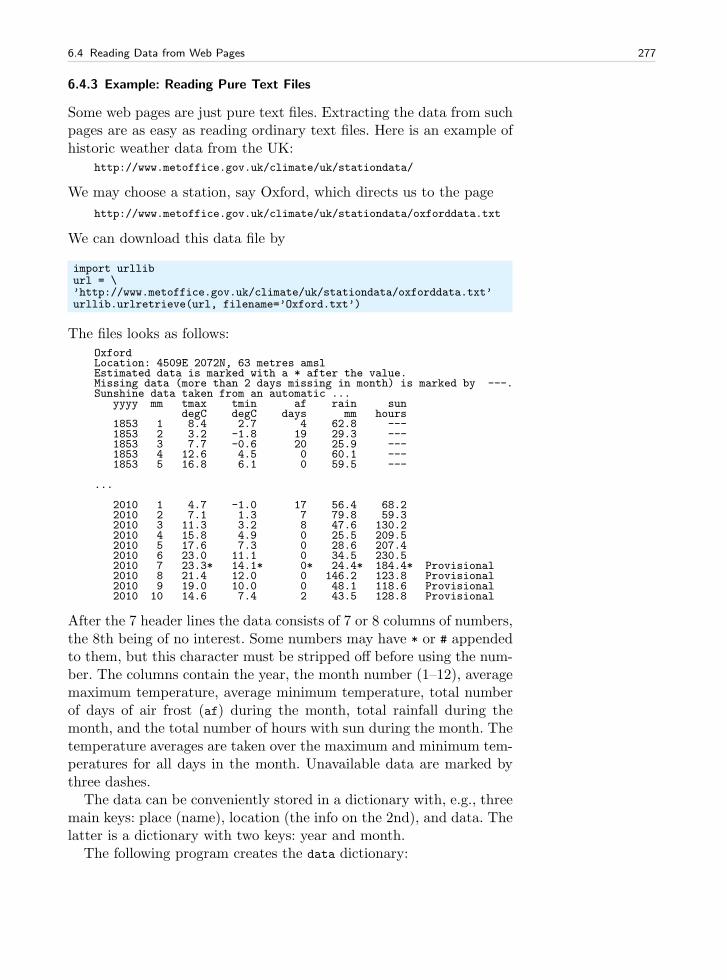
6.4 Reading Data from Web Pages 277

6.4.3 Example: Reading Pure Text Files

Some web pages are just pure text files. Extracting the data from suchpages are as easy as reading ordinary text files. Here is an example ofhistoric weather data from the UK:

http://www.metoffice.gov.uk/climate/uk/stationdata/

We may choose a station, say Oxford, which directs us to the page

http://www.metoffice.gov.uk/climate/uk/stationdata/oxforddata.txt

We can download this data file by

import urlliburl = \’http://www.metoffice.gov.uk/climate/uk/stationdata/oxforddata.txt’urllib.urlretrieve(url, filename=’Oxford.txt’)

The files looks as follows:OxfordLocation: 4509E 2072N, 63 metres amslEstimated data is marked with a * after the value.Missing data (more than 2 days missing in month) is marked by ---.Sunshine data taken from an automatic ...

yyyy mm tmax tmin af rain sundegC degC days mm hours

1853 1 8.4 2.7 4 62.8 ---1853 2 3.2 -1.8 19 29.3 ---1853 3 7.7 -0.6 20 25.9 ---1853 4 12.6 4.5 0 60.1 ---1853 5 16.8 6.1 0 59.5 ---

...

2010 1 4.7 -1.0 17 56.4 68.22010 2 7.1 1.3 7 79.8 59.32010 3 11.3 3.2 8 47.6 130.22010 4 15.8 4.9 0 25.5 209.52010 5 17.6 7.3 0 28.6 207.42010 6 23.0 11.1 0 34.5 230.52010 7 23.3* 14.1* 0* 24.4* 184.4* Provisional2010 8 21.4 12.0 0 146.2 123.8 Provisional2010 9 19.0 10.0 0 48.1 118.6 Provisional2010 10 14.6 7.4 2 43.5 128.8 Provisional

After the 7 header lines the data consists of 7 or 8 columns of numbers,the 8th being of no interest. Some numbers may have * or # appendedto them, but this character must be stripped off before using the num-ber. The columns contain the year, the month number (1–12), averagemaximum temperature, average minimum temperature, total numberof days of air frost (af) during the month, total rainfall during themonth, and the total number of hours with sun during the month. Thetemperature averages are taken over the maximum and minimum tem-peratures for all days in the month. Unavailable data are marked bythree dashes.

The data can be conveniently stored in a dictionary with, e.g., threemain keys: place (name), location (the info on the 2nd), and data. Thelatter is a dictionary with two keys: year and month.

The following program creates the data dictionary:

278 6 Files, Strings, and Dictionaries

infile = open(local_file, ’r’)data = data[’place’] = infile.readline().strip()data[’location’] = infile.readline().strip()# Skip the next 5 linesfor i in range(5):

infile.readline()

data[’data’] =for line in infile:

columns = line.split()

year = int(columns[0])month = int(columns[1])

if columns[-1] == ’Provisional’:del columns[-1]

for i in range(2, len(columns)):if columns[i] == ’---’:

columns[i] = Noneelif columns[i][-1] == ’*’ or columns[i][-1] == ’#’:

# Strip off trailing charactercolumns[i] = float(columns[i][:-1])

else:columns[i] = float(columns[i])

tmax, tmin, air_frost, rain, sun = columns[2:]

if not year in data[’data’]:data[’data’][year] =

data[’data’][year][month] = ’tmax’: tmax,’tmin’: tmin,’air frost’: air_frost,’sun’: sun

The code is available in the file historic_weather.py.With a few lines of code, we can extract the data we want, say a

two-dimensional array of the number of sun hours in a month (thesedata are available from year 1929):

sun = [[data[’data’][y][m][’sun’] for m in range(1,13)] \for y in range(1929, 2010)]

import numpy as npsun = np.array(sun)

One can now do analysis of the data as exemplified in Chapter 2.6.2and Exercise 5.7.

6.4.4 Example: Extracting Data from an HTML Page

Very often, interesting data in a web page appear inside HTML code.We then need to interpret the text using string operations and storethe data in variables. An example will clarify the principle.

The web site www.worldclimate.com contains data on temperatureand rainfall in a large number of cities around the world. For example,

http://www.worldclimate.com/cgi-bin/data.pl?ref=N38W009+2100+08535W

6.5 Writing Data to File 279

contains a table of the average rainfall for each month of the year inthe town Lisbon, Portugal. Our task is to download this web page andextract the tabular data (rainfall per month) in a list.

Downloading the file is done with urllib as explained in Chap-ters 6.4.2 and 6.4.3. Before attempting to read and interpret the textin the file, we need to look at the HTML code to find the interestingparts and determine how we can extract the data. The table with therainfall data appears in the middle of the file. A sketch of the relevantHTML code goes as follows:

<p>Weather station <strong>LISBOA</strong> ...<tr><th align=right><th> Jan<th> Feb<th> ... <br><tr><td> mm <td align=right> 95.2 <td align=right> 86.7 ...<br><tr><td>inches <td align=right>3.7<td align=right>3.4 ...<br>

Our task is to walk through the file line by line and stop for processingthe first and third line above:

infile = open(’Lisbon_rainfall.html’, ’r’)rainfall = []for line in infile:

if ’Weather station’ in line:station = line.split(’</strong>’)[0].split(’<strong>’)[0]

if ’<td> mm <td’ in line:data = line.split(’<td align=right>’)

The resulting data list looks like

[’<tr><td> mm ’, ’ 95.2 ’, ..., ’702.4<br> \n’]

To process this list further, we strip off the <br>... part of the lastelement:

data[-1] = data[-1].split(’<br>’)[0]

Then we drop the first element and convert the others to float objects:

data = [float(x) for x in data[1:]]

Now we have the rainfall data for each month as a list of real numbers.The complete program appears in the file Lisbon_rainfall.py. Therecipe provided in this example can be used to interpret many othertypes of web pages where HTML code and data are wired together.

6.5 Writing Data to File

Writing data to file is easy. There is basically one function to payattention to: outfile.write(s), which writes a string s to a file handledby the file object outfile. Unlike print, outfile.write(s) does notappend a newline character to the written string. It will therefore oftenbe necessary to add a newline character,

280 6 Files, Strings, and Dictionaries

outfile.write(s + ’\n’)

if the string s is meant to appear on a single line in the file and s doesnot already contain a trailing newline character. File writing is then amatter of constructing strings containing the text we want to have inthe file and for each such string call outfile.write.

Writing to a file demands the file object f to be opened for writing:

# write to new file, or overwrite file:outfile = open(filename, ’w’)

# append to the end of an existing file:outfile = open(filename, ’a’)

6.5.1 Example: Writing a Table to File

Problem. As a worked example of file writing, we shall write out anested list with tabular data to file. A sample list may take look as

[[ 0.75, 0.29619813, -0.29619813, -0.75 ],[ 0.29619813, 0.11697778, -0.11697778, -0.29619813],[-0.29619813, -0.11697778, 0.11697778, 0.29619813],[-0.75, -0.29619813, 0.29619813, 0.75 ]]

Solution. We iterate through the rows (first index) in the list, and foreach row, we iterate through the column values (second index) andwrite each value to the file. At the end of each row, we must insert anewline character in the file to get a linebreak. The code resides in thefile write1.py:

data = [[ 0.75, 0.29619813, -0.29619813, -0.75 ],[ 0.29619813, 0.11697778, -0.11697778, -0.29619813],[-0.29619813, -0.11697778, 0.11697778, 0.29619813],[-0.75, -0.29619813, 0.29619813, 0.75 ]]

outfile = open(’tmp_table.dat’, ’w’)for row in data:

for column in row:outfile.write(’%14.8f’ % column)

outfile.write(’\n’)outfile.close()

The resulting data file becomes0.75000000 0.29619813 -0.29619813 -0.750000000.29619813 0.11697778 -0.11697778 -0.29619813-0.29619813 -0.11697778 0.11697778 0.29619813-0.75000000 -0.29619813 0.29619813 0.75000000

An extension of this program consists in adding column and rowheadings:

column 1 column 2 column 3 column 4row 1 0.75000000 0.29619813 -0.29619813 -0.75000000row 2 0.29619813 0.11697778 -0.11697778 -0.29619813row 3 -0.29619813 -0.11697778 0.11697778 0.29619813row 4 -0.75000000 -0.29619813 0.29619813 0.75000000

6.5 Writing Data to File 281

To obtain this end result, we need to the add some statements to theprogram write1.py. For the column headings we need to know thenumber of columns, i.e., the length of the rows, and loop from 1 to thislength:

ncolumns = len(data[0])outfile.write(’ ’)for i in range(1, ncolumns+1):

outfile.write(’%10s ’ % (’column %2d’ % i))outfile.write(’\n’)

Note the use of a nested printf construction: The text we want to insertis itself a printf string. We could also have written the text as ’column’ + str(i), but then the length of the resulting string would dependon the number of digits in i. It is recommended to always use printfconstructions for a tabular output format, because this gives automaticpadding of blanks so that the width of the output strings remain thesame. As always, the tuning of the widths is done in a trial-and-errorprocess.

To add the row headings, we need a counter over the row numbers:

row_counter = 1for row in data:

outfile.write(’row %2d’ % row_counter)for column in row:

outfile.write(’%14.8f’ % column)outfile.write(’\n’)row_counter += 1

The complete code is found in the file write2.py. We could, alterna-tively, iterate over the indices in the list:

for i in range(len(data)):outfile.write(’row %2d’ % (i+1))for j in range(len(data[i])):

outfile.write(’%14.8f’ % data[i][j])outfile.write(’\n’)

6.5.2 Standard Input and Output as File Objects

Reading user input from the keyboard applies the function raw_input asexplained in Chapter 4.1. The keyboard is a medium that the computerin fact treats as a file, referred to as standard input.

The print command prints text in the terminal window. Thismedium is also viewed as a file from the computer’s point of view andcalled standard output. All general-purpose programming languages al-low reading from standard input and writing to standard output. Thisreading and writing can be done with two types of tools, either file-likeobjects or special tools like raw_input (see Chapter 4.1.1) and print inPython. We will here describe the file-line objects: sys.stdin for stan-dard input and sys.stdout for standard output. These objects behave

282 6 Files, Strings, and Dictionaries

as file objects, except that they do not need to be opened or closed.The statement

s = raw_input(’Give s:’)

is equivalent to

print ’Give s: ’,s = sys.stdin.readline()

Recall that the trailing comma in the print statement avoids the new-line that print by default adds to the output string. Similarly,

s = eval(raw_input(’Give s:’))

is equivalent to

print ’Give s: ’,s = eval(sys.stdin.readline())

For output to the terminal window, the statement

print s

is equivalent to

sys.stdout.write(s + ’\n’)

Why it is handy to have access to standard input and output as fileobjects can be illustrated by an example. Suppose you have a functionthat reads data from a file object infile and writes data to a file objectoutfile. A sample function may take the form

def x2f(infile, outfile, f):for line in infile:

x = float(line)y = f(x)outfile.write(’%g\n’ % y)

This function works with all types of files, including web pages asinfile (see Chapter 6.4). With sys.stdin as infile and/or sys.stdoutas outfile, the x2f function also works with standard input and/orstandard output. Without sys.stdin and sys.stdout, we would needdifferent code, employing raw_input and print, to deal with standardinput and output. Now we can write a single function that deals withall file media in a unified way.

There is also something called standard error. Usually this is theterminal window, just as standard output, but programs can distin-guish between writing ordinary output to standard output and errormessages to standard error, and these output media can be redirectedto, e.g., files such that one can separate error messages from ordinary

6.5 Writing Data to File 283

output. In Python, standard error is the file-like object sys.stderr. Atypical application of sys.stderr is to report errors:

if x < 0:sys.stderr.write(’Illegal value of x’); sys.exit(1)

This message to sys.stderr is an alternative to print or raising anexception.

Redirecting Standard Input, Output, and Error. Standard output froma program prog can be redirected to a file output instead of the screen,by using the greater than sign16:

Terminal

Unix/DOS> prog > output

Similarly, output to the medium called standard error can be redirectedby

Terminal

Unix/DOS> prog &> output

For example, error messages are normally written to standard error,which is exemplified in this little terminal session on a Unix machine:

Terminal

Unix> ls bla-bla1 bla-bla2ls: cannot access bla-bla1: No such file or directoryls: cannot access bla-bla2: No such file or directoryUnix> ls bla-bla1 bla-bla2 &> errorsUnix> cat errors # print the file errorsls: cannot access bla-bla1: No such file or directoryls: cannot access bla-bla2: No such file or directory

When the program reads from standard input (the keyboard), we canequally well redirect standard input to a file, say with name raw_input,such that the program reads from this file rather than from the key-board:

Terminal

Unix/DOS> prog < input

Combinations are also possible:

Terminal

Unix/DOS> prog < input > output

16 prog can be any program, including a Python program run as, e.g., python

myprog.py.

284 6 Files, Strings, and Dictionaries

Note. The redirection of standard output, input, and error does notwork for programs run inside IPython, only when run directly in theoperating system in a terminal window.

Inside a Python program we can also let standard input, output,and error work with ordinary files instead. Here is the technique:

sys_stdout_orig = sys.stdoutsys.stdout = open(’output’, ’w’)sys_stdin_orig = sys.stdinsys.stdin = open(’input’, ’r’)

Now, any print statement will write to the output file, and anyraw_input call will read from the input file. (Without storing the orig-inalsys.stdout and sys.stdin objects in new variables, these objectswould get lost in the redefinition above and we would never be able toreach the common standard input and output in the program.)

6.5.3 Reading and Writing Spreadsheet Files

From school you are probably used to spreadsheet programs such asMicrosoft Excel or OpenOffice. This type of program is used to rep-resent a table of numbers and text. Each table entry is known as acell, and one can easily perform calculations with cells that containnumbers. The application of spreadsheet programs for mathematicalcomputations and graphics is steadily growing.

Also Python may be used to do spreadsheet-type calculations ontabular data. The advantage of using Python is that you can easilyextend the calculations far beyond what a spreadsheet program can do.However, even if you can view Python as a substitute for a spreadsheetprogram, it may be beneficial to combine the two. Suppose you havesome data in a spreadsheet. How can you read these data into a Pythonprogram, perform calculations on the data, and thereafter read the databack to the spreadsheet program? This is exactly what we will explainbelow through an example. With this example, you should understandhow easy it is to combine Excel or OpenOffice with your own Pythonprograms.

The table of data in a spreadsheet can be saved in so-called CSVfiles, where CSV stands for comma separated values. The CSV file for-mat is very simple: each row in the spreadsheet table is a line in thefile, and each cell in the row is separated by a comma or some otherspecified separation character. CSV files can easily be read into Pythonprograms, and the table of cell data can be stored in a nested list (table,cf. Chapter 2.4), which can be processed as we desire. The modifiedtable of cell data can be written back to a CSV file and read into thespreadsheet program for further processing.

Figure 6.5 shows a simple spreadsheet in the OpenOffice program.The table contains 4 × 4 cells, where the first row contains column

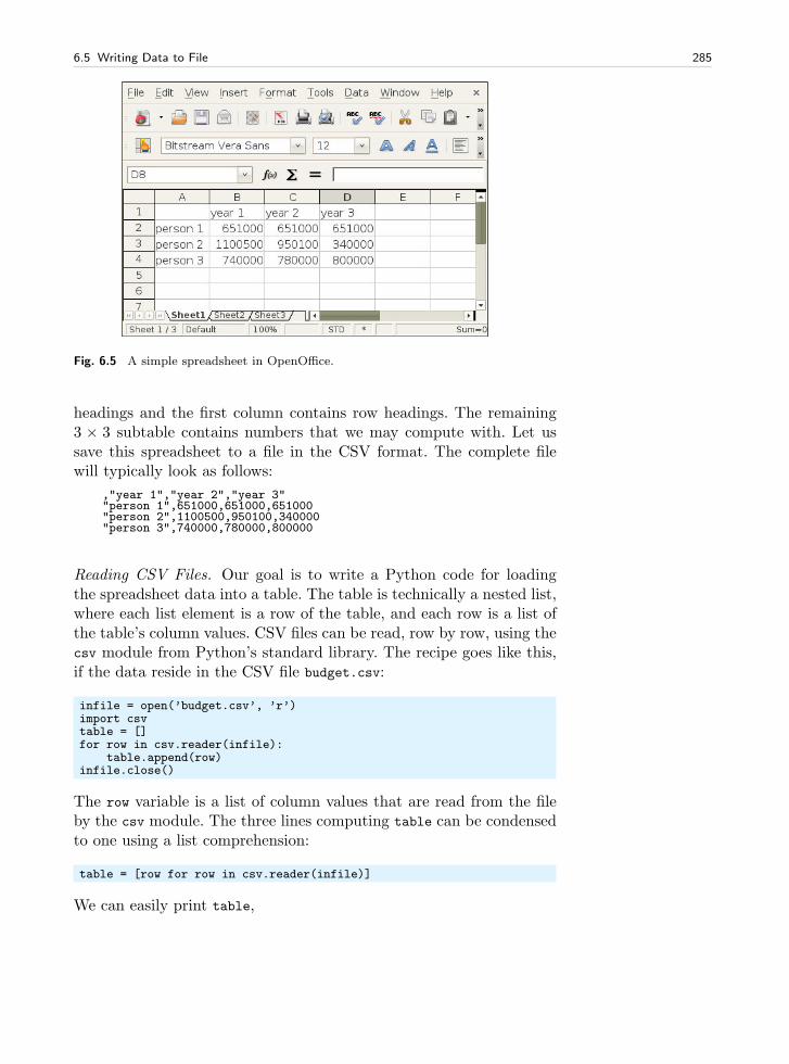
6.5 Writing Data to File 285

Fig. 6.5 A simple spreadsheet in OpenOffice.

headings and the first column contains row headings. The remaining3 × 3 subtable contains numbers that we may compute with. Let ussave this spreadsheet to a file in the CSV format. The complete filewill typically look as follows:

,"year 1","year 2","year 3""person 1",651000,651000,651000"person 2",1100500,950100,340000"person 3",740000,780000,800000

Reading CSV Files. Our goal is to write a Python code for loadingthe spreadsheet data into a table. The table is technically a nested list,where each list element is a row of the table, and each row is a list ofthe table’s column values. CSV files can be read, row by row, using thecsv module from Python’s standard library. The recipe goes like this,if the data reside in the CSV file budget.csv:

infile = open(’budget.csv’, ’r’)import csvtable = []for row in csv.reader(infile):

table.append(row)infile.close()

The row variable is a list of column values that are read from the fileby the csv module. The three lines computing table can be condensedto one using a list comprehension:

table = [row for row in csv.reader(infile)]

We can easily print table,

286 6 Files, Strings, and Dictionaries

import pprintpprint.pprint(table)

to see what the spreadsheet looks like when it is represented as a nestedlist in a Python program:

[[’’, ’year 1’, ’year 2’, ’year 3’],[’person 1’, ’651000’, ’651000’, ’651000’],[’person 2’, ’1100500’, ’950100’, ’340000’],[’person 3’, ’740000’, ’780000’, ’800000’]]

Observe now that all entries are surrounded by quotes, which meansthat all entries are string (str) objects. This is a general rule: the csv

module reads all cells into string objects. To compute with the num-bers, we need to transform the string objects to float objects. Thetransformation should not be applied to the first row and first column,since the cells here hold text. The transformation from strings to num-bers therefore applies to the indices r and c in table (table[r][c]),such that the row counter r goes from 1 to len(table)-1, and the col-umn counter c goes from 1 to len(table[0])-1 (len(table[0]) is thelength of the first row, assuming the lengths of all rows are equal tothe length of the first row). The relevant Python code for this trans-formation task becomes

for r in range(1,len(table)):for c in range(1, len(table[0])):

table[r][c] = float(table[r][c])

A pprint.pprint(table) statement after this transformation yields

[[’’, ’year 1’, ’year 2’, ’year 3’],[’person 1’, 651000.0, 651000.0, 651000.0],[’person 2’, 1100500.0, 950100.0, 340000.0],[’person 3’, 740000.0, 780000.0, 800000.0]]

The numbers now have a decimal and no quotes, indicating that thenumbers are float objects and hence ready for mathematical calula-tions.

Processing Data. Let us perform a very simple calculation with table,namely adding a final row with the sum of the numbers in the columns:

row = [0.0]*len(table[0])row[0] = ’sum’for c in range(1, len(row)):

s = 0for r in range(1, len(table)):

s += table[r][c]row[c] = s

As seen, we first create a list row consisting of zeros. Then we inserta text in the first column, before we invoke a loop over the numbersin the table and compute the sum of each column. The table list nowrepresents a spreadsheet with four columns and five rows:

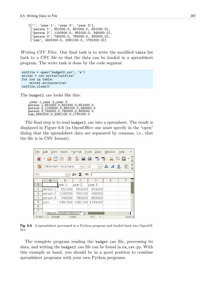
6.5 Writing Data to File 287

[[’’, ’year 1’, ’year 2’, ’year 3’],[’person 1’, 651000.0, 651000.0, 651000.0],[’person 2’, 1100500.0, 950100.0, 340000.0],[’person 3’, 740000.0, 780000.0, 800000.0],[’sum’, 2491500.0, 2381100.0, 1791000.0]]

Writing CSV Files. Our final task is to write the modified table listback to a CSV file so that the data can be loaded in a spreadsheetprogram. The write task is done by the code segment

outfile = open(’budget2.csv’, ’w’)writer = csv.writer(outfile)for row in table:

writer.writerow(row)outfile.close()

The budget2.csv looks like this:

,year 1,year 2,year 3person 1,651000.0,651000.0,651000.0person 2,1100500.0,950100.0,340000.0person 3,740000.0,780000.0,800000.0sum,2491500.0,2381100.0,1791000.0

The final step is to read budget2.csv into a spreadseet. The result isdisplayed in Figure 6.6 (in OpenOffice one must specify in the “open”dialog that the spreadsheet data are separated by commas, i.e., thatthe file is in CSV format).

Fig. 6.6 A spreadsheet processed in a Python program and loaded back into OpenOf-fice.

The complete program reading the budget.csv file, processing itsdata, and writing the budget2.csv file can be found in rw_csv.py. Withthis example at hand, you should be in a good position to combinespreadsheet programs with your own Python programs.

288 6 Files, Strings, and Dictionaries

Remark. You may wonder why we used the csv module to read andwrite CSV files when such files have comma separated values whichwe can extract by splitting lines with respect to the comma (in Chap-ter 6.2.6 use used this technique to read a CSV file):

infile = open(’budget.csv’, ’r’)for line in infile:

row = line.split(’,’)

This works well for the present budget.csv file, but the techniquebreaks down when a text in a cell contains a comma, for instance"Aug 8, 2007". The line.split(’,’) will split this cell text, while thecsv.reader functionality is smart enough to avoid splitting text cellswith a comma.

Representing Number Cells with Numerical Python Arrays. Instead ofputting the whole spreadsheet into a single nested list, we can make aPython data structure more tailored to the data at hand. What we haveare two headers (for rows and columns, respectively) and a subtableof numbers. The headers can be represented as lists of strings, whilethe subtable could be a two-dimensional Numerical Python array. Thelatter makes it easier to implement various mathematical operations onthe numbers. A dictionary can hold all the three items: two header listsand one array. The relevant code for reading, processing, and writingthe data is shown below and can be found in the file rw_csv_numpy.py:

infile = open(’budget.csv’, ’r’)import csvtable = [row for row in csv.reader(infile)]infile.close()

# Convert subtable of numbers (string to float)subtable = [[float(c) for c in row[1:]] for row in table[1:]]

data = ’column headings’: table[0][1:],’row headings’: [row[0] for row in table[1:]],’array’: array(subtable)

# Add a new row with sumsdata[’row headings’].append(’sum’)a = data[’array’] # short formdata[’column sum’] = [sum(a[:,c]) for c in range(a.shape[1])]

outfile = open(’budget2.csv’, ’w’)writer = csv.writer(outfile)# Aurn data dictionary into a nested list first (for easy writing)table = a.tolist() # transform array to nested listtable.append(data[’column sum’])table.insert(0, data[’column headings’])# Axtend table with row headings (a new column)table = [table[r].insert(0, data[’row headings’][r]) \

for r in range(len(table))]for row in table:

writer.writerow(row)outfile.close()

6.6 Summary 289

The code makes heavy use of list comprehensions, and the transforma-tion between a nested list, for file reading and writing, and the data

dictionary, for representing the data in the Python program, is non-trivial. If you manage to understand every line in this program, youhave digested a lot of topics in Python programming!

6.6 Summary

6.6.1 Chapter Topics

File Operations. This chapter has been concerned with file reading andfile writing. First a file must be openend, either for reading, writing,or appending:

infile = open(filename, ’r’) # readoutfile = open(filename, ’w’) # writeoutfile = open(filename, ’a’) # append

There are four basic reading commands:

line = infile.readline() # read the next linefilestr = infile.read() # read rest of file into stringlines = infile.readlines() # read rest of file into listfor line in infile: # read rest of file line by line

File writing is usually about repeatedly using the command

outfile.write(s)

where s is a string. Contrary to print s, no newline is added to s inoutfile.write(s).

When the reading and writing is finished,

somefile.close()

should be called, where somefile is the file object.

Downloading Internet Files. Internet files can be downloaded if weknow their URL:

import urlliburl = ’http://www.some.where.net/path/thing.html’urllib.urlretrieve(url, filename=’thing.html’)

The downloaded information is put in the local file thing.html in thecurrent working folder. Alternatively, we can open the URL as a fileobject:

290 6 Files, Strings, and Dictionaries

webpage = urllib.urlopen(url)

HTML files are often messy to interpret by string operations.

Table 6.1 Summary of important functionality for dictionary objects.

a = initialize an empty dictionarya = ’point’: [0,0.1], ’value’: 7 initialize a dictionarya = dict(point=[2,7], value=3) initialize a dictionary w/string keysa.update(b) add/update key-value pairs from b in a

a.update(key=value1, key2=value2) add/update key-value pairs in a

a[’hide’] = True add new key-value pair to a

a[’point’] get value corresponding to key point

’value’ in a True if value is a key in a

del a[’point’] delete a key-value pair from a

a.keys() list of keysa.values() list of valueslen(a) number of key-value pairs in a

for key in a: loop over keys in unknown orderfor key in sorted(a): loop over keys in alphabetic orderisinstance(a, dict) is True if a is a dictionary

Dictionaries. Array or list-like objects with text or other (fixed-valued)Python objects as indices are called dictionaries. They are very usefulfor storing general collections of objects in a single data structure.Table 6.1 displays some of the most important dictionary operations.

Strings. Some of the most useful functionalities in a string object s arelisted below.

Split the string into substrings separated by delimiter:

words = s.split(delimiter)

Join elements in a list of strings:

string = delimiter.join(words[i:j])

Extract substring:

substring = s[2:n-4]

Substitute a substring by new a string:

modified_string = s.replace(sub, new)

Search for the start (first index) of some text:

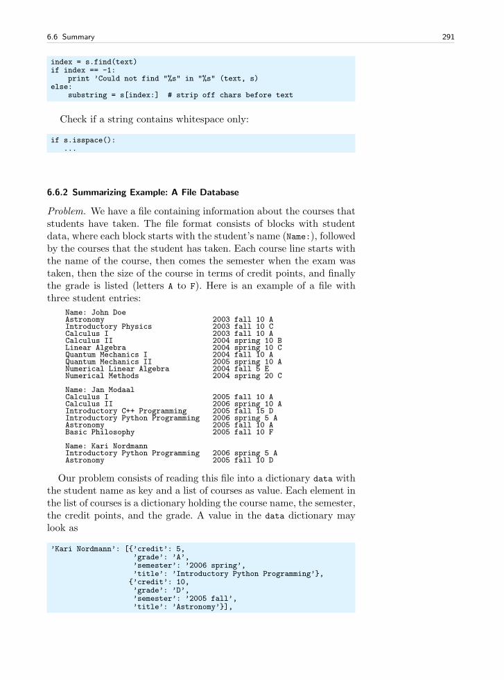
6.6 Summary 291

index = s.find(text)if index == -1:

print ’Could not find "%s" in "%s" (text, s)else:

substring = s[index:] # strip off chars before text

Check if a string contains whitespace only:

if s.isspace():...

6.6.2 Summarizing Example: A File Database

Problem. We have a file containing information about the courses thatstudents have taken. The file format consists of blocks with studentdata, where each block starts with the student’s name (Name:), followedby the courses that the student has taken. Each course line starts withthe name of the course, then comes the semester when the exam wastaken, then the size of the course in terms of credit points, and finallythe grade is listed (letters A to F). Here is an example of a file withthree student entries:

Name: John DoeAstronomy 2003 fall 10 AIntroductory Physics 2003 fall 10 CCalculus I 2003 fall 10 ACalculus II 2004 spring 10 BLinear Algebra 2004 spring 10 CQuantum Mechanics I 2004 fall 10 AQuantum Mechanics II 2005 spring 10 ANumerical Linear Algebra 2004 fall 5 ENumerical Methods 2004 spring 20 C

Name: Jan ModaalCalculus I 2005 fall 10 ACalculus II 2006 spring 10 AIntroductory C++ Programming 2005 fall 15 DIntroductory Python Programming 2006 spring 5 AAstronomy 2005 fall 10 ABasic Philosophy 2005 fall 10 F

Name: Kari NordmannIntroductory Python Programming 2006 spring 5 AAstronomy 2005 fall 10 D

Our problem consists of reading this file into a dictionary data withthe student name as key and a list of courses as value. Each element inthe list of courses is a dictionary holding the course name, the semester,the credit points, and the grade. A value in the data dictionary maylook as

’Kari Nordmann’: [’credit’: 5,’grade’: ’A’,’semester’: ’2006 spring’,’title’: ’Introductory Python Programming’,’credit’: 10,’grade’: ’D’,’semester’: ’2005 fall’,’title’: ’Astronomy’],

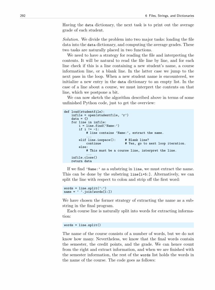
292 6 Files, Strings, and Dictionaries

Having the data dictionary, the next task is to print out the averagegrade of each student.

Solution. We divide the problem into two major tasks: loading the filedata into the data dictionary, and computing the average grades. Thesetwo tasks are naturally placed in two functions.

We need to have a strategy for reading the file and interpreting thecontents. It will be natural to read the file line by line, and for eachline check if this is a line containing a new student’s name, a courseinformation line, or a blank line. In the latter case we jump to thenext pass in the loop. When a new student name is encountered, weinitialize a new entry in the data dictionary to an empty list. In thecase of a line about a course, we must interpret the contents on thatline, which we postpone a bit.

We can now sketch the algorithm described above in terms of someunfinished Python code, just to get the overview:

def load(studentfile):infile = open(studentfile, ’r’)data = for line in infile:

i = line.find(’Name:’)if i != -1:

# line contains ’Name:’, extract the name....

elif line.isspace(): # Blank line?continue # Yes, go to next loop iteration.

else:# This must be a course line, interpret the line....

infile.close()return data

If we find ’Name:’ as a substring in line, we must extract the name.This can be done by the substring line[i+5:]. Alternatively, we cansplit the line with respect to colon and strip off the first word:

words = line.split(’:’)name = ’ ’.join(words[1:])

We have chosen the former strategy of extracting the name as a sub-string in the final program.

Each course line is naturally split into words for extracting informa-tion:

words = line.split()

The name of the course consists of a number of words, but we do notknow how many. Nevertheless, we know that the final words containthe semester, the credit points, and the grade. We can hence countfrom the right and extract information, and when we are finished withthe semester information, the rest of the words list holds the words inthe name of the course. The code goes as follows:

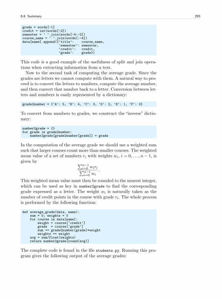
6.6 Summary 293

grade = words[-1]credit = int(words[-2])semester = ’ ’.join(words[-4:-2])course_name = ’ ’.join(words[:-4])data[name].append(’title’: course_name,

’semester’: semester,’credit’: credit,’grade’: grade)

This code is a good example of the usefulness of split and join opera-tions when extracting information from a text.

Now to the second task of computing the average grade. Since thegrades are letters we cannot compute with them. A natural way to pro-ceed is to convert the letters to numbers, compute the average number,and then convert that number back to a letter. Conversion between let-ters and numbers is easily represented by a dictionary:

grade2number = ’A’: 5, ’B’: 4, ’C’: 3, ’D’: 2, ’E’: 1, ’F’: 0

To convert from numbers to grades, we construct the “inverse” dictio-nary:

number2grade = for grade in grade2number:

number2grade[grade2number[grade]] = grade

In the computation of the average grade we should use a weighted sumsuch that larger courses count more than smaller courses. The weightedmean value of a set of numbers ri with weights wi, i = 0, . . . , n− 1, isgiven by

∑n−1i=0 wiri∑n−1

i=0 wi

.

This weighted mean value must then be rounded to the nearest integer,which can be used as key in number2grade to find the correspondinggrade expressed as a letter. The weight wi is naturally taken as thenumber of credit points in the course with grade ri. The whole processis performed by the following function:

def average_grade(data, name):sum = 0; weights = 0for course in data[name]:

weight = course[’credit’]grade = course[’grade’]sum += grade2number[grade]*weightweights += weight

avg = sum/float(weights)return number2grade[round(avg)]

The complete code is found in the file students.py. Running this pro-gram gives the following output of the average grades:

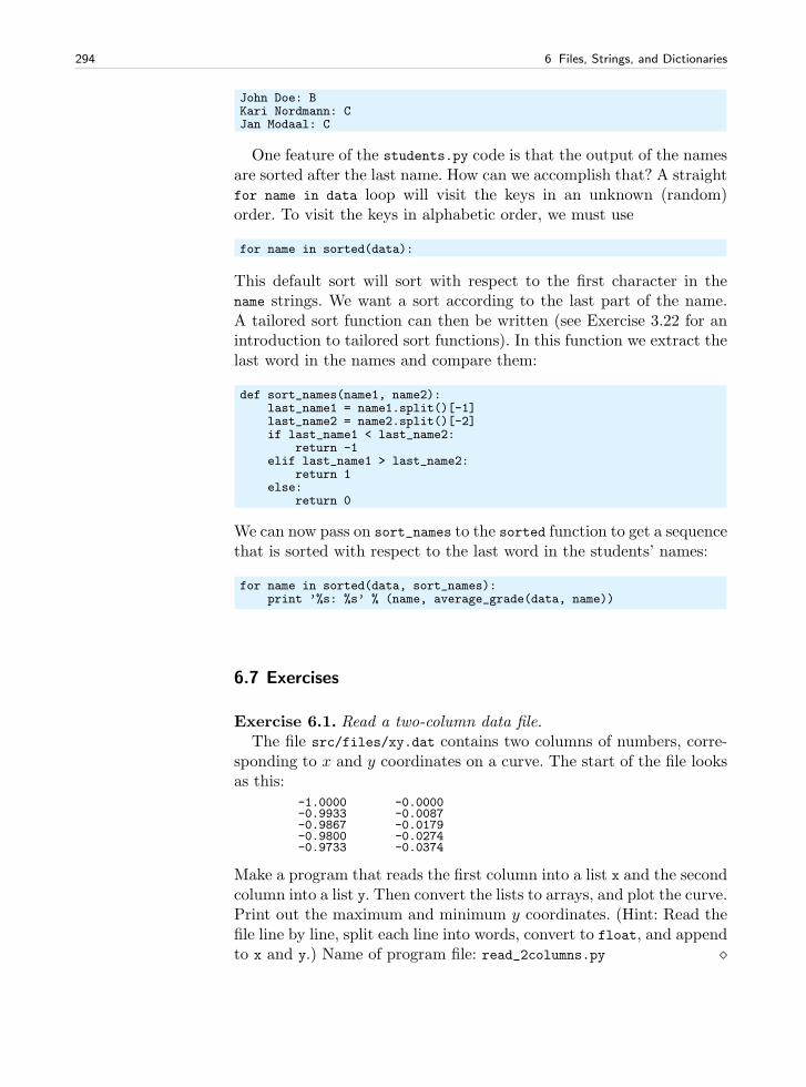
294 6 Files, Strings, and Dictionaries

John Doe: BKari Nordmann: CJan Modaal: C

One feature of the students.py code is that the output of the namesare sorted after the last name. How can we accomplish that? A straightfor name in data loop will visit the keys in an unknown (random)order. To visit the keys in alphabetic order, we must use

for name in sorted(data):

This default sort will sort with respect to the first character in thename strings. We want a sort according to the last part of the name.A tailored sort function can then be written (see Exercise 3.22 for anintroduction to tailored sort functions). In this function we extract thelast word in the names and compare them:

def sort_names(name1, name2):last_name1 = name1.split()[-1]last_name2 = name2.split()[-2]if last_name1 < last_name2:

return -1elif last_name1 > last_name2:

return 1else:

return 0

We can now pass on sort_names to the sorted function to get a sequencethat is sorted with respect to the last word in the students’ names:

for name in sorted(data, sort_names):print ’%s: %s’ % (name, average_grade(data, name))

6.7 Exercises

Exercise 6.1. Read a two-column data file.The file src/files/xy.dat contains two columns of numbers, corre-

sponding to x and y coordinates on a curve. The start of the file looksas this:

-1.0000 -0.0000-0.9933 -0.0087-0.9867 -0.0179-0.9800 -0.0274-0.9733 -0.0374

Make a program that reads the first column into a list x and the secondcolumn into a list y. Then convert the lists to arrays, and plot the curve.Print out the maximum and minimum y coordinates. (Hint: Read thefile line by line, split each line into words, convert to float, and appendto x and y.) Name of program file: read_2columns.py ⋄

6.7 Exercises 295

Exercise 6.2. Read a data file.The files density_water.dat and density_air.dat files in the folder

src/files contain data about the density of water and air (resp.) fordifferent temperatures. The data files have some comment lines startingwith # and some lines are blank. The rest of the lines contain densitydata: the temperature in the first column and the corresponding densityin the second column. The goal of this exercise is to read the data insuch a file and plot the density versus the temperature as distinct(small) circles for each data point. Let the program take the name ofthe data file as command-line argument. Apply the program to bothfiles. Name of program file: read_density_data.py ⋄

Exercise 6.3. Simplify the implementation of Exer. 6.1.Files with data in a tabular fashion are very common and so is

the operation of the reading the data into arrays. Therefore, thescitools.filetable module offers easy-to-use functions for load-ing data files with columns of numbers into NumPy arrays. Firstread about scitools.filetable using pydoc in a terminal window(cf. page 80). Then solve Exercise 6.1 using appropriate func-tions from the scitools.filetable module. Name of program file:read_2columns_filetable.py. ⋄

Exercise 6.4. Fit a polynomial to data.The purpose of this exercise is to find a simple mathematical formula

for the how the density of water or air depends on the temperature.First, load the density data from file as explained in Exercises 6.2 or6.3. Then we want to experiment with NumPy utilities that can find apolynomial that approximate the density curve.

NumPy has a function polyfit(x, y, deg) for finding a “best fit” ofa polynomial of degree deg to a set of data points given by the arrayarguments x and y. The polyfit function returns a list of the coeffi-cients in the fitted polynomial, where the first element is the coefficientfor the term with the highest degree, and the last element correspondsto the constant term. For example, given points in x and y, polyfit(x,y, 1) returns the coefficients a, b in a polynomial a*x + b that fits thedata in the best way17.

NumPy also has a utility poly1d which can take the tuple or list ofcoefficients calculated by, e.g., polyfit and return the polynomial asa Python function that can be evaluated. The following code snippetdemonstrates the use of polyfit and poly1d:

17 More precisely, a line y = ax+b is a“best fit”to the data points (xi, yi), i = 0, . . . , n−1

if a and b are chosen to make the sum of squared errors R =∑n−1

j=0(yj − (axj + b))2

as small as possible. This approach is known as least squares approximation to dataand proves to be extremely useful throughout science and technology.

296 6 Files, Strings, and Dictionaries

coeff = polyfit(x, y, deg)p = poly1d(coeff)print p # prints the polynomial expressiony_fitted = p(x)plot(x, y, ’r-’, x, y_fitted, ’b-’,

legend=(’data’, ’fitted polynomial of degree %d’ % deg’))

For the density–temperature relationship we want to plot the datafrom file and two polynomial approximations, corresponding to a 1stand 2nd degree polynomial. From a visual inspection of the plot, sug-gest simple mathematical formulas that relate the density of air totemperature and the density of water to temperature. Make three sep-arate plots of the Name of program file: fit_density_data.py ⋄

Exercise 6.5. Read acceleration data and find velocities.A file src/files/acc.dat contains measurements a0, a1, . . . , an−1 of

the acceleration of an object moving along a straight line. The mea-surement ak is taken at time point tk = k∆t, where ∆t is the timespacing between the measurements. The purpose of the exercise is toload the acceleration data into a program and compute the velocityv(t) of the object at some time t.

In general, the acceleration a(t) is related to the velocity v(t) throughv′(t) = a(t). This means that

v(t) = v(0) +

∫ t

0a(τ)dτ . (6.1)

If a(t) is only known at some discrete, equally spaced points in time,a0, . . . , an−1 (which is the case in this exercise), we must compute theintegral (6.1) in numerically, for example by the Trapezoidal rule:

v(tk) ≈ ∆t

(

1

2a0 +

1

2ak +

k−1∑

i=1

ai

)

, 1 ≤ k ≤ n− 1 . (6.2)

We assume v(0) = 0 so that also v0 = 0.Read the values a0, . . . , an−1 from file into an array, plot the accel-

eration versus time, and use (6.2) to compute one v(tk) value, where∆t and k ≥ 1 are specified on the command line. Name of programfile: acc2vel_v1.py. ⋄

Exercise 6.6. Read acceleration data and plot velocities.The task in this exercise is the same as in Exercise 6.5, except that

we now want to compute v(tk) for all time points tk = k∆t and plotthe velocity versus time. Repeated use of (6.2) for all k values is veryinefficient. A more efficient formula arises if we add the area of a newtrapezoid to the previous integral:

6.7 Exercises 297

v(tk) = v(tk−1) +

tk∫

tk−1

a(τ)dτ ≈ v(tk−1) +∆t1

2(ak−1 + ak), (6.3)

for k = 1, 2, . . . , n− 1, while v0 = 0. Use this formula to fill an array v

with velocity values. Now only ∆t is given on the command line, andthe a0, . . . , an−1 values must be read from file as in Exercise 6.5. Nameof program file: acc2vel.py. ⋄

Exercise 6.7. Find velocity from GPS coordinates.Imagine that a GPS device measures your position at every s

seconds. The positions are stored as (x, y) coordinates in a filesrc/files/pos.dat with the an x and y number on each line, exceptfor the first line which contains the value of s.

First, load s into a float variable and the x and y numbers intotwo arrays and draw a straight line between the points (i.e., plot the ycoordinates versus the x coordinates).

The next task is to compute and plot the velocity of the movements.If x(t) and y(t) are the coordinates of the positions as a function oftime, we have that the velocity in x direction is vx(t) = dx/dt, and thevelocity in y direction is vy = dy/dt. Since x and y are only known forsome discrete times, tk = ks, k = 0, . . . , n− 1, we must use numericaldifferentation. A simple (forward) formula is

vx(tk) ≈x(tk+1)− x(tk)

s, vy(tk) ≈

y(tk+1)− y(tk)

s, k = 0, . . . , n−2 .

Compute arrays vx and vy with velocities based on the formulas abovefor vx(tk) and vy(tk), k = 0, . . . , n−2. Plot vx versus time and vy versustime. Name of program file: position2velocity.py. ⋄

Exercise 6.8. Make a dictionary from a table.The file src/files/constants.txt contains a table of the values and

the dimensions of some fundamental constants from physics. We wantto load this table into a dictionary constants, where the keys arethe names of the constants. For example, constants[’gravitationalconstant’] holds the value of the gravitational constant (6.67259 ·10−11) in Newton’s law of gravitation. Make a function that that readsand interprets the text in the file, and thereafter returns the dictionary.Name of program file: fundamental_constants.py. ⋄

Exercise 6.9. Explore syntax differences: lists vs. dictionaries.Consider this code:

t1 = t1[0] = -5t1[1] = 10.5

Explain why the lines above work fine while the ones below do not:

298 6 Files, Strings, and Dictionaries

t2 = []t2[0] = -5t2[1] = 10.5

What must be done in the last code snippet to make it work properly?Name of program file: list_vs_dict.py. ⋄

Exercise 6.10. Improve the program from Ch. 6.2.4.Consider the program density.py from Chapter 6.2.4. One problem

we face when implementing this program is that the name of the sub-stance can contain one or two words, and maybe more words in a morecomprehensive table. The purpose of this exercise is to use string op-erations to shorten the code and make it more general. Implement thefollowing two methods in separate functions in the same program, andcontrol that they give the same result.

1. Let substance consist of all the words but the last, using the join

method in string objects to combine the words.2. Observe that all the densities start in the same column file and

use substrings to divide line into two parts. (Hint: Remember tostrip the first part such that, e.g., the density of ice is obtained asdensities[’ice’] and not densities[’ice ’].)

Name of program file: density_improved.py. ⋄

Exercise 6.11. Interpret output from a program.The program src/basic/lnsum.py produces, among other things, this

output:epsilon: 1e-04, exact error: 8.18e-04, n=55epsilon: 1e-06, exact error: 9.02e-06, n=97epsilon: 1e-08, exact error: 8.70e-08, n=142epsilon: 1e-10, exact error: 9.20e-10, n=187epsilon: 1e-12, exact error: 9.31e-12, n=233

Redirect the output to a file. Write a Python program that reads thefile and extracts the numbers corresponding to epsilon, exact error,and n. Store the numbers in three arrays and plot epsilon and theexact error versus n. Use a logarithmic scale on the y axis, which isenabled by the log=’y’ keyword argument to the plot function. Nameof program file: read_error.py. ⋄

Exercise 6.12. Make a dictionary.Based on the stars data in Exercise 3.22, make a dictionary where

the keys contain the names of the stars and the values correspond tothe luminosity. Name of program file: stars_data_dict1.py. ⋄

Exercise 6.13. Make a nested dictionary.Store the data about stars from Exercise 3.22 in a nested dictionary

such that we can look up the distance, the apparent brightness, andthe luminosity of a star with name N by

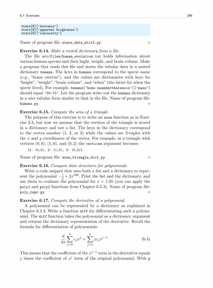
6.7 Exercises 299

stars[N][’distance’]stars[N][’apparent brightness’]stars[N][’luminosity’]

Name of program file: stars_data_dict2.py. ⋄

Exercise 6.14. Make a nested dictionary from a file.The file src/files/human_evolution.txt holds information about

various human species and their hight, weight, and brain volume. Makea program that reads this file and stores the tabular data in a nesteddictionary humans. The keys in humans correspond to the specie name(e.g., “homo erectus”), and the values are dictionaries with keys for“height”, “weight”, “brain volume”, and “when” (the latter for when thespecie lived). For example, humans[’homo neanderthalensis’][’mass’]

should equal ’55-70’. Let the program write out the humans dictionaryin a nice tabular form similar to that in the file. Name of program file:humans.py. ⋄

Exercise 6.15. Compute the area of a triangle.The purpose of this exercise is to write an area function as in Exer-

cise 3.3, but now we assume that the vertices of the triangle is storedin a dictionary and not a list. The keys in the dictionary correspondto the vertex number (1, 2, or 3) while the values are 2-tuples withthe x and y coordinates of the vertex. For example, in a triangle withvertices (0, 0), (1, 0), and (0, 2) the vertices argument becomes

1: (0,0), 2: (1,0), 3: (0,2)

Name of program file: area_triangle_dict.py. ⋄

Exercise 6.16. Compare data structures for polynomials.Write a code snippet that uses both a list and a dictionary to repre-

sent the polynomial −12 + 2x100. Print the list and the dictionary, and

use them to evaluate the polynomial for x = 1.05 (you can apply thepoly1 and poly2 functions from Chapter 6.2.3). Name of program file:poly_repr.py. ⋄

Exercise 6.17. Compute the derivative of a polynomial.A polynomial can be represented by a dictionary as explained in

Chapter 6.2.3. Write a function diff for differentiating such a polyno-mial. The diff function takes the polynomial as a dictionary argumentand returns the dictionary representation of the derivative. Recall theformula for differentiation of polynomials:

d

dx

n∑

j=0

cjxj =

n∑

j=1

jcjxj−1 . (6.4)

This means that the coefficient of the xj−1 term in the derivative equalsj times the coefficient of xj term of the original polynomial. With p

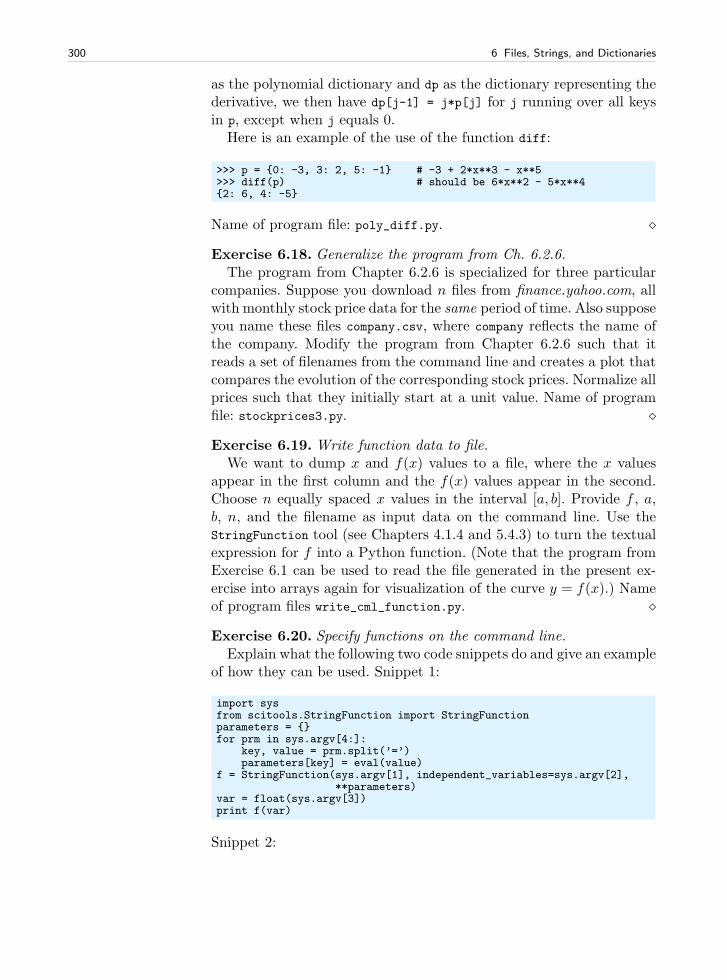
300 6 Files, Strings, and Dictionaries

as the polynomial dictionary and dp as the dictionary representing thederivative, we then have dp[j-1] = j*p[j] for j running over all keysin p, except when j equals 0.

Here is an example of the use of the function diff:

>>> p = 0: -3, 3: 2, 5: -1 # -3 + 2*x**3 - x**5>>> diff(p) # should be 6*x**2 - 5*x**42: 6, 4: -5

Name of program file: poly_diff.py. ⋄

Exercise 6.18. Generalize the program from Ch. 6.2.6.The program from Chapter 6.2.6 is specialized for three particular

companies. Suppose you download n files from finance.yahoo.com, allwith monthly stock price data for the same period of time. Also supposeyou name these files company.csv, where company reflects the name ofthe company. Modify the program from Chapter 6.2.6 such that itreads a set of filenames from the command line and creates a plot thatcompares the evolution of the corresponding stock prices. Normalize allprices such that they initially start at a unit value. Name of programfile: stockprices3.py. ⋄

Exercise 6.19. Write function data to file.We want to dump x and f(x) values to a file, where the x values

appear in the first column and the f(x) values appear in the second.Choose n equally spaced x values in the interval [a, b]. Provide f , a,b, n, and the filename as input data on the command line. Use theStringFunction tool (see Chapters 4.1.4 and 5.4.3) to turn the textualexpression for f into a Python function. (Note that the program fromExercise 6.1 can be used to read the file generated in the present ex-ercise into arrays again for visualization of the curve y = f(x).) Nameof program files write_cml_function.py. ⋄

Exercise 6.20. Specify functions on the command line.Explain what the following two code snippets do and give an example

of how they can be used. Snippet 1:

import sysfrom scitools.StringFunction import StringFunctionparameters = for prm in sys.argv[4:]:

key, value = prm.split(’=’)parameters[key] = eval(value)

f = StringFunction(sys.argv[1], independent_variables=sys.argv[2],**parameters)

var = float(sys.argv[3])print f(var)

Snippet 2:

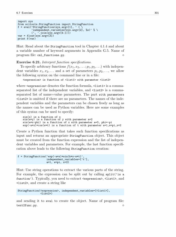
6.7 Exercises 301

import sysfrom scitools.StringFunction import StringFunctionf = eval(’StringFunction(sys.argv[1], ’ + \

’independent_variables=sys.argv[2], %s)’ % \(’, ’.join(sys.argv[4:])))

var = float(sys.argv[3])print f(var)

Hint: Read about the StringFunction tool in Chapter 4.1.4 and abouta variable number of keyword arguments in Appendix G.5. Name ofprogram file: cml_functions.py. ⋄

Exercise 6.21. Interpret function specifications.To specify arbitrary functions f(x1, x2, . . . ; p1, p2, . . .) with indepen-

dent variables x1, x2, . . . and a set of parameters p1, p2, . . ., we allowthe following syntax on the command line or in a file:

<expression> is function of <list1> with parameter <list2>

where <expression> denotes the function formula, <list1> is a comma-separated list of the independent variables, and <list2> is a comma-separated list of name=value parameters. The part with parameters

<list2> is omitted if there are no parameters. The names of the inde-pendent variables and the parameters can be chosen freely as long asthe names can be used as Python variables. Here are some examplesof this syntax can be used to specify:

sin(x) is a function of xsin(a*y) is a function of y with parameter a=2sin(a*x-phi) is a function of x with parameter a=3, phi=-piexp(-a*x)*cos(w*t) is a function of t with parameter a=1,w=pi,x=2

Create a Python function that takes such function specifications asinput and returns an appropriate StringFunction object. This objectmust be created from the function expression and the list of indepen-dent variables and parameters. For example, the last function specifi-cation above leads to the following StringFunction creation:

f = StringFunction(’exp(-a*x)*sin(k*x-w*t)’,independent_variables=[’t’],a=1, w=pi, x=2)

Hint: Use string operations to extract the various parts of the string.For example, the expression can be split out by calling split(’is a

function’). Typically, you need to extract <expression>, <list1>, and<list2>, and create a string like

StringFunction(<expression>, independent_variables=[<list1>],<list2>)

and sending it to eval to create the object. Name of program file:text2func.py. ⋄

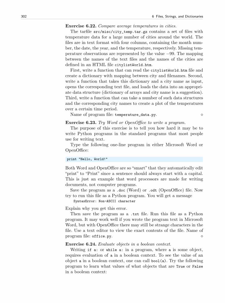
302 6 Files, Strings, and Dictionaries

Exercise 6.22. Compare average temperatures in cities.The tarfile src/misc/city_temp.tar.gz contains a set of files with

temperature data for a large number of cities around the world. Thefiles are in text format with four columns, containing the month num-ber, the date, the year, and the temperature, respectively. Missing tem-perature observations are represented by the value −99. The mappingbetween the names of the text files and the names of the cities aredefined in an HTML file citylistWorld.htm.

First, write a function that can read the citylistWorld.htm file andcreate a dictionary with mapping between city and filenames. Second,write a function that takes this dictionary and a city name as input,opens the corresponding text file, and loads the data into an appropri-ate data structure (dictionary of arrays and city name is a suggestion).Third, write a function that can take a number of such data structuresand the corresponding city names to create a plot of the temperaturesover a certain time period.

Name of program file: temperature_data.py. ⋄Exercise 6.23. Try Word or OpenOffice to write a program.

The purpose of this exercise is to tell you how hard it may be towrite Python programs in the standard programs that most peopleuse for writing text.

Type the following one-line program in either Microsoft Word orOpenOffice:

print "Hello, World!"

Both Word and OpenOffice are so“smart” that they automatically edit“print” to “Print” since a sentence should always start with a capital.This is just an example that word processors are made for writingdocuments, not computer programs.

Save the program as a .doc (Word) or .odt (OpenOffice) file. Nowtry to run this file as a Python program. You will get a message

SyntaxError: Non-ASCII character

Explain why you get this error.Then save the program as a .txt file. Run this file as a Python

program. It may work well if you wrote the program text in MicrosoftWord, but with OpenOffice there may still be strange characters in thefile. Use a text editor to view the exact contents of the file. Name ofprogram file: office.py. ⋄Exercise 6.24. Evaluate objects in a boolean context.

Writing if a: or while a: in a program, where a is some object,requires evaluation of a in a boolean context. To see the value of anobject a in a boolean context, one can call bool(a). Try the followingprogram to learn what values of what objects that are True or False

in a boolean context:

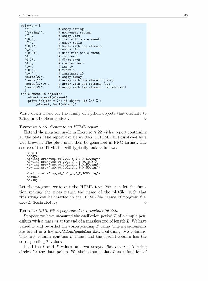
6.7 Exercises 303

objects = [’""’, # empty string’"string"’, # non-empty string’[]’, # empty list’[0]’, # list with one element’()’, # empty tuple’(0,)’, # tuple with one element’’, # empty dict’0:0’, # dict with one element’0’, # int zero’0.0’, # float zero’0j’, # complex zero’10’, # int 10’10.’, # float 10’10j’ # imaginary 10’zeros(0)’, # empty array’zeros(1)’, # array with one element (zero)’zeros(1)+10’, # array with one element (10)’zeros(2)’, # array with two elements (watch out!)]

for element in objects:object = eval(element)print ’object = %s; if object: is %s’ % \

(element, bool(object))

Write down a rule for the family of Python objects that evaluate toFalse in a boolean context. ⋄

Exercise 6.25. Generate an HTML report.Extend the program made in Exercise A.22 with a report containing

all the plots. The report can be written in HTML and displayed by aweb browser. The plots must then be generated in PNG format. Thesource of the HTML file will typically look as follows:

<html><body><p><img src="tmp_y0_0.01_q_0.1_N_50.png"><p><img src="tmp_y0_0.01_q_1_N_50.png"><p><img src="tmp_y0_0.01_q_1.5_N_50.png"><p><img src="tmp_y0_0.01_q_1.8_N_50.png">...<p><img src="tmp_y0_0.01_q_3_N_1000.png"></html></body>

Let the program write out the HTML text. You can let the func-tion making the plots return the name of the plotfile, such thatthis string can be inserted in the HTML file. Name of program file:growth_logistic4.py. ⋄

Exercise 6.26. Fit a polynomial to experimental data.Suppose we have measured the oscillation period T of a simple pen-

dulum with a mass m at the end of a massless rod of length L. We havevaried L and recorded the corresponding T value. The measurementsare found in a file src/files/pendulum.dat, containing two columns.The first column contains L values and the second column has thecorresponding T values.

Load the L and T values into two arrays. Plot L versus T usingcircles for the data points. We shall assume that L as a function of

304 6 Files, Strings, and Dictionaries

T is a polynomial. Use the NumPy utilities polyfit and poly1d, asexplained in Exercise 6.4, and experiment with fitting polynomials ofdegree 1, 2, and 3. Visualize the polynomial curves together with theexperimental data. Which polynomial fits the measured data best?Name of program file: fit_pendulum_data.py. ⋄Exercise 6.27. Generate an HTML report with figures.

The goal of this exercise is to let a program write a report in HTMLformat containing the solution to Exercise 5.21 on page 234. First,include the program from that Exercises, with additional explainingtext if necessary. Program code can be placed inside <pre> and </pre>

tags. Second, insert three plots of the f(x, t) function for three differentt values (find suitable t values that illustrate the displacement of thewave packet). Third, add an animated GIF file with the movie of f(x, t).Insert headlines (<h1> tags) wherever appropriate. Name of programfile: wavepacket_report.py. ⋄Exercise 6.28. Extract information from a weather page.

Find the Yahoo! page with the weather forecast for your favoritecity. Study the HTML source and write a program that downloadsthe HTML page, extracts forecast information such as weather type,temperature, etc. Write out this information in a compact style on thescreen. This exercise is a starter for the more useful Exercise 6.29 forcomparing alternative forecasts in a compact fashion. Name of programfile: Yahoo_weather.py. ⋄Exercise 6.29. Compare alternative weather forecasts.

For each of a collection of weather forecast sites, say

http://weather.yahoo.comhttp://www.weather.comhttp://www.weatherchannel.comhttp://weather.cnn.comhttp://yr.no

find the pages corresponding to your favorite location. Study theHTML sources and write a function for each HTML page that down-loads the web page and extracts basic forecast information: date,weather type (name of symbol), and temperature. Write out a com-parison of different forecasts on the screen. Name of program file:weather_forecast_comparison1.py. ⋄Exercise 6.30. Improve the output in Exercise 6.29.

Pure text on the screen was suggested as output in Exercise 6.29.A useful alternative is to construct an HTML page with compactforecast information, where also weather symbols (images) are dis-played. Extend each of the functions in Exercise 6.29 to also ex-tract the filename containing the weather symbol(s) and write thecode for presenting the comparison in HTML. Name of program file:weather_forecast_comparison2.py. ⋄

Introduction to Classes 7

A class packs a set of data (variables) together with a set of func-tions operating on the data. The goal is to achieve more modular codeby grouping data and functions into manageable (often small) units.Most of the mathematical computations in this book can easily becoded without using classes, but in many problems, classes enable ei-ther more elegant solutions or code that is easier to extend at a laterstage. In the non-mathematical world, where there are no mathemat-ical concepts and associated algorithms to help structure the problemsolving, software development can be very challenging. Classes maythen improve the understanding of the problem and contribute to sim-plify the modeling of data and actions in programs. As a consequence,almost all large software systems being developed in the world todayare heavily based on classes.

Programming with classes is offered by most modern programminglanguages, also Python. In fact, Python employs classes to a very largeextent, but one can – as we have seen in previous chapters – use thelanguage for lots of purposes without knowing what a class is. However,one will frequently encounter the class concept when searching booksor the World Wide Web for Python programming information. Andmore important, classes often provide better solutions to programmingproblems. This chapter therefore gives an introduction to the classconcept with emphasis on applications to numerical computing. Moreadvanced use of classes, including inheritance and object orientation,is the subject of Chapter 9.

The folder src/class contains all the program examples from thepresent chapter.

305

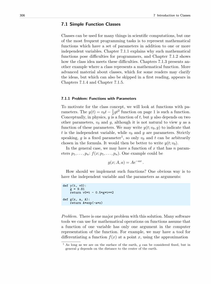
306 7 Introduction to Classes

7.1 Simple Function Classes

Classes can be used for many things in scientific computations, but oneof the most frequent programming tasks is to represent mathematicalfunctions which have a set of parameters in addition to one or moreindependent variables. Chapter 7.1.1 explains why such mathematicalfunctions pose difficulties for programmers, and Chapter 7.1.2 showshow the class idea meets these difficulties. Chapters 7.1.3 presents an-other example where a class represents a mathematical function. Moreadvanced material about classes, which for some readers may clarifythe ideas, but which can also be skipped in a first reading, appears inChapters 7.1.4 and Chapter 7.1.5.

7.1.1 Problem: Functions with Parameters

To motivate for the class concept, we will look at functions with pa-rameters. The y(t) = v0t− 1

2gt2 function on page 1 is such a function.

Conceptually, in physics, y is a function of t, but y also depends on twoother parameters, v0 and g, although it is not natural to view y as afunction of these parameters. We may write y(t; v0, g) to indicate thatt is the independent variable, while v0 and g are parameters. Strictlyspeaking, g is a fixed parameter1, so only v0 and t can be arbitrarilychosen in the formula. It would then be better to write y(t; v0).

In the general case, we may have a function of x that has n param-eters p1, . . . , pn: f(x; p1, . . . , pn). One example could be

g(x;A, a) = Ae−ax .

How should we implement such functions? One obvious way is tohave the independent variable and the parameters as arguments:

def y(t, v0):g = 9.81return v0*t - 0.5*g*t**2

def g(x, a, A):return A*exp(-a*x)

Problem. There is one major problem with this solution. Many softwaretools we can use for mathematical operations on functions assume thata function of one variable has only one argument in the computerrepresentation of the function. For example, we may have a tool fordifferentiating a function f(x) at a point x, using the approximation

1 As long as we are on the surface of the earth, g can be considered fixed, but ingeneral g depends on the distance to the center of the earth.

7.1 Simple Function Classes 307

f ′(x) ≈ f(x+ h)− f(x)

h(7.1)

coded as

def diff(f, x, h=1E-5):return (f(x+h) - f(x))/h

The diff function works with any function f that takes one argument:

def h(t):return t**4 + 4*t

dh = diff(h, 0.1)

from math import sin, pix = 2*pidsin = diff(sin, x, h=1E-6)

Unfortunately, diff will not work with our y(t, v0) function. Callingdiff(y, t) leads to an error inside the diff function, because it triesto call our y function with only one argument while the y functionrequires two.

Writing an alternative diff function for f functions having two ar-guments is a bad remedy as it restricts the set of admissible f functionsto the very special case of a function with one independent variable andone parameter. A fundamental principle in computer programming isto strive for software that is as general and widely applicable as pos-sible. In the present case, it means that the diff function should beapplicable to all functions f of one variable, and letting f take oneargument is then the natural decision to make.

The mismatch of function arguments, as outlined above, is a majorproblem because a lot of software libraries are available for operationson mathematical functions of one variable: integration, differentiation,solving f(x) = 0, finding extrema, etc. (see for instance Chapter 4.6.2and Appendices A.1.9, B, C, and E). All these libraries will try to callthe mathematical function we provide with only one argument.

A Bad Solution: Global Variables. The requirement is thus to de-fine Python implementations of mathematical functions of one variablewith one argument, the independent variable. The two examples abovemust then be implemented as

def y(t):g = 9.81return v0*t - 0.5*g*t**2

def g(t):return A*exp(-a*x)

These functions work only if v0, A, and a are global variables, initializedbefore one attempts to call the functions. Here are two sample callswhere diff differentiates y and g:

308 7 Introduction to Classes

v0 = 3dy = diff(y, 1)

A = 1; a = 0.1dg = diff(g, 1.5)

The use of global variables is in general considered bad program-ming. Why global variables are problematic in the present case can beillustrated when there is need to work with several versions of a func-tion. Suppose we want to work with two versions of y(t; v0), one withv0 = 1 and one with v0 = 5. Every time we call y we must rememberwhich version of the function we work with, and set v0 accordinglyprior to the call:

v0 = 1; r1 = y(t)v0 = 5; r2 = y(t)

Another problem is that variables with simple names like v0, a, andA may easily be used as global variables in other parts of the program.These parts may change our v0 in a context different from the y func-tion, but the change affects the correctness of the y function. In sucha case, we say that changing v0 has side effects, i.e., the change affectsother parts of the program in an unintentional way. This is one reasonwhy a golden rule of programming tells us to limit the use of globalvariables as much as possible.

Another solution to the problem of needing two v0 parameters couldbe to introduce two y functions, each with a distinct v0 parameter:

def y1(t):g = 9.81return v0_1*t - 0.5*g*t**2

def y2(t):g = 9.81return v0_2*t - 0.5*g*t**2

Now we need to initialize v0_1 and v0_2 once, and then we can workwith y1 and y2. However, if we need 100 v0 parameters, we need 100functions. This is tedious to code, error prone, difficult to administer,and simply a really bad solution to a programming problem.

So, is there a good remedy? The answer is yes: The class conceptsolves all the problems described above!

7.1.2 Representing a Function as a Class

A class contains a set of variables (data) and a set of functions, heldtogether as one unit. The variables are visible in all the functions in theclass. That is, we can view the variables as “global” in these functions.These characteristics also apply to modules, and modules can be usedto obtain many of the same advantages as classes offer (see comments

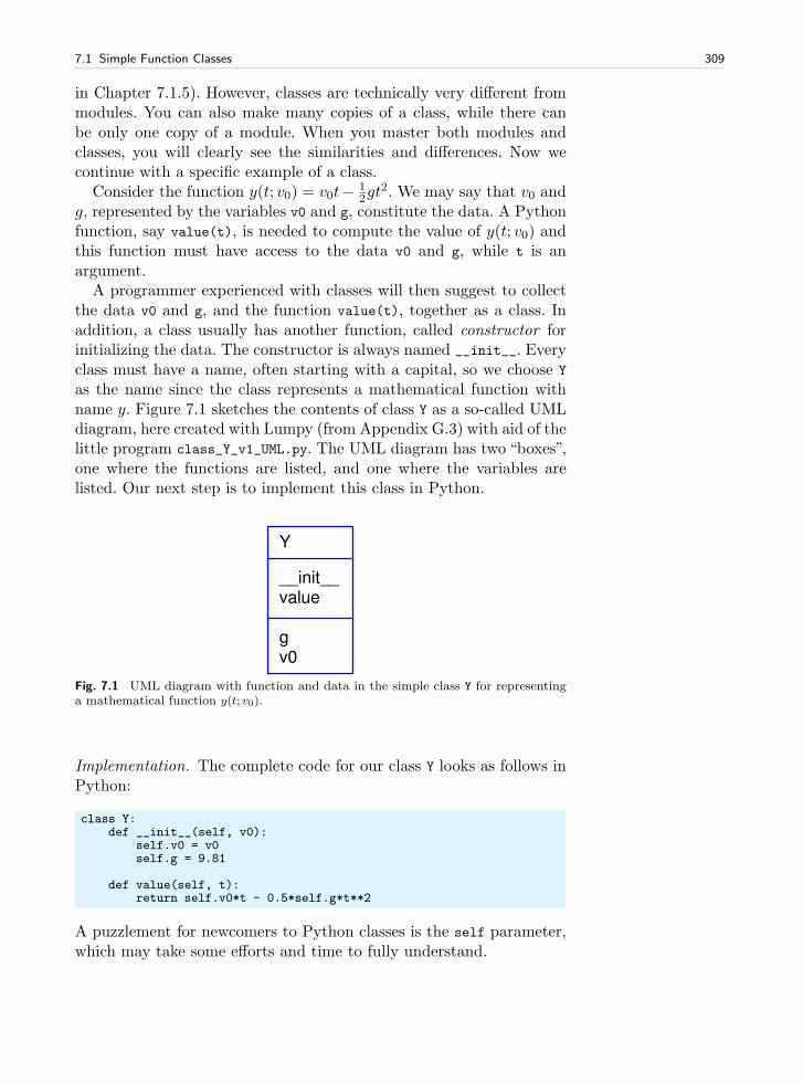
7.1 Simple Function Classes 309

in Chapter 7.1.5). However, classes are technically very different frommodules. You can also make many copies of a class, while there canbe only one copy of a module. When you master both modules andclasses, you will clearly see the similarities and differences. Now wecontinue with a specific example of a class.

Consider the function y(t; v0) = v0t− 12gt

2. We may say that v0 andg, represented by the variables v0 and g, constitute the data. A Pythonfunction, say value(t), is needed to compute the value of y(t; v0) andthis function must have access to the data v0 and g, while t is anargument.

A programmer experienced with classes will then suggest to collectthe data v0 and g, and the function value(t), together as a class. Inaddition, a class usually has another function, called constructor forinitializing the data. The constructor is always named __init__. Everyclass must have a name, often starting with a capital, so we choose Y

as the name since the class represents a mathematical function withname y. Figure 7.1 sketches the contents of class Y as a so-called UMLdiagram, here created with Lumpy (from Appendix G.3) with aid of thelittle program class_Y_v1_UML.py. The UML diagram has two “boxes”,one where the functions are listed, and one where the variables arelisted. Our next step is to implement this class in Python.

Y

__init__value

gv0

Fig. 7.1 UML diagram with function and data in the simple class Y for representinga mathematical function y(t; v0).

Implementation. The complete code for our class Y looks as follows inPython:

class Y:def __init__(self, v0):

self.v0 = v0self.g = 9.81

def value(self, t):return self.v0*t - 0.5*self.g*t**2

A puzzlement for newcomers to Python classes is the self parameter,which may take some efforts and time to fully understand.

310 7 Introduction to Classes

Usage and Dissection. Before we dig into what each in the class im-plementation means, we start by showing how the class can be used tocompute values of the mathematical function y(t; v0).

A class creates a new data type, here of name Y, so when we usethe class to make objects, those objects are of type Y2. An object of auser-defined class (like Y) is usually called an instance. We need suchan instance in order to use the data in the class and call the value

function. The following statement constructs an instance bound to thevariable name y:

y = Y(3)

Seemingly, we call the class Y as if it were a function. Actually, Y(3)is automatically translated by Python to a call to the constructor__init__ in class Y. The arguments in the call, here only the num-ber 3, are always passed on as arguments to __init__ after the self

argument. That is, v0 gets the value 3 and self is just dropped in thecall. This may be confusing, but it is a rule that the self argument isnever used in calls to functions in classes.

With the instance y, we can compute the value y(t = 0.1; v0 = 3) bythe statement

v = y.value(0.1)

Here also, the self argument is dropped in the call to value. To accessfunctions and variables in a class, we must prefix the function and vari-able names by the name of the instance and a dot: the value functionis reached as y.value, and the variables are reached as y.v0 and y.g.We can, for example, print the value of v0 in the instance y by writing

print y.v0

The output will in this case be 3.We have already introduced the term “instance” for the object of

a class. Functions in classes are commonly called methods , and vari-ables (data) in classes are called attributes. From now on we will usethis terminology. In our sample class Y we have two methods, __init__and value, and two attributes, v0 and g. The names of methods andattributes can be chosen freely, just as names of ordinary Python func-tions and variables. However, the constructor must have the name__init__, otherwise it is not automatically called when we create newinstances.

You can do whatever you want in whatever method, but it is aconvention to use the constructor for initializing the variables in theclass such that the class is “ready for use”.

2 All familiar Python objects, like lists, tuples, strings, floating-point numbers, inte-gers, etc., are in fact built-in Python classes, with names list, tuple, str, float,int, etc.

7.1 Simple Function Classes 311

The self Variable. Now we will provide some more explanation of theself parameter and how the class methods work. Inside the constructor__init__, the argument self is a variable holding the new instance tobe constructed. When we write

self.v0 = v0self.g = 9.81

we define two new attributes in this instance. The self parameter isinvisibly returned to the calling code. We can imagine that Pythontranslates y = Y(3) to

Y.__init__(y, 3)

so when we do a self.v0 = v0 in the constructor, we actually initializey.v0. The prefix with Y. is necessary to reach a class method (just likeprefixing a function in a module with the module name, e.g., math.exp).If we prefix with Y., we need to explicitly feed in an instance for theself argument, like y in the code line above, but if we prefix withy. (the instance name) the self argument is dropped. It is the latter“instance name prefix”which we shall use when computing with classes.

Let us look at a call to the value method to see a similar use of theself argument. When we write

value = y.value(0.1)

Python translates this to a call

value = Y.value(y, 0.1)

such that the self argument in the value method becomes the y in-stance. In the expression inside the value method,

self.v0*t - 0.5*self.g*t**2

self is y so this is the same as

y.v0*t - 0.5*y.g*t**2

The rules regarding “self” are listed below:

Any class method must have self as first argument3. self represents an (arbitrary) instance of the class. To access another class method or a class attribute, inside classmethods, we must prefix with self, as in self.name, where name isthe name of the attribute or the other method.

self is dropped as argument in calls to class methods.

3 The name can be any valid variable name, but the name self is a widely establishedconvention in Python.

312 7 Introduction to Classes

It takes some time to understand the self variable, but more examplesand hands-on experience with class programming will help, so just bepatient and continue reading.

Extension of the Class. We can have as many attributes and methodsas we like in a class, so let us add a new method to class Y. Thismethod is called formula and prints a string containing the formula ofthe mathematical function y. After this formula, we provide the valueof v0. The string can then be constructed as

’v0*t - 0.5*g*t**2; v0=%g’ % self.v0

where self is an instance of class Y. A call of formula does not needany arguments:

print y.formula()

should be enough to create, return, and print the string. However, evenif the formulamethod does not need any arguments, it must have a self

argument, which is left out in the call but needed inside the method toaccess the attributes. The implementation of the method is therefore

def formula(self):return ’v0*t - 0.5*g*t**2; v0=%g’ % self.v0

For completeness, the whole class now reads

class Y:def __init__(self, v0):

self.v0 = v0self.g = 9.81

def value(self, t):return self.v0*t - 0.5*self.g*t**2

def formula(self):return ’v0*t - 0.5*g*t**2; v0=%g’ % self.v0

Example on use may be

y = Y(5)t = 0.2v = y.value(t)print ’y(t=%g; v0=%g) = %g’ % (t, y.v0, v)print y.formula()

with the output

y(t=0.2; v0=5) = 0.8038v0*t - 0.5*g*t**2; v0=5

Remark. A common mistake done by newcomers to the class construc-tion is to place the code that applies the class at the same indentationas the class methods. This is illegal. Only method definitions and as-signments to so-called static attributes (Chapter 7.6) can appear in

7.1 Simple Function Classes 313

the indented block under the class headline. Ordinary attribute as-signment must be done inside methods. The main program using theclass must appear with the same indent as the class headline.

Using Methods as Ordinary Functions. We may create several y func-tions with different values of v0:

y1 = Y(1)y2 = Y(1.5)y3 = Y(-3)

We can treat y1.value, y2.value, and y3.value as ordinary Pythonfunctions of t, and then pass them on to any Python function thatexpects a function of one variable. In particular, we can send the func-tions to the diff(f, x) function from page 307:

dy1dt = diff(y1.value, 0.1)dy2dt = diff(y2.value, 0.1)dy3dt = diff(y3.value, 0.2)

Inside the diff(f, x) function, the argument f now behaves as a func-tion of one variable that automatically carries with it two variables v0and g. When f refers to (e.g.) y3.value, Python actually knows thatf(x) means y3.value(x), and inside the y3.value method self is y3,and we have access to y3.v0 and y3.g.

Doc Strings. A function may have a doc string right after the functiondefinition, see Chapter 3.1.7. The aim of the doc string is to explainthe purpose of the function and, for instance, what the arguments andreturn values are. A class can also have a doc string, it is just the firststring that appears right after the class headline. The convention isto enclose the doc string in triple double quotes """:

class Y:"""The vertical motion of a ball."""

def __init__(self, v0):...

More comprehensive information can include the methods and how theclass is used in an interactive session:

class Y:"""Mathematical function for the vertical motion of a ball.

Methods:constructor(v0): set initial velocity v0.value(t): compute the height as function of t.formula(): print out the formula for the height.

Attributes:v0: the initial velocity of the ball (time 0).g: acceleration of gravity (fixed).

314 7 Introduction to Classes

Usage:>>> y = Y(3)>>> position1 = y.value(0.1)>>> position2 = y.value(0.3)>>> print y.formula()v0*t - 0.5*g*t**2; v0=3"""

7.1.3 Another Function Class Example

Let us apply the ideas from the Y class to the v(r) function specifiedin (5.23) on page 238. We may write this function as v(r; β, µ0, n, R)to indicate that there is one primary independent variable (r) and fourphysical parameters (β, µ0, n, and R). The class typically holds thephysical parameters as variables and provides an value(r) method forcomputing the v function:

class VelocityProfile:def __init__(self, beta, mu0, n, R):

self.beta, self.mu0, self.n, self.R = beta, mu0, n, R

def value(self, r):beta, mu0, n, R = self.beta, self.mu0, self.n, self.Rn = float(n) # ensure float divisionsv = (beta/(2.0*mu0))**(1/n)*(n/(n+1))*\

(R**(1+1/n) - r**(1+1/n))return v

There is seemingly one new thing here in that we initialize severalvariables on the same line4:

self.beta, self.mu0, self.n, self.R = beta, mu0, n, R

This is perfectly valid Python code and equivalent to the multi-linecode

self.beta = betaself.mu0 = mu0self.n = nself.R = R

In the value method it is convenient to avoid the self. prefix in themathematical formulas and instead introduce the local short namesbeta, mu0, n, and R. This is in general a good idea, because it makes iteasier to read the implementation of the formula and check its correct-ness.

Here is one possible application of class VelocityProfile:

4 The comma-separated list of variables on the right-hand side forms a tuple so thisassignment is just the usual construction where a set of variables on the left-handside is set equal to a list or tuple on the right-hand side, element by element. Seepage 60.

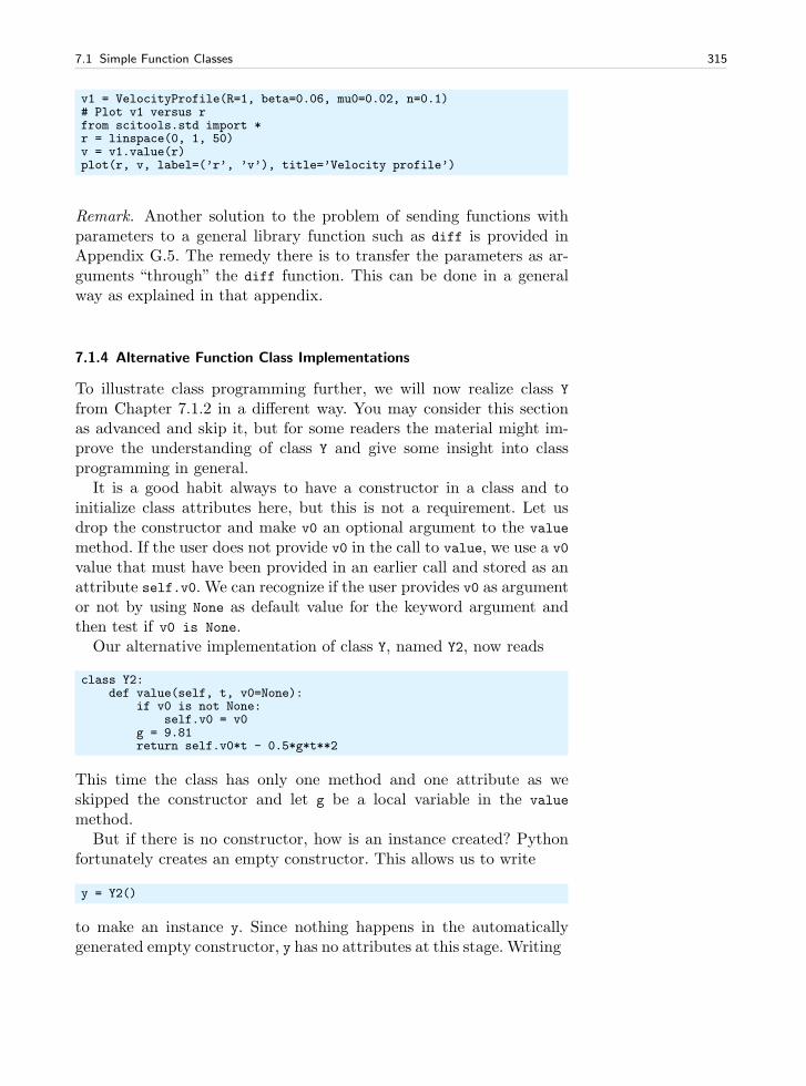
7.1 Simple Function Classes 315

v1 = VelocityProfile(R=1, beta=0.06, mu0=0.02, n=0.1)# Plot v1 versus rfrom scitools.std import *r = linspace(0, 1, 50)v = v1.value(r)plot(r, v, label=(’r’, ’v’), title=’Velocity profile’)

Remark. Another solution to the problem of sending functions withparameters to a general library function such as diff is provided inAppendix G.5. The remedy there is to transfer the parameters as ar-guments “through” the diff function. This can be done in a generalway as explained in that appendix.

7.1.4 Alternative Function Class Implementations

To illustrate class programming further, we will now realize class Y

from Chapter 7.1.2 in a different way. You may consider this sectionas advanced and skip it, but for some readers the material might im-prove the understanding of class Y and give some insight into classprogramming in general.

It is a good habit always to have a constructor in a class and toinitialize class attributes here, but this is not a requirement. Let usdrop the constructor and make v0 an optional argument to the value

method. If the user does not provide v0 in the call to value, we use a v0

value that must have been provided in an earlier call and stored as anattribute self.v0. We can recognize if the user provides v0 as argumentor not by using None as default value for the keyword argument andthen test if v0 is None.

Our alternative implementation of class Y, named Y2, now reads

class Y2:def value(self, t, v0=None):

if v0 is not None:self.v0 = v0

g = 9.81return self.v0*t - 0.5*g*t**2

This time the class has only one method and one attribute as weskipped the constructor and let g be a local variable in the value

method.But if there is no constructor, how is an instance created? Python

fortunately creates an empty constructor. This allows us to write

y = Y2()

to make an instance y. Since nothing happens in the automaticallygenerated empty constructor, y has no attributes at this stage. Writing

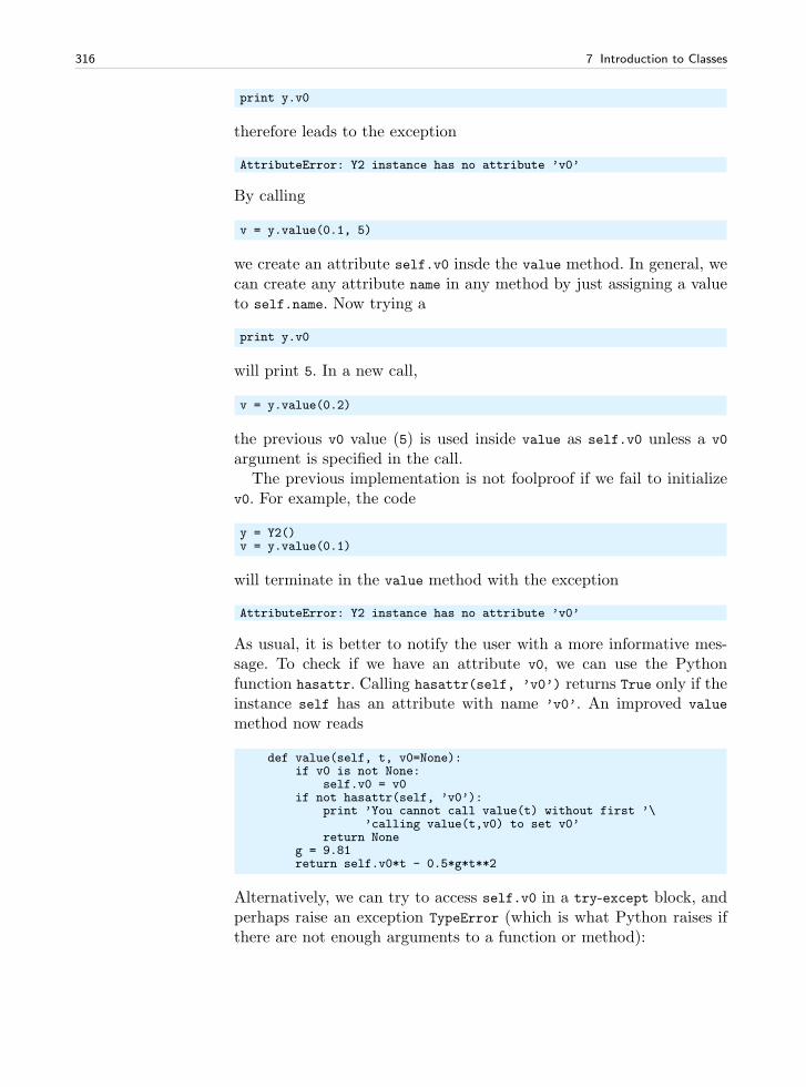
316 7 Introduction to Classes

print y.v0

therefore leads to the exception

AttributeError: Y2 instance has no attribute ’v0’

By calling

v = y.value(0.1, 5)

we create an attribute self.v0 insde the value method. In general, wecan create any attribute name in any method by just assigning a valueto self.name. Now trying a

print y.v0

will print 5. In a new call,

v = y.value(0.2)

the previous v0 value (5) is used inside value as self.v0 unless a v0

argument is specified in the call.The previous implementation is not foolproof if we fail to initialize

v0. For example, the code

y = Y2()v = y.value(0.1)

will terminate in the value method with the exception

AttributeError: Y2 instance has no attribute ’v0’

As usual, it is better to notify the user with a more informative mes-sage. To check if we have an attribute v0, we can use the Pythonfunction hasattr. Calling hasattr(self, ’v0’) returns True only if theinstance self has an attribute with name ’v0’. An improved value

method now reads

def value(self, t, v0=None):if v0 is not None:

self.v0 = v0if not hasattr(self, ’v0’):

print ’You cannot call value(t) without first ’\’calling value(t,v0) to set v0’

return Noneg = 9.81return self.v0*t - 0.5*g*t**2

Alternatively, we can try to access self.v0 in a try-except block, andperhaps raise an exception TypeError (which is what Python raises ifthere are not enough arguments to a function or method):

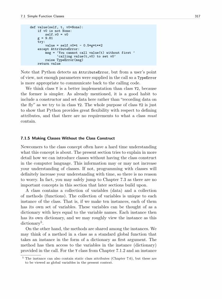
7.1 Simple Function Classes 317

def value(self, t, v0=None):if v0 is not None:

self.v0 = v0g = 9.81try:

value = self.v0*t - 0.5*g*t**2except AttributeError:

msg = ’You cannot call value(t) without first ’’calling value(t,v0) to set v0’

raise TypeError(msg)return value

Note that Python detects an AttributeError, but from a user’s pointof view, not enough parameters were supplied in the call so a TypeError

is more appropriate to communicate back to the calling code.We think class Y is a better implementation than class Y2, because

the former is simpler. As already mentioned, it is a good habit toinclude a constructor and set data here rather than “recording data onthe fly” as we try to in class Y2. The whole purpose of class Y2 is justto show that Python provides great flexibility with respect to definingattributes, and that there are no requirements to what a class mustcontain.

7.1.5 Making Classes Without the Class Construct

Newcomers to the class conecpt often have a hard time understandingwhat this concept is about. The present section tries to explain in moredetail how we can introduce classes without having the class constructin the computer language. This information may or may not increaseyour understanding of classes. If not, programming with classes willdefinitely increase your understanding with time, so there is no reasonto worry. In fact, you may safely jump to Chapter 7.3 as there are noimportant concepts in this section that later sections build upon.

A class contains a collection of variables (data) and a collectionof methods (functions). The collection of variables is unique to eachinstance of the class. That is, if we make ten instances, each of themhas its own set of variables. These variables can be thought of as adictionary with keys equal to the variable names. Each instance thenhas its own dictionary, and we may roughly view the instance as thisdictionary5.

On the other hand, the methods are shared among the instances. Wemay think of a method in a class as a standard global function thattakes an instance in the form of a dictionary as first argument. Themethod has then access to the variables in the instance (dictionary)provided in the call. For the Y class from Chapter 7.1.2 and an instance

5 The instance can also contain static class attributes (Chapter 7.6), but these areto be viewed as global variables in the present context.

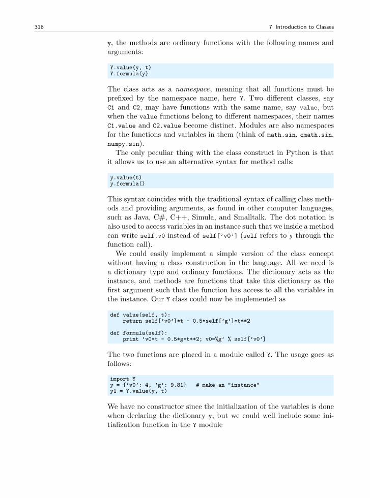
318 7 Introduction to Classes

y, the methods are ordinary functions with the following names andarguments:

Y.value(y, t)Y.formula(y)

The class acts as a namespace, meaning that all functions must beprefixed by the namespace name, here Y. Two different classes, sayC1 and C2, may have functions with the same name, say value, butwhen the value functions belong to different namespaces, their namesC1.value and C2.value become distinct. Modules are also namespacesfor the functions and variables in them (think of math.sin, cmath.sin,numpy.sin).

The only peculiar thing with the class construct in Python is thatit allows us to use an alternative syntax for method calls:

y.value(t)y.formula()

This syntax coincides with the traditional syntax of calling class meth-ods and providing arguments, as found in other computer languages,such as Java, C#, C++, Simula, and Smalltalk. The dot notation isalso used to access variables in an instance such that we inside a methodcan write self.v0 instead of self[’v0’] (self refers to y through thefunction call).

We could easily implement a simple version of the class conceptwithout having a class construction in the language. All we need isa dictionary type and ordinary functions. The dictionary acts as theinstance, and methods are functions that take this dictionary as thefirst argument such that the function has access to all the variables inthe instance. Our Y class could now be implemented as

def value(self, t):return self[’v0’]*t - 0.5*self[’g’]*t**2

def formula(self):print ’v0*t - 0.5*g*t**2; v0=%g’ % self[’v0’]

The two functions are placed in a module called Y. The usage goes asfollows:

import Yy = ’v0’: 4, ’g’: 9.81 # make an "instance"y1 = Y.value(y, t)

We have no constructor since the initialization of the variables is donewhen declaring the dictionary y, but we could well include some ini-tialization function in the Y module

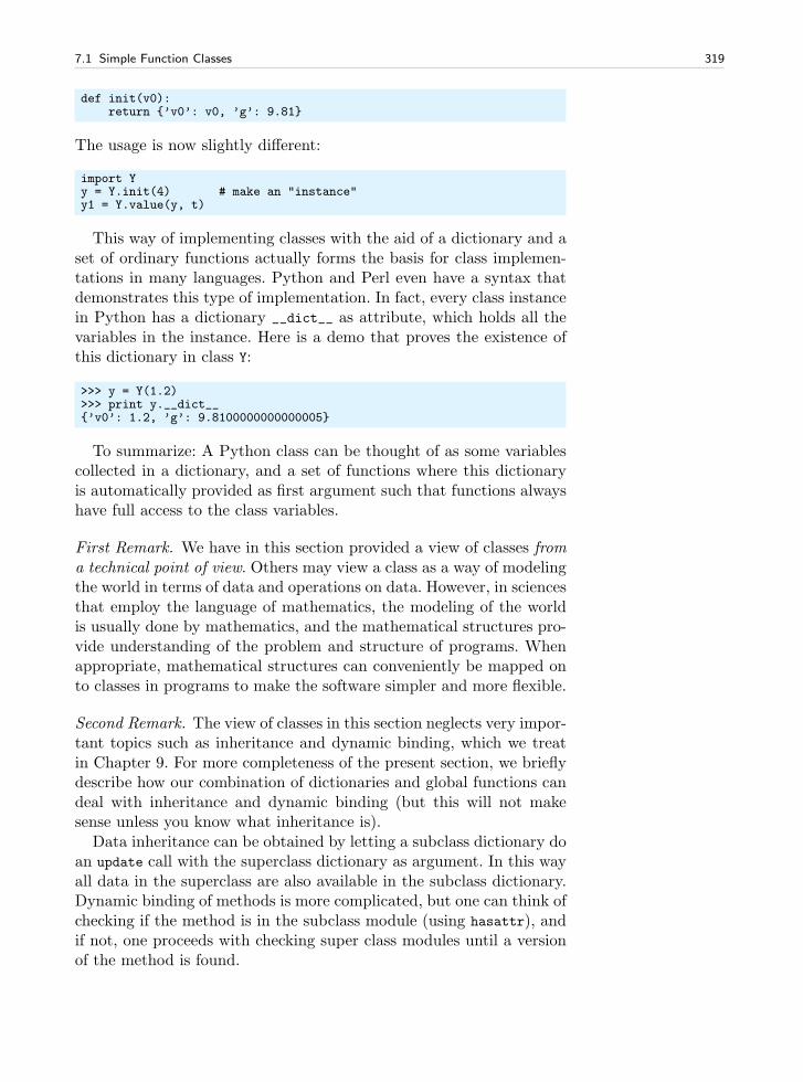
7.1 Simple Function Classes 319

def init(v0):return ’v0’: v0, ’g’: 9.81

The usage is now slightly different:

import Yy = Y.init(4) # make an "instance"y1 = Y.value(y, t)

This way of implementing classes with the aid of a dictionary and aset of ordinary functions actually forms the basis for class implemen-tations in many languages. Python and Perl even have a syntax thatdemonstrates this type of implementation. In fact, every class instancein Python has a dictionary __dict__ as attribute, which holds all thevariables in the instance. Here is a demo that proves the existence ofthis dictionary in class Y:

>>> y = Y(1.2)>>> print y.__dict__’v0’: 1.2, ’g’: 9.8100000000000005

To summarize: A Python class can be thought of as some variablescollected in a dictionary, and a set of functions where this dictionaryis automatically provided as first argument such that functions alwayshave full access to the class variables.

First Remark. We have in this section provided a view of classes froma technical point of view. Others may view a class as a way of modelingthe world in terms of data and operations on data. However, in sciencesthat employ the language of mathematics, the modeling of the worldis usually done by mathematics, and the mathematical structures pro-vide understanding of the problem and structure of programs. Whenappropriate, mathematical structures can conveniently be mapped onto classes in programs to make the software simpler and more flexible.

Second Remark. The view of classes in this section neglects very impor-tant topics such as inheritance and dynamic binding, which we treatin Chapter 9. For more completeness of the present section, we brieflydescribe how our combination of dictionaries and global functions candeal with inheritance and dynamic binding (but this will not makesense unless you know what inheritance is).

Data inheritance can be obtained by letting a subclass dictionary doan update call with the superclass dictionary as argument. In this wayall data in the superclass are also available in the subclass dictionary.Dynamic binding of methods is more complicated, but one can think ofchecking if the method is in the subclass module (using hasattr), andif not, one proceeds with checking super class modules until a versionof the method is found.

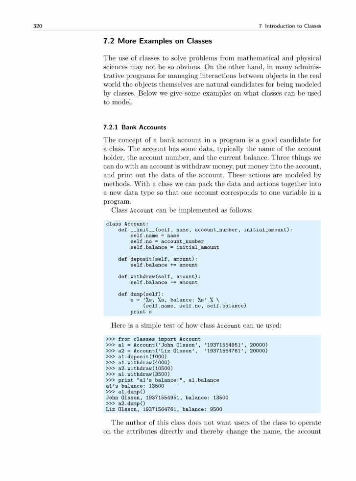
320 7 Introduction to Classes

7.2 More Examples on Classes

The use of classes to solve problems from mathematical and physicalsciences may not be so obvious. On the other hand, in many adminis-trative programs for managing interactions between objects in the realworld the objects themselves are natural candidates for being modeledby classes. Below we give some examples on what classes can be usedto model.

7.2.1 Bank Accounts

The concept of a bank account in a program is a good candidate fora class. The account has some data, typically the name of the accountholder, the account number, and the current balance. Three things wecan do with an account is withdraw money, put money into the account,and print out the data of the account. These actions are modeled bymethods. With a class we can pack the data and actions together intoa new data type so that one account corresponds to one variable in aprogram.

Class Account can be implemented as follows:

class Account:def __init__(self, name, account_number, initial_amount):

self.name = nameself.no = account_numberself.balance = initial_amount

def deposit(self, amount):self.balance += amount

def withdraw(self, amount):self.balance -= amount

def dump(self):s = ’%s, %s, balance: %s’ % \

(self.name, self.no, self.balance)print s

Here is a simple test of how class Account can ue used:

>>> from classes import Account>>> a1 = Account(’John Olsson’, ’19371554951’, 20000)>>> a2 = Account(’Liz Olsson’, ’19371564761’, 20000)>>> a1.deposit(1000)>>> a1.withdraw(4000)>>> a2.withdraw(10500)>>> a1.withdraw(3500)>>> print "a1’s balance:", a1.balancea1’s balance: 13500>>> a1.dump()John Olsson, 19371554951, balance: 13500>>> a2.dump()Liz Olsson, 19371564761, balance: 9500

The author of this class does not want users of the class to operateon the attributes directly and thereby change the name, the account

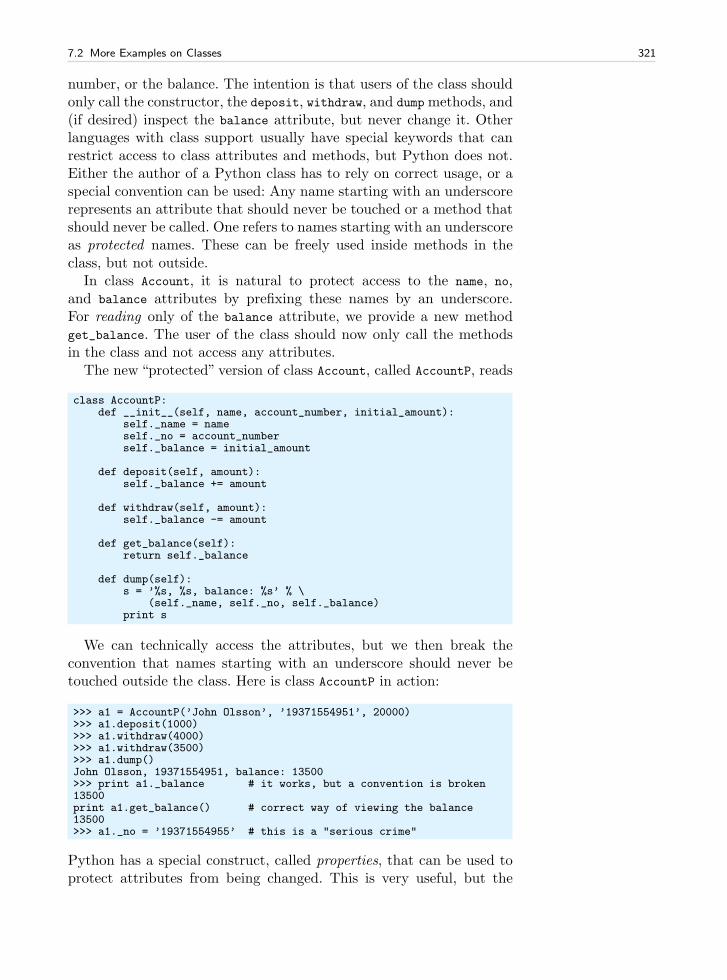
7.2 More Examples on Classes 321

number, or the balance. The intention is that users of the class shouldonly call the constructor, the deposit, withdraw, and dumpmethods, and(if desired) inspect the balance attribute, but never change it. Otherlanguages with class support usually have special keywords that canrestrict access to class attributes and methods, but Python does not.Either the author of a Python class has to rely on correct usage, or aspecial convention can be used: Any name starting with an underscorerepresents an attribute that should never be touched or a method thatshould never be called. One refers to names starting with an underscoreas protected names. These can be freely used inside methods in theclass, but not outside.

In class Account, it is natural to protect access to the name, no,and balance attributes by prefixing these names by an underscore.For reading only of the balance attribute, we provide a new methodget_balance. The user of the class should now only call the methodsin the class and not access any attributes.

The new “protected” version of class Account, called AccountP, reads

class AccountP:def __init__(self, name, account_number, initial_amount):

self._name = nameself._no = account_numberself._balance = initial_amount

def deposit(self, amount):self._balance += amount

def withdraw(self, amount):self._balance -= amount

def get_balance(self):return self._balance

def dump(self):s = ’%s, %s, balance: %s’ % \

(self._name, self._no, self._balance)print s

We can technically access the attributes, but we then break theconvention that names starting with an underscore should never betouched outside the class. Here is class AccountP in action:

>>> a1 = AccountP(’John Olsson’, ’19371554951’, 20000)>>> a1.deposit(1000)>>> a1.withdraw(4000)>>> a1.withdraw(3500)>>> a1.dump()John Olsson, 19371554951, balance: 13500>>> print a1._balance # it works, but a convention is broken13500print a1.get_balance() # correct way of viewing the balance13500>>> a1._no = ’19371554955’ # this is a "serious crime"

Python has a special construct, called properties, that can be used toprotect attributes from being changed. This is very useful, but the

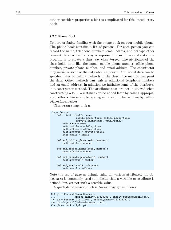
322 7 Introduction to Classes

author considers properties a bit too complicated for this introductorybook.

7.2.2 Phone Book

You are probably familiar with the phone book on your mobile phone.The phone book contains a list of persons. For each person you canrecord the name, telephone numbers, email adress, and perhaps otherrelevant data. A natural way of representing such personal data in aprogram is to create a class, say class Person. The attributes of theclass holds data like the name, mobile phone number, office phonenumber, private phone number, and email address. The constructormay initialize some of the data about a person. Additional data can bespecified later by calling methods in the class. One method can printthe data. Other methods can register additional telephone numbersand an email address. In addition we initialize some of the attributesin a constructor method. The attributes that are not initialized whenconstructing a Person instance can be added later by calling appropri-ate methods. For example, adding an office number is done by callingadd_office_number.

Class Person may look as

class Person:def __init__(self, name,

mobile_phone=None, office_phone=None,private_phone=None, email=None):

self.name = nameself.mobile = mobile_phoneself.office = office_phoneself.private = private_phoneself.email = email

def add_mobile_phone(self, number):self.mobile = number

def add_office_phone(self, number):self.office = number

def add_private_phone(self, number):self.private = number

def add_email(self, address):self.email = address

Note the use of None as default value for various attributes: the ob-ject None is commonly used to indicate that a variable or attribute isdefined, but yet not with a sensible value.

A quick demo session of class Person may go as follows:

>>> p1 = Person(’Hans Hanson’,... office_phone=’767828283’, email=’h@hanshanson.com’)>>> p2 = Person(’Ole Olsen’, office_phone=’767828292’)>>> p2.add_email(’olsen@somemail.net’)>>> phone_book = [p1, p2]

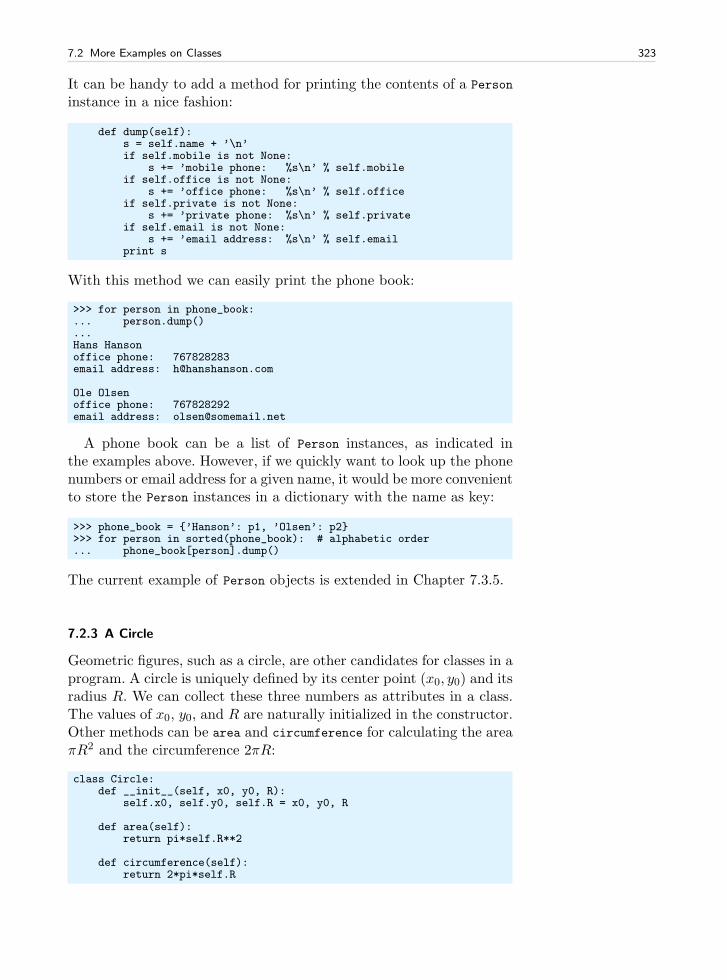
7.2 More Examples on Classes 323

It can be handy to add a method for printing the contents of a Person

instance in a nice fashion:

def dump(self):s = self.name + ’\n’if self.mobile is not None:

s += ’mobile phone: %s\n’ % self.mobileif self.office is not None:

s += ’office phone: %s\n’ % self.officeif self.private is not None:

s += ’private phone: %s\n’ % self.privateif self.email is not None:

s += ’email address: %s\n’ % self.emailprint s

With this method we can easily print the phone book:

>>> for person in phone_book:... person.dump()...Hans Hansonoffice phone: 767828283email address: h@hanshanson.com

Ole Olsenoffice phone: 767828292email address: olsen@somemail.net

A phone book can be a list of Person instances, as indicated inthe examples above. However, if we quickly want to look up the phonenumbers or email address for a given name, it would be more convenientto store the Person instances in a dictionary with the name as key:

>>> phone_book = ’Hanson’: p1, ’Olsen’: p2>>> for person in sorted(phone_book): # alphabetic order... phone_book[person].dump()

The current example of Person objects is extended in Chapter 7.3.5.

7.2.3 A Circle

Geometric figures, such as a circle, are other candidates for classes in aprogram. A circle is uniquely defined by its center point (x0, y0) and itsradius R. We can collect these three numbers as attributes in a class.The values of x0, y0, and R are naturally initialized in the constructor.Other methods can be area and circumference for calculating the areaπR2 and the circumference 2πR:

class Circle:def __init__(self, x0, y0, R):

self.x0, self.y0, self.R = x0, y0, R

def area(self):return pi*self.R**2

def circumference(self):return 2*pi*self.R

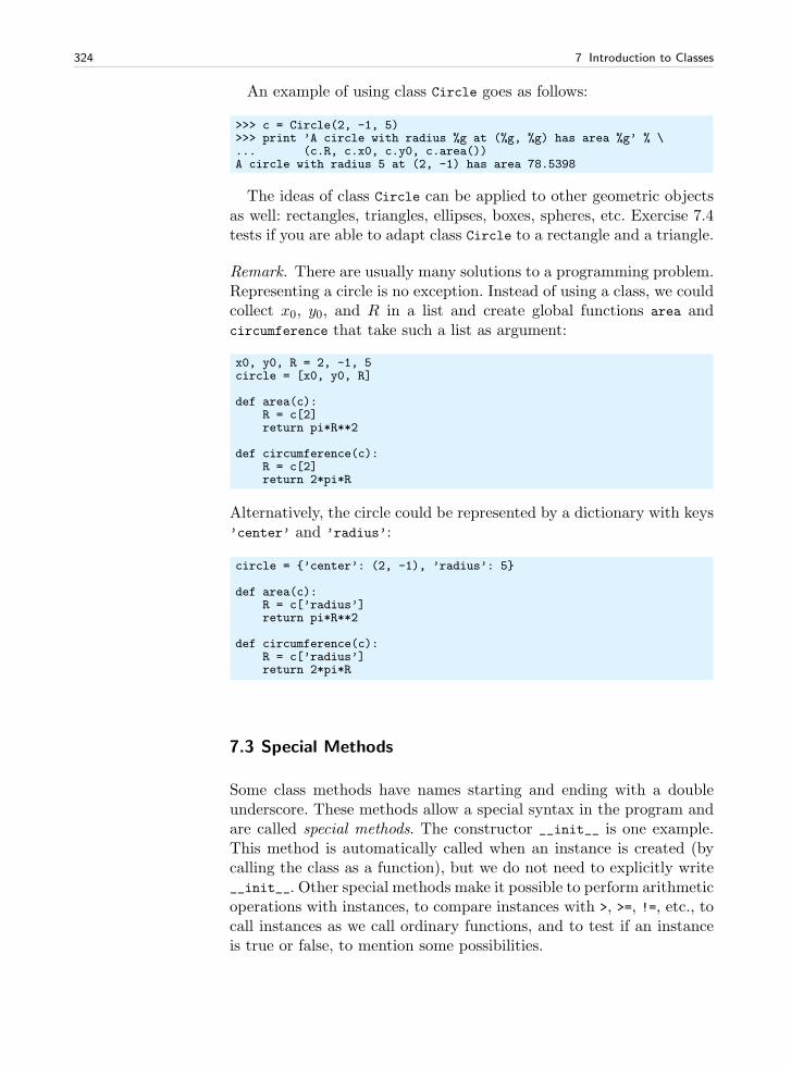
324 7 Introduction to Classes

An example of using class Circle goes as follows:

>>> c = Circle(2, -1, 5)>>> print ’A circle with radius %g at (%g, %g) has area %g’ % \... (c.R, c.x0, c.y0, c.area())A circle with radius 5 at (2, -1) has area 78.5398

The ideas of class Circle can be applied to other geometric objectsas well: rectangles, triangles, ellipses, boxes, spheres, etc. Exercise 7.4tests if you are able to adapt class Circle to a rectangle and a triangle.

Remark. There are usually many solutions to a programming problem.Representing a circle is no exception. Instead of using a class, we couldcollect x0, y0, and R in a list and create global functions area andcircumference that take such a list as argument:

x0, y0, R = 2, -1, 5circle = [x0, y0, R]

def area(c):R = c[2]return pi*R**2

def circumference(c):R = c[2]return 2*pi*R

Alternatively, the circle could be represented by a dictionary with keys’center’ and ’radius’:

circle = ’center’: (2, -1), ’radius’: 5

def area(c):R = c[’radius’]return pi*R**2

def circumference(c):R = c[’radius’]return 2*pi*R

7.3 Special Methods

Some class methods have names starting and ending with a doubleunderscore. These methods allow a special syntax in the program andare called special methods. The constructor __init__ is one example.This method is automatically called when an instance is created (bycalling the class as a function), but we do not need to explicitly write__init__. Other special methods make it possible to perform arithmeticoperations with instances, to compare instances with >, >=, !=, etc., tocall instances as we call ordinary functions, and to test if an instanceis true or false, to mention some possibilities.

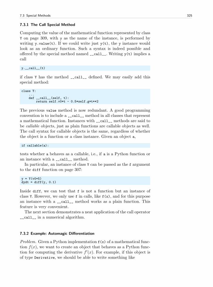
7.3 Special Methods 325

7.3.1 The Call Special Method

Computing the value of the mathematical function represented by classY on page 309, with y as the name of the instance, is performed bywriting y.value(t). If we could write just y(t), the y instance wouldlook as an ordinary function. Such a syntax is indeed possible andoffered by the special method named __call__. Writing y(t) implies acall

y.__call__(t)

if class Y has the method __call__ defined. We may easily add thisspecial method:

class Y:...def __call__(self, t):

return self.v0*t - 0.5*self.g*t**2

The previous value method is now redundant. A good programmingconvention is to include a __call__ method in all classes that representa mathematical function. Instances with __call__ methods are said tobe callable objects, just as plain functions are callable objects as well.The call syntax for callable objects is the same, regardless of whetherthe object is a function or a class instance. Given an object a,

if callable(a):

tests whether a behaves as a callable, i.e., if a is a Python function oran instance with a __call__ method.

In particular, an instance of class Y can be passed as the f argumentto the diff function on page 307:

y = Y(v0=5)dydt = diff(y, 0.1)

Inside diff, we can test that f is not a function but an instance ofclass Y. However, we only use f in calls, like f(x), and for this purposean instance with a __call__ method works as a plain function. Thisfeature is very convenient.

The next section demonstrates a neat application of the call operator__call__ in a numerical algorithm.

7.3.2 Example: Automagic Differentiation

Problem. Given a Python implementation f(x) of a mathematical func-tion f(x), we want to create an object that behaves as a Python func-tion for computing the derivative f ′(x). For example, if this object isof type Derivative, we should be able to write something like

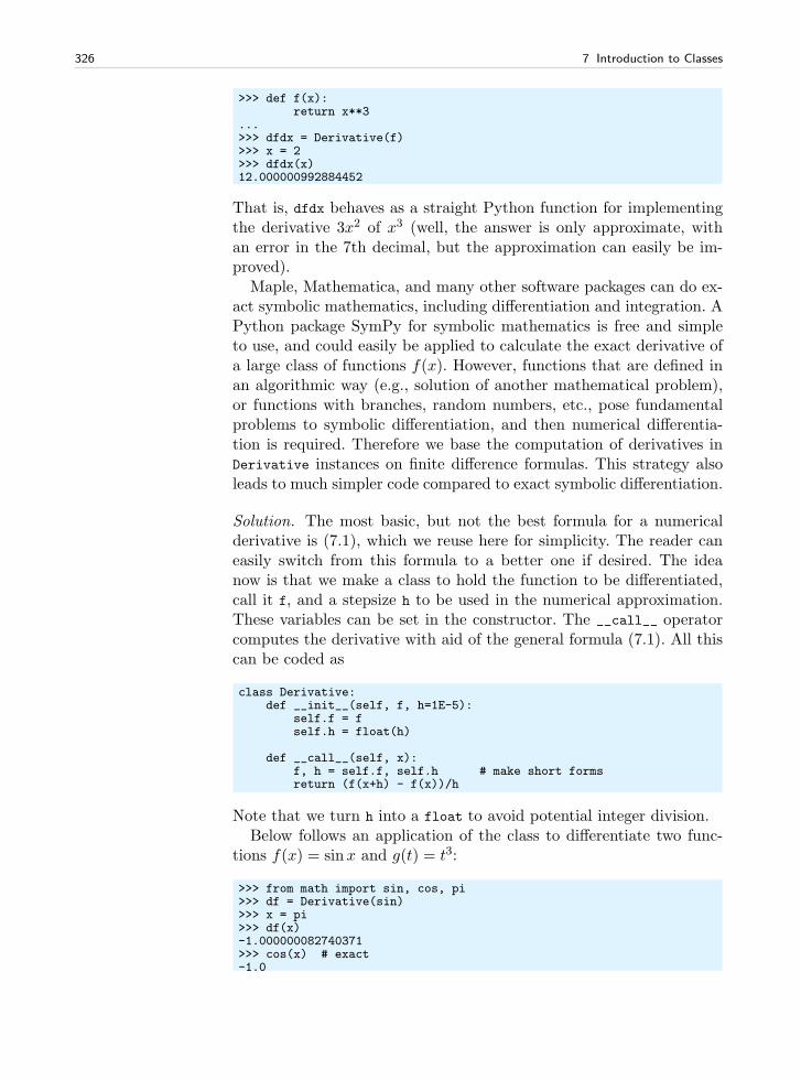
326 7 Introduction to Classes

>>> def f(x):return x**3

...>>> dfdx = Derivative(f)>>> x = 2>>> dfdx(x)12.000000992884452

That is, dfdx behaves as a straight Python function for implementingthe derivative 3x2 of x3 (well, the answer is only approximate, withan error in the 7th decimal, but the approximation can easily be im-proved).

Maple, Mathematica, and many other software packages can do ex-act symbolic mathematics, including differentiation and integration. APython package SymPy for symbolic mathematics is free and simpleto use, and could easily be applied to calculate the exact derivative ofa large class of functions f(x). However, functions that are defined inan algorithmic way (e.g., solution of another mathematical problem),or functions with branches, random numbers, etc., pose fundamentalproblems to symbolic differentiation, and then numerical differentia-tion is required. Therefore we base the computation of derivatives inDerivative instances on finite difference formulas. This strategy alsoleads to much simpler code compared to exact symbolic differentiation.

Solution. The most basic, but not the best formula for a numericalderivative is (7.1), which we reuse here for simplicity. The reader caneasily switch from this formula to a better one if desired. The ideanow is that we make a class to hold the function to be differentiated,call it f, and a stepsize h to be used in the numerical approximation.These variables can be set in the constructor. The __call__ operatorcomputes the derivative with aid of the general formula (7.1). All thiscan be coded as

class Derivative:def __init__(self, f, h=1E-5):

self.f = fself.h = float(h)

def __call__(self, x):f, h = self.f, self.h # make short formsreturn (f(x+h) - f(x))/h

Note that we turn h into a float to avoid potential integer division.Below follows an application of the class to differentiate two func-

tions f(x) = sinx and g(t) = t3:

>>> from math import sin, cos, pi>>> df = Derivative(sin)>>> x = pi>>> df(x)-1.000000082740371>>> cos(x) # exact-1.0

7.3 Special Methods 327

>>> def g(t):... return t**3...>>> dg = Derivative(g)>>> t = 1>>> dg(t) # compare with 3 (exact)3.000000248221113

The expressions df(x) and dg(t) look as ordinary Python functionsthat evaluate the derivative of the functions sin(x) and g(t). ClassDerivative works for (almost) any function f(x).

Application: Newton’s Method. In which situations will it be conve-nient to automatically produce a Python function df(x) which is thederivative of another Python function f(x)? One example arises whensolving nonlinear algebraic equations f(x) = 0 with Newton’s method(see Appendix A.1.9) and we, because of laziness, lack of time, orlack of training do not manage to derive f ′(x) by hand. Considerthe Newton function from page 510 for solving f(x) = 0: Newton(f,

x, dfdx, epsilon=1.0E-7, N=100), which requires the argument dfdx

representing f ′(x). Suppose our target equation reads

f(x) = 105(x− 0.9)2(x− 1.1)3 = 0 .

The function f(x) is plotted in Figure 7.2. The following session em-ploys the Derivative class to quickly make a derivative so we can callNewton’s method:

>>> from classes import Derivative>>> from Newton import Newton>>> def f(x):... return 100000*(x - 0.9)**2 * (x - 1.1)**3...>>> df = Derivative(f)>>> Newton(f, 1.01, df, epsilon=1E-5)(1.0987610068093443, 8, -7.5139644257961411e-06)

The output 3-tuple holds the approximation to a root, the number ofiterations, and the value of f at the approximate root (a measure ofthe error in the equation).

The exact root is 1.1, and the convergence toward this value is veryslow6 (for example, an epsilon tolerance of 10−10 requires 18 iterationswith an error of 10−3). Using an exact derivative gives almost the sameresult:

>>> def df_exact(x):... return 100000*(2*(x-0.9)*(x-1.1)**3 + \... (x-0.9)**2*3*(x-1.1)**2)...

6 Newton’s method converges very slowly when the derivative of f is zero at the rootsof f . Even slower convergence appears when higher-order derivatives also are zero,like in this example. Notice that the error in x is much larger than the error in theequation (epsilon).

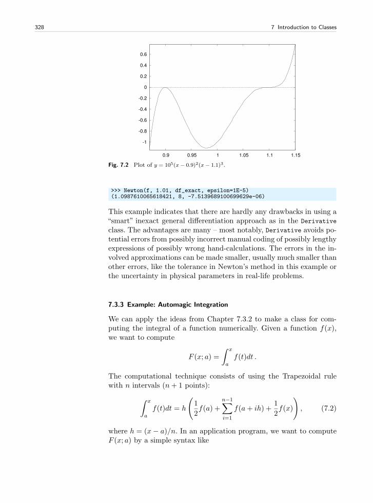
328 7 Introduction to Classes

-1

-0.8

-0.6

-0.4

-0.2

0

0.2

0.4

0.6

0.9 0.95 1 1.05 1.1 1.15

Fig. 7.2 Plot of y = 105(x− 0.9)2(x− 1.1)3.

>>> Newton(f, 1.01, df_exact, epsilon=1E-5)(1.0987610065618421, 8, -7.5139689100699629e-06)

This example indicates that there are hardly any drawbacks in using a“smart” inexact general differentiation approach as in the Derivative

class. The advantages are many – most notably, Derivative avoids po-tential errors from possibly incorrect manual coding of possibly lengthyexpressions of possibly wrong hand-calculations. The errors in the in-volved approximations can be made smaller, usually much smaller thanother errors, like the tolerance in Newton’s method in this example orthe uncertainty in physical parameters in real-life problems.

7.3.3 Example: Automagic Integration

We can apply the ideas from Chapter 7.3.2 to make a class for com-puting the integral of a function numerically. Given a function f(x),we want to compute

F (x; a) =

∫ x

af(t)dt .

The computational technique consists of using the Trapezoidal rulewith n intervals (n+ 1 points):

∫ x

a

f(t)dt = h

(

1

2f(a) +

n−1∑

i=1

f(a+ ih) +1

2f(x)

)

, (7.2)

where h = (x− a)/n. In an application program, we want to computeF (x; a) by a simple syntax like

7.3 Special Methods 329

def f(x):return exp(-x**2)*sin(10*x)

a = 0; n = 200F = Integral(f, a, n)print F(x)

Here, f(x) is the Python function to be integrated, and F(x) behavesas a Python function that calculates values of F (x; a).

A Simple Implementation. Consider a straightforward implementationof the Trapezoidal rule in a Python function:

def trapezoidal(f, a, x, n):h = (x-a)/float(n)I = 0.5*f(a)for i in iseq(1, n-1):

I += f(a + i*h)I += 0.5*f(x)I *= hreturn I

The iseq function, offered by scitools.std, is an alternative to range

where the upper limit, here n-1, is included in the set of numbers. Wecan alternatively use range(1, n), but the correspondence with theindices in the mathematical description of the rule is then not one-to-one.

Class Integral must have some attributes and a __call__ method.Since the latter method is supposed to take x as argument, the otherparameters a, f, and n must be class attributes. The implementationthen becomes

class Integral:def __init__(self, f, a, n=100):

self.f, self.a, self.n = f, a, n

def __call__(self, x):return trapezoidal(self.f, self.a, x, self.n)

Observe that we just reuse the trapezoidal function to performthe calculation. We could alternatively have copied the body of thetrapezoidal function into the __call__ method. However, if we al-ready have this algorithm implemented and tested as a function, it isbetter to call the function. The class is then known as a wrapper ofthe underlying function. A wrapper allows something to be called withalternative syntax. With the Integral(x) wrapper we can supply theupper limit of the integral only – the other parameters are suppliedwhen we create an instance of the Integral class.

An application program computing∫ 2π0 sinx dx might look as fol-

lows:

330 7 Introduction to Classes

from math import sin, pi

G = Integral(sin, 0, 200)value = G(2*pi)

An equivalent calculation is

value = trapezoidal(sin, 0, 2*pi, 200)

Remark. Class Integral is inefficient (but probably more than fastenough) for plotting F (x; a) as a function x. Exercise 7.22 suggests tooptimize the class for this purpose.

7.3.4 Turning an Instance into a String

Another special method is __str__. It is called when a class instanceneeds to be converted to a string. This happens when we say print a,and a is an instance. Python will then look into the a instance for a__str__ method, which is supposed to return a string. If such a specialmethod is found, the returned string is printed, otherwise just the nameof the class is printed. An example will illustrate the point. First wetry to print an y instance of class Y from Chapter 7.1.2 (where there isno __str__ method):

>>> print y<__main__.Y instance at 0xb751238c>

This means that y is an Y instance in the __main__ module (the mainprogram or the interactive session). The output also contains an ad-dress telling where the y instance is stored in the computer’s memory.

If we want print y to print out the y instance, we need to define the__str__ method in class Y:

class Y:...def __str__(self):

return ’v0*t - 0.5*g*t**2; v0=%g’ % self.v0

Typically, __str__ replaces our previous formula method and __call__

replaces our previous value method. Python programmers with theexperience that we now have gained will therefore write class Y withspecial methods only:

class Y:def __init__(self, v0):

self.v0 = v0self.g = 9.81

def __call__(self, t):return self.v0*t - 0.5*self.g*t**2

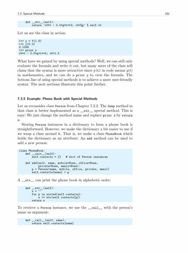
7.3 Special Methods 331

def __str__(self):return ’v0*t - 0.5*g*t**2; v0=%g’ % self.v0

Let us see the class in action:

>>> y = Y(1.5)>>> y(0.2)0.1038>>> print yv0*t - 0.5*g*t**2; v0=1.5

What have we gained by using special methods? Well, we can still onlyevaluate the formula and write it out, but many users of the class willclaim that the syntax is more attractive since y(t) in code means y(t)in mathematics, and we can do a print y to view the formula. Thebottom line of using special methods is to achieve a more user-friendlysyntax. The next sections illustrate this point further.

7.3.5 Example: Phone Book with Special Methods

Let us reconsider class Person from Chapter 7.2.2. The dump method inthat class is better implemented as a __str__ special method. This iseasy: We just change the method name and replace print s by return

s.Storing Person instances in a dictionary to form a phone book is

straightforward. However, we make the dictionary a bit easier to use ifwe wrap a class around it. That is, we make a class PhoneBook whichholds the dictionary as an attribute. An add method can be used toadd a new person:

class PhoneBook:def __init__(self):

self.contacts = # dict of Person instances

def add(self, name, mobile=None, office=None,private=None, email=None):

p = Person(name, mobile, office, private, email)self.contacts[name] = p

A __str__ can print the phone book in alphabetic order:

def __str__(self):s = ’’for p in sorted(self.contacts):

s += str(self.contacts[p])return s

To retrieve a Person instance, we use the __call__ with the person’sname as argument:

def __call__(self, name):return self.contacts[name]

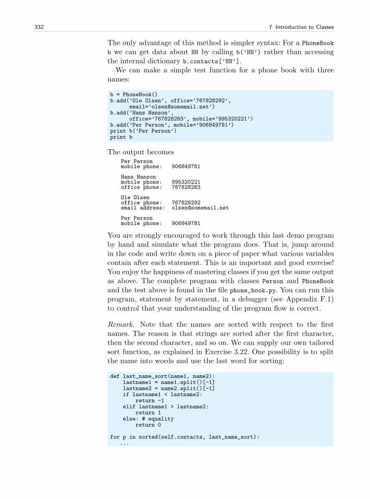
332 7 Introduction to Classes

The only advantage of this method is simpler syntax: For a PhoneBook

b we can get data about NN by calling b(’NN’) rather than accessingthe internal dictionary b.contacts[’NN’].

We can make a simple test function for a phone book with threenames:

b = PhoneBook()b.add(’Ole Olsen’, office=’767828292’,

email=’olsen@somemail.net’)b.add(’Hans Hanson’,

office=’767828283’, mobile=’995320221’)b.add(’Per Person’, mobile=’906849781’)print b(’Per Person’)print b

The output becomesPer Personmobile phone: 906849781

Hans Hansonmobile phone: 995320221office phone: 767828283

Ole Olsenoffice phone: 767828292email address: olsen@somemail.net

Per Personmobile phone: 906849781

You are strongly encouraged to work through this last demo programby hand and simulate what the program does. That is, jump aroundin the code and write down on a piece of paper what various variablescontain after each statement. This is an important and good exercise!You enjoy the happiness of mastering classes if you get the same outputas above. The complete program with classes Person and PhoneBook

and the test above is found in the file phone_book.py. You can run thisprogram, statement by statement, in a debugger (see Appendix F.1)to control that your understanding of the program flow is correct.

Remark. Note that the names are sorted with respect to the firstnames. The reason is that strings are sorted after the first character,then the second character, and so on. We can supply our own tailoredsort function, as explained in Exercise 3.22. One possibility is to splitthe name into words and use the last word for sorting:

def last_name_sort(name1, name2):lastname1 = name1.split()[-1]lastname2 = name2.split()[-1]if lastname1 < lastname2:

return -1elif lastname1 > lastname2:

return 1else: # equality

return 0

for p in sorted(self.contacts, last_name_sort):...

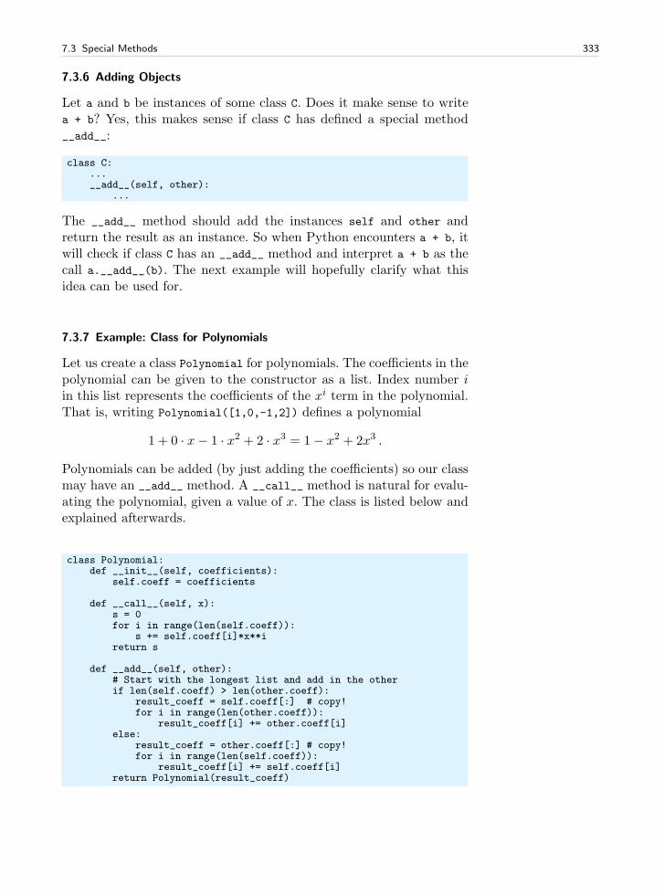
7.3 Special Methods 333

7.3.6 Adding Objects

Let a and b be instances of some class C. Does it make sense to writea + b? Yes, this makes sense if class C has defined a special method__add__:

class C:...__add__(self, other):

...

The __add__ method should add the instances self and other andreturn the result as an instance. So when Python encounters a + b, itwill check if class C has an __add__ method and interpret a + b as thecall a.__add__(b). The next example will hopefully clarify what thisidea can be used for.

7.3.7 Example: Class for Polynomials

Let us create a class Polynomial for polynomials. The coefficients in thepolynomial can be given to the constructor as a list. Index number iin this list represents the coefficients of the xi term in the polynomial.That is, writing Polynomial([1,0,-1,2]) defines a polynomial

1 + 0 · x− 1 · x2 + 2 · x3 = 1− x2 + 2x3 .

Polynomials can be added (by just adding the coefficients) so our classmay have an __add__ method. A __call__ method is natural for evalu-ating the polynomial, given a value of x. The class is listed below andexplained afterwards.

class Polynomial:def __init__(self, coefficients):

self.coeff = coefficients

def __call__(self, x):s = 0for i in range(len(self.coeff)):

s += self.coeff[i]*x**ireturn s

def __add__(self, other):# Start with the longest list and add in the otherif len(self.coeff) > len(other.coeff):

result_coeff = self.coeff[:] # copy!for i in range(len(other.coeff)):

result_coeff[i] += other.coeff[i]else:

result_coeff = other.coeff[:] # copy!for i in range(len(self.coeff)):

result_coeff[i] += self.coeff[i]return Polynomial(result_coeff)

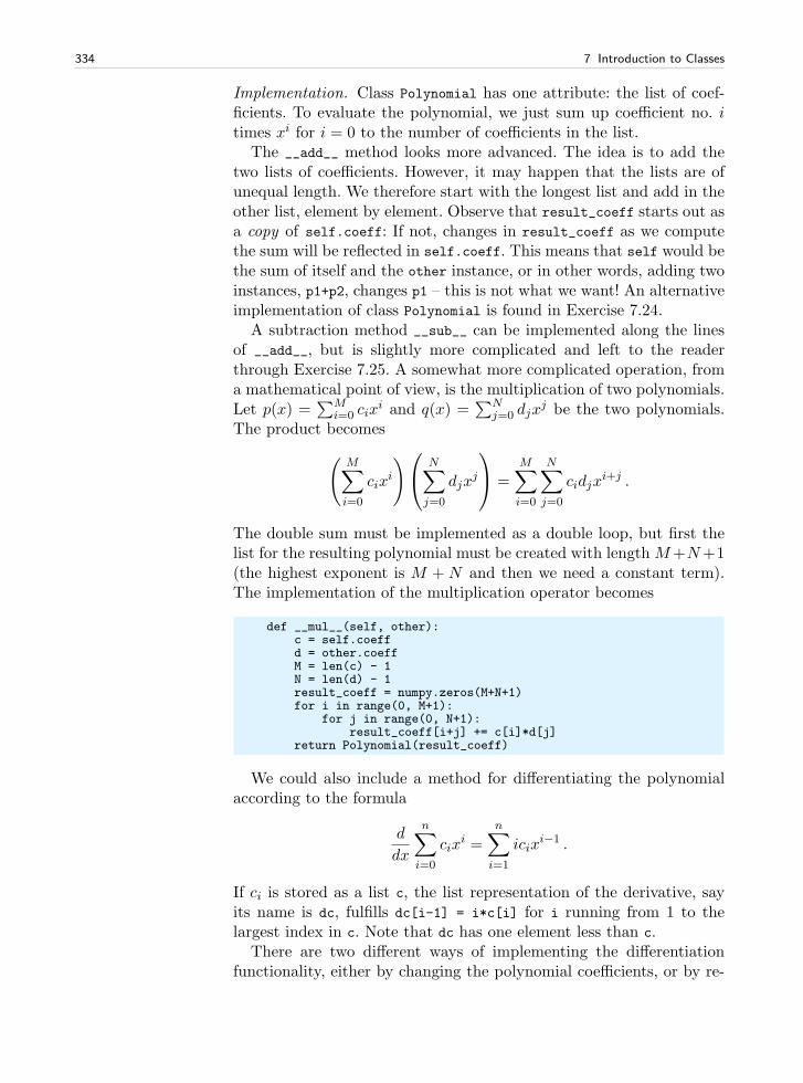
334 7 Introduction to Classes

Implementation. Class Polynomial has one attribute: the list of coef-ficients. To evaluate the polynomial, we just sum up coefficient no. itimes xi for i = 0 to the number of coefficients in the list.

The __add__ method looks more advanced. The idea is to add thetwo lists of coefficients. However, it may happen that the lists are ofunequal length. We therefore start with the longest list and add in theother list, element by element. Observe that result_coeff starts out asa copy of self.coeff: If not, changes in result_coeff as we computethe sum will be reflected in self.coeff. This means that self would bethe sum of itself and the other instance, or in other words, adding twoinstances, p1+p2, changes p1 – this is not what we want! An alternativeimplementation of class Polynomial is found in Exercise 7.24.

A subtraction method __sub__ can be implemented along the linesof __add__, but is slightly more complicated and left to the readerthrough Exercise 7.25. A somewhat more complicated operation, froma mathematical point of view, is the multiplication of two polynomials.Let p(x) =

∑Mi=0 cix

i and q(x) =∑N

j=0 djxj be the two polynomials.

The product becomes

(

M∑

i=0

cixi

)

N∑

j=0

djxj

=M∑

i=0

N∑

j=0

cidjxi+j .

The double sum must be implemented as a double loop, but first thelist for the resulting polynomial must be created with length M+N+1(the highest exponent is M + N and then we need a constant term).The implementation of the multiplication operator becomes

def __mul__(self, other):c = self.coeffd = other.coeffM = len(c) - 1N = len(d) - 1result_coeff = numpy.zeros(M+N+1)for i in range(0, M+1):

for j in range(0, N+1):result_coeff[i+j] += c[i]*d[j]

return Polynomial(result_coeff)

We could also include a method for differentiating the polynomialaccording to the formula

d

dx

n∑

i=0

cixi =

n∑

i=1

icixi−1 .

If ci is stored as a list c, the list representation of the derivative, sayits name is dc, fulfills dc[i-1] = i*c[i] for i running from 1 to thelargest index in c. Note that dc has one element less than c.

There are two different ways of implementing the differentiationfunctionality, either by changing the polynomial coefficients, or by re-

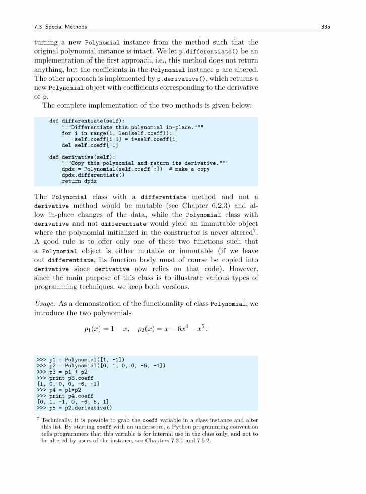
7.3 Special Methods 335

turning a new Polynomial instance from the method such that theoriginal polynomial instance is intact. We let p.differentiate() be animplementation of the first approach, i.e., this method does not returnanything, but the coefficients in the Polynomial instance p are altered.The other approach is implemented by p.derivative(), which returns anew Polynomial object with coefficients corresponding to the derivativeof p.

The complete implementation of the two methods is given below:

def differentiate(self):"""Differentiate this polynomial in-place."""for i in range(1, len(self.coeff)):

self.coeff[i-1] = i*self.coeff[i]del self.coeff[-1]

def derivative(self):"""Copy this polynomial and return its derivative."""dpdx = Polynomial(self.coeff[:]) # make a copydpdx.differentiate()return dpdx

The Polynomial class with a differentiate method and not aderivative method would be mutable (see Chapter 6.2.3) and al-low in-place changes of the data, while the Polynomial class withderivative and not differentiate would yield an immutable objectwhere the polynomial initialized in the constructor is never altered7.A good rule is to offer only one of these two functions such thata Polynomial object is either mutable or immutable (if we leaveout differentiate, its function body must of course be copied intoderivative since derivative now relies on that code). However,since the main purpose of this class is to illustrate various types ofprogramming techniques, we keep both versions.

Usage. As a demonstration of the functionality of class Polynomial, weintroduce the two polynomials

p1(x) = 1− x, p2(x) = x− 6x4 − x5 .

>>> p1 = Polynomial([1, -1])>>> p2 = Polynomial([0, 1, 0, 0, -6, -1])>>> p3 = p1 + p2>>> print p3.coeff[1, 0, 0, 0, -6, -1]>>> p4 = p1*p2>>> print p4.coeff[0, 1, -1, 0, -6, 5, 1]>>> p5 = p2.derivative()

7 Technically, it is possible to grab the coeff variable in a class instance and alterthis list. By starting coeff with an underscore, a Python programming conventiontells programmers that this variable is for internal use in the class only, and not tobe altered by users of the instance, see Chapters 7.2.1 and 7.5.2.

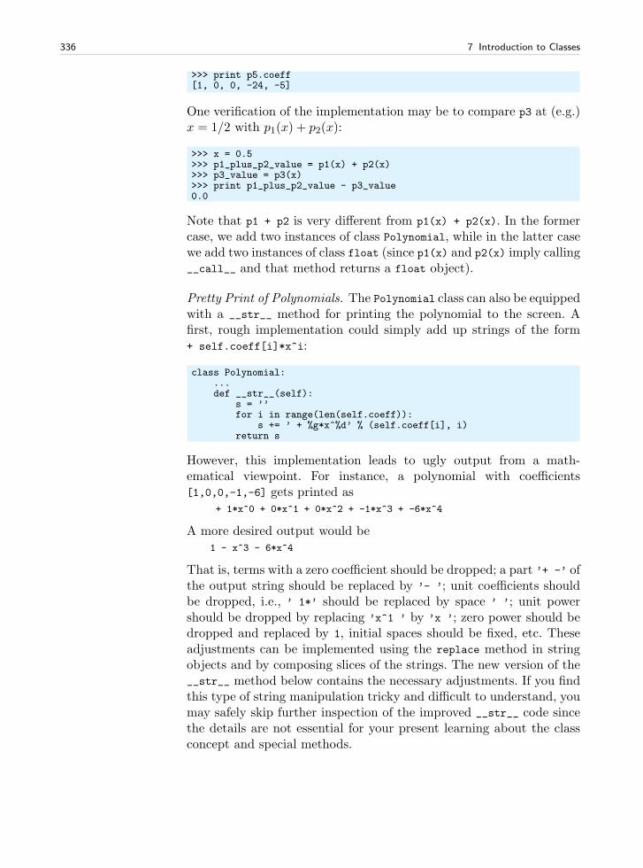
336 7 Introduction to Classes

>>> print p5.coeff[1, 0, 0, -24, -5]

One verification of the implementation may be to compare p3 at (e.g.)x = 1/2 with p1(x) + p2(x):

>>> x = 0.5>>> p1_plus_p2_value = p1(x) + p2(x)>>> p3_value = p3(x)>>> print p1_plus_p2_value - p3_value0.0

Note that p1 + p2 is very different from p1(x) + p2(x). In the formercase, we add two instances of class Polynomial, while in the latter casewe add two instances of class float (since p1(x) and p2(x) imply calling__call__ and that method returns a float object).

Pretty Print of Polynomials. The Polynomial class can also be equippedwith a __str__ method for printing the polynomial to the screen. Afirst, rough implementation could simply add up strings of the form+ self.coeff[i]*x^i:

class Polynomial:...def __str__(self):

s = ’’for i in range(len(self.coeff)):

s += ’ + %g*x^%d’ % (self.coeff[i], i)return s

However, this implementation leads to ugly output from a math-ematical viewpoint. For instance, a polynomial with coefficients[1,0,0,-1,-6] gets printed as

+ 1*x^0 + 0*x^1 + 0*x^2 + -1*x^3 + -6*x^4

A more desired output would be1 - x^3 - 6*x^4

That is, terms with a zero coefficient should be dropped; a part ’+ -’ ofthe output string should be replaced by ’- ’; unit coefficients shouldbe dropped, i.e., ’ 1*’ should be replaced by space ’ ’; unit powershould be dropped by replacing ’x^1 ’ by ’x ’; zero power should bedropped and replaced by 1, initial spaces should be fixed, etc. Theseadjustments can be implemented using the replace method in stringobjects and by composing slices of the strings. The new version of the__str__ method below contains the necessary adjustments. If you findthis type of string manipulation tricky and difficult to understand, youmay safely skip further inspection of the improved __str__ code sincethe details are not essential for your present learning about the classconcept and special methods.

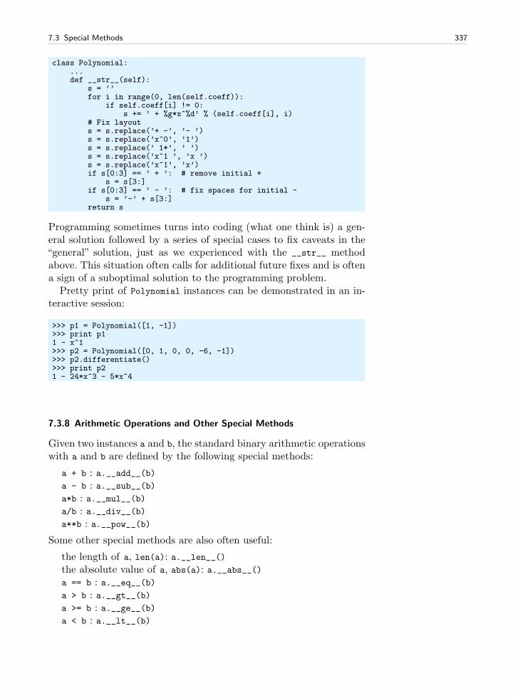
7.3 Special Methods 337

class Polynomial:...def __str__(self):

s = ’’for i in range(0, len(self.coeff)):

if self.coeff[i] != 0:s += ’ + %g*x^%d’ % (self.coeff[i], i)

# Fix layouts = s.replace(’+ -’, ’- ’)s = s.replace(’x^0’, ’1’)s = s.replace(’ 1*’, ’ ’)s = s.replace(’x^1 ’, ’x ’)s = s.replace(’x^1’, ’x’)if s[0:3] == ’ + ’: # remove initial +

s = s[3:]if s[0:3] == ’ - ’: # fix spaces for initial -

s = ’-’ + s[3:]return s

Programming sometimes turns into coding (what one think is) a gen-eral solution followed by a series of special cases to fix caveats in the“general” solution, just as we experienced with the __str__ methodabove. This situation often calls for additional future fixes and is oftena sign of a suboptimal solution to the programming problem.

Pretty print of Polynomial instances can be demonstrated in an in-teractive session:

>>> p1 = Polynomial([1, -1])>>> print p11 - x^1>>> p2 = Polynomial([0, 1, 0, 0, -6, -1])>>> p2.differentiate()>>> print p21 - 24*x^3 - 5*x^4

7.3.8 Arithmetic Operations and Other Special Methods

Given two instances a and b, the standard binary arithmetic operationswith a and b are defined by the following special methods:

a + b : a.__add__(b) a - b : a.__sub__(b) a*b : a.__mul__(b) a/b : a.__div__(b) a**b : a.__pow__(b)

Some other special methods are also often useful:

the length of a, len(a): a.__len__() the absolute value of a, abs(a): a.__abs__() a == b : a.__eq__(b) a > b : a.__gt__(b) a >= b : a.__ge__(b) a < b : a.__lt__(b)

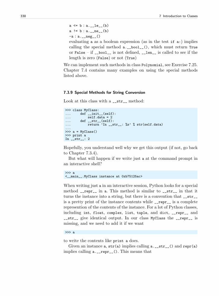
338 7 Introduction to Classes

a <= b : a.__le__(b) a != b : a.__ne__(b) -a : a.__neg__() evaluating a as a boolean expression (as in the test if a:) impliescalling the special method a.__bool__(), which must return True

or False – if __bool__ is not defined, __len__ is called to see if thelength is zero (False) or not (True)

We can implement such methods in class Polynomial, see Exercise 7.25.Chapter 7.4 contains many examples on using the special methodslisted above.

7.3.9 Special Methods for String Conversion

Look at this class with a __str__ method:

>>> class MyClass:... def __init__(self):... self.data = 2... def __str__(self):... return ’In __str__: %s’ % str(self.data)...>>> a = MyClass()>>> print aIn __str__: 2

Hopefully, you understand well why we get this output (if not, go backto Chapter 7.3.4).

But what will happen if we write just a at the command prompt inan interactive shell?

>>> a<__main__.MyClass instance at 0xb75125ac>

When writing just a in an interactive session, Python looks for a specialmethod __repr__ in a. This method is similar to __str__ in that itturns the instance into a string, but there is a convention that __str__is a pretty print of the instance contents while __repr__ is a completerepresention of the contents of the instance. For a lot of Python classes,including int, float, complex, list, tuple, and dict, __repr__ and__str__ give identical output. In our class MyClass the __repr__ ismissing, and we need to add it if we want

>>> a

to write the contents like print a does.Given an instance a, str(a) implies calling a.__str__() and repr(a)

implies calling a.__repr__(). This means that

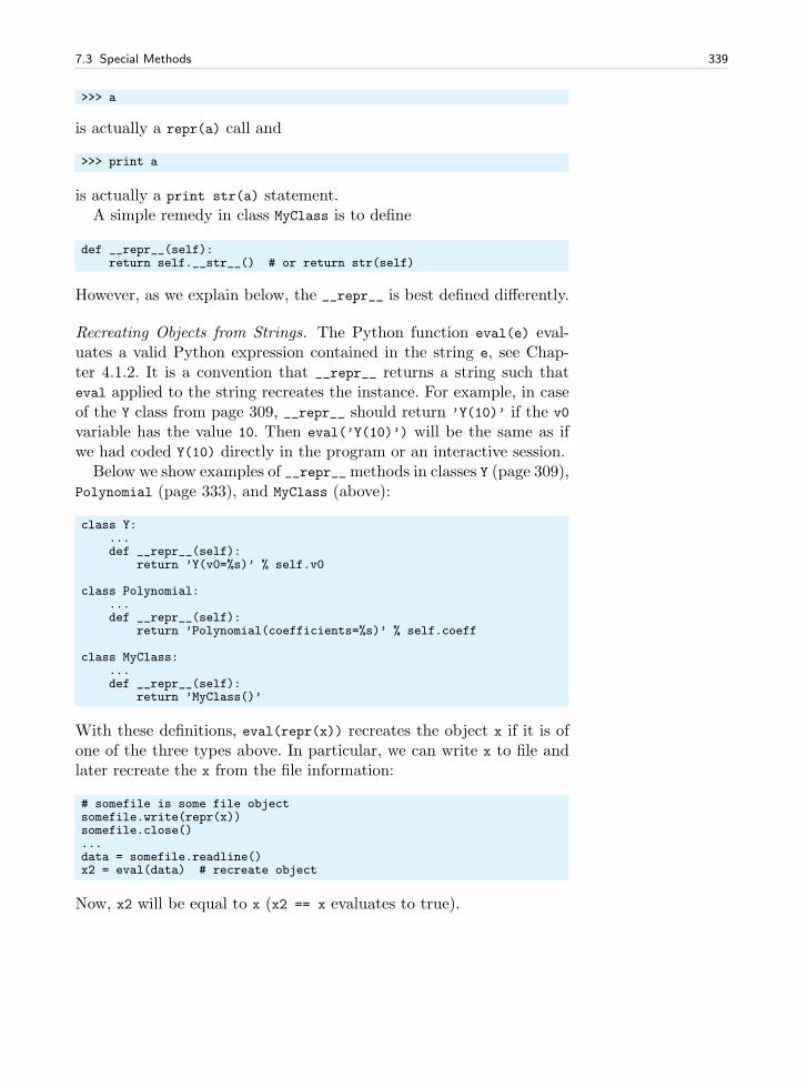
7.3 Special Methods 339

>>> a

is actually a repr(a) call and

>>> print a

is actually a print str(a) statement.A simple remedy in class MyClass is to define

def __repr__(self):return self.__str__() # or return str(self)

However, as we explain below, the __repr__ is best defined differently.

Recreating Objects from Strings. The Python function eval(e) eval-uates a valid Python expression contained in the string e, see Chap-ter 4.1.2. It is a convention that __repr__ returns a string such thateval applied to the string recreates the instance. For example, in caseof the Y class from page 309, __repr__ should return ’Y(10)’ if the v0

variable has the value 10. Then eval(’Y(10)’) will be the same as ifwe had coded Y(10) directly in the program or an interactive session.

Below we show examples of __repr__methods in classes Y (page 309),Polynomial (page 333), and MyClass (above):

class Y:...def __repr__(self):

return ’Y(v0=%s)’ % self.v0

class Polynomial:...def __repr__(self):

return ’Polynomial(coefficients=%s)’ % self.coeff

class MyClass:...def __repr__(self):

return ’MyClass()’

With these definitions, eval(repr(x)) recreates the object x if it is ofone of the three types above. In particular, we can write x to file andlater recreate the x from the file information:

# somefile is some file objectsomefile.write(repr(x))somefile.close()...data = somefile.readline()x2 = eval(data) # recreate object

Now, x2 will be equal to x (x2 == x evaluates to true).

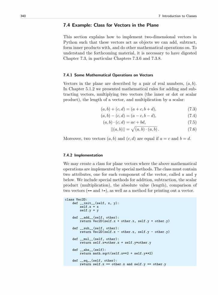
340 7 Introduction to Classes

7.4 Example: Class for Vectors in the Plane

This section explains how to implement two-dimensional vectors inPython such that these vectors act as objects we can add, subtract,form inner products with, and do other mathematical operations on. Tounderstand the forthcoming material, it is necessary to have digestedChapter 7.3, in particular Chapters 7.3.6 and 7.3.8.

7.4.1 Some Mathematical Operations on Vectors

Vectors in the plane are described by a pair of real numbers, (a, b).In Chapter 5.1.2 we presented mathematical rules for adding and sub-tracting vectors, multiplying two vectors (the inner or dot or scalarproduct), the length of a vector, and multiplication by a scalar:

(a, b) + (c, d) = (a+ c, b+ d), (7.3)

(a, b)− (c, d) = (a− c, b− d), (7.4)

(a, b) · (c, d) = ac+ bd, (7.5)

||(a, b)|| =√

(a, b) · (a, b) . (7.6)

Moreover, two vectors (a, b) and (c, d) are equal if a = c and b = d.

7.4.2 Implementation

We may create a class for plane vectors where the above mathematicaloperations are implemented by special methods. The class must containtwo attributes, one for each component of the vector, called x and y

below. We include special methods for addition, subtraction, the scalarproduct (multiplication), the absolute value (length), comparison oftwo vectors (== and !=), as well as a method for printing out a vector.

class Vec2D:def __init__(self, x, y):

self.x = xself.y = y

def __add__(self, other):return Vec2D(self.x + other.x, self.y + other.y)

def __sub__(self, other):return Vec2D(self.x - other.x, self.y - other.y)

def __mul__(self, other):return self.x*other.x + self.y*other.y

def __abs__(self):return math.sqrt(self.x**2 + self.y**2)

def __eq__(self, other):return self.x == other.x and self.y == other.y

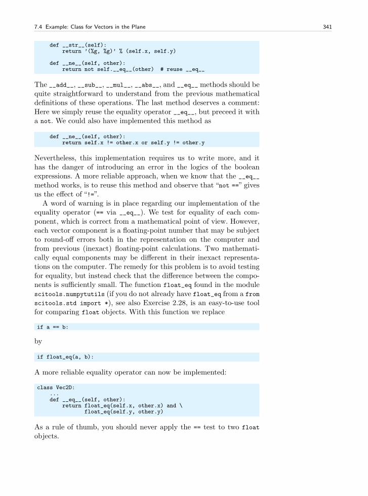
7.4 Example: Class for Vectors in the Plane 341

def __str__(self):return ’(%g, %g)’ % (self.x, self.y)

def __ne__(self, other):return not self.__eq__(other) # reuse __eq__

The __add__, __sub__, __mul__, __abs__, and __eq__ methods should bequite straightforward to understand from the previous mathematicaldefinitions of these operations. The last method deserves a comment:Here we simply reuse the equality operator __eq__, but preceed it witha not. We could also have implemented this method as

def __ne__(self, other):return self.x != other.x or self.y != other.y

Nevertheless, this implementation requires us to write more, and ithas the danger of introducing an error in the logics of the booleanexpressions. A more reliable approach, when we know that the __eq__

method works, is to reuse this method and observe that “not ==” givesus the effect of “!=”.

A word of warning is in place regarding our implementation of theequality operator (== via __eq__). We test for equality of each com-ponent, which is correct from a mathematical point of view. However,each vector component is a floating-point number that may be subjectto round-off errors both in the representation on the computer andfrom previous (inexact) floating-point calculations. Two mathemati-cally equal components may be different in their inexact representa-tions on the computer. The remedy for this problem is to avoid testingfor equality, but instead check that the difference between the compo-nents is sufficiently small. The function float_eq found in the modulescitools.numpytutils (if you do not already have float_eq from a from

scitools.std import *), see also Exercise 2.28, is an easy-to-use toolfor comparing float objects. With this function we replace

if a == b:

by

if float_eq(a, b):

A more reliable equality operator can now be implemented:

class Vec2D:...def __eq__(self, other):

return float_eq(self.x, other.x) and \float_eq(self.y, other.y)

As a rule of thumb, you should never apply the == test to two float

objects.

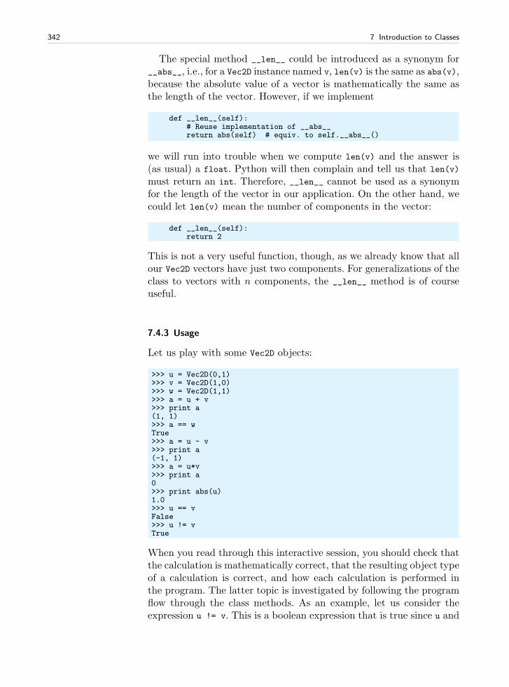
342 7 Introduction to Classes

The special method __len__ could be introduced as a synonym for__abs__, i.e., for a Vec2D instance named v, len(v) is the same as abs(v),because the absolute value of a vector is mathematically the same asthe length of the vector. However, if we implement

def __len__(self):# Reuse implementation of __abs__return abs(self) # equiv. to self.__abs__()

we will run into trouble when we compute len(v) and the answer is(as usual) a float. Python will then complain and tell us that len(v)

must return an int. Therefore, __len__ cannot be used as a synonymfor the length of the vector in our application. On the other hand, wecould let len(v) mean the number of components in the vector:

def __len__(self):return 2

This is not a very useful function, though, as we already know that allour Vec2D vectors have just two components. For generalizations of theclass to vectors with n components, the __len__ method is of courseuseful.

7.4.3 Usage

Let us play with some Vec2D objects:

>>> u = Vec2D(0,1)>>> v = Vec2D(1,0)>>> w = Vec2D(1,1)>>> a = u + v>>> print a(1, 1)>>> a == wTrue>>> a = u - v>>> print a(-1, 1)>>> a = u*v>>> print a0>>> print abs(u)1.0>>> u == vFalse>>> u != vTrue

When you read through this interactive session, you should check thatthe calculation is mathematically correct, that the resulting object typeof a calculation is correct, and how each calculation is performed inthe program. The latter topic is investigated by following the programflow through the class methods. As an example, let us consider theexpression u != v. This is a boolean expression that is true since u and

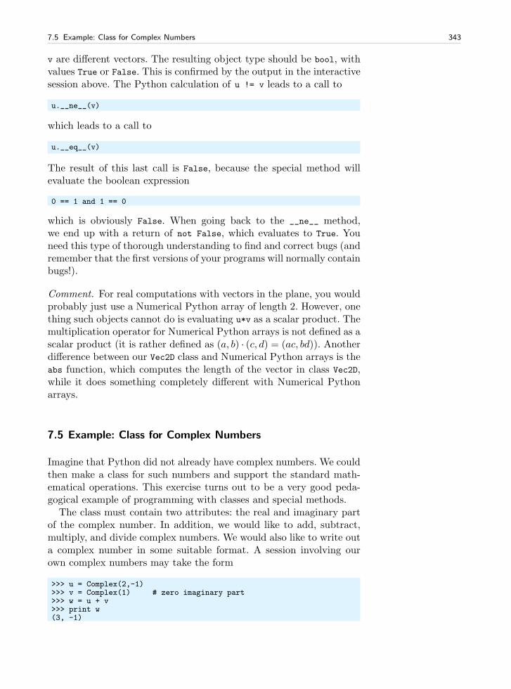
7.5 Example: Class for Complex Numbers 343

v are different vectors. The resulting object type should be bool, withvalues True or False. This is confirmed by the output in the interactivesession above. The Python calculation of u != v leads to a call to

u.__ne__(v)

which leads to a call to

u.__eq__(v)

The result of this last call is False, because the special method willevaluate the boolean expression

0 == 1 and 1 == 0

which is obviously False. When going back to the __ne__ method,we end up with a return of not False, which evaluates to True. Youneed this type of thorough understanding to find and correct bugs (andremember that the first versions of your programs will normally containbugs!).

Comment. For real computations with vectors in the plane, you wouldprobably just use a Numerical Python array of length 2. However, onething such objects cannot do is evaluating u*v as a scalar product. Themultiplication operator for Numerical Python arrays is not defined as ascalar product (it is rather defined as (a, b) · (c, d) = (ac, bd)). Anotherdifference between our Vec2D class and Numerical Python arrays is theabs function, which computes the length of the vector in class Vec2D,while it does something completely different with Numerical Pythonarrays.

7.5 Example: Class for Complex Numbers

Imagine that Python did not already have complex numbers. We couldthen make a class for such numbers and support the standard math-ematical operations. This exercise turns out to be a very good peda-gogical example of programming with classes and special methods.

The class must contain two attributes: the real and imaginary partof the complex number. In addition, we would like to add, subtract,multiply, and divide complex numbers. We would also like to write outa complex number in some suitable format. A session involving ourown complex numbers may take the form

>>> u = Complex(2,-1)>>> v = Complex(1) # zero imaginary part>>> w = u + v>>> print w(3, -1)

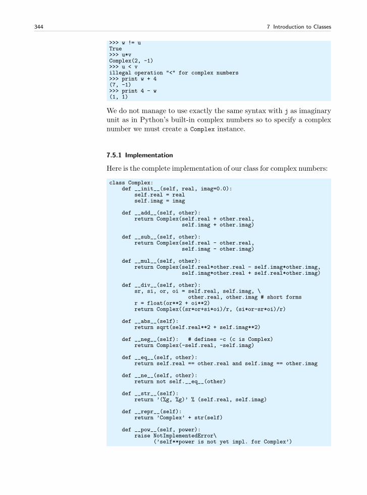
344 7 Introduction to Classes

>>> w != uTrue>>> u*vComplex(2, -1)>>> u < villegal operation "<" for complex numbers>>> print w + 4(7, -1)>>> print 4 - w(1, 1)

We do not manage to use exactly the same syntax with j as imaginaryunit as in Python’s built-in complex numbers so to specify a complexnumber we must create a Complex instance.

7.5.1 Implementation

Here is the complete implementation of our class for complex numbers:

class Complex:def __init__(self, real, imag=0.0):

self.real = realself.imag = imag

def __add__(self, other):return Complex(self.real + other.real,

self.imag + other.imag)

def __sub__(self, other):return Complex(self.real - other.real,

self.imag - other.imag)

def __mul__(self, other):return Complex(self.real*other.real - self.imag*other.imag,

self.imag*other.real + self.real*other.imag)

def __div__(self, other):sr, si, or, oi = self.real, self.imag, \

other.real, other.imag # short formsr = float(or**2 + oi**2)return Complex((sr*or+si*oi)/r, (si*or-sr*oi)/r)

def __abs__(self):return sqrt(self.real**2 + self.imag**2)

def __neg__(self): # defines -c (c is Complex)return Complex(-self.real, -self.imag)

def __eq__(self, other):return self.real == other.real and self.imag == other.imag

def __ne__(self, other):return not self.__eq__(other)

def __str__(self):return ’(%g, %g)’ % (self.real, self.imag)

def __repr__(self):return ’Complex’ + str(self)

def __pow__(self, power):raise NotImplementedError\

(’self**power is not yet impl. for Complex’)

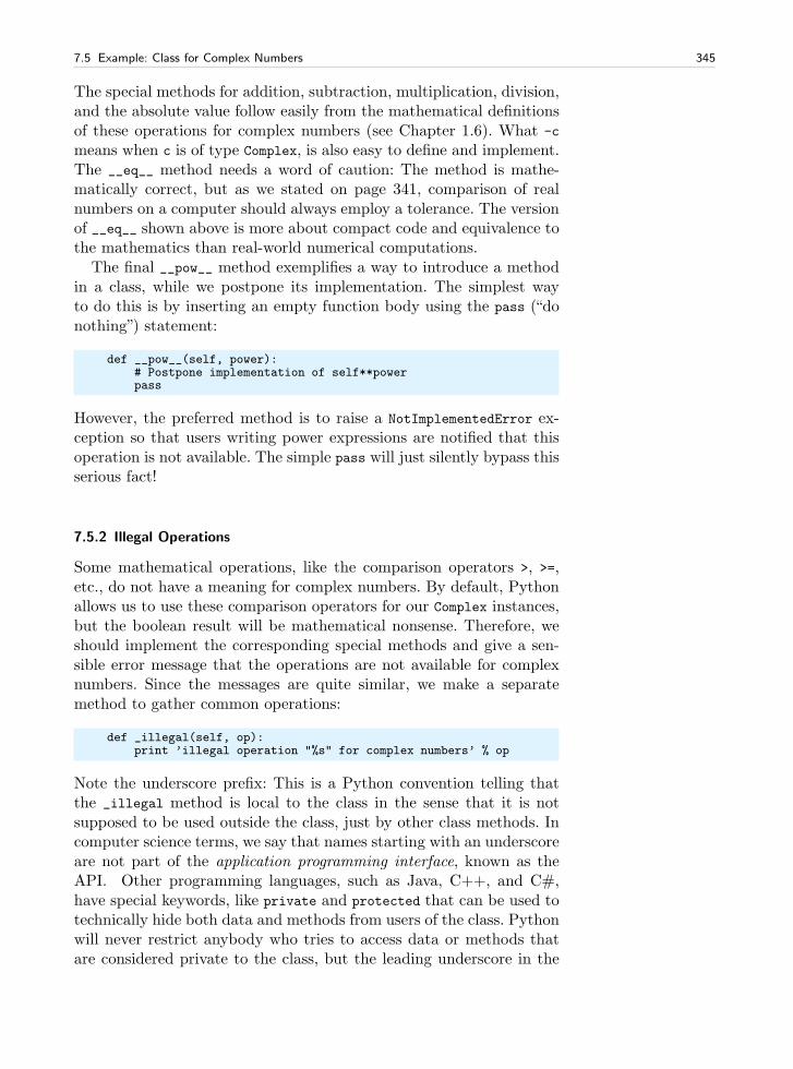
7.5 Example: Class for Complex Numbers 345

The special methods for addition, subtraction, multiplication, division,and the absolute value follow easily from the mathematical definitionsof these operations for complex numbers (see Chapter 1.6). What -c

means when c is of type Complex, is also easy to define and implement.The __eq__ method needs a word of caution: The method is mathe-matically correct, but as we stated on page 341, comparison of realnumbers on a computer should always employ a tolerance. The versionof __eq__ shown above is more about compact code and equivalence tothe mathematics than real-world numerical computations.

The final __pow__ method exemplifies a way to introduce a methodin a class, while we postpone its implementation. The simplest wayto do this is by inserting an empty function body using the pass (“donothing”) statement:

def __pow__(self, power):# Postpone implementation of self**powerpass

However, the preferred method is to raise a NotImplementedError ex-ception so that users writing power expressions are notified that thisoperation is not available. The simple pass will just silently bypass thisserious fact!

7.5.2 Illegal Operations

Some mathematical operations, like the comparison operators >, >=,etc., do not have a meaning for complex numbers. By default, Pythonallows us to use these comparison operators for our Complex instances,but the boolean result will be mathematical nonsense. Therefore, weshould implement the corresponding special methods and give a sen-sible error message that the operations are not available for complexnumbers. Since the messages are quite similar, we make a separatemethod to gather common operations:

def _illegal(self, op):print ’illegal operation "%s" for complex numbers’ % op

Note the underscore prefix: This is a Python convention telling thatthe _illegal method is local to the class in the sense that it is notsupposed to be used outside the class, just by other class methods. Incomputer science terms, we say that names starting with an underscoreare not part of the application programming interface, known as theAPI. Other programming languages, such as Java, C++, and C#,have special keywords, like private and protected that can be used totechnically hide both data and methods from users of the class. Pythonwill never restrict anybody who tries to access data or methods thatare considered private to the class, but the leading underscore in the

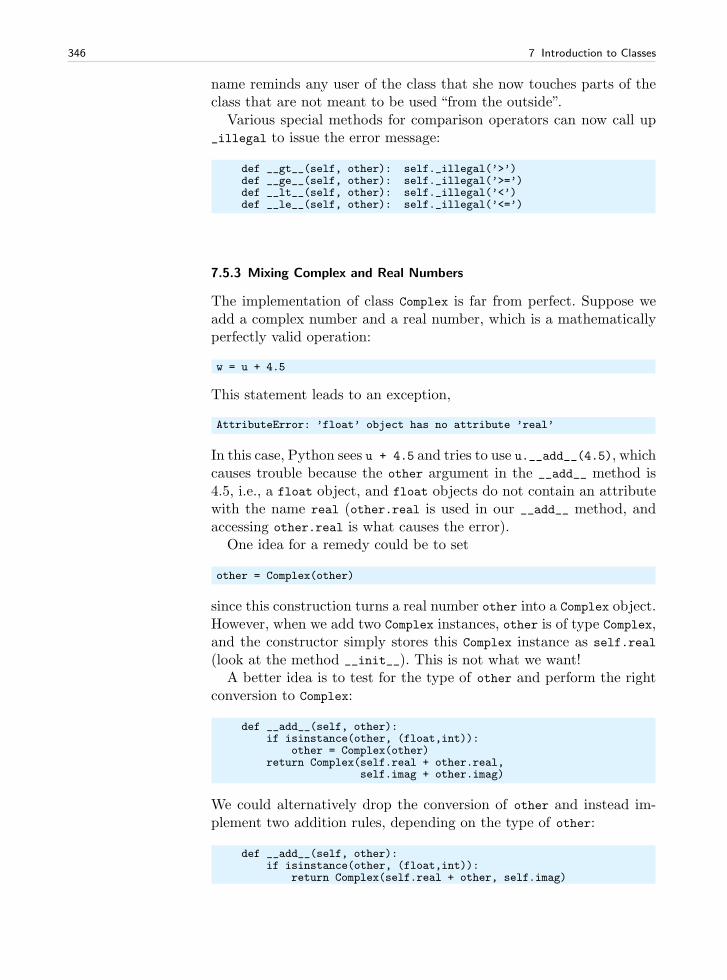
346 7 Introduction to Classes

name reminds any user of the class that she now touches parts of theclass that are not meant to be used “from the outside”.

Various special methods for comparison operators can now call up_illegal to issue the error message:

def __gt__(self, other): self._illegal(’>’)def __ge__(self, other): self._illegal(’>=’)def __lt__(self, other): self._illegal(’<’)def __le__(self, other): self._illegal(’<=’)

7.5.3 Mixing Complex and Real Numbers

The implementation of class Complex is far from perfect. Suppose weadd a complex number and a real number, which is a mathematicallyperfectly valid operation:

w = u + 4.5

This statement leads to an exception,

AttributeError: ’float’ object has no attribute ’real’

In this case, Python sees u + 4.5 and tries to use u.__add__(4.5), whichcauses trouble because the other argument in the __add__ method is4.5, i.e., a float object, and float objects do not contain an attributewith the name real (other.real is used in our __add__ method, andaccessing other.real is what causes the error).

One idea for a remedy could be to set

other = Complex(other)

since this construction turns a real number other into a Complex object.However, when we add two Complex instances, other is of type Complex,and the constructor simply stores this Complex instance as self.real

(look at the method __init__). This is not what we want!A better idea is to test for the type of other and perform the right

conversion to Complex:

def __add__(self, other):if isinstance(other, (float,int)):

other = Complex(other)return Complex(self.real + other.real,

self.imag + other.imag)

We could alternatively drop the conversion of other and instead im-plement two addition rules, depending on the type of other:

def __add__(self, other):if isinstance(other, (float,int)):

return Complex(self.real + other, self.imag)

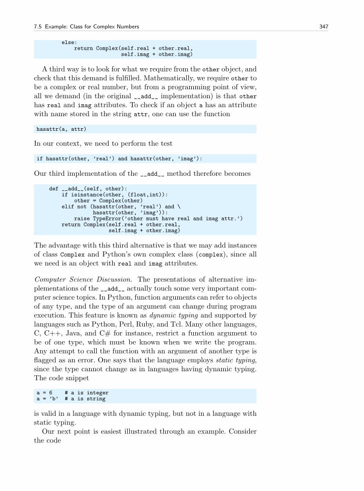
7.5 Example: Class for Complex Numbers 347

else:return Complex(self.real + other.real,

self.imag + other.imag)

A third way is to look for what we require from the other object, andcheck that this demand is fulfilled. Mathematically, we require other tobe a complex or real number, but from a programming point of view,all we demand (in the original __add__ implementation) is that other

has real and imag attributes. To check if an object a has an attributewith name stored in the string attr, one can use the function

hasattr(a, attr)

In our context, we need to perform the test

if hasattr(other, ’real’) and hasattr(other, ’imag’):

Our third implementation of the __add__ method therefore becomes

def __add__(self, other):if isinstance(other, (float,int)):

other = Complex(other)elif not (hasattr(other, ’real’) and \

hasattr(other, ’imag’)):raise TypeError(’other must have real and imag attr.’)

return Complex(self.real + other.real,self.imag + other.imag)

The advantage with this third alternative is that we may add instancesof class Complex and Python’s own complex class (complex), since allwe need is an object with real and imag attributes.

Computer Science Discussion. The presentations of alternative im-plementations of the __add__ actually touch some very important com-puter science topics. In Python, function arguments can refer to objectsof any type, and the type of an argument can change during programexecution. This feature is known as dynamic typing and supported bylanguages such as Python, Perl, Ruby, and Tcl. Many other languages,C, C++, Java, and C# for instance, restrict a function argument tobe of one type, which must be known when we write the program.Any attempt to call the function with an argument of another type isflagged as an error. One says that the language employs static typing,since the type cannot change as in languages having dynamic typing.The code snippet

a = 6 # a is integera = ’b’ # a is string

is valid in a language with dynamic typing, but not in a language withstatic typing.

Our next point is easiest illustrated through an example. Considerthe code

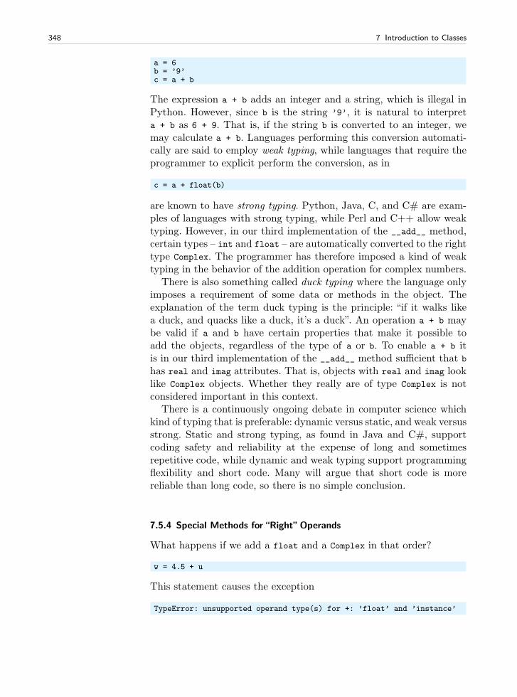
348 7 Introduction to Classes

a = 6b = ’9’c = a + b

The expression a + b adds an integer and a string, which is illegal inPython. However, since b is the string ’9’, it is natural to interpreta + b as 6 + 9. That is, if the string b is converted to an integer, wemay calculate a + b. Languages performing this conversion automati-cally are said to employ weak typing, while languages that require theprogrammer to explicit perform the conversion, as in

c = a + float(b)

are known to have strong typing. Python, Java, C, and C# are exam-ples of languages with strong typing, while Perl and C++ allow weaktyping. However, in our third implementation of the __add__ method,certain types – int and float – are automatically converted to the righttype Complex. The programmer has therefore imposed a kind of weaktyping in the behavior of the addition operation for complex numbers.

There is also something called duck typing where the language onlyimposes a requirement of some data or methods in the object. Theexplanation of the term duck typing is the principle: “if it walks likea duck, and quacks like a duck, it’s a duck”. An operation a + b maybe valid if a and b have certain properties that make it possible toadd the objects, regardless of the type of a or b. To enable a + b itis in our third implementation of the __add__ method sufficient that bhas real and imag attributes. That is, objects with real and imag looklike Complex objects. Whether they really are of type Complex is notconsidered important in this context.

There is a continuously ongoing debate in computer science whichkind of typing that is preferable: dynamic versus static, and weak versusstrong. Static and strong typing, as found in Java and C#, supportcoding safety and reliability at the expense of long and sometimesrepetitive code, while dynamic and weak typing support programmingflexibility and short code. Many will argue that short code is morereliable than long code, so there is no simple conclusion.

7.5.4 Special Methods for “Right”Operands

What happens if we add a float and a Complex in that order?

w = 4.5 + u

This statement causes the exception

TypeError: unsupported operand type(s) for +: ’float’ and ’instance’

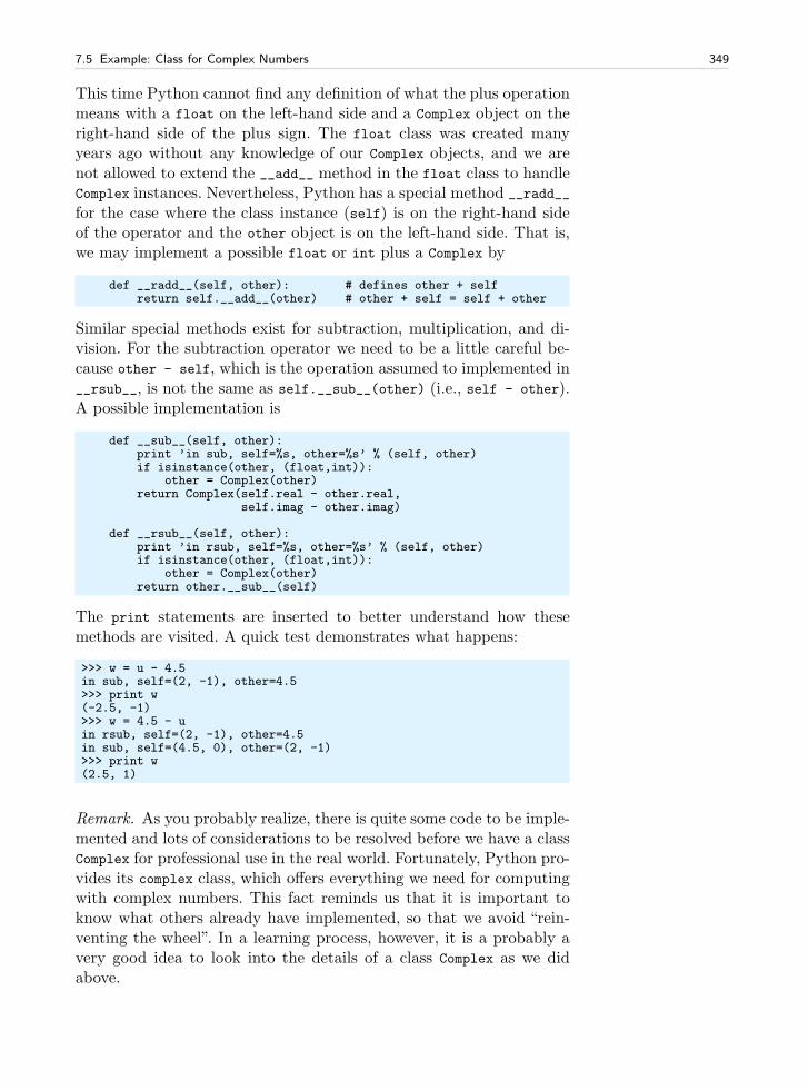
7.5 Example: Class for Complex Numbers 349

This time Python cannot find any definition of what the plus operationmeans with a float on the left-hand side and a Complex object on theright-hand side of the plus sign. The float class was created manyyears ago without any knowledge of our Complex objects, and we arenot allowed to extend the __add__ method in the float class to handleComplex instances. Nevertheless, Python has a special method __radd__

for the case where the class instance (self) is on the right-hand sideof the operator and the other object is on the left-hand side. That is,we may implement a possible float or int plus a Complex by

def __radd__(self, other): # defines other + selfreturn self.__add__(other) # other + self = self + other

Similar special methods exist for subtraction, multiplication, and di-vision. For the subtraction operator we need to be a little careful be-cause other - self, which is the operation assumed to implemented in__rsub__, is not the same as self.__sub__(other) (i.e., self - other).A possible implementation is

def __sub__(self, other):print ’in sub, self=%s, other=%s’ % (self, other)if isinstance(other, (float,int)):

other = Complex(other)return Complex(self.real - other.real,

self.imag - other.imag)

def __rsub__(self, other):print ’in rsub, self=%s, other=%s’ % (self, other)if isinstance(other, (float,int)):

other = Complex(other)return other.__sub__(self)

The print statements are inserted to better understand how thesemethods are visited. A quick test demonstrates what happens:

>>> w = u - 4.5in sub, self=(2, -1), other=4.5>>> print w(-2.5, -1)>>> w = 4.5 - uin rsub, self=(2, -1), other=4.5in sub, self=(4.5, 0), other=(2, -1)>>> print w(2.5, 1)

Remark. As you probably realize, there is quite some code to be imple-mented and lots of considerations to be resolved before we have a classComplex for professional use in the real world. Fortunately, Python pro-vides its complex class, which offers everything we need for computingwith complex numbers. This fact reminds us that it is important toknow what others already have implemented, so that we avoid “rein-venting the wheel”. In a learning process, however, it is a probably avery good idea to look into the details of a class Complex as we didabove.

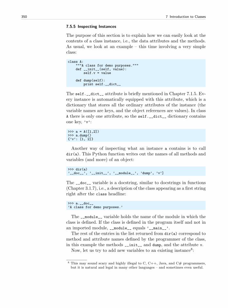
350 7 Introduction to Classes

7.5.5 Inspecting Instances

The purpose of this section is to explain how we can easily look at thecontents of a class instance, i.e., the data attributes and the methods.As usual, we look at an example – this time involving a very simpleclass:

class A:"""A class for demo purposes."""def __init__(self, value):

self.v = value

def dump(self):print self.__dict__

The self.__dict__ attribute is briefly mentioned in Chapter 7.1.5. Ev-ery instance is automatically equipped with this attribute, which is adictionary that stores all the ordinary attributes of the instance (thevariable names are keys, and the object references are values). In classA there is only one attribute, so the self.__dict__ dictionary containsone key, ’v’:

>>> a = A([1,2])>>> a.dump()’v’: [1, 2]

Another way of inspecting what an instance a contains is to calldir(a). This Python function writes out the names of all methods andvariables (and more) of an object:

>>> dir(a)’__doc__’, ’__init__’, ’__module__’, ’dump’, ’v’]

The __doc__ variable is a docstring, similar to docstrings in functions(Chapter 3.1.7), i.e., a description of the class appearing as a first stringright after the class headline:

>>> a.__doc__’A class for demo purposes.’

The __module__ variable holds the name of the module in which theclass is defined. If the class is defined in the program itself and not inan imported module, __module__ equals ’__main__’.

The rest of the entries in the list returned from dir(a) correspond tomethod and attribute names defined by the programmer of the class,in this example the methods __init__ and dump, and the attribute v.

Now, let us try to add new variables to an existing instance8:

8 This may sound scary and highly illegal to C, C++, Java, and C# programmers,but it is natural and legal in many other languages – and sometimes even useful.

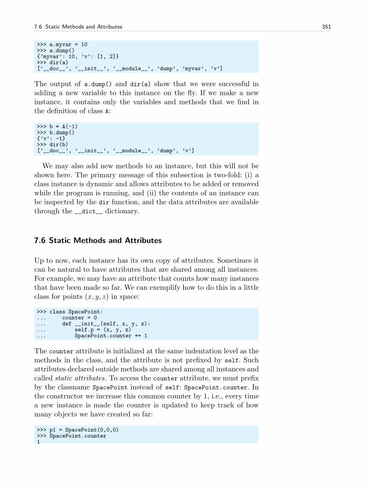
7.6 Static Methods and Attributes 351

>>> a.myvar = 10>>> a.dump()’myvar’: 10, ’v’: [1, 2]>>> dir(a)[’__doc__’, ’__init__’, ’__module__’, ’dump’, ’myvar’, ’v’]

The output of a.dump() and dir(a) show that we were successful inadding a new variable to this instance on the fly. If we make a newinstance, it contains only the variables and methods that we find inthe definition of class A:

>>> b = A(-1)>>> b.dump()’v’: -1>>> dir(b)[’__doc__’, ’__init__’, ’__module__’, ’dump’, ’v’]

We may also add new methods to an instance, but this will not beshown here. The primary message of this subsection is two-fold: (i) aclass instance is dynamic and allows attributes to be added or removedwhile the program is running, and (ii) the contents of an instance canbe inspected by the dir function, and the data attributes are availablethrough the __dict__ dictionary.

7.6 Static Methods and Attributes

Up to now, each instance has its own copy of attributes. Sometimes itcan be natural to have attributes that are shared among all instances.For example, we may have an attribute that counts how many instancesthat have been made so far. We can exemplify how to do this in a littleclass for points (x, y, z) in space:

>>> class SpacePoint:... counter = 0... def __init__(self, x, y, z):... self.p = (x, y, z)... SpacePoint.counter += 1

The counter attribute is initialized at the same indentation level as themethods in the class, and the attribute is not prefixed by self. Suchattributes declared outside methods are shared among all instances andcalled static attributes . To access the counter attribute, we must prefixby the classname SpacePoint instead of self: SpacePoint.counter. Inthe constructor we increase this common counter by 1, i.e., every timea new instance is made the counter is updated to keep track of howmany objects we have created so far:

>>> p1 = SpacePoint(0,0,0)>>> SpacePoint.counter1

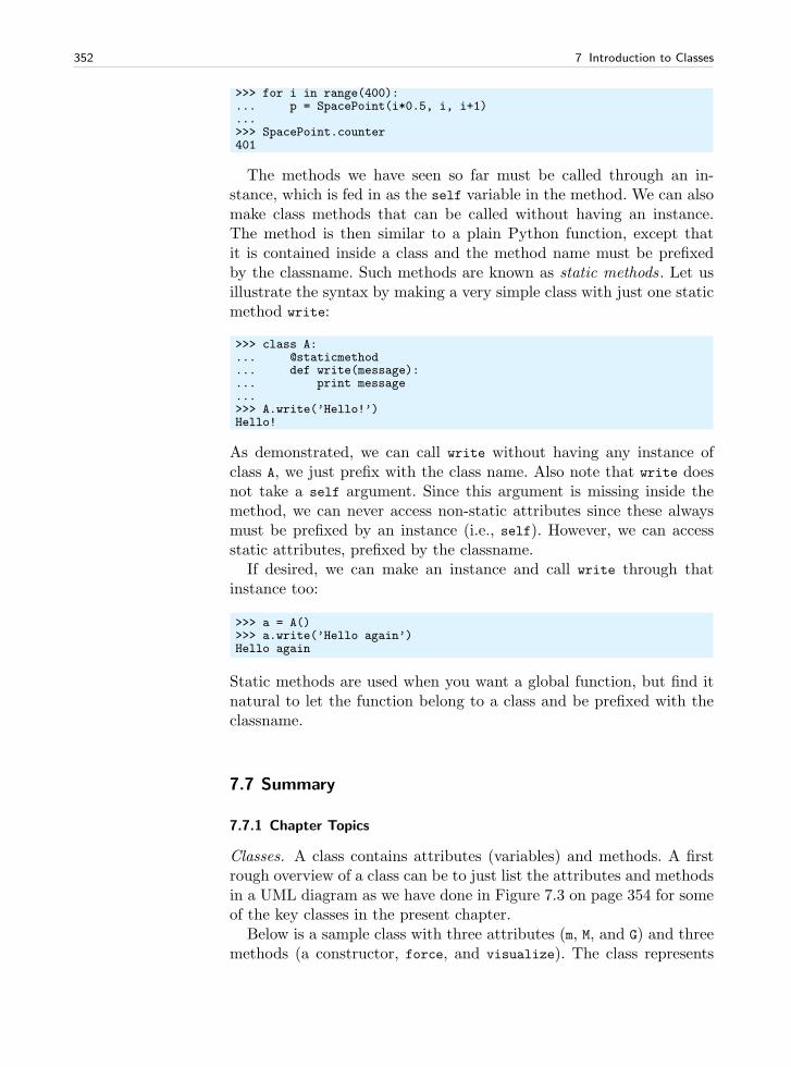
352 7 Introduction to Classes

>>> for i in range(400):... p = SpacePoint(i*0.5, i, i+1)...>>> SpacePoint.counter401

The methods we have seen so far must be called through an in-stance, which is fed in as the self variable in the method. We can alsomake class methods that can be called without having an instance.The method is then similar to a plain Python function, except thatit is contained inside a class and the method name must be prefixedby the classname. Such methods are known as static methods. Let usillustrate the syntax by making a very simple class with just one staticmethod write:

>>> class A:... @staticmethod... def write(message):... print message...>>> A.write(’Hello!’)Hello!

As demonstrated, we can call write without having any instance ofclass A, we just prefix with the class name. Also note that write doesnot take a self argument. Since this argument is missing inside themethod, we can never access non-static attributes since these alwaysmust be prefixed by an instance (i.e., self). However, we can accessstatic attributes, prefixed by the classname.

If desired, we can make an instance and call write through thatinstance too:

>>> a = A()>>> a.write(’Hello again’)Hello again

Static methods are used when you want a global function, but find itnatural to let the function belong to a class and be prefixed with theclassname.

7.7 Summary

7.7.1 Chapter Topics

Classes. A class contains attributes (variables) and methods. A firstrough overview of a class can be to just list the attributes and methodsin a UML diagram as we have done in Figure 7.3 on page 354 for someof the key classes in the present chapter.

Below is a sample class with three attributes (m, M, and G) and threemethods (a constructor, force, and visualize). The class represents

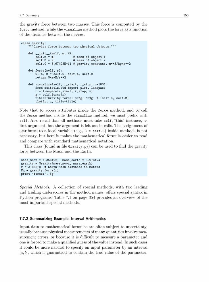
7.7 Summary 353

the gravity force between two masses. This force is computed by theforce method, while the visualize method plots the force as a functionof the distance between the masses.

class Gravity:"""Gravity force between two physical objects."""

def __init__(self, m, M):self.m = m # mass of object 1self.M = M # mass of object 2self.G = 6.67428E-11 # gravity constant, m**3/kg/s**2

def force(self, r):G, m, M = self.G, self.m, self.Mreturn G*m*M/r**2

def visualize(self, r_start, r_stop, n=100):from scitools.std import plot, linspacer = linspace(r_start, r_stop, n)g = self.force(r)title=’Gravity force: m=%g, M=%g’ % (self.m, self.M)plot(r, g, title=title)

Note that to access attributes inside the force method, and to callthe force method inside the visualize method, we must prefix withself. Also recall that all methods must take self, “this” instance, asfirst argument, but the argument is left out in calls. The assignment ofattributes to a local variable (e.g., G = self.G) inside methods is notnecessary, but here it makes the mathematical formula easier to readand compare with standard mathematical notation.

This class (found in file Gravity.py) can be used to find the gravityforce between the Moon and the Earth:

mass_moon = 7.35E+22; mass_earth = 5.97E+24gravity = Gravity(mass_moon, mass_earth)r = 3.85E+8 # Earth-Moon distance in metersFg = gravity.force(r)print ’force:’, Fg

Special Methods. A collection of special methods, with two leadingand trailing underscores in the method names, offers special syntax inPython programs. Table 7.1 on page 354 provides an overview of themost important special methods.

7.7.2 Summarizing Example: Interval Arithmetics

Input data to mathematical formulas are often subject to uncertainty,usually because physical measurements of many quantities involve mea-surement errors, or because it is difficult to measure a parameter andone is forced to make a qualified guess of the value instead. In such casesit could be more natural to specify an input parameter by an interval[a, b], which is guaranteed to contain the true value of the parameter.

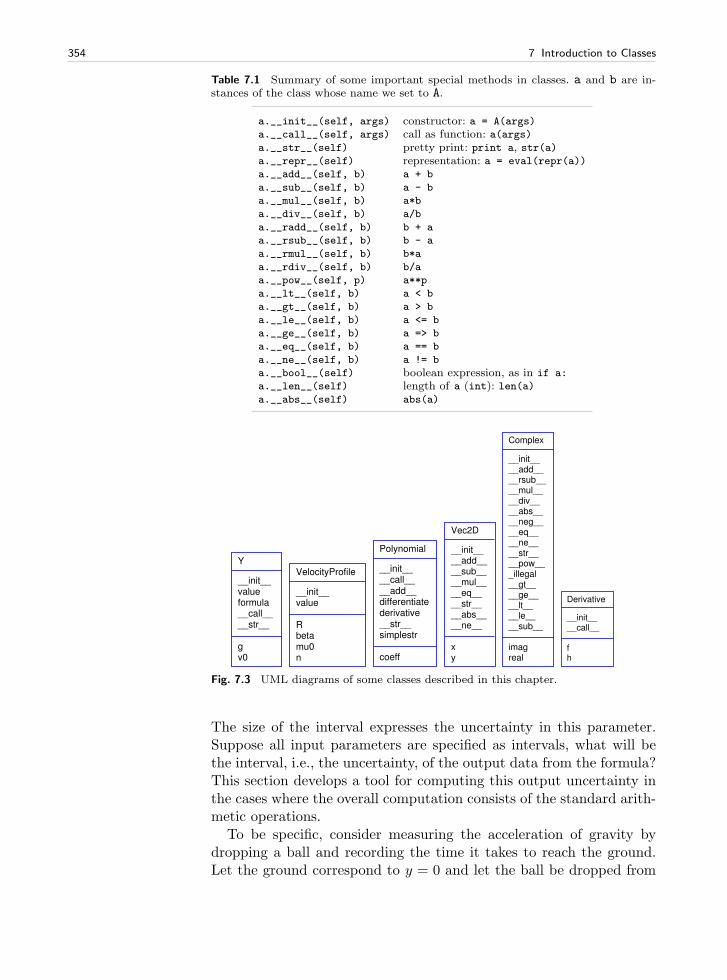
354 7 Introduction to Classes

Table 7.1 Summary of some important special methods in classes. a and b are in-stances of the class whose name we set to A.

a.__init__(self, args) constructor: a = A(args)

a.__call__(self, args) call as function: a(args)a.__str__(self) pretty print: print a, str(a)a.__repr__(self) representation: a = eval(repr(a))

a.__add__(self, b) a + b

a.__sub__(self, b) a - b

a.__mul__(self, b) a*b

a.__div__(self, b) a/b

a.__radd__(self, b) b + a

a.__rsub__(self, b) b - a

a.__rmul__(self, b) b*a

a.__rdiv__(self, b) b/a

a.__pow__(self, p) a**p

a.__lt__(self, b) a < b

a.__gt__(self, b) a > b

a.__le__(self, b) a <= b

a.__ge__(self, b) a => b

a.__eq__(self, b) a == b

a.__ne__(self, b) a != b

a.__bool__(self) boolean expression, as in if a:

a.__len__(self) length of a (int): len(a)a.__abs__(self) abs(a)

Y

__init__valueformula__call____str__

gv0

VelocityProfile

__init__value

Rbetamu0n

Polynomial

__init____call____add__differentiatederivative__str__simplestr

coeff

Vec2D

__init____add____sub____mul____eq____str____abs____ne__

xy

Complex

__init____add____rsub____mul____div____abs____neg____eq____ne____str____pow___illegal__gt____ge____lt____le____sub__

imagreal

Derivative

__init____call__

fh

Fig. 7.3 UML diagrams of some classes described in this chapter.

The size of the interval expresses the uncertainty in this parameter.Suppose all input parameters are specified as intervals, what will bethe interval, i.e., the uncertainty, of the output data from the formula?This section develops a tool for computing this output uncertainty inthe cases where the overall computation consists of the standard arith-metic operations.

To be specific, consider measuring the acceleration of gravity bydropping a ball and recording the time it takes to reach the ground.Let the ground correspond to y = 0 and let the ball be dropped from

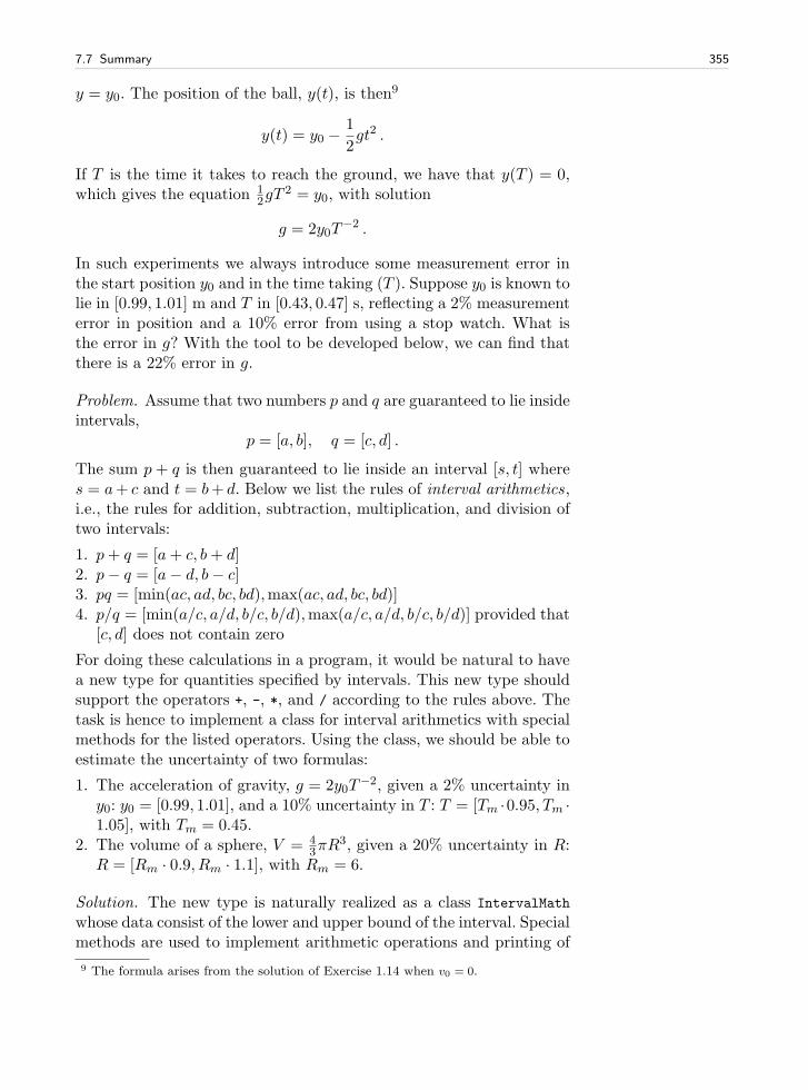
7.7 Summary 355

y = y0. The position of the ball, y(t), is then9

y(t) = y0 −1

2gt2 .

If T is the time it takes to reach the ground, we have that y(T ) = 0,which gives the equation 1

2gT2 = y0, with solution

g = 2y0T−2 .

In such experiments we always introduce some measurement error inthe start position y0 and in the time taking (T ). Suppose y0 is known tolie in [0.99, 1.01] m and T in [0.43, 0.47] s, reflecting a 2% measurementerror in position and a 10% error from using a stop watch. What isthe error in g? With the tool to be developed below, we can find thatthere is a 22% error in g.

Problem. Assume that two numbers p and q are guaranteed to lie insideintervals,

p = [a, b], q = [c, d] .

The sum p + q is then guaranteed to lie inside an interval [s, t] wheres = a+ c and t = b+ d. Below we list the rules of interval arithmetics,i.e., the rules for addition, subtraction, multiplication, and division oftwo intervals:

1. p+ q = [a+ c, b+ d]2. p− q = [a− d, b− c]3. pq = [min(ac, ad, bc, bd),max(ac, ad, bc, bd)]4. p/q = [min(a/c, a/d, b/c, b/d),max(a/c, a/d, b/c, b/d)] provided that

[c, d] does not contain zero

For doing these calculations in a program, it would be natural to havea new type for quantities specified by intervals. This new type shouldsupport the operators +, -, *, and / according to the rules above. Thetask is hence to implement a class for interval arithmetics with specialmethods for the listed operators. Using the class, we should be able toestimate the uncertainty of two formulas:

1. The acceleration of gravity, g = 2y0T−2, given a 2% uncertainty in

y0: y0 = [0.99, 1.01], and a 10% uncertainty in T : T = [Tm ·0.95, Tm ·1.05], with Tm = 0.45.

2. The volume of a sphere, V = 43πR

3, given a 20% uncertainty in R:R = [Rm · 0.9, Rm · 1.1], with Rm = 6.

Solution. The new type is naturally realized as a class IntervalMath

whose data consist of the lower and upper bound of the interval. Specialmethods are used to implement arithmetic operations and printing of

9 The formula arises from the solution of Exercise 1.14 when v0 = 0.

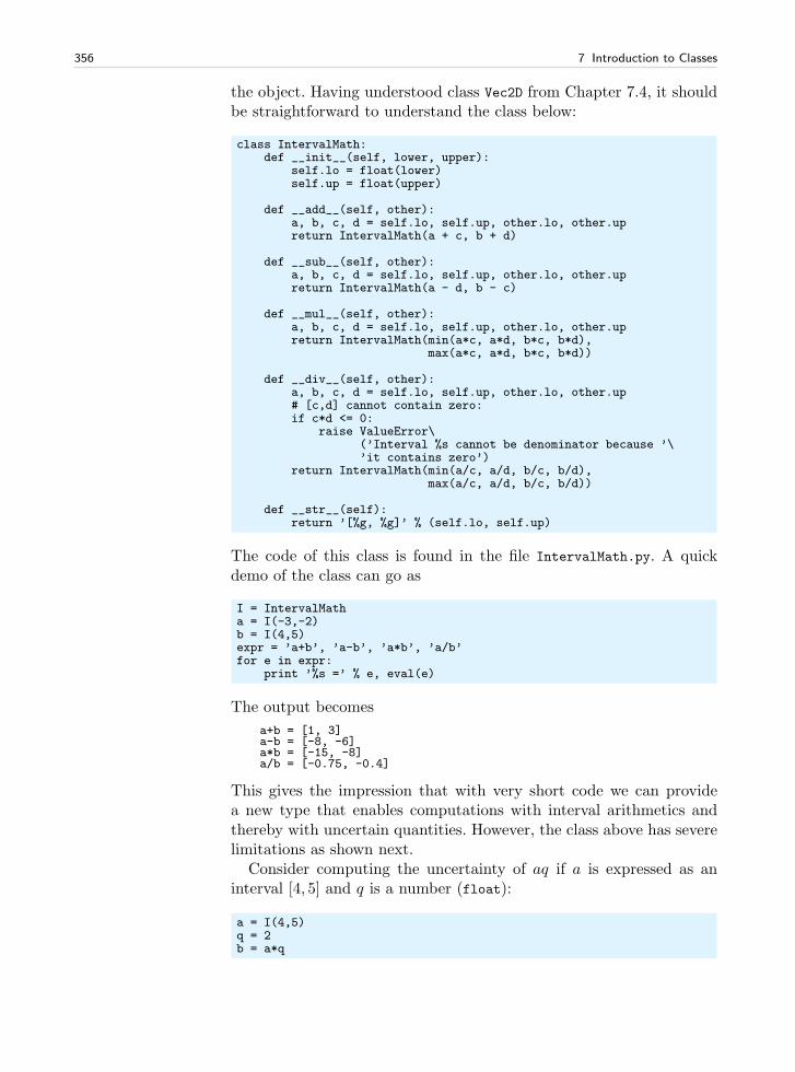
356 7 Introduction to Classes

the object. Having understood class Vec2D from Chapter 7.4, it shouldbe straightforward to understand the class below:

class IntervalMath:def __init__(self, lower, upper):

self.lo = float(lower)self.up = float(upper)

def __add__(self, other):a, b, c, d = self.lo, self.up, other.lo, other.upreturn IntervalMath(a + c, b + d)

def __sub__(self, other):a, b, c, d = self.lo, self.up, other.lo, other.upreturn IntervalMath(a - d, b - c)

def __mul__(self, other):a, b, c, d = self.lo, self.up, other.lo, other.upreturn IntervalMath(min(a*c, a*d, b*c, b*d),

max(a*c, a*d, b*c, b*d))

def __div__(self, other):a, b, c, d = self.lo, self.up, other.lo, other.up# [c,d] cannot contain zero:if c*d <= 0:

raise ValueError\(’Interval %s cannot be denominator because ’\’it contains zero’)

return IntervalMath(min(a/c, a/d, b/c, b/d),max(a/c, a/d, b/c, b/d))

def __str__(self):return ’[%g, %g]’ % (self.lo, self.up)

The code of this class is found in the file IntervalMath.py. A quickdemo of the class can go as

I = IntervalMatha = I(-3,-2)b = I(4,5)expr = ’a+b’, ’a-b’, ’a*b’, ’a/b’for e in expr:

print ’%s =’ % e, eval(e)

The output becomes

a+b = [1, 3]a-b = [-8, -6]a*b = [-15, -8]a/b = [-0.75, -0.4]

This gives the impression that with very short code we can providea new type that enables computations with interval arithmetics andthereby with uncertain quantities. However, the class above has severelimitations as shown next.

Consider computing the uncertainty of aq if a is expressed as aninterval [4, 5] and q is a number (float):

a = I(4,5)q = 2b = a*q

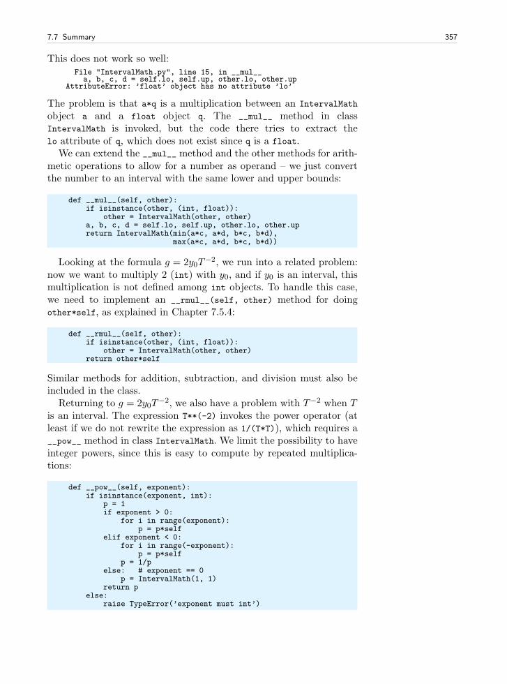
7.7 Summary 357

This does not work so well:File "IntervalMath.py", line 15, in __mul__a, b, c, d = self.lo, self.up, other.lo, other.up

AttributeError: ’float’ object has no attribute ’lo’

The problem is that a*q is a multiplication between an IntervalMath

object a and a float object q. The __mul__ method in classIntervalMath is invoked, but the code there tries to extract thelo attribute of q, which does not exist since q is a float.

We can extend the __mul__ method and the other methods for arith-metic operations to allow for a number as operand – we just convertthe number to an interval with the same lower and upper bounds:

def __mul__(self, other):if isinstance(other, (int, float)):

other = IntervalMath(other, other)a, b, c, d = self.lo, self.up, other.lo, other.upreturn IntervalMath(min(a*c, a*d, b*c, b*d),

max(a*c, a*d, b*c, b*d))

Looking at the formula g = 2y0T−2, we run into a related problem:

now we want to multiply 2 (int) with y0, and if y0 is an interval, thismultiplication is not defined among int objects. To handle this case,we need to implement an __rmul__(self, other) method for doingother*self, as explained in Chapter 7.5.4:

def __rmul__(self, other):if isinstance(other, (int, float)):

other = IntervalMath(other, other)return other*self

Similar methods for addition, subtraction, and division must also beincluded in the class.

Returning to g = 2y0T−2, we also have a problem with T−2 when T

is an interval. The expression T**(-2) invokes the power operator (atleast if we do not rewrite the expression as 1/(T*T)), which requires a__pow__ method in class IntervalMath. We limit the possibility to haveinteger powers, since this is easy to compute by repeated multiplica-tions:

def __pow__(self, exponent):if isinstance(exponent, int):

p = 1if exponent > 0:

for i in range(exponent):p = p*self

elif exponent < 0:for i in range(-exponent):

p = p*selfp = 1/p

else: # exponent == 0p = IntervalMath(1, 1)

return pelse:

raise TypeError(’exponent must int’)

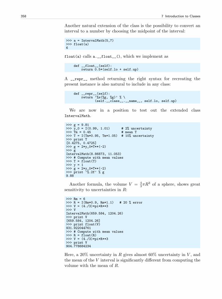
358 7 Introduction to Classes

Another natural extension of the class is the possibility to convert aninterval to a number by choosing the midpoint of the interval:

>>> a = IntervalMath(5,7)>>> float(a)6

float(a) calls a.__float__(), which we implement as

def __float__(self):return 0.5*(self.lo + self.up)

A __repr__ method returning the right syntax for recreating thepresent instance is also natural to include in any class:

def __repr__(self):return ’%s(%g, %g)’ % \

(self.__class__.__name__, self.lo, self.up)

We are now in a position to test out the extended classIntervalMath.

>>> g = 9.81>>> y_0 = I(0.99, 1.01) # 2% uncertainty>>> Tm = 0.45 # mean T>>> T = I(Tm*0.95, Tm*1.05) # 10% uncertainty>>> print T[0.4275, 0.4725]>>> g = 2*y_0*T**(-2)>>> gIntervalMath(8.86873, 11.053)>>> # Compute with mean values>>> T = float(T)>>> y = 1>>> g = 2*y_0*T**(-2)>>> print ’%.2f’ % g9.88

Another formula, the volume V = 43πR

3 of a sphere, shows greatsensitivity to uncertainties in R:

>>> Rm = 6>>> R = I(Rm*0.9, Rm*1.1) # 20 % error>>> V = (4./3)*pi*R**3>>> VIntervalMath(659.584, 1204.26)>>> print V[659.584, 1204.26]>>> print float(V)931.922044761>>> # Compute with mean values>>> R = float(R)>>> V = (4./3)*pi*R**3>>> print V904.778684234

Here, a 20% uncertainty in R gives almost 60% uncertainty in V , andthe mean of the V interval is significantly different from computing thevolume with the mean of R.

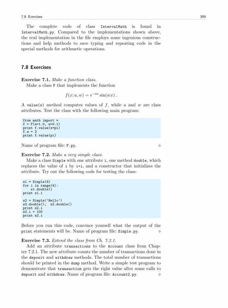
7.8 Exercises 359

The complete code of class IntervalMath is found inIntervalMath.py. Compared to the implementations shown above,the real implementation in the file employs some ingenious construc-tions and help methods to save typing and repeating code in thespecial methods for arithmetic operations.

7.8 Exercises

Exercise 7.1. Make a function class.Make a class F that implements the function

f(x; a, w) = e−ax sin(wx) .

A value(x) method computes values of f , while a and w are classattributes. Test the class with the following main program:

from math import *f = F(a=1.0, w=0.1)print f.value(x=pi)f.a = 2print f.value(pi)

Name of program file: F.py. ⋄

Exercise 7.2. Make a very simple class.Make a class Simple with one attribute i, one method double, which

replaces the value of i by i+i, and a constructor that initializes theattribute. Try out the following code for testing the class:

s1 = Simple(4)for i in range(4):

s1.double()print s1.i

s2 = Simple(’Hello’)s2.double(); s2.double()print s2.is2.i = 100print s2.i

Before you run this code, convince yourself what the output of theprint statements will be. Name of program file: Simple.py. ⋄

Exercise 7.3. Extend the class from Ch. 7.2.1.Add an attribute transactions to the Account class from Chap-

ter 7.2.1. The new attribute counts the number of transactions done inthe deposit and withdraw methods. The total number of transactionsshould be printed in the dump method. Write a simple test program todemonstrate that transaction gets the right value after some calls todeposit and withdraw. Name of program file: Account2.py. ⋄

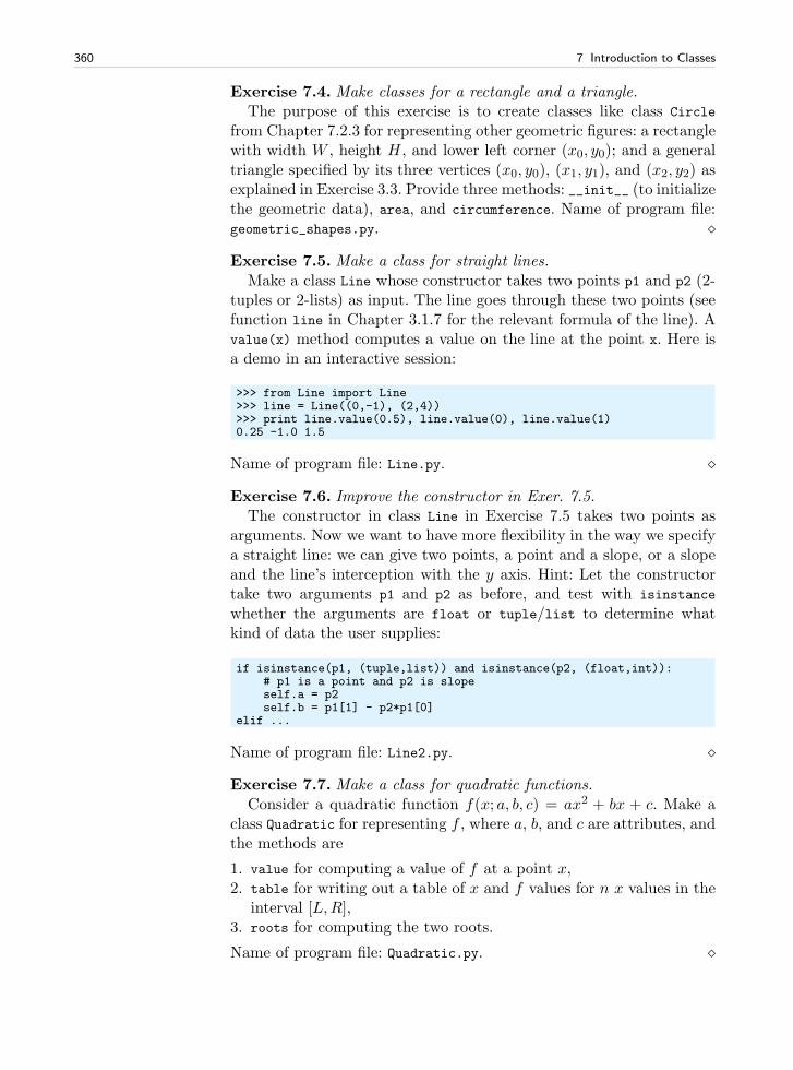
360 7 Introduction to Classes

Exercise 7.4. Make classes for a rectangle and a triangle.The purpose of this exercise is to create classes like class Circle

from Chapter 7.2.3 for representing other geometric figures: a rectanglewith width W , height H , and lower left corner (x0, y0); and a generaltriangle specified by its three vertices (x0, y0), (x1, y1), and (x2, y2) asexplained in Exercise 3.3. Provide three methods: __init__ (to initializethe geometric data), area, and circumference. Name of program file:geometric_shapes.py. ⋄

Exercise 7.5. Make a class for straight lines.Make a class Line whose constructor takes two points p1 and p2 (2-

tuples or 2-lists) as input. The line goes through these two points (seefunction line in Chapter 3.1.7 for the relevant formula of the line). Avalue(x) method computes a value on the line at the point x. Here isa demo in an interactive session:

>>> from Line import Line>>> line = Line((0,-1), (2,4))>>> print line.value(0.5), line.value(0), line.value(1)0.25 -1.0 1.5

Name of program file: Line.py. ⋄

Exercise 7.6. Improve the constructor in Exer. 7.5.The constructor in class Line in Exercise 7.5 takes two points as

arguments. Now we want to have more flexibility in the way we specifya straight line: we can give two points, a point and a slope, or a slopeand the line’s interception with the y axis. Hint: Let the constructortake two arguments p1 and p2 as before, and test with isinstance

whether the arguments are float or tuple/list to determine whatkind of data the user supplies:

if isinstance(p1, (tuple,list)) and isinstance(p2, (float,int)):# p1 is a point and p2 is slopeself.a = p2self.b = p1[1] - p2*p1[0]

elif ...

Name of program file: Line2.py. ⋄

Exercise 7.7. Make a class for quadratic functions.Consider a quadratic function f(x; a, b, c) = ax2 + bx + c. Make a

class Quadratic for representing f , where a, b, and c are attributes, andthe methods are

1. value for computing a value of f at a point x,2. table for writing out a table of x and f values for n x values in the

interval [L,R],3. roots for computing the two roots.

Name of program file: Quadratic.py. ⋄

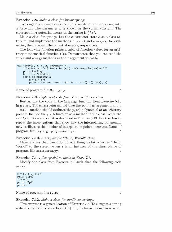
7.8 Exercises 361

Exercise 7.8. Make a class for linear springs.To elongate a spring a distance x, one needs to pull the spring with

a force kx. The parameter k is known as the spring constant. Thecorresponding potential energy in the spring is 1

2kx2.

Make a class for springs. Let the constructor store k as a class at-tribute, and implement the methods force(x) and energy(x) for eval-uating the force and the potential energy, respectively.

The following function prints a table of function values for an arbi-trary mathematical function f(x). Demonstrate that you can send theforce and energy methods as the f argument to table.

def table(f, a, b, n, heading=’’):"""Write out f(x) for x in [a,b] with steps h=(b-a)/n."""print headingh = (b-a)/float(n)for i in range(n+1):

x = a + i*hprint ’function value = %10.4f at x = %g’ % (f(x), x)

Name of program file: Spring.py. ⋄

Exercise 7.9. Implement code from Exer. 5.13 as a class.Restructure the code in the Lagrange function from Exercise 5.13

in a class. The constructor should take the points as argument, and a__call__ method should evaluate the pL(x) polynomial at an arbitrarypoint x. Include the graph function as a method in the class. Write theverify function and call it as described in Exercise 5.13. Use the class torepeat the investigations that show how the interpolating polynomialmay oscillate as the number of interpolation points increases. Name ofprogram file: Lagrange_polynomial3.py. ⋄

Exercise 7.10. A very simple “Hello, World!” class.Make a class that can only do one thing: print a writes “Hello,

World!” to the screen, when a is an instance of the class. Name ofprogram file: HelloWorld.py. ⋄

Exercise 7.11. Use special methods in Exer. 7.1.Modify the class from Exercise 7.1 such that the following code

works:

f = F2(1.0, 0.1)print f(pi)f.a = 2print f(pi)print f

Name of program file: F2.py. ⋄

Exercise 7.12. Make a class for nonlinear springs.This exercise is a generalization of Exercise 7.8. To elongate a spring

a distance x, one needs a force f(x). If f is linear, as in Exercise 7.8

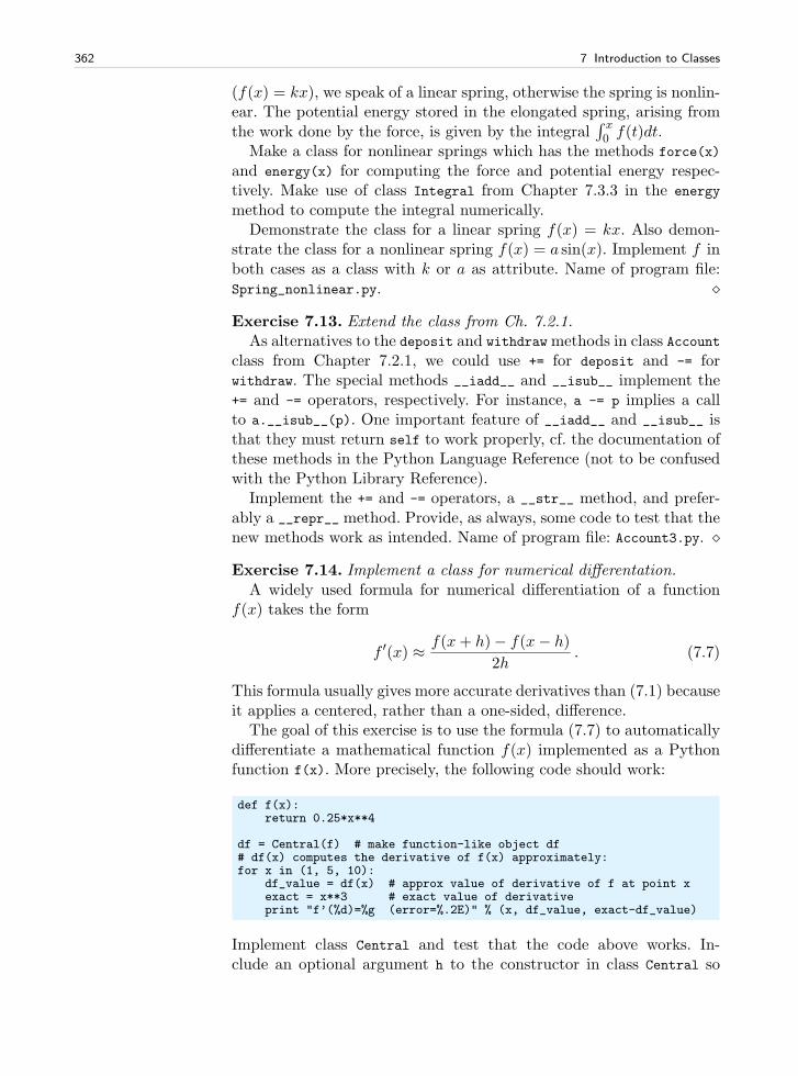
362 7 Introduction to Classes

(f(x) = kx), we speak of a linear spring, otherwise the spring is nonlin-ear. The potential energy stored in the elongated spring, arising fromthe work done by the force, is given by the integral

∫ x0 f(t)dt.

Make a class for nonlinear springs which has the methods force(x)

and energy(x) for computing the force and potential energy respec-tively. Make use of class Integral from Chapter 7.3.3 in the energy

method to compute the integral numerically.Demonstrate the class for a linear spring f(x) = kx. Also demon-

strate the class for a nonlinear spring f(x) = a sin(x). Implement f inboth cases as a class with k or a as attribute. Name of program file:Spring_nonlinear.py. ⋄

Exercise 7.13. Extend the class from Ch. 7.2.1.As alternatives to the deposit and withdrawmethods in class Account

class from Chapter 7.2.1, we could use += for deposit and -= forwithdraw. The special methods __iadd__ and __isub__ implement the+= and -= operators, respectively. For instance, a -= p implies a callto a.__isub__(p). One important feature of __iadd__ and __isub__ isthat they must return self to work properly, cf. the documentation ofthese methods in the Python Language Reference (not to be confusedwith the Python Library Reference).

Implement the += and -= operators, a __str__ method, and prefer-ably a __repr__ method. Provide, as always, some code to test that thenew methods work as intended. Name of program file: Account3.py. ⋄

Exercise 7.14. Implement a class for numerical differentation.A widely used formula for numerical differentiation of a function

f(x) takes the form

f ′(x) ≈ f(x+ h)− f(x− h)

2h. (7.7)

This formula usually gives more accurate derivatives than (7.1) becauseit applies a centered, rather than a one-sided, difference.

The goal of this exercise is to use the formula (7.7) to automaticallydifferentiate a mathematical function f(x) implemented as a Pythonfunction f(x). More precisely, the following code should work:

def f(x):return 0.25*x**4

df = Central(f) # make function-like object df# df(x) computes the derivative of f(x) approximately:for x in (1, 5, 10):

df_value = df(x) # approx value of derivative of f at point xexact = x**3 # exact value of derivativeprint "f’(%d)=%g (error=%.2E)" % (x, df_value, exact-df_value)

Implement class Central and test that the code above works. In-clude an optional argument h to the constructor in class Central so

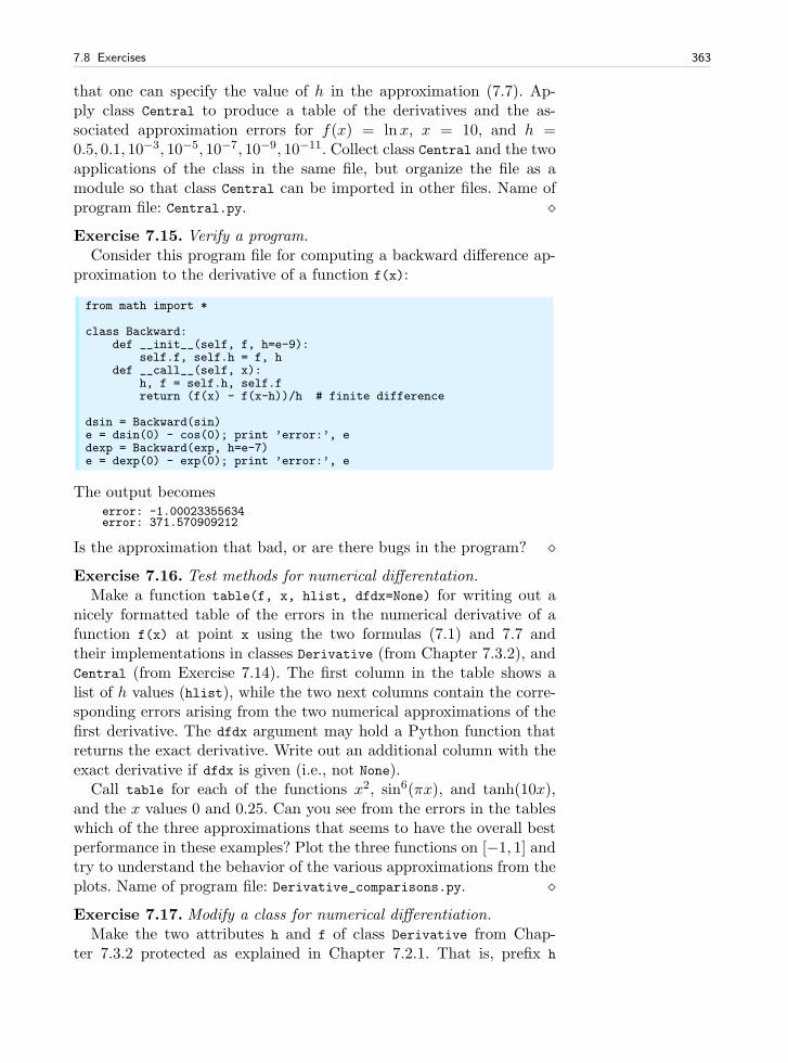
7.8 Exercises 363

that one can specify the value of h in the approximation (7.7). Ap-ply class Central to produce a table of the derivatives and the as-sociated approximation errors for f(x) = lnx, x = 10, and h =0.5, 0.1, 10−3, 10−5, 10−7, 10−9, 10−11. Collect class Central and the twoapplications of the class in the same file, but organize the file as amodule so that class Central can be imported in other files. Name ofprogram file: Central.py. ⋄Exercise 7.15. Verify a program.

Consider this program file for computing a backward difference ap-proximation to the derivative of a function f(x):

from math import *

class Backward:def __init__(self, f, h=e-9):

self.f, self.h = f, hdef __call__(self, x):

h, f = self.h, self.freturn (f(x) - f(x-h))/h # finite difference

dsin = Backward(sin)e = dsin(0) - cos(0); print ’error:’, edexp = Backward(exp, h=e-7)e = dexp(0) - exp(0); print ’error:’, e

The output becomeserror: -1.00023355634error: 371.570909212

Is the approximation that bad, or are there bugs in the program? ⋄Exercise 7.16. Test methods for numerical differentation.

Make a function table(f, x, hlist, dfdx=None) for writing out anicely formatted table of the errors in the numerical derivative of afunction f(x) at point x using the two formulas (7.1) and 7.7 andtheir implementations in classes Derivative (from Chapter 7.3.2), andCentral (from Exercise 7.14). The first column in the table shows alist of h values (hlist), while the two next columns contain the corre-sponding errors arising from the two numerical approximations of thefirst derivative. The dfdx argument may hold a Python function thatreturns the exact derivative. Write out an additional column with theexact derivative if dfdx is given (i.e., not None).

Call table for each of the functions x2, sin6(πx), and tanh(10x),and the x values 0 and 0.25. Can you see from the errors in the tableswhich of the three approximations that seems to have the overall bestperformance in these examples? Plot the three functions on [−1, 1] andtry to understand the behavior of the various approximations from theplots. Name of program file: Derivative_comparisons.py. ⋄Exercise 7.17. Modify a class for numerical differentiation.

Make the two attributes h and f of class Derivative from Chap-ter 7.3.2 protected as explained in Chapter 7.2.1. That is, prefix h

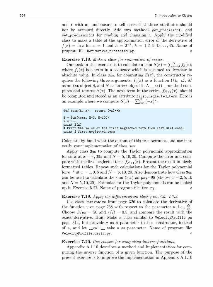
364 7 Introduction to Classes

and f with an underscore to tell users that these attributes shouldnot be accessed directly. Add two methods get_precision() andset_precision(h) for reading and changing h. Apply the modifiedclass to make a table of the approximation error of the derivative off(x) = lnx for x = 1 and h = 2−k, k = 1, 5, 9, 13 . . . , 45. Name ofprogram file: Derivative_protected.py. ⋄

Exercise 7.18. Make a class for summation of series.Our task in this exercise is to calculate a sum S(x) =

∑Nk=M fk(x),

where fk(x) is a term in a sequence which is assumed to decrease inabsolute value. In class Sum, for computing S(x), the constructor re-quires the following three arguments: fk(x) as a function f(k, x), Mas an int object M, and N as an int object N. A __call__ method com-putes and returns S(x). The next term in the series, fN+1(x), shouldbe computed and stored as an attribute first_neglected_term. Here isan example where we compute S(x) =

∑Nk=0(−x)k:

def term(k, x): return (-x)**k

S = Sum(term, M=0, N=100)x = 0.5print S(x)# Print the value of the first neglected term from last S(x) comp.print S.first_neglected_term

Calculate by hand what the output of this test becomes, and use it toverify your implementation of class Sum.

Apply class Sum to compute the Taylor polynomial approximationfor sinx at x = π, 30π and N = 5, 10, 20. Compute the error and com-pare with the first neglected term fN+1(x). Present the result in nicelyformatted tables. Repeat such calculations for the Taylor polynomialfor e−x at x = 1, 3, 5 and N = 5, 10, 20. Also demonstrate how class Sumcan be used to calculate the sum (3.1) on page 98 (choose x = 2, 5, 10and N = 5, 10, 20). Formulas for the Taylor polynomials can be lookedup in Exercise 5.27. Name of program file: Sum.py. ⋄

Exercise 7.19. Apply the differentiation class from Ch. 7.3.2.Use class Derivative from page 326 to calculate the derivative of

the function v on page 238 with respect to the parameter n, i.e., dvdn .

Choose β/µ0 = 50 and r/R = 0.5, and compare the result with theexact derivative. Hint: Make a class similar to VelocityProfile onpage 314, but provide r as a parameter to the constructor, insteadof n, and let __call__ take n as parameter. Name of program file:VelocityProfile_deriv.py. ⋄

Exercise 7.20. Use classes for computing inverse functions.Appendix A.1.10 describes a method and implementation for com-

puting the inverse function of a given function. The purpose of thepresent exercise is to improve the implementation in Appendix A.1.10

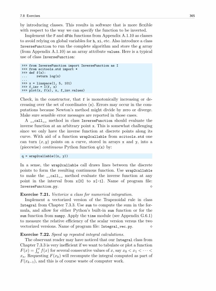
7.8 Exercises 365

by introducing classes. This results in software that is more flexiblewith respect to the way we can specify the function to be inverted.

Implement the F and dFdx functions from Appendix A.1.10 as classesto avoid relying on global variables for h, xi, etc. Also introduce a classInverseFunction to run the complete algorithm and store the g array(from Appendix A.1.10) as an array attribute values. Here is a typicaluse of class InverseFunction:

>>> from InverseFunction import InverseFunction as I>>> from scitools.std import *>>> def f(x):... return log(x)...>>> x = linspace(1, 5, 101)>>> f_inv = I(f, x)>>> plot(x, f(x), x, f_inv.values)

Check, in the constructor, that f is monotonically increasing or de-creasing over the set of coordinates (x). Errors may occur in the com-putations because Newton’s method might divide by zero or diverge.Make sure sensible error messages are reported in those cases.

A __call__ method in class InverseFunction should evaluate theinverse function at an arbitrary point x. This is somewhat challengingsince we only have the inverse function at discrete points along itscurve. With aid of a function wrap2callable from scitools.std onecan turn (x, y) points on a curve, stored in arrays x and y, into a(piecewise) continuous Python function q(x) by:

q = wrap2callable((x, y))

In a sense, the wrap2callable call draws lines between the discretepoints to form the resulting continuous function. Use wrap2callable

to make the __call__ method evaluate the inverse function at anypoint in the interval from x[0] to x[-1]. Name of program file:InverseFunction.py. ⋄

Exercise 7.21. Vectorize a class for numerical integration.Implement a vectorized version of the Trapezoidal rule in class

Integral from Chapter 7.3.3. Use sum to compute the sum in the for-mula, and allow for either Python’s built-in sum function or for thesum function from numpy. Apply the time module (see Appendix G.6.1)to measure the relative efficiency of the scalar version versus the twovectorized versions. Name of program file: Integral_vec.py. ⋄

Exercise 7.22. Speed up repeated integral calculations.The observant reader may have noticed that our Integral class from

Chapter 7.3.3 is very inefficient if we want to tabulate or plot a functionF (x) =

∫ xa f(x) for several consecutive values of x, say x0 < x1 < · · · <

xn. Requesting F (xk) will recompute the integral computed as part ofF (xk−1), and this is of course waste of computer work.

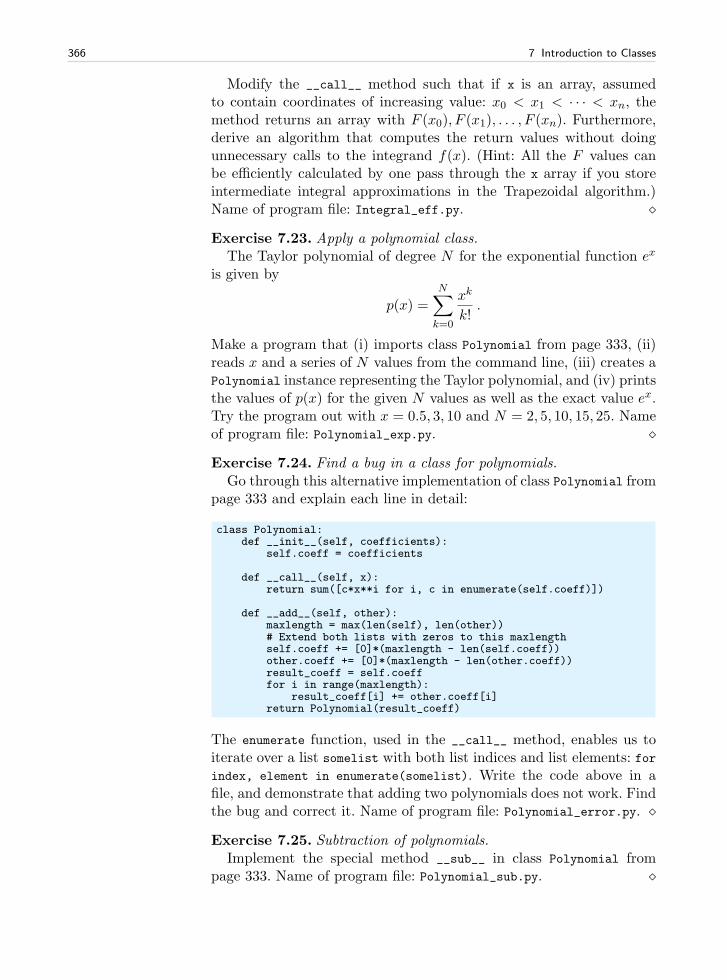
366 7 Introduction to Classes

Modify the __call__ method such that if x is an array, assumedto contain coordinates of increasing value: x0 < x1 < · · · < xn, themethod returns an array with F (x0), F (x1), . . . , F (xn). Furthermore,derive an algorithm that computes the return values without doingunnecessary calls to the integrand f(x). (Hint: All the F values canbe efficiently calculated by one pass through the x array if you storeintermediate integral approximations in the Trapezoidal algorithm.)Name of program file: Integral_eff.py. ⋄

Exercise 7.23. Apply a polynomial class.The Taylor polynomial of degree N for the exponential function ex

is given by

p(x) =

N∑

k=0

xk

k!.

Make a program that (i) imports class Polynomial from page 333, (ii)reads x and a series of N values from the command line, (iii) creates aPolynomial instance representing the Taylor polynomial, and (iv) printsthe values of p(x) for the given N values as well as the exact value ex.Try the program out with x = 0.5, 3, 10 and N = 2, 5, 10, 15, 25. Nameof program file: Polynomial_exp.py. ⋄

Exercise 7.24. Find a bug in a class for polynomials.Go through this alternative implementation of class Polynomial from

page 333 and explain each line in detail:

class Polynomial:def __init__(self, coefficients):

self.coeff = coefficients

def __call__(self, x):return sum([c*x**i for i, c in enumerate(self.coeff)])

def __add__(self, other):maxlength = max(len(self), len(other))# Extend both lists with zeros to this maxlengthself.coeff += [0]*(maxlength - len(self.coeff))other.coeff += [0]*(maxlength - len(other.coeff))result_coeff = self.coefffor i in range(maxlength):

result_coeff[i] += other.coeff[i]return Polynomial(result_coeff)

The enumerate function, used in the __call__ method, enables us toiterate over a list somelist with both list indices and list elements: forindex, element in enumerate(somelist). Write the code above in afile, and demonstrate that adding two polynomials does not work. Findthe bug and correct it. Name of program file: Polynomial_error.py. ⋄

Exercise 7.25. Subtraction of polynomials.Implement the special method __sub__ in class Polynomial from

page 333. Name of program file: Polynomial_sub.py. ⋄

7.8 Exercises 367

Exercise 7.26. Represent a polynomial by an array.Introduce a Numerical Python array for self.coeff in class

Polynomial from page 333. Go through the class code and run thestatements in the _test method in the Polynomial.py file to locatewhich statements that need to be modified because self.coeff is anarray and not a list. Name of program file: Polynomial_array1.py. ⋄

Exercise 7.27. Vectorize a class for polynomials.Introducing an array instead of a list in class Polynomial, as sug-

gested in Exercise 7.26, does not enhance the implementation. A realenhancement arise when the code is vectorized, i.e., when loops arereplaced by operations on whole arrays.

First, vectorize the __add__ method by adding the common partsof the coefficients arrays and then appending the rest of the longestarray to the result (appending an array a to an array b is done byconcatenate(a, b)).

Second, vectorize the __call__ method by observing that evaluationof a polynomial,

∑n−1i=0 cix

i, can be computed as the inner product oftwo arrays: (c0, . . . , cn−1) and (x0, x1, . . . , xn−1). The latter array canbe computed by x**p, where p is an array with powers 0, 1, . . . , n− 1.

Third, the differentiate method can be vectorized by the state-ments

n = len(self.coeff)self.coeff[:-1] = linspace(1, n-1, n-1)*self.coeff[1:]self.coeff = self.coeff[:-1]

Show by hand calculations in a case where n is 3 that the vector-ized statements produce the same result as the original differentiatemethod.

The __mul__ method is more challenging to vectorize so you mayleave this unaltered. Check that the vectorized versions of __add__,__call__, and differentiate work by comparing with the scalar codefrom Exercise 7.26 or the original, list-based Polynomial class. Nameof program file: Polynomial_array2.py. ⋄

Exercise 7.28. Use a dict to hold polynomial coefficients; add.Use a dictionary for self.coeff in class Polynomial from page 333.

The advantage with a dictionary is that only the nonzero coefficientsneed to be stored. Let self.coeff[k] hold the coefficient of the xk

term. Implement a constructor and the __add__ method. Exemplifythe implementation by adding x− 3x100 and x20 − x+ 4x100. Name ofprogram file: Polynomial_dict1.py. ⋄

Exercise 7.29. Use a dict to hold polynomial coefficients; mul.Extend the class in Exercise 7.28 with a __mul__ method. First,

study the algorithm in Chapter 7.3.7 for the __mul__ method whenthe coefficients are stored in lists. Then modify the algorithm to

368 7 Introduction to Classes

work with dictionaries. Implement the algorithm and exemplify it bymultiplying x − 3x100 and x20 − x + 4x100. Name of program file:Polynomial_dict2.py. ⋄

Exercise 7.30. Extend class Vec2D to work with lists/tuples.The Vec2D class from Chapter 7.4 supports addition and subtraction,

but only addition and subtraction of two Vec2D objects. Sometimes wewould like to add or subtract a point that is represented by a list or atuple:

u = Vec2D(-2, 4)v = u + (1,1.5)w = [-3, 2] - v

That is, a list or a tuple must be allowed in the right or left operand.Use ideas from Chapters 7.5.3 and 7.5.4 to implement this extension.Name of program file: Vec2D_lists.py. ⋄

Exercise 7.31. Extend class Vec2D to 3D vectors.Extend the implementation of class Vec2D from Chapter 7.4 to a class

Vec3D for vectors in three-dimensional space. Add a method cross forcomputing the cross product of two 3D vectors. Name of program file:Vec3D.py. ⋄

Exercise 7.32. Use NumPy arrays in class Vec2D.The internal code in class Vec2D from Chapter 7.4 can be valid for

vectors in any space dimension if we represent the vector as a NumPyarray in the class instead of seperate variables x and y for the vectorcomponents. Make a new class Vec where you apply NumPy function-ality in the methods. The constructor should be able to treat all thefollowing ways of initializing a vector:

a = array([1, -1, 4], float) # numpy arrayv = Vec(a)v = Vec([1, -1, 4]) # listv = Vec((1, -1, 4)) # tuplev = Vec(1, -1) # coordinates

We will provide some helpful advice. In the constructor, use variablenumber of arguments as described in Appendix G.5. All arguments arethen available as a tuple, and if there is only one element in the tuple,it should be an array, list, or tuple you can send through asarray to geta NumPy array. If there are many arguments, these are coordinates,and the tuple of arguments can be transformed by array to a NumPyarray. Assume in all operations that the involved vectors have equaldimension (typically that other has the same dimension as self). Recallto return Vec objects from all arithmetic operations, not NumPy arrays,because the next operation with the vector will then not take place inVec but in NumPy. If self.v is the attribute holding the vector as aNumPy array, the addition operator will typically be implemented as

7.8 Exercises 369

class Vec:...def __add__(self, other):

return Vec(selv.v + other.v)

Name of program file: Vec.py. ⋄

Exercise 7.33. Use classes in the program from Ch. 6.6.2.Modify the files/students.py program described in Chapter 6.6.2

by making the values of the data dictionary instances of class Student.This class contains a student’s name and a list of the courses. Eachcourse is represented by an instance of class Course. This class containsthe course name, the semester, the credit points, and the grade. Make__str__ and/or __repr__ write out the contents of the objects. Nameof program file: Student_Course.py. ⋄

Exercise 7.34. Use a class in Exer. 6.25.The purpose of this exercise is to make the program from Exer-

cise 6.25 on page 303 more flexible by creating a class that runs andarchives all the experiments. Here is a sketch of the class:

class GrowthLogistic:def __init__(self, show_plot_on_screen=False):

self.experiments = []self.show_plot_on_screen = show_plot_on_screenself.remove_plot_files()

def run_one(self, y0, q, N):"""Run one experiment."""# Compute y[n] in a loop...plotfile = ’tmp_y0_%g_q_%g_N_%d.png’ % (y0, q, N)self.experiments.append(’y0’: y0, ’q’: q, ’N’: N,

’mean’: mean(y[20:]),’y’: y, ’plotfile’: plotfile)

# Make plot...

def run_many(self, y0_list, q_list, N):"""Run many experiments."""for q in q_list:

for y0 in y0_list:self.run_one(y0, q, N)

def remove_plot_files(self):"""Remove plot files with names tmp_y0*.png."""import os, globfor plotfile in glob.glob(’tmp_y0*.png’):

os.remove(plotfile)

def report(self, filename=’tmp.html’):"""Generate an HTML report with plots of allexperiments generated so far."""# Open file and write HTML header...for e in self.experiments:

html.write(’<p><img src="%s">\n’ % e[’plotfile’])# Write HTML footer and close file...

Each time the run_one method is called, data about the current exper-iment is stored in the experiments list. Note that experiments contains

370 7 Introduction to Classes

a list of dictionaries. When desired, we can call the report method tocollect all the plots made so far in an HTML report. A typical use ofthe class goes as follows:

N = 50g = GrowthLogistic()g.run_many(y0_list=[0.01, 0.3],

q_list=[0.1, 1, 1.5, 1.8] + [2, 2.5, 3], N=N)g.run_one(y0=0.01, q=3, N=1000)g.report()

Make a complete implementation of class GrowthLogistic and test itwith the small program above. The program file should be constructedas a module. Name of program file: growth_logistic5.py. ⋄

Exercise 7.35. Apply the class from Exer. 7.34 interactively.Class GrowthLogistic from Exercise 7.34 is very well suited for inter-

active exploration. Here is a possible sample session for illustration:

>>> from growth_logistic5 import GrowthLogistic>>> g = GrowthLogistic(show_plot_on_screen=True)>>> q = 3>>> g.run_one(0.01, q, 100)>>> y = g.experiments[-1][’y’]>>> max(y)1.3326056469620293>>> min(y)0.0029091569028512065

Extend this session with an investigation of the oscillations in the so-lution yn. For this purpose, make a function for computing the localmaximum values yn and the corresponding indices where these localmaximum values occur. We can say that yi is a local maximum valueif

yi−1 < yi > yi+1 .

Plot the sequence of local maximum values in a new plot. If I0, I1, I2, . . .constitute the set of increasing indices corresponding to the localmaximum values, we can define the periods of the oscillations asI1 − I0, I2 − I1, and so forth. Plot the length of the periods in aseparate plot. Repeat this investigation for q = 2.5. Log the wholesession as explained in Exercise 1.12 (page 46). Name of program file:GrowthLogistic_interactive.py. ⋄

Exercise 7.36. Find local and global extrema of a function.Extreme points of a function f(x) are normally found by solving

f ′(x) = 0. A much simpler method is to evaluate f(x) for a set ofdiscrete points in the interval [a, b] and look for local minima andmaxima among these points. We work with n equally spaced pointsa = x0 < x1 < · · · < xn−1 = b, xi = a+ ih, h = (b− a)/(n− 1).

1. First we find all local extreme points in the interior of the domain.Local minima are recognized by

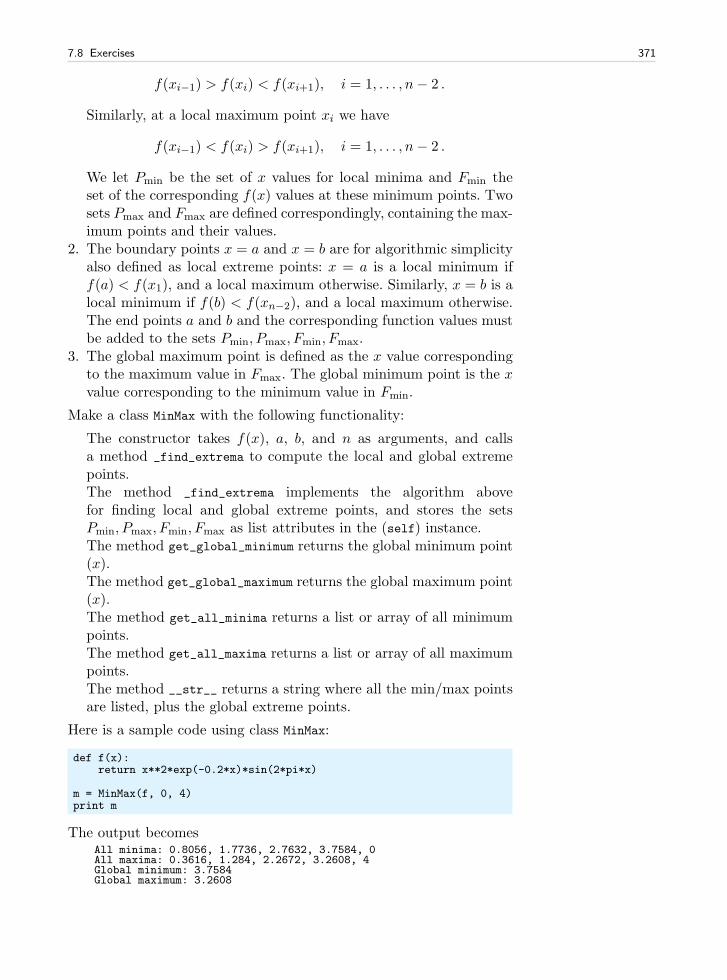
7.8 Exercises 371

f(xi−1) > f(xi) < f(xi+1), i = 1, . . . , n− 2 .

Similarly, at a local maximum point xi we have

f(xi−1) < f(xi) > f(xi+1), i = 1, . . . , n− 2 .

We let Pmin be the set of x values for local minima and Fmin theset of the corresponding f(x) values at these minimum points. Twosets Pmax and Fmax are defined correspondingly, containing the max-imum points and their values.

2. The boundary points x = a and x = b are for algorithmic simplicityalso defined as local extreme points: x = a is a local minimum iff(a) < f(x1), and a local maximum otherwise. Similarly, x = b is alocal minimum if f(b) < f(xn−2), and a local maximum otherwise.The end points a and b and the corresponding function values mustbe added to the sets Pmin, Pmax, Fmin, Fmax.

3. The global maximum point is defined as the x value correspondingto the maximum value in Fmax. The global minimum point is the xvalue corresponding to the minimum value in Fmin.

Make a class MinMax with the following functionality:

The constructor takes f(x), a, b, and n as arguments, and callsa method _find_extrema to compute the local and global extremepoints.

The method _find_extrema implements the algorithm abovefor finding local and global extreme points, and stores the setsPmin, Pmax, Fmin, Fmax as list attributes in the (self) instance.

The method get_global_minimum returns the global minimum point(x).

The method get_global_maximum returns the global maximum point(x).

The method get_all_minima returns a list or array of all minimumpoints.

The method get_all_maxima returns a list or array of all maximumpoints.

The method __str__ returns a string where all the min/max pointsare listed, plus the global extreme points.

Here is a sample code using class MinMax:

def f(x):return x**2*exp(-0.2*x)*sin(2*pi*x)

m = MinMax(f, 0, 4)print m

The output becomesAll minima: 0.8056, 1.7736, 2.7632, 3.7584, 0All maxima: 0.3616, 1.284, 2.2672, 3.2608, 4Global minimum: 3.7584Global maximum: 3.2608

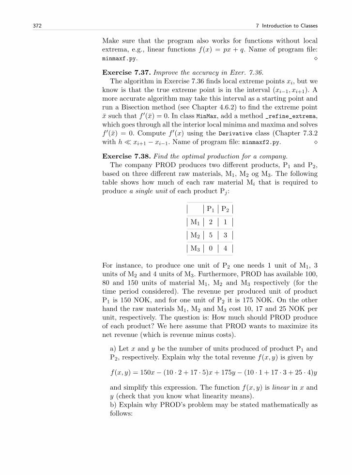
372 7 Introduction to Classes

Make sure that the program also works for functions without localextrema, e.g., linear functions f(x) = px + q. Name of program file:minmaxf.py. ⋄

Exercise 7.37. Improve the accuracy in Exer. 7.36.The algorithm in Exercise 7.36 finds local extreme points xi, but we

know is that the true extreme point is in the interval (xi−1, xi+1). Amore accurate algorithm may take this interval as a starting point andrun a Bisection method (see Chapter 4.6.2) to find the extreme pointx such that f ′(x) = 0. In class MinMax, add a method _refine_extrema,which goes through all the interior local minima and maxima and solvesf ′(x) = 0. Compute f ′(x) using the Derivative class (Chapter 7.3.2with h≪ xi+1 − xi−1. Name of program file: minmaxf2.py. ⋄

Exercise 7.38. Find the optimal production for a company.The company PROD produces two different products, P1 and P2,

based on three different raw materials, M1, M2 og M3. The followingtable shows how much of each raw material Mi that is required toproduce a single unit of each product Pj :

P1 P2

M1 2 1

M2 5 3

M3 0 4

For instance, to produce one unit of P2 one needs 1 unit of M1, 3units of M2 and 4 units of M3. Furthermore, PROD has available 100,80 and 150 units of material M1, M2 and M3 respectively (for thetime period considered). The revenue per produced unit of productP1 is 150 NOK, and for one unit of P2 it is 175 NOK. On the otherhand the raw materials M1, M2 and M3 cost 10, 17 and 25 NOK perunit, respectively. The question is: How much should PROD produceof each product? We here assume that PROD wants to maximize itsnet revenue (which is revenue minus costs).

a) Let x and y be the number of units produced of product P1 andP2, respectively. Explain why the total revenue f(x, y) is given by

f(x, y) = 150x− (10 · 2 + 17 · 5)x+ 175y − (10 · 1 + 17 · 3 + 25 · 4)y

and simplify this expression. The function f(x, y) is linear in x andy (check that you know what linearity means).b) Explain why PROD’s problem may be stated mathematically asfollows:

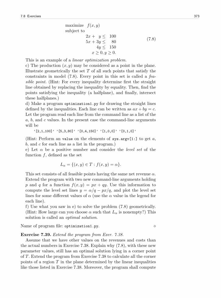
7.8 Exercises 373

maximize f(x, y)subject to

2x + y ≤ 1005x + 3y ≤ 80

4y ≤ 150x ≥ 0, y ≥ 0.

(7.8)

This is an example of a linear optimization problem.c) The production (x, y) may be considered as a point in the plane.Illustrate geometrically the set T of all such points that satisfy theconstraints in model (7.8). Every point in this set is called a fea-sible point. (Hint: For every inequality determine first the straightline obtained by replacing the inequality by equality. Then, find thepoints satisfying the inequality (a halfplane), and finally, intersectthese halfplanes.)d) Make a program optimization1.py for drawing the straight linesdefined by the inequalities. Each line can be written as ax+ by = c.Let the program read each line from the command line as a list of thea, b, and c values. In the present case the command-line argumentswill be

’[2,1,100]’ ’[5,3,80]’ ’[0,4,150]’ ’[1,0,0]’ ’[0,1,0]’

(Hint: Perform an value on the elements of sys.argv[1:] to get a,b, and c for each line as a list in the program.)e) Let α be a positive number and consider the level set of thefunction f , defined as the set

Lα = (x, y) ∈ T : f(x, y) = α.

This set consists of all feasible points having the same net revenue α.Extend the program with two new command-line arguments holdingp and q for a function f(x, y) = px + qy. Use this information tocompute the level set lines y = α/q − px/q, and plot the level setlines for some different values of α (use the α value in the legend foreach line).f) Use what you saw in e) to solve the problem (7.8) geometrically.(Hint: How large can you choose α such that Lα is nonempty?) Thissolution is called an optimal solution.

Name of program file: optimization1.py. ⋄

Exercise 7.39. Extend the program from Exer. 7.38.Assume that we have other values on the revenues and costs than

the actual numbers in Exercise 7.38. Explain why (7.8), with these newparameter values, still has an optimal solution lying in a corner pointof T . Extend the program from Exercise 7.38 to calculate all the cornerpoints of a region T in the plane determined by the linear inequalitieslike those listed in Exercise 7.38. Moreover, the program shall compute

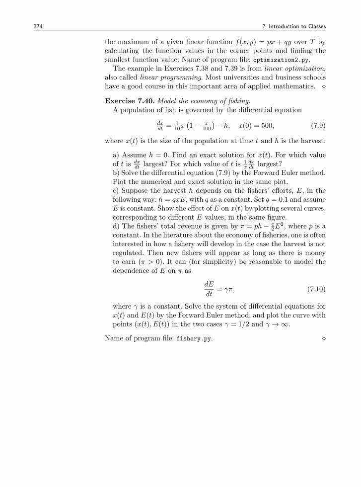
374 7 Introduction to Classes

the maximum of a given linear function f(x, y) = px + qy over T bycalculating the function values in the corner points and finding thesmallest function value. Name of program file: optimization2.py.

The example in Exercises 7.38 and 7.39 is from linear optimization,also called linear programming. Most universities and business schoolshave a good course in this important area of applied mathematics. ⋄

Exercise 7.40. Model the economy of fishing.A population of fish is governed by the differential equation

dxdt = 1

10x(

1− x100

)

− h, x(0) = 500, (7.9)

where x(t) is the size of the population at time t and h is the harvest.

a) Assume h = 0. Find an exact solution for x(t). For which valueof t is dx

dt largest? For which value of t is 1xdxdt largest?

b) Solve the differential equation (7.9) by the Forward Euler method.Plot the numerical and exact solution in the same plot.c) Suppose the harvest h depends on the fishers’ efforts, E, in thefollowing way: h = qxE, with q as a constant. Set q = 0.1 and assumeE is constant. Show the effect of E on x(t) by plotting several curves,corresponding to different E values, in the same figure.d) The fishers’ total revenue is given by π = ph− c

2E2, where p is a

constant. In the literature about the economy of fisheries, one is ofteninterested in how a fishery will develop in the case the harvest is notregulated. Then new fishers will appear as long as there is moneyto earn (π > 0). It can (for simplicity) be reasonable to model thedependence of E on π as

dE

dt= γπ, (7.10)

where γ is a constant. Solve the system of differential equations forx(t) and E(t) by the Forward Euler method, and plot the curve withpoints (x(t), E(t)) in the two cases γ = 1/2 and γ →∞.

Name of program file: fishery.py. ⋄

Random Numbers and Simple Games 8

Random numbers have many applications in science and computer pro-gramming, especially when there are significant uncertainties in a phe-nomenon of interest. The purpose of this chapter is to look at somepractical problems involving random numbers and learn how to pro-gram with such numbers. We shall make several games and also lookinto how random numbers can be used in physics. You need to be famil-iar with Chapters 1–5 in order to study the present chapter, but a fewexamples and exercises will require familiarity with the class conceptfrom Chapter 7.

The key idea in computer simulations with random numbers is firstto formulate an algorithmic description of the phenomenon we wantto study. This description frequently maps directly onto a quite simpleand short Python program, where we use random numbers to mimicthe uncertain features of the phenomenon. The program needs to per-form a large number of repeated calculations, and the final answersare “only” approximate, but the accuracy can usually be made goodenough for practical purposes. Most programs related to the presentchapter produce their results within a few seconds. In cases where theexecution times become large, we can vectorize the code. Vectorizedcomputations with random numbers is definitely the most demandingtopic in this chapter, but is not mandatory for seeing the power ofmathematical modeling via random numbers.

All files associated with the examples in this chapter are found inthe folder src/random.

375

376 8 Random Numbers and Simple Games

8.1 Drawing Random Numbers

Python has a module random for generating random numbers. The func-tion call random.random() generates a random number in the half openinterval1 [0, 1). We can try it out:

>>> import random>>> random.random()0.81550546885338104>>> random.random()0.44913326809029852>>> random.random()0.88320653116367454

All computations of random numbers are based on deterministic al-gorithms (see Exercise 8.19 for an example), so the sequence of numberscannot be truly random. However, the sequence of numbers appears tolack any pattern, and we can therefore view the numbers as random2.

8.1.1 The Seed

Every time we import random, the subsequent sequence ofrandom.random() calls will yield different numbers. For debuggingpurposes it is useful to get the same sequence of random numbersevery time we run the program. This functionality is obtained bysetting a seed before we start generating numbers. With a given valueof the seed, one and only one sequence of numbers is generated. Theseed is an integer and set by the random.seed function:

>>> random.seed(121)

Let us generate two series of random numbers at once, using a listcomprehension and a format with two decimals only:

>>> random.seed(2)>>> [’%.2f’ % random.random() for i in range(7)][’0.96’, ’0.95’, ’0.06’, ’0.08’, ’0.84’, ’0.74’, ’0.67’]>>> [’%.2f’ % random.random() for i in range(7)][’0.31’, ’0.61’, ’0.61’, ’0.58’, ’0.16’, ’0.43’, ’0.39’]

If we set the seed to 2 again, the sequence of numbers is regenerated:

>>> random.seed(2)>>> [’%.2f’ % random.random() for i in range(7)][’0.96’, ’0.95’, ’0.06’, ’0.08’, ’0.84’, ’0.74’, ’0.67’]

If we do not give a seed, the random module sets a seed based on thecurrent time. That is, the seed will be different each time we run the

1 In the half open interval [0, 1) the lower limit is included, but the upper limit is not.2 What it means to view the numbers as random has fortunately a firm mathematicalfoundation, so don’t let the fact that random numbers are deterministic stop youfrom using them.

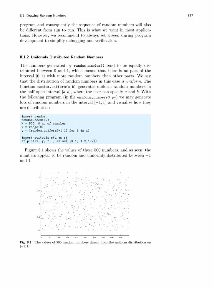
8.1 Drawing Random Numbers 377

program and consequently the sequence of random numbers will alsobe different from run to run. This is what we want in most applica-tions. However, we recommend to always set a seed during programdevelopment to simplify debugging and verification.

8.1.2 Uniformly Distributed Random Numbers

The numbers generated by random.random() tend to be equally dis-tributed between 0 and 1, which means that there is no part of theinterval [0, 1) with more random numbers than other parts. We saythat the distribution of random numbers in this case is uniform. Thefunction random.uniform(a,b) generates uniform random numbers inthe half open interval [a, b), where the user can specify a and b. Withthe following program (in file uniform_numbers0.py) we may generatelots of random numbers in the interval [−1, 1) and visualize how theyare distributed :

import randomrandom.seed(42)N = 500 # no of samplesx = range(N)y = [random.uniform(-1,1) for i in x]

import scitools.std as stst.plot(x, y, ’+’, axis=[0,N-1,-1.2,1.2])

Figure 8.1 shows the values of these 500 numbers, and as seen, thenumbers appear to be random and uniformly distributed between −1and 1.

-1

-0.5

0

0.5

1

0 50 100 150 200 250 300 350 400 450

Fig. 8.1 The values of 500 random numbers drawn from the uniform distribution on[−1, 1).

378 8 Random Numbers and Simple Games

8.1.3 Visualizing the Distribution

It is of interest to see how N random numbers in an interval [a, b] aredistributed throughout the interval, especially asN →∞. For example,when drawing numbers from the uniform distribution, we expect thatno parts of the interval get more numbers than others. To visualize thedistribution, we can divide the interval into subintervals and displayhow many numbers there are in each subinterval.

Let us formulate this method more precisely. We divide the interval[a, b) into n equally sized subintervals, each of length h = (b − a)/n.These subintervals are called bins. We can then draw N randomnumbers by calling random.random() N times. Let H(i) be the num-ber of random numbers that fall in bin no. i, [a + ih, a + (i + 1)h],i = 0, . . . , n− 1. If N is small, the value of H(i) can be quite differentfor the different bins, but as N grows, we expect that H(i) varies littlewith i.

Ideally, we would be interested in how the random numbers are dis-tributed as N →∞ and n→∞. One major disadvantage is that H(i)increases asN increases, and it decreases with n. The quantity H(i)/N ,called the frequency count, will reach a finite limit asN →∞. However,H(i)/N will be smaller and smaller as we increase the number of bins.The quantity H(i) = H(i)/(Nh) reaches a finite limit as N,n → ∞.The probability that a random number lies inside subinterval no. i isthen H(i)/N = H(i)h.

We can visualize H(i) as a bar diagram (see Figure 8.2), called anormalized histogram. We can also define a piecewise constant functionp(x) fromH(i): p(x) = H(i) for x ∈ [a+ih, a+(i+1)h), i = 0, . . . , n−1.As n,N → ∞, p(x) approaches the probability density function ofthe distribution in question. For example, random.uniform(a,b) drawsnumbers from the uniform distribution on [a, b), and the probabilitydensity function is constant, equal to 1/(b− a). As we increase n andN , we therefore expect p(x) to approach the constant 1/(b− a).

The function compute_histogram from scitools.std returns two ar-rays x and y such that plot(x,y) plots the piecewise constant functionp(x). The plot is hence the histogram of the set of random samples.The program below exemplifies the usage:

from scitools.std import plot, compute_histogramimport randomsamples = [random.random() for i in range(100000)]x, y = compute_histogram(samples, nbins=20)plot(x, y)

Figure 8.2 shows two plots corresponding to N taken as 103 and 106.For small N , we see that some intervals get more random numbersthan others, but as N grows, the distribution of the random numbersbecomes more and more equal among the intervals. In the limit N →∞, p(x)→ 1, which is illustrated by the plot.

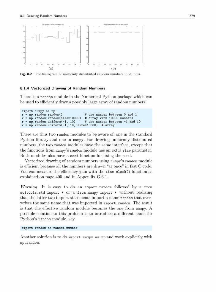
8.1 Drawing Random Numbers 379

0

0.2

0.4

0.6

0.8

1

1.2

1.4

0 0.1 0.2 0.3 0.4 0.5 0.6 0.7 0.8 0.9 1

1000 samples of uniform numbers on (0,1)

(a)

0

0.2

0.4

0.6

0.8

1

1.2

0 0.1 0.2 0.3 0.4 0.5 0.6 0.7 0.8 0.9 1

1000000 samples of uniform numbers on (0,1)

(b)

Fig. 8.2 The histogram of uniformly distributed random numbers in 20 bins.

8.1.4 Vectorized Drawing of Random Numbers

There is a random module in the Numerical Python package which canbe used to efficiently draw a possibly large array of random numbers:

import numpy as npr = np.random.random() # one number between 0 and 1r = np.random.random(size=10000) # array with 10000 numbersr = np.random.uniform(-1, 10) # one number between -1 and 10r = np.random.uniform(-1, 10, size=10000) # array

There are thus two random modules to be aware of: one in the standardPython library and one in numpy. For drawing uniformly distributednumbers, the two random modules have the same interface, except thatthe functions from numpy’s random module has an extra size parameter.Both modules also have a seed function for fixing the seed.

Vectorized drawing of random numbers using numpy’s random moduleis efficient because all the numbers are drawn “at once” in fast C code.You can measure the efficiency gain with the time.clock() function asexplained on page 405 and in Appendix G.6.1.

Warning. It is easy to do an import random followed by a from

scitools.std import * or a from numpy import * without realizingthat the latter two import statements import a name random that over-writes the same name that was imported in import random. The resultis that the effective random module becomes the one from numpy. Apossible solution to this problem is to introduce a different name forPython’s random module, say

import random as random_number

Another solution is to do import numpy as np and work explicitly withnp.random.

380 8 Random Numbers and Simple Games

8.1.5 Computing the Mean and Standard Deviation

You probably know the formula for the mean or average of a set of nnumbers x0, x1, . . . , xn−1:

xm =1

n

n−1∑

j=0

xj . (8.1)

The amount of spreading of the xi values around the mean xm can bemeasured by the variance3,

xv =1

n

n−1∑

j=0

(xj − xm)2 . (8.2)

A variant of this formula reads

xv =1

n

n−1∑

j=0

x2j

− x2m . (8.3)

The good thing with this latter formula is that one can, as a statisticalexperiment progresses and n increases, record the sums

sm =

q−1∑

j=0

xj , sv =

q−1∑

j=0

x2j (8.4)

and then, when desired, efficiently compute the most recent estimateon the mean value and the variance after q samples by

xm = sm/q, xv = sv/q − s2m/q2 . (8.5)

The standard deviationxs =

√xv (8.6)

is often used as an alternative to the variance, because the standarddeviation has the same unit as the measurement itself. A common wayto express an uncertain quantity x, based on a data set x0, . . . , xn−1,from simulations or physical measurements, is xm ± xs. This meansthat x has an uncertainty of one standard deviation xs to either sideof the mean value xm. With probability theory and statistics one canprovide many other, more precise measures of the uncertainty, but thatis the topic of a different course.

Below is an example where we draw numbers from the uniform distri-bution on [−1, 1) and compute the evolution of the mean and standard

3 Textbooks in statistics teach you that it is more appropriate to divide by n − 1

instead of n, but we are not going to worry about that fact in this book.

8.1 Drawing Random Numbers 381

deviation 10 times during the experiment, using the formulas (8.1) and(8.3)–(8.6):

import sysN = int(sys.argv[1])import randomfrom math import sqrtsm = 0; sv = 0for q in range(1, N+1):

x = random.uniform(-1, 1)sm += xsv += x**2

# Write out mean and st.dev. 10 times in this loopif q % (N/10) == 0:

xm = sm/qxs = sqrt(sv/q - xm**2)print ’%10d mean: %12.5e stdev: %12.5e’ % (q, xm, xs)

The if test applies the mod function, see Chapter 3.3.2, for checkingif a number can be divided by another without any remainder. Theparticular if test here is true when i equals 0, N/10, 2*N/10, . . ., N, i.e.,10 times during the execution of the loop. The program is available inthe file mean_stdev_uniform1.py. A run with N = 106 gives the output

100000 mean: 1.86276e-03 stdev: 5.77101e-01200000 mean: 8.60276e-04 stdev: 5.77779e-01300000 mean: 7.71621e-04 stdev: 5.77753e-01400000 mean: 6.38626e-04 stdev: 5.77944e-01500000 mean: -1.19830e-04 stdev: 5.77752e-01600000 mean: 4.36091e-05 stdev: 5.77809e-01700000 mean: -1.45486e-04 stdev: 5.77623e-01800000 mean: 5.18499e-05 stdev: 5.77633e-01900000 mean: 3.85897e-05 stdev: 5.77574e-011000000 mean: -1.44821e-05 stdev: 5.77616e-01

We see that the mean is getting smaller and approaching zero as ex-pected since we generate numbers between −1 and 1. The theoreticalvalue of the standard deviation, as N →∞, equals

√

1/3 ≈ 0.57735.We have also made a corresponding vectorized version of the code

above using numpy’s random module and the ready-made functions mean,var, and std for computing the mean, variance, and standard deviation(respectively) of an array of numbers:

import sysN = int(sys.argv[1])import numpy as npx = np.random.uniform(-1, 1, size=N)xm = np.mean(x)xv = np.var(x)xs = np.std(x)print ’%10d mean: %12.5e stdev: %12.5e’ % (N, xm, xs)

This program can be found in the file mean_stdev_uniform2.py.

8.1.6 The Gaussian or Normal Distribution

In some applications we want random numbers to cluster around aspecific value m. This means that it is more probable to generate a

382 8 Random Numbers and Simple Games

number close to m than far away from m. A widely used distributionwith this qualitative property is the Gaussian or normal distribution4.The normal distribution has two parameters: the mean valuem and thestandard deviation s. The latter measures the width of the distribution,in the sense that a small s makes it less likely to draw a number farfrom the mean value, and a large s makes more likely to draw a numberfar from the mean value.

Single random numbers from the normal distribution can be gener-ated by

import randomr = random.normalvariate(m, s)

while efficient generation of an array of length N is enabled by

import numpy as npr = np.random.normal(m, s, size=N)r = np.random.randn(N) # mean=0, std.dev.=1

The following program draws N random numbers from the normaldistribution, computes the mean and standard devation, and plots thehistogram:

import sysN = int(sys.argv[1])m = float(sys.argv[2])s = float(sys.argv[3])

import numpy as npnp.random.seed(12)samples = np.random.normal(m, s, N)print np.mean(samples), np.std(samples)

import scitools.std as stx, y = st.compute_histogram(samples, 20, piecewise_constant=True)st.plot(x, y, hardcopy=’tmp.eps’,

title =’%d samples of Gaussian/normal numbers on (0,1)’ % N)

The corresponding program file is normal_numbers1.py, which gives amean of −0.00253 and a standard deviation of 0.99970 when run withN as 1 million, m as 0, and s equal to 1. Figure 8.3 shows that therandom numbers cluster around the mean m = 0 in a histogram. Thisnormalized histogram will, as N goes to infinity, approach a bell-shapedfunction, known as the normal distribution probability density func-tion, given in (1.6) on page 45.

8.2 Drawing Integers

Suppose we want to draw a random integer among the values 1, 2,3, and 4, and that each of the four values is equally probable. One

4 For example, the blood pressure among adults of one gender has values that followa normal distribution.

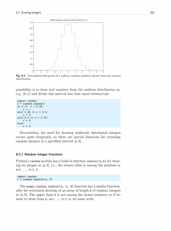
8.2 Drawing Integers 383

0

0.05

0.1

0.15

0.2

0.25

0.3

0.35

0.4

-5 -4 -3 -2 -1 0 1 2 3 4 5

1000000 samples of Gaussian/normal numbers on (0,1)

Fig. 8.3 Normalized histogram of 1 million random numbers drawn from the normaldistribution.

possibility is to draw real numbers from the uniform distribution on,e.g., [0, 1) and divide this interval into four equal subintervals:

import randomr = random.random()if 0 <= r < 0.25:

r = 1elif 0.25 <= r < 0.5:

r = 2elif 0.5 <= r < 0.75:

r = 3else:

r = 4

Nevertheless, the need for drawing uniformly distributed integersoccurs quite frequently, so there are special functions for returningrandom integers in a specified interval [a, b].

8.2.1 Random Integer Functions

Python’s random module has a built-in function randint(a,b) for draw-ing an integer in [a, b], i.e., the return value is among the numbers a,a+1, . . ., b-1, b.

import randomr = random.randint(a, b)

The numpy.random.randint(a, b, N) function has a similar function-ality for vectorized drawing of an array of length N of random integersin [a, b). The upper limit b is not among the drawn numbers, so if wewant to draw from a, a+1, . . ., b-1, b, we must write

384 8 Random Numbers and Simple Games

import numpy as npr = np.random.randint(a, b+1, N)

Another function, random_integers(a, b, N), also in numpy.random, in-cludes the upper limit b in the possible set of random integers:

r = np.random.random_integers(a, b, N)

8.2.2 Example: Throwing a Die

We can make a program that lets the computer throw a die N timesand count how many times we get six eyes:

import randomimport sysN = int(sys.argv[1]) # perform N experimentsM = 0 # no of times we get 6 eyesfor i in xrange(N):

outcome = random.randint(1, 6)if outcome == 6:

M += 1print ’Got six %d times out of %d’ % (M, N)

We use xrange instead of range because the former is more efficientwhen N is large (see remark in Exercise 2.14). The vectorized versionof this code can be expressed as follows:

import numpy as npimport sysN = int(sys.argv[1])eyes = np.random.randint(1, 7, N)success = eyes == 6 # True/False arrayM = np.sum(success) # treats True as 1, False as 0print ’Got six %d times out of %d’ % (M, N)

The eyes == 6 construction results in an array with True or False val-ues, and sum applied to this array treats True as 1 and False as 0 (theinteger equivalents to the boolean values), so the sum is the number ofelements in eyes that equals 6. A very important point here for com-putational efficiency is to use np.sum and not the standard sum functionthat is available in standard Python. With np.sum function, the vector-ized version runs about 50 times faster than the scalar version. WithPython’s standard sum function, the vectorized versions is in fact slowerthan the scalar version (!).

The two small programs above are found in the files roll_die.py

and roll_die_vec.py, respectively. You can try the programs and seehow much faster the vectorized version is (N probably needs to be ofsize at least 106 to see any noticable differences for practical purposes).

8.2 Drawing Integers 385

8.2.3 Drawing a Random Element from a List

Given a list a, the statement

re = random.choice(a)

picks out an element of a at random, and re refers to this element. Theshown call to random.choice is the same as

re = a[random.randint(0, len(a)-1)]

There is also a function shuffle that permutates the list elements in arandom order:

random.shuffle(a)

Picking now a[0], for instance, has the same effect as random.choice

on the original, unshuffled list. Note that shuffle changes the list givenas argument.

The numpy.random module has also a shuffle function with the samefunctionality.

A small session illustrates the various methods for picking a randomelement from a list:

>>> awards = [’car’, ’computer’, ’ball’, ’pen’]>>> import random>>> random.choice(awards)’car’>>> awards[random.randint(0, len(awards)-1)]’pen’>>> random.shuffle(awards)>>> awards[0]’computer’

8.2.4 Example: Drawing Cards from a Deck

The following function creates a deck of cards, where each card isrepresented as a string, and the deck is a list of such strings:

def make_deck():ranks = [’A’, ’2’, ’3’, ’4’, ’5’, ’6’, ’7’,

’8’, ’9’, ’10’, ’J’, ’Q’, ’K’]suits = [’C’, ’D’, ’H’, ’S’]deck = []for s in suits:

for r in ranks:deck.append(s + r)

random.shuffle(deck)return deck

Here, ’A’ means an ace, ’J’ represents a jack, ’Q’ represents a queen,’K’ represents a king, ’C’ stands for clubs, ’D’ stands for diamonds,’H’ means hearts, and ’S’ means spades. The computation of the list

386 8 Random Numbers and Simple Games

deck can alternatively (and more compactly) be done by a one-line listcomprehension:

deck = [s+r for s in suits for r in ranks]

We can draw a card at random by

deck = make_deck()card = deck[0]del deck[0]# or better:card = deck.pop(0) # return and remove element with index 0

Drawing a hand of n cards from a shuffled deck is accomplished by

def deal_hand(n, deck):hand = [deck[i] for i in range(n)]del deck[:n]return hand, deck

Note that we must return deck to the calling code since this list ischanged. Also note that the n first cards of the deck are random cardsif the deck is shuffled (and any deck made by make_deck is shuffled).

The following function deals cards to a set of players:

def deal(cards_per_hand, no_of_players):deck = make_deck()hands = []for i in range(no_of_players):

hand, deck = deal_hand(cards_per_hand, deck)hands.append(hand)

return hands

players = deal(5, 4)import pprint; pprint.pprint(players)

The players list may look like

[[’D4’, ’CQ’, ’H10’, ’DK’, ’CK’],[’D7’, ’D6’, ’SJ’, ’S4’, ’C5’],[’C3’, ’DQ’, ’S3’, ’C9’, ’DJ’],[’H6’, ’H9’, ’C6’, ’D5’, ’S6’]]

The next step is to analyze a hand. Of particular interest is thenumber of pairs, three of a kind, four of a kind, etc. That is, how manycombinations there are of n_of_a_kind cards of the same rank (e.g.,n_of_a_kind=2 finds the number of pairs):

def same_rank(hand, n_of_a_kind):ranks = [card[1:] for card in hand]counter = 0already_counted = []for rank in ranks:

if rank not in already_counted and \ranks.count(rank) == n_of_a_kind:

counter += 1already_counted.append(rank)

return counter

8.2 Drawing Integers 387

Note how convenient the count method in list objects is for countinghow many copies there are of one element in the list.

Another analysis of the hand is to count how many cards there areof each suit. A dictionary with the suit as key and the number of cardswith that suit as value, seems appropriate to return. We pay attentiononly to suits that occur more than once:

def same_suit(hand):suits = [card[0] for card in hand]counter = # counter[suit] = how many cards of suitfor suit in suits:

count = suits.count(suit)if count > 1:

counter[suit] = countreturn counter

For a set of players we can now analyze their hands:

for hand in players:print """\

The hand %shas %d pairs, %s 3-of-a-kind and%s cards of the same suit.""" % \(’, ’.join(hand), same_rank(hand, 2),same_rank(hand, 3),’+’.join([str(s) for s in same_suit(hand).values()]))

The values we feed into the printf string undergo some massage: wejoin the card values with comma and put a plus in between the countsof cards with the same suit. (The join function requires a string ar-gument. That is why the integer counters of cards with the same suit,returned from same_suit, must be converted to strings.) The output ofthe for loop becomes

The hand D4, CQ, H10, DK, CKhas 1 pairs, 0 3-of-a-kind and2+2 cards of the same suit.

The hand D7, D6, SJ, S4, C5has 0 pairs, 0 3-of-a-kind and2+2 cards of the same suit.

The hand C3, DQ, S3, C9, DJhas 1 pairs, 0 3-of-a-kind and2+2 cards of the same suit.

The hand H6, H9, C6, D5, S6has 0 pairs, 1 3-of-a-kind and2 cards of the same suit.

The file cards.py contains the functions make_deck, hand, hand2,same_rank, same_suit, and the test snippets above. With the cards.py

file one can start to implement real card games.

8.2.5 Example: Class Implementation of a Deck

To work with a deck of cards with the code from the previous sectionone needs to shuffle a global variable deck in and out of functions. Aset of functions that update global variables (like deck) is a primarycandidate for a class: The global variables are stored as attributes and

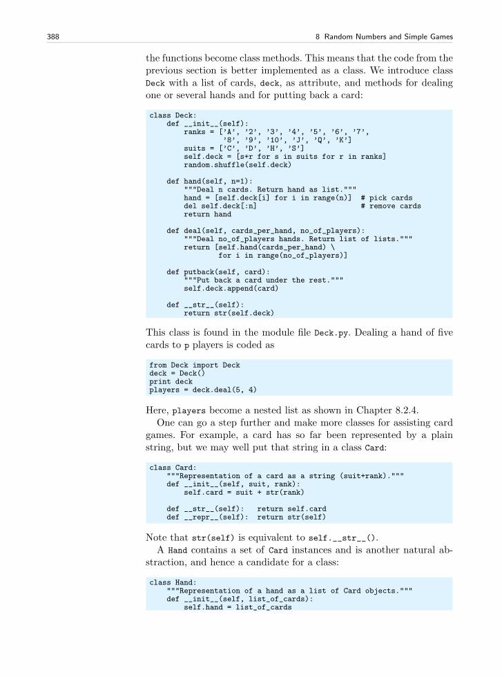
388 8 Random Numbers and Simple Games

the functions become class methods. This means that the code from theprevious section is better implemented as a class. We introduce classDeck with a list of cards, deck, as attribute, and methods for dealingone or several hands and for putting back a card:

class Deck:def __init__(self):

ranks = [’A’, ’2’, ’3’, ’4’, ’5’, ’6’, ’7’,’8’, ’9’, ’10’, ’J’, ’Q’, ’K’]

suits = [’C’, ’D’, ’H’, ’S’]self.deck = [s+r for s in suits for r in ranks]random.shuffle(self.deck)

def hand(self, n=1):"""Deal n cards. Return hand as list."""hand = [self.deck[i] for i in range(n)] # pick cardsdel self.deck[:n] # remove cardsreturn hand

def deal(self, cards_per_hand, no_of_players):"""Deal no_of_players hands. Return list of lists."""return [self.hand(cards_per_hand) \

for i in range(no_of_players)]

def putback(self, card):"""Put back a card under the rest."""self.deck.append(card)

def __str__(self):return str(self.deck)

This class is found in the module file Deck.py. Dealing a hand of fivecards to p players is coded as

from Deck import Deckdeck = Deck()print deckplayers = deck.deal(5, 4)

Here, players become a nested list as shown in Chapter 8.2.4.One can go a step further and make more classes for assisting card

games. For example, a card has so far been represented by a plainstring, but we may well put that string in a class Card:

class Card:"""Representation of a card as a string (suit+rank)."""def __init__(self, suit, rank):

self.card = suit + str(rank)

def __str__(self): return self.carddef __repr__(self): return str(self)

Note that str(self) is equivalent to self.__str__().A Hand contains a set of Card instances and is another natural ab-

straction, and hence a candidate for a class:

class Hand:"""Representation of a hand as a list of Card objects."""def __init__(self, list_of_cards):

self.hand = list_of_cards

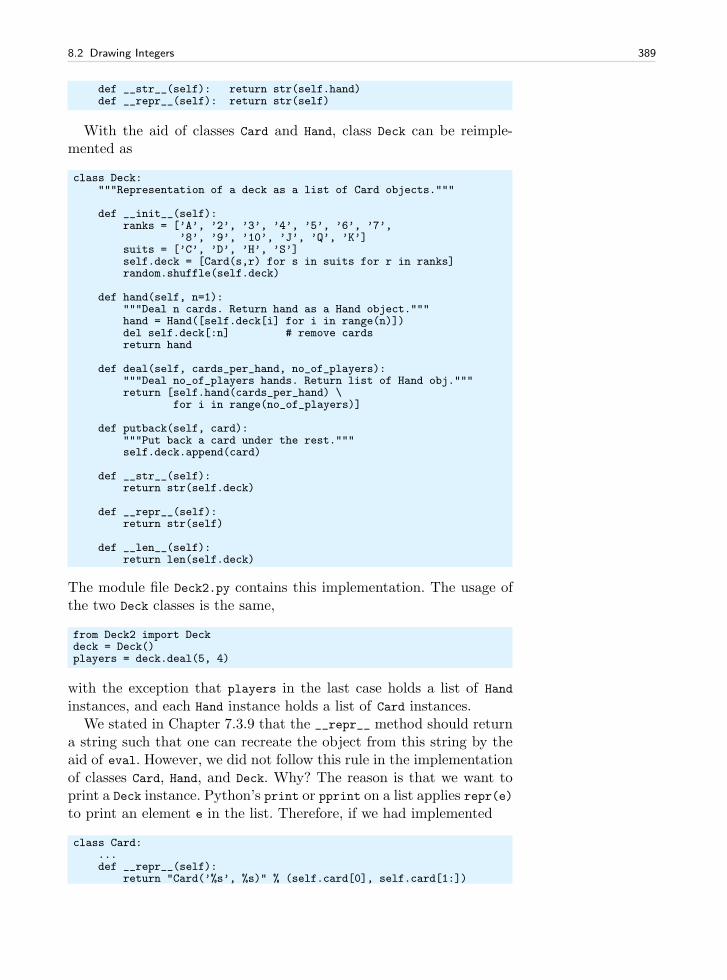
8.2 Drawing Integers 389

def __str__(self): return str(self.hand)def __repr__(self): return str(self)

With the aid of classes Card and Hand, class Deck can be reimple-mented as

class Deck:"""Representation of a deck as a list of Card objects."""

def __init__(self):ranks = [’A’, ’2’, ’3’, ’4’, ’5’, ’6’, ’7’,

’8’, ’9’, ’10’, ’J’, ’Q’, ’K’]suits = [’C’, ’D’, ’H’, ’S’]self.deck = [Card(s,r) for s in suits for r in ranks]random.shuffle(self.deck)

def hand(self, n=1):"""Deal n cards. Return hand as a Hand object."""hand = Hand([self.deck[i] for i in range(n)])del self.deck[:n] # remove cardsreturn hand

def deal(self, cards_per_hand, no_of_players):"""Deal no_of_players hands. Return list of Hand obj."""return [self.hand(cards_per_hand) \

for i in range(no_of_players)]

def putback(self, card):"""Put back a card under the rest."""self.deck.append(card)

def __str__(self):return str(self.deck)

def __repr__(self):return str(self)

def __len__(self):return len(self.deck)

The module file Deck2.py contains this implementation. The usage ofthe two Deck classes is the same,

from Deck2 import Deckdeck = Deck()players = deck.deal(5, 4)

with the exception that players in the last case holds a list of Hand

instances, and each Hand instance holds a list of Card instances.We stated in Chapter 7.3.9 that the __repr__ method should return

a string such that one can recreate the object from this string by theaid of eval. However, we did not follow this rule in the implementationof classes Card, Hand, and Deck. Why? The reason is that we want toprint a Deck instance. Python’s print or pprint on a list applies repr(e)to print an element e in the list. Therefore, if we had implemented

class Card:...def __repr__(self):

return "Card(’%s’, %s)" % (self.card[0], self.card[1:])

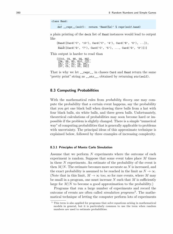
390 8 Random Numbers and Simple Games

class Hand:...def __repr__(self): return ’Hand(%s)’ % repr(self.hand)

a plain printing of the deck list of Hand instances would lead to outputlike

[Hand([Card(’C’, ’10’), Card(’C’, ’4’), Card(’H’, ’K’), ...]),...,Hand([Card(’D’, ’7’), Card(’C’, ’5’), ..., Card(’D’, ’9’)])]

This output is harder to read than

[[C10, C4, HK, DQ, HQ],[SA, S8, H3, H10, C2],[HJ, C7, S2, CQ, DK],[D7, C5, DJ, S3, D9]]

That is why we let __repr__ in classes Card and Hand return the same“pretty print” string as __str__, obtained by returning str(self).

8.3 Computing Probabilities

With the mathematical rules from probability theory one may com-pute the probability that a certain event happens, say the probabilitythat you get one black ball when drawing three balls from a hat withfour black balls, six white balls, and three green balls. Unfortunately,theoretical calculations of probabilities may soon become hard or im-possible if the problem is slightly changed. There is a simple“numericalway”of computing probabilities that is generally applicable to problemswith uncertainty. The principal ideas of this approximate technique isexplained below, followed by three examples of increasing complexity.

8.3.1 Principles of Monte Carlo Simulation

Assume that we perform N experiments where the outcome of eachexperiment is random. Suppose that some event takes place M timesin these N experiments. An estimate of the probability of the event isthenM/N . The estimate becomes more accurate as N is increased, andthe exact probability is assumed to be reached in the limit as N →∞.(Note that in this limit, M →∞ too, so for rare events, where M maybe small in a program, one must increase N such that M is sufficientlylarge for M/N to become a good approximation to the probability.)

Programs that run a large number of experiments and record theoutcome of events are often called simulation programs5. The mathe-matical technique of letting the computer perform lots of experiments

5 This term is also applied for programs that solve equations arising in mathematicalmodels in general, but it is particularly common to use the term when randomnumbers are used to estimate probabilities.

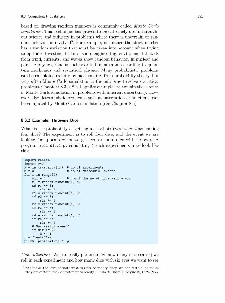
8.3 Computing Probabilities 391

based on drawing random numbers is commonly called Monte Carlosimulation. This technique has proven to be extremely useful through-out science and industry in problems where there is uncertain or ran-dom behavior is involved6. For example, in finance the stock markethas a random variation that must be taken into account when tryingto optimize investments. In offshore engineering, environmental loadsfrom wind, currents, and waves show random behavior. In nuclear andparticle physics, random behavior is fundamental according to quan-tum mechanics and statistical physics. Many probabilistic problemscan be calculated exactly by mathematics from probability theory, butvery often Monte Carlo simulation is the only way to solve statisticalproblems. Chapters 8.3.2–8.3.4 applies examples to explain the essenceof Monte Carlo simulation in problems with inherent uncertainty. How-ever, also deterministic problems, such as integration of functions, canbe computed by Monte Carlo simulation (see Chapter 8.5).

8.3.2 Example: Throwing Dice

What is the probability of getting at least six eyes twice when rollingfour dice? The experiment is to roll four dice, and the event we arelooking for appears when we get two or more dice with six eyes. Aprogram roll_dice1.py simulating N such experiments may look likethis:

import randomimport sysN = int(sys.argv[1]) # no of experimentsM = 0 # no of successful eventsfor i in range(N):

six = 0 # count the no of dice with a sixr1 = random.randint(1, 6)if r1 == 6:

six += 1r2 = random.randint(1, 6)if r2 == 6:

six += 1r3 = random.randint(1, 6)if r3 == 6:

six += 1r4 = random.randint(1, 6)if r4 == 6:

six += 1# Successful event?if six >= 2:

M += 1p = float(M)/Nprint ’probability:’, p

Generalization. We can easily parameterize how many dice (ndice) weroll in each experiment and how many dice with six eyes we want to see

6 “As far as the laws of mathematics refer to reality, they are not certain, as far asthey are certain, they do not refer to reality.”–Albert Einstein, physicist, 1879-1955.

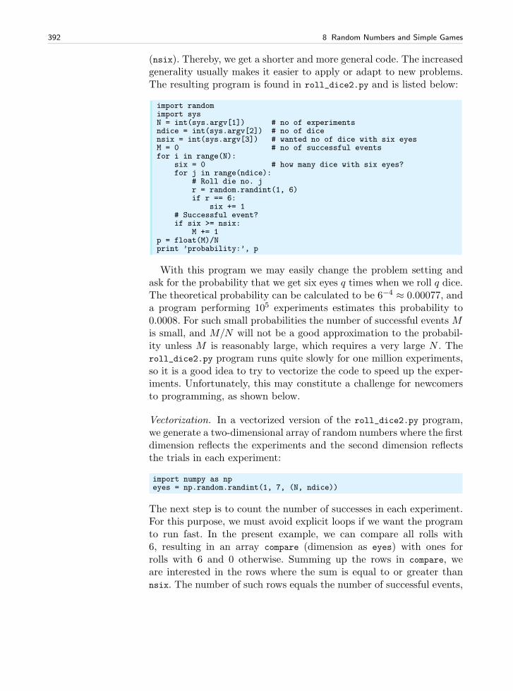
392 8 Random Numbers and Simple Games

(nsix). Thereby, we get a shorter and more general code. The increasedgenerality usually makes it easier to apply or adapt to new problems.The resulting program is found in roll_dice2.py and is listed below:

import randomimport sysN = int(sys.argv[1]) # no of experimentsndice = int(sys.argv[2]) # no of dicensix = int(sys.argv[3]) # wanted no of dice with six eyesM = 0 # no of successful eventsfor i in range(N):

six = 0 # how many dice with six eyes?for j in range(ndice):

# Roll die no. jr = random.randint(1, 6)if r == 6:

six += 1# Successful event?if six >= nsix:

M += 1p = float(M)/Nprint ’probability:’, p

With this program we may easily change the problem setting andask for the probability that we get six eyes q times when we roll q dice.The theoretical probability can be calculated to be 6−4 ≈ 0.00077, anda program performing 105 experiments estimates this probability to0.0008. For such small probabilities the number of successful events Mis small, and M/N will not be a good approximation to the probabil-ity unless M is reasonably large, which requires a very large N . Theroll_dice2.py program runs quite slowly for one million experiments,so it is a good idea to try to vectorize the code to speed up the exper-iments. Unfortunately, this may constitute a challenge for newcomersto programming, as shown below.

Vectorization. In a vectorized version of the roll_dice2.py program,we generate a two-dimensional array of random numbers where the firstdimension reflects the experiments and the second dimension reflectsthe trials in each experiment:

import numpy as npeyes = np.random.randint(1, 7, (N, ndice))

The next step is to count the number of successes in each experiment.For this purpose, we must avoid explicit loops if we want the programto run fast. In the present example, we can compare all rolls with6, resulting in an array compare (dimension as eyes) with ones forrolls with 6 and 0 otherwise. Summing up the rows in compare, weare interested in the rows where the sum is equal to or greater thannsix. The number of such rows equals the number of successful events,

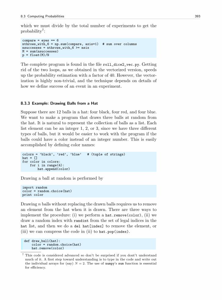
8.3 Computing Probabilities 393

which we must divide by the total number of experiments to get theprobability7:

compare = eyes == 6nthrows_with_6 = np.sum(compare, axis=1) # sum over columnsnsuccesses = nthrows_with_6 >= nsixM = sum(nsuccesses)p = float(M)/N

The complete program is found in the file roll_dice2_vec.py. Gettingrid of the two loops, as we obtained in the vectorized version, speedsup the probability estimation with a factor of 40. However, the vector-ization is highly non-trivial, and the technique depends on details ofhow we define success of an event in an experiment.

8.3.3 Example: Drawing Balls from a Hat

Suppose there are 12 balls in a hat: four black, four red, and four blue.We want to make a program that draws three balls at random fromthe hat. It is natural to represent the collection of balls as a list. Eachlist element can be an integer 1, 2, or 3, since we have three differenttypes of balls, but it would be easier to work with the program if theballs could have a color instead of an integer number. This is easilyaccomplished by defining color names:

colors = ’black’, ’red’, ’blue’ # (tuple of strings)hat = []for color in colors:

for i in range(4):hat.append(color)

Drawing a ball at random is performed by

import randomcolor = random.choice(hat)print color

Drawing n balls without replacing the drawn balls requires us to removean element from the hat when it is drawn. There are three ways toimplement the procedure: (i) we perform a hat.remove(color), (ii) wedraw a random index with randint from the set of legal indices in thehat list, and then we do a del hat[index] to remove the element, or(iii) we can compress the code in (ii) to hat.pop(index).

def draw_ball(hat):color = random.choice(hat)hat.remove(color)

7 This code is considered advanced so don’t be surprised if you dont’t understandmuch of it. A first step toward understanding is to type in the code and write outthe individual arrays for (say) N = 2. The use of numpy’s sum function is essentialfor efficiency.

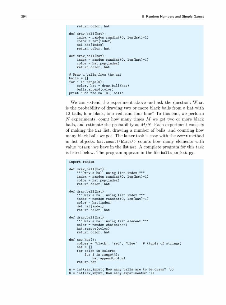
394 8 Random Numbers and Simple Games

return color, hat

def draw_ball(hat):index = random.randint(0, len(hat)-1)color = hat[index]del hat[index]return color, hat

def draw_ball(hat):index = random.randint(0, len(hat)-1)color = hat.pop(index)return color, hat

# Draw n balls from the hatballs = []for i in range(n):

color, hat = draw_ball(hat)balls.append(color)

print ’Got the balls’, balls

We can extend the experiment above and ask the question: Whatis the probability of drawing two or more black balls from a hat with12 balls, four black, four red, and four blue? To this end, we performN experiments, count how many times M we get two or more blackballs, and estimate the probability as M/N . Each experiment consistsof making the hat list, drawing a number of balls, and counting howmany black balls we got. The latter task is easy with the count methodin list objects: hat.count(’black’) counts how many elements withvalue ’black’ we have in the list hat. A complete program for this taskis listed below. The program appears in the file balls_in_hat.py.

import random

def draw_ball(hat):"""Draw a ball using list index."""index = random.randint(0, len(hat)-1)color = hat.pop(index)return color, hat

def draw_ball(hat):"""Draw a ball using list index."""index = random.randint(0, len(hat)-1)color = hat[index]del hat[index]return color, hat

def draw_ball(hat):"""Draw a ball using list element."""color = random.choice(hat)hat.remove(color)return color, hat

def new_hat():colors = ’black’, ’red’, ’blue’ # (tuple of strings)hat = []for color in colors:

for i in range(4):hat.append(color)

return hat

n = int(raw_input(’How many balls are to be drawn? ’))N = int(raw_input(’How many experiments? ’))

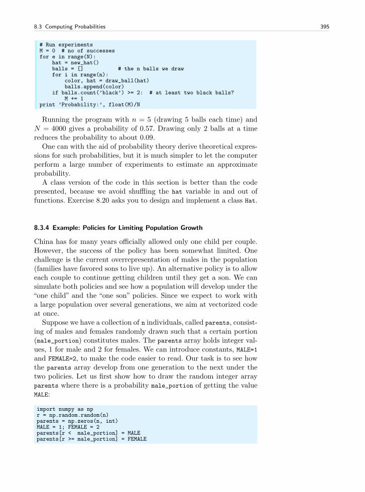
8.3 Computing Probabilities 395

# Run experimentsM = 0 # no of successesfor e in range(N):

hat = new_hat()balls = [] # the n balls we drawfor i in range(n):

color, hat = draw_ball(hat)balls.append(color)

if balls.count(’black’) >= 2: # at least two black balls?M += 1

print ’Probability:’, float(M)/N

Running the program with n = 5 (drawing 5 balls each time) andN = 4000 gives a probability of 0.57. Drawing only 2 balls at a timereduces the probability to about 0.09.

One can with the aid of probability theory derive theoretical expres-sions for such probabilities, but it is much simpler to let the computerperform a large number of experiments to estimate an approximateprobability.

A class version of the code in this section is better than the codepresented, because we avoid shuffling the hat variable in and out offunctions. Exercise 8.20 asks you to design and implement a class Hat.

8.3.4 Example: Policies for Limiting Population Growth

China has for many years officially allowed only one child per couple.However, the success of the policy has been somewhat limited. Onechallenge is the current overrepresentation of males in the population(families have favored sons to live up). An alternative policy is to alloweach couple to continue getting children until they get a son. We cansimulate both policies and see how a population will develop under the“one child” and the “one son” policies. Since we expect to work witha large population over several generations, we aim at vectorized codeat once.

Suppose we have a collection of n individuals, called parents, consist-ing of males and females randomly drawn such that a certain portion(male_portion) constitutes males. The parents array holds integer val-ues, 1 for male and 2 for females. We can introduce constants, MALE=1and FEMALE=2, to make the code easier to read. Our task is to see howthe parents array develop from one generation to the next under thetwo policies. Let us first show how to draw the random integer arrayparents where there is a probability male_portion of getting the valueMALE:

import numpy as npr = np.random.random(n)parents = np.zeros(n, int)MALE = 1; FEMALE = 2parents[r < male_portion] = MALEparents[r >= male_portion] = FEMALE

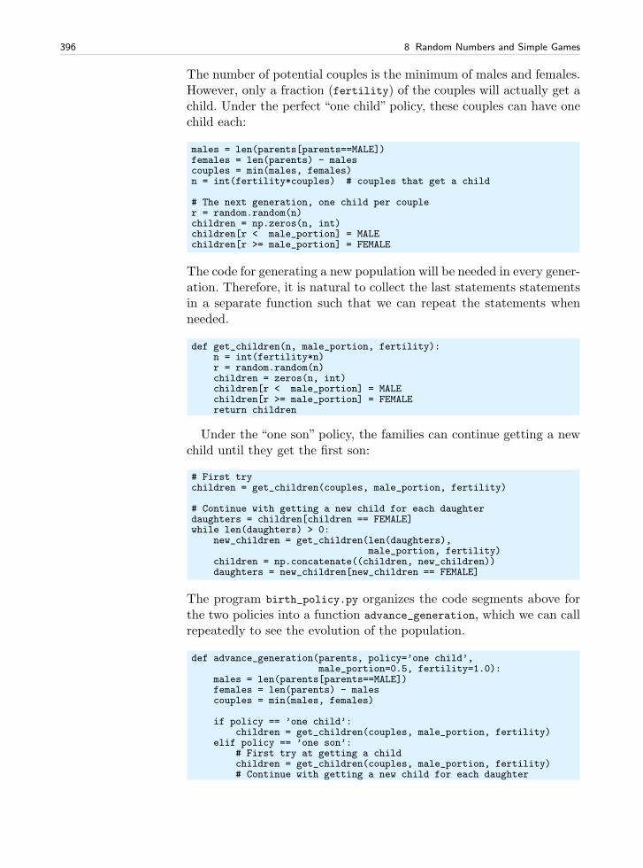
396 8 Random Numbers and Simple Games

The number of potential couples is the minimum of males and females.However, only a fraction (fertility) of the couples will actually get achild. Under the perfect “one child” policy, these couples can have onechild each:

males = len(parents[parents==MALE])females = len(parents) - malescouples = min(males, females)n = int(fertility*couples) # couples that get a child

# The next generation, one child per coupler = random.random(n)children = np.zeros(n, int)children[r < male_portion] = MALEchildren[r >= male_portion] = FEMALE

The code for generating a new population will be needed in every gener-ation. Therefore, it is natural to collect the last statements statementsin a separate function such that we can repeat the statements whenneeded.

def get_children(n, male_portion, fertility):n = int(fertility*n)r = random.random(n)children = zeros(n, int)children[r < male_portion] = MALEchildren[r >= male_portion] = FEMALEreturn children

Under the “one son” policy, the families can continue getting a newchild until they get the first son:

# First trychildren = get_children(couples, male_portion, fertility)

# Continue with getting a new child for each daughterdaughters = children[children == FEMALE]while len(daughters) > 0:

new_children = get_children(len(daughters),male_portion, fertility)

children = np.concatenate((children, new_children))daughters = new_children[new_children == FEMALE]

The program birth_policy.py organizes the code segments above forthe two policies into a function advance_generation, which we can callrepeatedly to see the evolution of the population.

def advance_generation(parents, policy=’one child’,male_portion=0.5, fertility=1.0):

males = len(parents[parents==MALE])females = len(parents) - malescouples = min(males, females)

if policy == ’one child’:children = get_children(couples, male_portion, fertility)

elif policy == ’one son’:# First try at getting a childchildren = get_children(couples, male_portion, fertility)# Continue with getting a new child for each daughter

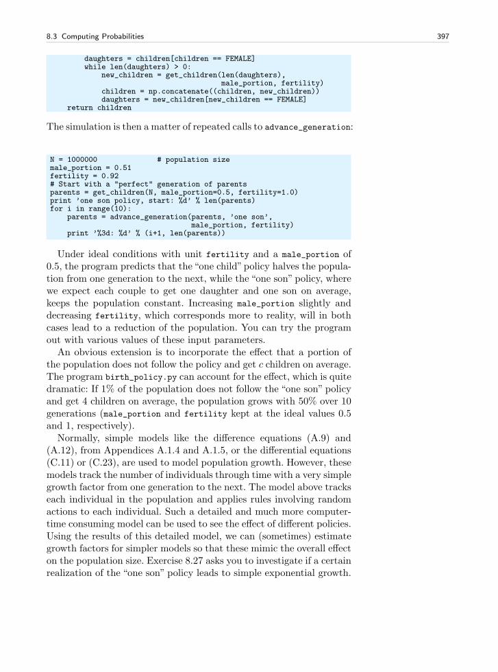
8.3 Computing Probabilities 397

daughters = children[children == FEMALE]while len(daughters) > 0:

new_children = get_children(len(daughters),male_portion, fertility)

children = np.concatenate((children, new_children))daughters = new_children[new_children == FEMALE]

return children

The simulation is then a matter of repeated calls to advance_generation:

N = 1000000 # population sizemale_portion = 0.51fertility = 0.92# Start with a "perfect" generation of parentsparents = get_children(N, male_portion=0.5, fertility=1.0)print ’one son policy, start: %d’ % len(parents)for i in range(10):

parents = advance_generation(parents, ’one son’,male_portion, fertility)

print ’%3d: %d’ % (i+1, len(parents))

Under ideal conditions with unit fertility and a male_portion of0.5, the program predicts that the“one child”policy halves the popula-tion from one generation to the next, while the “one son” policy, wherewe expect each couple to get one daughter and one son on average,keeps the population constant. Increasing male_portion slightly anddecreasing fertility, which corresponds more to reality, will in bothcases lead to a reduction of the population. You can try the programout with various values of these input parameters.

An obvious extension is to incorporate the effect that a portion ofthe population does not follow the policy and get c children on average.The program birth_policy.py can account for the effect, which is quitedramatic: If 1% of the population does not follow the “one son” policyand get 4 children on average, the population grows with 50% over 10generations (male_portion and fertility kept at the ideal values 0.5and 1, respectively).

Normally, simple models like the difference equations (A.9) and(A.12), from Appendices A.1.4 and A.1.5, or the differential equations(C.11) or (C.23), are used to model population growth. However, thesemodels track the number of individuals through time with a very simplegrowth factor from one generation to the next. The model above trackseach individual in the population and applies rules involving randomactions to each individual. Such a detailed and much more computer-time consuming model can be used to see the effect of different policies.Using the results of this detailed model, we can (sometimes) estimategrowth factors for simpler models so that these mimic the overall effecton the population size. Exercise 8.27 asks you to investigate if a certainrealization of the “one son” policy leads to simple exponential growth.

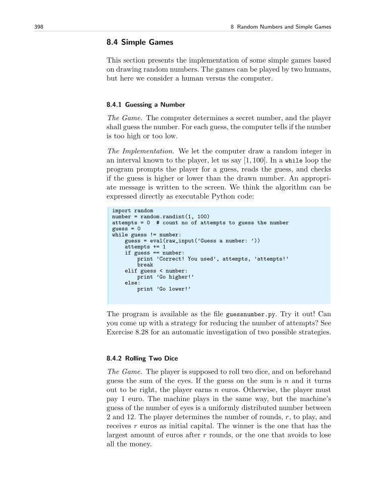
398 8 Random Numbers and Simple Games

8.4 Simple Games

This section presents the implementation of some simple games basedon drawing random numbers. The games can be played by two humans,but here we consider a human versus the computer.

8.4.1 Guessing a Number

The Game. The computer determines a secret number, and the playershall guess the number. For each guess, the computer tells if the numberis too high or too low.

The Implementation. We let the computer draw a random integer inan interval known to the player, let us say [1, 100]. In a while loop theprogram prompts the player for a guess, reads the guess, and checksif the guess is higher or lower than the drawn number. An appropri-ate message is written to the screen. We think the algorithm can beexpressed directly as executable Python code:

import randomnumber = random.randint(1, 100)attempts = 0 # count no of attempts to guess the numberguess = 0while guess != number:

guess = eval(raw_input(’Guess a number: ’))attempts += 1if guess == number:

print ’Correct! You used’, attempts, ’attempts!’break

elif guess < number:print ’Go higher!’

else:print ’Go lower!’

The program is available as the file guessnumber.py. Try it out! Canyou come up with a strategy for reducing the number of attempts? SeeExercise 8.28 for an automatic investigation of two possible strategies.

8.4.2 Rolling Two Dice

The Game. The player is supposed to roll two dice, and on beforehandguess the sum of the eyes. If the guess on the sum is n and it turnsout to be right, the player earns n euros. Otherwise, the player mustpay 1 euro. The machine plays in the same way, but the machine’sguess of the number of eyes is a uniformly distributed number between2 and 12. The player determines the number of rounds, r, to play, andreceives r euros as initial capital. The winner is the one that has thelargest amount of euros after r rounds, or the one that avoids to loseall the money.

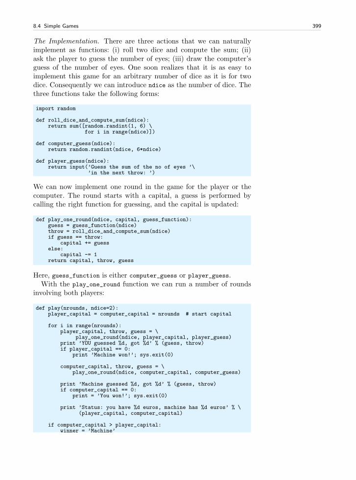
8.4 Simple Games 399

The Implementation. There are three actions that we can naturallyimplement as functions: (i) roll two dice and compute the sum; (ii)ask the player to guess the number of eyes; (iii) draw the computer’sguess of the number of eyes. One soon realizes that it is as easy toimplement this game for an arbitrary number of dice as it is for twodice. Consequently we can introduce ndice as the number of dice. Thethree functions take the following forms:

import random

def roll_dice_and_compute_sum(ndice):return sum([random.randint(1, 6) \

for i in range(ndice)])

def computer_guess(ndice):return random.randint(ndice, 6*ndice)

def player_guess(ndice):return input(’Guess the sum of the no of eyes ’\

’in the next throw: ’)

We can now implement one round in the game for the player or thecomputer. The round starts with a capital, a guess is performed bycalling the right function for guessing, and the capital is updated:

def play_one_round(ndice, capital, guess_function):guess = guess_function(ndice)throw = roll_dice_and_compute_sum(ndice)if guess == throw:

capital += guesselse:

capital -= 1return capital, throw, guess

Here, guess_function is either computer_guess or player_guess.With the play_one_round function we can run a number of rounds

involving both players:

def play(nrounds, ndice=2):player_capital = computer_capital = nrounds # start capital

for i in range(nrounds):player_capital, throw, guess = \

play_one_round(ndice, player_capital, player_guess)print ’YOU guessed %d, got %d’ % (guess, throw)if player_capital == 0:

print ’Machine won!’; sys.exit(0)

computer_capital, throw, guess = \play_one_round(ndice, computer_capital, computer_guess)

print ’Machine guessed %d, got %d’ % (guess, throw)if computer_capital == 0:

print = ’You won!’; sys.exit(0)

print ’Status: you have %d euros, machine has %d euros’ % \(player_capital, computer_capital)

if computer_capital > player_capital:winner = ’Machine’

400 8 Random Numbers and Simple Games

else:winner = ’You’

print winner, ’won!’

The name of the program is ndice.py.

Example. Here is a session (with a fixed seed of 20):

Guess the sum of the no of eyes in the next throw: 7YOU guessed 7, got 11Machine guessed 10, got 8Status: you have 9 euros, machine has 9 euros

Guess the sum of the no of eyes in the next throw: 9YOU guessed 9, got 10Machine guessed 11, got 6Status: you have 8 euros, machine has 8 euros

Guess the sum of the no of eyes in the next throw: 9YOU guessed 9, got 9Machine guessed 3, got 8Status: you have 17 euros, machine has 7 euros

Exercise 8.10 asks you to perform simulations to determine whether acertain strategy can make the player win over the computer in the longrun.

A Class Version. We can cast the previous code segment in a class.Many will argue that a class-based implementation is closer to theproblem being modeled and hence easier to modify or extend.

A natural class is Dice, which can throw n dice:

class Dice:def __init__(self, n=1):

self.n = n # no of dice

def throw(self):return [random.randint(1,6) \

for i in range(self.n)]

Another natural class is Player, which can perform the actions of aplayer. Functions can then make use of Player to set up a game. APlayer has a name, an initial captial, a set of dice, and a Dice objectto throw the object:

class Player:def __init__(self, name, capital, guess_function, ndice):

self.name = nameself.capital = capitalself.guess_function = guess_functionself.dice = Dice(ndice)

def play_one_round(self):self.guess = self.guess_function(self.dice.n)self.throw = sum(self.dice.throw())if self.guess == self.throw:

self.capital += self.guesselse:

self.capital -= 1self.message()self.broke()

8.5 Monte Carlo Integration 401

def message(self):print ’%s guessed %d, got %d’ % \

(self.name, self.guess, self.throw)

def broke(self):if self.capital == 0:

print ’%s lost!’ % self.namesys.exit(0) # end the program

The guesses of the computer and the player are specified by functions:

def computer_guess(ndice):# All guesses have the same probabilityreturn random.randint(ndice, 6*ndice)

def player_guess(ndice):return input(’Guess the sum of the no of eyes ’\

’in the next throw: ’)

The key function to play the whole game, utilizing the Player class forthe computer and the user, can be expressed as

def play(nrounds, ndice=2):player = Player(’YOU’, nrounds, player_guess, ndice)computer = Player(’Computer’, nrounds, computer_guess, ndice)

for i in range(nrounds):player.play_one_round()computer.play_one_round()print ’Status: user have %d euro, machine has %d euro\n’ % \

(player.capital, computer.capital)

if computer.capital > player.capital:winner = ’Machine’

else:winner = ’You’

print winner, ’won!’

The complete code is found in the file ndice2.py. There is no newfunctionality compared to the ndice.py implementation, just a newand better structuring of the code.

8.5 Monte Carlo Integration

One of the earliest applications of random numbers was numerical com-putation of integrals, that is, a non-random (deterministic) problem.

Here we shall address two related methods for computing∫ ba f(x)dx.

8.5.1 Standard Monte Carlo Integration

Let x1, . . . , xn be uniformly distributed random numbers between aand b. Then

(b− a)1

n

n∑

i=1

f(xi) (8.7)

402 8 Random Numbers and Simple Games

is an approximation to the integral∫ ba f(x)dx. This method is usually

referred to as Monte Carlo integration. It is easy to interpret (8.7). Awell-known result from calculus is that the integral of a function f over[a, b] equals the mean value of f over [a, b] multiplied by the length ofthe interval, b − a. If we approximate the mean value of f(x) by themean of n randomly distributed function evaluations f(xi), we get themethod (8.7).

We can implement (8.7) in a small function:

import random

def MCint(f, a, b, n):s = 0for i in range(n):

x = random.uniform(a, b)s += f(x)

I = (float(b-a)/n)*sreturn I

One normally needs a large n to obtain good results with thismethod, so a faster vectorized version of the MCint function is handy:

import numpy as np

def MCint_vec(f, a, b, n):x = np.random.uniform(a, b, n)s = np.sum(f(x))I = (float(b-a)/n)*sreturn I

Let us try the Monte Carlo integration method on a simple linearfunction f(x) = 2 + 3x, integrated from 1 to 2. Most other numeri-cal integration methods will integrate such a linear function exactly,regardless of the number of function evaluations. This is not the casewith Monte Carlo integration. It would be interesting to see how thequality of the Monte Carlo approximation increases n. To plot theevolution of the integral approximation we must store intermediate I

values. This requires a slightly modified MCint method:

def MCint2(f, a, b, n):s = 0# Store the intermediate integral approximations in an# array I, where I[k-1] corresponds to k function evals.I = np.zeros(n)for k in range(1, n+1):

x = random.uniform(a, b)s += f(x)I[k-1] = (float(b-a)/k)*s

return I

Note that we let k go from 1 to n while the indices in I, as usual, gofrom 0 to n-1. Since n can be very large, the I array may consume morememory than what we have on the computer. Therefore, we decide tostore only every N values of the approximation. Determining if a valueis to be stored or not can then be computed by the mod function (seepage 115):

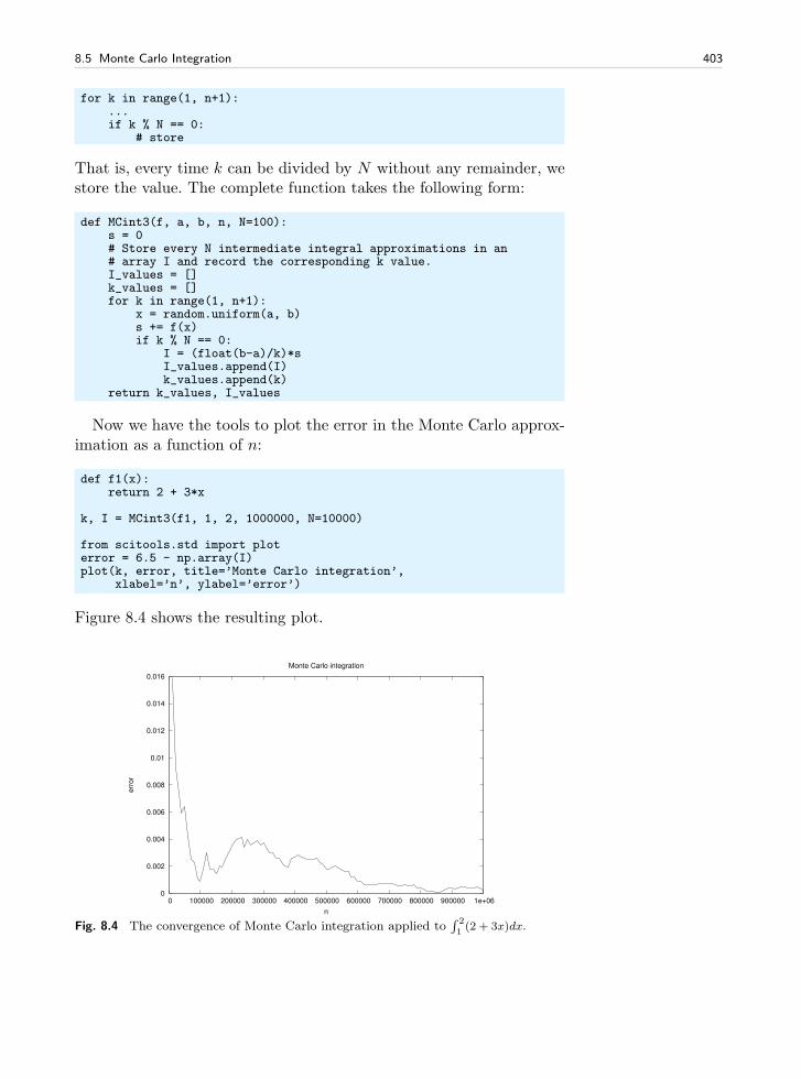
8.5 Monte Carlo Integration 403

for k in range(1, n+1):...if k % N == 0:

# store

That is, every time k can be divided by N without any remainder, westore the value. The complete function takes the following form:

def MCint3(f, a, b, n, N=100):s = 0# Store every N intermediate integral approximations in an# array I and record the corresponding k value.I_values = []k_values = []for k in range(1, n+1):

x = random.uniform(a, b)s += f(x)if k % N == 0:

I = (float(b-a)/k)*sI_values.append(I)k_values.append(k)

return k_values, I_values

Now we have the tools to plot the error in the Monte Carlo approx-imation as a function of n:

def f1(x):return 2 + 3*x

k, I = MCint3(f1, 1, 2, 1000000, N=10000)

from scitools.std import ploterror = 6.5 - np.array(I)plot(k, error, title=’Monte Carlo integration’,

xlabel=’n’, ylabel=’error’)

Figure 8.4 shows the resulting plot.

0

0.002

0.004

0.006

0.008

0.01

0.012

0.014

0.016

0 100000 200000 300000 400000 500000 600000 700000 800000 900000 1e+06

err

or

n

Monte Carlo integration

Fig. 8.4 The convergence of Monte Carlo integration applied to∫ 2

1(2 + 3x)dx.

404 8 Random Numbers and Simple Games

For functions of one variable, method (8.7) requires many pointsand is inefficient compared to other integration rules. Most integra-tion rules have an error that reduces with increasing n, typically liken−r for some r > 0. For the Trapezoidal rule, r = 2, while r = 1/2for Monte Carlo integration, which means that this method convergesquite slowly compared to the Trapezoidal rule. However, for functionsof many variables, Monte Carlo integration in high space dimensioncompletely outperforms methods like the Trapezoidal rule and Simp-son’s rule. There are also many ways to improve the performance of(8.7), basically by being “smart” in drawing the random numbers (thisis called variance reducing techniques).

8.5.2 Area Computing by Throwing Random Points

Think of some geometric region G in the plane and a surroundingbounding box B with geometry [xL, xH ]×[yL, yH ]. One way of comput-ing the area of G is to draw N random points inside B and count howmany of them, M , that lie inside G. The area of G is then the fractionM/N (G’s fraction of B’s area) times the area of B, (xH−xL)(yH−yL).Phrased differently, this method is a kind of dart game where yourecord how many hits there are inside G if every throw hits uniformlywithin B.

Let us formulate this method for computing the integral∫ ba f(x)dx.

The important observation is that this integral is the area under thecurve y = f(x) and above the x axis, between x = a and x = b. Weintroduce a rectangle B,

B = (x, y) | a ≤ x ≤ b, 0 ≤ y ≤ m,

where m ≤ maxx∈[a,b] f(x). The algorithm for computing the area un-der the curve is to draw N random points inside B and count howmany of them, M , that are above the x axis and below the y = f(x)curve, see Figure 8.5. The area or integral is then estimated by

M

Nm(b− a) .

First we implement the “dart method” by a simple loop over points:

def MCint_area(f, a, b, n, m):below = 0 # counter for no of points below the curvefor i in range(n):

x = random.uniform(a, b)y = random.uniform(0, m)if y <= f(x):

below += 1area = below/float(n)*m*(b-a)return area

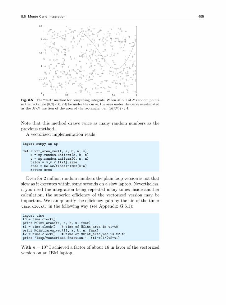
8.5 Monte Carlo Integration 405

0

0.5

1

1.5

2

2.5

0 0.5 1 1.5 2

Fig. 8.5 The“dart”method for computing integrals. When M out of N random pointsin the rectangle [0, 2]× [0, 2.4] lie under the curve, the area under the curve is estimatedas the M/N fraction of the area of the rectangle, i.e., (M/N)2 · 2.4.

Note that this method draws twice as many random numbers as theprevious method.

A vectorized implementation reads

import numpy as np

def MCint_area_vec(f, a, b, n, m):x = np.random.uniform(a, b, n)y = np.random.uniform(0, m, n)below = y[y < f(x)].sizearea = below/float(n)*m*(b-a)return area

Even for 2 million random numbers the plain loop version is not thatslow as it executes within some seconds on a slow laptop. Nevertheless,if you need the integration being repeated many times inside anothercalculation, the superior efficiency of the vectorized version may beimportant. We can quantify the efficiency gain by the aid of the timertime.clock() in the following way (see Appendix G.6.1):

import timet0 = time.clock()print MCint_area(f1, a, b, n, fmax)t1 = time.clock() # time of MCint_area is t1-t0print MCint_area_vec(f1, a, b, n, fmax)t2 = time.clock() # time of MCint_area_vec is t2-t1print ’loop/vectorized fraction:’, (t1-t0)/(t2-t1)

With n = 106 I achieved a factor of about 16 in favor of the vectorizedversion on an IBM laptop.

406 8 Random Numbers and Simple Games

8.6 Random Walk in One Space Dimension

In this section we shall simulate a collection of particles that movearound in a random fashion. This type of simulations are fundamentalin physics, biology, chemistry as well as other sciences and can be usedto describe many phenomena. Some application areas include molecularmotion, heat conduction, quantum mechanics, polymer chains, popu-lation genetics, brain research, hazard games, and pricing of financialinstruments.

Imagine that we have some particles that perform random moves,either to the right or to the left. We may flip a coin to decide themovement of each particle, say head implies movement to the rightand tail means movement to the left. Each move is one unit length.Physicists use the term random walk for this type of movement of aparticle8.

The movement is also known as “drunkard’s walk”. You may haveexperienced this after a very wet night on a pub: you step forwardand backward in a random fashion. Since these movements on averagemake you stand still, and since you know that you normally reach homewithin reasonable time, the model is not good for a real walk. We needto add a drift to the walk, so the probability is greater for going forwardthan backward. This is an easy adjustment, see Exercise 8.33. Whatmay come as a surprise is the following fact: even when there is equalprobability of going forward and backward, one can prove mathemati-cally that the drunkard will always reach his home. Or more precisely,he will get home in finite time (“almost surely” as the mathematiciansmust add to this statement). Exercise 8.34 asks you to experimentwith this fact. For many practical purposes, “finite time” does not helpmuch as there might be more steps involved than the time it takes toget sufficiently sober to remove the completely random component ofthe walk.

8.6.1 Basic Implementation

How can we implement ns random steps of np particles in a program?Let us introduce a coordinate system where all movements are along thex axis. An array of x values then holds the positions of all particles. Wedraw random numbers to simulate flipping a coin, say we draw fromthe integers 1 and 2, where 1 means head (movement to the right)and 2 means tail (movement to the left). We think the algorithm isconveniently expressed directly as a complete Python program:

8 You may try this yourself: flip the coin and make one step to the left or right, andrepeat this process.

8.6 Random Walk in One Space Dimension 407

import randomimport numpynp = 4 # no of particlesns = 100 # no of stepspositions = numpy.zeros(np) # all particles start at x=0HEAD = 1; TAIL = 2 # constants

for step in range(ns):for p in range(np):

coin = random.randint(1,2) # flip coinif coin == HEAD:

positions[p] += 1 # one unit length to the rightelif coin == TAIL:

positions[p] -= 1 # one unit length to the left

This program is found in the file walk1D.py.

8.6.2 Visualization

We may add some visualization of the movements by inserting a plot

command at the end of the step loop and a little pause to betterseparate the frames in the animation9:

plot(positions, y, ’ko3’, axis=[xmin, xmax, -0.2, 0.2])time.sleep(0.2) # pause

Recall from Chapter 5 that in an animation like this the axis must bekept fixed. We know that in ns steps, no particle can move longer thanns unit lengths to the right or to the left so the extent of the x axisbecomes [−ns, ns]. However, the probability of reaching these lower orupper limit is very small10. Most of the movements will take place inthe center of the plot. We may therefore shrink the extent of the axisto better view the movements. It is known that the expected extentof the particles is of the order

√ns, so we may take the maximum

and minimum values in the plot as ±2√ns. However, if a position ofa particle exceeds these values, we extend xmax and xmin by 2

√ns in

positive and negative x direction, respectively.The y positions of the particles are taken as zero, but it is necessary

to have some extent of the y axis, otherwise the coordinate systemcollapses and most plotting packages will refuse to draw the plot. Herewe have just chosen the y axis to go from -0.2 to 0.2. You can find thecomplete program in src/random/walk1Dp.py. The np and ns parameterscan be set as the first two command-line arguments:

Terminal

walk1Dp.py 6 200

9 These actions require from scitools.std import * and import time.10 The probability is 2−ns , which becomes about 10−9 for 30 steps.

408 8 Random Numbers and Simple Games

It is hard to claim that this program has astonishing graphics. In Chap-ter 8.7, where we let the particles move in two space dimensions, thegraphics gets much more exciting.

8.6.3 Random Walk as a Difference Equation

The random walk process can easily be expressed in terms of a differ-ence equation (see Appendix A for an introduction to difference equa-tions). Let xn be the position of the particle at time n. This position isan evolvement from time n− 1, obtained by adding a random variables to the previous position xn−1, where s = 1 has probability 1/2 ands = −1 has probability 1/2. In statistics, the expression “probabilityof event A” is written P(A). We can therefore write P(s = 1) = 1/2and P(s = −1) = 1/2. The difference equation can now be expressedmathematically as

xn = xn−1 + s, x0 = 0, P(s = 1) = P(s = −1) = 1/2 . (8.8)

This equation governs the motion of one particle. For a collection m

of particles we introduce x(i)n as the position of the i-th particle at the

n-th time step. Each x(i)n is governed by (8.8), and all the s values in

each of the m difference equations are independent of each other.

8.6.4 Computing Statistics of the Particle Positions

Scientists interested in random walks are in general not interested inthe graphics of our walk1D.py program, but more in the statistics ofthe positions of the particles at each step. We may therefore, at eachstep, compute a histogram of the distribution of the particles along thex axis, plus estimate the mean position and the standard deviation.These mathematical operations are easily accomplished by letting theSciTools function compute_histogram and the numpy functions mean andstd operate on the positions array (see Chapter 8.1.5)11 :

mean_pos = numpy.mean(positions)stdev_pos = numpy.std(positions)pos, freq = compute_histogram(positions, nbins=int(xmax),

piecewise_constant=True)

We can plot the particles as circles, as before, and add the histogramand vertical lines for the mean and the positive and negative standarddeviation (the latter indicates the “width” of the distribution of parti-cles). The vertical lines can be defined by the six lists

11 The number of bins in the histogram is just based on the extent of the particles. Itcould also have been a fixed number.

8.6 Random Walk in One Space Dimension 409

xmean, ymean = [mean_pos, mean_pos], [yminv, ymaxv]xstdv1, ystdv1 = [stdev_pos, stdev_pos], [yminv, ymaxv]xstdv2, ystdv2 = [-stdev_pos, -stdev_pos], [yminv, ymaxv]

where yminv and ymaxv are the minimum and maximum y values ofthe vertical lines. The following command plots the position of everyparticle as circles, the histogram as a curve, and the vertical lines witha thicker line:

plot(positions, y, ’ko3’, # particles as circlespos, freq, ’r’, # histogramxmean, ymean, ’r2’, # mean position as thick linexstdv1, ystdv1, ’b2’, # +1 standard dev.xstdv2, ystdv2, ’b2’, # -1 standard dev.axis=[xmin, xmax, ymin, ymax],title=’random walk of %d particles after %d steps’ %

(np, step+1))

This plot is then created at every step in the random walk. By observingthe graphics, one will soon realize that the computation of the extentof the y axis in the plot needs some considerations. We have foundit convenient to base ymax on the maximum value of the histogram(max(freq)), plus some space (chosen as 10 percent of max(freq)).However, we do not change the ymax value unless it is more than0.1 different from the previous ymax value (otherwise the axis “jumps”too often). The minimum value, ymin, is set to ymin=-0.1*ymax everytime we change the ymax value. The complete code is found in thefile walk1Ds.py. If you try out 2000 particles and 30 steps, the finalgraphics becomes like that in Figure 8.6. As the number of steps isincreased, the particles are dispersed in the positive and negative x di-rection, and the histogram gets flatter and flatter. Letting H(i) be thehistogram value in interval number i, and each interval having width∆x, the probability of finding a particle in interval i is H(i)∆x. It canbe shown mathematically that the histogram is an approximation tothe probability density function of the normal distribution (1.6) (seepage 45), with mean zero and standard deviation s ∼ √n, where n isthe step number.

8.6.5 Vectorized Implementation

There is no problem with the speed of our one-dimensional randomwalkers in the walk1Dp.py or walk1Ds.py programs, but in real-life ap-plications of such simulation models, we often have a very large numberof particles performing a very large number of steps. It is then impor-tant to make the implementation as efficient as possible. Two loops overall particles and all steps, as we have in the programs above, becomevery slow compared to a vectorized implementation.

A vectorized implementation of a one-dimensional walk should uti-lize the functions randint or random_integers from numpy’s randommod-

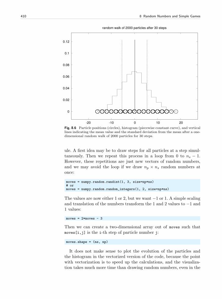
410 8 Random Numbers and Simple Games

0

0.02

0.04

0.06

0.08

0.1

0.12

-20 -10 0 10 20

random walk of 2000 particles after 30 steps

Fig. 8.6 Particle positions (circles), histogram (piecewise constant curve), and verticallines indicating the mean value and the standard deviation from the mean after a one-dimensional random walk of 2000 particles for 30 steps.

ule. A first idea may be to draw steps for all particles at a step simul-taneously. Then we repeat this process in a loop from 0 to ns − 1.However, these repetitions are just new vectors of random numbers,and we may avoid the loop if we draw np × ns random numbers atonce:

moves = numpy.random.randint(1, 3, size=np*ns)# ormoves = numpy.random.random_integers(1, 2, size=np*ns)

The values are now either 1 or 2, but we want −1 or 1. A simple scalingand translation of the numbers transform the 1 and 2 values to −1 and1 values:

moves = 2*moves - 3

Then we can create a two-dimensional array out of moves such thatmoves[i,j] is the i-th step of particle number j:

moves.shape = (ns, np)

It does not make sense to plot the evolution of the particles andthe histogram in the vectorized version of the code, because the pointwith vectorization is to speed up the calculations, and the visualiza-tion takes much more time than drawing random numbers, even in the

8.7 Random Walk in Two Space Dimensions 411

walk1Dp.py and walk1Ds.py programs from Chapter 8.6.4. We thereforejust compute the positions of the particles inside a loop over the stepsand some simple statistics. At the end, after ns steps, we plot the his-togram of the particle distribution along with circles for the positionsof the particles. The rest of the program, found in the file walk1Dv.py,looks as follows:

positions = numpy.zeros(np)for step in range(ns):

positions += moves[step, :]

mean_pos = numpy.mean(positions)stdev_pos = numpy.std(positions)print mean_pos, stdev_pos

nbins = int(3*sqrt(ns)) # no of intervals in histogrampos, freq = compute_histogram(positions, nbins,

piecewise_constant=True)

plot(positions, zeros(np), ’ko3’,pos, freq, ’r’,axis=[min(positions), max(positions), -0.01, 1.1*max(freq)],hardcopy=’tmp.ps’)

8.7 Random Walk in Two Space Dimensions

A random walk in two dimensions performs a step either to the north,south, west, or east, each one with probability 1/4. To demonstratethis process, we introduce x and y coordinates of np particles anddraw random numbers among 1, 2, 3, or 4 to determine the move. Thepositions of the particles can easily be visualized as small circles in anxy coordinate system.

8.7.1 Basic Implementation

The algorithm described above is conveniently expressed directly as acomplete working program:

def random_walk_2D(np, ns, plot_step):xpositions = numpy.zeros(np)ypositions = numpy.zeros(np)# extent of the axis in the plot:xymax = 3*numpy.sqrt(ns); xymin = -xymax

NORTH = 1; SOUTH = 2; WEST = 3; EAST = 4 # constants

for step in range(ns):for i in range(np):

direction = random.randint(1, 4)if direction == NORTH:

ypositions[i] += 1elif direction == SOUTH:

ypositions[i] -= 1

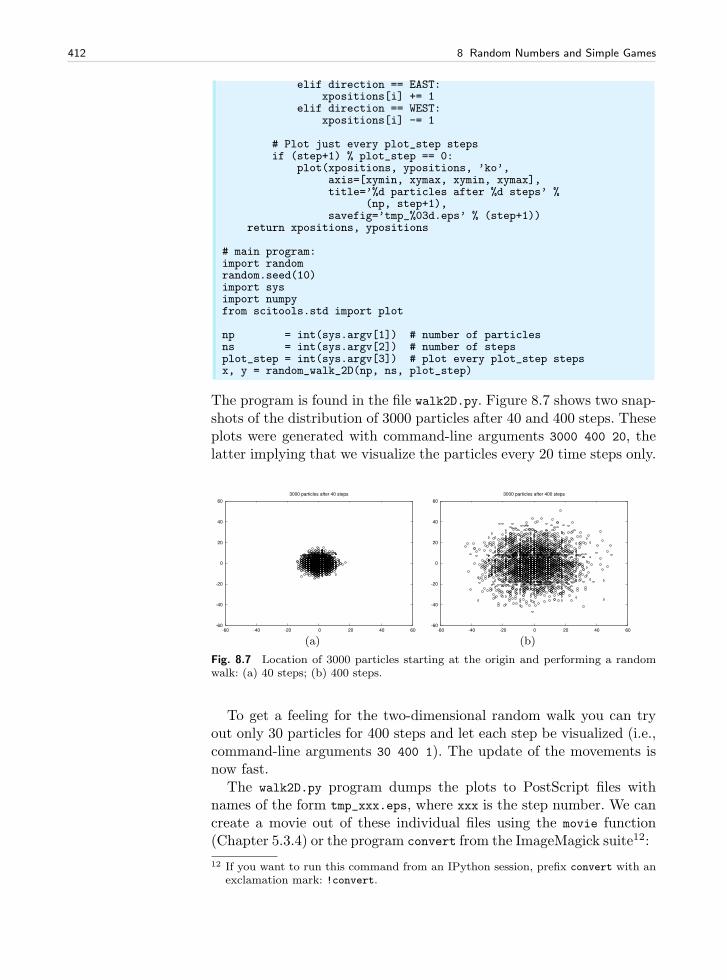
412 8 Random Numbers and Simple Games

elif direction == EAST:xpositions[i] += 1

elif direction == WEST:xpositions[i] -= 1

# Plot just every plot_step stepsif (step+1) % plot_step == 0:

plot(xpositions, ypositions, ’ko’,axis=[xymin, xymax, xymin, xymax],title=’%d particles after %d steps’ %

(np, step+1),savefig=’tmp_%03d.eps’ % (step+1))

return xpositions, ypositions

# main program:import randomrandom.seed(10)import sysimport numpyfrom scitools.std import plot

np = int(sys.argv[1]) # number of particlesns = int(sys.argv[2]) # number of stepsplot_step = int(sys.argv[3]) # plot every plot_step stepsx, y = random_walk_2D(np, ns, plot_step)

The program is found in the file walk2D.py. Figure 8.7 shows two snap-shots of the distribution of 3000 particles after 40 and 400 steps. Theseplots were generated with command-line arguments 3000 400 20, thelatter implying that we visualize the particles every 20 time steps only.

-60

-40

-20

0

20

40

60

-60 -40 -20 0 20 40 60

3000 particles after 40 steps

(a)

-60

-40

-20

0

20

40

60

-60 -40 -20 0 20 40 60

3000 particles after 400 steps

(b)

Fig. 8.7 Location of 3000 particles starting at the origin and performing a randomwalk: (a) 40 steps; (b) 400 steps.

To get a feeling for the two-dimensional random walk you can tryout only 30 particles for 400 steps and let each step be visualized (i.e.,command-line arguments 30 400 1). The update of the movements isnow fast.

The walk2D.py program dumps the plots to PostScript files withnames of the form tmp_xxx.eps, where xxx is the step number. We cancreate a movie out of these individual files using the movie function(Chapter 5.3.4) or the program convert from the ImageMagick suite12:

12 If you want to run this command from an IPython session, prefix convert with anexclamation mark: !convert.

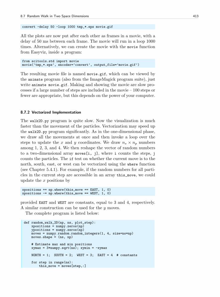
8.7 Random Walk in Two Space Dimensions 413

convert -delay 50 -loop 1000 tmp_*.eps movie.gif

All the plots are now put after each other as frames in a movie, with adelay of 50 ms between each frame. The movie will run in a loop 1000times. Alternatively, we can create the movie with the movie functionfrom Easyviz, inside a program:

from scitools.std import moviemovie(’tmp_*.eps’, encoder=’convert’, output_file=’movie.gif’)

The resulting movie file is named movie.gif, which can be viewed bythe animate program (also from the ImageMagick program suite), justwrite animate movie.gif. Making and showing the movie are slow pro-cesses if a large number of steps are included in the movie – 100 steps orfewer are appropriate, but this depends on the power of your computer.

8.7.2 Vectorized Implementation

The walk2D.py program is quite slow. Now the visualization is muchfaster than the movement of the particles. Vectorization may speed upthe walk2D.py program significantly. As in the one-dimensional phase,we draw all the movements at once and then invoke a loop over thesteps to update the x and y coordinates. We draw ns × np numbersamong 1, 2, 3, and 4. We then reshape the vector of random numbersto a two-dimensional array moves[i, j], where i counts the steps, jcounts the particles. The if test on whether the current move is to thenorth, south, east, or west can be vectorized using the where function(see Chapter 5.4.1). For example, if the random numbers for all parti-cles in the current step are accessible in an array this_move, we couldupdate the x positions by

xpositions += np.where(this_move == EAST, 1, 0)xpositions -= np.where(this_move == WEST, 1, 0)

provided EAST and WEST are constants, equal to 3 and 4, respectively.A similar construction can be used for the y moves.

The complete program is listed below:

def random_walk_2D(np, ns, plot_step):xpositions = numpy.zeros(np)ypositions = numpy.zeros(np)moves = numpy.random.random_integers(1, 4, size=ns*np)moves.shape = (ns, np)

# Estimate max and min positionsxymax = 3*numpy.sqrt(ns); xymin = -xymax

NORTH = 1; SOUTH = 2; WEST = 3; EAST = 4 # constants

for step in range(ns):this_move = moves[step,:]

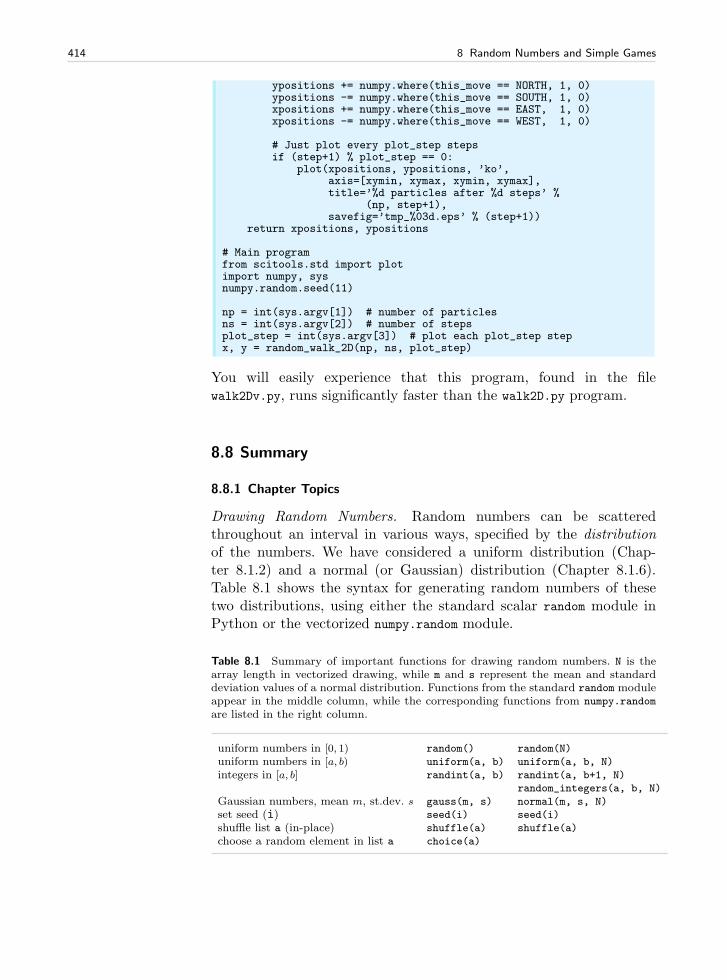
414 8 Random Numbers and Simple Games

ypositions += numpy.where(this_move == NORTH, 1, 0)ypositions -= numpy.where(this_move == SOUTH, 1, 0)xpositions += numpy.where(this_move == EAST, 1, 0)xpositions -= numpy.where(this_move == WEST, 1, 0)

# Just plot every plot_step stepsif (step+1) % plot_step == 0:

plot(xpositions, ypositions, ’ko’,axis=[xymin, xymax, xymin, xymax],title=’%d particles after %d steps’ %

(np, step+1),savefig=’tmp_%03d.eps’ % (step+1))

return xpositions, ypositions

# Main programfrom scitools.std import plotimport numpy, sysnumpy.random.seed(11)

np = int(sys.argv[1]) # number of particlesns = int(sys.argv[2]) # number of stepsplot_step = int(sys.argv[3]) # plot each plot_step stepx, y = random_walk_2D(np, ns, plot_step)

You will easily experience that this program, found in the filewalk2Dv.py, runs significantly faster than the walk2D.py program.

8.8 Summary

8.8.1 Chapter Topics

Drawing Random Numbers. Random numbers can be scatteredthroughout an interval in various ways, specified by the distributionof the numbers. We have considered a uniform distribution (Chap-ter 8.1.2) and a normal (or Gaussian) distribution (Chapter 8.1.6).Table 8.1 shows the syntax for generating random numbers of thesetwo distributions, using either the standard scalar random module inPython or the vectorized numpy.random module.

Table 8.1 Summary of important functions for drawing random numbers. N is thearray length in vectorized drawing, while m and s represent the mean and standarddeviation values of a normal distribution. Functions from the standard random moduleappear in the middle column, while the corresponding functions from numpy.random

are listed in the right column.

uniform numbers in [0, 1) random() random(N)

uniform numbers in [a, b) uniform(a, b) uniform(a, b, N)

integers in [a, b] randint(a, b) randint(a, b+1, N)

random_integers(a, b, N)

Gaussian numbers, mean m, st.dev. s gauss(m, s) normal(m, s, N)

set seed (i) seed(i) seed(i)

shuffle list a (in-place) shuffle(a) shuffle(a)

choose a random element in list a choice(a)

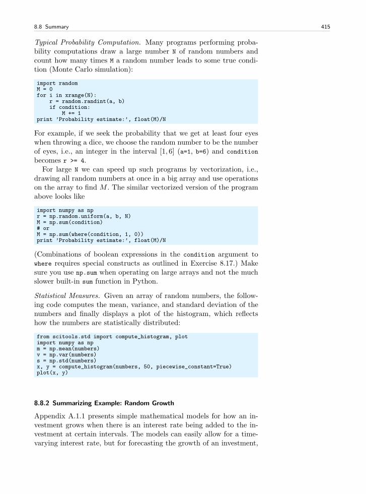
8.8 Summary 415

Typical Probability Computation. Many programs performing proba-bility computations draw a large number N of random numbers andcount how many times M a random number leads to some true condi-tion (Monte Carlo simulation):

import randomM = 0for i in xrange(N):

r = random.randint(a, b)if condition:

M += 1print ’Probability estimate:’, float(M)/N

For example, if we seek the probability that we get at least four eyeswhen throwing a dice, we choose the random number to be the numberof eyes, i.e., an integer in the interval [1, 6] (a=1, b=6) and condition

becomes r >= 4.For large N we can speed up such programs by vectorization, i.e.,

drawing all random numbers at once in a big array and use operationson the array to find M . The similar vectorized version of the programabove looks like

import numpy as npr = np.random.uniform(a, b, N)M = np.sum(condition)# orM = np.sum(where(condition, 1, 0))print ’Probability estimate:’, float(M)/N

(Combinations of boolean expressions in the condition argument towhere requires special constructs as outlined in Exercise 8.17.) Makesure you use np.sum when operating on large arrays and not the muchslower built-in sum function in Python.

Statistical Measures. Given an array of random numbers, the follow-ing code computes the mean, variance, and standard deviation of thenumbers and finally displays a plot of the histogram, which reflectshow the numbers are statistically distributed:

from scitools.std import compute_histogram, plotimport numpy as npm = np.mean(numbers)v = np.var(numbers)s = np.std(numbers)x, y = compute_histogram(numbers, 50, piecewise_constant=True)plot(x, y)

8.8.2 Summarizing Example: Random Growth

Appendix A.1.1 presents simple mathematical models for how an in-vestment grows when there is an interest rate being added to the in-vestment at certain intervals. The models can easily allow for a time-varying interest rate, but for forecasting the growth of an investment,

416 8 Random Numbers and Simple Games

it is difficult to predict the future interest rate. One commonly usedmethod is to build a probabilistic model for the development of theinterest rate, where the rate is chosen randomly at random times. Thisgives a random growth of the investment, but by simulating many ran-dom scenarios we can compute the mean growth and use the standarddeviation as a measure of the uncertainty of the predictions.

Problem. Let p be the annual interest rate in a bank in percent. Sup-pose the interest is added to the investment q times per year. Thenew value of the investment, xn, is given by the previous value of theinvestment, xn−1, plus the p/q percent interest:

xn = xn−1 +p

100qxn−1 .

Normally, the interest is added daily (q = 360 and n counts days),but for efficiency in the computations later we shall assume that theinterest is added monthly, so q = 12 and n counts months.

The basic assumption now is that p is random and varies with time.Suppose p increases with a random amount γ from one month to thenext:

pn = pn−1 + γ .

A typical size of p adjustments is 0.5. However, the central bank doesnot adjust the interest every month. Instead this happens every Mmonths on average. The probability of a γ 6= 0 can therefore be takenas 1/M . In a month where γ 6= 0, we may say that γ = m withprobability 1/2 or γ = −m with probability 1/2 if it is equally likelythat the rate goes up as down (this is not a good assumption, but amore complicated evolvement of γ is postponed now).

Solution. First we must develop the precise formulas to be imple-mented. The difference equations for xn and pn are in simple in thepresent case, but the details computing γ must be worked out. In aprogram, we can draw two random numbers to estimate γ: one for de-ciding if γ 6= 0 and the other for determining the sign of the change.Since the probability for γ 6= 0 is 1/M , we can draw a number r1 amongthe integers 1, . . . ,M and if r1 = 1 we continue with drawing a secondnumber r2 among the integers 1 and 2. If r2 = 1 we set γ = m, and ifr2 = 2 we set γ = −m. We must also assure that pn does not take onunreasonable values, so we choose pn < 1 and pn > 15 as cases wherepn is not changed.

The mathematical model for the investment must track both xn andpn. Below we express with precise mathematics the equations for xnand pn and the computation of the random γ quantity:

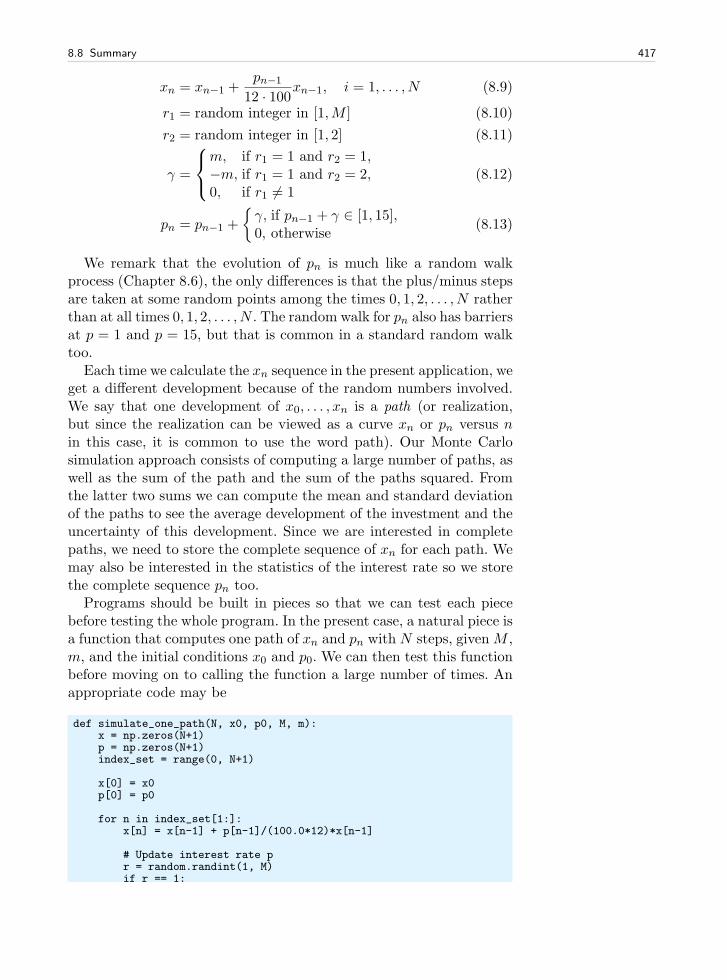
8.8 Summary 417

xn = xn−1 +pn−1

12 · 100xn−1, i = 1, . . . , N (8.9)

r1 = random integer in [1,M ] (8.10)

r2 = random integer in [1, 2] (8.11)

γ =

m, if r1 = 1 and r2 = 1,−m, if r1 = 1 and r2 = 2,0, if r1 6= 1

(8.12)

pn = pn−1 +

γ, if pn−1 + γ ∈ [1, 15],0, otherwise

(8.13)

We remark that the evolution of pn is much like a random walkprocess (Chapter 8.6), the only differences is that the plus/minus stepsare taken at some random points among the times 0, 1, 2, . . . , N ratherthan at all times 0, 1, 2, . . . , N . The random walk for pn also has barriersat p = 1 and p = 15, but that is common in a standard random walktoo.

Each time we calculate the xn sequence in the present application, weget a different development because of the random numbers involved.We say that one development of x0, . . . , xn is a path (or realization,but since the realization can be viewed as a curve xn or pn versus nin this case, it is common to use the word path). Our Monte Carlosimulation approach consists of computing a large number of paths, aswell as the sum of the path and the sum of the paths squared. Fromthe latter two sums we can compute the mean and standard deviationof the paths to see the average development of the investment and theuncertainty of this development. Since we are interested in completepaths, we need to store the complete sequence of xn for each path. Wemay also be interested in the statistics of the interest rate so we storethe complete sequence pn too.

Programs should be built in pieces so that we can test each piecebefore testing the whole program. In the present case, a natural piece isa function that computes one path of xn and pn with N steps, given M ,m, and the initial conditions x0 and p0. We can then test this functionbefore moving on to calling the function a large number of times. Anappropriate code may be

def simulate_one_path(N, x0, p0, M, m):x = np.zeros(N+1)p = np.zeros(N+1)index_set = range(0, N+1)

x[0] = x0p[0] = p0

for n in index_set[1:]:x[n] = x[n-1] + p[n-1]/(100.0*12)*x[n-1]

# Update interest rate pr = random.randint(1, M)if r == 1:

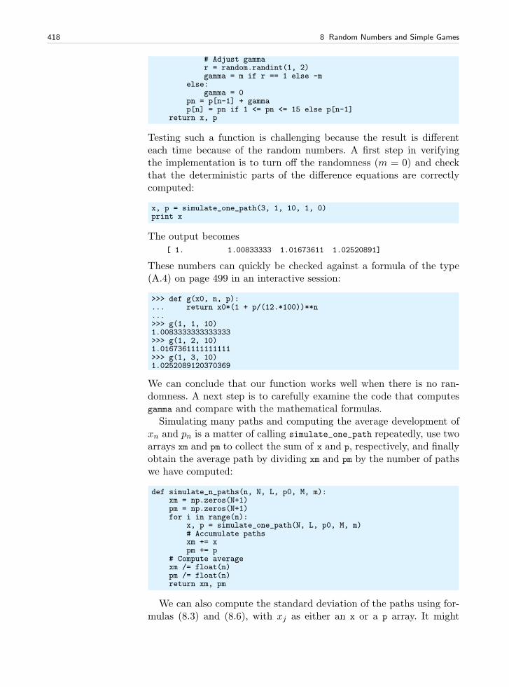
418 8 Random Numbers and Simple Games

# Adjust gammar = random.randint(1, 2)gamma = m if r == 1 else -m

else:gamma = 0

pn = p[n-1] + gammap[n] = pn if 1 <= pn <= 15 else p[n-1]

return x, p

Testing such a function is challenging because the result is differenteach time because of the random numbers. A first step in verifyingthe implementation is to turn off the randomness (m = 0) and checkthat the deterministic parts of the difference equations are correctlycomputed:

x, p = simulate_one_path(3, 1, 10, 1, 0)print x

The output becomes

[ 1. 1.00833333 1.01673611 1.02520891]

These numbers can quickly be checked against a formula of the type(A.4) on page 499 in an interactive session:

>>> def g(x0, n, p):... return x0*(1 + p/(12.*100))**n...>>> g(1, 1, 10)1.0083333333333333>>> g(1, 2, 10)1.0167361111111111>>> g(1, 3, 10)1.0252089120370369

We can conclude that our function works well when there is no ran-domness. A next step is to carefully examine the code that computesgamma and compare with the mathematical formulas.

Simulating many paths and computing the average development ofxn and pn is a matter of calling simulate_one_path repeatedly, use twoarrays xm and pm to collect the sum of x and p, respectively, and finallyobtain the average path by dividing xm and pm by the number of pathswe have computed:

def simulate_n_paths(n, N, L, p0, M, m):xm = np.zeros(N+1)pm = np.zeros(N+1)for i in range(n):

x, p = simulate_one_path(N, L, p0, M, m)# Accumulate pathsxm += xpm += p

# Compute averagexm /= float(n)pm /= float(n)return xm, pm

We can also compute the standard deviation of the paths using for-mulas (8.3) and (8.6), with xj as either an x or a p array. It might

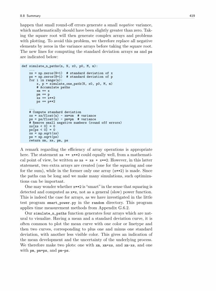
8.8 Summary 419

happen that small round-off errors generate a small negative variance,which mathematically should have been slightly greater than zero. Tak-ing the square root will then generate complex arrays and problemswith plotting. To avoid this problem, we therefore replace all negativeelements by zeros in the variance arrays before taking the square root.The new lines for computing the standard deviation arrays xs and ps

are indicated below:

def simulate_n_paths(n, N, x0, p0, M, m):...xs = np.zeros(N+1) # standard deviation of xps = np.zeros(N+1) # standard deviation of pfor i in range(n):

x, p = simulate_one_path(N, x0, p0, M, m)# Accumulate pathsxm += xpm += pxs += x**2ps += p**2

...# Compute standard deviationxs = xs/float(n) - xm*xm # varianceps = ps/float(n) - pm*pm # variance# Remove small negative numbers (round off errors)xs[xs < 0] = 0ps[ps < 0] = 0xs = np.sqrt(xs)ps = np.sqrt(ps)return xm, xs, pm, ps

A remark regarding the efficiency of array operations is appropriatehere. The statement xs += x**2 could equally well, from a mathemati-cal point of view, be written as xs = xs + x**2. However, in this latterstatement, two extra arrays are created (one for the squaring and onefor the sum), while in the former only one array (x**2) is made. Sincethe paths can be long and we make many simulations, such optimiza-tions can be important.

One may wonder whether x**2 is“smart”in the sense that squaring isdetected and computed as x*x, not as a general (slow) power function.This is indeed the case for arrays, as we have investigated in the littletest program smart_power.py in the random directory. This programapplies time measurement methods from Appendix G.6.2.

Our simulate_n_paths function generates four arrays which are nat-ural to visualize. Having a mean and a standard deviation curve, it isoften common to plot the mean curve with one color or linetype andthen two curves, corresponding to plus one and minus one standarddeviation, with another less visible color. This gives an indication ofthe mean development and the uncertainty of the underlying process.We therefore make two plots: one with xm, xm+xs, and xm-xs, and onewith pm, pm+ps, and pm-ps.

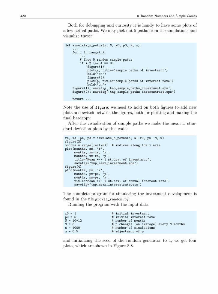
420 8 Random Numbers and Simple Games

Both for debugging and curiosity it is handy to have some plots ofa few actual paths. We may pick out 5 paths from the simulations andvisualize these:

def simulate_n_paths(n, N, x0, p0, M, m):...for i in range(n):

...# Show 5 random sample pathsif i % (n/5) == 0:

figure(1)plot(x, title=’sample paths of investment’)hold(’on’)figure(2)plot(p, title=’sample paths of interest rate’)hold(’on’)

figure(1); savefig(’tmp_sample_paths_investment.eps’)figure(2); savefig(’tmp_sample_paths_interestrate.eps’)...return ...

Note the use of figure: we need to hold on both figures to add newplots and switch between the figures, both for plotting and making thefinal hardcopy.

After the visualization of sample paths we make the mean ± stan-dard deviation plots by this code:

xm, xs, pm, ps = simulate_n_paths(n, N, x0, p0, M, m)figure(3)months = range(len(xm)) # indices along the x axisplot(months, xm, ’r’,

months, xm-xs, ’y’,months, xm+xs, ’y’,title=’Mean +/- 1 st.dev. of investment’,savefig=’tmp_mean_investment.eps’)

figure(4)plot(months, pm, ’r’,

months, pm-ps, ’y’,months, pm+ps, ’y’,title=’Mean +/- 1 st.dev. of annual interest rate’,savefig=’tmp_mean_interestrate.eps’)

The complete program for simulating the investment development isfound in the file growth_random.py.

Running the program with the input data

x0 = 1 # initial investmentp0 = 5 # initial interest rateN = 10*12 # number of monthsM = 3 # p changes (on average) every M monthsn = 1000 # number of simulationsm = 0.5 # adjustment of p

and initializing the seed of the random generator to 1, we get fourplots, which are shown in Figure 8.8.

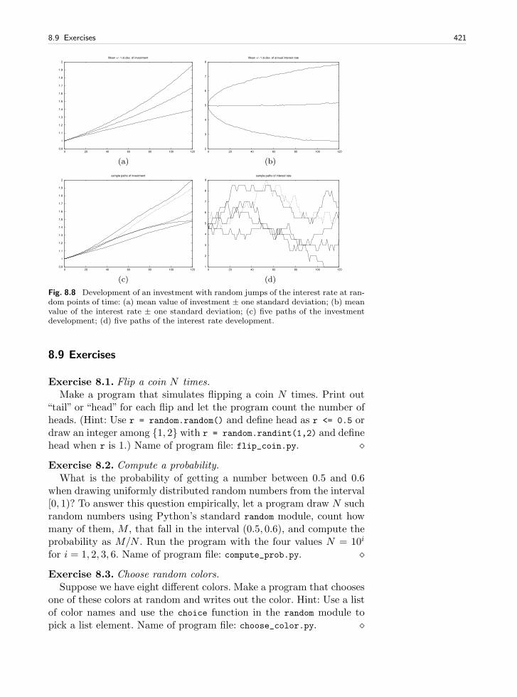
8.9 Exercises 421

0.9

1

1.1

1.2

1.3

1.4

1.5

1.6

1.7

1.8

1.9

2

0 20 40 60 80 100 120

Mean +/- 1 st.dev. of investment

(a)

2

3

4

5

6

7

8

0 20 40 60 80 100 120

Mean +/- 1 st.dev. of annual interest rate

(b)

0.9

1

1.1

1.2

1.3

1.4

1.5

1.6

1.7

1.8

1.9

2

0 20 40 60 80 100 120

sample paths of investment

(c)

1

2

3

4

5

6

7

8

9

0 20 40 60 80 100 120

sample paths of interest rate

(d)

Fig. 8.8 Development of an investment with random jumps of the interest rate at ran-dom points of time: (a) mean value of investment ± one standard deviation; (b) meanvalue of the interest rate ± one standard deviation; (c) five paths of the investmentdevelopment; (d) five paths of the interest rate development.

8.9 Exercises

Exercise 8.1. Flip a coin N times.Make a program that simulates flipping a coin N times. Print out

“tail” or “head” for each flip and let the program count the number ofheads. (Hint: Use r = random.random() and define head as r <= 0.5 ordraw an integer among 1, 2 with r = random.randint(1,2) and definehead when r is 1.) Name of program file: flip_coin.py. ⋄

Exercise 8.2. Compute a probability.What is the probability of getting a number between 0.5 and 0.6

when drawing uniformly distributed random numbers from the interval[0, 1)? To answer this question empirically, let a program draw N suchrandom numbers using Python’s standard random module, count howmany of them, M , that fall in the interval (0.5, 0.6), and compute theprobability as M/N . Run the program with the four values N = 10i

for i = 1, 2, 3, 6. Name of program file: compute_prob.py. ⋄

Exercise 8.3. Choose random colors.Suppose we have eight different colors. Make a program that chooses

one of these colors at random and writes out the color. Hint: Use a listof color names and use the choice function in the random module topick a list element. Name of program file: choose_color.py. ⋄

422 8 Random Numbers and Simple Games

Exercise 8.4. Draw balls from a hat.Suppose there are 40 balls in a hat, of which 10 are red, 10 are blue,

10 are yellow, and 10 are purple. What is the probability of gettingtwo blue and two purple balls when drawing 10 balls at random fromthe hat? Name of program file: 4balls_from10.py. ⋄

Exercise 8.5. Probabilities of rolling dice.

1. You throw a die. What is the probability of getting a 6?2. You throw a die four times in a row. What is the probability of

getting 6 all the times?3. Suppose you have thrown the die three times with 6 coming up all

times. What is the probability of getting a 6 in the fourth throw?4. Suppose you have thrown the die 100 times and experienced a 6 in

every throw. What do you think about the probability of getting a6 in the next throw?

First try to solve the questions from a theoretical or common sensepoint of view. Thereafter, make functions for simulating cases 1, 2,and 3. Name of program file: rolling_dice.py. ⋄

Exercise 8.6. Estimate the probability in a dice game.Make a program for estimating the probability of getting at least

one 6 when throwing n dice. Read n and the number of experimentsfrom the command line. (To verify the program, you can compare theestimated probability with the exact result 11/36 when n = 2.) Nameof program file: one6_ndice.py. ⋄

Exercise 8.7. Compute the probability of hands of cards.Use the Deck.py module (in src/random) and the same_rank and

same_suit functions from the cards module to compute the followingprobabilities by Monte Carlo simulation:

exactly two pairs among five cards, four or five cards of the same suit among five cards, four-of-a-kind among five cards.

Name of program file: card_hands.py. ⋄

Exercise 8.8. Decide if a dice game is fair.Somebody suggests the following game. You pay 1 unit of money and

are allowed to throw four dice. If the sum of the eyes on the dice is lessthan 9, you win 10 units of money, otherwise you lose your investment.Should you play this game? Answer the question by making a programthat simulates the game. Name of program file: sum9_4dice.py. ⋄

Exercise 8.9. Adjust the game in Exer. 8.8.It turns out that the game in Exercise 8.8 is not fair, since you lose

money in the long run. The purpose of this exercise is to adjust the

8.9 Exercises 423

winning award so that the game becomes fair, i.e., that you neitherlose nor win money in the long run.

Make a program that computes the probability p of gettinga sum less than s when rolling n dice. Name of program file:sum_s_ndice_fair.py.

If the cost of each game is q units of money, the game is fair if thepayment in case you win is r = q/p. Run the program you made fors = 9 and n = 4, which corresponds to the game in Exercise 8.8, andcompute the corresponding p. Modify the program from Exercise 8.8so that the award is r = 1/p, and run that program to see that nowthe game is fair.

Mathematical Explanation. The formula for a fair game given abovecan be developed as follows. Let p = M/N be the probability of win-ning, which means that you in the long run winM out of N games. Thecost is Nq and the income is Mr. To make the net income Mr − Nqzero, which is the requirement of a fair game, we get r = qN/M = q/p.(This reasoning is based on common sense and an intuitive interpreta-tion of probability. More precise reasoning from probability theory willintroduce the game as an experiment with two outcomes, either youwin with probability p and or lose with probability 1−p. The expextedpayment is then the sum of probabilities times the corresponding netincomes: −q(1− p) + (r− q)p (recall that the net income in a winninggame is r − q). A fair game has zero expected payment, i.e., r = q/p.)⋄Exercise 8.10. Compare two playing strategies.

Suggest a player strategy for the game in Chapter 8.4.2. Remove thequestion in the player_guess function in the file src/random/ndice2.py,and implement the chosen strategy instead. Let the program play alarge number of games, and record the number of times the computerwins. Which strategy is best in the long run: the computer’s or yours?Name of program file: simulate_strategies1.py. ⋄Exercise 8.11. Solve Exercise 8.10 with different no. of dice.

Solve Exercise 8.10 for two other cases with 3 and 50 dice, respec-tively. Name of program file: simulate_strategies2.py. ⋄Exercise 8.12. Extend Exercise 8.11.

Extend the program from Exercise 8.11 such that the computer andthe player can use a different number of dice. Let the computer choosea random number of dice between 2 and 20. Experiment to find out ifthere is a favorable number of dice for the player. Name of programfile: simulate_strategies3.py. ⋄Exercise 8.13. Investigate the winning chances of some games.

An amusement park offers the following game. A hat contains 20balls: 5 red, 5 yellow, 3 green, and 7 brown. At a cost of 2n units of

424 8 Random Numbers and Simple Games

money you can draw 4 ≤ n ≤ 10 balls at random from the hat (withoutputting them back). Before you are allowed to look at the drawn balls,you must choose one of the following options:

1. win 60 units of money if you have drawn exactly three red balls2. win 7+ 5

√n units of money if you have drawn at least three brown

balls3. win n3 − 26 units of money if you have drawn exactly one yellow

ball and one brown ball4. win 23 units of money if you have drawn at least one ball of each

color

For each of the 4n different types of games you can play, compute thenet income (per play) and the probability of winning. Is there any ofthe games (i.e., any combinations of n and the options 1-4) where youwill win money in the long run? Name of program file: draw_balls.py.⋄Exercise 8.14. Probabilities of throwing two dice.

Make a computer program for throwing two dice a large number oftimes. Record the sum of the eyes each time and count how many timeseach of the possibilities for the sum (2, 3, . . ., 12) appear. A dictionarywith the sum as key and count as value is convenient here. Divide thecounts by the total number of trials such that you get the frequency ofeach possible sum. Write out the frequencies and compare them withexact probabilities. (To find the exact probabilities, set up all the 6×6possible outcomes of throwing two dice, and then count how many ofthem that has a sum s for s = 2, 3, . . . , 12.) Name of program file:freq_2dice.py. ⋄Exercise 8.15. Play with vectorized boolean expressions.

Using the numpy.random module, make an array r containing N uni-formly distributed random numbers between 0 and 1. Print out the ar-rays r <= 0.5, r[r <= 0.5], where(r <= 0.5, 1, 0) and convince your-self that you understand what these arrays express. We want to com-pute how many of the elements in r that are less than or equal to 0.5.How can this be done in a vectorized way, i.e., without explicit loopsin the program, but solely with operations on complete arrays? Nameof program file: bool_vec.py. ⋄Exercise 8.16. Vectorize the program from Exer. 8.1.

Simulate flipping a coin N times and write out the number oftails. The code should be vectorized, i.e., there must be no loops inPython. Hint: Use ideas from Exercise 8.15. Name of program file:flip_coin_vec.py. ⋄Exercise 8.17. Vectorize the code in Exer. 8.2.

The purpose of this exercise is to speed up the code in Exercise 8.2by vectorization. Hint: First draw an array r with a large number

8.9 Exercises 425

of random numbers in [0, 1). The simplest way to count how manyelements in r that lie between 0.5 and 0.6, is to first extract the elementslarger than 0.5: r1 = r[r>0.5], and then extract the elements in r1 thatare less than 0.6 and get the size of this array: r1[r1<=0.6].size. Nameof program file: compute_prob_vec.py.

Remark. An alternative and more complicated method is to usethe where function. The condition (the first argument to where) isnow a compond boolean expression 0.5 <= r <= 0.6, but this can-not be used with NumPy arrays. Instead one must test for 0.5 <=

r and r < = 0.6. The needed boolean construction in the where callis operator.and_(0.5 <= r, r <= 0.6). See also the discussion of thesame topic in Chapter 5.4.1. ⋄

Exercise 8.18. Throw dice and compute a small probability.Compute the probability of getting 6 eyes on all dice when rolling

7 dice. Since you need a large number of experiments in this case (seethe first paragraph of Chapter 8.3), you can save quite some simula-tion time by using a vectorized implementation. Name of program file:roll_7dice.py. ⋄

Exercise 8.19. Difference equation for random numbers.Simple random number generators are based on simulating difference

equations. Here is a typical set of two equations:

xn = (axn−1 + c) mod m, (8.14)

yn = xn/m, (8.15)

for n = 1, 2, . . .. A seed x0 must be given to start the sequence. Thenumbers y1, y2, . . . , represent the random numbers and x0, x1, . . . are“help” numbers. Although yn is completely deterministic from (8.14)–(8.15), the sequence yn appears random. The mathematical expressionp mod q is coded as p % q in Python.

Use a = 8121, c = 28411, and m = 134456. Solve the system (8.14)–(8.15) in a function that generates and returns N random numbers.Make a histogram to examine the distribution of the numbers (the ynnumbers are randomly distributed if the histogram is approximatelyflat). Name of program file: diffeq_random.py. ⋄

Exercise 8.20. Make a class for drawing balls from a hat.Consider the example about drawing colored balls from a hat in

Chapter 8.3.3. It could be handy to have an object that acts as a hat:

# Make a hat with balls of 3 colors, each color appearing# on 4 ballshat = Hat(colors=(’red’, ’black’, ’blue’), number_of_each_color=4)

# Draw 3 balls at randomballs = hat.draw(number_of_balls=3)

426 8 Random Numbers and Simple Games

Realize such code with a class Hat. You can borrow useful code fromthe balls_in_hat.py program and ideas from Chapter 8.2.5. Use theHat class to solve the probability problem from Exercise 8.4. Name ofprogram file: Hat.py. ⋄Exercise 8.21. Independent vs. dependent random numbers.

Generate a sequence of N independent random variables with values0 or 1 and print out this sequence without space between the numbers(i.e., as 001011010110111010).

The next task is to generate random zeros and ones that are depen-dent. If the last generated number was 0, the probability of generatinga new 0 is p and a new 1 is 1 − p. Conversely, if the last generatedwas 1, the probability of generating a new 1 is p and a new 0 is 1− p.Since the new value depends on the last one, we say the variables aredependent. Implement this algorithm in a function returning an arrayof N zeros and ones. Print out this array in the condense format asdescribed above.

Choose N = 80 and try the probabilities p = 0.5, p = 0.8 andp = 0.9. Can you by visual inspection of the output characterize thedifferences between sequences of independent and dependent randomvariables? Name of program file: dependent_random_variables.py. ⋄Exercise 8.22. Compute the probability of flipping a coin.

Modify the program from either Exercise 8.1 or 8.16 to incorporatethe following extensions: look at a subset N1 ≤ N of the experimentsand compute probability of getting a head (M1/N1, where M1 is thenumber of heads in N1 experiments). Choose N = 1000 and print outthe probability for N1 = 10, 100, 500, 1000. (Generate just N numbersonce in the program.) How do you think the accuracy of the computedprobability vary with N1? Is the output compatible with this expecta-tion? Name of program file: flip_coin_prob.py. ⋄Exercise 8.23. Extend Exer. 8.22.

We address the same problem as in Exercise 8.22, but now we wantto study the probability of getting a head, p, as a function of N1, i.e.,for N1 = 1, . . . , N . We also want to vectorize all operations in the code.A first try to compute the probability array for p is

import numpy as nph = np.where(r <= 0.5, 1, 0)p = np.zeros(N)for i in range(N):

p[i] = np.sum(h[:i+1])/float(i+1)

An array q[i] = np.sum(h([:i])) reflects a cumulative sum and canbe efficiently generated by np.cumsum: q = np.cumsum(h). Thereafter wecan compute p by q/I, where I[i]=i+1 and I can be computed bynp.arange(1,N+1) or r_[1:N+1] (integers 1, 2, . . ., up to but not includ-ing N+1). Implement both the loop over i and the vectorized version

8.9 Exercises 427

based on cumsum and check in the program that the resulting p arrayhas the same elements (for this purpose you have to compare float

elements and you can use the float_eq function from SciTools, see Ex-ercise 2.28, or the allclose function in numpy (float_eq actually usesallclose for array arguments)). Plot p against I for the case whereN = 10000. Annotate the axis and the plot with relevant text. Nameof program file: flip_coin_prob_developm.py. ⋄

Exercise 8.24. Simulate the problems in Exer. 4.25.Exercise 4.25 describes some problems that can be solved exactly

using the formula (4.8), but we can also simulate these problems andfind approximate numbers for the probabilities. That is the task of thisexercise.

Make a general function simulate_binomial(p, n, x) for running nexperiments, where each experiment have two outcomes, with proba-bilities p and 1−p. The n experiments constitute a “success” if the out-come with probability p occurs exactly x times. The simulate_binomialfunction must repeat the n experiments N times. If M is the numberof “successes” in the N experiments, the probability estimate is M/N .Let the function return this probability estimate together with the er-ror (the exact result is (4.8)). Simulate the three cases in Exercise 4.25using this function. Name of program file: simulate_binomial.py. ⋄

Exercise 8.25. Simulate a poker game.Make a program for simulating the development of a poker (or sim-

plified poker) game among n players. Use ideas from Chapter 8.2.4.Name of program file: poker.py. ⋄

Exercise 8.26. Write a non-vectorized version of a code.Read the file birth_policy.py containing the code from Chap-

ter 8.3.4. To prove that you understand what is going on in this simula-tion, replace all the vectorized code by explicit loops over the randomarrays. For such code it is natural to use Python’s standard random

module instead of numpy.random. However, to verify your alternativeimplementation it is important to have the same sequence of randomnumbers in the two programs. To this end, use numpy.random, but drawa single number at a time. Name of program file: birth_policy2.py. ⋄

Exercise 8.27. Estimate growth in a simulation model.The simulation model in Chapter 8.3.4 predicts the number of indi-

viduals from generation to generation. Make a simulation of the “oneson”policy with 10 generations, a male portion of 0.51 among newbornbabies, set the fertility to 0.92, and assume that 6% of the populationwill break the law and want 6 children in a family. These parametersimplies a significant growth of the population. See if you can find afactor r such that the number of individuals in generation n fulfills thedifference equation

428 8 Random Numbers and Simple Games

xn = (1 + r)xn−1 .

Hint: Compute r for two consecutive generations xn−1 and xn (r =xn/xn−1 − 1) and see if r is approximately constant as n increases.Name of program file: estimate_growth.py. ⋄

Exercise 8.28. Investigate guessing strategies for Ch. 8.4.1.In the game from Chapter 8.4.1 it is smart to use the feedback from

the program to track an interval [p, q] that must contain the secretnumber. Start with p = 1 and q = 100. If the user guesses at somenumber n, update p to n + 1 if n is less than the secret number (noneed to care about numbers smaller than n+ 1), or update q to n− 1if n is larger than the secret number (no need to care about numberslarger than n− 1).

Are there any smart strategies to pick a new guess s ∈ [p, q]? To an-swer this question, investigate two possible strategies: s as the midpointin the interval [p, q], or s as a uniformly distributed random integer in[p, q]. Make a program that implements both strategies, i.e., the playeris not prompted for a guess but the computer computes the guess basedon the chosen strategy. Let the program run a large number of gamesand see if either of the strategies can be considered as superior in thelong run. Name of program file: strategies4guess.py. ⋄

Exercise 8.29. Make a vectorized solution to Exer. 8.8.Vectorize the simulation program from Exercise 8.8 with the aid of

the module numpy.random and the numpy.sum function. Name of programfile: sum9_4dice_vec.py. ⋄

Exercise 8.30. Compute π by a Monte Carlo method.Use the method in Chapter 8.5.2 to compute π by computing the

area of a circle. Choose G as the circle with its center at the originand with unit radius, and choose B as the rectangle [−1, 1] × [−1, 1].A point (x, y) lies within G if x2 + y2 < 1. Compare the approximateπ with math.pi. Name of program file: MC_pi.py. ⋄

Exercise 8.31. Do a variant of Exer. 8.30.This exercise has the same purpose of computing π as in Exer-

cise 8.30, but this time you should choose G as a circle with cen-ter at (2, 1) and radius 4. Select an appropriate rectangle B. A point(x, y) lies within a circle with center at (xc, yc) and with radius R if(x− xc)

2 + (y − yc)2 < R2. Name of program file: MC_pi2.py. ⋄

Exercise 8.32. Compute π by a random sum.Let x0, . . . , xN be N +1 uniformly distributed random numbers be-

tween 0 and 1. Explain why the random sum SN =∑N

i=0 2(1 − x2i )−1

is an approximation to π. (Hint: Interpret the sum as Monte Carlo in-tegration and compute the corresponding integral exactly by hand.)Make a program for plotting SN versus N for N = 10k, k =

8.9 Exercises 429

0, 1/2, 1, 3/2, 2, 5/2, . . . , 6. Write out the difference between S106 andpi from the math module. Name of program file: MC_pi_plot.py. ⋄

Exercise 8.33. 1D random walk with drift.Modify the walk1D.py program such that the probability of going to

the right is r and the probability of going to the left is 1 − r (drawnumbers in [0, 1) rather than integers in 1, 2). Compute the aver-age position of np particles after 100 steps, where np is read from thecommand line. Mathematically one can show that the average positionapproaches rns − (1 − r)ns as np → ∞. Write out this exact resulttogether with the computed mean position with a finite number ofparticles. Name of program file: walk1D_drift.py. ⋄

Exercise 8.34. 1D random walk until a point is hit.Set np=1 in the walk1Dv.py program and modify the program to

measure how many steps it takes for one particle to reach a givenpoint x = xp. Give xp on the command line. Report results for xp =5, 50, 5000, 50000. Name of program file: walk1Dv_hit_point.py. ⋄

Exercise 8.35. Make a class for 2D random walk.The purpose of this exercise is to reimplement the walk2D.py pro-

gram from Chapter 8.7.1 with the aid of classes. Make a class Particlewith the coordinates (x, y) and the time step number of a particle as at-tributes. A method move moves the particle in one of the four directionsand updates the (x, y) coordinates. Another class, Particles, holds alist of Particle objects and a plotstep parameter (as in walk2D.py). Amethod move moves all the particles one step, a method plot can makea plot of all particles, while a method moves performes a loop over timesteps and calls move and plot in each step.

Equip the Particle and Particles classes with print functionalitysuch that one can print out all particles in a nice way by saying print

p (for a Particles instance p) or print self (inside a method). Hint:In __str__, apply the pformat function from the pprint module to thelist of particles, and make sure that __repr__ just reuse __str__ in bothclasses.

To verify the implementation, print the first three positions of fourparticles in the walk2D.py program and compare with the correspond-ing results produced by the class-based implementation (the seed ofthe random number generator must of course be fixed identically inthe two programs). You can just perform p.move() and print p threetimes in a verify function to do this verification task.

Organize the complete code as a module such that the classesParticle and Particles can be reused in other programs. The testblock should call a run(N) method to run the walk for N steps, where N

is given on the command line.

430 8 Random Numbers and Simple Games

Compare the efficiency of the class version against the vectorizedversion in walk2Dv.py, using the techniques of Appendix G.6.1. Nameof program file: walk2Dc.py. ⋄

Exercise 8.36. Vectorize the class code from Exer. 8.35.The program developed in Exercise 8.35 cannot be vectorized as

long as we base the implementation on class Particle. However, if weremove that class and focus on class Particles, the latter can employarrays for holding the positions of all particles and vectorized updatesof these positions in the moves method. Use ideas from the walk2Dv.py

program to vectorize class Particle. Verify the code against walk2Dv.pyas explained in Exercise 8.35, and measure the efficiency gain over theversion with class Particle. Name of program file: walk2Dcv.py. ⋄

Exercise 8.37. 2D random walk with walls; scalar version.Modify the walk2D.py or walk2Dc.py programs from Exercise 8.35 so

that the walkers cannot walk outside a rectangular area A = [xL, xH ]×[yL, yH ]. Do not move the particle if its new position is outside A. Nameof program file: walk2D_barrier.py. ⋄

Exercise 8.38. 2D random walk with walls; vectorized version.Modify the walk2Dv.py program so that the walkers cannot walk

outside a rectangular area A = [xL, xH ]× [yL, yH ]. Hint: First performthe moves of one direction. Then test if new positions are outside A.Such a test returns a boolean array that can be used as index in theposition arrays to pick out the indices of the particles that have movedoutside A and move them back to the relevant boundary of A. Nameof program file: walk2Dv_barrier.py. ⋄

Exercise 8.39. Simulate the mixture of gas molecules.Suppose we have a box with a wall dividing the box into two equally

sized parts. In one part we have a gas where the molecules are uniformlydistributed in a random fashion. At t = 0 we remove the wall. The gasmolecules will now move around and eventually fill the whole box.

This physical process can be simulated by a 2D random walk insidea fixed area A as introduced in Exercises 8.37 and 8.38 (in reality themotion is three-dimensional, but we only simulate the two-dimensionalpart of it since we already have programs for doing this). Use theprogram from either Exercises 8.37 or 8.38 to simulate the processfor A = [0, 1] × [0, 1]. Initially, place 10000 particles at uniformly dis-tributed random positions in [0, 1/2] × [0, 1]. Then start the randomwalk and visualize what happens. Simulate for a long time and make ahardcopy of the animation (an animated GIF file, for instance). Is theend result what you would expect? Name of program file: disorder1.py.

Molecules tend to move randomly because of collisions and forcesbetween molecules. We do not model collisions between particles in therandom walk, but the nature of this walk, with random movements,

8.9 Exercises 431

simulates the effect of collisions. Therefore, the random walk can beused to model molecular motion in many simple cases. In particular,the random walk can be used to investigate how a quite ordered system,where one gas fills one half of a box, evolves through time to a moredisordered system. ⋄

Exercise 8.40. Simulate the mixture of gas molecules.Solve Exercise 8.39 when the wall dividing the box is not completely

removed, but instead we make a small hole in the wall initially. Nameof program file: disorder2.py. ⋄

Exercise 8.41. Guess beer brands.You are presented n glasses of beer, each containing a different

brand. You are informed that there are m ≥ n possible brands intotal, and the names of all brands are given. For each glass, you canpay p euros to taste the beer, and if you guess the right brand, you getq ≥ p euros back. Suppose you have done this before and experiencedthat you typically manage to guess the right brand T times out of 100,so that your probability of guessing the right brand is b = T/100.

Make a function simulate(m, n, p, q, b) for simulating the beertasting process. Let the function return the amount of money earnedand how many correct guesses (≤ n) you made. Call simulate a largenumber of times and compute the average earnings and the probabilityof getting full score in the case m = n = 4, p = 3, q = 6, and b = 1/m(i.e., four glasses with four brands, completely random guessing, and apayback of twice as much as the cost). How much more can you earnfrom this game if your ability to guess the right brand is better, sayb = 1/2? Name of program file: simulate_beer_tasting.py. ⋄

Exercise 8.42. Simulate stock prices.A common mathematical model for the evolution of stock prices can

be formulated as a difference equation

xn = xn−1 +∆tµxn−1 + σxn−1

√∆trn−1, (8.16)

where xn is the stock price at time tn, ∆t is the time interval betweentwo time levels (∆t = tn − tn−1), µ is the growth rate of the stockprice, σ is the volatility of the stock price, and r0, . . . , rn−1 are nor-mally distributed random numbers with mean zero and unit standarddeviation. An initial stock price x0 must be prescribed together withthe input data µ, σ, and ∆t.

We can make a remark that Equation (8.16) is a Forward Eulerdiscretization of a stochastic differential equation for x(t):

dx

dt= µx+ σN(t),

432 8 Random Numbers and Simple Games

where N(t) is a so-called white noise random time series signal. Suchequations play a central role in modeling of stock prices.

Make R realizations of (8.16) for n = 0, . . . , N for N = 5000 stepsover a time period of T = 180 days with a step size ∆t = T/N . Nameof program file: stock_prices.py. ⋄

Exercise 8.43. Compute with option prices in finance.In this exercise we are going to consider the pricing of so-called Asian

options. An Asian option is a financial contract where the owner earnsmoney when certain market conditions are satisfied.

The contract is specified by a strike price K and a maturity timeT . It is written on the average price of the underlying stock, and ifthis average is bigger than the strike K, the owner of the option willearn the difference. If, on the other hand, the average becomes less, theowner recieves nothing, and the option matures in the value zero. Theaverage is calculated from the last trading price of the stock for eachday.

From the theory of options in finance, the price of the Asian optionwill be the expected present value of the payoff. We assume the stockprice dynamics given as,

S(t+ 1) = (1 + r)S(t) + σS(t)ǫ(t), (8.17)

where r is the interest-rate, and σ is the volatility of the stock price.The time t is supposed to be measured in days, t = 0, 1, 2, . . ., whileǫ(t) are independent identically distributed normal random variableswith mean zero and unit standard deviation. To find the option price,we must calculate the expectation

p = (1 + r)−TE

[

max

(

1

T

T∑

t=1

S(t)−K, 0

)]

. (8.18)

The price is thus given as the expected discounted payoff. We will useMonte Carlo simulations to estimate the expectation. Typically, r andσ can be set to r = 0.0002 and σ = 0.015. Assume further S(0) = 100.

a) Make a function that simulates a path of S(t), that is, the functioncomputes S(t) for t = 1, . . . , T for a given T based on the recursivedefinition in (8.17). The function should return the path as an array.b) Create a function that finds the average of S(t) from t = 1 tot = T . Make another function that calculates the price of the Asianoption based on N simulated averages. You may choose T = 100days and K = 102.c) Plot the price p as a function of N . You may start with N = 1000.d) Plot the error in the price estimation as a function N (assumethat the p value corresponding to the largest N value is the “right”

8.9 Exercises 433

price). Try to fit a curve of the form c/√N for some c to this error

plot. The purpose is to show that the error is reduced as 1/√N .

Name of program file: option_price.py.If you wonder where the values for r and σ come from, you will

find the explanation in the following. A reasonable level for theyearly interest-rate is around 5%, which corresponds to a daily rate0.05/250 = 0.0002. The number 250 is chosen because a stock ex-change is on average open this amount of days for trading. The valuefor σ is calculated as the volatility of the stock price, correspondingto the standard deviation of the daily returns of the stock definedas (S(t + 1) − S(t))/S(t). “Normally”, the volatility is around 1.5%a day. Finally, there are theoretical reasons why we assume that thestock price dynamics is driven by r, meaning that we consider the risk-neutral dynamics of the stock price when pricing options. There is anexciting theory explaining the appearance of r in the dynamics of thestock price. If we want to simulate a stock price dynamics mimicingwhat we see in the market, r in Equation (8.17) must be substitutedwith µ, the expected return of the stock. Usually, µ is higher than r. ⋄

Exercise 8.44. Compute velocity and acceleration.In a laboratory experiment waves are generated through the impact

of a model slide into a wave tank. (The intention of the experiment isto model a future tsunami event in a fjord, generated by loose rocksthat fall into the fjord.) At a certain location, the elevation of the sur-face, denoted by η, is measured at discrete points in time using anultra-sound wave gauge. The result is a time series of vertical positionsof the water surface elevations in meter: η(t0), η(t1), η(t2), . . . , η(tn).There are 300 observations per second, meaning that the time differ-ence between to neighboring measurement values η(ti) and η(ti+1) ish = 1/300 second.

Write a Python program that accomplishes the following tasks:

1. Read h from the command line.2. Read the η values in the file src/random/gauge.dat into an array

eta.3. Plot eta versus the time values.4. Compute the velocity v of the surface by the formula

vi ≈ηi+1 − ηi−1

2h, i = 1, . . . , n− 1 .

Plot v versus time values in a separate plot.5. Compute the acceleration a of the surface by the formula

ai ≈ηi+1 − 2ηi + ηi−1

h2, i = 1, . . . , n− 1 .

Plot a versus the time values in a separate plot.

434 8 Random Numbers and Simple Games

Name of program file: labstunami1.py. ⋄

Exercise 8.45. Numerical differentiation of noisy signals.The purpose of this exercise is to look into numerical differentiation

of time series signals that contain measurement errors. This insightmight be helpful when analyzing the noise in real data from a labora-tory experiment in Exercises 8.44 and 8.46.

1. Compute a signal

ηi = A sin(2π

Tti), ti = i

T

40, i = 0, . . . , 200 .

Display ηi versus time ti in a plot. Choose A = 1 and T = 2π. Storethe η values in an array etabar.

2. Compute a signal with random noise Ei,

ηi = ηi + Ei,

Ei is drawn from the normal distribution with mean zero and stan-dard deviation σ = 0.04A. Plot this ηi signal as circles in the sameplot as ηi. Store the Ei in an array E for later use.

3. Compute the first derivative of ηi by the formula

ηi+1 − ηi−1

2h, i = 1, . . . , n− 1,

and store the values in an array detabar. Display the graph.4. Compute the first derivative of the error term by the formula

Ei+1 − Ei−1

2h, i = 1, . . . , n− 1,

and store the values in an array dE. Calculate the mean and thestandard deviation of dE.

5. Plot detabar and detabar + dE. Use the result of the standard devi-ation calculations to explain the qualitative features of the graphs.

6. The second derivative of a time signal ηi can be computed by

ηi+1 − 2ηi + ηi− 1

h2, i = 1, . . . , n− 1 .

Use this formula on the etabar data and save the result in d2etabar.Also apply the formula to the E data and save the result in d2E. Plotd2etabar and d2etabar + d2E. Compute the standard deviation ofd2E and compare with the standard deviation of dE and E. Discussthe plot in light of these standard deviations.

Name of program file: sine_noise.py. ⋄

8.9 Exercises 435

Exercise 8.46. Model the noise in the data in Exer. 8.44.We assume that the measured data can be modeled as a smooth

time signal η(t) plus a random variation E(t). Computing the velocityof η = η +E results in a smooth velocity from the η term and a noisysignal from the E term. We can estimate the level of noise in the firstderivative of E as follows. The random numbers E(ti) are assumed tobe independent and normally distributed with mean zero and standarddeviation σ. It can then be shown that

Ei+1 − Ei−1

2h

produces numbers that come from a normal distribution with meanzero and standard deviation 2−1/2h−1σ. How much is the original noise,reflected by σ, magnified when we use this numerical approximation ofthe velocity?

The fractionEi+1 − 2Ei + Ei−1

h2

will also generate numbers from a normal distribution with mean zero,but this time with standard deviation 2h−2σ. Find out how much thenoise is magnified in the computed acceleration signal.

The numbers in the gauge.dat file are given with 5 digits. This is nocertain indication of the accuracy of the measurements, but as a testwe may assume σ is of the order 10−4. Check if the visual results for thevelocity and acceleration are consistent with the standard deviation ofthe noise in these signals as modeled above. ⋄

Exercise 8.47. Reduce the noise in Exer. 8.44.If we have a noisy signal ηi, where i = 0, . . . , n counts time levels,

the noise can be reduced by computing a new signal where the valueat a point is a weighted average of the values at that point and theneighboring points at each side. More precisely, given the signal ηi,

i = 0, . . . , n, we compute a filtered (averaged) signal with values η(1)i

by the formula

η(1)i =

1

4(ηi+1 + 2ηi + ηi−1), i = 1, . . . , n− 1, η

(1)0 = η0, η(1)n = ηn .

(8.19)Make a function filter that takes the ηi values in an array eta as input

and returns the filtered η(1)i values in an array. Let η

(k)i be the signal

arising by applying the filtered function k times to the same signal.

Make a plot with curves ηi and the filtered η(k)i values for k = 1, 10, 100.

Make similar plots for the velocity and acceleration where these aremade from both the original η data and the filtered data. Discuss theresults. Name of program file: labstunami2.py. ⋄

436 8 Random Numbers and Simple Games

Exercise 8.48. Make a class for differentiating noisy data.Suppose you have some time series signal y(tk) for k = 0, . . . , n− 1,

where tk = k∆t are time points. Differentiating such a signal can givevery inaccurate results if the signal contains noise. Exercises 8.44–8.47explore this topic, and Exericse 8.47 suggests to filter the signal. Thepurpose of the present exercise is to make a tool for differentating noisysignals.

Make a class DiffNoisySignal where the constructor takes three ar-guments: the signal y(tk) (as an array), the order of the desired deriva-tive (as an int, either 1 or 2), and the name of the signal (as a string).A method filter(self, n) runs the filter from Exericse 8.47 n timeson the signal. The method diff(self) performs the differentiation andstores the differentiated signal as an attribute in the class. There shouldalso be some plotting methods: plot(self) for plotting the current(original or filtered) signal, plot_diff(self) for plotting the differen-tiated signal, animate_filter for animating the effect of filtering (runfilter once per frame in the movie), and animate_diff for animatingthe evolution of the derivative when filter and diff are called onceeach per frame.

Implement the class and test it on the noisy signal

y(tk) = cos(2πtk) + 0.1rk, tk = k∆t, k = 0, . . . , n− 1,

with ∆t = 1/60. The quantities rk are random numbers in [0, 1). Makeanimations with the animate_filter and animate_diff methods. Nameof program file: DiffNoisySignal.py. ⋄

Exercise 8.49. Find the expected waiting time in traffic lights.A driver must pass 10 traffic lights on a certain route. Each light

has a period red–yellow-green-yellow of two minutes, of which the greenand yellow lights last for 70 seconds. Suppose the driver arrives at atraffic light at some uniformly distributed random point of time duringthe period of two minutes. Compute the corresponding waiting time.Repeat this for 10 traffic lights. Run a large number of routes (i.e.,repetitions of passing 10 traffic lights) and let the program write outthe average waiting time. Does the computed time coincide with whatyou would expect? Name of program file: waiting_time.py. ⋄

Object-Oriented Programming 9

This chapter introduces the basic ideas of object-oriented program-ming. Different people put different meanings into the term object-oriented programming: Some use the term for programming with ob-jects in general, while others use the term for programming with classhierarchies. The author applies the second meaning, which is the mostwidely accepted one in computer science. The first meaning is betternamed object-based programming. Since everything in Python is anobject, we do object-based programming all the time, yet one usuallyreserves this term for the case when classes different from Python’sbasic types (int, float, str, list, tuple, dict) are involved.

A necessary background for the present chapter is Chapter 7. ForChapters 9.2 and 9.3 one must know basic methods for numerical dif-ferentiation and integration, for example from Appendix B. During aninitial readings of the chapter, it can be beneficial to skip the moreadvanced material in Chapters 9.2.3–9.2.6.

All the programs associated with this chapter are found in the src/oofolder.

9.1 Inheritance and Class Hierarchies

Most of this chapter tells you how to put related classes together infamilies such that the family can be viewed as one unit. This idea helpsto hide details in a program, and makes it easier to modify or extendthe program.

A family of classes is known as a class hierarchy. As in a biologicalfamily, there are parent classes and child classes. Child classes caninherit data and methods from parent classes, they can modify thesedata and methods, and they can add their own data and methods. Thismeans that if we have a class with some functionality, we can extend

437

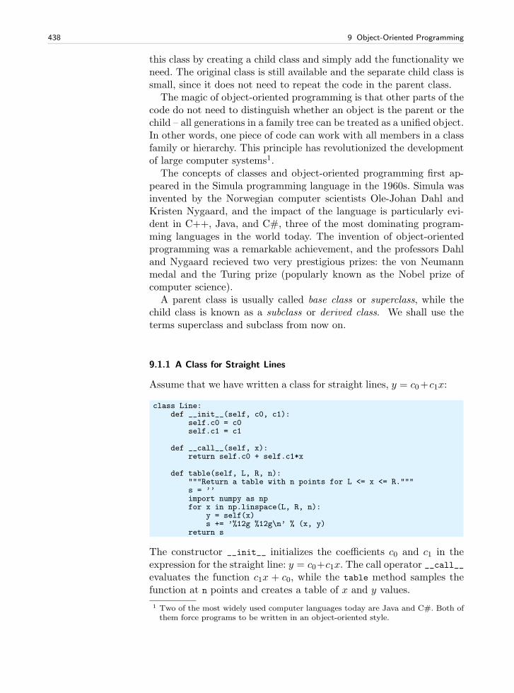
438 9 Object-Oriented Programming

this class by creating a child class and simply add the functionality weneed. The original class is still available and the separate child class issmall, since it does not need to repeat the code in the parent class.

The magic of object-oriented programming is that other parts of thecode do not need to distinguish whether an object is the parent or thechild – all generations in a family tree can be treated as a unified object.In other words, one piece of code can work with all members in a classfamily or hierarchy. This principle has revolutionized the developmentof large computer systems1.

The concepts of classes and object-oriented programming first ap-peared in the Simula programming language in the 1960s. Simula wasinvented by the Norwegian computer scientists Ole-Johan Dahl andKristen Nygaard, and the impact of the language is particularly evi-dent in C++, Java, and C#, three of the most dominating program-ming languages in the world today. The invention of object-orientedprogramming was a remarkable achievement, and the professors Dahland Nygaard recieved two very prestigious prizes: the von Neumannmedal and the Turing prize (popularly known as the Nobel prize ofcomputer science).

A parent class is usually called base class or superclass, while thechild class is known as a subclass or derived class. We shall use theterms superclass and subclass from now on.

9.1.1 A Class for Straight Lines

Assume that we have written a class for straight lines, y = c0+c1x:

class Line:def __init__(self, c0, c1):

self.c0 = c0self.c1 = c1

def __call__(self, x):return self.c0 + self.c1*x

def table(self, L, R, n):"""Return a table with n points for L <= x <= R."""s = ’’import numpy as npfor x in np.linspace(L, R, n):

y = self(x)s += ’%12g %12g\n’ % (x, y)

return s

The constructor __init__ initializes the coefficients c0 and c1 in theexpression for the straight line: y = c0+c1x. The call operator __call__evaluates the function c1x + c0, while the table method samples thefunction at n points and creates a table of x and y values.

1 Two of the most widely used computer languages today are Java and C#. Both ofthem force programs to be written in an object-oriented style.

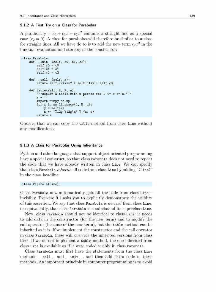
9.1 Inheritance and Class Hierarchies 439

9.1.2 A First Try on a Class for Parabolas

A parabola y = c0 + c1x + c2x2 contains a straight line as a special

case (c2 = 0). A class for parabolas will therefore be similar to a classfor straight lines. All we have do to is to add the new term c2x

2 in thefunction evaluation and store c2 in the constructor:

class Parabola:def __init__(self, c0, c1, c2):

self.c0 = c0self.c1 = c1self.c2 = c2

def __call__(self, x):return self.c2*x**2 + self.c1*x + self.c0

def table(self, L, R, n):"""Return a table with n points for L <= x <= R."""s = ’’import numpy as npfor x in np.linspace(L, R, n):

y = self(x)s += ’%12g %12g\n’ % (x, y)

return s

Observe that we can copy the table method from class Line withoutany modifications.

9.1.3 A Class for Parabolas Using Inheritance

Python and other languages that support object-oriented programminghave a special construct, so that class Parabola does not need to repeatthe code that we have already written in class Line. We can specifythat class Parabola inherits all code from class Line by adding“(Line)”in the class headline:

class Parabola(Line):

Class Parabola now automatically gets all the code from class Line –invisibly. Exercise 9.1 asks you to explicitly demonstrate the validityof this assertion. We say that class Parabola is derived from class Line,or equivalently, that class Parabola is a subclass of its superclass Line.

Now, class Parabola should not be identical to class Line: it needsto add data in the constructor (for the new term) and to modify thecall operator (because of the new term), but the table method can beinherited as it is. If we implement the constructor and the call operatorin class Parabola, these will override the inherited versions from classLine. If we do not implement a table method, the one inherited fromclass Line is available as if it were coded visibly in class Parabola.

Class Parabola must first have the statements from the class Line

methods __call__ and __init__, and then add extra code in thesemethods. An important principle in computer programming is to avoid

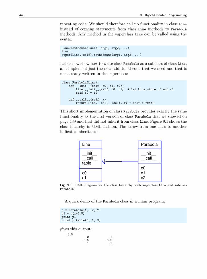
440 9 Object-Oriented Programming

repeating code. We should therefore call up functionality in class Lineinstead of copying statements from class Line methods to Parabola

methods. Any method in the superclass Line can be called using thesyntax

Line.methodname(self, arg1, arg2, ...)# orsuper(Line, self).methodname(arg1, arg2, ...)

Let us now show how to write class Parabola as a subclass of class Line,and implement just the new additional code that we need and that isnot already written in the superclass:

class Parabola(Line):def __init__(self, c0, c1, c2):

Line.__init__(self, c0, c1) # let Line store c0 and c1self.c2 = c2

def __call__(self, x):return Line.__call__(self, x) + self.c2*x**2

This short implementation of class Parabola provides exactly the samefunctionality as the first version of class Parabola that we showed onpage 439 and that did not inherit from class Line. Figure 9.1 shows theclass hiearchy in UML fashion. The arrow from one class to anotherindicates inheritance.

Line

__init____call__table

c0c1

Parabola

__init____call__

c0c1c2

Fig. 9.1 UML diagram for the class hierarchy with superclass Line and subclassParabola.

A quick demo of the Parabola class in a main program,

p = Parabola(1, -2, 2)p1 = p(x=2.5)print p1print p.table(0, 1, 3)

gives this output:8.5

0 10.5 0.51 1

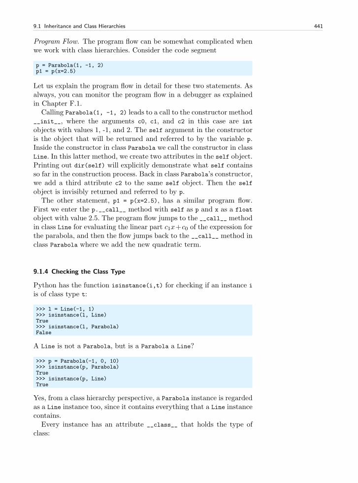
9.1 Inheritance and Class Hierarchies 441

Program Flow. The program flow can be somewhat complicated whenwe work with class hierarchies. Consider the code segment

p = Parabola(1, -1, 2)p1 = p(x=2.5)

Let us explain the program flow in detail for these two statements. Asalways, you can monitor the program flow in a debugger as explainedin Chapter F.1.

Calling Parabola(1, -1, 2) leads to a call to the constructor method__init__, where the arguments c0, c1, and c2 in this case are int

objects with values 1, -1, and 2. The self argument in the constructoris the object that will be returned and referred to by the variable p.Inside the constructor in class Parabola we call the constructor in classLine. In this latter method, we create two attributes in the self object.Printing out dir(self) will explicitly demonstrate what self containsso far in the construction process. Back in class Parabola’s constructor,we add a third attribute c2 to the same self object. Then the self

object is invisibly returned and referred to by p.The other statement, p1 = p(x=2.5), has a similar program flow.

First we enter the p.__call__ method with self as p and x as a float

object with value 2.5. The program flow jumps to the __call__ methodin class Line for evaluating the linear part c1x+c0 of the expression forthe parabola, and then the flow jumps back to the __call__ method inclass Parabola where we add the new quadratic term.

9.1.4 Checking the Class Type

Python has the function isinstance(i,t) for checking if an instance i

is of class type t:

>>> l = Line(-1, 1)>>> isinstance(l, Line)True>>> isinstance(l, Parabola)False

A Line is not a Parabola, but is a Parabola a Line?

>>> p = Parabola(-1, 0, 10)>>> isinstance(p, Parabola)True>>> isinstance(p, Line)True

Yes, from a class hierarchy perspective, a Parabola instance is regardedas a Line instance too, since it contains everything that a Line instancecontains.

Every instance has an attribute __class__ that holds the type ofclass:

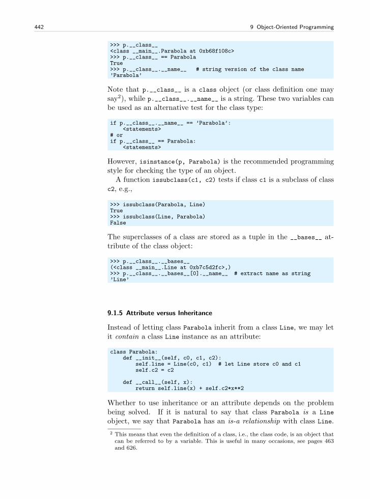
442 9 Object-Oriented Programming

>>> p.__class__<class __main__.Parabola at 0xb68f108c>>>> p.__class__ == ParabolaTrue>>> p.__class__.__name__ # string version of the class name’Parabola’

Note that p.__class__ is a class object (or class definition one maysay2), while p.__class__.__name__ is a string. These two variables canbe used as an alternative test for the class type:

if p.__class__.__name__ == ’Parabola’:<statements>

# orif p.__class__ == Parabola:

<statements>

However, isinstance(p, Parabola) is the recommended programmingstyle for checking the type of an object.

A function issubclass(c1, c2) tests if class c1 is a subclass of classc2, e.g.,

>>> issubclass(Parabola, Line)True>>> issubclass(Line, Parabola)False

The superclasses of a class are stored as a tuple in the __bases__ at-tribute of the class object:

>>> p.__class__.__bases__(<class __main__.Line at 0xb7c5d2fc>,)>>> p.__class__.__bases__[0].__name__ # extract name as string’Line’

9.1.5 Attribute versus Inheritance

Instead of letting class Parabola inherit from a class Line, we may letit contain a class Line instance as an attribute:

class Parabola:def __init__(self, c0, c1, c2):

self.line = Line(c0, c1) # let Line store c0 and c1self.c2 = c2

def __call__(self, x):return self.line(x) + self.c2*x**2

Whether to use inheritance or an attribute depends on the problembeing solved. If it is natural to say that class Parabola is a Line

object, we say that Parabola has an is-a relationship with class Line.

2 This means that even the definition of a class, i.e., the class code, is an object thatcan be referred to by a variable. This is useful in many occasions, see pages 463and 626.

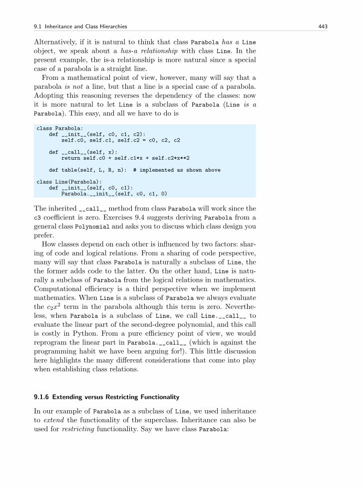
9.1 Inheritance and Class Hierarchies 443

Alternatively, if it is natural to think that class Parabola has a Line

object, we speak about a has-a relationship with class Line. In thepresent example, the is-a relationship is more natural since a specialcase of a parabola is a straight line.

From a mathematical point of view, however, many will say that aparabola is not a line, but that a line is a special case of a parabola.Adopting this reasoning reverses the dependency of the classes: nowit is more natural to let Line is a subclass of Parabola (Line is aParabola). This easy, and all we have to do is

class Parabola:def __init__(self, c0, c1, c2):

self.c0, self.c1, self.c2 = c0, c2, c2

def __call__(self, x):return self.c0 + self.c1*x + self.c2*x**2

def table(self, L, R, n): # implemented as shown above

class Line(Parabola):def __init__(self, c0, c1):

Parabola.__init__(self, c0, c1, 0)

The inherited __call__ method from class Parabola will work since thec3 coefficient is zero. Exercises 9.4 suggests deriving Parabola from ageneral class Polynomial and asks you to discuss which class design youprefer.

How classes depend on each other is influenced by two factors: shar-ing of code and logical relations. From a sharing of code perspective,many will say that class Parabola is naturally a subclass of Line, thethe former adds code to the latter. On the other hand, Line is natu-rally a subclass of Parabola from the logical relations in mathematics.Computational efficiency is a third perspective when we implementmathematics. When Line is a subclass of Parabola we always evaluatethe c2x

2 term in the parabola although this term is zero. Neverthe-less, when Parabola is a subclass of Line, we call Line.__call__ toevaluate the linear part of the second-degree polynomial, and this callis costly in Python. From a pure efficiency point of view, we wouldreprogram the linear part in Parabola.__call__ (which is against theprogramming habit we have been arguing for!). This little discussionhere highlights the many different considerations that come into playwhen establishing class relations.

9.1.6 Extending versus Restricting Functionality

In our example of Parabola as a subclass of Line, we used inheritanceto extend the functionality of the superclass. Inheritance can also beused for restricting functionality. Say we have class Parabola:

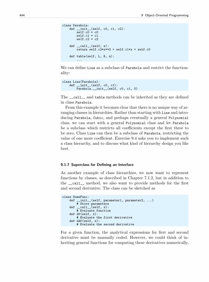
444 9 Object-Oriented Programming

class Parabola:def __init__(self, c0, c1, c2):

self.c0 = c0self.c1 = c1self.c2 = c2

def __call__(self, x):return self.c2*x**2 + self.c1*x + self.c0

def table(self, L, R, n):...

We can define Line as a subclass of Parabola and restrict the function-ality:

class Line(Parabola):def __init__(self, c0, c1):

Parabola.__init__(self, c0, c1, 0)

The __call__ and table methods can be inherited as they are definedin class Parabola.

From this example it becomes clear that there is no unique way of ar-ranging classes in hierarchies. Rather than starting with Line and intro-ducing Parabola, Cubic, and perhaps eventually a general Polynomialclass, we can start with a general Polynomial class and let Parabola

be a subclass which restricts all coefficients except the first three tobe zero. Class Line can then be a subclass of Parabola, restricting thevalue of one more coefficient. Exercise 9.4 asks you to implement sucha class hierarchy, and to discuss what kind of hierarchy design you likebest.

9.1.7 Superclass for Defining an Interface

As another example of class hierarchies, we now want to representfunctions by classes, as described in Chapter 7.1.2, but in addition tothe __call__ method, we also want to provide methods for the firstand second derivative. The class can be sketched as

class SomeFunc:def __init__(self, parameter1, parameter2, ...)

# Store parametersdef __call__(self, x):

# Evaluate functiondef df(self, x):

# Evaluate the first derivativedef ddf(self, x):

# Evaluate the second derivative

For a given function, the analytical expressions for first and secondderivative must be manually coded. However, we could think of in-heriting general functions for computing these derivatives numerically,

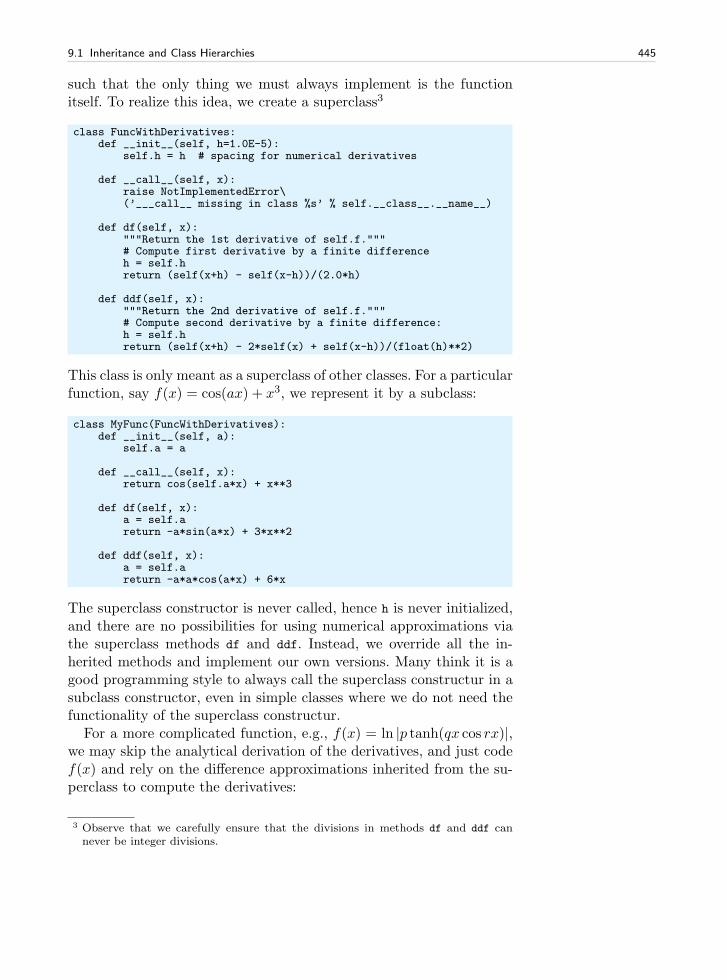
9.1 Inheritance and Class Hierarchies 445

such that the only thing we must always implement is the functionitself. To realize this idea, we create a superclass3

class FuncWithDerivatives:def __init__(self, h=1.0E-5):

self.h = h # spacing for numerical derivatives

def __call__(self, x):raise NotImplementedError\(’___call__ missing in class %s’ % self.__class__.__name__)

def df(self, x):"""Return the 1st derivative of self.f."""# Compute first derivative by a finite differenceh = self.hreturn (self(x+h) - self(x-h))/(2.0*h)

def ddf(self, x):"""Return the 2nd derivative of self.f."""# Compute second derivative by a finite difference:h = self.hreturn (self(x+h) - 2*self(x) + self(x-h))/(float(h)**2)

This class is only meant as a superclass of other classes. For a particularfunction, say f(x) = cos(ax) + x3, we represent it by a subclass:

class MyFunc(FuncWithDerivatives):def __init__(self, a):

self.a = a

def __call__(self, x):return cos(self.a*x) + x**3

def df(self, x):a = self.areturn -a*sin(a*x) + 3*x**2

def ddf(self, x):a = self.areturn -a*a*cos(a*x) + 6*x

The superclass constructor is never called, hence h is never initialized,and there are no possibilities for using numerical approximations viathe superclass methods df and ddf. Instead, we override all the in-herited methods and implement our own versions. Many think it is agood programming style to always call the superclass constructur in asubclass constructor, even in simple classes where we do not need thefunctionality of the superclass constructur.

For a more complicated function, e.g., f(x) = ln |p tanh(qx cos rx)|,we may skip the analytical derivation of the derivatives, and just codef(x) and rely on the difference approximations inherited from the su-perclass to compute the derivatives:

3 Observe that we carefully ensure that the divisions in methods df and ddf cannever be integer divisions.

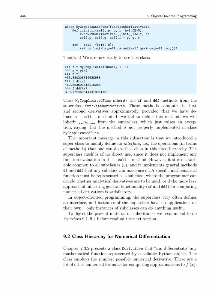
446 9 Object-Oriented Programming

class MyComplicatedFunc(FuncWithDerivatives):def __init__(self, p, q, r, h=1.0E-5):

FuncWithDerivatives.__init__(self, h)self.p, self.q, self.r = p, q, r

def __call__(self, x):return log(abs(self.p*tanh(self.q*x*cos(self.r*x))))

That’s it! We are now ready to use this class:

>>> f = MyComplicatedFunc(1, 1, 1)>>> x = pi/2>>> f(x)-36.880306514638988>>> f.df(x)-60.593693618216086>>> f.ddf(x)3.3217246931444789e+19

Class MyComplicatedFunc inherits the df and ddf methods from thesuperclass FuncWithDerivatives. These methods compute the firstand second derivatives approximately, provided that we have de-fined a __call__ method. If we fail to define this method, we willinherit __call__ from the superclass, which just raises an excep-tion, saying that the method is not properly implemented in classMyComplicatedFunc.

The important message in this subsection is that we introduced asuper class to mainly define an interface, i.e., the operations (in termsof methods) that one can do with a class in this class hierarchy. Thesuperclass itself is of no direct use, since it does not implement anyfunction evaluation in the __call__ method. However, it stores a vari-able common to all subclasses (h), and it implements general methodsdf and ddf that any subclass can make use of. A specific mathematicalfunction must be represented as a subclass, where the programmer candecide whether analytical derivatives are to be used, or if the more lazyapproach of inheriting general functionality (df and ddf) for computingnumerical derivatives is satisfactory.

In object-oriented programming, the superclass very often definesan interface, and instances of the superclass have no applications ontheir own – only instances of subclasses can do anything useful.

To digest the present material on inheritance, we recommend to doExercises 9.1–9.4 before reading the next section.

9.2 Class Hierarchy for Numerical Differentiation

Chapter 7.3.2 presents a class Derivative that “can differentiate” anymathematical function represented by a callable Python object. Theclass employs the simplest possible numerical derivative. There are alot of other numerical formulas for computing approximations to f ′(x):

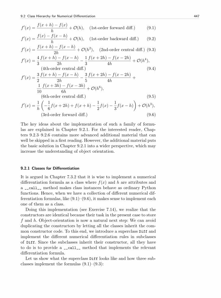
9.2 Class Hierarchy for Numerical Differentiation 447

f ′(x) =f(x+ h)− f(x)

h+O(h), (1st-order forward diff.) (9.1)

f ′(x) =f(x)− f(x− h)

h+O(h), (1st-order backward diff.) (9.2)

f ′(x) =f(x+ h)− f(x− h)

2h+O(h2), (2nd-order central diff.) (9.3)

f ′(x) =4

3

f(x+ h)− f(x− h)

2h− 1

3

f(x+ 2h)− f(x− 2h)

4h+O(h4),

(4th-order central diff.) (9.4)

f ′(x) =3

2

f(x+ h)− f(x− h)

2h− 3

5

f(x+ 2h)− f(x− 2h)

4h+

1

10

f(x+ 3h)− f(x− 3h)

6h+O(h6),

(6th-order central diff.) (9.5)

f ′(x) =1

h

(

−1

6f(x+ 2h) + f(x+ h)− 1

2f(x)− 1

3f(x− h)

)

+O(h3),

(3rd-order forward diff.) (9.6)

The key ideas about the implementation of such a family of formu-las are explained in Chapter 9.2.1. For the interested reader, Chap-ters 9.2.3–9.2.6 contains more advanced additional material that canwell be skipped in a first reading. However, the additional material putsthe basic solution in Chapter 9.2.1 into a wider perspective, which mayincrease the understanding of object orientation.

9.2.1 Classes for Differentiation

It is argued in Chapter 7.3.2 that it is wise to implement a numericaldifferentiation formula as a class where f(x) and h are attributes anda __call__ method makes class instances behave as ordinary Pythonfunctions. Hence, when we have a collection of different numerical dif-ferentiation formulas, like (9.1)–(9.6), it makes sense to implement eachone of them as a class.

Doing this implementation (see Exercise 7.14), we realize that theconstructors are identical because their task in the present case to storef and h. Object-orientation is now a natural next step: We can avoidduplicating the constructors by letting all the classes inherit the com-mon constructor code. To this end, we introduce a superclass Diff andimplement the different numerical differentiation rules in subclassesof Diff. Since the subclasses inherit their constructor, all they haveto do is to provide a __call__ method that implements the relevantdifferentiation formula.

Let us show what the superclass Diff looks like and how three sub-classes implement the formulas (9.1)–(9.3):

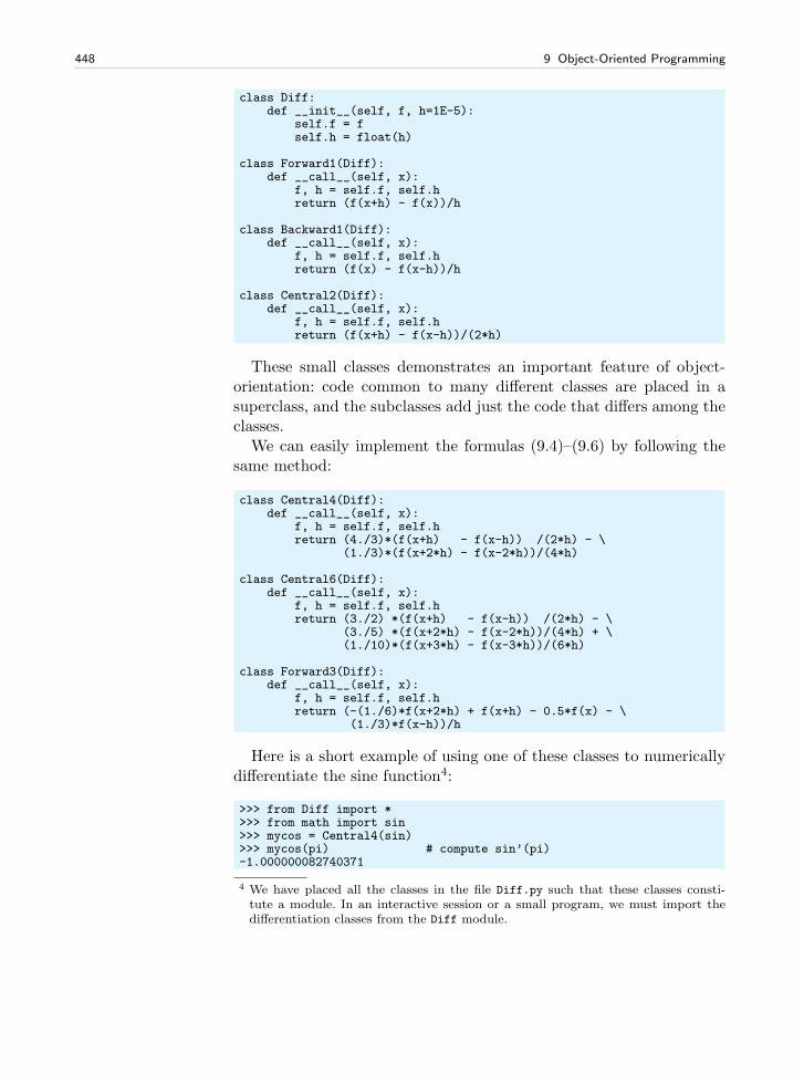
448 9 Object-Oriented Programming

class Diff:def __init__(self, f, h=1E-5):

self.f = fself.h = float(h)

class Forward1(Diff):def __call__(self, x):

f, h = self.f, self.hreturn (f(x+h) - f(x))/h

class Backward1(Diff):def __call__(self, x):

f, h = self.f, self.hreturn (f(x) - f(x-h))/h

class Central2(Diff):def __call__(self, x):

f, h = self.f, self.hreturn (f(x+h) - f(x-h))/(2*h)

These small classes demonstrates an important feature of object-orientation: code common to many different classes are placed in asuperclass, and the subclasses add just the code that differs among theclasses.

We can easily implement the formulas (9.4)–(9.6) by following thesame method:

class Central4(Diff):def __call__(self, x):

f, h = self.f, self.hreturn (4./3)*(f(x+h) - f(x-h)) /(2*h) - \

(1./3)*(f(x+2*h) - f(x-2*h))/(4*h)

class Central6(Diff):def __call__(self, x):

f, h = self.f, self.hreturn (3./2) *(f(x+h) - f(x-h)) /(2*h) - \

(3./5) *(f(x+2*h) - f(x-2*h))/(4*h) + \(1./10)*(f(x+3*h) - f(x-3*h))/(6*h)

class Forward3(Diff):def __call__(self, x):

f, h = self.f, self.hreturn (-(1./6)*f(x+2*h) + f(x+h) - 0.5*f(x) - \

(1./3)*f(x-h))/h

Here is a short example of using one of these classes to numericallydifferentiate the sine function4:

>>> from Diff import *>>> from math import sin>>> mycos = Central4(sin)>>> mycos(pi) # compute sin’(pi)-1.000000082740371

4 We have placed all the classes in the file Diff.py such that these classes consti-tute a module. In an interactive session or a small program, we must import thedifferentiation classes from the Diff module.

9.2 Class Hierarchy for Numerical Differentiation 449

Instead of a plain Python function we may use an object with a__call__ method, here exemplified through the function f(t; a, b, c) =at2 + bt+ c:

class Poly2:def __init__(self, a, b, c):

self.a, self.b, self.c = a, b, cdef __call__(self, t):

return self.a*t**2 + self.b*t + self.c

f = Poly2(1, 0, 1)dfdt = Central4(f)t = 2print "f’(%g)=%g" % (t, dfdt(t))

Let us examine the program flow. When Python encounters dfdt =

Central4(f), it looks for the constructor in class Central4, but there isno constructor in that class. Python then examines the superclasses ofCentral4, listed in Central4.__bases__. The superclass Diff contains aconstructor, and this method is called. When Python meets the dfdt(t)call, it looks for __call__ in class Central4 and finds it, so there is noneed to examine the superclass. This process of looking up methods ofa class is called dynamic binding.

Computer Science Remark. Dynamic binding means that a name isbound to a function while the program is running. Normally, in com-puter languages, a function name is static in the sense that it is hard-coded as part of the function body and will not change during theexecution of the program. This principle is known as static binding offunction/method names. Object orientation offers the technical meansto associate different functions with the same name, which yields a kindof magic for incrased flexibility in programs. The particular functionthat the name refers to can be set at run-time, i.e., when the programis running, and therefore known as dynamic binding.

In Python, dynamic binding is a natural feature since names (vari-ables) can refer to functions and therefore be dynamically bound dur-ing execution, just as any ordinary variable. To illustrate this point,let func1 and func2 be two Python functions of one argument, andconsider the code

if input == ’func1’:f = func1

elif input == ’func2’:f = func2

y = f(x)

Here, the name f is bound to one of the func1 and func2 function ob-jects while the program is running. This is a result of two features:(i) dynamic typing (so the contents of f can change), and (ii) func-tions being ordinary objects. The bottom line is that dynamic bindingcomes natural in Python, while it appears more like convenient magicin languages like C++, Java, and C#.

450 9 Object-Oriented Programming

9.2.2 A Flexible Main Program

As a demonstration of the power of Python programming, we shall nowwrite a program that accepts a function on the command-line, togetherwith information about the difference type (centered, backward, or for-ward), the order of the approximation, and a value of the independentvariable. The output from the program is the derivative of the givenfunction. An example of the usage of the program goes like this:

Terminal

differentiate.py ’exp(sin(x))’ Central 2 3.1-1.04155573055

Here, we asked the program to differentiate f(x) = esinx at x = 3.1with a central scheme of order 2 (using the Central2 class in the Diff

hierarchy).We can provide any expression with x as input and request any

scheme from the Diff hierarchy, and the derivative will be (approxi-mately) computed. One great thing with Python is that the code isvery short:

import sysfrom Diff import *from math import *from scitools.StringFunction import StringFunction

formula = sys.argv[1]f = StringFunction(formula)difftype = sys.argv[2]difforder = sys.argv[3]classname = difftype + difforderdf = eval(classname + ’(f)’)x = float(sys.argv[4])print df(x)

Read the code line by line, and convince yourself that you under-stand what is going on. You may need to review Chapters 4.1.2 and4.1.4.

One disadvantage is that the code above is limited to x as the nameof the independent variable. If we allow a 5th command-line argumentwith the name of the independent variable, we can pass this name onto the StringFunction constructor, and suddenly our program workswith any name for the independent variable!

varname = sys.argv[5]f = StringFunction(formula, independent_variables=varname)

Of course, the program crashes if we do not provide five command-line arguments, and the program does not work properly if we are notcareful with ordering of the command-line arguments. There is someway to go before the program is really user friendly, but that is beyondthe scope of this chapter.

9.2 Class Hierarchy for Numerical Differentiation 451

There are two strengths of the differentiate.py program: i) in-teractive specification of the function and the differentiation method,and ii) identical syntax for calling any differentiation method. Withone line we create the subclass instance based on input strings. Manyother popular programming languages (C++, Java, C#) cannot per-form the eval operation while the program is running. The result isthat we need if tests to turn the input string information into cre-ation of subclass instances. Such type of code would look like this inPython:

if classname == ’Forward1’:df = Forward1(f)

elif classname == ’Backward1’:df = Backward1(f)

...

and so forth. This piece of code is very common in object-oriented sys-tems and often put in a function that is referred to as a factory function.Factory functions can be made very compact in Python thanks to eval.

9.2.3 Extensions

The great advantage of sharing code via inheritance becomes obviouswhen we want to extend the functionality of a class hierarchy. It is pos-sible to do this by adding more code to the superclass only. Suppose wewant to be able to assess the accuracy of the numerical approximationto the derivative by comparing with the exact derivative, if available.All we need to do is to allow an extra argument in the constructorand provide an additional superclass method that computes the errorin the numerical derivative. We may add this code to class Diff, orwe may add it in a subclass Diff2 and let the other classes for variousnumerical differentiation formulas inherit from class Diff2. We followthe latter approach:

class Diff2(Diff):def __init__(self, f, h=1E-5, dfdx_exact=None):

Diff.__init__(self, f, h)self.exact = dfdx_exact

def error(self, x):if self.exact is not None:

df_numerical = self(x)df_exact = self.exact(x)return df_exact - df_numerical

class Forward1(Diff2):def __call__(self, x):

f, h = self.f, self.hreturn (f(x+h) - f(x))/h

The other subclasses, Backward1, Central2, and so on, must alsobe derived from Diff2 to equip all subclasses with new functionality

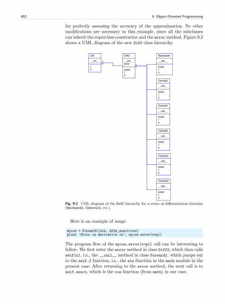
452 9 Object-Oriented Programming

for perfectly assessing the accuracy of the approximation. No othermodifications are necessary in this example, since all the subclassescan inherit the superclass constructor and the errormethod. Figure 9.2shows a UML diagram of the new Diff class hierarchy.

Diff

__init__

fh

Diff2

__init__error

exactfh

Backward1

__call__

exactfh

Central2

__call__

exactfh

Central4

__call__

exactfh

Central6

__call__

exactfh

Forward1

__call__

exactfh

Forward3

__call__

exactfh

Fig. 9.2 UML diagram of the Diff hierarchy for a series of differentiation formulas(Backward1, Central2, etc.).

Here is an example of usage:

mycos = Forward1(sin, dfdx_exact=cos)print ’Error in derivative is’, mycos.error(x=pi)

The program flow of the mycos.error(x=pi) call can be interesting tofollow. We first enter the error method in class Diff2, which then callsself(x), i.e., the __call__ method in class Forward1, which jumps outto the self.f function, i.e., the sin function in the math module in thepresent case. After returning to the error method, the next call is toself.exact, which is the cos function (from math) in our case.

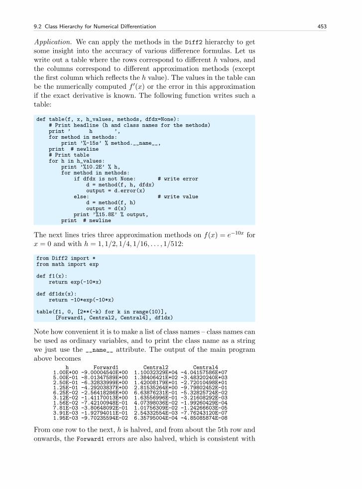
9.2 Class Hierarchy for Numerical Differentiation 453

Application. We can apply the methods in the Diff2 hierarchy to getsome insight into the accuracy of various difference formulas. Let uswrite out a table where the rows correspond to different h values, andthe columns correspond to different approximation methods (exceptthe first column which reflects the h value). The values in the table canbe the numerically computed f ′(x) or the error in this approximationif the exact derivative is known. The following function writes such atable:

def table(f, x, h_values, methods, dfdx=None):# Print headline (h and class names for the methods)print ’ h ’,for method in methods:

print ’%-15s’ % method.__name__,print # newline# Print tablefor h in h_values:

print ’%10.2E’ % h,for method in methods:

if dfdx is not None: # write errord = method(f, h, dfdx)output = d.error(x)

else: # write valued = method(f, h)output = d(x)

print ’%15.8E’ % output,print # newline

The next lines tries three approximation methods on f(x) = e−10x forx = 0 and with h = 1, 1/2, 1/4, 1/16, . . . , 1/512:

from Diff2 import *from math import exp

def f1(x):return exp(-10*x)

def df1dx(x):return -10*exp(-10*x)

table(f1, 0, [2**(-k) for k in range(10)],[Forward1, Central2, Central4], df1dx)

Note how convenient it is to make a list of class names – class names canbe used as ordinary variables, and to print the class name as a stringwe just use the __name__ attribute. The output of the main programabove becomes

h Forward1 Central2 Central41.00E+00 -9.00004540E+00 1.10032329E+04 -4.04157586E+075.00E-01 -8.01347589E+00 1.38406421E+02 -3.48320240E+032.50E-01 -6.32833999E+00 1.42008179E+01 -2.72010498E+011.25E-01 -4.29203837E+00 2.81535264E+00 -9.79802452E-016.25E-02 -2.56418286E+00 6.63876231E-01 -5.32825724E-023.12E-02 -1.41170013E+00 1.63556996E-01 -3.21608292E-031.56E-02 -7.42100948E-01 4.07398036E-02 -1.99260429E-047.81E-03 -3.80648092E-01 1.01756309E-02 -1.24266603E-053.91E-03 -1.92794011E-01 2.54332554E-03 -7.76243120E-071.95E-03 -9.70235594E-02 6.35795004E-04 -4.85085874E-08

From one row to the next, h is halved, and from about the 5th row andonwards, the Forward1 errors are also halved, which is consistent with

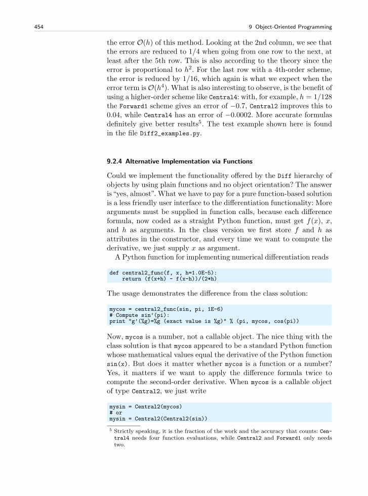
454 9 Object-Oriented Programming

the error O(h) of this method. Looking at the 2nd column, we see thatthe errors are reduced to 1/4 when going from one row to the next, atleast after the 5th row. This is also according to the theory since theerror is proportional to h2. For the last row with a 4th-order scheme,the error is reduced by 1/16, which again is what we expect when theerror term is O(h4). What is also interesting to observe, is the benefit ofusing a higher-order scheme like Central4: with, for example, h = 1/128the Forward1 scheme gives an error of −0.7, Central2 improves this to0.04, while Central4 has an error of −0.0002. More accurate formulasdefinitely give better results5. The test example shown here is foundin the file Diff2_examples.py.

9.2.4 Alternative Implementation via Functions

Could we implement the functionality offered by the Diff hierarchy ofobjects by using plain functions and no object orientation? The answeris“yes, almost”. What we have to pay for a pure function-based solutionis a less friendly user interface to the differentiation functionality: Morearguments must be supplied in function calls, because each differenceformula, now coded as a straight Python function, must get f(x), x,and h as arguments. In the class version we first store f and h asattributes in the constructor, and every time we want to compute thederivative, we just supply x as argument.

A Python function for implementing numerical differentiation reads

def central2_func(f, x, h=1.0E-5):return (f(x+h) - f(x-h))/(2*h)

The usage demonstrates the difference from the class solution:

mycos = central2_func(sin, pi, 1E-6)# Compute sin’(pi):print "g’(%g)=%g (exact value is %g)" % (pi, mycos, cos(pi))

Now, mycos is a number, not a callable object. The nice thing with theclass solution is that mycos appeared to be a standard Python functionwhose mathematical values equal the derivative of the Python functionsin(x). But does it matter whether mycos is a function or a number?Yes, it matters if we want to apply the difference formula twice tocompute the second-order derivative. When mycos is a callable objectof type Central2, we just write

mysin = Central2(mycos)# ormysin = Central2(Central2(sin))

5 Strictly speaking, it is the fraction of the work and the accuracy that counts: Cen-tral4 needs four function evaluations, while Central2 and Forward1 only needstwo.

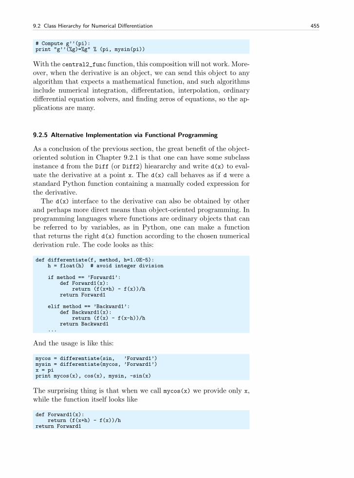
9.2 Class Hierarchy for Numerical Differentiation 455

# Compute g’’(pi):print "g’’(%g)=%g" % (pi, mysin(pi))

With the central2_func function, this composition will not work. More-over, when the derivative is an object, we can send this object to anyalgorithm that expects a mathematical function, and such algorithmsinclude numerical integration, differentation, interpolation, ordinarydifferential equation solvers, and finding zeros of equations, so the ap-plications are many.

9.2.5 Alternative Implementation via Functional Programming

As a conclusion of the previous section, the great benefit of the object-oriented solution in Chapter 9.2.1 is that one can have some subclassinstance d from the Diff (or Diff2) hieararchy and write d(x) to eval-uate the derivative at a point x. The d(x) call behaves as if d were astandard Python function containing a manually coded expression forthe derivative.

The d(x) interface to the derivative can also be obtained by otherand perhaps more direct means than object-oriented programming. Inprogramming languages where functions are ordinary objects that canbe referred to by variables, as in Python, one can make a functionthat returns the right d(x) function according to the chosen numericalderivation rule. The code looks as this:

def differentiate(f, method, h=1.0E-5):h = float(h) # avoid integer division

if method == ’Forward1’:def Forward1(x):

return (f(x+h) - f(x))/hreturn Forward1

elif method == ’Backward1’:def Backward1(x):

return (f(x) - f(x-h))/hreturn Backward1

...

And the usage is like this:

mycos = differentiate(sin, ’Forward1’)mysin = differentiate(mycos, ’Forward1’)x = piprint mycos(x), cos(x), mysin, -sin(x)

The surprising thing is that when we call mycos(x) we provide only x,while the function itself looks like

def Forward1(x):return (f(x+h) - f(x))/h

return Forward1

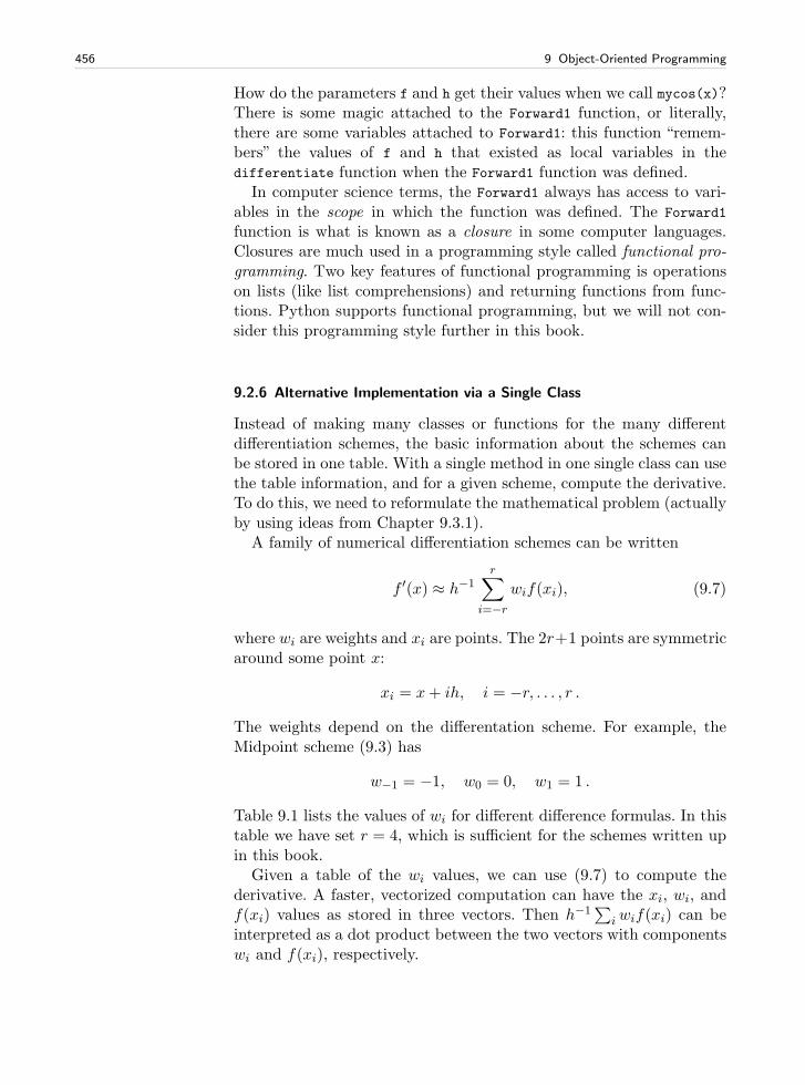
456 9 Object-Oriented Programming

How do the parameters f and h get their values when we call mycos(x)?There is some magic attached to the Forward1 function, or literally,there are some variables attached to Forward1: this function “remem-bers” the values of f and h that existed as local variables in thedifferentiate function when the Forward1 function was defined.

In computer science terms, the Forward1 always has access to vari-ables in the scope in which the function was defined. The Forward1

function is what is known as a closure in some computer languages.Closures are much used in a programming style called functional pro-gramming. Two key features of functional programming is operationson lists (like list comprehensions) and returning functions from func-tions. Python supports functional programming, but we will not con-sider this programming style further in this book.

9.2.6 Alternative Implementation via a Single Class

Instead of making many classes or functions for the many differentdifferentiation schemes, the basic information about the schemes canbe stored in one table. With a single method in one single class can usethe table information, and for a given scheme, compute the derivative.To do this, we need to reformulate the mathematical problem (actuallyby using ideas from Chapter 9.3.1).

A family of numerical differentiation schemes can be written

f ′(x) ≈ h−1r∑

i=−r

wif(xi), (9.7)

where wi are weights and xi are points. The 2r+1 points are symmetricaround some point x:

xi = x+ ih, i = −r, . . . , r .

The weights depend on the differentation scheme. For example, theMidpoint scheme (9.3) has

w−1 = −1, w0 = 0, w1 = 1 .

Table 9.1 lists the values of wi for different difference formulas. In thistable we have set r = 4, which is sufficient for the schemes written upin this book.

Given a table of the wi values, we can use (9.7) to compute thederivative. A faster, vectorized computation can have the xi, wi, andf(xi) values as stored in three vectors. Then h−1

∑

iwif(xi) can beinterpreted as a dot product between the two vectors with componentswi and f(xi), respectively.

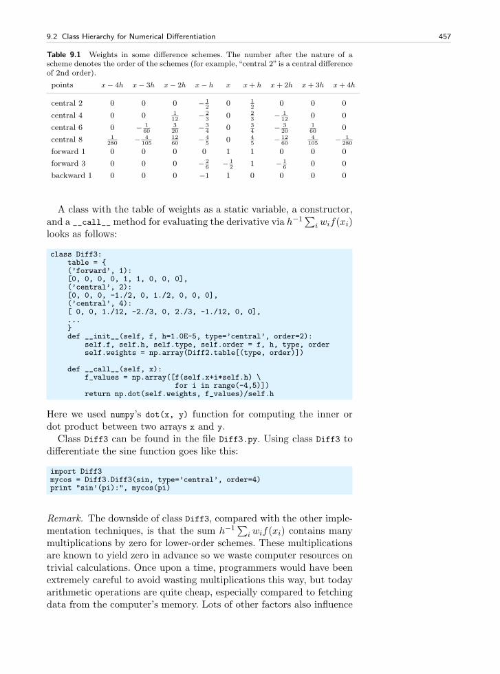
9.2 Class Hierarchy for Numerical Differentiation 457

Table 9.1 Weights in some difference schemes. The number after the nature of ascheme denotes the order of the schemes (for example, “central 2” is a central differenceof 2nd order).

points x− 4h x− 3h x− 2h x− h x x+ h x+ 2h x+ 3h x+ 4h

central 2 0 0 0 − 1

20 1

20 0 0

central 4 0 0 1

12− 2

30 2

3− 1

120 0

central 6 0 − 1

60

3

20− 3

40 3

4− 3

20

1

600

central 8 1

280− 4

105

12

60− 4

50 4

5− 12

60

4

105− 1

280

forward 1 0 0 0 0 1 1 0 0 0

forward 3 0 0 0 − 2

6− 1

21 − 1

60 0

backward 1 0 0 0 −1 1 0 0 0 0

A class with the table of weights as a static variable, a constructor,and a __call__method for evaluating the derivative via h−1

∑

iwif(xi)looks as follows:

class Diff3:table = (’forward’, 1):[0, 0, 0, 0, 1, 1, 0, 0, 0],(’central’, 2):[0, 0, 0, -1./2, 0, 1./2, 0, 0, 0],(’central’, 4):[ 0, 0, 1./12, -2./3, 0, 2./3, -1./12, 0, 0],...def __init__(self, f, h=1.0E-5, type=’central’, order=2):

self.f, self.h, self.type, self.order = f, h, type, orderself.weights = np.array(Diff2.table[(type, order)])

def __call__(self, x):f_values = np.array([f(self.x+i*self.h) \

for i in range(-4,5)])return np.dot(self.weights, f_values)/self.h

Here we used numpy’s dot(x, y) function for computing the inner ordot product between two arrays x and y.

Class Diff3 can be found in the file Diff3.py. Using class Diff3 todifferentiate the sine function goes like this:

import Diff3mycos = Diff3.Diff3(sin, type=’central’, order=4)print "sin’(pi):", mycos(pi)

Remark. The downside of class Diff3, compared with the other imple-mentation techniques, is that the sum h−1

∑

iwif(xi) contains manymultiplications by zero for lower-order schemes. These multiplicationsare known to yield zero in advance so we waste computer resources ontrivial calculations. Once upon a time, programmers would have beenextremely careful to avoid wasting multiplications this way, but todayarithmetic operations are quite cheap, especially compared to fetchingdata from the computer’s memory. Lots of other factors also influence

458 9 Object-Oriented Programming

the computational efficiency of a program, but this is beyond the scopeof this book.

9.3 Class Hierarchy for Numerical Integration

There are many different numerical methods for integrating a mathe-matical function, just as there are many different methods for differ-entiating a function. It is thus obvious that the idea of object-orientedprogramming and class hierarchies can be applied to numerical inte-gration formulas in the same manner as we did in Chapter 9.2.

9.3.1 Numerical Integration Methods

First, we list some different methods for integrating∫ ba f(x)dx using n

evaluation points. All the methods can be written as

∫ b

a

f(x)dx ≈n−1∑

i=0

wif(xi), (9.8)

where wi are weights and xi are evaluation points, i = 0, . . . , n − 1.The Midpoint method has

xi = a+h

2+ ih, wi = h, h =

b− a

n, i = 0, . . . , n− 1 . (9.9)

The Trapezoidal method has the points

xi = a+ ih, h =b− a

n− 1, i = 0, . . . , n− 1, (9.10)

and the weights

w0 = wn−1 =h

2, wi = h, i = 1, . . . , n− 2 . (9.11)

Simpson’s rule has the same evaluation points as the Trapezoidal rule,but

h = 2b− a

n− 1, w0 = wn−1 =

h

6, (9.12)

wi =h

3for i = 2, 4, . . . , n− 3, (9.13)

wi =2h

3for i = 1, 3, 5, . . . , n− 2 . (9.14)

Note that n must be odd in Simpson’s rule. A Two-Point Gauss-Legendre method takes the form

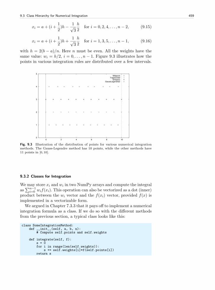
9.3 Class Hierarchy for Numerical Integration 459

xi = a+ (i+1

2)h− 1√

3

h

2for i = 0, 2, 4, . . . , n− 2, (9.15)

xi = a+ (i+1

2)h+

1√3

h

2for i = 1, 3, 5, . . . , n− 1, (9.16)

with h = 2(b − a)/n. Here n must be even. All the weights have thesame value: wi = h/2, i = 0, . . . , n − 1. Figure 9.3 illustrates how thepoints in various integration rules are distributed over a few intervals.

0

1

2

3

4

5

0 2 4 6 8 10

MidpointTrapezoidal

SimpsonGaussLegendre2

Fig. 9.3 Illustration of the distribution of points for various numerical integrationmethods. The Gauss-Legendre method has 10 points, while the other methods have11 points in [0, 10].

9.3.2 Classes for Integration

We may store xi and wi in two NumPy arrays and compute the integralas∑n−1

i=0 wif(xi). This operation can also be vectorized as a dot (inner)product between the wi vector and the f(xi) vector, provided f(x) isimplemented in a vectorizable form.

We argued in Chapter 7.3.3 that it pays off to implement a numericalintegration formula as a class. If we do so with the different methodsfrom the previous section, a typical class looks like this:

class SomeIntegrationMethod:def __init__(self, a, b, n):

# Compute self.points and self.weights

def integrate(self, f):s = 0for i in range(len(self.weights)):

s += self.weights[i]*f(self.points[i])return s

460 9 Object-Oriented Programming

Making such classes for many different integration methods soon re-veals that all the classes contain common code, namely the integrate

method for computing∑n−1

i=0 wif(xi). Therefore, this common codecan be placed in a superclass, and subclasses can just add the codethat is specific to a certain numerical integration formula, namely thedefinition of the weights wi and the points xi.

Let us start with the superclass:

class Integrator:def __init__(self, a, b, n):

self.a, self.b, self.n = a, b, nself.points, self.weights = self.construct_method()

def construct_method(self):raise NotImplementedError(’no rule in class %s’ %

self.__class__.__name__)

def integrate(self, f):s = 0for i in range(len(self.weights)):

s += self.weights[i]*f(self.points[i])return s

As we have seen, we store the a, b, and n data about the integra-tion method in the constructor. Moreover, we compute arrays or listsself.points for the xi points and self.weights for the wi weights. Allthis code can now be inherited by all subclasses.

The initialization of points and weights is put in a seperate method,construct_method, which is supposed to be implemented in each sub-class, but the superclass provides a default implementation whichtells the user that the method is not implemented. What happens isthat when subclasses redefine a method, that method overrides themethod inherited from the superclass. Hence, if we forget to redefineconstruct_method in a subclass, we will inherit the one from the su-perclass, and this method issues an error message. The construction ofthis error message is quite clever in the sense that it will tell in whichclass the construct_methodmethod is missing (self will be the subclassinstance and its __class__.__name__ is a string with the correspondingsubclass name).

In computer science one usually speaks about overloading a methodin a subclass, but the words redefining and overriding are also used. Amethod that is overloaded is said to be polymorphic. A related term,polymorphism, refers to coding with polymorphic methods. Very often,a superclass provides some default implementation of a method, and asubclass overloads the method with the purpose of tailoring the methodto a particular application.

The integrate method is common for all integration rules, i.e., forall subclasses, so it can be inherited as it is. A vectorized version canalso be added in the superclass to make it automatically available alsoin all subclasses:

9.3 Class Hierarchy for Numerical Integration 461

def vectorized_integrate(self, f):return np.dot(self.weights, f(self.points))

Let us then implement a subclass. Only the construct_method

method needs to be written. For the Midpoint rule, this is a matter oftranslating the formulas in (9.9) to Python:

class Midpoint(Integrator):def construct_method(self):

a, b, n = self.a, self.b, self.n # quick formsh = (b-a)/float(n)x = np.linspace(a + 0.5*h, b - 0.5*h, n)w = np.zeros(len(x)) + hreturn x, w

Observe that we implemented directly a vectorized code. We could alsohave used (slow) loops and explicit indexing:

x = np.zeros(n)w = np.zeros(n)for i in range(n):

x[i] = a + 0.5*h + i*hw[i] = h

Before we continue with other subclasses for other numerical inte-gration formulas, we will have a look at the program flow when weuse class Midpoint. Suppose we want to integrate

∫ 20 x2dx using 101

points:

def f(x): return x*xm = Midpoint(0, 2, 101)print m.integrate(f)

How is the program flow? The assignment to m invokes the construc-tor in class Midpoint. Since this class has no constructor, we invokethe inherited one from the superclass Integrator. Here attributes arestored, and then the construct_method method is called. Since self isa Midpoint instance, it is the construct_method in the Midpoint classthat is invoked, even if there is a method with the same name in the su-perclass. Class Midpoint overloads construct_method in the superclass.In a way, we “jump down” from the constructor in class Integrator

to the construct_method in the Midpoint class. The next statment,m.integrate(f), just calls the inherited integral method that is com-mon to all subclasses.

A vectorized Trapezoidal rule can be implemented in another sub-class with name Trapezoidal:

class Trapezoidal(Integrator):def construct_method(self):

x = np.linspace(self.a, self.b, self.n)h = (self.b - self.a)/float(self.n - 1)w = np.zeros(len(x)) + hw[0] /= 2w[-1] /= 2return x, w

462 9 Object-Oriented Programming

Observe how we divide the first and last weight by 2, using index 0(the first) and -1 (the last) and the /= operator (a /= b is equivalent toa = a/b). Here also we could have implemented a scalar version withloops. The relevant code is in function trapezoidal in Chapter 7.3.3.

Class Simpson has a slightly more demanding rule, at least if wewant to vectorize the expression, since the weights are of two types.

class Simpson(Integrator):def construct_method(self):

if self.n % 2 != 1:print ’n=%d must be odd, 1 is added’ % self.nself.n += 1

x = np.linspace(self.a, self.b, self.n)h = (self.b - self.a)/float(self.n - 1)*2w = np.zeros(len(x))w[0:self.n:2] = h*1.0/3w[1:self.n-1:2] = h*2.0/3w[0] /= 2w[-1] /= 2return x, w

We first control that we have an odd number of points, by checking thatthe remainder of self.n divided by two is 1. If not, an execption couldbe raised, but for smooth operation of the class, we simply increase nso it becomes odd. Such automatic adjustments of input is not a rule tobe followed in general. Wrong input is best notified explicitly. However,sometimes it is user friendly to make small adjustments of the input,as we do here, to achieve a smooth and successful operation. (In caseslike this, a user might become uncertain whether the answer can betrusted if she (later) understands that the input should not yield acorrect result. Therefore, do the adjusted computation, and provide anotification to the user about what has taken place.)

The computation of the weights w in class Simpson applies slices withstride (jump/step) 2 such that the operation is vectorized for speed.Recall that the upper limit of a slice is not included in the set, soself.n-1 is the largest index in the first case, and self.n-2 is thelargest index in the second case. Instead of the vectorized operation ofslices for computing w, we could use (slower) straight loops:

for i in range(0, self.n, 2):w[i] = h*1.0/3

for i in range(1, self.n-1, 2):w[i] = h*2.0/3

The points in the Two-Point Gauss-Legendre rule are slightly morecomplicated to calculate, so here we apply straight loops to make asafe first implementation:

class GaussLegendre2(Integrator):def construct_method(self):

if self.n % 2 != 0:print ’n=%d must be even, 1 is subtracted’ % self.nself.n -= 1

nintervals = int(self.n/2.0)

9.3 Class Hierarchy for Numerical Integration 463

h = (self.b - self.a)/float(nintervals)x = np.zeros(self.n)sqrt3 = 1.0/math.sqrt(3)for i in range(nintervals):

x[2*i] = self.a + (i+0.5)*h - 0.5*sqrt3*hx[2*i+1] = self.a + (i+0.5)*h + 0.5*sqrt3*h

w = np.zeros(len(x)) + h/2.0return x, w

A vectorized calculation of x is possible by observing that the(i+0.5)*h expression can be computed by np.linspace, and then wecan add the remaining two terms:

m = np.linspace(0.5*h, (nintervals-1+0.5)*h, nintervals)x[0:self.n-1:2] = m + self.a - 0.5*sqrt3*hx[1:self.n:2] = m + self.a + 0.5*sqrt3*h

The array on the right-hand side has half the length of x (n/2), butthe length matches exactly the slice with stride 2 on the left-hand side.

9.3.3 Using the Class Hierarchy

To verify the implementation, we first try to integrate a linear function.All methods should compute the correct integral value regardless of thenumber of evaluation points:

def f(x):return x + 2

a = 2; b = 3; n = 4for Method in Midpoint, Trapezoidal, Simpson, GaussLegendre2:

m = Method(a, b, n)print m.__class__.__name__, m.integrate(f)

Observe how we simply list the class names as a tuple (comma-separated objects), and Method will in the for loop attain the valuesMidpoint, Trapezoidal, and so forth. For example, in the first pass ofthe loop, Method(a, b, n) is identical to Midpoint(a, b, n).

The output of the test above becomesMidpoint 4.5Trapezoidal 4.5n=4 must be odd, 1 is addedSimpson 4.5GaussLegendre2 4.5

Since∫ 32 (x+ 2)dx = 9

2 = 4.5, all methods passed this simple test.A more challenging integral, from a numerical point of view, is

1∫

0

(

1 +1

m

)

t1

mdt = 1 .

To use any subclass in the Integrator hierarchy, the integrand mustbe a function of one variable only. For the present integrand, whichdepends on t and m, we use a class to represent it:

464 9 Object-Oriented Programming

class F:def __init__(self, m):

self.m = float(m)

def __call__(self, t):m = self.mreturn (1 + 1/m)*t**(1/m)

We now ask the question: How much is the error in the integral reducedas we increase the number of integration points (n)? It appears that theerror decreases exponentially with n, so if we want to plot the errorsversus n, it is best to plot the logarithm of the error versus lnn. Weexpect this graph to be a straight line, and the steeper the line is, thefaster the error goes to zero as n increases. A common conception is toregard one numerical method as better than another if the error goesfaster to zero as we increase the computational work (here n).

For a given m and method, the following function computes twolists containing the logarithm of the n values, and the logarithm of thecorresponding errors in a series of experiments:

def error_vs_n(f, exact, n_values, Method, a, b):log_n = [] # log of actual n values (Method may adjust n)log_e = [] # log of corresponding errorsfor n_value in n_values:

method = Method(a, b, n_value)error = abs(exact - method.integrate(f))log_n.append(log(method.n))log_e.append(log(error))

return log_n, log_e

We can plot the error versus n for several methods in the same plotand make one plot for each m value. The loop over m below makessuch plots:

n_values = [10, 20, 40, 80, 160, 320, 640]for m in 1./4, 1./8., 2, 4, 16:

f = F(m)figure()for Method in Midpoint, Trapezoidal, \

Simpson, GaussLegendre2:n, e = error_vs_n(f, 1, n_values, Method, 0, 1)plot(n, e); legend(Method.__name__); hold(’on’)

title(’m=%g’ % m); xlabel(’ln(n)’); ylabel(’ln(error)’)

The code snippets above are collected in a function test in theintegrate.py file.

The plots for m > 1 look very similar. The plots for 0 < m < 1 arealso similar, but different from the m > 1 cases. Let us have a look atthe results for m = 1/4 and m = 2. The first, m = 1/4, corresponds to∫ 10 5x4dx. Figure 9.4 shows that the error curves for the Trapezoidaland Midpoint methods converge more slowly compared to the errorcurves for Simpson’s rule and the Gauss-Legendre method. This is theusual situation for these methods, and mathematical analysis of themethods can confirm the results in Figure 9.4.

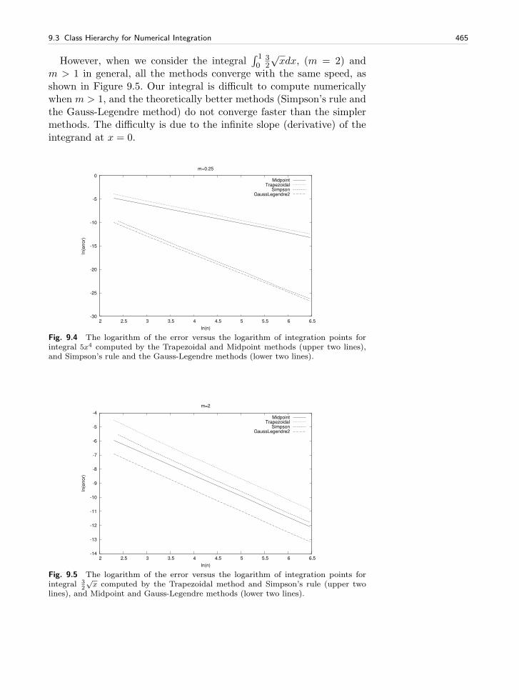
9.3 Class Hierarchy for Numerical Integration 465

However, when we consider the integral∫ 10

32

√xdx, (m = 2) and

m > 1 in general, all the methods converge with the same speed, asshown in Figure 9.5. Our integral is difficult to compute numericallywhen m > 1, and the theoretically better methods (Simpson’s rule andthe Gauss-Legendre method) do not converge faster than the simplermethods. The difficulty is due to the infinite slope (derivative) of theintegrand at x = 0.

-30

-25

-20

-15

-10

-5

0

2 2.5 3 3.5 4 4.5 5 5.5 6 6.5

ln(e

rror)

ln(n)

m=0.25

MidpointTrapezoidal

SimpsonGaussLegendre2

Fig. 9.4 The logarithm of the error versus the logarithm of integration points forintegral 5x4 computed by the Trapezoidal and Midpoint methods (upper two lines),and Simpson’s rule and the Gauss-Legendre methods (lower two lines).

-14

-13

-12

-11

-10

-9

-8

-7

-6

-5

-4

2 2.5 3 3.5 4 4.5 5 5.5 6 6.5

ln(e

rror)

ln(n)

m=2

MidpointTrapezoidal

SimpsonGaussLegendre2

Fig. 9.5 The logarithm of the error versus the logarithm of integration points forintegral 3

2

√x computed by the Trapezoidal method and Simpson’s rule (upper two

lines), and Midpoint and Gauss-Legendre methods (lower two lines).

466 9 Object-Oriented Programming

9.3.4 About Object-Oriented Programming

From an implementational point of view, the advantage of class hierar-chies in Python is that we can save coding by inheriting functionalityfrom a superclass. In programming languages where each variable mustbe specified with a fixed type, class hierarchies are particularly usefulbecause a function argument with a special type also works with allsubclasses of that type. Suppose we have a function where we need tointegrate:

def do_math(arg1, arg2, integrator):...I = integrator.integrate(myfunc)...

That is, integrator must be an instance of some class, or a module,such that the syntax integrator.integrate(myfunc) corresponds to afunction call, but nothing more (like having a particular type) is de-manded.

This Python code will run as long as integrator has a methodintegrate taking one argument. In other languages, the function argu-ments are specified with a type, say in Java we would write

void do_math(double arg1, int arg2, Simpson integrator)

A compiler will examine all calls to do_math and control that the ar-guments are of the right type. Instead of specifying the integrationmethod to be of type Simpson, one can in Java and other object-orientedlanguages specify integrator to be of the superclass type Integrator:

void do_math(double arg1, int arg2, Integrator integrator)

Now it is allowed to pass an object of any subclass type of Integratoras the third argument. That is, this method works with integrator oftype Midpoint, Trapezoidal, Simpson, etc., not just one of them. Classhierarchies and object-oriented programming are therefore importantmeans for parameterizing away types in languages like Java, C++, andC#. We do not need to parameterize types in Python, since argumentsare not declared with a fixed type. Object-oriented programming ishence not so technically important in Python as in other languages forproviding increased flexibility in programs.

Is there then any use for object-oriented programming beyond inher-itance? The answer is yes! For many code developers object-orientedprogramming is not just a technical way of sharing code, but it is morea way of modeling the world, and understanding the problem that theprogram is supposed to solve. In mathematical applications we alreadyhave objects, defined by the mathematics, and standard programmingconcepts such as functions, arrays, lists, and loops are often sufficientfor solving simpler problems. In the non-mathematical world the con-cept of objects is very useful because it helps to structure the problem

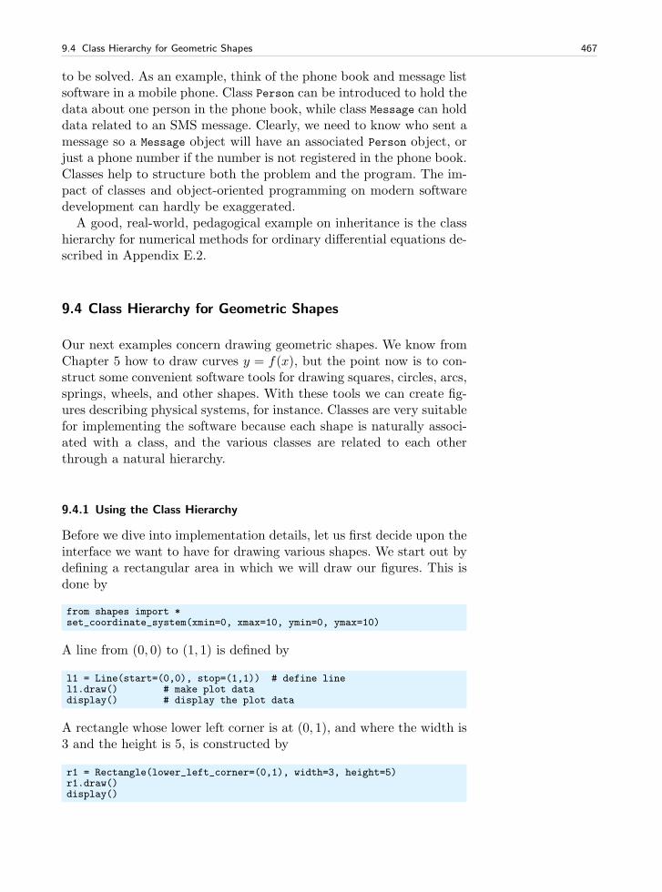
9.4 Class Hierarchy for Geometric Shapes 467

to be solved. As an example, think of the phone book and message listsoftware in a mobile phone. Class Person can be introduced to hold thedata about one person in the phone book, while class Message can holddata related to an SMS message. Clearly, we need to know who sent amessage so a Message object will have an associated Person object, orjust a phone number if the number is not registered in the phone book.Classes help to structure both the problem and the program. The im-pact of classes and object-oriented programming on modern softwaredevelopment can hardly be exaggerated.

A good, real-world, pedagogical example on inheritance is the classhierarchy for numerical methods for ordinary differential equations de-scribed in Appendix E.2.

9.4 Class Hierarchy for Geometric Shapes

Our next examples concern drawing geometric shapes. We know fromChapter 5 how to draw curves y = f(x), but the point now is to con-struct some convenient software tools for drawing squares, circles, arcs,springs, wheels, and other shapes. With these tools we can create fig-ures describing physical systems, for instance. Classes are very suitablefor implementing the software because each shape is naturally associ-ated with a class, and the various classes are related to each otherthrough a natural hierarchy.

9.4.1 Using the Class Hierarchy

Before we dive into implementation details, let us first decide upon theinterface we want to have for drawing various shapes. We start out bydefining a rectangular area in which we will draw our figures. This isdone by

from shapes import *set_coordinate_system(xmin=0, xmax=10, ymin=0, ymax=10)

A line from (0, 0) to (1, 1) is defined by

l1 = Line(start=(0,0), stop=(1,1)) # define linel1.draw() # make plot datadisplay() # display the plot data

A rectangle whose lower left corner is at (0, 1), and where the width is3 and the height is 5, is constructed by

r1 = Rectangle(lower_left_corner=(0,1), width=3, height=5)r1.draw()display()

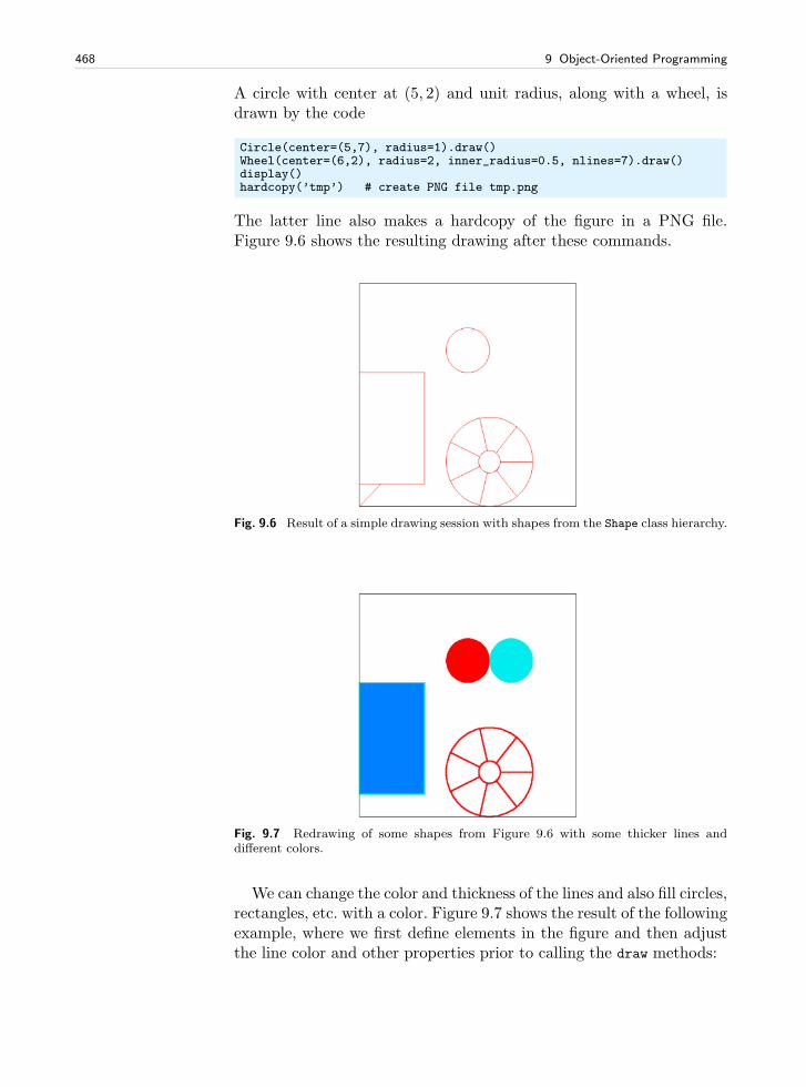
468 9 Object-Oriented Programming

A circle with center at (5, 2) and unit radius, along with a wheel, isdrawn by the code

Circle(center=(5,7), radius=1).draw()Wheel(center=(6,2), radius=2, inner_radius=0.5, nlines=7).draw()display()hardcopy(’tmp’) # create PNG file tmp.png

The latter line also makes a hardcopy of the figure in a PNG file.Figure 9.6 shows the resulting drawing after these commands.

Fig. 9.6 Result of a simple drawing session with shapes from the Shape class hierarchy.

Fig. 9.7 Redrawing of some shapes from Figure 9.6 with some thicker lines anddifferent colors.

We can change the color and thickness of the lines and also fill circles,rectangles, etc. with a color. Figure 9.7 shows the result of the followingexample, where we first define elements in the figure and then adjustthe line color and other properties prior to calling the draw methods:

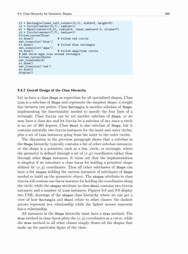
9.4 Class Hierarchy for Geometric Shapes 469

r1 = Rectangle(lower_left_corner=(0,1), width=3, height=5)c1 = Circle(center=(5,7), radius=1)w1 = Wheel(center=(6,2), radius=2, inner_radius=0.5, nlines=7)c2 = Circle(center=(7,7), radius=1)filled_curves(True)c1.draw() # filled red circleset_linecolor(’blue’)r1.draw() # filled blue rectangleset_linecolor(’aqua’)c2.draw() # filled aqua/cyan circle# Add thick aqua line around rectanglefilled_curves(False)set_linewidth(4)r1.draw()set_linecolor(’red’)w1.draw()display()

9.4.2 Overall Design of the Class Hierarchy

Let us have a class Shape as superclass for all specialized shapes. ClassLine is a subclass of Shape and represents the simplest shape: a strightline between two points. Class Rectangle is another subclass of Shape,implementing the functionality needed to specify the four lines of arectangle. Class Circle can be yet another subclass of Shape, or wemay have a class Arc and let Circle be a subclass of Arc since a circleis an arc of 360 degrees. Class Wheel is also subclass of Shape, but itcontains naturally two Circle instances for the inner and outer circles,plus a set of Line instances going from the inner to the outer circles.

The discussion in the previous paragraph shows that a subclass inthe Shape hierarchy typically contains a list of other subclass instances,or the shape is a primitive, such as a line, circle, or rectangle, wherethe geometry is defined through a set of (x, y) coordinates rather thanthrough other Shape instances. It turns out that the implementationis simplest if we introduce a class Curve for holding a primitive shapedefined by (x, y) coordinates. Then all other subclasses of Shape canhave a list shapes holding the various instances of subclasses of Shapeneeded to build up the geometric object. The shapes attribute in classCircle will contain one Curve instance for holding the coordinates alongthe circle, while the shapes attribute in class Wheel contains two Circle

instances and a number of Line instances. Figures 9.8 and 9.9 displaytwo UML drawings of the shapes class hierarchy where we can get aview of how Rectangle and Wheel relate to other classes: the darkestarrows represent is-a relationship while the lighter arrows representhas-a relationship.

All instances in the Shape hierarchy must have a draw method. Thedraw method in class Curve plots the (x, y) coordinates as a curve, whilethe draw method in all other classes simply draws all the shapes thatmake up the particular figure of the class:

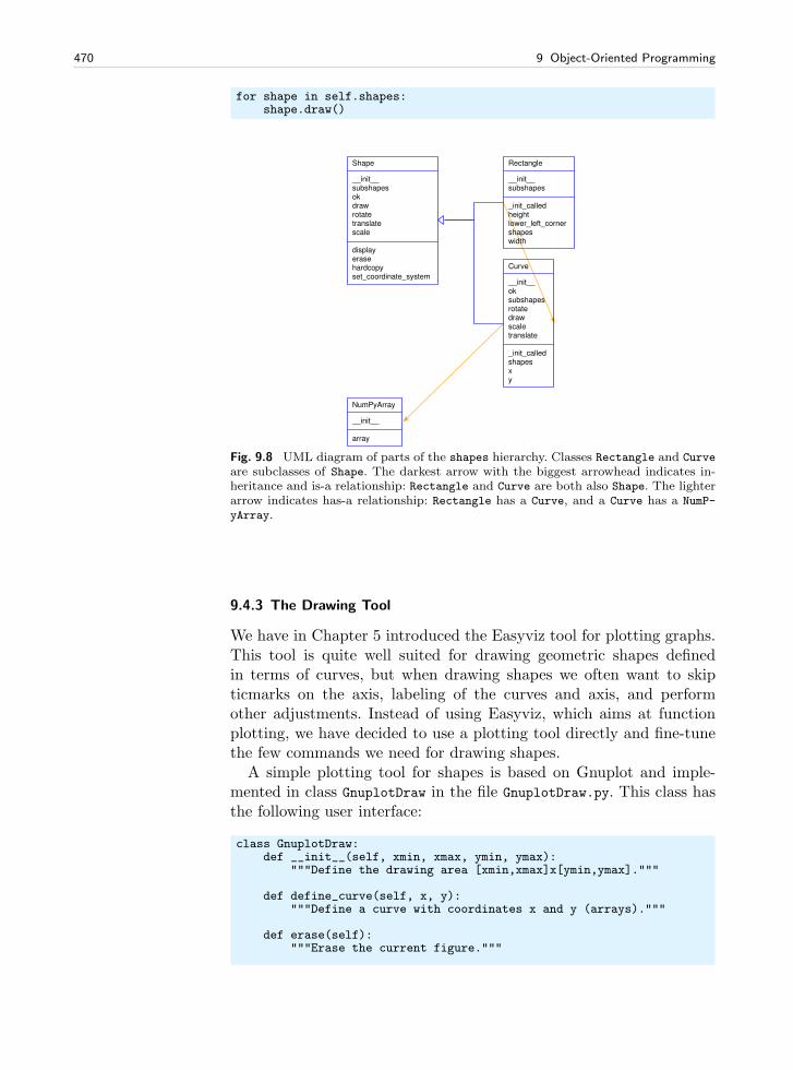
470 9 Object-Oriented Programming

for shape in self.shapes:shape.draw()

Shape

__init__subshapesokdrawrotatetranslatescale

displayerasehardcopyset_coordinate_system

Rectangle

__init__subshapes

_init_calledheightlower_left_cornershapeswidth

Curve

__init__oksubshapesrotatedrawscaletranslate

_init_calledshapesxy

NumPyArray

__init__

array

Fig. 9.8 UML diagram of parts of the shapes hierarchy. Classes Rectangle and Curve

are subclasses of Shape. The darkest arrow with the biggest arrowhead indicates in-heritance and is-a relationship: Rectangle and Curve are both also Shape. The lighterarrow indicates has-a relationship: Rectangle has a Curve, and a Curve has a NumP-

yArray.

9.4.3 The Drawing Tool

We have in Chapter 5 introduced the Easyviz tool for plotting graphs.This tool is quite well suited for drawing geometric shapes definedin terms of curves, but when drawing shapes we often want to skipticmarks on the axis, labeling of the curves and axis, and performother adjustments. Instead of using Easyviz, which aims at functionplotting, we have decided to use a plotting tool directly and fine-tunethe few commands we need for drawing shapes.

A simple plotting tool for shapes is based on Gnuplot and imple-mented in class GnuplotDraw in the file GnuplotDraw.py. This class hasthe following user interface:

class GnuplotDraw:def __init__(self, xmin, xmax, ymin, ymax):

"""Define the drawing area [xmin,xmax]x[ymin,ymax]."""

def define_curve(self, x, y):"""Define a curve with coordinates x and y (arrays)."""

def erase(self):"""Erase the current figure."""

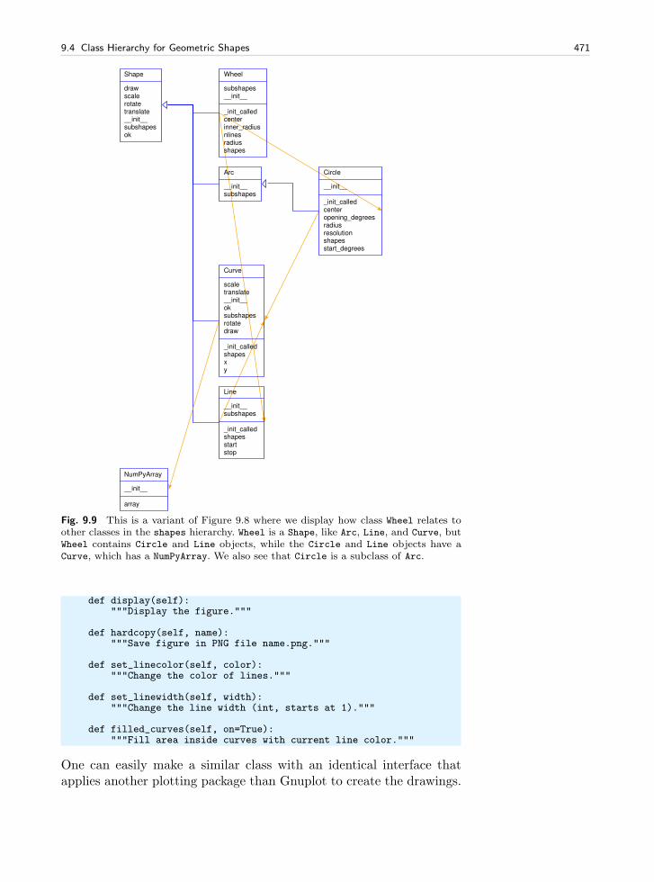
9.4 Class Hierarchy for Geometric Shapes 471

Shape

drawscalerotatetranslate__init__subshapesok

Wheel

subshapes__init__

_init_calledcenterinner_radiusnlinesradiusshapes

Arc

__init__subshapes

Circle

__init__

_init_calledcenteropening_degreesradiusresolutionshapesstart_degrees

Curve

scaletranslate__init__oksubshapesrotatedraw

_init_calledshapesxy

Line

__init__subshapes

_init_calledshapesstartstop

NumPyArray

__init__

array

Fig. 9.9 This is a variant of Figure 9.8 where we display how class Wheel relates toother classes in the shapes hierarchy. Wheel is a Shape, like Arc, Line, and Curve, butWheel contains Circle and Line objects, while the Circle and Line objects have aCurve, which has a NumPyArray. We also see that Circle is a subclass of Arc.

def display(self):"""Display the figure."""

def hardcopy(self, name):"""Save figure in PNG file name.png."""

def set_linecolor(self, color):"""Change the color of lines."""

def set_linewidth(self, width):"""Change the line width (int, starts at 1)."""

def filled_curves(self, on=True):"""Fill area inside curves with current line color."""

One can easily make a similar class with an identical interface thatapplies another plotting package than Gnuplot to create the drawings.

472 9 Object-Oriented Programming

In particular, encapsulating the drawing actions in such a class makesit trivial to change the drawing program in the future. The programpieces that apply a drawing tool like GnuplotDraw remain the same.This is an important strategy to follow, especially when developinglarger software systems.

9.4.4 Implementation of Shape Classes

Our superclass Shape can naturally hold a coordinate system specifica-tion, i.e., the rectangle in which other shapes can be drawn. This areais fixed for all shapes, so the associated variables should be static andthe method for setting them should also be static (see Chapter 7.6 forstatic attributes and methods). It is also natural that class Shape holdsaccess to a drawing tool, in our case a GnuplotDraw instance. This ob-ject is also static. However, it can be an advantage to mirror the staticattributes and methods as global variables and functions in the shapes

modules. Users not familiar with static class items can drop the Shape

prefix and just use plain module variables and functions. This is whatwe do in the application examples.

Class Shape defines an imporant method, draw, which just calls thedraw method for all subshapes that build up the current shape.

Here is a brief view of class Shape6:

class Shape:def __init__(self):

self.shapes = self.subshapes()if isinstance(self.shapes, Shape):

self.shapes = [self.shapes] # turn to list

def subshapes(self):"""Define self.shapes as list of Shape instances."""raise NotImplementedError(self.__class__.__name__)

def draw(self):for shape in self.shapes:

shape.draw()

In class Shape we require the shapes attribute to be a list, but if thesubshape method in subclasses returns just one instance, this is auto-matically wrapped in a list in the constructor.

First we implement the special case class Curve, which does not havesubshapes but instead (x, y) coordinates for a curve:

class Curve(Shape):"""General (x,y) curve with coordintes."""def __init__(self, x, y):

self.x, self.y = x, y# Turn to Numerical Python arraysself.x = asarray(self.x, float)

6 We have for simplicity omitted the static attributes and methods. These can beviewed in the shapes.py file.

9.4 Class Hierarchy for Geometric Shapes 473

self.y = asarray(self.y, float)Shape.__init__(self)

def subshapes(self):pass # geometry defined in constructor

The simplest ordinary Shape class is Line:

class Line(Shape):def __init__(self, start, stop):

self.start, self.stop = start, stopShape.__init__(self)

def subshapes(self):x = [self.start[0], self.stop[0]]y = [self.start[1], self.stop[1]]return Curve(x,y)

The code in this class works with start and stop as tuples, lists, orarrays of length two, holding the end points of the line. The underlyingCurve object needs only these two end points.

A rectangle is represented by a slightly more complicated class, hav-ing the lower left corner, the width, and the height of the rectangle asattributes:

class Rectangle(Shape):def __init__(self, lower_left_corner, width, height):

self.lower_left_corner = lower_left_corner # 2-tupleself.width, self.height = width, heightShape.__init__(self)

def subshapes(self):ll = self.lower_left_corner # short formx = [ll[0], ll[0]+self.width,

ll[0]+self.width, ll[0], ll[0]]y = [ll[1], ll[1], ll[1]+self.height,

ll[1]+self.height, ll[1]]return Curve(x,y)

Class Circle needs many coordinates in its Curve object in order todisplay a smooth circle. We can provide the number of straight linesegments along the circle as a parameter resolution. Using a defaultvalue of 180 means that each straight line segment approximates an arcof 2 degrees. This resolution should be sufficient for visual purposes.The set of coordinates along a circle with radius R and center (x0, y0)is defined by

x = x0 +R cos(t), (9.17)

y = y0 +R sin(t), (9.18)

for resolution+1 t values between 0 and 2π. The vectorized code forcomputing the coordinates becomes

t = linspace(0, 2*pi, self.resolution+1)x = x0 + R*cos(t)y = y0 + R*sin(t)

474 9 Object-Oriented Programming

The complete Circle class is shown below:

class Circle(Shape):def __init__(self, center, radius, resolution=180):

self.center, self.radius = center, radiusself.resolution = resolutionShape.__init__(self)

def subshapes(self):t = linspace(0, 2*pi, self.resolution+1)x0 = self.center[0]; y0 = self.center[1]R = self.radiusx = x0 + R*cos(t)y = y0 + R*sin(t)return Curve(x,y)

We can also introduce class Arc for drawing the arc of a circle. ClassArc could be a subclass of Circle, extending the latter with two addi-tional parameters: the opening of the arc (in degrees) and the startingt value in (9.17)–(9.18). The implementation of class Arc will then bealmost a copy of the implementation of class Circle. The subshapes

method will just define a different t array.Another view is to let class Arc be a subclass of Shape, and Circle

a subclass of Arc, since a circle is an arc of 360 degrees. Let us employthis idea:

class Arc(Shape):def __init__(self, center, radius,

start_degrees, opening_degrees, resolution=180):self.center = centerself.radius = radiusself.start_degrees = start_degrees*pi/180self.opening_degrees = opening_degrees*pi/180self.resolution = resolutionShape.__init__(self)

def subshapes(self):t = linspace(self.start_degrees,

self.start_degrees + self.opening_degrees,self.resolution+1)

x0 = self.center[0]; y0 = self.center[1]R = self.radiusx = x0 + R*cos(t)y = y0 + R*sin(t)return Curve(x,y)

class Circle(Arc):def __init__(self, center, radius, resolution=180):

Arc.__init__(self, center, radius, 0, 360, resolution)

In this latter implementation, we save a lot of code in class Circle sinceall of class Arc can be reused.

Class Wheel may conceptually be a subclass of Circle. One circle,say the outer, is inherited and the subclass must have the inner circleas an attribute. Because of this “asymmetric” representation of the twocircles in a wheel, we find it more natural to derive Wheel directly fromShape, and have the two circles as two attributes of type Circle:

9.4 Class Hierarchy for Geometric Shapes 475

class Wheel(Shape):def __init__(self, center, radius, inner_radius=None, nlines=10):

self.center = centerself.radius = radiusif inner_radius is None:

self.inner_radius = radius/5.0else:

self.inner_radius = inner_radiusself.nlines = nlinesShape.__init__(self)

If the radius of the inner circle is not defined (None) we take it as 1/5of the radius of the outer circle. The wheel is naturally composed oftwo Circle instances and nlines Line instances:

def subshapes(self):outer = Circle(self.center, self.radius)inner = Circle(self.center, self.inner_radius)lines = []t = linspace(0, 2*pi, self.nlines)Ri = self.inner_radius; Ro = self.radiusx0 = self.center[0]; y0 = self.center[1]xinner = x0 + Ri*cos(t)yinner = y0 + Ri*sin(t)xouter = x0 + Ro*cos(t)youter = y0 + Ro*sin(t)lines = [Line((xi,yi),(xo,yo)) for xi, yi, xo, yo in \

zip(xinner, yinner, xouter, youter)]return [outer, inner] + lines

For the fun of it, we can implement other shapes, say a sine wave

y = m+A sin kx, k = 2π/λ,

where λ is the wavelength of the sine waves, A is the wave amplitude,and m is the mean value of the wave. The class looks like

class Wave(Shape):def __init__(self, xstart, xstop,

wavelength, amplitude, mean_level):self.xstart = xstartself.xstop = xstopself.wavelength = wavelengthself.amplitude = amplitudeself.mean_level = mean_levelShape.__init__(self)

def subshapes(self):npoints = (self.xstop - self.xstart)/(self.wavelength/61.0)x = linspace(self.xstart, self.xstop, npoints)k = 2*pi/self.wavelength # frequencyy = self.mean_level + self.amplitude*sin(k*x)return Curve(x,y)

With this and the previous example, you should be in a position towrite your own subclasses. Exercises 9.19–9.23 suggest some smallerprojects.

476 9 Object-Oriented Programming

Functions for Controlling Lines, Colors, etc. The shapes module con-taining class Shape and all subclasses mentioned above, also offers someadditional functions that do not depend on any particular shape:

display() for displaying the defined figures so far (all figures whosedraw method is called).

erase() for ereasing the current figure. hardcopy(name) for saving the current figure to a PNG file name.png. set_linecolor(color) for setting the color of lines, where color

is a string like ’red’ (default), ’blue’, ’green’, ’aqua’, ’purple’,’yellow’, and ’black’.

set_linewidth(width) for setting the width of a line, measured asan integer (default is 2).

filled_curves(on) for turrning on (on=True) or off (on=False)whether the area inside a shape should be filled with the currentline color.

Actually, the functions above are static methods in class Shape

(cf. Chapter 7.6), and they are just mirrored as global functions7 inthe shapes module. Users without knowledge of static methods do notneed to use the Shape prefix for reaching this functionality.

9.4.5 Scaling, Translating, and Rotating a Figure

The real power of object-oriented programming will be obvious in aminute when we, with a few lines of code, suddenly can equip all shapeobjects with additional functionality for scaling, translating, and rotat-ing the figure.

Scaling. Let us first treat the simplest of the three cases: scaling. For aCurve instance containing a set of n coordinates (xi, yi) that make upa curve, scaling by a factor a means that we multiply all the x and ycoordinates by a:

xi ← axi, yi ← ayi, i = 0, . . . , n− 1 .

Here we apply the arrow as an assignment operator. The correspondingPython implementation in class Curve reads

class Curve:...def scale(self, factor):

self.x = factor*self.xself.y = factor*self.y

Note here that self.x and self.y are Numerical Python arrays, so thatmultiplication by a scalar number factor is a vectorized operation.

7 You can look into shapes.py to see how we automate the duplication of staticmethods as global functions.

9.4 Class Hierarchy for Geometric Shapes 477

In an instance of a subclass of Shape, the meaning of a methodscale is to run through all objects in the list self.shapes and ask eachobject to scale itself. This is the same delegation of actions to subclassinstances as we do in the draw method, and all objects, except Curve

instances, can share the same implementation of the scale method.Therefore, we place the scale method in the superclass Shape suchthat all subclasses can inherit this method. Since scale and draw areso similar, we can easily implement the scale method in class Shape bycopying and editing the draw method:

class Shape:...def scale(self, factor):

for shape in self.shapes:shape.scale(factor)

This is all we have to do in order to equip all subclasses of Shape

with scaling functionality! But why is it so easy? All subclasses inheritscale from class Shape. Say we have a subclass instance s and that wecall s.scale(factor). This leads to calling the inherited scale methodshown above, and in the for loop we call the scale method for eachshape object in the self.shapes list. If shape is not a Curve object, thisprocedure repeats, until we hit a shape that is a Curve, and then thescaling on that set of coordinates is performed.

Translation. A set of coordinates (xi, yi) can be translated x units inthe x direction and y units in the y direction using the formulas

xi ← x+ xi, yi ← y + yi, i = 0, . . . , n− 1 .

The corresponding Python implementation in class Curve becomes

class Curve:...def translate(self, x, y):

self.x = x + self.xself.y = y + self.y

The translation operation for a shape object is very similar to thescaling and drawing operations. This means that we can implement acommon method translate in the superclass Shape. The code is parallelto the scale method:

class Shape:....def translate(self, x, y):

for shape in self.shapes:shape.translate(x, y)

Rotation. Rotating a figure is more complicated than scaling and trans-lating. A counter clockwise rotation of θ degrees for a set of coordinates(xi, yi) is given by

478 9 Object-Oriented Programming

xi ← xi cos θ − yi sin θ,

yi ← xi sin θ + yi cos θ .

This rotation is performed around the origin. If we want the figure tobe rotated with respect to a general point (x, y), we need to extend theformulas above:

xi ← x+ (xi − x) cos θ − (yi − y) sin θ,

yi ← y + (xi − x) sin θ + (yi − y) cos θ .

The Python implementation in class Curve, assuming that θ is given indegrees and not in radians, becomes

def rotate(self, angle, x=0, y=0):angle = angle*pi/180c = cos(angle); s = sin(angle)xnew = x + (self.x - x)*c - (self.y - y)*synew = y + (self.x - x)*s + (self.y - y)*cself.x = xnewself.y = ynew

The rotate method in class Shape is identical to the draw, scale, andtranslate methods except that we have other arguments:

class Shape:....def rotate(self, angle, x=0, y=0):

for shape in self.shapes:shape.rotate(angle, x, y)

Application: Rolling Wheel. To demonstrate the effect of translationand rotation we can roll a wheel on the screen. First we draw the wheeland rotate it a bit to demonstrate the basic operations:

center = (6,2) # the wheel’s center pointw1 = Wheel(center=center, radius=2, inner_radius=0.5, nlines=7)# rorate the wheel 2 degrees around its center point:w1.rotate(angle=2, center[0], center[1])w1.draw()display()

Now we want to roll the wheel by making many such small rotations.At the same time we need to translate the wheel since rolling an arclength L = Rθ, where θ is the rotation angle (in radians) and R isthe outer radius of the wheel, implies that the center point moves adistance L to the left (θ > 0 means counter clockwise rotation). Incode we must therefore combine rotation with translation:

L = radius*angle*pi/180 # translation = arc lengthw1.rotate(angle, center[0], center[1])w1.translate(-L, 0)center = (center[0] - L, center[1])

9.4 Class Hierarchy for Geometric Shapes 479

We are now in a position to put the rotation and translation operationsin a for loop and make a complete function:

def rolling_wheel(total_rotation_angle):"""Animation of a rotating wheel."""set_coordinate_system(xmin=0, xmax=10, ymin=0, ymax=10)

center = (6,2)radius = 2.0angle = 2.0w1 = Wheel(center=center, radius=radius,

inner_radius=0.5, nlines=7)for i in range(int(total_rotation_angle/angle)):

w1.draw()display()

L = radius*angle*pi/180 # translation = arc lengthw1.rotate(angle, center[0], center[1])w1.translate(-L, 0)center = (center[0] - L, center[1])

erase()

To control the visual “velocity” of the wheel, we can insert a pausebetween each frame in the for loop. A call to time.sleep(s), where s

is the length of the pause in seconds, can do this for us.Another convenient feature is to save each frame drawn in the for

loop as a hardcopy in PNG format and then, after the loop, make ananimated GIF file based on the individual PNG frames. The latteroperation is performed either by the movie function from scitools.std

or by the convert program from the ImageMagick suite. With the latteryou write the following command in a terminal window:

convert -delay 50 -loop 1000 xxx tmp_movie.gif

Here, xxx is a space-separated list of all the PNG files, andtmp_movie.gif is the name of the resulting animated GIF file. Wecan easily make xxx by collecting the names of the PNG files from theloop in a list object, and then join the names. The convert commandcan be run as an os.system call.

The complete rolling_wheel function, incorporating the mentionedmovie making, will then be

def rolling_wheel(total_rotation_angle):"""Animation of a rotating wheel."""set_coordinate_system(xmin=0, xmax=10, ymin=0, ymax=10)

import timecenter = (6,2)radius = 2.0angle = 2.0pngfiles = []w1 = Wheel(center=center, radius=radius,

inner_radius=0.5, nlines=7)for i in range(int(total_rotation_angle/angle)):

w1.draw()display()

filename = ’tmp_%03d’ % i

480 9 Object-Oriented Programming

pngfiles.append(filename + ’.png’)hardcopy(filename)time.sleep(0.3) # pause 0.3 sec

L = radius*angle*pi/180 # translation = arc lengthw1.rotate(angle, center[0], center[1])w1.translate(-L, 0)center = (center[0] - L, center[1])

erase() # erase the screen before new figure

cmd = ’convert -delay 50 -loop 1000 %s tmp_movie.gif’ \% (’ ’.join(pngfiles))

import commandsfailure, output = commands.getstatusoutput(cmd)if failure: print ’Could not run’, cmd

The last two lines run a command, from Python, as we would run thecommand in a terminal window. The resulting animated GIF file canbe viewed with animate tmp_movie.gif as a command in a terminalwindow.

9.5 Summary

9.5.1 Chapter Topics

A subclass inherits everyting from its superclass, both attributes andmethods. The subclass can add new attributes, overload methods, andthereby enrich or restrict functionality of the superclass.

Subclass Example. Consider class Gravity from Chapter 7.7.1 for rep-resenting the gravity force GMm/r2 between two masses m and Mbeing a distance r apart. Suppose we want to make a class for the elec-tric force between two charges q1 and q2, being a distance r apart in amedium with permittivity ǫ0 is Gq1q2/r

2, where G−1 = 4πǫ0. We usethe approximate value G = 8.99 · 109 Nm2/C2 (C is the Coulumb unitused to measure electric charges such as q1 and q2). Since the electricforce is similar to the gravity force, we can easily implement the elet-ric force as a subclass of Gravity. The implementation just needs toredefine the value of G!

class CoulumbsLaw(Gravity):def __init__(self, q1, q2):

Gravity.__init__(self, q1, q2)self.G = 8.99E9

We can now call the inherited force(r) method to compute the eletricforce and the visualize method to make a plot of the force:

c = CoulumbsLaw(1E-6, -2E-6)print ’Electric force:’, c.force(0.1)c.visualize(0.01, 0.2)

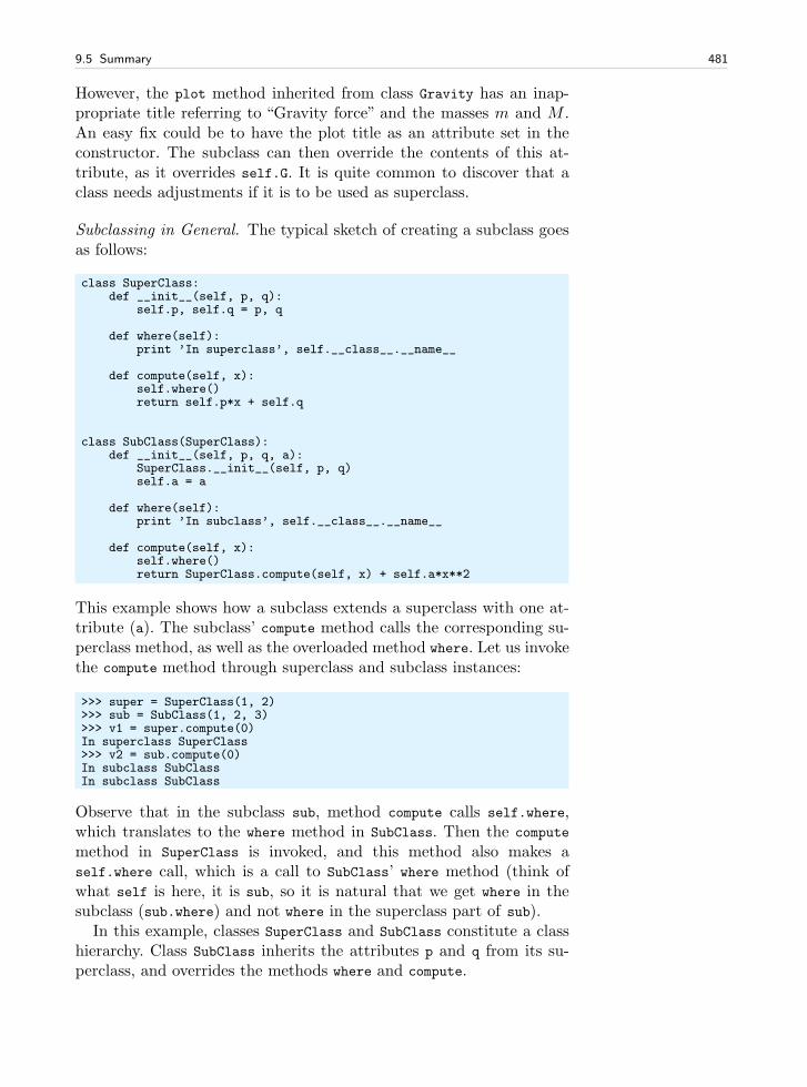
9.5 Summary 481

However, the plot method inherited from class Gravity has an inap-propriate title referring to “Gravity force” and the masses m and M .An easy fix could be to have the plot title as an attribute set in theconstructor. The subclass can then override the contents of this at-tribute, as it overrides self.G. It is quite common to discover that aclass needs adjustments if it is to be used as superclass.

Subclassing in General. The typical sketch of creating a subclass goesas follows:

class SuperClass:def __init__(self, p, q):

self.p, self.q = p, q

def where(self):print ’In superclass’, self.__class__.__name__

def compute(self, x):self.where()return self.p*x + self.q

class SubClass(SuperClass):def __init__(self, p, q, a):

SuperClass.__init__(self, p, q)self.a = a

def where(self):print ’In subclass’, self.__class__.__name__

def compute(self, x):self.where()return SuperClass.compute(self, x) + self.a*x**2

This example shows how a subclass extends a superclass with one at-tribute (a). The subclass’ compute method calls the corresponding su-perclass method, as well as the overloaded method where. Let us invokethe compute method through superclass and subclass instances:

>>> super = SuperClass(1, 2)>>> sub = SubClass(1, 2, 3)>>> v1 = super.compute(0)In superclass SuperClass>>> v2 = sub.compute(0)In subclass SubClassIn subclass SubClass

Observe that in the subclass sub, method compute calls self.where,which translates to the where method in SubClass. Then the compute

method in SuperClass is invoked, and this method also makes aself.where call, which is a call to SubClass’ where method (think ofwhat self is here, it is sub, so it is natural that we get where in thesubclass (sub.where) and not where in the superclass part of sub).

In this example, classes SuperClass and SubClass constitute a classhierarchy. Class SubClass inherits the attributes p and q from its su-perclass, and overrides the methods where and compute.

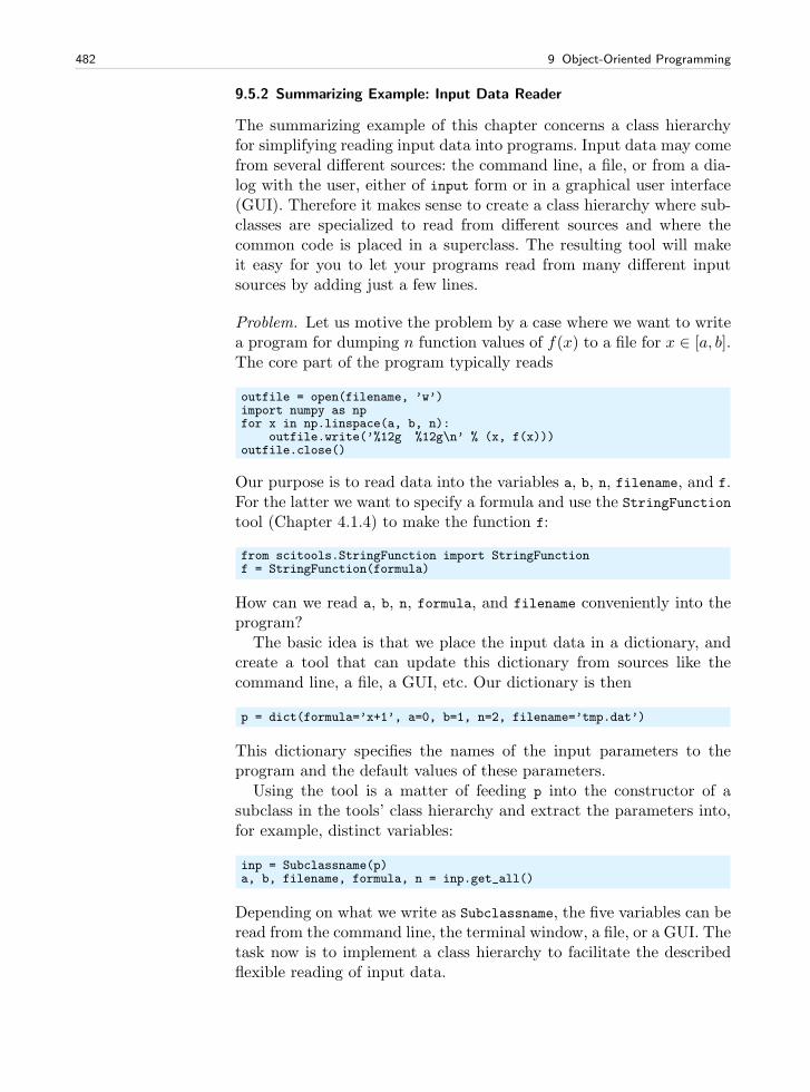
482 9 Object-Oriented Programming

9.5.2 Summarizing Example: Input Data Reader

The summarizing example of this chapter concerns a class hierarchyfor simplifying reading input data into programs. Input data may comefrom several different sources: the command line, a file, or from a dia-log with the user, either of input form or in a graphical user interface(GUI). Therefore it makes sense to create a class hierarchy where sub-classes are specialized to read from different sources and where thecommon code is placed in a superclass. The resulting tool will makeit easy for you to let your programs read from many different inputsources by adding just a few lines.

Problem. Let us motive the problem by a case where we want to writea program for dumping n function values of f(x) to a file for x ∈ [a, b].The core part of the program typically reads

outfile = open(filename, ’w’)import numpy as npfor x in np.linspace(a, b, n):

outfile.write(’%12g %12g\n’ % (x, f(x)))outfile.close()

Our purpose is to read data into the variables a, b, n, filename, and f.For the latter we want to specify a formula and use the StringFunctiontool (Chapter 4.1.4) to make the function f:

from scitools.StringFunction import StringFunctionf = StringFunction(formula)

How can we read a, b, n, formula, and filename conveniently into theprogram?

The basic idea is that we place the input data in a dictionary, andcreate a tool that can update this dictionary from sources like thecommand line, a file, a GUI, etc. Our dictionary is then

p = dict(formula=’x+1’, a=0, b=1, n=2, filename=’tmp.dat’)

This dictionary specifies the names of the input parameters to theprogram and the default values of these parameters.

Using the tool is a matter of feeding p into the constructor of asubclass in the tools’ class hierarchy and extract the parameters into,for example, distinct variables:

inp = Subclassname(p)a, b, filename, formula, n = inp.get_all()

Depending on what we write as Subclassname, the five variables can beread from the command line, the terminal window, a file, or a GUI. Thetask now is to implement a class hierarchy to facilitate the describedflexible reading of input data.

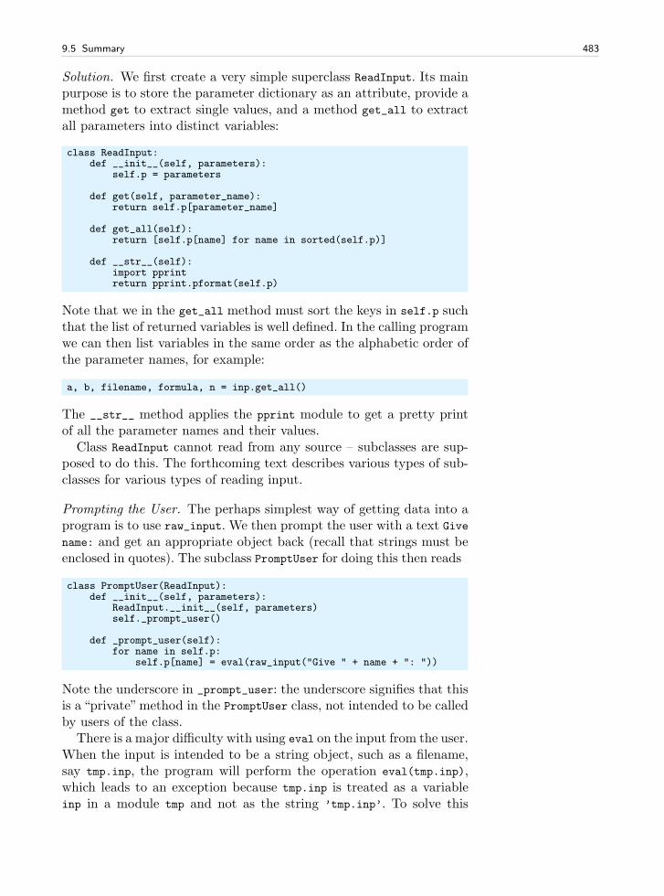
9.5 Summary 483

Solution. We first create a very simple superclass ReadInput. Its mainpurpose is to store the parameter dictionary as an attribute, provide amethod get to extract single values, and a method get_all to extractall parameters into distinct variables:

class ReadInput:def __init__(self, parameters):

self.p = parameters

def get(self, parameter_name):return self.p[parameter_name]

def get_all(self):return [self.p[name] for name in sorted(self.p)]

def __str__(self):import pprintreturn pprint.pformat(self.p)

Note that we in the get_all method must sort the keys in self.p suchthat the list of returned variables is well defined. In the calling programwe can then list variables in the same order as the alphabetic order ofthe parameter names, for example:

a, b, filename, formula, n = inp.get_all()

The __str__ method applies the pprint module to get a pretty printof all the parameter names and their values.

Class ReadInput cannot read from any source – subclasses are sup-posed to do this. The forthcoming text describes various types of sub-classes for various types of reading input.

Prompting the User. The perhaps simplest way of getting data into aprogram is to use raw_input. We then prompt the user with a text Givename: and get an appropriate object back (recall that strings must beenclosed in quotes). The subclass PromptUser for doing this then reads

class PromptUser(ReadInput):def __init__(self, parameters):

ReadInput.__init__(self, parameters)self._prompt_user()

def _prompt_user(self):for name in self.p:

self.p[name] = eval(raw_input("Give " + name + ": "))

Note the underscore in _prompt_user: the underscore signifies that thisis a “private”method in the PromptUser class, not intended to be calledby users of the class.

There is a major difficulty with using eval on the input from the user.When the input is intended to be a string object, such as a filename,say tmp.inp, the program will perform the operation eval(tmp.inp),which leads to an exception because tmp.inp is treated as a variableinp in a module tmp and not as the string ’tmp.inp’. To solve this

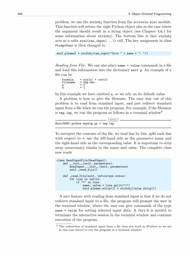
484 9 Object-Oriented Programming

problem, we use the str2obj function from the scitools.misc module.This function will return the right Python object also in the case wherethe argument should result in a string object (see Chapter 4.6.1 forsome information about str2obj). The bottom line is that str2obj

acts as a safer eval(raw_input(...)) call. The key assignment in classPromptUser is then changed to

self.p[name] = str2obj(raw_input("Give " + name + ": "))

Reading from File. We can also place name = value commands in a fileand load this information into the dictionary self.p. An example of afile can be

formula = sin(x) + cos(x)filename = tmp.data = 0b = 1

In this example we have omitted n, so we rely on its default value.A problem is how to give the filename. The easy way out of this

problem is to read from standard input, and just redirect standardinput from a file when we run the program. For example, if the filenameis tmp.inp, we run the program as follows in a terminal window8

Terminal

Unix/DOS> python myprog.py < tmp.inp

To interpret the contents of the file, we read line by line, split each linewith respect to =, use the left-hand side as the parameter name andthe right-hand side as the corresponding value. It is important to stripaway unnecessary blanks in the name and value. The complete classnow reads

class ReadInputFile(ReadInput):def __init__(self, parameters):

ReadInput.__init__(self, parameters)self._read_file()

def _read_file(self, infile=sys.stdin):for line in infile:

if "=" in line:name, value = line.split("=")self.p[name.strip()] = str2obj(value.strip())

A nice feature with reading from standard input is that if we do notredirect standard input to a file, the program will prompt the user inthe terminal window, where the user can give commands of the typename = value for setting selected input data. A Ctrl-D is needed toterminate the interactive session in the terminal window and continueexecution of the program.

8 The redirection of standard input from a file does not work in IPython so we arein this case forced to run the program in a terminal window.

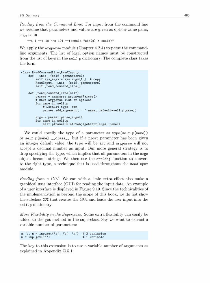
9.5 Summary 485

Reading from the Command Line. For input from the command linewe assume that parameters and values are given as option-value pairs,e.g., as in

--a 1 --b 10 --n 101 --formula "sin(x) + cos(x)"

We apply the argparse module (Chapter 4.2.4) to parse the command-line arguments. The list of legal option names must be constructedfrom the list of keys in the self.p dictionary. The complete class takesthe form

class ReadCommandLine(ReadInput):def __init__(self, parameters):

self.sys_argv = sys.argv[1:] # copyReadInput.__init__(self, parameters)self._read_command_line()

def _read_command_line(self):parser = argparse.ArgumentParser()# Make argparse list of optionsfor name in self.p:

# Default type: strparser.add_argument(’--’+name, default=self.p[name])

args = parser.parse_args()for name in self.p:

self.p[name] = str2obj(getattr(args, name))

We could specify the type of a parameter as type(self.p[name])

or self.p[name].__class__, but if a float parameter has been givenan integer default value, the type will be int and argparse will notaccept a decimal number as input. Our more general strategy is todrop specifying the type, which implies that all parameters in the args

object become strings. We then use the str2obj function to convertto the right type, a technique that is used throughout the ReadInput

module.

Reading from a GUI. We can with a little extra effort also make agraphical user interface (GUI) for reading the input data. An exampleof a user interface is displayed in Figure 9.10. Since the technicalities ofthe implementation is beyond the scope of this book, we do not showthe subclass GUI that creates the GUI and loads the user input into theself.p dictionary.

More Flexibility in the Superclass. Some extra flexibility can easily beadded to the get method in the superclass. Say we want to extract avariable number of parameters:

a, b, n = inp.get(’a’, ’b’, ’n’) # 3 variablesn = inp.get(’n’) # 1 variable

The key to this extension is to use a variable number of arguments asexplained in Appendix G.5.1:

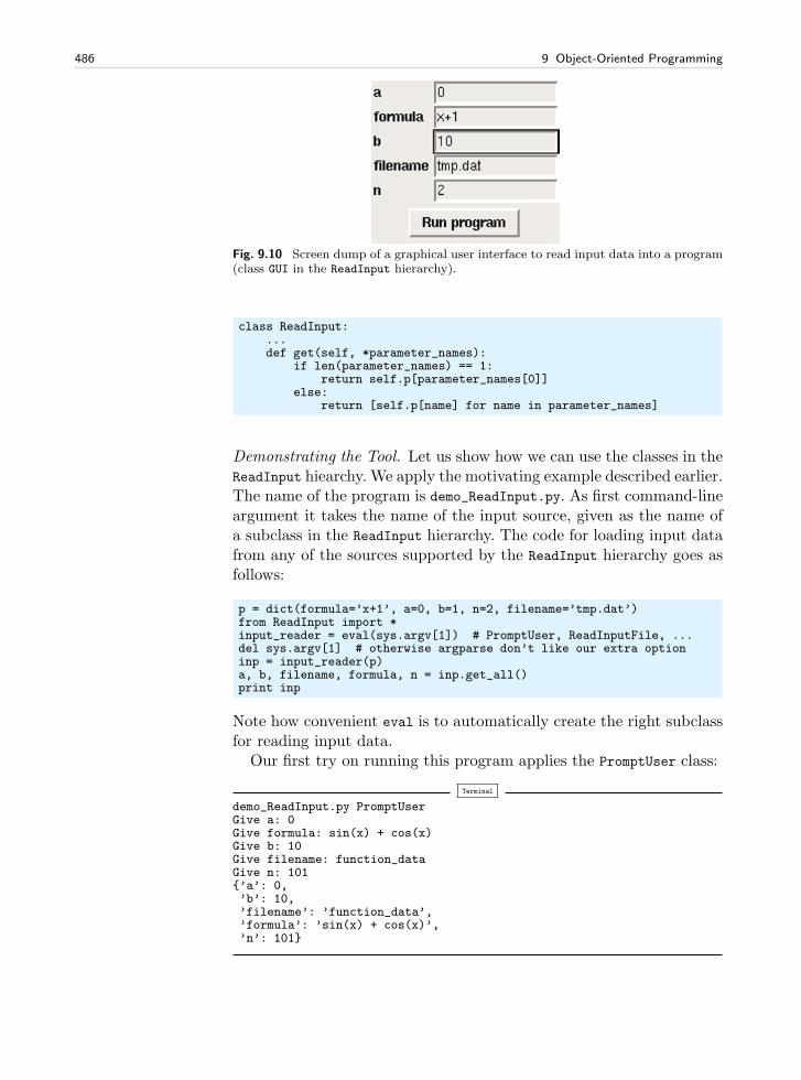
486 9 Object-Oriented Programming

Fig. 9.10 Screen dump of a graphical user interface to read input data into a program(class GUI in the ReadInput hierarchy).

class ReadInput:...def get(self, *parameter_names):

if len(parameter_names) == 1:return self.p[parameter_names[0]]

else:return [self.p[name] for name in parameter_names]

Demonstrating the Tool. Let us show how we can use the classes in theReadInput hiearchy. We apply the motivating example described earlier.The name of the program is demo_ReadInput.py. As first command-lineargument it takes the name of the input source, given as the name ofa subclass in the ReadInput hierarchy. The code for loading input datafrom any of the sources supported by the ReadInput hierarchy goes asfollows:

p = dict(formula=’x+1’, a=0, b=1, n=2, filename=’tmp.dat’)from ReadInput import *input_reader = eval(sys.argv[1]) # PromptUser, ReadInputFile, ...del sys.argv[1] # otherwise argparse don’t like our extra optioninp = input_reader(p)a, b, filename, formula, n = inp.get_all()print inp

Note how convenient eval is to automatically create the right subclassfor reading input data.

Our first try on running this program applies the PromptUser class:

Terminal

demo_ReadInput.py PromptUserGive a: 0Give formula: sin(x) + cos(x)Give b: 10Give filename: function_dataGive n: 101’a’: 0,’b’: 10,’filename’: ’function_data’,’formula’: ’sin(x) + cos(x)’,’n’: 101

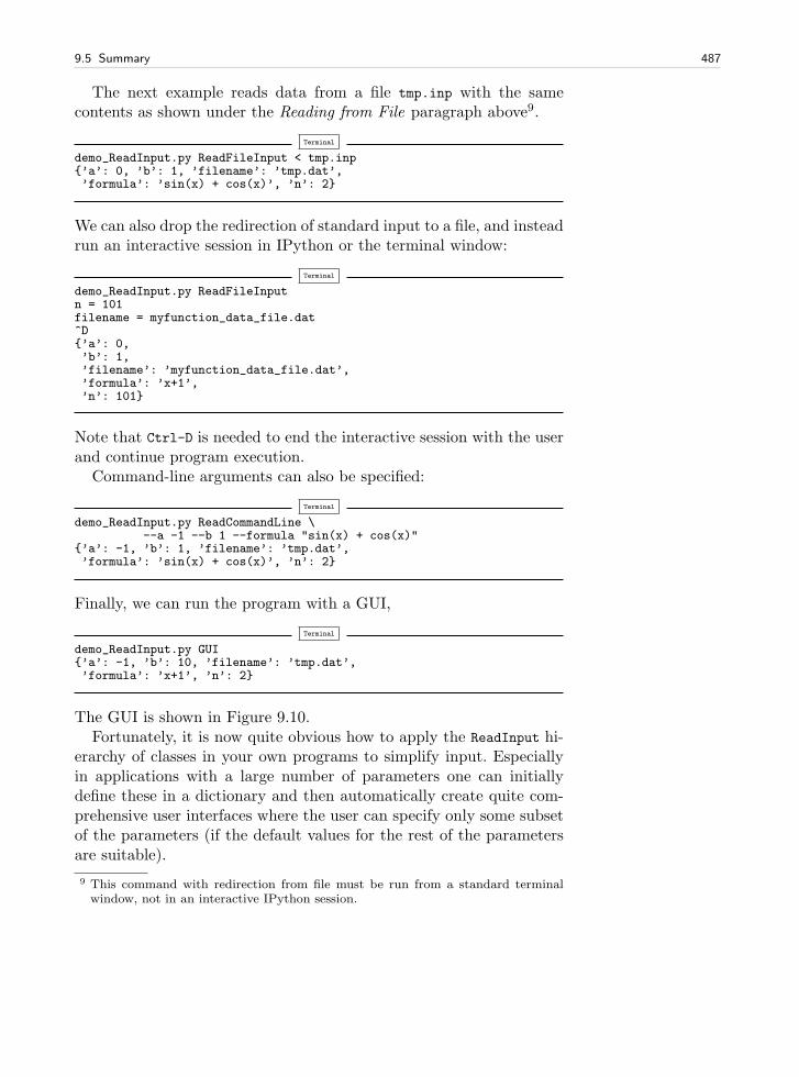
9.5 Summary 487

The next example reads data from a file tmp.inp with the samecontents as shown under the Reading from File paragraph above9.

Terminal

demo_ReadInput.py ReadFileInput < tmp.inp’a’: 0, ’b’: 1, ’filename’: ’tmp.dat’,’formula’: ’sin(x) + cos(x)’, ’n’: 2

We can also drop the redirection of standard input to a file, and insteadrun an interactive session in IPython or the terminal window:

Terminal

demo_ReadInput.py ReadFileInputn = 101filename = myfunction_data_file.dat^D’a’: 0,’b’: 1,’filename’: ’myfunction_data_file.dat’,’formula’: ’x+1’,’n’: 101

Note that Ctrl-D is needed to end the interactive session with the userand continue program execution.

Command-line arguments can also be specified:

Terminal

demo_ReadInput.py ReadCommandLine \--a -1 --b 1 --formula "sin(x) + cos(x)"

’a’: -1, ’b’: 1, ’filename’: ’tmp.dat’,’formula’: ’sin(x) + cos(x)’, ’n’: 2

Finally, we can run the program with a GUI,

Terminal

demo_ReadInput.py GUI’a’: -1, ’b’: 10, ’filename’: ’tmp.dat’,’formula’: ’x+1’, ’n’: 2

The GUI is shown in Figure 9.10.Fortunately, it is now quite obvious how to apply the ReadInput hi-

erarchy of classes in your own programs to simplify input. Especiallyin applications with a large number of parameters one can initiallydefine these in a dictionary and then automatically create quite com-prehensive user interfaces where the user can specify only some subsetof the parameters (if the default values for the rest of the parametersare suitable).

9 This command with redirection from file must be run from a standard terminalwindow, not in an interactive IPython session.

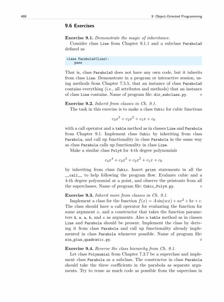
488 9 Object-Oriented Programming

9.6 Exercises

Exercise 9.1. Demonstrate the magic of inheritance.Consider class Line from Chapter 9.1.1 and a subclass Parabola0

defined as

class Parabola0(Line):pass

That is, class Parabola0 does not have any own code, but it inheritsfrom class Line. Demonstrate in a program or interactive session, us-ing methods from Chapter 7.5.5, that an instance of class Parabola0

contains everything (i.e., all attributes and methods) that an instanceof class Line contains. Name of program file: dir_subclass.py. ⋄

Exercise 9.2. Inherit from classes in Ch. 9.1.The task in this exercise is to make a class Cubic for cubic functions

c3x3 + c2x

2 + c1x+ c0

with a call operator and a tablemethod as in classes Line and Parabola

from Chapter 9.1. Implement class Cubic by inheriting from classParabola, and call up functionality in class Parabola in the same wayas class Parabola calls up functionality in class Line.

Make a similar class Poly4 for 4-th degree polynomials

c4x4 + c3x

3 + c2x2 + c1x+ c0

by inheriting from class Cubic. Insert print statements in all the__call__ to help following the program flow. Evaluate cubic and a4-th degree polynomial at a point, and observe the printouts from allthe superclasses. Name of program file: Cubic_Poly4.py. ⋄

Exercise 9.3. Inherit more from classes in Ch. 9.1.Implement a class for the function f(x) = A sin(wx) + ax2 + bx+ c.

The class should have a call operator for evaluating the function forsome argument x, and a constructor that takes the function parame-ters A, w, a, b, and c as arguments. Also a table method as in classesLine and Parabola should be present. Implement the class by deriv-ing it from class Parabola and call up functionality already imple-mented in class Parabola whenever possible. Name of program file:sin_plus_quadratic.py. ⋄

Exercise 9.4. Reverse the class hierarchy from Ch. 9.1.Let class Polynomial from Chapter 7.3.7 be a superclass and imple-

ment class Parabola as a subclass. The constructor in class Parabola

should take the three coefficients in the parabola as separate argu-ments. Try to reuse as much code as possible from the superclass in

9.6 Exercises 489

the subclass. Implement class Line as a subclass specialization of classParabola.

Which class design do you prefer – class Line as a subclass ofParabola and Polynomial, or Line as a superclass with extensions insubclasses? Name of program file: Polynomial_hier.py. ⋄

Exercise 9.5. Make circle a subclass of an ellipse.Chapter 7.2.3 presents class Circle. Make a similar class Ellipse

for representing an ellipse. Then create a new class Circle that is asubclass of Ellipse. Name of program file: Ellipse_Circle.py. ⋄

Exercise 9.6. Make super- and subclass for a point.A point (x, y) in the plane can be represented by a class:

class Point:def __init__(self, x, y):

self.x, self.y = x, y

def __str__(self):return ’(%g, %g)’ % (self.x, self.y)

We can extend the Point class to also contain the representation of thepoint in polar coordinates. To this end, create a subclass PolarPoint

whose constructor takes the polar representation of a point, (r, θ), asarguments. Store r and θ as attributes and call the superclass con-structor with the corresponding x and y values (recall the relationsx = r cos θ and y = r sin θ between Cartesian and polar coordinates).Add a __str__ method in class PolarPoint which prints out r, θ, x, andy. Verify the implementation by initializing three points and printingthese points. Name of program file: PolarPoint.py. ⋄

Exercise 9.7. Modify a function class by subclassing.Consider the VelocityProfile class from page 314 for computing

the function v(r; β, µ0, n, R) in formula (5.23) on page 238. Supposewe want to have v explicitly as a function of r and n (this is necessaryif we want to illustrate how the velocity profile, the v(r) curve, variesas n varies). We would then like to have a class VelocityProfile2 thatis initialized with β, µ0, and R, and that takes r and n as arguments inthe __call__ method. Implement such a class by inheriting from classVelocityProfile and by calling the __init__ and value methods in thesuperclass. It should be possible to try the class out with the followingstatements:

v = VelocityProfile2(beta=0.06, mu0=0.02, R=2)# Evaluate v for various n values at r=0for n in 0.1, 0.2, 1:

print v(0, n)

Name of program file: VelocityProfile2.py. ⋄

490 9 Object-Oriented Programming

Exercise 9.8. Explore the accuracy of difference formulas.The purpose of this exercise is to investigate the accuracy of the

Backward1, Forward1, Forward3, Central2, Central4, Central6 methodsfor the function10

v(x) =1− ex/µ

1− e1/µ.

To solve the exercise, modify the src/oo/Diff2_examples.py pro-gram which produces tables of errors of difference approximationsas discussed at the end of Chapter 9.2.3. Test the approximationmethods for x = 0, 0.9 and µ = 1, 0.01. Plot the v(x) func-tion for the two µ values using 1001 points. Name of program file:boundary_layer_derivative.py. ⋄

Exercise 9.9. Implement a subclass.Make a subclass Sine1 of class FuncWithDerivatives from Chap-

ter 9.1.7 for the sinx function. Implement the function only, and relyon the inherited df and ddf methods for computing the derivatives.Make another subclass Sine2 for sinx where you also implement thedf and ddf methods using analytical expressions for the derivatives.Compare Sine1 and Sine2 for computing the first- and second-orderderivatives of sinx at two x points. Name of program file: Sine12.py. ⋄

Exercise 9.10. Make classes for numerical differentiation.Carry out Exercise 7.14. Find the common code in the classes

Derivative, Backward, and Central. Move this code to a superclass,and let the three mentioned classes be subclasses of this superclass.Compare the resulting code with the hierarchy shown in Chapter 9.2.1.Name of program file: numdiff_classes.py. ⋄

Exercise 9.11. Implement a new subclass for differentiation.A one-sided, three-point, second-order accurate formula for differen-

tiating a function f(x) has the form

f ′(x) ≈ f(x− 2h)− 4f(x− h) + 3f(x)

2h. (9.19)

Implement this formula in a subclass Backward2 of class Diff fromChapter 9.2. Compare Backward2 with Backward1 for g(t) = e−t fort = 0 and h = 2−k for k = 0, 1, . . . , 14 (write out the errors in g′(t)).Name of program file: Backward2.py. ⋄

Exercise 9.12. Understand if a class can be used recursively.Suppose you want to compute f ′′(x) of some mathematical function

f(x), and that you apply some class from Chapter 9.2 twice, e.g.,

10 This function is discussed more in detail in Exercise 5.36.

9.6 Exercises 491

ddf = Central2(Central2(f))

Will this work? Hint: Follow the program flow, and find out what theresulting formula will be. Then see if this formula coincides with aformula you know for approximating f ′′(x). ⋄

Exercise 9.13. Represent people by a class hierarchy.Classes are often used to model objects in the real world. We may

represent the data about a person in a program by a class Person, con-taining the person’s name, address, phone number, date of birth, andnationality. A method __str__ may print the person’s data. Implementsuch a class Person.

A worker is a person with a job. In a program, a worker is nat-urally represented as class Worker derived from class Person, becausea worker is a person, i.e., we have an is-a relationship. Class Worker

extends class Person with additional data, say name of company, com-pany address, and job phone number. The print functionality must bemodified accordingly. Implement this Worker class.

A scientist is a special kind of a worker. Class Scientist may there-fore be derived from class Worker. Add data about the scientific dis-cipline (physics, chemistry, mathematics, computer science, ...). Onemay also add the type of scientist: theoretical, experimental, or com-putational. The value of such a type attribute should not be restrictedto just one category, since a scientist may be classified as, e.g., bothexperimental and computational (i.e., you can represent the value as alist or tuple). Implement class Scientist.

Researcher, postdoc, and professor are special cases of a scientist.One can either create classes for these job positions, or one may add anattribute (position) for this information in class Scientist. We adoptthe former strategy. When, e.g., a researcher is represented by a classResearcher, no extra data or methods are needed. In Python we cancreate such an “empty” class by writing pass (the empty statement) asthe class body:

class Researcher(Scientist):pass

Finally, make a demo program where you create and print instances ofclasses Person, Worker, Scientist, Researcher, Postdoc, and Professor.Print out the attribute contents of each instance (use the dir function).

Remark. An alternative design is to introduce a class Teacher as a spe-cial case of Worker and let Professor be both a Teacher and Scientist,which is natural. This implies that class Professor has two superclasses,Teacher and Scientist, or equivalently, class Professor inherits fromto superclasses. This is known as multiple inheritance and technicallyachieved as follows in Python:

492 9 Object-Oriented Programming

class Professor(Teacher, Scientist):pass

It is a continuous debate in computer science whether multiple inher-itance is a good idea or not. One obvious problem11 in the presentexample is that class Professor inherits two names, one via Teacher

and one via Scientist (both these classes inherit from Person). Nei-ther of the two widely used languages Java and C# allow multipleinheritance. Nor in this book will we persue the idea of multiple inher-itance further. Name of program file: Person.py. ⋄

Exercise 9.14. Add a new class in a class hierarchy.Add the Monte Carlo integration method from Chapter 8.5.1 as a

subclass in the Integrator hierarchy explained in Chapter 9.3. Im-port the superclass Integrator from the integrate module in thefile with the new integration class. Test the Monte Carlo integrationclass in a case with known analytical solution. Name of program file:MCint_class.py. ⋄

Exercise 9.15. Change the user interface of a class hierarchy.All the classes in the Integrator hierarchy from Chapter 9.3 take the

integration limits a and b plus the number of integration points n asinput to the constructor. The integrate method takes the function tointegrate, f(x), as parameter. Another possibility is to feed f(x) to theconstructor and let integrate take a, b, and n as parameters. Make thischange to the integrate.py file with the Integrator hierarchy. Nameof program file: integrate2.py. ⋄

Exercise 9.16. Compute convergence rates of numerical integrationmethods.

Most numerical methods have a discretization parameter, call it n,such that if n increases (or decreases), the method performs better.Often, the relation between the error in the numerical approximation(compared with the exact analytical result) can be written as

E = Cnr,

where E is the error, and C and r are constants.Suppose you have performed an experiment with a numerical

method using discretization parameters n0, n1, . . . , nN . You have com-puted the corresponding errors E0, E1, . . . , EN in a test problem withan analytical solution. One way to estimate r goes as follows. For twosuccessive experiments we have

Ei−1 = Cnri−1

11 It is usually not a technical problem, but more a conceptual problem when theworld is modeled by objects in a program.

9.6 Exercises 493

andEi = Cnr

i .

Divide the first equation by the second to eliminate C, and then takethe logarithm to solve for r:

r =ln(Ei−1/Ei)

ln(ni−1/ni).

We can compute r for all pairs of two successive experiments. Usually,the “last r”, corresponding to i = N in the formula above, is the “best”r value12. Knowing r, we can compute C as ENn−r

N .Having stored the ni and Ei values in two lists n and E, the following

code snippet computes r and C:

from scitools.convergencerate import convergence_rateC, r = convergence_rate(n, E)

Construct a test problem for integration where you know the an-alytical result of the integral. Run different numerical methods (theMidpoint method, the Trapezoidal method, Simpson’s method, MonteCarlo integration) with the number of evaluation points n = 2k +1 fork = 2, . . . , 11, compute corresponding errors, and use the code snippetabove to compute the r value for the different methods in questions.The higher the absolute error of r is, the faster the method convergesto the exact result as n increases, and the better the method is. Whichis the best and which is the worst method?

Let the program file import methods from the integrate moduleand the module with the Monte Carlo integration method from Exer-cise 9.14. Name of program file: integrators_convergence.py. ⋄

Exercise 9.17. Add common functionality in a class hierarchy.Suppose you want to use classes in the Integrator hieararchy from

Chapter 9.3 to calculate integrals of the form

F (x) =

∫ x

af(t)dt .

Such functions F (x) can be efficiently computed by the method fromExercise 7.22. Implement this computation of F (x) in an additionalmethod in the superclass Integrator. Test that the implementation iscorrect for f(x) = 2x− 3 for all the implemented integration methods(the Midpoint, Trapezoidal and Gauss-Legendre methods, as well asSimpson’s rule, integrate a linear function exactly). Name of programfile: integrate_efficient.py. ⋄

12 This guideline is good if the method converges and round-off errors do not influencethe values of Ei. For very large/small n, the computation of r may be unreliable.

494 9 Object-Oriented Programming

Exercise 9.18. Make a class hierarchy for root finding.Given a general nonlinear equation f(x) = 0, we want to imple-

ment classes for solving such an equation, and organize the classes in aclass hierarchy. Make classes for three methods: Newton’s method (Ap-pendix A.1.9), the Bisection method (Chapter 4.6.2), and the Secantmethod (Exercise A.14).

It is not obvious how such a hierarchy should be organized. One ideais to let the superclass store the f(x) function and its derivative f ′(x)(if provided – if not, use a finite difference approximation for f ′(x)). Amethod

def solve(start_values=[0], max_iter=100, tolerance=1E-6):...

in the superclass can implement a general iteration loop. Thestart_values argument is a list of starting values for the algorithm inquestion: one point for Newton, two for Secant, and an interval [a, b]containing a root for Bisection. Let solve define a list self.x holdingall the computed approximations. The initial value of self.x is simplystart_values. For the Bisection method, one can use the conventiona, b, c = self.x[-3:], where [a, b] represents the most recently com-puted interval and c is its midpoint. The solve method can return anapproximate root x, the corresponding f(x) value, a boolean indicatorthat is True if |f(x)| is less than the tolerance parameter, and a listof all the approximations and their f values (i.e., a list of (x, f(x))tuples).

Do Exercise A.15 using the new class hierarchy. Name of programfile: Rootfinders.py. ⋄

Exercise 9.19. Make a class for drawing an arrow.Make a class in the Shape hierarchy from Chapter 9.4 for drawing

an arrow. An arrow consists of three lines, so the arrow class naturallycontains three Line instances. Let each line in the arrow head makean angle of 30 degrees with the main line, and let the length of thearrow head be 1/8 of the length of the main line. It is easiest to alwaysdraw a vertical arrow in the Arrow class. The constructor can then takea bottom point and the length of the arrow as arguments. With therotate method the user can later rotate the arrow.

Make some arrows of different lengths, and call rotate to rotatethem differently. Name of program file: Arrow.py. ⋄

Exercise 9.20. Make a class for drawing a person.A very simple sketch of a human being can be made of a circle for

the head, two lines for the arms, one vertical line or a rectangle for thetorso, and two lines for the legs. Make a class in the Shape hierarchyfrom Chapter 9.4 for drawing such a simple sketch of a person. Build thefigure from Line and Circle instances. Supply the following arguments

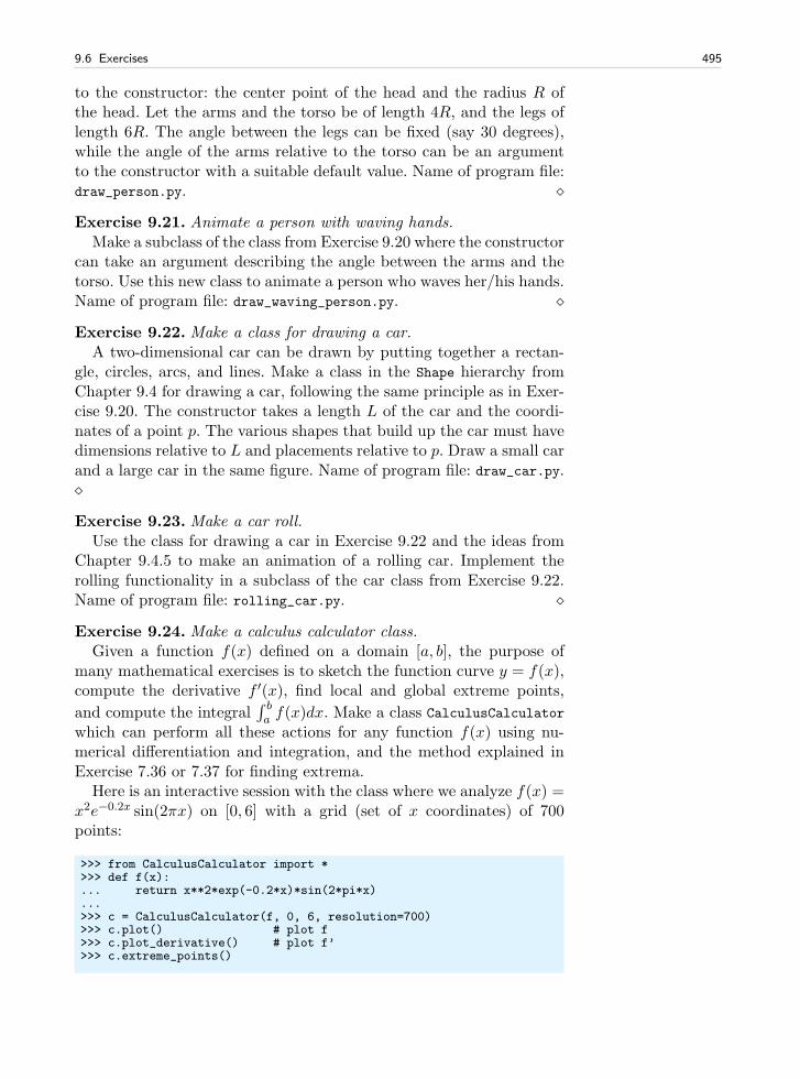
9.6 Exercises 495

to the constructor: the center point of the head and the radius R ofthe head. Let the arms and the torso be of length 4R, and the legs oflength 6R. The angle between the legs can be fixed (say 30 degrees),while the angle of the arms relative to the torso can be an argumentto the constructor with a suitable default value. Name of program file:draw_person.py. ⋄

Exercise 9.21. Animate a person with waving hands.Make a subclass of the class from Exercise 9.20 where the constructor

can take an argument describing the angle between the arms and thetorso. Use this new class to animate a person who waves her/his hands.Name of program file: draw_waving_person.py. ⋄

Exercise 9.22. Make a class for drawing a car.A two-dimensional car can be drawn by putting together a rectan-

gle, circles, arcs, and lines. Make a class in the Shape hierarchy fromChapter 9.4 for drawing a car, following the same principle as in Exer-cise 9.20. The constructor takes a length L of the car and the coordi-nates of a point p. The various shapes that build up the car must havedimensions relative to L and placements relative to p. Draw a small carand a large car in the same figure. Name of program file: draw_car.py.⋄

Exercise 9.23. Make a car roll.Use the class for drawing a car in Exercise 9.22 and the ideas from

Chapter 9.4.5 to make an animation of a rolling car. Implement therolling functionality in a subclass of the car class from Exercise 9.22.Name of program file: rolling_car.py. ⋄

Exercise 9.24. Make a calculus calculator class.Given a function f(x) defined on a domain [a, b], the purpose of

many mathematical exercises is to sketch the function curve y = f(x),compute the derivative f ′(x), find local and global extreme points,

and compute the integral∫ ba f(x)dx. Make a class CalculusCalculator

which can perform all these actions for any function f(x) using nu-merical differentiation and integration, and the method explained inExercise 7.36 or 7.37 for finding extrema.

Here is an interactive session with the class where we analyze f(x) =x2e−0.2x sin(2πx) on [0, 6] with a grid (set of x coordinates) of 700points:

>>> from CalculusCalculator import *>>> def f(x):... return x**2*exp(-0.2*x)*sin(2*pi*x)...>>> c = CalculusCalculator(f, 0, 6, resolution=700)>>> c.plot() # plot f>>> c.plot_derivative() # plot f’>>> c.extreme_points()

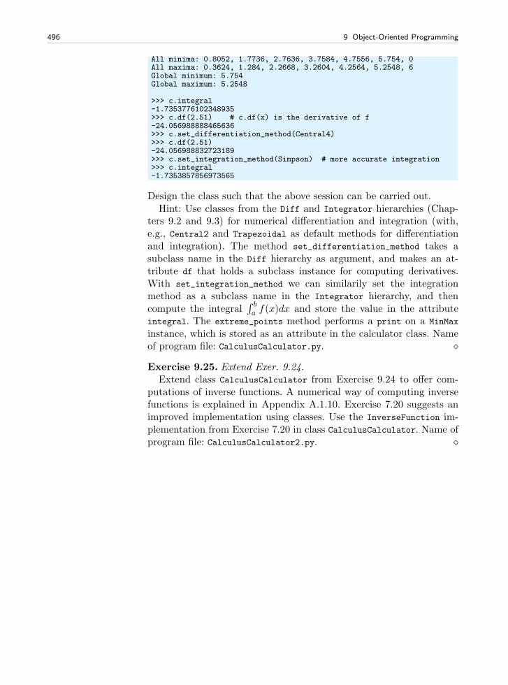
496 9 Object-Oriented Programming

All minima: 0.8052, 1.7736, 2.7636, 3.7584, 4.7556, 5.754, 0All maxima: 0.3624, 1.284, 2.2668, 3.2604, 4.2564, 5.2548, 6Global minimum: 5.754Global maximum: 5.2548

>>> c.integral-1.7353776102348935>>> c.df(2.51) # c.df(x) is the derivative of f-24.056988888465636>>> c.set_differentiation_method(Central4)>>> c.df(2.51)-24.056988832723189>>> c.set_integration_method(Simpson) # more accurate integration>>> c.integral-1.7353857856973565

Design the class such that the above session can be carried out.Hint: Use classes from the Diff and Integrator hierarchies (Chap-

ters 9.2 and 9.3) for numerical differentiation and integration (with,e.g., Central2 and Trapezoidal as default methods for differentiationand integration). The method set_differentiation_method takes asubclass name in the Diff hierarchy as argument, and makes an at-tribute df that holds a subclass instance for computing derivatives.With set_integration_method we can similarily set the integrationmethod as a subclass name in the Integrator hierarchy, and thencompute the integral

∫ ba f(x)dx and store the value in the attribute

integral. The extreme_points method performs a print on a MinMax

instance, which is stored as an attribute in the calculator class. Nameof program file: CalculusCalculator.py. ⋄

Exercise 9.25. Extend Exer. 9.24.Extend class CalculusCalculator from Exercise 9.24 to offer com-

putations of inverse functions. A numerical way of computing inversefunctions is explained in Appendix A.1.10. Exercise 7.20 suggests animproved implementation using classes. Use the InverseFunction im-plementation from Exercise 7.20 in class CalculusCalculator. Name ofprogram file: CalculusCalculator2.py. ⋄

Sequences and Difference Equations A

From mathematics you probably know the concept of a sequence, whichis nothing but a collection of numbers with a specific order. A generalsequence is written as

x0, x1, x2, . . . , xn, . . . ,

One example is the sequence of all odd numbers:

1, 3, 5, 7, . . . , 2n+ 1, . . .

For this sequence we have an explicit formula for the n-th term: 2n+1,and n takes on the values 0, 1, 2, . . .. We can write this sequence morecompactly as (xn)

∞n=0 with xn = 2n + 1. Other examples of infinite

sequences from mathematics are

1, 4, 9, 16, 25, . . . (xn)∞n=0, xn = (n+ 1)2, (A.1)

1,1

2,1

3,1

4, . . . (xn)

∞n=0, xn =

1

n+ 1. (A.2)

The former sequences are infinite, because they are generated fromall integers ≥ 0 and there are infinitely many such integers. Neverthe-less, most sequences from real life applications are finite. If you putan amount x0 of money in a bank, you will get an interest rate andtherefore have an amount x1 after one year, x2 after two years, and xNafter N years. This process results in a finite sequence of amounts

x0, x1, x2, . . . , xN , (xn)Nn=0 .

Usually we are interested in quite small N values (typically N ≤ 20−30). Anyway, the life of the bank is finite, so the sequence definitelyhas an end.

497

498 A Sequences and Difference Equations

For some sequences it is not so easy to set up a general formula forthe n-th term. Instead, it is easier to express a relation between two ormore consecutive elements. One example where we can do both thingsis the sequence of odd numbers. This sequence can alternatively begenerated by the formula

xn+1 = xn + 2 . (A.3)

To start the sequence, we need an initial condition where the value ofthe first element is specified:

x0 = 1 .

Relations like (A.3) between consecutive elements in a sequence iscalled recurrence relations or difference equations. Solving a differenceequation can be quite challenging in mathematics, but it is almost triv-ial to solve it on a computer. That is why difference equations are sowell suited for computer programming, and the present appendix isdevoted to this topic. Only programming concepts from Chapters 1–5are used in the material herein.

The program examples regarding difference equations are found inthe folder src/diffeq.

A.1 Mathematical Models Based on Difference Equations

The objective of science is to understand complex phenomena. Thephenomenon under consideration may be a part of nature, a group ofsocial individuals, the traffic situation in Los Angeles, and so forth. Thereason for addressing something in a scientific manner is that it appearsto be complex and hard to comprehend. A common scientific approachto gain understanding is to create a model of the phenomenon, anddiscuss the properties of the model instead of the phenomenon. Thebasic idea is that the model is easier to understand, but still complexenough to preserve the basic features of the problem at hand1. Mod-eling is, indeed, a general idea with applications far beyond science.Suppose, for instance, that you want to invite a friend to your homefor the first time. To assist your friend, you may send a map of yourneighborhood. Such a map is a model: It exposes the most importantlandmarks and leave out billions of details that your friend can do verywell without. This is the essence of modeling: A good model should beas simple as possible, but still rich enough to include the importantstructures you are looking for2.

1 “Essentially, all models are wrong, but some are useful.” –George E. P. Box, statis-tician, 1919-.

2 ”Everything should be made as simple as possible, but not simpler.” –Albert Ein-stein, physicist, 1879-1955.

A.1 Mathematical Models Based on Difference Equations 499

Certainly, the tools we apply to model a certain phenomenon differ alot in various scientific disciplines. In the natural sciences, mathematicshas gained a unique position as the key tool for formulating models.To establish a model, you need to understand the problem at handand describe it with mathematics. Usually, this process results in a setof equations, i.e., the model consists of equations that must be solvedin order to see how realistically the model describes a phenomenon.Difference equations represent one of the simplest yet most effectivetype of equations arising in mathematical models. The mathematics issimple and the programming is simple, thereby allowing us to focusmore on the modeling part. Below we will derive and solve differenceequations for diverse applications.

A.1.1 Interest Rates

Our first difference equation model concerns how much money an initialamount x0 will grow to after n years in a bank with annual interestrate p. You learned in school the formula

xn = x0

(

1 +p

100

)n. (A.4)

Unfortunately, this formula arises after some limiting assumptions, likethat of a constant interest rate over all the n years. Moreover, theformula only gives us the amount after each year, not after some monthsor days. It is much easier to compute with interest rates if we set upa more fundamental model in terms of a difference equation and thensolve this equation on a computer.

The fundamental model for interest rates is that an amount xn−1 atsome point of time tn−1 increases its value with p percent to an amountxn at a new point of time tn:

xn = xn−1 +p

100xn−1 . (A.5)

If n counts years, p is the annual interest rate, and if p is constant, wecan with some arithmetics derive the following solution to (A.5):

xn =(

1 +p

100

)

xn−1 =(

1 +p

100

)2xn−2 = . . . =

(

1 +p

100

)nx0 .

Instead of first deriving a formula for xn and then program this for-mula, we may attack the fundamental model (A.5) in a program(growth_years.py) and compute x1, x2, and so on in a loop:

from scitools.std import *x0 = 100 # initial amountp = 5 # interest rateN = 4 # number of yearsindex_set = range(N+1)

500 A Sequences and Difference Equations

x = zeros(len(index_set))

# Compute solutionx[0] = x0for n in index_set[1:]:

x[n] = x[n-1] + (p/100.0)*x[n-1]print xplot(index_set, x, ’ro’, xlabel=’years’, ylabel=’amount’)

The output of x is

[ 100. 105. 110.25 115.7625 121.550625]

Programmers of mathematical software who are trained in making pro-grams more efficient, will notice that it is not necessary to store all thexn values in an array or use a list with all the indices 0, 1, . . . , N . Justone integer for the index and two floats for xn and xn−1 are strictlynecessary. This can save quite some memory for large values of N .Exercise A.5 asks you to develop such a memory-efficient program.

Suppose now that we are interested in computing the growth ofmoney after N days instead. The interest rate per day is taken asr = p/D if p is the annual interest rate and D is the number of daysin a year. The fundamental model is the same, but now n counts daysand p is replaced by r:

xn = xn−1 +r

100xn−1 . (A.6)

A common method in international business is to choose D = 360, yetlet n count the exact number of days between two dates (see footnote onpage 152). Python has a module datetime for convenient calculationswith dates and times. To find the number of days between two dates,we perform the following operations:

>>> import datetime>>> date1 = datetime.date(2007, 8, 3) # Aug 3, 2007>>> date2 = datetime.date(2008, 8, 4) # Aug 4, 2008>>> diff = date2 - date1>>> print diff.days367

We can modify the previous program to compute with days instead ofyears:

from scitools.std import *x0 = 100 # initial amountp = 5 # annual interest rater = p/360.0 # daily interest rateimport datetimedate1 = datetime.date(2007, 8, 3)date2 = datetime.date(2011, 8, 3)diff = date2 - date1N = diff.daysindex_set = range(N+1)x = zeros(len(index_set))

# Compute solutionx[0] = x0

A.1 Mathematical Models Based on Difference Equations 501

for n in index_set[1:]:x[n] = x[n-1] + (r/100.0)*x[n-1]

print xplot(index_set, x, ’ro’, xlabel=’days’, ylabel=’amount’)

Running this program, called growth_days.py, prints out 122.5 as thefinal amount.

It is quite easy to adjust the formula (A.4) to the case where the in-terest is added every day instead of every year. However, the strengthof the model (A.6) and the associated program growth_days.py be-comes apparent when r varies in time – and this is what happens inreal life. In the model we can just write r(n) to explicitly indicate thedependence upon time. The corresponding time-dependent annual in-terest rate is what is normally specified, and p(n) is usually a piecewiseconstant function (the interest rate is changed at some specific datesand remains constant between these days). The construction of a cor-responding array p in a program, given the dates when p changes, canbe a bit tricky since we need to compute the number of days betweenthe dates of changes and index p properly. We do not dive into thesedetails now, but readers who want to compute p and who is ready forsome extra brain training and index puzzling can attack Exercise A.11.For now we assume that an array p holds the time-dependent annualinterest rates for each day in the total time period of interest. Thegrowth_days.py program then needs a slight modification, typically,

p = zeros(len(index_set))# set up p (might be challenging!)r = p/360.0 # daily interest rate...for n in index_set[1:]:

x[n] = x[n-1] + (r[n-1]/100.0)*x[n-1]

For the very simple (and not-so-relevant) case where p grows linearly(i.e., daily changes) from 4 to 6 percent over the period of interest,we have made a complete program in the file growth_days_timedep.py.You can compare a simulation with linearly varying p between 4 and6 and a simulation using the average p value 5 throughout the wholetime interval.

A difference equation with r(n) is quite difficult to solve mathemati-cally, but the n-dependence in r is easy to deal with in the computerizedsolution approach.

A.1.2 The Factorial as a Difference Equation

The difference equation

xn = nxn−1, x0 = 1 (A.7)

can quickly be solved recursively:

502 A Sequences and Difference Equations

xn = nxn−1

= n(n− 1)xn−2

= n(n− 1)(n− 2)xn−3

= n(n− 1)(n− 2) · · · 1 .

The result xn is nothing but the factorial of n, denoted as n! (cf. Ex-ercise 3.14). Equation (A.7) then gives a standard recipe to computen!.

A.1.3 Fibonacci Numbers

Every textbook with some material on sequences usually presents adifference equation for generating the famous Fibonacci numbers3:

xn = xn−1 + xn−2, x0 = 1, x1 = 1, n = 2, 3, . . . (A.8)

This equation has a relation between three elements in the sequence,not only two as in the other examples we have seen. We say that thisis a difference equation of second order, while the previous examplesinvolving two n levels are said to be difference equations of first or-der. The precise characterization of (A.8) is a homogeneous differenceequation of second order. Such classification is not important whencomputing the solution in a program, but for mathematical solutionmethods by pen and paper, the classification helps to determine whichmathematical technique to use to solve the problem.

A straightforward program for generating Fibonacci numbers takesthe form (fibonacci1.py):

import sysimport numpy as npN = int(sys.argv[1])x = np.zeros(N+1, int)x[0] = 1x[1] = 1for n in range(2, N+1):

x[n] = x[n-1] + x[n-2]print n, x[n]

Since xn is an infinite sequence we could try to run the program forvery large N . This causes two problems: The storage requirements ofthe x array may become too large for the computer, but long beforethis happens, xn grows in size far beyond the largest integer that canbe represented by int elements in arrays (the problem appears alreadyfor N = 50). A possibility is to use array elements of type int64, whichallows computation of twice as many numbers as with standard int

elements (see the program fibonacci1_int64.py). A better solution isto use float elements in the x array, despite the fact that the numbers

3 Fibonacci arrived at this equation when modelling rabbit populations.

A.1 Mathematical Models Based on Difference Equations 503

xn are integers. With float96 elements we can compute up to N =23600 (see the program fibinacci1_float.py).

The best solution goes as follows. We observe, as mentioned after thegrowth_years.py program and also explained in Exercise A.5, that weneed only three variables to generate the sequence. We can thereforework with just three standard int variables in Python:

import sysN = int(sys.argv[1])xnm1 = 1xnm2 = 1n = 2while n <= N:

xn = xnm1 + xnm2print ’x_%d = %d’ % (n, xn)xnm2 = xnm1xnm1 = xnn += 1

Here xnm1 denotes xn−1 and xnm2 denotes xn−2. To prepare for thenext pass in the loop, we must shuffle the xnm1 down to xnm2 and storethe new xn value in xnm1. The nice thing with int objects in Python(contrary to int elements in NumPy arrays) is that they can holdintegers of arbitrary size4. We may try a run with N set to 250:

x_2 = 2x_3 = 3x_4 = 5x_5 = 8x_6 = 13x_7 = 21x_8 = 34x_9 = 55x_10 = 89x_11 = 144x_12 = 233x_13 = 377x_14 = 610x_15 = 987x_16 = 1597...x_249 = 7896325826131730509282738943634332893686268675876375x_250 = 12776523572924732586037033894655031898659556447352249

In mathematics courses you learn how to derive a formula for then-th term in a Fibonacci sequence. This derivation is much more com-plicated than writing a simple program to generate the sequence, butthere is a lot of interesting mathematics both in the derivation and theresulting formula!

A.1.4 Growth of a Population

Let xn−1 be the number of individuals in a population at time tn−1. Thepopulation can consists of humans, animals, cells, or whatever objectswhere the number of births and deaths is proportional to the numberof individuals. Between time levels tn−1 and tn, bxn−1 individuals are

4 Note that int variables in other computer languages normally has a size limitationlike int elements in NumPy arrays.

504 A Sequences and Difference Equations

born, and dxn−1 individuals die, where b and d are constants. The netgrowth of the population is then (b− d)xn. Introducing r = (b− d)100for the net growth factor measured in percent, the new number ofindividuals become

xn = xn−1 +r

100xn−1 . (A.9)

This is the same difference equation as (A.5). It models growth ofpopulations quite well as long as there are optimal growing conditionsfor each individual. If not, one can adjust the model as explained inAppendix A.1.5.

To solve (A.9) we need to start out with a known size x0 of thepopulation. The b and d parameters depend on the time differencetn − tn−1, i.e., the values of b and d are smaller if n counts years thanif n counts generations.

A.1.5 Logistic Growth

The model (A.9) for the growth of a population leads to exponential in-crease in the number of individuals as implied by the solution A.4. Thesize of the population increases faster and faster as time n increases,and xn → ∞ when n → ∞. In real life, however, there is an upperlimit M of the number of individuals that can exist in the environmentat the same time. Lack of space and food, competition between indi-viduals, predators, and spreading of contagious diseases are exampleson factors that limit the growth. The number M is usually called thecarrying capacity of the environment, the maximum population whichis sustainable over time. With limited growth, the growth factor r mustdepend on time:

xn = xn−1 +r(n− 1)

100xn−1 . (A.10)

In the beginning of the growth process, there is enough resources andthe growth is exponential, but as xn approaches M , the growth stopsand r must tend to zero. A simple function r(n) with these propertiesis

r(n) = (

1− xnM

)

. (A.11)

For small n, xn ≪ M and r(n) ≈ , which is the growth rate withunlimited resources. As n → M , r(n) → 0 as we want. The model(A.11) is used for logistic growth. The corresponding logistic differenceequation becomes

xn = xn−1 +

100xn−1

(

1− xn−1

M

)

. (A.12)

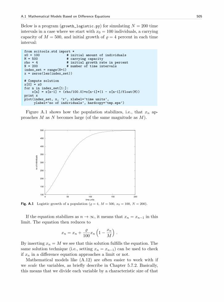
A.1 Mathematical Models Based on Difference Equations 505

Below is a program (growth_logistic.py) for simulating N = 200 timeintervals in a case where we start with x0 = 100 individuals, a carryingcapacity of M = 500, and initial growth of = 4 percent in each timeinterval:

from scitools.std import *x0 = 100 # initial amount of individualsM = 500 # carrying capacityrho = 4 # initial growth rate in percentN = 200 # number of time intervalsindex_set = range(N+1)x = zeros(len(index_set))

# Compute solutionx[0] = x0for n in index_set[1:]:

x[n] = x[n-1] + (rho/100.0)*x[n-1]*(1 - x[n-1]/float(M))print xplot(index_set, x, ’r’, xlabel=’time units’,

ylabel=’no of individuals’, hardcopy=’tmp.eps’)

Figure A.1 shows how the population stabilizes, i.e., that xn ap-proaches M as N becomes large (of the same magnitude as M).

100

150

200

250

300

350

400

450

500

0 50 100 150 200

no o

f in

div

iduals

time units

Fig. A.1 Logistic growth of a population ( = 4, M = 500, x0 = 100, N = 200).

If the equation stabilizes as n→∞, it means that xn = xn−1 in thislimit. The equation then reduces to

xn = xn +

100xn

(

1− xnM

)

.

By inserting xn = M we see that this solution fulfills the equation. Thesame solution technique (i.e., setting xn = xn−1) can be used to checkif xn in a difference equation approaches a limit or not.

Mathematical models like (A.12) are often easier to work with ifwe scale the variables, as briefly describe in Chapter 5.7.2. Basically,this means that we divide each variable by a characteristic size of that

506 A Sequences and Difference Equations

variable such that the value of the new variable is typically 1. In thepresent case we can scale xn by M and introduce a new variable,

yn =xnM

.

Similarly, x0 is replaced by y0 = x0/M . Inserting xn = Myn in (A.12)and dividing by M gives

yn = yn−1 + qyn−1 (1− yn−1) , (A.13)

where q = /100 is introduced to save typing. Equation (A.13) is sim-pler than (A.12) in that the solution lies approximately between5 y0and 1, and there are only two dimensionless input paramters to careabout: q and y0. To solve (A.12) we need knowledge of three parame-ters: x0, , and M .

A.1.6 Payback of a Loan

A loan L is to be paid back over N months. The payback in a monthconsists of the fraction L/N plus the interest increase of the loan.Let the annual interest rate for the loan be p percent. The monthlyinterest rate is then p

12 . The value of the loan after month n is xn, andthe change from xn−1 can be modeled as

xn = xn−1 +p

12 · 100xn−1 −(

p

12 · 100xn−1 +L

N

)

, (A.14)

= xn−1 −L

N, (A.15)

for n = 1, . . . , N . The initial condition is x0 = L. A major differencebetween (A.15) and (A.6) is that all terms in the latter are proportionalto xn or xn−1, while (A.15) also contains a constant term (L/N). Wesay that (A.6) is homogeneous and linear, while (A.15) is inhomoge-neous (because of the constant term) and linear. The mathematicalsolution of inhomogeneous equations are more difficult to find thanthe solution of homogeneous equations, but in a program there is nobig difference: We just add the extra term −L/N in the formula forthe difference equation.

The solution of (A.15) is not particularly exciting6. What is moreinteresting, is what we pay each month, yn. We can keep track of bothyn and xn in a variant of the previous model:

5 Values larger than 1 can occur, see Exercise A.21.6 Use (A.15) repeatedly to derive the solution xn = L− nL/N .

A.1 Mathematical Models Based on Difference Equations 507

yn =p

12 · 100xn−1 +L

N, (A.16)

xn = xn−1 +p

12 · 100xn−1 − yn . (A.17)

Equations (A.16)–(A.17) is a system of difference equations. In a com-puter code, we simply update yn first, and then we update xn, insidea loop over n. Exercise A.6 asks you to do this.

A.1.7 Taylor Series as a Difference Equation

Consider the following system of two difference equations

en = en−1 + an−1, (A.18)

an =x

nan−1, (A.19)

with initial conditions e0 = 0 and a0 = 1. We can start to nest thesolution:

e1 = 0 + a0 = 0 + 1 = 1,

a1 = x,

e2 = e1 + a1 = 1 + x,

a2 =x

2a1 =

x2

2,

e3 = e2 + a1 = 1 + x+x2

2,

e4 = 1 + x+x2

2+

x3

3 · 2 ,

e5 = 1 + x+x2

2+

x3

3 · 2 +x4

4 · 3 · 2The observant reader who has heard about Taylor series (see Chap-ter B.4) will recognize this as the Taylor series of ex:

ex =

∞∑

n=0

xn

n!. (A.20)

How do we derive a system like (A.18)–(A.19) for computing theTaylor polynomial approximation to ex? The starting point is the sum∑∞

n=0xn

n! . This sum is coded by adding new terms to an accumulationvariable in a loop. The mathematical counterpart to this code is adifference equation

en+1 = en +xn

n!, e0 = 0, n = 0, 1, 2, . . . . (A.21)

or equivalently (just replace n by n− 1):

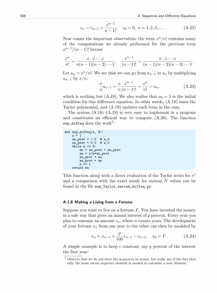
508 A Sequences and Difference Equations

en = en−1 +xn−1

n− 1!, e0 = 0, n = 1, 2, 3, . . . . (A.22)

Now comes the important observation: the term xn/n! contains manyof the computations we already performed for the previous termxn−1/(n− 1)! becase

xn

n!=

x · x · · ·xn(n− 1)(n− 2) · · · 1 ,

xn−1

(n− 1)!=

x · x · · · x(n− 1)(n− 2)(n− 3) · · · 1 .

Let an = xn/n!. We see that we can go from an−1 to an by multiplyingan−1 by x/n:

x

nan−1 =

x

n

xn−1

(n− 1)!=

xn

n!= an, (A.23)

which is nothing but (A.19). We also realize that a0 = 1 is the initialcondition for this difference equation. In other words, (A.18) sums theTaylor polynomial, and (A.19) updates each term in the sum.

The system (A.18)–(A.19) is very easy to implement in a programand constitutes an efficient way to compute (A.20). The functionexp_diffeq does the work7:

def exp_diffeq(x, N):n = 1an_prev = 1.0 # a_0en_prev = 0.0 # e_0while n <= N:

en = en_prev + an_prevan = x/n*an_preven_prev = enan_prev = ann += 1

return en

This function along with a direct evaluation of the Taylor series for ex

and a comparison with the exact result for various N values can befound in the file exp_Taylor_series_diffeq.py.

A.1.8 Making a Living from a Fortune

Suppose you want to live on a fortune F . You have invested the moneyin a safe way that gives an annual interest of p percent. Every year youplan to consume an amount cn, where n counts years. The developmentof your fortune xn from one year to the other can then be modeled by

xn = xn−1 +p

100xn−1 − cn−1, x0 = F . (A.24)

A simple example is to keep c constant, say q percent of the interestthe first year:

7 Observe that we do not store the sequences in arrays, but make use of the fact thatonly the most recent sequence element is needed to calculate a new element.

A.1 Mathematical Models Based on Difference Equations 509

xn = xn−1 +p

100xn−1 −

pq

104F, x0 = F . (A.25)

A more realistic model is to assume some inflation of I percent peryear. You will then like to increase cn by the inflation. We can extendthe model in two ways. The simplest and clearest way, in the author’sopinion, is to track the evolution of two sequences xn and cn:

xn = xn−1 +p

100xn−1 − cn−1, x0 = F, c0 =

pq

104F, (A.26)

cn = cn−1 +I

100cn−1 . (A.27)

This is a system of two difference equations with two unknowns. Thesolution method is, nevertheless, not much more complicated than themethod for a difference equation in one unknown, since we can firstcompute xn from (A.26) and then update the cn value from (A.27).You are encouraged to write the program (see Exercise A.7).

Another way of making a difference equation for the case with infla-tion, is to use an explicit formula for cn−1, i.e., solve (A.26) and endup with a formula like (A.4). Then we can insert the explicit formula

cn−1 =

(

1 +I

100

)n−1 pq

104F

in (A.24), resulting in only one difference equation to solve.

A.1.9 Newton’s Method

The difference equation

xn = xn−1 −f(xn−1)

f ′(xn−1), x0 given, (A.28)

generates a sequence xn where, if the sequence converges (i.e., ifxn − xn−1 → 0), xn approaches a root of f(x). That is, xn → x,where x solves the equation f(x) = 0. Equation (A.28) is the famousNewton’s method for solving nonlinear algebraic equations f(x) = 0.When f(x) is not linear, i.e., f(x) is not on the form ax+ b with con-stant a and b, (A.28) becomes a nonlinear difference equation. Thiscomplicates analytical treatment of difference equations, but poses noextra difficulties for numerical solution.

We can quickly sketch the derivation of (A.28). Suppose we want tosolve the equation

f(x) = 0

and that we already have an approximate solution xn−1. If f(x) werelinear, f(x) = ax+b, it would be very easy to solve f(x) = 0: x = −b/a.The idea is therefore to approximate f(x) in the vicinity of x = xn−1

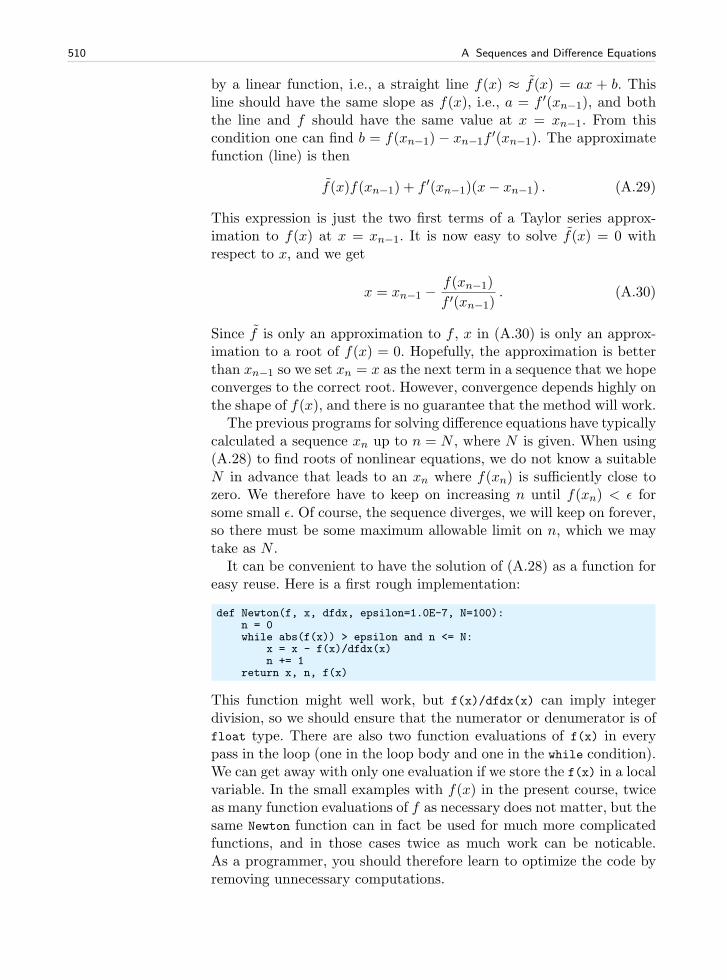
510 A Sequences and Difference Equations

by a linear function, i.e., a straight line f(x) ≈ f(x) = ax + b. Thisline should have the same slope as f(x), i.e., a = f ′(xn−1), and boththe line and f should have the same value at x = xn−1. From thiscondition one can find b = f(xn−1) − xn−1f

′(xn−1). The approximatefunction (line) is then

f(x)f(xn−1) + f ′(xn−1)(x− xn−1) . (A.29)

This expression is just the two first terms of a Taylor series approx-imation to f(x) at x = xn−1. It is now easy to solve f(x) = 0 withrespect to x, and we get

x = xn−1 −f(xn−1)

f ′(xn−1). (A.30)

Since f is only an approximation to f , x in (A.30) is only an approx-imation to a root of f(x) = 0. Hopefully, the approximation is betterthan xn−1 so we set xn = x as the next term in a sequence that we hopeconverges to the correct root. However, convergence depends highly onthe shape of f(x), and there is no guarantee that the method will work.

The previous programs for solving difference equations have typicallycalculated a sequence xn up to n = N , where N is given. When using(A.28) to find roots of nonlinear equations, we do not know a suitableN in advance that leads to an xn where f(xn) is sufficiently close tozero. We therefore have to keep on increasing n until f(xn) < ǫ forsome small ǫ. Of course, the sequence diverges, we will keep on forever,so there must be some maximum allowable limit on n, which we maytake as N .

It can be convenient to have the solution of (A.28) as a function foreasy reuse. Here is a first rough implementation:

def Newton(f, x, dfdx, epsilon=1.0E-7, N=100):n = 0while abs(f(x)) > epsilon and n <= N:

x = x - f(x)/dfdx(x)n += 1

return x, n, f(x)

This function might well work, but f(x)/dfdx(x) can imply integerdivision, so we should ensure that the numerator or denumerator is offloat type. There are also two function evaluations of f(x) in everypass in the loop (one in the loop body and one in the while condition).We can get away with only one evaluation if we store the f(x) in a localvariable. In the small examples with f(x) in the present course, twiceas many function evaluations of f as necessary does not matter, but thesame Newton function can in fact be used for much more complicatedfunctions, and in those cases twice as much work can be noticable.As a programmer, you should therefore learn to optimize the code byremoving unnecessary computations.

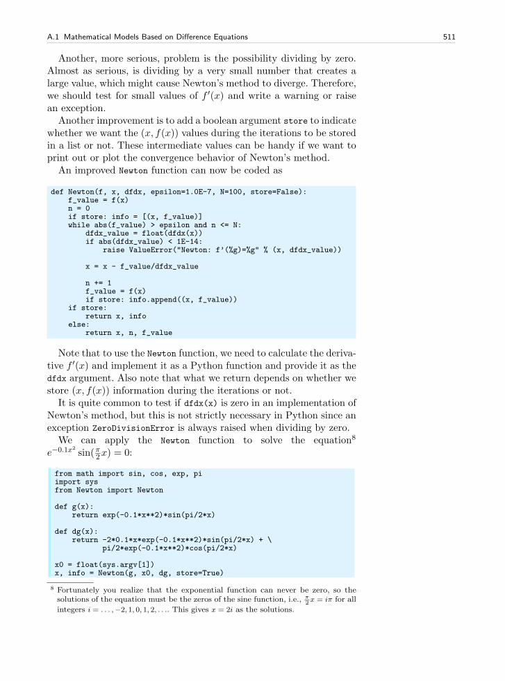
A.1 Mathematical Models Based on Difference Equations 511

Another, more serious, problem is the possibility dividing by zero.Almost as serious, is dividing by a very small number that creates alarge value, which might cause Newton’s method to diverge. Therefore,we should test for small values of f ′(x) and write a warning or raisean exception.

Another improvement is to add a boolean argument store to indicatewhether we want the (x, f(x)) values during the iterations to be storedin a list or not. These intermediate values can be handy if we want toprint out or plot the convergence behavior of Newton’s method.

An improved Newton function can now be coded as

def Newton(f, x, dfdx, epsilon=1.0E-7, N=100, store=False):f_value = f(x)n = 0if store: info = [(x, f_value)]while abs(f_value) > epsilon and n <= N:

dfdx_value = float(dfdx(x))if abs(dfdx_value) < 1E-14:

raise ValueError("Newton: f’(%g)=%g" % (x, dfdx_value))

x = x - f_value/dfdx_value

n += 1f_value = f(x)if store: info.append((x, f_value))

if store:return x, info

else:return x, n, f_value

Note that to use the Newton function, we need to calculate the deriva-tive f ′(x) and implement it as a Python function and provide it as thedfdx argument. Also note that what we return depends on whether westore (x, f(x)) information during the iterations or not.

It is quite common to test if dfdx(x) is zero in an implementation ofNewton’s method, but this is not strictly necessary in Python since anexception ZeroDivisionError is always raised when dividing by zero.

We can apply the Newton function to solve the equation8

e−0.1x2

sin(π2x) = 0:

from math import sin, cos, exp, piimport sysfrom Newton import Newton

def g(x):return exp(-0.1*x**2)*sin(pi/2*x)

def dg(x):return -2*0.1*x*exp(-0.1*x**2)*sin(pi/2*x) + \

pi/2*exp(-0.1*x**2)*cos(pi/2*x)

x0 = float(sys.argv[1])x, info = Newton(g, x0, dg, store=True)

8 Fortunately you realize that the exponential function can never be zero, so thesolutions of the equation must be the zeros of the sine function, i.e., π

2x = iπ for all

integers i = . . . ,−2, 1, 0, 1, 2, . . .. This gives x = 2i as the solutions.

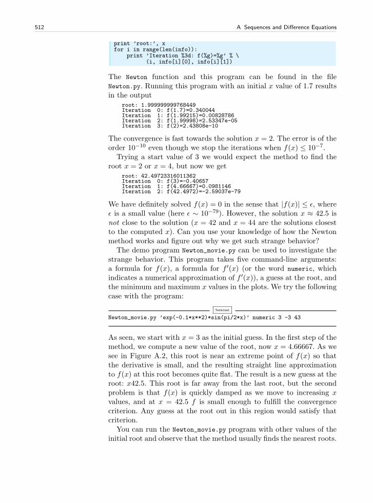
512 A Sequences and Difference Equations

print ’root:’, xfor i in range(len(info)):

print ’Iteration %3d: f(%g)=%g’ % \(i, info[i][0], info[i][1])

The Newton function and this program can be found in the fileNewton.py. Running this program with an initial x value of 1.7 resultsin the output

root: 1.999999999768449Iteration 0: f(1.7)=0.340044Iteration 1: f(1.99215)=0.00828786Iteration 2: f(1.99998)=2.53347e-05Iteration 3: f(2)=2.43808e-10

The convergence is fast towards the solution x = 2. The error is of theorder 10−10 even though we stop the iterations when f(x) ≤ 10−7.

Trying a start value of 3 we would expect the method to find theroot x = 2 or x = 4, but now we get

root: 42.49723316011362Iteration 0: f(3)=-0.40657Iteration 1: f(4.66667)=0.0981146Iteration 2: f(42.4972)=-2.59037e-79

We have definitely solved f(x) = 0 in the sense that |f(x)| ≤ ǫ, whereǫ is a small value (here ǫ ∼ 10−79). However, the solution x ≈ 42.5 isnot close to the solution (x = 42 and x = 44 are the solutions closestto the computed x). Can you use your knowledge of how the Newtonmethod works and figure out why we get such strange behavior?

The demo program Newton_movie.py can be used to investigate thestrange behavior. This program takes five command-line arguments:a formula for f(x), a formula for f ′(x) (or the word numeric, whichindicates a numerical approximation of f ′(x)), a guess at the root, andthe minimum and maximum x values in the plots. We try the followingcase with the program:

Terminal

Newton_movie.py ’exp(-0.1*x**2)*sin(pi/2*x)’ numeric 3 -3 43

As seen, we start with x = 3 as the initial guess. In the first step of themethod, we compute a new value of the root, now x = 4.66667. As wesee in Figure A.2, this root is near an extreme point of f(x) so thatthe derivative is small, and the resulting straight line approximationto f(x) at this root becomes quite flat. The result is a new guess at theroot: x42.5. This root is far away from the last root, but the secondproblem is that f(x) is quickly damped as we move to increasing xvalues, and at x = 42.5 f is small enough to fulfill the convergencecriterion. Any guess at the root out in this region would satisfy thatcriterion.

You can run the Newton_movie.py program with other values of theinitial root and observe that the method usually finds the nearest roots.

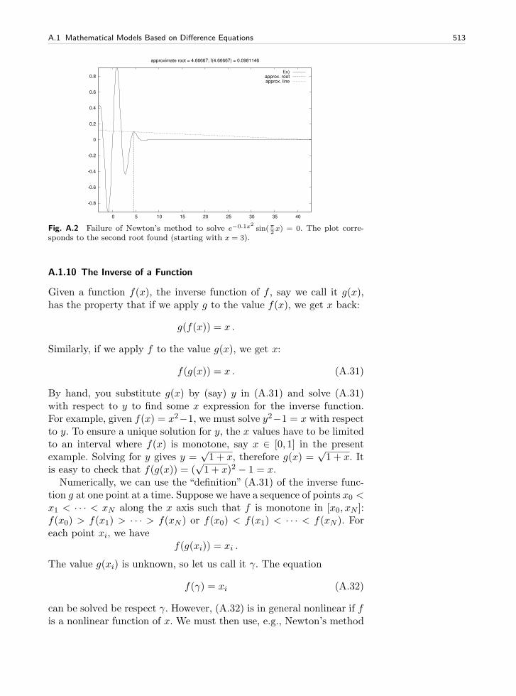
A.1 Mathematical Models Based on Difference Equations 513

-0.8

-0.6

-0.4

-0.2

0

0.2

0.4

0.6

0.8

0 5 10 15 20 25 30 35 40

approximate root = 4.66667; f(4.66667) = 0.0981146

f(x)approx. rootapprox. line

Fig. A.2 Failure of Newton’s method to solve e−0.1x2

sin(π2x) = 0. The plot corre-

sponds to the second root found (starting with x = 3).

A.1.10 The Inverse of a Function

Given a function f(x), the inverse function of f , say we call it g(x),has the property that if we apply g to the value f(x), we get x back:

g(f(x)) = x .

Similarly, if we apply f to the value g(x), we get x:

f(g(x)) = x . (A.31)

By hand, you substitute g(x) by (say) y in (A.31) and solve (A.31)with respect to y to find some x expression for the inverse function.For example, given f(x) = x2−1, we must solve y2−1 = x with respectto y. To ensure a unique solution for y, the x values have to be limitedto an interval where f(x) is monotone, say x ∈ [0, 1] in the presentexample. Solving for y gives y =

√1 + x, therefore g(x) =

√1 + x. It

is easy to check that f(g(x)) = (√1 + x)2 − 1 = x.

Numerically, we can use the “definition” (A.31) of the inverse func-tion g at one point at a time. Suppose we have a sequence of points x0 <x1 < · · · < xN along the x axis such that f is monotone in [x0, xN ]:f(x0) > f(x1) > · · · > f(xN ) or f(x0) < f(x1) < · · · < f(xN ). Foreach point xi, we have

f(g(xi)) = xi .

The value g(xi) is unknown, so let us call it γ. The equation

f(γ) = xi (A.32)

can be solved be respect γ. However, (A.32) is in general nonlinear if fis a nonlinear function of x. We must then use, e.g., Newton’s method

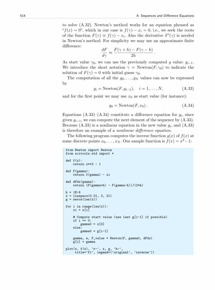
514 A Sequences and Difference Equations

to solve (A.32). Newton’s method works for an equation phrased as“f(x) = 0”, which in our case is f(γ) − xi = 0, i.e., we seek the rootsof the function F (γ) ≡ f(γ) − xi. Also the derivative F ′(γ) is neededin Newton’s method. For simplicity we may use an approximate finitedifference:

dF

dγ≈ F (γ + h)− F (γ − h)

2h.

As start value γ0, we can use the previously computed g value: gi−1.We introduce the short notation γ = Newton(F, γ0) to indicate thesolution of F (γ) = 0 with initial guess γ0.

The computation of all the g0, . . . , gN values can now be expressedby

gi = Newton(F, gi−1), i = 1, . . . , N, (A.33)

and for the first point we may use x0 as start value (for instance):

g0 = Newton(F, x0) . (A.34)

Equations (A.33)–(A.34) constitute a difference equation for gi, sincegiven gi−1, we can compute the next element of the sequence by (A.33).Because (A.33) is a nonlinear equation in the new value gi, and (A.33)is therefore an example of a nonlinear difference equation.

The following program computes the inverse function g(x) of f(x) atsome discrete points x0, . . . , xN . Our sample function is f(x) = x2−1:

from Newton import Newtonfrom scitools.std import *

def f(x):return x**2 - 1

def F(gamma):return f(gamma) - xi

def dFdx(gamma):return (F(gamma+h) - F(gamma-h))/(2*h)

h = 1E-6x = linspace(0.01, 3, 21)g = zeros(len(x))

for i in range(len(x)):xi = x[i]

# Compute start value (use last g[i-1] if possible)if i == 0:

gamma0 = x[0]else:

gamma0 = g[i-1]

gamma, n, F_value = Newton(F, gamma0, dFdx)g[i] = gamma

plot(x, f(x), ’r-’, x, g, ’b-’,title=’f1’, legend=(’original’, ’inverse’))

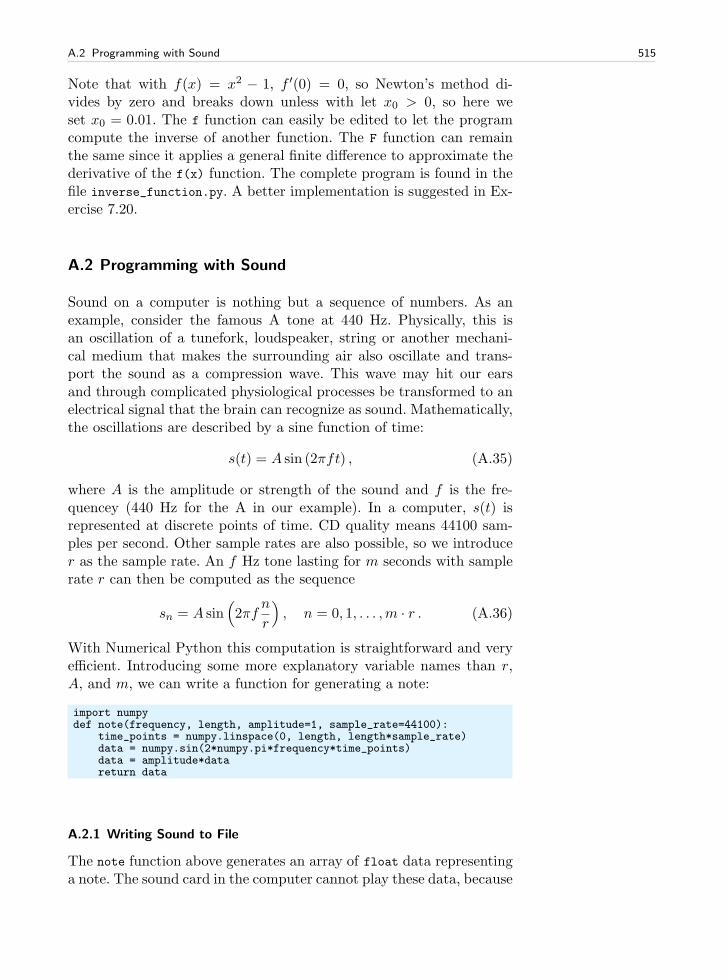
A.2 Programming with Sound 515

Note that with f(x) = x2 − 1, f ′(0) = 0, so Newton’s method di-vides by zero and breaks down unless with let x0 > 0, so here weset x0 = 0.01. The f function can easily be edited to let the programcompute the inverse of another function. The F function can remainthe same since it applies a general finite difference to approximate thederivative of the f(x) function. The complete program is found in thefile inverse_function.py. A better implementation is suggested in Ex-ercise 7.20.

A.2 Programming with Sound

Sound on a computer is nothing but a sequence of numbers. As anexample, consider the famous A tone at 440 Hz. Physically, this isan oscillation of a tunefork, loudspeaker, string or another mechani-cal medium that makes the surrounding air also oscillate and trans-port the sound as a compression wave. This wave may hit our earsand through complicated physiological processes be transformed to anelectrical signal that the brain can recognize as sound. Mathematically,the oscillations are described by a sine function of time:

s(t) = A sin (2πft) , (A.35)

where A is the amplitude or strength of the sound and f is the fre-quencey (440 Hz for the A in our example). In a computer, s(t) isrepresented at discrete points of time. CD quality means 44100 sam-ples per second. Other sample rates are also possible, so we introducer as the sample rate. An f Hz tone lasting for m seconds with samplerate r can then be computed as the sequence

sn = A sin(

2πfn

r

)

, n = 0, 1, . . . ,m · r . (A.36)

With Numerical Python this computation is straightforward and veryefficient. Introducing some more explanatory variable names than r,A, and m, we can write a function for generating a note:

import numpydef note(frequency, length, amplitude=1, sample_rate=44100):

time_points = numpy.linspace(0, length, length*sample_rate)data = numpy.sin(2*numpy.pi*frequency*time_points)data = amplitude*datareturn data

A.2.1 Writing Sound to File

The note function above generates an array of float data representinga note. The sound card in the computer cannot play these data, because

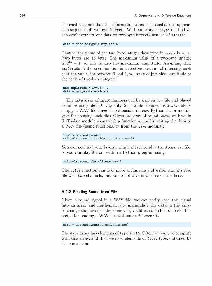
516 A Sequences and Difference Equations

the card assumes that the information about the oscillations appearsas a sequence of two-byte integers. With an array’s astype method wecan easily convert our data to two-byte integers instead of floats:

data = data.astype(numpy.int16)

That is, the name of the two-byte integer data type in numpy is int16

(two bytes are 16 bits). The maximum value of a two-byte integeris 215 − 1, so this is also the maximum amplitude. Assuming thatamplitude in the note function is a relative measure of intensity, suchthat the value lies between 0 and 1, we must adjust this amplitude tothe scale of two-byte integers:

max_amplitude = 2**15 - 1data = max_amplitude*data

The data array of int16 numbers can be written to a file and playedas an ordinary file in CD quality. Such a file is known as a wave file orsimply a WAV file since the extension is .wav. Python has a modulewave for creating such files. Given an array of sound, data, we have inSciTools a module sound with a function write for writing the data toa WAV file (using functionality from the wave module):

import scitools.soundscitools.sound.write(data, ’Atone.wav’)

You can now use your favorite music player to play the Atone.wav file,or you can play it from within a Python program using

scitools.sound.play(’Atone.wav’)

The write function can take more arguments and write, e.g., a stereofile with two channels, but we do not dive into these details here.

A.2.2 Reading Sound from File

Given a sound signal in a WAV file, we can easily read this signalinto an array and mathematically manipulate the data in the arrayto change the flavor of the sound, e.g., add echo, treble, or bass. Therecipe for reading a WAV file with name filename is

data = scitools.sound.read(filename)

The data array has elements of type int16. Often we want to computewith this array, and then we need elements of float type, obtained bythe conversion

A.2 Programming with Sound 517

data = data.astype(float)

The write function automatically transforms the element type back toint16 if we have not done this explicitly.

One operation that we can easily do is adding an echo. Mathemat-ically this means that we add a damped delayed sound, where theoriginal sound has weight β and the delayed part has weight 1 − β,such that the overall amplitude is not altered. Let d be the delay inseconds. With a sampling rate r the number of indices in the delaybecomes dr, which we denote by b. Given an original sound sequencesn, the sound with echo is the sequence

en = βsn + (1− β)sn−b . (A.37)

We cannot start n at 0 since e0 = s0−b = s−b which is a value outsidethe sound data. Therefore we define en = sn for n = 0, 1, . . . , b, and addthe echo thereafter. A simple loop can do this (again we use descriptivevariable names instead of the mathematical symbols introduced):

def add_echo(data, beta=0.8, delay=0.002, sample_rate=44100):newdata = data.copy()shift = int(delay*sample_rate) # b (math symbol)for i in range(shift, len(data)):

newdata[i] = beta*data[i] + (1-beta)*data[i-shift]return newdata

The problem with this function is that it runs slowly, especially whenwe have sound clips lasting several seconds (recall that for CD qualitywe need 44100 numbers per second). It is therefore necessary to vec-torize the implementation of the difference equation for adding echo.The update is then based on adding slices:

newdata[shift:] = beta*data[shift:] + \(1-beta)*data[:len(data)-shift]

A.2.3 Playing Many Notes

How do we generate a melody mathematically in a computer program?With the note function we can generate a note with a certain ampli-tude, frequence, and duration. The note is represented as an array.Putting sound arrays for different notes after each other will make upa melody. If we have several sound arrays data1, data2, data3, . . ., wecan make a new array consisting of the elements in the first array fol-lowed by the elements of the next array followed by the elements inthe next array and so forth:

518 A Sequences and Difference Equations

data = numpy.concatenate((data1, data2, data3, ...))

Here is an example of creating a little melody (start of “NothingElse Matters” by Metallica) using constant (max) amplitude of all thenotes:

E1 = note(164.81, .5)G = note(392, .5)B = note(493.88, .5)E2 = note(659.26, .5)intro = numpy.concatenate((E1, G, B, E2, B, G))high1_long = note(987.77, 1)high1_short = note(987.77, .5)high2 = note(1046.50, .5)high3 = note(880, .5)high4_long = note(659.26, 1)high4_medium = note(659.26, .5)high4_short = note(659.26, .25)high5 = note(739.99, .25)pause_long = note(0, .5)pause_short = note(0, .25)song = numpy.concatenate((intro, intro, high1_long, pause_long, high1_long,pause_long, pause_long,high1_short, high2, high1_short, high3, high1_short,high3, high4_short, pause_short, high4_long, pause_short,high4_medium, high5, high4_short))

scitools.sound.play(song)scitools.sound.write(song, ’tmp.wav’)

We could send song to the add_echo function to get some echo, andwe could also vary the amplitudes to get more dynamics into thesong. You can find the generation of notes above as the functionNothing_Else_Matters(echo=False) in the scitools.sound module.

A.2.4 Music of a Sequence

Problem. The purpose of this example is to listen to the sound gen-erated by two mathematical sequences. The first one is given by anexplicit formula, constructed to oscillate around 0 with decreasing am-plitude:

xn = e−4n/N sin(8πn/N) . (A.38)

The other sequence is generated by the difference equation (A.13) forlogistic growth, repeated here for convenience:

xn = xn−1 + qxn−1 (1− xn−1) , x = x0 . (A.39)

We let x0 = 0.01 and q = 2. This leads to fast initial growth toward thelimit 1, and then oscillations around this limit (this problem is studiedin Exercise A.21).

The absolute value of the sequence elements xn are of size between0 and 1, approximately. We want to transform these sequence elementsto tones, using the techniques of Appendix A.2. First we convert xn to

A.2 Programming with Sound 519

a frequency the human ear can hear. The transformation

yn = 440 + 200xn (A.40)

will make a standard A reference tone out of xn = 0, and for themaximum value of xn around 1 we get a tone of 640 Hz. Elements of thesequence generated by (A.38) lie between -1 and 1, so the correspondingfrequences lie between 240 Hz and 640 Hz. The task now is to make aprogram that can generate and play the sounds.

Solution. Tones can be generated by the note function from thescitools.sound module. We collect all tones corresponding to all theyn frequencies in a list tones. Letting N denote the number of sequenceelements, the relevant code segment reads

from scitools.sound import *freqs = 440 + x*200tones = []duration = 30.0/N # 30 sec sound in totalfor n in range(N+1):

tones.append(max_amplitude*note(freqs[n], duration, 1))data = concatenate(tones)write(data, filename)data = read(filename)play(filename)

It is illustrating to plot the sequences too,

plot(range(N+1), freqs, ’ro’)

To generate the sequences (A.38) and (A.39), we make two func-tions, oscillations and logistic, respectively. These functions takethe number of sequence elements (N) as input and return the sequencestored in an array.

In another function make_sound we compute the sequence, transformthe elements to frequencies, generate tones, write the tones to file, andplay the sound file.

As always, we collect the functions in a module and include a testblock where we can read the choice of sequence and the sequence lengthfrom the command line. The complete module file look as follows:

from scitools.sound import *from scitools.std import *

def oscillations(N):x = zeros(N+1)for n in range(N+1):

x[n] = exp(-4*n/float(N))*sin(8*pi*n/float(N))return x

def logistic(N):x = zeros(N+1)x[0] = 0.01q = 2for n in range(1, N+1):

520 A Sequences and Difference Equations

x[n] = x[n-1] + q*x[n-1]*(1 - x[n-1])return x

def make_sound(N, seqtype):filename = ’tmp.wav’x = eval(seqtype)(N)# Convert x values to frequences around 440freqs = 440 + x*200plot(range(N+1), freqs, ’ro’)# Generate tonestones = []duration = 30.0/N # 30 sec sound in totalfor n in range(N+1):

tones.append(max_amplitude*note(freqs[n], duration, 1))data = concatenate(tones)write(data, filename)data = read(filename)play(filename)

if __name__ == ’__main__’:try:

seqtype = sys.argv[1]N = int(sys.argv[2])

except IndexError:print ’Usage: %s oscillations|logistic N’ % sys.argv[0]sys.exit(1)

make_sound(N, seqtype)

This code should be quite easy to read at the present stage in the book.However, there is one statement that deserves a comment:

x = eval(seqtype)(N)

The seqtype argument reflects the type of sequence and is a string thatthe user provides on the command line. The values of the string equalthe function names oscillations and logistic. With eval(seqtype)

we turn the string into a function name. For example, if seqtype is’logistic’, performing an eval(seqtype)(N) is the same as if we hadwritten logistic(N). This technique allows the user of the program tochoose a function call inside the code. Without eval we would need toexplicitly test on values:

if seqtype == ’logistic’:x = logistic(N)

elif seqtype == ’oscillations’:x = oscillations(N)

This is not much extra code to write in the present example, but if wehave a large number of functions generating sequences, we can save alot of boring if-else code by using the eval construction.

The next step, as a reader who have understood the problem andthe implementation above, is to run the program for two cases: theoscillations sequence with N = 40 and the logistic sequence withN = 100. By altering the q parameter to lower values, you get othersounds, typically quite boring sounds for non-oscillating logistic growth(q < 1). You can also experiment with other transformations of theform (A.40), e.g., increasing the frequency variation from 200 to 400.

A.3 Exercises 521

A.3 Exercises

Exercise A.1. Determine the limit of a sequence.Given the sequence

an =7 + 1/n

3− 1/n2,

make a program that computes and prints out an for n = 1, 2, . . . , N .Read N from the command line. Does an approach a finite limit whenn→∞? Name of program file: sequence_limit1.py. ⋄

Exercise A.2. Determine the limit of a sequence.Solve Exercise A.1 when the sequence of interest is given by

Dn =sin(2−n)

2−n.

Name of program file: sequence_limit2.py. ⋄

Exercise A.3. Experience convergence problems.Given the sequence

Dn =f(x+ h)− f(x)

h, h = 2−n (A.41)

make a function D(f, x, N) that takes a function f(x), a value x, andthe number N of terms in the sequence as arguments, and returns anarray with the Dn values for n = 0, 1, . . . , N − 1. Make a call to the D

function with f(x) = sinx, x = 0, and N = 80. Plot the evolution ofthe computed Dn values, using small circles for the data points.

Make another call to D where x = π and plot this sequence in aseparate figure. What would be your expected limit? Why do the com-putations go wrong for large N? (Hint: Print out the numerator anddenominator in Dn.) Name of program file: sequence_limits3.py. ⋄

Exercise A.4. Convergence of sequences with π as limit.The following sequences all converge to π:

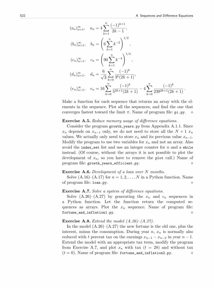
522 A Sequences and Difference Equations

(an)∞n=1, an = 4

n∑

k=1

(−1)k+1

2k − 1,

(bn)∞n=1, bn =

(

6

n∑

k=1

k−2

)1/2

,

(cn)∞n=1, cn =

(

90n∑

k=1

k−4

)1/4

,

(dn)∞n=1, dn =

6√3

n∑

k=0

(−1)k3k(2k + 1)

,

(en)∞n=1, en = 16

n∑

k=0

(−1)k52k+1(2k + 1)

− 4n∑

k=0

(−1)k2392k+1(2k + 1)

.

Make a function for each sequence that returns an array with the el-ements in the sequence. Plot all the sequences, and find the one thatconverges fastest toward the limit π. Name of program file: pi.py. ⋄

Exercise A.5. Reduce memory usage of difference equations.Consider the program growth_years.py from Appendix A.1.1. Since

xn depends on xn−1 only, we do not need to store all the N + 1 xnvalues. We actually only need to store xn and its previous value xn−1.Modify the program to use two variables for xn and not an array. Alsoavoid the index_set list and use an integer counter for n and a while

instead. (Of course, without the arrays it is not possible to plot thedevelopment of xn, so you have to remove the plot call.) Name ofprogram file: growth_years_efficient.py. ⋄

Exercise A.6. Development of a loan over N months.Solve (A.16)–(A.17) for n = 1, 2, . . . , N in a Python function. Name

of program file: loan.py. ⋄

Exercise A.7. Solve a system of difference equations.Solve (A.26)–(A.27) by generating the xn and cn sequences in

a Python function. Let the function return the computed se-quences as arrays. Plot the xn sequence. Name of program file:fortune_and_inflation1.py. ⋄

Exercise A.8. Extend the model (A.26)–(A.27).In the model (A.26)–(A.27) the new fortune is the old one, plus the

interest, minus the consumption. During year n, xn is normally alsoreduced with t percent tax on the earnings xn−1 − xn−2 in year n− 1.Extend the model with an appropriate tax term, modify the programfrom Exercise A.7, and plot xn with tax (t = 28) and without tax(t = 0). Name of program file: fortune_and_inflation2.py. ⋄

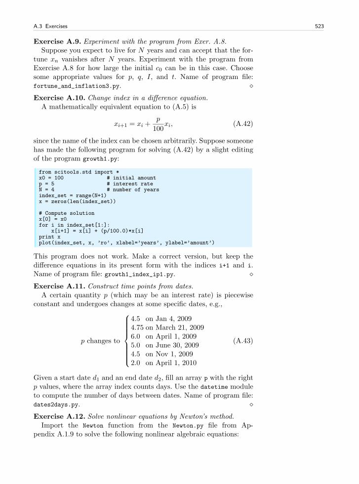
A.3 Exercises 523

Exercise A.9. Experiment with the program from Exer. A.8.Suppose you expect to live for N years and can accept that the for-

tune xn vanishes after N years. Experiment with the program fromExercise A.8 for how large the initial c0 can be in this case. Choosesome appropriate values for p, q, I, and t. Name of program file:fortune_and_inflation3.py. ⋄Exercise A.10. Change index in a difference equation.

A mathematically equivalent equation to (A.5) is

xi+1 = xi +p

100xi, (A.42)

since the name of the index can be chosen arbitrarily. Suppose someonehas made the following program for solving (A.42) by a slight editingof the program growth1.py:

from scitools.std import *x0 = 100 # initial amountp = 5 # interest rateN = 4 # number of yearsindex_set = range(N+1)x = zeros(len(index_set))

# Compute solutionx[0] = x0for i in index_set[1:]:

x[i+1] = x[i] + (p/100.0)*x[i]print xplot(index_set, x, ’ro’, xlabel=’years’, ylabel=’amount’)

This program does not work. Make a correct version, but keep thedifference equations in its present form with the indices i+1 and i.Name of program file: growth1_index_ip1.py. ⋄Exercise A.11. Construct time points from dates.

A certain quantity p (which may be an interest rate) is piecewiseconstant and undergoes changes at some specific dates, e.g.,

p changes to

4.5 on Jan 4, 20094.75 on March 21, 20096.0 on April 1, 20095.0 on June 30, 20094.5 on Nov 1, 20092.0 on April 1, 2010

(A.43)

Given a start date d1 and an end date d2, fill an array p with the rightp values, where the array index counts days. Use the datetime moduleto compute the number of days between dates. Name of program file:dates2days.py. ⋄Exercise A.12. Solve nonlinear equations by Newton’s method.

Import the Newton function from the Newton.py file from Ap-pendix A.1.9 to solve the following nonlinear algebraic equations:

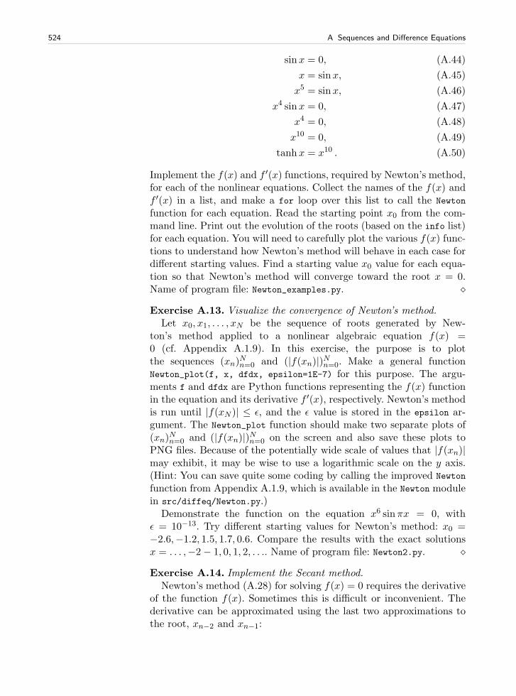
524 A Sequences and Difference Equations

sinx = 0, (A.44)

x = sinx, (A.45)

x5 = sinx, (A.46)

x4 sinx = 0, (A.47)

x4 = 0, (A.48)

x10 = 0, (A.49)

tanh x = x10 . (A.50)

Implement the f(x) and f ′(x) functions, required by Newton’s method,for each of the nonlinear equations. Collect the names of the f(x) andf ′(x) in a list, and make a for loop over this list to call the Newton

function for each equation. Read the starting point x0 from the com-mand line. Print out the evolution of the roots (based on the info list)for each equation. You will need to carefully plot the various f(x) func-tions to understand how Newton’s method will behave in each case fordifferent starting values. Find a starting value x0 value for each equa-tion so that Newton’s method will converge toward the root x = 0.Name of program file: Newton_examples.py. ⋄

Exercise A.13. Visualize the convergence of Newton’s method.Let x0, x1, . . . , xN be the sequence of roots generated by New-

ton’s method applied to a nonlinear algebraic equation f(x) =0 (cf. Appendix A.1.9). In this exercise, the purpose is to plotthe sequences (xn)

Nn=0 and (|f(xn)|)Nn=0. Make a general function

Newton_plot(f, x, dfdx, epsilon=1E-7) for this purpose. The argu-ments f and dfdx are Python functions representing the f(x) functionin the equation and its derivative f ′(x), respectively. Newton’s methodis run until |f(xN )| ≤ ǫ, and the ǫ value is stored in the epsilon ar-gument. The Newton_plot function should make two separate plots of(xn)

Nn=0 and (|f(xn)|)Nn=0 on the screen and also save these plots to

PNG files. Because of the potentially wide scale of values that |f(xn)|may exhibit, it may be wise to use a logarithmic scale on the y axis.(Hint: You can save quite some coding by calling the improved Newton

function from Appendix A.1.9, which is available in the Newton modulein src/diffeq/Newton.py.)

Demonstrate the function on the equation x6 sinπx = 0, withǫ = 10−13. Try different starting values for Newton’s method: x0 =−2.6,−1.2, 1.5, 1.7, 0.6. Compare the results with the exact solutionsx = . . . ,−2− 1, 0, 1, 2, . . .. Name of program file: Newton2.py. ⋄

Exercise A.14. Implement the Secant method.Newton’s method (A.28) for solving f(x) = 0 requires the derivative

of the function f(x). Sometimes this is difficult or inconvenient. Thederivative can be approximated using the last two approximations tothe root, xn−2 and xn−1:

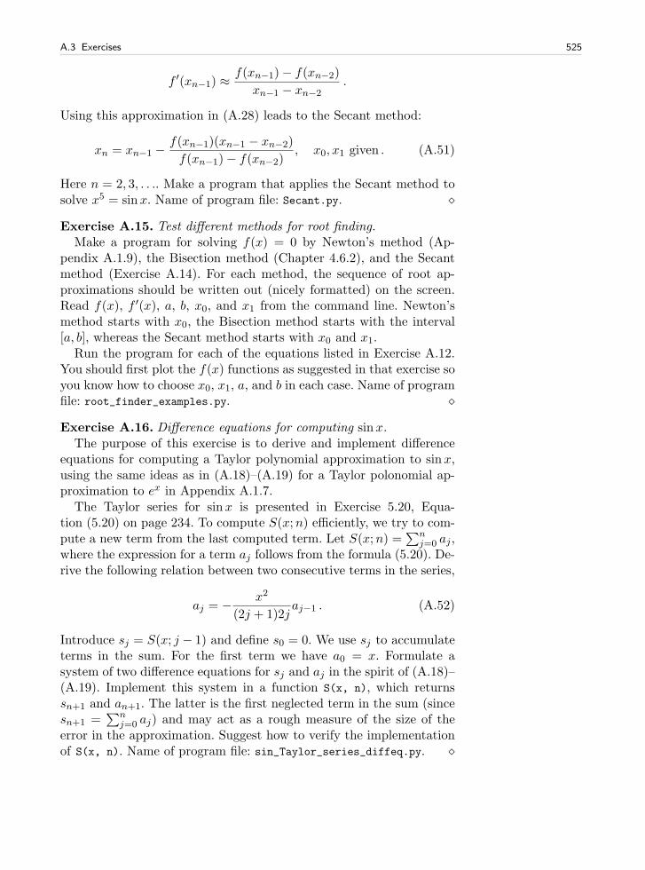
A.3 Exercises 525

f ′(xn−1) ≈f(xn−1)− f(xn−2)

xn−1 − xn−2.

Using this approximation in (A.28) leads to the Secant method:

xn = xn−1 −f(xn−1)(xn−1 − xn−2)

f(xn−1)− f(xn−2), x0, x1 given . (A.51)

Here n = 2, 3, . . .. Make a program that applies the Secant method tosolve x5 = sinx. Name of program file: Secant.py. ⋄

Exercise A.15. Test different methods for root finding.Make a program for solving f(x) = 0 by Newton’s method (Ap-

pendix A.1.9), the Bisection method (Chapter 4.6.2), and the Secantmethod (Exercise A.14). For each method, the sequence of root ap-proximations should be written out (nicely formatted) on the screen.Read f(x), f ′(x), a, b, x0, and x1 from the command line. Newton’smethod starts with x0, the Bisection method starts with the interval[a, b], whereas the Secant method starts with x0 and x1.

Run the program for each of the equations listed in Exercise A.12.You should first plot the f(x) functions as suggested in that exercise soyou know how to choose x0, x1, a, and b in each case. Name of programfile: root_finder_examples.py. ⋄

Exercise A.16. Difference equations for computing sinx.The purpose of this exercise is to derive and implement difference

equations for computing a Taylor polynomial approximation to sinx,using the same ideas as in (A.18)–(A.19) for a Taylor polonomial ap-proximation to ex in Appendix A.1.7.

The Taylor series for sinx is presented in Exercise 5.20, Equa-tion (5.20) on page 234. To compute S(x;n) efficiently, we try to com-pute a new term from the last computed term. Let S(x;n) =

∑nj=0 aj ,

where the expression for a term aj follows from the formula (5.20). De-rive the following relation between two consecutive terms in the series,

aj = −x2

(2j + 1)2jaj−1 . (A.52)

Introduce sj = S(x; j − 1) and define s0 = 0. We use sj to accumulateterms in the sum. For the first term we have a0 = x. Formulate asystem of two difference equations for sj and aj in the spirit of (A.18)–(A.19). Implement this system in a function S(x, n), which returnssn+1 and an+1. The latter is the first neglected term in the sum (sincesn+1 =

∑nj=0 aj) and may act as a rough measure of the size of the

error in the approximation. Suggest how to verify the implementationof S(x, n). Name of program file: sin_Taylor_series_diffeq.py. ⋄

526 A Sequences and Difference Equations

Exercise A.17. Difference equations for computing cosx.Carry out the steps in Exercise A.16, but do it for the Taylor se-

ries of cos x instead of sinx (look up the Taylor series for cosx in amathematics textbook or search on the Internet). Name of programfile: cos_Taylor_series_diffeq.py. ⋄

Exercise A.18. Make a guitar-like sound.Given start values x0, x1, . . . , xp, the following diffference equation

is known to create guitar-like sound:

xn =1

2(xn−p + xn−p−1), n = p+ 1, . . . , N . (A.53)

With a sampling rate r, the frequency of this sound is given by r/p.Make a program with a function solve(x, p) which returns the solu-tion array x of (A.53). To initialize the array x[0:p+1] we look at twomethods, which can be implemented in two alternative functions:

1. x0 = 1, x1 = x2 = · · · = xp = 02. x0, . . . , xp are uniformly distributed random numbers in [−1, 1]Import max_amplitude, write, and play from the scitools.sound mod-ule. Choose a sampling rate r and set p = r/440 to create a 440 Hz tone(A). Create an array x1 of zeros with length 3r such that the tone willlast for 3 seconds. Initialize x1 according to method 1 above and solve(A.53). Multiply the x1 array by max_amplitude. Repeat this processfor an array x2 of length 2r, but use method 2 for the initial values andchoose p such that the tone is 392 Hz (G). Concatenate x1 and x2, callwrite and then play to play the sound. As you will experience, thissound is amazingly similar to the sound of a guitar string, first playingA for 3 seconds and then playing G for 2 seconds. (The method (A.53)is called the Karplus-Strong algorithm and was discovered in 1979 by aresearcher, Kevin Karplus, and his student Alexander Strong, at Stan-ford University.) Name of program file: guitar_sound.py. ⋄

Exercise A.19. Damp the bass in a sound file.Given a sequence x0, . . . , xN−1, the following filter transforms the

sequence to a new sequence y0, . . . , yN−1:

yn =

xn, n = 0−1

4(xn−1 − 2xn + xn+1), 1 ≤ n ≤ N − 2xn, n = N − 1

(A.54)

If xn represents sound, yn is the same sound but with the bass damped.Load some sound file (e.g., the one from Exercise A.18) or call

x = scitools.sound.Nothing_Else_Matters(echo=True)

to get a sound sequence. Apply the filter (A.54) and play the result-ing sound. Plot the first 300 values in the xn and yn signals to see

A.3 Exercises 527

graphically what the filter does with the signal. Name of program file:damp_bass.py. ⋄

Exercise A.20. Damp the treble in a sound file.Solve Exercise A.19 to get some experience with coding a filter and

trying it out on a sound. The purpose of this exercise is to explore someother filters that reduce the treble instead of the bass. Smoothing thesound signal will in general damp the treble, and smoothing is typicallyobtained by letting the values in the new filtered sound sequence bean average of the neighboring values in the original sequence.

The simplest smoothing filter can apply a standard average of threeneighboring values:

yn =

xn, n = 013(xn−1 + xn + xn+1), 1 ≤ n ≤ N − 2xn, n = N − 1

(A.55)

Two other filters put less emphasis on the surrounding values:

yn =

xn, n = 014(xn−1 + 2xn + xn+1), 1 ≤ n ≤ N − 2xn, n = N − 1

(A.56)

yn =

xn, n = 0116(xn−2 + 4xn−1 + 6xn + 4xn+1 + xn+2), 1 ≤ n ≤ N − 2xn, n = N − 1

(A.57)Apply all these three filters to a sound file and listen to the result.Plot the first 300 values in the xn and yn signals for each of the threefilters to see graphically what the filter does with the signal. Name ofprogram file: damp_treble.py. ⋄

Exercise A.21. Demonstrate oscillatory solutions of (A.13).Modify the growth_logistic.py program from Appendix A.1.5 to

solve the equation (A.13) on page 506. Read the input parameters y0,q, and N from the command line.

Equation (A.13) has the solution yn = 1 as n → ∞. Demonstrate,by running the program, that this is the case when y0 = 0.3, q = 1,and N = 50.

For larger q values, yn does not approach a constant limit, but ynoscillates instead around the limiting value. Such oscillations are some-times observed in wildlife populations. Demonstrate oscillatory solu-tions when q is changed to 2 and 3.

It could happen that yn stabilizes at a constant level for larger N .Demonstrate that this is not the case by running the program withN = 1000. Name of program file: growth_logistic2.py. ⋄

528 A Sequences and Difference Equations

Exercise A.22. Improve the program from Exer. A.21.It is tedious to run a program like the one from Exercise A.21 re-

peatedly for a wide range of input parameters. A better approach isto let the computer do the manual work. Modify the program fromExercise A.21 such that the computation of yn and the plot is madein a function. Let the title in the plot contain the parameters y0 and q(N is easily visible from the x axis). Also let the name of the hardcopyreflect the values of y0, q, and N . Then make loops over y0 and q toperform the following more comprehensive set of experiments:

y = 0.01, 0.3 q = 0.1, 1, 1.5, 1.8, 2, 2.5, 3 N = 50

How does the initial condition (the value y0) seem to influence thesolution?

The keyword argument show=False can be used in the plot call ifyou do not want all the plot windows to appear on the screen. Nameof program file: growth_logistic3.py. ⋄

Exercise A.23. Simulate the price of wheat.The demand for wheat in year t is given by

Dt = apt + b,

where a < 0, > 0, and pt is the price of wheat. Let the supply of wheatbe

St = Apt−1 +B + ln(1 + pt−1),

where A and B are given constants. We assume that the price pt adjustssuch that all the produced wheat is sold. That is, Dt = St.

For A = 1, a = −3, b = 5, B = 0, find from numerical computations,a stable price such that the production of wheat from year to year isconstant. That is, find p such that ap+ b = Ap+B + ln(1 + p).

Assume that in a very dry year the production of wheat is muchless than planned. Given that price this year, p0, is 4.5 and Dt =St, compute in a program how the prices p1, p2, . . . , pN develop. Thisimplies solving the difference equation

apt + b = Apt−1 +B + ln(1 + pt−1) .

From the pt values, compute St and plot the points (pt, St) for t =0, 1, 2, . . . , N . How do the prices move whenN →∞? Name of programfile: wheat.py. ⋄

Introduction to Discrete Calculus B

This appendix is authored by Aslak Tveito

In this chapter we will discuss how to differentiate and integrate func-tions on a computer. To do that, we have to care about how to treatmathematical functions on a computer. Handling mathematical func-tions on computers is not entirely straightforward: A function f(x)contains and infinite amount of information (function values at an in-finite number of x values on an interval), while the computer can onlystore a finite1 amount of data. Think about the cosx function. Thereare typically two ways we can work with this function on a computer.One way is to run an algorithm, like that in Exercise 3.21 on page 122,or we simply call math.cos(x) (which runs a similar type of algorithm),to compute an approximation to cos x for a given x, using a finite num-ber of calculations. The other way is to store cosx values in a tablefor a finite number of x values2 and use the table in a smart way tocompute cosx values. This latter way, known as a discrete representa-tion of a function, is in focus in the present chapter. With a discretefunction representation, we can easily integrate and differentiate thefunction too. Read on to see how we can do that.

The folder src/discalc contains all the program example files re-ferred to in this chapter.

B.1 Discrete Functions

Physical quantities, such as temperature, density, and velocity, are usu-ally defined as continuous functions of space and time. However, as

1 Allow yourself a moment or two to think about the terms “finite” and “infinite”;inifinity is not an easy term, but it is not infinitely difficult. Or is it?

2 Of course, we need to run an algorithm to populate the table with cos x numbers.

529

530 B Introduction to Discrete Calculus

mentioned in above, discrete versions of the functions are more con-venient on computers. We will illustrate the concept of discrete func-tions throught some introductory examples. In fact, we used discretefunctions in Chapter 5 to plot curves: We defined a finite set of co-ordinates x and stored the corresponding function values f(x) in anarray. A plotting program would then draw straight lines between thefunction values. A discrete representation of a continuous function is,from a programming point of view, nothing but storing a finite set ofcoordinates and function values in an array. Nevertheless, we will inthis chapter be more formal and describe discrete functions by precisemathematical terms.

B.1.1 The Sine Function

Suppose we want to generate a plot of the sine function for values ofx between 0 and π. To this end, we define a set of x-values and anassociated set of values of the sine function. More precisely, we definen+ 1 points by

xi = ih for i = 0, 1, . . . , n (B.1)

where h = π/n and n > 1 is an integer. The associated function valuesare defined as

si = sin(xi) for i = 0, 1, . . . , n. (B.2)

Mathematically, we have a sequence of coordinates (xi)ni=0 and of func-

tion values (si)ni=0 (see the start of Appendix A for an explanation of

the notation and the sequence concept). Often we “merge” the two se-quences to one sequence of points: (xi, si)

ni=0. Sometimes we also use

a shorter notation, just xi, si, or (xi, si) if the exact limits are not ofimportance. The set of coordinates (xi)

ni=0 constitutes a mesh or a

grid. The individual coordinates xi are known as nodes in the mesh(or grid). The discrete representation of the sine function on [0, π] con-sists of the mesh and the corresponding sequence of function values(si)

ni=0 at the nodes. The parameter n is often referred to as the mesh

resolution.In a program, we represent the mesh by a coordinate array, say

x, and the function values by another array, say s. To plot the sinefunction we can simply write

from scitools.std import *

n = int(sys.argv[1])

x = linspace(0, pi, n+1)s = sin(x)plot(x, s, legend=’sin(x), n=%d’ % n, hardcopy=’tmp.eps’)

Figure B.1 shows the resulting plot for n = 5, 10, 20 and 100. Aspointed out in Chapter 5, the curve looks smoother the more points

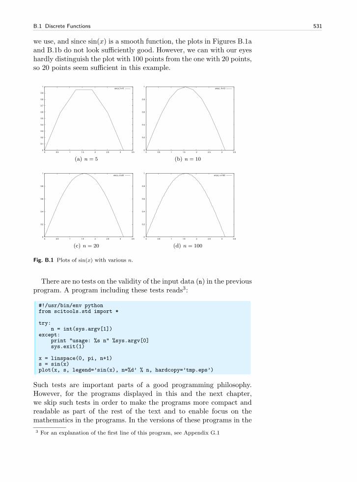
B.1 Discrete Functions 531

we use, and since sin(x) is a smooth function, the plots in Figures B.1aand B.1b do not look sufficiently good. However, we can with our eyeshardly distinguish the plot with 100 points from the one with 20 points,so 20 points seem sufficient in this example.

0

0.1

0.2

0.3

0.4

0.5

0.6

0.7

0.8

0.9

1

0 0.5 1 1.5 2 2.5 3 3.5

sin(x), n=5

(a) n = 5

0

0.2

0.4

0.6

0.8

1

0 0.5 1 1.5 2 2.5 3 3.5

sin(x), n=10

(b) n = 10

0

0.2

0.4

0.6

0.8

1

0 0.5 1 1.5 2 2.5 3 3.5

sin(x), n=20

(c) n = 20

0

0.2

0.4

0.6

0.8

1

0 0.5 1 1.5 2 2.5 3 3.5

sin(x), n=100

(d) n = 100

Fig. B.1 Plots of sin(x) with various n.

There are no tests on the validity of the input data (n) in the previousprogram. A program including these tests reads3:

#!/usr/bin/env pythonfrom scitools.std import *

try:n = int(sys.argv[1])

except:print "usage: %s n" %sys.argv[0]sys.exit(1)

x = linspace(0, pi, n+1)s = sin(x)plot(x, s, legend=’sin(x), n=%d’ % n, hardcopy=’tmp.eps’)

Such tests are important parts of a good programming philosophy.However, for the programs displayed in this and the next chapter,we skip such tests in order to make the programs more compact andreadable as part of the rest of the text and to enable focus on themathematics in the programs. In the versions of these programs in the

3 For an explanation of the first line of this program, see Appendix G.1

532 B Introduction to Discrete Calculus

files that can be downloaded you will, hopefully, always find a test oninput data.

B.1.2 Interpolation

Suppose we have a discrete representation of the sine function:(xi, si)

ni=0. At the nodes we have the exact sine values si, but what

about the points in between these nodes? Finding function values be-tween the nodes is called interpolation, or we can say that we interpolatea discrete function.

A graphical interpolation procedure could be to look at one of theplots in Figure B.1 to find the function value corresponding to a pointx between the nodes. Since the plot is a straight line from node valueto node value, this means that a function value between two nodesis found from a straight line approximation4 to the underlying con-tinuous function. We formulate this procedure precisely in terms ofmathematics in the next paragraph.

Assume that we know that a given x∗ lies in the interval from x = xkto xk+1, where the integer k is given. In the interval xk 6 x < xk+1, wedefine the linear function that passes through (xk, sk) and (xk+1, sk+1):

Sk(x) = sk +sk+1 − skxk+1 − xk

(x− xk). (B.3)

That is, Sk(x) coincides with sin(x) at xk and xk+1, and between thesenodes, Sk(x) is linear. We say that Sk(x) interpolates the discrete func-tion (xi, si)

ni=0 on the interval [xk, xk+1].

B.1.3 Evaluating the Approximation

Given the values (xi, si)ni=0 and the formula (B.3), we want to compute

an approximation of the sine function for any x in the interval fromx = 0 to x = π. In order to do that, we have to compute k for a givenvalue of x. More precisely, for a given x we have to find k such thatxk 6 x 6 xk+1. We can do that by defining

k = ⌊x/h⌋

where the function ⌊z⌋ denotes the largest integer that is smaller thanz. In Python, ⌊z⌋ is computed by int(z). The program below takes xand n as input and computes the approximation of sin(x). The program

4 Strictly speaking, we also assume that the function to be interpolated is rathersmooth. It is easy to see that if the function is very wild, i.e., the values of thefunction changes very rapidly, this procedure may fail even for very large values ofn. Chapter 5.4.2 provides an example.

B.1 Discrete Functions 533

prints the approximation S(x) and the exact5 value of sin(x) so we canlook at the development of the error when n is increased.

from numpy import *import sys

xp = eval(sys.argv[1])n = int(sys.argv[2])

def S_k(k):return s[k] + \

((s[k+1] - s[k])/(x[k+1] - x[k]))*(xp - x[k])h = pi/nx = linspace(0, pi, n+1)s = sin(x)k = int(xp/h)

print ’Approximation of sin(%s): ’ % xp, S_k(k)print ’Exact value of sin(%s): ’ % xp, sin(xp)print ’Eror in approximation: ’, sin(xp) - S_k(k)

To study the approximation, we put x =√2 and use the program

eval_sine.py for n = 5, 10 and 20.

Terminal

eval_sine.py ’sqrt(2)’ 5Approximation of sin(1.41421356237): 0.951056516295Exact value of sin(1.41421356237): 0.987765945993Eror in approximation: 0.0367094296976

Terminal

eval_sine.py ’sqrt(2)’ 10Approximation of sin(1.41421356237): 0.975605666221Exact value of sin(1.41421356237): 0.987765945993Eror in approximation: 0.0121602797718

Terminal

eval_sine.py ’sqrt(2)’ 20Approximation of sin(1.41421356237): 0.987727284363Exact value of sin(1.41421356237): 0.987765945993Eror in approximation: 3.86616296923e-05

Note that the error is reduced as the n increases.

B.1.4 Generalization

In general, we can create a discrete version of a continuous function asfollows. Suppose a continuous function f(x) is defined on an interval

5 The value is not really exact – it is the value of sin(x) provided by the computer,math.sin(x), and this value is calculated from an algorithm that only yields anapproximation to sin(x). Exercise 3.21 provides an example of the type of algorithmin question.

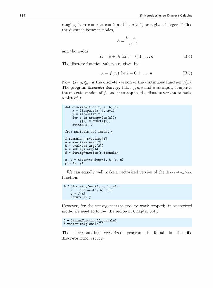
534 B Introduction to Discrete Calculus

ranging from x = a to x = b, and let n > 1, be a given integer. Definethe distance between nodes,

h =b− a

n,

and the nodesxi = a+ ih for i = 0, 1, . . . , n. (B.4)

The discrete function values are given by

yi = f(xi) for i = 0, 1, . . . , n. (B.5)

Now, (xi, yi)ni=0 is the discrete version of the continuous function f(x).

The program discrete_func.py takes f, a, b and n as input, computesthe discrete version of f , and then applies the discrete version to makea plot of f .

def discrete_func(f, a, b, n):x = linspace(a, b, n+1)y = zeros(len(x))for i in xrange(len(x)):

y[i] = func(x[i])return x, y

from scitools.std import *

f_formula = sys.argv[1]a = eval(sys.argv[2])b = eval(sys.argv[3])n = int(sys.argv[4])f = StringFunction(f_formula)

x, y = discrete_func(f, a, b, n)plot(x, y)

We can equally well make a vectorized version of the discrete_func

function:

def discrete_func(f, a, b, n):x = linspace(a, b, n+1)y = f(x)return x, y

However, for the StringFunction tool to work properly in vectorizedmode, we need to follow the recipe in Chapter 5.4.3:

f = StringFunction(f_formula)f.vectorize(globals())

The corresponding vectorized program is found in the filediscrete_func_vec.py.

B.2 Differentiation Becomes Finite Differences 535

B.2 Differentiation Becomes Finite Differences

You have heard about derivatives. Probably, the following formulas arewell known to you:

d

dxsin(x) = cos(x),

d

dxln(x) =

1

x,

d

dxxm = mxm−1,

But why is differentiation so important? The reason is quite simple:The derivative is a mathematical expression of change. And change is,of course, essential in modeling various phenomena. If we know thestate of a system, and we know the laws of change, then we can, inprinciple, compute the future of that system. Appendix C treats thistopic in detail. Appendix A also computes the future of systems, basedon modeling changes, but without using differentiation. In Appendix Cyou will see that reducing the step size in the difference equations inAppendix A results in derivatives instead of pure differences. However,differentiation of continuous functions is somewhat hard on a computer,so we often end up replacing the derivatives by differences. This ideais quite general, and every time we use a discrete representation of afunction, differentiation becomes differences, or finite differences as weusually say.

The mathematical definition of differentiation reads

f ′(x) = limε→0

f(x+ ε)− f(x)

ε.

You have probably seen this definition many times, but have you un-derstood what it means and do you think the formula has a greatpractical value? Although the definition requires that we pass to thelimit, we obtain quite good approximations of the derivative by usinga fixed positive value of ε. More precisely, for a small ε > 0, we have

f ′(x) ≈ f(x+ ε)− f(x)

ε.

The fraction on the right-hand side is a finite difference approximationto the derivative of f at the point x. Instead of using ε it is morecommon to introduce h = ε in finite differences, i.e., we like to write

f ′(x) ≈ f(x+ h)− f(x)

h. (B.6)

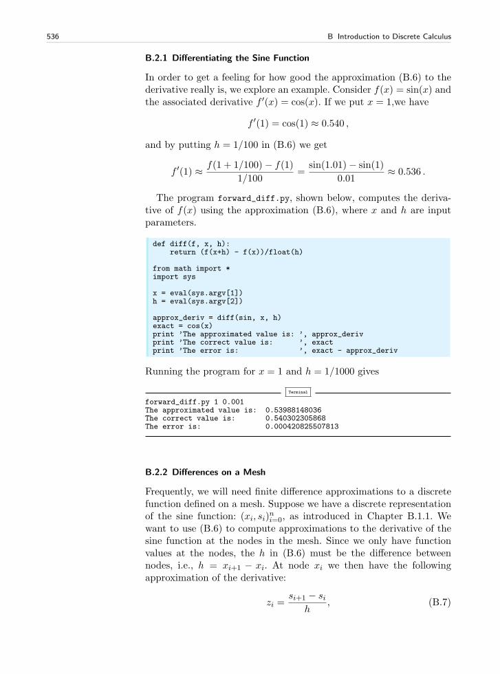
536 B Introduction to Discrete Calculus

B.2.1 Differentiating the Sine Function

In order to get a feeling for how good the approximation (B.6) to thederivative really is, we explore an example. Consider f(x) = sin(x) andthe associated derivative f ′(x) = cos(x). If we put x = 1,we have

f ′(1) = cos(1) ≈ 0.540 ,

and by putting h = 1/100 in (B.6) we get

f ′(1) ≈ f(1 + 1/100)− f(1)

1/100=

sin(1.01)− sin(1)

0.01≈ 0.536 .

The program forward_diff.py, shown below, computes the deriva-tive of f(x) using the approximation (B.6), where x and h are inputparameters.

def diff(f, x, h):return (f(x+h) - f(x))/float(h)

from math import *import sys

x = eval(sys.argv[1])h = eval(sys.argv[2])

approx_deriv = diff(sin, x, h)exact = cos(x)print ’The approximated value is: ’, approx_derivprint ’The correct value is: ’, exactprint ’The error is: ’, exact - approx_deriv

Running the program for x = 1 and h = 1/1000 gives

Terminal

forward_diff.py 1 0.001The approximated value is: 0.53988148036The correct value is: 0.540302305868The error is: 0.000420825507813

B.2.2 Differences on a Mesh

Frequently, we will need finite difference approximations to a discretefunction defined on a mesh. Suppose we have a discrete representationof the sine function: (xi, si)

ni=0, as introduced in Chapter B.1.1. We

want to use (B.6) to compute approximations to the derivative of thesine function at the nodes in the mesh. Since we only have functionvalues at the nodes, the h in (B.6) must be the difference betweennodes, i.e., h = xi+1 − xi. At node xi we then have the followingapproximation of the derivative:

zi =si+1 − si

h, (B.7)

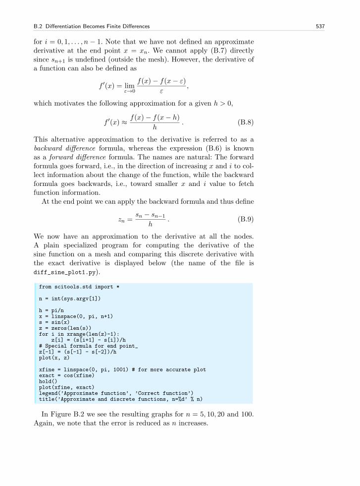
B.2 Differentiation Becomes Finite Differences 537

for i = 0, 1, . . . , n − 1. Note that we have not defined an approximatederivative at the end point x = xn. We cannot apply (B.7) directlysince sn+1 is undefined (outside the mesh). However, the derivative ofa function can also be defined as

f ′(x) = limε→0

f(x)− f(x− ε)

ε,

which motivates the following approximation for a given h > 0,

f ′(x) ≈ f(x)− f(x− h)

h. (B.8)

This alternative approximation to the derivative is referred to as abackward difference formula, whereas the expression (B.6) is knownas a forward difference formula. The names are natural: The forwardformula goes forward, i.e., in the direction of increasing x and i to col-lect information about the change of the function, while the backwardformula goes backwards, i.e., toward smaller x and i value to fetchfunction information.

At the end point we can apply the backward formula and thus define

zn =sn − sn−1

h. (B.9)

We now have an approximation to the derivative at all the nodes.A plain specialized program for computing the derivative of thesine function on a mesh and comparing this discrete derivative withthe exact derivative is displayed below (the name of the file isdiff_sine_plot1.py).

from scitools.std import *

n = int(sys.argv[1])

h = pi/nx = linspace(0, pi, n+1)s = sin(x)z = zeros(len(s))for i in xrange(len(z)-1):

z[i] = (s[i+1] - s[i])/h# Special formula for end point_z[-1] = (s[-1] - s[-2])/hplot(x, z)

xfine = linspace(0, pi, 1001) # for more accurate plotexact = cos(xfine)hold()plot(xfine, exact)legend(’Approximate function’, ’Correct function’)title(’Approximate and discrete functions, n=%d’ % n)

In Figure B.2 we see the resulting graphs for n = 5, 10, 20 and 100.Again, we note that the error is reduced as n increases.

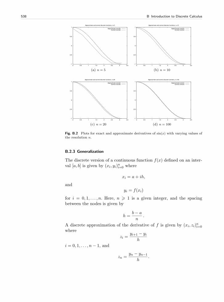
538 B Introduction to Discrete Calculus

-1

-0.5

0

0.5

1

0 0.5 1 1.5 2 2.5 3 3.5

Approximate and correct discrete functions, n=5

Approximate functionCorrect function

(a) n = 5

-1

-0.5

0

0.5

1

0 0.5 1 1.5 2 2.5 3 3.5

Approximate and correct discrete functions, n=10

Approximate functionCorrect function

(b) n = 10

-1

-0.5

0

0.5

1

0 0.5 1 1.5 2 2.5 3 3.5

Approximate and correct discrete functions, n=20

Approximate functionCorrect function

(c) n = 20

-1

-0.5

0

0.5

1

0 0.5 1 1.5 2 2.5 3 3.5

Approximate and correct discrete functions, n=100

Approximate functionCorrect function

(d) n = 100

Fig. B.2 Plots for exact and approximate derivatives of sin(x) with varying values ofthe resolution n.

B.2.3 Generalization

The discrete version of a continuous function f(x) defined on an inter-val [a, b] is given by (xi, yi)

ni=0 where

xi = a+ ih,

andyi = f(xi)

for i = 0, 1, . . . , n. Here, n > 1 is a given integer, and the spacingbetween the nodes is given by

h =b− a

n.

A discrete approximation of the derivative of f is given by (xi, zi)ni=0

where

zi =yi+1 − yi

h

i = 0, 1, . . . , n− 1, and

zn =yn − yn−1

h.

B.3 Integration Becomes Summation 539

The collection (xi, zi)ni=0 is the discrete derivative of the discrete version

(xi, fi)ni=0 of the continuous function f(x). The program below, found

in the file diff_func.py, takes f, a, b and n as input and computes thediscrete derivative of f on the mesh implied by a, b, and h, and thena plot of f and the discrete derivative is made.

def diff(f, a, b, n):x = linspace(a, b, n+1)y = zeros(len(x))z = zeros(len(x))h = (b-a)/float(n)for i in xrange(len(x)):

y[i] = func(x[i])for i in xrange(len(x)-1):

z[i] = (y[i+1] - y[i])/hz[n] = (y[n] - y[n-1])/hreturn y, z

from scitools.std import *f_formula = sys.argv[1]a = eval(sys.argv[2])b = eval(sys.argv[3])n = int(sys.argv[4])

f = StringFunction(f_formula)y, z = diff(f, a, b, n)plot(x, y, ’r-’, x, z, ’b-’,

legend=(’function’, ’derivative’))

B.3 Integration Becomes Summation

Some functions can be integrated analytically. You may remember6 thefollowing cases,

∫

xmdx =1

m+ 1xm+1 for m 6= −1,

∫

sin(x)dx = − cos(x),∫

x

1 + x2dx =

1

2ln(

x2 + 1)

.

These are examples of so-called indefinite integrals. If the function canbe integrated analytically, it is straightforward to evaluate an associ-ated definite integral. For example, we have7

6 Actually, we congratulate you if you remember the third one!7 Recall, in general, that

[f(x)]ba = f(b)− f(a).

540 B Introduction to Discrete Calculus

∫ 1

0xmdx =

[

1

m+ 1xm+1

]1

0

=1

m+ 1,

∫ π

0

sin(x)dx = [− cos(x)]π0 = 2,

∫ 1

0

x

1 + x2dx =

[

1

2ln(

x2 + 1)

]1

0

=1

2ln 2.

But lots of functions cannot be integrated analytically and thereforedefinite integrals must be computed using some sort of numerical ap-proximation. Above, we introduced the discrete version of a function,and we will now use this construction to compute an approximation ofa definite integral.

B.3.1 Dividing into Subintervals

Let us start by considering the problem of computing the integral ofsin(x) from x = 0 to x = π. This is not the most exciting or challengingmathematical problem you can think of, but it is good practice to startwith a problem you know well when you want to learn a new method.In Chapter B.1.1 we introduce a discrete function (xi, si)

ni=0 where

h = π/n, si = sin(xi) and xi = ih for i = 0, 1, . . . , n. Furthermore, inthe interval xk 6 x < xk+1, we defined the linear function

Sk(x) = sk +sk+1 − skxk+1 − xk

(x− xk).

We want to compute an approximation of the integral of the functionsin(x) from x = 0 to x = π. The integral

∫ π

0sin(x)dx

can be divided into subintegrals defined on the intervals xk 6 x < xk+1,leading to the following sum of integrals:

∫ π

0

sin(x)dx =

n−1∑

k=0

∫ xk+1

xk

sin(x)dx .

To get a feeling for this split of the integral, let us spell the sum outin the case of only four subintervals. Then n = 4, h = π/4,

B.3 Integration Becomes Summation 541

x0 = 0,

x1 = π/4,

x2 = π/2,

x3 = 3π/4

x4 = π.

The interval from 0 to π is divided into four intervals of equal length,and we can divide the integral similarily,

∫ π

0

sin(x)dx =

∫ x1

x0

sin(x)dx+

∫ x2

x1

sin(x)dx+

∫ x3

x2

sin(x)dx+

∫ x4

x3

sin(x)dx . (B.10)

So far we have changed nothing – the integral can be split in this way– with no approximation at all. But we have reduced the problem ofapproximating the integral

∫ π

0

sin(x)dx

down to approximating integrals on the subintervals, i.e. we need ap-proxiamtions of all the following integrals

∫ x1

x0

sin(x)dx,

∫ x2

x1

sin(x)dx,

∫ x3

x2

sin(x)dx,

∫ x4

x3

sin(x)dx .

The idea is that the function to be integrated changes less over thesubintervals than over the whole domain [0, π] and it might be rea-sonable to approximate the sine by a straight line, Sk(x), over eachsubinterval. The integration over a subinterval will then be very easy.

B.3.2 Integration on Subintervals

The task now is to approximate integrals on the form∫ xk+1

xk

sin(x)dx.

Sincesin(x) ≈ Sk(x)

on the interval (xk, xk+1), we have

∫ xk+1

xk

sin(x)dx ≈∫ xk+1

xk

Sk(x)dx.

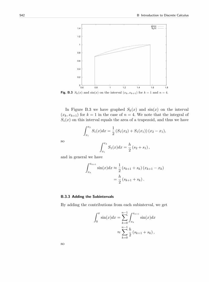
542 B Introduction to Discrete Calculus

0

0.2

0.4

0.6

0.8

1

1.2

1.4

0.6 0.8 1 1.2 1.4 1.6 1.8

sin(x)Sk(x)

Fig. B.3 Sk(x) and sin(x) on the interval (xk, xk+1) for k = 1 and n = 4.

In Figure B.3 we have graphed Sk(x) and sin(x) on the interval(xk, xk+1) for k = 1 in the case of n = 4. We note that the integral ofS1(x) on this interval equals the area of a trapezoid, and thus we have

∫ x2

x1

S1(x)dx =1

2(S1(x2) + S1(x1)) (x2 − x1),

so∫ x2

x1

S1(x)dx =h

2(s2 + s1) ,

and in general we have∫ xk+1

xk

sin(x)dx ≈ 1

2(sk+1 + sk) (xk+1 − xk)

=h

2(sk+1 + sk) .

B.3.3 Adding the Subintervals

By adding the contributions from each subinterval, we get

∫ π

0sin(x)dx =

n−1∑

k=0

∫ xk+1

xk

sin(x)dx

≈n−1∑

k=0

h

2(sk+1 + sk) ,

so

B.3 Integration Becomes Summation 543

∫ π

0

sin(x)dx ≈ h

2

n−1∑

k=0

(sk+1 + sk) . (B.11)

In the case of n = 4, we have∫ π

0sin(x)dx ≈ h

2[(s1 + s0) + (s2 + s1) + (s3 + s2) + (s4 + s3)]

=h

2[s0 + 2 (s1+s2+s3) + s4] .

One can show that (B.11) can be alternatively expressed as8

∫ π

0sin(x)dx ≈ h

2

[

s0 + 2

n−1∑

k=1

sk + sn

]

. (B.12)

This approximation formula is referred to as the Trapezoidal rule of nu-merical integration. Using the more general program trapezoidal.py,presented in the next section, on integrating

∫ π0 sin(x)dx with n =

5, 10, 20 and 100 yields the numbers 1.5644, 1.8864, 1.9713, and 1.9998respectively. These numbers are to be compared to the exact value 2.As usual, the approximation becomes better the more points (n) weuse.

B.3.4 Generalization

An approximation of the integral

∫ b

af(x)dx

can be computed using the discrete version of a continuous functionf(x) defined on an interval [a, b]. We recall that the discrete version off is given by (xi, yi)

ni=0 where

xi = a+ ih, and yi = f(xi)

for i = 0, 1, . . . , n. Here, n > 1 is a given integer and h = (b − a)/n.The Trapezoidal rule can now be written as

∫ b

af(x)dx ≈ h

2

[

y0 + 2

n−1∑

k=1

yk + yn

]

.

The program trapezoidal.py implements the Trapezoidal rule for ageneral function f .

8 There are fewer arithmetic operations associated with (B.12) than with (B.11), sothe former will lead to faster code.

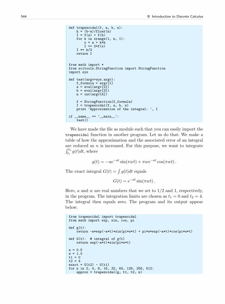
544 B Introduction to Discrete Calculus

def trapezoidal(f, a, b, n):h = (b-a)/float(n)I = f(a) + f(b)for k in xrange(1, n, 1):

x = a + k*hI += 2*f(x)

I *= h/2return I

from math import *from scitools.StringFunction import StringFunctionimport sys

def test(argv=sys.argv):f_formula = argv[1]a = eval(argv[2])b = eval(argv[3])n = int(argv[4])

f = StringFunction(f_formula)I = trapezoidal(f, a, b, n)print ’Approximation of the integral: ’, I

if __name__ == ’__main__’:test()

We have made the file as module such that you can easily import thetrapezoidal function in another program. Let us do that: We make atable of how the approximation and the associated error of an integralare reduced as n is increased. For this purpose, we want to integrate∫ t2t1

g(t)dt, where

g(t) = −ae−at sin(πwt) + πwe−at cos(πwt) .

The exact integral G(t) =∫

g(t)dt equals

G(t) = e−at sin(πwt) .

Here, a and w are real numbers that we set to 1/2 and 1, respectively,in the program. The integration limits are chosen as t1 = 0 and t2 = 4.The integral then equals zero. The program and its output appearbelow.

from trapezoidal import trapezoidalfrom math import exp, sin, cos, pi

def g(t):return -a*exp(-a*t)*sin(pi*w*t) + pi*w*exp(-a*t)*cos(pi*w*t)

def G(t): # integral of g(t)return exp(-a*t)*sin(pi*w*t)

a = 0.5w = 1.0t1 = 0t2 = 4exact = G(t2) - G(t1)for n in 2, 4, 8, 16, 32, 64, 128, 256, 512:

approx = trapezoidal(g, t1, t2, n)

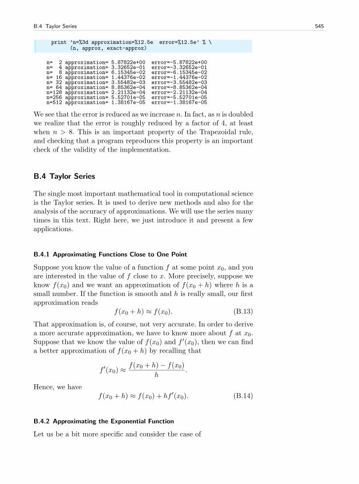
B.4 Taylor Series 545

print ’n=%3d approximation=%12.5e error=%12.5e’ % \(n, approx, exact-approx)

n= 2 approximation= 5.87822e+00 error=-5.87822e+00n= 4 approximation= 3.32652e-01 error=-3.32652e-01n= 8 approximation= 6.15345e-02 error=-6.15345e-02n= 16 approximation= 1.44376e-02 error=-1.44376e-02n= 32 approximation= 3.55482e-03 error=-3.55482e-03n= 64 approximation= 8.85362e-04 error=-8.85362e-04n=128 approximation= 2.21132e-04 error=-2.21132e-04n=256 approximation= 5.52701e-05 error=-5.52701e-05n=512 approximation= 1.38167e-05 error=-1.38167e-05

We see that the error is reduced as we increase n. In fact, as n is doubledwe realize that the error is roughly reduced by a factor of 4, at leastwhen n > 8. This is an important property of the Trapezoidal rule,and checking that a program reproduces this property is an importantcheck of the validity of the implementation.

B.4 Taylor Series

The single most important mathematical tool in computational scienceis the Taylor series. It is used to derive new methods and also for theanalysis of the accuracy of approximations. We will use the series manytimes in this text. Right here, we just introduce it and present a fewapplications.

B.4.1 Approximating Functions Close to One Point

Suppose you know the value of a function f at some point x0, and youare interested in the value of f close to x. More precisely, suppose weknow f(x0) and we want an approximation of f(x0 + h) where h is asmall number. If the function is smooth and h is really small, our firstapproximation reads

f(x0 + h) ≈ f(x0). (B.13)

That approximation is, of course, not very accurate. In order to derivea more accurate approximation, we have to know more about f at x0.Suppose that we know the value of f(x0) and f ′(x0), then we can finda better approximation of f(x0 + h) by recalling that

f ′(x0) ≈f(x0 + h)− f(x0)

h.

Hence, we havef(x0 + h) ≈ f(x0) + hf ′(x0). (B.14)

B.4.2 Approximating the Exponential Function

Let us be a bit more specific and consider the case of

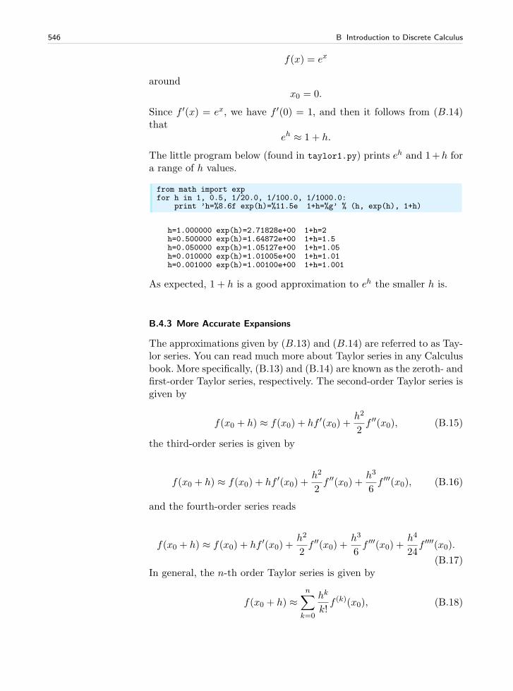
546 B Introduction to Discrete Calculus

f(x) = ex

aroundx0 = 0.

Since f ′(x) = ex, we have f ′(0) = 1, and then it follows from (B.14)that

eh ≈ 1 + h.

The little program below (found in taylor1.py) prints eh and 1+h fora range of h values.

from math import expfor h in 1, 0.5, 1/20.0, 1/100.0, 1/1000.0:

print ’h=%8.6f exp(h)=%11.5e 1+h=%g’ % (h, exp(h), 1+h)

h=1.000000 exp(h)=2.71828e+00 1+h=2h=0.500000 exp(h)=1.64872e+00 1+h=1.5h=0.050000 exp(h)=1.05127e+00 1+h=1.05h=0.010000 exp(h)=1.01005e+00 1+h=1.01h=0.001000 exp(h)=1.00100e+00 1+h=1.001

As expected, 1 + h is a good approximation to eh the smaller h is.

B.4.3 More Accurate Expansions

The approximations given by (B.13) and (B.14) are referred to as Tay-lor series. You can read much more about Taylor series in any Calculusbook. More specifically, (B.13) and (B.14) are known as the zeroth- andfirst-order Taylor series, respectively. The second-order Taylor series isgiven by

f(x0 + h) ≈ f(x0) + hf ′(x0) +h2

2f ′′(x0), (B.15)

the third-order series is given by

f(x0 + h) ≈ f(x0) + hf ′(x0) +h2

2f ′′(x0) +

h3

6f ′′′(x0), (B.16)

and the fourth-order series reads

f(x0 + h) ≈ f(x0) + hf ′(x0) +h2

2f ′′(x0) +

h3

6f ′′′(x0) +

h4

24f ′′′′(x0).

(B.17)In general, the n-th order Taylor series is given by

f(x0 + h) ≈n∑

k=0

hk

k!f (k)(x0), (B.18)

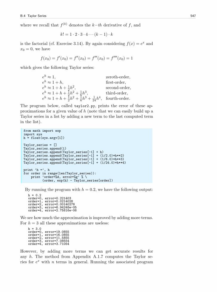
B.4 Taylor Series 547

where we recall that f (k) denotes the k−th derivative of f , and

k! = 1 · 2 · 3 · 4 · · · (k − 1) · k

is the factorial (cf. Exercise 3.14). By again considering f(x) = ex andx0 = 0, we have

f(x0) = f ′(x0) = f ′′(x0) = f ′′′(x0) = f ′′′′(x0) = 1

which gives the following Taylor series:

eh ≈ 1, zeroth-order,eh ≈ 1 + h, first-order,eh ≈ 1 + h+ 1

2h2, second-order,

eh ≈ 1 + h+ 12h

2 + 16h

3, third-order,eh ≈ 1 + h+ 1

2h2 + 1

6h3 + 1

24h4, fourth-order.

The program below, called taylor2.py, prints the error of these ap-proximations for a given value of h (note that we can easily build up aTaylor series in a list by adding a new term to the last computed termin the list).

from math import expimport sysh = float(sys.argv[1])

Taylor_series = []Taylor_series.append(1)Taylor_series.append(Taylor_series[-1] + h)Taylor_series.append(Taylor_series[-1] + (1/2.0)*h**2)Taylor_series.append(Taylor_series[-1] + (1/6.0)*h**3)Taylor_series.append(Taylor_series[-1] + (1/24.0)*h**4)

print ’h =’, hfor order in range(len(Taylor_series)):

print ’order=%d, error=%g’ % \(order, exp(h) - Taylor_series[order])

By running the program with h = 0.2, we have the following output:h = 0.2order=0, error=0.221403order=1, error=0.0214028order=2, error=0.00140276order=3, error=6.94248e-05order=4, error=2.75816e-06

We see how much the approximation is improved by adding more terms.For h = 3 all these approximations are useless:

h = 3.0order=0, error=19.0855order=1, error=16.0855order=2, error=11.5855order=3, error=7.08554order=4, error=3.71054

However, by adding more terms we can get accurate results forany h. The method from Appendix A.1.7 computes the Taylor se-ries for ex with n terms in general. Running the associated program

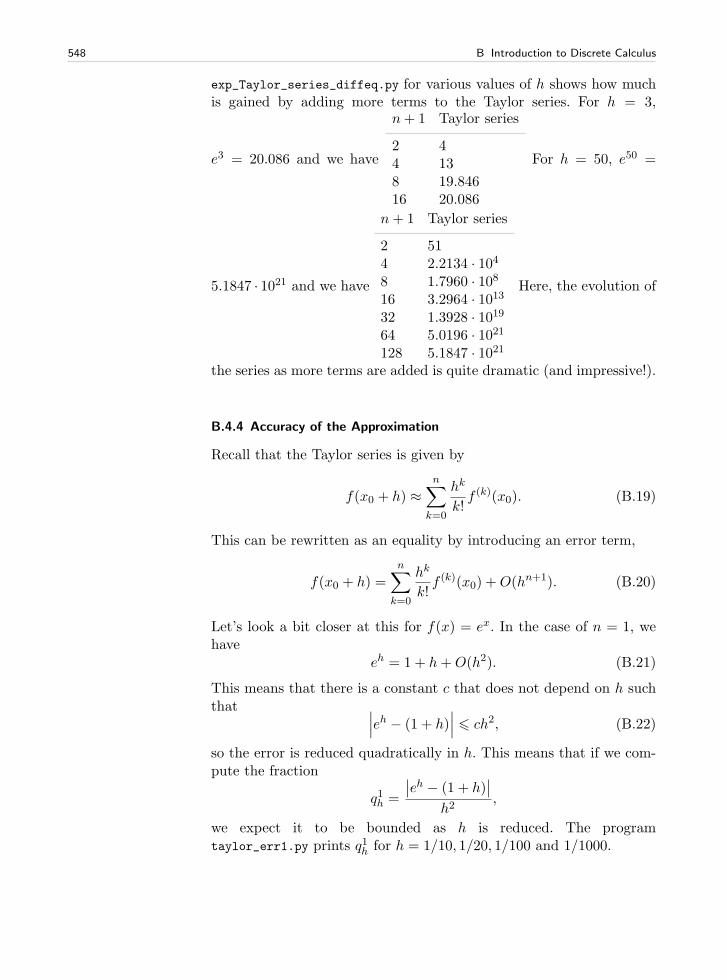
548 B Introduction to Discrete Calculus

exp_Taylor_series_diffeq.py for various values of h shows how muchis gained by adding more terms to the Taylor series. For h = 3,

e3 = 20.086 and we have

n+ 1 Taylor series

2 44 138 19.84616 20.086

For h = 50, e50 =

5.1847 · 1021 and we have

n+ 1 Taylor series

2 514 2.2134 · 1048 1.7960 · 10816 3.2964 · 101332 1.3928 · 101964 5.0196 · 1021128 5.1847 · 1021

Here, the evolution of

the series as more terms are added is quite dramatic (and impressive!).

B.4.4 Accuracy of the Approximation

Recall that the Taylor series is given by

f(x0 + h) ≈n∑

k=0

hk

k!f (k)(x0). (B.19)

This can be rewritten as an equality by introducing an error term,

f(x0 + h) =n∑

k=0

hk

k!f (k)(x0) +O(hn+1). (B.20)

Let’s look a bit closer at this for f(x) = ex. In the case of n = 1, wehave

eh = 1 + h+O(h2). (B.21)

This means that there is a constant c that does not depend on h suchthat

∣

∣

∣eh − (1 + h)

∣

∣

∣6 ch2, (B.22)

so the error is reduced quadratically in h. This means that if we com-pute the fraction

q1h =

∣

∣eh − (1 + h)∣

∣

h2,

we expect it to be bounded as h is reduced. The programtaylor_err1.py prints q1h for h = 1/10, 1/20, 1/100 and 1/1000.

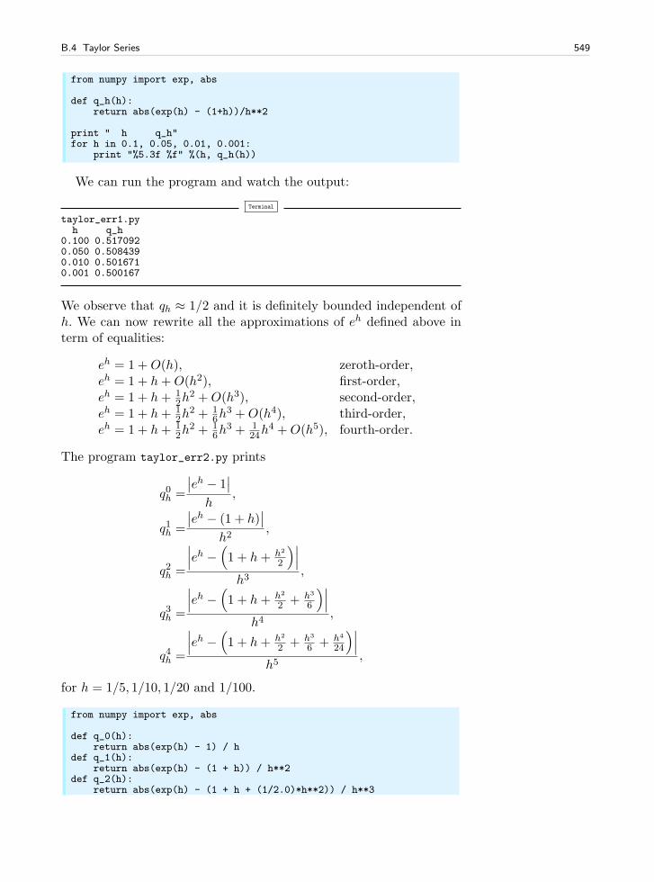
B.4 Taylor Series 549

from numpy import exp, abs

def q_h(h):return abs(exp(h) - (1+h))/h**2

print " h q_h"for h in 0.1, 0.05, 0.01, 0.001:

print "%5.3f %f" %(h, q_h(h))

We can run the program and watch the output:

Terminal

taylor_err1.pyh q_h

0.100 0.5170920.050 0.5084390.010 0.5016710.001 0.500167

We observe that qh ≈ 1/2 and it is definitely bounded independent ofh. We can now rewrite all the approximations of eh defined above interm of equalities:

eh = 1 +O(h), zeroth-order,eh = 1 + h+O(h2), first-order,eh = 1 + h+ 1

2h2 +O(h3), second-order,

eh = 1 + h+ 12h

2 + 16h

3 +O(h4), third-order,eh = 1 + h+ 1

2h2 + 1

6h3 + 1

24h4 +O(h5), fourth-order.

The program taylor_err2.py prints

q0h =

∣

∣eh − 1∣

∣

h,

q1h =

∣

∣eh − (1 + h)∣

∣

h2,

q2h =

∣

∣

∣eh −

(

1 + h+ h2

2

)∣

∣

∣

h3,

q3h =

∣

∣

∣eh −(

1 + h+ h2

2 + h3

6

)∣

∣

∣

h4,

q4h =

∣

∣

∣eh −

(

1 + h+ h2

2 + h3

6 + h4

24

)∣

∣

∣

h5,

for h = 1/5, 1/10, 1/20 and 1/100.

from numpy import exp, abs

def q_0(h):return abs(exp(h) - 1) / h

def q_1(h):return abs(exp(h) - (1 + h)) / h**2

def q_2(h):return abs(exp(h) - (1 + h + (1/2.0)*h**2)) / h**3

550 B Introduction to Discrete Calculus

def q_3(h):return abs(exp(h) - (1 + h + (1/2.0)*h**2 + \

(1/6.0)*h**3)) / h**4def q_4(h):

return abs(exp(h) - (1 + h + (1/2.0)*h**2 + (1/6.0)*h**3 + \(1/24.0)*h**4)) / h**5

hlist = [0.2, 0.1, 0.05, 0.01]print "%-05s %-09s %-09s %-09s %-09s %-09s" \

%("h", "q_0", "q_1", "q_2", "q_3", "q_4")for h in hlist:

print "%.02f %04f %04f %04f %04f %04f" \%(h, q_0(h), q_1(h), q_2(h), q_3(h), q_4(h))

By using the program, we get the following table:h q_0 q_1 q_2 q_3 q_40.20 1.107014 0.535069 0.175345 0.043391 0.0086190.10 1.051709 0.517092 0.170918 0.042514 0.0084740.05 1.025422 0.508439 0.168771 0.042087 0.0084030.01 1.005017 0.501671 0.167084 0.041750 0.008344

Again we observe that the error of the approximation behaves as indi-cated in (B.20).

B.4.5 Derivatives Revisited

We observed aboved that

f ′(x) ≈ f(x+ h)− f(x)

h.

By using the Taylor series, we can obtain this approximation directly,and also get an indication of the error of the approximation. From(B.20) it follows that

f(x+ h) = f(x) + hf ′(x) +O(h2),

and thus

f ′(x) =f(x+ h)− f(x)

h+O(h), (B.23)

so the error is proportional to h. We can investigate if this is thecase through some computer experiments. Take f(x) = ln(x), so thatf ′(x) = 1/x. The program diff_ln_err.py prints h and

1

h

∣

∣

∣

∣

f ′(x)− f(x+ h)− f(x)

h

∣

∣

∣

∣

(B.24)

at x = 10 for a range of h values.

def error(h):return (1.0/h)*abs(df(x) - (f(x+h)-f(x))/h)

from math import log as ln

def f(x):return ln(x)

B.4 Taylor Series 551

def df(x):return 1.0/x

x = 10hlist = []for h in 0.2, 0.1, 0.05, 0.01, 0.001:

print "%.4f %4f" % (h, error(h))

From the output0.2000 0.0049340.1000 0.0049670.0500 0.0049830.0100 0.0049970.0010 0.005000

we observe that the quantity in (B.24) is constant (≈ 0.5) independentof h, which indicates that the error is proportional to h.

B.4.6 More Accurate Difference Approximations

We can also use the Taylor series to derive more accurate approxima-tions of the derivatives. From (B.20), we have

f(x+ h) ≈ f(x) + hf ′(x) +h2

2f ′′(x) +O(h3). (B.25)

By using −h insted of h, we get

f(x− h) ≈ f(x)− hf ′(x) +h2

2f ′′(x) +O(h3). (B.26)

By subtracting (B.26) from (B.25), we have

f(x+ h)− f(x− h) = 2hf ′(x) +O(h3),

and consequently

f ′(x) =f(x+ h)− f(x− h)

2h+O(h2). (B.27)

Note that the error is now O(h2) whereas the error term of (B.23) isO(h). In order to see if the error is actually reduced, let us comparethe following two approximations

f ′(x) ≈ f(x+ h)− f(x)

hand f ′(x) ≈ f(x+ h)− f(x− h)

2h

by applying them to the discrete version of sin(x) on the interval (0, π).As usual, we let n > 1 be a given integer, and define the mesh

xi = ih for i = 0, 1, . . . , n,

where h = π/n. At the nodes, we have the functional values

552 B Introduction to Discrete Calculus

si = sin(xi) for i = 0, 1, . . . , n,

and at the inner nodes we define the first (F) and second (S) orderapproximations of the derivatives given by

dFi =si+1 − si

h,

and

dSi =si+1 − si−1

2h,

respectively for i = 1, 2, . . . , n − 1. These values should be comparedto the exact derivative given by

di = cos(xi) for i = 1, 2, . . . , n− 1.

The following program, found in diff_1st2nd_order.py, plots the dis-crete functions (xi, di)

n−1i=1 , (xi, d

Fi )

n−1i=1 , and (xi, d

Si )

n−1i=1 for a given n.

Note that the first three functions in this program are completely gen-eral in that they can be used for any f(x) on any mesh. The specialcase of f(x) = sin(x) and comparing first- and second-order formulasis implemented in the example function. This latter function is calledin the test block of the file. That is, the file is a module and we canreuse the first three functions in other programs (in particular, we canuse the third function in the next example).

def first_order(f, x, h):return (f(x+h) - f(x))/h

def second_order(f, x, h):return (f(x+h) - f(x-h))/(2*h)

def derivative_on_mesh(formula, f, a, b, n):"""Differentiate f(x) at all internal points in a meshon [a,b] with n+1 equally spaced points.The differentiation formula is given by formula(f, x, h)."""h = (b-a)/float(n)x = linspace(a, b, n+1)df = zeros(len(x))for i in xrange(1, len(x)-1):

df[i] = formula(f, x[i], h)# Return x and values at internal points onlyreturn x[1:-1], df[1:-1]

def example(n):a = 0; b = pi;x, dF = derivative_on_mesh(first_order, sin, a, b, n)x, dS = derivative_on_mesh(second_order, sin, a, b, n)# Accurate plot of the exact derivative at internal pointsh = (b-a)/float(n)xfine = linspace(a+h, b-h, 1001)exact = cos(xfine)plot(x, dF, ’r-’, x, dS, ’b-’, xfine, exact, ’y-’,

legend=(’First-order derivative’,’Second-order derivative’,’Correct function’),

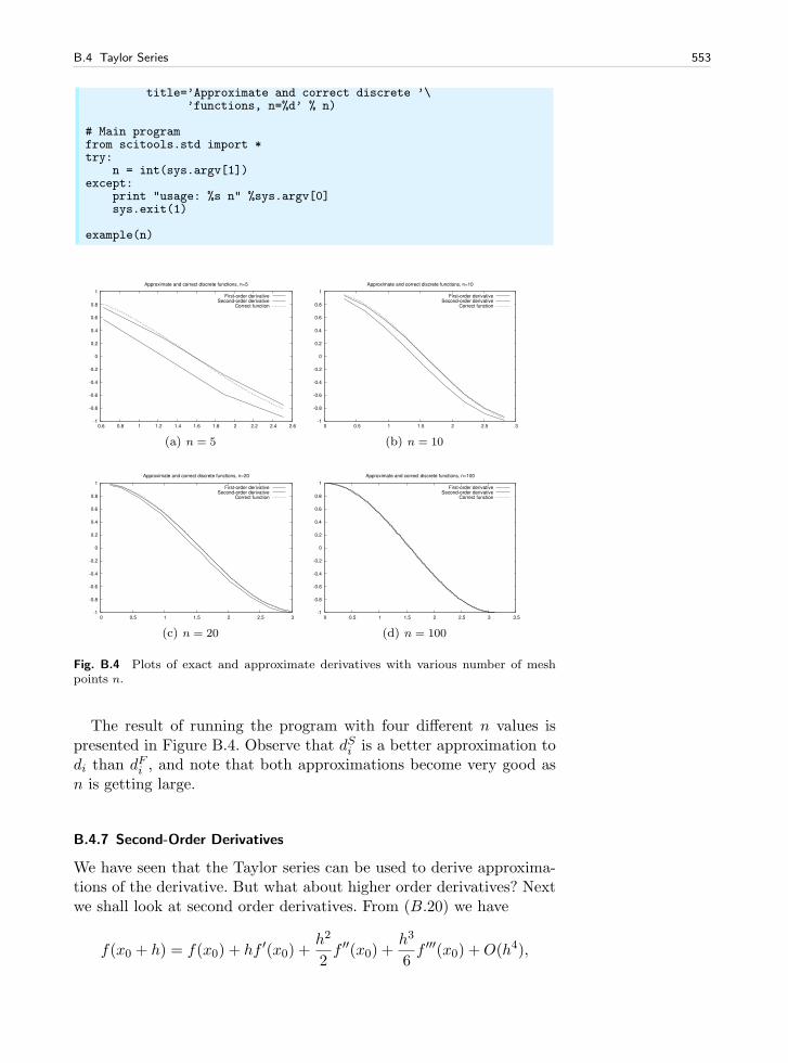
B.4 Taylor Series 553

title=’Approximate and correct discrete ’\’functions, n=%d’ % n)

# Main programfrom scitools.std import *try:

n = int(sys.argv[1])except:

print "usage: %s n" %sys.argv[0]sys.exit(1)

example(n)

-1

-0.8

-0.6

-0.4

-0.2

0

0.2

0.4

0.6

0.8

1

0.6 0.8 1 1.2 1.4 1.6 1.8 2 2.2 2.4 2.6

Approximate and correct discrete functions, n=5

First-order derivativeSecond-order derivative

Correct function

(a) n = 5

-1

-0.8

-0.6

-0.4

-0.2

0

0.2

0.4

0.6

0.8

1

0 0.5 1 1.5 2 2.5 3

Approximate and correct discrete functions, n=10

First-order derivativeSecond-order derivative

Correct function

(b) n = 10

-1

-0.8

-0.6

-0.4

-0.2

0

0.2

0.4

0.6

0.8

1

0 0.5 1 1.5 2 2.5 3

Approximate and correct discrete functions, n=20

First-order derivativeSecond-order derivative

Correct function

(c) n = 20

-1

-0.8

-0.6

-0.4

-0.2

0

0.2

0.4

0.6

0.8

1

0 0.5 1 1.5 2 2.5 3 3.5

Approximate and correct discrete functions, n=100

First-order derivativeSecond-order derivative

Correct function

(d) n = 100

Fig. B.4 Plots of exact and approximate derivatives with various number of meshpoints n.

The result of running the program with four different n values ispresented in Figure B.4. Observe that dSi is a better approximation todi than dFi , and note that both approximations become very good asn is getting large.

B.4.7 Second-Order Derivatives

We have seen that the Taylor series can be used to derive approxima-tions of the derivative. But what about higher order derivatives? Nextwe shall look at second order derivatives. From (B.20) we have

f(x0 + h) = f(x0) + hf ′(x0) +h2

2f ′′(x0) +

h3

6f ′′′(x0) +O(h4),

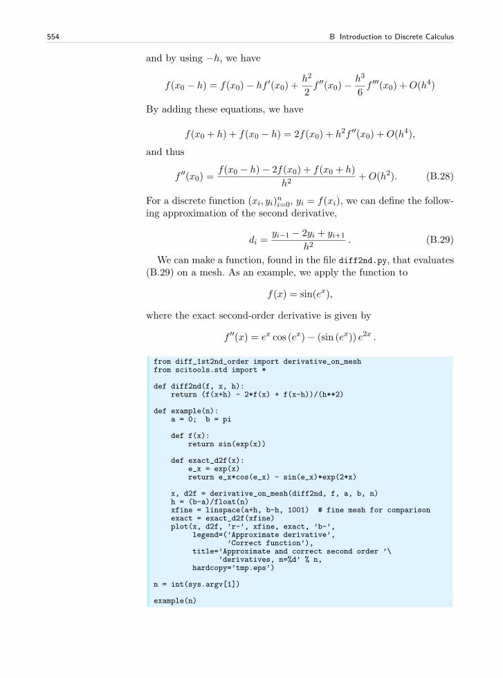
554 B Introduction to Discrete Calculus

and by using −h, we have

f(x0 − h) = f(x0)− hf ′(x0) +h2

2f ′′(x0)−

h3

6f ′′′(x0) +O(h4)

By adding these equations, we have

f(x0 + h) + f(x0 − h) = 2f(x0) + h2f ′′(x0) +O(h4),

and thus

f ′′(x0) =f(x0 − h)− 2f(x0) + f(x0 + h)

h2+ O(h2). (B.28)

For a discrete function (xi, yi)ni=0, yi = f(xi), we can define the follow-

ing approximation of the second derivative,

di =yi−1 − 2yi + yi+1

h2. (B.29)

We can make a function, found in the file diff2nd.py, that evaluates(B.29) on a mesh. As an example, we apply the function to

f(x) = sin(ex),

where the exact second-order derivative is given by

f ′′(x) = ex cos (ex)− (sin (ex)) e2x .

from diff_1st2nd_order import derivative_on_meshfrom scitools.std import *

def diff2nd(f, x, h):return (f(x+h) - 2*f(x) + f(x-h))/(h**2)

def example(n):a = 0; b = pi

def f(x):return sin(exp(x))

def exact_d2f(x):e_x = exp(x)return e_x*cos(e_x) - sin(e_x)*exp(2*x)

x, d2f = derivative_on_mesh(diff2nd, f, a, b, n)h = (b-a)/float(n)xfine = linspace(a+h, b-h, 1001) # fine mesh for comparisonexact = exact_d2f(xfine)plot(x, d2f, ’r-’, xfine, exact, ’b-’,

legend=(’Approximate derivative’,’Correct function’),

title=’Approximate and correct second order ’\’derivatives, n=%d’ % n,

hardcopy=’tmp.eps’)

n = int(sys.argv[1])

example(n)

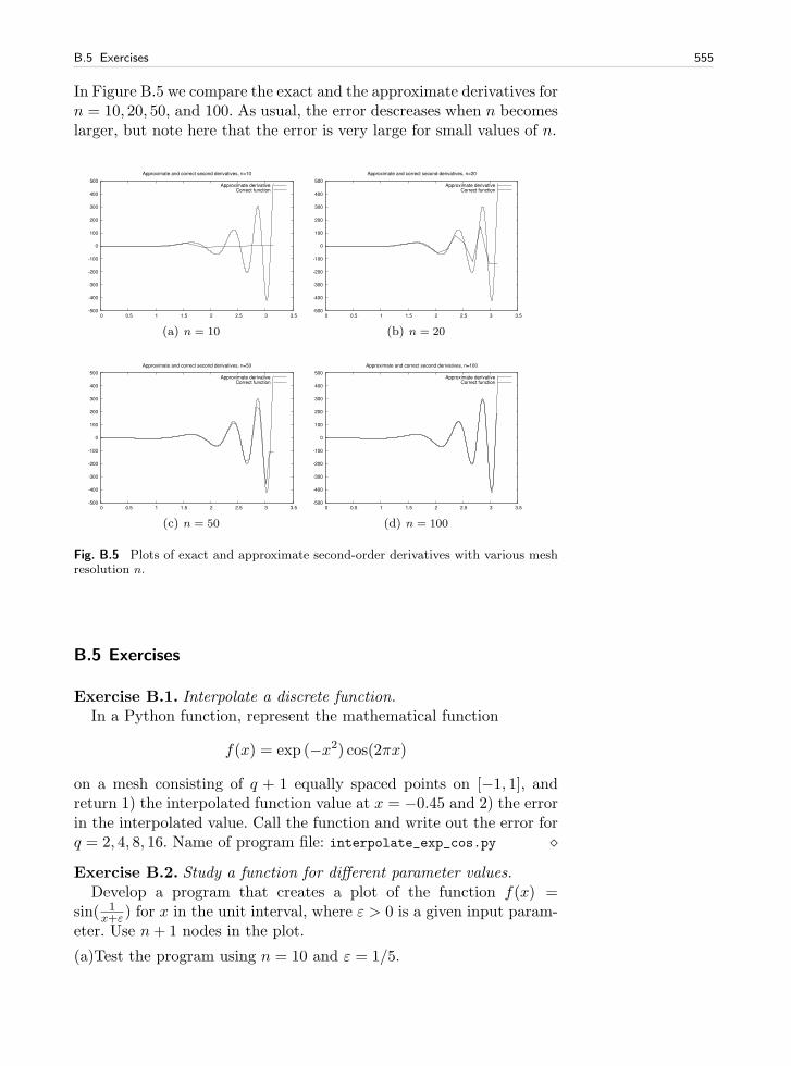
B.5 Exercises 555

In Figure B.5 we compare the exact and the approximate derivatives forn = 10, 20, 50, and 100. As usual, the error descreases when n becomeslarger, but note here that the error is very large for small values of n.

-500

-400

-300

-200

-100

0

100

200

300

400

500

0 0.5 1 1.5 2 2.5 3 3.5

Approximate and correct second derivatives, n=10

Approximate derivativeCorrect function

(a) n = 10

-500

-400

-300

-200

-100

0

100

200

300

400

500

0 0.5 1 1.5 2 2.5 3 3.5

Approximate and correct second derivatives, n=20

Approximate derivativeCorrect function

(b) n = 20

-500

-400

-300

-200

-100

0

100

200

300

400

500

0 0.5 1 1.5 2 2.5 3 3.5

Approximate and correct second derivatives, n=50

Approximate derivativeCorrect function

(c) n = 50

-500

-400

-300

-200

-100

0

100

200

300

400

500

0 0.5 1 1.5 2 2.5 3 3.5

Approximate and correct second derivatives, n=100

Approximate derivativeCorrect function

(d) n = 100

Fig. B.5 Plots of exact and approximate second-order derivatives with various meshresolution n.

B.5 Exercises

Exercise B.1. Interpolate a discrete function.In a Python function, represent the mathematical function

f(x) = exp (−x2) cos(2πx)

on a mesh consisting of q + 1 equally spaced points on [−1, 1], andreturn 1) the interpolated function value at x = −0.45 and 2) the errorin the interpolated value. Call the function and write out the error forq = 2, 4, 8, 16. Name of program file: interpolate_exp_cos.py ⋄

Exercise B.2. Study a function for different parameter values.Develop a program that creates a plot of the function f(x) =

sin( 1x+ε) for x in the unit interval, where ε > 0 is a given input param-

eter. Use n+ 1 nodes in the plot.

(a)Test the program using n = 10 and ε = 1/5.

556 B Introduction to Discrete Calculus

(b)Refine the program such that it plots the function for two values ofn; say n and n+ 10.

(c)How large do you have to choose n in order for the difference betweenthese two functions to be less than 0.1? Hint: Each function givesan array. Create a while loop and use the max function of the arraysto retrieve the maximum value and compare these.

(d)Let ε = 1/10, and repeat (c).(e)Let ε = 1/20, and repeat (c).(f)Try to find a formula for how large n needs to be for a given value

of ε such that increasing n further does not change the plot so muchthat it is visible on the screen. Note that there is no exact answerto this question.

Name of program file: plot_sin_eps.py ⋄

Exercise B.3. Study a function and its derivative.Consider the function

f(x) = sin

(

1

x+ ε

)

for x ranging from 0 to 1, and the derivative

f ′(x) =− cos

(

1x+ε

)

(x+ ε)2.

Here, ε is a given input parameter.

(a)Develop a program that creates a plot of the derivative of f = f(x)based on a finite difference approximation using n computationalnodes. The program should also graph the exact derivative given byf ′ = f ′(x) above.

(b)Test the program using n = 10 and ε = 1/5.(c)How large do you have to choose n in order for the difference between

these two functions to be less than 0.1? Hint: Each function givesan array. Create a while loop and use the max function of the arraysto retrieve the maximum value and compare these.

(d)Let ε = 1/10, and repeat (c).(e)Let ε = 1/20, and repeat (c).(f)Try determine experimentally how large n needs to be for a given

value of ε such that increasing n further does not change the plotso much that you can view it on the screen. Note, again, that thereis no exact solution to this problem.

Name of program file: sin_deriv.py ⋄

Exercise B.4. Use the Trapezoidal method.The purpose of this excercise is to test the program trapezoidal.py.

(a)Let

B.5 Exercises 557

a =

∫ 1

0e4xdx =

1

4e4 − 1

4.

Compute the integral using the program trapezoidal.py and, for agiven n, let a(n) denote the result. Try to find, experimentally, howlarge you have to choose n in order for

|a− a(n)| 6 ε

where ε = 1/100.(b)Repeat (a) with ε = 1/1000.(c)Repeat (a) with ε = 1/10000.(d)Try to figure out, in general, how large n has to be in order for

|a− a(n)| 6 ε

for a given value of ε.

Name of program file: trapezoidal_test_exp.py ⋄

Exercise B.5. Compute a sequence of integrals.

(a)Let

bk =

∫ 1

0xkdx =

1

k + 1,

and let bk(n) denote the result of using the program trapezoidal.py

to compute∫ 10 xkdx. For k = 4, 6 and 8, try to figure out, by doing

numerical experiments, how large n needs to be in order for bk(n)to satisfy

∣

∣bk − bk(n)∣

∣ 6 0.0001.

Note that n will depend on k. Hint: Run the program for each k,look at the output, and calculate

∣

∣bk − bk(n)∣

∣ manually.(b)Try to generalize the result in (a) to arbitrary k > 2.(c)Generate a plot of xk on the unit interval for k = 2, 4, 6, 8, and 10,

and try to figure out if the results obtained in (a) and (b) are rea-sonable taking into account that the program trapezoidal.py wasdeveloped using a piecewise linear approximation of the function.

Name of program file: trapezoidal_test_power.py ⋄

Exercise B.6. Use the Trapezoidal method.The purpose of this excercise is to compute an approximation of the

integral9

I =

∫ ∞

−∞e−x2

dx

using the Trapezoidal method.

9 You may consult your Calculus book to verify that the exact solution is√π.

558 B Introduction to Discrete Calculus

(a)Plot the function e−x2

for x ranging from −10 to 10 and use theplot to argue that

∫ ∞

−∞e−x2

dx = 2

∫ ∞

0e−x2

dx.

(b)Let T (n,L) be the approximation of the integral

2

∫ L

0

e−x2

dx

computed by the Trapezoidal method using n computational points.Develop a program that computes the value of T for a given n andL.

(c)Extend the program developed in (b) to write out values of T (n,L)in a table with rows corresponding to n = 100, 200, . . . , 500 andcolumns corresponding to L = 2, 4, 6, 8, 10.

(d)Extend the program to also print a table of the errors in T (n,L) forthe same n and L values as in (c). The exact value of the integralis√π.

Comment. Numerical integration of integrals with finite limits requiresa choice of n, while with infinite limits we also need to truncate thedomain, i.e., choose L in the present example. The accuracy dependson both n and L. Name of program file: integrate_exp.py ⋄

Exercise B.7. Trigonometric integrals.The purpose of this excercise is to demonstrate a property of trigono-

metric functions that you will meet in later courses. In this excercise,you may compute the integrals using the program trapezoidal.py withn = 100.

(a)Consider the integrals

Ip,q = 2

∫ 1

0sin(pπx) sin(qπx)dx

and fill in values of the integral Ip,q in a table with rows correspond-ing to q = 0, 1, . . . , 4 and columns corresponding to p = 0, 1, . . . , 4.

(b)Repeat (a) for the integrals

Ip,q = 2

∫ 1

0cos(pπx) cos(qπx)dx.

(c)Repeat (a) for the integrals

Ip,q = 2

∫ 1

0cos(pπx) sin(qπx)dx.

Name of program file: ortho_trig_funcs.py ⋄

B.5 Exercises 559

Exercise B.8. Plot functions and their derivatives.

(a)Use the program diff_func.py to plot approximations of the deriva-tive for the following functions defined on the interval ranging fromx = 1/1000 to x = 1:

f(x) = ln

(

x+1

100

)

,

g(x) = cos(e10x),

h(x) = xx.

(b)Extend the program such that both the discrete approximation andthe correct (analytical) derivative can be plotted. The analyticalderivative should be evaluated in the same computational points asthe numerical approximation. Test the program by comparing thediscrete and analytical derivative of x3.

(c)Use the program develped in (b) to compare the analytical anddiscrete derivatives of the functions given in (a). How large do youhave to choose n in each case in order for the plots to becomeindistinguishable on your screen. Note that the analytical derivativesare given by:

f ′(x) =1

x+ 1100

,

g′(x) = −10e10x sin(

e10x)

h′(x) = (lnx)xx + xxx−1

Name of program file: diff_functions.py ⋄

Exercise B.9. Use the Trapezoidal method.Develop an efficient program that creates a plot of the function

f(x) =1

2+

1√π

∫ x

0

e−t2dt

for x ∈ [0, 10]. The integral should be approximated using the Trape-zoidal method and use as few function evaluations of e−t2 as possible.Name of program file: plot_integral.py ⋄

Introduction to Differential Equations C

This appendix is authored by Aslak Tveito

Differential equations have proven to be an immensely successful in-strument for modeling phenomena in science and technology. It ishardly an exaggeration to say that differential equations are used todefine mathematical models in virtually all parts of the natural sci-ences. In this chapter, we will take the first steps towards learning howto deal with differential equations on a computer. This is a core issuein Computational Science and reaches far beyond what we can coverin this text. However, the ideas you will see here are reused in lotsof advanced applications, so this chapter will hopefully provide usefulintroduction to a topic that you will probably encounter many timeslater.

We will show you how to build programs for solving differential equa-tions. More precisely, we will show how a differential equation can beformulated in a discrete manner suitable for analysis on a computer,and how to implement programs to compute the discrete solutions. Thesimplest differential equations can be solved analytically in the sensethat you can write down an explicit formula for the solutions. How-ever, differential equations arising in practical applications are usuallyrather complicated and thus have to be solved numerically on a com-puter. Therefore we focus on implementing numerical methods to solvethe equations. Appendix E describes more advanced implementationtechniques aimed at making an easy-to-use toolbox for solving differ-ential equations. Exercises in the present appendix and Appendix Eaim at solving a variety of differential equations arising in various dis-ciplines of science.

As with all the other chapters, the source code can be found insrc, in this case in the subdirectory ode1. The short form ODE (plu-ral: ODEs) is commonly used as abbreviation for ordinary differential

561

562 C Introduction to Differential Equations

equation, which is the type of differential equation that we addressin this appendix. Actually, differential equations are divided into twogroups: ordinary differential equations and partial differential equa-tions. Ordinary differential equations contain derivatives with respectto one variable (usually t in our examples), whereas partial differentialequations contain derivatives with respect to more than one variable,typically with respect to space and time. A typical ordinary differentialequation is

u′(t) = u(t),

and a typical partial differential equation is

∂u

∂t=

∂2u

∂x2+

∂2u

∂y2,

The latter is known as the heat or diffusion equation.

C.1 The Simplest Case

Consider the problem of solving the following equation

u′(t) = t3 . (C.1)

The solution can be computed directly by integrating (C.1), whichgives

u(t) =1

4t4 + C,

where C is an arbitrary constant. To obtain a unique solution, we needan extra condition to determine C. Specifying u(t1) for some time pointt1 represents a possible extra condition. It is common to view (C.1) asan equation for the function u(t) for t ∈ [0, T ], and the extra conditionis usually that the start value u(0) is known. This is called the initialcondition. Say

u(0) = 1 . (C.2)

In general, the solution of the differential equation (C.1) subject to theinitial condition C.2 is1

u(t) = u(0) +

∫ t

0u′(τ)dτ,

= 1 +

∫ t

0τ3dτ

= 1 +1

4t4 .

1 If you are confused by the use of t and τ, don’t get too upset; you see: ”In mathemat-ics you don’t understand things. You just get used to them.” –John von Neumann,mathematician, 1903-1957.

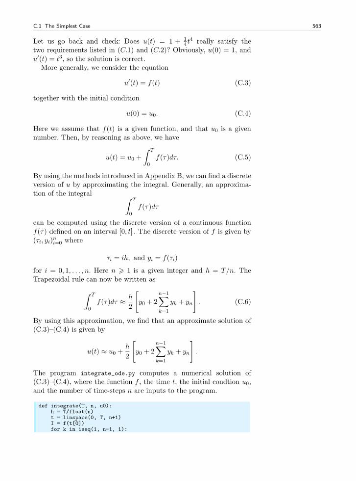
C.1 The Simplest Case 563

Let us go back and check: Does u(t) = 1 + 14 t

4 really satisfy thetwo requirements listed in (C.1) and (C.2)? Obviously, u(0) = 1, andu′(t) = t3, so the solution is correct.

More generally, we consider the equation

u′(t) = f(t) (C.3)

together with the initial condition

u(0) = u0. (C.4)

Here we assume that f(t) is a given function, and that u0 is a givennumber. Then, by reasoning as above, we have

u(t) = u0 +

∫ T

0f(τ)dτ. (C.5)

By using the methods introduced in Appendix B, we can find a discreteversion of u by approximating the integral. Generally, an approxima-tion of the integral

∫ T

0

f(τ)dτ

can be computed using the discrete version of a continuous functionf(τ) defined on an interval [0, t] . The discrete version of f is given by(τi, yi)

ni=0 where

τi = ih, and yi = f(τi)

for i = 0, 1, . . . , n. Here n > 1 is a given integer and h = T/n. TheTrapezoidal rule can now be written as

∫ T

0f(τ)dτ ≈ h

2

[

y0 + 2

n−1∑

k=1

yk + yn

]

. (C.6)

By using this approximation, we find that an approximate solution of(C.3)–(C.4) is given by

u(t) ≈ u0 +h

2

[

y0 + 2

n−1∑

k=1

yk + yn

]

.

The program integrate_ode.py computes a numerical solution of(C.3)–(C.4), where the function f , the time t, the initial condtion u0,and the number of time-steps n are inputs to the program.

def integrate(T, n, u0):h = T/float(n)t = linspace(0, T, n+1)I = f(t[0])for k in iseq(1, n-1, 1):

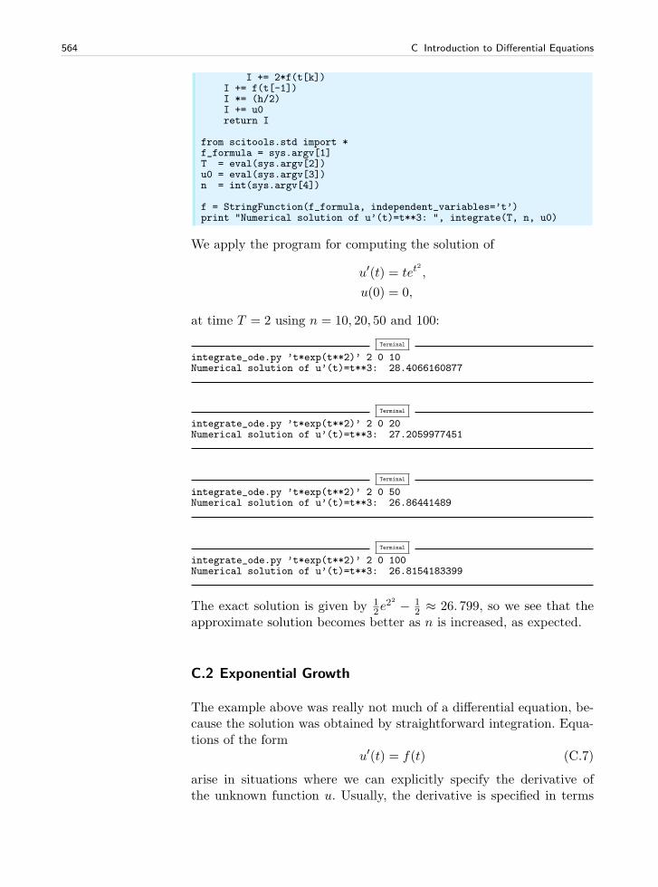
564 C Introduction to Differential Equations

I += 2*f(t[k])I += f(t[-1])I *= (h/2)I += u0return I

from scitools.std import *f_formula = sys.argv[1]T = eval(sys.argv[2])u0 = eval(sys.argv[3])n = int(sys.argv[4])

f = StringFunction(f_formula, independent_variables=’t’)print "Numerical solution of u’(t)=t**3: ", integrate(T, n, u0)

We apply the program for computing the solution of

u′(t) = tet2

,

u(0) = 0,

at time T = 2 using n = 10, 20, 50 and 100:

Terminal

integrate_ode.py ’t*exp(t**2)’ 2 0 10Numerical solution of u’(t)=t**3: 28.4066160877

Terminal

integrate_ode.py ’t*exp(t**2)’ 2 0 20Numerical solution of u’(t)=t**3: 27.2059977451

Terminal

integrate_ode.py ’t*exp(t**2)’ 2 0 50Numerical solution of u’(t)=t**3: 26.86441489

Terminal

integrate_ode.py ’t*exp(t**2)’ 2 0 100Numerical solution of u’(t)=t**3: 26.8154183399

The exact solution is given by 12e

22 − 12 ≈ 26. 799, so we see that the

approximate solution becomes better as n is increased, as expected.

C.2 Exponential Growth

The example above was really not much of a differential equation, be-cause the solution was obtained by straightforward integration. Equa-tions of the form

u′(t) = f(t) (C.7)

arise in situations where we can explicitly specify the derivative ofthe unknown function u. Usually, the derivative is specified in terms

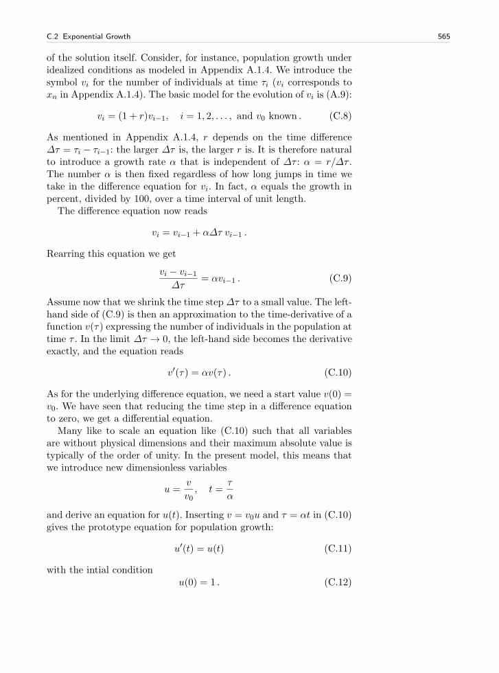
C.2 Exponential Growth 565

of the solution itself. Consider, for instance, population growth underidealized conditions as modeled in Appendix A.1.4. We introduce thesymbol vi for the number of individuals at time τi (vi corresponds toxn in Appendix A.1.4). The basic model for the evolution of vi is (A.9):

vi = (1 + r)vi−1, i = 1, 2, . . . , and v0 known . (C.8)

As mentioned in Appendix A.1.4, r depends on the time difference∆τ = τi − τi−1: the larger ∆τ is, the larger r is. It is therefore naturalto introduce a growth rate α that is independent of ∆τ : α = r/∆τ .The number α is then fixed regardless of how long jumps in time wetake in the difference equation for vi. In fact, α equals the growth inpercent, divided by 100, over a time interval of unit length.

The difference equation now reads

vi = vi−1 + α∆τ vi−1 .

Rearring this equation we get

vi − vi−1

∆τ= αvi−1 . (C.9)

Assume now that we shrink the time step ∆τ to a small value. The left-hand side of (C.9) is then an approximation to the time-derivative of afunction v(τ) expressing the number of individuals in the population attime τ . In the limit ∆τ → 0, the left-hand side becomes the derivativeexactly, and the equation reads

v′(τ) = αv(τ) . (C.10)

As for the underlying difference equation, we need a start value v(0) =v0. We have seen that reducing the time step in a difference equationto zero, we get a differential equation.

Many like to scale an equation like (C.10) such that all variablesare without physical dimensions and their maximum absolute value istypically of the order of unity. In the present model, this means thatwe introduce new dimensionless variables

u =v

v0, t =

τ

α

and derive an equation for u(t). Inserting v = v0u and τ = αt in (C.10)gives the prototype equation for population growth:

u′(t) = u(t) (C.11)

with the intial conditionu(0) = 1 . (C.12)

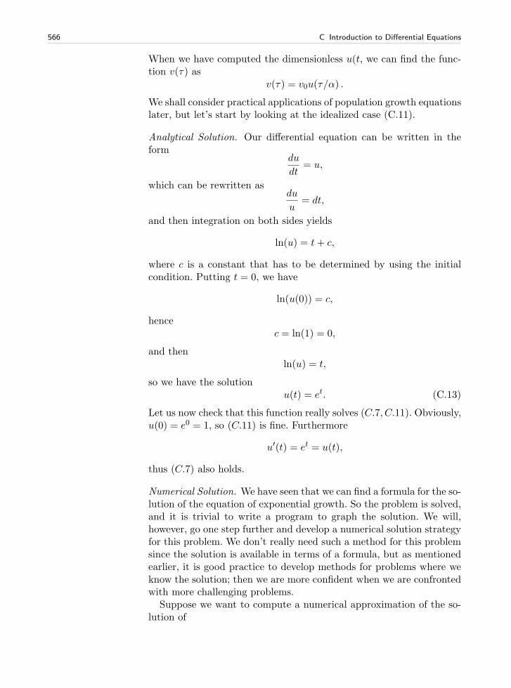
566 C Introduction to Differential Equations

When we have computed the dimensionless u(t, we can find the func-tion v(τ) as

v(τ) = v0u(τ/α) .

We shall consider practical applications of population growth equationslater, but let’s start by looking at the idealized case (C.11).

Analytical Solution. Our differential equation can be written in theform

du

dt= u,

which can be rewritten asdu

u= dt,

and then integration on both sides yields

ln(u) = t+ c,

where c is a constant that has to be determined by using the initialcondition. Putting t = 0, we have

ln(u(0)) = c,

hencec = ln(1) = 0,

and thenln(u) = t,

so we have the solutionu(t) = et. (C.13)

Let us now check that this function really solves (C.7, C.11). Obviously,u(0) = e0 = 1, so (C.11) is fine. Furthermore

u′(t) = et = u(t),

thus (C.7) also holds.

Numerical Solution. We have seen that we can find a formula for the so-lution of the equation of exponential growth. So the problem is solved,and it is trivial to write a program to graph the solution. We will,however, go one step further and develop a numerical solution strategyfor this problem. We don’t really need such a method for this problemsince the solution is available in terms of a formula, but as mentionedearlier, it is good practice to develop methods for problems where weknow the solution; then we are more confident when we are confrontedwith more challenging problems.

Suppose we want to compute a numerical approximation of the so-lution of

C.2 Exponential Growth 567

u′(t) = u(t) (C.14)

equipped with the intial condition

u(0) = 1. (C.15)

We want to compute approximations from time t = 0 to time t = 1.Let n > 1 be a given integer, and define

∆t = 1/n . (C.16)

Furthermore, let uk denote an approximation of u(tk) where

tk = k∆t (C.17)

for k = 0, 1, . . . , n. The key step in developing a numerical method forthis differential equation is to invoke the Taylor series as applied to theexact solution,

u(tk+1) = u(tk) +∆tu′(tk) +O(∆t2), (C.18)

which implies that

u′(tk) ≈u(tk+1)− u(tk)

∆t. (C.19)

By using (C.14) , we get

u(tk+1)− u(tk)

∆t≈ u(tk). (C.20)

Recall now that u(tk) is the exact solution at time tk, and that uk isthe approximate solution at the same point in time. We now want todetermine uk for all k > 0. Obviously, we start by defining

u0 = u(0) = 1.

Since we want uk ≈ u(tk), we require that uk satisfy the followingequality

uk+1 − uk∆t

= uk (C.21)

motivated by (C.20) . It follows that

uk+1 = (1 +∆t)uk . (C.22)

Since u0 is known, we can compute u1, u2 and so on by usingthe formula above. The formula is implemented2 in the programexp_growth.py.

2 Actually, we do not need the method and we do not need the program. It followsfrom (C.22) that

uk = (1 +∆t)ku0

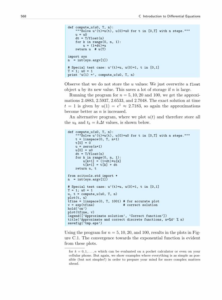
568 C Introduction to Differential Equations

def compute_u(u0, T, n):"""Solve u’(t)=u(t), u(0)=u0 for t in [0,T] with n steps."""u = u0dt = T/float(n)for k in range(0, n, 1):

u = (1+dt)*ureturn u # u(T)

import sysn = int(sys.argv[1])

# Special test case: u’(t)=u, u(0)=1, t in [0,1]T = 1; u0 = 1print ’u(1) =’, compute_u(u0, T, n)

Observe that we do not store the u values: We just overwrite a float

object u by its new value. This saves a lot of storage if n is large.Running the program for n = 5, 10, 20 and 100, we get the approxi-

mations 2.4883, 2.5937, 2.6533, and 2.7048. The exact solution at timet = 1 is given by u(1) = e1 ≈ 2.7183, so again the approximationsbecome better as n is increased.

An alternative program, where we plot u(t) and therefore store allthe uk and tk = k∆t values, is shown below.

def compute_u(u0, T, n):"""Solve u’(t)=u(t), u(0)=u0 for t in [0,T] with n steps."""t = linspace(0, T, n+1)t[0] = 0u = zeros(n+1)u[0] = u0dt = T/float(n)for k in range(0, n, 1):

u[k+1] = (1+dt)*u[k]t[k+1] = t[k] + dt

return u, t

from scitools.std import *n = int(sys.argv[1])

# Special test case: u’(t)=u, u(0)=1, t in [0,1]T = 1; u0 = 1u, t = compute_u(u0, T, n)plot(t, u)tfine = linspace(0, T, 1001) # for accurate plotv = exp(tfine) # correct solutionhold(’on’)plot(tfine, v)legend([’Approximate solution’, ’Correct function’])title(’Approximate and correct discrete functions, n=%d’ % n)savefig(’tmp.eps’)

Using the program for n = 5, 10, 20, and 100, results in the plots in Fig-ure C.1. The convergence towards the exponential function is evidentfrom these plots.

for k = 0, 1, . . . , n which can be evaluated on a pocket calculator or even on yourcellular phone. But again, we show examples where everything is as simple as pos-sible (but not simpler!) in order to prepare your mind for more complex mattersahead.

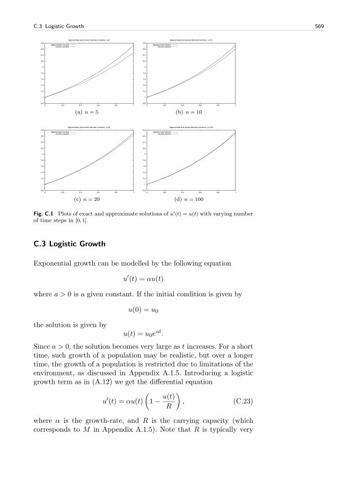
C.3 Logistic Growth 569

0.8

1

1.2

1.4

1.6

1.8

2

2.2

2.4

2.6

2.8

0 0.2 0.4 0.6 0.8 1

Approximate and correct discrete functions, n=5

Approximate solutionCorrect solution

(a) n = 5

0.8

1

1.2

1.4

1.6

1.8

2

2.2

2.4

2.6

2.8

0 0.2 0.4 0.6 0.8 1

Approximate and correct discrete functions, n=10

Approximate solutionCorrect solution

(b) n = 10

0.8

1

1.2

1.4

1.6

1.8

2

2.2

2.4

2.6

2.8

0 0.2 0.4 0.6 0.8 1

Approximate and correct discrete functions, n=20

Approximate solutionCorrect solution

(c) n = 20

0.8

1

1.2

1.4

1.6

1.8

2

2.2

2.4

2.6

2.8

0 0.2 0.4 0.6 0.8 1

Approximate and correct discrete functions, n=100

Approximate solutionCorrect solution

(d) n = 100

Fig. C.1 Plots of exact and approximate solutions of u′(t) = u(t) with varying numberof time steps in [0, 1].

C.3 Logistic Growth

Exponential growth can be modelled by the following equation

u′(t) = αu(t)

where a > 0 is a given constant. If the initial condition is given by

u(0) = u0

the solution is given byu(t) = u0e

αt.

Since a > 0, the solution becomes very large as t increases. For a shorttime, such growth of a population may be realistic, but over a longertime, the growth of a population is restricted due to limitations of theenvironment, as discussed in Appendix A.1.5. Introducing a logisticgrowth term as in (A.12) we get the differential equation

u′(t) = αu(t)

(

1− u(t)

R

)

, (C.23)

where α is the growth-rate, and R is the carrying capacity (whichcorresponds to M in Appendix A.1.5). Note that R is typically very

570 C Introduction to Differential Equations

large, so if u(0) is small, we have

u(t)

R≈ 0

for small values of t, and thus we have exponential growth for small t;

u′(t) ≈ au(t).

But as t increases, and u grows, the term u(t)/R will become importantand limit the growth.

A numerical scheme for the logistic equation (C.23) is given by

uk+1 − uk∆t

= αuk

(

1− ukR

)

,

which we can solve with respect to the unknown uk+1:

uk+1 = uk +∆tαuk

(

1− ukR

)

. (C.24)

This is the form of the equation that is suited for implementation.

C.4 A Simple Pendulum

So far we have considered scalar ordinary differential equations, i.e.,equations with one single function u(t) as unknown. Now we shall dealwith systems of ordinary differential equations, where in general n un-known functions are coupled in a system of n equations. Our introduc-tory example will be a system of two equations having two unknownfunctions u(t) and v(t). The example concerns the motion of a pendu-lum, see Figure C.2. A sphere with mass m is attached to a masslessrod of length L and oscillates back and forth due to gravity. Newton’ssecond law of motion applied to this physical system gives rise thedifferential equation

θ′′(t) + α sin(θ) = 0 (C.25)

where θ = θ(t) is the angle the rod makes with the vertical, measuredin radians, and α = g/L (g is the acceleration of gravity). The un-known function to solve for is θ, and knowing θ, we can quite easilycompute the position of the sphere, its velocity, and its acceleration,as well as the tension force in the rod. Since the highest derivativein (C.25) is of second order, we refer to (C.25) as a second-order dif-ferential equations. Our previous examples in this chapter involvedonly first-order derivatives, and therefore they are known as first-orderdifferential equations.

Equation (C.25) can be solved by the same numerical method as weuse in Appendix D.1.2, because (C.25) is very similar to Equation D.8,

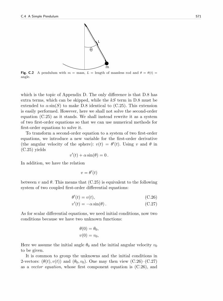
C.4 A Simple Pendulum 571

Fig. C.2 A pendulum with m = mass, L = length of massless rod and θ = θ(t) =

angle.

which is the topic of Appendix D. The only difference is that D.8 hasextra terms, which can be skipped, while the kS term in D.8 must beextended to α sin(S) to make D.8 identical to (C.25). This extensionis easily performed. However, here we shall not solve the second-orderequation (C.25) as it stands. We shall instead rewrite it as a systemof two first-order equations so that we can use numerical methods forfirst-order equations to solve it.

To transform a second-order equation to a system of two first-orderequations, we introduce a new variable for the first-order derivative(the angular velocity of the sphere): v(t) = θ′(t). Using v and θ in(C.25) yields

v′(t) + α sin(θ) = 0 .

In addition, we have the relation

v = θ′(t)

between v and θ. This means that (C.25) is equivalent to the followingsystem of two coupled first-order differential equations:

θ′(t) = v(t), (C.26)

v′(t) = −α sin(θ) . (C.27)

As for scalar differential equations, we need initial conditions, now twoconditions because we have two unknown functions:

θ(0) = θ0,

v(0) = v0,

Here we assume the initial angle θ0 and the initial angular velocity v0to be given.

It is common to group the unknowns and the initial conditions in2-vectors: (θ(t), v(t)) and (θ0, v0). One may then view (C.26)–(C.27)as a vector equation, whose first component equation is (C.26), and

572 C Introduction to Differential Equations

the second component equation is (C.27). In Python software, thisvector notation makes solution methods for scalar equations (almost)immediately available for vector equations, i.e., systems of ordinarydifferential equations.

In order to derive a numerical method for the system (C.26)–(C.27),we proceed as we did above for one equation with one unknown func-tion. Say we want to compute the solution from t = 0 to t = T whereT > 0 is given. Let n > 1 be a given integer and define the time step

∆t = T/n.

Furthermore, we let (θk, vk) denote approximations of the exact solu-tion (θ(tk), v(tk)) for k = 0, 1, . . . , n. A Forward Euler type of methodwill now read

θk+1 − θk∆t

= vk, (C.28)

vk+1 − vk∆t

= −α sin(θk). (C.29)

This scheme can be rewritten in a form more suitable for implementa-tion:

θk+1 = θk +∆t vk, (C.30)

vk+1 = vk − α∆t sin(θk) . (C.31)

The next program, pendulum.py, implements this method in the func-tion pendulum. The input parameters to the model, θ0, v0,, the final timeT , and the number of time-steps n, must be given on the commandline.

def pendulum(T, n, theta0, v0, alpha):"""Return the motion (theta, v, t) of a pendulum."""dt = T/float(n)t = linspace(0, T, n+1)v = zeros(n+1)theta = zeros(n+1)v[0] = v0theta[0] = theta0for k in range(n):

theta[k+1] = theta[k] + dt*v[k]v[k+1] = v[k] - alpha*dt*sin(theta[k+1])

return theta, v, t

from scitools.std import *n = int(sys.argv[1])T = eval(sys.argv[2])v0 = eval(sys.argv[3])theta0 = eval(sys.argv[4])alpha = eval(sys.argv[5])

theta, v, t = pendulum(T, n, theta0, v0)plot(t, v, xlabel=’t’, ylabel=’velocity’)figure()plot(t, theta, xlabel=’t’, ylabel=’velocity’)

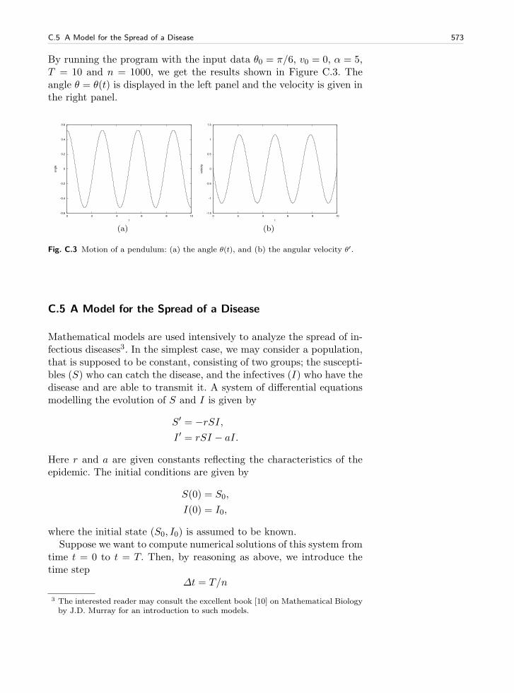
C.5 A Model for the Spread of a Disease 573

By running the program with the input data θ0 = π/6, v0 = 0, α = 5,T = 10 and n = 1000, we get the results shown in Figure C.3. Theangle θ = θ(t) is displayed in the left panel and the velocity is given inthe right panel.

-0.6

-0.4

-0.2

0

0.2

0.4

0.6

0 2 4 6 8 10

an

gle

t

(a)

-1.5

-1

-0.5

0

0.5

1

1.5

0 2 4 6 8 10

ve

locity

t

(b)

Fig. C.3 Motion of a pendulum: (a) the angle θ(t), and (b) the angular velocity θ′.

C.5 A Model for the Spread of a Disease

Mathematical models are used intensively to analyze the spread of in-fectious diseases3. In the simplest case, we may consider a population,that is supposed to be constant, consisting of two groups; the suscepti-bles (S) who can catch the disease, and the infectives (I) who have thedisease and are able to transmit it. A system of differential equationsmodelling the evolution of S and I is given by

S′ = −rSI,I ′ = rSI − aI.

Here r and a are given constants reflecting the characteristics of theepidemic. The initial conditions are given by

S(0) = S0,

I(0) = I0,

where the initial state (S0, I0) is assumed to be known.Suppose we want to compute numerical solutions of this system from

time t = 0 to t = T. Then, by reasoning as above, we introduce thetime step

∆t = T/n

3 The interested reader may consult the excellent book [10] on Mathematical Biologyby J.D. Murray for an introduction to such models.

574 C Introduction to Differential Equations

and the approximations (Sk, Ik) of the solution (S(tk), I(tk)). An ex-plicit Forward Euler method for the system takes the following form,

Sk+1 − Sk

∆t= −rSkIk,

Ik+1 − Ik∆t

= rSkIk − aIk,

which can be rewritten on computational form

Sk+1 = Sk −∆trSkIk,

Ik+1 = Ik +∆t (rSkIk − aIk) .

This scheme is implemented in the program exp_epidemic.py wherer, a, S0, I0, n and T are input data given on the command line. Thefunction epidemic computes the solution (S, I) to the differential equa-tion system. This pair of time-dependent functions is then plotted intwo separate plots.

def epidemic(T, n, S0, I0, r, a):dt = T/float(n)t = linspace(0, T, n+1)S = zeros(n+1)I = zeros(n+1)S[0] = S0I[0] = I0for k in range(n):

S[k+1] = S[k] - dt*r*S[k]*I[k]I[k+1] = I[k] + dt*(r*S[k]*I[k] - a*I[k])

return S, I, t

from scitools.std import *n = int(sys.argv[1])T = eval(sys.argv[2])S0 = eval(sys.argv[3])I0 = eval(sys.argv[4])r = eval(sys.argv[5])a = eval(sys.argv[6])

plot(t, S, xlabel=’t’, ylabel=’Susceptibles’)plot(t, I, xlabel=’t’, ylabel=’Infectives’)

We want to apply the program to a specific case where an influenzaepidemic hit a British boarding school with a total of 763 boys4. Theepidemic lasted from 21st January to 4th February in 1978. We lett = 0 denote 21st of January and we define T = 14 days. We putS0 = 762 and I0 = 1 which means that one person was ill at t = 0. Inthe Figure C.4 we se the numerical results using r = 2.18× 10−3, a =0.44, n = 1000. Also, we have plotted actual the measurements, andwe note that the simulations fit the real data quite well.

4 The data are from Murray [10], and Murray found the data in the British MedicalJournal, March 4, 1978.

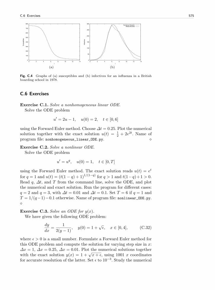
C.6 Exercises 575

0

100

200

300

400

500

600

700

800

0 2 4 6 8 10 12 14

Susceptible

s

t

(a)

0

50

100

150

200

250

300

0 2 4 6 8 10 12 14

Infe

ctives

t

Numerical SolutionMeasured data

(b)

Fig. C.4 Graphs of (a) susceptibles and (b) infectives for an influenza in a Britishboarding school in 1978.

C.6 Exercises

Exercise C.1. Solve a nonhomogeneous linear ODE.Solve the ODE problem

u′ = 2u− 1, u(0) = 2, t ∈ [0, 6]

using the Forward Euler method. Choose∆t = 0.25. Plot the numericalsolution together with the exact solution u(t) = 1

2 + 2e2t. Name ofprogram file: nonhomogeneous_linear_ODE.py. ⋄

Exercise C.2. Solve a nonlinear ODE.Solve the ODE problem

u′ = uq, u(0) = 1, t ∈ [0, T ]

using the Forward Euler method. The exact solution reads u(t) = et

for q = 1 and u(t) = (t(1− q) + 1)1/(1−q) for q > 1 and t(1−q)+1 > 0.Read q, ∆t, and T from the command line, solve the ODE, and plotthe numerical and exact solution. Run the program for different cases:q = 2 and q = 3, with ∆t = 0.01 and ∆t = 0.1. Set T = 6 if q = 1 andT = 1/(q−1)−0.1 otherwise. Name of program file: nonlinear_ODE.py.⋄

Exercise C.3. Solve an ODE for y(x).We have given the following ODE problem:

dy

dx=

1

2(y − 1), y(0) = 1 +

√ǫ, x ∈ [0, 4], (C.32)

where ǫ > 0 is a small number. Formulate a Forward Euler method forthis ODE problem and compute the solution for varying step size in x:∆x = 1, ∆x = 0.25, ∆x = 0.01. Plot the numerical solutions togetherwith the exact solution y(x) = 1 +

√x+ ǫ, using 1001 x coordinates

for accurate resolution of the latter. Set ǫ to 10−3. Study the numerical

576 C Introduction to Differential Equations

solution with ∆x = 1, and use that insight to explain why this problemis hard to solve numerically. Name of program file: yx_ODE.py. ⋄

Exercise C.4. Experience instability of an ODE.Consider the ODE problem

u′ = αu, u(0) = u0,

solved by the Forward Euler method. Show by repeatedly applying thescheme that

uk = (1 + α∆t)ku0 .

We now turn to the case α < 0. Show that the numerical solution willoscillate if ∆t > −1/α. Make a program for computing uk, set α = −1,and demonstrate oscillatory solutions for ∆t = 1.1, 1.5, 1.9. Recall thatthat the exact solution, u(t) = eαt, never oscillates.

What happens if ∆t > −2/α? Try it out in the program and explainthen mathematically why not uk → 0 as k → ∞. Name of programfile: unstable_ODE.py. ⋄

Exercise C.5. Solve an ODE for the arc length.Given a curve y = f(x), the length of the curve from x = x0 to some

point x is given by the function s(x), which fulls the problem

ds

dx=√

1 + [f ′(x)]2, s(x0) = 0 . (C.33)

Since s does not enter the right-hand side, (C.33) can immediately beintegrated from x0 to x. However, we shall solve (C.33) as an ODE.Use the Forward Euler method and compute the length of a straightline (for verification) and a sine curve: f(x) = 1

2x + 1, x ∈ [0, 2];f(x) = sin(πx), x ∈ [0, 2]. Name of program file: arclength_ODE.py. ⋄

Exercise C.6. Solve an ODE with time-varying growth.Consider the ODE for exponential growth,

u′ = αu, u(0) = 1, t ∈ [0, T ] .

Now we introduce a time-dependent α such that the growth decreaseswith time: α(t) = a− bt. Solve the problem for a = 1, b = 0.1, and T =10. Plot the solution and compare with the corresponding exponentialgrowth using the mean value of α(t) as growth factor: e(a−bT/2)t. Nameof program file: time_dep_growth.py. ⋄

A Complete Differential Equation Project D

The examples in the ordinary chapters of this book are quite compactand composed to convey programming constructs in a gentle pedagog-ical way. In this appendix the idea is to solve a more comprehensivereal-world problem by programming. The problem solving process getsquite advanced because we bring together elements from physics, math-ematics, and programming, in a way that a scientific programmer mustmaster. Each individual element is quite forward in the sense that youhave probably met the element already, either in high school physicsor mathematics, or in this book. The challenge is to understand theproblem, and analyze it by breaking it into a set of simpler elements.It is not necessary to understand this problem solving process in de-tail. As a computer programmer, all you need to understand is howyou translate the given algorithm into a working program and how totest the program. We anticipate that this task should be doable with-out a thorough understanding of the physics and mathematics of theproblem.

You can read the present appendix after the material from Chap-ters 1–5 is are digested. More specifically, you can read Appendices D.1and D.2 after Chapter 4, while Appendix D.3 requires knowledge aboutcurve plotting from Chapter 5.

All Python files associated with this appendix are found insrc/box_spring.

D.1 About the Problem: Motion and Forces in Physics

D.1.1 The Physical Problem

We shall study a simple device which models oscillating systems. Abox with mass m and height b is attached to a spring of length L as

577

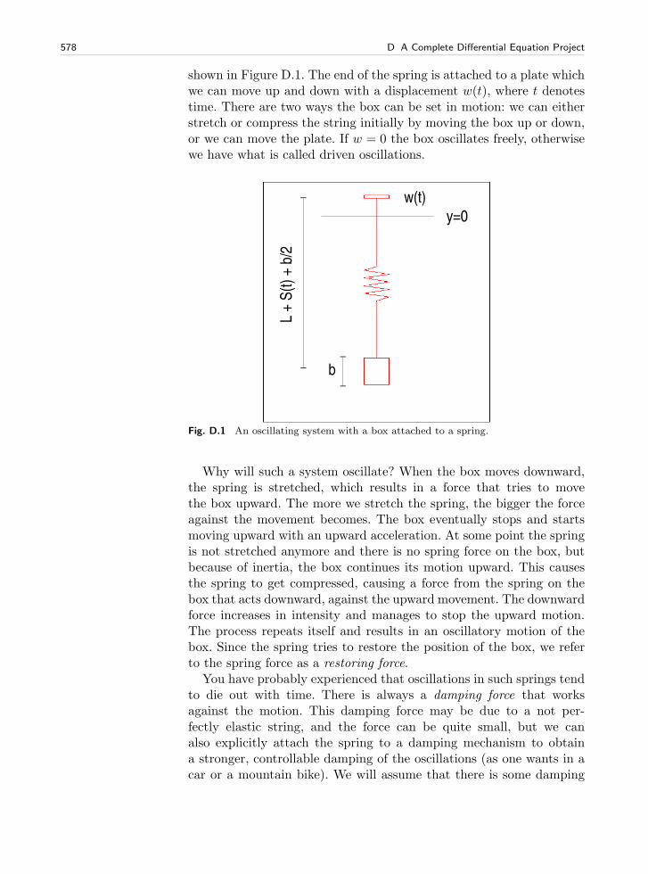
578 D A Complete Differential Equation Project

shown in Figure D.1. The end of the spring is attached to a plate whichwe can move up and down with a displacement w(t), where t denotestime. There are two ways the box can be set in motion: we can eitherstretch or compress the string initially by moving the box up or down,or we can move the plate. If w = 0 the box oscillates freely, otherwisewe have what is called driven oscillations.

Fig. D.1 An oscillating system with a box attached to a spring.

Why will such a system oscillate? When the box moves downward,the spring is stretched, which results in a force that tries to movethe box upward. The more we stretch the spring, the bigger the forceagainst the movement becomes. The box eventually stops and startsmoving upward with an upward acceleration. At some point the springis not stretched anymore and there is no spring force on the box, butbecause of inertia, the box continues its motion upward. This causesthe spring to get compressed, causing a force from the spring on thebox that acts downward, against the upward movement. The downwardforce increases in intensity and manages to stop the upward motion.The process repeats itself and results in an oscillatory motion of thebox. Since the spring tries to restore the position of the box, we referto the spring force as a restoring force.

You have probably experienced that oscillations in such springs tendto die out with time. There is always a damping force that worksagainst the motion. This damping force may be due to a not per-fectly elastic string, and the force can be quite small, but we canalso explicitly attach the spring to a damping mechanism to obtaina stronger, controllable damping of the oscillations (as one wants in acar or a mountain bike). We will assume that there is some damping

D.1 About the Problem: Motion and Forces in Physics 579

force present in our system, and this can well be a damping mechanismalthough this is not explicitly included in Figure D.1.

Oscillating systems of the type depicted in Figure D.1 have a hugenumber of applications throughout science and technology. One simpleexample is the spring system in a car or bicycle, which you have proba-bly experienced on a bumpy road (the bumps lead to a w(t) function).When your washing machine jumps up and down, it acts as a highlydamped oscillating system (and the w(t) function is related to unevendistribution of the mass of the clothes). The pendulum in a wall clock isanother oscillating system, not with a spring, but physically the systemcan (for small oscillations) be modeled as a box attached to a springbecause gravity makes a spring-like force on a pendulum (in this case,w(t) = 0). Other examples on oscillating systems where this type ofequation arise are briefly mentioned in Exercise E.30. The bottom lineis that understanding the dynamics of Figure D.1 is the starting pointfor understanding the behavior of a wide range of oscillating phenom-ena in nature and technical devices.

Goal of the Compuations. Our aim is to compute the position of thebox as a function of time. If we know the position, we can compute thevelocity, the acceleration, the spring force, and the damping force. Themathematically difficult thing is to calculate the position – everythingelse is much easier1.

We assume that the box moves in the vertical direction only, so weintroduce Y (t) as the vertical position of the center point of the box.We shall derive a mathematical equation that has Y (t) as solution. Thisequation can be solved by an algorithm which can be implemented ina program. Our focus is on the implementation, since this is a bookabout programming, but for the reader interested in how computersplay together with physics and mathematics in science and technology,we also outline how the equation and algorithm arise.

The Key Quantities. Let S be the stretch of the spring, where S > 0means stretch and S < 0 implies compression. The length of the springwhen it is unstretched is L, so at a given point of time t the actuallength is L+ S(t). Given the position of the plate, w(t), the length ofthe spring, L+ S(t), and the height of the box, b, the position Y (t) isthen, according to Figure D.1,

Y (t) = w(t)− (L+ S(t))− b

2. (D.1)

1 More precisely, to compute the position we must solve a differential equation whilethe other quantities can be computed by differentiation and simple arithmetics.Solving differential equations is historically considered very difficult, but computershave simplified this task dramatically. Appendices C and E are devoted to this topic.

580 D A Complete Differential Equation Project

You can think as follows: We first “go up” to the plate at y = w(t),then down L+ S(t) along the spring and then down b/2 to the centerof the box. While L, w, and b must be known as input data, S(t) isunknown and will be output data from the program.

D.1.2 The Computational Algorithm

Let us now go straight to the programming target and present therecipe for computing Y (t). The algorithm below actually computesS(t), but at any point of time we can easily find Y (t) from (D.1) if weknow S(t). The S(t) function is computed at discrete points of time,t = ti = i∆t, for i = 0, 1, . . . , N . We introduce the notation Si forS(ti). The Si values can be computed by the following algorithm.

1. Set initial stretch S0 from input data2. Compute S1 by

Si+1 =1

2m

(

2mSi −∆t2 kSi +m (wi+1 − 2wi + wi−1) +∆t2 mg)

,

(D.2)with i = 0.

3. For i = 1, 2, . . . , N − 1, compute Si+1 by

Si+1 = (m+ γ)−1(

2mSi −mSi−1 + γ∆tSi−1 −∆t2 kSi +

m(wi+1 − 2wi + wi−1) +∆t2mg)

. (D.3)

The parameter γ equals 12β∆t. The input data to the algorithm are

the mass of the box m, a coefficient k characterizing the spring, acoefficient β characterizing the amount of damping in the system, theacceleration of gravity g, the movement of the plate w(t), the initialstretch of the spring S0, the number of time steps N , and the time ∆tbetween each computation of S values. The smaller we choose ∆t, themore accurate the computations become.

Now you have two options, either read the derivation of this algo-rithm in Appendix D.1.3–D.1.4 or jump right to implementation inAppendix D.2.

D.1.3 Derivation of the Mathematical Model

To derive the algorithm we need to make a mathematical model ofthe oscillating system. This model is based on physical laws. The mostimportant physical law for a moving body is Newton’s second law ofmotion:

F = ma, (D.4)

where F is the sum of all forces on the body, m is the mass of the body,and a is the acceleration of the body. The body here is our box.

D.1 About the Problem: Motion and Forces in Physics 581

Let us first find all the forces on the box. Gravity acts downwardwith magnitude mg. We introduce Fg = −mg as the gravity force,with a minus sign because a negative force acts downward, in negativey direction.

The spring force on the box acts upward if the spring is stretched,i.e., if S > 0 we have a positive spring force Fs. The size of the force isproportional to the amount of stretching, so we write2 Fs = kS, wherek is commonly known as the spring constant. We also assume that wehave a damping force that is always directed toward the motion andproportional with the “velocity of the stretch”, −dS/dt. Naming theporportionaly constant β, we can write the damping force as Fd =βdS/dt. Note that when dS/dt > 0, S increases in time and the boxmoves downward, the Fd force then acts upward, against the motion,and must be positive. This is the way we can check that the dampingforce expression has the right sign.

The sum of all forces is now

F = Fg + Fs + Fd,

= −mg + kS + βdS

dt. (D.5)

We now know the left-hand side of (D.4), but S is unknown to us.The acceleration a on the right-hand side of (D.4) is also unknown.However, acceleration is related to movement and the S quantity, andthrough this relation we can eliminate a as a second unknown. Fromphysics, it is known that the acceleration of a body is the second deriva-tive in time of the position of the body, so in our case,

a =d2Y

dt2,

=d2w

dt2− d2S

dt2, (D.6)

(remember that L and b are constant).Equation (D.4) now reads

−mg + kS + βdS

dt= m

(

d2w

dt2− d2S

dt2

)

. (D.7)

It is common to collect the unknown terms on the left-hand side and theknown quantities on the right-hand side, and let higher-order deriva-tives appear before lower-order derivatives. With such a reordering ofterms we get

2 Spring forces are often written in the canonical form “F = −kx”, where x is thestretch. The reason that we have no minus sign is that our stretch S is positive inthe downward (negative) direction.

582 D A Complete Differential Equation Project

md2S

dt2+ β

dS

dt+ kS = m

d2w

dt2+mg . (D.8)

This is the equation governing our physical system. If we solve theequation for S(t), we have the position of the box according to (D.1),the velocity v as

v(t) =dY

dt=

dw

dt− dS

dt, (D.9)

the acceleration as (D.6), and the various forces can be easily obtainedfrom the formulas in (D.5).

A key question is if we can solve (D.8). If w = 0, there is in fact awell-known solution which can be written

S(t) =m

kg +

e−ζt(

c1et√β2−1 + c2e

−t√ζ2−1

)

, ζ > 1,

e−ζt(c1 + c2t), ζ = 1,

e−ζt[

c1 cos(

√

1− ζ2t)

+ c2 sin(

√

1− ζ2t)]

, ζ < 1 .

(D.10)Here, ζ is a short form for β/2, and c1 and c2 are arbitrary constants.That is, the solution (D.10) is not unique.

To make the solution unique, we must determine c1 and c2. This isdone by specifying the state of the system at some point of time, sayt = 0. In the present type of mathematical problem we must specify Sand dS/dt. We allow the spring to be stretched an amount S0 at t = 0.Moreover, we assume that there is no ongoing increase or decrease inthe stretch at t = 0, which means that dS/dt = 0. In view of (D.9), thiscondition implies that the velocity of the box is that of the plate, andif the latter is at rest, the box is also at rest initially. The conditionsat t = 0 are called initial conditions:

S(0) = S0,dS

dt(0) = 0 . (D.11)

These two conditions provide two equations for the two unknown con-stants c1 and c2. Without the initial conditions two things happen: (i)there are infinitely many solutions to the problem, and (ii) the compu-tational algorithm in a program cannot start.

Also when w 6= 0 one can find solutions S(t) of (D.8) in terms ofmathematical expressions, but only for some very specific choices ofw(t) functions. With a program we can compute the solution S(t) forany “reasonable” w(t) by a quite simple method. The method givesonly an approximate solution, but the approximation can usually bemade as good as desired. This powerful solution method is describedbelow.

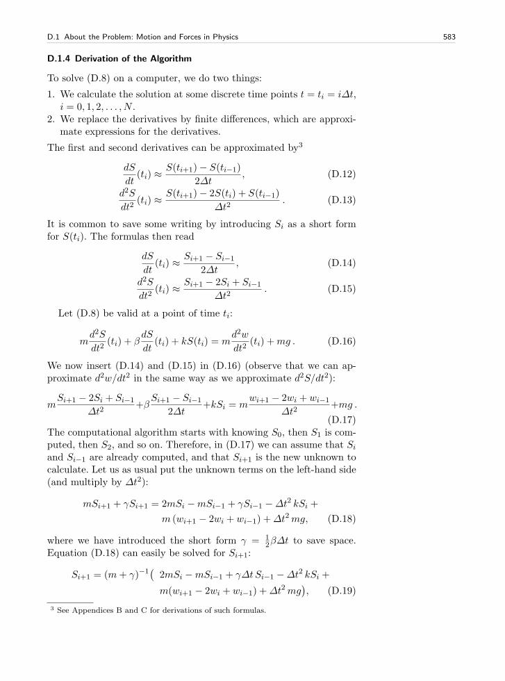
D.1 About the Problem: Motion and Forces in Physics 583

D.1.4 Derivation of the Algorithm

To solve (D.8) on a computer, we do two things:

1. We calculate the solution at some discrete time points t = ti = i∆t,i = 0, 1, 2, . . . , N .

2. We replace the derivatives by finite differences, which are approxi-mate expressions for the derivatives.

The first and second derivatives can be approximated by3

dS

dt(ti) ≈

S(ti+1)− S(ti−1)

2∆t, (D.12)

d2S

dt2(ti) ≈

S(ti+1)− 2S(ti) + S(ti−1)

∆t2. (D.13)

It is common to save some writing by introducing Si as a short formfor S(ti). The formulas then read

dS

dt(ti) ≈

Si+1 − Si−1

2∆t, (D.14)

d2S

dt2(ti) ≈

Si+1 − 2Si + Si−1

∆t2. (D.15)

Let (D.8) be valid at a point of time ti:

md2S

dt2(ti) + β

dS

dt(ti) + kS(ti) = m

d2w

dt2(ti) +mg . (D.16)

We now insert (D.14) and (D.15) in (D.16) (observe that we can ap-proximate d2w/dt2 in the same way as we approximate d2S/dt2):

mSi+1 − 2Si + Si−1

∆t2+β

Si+1 − Si−1

2∆t+kSi = m

wi+1 − 2wi + wi−1

∆t2+mg .

(D.17)The computational algorithm starts with knowing S0, then S1 is com-puted, then S2, and so on. Therefore, in (D.17) we can assume that Si

and Si−1 are already computed, and that Si+1 is the new unknown tocalculate. Let us as usual put the unknown terms on the left-hand side(and multiply by ∆t2):

mSi+1 + γSi+1 = 2mSi −mSi−1 + γSi−1 −∆t2 kSi +

m (wi+1 − 2wi + wi−1) +∆t2mg, (D.18)

where we have introduced the short form γ = 12β∆t to save space.

Equation (D.18) can easily be solved for Si+1:

Si+1 = (m+ γ)−1(

2mSi −mSi−1 + γ∆tSi−1 −∆t2 kSi +

m(wi+1 − 2wi + wi−1) +∆t2 mg)

, (D.19)

3 See Appendices B and C for derivations of such formulas.

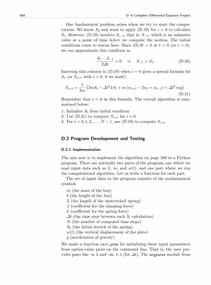
584 D A Complete Differential Equation Project

One fundamental problem arises when we try to start the compu-tations. We know S0 and want to apply (D.19) for i = 0 to calculateS1. However, (D.19) involves Si−1, that is, S−1, which is an unknownvalue at a point of time before we compute the motion. The initialconditions come to rescue here. Since dS/dt = 0 at t = 0 (or i = 0),we can approximate this condition as

S1 − S−1

2∆t= 0 ⇒ S−1 = S1 . (D.20)

Inserting this relation in (D.19) when i = 0 gives a special formula forS1 (or Si+1 with i = 0, if we want):

Si+1 =1

2m

(

2mSi −∆t2 kSi +m (wi+1 − 2wi + wi−1) +∆t2 mg)

.

(D.21)Remember that i = 0 in this formula. The overall algorithm is sum-marized below:

1. Initialize S0 from initial condition2. Use (D.21) to compute Si+1 for i = 03. For i = 0, 1, 2, . . . , N − 1, use (D.19) to compute Si+1

D.2 Program Development and Testing

D.2.1 Implementation

The aim now is to implement the algorithm on page 580 in a Pythonprogram. There are naturally two parts of the program, one where weread input data such as L, m, and w(t), and one part where we runthe computational algorithm. Let us write a function for each part.

The set of input data to the program consists of the mathematicalsymbols

m (the mass of the box) b (the height of the box) L (the length of the unstretched spring) β (coefficient for the damping force) k (coefficient for the spring force) ∆t (the time step between each Si calculation) N (the number of computed time steps) S0 (the initial stretch of the spring) w(t) (the vertical displacement of the plate) g (acceleration of gravity)

We make a function init_prms for initializing these input parametersfrom option-value pairs on the command line. That is, the user pro-vides pairs like -m 2 and -dt 0.1 (for ∆t). The argparse module from

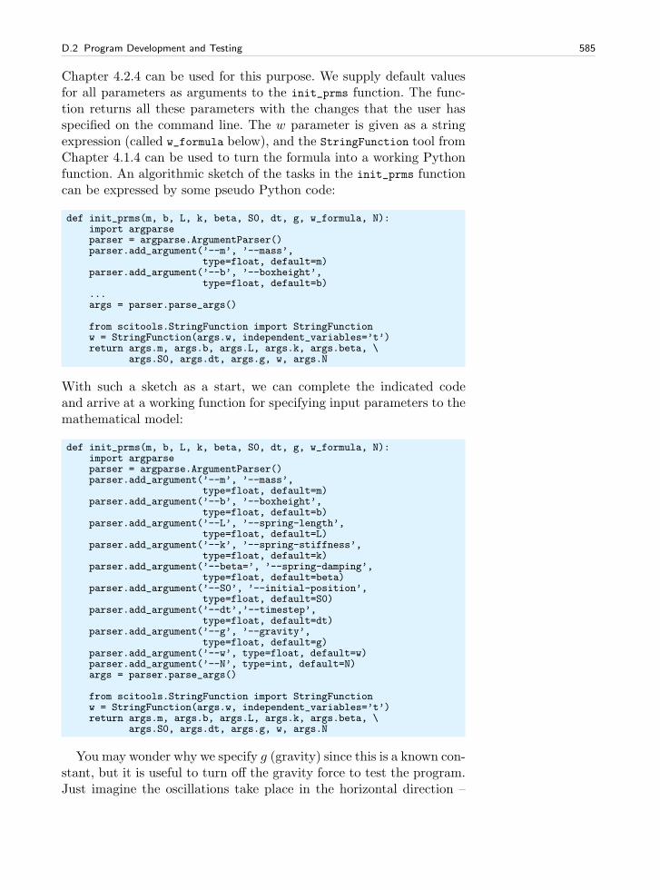
D.2 Program Development and Testing 585

Chapter 4.2.4 can be used for this purpose. We supply default valuesfor all parameters as arguments to the init_prms function. The func-tion returns all these parameters with the changes that the user hasspecified on the command line. The w parameter is given as a stringexpression (called w_formula below), and the StringFunction tool fromChapter 4.1.4 can be used to turn the formula into a working Pythonfunction. An algorithmic sketch of the tasks in the init_prms functioncan be expressed by some pseudo Python code:

def init_prms(m, b, L, k, beta, S0, dt, g, w_formula, N):import argparseparser = argparse.ArgumentParser()parser.add_argument(’--m’, ’--mass’,

type=float, default=m)parser.add_argument(’--b’, ’--boxheight’,

type=float, default=b)...args = parser.parse_args()

from scitools.StringFunction import StringFunctionw = StringFunction(args.w, independent_variables=’t’)return args.m, args.b, args.L, args.k, args.beta, \

args.S0, args.dt, args.g, w, args.N

With such a sketch as a start, we can complete the indicated codeand arrive at a working function for specifying input parameters to themathematical model:

def init_prms(m, b, L, k, beta, S0, dt, g, w_formula, N):import argparseparser = argparse.ArgumentParser()parser.add_argument(’--m’, ’--mass’,

type=float, default=m)parser.add_argument(’--b’, ’--boxheight’,

type=float, default=b)parser.add_argument(’--L’, ’--spring-length’,

type=float, default=L)parser.add_argument(’--k’, ’--spring-stiffness’,

type=float, default=k)parser.add_argument(’--beta=’, ’--spring-damping’,

type=float, default=beta)parser.add_argument(’--S0’, ’--initial-position’,

type=float, default=S0)parser.add_argument(’--dt’,’--timestep’,

type=float, default=dt)parser.add_argument(’--g’, ’--gravity’,

type=float, default=g)parser.add_argument(’--w’, type=float, default=w)parser.add_argument(’--N’, type=int, default=N)args = parser.parse_args()

from scitools.StringFunction import StringFunctionw = StringFunction(args.w, independent_variables=’t’)return args.m, args.b, args.L, args.k, args.beta, \

args.S0, args.dt, args.g, w, args.N

You may wonder why we specify g (gravity) since this is a known con-stant, but it is useful to turn off the gravity force to test the program.Just imagine the oscillations take place in the horizontal direction –

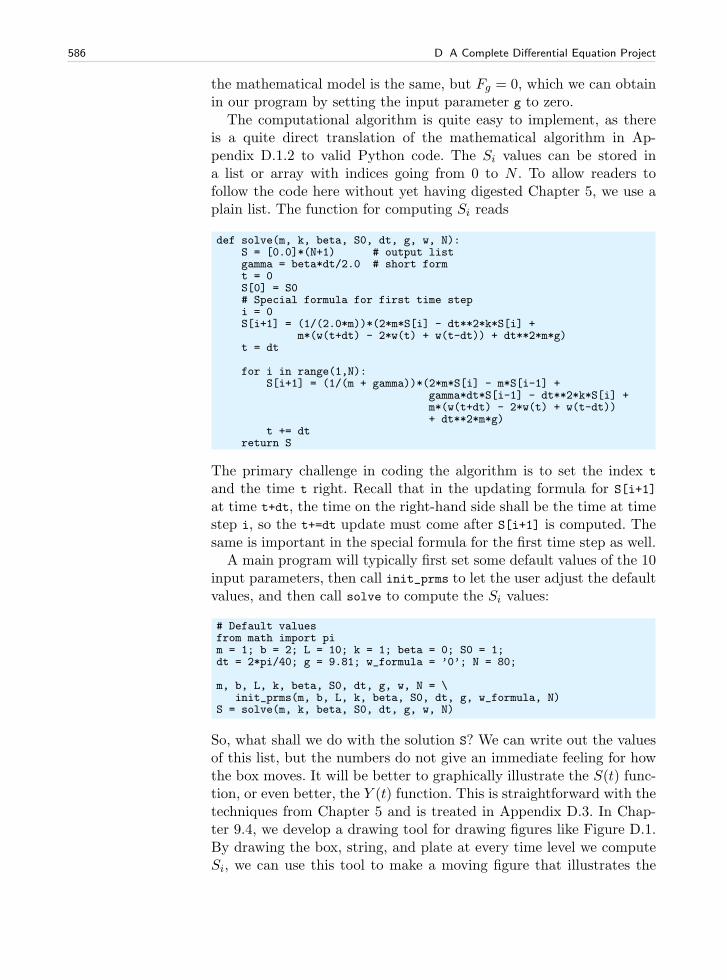
586 D A Complete Differential Equation Project

the mathematical model is the same, but Fg = 0, which we can obtainin our program by setting the input parameter g to zero.

The computational algorithm is quite easy to implement, as thereis a quite direct translation of the mathematical algorithm in Ap-pendix D.1.2 to valid Python code. The Si values can be stored ina list or array with indices going from 0 to N . To allow readers tofollow the code here without yet having digested Chapter 5, we use aplain list. The function for computing Si reads

def solve(m, k, beta, S0, dt, g, w, N):S = [0.0]*(N+1) # output listgamma = beta*dt/2.0 # short formt = 0S[0] = S0# Special formula for first time stepi = 0S[i+1] = (1/(2.0*m))*(2*m*S[i] - dt**2*k*S[i] +

m*(w(t+dt) - 2*w(t) + w(t-dt)) + dt**2*m*g)t = dt

for i in range(1,N):S[i+1] = (1/(m + gamma))*(2*m*S[i] - m*S[i-1] +

gamma*dt*S[i-1] - dt**2*k*S[i] +m*(w(t+dt) - 2*w(t) + w(t-dt))+ dt**2*m*g)

t += dtreturn S

The primary challenge in coding the algorithm is to set the index t

and the time t right. Recall that in the updating formula for S[i+1]

at time t+dt, the time on the right-hand side shall be the time at timestep i, so the t+=dt update must come after S[i+1] is computed. Thesame is important in the special formula for the first time step as well.

A main program will typically first set some default values of the 10input parameters, then call init_prms to let the user adjust the defaultvalues, and then call solve to compute the Si values:

# Default valuesfrom math import pim = 1; b = 2; L = 10; k = 1; beta = 0; S0 = 1;dt = 2*pi/40; g = 9.81; w_formula = ’0’; N = 80;

m, b, L, k, beta, S0, dt, g, w, N = \init_prms(m, b, L, k, beta, S0, dt, g, w_formula, N)

S = solve(m, k, beta, S0, dt, g, w, N)

So, what shall we do with the solution S? We can write out the valuesof this list, but the numbers do not give an immediate feeling for howthe box moves. It will be better to graphically illustrate the S(t) func-tion, or even better, the Y (t) function. This is straightforward with thetechniques from Chapter 5 and is treated in Appendix D.3. In Chap-ter 9.4, we develop a drawing tool for drawing figures like Figure D.1.By drawing the box, string, and plate at every time level we computeSi, we can use this tool to make a moving figure that illustrates the

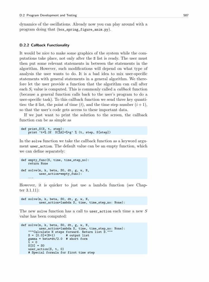
D.2 Program Development and Testing 587

dynamics of the oscillations. Already now you can play around with aprogram doing that (box_spring_figure_anim.py).

D.2.2 Callback Functionality

It would be nice to make some graphics of the system while the com-putations take place, not only after the S list is ready. The user mustthen put some relevant statements in between the statements in thealgorithm. However, such modifications will depend on what type ofanalysis the user wants to do. It is a bad idea to mix user-specificstatements with general statements in a general algorithm. We there-fore let the user provide a function that the algorithm can call aftereach Si value is computed. This is commonly called a callback function(because a general function calls back to the user’s program to do auser-specific task). To this callback function we send three key quanti-ties: the S list, the point of time (t), and the time step number (i+1),so that the user’s code gets access to these important data.

If we just want to print the solution to the screen, the callbackfunction can be as simple as

def print_S(S, t, step):print ’t=%.2f S[%d]=%+g’ % (t, step, S[step])

In the solve function we take the callback function as a keyword argu-ment user_action. The default value can be an empty function, whichwe can define separately:

def empty_func(S, time, time_step_no):return None

def solve(m, k, beta, S0, dt, g, w, N,user_action=empty_func):

...

However, it is quicker to just use a lambda function (see Chap-ter 3.1.11):

def solve(m, k, beta, S0, dt, g, w, N,user_action=lambda S, time, time_step_no: None):

The new solve function has a call to user_action each time a new Svalue has been computed:

def solve(m, k, beta, S0, dt, g, w, N,user_action=lambda S, time, time_step_no: None):

"""Calculate N steps forward. Return list S."""S = [0.0]*(N+1) # output listgamma = beta*dt/2.0 # short formt = 0S[0] = S0user_action(S, t, 0)# Special formula for first time step

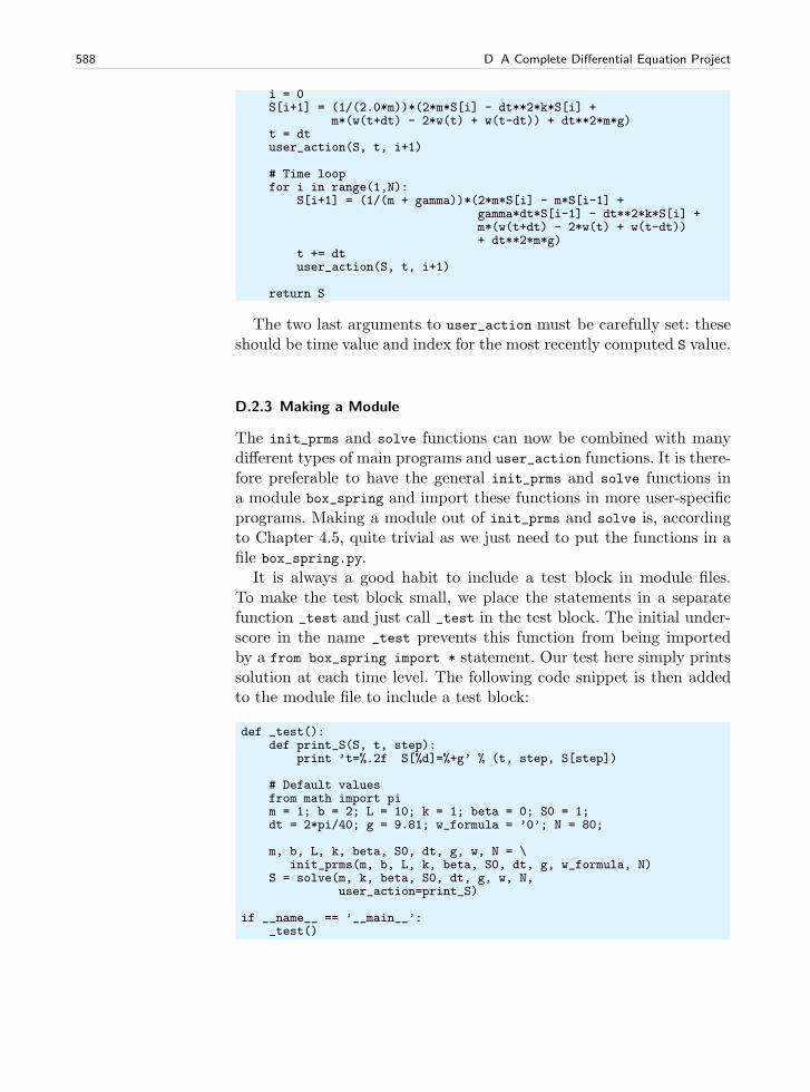
588 D A Complete Differential Equation Project

i = 0S[i+1] = (1/(2.0*m))*(2*m*S[i] - dt**2*k*S[i] +

m*(w(t+dt) - 2*w(t) + w(t-dt)) + dt**2*m*g)t = dtuser_action(S, t, i+1)

# Time loopfor i in range(1,N):

S[i+1] = (1/(m + gamma))*(2*m*S[i] - m*S[i-1] +gamma*dt*S[i-1] - dt**2*k*S[i] +m*(w(t+dt) - 2*w(t) + w(t-dt))+ dt**2*m*g)

t += dtuser_action(S, t, i+1)

return S

The two last arguments to user_action must be carefully set: theseshould be time value and index for the most recently computed S value.

D.2.3 Making a Module

The init_prms and solve functions can now be combined with manydifferent types of main programs and user_action functions. It is there-fore preferable to have the general init_prms and solve functions ina module box_spring and import these functions in more user-specificprograms. Making a module out of init_prms and solve is, accordingto Chapter 4.5, quite trivial as we just need to put the functions in afile box_spring.py.

It is always a good habit to include a test block in module files.To make the test block small, we place the statements in a separatefunction _test and just call _test in the test block. The initial under-score in the name _test prevents this function from being importedby a from box_spring import * statement. Our test here simply printssolution at each time level. The following code snippet is then addedto the module file to include a test block:

def _test():def print_S(S, t, step):

print ’t=%.2f S[%d]=%+g’ % (t, step, S[step])

# Default valuesfrom math import pim = 1; b = 2; L = 10; k = 1; beta = 0; S0 = 1;dt = 2*pi/40; g = 9.81; w_formula = ’0’; N = 80;

m, b, L, k, beta, S0, dt, g, w, N = \init_prms(m, b, L, k, beta, S0, dt, g, w_formula, N)

S = solve(m, k, beta, S0, dt, g, w, N,user_action=print_S)

if __name__ == ’__main__’:_test()

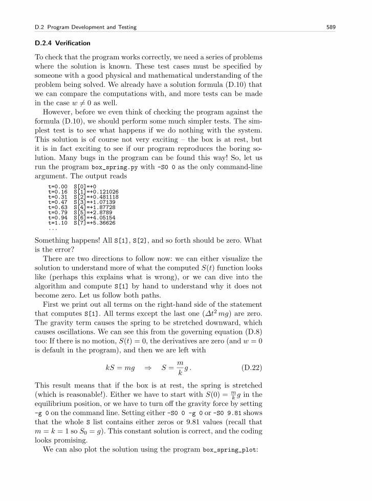
D.2 Program Development and Testing 589

D.2.4 Verification

To check that the program works correctly, we need a series of problemswhere the solution is known. These test cases must be specified bysomeone with a good physical and mathematical understanding of theproblem being solved. We already have a solution formula (D.10) thatwe can compare the computations with, and more tests can be madein the case w 6= 0 as well.

However, before we even think of checking the program against theformula (D.10), we should perform some much simpler tests. The sim-plest test is to see what happens if we do nothing with the system.This solution is of course not very exciting – the box is at rest, butit is in fact exciting to see if our program reproduces the boring so-lution. Many bugs in the program can be found this way! So, let usrun the program box_spring.py with -S0 0 as the only command-lineargument. The output reads

t=0.00 S[0]=+0t=0.16 S[1]=+0.121026t=0.31 S[2]=+0.481118t=0.47 S[3]=+1.07139t=0.63 S[4]=+1.87728t=0.79 S[5]=+2.8789t=0.94 S[6]=+4.05154t=1.10 S[7]=+5.36626...

Something happens! All S[1], S[2], and so forth should be zero. Whatis the error?

There are two directions to follow now: we can either visualize thesolution to understand more of what the computed S(t) function lookslike (perhaps this explains what is wrong), or we can dive into thealgorithm and compute S[1] by hand to understand why it does notbecome zero. Let us follow both paths.

First we print out all terms on the right-hand side of the statementthat computes S[1]. All terms except the last one (∆t2mg) are zero.The gravity term causes the spring to be stretched downward, whichcauses oscillations. We can see this from the governing equation (D.8)too: If there is no motion, S(t) = 0, the derivatives are zero (and w = 0is default in the program), and then we are left with

kS = mg ⇒ S =m

kg . (D.22)

This result means that if the box is at rest, the spring is stretched(which is reasonable!). Either we have to start with S(0) = m

k g in theequilibrium position, or we have to turn off the gravity force by setting-g 0 on the command line. Setting either -S0 0 -g 0 or -S0 9.81 showsthat the whole S list contains either zeros or 9.81 values (recall thatm = k = 1 so S0 = g). This constant solution is correct, and the codinglooks promising.

We can also plot the solution using the program box_spring_plot:

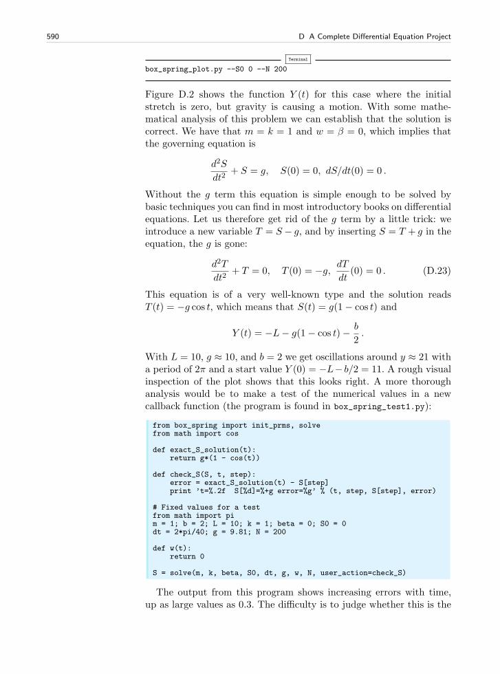
590 D A Complete Differential Equation Project

Terminal

box_spring_plot.py --S0 0 --N 200

Figure D.2 shows the function Y (t) for this case where the initialstretch is zero, but gravity is causing a motion. With some mathe-matical analysis of this problem we can establish that the solution iscorrect. We have that m = k = 1 and w = β = 0, which implies thatthe governing equation is

d2S

dt2+ S = g, S(0) = 0, dS/dt(0) = 0 .

Without the g term this equation is simple enough to be solved bybasic techniques you can find in most introductory books on differentialequations. Let us therefore get rid of the g term by a little trick: weintroduce a new variable T = S − g, and by inserting S = T + g in theequation, the g is gone:

d2T

dt2+ T = 0, T (0) = −g, dT

dt(0) = 0 . (D.23)

This equation is of a very well-known type and the solution readsT (t) = −g cos t, which means that S(t) = g(1− cos t) and

Y (t) = −L− g(1− cos t)− b

2.

With L = 10, g ≈ 10, and b = 2 we get oscillations around y ≈ 21 witha period of 2π and a start value Y (0) = −L− b/2 = 11. A rough visualinspection of the plot shows that this looks right. A more thoroughanalysis would be to make a test of the numerical values in a newcallback function (the program is found in box_spring_test1.py):

from box_spring import init_prms, solvefrom math import cos

def exact_S_solution(t):return g*(1 - cos(t))

def check_S(S, t, step):error = exact_S_solution(t) - S[step]print ’t=%.2f S[%d]=%+g error=%g’ % (t, step, S[step], error)

# Fixed values for a testfrom math import pim = 1; b = 2; L = 10; k = 1; beta = 0; S0 = 0dt = 2*pi/40; g = 9.81; N = 200

def w(t):return 0

S = solve(m, k, beta, S0, dt, g, w, N, user_action=check_S)

The output from this program shows increasing errors with time,up as large values as 0.3. The difficulty is to judge whether this is the

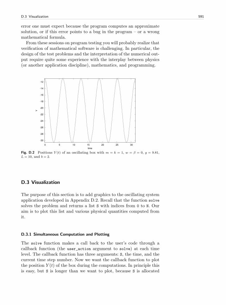
D.3 Visualization 591

error one must expect because the program computes an approximatesolution, or if this error points to a bug in the program – or a wrongmathematical formula.

From these sessions on program testing you will probably realize thatverification of mathematical software is challenging. In particular, thedesign of the test problems and the interpretation of the numerical out-put require quite some experience with the interplay between physics(or another application discipline), mathematics, and programming.

-30

-28

-26

-24

-22

-20

-18

-16

-14

-12

0 5 10 15 20 25 30

Y

time

Fig. D.2 Positions Y (t) of an oscillating box with m = k = 1, w = β = 0, g = 9.81,L = 10, and b = 2.

D.3 Visualization

The purpose of this section is to add graphics to the oscillating systemapplication developed in Appendix D.2. Recall that the function solve

solves the problem and returns a list S with indices from 0 to N. Ouraim is to plot this list and various physical quantities computed fromit.

D.3.1 Simultaneous Computation and Plotting

The solve function makes a call back to the user’s code through acallback function (the user_action argument to solve) at each timelevel. The callback function has three arguments: S, the time, and thecurrent time step number. Now we want the callback function to plotthe position Y (t) of the box during the computations. In principle thisis easy, but S is longer than we want to plot, because S is allocated

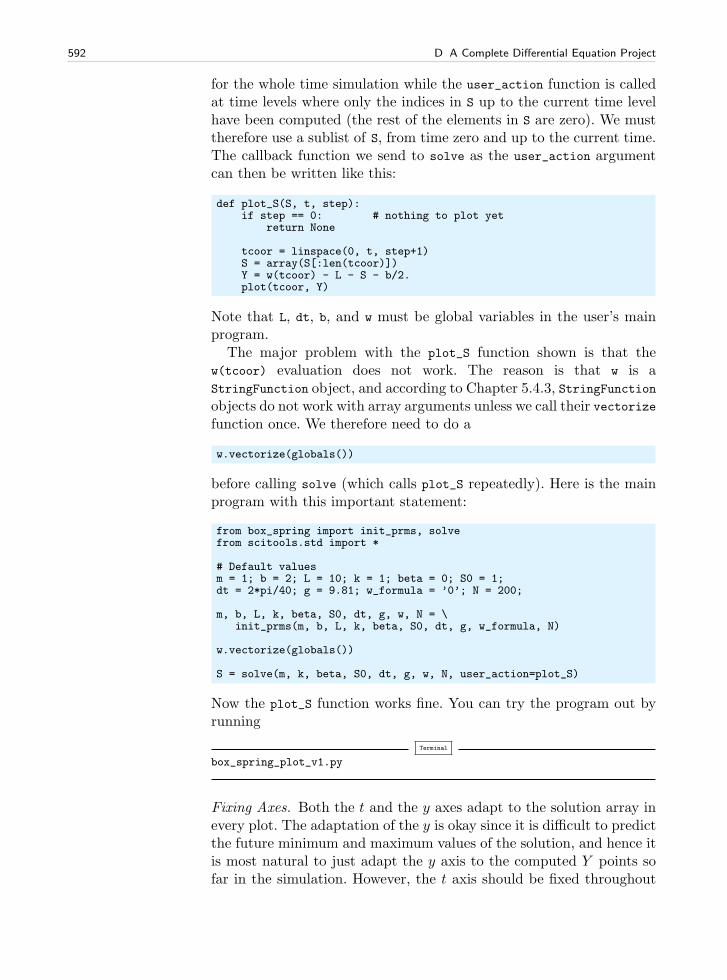
592 D A Complete Differential Equation Project

for the whole time simulation while the user_action function is calledat time levels where only the indices in S up to the current time levelhave been computed (the rest of the elements in S are zero). We musttherefore use a sublist of S, from time zero and up to the current time.The callback function we send to solve as the user_action argumentcan then be written like this:

def plot_S(S, t, step):if step == 0: # nothing to plot yet

return None

tcoor = linspace(0, t, step+1)S = array(S[:len(tcoor)])Y = w(tcoor) - L - S - b/2.plot(tcoor, Y)

Note that L, dt, b, and w must be global variables in the user’s mainprogram.

The major problem with the plot_S function shown is that thew(tcoor) evaluation does not work. The reason is that w is aStringFunction object, and according to Chapter 5.4.3, StringFunctionobjects do not work with array arguments unless we call their vectorizefunction once. We therefore need to do a

w.vectorize(globals())

before calling solve (which calls plot_S repeatedly). Here is the mainprogram with this important statement:

from box_spring import init_prms, solvefrom scitools.std import *

# Default valuesm = 1; b = 2; L = 10; k = 1; beta = 0; S0 = 1;dt = 2*pi/40; g = 9.81; w_formula = ’0’; N = 200;

m, b, L, k, beta, S0, dt, g, w, N = \init_prms(m, b, L, k, beta, S0, dt, g, w_formula, N)

w.vectorize(globals())

S = solve(m, k, beta, S0, dt, g, w, N, user_action=plot_S)

Now the plot_S function works fine. You can try the program out byrunning

Terminal

box_spring_plot_v1.py

Fixing Axes. Both the t and the y axes adapt to the solution array inevery plot. The adaptation of the y is okay since it is difficult to predictthe future minimum and maximum values of the solution, and hence itis most natural to just adapt the y axis to the computed Y points sofar in the simulation. However, the t axis should be fixed throughout

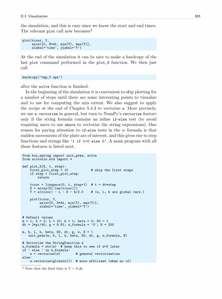
D.3 Visualization 593

the simulation, and this is easy since we know the start and end times.The relevant plot call now becomes4

plot(tcoor, Y,axis=[0, N*dt, min(Y), max(Y)],xlabel=’time’, ylabel=’Y’)

At the end of the simulation it can be nice to make a hardcopy of thelast plot command performed in the plot_S function. We then justcall

hardcopy(’tmp_Y.eps’)

after the solve function is finished.In the beginning of the simulation it is convenient to skip plotting for

a number of steps until there are some interesting points to visualizeand to use for computing the axis extent. We also suggest to applythe recipe at the end of Chapter 5.4.3 to vectorize w. More precisely,we use w.vectorize in general, but turn to NumPy’s vectorize featureonly if the string formula contains an inline if-else test (to avoidrequiring users to use where to vectorize the string expressions). Onereason for paying attention to if-else tests in the w formula is thatsudden movements of the plate are of interest, and this gives rise to stepfunctions and strings like ’1 if t>0 else 0’. A main program with allthese features is listed next.

from box_spring import init_prms, solvefrom scitools.std import *

def plot_S(S, t, step):first_plot_step = 10 # skip the first stepsif step < first_plot_step:

return

tcoor = linspace(0, t, step+1) # t = dt*stepS = array(S[:len(tcoor)])Y = w(tcoor) - L - S - b/2.0 # (w, L, b are global vars.)

plot(tcoor, Y,axis=[0, N*dt, min(Y), max(Y)],xlabel=’time’, ylabel=’Y’)

# Default valuesm = 1; b = 2; L = 10; k = 1; beta = 0; S0 = 1dt = 2*pi/40; g = 9.81; w_formula = ’0’; N = 200

m, b, L, k, beta, S0, dt, g, w, N = \init_prms(m, b, L, k, beta, S0, dt, g, w_formula, N)

# Vectorize the StringFunction ww_formula = str(w) # keep this to see if w=0 laterif ’ else ’ in w_formula:

w = vectorize(w) # general vectorizationelse:

w.vectorize(globals()) # more efficient (when no if)

4 Note that the final time is T = N∆t.

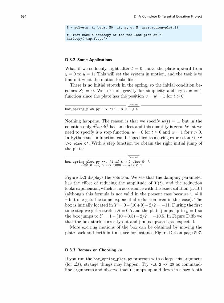
594 D A Complete Differential Equation Project

S = solve(m, k, beta, S0, dt, g, w, N, user_action=plot_S)

# First make a hardcopy of the the last plot of Yhardcopy(’tmp_Y.eps’)

D.3.2 Some Applications

What if we suddenly, right after t = 0, move the plate upward fromy = 0 to y = 1? This will set the system in motion, and the task is tofind out what the motion looks like.

There is no initial stretch in the spring, so the initial condition be-comes S0 = 0. We turn off gravity for simplicity and try a w = 1function since the plate has the position y = w = 1 for t > 0:

Terminal

box_spring_plot.py --w ’1’ --S 0 --g 0

Nothing happens. The reason is that we specify w(t) = 1, but in theequation only d2w/dt2 has an effect and this quantity is zero. What weneed to specify is a step function: w = 0 for t ≤ 0 and w = 1 for t > 0.In Python such a function can be specified as a string expression ’1 if

t>0 else 0’. With a step function we obtain the right initial jump ofthe plate:

Terminal

box_spring_plot.py --w ’1 if t > 0 else 0’ \--S0 0 --g 0 --N 1000 --beta 0.1

Figure D.3 displays the solution. We see that the damping parameterhas the effect of reducing the amplitude of Y (t), and the reductionlooks exponential, which is in accordance with the exact solution (D.10)(although this formula is not valid in the present case because w 6= 0– but one gets the same exponential reduction even in this case). Thebox is initially located in Y = 0−(10+0)−2/2 = −11. During the firsttime step we get a stretch S = 0.5 and the plate jumps up to y = 1 sothe box jumps to Y = 1− (10+0.5)− 2/2 = −10.5. In Figure D.3b wethat the box starts correctly out and jumps upwards, as expected.

More exciting motions of the box can be obtained by moving theplate back and forth in time, see for instance Figure D.4 on page 597.

D.3.3 Remark on Choosing ∆t

If you run the box_spring_plot.py program with a large -dt argument(for ∆t), strange things may happen. Try -dt 2 -N 20 as command-line arguments and observe that Y jumps up and down in a saw tooth

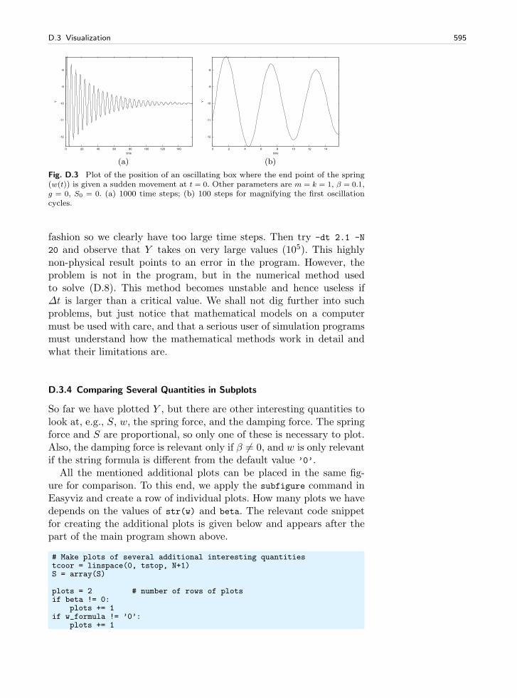
D.3 Visualization 595

-12

-11

-10

-9

-8

0 20 40 60 80 100 120 140

Y

time

(a)

-12

-11

-10

-9

-8

0 2 4 6 8 10 12 14

Y

time

(b)

Fig. D.3 Plot of the position of an oscillating box where the end point of the spring(w(t)) is given a sudden movement at t = 0. Other parameters are m = k = 1, β = 0.1,g = 0, S0 = 0. (a) 1000 time steps; (b) 100 steps for magnifying the first oscillationcycles.

fashion so we clearly have too large time steps. Then try -dt 2.1 -N

20 and observe that Y takes on very large values (105). This highlynon-physical result points to an error in the program. However, theproblem is not in the program, but in the numerical method usedto solve (D.8). This method becomes unstable and hence useless if∆t is larger than a critical value. We shall not dig further into suchproblems, but just notice that mathematical models on a computermust be used with care, and that a serious user of simulation programsmust understand how the mathematical methods work in detail andwhat their limitations are.

D.3.4 Comparing Several Quantities in Subplots

So far we have plotted Y , but there are other interesting quantities tolook at, e.g., S, w, the spring force, and the damping force. The springforce and S are proportional, so only one of these is necessary to plot.Also, the damping force is relevant only if β 6= 0, and w is only relevantif the string formula is different from the default value ’0’.

All the mentioned additional plots can be placed in the same fig-ure for comparison. To this end, we apply the subfigure command inEasyviz and create a row of individual plots. How many plots we havedepends on the values of str(w) and beta. The relevant code snippetfor creating the additional plots is given below and appears after thepart of the main program shown above.

# Make plots of several additional interesting quantitiestcoor = linspace(0, tstop, N+1)S = array(S)

plots = 2 # number of rows of plotsif beta != 0:

plots += 1if w_formula != ’0’:

plots += 1

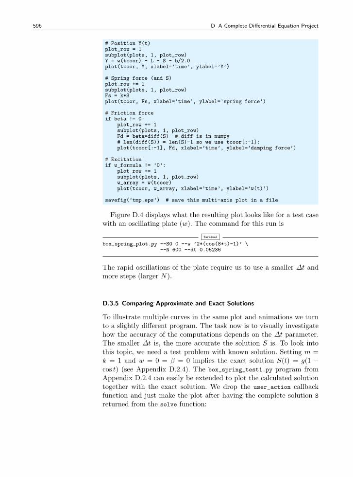
596 D A Complete Differential Equation Project

# Position Y(t)plot_row = 1subplot(plots, 1, plot_row)Y = w(tcoor) - L - S - b/2.0plot(tcoor, Y, xlabel=’time’, ylabel=’Y’)

# Spring force (and S)plot_row += 1subplot(plots, 1, plot_row)Fs = k*Splot(tcoor, Fs, xlabel=’time’, ylabel=’spring force’)

# Friction forceif beta != 0:

plot_row += 1subplot(plots, 1, plot_row)Fd = beta*diff(S) # diff is in numpy# len(diff(S)) = len(S)-1 so we use tcoor[:-1]:plot(tcoor[:-1], Fd, xlabel=’time’, ylabel=’damping force’)

# Excitationif w_formula != ’0’:

plot_row += 1subplot(plots, 1, plot_row)w_array = w(tcoor)plot(tcoor, w_array, xlabel=’time’, ylabel=’w(t)’)

savefig(’tmp.eps’) # save this multi-axis plot in a file

Figure D.4 displays what the resulting plot looks like for a test casewith an oscillating plate (w). The command for this run is

Terminal

box_spring_plot.py --S0 0 --w ’2*(cos(8*t)-1)’ \--N 600 --dt 0.05236

The rapid oscillations of the plate require us to use a smaller ∆t andmore steps (larger N).

D.3.5 Comparing Approximate and Exact Solutions

To illustrate multiple curves in the same plot and animations we turnto a slightly different program. The task now is to visually investigatehow the accuracy of the computations depends on the ∆t parameter.The smaller ∆t is, the more accurate the solution S is. To look intothis topic, we need a test problem with known solution. Setting m =k = 1 and w = 0 = β = 0 implies the exact solution S(t) = g(1 −cos t) (see Appendix D.2.4). The box_spring_test1.py program fromAppendix D.2.4 can easily be extended to plot the calculated solutiontogether with the exact solution. We drop the user_action callbackfunction and just make the plot after having the complete solution S

returned from the solve function:

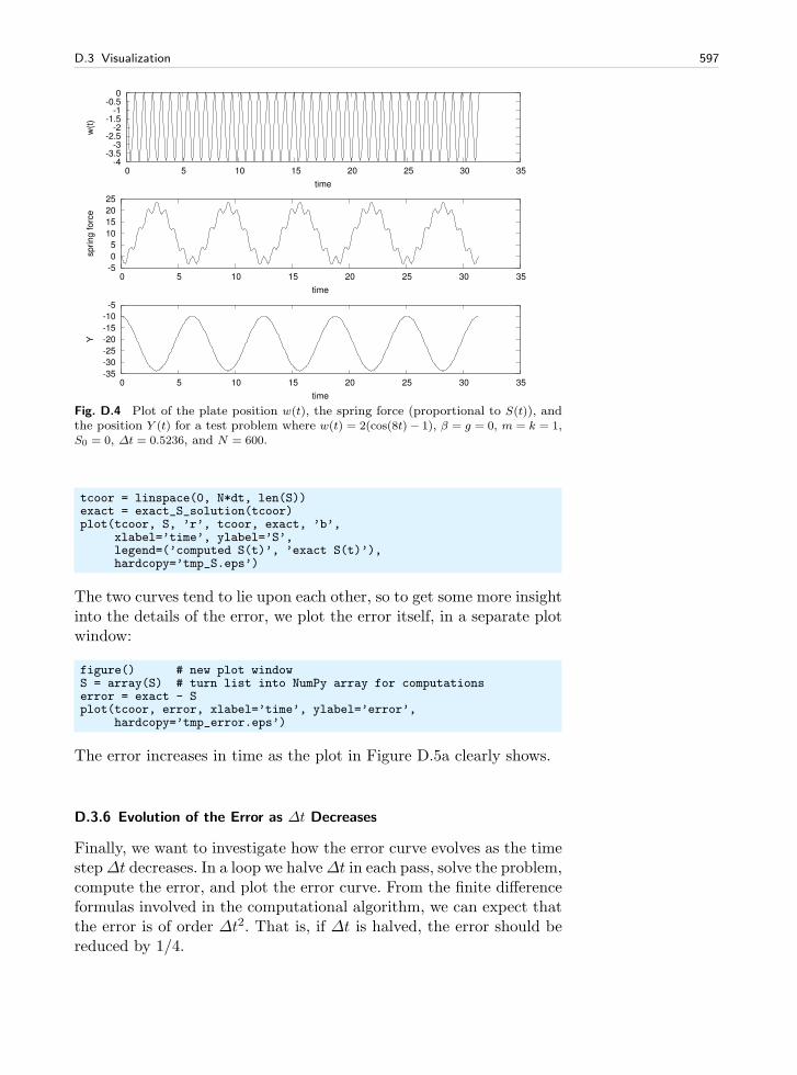
D.3 Visualization 597

-35

-30

-25

-20

-15

-10

-5

0 5 10 15 20 25 30 35

Y

time

-5

0

5

10

15

20

25

0 5 10 15 20 25 30 35

sp

rin

g f

orc

e

time

-4-3.5

-3-2.5

-2-1.5

-1-0.5

0

0 5 10 15 20 25 30 35

w(t

)

time

Fig. D.4 Plot of the plate position w(t), the spring force (proportional to S(t)), andthe position Y (t) for a test problem where w(t) = 2(cos(8t)− 1), β = g = 0, m = k = 1,S0 = 0, ∆t = 0.5236, and N = 600.

tcoor = linspace(0, N*dt, len(S))exact = exact_S_solution(tcoor)plot(tcoor, S, ’r’, tcoor, exact, ’b’,

xlabel=’time’, ylabel=’S’,legend=(’computed S(t)’, ’exact S(t)’),hardcopy=’tmp_S.eps’)

The two curves tend to lie upon each other, so to get some more insightinto the details of the error, we plot the error itself, in a separate plotwindow:

figure() # new plot windowS = array(S) # turn list into NumPy array for computationserror = exact - Splot(tcoor, error, xlabel=’time’, ylabel=’error’,

hardcopy=’tmp_error.eps’)

The error increases in time as the plot in Figure D.5a clearly shows.

D.3.6 Evolution of the Error as ∆t Decreases

Finally, we want to investigate how the error curve evolves as the timestep∆t decreases. In a loop we halve∆t in each pass, solve the problem,compute the error, and plot the error curve. From the finite differenceformulas involved in the computational algorithm, we can expect thatthe error is of order ∆t2. That is, if ∆t is halved, the error should bereduced by 1/4.

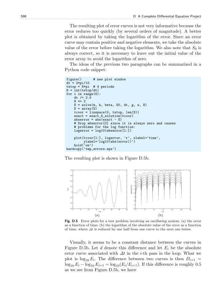
598 D A Complete Differential Equation Project

The resulting plot of error curves is not very informative because theerror reduces too quickly (by several orders of magnitude). A betterplot is obtained by taking the logarithm of the error. Since an errorcurve may contain positive and negative elements, we take the absolutevalue of the error before taking the logarithm. We also note that S0 isalways correct, so it is necessary to leave out the initial value of theerror array to avoid the logarithm of zero.

The ideas of the previous two paragraphs can be summarized in aPython code snippet:

figure() # new plot windowdt = 2*pi/10tstop = 8*pi # 4 periodsN = int(tstop/dt)for i in range(6):

dt /= 2.0N *= 2S = solve(m, k, beta, S0, dt, g, w, N)S = array(S)tcoor = linspace(0, tstop, len(S))exact = exact_S_solution(tcoor)abserror = abs(exact - S)# Drop abserror[0] since it is always zero and causes# problems for the log function:logerror = log10(abserror[1:])

plot(tcoor[1:], logerror, ’r’, xlabel=’time’,ylabel=’log10(abs(error))’)

hold(’on’)hardcopy(’tmp_errors.eps’)

The resulting plot is shown in Figure D.5b.

-0.3

-0.2

-0.1

0

0.1

0.2

0.3

0.4

0 5 10 15 20 25 30 35

err

or

time

(a)

-10

-9

-8

-7

-6

-5

-4

-3

-2

-1

0

0 5 10 15 20 25 30

log

10

(ab

s(e

rro

r))

time

(b)

Fig. D.5 Error plots for a test problem involving an oscillating system: (a) the erroras a function of time; (b) the logarithm of the absolute value of the error as a functionof time, where ∆t is reduced by one half from one curve to the next one below.

Visually, it seems to be a constant distance between the curves inFigure D.5b. Let d denote this difference and let Ei be the absoluteerror curve associated with ∆t in the i-th pass in the loop. What weplot is log10Ei. The difference between two curves is then Di+1 =log10Ei − log10Ei+1 = log10(Ei/Ei+1). If this difference is roughly 0.5as we see from Figure D.5b, we have

D.3 Visualization 599

log10Ei

Ei+1= d = 0.5 ⇒ Ei+1 =

1

3.16Ei .

That is, the error is reduced, but not by the theoretically expectedfactor 4. Let us investigate this topic in more detail by plotting Di+1.

We make a loop as in the last code snippet, but store the logerror ar-ray from the previous pass in the loop (Ei) in a variable logerror_prev

such that we can compute the difference Di+1 as

logerror_diff = logerror_prev - logerror

There are two problems to be aware of now in this array subtraction:(i) the logerror_prev array is not defined before the second pass in theloop (when i is one or greater), and (ii) logerror_prev and logerror

have different lengths since logerror has twice as many time intervalsas logerror_prev. Numerical Python does not know how to computethis difference unless the arrays have the same length. We thereforeneed to use every two elements in logerror:

logerror_diff = logerror_prev - logerror[::2]

An additional problem now arises because the set of time coordinates,tcoor, in the current pass of the loop also has twice as many intervalsso we need to plot logerror_diff against tcoor[::2].

The complete code snippet for plotting differences between the log-arithm of the absolute value of the errors now becomes

figure()dt = 2*pi/10tstop = 8*pi # 4 periodsN = int(tstop/dt)for i in range(6):

dt /= 2.0N *= 2S = solve(m, k, beta, S0, dt, g, w, N)S = array(S)tcoor = linspace(0, tstop, len(S))exact = exact_S_solution(tcoor)abserror = abs(exact - S)logerror = log10(abserror[1:])if i > 0:

logerror_diff = logerror_prev - logerror[::2]plot(tcoor[1::2], logerror_diff, ’r’, xlabel=’time’,

ylabel=’difference in log10(abs(error))’)hold(’on’)meandiff = mean(logerror_diff)print ’average log10(abs(error)) difference:’, meandiff

logerror_prev = logerrorhardcopy(’tmp_errors_diff.eps’)

Figure D.6 shows the result. We clearly see that the differences betweenthe curves in Figure D.5b are almost the same even if ∆t is reducedby several orders of magnitude.

In the loop we also print out the average value of the differencecurves in Figure D.6:

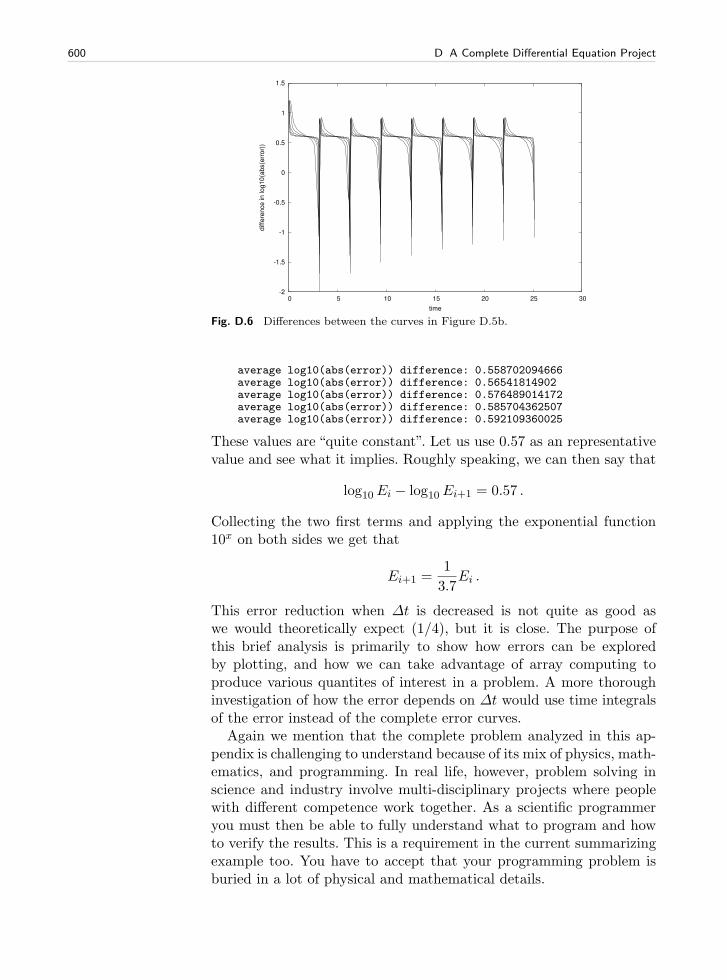
600 D A Complete Differential Equation Project

-2

-1.5

-1

-0.5

0

0.5

1

1.5

0 5 10 15 20 25 30

diffe

rence in log10(a

bs(e

rror)

)

time

Fig. D.6 Differences between the curves in Figure D.5b.

average log10(abs(error)) difference: 0.558702094666average log10(abs(error)) difference: 0.56541814902average log10(abs(error)) difference: 0.576489014172average log10(abs(error)) difference: 0.585704362507average log10(abs(error)) difference: 0.592109360025

These values are “quite constant”. Let us use 0.57 as an representativevalue and see what it implies. Roughly speaking, we can then say that

log10Ei − log10Ei+1 = 0.57 .

Collecting the two first terms and applying the exponential function10x on both sides we get that

Ei+1 =1

3.7Ei .

This error reduction when ∆t is decreased is not quite as good aswe would theoretically expect (1/4), but it is close. The purpose ofthis brief analysis is primarily to show how errors can be exploredby plotting, and how we can take advantage of array computing toproduce various quantites of interest in a problem. A more thoroughinvestigation of how the error depends on ∆t would use time integralsof the error instead of the complete error curves.

Again we mention that the complete problem analyzed in this ap-pendix is challenging to understand because of its mix of physics, math-ematics, and programming. In real life, however, problem solving inscience and industry involve multi-disciplinary projects where peoplewith different competence work together. As a scientific programmeryou must then be able to fully understand what to program and howto verify the results. This is a requirement in the current summarizingexample too. You have to accept that your programming problem isburied in a lot of physical and mathematical details.

D.4 Exercises 601

Having said this, we expect that most readers of this book alsogain a background in physics and mathematics so that the presentsummarizing example can be understood in complete detail, at leastat some later stage.

D.4 Exercises

Exercise D.1. Use a w function with a step.Set up a problem with the box_spring_plot.py program where the

initial stretch in the spring is 1 and there is no gravity force. Betweent = 20 and t = 30 we move the plate suddenly from 0 to 2 and backagain:

w(t) =

2, 20 < t < 30,0, otherwise

Run this problem and view the solution. ⋄Exercise D.2. Make a callback function in Exercise D.1.

Doing Exercise D.1 shows that the Y position increases significantlyin magnutude when the “jump” the plate upward and back again att = 20 and t = 30, respectively. Make a program where you im-port from the box_spring module and provide a callback function thatchecks if Y < 9 and then aborts the program. Name of program file:box_spring_Ycrit.py. ⋄Exercise D.3. Improve input to the simulation program.

The oscillating system in Appendix D.1 has an equilibrium positionS = mg/k, see (D.22) on page 589. A natural case is to let the boxstart at rest in this position and move the plate to induce osciallations.We must then prescribe S0 = mg/k on the command line, but thenumerical value depends on the values of m and g that we might alsogive in the command line. However, it is possible to specify -S0 m*g/k

on the command line if we in the init_prms function first let S0 bea string in the elif test and then, after the for loop, execute S0 =

eval(S0). At that point, m and k are read from the command line sothat eval will work on ’m*g/k’, or any other expression involving datafrom the command. Implement this idea.

A first test problem is to start from rest in the equilibrium positionS(0) = mg/k and give the plate a sudden upward change in positionfrom y = 0 to y = 1. That is,

w(t) =

0, t ≤ 0,1, t > 0

You should get oscillations around the displaced equilibrium positionY = w − L− S0 = −9− 2g. Name of program file: box_spring2.py. ⋄

Programming of Differential Equations E

Appendices C and D give a brief introduction differential equations,with a focus on a few specific equations and programs that are tailoredto these equations. The present appendix views differential equationsfrom a more abstract point of view, which allows us to formulate nu-merical methods and create general software that are applicable toa large family of widely different problems from physics, biology, fi-nance, and numerous other disciplines. More specifically, the abstractview is motivated by the slogan implement once, apply anywhere. Wehave in fact met this principle several places in the book: differenti-ation (f ′′(x)) in Chapters 3.1.9 and 7.3.2, integration (

∫ ba f(x)dx) in

Chapters 3.3.2 and 7.3.3, and root finding (f(x) = 0) in Chapter 4.6.2and Appendix A.1.9. In all of the referred implementations, we workwith a general function f(x) so that any problem can be solved bythe same piece of code as long as we can define the problem in termsof a function f(x). This is an excellent demonstration of the power ofmathematics, and this abstract view of problems in terms of some f(x)is especially powerful in numerical methods and programming. Now weshall formulate differential equations on the abstract form u′ = f(u, t)and create software that can solve any equation for which the f(u, t)is given.

Before studying the present appendix, the reader should have somefamiliarity with differential equations at the level of Appendix C. Ap-pendix D can also be advantageous to read, although this is not strictlyrequired. Fundamental programming skills corresponding to Chap-ters 1–5 are required for the basic material in this appendix. However,we also use classes to a large extent, which demands familiarity withthe concepts in Chapter 7. The material on object-oriented program-ming in Appendix E.2.5 requires good knowledge of class hierarchiesfrom Chapter 9.

603

604 E Programming of Differential Equations

All computer codes associated with this appendix is found insrc/ode2.

E.1 Scalar Ordinary Differential Equations

We shall in this appendix work with ordinary differential equations(ODEs) written on the abstract form

u′(t) = f(u(t), t) . (E.1)

There is an infinite number of solutions to such an equation, so to makethe solution u(t) unique, we must also specify an initial condition

u(0) = U0 . (E.2)

Given f(u, t) and U0, our task is to compute u(t).A first sight, (E.1) is only a first-order differential equation, since

only u′ and not higher-order derivatives like u′′ are present in theequation. However, equations with higher-order derivatives can also bewritten on the abstract form (E.1) by introducing auxiliary variablesand interpreting u and f as vector functions. This rewrite of the origi-nal equation leads to a system of first-order differential equations andwill be treated in Appendix E.2. The bottom line is that a very largefamily of differential equations can be written as (E.1). Forthcomingexamples will provide evidence.

We shall first assume that u(t) is a scalar function, meaning that ithas one number as value, which can be represented as a float objectin Python. We then refer to (E.1) as a scalar differential equation. Thecounterpart vector function means that u is a vector of scalar functionsand the equation is known as a system of ODEs (also known as a vectorODE ). The value of a vector function is a list or array in a program,not more complicated than explained in Chapter 5.

E.1.1 Examples on Right-Hand-Side Functions

To write a specific differential equation on the form (E.1) we need toidentify what the f function is. Say the equation reads

y2y′ = x, y(0) = Y,

with y(x) as the unknown function. First, we need to introduce u andt as new symbols: u = y, t = x. This gives the equivalent equationu2u′ = t and the initial condition u(0) = Y . Second, the quantity u′

must be isolated on the left-hand side of the equation in order to bringthe equation on the form (E.1). Dividing by u2 gives

E.1 Scalar Ordinary Differential Equations 605

u′ = tu−2 .

This fits the form (E.1), and the f(u, t) function is simply the formulainvolving u and t on the right-hand side:

f(u, t) = tu−2 .

The t parameter is very often absent on the right-hand side such thatf involves u only.

Below is a set of commonly arising scalar differential equations andtheir corresponding f functions.

1. Exponential growth of money or populations:

u′ = αu, (E.3)

where α > 0 is a given constant expressing the growth rate of u.

f(u, t) = αu . (E.4)

2. Logistic growth of a population under limited resources:

u′ = αu(

1− u

R

)

, (E.5)

where α > 0 is the initial growth rate andR is the maximum possiblevalue of u.

f(u, t) = αu(

1− u

R

)

. (E.6)

3. Radioactive decay of a substance:

u′ = −au, (E.7)

where a > 0 is the rate of decay of u.

f(u, t) = −au . (E.8)

4. Body falling in a fluid:

u′ + b|u|u = g, (E.9)

where b > 0 models the fluid resistance, g is the acceleration ofgravity, and u is the body’s velocity (see Exercise E.5 on page 635).

f(u, t) = −b|u|u+ g . (E.10)

5. Newton’s law of cooling:

u′ = −h(u− s), (E.11)

where u is the temperature of a body, h > 0 is a proportionalityconstant, normally to be estimated from experiments, and s is the

606 E Programming of Differential Equations

temperature of the surroundings.

f(u, t) = −h(u− s) . (E.12)

E.1.2 The Forward Euler Scheme

Our task now is to define numerical methods for solving equations ofthe form (E.1). The simplest such method is the Forward Euler scheme.Equation (E.1) is to be solved for t ∈ (0, T ], and we seek the solution uat discrete time points ti = i∆t, i = 1, 2, . . . , n. Clearly, tn = n∆t = T ,determining the number of points n as T/∆t. The corresponding valuesu(ti) are often abbreviated as ui, just for notational simplicity.

Equation (E.1) is to be fulfilled at all time points t ∈ (0, T ]. However,when we solve (E.1) numerically, we only require the equation to besatisfied at the discrete time points t1, t2, . . . , tn. That is,

u′(tk) = f(u(tk), tk),

for k = 1, . . . , n. The fundamental idea of the Forward Euler scheme isto approximate u′(tk) by a one-sided, forward difference:

u′(tk) ≈u(tk+1)− u(tk)

∆t=

uk+1 − uk∆t

.

This removes the derivative and leaves us with the equation

uk+1 − uk∆t

= f(uk, tk) .

We assume that uk is already computed, so that the only unknown inthis equation is uk+1, which we can solve for:

uk+1 = uk +∆tf(uk, tk) . (E.13)

This is the Forward Euler scheme for a scalar first-order differentialequation u′ = f(u, t).

Equation (E.13) has a recursive nature. We start with the initialcondition, u0 = U0, and compute u1 as

u1 = u0 +∆tf(u0, t0) .

Then we can continue with

u2 = u1 +∆tf(u1, t1),

and then with u3 and so forth. This recursive nature of the methodalso demonstrates that we must have an initial condition – otherwisethe method cannot start.

E.1 Scalar Ordinary Differential Equations 607

E.1.3 Function Implementation

The next task is to write a general piece of code that implementsthe Forward Euler scheme (E.13). The complete original (continuous)mathematical problem is stated as

u′ = f(u, t), t ∈ (0, T ], u(0) = U0, (E.14)

while the discrete numerical problem reads

uk+1 = uk+∆tf(uk, tk), tk = k∆t, k = 1, . . . , n, n = T/∆t, u0 = U0 .(E.15)

We see that the input data to the numerical problem consist of f , U0,T , and ∆t or n. The output consists of u1, u2, . . . , un and the corre-sponding set of time points t1, t2, . . . , tn.

Let us implement The Forward Euler scheme in a functionForwardEuler that takes f , U0, T , and n as input, and that returnsu0, . . . , un and t0, . . . , tn:

def ForwardEuler(f, U0, T, n):"""Solve u’=f(u,t), u(0)=U0, with n steps until t=T."""import numpy as npt = np.zeros(n+1)u = np.zeros(n+1) # u[k] is the solution at time t[k]u[0] = U0t[0] = 0dt = T/float(n)for k in range(n):

t[k+1] = t[k] + dtu[k+1] = u[k] + dt*f(u[k], t[k])

return u, t

Note the close correspondance between the implementation and themathematical specification of the problem to be solved. The argumentf to the ForwardEuler function must be a Python function f(u, t)

implementing the f(u, t) function in the differential equation (i.e., f isthe definition of the equation to be solved). For example, we may solveu′ = u for t ∈ (0, 3), with u(0) = 1, and ∆t = 0.1 by the following codeutilizing the ForwardEuler function:

def f(u, t):return u

u, t = ForwardEuler(f, U0=1, T=3, n=30)

With the u and t arrays we can easily plot the solution or performdata analysis on the numbers.

E.1.4 Verifying the Implementation

The simplest, yet very effective, way to verify the implementation is tocompute a couple of time steps by hand, say u1 and u2:

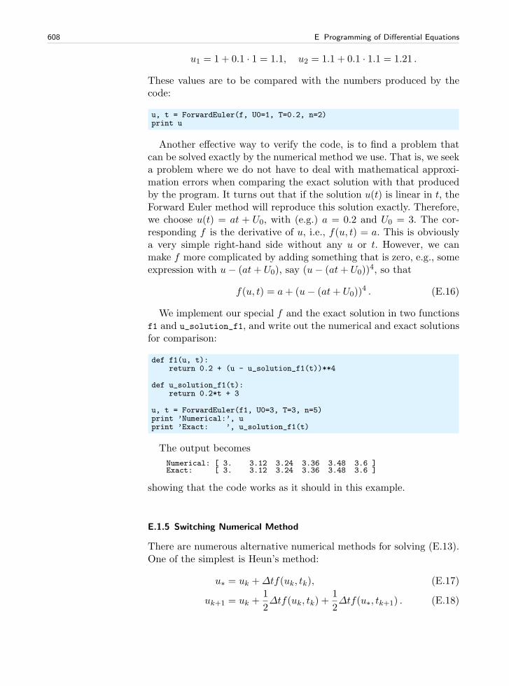
608 E Programming of Differential Equations

u1 = 1 + 0.1 · 1 = 1.1, u2 = 1.1 + 0.1 · 1.1 = 1.21 .

These values are to be compared with the numbers produced by thecode:

u, t = ForwardEuler(f, U0=1, T=0.2, n=2)print u

Another effective way to verify the code, is to find a problem thatcan be solved exactly by the numerical method we use. That is, we seeka problem where we do not have to deal with mathematical approxi-mation errors when comparing the exact solution with that producedby the program. It turns out that if the solution u(t) is linear in t, theForward Euler method will reproduce this solution exactly. Therefore,we choose u(t) = at + U0, with (e.g.) a = 0.2 and U0 = 3. The cor-responding f is the derivative of u, i.e., f(u, t) = a. This is obviouslya very simple right-hand side without any u or t. However, we canmake f more complicated by adding something that is zero, e.g., someexpression with u− (at+ U0), say (u− (at+ U0))

4, so that

f(u, t) = a+ (u− (at+ U0))4 . (E.16)

We implement our special f and the exact solution in two functionsf1 and u_solution_f1, and write out the numerical and exact solutionsfor comparison:

def f1(u, t):return 0.2 + (u - u_solution_f1(t))**4

def u_solution_f1(t):return 0.2*t + 3

u, t = ForwardEuler(f1, U0=3, T=3, n=5)print ’Numerical:’, uprint ’Exact: ’, u_solution_f1(t)

The output becomes

Numerical: [ 3. 3.12 3.24 3.36 3.48 3.6 ]Exact: [ 3. 3.12 3.24 3.36 3.48 3.6 ]

showing that the code works as it should in this example.

E.1.5 Switching Numerical Method

There are numerous alternative numerical methods for solving (E.13).One of the simplest is Heun’s method:

u∗ = uk +∆tf(uk, tk), (E.17)

uk+1 = uk +1

2∆tf(uk, tk) +

1

2∆tf(u∗, tk+1) . (E.18)

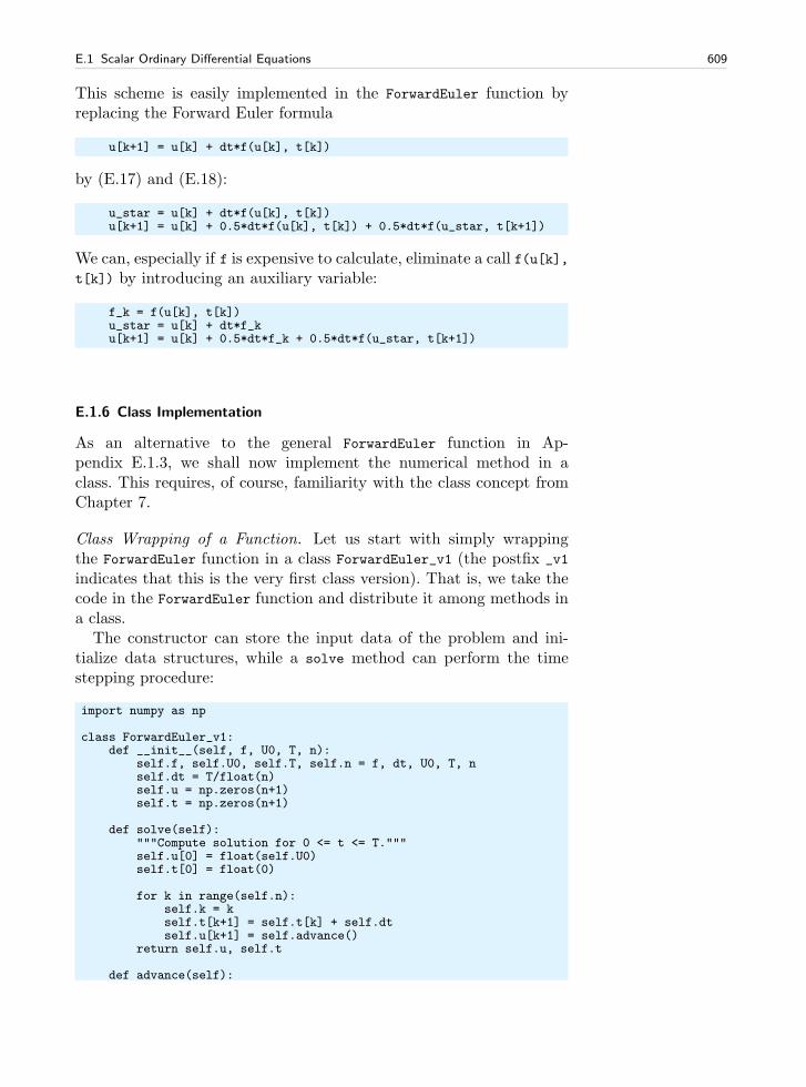
E.1 Scalar Ordinary Differential Equations 609

This scheme is easily implemented in the ForwardEuler function byreplacing the Forward Euler formula

u[k+1] = u[k] + dt*f(u[k], t[k])

by (E.17) and (E.18):

u_star = u[k] + dt*f(u[k], t[k])u[k+1] = u[k] + 0.5*dt*f(u[k], t[k]) + 0.5*dt*f(u_star, t[k+1])

We can, especially if f is expensive to calculate, eliminate a call f(u[k],t[k]) by introducing an auxiliary variable:

f_k = f(u[k], t[k])u_star = u[k] + dt*f_ku[k+1] = u[k] + 0.5*dt*f_k + 0.5*dt*f(u_star, t[k+1])

E.1.6 Class Implementation

As an alternative to the general ForwardEuler function in Ap-pendix E.1.3, we shall now implement the numerical method in aclass. This requires, of course, familiarity with the class concept fromChapter 7.

Class Wrapping of a Function. Let us start with simply wrappingthe ForwardEuler function in a class ForwardEuler_v1 (the postfix _v1

indicates that this is the very first class version). That is, we take thecode in the ForwardEuler function and distribute it among methods ina class.

The constructor can store the input data of the problem and ini-tialize data structures, while a solve method can perform the timestepping procedure:

import numpy as np

class ForwardEuler_v1:def __init__(self, f, U0, T, n):

self.f, self.U0, self.T, self.n = f, dt, U0, T, nself.dt = T/float(n)self.u = np.zeros(n+1)self.t = np.zeros(n+1)

def solve(self):"""Compute solution for 0 <= t <= T."""self.u[0] = float(self.U0)self.t[0] = float(0)

for k in range(self.n):self.k = kself.t[k+1] = self.t[k] + self.dtself.u[k+1] = self.advance()

return self.u, self.t

def advance(self):

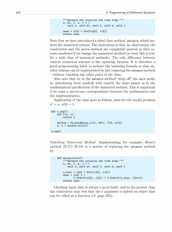
610 E Programming of Differential Equations

"""Advance the solution one time step."""u, dt, f, k, t = \

self.u, self.dt, self.f, self.k, self.t

unew = u[k] + dt*f(u[k], t[k])return unew

Note that we have introduced a third class method, advance, which iso-lates the numerical scheme. The motivation is that, by observation, theconstructor and the solve method are completely general as they re-main unaltered if we change the numerical method (at least this is truefor a wide class of numerical methods). The only difference betweenvarious numerical schemes is the updating formula. It is therefore agood programming habit to isoloate the updating formula so that an-other scheme can be implemented by just replacing the advancemethod– without touching any other parts of the class.

Also note that we in the advance method “strip off” the self prefixby introducing local symbols with exactly the same names as in themathematical specification of the numerical method. This is importantif we want a one-to-one correspondance between the mathematics andthe implementation.

Application of the class goes as follows, here for the model problemu′ = u, u(0) = 1:

def u_exp():def f(u, t):

return u

method = ForwardEuler_v1(f, U0=1, T=3, n=15)u, t = method.solve()

u_exp()

Switching Numerical Method. Implementing, for example, Heun’smethod (E.17)–(E.18) is a matter of replacing the advance methodby

def advance(self):"""Advance the solution one time step."""u, dt, f, k, t = \

self.u, self.dt, self.f, self.k, self.t

u_star = u[k] + dt*f(u[k], t[k])unew = u[k] + \

0.5*dt*f(u[k], t[k]) + 0.5*dt*f(u_star, t[k+1])return unew

Checking input data is always a good habit, and in the present classthe constructor may test that the f argument is indeed an object thatcan be called as a function (cf. page 325):

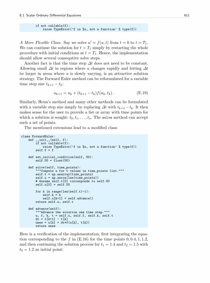
E.1 Scalar Ordinary Differential Equations 611

if not callable(f):raise TypeError(’f is %s, not a function’ % type(f))

A More Flexible Class. Say we solve u′ = f(u, t) from t = 0 to t = T1.We can continue the solution for t > T1 simply by restarting the wholeprocedure with initial conditions at t = T1. Hence, the implementationshould allow several consequtive solve steps.

Another fact is that the time step ∆t does not need to be constant.Allowing small ∆t in regions where u changes rapidly and letting ∆tbe larger in areas where u is slowly varying, is an attractive solutionstrategy. The Forward Euler method can be reformulated for a variabletime step size tk+1 − tk:

uk+1 = uk + (tk+1 − tk)f(uk, tk) . (E.19)

Similarly, Heun’s method and many other methods can be formulatedwith a variable step size simply by replacing ∆t with tk+1− tk. It thenmakes sense for the user to provide a list or array with time points forwhich a solution is sought: t0, t1, . . . , tn. The solve method can acceptsuch a set of points.

The mentioned extensions lead to a modified class:

class ForwardEuler:def __init__(self, f):

if not callable(f):raise TypeError(’f is %s, not a function’ % type(f))

self.f = f

def set_initial_condition(self, U0):self.U0 = float(U0)

def solve(self, time_points):"""Compute u for t values in time_points list."""self.t = np.asarray(time_points)self.u = np.zeros(len(time_points))# Assume self.t[0] corresponds to self.U0self.u[0] = self.U0

for k in range(len(self.t)-1):self.k = kself.u[k+1] = self.advance()

return self.u, self.t

def advance(self):"""Advance the solution one time step."""u, f, k, t = self.u, self.f, self.k, self.tdt = t[k+1] - t[k]unew = u[k] + dt*f(u[k], t[k])return unew

Here is a verification of the implementation, first integrating the equa-tion corresponding to the f in (E.16) for the time points 0, 0.4, 1, 1.2,and then continuing the solution process for t1 = 1.4 and t2 = 1.5 witht0 = 1.2 as initial point:

612 E Programming of Differential Equations

def _verify_f1_ForwardEuler():U0 = 3method = ForwardEuler(_f1)method.set_initial_condition(U0)t = [0, 0.4, 1, 1.2]u1, t1 = method.solve(t)# Continue with a new time intervalmethod.set_initial_condition(u1[-1])t = [1.2, 1.4, 1.5]u2, t2 = method.solve(t)u = np.concatenate((u1, u2))t = np.concatenate((t1, t2))u_exact = _u_solution_f1(t)print ’time values:’, tprint ’Numerical: ’, uprint ’Exact: ’, u_exact

The output is exactly what we would expect:

time values: [ 0. 0.4 1. 1.2 1.2 1.4 1.5]Numerical: [ 3. 3.08 3.2 3.24 3.24 3.28 3.3 ]Exact: [ 3. 3.08 3.2 3.24 3.24 3.28 3.3 ]

E.1.7 Example: Logistic Growth

A more exciting application is to solve the logistic equation (C.23),

u′(t) = αu(t)

(

1− u(t)

R

)

.

The f(u, t) function is simply the right-hand side of this ODE.Implementing this problem with the aid of the ForwardEuler function

from Appendix E.1.3 is left as an exercise for the reader, while we hereexplain how to utilize class ForwardEuler from Appendix E.1.6. Alsothe right-hand-side function f(u, t) will be implemented as a class,because it contains the parameters α and R. We may store the initialcondition as part of this class and have a __str__ method for prettyprint of the formula for the right-hand-side of the logistic equation.

This problem class can then be expressed as

class Logistic:"""Problem class for a logistic ODE."""def __init__(self, alpha, R, U0):

self.alpha, self.R, self.U0 = alpha, float(R), U0

def __call__(self, u, t):"""Return f(u,t) for the logistic ODE."""return self.alpha*u*(1 - u/self.R)

def __str__(self):"""Return ODE and initial condition."""return "u’(t) = %g*u*(1 - u/%g)\nu(0)=%g" % \

(self.alpha, self.R, self.U0)

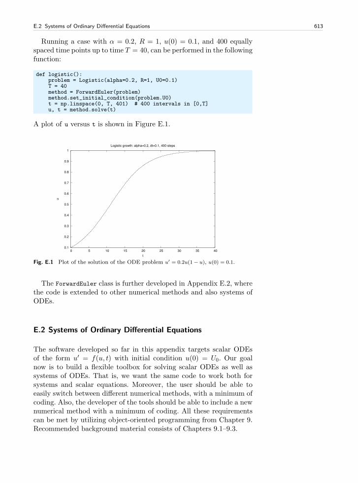
E.2 Systems of Ordinary Differential Equations 613

Running a case with α = 0.2, R = 1, u(0) = 0.1, and 400 equallyspaced time points up to time T = 40, can be performed in the followingfunction:

def logistic():problem = Logistic(alpha=0.2, R=1, U0=0.1)T = 40method = ForwardEuler(problem)method.set_initial_condition(problem.U0)t = np.linspace(0, T, 401) # 400 intervals in [0,T]u, t = method.solve(t)

A plot of u versus t is shown in Figure E.1.

0.1

0.2

0.3

0.4

0.5

0.6

0.7

0.8

0.9

1

0 5 10 15 20 25 30 35 40

u

t

Logistic growth: alpha=0.2, dt=0.1, 400 steps

Fig. E.1 Plot of the solution of the ODE problem u′ = 0.2u(1− u), u(0) = 0.1.

The ForwardEuler class is further developed in Appendix E.2, wherethe code is extended to other numerical methods and also systems ofODEs.

E.2 Systems of Ordinary Differential Equations

The software developed so far in this appendix targets scalar ODEsof the form u′ = f(u, t) with initial condition u(0) = U0. Our goalnow is to build a flexible toolbox for solving scalar ODEs as well assystems of ODEs. That is, we want the same code to work both forsystems and scalar equations. Moreover, the user should be able toeasily switch between different numerical methods, with a minimum ofcoding. Also, the developer of the tools should be able to include a newnumerical method with a minimum of coding. All these requirementscan be met by utilizing object-oriented programming from Chapter 9.Recommended background material consists of Chapters 9.1–9.3.

614 E Programming of Differential Equations

E.2.1 Mathematical Problem

A scalar ODE involves the single equation

u′(t) = f(u(t), t)

with a single function u(t) as unknown, while a system of ODEs in-volves n scalar ODEs and consequently n unknown functions. Let usdenote the unknown functions in the system by u(i)(t), with i as acounter, i = 0, . . . ,m− 1. The system of n ODEs can then be writtenin the following abstract form:

du(0)

dt= f (0)(u(0), u(1), . . . , u(m−1), t), (E.20)

... (E.21)

du(i)

dt= f (i)(u(0), u(1), . . . , u(m−1), t), (E.22)

... (E.23)

du(m−1)

dt= f (m−1)(u(0), u(1), . . . , u(m−1), t), (E.24)

In addition, we need n initial conditions for the n unknown functions:

u(i)(0) = U(i)0 , i = 0, . . . ,m− 1 . (E.25)

Instead of writing out each equation as in (E.20)–(E.24), mathemati-cians like to collect the individual functions u(0), u(1), . . . , u(m−1) in avector

u = (u(0), u(1), . . . , u(m−1)) .

The different right-hand-side functions f (0), f (1), . . . , f (m−1) in (E.20)–(E.24) can also be collected in a vector

f = (f (0), f (1), . . . , f (m−1)) .

Similarly, we put the initial conditions also in a vector

U0 = (U(0)0 , U

(1)0 , . . . , U

(m−1)0 ) .

With the vectors u, f , and U0, we can write the ODE system (E.20)–(E.24) with initial conditions (E.25) as

u′ = f(u, t), u(0) = U0 . (E.26)

This is exactly the same notation as we used for a scalar ODE (!). Thepower of mathematics is that abstractions can be generalized so thatnew problems look like the familiar ones, and very often methods carry

E.2 Systems of Ordinary Differential Equations 615

over to the new problems in the new notation without any changes.This is true for numerical methods for ODEs too.

Let us apply the Forward Euler scheme to each of the ODEs in thesystem (E.20)–(E.24):

u(0)k+1 = u

(0)k +∆tf (0)(u

(0)k , u

(1)k , . . . , u

(m−1)k , tk), (E.27)

... (E.28)

u(i)k+1 = u

(i)k +∆tf (i)(u

(0)k , u

(1)k , . . . , u

(m−1)k , tk), (E.29)

... (E.30)

u(m−1)k+1 = u

(m−1)k +∆tf (m−1)(u

(0)k , u

(1)k , . . . , u

(m−1)k , tk), (E.31)

Utilizing the vector notation, (E.27)–(E.31) can be compactly writtenas

uk+1 = uk +∆tf(uk, tk), (E.32)

and this is again nothing but the formula we had for the Forward Eulerscheme applied to a scalar ODE.

To summarize, the notation u′ = f(u, t), u(0) = U0, is from nowon used both for scalar ODEs and for systems of ODEs. In the formercase, u and f are scalar functions, while in the latter case they arevectors. This great flexibility carries over to programming too: we candevelop code for u′ = f(u, t) that works for scalar ODEs and systemsof ODEs, the only difference being that u and f correspond to float

objects for scalar ODEs and to arrays for systems of ODEs.Unless you are quite familiar with systems of ODEs and array arith-

metics, it can be a good idea to just think about scalar ODEs andthat u(t) is a function of one variable when you read on. Later, youcan come back and reread the text with systems of ODEs and u(t)as a vector (array) in mind. The invisible difference between scalarODEs and systems of ODEs is not only important for addressing bothnewcomers to ODEs and more experienced readers. The principle isvery important for software development too: We can write code withscalar ODEs in mind and test this code. Afterwards, the code shouldalso work immediately for systems and u(t) as a vector of functions.This remarkable achievement is obtained by an elegant interplay be-tween abstractions in mathematics and the functionality and syntax ofthe Python programming language.

E.2.2 Example of a System of ODEs

An oscillating spring-mass system can be governed by a second-orderODE (see (D.8) in Appendix D for derivation):

mu′′ + βu′ + ku = F (t), u(0) = U0, u′(0) = 0 . (E.33)

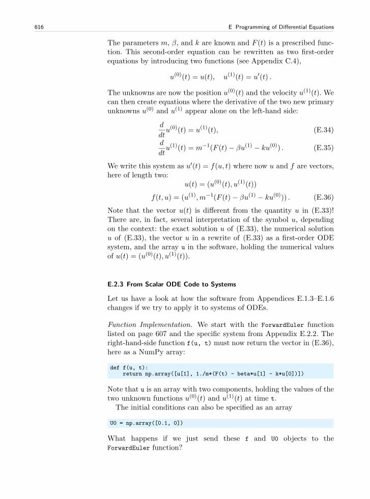
616 E Programming of Differential Equations

The parameters m, β, and k are known and F (t) is a prescribed func-tion. This second-order equation can be rewritten as two first-orderequations by introducing two functions (see Appendix C.4),

u(0)(t) = u(t), u(1)(t) = u′(t) .

The unknowns are now the position u(0)(t) and the velocity u(1)(t). Wecan then create equations where the derivative of the two new primaryunknowns u(0) and u(1) appear alone on the left-hand side:

d

dtu(0)(t) = u(1)(t), (E.34)

d

dtu(1)(t) = m−1(F (t)− βu(1) − ku(0)) . (E.35)

We write this system as u′(t) = f(u, t) where now u and f are vectors,here of length two:

u(t) = (u(0)(t), u(1)(t))

f(t, u) = (u(1),m−1(F (t)− βu(1) − ku(0))) . (E.36)

Note that the vector u(t) is different from the quantity u in (E.33)!There are, in fact, several interpretation of the symbol u, dependingon the context: the exact solution u of (E.33), the numerical solutionu of (E.33), the vector u in a rewrite of (E.33) as a first-order ODEsystem, and the array u in the software, holding the numerical valuesof u(t) = (u(0)(t), u(1)(t)).

E.2.3 From Scalar ODE Code to Systems

Let us have a look at how the software from Appendices E.1.3–E.1.6changes if we try to apply it to systems of ODEs.

Function Implementation. We start with the ForwardEuler functionlisted on page 607 and the specific system from Appendix E.2.2. Theright-hand-side function f(u, t) must now return the vector in (E.36),here as a NumPy array:

def f(u, t):return np.array([u[1], 1./m*(F(t) - beta*u[1] - k*u[0])])

Note that u is an array with two components, holding the values of thetwo unknown functions u(0)(t) and u(1)(t) at time t.

The initial conditions can also be specified as an array

U0 = np.array([0.1, 0])

What happens if we just send these f and U0 objects to theForwardEuler function?

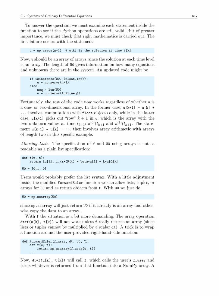
E.2 Systems of Ordinary Differential Equations 617

To answer the question, we must examine each statement inside thefunction to see if the Python operations are still valid. But of greaterimportance, we must check that right mathematics is carried out. Thefirst failure occurs with the statement

u = np.zeros(n+1) # u[k] is the solution at time t[k]

Now, u should be an array of arrays, since the solution at each time levelis an array. The length of U0 gives information on how many equationsand unknowns there are in the system. An updated code might be

if isinstance(U0, (float,int)):u = np.zeros(n+1)

else:neq = len(U0)u = np.zeros((n+1,neq))

Fortunately, the rest of the code now works regardless of whether u isa one- or two-dimensional array. In the former case, u[k+1] = u[k] +

... involves computations with float objects only, while in the lattercase, u[k+1] picks out “row” k + 1 in u, which is the array with thetwo unknown values at time tk+1: u

(0)(tk+1 and u(1)(tk+1. The state-ment u[k+1] = u[k] + ... then involves array arithmetic with arraysof length two in this specific example.

Allowing Lists. The specification of f and U0 using arrays is not asreadable as a plain list specification:

def f(u, t):return [u[1], 1./m*(F(t) - beta*u[1] - k*u[0])]

U0 = [0.1, 0]

Users would probably prefer the list syntax. With a little adjustmentinside the modified ForwardEuler function we can allow lists, tuples, orarrays for U0 and as return objects from f. With U0 we just do

U0 = np.asarray(U0)

since np.asarray will just return U0 if it already is an array and other-wise copy the data to an array.

With f the situation is a bit more demanding. The array operationdt*f(u[k], t[k]) will not work unless f really returns an array (sincelists or tuples cannot be multiplied by a scalar dt). A trick is to wrapa function around the user-provided right-hand-side function:

def ForwardEuler(f_user, dt, U0, T):def f(u, t):

return np.asarray(f_user(u, t))...

Now, dt*f(u[k], t[k]) will call f, which calls the user’s f_user andturns whatever is returned from that function into a NumPy array. A

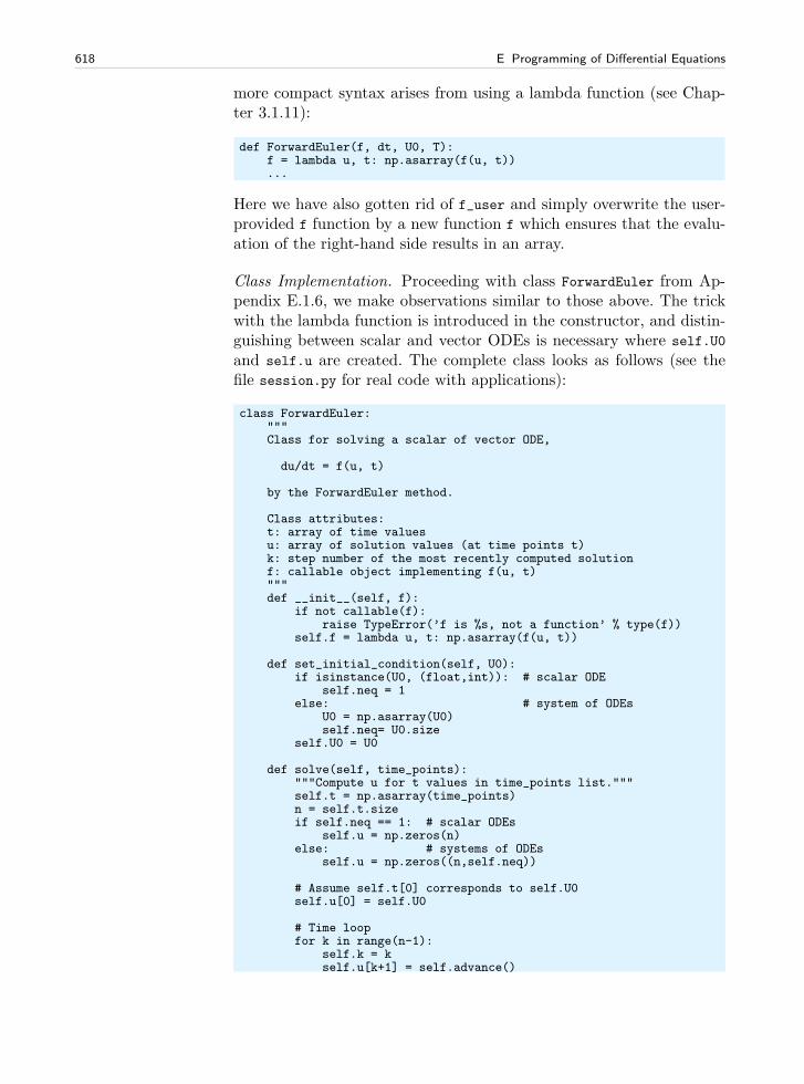
618 E Programming of Differential Equations

more compact syntax arises from using a lambda function (see Chap-ter 3.1.11):

def ForwardEuler(f, dt, U0, T):f = lambda u, t: np.asarray(f(u, t))...

Here we have also gotten rid of f_user and simply overwrite the user-provided f function by a new function f which ensures that the evalu-ation of the right-hand side results in an array.

Class Implementation. Proceeding with class ForwardEuler from Ap-pendix E.1.6, we make observations similar to those above. The trickwith the lambda function is introduced in the constructor, and distin-guishing between scalar and vector ODEs is necessary where self.U0

and self.u are created. The complete class looks as follows (see thefile session.py for real code with applications):

class ForwardEuler:"""Class for solving a scalar of vector ODE,

du/dt = f(u, t)

by the ForwardEuler method.

Class attributes:t: array of time valuesu: array of solution values (at time points t)k: step number of the most recently computed solutionf: callable object implementing f(u, t)"""def __init__(self, f):

if not callable(f):raise TypeError(’f is %s, not a function’ % type(f))

self.f = lambda u, t: np.asarray(f(u, t))

def set_initial_condition(self, U0):if isinstance(U0, (float,int)): # scalar ODE

self.neq = 1else: # system of ODEs

U0 = np.asarray(U0)self.neq= U0.size

self.U0 = U0

def solve(self, time_points):"""Compute u for t values in time_points list."""self.t = np.asarray(time_points)n = self.t.sizeif self.neq == 1: # scalar ODEs

self.u = np.zeros(n)else: # systems of ODEs

self.u = np.zeros((n,self.neq))

# Assume self.t[0] corresponds to self.U0self.u[0] = self.U0

# Time loopfor k in range(n-1):

self.k = kself.u[k+1] = self.advance()

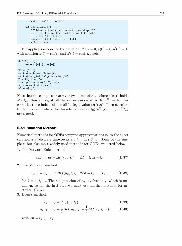
E.2 Systems of Ordinary Differential Equations 619

return self.u, self.t

def advance(self):"""Advance the solution one time step."""u, f, k, t = self.u, self.f, self.k, self.tdt = t[k+1] - t[k]unew = u[k] + dt*f(u[k], t[k])return unew

The application code for the equation u′′+u = 0, u(0) = 0, u′(0) = 1,with solution u(t) = sin(t) and u′(t) = cos(t), reads

def f(u, t):return [u[1], -u[0]]

U0 = [0, 1]method = ForwardEuler(f)method.set_initial_condition(U0)T = 12; n = 100t = np.linspace(0, T, n+1)u, t = method.solve(t)u0 = u[:,0]

Note that the computed u array is two-dimensional, where u[k,i] holdsu(i)(tk). Hence, to grab all the values associated with u(0), we fix i as0 and let the k index take on all its legal values: u[:,0]. Then u0 refersto the piece of u where the discrete values u(0)(t0), u

(0)(t1), . . . , u(0)(tn)

are stored.

E.2.4 Numerical Methods

Numerical methods for ODEs compute approximations uk to the exactsolution u at discrete time levels tk, k = 1, 2, 3, . . .. Some of the sim-plest, but also most widely used methods for ODEs are listed below.

1. The Forward Euler method:

uk+1 = uk +∆t f(uk, tk), ∆t = tk+1 − tk . (E.37)

2. The Midpoint method:

uk+1 = uk−1 + 2∆tf(uk, tk), 2∆t = tk+1 − tk−1 (E.38)

for k = 1, 2, . . .. The computation of u1 involves u−1, which is un-known, so for the first step we must use another method, for in-stance, (E.37).

3. Heun’s method:

u∗ = uk +∆tf(uk, tk), (E.39)

uk+1 = uk +1

2∆tf(uk, tk) +

1

2∆tf(u∗, tk+1), (E.40)

with ∆t = tk+1 − tk.

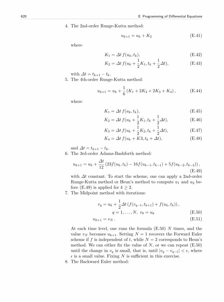
620 E Programming of Differential Equations

4. The 2nd-order Runge-Kutta method:

uk+1 = uk +K2 (E.41)

where

K1 = ∆t f(uk, tk), (E.42)

K2 = ∆t f(uk +1

2K1, tk +

1

2∆t), (E.43)

with ∆t = tk+1 − tk.5. The 4th-order Runge-Kutta method:

uk+1 = uk +1

6(K1 + 2K2 + 2K3 +K4) , (E.44)

where

K1 = ∆t f(uk, tk), (E.45)

K2 = ∆t f(uk +1

2K1, tk +

1

2∆t), (E.46)

K3 = ∆t f(uk +1

2K2, tk +

1

2∆t), (E.47)

K4 = ∆t f(uk +K3, tk +∆t), (E.48)

and ∆t = tk+1 − tk.6. The 3rd-order Adams-Bashforth method:

uk+1 = uk +∆t

12(23f(uk, tk)− 16f(uk−1, tk−1) + 5f(uk−2, tk−2)) ,

(E.49)with ∆t constant. To start the scheme, one can apply a 2nd-orderRunge-Kutta method or Heun’s method to compute u1 and u2 be-fore (E.49) is applied for k ≥ 2.

7. The Midpoint method with iterations:

vq = uk +1

2∆t (f(vq−1, tk+1) + f(uk, tk)) ,

q = 1, . . . , N, v0 = uk (E.50)

uk+1 = vN . (E.51)

At each time level, one runs the formula (E.50) N times, and thevalue vN becomes uk+1. Setting N = 1 recovers the Forward Eulerscheme if f is independent of t, while N = 2 corresponds to Heun’smethod. We can either fix the value of N , or we can repeat (E.50)until the change in vq is small, that is, until |vq − vq−1| < ǫ, whereǫ is a small value. Fixing N is sufficient in this exercise.

8. The Backward Euler method:

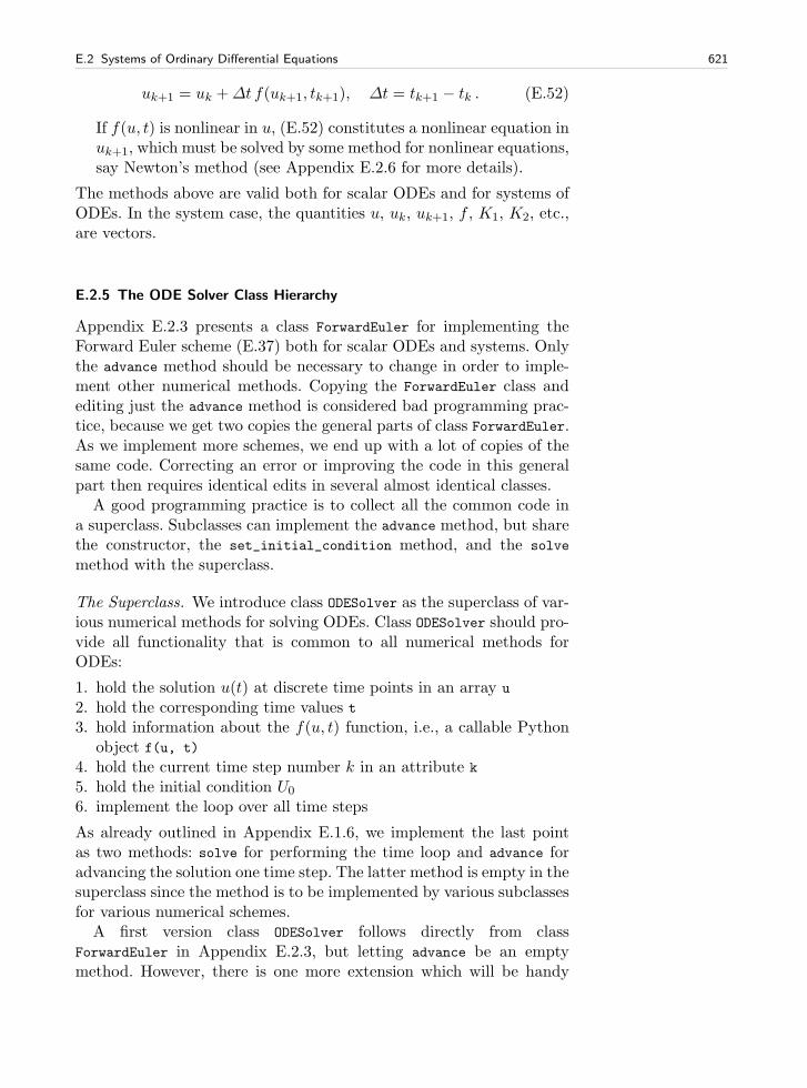
E.2 Systems of Ordinary Differential Equations 621

uk+1 = uk +∆t f(uk+1, tk+1), ∆t = tk+1 − tk . (E.52)

If f(u, t) is nonlinear in u, (E.52) constitutes a nonlinear equation inuk+1, which must be solved by some method for nonlinear equations,say Newton’s method (see Appendix E.2.6 for more details).

The methods above are valid both for scalar ODEs and for systems ofODEs. In the system case, the quantities u, uk, uk+1, f , K1, K2, etc.,are vectors.

E.2.5 The ODE Solver Class Hierarchy

Appendix E.2.3 presents a class ForwardEuler for implementing theForward Euler scheme (E.37) both for scalar ODEs and systems. Onlythe advance method should be necessary to change in order to imple-ment other numerical methods. Copying the ForwardEuler class andediting just the advance method is considered bad programming prac-tice, because we get two copies the general parts of class ForwardEuler.As we implement more schemes, we end up with a lot of copies of thesame code. Correcting an error or improving the code in this generalpart then requires identical edits in several almost identical classes.

A good programming practice is to collect all the common code ina superclass. Subclasses can implement the advance method, but sharethe constructor, the set_initial_condition method, and the solve

method with the superclass.

The Superclass. We introduce class ODESolver as the superclass of var-ious numerical methods for solving ODEs. Class ODESolver should pro-vide all functionality that is common to all numerical methods forODEs:

1. hold the solution u(t) at discrete time points in an array u

2. hold the corresponding time values t3. hold information about the f(u, t) function, i.e., a callable Python

object f(u, t)

4. hold the current time step number k in an attribute k

5. hold the initial condition U0

6. implement the loop over all time steps

As already outlined in Appendix E.1.6, we implement the last pointas two methods: solve for performing the time loop and advance foradvancing the solution one time step. The latter method is empty in thesuperclass since the method is to be implemented by various subclassesfor various numerical schemes.

A first version class ODESolver follows directly from classForwardEuler in Appendix E.2.3, but letting advance be an emptymethod. However, there is one more extension which will be handy

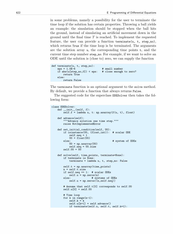
622 E Programming of Differential Equations

in some problems, namely a possibility for the user to terminate thetime loop if the solution has certain properties. Throwing a ball yieldsan example: the simulation should be stopped when the ball hitsthe ground, instead of simulating an artificial movement down in theground until the final time T is reached. To implement the requestedfeature, the user can provide a function terminate(u, t, step_no),which returns True if the time loop is be terminated. The argumentsare the solution array u, the corresponding time points t, and thecurrent time step number step_no. For example, if we want to solve anODE until the solution is (close to) zero, we can supply the function

def terminate(u, t, step_no):eps = 1.0E-6 # small numberif abs(u[step_no,0]) < eps: # close enough to zero?

return Trueelse:

return False

The terminate function is an optional argument to the solve method.By default, we provide a function that always returns False.

The suggested code for the superclass ODESolver then takes the fol-lowing form:

class ODESolver:def __init__(self, f):

self.f = lambda u, t: np.asarray(f(u, t), float)

def advance(self):"""Advance solution one time step."""raise NotImplementedError

def set_initial_condition(self, U0):if isinstance(U0, (float,int)): # scalar ODE

self.neq = 1U0 = float(U0)

else: # system of ODEsU0 = np.asarray(U0)self.neq = U0.size

self.U0 = U0

def solve(self, time_points, terminate=None):if terminate is None:

terminate = lambda u, t, step_no: False

self.t = np.asarray(time_points)n = self.t.sizeif self.neq == 1: # scalar ODEs

self.u = np.zeros(n)else: # systems of ODEs

self.u = np.zeros((n,self.neq))

# Assume that self.t[0] corresponds to self.U0self.u[0] = self.U0

# Time loopfor k in range(n-1):

self.k = kself.u[k+1] = self.advance()if terminate(self.u, self.t, self.k+1):

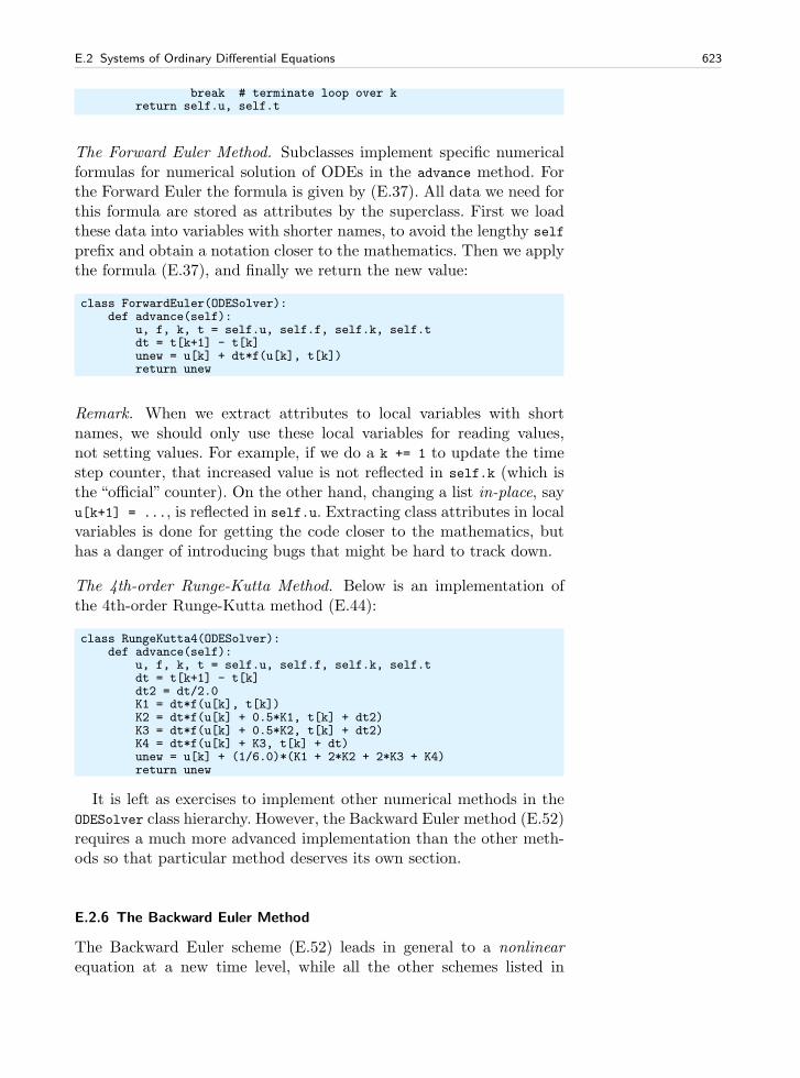
E.2 Systems of Ordinary Differential Equations 623

break # terminate loop over kreturn self.u, self.t

The Forward Euler Method. Subclasses implement specific numericalformulas for numerical solution of ODEs in the advance method. Forthe Forward Euler the formula is given by (E.37). All data we need forthis formula are stored as attributes by the superclass. First we loadthese data into variables with shorter names, to avoid the lengthy self

prefix and obtain a notation closer to the mathematics. Then we applythe formula (E.37), and finally we return the new value:

class ForwardEuler(ODESolver):def advance(self):

u, f, k, t = self.u, self.f, self.k, self.tdt = t[k+1] - t[k]unew = u[k] + dt*f(u[k], t[k])return unew

Remark. When we extract attributes to local variables with shortnames, we should only use these local variables for reading values,not setting values. For example, if we do a k += 1 to update the timestep counter, that increased value is not reflected in self.k (which isthe “official” counter). On the other hand, changing a list in-place, sayu[k+1] = ..., is reflected in self.u. Extracting class attributes in localvariables is done for getting the code closer to the mathematics, buthas a danger of introducing bugs that might be hard to track down.

The 4th-order Runge-Kutta Method. Below is an implementation ofthe 4th-order Runge-Kutta method (E.44):

class RungeKutta4(ODESolver):def advance(self):

u, f, k, t = self.u, self.f, self.k, self.tdt = t[k+1] - t[k]dt2 = dt/2.0K1 = dt*f(u[k], t[k])K2 = dt*f(u[k] + 0.5*K1, t[k] + dt2)K3 = dt*f(u[k] + 0.5*K2, t[k] + dt2)K4 = dt*f(u[k] + K3, t[k] + dt)unew = u[k] + (1/6.0)*(K1 + 2*K2 + 2*K3 + K4)return unew

It is left as exercises to implement other numerical methods in theODESolver class hierarchy. However, the Backward Euler method (E.52)requires a much more advanced implementation than the other meth-ods so that particular method deserves its own section.

E.2.6 The Backward Euler Method

The Backward Euler scheme (E.52) leads in general to a nonlinearequation at a new time level, while all the other schemes listed in

624 E Programming of Differential Equations

Appendix E.2.4 have a simple formula for the new uk+1 value. Thenonlinear equation reads

uk+1 = uk +∆t f(uk+1, tk+1) .

For simplicity we assume that the ODE is scalar so the unknown uk+1

is a scalar. It might be easier to see that the equation for uk+1 isnonlinear if we rearrange the equation to to

F (w) ≡ w −∆tf(w, tk+1)− uk = 0, (E.53)

where w = uk+1. If now f(u, t) is a nonlinear function of u, F (w) willalso be a nonlinear function of w.

To solve F (w) = 0 we can use the Bisection method from Chap-ter 4.6.2, Newton’s method from Appendix A.1.9, or the Secant methodfrom Exercise A.14. Here we apply Newton’s method and the imple-mentation given in src/diffeq/Newton.py. A disadvantage with New-ton’s method is that we need the derivative of F with respect to w,which requires the derivative ∂f(w, t)/∂w. A quick solution is to use anumerical derivative, e.g., class Derivative from Chapter 7.3.2.

We make a subclass BackwardEuler. As we need to solve F (w) = 0at every time step, we also need to implement the F (w) function. Thisis conveniently done in a local function inside the advance method1:

def advance(self):u, f, k, t = self.u, self.f, self.k, self.t

def F(w):return w - dt*f(w, t[k+1]) - u[k]

dFdw = Derivative(F)w_start = u[k] + dt*f(u[k], t[k]) # Forward Euler stepunew, n, F_value = Newton(F, w_start, dFdw, N=30)if n >= 30:

print "Newton’s failed to converge at t=%g "\"(%d iterations)" % (t, n)

return unew

The derivative dF/dw is computed numerically by a class Derivative,which is a slight modification of the similar class in Chapter 7.3.2,because we now want to use a more accurate, centered formula:

class Derivative:def __init__(self, f, h=1E-5):

self.f = fself.h = float(h)

def __call__(self, x):f, h = self.f, self.hreturn (f(x+h) - f(x-h))/(2*h)

1 The local variables in the advance function, e.g., dt and u, act as “global” variablesfor the F function. Hence, when F is sent away to some Newton function, F remembersthe values of dt, f, t, and u!.

E.2 Systems of Ordinary Differential Equations 625

This code is included in the ODESolver.py file after class BackwardEuler.The next step is to call Newton’s method. For this purpose we

need to import the Newton function from the Newton module. TheNewton.py file must then reside in the same directory as ODESolver.py,or Newton.py must be in one of the directories listed in the sys.path

list or the PYTHONPATH environment variable (cf. Chapter 4.5.3).Having the Newton(f, x_start, dfdx, N) function from Ap-

pendix A.1.9 accessible in our ODESolver.py file, we can make acall and supply our F function as the argument f, a start value for theiteration, here called w_start, as the argument x, and the derivativedFdw for the argument dfdx. We rely on default values for the epsilon

and store arguments, while the maximum number of iterations is setto N=30. The program is terminated if it happens that the number ofiterations exceeds that value, because then the method is not consid-ered to have converged (at least not quickly enough), and we haveconsequently not been able to compute the next uk+1 value.

The starting value for Newton’s method must be chosen. As weexpect the solution to not change much from one time level to thenext, uk could be a good initial guess. However, we can do better byusing a simple Forward Euler step uk + ∆tf(uk, tk), which is exactlywhat we do in the advance function above.

Since Newton’s method always has the danger of converging slowly,it can be interesting to store the number of iterations at each time levelas an attribute in the BackwardEuler class. We can easily insert extrastatement for this purpose:

def advance(self):...unew, n, F_value = Newton(F, w_start, dFdw, N=30)if k == 0:

self.Newton_iter = []self.Newton_iter.append(n)...

Note the need for creating an empty list (at the first call of advance)before we can append elements.

There is now one important question to ask: Will the advancemethodwork for systems of ODEs? In that case, F (w) is a vector of functions.The implementation of F will work when w is a vector, because all thequantities involved in the formula are arrays or scalar variables. ThedFdw instance will compute a numerical derivative of each componentof the vector function dFdw.f (which is simply our F function). The callto the Newton function is more critical: It turns out that this function,as the algorithm behind it, works for scalar equations only. Newton’smethod can quite easily be extended to a system of nonlinear equa-tions, but we do not consider that topic here. Instead we equip classBackwardEuler with a constructor that calls the f object and controlsthat the returned value is a float and not an array:

626 E Programming of Differential Equations

class BackwardEuler(ODESolver):def __init__(self, f):

ODESolver.__init__(self, f)# Make a sample call to check that f is a scalar function:try:

u = np.array([1]); t = 1value = f(u, t)

except IndexError: # index out of bounds for uraise ValueError(’f(u,t) must return float/int’)

Observe that we must explicitly call the superclass constructor andpass on the argument f to achieve the right storage and treatment ofthis argument.

Understanding class BackwardEuler implies a good understandingof classes in general; a good understanding of numerical methods forODEs, for numerical differentiation, and for finding roots of functions;and a good understanding on how to combine different code segmentsfrom different parts of the book. Therefore, if you have digested classBackwardEuler, you have all reasons to believe that you have digestedthe key topics of this book.

E.2.7 Application 1: u′ = u

The perhaps simplest of all ODEs, u′ = u, is our first target problem forthe classes in the ODESolver hierarchy. The basic part of the applicationof class ForwardEuler goes as follows:

import ODESolver

def f(u, t):return u

method = ODESolver.ForwardEuler(f)method.set_initial_condition(1.0)t_points = linspace(0, 3, 31)u, t = method.solve(t_points)plot(t, u)

We can easily demonstrate how superior the 4-th order Runge-Kuttamethod is for this equation when the time step is bigger (∆t = 1):

from scitools.std import *import ODESolver

def f(u, t):return u

method = ODESolver.ForwardEuler(f)method.set_initial_condition(1.0)t_points = linspace(0, 3, 31)u, t = method.solve(t_points)plot(t, u)

# Test more n values and plotfigure()T = 3

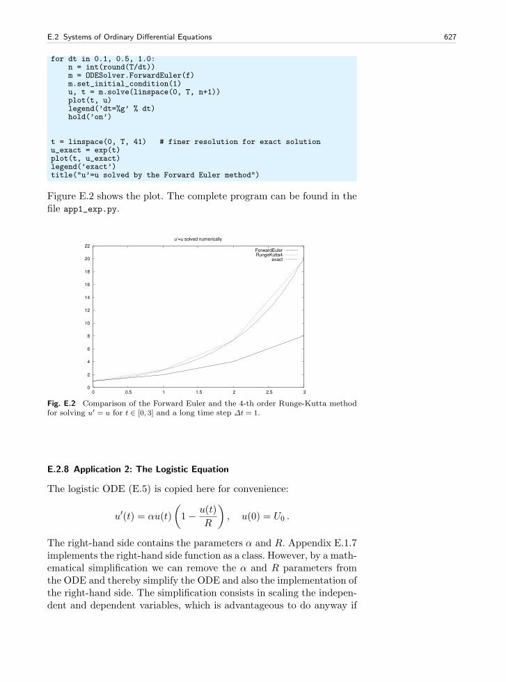
E.2 Systems of Ordinary Differential Equations 627

for dt in 0.1, 0.5, 1.0:n = int(round(T/dt))m = ODESolver.ForwardEuler(f)m.set_initial_condition(1)u, t = m.solve(linspace(0, T, n+1))plot(t, u)legend(’dt=%g’ % dt)hold(’on’)

t = linspace(0, T, 41) # finer resolution for exact solutionu_exact = exp(t)plot(t, u_exact)legend(’exact’)title("u’=u solved by the Forward Euler method")

Figure E.2 shows the plot. The complete program can be found in thefile app1_exp.py.

0

2

4

6

8

10

12

14

16

18

20

22

0 0.5 1 1.5 2 2.5 3

u’=u solved numerically

ForwardEulerRungeKutta4

exact

Fig. E.2 Comparison of the Forward Euler and the 4-th order Runge-Kutta methodfor solving u′ = u for t ∈ [0, 3] and a long time step ∆t = 1.

E.2.8 Application 2: The Logistic Equation

The logistic ODE (E.5) is copied here for convenience:

u′(t) = αu(t)

(

1− u(t)

R

)

, u(0) = U0 .

The right-hand side contains the parameters α and R. Appendix E.1.7implements the right-hand side function as a class. However, by a math-ematical simplification we can remove the α and R parameters fromthe ODE and thereby simplify the ODE and also the implementation ofthe right-hand side. The simplification consists in scaling the indepen-dent and dependent variables, which is advantageous to do anyway if

628 E Programming of Differential Equations

the goal is to understand more of the model equation and its solution.The scaling implies introducing new variables

v =u

R, τ = αt .

Inserting u = Rv and t = τ/α in the equation gives

dv

dτ= v(1− v), v(0) =

U0

R.

Assume that we start with a small population, say U0/R = 0.05. Amaz-ingly, there are no parameters in the equation for v(τ). That is, we cansolve for v once and for all, and then recover u(t) for any R and α by

u(t) = Rv(αt) .

Geometrically, the transformation from v to u is just a stretching ofthe two axis in the coordinate system.

We can compute v(τ) by the 4-th order Runge-Kutta method in aprogram:

v0 = 0.05dtau = 0.05T = 10n = int(round(T/dtau))t_points = linspace(0, T, n+1)method = ODESolver.RungeKutta4(lambda v, tau: v*(1-v))method.set_initial_condition(v0)v, tau = method.solve(t_points)

Observe that we use a lambda function (Chapter 3.1.11) to save sometyping of a separate function for the right-hand side of the ODE. Nowwe need to run the program only once to compute v(t), and from thissolution we can easily create the solution u(t), represented in terms ofu and t arrays, by

t = alpha*tauu = R*v

Below we make a plot to show how the u(t) curve varies with α:

from scitools.std import *import ODESolver

v0 = 0.05dtau = 0.05T = 10n = int(round(T/dtau))t_points = linspace(0, T, n+1)method = ODESolver.RungeKutta4(lambda v, tau: v*(1-v))method.set_initial_condition(v0)v, tau = method.solve(t_points)plot(tau, v, title=’Scaled logistic equation’,

hardcopy=’tmp_logistic.eps’)

def u_and_t(v, tau, alpha, R):

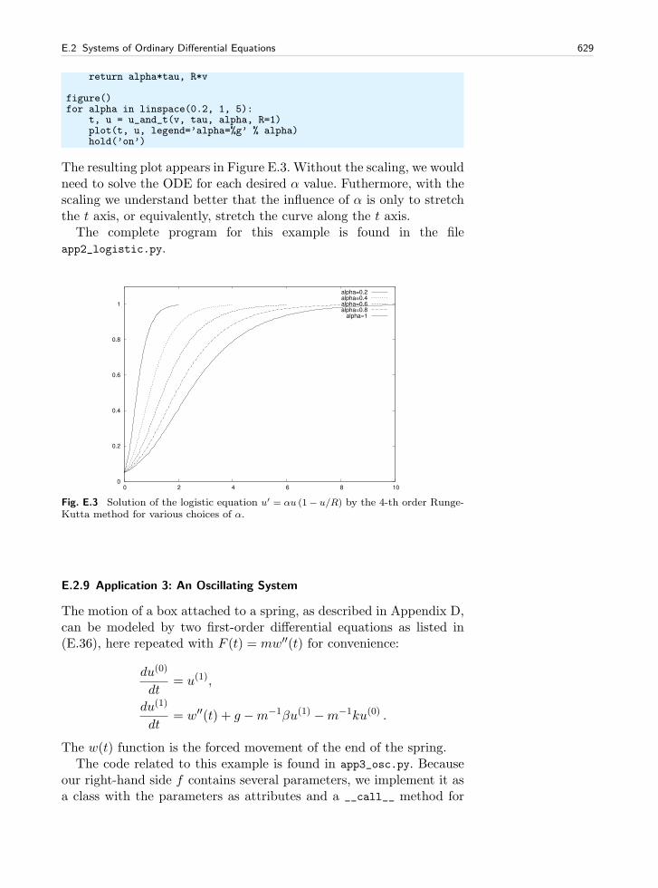
E.2 Systems of Ordinary Differential Equations 629

return alpha*tau, R*v

figure()for alpha in linspace(0.2, 1, 5):

t, u = u_and_t(v, tau, alpha, R=1)plot(t, u, legend=’alpha=%g’ % alpha)hold(’on’)

The resulting plot appears in Figure E.3. Without the scaling, we wouldneed to solve the ODE for each desired α value. Futhermore, with thescaling we understand better that the influence of α is only to stretchthe t axis, or equivalently, stretch the curve along the t axis.

The complete program for this example is found in the fileapp2_logistic.py.

0

0.2

0.4

0.6

0.8

1

0 2 4 6 8 10

alpha=0.2alpha=0.4alpha=0.6alpha=0.8

alpha=1

Fig. E.3 Solution of the logistic equation u′ = αu (1− u/R) by the 4-th order Runge-Kutta method for various choices of α.

E.2.9 Application 3: An Oscillating System

The motion of a box attached to a spring, as described in Appendix D,can be modeled by two first-order differential equations as listed in(E.36), here repeated with F (t) = mw′′(t) for convenience:

du(0)

dt= u(1),

du(1)

dt= w′′(t) + g −m−1βu(1) −m−1ku(0) .

The w(t) function is the forced movement of the end of the spring.The code related to this example is found in app3_osc.py. Because

our right-hand side f contains several parameters, we implement it asa class with the parameters as attributes and a __call__ method for

630 E Programming of Differential Equations

returning the 2-vector f . We assume that the user of the class suppliesthe w(t) function, so it is natural to compute w′′(t) by a finite differenceformula.

class OscSystem:def __init__(self, m, beta, k, g, w):

self.m, self.beta, self.k, self.g, self.w = \float(m), float(beta), float(k), float(g), w

def __call__(self, u, t):u0, u1 = um, beta, k, g, w = \

self.m, self.beta, self.k, self.g, self.w# Use a finite difference for w’’(t)h = 1E-5ddw = (w(t+h) - 2*w(t) + w(t-h))/(h**2)f = [u1, ddw + g - beta/m*u1 - k/m*u0]return f

A simple test case arises if we set m = k = 1 and β = g = w = 0:

du(0)

dt= u(1),

du(1)

dt= −u(0) .

Suppose that u(0)(0) = 1 and u(1)(0) = 0. An exact solution is then

u(0)(t) = cos t, u(1)(t) = − sin t .

We can use this case to check how the Forward Euler method compareswith the 4-th order Runge-Kutta method:

import ODESolverfrom scitools.std import *f = OscSystem(1.0, 0.0, 1.0, 0.0, lambda t: 0)u_init = [1, 0] # initial conditionnperiods = 3.5 # no of oscillation periodsT = 2*pi*nperiodsfor method_class in ODESolver.ForwardEuler, ODESolver.RungeKutta4:

if method_class == ODESolver.ForwardEuler:npoints_per_period = 200

elif method_class == ODESolver.RungeKutta4:npoints_per_period = 20

n = npoints_per_period*nperiodst_points = linspace(0, T, n+1)method = method_class(f)method.set_initial_condition(u_init)u, t = method.solve(t_points)

# u is an array of [u0,u1] pairs for each time level,# get the u0 values from u for plottingu0_values = u[:, 0]u1_values = u[:, 1]u0_exact = cos(t)u1_exact = -sin(t)figure()alg = method_class.__name__ # (class) name of algorithmplot(t, u0_values, ’r-’,

t, u0_exact, ’b-’,legend=(’numerical’, ’exact’),

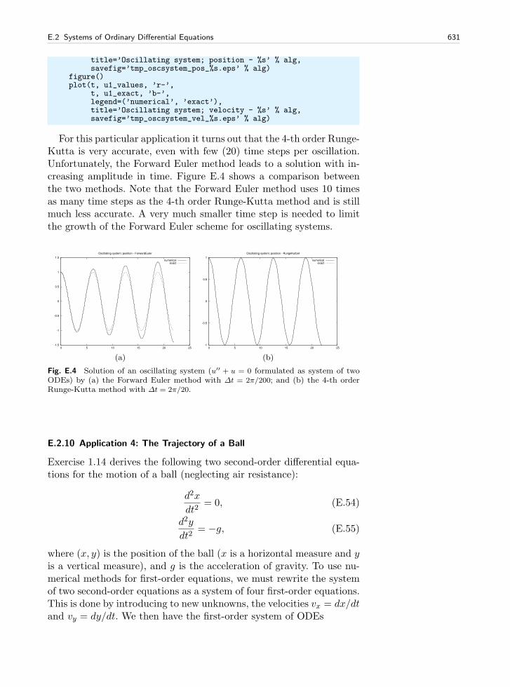
E.2 Systems of Ordinary Differential Equations 631

title=’Oscillating system; position - %s’ % alg,savefig=’tmp_oscsystem_pos_%s.eps’ % alg)

figure()plot(t, u1_values, ’r-’,

t, u1_exact, ’b-’,legend=(’numerical’, ’exact’),title=’Oscillating system; velocity - %s’ % alg,savefig=’tmp_oscsystem_vel_%s.eps’ % alg)

For this particular application it turns out that the 4-th order Runge-Kutta is very accurate, even with few (20) time steps per oscillation.Unfortunately, the Forward Euler method leads to a solution with in-creasing amplitude in time. Figure E.4 shows a comparison betweenthe two methods. Note that the Forward Euler method uses 10 timesas many time steps as the 4-th order Runge-Kutta method and is stillmuch less accurate. A very much smaller time step is needed to limitthe growth of the Forward Euler scheme for oscillating systems.

-1.5

-1

-0.5

0

0.5

1

1.5

0 5 10 15 20 25

Oscillating system; position - ForwardEuler

numericalexact

(a)

-1

-0.5

0

0.5

1

0 5 10 15 20 25

Oscillating system; position - RungeKutta4

numericalexact

(b)

Fig. E.4 Solution of an oscillating system (u′′ + u = 0 formulated as system of twoODEs) by (a) the Forward Euler method with ∆t = 2π/200; and (b) the 4-th orderRunge-Kutta method with ∆t = 2π/20.

E.2.10 Application 4: The Trajectory of a Ball

Exercise 1.14 derives the following two second-order differential equa-tions for the motion of a ball (neglecting air resistance):

d2x

dt2= 0, (E.54)

d2y

dt2= −g, (E.55)

where (x, y) is the position of the ball (x is a horizontal measure and yis a vertical measure), and g is the acceleration of gravity. To use nu-merical methods for first-order equations, we must rewrite the systemof two second-order equations as a system of four first-order equations.This is done by introducing to new unknowns, the velocities vx = dx/dtand vy = dy/dt. We then have the first-order system of ODEs

632 E Programming of Differential Equations

dx

dt= vx, (E.56)

dvxdt

= 0, (E.57)

dy

dt= vy, (E.58)

dvydt

= −g . (E.59)

The initial conditions are

x(0) = 0, (E.60)

vx(0) = v0 cos θ, (E.61)

y(0) = y0, (E.62)

vy(0) = v0 sin θ, (E.63)

where v0 is the initial magnitude of the velocity of the ball. The initialvelocity has a direction that makes the angle θ with the horizontal.

The code related to this example is found in app4_ball.py. A func-tion returning the right-hand side of our ODE system reads

def f(u, t):x, vx, y, vy = ug = 9.81return [vx, 0, vy, -g]

It makes sense to solve the ODE system as long as the ball as above theground, i.e., as long as y ≥ 0. We must therefore supply a terminate

function as explained on page 622:

def terminate(u, t, step_no):return False if u[step_no,2] >= 0 else True

Observe that all the y values are given by u[:,2] and we want to testthe value at the current step, which becomes u[step_no,2].

The main program for solving the ODEs can be set up as

v0 = 5theta = 80*pi/180U0 = [0, v0*cos(theta), 0, v0*sin(theta)]T = 1.2; dt = 0.01; n = int(round(T/dt))method = ODESolver.ForwardEuler(f)method.set_initial_condition(U0)

def terminate(u, t, step_no):return False if u[step_no,2] >= 0 else True

u, t = method.solve(linspace(0, T, n+1), terminate)

Now, u[:,0] represents all the x(t) values, u[:,1] all the vx(t) values,u[:,2] all the y(t) values, and u[:,3] all the vy(t) values. However,recall that we have stopped the simulation at some time level wheny < 0. From the code in the solve method in class ODESolver we see

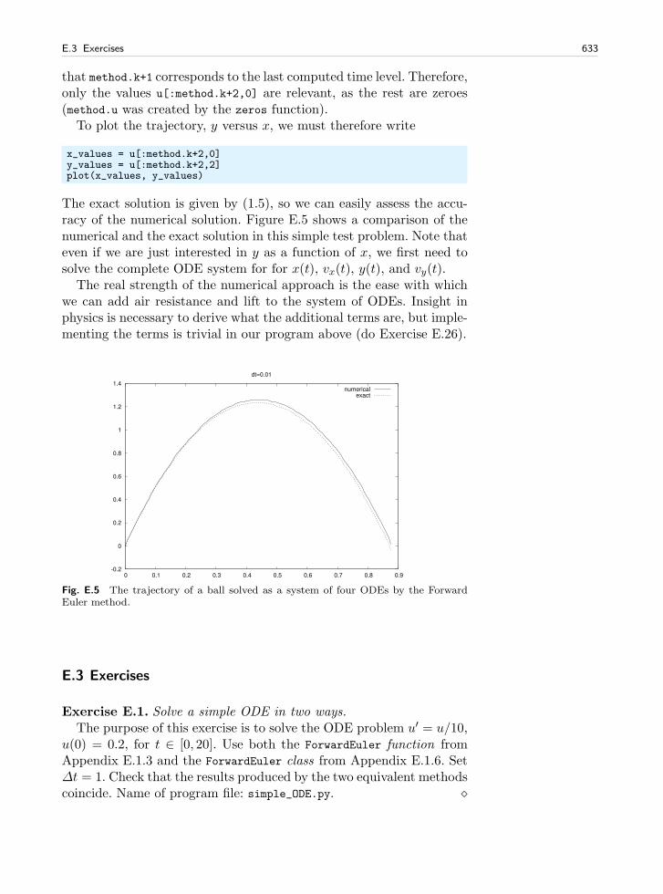
E.3 Exercises 633

that method.k+1 corresponds to the last computed time level. Therefore,only the values u[:method.k+2,0] are relevant, as the rest are zeroes(method.u was created by the zeros function).

To plot the trajectory, y versus x, we must therefore write

x_values = u[:method.k+2,0]y_values = u[:method.k+2,2]plot(x_values, y_values)

The exact solution is given by (1.5), so we can easily assess the accu-racy of the numerical solution. Figure E.5 shows a comparison of thenumerical and the exact solution in this simple test problem. Note thateven if we are just interested in y as a function of x, we first need tosolve the complete ODE system for for x(t), vx(t), y(t), and vy(t).

The real strength of the numerical approach is the ease with whichwe can add air resistance and lift to the system of ODEs. Insight inphysics is necessary to derive what the additional terms are, but imple-menting the terms is trivial in our program above (do Exercise E.26).

-0.2

0

0.2

0.4

0.6

0.8

1

1.2

1.4

0 0.1 0.2 0.3 0.4 0.5 0.6 0.7 0.8 0.9

dt=0.01

numericalexact

Fig. E.5 The trajectory of a ball solved as a system of four ODEs by the ForwardEuler method.

E.3 Exercises

Exercise E.1. Solve a simple ODE in two ways.The purpose of this exercise is to solve the ODE problem u′ = u/10,

u(0) = 0.2, for t ∈ [0, 20]. Use both the ForwardEuler function fromAppendix E.1.3 and the ForwardEuler class from Appendix E.1.6. Set∆t = 1. Check that the results produced by the two equivalent methodscoincide. Name of program file: simple_ODE.py. ⋄

634 E Programming of Differential Equations

Exercise E.2. Use the ODESolver hierarchy to solve a simple ODE.Solve the ODE problem u′ = u/2 with u(0) = 1, using a class in

the ODESolver hierarchy. Choose ∆t = 0.5 and find u(t) for t ∈ [0, 6].Write out the approximate final un value together with the exact valuee3. Repeat the calculations for ∆t = 0.001. Name of program file:ODESolver_demo.py. ⋄

Exercise E.3. Solve an ODE for emptying a tank.A cylindrical tank of radius R is filled with water to a height h0. By

opening a valve of radius r at the bottom of the tank, water flows out,and the height of water, h(t), decreases with time. We can derive anODE that governs the height function h(t).

Mass conservation of water requires that the reduction in heightbalances the outflow. In a time interval ∆t, the height is reduced by∆h, which corresponds to a water volume of πR2∆h. The water leavingthe tank in the same interval of time equals πr2v∆t, where v is theoutflow velocity. It can be shown (from what is known as Bernoulli’sequation) that

v(t) =√

2gh(t)− h′(t)2,

g being the acceleration of gravity [6, 11]. Letting ∆h > 0 correspondto an increase in h, we have that the −πR2∆h must balance πr2v∆t,which in the limit ∆t→ 0 leads to the ODE

dh

dt= −

( r

R

)2(

1 +( r

R

)4)−1/2

√

2gh . (E.64)

A proper initial condition follows from the initial height of water, h0,in the tank: h(0) = h0.

Solve (E.64) by a numerical method of your choice in a program.Set r = 1 cm, R = 20 cm, g = 9.81 m/s2, and h0 = 1 m. Use a timestep of 10 seconds. Plot the solution, and experiment to see what aproper time interval for the simulation is. Can you find an analyticalsolution of the problem to compare the numerical solution with? Nameof program file: tank_ODE.py. ⋄

Exercise E.4. Logistic growth with time-varying carrying capacity.We shall study population growth according to a logistic model

(E.5). The carrying capacity of the environment, R, now changes withtime:

R(t) =

Rmax, tswitch < t < 2tswitch,Rmin, otherwise

(E.65)

Solve (E.5) with this R(t) and plot the solution. Use these parameters:α = 0.3, Rmin = 10, Rmin = 50, and tswitch = 20. Simulate for t ∈[0, 60]. Explain the shape of the curve from knowledge of the modelbehind the ODE and the special choice of R(t) in the present case.Name of program file: time_varying_logistic_growth.py. ⋄

E.3 Exercises 635

Exercise E.5. Simulate a falling or rising body in a fluid.A body moving vertically through a fluid (liquid or gas) is subject

to three different types of forces:

1. the gravity force Fg = −mg, where m is the mass of the body andg is the acceleration of gravity;

2. the drag force2 Fd = −12CDA|v|v (see also Exercise 1.11), where

CD is a dimensionless drag coefficient depending on the body’sshape, is the density of the fluid, A is the cross-sectional area(produced by a cutting plane y = const through the thickest partof the body), and v is the velocity;

3. the uplift or buoyancy force (“Archimedes force”) Fb = gV , whereV is the volume of the body.

Newton’s second law applied to the body says that the sum of theseforces must equal the mass of the body times its acceleration a:

Fg + Fd + Fb = ma,

which gives

−mg − 1

2CDA|v|v + gV = ma .

The unknowns here are v and a, i.e., we have two unknowns but onlyone equation. From kinetmatics in physics we know that the accel-eration is the time derivative of the velocity: a = dv/dt. This is oursecond equation. We can easily eliminate a and get a single differentialequation for v:

−mg − 1

2CDA|v|v + gV = m

dv

dt.

A small rewrite of this equation is handy: We express m as bV , whereb is the density of the body, and we isolate dv/dt on the left-handside,

dv

dt= −g

(

1−

b

)

− 1

2CD

A

bV|v|v . (E.66)

This differential equation must be accompanied by an initial condition:v(0) = V0.

Make a program for solving (E.66) numerically, using any numericalmethod of your choice. Implement the right-hand side of (E.66) in the__call__ method of a class where the parameters g, , b, CD, A, andV are attributes.

To verify the program, assume a heavy body in air such that the Fb

force can be neglected, and assume a small velocity such that the airresistance Fd can also be neglected. Setting = 0 removes both these

2 Roughly speaking, the Fd formula is suitable for medium to high velocities, whilefor very small velocities, or very small bodies, Fd is proportional to the velocity,not the velocity squared, see [11].

636 E Programming of Differential Equations

terms from the equation. The motion then leads to the exact velocityv(t) = y′(t) = v0−gt. See how well the program reproduces this simplesolution.

After the program is verified, we are ready to run two real examplesand plot the evolution of v:

1. Parachute jumper. The point is to compute the motion of aparachute jumper in free fall before the parachute opens. We setthe density of the human body as b = 1003 kg/m3 and the massas m = 80 kg, implying V = m/b = 0.08 m3. We can base thecross-sectional area A on the height 1.8 m and a width of 50 cm,giving giving A ≈ πR2 = 0.9 m2. The density of air decreases withheight, and we here use the value 0.79 kg/m3 which is relevant forabout 5000 m height. The CD coefficient can be set as 0.6. Startwith v0 = 0.

2. Rising ball in water. A ball with the size of a soccer ball is placedin deep water, and we seek to model its motion upwards. Contraryto the former example, where the buoyancy force Fb is very small,Fb is now the driving force, and the gravity force Fg is small. SetA = πa2 with a = 11 cm, the mass of the ball is 0.43 kg, the densityof water is 1000 kg/m3, and CD is 0.2. Start with v0 = 0 and seehow the ball rises.

Name of program file: body_in_fluid.py. ⋄

Exercise E.6. Check the solution’s limit in Exer. E.5.The solution of (E.66) often tends to a constant velocity, called the

terminal velocity. This happens when the sum of the forces, i.e., theright-hand side in (E.66) vanishes. Compute the formula for the ter-minal velocity by hand. Solve the ODE using class ODESolver andcall the solve method with a terminate function that terminatesthe computations when a constant velocity is reached, that is, when|v(tn) − v(tn−1)| ≤ ǫ, where ǫ is a small number. Run a series of∆t values and make a graph of the terminal velocity as a functionof ∆t for the two cases in Exercise E.5. Indicate the exact termi-nal velocity in the plot by a horizontal line. Name of program file:body_in_fluid_termvel.py. ⋄

Exercise E.7. Visualize the different forces in Exer. E.5.The purpose of this exercise is to plot the forces Fg, Fb, and Fd in the

model from Exercise E.5 as functions of t. Seeing the relative impor-tance of the forces as time develops gives an increased understandingof how the different forces contribute to change the velocity. Name ofprogram file: body_in_fluid_forces.py. ⋄

Exercise E.8. Solve an ODE until constant solution.Newton’s law of cooling,

E.3 Exercises 637

dT

dt= −h(T − Ts) (E.67)

can be used to see how the temperature T of an object changes be-cause of heat exchange with the surroundings, which have a tempera-ture Ts. The parameter h, with unit s−1 is an experimental constant(heat transfer coefficient) telling how efficient the heat exchange withthe surroundings is. For example, (E.67) may model the cooling of ahot pizza taken out of the oven. The problem with applying (E.67),nevertheless, is that h must be measured. Suppose we have measuredT at t = 0 and t1. We can use a rough Forward Euler approximationof (E.67) with one time step of length t1,

T (t1)− T (0)

t1= −h(T (0)− Ts),

to make the estimate

h =T (t1)− T (0)

t1(Ts − T (0)). (E.68)

Suppose now you take a hot pizza out of the oven. The temperatureof the pizza is 200 C at t = 0 and 180 C after 20 seconds, in a roomwith temperature 20 C. Find an estimate of h from the formula above.

Solve (E.67) to find the evolution of the temperature of the pizza.Use class ForwardEuler or RungeKutta4, and supply a terminate func-tion to the solve method so that the simulation stops when T is suffi-ciently close to the final room temperature Ts. Plot the solution. Nameof program file: pizza_cooling1.py. ⋄Exercise E.9. Use classes in Exer. E.8.

Solve Exercise E.8 with a class Problem containing the parameters h,Ts, T (0), t1, and T (t1) as attributes. The class should have a methodestimate_h for returning an estimate of h, given the other parameters.Also a method __call__ for computing the right-hand side must be in-cluded. The terminate function can be a method in the class as well. Byusing class Problem, we avoid having the physical parameters as globalvariables in the program. Name of program file: pizza_cooling2.py. ⋄Exercise E.10. Scale away parameters in Exer. E.8.

Use the scaling approach from Appendix E.2.8 to “scale away” theparameters in the ODE in Exercise E.8. That is, introduce a new un-known u = (T −Ts)/(T (0)−Ts) and a new time scale τ = th. Find theODE and the initial condition that governs the u(τ) function. Makea program that computes u(τ ) until |u| < 0.001. Store the discreteu and τ values in a file u_tau.dat if that file is not already present(you can use os.path.isfile(f) to test if a file with name f exists).Create a function T(u, tau, h, T0, Ts) that loads the u and τ datafrom the u_tau.dat file and returns two arrays with T and t values,

638 E Programming of Differential Equations

corresponding to the computed arrays for u and τ . Plot T versus t.Give the parameters h, Ts, and T (0) on the command line. Note thatthis program is supposed to solve the ODE once and then recover anyT (t) solution by a simple scaling of the single u(τ) solution. Name ofprogram file: pizza_cooling3.py. ⋄

Exercise E.11. Use the 4th-order Runge-Kutta on (C.32).Investigate if the 4th-order Runge-Kutta method is better than the

Forward Euler scheme for solving the challenging ODE problem (C.32)from Exercise C.3 on page 575. Name of program file: yx_ODE2.py. ⋄

Exercise E.12. Compare ODE methods.The equation u′ = −au is a relevant model for radioactive decay,

where u(t) is the fraction of particles that remains in the radioactivesubstance at time t. The parameter a is the inverse of the so-calledmean lifetime of the substance. The initial condition is u(0) = 1.

Introdce a class Decay to hold information about the physical prob-lem: the parameter a, the initial condition, and a __call__ method forcomputing the right-hand side −au of the ODE. Initialize an instanceof class Decay with a = ln(2)/5600 1/years (this value of a correspondsto the Carbon-14 radioactive isotope whose decay is used extensivelyin dating organic material that is tens of thousands of years old).

Solve (E.7) by both the Forward Euler and the 4-th order Runge-Kutta method, using the ForwardEuler and the RungeKutta4 classes inthe ODESolver hierarchy. Use a time step of 500 years, and simulatedecay for T = 20, 000 years (let the time unit be 1 year). Plot the twosolutions. Write out the final u(T ) value and compare it with the exactvalue e−aT . Name of program file: radioactive_decay.py. ⋄

Exercise E.13. Compare ODE methods.Consider the problem described in Exercise E.3 on page 634.

Solve this ODE problem using the ForwardEuler, BackwardEuler, andRungeKutta4 classes in the ODESolver hierarchy. Read ∆t from the com-mand line and try out values between 5 and 50 s. Compare the nu-merical solutions in a plot. Comment upon the quality of the variousmethods to compute a correct limiting value of h as ∆t is varied. (Hint:negative h values may appear when the problem is solved numerically,so set h = 0 if h < 0 before computing

√h.) Name of program file:

tank_ODE_3methods.py. ⋄

Exercise E.14. Solve two coupled ODEs for radioactive decay.Consider two radioactive substances A and B. The nuclei in sub-

stance A decay to form nuclei of type B with a mean lifetime τA, whilesubstance B decay to form type A nuclei with a mean lifetime τB . Let-ting uA and uB be the fractions of the initial amount of material insubstance A and B, respectively, the following system of ODEs governsthe evolution of uA(t) and uB(t):

E.3 Exercises 639

u′A = uB/τB − uA/τA, (E.69)

u′B = uA/τA − uB/τB , (E.70)

with uA(0) = uB(0) = 1. As in Exercise E.12, introduce a problemclass, which holds the parameters τA and τB and offers a __call__

method to compute the right-hand side vector of the ODE system,i.e., (uB/τB − uA/τA, uA/τA − uB/τB). Solve for uA and uB using asubclass in the ODESolver hierarchy and the parameter choice τA = 8minutes, τB = 40 minutes, and ∆t = 10 seconds. Plot uA and uBagainst time measured in minutes. From the ODE system it followsthat the ratio uA/uB → τA/τB as t → ∞ (asssuming u′A = u′B = 0in the limit t→∞). Check that the solutions fulfills this requirement(this is a partial verification of the program). Name of program file:radioactive_decay2.py. ⋄

Exercise E.15. Code a 2nd-order Runge-Kutta method; function.Implement the 2nd-order Runge-Kutta method specified in formula

(E.41). Use a plain function RungeKutta2 of the type shown in Ap-pendix E.1.2 for the Forward Euler method. Construct a test problemwhere you know the analytical solution, and plot the difference be-tween the numerical and analytical solution. Name of program file:RungeKutta2_func.py. ⋄

Exercise E.16. Code a 2nd-order Runge-Kutta method; class.Make a new subclass RungeKutta2 in the ODESolver hierarchy from

Appendix E.2.5 for solving ordinary differential equations with the2nd-order Runge-Kutta method specified in formula (E.41). Constructa test problem where you know the analytical solution, and plot thedifference between the numerical and analytical solution. Store theRungeKutta2 class and the test problem in a separate file where thebase class ODESolver is imported from the ODESolver module. Name ofprogram file: RungeKutta2.py. ⋄

Exercise E.17. Make an ODESolver subclass for Heun’s method.Implement the numerical method (E.39)–(E.40) in a subclass of

ODESolver. Place the code in a separate file where the ODESolver classis imported. How can you verify that the implementation is correct?Name of program file: Heun.py. ⋄

Exercise E.18. Make an ODESolver subclass for the Midpointmethod.

Implement the Midpoint method specified in formula (E.38) frompage 619 in a subclass of ODESolver.

Compare in a plot the Midpoint method with the Forward Eulerand 4th-order Runge-Kutta methods and the exact solution for theproblem u′ = u, u(0) = 1, with 10 steps between 0 and the end timeT = 5. Name of program file: Midpoint.py. ⋄

640 E Programming of Differential Equations

Exercise E.19. Make an ODESolver subclass for an Adams-Bashforthmethod.

Implement the Adams-Bashforth method (E.49) on page 620 in asubclass of ODESolver. Use Heun’s method (E.40) to compute u1.

Compare in a plot the Adams-Bashforth method with the ForwardEuler and 4th-order Runge-Kutta methods and the exact solution forthe problem u′ = u, u(0) = 1, with 10 steps between 0 and the endtime T = 5. Name of program file: AdamsBashforth3.py. ⋄

Exercise E.20. Implement the iterated Midpoint method; function.Implement the numerical method (E.50)–(E.51) as a function

iterated_Midpoint_method(f, U0, T, n, N)

where f is a Python implementation of f(u, t), U0 is the initial condi-tion u(0) = U0, T is the final time of the simulation, n is the numberof time steps, and N is the parameter N in the method (E.50). Theiterated_Midpoint_method should return two arrays: u0, . . . , un andt0, . . . , tn. To verify the implementation, calculate by hand u1 and u2when N = 2 for the ODE u′ = −2u, u(0) = 1, with ∆t = 1/2. Compareyour hand calculations with the results of the program. Thereafter, runthe program for the same ODE problem but with ∆t = 0.1 and T = 2.Name of program file: MidpointIter_func.py. ⋄

Exercise E.21. Implement the iterated Midpoint method; class.The purpose of this exercise is to implement the numerical

method (E.50)–(E.51) in a class like the ForwardEuler class fromAppendix E.1.6. Create a module containing the class and a testfunction demonstrating the use:

def _test():def f(u, t):

return -2*u

method = MidpointIter(f, N=4)method.set_initial_condition(1)t_points = numpy.linspace(0, 1.5, 16)u, t = method.solve(t_points)from scitools.std import plotplot(t, u)

Call the _test function from the test block in the module file. Nameof program file: MidpointIter_class.py. ⋄

Exercise E.22. Make an ODESolver subclass for the iterated Midpointmethod.

Implement the numerical method (E.50)–(E.51) in a subclass ofODESolver. The code should reside in a separate file where the ODESolverclass is imported. One can either fix N or introduce an ǫ and iterateuntil the change in |vq − vq−1| is less than ǫ. Allow the constructor totake both N and ǫ as arguments. Compute a new vq as long as q ≤ N

E.3 Exercises 641

or |vq − vq−1| > ǫ. Let N = 20 and ǫ = 10−6 by default. Name ofprogram file: MidpointIter.py. ⋄

Exercise E.23. Study convergence of numerical methods for ODEs.The approximation error when solving an ODE numerically is usu-

ally of the form C∆tr, where C and r are constants that can be es-timated from numerical experiements. The constant r, called the con-vergence rate, is of particular interest. Halving ∆t halves the error ifr = 1, but if r = 3, halving ∆t reduces the error by a factor of 8.

Exercise 9.16 describes a method for estimating r from two conse-qutive experiments. Make a function

ODE_convergence(f, U0, u_e, method, dt=[])

that returns a series of estimated r values corresponding to a seriesof ∆t values given as the dt list. The argument f is a Python imple-mentation of f(u, t) in the ODE u′ = f(u, t). The initial condition isu(0) = U0, where U0 is given as the U0 argument, u_e is the exactsolution ue(t) of the ODE, and method is the name of a class in theODESolver hierarchy. The error between the exact solution ue and thecomputed solution u0, u1, . . . , un can be defined as

e =

(

∆t

n∑

i=0

(ue(ti)− ui)2

)1/2

.

Call the ODE_convergence function for some methods you have in theODESolver hierarchy and answers to exercises, and print the estimatedr values for each method. Use an ODE problem of your own choice.Name of program file: ODE_convergence.py. ⋄

Exercise E.24. Solve an ODE specified on the command line.To solve an ODE, we want to make a program cmlodesolver.py

which accepts an ODE problem to be specified on the command line.The command-line arguments are f u0 dt T, where f is the right-hand side f(u, t) specified as a string formula (to be converted to aStringFunction object), u0 is the initial condition, dt is the time step,and T is the final time of the simulation. A fifth optional argument canbe given to specify the class name of the numerical solution method(set any method of choice as default value). A curve plot of the solutionversus time should be produced and stored in a file plot.png. Name ofprogram file: cmlodesolver.py. ⋄

Exercise E.25. Find the body’s position in Exer. E.5.In Exercise E.5 we compute the velocity v(t). The position of the

body, y(t), is related to the velocity by y′(t) = v(t). Extend the programfrom Exercise E.5 to solve the system

642 E Programming of Differential Equations

dy

dt= v,

dv

dt= −g

(

1−

b

)

−−1

2CD

A

bV|v|v .

Name of program file: body_in_fluid2.py. ⋄

Exercise E.26. Add the effect of air resistance on a ball.The differential equations governing the horizontal and vertical mo-

tion of a ball subject to gravity and air resistance read3

d2x

dt2= −3

8CD ¯a−1

√

(

dx

dt

)2

+

(

dy

dt

)2dx

dt, (E.71)

d2y

dt2= −g − 3

8CD ¯a−1

√

(

dx

dt

)2

+

(

dy

dt

)2dy

dt, (E.72)

where (x, y) is the position of the ball (x is a horizontal measure andy is a vertical measure), g is the acceleration of gravity, CD = 0.2 isa drag coefficient, ¯ is the ratio of the density of air and the ball, anda is the radius of the ball. The latter two quantities can be taken as0.017 and 11 cm for a football.

Let the initial condition be x = y = 0 (start position in origo) and

dx/dt = v0 cos θ, dy/dt = v0 sin θ,

where v0 is the magnitude of the initial velocity and θ is the angle thevelocity makes with the horizontal. For a hard football kick we can setv0 = 120 km/h and take θ as 30 degrees.

Express the two second-order equations above as a system of fourfirst-order equations with four initial conditions. Implement the right-hand side in a problem class where the physical parameters CD, ¯, a,v0, and θ are stored along with the initial conditions.

Solve the ODE system for CD = 0 (no air resistance) and CD = 0.2,and plot y as a function of x in both cases to illustrate the effect ofair resistance. Use the 4-th order Runge-Kutta method. Make sureyou express all units in kg, m, s, and radians. Name of program file:kick2D.py. ⋄

Exercise E.27. Solve an ODE system for an electric circuit.An electric circuit with a resistor, a capacitor, an inductor, and a

voltage source can be described by the ODE

LdI

dt+RI +

Q

C= E(t), (E.73)

3 The equations arise by combining the models in Exercises 1.11 and 1.14.

E.3 Exercises 643

where LdI/dt is the voltage drop across the inductor, I is the current(measured in amperes, A), L is the inductance (measured in henrys,H), R is the resistance (measured in ohms, Ω), Q is the charge on thecapacitor (measured in coulombs, C), C is the capacitance (measuredin farads, F), E(t) is the time-variable voltage source (measured involts, V), and t is time (measured in seconds, s). There is a relationbetwen I and Q:

dQ

dt= I . (E.74)

Equations (E.73)–(E.74) is a system two ODEs. Solve these for L = 1H, E(t) = 2 sinωt V, ω2 = 3.5 s−2, C = 0.25 C, R = 0.2 Ω, I(0) = 1 A,and Q(0) = 1C. Use the Forward Euler scheme with ∆t = 2π/(60ω).The solution will, after some time, oscillate with the same period asE(t), a period of 2π/ω. Simulate 10 periods. (Actually, it turns outthat the Forward Euler scheme overestimates the amplitudes of theoscillations. Exercise E.28 compares the Forward Euler scheme withthe more accurate 4th-order Runge-Kutta method.) Name of programfile: electric_circuit.py. ⋄

Exercise E.28. Compare methods for solving (E.73)–(E.74).Consider the system of ODEs in Exercise E.27 for simulating an elec-

tric circuit. The purpose now is to compare the Forward Euler schemewith the 4-th order Runge-Kutta method. Make a class Circuit forstoring the physical parameters of the problem (L, R, C, E(t)) as wellas the initial conditions (I(0), Q(0)). Class Circuit should also definethe right-hand side of the ODE through a __call__ method. Createtwo solver instances, one from the ForwardEuler class and one from theRungeKutta4 class. Solve the ODE system using both methods. Plot thetwo I(t) solutions for comparison. As you will see, the Forward Eulerscheme overestimates the amplitudes significantly, compared with themore accurate 4th-order Runge-Kutta method. Name of program file:electric_circuit2.py. ⋄

Exercise E.29. Explore predator-prey population interactions.Suppose we have two species in an environment: a predator and a

prey. How will the two populations interact and change with time?A system of ordinary differential equations can give insight into thisquestion. Let x(t) and y(t) be the size of the prey and and the predatorpopulations, respectively. In the absence of a predator, the populationof the prey will follow the ODE derived in Appendix C.2:

dx

dt= rx,

with r > 0, assuming there are enough resources for exponentialgrowth. Similarly, in the absence of prey, the predator population willjust experience a death rate m > 0:

644 E Programming of Differential Equations

dy

dt= −my .

In the presence of the predator, the prey population will experience areduction in the growth proportional to xy. The number of interactions(meetings) between x and y numbers of animals is xy, and in a certainfraction of these interactions the predator eats the prey. The predatorpopulation will correspondingly experience a growth in the populationbecause of the xy interactions with the prey population. The adjustedgrowth of both populations can now be expressed as

dx

dt= rx− axy, (E.75)

dy

dt= −my + bxy, (E.76)

(E.77)

for positive constants r, m, a, and b. Solve this system and plot x(t)and y(t) for r = m = 1, a = 0.3, b = 0.2, x(0) = 1, and y(0) = 1,t ∈ [0, 20]. Try to explain the dynamics of the population growth youobserve. Experiment with other values of a and b. Name of programfile: predator_prey.py. ⋄

Exercise E.30. Formulate a 2nd-order ODE as a system.In this and subsequent exercises we shall deal with the following

second-order ordinary differential equation with two initial conditions:

mu+ f(u) + s(u) = F (t), t > 0, u(0) = U0, u(0) = V0 . (E.78)

The notation u and u means u′(t) and u′′(t), respectively. Write (E.78)as a system of two first-order differential equations. Also set up theinitial condition for this system.

Physical Applications. Equation (E.78) has a wide range of applicationsthroughout science and engineering. A primary application is dampedspring systems in, e.g., cars and bicycles: u is the vertical displacementof the spring system attached to a wheel; u is then the correspondingvelocity; F (t) resembles a bumpy road; s(u) represents the force fromthe spring; and f(u) models the damping force (friction) in the springsystem. For this particular application f and s will normally be linearfunctions of their arguments: f(u) = βu and s(u) = ku, where k is aspring constant and β some parameter describing viscous damping.

Equation (E.78) can also be used to describe the motions of amoored ship or oil platform in waves: the moorings act as a nonlin-ear spring s(u); F (t) represents environmental excitation from waves,wind, and current; f(u) models damping of the motion; and u is theone-dimensional displacement of the ship or platform.

E.3 Exercises 645

Oscillations of a pendulum can be described by (E.78): u is the anglethe pendulum makes with the vertical; s(u) = (mg/L) sin(u), where Lis the length of the pendulum,m is the mass, and g is the acceleration ofgravity; f(u) = β|u|u models air resistance (with β being some suitableconstant, see Exercises 1.11 and E.35); and F (t) might be some motionof the top point of the pendulum.

Another application is electric circuits with u(t) as the charge, m =L as the inductance, f(u) = Ru as the voltage drop accross a resistorR, s(u) = u/C as the voltage drop accross a capacitor C, and F (t) asan electromotive force (supplied by a battery or generator).

Furthermore, Equation (E.78) can act as a simplified model of manyother oscillating systems: aircraft wings, lasers, loudspeakers, micro-phones, tuning forks, guitar strings, ultrasound imaging, voice, tides,the El Nino phenomenon, climate changes – to mention some.

We remark that (E.78) is a possibly nonlinear generalization ofEquation (D.8) explained in Appendix D.1.3. The case in Appendix Dcorresponds to the special choice of f(u) proportional to the velocity u,s(u) proportional to the displacement u, and F (t) as the accelerationw of the plate and the action of the gravity force. ⋄

Exercise E.31. Solve the system in Exer. E.30 in a special case.Make a function

def rhs(u, t):...

for returning a list with two elements with the two right-hand sideexpressions in the first-order differential equation system from Exer-cise E.30. As usual, the u argument is an array or list with the twosolution components u[0] and u[1] at some time t. Inside rhs, assumethat you have access to three global Python functions friction(dudt),spring(u), and external(t) for evaluating f(u), s(u), and F (t), respec-tively.

Test the rhs function in combination with the functions f(u) = 0,F (t) = 0, s(u) = u, and the choice m = 1. The differential equationthen reads u + u = 0. With initial conditions u(0) = 1 and u(0) = 0,one can show that the solution is given by u(t) = cos(t). Apply two nu-merical methods: the 4th-order Runge-Kutta method and the ForwardEuler method from the ODESolvermodule developed in Appendix E.2.5.Use a time step ∆t = π/20.

Plot u(t) and u(t) versus t together with the exact solutions. Alsomake a plot of u versus u (plot(u[:,0], u[:,1]) if u is the array re-turned from the solver’s solve method). In the latter case, the exactplot should be a circle4, but the ForwardEuler method results in aspiral. Investigate how the spiral develops as ∆t is reduced.

4 The points on the curve are (cos t, sin t), which all lie on a circle as t is varied.

646 E Programming of Differential Equations

The kinetic energy K of the motion is given by 12mu2, and the po-

tential energy P (stored in the spring) is given by the work done bythe spring force: P =

∫ u0 s(v)dv = 1

2u2. Make a plot with K and P as

functions of time for both the 4th-order Runge-Kutta method and theForward Euler method. In the present test case, the sum of the kineticand potential energy should be constant. Compute this constant ana-lytically and plot it together with the sum K +P as calculated by the4th-order Runge-Kutta method and the Forward Euler method.

Name of program file: oscillator_v1.py. ⋄

Exercise E.32. Enhance the code from Exer. E.31.The rhs function written in Exercise E.31 requires that there exist

three Python functions friction(dudt), spring(u), and external(t)

representing f(u), s(u), and F (t), respectively. One must also assumethat a global variable m holds the value of m. Frequently, we want towork with different choices of f(u), s(u), and F (t), which with the rhs

function proposed in Exercise E.31 leads to if tests for the choicesinside the friction, spring, and external functions. For example,

def spring(u):if spring_type == ’linear’:

return k*uelif spring_type == ’cubic’:

return k*(u - 1./6*u**3)

It would in this example be better to introduce two different spring

functions instead, or represent these functions by classes as explainedin Chapter 7.1.2.

Instead of the rhs function in Exercise E.31, develop a class RHS

where the constructor takes the f(u), s(u), and F (t) functions as ar-guments friction, spring, and external. The m parameter must alsobe an argument. Use a __call__ method to evaluate the right-handside of the differential equation system arising from (E.78).

Write a function

def solve(T,dt,initial_u,initial_dudt,method=RungeKutta4,m=1.0,friction=lambda dudt: 0,spring=lambda u: u,external=lambda t: 0):

...return u, t

for solving (E.78) from time zero to some stopping time T with timestep dt. The other arguments hold the initial conditions for u and u, theclass for the numerical solution method, as well as the f(u), s(u), andF (t) functions. (Note the use of lambda functions, see Chapter 3.1.11,to quickly define some default choices for f(u), s(u), and F (t)). The

E.3 Exercises 647

solve function must create an RHS instance and feed this to an instanceof the class referred to by method.

Also write a function

def makeplot(T,dt,initial_u,initial_dudt,method=RungeKutta4,m=1.0,friction=lambda dudt: 0,spring=lambda u: u,external=lambda t: 0,u_exact=None):

which calls solve and makes plots of u versus t, u versus t, and u versusu. If u_exact is not None, this argument holds the exact u(t) solution,which should then be included in the plot of the numerically computedsolution.

Make a function get_input, which reads input data from the com-mand line and calls makeplot with these data. Use option-value pairson the command line (see Chapter 4.2.4) to specify T, dt, initial_u,initial_dudt, m, method, friction, spring, external, and u_exact. Useeval on the first five values so that mathematical expressions like pi/10can be specified. Also use eval on method to transform the string witha class name into a Python class object. For the latter four arguments,assume the command-line value is a string that can be turned into afunction via the StringFunction tool from Chapter 4.1.4. Let stringformulas for friction, spring, and external have dudt, u, and t asindependent variables, respectively. For example,

elif option == ’--friction’:friction = StringFunction(value, independent_variable=’dudt’)

The friction, spring, and external functions will be called with ascalar (real number) argument, while it is natural to call u_exact withan array of time values. In the latter case, the StringFunction objectmust be vectorized (see Chapter 5.4.3):

elif option == ’--u_exact’:u_exact = StringFunction(value, independent_variable=’t’)u_exact.vectorize(globals())

Collect the functions in a module, and let the test block in thismodule call the get_input function. Test the module by running thetasks from Exercise E.31:

Terminal

oscillator_v2.py --method ForwardEuler --u_exact "cos(t)" \--dt "pi/20" --T "5*pi"

oscillator_v2.py --method RungeKutta4 --u_exact "cos(t)" \--dt "pi/20" --T "5*pi"

oscillator_v2.py --method ForwardEuler --u_exact "cos(t)" \

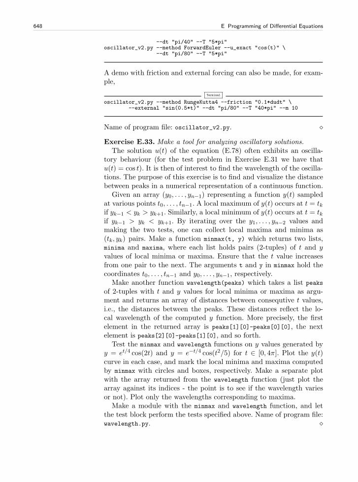
648 E Programming of Differential Equations

--dt "pi/40" --T "5*pi"oscillator_v2.py --method ForwardEuler --u_exact "cos(t)" \

--dt "pi/80" --T "5*pi"

A demo with friction and external forcing can also be made, for exam-ple,

Terminal

oscillator_v2.py --method RungeKutta4 --friction "0.1*dudt" \--external "sin(0.5*t)" --dt "pi/80" --T "40*pi" --m 10

Name of program file: oscillator_v2.py. ⋄

Exercise E.33. Make a tool for analyzing oscillatory solutions.The solution u(t) of the equation (E.78) often exhibits an oscilla-

tory behaviour (for the test problem in Exercise E.31 we have thatu(t) = cos t). It is then of interest to find the wavelength of the oscilla-tions. The purpose of this exercise is to find and visualize the distancebetween peaks in a numerical representation of a continuous function.

Given an array (y0, . . . , yn−1) representing a function y(t) sampledat various points t0, . . . , tn−1. A local maximum of y(t) occurs at t = tkif yk−1 < yk > yk+1. Similarly, a local minimum of y(t) occurs at t = tkif yk−1 > yk < yk+1. By iterating over the y1, . . . , yn−2 values andmaking the two tests, one can collect local maxima and minima as(tk, yk) pairs. Make a function minmax(t, y) which returns two lists,minima and maxima, where each list holds pairs (2-tuples) of t and yvalues of local minima or maxima. Ensure that the t value increasesfrom one pair to the next. The arguments t and y in minmax hold thecoordinates t0, . . . , tn−1 and y0, . . . , yn−1, respectively.

Make another function wavelength(peaks) which takes a list peaks

of 2-tuples with t and y values for local minima or maxima as argu-ment and returns an array of distances between consequtive t values,i.e., the distances between the peaks. These distances reflect the lo-cal wavelength of the computed y function. More precisely, the firstelement in the returned array is peaks[1][0]-peaks[0][0], the nextelement is peaks[2][0]-peaks[1][0], and so forth.

Test the minmax and wavelength functions on y values generated byy = et/4 cos(2t) and y = e−t/4 cos(t2/5) for t ∈ [0, 4π]. Plot the y(t)curve in each case, and mark the local minima and maxima computedby minmax with circles and boxes, respectively. Make a separate plotwith the array returned from the wavelength function (just plot thearray against its indices - the point is to see if the wavelength variesor not). Plot only the wavelengths corresponding to maxima.

Make a module with the minmax and wavelength function, and letthe test block perform the tests specified above. Name of program file:wavelength.py. ⋄

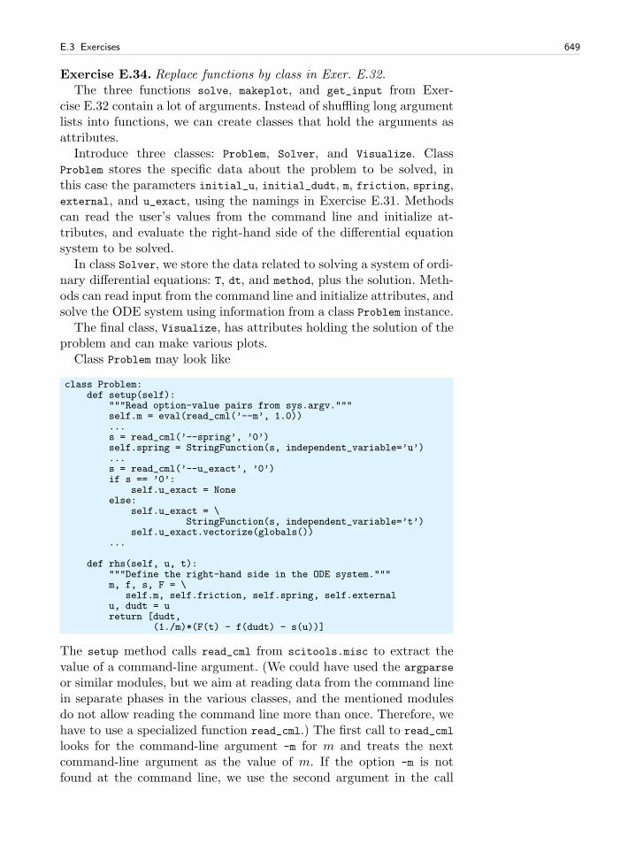
E.3 Exercises 649

Exercise E.34. Replace functions by class in Exer. E.32.The three functions solve, makeplot, and get_input from Exer-

cise E.32 contain a lot of arguments. Instead of shuffling long argumentlists into functions, we can create classes that hold the arguments asattributes.

Introduce three classes: Problem, Solver, and Visualize. ClassProblem stores the specific data about the problem to be solved, inthis case the parameters initial_u, initial_dudt, m, friction, spring,external, and u_exact, using the namings in Exercise E.31. Methodscan read the user’s values from the command line and initialize at-tributes, and evaluate the right-hand side of the differential equationsystem to be solved.

In class Solver, we store the data related to solving a system of ordi-nary differential equations: T, dt, and method, plus the solution. Meth-ods can read input from the command line and initialize attributes, andsolve the ODE system using information from a class Problem instance.

The final class, Visualize, has attributes holding the solution of theproblem and can make various plots.

Class Problem may look like

class Problem:def setup(self):

"""Read option-value pairs from sys.argv."""self.m = eval(read_cml(’--m’, 1.0))...s = read_cml(’--spring’, ’0’)self.spring = StringFunction(s, independent_variable=’u’)...s = read_cml(’--u_exact’, ’0’)if s == ’0’:

self.u_exact = Noneelse:

self.u_exact = \StringFunction(s, independent_variable=’t’)

self.u_exact.vectorize(globals())...

def rhs(self, u, t):"""Define the right-hand side in the ODE system."""m, f, s, F = \

self.m, self.friction, self.spring, self.externalu, dudt = ureturn [dudt,

(1./m)*(F(t) - f(dudt) - s(u))]

The setup method calls read_cml from scitools.misc to extract thevalue of a command-line argument. (We could have used the argparse

or similar modules, but we aim at reading data from the command linein separate phases in the various classes, and the mentioned modulesdo not allow reading the command line more than once. Therefore, wehave to use a specialized function read_cml.) The first call to read_cml

looks for the command-line argument -m for m and treats the nextcommand-line argument as the value of m. If the option -m is notfound at the command line, we use the second argument in the call

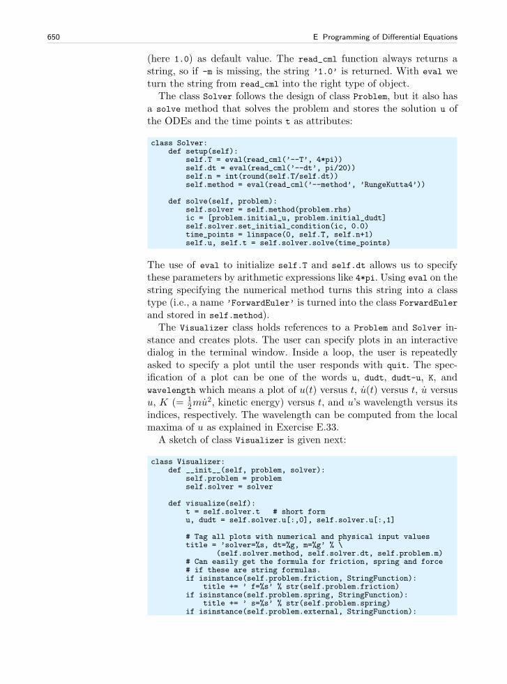
650 E Programming of Differential Equations

(here 1.0) as default value. The read_cml function always returns astring, so if -m is missing, the string ’1.0’ is returned. With eval weturn the string from read_cml into the right type of object.

The class Solver follows the design of class Problem, but it also hasa solve method that solves the problem and stores the solution u ofthe ODEs and the time points t as attributes:

class Solver:def setup(self):

self.T = eval(read_cml(’--T’, 4*pi))self.dt = eval(read_cml(’--dt’, pi/20))self.n = int(round(self.T/self.dt))self.method = eval(read_cml(’--method’, ’RungeKutta4’))

def solve(self, problem):self.solver = self.method(problem.rhs)ic = [problem.initial_u, problem.initial_dudt]self.solver.set_initial_condition(ic, 0.0)time_points = linspace(0, self.T, self.n+1)self.u, self.t = self.solver.solve(time_points)

The use of eval to initialize self.T and self.dt allows us to specifythese parameters by arithmetic expressions like 4*pi. Using eval on thestring specifying the numerical method turns this string into a classtype (i.e., a name ’ForwardEuler’ is turned into the class ForwardEulerand stored in self.method).

The Visualizer class holds references to a Problem and Solver in-stance and creates plots. The user can specify plots in an interactivedialog in the terminal window. Inside a loop, the user is repeatedlyasked to specify a plot until the user responds with quit. The spec-ification of a plot can be one of the words u, dudt, dudt-u, K, andwavelength which means a plot of u(t) versus t, u(t) versus t, u versusu, K (= 1

2mu2, kinetic energy) versus t, and u’s wavelength versus itsindices, respectively. The wavelength can be computed from the localmaxima of u as explained in Exercise E.33.

A sketch of class Visualizer is given next:

class Visualizer:def __init__(self, problem, solver):

self.problem = problemself.solver = solver

def visualize(self):t = self.solver.t # short formu, dudt = self.solver.u[:,0], self.solver.u[:,1]

# Tag all plots with numerical and physical input valuestitle = ’solver=%s, dt=%g, m=%g’ % \

(self.solver.method, self.solver.dt, self.problem.m)# Can easily get the formula for friction, spring and force# if these are string formulas.if isinstance(self.problem.friction, StringFunction):

title += ’ f=%s’ % str(self.problem.friction)if isinstance(self.problem.spring, StringFunction):

title += ’ s=%s’ % str(self.problem.spring)if isinstance(self.problem.external, StringFunction):

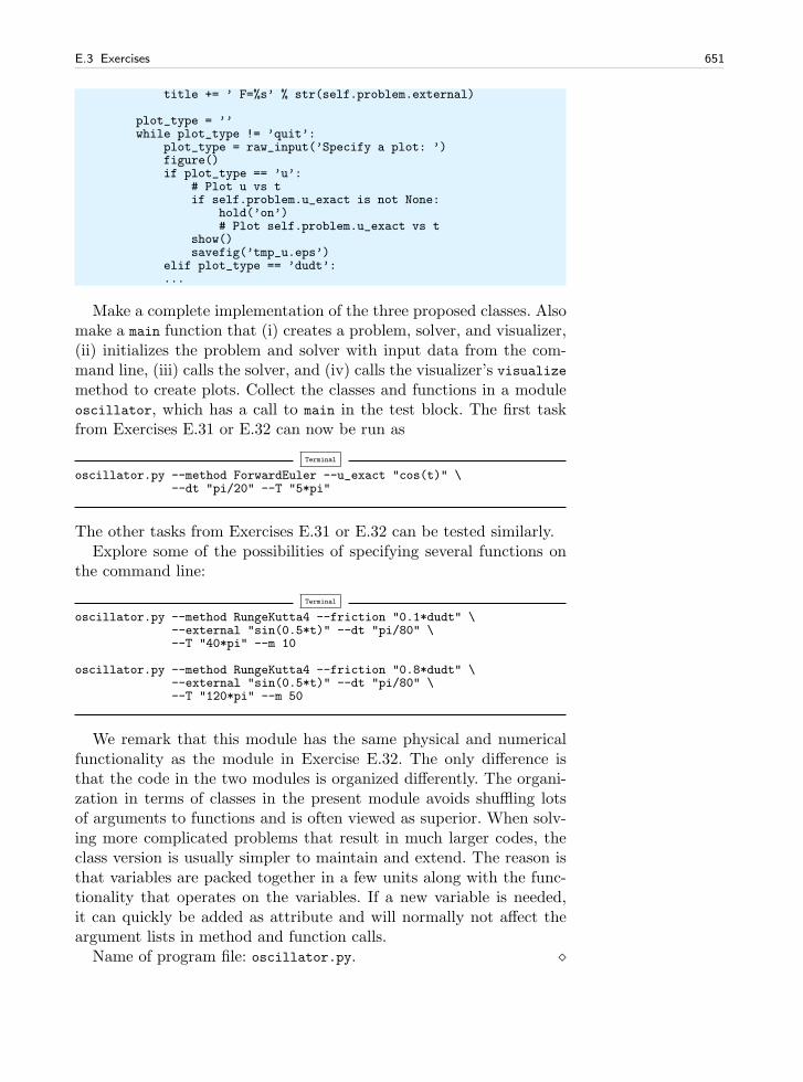
E.3 Exercises 651

title += ’ F=%s’ % str(self.problem.external)

plot_type = ’’while plot_type != ’quit’:

plot_type = raw_input(’Specify a plot: ’)figure()if plot_type == ’u’:

# Plot u vs tif self.problem.u_exact is not None:

hold(’on’)# Plot self.problem.u_exact vs t

show()savefig(’tmp_u.eps’)

elif plot_type == ’dudt’:...

Make a complete implementation of the three proposed classes. Alsomake a main function that (i) creates a problem, solver, and visualizer,(ii) initializes the problem and solver with input data from the com-mand line, (iii) calls the solver, and (iv) calls the visualizer’s visualizemethod to create plots. Collect the classes and functions in a moduleoscillator, which has a call to main in the test block. The first taskfrom Exercises E.31 or E.32 can now be run as

Terminal

oscillator.py --method ForwardEuler --u_exact "cos(t)" \--dt "pi/20" --T "5*pi"

The other tasks from Exercises E.31 or E.32 can be tested similarly.Explore some of the possibilities of specifying several functions on

the command line:

Terminal

oscillator.py --method RungeKutta4 --friction "0.1*dudt" \--external "sin(0.5*t)" --dt "pi/80" \--T "40*pi" --m 10

oscillator.py --method RungeKutta4 --friction "0.8*dudt" \--external "sin(0.5*t)" --dt "pi/80" \--T "120*pi" --m 50

We remark that this module has the same physical and numericalfunctionality as the module in Exercise E.32. The only difference isthat the code in the two modules is organized differently. The organi-zation in terms of classes in the present module avoids shuffling lotsof arguments to functions and is often viewed as superior. When solv-ing more complicated problems that result in much larger codes, theclass version is usually simpler to maintain and extend. The reason isthat variables are packed together in a few units along with the func-tionality that operates on the variables. If a new variable is needed,it can quickly be added as attribute and will normally not affect theargument lists in method and function calls.

Name of program file: oscillator.py. ⋄

652 E Programming of Differential Equations

Exercise E.35. Allow flexible choice of functions in Exer. E.34.Some typical choices of f(u), s(u), and F (t) in (E.78) are listed

below:

1. Linear friction force (low velocities): f(u) = 6πµRu (Stokes drag),where R is the radius of a spherical approximation to the body’sgeometry, and µ is the viscosity of the surrounding fluid.

2. Quadratic friction force (high velocities): f(u) = 12CDA|u|u, see

Exercise 1.11 for explanation of symbols.3. Linear spring force: s(u) = ku, where k is a spring constant.4. Sinusoidal spring force: s(u) = k sinu, where k is a constant.5. Cubic spring force: s(u) = k(u− 1

6u3), where k is a spring constant.

6. Sinusoidal external force: F (t) = F0+A sinωt, where F0 is the meanvalue of the force, A is the amplitude, and ω is the frequency.

7. “Bump” force: F (t) = H(t− t1)(1−H(t− t2))F0, where H(t) is theHeaviside function from Exercise 3.19, t1 and t2 are two given timepoints, and F0 is the size of the force. This F (t) is zero for t < t1and t > t2, and F0 for t ∈ [t1, t2].

8. Random force 1: F (t) = F0 + A · U(t;B), where F0 and A areconstants, and U(t;B) denotes a function whose value at time t israndom and uniformly distributed in the interval [−B,B].

9. Random force 2: F (t) = F0 + A · N(t;µ, σ), where F0 and A areconstants, and N(t;µ, σ) denotes a function whose value at time tis random, Gaussian distributed number with mean µ and standarddeviation σ.

Make a module functions where each of the choices above are imple-mented as a class with a __call__ special method. Also add a class Zerofor a function whose value is always zero. It is natural that the parame-ters in a function are set as arguments to the constructor. The differentclasses for spring functions can all have a common base class holdingthe k parameter as attribute. Name of program file: functions.py. ⋄

Exercise E.36. Use the modules from Exer. E.34 and E.35.The purpose of this exercise is to demonstrate the use of the classes

from Exercise E.35 to solve problems described by (E.78).With a lot of models for f(u), s(u), and F (t) available as classes in

functions.py, the setup method in class Problem will not work well.For example, setup assumes that s(u) is given as an expression, turnedinto a Python function via StringFunction. Having the functions mod-ule, s(u) may be given as (e.g.) CubicSpring(1.8). One can modify thesetup method and use the read_cml_func function from scitools.misc,which allows either a mathematical formula or an instance creation like’CubicSpring(1.8)’ to be specified on the command-line. The modifi-cation reads

E.3 Exercises 653

self.spring = read_cml_func(’--spring’, ’0’, iv=’u’)

Here, ’0’ is the default expression, and iv denotes the name of the ind-pendent variable if a mathematical expression is given on the commandline.

As an alternative to this reimplementation of the setup method, onecan simply assign values to the attributes in a Problem instance directly,e.g.,

problem = Problem()problem.m = 1.0k = 1.2problem.spring = CubicSpring(k)...

This is the most straightforward approach to make use of the objectsin the functions module.

Note that the setup method in class Solver is unaffected by thenew objects from the functions module, so flexible initialization viacommand-line arguments works as before.

Make a new file say oscillator_test.py where you import classProblem, Sover, and Visualizer, plus all classes from the functions

module. Provide a main1 function for solving the following problem:m = 1, u(0) = 1, u(0) = 0, no friction (use class Zero), no externalforcing (class Zero), a linear spring s(u) = u, ∆t = π/20, T = 8π, andexact u(t) = cos(t). Use the Forward Euler method.

Then make another function main2 for the case with m = 5, u(0) =1, u(0) = 0, linear friction f(u) = 0.1u, s(u) = u, F (t) = sin(12 t),∆t = π/80, T = 60π, and no knowledge of an exact solution. Use the4-th order Runge-Kutta method.

Let a test block use the first command-line argument to indicate acall to main1 or main2. Name of program file: oscillator_test.py. ⋄

Exercise E.37. Use the modules from Exer. E.34 and E.35.Make a program oscillator_conv.py where you import the Problem

and Solver classes from the oscillator module in Exercise E.35 andimplement a loop in which ∆t is reduced. The end result should be aplot with the curves u versus t corresponding to the various ∆t values.Typically, we want to do something like

from oscillator import Problem, Solverfrom scitools.std import plot, hold

problem = Problem()problem.setup()solver = Solver()solver.setup()

# See how the solution changes by halving dt n timesn = 4for k in range(n):

654 E Programming of Differential Equations

solver.solve(problem)u, t = solver.u[:,0], solver.tplot(t, u, legend=’dt=%g’ % solver.dt)hold(True)solver.dt = solver.dt/2.0

Extend this program with another loop over increasing m values.Hopefully, you will realize how flexible the classes from Exer-

cises E.34 and E.35 are for solving a variety of problems. We can givea set of physical and numerical parameters in a flexible way on thecommand line, and in the program we may make loops or other con-structions to manipulate the input data further.

Name of program file: oscillator_conv.py. ⋄

Debugging F

F.1 Using a Debugger

A debugger is a program that can help you to find out what is going onin a computer program. You can stop the execution at any prescribedline number, print out variables, continue execution, stop again, exe-cute statements one by one, and repeat such actions until you trackdown abnormal behavior and find bugs.

Here we shall use the debugger to demonstrate the program flow ofthe Simpson.py code from Chapter 3.3.2. You are strongly encouragedto carry out the steps below on your computer to get a glimpse of whata debugger can do.

1. Go to the folder src/funcif associated with Chapter 3.2. Start IPython:

Terminal

Unix/DOS> ipython

3. Run the program Simpson.py with the debugger on (-d):

In [1]: run -d Simpson.py

We now enter the debugger and get a prompt

ipdb>

After this prompt we can issue various debugger commands. The mostimportant ones will be described as we go along.

4. Type continue or just c to go to the first line in the file. Now youcan see a printout of where we are in the program:

655

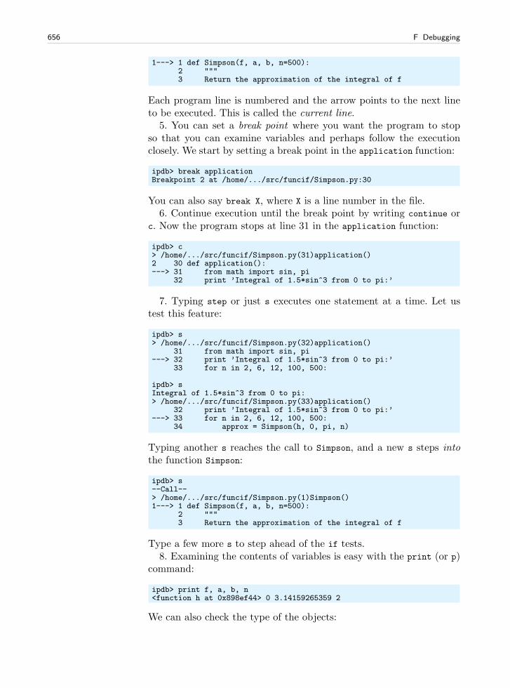
656 F Debugging

1---> 1 def Simpson(f, a, b, n=500):2 """3 Return the approximation of the integral of f

Each program line is numbered and the arrow points to the next lineto be executed. This is called the current line.

5. You can set a break point where you want the program to stopso that you can examine variables and perhaps follow the executionclosely. We start by setting a break point in the application function:

ipdb> break applicationBreakpoint 2 at /home/.../src/funcif/Simpson.py:30

You can also say break X, where X is a line number in the file.6. Continue execution until the break point by writing continue or

c. Now the program stops at line 31 in the application function:

ipdb> c> /home/.../src/funcif/Simpson.py(31)application()2 30 def application():---> 31 from math import sin, pi

32 print ’Integral of 1.5*sin^3 from 0 to pi:’

7. Typing step or just s executes one statement at a time. Let ustest this feature:

ipdb> s> /home/.../src/funcif/Simpson.py(32)application()

31 from math import sin, pi---> 32 print ’Integral of 1.5*sin^3 from 0 to pi:’

33 for n in 2, 6, 12, 100, 500:

ipdb> sIntegral of 1.5*sin^3 from 0 to pi:> /home/.../src/funcif/Simpson.py(33)application()

32 print ’Integral of 1.5*sin^3 from 0 to pi:’---> 33 for n in 2, 6, 12, 100, 500:

34 approx = Simpson(h, 0, pi, n)

Typing another s reaches the call to Simpson, and a new s steps intothe function Simpson:

ipdb> s--Call--> /home/.../src/funcif/Simpson.py(1)Simpson()1---> 1 def Simpson(f, a, b, n=500):

2 """3 Return the approximation of the integral of f

Type a few more s to step ahead of the if tests.8. Examining the contents of variables is easy with the print (or p)

command:

ipdb> print f, a, b, n<function h at 0x898ef44> 0 3.14159265359 2

We can also check the type of the objects:

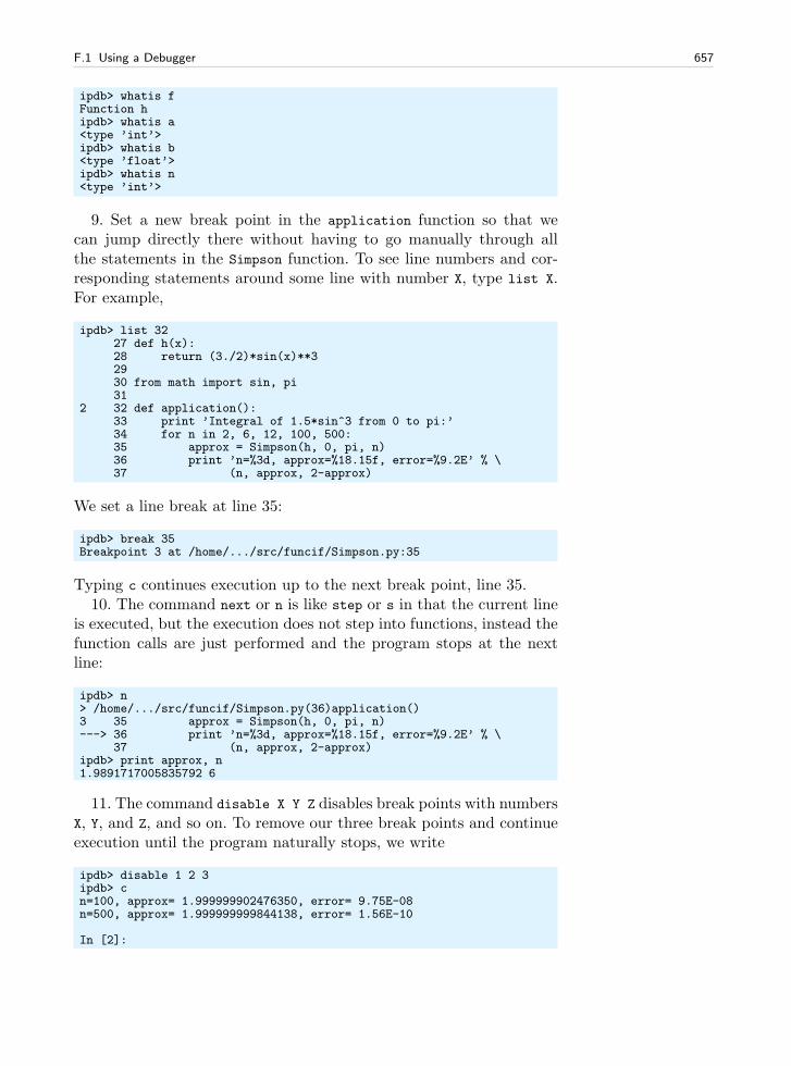
F.1 Using a Debugger 657

ipdb> whatis fFunction hipdb> whatis a<type ’int’>ipdb> whatis b<type ’float’>ipdb> whatis n<type ’int’>

9. Set a new break point in the application function so that wecan jump directly there without having to go manually through allthe statements in the Simpson function. To see line numbers and cor-responding statements around some line with number X, type list X.For example,

ipdb> list 3227 def h(x):28 return (3./2)*sin(x)**32930 from math import sin, pi31

2 32 def application():33 print ’Integral of 1.5*sin^3 from 0 to pi:’34 for n in 2, 6, 12, 100, 500:35 approx = Simpson(h, 0, pi, n)36 print ’n=%3d, approx=%18.15f, error=%9.2E’ % \37 (n, approx, 2-approx)

We set a line break at line 35:

ipdb> break 35Breakpoint 3 at /home/.../src/funcif/Simpson.py:35

Typing c continues execution up to the next break point, line 35.10. The command next or n is like step or s in that the current line

is executed, but the execution does not step into functions, instead thefunction calls are just performed and the program stops at the nextline:

ipdb> n> /home/.../src/funcif/Simpson.py(36)application()3 35 approx = Simpson(h, 0, pi, n)---> 36 print ’n=%3d, approx=%18.15f, error=%9.2E’ % \

37 (n, approx, 2-approx)ipdb> print approx, n1.9891717005835792 6

11. The command disable X Y Z disables break points with numbersX, Y, and Z, and so on. To remove our three break points and continueexecution until the program naturally stops, we write

ipdb> disable 1 2 3ipdb> cn=100, approx= 1.999999902476350, error= 9.75E-08n=500, approx= 1.999999999844138, error= 1.56E-10

In [2]:

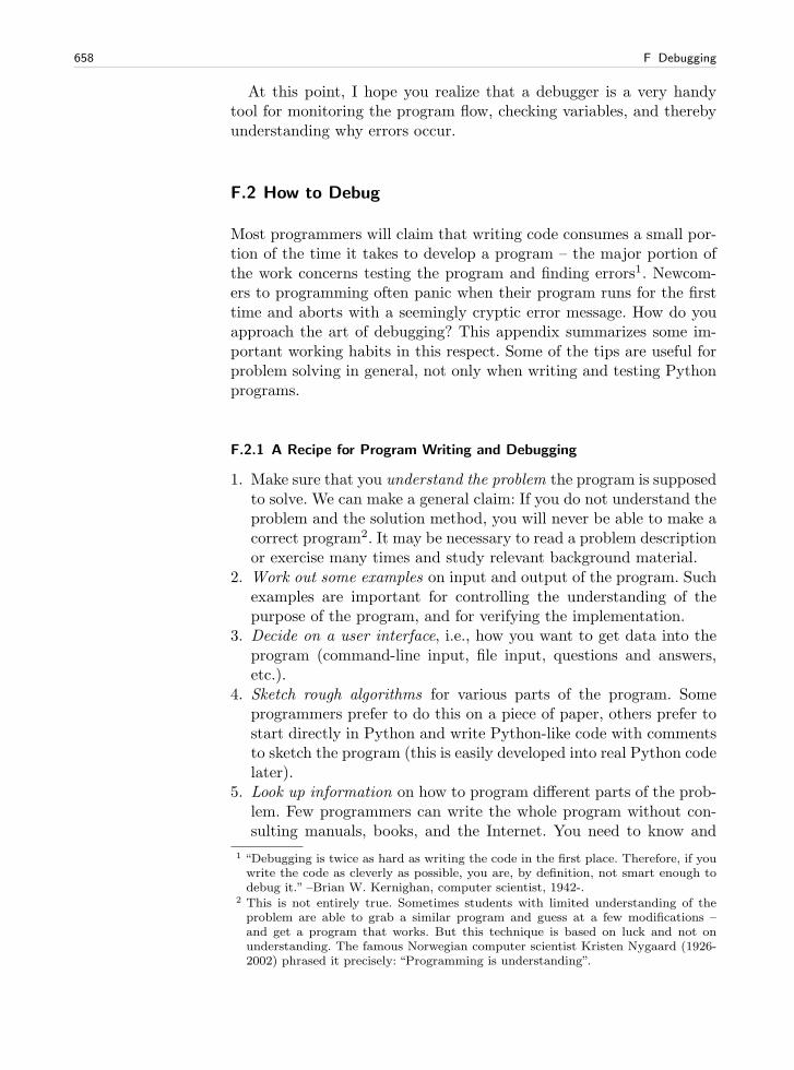
658 F Debugging

At this point, I hope you realize that a debugger is a very handytool for monitoring the program flow, checking variables, and therebyunderstanding why errors occur.

F.2 How to Debug

Most programmers will claim that writing code consumes a small por-tion of the time it takes to develop a program – the major portion ofthe work concerns testing the program and finding errors1. Newcom-ers to programming often panic when their program runs for the firsttime and aborts with a seemingly cryptic error message. How do youapproach the art of debugging? This appendix summarizes some im-portant working habits in this respect. Some of the tips are useful forproblem solving in general, not only when writing and testing Pythonprograms.

F.2.1 A Recipe for Program Writing and Debugging

1. Make sure that you understand the problem the program is supposedto solve. We can make a general claim: If you do not understand theproblem and the solution method, you will never be able to make acorrect program2. It may be necessary to read a problem descriptionor exercise many times and study relevant background material.

2. Work out some examples on input and output of the program. Suchexamples are important for controlling the understanding of thepurpose of the program, and for verifying the implementation.

3. Decide on a user interface, i.e., how you want to get data into theprogram (command-line input, file input, questions and answers,etc.).

4. Sketch rough algorithms for various parts of the program. Someprogrammers prefer to do this on a piece of paper, others prefer tostart directly in Python and write Python-like code with commentsto sketch the program (this is easily developed into real Python codelater).

5. Look up information on how to program different parts of the prob-lem. Few programmers can write the whole program without con-sulting manuals, books, and the Internet. You need to know and

1 “Debugging is twice as hard as writing the code in the first place. Therefore, if youwrite the code as cleverly as possible, you are, by definition, not smart enough todebug it.” –Brian W. Kernighan, computer scientist, 1942-.

2 This is not entirely true. Sometimes students with limited understanding of theproblem are able to grab a similar program and guess at a few modifications –and get a program that works. But this technique is based on luck and not onunderstanding. The famous Norwegian computer scientist Kristen Nygaard (1926-2002) phrased it precisely: “Programming is understanding”.

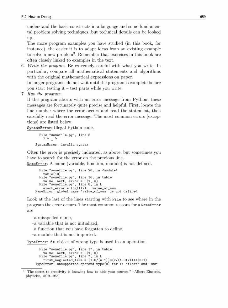
F.2 How to Debug 659

understand the basic constructs in a language and some fundamen-tal problem solving techniques, but technical details can be lookedup.The more program examples you have studied (in this book, forinstance), the easier it is to adapt ideas from an existing exampleto solve a new problem3. Remember that exercises in this book areoften closely linked to examples in the text.

6. Write the program. Be extremely careful with what you write. Inparticular, compare all mathematical statements and algorithmswith the original mathematical expressions on paper.In longer programs, do not wait until the program is complete beforeyou start testing it – test parts while you write.

7. Run the program.If the program aborts with an error message from Python, thesemessages are fortunately quite precise and helpful. First, locate theline number where the error occurs and read the statement, thencarefully read the error message. The most common errors (excep-tions) are listed below.SyntaxError: Illegal Python code.

File "somefile.py", line 5x = . 5

^SyntaxError: invalid syntax

Often the error is precisely indicated, as above, but sometimes youhave to search for the error on the previous line.NameError: A name (variable, function, module) is not defined.

File "somefile.py", line 20, in <module>table(10)

File "somefile.py", line 16, in tablevalue, next, error = L(x, n)

File "somefile.py", line 8, in Lexact_error = log(1+x) - value_of_sum

NameError: global name ’value_of_sum’ is not defined

Look at the last of the lines starting with File to see where in theprogram the error occurs. The most common reasons for a NameError

are

–a misspelled name,–a variable that is not initialized,–a function that you have forgotten to define,–a module that is not imported.

TypeError: An object of wrong type is used in an operation.

File "somefile.py", line 17, in tablevalue, next, error = L(x, n)

File "somefile.py", line 7, in Lfirst_neglected_term = (1.0/(n+1))*(x/(1.0+x))**(n+1)

TypeError: unsupported operand type(s) for +: ’float’ and ’str’

3 “The secret to creativity is knowing how to hide your sources.” –Albert Einstein,physicist, 1879-1955.

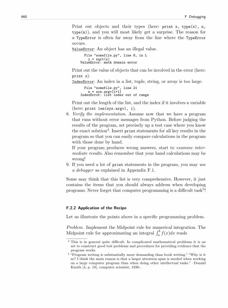
660 F Debugging

Print out objects and their types (here: print x, type(x), n,

type(n)), and you will most likely get a surprise. The reason fora TypeError is often far away from the line where the TypeError

occurs.ValueError: An object has an illegal value.

File "somefile.py", line 8, in Ly = sqrt(x)

ValueError: math domain error

Print out the value of objects that can be involved in the error (here:print x).IndexError: An index in a list, tuple, string, or array is too large.

File "somefile.py", line 21n = sys.argv[i+1]

IndexError: list index out of range

Print out the length of the list, and the index if it involves a variable(here: print len(sys.argv), i).

8. Verify the implementation. Assume now that we have a programthat runs without error messages from Python. Before judging theresults of the program, set precisely up a test case where you knowthe exact solution4. Insert print statements for all key results in theprogram so that you can easily compare calculations in the programwith those done by hand.If your program produces wrong answers, start to examine inter-mediate results. Also remember that your hand calculations may bewrong!

9. If you need a lot of print statements in the program, you may usea debugger as explained in Appendix F.1.

Some may think that this list is very comprehensive. However, it justcontains the items that you should always address when developingprograms. Never forget that computer programming is a difficult task5!

F.2.2 Application of the Recipe

Let us illustrate the points above in a specific programming problem.

Problem. Implement the Midpoint rule for numerical integration. TheMidpoint rule for approximating an integral

∫ ba f(x)dx reads

4 This is in general quite difficult. In complicated mathematical problems it is anart to construct good test problems and procedures for providing evidence that theprogram works.

5 “Program writing is substantially more demanding than book writing.”“Why is itso? I think the main reason is that a larger attention span is needed when workingon a large computer program than when doing other intellectual tasks.” –DonaldKnuth [4, p. 18], computer scientist, 1938-.

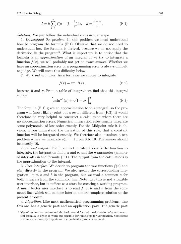
F.2 How to Debug 661

I = h

n∑

i=1

f(a+ (i− 1

2)h), h =

b− a

n. (F.1)

Solution. We just follow the individual steps in the recipe.1. Understand the problem. In this problem we must understand

how to program the formula (F.1). Observe that we do not need tounderstand how the formula is derived, because we do not apply thederivation in the program6. What is important, is to notice that theformula is an approximation of an integral. If we try to integrate afunction f(x), we will probably not get an exact answer. Whether wehave an approximation error or a programming error is always difficultto judge. We will meet this difficulty below.

2. Work out examples. As a test case we choose to integrate

f(x) = sin−1(x) . (F.2)

between 0 and π. From a table of integrals we find that this integralequals

[

x sin−1(x) +√

1− x2]π

0. (F.3)

The formula (F.1) gives an approximation to this integral, so the pro-gram will (most likely) print out a result different from (F.3). It wouldtherefore be very helpful to construct a calculation where there areno approximation errors. Numerical integration rules usually integratesome polynomial of low order exactly. For the Midpoint rule it is ob-vious, if you understand the derivation of this rule, that a constantfunction will be integrated exactly. We therefore also introduce a testproblem where we integrate g(x) = 1 from 0 to 10. The answer shouldbe exactly 10.

Input and output : The input to the calculations is the function tointegrate, the integration limits a and b, and the n parameter (numberof intervals) in the formula (F.1). The output from the calculations isthe approximation to the integral.

3. User interface. We decide to program the two functions f(x) andg(x) directly in the program. We also specify the corresponding inte-gration limits a and b in the program, but we read a common n forboth integrals from the command line. Note that this is not a flexibleuser interface, but it suffices as a start for creating a working program.A much better user interface is to read f , a, b, and n from the com-mand line, which will be done later in a more complete solution to thepresent problem.

4. Algorithm. Like most mathematical programming problems, alsothis one has a generic part and an application part. The generic part

6 You often need to understand the background for and the derivation of a mathemat-ical formula in order to work out sensible test problems for verification. Sometimesthis must be done by experts on the particular problem at hand.

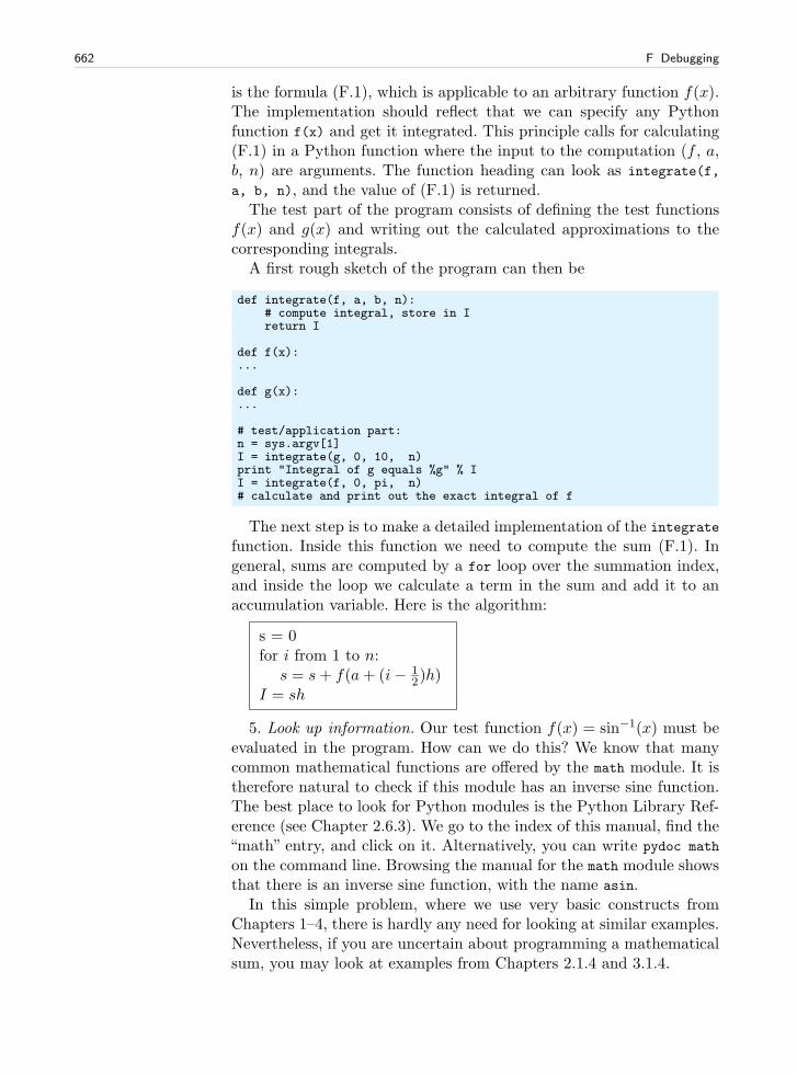
662 F Debugging

is the formula (F.1), which is applicable to an arbitrary function f(x).The implementation should reflect that we can specify any Pythonfunction f(x) and get it integrated. This principle calls for calculating(F.1) in a Python function where the input to the computation (f , a,b, n) are arguments. The function heading can look as integrate(f,

a, b, n), and the value of (F.1) is returned.The test part of the program consists of defining the test functions

f(x) and g(x) and writing out the calculated approximations to thecorresponding integrals.

A first rough sketch of the program can then be

def integrate(f, a, b, n):# compute integral, store in Ireturn I

def f(x):...

def g(x):...

# test/application part:n = sys.argv[1]I = integrate(g, 0, 10, n)print "Integral of g equals %g" % II = integrate(f, 0, pi, n)# calculate and print out the exact integral of f

The next step is to make a detailed implementation of the integratefunction. Inside this function we need to compute the sum (F.1). Ingeneral, sums are computed by a for loop over the summation index,and inside the loop we calculate a term in the sum and add it to anaccumulation variable. Here is the algorithm:

s = 0for i from 1 to n:

s = s+ f(a+ (i− 12)h)

I = sh

5. Look up information. Our test function f(x) = sin−1(x) must beevaluated in the program. How can we do this? We know that manycommon mathematical functions are offered by the math module. It istherefore natural to check if this module has an inverse sine function.The best place to look for Python modules is the Python Library Ref-erence (see Chapter 2.6.3). We go to the index of this manual, find the“math” entry, and click on it. Alternatively, you can write pydoc math

on the command line. Browsing the manual for the math module showsthat there is an inverse sine function, with the name asin.

In this simple problem, where we use very basic constructs fromChapters 1–4, there is hardly any need for looking at similar examples.Nevertheless, if you are uncertain about programming a mathematicalsum, you may look at examples from Chapters 2.1.4 and 3.1.4.

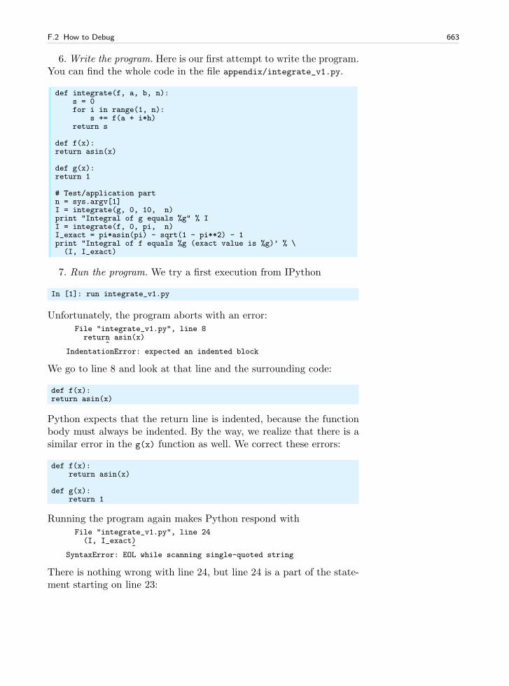
F.2 How to Debug 663

6. Write the program. Here is our first attempt to write the program.You can find the whole code in the file appendix/integrate_v1.py.

def integrate(f, a, b, n):s = 0for i in range(1, n):

s += f(a + i*h)return s

def f(x):return asin(x)

def g(x):return 1

# Test/application partn = sys.argv[1]I = integrate(g, 0, 10, n)print "Integral of g equals %g" % II = integrate(f, 0, pi, n)I_exact = pi*asin(pi) - sqrt(1 - pi**2) - 1print "Integral of f equals %g (exact value is %g)’ % \(I, I_exact)

7. Run the program. We try a first execution from IPython

In [1]: run integrate_v1.py

Unfortunately, the program aborts with an error:File "integrate_v1.py", line 8return asin(x)

^IndentationError: expected an indented block

We go to line 8 and look at that line and the surrounding code:

def f(x):return asin(x)

Python expects that the return line is indented, because the functionbody must always be indented. By the way, we realize that there is asimilar error in the g(x) function as well. We correct these errors:

def f(x):return asin(x)

def g(x):return 1

Running the program again makes Python respond withFile "integrate_v1.py", line 24(I, I_exact)

^SyntaxError: EOL while scanning single-quoted string

There is nothing wrong with line 24, but line 24 is a part of the state-ment starting on line 23:

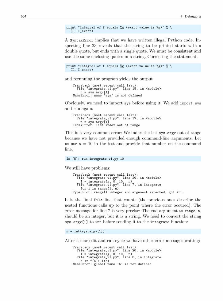
664 F Debugging

print "Integral of f equals %g (exact value is %g)’ % \(I, I_exact)

A SyntaxError implies that we have written illegal Python code. In-specting line 23 reveals that the string to be printed starts with adouble quote, but ends with a single quote. We must be consistent anduse the same enclosing quotes in a string. Correcting the statement,

print "Integral of f equals %g (exact value is %g)" % \(I, I_exact)

and rerunning the program yields the output

Traceback (most recent call last):File "integrate_v1.py", line 18, in <module>n = sys.argv[1]

NameError: name ’sys’ is not defined

Obviously, we need to import sys before using it. We add import sys

and run again:

Traceback (most recent call last):File "integrate_v1.py", line 19, in <module>n = sys.argv[1]

IndexError: list index out of range

This is a very common error: We index the list sys.argv out of rangebecause we have not provided enough command-line arguments. Letus use n = 10 in the test and provide that number on the commandline:

In [5]: run integrate_v1.py 10

We still have problems:

Traceback (most recent call last):File "integrate_v1.py", line 20, in <module>I = integrate(g, 0, 10, n)

File "integrate_v1.py", line 7, in integratefor i in range(1, n):

TypeError: range() integer end argument expected, got str.

It is the final File line that counts (the previous ones describe thenested functions calls up to the point where the error occured). Theerror message for line 7 is very precise: The end argument to range, n,should be an integer, but it is a string. We need to convert the stringsys.argv[1] to int before sending it to the integrate function:

n = int(sys.argv[1])

After a new edit-and-run cycle we have other error messages waiting:

Traceback (most recent call last):File "integrate_v1.py", line 20, in <module>I = integrate(g, 0, 10, n)

File "integrate_v1.py", line 8, in integrates += f(a + i*h)

NameError: global name ’h’ is not defined

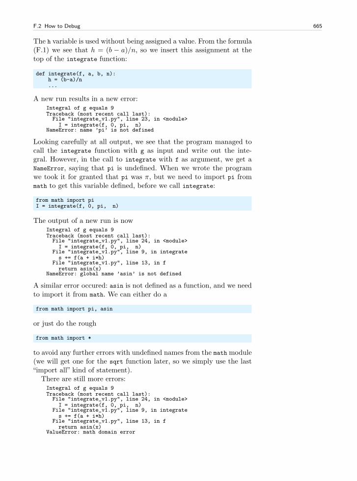
F.2 How to Debug 665

The h variable is used without being assigned a value. From the formula(F.1) we see that h = (b − a)/n, so we insert this assignment at thetop of the integrate function:

def integrate(f, a, b, n):h = (b-a)/n...

A new run results in a new error:Integral of g equals 9Traceback (most recent call last):File "integrate_v1.py", line 23, in <module>I = integrate(f, 0, pi, n)

NameError: name ’pi’ is not defined

Looking carefully at all output, we see that the program managed tocall the integrate function with g as input and write out the inte-gral. However, in the call to integrate with f as argument, we get aNameError, saying that pi is undefined. When we wrote the programwe took it for granted that pi was π, but we need to import pi frommath to get this variable defined, before we call integrate:

from math import piI = integrate(f, 0, pi, n)

The output of a new run is nowIntegral of g equals 9Traceback (most recent call last):File "integrate_v1.py", line 24, in <module>I = integrate(f, 0, pi, n)

File "integrate_v1.py", line 9, in integrates += f(a + i*h)

File "integrate_v1.py", line 13, in freturn asin(x)

NameError: global name ’asin’ is not defined

A similar error occured: asin is not defined as a function, and we needto import it from math. We can either do a

from math import pi, asin

or just do the rough

from math import *

to avoid any further errors with undefined names from the math module(we will get one for the sqrt function later, so we simply use the last“import all” kind of statement).

There are still more errors:Integral of g equals 9Traceback (most recent call last):File "integrate_v1.py", line 24, in <module>I = integrate(f, 0, pi, n)

File "integrate_v1.py", line 9, in integrates += f(a + i*h)

File "integrate_v1.py", line 13, in freturn asin(x)

ValueError: math domain error

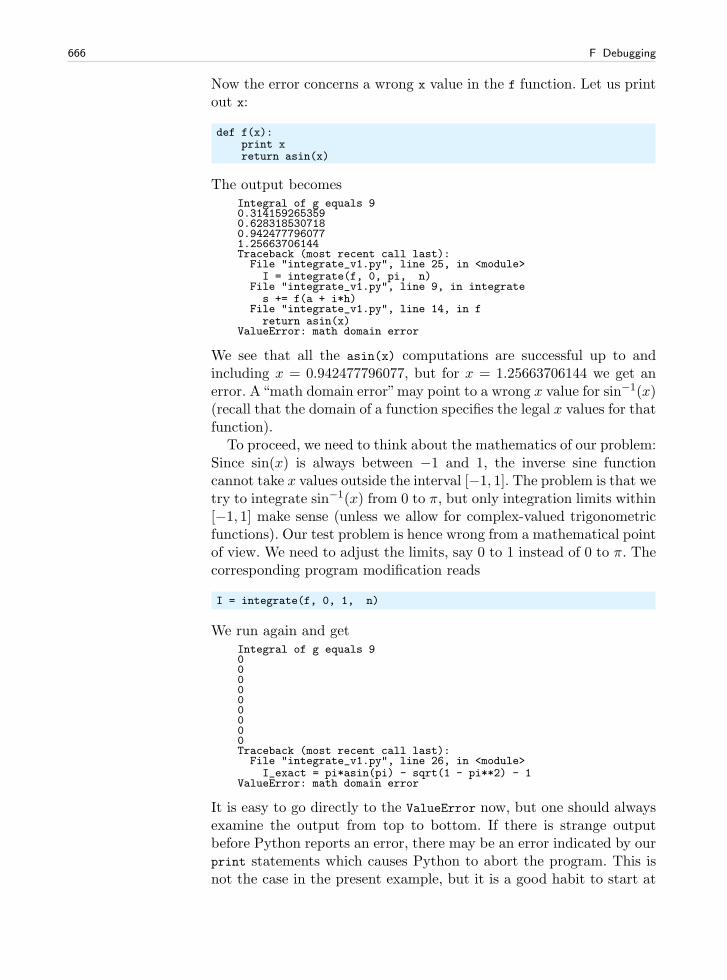
666 F Debugging

Now the error concerns a wrong x value in the f function. Let us printout x:

def f(x):print xreturn asin(x)

The output becomesIntegral of g equals 90.3141592653590.6283185307180.9424777960771.25663706144Traceback (most recent call last):File "integrate_v1.py", line 25, in <module>I = integrate(f, 0, pi, n)

File "integrate_v1.py", line 9, in integrates += f(a + i*h)

File "integrate_v1.py", line 14, in freturn asin(x)

ValueError: math domain error

We see that all the asin(x) computations are successful up to andincluding x = 0.942477796077, but for x = 1.25663706144 we get anerror. A“math domain error”may point to a wrong x value for sin−1(x)(recall that the domain of a function specifies the legal x values for thatfunction).

To proceed, we need to think about the mathematics of our problem:Since sin(x) is always between −1 and 1, the inverse sine functioncannot take x values outside the interval [−1, 1]. The problem is that wetry to integrate sin−1(x) from 0 to π, but only integration limits within[−1, 1] make sense (unless we allow for complex-valued trigonometricfunctions). Our test problem is hence wrong from a mathematical pointof view. We need to adjust the limits, say 0 to 1 instead of 0 to π. Thecorresponding program modification reads

I = integrate(f, 0, 1, n)

We run again and getIntegral of g equals 9000000000Traceback (most recent call last):File "integrate_v1.py", line 26, in <module>I_exact = pi*asin(pi) - sqrt(1 - pi**2) - 1

ValueError: math domain error

It is easy to go directly to the ValueError now, but one should alwaysexamine the output from top to bottom. If there is strange outputbefore Python reports an error, there may be an error indicated by ourprint statements which causes Python to abort the program. This isnot the case in the present example, but it is a good habit to start at

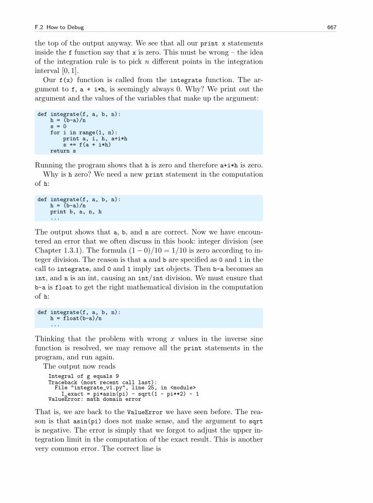
F.2 How to Debug 667

the top of the output anyway. We see that all our print x statementsinside the f function say that x is zero. This must be wrong – the ideaof the integration rule is to pick n different points in the integrationinterval [0, 1].

Our f(x) function is called from the integrate function. The ar-gument to f, a + i*h, is seemingly always 0. Why? We print out theargument and the values of the variables that make up the argument:

def integrate(f, a, b, n):h = (b-a)/ns = 0for i in range(1, n):

print a, i, h, a+i*hs += f(a + i*h)

return s

Running the program shows that h is zero and therefore a+i*h is zero.Why is h zero? We need a new print statement in the computation

of h:

def integrate(f, a, b, n):h = (b-a)/nprint b, a, n, h...

The output shows that a, b, and n are correct. Now we have encoun-tered an error that we often discuss in this book: integer division (seeChapter 1.3.1). The formula (1− 0)/10 = 1/10 is zero according to in-teger division. The reason is that a and b are specified as 0 and 1 in thecall to integrate, and 0 and 1 imply int objects. Then b-a becomes anint, and n is an int, causing an int/int division. We must ensure thatb-a is float to get the right mathematical division in the computationof h:

def integrate(f, a, b, n):h = float(b-a)/n...

Thinking that the problem with wrong x values in the inverse sinefunction is resolved, we may remove all the print statements in theprogram, and run again.

The output now readsIntegral of g equals 9Traceback (most recent call last):File "integrate_v1.py", line 25, in <module>I_exact = pi*asin(pi) - sqrt(1 - pi**2) - 1

ValueError: math domain error

That is, we are back to the ValueError we have seen before. The rea-son is that asin(pi) does not make sense, and the argument to sqrt

is negative. The error is simply that we forgot to adjust the upper in-tegration limit in the computation of the exact result. This is anothervery common error. The correct line is

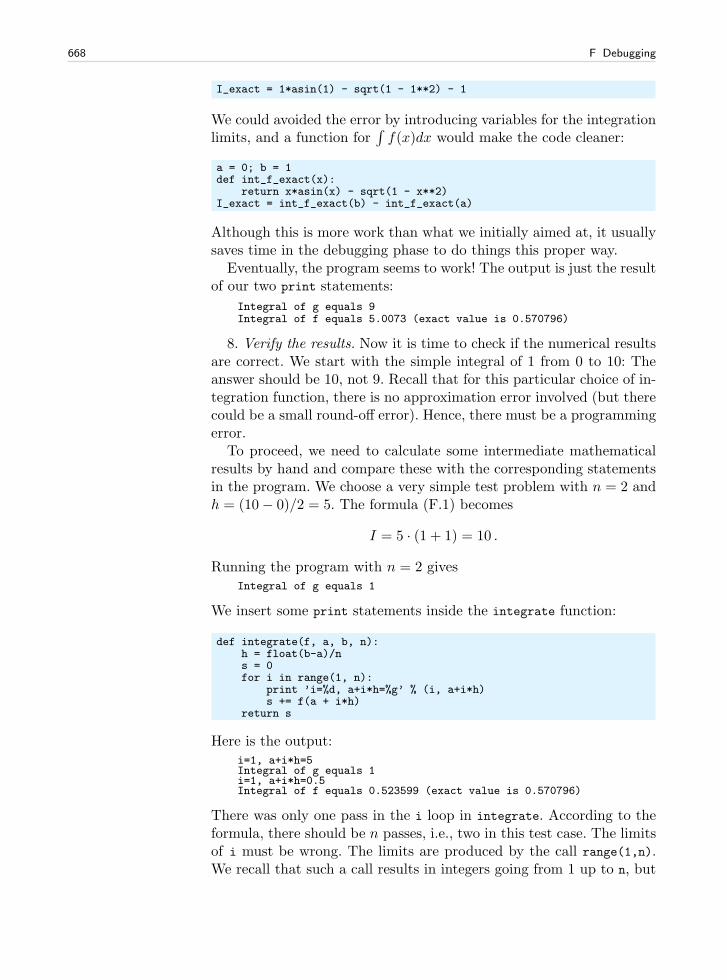
668 F Debugging

I_exact = 1*asin(1) - sqrt(1 - 1**2) - 1

We could avoided the error by introducing variables for the integrationlimits, and a function for

∫

f(x)dx would make the code cleaner:

a = 0; b = 1def int_f_exact(x):

return x*asin(x) - sqrt(1 - x**2)I_exact = int_f_exact(b) - int_f_exact(a)

Although this is more work than what we initially aimed at, it usuallysaves time in the debugging phase to do things this proper way.

Eventually, the program seems to work! The output is just the resultof our two print statements:

Integral of g equals 9Integral of f equals 5.0073 (exact value is 0.570796)

8. Verify the results. Now it is time to check if the numerical resultsare correct. We start with the simple integral of 1 from 0 to 10: Theanswer should be 10, not 9. Recall that for this particular choice of in-tegration function, there is no approximation error involved (but therecould be a small round-off error). Hence, there must be a programmingerror.

To proceed, we need to calculate some intermediate mathematicalresults by hand and compare these with the corresponding statementsin the program. We choose a very simple test problem with n = 2 andh = (10− 0)/2 = 5. The formula (F.1) becomes

I = 5 · (1 + 1) = 10 .

Running the program with n = 2 givesIntegral of g equals 1

We insert some print statements inside the integrate function:

def integrate(f, a, b, n):h = float(b-a)/ns = 0for i in range(1, n):

print ’i=%d, a+i*h=%g’ % (i, a+i*h)s += f(a + i*h)

return s

Here is the output:i=1, a+i*h=5Integral of g equals 1i=1, a+i*h=0.5Integral of f equals 0.523599 (exact value is 0.570796)

There was only one pass in the i loop in integrate. According to theformula, there should be n passes, i.e., two in this test case. The limitsof i must be wrong. The limits are produced by the call range(1,n).We recall that such a call results in integers going from 1 up to n, but

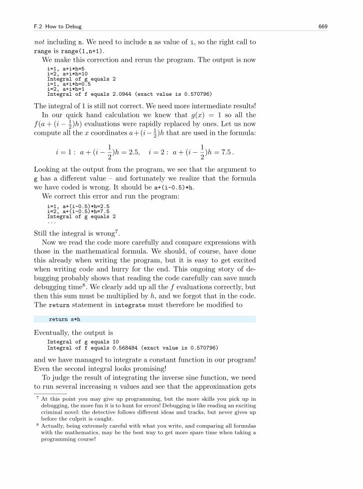
F.2 How to Debug 669

not including n. We need to include n as value of i, so the right call torange is range(1,n+1).

We make this correction and rerun the program. The output is nowi=1, a+i*h=5i=2, a+i*h=10Integral of g equals 2i=1, a+i*h=0.5i=2, a+i*h=1Integral of f equals 2.0944 (exact value is 0.570796)

The integral of 1 is still not correct. We need more intermediate results!In our quick hand calculation we knew that g(x) = 1 so all the

f(a+ (i− 12)h) evaluations were rapidly replaced by ones. Let us now

compute all the x coordinates a+(i− 12)h that are used in the formula:

i = 1 : a+ (i− 1

2)h = 2.5, i = 2 : a+ (i− 1

2)h = 7.5 .

Looking at the output from the program, we see that the argument tog has a different value – and fortunately we realize that the formulawe have coded is wrong. It should be a+(i-0.5)*h.

We correct this error and run the program:

i=1, a+(i-0.5)*h=2.5i=2, a+(i-0.5)*h=7.5Integral of g equals 2...

Still the integral is wrong7.Now we read the code more carefully and compare expressions with

those in the mathematical formula. We should, of course, have donethis already when writing the program, but it is easy to get excitedwhen writing code and hurry for the end. This ongoing story of de-bugging probably shows that reading the code carefully can save muchdebugging time8. We clearly add up all the f evaluations correctly, butthen this sum must be multiplied by h, and we forgot that in the code.The return statement in integrate must therefore be modified to

return s*h

Eventually, the output isIntegral of g equals 10Integral of f equals 0.568484 (exact value is 0.570796)

and we have managed to integrate a constant function in our program!Even the second integral looks promising!

To judge the result of integrating the inverse sine function, we needto run several increasing n values and see that the approximation gets

7 At this point you may give up programming, but the more skills you pick up indebugging, the more fun it is to hunt for errors! Debugging is like reading an excitingcriminal novel: the detective follows different ideas and tracks, but never gives upbefore the culprit is caught.

8 Actually, being extremely careful with what you write, and comparing all formulaswith the mathematics, may be the best way to get more spare time when taking aprogramming course!

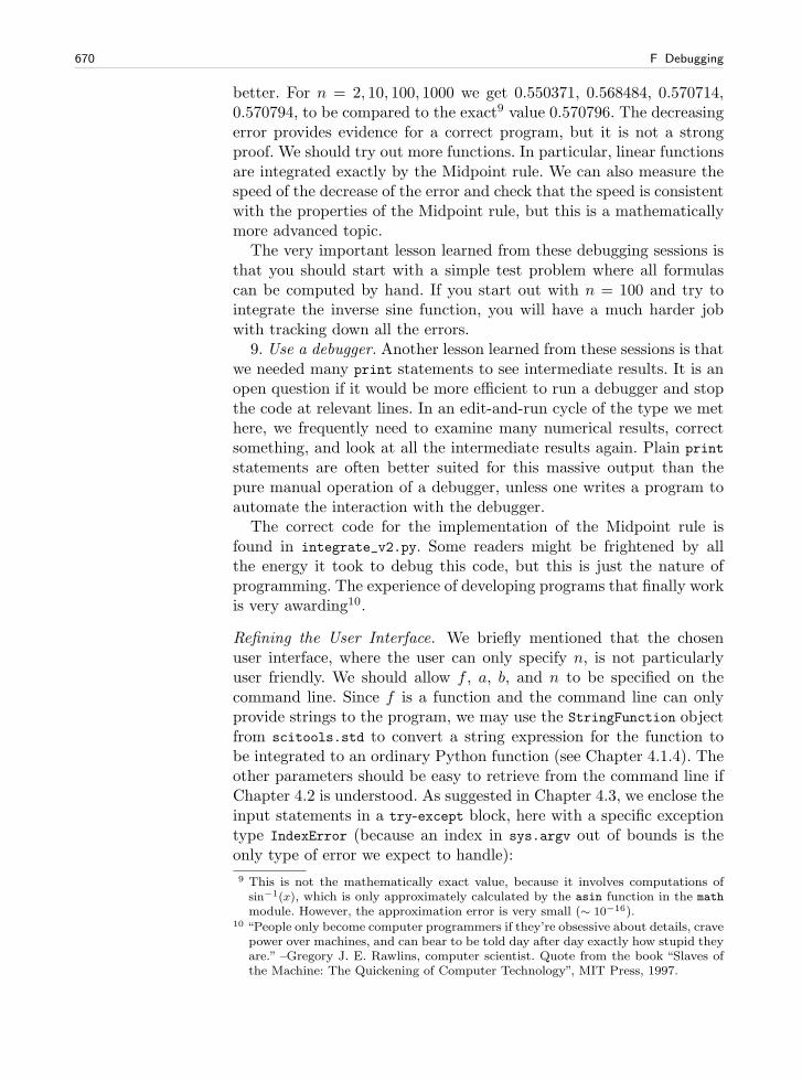
670 F Debugging

better. For n = 2, 10, 100, 1000 we get 0.550371, 0.568484, 0.570714,0.570794, to be compared to the exact9 value 0.570796. The decreasingerror provides evidence for a correct program, but it is not a strongproof. We should try out more functions. In particular, linear functionsare integrated exactly by the Midpoint rule. We can also measure thespeed of the decrease of the error and check that the speed is consistentwith the properties of the Midpoint rule, but this is a mathematicallymore advanced topic.

The very important lesson learned from these debugging sessions isthat you should start with a simple test problem where all formulascan be computed by hand. If you start out with n = 100 and try tointegrate the inverse sine function, you will have a much harder jobwith tracking down all the errors.

9. Use a debugger. Another lesson learned from these sessions is thatwe needed many print statements to see intermediate results. It is anopen question if it would be more efficient to run a debugger and stopthe code at relevant lines. In an edit-and-run cycle of the type we methere, we frequently need to examine many numerical results, correctsomething, and look at all the intermediate results again. Plain print

statements are often better suited for this massive output than thepure manual operation of a debugger, unless one writes a program toautomate the interaction with the debugger.

The correct code for the implementation of the Midpoint rule isfound in integrate_v2.py. Some readers might be frightened by allthe energy it took to debug this code, but this is just the nature ofprogramming. The experience of developing programs that finally workis very awarding10.

Refining the User Interface. We briefly mentioned that the chosenuser interface, where the user can only specify n, is not particularlyuser friendly. We should allow f , a, b, and n to be specified on thecommand line. Since f is a function and the command line can onlyprovide strings to the program, we may use the StringFunction objectfrom scitools.std to convert a string expression for the function tobe integrated to an ordinary Python function (see Chapter 4.1.4). Theother parameters should be easy to retrieve from the command line ifChapter 4.2 is understood. As suggested in Chapter 4.3, we enclose theinput statements in a try-except block, here with a specific exceptiontype IndexError (because an index in sys.argv out of bounds is theonly type of error we expect to handle):

9 This is not the mathematically exact value, because it involves computations ofsin−1(x), which is only approximately calculated by the asin function in the math

module. However, the approximation error is very small (∼ 10−16).10 “People only become computer programmers if they’re obsessive about details, crave

power over machines, and can bear to be told day after day exactly how stupid theyare.” –Gregory J. E. Rawlins, computer scientist. Quote from the book “Slaves ofthe Machine: The Quickening of Computer Technology”, MIT Press, 1997.

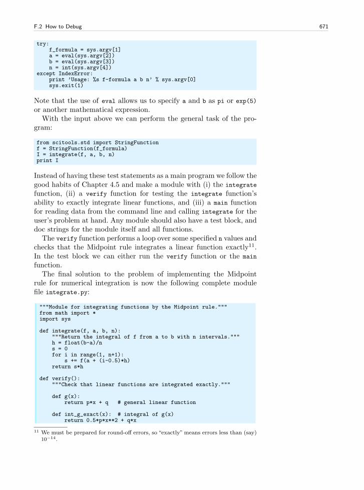
F.2 How to Debug 671

try:f_formula = sys.argv[1]a = eval(sys.argv[2])b = eval(sys.argv[3])n = int(sys.argv[4])

except IndexError:print ’Usage: %s f-formula a b n’ % sys.argv[0]sys.exit(1)

Note that the use of eval allows us to specify a and b as pi or exp(5)

or another mathematical expression.With the input above we can perform the general task of the pro-

gram:

from scitools.std import StringFunctionf = StringFunction(f_formula)I = integrate(f, a, b, n)print I

Instead of having these test statements as a main program we follow thegood habits of Chapter 4.5 and make a module with (i) the integrate

function, (ii) a verify function for testing the integrate function’sability to exactly integrate linear functions, and (iii) a main functionfor reading data from the command line and calling integrate for theuser’s problem at hand. Any module should also have a test block, anddoc strings for the module itself and all functions.

The verify function performs a loop over some specified n values andchecks that the Midpoint rule integrates a linear function exactly11.In the test block we can either run the verify function or the main

function.The final solution to the problem of implementing the Midpoint

rule for numerical integration is now the following complete modulefile integrate.py:

"""Module for integrating functions by the Midpoint rule."""from math import *import sys

def integrate(f, a, b, n):"""Return the integral of f from a to b with n intervals."""h = float(b-a)/ns = 0for i in range(1, n+1):

s += f(a + (i-0.5)*h)return s*h

def verify():"""Check that linear functions are integrated exactly."""

def g(x):return p*x + q # general linear function

def int_g_exact(x): # integral of g(x)return 0.5*p*x**2 + q*x

11 We must be prepared for round-off errors, so “exactly”means errors less than (say)10−14.

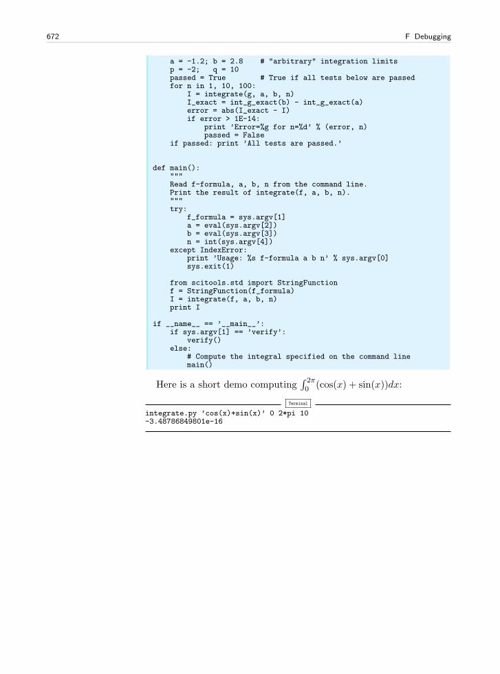
672 F Debugging

a = -1.2; b = 2.8 # "arbitrary" integration limitsp = -2; q = 10passed = True # True if all tests below are passedfor n in 1, 10, 100:

I = integrate(g, a, b, n)I_exact = int_g_exact(b) - int_g_exact(a)error = abs(I_exact - I)if error > 1E-14:

print ’Error=%g for n=%d’ % (error, n)passed = False

if passed: print ’All tests are passed.’

def main():"""Read f-formula, a, b, n from the command line.Print the result of integrate(f, a, b, n)."""try:

f_formula = sys.argv[1]a = eval(sys.argv[2])b = eval(sys.argv[3])n = int(sys.argv[4])

except IndexError:print ’Usage: %s f-formula a b n’ % sys.argv[0]sys.exit(1)

from scitools.std import StringFunctionf = StringFunction(f_formula)I = integrate(f, a, b, n)print I

if __name__ == ’__main__’:if sys.argv[1] == ’verify’:

verify()else:

# Compute the integral specified on the command linemain()

Here is a short demo computing∫ 2π0 (cos(x) + sin(x))dx:

Terminal

integrate.py ’cos(x)+sin(x)’ 0 2*pi 10-3.48786849801e-16

Technical Topics G

G.1 Different Ways of Running Python Programs

Python programs are compiled and interpreted by another programcalled python. To run a Python program, you need to tell the operatingsystem that your program is to be interpreted by the python program.This section explains various ways of doing this.

G.1.1 Executing Python Programs in IPython

The simplest and most flexible way of executing a Python program isto run it inside IPython. See Chapter 1.5.3 for a quick introductionto IPython. You start IPython either by the command ipython in aterminal window, or by double-clicking the IPython program icon (onWindows). Then, inside IPython, you can run a program prog.py by

In [1]: run prog.py arg1 arg2

where arg1 and arg2 are command-line arguments.This method of running Python programs works the same way on

all platforms. One additional advantage of running programs underIPython is that you can automatically enter the Python debugger if anexception is raised (see Appendix F.1. Although we advocate runningPython programs under IPython in this book, you can also run themdirectly under specific operating systems. This is explained next forUnix, Windows, and Mac OS X.

G.1.2 Executing Python Programs on Unix

There are two ways of executing a Python program prog.py on Unix.The first explicitly tells which Python interpreter to use:

673

674 G Technical Topics

Terminal

Unix> python prog.py arg1 arg2

Here, arg1 and arg2 are command-line arguments.There may be many Python interpreters on your computer system,

usually corresponding to different versions of Python or different setsof additional packages and modules. The Python interpreter (python)used in the command above is the first program with the name python

appearing in the folders listed in your PATH environment variable. Aspecific python interpreter, say in /home/hpl/local/bin, can easily beused to run a program prog.py in the current working folder by speci-fying the interpreter’s complete filepath:

Terminal

Unix> /home/hpl/bin/python prog.py arg1 arg2

The other way of executing Python programs on Unix consists ofjust writing the name of the file:

Terminal

Unix> ./prog.py arg1 arg2

The leading ./ is needed to tell that the program is located in thecurrent folder. You can also just write

Terminal

Unix> prog.py arg1 arg2

but then you need to have the dot1 in the PATH variable, and this isnot recommended for security reasons.

In the two latter commands there is no information on which Pythoninterpreter to use. This information must be provided in the first lineof the program, normally as

#!/usr/bin/env python

This looks like a comment line, and behaves indeed as a comment linewhen we run the program as python prog.py. However, when we runthe program as ./prog.py, the first line beginning with #! tells theoperating system to use the program specified in the rest of the firstline to interpret the program. In this example, we use the first pythonprogram encountered in the folders in your PATH variable. Alternatively,a specific python program can be specified as

1 The dot acts as the name of the current folder (usually known as the current workingdirectory). A double dot is the name of the parent folder.

G.1 Different Ways of Running Python Programs 675

#!/home/hpl/special/tricks/python

It is a good habit to always include such a first line (also called she-bang line) in all Python programs and modules, but we have not donethat in this book.

G.1.3 Executing Python Programs on Windows

In a DOS window you can always run a Python program by

Terminal

DOS> python prog.py arg1 arg2

if prog.py is the name of the program, and arg1 and arg2 are command-line arguments. The extension .py can be dropped:

Terminal

DOS> python prog arg1 arg2

If there are several Python installations on your system, a particularinstallation can be specified:

Terminal

DOS> E:\hpl\myprogs\Python2.5.3\python prog arg1 arg2

Files with a certain extension can on Windows be associated with afile type, and a file type can be associated with a particular program tohandle the file. For example, it is natural to associate the extension .py

with Python programs. The corresponding program needed to interpret.py files is then python.exe. When we write just the name of the Pythonprogram file, as in

Terminal

DOS> prog arg1 arg2

the file is always interpreted by the specified python.exe program. Thedetails of getting .py files to be interpreted by python.exe go as follows:

Terminal

DOS> assoc .py=PyProgDOS> ftype PyProg=python.exe "%1" %*

Depending on your Python installation, such file extension bindingsmay already be done. You can check this with

Terminal

DOS> assoc | find "py"

676 G Technical Topics

To see the programs associated with a file type, write ftype name wherename is the name of the file type as specified by the assoc command.Writing help ftype and help assoc prints out more information aboutthese commands along with examples.

One can also run Python programs by writing just the basename ofthe program file, i.e., prog.py instead of prog.py, if the file extensionis registered in the PATHEXT environment variable.

Double-Clicking Python Files. The usual way of running programs onWindows is to double click on the file icon. This does not work well withPython programs without a graphical user interface. When you doubleclick on the icon for a file prog.py, a DOS window is opened, prog.pyis interpreted by some python.exe program, and when the programterminates, the DOS window is closed. There is usually too little timefor the user to observe the output in this short-lived DOS window.

One can always insert a final statement that pauses the program bywaiting for input from the user:

raw_input(’Type CR:’)

or

sys.stdout.write(’Type CR:’); sys.stdin.readline()

The program will “hang” until the user presses the Return key. Duringthis pause the DOS window is visible and you can watch the outputfrom previous statements in the program.

The downside of including a final input statement is that you mustalways hit Return before the program terminates. This is inconvenientif the program is moved to a Unix-type machine. One possibility is tolet this final input statement be active only when the program is runon Windows:

if sys.platform[:3] == ’win’:raw_input(’Type CR:’)

Python programs that have a graphical user interface can be double-clicked in the usual way if the file extension is .pyw.

Gnuplot Plots on Windows. Programs that call plot to visualize agraph with the aid of Gnuplot suffer from the same problem as de-scribed above: the plot window disappears quickly. Again, the recipeis to insert a raw_input call at the end of the program.

G.2 Integer and Float Division 677

G.1.4 Executing Python Programs on Macintosh

Since a variant of Unix is used as core in the Mac OS X operatingsystem, you can always launch a Unix terminal and use the techniquesfrom Appendix G.1.2 to run Python programs.

G.1.5 Making a Complete Stand-Alone Executable

Python programs need a Python interpreter and usually a set of mod-ules to be installed on the computer system. Sometimes this is incon-venient, for instance when you want to give your program to somebodywho does not necessarily have Python or the required set of modulesinstalled.

Fortunately, there are tools that can create a stand-alone executableprogram out of a Python program. This stand-alone executable can berun on every computer that has the same type of operating systemand the same chip type. Such a stand-alone executable is a bundlingof the Python interpreter and the required modules, along with yourprogram, in a single file. Details of producing this single file are givenin the book [9].

G.2 Integer and Float Division

Many languages, including C, C++, Fortran, and classical Python,interpret the division operator in two ways:

1. Integer division: If both operands a and b are integers, the result a/bis the floor of the mathematical result a/b. This yields the largestinteger that b can be multiplied with such that the product is lessthan or equal to a. Or phrased simpler: The result of a/b is aninteger which is “rounded down”. As an example, 5/2 becomes 2.

2. Float division: If one of the operands is a floating-point numberor a complex number, a/b returns the mathematical result of thedivision.

Accidental integer division in places where mathematical division isneeded, constitutes a very common source of errors in numerical pro-grams.

It is often argued that in a statically typed language, where eachvariable is declared with a fixed type, the programmer always knowsthe type of the operands involved in a division expression. Therefore theprogrammer can determine whether an expression has the right formor not (the programmer can still oversee such errors). In a dynamicallytyped language, such as Python, variables can hold objects of any type.If a or b is provided by the user of the program, one can never know ifboth types end up as integer and a/b will imply integer division.

678 G Technical Topics

The only safe solution is to have two different operands for inte-ger division and mathematical division. Python is currently moving inthis direction. By default, a/b still has its original double meaning, de-pending on the types of operands. A new operator // is introduced forexplicitly employing integer division. To force a/b to mean standardmathematical float division, one can write

from __future__ import division

This import statement must be present in every module file or scriptwhere the / operator always shall imply float division. Alternatively,one can run a Python program someprogram.py from the command linewith the argument -Qnew to the Python interpreter:

Unix/DOS> python -Qnew someprogram.py

The future Python 3.0 is suggested to abandon integer division inter-pretation of a/b, i.e., a/b will always mean the relevant float division,depending on the operands (float division for int and float operands,and complex division if one of the operands is a complex).

Running a Python program with the -Qwarnall argument, say

Unix/DOS> python -Qwarnall someprogram.py

will print out a warning every time an integer division expression isencountered.

There are currently alternative ways out of the integer division prob-lem:

1. If the operands involve an integer with fixed value, such as in a/2,the integer can be written as a floating-point number, as in a/2.0

or a/2., to enforce mathematical division regardless of whether a isinteger, float, or complex.

2. If both operands are variables, as in a/b, the only safe way out ofthe problem is to write 1.0*a/b. Note that float(a)/b or a/float(b)will work correctly from a mathematical viewpoint if a and b are ofinteger or floating-point type, but not if the argument to float iscomplex.

G.3 Visualizing a Program with Lumpy

Lumpy is a nice tool for graphically displaying the relations betweenthe variables in a program. Consider the following program (inspiredby Chapter 2.4.3), where we extract a sublist and modify the originallist:

l0 = [1, 4, 3]l1 = l0l2 = l1[:-1]l1[0] = 100

G.3 Visualizing a Program with Lumpy 679

The point is that the change in l1 is reflected in l0, but not in l2,because sublists are created by taking a copy of the original list, whilel1 and l0 refer to the same object. Lumpy can visually display thevariables and how they relate, and thereby making it obvious that l0

and l1 refer to the same object and that l2 is a different object. Touse Lumpy, some extra statements must be inserted in the program:

from scitools.Lumpy import Lumpylumpy = Lumpy()lumpy.make_reference()l0 = [1, 4, 3]l1 = l0l2 = l1[:-1]l1[0] = 100lumpy.object_diagram()

By running this program a graphical window is shown on the screenwith the variables in the program, see Figure G.1a. The variables havelines to the object they point to, and inside the objects we can see thecontents, i.e., the list elements in this case.

We can add some lines to the program above and make a new,additional drawing:

lumpy = Lumpy()lumpy.make_reference()n1 = 21.5n2 = 21l3 = [l1, l2, [n1, n2]]s1 = ’some string’lumpy.object_diagram()

Figure G.1b shows the second object diagram with the additional vari-ables.

We recommend to actively use Lumpy to make graphical illustrationsof programs, especially if you search for an error and you are not 100%sure of how all variables related to each other.

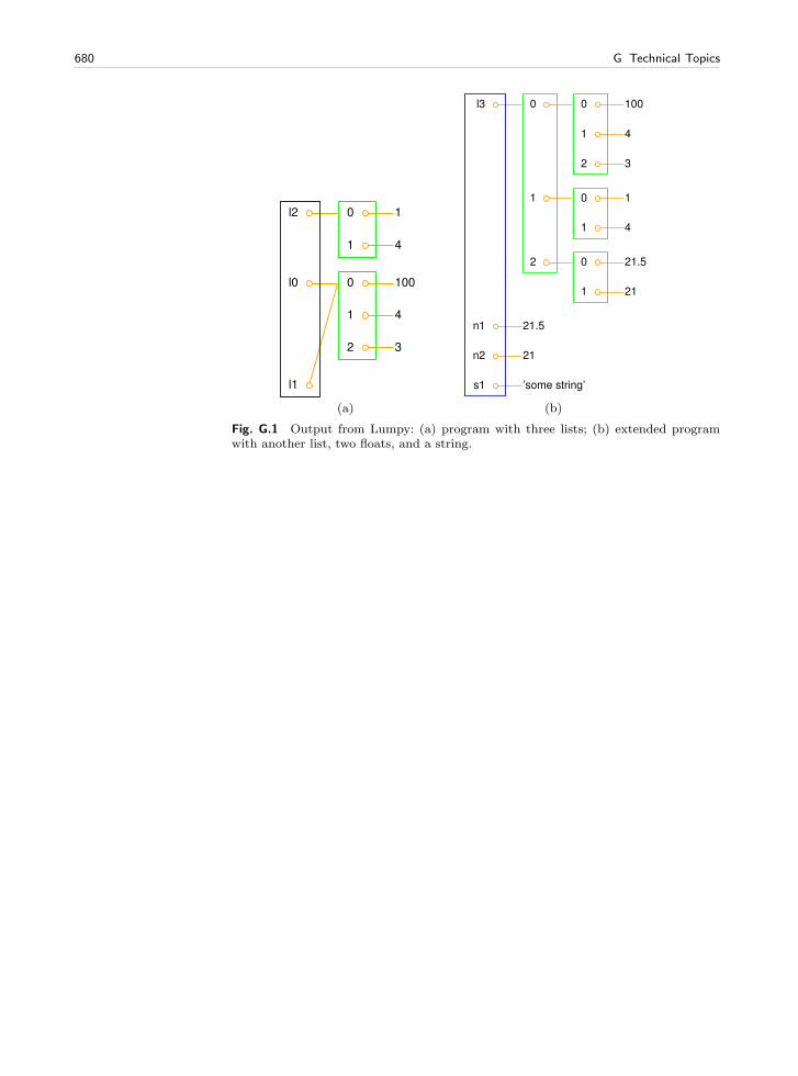
680 G Technical Topics

l2 0 1

1 4

l0 0 100

1 4

2 3

l1

(a)

l3 0 0 100

1 4

2 3

1 0 1

1 4

2 0 21.5

1 21

n1 21.5

n2 21

s1 ’some string’

(b)

Fig. G.1 Output from Lumpy: (a) program with three lists; (b) extended programwith another list, two floats, and a string.

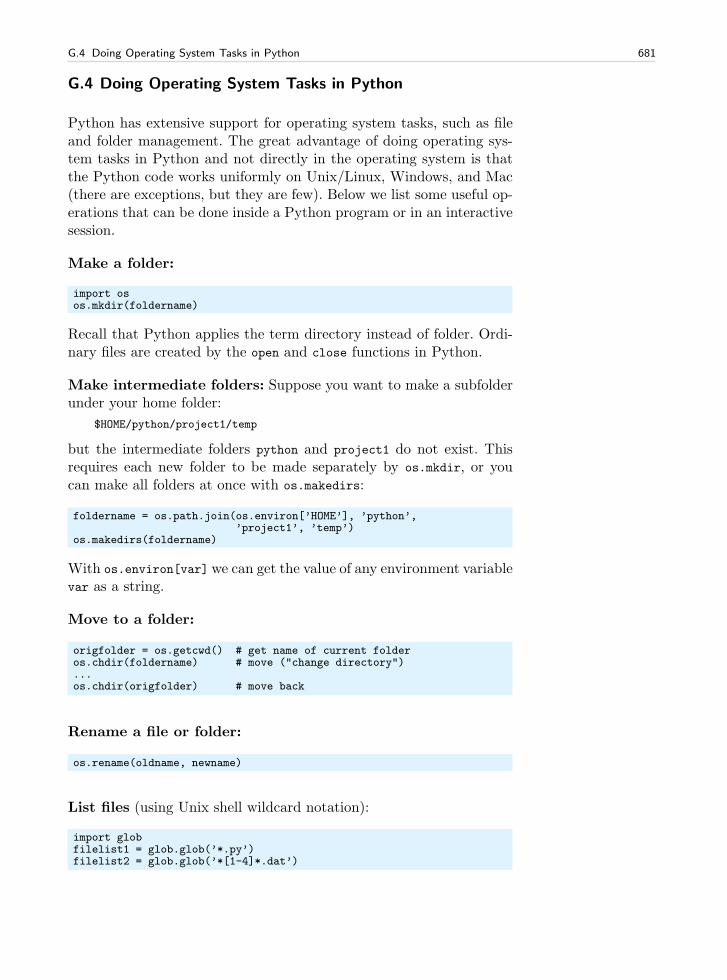
G.4 Doing Operating System Tasks in Python 681

G.4 Doing Operating System Tasks in Python

Python has extensive support for operating system tasks, such as fileand folder management. The great advantage of doing operating sys-tem tasks in Python and not directly in the operating system is thatthe Python code works uniformly on Unix/Linux, Windows, and Mac(there are exceptions, but they are few). Below we list some useful op-erations that can be done inside a Python program or in an interactivesession.

Make a folder:

import osos.mkdir(foldername)

Recall that Python applies the term directory instead of folder. Ordi-nary files are created by the open and close functions in Python.

Make intermediate folders: Suppose you want to make a subfolderunder your home folder:

$HOME/python/project1/temp

but the intermediate folders python and project1 do not exist. Thisrequires each new folder to be made separately by os.mkdir, or youcan make all folders at once with os.makedirs:

foldername = os.path.join(os.environ[’HOME’], ’python’,’project1’, ’temp’)

os.makedirs(foldername)

With os.environ[var] we can get the value of any environment variablevar as a string.

Move to a folder:

origfolder = os.getcwd() # get name of current folderos.chdir(foldername) # move ("change directory")...os.chdir(origfolder) # move back

Rename a file or folder:

os.rename(oldname, newname)

List files (using Unix shell wildcard notation):

import globfilelist1 = glob.glob(’*.py’)filelist2 = glob.glob(’*[1-4]*.dat’)

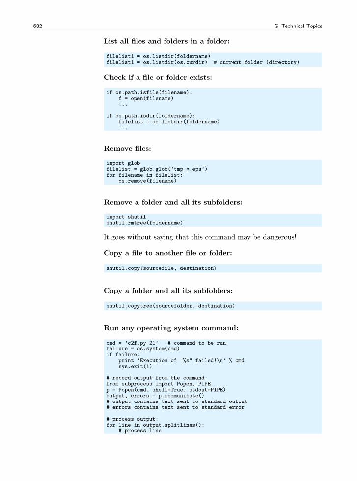
682 G Technical Topics

List all files and folders in a folder:

filelist1 = os.listdir(foldername)filelist1 = os.listdir(os.curdir) # current folder (directory)

Check if a file or folder exists:

if os.path.isfile(filename):f = open(filename)...

if os.path.isdir(foldername):filelist = os.listdir(foldername)...

Remove files:

import globfilelist = glob.glob(’tmp_*.eps’)for filename in filelist:

os.remove(filename)

Remove a folder and all its subfolders:

import shutilshutil.rmtree(foldername)

It goes without saying that this command may be dangerous!

Copy a file to another file or folder:

shutil.copy(sourcefile, destination)

Copy a folder and all its subfolders:

shutil.copytree(sourcefolder, destination)

Run any operating system command:

cmd = ’c2f.py 21’ # command to be runfailure = os.system(cmd)if failure:

print ’Execution of "%s" failed!\n’ % cmdsys.exit(1)

# record output from the command:from subprocess import Popen, PIPEp = Popen(cmd, shell=True, stdout=PIPE)output, errors = p.communicate()# output contains text sent to standard output# errors contains text sent to standard error

# process output:for line in output.splitlines():

# process line

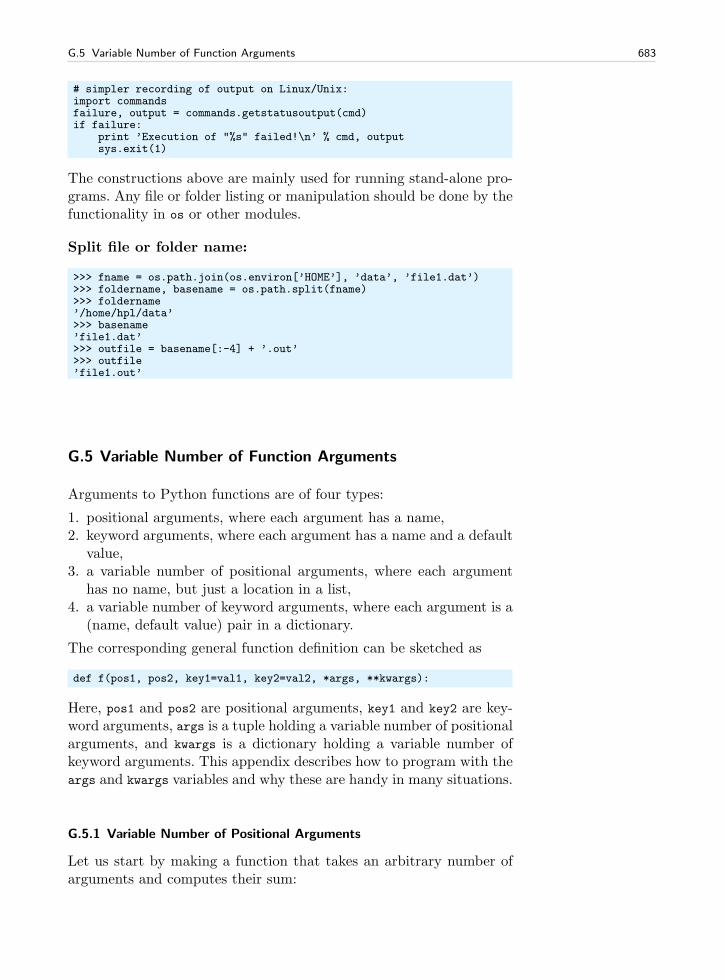
G.5 Variable Number of Function Arguments 683

# simpler recording of output on Linux/Unix:import commandsfailure, output = commands.getstatusoutput(cmd)if failure:

print ’Execution of "%s" failed!\n’ % cmd, outputsys.exit(1)

The constructions above are mainly used for running stand-alone pro-grams. Any file or folder listing or manipulation should be done by thefunctionality in os or other modules.

Split file or folder name:

>>> fname = os.path.join(os.environ[’HOME’], ’data’, ’file1.dat’)>>> foldername, basename = os.path.split(fname)>>> foldername’/home/hpl/data’>>> basename’file1.dat’>>> outfile = basename[:-4] + ’.out’>>> outfile’file1.out’

G.5 Variable Number of Function Arguments

Arguments to Python functions are of four types:

1. positional arguments, where each argument has a name,2. keyword arguments, where each argument has a name and a default

value,3. a variable number of positional arguments, where each argument

has no name, but just a location in a list,4. a variable number of keyword arguments, where each argument is a

(name, default value) pair in a dictionary.

The corresponding general function definition can be sketched as

def f(pos1, pos2, key1=val1, key2=val2, *args, **kwargs):

Here, pos1 and pos2 are positional arguments, key1 and key2 are key-word arguments, args is a tuple holding a variable number of positionalarguments, and kwargs is a dictionary holding a variable number ofkeyword arguments. This appendix describes how to program with theargs and kwargs variables and why these are handy in many situations.

G.5.1 Variable Number of Positional Arguments

Let us start by making a function that takes an arbitrary number ofarguments and computes their sum:

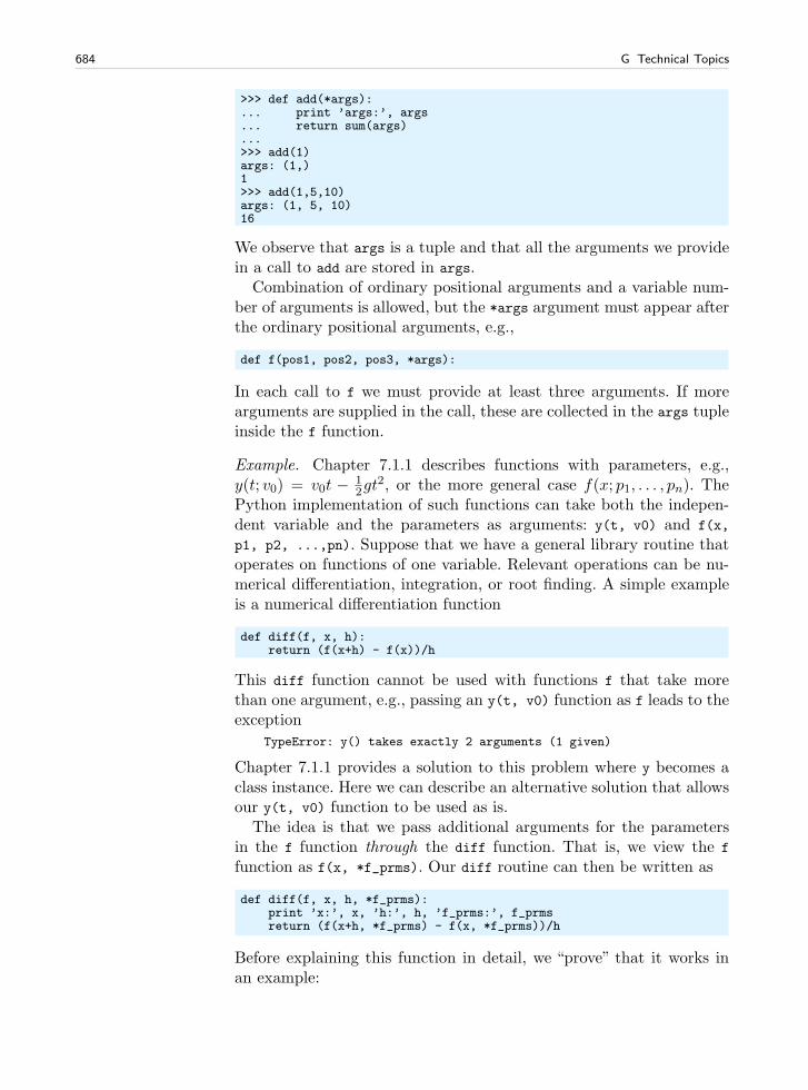
684 G Technical Topics

>>> def add(*args):... print ’args:’, args... return sum(args)...>>> add(1)args: (1,)1>>> add(1,5,10)args: (1, 5, 10)16

We observe that args is a tuple and that all the arguments we providein a call to add are stored in args.

Combination of ordinary positional arguments and a variable num-ber of arguments is allowed, but the *args argument must appear afterthe ordinary positional arguments, e.g.,

def f(pos1, pos2, pos3, *args):

In each call to f we must provide at least three arguments. If morearguments are supplied in the call, these are collected in the args tupleinside the f function.

Example. Chapter 7.1.1 describes functions with parameters, e.g.,y(t; v0) = v0t − 1

2gt2, or the more general case f(x; p1, . . . , pn). The

Python implementation of such functions can take both the indepen-dent variable and the parameters as arguments: y(t, v0) and f(x,

p1, p2, ...,pn). Suppose that we have a general library routine thatoperates on functions of one variable. Relevant operations can be nu-merical differentiation, integration, or root finding. A simple exampleis a numerical differentiation function

def diff(f, x, h):return (f(x+h) - f(x))/h

This diff function cannot be used with functions f that take morethan one argument, e.g., passing an y(t, v0) function as f leads to theexception

TypeError: y() takes exactly 2 arguments (1 given)

Chapter 7.1.1 provides a solution to this problem where y becomes aclass instance. Here we can describe an alternative solution that allowsour y(t, v0) function to be used as is.

The idea is that we pass additional arguments for the parametersin the f function through the diff function. That is, we view the f

function as f(x, *f_prms). Our diff routine can then be written as

def diff(f, x, h, *f_prms):print ’x:’, x, ’h:’, h, ’f_prms:’, f_prmsreturn (f(x+h, *f_prms) - f(x, *f_prms))/h

Before explaining this function in detail, we “prove” that it works inan example:

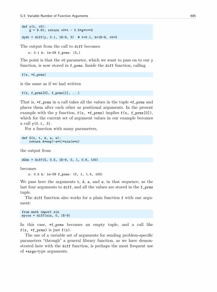
G.5 Variable Number of Function Arguments 685

def y(t, v0):g = 9.81; return v0*t - 0.5*g*t**2

dydt = diff(y, 0.1, 1E-9, 3) # t=0.1, h=1E-9, v0=3

The output from the call to diff becomes

x: 0.1 h: 1e-09 f_prms: (3,)

The point is that the v0 parameter, which we want to pass on to our yfunction, is now stored in f_prms. Inside the diff function, calling

f(x, *f_prms)

is the same as if we had written

f(x, f_prms[0], f_prms[1], ...)

That is, *f_prms in a call takes all the values in the tuple *f_prms andplaces them after each other as positional arguments. In the presentexample with the y function, f(x, *f_prms) implies f(x, f_prms[0]),which for the current set of argument values in our example becomesa call y(0.1, 3).

For a function with many parameters,

def G(x, t, A, a, w):return A*exp(-a*t)*sin(w*x)

the output from

dGdx = diff(G, 0.5, 1E-9, 0, 1, 0.6, 100)

becomesx: 0.5 h: 1e-09 f_prms: (0, 1, 1.5, 100)

We pass here the arguments t, A, a, and w, in that sequence, as thelast four arguments to diff, and all the values are stored in the f_prms

tuple.The diff function also works for a plain function f with one argu-

ment:

from math import sinmycos = diff(sin, 0, 1E-9)

In this case, *f_prms becomes an empty tuple, and a call likef(x, *f_prms) is just f(x).

The use of a variable set of arguments for sending problem-specificparameters “through” a general library function, as we have demon-strated here with the diff function, is perhaps the most frequent useof *args-type arguments.

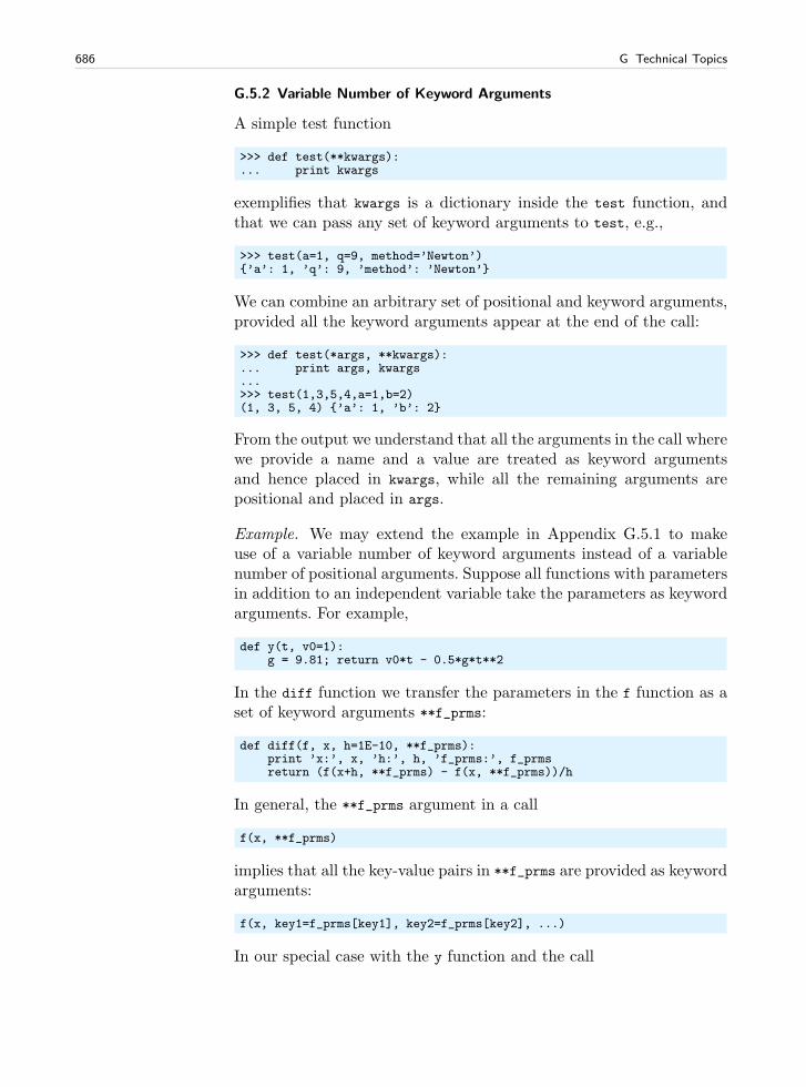
686 G Technical Topics

G.5.2 Variable Number of Keyword Arguments

A simple test function

>>> def test(**kwargs):... print kwargs

exemplifies that kwargs is a dictionary inside the test function, andthat we can pass any set of keyword arguments to test, e.g.,

>>> test(a=1, q=9, method=’Newton’)’a’: 1, ’q’: 9, ’method’: ’Newton’

We can combine an arbitrary set of positional and keyword arguments,provided all the keyword arguments appear at the end of the call:

>>> def test(*args, **kwargs):... print args, kwargs...>>> test(1,3,5,4,a=1,b=2)(1, 3, 5, 4) ’a’: 1, ’b’: 2

From the output we understand that all the arguments in the call wherewe provide a name and a value are treated as keyword argumentsand hence placed in kwargs, while all the remaining arguments arepositional and placed in args.

Example. We may extend the example in Appendix G.5.1 to makeuse of a variable number of keyword arguments instead of a variablenumber of positional arguments. Suppose all functions with parametersin addition to an independent variable take the parameters as keywordarguments. For example,

def y(t, v0=1):g = 9.81; return v0*t - 0.5*g*t**2

In the diff function we transfer the parameters in the f function as aset of keyword arguments **f_prms:

def diff(f, x, h=1E-10, **f_prms):print ’x:’, x, ’h:’, h, ’f_prms:’, f_prmsreturn (f(x+h, **f_prms) - f(x, **f_prms))/h

In general, the **f_prms argument in a call

f(x, **f_prms)

implies that all the key-value pairs in **f_prms are provided as keywordarguments:

f(x, key1=f_prms[key1], key2=f_prms[key2], ...)

In our special case with the y function and the call

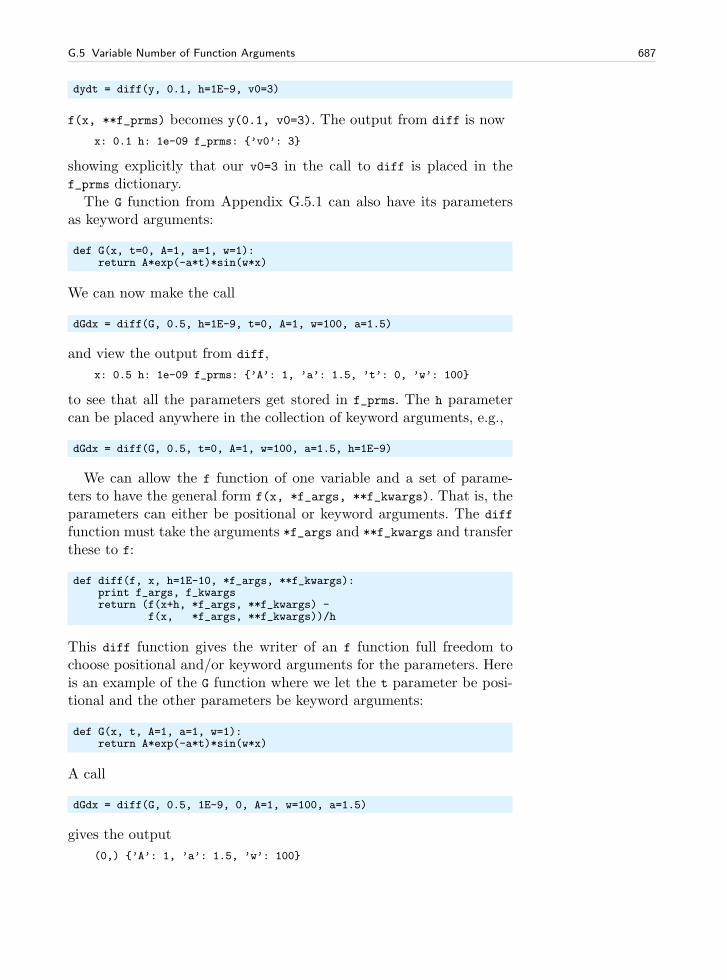
G.5 Variable Number of Function Arguments 687

dydt = diff(y, 0.1, h=1E-9, v0=3)

f(x, **f_prms) becomes y(0.1, v0=3). The output from diff is now

x: 0.1 h: 1e-09 f_prms: ’v0’: 3

showing explicitly that our v0=3 in the call to diff is placed in thef_prms dictionary.

The G function from Appendix G.5.1 can also have its parametersas keyword arguments:

def G(x, t=0, A=1, a=1, w=1):return A*exp(-a*t)*sin(w*x)

We can now make the call

dGdx = diff(G, 0.5, h=1E-9, t=0, A=1, w=100, a=1.5)

and view the output from diff,

x: 0.5 h: 1e-09 f_prms: ’A’: 1, ’a’: 1.5, ’t’: 0, ’w’: 100

to see that all the parameters get stored in f_prms. The h parametercan be placed anywhere in the collection of keyword arguments, e.g.,

dGdx = diff(G, 0.5, t=0, A=1, w=100, a=1.5, h=1E-9)

We can allow the f function of one variable and a set of parame-ters to have the general form f(x, *f_args, **f_kwargs). That is, theparameters can either be positional or keyword arguments. The diff

function must take the arguments *f_args and **f_kwargs and transferthese to f:

def diff(f, x, h=1E-10, *f_args, **f_kwargs):print f_args, f_kwargsreturn (f(x+h, *f_args, **f_kwargs) -

f(x, *f_args, **f_kwargs))/h

This diff function gives the writer of an f function full freedom tochoose positional and/or keyword arguments for the parameters. Hereis an example of the G function where we let the t parameter be posi-tional and the other parameters be keyword arguments:

def G(x, t, A=1, a=1, w=1):return A*exp(-a*t)*sin(w*x)

A call

dGdx = diff(G, 0.5, 1E-9, 0, A=1, w=100, a=1.5)

gives the output

(0,) ’A’: 1, ’a’: 1.5, ’w’: 100

688 G Technical Topics

showing that t is put in f_args and transferred as positional argumentto G, while A, a, and w are put in f_kwargs and transferred as keywordarguments. We remark that in the last call to diff, h and t must betreated as positional arguments, i.e., we cannot write h=1E-9 and t=0

unless all arguments in the call are on the name=value form.In the case we use both *f_args and **f_kwargs arguments in f and

there is no need for these arguments, *f_args becomes an empty tupleand **f_kwargs becomes an empty dictionary. The example

mycos = diff(sin, 0)

shows that the tuple and dictionary are indeed empty since diff justprints out

()

Therefore, a variable set of positional and keyword arguments can beincorporated in a general library function such as diff without anydisadvantage, just the benefit that diff works with different types f

functions: parameters as global variables, parameters as additional po-sitional arguments, parameters as additional keyword arguments, orparameters as instance variables (Chapter 7.1.2).

The program varargs1.py in the appendix folder implements theexamples in this appendix.

G.6 Evaluating Program Efficiency

G.6.1 Making Time Measurements

Time is not just “time” on a computer. The elapsed time or wall clocktime is the same time as you can measure on a watch or wall clock,while CPU time is the amount of time the program keeps the centralprocessing unit busy. The system time is the time spent on operatingsystem tasks like I/O. The concept user time is the difference betweenthe CPU and system times. If your computer is occupied by manyconcurrent processes, the CPU time of your program might be verydifferent from the elapsed time.

The time Module. Python has a time module with some useful func-tions for measuring the elapsed time and the CPU time:

import timee0 = time.time() # elapsed time since the epochc0 = time.clock() # total CPU time spent in the program so far<do tasks...>elapsed_time = time.time() - e0cpu_time = time.clock() - c0

G.6 Evaluating Program Efficiency 689

The term epoch means initial time (time.time() would return 0), whichis 00:00:00 January 1, 1970. The time module also has numerous func-tions for nice formatting of dates and time, and the more recentdatetime module has more functionality and an improved interface.Although the timing has a finer resolution than seconds, one shouldconstruct test cases that last some seconds to obtain reliable results.

The timeit Module. To measure the efficiency of a certain set of state-ments or an expression, the code should be run a large number oftimes so the overall CPU-time is of order seconds. The timeit mod-ule has functionality for running a code segment repeatedly. Below isan illustration of timeit for comparing the efficiency sin(1.2) versusmath.sin(1.2):

>>> import timeit>>> t = timeit.Timer(’sin(1.2)’, setup=’from math import sin’)>>> t.timeit(10000000) # run ’sin(1.2)’ 10000000 times11.830688953399658>>> t = timeit.Timer(’math.sin(1.2)’, setup=’import math’)>>> t.timeit(10000000)16.234833955764771

The first argument to the Timer constructor is a string containing thecode to execute repeatedly, while the second argument is the necessarycode for initialization. From this simple test we see that math.sin(1.2)runs almost 40 percent slower than sin(1.2)!

If you want to time a function, say f, defined in the same programas where you have the timeit call, the setup procedure must import fand perhaps other variables from the program, as exemplified in

t = timeit.Timer(’f(a,b)’, setup=’from __main__ import f, a, b’)

Here, f, a, and b are names initialized in the main program. Anotherexample is found in src/random/smart_power.py.

Hardware Information. Along with CPU-time measurements it is oftenconvenient to print out information about the hardware on which theexperiment was done. Python has a module platform with informationon the current hardware. The function scitools.misc.hardware_info

applies the platform module to extract relevant hardware information.A sample call is

>>> import scitools.misc, pprint>>> pprint.pprint(scitools.misc.hardware_info())’cpuinfo’:’CPU speed’: ’1196.170 Hz’,’CPU type’: ’Mobile Intel(R) Pentium(R) III CPU - M 1200MHz’,’cache size’: ’512 KB’,’vendor ID’: ’GenuineIntel’,

’identifier’: ’Linux-2.6.12-i686-with-debian-testing-unstable’,’python build’: (’r25:409’, ’Feb 27 2007 19:35:40’),’python version’: ’2.5.0’,’uname’: (’Linux’,

690 G Technical Topics

’ubuntu’,’2.6.12’,’#1 Fri Nov 25 10:58:24 CET 2005’,’i686’,’’)

G.6.2 Profiling Python Programs

A profiler computes the time spent in the various functions of a pro-gram. From the timings a ranked list of the most time-consuming func-tions can be created. This is an indispensable tool for detecting bot-tlenecks in the code, and you should always perform a profiling beforespending time on code optimization. The golden rule is to first writean easy-to-understand program, then verify it, then profile it, and thenthink about optimization2.

Python comes with two profilers implemented in the profile andhotshot modules, respectively. The Python Library Reference has agood introduction to profiling in Python (Chapter 10: “The PythonProfiler”). The results produced by the two alternative modules arenormally processed by a special statistics utility pstats developed foranalyzing profiling results. The usage of the profile, hotshot, andpstats modules is straightforward, but somewhat tedious so SciToolscomes with a command scitools profiler that allows you to profileany program (say) m.py by writing

Terminal

Unix/DOS> scitools profiler m.py c1 c2 c3

Here, c1, c2, and c3 are command-line arguments to m.py.We refer to the Python Library Reference for detailed information

on how to interpret the output. A sample output might read

1082 function calls (728 primitive calls) in 17.890 CPU seconds

Ordered by: internal timeList reduced from 210 to 20 due to restriction <20>

ncalls tottime percall cumtime percall filename:lineno(function)5 5.850 1.170 5.850 1.170 m.py:43(loop1)1 2.590 2.590 2.590 2.590 m.py:26(empty)5 2.510 0.502 2.510 0.502 m.py:32(myfunc2)5 2.490 0.498 2.490 0.498 m.py:37(init)1 2.190 2.190 2.190 2.190 m.py:13(run1)6 0.050 0.008 17.720 2.953 funcs.py:126(timer)

...

In this test, loop1 is the most expensive function, using 5.85 seconds,which is to be compared with 2.59 seconds for the next most time-consuming function, empty. The tottime entry is the total time spent

2 “Premature optimization is the root of all evil.” –Donald Knuth, computer scientist,1938-.

G.6 Evaluating Program Efficiency 691

in a specific function, while cumtime reflects the total time spent in thefunction and all the functions it calls.

The CPU time of a Python program typically increases with a factorof about five when run under the administration of the profilemodule.Nevertheless, the relative CPU time among the functions are probablynot much affected by the profiler overhead.

References

[1] D. Beazley. Python Essential Reference. SAMS, 2nd edition, 2001.[2] J. E. Grayson. Python and Tkinter Programming. Manning, 2000.[3] D. Harms and K. McDonald. The Quick Python Book. Manning,

1999.[4] D. E. Knuth. Theory and practice. EATCS Bull., 27:14–21, 1985.[5] H. P. Langtangen. Python Scripting for Computational Science,

volume 3 of Texts in Computational Science and Engineering.Springer, third edition, 2009.

[6] L. S. Lerner. Physics for Scientists and Engineers. Jones andBarlett, 1996.

[7] M. Lutz. Programming Python. O’Reilly, second edition, 2001.[8] M. Lutz and D. Ascher. Learning Python. O’Reilly, 1999.[9] A. Martelli. Python in a Nutshell. O’Reilly, 2003.

[10] J. D. Murray. Mathematical Biology I: An Introduction. Springer,3rd edition, 2007.

[11] F. M. White. Fluid Mechanics. McGraw-Hill, 2nd edition, 1986.

693

Index

**kwargs, 686*=, 54*args, 683+=, 54-=, 54/=, 54\n, 13

allocate, 185animate, 413API, 345aplotter (from scitools), 203append (list), 58application, 14application programming interface, 345argparse module, 141array (from numpy), 184array (datatype), 184array computing, 184array shape, 216, 217array slicing, 185asarray (from numpy), 214attribute (class), 310average, 380

backend (Easyviz), 195, 198base class, 438bin (histogram), 378binomial distribution, 175bits, 249blank lines in files, 269

blanks, 17body of a function, 92boolean expressions, 55break, 246bytes, 249

callable objects, 325callback function, 587check an object’s type, 28, 215, 346, 441check file/folder existence (in Python), 682class hierarchy, 437class relationship

derived class, 438has-a, 442inheritance, 438is-a, 442subclass, 438superclass, 438

closure, 456cmath module, 33command-line arguments, 137commands module, 682comments, 10comparing

floating-point numbers, 87objects, 87real numbers, 87

complex numbers, 31concatenate (from numpy), 517console (terminal) window, 4

695

696 Index

constructor (class), 309convergence rate, 492, 641convert program, 412copy files (in Python), 682copy folders (in Python), 682CPU time measurements, 688cumulative sum, 426curve plotting, 188

datetime module, 500, 689debugger tour, 655del, 58delete files (in Python), 202, 369, 682delete folders (in Python), 682derived class, 438dictionary, 252

comprehensions, 256functionality, 290nested, 258

difference equations, 498nonlinear, 514

differential equations, 561, 603, 604, 613dir function, 350directory, 1, 4, 681doc strings, 103dtype, 214duck typing, 348dynamic binding, 449dynamic typing, 347

editor, 3efficiency, 688efficiency measure, 405elapsed time, 688enumerate function, 65, 366environment variables, 681eval function, 131, 450event loop, 150except, 143Exception, 147exceptions, 143execute programs (from Python), 682execute Python program, 7, 29, 673expression, 16

factorial, 56

factorial function, 120factory function, 451find (string method), 266first-order ODEs, 570float_eq, 87Forward Euler scheme, 606Fourier series, 118function argumentskeyword, 101named, 101positional, 101

function body, 92function header, 92function inside function, 624functional programming, 456

Gaussian function, 45glob.glob function, 369, 681global, 94globals function, 93, 211, 592grid, 530

has-a class relationship, 442Heaviside function, 122heterogeneous lists, 183histogram (normalized), 378

Idle, 4immutable objects, 254, 335in-place array arithmetics, 213IndexError, 144, 145information hiding, 345initial condition, 498, 562, 582input (data), 17insert (list), 58instance (class), 310integer random numbers, 382interactive sessionsIPython, 29session recording (logging), 46standard Python shell, 26

interpolation, 231interval arithmetics, 355IPython, 29is, 100is-a class relationship, 442

Index 697

isdigit (string method), 268isinstance function, 75, 215, 346, 441isspace (string method), 268

join (string method), 269

keys (dictionaries), 253keyword arguments, 101, 683

Lagrange’s interpolation formula, 231lambda functions, 107, 110least squares approximation, 295len (list), 58line break, 13linspace (from numpy), 185, 216list comprehension, 65, 68list files (in Python), 681list functionality, 75list, nested, 66lists, 57logical expressions, 55loops, 52lower (string method), 268lstrip (string method), 269

Mac OS X, 18main program, 106make a folder (in Python), 681making graphs, 188making movie, 412math module, 23mean, 380mean (from numpy), 381, 415measure time in programs, 405mesh, 530method (class), 60method (in class), 310mod function, 115, 381module folders, 159modules, 151Monte Carlo integration, 401Monte Carlo simulation, 391move to a folder (in Python), 681multiple inheritance, 491mutable objects, 254, 335

named arguments, 101

NameError, 145namespace, 318nested dictionaries, 258nested lists, 67nested loops, 72newline character (line break), 13Newton’s method, 327, 509None, 100nonlinear difference equations, 514normal (from numpy.random), 382normally distributed random numbers, 381not, 55np prefix (numpy), 184np.array function, 184np.linspace function, 185np.zeros function, 184Numerical Python, 184NumPy, 184numpy, 184numpy.lib.scimath module, 33

object-based programming, 437object-oriented programming, 437objects, 20ODE, 561, 603operating system (OS), 18optimization of Python code, 690option-value pairs (command line), 140OrderedDict class, 254ordinary differential equations, 561, 603,

604os module, 681os.chdir function, 681os.listdir function, 682os.makedirs function, 681os.mkdir function, 681os.pardir, 159os.path.isdir function, 682os.path.isfile function, 682os.path.join function, 159, 681os.path.split function, 683os.remove function, 202, 369, 682os.rename function, 681os.system function, 682oscillating systems, 570, 577, 584, 629

698 Index

output (data), 17overloading (of methods), 460

parent class, 438pass, 345plot (from scitools), 195plotting, 188Poisson distribution, 176polymorphism, 460positional arguments, 101, 683pprint.pformat, 69pprint.pprint, 68pprint2 (from scitools), 68pretty print, 68private attributes (class), 345probability, 390profiler.py, 690profiling, 690protected attributes (class), 335, 345pydoc program, 80pyreport program, 42, 233

r_ (array creation), 216raise, 147randint (from numpy.random), 410randn (from numpy.random), 382random (from numpy.random), 379random (from numpy), 379random module, 376random numbers, 375

histogram, 378integers, 382integration, 401Monte Carlo simulation, 391normal distribution, 381random walk, 406statistics, 380uniform distribution, 377vectorization, 379

random walk, 406random.normalvariate function, 382random_integers (from numpy.random), 410raw_input function, 130refactoring, 167remove files (in Python), 202, 369, 682remove folders (in Python), 682

rename file/folder (in Python), 681replace (string method), 267resolution (mesh), 530round function, 29round-off errors, 25rounding float to integer, 29rstrip (string method), 269run programs (from Python), 682run Python program, 7, 29, 673

scalar (math. quantity), 180scalar code, 187scalar differential equation, 604scalar differential equations, 570scalar function, 604scaling, 505scitools.pprint2 module, 68scitools.pprint2.pprint, 69scitools.std, 194search for module files, 159Secant method, 525second-order ODEs, 570, 581, 629seed, 376sequence (data type), 76sequence (mathematical), 497shape (of an array), 216, 217shutil.copy function, 682shutil.copytree function, 682shutil.rmtree function, 682∑

notation, 76slicing, 69, 266sort (list), 123source code, 14special methods (in classes), 324split (string method), 267split filename, 683spread of a disease (model), 573standard deviation, 380standard error, 282standard input, 281standard output, 281statements, 15static class attributes, 351static class methods, 352static class variables, 351

Index 699

static typing, 347std (from numpy), 381, 415str2obj (from scitools), 160string, 11

case change, 268joining list elements, 269searching, 266splitting, 267stripping leading/trailing blanks, 269substitution, 267substrings, 266testing for number, 268

string slicing, 266StringFunction (from scitools), 136strip (string method), 269strong typing, 347subarrays, 185subclass, 438sublist, 69subprocess module, 682substitution (in text), 267substrings, 266sum (from numpy), 384superclass, 438syntax, 17SyntaxError, 145sys module, 137sys.argv, 137sys.exit function, 142sys.path, 159sys.stderr, 283sys.stdin, 281sys.stdout, 281system time, 688systems of differential equations, 570, 613

terminal window, 4test block (in module files), 153time

CPU, 688elapsed, 688system, 688user, 688

time module, 87, 111, 405, 407, 688timeit module, 689

timing utilities, 688triple-quoted strings, 13try, 143tuples, 73type function, 28type conversion, 28TypeError, 146

UML class diagram, 309uniform (from numpy.random), 379uniformly distributed random numbers,

377Unix, 18upper (string method), 268user (of a program), 18user time, 688user-defined datatype (class), 310using a debugger, 655

_v1 (version numbering), 19ValueError, 144, 145var (from numpy), 381, 415variable no. of function arguments, 683variance, 380vector computing, 179vectorization, 184, 186vectorized drawing of random numbers,

379vectors, 178

weak typing, 347whitespace, 17, 268widgets, 149Windows, 18wrap2callable function, 365wrapper code, 329

xrange function, 83, 186, 384

ZeroDivisionError, 145zeros (from numpy), 184zip function, 66

Editorial Policy

1. Textbooks on topics in the field of computational science and engineering will be considered. They should bewritten for courses in CSE education. Both graduate and undergraduate textbooks will be published in TCSE. Multi-disciplinary topics and multidisciplinary teams of authors are especially welcome.

2. Format: Only works in English will be considered. For evaluation purposes, manuscripts may be submitted in printor electronic form, in the latter case, preferably as pdf- or zipped ps- files. Authors are requested to use the LaTeX stylefiles available from Springer at: http://www.springer.com/authors/book+authors?SGWID= 0-154102-12-417900-0(for monographs, textbooks and similar)Electronic material can be included if appropriate. Please contact the publisher.

3. Those considering a book which might be suitable for the series are strongly advised to contact the publisher or theseries editors at an early stage.

General Remarks

Careful preparation of manuscripts will help keep production time short and ensure a satisfactory appearance of thefinished book.

The following terms and conditions hold:

Regarding free copies and royalties, the standard terms for Springer mathematics textbooks hold. Please write tomartin.peters@springer.com for details.

Authors are entitled to purchase further copies of their book and other Springer books for their personal use, at adiscount of 33.3 % directly from Springer-Verlag.

Series Editors

Timothy J. BarthNASA Ames Research CenterNAS DivisionMoffett Field, CA 94035, USAbarth@nas.nasa.gov

Michael GriebelInstitut für Numerische Simulationder Universität BonnWegelerstr. 653115 Bonn, Germanygriebel@ins.uni-bonn.de

David E. KeyesMathematical and Computer Sciencesand EngineeringKing Abdullah University of Scienceand TechnologyP.O. Box 55455Jeddah 21534, Saudi Arabiadavid.keyes@kaust.edu.sa

and

Department of Applied Physicsand Applied MathematicsColumbia University500 W. 120 th StreetNew York, NY 10027, USAkd2112@columbia.edu

Risto M. NieminenDepartment of Applied PhysicsAalto University School of Scienceand Technology00076 Aalto, Finlandristo.nieminen@tkk.fi

Dirk RooseDepartment of Computer ScienceKatholieke Universiteit LeuvenCelestijnenlaan 200A3001 Leuven-Heverlee, Belgiumdirk.roose@cs.kuleuven.be

Tamar SchlickDepartment of Chemistryand Courant Instituteof Mathematical SciencesNew York University251 Mercer StreetNew York, NY 10012, USAschlick@nyu.edu

Editor for Computational Scienceand Engineering at Springer:Martin PetersSpringer-VerlagMathematics Editorial IVTiergartenstrasse 1769121 Heidelberg, Germanymartin.peters@springer.com

Textsin Computational Scienceand Engineering

1. H. P. Langtangen, Computational Partial Differential Equations. Numerical Methods and Diffpack Pro-gramming. 2nd Edition

2. A. Quarteroni, F. Saleri, P. Gervasio, Scientific Computing with MATLAB and Octave. 3rd Edition

3. H. P. Langtangen, Python Scripting for Computational Science. 3rd Edition

4. H. Gardner, G. Manduchi, Design Patterns for e-Science.

5. M. Griebel, S. Knapek, G. Zumbusch, Numerical Simulation in Molecular Dynamics.

6. H. P. Langtangen, A Primer on Scientific Programming with Python. 2nd Edition

7. A. Tveito, H. P. Langtangen, B. F. Nielsen, X. Cai, Elements of Scientific Computing.

8. B. Gustafsson, Fundamentals of Scientific Computing

For further information on these books please have a look at our mathematics catalogue at the following URL:www.springer.com/series/5151

Monographsin Computational Scienceand Engineering

1. J. Sundnes, G.T. Lines, X. Cai, B.F. Nielsen, K.-A. Mardal, A. Tveito, Computing the Electrical Activity inthe Heart.

For further information on this book, please have a look at our mathematics catalogue at the following URL:www.springer.com/series/7417

Lecture Notesin Computational Scienceand Engineering

1. D. Funaro, Spectral Elements for Transport-Dominated Equations.

2. H.P. Langtangen, Computational Partial Differential Equations. Numerical Methods and Diffpack Program-ming.

3. W. Hackbusch, G. Wittum (eds.), Multigrid Methods V.

4. P. Deuflhard, J. Hermans, B. Leimkuhler, A.E. Mark, S. Reich, R.D. Skeel (eds.), Computational MolecularDynamics: Challenges, Methods, Ideas.

5. D. Kröner, M. Ohlberger, C. Rohde (eds.), An Introduction to Recent Developments in Theory and Numericsfor Conservation Laws.

6. S. Turek, Efficient Solvers for Incompressible Flow Problems. An Algorithmic and Computational Ap-proach.

7. R. von Schwerin, Multi Body System SIMulation. Numerical Methods, Algorithms, and Software.

8. H.-J. Bungartz, F. Durst, C. Zenger (eds.), High Performance Scientific and Engineering Computing.

9. T.J. Barth, H. Deconinck (eds.), High-Order Methods for Computational Physics.

10. H.P. Langtangen, A.M. Bruaset, E. Quak (eds.), Advances in Software Tools for Scientific Computing.

11. B. Cockburn, G.E. Karniadakis, C.-W. Shu (eds.), Discontinuous Galerkin Methods. Theory, Computationand Applications.

12. U. van Rienen, Numerical Methods in Computational Electrodynamics. Linear Systems in Practical Appli-cations.

13. B. Engquist, L. Johnsson, M. Hammill, F. Short (eds.), Simulation and Visualization on the Grid.

14. E. Dick, K. Riemslagh, J. Vierendeels (eds.), Multigrid Methods VI.

15. A. Frommer, T. Lippert, B. Medeke, K. Schilling (eds.), Numerical Challenges in Lattice Quantum Chro-modynamics.

16. J. Lang, Adaptive Multilevel Solution of Nonlinear Parabolic PDE Systems. Theory, Algorithm, and Appli-cations.

17. B.I. Wohlmuth, Discretization Methods and Iterative Solvers Based on Domain Decomposition.

18. U. van Rienen, M. Günther, D. Hecht (eds.), Scientific Computing in Electrical Engineering.

19. I. Babuška, P.G. Ciarlet, T. Miyoshi (eds.), Mathematical Modeling and Numerical Simulation in ContinuumMechanics.

20. T.J. Barth, T. Chan, R. Haimes (eds.), Multiscale and Multiresolution Methods. Theory and Applications.

21. M. Breuer, F. Durst, C. Zenger (eds.), High Performance Scientific and Engineering Computing.

22. K. Urban, Wavelets in Numerical Simulation. Problem Adapted Construction and Applications.

23. L.F. Pavarino, A. Toselli (eds.), Recent Developments in Domain Decomposition Methods.

24. T. Schlick, H.H. Gan (eds.), Computational Methods for Macromolecules: Challenges and Applications.

25. T.J. Barth, H. Deconinck (eds.), Error Estimation and Adaptive Discretization Methods in ComputationalFluid Dynamics.

26. M. Griebel, M.A. Schweitzer (eds.), Meshfree Methods for Partial Differential Equations.

27. S. Müller, Adaptive Multiscale Schemes for Conservation Laws.

28. C. Carstensen, S. Funken, W. Hackbusch, R.H.W. Hoppe, P. Monk (eds.), Computational Electromagnetics.

29. M.A. Schweitzer, A Parallel Multilevel Partition of Unity Method for Elliptic Partial Differential Equations.

30. T. Biegler, O. Ghattas, M. Heinkenschloss, B. van Bloemen Waanders (eds.), Large-Scale PDE-ConstrainedOptimization.

31. M. Ainsworth, P. Davies, D. Duncan, P. Martin, B. Rynne (eds.), Topics in Computational Wave Propagation.Direct and Inverse Problems.

32. H. Emmerich, B. Nestler, M. Schreckenberg (eds.), Interface and Transport Dynamics. Computational Mo-delling.

33. H.P. Langtangen, A. Tveito (eds.), Advanced Topics in Computational Partial Differential Equations. Nu-merical Methods and Diffpack Programming.

34. V. John, Large Eddy Simulation of Turbulent Incompressible Flows. Analytical and Numerical Results for aClass of LES Models.

35. E. Bänsch (ed.), Challenges in Scientific Computing - CISC 2002.

36. B.N. Khoromskij, G. Wittum, Numerical Solution of Elliptic Differential Equations by Reduction to theInterface.

37. A. Iske, Multiresolution Methods in Scattered Data Modelling.

38. S.-I. Niculescu, K. Gu (eds.), Advances in Time-Delay Systems.

39. S. Attinger, P. Koumoutsakos (eds.), Multiscale Modelling and Simulation.

40. R. Kornhuber, R. Hoppe, J. Périaux, O. Pironneau, O. Wildlund, J. Xu (eds.), Domain Decomposition Me-thods in Science and Engineering.

41. T. Plewa, T. Linde, V.G. Weirs (eds.), Adaptive Mesh Refinement – Theory and Applications.

42. A. Schmidt, K.G. Siebert, Design of Adaptive Finite Element Software. The Finite Element Toolbox AL-BERTA.

43. M. Griebel, M.A. Schweitzer (eds.), Meshfree Methods for Partial Differential Equations II.

44. B. Engquist, P. Lötstedt, O. Runborg (eds.), Multiscale Methods in Science and Engineering.

45. P. Benner, V. Mehrmann, D.C. Sorensen (eds.), Dimension Reduction of Large-Scale Systems.

46. D. Kressner, Numerical Methods for General and Structured Eigenvalue Problems.

47. A. Boriçi, A. Frommer, B. Joó, A. Kennedy, B. Pendleton (eds.), QCD and Numerical Analysis III.

48. F. Graziani (ed.), Computational Methods in Transport.

49. B. Leimkuhler, C. Chipot, R. Elber, A. Laaksonen, A. Mark, T. Schlick, C. Schütte, R. Skeel (eds.), NewAlgorithms for Macromolecular Simulation.

50. M. Bücker, G. Corliss, P. Hovland, U. Naumann, B. Norris (eds.), Automatic Differentiation: Applications,Theory, and Implementations.

51. A.M. Bruaset, A. Tveito (eds.), Numerical Solution of Partial Differential Equations on Parallel Computers.

52. K.H. Hoffmann, A. Meyer (eds.), Parallel Algorithms and Cluster Computing.

53. H.-J. Bungartz, M. Schäfer (eds.), Fluid-Structure Interaction.

54. J. Behrens, Adaptive Atmospheric Modeling.

55. O. Widlund, D. Keyes (eds.), Domain Decomposition Methods in Science and Engineering XVI.

56. S. Kassinos, C. Langer, G. Iaccarino, P. Moin (eds.), Complex Effects in Large Eddy Simulations.

57. M. Griebel, M.A Schweitzer (eds.), Meshfree Methods for Partial Differential Equations III.

58. A.N. Gorban, B. Kégl, D.C. Wunsch, A. Zinovyev (eds.), Principal Manifolds for Data Visualization andDimension Reduction.

59. H. Ammari (ed.), Modeling and Computations in Electromagnetics: A Volume Dedicated to Jean-ClaudeNédélec.

60. U. Langer, M. Discacciati, D. Keyes, O. Widlund, W. Zulehner (eds.), Domain Decomposition Methods inScience and Engineering XVII.

61. T. Mathew, Domain Decomposition Methods for the Numerical Solution of Partial Differential Equations.

62. F. Graziani (ed.), Computational Methods in Transport: Verification and Validation.

63. M. Bebendorf, Hierarchical Matrices. A Means to Efficiently Solve Elliptic Boundary Value Problems.

64. C.H. Bischof, H.M. Bücker, P. Hovland, U. Naumann, J. Utke (eds.), Advances in Automatic Differentiation.

65. M. Griebel, M.A. Schweitzer (eds.), Meshfree Methods for Partial Differential Equations IV.

66. B. Engquist, P. Lötstedt, O. Runborg (eds.), Multiscale Modeling and Simulation in Science.

67. I.H. Tuncer, Ü. Gülcat, D.R. Emerson, K. Matsuno (eds.), Parallel Computational Fluid Dynamics 2007.

68. S. Yip, T. Diaz de la Rubia (eds.), Scientific Modeling and Simulations.

69. A. Hegarty, N. Kopteva, E. O’Riordan, M. Stynes (eds.), BAIL 2008 – Boundary and Interior Layers.

70. M. Bercovier, M.J. Gander, R. Kornhuber, O. Widlund (eds.), Domain Decomposition Methods in Scienceand Engineering XVIII.

71. B. Koren, C. Vuik (eds.), Advanced Computational Methods in Science and Engineering.

72. M. Peters (ed.), Computational Fluid Dynamics for Sport Simulation.

73. H.-J. Bungartz, M. Mehl, M. Schäfer (eds.), Fluid Structure Interaction II - Modelling, Simulation, Optimi-zation.

74. D. Tromeur-Dervout, G. Brenner, D.R. Emerson, J. Erhel (eds.), Parallel Computational Fluid Dynamics2008.

75. A.N. Gorban, D. Roose (eds.), Coping with Complexity: Model Reduction and Data Analysis.

76. J.S. Hesthaven, E.M. Rønquist (eds.), Spectral and High Order Methods for Partial Differential Equations.

77. M. Holtz, Sparse Grid Quadrature in High Dimensions with Applications in Finance and Insurance.

78. Y. Huang, R. Kornhuber, O.Widlund, J. Xu (eds.), Domain Decomposition Methods in Science and Engi-neering XIX.

79. M. Griebel, M. A. Schweitzer (eds.), Meshfree Methods for Partial Differential Equations V.

80. P.H. Lauritzen, C. Jablonowski, M.A. Taylor, R.D. Nair (eds.), Numerical Techniques for Global Atmosphe-ric Models.

81. C. Clavero, J.L. Gracia, F. Lisbona (eds.), BAIL 2010- Boundary and Interior Layers, Computational andAsymptotic Methods.

For further information on these books please have a look at our mathematics catalogue at the following URL:www.springer.com/series/3527