Journal of

Mechanics ofMaterials and Structures

A ONE-DIMENSIONAL VARIATIONAL FORMULATION FORQUASIBRITTLE FRACTURE

Claudia Comi, Stefano Mariani, Matteo Negri and Umberto Perego

Volume 1, Nº 8 October 2006

mathematical sciences publishers

JOURNAL OF MECHANICS OF MATERIALS AND STRUCTURESVol. 1, No. 8, 2006

A ONE-DIMENSIONAL VARIATIONAL FORMULATION FOR QUASIBRITTLEFRACTURE

CLAUDIA COMI, STEFANO MARIANI, MATTEO NEGRI AND UMBERTO PEREGO

Besides efficient techniques allowing for the finite-element modeling of propagating displacement dis-continuities, the numerical simulation of fracture processes in quasibrittle materials requires the defini-tion of criteria for crack initiation and propagation. Among several alternatives proposed in the literature,the possibility to characterize energetically the discontinuous solution has recently attracted special in-terest. In this work, the initiation and propagation of cohesive cracks in an inhomogeneous elastic bar,subject to an axial body force is considered. The incremental finite-step problem for the evolving discon-tinuity is formulated accounting for progressive damage in the cohesive interface. For assigned loadingconditions, it is shown that the equilibrium of the system and the position where the crack actually formscan be obtained from the minimality conditions of an energy functional including the bulk elastic energyand the crack surface energy. The subsequent step-by-step propagation of the cohesive crack is alsoobtained from the minimality conditions of an energy functional defined for each step. The issue of thealgorithmic selection of the energetically more convenient solution is briefly discussed.

1. Introduction

Computational finite element approaches to the simulation of crack inception and propagation in brit-tle and quasibrittle solids can be subdivided into the broad categories of smeared and discrete crackdescriptions.

Smeared crack approaches, based on the simulation of damage growth in the bulk material, are par-ticularly suited for the description of the initial phase of strain localization and consequent materialdegradation, but lack of physical foundation in the late stage of material separation and, in general,require a finer discretization to accurately resolve the localization band.

Conversely, discrete crack approaches, by their very nature, do not incorporate information on theinitial stage of formation of microdamage in the bulk, but are particularly suited for the description ofthe propagation of displacement discontinuities in the material.

In the past, the simulation of a propagating discontinuity in a finite element mesh was one of the mainproblems involved with the discrete crack approach. Nowadays, computationally effective techniques areavailable, for example, adaptive remeshing [Askes and Sluys 2000; Rodrıguez-Ferran and Huerta 2000;Pandolfi and Ortiz 2002], the strong discontinuity approach (SDA) [Simo et al. 1993; Oliver et al. 2002;Oliver et al. 2003], the extended finite element method (X-FEM) [Moes et al. 1999; Wells and Sluys

Keywords: cohesive crack, variational formulation, finite-step problem.This work has been carried out within the context of MIUR-PRIN 2003 contract 2003082105_003 on Interfacial damage failurein structural systems: applications to civil engineering and emerging research fields.

1323

1324 CLAUDIA COMI, STEFANO MARIANI, MATTEO NEGRI AND UMBERTO PEREGO

2001; Moes and Belytschko 2002; Mariani and Perego 2003], which, in conjunction with the adoptionof cohesive crack models, have greatly improved the accuracy and efficiency of the simulation.

If attention is restricted to the case of a cohesive crack propagating in an elastic medium, one of themain issues still open in the finite element implementation is the definition of a criterion for initiation andpropagation. In a portion of the mesh which is not yet crossed by a crack, the displacement discontinuitydoes not exist until it is introduced according to a pre-defined criterion which is either local (that is, basedon some measure of the local stress or strain state) or global (for example, based on some measure ofthe energy or other averaged quantities).

In the case of propagation, another problem is the definition of the correct shape and length of theincremental discontinuity corresponding to the assigned load increment. This is usually solved in aniterative way by assigning a tentative length of propagation, solving the problem with the augmentedcrack extension, and then verifying a posteriori whether at the new tip the propagation condition is stillsatisfied.

Variational approaches, in which the shape of the crack increment is chosen so as to minimize anenergy functional, have attracted considerable attention in recent times in view of their strong mechani-cal foundation. Both numerical [Bourdin et al. 2000; Negri 2003; Angelillo et al. 2003] and theoreticalresults [Francfort and Marigo 1998; Dal Maso and Toader 2002; Chambolle 2003] have been presentedfor perfectly brittle materials, employing a potential given by the sum of elastic and fracture energies.In this framework, the propagation history is obtained as a quasistatic evolution, defined by means of aminimizing sequence: the time interval is discretized with a finite increment 1t and the configuration atthe end of each time step is given by a minimizer, with suitable irreversibility constraints. In this kindof model the main source of mathematical difficulties is related to the convergence of the fracture setsas 1t → 0. In the case of brittle materials this technical problem has been solved in different waysin [Dal Maso and Toader 2002; Chambolle 2003] and in [Francfort and Larsen 2003]. For cohesiveenergies some results have been obtained in [Dal Maso and Zanini 2007], assuming a priori the path ofpropagation, while the general case is still an open problem. A numerical application has been presentedin [Dumstorff and Meschke 2005], without addressing, however, the convergence issue. In the one-dimensional framework, these kinds of difficulties are not encountered and more general forms of thefracture energy can be considered (see for instance [Braides et al. 1999; Del Piero and Truskinovsky2001]). This is the setting adopted in the present work.

A linear elastic bar, constrained at both ends, subjected to a uniformly distributed axial load and to animposed displacement at one end is considered. The material has a limit strength with a cohesive fractureenergy depending on the position. The axial force transmitted through the cohesive crack decreases withthe crack opening and the loading-unloading behavior of the interface is governed by a nondecreasing,damage-like internal variable. The solution of the associated incremental problem is shown to be a localminimizer of the potential energy. Following [Braides et al. 1999], it is shown that a single crack isenergetically more convenient than multiple cracks at the first crack initiation. This is also shown tobe true for subsequent time steps, provided that the algorithmic criterion proposed for the selection offeasible solutions is adopted. The position of the first fracture and the amplitude of its jump are againdetermined by enforcing minimality. The resulting evolution is quasistatic and satisfies the loading-unloading conditions in Kuhn–Tucker form.

A ONE-DIMENSIONAL VARIATIONAL FORMULATION FOR QUASIBRITTLE FRACTURE 1325

2. Problem definition

A bar of unit cross section, constrained at both ends and subject to a body force b(x) directed along itsaxis, is considered. The reference configuration of the bar is represented by the interval I = (0, L). Inorder to account for fractures, the admissible configurations are assumed to belong to a space of (possibly)discontinuous displacement fields u satisfying the boundary conditions u(0) = 0 and u(L) = η. The set ofpoints where u is discontinuous, denoted by Su , is not prescribed a priori and may contain the endpointsof the bar. Interpenetration is ruled out by the constraint [u] ≥ 0, [u] denoting the jump of u. A cohesivesoftening model is assumed for the opening crack. This means that the fracture energy, necessary tocreate the crack, is progressively released as the jump [u] grows, until the critical value [u]crit is reached,beyond which no tractions can be transmitted across the discontinuity.

In the bulk, that is, at points belonging to I \ Su , the current state of the bar is governed by thefollowing equations for compatibility, equilibrium with nonzero body forces b(x), and elastic (bulk)behavior, respectively,

ε =dudx

,dσ

dx+ b = 0, σ = Eε,

where ε is the longitudinal strain, σ the axial stress and E the Young’s modulus. On the other hand, forevery crack point z ∈ Su we have conditions for compatibility at the interface and equilibrium across thecrack

[u](z) = u+(z) − u−(z) ≥ 0, σ+(z) = σ−(z).

The bar behaves elastically as long as the axial stress σ(x) is below a threshold p(x), which is assumedto vary along the bar. The cohesive crack model is assumed to obey a nonreversible damaging law (seeFigure 1). The accumulated damage is taken into account by a nondecreasing kinematic internal variableξ , depending on the material point x . The traction p which can be transmitted across the crack is governedby a softening function g(ξ), with dg

dξ≤ 0, and the maximum p of p is such that p(x) = a(x)g(0), where

a(x) accounts for the variation of the resistance along the bar.The inelastic potential G(ξ) for ξ ≥ 0 is defined as

G(ξ) =

∫ ξ

0g(µ)dµ.

In this way, the softening function g(ξ) is interpreted as the static internal variable conjugate to thedamage ξ through the state equation

g(ξ) =dG(ξ)

dξ,

where, for ξ = 0, dG(ξ)dξ

should be intended as the right derivative of G(ξ). The quantity G(ξ = [u]crit)

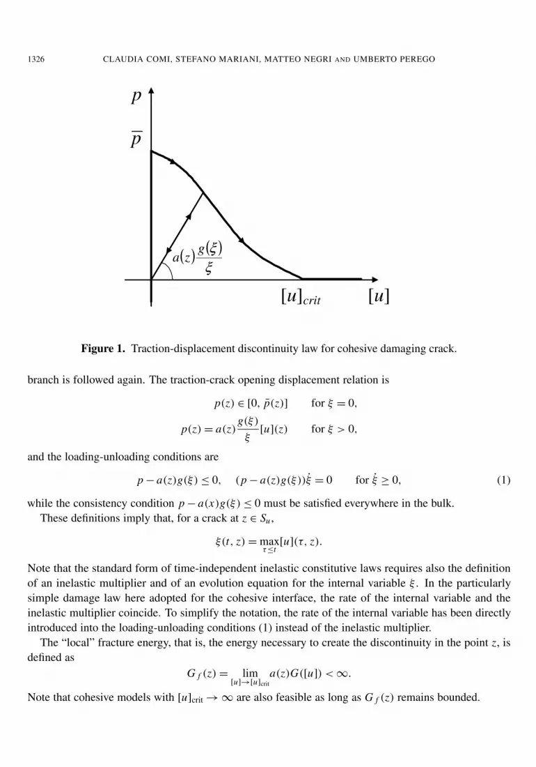
is commonly referred to as fracture energy and is a material property.For increasing opening displacement [u], following the softening branch a(z)g(ξ) the traction de-

creases until the limit opening [u]crit is reached. For displacement jumps [u] > [u]crit no traction istransmitted across the crack (Figure 1). For decreasing opening displacement, a linear unloading path isfollowed, with slope a(z)g(ξ)/ξ depending on the current value of damage. Upon reloading, the samelinear path is followed until the current traction threshold p(z) = a(z)g(ξ) is reached, then the softening

1326 CLAUDIA COMI, STEFANO MARIANI, MATTEO NEGRI AND UMBERTO PEREGO

[u] [u]crit

p

p

( ) ( )ξξgza

Figure 1. Traction-displacement discontinuity law for cohesive damaging crack.

branch is followed again. The traction-crack opening displacement relation is

p(z) ∈ [0, p(z)] for ξ = 0,

p(z) = a(z)g(ξ)

ξ[u](z) for ξ > 0,

and the loading-unloading conditions are

p − a(z)g(ξ) ≤ 0, (p − a(z)g(ξ))ξ = 0 for ξ ≥ 0, (1)

while the consistency condition p − a(x)g(ξ) ≤ 0 must be satisfied everywhere in the bulk.These definitions imply that, for a crack at z ∈ Su ,

ξ(t, z) = maxτ≤t

[u](τ, z).

Note that the standard form of time-independent inelastic constitutive laws requires also the definitionof an inelastic multiplier and of an evolution equation for the internal variable ξ . In the particularlysimple damage law here adopted for the cohesive interface, the rate of the internal variable and theinelastic multiplier coincide. To simplify the notation, the rate of the internal variable has been directlyintroduced into the loading-unloading conditions (1) instead of the inelastic multiplier.

The “local” fracture energy, that is, the energy necessary to create the discontinuity in the point z, isdefined as

G f (z) = lim[u]→[u]crit

a(z)G([u]) < ∞.

Note that cohesive models with [u]crit → ∞ are also feasible as long as G f (z) remains bounded.

A ONE-DIMENSIONAL VARIATIONAL FORMULATION FOR QUASIBRITTLE FRACTURE 1327

Stable global response (that is, no snap-back) of the bar is assumed under the imposed end displace-ment η. It is easy to show that a snap-back response is ruled out if

L < −E

a(z) dgdξ

, for 0 ≤ ξ ≤ [u]crit.

3. Finite-step problem

In view of the nonreversible nature of the crack evolution, the analysis of the bar response to an assignedhistory η(t), with t ∈ [0, T ], of the imposed displacement, requires the definition of a step-by-step timemarching procedure. The structural response un+1 at time tn+1 = tn + 1t satisfies in the bulk

εn+1 =dun+1

dx, σn+1 = Eεn+1,

dσn+1

dx+ b = 0, (2)

and in the crack points

[u]n+1(z) = u+

n+1(z) − u−

n+1(z) ≥ 0, σ+

n+1(z) = σ−

n+1(z) = pn+1(z).

Knowing the configuration at time tn , the following stepwise-reversible behavior is assumed for thecohesive cracks

ξn+1 = ξn + 1ξ, pn+1 = a(z)g(ξn+1)

ξn+1[u]n+1, for ξn+1 > 0, (3)

pn+1 − a(z)g(ξn+1) ≤ 0, (pn+1 − a(z)g(ξn+1))1ξ = 0, for 1ξ ≥ 0, (4)

where the second equation in (3) is the traction-crack opening displacement relation, and the relationsin (4) represent the loading-unloading conditions. Note that the above defined finite-step problem canbe conceived as resulting from a backward-difference integration of the incremental problem, while theoriginal (continuous) problem will be recovered for 1t → 0.

It is therefore possible to define an energy G([u], ξn) associated to the reversible finite-step law

G([u], ξn) =

{g(ξn)

2ξn[u]

2, for [u] ≤ ξn,

G([u]) − G(ξn) +ξn g(ξn)

2 , for [u] ≥ ξn.(5)

For ξn = 0, one has G([u], ξn) = G([u]). The adopted cohesive finite-step law with the associated energyis shown in Figure 2a at initiation and in Figure 2b in correspondence of a generic time-step.

For η = ηn+1, the following functional is defined for the current time-step

U η(u, ξn) =12

∫I

E(du

dx

)2dx +

∑z∈Su

a(z)G([u](z), ξn(z)) −

∫I

bu dx . (6)

In the expression of the functional, ξn plays the role of an assigned parameter. At the end of each step,the internal variable is updated and the functional changes its expression. The updating procedure isschematically shown in Figure 3 where numbered dots denote the value of the functional at the end ofthe step, before updating, while dots with starred numbers denote the corresponding updated value.

1328 CLAUDIA COMI, STEFANO MARIANI, MATTEO NEGRI AND UMBERTO PEREGO

[u][u]crit

p

p ( ) [ ]( ) ( ) [ ]( )uGzauGza == 0,~ ξpn

ξn

( ) [ ]( )nuGza ξ,~

[u]crit

p

p

[u][u][u]crit

p

p ( ) [ ]( ) ( ) [ ]( )uGzauGza == 0,~ ξpn

ξn

( ) [ ]( )nuGza ξ,~

[u]crit

p

p

p

p

[u]

(a) (b)(a) (b)

Figure 2. Finite-step cohesive law at initiation (a), at a time-step tn (b).

Let u′ denote the (distributional) derivative of u, that is,

u′=

dudx

dx +

∑z∈Su

[u](z)δz, (7)

where δz denotes the Dirac delta concentrated in z. We assume that u′ is a bounded measure, that is,∣∣u′∣∣(I ) =

∫I

∣∣∣dudx

∣∣∣dx +

∑z∈Su

|[u]| < ∞.

Following [Braides et al. 1999] let B(x) be a primitive of b(x) vanishing in zero. Integrating by partsthe body force work, the functional can be rewritten as

U η(u, ξn) =12

∫I

E(du

dx

)2dx +

∑z∈Su

a(z)G([u](z), ξn(z)) +

∫[0,L]

Bu′− B(L)η.

Taking into account the definition of the distributional derivative in Equation (7), one obtains

U η(u, ξn) =

∫I

dudx

(12 E

dudx

+ B)

dx +

∑z∈Su

(a(z)G([u](z), ξn(z)) + B(z)[u](z)

)− B(L)η. (8)

Remark 1. Such functionals have been widely studied in the recent mathematical literature on freediscontinuity problems (see, for instance, [Braides et al. 1999]). In this framework the potential energywould be defined in the space SBV (0, L) of special functions with bounded variation (for a definition ofSBV spaces, see for example, [Ambrosio et al. 2000]), that is, for the displacements u whose distribu-tional derivative is a bounded measure which can be written as in Equation (7). Existence of minimizers(local and global) in SBV will be discussed in the next section.

A ONE-DIMENSIONAL VARIATIONAL FORMULATION FOR QUASIBRITTLE FRACTURE 1329

bulk energy

energy functional for the continuous loading problem

( )0, 1 =ξη uU

( )2,ξη uU

( )3,ξη uU

1 2

3

4

0

2*

3*

ηU

η

Figure 3. Updating procedure for energy functional. Numbers refer to end of step.Starred numbers refer to updated values of functional.

A displacement un+1 at the end of the finite-step is considered a local minimizer of U η defined inEquation (6) if U η(v, ξ) ≥ U η(u, ξ) for every v ∈ SBV (0, L) such that∫

I|v − u| dx ≤ α,

for some α sufficiently small. In the following sections it will be shown that the discrete evolution definedby a sequence of local minimizers of Equation (6) satisfies the governing equations (2)-(4). To proceedin the discussion, it is convenient to consider separately the crack initiation problem (ξn = 0) and thesubsequent crack opening problem (ξn 6= 0).

4. Crack initiation problem

The following crack initiation problem is considered. The bar is subject to an assigned body force b(x),whose intensity is such that the tensile strength p(x) is not exceeded in any point of the bar. Then agrowing positive displacement η is imposed at x = L until the threshold value η is reached for which, ata position z, the stress σ reaches its limit value p(z). The value of η depends on the strength of the barand on the body force.

Following the path of reasoning proposed by Braides, Dal Maso and Garroni [Braides et al. 1999],first we prove that the minimizers (both local and global) have a single fracture. Assume that two cracksare activated at z1 and z2, with jumps w1 and w2 respectively. Let w = w1 + w2 and let ai = a(zi ),Bi = B(zi ). Let H([u]) be the energy associated to the discontinuity in Equation (8), that is,

H([u]) =

∑z∈Su

{a(z)G([u](z), ξn(z)) + B(z)[u](z)} .

1330 CLAUDIA COMI, STEFANO MARIANI, MATTEO NEGRI AND UMBERTO PEREGO

Noting that at crack initiation (ξn = 0) one has G ≡ G and considering z1, z2 and w as fixed, we canwrite H and its second derivative as a function of w1 alone as

H(w1) = a1G(w1) + B1w1 + a2G(w − w1) + B2(w − w1),

d2 H(w1)

dw21

= a1dg(w1)

dw1+ a2

dg(w − w1)

d(w − w1),

for 0 ≤ w1 ≤ w. As dg/dwi ≤ 0 and ai > 0, it follows that H is concave and thus its minimum, in theinterval [0, w], is in the endpoints. This means that either w1 = w and w2 = 0 or w1 = 0 and w2 = w.Hence in one of the points zi there is no jump. Since the bulk energy does not depend on w, followingthe previous reasoning it is not hard to see that a minimizer can have only one fracture point. We willdenote it by z.

Remark 2. Note that by a similar argument it follows that the minimization problem in SBV is wellposed even if the relaxed functional would be defined in the whole BV (see [Braides et al. 1999] and thereferences therein).

Denoting for notation convenience U η→η+

= limη→η+ U η, the following proposition holds.

Proposition 3. Starting from an elastic state with ξn = 0, for an assigned value η of the imposeddisplacement, the governing equations can be obtained from the stationarity conditions of U η. Theposition z of the activated crack can be obtained from the minimality of U η→η+

(u, 0).

Proof. Assume that u is a stationary point of U η and consider the variations of the form u +λv, whereλ is a scalar variable and v : [0, L] → < a suitable test function. As u + λv must satisfy the boundaryconditions, we assume that v(0) = v(L) = 0. Moreover, v may have a unit jump in Sv , which we denoteby [v] = 1. Since interpenetration is not allowed, we must assume that [u] + λ[v] ≥ 0 for λ sufficientlysmall. The stationarity condition is given, in terms of the first variation of U η, by the inequality

limλ→0+

1λ

(U η(u + λv, 0) − U η(u, 0)

)= lim

λ→0+

12λ

∫I

[E

(dudx

+ λdv

dx

)2− E

(dudx

)2]dx

+ limλ→0+

1λ

∑z∈Su∪Sv

(a(z)G

([u + λv](z)

)− a(z)G

([u](z)

))−

∫I

bv dx

=

∫I

(E

dudx

)dv

dxdx + lim

λ→0+

1λ

∑z∈Su∪Sv

(a(z)G

([u + λv](z)

)− a(z)G

([u](z)

))−

∫I

bv dx ≥ 0. (9)

In general, the configuration u + λv may have two jumps, at Su = {z} and Sv = {zv}. If Su = Sv, thenSu+λv = Su . In this case, the second term in Equation (9) can be written as

limλ→0+

1λ

(a(z)G

([u + λv](z)

)− a(z)G

([u](z)

))= a(z)g([u](z))[v] ≥ 0.

A ONE-DIMENSIONAL VARIATIONAL FORMULATION FOR QUASIBRITTLE FRACTURE 1331

If Su 6= Sv, then Su+λv = Su ∪ Sv and the previous condition becomes

limλ→0+

1λ

(a(z)G

([u + λv](z)

)+ a(zv)G

([u + λv](zv)

)− a(z)G

([u](z)

))= lim

λ→0+

1λ

(a(z)G

([u](z)

)+ a(zv)G

([λv](zv)

)− a(z)G

([u](z)

))= lim

λ→0+

1λ

a(zv)G([λv](zv)

)= a(zv)g(0)[v] ≥ 0.

Now we consider some particular variations v in order to obtain the governing equations.

• Assume first that Su = ∅ and that v(z) = 0. Integrating by parts the first integral in Equation (9),the inequality becomes

Edudx

v

∣∣∣∣z

0−

∫ z

0

(E

d2udx2 + b

)v dx + E

dudx

v

∣∣∣∣L

z−

∫ L

z

(E

d2udx2 + b

)v dx

= −

∫ z

0

(E

d2udx2 + b

)v dx −

∫ L

z

(E

d2udx2 + b

)v dx ≥ 0,

which gives (E d2udx2 + b) = 0, a.e. in [0, L]. This is the condition of equilibrium in the bulk.

• Consider now a variation v such that v(z)+ = v(z)− 6= 0. Taking into account that (E d2udx2 + b) = 0,

Equation (9) then becomes (E

dudx

)−

v−−

(E

dudx

)+

v+≥ 0,

which gives easily σ+(z) = σ−(z). This is the condition of equilibrium across the crack.

• Now we can choose a variation v having a unit discontinuity at zv ∈ [0, L]. According to thisdefinition [v](zv) = 1 and

∫ L0

dvdx dx = −[v](zv) = −1. Let us consider first the case z 6= zv . Making

reference to the expression in Equation (8) of the energy, the stationarity condition can be writtenas ∫

I

(E

dudx

+ B)dv

dxdx + B(zv)[v] + a(zv)g(0)[v] ≥ 0. (10)

Note that, in view of the bulk equilibrium (E d2udx2 +b = 0), the stress σ η

= E dudx + B, which depends

on the imposed boundary displacement η, is constant along x . Therefore, one can write

−σ η+ B(zv) + a(zv)g(0) ≥ 0. (11)

Taking into account that σ η− B(z) = σ(z) is the stress in the bar due to the dead load and the

imposed boundary displacement and that a(zv)g(0) = p(zv), one has

σ − p ≤ 0 for zv 6= z. (12)

When Su = Sv, that is, for zv = z, since [u] > 0 a perturbed configuration of the form u − λv canbe considered (as for λ small enough [u − λv](z) ≥ 0). Computing again the limit for λ → 0+, and

1332 CLAUDIA COMI, STEFANO MARIANI, MATTEO NEGRI AND UMBERTO PEREGO

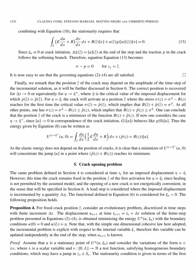
combining with Equation (10), the stationarity requires that∫I

(E

dudx

+ B)dv

dxdx + B(z)[v] + a(z)g([u](z))[v] = 0. (13)

Since ξn ≡ 0 at crack initiation, 1ξ(z) = [u](z) at the end of the step and the traction p in the crackfollows the softening branch. Therefore, equation Equation (13) becomes

σ − p = 0 for zv = z.

It is now easy to see that the governing equations (2)–(4) are all satisfied. �

Finally, we remark that the position z of the crack may depend on the amplitude of the time-step ofthe incremental solution, as it will be further discussed in Section 6. The correct position is recoveredfor 1t → 0 or equivalently for η → η+, where η is the critical value of the imposed displacement forwhich p(z) = p(z). For η = η, the crack will activate at a position z where the stress σ(z) = σ η

− B(z)reaches for the first time the critical value σ(z) = p(z), which implies that B(z) + p(z) = σ η. At allother points, one has σ(z) = σ η

− B(z) ≤ p(z), which implies that B(z)+ p(z) ≥ σ η. One can concludethat the position z of the crack is a minimizer of the function B(z)+ p(z). If now one considers the caseη → η+, since [u] → 0 in correspondence of the crack initiation, G([u]) behaves like g(0)[u]. Thus theenergy given by Equation (8) can be written as

U η→η+

(u, 0) =

∫I

dudx

(12

E dudx

+ B)

dx + ( p(z) + B(z))[u].

As the elastic energy does not depend on the position of cracks, it is clear that a minimizer of U η→η+

(u, 0)

will concentrate the jump [u] in a point where ( p(z) + B(z)) reaches its minimum.

5. Crack opening problem

The same problem defined in Section 4 is considered at time tn for an imposed displacement η > η.However, this time the crack remains fixed in the position z of the first activation for η = η, since healingis not permitted by the assumed model, and the opening of a new crack is not energetically convenient, inthe sense that will be specified in Section 6. A load step is considered where the imposed displacementis incremented by a quantity 1η. The functional defined in Equation (6) is considered for ξn > 0. Thefollowing proposition holds.

Proposition 4. For fixed crack position z, consider an evolutionary problem, discretized in time stepswith finite increment 1t . The displacement un+1 at time tn+1 = tn + 1t solution of the finite-stepproblem presented in Equations (2)–(4), is obtained minimizing the energy U η(u, ξn) with the boundaryconditions u(0) = 0 and u(L) = η. Note that, with the simple one dimensional cohesive law here adopted,the incremental problem is explicit with respect to the internal variable ξ, therefore this variable can beupdated independently at the end of the step, when un+1 is known.

Proof. Assume that u is a stationary point of U η(u, ξn) and consider the variations of the form u +

λv, where λ is a scalar variable and v : [0, L] → < a test function, satisfying homogeneous boundaryconditions, which may have a jump in zv ∈ Sv. The stationarity condition is given in terms of the first

A ONE-DIMENSIONAL VARIATIONAL FORMULATION FOR QUASIBRITTLE FRACTURE 1333

variation of U η(u, ξn) by the inequality

limλ→0+

1λ

(U η(u + λv, ξn) − U η(u, ξn)

)= lim

λ→0+

12λ

∫I

[E

(dudx

+ λdv

dx

)2− E

(dudx

)2]dx

+ limλ→0+

1λ

∑z∈Su∪Sv

(a(z)G

([u + λv], ξn

)− a(z)G([u], ξn)

)−

∫I

bv dx ≥ 0.

Making use of the same arguments discussed in the previous section, the previous condition can berewritten as ∫

I

(E

dudx

)dv

dxdx + a(zv)

dG([u], ξn)

d[u][v] −

∫I

bv dx ≥ 0.

Now we consider some particular variations v in order to obtain the governing equations.

• Assuming [v] = 0, following the same path of the previous section one can obtain equilibriumconditions in the bulk and across the interface in z.

• Now we can choose a variation v having a unit discontinuity at z. Consider again the form of thefunctional given in Equation (8) obtained by integrating by parts the body force integral. Takinginto account the bulk equilibrium, the stationarity conditions of Equation (8) read

−σ η+ B(z) + a(z)

dG([u], ξn)

d[u]≥ 0. (14)

Accounting for the definition of G([u], ξn) in Equation (5) and noting that σ η− B(x) = σ(z) = p

is the stress acting on the crack, from Equation (14) one obtains

−p + a(z)g(ξn)

ξn[u] ≥ 0, for [u] ≤ ξn, (15)

−p + a(z)g([u]) ≥ 0, for [u] ≥ ξn. (16)

When [u] = 0 < ξn, condition in Equation (15) gives p ≤ 0, meaning that, if the crack has beenalready activated (ξn > 0), a complete closure of the crack ([u] = 0) corresponds to zero or negativestress. Assume now [u] > 0, in this case also a perturbation u − λv is admissible for small λ, andinequalities opposite to Equations (15)–(16) are obtained. Therefore one has

p = a(z)g(ξn)

ξn[u], for [u] ≤ ξn, (17)

p = a(z)g([u]), for [u] ≥ ξn. (18)

From Equation (17) one obtains

p ≤ a(z)g(ξn), for [u] ≤ ξn. (19)

• Consider a variation v having a unit discontinuity in zv /∈ Su . Having in mind that, for x 6= z,[u](x) = ξn(x) = 0, one has

a(zv)dG([u](zv), ξn(zv))

d[u]= a(zv)g(0) = p(zv)

1334 CLAUDIA COMI, STEFANO MARIANI, MATTEO NEGRI AND UMBERTO PEREGO

and the stationarity conditions simply give the consistency condition in the bulk −σ(x) + p(x) ≥ 0.

Noting that, by definition, at the end of the step 1ξ = 0 if [u] ≤ ξn while 1ξ = [u]− ξn if [u] ≥ ξn,

one obtains that : (i) Equations (17) and (18) define the traction-crack opening displacement relation (3);(ii) Equations (18) and (19) can be rewritten in the Kuhn–Tucker form seen in Equation (4) and thusprovide the finite-step loading-unloading conditions for the cohesive crack. �

6. Algorithmic aspects

One of the important features of the present finite-step formulation is that the governing equations andthe nonreversibility of damage growth are enforced only at the end of the step. In view of the nonconvexcharacter of the energy functional, this implies that solutions may exist which minimize the energy butcould not be reached in a continuous process due to the existence of energy barriers. These solutionsappears to be an artifact of the algorithmic formulation of the finite-step problem and does not reflectthe physical behavior. Therefore, it seems necessary to complement the algorithm with criteria for theexclusion of nonphysical solutions.

Let us consider first the crack initiation problem. At the end of Section 4, it has been proven thatfor η → η+, the position of the first crack minimizes the functional U η→η+

(u, 0). We now considerthe more general case where η can assume arbitrary values with respect to η. The solution of the stepproblem is sought by searching for minimizers of the energy U η(u, 0). A classical approach consists ofcomputing first an elastic trial, that is, a tentative solution assuming unlimited elastic behavior. If this isnot a minimizer, then a better solution is found minimizing the energy along a descent direction, definedby the local gradient. The procedure is repeated until a minimizer is found.

Let utr be the elastic (trial) solution, that is, the minimizer of U η restricted to the space of admissibledisplacements without cracks. Equilibrium in the bulk is clearly satisfied, that is, (E(utr )′ + B)′ =

(σ η,tr )′ = 0; hence for every admissible variation v with jump [v](zv) > 0, from Equation (10) one has

limλ→0+

1λ

(U η(utr

+ λv, 0) − U η(utr , 0))=

(− σ η,tr

+ B(zv) + a(zv)g(0))[v]. (20)

If the variation of U η given in Equation (20), computed in utr and with respect to every variation v,is positive, that is, if

limλ→0+

1λ

(U η(utr

+ λv, 0) − U η(utr , 0))≥ 0,

then utr is a local minimizer. As discussed in Section 4, (Equations (11) and (12)), since [v](zv) > 0,from Equation (20) it follows that −σ η,tr

+ B(zv) + a(zv)g(0) > 0 and thus σ η,tr (zv) < p(zv). Thismeans that the stress associated to utr is everywhere below the limit strength and therefore un+1 = utr

will be the solution of the step. On the contrary, if there exists a variation v such that

limλ→0+

1λ

(U η(utr

+ λv, 0) − U η(utr , 0))=

(− σ η,tr

+ B(zv) + a(zv)g(0))[v] < 0, (21)

then a new solution un+1 6= utr will be computed along a descent direction. From the physical point ofview it seems reasonable to consider that a fracture could appear in any of the points zv where the limitstrength is exceeded, that is, where Equation (21) holds (for a variation v with a single discontinuity inzv).

A ONE-DIMENSIONAL VARIATIONAL FORMULATION FOR QUASIBRITTLE FRACTURE 1335

In Section 4 it has been shown that for crack initiation (that is, for η = η) it is energetically convenient toopen just one crack. It is shown below that the same result is obtained also in a computational procedurestarting from the trial solution. Let us assume to be using a solution algorithm capable to deal withmultiple cracks. Starting from the trial solution, it may happen that for a suitable variation v with twojumps in z1

v and z2v, we get

limλ→0+

1λ

(U η(utr

+ λv, 0) − U η(utr , 0))

=(− σ η,tr

+ B(z1v) + a(z1

v)g(0))[v](z1

v) +(− σ η,tr

+ B(z2v) + a(z2

v)g(0))[v](z2

v) < 0

with (− σ η,tr

+ B(z2v) + a(z2

v)g(0))> 0. (22)

This means that a solution with multiple cracks may appear as energetically convenient with respectto the trial solution, and therefore reachable along a descent direction, even if at one of the points ofactivation (z2

v in this case) a local energy barrier (that is, a local stress below the limit strength) preventsthe actual opening of the crack. Such a solution seems not acceptable from a physical point of view andsince fracture is a phenomenon governed by the local state of the material, it seems more reasonable toexclude from the search those locations where Equation (22) holds. Therefore, starting from the trialsolution, only those points zv where(

− σ η,tr+ B(zv) + a(zv)g(0)

)< 0, (23)

that is, points where the trial stress exceeds the local strength, will be considered as possible locationsof the cracks in the search algorithm. Note that this argument in general does not exclude solutionswith multiple cracks. There may be cases where solutions with multiple cracks can be reached alongdescending paths where condition in Equation (23) is satisfied at each crack location. These solutionsare ruled out by the minimality, as for the crack initiation problem the concavity of the inelastic potentialG([u]) makes it convenient to open only one crack. Its correct position z can be obtained searching forthe solution along the steepest descent direction v from utr , that is, looking for the lowest value of thederivative of U η computed in utr . It can be readily seen that this is obtained when the crack positionminimizes the quantity B(zv) + a(zv)g(0).

Let us consider now the crack opening problem. Assume that at time tn only the first crack at z isopen. A displacement η > ηn be assigned at the bar end.

As in the previous case, let utr be the “elastic” trial solution. Since a damage model is used forthe description of the cohesive crack behavior, it is appropriate to compute the trial solution using asecant elastic modulus. This allows to obtain the exact solution in the case of unloading. The followingunlimited elastic behavior is assumed for the active cohesive crack (see Figure 4):

ptr (z) = a(z)g(ξn)

ξn[utr

](z).

In this case, given η > ηn we have [utr] > ξn and

ptr (z) = σ η,tr− B(z) > a(z)g

([utr

](z)). (24)

1336 CLAUDIA COMI, STEFANO MARIANI, MATTEO NEGRI AND UMBERTO PEREGO

[u] [u]crit

p

[utr] nξ

( ) ( )tra z g u

trp

np

( ) ( )n

n

ga z

ξξ

Figure 4. Unlimited elastic cohesive law used for computing the trial solution.

Hence, utr is not stable with respect to variations v with [v](z) > 0. Indeed

limλ→0+

1λ

(U η(utr

+ λv, ξn) − U η(utr , ξn))=

(− σ η,tr

+ B(z) + a(z)g([utr](z))

)[v](z) < 0. (25)

A possible minimizer has to be sought within one of the following situations that may arise: (i) thecrack at z closes and one or more new cracks open; (ii) the crack at z grows and one or more new cracksinitiate; (iii) the crack at z remains constant and one or more new cracks initiate; (iv) the crack at z growsand no other cracks initiate.

As done for the crack initiation case, the physical feasibility of possible solutions is tested consideringvariations with a single jump. Variations v which close the crack, that is, with [v](z) < 0, lead to a positivederivative in Equation (25) and therefore are not energetically convenient with respect to the trial solution.For this reason, case (i) can be ruled out and only displaced configurations such that [u](z) ≥ [utr

](z)will be considered henceforth.

Now we will show that, starting from the trial solution, both closing the active crack and/or initiatingnew cracks are energetically less convenient than further opening the existing crack (that is, situation(iv)). Let us consider first the situation (ii). According to the criterion in Equation (21) of negativederivative for the selection of possible locations zv 6= z of new cracks, variations with [v](zv) > 0 lead tothe local condition σ η,tr > a(zv)g(0)+ B(zv). Denote by w1 ≥ 0 the incremental opening of the crack atz, that is, [u](z) = [utr

](z)+w1, and by w2 = [v](zv) = w−w1 ≥ 0 the opening of a new crack at zv 6= z,w being the total incremental opening with respect to the trial solution. As G([utr

](z) + w1, ξn(z)) isconcave in the variable w1, the argument used in Section 4 allows to state that a single active fracture(corresponding to w1 = 0 or w2 = 0) is always energetically more convenient, which rules out case (ii).

It remains to show that the minimizer is given by w2 = 0 and hence that also case (iii) can be ruledout. Assume by contradiction that u is a minimizer with w1 = 0, so that

[u](z) = [utr](z) and [u](zv) = w2 = w > 0.

A ONE-DIMENSIONAL VARIATIONAL FORMULATION FOR QUASIBRITTLE FRACTURE 1337

In this case, the total energy (see Equation (8)) would be given by

U η(u, ξn) =∫I

dudx

(12 E

dudx

+B)

dx+a(z)G([utr](z), ξn(z))+B(z)[utr

](z)+a(zv)G(w2)+B(zv)w2−B(L)η. (26)

In view of the results of Proposition 4, assuming that u is a minimizer implies that equilibrium has tobe satisfied. Imposing equilibrium we obtain a(zv)g(w2)+ B(zv) = a(z)g([utr

](z))+ B(z) = σ η. Beinga(zv)g(w) + B(zv) a nonincreasing function, in the variable w, we get

a(zv)g(w2) + B(zv) = a(z)g([utr](z)) + B(z) ≥ a(z)g([utr

](z) + w1) + B(z), (27)

for every choice of w1 ≥ 0. Taking w1 = w2, one has

a(zv)G(w2) + B(zv)w2 =

∫ w2

0

(a(zv)g(w) + B(zv)

)dw ≥

∫[utr

](z)+w2

[utr ](z)

(a(z)g(w) + B(z)

)dw

= a(z)(

G([utr](z) + w2) − G([utr

](z)))

+ B(z)w2.

By this inequality and taking into account that from Equation (5) one has G([utr](z)+w2)−G([utr

](z))=

G([utr](z)+w2, ξn(z))−G([utr

](z), ξn(z)), it turns out that the total energy corresponding to the openingw2 = w concentrated in the first crack, that is, with [u](z) = [utr

](z) + w and [u](zv) = 0, is

U η(u, ξn) =

∫I

dudx

(12 E

dudx

+ B)

dx + a(z)G([utr](z) + w2, ξn(z)) + B(z)([utr

](z) + w2) − B(L)η,

and is smaller than the energy in Equation (26). This proves that the situation (iv) is the one whichminimizes the energy.

In conclusion, provided that criterion in Equation (23) is used at each step to assess the feasibilityof a point as location of a new crack, it can be stated that also in the present finite-step computationalapproach, for monotonically increasing imposed displacement, it is always energetically more convenientto open only one crack.

7. An explicit computation

The quasistatic evolution, defined in terms of local minimizers of the potential energy, is verified on asimple one-dimensional example whose step-by-step solution can be obtained analytically.

Consider a bar of length L = 10 mm and uniform elastic modulus E = 1 MPa, subject to a constantbody force b = 0.2E/L and a monotonically increasing imposed displacement η(t). The bar is assumed tohave a fracture strength p(x) = a(x)g(0) = a(x)g varying along the bar with a(x) = 1+100(x/L −1/2)2

and p(L/2) = g = 0.1E . Denoting by w the displacement discontinuity, a linear cohesive crack modelis considered

g(w) =

{g(1 −

1wcrit

w), for w ≤ wcrit,

0, for w > wcrit,

1338 CLAUDIA COMI, STEFANO MARIANI, MATTEO NEGRI AND UMBERTO PEREGO

where wcrit = 0.15L is the critical opening beyond which no traction can be transmitted across the crack.The potential G(w) is then given by

G(w) =

{g(w −

12wcrit

w2), for w ≤ wcrit,

g wcrit2 , for w ≥ wcrit.

Let A(η, w) be the set of displacements such that u(0)= 0, u(L)= η and [u]=w. Assuming a holonomicprocess (ξ = 0) and imposing equilibrium in the bulk, one can express the displacements along the barin terms of the assigned end displacement η, the crack opening w and the crack position z. Equivalentlyone can minimize U η with respect to u ∈ A(η, w), thus obtaining the energy function U(η, w, z)

U(η, w, z) = min{U η(u, 0) : u ∈ A(η, w)}. (28)

For this simple example the solution u(x) can be explicitly computed and is given by

u(x) =

−b

2E x2+

(η − w +

bL2

2E

)xL , for x < z,

−b

2E x2+

(η − w +

bL2

2E

)xL + w, for x > z.

(29)

The energy function is then obtained substituting Equation (29) into Equation (8) and working out theintegrals

U(η, w, z) =E (η − w)2

2L+

b(2wz − L (η + w))

2−

b2L3

24E+

[1 + 100

( zL

−12

)2]G(w). (30)

Note that U(η, w, z) is differentiable with respect to w and z. Local minimizers are found from

∂U

∂w= −

E (η − w)

L+

b(2 z − L )

2+

[1 + 100

( zL

−12

)2]g(w) = 0,

∂U

∂ z= bw +

100L

(2zL

− 1)

G(w) = 0.

(31)

The second stationarity condition reflects the requirement that the crack must initiate in a positionwhich minimizes the potential energy. At crack initiation (w → 0+), G(w) behaves like g(0)w and thesecond condition in Equation (31) requires that

b +100L

(2zL

− 1)

g(0) = 0,

which is solved for z = 0.49L . From the first condition in Equation (31), for z = 0.49L and w = 0, oneobtains the value η = 0.099L of the imposed displacement at crack initiation.

Figure 5a shows the plot of U as a function of the crack position and opening displacement for η = η

(for representation convenience values of U >0.2 have been cut in this plot). It should be noted that forη = η , z = 0.49L is the position of the point where the curve representing the stress along the bar istangent to the curve representing the fracture strength p(x) = g[1 + (x −

12 L)2

], see Figure 5b.For η > η the minimizers of Equation (30) give a position of the crack different from z = 0.49L , which

is not feasible for the real problem: once the material is broken at a certain position it cannot heal and

A ONE-DIMENSIONAL VARIATIONAL FORMULATION FOR QUASIBRITTLE FRACTURE 1339

02

46

810 0

0.5

1

1.5

� 0.10

0.1

0.2

02

46

810

w [mm]

U [MPa]

x [mm]

(a)

2 4 6 8 10

0.2

0.4

0.6

0.8

1

1.2

x [mm]

tract

ion

[MPa

]

(b)

p(x)

σ(x)

Figure 5. (a) Energy function for η = η; (b) crack position.

the crack position cannot change. In this case, the solution has to be sought solving the first conditionof Equation (31) for z = 0.49L .

The history of the assigned end displacement is shown in Figure 6a together with the correspondingcomputed crack opening. After initiation, the crack position is kept fixed at z = 0.49L . The damagevariable ξ is updated at the end of each step. The solution at each step is computed analytically mini-mizing the updated functional U η(u, ξn) according to the step-by-step procedure outlined in Section 5.Since in each step the bar is either monotonically loaded or unloaded, the computed and exact solutionscoincide. The computed history of cohesive traction is shown in Figure 6b. The values of the crackopening displacement and the explicit expressions of the energy functionals to be minimized at each stepare reported in Table 1.

Contour plots of the minimized functionals are shown in Figure 7. The computed solutions are denotedby a white dot. As expected, the dots do not coincide with the absolute minimum of the functionals, sincethe crack position has to remain fixed.

The optimal value of the energy U as a function of the imposed displacement η is plotted in Figure 8.The curve from point 0 to point 1 represents the bulk energy, while the curve from 1 to 2 corresponds to

step η [mm] functional to be minimized w [mm]

1 0.99 U η=0.99(u, ξ = 0) = bulk energy +a(z)G(w) 0.00

2 1.20 U η=1.20(u, ξ = 0) = bulk energy +a(z)G(w) 0.64

3 0.90 U η=0.90(u, ξ = 0.64) = bulk energy +a(z) g(0.64)

2·0.64 w2 0.48

4 1.30 U η=1.30(u, ξ = 0.64) = bulk energy +a(z)(G(w)−G(0.64)+0.64 g(0.64)

2

)0.95

Table 1. Energy functionals to be minimized at each step.

1340 CLAUDIA COMI, STEFANO MARIANI, MATTEO NEGRI AND UMBERTO PEREGO

0 1 2 3 4step

0

0.4

0.8

1.2

1.6

η

w

η

0 0.4 0.8 1.2 1.6 2

w [mm]

0

0.04

0.08

0.12

p(0.

49L)

[MPa

]

1

2

3 4

0

p

(a) (b)

Figure 6. (a) History of assigned end displacement and corresponding computed crackopening; (b) history of cohesive traction across the crack.

4.6 4.7 4.8 4.9 5 5.1 5.20

0.02

0.04

0.06

0.08

0.1

4.6 4.7 4.8 4.9 5 5.1 5.20

0.2

0.4

0.6

0.8

1

1.2

1.4

4.6 4.7 4.8 4.9 5 5.1 5.20

0.2

0.4

0.6

0.8

1

1.2

1.4

4.6 4.7 4.8 4.9 5 5.1 5.20

0.2

0.4

0.6

0.8

1

1.2

1.4 η2 = 1.2 mm

η4 = 1.3 mmη3 = 0.9 mm

(a)

(c) (d)

(b)

η1 = = 0.99 mmη

x [mm]

w [m

m]

x [mm]

w [m

m]

x [mm]

w [m

m]

x [mm]

w [m

m]

Figure 7. Contour plots of functionals to be minimized at each step. White dots denotecomputed solutions.

A ONE-DIMENSIONAL VARIATIONAL FORMULATION FOR QUASIBRITTLE FRACTURE 1341

0.25 0.5 0.75 1 1.25 1.5

-0.14

-0.12

-0.1

-0.08

-0.06

-0.04

-0.02

1 2

2* 43

η [mm]

U[N/mm]

0

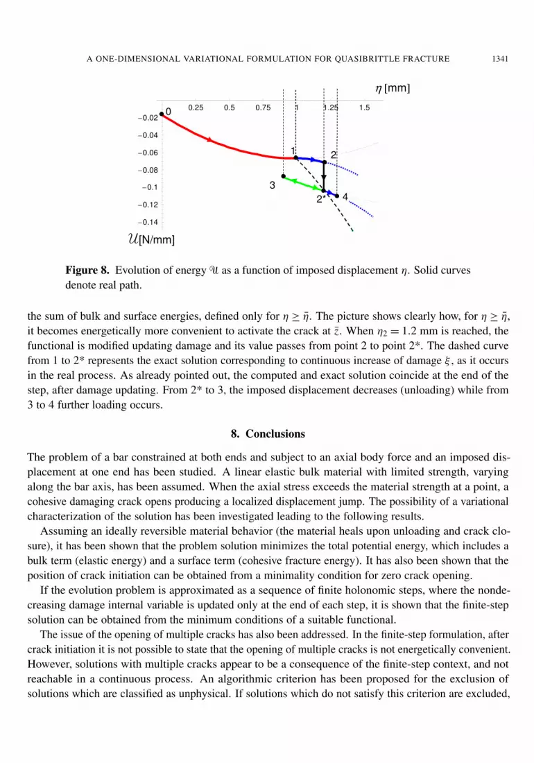
Figure 8. Evolution of energy U as a function of imposed displacement η. Solid curvesdenote real path.

the sum of bulk and surface energies, defined only for η ≥ η. The picture shows clearly how, for η ≥ η,it becomes energetically more convenient to activate the crack at z. When η2 = 1.2 mm is reached, thefunctional is modified updating damage and its value passes from point 2 to point 2*. The dashed curvefrom 1 to 2* represents the exact solution corresponding to continuous increase of damage ξ , as it occursin the real process. As already pointed out, the computed and exact solution coincide at the end of thestep, after damage updating. From 2* to 3, the imposed displacement decreases (unloading) while from3 to 4 further loading occurs.

8. Conclusions

The problem of a bar constrained at both ends and subject to an axial body force and an imposed dis-placement at one end has been studied. A linear elastic bulk material with limited strength, varyingalong the bar axis, has been assumed. When the axial stress exceeds the material strength at a point, acohesive damaging crack opens producing a localized displacement jump. The possibility of a variationalcharacterization of the solution has been investigated leading to the following results.

Assuming an ideally reversible material behavior (the material heals upon unloading and crack clo-sure), it has been shown that the problem solution minimizes the total potential energy, which includes abulk term (elastic energy) and a surface term (cohesive fracture energy). It has also been shown that theposition of crack initiation can be obtained from a minimality condition for zero crack opening.

If the evolution problem is approximated as a sequence of finite holonomic steps, where the nonde-creasing damage internal variable is updated only at the end of each step, it is shown that the finite-stepsolution can be obtained from the minimum conditions of a suitable functional.

The issue of the opening of multiple cracks has also been addressed. In the finite-step formulation, aftercrack initiation it is not possible to state that the opening of multiple cracks is not energetically convenient.However, solutions with multiple cracks appear to be a consequence of the finite-step context, and notreachable in a continuous process. An algorithmic criterion has been proposed for the exclusion ofsolutions which are classified as unphysical. If solutions which do not satisfy this criterion are excluded,

1342 CLAUDIA COMI, STEFANO MARIANI, MATTEO NEGRI AND UMBERTO PEREGO

then it has been shown that the energy is always minimized by opening only one crack. In our opinion, thisdiscussion may provide a useful insight also in view of possible extensions of the present computationalapproach to 2 or 3-dimensional problems, where, however, the appropriate underlying mathematicalsetting is still debated in the current literature on the subject. A simple example with a uniform axialbody force has been used to illustrate the theoretical results obtained.

References

[Ambrosio et al. 2000] L. Ambrosio, N. Fusco, and D. Pallara, Special Functions of Bounded Variation and Free DiscontinuityProblems, Oxford University Press, Oxford, 2000.

[Angelillo et al. 2003] M. Angelillo, E. Babilio, and A. Fortunato, “A computational approach to fracture of brittle solids basedon energy minimization”, Preprint, Università di Salerno, 2003.

[Askes and Sluys 2000] H. Askes and L. Sluys, “Remeshing strategies for adaptive ALE analysis of strain localisation”, Euro-pean Journal of Mechanics - A/Solids 19 (2000), 447–467.

[Bourdin et al. 2000] B. Bourdin, G. Francfort, and J. Marigo, “Numerical experiments in revisited brittle fracture”, Journal ofthe Mechanics and Physics of Solids 48 (2000), 797–826.

[Braides et al. 1999] A. Braides, G. Dal Maso, and A. Garroni, “Variational formulation of softening phenomena in fracturemechanics: The one-dimensional case”, Archive for Rational Mechanics and Analysis 146 (1999), 23–58.

[Chambolle 2003] A. Chambolle, “A density result in two-dimensional linearized elasticity and applications”, Archive forRational Mechanics and Analysis 167 (2003), 211–233.

[Dal Maso and Toader 2002] G. Dal Maso and R. Toader, “A model for the quasi-static growth of a brittle fracture: existenceand approximation results”, Archive for Rational Mechanics and Analysis 162 (2002), 101–135.

[Dal Maso and Zanini 2007] G. Dal Maso and C. Zanini, “Quasistatic crack growth for a cohesive zone model with prescribedcrack path”, Proc. of the Royal Soc. of Edinburgh, section A, mathematics 137A (2007), 1–27.

[Del Piero and Truskinovsky 2001] G. Del Piero and L. Truskinovsky, “Macro- and micro-cracking in one-dimensional elastic-ity”, International Journal of Solids and Structures 38 (2001), 1135–1148.

[Dumstorff and Meschke 2005] P. Dumstorff and G. Meschke, “Modelling of cohesive and non-cohesive cracks via X-FEMbased on global energy criteria”, pp. 565–568 in COMPLAS VIII, VIII International Conference on Computational Plasticity,edited by E. Onate and D.R.J. Owen, CIMNE, Barcelona (Spain), 2005.

[Francfort and Larsen 2003] G. Francfort and C. Larsen, “Existence and convergence for a quasi-static evolution in brittlefracture”, Communications on Pure and Applied Mathematics 56 (2003), 1465–1500.

[Francfort and Marigo 1998] G. Francfort and J. Marigo, “Revisiting brittle fracture as an energy minimization problem”,Journal of the Mechanics and Physics of Solids 46 (1998), 1319–1342.

[Mariani and Perego 2003] S. Mariani and U. Perego, “Extended finite element method for quasi-brittle fracture”, InternationalJournal for Numerical Methods in Engineering 58 (2003), 103–126.

[Moes and Belytschko 2002] N. Moes and T. Belytschko, “Extended finite element method for cohesive crack growth”, Engi-neering Fracture Mechanics 69 (2002), 813–833.

[Moes et al. 1999] N. Moes, J. Dolbow, and T. Belytschko, “A finite element method for crack growth without remeshing”,International Journal for Numerical Methods in Engineering 46 (1999), 131–150.

[Negri 2003] M. Negri, “A finite element approximation of the Griffith’s model in fracture mechanics”, Numerische Mathematik95 (2003), 653–687.

[Oliver et al. 2002] J. Oliver, A. Huespe, M. Pulido, and E. Chaves, “From continuum mechanics to fracture mechanics: thestrong discontinuity approach”, Engineering Fracture Mechanics 69 (2002), 113–136.

[Oliver et al. 2003] J. Oliver, A. Huespe, and E. Samaniego, “A study on finite elements for capturing strong discontinuities”,International Journal for Numerical Methods in Engineering 56 (2003), 2135–2161.

[Pandolfi and Ortiz 2002] A. Pandolfi and M. Ortiz, “An efficient adaptive procedure for three-dimensional fragmentationsimulations”, Engineering with Computers 18 (2002), 148–159.

A ONE-DIMENSIONAL VARIATIONAL FORMULATION FOR QUASIBRITTLE FRACTURE 1343

[Rodríguez-Ferran and Huerta 2000] A. Rodríguez-Ferran and A. Huerta, “Error estimation and adaptivity for nonlocal damagemodels”, International Journal of Solids and Structures 37 (2000), 7501–7528.

[Simo et al. 1993] J. Simo, J. Oliver, and F. Armero, “An analysis of strong discontinuities induced by strain softening inrate-independent inelastic solids”, Computational Mechanics 12 (1993), 277–296.

[Wells and Sluys 2001] G. Wells and L. Sluys, “A new method for modelling cohesive cracks using finite elements”, Interna-tional Journal for Numerical Methods in Engineering 50 (2001), 2667–2682.

Received 21 Nov 2005.

CLAUDIA COMI: claudia.comi@polimi.itDipartimento di Ingegneria Strutturale, Politecnico di Milano, Piazza L. da Vinci 32, 20133 Milano, Italyhttp://www.stru.polimi.it

STEFANO MARIANI: stefano.mariani@polimi.itDipartimento di Ingegneria Strutturale, Politecnico di Milano, Piazza L. da Vinci 32, 20133 Milano, Italyhttp://www.stru.polimi.it

MATTEO NEGRI: matteo.negri@unipv.itDipartimento di Matematica, Università degli Studi di Pavia, Via Ferrata 1, 27100 Pavia, Italyhttp://www-dimat.unipv.it

UMBERTO PEREGO: umberto.perego@polimi.itDipartimento di Ingegneria Strutturale, Politecnico di Milano, Piazza L. da Vinci 32, 20133 Milano, Italyhttp://www.stru.polimi.it